Economic distributions and primitive distributions in ...

Economic distributions and primitive distributions in

monopolistic competition

Simon P. Anderson and André de Palma∗

Revised July 2015

Abstract

We link fundamental technological and taste distributions to endogenous economic dis-

tributions of firm size (output, profit) and prices in extensions of canonical IO and Trade

models. We develop a continuous logit model of monopolistic competition to show that

exponential or normal distributions respectively generate Pareto or log-normal economic

size distributions. Two groups of distributions (output, profit, and quality-cost; and price

and cost) are linked through the technological relation between cost and quality-cost.

We formulate a general monopolistic competition model and recover the demand struc-

ture, mark-ups, and the quality-cost distribution from the output and profit distributions.

Adding the price distribution recovers the cost distribution and the relation between

quality-cost and cost. We also find long-run equilibrium distributions as a function of the

primitives. On the Trade side, we provide a parallel analysis for the CES and break the

Pareto circle by introducing quality.

JEL Classification: L13

Keywords: Primitive and economic distributions, price and profit dispersion, general

monopolistic competition model, Pareto and log-normal distribution, Logit, CES.

∗Simon P. Anderson: Department of Economics, University of Virginia, PO Box 400182, Charlottesville

VA 22904-4128, USA, [email protected]. André de Palma: Economics, ENS-Cachan; CES, Paris, FRANCE.

[email protected]. The first author gratefully acknowledges research funding from the NSF. We

thank Maxim Engers, Farid Toubal, James Harrigan, and Ariell Resheff for valuable comments, and seminar

participants at Melbourne University, Stockholm University, KU Leuven, Laval, Vrij Universiteit Amsterdam,

and Paris Dauphine.

1 Introduction

Distributions of economic variables have attracted the interest of economists at least since

Pareto (1896). In industrial organization, firm size (output, sales, or profit) distributions have

been analyzed, while different studies have looked at the distribution of prices within an in-

dustry. Firm sizes (profitability, say) within industries are wildly asymmetric, and frequently

involve a long-tail of smaller firms. The idea of the long tail has recently been invoked promi-

nently in studies of Internet Commerce (Anderson, 2006, Elberse and Oberholzer-Gee, 2006),

and particular distributions — mainly the Pareto and log-normal — seem to fit the data well in

other areas too (see Head, Mayer, and Thoenig, 2014).

In international trade, recent advances have enabled studying distributions of sales revenues

(see, e.g., Eaton, Kortum, and Kramarz, 2011). The distributions of these “economic” variables

are (presumably) jointly determined by the fundamental underlying distributions of tastes and

technologies. In this paper we determine the links between the various distributions. We link

the economic ones to each other and to the primitive distributions and tastes. Moreover, the

primitives can be uncovered from the observed economic distributions.

To set the stage, we start by deploying the logit model of monopolistic competition, which

we develop and extend here to a continuum of firms.1 The logit is the workhorse model in

structural empirical IO, and it readily incorporates taste and cost heterogeneity.2 We show a

three-way relation between two groups of distributions and the quality-to-cost relation: know-

ing one element from any two of these ties down the third. On one leg, we generate the relation

between equilibrium profit dispersion, firm outputs, and the fundamental quality-cost distrib-

ution. On a second leg, we show the relation between the cost distribution and equilibrium

1An alternative tractable model we analyze is the logit’s close cousin, the CES model.2Ironically, Chamberlin (1933) is best remembered for his symmetric monopolistic competition analysis. Yet

he went to great length to point out that he believed asymmetry to be the norm, and that symmetry was a very

restrictive assumption. We model both quality and production cost differences across firms.

1

price dispersion. Knowing any one of the distributions on one leg suffices to determine the

others on that leg. Moreover, knowing a distribution from each leg allows us to determine what

the relation between cost and quality must be on the third leg. Some important equivalences

include that normally distributed quality-costs induce log-normal distributions of profits, and

that a power distribution of costs along with an exponential distribution of quality-costs leads

to a Pareto distribution for profit. These results also apply to a long-run analysis in the spirit

of Melitz (2003) with the set of active firms determined endogenously.

With that back-drop, we then broaden our scope by deploying a more general model of

monopolistic competition by relaxing the constant mark-up property of the logit. We first show

how the demand function delivers a mark-up function, and then we show our key converse result

that the mark-up (or “pass-through” function of Weyl and Fabinger, 2013) determines the form

of the demand function. We next engage these results to show how the economic profit and

output distributions allow us to determine the demand function and quality-cost distributions.

Knowledge of the price distribution then enables us to recover the other primitives, which are

the cost distribution and the relation between costs and quality-cost.

We provide a parallel analysis for the CES model.3 The CES representative consumer model

is widely used in economics in conjunction with a market structure assumption of monopolistic

competition It is used as a theoretical component in the New Economic Geography and Ur-

ban Economics, it is the linchpin of Endogenous Growth Theory, Keynesian underpinnings in

Macro, and of course, Industrial Organization. The current most intensive use of the model is

in International Trade, following Melitz (2003), where it is at the heart of empirical estimation.

The convenience of the model stems from its analytic manipulability. The CES model delivers

equilibrium mark-ups proportional to marginal costs, and so delivers market imperfection (im-

3The Logit is an attractive alternative framework to the CES. Anderson, de Palma, and Thisse (1992) have

shown that the CES can be viewed as a form of Logit model.

2

perfect competition) in a simple way without complex market interaction. The standard models

in this vein (following Melitz, 2003) assume that firms’ unit production costs are heterogeneous.

However, when we apply this model to distributions, if one distribution (such as profits) is

described as a Pareto distribution, then the distributions of all the economic variables lie in

the Pareto family. This we call the “Pareto circle” (or, more generally, the CES circle because

the result applies to any distribution). The circle is broken by introducing qualities (as do

Baldwin and Harrigan, 2011, and Feenstra and Romalis, 2014) into the demand model. Doing

so delivers two fundamental drivers of equilibrium distributions (instead of just one) — the cost

distribution and the quality/cost one. Even if one distribution is Pareto, then others can take

different forms. Most notably, the output distribution depends on the cost distribution (as

before) but now also on the quality/cost distribution.

2 The Logit model of monopolistic competition

There is a continuum of active firms. Each firm, , is associated to a distinctive quality ,

(constant) marginal production cost, , and chooses a price, .4 Let Ω be the set of active

(producing) firms, and let denote an element of this set. Total demand is normalized to 1,

w.l.o.g. Demand for Firm is a Logit function of active firms’ qualities and prices:5

=exp

³−

´R∈Ω exp

³()−()

´ + exp

³0

´ ∈ Ω, (1)

where 0 measures the degree of product heterogeneity and 0 ∈ (−∞∞) measures the at-

tractivity of the outside option (which could also represent a competitive sector). We thus adapt

the continuous Logit model (see Ben-Akiva and Watanada, 1981) to monopolistic competition.6

4Both and can be optimally determined by the firm, according to some fundamental firm “productivity.”

More details anon.5We assume that the integral in the denominator is bounded: conditions are given below.6Anderson et al. (1992) show that logit demands can be generated from an entropic representative consumer

utility function as well as the traditional discrete choice theoretic root (see McFadden, 1978).

3

Consumer choices are driven by two forces. First, absent product differentiation, consumers

want the best quality-price deal (highest − ). Second, consumers have idiosyncratic tastes

for differentiated products. When product differentiation (measured by ) is very large, quality-

price is unimportant and each good has the same purchase probability. Otherwise, there is a

trade-off between objective quality (vertical differentiation) and subjective quality (horizontal

differentiation). The (gross) profit for Firm is = ( − ) , ∈ Ω. Because the firm

has no impact on the denominator in (1), under monopolistic competition the own-demand

derivative is = −

∈ Ω. Hence

=

h1− (−)

i ∈ Ω, and, since the term inside

the square brackets is strictly decreasing in , the profit function is strictly quasi-concave and

the profit-maximizing price of Firm is7

∗ = + ∈ Ω (2)

The absolute mark-up is the same for all firms.8 The corresponding equilibrium outputs are

=exp

³−

´R∈Ω exp

³()−()

´ + V0

∈ Ω (3)

where V0 ≡ exp³0+ 1´≥ 0 (and where henceforth stands for the equilibrium output). Let

= − be a one-dimensional parameterization of quality-cost (to be read as quality minus

cost). (3) indicates an output ranking over firms:

if and only if ∈ Ω

The equilibrium (gross) profit is , ∈ Ω, so outputs and profits are fully characterized

7For oligopoly with firms, the equilibrium prices are (implicit) solutions to ∗ = +

1− , = 1. Undersymmetry, ∗ = +

−1 , which converges to + as →∞ (Anderson, de Palma, and Thisse, 1992, Ch.7).8The CES model gives a constant relative mark-up property, ∗ = (1 + ), regardless of quality (see Section

7). The similarity between the Logit and CES is not fortuitous: is related to in CES models by = 1−.

Both models can be construed as sharing their individual discrete choice roots (Anderson et al. 1992).

4

by quality-cost levels:

Proposition 1 In the Logit Monopolistic Competition model, all firms set the same absolute

mark-up, . Higher quality-cost entails higher equilibrium output and profit.

A high quality with a high cost is equivalent (for output and profit) to a low quality/ low

cost combination. Hence, all we need to track is the distribution of quality-cost. Insofar as

higher qualities are also higher costs in practice, then they are also higher priced. However,

output and profitability may well be highest for medium-quality products (see Section 4.2).

2.1 Quality-cost, output, and profit distributions

Let the distribution of quality-cost be () = Pr ( ), with density (·) and support

[∞). We seek the corresponding distribution of equilibrium output, (), and the relation

between and is9

=exp ()

≥ =

exp ()

(4)

where we assume henceforth that (·) ensures the output denominator is finite:10

=

Z≥

exp () () + V0 (5)

and = kΩk is the total mass of firms. Equilibrium (gross) profit is = ≥ = . Let

and denote average output and profit, respectively.

Theorem 1 For the Logit Monopolistic Competition model, the quality-cost distribution, (),

generates the equilibrium output distribution () = ( ln ()) and the equilibrium profit

distribution Π () = ( ln ()), where is given by (5). Conversely, () can be

derived from the equilibrium output distribution as

³exp()

´, where = V0/ (1−);

or from the equilibrium profit distribution as Π

³exp()

´, where = V0/

³1−

´.

9Here all firms are active. Section 6 introduces fixed costs to determine endogenously the set of active firms.10This holds true for any finite support as well as for the examples below.

5

(Proof in Appendix 2). The key relation underlying the twinning of distributions is the

increasing relation between quality-cost and output (or profit) for the Logit. Similar increasing

relations hold for other models like the model in Section 5 below, as well as the CES (under

some restrictions: see Section 7). The theorem uses this increasing relation to describe how

quality-costs can be determined from output or profit distributions. A specific quality-cost

distribution generates a specific output (resp. profit) distribution. Conversely, this output or

profit distribution could only have been generated from the initial quality-cost distribution.

2.2 Comparative statics of distributions

We here briefly consider the comparative static properties. Because we are dealing with distri-

butions, the natural way of doing so is to engage first order stochastic dominance (fosd).

Proposition 2 A fosd increase or a mean-preserving spread in quality-cost increases mean

output and mean profit, and strictly so if the market is not fully covered (i.e., if V0 0).

Even though the proof of the first part of the Proposition is straightforward, it belies some

counteracting effects. While moving up quality-cost mass will move up output mass ceteris

paribus, it also increases competition for all the other firms (a effect), which ceteris paribus

reduces their output. Mean output does not necessarily rise if mean quality-cost rises.11

Because the relation between output and profit distributions (Π () = ()) does not

involve , a fosd increase in output implies an increase in profit, and vice versa. However, a

fosd increase in quality-cost does not necessarily lead to a fosd increase in output. Suppose

for example that the increase in quality-cost is small for low quality-costs, but large for high

ones. Then competition is intensified (an increase in ), and output at the bottom end goes

down, while rising at the top end. So then there can be a rotation of () (in the sense of

11Mean output rises with a mean-preserving spread (part (ii)) but then if the mean of quality-cost is reduced

slightly, mean output can still go up overall, so the two means can move in opposite directions.

6

Johnson and Myatt, 2006) without fosd (a similar rotation is delivered in Proposition 3 below).

Nevertheless, specific examples do deliver stronger relations, as we show in Section 3.

We next determine how the economic parameters feed through into the endogenous economic

distributions. To do so, we first prove an ancillary result of independent economic interest.

Lemma 1 For the logit model, consumer surplus (at fixed prices) increases with product dif-

ferentiation, ; hence ln increases in .

The proof proceeds by showing that the derivative of consumer surplus is given by the

Shannon (1948) measure of information (entropy), which is positive.

Proposition 3 A more attractive outside option (V0) fosd decreases outputs and profits. More

product differentiation () fosd increases outputs and profits for low quality-cost and fosd de-

creases them for high quality-cost; a lower profit implies a firm has a lower output.

The first result is quite obvious, but the impact of higher product heterogeneity is more

subtle. When goes up, weak (low quality-cost) firms are helped and good ones are hurt.

The intuition is as follows. With little product differentiation, consumers tend to buy the

best quality-cost products. With more product differentiation (which increases the mark-up),

consumers tend to buy more of the low quality-cost goods (which have lower outputs, as per

Proposition 1) and less of the high quality-cost goods (which have higher outputs). Hence,

higher evens out demands across options. The fact that output may decrease and profit

increase with follows because = . Thus it can happen that doubling does not double

the profit of the top quality-cost firms, but it may more than double the profit of the lowest

quality-cost firms. Whether high or low qualities are most profitable depends on whether

quality-costs rise or fall with quality.

7

3 Specific distributions

We derive the equilibrium profit distributions: the equilibrium output distributions are anal-

ogous (because = ). We express all examples from quality-cost distributions to implied

profit distributions: from Theorem 1 the reverse relations hold too, and output relations are

analogous. Proofs are in Appendix 2.

The normal distribution is perhaps the most natural primitive assumption to take for

quality-costs. Then profit Π ∈ (0∞) is log-normally distributed. The log-normal has some-

times been fitted to firm size distribution (see Cabral and Mata, 2003, for a well-cited study

of Portuguese firms). Note that a truncated normal begets a truncated log-normal (which is

therefore important once we consider free entry equilibria below).

The simplest text-book case is the uniform distribution. Then the equilibrium profit Π has

distribution Π () = ln³

´and its density is unit elastic. A truncated Pareto distribution

leads to a truncated Log-Pareto for profit (or output).

At a simplistic level, Theorem 1 indicates that we just need to find the log-distribution of

the seed distribution. However, we still need to match parameters, as done in Appendix 2 for

the examples, and we also need to find the corresponding expression for and ensure it is

defined. Notice too that the methods described above work for more general demands under

monopolistic competition (see Section 5).

The most successful function to fit the distribution of firm size has been the Pareto. We

reverse-engineer using Theorem 1 to find the distribution of quality-cost. This gives:

Proposition 4 Let quality-cost be exponentially distributed: () = 1 − exp (− (− )),

0, 0, ∈ [∞), with 1. Then equilibrium profit is Pareto distributed: Π () =

1− ¡

¢, where = 1. Equilibrium output is Pareto distributed: () = 1−

³

´,

where = 1. A Pareto distribution for equilibrium output or profit can only be generated

8

by an exponential distribution of quality-costs.

Thus the shape parameter, = , for the endogenous economic distributions depends just

on the product of the taste heterogeneity and the technology shape parameter. is bounded

if 1: which requires that taste heterogeneity exceeds average quality-cost.

4 Three-way synthesis

The distributions of quality-cost, output, and profit are determined from any one of them

(Theorem 1). Likewise, price and cost distributions are determined from either one. The link

between any of the former distributions and either of the latter two is determined by the relation

between costs and quality-costs. This section draws together these relations, and shows how

the link between distributions can be determined. Conversely, knowing the relation between

cost and quality-cost and one distribution enables us to tie down the other distributions.

Note some special case results. First, there is no price dispersion if and only if there is no cost

dispersion. Second, there is no profit dispersion if and only if there is no quality-cost dispersion:

then there is only cost dispersion, with price dispersion mirroring the cost dispersion as per the

formula in 1 below. The “classic” symmetry assumption often analyzed in the literature (e.g.,

Chamberlin, 1933) has neither cost nor profit dispersion.

4.1 Legs and Bridge

We proceed by describing the two separate groups of distributions (the two “legs”) and how

they are linked (the “bridge”).

Leg #1: Quality-cost, output, and profit. As shown in Theorem 1, knowledge of any one of

these distributions ties down the other two.

Leg #2: Prices and costs. The distribution of costs () and the distribution of prices

() are related by the shift, = + , so () = Pr ( + ) = (+ ), with

9

= + . Conversely, knowing the price distribution ties down the cost distribution. If the

price distribution follows the Pareto form (suggested as empirically viable) () = 1−³

´,

with ∈ [∞) and 1, the corresponding cost distribution is

() = 1−µ+

+

¶

∈ [∞) 1 (6)

Bridge: Quality-costs and costs. We just showed that knowing one distribution from either

leg enables us to determine the other(s) on that leg. We link the distributions across the two legs

by postulating a functional relation between tastes and technology, and so we link quality-cost

from the first leg with cost from the second leg.

Suppose then that it is known that = (). Then we can determine the relation between

quality, , and cost as = () + . Several cases are possible. Normally, one might expect

that quality should increase with cost, so 0 () −1. Otherwise, quality might be increasing

or decreasing in or non-monotonic. A hump-shaped relation represents highest quality-costs

for intermediate cost levels (see Figure 2 below).

We can either treat () as a datum to determine other relations, or else we can infer it from

a seed distribution from each distribution leg. In the sequel, we analyze 0 () 0, i.e., “better”

products have higher costs. Other cases are treated after the main analysis. The material that

follows that pertains to () applies also to the more general model of Section 5.

We can also view both and as determined by the firm, depending on the firm’s type. In

this case the bridge function traces the relation between optimal choices.12

12Because higher gives higher equilibrium profit, then each firm wants to maximize under whatever

technological transformation it faces. For example, following the lines of Feenstra and Romalis (2014), we could

assume a production function of the form = with corresponding cost , where is labor input, is the

wage, ∈ (0 1), and is a firm-specific productivity parameter. Then we get a linear bridge function = 1−

.

This one shows up in the last example in Section 5.

10

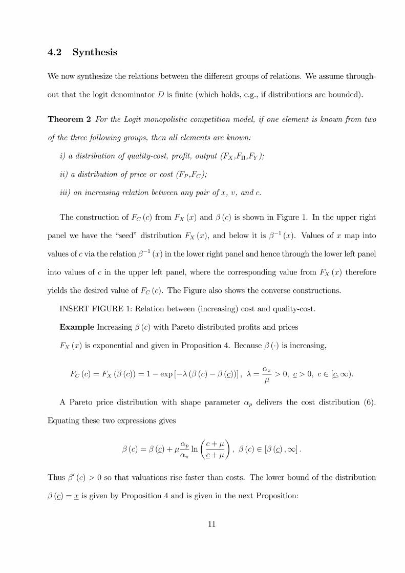
4.2 Synthesis

We now synthesize the relations between the different groups of relations. We assume through-

out that the logit denominator is finite (which holds, e.g., if distributions are bounded).

Theorem 2 For the Logit monopolistic competition model, if one element is known from two

of the three following groups, then all elements are known:

i) a distribution of quality-cost, profit, output (,Π, );

ii) a distribution of price or cost ( ,);

iii) an increasing relation between any pair of , , and .

The construction of () from () and () is shown in Figure 1. In the upper right

panel we have the “seed” distribution (), and below it is −1 (). Values of map into

values of via the relation −1 () in the lower right panel and hence through the lower left panel

into values of in the upper left panel, where the corresponding value from () therefore

yields the desired value of (). The Figure also shows the converse constructions.

INSERT FIGURE 1: Relation between (increasing) cost and quality-cost.

Example Increasing () with Pareto distributed profits and prices

() is exponential and given in Proposition 4. Because (·) is increasing,

() = ( ()) = 1− exp [− ( ()− ())] =

0 0 ∈ [∞)

A Pareto price distribution with shape parameter delivers the cost distribution (6).

Equating these two expressions gives

() = () +

ln

µ+

+

¶ () ∈ [ () ∞]

Thus 0 () 0 so that valuations rise faster than costs. The lower bound of the distribution

() = is given by Proposition 4 and is given in the next Proposition:

11

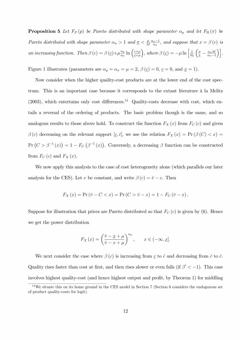
Proposition 5 Let () be Pareto distributed with shape parameter and let Π () be

Pareto distributed with shape parameter 1 and

−1, and suppose that = () is

an increasing function. Then () = ()+ln³+

+

´, where () = − ln

h1V0

³

−

−1

´i.

Figure 1 illustrates (parameters are = = = 2, () = 0, = 0, and = 1).

Now consider when the higher quality-cost products are at the lower end of the cost spec-

trum. This is an important case because it corresponds to the extant literature à la Melitz

(2003), which entertains only cost differences.13 Quality-costs decrease with cost, which en-

tails a reversal of the ordering of products. The basic problem though is the same, and so

analogous results to those above hold. To construct the function () from () and given

() decreasing on the relevant support [ ], we use the relation () = Pr ( () ) =

Pr¡ −1 ()

¢= 1 −

¡−1 ()

¢. Conversely, a decreasing function can be constructed

from () and ().

We now apply this analysis to the case of cost heterogeneity alone (which parallels our later

analysis for the CES). Let be constant, and write () = − . Then

() = Pr ( − ) = Pr ( − ) = 1− ( − ) .

Suppose for illustration that prices are Pareto distributed so that () is given by (6). Hence

we get the power distribution

() =

µ − +

− +

¶

, ∈ (−∞ ]

We next consider the case where () is increasing from to and decreasing from to .

Quality rises faster than cost at first, and then rises slower or even falls (if 0 −1). This case

involves highest quality-cost (and hence highest output and profit, by Theorem 1) for middling

13We situate this on its home ground in the CES model in Section 7 (Section 6 considers the endogenous set

of product quality-costs for logit).

12

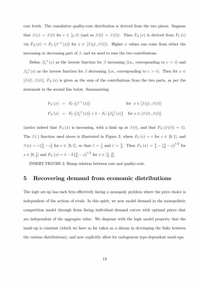
cost levels. The cumulative quality-cost distribution is derived from the two pieces. Suppose

that () () for ∈ [ ) (and so () = ()). Then () is derived from ()

via () =

¡−1 ()

¢for ∈ [ () ()). Higher values can come from either the

increasing or decreasing part of , and we need to sum the two contributions.

Define −1 () as the inverse function for increasing (i.e., corresponding to ) and

−1 () as the inverse function for decreasing (i.e., corresponding to ). Then for ∈

[ () ()], () is given as the sum of the contributions from the two parts, as per the

statement in the second line below. Summarizing:

() =

¡−1 ()

¢for ∈ [ () ())

() =

¡−1 ()

¢+ 1−

¡−1 ()

¢for ∈ [ () ()]

(notice indeed that () is increasing, with a kink up at (), and that ( ()) = 1).

The () function used above is illustrated in Figure 2, where () = for ∈ [0 1], and

() = ¡43− ¢for ∈ [0 1], so that = 1

3and = 2

3. Then () =

23− ¡4

9−

¢12for

∈ [0 13] and () = 1− 2

¡49−

¢12for ∈ [1

3 49].

INSERT FIGURE 2: Hump relation between cost and quality-cost.

5 Recovering demand from economic distributions

The logit set-up has each firm effectively facing a monopoly problem where the price choice is

independent of the actions of rivals. In this spirit, we now model demand in the monopolistic

competition model through firms facing individual demand curves with optimal prices that

are independent of the aggregate value. We dispense with the logit model property that the

mark-up is constant (which we have so far taken as a datum in developing the links between

the various distributions), and now explicitly allow for endogenous type-dependent mark-ups.

13

This section delivers what are perhaps the strongest results of the paper. We allow for

a general demand formulation as an additional primitive to the model, and show how the

primitives feed through to the endogenous economic distributions and variables. Conversely,

the derived economic distributions can be reverse engineered to back out the model’s primitives.

We first give the demand model, and derive the equilibrium mark-up schedule in Theorem

3 as a function of firm quality-cost (). Theorem 4 inverts the mark-ups to deliver not only the

equilibrium output choices, but also the form of the demand curve (on the support corresponding

to the set of quality-costs in the market). This analysis constitutes an stand-alone contribution

to the theory of monopoly pass-through, extending Weyl and Fabinger (2013) by working from

pass-through back to implied demands.

Theorem 5 shows how the (potentially observable) output and profit distributions can be

inverted to determine the underlying primitive distribution of quality-cost, (), and the

underlying demand form. This step also determines the equilibrium mark-up distribution,

which in turn determines (Theorem 6) the underlying distribution of costs, (), from the

(potentially observable) economic distribution of prices, (). This last step also enables us

to uncover the “bridge” function, (), from () and (). Throughout, we assume the

appropriate monotonicity conditions that ensure invertibility (see the analogous discussion in

Section 4.1).

5.1 Demand and mark-ups

Suppose now that demands are generated from the relation

= ( − )

∈ Ω, (7)

which generalizes (1), and where is an aggregate value determined by the actions of all

firms, but treated as constant by firms under the monopolistic competition assumption. We

14

refer to () as a “quasi-demand.” It is a positive, increasing, twice differentiable function of

quality-price, and strictly (−1)-concave.14 The exponential form of the Logit is a log-linear

quasi-demand: other cases are spotlighted below.

One useful case to think about the quasi-demand is as a “scale value” in a Lucian demand

system (based on the IIA property of the Logit, which property is shared with the CES), where

=R∈Ω ( ()− ()) + V0, or

=V0

1−R

() () (8)

There is leeway for normalization here. V0 can be set to one, or else the equilibrium for the

lowest quality-cost firm can be one (this is ∗ () below).15 We will follow the second route, and

express quasi-demands relative to the base value. Hence, when we say below (e.g., in Theorem

4) that () is uniquely determined, it means up to a positive multiplicative factor. As seen

below, we can also set = 0 and rescale how we measure quality-cost.

We now return to the more general case for . Firm ’s profit is = ( − )(−)

=

(−)

∈ Ω, where = − is ’s mark-up.

16 Under monopolistic competition, the

equilibrium mark-up satisfies

= ( −)

0 ( −) ∈ Ω (9)

Theorem 3 Let () be a positive, increasing, strictly (−1)-concave, and twice differentiable

quasi-demand function. Then the associated monopolistic competition mark-up, () is the

unique solution to (9), with 0 () 1. The associated equilibrium quasi-demand, ∗ () ≡14This is equivalent to 1

()strictly convex, and is the minimal condition ensuring a maximum to profit. See

Caplin and Nalebuff (1991) and Anderson, de Palma, and Thisse (1992) for more on -concave functions; and

Weyl and Fabinger (2013) for the properties of pass-through as a function of demand curvature: the analogue

to cost pass-through is here the complementary feature of quality-pass-through.15The first route is most familiar to econometricians in discrete choice. The second route does not allow us

to deal nicely with endogenous quality-costs (which we do in the long-run model of the next Section).16By the envelope theorem, the maximized value, ∗ () is increasing in : see also Theorem 3.

15

(− ()), is strictly increasing, as is ∗ () = ()∗ ().

Proof. The solution to (9), denoted (), is uniquely determined (and strictly positive) when

the RHS of (9) has slope less than one, as is implied by () being strictly (−1)-concave.

Applying the implicit function theorem to (9) shows that

0 () =

³(−)0(−)

´01 +

³(−)0(−)

´0 1 (10)

where the numerator is strictly positive when is (−1)-concave.17 The mark-up thus has slope

less than one. Let ∗ () = (− ()) denote the value of () under the profit-maximizing

mark-up. Then, given that 0 () 1, ∗ () is strictly increasing, as claimed, because

∗ () = (1− 0 ())0 (− ()) 0 (11)

Finally, ∗ () = ()∗ () is strictly increasing from the envelope theorem.

The only quasi-demand function with constant mark-up is the exponential (associated to

the Logit), which has (·) log-linear, and so (−)0(−) is constant. For (·) strictly log-concave,

0 () 0, so firms with higher quality-costs have higher mark-ups in the cross-section of firm

types. They also have higher equilibrium outputs. When (·) is strictly log-convex, the mark-

up decreases with : this is analogous to a cost pass-through greater than 1. Notice that the

property 0 () 1 is just the property that price never goes down as costs increase.

An important special case is when quasi-demand is −linear (which means that is linear).

Suppose then that () = ( + − )1, where is a constant. Then

() = (+ )

1 +

which is linear in . For = 1 quasi-demand is linear and the standard property is apparent

17We can have quality rise and mark-up go down immensely near the -1-concave limit: think too of cost

pass-through; with a demand 1/p then a zero cost gives a price of zero, but a small cost gives an infinite price.

16

that mark-ups rise fifty cents on the dollar with quality-cost.18 Note for such −linear demands

that ∗ () =³+1+

´1and it is readily verified that

∗()∗() = 1

(+)=

1−0()()

(see (12) below).

The converse result to Theorem 3 indicates how the mark-up function can be inverted to

determine the form of ∗ (and hence ()).

Theorem 4 Let there be a mark-up function () for ∈ [ ] with 0 () 1. Then there

exists a unique equilibrium quasi-demand function ∗ (·) defined on its support [ ] and given

by (13). The associated primitive quasi-demand function (·), given by (14), is strictly (−1)-

concave on its support [− () − ()].

Proof. First note from (9) and (11) that

∗ () ∗ ()

=(1− 0 ())0 (− ())

(− ())=(1− 0 ())

()≡ () (12)

Thus [ln∗ ()]0 = (), and so ln³∗()∗()

´=R () , which implies

∗ () = ∗ () exp

µZ

()

¶ ≥ (13)

which therefore determines ∗ () up to a positive factor.

We can now use ∗ () to back out the original function (−) via the following steps.

First, define = () = − (), which is monotone increasing because 1− 0 () 0, so the

inverse function −1 (·) is increasing. Now, () = ∗¡−1 ()

¢with ∈ [− () − ()]

and thus the function (·) is recovered on the support. Using (13) with () = ∗¡−1 ()

¢,

() = ∗ () expZ −1()

() (14)

18If = 0 we have log-linearity. The astute reader will note that the expression given does not go to the

constant mark-up of the Logit. To properly derive the Logit limit, we could write instead our -linear demand

as () = ³1 +

(+−)

´1

which has the limit lim→0

() = exp³(+−)

´.

17

and so (by (12)), and because 0 () = 1− 0 ():

()

0 ()=

1

¡−1 ()

¢ £−1 ()

¤0 = 0 ()(1−0())

()

= ()

Thus () is strictly (−1)-concave because19

∙ ()

0 ()

¸0=

0 ()1− 0 ()

−1

The steps above are readily confirmed for the −linear example given before Theorem 4.

Taking Theorems 3 and 4 together, knowing either () or () suffices to determine the other

and ∗ (). This constitutes a strong characterization result for monopoly pass-through (see

Weyl and Fabinger, 2013, for the state of the art, which deeply engages -concave functions).

Notice that the function (·) is tied down only on the support corresponding to the domain

on which we have information about the equilibrium value in the market. Outside that support,

we know only that (·) must be consistent with the maximizer (), which restricts the shape

of (·) to be not “too” convex. The case of positive quality pass-through (which is equivalent

to cost pass-through below 100%) is associated to log-concave demand.

5.2 Deriving demand form from output and profit distributions

We here engage the output and profit distributions ( and Π) to show how to back out

the underlying quality-cost distribution (), and the implied demand. Before this reverse

engineering, we first determine how the primitives and () generate the pertinent economic

distributions and mark-ups.

19When () is strictly (−1)-concave, then ()00 ()− 2 [0 ()]2 0, which rearranges toh()

0()

i0 −1.

18

As shown already, ∗ () and () are derived from () via Theorems 3 and 4. Now note

() = Pr

µ

∗ ()

¶= Pr ( ∗ ()) =

¡∗−1 ( )

¢

and, analogously,

Π () = Pr

µΠ

∗ ()

¶= Pr (Π ∗ ()) =

¡∗−1 (Π)

¢

where we have used Theorem 3 that ∗ () and ∗ () are strictly increasing.

The converse result is the key theorem. It tells us how to uncover the primitives from the

economic distributions and Π.

Theorem 5 Consider a demand model (7) under monopolistic competition. Assume that the

corresponding distributions of output, , and profit, Π, are known. Then the quality-cost dis-

tribution, , is given by (19) below, the mark-up function is found from (17), and equilibrium

quasi-demand is found from (16).

Proof. We know that ∗ () and hence = ∗()

are strictly increasing in , and so too is

∗ () = ()∗ () (by Theorem 3). We hence choose some arbitrary level ∈ (0 1) such that

() = () = Π () = (15)

This means that all firm types with quality-cost levels below = −1 () are the firms with

outputs and profits below and . For this proof, we introduce as an argument into the

various outcome variables to track the dependence of the variables on the level of (). Then

we can write () = −1 () and quasi-demand is

∗ () = ( ()) = −1 ( ()) (16)

19

Because ∗ () = () () = −1Π () then

() =−1Π ( ())

−1 ( ())= () , (17)

and equilibrium profit is ∗ () = ()∗()

= −1Π ( ()).

Hence 0 () = 0 ( ()) 0 () and ∗0 () = 0 ( ()) 0 (). These two unknown functions

satisfy condition (12), which implies0(())0()

(())=

(1−0(())0())(())

, so that

0 () = ( ())

( ( ()) ( ()))0 =

−1 ( ())¡−1Π ( ())

¢0or, inverting, we can write 0 () =

=

(()())0

()=(−1Π

())0

−1(). Integrating,

() = (0) +

Z

0

¡−1Π ()

¢0−1 ()

= +Ψ () . (18)

BecauseΨ0 () = (−1Π ())0

−1()

0, the required correspondence between and is = Ψ−1 (− ).

This makes clear that we can normalize because the values are all relative to this base

(nonetheless, we retain in what follows). The distribution of quality-cost is thus given by

() = () = Ψ−1 (− ) (19)

thus we have an expression for (). Now that we know (), the remaining unknowns can

now be backed out.

Example (-linear demands and uniform quality-cost distribution)

Suppose that () =(1+)−1

, ∈

∙³11+

´1 1

¸, and Π () =

(1+)(1+)−1

, ∈∙³11+

´(1+) 1

¸. Hence −1 () =

³+1

1+

´1and −1Π () =

³+1

1+

´(1+). The ratio of these

two yields () = +1

1+. Because

¡−1Π ()

¢0=³+1

1+

´1, we can write 0 () =

(−1Π ())0

−1()

= 1,

and hence, from (18) () = (0)+R 0 = +Ψ (), or () = +, i.e. () = = −.

Then () =(−)+11+

, and so () = −1 ( ()) =³(−)+11+

´1, and because ∗ () = (),

20

() is therefore a −linear demand function. Note that () =³

11+

´1, as verified by the

lower bound, , while the upper bound condition = 1 implies that − = 1.20 Lastly,

lim→0

() = lim→0

³(−)+11+

´1= exp (− ) gives the logit model with a unit mark-up.

5.3 Deriving costs and the quality-cost to cost relation

If we also have the price distribution, () then we can furthermore back out the cost distrib-

ution, (), and the quality-cost to cost relation (). The steps are as follows. First, deter-

mine the mark-up distribution, (), from the mark-up relation () and the quality-cost

distribution, (). Then, use () with the price distribution to uncover the underlying

cost distribution, (). Matching this with () uncovers the relation between cost and

quality-cost (the function () from Section 4).

In the sequel we shall consider the special case of strictly log-concave (), which implies

(and is implied by) 0 () ∈ (0 1). Knowledge of () and Π () determines () and ()

from Theorem 5. Then we can derive the mark-up distribution, (), from the relation:

() = Pr ( ) = Pr ( () ) =

¡−1 ()

¢ (20)

where we have used that 0 () 0. Notice that there are implied properties on the re-

sulting mark-up distribution function. Because () = ( ()) then 0 () 1 implies

( ()) ().21

With the mark-up function () thus determined, suppose that () is known. To

uncover () requires knowing whether costs and mark-ups move together or not. Suppose

20Using the definition of from (8) we get V0 = ³1− (1 + )

−1−1´. Hence we can either normalize

V0 = 1 here so = 1

(1−(1+)−1−1), or else we can normalize ∗ () = () = 1 so that =

³11+

´−1and thus V0 =

³11+

´−1 ³1− (1 + )

−1−1´. In either case, we are at liberty to set = 0.

21Note also that 0 () = ()

(()) 0, as desired for a strictly log-concave .

21

that it is known that they do, then higher costs also entail higher prices. In this case we can

match distributions by choosing a common level of the distributions and write

() = () = () = ; with − =

Then we can uncover () through the relation

−1 () = −1 ()− −1 () . (21)

With () thus determined, the final primitive to determine is the relation between quality-

cost and cost. We can here proceed as we did in Section 4, and recover the relation between

() and () via the transformation function () (see Figure 1). Given that () is an

increasing function, we have (because = −1 () by (15)):

= () = −1 ( ()) (22)

The results above are summarized as follows.

Theorem 6 Consider a demand model (7) under monopolistic competition, where it is known

that () is strictly log-concave and quality-cost increases with cost. Assume that the distribu-

tions of profit and output and price are known. Then the quality-cost distribution is given by

(19), the mark-up function is given by (17), and equilibrium quasi-demand is given by (16).

The cost distribution is given by (21), and the quality-cost bridge is given by (22).

Example

Suppose we know that 0 (= + 1) and 0, and Π () = 2√ − (= ) for

∈h2

4

2

4

i, () = 2 − (= ) for ∈ £

2 2

¤, and () =

¡−

¢with 2.

22

Then −1Π () = 1

¡+2

¢2and −1 () = +

2; the relation between and is given by (18) as

Z

0

¡−1Π ()

¢0−1 ()

=

Z

0

= = Ψ () = −

so = Ψ−1 (− ) = () = −, and () is uniform on [ + 1]. Then the mark-up is

() =−1Π (− )

−1 (− )=

− +

2

Then ∗ () = −+2

(using (16)), and the associated function is ( − ) = (−) =

(− + −) (from Theorem 4) so this is a linear quasi-demand. Using the specification

(8) gives = V0¡1−

4(1 + 2)

¢.22

Because () = (−1 ()), and () = −+

2, then () = 2− (for ∈

£2 2

¤).

We can now find the cost distribution from the price distribution, using (21): −1 () =

−1 ()− −1 (). This gives −1 () =³

+ ´− ¡ +

2

¢=

³1− 1

2

´+ . Hence we have a

uniform distribution, () =³22−

´(− ) (where = −). We can now determine the

bridge function () from (22): = () = −1 ( ()). That is, () =³22−

´(− ) +

(equivalently, − =³22−

´(− )); here 0 () 0, as stipulated, given the restriction

2.23

An analogous analysis to that in Theorem 6 applies for 0 () 0, which corresponds

to strictly log-convex demand (although recall we still require demand to be (−1)-concave

to guarantee a unique maximum to firms’ profit functions). In the log-convex case, mark-

ups decrease with firm quality-cost and the relation we uncover below between the mark-

up distribution and the quality-cost one is inverted, analogously to the inversion of the ()

function analyzed in Section 4.2. Finally, if () is non-monotone, the primitives cannot be

backed out on their full support, analogous to the discussion in Section 4.2. Note that 0 () = 0

22As discussed above, we can normalize V0 = 1, or else ∗ () = 2= 1 so = 2

. We can also set = 0.

23Such a linear bridge function can arise from endogenous quality-cost choices of heterogeneous firms: see the

example in Section 4.1.

23

corresponds to the Logit case, which we have already analyzed in full.

6 Long run Logit

Here we develop the long-run analysis of the logit model following recent directions in Trade

models, and emphasize the shape of the equilibrium distributions that ensue. A fuller (more

general) analysis along the lines of the previous section would follow similar lines, but here we

aim for simplicity. We assume in the groove of Melitz (2003) that firms first pay a cost 1

to get a quality-cost draw, then they pay 2 to actively produce. We solve backwards.24 To

put in play market size effects, we introduce market size (number of consumers) (which was

normalized to 1 in the analysis so far).

For a given mass, , of firms that have paid 1, equilibrium involves all sufficiently good

types paying the subsequent fixed cost 2. The firm of type just covers its cost, 2, and

≥ if 2 is low enough. All types ≥ will produce (because profits increase in by

Proposition 1). The gross profit of firm with quality-cost is now

( ) = exp

³

´ ( )

where ( ) ≡ R≥ exp

() + V0 ≤ (see (5)). ( ) is decreasing in so

that the profit of the marginal firm, ( ) is increasing in . Hence, as long as ( ) 2,

there is a unique cut-off value such that

( ) = 2. (23)

This is the case we consider: otherwise, all firms enter, and all make strictly positive profits.

Once a firm has paid the cost 1 to get a draw, it has a probability 1 − () to get a

good enough draw, and to be active. The mass of potentially active firms, , is determined at

24If is observed by firms before entry, only the first part of the analysis should be retained.

24

the first step via the zero-profit condition:

R≥ exp

³

´ ()

( )−2

Z≥

() = 1 (24)

The first term is the expected gross profit of a firm which has paid the entry cost 1 to get

a draw. The second is the fixed (continuation) cost, to be paid by all firms with a draw of at

least . Inserting (23) in (24) gives

Z≥

µexp

µ−

¶− 1¶ () =

1

2

(25)

The LHS is monotonically decreasing in so there is a unique solution for that depends

only on the parameters in (25) — it is independent of market size and of V0 (Bertoletti and

Etro, 2014, show a similar neutrality result). The condition for an interior solution is that

Z≥

µexp

µ−

¶− 1¶ ()

1

2

(26)

Otherwise, all firms are in the market. Given the solution for , we can then determine from

(23) with ( ) and defining = max :

=

2exp

³

´− V0R

≥ exp³

´ ()

(27)

Therefore 0 if

≡

2

exp

µ

¶ V0 (28)

Otherwise, there is no entry ( = 0). Note that condition (28) depends on both 1 and 2

since depends on 12.

25

Proposition 6 (Logit, long-run) Consider the Logit Monopolistic Competition model, with cost

1 to get a quality-cost draw, and cost 2 to actively produce. Some firms enter if (28) holds;

some of these entrants do not produce if (26) holds. Then the solution satisfies (23) and (27).

This solution parallels that for the Melitz (2003) model.25 Some comparative static prop-

erties readily follow. The elasticity of with respect to is (using (28))¡1− V0

¢−1 1.

Hence, if the market is covered (V0 = 0), the number of firms is proportional to market size.

Otherwise, firm numbers more than double (see also Melitz, 2003; Bertoletti and Etro, 2014,

show the opposite case can arise when there are income effects).

Thus, the long-run uniquely determines and . From these, the long-run distribution

of quality-cost is () =()−()1−() for ∈ [ ], and then Theorems 1 and 2 hold. More-

over, the inheritance properties of the key distributions still apply. In particular, if is an

exponential distribution for then so is ( = 1 − exp (− (− ))). Thus profits and

outputs are Pareto, and then we can link to the cost and price distributions as we did before:

the size distribution of output and profit is Pareto, with shape parameter .

The comparative statics results of Proposition 3 are readily amended: for fixed at the

bottom of the support, a higher V0 decreases profits, while a higher raises them for low

quality-cost firms and reduces them for high quality-cost firms. Now, when the lower bound is

endogenous, it is clear from (25) that is unchanged when V0 rises, but falls (from (27)).

Thus the effect is just as before, except now milder by the exit of firms. For higher , by (27)

falls,26 so that increased taste heterogeneity increases the range of firm types that will stay

in the market after their initial draw. However, the number of firms taking the first draw ()

may increase or decrease — high quality firm types get lower profits (cf. Proposition 3), and

25We can readily include a second threshold for exporting firms in an international trade context.26For example, for the exponential distribution of quality-cost, = + 1

ln³2

1

1−1

´, which is decreasing

in . The corresponding mass of entering firms is = 1− V0

2

1exp

³−

´.

26

this may decrease the desire to enter.

7 CES models

A flurry of recent contributions use the CES and variants thereof (e.g., Dhingra and Morrow,

2013, Zhelobodko, Kokovin, Parenti, and Thisse, 2012, Bertoletti and Etro, 2014, etc.). Most

noticeably, it has enjoyed a huge spurt in popularity in the new international trade literature.27

Here we apply the distributional analysis to the CES. We start with the standard CES

monopolistic competition model with heterogeneity only in firms’ unit production costs (this

is the basic Melitz, 2003, approach). Hence, all economic distributions (prices, output, profit,

and revenue) are tied down by the cost distribution.

A central distribution in the literature has been the Pareto. We show that all relevant

distributions are Pareto if any one is (caveat: for prices and costs it is the distribution of the

reciprocal that is Pareto). This result we term the Pareto circle. To put this another way,

if we posit that the reciprocal of costs is Pareto distributed (equivalently, costs have a power

distribution), then so is the reciprocal of prices, and the other variables (output, revenue, and

profit) are all Pareto distributed. It is not possible to have (for example) a Pareto distribution

for profits and (another) Pareto distribution for prices in the CES model. The Pareto circle

cannot be escaped if one element is Pareto. Similar results hold for other distributions, yielding

a more general CES circle.

Following Baldwin and Harrigan (2011) and Feenstra and Romalis (2014), we therefore

introduce a further dimension of heterogeneity, just as we did for the logit, and again interpreted

as “quality.” As with the logit analysis we link the two distributions via a bridge function

(analogous to () above) that writes quality as a function of cost. Doing this then enables

us to get two linked groups of distributions. In one group are profit and revenue, and in the

27Although note that Fajgelbaum, Grossman, and Helpman (2009) take a nested multinomial logit approach.

27

other are costs and prices, while output forms a convex combination. Our leading example is a

bridge function that delivers Pareto distributions in each group. We first develop the analysis

for cost heterogeneity alone.

7.1 Standard CES model

Several forms of CES representative consumer utility functions are prevalent in the literature.

We nest these into one embracing form. The CES representative consumer involves a sub-utility

functional for the differentiated product =¡R

Ω ()

¢1

with ∈ (0 1) (with = 1 being

perfect substitutes, and → 0 being independent demands), and the ’s are quantities consumed

of the differentiated variants. Common forms of representative consumer formulation are (i)

Melitz model (see also Dinghra and Morrow, 2013) where = so there is only one sector);

(ii) the classic Dixit-Stiglitz (1977) case much used in earlier trade theory, = 0 with 0,

where 0 is consumption in an outside sector; (iii) = ln + 0, which constitutes a partial

equilibrium approach in the sense that there are no income effects (see Anderson and de Palma,

2000). The first two involve unit income elasticities, hence their popularity in Trade models.

Utility is maximized under the budget constraintRΩ () () + 0 ≤ , where is income.

The next results are quite standard. For a given set of prices and a set Ω of active firms,

Firm ’s demand (output) is:

=Ξ ()

−1R

∈Ω ()

−1 (29)

where Ξ () is for case (i), 1+

for case (ii) (which clearly nests case (i) for = 0); and 1

for the last case. In each case, Ξ () is the amount spent on the differentiated commodity in

aggregate. In the sequel we follow case (iii); the others are similarly straightforward.

The price solves max

(−)

−1 , so =

, and the Lerner index is −

= (1− ). Given

28

such pricing, Firm ’s equilibrium output is

= Ξ ()

−1−1

(30)

where = R ()

−1 () , and () is the unit cost density. Firm ’s equilibrium

profit is a constant fraction of its sales revenue, = , with = Ξ ()

−1

, so = (1− ) .

We can now tie together the various equilibrium distributions with the help of the following

straightforward result, which tells us how distributions are modified by powers and multiplica-

tive transformations. These transformations relate profit, revenue, output, price reciprocal

(1), cost reciprocal (1) in the CES model.

Lemma 2 (Transformation) Let () be the CDF associated to a random variable . Then

the CDF of with 0 is () =

h¡

¢ 1

ifor 0, and () = 1−

h¡

¢ 1

ifor 0.

For example, power distributions beget power distributions under positive power transforms

and Pareto distributions under negative power transforms. Furthermore, normal distributions

beget normal distributions in both cases, due to the symmetry of the normal distribution, etc.

We refer to pairs of distributions with the same functional forms but different parameters as

being in the same class (e.g., Pareto, power, normal distributions are all classes).

Proposition 7 (CES circle) For the CES, the distributions of profit, revenue, output, price

reciprocal and cost reciprocal are all in the same class.

Proof. From the analysis above, all these variables for the CES involve positive power trans-

formation and/or multiplication by positive constants. Profit is proportional to revenue; price

is proportional to cost, and likewise for their reciprocals. From (30), equilibrium output, ,

is related to the cost reciprocal, 1, by a positive power and a positive factor. The other

relations follow directly.

29

In particular, if any one of these distributions is Pareto (resp. power), then they all are

Pareto (resp. power) class, although they have different parameters. Similarly, if one is normal

(resp. log-normal) then all are normal (resp. log-normal). This result we term the CES-circle.

It means that the standard CES model with cost heterogeneity alone cannot deliver (say) Pareto

distributions for both profit and prices. Indeed, if profit is Pareto distributed, then price must

follow a power distribution. We next introduce quality heterogeneity to break the CES-circle.

7.2 CES quality-enhanced model

To now extend the model to allow for quality differences across products, we rewrite the sub-

utility functional as =¡R

Ω ()

¢1

with ∈ (0 1) and interpreting = as the

quality-adjusted consumption (see Baldwin and Harrigan, 2011, and Feenstra and Romalis,

2014). The corresponding demands are:

=Ξ ()

−1R

∈Ω ()

−1 (31)

where we have defined = which is interpreted as the price per unit of “quality” and Ξ ()

is as above for the three different cases (the amount spent on the differentiated commodity).

The key feature of (31) is that enters both with and without quality in the denominator.

The standard model (29) ensues when all the ’s are the same.

Under monopolistic competition, Firm ’s equilibrium price solves max

(−)

−1 so the pric-

ing solution =still holds. Hence, using = ,

28 which we refer to as quality/cost, the

equilibrium profit is29

= (1− )Ξ ()

1−R

∈Ω ()

1− = (1− ) (32)

Equilibrium profit is still a fraction (1− ) of revenue. This implies that profit, sales revenue,

28This is quality/cost whereas the logit has quality-cost.29Proposition 1 holds here too except for the CES proportional mark-up.

30

and quality/costs distributions are in the same class.30

Price and cost distributions are still in the same class, but reciprocal costs and profits are

not necessarily so. How the cost and profit distributions are linked is determined by the relation

between cost and quality. A functional relation between cost and quality/cost ties down the

bridging relation, and the distributions on the “other” side.

A central example of a bridging function is = so that quality/cost is increasing with

cost (so quality rises faster than cost) if 0 and it is decreasing if 0. The latter case

is embodied in the standard CES model above where = −1 and so “better” firms are those

with lower costs. The former case effectively corresponds to Feenstra and Romalis (2014). The

advantage of the constant elasticity bridging function is that it allows us to deploy results

(Lemma 2) on applying power transforms to random variables.

Because profits are proportional to

1− (see (32)), they are proportional to

1−

. Hence if

0 profits are in the same distribution class as costs. So then too are revenues and quality-

costs. But if 0, profits, revenues and quality-costs are in the “opposite” (or “inverse”)

class - this is the generalization of the earlier standard CES result. Prices, of course, are in the

same class as costs, but output is more intricate because it draws its influences from both sides.

Indeed, output is proportional to

1− (see (31)) which equals

1−−1

under the constant

elasticity formulation. This implies that for 1 − 1 0 the output distribution is in the

inverse class, while otherwise it is in the same class.

For what follows, we define two distributions as in the same class if they have the same

functional form. One distribution is the inverse of another one if it is the survival function of

the other distribution. A summarizing statement:

30Profits are increasing in so that firms would like this as large as possible. As we did with Logit, we can

link cost and quality through a type of "production" function and have (heterogeneous) firms choose their .

Along the same lines as Feenstra and Romalis (2014), we can let = be the quality produced at cost +

with a firm-specific productivity shock. Then, maximizing = ( + ) gives the optimized value relation

between cost and quality as =¡

¢−1 and so the bridge function takes a power form. Here it is decreasing

(and depends on the fundamental via = −1).

31

Proposition 8 (Breaking the CES circle) Consider the quality-enhanced CES model of mo-

nopolistic competition with = . Then:

i) the equilibrium price distribution mirrors the unit cost distribution;

ii) equilibrium profits, sales revenue, and quality/cost are in the same distribution class for

0 and in the inverse class for 0;

iii) equilibrium output is in the inverse distribution class for 1− 1 0, and in the same

distribution class for 1− 1.

Note that inverse distributions take the same form for symmetric distributions such as the

Normal, so then all distributions belong to the same class — once a normal, always a normal.

Take the example of a Pareto distribution for costs. First, prices are also Pareto distributed.

Second, profits, revenue, and quality/cost are Pareto distributed for 0 and power distributed

for 0 (they are independent of cost if = 0). Third, output is power distributed for

1 − 1 0, and Pareto distributed for 1 − 1

. If costs are power distributed, Pareto

and power are reversed in the above statements. Hence, we resolve the puzzle of getting Pareto

distributions for both prices and profits by including the appropriate bridge function.

Proposition 8(ii) indicates that quality/cost and profits fall in the same distribution. For

example, suppose that the distribution of quality/costs is Pareto: () = 1−¡

¢and assume

that 1−

1. Then the size distribution of profit is Pareto with tail parameter Π = 1−.

The well-known claimed empirical regularity “80-20” rule (that the top 20% of firms account

for 80% of sales) corresponds to a value Π of 1.161. The result here is that the profit tail

parameter is the confluence of a preference parameter and a quality/cost distribution one.31

31Although why they yield the same constant across settings remains intriguing.

32

8 Conclusions

The basic ideas here are simple. Market performance depends on the economic fundamentals

of tastes and technologies, and how these interact in the market-place.32 The fundamental

distribution of tastes and technologies feeds through the economic process to generate the

endogenous distribution of economic variables, such as prices, outputs, and profits. By invoking

the monopolistic competition assumption we get a straight feed-through from fundamental

distributions to performance distributions.

Quality and cost differences are especially interesting for empirical work and studying asym-

metric firms. A normal quality-cost distribution leads to a log-normal distribution of firm size,

and an exponential quality-cost distribution generates a Pareto distribution. In the CES formu-

lation, the assumed distribution of costs is also the equilibrium distribution of outputs: Pareto

begets Pareto. This cycle is broken by allowing for quality heterogeneity in the CES.

The CES model has been the workhorse model of monopolistic competition with asymmetric

firms. The Logit model gives some similar properties, while differing on others. For example,

the simple CES has constant percentage mark-ups while the Logit has constant absolute mark-

ups.33 The Logit can be deployed for similar purposes as the CES, and has an established

pedigree in its micro-economic underpinnings. It has a strong econometric backdrop which is

at the heart of much of the structural empirical industrial organization revolution.

Our main results in the heart of the paper show how to back out the demand form from profit

and output distributions, and hence, with the addition of knowledge of the price distribution,

to recover all the primitives of the model. To do this, though, we relied on there being a one-

dimensional underlying relationship between costs and quality-costs (which we also showed how

to recover). One direction for future research is to consider a multi-dimensional relationship.

32Firm size distributions have recently come to the fore in Chris Anderson’s (2006) work on the Long Tail of

internet sales.33The latter property is perhaps quite descriptive for cinema movies, DVDs, and CDs.

33

References

[1] Anderson, Chris (2006). The Long Tail: Why the Future of Business Is Selling Less of

More. New York: Hyperion.

[2] Anderson, Simon and André de Palma (2000), “From local to Global Competition,” Eu-

ropean Economic Review, 44, 423-448.

[3] Anderson, Simon P., André de Palma, and Jacques François Thisse (1992). Discrete Choice

Theory of Product Differentiation. Cambridge, MA: MIT Press.

[4] Baldwin, Richard, and James Harrigan (2011). “Zeros, Quality, and Space: Trade Theory

and Trade Evidence.” American Economic Journal: Microeconomics 3(2), 60-88.

[5] Ben-Akiva, Moshe, and Thawat Watanatada (1981). “Application of a Continuous Spatial

Choice Logit Model.” Structural Analysis of Discrete Data with Econometric Application.

Ed. Charles F. Manski and Daniel McFadden. Cambridge, MA: MIT.

[6] Bertoletti, Paolo, and Federico Etro (2014). “Monopolistic competition when income mat-

ters.” DEM WP55, University of Pavia, Department of Economics and Management.

[7] Cabral, Luis MB, and Jose Mata (2003). “On the evolution of the firm size distribution:

Facts and theory.” American Economic Review, 93(4), 1075-1090.

[8] Caplin, Andrew, and Barry Nalebuff (1991). “Aggregation and imperfect competition: On

the existence of equilibrium.” Econometrica, 59(1), 25—59.

[9] Chamberlin, Edward (1933). Theory of Monopolistic Competition. Cambridge, MA: Har-

vard University Press

[10] Crozet, Matthieu, Keith Head, and Thierry Mayer (2011). “Quality Sorting and Trade

Firm-level Evidence for French Wine.” Review of Economic Studies, 79(2), 609-644.

34

[11] Dixit, Avinash K., and S. Stiglitz (1977). “Monopolistic Competition and Optimal Product

Diversity.” American Economic Review, 67(3), 297-308.

[12] Dhingra Swati and John Morrow (2013) Monopolistic competition and optimum product

diversity under firm heterogeneity, LSE, mimeo.

[13] Eaton, Jonathan, Samuel Kortum, and Francis Kramarz (2011). “An Anatomy of Interna-

tional Trade from French Firms.” Econometrica, 79(5), 1453-1498.

[14] Elberse, Anita, and Felix Oberholzer-Gee (2006). Superstars and underdogs: An examina-

tion of the long tail phenomenon in video sales. Harvard Business School.

[15] Fajgelbaum, Pablo D., Gene M. Grossman, and Elhanan Helpman (2011). “Income Distri-

bution, Product Quality, and International Trade.” Journal of Political Economy, 119(4),

721-765.

[16] Feenstra, Robert C. and John Romalis (2014). International Prices and Endogenous Qual-

ity, Quarterly Journal of Economics, 129(2), 477-527.

[17] Fisk, Peter R. (1961). “The Graduation of Income Distributions.” Econometrica, 29(2),

171-185.

[18] Head, Keith, Thierry Mayer, and Mathias Thoenig (2014). “Welfare and Trade without

Pareto.” American Economic Review 104(5): 310-16.

[19] Johnson, Justin P. and David, P. Myatt (2006). “Multiproduct Cournot oligopoly”. The

RAND Journal of Economics, 37(3), 583-601.

[20] McFadden, Daniel (1978) “Modelling the Choice of Residential Location.” in A. Karlqvist,

L. Lundqvist, F. Snickars, and J. Weibull (eds.), Spatial Interaction Theory and Planning

35

Models, Amsterdam: North Holland, 75-96, Reprinted in J. Quigley (ed.), 1997, The

economics of housing, Vol. I, Edward Elgar: London, 531-552.

[21] Melitz, Marc J. (2003). “The Impact of Trade on Intra-Industry Reallocations and Aggre-

gate Industry Productivity.” Econometrica, 71(6), 1695-1725..

[22] Pareto, Vilfredo (1965). “La Courbe de la Repartition de la Richesse” (Original in 1896):

Oeuvres Complètes de Vilfredo. Ed. Busino G. Pareto. Geneva: Librairie Droz, 1-5.

[23] Shannon, Claude. E. (1948). “A Mathematical Theory of Communication,” Bell System

Technical Journal, 27(3), 379—423.

[24] Weyl, Glen,and Michal Fabinger (2013). “Pass-Through as an Economic Tool: Principles

of Incidence under Imperfect Competition.” Journal of Political Economy, 121(3), 528-583.

[25] Zhelobodko, Evgeny, Sergey Kokovin, Mathieu Parenti, and Jacques-François Thisse

(2012). “Monopolistic competition: Beyond the constant elasticity of substitution.” Econo-

metrica 80(6), 2765-2784.

36

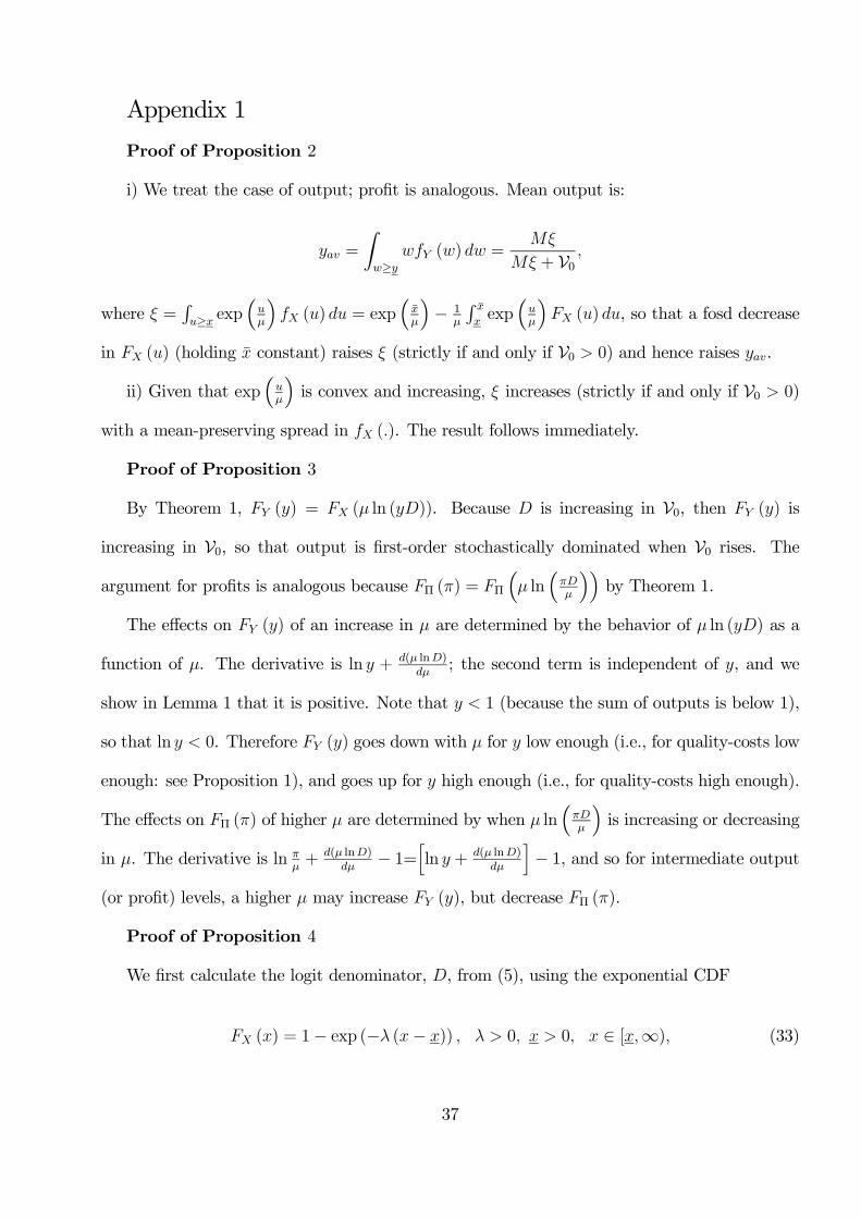
Appendix 1

Proof of Proposition 2

i) We treat the case of output; profit is analogous. Mean output is:

=

Z≥

() =

+ V0

where =R≥ exp

³

´ () = exp

³

´− 1

R exp

³

´ () , so that a fosd decrease

in () (holding constant) raises (strictly if and only if V0 0) and hence raises .

ii) Given that exp³

´is convex and increasing, increases (strictly if and only if V0 0)

with a mean-preserving spread in (). The result follows immediately.

Proof of Proposition 3

By Theorem 1, () = ( ln ()). Because is increasing in V0, then () is

increasing in V0, so that output is first-order stochastically dominated when V0 rises. The

argument for profits is analogous because Π () = Π

³ ln

³

´´by Theorem 1.

The effects on () of an increase in are determined by the behavior of ln () as a

function of . The derivative is ln +( ln)

; the second term is independent of , and we

show in Lemma 1 that it is positive. Note that 1 (because the sum of outputs is below 1),

so that ln 0. Therefore () goes down with for low enough (i.e., for quality-costs low

enough: see Proposition 1), and goes up for high enough (i.e., for quality-costs high enough).

The effects on Π () of higher are determined by when ln³

´is increasing or decreasing

in . The derivative is ln +

( ln)

− 1=

hln +

( ln)

i− 1, and so for intermediate output

(or profit) levels, a higher may increase (), but decrease Π ().

Proof of Proposition 4

We first calculate the logit denominator, , from (5), using the exponential CDF

() = 1− exp (− (− )) 0 0 ∈ [∞) (33)

37

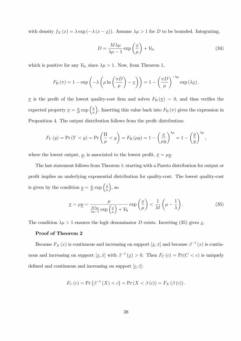
with density () = exp (− (− )). Assume 1 for to be bounded. Integrating,

=

− 1 expµ

¶+ V0 (34)

which is positive for any V0, since 1. Now, from Theorem 1,

Π () = 1− expµ−

µ ln

µ

¶−

¶¶= 1−

µ

¶−exp () .

is the profit of the lowest quality-cost firm and solves Π () = 0, and thus verifies the

expected property =

exp

³

´. Inserting this value back into Π () gives the expression in

Proposition 4. The output distribution follows from the profit distribution:

() = Pr ( ) = Pr

µΠ

¶= Π () = 1−

µ

¶

= 1−µ

¶

,

where the lowest output, , is associated to the lowest profit, = .

The last statement follows from Theorem 1: starting with a Pareto distribution for output or

profit implies an underlying exponential distribution for quality-cost. The lowest quality-cost

is given by the condition =

exp

³

´, so

= =

−1 exp³

´+ V0

exp

µ

¶1

µ− 1

¶ (35)

The condition 1 ensures the logit denominator exists. Inverting (35) gives .

Proof of Theorem 2

Because () is continuous and increasing on support [ ] and because −1 () is contin-

uous and increasing on support [ ] with −1 () 0. Then () = Pr( ) is uniquely

defined and continuous and increasing on support [ ]:

() = Pr¡−1 ()

¢= Pr ( ()) = ( ())

38

The last term is a continuous and increasing function of a continuous and increasing function,

so () is recovered. Constructing () from () and () is completely analogous.

We now show how to construct a unique increasing () from the two distributions: let

() = Pr ( ) and we postulate that there exists a continuous increasing function

() = and so () = Pr ( () ) = Pr¡ −1 ()

¢which is then equal to

¡−1 ()

¢.

Now, since () =

¡−1 ()

¢, then −1 () = −1 ( ()), so () =

£−1 ( ())

¤−1and () = −1 ( ()). This is clearly increasing and continuous in as desired.

The claim in the Theorem is shown because () can be used to construct the other

distributions on its leg, and can be constructed from them; and likewise for ().

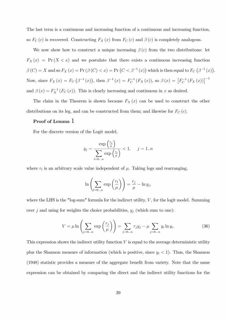
Proof of Lemma 1

For the discrete version of the Logit model,

=exp

³

´X=0

exp³

´ 1 = 1

where is an arbitrary scale value independent of . Taking logs and rearranging,

ln

à X=0

exp

µ

¶!=

− ln

where the LHS is the "log-sum" formula for the indirect utility, , for the logit model. Summing

over and using for weights the choice probabilities, (which sum to one):

= ln

à X=0

exp

µ

¶!=X

=0

− X

=0

ln (36)

This expression shows the indirect utility function is equal to the average deterministic utility

plus the Shannon measure of information (which is positive, since 1). Thus, the Shannon

(1948) statistic provides a measure of the aggregate benefit from variety. Note that the same

expression can be obtained by comparing the direct and the indirect utility functions for the

39

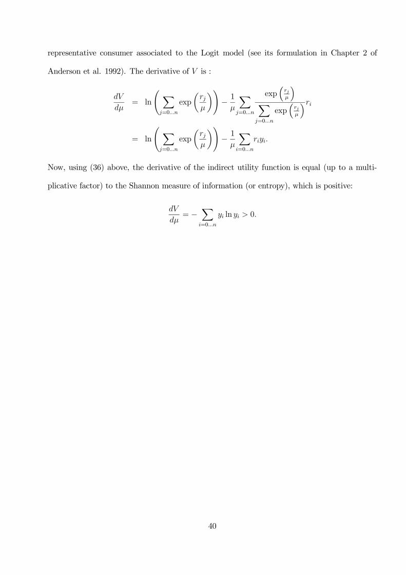
representative consumer associated to the Logit model (see its formulation in Chapter 2 of

Anderson et al. 1992). The derivative of is :

= ln

à X=0

exp

µ

¶!− 1

X=0

exp³

´X

=0

exp³

´= ln

à X=0

exp

µ

¶!− 1

X=0

Now, using (36) above, the derivative of the indirect utility function is equal (up to a multi-

plicative factor) to the Shannon measure of information (or entropy), which is positive:

= −

X=0

ln 0

40

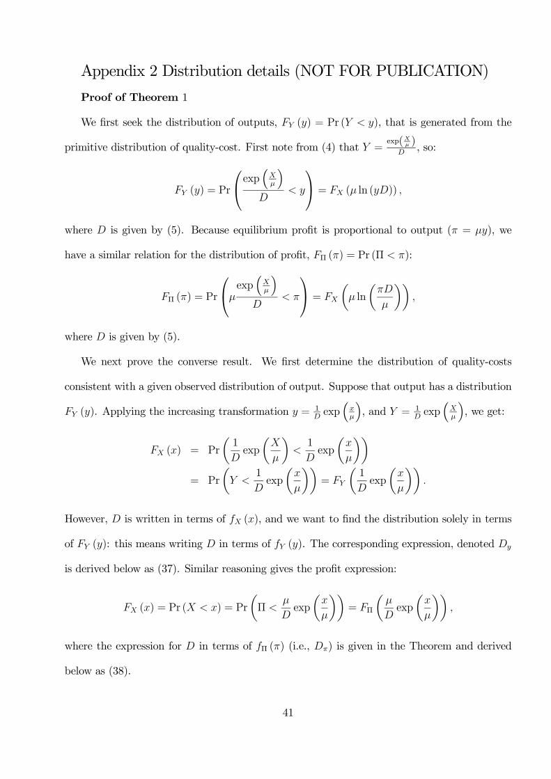
Appendix 2 Distribution details (NOT FOR PUBLICATION)

Proof of Theorem 1

We first seek the distribution of outputs, () = Pr ( ), that is generated from the

primitive distribution of quality-cost. First note from (4) that =exp( )

, so:

() = Pr

⎛⎝exp³

´

⎞⎠ = ( ln ())

where is given by (5). Because equilibrium profit is proportional to output ( = ), we

have a similar relation for the distribution of profit, Π () = Pr (Π ):

Π () = Pr

⎛⎝exp

³

´

⎞⎠ =

µ ln

µ

¶¶

where is given by (5).

We next prove the converse result. We first determine the distribution of quality-costs

consistent with a given observed distribution of output. Suppose that output has a distribution

(). Applying the increasing transformation = 1exp

³

´, and = 1

exp

³

´, we get:

() = Pr

µ1

exp

µ

¶1

exp

µ

¶¶= Pr

µ

1

exp

µ

¶¶=

µ1

exp

µ

¶¶

However, is written in terms of (), and we want to find the distribution solely in terms

of (): this means writing in terms of (). The corresponding expression, denoted

is derived below as (37). Similar reasoning gives the profit expression:

() = Pr ( ) = Pr

µΠ

exp

µ

¶¶= Π

µ

exp

µ

¶¶

where the expression for in terms of Π () (i.e., ) is given in the Theorem and derived

below as (38).

41

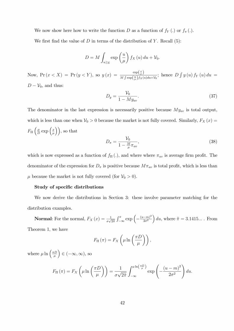
We now show here how to write the function as a function of () or ().

We first find the value of in terms of the distribution of . Recall (5):

=

Z≥

exp

µ

¶ () + V0

Now, Pr ( ) = Pr ( ), so () =exp( )

exp()()+V0

; hence R () () =

− V0, and thus:

=V0

1− (37)

The denominator in the last expression is necessarily positive because is total output,

which is less than one when V0 0 because the market is not fully covered. Similarly, () =

Π

³

exp

³

´´, so that

=V0

1−

(38)

which is now expressed as a function of Π (), and where where is average firm profit. The

denominator of the expression for is positive because is total profit, which is less than

because the market is not fully covered (for V0 0).

Study of specific distributions

We now derive the distributions in Section 3: these involve parameter matching for the

distribution examples.

Normal: For the normal, () =1

√2

R −∞ exp

³− (−)2

22

´, where = 31415 . From

Theorem 1, we have

Π () =

µ ln

µ

¶¶

where ln³

´∈ (−∞∞), so

Π () =

µ ln

µ

¶¶=

1

√2

Z ln( )

−∞exp

Ã−(−)

2

22

!

42

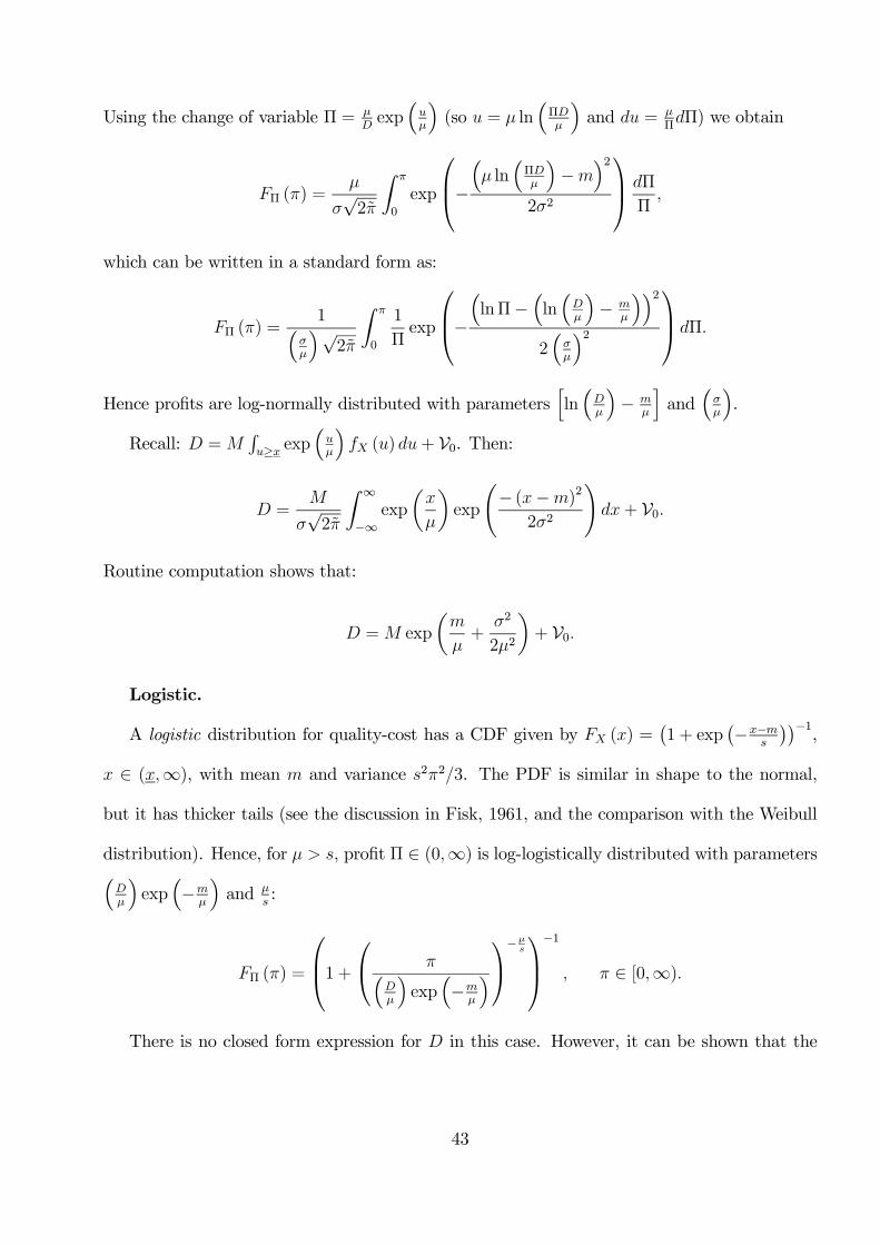
Using the change of variable Π =

exp

³

´(so = ln

³Π

´and =

ΠΠ) we obtain

Π () =

√2

Z

0

exp

⎛⎜⎝−³ ln

³Π

´−

´222

⎞⎟⎠ Π

Π

which can be written in a standard form as:

Π () =1³

´√2

Z

0

1

Πexp

⎛⎜⎝−³lnΠ−

³ln³

´−

´´22³

´2⎞⎟⎠ Π

Hence profits are log-normally distributed with parametershln³

´−

iand

³

´.

Recall: =R≥ exp

³

´ () + V0. Then:

=

√2

Z ∞

−∞exp

µ

¶exp

Ã− (−)

2

22

!+ V0

Routine computation shows that:

= exp

µ

+

2

22

¶+ V0

Logistic.

A logistic distribution for quality-cost has a CDF given by () =¡1 + exp

¡−−

¢¢−1,

∈ (∞), with mean and variance 223. The PDF is similar in shape to the normal,

but it has thicker tails (see the discussion in Fisk, 1961, and the comparison with the Weibull

distribution). Hence, for , profit Π ∈ (0∞) is log-logistically distributed with parameters³

´exp

³−

´and

:

Π () =

⎛⎜⎝1 +⎛⎝ ³

´exp

³−

´⎞⎠−

⎞⎟⎠−1

∈ [0∞)

There is no closed form expression for in this case. However, it can be shown that the

43

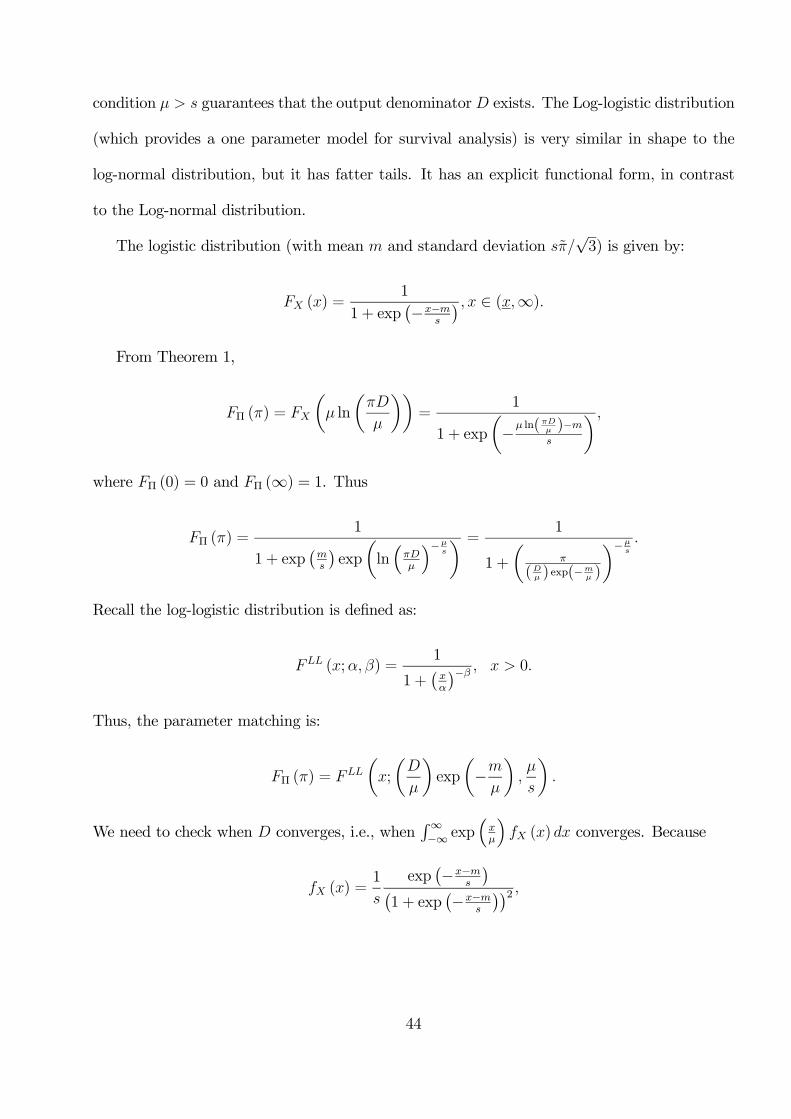
condition guarantees that the output denominator exists. The Log-logistic distribution

(which provides a one parameter model for survival analysis) is very similar in shape to the

log-normal distribution, but it has fatter tails. It has an explicit functional form, in contrast

to the Log-normal distribution.

The logistic distribution (with mean and standard deviation √3) is given by:

() =1

1 + exp¡−−

¢ ∈ (∞)From Theorem 1,

Π () =

µ ln

µ

¶¶=

1

1 + exp

µ− ln( )−

¶ where Π (0) = 0 and Π (∞) = 1. Thus

Π () =1

1 + exp¡

¢exp

µln³

´−

¶ = 1

1 +

µ

( ) exp(− )

¶−

Recall the log-logistic distribution is defined as:

(; ) =1

1 +¡

¢− 0

Thus, the parameter matching is:

Π () =

µ;

µ

¶exp

µ−

¶

¶

We need to check when converges, i.e., whenR∞−∞ exp

³

´ () converges. Because

() =1

exp¡−−

¢¡1 + exp

¡−−

¢¢2

44

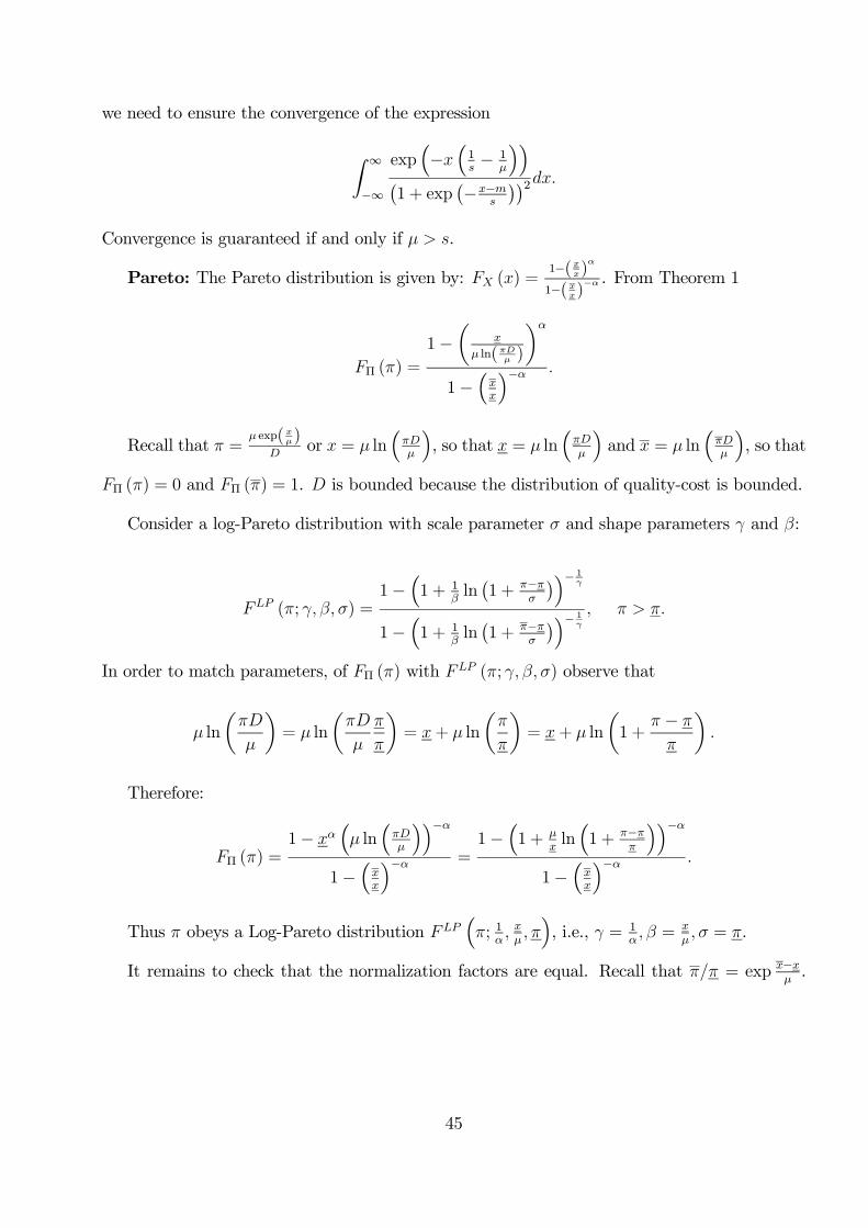
we need to ensure the convergence of the expression

Z ∞

−∞

exp³−³1− 1

´´¡1 + exp

¡−−

¢¢2Convergence is guaranteed if and only if .

Pareto: The Pareto distribution is given by: () =1−()

1−()− . From Theorem 1

Π () =

1−µ

ln( )

¶

1−³

´−

Recall that = exp( )

or = ln

³

´, so that = ln

³

´and = ln

³

´, so that

Π () = 0 and Π () = 1. is bounded because the distribution of quality-cost is bounded.

Consider a log-Pareto distribution with scale parameter and shape parameters and :

(; ) =1−

³1 + 1

ln¡1 + −

¢´− 1

1−³1 + 1

ln¡1 + −

¢´− 1

In order to match parameters, of Π () with (; ) observe that

ln

µ

¶= ln

µ

¶= + ln

µ

¶= + ln

µ1 +

−

¶

Therefore:

Π () =1−

³ ln

³

´´−1−

³

´− =1−

³1 +

ln³1 + −

´´−1−

³

´−

Thus obeys a Log-Pareto distribution ³; 1

´, i.e., = 1

=

= .

It remains to check that the normalization factors are equal. Recall that = exp −.

45

Using the specification = 1 =

= , we get:

µ1 +

ln

µ1 +

−

¶¶−=

µ1 +

ln

µ

¶¶−=

µ1 +

µ−

¶¶−=

µ

¶−

46

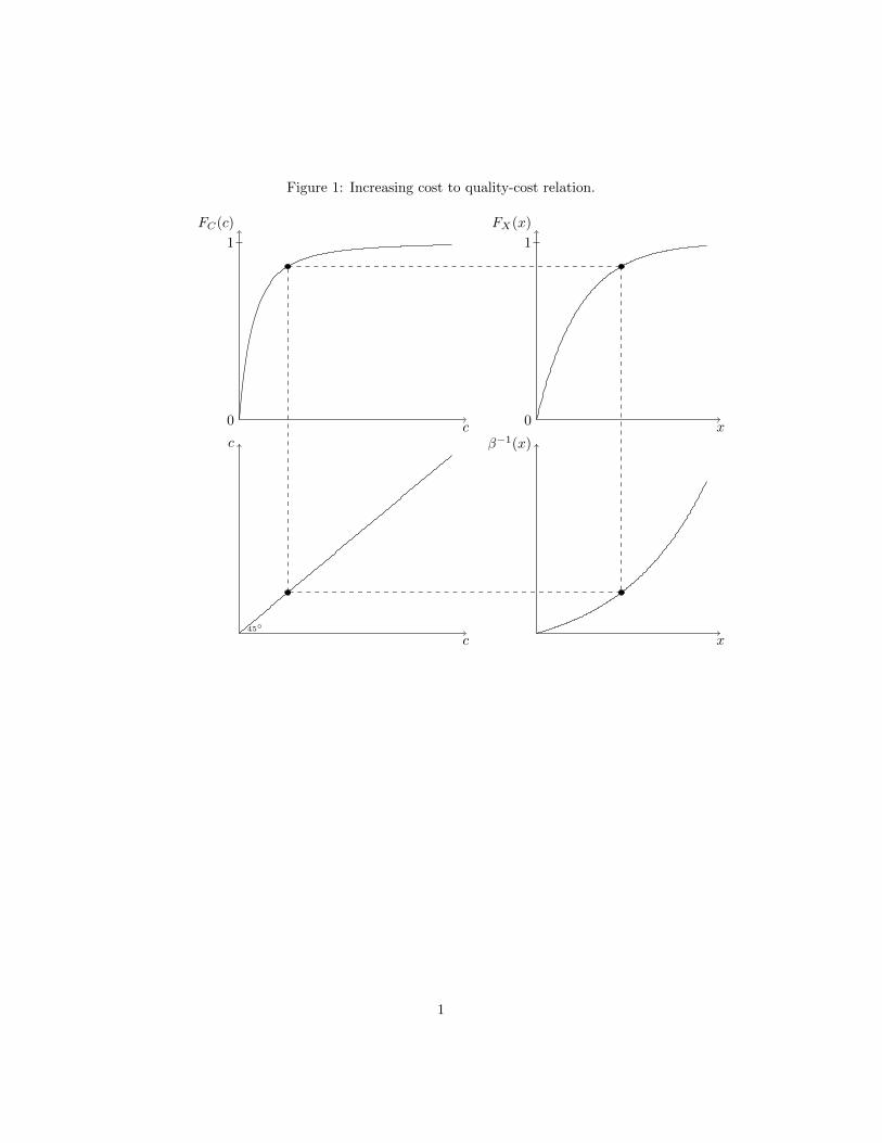
Figure 1: Increasing cost to quality-cost relation.

0

1

0

1

FC(c)

c

FX(x)

xc

c

β−1(x)

x45

1

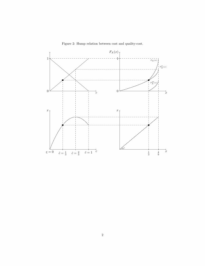
Figure 2: Hump relation between cost and quality-cost.

0

1

0

1

FUX

(x)

FDX

(x)

FX (x)

c = 23

49

13

c

FX(x)

x

x

cc = 1c = 13

c = 0

x

x45

2