Economic Development, Vertical Intra-Industry Trade and Gains from Trade

Modern Economy, 2014, 5, 1-10 Published Online January 2014 (http://www.scirp.org/journal/me) http://dx.doi.org/10.4236/me.2014.51001

Economic Development, Vertical Intra-Industry Trade and Gains from Trade

Le Duc Niem1, Taegi Kim2* 1Department of Economics, Tay Nguyen University, Dak Lak Province, Vietnam

2Department of Economics, Chonnam National University, Gwangju, South Korea Email: *[email protected]

Received November 19, 2013; revised December 19, 2013; accepted December 26, 2013

Copyright © 2014 Le Duc Niem, Taegi Kim. This is an open access article distributed under the Creative Commons Attribution Li-cense, which permits unrestricted use, distribution, and reproduction in any medium, provided the original work is properly cited. In accordance of the Creative Commons Attribution License all Copyrights © 2014 are reserved for SCIRP and the owner of the intel-lectual property Le Duc Niem, Taegi Kim. All Copyright © 2014 are guarded by law and by SCIRP as a guardian.

ABSTRACT This paper investigates the impact of economic development on international trade and sources of gains from trade based on a theoretical model that considers consumers’ preference diversity for quality and economies of scale in production. We confirm that both the volume of trade and the share of intra-industry trade increase with increases in the level of economic development in the region. We also find that the intra-industry trade share increases as the technology levels of the two countries become similar. Additionally, we find that both countries can gain from trade and that those gains come from three sources: internal economies of scale, more consumption, and more variety of goods. KEYWORDS Product Quality; Volume of Trade; Intra-Industry Trade; Economic Development; Gains from Trade

1. Introduction It has been generally accepted that trade is concentrated among the industrialized countries, and trade among in- dustrialized countries is principally vertical intra-industry trade (IIT). For example, Bergoeing and Kohoe [1] found that trade within the OECD countries has increased at a much more rapid rate than OECD trade with the rest of the world. Additionally, Gabrisch and Segnana [2] deter- mined that more than 50% of trade among EU countries was IIT, and that the intra-industry trade among EU coun- tries was composed, in large part, of vertical IIT.

In explaining these characteristics of trade, most stu- dies have emphasized economies of scale, product diffe- rentiation, and imperfect competition as the determinants of intra-industry trade. For example, seminal papers by Krugman [3] and Lancaster [4] developed this theoretical framework. However, these models pertain to horizontal product differentiation, assuming that these products are identical in quality. Flam and Helpman’s [5] considered a model where the North exports high-quality products and

the South exports low-quality products, and they evalu- ated the effects on trade of factors such as technical pro- gress, income distribution, and population growth. Hallak [6] suggested that Linder’s hypothesis (see Linder [7]) might not be found due to a systematic bias caused by ag- gregation across sectors, and he proposed that this hypo- thesis should be formulated at the sector level with a con- trol for inter-sectoral determinants of trade.

In the opposite direction, Falvey and Kierzkowski [8] returned to HOS fashion to explain IIT without modify- ing traditional trade theoretic models. Davis [9] and Bhag- wati and Davis [10] showed that IIT can occur in tradi- tional trade models as a consequence of technical differ- ences within an industry. For this reason, they argued whe- ther one should call this kind of trade vertical IIT or just inter-industry trade. Especially, Lüthje [11] stressed that foreign trade is mostly inter-industry trade because what called vertical IIT is in fact not IIT, but inter-industry trade.

The contribution of this paper is as follows. First, we considered determinants of the international trade with the assumption that products are vertically differentiated. *Corresponding author.

OPEN ACCESS ME

L. D. NIEM, T. KIM 2

It is worthwhile to note that Krugman [3] and Lancaster [4] investigated IIT regarding horizontally differentiated products so these models do not provide any explanation to vertical intra-industry trade. Second, our paper does provide an explanation to the gains from vertical IIT while previous works do not. This finding is, at least in the settings of this model, the evidence against the argu- ment that vertical IIT is actually inter-industry trade. Fur- thermore, this paper proposes a new and simple model to investigate vertical IIT.

This paper is organized as follows. Section 2 describes the basic model, and Section 3 derives the determinants of trade volume and vertical IIT share using a theoretical model. Section 4 examines the sources of gains from trade. Section 5 presents empirical implications of our findings. The final section contains our conclusions.

2. The Model We consider a 2 × 2 × 2 model: two countries, two firms, and two varieties of goods. Suppose that there is a world in which only two countries exist. One of them we will call Home, and the other we will refer to as Foreign. Both countries are assumed to be at the same level of economic development, and their per-capita incomes are assumed to be identical. We also assume that their tech-nology levels differ from industry to industry. For exam-ple, Home enjoys higher-level technology in some indus-tries, but Foreign has higher-level technology in other industries. As the two countries trade with one another, Home exports higher-quality goods in some industries, but also exports lower-quality goods in other industries. Even though there may be many different industries in a country, we hereinafter focus on the trade of goods in a single industry wherein goods are identical, but can be differentiated by quality. We utilize the term “quality- differentiated good” to reference this industry.

2.1. Supply Side Each country has one firm that produces one type of the quality-differentiated good1. Without any loss of general-ity, we assume that the foreign firm produces high-qual- ity goods and that the home firm produces low-quality goods in the considered industry; this implies that the technology level of the foreign firm is higher than that of the home firm in that industry2. In Grossman and Help-man’s [13] rising product quality model, the quality of each product is determined endogenously with R&D in-vestments. In this paper, we assume that the quality of each product is a consequence of R&D investment;

however, this expenditure has been sunk and become a fixed cost in the production process3. For this reason, we consider these qualities to be given and can be used as a proxy for technology level.

In producing the goods, two firms have cost functions as follows:

for ,i i iTC cX F i L H= + = (1)

In the cost function (1), we utilize H and L to desig- nate the high and low quality firms, respectively. Thus, the total cost, iTC , is the cost of firm i associated with

iX units of output. The marginal variable cost, or c, is identical for both firms. The fixed cost, iF , is the quality cost incurred by firm i. The higher the quality is, the more a firm has spent on R&D. Thus, we can say

L HF F≤ . It is worth mentioning that the total cost func-tions of both firms possess internal economies of scale property.

2.2. Demand Side The populations of consumers in Home and Foreign are the same and are normalized to 1. In each country, con-sumers are distributed uniformly between 0 and b ac-cording to the preference for quality iJ . Thus, parameter b measures the heterogeneity in consumer tastes for qual-ity in a country4. Each consumer may purchase a good from one of the firms, or none at all. The consumer’s utility function when consuming a good with quality lev-el q and price p is described as follows.

( )i iU J J q p= − (2)

This function is an indirect utility function of consum- er i, identified by the parameter iJ . A consumer’s utility is zero if he does not purchase this good. In the case of goods purchased only from one firm, a consumer will buy the good if it generates non-negative utility. If goods from two firms are available, consumers will elect to pur- chase the good that generates a higher and non-negative utility.

We denote the corresponding quality level and price level of high-quality and low-quality goods by Hq , Lq and Hp , Lp . The marginal consumer JLH is indifferent with regard to the consumption of either of the two pro- ducts. That is, the consumer, JLH, satisfies the condition ( ) ( ), ,H H L LU q p U q p= . In Equation (2), the marginal

consumer, JLH, is defined as

( )( )

H LLH

H L

p pJ

q q−

=−

(3)

1We consider our model only in the short-run. Thus, the reason for only one firm operates in each country is a high entry cost. See Beloqui and Usategui [12] for entry blockage and deterrence. 2This assumption is the same as in the study of Flam and Helpman [5].

3Grossman and Helpman [13] considered product quality changes over time due to R&D investments, but our model addresses a situation in which quality has been determined by R&D, and considers comparative statics with a one-time change in product quality. 4This assumption is widely used in vertical production differentiation studies, such as those of Wauthy [14], Beloqui and Usategui [12], and Sutton [15].

OPEN ACCESS ME

L. D. NIEM, T. KIM 3

Some consumers do not wish to buy any goods at the prevailing prices. We denote by JL a consumer who is indifferent with regard to the purchase of a low-quality product or refraining from buying. In Equation (2), this type of marginal consumer is defined as

LL

L

pJq

= (4)

All consumers satisfying the condition Ji > JLH will purchase high-quality goods, all consumers having JL < Ji < JLH will purchase low-quality goods, and all consumers having Ji < JL will purchase no goods5.

2.3. Trade between Countries Let us model a game as follows: There is not any trade barrier between Home and Foreign, and the two firms sell their goods to both countries. Thus, the competition is purely Bertrand in price. We also assume that no price discrimination is possible because the goods can move freely without any transportation costs between the two countries.

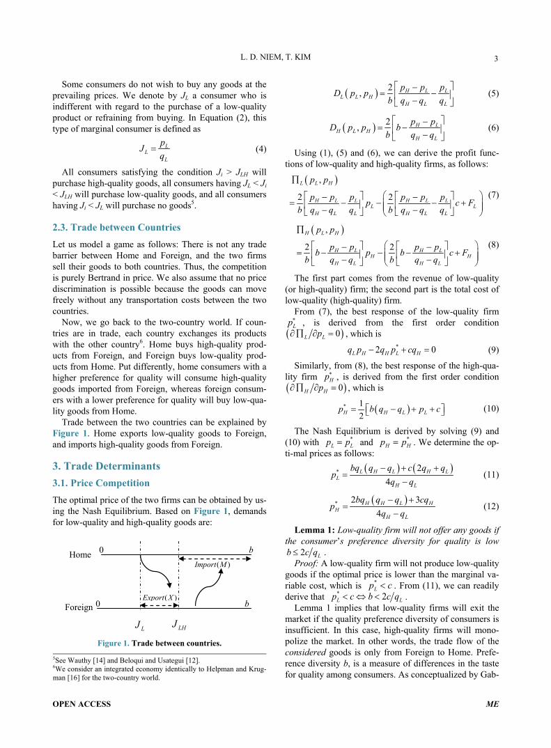
Now, we go back to the two-country world. If coun- tries are in trade, each country exchanges its products with the other country6. Home buys high-quality prod- ucts from Foreign, and Foreign buys low-quality prod- ucts from Home. Put differently, home consumers with a higher preference for quality will consume high-quality goods imported from Foreign, whereas foreign consum-ers with a lower preference for quality will buy low-qua- lity goods from Home.

Trade between the two countries can be explained by Figure 1. Home exports low-quality goods to Foreign, and imports high-quality goods from Foreign.

3. Trade Determinants 3.1. Price Competition The optimal price of the two firms can be obtained by us- ing the Nash Equilibrium. Based on Figure 1, demands for low-quality and high-quality goods are:

Home

Foreign 0

b

b

0

LJ LHJ

)(XExport

( )Import M

Figure 1. Trade between countries.

( ) 2, H L LL L H

H L L

p p pD p pb q q q −

= − − (5)

( ) 2, H LH L H

H L

p pD p p bb q q −

= − − (6)

Using (1), (5) and (6), we can derive the profit func- tions of low-quality and high-quality firms, as follows:

( ),

2 2

L L H

H L L H L LL L

H L L H L L

p p

p p p p p pp c Fb q q q b q q q

∏

− −= − − − + − −

(7)

( ),

2 2

H L H

H L H LH H

H L H L

p p

p p p pb p b c Fb q q b q q

∏

− −= − − − + − −

(8)

The first part comes from the revenue of low-quality (or high-quality) firm; the second part is the total cost of low-quality (high-quality) firm.

From (7), the best response of the low-quality firm Lp∗ , is derived from the first order condition

( )0L Lp∂∏ ∂ = , which is *2 0L H H L Hq p q p cq− + = (9)

Similarly, from (8), the best response of the high-qua- lity firm Hp∗ , is derived from the first order condition ( )0H Hp∂∏ ∂ = , which is

( )* 12H H L Lp b q q p c= − + + (10)

The Nash Equilibrium is derived by solving (9) and (10) with *

L Lp p= and *H Hp p= . We determine the op-

ti-mal prices as follows:

( ) ( )* 24

L H L H LL

H L

bq q q c q qp

q q− + +

=−

(11)

( )* 2 34

H H L HH

H L

bq q q cqp

q q− +

=−

(12)

Lemma 1: Low-quality firm will not offer any goods if the consumer’s preference diversity for quality is low

2 Lb c q≤ . Proof: A low-quality firm will not produce low-quality

goods if the optimal price is lower than the marginal va- riable cost, which is *

Lp c< . From (11), we can readily derive that * 2L Lp c b c q< ⇔ < .

Lemma 1 implies that low-quality firms will exit the market if the quality preference diversity of consumers is insufficient. In this case, high-quality firms will mono- polize the market. In other words, the trade flow of the considered goods is only from Foreign to Home. Prefe- rence diversity b, is a measure of differences in the taste for quality among consumers. As conceptualized by Gab-

5See Wauthy [14] and Beloqui and Usategui [12]. 6We consider an integrated economy identically to Helpman and Krug- man [16] for the two-country world.

OPEN ACCESS ME

L. D. NIEM, T. KIM 4

szewics and Thisse [17], a preference for quality is de- pendent on consumers’ income; the more income a con- sumer has, the more he is willing to pay for a given qual- ity level. Additionally, Sutton [15] also came to a similar conclusion, and determined that the preference for quail- ty increases with rising income. For this reason, b varia- ble can be seen as a proxy for a country income level7.

We allow Hq Q= and Lq aQ= . The parameter a, re-presents the relative level of technology between For-eign and Home. In addition, it is worthy noting that an increase in Q implies that technology levels in both countries increase (given that a is unchanged). Thus, Q can be used as a proxy for our world technology level (or regional technology level when we view the two coun-tries as a region).

A region is considered to have a high economic de-velopment level if it has high income and a high tech-nology level. For this reason, we utilize bQ as a proxy for regional economic development. It is also worth noting that 2 2Lb c q bQ c a≤ ⇔ ≤ . In addition, we always have 1a ≤ or bQ can be less than 2c a for any possi-ble value of a. Based on lemma 1 with the product of b and Q serving as a proxy for the regional economic de-velopment level, we derive the following proposition:

Proposition 1: Vertical intra-industry trade is unlikely to be observed in a region at very low economic develop- ment ( )2bQ c a≤ .

3.2. Determinants of Intra-Industry Trade If 2 Lb c q> , intra-industry trade between Home and Foreign will occur. Home exports low-quality products to Foreign, but imports high-quality products from For- eign. The export value and import value of Home can be expressed as follows.8

1 H L LL

H L L

p p pX Pb q q q −

= − − (13)

1 H LH

H L

p pM b Pb q q −

= − − (14)

Now, replacing optimal prices in (11) and (12) into (13) and (14), and then substituting Hq Q= and Lq aQ= , we obtain the following:

( ) ( )

( )2

2 1 2

4

ca bQ a a c abQ

Xa a

− − + +

=−

(15)

( )

( )2

2 2 1 3

4

c bQ a cbQ

Ma

− − +

=−

(16)

Proposition 2: When both trading countries are at a higher level of economic development, the volume of trade between them will be higher.

Proof: From (15) and (16), we can conclude directly that X and M both increase in b and Q.

Now, note that the imports (M) shown in (16) always exceed the exports (X) shown in (15). Thus, the Gru-bel-Lloyd index used to compute the IIT index can be written as follows, and is related to the ratio of exports to imports, R X M= .

2 211

M X X RIITM X M X R

−= − = =

+ + + (17)

We can see that IIT increases directly with R. That is, IIT behaves as R does.

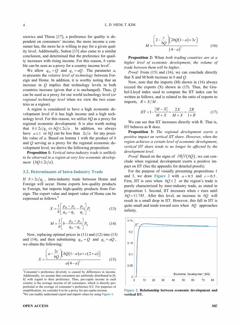
Proposition 3: The regional development exerts a positive impact on vertical IIT share. However, when the region achieves a certain level of economic development, vertical IIT share tends to no longer be affected by the development level.

Proof: Based on the signs of ( )R bQ∂ ∂ , we can con-clude when regional development exerts a positive im-pact on IIT (See the appendix for detailed proofs).

For the purpose of visually presenting propositions 1 and 3, we draw Figure 2 with 0.5a = and 0.5c = . First, IIT is zero when 2bQ ≤ or the region’s trade is purely characterized by inter-industry trade, as stated in proposition 1. Second, IIT increases when x rises until

11.745bQ = . After this level, an increase in bQ will result in a small drop in IIT. However, this fall in IIT is quite small and tends toward zero when bQ approaches infinity.

Figure 2. Relationship between economic development and vertical IIT.

7Consumer’s preference diversity is caused by differences in income. Additionally, we assume that consumers are uniformly distributed in [0, b] with regard to their preference. Thus, per-capita income in each country is the average income of all consumers, which is directly pro-portional to the average of consumer’s preference b/2. For purposes of simplification, we consider b to be a proxy for per-capita income. 8We can readily understand export and import values by using Figure 1.

OPEN ACCESS ME

L. D. NIEM, T. KIM 5

Proposition 4: The IIT index increases as the techno- logy levels between countries become similar.

Proof: We only prove 0R a∂ ∂ > . (See the appendix for detailed proofs).

4. Gains from Trade In this section, we try to identify why countries become better off when they are in trade with each other. We prove that countries in trade are better off for the follow- ing three reasons: goods are produced more efficiently, more goods are consumed, and a greater variety of goods are available. All of these findings are derived from ana-lyses of the welfare of both countries before trade and after trade.

4.1. Closed Economy If the two countries are not currently trading with each other, the high-quality firm will be a monopolist in For- eign and the low-quality firm will be a monopolist in Home.

For the purposes of our analyses, the following are the optimal prices, the consumers with the lowest preference for quality who can buy goods, and the welfare in both Home and Foreign. The detailed mathematical calcula- tions are presented in the appendix section.

1) The optimal prices established by the high-quality and low-quality firms are

2 2NF HH

bq c bQ cp + += = (18)

(In Foreign, set by high-quality firm)

2 2NH LL

bq c baQ cp + += = (19)

(In Home, set by low-quality firm) 2) The marginal consumer with the lowest preference

for quality can buy the good:

( )In Foreign2 2

NFH

b cJQ

= + (20)

( )In Home2 2

NHL

b cJaQ

= + (21)

3) Welfare when countries are closed:

( ) ( )23

In Foreign8

NFH

bQ cW F

bQ−

= − (22)

( ) ( )23

In Home8

NHL

baQ cW F

abQ−

= − (23)

Note that the superscript NF or NH indicates the “no- trade” case in Foreign or in Home.

4.2. In Trade

If Home and Foreign are currently trading, each country exchanges its products with the other country. Home consumers with a high preference for quality buy high- quality products from Foreign, and foreign consumers with low preference for quality buy low-quality products from Home. From section III, we have the following:

1) From (11) and (12), the optimal prices established by high-quality low-quality firms are

( ) ( )2 3 2 1 34 4

H H L HTH

H L

bq q q cq b a Q cp

q q a− + − +

= =− −

(24)

(High-quality good)

( ) ( )

( ) ( )

24

1 24

H L L H LTL

H L

b q q q c q qp

q qb a aQ c a

a

− + +=

−

− + +=

−

(25)

(Low-quality good) Note that these prices are the same in both countries. 2) Substituting (11) and (12) into (3) and (4), the mar-

ginal consumers with the lowest preference for quality can buy the high-quality good and the low-quality good as follows:

( )( )

24 4

TLH

b a cJa a Q−

= +− −

(26)

(For high-quality goods in both countries)

( ) ( )( )

1 24 4

TL

b a c aJ

a a aQ− +

= +− −

(27)

(For low-quality goods in both countries) 3) Welfares when countries are in trade (see appendix

for detailed mathematic calculations). Note that the TF or TH superscript indicates the “trade”

case in Foreign or in Home.

( ) ( ) ( ) ( )( )

( )2 2 2

2

20 11 32 14 4 9 4In Foreign

2 4TF

H

a a bQ a acbQ a a cW F

a a bQ

− − − + − + += −

− (28)

( ) ( ) ( ) ( )( )

( )22 2

2

4 9 4 32 14 20 11In Home

2 4TH

L

a a a bQ a acbQ a cW F

a a bQ

− + + − − + −= −

− (29)

OPEN ACCESS ME

L. D. NIEM, T. KIM 6

4.3. Sources of the Gains By comparing (22) with (28) and (23) with (29), we have

andTF NF TH NHW W W W> > (30)

Lemma 3: Both Home and Foreign gain when they are in trade with one another.

Lemma 3 demonstrates that both countries gain from trade. Where, though, do the gains come from? If we consider Home and Foreign as a single region, “some-thing better” must occur in the region when countries are in trade. So, what might that be?

Intuitively, regional welfare derives from the gross services of good consumption minus the total cost in-curred by both firms. Note that the revenues of firms are only a part of these gross services that firms capture from consumers.

By comparing (20) and (21) with (27), we have T NF NHL H LJ J J< < (31)

The inequalities in (31) imply that more consumers can buy the good (regardless of high-quality or low- quality ones) when countries are in trade.

Lemma 4: Goods are produced and consumed more if countries are in trade.

We note that quality costs of goods are fixed. Two im-plications can be gleaned from lemma 4. First, goods can be produced more cheaply because the total output of both firms is higher when countries are in trade. Put dif-ferently, economies of scale contribute to increases in the total welfare of the region9. Second, greater consumption of goods in both countries implies that more services are generated. Because these additional services are greater than their cost, this consumption results in an increase in the total welfare of the region.

Furthermore, when countries trade with each other, we have

T NHLH LJ J< (32)

which implies that all consumers (in Home) who pur-chase low-quality goods prior to trading will shift to con- suming high-quality goods. Thus, trade provides consu- mers with more choices of goods. This shifting from “low quality to high quality” provides more services to the region because it results in the consumption of more quality units. This gain derives from the greater variety of goods available when countries are in trade.

Proposition 5: Both countries gain from trade and these gains derive from three sources: firm’s economies of scale, more consumption, and more choice of goods.

5. Empirical Implications First, we have demonstrated that the volume of trade and IIT index are positively proportional to a product of b and Q, which implies the level of regional economic de-velopment. Therefore, propositions 2 and 3 demonstrate that an increase in economic development of the whole region will result in an increase in the volume of trade and IIT share within the region. This implication con-forms to the empirical fact that the volume of trade and IIT are higher among rich countries than among low-in- come countries (Bergoeing and Timothy [1]; Schott [18]; Hummels and Klenow [19]; Hallak [6]).

Second, the value a shows the convergence of tech-nology levels among countries. When the value a ap- proaches 1, the two countries become more similar in terms of technology levels. Proposition 4 shows that IIT index increases as the value a increases, which is consis-tent with the empirical fact that IIT is higher among sim-ilar countries in terms of economic development. This also implies that technology spillover among countries contributes to increases in IIT index. That is, the IIT in-dex is higher in industries in which a lower technology country attempts to catch up to one with higher technol-ogy. Note that trade volume may be low, proposition 4 implies the share of IIT should always be higher when a increases.

Third, proposition 1 shows that intra-industry trade does not occur among countries whose economic devel-opment levels are both very low. This means that, if the regional economic development is quite low, the oppor-tunity for two-way flows of trade will be eliminated. This is because high-quality firm will block low-quality firm and monopolize the entire market. This explains why vertical IIT is unlikely to be observed between countries at a very low level of economic development.

Finally, our model confirms that gains from vertical IIT come from economies of scale and more varieties, which is similar to the sources of gains from horizontal IIT in Krugman [3]. However, the role of economies of scale is different between our model and Krugman [3]. In Krugman [3], price falls because of economies of scale. In our model, more competition due to trade makes price fall, and the lower price stimulates more consumption as well as total product output. The expansion of this output causes economies of scale that increases in the regional welfare. Furthermore, vertical IIT allows more consump- tion that makes the region better off. It is important to note that this finding is obtained only in the short-run as firms are not allowed to select different quality levels for their goods.

6. Conclusions In this paper, the determinants of vertical intra-industry

9This does not mean that economies of scale are always in effect in both firms. It only means that the value of the “sum-up effects” of eco- nomies of scale in both firms must be positive.

OPEN ACCESS ME

L. D. NIEM, T. KIM 7

trade between two countries have been evaluated. Addi- tionally, gains from trade have also been identified. The principal findings of this study are as follows:

First, the economic development of a region, which is defined as a product of the income and the regional tech- nology levels, increases the volume of trade and the in- tra-industry share. This explains why the IIT index and trade volume are higher among developed countries as compared to developing countries. Second, the IIT share is positively related to the similarity in technology levels between countries. Third, vertical IIT is unlikely to be observed in regions with very low levels of economic development. This finding implies that trade among low-income countries can be characterized purely by in- ter-industry trade, even if the traded goods are markedly different in quality. Basically, the findings of this study are generally consistent with the previous reports of Ber- goeing and Kehoe [1], Schott [18], Hummels and Kle- now [19], and Hallak [6]. Finally, we have demonstrated that this kind of trade can improve both countries. Three sources of the gains from trade being identified include internal economies of scale, increased consumption, and greater varieties of goods.

Even if this model provides some theoretical explana- tions for vertical intra-industry trade, it still has a limita- tion. The model includes quality-differentiated products only in an oligopoly market and product qualities are gi- ven. However, we expect that the results will be similar in other market structures and when firms are allowed to select quality levels for their goods.

Acknowledgements The first author would like to thank the Vietnam National Foundation for Science and Technology Development (NAFOSTED) for supporting this research under grant number II1.1-2012.17.

REFERENCES [1] R. Bergoeing and T. J. Kohoe, “Trade Theory and Trade

Facts,” Federal Reserve Bank of Minneapolis Research Department, Staff Report No. 284, 2003.

[2] H. Gabrisch and M. L. Segnana, “Vertical and Horizontal Patterns of Intra-Industry Trade between EU and Candi- date Countries,” IWH-Sonderheft, Halle Institute for Eco- nomic Research, 2003.

[3] P. Krugman, “Increasing Returns, Monopolistic Competi- tion, and International Trade,” Journal of International Economics, Vol. 9, No. 4, 1979, pp. 469-479. Uhttp://dx.doi.org/10.1016/0022-1996(79)90017-5 U

[4] K. Lancaster, “Intra-Industry Trade under Perfect Mono- polistic Competition,” Journal of International Econom-

ics, Vol. 10, No. 2, 1980, pp. 151-175. Uhttp://dx.doi.org/10.1016/0022-1996(80)90052-5 U

[5] H. Flam and E. Helpman, “Vertical Product Differentia- tion and North-South Trade,” The American Economic Review, Vol. 77, No. 5, 1987, pp. 810-822.

[6] J. C. Hallak, “A Product-Quality View of the Linder Hy- pothesis,” The Review of Economics and Statistics, Vol. 92, No. 3, 2010, pp. 238-265. Uhttp://dx.doi.org/10.1162/REST_a_00001 U

[7] S. Linder, “An Essay on Trade and Transformation,” Wi- ley, New York, 1961.

[8] R. Falvey and H. Kierzkowski, “Product Quality, Intrain- dustry Trade and (Im)Perfect Competition in H. Kierz- kowski, (ed.), Protection and Competition in International Trade,” Essays in Honor of W.M. Corden, Basil Black- well, Oxford, 1987.

[9] D. R. Davis, “Intraindustry Trade: A Heckscher-Ohlin- Ricardo Approach,” Harvard University, Mimeo, 1993.

[10] J. Bhagwati and D. R. Davis, “Intraindustry Trade Issues and Theory,” Discussion Paper No. 1695, Harvard Insti- tute of Economic Research, 1994.

[11] T. Lüthje, “Discussion of the Concept Intra-Industry Trade,” Economic Discussion Papers, Faculty of Social Sciences, University of Southern Denmark, No. 4, 2001.

[12] L. Beloqui and J. M. Usategui, “Vertical Differentiation and Entry Deterrence: A Reconsideration,” WP 2005-06, Dept. Fundamentos del Analisis Economico II, Universi- dad del Pais Vasco, 2005.

[13] G. M. Grossman and E. Helpman, “Innovation and Growth in the World Economy,” MIT Press, Cambridge, 1991.

[14] X. Wauthy, “Quality Choice in Models of Vertical Diffe- rentiation,” The Journal of Industrial Economics, Vol. 44, No. 3, 1996, pp. 345-353. Uhttp://dx.doi.org/10.2307/2950501 U

[15] J. Sutton, “Vertical Product Differentiation: Some Basic Themes,” The American Economic Review, Vol. 76, 1986, pp. 393-398.

[16] E. Helpman and P. Krugman, “Market Structure and For- eign Trade: Increasing Returns, Imperfect Competition and the International Economy,” Wheatsheaf Books, Brighton, 1985.

[17] J. Gabszewicz and J. F. Thisse, “Price Competition, Quali- ty and Income Disparities,” Journal of Economic Theory, Vol. 20, No. 3, 1979, pp. 340-359. Uhttp://dx.doi.org/10.1016/0022-0531(79)90041-3 U

[18] P. K. Schott, “Across-Product Versus within-product Spe- cialization in International Trade,” Quarterly Journal of Economics, Vol. 119, 2004, pp. 647-678. Uhttp://dx.doi.org/10.1162/0033553041382201 U

[19] D. Hummels and P. J. Klenow, “The Variety and Quality of a Nation’s Exports,” The American Economic Review, Vol. 95, 2005, pp. 704-724. Uhttp://dx.doi.org/10.1257/0002828054201396 U

OPEN ACCESS ME

L. D. NIEM, T. KIM 8

Appendix 1) Proof of proposition 3: From (15) and (16), we get the following:

( ) ( ) ( )( ) ( )

2 1 22 2 1 3

abQ c bQ a a c aR

abQ ac bQ a c− − + + =

− − + (A1)

We are using bQ as a proxy for regional economic development. If we let bQ = x, then (A1) can be rewritten as fol-lows:

( ) ( )( ) ( )

2 2 2 2

2 2

1 3 2 24 1 2 2 3

a a x a cx a cR

a ax a acx ac− + − +

=− + + −

(A2)

Differentiating R with respect to x, we obtain:

( )( ) ( )( )( ) ( )( )( ) ( )

3 2 2 3

22 2

2 1 4 2 1 4 4 3 4 4 5

4 1 2 2 3

a a a cx a a a ac x a a acRx a ax a acx ac

− − − + − − + + − +∂=

∂ − + + − (A3)

Let ( )f x be

( ) ( ) ( )( ) ( )2 2 22 1 2 1 4 3 4 5f x a a x a a cx a c= − − + − + + + (A4)

We note that 0 1a< < and 0c ≥ . Thus, the function R x∂ ∂ has the same signs of ( )f x . In addition, ( )f x has a form ( ) 2f x Ax Bx C= + + with 0A < and 0AC < or the function ( )f x has two roots with opposite signs.

By solving (A4), we obtain ( )( ) ( )( )

( )

3 2

1 2

1 10 7 8 16 1 4 30

2 1

a a a a a a cx

a a

− − + + + − + = >−

.

Thus, it can be readily seen that ( ) ( ]10 2 ,f x x c a x≥ ∀ ∈ . The following lemma is stated: Lemma A1: The ratio of exports to imports R is higher when x increases provided that 12c a x x< ≤ .

We have ( ) ( )( ) ( )

2 2 2 2

2 2

1 3 2 2lim lim

44 1 2 2 3x x

a a x a cx a c aRa ax a acx ac→+∞ →+∞

− + − += =

− + + −. Additionally, we can readily prove that 14

aR x x> ∀ > .

Lemma A2: When 1x x> , the ratio of exports to imports decreases but is bounded from below and asymptotic to

4a as x increases to infinity.

From formula (17), we derive ( )12 for ,

4aIIT x xa

> ∈ ∞+

and 2 2Lim Lim

1 4x x

R aIITR a→+∞ →+∞

= = + + .

From lemma A1 and Lemma A2, proposition 3 can be proven. 2) Proof of Proposition 4 We rewrite R as follows:

( )( ) ( )

2 3 2 2 2 2

2 2 2 2

3 2 4

2 2 4 4 3

x a x cx a c a cR

x cx a x cx c a

− + + +=

− − + − (A5)

Deriving differential of (A5) with respect to a and then rearranging it, we have

( ) ( ) ( ) ( )( ) ( )

22 4 2 2 3 3 2 2 2 2 3 4

22 2

4 1 2 4 8 6 32 16 5 16 16 12

4 1 2 2 3

a a x a a a cx a a a c x a a c x cRa a ax a acx ac

− + − − + + + − + + − + + −∂=

∂ − + + − (A6)

Now, we let:

( ) ( )2 2 3 3 2 2 21 2 4 8 6 32 16Y a a a cx a a a c x= − − + + + − + (A7)

( )2 3 42 5 16 16 12Y a a c x c= − + + − (A8)

OPEN ACCESS ME

L. D. NIEM, T. KIM 9

It is worth noting that (A6) is obtained with the condition that 2x bQ c a= > , 0 1a< < , and 0c ≥ . Because 2x c a> , we have

( ) ( ) ( )22 2 2 3 2 2 2 3 2 21

22 4 8 6 32 16 2 15 16 0cY a a a cx a a a c x a a c xa

> − − + + + − + = − + > (A9)

( )4

2 3 4 4 42

25 16 16 12 10 20 32 0c cY a a c c ac ca a

> − + + − = − + + > (A10)

From (A6), (A9), and (A10), we can derive 0R a∂ ∂ > or R increases as a increases. Note that IIT behaves precisely as R does. Thus, IIT will increase if a increases. Put differently, IIT increases with

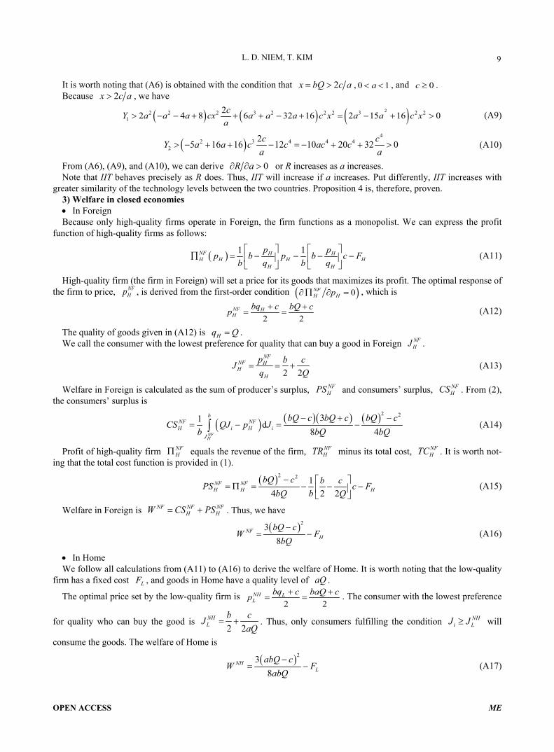
greater similarity of the technology levels between the two countries. Proposition 4 is, therefore, proven. 3) Welfare in closed economies • In Foreign Because only high-quality firms operate in Foreign, the firm functions as a monopolist. We can express the profit

function of high-quality firms as follows:

( ) 1 1NF H HH H H H

H H

p pp b p b c Fb q b q

∏ = − − − −

(A11)

High-quality firm (the firm in Foreign) will set a price for its goods that maximizes its profit. The optimal response of the firm to price, NF

Hp , is derived from the first-order condition ( )0NFH Hp∂∏ ∂ = , which is

2 2NF HH

bq c bQ cp + += = (A12)

The quality of goods given in (A12) is Hq Q= . We call the consumer with the lowest preference for quality that can buy a good in Foreign NF

HJ .

2 2

NFNF HH

H

p b cJq Q

= = + (A13)

Welfare in Foreign is calculated as the sum of producer’s surplus, NFHPS and consumers’ surplus, NF

HCS . From (2), the consumers’ surplus is

( ) ( )( ) ( )2 231 d8 4NF

H

bNF NFH i H i

J

bQ c bQ c bQ cCS QJ p J

b bQ bQ− + −

= − = −∫ (A14)

Profit of high-quality firm NFHΠ equals the revenue of the firm, NF

HTR minus its total cost, NFHTC . It is worth not-

ing that the total cost function is provided in (1).

( )2 2 14 2 2

NF NFH H H

bQ c b cPS c FbQ b Q−

= Π = − − −

(A15)

Welfare in Foreign is NF NF NFH HW CS PS= + . Thus, we have

( )238

NFH

bQ cW F

bQ−

= − (A16)

• In Home We follow all calculations from (A11) to (A16) to derive the welfare of Home. It is worth noting that the low-quality

firm has a fixed cost LF , and goods in Home have a quality level of aQ .

The optimal price set by the low-quality firm is 2 2

NH LL

bq c baQ cp + += = . The consumer with the lowest preference

for quality who can buy the good is 2 2

NHL

b cJaQ

= + . Thus, only consumers fulfilling the condition NHi LJ J≥ will

consume the goods. The welfare of Home is

( )238

NHL

abQ cW F

abQ−

= − (A17)

OPEN ACCESS ME

L. D. NIEM, T. KIM 10

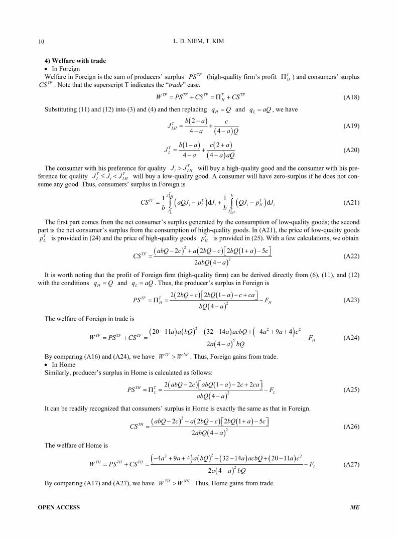
4) Welfare with trade • In Foreign Welfare in Foreign is the sum of producers’ surplus TFPS (high-quality firm’s profit T

HΠ ) and consumers’ surplusTFCS . Note that the superscript T indicates the “trade” case.

TF TF TF T TFHW PS CS CS= + = Π + (A18)

Substituting (11) and (12) into (3) and (4) and then replacing Hq Q= and Lq aQ= , we have

( )( )

24 4

TLH

b a cJa a Q−

= +− −

(A19)

( ) ( )( )

1 24 4

TL

b a c aJ

a a aQ− +

= +− −

(A20)

The consumer with his preference for quality Ti LHJ J> will buy a high-quality good and the consumer with his pre-

ference for quality T TL i LHJ J J≤ < will buy a low-quality good. A consumer will have zero-surplus if he does not con-

sume any good. Thus, consumers’ surplus in Foreign is

( ) ( )1 1d dTLH

T TL LH

J bTF T T

i L i i H iJ J

CS aQJ p J QJ p Jb b

= − + −∫ ∫ (A21)

The first part comes from the net consumer’s surplus generated by the consumption of low-quality goods; the second part is the net consumer’s surplus from the consumption of high-quality goods. In (A21), the price of low-quality goods

TLp is provided in (24) and the price of high-quality goods T

Hp is provided in (25). With a few calculations, we obtain

( ) ( ) ( )( )

2

2

2 2 2 1 5

2 4TF abQ c a bQ c bQ a c

CSabQ a

− + − + − =−

(A22)

It is worth noting that the profit of Foreign firm (high-quality firm) can be derived directly from (6), (11), and (12) with the conditions Hq Q= and Lq aQ= . Thus, the producer’s surplus in Foreign is

( ) ( )( )2

2 2 2 1

4TF T

H H

bQ c bQ a c caPS F

bQ a

− − − + = Π = −−

(A23)

The welfare of Foreign in trade is

( ) ( ) ( ) ( )( )

2 2 2

2

20 11 32 14 4 9 4

2 4TF TF TF

H

a a bQ a acbQ a a cW PS CS F

a a bQ

− − − + − + += + = −

− (A24)

By comparing (A16) and (A24), we have TF NFW W> . Thus, Foreign gains from trade. • In Home Similarly, producer’s surplus in Home is calculated as follows:

( ) ( )( )2

2 2 1 2 2

4TH T

L L

abQ c abQ a c caPS F

abQ a

− − − + = Π = −−

(A25)

It can be readily recognized that consumers’ surplus in Home is exactly the same as that in Foreign.

( ) ( ) ( )( )

2

2

2 2 2 1 5

2 4TH abQ c a bQ c bQ a c

CSabQ a

− + − + − =−

(A26)

The welfare of Home is

( ) ( ) ( ) ( )( )

22 2

2

4 9 4 32 14 20 11

2 4TH TH TH

L

a a a bQ a acbQ a cW PS CS F

a a bQ

− + + − − + −= + = −

− (A27)

By comparing (A17) and (A27), we have TH NHW W> . Thus, Home gains from trade.

OPEN ACCESS ME