NREL/TP-430-20517 •UC Category: 1503 • DE96000497 Economic Development Through Biomass System Integration: Volume 1 Max M. DeLong Northern States Power Company Minneapolis, Minnesota NREL Technical Monitor: Kevin Craig National Renewable Energy Laboratory 1617 Cole Boulevard Golden, Colorado 80401-3393 A national laboratory of the U.S. Department of Energy Managed by the Midwest Research Institute for the U.S. Department of Energy under Contract No. DE-AC36-83CH10093 Prepared under Subcontract No. AAE-5-14456-01 October 1995 MASTER

Welcome message from author
This document is posted to help you gain knowledge. Please leave a comment to let me know what you think about it! Share it to your friends and learn new things together.
Transcript
NREL/TP-430-20517 •UC Category: 1503 • DE96000497
Economic Development Through Biomass System Integration: Volume 1
Max M. DeLong Northern States Power Company Minneapolis, Minnesota
NREL Technical Monitor: Kevin Craig
National Renewable Energy Laboratory 1617 Cole Boulevard Golden, Colorado 80401-3393 A national laboratory of the U.S. Department of Energy Managed by the Midwest Research Institute for the U.S. Department of Energy under Contract No. DE-AC36-83CH10093
Prepared under Subcontract No. AAE-5-14456-01
October 1995
MASTER
NREL User
Go to NREL/TP-430-20517 Summary Report
NREL User
Go to NREL/TP-430-20517 Volumes 2-4
NOTICE
This report was prepared as an account of work sponsored by an agency of the United States government. Neither the United States government nor any agency thereof, nor any of their employees, makes any warranty, express or implied, or assumes any legal liability or responsibility for the accuracy, completeness, or usefulness of any information, apparatus, product, or process disclosed, or represents that its use would not infringe privately owned rights. Reference herein to any specific commercial product, process, or service by trade name, trademark, manufacturer, or otherwise does not necessarily constitute or imply its endorsement, recommendation, or favoring by the United States government or any agency thereof. The views and opinions of authors expressed herein do not necessarily state or reflect those of the United States government or any agency thereof.
Available to DOE and DOE contractors from: Office of Scientific and Technical Information (OSTI) P.O. Box62 Oak Ridge, TN 37831
Prices available by calling (615) 576-8401
Available to the public from: National Technical Information Service (NTIS) U.S. Department of Commerce 5285 Port Royal Road Springfield, VA 22161 (703) 487 -4650
,.#\ Printed on paper containing at least 50"!0 wastepaper, including 10"/o postconsumer waste .....
DISCLAIMER
Portions of this document may be illegible in electronic image products. Images are produced from the best available original· document.
Project Team
The Center for Alternative Plant and Animal Products (CAP AP) within the College of
Agriculture, University of Minnesota is coordinating the work related to alfalfa production as part of the dedicated feedstock supply system (DFSS) and will help evaluate the sustainability of the proposed system. To accomplish these tasks, CAP AP is working closely
with farmers, business persons and local government agencies in the region, and with the Minnesota Extension Servic~ (MES), the Minnesota Institute for Sustainable Agriculture (MISA}, the United States Department of Agriculture - Agricultural Research Service (USDA-ARS), the Soil Conservation Service (SCS}, the Minnesota Department of
Agriculture (MDA}, and the Minnesota Department of Natural Resources (MNDNR).
We welcome your comments, concerns, and suggestions. Project meetings and information gathering sessions will continue throughout the development and implementation of this
project. Contact the University of Minnesota for more information.
UNIVERSITY OF MINNESOTA
College of Agriculture
Center for Alternative Plant and Animal Products
340 Alderman Hall 1970 Folwell Avenue
St. Paul, MN 55108
phone: (612) 625-5747 fax: (612) 624-4941
CHAPTER
TABLE OF CONTENTS VOLUME I
PAGES
CHAPTER 1. IN'TRODUCTION ..•••••••••••••••••••••.••.•.••••••••••••••••••••..•••••••••.•••..•••••••••••.•.•••.••••.•.•..•. 1 1.1 THE PRODUCTION SYSTEM .....................•................•........................ ·····•····················•·•·············•··········· 4 1.2 THE CONVERSION TECHNOLOGY ..................••.....................•............................................................•.... 6 1.3 SUSTAINABILITY ..•..•............•..•...................•..•........•.••.......•.........•............................................•............. 7 1.4 MI~'l\'ESOTA v ALLEY BIOPoWER COOPERATIVE···················································································· 11 1.5 Tl\1E FRAME FOR FuLL PRODUCTION OF THE DFSS .......•............................................•..............••....... 12
CH.:\nER 2 . .ALFALFA BASICS ............................................................... - ••••••••••••••••••••••...•.. 13 2.1 DIVERSITY AND ADAPTABILITY ...•..............................•....•............•...................................................... 13 2.::'. SEED AVAILABILITY .......•.........•..............................•.....•.............................•...............•........................ 16 2.3 Esr ABLISHMENT AND GROWTH ......................•......•.......•....••.....•..........•........•.........•...•........................ 17 2.~ ALFALFA PEsTS .............•.....•.................•.••.....•......................•...............•................•.....•....................... 19 2.5 HARVEST ...•.•...........•...........•......................••.............•...................................•.................•.................... 20 2.6 FAR~t MACHINERY ......................................................................................................................... 24
Cll..\.nER 3 PRODUCTION RISKS •• - ................................................................................... 27 3 I AU-ALFA PRODUCER SURVEY AND HAY SAMPLING RESEARCH .........................•...........................•... 27 :.:..: HAR\ EST LOSSES ...........................................•............................................•..........•............................. 33 3 ' Pl:'ST ·HARVEST LOSSES ......•......................................•.......•..........................•...................................... 44 3 ... RITT.\TIO~ALEFFECTS ...........................................................................•.....................•....•................... 48
l~llAP'TER 4 PRODUCTION ECONOl\fiCS ·•···································-·-·····-·-···············-···69 .; I f"fi:OC>l.C'TlONREGIONS ..•••••.•..•••.••.••..•..•••..•••••••.••.••.•••.••••••.•••••.•••..•••.••.•••.••.•••..••.••••••••••••.••.••.•..••.•.••..•. 69 .; : f"fi:o f-OR\IA BUDGETS BY REGION .........•.......•.....•..•.....•...........•...........•...................•...•...................... 76 .; .; Bl(>\tASS SUPPLY CURVE .............................................................................................................. 90
CH ·\PTI:R 5. TRANSPORTATION AND STORAGE ••.••••••.•..•• - ....................................... 103 (.I Ti<."'-''PORTATIONANDSTORAGELOGISTICS .........................••.............................•.....•...............•..... 103 ': 11ol-'''f'l:>RTATIONANDSTORAGECOSTS ................................•.................................•.........•.............. 107 ": l~'''J'l'.>RTATIONlNFRASTRUCTURE ..................................................................•............................. 114 ~.: \ 1111<1. f REGULATIONS .................................................•...............................................•.....•............. 121 ~ ~ ~rn kl GL"LATIONS ....................•......•.........................•.•......................................•........•........•........... 122 ~ f-. f"fi:I\ .\TI CO~'TRACTOR OPPORTUNITIES ...•.....•.•..•••.•.••.•••••••.•.•.••...•..•..•.•....•••..••......•.••.••••••••....••..•..•. 125
CH.:\JYfER 6. PROCESSING •••••••••• -··························-··········-··············································127 6. I and 6.~ were removed to Vol. 4, Site Considerations, Chapters 2 and 4 respectively. 127-133 6.3 EXPERIMENTAL SEPARATION STUDY ..................................................................................... 134
7. PRODUCTS • • • • • • • • • • • • • • • • • • • • • • • • • • • • • • • • • 139 7 .1 Electricity . . . . . . . . . . . . . . . . . . . . . . . . . . . . . . . . . . . . . . . . . 139
Ash By-product . . . . . . . . . . . . . . . . . . . . . . . . . . . . . . . . . . . . . 141
7.2 Co-products . . . . . . . . . . . . . . . . . . . . . . . . . . . . . . . . . . . . . . . . 143
7.3 Nutritional Characteristics of Leaf Meal . . . . . . . . . . . . . . . . . . . 144
7.4 Ration Formulation . . . . . . . . . . . . . . . . . . . . . . . . . . . . . . . . . . 148
7 .5 Bypass Protein Enhancement . . . . . . . . . . . . . . . . . . . . . . . . . . . 153
7.6 Future Nutritional Evaluation and Products . . . . . . . . • . . . . . . . 157
8 . .MA.RKE"I' AN.AL YSIS .. • • • • • • • • • • • • • • • • • • • • • • • • • 159 8.1 Electricity . . . . . . . . . . . . . . . . . . . . . . . . • . . . . . . . . • . . . . . . . 159 8.2 Leaf Meal . . . . . . . . . . . . . . . . . . . . . . . . . . . . . . . . . . . . . . . . . 163
Production and Supplies . . . . . . . . . . . . . . . . . . . . . . . . . . . . . 163
Market Potential . . . . . . . . . . . . . . . . . . . . . . . . . . . . . . . . . . . 171 Competing Feeds . . . . . . . . . . . . . . . . . . . . . . . . . . . . . . . . . . . 183
Marketing Strategy . . . . . . . . . . . . . . . . . . . . . . . . . . . . . . . . . . 187
9. BUSINESS AN.AL YSIS • • • • • • • • • • • • • • • • • • • • • • • • • 189 9.1 Organizational Structure . . . . . . . . . . . . . . . . . . . . . . . . . . . . . . . 190
9.2 Contracting for Production . . . . . . . . . . . . . . . . . . . . . . . . . . . . . 197
9 3 Coop Development . . . . . . . . . . . . . . . . . . . . . . . . . . . . . . . • . . 202
10. ENVIRONMENT.AL IMPACT •••••••••••••••••••• 203 . 10.1 Energy Balance . . . . . . . . . . . . . . . . . . . . . . . . . . . . . . . . . . . . . . 203
10.2 Soil and Water . . . . . . . . . . . . . . . . . . . . . . . . . . . . . . . . . . . . . 209
10.3 Soil Structure . . . . . . . . . . . . . . . . . . . . . . . . . . . . . . . . . . . . . . . 213
J0.4 Minnesota River . . . . . . . . . . . . . . . . . . . . . . . . . . . . . . . . . . . . . 214
10.5 Wildlife . . . . . . . . . . . . . . . . . . . . . . . .. . . . . . . . . . . . . . . . . . . . 217
11. POLICY' ISSUES ••••••••••••••••••••••••••••• 237 11.1 The 1995 Farm Bill . . . . . . . . . . . . . . . . . . . . . . . . . . . . . . . . . . . 237
11.2 Conservation Reserve Program . . . . . . . . . . . . . . . . . . . . . . . . . . 241
11.3 Crop Insurance . . . . . . . . . . . . . . . . . . . . . . . . . . . . . . . . . . . . . . 242
12. CONCLUSIONS • • • • • • • • • • • • • • • • • • • • • • • • • • • • • • 245 12.1 Feasibility . . . . . . . . . . . . . . . . . . . . . . . . . . . . . . . . . . . . . . . . . . 245
12.2 Recommendations . . . . . . . . . . . . . . . . . . . . . . . . . . . . . . . . . . . . 246
APPENDIX - VOLUME 1 Supporting documents by Chapter Bibliography
FIGURES, TABLES and ILLUSTRATIONS
FIGURES:
1.1-1 Change in erosion type and level . . . . . . . . . . . . . . . . . . . . . . . . 8 2.3-1 Alfalfa leaf and stem yield . . . . . . . . . . . . . . . . . . . . . . . . . . . . 16 2.3-1 Yield of 1st Cutting over Time . . . . . . . . . . . . . . . . . . . . . . . . . 18 25-1 Yield of leaf and stem by cutting schedule . . . . . . . . . . . . . . . . 23 32-1 Respiration losses . . . . . . . . . . . . . . . . . . . . . . . . . . . . . . . . . . . 35 32-2 Rainfall losses . . . . . . . . . . . . . . . . . . . . . . . . . . . . . . . . . . . . . 36 32-3 Probability of three dry days . . . . . . . . . . . . . . . . . . . . . . . . . . . 37 32-4 Average daily precipitation . . . . . . . . . . . . . . . . . . . . . . . . . . . . 38 32-5 Probability of various rainfall amounts . . . . . . . . . . . . . . . . . . . 39 3.3-1 Dry matter losses in storage . . . . . . . . . . . . . . . . . . . . . . . . . . . 44 3 .4-la Nine-county precipitation . . . . . . . . . . . . . . . . . . . . . . . . . . . . . 50 3.4-lb Minnesota precipitation . . . . . . . . . . . . . . . . . . . . . . . . . . . . . . 51 3.4-2 MN annual pan evaporation . . . . . . . . . . . . . . . . . . . . . . . . . . . 51 3.4-3 MN annual temperature . . . . . . . . . . . . . . . . . . . . . . . . . . . . . . 51 3.4-4 MN average Growing Degree Days (GDD) . . . . . . . . . . . . . . . . 51 .3.4-5 . Soil associations of biomass shed . . . . . . . . . . . . . . . . . . . . . . . 52 3.4-6 Com yield Yellow Medicine county . . . . . . . . . . . . . . . . . . . . . . 58 3.4-7 Com yield Stevens county . . . . . . . . . . . . . . . . . . . . . . . . . . . . . 59 3.4-8 Com yield/water holding capacity . . .. . . . . . . . . . . . . . . . . . . . . 61 3.4-9 Com yield/annual precipitation . . . . . . . . . . . . . . . . . . . . . . . . 61 3.4-10 Yield loss contour (fixed cutting) . . . . . . . . . . . . . . . . . . . . . . . 62 3.4-11 Yield loss contour (floating cutting) ................... ·. . 63 4.1-1 Rent by region . . . . . . . . . . . . . . . . . . . . . . . . . . . . . . . . . . . . . 75 42-1 DFSS rotation returns . . . . . . . . . . . . . . . . . . . . . . . . . . . . . . . . 83 42-2 Breakeven price (w/o deficiency) ....................... 84 4.2-3 Breakeven price (high yield) . . . . . . . . . . . . . . . . . . . . . . . . . . . 85 42-4 Breakeven price (high com/bean prices) . . . . . . . . . . . . . . . . . . 86 42-5 Breakeven price (cutting schedule) . . . . . . . . . . . . . . . . . . . . . . 87 4.2-6 Breakeven price (stem price = $30/ton) .................. 88 4.3-1 Adoption Rate . . . . . . . . . . . . . . . . . . . . . . . . . . . . . . . . . . . . 92
FIGURES (continued):
43-2
43-3
43-4
43-5
43-6 - 43-7
5.2-1
5.2-2
5.2-3
6.1-1
8.2-1
8.2-2
8.2-3 8.2-4
8.2-5
8.2~
8.2-7
8.2.S
8.2-9
8.2-10
8.2-11
8.2-12
8.2-13
8.2-14
8.2-1~
8.2-16
8.2-17
Regional supply curve (base scenario) . . . . . . . . . . . . . . . . . . . . 93
Regional supply curve (w/o com deficiency payment) ........ 94
Regional supply curve {high hay yield) . . . . . . . . . . . . . . . . . . . 95
Regional supply curve (low hay yield) . . . . . . . . . . . . . . . . . . . . 96
Regional supply curve (low adoption rate) . . . . . . . . . . . . . . . • 97
Regional supply curve (2-cut system) . . . . . . . . . . . . . . . . . . . . . 98
Transportation and storage cost ($/ton) . . . . . . . . . . . . . . . . . 110
Transportation and storage cost ($/year) . . . . . . . . . . . . • . . . . 111
Transport distance to remote storage . . . . . . . . . . . . . . . . . . . 112
Alfalfa processing plant . . . . . . . . . . . . . . . . . . . . . . . . . . . . . 128
MN alfalfa production and acreage (1974-1993) . . . . . . . . . . . 165
MN alfalfa production by region . . . . . . . . . . . . . . . . . . . . . . .
Alfalfa production ranking by region ................... .
Correlation - alfalfa production and price (1974-1993) ...... .
Alfalfa price trend (1984-1993) ....................... .
Alfalfa production in top ten producing states ........... -..
MN dairy cow inventory by region . . . . . ............... .
Protein requirements and total dry matter in dairy feed ..... .
Top ten U.S. dairy states . · .......................... .
U.S. export of protein meals and feeds/fodders ........... .
Largest markets for U.S. protein meals (by value) ......... .
Largest markets for U.S. protein meals (by volume) ....... .
Consumption of processed feed & protein meals in U.S. . ... .
Protein feed prices (1975-1993) ....................... .
Price of protein equivalent in protein meals (1975-1993) .... .
Prices of alfalfa hay and meal (1976-1993) .............. .
Alfalfa meal prices (1975-1993) ....................... .
166
166 167
168
170
173
174
178
180
181
182 183
185
185
186
186
10.2-1 Current land use in biomass shed . . . . . . . . . . . . . . . . . . . . . . 209
10.2-~ Crops in biomass shed . . . . . . . . . . . . . . . . . . . . . . . . . . . . . . 210
10.2-3 Sheet/rill erosion . . . . . . . . . . . . . . . . . . . . . . . . . . . . . . . . . . 211
10.2-4 Wind erosion loss (tons/acre) . . . . . . . . . . . . . . . . . . . . . . . . . 212
103-1 Percent fledged nests by week (songbirds) . . . . . . . . . . . . . . . . 222
103-2 Percent hatched nests by week (gamebirds) . . . . . . . . . . . . . . . 223
103-3 Percent hens killed, active & hatched nests (pheasants) . . . • . . 224
FIGURES (continued):
103-4 Potential impacts of availability of residual nesting cover 226 103-5 Potential impacts of availability of residual nesting cover... . . 227 10.3-6 Potential impacts of availability of residual nesting cover . . . . . 228 10.3"'. 7 Percent of white-tailed deer fawns born by week . . . . . . . . . . 229 10.3-8 Typical mowing pattern . . . . . . . . . . . . . . . . . . . . . . . . . . . . . 233 10.3-9 Recommended mowing patterns . . . . . . . . . . . . . . . . . . . . . . . 234
TABLES:
25-1 Cutting dates and maturity . . . . . . . . . . . . . . . . . . . . . . . . . . . . 21 25-2 Yield by cutting schedule . . . . . . . . . . . . . . . . . . . . . . . . . . . . . 22 3 .1-1 Alfalfa yield . . . . . . . . . . . . . . . . . . . . . . . . . . . . . . . . . . . . . . 28 3.1-2 Yield by stand age . . . . . . . . . . . . . . . . . . . . . . . . . . . . . . . . . . 29 3.1-3 Forage quality of stored alfalfa . . . . . . . . . . . . . . . . . . . . . . . . . 31 3 2-1 Harvest losses . . . .· . . . . . . . . . . . . . . . . . . . . . . . . . . . . . . . . . . 33 3.4-1 Rotations considered . . . . . . . . . . . . . . . . . . . . . . . . . . . . . . . . 57 3.4-2 Floating cutting schedule . . . . . . . . . . . . . . . . . . . . . . . . . . . . . 60 3.4-3 Yield loss (fixed cutting schedule) . . . . . . . . . . . . . . . . . . . . . . . 64 3.4-4 Yield loss (floating cutting schedule) . . . . . . . . . . . . . . . . . . . . . 64 3.4-5 Yield differences in Lac Qui Parle county . . . . . . . . . . . . . . . . . 66 3.4-6 Yield differences in Kandiyohi county . . . . . . . . . . . . . . . . . . . . 66 4.1-1 CER by region . . . . . . . . . . . . . . . . . . . . . . . . . . . . . . . . . . . . . 71 4.1-2 EMV by region . . . . . . . . . . . . . . . . . . . . . . . . . . . . . . . . . . . . 73 42-1 Estimated net return per acre . . . . . . . . . . . . . . . . . . . . . . . . . . 80 4.2-2 Breakeven alfalfa price ($/ton) . . . . . . . . . . . . . . . . . . . . . . . . . 82 4.3-1 Alfalfa production potential by region . . . . . . . . . . . . . . . . . . . 92 4.3-2 Regional supply (base scenario) . . . . . . . . . . . . . . . . . . . . . . . . 93 4.3-3 Regional supply (w/o com deficiency payment) ............. 94 43-4 Regional supply (high hay yield) . . . . . . . . . . . . . . . . . . . . . . . . 95 43-5 Regional supply (low hay yield) . . . . . . . . . . . . . . . . . . . . . . . . 96 4.3-6 Regional supply (low adoption rate) . . . . . . . . . . . . . . . . . . . . . 97
TABLES (continued)
4.3-7 Regional supply (2-cut system) . . . . . . . . . . . . . . . . . . . . . . . . . 98
43-8 Adoption-rate schedule . . . . . . . . . . . . . . . . . . . . . . . . . . . . . . 100
52-1 Transportation and storage costs . . . . . . . . . . . . . . . . . . . . . . . 107
5.3-1 Roadways in biomass shed . . . . . . . . . . . . . . . . . . . . . . . . . . . 115
53-2 Railroads in biomass shed . . . . . . . . . . . . . . . . . . . . . . . . . . . 117
62-1 Processing plant operations and maintenance costs . . . . . . . . . 133
6.3-1 Leaf, stem and weeds in commercial hay bales . . . . . . . . . . . . 137
7 3-1 Nutrient composition and digestJ.bility of leaves and stems . . . . 146
7 3-2 Elemental compostion of leaves and stems . . . . . . . . . . . . . . . 147
7.4-1 Ration formulation constraints . . . . . . . . . . . . . . . . . . . . . . . . 149
7.4-2 Available feeds . . . . . . . . . . . . . . . . . . . . . . . . . . . . . . . . . . . . 150
7.4-3 Inclusion rate for leaf meal in rations . . . . . . . . . . . . . . . . . . . 151
7.4-4 Leaf meal value ($/ton) . . . . . . . . . . . . . . . . . . . . . . . . . . . . . 152
7 .5-1 Results of heat treatment . . . . . . . . . . . . . . . . . . . . . . . . . . . . 155
8.1-1 Schedule of expected electricity needs . . . . . . . . . . . . . . . . . . . 159
82-1 MN alfalfa production, acreage and yield (1974-1993) . . . . . . . 165
82-2 MN alfalfa hay prices . . . . . . . . . . . . . . . . . . . . . . . . . . . . . . . 167
82-3 MN and U.S. alfalfa prices (10 year trend) . . . . . . . . . . . . . . . 168
82-4 Production history of top 10 producing states . . . . . . . . . . . . . 170
82-5 Potential comsumption of leaf meal (MN dairy cows) . . . . . . . 175
82-6 MN livestock production . . . . . . . . . . . . . . . . . . . . . . . . . . . . . 179
8.2-7 U.S. protein feed exports (by value) .. . . . . . . . . . . . . . . . . . . . 181
82-8 U.S. protein feed exports (by volume) .. _. . . . . . . . . . . . . . . . . 182
82-9 Processed feed and protein meal prices . . . . . . . . . . . . . . . . . . 184
10.1-1 Energyinputs ................................. ~ ... 205
10.1-2 Energy balance for alfalfa . . . . . . . . . . . . . . . . . . . . . . . . . . . . 207
10.1-3 Energy balance for coal . . . . . . . . . . . . . . . . . . . . . . . . . . . . . 208
10.3-1 CRP, Wildlife Area, Waterfowl Production & RIM lands . . . . 219
10.3-2 Impact of mowing on wildlife species . . . . . . . . . . . . . . . . . . . 221
10.3-3 Impact of cover type replacement w/alfalfa . . . . . . . . . . . . . . . 232
ILLUSIRATIONS:
1.1-1 Map of the Upper Midwest . . . . . . . . . . . . . . . . . . . . . . . . . . . . 2 3.3-1 Bale storage (no cover) . . . . . . . . . . . . . . . . . . . . . . . . . . . . . . 46 3.3-2 Bale storage (plastic cover) . . . . . . . . . . . . . . . . . . . . . . . . . . . . 46 3.3-3 Bale storage (root) . . . . . . . . . . . . . . . . . . . . . . . . . . . . . . . . . . 47 4.1-1 Production regions . . . . . . . . . . . . . . . . . . . . . . . . . . . . . . . . . . 72 4.3-1 Production .regions . . . . . . . . . . . . . . . . . . . . . . . . . . . . . . . . . . 91 5.3-1 Regional railroad routes . . . . . . . . . . . . . . . . . . . . . . . . . . . . . 118 8.2-1 MN alfalfa production by county ......... · . ~ . . . . . . . . . . . . 164 8.2-2 Alfalfa production in the U.S. . . . . . . . . . . . . . . . . . . . . . . . . . 169 8.2-3 MN dairy cow inventory . . . . . . . . . . . . . . . . . . . . . . . . . . . . . 172 8.2-4 U.S. dairy production . . . . . . . . . . . . . . . . . . . . . . . . . . . . . . . 177
CHAPTER!. INTRODUCTION
A Study To Determine The Feasibility of Producing Electricity and Leaf Meal Protein
From Alfalfa
C.V. Hanson\ Helene Murray2, Earl Bracewell3, Erv Oelke\ and Don Wyse2
1Center for Alternative Plant and Animal Products, 2Minnesota Institute for Sustainable Agriculture, and the 3Centre for Agricultural Education, University of Minnesota
The U.S. Department of Energy (DOE) predicts that renewable biomass energy crops will provide a significant portion of future fuel needs in America. This is good news for farmers. Crops grown specifically for.energy production provide a major new market for agriculture.
To make electricity from biomass (plant matter) you could burn it, making steam that would drive a steam turbine which in tum produces electricity. Most of the electricity produced in America today is made by burning fossil fuels (coal and natural gas).
A more efficient process t~ convert m~s to electricity is gasification. Plant matter placed in a chamber under pressure and at high temperature (over 1500°F) is converted to gases (over 95% conversion). Biomass gasification produces a low Btu gas which may then be ignited in a combustion turbine for the production of electricity. Biomass electricity generation by a combustion turbine is more efficient and may be done on a much smaller scale than is typical for steam-turbine power plants.
Biomass fueled power plants distributed on the transmission system reduce grid and capacity upgrade requirements and also distribute cooperative business opportunities between biomass producers and power companies.
Northern States Power Company (NSP), Minnesota's largest electric utility, submitted a proposal to DOE and the Electric Power Research Institute (EPRI) to evaluate a proposed biomass energy production system. The following report analyses the feasibility of an alfalfa biomass fueled electric power generation system at an existing NSP power plant in Granite Falls, Minnesota (IDustration 1.0-1).
1
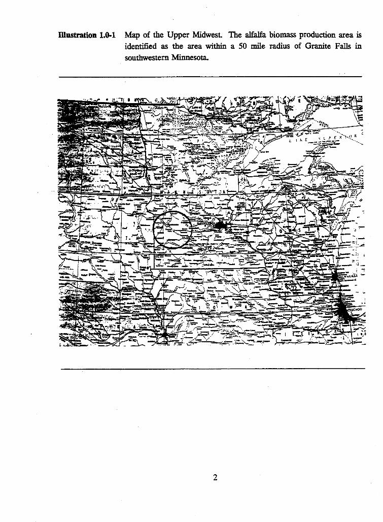
mustration 1.0-1 Map of the Upper Midwest. The alfalfa biomass production area is
identified as the area within a 50 mile radius of Granite Falls in
southwestern Minnesota.
2
NSP contracted with the University of Minnesota to determine the technical and economic feasibility of the biomass feedstock supply system. Power plants must have reliable, dedicated fuel supplies and biomass energy cropping systems must be sustainable. To be sustainable biomass energy production systems must provide viable economic returns for farmers and produce electrical power at a price that is competitive with new fossil fuel systems. Because all biomass fuels are less energy dense than coal, biomass crops must provide other sources of revenue for producers and utilities.
Alfalfa may be processed, much like we process com and soybeans, to produce a wide variety of renewable products including electricity. Alfalfa grown in rotation with corn, soybeans, and other crops in the region, has the potential to provide a stable biomass fuel supply, improve profitability for farmers, and fuel electric power generation at a cost that is competitive with 'new generation' power production systems.
Alfalfa yields in southwestern Minnesota around the Granite Falls plant site are sufficient for sustainable biomass energy production. Additionally, currerit alfalfa breeding programs such as a joint effort by researchers at the University of Minnesota, United States Department of Agriculture-Agricultural Research Service (USDA-ARS), Pioneer Hi-Bred International and Forage Genetics are expected to provide alfalfa varieties specifically adapted for energy production. Selection for elevated lignin concentrations in alfalfa stems to increase energy- density--is one aspea of -this-- plant breeding -effort. Although improvements in per acre yield and energy yield (Chapter 2) are expected, we believe that current yields are adequate to establish alfalfa as a base crop for biomass energy production.
Benefits from including alfalfa in the rotation include: increased yield from other crops in the rotation, reduced external inputs of nitrogen, lower overall production costs (fossil fuels inputs), and distinct environmental benefits (Chapter 10). Environmental benefits include reduced soil erosion, improved soil tilth, increased soil organic matter levels, reduced potential for nitrate leaching, and a reduction in diffuse source pollutants.
The integration of energy production systems into rural communities has great potential to stimulate economic development by creating new opportunities for small businesses and diversifying our rural economic base. The integration of alfalfa biomass energy crops into traditional agricultural cropping systems provides a dedicated energy fuel supply capability that is here, today.
3
1.1 THE PRODUCTION SYSTEM
Minnesota farmers currently produce over 6.9 million tons of alfalfa hay per year, the fourth
largest production level of alfalfa in the country. However, alfalfa acreage covers less than
6% of Minnesota's total cropland (Minnesota Agricultural Statistics 1992). The production
of alfalfa for energy is a major new market that allows producers to benefit from including
alfalfa in traditional rotations. Alfalfa production for multiple use, as in the proposed
biomass energy production system, will be significantly different from alfalfa produced
strictly as feed.
The proposed production area for alfalfa (biomass shed) is defined for this study as an area
within a 50 mile radius of Granite Falls, Minnesota. This region of southwestern Minnesota
depends primarily on cash crop production agriculture. The farmland within the counties
included in the shed currently prod:uce 2.8, 2.6, and 034 million acres of com, soybean, and
alfalfa, respectively. The size of the average farm in the shed is 580 acres.
Based on focus group interviews (Appendix 1.1), we anticipate that biomass producers will
be experienced farmers operating farms in the biomass shed. These farmers will be
motivated to start producing or increase their production of alfalfa to increase profitability,
reduce risk through diversification, and enhance environmental quality on their farms.
Economic evaluation of a dedicated feedstock supply system (DFSS) for the production of
energy from alfalfa indicates that the breakeven price for alfalfa in this system (compared
to a conventional com-soybean rotation) is about $67 /ton (Chapter 4). The example 7-ye~
biomass rotation (DFSS rotation) evaluated in this study was four years of alfalfa followed
by two years of com and then one year of soybeans. Economic advantages of the DFSS
rotation may be directly attributed to the inclusion of a perennial legume in the rotation.
Reduced input costs, compared to conventional rotations and increased yields for other
crops in the rotation result in increased profits for producers.
The benefits of including alfalfa in a rotation are well documented. However, alfalfa
production has been limited due to the problems associated with shipping alfalfa long
distances (hundreds of miles in some cases) to reach markets and a declining market for
average quality hay (Chapter 8). High regional demand for alfalfa, such as that provided
by a biomass power plant, will stimulate production, allow for value-added processing, and
allow producers to achieve the economic and environmental benefits of a perennial legume
in agricultural production systems.
4
Overview of Biomass Energy Production
About 2000 farmers in southwestern Minnesota invest in a biomass energy cooperative and sign contracts to produce about 680,000 tons of alfalfa annually for their grower-owned cooperative (contract price offered is competitive with other crops in the region). Growerowners are paid on the basis of tonnage and quality.
Biomass-type alfalfa varieties are developed specifically for biomass energy production. Biomass-type alfalfa varieties have greater standability than current varieties and allow producers to opt for a two-harvest production system (Chapter 2).
Alfalfa is baled into large-round bales and transported by the grower to one of the regional storage sites that surround the alfalfa processing plant in Granite Falls, MN. The transponation and storage system has been designed so that most producers have less than 5 miles to travel to a remote storage site. Alfalfa is weighed and tested for quality at the remote storage site. During the growing season about 40% of the crop is direct-hauled from remote storage, by the cooperative, to the processing plant. About 60% of the crop is placed in storage at the remote site (under plastic cover and/or in steel pole buildings, see Chapter 5).
A fleet of twenty tractor-trailer rigs work two shifts per day, 6·days per week for about 300 days per year delivering alfalfa to the plant. A small stockpile, two or three days worth, of alfalfa is held at the plant for processing during times when delivery is interrupted by bad weather or other supply system problems.
At the plant. alfalfa is separated into stem and leaf fractions. The stem fraction is fed under pres..~ure to a gasifier, converted to a low Btu fuel gas, and combusted in a turbine to produce electricity. The leaf fraction is processed into various alfalfa leaf meal products.
Farmer members of the cooperative produce alfalfa and deliver their crop to remote storage where ownership of feedstock changes hands. Growers are paid based on tonnage and quality. The alfalfa cooperative now collectively owns the crop. Storage losses, trin..~ponation. and processing become the responsibility of the cooperative or potentially a joint-venture between a cooperative and NSP.
5
1.2 THE CONVERSION TECHNOWGY
NSP has also contracted with the Institute of Gas Technology (IGT), Tampella Power
Company, and Westinghouse Electric Corporation. IGT is a private non-profit research
organization with ten years of development work on the process of pressurized biomass
gasification. Tampella is a Finnish company with subsidiaries in the U.S. and has the
capability to design and construct power plants. Westinghouse manufactures combustion
turbines and has ·developed the hot gas cleanup system proposed for this project.
IGT developed the RENUGASTM biomass gasification process, a pressurized, air-blown,
single-stage fluidized bed gasifier. The RENUGAS™ ·process has been designed to operate
at pressure, uses single-screened feedstock, uses no catalyst, and is mechanically simple to
operate. Gasification tests in a 10 ton-per-day process development unit have been
conducted at IGT in Chicago with a variety of biomass sources, including alfalfa. These
tests have demonstrated high carbon conversions and high thermal efficiencies with a low
production of condensible products. The RENUGAS™ process will handle a wide range
of biomass materials from whole-tree-chips to finely chopped sugarcane bagasse.
Westinghouse has developed a hot-gas cleaning system that is critical for the successful
integration of a biomass gasifier with a combustion turbine for high-efficiency power
generation:· Fuel gases derived from alfalfa biomass will contain contaminants which could
lead to corrosion, erosion, and deposition in the combustion turbine. Therefore, a gas
cleanup syste~ including particulate removal, and possibly alkali removal, is necessary.
A commercially available Westinghouse combustion turbine is specified in this design.
Combustion turbines used for electricity production are similar, in design, to turbine engines
on commercial jet aircraft. Westinghouse has developed a low NOx combustor (multi
annualar swirl burner) that reduces the conversion of fuel bound nitrogen to NOr Alfalfa
stems are higher in fuel bound nitrogen than many other biomass feedstocks therefore NOx
emissions have been a concern. Westinghouse test results confirm and warrantees and /or
guarantees will assure that NOx levels do not exceed EPA clean air standards.
Tampella Power Company together with NSP determined capital cost of the power plant
and the cost of electricity from the proposed system. Tampella has constructed and operates
a biomass gasification plant in Finland that uses wood chips. The final report on the
conversion technology is in Volume 2.
6
1.3 SUSTAINABILTIY
Sustainable biomass energy production systems must be productive (positive energy balance), must provide viable economic and environmental returns for farmers and rural communities, and must provide society at large with low cost environmentally friendly energy.
Ener2)' balance:
Chapter 10 of this volume offers a detailed analysis of the energy balance for the proposed project. Energy input:output analysis indicates the conversion of alfalfa to electricity results in a highly positive energy balance (1:3). The ratio of energy in to energy out is critical in determining the overall system efficiency for biomass energy production. Energy balances for the two different crop rotations studied (DFSS and com-soybean) indicate that the DFSS rotation generates more gross energy and more crude protein per acre with lower energy inputs than a traditional com-soybean rotation.
Economic and Environmental Benefits:
Will farmers and rural communities benefit from alfalfa biomass energy production? ·
Economic Impact
The economics for alfalfa biomass energy production are calculated to provide equal or higher returns to growers for the production of biomass in the proposed DFSS rotation compared to traditional com-soybean rotations. Diversification of the agricultural base in the region is expected to stimulate small business development and provide economic stability in the region (Chapter 5.6).
Feedstock production, in state, replaces imported coal from the western U.S. and contributes to Minnesota's energy self-sufficiency. A 75 MWe coal fired power plant would consume over $10 million dollars of coal annually.
The processing plant will employ over 50 persons (full-time) to produce both electricity and leaf meal pro~ucts. Over 50 (full-time) transportation related jobs and 60 - 80 (part-time) jobs will be created for storage and handling of the feedstock. Distribution, sales, and marketing of leaf meal products will provide additional economic opportunities.
7
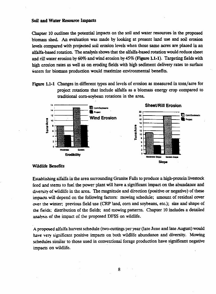
Soil and Water Resource Impacts
Chapter 10 outlines the potential impacts on the soil and water resources in the proposed
biomass shed. An evaluation was made by looking at present land use and soil erosion
levels compared with projected soil erosion levels when those same acres are placed in an
alfalfa-based rotation. The analysis shows that the alfalfa-based rotation would reduce sheet
and rill water erosion by 60% and wind erosion by 45% (Yigure Ll-1). Targeting fields with
high erosion rates as well as on eroding fields with high sediment delivery rates to surface
'Waters for biomass production would maximize environmental benefits.
Figure 1.1-1 Changes in different types and levels of erosion as measured in tons/acre for
project rotations that include alfalfa as a biomass energy crop compared to
traditional com-soybean rotations in the area.
16.,.-.------
14,.....------'
12---
! •o-· ---~ • c 0 ....
0
Waldlife Benefits
Erocflbility
m ComlSoybaans .,.,. Wind Erosion
Sheet/Rill Erosion 22 ,.....-------
20 r-----,----18 f-----
161-----
! 14---g ct 121-----• c 10
::. 8
6
4
2
0
Establishing alfalfa in the area surrounding Granite Falls to produce a high-protein livestock
feed and stems to fuel the power plant will have a significant impact.on the abundance and
divenity of wildlife in the area. The magnitude and direction (positive or negative) of these
impacts \\rill depend on the following factors: mowing schedule; amount of residual cover
over the winter; previous field use (CRP land, com and soybeans, etc.); size and shape of
the fields; distribution of the fields; and mowing patterns. Chapter 10 includes a detailed
anaJ~i.s of the impact of the proposed DFSS on wildlife.
A proposed alfalfa harvest schedule (two-cuttings per year (late June and late August) would
have very significant positive impacts on both wildlife abundance and diversity. Mowing
schedules similar to those used in conventional forage production have significant negative
impacts on wildlife.
8
Perceptions and Attitudes
What are the impacts on communities and rural residents in the proposed biomass shed should a demonstration project be approved for the Granite Falls power plant?
Farmers Concerns and Willingness to Participate
Farmers participating in focus group interviews generally expressed the belief that the plan could benefit them and the community at large. However, farmers indicate they would require a clear, concise plan before making a decision about including alfalfa in their crop rotation. The complete report of the focus group study is found in Appendix 1.
In all five of the focus groups conducted for this project, the idea that alfalfa is a "good" crop to grow was unanimous; participants clearly understood the benefits of including a perennial legume in their crop rotations. Yet, this perception of "good" was continually tempered with the farmers' perception of financial risk.
Given the perception that change is risky, farmers must have assurances that the rewards for changing their crop rotations to include alfalfa as a biomass energy crop will be substantially greater than they presently receive with their current cropping system. Farmers indicated that if they perceive the rewards to be less than, equal to, or even slightly more than they currently receive, they would not participate.
Community Impacts
Regular community meetings were held during the course of the nine-month study. Meetings were held with area farmers, county Commissioners, county Extension Educators, the Granite Falls Chamber of Commerce, as open public forums, and with employees at NSP's existing Minnesota Valley power generation facility. A complete list of meeting is included in Appendix 13.
9
During these meetings community members expressed:
* concerns about this being "just another project touted to be good for the region with
no positive impacts realized" (they cited problems in the past with Jerusalem
artichokes and wind energy proposals);
* that farmers need a long-term commitment from NSP regarding purchase of the
alfalfa stems for biogasifi.cation;
* concern about marketing the high-protein by-product and competition with other
sources of animal feed supplements produced regionally;
* various opinions on storage issues;
* an~ about the benefits of increasing jobs at the power plant and in the production,
transportation and handling sectors in the region.
Interestingly, there was some, but very limited, concern about increased traffic around the
power plant facility and on roads in the counties. Appendix 1.3 provides an overview of
questions and comments made during some of these meetings.
It is important to note that in spite of concerns expressed and questions asked about the
plan by people attending the community meetings, overall support for the plan was very
high. Should a demonstration project be implemented in Granite Falls, additional meetings
(potentially using the focus group format) should be held to solicit further community input
into the development of sustainable biomass energy production.
An Agricultural Advisory Council was formed early during the course of the nine month
study. The Ag Advisory Council is made up of persons from southwestern Minnesota that
are interested in this project. A complete listing of the Ag Advisory Council is included in
Appendix 1.3. At the conclusion of this study a subset of the council (all active farmers)
decided to form a producers cooperative to further their ability to continue to evaluate and
potentially to implement sustainable biomass energy production in Minnesota. The list of
the Board of Directors of the newly formed Minnesota Valley Alfalfa Producers follows.
10
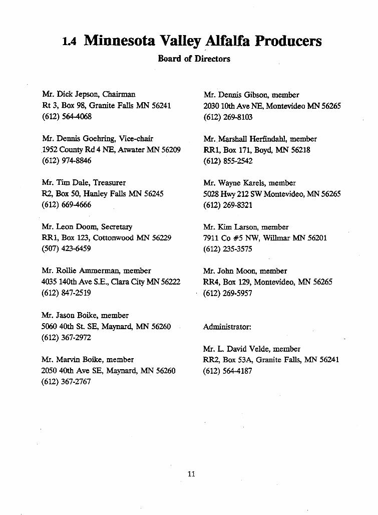
1.4 Minnesota Valley Alfalfa Producers Board of Directors
Mr. Dick Jepson, Chairman
Rt 3, Box 98, Granite Falls MN 56241
(612) 564-4068
Mr. Dennis Goehring, Vice-chair 1952 County Rd 4 NE, Atwater MN 56209 ( 612) 974-8846
Mr. Tim Dale, Treasurer
R2, Box 50, Hanley Falls MN 56245
(612) 669-4666
Mr. Leon Doom, Secretary RRl, Box 123, Cottonwood MN 56229
(507) 423-6459
Mr. Rollie .Ammerman, member
4035 140th Ave S.E., Clara City MN 56222
(612) 847-2519
Mr. Jason Boike, member
5060 40th St. SE, Maynard, MN 56260
(612) 367-2972
Mr. Marvin Boike, member
2050 40th Ave SE, Maynard, MN 56260 (612) 367-2767
11
Mr. Dennis Gibson, member
2030 10th Ave NE, Montevideo MN 56265
(612) 269-8103
Mr .. Marshall Herfindahl, member RRl, Box 171, Boyd, MN 56218
(612) 855-2542
Mr. Wayne Karels, member 5028 Hwy 212 SW Montevideo, MN 56265
(612) 269-8321
Mr. Kim Larson, member 7911 Co #5 NW, Willmar MN 56201
(612) 235-3575
Mr. John Moon, member
RR4, Box 129, Montevideo, MN 56265
(612) 269-5957
Administrator:
Mr. L. David Velde, member RR2, Box 53A, Granite Falls, MN 56241
(612) 564-4187
1.S Time Frame for Full Production of the DFSS
Maximum yield of alfalfa is reached in the second year after seeding. The establishment
year yield is typically 40 - 60% of full production. · Because success in alfalfa establishment
is influenced by weather, growers participating in the production of alfalfa biomass for
energy should consider planting a portion of their total acreage commitment over a number
of years thereby achieving diversity of stand age and minimizing establishment year risk.
Biomass Project Team
Minnesota farmers University of Minnesota
Minnesota Extension Service
Minnesota Department of Agriculture
Minnesota Depart~ent o~. Natura~ .R~ources Minnesota Institute for Sustainable Agriculture
Agricultural Research Service, USDA
Soil Conservation Service, USDA
Local community leaders
and others
12
CHAPTER 2. ALFALFA BASICS
2.1 Diversity and Adaptability
Donald K Barnes, Research Leader, Plant Science Research Unit, ARS, USDA
Introduction
Alfalfa is the primary forage legume in the United States. In Minnesota alone, there are about 2,000,000 acres. It is grown for livestock feed and is harvested and stored as hay or silage. A smaller amount is harvested as greenchop or grazed by cattle. Hay, silage, and greenchop differ in the moisture content at harvest. Greenchop is cut directly from the field at a moisture content often > 80% and is fed immediately to animals. In hay and silage production, moisture loss must occur for effective long-term storage. Hay is stored aerobically at moisture content of < 20%, while silage is stored anaerobically at between 40 and 75% moisture.
Genetic Diversity and Adaptability of Alfalfa Alfalfa is grown in many areas of the world. It is a highly adaptable plant with aspects of genetic diversity that are exploited in various climates. Alfalfa originated near Iran, Turkey, and southwest Russia, although forms of it and related species are found as wild plants over central Asia and Siberia. Alfalfa may have first been cultivated in Iran. Romans record the introduction. of the plant into Greece around 500 B.C. Alfalfa spread around the world, as fuel for horses of invading armies. Spanish explorers brought the crop to Central and South America.
Alfalfa was unsuccessfully tried in the colony of Georgia in 1736, and by George Washington and Thomas Jefferson in the 1790's. It was successfully introduced in California by gold seekers and missionaries who obtained seed from Chile (1850's). From California the crop spread east to Kansas, the Midwest, and later to the Eastern U.S.
In 1857 seed from Baden, Germany was introduced in Carver County, Minnesota by Wendelian Grimm. After many years of selecting seed from plants surviving Minnesota winters the variety "Grimm" was produced. Grimm proved winterhardy for north central states and Canada. The most rapid expansion of alfalfa acreage in this part of the country took place in the 1950's when varieties combining winterhardiness and resistance to bacterial wilt were developed.
13
Alfalfa grows under many diverse environmental conditions. It is noted for its tolerance of
extremes in temperatures as well as its ability to survive moisture deficits. Adapted varieties
have survived temperatures below-35°C (-31°F) and above 5C>°C (1200F). Alfalfa becomes
dormant during periods of drought and resumes growth when moisture conditions become
favorable. In Minnesota, adapted disease resistant varieties usually maintain productive
stands for four years following the seeding year. However, management and cultural
practices can affect stand longevity. Variation of temperature and moisture during the
growing season influence yields. Highest growth rates usually occur in the spring with lower
growth rates in mid-through late summer.
Alfalfa is best adapted to deep loam soils with porous subsoils which are well drained.
Alfalfa grows best when soil pH levels are between 6.0 and 7.0 and when there are adequate
levels of phosphorous, potassium, and micronutrients.
Over sixty years of intense breeding activity by public institutions and private companies has
resulted in persistent varieties with high yields, disease resistance, and winterhardiness.
Varieties are available that can be grown in most areas of the United States. Advances
have been made in breeding alfalfas with improved forage quality, a characteristic that
allows greater intake and nutritional benefits for most livestock. Alfalfas of this type require
frequent harvests to prevent lodging with maturity. Breeding for resistance to plant diseases
and insects has proven to be very beneficial. All varieties are now rated for resistance to
various wilts, root rots, and particular insects. Nonhardy varieties have been released with
abilities to fix large amounts of nitrogen for the succeeding crop in a plow-down situation.
Alfalfa Breeding Goals and Challenges
This review of the genetic variability found in alfalfa allows one to appreciate its broad
range of adaptability and the special characteristics of the plant that can be exploited in a
directed breeding program. Many recently developed alfalfa varieties currently are being
sold in the proposed biomass shed. Most of these varieties have been bred for improved
pest resistance and improved forage quality for the dairy animal. The current varieties have
also been selected under either three or four harvest management systems.
Current varieties vary in potential to fit into a two-harvest co-product (leaves and stems),
biomass system. Within the next several years the best available varieties will be used in
the scale up of the biomass production system. Newly developed biomass-type varieties will
increase the efficiency of the proposed system.
14
A proposed prototype variety would include the followiilg traits: winterhardy; resistant to bacterial wilt, Phytophthora root rot, and Fusarium wilt; large diameter, solid stems with high lignin; late flowering; tall; non-lodging; resistant to common leafspot; and leafy with leaves that are retained during harvest Development of this prototype will require that plant breeders go back to some old germplasm sources that will provide the needed stem morphology and quality traits. Breeding varieties with a combination of late maturing, common leafspot resistant, with high leaf retention will not be easy. This is because all current varieties were selected under frequent harvest systems that favored early maturity, and common leafspot was controlled by frequent harvest
A program to select for tall, large diameter, and solid stems has been under way for several years in the USDA-ARS alfalfa breeding program at St. Paul. A population of plants with the desired stem traits was selected in 1993, intercrossed in the greenhouse during the 1993-94 winter, and that seed sent to Prosser, WA, in April 1994 for a seed increase. This seed will be available for planting in May 1995 and should provide a basis for comparing current varieties with prototype populations under several biomass harvest systems. Plantings of various selected populations also were planted in 1994 in order that further selections could be made in 1995.
It is our opinion that the alfalfa management and production data previously obtained on varieties provides a realistic set of baseline data for judging the feasibility of the proposed Biomass System. However, it should be possible to increase the efficiency of the system by at least 25% if varieties similar to the proposed prototype variey were available. We believe this could be accomplished within a period of-about 6 years (2000). It should be possible to develop varieties with a partial list of desired traits in a shorter period. Until new prototype varieties are available growers should grow current varieties that are tall, high yielding, and least prone to lodging. Available yield data from Morris.and Lamberton can help delineate better varieties.
15
2.2 Seed Availability
Neal P. Martin and Craig C. Sheaffer Department of Agronomy and Plant Genetics
University of Minnesota
Alfalfa varieties are developed and supplied primarily by commercial companies. Over 100
different varieties are available, in state, and have been tested in Minnesota. These
varieties are distnbuted by more than 50 retail dealers throughout Minnesota and the Midwest. Minnesota producers annually seed about 425,000 acres at about 16 lb/ A
Approximately, 6.8 million pounds of alfalfa seed are sold annually in Minnesota. The
proposed "Alfalfa Biomass Energy Demonstration Project" will require 150,000 to 200,000
acres of alfalfa at full production. At the recommended seeding rate, an 8% to 11 %
increase in annual seed supply in Minnesota will be needed. Minnesota's seed requirements
are less than 10% of the U.S. annual supply. Adequate supplies of alfalfa seed would be
available even if the entire acreage were to be seeded in one year.
16
2.3 Establishment and Growth
Alfalfa establishment is a critical first step in insuring a profitable crop. In extreme
situations, poor establishment may necessitate reseeding; however, more often poor
establishment results in thin stands with decreased production potential. Steps for effective alfalfa establishment follow:
- 1. Select well drained soils which are free of perennial weeds such as quackgrass and free from herbicide carryover.
2. Test the soil to evaluate the fertility level and pH of the soil. Fertilizer and lime should be applied based on Minnesota soil testing recommendations. Lime, if required, should be applied and mixed within the soil plow-layer 12 months before seeding.
3. Select a disease resistant variety with sufficient winterhardiness to provide long-term persistence. Since the target area in western Minnesota includes regions with high winter injury potential, "fall dormant" varieties should be used with at least moderate levels of resistant to bacterial wilt, phytophthora root rot, fusarium wilt, anthracnose, and verticillium wilt Select varieties with demonstrated high yield potential at Morris and Lamberton.
4. Seed in spring from April 15 to May 15 or in summer from August 1 to 15. Spring seedings are usually more successful because they occur during favorable periods of moisture and provide a full season for growth.
5. Prepare a firm seedbed. A firm seedbed insures good soil-seed contact and shallow seed placement enhances seedling establishment. Seed from 1/4 to 1/2 inch deep. A firm seedbed can be achieved by tillage of the seedbed followed by smoothing or by using minimum tillage procedures. Packing of the seedbed using press wheels or rollers enhances establishment.
6. Suppress weeds which interfere with alfalfa establishment. Perennial weeds should be controlled in the year before seeding and annual weeds can be controlled using herbicides. Details on herbicides for weed control in alfalfa are provided in the publication: Cultural and Chemical Weed Control in Field Crops, Minnesota Extension Bulletin AG-BU-3157.
7. Seed at rates between 12 and 15 pounds per acre, use 15 pounds when direct seeding without a companion crop. With a firm seedbed, these seeding rates will result in seeding year stand densities of greater than 30 plants per square foot.
8. Schedule the first cutting in the seeding year about 60 days following emergence.
9. Companion crops such as oats or barley can be used as nurse crops on erodible soils and for weed suppression; however, alfalfa yields in the seeding year will likely be reduced by 60-70% compared to establishment using a herbicide.
17
Alfalfa Growth Patterns
Alfalfa is a perennial crop which, following winter or cutting, regrows from the crown. A growth cycle consists of plant development from vegetative through bud and flowering stages. H uncut, new regrowth will occur from the crown when alfalfa flowers. As alfalfa proceeds through a regrowth cycle, forage yield or biomass accumulates rapidly until early or first flowering. Forage biomass accumulation continues until full flower, but often loss of mature leaves from lower portions of the canopy reduces the rate of yield increase after first flower. H uncut, alfalfa in southern Minnesota will go through two regrowth cycles.
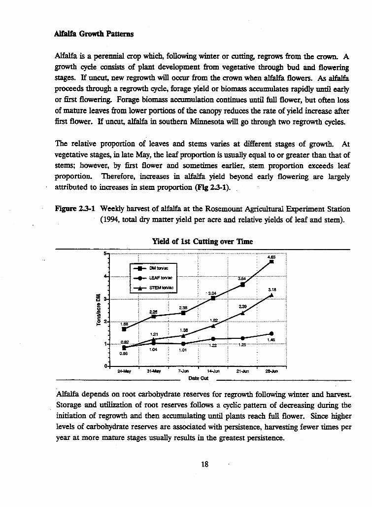
The relative proportion of leaves and stems varies at different stages of growth. At vegetative stages, in late May, the leaf proportion is usually equal to or greater than that of stems; however, by first flower and sometimes earlier, stem proportion exceeds leaf proportion. Therefore, increases in alfalfa yield beyond early flowering are largely attributed to increases in stem proportion (Fig 23-1).
Figure 23-1 Weekly harvest of alfalfa at the Rosemount Agricultural Experiment Station (1994, total dry matter yield per acre and relative yields of leaf and stem).
Yield of 1st Cutting over 'Ilme
s ·····················r····················::····················-::-·····················:······················:········4:ss········1
-9- OM tonlac
····•····•··••· - LSAFIOl\lac ···············:······················:·· .. ···:rs.r· .. ··:········ .............. ! _..,... STEMtonlac 3.18
·········:·····················-:-···· ···············; . .
0.86
31-May 7.Jun 14..Jun 21..Jun
DateCut
Alfalfa depends on root carbohydrate reserves for regrowth following winter and harvest. Storage and utilization of root reserves follows a cyclic pattern of decreasing during the initiation of regrowth and then accumulating until plants reach full flower. Since higher levels of carbohydrate reserves are associated with persistence, harvesting fewer times per year at more mature stages usually results in the greatest persistence.
18
2.4 Alfalfa Pests Yield Reducing Factors: Insects, Diseases, and Weed Competition
Insect pests
The alfalfa weevil and potato leafhopper are insect pests which have the potential to reduce alfalfa yield and quality in the biomass shed. Potato leafhoppers are small (1/8 inch) green insects which migrate into Minnesota on winds from the southern USA in about mid-June. They suck sap from plants and inject a toxin which causes leaves to turn yellow. Yield and
quality losses occur before symptoms occur; therefore, scouting of fields beginning in June is essential. There is a 70% chance of potato leafhopper damage in the biomass shed with an average protein loss of about 500 lb/acre; dry matter yields are less affected. Several
insecticides are available for control of leafhoppers. Insecticides should be applied only
when populations reach the economic threshold control level.
The alfalfa weevil overwinters in Minnesota and lays eggs in the spring. Eggs hatch beginning in mid-May and larvae chew and skeletonize leaves. Damage is most often limited to growth during spring, as feeding falls off in mid-June and a harvest in early June
usually removes most of the larvae. The alfalfa weevil is not a serious pest in the biomass shed "ith only a 10% probability of having weevil numbers sufficient to damage alfalfa. With routine scouting of alfalfa fields, populations can be monitored so that insecticides can be applied should populations reach economic threshold levels.
Di,ew-cs
There arc many diseases which affect alfalfa yield and persistence. For most vascular and systematic diseases, the best control measure is to select a disease resistant variety.
Varieties lack resistance to most of the leaf diseases. Leaf loss due to leaf disease is more ~·ere as the canopy matures and becomes dense; therefore, delaying the first harvest
~·ond early June or extending harvest intervals beyond 40 days is likely to predispose the stand to greater leaf loss. The relatively dry climate in the biomass shed should reduce the
~·criry of most alfalfa leaf diseases.
Wtedo;,
Weed invasion can increase as stands of alfalfa age. Grasses that tolerate the frequency of
alfalfa harvests can become invader species. Broadleaf species such as dandelion, with their ground-hugging profile can also invade and multiply as alfalfa stands age. Areas of fields "With seasonally excessive wetness may lose alfalfa plants due to the lack of oxygen and also
the prevalence of diseases. Areas of fields with dead or declining alfalfa stands are soon
replaced by weeds that can tolerate those conditions such as quackgrass. Producer practices such as soil nutrient maintenance and timely harvests encourage healthy alfalfa stands.
19
2.5 Harvest
Yields and Character of Yields Under Dilferent Cutting Schedules
Craig Sheaffer
Agronomy and Plant Genetics, University of Minnesota
Alfalfa yields in the state of Minnesota average about 3 ton per acre per year. Yield
potential is influenced by soil and climatic conditions within a region. In long-term yield
trials at Lamberton and Morris which are in and bordering the biomass shed, 'Vernal'
alfalfa, a widely grown public variety, yielded an average of 4.1 tons per acre and had
minimum and maximum yields of 1.6 and 6.7 tons per acre (dry weight). Extreme variation
in yield is related to environmental conditions, especially moisture.
Based on the growing season temperature and rainfall in southern Minnesota, producers
currently harvest alfalfa either three or four times per year when alfalfa is at bud to first
flower stages. These schedules provide feed for beef and dairy cattle. Harvest schedules
with only two cuts per season were routinely used before 1950 when varieties lacked
persistence and yield but two-cut schedules are not currently used unless induced by
weather.
We have summarized recent alfalfa cutting management research conducted in southern
Minnesota (Tables 2.5-1 and 2). This research compared the effect of several 2, 3, and 4
cut schedules on leaf percentage, total forage yield, leaf yield, and stem yield of alfalfa As
the number of cuts increased from 2 to 4 per season, leaf percentage increased. Leaf yield
was consistently lower for the 2-cut schedules than for the 3- and 4-cut schedules (Fig 2.5-1).
Overall, dry matter yields were greatest for the 3-cut schedules with yields similar for some
two and four cut schedules. Within the 2- and 3-cut schedules, there is considerable
flexibility in selection of a harvest regime. Within the 4-cut schedule, schedule 7 which
consists of cuttings at bud stage resulted in exceptional yields of total forage and leaves;
however, this schedule might have very detrimental affects on nesting wildlife due to the
early and frequent cutting.
Other cutting schedules are possible in addition to the ten shown. Such schedules may vary
the interval. between harvests during the season or focus on providing a very leafy forage at
one harvest with a less leafy forage at subsequent harvests. Such a schedule would roughly
involve harvests on 25 May at bud stage, 4 July at first flower, and 25 August at first flower.
20
Table 2.5-1 Average cutting dates and alfalfa maturity for ten different cutting schedules
in southern Minnesota.
Cutting Date and Maturity
Cutting Maturity at cuttirig2
Schedule Cutting Date1 1 2
1 25 June 1 Sep. Flfl-Sd Fl fl
2 25 June 15 Sep. Flfl-Sd Sd
3 25 June 15 Oct Flfl-Sd Sd
4 4June 14July 1 Sep. Lt bud Fst fl
5 4June 14July 15 Sep. Lt bud Fst fl
6 4June 14 July 15 Oct. Lt bud Fst fl
7 24May 25 June 4Aug. 1 Sep. Bud Bud
8 24May 25 June 4Aug. 15 Sep. Bud Bud
9 24May 25 June 4Aug. 15 Oct. Bud Bud
10 4June 14July lSep. 15 Oct. Lt bud Fst fl
1 Average dates are shown. Specific cutting dates varied + /- 1 day of average.
3
Fl fl
Fl fl
Fl fl
Bud
Bud
Bud
Fl fl
4
Bud
Lt Bud
Fst fl. Bud
2 Full flower (Fl fl) = > 80% of stems with flowers; Fll"St flower (Fst fl) = 10% of stems with flowers; Bud = flower buds formed; Late bud (Lt bud) = flower buds formed and beginning to open on stems; Seed (Sd) = seed pods formed on 25% of stems
Source: Sheaffer and Martin (1990), J. Prod. Agric 3:486-491
A cutting schedule with harvests on 25 June and 1 September (Table 2.5-1) has been
suggested to sustain and improve wildlife diversity and abundance. Because of the advanced
maturity at harvest of current varieties, this schedule likely will result in a loss in dry matter
and leaf yield using current alfalfa varieties. A two-cut schedule with harvests on 25 June
and 1 September (cutting schedule 1) results in about 20% less leaf yield than a three-cut
schedule with harvests on 4 June, 14 July, and 1 September (cutting schedule 4) as shown
in Table 2.5-2.
Another option would be to develop a three-cut schedule with harvests on 25 June, 30 July,
and early September. However, such a harvest schedule would likely result in very low
yields at the second and third harvests due to soil moisture depletion during the first
regrowth. While the aforementioned schedules with delayed first harvests are feasible, it
· is likely they would only be economically viable to producers using available varieties if
subsidized to enhance wildlife populations.
21
Table 2.5-2 Dry matter yield (tons per acre) of alfalfa under ten different cutting schedules1
at the West Central Agricultural Experiment Station, Morris, MN.
Yield by Cutting Schedule
Schedule1 Total Leaf Stem
1 2-cut 4.0 1.7 2.3
2 2-cut 4.1 L7 2.4
3 2-cut 3.6 1.4 2.2
4 3-cut 4.4 2.1 2.3
5 3-cut: 43 2.1 2.2
6 3-cut: 42 2.0 22
7 4-cut 4.S 2.6 1.9
8 4-cut 3.6 2.0 1.6
9 4-cut 3.9 22 L7
10 4-cut 4.0 2.0 -2.0
1 Cutting Schedule from Table 2.5-1
Source: Sheaffer and Martin (1990, J. Prod. Agric. 3:486-491
Cutting alfalfa after September 1 can pose a risk to the long-term persistence of alfalfa
because fall cutting predisposes alfalfa to winter injury. This risk is associated with removal
of stubble, which insulates the soil and catches snow, and by depletion of root reserves
caused by regrowth. Cutting on September 15 is considered more detrimental to stand
persistence than cutting on October 15 or later because after October 15 air temperatures
are low enough to prevent regrowth and depletion of root reserves. Fall cutting also
removes stubble and residue which provide feed, refuge, and spring nesting sites for wildlife.
For these reasons, schedules 2, 5, and 8 shown in Tables 2.5-1 and -2, 15 September cutting
date, would not be recommended and schedules 3, 6, 9 and 10 would be recommended only
for producers who utilize excellent management practices.
Summazy
Several alternative harvest ~chedules may be selected by producers. The most appropriate
harvest schedule will maximize returns from both the leaf and stem components of the
whole plant.
22
F'J.g111'e 2.S-1 The proportion of leaf and stem in alfalfa bay is dependent on cutting schedule. By location, the curve represents the combination of leaf and stem yields under different cutting schedules. Leaf yield declines and stem yield increases going from four-cut, to three-cut, to a two-cut schedule. The dashed line (trend line), shows expected leaf and stem yield at locations with higher and/or lower total average yields. For example, total yield in a threecut system at St. Paul (the right hand curve) is (2.4 leaf + 2.5 stem) a total of 4.9 tons/acre. Morris and Lamberton locations (2.2 leaf + 2.2 stem) a total of 4.4 tons/acre.
Relative Yields of Leaf and Stem by cutting and location
3~--------------..---...... ----...... ------------
El Morris
• SaintPaul
•· Lamberton
1.0 ..._ __ ....i-_______ ...._ _____ .__.....__ ....... _ _..i
1.00 1.25 1.50 1.75 2.00 2.25 2.50 2.75 3.00
Stems (tons per acre)
23
2.6 FARM MACHINERY
Basics of Hay Handling
David Schmidt and William Wilcke
Agricultural Engineering, University of Minnesota
Alfalfa production requires the use of many different pieces of farm equipment. Some of
the equipment can also be used for production of other crops. Although there are many .
possible options in choosing a complement of equipment for alfalfa production, specific
machines have been identified in the following section for purposes of this study.
Equipment selection impacts labor requirements and harvest losses. These issues, in turn,
affect alfalfa production economics.
A requirement for this project is the use of technologies that are both proven and readily
available. Machines identified in succeeding sections of this feasibility study are all readily
available with proven performance histories. Certainly, there are new machines currently
being developed that will improve the efficiencies and economics of alfalfa production. The
participants in this project are likely to incorporate any new technologies and machines as
they become available and prove practical.
Alfalfa production begins with seedbed preparation, which requires the use of both primary
and secondary tillage equipment. A disk chisel, field cultivator and a spring tooth harrow
provide adequate seedbed preparation. This tillage equipment is common and used for
other crop production. A presswheel drill is used to plant the alfalfa seed, a sprayer is used
to apply insecticides and herbicides while a broadcast fertilizer spreader is used to apply
fertilizer. This equipment is also used to produce other crops.
Several pieces of equipment are specific to alfalfa production. Alfalfa is generally cut three
times per year using either a mower/ conditioner or swather/ conditioner. The conditioning
process crushes the alfalfa stems. Conditioned alfalfa will dry faster in the field than
unconditioned .alfalfa. The mower/ conditioner or swather/ conditioner will leave the alfalfa
in the field in wide windrows. These windrows of alfalfa are then allowed to field dry to
approximately 18-20% moisture. This drying process takes from . two to three days
depending on weather conditions. If rainfall occurs while alfalfa is in windrows or if poor
drying conditions exist, a hay rake may be used to tum the windrow over to hasten the
drying process. The final piece of equipment used in alfalfa production is the baler. A
24

baler picks up the dried alfalfa from the field and forms it into one of several shapes. Bales can be formed into small rectangular bales (approximately 16''x16"x36"), large square bales (approximately 3'x4'x8'), or large round bales (approximately 5' dia. x 5' length). Bale size, shape, and density depends upon the brand and model of baler.
Although a variety of balers exist, this study recommends the use of large-round balers and a bale size of 6' diameter and 4' length. Bale dimensions are critical when transportation issues are considered (Chapter 5). Large square bales have not been recommended due to the lack of storage loss information for the geographic area proposed and because these bales have not been widely accepted by producers as a consequence of a poor reputation for maintaining hay quality under Minnesota conditions. Because of their lower density, large round bales facilitate drying "in the bale" to a greater degree than large square bales.
25

26
CHAPTER 3 PRODUCTION RISKS
3.1 Alfalfa Producer Survey and Hay Sampling Research
Neal P. Martin Department of Agronomy and Plant Genetics, University of Minnesota
Forty-nine (49) faims currently producing alfalfa in the biomass shed were surveyed to assess current alfalfa production practices and to estimate the current state of quality for alfalfa in storage at the time of the survey (winter 93-94). Sixty-seven (67) alfalfa hay samples were collected and analyzed for quality and leaf content.
Fann Characteristics
The average farm size of the 49 sample farms in this study was 552 acres (farm size ranged from 240 to 3,260 acres). Farms in the swvey were located in Renville, Swift, Chippewa, Yellow Medicine, Redwood, Lyon and Lac Qui Parle counties of southwestern Minnesota. Average alfalfa acreage per farm was 54 acres (range 11 - 160 acres per farm). Com acreage per farm averaged 267 acres and soybeans averaged 256 acres per farm. The only other crop being produced by this group of alfalfa producers was wheat.
Alfalfa Production
Only two of the growers surveyed reported a value for alfalfa yield (6 t/a and 3.5 t/a). Most current alfalfa producers are internal users and commonly evaluate yield in terms of the number of bales produced per acre. Reported alfalfa yield from published agricultural statistics for the counties included in this swvey averaged 3.11 t/a (range 4.6 to 1.9 t/a). Total alfalfa production in the seven counties swveyed has averaged just under 75,000 acres per year (last five years).
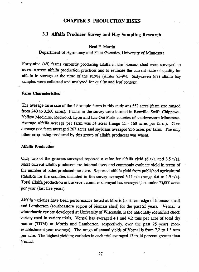
Alfalfa varieties have been performance tested at Morris (northern edge of biomass shed) and Lamberton (southeastern region of biomass shed) for the past 25 years. 'Vernal,' a winterhardy variety developed at University of Wisconsin, is the nationally identified check variety used in variety trials. Vernal has averaged 4.1 and 42 tons per acre of total dry matter (IDM) at Morris and Lamberton, respectively, over the past 25 years (nonestablishment year average). The range of annual yields of Vernal is from 7 2 to 1.3 tons per acre. The highest yielding varieties in each trial averaged 13 to 14 percent greater than Vernal.
27
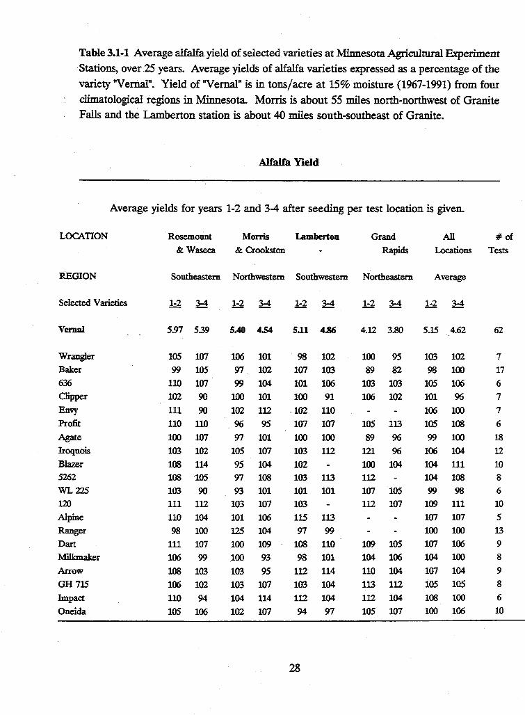
Table 3.1-1 Average alfalfa yield of selected varieties at Minnesota Agricultural Experiment Stations, over 25 years. Average yields of alfalfa varieties expressed as a percentage of the variety "Vernal". Yield of "Vernal" is in tons/acre at 15% moisture (1967-1991) from four climatological regions in Minnesota. Morris is about 55 miles north-northwest of Granite Falls and the Lamberton station is about 40 miles south-southeast of Granite.
Alfalfa Yield
Average yields for years 1-2 and 3-4 after seeding per test location is given.
LOCATION Rosemount Monis Lamberton Grand All #of & Waseca & Crookston Rapids Locations Tests
REGION Southeast em Northwestern Southwestern Northeastern Average
Selected Varieties 1-2 3-4 1-2 3-4 1-2 3-4 1-2 3-4 1-2 3-4
Vernal 5.97 5.39 5.40 4.54 5.11 4.86 4.12 3.80 5.15 4.62 62
Wrangler 105 107 106 101 98 102 100 95 103 102 7 Baker 99 105 97 102 107 103 89 82 98 100 17 636 110 107 99 104 101 106 103 103 105 106 6 Clipper 102 90 100 101 100 91 106 102 101 96 7
Envy 111 90 102 112 .102 110 106 100 7 Profit 110 110 96 95 107 107 105 113 105 108 6 Agate 100 107 97 101 100 100 89 96 99 100 18 Iroquois 103 102 105 107 103 112 121 96 106 104 12 Blazer 108 114 95 104 102 100 104 104 111 10
5262 108 105 97 108 103 113 112 104 108 8 WL225 103 90 93 101 101 101 107 105 99 98 6 120 111 112 103 107 103 112 107 1()1) 111 10 Alpine 110 104 101 106 115 113 107 107 5 Ranger 98 100 125 104 97 99 100 100 13 Dart 111 107 100 1()1) 108 110 1()1) 105 107 106 9
Milkmaker 106 99 100 93 98 101 104 106 104 100 8 Arrow 108 103 103 95 112 114 110 104 107 104 9
GH715 106 102 103 107 103 104 113 112 105 105 8
Impact 110 94 104 114 112 104 112 104 108 100 6 Oneida 105 106 102 107 94 97 105 107 100 106 10
28
The alfalfa variety trials have experienced complete winter kill once in twenty-five years at Morris and once at Lamberton; not the same year. Moderate winter injury was experienced 5 and 3 years of the 25 at Morris and Lamberton, respectively. Drought reduced yields by 20% in 6 and 5 of the 25 years at Morris and Lamberton, respectively. Yields often peak at 2 or 3 years after seeding. However, the performance of varieties is influenced more by weather than stand age (Table 3.1-2 note: variety performance by stand age). Recently released varieties perform better than Vernal at older stand ages. Preliminary tests at the University of Minnesota's Rosemount Experiment Station of selected available varieties show significant differences in leaf retention. This characteristic could be an important selection criterion for biomass production.
Table 3.1-2 The average yield of 'Vernal' (a common check variety) and of the highest yielding variety in alfalfa performance trials conducted at Lamberton and Morris from 1968 to 1993. Yield is given as total dry matter (TDM) per acre.
Yield by Stand Age (0% moisture)
Morris Lamberton
Stand Number stand Number Variety age trials Yield Variety age trials Yield
---years--- TDM/A ---years--- TDM/A
Vernal 1 8 4.16 Vernal 1 8 4.40 2 8 4.24 2 8 4.49
3 5 3.51 3 6 431 4 5 4.20 4 6 3.05
5 2 3.47
Top variety 1 1 4.58 Top variety 1 1 4.93 2 1 4.83 2 1 5.30 3 5 4.11 3 5 4.82 4 5 4.96 4 6 3.57
5 2 3.81
29
Management Practices
Seeding techniques and storage practices offer opportunities for significant improvements in currer alfalfa management practices. Stand establishment has a major impact on productivity and stand Im Twenty-five (25) growers reported stand life after establishment for an average of 2.95 years (1 to· year range in reported values). We expect growers in the proposed biomass shed will be able to plar varieties that will persist, on average, for 4 years after seeding.
Current storage methods for large round bales varies from farm to farm, however most large roun1 bales are stored outside without cover. Cooperative storage, provided by the alfalfa cooperative, shoul1 dramatically improve the quality stored alfalfa.
Alfalfa requires high levels of potassium and performs best under conditions of neutral soil pH. Th soils in the proposed biomass shed are characterized excellent for alfalfa. Within the biomass shed soi pH's approach 7.0 and are generally high in soil potassium. Yields will be dependent upon a specifi soil's water holding capacity more than nutrient levels or soil pH. Alfalfa is a heavy transpiring croi with a deep tap root. Alfalfa yields better than other crops during a drought, but its yield will b limited following drought years. In severe cases, the yield of the crop following alfalfa is reduced du t6 soil moisture depletion.
Analysis of Alfalfa Samples
Fifty-two ( 52%) percent of the hay samples collected were alfalfa hay; 48% were alfalfa-grass mixture~ Alfalfa-grass mixtures have less protein and more fiber than "pure" alfalfa. Alfalfa samples average4 19.8% crude protein (CP), alfalfa-grass mixture averaged 17.6% CP (Table 3.1-3).
Alfalfa samples came from either the first, second, or third cutting of the previous season crop (1993~ Third cutting alfalfa hay had the highest quality (% CP and relative feed value (RFV) and the highes percentage of leaf (Table 3.1-3). Relative feed value (RFV) is a standard index of forage quality. Lea percentage of alfalfa hay is influenced by percent alfalfa in the stand, stage of maturity at harvest, typ of bale, storage method, and rain damage.
Half of the hay analyzed was in small square bales (50 lb /bale) and half of the hay came from larg1
round bales (1000 lb/bale). Alfalfa hay samples from small square bales averaged higher in lea content than large round bales (44% vs 38% leaves). The majority of the small square bales wer1
stored inside (57%) and the majority of the large round bales were stored outside without cover (62% ~
30
Table 3.1-3 Forage quality tests were conducted on hay samples from on-farm storage in the proposed biomass shed. Samples were collected from December 1993 to February of 1994. Results are given for crude protein (CP), acid detergent fiber (ADF), neutral detergent fiber (NDF), relative feed value (RFV), percentage of leaf(% Leaf), calcium (Ca), phosphorus (P), and potassium (K).
Samgle CP ADF NDF RFV %Leaf Ca p K
-------%ofdwt-------- index ----------%ofdwt----------
Alfalfa & alfalfa grass mixtures (n=67l
average 18.6 385 53.6 106 395 135 .30 256 max. 24.0 57.6 775 157 545 1.61 .41 3.34 mm. 82 282 39.7 53 7.7 .67 .07 33
Alfalfa tn = 29)
average 19.8 36.4 50.1 115 425 1.42 31 2.73
Alfalfa=erus mixture (n = 27)
average 17.6 39.4 55.7 101 37.0 127 .30 2.48
1st nu (n .. n
average 195 38.8 52.1 110. 42.9 1.47 .30 2.60 LR(~) 18.0 42.6 573 93 402 1.41 29 2.42 so (5) 20.0 373 50.0 116 44.0 1.50 31 2.68
2nd at In " 1 U
a\"Cragc 202 37.4 52.8 107 395 1.37 33 2.77 LR(4) 20.0 36.68 52.4 107 38.7 136 32 2.75 so (7) 202 37.7 52.2 107 40.0 1.38 33 2.78
3nt cwt !n• lJ)
3\"Cf~ 19.6 34.0 46.6 128 453 1.42 .30 2.76 LR C~I 16.6 40.8 54.0 105 36.4 129 28 255 SO (II) 203 32.5 45.0 133 473 1.45 31 2.81
Rai• ck•md tp=30)
aver~ 19.8 36.7 503 114 422 1.41 31 2.74 dr)· storage ( 19) 202 34.7 47.4 123 45.4 L44 31 2.81 no CO\"Cf ( 11) 19.1 40.0 55.4 99 36.8 135 31 2.61
31
. Analysis of Alfalfa Samples (continued)
Large round bales stored inside were 47% leaf, bales stored outside with no cover were 37% leaf. All bales stored outside were stored on earth (storage losses from weathering can be reduced when bales are stored on gravel or other well-drained materials). Thirty-seven (37%) percent of the hay samples suffered from rain damage but only 5% of the samples were moldy. Best management practices for harvest and storage management would significantly improve alfalfa quality and returns.
Results of forage quality tests to determine crude protein (CP), acid detergent fiber (ADF), neutral detergent fiber {NDF), relative feed value {RFV), percent leaf(% Leaf), percent calcium ( % Ca), percent phosphorus (% P), and percent potassium ( % K) are shown in Table 3.1-3. The 67 hay samples were generally representative of alfalfa and alfalfa-grass ~es grown in Minnesota. The relative feed value (RFV) index is a standard quality measure for alfalfa. RFV's from 140 to 160 are recommended for high producing dairy cattle or cows in early lactation. RFV's below 100 are used for livestock rations with low nutrient requirements. Hay rated below 100 RFV is used in rations for maintenance and often would require supplemental protein, energy, and mineral additions. Almost half of the samples tested analyzed below 100 RFV index. Fiber tests are used to predict digestibility (ADF) and potential dry matter intake (NDF). ADF and NDF are related. As fiber increases, animal digestibility and intake declines.
32
3.2 Harvest Losses Mechanical, Respiration, and Rainfall Losses
Douglas G. Tiffany1, Jerry Fruin1, Craig Sheaffer2, Xueping Pang3 and David Schmidt4
1Ag & App. Economics, 2 Agron & Plant Genetics, 3Soil Science, and 4Ag Engineering, University of Minnesota
Hay harvest can result in losses from 7 to 31% of standing forage dry matter (Table 3.2-1).
Most of the dry matter loss is due to loss of the fragile leaf fraction, while stem material is
usually retained. When unfavorable conditions for drying occur, losses can be as high as
100% of the leaf fraction.- In haymaking, losses occur during harvesting operations and
during field exposure prior to harvest. Field exposure losses are associated with respiration (Figure 3.2-1) and rain damage (Figure 3.2-2).
Table 3.2-1 Losses from alfalfa during harvest operations. Harvest Losses
Operation
Mowing Mowing/conditioning
reciprocating mower, fluted rolls disc mower, fluted rolls disc mower, flail conditioner
Raking: at 70% moisture at 60% moisture at 50% moisture at 33% moisture at 20% moisture
Tedding: at 70% moisture at 60% moisture at 50% moisture at 33% moisture at 20% moisture
Baling, pickup + chamber: at 25% moisture• at 20% moisture at 12% moisture
Baling at 18% moisture: ·conventional square baler/ ejector round, variable chamber round, fixed chamber
Stack wagon
Total
a Requires a preservative for safe storage.
% of DM lost
1 2 3 3 4
2 2 3 7
12
1 1 3 6
11
3 4 6
5 6
13 15
7-31
Source: Kjelgaard (1979), Rotz (1989), Hundtoft (1965), in Pitt (1990)
33
% of Leaves lost
2 3 4 4 5
2 3 5
12 21
2 3 5
12 21
4 6 8
8 10 21 24
12-50
Mechanical Losses
Losses in dry matter and leaves during harvesting operations can be large because of the necessity of handling forage low in moisture content and the fragile attachment of leaves to stems (Table 3.2-1 ). Dry matter losses average from 7 to 31 percent while leaf loss averages from 12 to 50 percent. Losses can be minimiz.ed if the number of field operations are minimized. For example, with good drying conditions brought about by low humidity and high temperatures raking can.be eliminated. Tedding or fluffing the windrows to enhance air passage is seldom necessary if small windrows are initially formed. New machinery developments such as windrow inverters allow the turning of windrowed forage with negligible leaf loss.
Because leaves dry to moisture levels suitable for storage faster than stems, they are prone to shattering. Therefore, turning of hay by raking should be conducted at moisture levels greater than 40% or in mornings when dew has moistened the leaves. Likewise, overdrying forage to moisture concentrations below 18% moisture enhances leaf and dry matter loss.
34
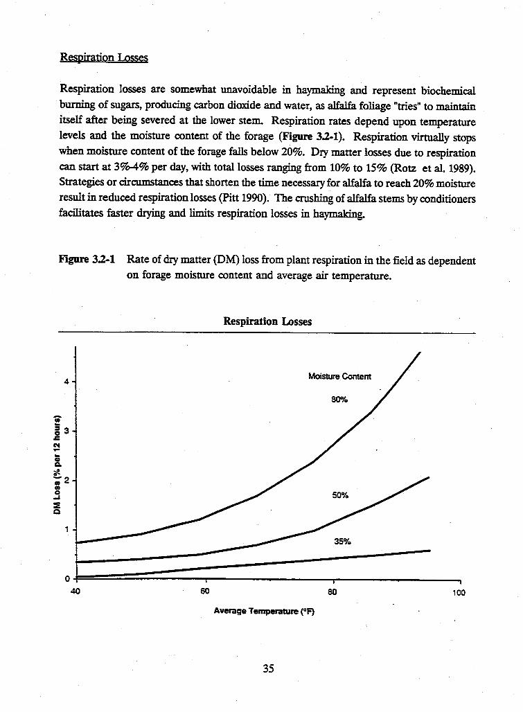
Remiration Losses
Respiration losses are somewhat unavoidable in haymaking and represent biochemical burning of sugars, producing carbon dioxide and water, as alfalfa foliage "tries" to maintain itself after being severed at the lower stem. Respiration rates depend upon temperature levels and the moisture content of the forage (Figure 3.2-1 ). Respiration virtually stops when moisture content of the forage falls below 20%. Dry matter losses due to respiration can start at 3o/o-4% per day, with total losses ranging from 10% to 15% (Rotz et al. 1989). Strategies or circumstances that shorten the time necessary for alfalfa to reach 20% moisture result in reduced respiration losses (Pitt 1990). The crushing of alfalfa stems by conditioners facilitates faster drying and limits respiration losses in haymaking.
Figure 3.2-1 Rate of dry matter (DM) loss from plant respiration in the field as dependent on forage moisture content and average air temperature.
4
... i3 J: N .... .. ID ~ ..,. -; 2 fl) 0 ...a :: Q
1
40
Respiration Losses
Moisture Content
SOo/o
60 80 100
Average Temperature (0 F}
35
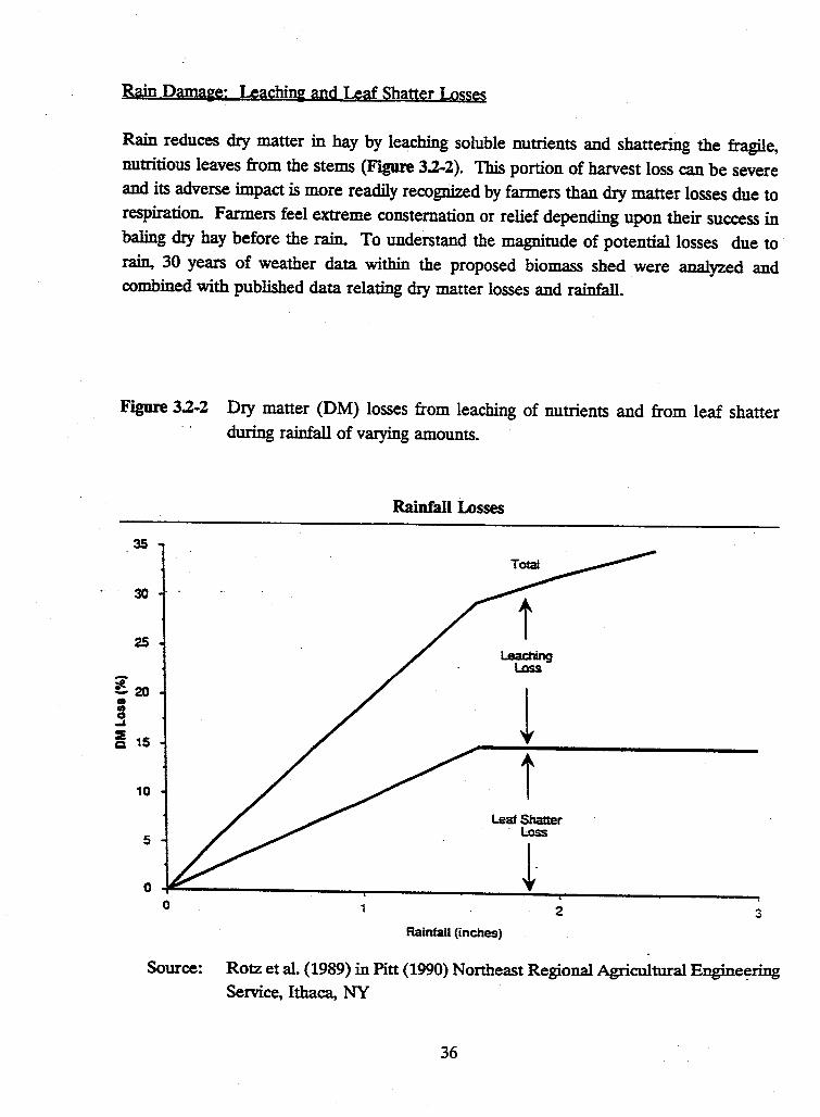
Rain D~: Leachin& and Lea{ Shaner Losses
Rain reduces dry matter in hay by leaching soluble nutrients and shattering the fragile, nutritious leaves from the stems (Figure 3.2-2). This portion of harvest loss can be severe and its adverse impact is more readily recognized by farmers than dry matter losses due to respiration. Farmers feel extreme consternation or relief depending upon their success in baling dry hay before the rain. To understand the magnitude of potential losses due to rain, 30 years of weather data within the proposed biomass shed were analyzed and combined with published data relating dry matter losses and rainfall.
Figure 3.2-2 Dry matter (DM) losses from leaching of nutrients and from leaf shatter during rainfall of varying amounts.
Rainfall L-Osses
35
30
25 Leaching
Lass
~20 t • • 0 ~
:E Q 15
10 i Leaf Shatter
. Loss 5
i 0 0 1 2 3
Rainfall (inches)
Source: Rotz et al (1989) in Pitt (1990) Northeast Regional Agricultural Engine~ring Service~ Ithaca, NY
36
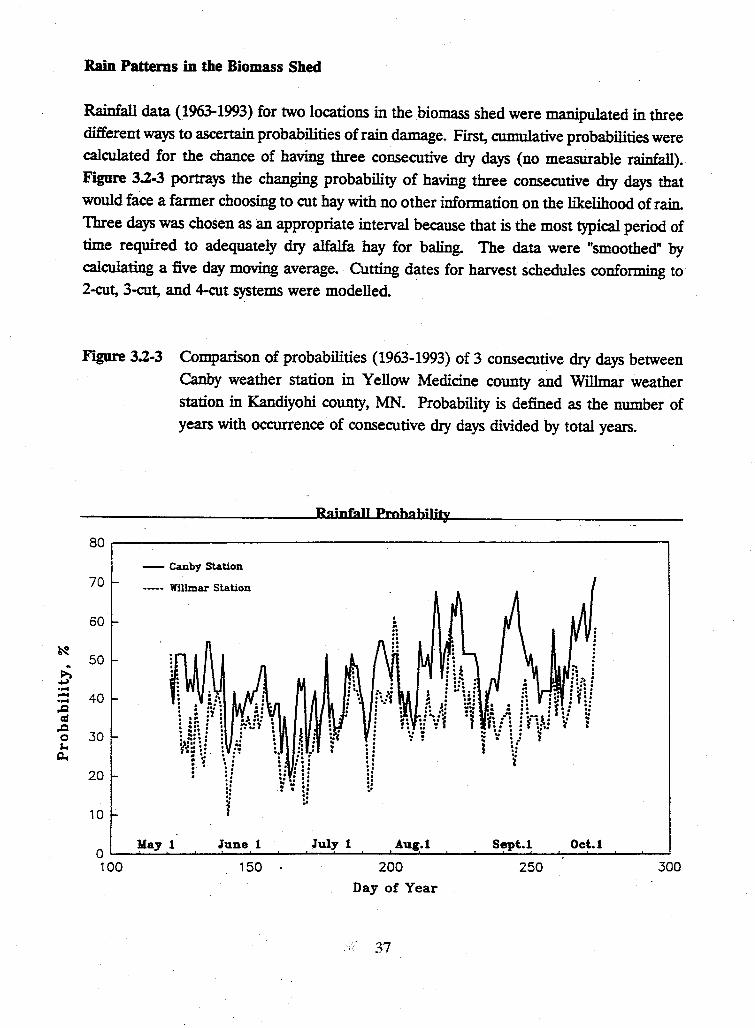
~
~ ~ .... -.... ..c = ..c 0 ,..
g,,.
Rain Patterns in the Biomass Shed
RainfaU data (1963-1993) for two locations in the biomass shed were manipulated in three different ways to ascertain probabilities of rain damage. First, cumulative probabilities were calculated for the chance of having three consecutive dry days (no measurable rainfall). Figlll'e 3.2-3 portrays the changing probability of having three consecutive dry days that would face a farmer choosing to cut hay with no other information on the likelihood of rain. Three days was chosen as an appropriate interval because that is the most typical period of time required to adequately dry alfalfa hay for baling. The data were "smoothed" by calculating a five day moving average. Cutting dates for harvest schedules conforming to 2-cut, 3-cut, and 4-cut systems were modelled.
Figure 3.2-3 Comparison of probabilities {1963-1993) of 3 consecutive dry days between Canby weather station in Yellow Medicine county and Willmar weather station in Kandiyohi county, MN. Probability is defined as the number of years with occurrence of consecutive dry days divided by total years.
Rainfall Pmhahilitf
80
- Canby Station
70 ••••• Willmar Station
60
50
40
30
20
10
Oct.1 May 1 June 1 July 1 Aug.1 Sept.1 oL--=.:~=--_..__.:;._::=...::.....:...._.___...__...:.....__._ __ ...__-=----.___._____..;-___._-'-:~"'---"---'---' 1 00 150 200 250 300
Day of Year
.<: 37
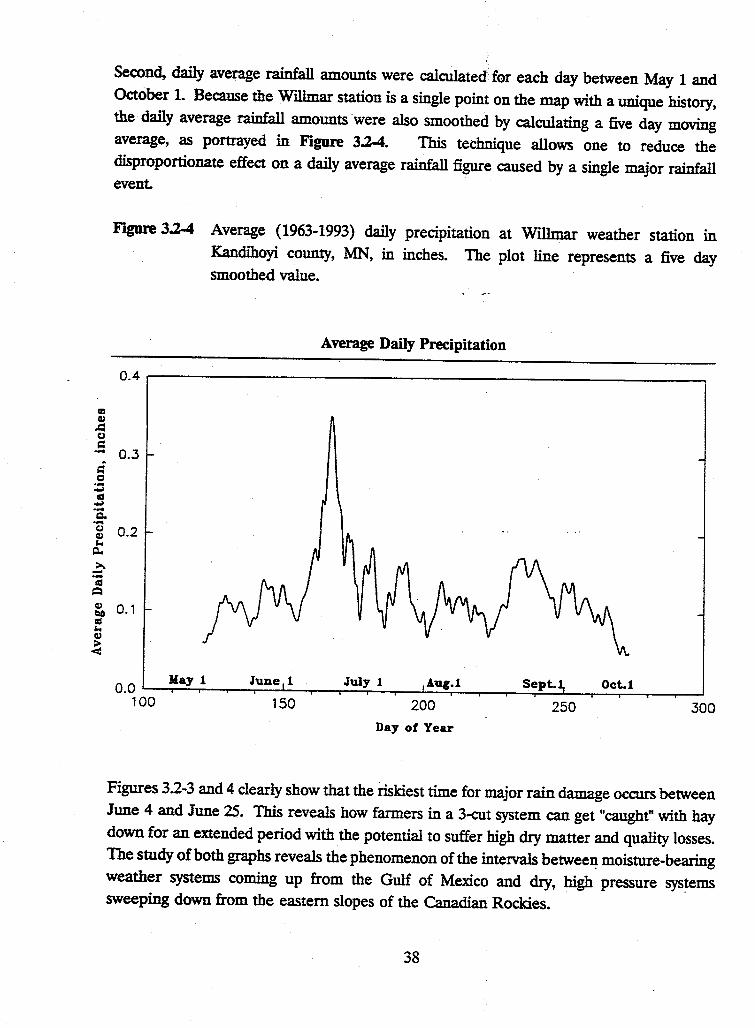
m Q)
.::= CJ = .... = 0 .... ~
CIS ~ .... Q., .... CJ Q)
"" i:i. >... -... CIS
Q
CP ~ CIS ... CP > <
Second, daily average rainfall amounts were calculated' for each day between May 1 and October 1. Because the Willmar station is a single point on the map with a unique history, the daily average rainfall amounts· were also smoothed by calculating a five day moving average, as portrayed in Figure 3.2-4. This technique allows one to reduce the disproportionate effect on a daily average rainfall figure caused by a single major rainfall event.
Figure 3.2-4 Average (1963-1993) daily precipitation at Willmar weather station in Kandihoyi county, MN, in inches. The plot line represents a five day smoothed value.
Average Daily Precipitation
0.4 ..--------------------------------,
0.3
0.2
0.1
Oct.1 Hay 1 June 1 July 1 A.ug.1 Sept. 0.0 '---.-...;....,.---.---..--'---,.-...--.--...---'----"..---r----,.--_,...;;;.---'---.---r---r---r---' 100 150 200 250 300 Day of Year
Figures 32-3 and 4 clearly show that the riskiest time for major rain damage occurs between June 4 and June 25. This reveals how farmers in a 3-cut system can get "caught" with hay down for an extended period with the potential to suffer high dry matter and quality losses. The study of both graphs reveals the phenomenon of the intervals betweeJ:!. moisture-bearing weather systems coming up from the Gulf of Mexico and dry, high pressure sys~ems sweeping down from the eastern slopes of the Canadian Rockies.
38
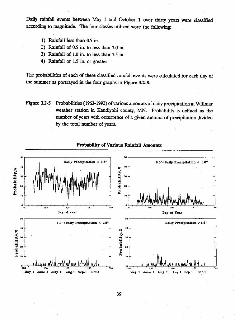
N
~ - JO --,Q
.: 20
0 ... ""' 10
Daily rainfall events between May 1 and October 1 over thirty years were classified according to magnitude. The four classes utilized were the following:
1) Rainfall less than 0.5 in. 2) Rainfall of 0.5 in. to less than 1.0 in. 3) Rainfall of 1.0 in. to less than 1.5 in.
4) Rainfall or 1.5 in. or greater
The probabilities of each of these classified rainfall events were calculated for each day of the summer as portrayed in the four graphs in Figure 3.2-5.
Figure 3.2-5 Probabilities (1963-1993) of various amounts of daily precipitation at Willmar weather station in Kandiyohi county, :MN. Probability is defined as the
number of years with occurrence of a given amount of precipitation divided by the total number of years.
Probability of Various Rainfall Amounts
Daily Precipitation < 0.5"
N "° ~ ::::: 30. -.a al . .a 20 0 ...
g., 10
0.5"<Daily Precipitation < 1.0"
oi........-.--.-......-.____,.._,........,.-..___,,.......,._,.....,.-.........,r-T"-r---r-' 100 1$0 200 250 300
N po.
- 30 ---,Q
.: 20
0 ... ll. 10
Day ot Year
l.O"<Daily Precipitation < 1.5"
oL......,--IJ..JJ,111~.L.ai.J..l.,tlLI,-l-!UJm.J..11~...UL,-..J/WJUJ.,u.,JL..,--,--l 100 150 200 250 300
Kay 1 June 1 July 1 Aug.1 Sep.1 OcLl
40 ~
~ - 30 --,g al ,g 20 0 ... ""' 10
Day of Year
Daily Precipitation > 1.5"
oL...r---.--9--flll....llm.!p.....l,llLll,IJ'.J\11114:-1'\A-flll!Q.\V-J.LpJ.~lf-Ai;-,..~ 100 150 250 300
Kay 1 June 1 July I Aug.I Sep.l Oct.I
39
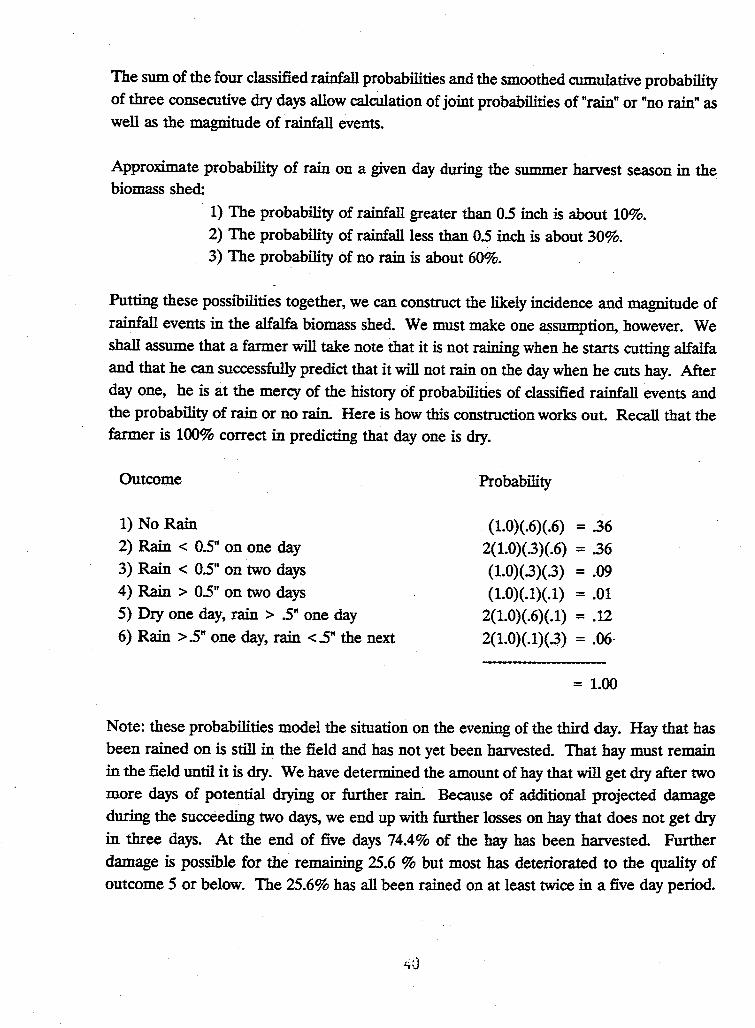
The sum of the four classified rainfall probabilities and the smoothed cumulative probability of three consecutive dry days allow calculation of joint probabilities of "rain" or "no rain" as well as the magnitude of rainfall events.
Approximate probability of rain on a given day during the summer harvest season in the biomass shed:
1) The probability of rainfall greater than 05 inch is about 10%. 2) The probability of rainfall less than 05 inch is about 30%. 3) The probability of no rain is about 60%.
Putting these possibilities together, we can construct the likely incidence and magnitude of rainfall events in the alfalfa biomass shed. We must make one assumption, however. We shall assume that a farmer will take note that it is not raining when he starts cutting alfalfa and that he can successfully predict that it will not rain on the day when he cuts hay. After day one, he is at the mercy of the history of probabilities of classified rainfall events and the probability of rain or no rain. Here is how this construction works out. Recall that the farmer is 100% correct in predicting that day one is dry.
Outcome
1) No Rain
2) Rain < 05" on one day 3) Rain < 05" on two days 4) Rain > 05'' on two days 5) Dry one day, rain > 5" one day 6) Rain > 5" one day, rain < 5" the next
Probability
(1.0)(.6)(.6) = 36 2(1.0)(3)(.6) = 36 (1.0)(3)(3) = .09 {1.0)(.1)(.1) = .01
2(1.0)(.6)(.1) = .12 2(1.0)(.1)(.3) = .06-
= 1.00
Note: these probabilities model the situation on the evening of the third day. Hay that has been rained on is still in the field and has not yet been harvested. That hay must remain in the field until it is dry. We have determined the amount of hay that will get dry after two more days of potential drying or further rain. Because of additional projected damage during the succeeding two days, we end up with further losses on hay that does not get dry in three days. At the end of five days 74.4% of the hay has been harvested. Further damage is possible for the remaining 25.6 % but most ltas deteriorated to the quality of outcome 5 or below. The 25.6% has all been rained on at least twice in a five day period.
Combining the calculated joint probabilities of rainfall events with published data on dry
matter losses due to rain (Rotz et al. 1989 in Pitt (1990)) allows one to calculate dry matter losses that would be due to rain. Here is how things work out with respect to dry matter and leaf shatter loss (after 5th day):
Assumed outcome Rain Probability DM Loss Leaf Loss
1 -0- 36 -0- -0-2 .25" .17 .05 .02 3 .50" .13 .10 .04 4 .75" .10 .15 .07 5 1.00" .16 .19 .09
6 1.50" .05 .28 .14 7 1.75" .03 .30 .15
The summed probable dry matter losses due to rain that would befall alfalfa producers would average 8.99%. This conclusion represents an aggregate view of the risk and extent of rain damage over the proposed alfalfa biomass shed.
There will need to be management decisions regarding hay produced under the different outcomes in an alfalfa biomass project where revenues from leaf separation activities are crucial to profitability. Here are some preliminary judgements about the usefulness of hay produced under the various outcomes:
Outcome 1; no problems, beautiful hay
Outcome 2; very nice hay, but .25" of rain Outcome 3; .5" of rain sustained, fair quality Outcome 4; .75" of rain, poor but usable Outcome 5; 1.0" of rain, very popr Outcome 6; 1.5" of rain, stems only Outcome 7; 1.75" of rain, very poor quality
41
36%
17% 13%
10% 16%
5%
~ 100%
Weather Risk and Management Expectations
What should management at the alfalfa fractionation facility expect?
Management should expect that approximately 66% of the crop (Outcomes 1+2+ 3) will be in good condition. Therefore approximately 34% of the crop may be expected to be in poor condition reflecting Outcomes 4, 5, 6, and 7. Outcomes 4-7 have poor feed value but only moderately reduced biomass energy value. Supply management strategies may be implemented to further reduce rain damage losses by direct-delivery of high moisture rain damaged hay to the processing plant.
Additionally, a self-insuring strategy may be implemented to spread harvest dates over the biomass shed. Production dispersion spreads risk over time and location. Quality, condition, dry matter yield, and leaf losses are discussed further in Section 9 .2 (Contracting for Production).
42
Chemical Preservation of Hay: Problems Solved and Created
Hay preservatives such as propionic acid and derived buffered products have been used
successfully to preserve forages. They are effective at preventing mold growth and
associated losses in forage quality in hay with moisture levels from 20 to 35 %. Because they
could allow harvest at higher moisture levels, they could reduce exposure to rain damage.
Their use could also result in lower leaf and dry matter losses caused by machine
operations. Recommended rates increase as hay moisture concentration increases (See
Sheaffer and Martin, Minnesota Agric. Ext. Service Folder 489-1979). For hay with a 20-
25 % moisture level, 10 lb/ ton of preservative should be applied; for hay of 30-35 % moisture
30 lb/ton are required. At $.50 to $1.00 per pound, treatment of hay containing 22%
moisture would require from $5 to $10 dollars of additional cost per ton.
Although sometimes useful for an individual producer, there are a number of reasons for
prohibiting preservative use for hay involved in biomass production including the following:
1. Long-term storage of hay treated with organic acids has been poor.
2. Bales treated with preservatives tend to shrink, leading to loose twine and bale breakage.
3. Inconsistent application of preservatives to ''high moisture" bales (20-25%) could pose storage- hazards. If a farmer were to produce even a small number of -bales without adequate preservative, those untreated or undertreated bales could easily heat and start a fire.
4. High moisture bales treated with preservatives will require more heat for drying before fractionating.
5. Prcscn.-ative costs from $5-10/T are significant.
Rewarcb Seeds:
A' documented, field and harvest losses of leaf and stem dry matter and forage quality can
be large. While we have confidence in the data used in this study, we recognize that data
wa..\ not available to most accurately describe the range in potential harvest schedules which
"ill likcl~· be used in the biomass shed. For example, if a two-cut schedule is used it is
likely that leaf losses will be greater during some phases of the drying processes than for a
four-cut schedule. In subsequent research, we propose to examine the effects of interactions
of harvest schedules, harvesting equipment, and rainfall on leaf and stem yield and leaf
quality.
43
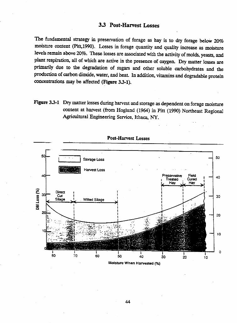
3.3 Post-Harvest Losses
The fundamental strategy in preservation of forage as hay is to dry forage belo\v 20% moisture content (Pift,1990). Losses in forage quantity and quality increase as moisture levels remain above 20%. These losses are associated with the activity of molds, yeasts, and plant respiration, all of which are active in the presence of oxygen. Dry matter losses are primarily due to the degradation of sugars and other soluble carbohydrates and the production of carbon dioxide, water, and heat. In addition, vitamins and degradable protein concentrations may be affected (Figure 3.3-1).
Figure 3.3-1 Dry matter losses during harvest and storage as dependent on forage moisture content at harvest (from Hoglund (1964) in Pitt (1990) Northeast Regional Agricultural Engineering Service, Ithaca, NY.
Post-Harvest Losses
50 I Storage Loss 50
I•- Harvest Loss
40 Preservative Ftek:I I 40
I Treated Cured I
k Hay ;ii.~ Hay >{ ~ I I I.
I I ";;;" 3 I I 30 en Wilted Silage I I 0
I -i I :E I Q
20
10
0
Moisture When Harvested (%)
44
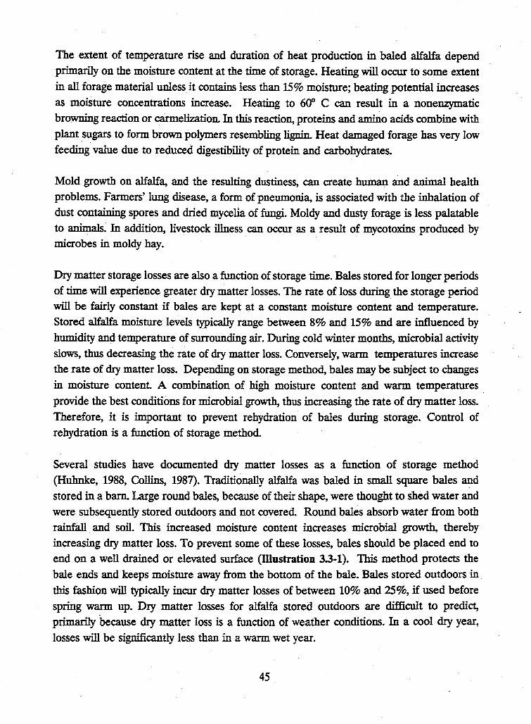
The extent of temperature rise and duration of heat production in baled alfalfa depend primarily on the moisture content at the time of storage. Heating will occur to some extent in all forage material unless it contains less than 15% moisture; heating potential increases as moisture concentrations increase. Heating to 60° C can result in a nonenzymatic browning reaction or carmelization. In this reaction, proteins and amino acids combine with plant .sugars to form brown polymers resembling lignin. Heat damaged forage has very low feeding value due to reduced digestibility of protein and carbohydrates.
Mold growth on alfalfa, and the resulting dustiness, can create human and animal health problems. Farmers' lung disease, a form of pneumonia, is associated with the inhalation of dust containing spores and dried mycelia of fungi. Moldy and dusty forage is less palatable to animals. In addition, livestock illness can occur as a result of mycotoxi.ns produced by microbes in moldy hay.
Dry matter storage losses are also a function of storage time. Bales stored for longer periods of time will experience greater dry matter losses. The rate of loss during the storage period will be fairly constant if bales are kept at a constant moisture content and temperature. Stored alfalfa moisture levels typically range between 8% and 15% and are influenced by humidity and temperature of surrounding air. During cold winter months, microbial activity slows, thus decreasing the rate of dry matter loss. Conversely, warm temperatures increase the rate of dry matter loss. Depending on storage method, bales may be subject to changes in moisture content. A combination of high moisture content and warm temperatures provide the best conditions for microbial growth, thus increasing the rate of dry matter loss. Therefore, it is important to prevent rehydration of bales during storage. Control of rehydration is a function of storage method.
Several studies have documented dry matter losses as a function of storage method (Huhnke, 1988, Collins, 1987). Traditionally alfalfa was baled in small square bales and stored in a barn. Large round bales, because of their shape, were thought to shed water and were subsequently stored outdoors and not covered. Round bales absorb water from both rainfall and soil. This increased moisture content increases microbial growth, thereby increasing dry matter loss. To prevent some of these losses, bales should be placed end to end on a well drained or elevated surface (Illustration 3.3-1). This method protects the bale ends and keeps moisture away from the bottom of the bale. Bales stored outdoors in this fashion will typically incur dry matter losses of between 10% and 25%, if used before spring warm up. Dry matter losses for alfalfa stored outdoors are difficult to predict, primarily because dry matter loss is a function of weather conditions. In a cool dry year, losses will be significantly less than in a warm wet year.
45
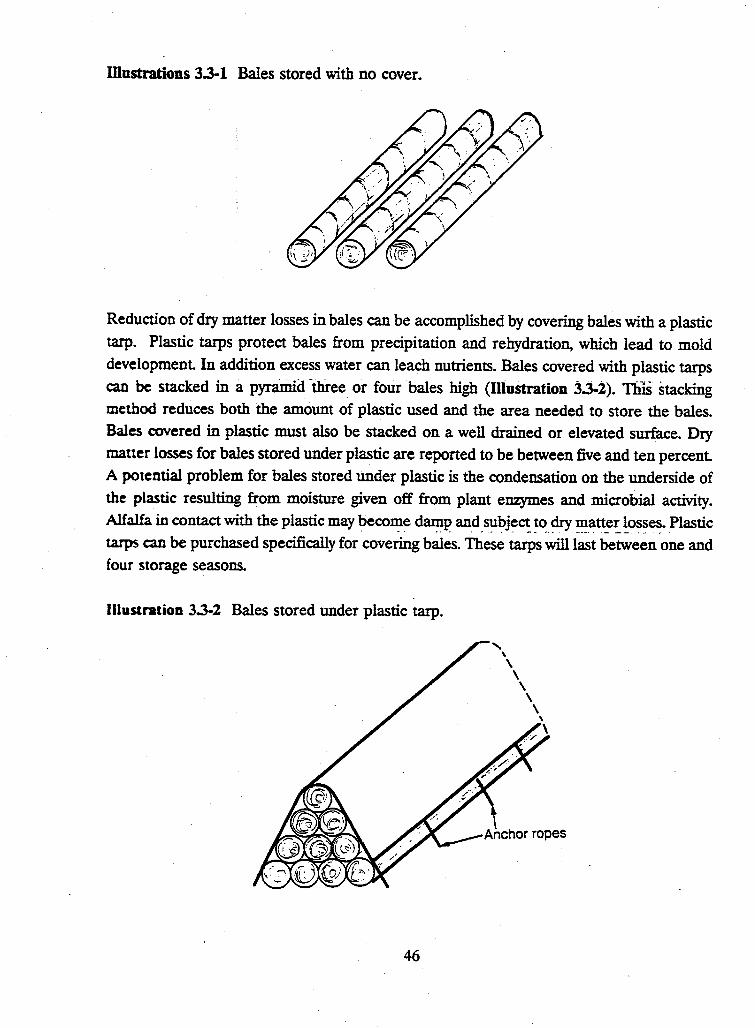
mustrations 3.3-1 Bales stored with no cover.
Reduction of dry matter losses in bales can be accomplished by covering bales with a plastic tarp. Plastic tarps protect bales from precipitation and rehydration, which lead to mold development. In addition excess water can leach nutrients. Bales covered with plastic tarps can be stacked in a pyramid -three or four bales high (Illustration 3.3-2). nus stacking method reduces both the amount of plastic used and the area needed to store the bales. Bales covered in plastic must also be stacked on a well drained or elevated surface. Dry matter losses for bales stored under plastic are reported to be between five and ten percent. A potential problem for bales stored under plastic is the condensation on the underside of the plastic resulting from moisture given off from plant enzymes and microbial activity. Alfalfa in contact with the plastic may ~ecoll_le d~p an_d _ s?bj~C! ~~ ~ry ~_att~~ !o~~e~. Plastic tarps can be purchased specifically for covering bales. These tarps will last between one and four storage seasons.
Illustration 3.3-2 Bales stored under plastic tarp.
46
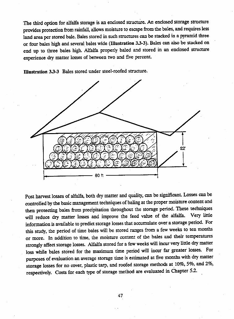
The third option for alfalfa storage is an enclosed structu're. An enclosed storage structure
provides protection from rainfall, allows moisture to escape from the bales, and requires less
land area per stored bale. Bales stored in such structures can be stacked in a pyramid three
or four bales high and several bales wide (Illustration 3.3-3). Bales can also be stacked on
end up to three bales high. Alfalfa properly baled and stored in an enclosed structure
experience dry matter losses of between two and five percent.
illustration 3.3-3 Bales stored under steel-roofed structure.
I~·---------------~ soft------------------...
Post harvest losses of alfalfa, both dry matter and quality, can be significant. Losses can be
controlled by the basic management techniques of baling at the proper moisture content and
then protecting bales from precipitation throughout the storage period. These techniques
will reduce dry matter losses and improve the feed value of the alfalfa. Very little
information is available to predict storage losses that accumulate over a storage period. For
this study, the period of time bales will be stored ranges from a few weeks to ten months
or more. In addition to time, the moisture content of the bales and their temperatures
strongly affect storage losses. Alfalfa stored for a few weeks will incur very little dry matter
loss while bales stored for the maximum time period will incur far greater losses. For
purposes of evaluation an average storage time is estimated at five months with dry matter
storage losses for no cover, plastic tarp, and roofed storage methods at .10%, 5%, and 2%,
respectively. Costs for each type of storage method are evaluated in Chapter 5.2.
47
3.4 Rotational Effects
Risk of Yield Loss Resulting from the Addition of Alfalfa
to Com and Soybean Rotations in Southwestern Minnesota
Xueping Pang, J. F. Moncrief and S. C. Gupta Department of Soil Science, University of Minnesota
INTRODUCTION:
Since rainfall in western Minnesota is low and other water sources are limited, the specific question posed in this part of the study was: how will crop yields be influenced by water consumption by alfalfa that is introduced into a com and soybean rotation in western Minnesota?
Although many studies document the effects of water availability on crop yield, there is limited information on the effects of alfalfa on yield of subsequent crops. It is well established that crop yield increases with an increase in availability of soil water provided sufficient nutrients are available (Smika et al; 1965; Hanks, 1983; Power, 1983). The degree of increase, of course, depends upon the crop, soil and the climate of the area. Morey et al. (1980) showed that for every cm of water use above a threshold value, com yield increased by 135 Bu/ A (890 kg ha-1
) in western Minnesota. Similar rates of increase for soybean and alfalfa are 2.0 Bu/ A (132 kg ha-1
) (Stegman, 1989) and 0.071 t/a (159 kg ha-1)
(Bauder et al, 1978), respectively. These studies were done in eastern North Dakota, an area with climate similar to that of western Minnesota.
Two studies report the direct effects of water consumption by alfalfa on yield of subsequent crops (Hobbs, 1953 and Voorhees and Holt, 1969). Hobbs (1953) studied the depletion of water in Kansas soils to a depth of 25 feet (7 5 m) both under conditions where alfalfa had been grown for 4 years following 12 years of cereal crops and where cereal grains have been grown for 12 years followings 4 years of alfalfa. The author concluded that (1) in four years of alfalfa, soil moisture was utilized to a depth of 18 feet (5.4 m), (2) the moisture reserve under fertilized alfalfa was lower than that of unfertilized alfalfa; and (3) there was partial restoration of soil moisture during the subsequent 12 years of cereal production, provided the rainfall was above normal. For western Minnesota, Voorhees and Holt (1969) reported
48
that first year alfalfa extracted water from at least a depth of 9 feet (2.4 m) and summer fallowing was not an effective way of conserving rainfall prior to August because of higher evaporative losses compared to rainfall. In an earlier study, Holt et al (1964) showed that corn yield was critically linked with the soil moisture stored at planting and only above-average rainfall during the critical growth period minimized the effects of stored soil moisture. These authors concluded that there is a need for moisture conservation in areas of rainfall from 19 to 26 inches (48 to 66 cm) such as in western Minnesota.
Voss and Schrader {1984) reported the summary of 19 years of data on the effects of alfalfa management on soil water and following corn yield !or_ northwest Iowa. Water available to. corn was 42 inches (10.7 cm), 3.7 inches (9.4 cm) and 22 inches (5.7cm) after first cutting, second cutting and two years of alfalfa, respectively. Corn yields for these treatments were 66 ( 439), 62( 4.08), and 455 Bu/ A (3.01 Mg ha-1). The authors concluded that in drought
_prone .areas, a trade off between the current alfalfa crop and the following corn crop may have to be made to achieve maximum profit
PROCEDURES:
Water availability is the main limiting factor for crop growth in western Minnesota. Since . ··-water limitation could contribute to a reduction in yield of the following crops when alfalfa
is in the rotation, a procedure was developed to estimate soil water reserves during corn and soybean growth with and without alfalfa in rotation. The estimated crop available soil water reserves are calculated using the inputs of rainfall and estimated evapotranspiration. 'When the estimated evapotranspiration is more than the soil water reserve, then evapotranspiration is set equal to soil water reserve. Seasonal cumulative evapotranspiration is then used to estimate crop yield. Evapotranspiration calculations are based on the Jensen-Haise's equation. Inputs needed for these calculations are the soil water holding capacity, daily precipitation, solar radiation and maximum and minimum air temperatures. Risk of yield loss of corn and soybean when alfalfa is introduced is assessed using the weather records from the past 31 years.
Since the NSP power plant under consideration for this feasibility study is located at Granite Falls, Minnesota, the biomass production area is projected to be within 50 miles of Granite Falls. This area includes nine entire counties: Chippewa, Lac Qui Parle, Lincoln, Lyon, Kandiyohi, Redwood, Renville, Swift, and Yellow Medicine and eight partial counties. Only the nine entire counties are considered in our calculations (Figure 3.4-la).
49
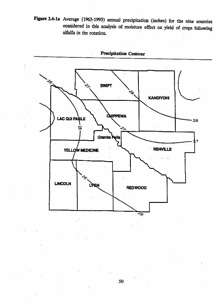
Figure 3.4-la Average {196~1993) annual precipitation (inches) for the nine counties considered in this analysis of moisture effect on yield of crops following alfalfa in the rotation.
Precipitation Contour
SWIFT
KANDIYOHI
28
7
RENVILLE
LINCOLN REDWOOD
50
At the latitude of Granite Falls in Minnesota, average annual rainfall varies from 29 inches
in the east to 24 inches to the west (Figure 3.4-la and lb) and the corresponding mean
annual pan evaporation is from 36 inches in the east to 43 inches in the west (FJ.gUre 3.4-2).
Similarly, mean annual air temperatures decrease from 45 °Fin the east to 43 °F in the west
(Figure 3.4-3) and the corresponding Growing Degree Day (GOD) are 2600 °Fin the east
to 2300 °F in the west (Figure 3.4-4) (Baker and Crookston, 1991).
Figure 3.4-lb Normal annual total precipitation (inches).
3l r.,
F'JgUre 3.4-3 Annual normal temperature. 51
p· ... ----
42 -
Figme 3.4-2 Mean annual pan evaportation (inches)
based upon records available (1960-1917).
Figure 3.4-4 Average total GDD in hundreds (To= 50"F)
accumulated during the warm season crop
period (late spring through late fall).
The major soil associations in the area are shown on Figure 3.4-5. Most of soils are formed in sandy to clayey lacustrine sediments, in very thin to thick lacustrine sediments overlaying glacial till or lacustrine modified glacial till overlying glacial till, and in calcareous loamy glacial till. For detailed soil description see Appendix A Water holding capacities in a 6 foot soil profile in the area ranges from 3 to 13 inches. The combination of limited rainfall, high evaporation and lower soil water holding capacities are factors affecting the sustainability of alfalfa production in this area.
Figure 3.4-S Soil associations of the biomass shed (source: Minnesota Soil Survey Staff of the U.S. Department of Agriculture, Soil Conservation Service, Universtiy of Minnesota, Agricultural Experiment Station (October 1983 4-R-38340)). For soil water holding capacity infromation see Appendix A and for. detailed soil association description see Appendix B.
Soils Map of Biomass Shed
52
Soil Legend for Figure 3.4-5
SOIL LEGEND
02 Barnes-Flom-Buse
03 Wadenill Sunburg-Koronis
04 Canisteo-Ves-Normania
05 Forman-Aastad-Flom
06 Canisteo-Nicollet-Okoboji
-
53
Kranzburg-Vienna-Hidewood
Bearden-Mcintosh-Colvin
Burr-DuPage
Sinai-Fulda-Hattie
Spicer-Ves-Tara
Arveson-Marysland-Sverdrup
Biscay-Estherville-Hawick
Colalld-Storden-Swanlake

The water budget model developed in this study to predict corn and soybean yield with and
without alfalfa in the rotation is a capacity type of model. When the rain water percolating
to a given layer exceeds its water holding capacity, the excess water is percolated to the next
soil layer. Weather is the driving force for crop water use (evapotranspiration (ET)). Soil
provides water storage and is a limiting factor. When available soil water becomes less than
ET then ET is set equal to the available soilwater. H the soil available water becomes zero
then ET becomes zero also. The water holding capacity of a soil profile is a function of
crop rooting depth and is equal to the summation of the individual water holding capacity
of the all soil layers in the rooting depth. Runoff, snow catch, and improvements in soil
water holding capacity that directly result from alfalfa production are not included in this
model.
Water balance is calculated using the follow equation:
DS = P + dSW - ETa
where: DS p
dSW
swcont
dz
ETa
= soil water storage in crop rooting. zone (in)
= precipitation (in)
= contributic: of previous year's soil moisture
= dz*swcont
= previous year soil water content
= DSend/Zend
= rooting depth increment in a given day
= actual evapotranspiration (in)
DSend and Zend are DS and are a function of root depth at the end of
previous year.
DS and ETa are always positive
H DS > WHCRZ (the water holding capacity of the root zone)
then DR (deep drainage in inches) = DS-WHCRZ, and DS = WHCRZ
54
Evapotranspiration (ET) is calculated using the Jensen-Raise method:
ETa = ( (0.014*Tm)-0.37)*(RAD*0.000673)*Kcrop
where: ETa
Tm
RAD Kcrop
Oimate Input Data
= actual daily evapotranspiration (in)
= daily mean air temperature (°F)
= daily solar radiation
= crop water use coefficient
(different crops have different Kcrop values)
A thiny-one year (1963-1993) solar radiation data set from St. Paul, MN was combined with
air temperatures and precipitation data for the same period from a given location in each
of the nine counties.
Soil Input Data
Only major soils are considered in the simulations. Major soils in this study are defined as
the soils which occupy more than 2.5% of the total county area. This resulted in less than
1~ soib per county. Soils comidered in this analysis by each county are listed in Table B-1
in Appendix B. The soil's input included the soil water holding capacity and the depth of
each la~·er. A total of three layers are considered. Water holding capacities by soil layer
are uk.en from Soil Survey data for each of the nine counties. It is assumed that soils below
the la...\t layer reported in the soil survey have the same characteristics as the last layer. Also,
we M-\umed that soil in each layer is homogeneous. It is also assumed that root restricting
facto~ such as impermeable layers and shallow ground water tables do not exist in these
soils. The soil water is recharged and consumed starting with the top layer. Any water
retained in the soil profile in the previous year is evenly distributed in the soil profile before
the next year's simulation, but the water content of each soil layer is not allowed to exceed
the water holding capacity.
55
Crop Input Data
Each year, com is assumed to be planted on May 1 and assumed matured when GDD
reached 2254°F or when the minimum air temperature was lower than 28°F. The
development of com and the corresponding Kcrop values are based on the GDD. Each year,
soybeans were also assumed to be planted on May 1. As stated earlier, it was assumed that
the growth of soybeans was related to day length and not based on GDD. Therefore, the
Kcrop value for soybean depended upon the calendar day and was thus the same for every
year. Kcrop values of com varied from year to year. The values of Kcrops for both com and
soybeans were taken from Seeley and Spoden (1982).
The growth of alfalfa is closely related to GDD, however, alfalfa can grow at lower
temperatures in early spring and at higher temperatures during the rest of the season.
Therefore, two base~temperature GDD values are used. The base temperature in spring is
set at 36°F and the base temperature for the remainder of the growing season is set at 5Q°F
(Sharratt et al. 1987). The number of alfalfa cuttings has a large impact on alfalfa yield and
com yield in the following year. All three crops die or become dormant when daily
minimum air temperature is 28°F.
Crop Yield Prediction:
The model for predicting crop yield is based on the growing season ETa and utilizes the
foll~wing equations:
Com
Soybean
Alfalfa
Y = -5840 + 890 *ETa (Morey et al. 1980)
Y = -1654 + 132 *ETa (Stegman 1989)
Y = - 833 + 159 *ETa (Bauder et al. 1978)
56
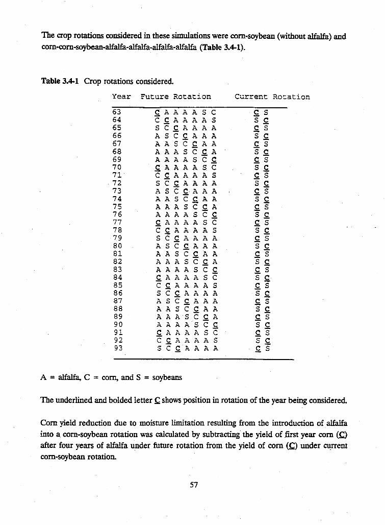
The crop rotations considered in these simulations were com-soybean (without alfalfa) and com-com-soybean-alfalfa-alfalfa-alfalfa-alfalfa (Table 3.4-1 ).
Table 3.4-1 Crop rotations considered.
Year Future Rotation
63 £. A A A A S C 64 C £. A A A A S 65 S C C A A A A 66 A S C C A A A 67 A A S C C A A 68 A A A S C C A 69 A A A A S C C 70 £. A A A A S C 71 C C A A A A S
· 72 S C £. A A A A 73 AS C C·A A A 74 A A S C £.A A 75 A A A S C C A 76 A A A A S C £. 77 C A A A A S C 78 C C A A A A S 79 S C C A A A A 80 A S C C A A A 81 A A S C C A A 82 A A A S C C A 83 A A A A S C £. 84 £. A A A A S C 85 C C A A A A S 86 S C C A A A A 87 A S C C A A A 88 A A S C C A A 89 A A A S C C A 90 A A A A'S C C 91 C A A A A S C 92 C C A A A A S 93 S C C A A A A
A = alfalfa, C = corn, and S = soybeans
Current Rotation
£. s s c £. s s c c s s c c s s c c s s £. c s s c c s s £. c s s c c s s £. c s s c c s s c c s s c £. s s c c s s c c s s c c s
The underlined and bolded letter C shows position in rotation of the year being considered.
Com yield reduction due to moisture limitation resulting from the introduction of alfalfa into a com-soybean rotation was calculated by subtracting the yield of .first year com (~) after four years of alfalfa under future rotation from the yield of com (~) under ~ent com-soybean rotation.
57
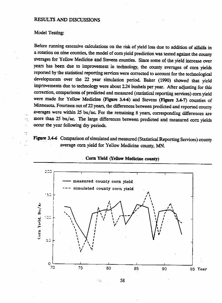
RESULTS AND DISCUSSIONS
Model Testing:
Before mnning extensive calculations on the risk of yield loss due to addition of alfalfa in a rotation on nine counties, the model of com yield prediction was tested against the county averages for Yellow Medicine and Stevens counties. Since some of the yield increase over years has been due to improvement in technology, the county averages of com yields reported by the statistical reporting services were corrected to account for the technological developments over the 22 year simulation period. Baker (1990) showed that yield improvements due to technology were about 224 bushels per year. After adjusting for this correctio~ comparisons of predicted and measured (statistical reporting services) com yield were made for Yellow Medicine (Figure 3.4-6) and Stevens (Figure 3.4-7) counties of Minnesota. Fourteen out of 22 years, the differences between predicted and reported county averages were within 25 bu/ac. For the remaining 8 years, corresponding differences are more than 25 bu/ac. The large differences between predicted and measured com yields occur the year following city periods.
Figure 3.4-6 Comparison of simulated and measured (Statistical Reporting Services) county average com yield for Yellow Medicine county, MN.
Com Yield (Yellow Medicine county)
- measured county corn yield
simulated county corn yield
0 '--~~~~---~~~~......._~~~~-'-~~~~ ....... ~~~~--' 70 75 80 85 90 95 Year
·;,; 58
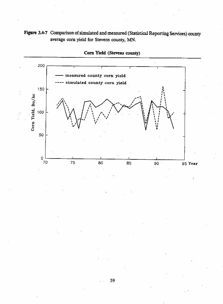
FJ.gUre 3.4-7 Comparison of simulated and measured (Statistical Reporting Services) county average com yield for Stevens county, MN.
Com Yield (Stevens county)
-- measured county corn yield
---- simulated county corn yield
150 0 < '-..
= il:I
~ 1.00 -Cl ... >-= i.. 0
C.)
50
0 .__ ________ __. __________ __._ __________ __.. __________ _._ __________ _. 70 75 80 85 90 95 Year
59
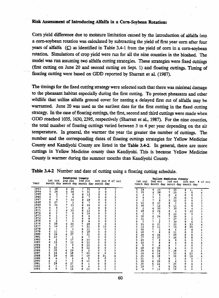
Risk Assessment of Introducing Alfalfa in a Com-Soybean Rotation:
Com yield difference due to moisture limitation caused by the introduction of alfalfa into a com-soybean rotation was calculated by subtracting the yield of first year com after four years of alfalfa ( C) as identified in Table 3.4-1 from the yield of com in a com-soybean rotation. Simulations of crop yield were run for all the nine counties in the bioshed The model was run assuming two alfalfa cutting strategies. These strategies were fixed cuttings (first cutting on June 20 and second cutting on Sept. 1) and floating cuttings. Timing of floating cutting were based on GDD reported by Sharratt et al. (1987).
The timings for the fixed cutting strategy were selected such that there was minimal damage to the pheasant habitat especially during the first cutting. To protect pheasants and other wildlife that utilize alfalfa ground cover for nesting a delayed first cut of alfalfa may be warranted. June 20 was used as the earliest date for the first cutting in the fixed cutting strategy. In the case of floating cuttings, the first, second and third cuttings were made when GDD reached 1035, 1630, 2395, respectively (Sharratt et al., 1987). For the nine counties, the total number of floating cuttings varied between 3 to 4 per year depending on the air temperature. In general, the warmer the year the greater the number of cuttings. The number and the corresponding dates of floating cuttings strategies for Yellow Medicine County and Kandiyohi· County are listed in the Table 3.4-2~ In general, there are more cuttings in Yellow Medicine county than Kandiyohi. This is because Yellow Medicine County is warmer during the summer months than Kandiyohi County.
Table 3.4-2 Number and date of cutting using a floating cutting schedule. hzldiyobi County Yel.l.ow Hedic:iDe C01mty
lst cut 2nd cut 3rd cut 4th cut I of cut 1st cut 2nd cut 3rd cut 4th cut ~ of cut Year month day month day month day month day month day month day month day month day
1963 5 28 6 29 7 31 0 0 3 s 24 6 24 7 24 8 31 4 1964 5 26 6 30 7 31 0 0 3 5 25 6 28 7 25 9 5 4 1965 6 5 7 8 8 13 0 0 3 6 2 7 5 8 6 0 0 3 1966 6 7 7 6 8 7 0 0 3 6 4 7 3 7 30 0 0 3 1967 6 6 7 14 8 18 0 0 3 6 2 7 8 8 12 0 0 3 1968 5 27 7 3 8 7 0 0 3 5 22 6 27 8 2 0 0 3 1969 5 31 7 13 8 16 0 0 3 s 30 7 12 8 11 0 0 3 1970 6 4 7 2 8 4 0 0 3 6 2 6 30 7 30 9 4 4 1971 6 2 6 30 8 13 0 0 3 5 29 6 26 8 4 9 10 4 1972 6 2 7 8 8 16 0 0 3 6 2 7 7 8 12 0 0 3 1973 6 1 7 2 8 6 0 0 3 5 30 6 26 7 30 9 l 4 1974 6 5 7 6 8 8 0 0 3 5 31 7 l 7 27 0 0 3 1975 6 5 7 5 8 6 0 0 3 6 3 7 2 7 30 9 6 4 1976 5 25 6 24 7 28 9 6 4 5 21 6 21 7 22 8 23 4 1977 5 16 6 17 7 21 9 10 4 5 14 6 11 7 15 8 25 4 1978 6 l 7 3 8 11 0 0 3 5 30 7 2 8 6 9 8 4 1979 6 11 7 11 8 19 0 0 3 6 10 7 8 8 11 0 0 3 1980 5 26 6 27 7 31 0 0 3 5 26 6 26 7 29 9 8 4 1981 5 23 7 1 8 7 0 0 3 5 17 6 25 7 26 9 8 4 1982 6 2 7 17 8 23 0 0 3 5 29 7 9 8 9 0 0 3 1983 6 12 7 12 8 13 0 0 3 6 10 7 8 8 4 9 6 4 1984 6 5 7 9 8 13 0 0 3 6 5 7 8 8 7 0 0 3 1985 5 22 7 4 8 12 0 0 3 5 19 6 30 8 4 0 0 3 1986 5 30 6 29 8 2 0 0 3 5 29 6 26 7 . 28 0 0 3 1987 5 16 6 18 7 23 9 6 4 5 14 6 16 7 20 8 23 4 1988 5 26 6 20 7 19 8 21 4 5 25 6 18 7 16 8 16 4 1989 6 4 7 5 8 5 0 0 3 5 31 7 2 8 l 0 0 3 1990 6 2 7 3 8 13 0 0 3 5 30 6 29 8 4 0 0 3 1991 5 29 6 27 8 1 0 0 3 5 25 6 22 7 25 9 4 4 1992 6 3 7 12 9 4 0 0 3 5 29 7 9 8 24 0 0 3 1993 6 8 7 16 8 23 0 0 3 6 6 7 13 8 19 0 0 3
60
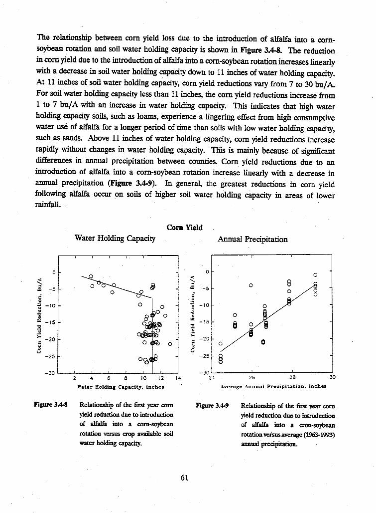
The relationship between com yield loss due to the introduction of alfalfa into a comsoybean rotation and soil water holding capacity is shown in Figure 3.4-8. The reduction in com yield due to the introduction of alfalfa into a com-soybean rotation increases linearly with a decrease in soil water holding capacity down to 11 inches of water holding capacity. At 11 inches of soil water holding capacity, com yield reductions vary from 7 to 30 bu/ A For soil water holding capacity less than 11 inches, the com yield reductions increase from 1 to 7 bu/ A with an increase in water holding capacity. This indicates that high water holding capacity soils, such as loams, experience a lingering effect from high consumptive water use of alfalfa for a longer period of time than soils with low water holding capacity, such as sands. Above 11 inches of water holding capacity, com yield reductions increase rapidly without changes in water holding capacity. "TliiS is mainly because of significant differences in annual precipitation between counties. Com yield reductions due to an introduction of alfalfa into a com-soybean rotation increase linearly with a decrease in annual precipitation (Figure 3.4-9). In general, the greatest reductions in com yield followii:tg. alfalfa occur on soils of higher . soil water holding capacity in areas of lower rainfall.
Com Yield
< ........
0
&l -5
i:: Q
:g -10 = -= «> = -15 -= o;
>= -20 i:: .. Q
t.)
-25
Water Holding Capacity
0
2 4 6 8 10 12 14
Water Holding Capacity, inches
F°JgUl'e 3.4-8 Relationship of the first year com
yield reduction due to introduction of alfalfa into a com-soybean
rotation versus aop available soil water holding capacity.
< ........ = g:i
a ·.2 _.
Q
= ~ «> = ~ o; >= i:: .. Q
t.)
61
Annual Precipitation
0 0
8 0 -5 0
-10
0 -15 8 0
-20 0 0
-25 § -30
24 26 28 30
Average Annual Precipitation, inches
Figure 3.4-9 Relationship of the first year com yield reduction due to introduction of alfalfa into a aon-soybean rotation versus average (1963-1993) annual· precipitation.
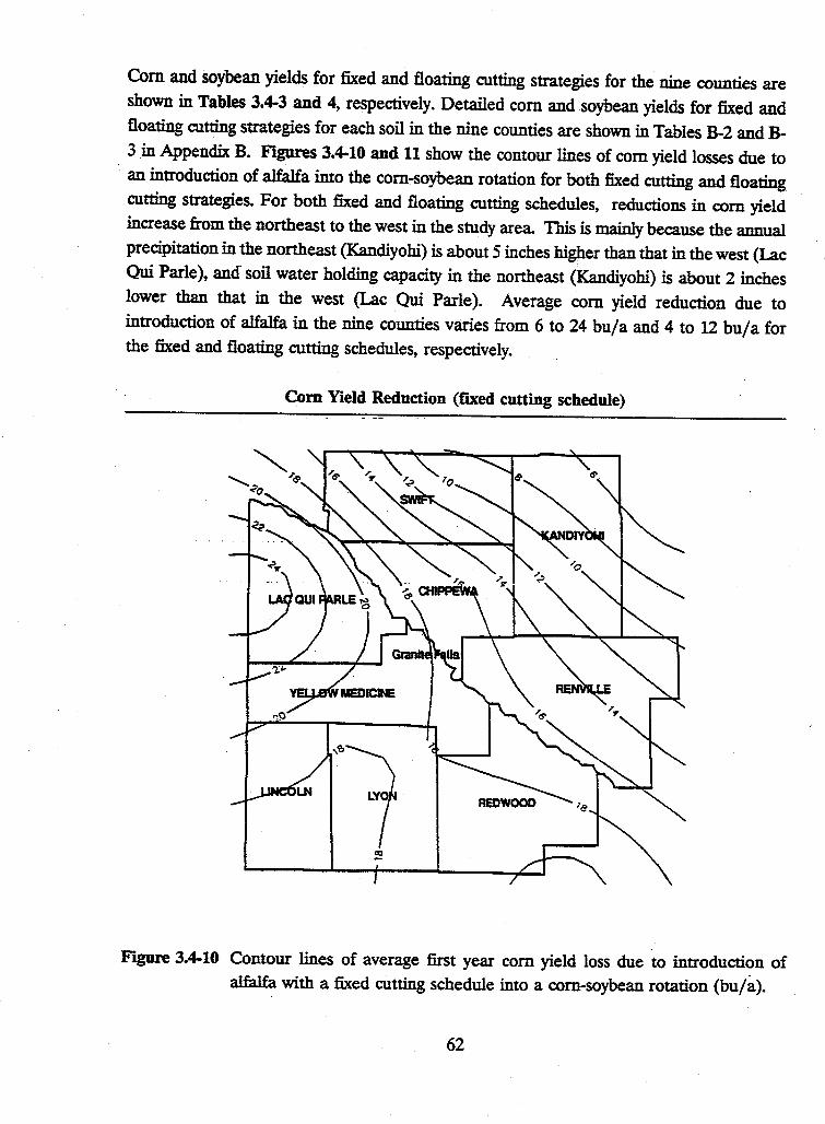
Com and soybean yields for fixed and floating cutting strategies for the nine counties are shown in Tables 3.4-3 and 4, respectively. Detailed com and soybean yields for fixed and floating cutting strategies for each soil in the nine counties are shown in Tables B-2 and B-3 in Appendix B. Figures 3.4-10 and 11 show the contour lines of com yield losses due to
· an introduction of alfalfa into the com-soybean rotation for both fixed cutting and floating cutting strategies. For both fixed and floating cutting schedules, reductions in com yield increase from the northeast to the west in the study area. This is mainly because the annual precipitation in the northeast (Kandiyohi) is about 5 inches higher than that in the west (Lac Qui Parle), and· soil water holding capacity in the northeast (Kandiyohi) is about 2 inches lower than that in the west (Lac Qui Parle). Average com yield reduction due to introduction of alfalfa in the nine counties varies from 6 to 24 bu/a and 4 to 12 bu/a for the fixed and floating cutting schedules, respectively.
Com Yield Reduction (fixed cutting schedule)
Figure 3.4-10 Contour lines of average first year com yield loss due to introduction of alfalfa with a fixed cutting schedule into a com-soybean rotation (bu/a).
62
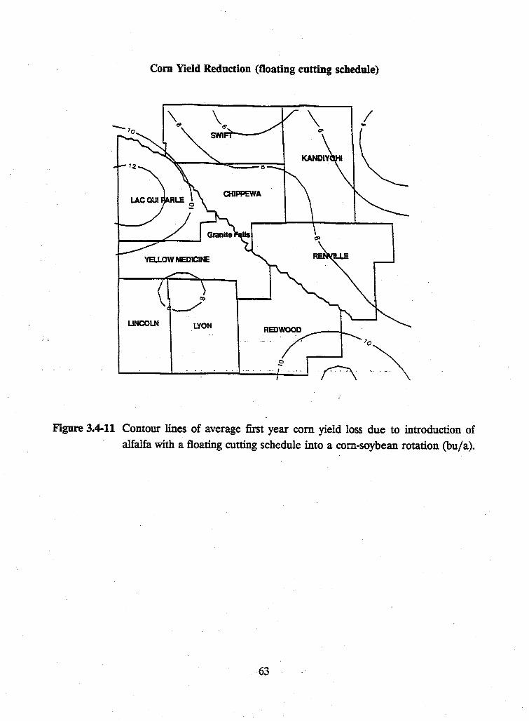
Com Yield Reduction (floating cutting schedule)
\ I ...
LINCOLN LYON REDWOOD
Figure 3.4-11 Contour lines of average first year com yield loss due to introduction of alfalfa with a floating cutting schedule into a com-soybean rotation (bu/a).
63
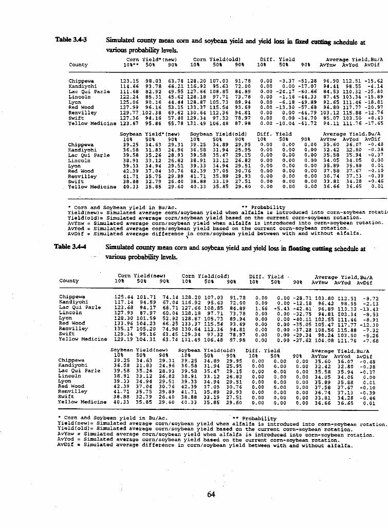
Table 3.4-3 Simulated county mean com and soybean yield and yield loss in fixed cutting schedule at various probability levels.
County Corn Yield'*(new)
10%** 50% 90% Corn Yield(old)
10% 50% 90% Diff. Yield Average Yield.Bu/A
10% 50% 90% AvYnw AvYod AvDif
Chippewa 123.15 98.03 63.78 128.20 107.03 9l. 78 0.00 -3.37 -51.28 96.90 112.51 -15.62 Kandiyohi 114.66 93.78 66.21 116.92 95.63 72.00 0.00 0.00 -17.07 94.41 98.55 -4.14 Lac Qui Parle 111.68 82.92 49.55 127.66 108.85 84.89 0.00 -24.17 -60.66 84.53 110.32 -25.80 Lincoln 122.24 85.31 45.62 128.18 97.71 73. 78 0.00 -1.16 -44.33 87.45 103.34 -15.89 Lyon 125.06 90.16 44.44 128.87 105.73 89.94 0.00 -6.18 -49.89 92.65 lll.46 -18.81 Red Wood 127.99 96.16 53 .15 133."37 115.54 93.69 0.00 -13.30 -57.68 96.80 117.77 -20.97 Renvilley 129.77 102.38 69.62 130.64 112.36 94.81 0.00 o.oo -44. 79 103.12 115.88 -12.76 Swift 127.36 94.16 57.40 129.34 97.32 78.97 0.00 0.00 -34.70 95.07 103.50 -8.43 Yellow Medicine 123. 67 95.86 55.78 131. 49 106.48 87.98 0.00 -10.04 -41.72 94.11 111.76 -17.65
Soybean Yield*(new) Soybean Yield(old) Diff. Yield Average Yield,Bu/A 10% 50% 90% 10% 50% 90% 10% 50% 90% AvYnw AvYod AvDif
Chippewa 39.25 34.63 29.31 39.25 34.89 29.95 0.00 0.00 0.00 35.60 36. 07 -0.48 Kandiyohi 36.58 31.83 24.96 36.58 31.94 25.95 0.00 0.00 0.00 32.42 3.2. 8.0 -0.38 Lac Qui Parle 39.58 35.26 28.93 39.58 35.47 29.l-S 0.00 0.00 o.oo 35.58 35.94 -0.37 Lincoln 38.91 33.12 26.82 38.91 33.12 26.82 0.00 o.oo o.oo 34.05 34.05 0.00 Lyon 39.33 34.94 29.51 39.33 34.94 29.51 0.00 0.00 0.00 35.89 35.88 0.01 Red Wood 42.39 37.04 30. 76 42.39 37.05 30.76 0.00 0.00 0.00 37.58 37.67 -0.10 Renvilley 41. 7l 35. 75 29.89 41. 7l 35.89 29.93 0.00 0.00 o.oo 36.74 37.13 -0.39 Swift 38.88 32.79 26.40 38.88 33.19 27 .51 0.00 0.00 0.00 33.81 34.28 -0.46 Yellow Medicine 40.33 35.85 29.60 40.33 35.85 29.60 0.00 0.00 0.00 36.66 36.65 0.01
** Probability * Corn and Soybean yield in Bu/Ac. Yield(new)= Simulated average com/soybean yield when alfalfa is introduced into corn-soybean rotatic Yield(oldl= Simulated average corn/soybean yield based on the current corn-soybean rotation. . Av'inw = Simulated average corn/soybean yield when alfalfa is introduced into corn-soybean rotation.
Simulated average corn/soybean yield based on the current corn-soybean rotation. AvYod AvDif = Simulated average difference in corn/soybean yield between with and without alfalfa.
\
Table 3.4-4 Simulated county mean com and soybean yield and yield loss in floating cutting schedule at various probability levels.
Corn Yield(new) Corn Yield(oldl Diff.· Yield Average Yield.Bu/A County 10% 50% 90% 10% 50% 90% 10% 50% 90% AvYnw AvYod AvDif
Chippewa 125.44 101. 7l 74.14 128.20 107. 03 91. 78 0.00 0.00 -28.71 103.80 112.Sl -8.72 Kandiyohi 117.14 94.59 67. 04 116.92 95.63 72.00 0.00 0.00 -12.18 96.42 98.55 -2.13 Lac Qui Parle 123.68 94.17 68.71 127.66 108.85 84.89 1. 66 -5.43 -42.81 96.89 110.32 -13.43 Lincoln 127.93 87.97 60.04 128.18 97. 71 73.78 0.00 0.00 -32.75 94.81 !03.34 -8.53 Lyon 128.30 101. 59 52.92 128.87 105.73 89.94 0.00 0.00 -40.11 102.55 111.46 -8.91 Red Wood 133.96 104.23 66.25 133.37 115.54 93.69 0.00 o.oo -35.05 105.47 117.77 -12.30 Renvilley 135.17 105.20 74.98 130.64 112.36 94.81 0.00 0.00 -37.28 108.56 115.88 -7.32 Swift 129.34 95.16 63.45 129.34 97.32 78.97 o.oo o.oo -29.34 98.24 103.50 -5.26 Yellow Medicine 129.19 ·104.31 63.74 131. 49 106.48 87.98 0.00 0.00 -27.62 104.08 111. 76 -7.68
Soybean Yield(new) Soybean Yield(old) Diff. Yield Average Yield,Bu/A 10% 50% 90% 10% 50% 90% 10% 50% 90% AvYnw AvYod AvDif
Chippewa 39.25 34.63 29.31 39.25 34.89 29.95 o.oo 0.00 0.00 35.60 36.07 -0.48 Kandiyohi 36.58 31.83 24.96 36.58 31.94 25.95 0.00 o.oo 0.00 32.42 32.80 -0.38 Lac Qui Parle 39.58 35.26 28.93 39.58 35.47 29.15 . 0. 00 0.00 0.00 35.58 35.94 -0.37 Lincoln 38.91 33.12 26.82 38.91 33.12 26.82 0.00 0.00 0.00 34.05 34.05 0.00 Lyon 39.33 34.94 29.51 39.33 34.94 29.51 0.00 o.oo 0.00 35.89 35.88 O.Ol Red Wood 42.39 37.04 30.76 42.39 37.05 30. 76 0.00 0.00 o.oo 37.58 37 .67 -0.10 Renvilley 41. 71 35.75 29.89 41. 71 35.89 29.93 0.00 o.oo 0.00 36.74 37 .13 -0.39 Swift 38.88 32.79 26.40 38.88 33.19 27.51 0.00 o.oo 0.00 33.81 34.28 -0.46 Yellow Medicine 40.33 35.85 29.60 40.33 35.85 29.60 0.00 o.oo 0.00 36.66 36.65 0.01
* Corn and Soybean yield in Bu/Ac. ** Probability Yield(new)= Simulated average corn/soybean yield when alfalfa is introduced into corn-soybean rotation. Yield(old)= Simulated average corn/soybean yield based on the current corn-soybean rotation. AvYnw Simulated average corn/soybean yield when alfalfa is introduced into corn-soybean rotation. AvYod Simulated average corn/soybean yield based on the current corn-soybean rotation. · AvDif = Simulated average difference in corn/soybean yield between with and without alfalfa.
64
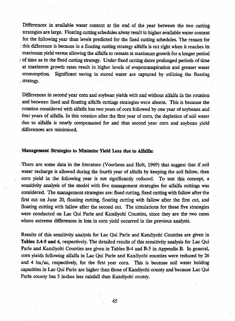
Differences in available water content at the end of the year between the two cutting strategies are large. Floating cutting schedules alway result in higher available water content for the following year than levels predicted for the fixed cutting schedules. The reason for
: this difference is because in a floating cutting strategy alfalfa is cut right when it reaches its -maximum yield versus allowing the alfalfa to remain at maximum growth for a longer period
: of time as in the fixed cutting strategy. Under fixed cutting dates prolonged periods of time at maximum growth rates result in higher levels of evapotranspiration and greater water consumption. Significant saving in stored water are capiw-ed by utilizing the floating
~strategy.
Differences in second year com and soybean yields with and without alfalfa in the rotation and between fixed and floating alfalfa cuttings strategies were absent. This is because the rotation considered with alfalfa has two years of com followed by one year of soybeans and four years of alfalfa In this rotatjon after the first year of corn, the depletion of soil water due to alfalfa is nearly compensated for and thus second year com and soybean yield differences are minimized.
. Management Strategies to Minimize Yield Loss due to Alfalfa:
There-are some data in the literature (Voorhees and Holt, 1969) that suggest that if soil water recharge is allowed during the fourth year of alfalfa by keeping the soil fallow, then com yield in the following year is not significantly reduced. To test this concept, a sensitivity analysis of the model with five management strategies for alfalfa cuttings was considered. The management strategies are: fixed cutting, fixed cutting with fallow after the first cut on June 20, floating cutting, floating cutting with fallow after the first cut, and floating cutting with fallow after the second cut. The simulations for these five strategies were conducted on Lac Qui Parle and Kandiyohi Counties, since they are the two cases where extreme differences in loss in com yield occurred in the previous analysis.
Results of this sensitivity analysis for Lac Qui Parle and Kandiyohi Counties are given in Tables 3.4-5 and 6, respectively. The detailed results of this sensitivity analysis for Lac Qui Parle and Kandiyohi Counties are given in Tables B-4 and B-5 in Appendix B. In general, com yields following alfalfa in Lac Qui Parle and Kandiyohi counties were reduced by 26 and 4 bu/ac, respectively, for the first year com This is because soil water holding capacities in Lac Qui Parle are higher than those of Kandiyohi county and because Lac Qui Parle county has 5 inches less rainfall than Kandiyohi county.
65
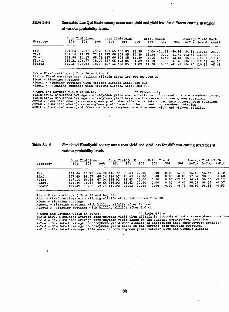
Table 3.4-5 Simulated Lac Qui Parle county mean com yield and yield loss for different cutting strategies at various probability levels.
Corn Yield(new) Corn Yield(old) Diff. Yield Average Yield, Bu/A Strategy 10% 50% 90% 10% 50% 90% 10% 50% 90% AvYnw AvYod AvOif
Fix lll.84 82.92 49.23 127.66 108.85 84.89 0.00 -24.13 -60.95 84.56 110.32 -25.76 Fixl 132.16 99.27 77.18 127.66 108.85 84.89 ll.30 0.00 -41.49 102.55 ll0.32 -7.78 Float 123.68 94.17 68.71 127.66 108.85 84.89 1.66 -5.43 -42.81 96.89 110.32 -13.43 Floatl 132.21 104.77 78.00 127. 66 108.85 84.89 ll.30 0.00 -41.49 106.05 110.32 -4.27 Float2 132.21 103.94 78.00 127.66 108.85 84.89 ll.30 0.00 -41.49 104.90 110.32 -5.43
Fix = Fixed cuttings ( June 20 and Aug 31) Fixl = Fixed cuttings with killing alfalfa after 1st cut on June 20 Float = Floating cuttings Floatl = Floating cuttings with killing alfalfa after lst cut Flaot2 = Floating cuttings with killing alfalfa after 2nd cut
* Corn and Soybean yield in Bu/Ac. ** Probability Yield(newJ= Simulated average corn/soybean yield when alfalfa is introduced into corn-soybean rotation. Yield(oldl= Simulated average corn/soybean yield based on the current corn-soybean rotation. AvYnw Simulated average corn/soybean yield when alfalfa is introduced into corn-soybean rotation. AvYod Simulated average com/soybean yield based on the current corn-soybean rotation. AvDif = Simulated average difference in com/soybean yield between with and without alfalfa.
Table 3.4-6 Simulated Kandiyohi county mean com yield and yield loss for different cutting strategies at various probability levels.
Corn Yield(new) Corn Yield(old) Oiff. Yield Average Yield, Bu/A Strategy 10% 50% 90% 10% 50% 90% 10%
Fix 114.66 93. 78 66.28 116.92 95.63 72.00 0.00 Fixl 117.49 96.57 68.34 116.92 95.63 72.00 0.00 Float 117 .14 94.59 67 .04 116.92 95.63 72.00 0.00 Floatl 117 .49 96.57 69.66 116.92 95.63 72.00 0.00 Float2 117 .49 95.88 69.34 116.92 95.63 72.00 0.00
·Fix= Fixed cuttings (June 20 and Aug 31) Fixl = Fixed cuttings with killing alfalfa after 1st cut on June 20 Float = Floating cuttings · Floatl = Floating cuttings with killing alfalfa after lst cut Flaot2 = Floating cuttings with killing alfalfa after 2nd cut
50% 90% AvYnw AvYod AvOif
0.00 -16.99 94.45 98.55 -4.10 0.00 -0.08 97 .87 98.55 -0.68 0.00 -12.18 96.42 98.55 -2.13 0.00 o.oo 98.18 98.55 -0.37 0.00 -0.71 98.02 98.55 -0.53
* Corn and Soybean yield in Bu/Ac. *'" l?robal:>il~ty . . Yield(new)= Simulated average corn/soybean yield when alfalfa is introduced into corn-so~bean rotation Yield(oldl= Simulated average corn/soybean yield based on the current corn-soybean rotation. AvYnw = Simulated average corn/soybean yield when alfalfa is introduced into corn-so~bean rotation. AvYod = Simulated average corn/soybean yield based on the current corn-soybean rotation. AvOif = Simulated average difference in corn/soybean yield between with and without alfalfa.
66
In Lac Qui Parle County, killing alfalfa after the first cut in the fourth year of alfalfa could
reduce the com yield loss from 25 to 8 and from 13 to 4 bu/a for fixed and floating cutting
-- strategies, respectively (Table 3.4-5 and 6). This is because the high water holding capacity
soils of this region recharge during the late summer and fall by rain, and this water becomes
very important for the following year's corn. The same situation is true for Kandiyohi
county; however, the degree of this effect is less since Kandiyohi has higher precipitation
and less soil water holding capacity. There was no difference in soybean yield between the · five strategies.
SUMMARY:
Fourteen out of 22 years, the differences between predicted and reported county averages
are within 23%, The large differences between predicted and measured com yield occur
in the year following dry periods.
The reduction in com yield due to introduction of alfalfa into a com-soybean rotation
increases linearly with an increase in soil water holding capacity up to 11 inches of water
holding capacity, and with a decrease in annual precipitation. In general, the higher soil
water holding capacity and lower reainfall, the greater -is the reduction in com yield
following alfalfa. ·· ··-···""-· ·· ·· · ·· -- - ···· · · · -· - -· -·- ·· ·
In this paper, we outline floating cutting schedules as other management options that may
facilitate alfalfa introduction in a com-soybean rotation without significantly reducing
subsequent com yield. Average first year com yield reduction due to introduction of alfalfa
in the nine counties varies from 6 to 24 bu/a and 4 to 12 bu/a for the fixed and floating
cutting schedules, respectively. The differences in second year com and soybean yields with
and without alfalfa in the rotation or between the fixed and floating cutting strategies were
absent.
If the soil is allowed to recharge by leaving it fallow during the fourth year of alfalfa, the
com yield in the following year is not reduced significantly. In Lac Qui Parle, the county
with the greatest com yield reduction when alfalfa is introduced, killing alfalfa after the first
cut in the fourth year of alfalfa could reduce the com yield loss from 25 to 8 and from 13
to 4 bu/a for fixed and floating cutting strategies, respectively.
67
FUTURE RESEARCH
This simulation study points out the following areas where additional research is needed:
1. Since simulation models are based on data bases from a given location under a given
climate, it is always prudent to validate the model before assuming that model predictions
are accurate and applicable for a given scenario. Therefore, the modelled predictions of
corn, soybeans an~ alfalfa yields in this study should be validated by conducting field experiments.
2. Calculations of alfalfa yield in this study are based on the relationship between dry
matter production and seasonal consumptive use. The data base used to develop these
relationships had seasonal consumptive values which were measured for three cutting schedules. Therefore for cutting schedules other than three cuttings, additional data bases and dry matter production functions are needed to test the effects of floating cutting
schedules on alfalfa yield.
68
CHAPTER 4 PRODUCT10N ECONOMICS
4.1 Production Regions
. Douglas G. Tiffany1, and John F. Moncrief2 1Agricultural and Applied Economics, and
2Soil Science,
University of Minnesota
The biomass production area is described by a 50 mile radius around the city of Granite
Falls, Minnesota. Fields of com and soybeans dominate the agricultural landscape in this . region. Other crops in the ·biomass shed include sugarbeets, oats, ciry edible beans, sweet
corn, peas, and wheat.
The geological history of this area resulted in the development of many different individual soil types. Climate and soil interactions affect crop yields. Additionally, drainage practices,
- . - - - --the production of high value crops, and other factors result in different land values (rents)
throughout the biomass shed. Thirteen regions within the shed have been identified and
characterized with respect to their inherent productivity and to existing market levels of cash rents.
Geology and Soils
The biomass shed is located in the upper Minnesota River Basin. The soils of this area
developed in glacial material (Soil Association Map, lliustration 3.4-1). During the last
glacier (Wisconsin) Glacial Lake Agassiz occupied most of Manitoba, the western half of Ontario, and the northern third of Minnesota. This was the largest fresh water lake known.
A finger of this lake projected south roughly on the North Dakota-Minnesota border and then southeast along the present day MN River. This lake drained to the south by Glacial
River Warren into the Mississippi watershed. As the ice receded and the lake level became lower it reached a point where the lake no longer drained south but north by the Red River.
The Minnesota Rive~ still drained to the southeast and into the Mississippi Watershed.
69
Many of the soils of the bioshed have developed in the calcareous lake sediments from Glacial Lake Agassiz. The soil textures generally range from loam to clay with most classified as clay loam. The landscape is somewhat flat to gently rolling with islands of glacial till. This results in poor surface and internal soil drainage.
As the Des Moines Lobe (glaciated most of Minnesota and reached as far south as Des Moines, Iowa) of the Wisconsin Glacier retreated, the meltwaters deposited sandy material in putwash plains in Kandiyohi and Pope Counties. There are also soils which developed in calcareous sandy material from the shoreline beaches of Glacial Lake Agassiz as well as outwasb plains in Chippewa, Lac Qui Parle, and Big Stone Counties. These soils range in drainage from poor to excessively well.
The rest of the soils in the bioshed developed in calcareous glacial till. They have somewhat poor internal drainage _and predominately c~y t9am_1~xture. The l®,dscapes where these soils formed are steeper than the lake basinS or outwash plains~
Implications for Crop Production
Water storage and internal drainage of soils within the shed vary widely (Chapter 3.4). Soils ~ith somewhat poor internal drainage require tile fil:ainage- for optimal crop-production. Introducing alfalfa into the rotation tends to enhance soil drainage and aeration. Cementing agents (such as polysaccharides and gels) are introduced directly from alfalfa root exudates
. ~·hich also stimulate microbial activity. The combination of root exudates and microbial acti,ity enhances soil aggregation (binding together of individual soil particles which then act~ a larger particle). The effect is to reduce soil bulk density, increase pore space and aeration. and create macropores that provide for better water flow. The absence of tillage on established alfalfa allows soil structure formation, increases soil organic matter, generally enhancing physical and biological soil properties.
Soib dC\·cloped from calcareous parent material in relatively low rainfall areas do not require liming (pH adjustment) to achieve optimal alfalfa production. Soils with a pH below 7 result in reduced growth rates of alfalfa Soils in the proposed biomass shed would not require lime for maximal alfalfa production. Soils in this part of the state test relatively low in phosporus and high in potassium. Phosphorus application may be needed to achieve maximum alfalfa yields.
70
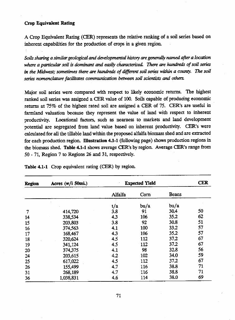
Crop Equivalent Rating
A Crop Equivalent Rating (CER) represents the relative ranking of a soil series based on
inherent· capabilities for the production of crops in a given region.
Soils sharing a similar geological and developmental history are generally named after a location
where a particular soil is dominant and easily characterized. There are hundreds of soil series
in the Midwest; sometimes there are hundreds of different soils~ within a county. The soil
series nomenclature facilitates communication between soil scientists and others.
Major soil series were compared with respect to likely economic returns. The highest
ranked soil series was assigned a CER value of 100. Soils capable of producing economic
returns at 75% of the highest rated soil are assigned a CER of 75. CER's are useful in
farmland valuation because they represent the value of land with respect to inherent
productivity. Locational factors, such as nearness to markets and land development
potential are segregated from land value based on inherent productivity. CER's were
calculated for all the tillable land within the proposed alfalfa biomass shed and are extracted
for each production region. Illustration 4.1-1 (following page) shows production regions in
the biomass shed. Table 4.1-1 shows average CER's by region. Average CER's range from
50 - 71, Region 7 to Regions 26 and 31, respectively.
Table 4.1-1 Crop equivalent rating (CER) by region.
Region Acres (w/i SOmi.) Expected Yield
7 14 15 16 17 18 19 20 24 25 26 31 36
414,720 338,534 203,803 374,563 168,467 320,624 341,124 374,375 203,615 617,022 155,499 268,189
1,038,831
Alfalfa
t/a 3.8 43 3.8 4.1 43 4.5 4.5 4.1 4.2 4.5 4.7 4.7 4.6
71
Com
bu/a 91
106 92
100 106 112 112 98
102 112 116 116 114
Beans
bu/a 30.4 35.2 30.8 33.2 35.2 37.2 37.2 32.8 34.0 37.2 38.8 38.8 38.0
CER
50 62 51 57 57 67 67 56 59 67 71 71 69
mustration 4.1-1 Map of production regions within the biomass shed.
7 14 15 16 17 18 19
I I '-· -- -'- --·
U>IC£ -
lll'ATE
- /" -TH • .f t£llO TRC .
-···26····· -S!ElO• HCLl..1
woccs sr .• 'l>HS
LON£ ;RE; ;;cwuous.
~~ o/ .lf .., .. ~~ ....
COVRE.
• ii> .;,"' .s/: <J-~ ocrON w!W'<Oll .... <>· ,,_v.,~ ..... + _;,~~ ,~"'
~ F~UN ...,~-;p #<; QO&IUAF ;;: ... ~ '-" <S
·-
. ~</· I . __. __ _,. __ ..._ __________ .._ __ ~ - _;..,. -- -=- - _..: . . ---;---,--,-Region
Green Lake Benson-Lac Qui Parle Plain Appleton-Oontarf Sands Big Stone Moraine Marietta Lac Qui Parle Dawson
72
Region
20 Lake Shaokatan 24 Coteau Headwaters 25 Redwood-Cottonwood River Valley 26 Tracy 31 Morgan 36 Olivia Ytll Plain
Estimated Market Value
Estimated Market Value (EMV) is established for farmland for the purposes of property
tax allocation. County Assessors scrutinize all free market farmland transactions for the purpose of estimating market value. Values are assigned to each parcel of land consistent
with the~ quality of the land and market value. EMV's were extracted for each of the
production regions and averages were computed. Average EMV's for the regions are found in Table A.1-2.
Table 4.1-2 Estimated market value (EMV) by region.
Estimated Market Value
# Region CER EMV
7 Green Lake 50 913 14 Benson Lac. Plain 62 813 15 Appl-Oont. Sands 51 725 16 Big Stone Moraine 57 675 17 Marietta 62 788 18 Lac Qui Parle 67 975 19 Dawson 67 1025 20 Lake Shaokaton 56 600 24 Coteau Headwaters 59 613 25 Redwd-Cotwd R. Vals 67 1088 26 Tracy 71 1038 31 Morgan 71 1313 36 Olivia Till Plain 69 1213
73
Rental Returns
Land Rental values are the level of annual payments to landlords needed to recruit land for a particular economic activity. Rental levels reflect the market influences of supply and demand for land with respect to specific uses. For example, land rents in Lincoln County may have been increased as the result of federal incentives aimed at enrolling land in the Conservation Reserve Program (CRP). In Lincoln county, 23% of the tillable farmland ei;irolled in CRP at an average ann~al payment le:vel of $66.()Z_ pe:r ;i<;re.. Removal of land from production by enrolling in the CRP program increases competition for land available for rent. High returns per acre from sugar beet production and other specialty crop production have also raised rents in some areas of the biomass production area. Competitive rental values range from 47 - 91 dollars per acre, Region 20 to Region 31, respectively. Averages can be deceiving if they, alone, are used to characterize regions. The Olivia Till Plain, th~ largest region identjfied in .µµs -~~Qy, Pa$_ IJ~A~. $~~ r:@g~. _fygpi over $120 per acre (ideal sugar beet production acres) down to $70.00 per acre for an overall average rent of $89.16 per acre.
Rental levels were derived from data supplied by two sources. Estimated market values developed by County Assessors and from capitalization rates. !or groups of counties (rent/ estimated market value) by Lazarus, et al. (1993). Where production regions included portions of several counties with. different capitalization rates; a-weighted capitalization rate was developed based upon the proportion of land area from each county comprising the production region. By multiplying capitalization rate by EMV we calculate rental levels representing the weighted qualities of all lands within the production regions. Figure 4.1-3 shows calculated rental levels by region.
74
Table 4.1-3 Rental value by region.
Rental Values
# Region CER RENT
7 Green Lake 50 71.21 14 Benson Lac. Plain 62 65.53 15 Appl-Oont. Sands 51 60.18 16 Big Stone Moraine 57 58.05
17 Marietta 62 62.25
18 Lac Qui Parle 67 77.03
J,9_ _ - Paw.son 67_ 80.98
20 Lake Shaokaton 56 47.40
24 Coteau Headwaters 59 48.43
25 Redwd-Cotwd R. Vais 67 80.51
26 Tracy 71 82.00
31-. - .
Morgan 71 90.60
36 Olivia Till Plain 69 89.16
Conclusions
A number of factors govern the inherent productivity of soils in a given region. Soil
productivity combined with economic forces that affect demand for land resources determine
land value. Thirteen unique production regions have been described for the purpose of
developing pro forma budgets for alfalfa biomass production. Budgets represent a relative
advantage or disadvantage of an alfalfa biomass rotation versus a conventional com-soybean
rotation.
75
4.2 Pro Forma Budgets by Region
Douglas G. Tiffany and J.E. Fruin Agricultural and Applied Economics
University of Minnesota
Alfalfa Biomass Rotation compared. to a Traditional Com/Soybean Rotation
Pro forma budgets are a means to portray alternative _business plans. In the case of the proposed alfalfa biomass project based at Granite Falls, Minnesota, pro foona farm budgets were used to compare the net returns to farmers of rotations including alfalfa versus traditional com-soybean rotations. To make comparisons one must accurately and systematically portray all streams of revenue or value and identify all costs, whether explicit or latent. All activities such as tillage, planting, harvest, etc. needed to produce various crops must be orchestrated with their costs being assigned to the proper crop .year .. In the case of the "biomass" rotation, or DFSS (Dedicated Feed Stock Supply) the sequence AAAACCS was assumed, which stands for a seven year rotation with four years of alfalfa followed by corn, corn, and then soybeans after which the sequence repeats.
- Specific proformas were generated for each of ·the thirteen production regions (Chapter 4.1) to accurately portray each region's crop yield potential and cash rent environment. Pro forma net returns identify the production regions where the alfalfa biomass rotation will best · compete with the traditional com-soybean ·rotation. It should be emphasized that comparisons are between the multi-year rotations, not the individual crops. Net income to
. producers is expressed on an annualized basis for the two competing rotations with different durations. DFSS has a seven year cycle, while C-S has a two year cycle.
Analysis was also performed based strictly upon CER score, which reflects the inherent productivity of soils. CER's are an index developed for Minnesota soils that measures relative net income of soils based on typical rotations and crop mixes found on different soils. Exogenous changes, such as elimination of feed grain deficiency payments or dramatic yield increases in alfalfa yields (perhaps due to future alfalfa breeding) were modelled. Rents were assumed to be zero at all CER's in order to demonstrate how effects can vary for soils across the range of relevant productivities. In this fashion it is possible to determine the effects of exogenous changes on breakeven alfalfa prices, as well as how these effects relate to inherent productivity.
76
The following list characterizes groups of pro form.as:
1) Baseline production, 3 cut system at $60 /T. hay price and also the hay price necessary for DFSS returns to equal C-S returns for each production region. DFSS and C-S baseline net returns ($60/T., with deficiency payments) organized by CER as well as for hay prices of $70 and $80 per ton. .. . ..
2) Three cut, $60 /T. hay price with elimination of deficiency payments on corn necessary to make DFSS returns equal C-S returns, organized by production region.
3) Plus 20% change in yields of alfalfa and necessary hay prices for DFSS to equal C-S net incomes, organized by CER
4) Plus and minus 20% changes in net incomes from C-S and the resulting hay prices _ _ _ necessary for DFSS to equal C-S net incomes, organized by CER
5) Two, three, and four cut system hay prices necessary for DFSS to equal levels of net income produced by C-S, organized by CER
. §) Ne~essary leaf meal prices with $30 stem prices for DFSS to equal C-S net incomes for 2,3,and 4 cut systems, organized by CER.
This assembled group of pro formas offers insight into the effects of elimination of corn
deficiency payments, which represents a policy choice of the U.S. Congress. Changes in
yields from average levels represented in the baseline proformas show the effect that
enhanced yields could have on the profitability and competiveness of the alfalfa biomass
_rQtation. . Price fluctuations represent market and policy elements. Finally, _the harvest
schedules represent management choices that farmers might make to alter the leaf-stem
ratios of their hay and perhaps capture more net profit for their efforts.
The following relational and logical assumptions are built into the pro form.as:
cash rents
Cash rents were derived for each of the production regions by multiplying appropriate capitalization rates (rent/estimated market value) by known levels of estimated market value extracted for each region. University of Minnesota and Minnesota Department of Revenue published data were used in each case (Lazarus 1994 and Taff 1993).
77
The following list characterizes groups of pro formas:
1) Baseline production, 3 cut system at $60 fT. hay price and also the hay price necessary for DFSS returns to equal C-S returns for each production region. DFSS and C-S baseline net returns ($60/T., with deficiency payments) organized by CER as well as for hay prices of $70 and $80 per ton. .. . ..
2) Three cut, $60 /T. hay price with elimination of deficiency payments on corn necessary to make DFSS returns equal C-S returns, organized by production region.
3) Plus 20% change in yields of alfalfa and necessary hay prices for DFSS to equal C-S net incomes, organized by CER
4) Plus and minus 20% changes in net incomes from C-S and the resulting hay prices ___ necessary for DFSS to equal C-S net incomes, organized by CER.
5) Two, three, and four cut system hay prices necessary for DFSS to equal levels of net income produced by C-S, organized by CER.
_ §) Nec;:essary leaf meal prices with $30 stem prices for DFSS to equal C-S net incomes for 2,3,and 4 cut systems, organized by CER
This assembled group of pro formas offers insight into the effects of elimination of corn
deficiency payments, which represents a policy choice of the U.S. Congress. Changes in
yields from average levels represented in the baseline proformas show the effect that
enhanced yields could have on the profitability and competiveness of the alfalfa biomass
.r<?tation. . Price fluctuations represent market and policy elements. Finally, _the harvest
schedules represent management choices that farmers might make to alter the leaf-stem
ratios of their hay and perhaps capture more net profit for their efforts.
The following relational and logical assumptions are built into the pro formas:
cash rents
Cash rents were derived for each of the production regions by multiplying appropriate capitalization rates (rent/estimated market value) by known levels of estimated market value extracted for each region. University of Minnesota and Minnesota Department of Revenue published data were used in each case (Lazarus 1994 and Taff 1993).
77
· support payments
The federal government pays farmers deficiency payments based on established yields for com and acres of com raised on a farm over a certain period. Assuming established com yields represent 80% of average yields and that payments will soon be based on 77 5% of com base acres (versus 85% of com base acres used currently) we can calculate that current deficiency payments of $.40 per established bushel will next year translate into $29 per bushel of average yield. Considering the vulnerability of deficiency payments to the budgetary ax and the fact that not all farmers participate in government programs, we have assumed $20 per bushel of predicted com yields.
com yields
Com yields are based are CER's. A linear regression was derived to predict com yield based on CER. The model was based on soils having their locational reference within the biomass shed.
soybean yields
Soybean yields have a remarkably consistent relationship to com yields at 1/3 of com yields. State of Minnesota yield data by county was analyzed to establish this relationship.
alfalfa yields
Alfalfa yields are based on CER's and a three cut harvest. A· regression was derived relating hay yields to CER's. The establishment year of alfalfa is assumed to produce 45% of the predicted yields for years 2,3, and 4 of the stand. Years 2, 3, and 4 are assumed to have equal yields. The magnitudes and leaf:stem ratios of hay produced under two cut or four cut harvests were based on University of Minnesota Agronomy Department research (Sheaffer and Martin 1990).
nitrogen credits
Based on University of Minnesota soil fertility recommendations, it is assumed that first year com following alfalfa will have 150 lb. of available nitrogen from the alfalfa. Second year com will have 75 lb. of available nitrogen from the alfalfa (UofM BU-6240-E).
nitrogen application and prices
Due to the small amount of nitrogen needed on the second year of com in the DFSS rotation, nitrogen in the urea form was assumed to be applied. In contrast, corn in the com-soybean rotation was assumed to receive its nitrogen as anhydrous ammonia, the cheapest form. In both cases these are assumed to be the most cost effective methods, considering cost of material and application. Anhydrous ammonia prices are $ 0.12 per pound of nitrogen, while urea is $ 0.22 per pound of nitrogen. Nitrogen rates were based on predicted com yields and University of Minnesota recommendations.
78
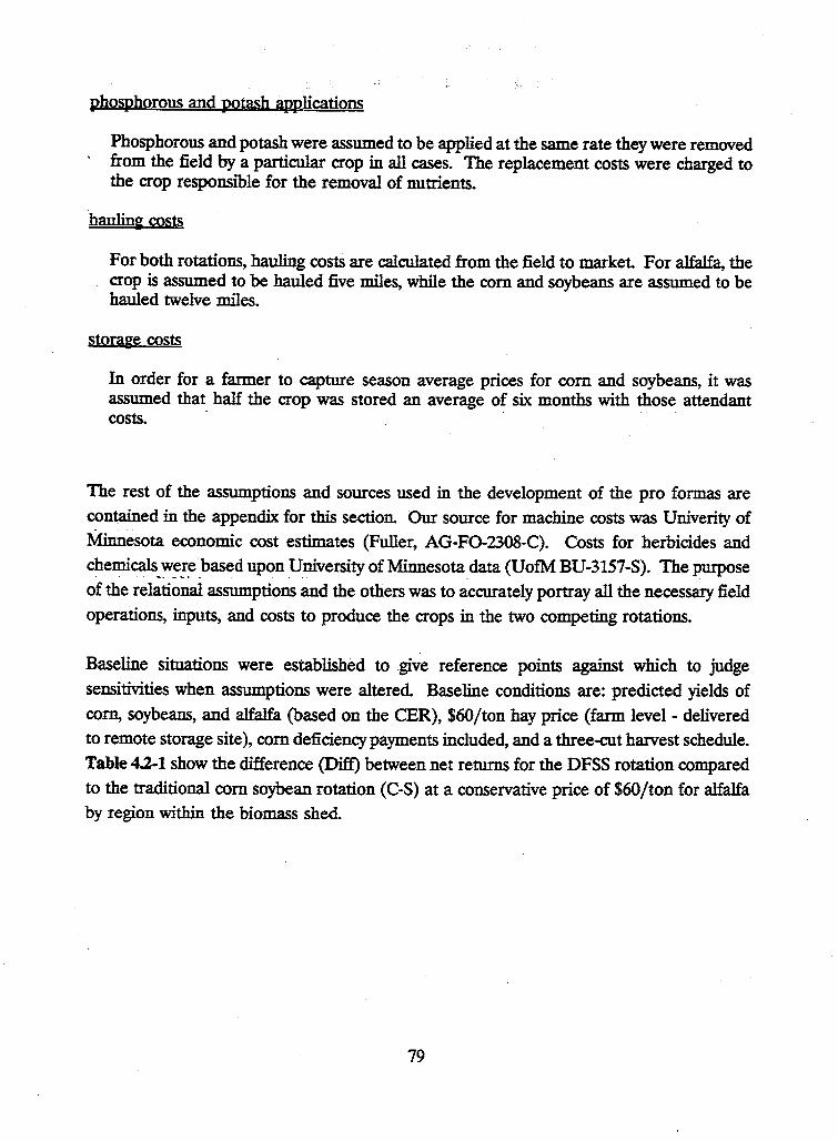
pho§I>horous and potash ap_plications
Phosphorous and potash were assumed to be applied at the same rate they were removed · from the field by a particular crop in all cases. The replacement costs were charged to
the crop responsible for the removal of nutrients.
hauling costs
For both rotations, hauling costs are calculated from the field to market. For alfalfa, the crop is assumed to be hauled five miles, while the com and soybeans are assumed to be hauled twelve miles.
storage costs
In order for a farmer to capture season average prices for com and soybeans, it was assumed that half the crop was stored an average of six months with those attendant costs. · ·
The rest of the assumptions and sources used in the development of the pro formas are contained in the appendix for this section. Our source for machine costs was Univerity of Minnesota economic cost estimates (Fuller, AG-F0-2308-C). Costs for herbicides and che~~-~~!~ _based upon l]niversity of Minnesota data (UofM BU-3157-S). The purpose of the relational assumptions and the others was to accurately portray all the necessary field operations, inputs, and costs to produce the crops in the two competing rotations.
Baseline situations were established to give reference points against which to judge sensitivities when assumptions were altered. Baseline conditions are: predicted yields of corn, soybeans, and alfalfa {based on the CER), $60/ton hay price (farm level - delivered to remote storage site), com deficiency payments included, and a three-cut harvest schedule. Table 4.2-1 show the difference (Diff) between net returns for the DFSS rotation compared to the traditional com soybean rotation (C-S) at a conservative price of $60/ton for alfalfa by region within the biomass shed.
79
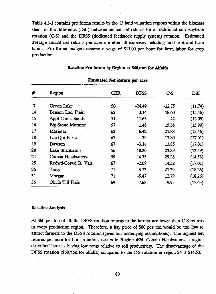
Table 4.2-1 contains pro forma results by the 13 land valuation regions within the biomass shed for the difference (Diff) between annual net returns for a traditional com-soybean rotation (C-S) and the DFSS (dedicated feedstock supply system) rotation. Estimated average annual net returns per acre are after all expenses including land rent and farm labor. Pro forma budgets assume a wage of $11.00 per hour for farm labor for crop production.
Baseline Pro fonna by.Region at $60/ton for Alfalfa
Estimated Net Return per acre
# Region CER DFSS c-s Diff
7 Green Lake 50 -24.49 -.12.75 (11.74) 14 Benson Lac. Plain 62 3.14 18.60 (15.46) 15 Appl-Cont. Sands 51 -11.63 .42 (12.05) 16 Big Stone Moraine 57 1.48 15.38 (13.90) 17 Marietta 62 6.42 21.88 (15.46) .
18 Lac Qui Parle 67 .79 17.80 (17.01) 19 Dawson 67 -3.16 13.85 (17.01) 20. . Lake Shaokaton 56 10.30 23.89 (13.59) 24 Coteau Headwaters 59 14.75 29.28 (14.53) 25 Redwd-Cotwd R. Vais 67 -2.69 14.32 (17.01) 26 Tracy 71 3.13 21.39 (18.26) 31 Morgan 71 -5.47 12.79 (1826) 36 Olivia Till Plain 69 -7.68 9.95 (17.63)
Baseline Analysis
At $60 per ton of alfalfa, OFFS rotation returns to the farmer are lower than C-S returns in every production region. Therefore, a hay price of $60 per ton would be too low to attract farmers to the DFSS rotation (given our underlying assumptions). The highest net returns per acre for both rotations occurs in Region #24, Coteau Headwaters, a region described here as having low rents relative to soil productivity. The disadvantage of the DFSS rotation ($60/ton for alfalfa) compared to the C-S rotation in region 24 is $14.53.
80
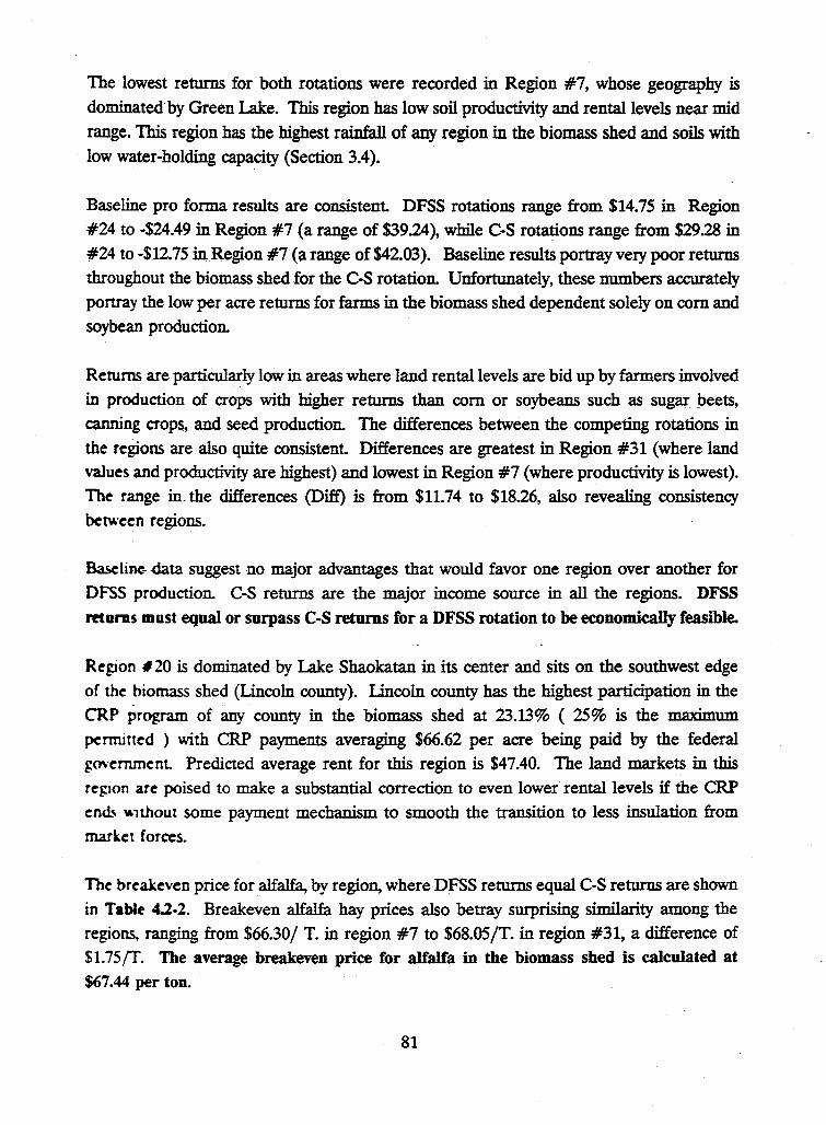
The lowest returns for both rotations were recorded in Region #7, whose geography is
dominated· by Green Lake. This region has low soil productivity and rental levels near mid
range. This region has the highest rainfall of any region in the biomass shed and soils with
low water-holding capacity (Section 3.4).
Baseline proforma results are consistent. DFSS rotations range from $14.75 in Region
#24 to -$24.49 in Region #7 (a range of $39.24), while C-S rotations range from $29.28 in
#24 to -$12.75 in, Region #7 (a range of $42.03). Baseline results portray very poor returns
throughout the biomass shed for the C-S rotation. Unfortunately, these numbers accurately
ponray the low per acre returns for farms in the biomass shed dependent solely on com and
soybean production.
Returns are particularly low in areas where land rental levels are bid up by farmers involved
in produ~on of crops with higher returns than com or soybeans such as sugar_ J:>eets,
canning crops, and seed production. The differences between the competing rotations in
the rc~ons are also quite consistent. Differences are greatest in Region #31 (where land
values and productivity are highest) and lowest in Region #7 (where productivity is lowest).
The range in. the differences (Diff) is from $11.74 to $18.26, also revealing consistency
between regions.
~line- -data suggest no major advantages that would favor one region over another for
DFSS production. C-S returns are the major income source in all the regions. DFSS
returns must equal or surpass C-S returns for a DFSS rotation to be economically feasible.
Region # 20 is dominated by Lake Shaokatan in its center and sits on the southwest edge
of the biomass shed (Llncoln county). Lincoln county has the highest participation in the
CRP program of any county in the biomass shed at 23.13% ( 25% is the maximum
permitted ) with CRP payments averaging $66.62 per acre being paid by the federal
~O\·ernrncnt Predicted average rent for this region is $47.40. The land markets in this re~ion are poised to make a substantial correction to even lower rental levels if the CRP
en~ -.1thout some payment mechanism to smooth the transition to less insulation from
mark.ct forces.
The brcakcven price for alfalfa, by region, where DFSS returns equal C-S returns are shown
in Table 4.2-2. Breakeven alfalfa hay prices also betray surprising similarity among the
regions, ranging from $66.30/ T. in region #7 to $68.05/T. in region #31, a difference of $1. 75 jT. The average breakeven price for alfalfa in the biomass shed is calculated at $67.44 per ton.
81
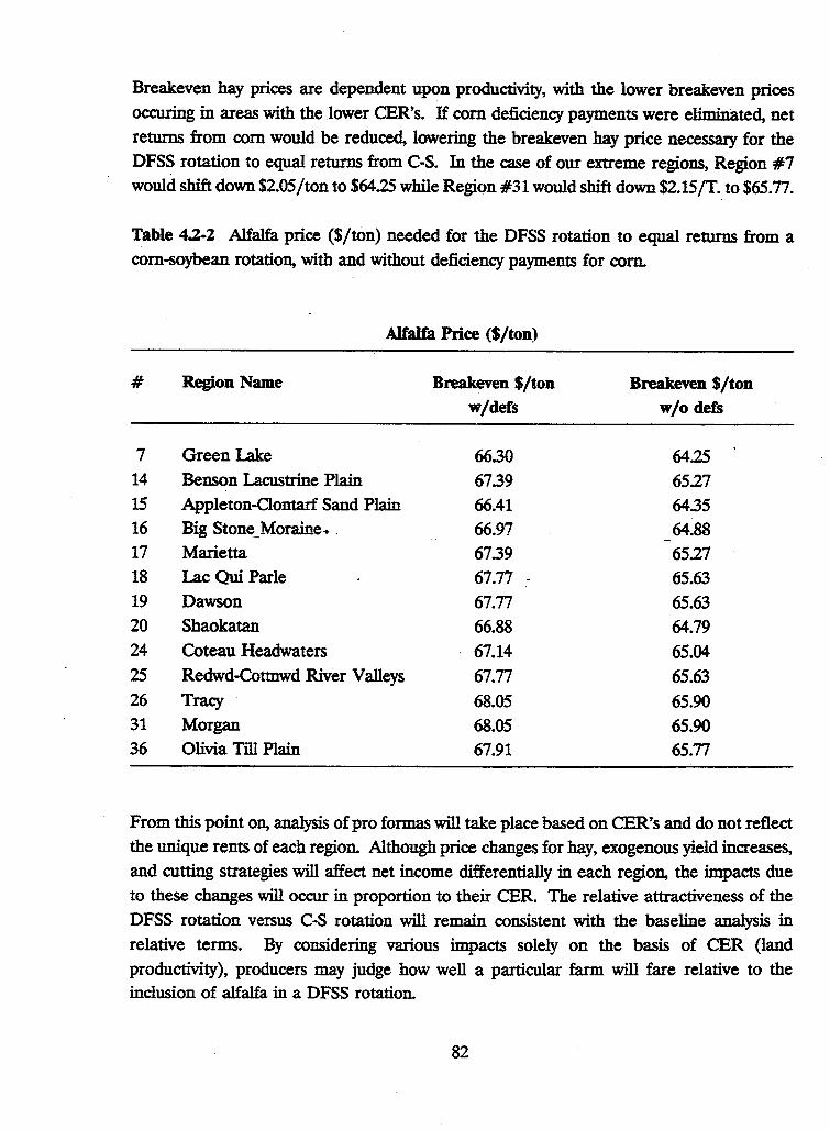
Breakeven hay prices are dependent upon productivity, with the lower breakeven prices occuring in areas with the lower CER's. If com deficiency payments were eHminated, net returns from com would be reduced, lowering the breakeven hay price necessary for the DFSS rotation to equal returns from C-S. In the case of our extreme regions, Region #7 would shift down $2.05/ton to $64.25 while Region #31 would shift down $2.15/T. to $65.77.
Table 4.2-2 Alfalfa price ($/ton) needed for the DFSS rotation to equal returns from a com-soybean rotation, with and without deficiency payments for com.
Alfalfa Price ($/ton)
# Region Name Breakeven $/ton Breakeven $/ton w/defs w/o defs
7 Green Lake 6630 64.25 14 Benson Lacustrine Plain 6739 6527 15 Appleton-Clontarf Sand Piam 66.41 64.35 16 Big Stone_ Moraine~ . 66.97 64.88 17 Marietta 67.39 6527 18 Lac Qui Parle 67.77 - 65.63 19 Dawson 67.77 65.63 20 Shaokatan 66.88 64.79 24 Coteau Headwaters 67.14 65.04 25 Redwd-Cottnwd River Valleys 67.77 65.63 26 Tracy 68.05 65.90 31 Morgan 68.05 65.90 36 Olivia Till Plam 67.91 65.77
From this point on, analysis of pro form.as will take place based on CER's and do not reflect the unique rents of each region. Although price changes for hay, exogenous yield increases, and cutting strategies will affect net income differentially in each region, the impacts due to these changes will occur in proportion to their CER. The relative attractiveness of the DFSS rotation versus C-S rotation . will remain consistent with the baseline analysis in relative terms. By considering various impacts solely on the basis of CER (land productivity), producers may judge how well a particular farm will fare relative to the inclusion of alfalfa in a DFSS rotation.
82
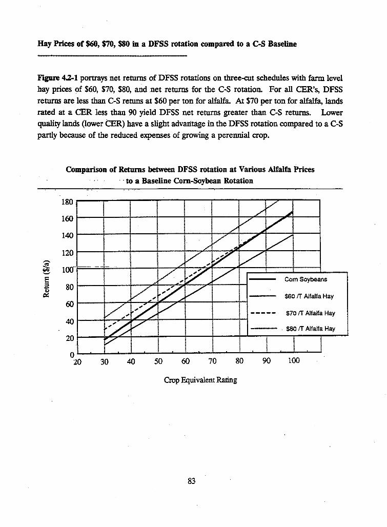
Hay Prices of $60, $70, $80 in a DFSS rotation compared to a C-S Baseline
Figure 4.2-1 portrays net returns of DFSS rotations on three-cut schedules with farm level
hay prices of $60, $70, $80, and net returns for the C-S rotation. For all CER's, DFSS
returns are less than C-S retuns at $60 per ton for alfalfa. At $70 per ton for alfalfa, lands
rated at a CER less than 90 yield DFSS net returns greater than C-S returns. Lower
quality lands (lower CER) have a slight advaiitage in the DFSS rotation compared to a C-S
partly because of the reduced expenses of growing a perennial crop.
-~ ..-;; -E ::::: -Q,)
c:::
Comparison of Returns between DFSS rotation at Various Alfalfa Prices - · to a Baseline Com-Soybean Rotation
180
160
140
120
100-Com Soybeans
80 $60 IT Alfalfa Hay
60 - - - - - $70 IT Alfalfa Hay
40 --- . $80 IT Alfalfa Hay
20
0 20 30 40 50 60 70 80 90 100
Crop Equivalent Rating
83
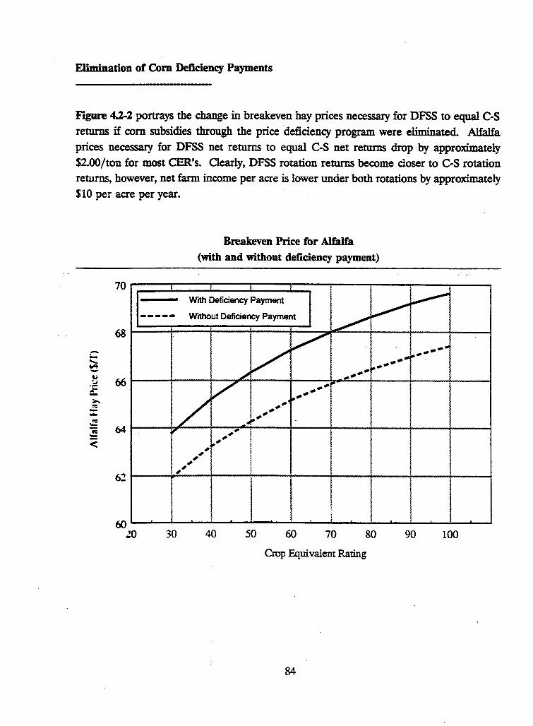
Elimination of Com Deficiency Payments
Figure 4.2-2 portrays the change in breakeven hay prices necessary for DFSS to equal C-S returns if com subsidies through the price deficiency program were eHminated. Alfalfa prices necessary for DFSS net returns to equal C-S net returns drop ·by approximately $2.00/ton for most CER's. Oearly, DFSS rotation returns become closer to C-S rotation returns, however, net farm income per acre is lower under both rotations by approximately $10 per acre per year.
-.... ...... 4IA -u ~
F ->. .::: -~
~
<
70
68
66
64
62
60 .!O
I
Breakeven Price for Alfalfa (with and without deficiency payment)
! i t
Wrth Deficiency Payment ...------~ ----- Without Deficiency Payment
~
v ~ ...... -------
----~ .. -v -~ ----/ --- I , .. _.,,. .. , ,~
I , .. ,~
' ,,' 1 , ! , ' ! I ~ ;
30 40 50 60 70 80 90 100
Crop Equivalent Rating
84
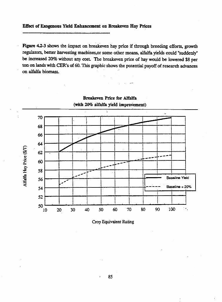
Effect of Exogenous Yield Enhancement on Breakeven Hay Prices
Figure 4.2-3 shows the impact on breakeven hay price if through breeding efforts, growth
regulators, better harvesting machines,or some other means, alfalfa yields could "suddenly"
be increased 20% without any cost. The breakeven price of hay would be lowered $8 per
ton on lands with CER's of 60. This graphic shows the potential payoff of research advances on alfalfa biomass.
-~ -Q 0 ·c
Q. >. ~
:I: .:! ;.§ <
70
68
66
64
62
60
58
56
54
52
50 10
-/
Breakeven Price for Alfalfa
(with 20% alfalfa yield improvement)
. I i
l --·..---L.----- -;/ ~
.... . -
I
.,
! ~
!
I I t
I I I i ..... -----------r --I t -- I ---- ' -- .. - . ' ...... r- !
i.. ...... Baseline Yield , , I I ..... Baseline + 20% -----
I I ~
l I i I l .
20 30 40 50 60 70 80 90 100 •.
Crop Equivalent Rating
85
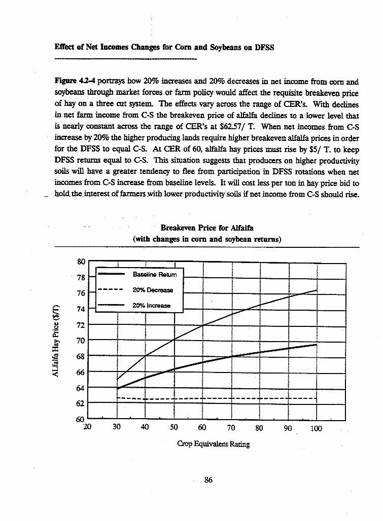
Effect of Net Incomes Changes for Corn and Soybeans on DFSS
Figure 4.2-4 portrays how 20% increases and 20% decreases in net income from com and soybeans through market forces or farm policy would affect the requisite breakeven price of hay on a three cut system. The effects vary across the range of CER's. With declines in net farm income from C-S the breakeven price of alfalfa declines to a lower level that is nearly constant across the range of CER's at $6257 / T. When net incomes from C-S increase by 20% the higher producing lands require higher breakeven alfalfa prices in order for the DFSS to equal C-S. At CER of 60, alfalfa hay prices must rise by $5 / T. to keep DFSS returns equal to C-S. This situation suggests that producers on higher productivity soils will have a greater tendency to flee from participation in DFSS rotations when net incomes from C-S increase from baseline levels. It will cost less per ton in hay price bid to h.old_ the.interest .of farmers with lower productivity soils if net income from C-S should rise.
~ -Q,) Q
a: >. CIS
::r:: ~ :s ,..J <
80
78 -76 -74 -72
70
68
66
64
62
60 20
· · Breakeven Price for Alfalfa (with changes in corn and soybean returns)
Baseline Return
----- 20% Decrease --· -------
-200k Increase ~
~ ~
~ / .........:
l / -------
~ ~
/~ ~
-----l-----1-----·,-----------· !-'>----------i . I .
30 40 50 60 70 80 90 100
Crop Equivalent Rating
86
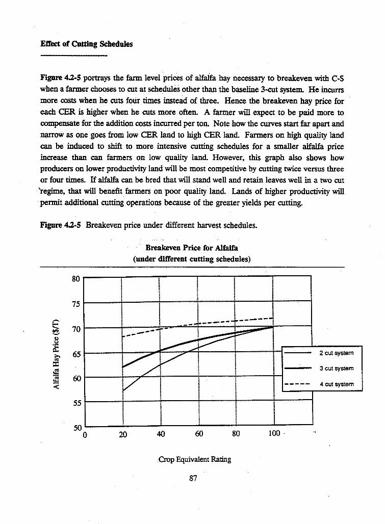
Effect of Cutting Schedules
Figure 4.2-5 portrays the farm level prices of alfaifa hay necessary to breakeven with C-S
when a farmer chooses to cut at schedules other than the baseline 3-cut system. He incurrs more costs when he cuts folir times instead of three. Hence the breakeven hay price for each CER is higher when he cuts more often. A farmer will expect to be paid more to compensate for the addition costs incurred per ton. Note how the curves start far apart and narrow as one goes from low CER land to high CER land. Farmers on high quality land can be induced to shift to more intensive cutting schedules for a smaller alfalfa price increase than can farmers on low quality land. However, this graph also shows how producers on lower productivity land will be most competitive by cutting twice versus three or four times. If alfalfa can be bred that will stand well and retain leaves well in a two cut "regime, that will benefit farmers on poor quality land. Lands of higher productivity will permit additional cutting operations because of the greater yields per cutting.
Figure 4.2-5 Breakeven price under different harvest schedules.
$ -u CJ
if >. co: ::c
JS ~ <
80
75
70
65
60
55
50 0
·· · Breakeven Price for Alfalfa
(under dilTerent cutting schedules)
-------------------___ ..... ---- I~-... -- _...----:::
~ / v -----
20 40 60 80 100.
Crop Equivalent Rating
87
2 cut system
3 cut system
4 cut system
"
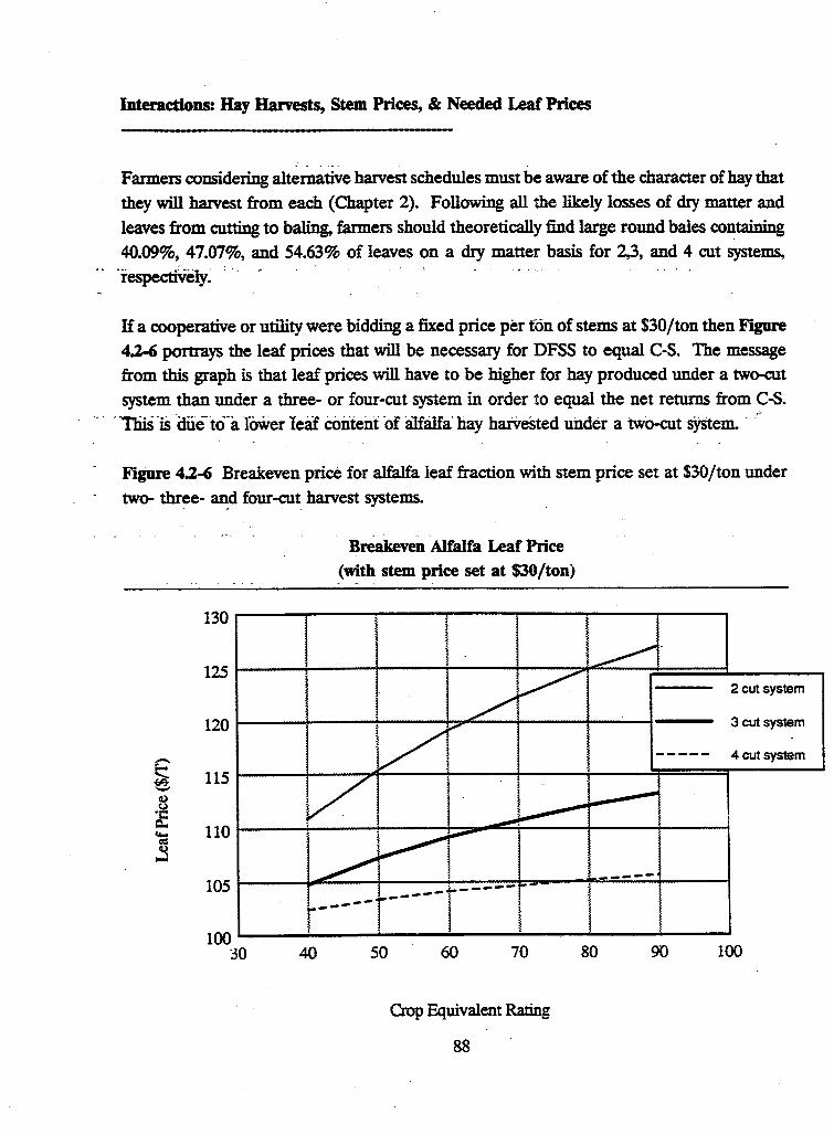
Interactions: Hay Harvests, Stem Prices, & Needed Leaf Prices
- ·-· -
Farmers considering alternative harvest schedules must be aware of the character of hay that
they will harvest from each (Chapter 2). Following all the likely losses of dry matter and
leaves from cutting to baling, farmers should theoretically find large round bales containing
40.09%, 47.07%, and 54.63% of leaves on a dry matter basis for 2,3, and 4 cut systems, • · ·respectiVeiy ~ ' · · - ·
If a cooperative or utility were bidding a fixed price per fon of stems at $30/ton then Figure
4.2-6 portrays the leaf prices that will be necessary for DFSS to equal C-S. The message
from this graph is that leaf prices will have to be higher for hay produced under a two-cut
system than under a three- or four-cut system in order to equal the net returns from C-S. -- - -Tl:iiS-iS ·aue-to·a. Tower leaf ooiitei:J.t of alfa.Ifa· hay harvested under a twO-cut syste~ - '
Figure 4.2-6 Breakeven price for alfalfa leaf fraction with stem price set at $30/ton under
two- three- ~d four-cut. harvest systems.
s -G> u
if ... cu ~
130
125
120
115
110
105
100 30
Breakeven Alfalfa Leaf Price
(with stem price set at $30/ton)
/ ~
/ ........
~-
------v -----------~
~ I ----- ------r-------40 50 60 70
Crop Equivalent Raring
88
-----
80 9D
2cutsystem
3cutsystem
4cut system
100
Different cutting strategies on different qualities of land may produce alfalfa leaf fractions
(under a set stem price) that result in equivalent net returns for the DFSS rotation and the
C-S rotation. For example, at a leaf price of $105/ton to the farmer (with stem price set at $30/ton), a three-cut system on 40. CER soils would be equivalent to a four-cut system on 80 CER soils. Each would each capture returns that would make the net DFSS rotation
returns equal to the net returns from a C-S rotation. Higher productivity lands in general will require higher aggregate alfalfa prices to be competitive with current rotations.
Major Conclusions from Pro formas:
The alternative assumptions modelled in the proformas offer many useful perspectives on alfalfa price levels and net DFSS returns across the biomass shed. Here are the major
lessons from these exercises:
1) The production regions within· the biomass shed are remarkably similar with respect their propensity to produce alfalfa for the DFSS rotation. Breakeven hay prices on three cut systems range from $6630/ T. to $68.05/ T.
2) Elimination of com deficiency payments would allo\\'._ the DFSS rotation to equal C-S at lower hay prices by about $2/T.;- however, net annual income would be lower for both rotations in the absence of com deficiencies. ·
3) The breakeven price for alfalfa on lower quality lands is lower than on higher quality lands.
4) Increases in alfalfa yield per acre can dramatically reduce per ton alfalfa breakeven prices needed to be competitive with com and soybeans.
5) When net returns for C-S increase, higher quality lands will be the first to leave DFSS. When net returns for C-S fall, there is little difference in breakeven hay price for all qualities of land.
6) When farmers cut their hay more often, they need to receive higher prices for the hay they produce. Farmers on higher quality land need less price inducement to change to a four-cut system than farmers on poorer quality land.
7) Since the cutting schedule influences the stem and leaf proportion, cutting schedule impacts farm price if pricing is based on percent leaf/ stem.
89
4.3 BIOMASS SUPPLY CURVE
Steven Taff Agricultural and Applied Economics
University of Minnesota
A supply curve is a schedule that relates a quantity offered to a stated price. All other variables - technological, institutional, financial - are suppressed or embedded in the supply -schedule. Any changes to these variables are evidenced by "shifts" in the supply curve -essentially by a new curve with new embedded parameter values.
There is an implicit supply schedule associated with each exchangeable product, whether or not that product is ~ctually offered for sale. In our case, there is a supply schedule for acres .of hay, for bales of hay, for tons of hay,.for leaves, for stems, for BTUs, or for ash. For present purposes, we will estimate a sup~ly schedule for tons of hay (of a "typical" moisture and protein content). delivered to the regional storage sites. The price will be that which producers expect to be offered in a "typical" year. All transport and preparation costs prior to the regional site are assumed borne by the producers and excluded from the offer price
- "Ca!Cufatlon:-··Aii "costs at antf from the regioiial sites are assumed borne l>Y- the alfalfa cooperative or joint-venture and so are embedded in the offer price itself.
What we seek are estimates of the number of tons of hay that will be offered by producers in exchange for a stated set of prices. Because climate and land productivity vary throughout the biomass shed, we need to estimate the production decisions of a range of farmers. Our approach is to divide the biomass shed into homogeneous production districts, within which producers are asserted to face similar land quality, land markets, and production constraints. A budget is constructed for a representative farm within each district with the relative returns for com-soybean (C-S) and the biomass (DFSS) rotation for a range of hay prices are compared. An adoption-rate algorithm is applied to this comparison, and total hay production responses are derived for each district at each hay price level. The aggregate of these relationships constitutes the regional biomass supply curve.
The production district boundaries used in this analysis are adapted from those used by the Minnesota Department of Revenue for property tax equaliz3.tion purposes. These, in tum, had their origins in geomorphological and soil association maps. The biomass production districts used here are divided along township lines as shown in Illustration 4.3-1.
90
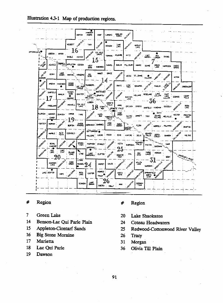
lliustration 4.3-1 Map of production regions .
Ol'TOWtuE':,,__• CllESSo> ; AKRON
~.>:: "'--' MOYER
I ,,,,• ~-~~
• Hlll/CDCX IOlRI!
TARA
~.,R
~I '-st
SI> MILE CllOV£
~ .
# is·---
• 8ENSCl< . CAl<P
LAKE
• TORNING Kii.OM£ ..§-"' ~~ . t.Al<E NEV
~o, . OIO'IE• · LOIOlN
.......--- i· cOSMa I,._"'? AGASSIZ ·'-=c.. ~· ElllSON
' ~ ···::.,_,_;----· .... ----.-----....l.-\IEST - . SllENOOO ~<.AKE
#
7 14 15 16 17
18 19
I 1-.
Region
Green Lake Benson-Lac Qui Parle Plain Appleton-Oontarf Sands Big Stone Moraine Marietta Lac Qui Parle Dawson
91
ACTON
# Region
20 Lake Shaokaton 24 Coteau Headwaters 25 Redwood-Cottonwood River Valley 26 Tracy 31 Morgan 36 Olivia Till Plain
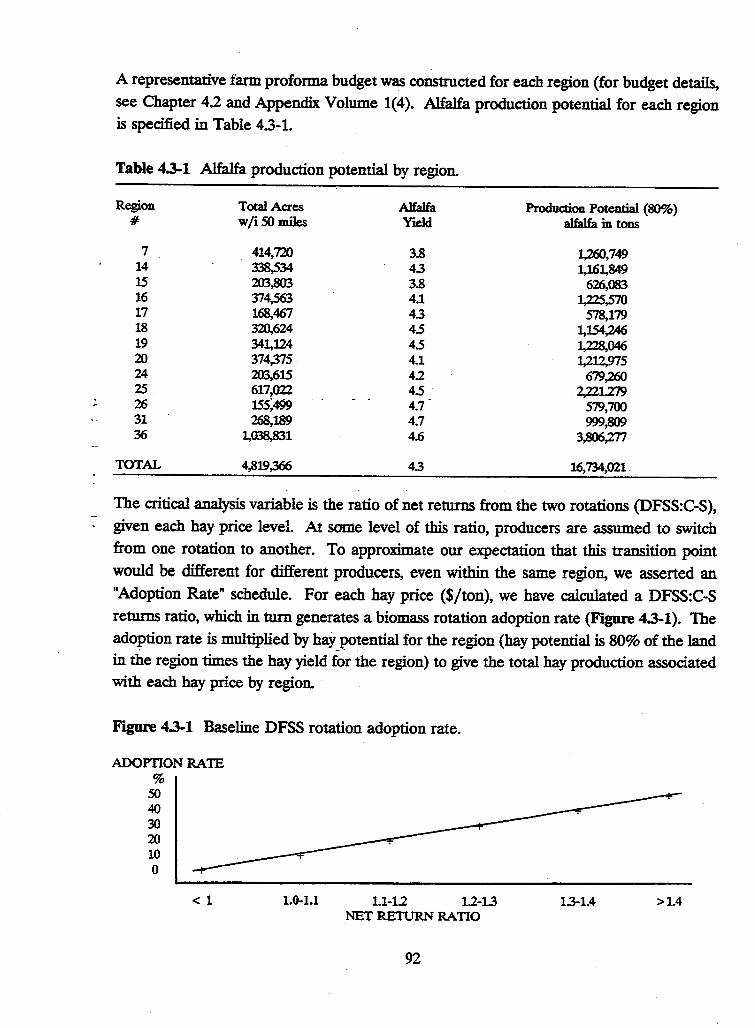
-~
A representative farm proforma budget was constructed for each region (for budget details, see Chapter 42 and Appendix Volume 1(4). Alfalfa production potential for each region is specified in Table 43-1.
Table 4.3-1 Alfalfa production potential by region.
Region Total Acres A1falfa Production Potential (80%) # w/i 50 miles Yield alfalfa in tons
7 414,720 3.8 1,260,749 14 338,534 43 1,161,849 15 203,803 3.8 626,083 16 374,563 4.1 1,225,570 17 168,467 43 578,179 18 320,624 45 1,154,246 19 341,124 45 1,228,046 20 374,375 4.1 1,212,975 24 203,615 4.2 679;2DJ 25 617,'112 45 2,221.279 26 155~499 4.7 579,700 31 268,189 4.7 999,809 36 1,038,831 4.6 3$167TI
TOTAL 4,819,366 43 16, 734,021.
The critical analysis variable is the ratio of net returns from the two rotations (DFSS:C-S), given each hay price level At SODle level of this ratio, producers are assumed to switch from one rotation to another. To approximate our expectation that this transition point would be different for different producers, even within the same region, we asserted an "Adoption Rate" schedule. For each hay price ($/ton), we have calculated a DFSS:C-S returns ratio, which in turn generates a biomass rotation adoption rate (Figure 4.3-1). The adoption rate is multiplied by hay_J?<>tential for the region (hay potential is 80% of the land in the region times the hay yield for the region) to give the total hay production associated with each hay price by region.
Figure 4.3-1 Baseline DFSS rotation adoption rate.
ADOPTION RATE %
50 40 30 20 10 0
< 1 1.0-1.l 1.1-1.2 1.2-13 NET RETURN RATIO
92
13-L4 >1.4
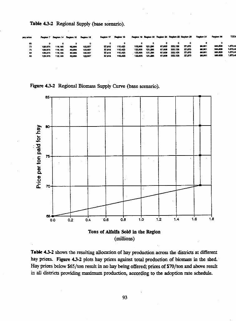
Table 4.3-2 Regional Supply (base scenario).
i-Yprico R9gion7 Region 1.C R9gion 15 llegian 18 llegian 17 llegiall 111 llegian 111 ........ 2D llegiall 24 llegian 25 llegion 211
es 0 0 0 0 0 0 0 0 0 0 0
70 1211,075 1111,1115 112.eoa 1Z2.557 57,8111 115,G 12UCl5 121.ae .,.
222.1211 57.ll70
75 1215.075 1111,185 112.- 1Z2.557 57.8111 115.425 122.IOS m.ae Sf .1211 222.13 57.ll70
eo 13.075 1111,185 112,ms 122,557 57,8111 115,425 -122.IOS 121.ae Sf .1211 222.13 57.ll70
85 13,075 1111,185 ~ 122,557 57,8111 115,425 122.IOS 121.3111 Sf .1211 222.13 57.ll70
Figure 4.3-2 Regional Biomass Supply Curve (base scenario).
85
>. 80 ca .c ... J2
- "C --a c. c 0 -... Cl> c. G> u
·;::
75
c.. 70
5S 0.0
L.----L.----~
L.----L---,____-L---
L.--------0.2 0.4 0.6 0.8 1.0 1.2
Tons of Alfalfa Sold in the Region
{millions)
1.4 1.6
"""°" 31 llegian 311
0 0 1111.1181 380,1211 1111,1181 3llO.l2ll 1111.1181 31111,aa 1111,11111 3llO.l2ll
1.8
Table 4.3-2 shows the resulting allocation of hay production across the districts at different
hay prices. Figure 4.3-2 plots hay prices against total production of biomass in the shed.
Hay prices below $65/ton result in no hay being offered; prices of $70/ton and above result
in all districts providing maximum production, according to the adoption rate schedule.
93
TOFA
1,873,«I 1.1173,«1
1.m.«I
1.173.C
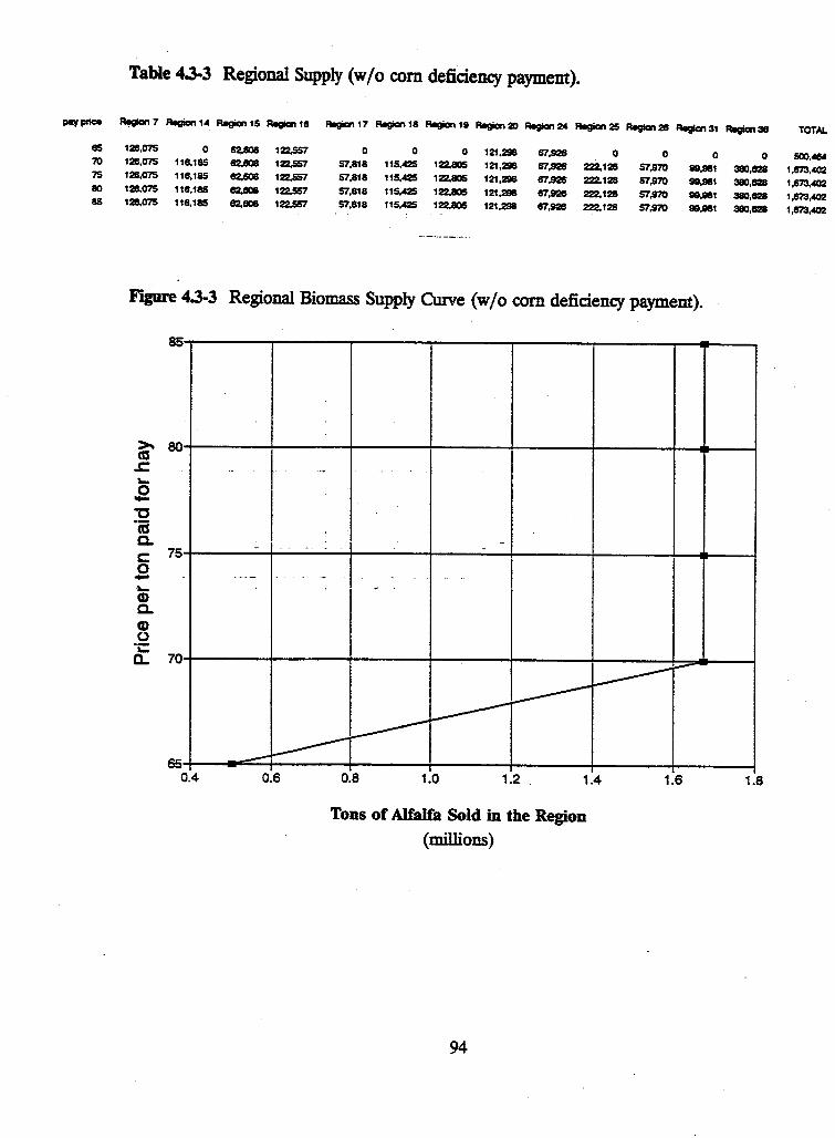
pay!lflc:e
8S
7tl 75 80 as
Table 4.3-3 Regional Supply (w/o com deficiency payment).
Regian 7 Regian 14 Regian 15 Aegicn 18 Regia\ 17 Regicn 18 Region 19 Aegicn 20 Region 24 Regicn 25 Regicn 28 Region 31 R9gicn 38
128.075 0 62,608 122,SST 0 0 0 121.298 ff'/,928 0 0 0 128,075 118,185 82,608 122,SST 57,818 115,425 122,805 121,298 87,928 222,128 57,970 a&,981 128,075 118,185 82,608 122,SST 57,818 115.425 122,805 121,298 87,926 222,128 57,970 99,981 128,075 118,185 82,908 122,SST 57,818 11$.425 122,805 121,298 87,928 222,128 57,970 118,8111 128,075 118,185 82,608 122,SST 57,818 115,425 122,805 121,298 87,928 222,128 57,970 99,961
···-···-·---··
Figure 4.3-3 Regional Biomass Supply Curve {w/o com deficiency payment).
~ 80 .s:::. '-J2 "'C "(ij c. c: 0 -·\,,,, CD c. CD 0
"i:: a..
0.6 0.8 1.0 1.2 1.4
Tons of Alfalfa Sold in the Region {millions)
94
1.6
0 380,S28
380.828 380,S28 380,S28
1.8
TOTAL
500,484 1,613,402
1,873,402
1,613,«>2 1,873,«)2
Table 4.3-4 Regional Supply (high hay yield).
pay price Regicn 7 Ragicn 14 Region 15 Regicn 16 Ragian 17 Ragian 18 Ragian 19 Ragicn 20 Amgian24
60 0 0 0 0 0 0 .o 0 0 65 131U82 127,803 68,869 134,813 63,600 128,967 135,085 133,427 74,719 70 138,682 127,803 68,869 134,813 113,600 129,967 135,085 133,427 74,719 75 138,682 127,803 68,869 134,813 ss.eoo 128,967 135,085 133,427 74,719 80 138,682 127,803 68,869 134,813 63,600 128,967 135,085 133,427 74,719
Figure 4.3-4 Regional Biomass Supply Curve (high hay yield).
SS
>. 80 ttS .c: ,._ J2 "C ·a a. c: 0 -,._ Q) a. CD 0
"t:: CL
75
70
-
-
-· -
Regian 25 Region Aegian31
0 0 0 244,341 113,787 109,979
244,341 63,787 109,979
244,341 63,787 109.979
2"4,341 63,787 109.979
..
~ L---l---L.---
65 0.0
L.---L-----------~
0.2 0.4 0.6 0.8 1.0 1.2
Tons of Alfalfa Sold in the Region
(millions)
95
1.4 1.6 1.8
Ragian38 TOTA
0 418,890 1,8C0,74
418,e90 1,840,74
418,ISSO 1,840,74:
418,890 1,M0,74:
2.0
Table 4.3-5 Regional Supply (low hay yield).
pay price Regicn 7 Aagicn 14 Aagicn 15 Aagicn 16 Aagicn 17 Aagicn 18 Aegicn 19 Aagicn 20 Aegicn 24 Aagicn 25 Aagicn 28 Regicn 31
65 0 0 0 0 0 0 0 0 0 70 0 0 0 0 0 0 0 0 0 75 113.467 104.586 58,347 110,301 52.036 0 0 109,168 81,133 80 113,487 104.586 58,347 11o,301 52.036 103,882 110,524 109,168 81,133 85 113,467 104,566 58,347 110,301 52,036 103,882 110,524 109,168 81,133
Figure 4.3-5 Regional Biomass Supply Curve (low hay yield).
85
>- 80 ta
.s:::.
0 0 0 0 0 0 0 0 0
1911,915 52,173 89,983 1911,915 52,173 89,983
1--""
~ ~
~
~
0 --····--- - -- ~ -- ·--·-
1 ____..--
I 75
v v 70 /
65 0.0 0.2
-
0.4 0.6 0.8 1.0
Tons of Alfalfa Sold in the Region
(millions)
96
1.2 1.4
Aegion36 TO
0 0 0 ll07,
342,S6S 1,500,
3'C2,56S 1,508,
1.6
pay price
70
75 80
85
90
Table 4.3-(; Regional Supply (low adoption rate).
Regicn 7 Regicn 14 Regicn 15 Regicn 16 Regicn 17 Flegiclrl 18 Regicn 19 Regicn 20 Region 24 Regicn 25 Regicn 28 Regiarl 31
0 0 0 0 0 0 0 0 0 0 0 0 12,607 0 6,261 12.256 0 0 0 12,130 .6,793 0 0 0
128,075 58.092 62,608 61,279 28,909 11,542 12,280 60,649 33,963 22,213 5,797 9,996 128,075 118,185 82,S08 122,557 57,818 115,425 122,805 121,298 67,926 222,128 26,985 48,980 126,075 118,185 82,608 122,557 57,818 115,425 122.805 121,298 67,926 222,128 57,970 99,981
Figure 4.3-6 Regional Biomass Supply Curve (low adoption rate).
~ .s:::. """' .E
"O ·a a. c 0 -"""' Q) a. Q) 0
·;:::: 0...
90
88
86
84
82
80
78
76
f 74
I 72
70 0.0
v /
0.2
__,.. ~
~ --......
v /
0.4 0.6 0.8 1.0 1.2
Tons of Alfalfa Sold in the Region
(millions)
97
v /
/ ,/ v
... . . ... _ .. ·- .....
I
1.4 1.6
Regicn36 TOTAi
0 (
0 50,l)ll
38,063 531,'81
190,314 1,404,11~
380,628 1,673AQ::
1.8
pay price
65 70 75 80
85
Table 4.3-7 Regional Supply (2-cut system).
Region 7 Regicn 14 Regicrl 15 Region 18 Aegia117 Regiat 18 Regicn 19 Ragion 20 Regian 24 Region 25
0 0 0 0 0 0 0 0 0 0 114,8511 105,Moll 57,ms 111,1149 52,872 105,152 111,875 110,502 81.881 202,359 114,854 105,844 57,038 111,849 52,872 105;152' 11t-,87S . 110.502 81.881 202,359 114,8511 105,844 57.038 111,849 52,872 105,152 111,875 110,502 81,881 202,359 114,854 105.844 57,038 111,SG 52,672 105,152 111,875 110,502 . 81,881 202,359
Figure 4.3-7 Regional Biomass Supply Curve (2-cut system).
85
~ 80 .c "-
.!2 1:l ·a a. c: 0 -"-Q) a. Q) 0
•t:: CL
75
70
65
.-------: --------L----L--------
Region 28 Region 31 Region 38
0 0 0 52,811 91,083 348,752 52,811 91,083 348,752 52,811 91,083 348,752 52,811 91,083 348,752
-----
0.0 0.2 0.4 0.6 0.8 1.0 1.2 1.4 1.6
Tons of Alfalfa Sold in the Region (millions)
98
TOTAL
0
1.524.Ml!I 1,524,4119
1.524.• 1,524,'811
Suuply Schedule Shifters
How stable are these production estimates? We here examine the effects of four separate
changes in our baseline assumptions. Each change is but one example of several that might
be posed within that general category. While the baseline incorporates our best estimates
of the various parameter values, this sensitivity analysis can help the reader decide which
of our initial estimates need further specification. W ~ ~ see that relatively small changes
in the baseline assumptions lead to relatively large swings in the regional biomass supply
schedule. This is because the relative net returns to the two rotations are so similar in the
baseline.
There are many events that might lead to a shift in our most fundamental variable, the
DFSS:C-S returns ratio. What happens to the supply schedule, which relates hay production
and hay prices, if the expected price of com were reduced (i.e. due to the abolition of
deficiency payments)? The price change alters the DFSS:C-S return ratios, which in turn
alter the adoption ratios (Table 4.3-3). This exercise is charted in Figure 4.3-3, which shows
the zero deficiency payment supply curve. At a ·$6750/ton hay price, the lower expected
com price would result in over 12 million tons of hay being offered, a large increase over
the baseline of 800,000 tons at this price.
Yields
What if plant breeders succeed in developing varieties that yield more biomass per acre?
Or, what if our hay yield estimates prove overly optimistic? In this exercise, we vary the hay
yields by 10% in each production district. Table 4.3-4 and Figure 4.3-4 show that a 10%
increase in hay yield increases overall hay production at the $67.50 /ton level to 900,000 tons,
A 10% reduction in alfalfa yield, at the same price level ($67 50/ton) as shown in Table 4.3-
5 and FJ.gUre 4.3-5, results in no hay offered. Under low yield expectations, farmers would
expect a price over $75.00/ton before our assumptions would yield a production level
sufficient to supply the needs of the alfalfa processing plant.
99
Behavior
What if our biomass rotation "adoption-rate" schedule turns out to be incorrect? After all, it is based on expected producer responses and our judgment of "typical" producer behavior. Because this schedule is critical to the development of the regional biomass supply curve, it warrants special attention. Here, we show the effects of specifying a lower, more "pessimistic" adoption rate as shown in Table 4.3-8. The lower adoption-rate increases the price necessary to elicit 700,000 tons of production from $67 /ton (baseline scenario) to $81/ton as shown in Table 4.3-6 and Figure 4.3-6.
Table 4.3-8 Biomass adoption-rate schedules based on the ratio of net returns between the DFSS rotation and traditional com-soybean rotation at both a low and a baseline level of producer acceptance.
Adoption Rate Schedule
Net Return Ratio1 Low Adoption Rate2 Baseline Adoption Rate3
< 1.0 0 0 1.0 - 1.1 0 0.10 1.1 - 1.2 0 0.10 1.2 - 1.3 0.01 0.10 1.3-1.4 0.05 0.10 > 1.4 0.10 0.10
1- Net return ratio is the ratio between net returns from the DFSS rotation and a Com-soybean rotation.
2- Low ad<mtion rate reflects poor acceptance by producers.
3- Baseline adoption rate expected level of producer acceptance.
100
Regulations
All prices and costs a have an institutional, as well as a technological basis. For example,
holding farmers responsible for the off-farm costs of soil erosion could dramatically affect
the costs of row-crop production on erodible soils and, as result, shift the geographical focus
of production.
In the present setting, we examine the implication of one such rule change: requiring
contracted hay producers to delay their first cutting of hay until late June (late June harvest
_ would extend the period of favorable habitat for nesting birds on these lands). This
"habitat-constrained" system where the first cutting is delayed until late June results in a two
cut harvest system due to seasonal constraints. The baseline supply curve assumes a three
- .cut harvest ~tem, with the first cutting in early June.
The "habitat-constrained" system results in reduced total annual yield but also reduces · · annual harvest costs (one less cutting per year). We estimate that hay yield be reduced by
almost 9%, however net biomass rotation returns actually increases due to lower production
costs. The net effect on both the aggregate supply schedule and on geographic distribution
of production is modest as shown in Table 4.3-7 and Figure 4.3-7, respectively.
CONCLUSIONS:
The exercise of generating a regional biomass supply curve, even though it necessarily
requires several ·assumptions that can be tested only in actual system operation, forces us
to confront certain aspects of the decision environment faced by potential hay producers.
In particular, the exercise demonstrates the effects of hay yields, federal com subsidies, and
producer attitudes toward risk. Relatively small changes in any of these parameters in our
baseline assumptions lead to relatively large swings in the volume of hay production in the biomass shed. In general, we are led to conclude that hay prices above $67 /ton will most
likely elicit enough hay production in the region to fuel the design power plant. One might expect a disproportionate amount of this production will come from farms with lower
productivity com land and few other competing market opportunities. However, even high
productivity com land might be turned to the DFSS rotation at hay prices above $70/ton
or as the result of other considerations.
101
102
, ~-
CHAPTER 5. TRANSPORTATION AND STORAGE
5.1 Transportation and Storage Logistics
Fruin\ Wilcke2, and Schmidt
Agricultural and Applied Economics1 and Agricultural Engineering2
University of Minnesota
Introduction
The efficiency of using biomass as an energy source is often limited by the cost of biomass
transportation and handling. Two common concerns associated with biomass transportation
are that biomass tends to have a low bulk density and high moisture content. This report
- · outlines -a cost effective design to provide a steady supply of alfalfa biomass to the
processing plant. The economics of transportation and storage for both alfalfa producers
· and for a proposed Alfalfa Cooperative {AC) are included. Harvest, transportation, and
storage of alfalfa is accomplished through the use of existing equipment and technologies.
Technological advances will likely improve overall system efficiency.
Overview of Logistics
Alfalfa is harvested over approximately a three month period. The power plant is designed
to operate at least ten months per year. Therefore, a significant portion of the total crop
( 60%) must be stored for a period of time. Maintaining alfalfa quality throughout storage
is critical. Storage losses can reduce both total dry matter and alfalfa quality. Two options
exist for protecting alfalfa in storage; roofed structures and plastic tarps are both readily
available to protect alfalfa from quality and dry matter losses.
Alfalfa storage could be accomplished either on-farm or at remote storage locations.
Currently very few producers have facilities for on-farm alfalfa storage. Because comparable
storage cost per ton is independent of storage location, on-farm storage of alfalfa is possible;
however, the existence of farm size quantities of baled alfalfa scattered throughout the
production area presents certain difficulties. Road restrictions, quality monitoring, night
hauling on country roads, and simply finding the stored alfalfa on the farm are a few of the
transportation problems that would be encountered with on-farm storage. Properly sited
regional storage sites will be easy to find and accessible day or night year round. Loading
and unloading equipment, weigh scales, and alfalfa testing equipment will be located at the
regional facilities.
103
Harvest dates initiate the tidal flows of alfalfa from fields to storage sites. Alfalfa may be
harvested as early as late May and as late as early October. This report utilizes data for
standard three-cut harvest systems.
The biomass power plant is designed to operate at least 300 days per year. Power
., companies traditionally plan for power plant routine maintenance during either the spring
or fall periods of lighter power loads. To minimize storage cos~ the biomass power plant
, . could schedule "down time" for the 65 day period preceding hay harvest. . The plant should
be ready for full and continuous operation beginning June 1. The power plant would then
be constantly consuming alfalfa stems during the entire harvest season and beyond with
minimal storage costs or post-harvest losses on direct-haul biomass. This report anticipates
that 40% of total production will be direct-haul (no storage) from June through September.
_ . Bale. size and density is specified for consistency and efficiency throughout the operation.
Large high-density square bales offer transportation and storage advantages however large
square balers are relatively new to the production area. Small-square bales require
additional labor both in the field and at the storage facilities. The large-round bale ( 4'x6')
specified for this study is widely utilized by farmers in the area.
Transportation costs from the field to a remote storage site are considered to be the
responsibility of the producer. Farm· to regional ·storage· tra.nsport·could ·be done using
wagons, trucks, or special hay hauling equipment. Simple efficiencies of transportation
reward growers hauling more tons per load. Bales move from the regional storage sites to
the processing plant on specially designed flat- bed trucks.
104
Storage Options
Three basic storage options were analysed. The "no cover" option indicates that bales are
stored outdoors without protection. The ''plastic" option indicates bales stored in a 10 bale · pyramid and covered with a specially designed plastic tarp. The "roofed" option indicates : bales stored in a pyramid four rows high in a pole barn type structure with a roof and two
or three sides enclosed (Section 3.3). The current analysis is limited to using only one c .storage option for storing all of the alfalfa in the bioshed. Most likely, some combination
of storage sytems will give a best case scenario. Long-term storage of alfalfa may be in a
roofed structure and short-term storage may be with no cover. Plastic tarps may be used
as short or long-term storage or even for years in the event of an oversupply situation.
Method of storage and resulting storage losses determine the level of production needed to
satisfy the fuel needs of the power plant. Production, transportation, and storage are linked. Dry matter and quality loss under different storage scenarios affect farm level production requirements and transportation costs. Spreadsheets were developed to facilitate
comparisons of storage and transportation systems.
Logistical Considerations
The year's supply of alfalfa will be delivered to regional storage sites during a four month
period. This will require a seasonal work force. Storage sites may need to be open and
staffed daily to facilitate the delivery of alfalfa from the growers. Sites must be staffed by at least one, and possibly two, qualified persons to provide timely weighing, testing,
unloading. and stacking of the alfalfa bales. The flow of alfalfa from farm fields to remote
s.toragc sites will fluctuate with weather conditions. Therefore, the demand on the labor
force "'ill also fluctuate with the weather.
The logistics of transport of alfalfa to the processing plant requires planning and coordination. Approximately 750,000 tons of alfalfa must be transported from 50 to 80
remote storage sites to the processing plant annually (ca. 2500 t/d). This requires approximately 20 trucks hauling 16 hours per day, 6 days a week.
105
Equipment Needs
As stated previously, a condition of this study was to utilize proven and available equipment.
· The farm equipment needed for alfalfa production is common and familiar to many farmers
in the area. Such equipment includes tractors, tillage equipment, fertilizer spreaders, boom
sprayers, cultivators and planters, mower conditioners, swather conditioners, hay rakes, and
round balers. The only piece of production equipment that must be specified is the round
baler ... The size and type of bale produced is a critical factor.in providing a least cost system
for transportation and storage.
Current methods used by farmers for transporting alfalfa from field to the storage sites
include many sizes of trucks, tractors, and hay wagons. Generally volumes and distances
moved are low for most farmers. In recent years, some specialized equipment has been
developed to accomplish the transportation task more efficiently. Specialized trucks and
wagons are available to pick up bales in the field, tra.nSport them, and unload rapidly at a
storage area. Fork lifts/loaders that extend up to 20 feet will be used to stack and handle
bales at the storage site.
Bales are cored and sampled upon delivery at the regional storage site. Grower's name or
identification number, and alfalfa weight, quality, and moisture are recorded by a
computerized data collection system. Weighing and testing needs to be done rapidly and
accurately. An automated process for testing alfalfa is not currently available. Automated
systems in use for sampling and weighing grains and sugar beets may be modified for this
specific purpose.
106
5.2 Transportation and Storage Costs
Introduction r
A spreadsheet was developed to estimate the cost of different options for the transportation · · ·· and storage of the baled alfalfa. Three basic costs were analyzed in the calculations:
transportation costs from the farm to the regional storage site, storage costs, and transportation costs· from the regional storage site to the processing plant (Table 5.2-1).
Table 5.2-1 Summary of transportation and storage costs under the assumptions described on the following pages.
STORAGE METHOD No Cover Plastic Roof
· Tons alfalfa per year (15% moisture) 679,016 656,680 644,372 · ·Number of bales 1,200,765 1,161,266 1,139,501
Alfalfa acres in bioshed 178,688 172,811 169,572 % alfalfa acres in bioshed 6.9 6.7 6.6 Optimum storage sites 83 80 79 Haul days per site 2.3 2.3 2.3
COSTS
Transport to regional storage $2,285,456 $2,210,277 $2,168,851
Storage $4,880,494 $4,854,087 $7,151,448
Transport to plant $2,401,528 $2,322,530 $2,279,001
Total costs $9,567,478 $9,386,894 $11,599,300
Cost per ton (after loss) $15.03 $14.75 $18.22
107
General Assumptions
Tons of stems delivered per day to the gasifier:
Alfalfa dry matter storage losses:
Alfalfa yield per acre in the biomass shed:
Bale moisture content:
Bale density (large round bale):
Bale size (based on maximum truck capacity):
Leaf:Stem ratio:
Direct-haul (no storage):
. . . . Tillable acres in biomass shed:
Labor charge (including benefits):
Depreciation, interest, repairs, taxes,
insurance on capital investment:
992 t/d (dw), 1167 t/d (15%).
2% - roofed structure
5% - plastic cover
10% - no cover
. _3.~ _tons per acre
15%
10 lbs/ft3 (15% moisture) 4'x6' (length x diameter)
45:55
40% of total production
80%
$11.00/hr
15%
Transportation from Farm to Storaee Site Assumptions
!"umber of bales per load:
A,·cragc delivery speed:
Cost per mile (equipment, maintenance and fuel): Hauling distance:
108
10
15 mph
$0.50 per mile logged variable
Storaie Assumptions
. Annual land value:
Site preparation and gravel base:
Plastic tarps:
(includes tarp, springs, clamps and tarp disposal) _ Steel storage structure (cost per square foot):
Miscellaneous equipment at regional storage site: (includes weigh scale, office space,
and computerized bale testing equipment) - Loading equipment:
. Storage site hours of operation in peak season:
Percent of total harvest as first cutting :
(three-cut. schedule)
Time to get first cutting from field to storage:
Labor per bale:
(includes weighing, testing, unloading, stacking) - Additional labor per bale for plastic cover:
(covering and uncovering)
$100 per acre per year
$20,000 per acre
$1.00fbale-3 year life
$5.50/ft2
$100,000 per site
$70,000
16 hours
33%
15 days
3 minutes
1.5 minutes/bale
Tranmortation to Processin& Plant Assumptions
Processing plant operations:
Delivery from remote storage:
Average road speed:
Time on road per day:
Loading time:
Unloading time:
Bales per truck load:
Cost per mile:
(labor, fuel, maintenance, purchase)
109
7 days per week
6 days per week
40mph
16 hours
0.50 minutes per bale
0.33 minutes per bale
30
$0. 75 per mile logged
Discussion
The costs of farm transportation, storage, and transportation to the processing plant range from 9.4 to 11.6 million dollars per year (Table 5.2-1). The price per ton (including storage loss) ranges from $14.75 to $18.22.
Many factors impact the cost of transportation and storage. Figure 5.2-1 indicates the effect . of production area on transportation and storage costs by representing a biomass shed with a 30, 40, and 50 mile radius. The most compressed biomass shed (30 inile) results in·cost savings of $2.73/ton of alfalfa compared to a biomass shed with a 50 mile radius. Achievement of these savings in transportation costs requires increasing the percentage of alfalfa in the landscape from 5% of tillable acres (50 mile radius biomass shed) to 20% (30 mile radius biomass shed). Note: approximately 5% of the tillable land within a 50 mile radius of the processing plant is currently enrolled in the Conservation Reserve Program (CRP).
Figure 5.2-1 Predicted per ton cost for transportation and roofed storage of alfalfa per number of storage sites.
25
24 23
-= 22 0 21 ~ - 20 <c;;
8 19 18 17 16
0
Transportation and Storage Cost ($/ton)
25 50
50 mile bioshecl radius 40 mile bioshed radius
75 100 Number of Storage Sites
110
125 150
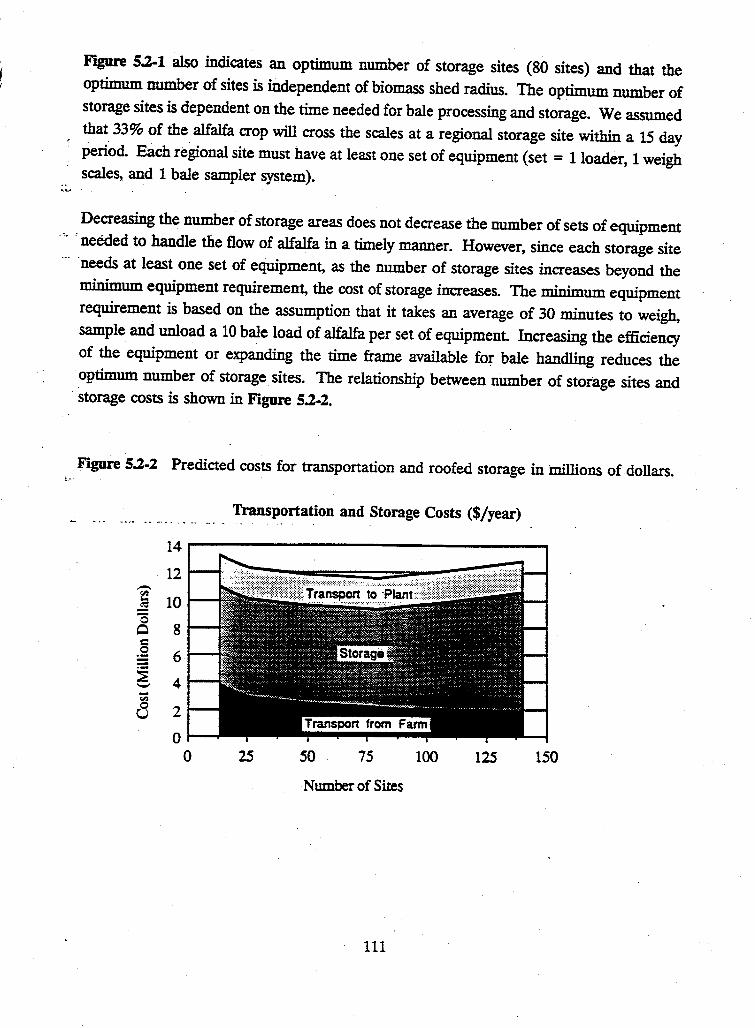
Figure 5.2-1 also indicates an optimum number of storage sites (80 sites) and that the optimum number of sites is independent of biomass shed radius. The optimum number of storage sites is dependent on the time needed for bale processing and storage. We assumed that 33% of the alfalfa crop will cross the scales at a regional storage site within a 15 day period. Each regional site must have at least one set of equipment (set = I loader, 1 weigh scales, and 1 bale sampler system).
Decreasing the number of storage areas does not decrease the number of sets of equipment -·- 'needed to handle the flow of alfalfa in a timely manner. However, since each storage site ··- ·needs at least one set of equipment, as the number of storage sites increases beyond the
minimum equipment requirement, the cost of storage increases. The minimum equipment requirement is based on the assumption that it takes an average of 30 minutes to weigh, sample and unload a 10 bale load of alfalfa per set of equipment. Increasing the efficiency of the equipment or expanding the time frame available fo:r bale handling reduces the
·optimum number of storage sites. The relationship between number of storage sites and · storage costs is shown in Figure 5.2-2.
FigUre 5.2-2 Predicted costs for transportation and roofed storage in millions of dollars.
Transportation and Storage Costs ($/year) . .
14-----------------------------------. -~ . 12
~ 10 0 Q 8
6
4
2
0 0 25 50 75 100 125 150
Number of Sites
111
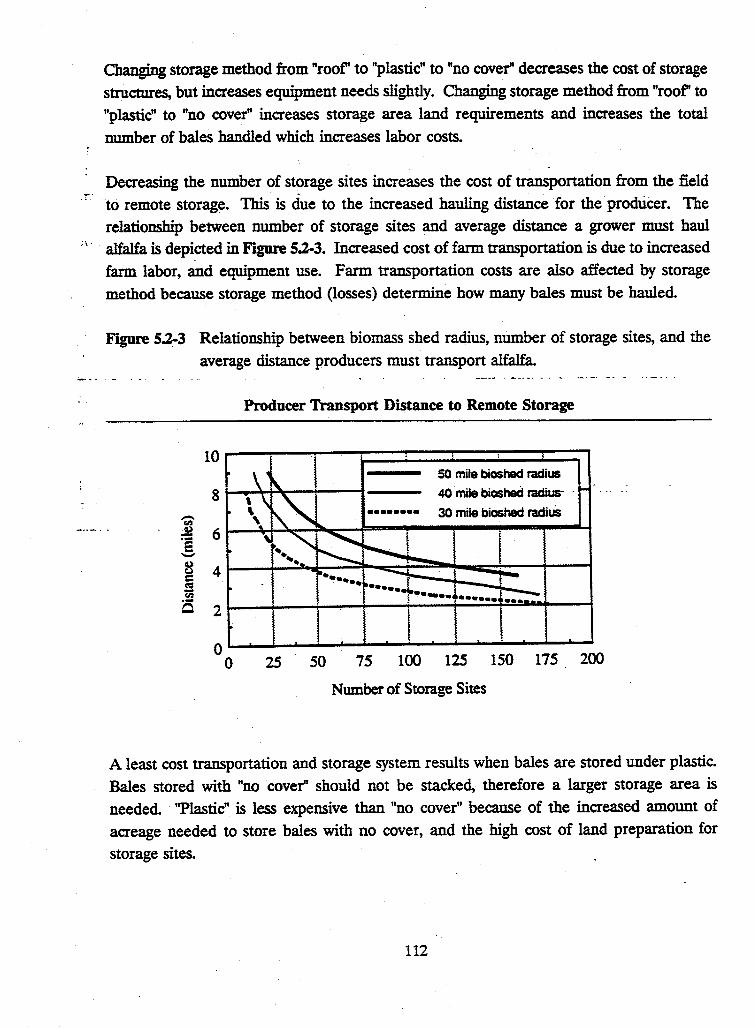
Changing storage method from "roof' to "plastic" to "no cover" decreases the cost of storage
structures, but increases equipment needs slightly. Changing storage method from "roof' to
"plastic" to "no cover" increases storage area land requirements and increases the total
number of bales handled which increases labor costs.
Decreasing the number of storage sites increases the cost of transportation from the field
·· to remote storage. This is due to the increased hauling distance for the producer. The
relationship between number of storage sites and average distance a grower must haul
;, · alfalfa is depicted in FigDl'e 5.2-3. Increased cost of farm transportation is due to increased
farm labor, and equipment use. Farm transportation costs are also affected by storage
method because storage method (losses) determine how many bales must be hauled.
FigDl'e 5.2-3 Relationship between biomass shed radius, number of storage sites, and the
average distance producers must transport alfalfa.
10
8
~ ~ 6 ·5 -«)
4 u = s en Q 2
0 0
Producer Transport Distance to Remote Storage
25 so
50 mile bioshed radius
40 ·mile bioshed radius- -
30 mile bioshed radius
75 100 125 150 175 200
Number of Storage Sites
A least cost transportation and storage system results when bales are stored under plastic.
Bales stored with "no cover" should not be stacked, therefore a larger storage area is
needed. "Plastic" is less expensive than "no cover" because of the increased amount of
acreage needed to store bales with no cover, and the high cost of land preparation for
storage sites.
112
Storage and transport costs of alfalfa $15.03/ton (no cover), $14.75/ton (plastic) and $18.22/ton (roof) are also linked to production costs. Total production of 679,016 tons/year (no cover), 656,680 tons/year (plastic), 644,372 tons/year (roof) reflect losses of dry matter in storage. Using a $60.00 per ton as the cost of production plus transportation, and storage costs, total costs for production, transportation, and storage are approximately $48.0 million (no cover), $46.6 million (plastic), and $48.1 million (roof). Total costs are within 3% indicating no significant cost difference between storage methods. However, as cited in
;section 33, storagelosses include not only dry matter loss but also quality losses. Quality •losses in alfalfa stored without protection would largely impact leaf meal products rather . than energy production characteristics. Therefore, although cost per quantity of alfalfa may . be similar for all storage options, quality considerations for leaf meal are important (see : section 6.3, and section 7.3).
: A_ :r.e_m:;ii_ning_ st.orage_ CQ:QSideration is that alfalfa stor~d. without a .~over Jlas a significant '.potential to increase in moisture content. Increased moisture increases transportation and '.drying costs.
~Conclusions
;.. All storage methods analyzed result in nearly the same cost when production aspects are considered. Therefore, storage method should be dictated by the quality of alfalfa leaf meal desired.
' * The cost of transportation from the farm to the storage area is dictated by the producers hauling distance. Hauling distance is a result of the number of storage sites. The number of storage sites significantly impacts the farm to storage transportation costs. The optimum number of storage sites is dictated by the amount of equipment needed to process the alfalfa in a given time frame.
* The cost of transportation from the storage site to the processing plant increases as the biomass shed radius increases. Therefore, it is important to restrict the biomass shed radius.
note: all weights expressed as tons are U.S. tons (2000 pounds)
113
S.3 Transportation Infrastructure
' The trunk highway network in the project area consists of 1~ 172 miles of federal and state
· highways. The federal and state roads are all paved and are maintained year round. There
l are -also over 4,500 miles of county and county state aid roads and over 7,000 miles of
. township roads laid out in a square mile grid system. Consequently there is a road almost
; every mile throughout the area. __ . _ _ ... . _ .
: Fifty-five percent or 2,498 miles of the county and county state aid roads in the biomass
shed are paved (Table 5.3-1). All county and county state aid roads are maintained year
: round. Township roads vary widely in quality and level of maintenance. Most township
; roads are graveled and passable in all seasons. A limited number of township roads have
dirt surfaces and are not maintained or snow-plowed. A small number of gravel township
roads do not receive snow-plowing; however, there are typically no residences or building
sites on roads that are not snow-plowed.
Traffic counts on the county roads within this region are typically less than 100 per day.
Township traffic counts are even less. There. are no short or long·t~rm -~pacjt_y J:?roblems
that would develop on the township and country roads as a result of traffic to and from
remote storage sites.
The number of paved county and all-weather county roads is such that selection of remote
storage sites can be easily accomplished. The criteria for adequate transportation from the
remote storage sites to the processing facility are that there be an all-weather road
(preferably paved), routine snow-plowing, and no permanent obstructions or hazards (e.g.,
narrow bridges or low hanging wires) that would cause indirect routing from the remote site
to the power plant.
The NSP power plant site and potential processing station are located on U.S. Highway 212
and Minnesota #23. U.S. 212 is a major east-west artery from Minneapolis to Yellowstone
National Park. It is the main access from the Granite Falls area to the Twin Cities.
Minnesota #23 cuts from the southwest comer of Minnesota to the Twin Ports of Duluth
and Superior. Both roads are considered strategic thoroughfares by the Minnesota
Department of Transportation. Both are excellent two lane highways in the Granite Falls
area. A passing lane is in place to the east of the plant. The highway widens to four lanes
as it goes west into and through Granite Falls.
114
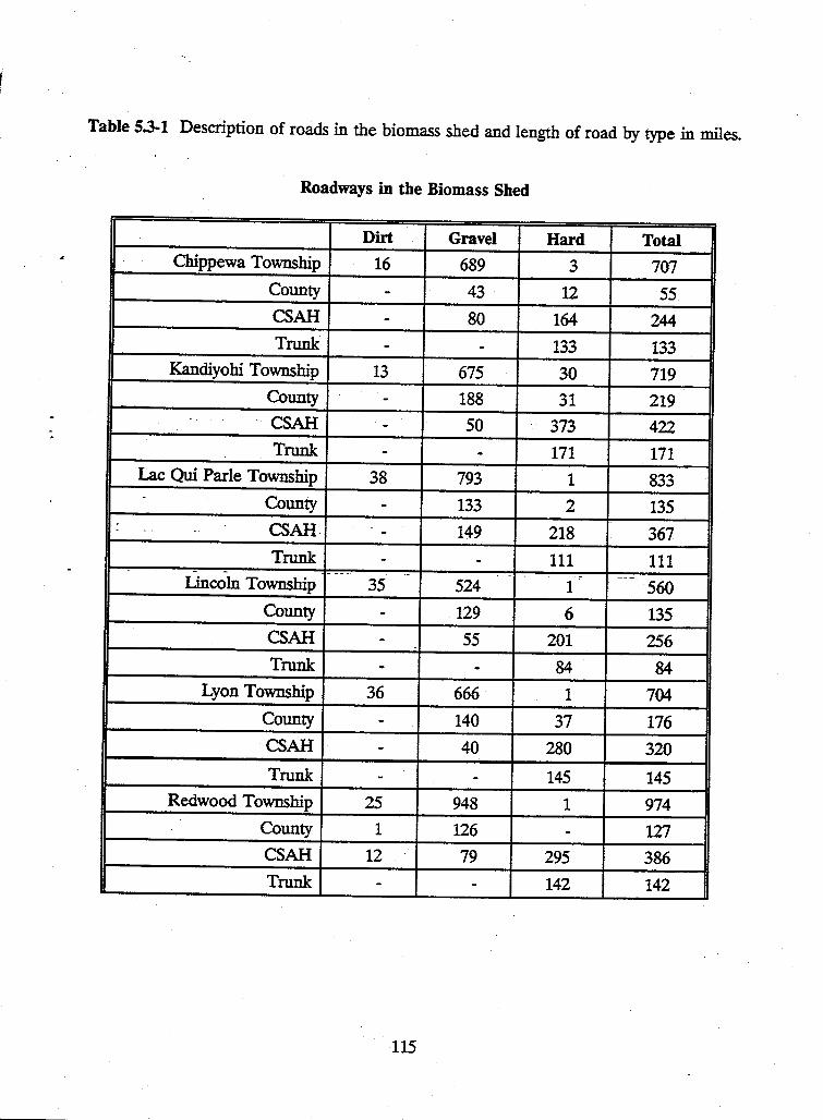
Table 5.3-1 Description of roads in the biomass shed and length of road by type in miles.
Roadways in the Biomass Shed
Dirt Gravel Hard Total Chippewa Township 16 689 3 707
County - 43 12 55 CSAH - 80 164 244 Trunk - - 133 133
Kandiyohi Township· 13 675 30 719 County - 188 31 219
.. · CSAH - 50 373 422 Trunk - - 171 171
Lac Qui Parle Township 38 793 1 833 - County 133 2 135 -- - .. CSAH. - 149 218 367
Trunk - - 111 111 - - -· ... _ - - . .. - -· . -··-Lincoln Township 35 524 1 560 County - 129 6 135 CSAH - 55 201 256 Trunk - - 84 84
Lyon Township 36 666 1 704 County - 140 37 176 CSAH - 40 280 320 Trunk - - 145 145
Redwood Township 25 948 1 974 County 1 126 - 127 CSAH 12 79 295 386 Trunk - - 142 142
115
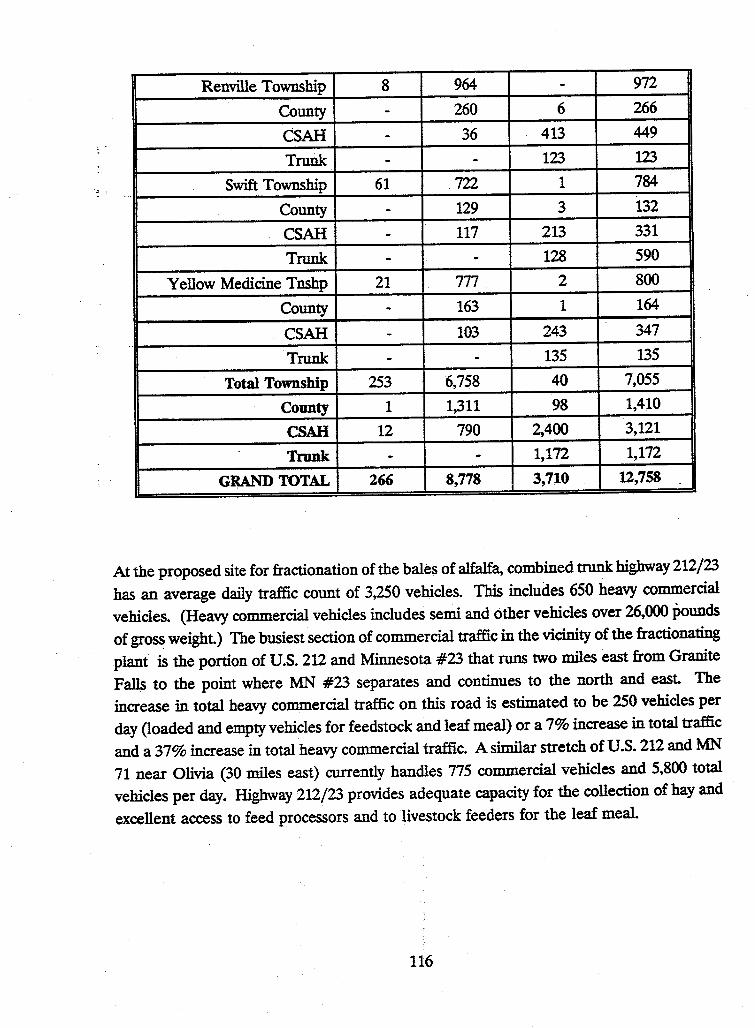
Renville Township 8 964 - 972
County - 260 6 266
CSAH - 36 413 449
Trunk - - 123 123
Swift Township 61 722 1 784
County - 129 3 132
CSAH - 117 213 331
Trunk - - 128 590
Yellow Medicine Tnshp 21 777 2 800
County - 163 1 164
CSAH - 103 243 347
Trunk - - 135 135
Total Township 253 6,758 40 7,055
County 1 1,311 98 1,410
CSAH 12 790 2,400 3,121
Trunk - - 1,172 1,172
GRAND TOTAL 266 8,778 3,710 12,758
At the proposed site for fractionation of the bales of alfalfa, combined trunk highway 212/23
has an average daily traffic count of 3,250 vehicles. This includes 650 heavy commercial
vehicles. (Heavy commercial vehicles includes semi and other vehicles over 26,000 pounds
of gross weight.) The busiest section of commercial traffic in the vicinity of the fractionating
plant is the portion of U.S. 212 and Minnesota #23 that runs two miles east from Granite
Falls to the point where MN #23 separates and continues to the north and east. The
increase in total heavy commercial traffic on this road is estimated to be 250 vehicles per
day (loaded and empty vehicles for feedstock and leaf meal) or a 7% increase in total traffic
and a 37% increase in total heavy commercial traffic. Asimilar stretch of U.S. 212 and MN
71 near Olivia (30 miles east) currently handles 775 commercial vehicles and 5,800 total
vehicles per day. Highway 212/23 provides adequate capacity for the collection of hay and
excellent access to feed processors and to livestock feeders for the leaf meal.
116
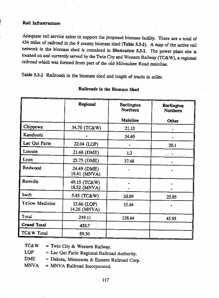
Rail Infrastructure
Adequate rail service exists to support the proposed biomass facility. There are a total of 434 miles of railroad in the 9 county biomass shed (Table 5.3-2). A map of the active rail network in the biomass shed is contained in Illustration 5.3-1. The power plant site is located on and currently served by the Twin City and Western Railway (TC&W), a regional railroad which was formed from part of the old Milwaukee Road mainline.
Table 5.3-2 Railroads in the biomass shed and length of tracks in miles.
Railroads in the Biomass Shed
Regional Burlington North em
Mainline
Chippewa 34.70 (Tc&W) 21.13
Kandiyohi - 34.40
Lac Qui Parle 22.04 (LQP) -Lincoln 21.68 . .(DME) .J.3 .. .
Lvon 25.75 (DME) 37.48
Redwood 24.49 (DME) -19.41 (MNVA)
Remille 49.15 (Tc&W) -1852 (MNVA) -
Swift 5.45 (Tc&W) 28.89
Yellow Medicine 13.66 (LQP) 15.44 14.26 (MNVA)
Total 249.11 138.64
Grand Total 433.7
Tc.&W Total 89.30
TC&W
LQP
DME
MNVA
= Twin City & Western Railway. = Lac Qui Parle Regional Railroad Authority. = Dakota, Minnesota & Eastern Railroad Corp. = MNV A Railroad Incorporated.
.. 117
Burlington Northern
Other
--
20.1
-..... . ...
--
--
25.85
-
45.95
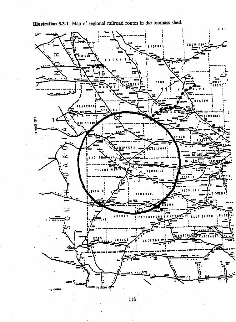
IDustration 5.3-1
... .....
10.-
Map of regional railroad routes in the biomass shed.
I ; I I . I . I
. . l
' t R 0 I
1 I T
l-. . -_, . .. _ I •lll. l E i1
·11.ac s .... i !
I \-.. . I
.... '-"1>1:'i: ____ ._i__;_! I . L..
I
118
The TC& W goes from Appleton to the Minneapolis-St. Paul area and has further trackage rights to Mississippi River ports such as Savage, Shakopee and Hastings. This line would provide access to barge transportation if the alfalfa leaf meal is to be marketed internationally. The TC&W connects to the Burlington Northern (BN) at its western terminus in Appleton. The BN owns that portion of the old Milwaukee Road mainline. This connection would provide access to West Coast markets and Pacific Northwest ports for leaf meal.
Excellent mainline service to the region is provided by the BN which has a north-south mainline that goes through Granite Falls. This BN mainline connects with the east-west BN rnainJine from the Twin Cities to the West Coast at Willmar. The TC&W can switch to the N-S mainline at Granite Falls. Because of these connections, the power plant site at Granite Falls is well suited for rail transportation of alfalfa leaf meal into statewide, _na,tional, and int~rnational mark~ts.
The other railroads in the region are either. shortline or regional railroads without direct connections to Granite Falls, (i.e., traffic to and from Granite Falls generally is switched outside of the biomass shed in the Twin Cities or other rail centers). The NMV A railroad is a regional railroad that goes east from Hanley Falls to Norwood with trackage rights on into the Twin Cities. The Dakota Minnesota and Eastern railroad is a regional railroad through the southern part of the biomass shed fromSouthDakota to the Mississippi River. Its traffic is oriented to the Mississippi River or switching points outside of the biomass shed. The BN manages a branchline for the Lac Qui Parle Regional Railroad Authority that runs from Madison to Hanley Falls. The BN has a local line runs that from the west border of the biomass shed to Benson where it terminates.
Rail Collection of Biomass
The use of rail to transport alfalfa biomass from remote transfer stations to the separator was analyzed. Approximately 44% of the biomass shed could be served by rail from remote sites established on the railroads. Twelve percent of the biomass shed could be served directly by the TC& W. Another ten percent of the biomass shed could be seived by switching from the BN mainline to the TC&W at Granite Falls. Another 22 percent could be seived by other railroads but would require 2 or more switches and/ or movement of up to 200 miles more than by road. It was determined that the rail transportation of round bales would have lower line haul labor and fuel cost and have less environmental impacts for at least 22% of the biomass shed. However, total handling and transportation costs even for that 22% would be higher for rail than truck.
119
Cost factors impacting the rail transportation of biomass:
a. The estimated time to load a bale on a rail car is 3 times that of trucks because of the
need to move bales greater distances to rail cars, to load three-high and to load from
only one side. Trucks can go closer to stored bales and are loaded only two-high from
both sides. The· unloading time would also be greater for rail than trucks.
b. Cost of rail sidings would average $250,000 per remote rail site. This is in addition to
land and warehouse cost.
c. A larger investment in rail rolling stock would be required proportionately than for
trucks for that portion of the shed served by rail. This is because of the slower
turnaround time of rail, even though standard flat cars loaded 3 high are able to carry
twice as many bales as a lowboy semi trailer and specially designed flat beds would have
a capacity 3 times that of a truck. Only two rail turns a day would be possible on the
TC& W, 1 tum .a day from the BN, and less than 1/2 turn a day from the lines where 2
~tche,s ~~.r~q.~~~-. . . ·-
. d A dual system for both truck and rail unloading facilities at Granite Falls would add to
the cost and complexity of the unloading facility at the separator.
Rail Transportation of Stems .
Under some conditions, it may be desirable to have one or more separator units located
a"'-ay from the Granite Falls plant. (For example, a feed mill or processor that has
contracted to use or sell the leaf meal.) Rail hopper cars will be the most cost effective way
to move stems from a remote separator to a plant located on the TC&W or the BN to the
Granite Falls facility.
120
5.4 Vehicle Regulations
Limits, Weights, and Permits
Minnesota law places restrictions on the size and configuration of trucks on public ·roads. The limits pertinent to the transportation of hay are generally width, !en~ and height, but not weight, due to the low density of the product. Straight trucks cannot exceed 40 feet in length. The combined length of semi-tractor and trailers cannot exceed 65'. The standard width for all vehicles is 8' 6" , which may be exceeded only by permit. There is a round bale permit that allows a maximum width of 11'6" for travel during daylight hours, only. There is anm1al cost for such a permit of $15. Height limit is 13' 6". Regulations for tractor-drawn implements would apply to the use of equipment such as specially designed hay hauling trailers. Lighting, width, and signing regulations would apply as they do to other farm implements travelling on public roads.
Road and bridge weight restrictions also limit total vehicle weight and the maximum weight per axle. Additionally, more restrictive seasonal weight restrictions on some roads during the spring thaw period are imposed. Virtually all county roads have limits of seven or nine tons per axle. Normally, state and federal roads are all nine or ten ton roads. Vehicles on ten ton roads are limited to 80,000 lbs. gross weight, 34,000 lbs per tandem axle, and 20,000 lbs. per single axle. Vehicles on nine ton roads are· limited to 73,280 lbs. gross weight, 32,000 lbs. per tandem axle and 18,000 lbs. per single axle. Limits on 7 ton roads are approximately 62,000 gross weight, 26,440 lbs per tandem axle and 14,000 lbs. per single axle. Limits on 5 ton roads are approximately 46,000 lbs gross weight, 18,889 lbs. P.er tandem axle and 10,000 lbs. on single axles. Maximum payloads then are approximately 28 tons, 24 tons, 18 tons, and 12 tons, for roads rated 10 tons, 9 tons, 7 tons, and 5 tons, respectively. Based on the density of alfalfa in round bales, weight limits won't be exceeded on county, state, or federal roads with seven ton or higher limits.
Township roads, have nine ton limits for most of the year. However, during the six week spring thaw period, township roads have five ton limits, unless otherwise posted. Some county roads are also posted at lower levels during the spring thaw. It is imperative that remote storage sites of large. round bales be located on roads that will have at least seven ton limits year round. As noted in section 5.3, an adequate network of local roads exists so that numerous locations will be available. A few rural bridges have been posted for gross weights less than our expected truckload weights; however, the redundancy of the square mile network is adequate to avoid any costly detours. The impact of such bridge restrictions may also be minimized by careful selection of transfer/storage sites.
121
5.5 Site Regulations
Dust, Noise, Runoff, Vermin, and Fire
State laws and local building codes and ordinances must be met before an alfalfa processing
facility could be built. The following issues are judged to be the most significant for this
type of plant. Efforts to control the noted issues are not judged expensive and can be
- accomplished on any site.
Fugitive Dust
State environmental air quality regulations require that not only emissions from a process
be controlled but that fugitive dust external to the process be controlled. Process emissions
are controlled by equipment selection and good maintenance practices.
Fugitive dust in the vicinity of the plant will be caused from truck traffic into the plant, the
pellet truck load-out facility, and the alfalfa truck unloading building. Except for the road
traffic, these sources can be characterized as the· entry and exit-points of the system. Road
dust will be minimized by cleaning and wetting. It is assumed that hay debris that may drop
from a truck is not an environmental problem because it is heavy enough that it will settle
along roadways and not threaten environmental air quality. Airborne dust that is stirred up
by passing trucks could carry some distance and cause discomfort for area residents and
plant employees. A program of sweeping or vacuuming the roadways around the plant will
need to be implemented if dust becomes a problem. The plant will need to develop a policy
regarding spraying the roadways with water in the summer when dry conditions are creating
a dust problem.
Some dusting is expected at the pellet load out facility. The dusting will be controlled by
a dust collector which pulls a vacuum around the pellet stream and carries away the dust.
This equipment is common throughout the grain industry. The alfalfa unloading area will
minimize the fugitive dust by using low impact methods of moving the bales off the trucks
and into the conveyor feed to the bale buster. The dust generated at the bale buster will
be captured by an airflow that pulls air and alfalfa through the bale buster. The air steam
will go to a cyclone separator where the dust material will be removed and the air exhausted
to the outside. The dust generated at this point has value because much of it will be leaf
material.
122
Noise Levels
The main source of noise from the plant will be from trucks delivering alfalfa and exiting. It is expected adherence to local noise ordinances for vehicular traffic will keep the noise to a tolerable level. Since the plant is in a valley, there will be only slight exhaust noise as the trucks come downhill. Most exhaust noise will come with unloaded trucks as they climb the hill on Hwy 212 leaving the plant. Most of the noise created within the processing plant will be contained by the building. For people working in the plant, warning signs will be po_ste9 in areas where OSHA noise limits are sometimes exceeded and protective equipment will be issued. The potential sources of higher noise levels are rotating equipment where the alfalfa is impacted or squeezed such as the bale buster, the hammermill, and the pellet mill. Fans can often be noisy from harmonics in tlie casing sheetmetal ~d ductwork. Good design practices and noise attenuators are two methods for minimizing fan noise.
Runoff Control
It is expected that no unusual runoff collection basins will be required for the alfalfa processing plant because of the biodegradable - non hazardous waste nature of the material. Normal good plant design practice will raise the building slightly above the surroundings so that rainfall will flow away from it. The roadway and staging area for trucks will be crested so that rainfall will flow away to ditches along side. Most of the rain will be absorbed into the soil on the site. Unusually heavy rainfalls may see some water reaching the river. This is not a problem for the reasons stated earlier.
Vermin Control
The plant will have on-site long term storage of stems sufficient to supply the gasifier for one week. To remove the opportunity for infestation of vermin, the storage area will be enclosed.
The plant will also have an active storage pile of bales to be processed during the night shift. The rotation of the pile will be daily and no additional vermin protection is required.
123
Fire Protection
The alfalfa processing plant will be equipped. with wall hydrants and hose stations at
strategic locations. The water supply will be from the city of Granite Falls.
The building housing the processing equipment will be constructed of nonflammable
material, primarily steel and concrete. The facility is expected to be very clean with daily
cleanup so that no accumulation of combustible material is allowed to develop. Good
maintenance practices will prevent equipment from leaking combustible material onto the
floor or into the building air space.
Equipment will be selected that has surface temperatures far below the ignition temperature
of the alfalfa stem and leaf even during upset conditions. The dryer heat source (burner)
will include safeguards to automatically shut down if temperatures limits are exceeded. All
motors will be equipped with overload protection to prevent overheating. Since the dryers
are a potential major source of fires, the entire line including fans, hammer mills, .and
pelletizer will shutdown automatically at preset temperature levels and an extinguishing
__ system will be activated. Temperature-sensors throughout the system will monitor for high
temperatures and alert the operator if encountered.
124
5.6 PRIVATE CONTRACTOR OPPOR1UNITIES
Typically a farmer will handle alfalfa production from seedbed preparation to market. This need not be the case. Many aspects of alfalfa production on a large scale could involve the use of specialty equipment, custom operators, and consultants. The following is a partial list of some of the areas where private contractors could become involved.
Seedbed Preparation and Alfalfa Seeding
Success in establishing alfalfa stands is sometimes elusive for farmers. Alfalfa seed is expensive on a per acre basis relative to other crops, and seedbed preparation requires some care. Quality seedbed preparation, alfalfa seeding with specialized equipment, and guaranteed results might emerge as packaged services offered by private contractors. These processes are required only once per field planted in a seven year biomass rotation. Although growers would typically be seeding some fields each year, individual ownership of specialized equipment is not economic, if underutilized. Therefore, the seedbed preparation and the alfalfa seeding phase of production could be an attractive contracting opportunity.
Crop Consultants
Maintaining the quality of an alfalfa stand· requires expertise in weed control, pest management, and soil fertility. Crop consultants may also be needed to advise growers of possible crop rotations, cutting schedules, and alfalfa varieties.
Alfalfa Harvest
The major labor and equipment requirement for alfalfa production occurs with the cutting and baling operations. Producers may choose to have private contractors come in to harvest their alfalfa. Custom contractors may be able to economically justify larger, more specialized equipment and maintain a labor force by contracting for full utilization of their equipment and moving from farm to farm.
Alfalfa Transport from Field to Remote Site
125
The transportation of alfalfa from the farm to remote storage areas may be most efficiently
accomplished through the use of specialized bale handling equipment. Hauling bales from
the field to remote storage sites is most cost effective as the number of bales hauled per
load increases. Becalise most standard farm equipment is not geared to transporting several
round bales at a time, there may be a market for contractors to handle/haul ten or more
bales per load from the field to the remote storage area with specialized trucks or tractor
drawn equipment.
Alfalfa Storage
Although an alfalfa cooperative will most likely be involved in choosing appropriate sites
for the remote storage areas, it is possible that these storage areas may be located on
private lands and operated priva~ly.
Alfalfa Testing
Quality of alfalfa. will be a major factor in the economics of growillg alfalfa. Laboratories
will need to test the alfalfa and characterize the protein percentage as well as leaf and stem
fractions. Growers will be paid based on the results of the testing. Testing laboratories may
be owned privately or by an established alfalfa growers' cooperative.
Alfalfa Transport from Remote Sites to the Processing Plant
At maximum capacity, about 2500 tons per day of alfalfa will need to be transported from
remote storage sites to the power plant or fractionation facility during 300 days of the year.
This transportation may be done by the cooperative or by private trucking companies.
126
6.1 Separation Process and Facilities and 6.2, Pr<>Ce$ing Costs. '
Pages 127-133 have been intentionally left blank. The infonnation initially contained on these pages can be found in Volume 4, Site Considerations, Chapter 3, Processing and Chapter 4, Maintenance and-Operating Costs. respectively.
- 127 - 133
CHAPTER 6. PROCESSING
6.3 EXPERIMENTAL SEPARATION STUDY
Hans-Joachim G. Jung,1,2,3 Carla S. Kuehn,2 and James G. Linn2
1Research Dairy Scientist, USDA:ARS
Departments 2 Animal Science, and 3 Agronomy and Plant Genetics,
University of Minnesota
Rationale
Studies of alfalfa development have demonstrated that the above ground biomass is predominately
leaf material (58% leaf: 42% stem) at the pre-bud stage of growth, but that the leaf proportion
declines with maturity to about 38-% leaf: 62% stem at the early seed pod stage (Albrecht et al.,
1987). Overall nutritional quality of the alfalfa plant for cattle feeding declines during this
maturation process; however, this decline in feeding value is restricted to the stem portion of
alfalfa. Fiber content increases and digestibility decreases for alfalfa stems from pre-bud through
early pod development (34 to 51 % and 75 to 52%, respectively) whereas leaf quality remains
almost constant (18-19% fiber and 81-80% digestibility) during this same period (Albrecht et al.,
1987). These data indicate that if alfalfa leaves can be effectively separated from stem material,
regardless of the maturity stage of the alfalfa. a high quality animal feedstuff could be produced as a
value added by-product from the biomass energy system.
Unlike research plot samples, field cured hay often suffers from leaf loss and reduction in protein
content during the drying and baling operations of commercial farming. It was necessary to
determine the leaf proportion and quality of the alfalfa leaves from typical hays to establish if
constant feeding values of alfalfa leaf product can be expected from a_ commercial operation as have
been observed under research conditions. An experimental separation and quality analysis of
alfalfa hay was conducted to address this question.
134
Protocol
Alfalfa hay samples were collected from four commercial hay auctions (Sauk Center [2x], Houston county, and Goodhue county) held in l\1innesota during December 1993 and January 1994. Hays sold at these auctions were produced throughout Minnesota, the Dakotas, and southern Canada. Hay is routinely sold at auction under six quality grades (prime and standards one, two, three, four, & five) determined by their relative feed value (RFV}: Lots of hay are sampled upon arrival at auctions by taking core samples with a special drill. These samples are then analyzed for neutral and acid detergent fiber concentration by near-infrared reflectance spectroscopy (NIRS). The fiber values determined by, NIRS are then used to calculate RFV for the hay lot. The alfalfa biomass project purchased one hay bale from each of 38 hay lots identified by the seller as being alfalfa hay. Hay lots sampled were nine prime, 12 standard one, nine standard two, six standard three and one each from standards four and five. These hay bales were small rectangular bales rather than the large round bales envisioned for the biomass energy system. It was not technically feasible for us to conduct the necessary separations of leaf and stem on large round bales. However, by sampling all the quality grades we have acquired data which is applicable to any hay package.
The sorting system empleyed was-a combination of mechanical and hand separation. Three slugs (small rectangular bales are divided into slugs of hay by the plunger mechanism of the baler) were collected from each bale, roughly equally spaced along the bale's length. These hay slugs were then dried in a 1 OO°F oven over-night to aid separation. Dried hay slugs were initially beaten with a baseball bat to dislodge most of the leaf material. The coarse stems were then removed and weeds, mostly grasses, were also separated from the alfalfa. Based on their weed content, 11 of the hay samples were excluded from the following analyses as they were greater than 100/o weeds. While some weediness can be expected in alfalfa hay, the principal investigators decided that questions of how weeds impacted the separation of alfalfa leaves and stems, and altered leaf meal quality, were beyond the scope of this feasibility study. The leaves and small pieces of broken stem remaining after the hand separation were then subjected to a mechanical sieving. The sieving mechanism was an oscillating screen separator developed by researchers to assess mean particle length of forage that has been chopped by silage choppers. There are five screens and a collection pan for the fines in this separator. The screen holes are square in shape and have nominal openings of 0.75, 0.50, 0.25, 0.156, and 0.046 inches. Screen thickness decreases from the largest screen size (0.50 in.) to the smallest (0.025 in.) to reduce passage of long, narrow particles through the screens. The leaf meal and small stem fragment samples from the bales were oscillated on this sieve for one minute. All screens and the pan contained
135
three largest screens contained primarily stem material, which was added to the coarse stems
collected during the hand separation. The two smallest screens and pan were identified as being the
leaf fraction, with the pan being the most pure leaf meal. Leaf, stem and weed fractions were
determined for each of the three slugs from each bale, corrected to a 100°C dry matter basis, and
then subsampled for nutritional analysis. The three subsamples from each bale were composited
prior to grinding to pass a 1-mm screen in a Wiley mill.
The hays were relatively dry as sampled (10.8% moisture) and easily separated after the minor
additional drying. This additional drying may or may not be necessary in an industrial facility.
Results
Based on the analysis of fiber content of these hays, relative feed values (RFV) were recalculated
and each hay bale was assigned to its appropriate quality grade. As expected, there was some
shifting of hays from the originally assigned quality grade for the hay lot compared to the actual
quality of the bale as sampled. The correlation between the hay lot quality grade and the actual bale
quality grade was r = 0.55 (P<:0.01). All subsequent discussion is based on these actual quality
gr.idc~ for the bales with the following representation among the grades: five prime bales, six
standard one. six standard two, eight standard three, and two standard five (Table 6.3-1).
136
Table 6.3-1
Quality Grade
Prime Standard One Standard Two
Proportions of leaf, stem and weeds in commercial alfalfa hay bales from five of the six common quality grades.
Alfalfa
Number of Bales Leaf Stem Weeds
% dry matter-----5 60.Sa 36.Sa 2.6 6 49.3b 47.9b 2.9 6 49.9b 47.9b 2.3
Standard Three 8 38.6c 57.9c 3.5 Standard Four . not sampled Standard Five 2 3 l.3c 68.2d 0.5
Combined 27 47.0 50.3 2.7
abed Means in the same column not sharing a superscript differ (P<0.05).
137
The hay quality grades largely reflect differences in proportions of leaf (Table 6.1-1). The
highest quality hay had the largest proportion leaf, which declined markedly in the lower .
quality grades. Overall, the alfalfa bay contained 47.0% leaf, 50.3% stem and 2.7% weed.
Based on these results, we conclude that the higher the quality grade of the hay provided to the
biomass separation facility, the higher the expected yield of leaf meal.
The reader is reminded that 11 of 3 8 alfalfa hay bales collected were excluded from the analysis
because they contained greater than 100/o weeds. It must also be emphasized that the yield of leaf
meal, and its subsequent nutrient content, is directly a function of the separation procedure
employed. The presence of leaves on the stem screens and stem :fragments on the leaf screens have
caused some undetennined bias in the results for leaf meal yield and quality. Compared to careful hand
separation of research plot alfalfa samples, the leaf yields seem quite reasonable. But as reported in the
. nutritional analysis section 7.3, the presence of even small amounts of stem in the leaf meal results in
significant reductions in leaf meal quality. Actual leaf meal yield and quality depend directly on the
effectiveness of the industrial separation procedure developed for the biomass energy system.
138
Quantity:
CHAPTER 7. PRODUCT CHARACTERISTICS
7.1 Electricity
C.V.Hanson Center for Alternative Plant and Animal Products
University ofMinnesota
The biomass energy production system will produce 7 5 MW of electricity and is designed to operate at a capacity factor of 800/o or higher. The electricity produced has access to the grid at the existing NSP power plant sub-station in Granite Falls. Significant sub-station upgrade is not anticipated to be necessary for this additional electric power output.
75 MW of electricity amounts to about 1% ofNSP's current system capacity of approximately 7000 MWe. The proposed cost-shared demonstration of sustainable biomass energy production will result in a cost of electricity that is competitive with 'new generation' power plants and may be accomplished at a much smaller scale. Smaller scale electric power production can benefit utilities by reducing the need for grid and capacity upgrades of their distnbution systems and by stimulating economic development within their service temtories. New business, new customers, and new technologies will help maintain a competitive edge for progressive power companies in an increasingly competitive marketplace.
Quality:
The proposed biomass electric power production system is designed to supply baseload power. Baseload power is the backbone of a power supply system. Baseload power systems are designed to operate at maximum efficiency on a nearly continuous basis. The proposed system has a design capacity factor of 80%. This means that this system would operate 800/o of the time, day and night, year round.
139
Baseload power production systems are said to be dispatchable. Power production systems are
dispatched relative to the cost of electricity (COE) that they are producing. This results in the lowest
rates for utility customers and the highest marginal returns for the utility.
Cost ofElectricity:
Many factors determine the overall COE including the capital cost of the power plant, the cost of fuel,
··and environmental considerations such as sulfur dioxide offset credits, potentially carbon dioxide offset
credits and other real costs of electric power production. The COE for the proposed biomass power
plant will likely be around 6.5 cents per kilowatt hour (kWh). See Volume 3 - Business Plan for
details. This is comparable to todays average retail price of electricity in the Upper :Midwest. Many
regions of the country currently pay much higher retail rates, for example, over I 0 cents on the east
and west coasts.
The COE for this first of a kind biomass power plant may be higher than 2nd generation biomass
power plants. However, 6.5 cents/kWh is a very reasonable cost for the demonstration of 'new
generation' renewable biomass electric production. The actual effect on consumer rates based on 75
MW of biomass power production in NSP's 7000 MW system would be about a 1% increase on the
difference between NSP's average COE (around 3.5 cents/kWh) and the biomass COE of 6.5
cents/kWh (about 1% of3 cents/kWh= 0.03 cents/kWh to the customer).
The benefits to :Minnesota agriculture, our rural economy, our environment, and to NSP far outweigh
an estimated increase of0.03 cents/kWh on our electric bills. The real issue is not the COE but of the
risk involved in a new venture. Carefull analysis of risk by the biomass producers and by the utility is
the next step.
By-products:
The ash remaining after gasification of a]falfa is expected to returnable to the land and may have value
as a soil ammendment or fertilizer. The character and value of this by-product of electricity production
needs to be determined. Although the creation of a hazardous waste product like coal ash is not
expected, thorough economic and environmental analysis cannot be made without more information on
the compositon and plant availability of the ash. The following study has been designed to answer
those questions.
140
Ash By-product
Characterization and Agronomic Use of Ash Generated from Alfalfa Biomass Gasification
Carl Rosen1, Michael Russellei+2, and Edward Nater1
Department of Soil Science, University of Minnesota 2uSDA Soil Scientist
Background and Rationale
Alfalfa biomass has been proposed to be used as feedstock material for the production of electrical power by gasification and combustion. Innovative combustion turbine technology designed for biomass has been developed by the Institute of Gas Technology (IGT) in Chicago. Unlike conventional combustion turbines that operate under oxidizing conditions, the unit ·developed by IGT operates under reducing conditions. Advantages of this technology include more efficient energy production and reduced air emissions. However, as With.. oonveiit:fonal combuStion technology, aD. ash residue remains after the material is gasified. The characteristics of the ash are dependent on the material used and the conditions of combustion/ gasification.
With limited landfill space, one of the major challenges in society today is to recycle or find beneficial uses of generated wastes. Sustainability of the alfalfa gasification process is partially dependent upon finding a suitable end use for the ash. An ultimate intent of using alfalfa biomass as an energy source is to apply the ash generated from the gasification process on land to recycle nutrients for crop production. Thus, a nearly complete nutrient cycle can be achieved.
Before land application of the ash can be made, physical and chemical properties of the ash need to be known. While numerous studies have been conducted evaluating the use Qf various ash products as soil amendments, there is no information related to ash that has been generated under reducing conditions. It is therefore impossible to extrapolate results from previous studies to predict whether beneficial or potentially harmful effects of alfalfa gasification ash might Occur if applied to soil.
141
Physical characterization and mineralogical make up of the ash needs to be known so that
estimates of weathering of the ash can be made. Information on mechanisms controlling
the solubility of elements present in waste materials can be used to determine the long term
behavior of both beneficial and potentially deleterious elements in the environment. If the
solubility controlling mechanisms are known, informed management decisions can be made
to maximize the benefits and minimize the problems resulting from waste product
application to agricultural land The effect of the ash on soil chemical properties and crop
response needs to be known so that predictions can be made for appropriate rates to apply
as well as frequency of application.
Objectives
1) Physically and chemically characterize the ash.
__ 2) Model secondary solid formation and elemental solubilities in ash-amended soils.
3) Evaluate crop response to ash-amended soil in greenhouse experiments.
4) Determine effects of land application of ash on crop production and the environment.
Expected Results
From this research, an economic projection on the value ($/ton) of the ash based on
nutrient availability and shipping costs will be made. Enough information will be obtained
to develop best management practices for use of the ash in crop production.
142
7 :Z Co-products
C.V. Hanson Center for Alternative Plant and Animal Products
University of Minnesota
Alfalfa leaves may be processed into many valuable products. Alfalfa leaf meal protein for cattle feed is the basic alfalfa leaf product focused on in this _study. But just like we process com and soybeans into many renewable products, we can process alfalfa leaves into many valuable renewable products. Other alfalfa leaf products currently being produced at some level include: alfalfa leaf pigments (xanthophylls), liquid protein products for human and animal consumption, fragrances for shampoos and cosmetics, and natural biological molecules for pharmaceuticals. Further investigation of these and other alternative products will proceed as a natural research and development" activity of alfalfa biomass energy production.
Alfalfa has also been used extensively in research for the production of "secondary plant metabolites", essentially using the machinery of the plant to produce specific high value biological molecules, such as the enzymes needed for processing plant material into ethanol. Using plants as factories for the production of everything from plastics to pharmaceuticals is well underway. Renewable plant derived products may someday soon replace many synthetic and petroleum-derived fuels and feedstocks. The commercial production of secondary plant metabolites has been demonstrated, but not to my knowledge commercially in alfalfa, yet. This is an exciting area of research and development, but not something to build a business ~n. I include this here to allow speculation on how biomass energy production and agricultural processing may continue to be integrated in the future. The processing of high value plant products and biomass energy production can provide potent economic synergy, as demonstrated by alfalfa biomass energy production.
The production of only electricity from a biomass energy crop is not economically viable, has not been demonstrated, and is likely a wasteful use of renewable plant resources. Dedicated energy crops like alfalfa also provide other valuable feedstock resources. The 'best use' of biomass resources can and will result in sustainable biomass power production and improve the sustainability of current agricultural systems through the integration of energy and agricultural production. This concept may be adapted for many different agricultural cropping systems. 'Best use' of crop resources, not the singular use of crops for energy production, but an integrated approach that maximizes energy and co-product value.
143
Rationale
7.3 Nutritional Characteristics
Stem and Leaf Meal Nutritional Characteristics
Hans-Joachim G. Jung,1.2.3 Carla S. Kuehn,2 and James G. Llnn2 -1Research Dairy Scientist, USDA:.ARS
Departments 2 Animal Science, and 3 Agronomy and Plant Genetics,
University of Minnesota
The economic value of the alfalfa leaf meal co-product will be a function of its nutritional characteristics. Ultimately, feeding value of a new feedstuff can only be accurately assessed through animal feeding trials. Because of the unavailability of an alfalfa leaf meal product in bulk at this time, and the short time frame for the current feasibility study, a number of
_. laboratory measurements of nutrient content and value were utilized to provide an estimate of the nutritional value of the alfalfa leaf meal to livestock feeding. The alfalfa stem material was also analyzed to provide further information on its composition and to evaluate the efficiency of leaf-stem separation.
The primary objective of the analysis for leaf- meal quality was to determine if leaf meal
quality varies depending on the overall quality of the hay produced. As pointed out in section 6.3, alfalfa leaves do not change appreciably in quality with time while they are alive.
However, it is uncertain if differences in leaf quality are generated during the harvesting, drying and storage phases of hay production. This portion of the study addresses this point
using samples of commercial hays.
144
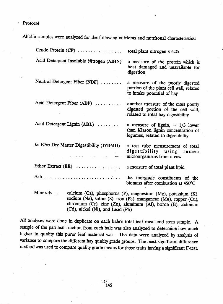
Protocol
Alfalfa samples were analyzed for the following nutrients and nutritonal characteristics:
Crude Protein (CP) . . . . . . . . . . . . . . . . . total plant nitrogen x 625
Acid Detergent Insoluble Nitrogen (ADIN) a measure of the protein which is heat damaged and unavailable for digestion
Neutral Detergent Fiber (NDF) a measure of the poorly digested portion of the plant cell wall, related to intake potential of hay
Acid Detergent Fiber (ADF) another measure of the most poorly digested portion of the cell wall, related to total hay digestibility
Acid Detergent Llgnin (ADL) . . . . . . . . . a measure of lignin, - 1/3 lower than Klason lignin concentration of legumes, related to digestibility
In Vztro Dry Matter Digestibility (IVDMD) a test tube measurement of total digestibility using rumen
-microorganisms from a cow
Ether Extract (EE) a measure of total plant lipid
Ash . . . . . . . . . . . . . . . . . . . . . . . . . . · . . . the inorganic constituents of the biomass after combustion at 4500C
Minerals calcium (Ca), phosphorus (P), magnesium (Mg), potassium (K), sodium (Na), sulfur (S), iron (Fe), manganese (Mn), copper (Cu), chromium (Cr), zinc (Zn), aluminum (Al), boron (B), cadmium (Cd), nickel (Ni), and Lead (Pb)
All analyses were done in duplicate on each bale's total leaf meal and stem sample. A sample of the pan leaf fraction from each bale was also analyzed to determine how much higher in quality this purer leaf material was. The data were analyzed by analysis of variance to compare the different hay quality grade groups. The least significant difference method was used to compare quality grade means for those traits having a significant F-test.
'46 145
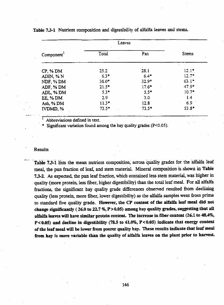
Table 7.3-1 Nutrient composition and digestibility of alfalfa leaves and stems.
Component1
CP. %DM ADIN, % N NDF, %DM ADF. %DM ADL, %DM EE. %DM Ash. %DM IVDMD, %
Total
25.2 6.3*
36.0* 21.5*
5.3* 2.9
11.3* 73.5*
1 Abbreviations defined in text.
Leaves
Pan
28.1 6.4*
32.9* 17.6* 5.5* 3.0
12.8 73.5*
* Significant variation found among the hay quality grades (P<0.05). ·
Results
Stems
12.1 * 12.7* 63. l * 47.9*. 10.7*
1.4 6.9 .
53.8*
Table 7.3~1 liSts the mean nutrient composition;· across quality grades for the alfalfa leaf
mea4 the pan fraction of leaf, and stem material. Mineral composition is shown in Table
7.3-2. As expected, the pan leaf fraction, which contained less stem materia4 was higher in
quality (more protein, less fiber, higher digestibility) than the total leaf meal. For all alfalfa
fractions, the significant hay quality grade differences observed resulted from declining
quality (less protein, more fiber, lower digestibility) as the alfalfa samples went from prime
to standard five quality grade. However, the CP content of the alfalfa leaf meal did not
change significantly ( 26.0 to 22. 7 %, P > 0.05) among hay quality grades, suggesting that all
alfalfa leaves will have similar protein content. The increase in fiber content (26.1 to 48.4%,
P < 0.05) and decline in digestibility (78.S to 61.0%, P < 0.05) indicate that energy content
of the leaf meal will be lower from poorer quality hay. These results indicate that leaf meal
from hay is more variable than the quality of alfalfa leaves on the plant prior to harvest.
146
Table 7.3-2 Elemental composition of alfalfa leaves and stems.
Leaves
Element Total Pan Stems
Ca, %DM 1.88 2.29 0.70 P,%DM 0.33 0.34 0.24 Mg,%DM 0.37 0.40 0.20* K.%DM 2.31* 2.04* 2.18 Na, %DM 0.04 0.04 0.05 S.%DM 0.32* 0.36* 0.12. Fe. ppm 184.18 288.92 56.13 Mn. ppm 63.44 88.35 19.78 Cu. ppm 8.01 9.11 6.62 Cr. ppm 0.81 0.94 0.47 Zn. ppm 24.94 28.23 16.46* Al. ppm 141.05 241.54 37.04 B. ppm 42.91 * 51.86* 18.67* Cd. ppm 0.17 0.20 0.11 ~i. ppm. 2.28 2.56 1.34 Pb. ppm 1.22 2.39 0.51
• Significant variation found among the hay quality grades (P<0.05).
Data from the Joint US - Canadian Feed Composition Tables for alfalfa leaf meal indicate a CP content of 30%, NDF of 20%, ADF of 15%, Ca of 2.5%, and P of 027%. The quality of the total leaf meal and the pan leaf fraction from our study was lower than these publi~hed data. Other data in the scientific literature indicate that the 30% CP and 20% SDF values for pure leaf meal are correct (Albrecht et al., 1987; Hatfield et al., 1994). The fact that our values are lower, plus the visual observations made during the separation pr~ indicate that the separation method we used was inadequate to achieve a pure leaf meal. 'lllis lack of complete elimination of stems from the leaf meal will negatively impact the rttetin& value of this product. As for leaf yield, the industrial separation technology utilized will have a major impact on the economic value of the leaf meal by-product from this biomass energy system.
147
Rationale
- 7.4 Ration Formulation
Hans-Joachim G. Jung,1.2.3 James G. Llnn2 and Carla S. Kuehn,2 and 1Research Dairy Scientist, USDA:ARS
Departments 2 Animal Science, and 3 Agronomy and Plant Genetics,
University of Minnesota
To determine an economic value for the leaf meal by-product in livestock feeding, this new
feedstuff must be evaluated in typical diet formulations that will meet the nutritional
requirements of the target livestock species and be acceptable to the producer. This is
accomplished by formulating rations to meet the requirements of the animals and forcing
the new feedstuff to compete with the typical ingredients available, and at realistic prices
for those ingredients. We have taken this approach for dairy cattle feeding in the Upper
Midwest.
While alfalfa leaf meal could be effectively fed to poultry and swine, consultation with
experts for these species suggest that producer acceptance of this new feedstuff would be
poor. The problem is primarily one of energy content. The moderate fiber concentration
of the leaf meal reduces the energetic value of the feed for nonruminant livestock and,
therefore, will slow their growth rate. Reductions in growth rate have serious economic
repercussions. The requirement for supplemental protein for beef cattle feeding is relatively
small. They could certainly utilize alfalfa leaf meal, but generally the lowest cost protein
supplement is adequate. Non-protein nitrogen, such as urea, is often fed and is very
inexpensive. As a result of this information we chose not to evaluate alfalfa leaf meal for
species other than dairy cattle at this time.
Protocol
Rations were formulated for dairy cows in early (90 lb of milk/day) and mid (60 lb of
milk/day) lactation, as nutrient requirements differ substantially. The nutrient constraints
included in the diet formulations are listed in Table 7.4-1. Feed ingredient combinations
of formulated rations meet or exceed these constraints. High producing, early lactation cows
require more feed, higher concentrations of protein, energy (net energy for lactation, NEJ, and minerals, and lower concentrations of fiber than do cows with lower levels of milk
148
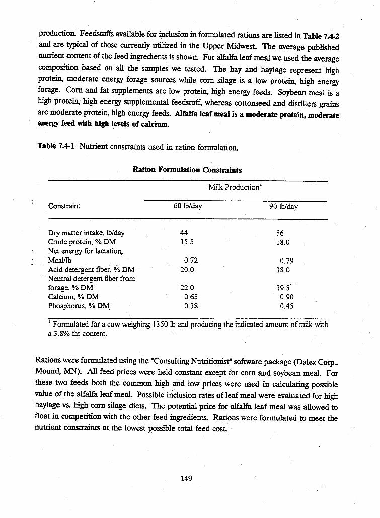
production. Feedstuffs available for inclusion in formulated rations are listed in Table 7.4-2 and are typical of those currently utilized in the Upper Midwest. The average published nutrient content of the feed ingredients is shown. For alfalfa leaf meal we used the average composition based on all the samples we tested. The hay and haylage represent high protein, moderate energy forage sources while com silage is a low protein, high energy forage. Com and fat supplements are low protein, high energy feeds. Soybean meal is a high protein, high energy supplemental feedstuff, whereas cottonseed and distillers grains are moderate protein, high energy feeds. Alfalfa leaf meal is a moderate protein, moderate energy feed with high levels of calcium.
Table 7.4-1 Nutrient constraints used in ration formulation.
Ration Formulation Constraints
Milk Production 1
Constraint 60 lb/day 90 lb/day
Dry matter intake. lb/day 44 56 Crude protein, % DM 15.5 18.0 Net energy for lactation, Meal/lb 0.72 0.79 Acid detergent fiber~ % DM 20.0 18.0 Neutral detergent fiber from forage. %DM 22.0 19.5 Calcium. % DM 0.65 0.90 Phosphorus, % DM. 0.38 0.45
1 Formulated for a cow weighing 1350 lb and producing the indicated amount of milk with a 3. 8% fat content.
Rations were formulated using the •consulting Nutritionist• software package (Dalex Corp., Moun4 MN). All feed prices were held constant except for com and soybean meal. For these two feeds both the common high and low prices were used in calculating possible value of the alfalfa leaf meal. Possible illciusion rates of leaf meal were evaluated for high haylage vs. high com silage diets. The potential price for alfalfa leaf meal was allowed to float in competition with the other feed ingredients. Rations were formulated to meet the nutrient constraints at the lowest possible total feed cost.
149
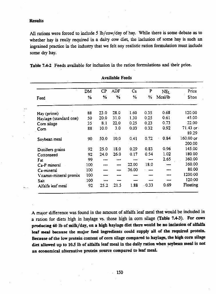
Results
All rations were forced to include 5 lb/ cow/ day of hay. While there is some debate as to
whether hay is really required in a dairy cow diet, the inclusion of some hay is such an
ingrained practice in the industry that we felt any realistic ration formulation must include
some dry hay.
Table 7.4-2 Feeds available for inclusion in the ration formulations and their price.
Feed
Hay (prime) Haylage (standard one) Corn silage Corn
Soybean meal
Distillers grains Cottonseed Fat Ca-P mineral Ca-mineral Vitamin-mineral premix Salt Alfalfa leaf meal
DM
%
88 50 35 88
90
92 92 99
100 100 100 100 92
Available Feeds
CP ADF % %
23.0 28.0 20.0 31.0
8.1 22.0 10.0 3.0
50.0 10.0
25.0 18.0 24.0 26.0
25.2 21.5
Ca %
1.60 1.30 0.25 0.03
0.41
0.29 0.17
22.00 36.00
1.88
P NEt % McaVlb
0.35 0.68 0.25 0.61 0.23 0.73 0.32 0.92
0.72 0.84
0.83 0.96 0.54 1.02
2.65 18.0
·0.33 0.69
Price
$/ton
120.00 45.00 22.00
71.43 or· 89.29
160.00 or 200.00 145.00 180.00 360.00 360.00
80.00 1200.00 120.00
Floating
A major difference was found in the amount of alfalfa leaf meal that would be included in
a ration for diets high in haylage vs. those high in com silage (Table 7.4-3). For cows
producing 60 lb of milk/day, on a high haylage diet there would be no inclusion of aitalfa
leaf meal because the major feed ingredients could supply all of the required protein.
Because or the low protein content of com silage compared to haylage, the high com silage
diet allowed up to 10.5 lb of alfalfa leaf meal in the daily ration when soybean meal is not
an economical alternative protein source compared to leaf meal.
150
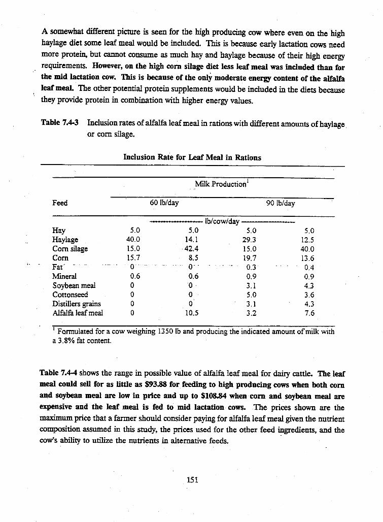
A somewhat different picture is seen for the high producing cow where even on the high haylage diet some leaf meal would be included. This is because early lactation cows need more protein, but cannot consume as much hay and haylage because of their high energy requirements. However, on the high com silage diet less leaf meal was included than for the mid lactation cow. This is because of the only moderate energy content of the alfalfa leaf meal. The other potential protein supplements would be included in the diets because they provide protein in combination with higher energy values.
Table 7.4-3 Inclusion rates of alfalfa leaf meal in rations with different amounts of haylage or com silage.
Feed
Hay Haylage Com silage Com Fat· - ..
Mineral Soybean meal Cottonseed Distillers grains Alfalfa leaf meal
Inclusion Rate for Leaf Meal in Rations
Milk Production 1
60 lb/day
lb/cow/day 5.0 5.0 5.0
40.0 14.1 29.3 15.0 42.4 15.0 15.7 8.5 19.7 o·. ··- o-. . . - ·- . 0.3 0.6 0.6 0.9 0 O· 3.1 0 0 5.0 0 0 3.1 0 10.5 3.2
90 lb/day
5.0 12.5 40.0 13.6 0-4 0.9 4.3 3.6 4.3 7.6
1 Formulated for a cow weighing 1350 lb and producing the indicated amount of milk with a 3.8% fat content.
Table 7.4-4 shows the range in possible value of alfalfa leaf meal for dairy cattle. The leaf meal could sell for as little as $93.88 for feeding to high producing cows when both com and soybean meal are low in price and up to $108.84 when· com and soybean meal are expensive and the leaf meal is fed to mid lactation· cows. The prices shown are the maximum price that a farmer should consider paying for alfalfa leaf meal given the nutrient composition assumed in this study, the prices used for the other feed ~edients, and the cow's ability to utilize the nutrients in alternative feeds.
151
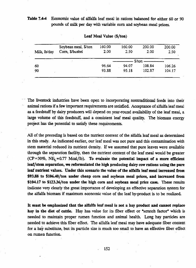
Table 7.4-4 Economic value of alfalfa leaf meal in rations balanced for either 60 or 90
pounds of milk per day with variable com and soybean meal prices.
Leaf Meal Value ($/ton)
Soybean meal, $/ton Milk, lb/day Com, $/bushel
60 90
160.00 2.00
96.64 93.88
160.00 2.50
200.00 2.00
----$/ton----94.07 108.84 95.18 102.87
200.00 2.50
106.26 104.17
· · · The livestock industries have been op~n to incorporating nontraditional feeds into their
animal rations if a few important requirements are satisfied. Acceptance of alfalfa leaf meal
as a feedstuff by dairy producers will depend on year-round availability of the leaf meal, a
large volume of this feedstuff, and a consistent leaf meal quality. The biomass energy
project has the. potential to satisfy these requirements.
All of the preceding is based on the nutrient content of the alfalfa leaf meal as determined
in this study. As indicated earlier, our leaf meal was not pure and this contamination with
stem material reduced its nutrient density. If we assumed that pure leaves were available
through the separation facility, then the nutrient content of the leaf meal would be greater
{CP=30%, NEi, =0.77 Meal/lb). To evaluate the potential impact of a more efficient leaf/stem separation, we reformulated the high producing dab:y cow rations using the pure
leaf nutrient values. Under this scenario the value of the alfalfa leaf meal increased from $93.88 to $16'.40/ton under cheap com and soybean meal prices, and increased from $104.17 to $123.36/ton under the high com and soybean meal price case. These results
indicate very clearly the great importance of developing an effective separation system for
the alfalfa biomass if maximum economic value of the leaf by-product is to be realized.
It must be emphasized that the alfalfa leaf meal is not a hay product and cannot replace hay in the diet of cattle. Hay has value for its fiber effect or •scratch factor- which is
needed to maintain proper rumen function and animal health. Long hay particles are
needed to achieve this fiber effect. The alfalfa leaf meal may have adequate fiber content
for a hay substitute, but its particle size is much too small to have an effective fiber effect on rumen function.
152
7.5 Bypass Protein Enhancement
Hans-Joachim G. Jung, W Marshall Stern, 2 James G. Linn2 and Carla S. Kuehn, 2
· 1Research Dairy Scientist, USDA:ARS
Rationale
Departments 2 Animal Science, and 3 Agronomy and Plant Genetics, University of Minnesota
The preceding ration formulation was based on total protein content of the feedstuffs and animal requirements for protein concentration. This is the most common manner in which rations are currently formulated; however, many of the larger and more productive dairy herds are now also considering protein digestibility characteristics of their feeds in formulating diets. There are two primary concerns with protein digestibility of feeds for dairy cattle. First, for some feeds such as alfalfa haylage, too much of the protein is digested in the rumen by the microorganisms residing there. The result is that too little intact feed protein is available for intestinal digestion and absorption. Feeding of protein sources with reduced mminaJ digestion has shown increased milk production because the amino acid requirements of the cow are more completely satisfied. These proteins are often referred to as bypass proteins because their low ruminal digestibility. The second concern about protein digestibility relates to these bypass proteins. Some proteins are so effectively protected from digestion that they not only bypass mminal digestion, but are also not digested in the small intestine. This results in a wastage of protein and added feed costs.
Numerous chemical treatments, including use of compounds such as formaldehyde, have been used to increase the bypass protein value of alfalfa. However, these chemical treatments often raise questions of safety and environmental pollution. There is one report of heat treatment of alfalfa hay to increase protein bypass (Yang et al., 1993). These workers reported that heat treatment significantly decreased mminal protein digestibility in an in vitro system. Steam heating of the hay increased the bypass value more quickly than dry heat, but a large amount of heat damaged (ADIN), and presumably unavailable, protein was formed by extended heat treatment. A companion animal study (Broderick et al., 1993) found an improvement in protein utilization after steam heating of alfalfa, but a decline in energy availability from the hay'. However, the degree of reduction in mminal degradability of this heat treated hay was insufficient to convert it into a bypass protein feedstuff.
153
- Because the combined-cycle power generation system planned for this alfalfa biomass energy
system would have some waste heat available after electricity generation, the research team
decided to evaluate the potential of using heat to increase the protein bypass value of the
alfalfa leaf meal to increase its nutritional and economic value. The pan fraction of the leaf
meal was chosen for heat treatment, as a bypass protein source should have not only a low
rnmina] protein digestibility, but also a high protein concentration.
Protocol
A composite sample of alfalfa leaf meal was made from the hay bales sampled and
separated. This hay was heated in a forced air oven for 0, 15, 30, · 60 or 120 minutes at
150°C. This temperature was chosen, as it is the approximate temperature of the waste heat
stream available from the steam turbine generator. The treatments were done on three
separate batches of leaf meal to allow statistical evaluation of the effectiveness of the
treatment. The control (0 minutes heating) and treated leaf meal samples were evaluated
for unavailable protein (ADIN), soluble protein content, rnminal rate and extent of digestion
rising nylon bags suspended in the rumen of a dairy cow, and in vitro intestinal protein
digestion of the residual protein after mminal incubation. From these measurements
·- intestinally absorbable dietary-protein-and-total tract.unavailable- protein were calculated.
Results
As expected, heating of the alfalfa leaf meal increased the proportion of the protein which
was heat damaged and unavailable for digestion (Table 5.3-1). The soluble protein also
declined as a result. Rnminal protein digestibility was reduced from 64.9% in the control
to 535% after 120 minutes of heating. Rate of protein digestion was only reduced at the
longest treatment time. Most of the increase in the amount of protein that bypassed
rnminal digestion was protein that was available for intestinal digestion, as shown in the
increased intestinal protein digesttbility. The net result was an increase in intestinally
available dietary protein after heat treatment. There was no increase in protein wastage as
total tract unavailable protein proportion did not change due to treatment.
154
Our results, plus those published previously (Broderick et al., 1993; Yang et al., 1993), indicate that alfalfa leaf protein can be partially protected from ruminal digestion. However, this decrease in protein digestibility was insufficient to qualify the alfalfa leaf meal as a bypass protein feedstuft'. Generally, the mminaJ digestibility of bypass proteins is 40% or less. The alfalfa leaf meal only declined to a mminal digestibility of 53.5% after extended heat treatment This is very similar to the approximately 50% mminal digestibility of the alfalfa hay treated with dry heat or steam. Modification of the heat treatment or addition of some chemical treatment will apparently be necessary for leaf meal to be converted to a bypass protein feed.
Table 7.5-1 Effect of heat treatment of alfalfa leaf meal (pan fraction) on mminal and intestinal protein digestibility.
Results of Heat Treatment
Tune of Heat Treatment (minutes)
-. Tiait1 0 15 .30 60 120 .
ADIN, %CP 3.8a 3.3a 5. iab 6.7b 15. lc Soluble protein, % CP 25.3a 22.0b 21.0b 19.lbc 17.6c Ruminal Digestion
Rate, %/hour 6.9a 7.0a 6.8a 6.2a 4.6b Extent,% 64.9a 64.0a 62.Tb 60."i b 53.Sb
Intestinal Digestion Extent,% 48.4a 50.2ab 54.7bc 58.9cd 60.sd IADP, %CP. 16.9a 18.0ab 20.4b 23.Sc 28.3d
ITUP, % CP 18.2 18.0 16.9 16.3 18.2
1 Intestinally absorbable dietary protein (IADP), total tract unavailable protein (TTUP). abed Means in the same row not sharing a superscript differ (P<0.05).
155
While we were unable to convert the alfalfa leaf meal to a bypass protein source with the
heat treatment utilized, it was decided to evaluate the economic value of such a product if
it could be developed. A diet was formulated using $2.50/busbel com and $200/ton
soybean meal for a cow producing 90 lb of milk/day. Blood meal at $450/ton was included
as a competing high protein, high bypass feed (30% mminal digestibility) in a diet
formulated to contain 37 5% undegradable intake protein. The alfalfa leaf meal was
assumed to have a niminal protein digestibility of 40% in this scenario. Rations were
formulated for the 252% CP leaf meal we found in our separation study and for the pure
leaf meal (30_% CP). Under these conditions the alfalfa leaf meal would increase from
$104.17 to $165.56/ton for the low protein leaf meal, and from $123.36 to $187.39 /ton for
the high protein leaf meal.
The reader is warned that these economic values for treated alfalfa leaf meal based on
ration formulation for bypass protein may be over-estimates. While the theoretical basis
for the importance of bypass protein is well established in dairy cattle nutrition, there is still
some concern with how well we have characterized the actual bypass protein requirement
of dairy cattle and how accurate our laboratory methods are at evaluating protein bypass.
Formulating rations on bypass protein requirements in addition to those of basic protein,
energy and fiber concentrations often leads to unrealistic feeding programs in terms of cost
and practicality. Our suggestion is that the increased value of a bypass alfalfa protein leaf
meal product might best be estimated as half of the observed increase derived in this
formulation exercise. Whether the costs of converting leaf meal to a bypass protein
feedstuff prove economic is unknown at this time.
156
7.6 Future Nutritional Evaluation and Products
There are several additional nutritional evaluations that will need to be done before an alfalfa leaf meal product can be released to the marketplace with expectations of achieving maximal prices. Prior to the initiation of such studies, it is absolutely imperative that the leaf/stem separation technology be developed and standardized. There is little, if any, point to conducting further nutritional evaluation with anything other than the actual leaf meal that can be produced in bulk by the biomass energy system. Otherwise, all the evaluation may need to be re-done if the leaf meal product changes after construction of the biomass power plant.
While laboratory analyses such as those done for this feasibility study are useful and necessary, farmer acceptance of the leaf meal product will require actual animal performance data. Several lactation trials will need to be done utilizing a number of different mixes of feed ingredients. Producers will want to know how readily the leaf meal is consumed by cattle, how much milk the cows produce in comparison to control diets containing standard protein supplements such as soybean meal, and whether the usefulness of the leaf meal is limited to certain dietary conditions. To conduct a dairy trial will require approximately 20 cows per treatment, with a control treatment and then replacement treatments of the protein supplement with 1/3, 2/3 and 100% alfalfa leaf meal, as an example. These cows would need to start the trial in early lactation and be on trial for a minimum of 60 days. Such a trial would involve an expenditure of about $20,000 (80 cows x 60 days x $4 / d), using the University of Minnesota herd as an example. As indicated earlier, several such trials would be needed to establish credibility with producers and to insure that resulting feeding recommendations are valid.
Further work on identifying a treatment for producing a bypass protein form of alfalfa leaf meal should receive attention because of the opportunity to add significantly to the economic value of the leaf meal. There are numerous avenues to explore with regard to heating (temperature, time, form, etc.) as well as the addition of chemicals such as formic acid, ethanol, etc. There was insufficient time to pursue this topic in depth in the current study. We expect there are several avenues for producing a viable bypass protein. A major question will be which of these is economically attractive.
Opportunities should be explored for combining the alfalfa leaf meal with other products to increase its value. One possibility would be to add whey, a waste product of the cheese industry, to increase the energy content of the final product. The final product of a combination with whey would probably also have a caramel type color and taste which is
157
relished by cattle. In handling the leaf meal, using soybean oil or molasses would reduce
dust and at the same time add energy to the product. If the leaf meal could be converted
to a bypass protein source, then a combination with a com-based bypass feed like distillers
grains may be worthwhile to provide a better amino acid profile in the total bypass protein.
Any of these combination products would need some nutritional evaluation, both laboratory
and animal feeding.
Looking beyond the dairy industry, if the. energy and/ or protein concentration of an alfalfa
leaf meal based product could be increased, ·then the poultry and swine industries may
provide a further outlet for this product. Obviously nutritional testing would be needed.
The equine feeding market should be a potential industry that could use significant amounts
of leaf meal. For this market, development of complete feeds or combined energy and
protein supplements would be needed. Unlike the food animal industries where many
producers buy ingredients and mix their own diets, horse owners rely more heavily on
premixed diets. Based on the nutrient content of alfalfa leaf meal, it could be used in the
dog food industry. However, for this species animal trials to evaluate acceptability are
critical. Vegetable proteins are often excluded from dog food because of taste and aroma
problems that make the feeds unpalatable to dogs, or the presence of fermentable
oligosaccharides cause flatus problems that make the feeds unacceptable to owners. These
characteristics of feedstuffs can only be evaluated in animal trials.
Finally, the biomass energy system should consider production of high quality (prime or
standard one) hay as a product. The ability to remove a portion of the stem material from
poor quality hay would allow the production of high quality, high value hay from almost any
quality hay delivered to the biomass project. Such a product would be of value for dairy and
beef throughout the U.S. and could also be exported to regions of the world deficient in
high quality forage such as Asia. Such a product would reduce the quantity of stem material
available from the biomass and, therefore, the tonnage of alfalfa produced would need to
increase dramatically to insure the power plant's needs would be fulfilled.
158
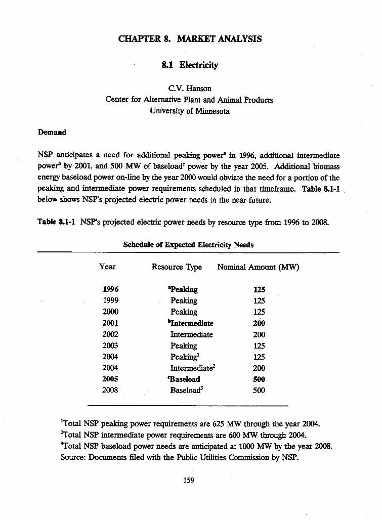
Demand
CHAPI'ER 8. MARKET ANALYSIS
8.1 Electricity
C.V. Hanson Center for Alternative Plant and Animal Products
University of Minnesota
NSP anticipates a need for additional peaking powet' in 1996, additional intermediate power' by 2001, and 500 MW of baseloadc power by the year 2005. Additional biomass energy baseload power on-line by the year 2000 would obviate the need for a portion of the peaking and intermediate power requirements scheduled in that timeframe. Table 8.1-1 belo\\r shows NSP's projected electric power needs in the near future.
Table 8.1-1 NSP's projected electric power needs by resource type from 1996 to 2008.
Schedule of Expected Electricity Needs
Year Resource Type Nominal Amount (MW)
1996 8Peaking 125 1999 Peakiiig 125 2000 Peaking 125 2001 blntermediate 200 2002 Intermediate 200 2003 Peaking 125 2004 Peaking1 125 2004 Intermediate2 200 2005 ~aseload 500
2008 Baseload3 500
1Total NSP peaking power requirements are 625 MW through the year 2004. 1'otal NSP intermediate power requirements are 600 MW through 2004. 1"otal NSP baseload power needs are anticipated at 1000 MW by the year 2008. Source: Documents filed with the Public Utilities Commission by NSP.
159
Marketing
In a joint venture between a producers cooperative and NSP the marketing of electricity
may likely be the respollSloility of-NSP. Certain advantages for the production of renewable
baseload power would likely figure in the marketing and public relations strategy for the
joint venture.
Other marketing opportunities exist within marketing pools that dispatch electric power
generated in the Midwest and potentially with Rural Electric Cooperatives or Municipal
Utilities in the region. Independent electricity marketing may also be undertaken by
forming marketing alliances with other renewable energy producers.
PURP A Legislation
This federal legislation requires that public utilities purchase electricity from independent
power producers at a price that is descnbed as the avoided cost for comparable power
generation. A question arises as to whether a difference exists between renewable avoided
cost and the avoided cost for conventional power production systems and whether the
avoided cost should be based on current systems or 'new generation' systems. This question
will likely require resolution before the Public Utilities Commission.
The best case marketing scenario may well be established as the result of a long-term joint
venture with NSP. NSP's expertise in the electric power generation and distribution business
would certainly be a major asset to the joint venture.
The following two pages contain excerpts from
INVESTING IN TIIB FUTIJRE, A Regulators Guide to Renewables
by Dr. Jan Hamrin and Nancy Rader,
published by National Association of Regulatory Utility Commissioners,
February 1993.
160
Summary Obserntions
The main lessons learned from assessing renewable resource development in all 50 states and specific programs in 26 states are:
• State utility regulatory policy is aitically important to renewable energy development.
• To the extent that renewable resource attributes are undervalued in utility resource planning, more costly·non-renewable resources will be selected.
• The full value1 of renewable resource invem ments is not presently recognimt in many resource planning and acquisition processes.
• Indindual renewable resource technologies should be examined and evaluated separately in order to design effective programs.
• Most competitive bidding programs have not been designed in a manner that allows renewable technologies to sw:cessfully compete.
• Renewable resources developed under diffeient industry structure and ownership patterns will have differem ratepayer impacts which will also differ by technology.
• Unlike fossil and nuclear technologies, many renewable technologies have geographic-specific research, development & demonstration .(RD&D) and commercializati issues which must be addressed before smtainable development can occur.
• Though local RD&D and ccpmerdaHr.ation adhities are of critical importance to the sustainable development of many renewable technologies, few states or utilities have planned for or funded such activities.
• As the electric utility industry changes, renewable resomce technologies offer attractive options for diversifying the energy services a utility can offer.
State utility regulatory policy is critically important to renewable resource development. Regardless of federal rules, regulations and policies, it is at the state level where the •rubber meets the road." Though all 50 states were under the same federal regulations and policies (i.e., the Public Utility Regulatory Policies Act, PURP A, which was designed, in part, to encourage greater use of conservation and renewables) and all SO states have renewable resources, only a few states have successfully moved forward with the development of their renewable energy resource base. For those states, specific utility regulatory policy was the important link to success. '
161
There are certain elements of utility planning and acquisition programs that are essential to the proper assessment of all resources that states should employ whether or not they have a specific interest in promoting renewables. Beyond that, there are various strategic programs that states interested in accelerating renewables development can pursue. There is no single •correct• strategy-the path to follow depends on the characteristics of a state's need for power and its renewable resource base, as well as its resource planning goals-different goals
will lead to quite different programs. Strategies for accelerating renewables fit within the regulatory framework
for sound resource planning and acquisition, but further develop the framework in key areas. These strategies are not mutually exclusive, and, by combining strategy •building blocks,• appropriate pathways can be created for different
simations. The strategies omlined in this report draw on the policies and programs
that have been successfully implemented in the states that lead in renewables development. Also drawn on are programs that are cmrently being developed to encourage renewables and that appear to appropriately address identified barriers ·or issues. The basic strategies for accelerating renewables, which overlap and interconnect in some cases, include:
• Use of appropriate planning tools
• Environmental compliance and risk avoidance • Resolution of transmis.9on issues • Appropriate acquisition programs • Local RD&D/commercialiution programs • Resource assessmentfconfirm3tion admties • . Identification of ~-effecti~. ~d-~. J!!~ and utility aqaplications • Regulatory treatment appropriate to utility structure
Numerous sample pathways are developed that can be pursued by states
inrerested in adding renewable energy technologies to their electtic resource base. Tbe program elements to include and empbasi7.e-elements from both the regulatory framework and strategy sections-should be selected on the basis of the timing of a state's need for power, its renewable resource base, and its resource pluming goals. Individual states must therefore conduct an accouming of their own situation in these areas and create a suitable pathway designed to meet
specific goals.
Coadusion
All states, even those that are relatively advanced in the development of renr:wables for electric generation, could employ strategies to more effectively incorporate the attributes of renewable resources into planning and acquisition methodologies, plan for the susrainerl development of renewables, and further their integration into the utility system. Utility regulatmy policies are the key to _ advancing these resources, which can bring substantial benefits to ratepayers in the near future and over the long term. ·
162
8.2 Leaf Meal Markets
Alfalfa Leaf Meal Market Research Report Alfalfa Production and Supply: A Marketing Penpective
Introduction
Su Ye, Principal Researcher, Minnesota Department of Agriculture
As the 5th largest alfalfa producer in the U.S., Minnesota harvested 4.8 million tons of alfalfa hay from 1.6 million acres in 1993. The four top producing states, California, South Dakota, Wisconsin, and Michigan, produced 6.4 million tons, 6.0 million tons, 5.1 million tons, and 5.0 million tons, respectively.
From 1974 to 1993, Minnesota's alfalfa production ranged from 7.6 million tons (1986) to 4.4 million tons (1989). Production acreage ranged from 2.4 million acres (1988) to 1.5 million acres (1992). The highest average yield during the same period was 3.9 tons per acre (1986), while the lowest was 1.9 tons per acre (1988). In an average year, however, Minnesota produ~s approximately 6 million tons of alfalfa hay, or 7% of_ the ~--~· total production, from 1.9 million acres of land. The average yield is 3.1 tons per acre. The two biggest alfalfa-producing regions in the state are central and southeastern Minnesota, where nearly one-half of Minnesota's alfalfa hay is produced. Over 80% of Minnesota's alfalfa production is consumed on-farm, and the rest is sold commercially in Minnesota or elsewhere. Minnesota alfalfa growers receive about $76 per ton for their alfalfa hay (10-year average from 1984-1993), less than the national average of $79 per ton.
In Minnesota's alfalfa hay market, inter-state trading has increased during the last few years. Minnesota both imports and exports alfalfa hay. The volume of imports and exports vary from year to year, depending on alfalfa crop conditions, supply and demand in Minnesota and the surrounding states.
The following tables, figures and illustrations reflect Minnesota alfalfa production, acreage, yield, and price trends. National production and price data are also included.
163
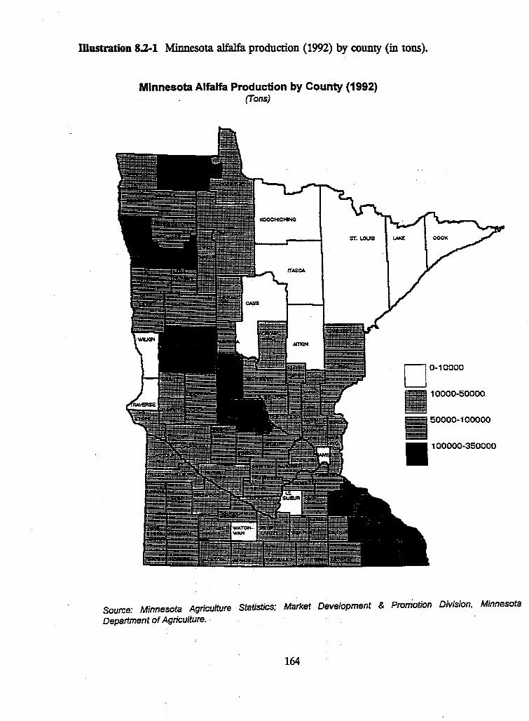
IDustration 8.2-1 Minnesota alfalfa production (1992) by county (in tons).
Minnesota Alfalfa Production by County (1992) (Tons)
D 0-10000
• 10000-50000
• 50000-100000
100000-350000
Source: Minnesota Agriculture Statistics; Market Development & Promotion Division, Minnesota
Department of Agriculture. ·
164
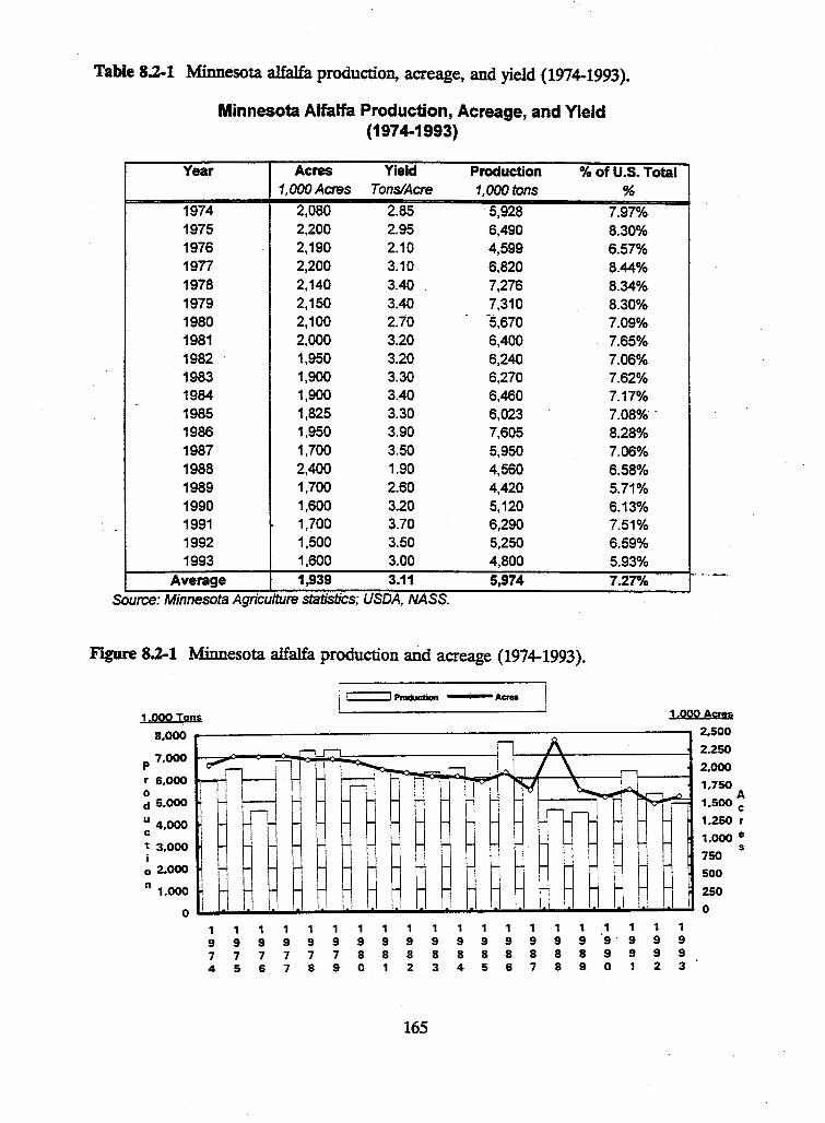
Table 8.2-1 Minnesota alfalfa production, acreage, and yield (1974-1993).
Minnesota Alfalfa Production, Acreage, and Yield (1974-1993)
Year Acres Yield Production % of U.S. Total 1,000Acres Tons/Acre 1,000 tons
1974 2,080 2.85 5,928 1975 2,200 2.95 6,490 1976 2,190 2.10 4,599 1977 2,200 3.10 6,820 1978 2,140 3.40 7,276 1979 2,150 3.40 7,310 1980 2,100 2.70 -5,670 1981 2,000 3.20 6,400 1982 1,950 3.20 6,240 1983 1,900 3.30 6,270 1984 1,900 3.40 6,460 1985 1,825 3.30 6,023 1986 1,950 3.90 7,605 1987 1,700 3.50 5,950 1988 2,400 1.90 4,560 1989 1,700 2.60 4,420 1990 1,600 3.20 5,120 1991 1,700 3.70 6,290 1992 1,500 3.50 5,250 1993 1,600 3.00 4,800
Average 1,939 3.11 5,974 . .
Source: Mmnesota Agnculture statistics; USDA, NASS .
Figure 8.2-1 Minnesota alfalfa production and acreage (1974-1993) .
.....__ __ l'nlcluc:tion --Aa..
1.000 Tons
8.000
~ I A ~':-1 .!~ ' \ ,_
p 7,000
r 6,000 0 .::-~ ---4
-1 l H~,... It-! \..... d 5.000
u 4000 c • t 3.000 i 0 2.000
" 1.000
0
r- ----- - - - ,... - -~ ~ ~--
..-- -,... .... ,... ,... - ,... ,... ,... -I
I
' I
.... .... ,... .... ,... ,... ,... ,... - ,...
- ,... ,... ,... ,... - - .... ,...
.... .... - - - ,... - ,... - - -
1111111111111111 9 9 9 9 9 9 9 9 9 9 9 9 9 9 9 9 7 7 7 7 7 7 8 8 8 8 8 8 8 8 8 8 4 5 6 7 8 9 0 1 2 3 4 5 6 7 8 9
165
-,...
,...
'
%
7.97% 8.30% 6.57% 8.44% 8.34% 8.30% 7.09% 7.65% 7.06% 7.62% 7.17% 7.08%. 8.28% 7.06% 6.58% 5.71% 6.13% 7.51% 6.59% 5.93% 7.2'1°.k
-·
. ,.--I .0..
1.000 Acres
2.500
2,250
2.000 1,750 A
1.500 c 1.250 r
1.000 e
,...-- ....t:i
,...
,...
r-
1 1 9 9 9 9 0 1
r-
,...
....
~ ~
r-
,...
1 1 9 9 9 9 2 3
s 750
500
250
0
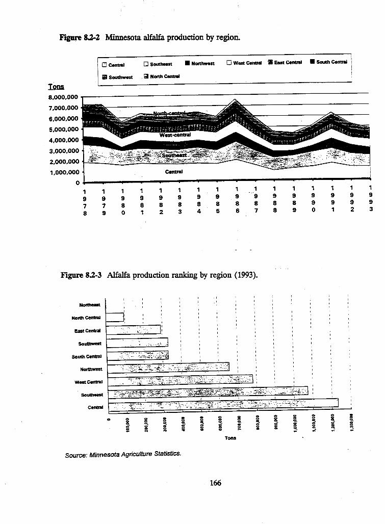
Ftglq'e 8.2-2 Minnesota alfalfa production by region.
:um
I
!~=-0 Souttwnt • Northwest 0 West Central II East Central • Soudl Central
. Q North Central
8,000,000 ~~~~~~~~~~~~~~~~~~~~~~~~~~~~~~~~~~~~~~~~~~~~
7,000,000
6,000,000
5,000,000
4,000,000
3,000,000
2,000.000
1,000.000
0
1 9 7 8
1 9 7 9
1 9 8 0
1 9 8 1
1 9 8 2
1 9 8 3
1 9 8 4
1 9 8 5
1 9 8 6
1 9 8 7
Figure 8.2-3 Alfalfa production ranking by region (1993).
Northeast
Monti Central 0 East Central ~==:::::::::.:.-~ ... · ::::::=1:
South Central
Northwest
West Central
SoutheMt
0 0 0 0 0 0 0 C> .. .. C> .. C> 0 C> C> .. C!. C!. :- .. _ :- C!. 0 ... C> 0 C> C> 0 .. ~
C> .. C> .. C> C> .. ... .., .. ... .. ,_ .. Tons
Source: Minnesota Agriculture Statistics.
166
..
1 9 8 8
C> C!. .. .. ...
.. C>
1 9 8 9
C!. C> .. ~
.. C> C!. ..
1 9 9 0
!:
1 9 9 1
0 .. o. .. C> .., .:
, 9 9 2
1 9 9 3
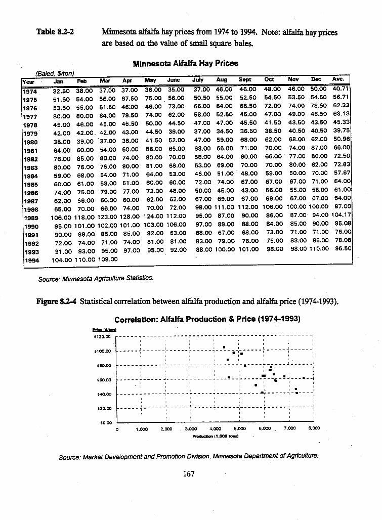
Table 8.2-2 Minnesota alfalfa hay prices from 1974 to 1994. Note: alfalfa hay prices
are based on the value of small square bales.
Minnesota Alfalfa Hay Prices (Baled, $/ton)
Year Jan Feb Mar Apr May June July Aug Sept Oct Nov Dec Ave.
1974 32.50 38.00 37.00 37.00 36.00 35.00 37.00 46.00 46.00 48.00 46.00 50.00 40.71
1975 51.50 54.00 56.00 67.50 75.00 56.00 50.50 55.00 52.50 54.50 53.50 54.50 56.71
1976 53.50 55.00 51.50 46~00 46.00 73.00 66.00 64.00 68.50 72.00 74.00 78.50 62.33
1977 80.00 80.00 84.00 79.50 74.00 62.00 58.00 52.50 45.00 47.00 49.00 46.50 63.13
1978 45.00 46.00 45.00 45.50 50.00 44.50 47.00 47.00 45.50 41.50 43.50 43.50 45.33
1979 42.00 42.00" 42.00 43.00 44.50 36.00 37.00 34.50 36.50 38.50 40.50 40.50 39.75
1980 38.00 39.00 37.00 38.00 41.50 52.00 47.00 59.00 68.00 62.00 68.00 62.00 50.96
1981 64.00 60.00 54.00 60.00 58.00 65.00 63.00 66.00 71.00 70.00 74.00 87.00 66.00
1982 76.00 85.00 80.00 74.00 80.00 70.00 58.00 64.00 60.00 66.00 77.00 80.00 72.50
1983 80.00 76.00 75.00 80.00 81.00 68.00 63.00 69.00 70.00 70.00 80.00 62.00 72.83
1984 59.00 68.00 54.00 71.00 64.00 53.00 45.00 51.00 48.00 59.00 50.00 70.00 57.67
1985 60.00 61.00 58.00 51.00 60.00 60.00 72.00 74.00 67.00 67.00 67.00 71.00 64.00
1986 74.00 75.00 79.00 77.00 72.00 48.00 50.00 45.00 43.00 56.00 55.00 58.00 61.00
1987 62.00 56.00 60.00 60.00 62.00 62.00 67.00 69.00 67.00 69.00 67.00 67.00 64.00
1988 65.00 70.00 66.00 74.00 70.00 72.00 98.00 111 .00 112.00 106.00 100.00 100.00 87.00
1989 106.00 118.00 123.00 128.00 124.00 112.00 95.00 87.00 90.00 86.00 87.00 94.00 104. 17
1990 95.00 101.00 102.00 101.00 103.00 106.00 97.00 89.00 88.00 84.00 85.00 90.00 95.08
1991 90.00 89.00 85.00 85.00 82.00 63.00 68.00 67.00 68.00 73.00 71.00 71.00 76.00
1992 72.00 74.00 71.00 74.00 81.00 81.00 83.00 79.00 78.00 75.00 . 83.00 86.00 78.08
1993 91.00 93.00 95.00 97.00 95.00 92.00 88.00 100.00 101.00 98.00 98.00 110.00 96.50
1994 104.00 110.00 109.00
Source: Minnesota Agriculture Statistics.
Figure 8.2-4 Statistical correlation between alfaifa production and alfalfa price (1974-1993).
Correlation: Alfalfa Production & Price (1974-1993) Prier ($hQn!
$120.00 - - - - - "" - - - - - -,- - - - - - ,.. - 7 - - - - - - - - - -,- - - - - - ,.. - - - - - ., - - - - - -;
I I ' ' l I I I
1 1 .
! I I • ! I :
- - - - -i- ---- -:- -- - -- - - - - - -i- - - -·-:-;.-- -- -1 - - ---1- ---- -$100.00
l • I ! : '
- - - - - ~ - - - - - -;- - - - - - ~ - - - - - ~ - - - - - -:-. - - - -~ -.- - - - ~ - - - - - -: I I i \ 1 • I
$80.00
$60.00 - - - - - ~ - - - - - _: _ - - - - - .... - - - - - ~ - - - ! - _;_ - - - - -~ - _. - - ! .. - - - • ' Ill - -1
I I • !
$40.00 l I I 1 I 1 1 •
- - - - - -r - - - - - -i- - - - - - ; - - - - - ; - - - - - -1- - - - - ~ - - - - - .., - ·- - -
$20.00 · . I . t I I
---- - "7- - --- -;- - - - -- :- - - - --~-- -- --,---- - -:- - - --l- ----
$0.00
0 1.000 2.000 3.000 4,000 5,000 6,000 7,000 8.000
Pnlduclion 11.000 _,
Source: Market Development and Promotion Division, Minnesota Department of Agriculture.
167
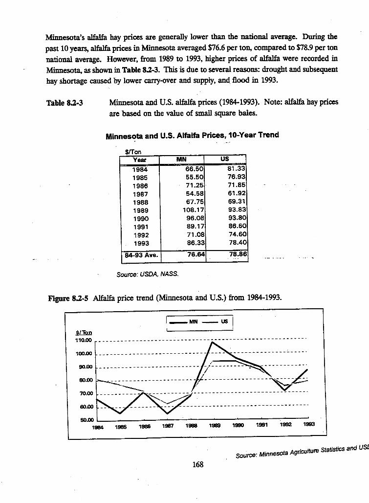
Minnesota's alfalfa hay prices are generally lower than the national average. During the
past 10 years, alfalfa prices in Minnesota averaged $76.6 per ton, compared to $78.9 per ton
national average. However, from 1989 to 1993, higher prices of alfalfa were recorded in
Minnesota, as shown in Table 8.2-3. This is due to several reasons: drought and subsequent
hay shonage caused by lower carry-over and supply, and. flood in 1993.
Table 8.2-3 Minnesota and U.S. alfalfa prices (1984-1993). Note: alfalfa hay prices
are based on the value of small square bales.
Minnesota and U.S. Alfalfa Prices, 10-Year Trend
$!Ton Year MN us 1984 66.50 81.33
1985 55.50 76.93
1986 71.25. 71.85
1987 54.58 61.92
1988 67.75 69.31
1989 108.17 93.83
1990 96.08 93.80
1991 89.17 86.60
1992 71.08 74.60
1993 86.33 78.40
84-93 Ave. 76.64 78.86 ..
Source: USDA, NASS.
F'igure 8.2-5 Alfalfa price trend (Minnesota and U.S.) from 1984-1993.
1-MN-usl I I
50.00L-~--~~--~--~..;_...._~--~~--~---~--:-......_~-
1984 1985 1986 1987 1988 1989 1990 1991 1992 1993
Source: Minnesota Agricutture .Statistics and US!
168
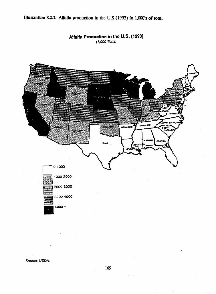
mustration 8.2-l Alfalfa production in the u.s (1993) in 1,000's of tons.
Alfalfa Production in the U.S. (1993) (1,000 Tons)
00-1000
/''"':~g;~; 1000-2000
2000-3000
.300o-4000
.4000+
Source: USDA.
169
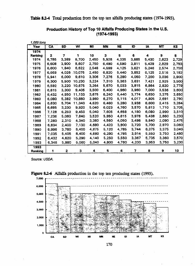
Table 8.2-4 Total production from the top ten alfalfa producing states (1974-1993).
1,000tons Year
1974 Ranking
1974 1975
"1976 1977 1978 1979 1980 1_981 1982 1983 1984 1985 1986 1987 1988 1989 1990 1991 1992 1993 1993
Ranking
Production History of Top 10 Alfalfa Producing States in the U.S. (1974-1993)
CA SD WI Ml MN NE ID IA MT
2 7 1 10 3 5 6 4 9 6,785 3,389 8,700 2,450 5,928 4,335 3,885 5,430 2,623 6,608 3,900 8,607 2,750 6,490 4,590 3,811 5,429 2,829 6,600 1,840 6,622 2,548 4,599 4,125 3,621 5,246 2,574 6,669 4,026 .10,075 2,450 6,820 5,440 3,852 6,125 2,516 5,941 6,000 9,610 3,306 7,276 5,280 4,050 7,200 3,036 6,300 5,500 10,230 3,224 7,310 5,363 3,631 7,421 2,925 6,592 3,220 10,675 3,264 5,670 5,033 3,815 6,864 2,820 6,615 3,300 9,405 3,500 6,400 4,960 3,960 7,000 3,536 6,432 4,950 11, 133 3,675 6,240 5,440 3,774 6,630 3,375 6,080 5,382 10,880 3,960 6,270 5, 115 4,017 4,805 2,691 6,630 5, 704 11,340 4,620 6,460 5,280 3,938 6,600 2,415 6,695 3,230 9,920 5,040 6,023 4,760 3,570 5,813 1,710 7,128 6,250 9,450 5,040 7,605 4,658 4,180 6,080 2,990 7,236 5,060 7,840 3,520 5,950 4,615 3,978 5,438 2,860 7,260 2,310 4,340 3,380 4,560 4,050 3,496 5,640 2,090 6,834 2,400 7,130 4,680 4,420 3,900 3,720 5,700 2,970 6,996 3,780 8,400 4,875 5,120 4,785 3,744 6,375 3,375 7,035 5,405 8,400 4,680 6,290 4,785 3,914 5,550 3,750 6,432 4,620 5,290 4,140 5,250 5,550 3,361"" 5,735 3,360 6,348 5,980 5,060 5,040 4,800 4,760 4,200 3,953 3,750
1 2 3 4 5 6 7 8 9
Source: USDA.
Figure 8.2-6 Alfalfa production in the top ten producing states (1993). 7,000 -------------------------------------------------------------
6,000 ---___,.-------------------------------------------------·· .... · .. . : ~~ ~-:-~ ·.·: .
; :.·. .- ~:: ~
s.ooo -~-~-~-- -- - - - - -- - - -- - -- - -- --- - - - - - ----- -- - -
4.000
3.000
2.000
1.000
CA SD WI Ml MN NE ID IA MT KS
170
KS
8 2,729 2,793 2,750 3,182 2,900 3,500 2,779 3,600 3,650 2,790 3,264 3,705 3,510 3,230 2,475 3,060 3,040 2,480 3,570 3,230
10
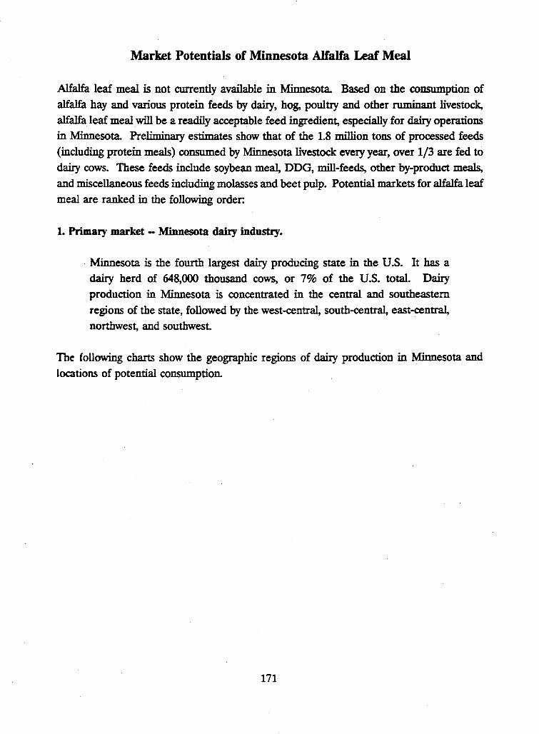
Market Potentials of Minnesota Alfalfa Leaf Meal
Alfalfa leaf meal is not currently available in Minnesota. Based on the consumption of alfalfa hay and various protein feeds by dairy, hog, poultry and other niminant livestock, alfalfa leaf meal will be a readily acceptable feed ingredient, especially for dairy operations in Minnesota. Preliminary estimates show that of the 1.8 million tons of processed feeds
(including protein meals) consumed by Minnesota livestock every year, over 1/3 are fed to dairy cows. These feeds include soybean meal, DDG, mill-feeds, other by-product meals, and miscellaneous feeds including molasses and beet pulp. Potential markets for alfalfa leaf meal are ranked in the following order:
1. Primary market -- Minnesota dairy industcy.
· Minnesota is the fourth largest dairy producing state in the U.S. It has a dairy herd of 648,000 thousand cows, or 7% of the U.S. total. Dairy production in Minnesota is concentrated in the central and southeastern regions of the state, followed by the west-central, south-central, east-central, northwest, and southwest.
The following charts show the geographic regions of dairy production in Minnesota and locations of potential consumption.
171
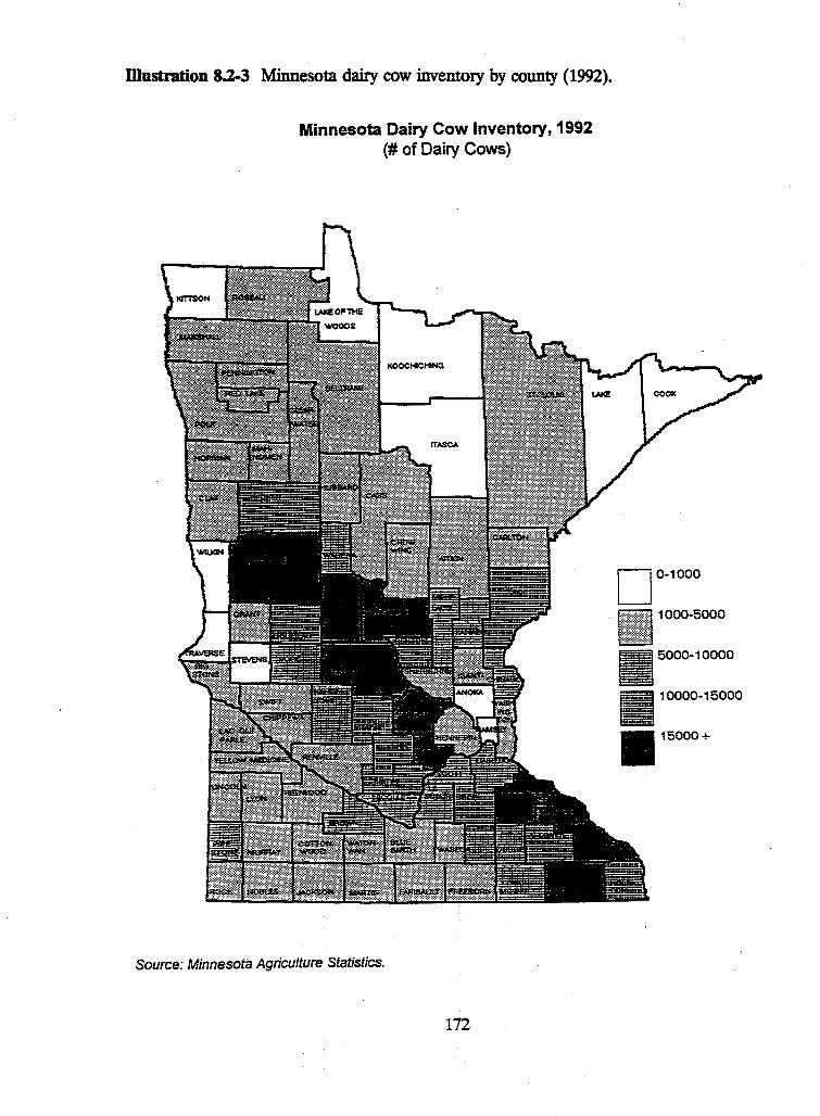
Wustration 8.2-3 Minnesota dairy cow inventory by county (1992).
Minnesota Dairy Cow Inventory, 1992 (# of Dairy Cows)
Source: Minnesota Agriculture Statistics.
172
• 5000-10000
[ !!ii 11 10000-15000
.15000+
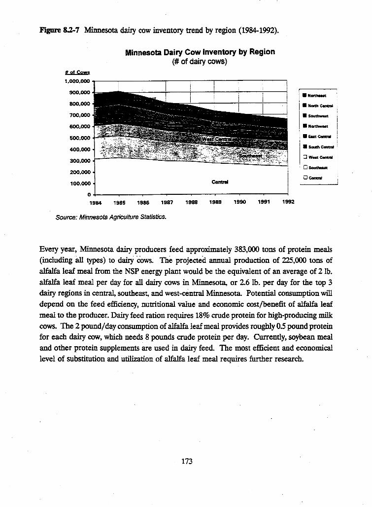
Figure 8.2-7 Minnesota dairy cow inventory trend by region (1984-1992).
#of Cows
Minnesota Dairy Cow Inventory by Region (# of dairy cows)
1.000.000 -----,---..,---,---~--....,..---~----,---,
900,000
800,000
700,000
600,000
::: ~~~ii.,l~;;;t(:;j:~ ... 300.000 1-=------==::::;.:r::::.:a~~Ed~DGC~~~~~~i_j
200,000
100.000
0-4------~--....---r--""T"'""--.-----.----;
1984 1985 1986 1987 1988 1989 1990 1991 1992
Source: Minnesota Agriculture Statistics.
I • Nortllaat
1 •NonhC-.1
I • s-
.Nonhwest
I • East Centnl
i • Soulh Ceatnll
I ~W-Centnl 1 LJ Southeut I
l CJ Cemnl I I
Every year, Minnesota dairy producers feed approximately 383,000 tons of protein meals (including an types) to dany rows. The projected annual production of 225,000 tons of
alfalfa leaf meal from the NSP energy plant would be the equivalent of an average of 2 lb.
alfalfa leaf meal per day for all dairy cows in Minnesota, or 2.6 lb. per day for the top 3 dairy regions in central, southeast, and west-central Minnesota. Potential consumption will depend on the feed efficiency, nutritional value and economic cost/benefit of alfalfa leaf
meal to the producer. Dairy feed ration requires 18% crude protein for high-producing milk cows. The 2 pound/day consumption of alfalfa leaf meal provides roughly 05 pound protein for each dairy cow, which needs 8 pounds crude protein per day. Currently, soybean meal and other protein supplements are used in dairy feed. The most efficient and economical
level of substitution and utilization of alfalfa leaf meal requires further research.
173
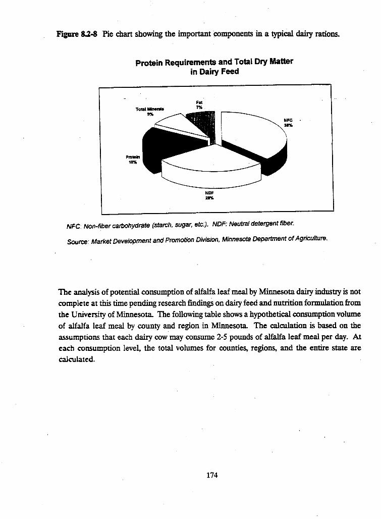
FJgme 8.2-8 Pie chart showing the important components in a typiCal dairy rations.
Protein Requirements and Total Dry Matter in Dairy Feed
NDF 21%
NFC. Non-fiber carbohydrate (starch, sugar, etc.). NDF: Neutral detergent fiber.
Source: Market Development and Promotion Division, Minnesota Department of Agriculture.
The analysis of potential consumption of alfalfa leaf meal by Minnesota dairy industry is not
complete at this time pending research findingS on dairy feed and nutrition formulation from
the U nivcrsity of Minnesota. The following table shows a hypothetical consumption volume
of alfalfa leaf meal by county and region in Minnesota. The calculation is based on the
.wumptions that each dairy cow may consume 2-5 pounds of alfalfa leaf meal per day. At
each consumption level, the total volumes for counties, regions, and the entire state are
calculated.
174
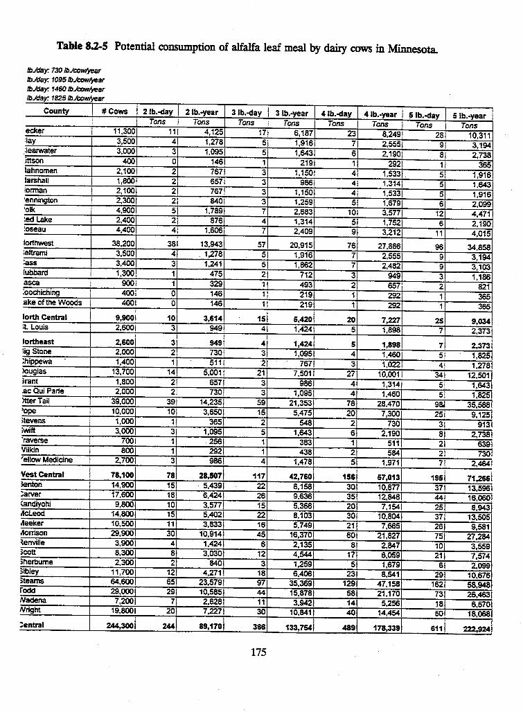
Table 8.2-5 Potential consumption of alfalfa leaf meal by dairy cows in Minnesota.
lb.lday: 730 lb./cow/year lb.lday: 1095 lb~ar lb.Jday: 1460 lb./cow(year lb.lday: 1825 lb.Jcow(year
County #Cows
ecker 11,300 :lay 3,500 :Jearwater 3,000 ittson 400 lahnomen 2,100 larshall 1,800 lorman 2,100 ·ennington 2,300 'Olk 4,900 :ect lake 2,400 :oseau 4,400
lorthwest 38,200 :eltrami 3,500 :ass 3,400 lubbard 1,300 asca 900 :Oochiching 400 ake of the Woods 400
lorth Central 9,900 it Louis 2,600
lortheast 2,600 lig Stone 2,000 ~hippeWc:I 1,400 >ouglas 13,700 >rant 1,800 .ac Qui Pane 2.0001 >tterTail 39,000 'ope 10,000 itevens 1,000 iwift 3,0001 'raverse 700 Vil kin 800 'ellow Medicine 2,700
Yest Central 78,100 3enton 14,900 :arver 17,600 <andiyohi 9,800 "1cLeod 14,800 "1eeker 10,500 ..1orrison 29,900 ~enville 3,9001 )cott 8,300 Sherburne 2,3001 Sibley 11,7001 Steams 64,600 fodd 29,000 Nadena 7,200 Nright 19,800
:entral 244,300
2 lb.-day Tons
11 4 3 0 2 2 2 2 5 2 4
38 4 31 1 1 0 0
10 3
3 2 1
14 2 2
39 10 1 3 1 1 3
78 15 18 10 15 11 30 4 8 2
12 65 29
7 20
244
2 lb.-year 3 lb.-day Tons Tons
4,125 171 1,278 51 1,095 5
146 1 7671 3 657 3 7671 3 840 3
1,789 71 876 4
1,6061 7
13,943, 57 . 1,278 5
1,241 5 475 2 329 1 146 1 146 1
3,614 15 949 4
949 4 730 3 511 2
5,001! 21 657 3 730 3
14,235 59 3,650 15
365 2 1,095 5
256 1 292 11 986 4
28,507 117 5,439 22 6,424 26 3,sn 15 5,402 22 3,833 16
10,914 45 1,424 6 3,030 12
840 3 4,271 18
23,5791 97 10,585 44 2,628 11 7,227 30
89,170 366
175
3 lb.-year 41b.-day 4 lb.-year 5 lb.-day Tons Tons I Tons Tons
6,187 23 8.249 28 1,916 7 2,555 91 1,643 6 2,190) 8
219 1 292 1 1,150 4 1,533 ' 5
986 4 1,314 5 1,150 4 1,533 5 1,259 5 1,679 6 2,683 10 3,5n 12 1,314 5 1,7521 6 2,409 9 3,212! 11
! 20,915 76 27,8861 96
1,916 7 2,555 9 1,862 7 2.4821 9
712 3 949 3 493 2 657' 21 219 1 292 1 219 1 292 1
5,420 20 7,227 25 1,424 5 1,898 7
1,424 5 1,8981 7 1,095 4 1,460 5
767 3 1,0221 4 7,501 27 10,001 34
986 4 1,314 5 1,095 4 1,460 5
21,353 78 28,470 98. 5,475 20 7,300 25
548 2 730 3 1,643 6 2,190 8
383 1 511 2 438 2 584 2
1,478 5 1,971 7
42,760 156 57,013 195 8,158 30 10,8n 37 9,636 35 12,848 44 5,366 20 7,1541 25 8,103 30 10,804 37 5,749 21 7,665 26
16,370 60 21,827 75 2,135 8 2,847 10 4,544 17 6,059 21 1,259 5 1,679 6 6,406 23 8,541 29
35,369 129 47,158 162 15,878 58 21,170 73 3,942 14 5,256 18
10,841 40 14,454 50
133,754 489 178,339 611
5 lb.-year Tons
10,311 3,194 2,738
365 1,916 1,643 1,916 2,099 4,471 2,190 4,015
34,858 3,194 3,103 1,186
821 365 365
9,034 2,373
2,373 1,825 1,278
12,501 1,643 1,825
35,588 9,125
913 2,738
639 730
2,464
71,266 13,596 16,060 8,943
13,505 9,581
27,284 3,559 7,574 2,099
10,676 58,948 26,463
6,570 18,068
222,924
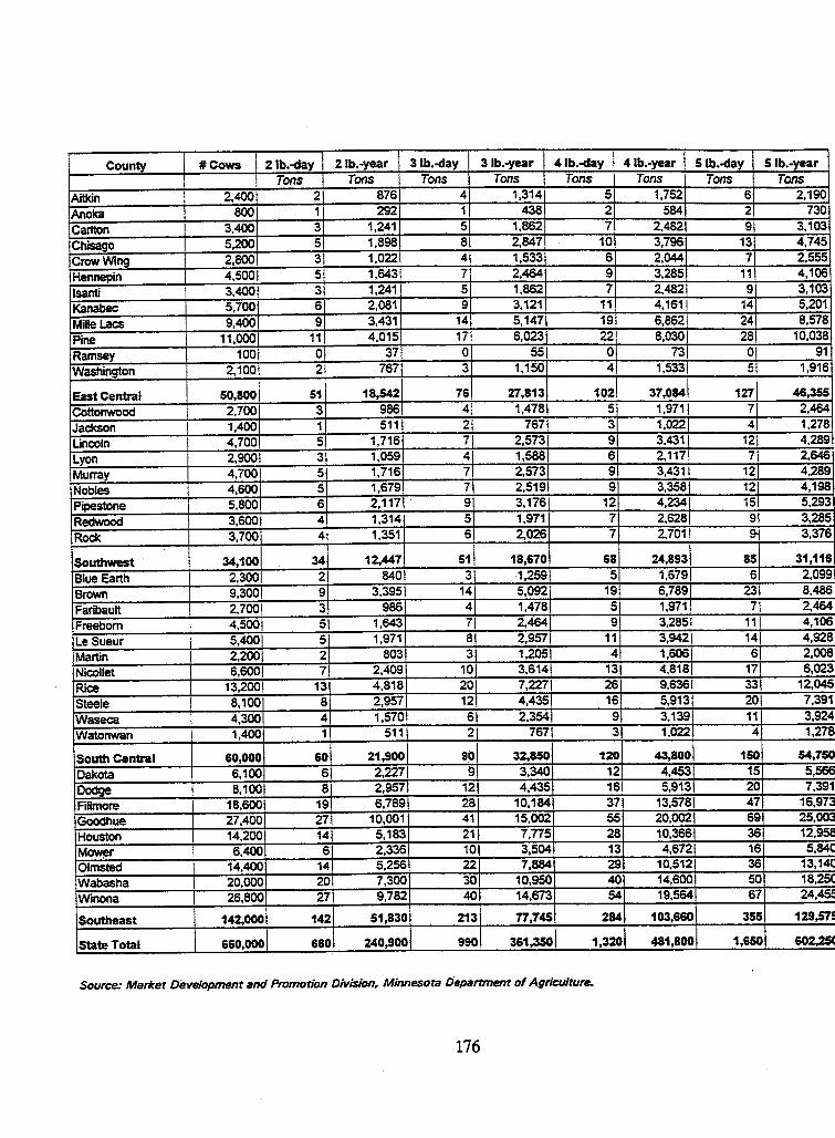
County #Cows 2 lb.-day 2 lb.-year 3 lb.-day 3 lb.-year 41b.-day 4 lb.-year 5 lb.-day 5 lb.-year
Tons Tons Tons Tons Tons Tons Tons Tons Aitkin 2,400 2 876 4 1,314 5 1,752 6 2,190
Anoka 800 1 292 1 438 2 584 2 730
Carlton 3,400 3 1,241 5 1,862 7 2,482 9 3,103
Chisago 5,200 5 1,898 8 2,847 10 3,796 13 4,745
Crow Wing 2,800 3 1,022 4 1,533 6 2,044 7 2,555
Hennepin 4,500 5 1,643 7 2,464 9 3,285 11 4,106
Isanti I 3,400 3 1,241 5 1,862 7 2,482 9 3,103
Kanabec 5,700 6 2,081 9 3,121 11 4,161 14 5,201
Mille Lacs 9,4001 9 3,431 14 5,147 19 6,862 24 8,578
Pine 11,000 11 4,015 17 6,023 22 8,030 28 10,038
Ramsey 100 0 37 0 551 0 73 0 91
Washington 2,100 2 767 3 1,150 4 1,5331 SI 1,916
East Central 50,800 51 18,542 76 27,813 102 37,0841 127 46,355
Cottonwood 2,700 3 986 41 1,478 5 1,9711 7 2.464
Jackson 1,400 1 511 2 767 3 1,022 4 1,278
Lincoln 4,700 5 1,716 7 2,573 9 3,431 12 4,289
Lyon 2,9001 3 1,059 4 1,588 6 2,117\ 7 2,646
Murray 4,700 5 1,716 7 2,573 9 3,431 I 12 4,289
Nobles 4,600 5 1,679 7 2,519 9 3,358 121 4,198
Pipestone 5,800 6 2,117 9 3,176 12 4,2341 15 5,293
Redwood 3,600 4 1,314 5 1,971 7 2,628 9 3,285
Rock 3,700 4 1,351 6 2,026 7 2,7011 g. 3,376
Southwest 34,100 34 12,447 s1I 18,670 68 24,893 85 31,116
Blue Earth 2.3001 2 8401 3 1,259 5 1,679 6 2,099
Brown 9,300 9 3,395 14 5,092 19 6,789 23 8,486
Faribault 2,7001 3 986 4 1,478 5 1,9711 71 2,464
Freeborn 4,5001 5 1,643 7 2,464 9 3,285 11 4,106
Le Sueur 5,400 5 1,971 8 2,957 11 3,942 14 4,928
Martin I 2.2001 2 803 3 1,205 4 1,606 6 2,008 I
Nicollet 6,6001 7 2,409 10 3,614 13 4,818 17 6,023
Rice 13,200\ 13 4,818 20 7,2271 26 9,6361 33 12,045
Steele 8,100 8 2,957 12 4,435 16 5,9131 20 7,391
Waseca I 4,300 4 1,570 6 2,354 9 3,139 11 3,924
Watonwan I 1,400 1 511 21 767 3 1,022 4 1,278
South Central 60,000 60 21,900 90 32,850 120 43,800 150 54,750
Dakota 6,100 SI 2,2271 9 3,340 12 4,453 15 5,566
Dodge 8,1001 8 2,957 12 4,435 16 5,9131 20 7,391
Fillmore 18,6001 19 6,789 28 10,184 37 13,5781 47 16,973
Goodhue 27,400 27 10,001 41 15,002 55 20,002 69 25,003
Houston 14,200 14 5,183 21 7,775 28 10,366 36 12,958
M~r 6,400 6 2,336 10 3,504 13 4,672 16 5,840
Olmsted 14,400 14 5,256 22 7,884 29 10,512 36 13,140
Wabasha 20,000 20 7,300 30 10,950 40 14,600 50 18,250
Winona 26,800 27 9,782 40 14,673 54 19,564 67 24,45S
Southeast 142,000 142 51,830 213 77,745 284 103,660 355 129,57!i
State Total 660,000 660 240,900 9901 361,350 1,320 481,800 1,650 602,2SC
Source: Market D'evelopment and Promotion Division, Minnesota Depanment of Agriculture.
176
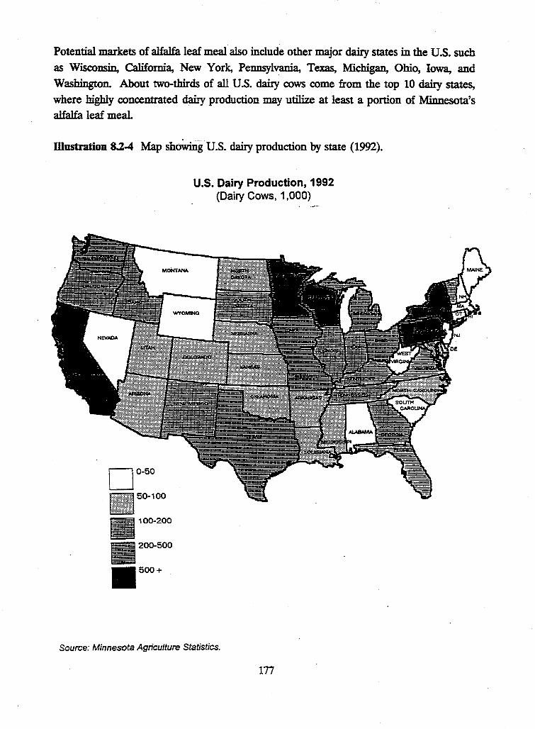
Potential markets of alfalfa leaf meal also include other major dairy states in the U.S. such as Wisconsin, California, New York, Pennsylvania, Texas, Michigan, Ohio, Iowa, and Washington. About two-thirds of all U.S. dairy cows come from the top 10 dairy states, where highly concentrated dairy production may utilize at least a portion of Minnesota's alfalfa leaf meal.
IDustration 8.2-4 Map showing U.S. dairy production by state (1992).
o0-50
llllJllll!lll 5°-100
100-200
;:1200-500
500+
U.S. Dairy Production, 1992 (Dairy Cows, 1,000)
Source: Minnesota Agriculture Statistics.
177
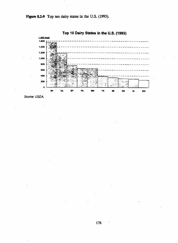
Figure 8.2-9 Top ten dairy states in the U.S. (1993).
Top 10 Dairy States in the U.S. (1993) 1 000 btad
1,600 --------------------------------------------------------
1.400
1.200
1.000
800
600
400
200
0
WI CA NY
Source: USDA.
PA MN TX Ml
178
. ~ : .. -·~; ...... -,~ -. _:r~.
·~ .... ·~.:-- ···~·
OH IA WA
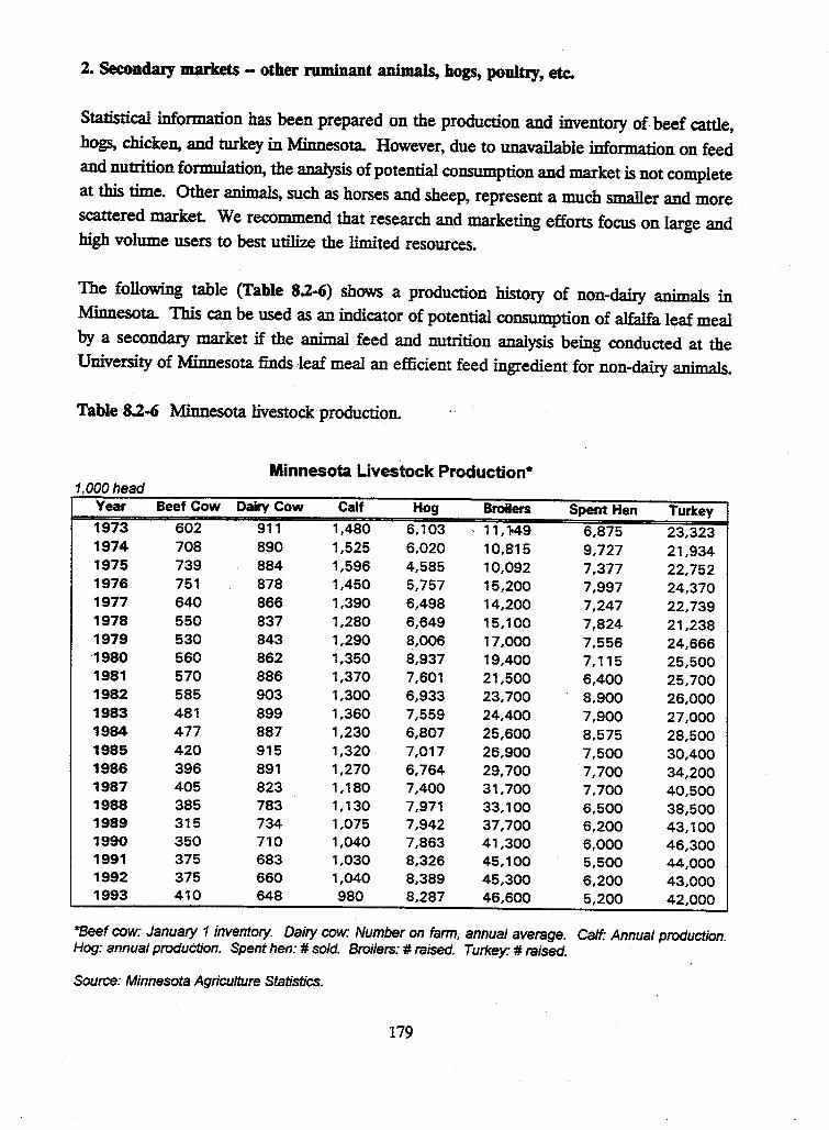
2. Secondaly markets - other ruminant animals, hogs, poultJ:y, etc.
Statistical information has been prepared on the production and inventory of beef cattle, hogs, chicken, and turkey in Minnesota. However, due to unavailable information on feed and nutrition formulation, the analysis of potential consumption and market is not complete at this time. Other animals, such as horses and sheep, represent a much smaller and more scattered market. We recommend that research and marketing efforts focus on large and high volume users to best utilize the limited resources.
The following table (Table 8.2-6) shows a production history of non-dairy animals in Minnesota. This can be used as an indicator of potential consumption of alfalfa leaf meal by a secondary market if the animal feed and nutrition analysis being conducted at the University of Minnesota finds leaf meal an efficient feed ingredient for non-dairy animals.
Table 8.2-6 Minnesota livestock production.
Minnesota Livestock Production* 1 ODO head '
Year Beef Cow Dairy Cow Calf Hog Broilers Spent Hen Turkey 1973 602 911 1,480 6, 103 '11,149 6,875 23,323 1974 708 890 1,525 6,020 10,815 9,727 21,934 1975 739 884 1,596 4,585 10,092 7,377 22,752 1976 751 878 1,450 5,757 15,200 7,997 24,370 1977 640 866 1,390 6,498 14,200 7,247 22,739 1978 550 837 1,280 6,649 15, 100 7,824 21,238 1979 530 843 1,290 8,006 17,000 7,556 24,666 ·1980 560 862 1,350 8,937 19,400 7, 115 25,500 1981 570 886 1,370 7,601 21,500 6,400 25,700 1982 585 903 1,300 6,933 23,700 8,900 26,000 1983 481 899 1,360 7,559 24,400 7,900 27,000 1984 477 887 1,230 6,807 25,600 8,575 28,500 1985 420 915 1,320 7,017 26,900 7,500 30,400 1986 396 891 1,270 6,764 29,700 7,700 34,200 1987 405 823 1, 180 7,400 31,700 7,700 40,500 1988 385 783 1,130 7,971 33,100 6,500 38,500 1989 315 734 1,075 7,942 37,700 6,200 43,100 1990 350 710 1,040 7,863 41,300 6,000 46,300 1991 375 683 1,030 8,326 45, 100 5,500 44,000 1992 375 660 1,040 8,389 45,300 6,200 43,000 1993 410 648 980 8,287 46,600 5,200 42,000
*Beef cow: January 1 inventory. Dairy cow: Number on farm, annual average. Calf: Annual production. Hog: annual production. Spent hen: #sold. Broilers: # raised. Turkey: # raised.
Source: Minnesota Agriculture Statistics.
179
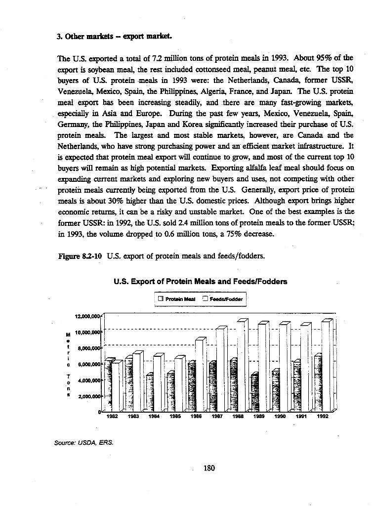
3. Other markets - export market.
The U.S. exported a total of 7 2 million tons of protein meals in 1993. About 95% of the export is soybean meal, the rest included cottonseed meal, peanut meal, etc. The top 10 buyers of U.S. protein -meals in 1993 were: the Netherlands, Canada, former USSR, Venezuela, Mexico, Sp~ the Philippines, Algeria, France, and Japan. The U.S. protein meal export has been increasing steadily, and there are many fast-growing markets, especially in Asia and Europe. During the past few years, Mexico, Venezuela, Sp~ Germany, the Philippines, Japan and Korea significantly increased their purchase of U.S. protein meals. The largest and most stable markets, however, are Canada and the Netherlands, who have strong purchasing power and an- efficient market infrastructure. It is expected that protein meal export will continue to grow, and most of the current top 10 buyers will remain as high potential markets. Exporting alfalfa leaf meal should focus on expanding current markets and exploring new buyers and uses, not competing with other protefu meals currently being exported from the U.S. Generally, export price· of protein meals is about 30% higher than the U.S. domestic prices. Although export brings higher economic returns, it can be a risky and unstable market. One of the best examples is the former USSR: in 1992, the U.S. sold 2.4 million tons of protein meals to the former USSR; in 1993, the volume dropped to 0.6 million tons, a 75% decrease.
FJ.gDre 8.2-10 U.S. export of protein meals and feeds/fodders.
U.S. Export of Protein Meals and Feeds/Fodders
I [] Protein Meal 0 °Feeds1Fodder i I
12,000,000
I M 10,000,000 r- ---------------------------e i : a.000.000 r----------------------1 i I . I
: 6,000,000 f ,;~ - -1
~ 4,000.000 r : s 2,000,000 ~-": . ,
I ·. :~~{
--1 I
- - ~ I
--~
--m1 i I I
- - I \
I
01-----~_,_ ......... .......__..........__.. ............................... "'-'-""-""----................. _........._.___.."-'--..._ .......... _,__~ 1982 1983 1984 1985 1986 1987 1988 1989 1990 1991 1992
Source: USDA, ERS,
180
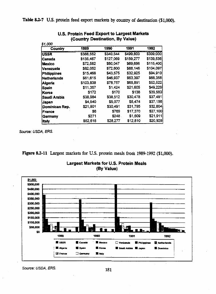
Table 8.2-7 U.S. protein feed export markets by country of destination ($1,000).
U.S. Protein Feed Export to Largest Markets (Country Destination, By Value)
$1,000 Country 1989 1990 1991 1992
USSR $388,552 $340,544 $499,803 $309,000 Canada $135,467 $127,069 $159,277 $139,536 Mexico $72,582 $60,047 $69,696 $115,400 Venezuela $82,052 $72,600 $88,146 $104,097 Philippines $15,468 $43,575 $32,925 $94,910 Netherlands $61,615 $46,937 $63,397 $68,358 Algeria $103,838 $78,757 $65,891 $52,522 Spain $11,357 $1,424 $21,605 $49,229 Korea $172 $170 $138 $39,583 Saudi Arabia $38,984 $38,512 $30,478 $37,481 Japan $4,540 $5,077 $5,474 $37,156 Dominican Rep. $21,801 $30,491 $31,795 $32,804 France $6 $769 $17,370 $27,100 Gennany $271 $248 $1,609 $21,911 Italy $52,618 $28,277 $12,810 $20,928
Source: USDA, ERS.
Figure 8.2-11 Largest markets for U.S. protein meals from 1989-1992 ($1,000).
$1.000
$500,000
Largest Markets for U.S. Protein Meals (By Value)
$450,000 1----------------111-------------$400,000 1----------------111--------------$350,000
$300,000
$250,000
$200,000 ----------------111---------------$150,000
$100,000
$50,000
$0 1989
I •ussR i • Algeria I i Bi France I
Source: USDA, ERS.
• c:anacia
• Spain
0 Germany
1990 1991 1992
• Mexico 0 Venft.tala • Pllilippi- ;!_ Netllertanda
•Kena • Saudi Arabia • Japan • Dominica
• Italy
181
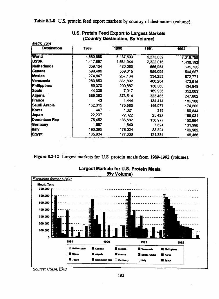
Table 8.2-8 U.S. protein feed export markets by country of destination (volume).
Metric Tons Destination
World USSR Netherlands Canada Mexico Venezuela Philippines Spain Algeria France Saudi Arabia Korea Japan Dominican Rep Gennany Italy Egypt
U.S. Protein Feed Export to Largest Markets (Country Destination, By Volume)
1989 1990 1991
4,860,680 5,137,503 6,273,832 1,417,887 1,581,944 2,322,016
359,164 430,063 555,954 599,480 559,015 659,095 274,847 267,134 334,253 283,853 331,892 406,204
59,070 200,887 150,360 44,309 7,017 169,936
389,062 373,514 323,485 43 4,444 134,414
152,615 175,583 145,071 447 1,021 319
22,237 22,322 25,427 76,452 136,582 156,977
1,557 1,640 7,824 190,395 178,024 83,824 165,934 177,606 121,384
1992
7,019,755 1,438,192
635,755 594,557 572,771 473,915 434,848 352,063 247,802 186,188 174,265 169,844 168,031 150,994 131,998 109,982 46,456
Figure 8.2-12 Largest markets for U.S. protein meals· from 1989-1992 (volume).
Excluding former USSR Metric Tons
Largest Markets for U.S. Protein Meals (By Volume)
700,000 -----------------------------------------------------------------·
600,000 - - - - - - - - - - - - - - - - - - - - - - - - - - - - - - -
500,000 --------------- -------------
400,000
300,000
200,000
100,000
0 1989
i [] Netherlands I
I •Spain
.• Japan
Source: USDA, ERS.
1990
• Canadll
• Algeria
• MexiCo
•France
• Dominican Rep 0 Gennany
182
1991 1992
•v-ia • Philippi.- I !
• SndiAnlllill •ic-0 llaly • Egypt
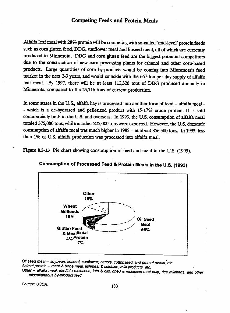
Competing Feeds and Protein Meals
Alfalfa leaf meal with 28% protein will be competing with so-called "mid-level" protein feeds such as com gluten fee4 DDG, sunflower meal and linseed meal, all ofwhicb are currently produced in Minnesota. DDG and com gluten feed are the biggest potential competitors due to the construction of new com processing plants for ethanol and other com-based products. Large quantities of com by-products would be coming into Minnesota's feed market in the next 2-3 years, and would coincide with the 667-ton-per-day supply of alfalfa leaf meal. By 1997, there will be at least 112,326 tons of DDG produced annually in Minnesota, compared to the 25,116 tons of current production.
In some states in the U.S., alfalfa hay is processed into another form of feed - alfalfa meal -- which is a de-hydrated and pelletized product with 15-17% crude protein. It is sold commercially both in the U.S. and overseas. In 1993, the U.S. consumption of alfalfa meal totaled 375,000 tons, while another 225,000 tons were exported. However, the U.S. domestic consumption of alfalfa meal was much higher in 1985 - at about 856,500 tons. In 1993, less than 1 % of U.S. alfalfa production was processed into alfalfa meal.
Figure 8.2-13 Pie chart showing consumption of feed and meal in the U.S. (1993).
Consumption of Processed Feed & Protein Meals in the U.S. (1993)
Wheat Millfeeds
15%
Gluten Feed
Other 15%
& Meainimal 43Protein
7%
j Oil Seed Meal 59%
Oil seed meal - soybean, linseed, sunflower, canola, cottonseed, and peanut meals,· etc. Animal protein - meat & bone meal, fishmeal & solubles, milk products, etc. Other - alfalfa meal, inedible mo/asses, fats & oils, dried & mo/asses beet pulp, rice mil/feeds, and other
miscellaneous by-product feed.
Source: USDA. 183
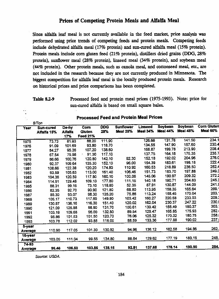
Prices of Competing Protein Meals and Alfalfa Meal
Since alfalfa leaf meal is not currently available in the feed market, price analysis was
performed using price trends of competing feeds and protein meals. Competing feeds
include dehydrated alfalfa meal (17% protein) and sun-cured alfalfa meal (15% protein).
Protein meals include com gluten feed (21 % protein), distillers dried grains (DDG, 28%
protein), sunflower meal (28% protein), linseed meal (34% protein), and soybean meal
(44% protein). Other protein meals, such as canola meal, and cottonseed meal, etc., are
not Included in the research because they are not currently produced in Minnesota. The
biggest competition for alfalfa leaf meal is the locally produced protein meals. Research
on historical prices and price comparisons has been completed.
Table 8.2-9
$/Ton
Processed feed and protein meal prices (1975-1993). Note: price for
sun-cured alfalfa is based on small square bales.
Processed Feed and Protein Meal Prices
Year Sun-cured De-hy Com DOG Sunflower Linseed Soybean Soybean Com Gluten
Alfalfa 15% Alfalfa Gluten 28% Meal28% Meal34% Meal44% Meal48% Meal60%
17°/0 Feed21%
1975 73.73 81.03 88.20 111.90 126.66 131.78 141.50 234.1
1976 91.09 101.69 93.80 118.70 134.55 147.90 157.60 230.4
1977 84.27 95.36 107.20 138.60 156.87 199.78 213.90 208.4
1978 67.54 75.98 - 91.30 117.10 137.75 164.18 175.35 235.7
1979 86.66 100.76 120.80 142.10 92.30 152.18 192.02 204.96 276.0
1980 92.37 109.64 125.30 152.10 96.00 154.39 183.61 198.18 222.4
1981 108.66 122.38 120.20 174.80 110.92 160.53 218.89 236.50 262.4
1982 93.59 105.63 113.00 161.40 106.46 151.73 183.70 197.88 249.::
1983 104.36 120.59 117.80 160.10 100.06 145.06 190.97 209.32 272.2
1984 114.91 129.48 109.10 177.80 111.15 140.18 190.71 204.83 245.~
1985 88.31 99.16 73.10 118.80 52.35 87.91 130.87 144.09 241.5
1986 82.35 92.70 90.90 121.80 68.80 113.95 158.35 165.64 269.1
1987 85.30 93.07 98.30 125.20 75.86 113.24 158.45 170.04 203.1
1988 105.17 110.73 117.60 149.80 103.42 160.27 220.58 233.03 209.~
1989 130.57 136.16 116.30 151.40 120.02 162.04 230.37 247.22 230.!
1990 121.09 125.88 98.80 131.70 100.61 130.42 168.49 180.37 303.'
1991 103.19 109.68 96.00 132.80 89.54 129.47 165.85 175.93 282.4
1992 95.86 101.53 101.50 120.70 76.06 125.32 170.32 180.75 258.<
1993 103.78 112.02 93.88 118.00 88.59 133.36 177.88 190.02 237.E
5-year Average 110.90 117.05 101.30 130.92 94.96 136.12 182.58 194.86 262.:
10-year Average 103.05 111.04 99.55 134.80 88.64 129.62 177.19 189.19 248.1
74-93 Av~rage 96.46 106.50 103.85 138.15 92.81 137.68 178.14 190.90 284.1
Source: USDA.
184
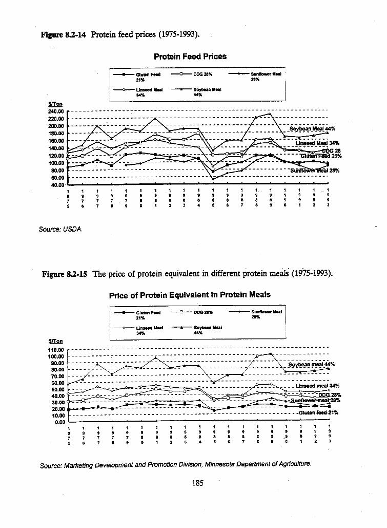
Figure 8.2-14 Protein feed prices (1975-1993).
m:.en 240.00 220.00
1 9 7 5
1 9 7 6
Source: USDA
1 9 7 7
Protein Feed Prices
II Glldllft Feed -~ DOG 21% 21%
: --<>--- Linseed Meal Soybelln Meat i M% ~%
1 9 7 a
1 9 7 9
1 9 a 0
1 9 a 1
1 9 a 2
1 9 a 3
1 9 a 4
1 9 a 5
1 9 a 6
--- s...ii-Meal I
1 9 a 7
21% I
1. 1 9 9 a a a 1
I
1 9 9 0
1 9 9 1
1 9 9 2
9 9 3
Figure 8.2-15 The price of protem equivalent in different protein meals (1975~1993).
1!!2!? 110.00 100.00
90.00 80.00 70.00 60.00 50.00 40.00 30.00
Price of Protein Equivalent in Protein Meals
j --- GIU11tn Feed -a-- DOG 21% ! 21%
: --<>-- Linseed Meal ----- SoybNn Meal 34% ~%
~-11 I
======~============~==~=======================~====~% --- ------ ----------------------- ---- ----------------------
20.00 - ---------------------10.00 - - - - - - - - - - - - - - - - - - - - - - - - - - - - - - - - - - - - - - - - - - - - - - - - - - - - - - - - - -GluteR.feed-21% 0.00 .__ ____________ ~ _______ ..__.. _____________ ..___....__.. ____ ~___.
1 9 7 5
9 7 6
9 7 7
9 7 8
1 9 7 9
1 9 a 0
9 a
9 8 2
1 9 8 3
1 9 8 4
9 a 5
1 9 a 6
1 9 8 7
1 9 a 8
1 1 9 9 8 .9 9 0
1 9 9
Source: Marketing Development and Promotion Division, Minnesota Department of Agriculture.
185
1 9 9 2
1 9 9 3
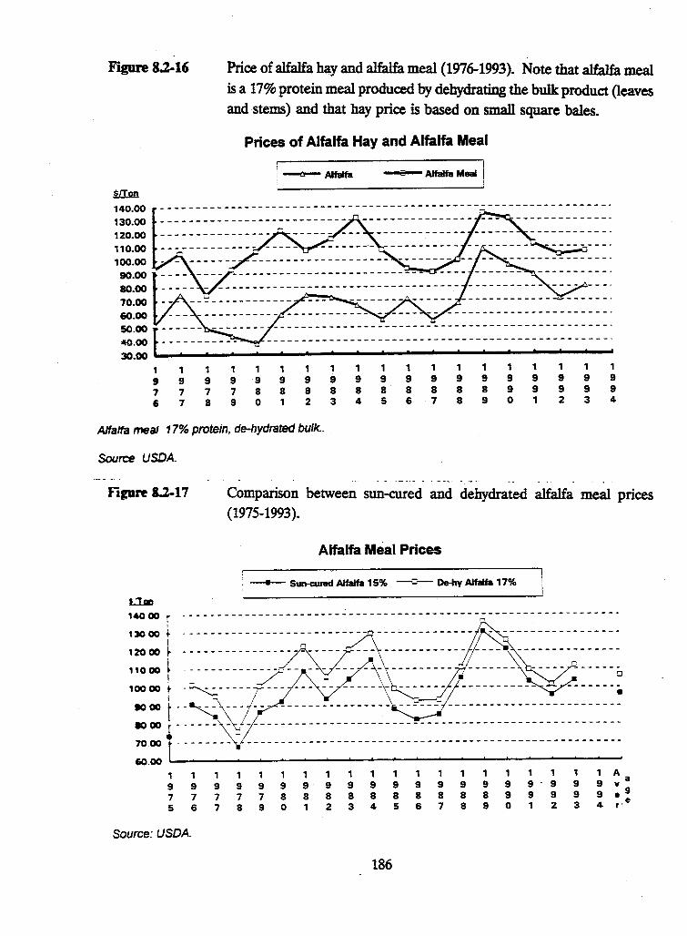
Price of alfalfa hay and alfalfa meal (1976-1993). Note that alfalfa meal
is a 17% protein meal produced by dehydrating the bulk product (leaves
and stems) and that hay price is based on small square bales.
1IIm 140.00
130.00 120.00
110.00 100.00
90.00
80.00
70.00
60.00
Prices of Alfalfa Hay and Alfalfa Meal
- Alfalfa Alfalfa Meal I
50.00 f- ----- --------40.00 - - - - - - - - - - - - - - - - - - - - - - - - - - - - - - - - - - - - - - - - - - - - - - - - - - - - - - - - - - - - - '
30.00 . . . 0
1 1 1 1 1 9 9 9 9 9 7 7 7 7 8 6 7 8 9 0
1 9 8 1
1 1 9 9 8 8 2 3
Alfalfa meal 17% protein, de-hydrated bulk ..
Source USDA.
1 1 9 9 8 8 4 5
1 1 9 9 8 8 6 7
1 9 8 8
1 9 8 9
1 9 9 0
1 9 9 1
1 9 9 2
1 9 9 3
1 9 9 4
figure 1.2-17 Comparison between sun-cured and dehydrated alfalfa meal prices
(1975-1993).
Alfalfa Meal Prices
: ---- Sun-cured Alfalfa 15% --a- De-hy Alfalfa 17%
14000 r -----------------------~-------------------~-------------------, ::: [ ::::::::::;~~:::::::::::::::::: _____ _
10000 ~ -~--------- -- ?:-\~---- -----------90 00 t .. ~ \- ---~ - ---------------- ------- -------------------------'° 00 T •• ___ ~\v-----------------------------------------------------:.: r · ------~ ---- -- ------_ ------ .- --~ --~ ---_ ---- -- ~ -- -------. -------- --.
, , , 1 1 1 1 1 1 1 1 1 1 1 1 1 1 1 1 1 A a 9 9 9 9 9 9 9 9 9 9 9 9 9 9 9 9 9· 9 9 9 v
7 7 7 7 7 8 8 8 8 8 8 8 8 8 8 9 9 9 9 9 e g e
5 6 7 8 9 0 1 2 3 4 5 6 7 8 9 0 1 2 3 4 r.
Source: USDA.
186
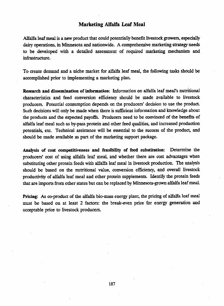
Marketing Alfalfa Leaf Meal
Alfalfa leaf meal is a new product that could potentially benefit livestock growers, especially
dairy operations, in Minnesota and nationwide. A comprehensive marketing strategy needs
to be developed with a detailed assessment of required marketing mechanism and
infrastructure.
To create demand and a niche market for alfalfa leaf meal, the following tasks should be
accomplished prior to implementing a marketing plan.
Research and dissemination of information: Information on alfalfa leaf meal's nutritional
characteristics and feed conversion efficiency should be made available to livestock
producers. Potential consumption depends on the producers' decision to use the product.
Such decisions will only be made when there is sufficient information and knowledge about
the products and the expected payoffs. Producers need to be convinced of the benefits of
alfalfa leaf meal such as by-pass protein and other feed qualities, and increased production
potentials, etc. Technical assistance will be essential to the success of the product, and
should be made available as part of the marketing support package.
Analysis of cost competitiveness and feasibility of feed substitution: Determine the
producers' cost of using alfalfa leaf meal, and whether there are cost advantages when
substituting other protein feeds with alfalfa leaf meal in livestock production. The analysis
should be based on the nutritional value, conversion efficiency, and overall livestock
productivity of alfalfa leaf meal and other protein supplements. Identify the protein feeds
that are imports from other states but can be replaced by Minnesota-grown alfalfa leaf meal.
Pricing: As co-product of the alfalfa bio-mass energy plant, the pricing of alfalfa leaf meal
must be based on at lea5t 2 factors: the break-even price for energy generation and
acceptable price to livestock producers.
187
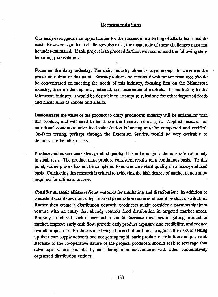
Recommendations
Our analysis suggests that opportunities for the successful marketing of alfaJfa leaf meal do
exist. However, significant challenges also exist; the magnitude of these challenges must not
be under-estimated. If this project is to proceed further, we recommend the following steps be strongly considered:
Focus on the dairy industry: The dairy industry alone is large enough to consume the
projected output of this plant. Scarce product and market development resources should
be concentrated on meeting the needs of this industry, focusing first on the Minnesota
industry, then on the regional, national, and international markets. In marketing to the
Minnesota industry, it would be desirable to attempt to substitute for other imported feeds
and meals such as canola and alfalfa.
Demonstrate the value of the product to dairy producers: Industry will be unfammar with·
this product, and will need to be shown the benefits of using it. Applied research on
nutritional content/relative feed value/ration balancing must be completed and verified. On-farm testing, perhaps through the Extension Service, would be very desirable to
demonstrate benefits of use.
Produce and ensure consistent product quality; It·is ·not enough· to demonstrate value only
in small tests. The product must produce consistent results on a continuous basis. To this
point, scale-up work has not be completed to ensure consistent quality on a mass-produced
basis. Conducting this research is critical to achieving the high degree of market penetration
required for ultimate success.
Consider strategic alliances/joint ventures for marketing and distribution: In addition to
consistent quality assurance, high market penetration requires efficient product distnbution.
Rather than create a distribution network, producers might consider a partnership /joint
venture with an entity that already controls feed distribution in targeted market areas.
Properly structured, such a partnership should decrease time lags in getting product to
market, improve early cash flow, provide early product exposure and credibility, and reduce
overall project risk. Producers must weigh the cost of partnership against the risks of setting up their own supply network and not getting rapid, early product distribution and payment. Because of the co-operative nature of the project, producers should seek to leverage that
advantage, where possible, by considering alliances/ventures with other cooperatively
organized distribution entities.
188
Introduction
CHAPTER 9. BUSINESS ANALYSIS
9.1 Organizational Structure
Orga~tional Options for Alfalfa Biomass Energy Production
E.G. Nadeau, Cooperative Development Services
Madison, Wisconsin
The purpose of this chapter of the feasibility report is to identify and evaluate organizational
structure options for the proposed biomass plant in Granite Falls. The chapter focuses on ·
potential relationships between Northern States Power (NSP) and alfalfa growers within a
fifty mile radius of Granite Falls.
Most of the conclusions and recommendations in this chapter derive from two meetings with
the Agriculture Advisory Council for this project (for a list of participants see Appendix 9.1).
The Ag Advisory Council is comprised of farmers and other residents of southwestern
Minnesota.
The chapter is divided into four sections: review of organizational options; comparison of
options; evaluation of options; and investment and contractual issues.
Review of Organizational Options
There are many possible ways to structure the ownership and operation of the proposed
biomass plant. This section of the chapter reviews four options: 100% ownership by NSP;
100% ownership by an alfalfa growers' cooperative; and two joint venture options between
NSP and a growers' co-op. These options are intended to represent key points along a
continuum of possible ownership models.
189
A. Organizational Options:
1. NSP Ownership
One key feature of the NSP ownership option is that the utility would be responsible for accessing all of the capital required to build and maintain the plant. It would, thus, take all of the financial risks and receive all of the profits. The estimated capitalization cost for the plant is around $130 million dollars. In this scenario, NSP would contract with growers in the region to secure an adequate supply of alfalfa for the plant.
2. Producer Cooperative Ownership
The following three options all involve the formation of a '1imited membership" cooperative which would either own the biomass plant outright or as part of a joint venture with NSP. The· key features of a "limited membership" cooperative are: there is a specified number of shares available for purchase by producers (and, in some cases, other investors); the number of shares is based on the processing and marketing capabilities and goals of the coop; members purchase shares in the co-op in proportion to the volume of product they agree to sell to the co-op; and members get a return on their investment-based on the profitability of the co-op and on the value of product they sell to the co-op.
''Limited membership" cooperatives provide a- means for farmers to secure market outlets for their products and to share in the value added to their products through processing and marketing. This approach also provides a means to raise equity capital for cooperative investment in processing and other activities that enhance the value of agricultural products. There are numerous successful examples of this type of cooperative in Minnesota and North Dakota, including a number in the Granite Falls area, such as Minnesota Com Processors and several nearby sugar beet cooperatives.
190
Following are the main features of the organizational option based on 100% ownership by
a producer cooperative.
*'.Producers would need to secure all of the estimated $130 million for the plant. Between
30% and 40% of this (approximately $40-50 million) would probably need to be in the
form of member equity and the remainder in debt financing.
* The plant would need an estimated 700,000 tons of alfalfa per year. If farmers invest in
the plant based on the tonnage of alfalfa they agree to sell to the plant each year, they
would need to invest an estimated $60 to $85 per ton.
* Producer members would receive a share in the profits of the cooperative proportional
to the value of alfalfa each member sells to the co-op. Members would also be risking
their equity in the event the cooperative were not profitable.
3. Joint Ownership Option I
There are many possible variations on joint ownership of the biomass plant by NSP and a
producers' cooperative. The specific option presented here would involve NSP ownership
of- the gasification and electricity generating components of the plant; co-op ownership of
the alfalfa leaf meal processing and marketing components; and joint ownership of the
remote storage sites, the transportation system, storage at the central facility and the
separator. The major characteristics of this option are:
* Depending on the specific terms of the joint venture agreement, the co-op's share of
capitalization costs may be around $15 million .with the remainder being capitalized by
NSP. Assuming 30-40% equity capitalization for the co-op, this comes out to an
investment of between $6 and $9 per ton of alfalfa committed to the joint venture by the
co-op's members.
* Co-op members would get a return on their equity proportionate to the value of the
alfalfa they sell to the joint venture. The return would be based on two components: The
purchase price paid by NSP for alfalfa stems; and the value added by the co-op's leaf
processing and marketing.
191
4. Joint Ownership Option II
This option would be based on joint ownership of the entire operation by NSP and the growers' co-op. Joint ownership would cover storage, transportation, separation, leaf processing and marketing, gasification and electrical generation. The percentage of ownership would be determined jointly by the two parties. NSP and the co-op could each own half of the business; or one party or the other could own a majority of the company. The key features of this option are the following:
* Investment capital, risk and return would be shared p_roportionately by the joint venture partners. For example, in a 50-50 joint venture model, producers would invest $30 to $43 per ton of alfalfa committed to the co-op (half of the investment that would be required if the co-op owned the entire plant).
* This option could include a division of responsibility within the joint venture, for example the co-op managing the leaf processing operation and NSP managing the electricity generating operation.
* Return on investment for co-op members would be based on the value of the alfalfa each member had sold to the joint venture and the profitability of the entire operation.
B. Comparison of Options
An advantage of the NSP ownership option from the producers' point of view is that there is minimal up-front risk. Producers would agree to grow a specified amount of alfalfa and would receive a specified price or a price based on an index. This contractual approach requires on-farm expenditures, but does not require an investment in the biomass plant and. thus, does not involve the risk of such an investment. On the other hand. producers would not participate in the upside of these investments. That is, they would not realize a return on the value added to their alfalfa either through electrical generation or through conversion into leaf meal or other co-products.
The primary advantage of a producers' co-op owning the entire biomass facility is that producers would share in a return on all the value added to alfalfa as a result of electricity generation and leaf processing and marketing. The downside, of course, is that they would also have to come up with a large amount of equity and would have all of the risk if the biomass plant should run into trouble.
192
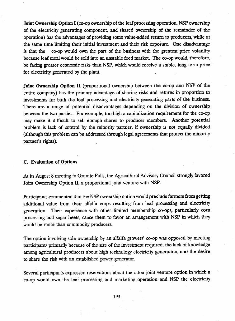
Joint Ownership Option I (co-op ownership of the leaf processing operation, NSP ownership
of the electricity generating component, and shared ownership of the remainder of the
operation) has the advantages of providing some value-added return to producers, while at
the same time limiting their initial investment and their risk exposure. One disadvantage
is that the co-op would own the part of the business with the greatest price volatility ·
because leaf meal would be sold into an unstable feed market. The co-op would, therefore,
be facing greater economic risks than NSP, which would receive a stable, long term price
for electricity generated by the plant.
Joint Ownership Option II (proportional ownership between the co-op and NSP of the
entire company) has the primary advantage of sharing risks and returns in proportion to
investments for both the leaf processing and electricity generating parts of the business.
There are a range of potential disadvantages depending on the division of ownership
between the two parties. For example, too high a capitalization requirement for the co-op
may make it difficult to sell enough shares to producer member$. Another potential
problem is lack of control by the minority partner, if ownership is not equally divided
(although this problem can be addressed through legal agreements that protect the minority
partner's rights).
· C. Evaluation of Options
At its August 8 meeting in Granite Falls, the Agricultural Advisory Council strongly favored
Joint Ownership Option II, a proportional joint venture with NSP.
Participants commented that the NSP ownership option would preclude farmers from getting
additional value from their alfalfa crops resulting from leaf processing and electricity
generation. Their experience with other limited membership co-ops, particularly com
processing and sugar beets, cause them to favor an arrangement with NSP in which they
would be more than commodity producers.
The option involving sole ownership by an alfalfa growers' co-op was opposed by meeting
participants primarily because of the size of the investment required, the lack of knowledge
among agricultural producers about high technology electricity generation, and the desire
to share the risk with an established power generator.
Several participants expressed reservations about the other joint venture option in which a
co-op would own the leaf processing and marketing operation and NSP the electricity
193
generating component. The major concern was that the co-op would be selling leaf meal into a volatile feed market, while NSP would receive a stable price for electricity generated from alfalfa stems. They argued that the joint venture partners should share more equitably in the returns from the volatile leaf product sales and the stable electricity sales.
In the end, the option involving proportional ownership of the entire biomass plant was clearly favored by the participants in the meeting. Although there was no detailed discussion on the shares of ownership between the two joint venture partners, several people commented that they would like to see minority ownership by a co-op and majority ownership by NSP (for example, a 25-75 split) as long as an equitable decision making procedure between the two parties could be worked out.
D. Investment and Contractual Issues
Participants in the August 8 meeting commented on a number of issues related to the biomass project, particularly related to investing in the co-op and contracting with the joint venture.
1. Leaf meal market. When asked what the major issues are that need to be resolved before the biomass plant is developed, the. biggest concern raised- was the . need to identify a firm market for leaf products.
2. Acreage per producer. There were differences of opinion among the group about the average number of acres farmers would be willing to commit to the biomass plant H the average of grow.er contracts was 100 acres per member then approximately 1,800 grower-owners would be needed. Some participants thought that the average number of acres per farmer would be under 100 acres probably in the range of 60 to 80 acres. H this estimate is correct, over 2,250 members would be needed to meet the plant's feedstock demand (coop membership estimates are based on a production average of 3.9 tons per acre, annual feedstock demand for 700,000 tons {leaves and stems}, yielding an acreage requirement of ca. 180,000 acres).
3. Contracts based on tons/acres. Participants favored sales agreements to the biomass plant based on tons and quality. Stock purchases in the co-op could be based on tons or by the acre. Minnesota Com Processors (MCP), a local com wet-milling cooperative, has stock purchases and production commitments based on bushels. Southern Minnesota Sugarbeet Growers Association (SMSBG), a local sugarbeet cooperative, bases
194
membership shares on acres. Participants expressed concerns about having sales
agreements that are too complicated, for example requiring cutting at specific times of
the year or requiring only two cuttings.
4. Price per ton. Several participants are currently selling prime hay at $100 per ton. One
of these growers commented that he would accept $80 per ton from the co-op because
he could reduce labor and transportation costs below those he experiences with his
current baling and marketing approach. Assuming that the co-op will pay differential
prices based on hay quality, an $80 price for prime hay probably translates into a
average price for hay of different qualities in the mid to low $70's.
5. Amount of equity per farmer. There was general agreement that an average of $15,000
to $20,000 in stock purchases was a reasonable investment level for the co-op. If the
investment is considered a good one by the producer's bank, it will accept the stock
certificate as the collateral for a loan of that size.
6. Return on investment. Based on returns being received by members of other limited
membership co-ops, participants in the meeting would like to see returns of 15 to 20%
on their investments in the alfalfa co-op. One of the financial advisors pointed out that
projected returns would have to be that high if farmers were to borrow in order to buy
co-op shares.
7. Length of contracts. Most participants favored a contracting system similar to those
used by other limited membership co-ops .. Farmers could sell their shares in the co-op
to another producer at any time, thus passing on the production contract to that
producer. If a farmer were not able to sell his shares to another farmer, he could submit
a notice of termination to the co-op. However, he would need to continue to meet his
contractual obligation for a specified period of time after his notice of termination (e.g.,
3 years, 5 years). Participants also reported that many limited membership co-ops are
not obligated to buy product from their members (although members have priority over
non-members). Participants thought that because of the long term production needs of
a biomass energy plant; however, the contract between the co-op members and the joint
venture should be more of a long term reciprocal agreement than in the case of some
other limited membership co-ops.
8. Adjustment .of prices. There was no clear agreement on how to adjust alfalfa prices
from year to year. Suggestions included using hay auction prices, a formula based on
soybean and com prices, and a formula based on sale prices of leaf meal/ other feeds.
195
9. Insurance against crop losses. Many participants expressed a concern about weatherrelated risks of growing alfalfa. One person reported that USDA crop insurance is available in some areas for alfalfa. There was also some discussion of the biomass plant not obligating producers to meet their contracts if they could certify their crop loss. The possibility of some type of risk sharing pool among co-op members was also discussed.
Conclusion
Agricultural Advisory Council participants clearly favor a joint venture model between NSP and a growers' cooperative in which investments, risks and returns are equitably shared among the two venture partners.
The Agricultural Advisory Council also identified a number of specific marketing, financial and contractual issues that should be taken into account in the development of the co-op and the joint venture. These issues are described in the preceding section.
It is worth noting that the Agricultural Advisory Council meeting on August 8 concluded with the formation of an alfalfa growers' cooperative steering committee. Ten participants agreed to meet to discuss the next steps alfalfa producers should take in order to prepare for further development of the biomass plant as well as for other processing and marketing opportunities for alfalfa. Subsequent meetings resulted in the formation of the Minnesota Valley BioPower Cooperative (BPC). The BPC is a grower-owned cooperative formed to evaluate the opportunity for sustainable biomass energy production from alfalfa. BPC Board members are listed in Chapter 1.
196
9.2 Contracting for Production
Douglas G. Trliany and Jerry Fruin
Agricultural and Applied Economics, University of Minnesota
Establishing contract terms that clearly communicate how· growers will be paid is crucial.
By definition, contracts are designed to guide the performance of two parties and protect
each through the course of a transaction. Regardless of to whom growers sell their alfalfa,
the following issues will need to be clearly understood by each party:
1) the quantity of alfalfa to be delivered and the delivery location (tons/acres),
2) the minimum acceptable quality,
-3) fair price differentials between quality grades,
4) the timing of delivery or method of flow control,
5) approved production practices (weed control, use of pesticides),
6) the payment schedule,
7) the risk borne by each party, and risk sharing,
8) auxiliary services provided by the contractor,
Q) conditions allowing adjustment of contract terms and means to mediate disputes,
10) a means to prevent leakage of contracted supply and fraud.
If a fair contract can be drafted, then both the grower and the contractor will benefit from
continuity and long term relationships. Retention of growers is important because it can
result in substantial savings for the contractor in terms of reduced transaction costs to
recruit new growers. Since the proposed project would utilize the hay from nearly 180,000
acres and could involve 2,000 growers, transaction costs and grower retention
are very important.
197
There are umque aspects of alfalfa biomass production. Unique conditions require unique
contract specifications. With 180,000 acres of alfalfa being grown, harvests could occur from
May 25 to September 1 or later, depending on contract terms and incentives as well as grower attitudes. Because the project is large in scale and because 60% of the crop must
have storage, remote storage sites will be important. They will .provide storage as well as
quality testing. The remote storage sites are assumed to be spaced around the biomass shed
within 5 miles of each grower. Two types of vehicles were identified as suitable for
transportation of large round bales to the remote storage sites. The number of remote storage sites specified in Chapter 5 is large in order to reduce the costs of transportation from field to remote storage site. It is assumed that all hay can be brought in or through the remote storage sites within 15 days of harvest. Approximately 40% of all the production
of alfalfa stems will be consumed during the growing season. Therefore, alfalfa processing must occur for 40% of the hay in this time period.
Quantity delivered
At issue is whether or not contracts should be based on acres of hay or tons of hay. H a contract is based on acres, such as canning contracts or sugar beets, it is often because there are no other market channels for these crops than through the contractor. In the case of com for processing, contracts are made on the basis of bushels. This is partly due to the
. fact that there are readily available market channels for extra crop grown on farms and
there are readily available market sources for the contractor in years when grower yields are
too poor to fulfill the contract. The biomass energy facility will be designed to provide
stems to fuel electric power production and leaves for co-product processing. The power plant and alfalfa processing facility will be designed with minimum and maximum capacities.
If growers contract on the basis of tons and are unable to deliver, growers may be asked to
compensate the power plant for the additional ce>st above alfagas (biomass fuel) needed to buy natural gas to fire the combustion turbine. Essentiauy, the growers would be contracting to deliver stems sufficient to provide so many BTU's. If they didn't, they may
be responsible for the cost of a higher price substitute fuel (natural gas).
If growers were to contract their production from a given number of acres of alfalfa, there would be temptations for some to report low yields in years of high hay prices and divert
some of their hay to the hay market. This is called "contract leakage".
198
The place to certify the amount delivered will be the remote storage site. Should there be
different prices paid for hay delivered to remote storage sites - based on distance to the
site? For contracted sugarbeet production, transportation allowances attempt to equalize trucking costs from remote storage to the central processing plant. Since title to the alfalfa changes at the remote storage site, the quantity and quality of hay for future payment is determined there. Because the grower co-op needs growers far and near to spread risk and attain the critical mass for plant economies, it can be argued that there should be no price differentials due to production location (within a set maximum boundary).
Minimum quality acceptable
Quality becomes an issue in several dimensions. One attribute that must be specified is acceptable moisture. H bales are too wet, microbial activity can cause them to heat, causing dry matter losses as well as the possibility of fire from spontaneous combustion. Perhaps any bale exceeding 18% should be rejected from storage at remote sites and sent directly for drying and fractionation. H alfalfa bales are too wet for safe storage, producers must
suffer sharp discounts thereby discouraging this practice. Perhaps a continuous-weighing conveyor or a scale device built into the fork of a forklift could effectively detect wet bales based on their weight.
Quality testing
It is important that the contractor not suffer quality losses caused by growers sorting out poorer bales for delivery. Alfalfa will need to be tested at the regional storage site upon
receipt. Near infrared reflectance spectroscopy (NIRS) is a rapid testing method used in
the U.S. to test forages. The test can be performed within minutes after samples are prepared. Hay delivered to the biomass shed should be tested for moisture, crude protein (CP), acid detergent fiber (ADF), neutral detergent fiber (NDF), relative feed value (RFV), % leaf fraction, and % weeds.
Fair Price Ditrerentials Between Quality Grades
A great way to encourage unhappy growers and lose grower continuity is for the contractor to be imprecise in measuring quality and thus overpaying for poor quality. This also creates
fQrther incentives for quality leakage.
199
'liming of Delivery or Flow Control
C-anning companies offer incentives for growers of peas and sweet com to grow for them
at times of the season when maximum yields are not possible in order to keep a consistent
volume of product fl.owing to the processing facility. To encourage pea and sweet com
growers to produce for the non-optimum times, they must be compensated according to
planting date. Similarly, in order to have flow control and some measure of risk balancing,
the biomass contractor may wish to encourage some growers to use different cutting
schedules so that the cutting times will be dispersed over the whole biomass shed. Flow
control would be accomplished in an area by offering price incentives to time particular
cuttings in order to smooth out the amount of hay heading into the remote storage sites during particular harvest windows.
Approved Production Practices
Producers will probably want an initial payment when their bales are graded and enter the remote storage site. The contractor will probably wish to make payments only as fast as
sales of leaves and stems occur in aggregate for the biomass shed. Subsequent payments
may be made over the next ten months as sales of leaves and stems occur.
Risk Borne by Each Party, Risk Sharing
Producers will generally accept the risk of rain damage and poor growing conditions. Once
the hay is delivered at the remote site, the ·quality grade is established upon which the
grower will be compensated. Weight and quality losses during storage would then be the
responsibility of the cooperative or the joint venture.
Auxiliary Senices Provided by the Contractor
Sc\.·eral possible services that the contractor (or other private contractors) could provide for
gro-.·e~ include field pick-up of bales with specialized equipment and hauling to remote
storage sites. Under such a scenario the grower may get nervous waiting for his bales to be
moved in before they suffer damage due to rain while already baled. By supplying transport
sef'\ices from the field to remote storage, the contractor could effectively prevent "leakage"
of contracted hay. The contractor will either provide or contract with trucking companies
for hauling_ of hay on semi's from remote storage sites or from fields in a direct haul
situation during harvest to the processing plant.
200
Conditions Allowing Adjustment of Contract Terms, Dispute Resolution
Pertinent to this issue are situations when a grower might wish to leave the co-op. A worthy
mechanism utilized by others is that of requiring a grower to officially notify the co-op of
his plan to leave three years before his obligations end.
H farmers differ with grain elevators on measured quality grades, they theoretically have
avenues for a re-grade through state and federal agencies. Perhaps there will need to be
a similar path for dispute resolution with hay.
Means to Prevent Leakage of Contracted Supply and Fraud
As stated previously, answers to this issue lie in crafting clear contracts and spending the
money to measure quality precisely. Contract terms could specify tonnages with defined leaf
and stem percentages with recourse against the grower to compensate for insufficient
delivery. Penalties could be based on the additional expenses born for insufficient feedstock
delivery.
Another important task of the contractor is monitoring performance. The contractor must
ask whether or not contract terms provide sufficient incentives to keep the proper balance
of quantity and quality needed for profitability.
201
9.3 Coop Development
Key Components for Success
USDA:RDA Cooperative Development Program
- The Cooperative Development Program within USDA has available no cost technical assistance for the development of ,producer cooperatives for biomass energy production. Financial assistance for cooperatives to develop marketing strategies and for other cooperative related business functions has also been available through a competitive grant process, pending funding allocation. Further information on the Cooperative Development Program is available by contacting the Center for Alternative Plant and Animal Products, University of Minnesota.
202
Introduction
CHAPTER 10. ENVIRONMENTAL IMPACT
10.1 Energy Balance
David Schmidt and William Wilcke Agricultural Engineering, University of Minnesota
Does energy input into production, transport, and processing of alfalfa for fuel result in a net energy gain or loss? The answer to the question is one of utmost importance when biomass is proposed as a viable energy source. If indeed the biomass system consumes more energy than it produces, it may be more environmentally sound use fossil fuels directly.
Evaluating energy inputs and outputs for a biomass system is not as easy as it might seem. First, it is difficult to determine what inputs should be included in the system and to get accurate values for those inputs. Depending on the inputs chosen and the values assigned to these inputs, an energy balance can be •adjusted" significantly. Secondly, with a biomass
system, there are often co-products generated. These co-products cannot logically be evaluated on their gross energy because they are not converted to heat, but are used as a food or feed source. For example, the protein leaf meal generated in alfalfa conversion
must be evaluated in terms of feed value, not gross energy content. A biomass energy
balance should be viewed only as one of many guides in determining the effectiveness of
using biomass as an energy source. Energy inputs and outputs used in the following
evaluation are based on the best information available. All assumptions and references are
given to assist readers in reaching an independant conclusion.
Energy Analysis
Energy inputs into the dedicated feedstock supply system (DFSS) rotation (four years alfalfa, two years com and one year soybeans) are compared to energy inputs in a conventional crop rotation (one year corn, one year soybeans). A comparison of energy inputs for these
rotations aids an evaluation of the sustainability of those systems. The net energy balance (energy inputs : energy outputs) for the conversion of alfalfa feedstock to electricity and protein meal is also determined.
203
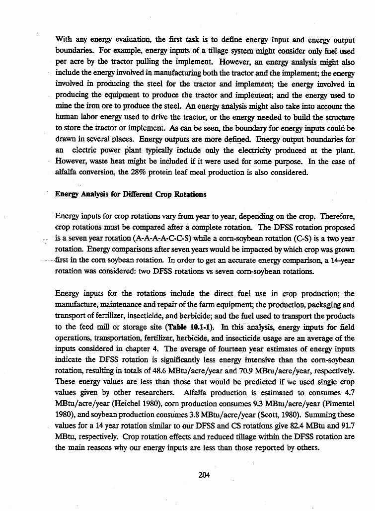
With any energy evaluation, the first task is to define energy input and energy output boundaries. For example, energy inputs of a tillage system might consider only fuel used per acre by the tractor pulling the implement However, an energy analysis might also include the energy involved in manufacturing both the tractor and the implement; the energy involved in producing the steel for the tractor and implement; the energy involved in producing the equipment to produce the tractor and implement; and the energy used to mine the iron ore to produce the steel. An energy analysis might also take into account the human labor energy used to drive the tractor, or the energy needed to build the structure to store the tractor or implement As can be seen, the boundary for energy inputs could be drawn in several places. Energy outputs are more d~fil!~d. Energy output boundaries for an electric power plant typically include only the electricity produced at the plant. However, waste heat might be included if it were used for some purpose. In the case of alfalfa conversion, the 28% protein leaf meal production is also considered.
Energ_v Analysis for Different Crop Rotations
Energy inputs for crop rotations vary from year to year, depending on the crop. Therefore, crop rotations must be compared after a complete rotation. The DFSS rotation proposed
-- is a seven year rotation (A-A-A-A-C-C-S) while a com-soybean rotation (C-S) is a two year rotation. Energy comparisons after seven years would be impacted by which crop was grown
. -.... first in the com soybean rotation. In order to get an accurate energy comparison, a 14-year rotation was considered: two DFSS rotations vs seven com-soybean rotations.
Energy inputs for the rotations include the direct fuel use in crop production; the manufacture, maintenance and repair of the farm equipment; the production, packaging and transport of fertilizer, insecticide, and herbicide; and the fuel used to transport the products to the feed mill or storage site (Table 10.1-1). In this analysis, energy inputs for field operations, transportation, fertilizer, herbicide, and insecticide usage are an average of the inputs considered in chapter 4. The average of fourteen year estimates of energy inputs indicate the DFSS rotation is significantly less energy intensive than the com-soybean rotation, resulting in totals of 48.6 MBtu/acre/year and 70.9 MBtu/acre/year, respectively. These energy values are less than those that would be predicted if we used single crop values given by other researchers. Alfalfa production is estimated to consumes 4.7 MBtu/acre/year (Heichel 1980), com production consumes 93 MBtu/acre/year (Pimentel 1980), and soybean production consumes 3.8 MBtu/acre/year (Scott, 1980). Summing these values for a 14 year rotation similar to our DFSS and CS rotations give 82.4 MBtu and 91.7 MBtu, respectively. Crop rotation effects and reduced tillage within the DFSS rotation are the main reasons why our energy inputs are less than those reported by others.
204
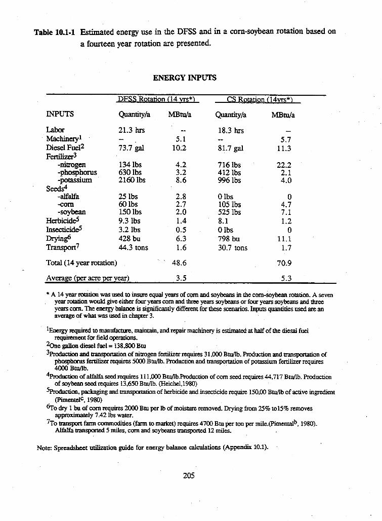
Table 10.1-1 Estimated energy use in the DFSS and in a com-soybean rotation based on a fourteen year rotation are presented.
ENERGY INPUTS
DFSS Rotation <14 yrs*) CS Rotation <14yrs*)
INPUTS Quantity/a :MBtu/a Quantity/a :MBtu/a
Labor 21.3 hrs 18.3 hrs Machinery I 5.1 5.7 Diesel FueI2 73.7 gal 10.2 81.7 gal 11.3 Fertilizer3
-nitrogen 134 lbs 4.2 716 lbs 22.2 -phosphorus 630lbs 3.2 412 lbs 2.1 -potassium 2160 lbs 8.6 996 lbs 4.0
Seeds4 -alfalfa 25 lbs 2.8 Olbs 0 -com 60lbs 2.7 105 lbs 4.7 -soybean 150 lbs 2.0 525 lbs 7.1
Herbicide5 9.3 lbs 1.4 8.1 1.2 InsecticideS 3.2 lbs 0.5 Olbs 0 Drying6 428bu 6.3 798 bu 11.1 Transpon7 44.3 tons 1.6 30.7 tons 1.7
Total (14 year rotation) 48.6 70.9
Average (per acre per year) 3.5 5.3
* A 14 year rotation was used to insme equal years of C()m and soybeans in the com-soybean rotation. A seven year rotation would give either four years com and three years soybeans or four years soybeans and three years com. The energy ba1ance is significantly different for these scenarios. Inputs quantities used are an average of what was used in chapter 3.
1 Energy required to manufacture. maintain. and repair machinery is estimated at half of the diesal fuel requirement for field operations.
2one gallon diesel fuel = 138.800 Btu 3Production and transportation of nitrogen fertilizer requires 31,000 Btu/lb. Production and transpOrtation of
phosphorus fertilizer requires 5000 Btu/lb. Production and transponation of potassium fertilizer requires 4000 Btu/lb.
4Production of alfalfa seed requires 111.000 Btu/lb.Production of com seed requires 44,717 Btu/lb. Production of soybean seed requires 13.650 Btu/lb. (Heichel,1980)
5Production, packaging and transportation of herbicide and insecticide require 150.00 Btu/lb of active ingredient (PimentelC, 1980)
6ro dry 1 bu of corn requires 2000 Btu per lb of moisture removed. Drying from 25% to 15% removes approximately 7.42 lbs water.
7To ttansport farm commodities (farm to market) requires 4700 Btu per ton per mile.(Pimentalb, 1980). Alfalfa transported 5 miles, com and soybeans transpOrted 12 miles.
Note: Spreadsheet utilization guide for energy balance calculations (Appendix 10.1).
205
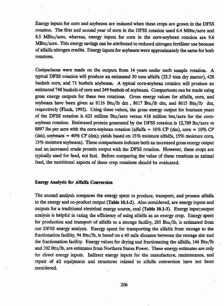
Energy inputs for com and soybeans are reduced when these crops are grown in the DFSS rotation. The first and second year of com in the DFSS rotation used 6.4 MBtu/acre and 85 MBtu/acre, whereas,-energy inputs for com in the com-soybean rotation are 9.6 MBtu/acre. This energy savings can be attributed to reduced nitrogen fertilizer use because of alfalfa nitrogen credits. Energy inputs for soybeans were approximately the same for both rotations.
Comparisons were made on the outputs from 14 years under each sample rotation. A typical DFSS rotation will produce an estimated 30 tons alfalfa (25.5 tons dry matter), 428 bushels corn, and 71 bushels soybeans. A typical com-soybean rotation will produce an estimated 748 bushels of com and 249 bushels of soybeans. Comparisons can be made using gross energy outputs for these two rotations. Gross energy values for alfalfa, corn, and soybeans have been given as 8116 Btu/lb dm, 8617 Btu/lb dm, and 8615 Btu/lb dm, respectively (Fluck, 1992). Using these values, the gross energy output for fourteen years of the DFSS rotation is 623 million Btu/acre versus 418 million btu/acre for the comsoybean rotation. Estimated protein generated by the DFSS rotatio:Q. is 12,789 lbs/acre vs 8897 lbs per acre with the com-soybean rotation (alfalfa= 18% CP (dm), com= 10% CP ( dm), soybeans = 40% CP ( dm); yields based on 15% moisture alfalfa, 15% moisture com, 13% moisture soybeans). These comparisons indicate both an increased gross energy output and an increased crude protein output with the DFSS rotation. However, these crops are typically used for feed, not fuel Before compar..ng the value of these rotations as animal feed, the nutritional aspects of these crop rotations should be evaluated.
Energy Analysis for Alfalfa Conversion
The second analysis compares the energy spent to produce, transport, and process alfalfa to the energy and co-product output (Table 10.1-2). Also considered, are energy inputs and outputs for a traditional electrical energy source, coal (Table 10.1-3). Energy input:output analysis is helpful in rating the efficiency of using alfalfa as an energy crop. Energy spent for production and transport of alfalfa to a storage facility, 285 Btu/lb, is estimated from our DFSS energy analysis. Energy spent for transporting the alfalfa from storage to the fractionation facility, 94 Btu/lb, is based on a 40 mile distance between the storage site and the fractionation facility. Energy values for drying and fractionating the alfalfa, 146 Btu/lb and 102 Btu/lb, are estimates from Northern States Power. These energy estimates are only for direct energy inputs. Indirect energy inputs for the manufacture, maintenance, and repair of all equipment and structures related to alfalfa conversion have not been considered.
206
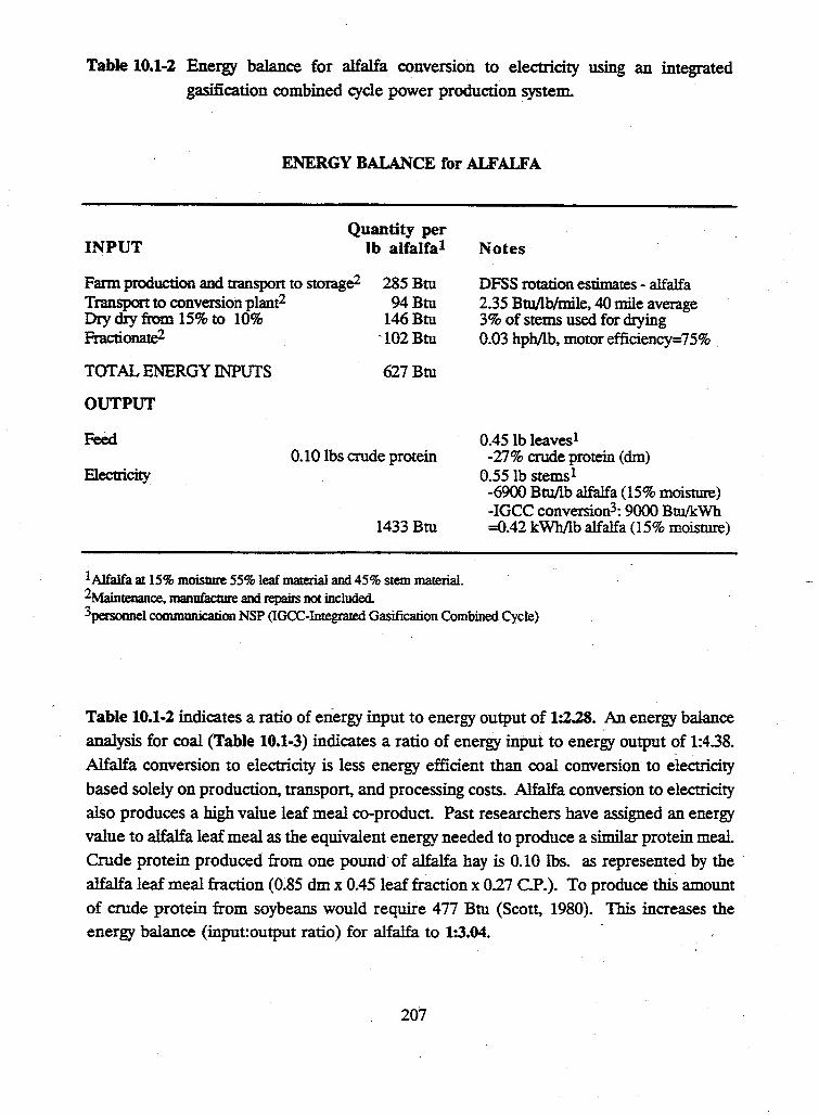
Table 10.1-2 Energy balance for alfalfa conversion to electricity using an integrated gasification combined cycle power production system.
ENERGY BALANCE for ALFALFA
INPUT Quantity per
lb alfalfal
Farm production and transport to storage2 Transport to conversion plant2
285 Btu 94Btu
146Btu Dry dry from 15% to 10% Fractionate2
TOTAL ENERGY INPlITS
OUTPUT
Feed
Electricity
'102 Btu
627 Btu
0.10 lbs crude protein
1433 Btu
1 Alfalfa at 15% moisture 55% leaf material and 45% stem material. 2Mainrenance. manufacture and repairs not included.
Notes
DFSS rotation estimates - alfalfa 2.35 BttJ/lb/mile, 40 mile average 3% of stems used for drying 0.03 hph/lb, motor effi.ciency=75%
0.45 lb leavesl -27% crude protein (ciin)
0.55 lb stemsl -6900 BttJ/lb alfalfa (15% moisture) -IGCC conversion3: 9000 Btu/kWh =0.42 kWh/lb alfalfa (15% moisture)
3personnel communication NSP (IGCC-Integrated Gasification Combined Cycle)
Table 10.1-2 indicates a ratio of energy input to energy output of 1:2.28. An energy balance analysis for coal (Table 10.1-3) indicates a ratio of energy input to energy output of 1:438.
Alfalfa conversion to electricity is less energy efficient than coal conversion to electricity based solely on production, transport, and processing costs. Alfalfa conversion to electricity also produces a high value leaf meal co-product. Past researchers have assigned an energy value to alfalfa leaf meal as the equivalent energy needed to produce a similar protein meal. Crude protein produced from one pound of alfalfa hay is 0.10 lbs. as represented by the alfalfa leaf meal fraction (0.85 dm x 0.45 leaf fraction x 027 C.P.). To produce this amount of crude protein from soybeans would require 477 Btu (Scott, 1980). This increases the energy balance (input: output ratio) for alfalfa to 1:3.04.
207
Table 10.1-3 Estimated energy balance for coal conversion to electricity using an integrated gasification combined cycle electric power production system.
ENERGY BALANCE for COAL
INPUTS
Mining transport. breaking, sizing, washing, distribution 1
OUTPUTS
Electricity
Quantity per lb coal
827 Btu
3625 Btu
1 Manufacture, maintenance, and repair of equipment not included.
Notes
Cervinka(l 980) =7.3% of high heat value
8500 Btu/lb coal (25% moisture) -IGCC conversion2: 8000 Btu/kWh =l.06kWMb coal
2Personne1 communication NSP (IGCC-Integrated Gasification Combined Cycle)
Conclusions
A primary concern when converting biomass to energy is the energy balance. Our energy analysis indicates the conversion of alfalfa to electricity results in a net energy increase. The ratio of energy input to energy output (1:3) is less than for coal conversion to electricity (1:4.4) however, this is not surprising, given that energy in coal represents biomass energy that over millions of years was concentrated to a form that need only be stripped out of the ground and loaded on trains. Biomass energy in alfalfa reflects solar energy sequestered in ·plant tissues in a period of less than a year. The lower energy density of biomass may well be compensated for by other environmental and economic considerations. The highly positive energy balance (1:3) indicates that alfalfa is a very energy efficient biomass energy crop. Our analysis indicates that the DFSS rotation generates more gross energy and more crude protein than a traditional com-soybean rotation and does it with lower energy Uiputs.
208
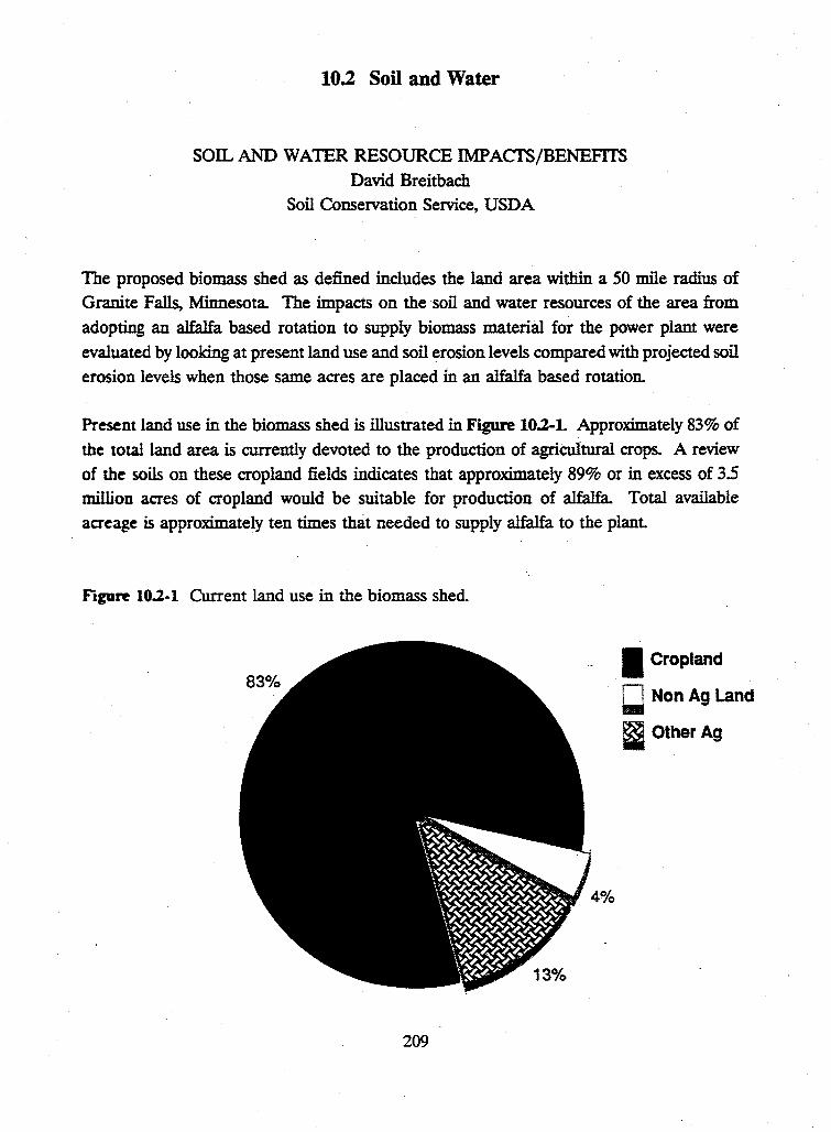
10.2 Soil and Water
SOIL AND WATER RESOURCE IMP ACTS/BENEFITS
David Breitbach Soil Conservation Service, USDA
The proposed biomass shed as defined includes the land area within a 50 mile radius of Granite Falls, Minnesota. The impacts on the ·soil and water resources of the area from
adopting an alfalfa based rotation to supply biomass materia.1. for the power plant were
evaluated by looking at present land use and soil erosion levels compared with projected soil
erosion levels when those same acres are placed in an alfalfa based rotation.
Present land use in the biomass shed is illustrated in Figure 10.2-1. Approximately 83% of
the total land area is currently devoted to the production of agricultural crops. A review
of the soils on these cropland fields indicates that approximately 89% or in excess of 3.5 million acres of cropland would be suitable for production of alfalfa. Total available acreage is approximately ten times that needed to supply alfalfa to the plant.
figutt 10.2-1 Current land use in the biomass shed.
209
.1 Cropland
~Non Ag Land
~Other Ag
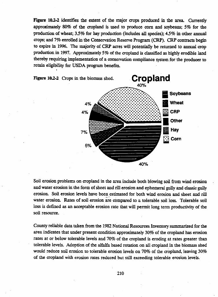
Figure 10.2-2 identifies the extent of the major crops produced in the area. Currently approximately 80% of the cropland is used to produce com and soybeans; 5% for the production of wheat; 3.5% for hay production (includes all species); 4.5% in other annual crops; and 7% enrolled in the Conservation Reserve Program (CRP). CRP contracts begin to expire in 1996. The majority of CRP acres will potentially be returned to annual crop production in 1997. Approximately 5% of the cropland is classified as highly erodJ."ble land thereby requiring implementation of a conservation compliance system for the producer to retain eligibility for USDA program benefits.
Figure 10.2-2 Crops in the biomass shed.
4%
7%
..cropland 40%
_,.....,....,_
40%
I Soybeans
I Wheat
I Hay
~Corn
Soil erosion problems on cropland in the area include both blowing soil from wind erosion and water erosion in the form of sheet and rill erosion and ephemeral gully and classic gully erosion. Soil erosion levels have been estimated for both wind erosion and sheet and rill water erosion. Rates of soil erosion~~ compared to a tolerable soil loss. Tolerable soil loss is defined as an acceptable erosion rate that will permit long term productivity of the soil resource.
County reliable data taken from the 1982 National Resources Inventory summarized for the area indicates that under present condition approximately 30% of the cropland has erosion rates at or below tolerable levels and 70% of the cropland is eroding at rates greater than tolerable levels. Adoption of the alfalfa based rotation on all cropland in the biomass shed would reduee soil erosion to tolerable erosion levels on 70% of the cropland, leaving 30% of the cropland with erosion rates reduced but still exceeding tolerable erosion levels.
210
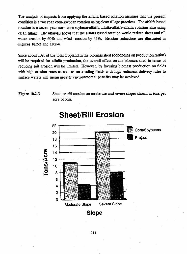
The analysis ~f impacts from applying the alfalfa based rotation assumes that the present
condition is a two year com-soybean rotation using clean tillage practices. The alfalfa based
rotation is a seven year com-com-soybean-alfalfa-alfalfa-alfalfa-alfalfa rotation also using
clean tillage. The analysis shows that the alfalfa based rotation would reduce· sheet and rill
water erosion by 60% and wind erosion by 45%. Erosion reductions are illustrated in
F°IgUreS 10.2-3 and 10.2-4.
Since about 10% of the total cropland in the biomass shed (depending on production radius)
will be required for alfalfa production, the overall effect on the biomass shed in terms of
reducing soil erosion will be limited. However, by focusing biomass production on fields
with high erosion rates as well as on eroding fields with high sediment delivery rates to
surface waters will mean greater environmental benefits may be achieved.
Figure 10.2-3
Cl) .... (,) c( --ti) c 0 I-
Sheet or rill erosion on moderate and severe slopes shown as tons per
acre of loss.
Sheet/Rill Erosion 22 ..-------------
20 +------'"'BIJllll!!l!l!lllll!ll!lll!)lll!ii;"--
18 +---------· 16 +-----------; 14 +--------~
12 +-------~
10
8
6
4
2
0 Moderate Slope Severe Slope
Slope
211
CJ!~ Com/Soybeans
II Project
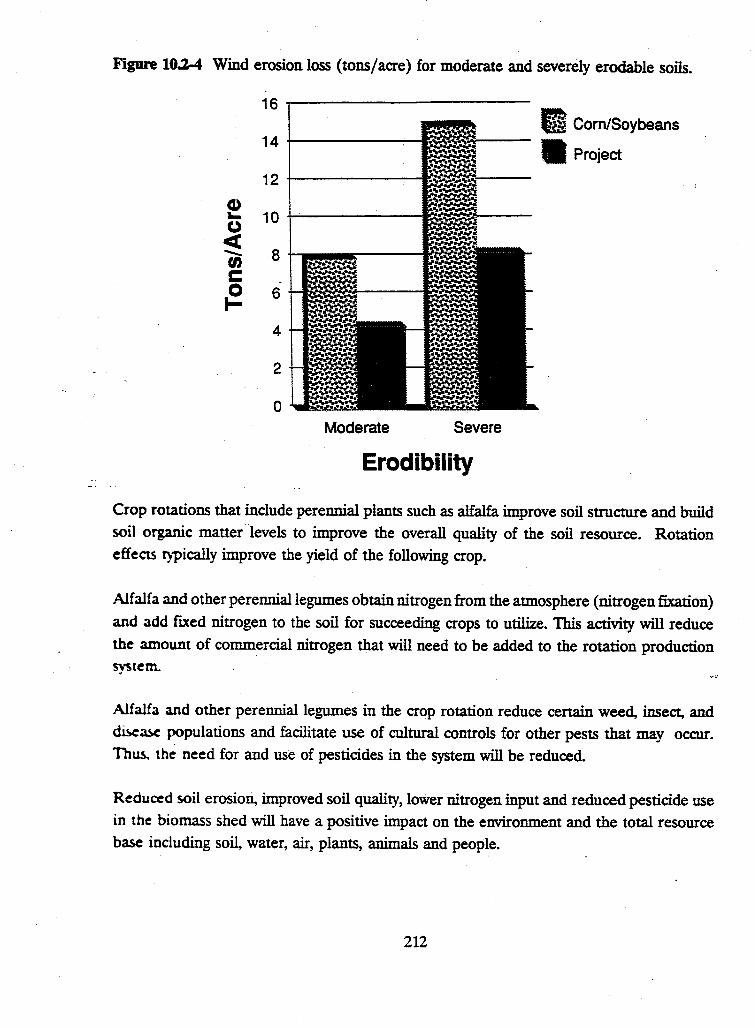
FJ.gU.re 10.2-4 Wind erosion loss (tons/acre) for moderate and severely erodable soils.
CD ~ (.)
< -.... tn c 0 I-
16
14
12
10
8
6
4
2
0 Moderate Severe
Erodibility
e Corn/Soybeans
II Project
Crop rotations that include perennial plants such as alfalfa improve soil structure and build soil organic matter levels to improve the overall quality of the soil resource. Rotation effects typically improve the yield of the following crop.
Alfalfa and other perennial legumes obtain nitrogen from the atmosphere (nitrogen fixation) and add fixed nitrogen to the soil for succeeding crops to utilize. This activity will reduce the amount of commercial nitrogen that will need to be added to the rotation production system.
Alfalfa and other perennial legumes in the crop rotation reduce certain weed, insect, and d™:~ populations and facilitate use of cultural controls for other pests that may occur. Th~ the need for and use of pesticides in the system will be reduced.
Reduced soil erosion, improved soil quality, lower nitrogen input and reduced pesticide use in the biomass shed will have a positive impact on the environment and the total resource base including soil, water, air, plants, animals and people.
212
10.3 Changes in Soil Structure
J.F. Moncrief
Soil Science, University of Minnesota
Com grain yields are 10 to 15% higher when following alfalfa compared to com due to the
"rotation effect". Although there is a benefit from the atmospheric N that is converted to
available forms f!Jr the following com crop, the "rotation effect" is independent of the
response to soil N. There is also less pressure from insects, diseases, and weeds when
rotations are followed. Although all of these factors contribute to the better crop
performance when alfalfa is in the rotation, the soil influence is not to be undervalued
Water and gas flows through soil are largely dependent on not only the total porosity, but
also the pore size distribution, continuity, and tortuosity. The pore characteristics are
influenced mostly by the soil particle size distnbution. Soil particles can be bound together
by cementing agents, causing them to act like larger particles. This phenomenon affects
water and gas fl.ow.
When alfalfa is introduced into a rotation, several changes in soil properties occur.
Cementing agents (such as polysaccharides and gels) are introduced from direct alfalfa root
exudates which also stimulate microbial activity. Together these influences reduce soil bulk
density, increase pore space, and aeration, and provide macropores that provide for better ,., water flow. The absence of tillage during the·alfalfa years of the rotation also allows soil
structure formation, increased soil organic matter, and enhanced physical and biological soil
properties.
Most farmers generally recognize improved soil tilth when following alfalfa. The soil is well
aggregated and the aggregates are very stable. It is hard to assign a dollar value to
improved soil tilth. The benefits of the alfalfa in the rotation are greatest on the fine
textured soils (developed in glacial till or lacustrine sediments). Alfalfa has the greatest
impact on improving the internal soil drainage and aeration of these soils, which need tile
drainage to effectively grow crops. In wet years enhanced internal drainage on soils
previously in alfalfa can influence yields about 25%. On average the influence of good
internal drainage on yields is about 15%. Alfalfa in a rotation increases the effectiveness
of the tile.
213
Introduction
10.4 Environmental Impacts of Biomass Production in the Upper Minnesota River Basin
S.C. Gupta and J.F. Moncrief Soil Science, University of Minnesota
Non-point source monitoring studies ·conducted by the Minnesota Waste Control Commission, MWCC, {1990, 1991, 1994) have doaunented that during 1976-1992 the water quality of the Minnesota River has been worse than that of the Mississippi and St. Croix Rivers. The loading of total suspended solids in the lower Minnesota River was 22 times greater than that in the St. Croix River and 3.6 times greater than that in Mississippi river (MWCC, 1994). According to MWCC, these numbers translate to approximately 625,000 tons per year of total suspended solids (86 20-ton truckload per day) transported by the Minnesota River at Fort Snelling in the Twin Cities. Loading of total P from the Minnesota River was 5.5 times greater than from the St. Croix River and 1.5 times greater than from the Mississippi River (MWCC, 1994). During 1990-1992, 84% to 96% of the entire annual loading of chemical oxygen demand (COD), nitrate, total suspended solids, and total P to the lower Minnesota River was from diffuse sources upstream.
The poor water quality of the Minnesota River is one of the major water quality issues facing the state of Minnesota. The Minnesota Pollution Control Agency (MPCA) has estimated that a 40% reduction in head water pollutant loading will be necessary to achieve federally mandated water quality goals in the lower Minnesota River.
A recent study (Ginting et al, 1993) in West Central Minnesota has shown that although total P and sediment losses in spring runoff are higher from moldboard plowed tillage systems, systems that leave crop residues· on the surface result in more soluble P in snow melt. After several major runoff events during the early growing season, sediment losses under the moldboard system surpass those of cropping systems that leave crop .residues on the soil surface.
Estimates from this feasibility study have shown a great reduction in sediment losses when tillage is eliminated and soil cover provided with alfalfa prodµction. This could translate to a substantial reduction in loading of biological oxygen demand, phosphorus, and sediment to the Minnesota River. The caveat is the unknown contribution of the soluble P leaching from alfalfa residues during the spring thaw period.
214
Research Needed
Future research is necessary to quantify the effect of introducing alfalfa into a com-soybean
rotation on the transport of sediment, P, N, and carbonaceous material in surface runoff
from watersheds under the climatic and soil conditions of West Central Minnesota. The
impact on both individual storms and annual loading needs to be considered. The specific
research objectives are:
1. To evaluate the effect of alfalfa introduction into a com-soybean rotation on water
quality of surface runoff at the subwatershed ~ca.l_e during fall, spring and summer
months. This will quantify the effect on annual loading of runoff; sediment; total, bio
available, and soluble P; nitrate and carbonaceous material from the watershed.
2. To .quantify processes affecting runoff water quality at the plot scale under natural
precipitation.
3. To quantify and model processes affecting runoff water quality during the snow melt
period.
4. To develop methods of upscaling plot runoff and water quality data to the watershed
scale.
5. To assess the cost-benefit ratios of various management practices in improving the runoff
water quality at the watershed scale.
Models and Scaling:
Even though considerable research data might exist for a given problem in the literature,
upscaling and extrapolating the data both in space and time is difficult. Models provide an
excellent and inexpensive opportunity for such scaling.
For the sediment and nutrient transport in surface runoff, there is extensive literature at a
plot level. However, there has been limited effort in upscaling this data to the watersheds.
Procedures are needed to take data from the plot studies and apply them to large areas
such as small and large watersheds, or to even subbasin scale. In addition, as most of the
research covers a small time scale, methods are needed to extrapolate data to longer time
periods.
215
A few of the well known functional models in the literature dealing with sediment and nutrient transport are GLEAMS (Groundwater Loading Effects of Agricultural Management Systems) and AGNPS (Agricultural Non-point Source Pollution Model). Each of these models is applicable at a different scale. Application· of GLEAMS is appropriate at a plot/field scale whereas that of AGNPS is more suitable for a watershed scale. However, little effort has been made to link these models.
A recent study conducted by the Soil Conservation Service (1993) used these models to assess the impact of land management in 10 watersheds along the Minnesota River. These models were used separately for a given purpose. For example, GLEAMS was used to estimate nutrient loading whereas AGNPS was used to predict sheet and rill soil erosion and sediment yield. The prediction from these two models were used in conjunction with 1R-20 (Technical Release-20, SCS, 1991) Hydrologic Delivery model outputs to estimate losses of sediment and _nutrients at both the field and watershed level. Although the assessment based on this approach has been useful in identifying broad alternatives for reducing the sediment and contaminant transport to the Minnesota River, no effort has been made to test and validate these upscaling procedures. In addition, the manure management alternatives were not considered in the approach. Since both the AGNPS and GLEAMS models either lack or include an over-simplified. description of frozen soil conditions, there is a need to include or improve such a component in these models to make these models fully applicable to cold climate regions. Furthermore, both plot and small watershed level scale experiments proposed in this study provide a unique opportunity to test and possibly develo~ new · upscaling procedures for extrapolating data. Although limited in time scale, this three year study will also be used to consider scaling and extrapolating issues with respect to time.
216
INTRODUCTION
10.S Wildlife
Impact of Alfalfa Biomass Production on
Wildlife Diversity and Abundance
Al Bemer and Allison Leete Minnesota Department of Natural Resources.
The purpose of this report is to provide information on the impacts of suggested practices to be used in managing alfalfa for production of biomass on the abundance and diversity of wild birds and mammals. The biomass grown will be used to produce a high protein leaf meal and to provide 1,000 tons per day of fuel for a proposed gasification generation power plant in Granite Falls, Minnesota. These findings are based upon a literature review and interviews with wildlife experts.
BACKGROUND
The nine major counties affected by this project are primarily in the Minnesota River watershed and lie on both sides of this major river drainage system. Historically, this area was characterized by flat to rolling topography with vast expanses of native prairie, grassforb communities laden with wetlands. The majority of the wildlife species in these areas evolved with a dependence on these two major vegetation. types.
Most wildlife species continued to cope or in some cases flourish with the advent of diversified agriculture. However, in the early 1960's with the shift to monotypic, production agriculture, which was accelerated by federal feed grain farm policies, abundance of most wildlife species changed dramatically (Bemer 1988).
Most wildlife populations declined until the early 1970's, leveled off in the late 1970's and early 1980's, and began increasing with the establishment of permanent cover on Conservation Reserve Program (CRP) and Reinvest in Minnesota (RIM) acres. For example, pheasant populations, which generally mirrored the changes seen in most bird species dependent on undisturbed grasslands for reproduction, showed the following changes between 1955 and 1993 in the major 9 counties that will be affected by this project.
217
During the period of 1955-1964, pheasant densities varied from 84 to 214, and averaged 140
birds per square mile. With the conversion of Soil Bank's Conservation Reserve Acres,
grassland (e.g., native hay, pastures) and wetland areas, and small grains to row crops,
pheasant populations declined precipitously from 1965 to 1976, varying from 2 to 43, and
averaging 15 birds per square mile. Since 1987, with the onset of cover establishment on
CRP acres, pheasant densities have ranged from 25 to 104, and averaged 40 birds per square
mile. Although there are few data available, one would suggest that small mammals that
depend on undisturbed grasslands would have been affected similarly.
Bird species that require little cover or nest early (e.g., killdeer, horned larks) were either
benefitted or not affected. Also, some species that utilize grasslands but are not dependent
on them, such as white-tailed deer, have experienced notable increases. Deer populations
in the fall have increased from less than one deer per square mile in the 1960's to over 3.8
deer per square mile since 1985.
To preserve the diversity of plants and animals in the face of intensive agriculture, state and
federal natural resource agencies (e.g., Minnesota Department of Natt.iral Resources, U.S.
Fish and Wildlife Service) have attempted to protect key natural habitat components (e.g.,
grasslands, wetlands, riparian woodlands) through acquisition and easements (e.g., RIM).
To date, these programs have affected over 92,150 acres or about 2.4% of the project area
(Table 10.5-1).
In comparison, the CRP has retired almost 250,000 acres or 5.7% of the landscape within
the biomass shed since 1985 (Table 10.5-1). And, another 4% of the land has been idled
annually under the federal Acreage Reduction Program (ARP). The alfalfa biomass project,
if operated at expected capacity, would impact about 35% of the 9-county area. The
proposed project, therefore, would impact over 40% more land than state and federal
agencies have been able to protect since 1952 and almost equal to the acres presently idled
under ARP.
FINDINGS
Alfalfa is one of the most attractive, herbaceous cover types to nesting birds in the Midwest.
Only wetlands, other legumes, mixed hay, and undisturbed grasslands (e.g., CRP) equal or
exceed the diversity and abundance of breeding bird species observed using alfalfa (Graber
and Graber 1963, Sample 1989).
218
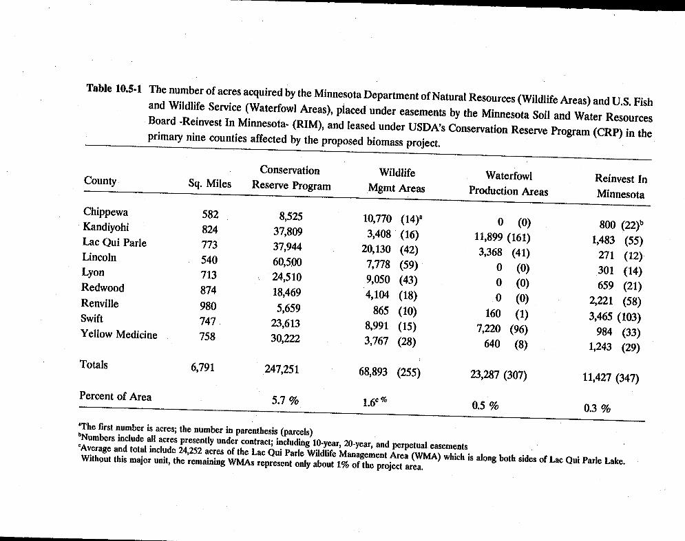
~~----------------------............. Table 10.5-1 The number of acres acquired by the Minnesota Department of Natural Resources (Wildlife Areas) and U.S. Fish and Wildlife Service (Waterfowl Areas), placed under easements by the Minnesota Soil and Water Resources Board -Reinvest In Minnesota- (RIM), and leased under USDA's Conservation Reserve Program (CRP) in the primary nine counties affected by the proposed biomass project.
Conservation Wildlife Waterfowl Reinvest In County Sq. Miles Reserve Program Mgmt Areas Production Areas Minnesota
Chippewa 582 8,525 10,770 (14)8 0 (0) 800 (22)b Kandiyohi 824 37,809 3,408 (16) 11,899 (161) 1,483 (55) Lac Qui Parle 773 37,944 20,130 (42) 3,368 (41) 271 (12) Lincoln 540 60,5.00 7,778 (59) 0 (0) 301 (14) Lyon 713 24,510 9,050 (43) 0 (0) 659 (21) Redwood 874 18,469 4,104 (18) 0 (0) 2,221 (58) Renville 980 5,659 865 (10) 160 (1) 3,465 (103) Swift 747 23,613 8,991 (15) 7,220 (96) 984 (33) Yellow Medicine 758 30,222 3,767 (28) 640 (8) 1,243 (29)
Totals 6,791 247,251 68,893 (255) 23,287 (307) 11,427 (347)
Percent of Area 5.7% 1.6c% 0.5 % 0.3 %
*The first number is acres; the number in parenthesis (parcels) hNumbers include all acres presently under contract; including 10-year, 20-year, and perpetual easements cAverage and total include 24,252 acres of the Lac Qui Parle Wildlife Management Area (WMA) which is along both sides of Lac Qui Parle Lake. Without this major unit, the remaining WMAs represent only about 1 % of the project area.
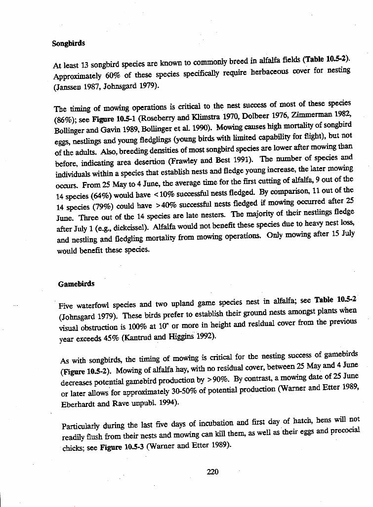
Songbirds
At least 13 songbird species are known to commonly breed in alfalfa fields (Table 10.5-2).
Approximately 60% of these species specifically require ·herbaceous cover for nesting
(Janssen 1987, Johnsgard 1979).
The timing of mowing operations is critical to the nest success of most of these species
(86%); see Figure 10.5-1 (Roseberry and Klimstra 1970, Dolbeer 1976, Zimmerman 1982,
Bollinger and Gavin 1989, Bollinger et al 1990). Mowing causes high mortality of songbird
eggs, nestlings and young fledglings (young birds with limited capability for flight), but not
of the adults. Also, breeding densities of most songbird species are lower after mowing than
before, indicating area desertion (Frawley and Best 1991). The number of species and
individuals within a species that establish nests and fledge young increase, the later mowing
occurs. From 25 May to 4 June, the average time for the first cutting of alfalfa, 9 out of the
14 species ( 64%) would have < 10% successful nests fledged. By oomparison, 11 out of the
14 species (79%) could have >40% successful nests fledged if mowing occurred after 25
June. Three out of the 14 species are late nesters. The majority of their nestlings fledge
after July 1 (e.g., dickcissel). Alfalfa would not benefit these species due to heavy nest loss,
and nestling and fledgling mortality from mowing operations. Only mowing after 15 July
would benefit these species.
Gamebirds
Five waterfowl species and two upland game species nest in alfalfa; see Table 10.S-2 ·
(Johnsgard 1979). These birds prefer to establish their ground nests amongst plants when
visual obstruction is 100% at 10" or more in height and residual cover from the previous
year exceeds 45% (Kantrud and Higgins 1992).
As with songbirds, the timing of mowing is critical for the nesting success of gamebirds
(Figure 10.5-2). Mowing of alfalfa hay, with no residual cover, between 25 May and 4 June
decreases potential game bird production by > 90%. By contrast, a mowing date of 25 June
or later allows for approximately 30-50% of potential production (Warner and Etter 1989,
Eberhardt and Rave unpubl. 1994 ).
Particularly during the last five days of incubation and first day of hatch, hens will not
readily flush from their nests and mowing can kill them, as well as their eggs and precocial
chicks; see Figure 10.5-3 (Warner and Etter 1989).
220
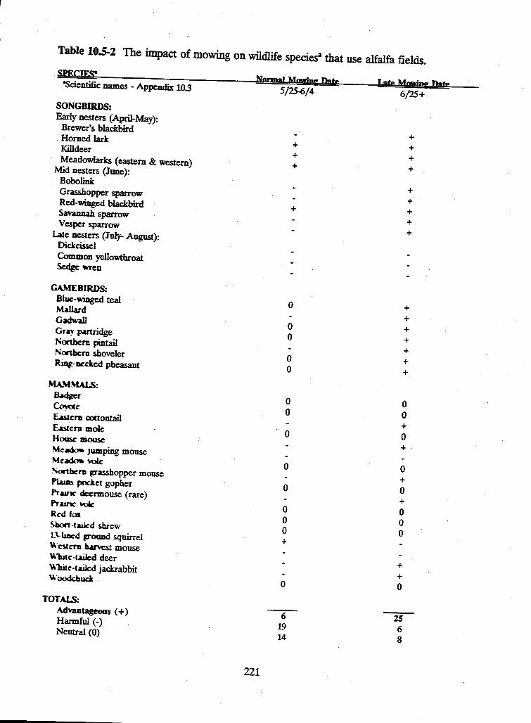
Table 10.5-2 The impact of mowing on wildlife species3 that use alfalfa fields.
"Scientific names - Appendix 10.3
SONGBIRDS: Early nesters (April-May):
Brewer's blackbird Horned lark Killdeer Meadowlarks (eastern & western)
Mid nesters (June): Bobolink Grasshopper sparrow Red-winged blackbird Savannah sparrow Vesper sparrow
Lale ncstcrs (July- August): Dickcisscl Common yellowthroat Sedge wren
GA.\IEBIRDS: Blue-winged teal Mallard Gadwall Gray partridge Northern pintail Northern shoveler Rin(?-nccked pheasant
MA.'IMALS: ~dfrcr ~c E.utcrn CQ(tontail E.utcni mole Home mouse Meadow. JWDping mouse Mc~'* Sortbcni grasshopper mouse rWm. pocket gopher Pr&anC dc.crmouse (rare) Pr&111C ~ ' Red fas Sbort ·t•d shrew n-bocd ground squirrel Wnzcni b.arvcst mouse \\'hilc·t~ deer \\'lUlc-t&ilcd jackrabbit Woodchuck
TOT MS: Advantageous ( +) Harmful(-) Neutral (0)
Normal Mmrinr Date
221
5/25-6/4
+ + +
+
0
0 0
0 0
0 0
0
0
0
0 0 0 +
0
6 19 14
I ate Mowing Date
6/25+
+ + + +
+ + + + +
+ + + + + + +
0 0 + 0 +·
0 + 0 + 0 0 0
+ + 0
25 6 8
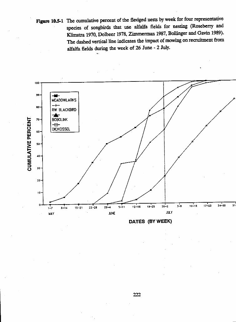
... z w 0 a: w CL w >
5 :::> :e :::> 0
Figure 10.5-1 The cumulative percent of the fledged nests by week for four representative
species of songbirds that use alfalfa fields for nesting (Roseberry and
Klimstra 1970, Dolbeer 1978, Zimmerman 1987, Bollinger and Gavin 1989).
The dashed vertical line indicates the impact of mowing on recruitment from
alfalfa fields during the week of 26 June - 2 July.
100
90 ---MEADOWLARKS
BO -+-RW BLACKBIRD .....
70 BOBOLINK t-
60 DICK CISSEL
50
40
30
20
10
1-7 8-14 15-21 22-28 29-4 5-11 12-18 19-25 26-2 3-9 10-16 17-23 24-30 31·
MAY JUNE JULY
DATES {BY WEEK)
222
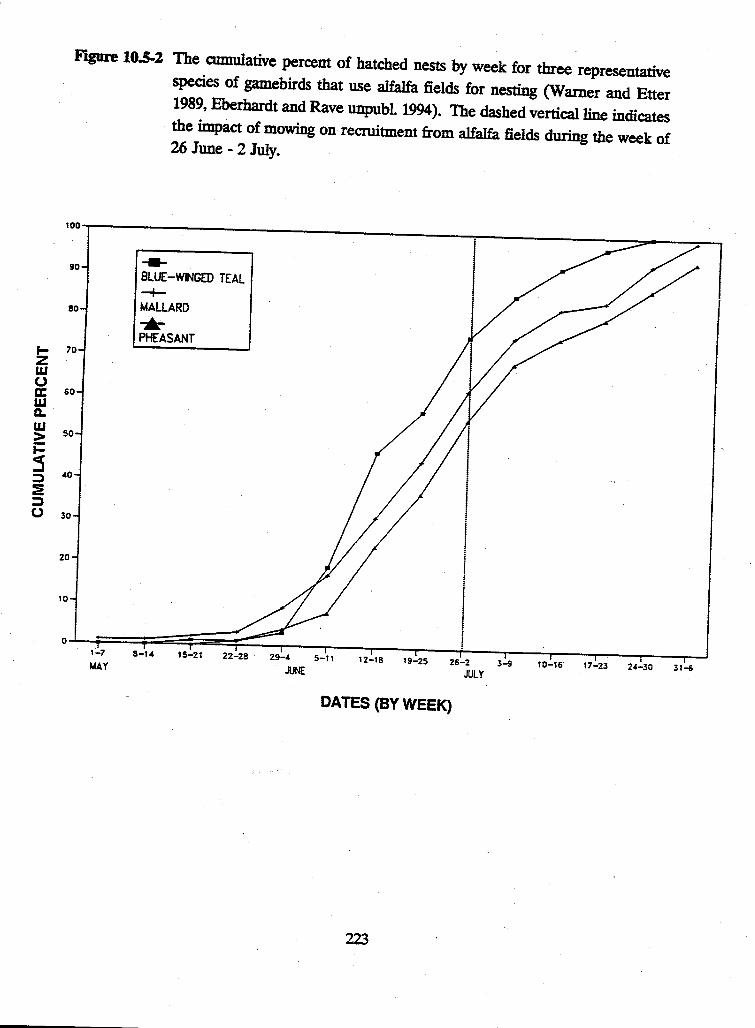
f-z w 0 a: w CL w > i= :3 :::> :E :::> 0
Figure 10.S..2 The aunulative percent of hatched nests by week for three representative species of gamebirds that use alfalfa fields for nesting (Warner and Etter 1989, Eberhardt and Rave unpubl 1994). The dashed vertical line indicates the impact of mowing on recruitment from alfalfa fields during the week of 26 June - 2 July.
100
90 ---BLUE-WINGED TEAL -+-
80 MALLARD .... PHEASANT
70
60
so
"° 30
20
10
1-1 8-1' 15-21 22-28 29-.4 5-11 12-1s 19-25 26-2 3-9 10-16 11-23 24-30 31-s MA Y JUNE JULY
OATES (BY WEEK)
223
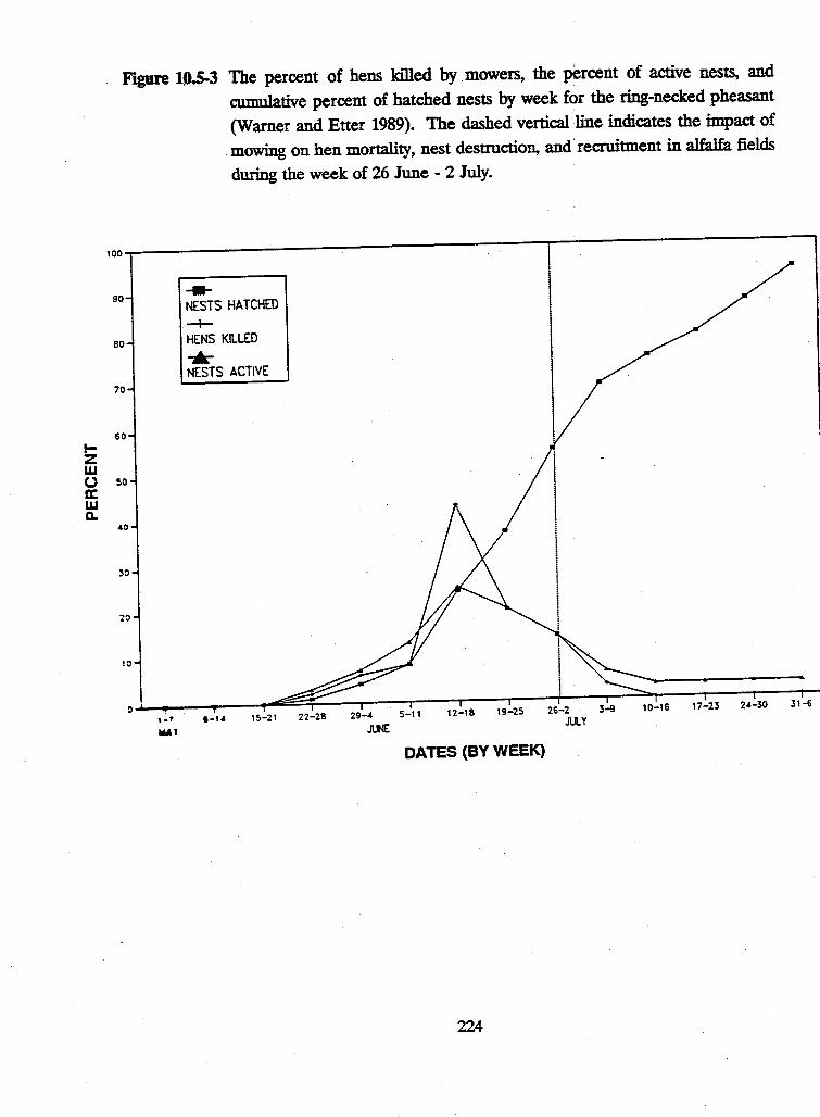
I-z w 0 a: w a.
100
90
80
70
60
so
£0
30
20
10
FJgU.re 10.5-3 The percent of hens killed by .mowers, the percent· of active nests, and
cumulative percent of hatched nests by week for the ring-necked pheasant
(Warner and Etter 1989). The dashed vertical line indicates the impact of
mowing on hen mortality, nest destruction, and· recruitment in alfalfa fields
during the week of 26 June - 2 July.
---NESTS HATCHED
-+-HENS KILLED
* NESTS ACTIVE
o1-~,_-,~-.~_-,.~-,~S-~21~§22~4~8==--29T4~~5-T1-1---12T_,-8---19r4-5~-26~4~~~~1~0---16:---~,7~-=23:---~24~-3=0~:3,~~:--
MA l .n.JNE JUL y
DATES (BY WEEK)
224
Spring Cover
The amount of residual cover available in the spring greatly affects when these species, particularly pheasants and mallards, establish nests, incubate, hatch young, and are most vulnerable to mowing mortalities (Martz 1967, Kirsch et al. 1978). H there is no residual cover over winter, sufficient growth must occur before nests are established. In the case of pheasants, hen mortality would be greatest (approximately 30% of the nesting hens) during the third week of June with an approximate 30% of potential production. In contrast, an excellent over winter residual cover would shift the nesting activity up to two weeks earlier than with no residual cover; see Figures 10.5-4, 5 and 6 (Gates et al. 1970, Trautman 1982, Kantrud and Higgins 1992). In this case, by 25 June over 60% potential pheasant production (FigDre 10.5-6) and < 10% hen mortality (Figure 10.5-5) are expected. Also, residual cover provides roosting and escape cover for resident upland gamebirds (pheasants and partridge), thereby increasing their fall to spring survivorship.
225
tz w (.) cc w c.
20
15
10
5
Figure 10.5-4 Potential impacts of the availability of residual nesting cover in alfalfa fields
in spring on the temporal pattern of active ring-necked pheasant nests
(Kirsch et al. 197~ Warner and Etter 1989). The dashed vertical line
indicates the impact of mowing on hen mortality in alfalfa fields under three
residual cover scenarios during the week of 26 June - 2 July.
---NO RESIDUAL COVER
-+-GOOD RESIDUAL ..... EXCELLENT RESIDUAL
OATES (BY WEEK)
226
.,_ z w 0 a: w Q.
Figure 10.5-5 Potential impacts of the availability of residual nesting cover in alfalfa fields in spring on the temporal pattern of active ring-necked pheasant hen mortality caused by mowing (Kirsch et al. 1978, Warner and Etter 1989). The dashed vertical line indicates the impact of mowing on nesting hens in alfalfa fields under three residual cover scenarios during the week of26 June - 2 July.
45
~ 40 NO RESIDUAL COVER
-+-GOOD RESIDUAL
35 ..... _ EXCELLENT RESIDUAL
30
25
20
15
10
DATES (BY WEEK)
227
100
90
80
70
60 I-z w (J 50 a: w D..
40
30
20
10
Figure 10.5-6 Potential impacts of the availability of residual nesting cover in alfalfa fields
in spring on the cumulative percent of successful ring-necked pheasant nests
(Kirsch et al. 1978, Wartier and Etter 1989). The dashed vertical line
indicates the impact of mowing on recruitment from alfalfa fields under three
residual cover scenarios during the week of 26 June - 2 July.
---NO RESIDUAL COVER
-+-GOOD RESIDUAL ..... EXCELLENT RESIDUAL
1-1 8-u 15-21 22-28 29-4 5-11 12-1s 19-25 26-2 3-9 10-16 11-23 24-30 31-6
MA Y JUNE JULY
DATES (BY WEEK)
228
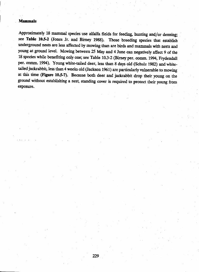
Mammals
Approximately 18 mammal species use alfalfa fields for feeding, hunting and/or denning; see Table 10.5-2 (Jones Jr. and Birney 1988). Those breeding species that establish underground nests are less affected by mowing than are birds and mammals with nests and young at ground level. Mowing between 25 May and 4 June can negatively affect 9 of the 18 species while benefiting only one; see Table 10.3-2 (Birney per. comm. 1994, Frydendall per. comm. 1994). Young white-tailed deer, less than 8 days old (Schulz 1982) and whitetailedjackrabbit, less than 4 weeks old (Jackson 1961) are particularlywlnerable to mowing at this time (Figure 10.5-7). Because both deer and jackrabbit drop their young on the ground without establishing a nest, standing cover is required to protect their young from exposure.
229
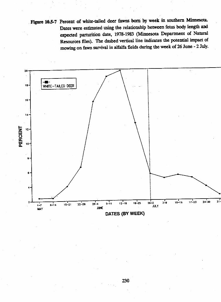
18
16
t-z 12
w 0 a: w 10 a.
8
6
Figure 10.S-7 Percent of white-tailed deer fawns born by week in southern Minnesota.
Dates were estimated using the relationship between fetus body length and
expected parturition date, 1978-1983 (Minnesota Department of Natural
Resources files). The dashed vertical line indicates the potential impact of
mowing on fawn survival in alfalfa fields during the week of 26 June - 2 July.
I ~E-T AILED DEER I
1-7 8-14 15-21 22-28 29-4 5-11 12-18 19-25 26-2 3-9
MAY JUNE JULY
DATES (BY WEEK)
230
Although later mowing benefits some rodent species, regular mowing keeps potential pest species (e.g., pocket gophers and meadow and prairie voles) at lower population levels by some den and tunnel destruction through compaction, as well as periodic· removal of food and cover (particularly the accumulation of litter) by mowing. The periodic removal of cover, regardless of when it occurs, exposes the field residents to increased predation from both mammalian and avian predators (Birney per. comm. 1994, Frydendall per. comm. 1994).
Landscape Effects
The size, shape, and distnoution of alfalfa fields affect the diversity, abundance, and success of nesting birds. Mammalian predation and nest parasitism by brown-headed cowbirds increase as field size decreases. To minimi:ze the effects of predation, a minimal field width of 150 feet is recommended (Johnson and Temple 1990). In addition, cowbirds parasitize nests at a higher rate within 150 feet from the field's edge (Sample 1989; Johnson and Temple 1990). Therefore, to minimize the impact on parasitized species, a minimum field width of 600 feet and size of 8 acres are recommended.
If alfalfa grown for this project is managed in a manner favorable to nesting birds (mowing after 25 June and good residual cover in spring), then the expected density of 22.4 acres per square mile could significantly affect wildlife populations in the area (50 mile radius = 7,853 square miles and 176,000 acres of alfalfa). Even so, depending on the quality of the existing habitat and what cover types the alfalfa replaces, population changes still might vary from a notable decline to a substantial increase from existing levels. Using the ring-necked pheasant as an example, replacing very productive undisturbed grasslands, such as CRP, with traditionally managed alfalfa would be very negative to pheasant populations. While, replacing annual set-asides, such as ARP acres (Bemer 1988) or row crops with late mowed alfalfa would be very positive (Table 10.5-3).
231
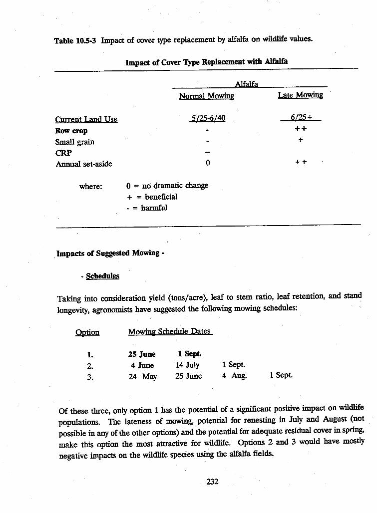
Table 10.5-3 Impact of cover type replacement by alfalfa on wildlife values.
Current Land Use
Row crop
Small grain
CRP
Annual set-aside
where:
Impact of Cover Type Replacement with Alfalfa
Normal Mowin&
5/25-6/40
0
0 = no dramatic change
+ = beneficial
- =harmful
;
Alfalfa
Late Mowing
6125+
++ +
++
. Impacts of Suggested Mowing -
- Schedules
Taking into consideration yield (tons/acre), leaf to stem ratio, leaf retention, and stand
longevity, agronomists have suggested the following mowing schedules:
Option Mowing Schedule Dates
1. 25 June 1 Sept.
2. 4June 14 July 1 Sept.
3. 24 May 25 June 4 Aug. 1 Sept.
Of these three, only option 1 has the potential of a significant positive impact on wildlife
populations. The lateness of mowing, potential for renesting in July and August (not
possible in any of the other options) and the potential for adequate residual cover in spring,
make this option the most attractive for wildlife. Options 2 and 3 would have mostly
negative impacts on the wildlife species using the alfalfa fields.
232

In an attempt to optimize the positive impacts of bio~ alfalfa on wildlife diversity and abundance, while taking alfalfa quality production needs into consideration, one would suggest two additional mowing schedule options:
Option
A. B.
_ Mowin& Schedule Dates
25 June 25 June
25 Aug. 25 July 1 Sept.
Impacts of option A are very similar to those observed under option 1, while option B impacts are intermediate to options 1 and 2.
- Patterns
Typically, alfalfa fields are mowed in an inward, spiraling pattern (Figure 10.5-8). This pattern of mowing creates an ever- decreasing area of cover into which young gamebird broods ( < 1 week old) are gradually herded and then usually killed by the mower. With new types of mowing_ equipment (e.g., swathers), this deadly pattern of mowing does not have to occur. If p<>SSible, fields should be mowed from one side to the other (Figure 10.5-9a) or from the middle outward in both directions (Figure 10.5-9b ). The latter two mowing patterns should minimize mortality of young chicles by mowers.
Figllft I 0.5-8 Typical pattern used in the mowing of alfalfa fields.
Typical MoWing Pattern
-., . .,
. , . ,
. ,
~ -
----~
-~
-~
233
F'igure 10.5-'8 +b Two recommended mowing patterns to reduce kt11ing young - less than
one week old - gamebirds in aJfaJfa fields (Olsen and Leatham 1980).
RECOMMENDED MOWING PATIERNS
A B
r-<· ,-<- r> r>
I<· I<· ~>- ->-
Changing from an inward, spiraling mowing pattern to one that goes from one side to other
or from the middle outward in both directions reduces th~ number of young (less than 1
week old) gamebirds killed by mowers.
234
SUMMARY
EstabJishing about 176,000 acres of alfalfa (22.4 acres per square mile in the 7,853 square mile biomass shed around Granite·Falls) to produce electricity and a high protein feed, will have a significant impact on the abundance and diversity of wildlife in the area. The magnitude and direction ( + or -) of these impacts will depend on the following factors: mowing schedule, availability of overwinter residual cover, cover type replacement, size and shape of fields, distnoution of fields, and mowing patterns.
A two-cut schedule with late June and late August mowing dates will have very significant positive impacts on both wildlife abundance and diversity. Mowing schedules similar to those used in conventional forage production, however, will have significant negative impacts on wildlife. Mowing schedules that result in 1) the development of good residual cover for winter (this aids earlier nest establishment), and 2) later first ~t mowing in the spring will greatly increase the potential nest success of most species utilizing alfalfa
Assuming favorable mowing schedules, replacing row crops or annual set-asides (ARP acres) with alfalfa, will result in favorable wildlife impacts. H these alfalfa acres replace CRP, however, reduced wildlife benefits will be expected. Late June and late August mowing will .produce a neutral to slight reduction (less than 20%), while early June, mid-July and late August mowing results in a substantial reduction (greater than 30% ).
Fields eight acres or larger and 600 feet or more in width produce the best wildlife population results. Long, narrow fields are less productive due to increased nest predation and parasitism.
Assuming adequate availability of other critical wildlife habitat components (e.g., winter cover, wetlands), an even distribution of fields will produce favorable results. A distnbution pattern that complements existing habitat components will promote even greater wildlife abundance and diversity.
235

236
CHAPTER 11. POLICY ISSUES
11.1 The 1995 Farm Bill Steven Taff
Agricultural and Applied Economics, University of Minnesota
Incentives and Policy
We are interested in agricultural policies affecting this project, at least to the extent to that particular policies may affect the market position of the proposed alfalfa biomass rotation of (AAAACCS) versus any competing rotations, particularly com-soybeans (CS). The alfalfa biomass rotation gains whenever policies in aggregate act to raise its relative profits, either by raising its relative price or by lowering its relative production costs. The rotation loses whenever policies in aggregate lower their relative profits. It is useful to examine the major elements of current U.S. agricultural policy to learn how they may affect the relative position of the alfalfa rotation. We discuss in particular the workings of the present crop subsidy programs and how their expected alterations could either help or harm the alfalfa biomass rotation. Much of this section is speculative, so it will be kept short. What we identified in Section 32 (regional biomass supply curve) will help us decide which of the policy-affect project parameters are so critical that they merit further elaboration. We expect that the whole project will succeed or fail mostly on its own merits.
In the second section, we speculate on the relative position of the alfalfa rotation in the current conservation compliance provisions of the farm program. Does even a single year of beans on highly erodtole land mean that the sequence does not meet conservation goals? What will expected state-level pollution controls stemming from the new Oean Water Act do to com-bean rotations in the project area? Will alfalfa rotations be eligible for the "green payments" now touted for the next farm bill?
Changing the rules under which agricultural producers operate changes the prices and costs they face. Different price-cost reiim.es might lead to different management choices. The changes might be direct, as in a tax on certain pesticides or a supplemental cash payment on certain crops, or indirect, as in the soil erosion liability shift discussed in the section on supply-curve shifters or in the imposition of size constrains on farming operations.
Any rule change that increases the net returns from the alfalfa biomass rotation versus the com-bean rotation will lead to relatively more hay being offered to the processing cooperative.
237
Of the myriad legal poSSil>ilities, we focus here on a handful of rule changes that appear to
be politically possible as well. In doing so, we offer no predictions about and no
recommendations toward the writing of the next federal farm bill. We do explore, however,
the ramifications of certain farm bill proposals on the financial structure of the hay power
system. We look at changes in: (1) set-aside requirements, (2) feed grain subsidies, (3)
water pollution control laws, and ( 4) the conservation reserve program. This brief list
illustrates the diversity of policy instruments that could affect the financial viability of the
hay power system.
(1) Permit hay production on set-aside lands: Under current federal farm policy, producers
who wish to receive price subsidies for feed grains such as com must set aside (not plant)
a designated portion of their cropland each year. This forced land idling, which is best
thought of as a tax on the federal subsidies, can range from zero (as in 1994) to 20% (as in
1987 and 1988) of a producer's crop base. On annual set-aside land, no income-producing
crop is permitted under current rules. In recent years, Congr~ has added an additional
10-25% "flex" acres provision. On this land, the farmer can grow a feed grain, but with no
subsidy paid over and above what the farmer receives in the market.
If both annual set-aside and flex acres could be planted to hay, the amount of hay produced
would increase dramatically because any payment for hay from idled land in excess of
production costs would be financially beneficial. Land charges are already being borne, so
any income-producing crop would improve the farmer's financial situation. Of course, in
years in which .the set-aside rate is zero, hay production would have to "compete" more
directly with regular, subsidized com production.
Because alfalfa is most efficiently grown in a multi year system, annual set-aside rules would
have to be changed to permit a saleable crop to be grown on the same idled acres each year
for a period of at least four years. Such a change presumes that there will be at least this
number of acres each year in required set aside. A possible rule variant might be to perm.it
alfalfa land to be designated as set-aside only in those years in which idling is required. No
"multiyear contract" would be needed. All the producer would need do, essentially, is to
demonstrate to the government that the required number of acres are not being planted to
com. One of the purposes of the set-aside requirement is to reduce the production of the
designated crop - com, in our case - put onto the market. This provision increases the
market price of com, which in tum reduces the size of the associated subsidy and, hence,
the size of the federal budget outlay.
238
Permitting noncom.modity crops such as alfalfa on set aside land will lead to increased production and decreased market prices for hay, both within and outside the biomass shed. This may have a dampening effect upon producer income to the extent that hay growers sell into the open market as well as into the biomass market.
(2) Reduce com subsidies: Eligible feed grain producers receive a deficiency payment (the difference between a mandated target price and the market price) for each bushel of com _they legally produce. Farmers can grow com only the number of acres assigned to their crop "base", less any required set-aside. In the study area, deficiency payments were $20 per bushel of yield potential on planted com acr~s. __ . Absent this subsidy, the average biomass:com-soy net· returns ratio improves considerably in favor of biomass, as discussed in section 3.2, above .
.. Oearly, the presence of this subsidy for com is a "barrjer" to the adoption of the biomass rotation on a wider scale. Its demise would reduce the net returns of the com-soybean rotation relative to the biomass rotation. However, elimination of com subsidies would also reduce the absolute net returns of the biomass rotation itself, for two years in that rotation are corn. Thus, abolition of the subsidy improves the position of alfalfa relative to com, but diminishes the ability of the producer to earn the income necessary to support the initial investment needed to switch to the biomass rotation.
The chances that the long-nmning price support and subsidy programs will be soon replaced are unknown. Typical of this time in the farm bill cycle, numerous proposals have been put forward to reduce or redirect farm subsidy spending. The farm bill itself will not be updated until late 1995 at the earliest. We think it prudent at this point to analyze the financial merits of the hay power system in a conservative, skeptical manner. That means assessing relative crop returns with current subsidies. If the biomass rotation is economically favorable for some farms under current policy regimes, it can't help but work for more farms under a regime of zero com subsidy, if that situai:ion ever comes to pass.
(3) Increase soil erosion damage liability: Many policies that influence farmers' management decisions come, not from the farm bill, but from legislation focused on other related topics. One such example is the Oean Water Act, slated for reauthorization in late 1994. Most observers expect special attention this time to nonpoint sources of pollution, such as erosion from farm fields. A recent major study of the Minnesota River, which drains most of the biomass shed, suggests that soil erosion over vast areas accounts for a substantial share of the pollution in that river.
239
Oeaning up nonpoint pollution could be an expensive process, if anyone is forced to pay the
bill. It is likely that Congress will provide less than sufficient money to states to match the
clean-up requirements expected to be imposed. Minnesota is also likely to under-fund the
cleanups in agricultural areas to meet the new requirements. We judge that a new round
of regulations dealing with ·soil erosion and livestock waste management are a plaUSI°ble
consequence of this mismatch of goals and resources. The cost of any new farm regulations
are necessarily borne by the landowners, much as the fruits of farm subsidy programs are
harvested by the same individuals.
All this leads to a situation in which the relative costs of complying with the new regulations
becomes important. Which rotation will be the more expensive to maintain under the new
rules? H the biomass rotation proves the less costly, then it gains relative to the com
soybean rotation.
240
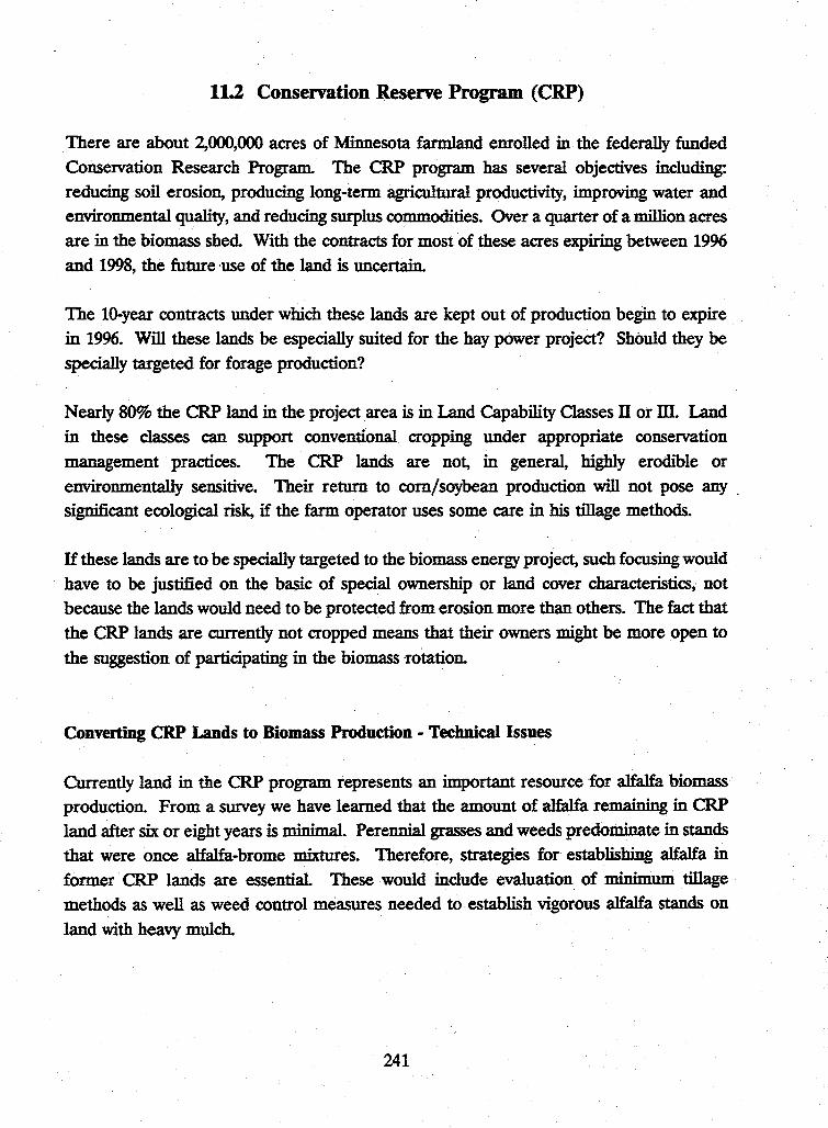
11.2 Conservation Reserve Program (CRP)
There are about 2,000,000 acres of Minnesota farmland enrolled in the federally funded
Conservation Research Program. The CRP program has several objectives including:
reducing soil erosion, producing long-term agricultural productivity, improving water and environmental quality, and reducing surplus commodities. Over a quarter of a million acres
are in the biomass shed. With the contracts for most of these acres expiring between 1996
and 1998, the future ·use of the land is uncertain.
The 10-year contracts under which these lands are kept out of production begin to expire in 1996. Will these lands be especially suited .for the hay power project? Should they be
specially targeted for forage production?
Nearly 80% the CRP land in the project area is in Land Capability Oasses II or m. Land
in these classes can support conventional cropping under appropriate conservation
management practices. The CRP lands are not, in general, highly erodlole or
environmentally sensitive. Their return to com/soybean production will not pose any .
significant ecological risk, if the farm operator uses some care in his tillage methods.
If these lands are to be specially targeted to the biomass energy project, such focusing would
have to be justified on the basic of special ownership or land cover characteristics; not
because the lands would need to be protected from erosion more than others. The fact that
the CRP lands are currently not cropped means that their owners might be more open to
the suggestion of participating in the biomass ·rotation.
Converting CRP Lands to Biomass Production - Technical Issues
Currently land in the CRP program represents an important resource for alfalfa biomass production. From· a survey we have learned that the a.mount of alfalfa remaining in CRP
land after six or eight years is minimal. Perennial grasses and weeds predominate in stands
that were once alfalfa-brome mixtures. Therefore, strategies for- establishing alfalfa in
former CRP lands are essential. These would include evaluation. of minimum tillage
methods as well as weed control measures needed to establish vigorous alfalfa stands on
land with heavy mulch.
241
11.3 Crop Insurance
Production Risk Management (Crop Insurance)
Steven Taff
Agricultural and Applied Economics, University of Minnesota
Businesses insure parts or all of their operations from adverse fiscal effects caused by
predictable events occurring with uncertain timing. In the present project, producers' price
risk is expected to be managed by the contract with the coop: prices will be known and
certain. Producers will still have to contend with production risk. What happens when
yields don't meet expectations? What circumstances or events cause yields to suffer?
Ia this feasibility study we have characterized production risks as events or circumstances
that harm yield of the growing or living crop. Among the possibilities are drought, excessive
moisture, disease, insect infestations, winter kill, and hail. Alfalfa yields can also suffer
losses in dry matter and quality caused by rainfall or hail after cutting, but before baling.
Farmers also suffer losses due to quality in their alfalfa crop due to tactical decisions to
delay harvest. Ironically, the main reason farmers may delay harvest and precipitate quality
losses is their desire to avoid the possibility of imminent rain. Of all the types of losses
mentioned, none of the various insurance programs are designed to protect the grower from
the losses in dry matter and quality that can occur at harvest. The insurance industry and
federal government are attempting to reduce a farmer's risk in alfalfa production with
respect to the levels of dry matter yield affected primarily by vagaries in moisture patterns.
We generally assume that the producer, not the coop, will be subject to production risk on
the producer's land. This need not be the case. For example, the coop could guarantee a
fixed payment per acre, whatever the yield, as long as the farmer follows management
guidelines specified by the coop.
Even if insurance is shown to be useful for the producer, it may not be a good buy. We will
examine current crop insurance programs policies here and identify gaps in current
insurance availability.
,-~ 242
The crop insurance policies available in part or all of the project area are: (1) hail insurance, (2) federal multiple peril crop insurance (MPCI), and (3) the pilot forage group risk plan (GRP).
Hail insurance is widely sold by private companies. It covers crop damage from a severe storm, but few other risks. This coverage, which is not subsidized or sponsored by the federal government, is presumed to be actuarially sound.
The MPCI covers a wide range of weather risks for crop farmers and forage growers. Subsidized in part by the federal government, it is offered largely through private agents. Com and soybean coverage is available to all parts of the project area, but the forage policy is sold only in Kandiyohi, McLeod, Meeker, and Swift Counties. Farmers can cover themselves within a specified range of yield and market price possibilities. Actual farm yields, measured against yield histories for the same f~ are the basis of loss calculations. Policies are widely sold for com and beans, but are relatively rare for forages, given their high premium levels and perceived poor payoff.
The relatively low MPCI participation by forage producers led to the. creation (starting in 1994 crop year) of the forage GRP. Counties within the pilot forage GRP and biomass feasibility study are McLeod and Meeker. This policy is touted as administratively simple and financially prudent for some producers. Forage GRP policies offer farmers the opportunity to peg a combination of market price and yield levels to insure against, much as MPCI. Its distinguishing feature is the calculation of loss: all yields are measured by county averages, not by individual participants. The GRP is said to be best suited for ~gh performance operations whose yield histories tend to move in concert with county averages.
As of this writing, Congress is considering a major overhaul of the federal crop insurance programs, in response to the spotty participation of farmers who experienced yield losses during 1993's floods. It is uncertain how a new program might affect growers in the project area. We are fairly certain, however, that the present narrower coverage for forage crops versus com and soybeans will continue. This implies that the forage enterprises of farmers participating in the project will be relatively more exposed to weather risks than will be their com and soybean enterprises. A producers' cooperative may wish to explore self-insurance, special group coverage, or other risk-management options for its member growers.
243

244
CHAPTER 12. CONCLUSIONS
12.1 Technical and Economic Feasibility
Ervin A. Oelke1.2 1Center for Alternative Plant and Animal Products
2Department of Agronomy and Plant Genetics, University of Minnesota
Biomass energy production systems must provide viable economic returns for producers of
biomass (farmers) and produce electrical power at a price that is competitive with future
fossil fuel systems. Because all biomass fuels are less energy dense than coal, the biomass
crop must provide other sources of revenue for producers and for utilities.
Biomass energy crops are similar to other agricultural crops. High yielding biomass energy
crops require high inputs of water and nutrients, just like other high input agricultural crops.
Multiple use crops that provide food or fiber, and energy integrate traditional agricultural
production and processing with "new generation" energy production and processing.
Agriculture dependent electricty production must be integrated with agricultural processing
to be sustainable.
The integration of agricultural production and energy production benefits both agriculture
and energy production systems. Efficiency is the goal, not maximum production. This is not
a new idea; it has been successfully implemented in the paper industry and by the
production of ethanol and co-products from com Single use crops for energy production
based on maximizing biomass yield ignore the efficiencies that may be gained from
integrating these systems.
Alfalfa, an herbaceous perennial legume, is an ideal biomass energy crop to integrate
agricultural and energy systems. First, alfalfa can be grown in rotation with row crops such
as com and soybeans providing substantial environmental benefits as a part of a traditional
rotation. Second, growing alfalfa is not new to farmers in. the proposed biomass shed.
Third, alfalfa can be separated into two high value feedstocks: alfalfa stems and alfalfa
leaves. Alfalfa stems (over 8000 BTU /pound dry) can be gasified to produce electricity and
alfalfa leaves (about 30% crude protein) can be processed into value-added alfalfa. The two
revenue streams, one for electricity and one for leaf meal products, makes the alfalfa
biomass system feasible and economical and results in a ver:y efficient use of feedstock
resource.
245
The feasibility of growing alfalfa in the proposed biomass shed is excellent based on present
production knowledge by farmers and the wealth of research data available in the
management and production of alfalfa. Seed of present varieties is available and needed
acreage could be brought into production within a two to four years. Farm equipment
already exists for production and harvesting of alfalfa. Equipment for separating leaves and
stems is available by modifying existing equipment being used in the alfalfa dehydration
industry.
Alfalfa forage has been used an animal feed for centuries and continues to be an important
animal feed today. Alfalfa leaf meal will be used as a protein supplement. Alfalfa leaf
protein will compete in the marketplace with other protein sources. However, since alf8.1fa
in a biomass rotation replaces other protein meal sources (com and soybeans), there will
be only a minor influence on total feed protein production.
Alfalfa leaves may also be processed into many other valuable products. Other alfalfa leaf
products currently being produced at some level include: alfalfa leaf pigments
(xanthophylls ), liquid protein products for human and animal consumption, fragrances for
shampoos and cosmetics, and natural biological molecules for pµarmaceuticals. Once the
alfalfa biomass system is in operation further investigation of these and other alternative
products will proceed, potentially making alfalfa leaves an even more valuable co-product.
Presently, the economic feasibility of the alfalfa biomass business venture is viable under a
3 or 4 cut alfalfa production system using existing alfalfa varieties. Cutting alfalfa three or
four times results in maximum leaf and stem tonnage production thus resulting in the
highest amount of revenue. This production information is based on data obtained with
present varieties. A program to select for tall, large diameter and solid stems with higher
lignin content has been underway for several years in the USDA-ARS alfalfa breeding
program at St Paul. Some seed of alfalfa biomass types will be available for testing in 1995.
These alfalfas could move alfalfa production to a 2 cut system and increase the efficiency
of the system by 25% in the near term. It is the opinion of alfalfa breeders that varieties
with all the desired traits could be accomplished within a period of six years.
Four years of alfalfa inserted into a 7-year com/soybean rotation based on production costs
and value of alfalfa stems and leaves is economically viable. Economic advantages of the
rotation may be directly attributed to the inclusion of a perennial legume in the rotation.
Reduced input costs, compared to contentional rotations and increased yields for other crops
in the rotation result in increased profit for producers. The system improves agricultural
sustainability by reducing chemical inputs and reducing soil erosion.
246
SUSTAINABLE BIOMASS ENERGY PRODUCTION
APPENDIX

TABLE OF CONTENTS VOLUME 1 -Appendix
(Appendix numbers correspond to the chapter in Volume 1 where the topic is covered)
1.0 FOCUS GROUP STUDY •.•..•..••..•.•..............•.••....•...•..•..•........•.....•..
Introduction ........................................................................................................ . Research context ....................................................................................... . Location and participation selection .......................................................... . Assumptions ............................................................................................. .
Results ......................................................................................................... . Alfalfa - Good to grow, not to harvest and market.. .................................. . Stems or leaves - Which one drives the plan? ........................................ . Quality - How is it measured? ................................................................... . Technical concerns-Separation, Ash, Contracts, and More .................. . One Buyer - One Product .......................................................................... . Particiption - Farms and Farmers .............................................................. . Co-ops - Models that work & relationship to NSP .................................... . Community - Benefits and disadvantages ................................................ . Survey results ............................................................................................ .
Summary ....................................................................................................... . Appendices to focus group ................................................................................. .
Research Procedures ................................................................................ . Invitation Protocol ........................................ : ............................................ .
Telephone Screening .................................................................... . Sample Letter of Confirmation ....................................................... . Sample Letter Of Thank-You .......................................................... .
Overview Of The Feasibility Study ............................................................ . Key Questions ........................................................................................... . Participation Survey ................................................................................... . Researchers ............................................................................................... .
1.1 LOCAL BIOMASS PROJECT MEETINGS ............................ ._ ••• 1.2 MEETING COMMENTS ................................................................. . 1.3 AG ADVISORY COUNCIL INTEREST LIST .•...•.•.........••••.•....•... 3.0 DESCRIPTION OF SOILS (Appendix A&B) ................................. . 4.0 ALF ALFA PRODUCTION COST SPREADSHEET .................... . 5.2 ALFALFA TRANSPORTATION AND STORAGE COSTS ....•••. 9.0 BREAKEVEN ALF ALF A, STEM AND LEAF PRICES •.••••.•.•••.• 10.1 GUIDE TO USING "PRODUCTION" SPREADSHEET ••.•..•••••. 10.3 COMMON BIRD AND MAMMAL NAMES .............................. . BIBLIOGRAPHY .................................................................................... .

APPENDIX 1.0
SUSTAINABLE BIOMASS ELECTRICITY PRODUCTION
FOCUS GROUP STUDY
FINAL REPORT
Earl W. Bracewell, Ph.D., Centre for Education in Agriculture and Extension; 320 VoTech Building, University of Minnesota, Saint Paul. MN 55108 office: 612/625-1225 fax: 612/625-2798
Helene Murray, Ph.D., Minnesota Institute for Sustainable Agriculture, 411 Borlaug Baa University of Minnesota, Saint Pau4 MN 55108 office: 612/625-0220 fax: 612/625-1268
August 1994
'

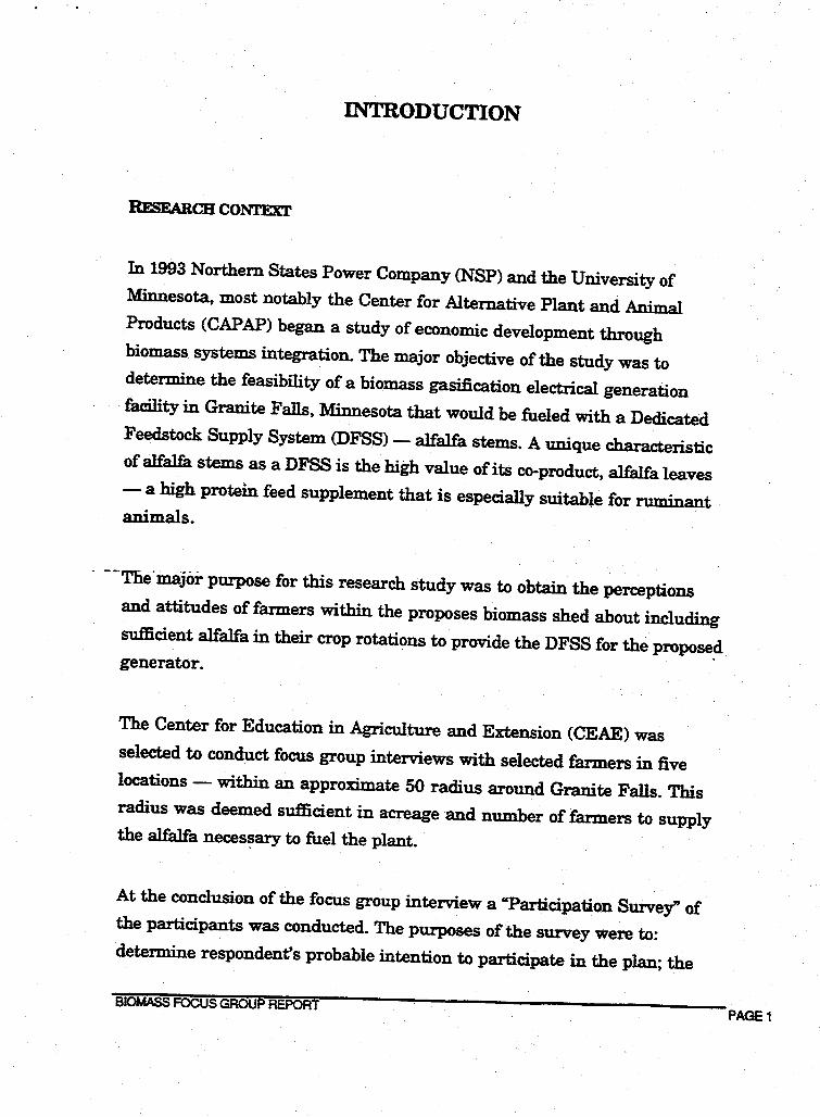
INTRODUCTION
RF.sEARcB CONTEXT
In 1993 Northern States Power Company (NSP) and the University of Minnesota, most not.ably the Center for Alternative Plant and Animal Products (CAPAP) began a study of economic development through biomass systems integration. The major objective of the study was to determine the feasibility of a biomass gasification electrical generation
-facility in Granite Falls, Minnesota that would be fueled with a Dedicated Feedstock Supply System (DFSS) - alfalfa stems. A unique characteristic of alfalfa stems as a DFSS is the high value of its co-product, alfalfa leaves - a high protein feed supplement that is especially suitable for ruminant animals.
- --The-inajor purpose for this research study was to obtain the perceptions and attitudes of farmers within the proposes biomass shed about including sufficient alfalfa in their crop rotati<:>ns to provide the DFSS for the propose~ generator.
The Center for Education in Agriculture and Extension (CEAE) was selected to conduct focus group interviews with selected farmers in five locations -within an approximate 50 radius around Granite Falls. This radius was deemed sufficient in acreage and number of farmers to supply the alfalfa neces~ary to fuel the plant.
At the conclusion of the focus group interview a "Participation Survey" of the participants was conducted. The purposes of the survey were to: determine respondent's probable intention to participate in the plan; the
BIOMASS FOCUS GROUP REPORT PAGE1
acreage that would likely be designated; and to determine concerns or areas
where lack of knowledge exist, before a decision about participation could be
made.
This report does not seek to persuade CAP AP personnel, NSP
professionals, farmers, or others to a particular point of view. Instead, it
seeks to respectfully listen, to gain understanding and knowledge about the
perceptions and insights of area farmers have about producing alfalfa for
biomass energy and animal feed.
LOCATION AND PARTICIPANT SELECTION
Five locations within a fifty-mile radius of Granite Falls, Minnesota, were
selected to represent identifiable, major, farm enterprises within the
proposed biomass shed. Thus, Wi11mar participants represented dairy
farmers, A_ppleton partici:Qants represented farmers that irrigate, Canby
represented farmers with large acreages in Conservation .Reserve Program
(CRP), Marshall represented farmers that plant large acreages of com and
soybeans, and the Olivia focus group participants represented farmers that
grow sugarbeets
Names of farmers, that fit each respective group, were obtained from lists
obtained from County Extension Educators,_ agriculture commodity groups,
and other farmer organizations and cooperatives. Following a screening
procedure, forty farmers, all men, were invited to participate in the five
focus group interviews. Thirty-nine of those invited participated in the
interviews. Generally, participants were experienced, operating farmers,
with average to larger than average farming operations.
BIOMASS FOCUS GROUP REPORT PAGI
Interviews were conducted between April 4-6, 1994 in the five towns previously identified.
At the outset of each focus group a 10-minute overview of the feasibility study was presented (Appendix A). Topics included: defining the DFSS, organizational possibilities, project scope and scale, probable transportation and quality·scenarios,. assumed rotational benefits, and general project expectations.
At the conclusion of each focus group interview, participants were asked to complete a brief"Participation Survey." The purposes of the survey were to: determine respondent's probable intention to participate in the plan; the acreage that would likely be designated; and to determine areas of concern or lack of knowledge before a decision about participation could be made.
ASSUMPrIONS
This focus group project, like all re~earch projects, is subject to assumptions that create limitations. An assumption in this project is that the questioning route devised by the researchers and others was sufficient both in depth and breadth to provide responses to assist CAP.AP and NSP to better determine the feasibility of a biomass gasification electrical generation facility in Granite Falls fueled with alfalfa.
Another assumption of this project is that the participants represented the broad range of farmers, including both men and women, within the biomass shed.
BIOMASS FOCUS GROUP REPORT PAGES
..
For some participants the outline of the project presented before the focus
group interview was their introduction to the feasibility study, for others it
added to existing knowledge. Therefore, this report is limited in that
participants did not have equal prior knowledge of the project and therefore
may not have had equal opportunity to formulate responses to the questions.
These assumptions and limitations not withstanding, this report gives the
reader insight into the perceptions of, and concerns about, the proposed
project, as verbalized by farmers within the area.
Representative participant quotes are used throughout the report to support
the common concerns identified across focus groups. These quotes
represent the perspective of the participants and have much to offer in
understanding the feelings they hold about the topic.
The results of this report are not organized according to the fOCU.S group
questions. Instead, the report is organized around major themes that
evolved from the discussions. Effort has been made to present these themes
as distinct and separate, yet considerable overlap exists. Themes are
presented in order of relatedness to one another and not in order of
importance.
BIOMASS FOCUS GROUP REPORT PAGE
RESULTS
ALFALFA-GQOD TO GROW, NOTTO HARVEST AND MARKET.
Farmers participating in all five focus groups expressed a strong interest in finding a way to include alfalfa into their current crop rotations. Desirable reasons that participants stated included: erosion control benefits; soil fertility and tilth improvement; and pest control benefits. A major theme from all the focus groups conducted for this project is the idea that aJfalfa is a i'.2Q.d crop - a desirable and valuable crop in the rotation.
I always raised alfalfa. We got away from It In the last year or so because we got out of cattle and It kind of bothers me not to have alfalfa Into the rotation. So It would be a real positive to allow noncattle or non-dairy producers to have alfalfa In the rotation.
\ -Marshall Participant-
[Alfalfa Is a] renewal resource, environmentally friendly, I think. -Olivia Participant-
The environmental aspects of this project are very important based on the location of the project at the Minnesota River basin.
-Appleton Participant-
Contrasting with the belief that alfalfa is a good and desirable crop to grow, there is a belief that alfalfa is not a "good" crop to harvest and market. Timeliness of harvest, the necessity for specialty equipment, weather problems, the bulkiness of hay, together with limited market opportunities and uncertain prices were among the factors cited that have contributed to the limited amount of alfalfa presently grown.
Participants believe year-to-year weather variations make alfalfa a risky crop to harvest. For many participants, the negative factors of harvesting
BIO-MASS FOCUS GROUP REPORT PAGE5
..
and marketing out weighed the favorable factors of growing alfalfa -factors that were often cited as reasons not to include it as a crop.
It's really a high stress crop. I mean you have to cut It at exactly the right time; you have to harvest It exactly at the right time, usually at night. You have to let It dry out and then the night air comes back on. So I think the reason Ifs not a big cash crop In this area Is because of our high humidity and higher rainfalls.
-Marshall Participant-
There ls no real market for It except the sale at the auction barn and the whim of the market. Like this year, I've heard guys pay $120 per ton for alfalfa and then the next year they'll pay $20 for the same quality hay. Well, you can't stay In business with that type of fluctuation.
-Marshall Participant-
Well, everybody knows that there's only so much market for so much good quality. Are you the person thars going to take that risk or not?
-canby Participant-
8T.EMs ORLEAWS-WHICH ONE DRIVES THE PLAN?
Participants were perplexed by the relationship between the comparative value of alfalfa leaves and stems as outlined in the currently J?roposed plan. They questioned the logic of basing the feasibility of the plan around stems when that portion sells for only $20.00 per ton compared to the projected sale price of processed leaves at $125.00 or more per ton.
Since the leaves appear to be the more valuable portion of the plant, they reasoned it seems more practical to grow alfalfa cultivars that have a greater percentage of leaves and not concentrate on growing alfalfa cultivars that contain a higher lignin content in the stems. Since leaves are more valuable than stems, and probably since farmers traditionally place
Bio-MASS FOCUS GROUP REPORT PAGE
more emphasis on management for leaf quality than they do for stem quality, they questioned the rationale of only two cuttings as a practice to obtain higher per acre lignin production. They asked, "Wouldn't it make more economic sense to take four cuttings instead of two?,,
I guess I've got a problem with this where you're going to raise hay for the stems and It's the less profitable part. We're going to want types of hay for the stem part and It's less profitable than the leaves? The leaves are going to be the best part, I just don't quite understand what we're going after here.
-Marshall Participant-
If 90% of your money is coming from these leaves, why wouldn't you plant a high producing leafy alfalfa that you're going to get four cuttings from? You're only getting 10% from by-products.
-Canby Participant-
QUALITY-HOW IS rr MEASURED?
Fanner participants were concerned with quality issues. They have experienced harvest problems with alfalfa in the past. They were concerned with probable quality dockages caused by rain, storage, or other harvesting problems.
Additional quality issues were articulated in a myriad of questions. Among questions raised were the following: complex management concerns; acceptable varieties, particularly those that retain leaves better than others; desirable stage of growth; acceptable ratios of leaves to stems; bale size and &hape; planting rates; and transportation.
This Is the big question In my mind when you start talking about 15% moisture hay. What are your dockage's going to be and this and that? All hay Isn't equal.
-Willmar Participant-
BIO-MASS FOCUS GROUP REPORT PAGE7
That would be just like MCP [Minnesota Com Processors Association], you don't haul moldy com, you don't haul light com. There's a certain standard set up by farmers and that would be the same thing. You would have to be paid for the quality you bring In. You couldn't pay the guy that left his leaves on the same as the guy that came In with Just stems.
-Canby Participant-
TECHNICAL CONCERNS- SEPARATION, AsB, CONTRACTS, AND MORE.
Focus group participants listed many questions they would like answered
or researched before committing to participation in an alfalfa biomass
energy production program. Among the questions and concerns were those
that dealt with: complex management and risk; assurance of long-term
contracts; acceptable cultivars; desirable stage of growth for harvest;
acceptable ratio of leaves to stems; bale size and type; storage; moisture
content within bales; leaf-stem separation and processing; and ash use,
disposal and handling costs; and costs of transportation on the farm t.o a
· -receiving site.
All of us know that weather has a bigger Impact on alfalfa than It does on any other crop as far ~ harvesting It and that could be a risk. If the farmer has to assume It all, then he cuts down his 1 oo acres on June 15 and It all gets rained on two or three times and It's not worth anything. Then that's a fairly big risk on the farmer's part.
-Willmar Participant-
There's going to have to be something built Into the contract there cause they're (NSPJ going to have to live with a contract to assure the [electrical] supply, but they can't use their over-supply to kill off or to lower price [of alfalfa].
-Marshall Participant-
Maybe we should start with market first. What can we get for the material? Then, you decide whether It's going to be the contract [with NSP] or H people want to make their organization [form a coop] to supply the market. Get some concrete numbers on your
BIO-MASS FOCUS GROUP REPORT PAG
market then things will take care of themselves. If there's a place to sen It and make some money, you'll get the stuff.
-Marshall Participant- -
ONE BUYER-ONE PRODUCT •.
· Participants were· skeptical about partnering with NSP in a biomass purchasing plan. Why is NSP interested in alfalfa? Participants had a consistent belief that they could be put into a subordinate position and that NSP could take advantage of them. They believed that they were playing on an uneven field and that NSP had all the players necessary to win! They were.curious about the financial commitment and motivation to the project of NSP. They wanted assurances that they could be~ partners in the plan.
What Is NSP's tax advantage for doing this and everything else? -Canby Participant-
If _NSP ~~I of a SL!~def1 sa~ to th~s co-op [us], "We don't want your hay," What are you [farmers] going to do with It? ••• So they have to have some risk Involved In this thing or, you're [farmers] going to get stuck holding the bag.
-Appleton Participant-
Too, participants were concerned that they would be producing a product for which there would be only one buyer - NSP. This made them feel uncomfortable and vulnerable.
Bob brought up the biggest thing - right now you only got one market!
-Appleton Participant-
Farmers were also concerned the leaf meal product, upon which much of the economic feasibility of the plan is based, is an untested, unresearched,
PAGE9
product that does not have an established market. This brought up
concerns of market development, protein product competition, and possible
depression of corn· and soybean prices.
Yeah, are we going to set some other market off here. If we're going to bring 100,000 acres of leaves [leaf meal] on the market, we got to sell them. They weren't sold the year before and I have no Ide~ what kind of quantity or tons or percentage or, whatever, but ls there a market for that?
-Canby Participant-
Participants also expressed a collective anxiety about the possible
agricultural market disruption if several more alfalfa gasification plants
were established.
PARTICIPATION-FARMSAND FARMERS.
There was a lack of consensus about what kind of farmers would most
likely be interested in participating in alfalfa production to generate
biomass energy. Several farmers felt alfalfa is a crop that could work for all types of farm operations. Others thought that farmers with large acreage would be willing to participate, although the exact meaning of the term
,arge farms" was unclear during the interviews.
Dairy focus group participants thought few dairy farmers would -be interested in participating primarily because they tend to have limited acreage and the local supply of good quality alfalfa hay to purchase for feed
is acarce so dairy farmers need to produce their own high quality alfalfa bay. Non-dairy producers pointed out that dairy farmers tend to already
own equipment necessary to produce alfalfa and consequently thought dairy farmers would be likely candidates to produce for the biomass energy
project.
There's a niche for every farmer and It can work for everybody.
-Canby Participant-
BIO-MASS FOCUS GROUP REPORT PAGE'
I don't think It necessarily will be the dairy farmers probably doing most of their growing. I think it's going to be grain farmers that are going to be growing It. They have the acres; we don't
-Willmar Participant-
If you could go out and say that the co-op is going to help you purchase your machinery and there's a real minimal Investment up front. If It's $10.00 an acre Just so he's made a commitment to come there and sign a grower agreement and get some of these other agencies Involved In financing It, I don't think you're going to have a problem selling [procuring] acres.
-Appleton Participant-
He's [dairy farmers In general) already got the equipment He's got to go through the exercise anyway [harvesting] so, in a way, It might flt Into his program fo add another 25 to 50% to his crop. Then he could keep the best up on his farm and maybe give the rest to the power plant.
-Marshall Participant-
A big one [farm operation], because you're going to have so much equipment on this hay and hay shed that you're not going to mess
________ -"~~-~-1'.le'.f.~tl'.1.?Q ~o-~_Qq_~c~! _t!~ way!_ _ •Marshall Participant-
That's going to be the risk takers and those guys are the ones that will be well enough capitalized~ well enough educated to say, "Well, lefs take a chance." I think It will be the large grain farmers and you only need 500 of them and you draw that big circle and that Isn't going to be hard to find [farmer participants].
-Marshall Participant-
You're talking about the younger guy that's got the energy. -Marshall Participant-
I think one Important factor that nobody brought up would be four years coming out of a rotation as we're sitting right now In our operation. It would be tough to come up with any number of acres that you could pull out of your current rotation, a three year rotation, that you could pull out for four years and put Into a different crop.
BIO-MASS FOCUS GROUP REPORT PAGE 11
. ... . .
-Olivia Participant-
I would think the area that has a lot of CRP [Crop Reserve Program] right now/. I would think that It would be more feasible In an area like that than In an area around here where there's very little CRP.
-Olivia Participant-
I think this would appear to guys that are getting closer to retirement and saying, "I'd llke to slow down a little bit, I wouldn't like to work quite so hard." They could put some of their acres In this, but thafs also the point when they're not, maybe, as open to Invest In new businesses at that time either and If this would call for an Investment In the cooperative to do that It could be detracting from that.
-Olivia Participant-
CO-OPS-MODELS THAT WORK & RELATIONSBIPTO NSP.
Parijcipants expressed belief that they were playing on an uneven field and that NSP had "all the players necessary to win." They were curious about NSP's financial commitment, motivation and involvement in the study as
· well as in a possible demonstration facility.
You take the sweet corn people. I mean, sweetcom•s got to come [be harvested] when the company says, not when the grower wants IL I mean, maybe It will and maybe It won't have to be but It might have to be. You might have to give up that control too.
-Olivia Participant-
Right or wrong, I want to throw one out here. Why don't NSP Just go ahead and build this plant and contract with farmers to haul (produce] It?
-Olivia Participant-
[The Co-op should] contract the acres, set up facilities to own the leaf processing end of It all the way through, and Sell off [to NSP] the stems.
-Olivia Participant-
BIO-MASS FOCUS GROUP REPORT PAGE
Although some participants expressed negative feelings toward the establishment of a cooperative to supply alfalfa stems to NSP and to market the leaf meal product, most participants believed a co-op would be a valuable business organization and should be part of the plan. Not only did they approve of the Co-op - NSP relationship, they offered concrete suggestions about the organization of it. Most of the suggestions were in the form of comparis.ons with existing, successful co-ops. "Pay-to-play," and "farmer-oriented" were key concepts of a successful co-op that were voiced by participants.
Patterning It on the MCP Is an excellent Idea, but because of the fact that MCP Is working as a farmer-owned co-op and doesn't really have a large entity like Northern States Power Involved, whereas this operation would. So you need some kind of firm commitment [from NSPJ that are means of tying them down.
-Canby Participant-
Basically, what you need is a whole new cooperauve formed. Just llke the sugar beet cooperative. You want to invest In that [cooperative], If you want to invest in this plan you buy so many shares.
-Willmar Participant-
What I'm saying ts if there are some benefits In It for NSP, I think they should shoulder some of the costs of building, or at least putting some of the equity Into the cooperative. I don't know H they've put money Into a cooperative or not, It would probably be a whole different ball game then, but I don't know If the farmer wants to take on the whole responsibility of funding this thing, because If for some reason, it doesn't work, then what? The farmer's already got enough hanging on his head. He sure doesn't need anymore. At least that's my feelings.
-Appleton Participant-
The Ideal would be to sell to them under a contract. That way If It goes bust then we don't lose all the money. Well, on the other hand, If It's profitable, It never hurt anyone to own Shares In MCP [Minnesota Com Producers].
-Marshall Participant-
BIO-MASS FOCUS GROUP REPORT PAGE 13
Well, I was Just wondering Is NSP looking for the farmer to finance this plant to process this hay? You know, It sounds like you're looking for another co-op. ff you're looking for a co-op, that means farmer owned Investment, farmer Investment. Or Is NSP going to put up the processing plant, and we Just sell to them under contract?
-Marshall Participant-
H Northern States Power Is going to be this Involved to the extent that I believe they are with this, I believe a joint ownership of the operation with them, combining aJot of their managerial skills can be available [helpful] to us.
-Canby Participant-
.COMMUNJTY- BENEFITS AND DISADVANTAGES.
Overall, farmers thought the plan as described would have positive benefits to the communities in the region, -especially in the town of Granite Falls. Producers noted that when farm income is steady local businesses benefit, resulting in stronger communities. They also felt it was better to keep dollars spent on energy at home, rather than buying coal from other regions of the country. "It's hard to see a lot of drawbacks" was the consensus.
When participants were asked about any possible negative impacts on communities, few were cited. Participants thought the area immediately surrounding the power facility would be most affected by increased traffic. However, they noted "there are already lots of trucks on the road" and didn't see the increased traffic as a major problem. Some participants wondered there would be increased dust and air pollution resulting from the change from coal to alfalfa biomass.
It's hard to see a lot of drawbacks.
-Willmar Participant-
BIOMASS FOCUS GROUP REPORT PAGE
I think It kind of starts back out on the farm. When the farmer's makes money, everyone makes money and everybody has a good time. Really, It does. I mean Main Street, your car dealers, your grocery stores. You go places. You do things. Dollars get spent.
-Olivia Participant-
Keeps the money at home. You have dealers who are selling equipment. You got seed dealers. What It Is doing Is keeping the money In the local area.
-Willmar Participant-
BIOMASS FOCUS GROUP REPORT PAGE15
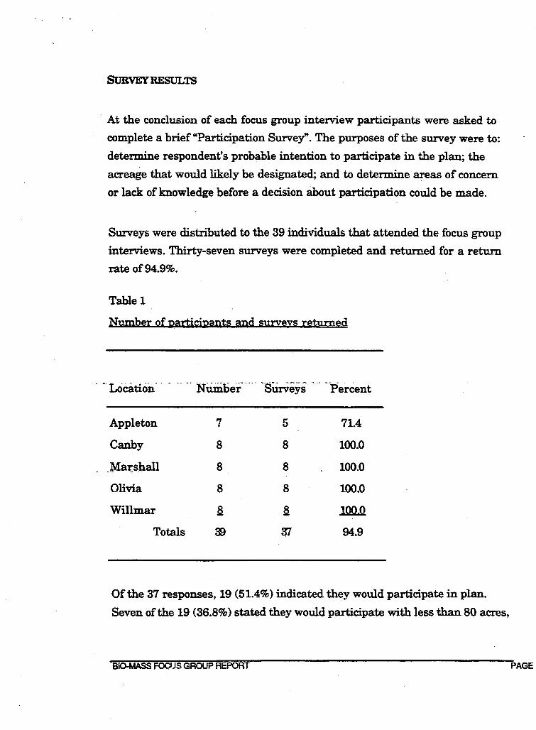
SURVEY RESULTS
At the conclusion of each focus group interview participants were asked to
complete a brief "Participation Survey". The purposes of the survey were to:
determine respondent's probable intention to participate in the plan; the
acreage that would likely be designated; and to determine areas of concern
or lack of knowledge before a decision about participation could be made.
Surveys were distributed to the 39 individuals that attended the focus group
interviews. Thirty-seven surveys were completed and returned for a return
rate of94.9%.
Table 1
Number of participants and survevs returned
· · - Location· · - · · · · '.Number· · · · ~SiirVeys -- --Percent
Appleton 7 5 71.4
Canby 8 8 100.0
_ l.\1ai:shall 8 8 100.0
Olivia 8 8 100.0
Willmar a a lOOJl
Totals re :rr 94.9
Of the 37 responses, 19 (51.4%) indicated they would participate in plan.
Seven of the 19 (36.8%) stated they would participate with less than 80 acres,
BIO-MASS FOCUS GROUP REPORT PAGE·
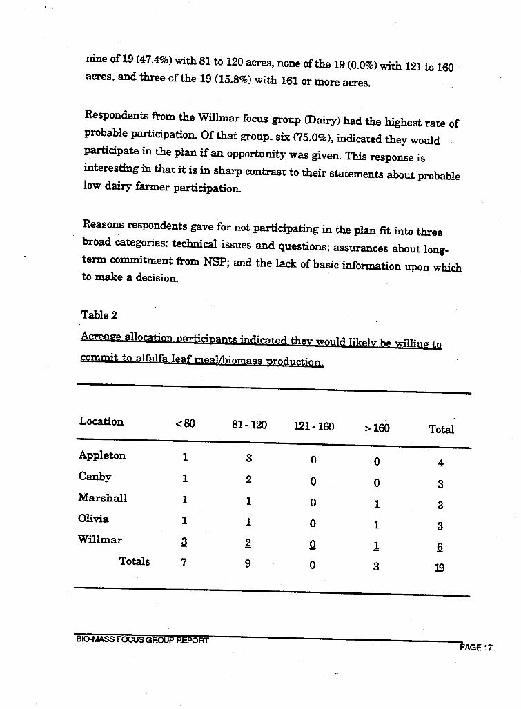
nine of 19 (47.4%) with 81 to 120 acres, none of the 19 (0.0%) with 121 to 160 acres, and three of the 19 (15.8%) with 161 or more acres.
Respondents from the Willmar focus group (Dairy) had the highest rate of probable participation. Of that group, six (75.0%), indicated they would participate in the plan if an opportunity was given. This response is interesting in that it is in sharp contrast to their statements about probable low dairy farmer participation.
Reasons respondents gave for not participating in the plan fit into three broad categories: technical issues and questions; assurances about longterm commitment from NSP; and the lack of basic information upon which to make a decision.
Table2
Acreaie allocation participants indicated they wQUld likely be willing to commit to alfalfa leaf meal/biomass production.
Location <80 81-120 121-160 >160 Total
Appleton 1 3 0 0 4 Canby 1 2 0 0 3 Marshall 1 1 0 1 3 Olivia 1 1 0 1 3 Willmar ~ ~ Q l ti
Totals 7 9 0 3 19
BIO-MASS FOCUS GROUP REPORT PAGE 17
SUMMARY
Farmers would require a clear, concise plan before making a· decision
about including alfalfa for a DFSS. This is ·in spite of the fact they generally
believe the plan could benefit themselves and the community-at-large.
In all the focus groups conducted for this project, the idea that alfalfa is a "good" crop was 11ll3nimous. Yet, this perception of "good" was continually tempered with the farmers' perception of financial risk. Participants
clearly understood the many benefits of including a perennial legume in
_ the~ crop ~~tjons. _ .
Farmers perceive change as being risky. The level of perceived risk,
together with the perception of enhanced rewards (i.e. -- more money, less work) are major factors upon which farmers make decisions. Given the perception that change is risky, farmers must have assurances that the
rewards for changing their crop rotations to include some or more alfalfa will be substantially greater than they presently receive with their present crop rotations. If farmers perceive the rewards to be less than, equal to, or even slightly more than, they receive from their present crop rotations, they
will not participate in a plan to produce alfalfa for a DFSS. They will change their cropping rotations and participate in DFSS only when they believe the
potential rewards for participation are substantially greater than they receive from their present crop rotations.
BIO-MASS FOCUS GROUP REPORT PAGE'
The study was conducted using the following procedures. 1. With input from the appropriate representatives of the CAP AP and
College of Agriculture (COA) faculty, the final questioning route was refined and finalized.
2. With consultation from the appropriate representatives of the CAP AP and COA, a design for sampling was established and exact locations were identified. Five locations were selectedrepresentative of the agriculture diversity within an approximate 50 mile radius of Granite Falls-in which to conduct focus group interviews. The locations selected were Appleton, Canby, Marshall, Olivia, and Willmar.
3. Using guidelines established by the primary researcher, the CAPAP reserved locations for each of the focus group interviews.
4. Using a pro-form.a established by the primary researcher, the CAP AP invited eight individuals to each of the five focus group locations for the interview.
5. Each focus group interview lasted approximately 1 and 112 hours and was audio taped. The same questioning route was used at each location.
6. From a "1099" information form, CAP AP was responsible for paying $30.00 to each focus group participant.
7. The audio tapes were transcribed by CAP AI> and the transcripts analyzed for key themes. This report represents the result of analysis of those transcripts.
BIO.MASS FOCUS GROUP REPORT PAGE19
INVITATION PROTOCOL
Telephone Screening
Name
.. Date ------------Address
Phone
Hello, my name is and I'm calling from the University of Minnesota~ We want to get the· opinion of farmers in Southwestern Minnesota o a project we are working on. This will take less than minutes. May I proceed?
1 Is this the head of the household?
()
()
Yes
No
[CONTINUE]
[May I please speak to the head of the household?]
2. Does the majority of your income come from farming sources?
()
()
Yes
No
[CONTINUE]
[TERMINATE]
2. Do you make the crop or livestock decisions on your farm?
() Yes [CONTINUE]
() No [TERMINATE]
3. Do you farm 400 or more acres?
() Yes [CONTINUE]
() No [TERMINATE]
5. Are you between the ages of 30 and 50?
() Yes [CONTINUE]
() No [TERMINATE]
BIO-MASS FOCUS GROUP REPORT PAGE
[IF "YES" TO ALL QUALIFYING QUESTIONS, CONTINUE] We are asking people like you to join us for a discussion about a cropping rotation we are working on. We want your opinion. You will be given $30.00 for your time and travel expenses and a free meal will be provided before or after the meeting. The discussion will be (time) (date) (place) and will last about one and one-half hours. Would you be able to participate in the meeting?
( ) YES [If YES] I will be sending you a letter confirming this information. Thank you very much for your cooperation. ( ) NO [If NO] Thank you for your time. You are welcome to attend a general information meeting on this project that will be held April 11at2:00 PM in the Montevideo Courthouse Assembly Room.
BIO-MASS FOCUS GROUP REPORT PAGE 21
Dear
Thank you for accepting our invitation to participate in the discussion
group in the (time) (date) (place). Because our time together is limited, we
will begin promptly.
As you know, the purpose of our meeting is to discuss various aspects of
alfalfa production. Topics to be covered will include, ~ut not be limited to:
1.
2.
3.
Your insights and opinions are very important.
We are looking forward to meeting With you. If you have any questions,_
please do not hesitate to call me. My number is -----
At x:OO p. m., prior to the meeting, dinner Gunch) will be provided. You will
be given $30.00 to help with the cost of your transportation and for your
contribution of time.
Sincerely,
Earl W. Bracewell, Primary Researcher
BIO-MASS FOCUS GROUP REPORT PAGE
Dear
Thank you for giving your time and thoughts to the discussion of the
University of Minnesota CAPAP for Alternative Plant and Anima]
Products sponsored focus group that discussed various aspects ·of alfalfa
production.
There were many excellent suggestions and comments. Your suggestions
will undoubtedly help the agricultural industry of Minnesota.
- -I enjoyed getting to meet with you. Our meetings were very useful as we
strive to better serve the agricultural community of Minnesota.
Best wishes in the future.
Sincerely
Earl W. Bracewell, Primary Researcher
BIO-MASS FOCUS GROUP REPORT PAGE 23
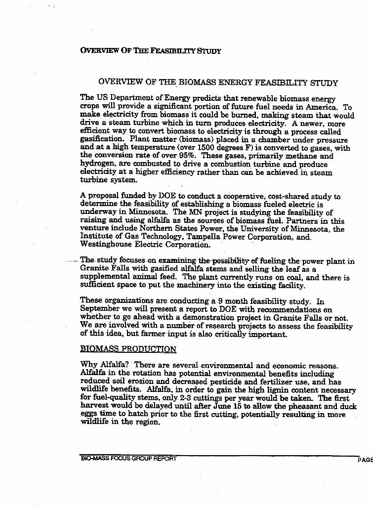
OVERVIEW OF THE FEAsmILITY STuDY
OVERVIEW OF THE BIOMASS ENERGY FEASIBILITY STUDY
The US Department of Energy predicts that renewable biomass energy crops will provide a significant portion of future fuel needs in America. To make el~ctricity from biomass it could be burned, waking steam that would drive a steam turbine which in turn produces electricity. A newer, more efficient way to convert biomass to electricity is through a process called gasification. Plant matter (biomass) placed in a chamber under pressure and at a high temperature (over 1500 degrees F) is converted to gases, with the conversion rate of over 95%. These gases, primarily methane and hydrogen, are combusted to drive a combustion turbine and produce electricity at a higher efficiency rather than can be achieved in steam turbine system.
A proposal funded by DOE to conduct a cooperative, cost-shared study to determine the feasibility of establishing a biomass fueled electric is underway in Minnesota. The MN project is studying the feasibility of raising and using alfalfa as the sourees of biomass fuel. Partners in this venture include Northern States Power, the University of Minnesota, the Institute of Gas Technology, Tampella Power Corporation, an<l Westinghouse Electric Corporation. -
.. -- The. study focuses on examining ~-possibility-of fueling the-power plant in Granite Falls with gasified alfalfa stems and selling the leaf as a supplemental animal feed. The plant currently runs on coal, and there is sufficient space to put the machinery into the existing facility.
These organizations are conducting a 9 month feasibility study. In September we will present a report to DOE with recommendations on whether to go ahead with a demonstration project in Granite Falls or not. We are involved with a number of research projects to assess the feasibility of this idea, but farmer input is also critically important.
BIOMASS PRODUCTION
Why Alfalfa? There are several environmental and economic reasons. Alfalfa in the rotation has potential environmental benefits including reduced soil erosion and decreased pesticide and fertilizer use, and has wildlife benefits. Alfalfa, in order to gain the high lignin content necessary for fuel-quality stems, only 2-3 cuttings per year would be taken. The first harvest would be delayed until after June 15 to allow the pheasant and duck eggs time to hatch prior to the first cutting, potentially resulting in more wildlife in the region.
BIO-MASS FOCUS GROUP REPORT PAGE
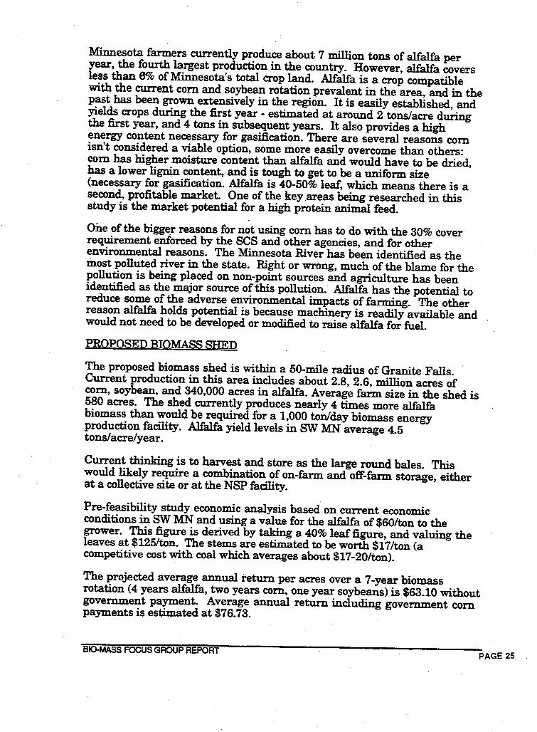
Minnesota farmers currently produce about 7 million tons of alfalfa per year, the fourth largest production in the country. However, alfalfa covers less than 6% of Minnesota's total crop land. Alfalfa is a crop compatible with the current com and soybean rotation prevalent in the area, and in the past bas been grown extensively in the region. It is easily established, and yields crops during the first year - estimated at around 2 tons/acre during the first year, and 4 tons in subsequent years. It also provides a high energy content necessary for gasification. There are several reasons com isn't considered a viable option, some more easily overcome than others: com has higher moisture content than alfalfa and would have to be dried, has a lower lignin content, and is tough to get to be a uniform size (necessary for gasification. Alfalfa is 40-50% leaf, which means there is a second, profitable market. One of the key .areas being researched in this study is the market potential for a high protein animal feed.
one of the bigger reasons for not using com has to do with the 30% cover requirement enforced by the SCS and other agencies, and for other environmental reasons. The Minnesota River has been identified as the most polluted river in the state. Right or wrong, much of the blame for the pollution is being placed on non-point sources and agriculture has been identified as the major source of this pollution. Alfalfa has the potential to reduce some of the adverse environmental impacts of farming. The other reason alfalfa holds potential is because machinery is readily available and would not need to be developed or modified to raise alfalfa for fuel.
PROPOSED BIOMASS SHED
The proposed biomass shed is within a 50-mile radius of Granite Falls. Current production in this area includes about 2.8, 2.6, million acres of com, soybean, and 340,000 acres in alfalfa. Average farm size in the shed is 580 acres. The shed currently produces nearly 4 times more alfalfa biomass than would be required for a 1,000 ton/day biomass energy production facility. Alfalfa yield levels in SW MN average 4.5 tons/acre/year.
Current thinking is to harvest and store as the large round bales. This would likely require a combination of on-farm and off-farm storage, either at a collective site or at the NSP facility.
Pre-feasibility study economic analysis based on current economic conditions in SW MN and using a value for the alfalfa of $60/ton to the grower. This figure is derived by taking a 40% leaf figure, and valuing the leaves at $125/ton. The stems are estimated to be worth $17/ton (a competitive cost with coal which averages about $17-20/ton).
The projected average annual return per acres over a 7-year biomass rotation (4 years alfalfa, two years com, one year soybeans) is $63.10 without government payment. Average annual return including government com payments is estimated at $76.73.
BIO-MASS FOCUS GROUP REPORT PAGE 25
This analysis indicates that the biomass rotation would be more profitable for the farmer than the conventional com-soybean rotation with or without government programs payments. Future reductions in government program payments, as are likely, would further increase the profit spread for the biomass producer over the conventional rotation.
Economic benefits of the biomass rotation are directly attributed to the inclusion of a perennial legume in the rotation. Reduced input costs of the biomass rotation compared to the conventional rotation combined with minor yield increases for com and beans in the biomass rotation result in increased profitS for the grower.
The benefits of including alfalfa in a rotation are well documented. However, increases in total alfalfa production have been limited because of the problems associated with shipping alfalfa long distances to reach markets and a declining dairy market for average quality bay.
ALFALFA COOPERATIVE
A proposed farmer-owned alfalfa cooperative (AC) is one example of a potential business arrangeinent that will be examined in this feasibility study. The AC could contract with growers to produce a]falfa. The AC could possibly separate the alfalfa into stem and leaf fractions at a facility integrated with the power plant. The reason for separating at NSP is because the leaves could· be heat treated to decrease the protein digestibility in the rumen of cows and bi-pass proteins have a higher economic value than soybeans, for example. The power plant has waste heat that could be used to treat the leaves. There is, of course, a danger of over-heating the leaves and n1ining them but research is being done on this right now at the UofM.
Densified alfalfa st.em fraction could be sold under a long-term guaranteed purchase agreement to NSP as a uniform high quality biomass fuel (about $17-20/ton) The alfalfa leaf fraction is sold as a relatively low-cost ($125/ton or more), high prote~, high ene~ feed supple1J1ent.
The ability to separate a value-added leaf meal product from the stem fuel should help make alfalfa biomass fuel competitive with other alternative fuels. Quality issues are important -NSP needs a high quality stem portion to run the plant, farmers will need high quality leaf to sell. Both can agronomically be accomplished. Separation techniques are being evaluated by the ag engineers working on the project.
The storage issues of this quantity of alfalfa are important to determining whether or not to go ahead with a demonstration project. What it comes down to is this is a tremendous amount of material. On-farm covered storage sheds with a crushed gravel base, with a maximum storage height of 12 feet are estimated to cost $3/square foot. Tarps cost around 20 cents/square foot, but a 10% loss can be expected.
BIO-MASS FOCUS GROUP REPORT PAGE
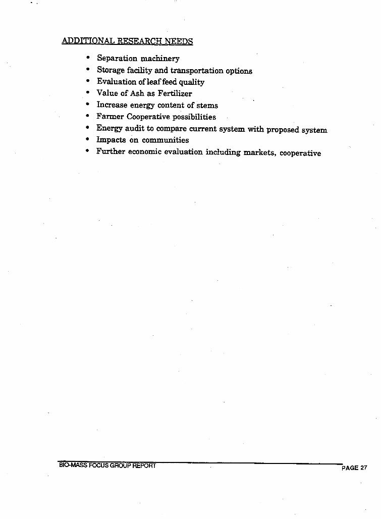
ADDITIONAL RESEARCH NEEDS
• Separation machinery • Storage facility and transportation options • Evaluation ofleaffeed quality • Value of Ash as Fertilizer • Increase energy content of stems • Farmer Cooperative possibilities • Energy audit to compare current system with proposed system • Impacts on communities • Further economic evaluation including markets, cooperative
BIO-MASS FOCUS GROUP REPORT PAGE 27
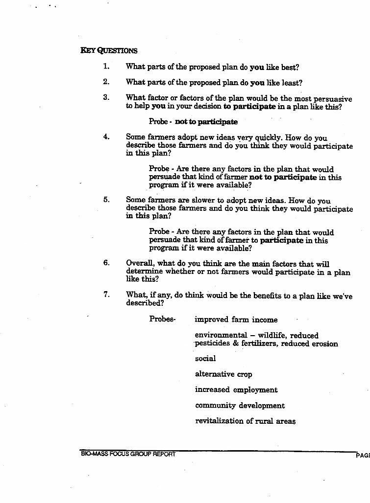
. .
KEYQuEsTIONS
1. What parts of the proposed plan do you like best?
2. What parts of the proposed plan do you like least?
3. What factor or factors of the plan would be the most persuasive to help you in your decision t.o participate in a plan like this?
Probe - not to participate
4. Some farmers adopt new ideas yery quickly. How do you describe those farmers and do you think they would participate in this plan?
Probe - Are there any factors in the plan that would persuade that kind of farmer not to participate in this program if it were availabl~?
5. Some farmers are slower to adopt new ideas. How do you describe those farmers and do you think they would participate in this plan?
Probe - Are there any factors in the plan that would persuade that kind of farmer to participate in this program if it were available?
6. Overall, what do you think are the main factors that will determine whether or not farmers would participate in a plan like this?
7. What, if any, do think would be the benefits to a plan like we've described?
Probes-
BJO.MASS FOCUS GROUP REPORT
improved farm income
environmental - wildlife, reduced ·pesticides & fertilizers, reduced erosion
social
alternative crop
increased employinent
community development
revitalization of rural areas
PAGE
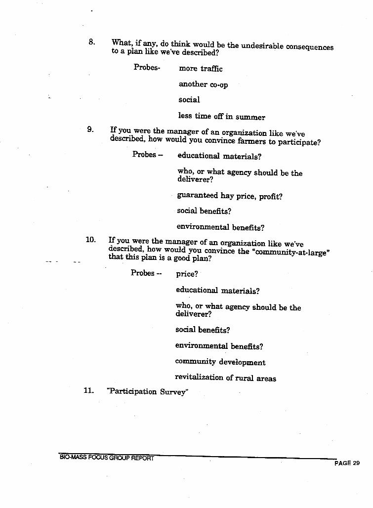
8. What, if any, do think would be the undesirable consequences to a plan like we've described?
Probes- more traffic
another co-op
social
less time off in summer
9. If you were the manager of an organization like we've described, how would you convince farmers to participate?
Probes- educational materials?
who, or what agency should be the deliverer?
guaranteed hay price, profit?
social benefits?
environmental benefits?
10. If you were the manager of an organization like we've described, how would you convince the "community-at-large" that this plan is a good plan?
Probes -- price?
educational materials?
who, or what agency should be the deliverer?
social benefits?
environmental benefits?
community development
revitalization of rural areas 11. "Participation Survey"
BIO-MASS FOCUS GROUP REPORT PAGE 29
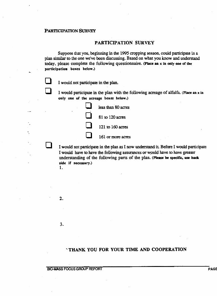
PARTICIPATION SURVEY
PARTICIPATION SURVEY
Suppose that you, beginning in the 1995 cropping season, could participate in a plan simj)ar to the one we've been discussing. Based on what you know and understand today, please complete the following questionnaire. (Place an x in only one of the participation boxes below.)
0 I would not participate in the plan.
0 I would participate in the plan with the following acreage of alfalfa. (Place an x in
only one of the acreage boxes below.)
D less than 80 acres
D 81 to 120 acres
0 121 to HiO acres
D 161 or more acres
0 I would not participate in the plan as I now understand iL Before I would participate I would have to have the following assurances or would have to have greater understanding of the following pans of the plan. (Please be specific, use back
side if necessary.) 1.
2.
3.
"THANK YOU FOR YOUR TIME AND COOPERATION
BIO-MASS FOCUS GROUP REPORT PAGE
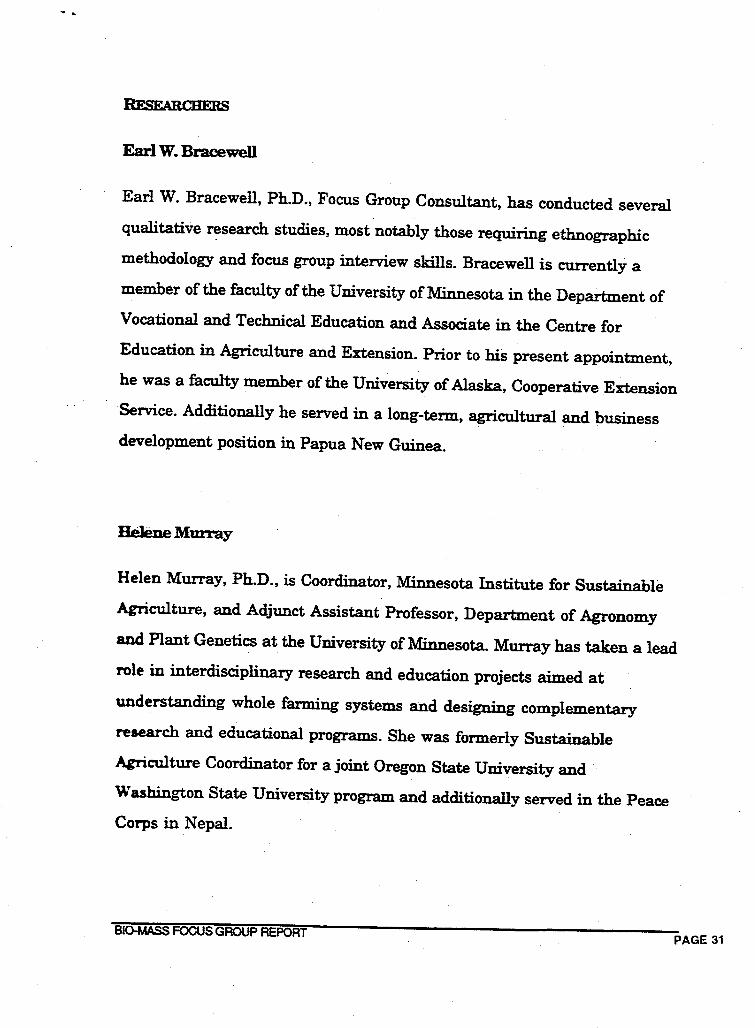
Earl W. Bracewell
Earl W. Bracewell, Ph.D., Focus Group Consultant, has conducted several qualitative research studies, most notably those requiring ethnographic methodology and focus group interview skills. Bracewell is currently a member of the faculty of the University of Minnesota in the Department of Vocational and Technical Education and Associate in the Centre for Education in Agriculture and Extension. Prior to his present appointment, he was a faculty member of the University of Alaska, Cooperative Extension Service. Additionally he served in a long-term, agricultural and business development position in Papua New Guinea.
BeJene Murray
Helen Murray, Ph.D., is Coordinator, Minnesota Institute for Sustainable Agriculture, and Adjunct Assistant Professor, Department of Agronomy and Plant Genetics at the University of Minnesota. Murray has taken a lead role in interdisciplinary research and education projects aimed at understanding whole farming systems and designing complementary research and educational programs. She was formerly Sustainable Agriculture Coordinator for a joint Oregon State University and Washington State University program and additionally served in the Peace Corps in Nepal.
BIO-MASS FOCUS GROUP REPORT PAGE 31
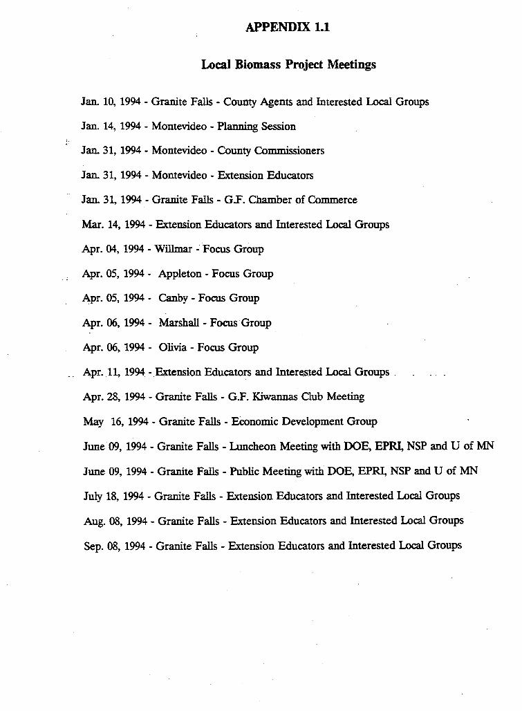
.
APPENDIX 1.1
Local Biomass Project Meetings
Jan. 10, 1994 - Granite Falls - County Agents and Interested Local Groups
Jan. 14, 1994 - Montevideo - Planning Session
Jan. 31, 1994 - Montevideo - County Commissioners
Jan. 31, 1994 - Montevideo - Extension Educators
Jan. 31, 1994 - Granite Falls - G.F. Chamber of Commerce
Mar. 14, 1994 - Extension Educators and Interested Local Groups
Apr. 04, 1994 - Willmar - Focus Group
Apr. 05, 1994 - Appleton - Focus Group
Apr. 05, 1994 - Canby - Focus Group
Apr. 06, 1994 - Marshall - Focus Group
Apr. 06, 1994 - Olivia - Focus Group
_ . Apr .. 11, 1994 - .Extension Educators and Interested Local Groups .
Apr. 28, 1994 - Granite Falls - G.F. Kiwannas Oub Meeting
May 16, 1994 - Granite Falls - Economic Development Group
June 09, 1994 - Granite Falls - Luncheon Meeting with DOE, EPRI, NSP and U of MN
June 09, 1994 - Granite Falls - Public Meeting with DOE, EPRI, NSP and U of MN
July 18, 1994 - Granite Falls - Extension Educators and Interested Local Groups
Aug. 08, 1994 - Granite Falls - Extension Educators and Interested Local Groups
Sep. 08, 1994 - Granite Falls - Extension Educators and Interested Local Groups
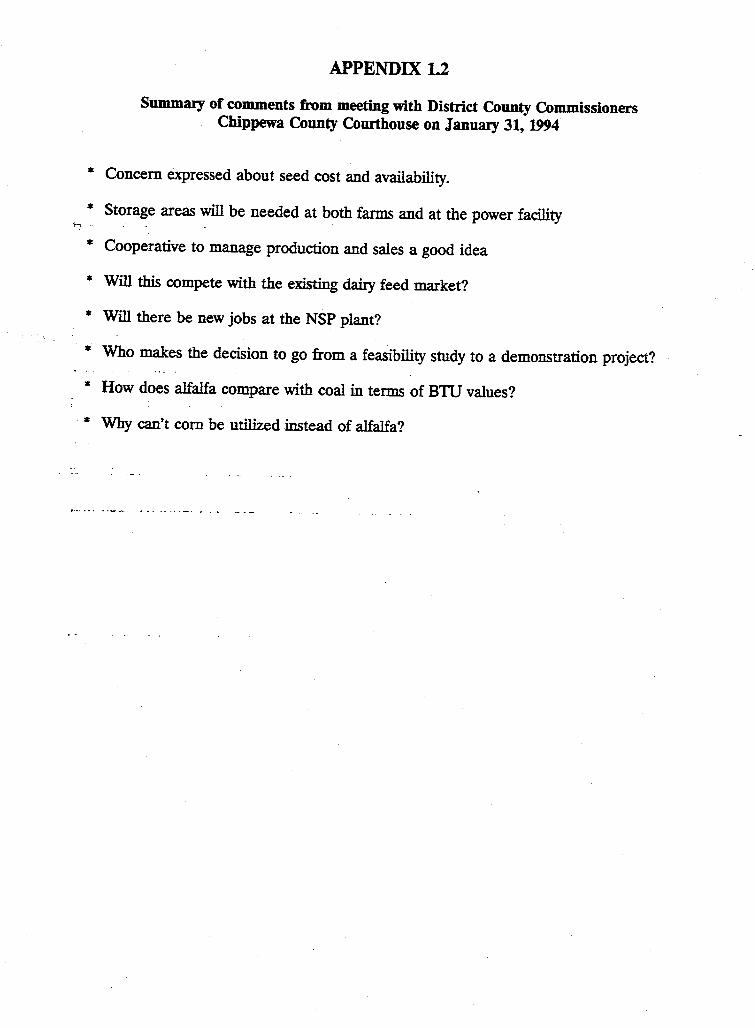
APPENDIX 1.2
Summary of comments from meeting with District County Commissioners Chippewa County Courthouse on January 31, 1994
* Concern expressed about seed cost and availability.
* Storage areas will be needed at both farms and at the power facility s-. ..
* Cooperative to manage production and sales a good idea
* Will this compete with the existing dairy feed market?
* Will there be new jobs at the NSP plant?
* Who makes the decision to go from a feasibility study to a demonstration project?
* How does alfalfa compare with coal in terms of BTU values?
* Why can't corn be utilized instead of alfalfa?
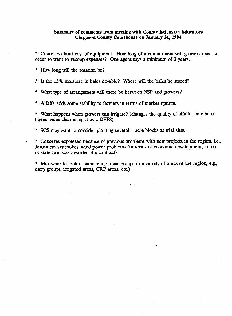
Summary of comments from meeting with County Extension Educators Chippewa County Courthouse on January 31, 1994
* Concerns about cost of equipment. How long of a commitment will growers need in order to want to recoup expenses? One agent says a minimum of 3 years.
* How long will the rotation be?
· * Is the 15% moisture in bales do-able? Where will the bales be stored?
* What type of arrangement will there be between NSP and growers?
* Alfalfa adds some stability to farmers in terms of market options
• What happens when growers can irrigate? (changes the quality of alfalfa, may be of higher value than using it as a DFFS)
• SCS may want to consider planting several 1 acre blocks as trial sites
• Concerns expressed because of previous problems with new projects in the region, i.e., Jerusalem artichokes, wind power problems (in terms of economic development, an out of state firm was awarded the contract)
• May want to look at conducting focus groups in a variety of areas of the region, e.g., dairy groups, irrigated areas, CRP areas, etc.)
Summary of comments from meeting with Granite Falls Chamber of Commerce on January 31, 1994
* One farmer says that as alfalfa matures it ends up with aphid problems and leaves fall off
* How many more diseases will we have with more alfalfa planted?
~* How far away will we need to go to sell the alfalfa leaf meal
* Will it compete with distillery grains?
* Energy issues are tough. For example ethanol is renewable but is getting a ''bad rap"
* How are you planning to pay farmers?
* : What is the length of the potential demonstration project?
* If you can use alfalfa why can't you use com and soybean residues? (com has higher moisture content, low lignin content, and is tough to get to be a uniform size; soybeans . have higher lignin values but lower yields)
* What is·EPA's-role in'thiS project? Are they a thorn or ally?
* Will need considerable research on what to do with the alfalfa meal
* How long before we see an inflated price on coal?
* How long will it be before the plant breeders come up with a specific cultivar that is well suited to this type of goal (high lignin, high quality fuel)
* Is there potential for a farmer-owned cooperative?
* How many BTUs are there in alfalfa versus coal? (6,000 for alfalfa, 8,000 for coal}
* What about the impacts on wildlife when alfalfa is planted? What about the impacts on farms if wildlife increases? For example, will we see increased pocket gophers resulting in huge problems for farmers?
* Would sweet clover fit into this program? (no, a one year crop with slow recovery after one cutting)
* Are there problems getting the alfalfa to 15% moisture?
;.
* The Integrated Farm Management program is in place. Could possibly seed mixtures . of oats and alfalfa, then harvest and sell the oats while alfalfa is getting established
* Seedbed preparation questions asked. Concern about how to do this, there is a critical need for more information. Farmers will need to modify their equipment for seeding alfalfa and will need to adjust their rotational patterns, fertilizer rates, etc.
* Potassium tends to be limiting in alfalfa plantings.
·· * Alfalfa lower pesticide and fertilizer use, resulting in increased earthworm activity which helps improve drainage
* Pocket gopher problems likely to be high if planting CRP land to alfalfa
* How does the com co-operative schedule their arrivals and deliveries?
* ~<?W ~l!ch _of ~e alfalf~ leaf drops off as the plant matures?
APPENDIX 1.3
AG ADVISORY COUNCIL INTEREST LIST
*Rollie Ammerman RRl, Box 90, Oara City, MN 56222 (612) 847-2519
*Leslie Bergquist, Yellow Medicine County Bank 180 8th Avenue, Granite Falls, MN 56241 (612) 564-4611
Pat Beyers, Granite Falls Community Development Commission 155 W 7th Ave, PO Box 220, Granite Falls MN 56241-0220 (612) 564-2255
#Dan·Borgmeier PO Box 250, Redwood Falls, MN 56283
Don Brower . mobile phone: 720-4888
Robert J. Byrnes, Lyon Co Ext Office - 1400 East Lyon Street, Marshall MN 56258
John P. Cunningham, Big Stone Co Ext Office . 20 SE 2nd St, Ortonville MN 56278
*Mark Dahl 7050 20th Ave SW, Montevideo, MN 56265 (612) 269-8057
*Tim Dale R2, Box 50, Hanley Falls, MN 56245 (612) 669-4666
*Neale Deters, Southwestern Technical College 1593 11th Ave, Granite Falls, MN 56241 (612) 564-4511
. #LeonDoom RRl Box 123, Cottonwood MN 56229 (507) 423-6459
Kevin Doyle, Cottonwood Co-op Oil Box 318, Cottonwood MN 56229 800-569-1352
Roger Engstrom Rt 2, Box 99, Detroit Lakes, :MN 56501 (218) 847-8841
*Dwayne Ericksen Rt2, Box 68, Granite Falls, :MN 56241
. (612) 564-4078
Dave Frederickson, MN Farmers Union (612) 875-3531
Dane Fredrickson Rt 1, Box 102, Murdock MN 56271
*Jerry F~ Ag & Applied Economics, Univ. of Minnesota 316 CLA Off Bldg, 1994 Buford Ave, St. Paul MN 55108 (612) 625-8720
~-Dennis Gibson 2030 10th Ave NE, Montevideo, MN 56265 ·(612) 269-8103
Norman Giese - - (612) 289-2647
#Dennis Goehring 1952 County Road 4 NE, Atwater, MN 56209 (612) 974-8846
Wayne J. Hansen, Redwood Co Ext Office Courthouse, PO Box 46, Redwood Falls MN 56283
Gunder Hanson Detroit Lakes MN (218) 847-5186
Don Haubrick R 1, Box 58, Danville MN (612) 826-2543
Grant Herfindahl Rt 1, Box 150A, Benson, MN 56215 (612) 843-2523
Chuck Jahn 4025 90th Ave SW, Montevideo MN (612) 269-9311
Dick Jepson Rt 3, Box 98, Granite Falls MN 56241 (612) 564-4068
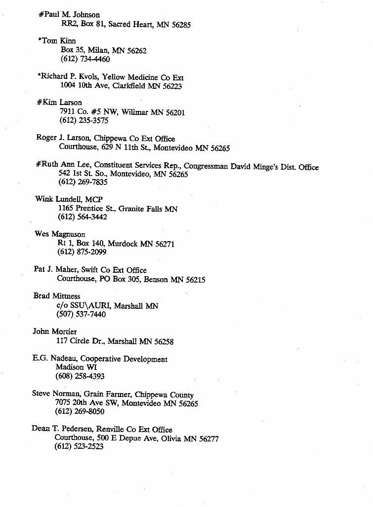
#Paul M. Johnson RR2, .Box 81, Sacred Heart, MN 56285
*Tom Kinn Box 35, Milan, MN 56262 (612) 734-4460
*Richard P. Kvols, Yellow Medicine Co Ext 1004 10th Ave, Oarkfield MN 56223
#Kim Larson 7911 Co. #5 NW, Willmar MN 56201 (612) 235-3575
Roger J. Larson, Chippewa Co Ext Office Courthouse, 629 N 11th St., Montevideo MN 56265
#Ruth Ann Lee, Constituent Services Rep., Congressman David Minge's Dist. Office 542 1st St. So., Montevideo, MN 56265 (612) 269-7835
Wink Lundell, MCP 1165 Prentice St., Granite Falls MN (612) 564-3442
Wes Magnuson Rt 1, Box 140, Murdock MN 56271 (612) 875-2099
Pat J. Maher, Swift Co Ext Office Courthouse, PO Box 305, Benson MN 56215
Brad Mittness c/o SSU\AURI, Marshall MN (507) 537-7440
John Mortier 117 Circle Dr., Marshall MN 56258
E.G. Nadeau, Cooperative Development Madison WI ( 608) 258-4393
Steve Norman, Grain Farmer, Chippewa County 7075 20th Ave SW, Montevideo MN 56265 (612) 269-8050
Dean T. Pedersen, Renville Co Ext Office Courthouse, 500 E Depue Ave, Olivia MN 56277 (612) 523-2523
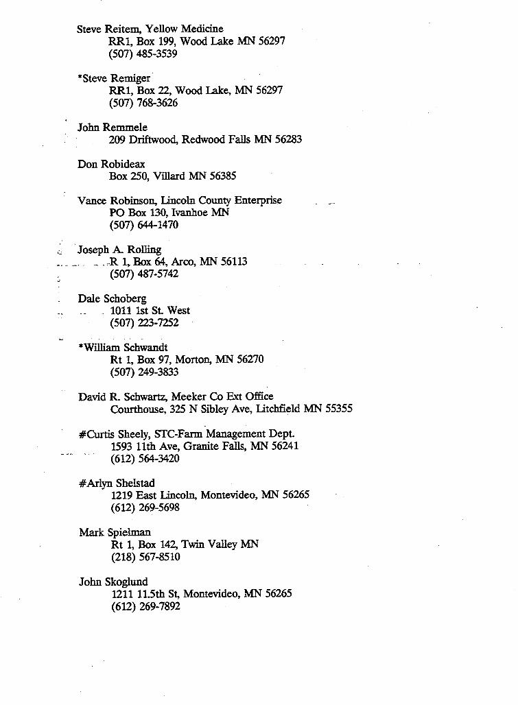
Steve Reitem, Yellow Medicine RRl, Box 199, Wood Lake MN 56297 (507) 485-3539
*Steve Remiger RRl, Box 22, Wood Lake, MN 56297 (507) 768-3626
John Remmele 209 Driftwood, Redwood Falls MN 56283
Don Robideax Box 250, Villard MN 56385
Vance Robinso~ Lincoln County Enterprise PO Box 130, Ivanhoe MN (507) 644-1470
Joseph A. Rolling _ . ,-R 1,. Box 64, Arco, MN 56113
(507) 487-5742
Dale Schoberg . 1011 1st St. West
(507) 223-7252 ..
*William Schwandt Rt 1, Box 97, Morto~ MN 56270 (507) 249-3833
David R. Schwartz, Meeker Co Ext Office Courthouse, 325 N Sibley Ave, Litchfield MN 55355
#Curtis Sheely, STC-Farm Management Dept. 1593 11th Ave, Granite Falls, MN 56241
- -·· ...... (612) 564-3420
#Arlyn Shelstad 1219 East Lincoln, Montevideo, MN 56265 (612) 269-5698
Mark Spielman Rt 1, Box 142, Twin Valley MN (218) 567-8510
John Skoglund 1211 11.Sth St, Montevideo, MN 56265 ( 612) 269-7892
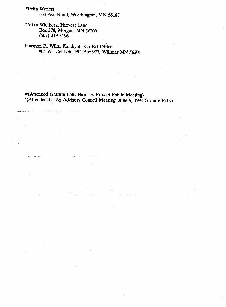
*Erlin Weness 633 Ash Road, Worthington, :MN 56187
*Mike Wielberg, Harvest Land Box 278, Morgan, MN 56266 (507) 249-3196
Hannon R. Wilts, Kandiyohi Co Ext Office 905 W Lltchfield, PO Box 977, Willmar MN 56201
#{Attended Granite Falls Biomass Project Public Meeting) *(Attended 1st Ag Advisory Council Meeting, June 9, 1994 Granite Falls)
APPENDIX3
Appendix A: DESCRIPTION OF SOIL ASSOCIATIONS
(source: Soil Associations of Minnesota of Minnesota Soil Survey Staff of the U.S. Department of Agriculture. Soil Conservation Service and University of Minnesota
• Agricultural Experiment Station. October 1983 4-R-38340).
B3 BEARDEN-MCINTOSH-COL VIN
The soils in this association are on very gently sloping to nearly level ground moraines with a covering of calcareous silty lacustrine material. This association is in western Minnesota. The landscape consists of broad low lying areas of Colvin soils between the BCarden and Mcintosh soils on rises. Native vegetation was prairie. Bearden and Colvin formed in thick deposits of silty lacustrine sediments. Mcintosh formed in thinner silty
·· se:diments. Bearden· and Mcintosh are somewhat poorly drained. Colvin is poorly drained. .•.. Bearden and Colvin have surface layers of silty clay loam. Mcintosh has a surface layer of
silt loam that is underlain by loam glacial till. All of the soils are calcareous. Minor soils in the association are· Hamerly, Winger, and Perella.
B7 BURR-DUPAGE
The soils in this association are nearly level and are on a narrow Glacial Lake Plain in southwestern Minnesota. They formed in calcareous silty lacustrine deposits and loamy alluvial deposits from streams that cross the lake bed. The landscape is a broad flat. with a few low knolls of glacial till. Native vegetation was prairie. Burr is poorly drained. and has a high content of gypsum. It has a thick surface layer of silty clay loam and silty clay .. DuPage is moderately well drained. It has a loam surface layer. Both soils are occasionally flooded. Mcintosh Variant. which is also common in this association, is not flooded. Minor .soils ar.e Arvilla, Egeland. Oldham. and Ves soils.
C2 SINAI-FULDA-HATTIE
The soils in this association are on nearly level to sloping ground moraines in westcentral Minnesota. Some of the moraines are covered with a thin layer of clayey lacustrine sediments. Sinai is on plane or slightly convex areas and gentle side slopes. Fulda is on broad flats or in swales. Hattie is on convex knolls and sideslopes. Native vegetation was prairie. Sinai is moderately well or well drained md Fulda is poorly drained. Both soils formed in lacustrine sediments and have silty clay surface soil and subsoil. Hattie is well or moderately well drained. and calcareous. It formed in glacial till and has a clay surface layer and subsoil. Minor soils are Dovray. Hegne. and Tonka.
C3 SPICER-VES-TARA
The soils in this association are on nearly level to undulating lake plains in western Minnesota. The landScape consists of a broad nearly level lake basin of silty lacustrine sediments with numerous islands of loamy glacial till, and islands of till covered with lacustrine sediments. -Native vegetation was prairie. Spicer is calcareous and poorly drained. It formed in the laclistrine sediments and has a silty clay loam surface soil and silt loam subsoil. Ves is well drained md formed on islands of glacial till. It has a loam surface soil and subsoil. Tara is moderately well drained and formed on silt covered islands of glacial till. It has a silt loam surface soil and subsoil. Minor soils are Canisteop Colvin, Doland, Mcintosh, Nomania, Okoboji, Storden, and Webster.
D2 BARNES-FLOM-BUSE
The soils in this assOciarion are on steep to nearly level moraines in western Minnesota. They formed in_ calcareous. loamy glacial till. Barnes is on irregular convex side slopes and knolls while Buse is on steep end moraines. Flom soils are in shallow drainageways and on wet flats. Native vegetation was prairie. Barnesis well drained. It has a . . loam surface soil and subsoil. Flom is poorly drained. The surf~e soil is silty clay loam and the subsoilis clay loam. Buse is well drained and calcareous. It has a loam surface soil and subsoil. Minor soils are Fulda, Langhei. Oak Lake, Parnell, Poinsett, quam, Singaas. and Vallers.
D3 W ADENILL-SUNBURG-KORONIS
The soils in this association are on undulating to moderately steep ground moraines in central Minnesota. They formed in calcareous loam glacial till. Wad.enill and Sunburg formed under prairie vegetation. Koranis formed in an area transitional between prairie and forest. All of the soils are well drained aid are on knolls and sideslopes. W adenill has a fine sandy loam surface soil and subsoil. Sunburg has a calcareous loam surface layer over a fine sandy loam subsoil. Koronis has a loam surface layer and fine sandy loam subsoil. Minor Soils are Canisteo, Delft, Glencoe, Marcellon. and Palms.
D4 CANISTEO-YES-NORMANIA
The soils of this association are on nearly level to undulating ground moraines in southwestern Minnesota. They formed in calcareous shaly, loamy glacial till. Canisteo are on broad flats and rims of depressions, Ves on low knolls and convex side slopes, and Normania on slight rises and the concave part of lower side slopes. Native vegetation was prairie. Canisteo is poorly drained. and calcareous. The surface soil and subsoil are clay loam. Ves is well drained and Nomania is moderately well drained. Both Ves and Nomania have loam a surface layer and subsoil. Minor soils are Glencoe. Harps, Okoboji. Seafonh, Spicer. Storden. and Webster.
D5 FORMAN-AASTAD-FLOM
The soils in this association are on undulating to nearly level moraines and till plains in southwestern Minnesota. They formed in loamy glacial till. Forman is on convex pans of the landscape and adjacent to steep side slopes along the deep drainageways. Aastad is on the plane and slightly convex areas. Flom is in shallow drainageways. Native vegetation was prairie. Forman is well drained, Aastad is moderately well drained and Flom is poorly drained. All three soils have a clay loam surface soil and a finn clay loam subsoil. Minor soils are Buse, Darnen, Hamerly, Quam, and Vallers.
D6 CANISTEO-NICOLLET-OKOBOil
The soils in this association are on nearly level to gently undulating ground moraines in southwestern Minnesota. The ground moraine is covered with a layer of silty and clayey lacustrine sediments in Kandiyohi, Meeker, and northern Renville counties. Canisteo soils are on broad flats and on rims of depressions, Nicollet on low rises, and Okoboji in depressions. Native vegetation was prairie. Canisteo is poorly drained, and calcareous and Nicollet is moderately well or somewhat poorly drained. Commonly Canisteo and Nicollet have a clay loam surface layer and subsoil where the ground moraine is covered with lacustrine sediments. The surface and subsoil layers are silty clay loam. Okoboji is very poorly drained. The surface soil is silty clay loam and the subsoil is silty clay. Minor soils are Brawnton, Clarion, Crippin, Glencoe, Guckeen, Mama, Palms, Webster, and Storden.
HI KRANZBURG-VIENNA-HIDEWOOD
The soils in this association are on gently sloping to nearly level loess covered ground moraines in southwestern Minnesota. They formed in a covering of loess over calcareous loamy glacial till. Kranzburg and Vienna are on ridgetops and side slopes. Hidewood is in drainageways. Native vegetation was prairie. Kranzburg has a silty clay loam surface soil and subsoil. Vienna has silty clay loam surface soil formed in loess and glacial till and a clay loam subsoil formed in glacial till. Both Kranzburg and Vienna are well drained. Hidewood is somewhat poorly drained. They have a silty clay loam surface soil and subsoil. Minor soils are Brookings, Buse, Darnei, and LismDre.
I2 ARVESON-MARYSLAND-SVERDRUP
The soils in this association are on nearly level to undulating glacial outwash plains and glacial lake beaches in west-central Minnesota. They formed in loamy water-deposited sediments. Arveson and Marysland are on broad flat areas and in swales. Sverdrup is on low rises and convex ridges. Native vegetation was prairie. Arveson and Marysland are poorly to very poorly drained, and calcareous. Both soils are moderately deep to sandy sediments. Arveson soils have a clay loam surface soil and a loam or sandy loam subsoil over a loamy sand or fine sand substrarum. Marysland soils have loam surface and subsurface layers and a sand subsoil. Sverdrup is well drained and has a sandy loam surface soil, and sandy loam or loamy sand subsoil that is underlain by sand. Minor soils in the association are Oontarf, FossLun, Maddock, Renshaw, and Swenoda.
14 BISCA Y-ESTIIBRVILLE-HA WICK
The soils in this association are on nearly level to sloping outwash plains, valley trains, and river terraces in south-central Minnesota. Biscay formed in a moderately thick covering of loamy sediments. Estherville formed in a thin covering of loamy sediments. Hawick formed in very thin loamy sediments or sandy materials.
Jl COLAND-STORDEN-SW ANLAKE
The soils in ibis association are on nearly level bottomlands and steep side slopes in the Upper Minnesota River Valley. Coland formed in alluvium. Storden and Swanlake formed in calcareous loamy glacial till. Coland soils are on bottcmlands, Storden on west and south facing sideslopes and Swanlake on north and east facing sideslopes. Coland aid Storden soils formed under prairie vegetation and Swanlake soils formed under woodland. Coland is poorly drained and has a thick silty clay loam surface layer over a sandy loam subsoil. Sta-den and Swanlake are well drained and have a loam surface layers and underlying material. Minor soils are Calco, Comfrey,. Copaston, Dorchester, DuPage, Lester, Millington, Nishn~ Terril, andwadena
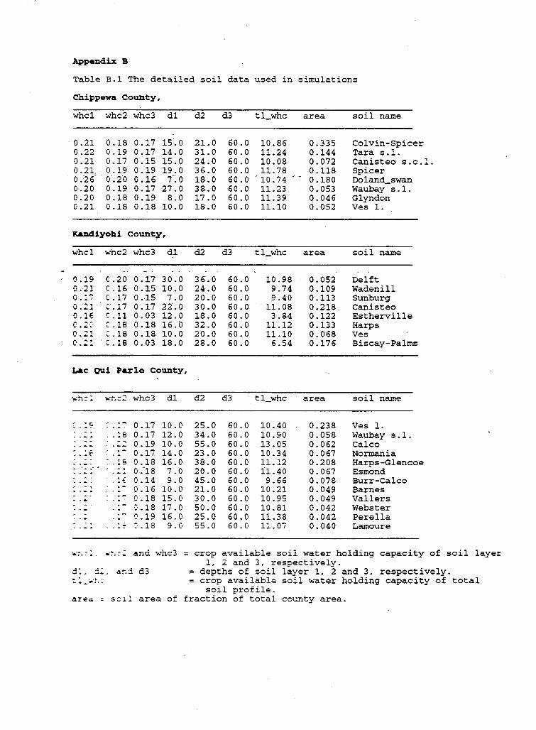
Appendix B
Table B.1 The detailed soil data used in simulations
Chippewa County,
whcl whc2 whc3 dl
'0 .21 0.22 0.21 0.21 0 .'2 6" 0.20 0.20 0.21
0.18 0.19 0.17 0.19 0 .2·0 0.19 0.18 0.18
0.17 0.17 0.15 0.19 0.16 0.17 0.19 0.18
15·.o 14.0 15.0 19.0
7·:0 27.0 8.0
10.0
Kandiyohi County,
whcl
0.19 0.21 0.: "7 0 :21 0 .lE 0. 2C. 0.21 0 .: !
.,..hc2 whc3
C.20 0.17 C.16 0.15 C.17 0.15 C.17 0.17 C.ll 0.03 :.1s 0.18 C.18 0.18
' c . 18 0. 03
dl
30.0 10.0 7.0
22.0 12.0 16.b 10.0 18.0
Lac OUi Parle County,
c . : c. ' . : 8
-: . 15
whc3
0 .17 0.17 0.19 0 .17 0.18 o :18 0.14 0.16 0.18 :.18 0.19 :· .18
dl
10.0 12.0 10.0 14.0 16.0 7.0 9.0
10.0 15.0 17. 0 16.0 9.0
d2
21.0 31.0 24.0 36.0 18.0 38.0 17.0 18.0
d2
36.0 24.0 20.0 30.0 18.0 32.0 20.0 28.0
d2
25.0 34.0 55.0 23.0 38.0 20.0 45.0 21.0 30.0 50.0 25.0 55.0
d3
60.0 60.0 60.0 60.0 60.0 60.0 60.0 60.0
d3
60.0 60.0 60.0 60.0 60.0 60.0 60.0 60.0
d3
60.0 60.0 60.0 60.0 60.0 60.0 60.0 60.0 60.0 60.0 60.0 60.0
tl_whc
10.86 11.24 10.08 11.78
'10.74 11.23 11.39 11.10
tl_whc
10.98 9.74 9.40
11.08 3.84
11.12 11.10
6.54
tl_whc
10.40 10.90 13.05 10.34 11.12 il.40 9.66
10.21 10.95 10.81 11.38 11. 07
area
0.335 0.144 0.072 0 .118 0.180 0.053 0.046 0.052
area
0.052 0.109 0.113 0.218 0.122 0.133 0.068 0.176
area
0.238 0.058 0.062 0. 067 0.208 0.067 0.078 0.049 0.049 0.042 0.042 0.040
soil name
Colvin-Spicer Tara s.1. Canisteo s.c.l. Spicer Doland_swan Waubay s.l. Glyndon Ves l.
soil name
Delft Wadenill Sunburg Canisteo Estherville Harps Ves Biscay-Palms
soil name
Ves 1. Waubay s.l. Calco Normania Harps-Glencoe Esmond Burr-Calco Barnes Vallers Webster Perella Lamoure
••~.::. • .. ~.:; 4nd whc3 = crop available soil water holding capacity of soil layer 1, 2 and 3, respectively.
d:. --· d~~ d3 =depths of soil layer 1, 2 and 3, respectively. ':. :_...-:.: = crop available soil water holding capacity of total
soil profile. 4reo = s=il area of fraction of total county area.
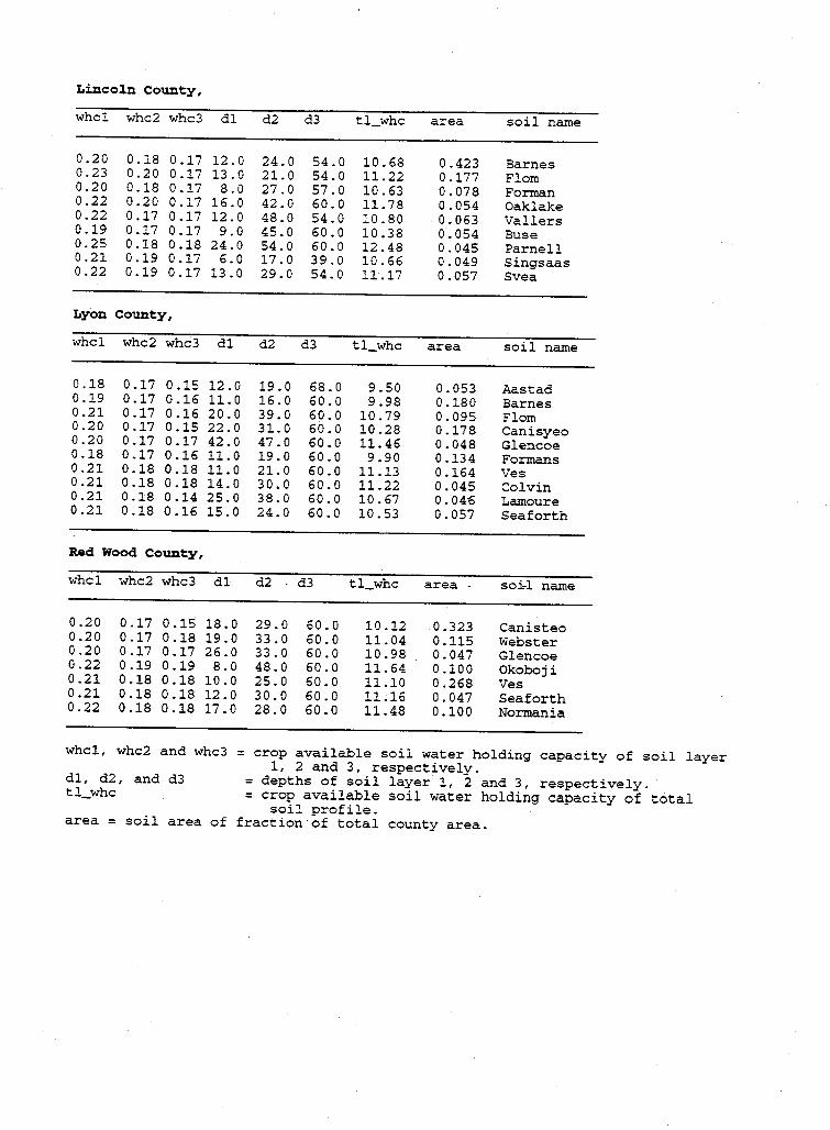
Lincoln county,
whcl whc2 whc3 dl
0 .20 0.23 0.20 0.22 0.22 0.19 0.25 0.21 0.22
0.18 0.20 0.18 0.20 0.17 0.17 0.18 0.19 0.19
0.17 0.17 0 .17 0.17 0.17 0.17 0.18 0.17 0.17
12.0 13.0 8.0
16.0 12.0 9.0
24.0 6.0
13.0
Lyon County,
whcl whc2 whc3 dl
0.18 0.19 0.21 0.20 0.20 0.18 0 .21 0.21 0.21 0.21
0.17 0.15 12.0 0.17 0.16 11.0 0.17 0.16 20.0 0 .17 0 .15 22. 0 0 • 17 0 • 17 42 . 0 0.17 0.16 11.0 0.18 0.18 11.0 0.18 0.18 14.0 0.18 0.14 25.0 0.18 0.16 15.0
Red Wood County,
whcl whc2 whc3 dl
0.20 0.20 0.20 0.22 0 .21 0.21 0.22
0.17 0.17 0.17 0.19 0.18 0.18 0.18
0.15 0.18 0.17 0.19 0.18 0.18 0.18
18.0 19.0 26.0 8.0
10.0 12.0 17.0
d2
24.0 21.0 27.0 42.0 48.0 45.0 54.0 17.0 29.0
d2
19.0 16.0 39.0 31. 0 47.0 19.0 21.0 30.0 38.0 24.0
d3
54.0 54.0 57.0 60.0 54.0 60.0 60.0 39.0 54.0
d3
68.0 60.0 60.0 60.0 60.0 60.0 60.0 60.0 60.0 60.0
d2 d3
29.0 33.0 33.0 48.0 25.0 30.0 28.0
60.0 60.0 60.0 60.0 60.0 60.0 60.0
tl_whc
10.68 11.22 10. 63 11. 78 10.80 10.38 12.48 10.66 11.17
tl_whc
9.50 9.98
10.79 10.28 11. 46 9.90
11.13 11.22 10.67 10.53
tl_whc
10.12 11.04 10.98 11.64 11.10 11.16 11.48
area
0.423 0.177 0.078 0.054 0.063 0.054 0.045 0.049 0.057
area
0.053 0.180 0.095 0.178 0.048 0.134 0.164 0.045 0.046 0.057
area -
0.323 0.115 0.047 0.100 0 .268 0.047 0.100
soil name
Barnes Flom Forman Oaklake Vallers Buse Parnell Singsaas Svea
soil name
Aastad Barnes Flom Canisyeo Glencoe Formans Ves Colvin Lamoure Seaforth
soi-1 name
Canisteo Webster Glencoe Okoboji Ves Seaforth Normania
whcl, whc2 and whc3 = crop available soil water holding capacity of soil layer
dl, d2, and d3 tl_whc
1, 2 and 3, respectively. = depths of soil layer 1, 2 and 3, respectively. = crop available soil water holding capacity of total
soil profile. area = soil area of fraction of total county area.
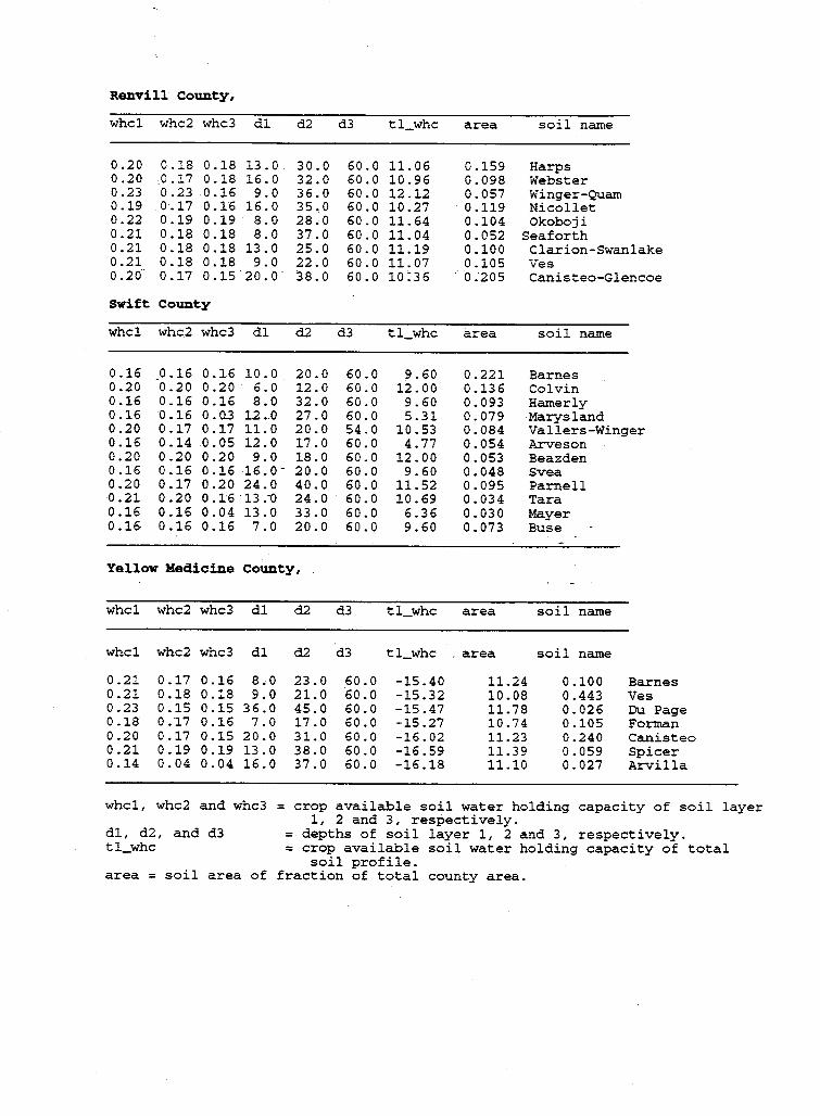
Renvill County,
whcl whc2 whc3 dl
0.20 0.20 0.23 0.19 0.22 0.21 0.21 0.21 0 .20-
-
0.18 0.18 0.17 0.18 0.23 0.16 0.17 0.16 0.19 0.19 0.18 0.18 0.18 0.18 0.18 0.18 0.17 0.15
13.0. 16.0 9.0
16.0 8.0 8.0
13.0 9.0
20.0·
swift county
whcl whc2 whc3 dl
0.16 0.20 0.16 0.16 0.20 0.16 0.20 0.16 0.20 0.21 0.16 0.16
_o .16 0.20 0.16 0.16 0.17 0.14 0.20 0.16 0.17 0.20 0.16 0.16
0.16 10.0 0.20 6.0 0.16 8.0 0. 03 12 •. 0 0 .17 11. 0 0.05 12.0 0.20 9.0 0.16 16.0-0.20 24.0 0.16 13.-0 0.04 13.0 0.16 7.0
d2
30.0 32.0 36.0 35.0 28.0 37.0 25.0 22.0 38.0
d2
20.0 12.0 32.0 27.0 20.0 17. 0 18.0 20.0 40.0 24.0 33.0 20.0
d3
60.0 60.0 60.0 60.0 60.0 60.0 60.0 60.0 60.0
d3
60.0 60.0 60.0 60.0 54.0 60.0 60.0 60.0 60.0 60.0 60.0 60.0
tl_whc
11. 06 10.96 12.12 10.27 11.64 11.04 11.19 11.07 10:36
tl_whc
9.60 12.00 9.60 5.31
10.53 4. 77
12.00 9.60
11.52 10.69
6.36 9.60
area
0.159 0.098 0.057 0.119 0.104 0.052 0.100 0.105 o :20s
area
0.221 0.136 0.093 0.079 0.084 0.054 0.053 0.048 0.095 0.034 0.030 0.073
soil name
Harps Webster Winger-Quam Nicollet Okoboji
Seaforth Clarion-Swanlake Ves Canisteo-Glencoe
soil name
Barnes Colvin Hamerly Marysland Vallers-Winger Arveson Beaz den Svea Parnell Tara Mayer Buse
Yellow Medicine County,
whcl whc2 whc3 dl
whcl whc2 whc3 dl
0.21 0.21 0.23 0.18 0.20 0.21 0.14
0.17 0.18 0.15 0.17 0.17 0.19 0.04
0.16 0.18 0.15 0.16 0.15 0.19 0.04
8.0 9.0
36.0 7.0
20.0 13.0 16.0
d2
d2
23.0 21.0 45.0 17 .0 31.0 38.0 37.0
d3
d3
60.0 60.0 60.0 60.0 60.0 60.0 60.0
tl_whc area
tl_whc . area
-15.40 -15.32 -15.47 -15.27 -16.02 -16.59 -16.18
11.24 10.08 11.78 10.74 11.23 11.39 11.10
soil name
soil name
0.100 0.443 0.026 0.105 0.240 0.059 0.027
Barnes Ves Du Page Forman Canisteo Spicer Arvilla
whcl, whc2 and whc3 = crop available soil water holding capacity of soil layer
dl, d2, and d3 tl_whc
1, 2 and 3, respectively. = depths of soil layer 1, 2 and 3, respectively. = crop available soil water holding capacity of total
soil profile. area = soil area of fraction of total county area.
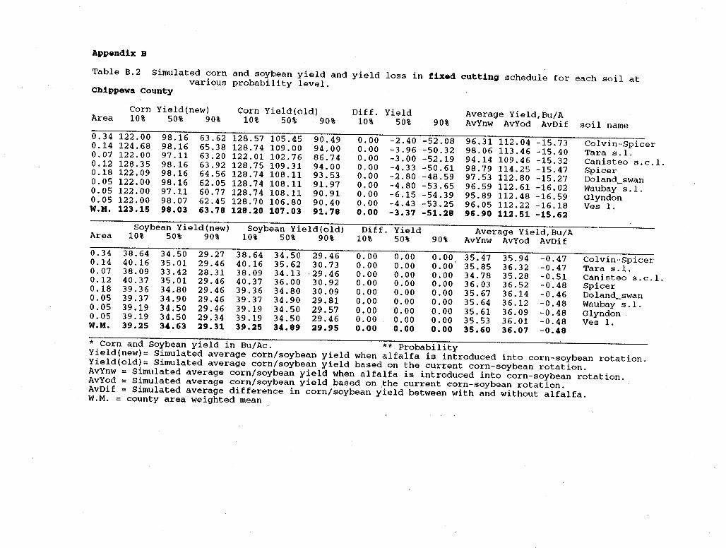
Appendix B
Table B.2 Simulated corn and soybean yield and yield loss in fixed cutting schedule for each soil at various probability level. Chippewa county
Corn Yield(new) Corn Yield(old) Diff. Yield Average Yield,Bu/A Area 10% 50% 90% 10% 50% 90% 10% 50% 90% AvYnw AvYod AvDif soil name 0.34 122.00 98.16 63.62 128.57 105.45 90.49 0.00 -2.40 -52.08 96.31 112.04 -15.73 Colvin-Spicer 0.14 124.68 98.16 65 .38 128.74 109.00 94.00 o.oo -3.96 -50.32 98.06 113. 46 -15.40 Tara s.l. 0.07 122.00 97 .11 63.20 122.01 102.76 86.74 0.00 -3.00 -52.19 94.14 109.46 -15.32 Canisteo s.c.1. 0.12 128 .35 98.16 63.92 128.75 109.31 94.00 0.00 -4.33 -50.61 98.79 114. 25 -15.47 Spicer 0.18 122.09 98.16 64.56 128.74 108 .11 93.53 0.00 -2.80 -48.59 97.53 112. 80 -15.27 Doland_swan 0.05 122.00 98.16 62.05 128.74 108.11 91. 97 0.00 -4.80 -53.65 96.59 112. 61 -16.02 Waubay s.l. 0.05 122.00 97 .11 60.77 128.74 108 .11 90. 91 0.00 -6.15 -54.39 95.89 112. 48 -16.59 Glyndon 0.05 122.00 98.07 62.45 128.70 106.80 90.40 0.00 -4.43 -53.25 96.05 112. 22 -16.18 Ves 1. W.M. 123.15 98.03 63.78 128.20 107.03 91.78 o.oo -3.37 -51.28 96.90 112.51 -15.62
Soybean Yield(new) Soybean Yield(old) Diff. Yield Average Yield,Bu/A Area 10% 50% 90% 10% 50% 90% 10% 50% 90% AvYnw AvYod AvDif 0.34 38.64 34.50 29.27 38.64 34.50 29.46 o.oo o.oo 0.00 35.47 35.94 -0.47 Colvin-Spicer 0.14 40.16 35.01 29.46 40.16 35.62 30. 73 0.00 0.00 0.00 35.85 36.32 -0.47 Tara s.l. 0.07 38.09 33.42 28.31 38.09 34.13 ·29.46 0.00 0.00 o.oo 34.78 35.28 -0.51 Canisteo s.c.l. 0.12 40.37 35.01 29.46 40.37 36.00 30.92 0.00 0.00 o.oo 36.03 36.52 -0.48 Spicer 0.18 39.36 34.80 29.46 39.36 34.80 30.09 o.oo 0.00 0.00 35. 67 36.14 -0.46 Doland_swan 0.05 39.37 34.90 29.46 39.37 34.90 29.81 0.00 0.00 0.00 35.64 36.12 -0.48 Waubay s.l. 0.05 39.19 34.50 29.46 39.19 34.50 29.57 0.00 0.00 0.00 35.61 36.09 -0.48 Glyndon 0.05 39.19 34.50 29.34 39.19 34.50 29.46 0.00 0.00 0.00 35.53 36.01 -0.48 Ves 1. W.M. 39.25 34.63 29.31 39.25 34.89 29.95 o.oo o.oo o.oo 35.60 36.07 -0.48 * Corn and Soybean yield in Bu/Ac. ** Probability Yield(new)= Simulated average corn/soybean yield when alfalfa is introduced into corn-soybean rotation. Yield(old)= Simulated average corn/soybean yield based on the current corn-soybean rotation. AvYnw = Simulated average corn/soybean yield when alfalfa is introduced into corn-soybean rotation. AvYod = Simulated average corn/soybean yield based on ,the current corn-soybean rotation. AvDif = Simulated average difference in corn/soybean yield between with and without alfalfa. W.M. = county area weighted mean
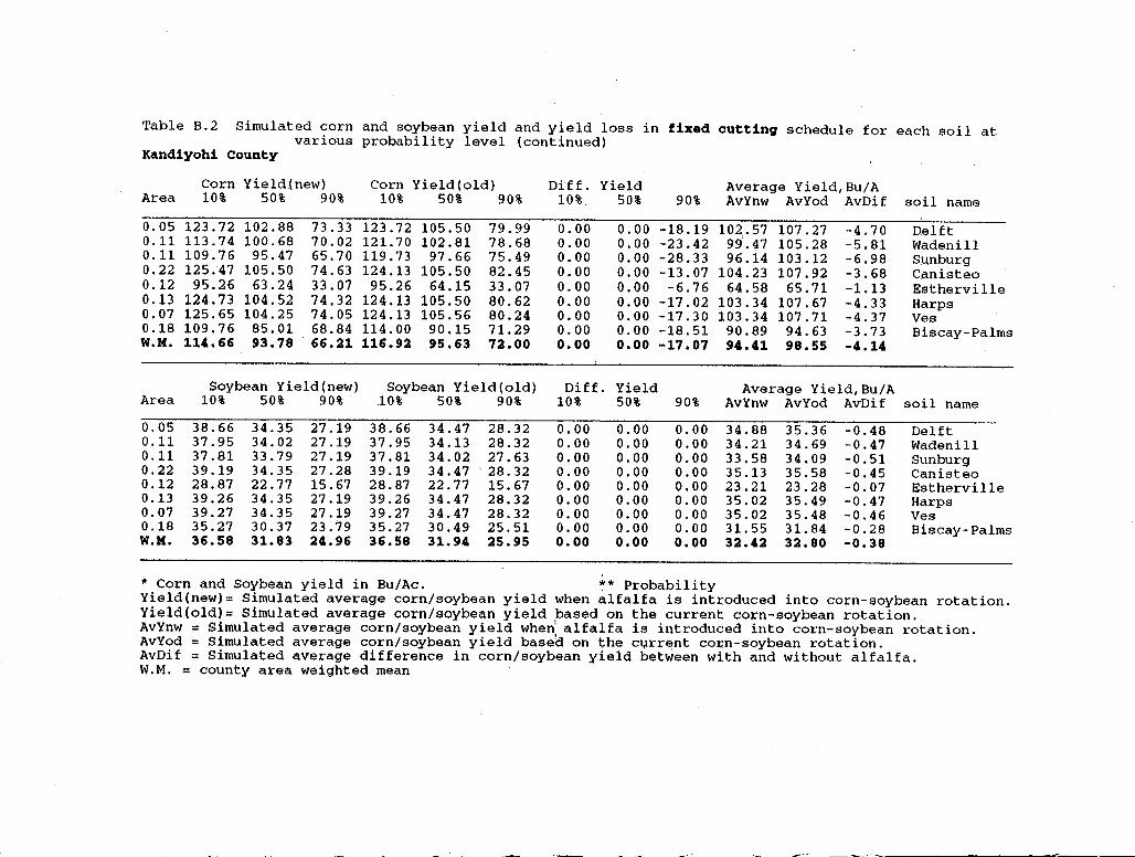
Table B.2 Simulated corn and soybean yield and yield loss in fixed cutting schedule for each soil at various probability level (continued)
Kandiyohi County
Area
0.05 0.11 0.11 0.22 0.12 0.13 0.07 0.18 W.M.
Corn Yield(new) 10% 50% 90%
123.72 102.88 113.74 100.68 109.76 95.47 125.47 105.50
95.26 63.24 124.73 104.52 125.65 104.25 109.76 85.01 114.66 93.78
73.33 70.02 65.70 74.63 33.07 74,32 74.05 68.84 66.21
Corn Yield(old) 10% 50% 90%
123. 72 121. 70 119. 73 124 .13
95.26 124 .13 124.13 114. 00 116.92
105.50 102.81
97. 66 105.50 64.15
105.50 105.56
90.15 95.63
79.99 78.68 75.49 82.45 33.07 80.62 80.24 71.29 72.00
Diff. Yield 10% 50%
0.00 0.00 0.00 0.00 0.00 0.00 0.00 0.00 o.oo
0.00 0.00 0.00 o.oo 0.00 0.00 0.00 0.00 o.oo
Soybean Yield(new) Soybean Yield(old) Diff. Yield
90%
-18.19 -23.42 -28.33 -13. 07 -6. 76
-17.02 -17.30 -18.51 -17 .07
Area 10% 50% 90% 10% 50% 90% 10% 50% 90%
0.05 0.11 0.11 0.22 0.12 0.13 0.07 0.18 W.M.
38.66 37.95 37.81 39.19 28.87 39.26 39.27 35.27 36.58
34.35 34.02 33.79 34.35 22.77 34.35 34.35 30.37 31.83
27.19 27.19 27.19 27.28 15.67 27.19 27.19 23.79 24.96
38.66 37.95 37.81 39.19 28. 87 39.26 39.27 35.27 36.58
34.47 34.13 34.02 34.47 22.77 34.47 34.47 30.49 31.94
28.32 28.32 27.63
'28.32 15.67 28.32 28.32 25.51 25.95
o.oo 0.00 0.00 0.00 0.00 0.00 0.00 0.00 o.oo
0.00 0.00 0.00 0.00 o.oo 0.00 0.00 0.00 o.oo
0.00 0.00 0.00 o.oo 0.00 0.00 0.00 0.00 O.QO
* Corn and Soybean yield in Bu/Ac. ** Probability
Average Yield,Bu/A AvYnw AvYod AvDif soil name
102.57 99.47 96.14
104.23 64.58
103.34 103.34 90.89 94.41
107.27 105.28 103.12 107.92
65.71 107. 67 107. 71 94.63 98.55
-4. 70 -5.81 -6.98 -3.68 -1.13 -4.33 -4.37 -3.73 -4.14
Average Yield,Bu/A
Delft Wadenill S.l\nburg Canisteo Estherville Harps Ves Biscay-Palms
AvYnw AvYod AvDif soil name
34.88 34.21 33.58 35.13 23.21 35.02 35.02 31. 55 32.42
35.36 34.69 34.09 35. 58 23.28 35.49 35.48 31.84 32.80
-0.48 -0.47 -0.51 -0.45 -0.07 -0.47 -0.46 -0.28 -0.38
Delft Wadenill Sunburg Canisteo Estherville Harps Ves Biscay-Palms
Yield(new)= Simulated average corn/soybean yield when alfalfa is introduced into corn-soybean rotation. Yield(old)= Simulated average corn/soybean yield based on the current corn-soybean rotation. AvYnw = Simulated average corn/soybean yield whe~ alfalfa is introduced into corn-soybean rotation. AvYod = Simulated average corn/soybean yield based on the c~rrent co~n-soybean rotation. AvDif = Simulated average difference in corn/soybean yield between with and without alfalfa. W.M. = county area weighted mean
------- -----=-·-~----~-~-~~--
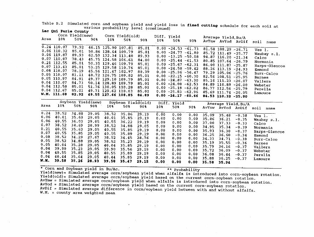
Table B.2 Simulated corn and soybean yield and yield loss in fixed cutting schedule for each soil at various probability level (continued) Lac Qui Parle County
Corn Yield(new) Corn Yield(old) Diff. yield Average Yield,Bu/A Area 10% 50% 90% 10% 50% 90% 10% 50% 90% AvYnw AvYod AvDif soil name 0.24 110. 07 79.92 46.15 125.90 107.81 85.01 0.00 -24.53 -61.73 81. 58 108.29 -26. 71 Ves 1. 0.06 110. 32 85.01 50.86 128.64 109.79 85.01 0.00 -24.77 -61. 80 85.72 111. 49 -25.77 Waubay s. l. 0.06 119. 87 89.93 62.59 132. 34 113.40 89.93 0.00 -13.25 -50.08 94.87 116. 20 -21. 34 Calco 0.07 110. 07 78.43 45. 75 124.58 106.61 84.00 0.00 -25.44 -61. 53 80.85 107.64 -26.79 Normania 0.21 112. 55 85.01 50.35 129.46 109.79 85.01 o.oo -25.67 -62. 31 86.00 111. 87 -25.87 Harps-Glencoe 0.07 113. 43 85.01 53.25 129.58 110.76 85.01 0.00 -24.58 -59.42 88.26 113 .19 -24.93 Esmond 0.08 110. 07 78.19 45.56 121. 47 102.97 80.39 0.00 -25 .-36 -56.47 79.29 105. 06 -25.76 Burr-Calco 0.05 110. 07 81.11 48.72 126.75 109.02 85.01 0.00 -22.15 -60.30 82.56 108.51 -25.95 Barnes 0.05 110. 97 84.91 49.37 129.10 109.79 85.01 0.00 -24.87 -63.30 85.16 111. 23 -:26.07 Vallers 0.04 110. 07 84.73 50.14 128.89 109.79 85.01 0.00 -24.00 -62.53 84.89 110. 89 -26.00 Webster 0.04 112. 58 85.01 51. 76 130.05 110. 28 85.01 o.oo -25.18 -62.02 86.77 112.56 -25.79 Perella 0.04 112. 67 85.01 49.71 129.62 110. 03 85.01 0.00 -25.83 -62.96 85.69 111. 74 -26.05 Lamoure W.M. 111. 68 82.92 49.55 127.66 108.85 84.89 o.oo -24.17 -60.66 84.53 110.32 -25.80
Soybean Yield(new) Soybean Yield(old) Diff. Yield Average Yield,Bu/A Area 10% 50% 90% 10% 50% 90% 10% 50% 90% AvYnw AvYod AvDif soil name 0.24 38.52 34.88 29.05 38.52 35.06 29.19 0.00 o.oo o.oo 35.09 35.48 -0.38 Ves 1. 0.06 40.01 35.60 29.05 40.01 35.85 . 29 .19 0.00 0.00 0.00 35.86 36.21 -0.35 Waubay s. l. 0.06 40.55 36.03 29.05 40.55 36.22 29.19 0.00 o.oo 0.00 37.00 37.33 -0.33 Calco 0.07 38.52 34.69 28.99 38.52 34.88 29.05 0.00 0.00 0.00 34.95 35.34 -0.39 Normania 0.21 40.55 35.63 29.05 40.55 35.85 29.19 0.00 0.00 o.oo 35.93 36. 30 -0.37 Harps-Glencoe 0.07 40.55 35.85 29.05 40.55 35.89 29.19 0.00 0.00 0.00 36.25 36.60 -0.34 Esmond 0.08 38.52 34.29 27.67 38.52 34.45 28.76 0.00 0.00 0.00 34.33 34.71 -0.38 Burr-Calco 0.05 38.52 34.88 29.05 38.52 35.23 29.19 0.00 o.oo 0.00 35.19 35.55 -0.36 Barnes 0.05 40.04 35.28 29.05 40.04 35.85 29.19 o.oo 0.00 0.00 35. 79 36.16 -0.37 Vallers 0.04 39.90 35.23 29.05 39.90 35.56 29.19 0.00 o.oo o.oo 35.72 36.09 -0.37 Webster 0.04 40.55 35.85 29.05 40.55 35.89 29.19 0.00 0.00 0.00 36.08 36. 44 -0.37 Perella 0.04 40.44 35.64 29.05 40.44 35.85 29.19 0.00 0.00 0.00 35.88 36.25 -0.37 Lamoure W.M. 39.58 35.26 28.93 39.58 35.47 29.15 o.oo o.oo o.oo 35.58 35.94
* Corn and Soybean yield in Bu/Ac. **· Probability Yield(new)= Simulated average corn/soybean yield when alfalfa is introduced into corn-soybean rotation. Yield(old)= Simulated average corn/soybean yield based on the current corn-soybean rotation. AvYnw = Simulated average corn/soybean yield when alfalfa is introduced into corn-soybean rotation. AvYod = Simulated average corn/soybean yield based on the current corn-soybean rotation. AvDif = Simulated average difference in corn/soybean yield between with and without alfalfa. W.M. = county area weighted mean
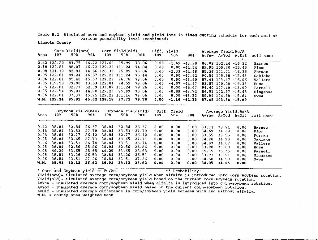
Table B.2 Simulated corn and soybean yield and yield loss in fixed cutting schedule for each soil at various probability level (continued)
Lincoln County
Corn Yield(new) Corn Yield(old) Diff. Yield Average Yield,Bu/A Area 10% 50% 90% 10% 50% 90% 10% 50% 90% AvYnw AvYod AvDif soil name
0.42 122.20 83. 75 44.72 127.60 95.99 73.06 0.00 .. -1. 69 -43.98 86.02 102.24 -16.22 Barnes 0.18 122.81 88.07 46. 72 129.23 101. 24 74.84 0.00 0.00 -44.54 89.95 105.40 -15.45 Flom 0.08 121.19 82.81 44.66 126.33 95.99 73.06 0.00 -2. 3'3 -44.48 85.36 101.71 -16.35 Forman 0.05 122.81 89.24 46.87 129.23 101. 24 75.44 0.00 o.oo -47.62 90.54 105.98 -15.43 Oaklake 0.06 122.81 85.40 45.57 129.23 96.78 73.06 0.00 0.00 -43.60 87.41 103.47 -16.'06 Vallers 0.05 119. 58 79.80 43.83 122.81 94.59 73.06 0.00 -4.07 -44.87 83.87 100.20 -16.33 Buse 0.05 122.81 92. 77 52.39 133. 89 101. 24 79.26 0.00 0.00 -45.07 94.40 107.40 -13.00 Parnell 0.05 122.54 85.07 44.98 129.23 95.99 73.06 0.00 -0.89 -43.72 86.51 102.97 -16.45 Singsaas 0.06 122.81 87.37 45.95 129.23 101.16 73. 06 0.00 0.00 -43.32 89.04 104.88 -15.84 Svea W.M·. 122.24 85.31 45.62 128.18 97.71 73.78 o.oo -1.16 -44.33 87.45 103.34 -15.89
Soybean Yield(new) Soybean Yield(old) Di ff. Yield Average Yield,Bu/A Area 10% 50% 90% 10% 50% 90% 10% 50% 90% AvYnw AvYod AvDif soil name
0.42 38.84 32.84 26. 37 38.84 32.84 26.37 0.00 0.00 0.00 33. 71 33. 71 0.00 Barnes 0.18 38.84 33.53 27.70 38.84 33. 53 . 27.70 0.00 o.oo 0.00 34.69 34.69 0.00 Flom 0.08 38.84 32.77 26.12 38.84 32. 77 26.12 0.00 0.00 0.00 33.55 33.55 0.00 Forman 0.05 38.84 33.65 27.73 38.84 33.65 27.73 0.00 0.00 0.00 34.90 34.90 0.00 Oak lake 0.06 38.84 33.51 26.74 38.84 33.51 26.74 0.00 0.00 0.00 34.07 34. 07 0 .'00 Vallers 0.05 38.84 32.56 25.86 38.84 32.56 25.86 0.00 0.00 0.00 33.08 33.08 0.00 Buse 0.05 40.29 33.65 28.6& 40.29 33.65 28.68 0.00 0.00 o.oo 35. 35 3 5. 3'.5 0.00 Parnell 0.05 38.84 33.26 26.53 38.84 33.26 26.53 0.00 0.00 0.00 33.91 33.91 0.00 Singsaas 0.06 38.84 33.51 27.26 38.84 33.51 27.26 0.00 o.oo 0.00 34.50 34.50 0.00 Svea W.M. 38.91 33.12 26.82 H.91 33.12 26.82 o.oo o.oo o.oo· •34.05 34.05 o.oo
* Corn and Soybean yield in Bu/Ac. ** Probability· Yield(new)= Simulated average corn/soybean yield when alfalfa is introduced into corn-~oybean rotation. Yield(old)= Simulated average corn/soybean yield·based on the current corn-soybean rotation. AvYnw = Simulated average corn/soybean yield when alfalfa is introduced into corn-soybean rotation. AvYod = Simulated average corn/soybean yield based on the current corn-soybean rotation. AvDif = Simulated average difference in corn/soybean yield between with and without alfalfa. W.M. = county area weighted mean
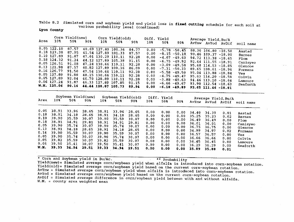
Table B.2 Simulated corn and soybean yield and yield los·s in fixed cutting schedule for each soil at various probability level (continued) Lyon county
Corn Yield(new) Corn Yield(old) Diff. Yield Average Yield,Bu/A Area 10% 50% 90% 10% 50% 90% 10% 50% 90% AvYnw AvYod AvDif soil name 0.05 122.10 87.57 40.69 127.89 100.36 84. 77 0.00 -5.78 -50.45 88. 30 106.80 -18.50 Aastad 0.18 123.38 87.95 41.54 127.89 101. 33 87.57 0.00 -8.15 -50.18 90.46 109.37 -18.90 Barnes 0.10 127.89 91.87 47.01 130.29 110.11 92.28 0.00 -4.07 -49.60 94.72 113. 38 -18.65 Flom 0.18 124.32 91. 24 44.12 127.89 105.38 91.15 o.oo -6. 75 -49.92 92.64 111. 55 -18.91 Canisyeo 0.05 126.51 91. 08 47.24 130. 66 110.11 92.28 0.00 -3.09 -49.58 95.68 114. 53 -18.85 Glencoe 0.13 121. 98 87.57 40.82 127.89 100.36 86.09 0.00 -7.31 -50.33 89.65 108.61 -18.96 Formans 0.16 126.77 91. 50 47.54 130. 66 110 .11 92.28 0.00 -5.58 -49.50 95.04 113. 88 -18.84 Ves 0.05 127.89 91. 88 48.15 130.66 110 .11 92.28 o.oo -4. 75 -49.47 95.63 114. 20 -18.58 Colvin 0.05 127.89 92.04 46. 70 128.89 110 .11 92.28 0.00 -3.88 -49.63 94.46 113 .10 -18.64 Lamoure 0.06 127.24 91. 87 46.33 127.89 107.85 91.15 0.00 -6.66 -49.67 93.90 112. 54 -18.63 Seaforth W.M. 125.06 90.16 44.44 128.87 105.73 89.94 o.oo -6.18 -49.89 92.65 111.46 -18.81
Soybean Yield(new) Soybean Yield(old) Di ff. Yield Average Yield,Bu/A Area 10% 50% 90% 10% 50% 90% 10% 50% 90% AvYnw AvYod AvDif soil name
0.05 38.91 33.96 28.65 38.91 33.96 . 28. 65 0.00 0.00 0.00 34.40 34.39 0.01 Aastad 0.18 38.91 34.18 28.65 38.91 34.18 28.65 0.00 0.00 o.oo 35.25 35.23 0.02 Barnes 0.10 39.90 35.59 30.07 39.90 35.59 30.07 0.00 0.00 0.00 36.49 36.49 0.00 Flom 0.18 38.91 34.91 29.81 38.91 34.91 29.81 0.00 0.00 o.oo 36. 01 36.01 0.00 Canisyeo 0.05 39.90 35.74 30.07 39.90 35.74 30.07 0.00 0.00 0.00 36. 75 36. 75 o.oo Glencoe 0.13 38.91 34.18 28.65 38.91 34.18 28.65 o.oo o.oo o.oo 34.99 34.97 0.02 Formans 0.16 39.90 35.59 30.07 39.90 35.59 30.07 0.00 o.oo 0.00 36.57 36.57 0.00 Ves 0.05 39.90 35.74 30.07 39.90 35.74 30.07 0.00 0.00 o.oo 36.66 36.66 0.00 Colvin 0.05 39.82 35.59 30.07 39.82 35.59 30.07 0.00 0.00 o.oo 36.45 36.45 0.00 Lamoure 0.06 39.50 35.41 30.07 39.50 35.41 30.07 0.00 o.oo 0.00 36.29 36.29 0.00 Seaforth W.M. 39.33 34.94 29.51 39.33 34.94 29.51 o.oo o.oo o.oo 35.89 35.88 0.01
* Corn and Soybean yield in Bu/Ac. ** Probability Yield(new)= Simulated average corn/soybean yield when ~lfalfa is introduced into corn-soybean rotation. Yield(old)= Simulated average corn/soybean yield based on the current corn-soybean rotation. AvYnw = Simulated average corn/soybean yield when alfalfa is introduced into corn-soybean rotation. AvYod = Simulated average corn/soybean yield based on the current corn-soybean rotation. AvDif = Simulated average difference in corn/soybean yield between with and without alfalfa. W.M. = county area weighted mean
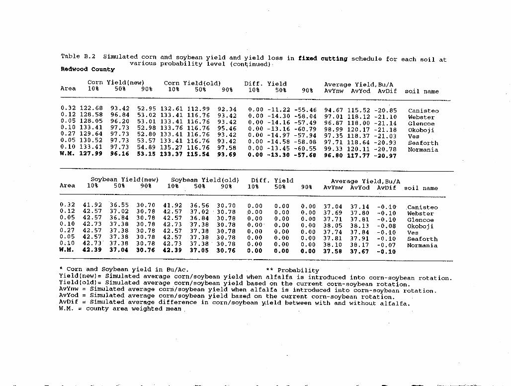
Table B.2 Simulated corn and soybean yield and yield loss in fixed cutting schedule for each soil at various probability level (cont;inued): Redwood County
Corn Yield(new) Corn Yield(old) Diff. Yield Average Yield,Bu/A Area 10% 50% 90% 10% 50% 90% 10% 50% 90% AvYnw AvYod AvDif so.il name
o. 32 122.68 93.42 52.95 132. 61 112. 99 92.34 0.00 -11. 22 -55.46 94.67 115. 52 -20.85 Canisteo 0.12 128.58 96.84 53.02 133. 41 116.76 93.42 0.00 -14.30 -58.04 97.01 118 .12 -21.10 Webster 0.05 128.05 96.20 53.01 133.41 116.76 93.42 0.00 -14.16 -57.49 96.87 118. 00 -21.14 Glencoe 0.10 133.41 97.73 52.98 133. 76 116. 76 95.46 0.00 -13.16 -60.19 98.99 120.17 -21.18 Okoboji 0.27 129.64 97.73 52.80 133.41 116. 76 93.42 0.00 -14.97 -57.94 97.35 118. 37 -21. 03 Ves 0.05 130. 52 97.73 53.57 133. 41 116. 76 93.42 0.00 -14.58 -58.08 97. 71 118. 64 -20.93 Seaforth 0.10 133. 41 97.73 54.89 135. 27 116. 76 97.58 0.00 -13. 45 -60.55 99.33 120 .11 ~20 .78 Normania W.M. 127.99 96.16 53.15 133.37 115.54 93.69 o.oo -13.30 -57.68 96.80 117.77 -20.97
Soybean Yield(new) Soybean Yield(old) Diff. Yield Average Yield,Bu/A Area 10% 50% 90% 10% 50% 90% 10% 50% 90% AvYnw AvYod AvDif soil name
0.32 41. 92 36.55 30.70 41. 92 36.56 30.70 0.00 o.oo o.oo 37.04 37.14 -0. '10· Canisteo 0.12 42.57 37.02 30.78 42.57 37.02 '30. 78 0.00 o.oo 0.00 37.69 37.80 -0.10 Webster 0.05 42.57 36.84 30.78 42.57 36.84 30.78 0.00 o.oo 0.00 37. 71 37.81 -0.10 Glencoe 0.10 42.73 37.38 30.78 42.73 37.38 30.78 0.00 0.00 0.00 38.05 38.13 -0.08 Okoboji 0.27 42.57 37.38 30.78 42.57 37.38 30.78 0.00 0.00 0.00 37.74 37.84 -0.10 Ves 0.05 42.57 37.38 30.78 42.57 37.38 30.78 0.00 0.00 o.oo 37.81 37.91 -0.10 Seaforth 0.10 42.73 37.38 30.78 42.73 37.38 30. 78 0.00 0.00 0.00 38.10 38.17 -0.07 Normania W.M. 42.39 37.04 30.76 42.39 37.05 30.76 o.oo o.oo o.oo 37.58 37.67 -0.10
* Corn and Soybean yield in Bu/Ac. ** Probability Yield(new)= Simulated average corn/soybean yield when alfalfa is introduced into corn-soybean rotation. Yield(old)= Simulated average corn/soybean yield based on the current corn-soybean rotation. AvYnw = Simulated average corn/soybean yield when alfalfa is introduced into corn-soybean rotation. AvYod = Simulated average corn/soybean yield based on the current corn-soybean rotation. AvDif = Simulated average difference in corn/soybean y,ield between with and without alfalfa. W.M. = county area weighted mean. ·
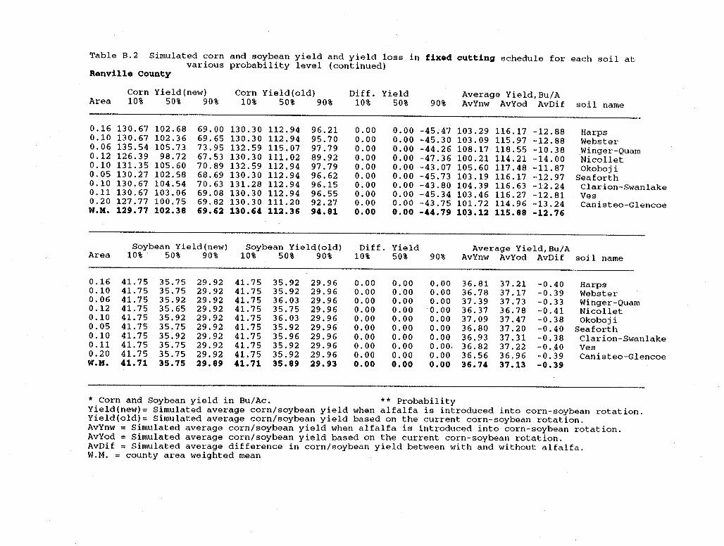
Table B.2 Simulated corn and soybean yield and yield loss in fixed cutting schedule for each soil at various probability level (continued)
Renville County
Corn Yield(new) Corn Yield(old) Diff. Yield Average Yield,Bu/A Area 10% 50% 90% 10% 50% 90% 10% 50% 90% AvYnw AvYod AvDif soil name
0.16 130. 67 102.68 69. 00 130.30 112. 94 96. 21 0.00 0.00 -45.47 103.29 116 .17 -12.88 Harps 0.10 130.67 102.36 69.65 130.30 112. 94 95.70 0.00 0.00 -45.30 103.09 115. 97 -12.88 Webster 0.06 135. 54 105.73 73.95 132. 59 115. 07 97.79 0.00 0.00 -44.26 108.17 118. 55 -10.38 Winger-Quam 0.12 126.39 98.72 67.53 130.30 111. 02 89.92 0.00 0.00 -47.36 100.21 114. 21 -14.00 Nicollet 0.10 131. 35 105.60 70.89 132. 59 112. 94 97.79 0.00 0.00 -43.07 105.60 117. 48 -11. 87 Okoboji 0.05 130.27 102.58 68.69 130.30 112. 94 96.62 0.00 0.00 -45.73 103.19 116 .17 -12.97 Seaforth 0.10 130.67 104.54 70.63 131.28 112. 94 96.15 o.oo 0.00 -43.80 104.39 116. 63 -12.24 Clarion-Swan lake 0.11 130.67 103.06 69.08 130.30 112. 94 96.55 0.00 0.00 -45.34 103.46 116. 27 -12.81 Ves 0.20 127.77 100.75 69.82 130.30 111. 20 92.27 0.00 0.00 -43.75 101. 72 114. 96 -13.24 Canisteo-Glencoe W.M. 129.77 102.38 69.62 130.64 112.36 94.81 o.oo o.oo -44.79 103.12 115.88 -12.76
Soybean Yield(new) Soybean Yield(old) Diff. Yield Average Yield,Bu/A Area 10% 50% 90% 10% 50% 90% 10% 50% 90% AvYnw AvYod AvDif soil name
0.16 41. 75 35.75 29.92 41. 75 35.92 29.96 0.00 0.00 0.00 36.81 37.21 -0.40 Harps 0.10 41. 75 35. 75 29.92 41. 75 35.92 29.96 o.oo o.oo 0.00 36.78 37 .17 -0.39 Webster 0.06 41. 75 35.92 29.92 41. 75 36.03 29.96 0.00 o.oo 0.00 37.39 37.73 -0.33 Winger-Quam 0.12 41. 75 35.65 29. 92 41. 75 35.75 29.96 0.00 0.00 0.00 36.37 36.78 -0.41 Nicollet 0.10 41. 75 35.92 29.92 41. 75 36.03 29.96 0.00 0.00 0.00 37.09 37.47 -0.38 Okoboji 0.05 41. 75 35. 75 29.92 41. 75 35.92 29.96 0.00 0.00 0.00 36.80 37.20 -0.40 Seaforth 0.10 41. 75 35.92 29.92 41. 75 35.96 29.96 0.00 0.00 0.00 36.93 37 .31 -0.38 Clarion-Swanlake 0.11 41. 75 35. 75 29.92 41. 75 35.92 29.96 0.00 0.00 0. 00~ 36.82 37.22 -0 .. 40 Ves 0.20 41. 75 35. 75 29.92 41. 75 35.92 29.96 0.00 0.00 0.00 36.56 36.96 -0.39 Canisteo-Glencoe W.M. 41.71 35.75 29.89 41.71 35.89 29.93 o.oo o.oo o.oo 36.74 37.13 -0.39
* Corn and Soybean yield in Bu/Ac. ** Probability Yield(new)= Simulated average corn/soybean yield when alfalfa is introduced into corn-soybean rotation. Yield(old)= Simulated average corn/soybean yield based on the current corn-soybean rotation. AvYnw = Simulated average corn/soybean yield when alfalfa is introduced into corn-soybean rotation. AvYod = Simulated average corn/soybean yield based on the current corn-soybean rotation. AvDif = Simulated average difference in corn/soybean yield between with and without alfalfa. W.M. = county area weighted mean
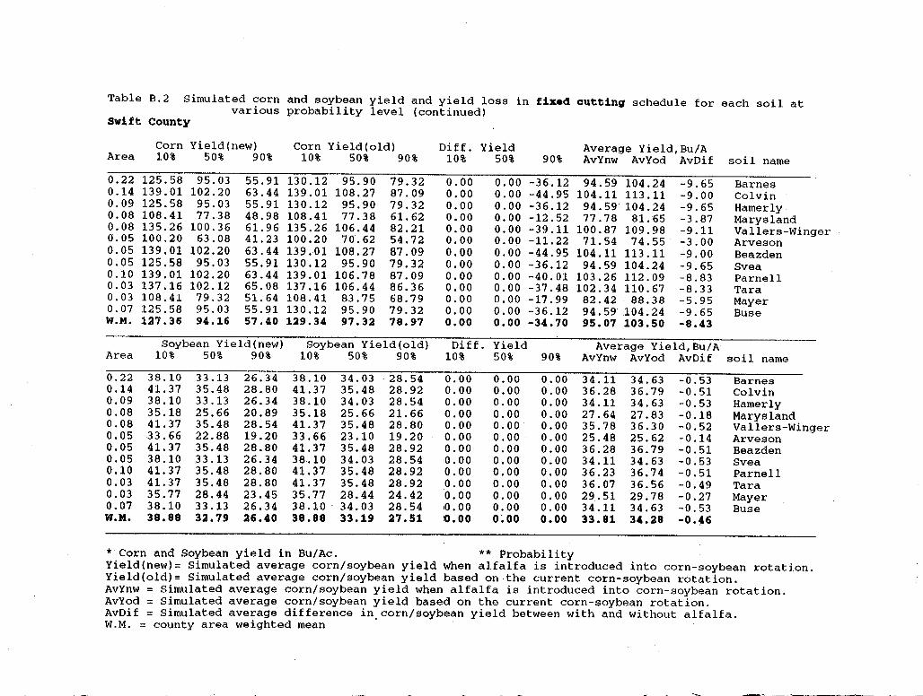
Table B.2 Simulated corn and soybean yield and yield loss in fixed cutting schedule for each soil at various probability level (continued)
Swift County
Corn Yield(new) Corn Yield(old) Diff. Yield Average Yield,Bu/A Area 10% 50% 90% 10% 50% 90% 10% 50% 90% AvYnw AvYod AvDif soil name
0.22 125.58 95.03 55.91 130.12 95.90 79.32 0.00 0.00 -36.12 94.59 104.24 -9.65 Barnes 0.14 139. 01 102.20 63.44 139.01 108.27 87.09 0.00 0.00 -44.95 104 .11 113 .11 -9.00 Colvin 0.09 125.58 95.03 55.91 130 .12 95.90 79.32 0.00 0.00 -36.12 94.59 104.24 -9.65 Hamerly 0.08 108.41 77 .38 48.98 108.41 77 .38 61.62 0.00 0.00 -12.52 77. 78 81. 65 -3.87 Marysland 0.08 135. 26 100.36 61. 96 135.26 106.44 82.21 0.00 0.00 -39 .11 100.87 109.98 -9.11 Vallers-Winger 0.05 100.20 63.08 41. 23 100.20 70.62 54.72 o.oo 0.00 -11.22 71. 54 74.55 -3.00 Arveson 0.05 139.01 102.20 63.44 139.01 108.27 87.09 0.00 0.00 -44.95 104 .11 113 .11 -9.00 Beazden 0.05 125.58 95.03 55.91 130.12 95.90 79.32 0.00 0.00 -36.12 94.59 104.24 -9.65 Svea 0.10 139.01 102.20 63.44 139.01 106.78 87.09 0.00 0.00 -40.01 103.26 112. 09 -8.83 Parnell 0.03 137.16 102.12 65.08 137 .16 106.44 86. 36 o.oo 0.00 -37.48 102.34 110. 67 -8.33 Tara 0.03 108.41 79.32 51. 64 108.41 83. 75 68. 79 0.00 0.00 -17.99 82.42 88.38 -5.95 Mayer 0.07 125.58 95.03 55.91 130.12 95.90 79.32 0.00 0.00 -36.12 94.59 104.24 -9.65 Buse W.M. 127.36 94.16 57.40 129.34 97.32 78.97 o.oo o.oo -34.70 95.07 103.50 -8.43
Soybean Yield(new) Soybean Yield(old) Diff. Yield Average Yield,Bu/A Area 10% 50% 90% 10% 50% 90% 10% 50% 90% AvYnw AvYod AvDif soil name
0.22 38.10 33.13 26.34 38.10 34.03 '28. 54 0.00 0.00 o.oo 34.11 34.63 -0.53 Barnes 0.14 41.37 35.48 28.80 41.37 35.48 28.92 0.00 0.00 0.00 36.28 36.79 -0.51 Colvin 0.09 38.10 33.13 26.34 38.10 34.03 28.54 0.00 0.00 0.00 34.11 34.63 -0.53 Hamerly 0.08 35.18 25.66 20.89 35.18 25.66 21. 66 0.00 0.00 0.00 27.64 27.83 -0.18 Marysland 0.08 41. 37 35.48 28.54 41.37 35.48 28.80 0.00 0.00 0.00 35. 78 36.30 -0.52 Vallers-Winger 0.05 33.66 22.88 19.20 33.66 23.10 19.20 0.00 0.00 0.00 25.48 25.62 -0.14 Arveson 0.05 41. 37 35.48 28.80 41. 37 35.48 28.92 0.00 0.00 0.00 36.28 36.79 -0.51 Beazden 0.05 38.10 33 .13 26. 34 38.10 34.03 28.54 :0. 00 0.00 0.00 34.11 34.63 -0.53 Svea 0.10 41. 37 35.48 28.80 41. 37 35.48 28.92 0.00 0.00 0.00 36.23 36.74 -0.51 Parnell 0.03 41.37 35.48 28.80 41. 37 35.48 28.92 0.00 0.00 0.00 36. 07 36.56 -0.49 Tara 0.03 35. 77 28.44 23.45 35.77 28.44 24.42 o.oo 0.00 0.00 29.51 29.78 -0.27 Mayer 0.07 38.10 33 .13 26.34 38 .10 ' 34.03 28.54 10. 00 0.00 0.00 34.11 34.63 -0.53 Buse W.M. 38.88 32.79 26.40 38.88 33.19 27.51 o.oo 0~00 o.oo 33.81 34.28 -0 •• 6
* Corn and Soybean yield in Bu/Ac. ** Probability Yield(new)= Simulated average corn/soybean yield when alfalfa is introduced into corn-soybean rotation. Yield(old)= Simulated average corn/soybean yield based on the current corn-soybean rotation. AvYnw = Simulated average corn/soybean yield when alfalfa is introduced into corn-soybean rotation. AvYod = Simulated average corn/soybean yield based on the current corn-soybean rotation. AvDif =Simulated average difference in.corn/soybean yield between with and without alfalfa. W.M. = county area weighted mean
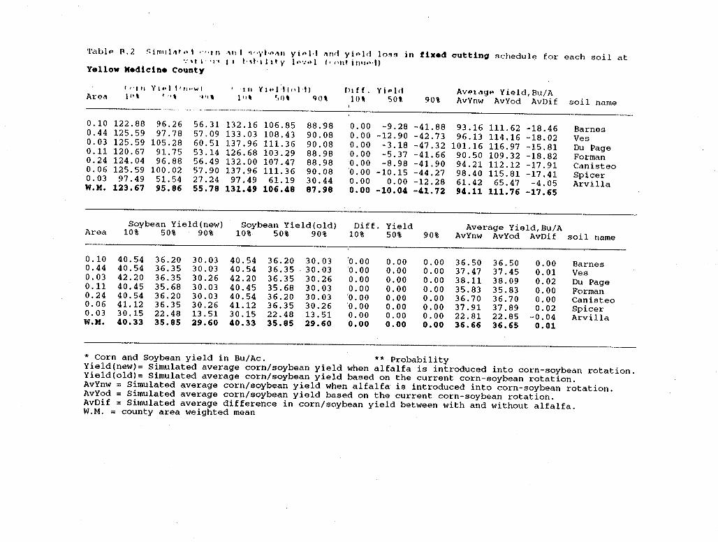
Table B.2 ~ i m• 1 1., t ,, I ,.f,, n ,, II I 'l'•j't•o.,11 y io l•I .,111i y io Id lo~rn in fixed cutting schedule for each soil at '.' 't I · .,., 11 I·' I· I l 1 t y 1 ·~ ·.·•• l I• nnt i 1111•"1) Yellow Medicine County
("•·111 Y 1 •• l I 1 ri .. w I I 'I II Y1••l·llnl•ll P1 ff. YiPld AveragP Yield,Bu/A Area 111' r, '' t •jf)' 1 fl' r, ()' Q(1' l!H 50\ 90% AvYnw AvYod AvDif soil name
·---····--- --·- -·--····--~--
0.10 122.88 96.26 56.31 132 .16 106.85 88.98 0.00 -9.28 -41. BB 93.16 111. 62 -18.46 Barnes 0.44 125.59 97.78 57.09 133. 03 108.43 90.08 0.00 -12.90 -42.73 96 .13 114 .16 -18.02 Ves 0.03 125.59 105.28 60.51 137. 96 111.36 90.08 0.00 -3.18 -47.32 101.16 116. 97 -15.81 Du Page 0.11 120.67 91. 75 53.14 126.68 103.29 88.98 ·o. oo -5.37 -41. 66 90.50 109.32 -18.82 Forman 0.24 124.04 96.88 56.49 132. 00 107.47 88.98 :o. 00 -8.98 -41. 90 94.21 112 .12 -17.91 Canisteo 0.06 125.59 100.02 57.90 137. 96 111.36 90.08 'O. 00 -10.15 -44.27 98.40 115. 81 -17.41 Spicer 0.03 97.49 51. 54 27.24 97.49 61.19 30.44 o.oo 0.00 -12.28 61.42 65.47 -4.05 Arvilla W.M. 123.67 95.86 55.78 131.49 106.48 87.98 o.oo -10.04 -41.72 94.11 111. 76 -17.65
Soybean Yield(new) Soybean Yield(old) Diff. Yield Average Yield,Bu/A Area 10% 50% 90% 10% 50% 90% 10% 50% 90% AvYnw AvYod AvDif soil name
0.10 40.54 36.20 30. 03 40.54 36.20 30.03 ~o. oo 0.00 0.00 36.50 36.50 o.oo Barnes 0.44 40.54 36.35 30.03 40.54 36.35 30.03 'o. oo 0.00 0.00 37.47 37.45 0.01 Ves 0.03 42.20 36.35 30.26 42.20 36.35 30.26 0.00 0.00 0.00 38.11 38.09 0.02 Du Page 0.11 40.45 35.68 30.03 40.45 35.68 30.03 0.00 0.00 0.00 35.83 35.83 0.00 Forman 0.24 40.54 36.20 30.03 40.54 36.20 30.03 ·o. oo 0.00 0.00 36.70 36.70 0.00 Canisteo 0.06 41.12 36. 35 30.26 41.12 36.35 30.26 'O. 00 0.00 0.00 37.91 37.89 0.02 Spicer 0.03 30.15 22.48 13.51 30.15 22.48 13.51 0.00 o.oo 0.00 22.81 22.85 -0.04 Arvilla W.M. 40.33 35.85 29.60 40.33 35.85 29.60 0.00 o.oo o.oo 36.66 36.65 0.01
* Corn and Soybean yield in Bu/Ac. ** Probability Yield(new)= Simulated average corn/soybean yield when alfalfa is introduced into corn-soybean rotation. Yield(old)= Simulated average corn/soybean yield based on the current corn-soybean rotation. AvYnw = Simulated average corn/soybean yield when alfalfa is introduced into corn-soybean rotation. AvYod = Simulated average corn/soybean yield based on the current corn-soybean rotation. AvDif = Simulated average difference in corn/soybean yield between with and without alfalfa. W.M. = county area weighted mean
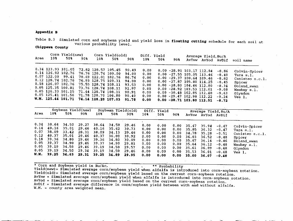
Appendix B
Table 8.3 Simulated corn and soybean yield and yield loss in floating cutting schedule for each soil at various probability level. Chippewa county
Corn Yield(new) Corn Yield(old) Diff. Yield Average Yield,Bu/A Area 10% 50% 90% 10% 50% 90% 10% 50% 90% AvYnw AvYod AvDif soil name
0.34 123.93 101. 05 72.82 128.57 105.45 90.49 0.00 o.oo -28.91 103.17 112. 04 -8.86 Colvin-Spicer 0.14 126.92 102.76 76.76 128.74 109.00 94.00 0.00 0.00 -27.55 105.05 113. 46 -8.40 Tara s.l. 0.07 122.00 99.41 70.69 122.01 102.76 86.74 o.oo 0.00 -29.37 100.64 109.46 -8.82 Canisteo s.c.1. 0.12 128.74 102.76 76.93 128.75 109.31 94.00 0.00 0.00 -27.87 105.80 114. 25 -8.45 Spicer 0.18 126.07 102.76 75.55 128.74 108.11 93.53 0.00 0.00 -28.80 104.46 112. 80 -8.34 Doland_swan 0.05 125.35 100.81 73. 76 128.74 108.11 91. 97 0.00 0.00 -28.92 103.53 112. 61 -9.08 Waubay s .1. 0.05 126.33 101.15 71.44 128.74 108 .11 90.91 0.00 0.00 -30.48 102.85 112. 48 -9.63 Glyndon 0.05 125.41 101. 56 71. 78 128.70 106.80 90.40 0.00 0.00 -29.47 102.98 112. 22 -9.24 Ves 1. W.M. 125.44 101. 71 74.14 128.20 107.03 91.78 o.oo o.oo -28.71 103.80 112.51 -8.72
Soybean Yield(new) Soybean Yield(old) Diff. Yield Average Yield,BU/A Area 10% 50% 90% 10% 50% 90% 10% 50% 90% AvYnw AvYod AvDif
0.34 38.64 34.50 29.27 38.64 34.50 29.46 0.00 0.00 0.00 35.47 35.94 -0.47 Colvin-Spicer 0.14 40.16 35.01 29.46 40.16 35.62 30.73 0.00 0.00 0.00 35.85 36.32 -0.47 Tara s.l. 0.07 38.09 33.42 28.31 38.09 34.13 29.46 0.00 0.00 0.00 34.78 35.28 -0.51 Canisteo s.c.l. 0.12 40.37 35.01 29.46 40.37 36.00 30.92 o.oo 0.00 0.00 36.03 36.52 -0.48 Spicer 0.18 39.36 34.80 29.46 39.36 34.80 30.09 0.00 0.00 0.00 35. 67 36.14 -0.46 Doland_swan 0.05 39.37 34.90 29.46 39.37 34.90 29.81 0.00 0.00 0.00 35.64 36.12 -0.48 Waubay s.l. 0.05 39.19 34.50 29.46 39.19 34.50 29.57 0.00 0.00 0.00 35.61 36.09 -0.48 Glyndon 0.05 39.19 34.50 29.34 39.19 34.50 29.46 0.00 0.00 0.00 35.53 36.01 -0.48 Ves 1. W.M. 39.25 34.63 29.31 39.25 34.89 29.95 o.oo o.oo o.oo 35.60 36.07 -0.48
* Corn and Soybean yield in Bu/Ac:. 1 ** Probability· Yield(new)= Simulated average corn/soybean yield when alfalfa is introduced into corn-soybean rotation. Yield(old)= Simulated average corn/soybean yield based on the current corn-soybean rotation. AvYnw = Simulated average corn/soybean yield when alfalfa is introduced into corn-soybean rotation. AvYod = Simulated average corn/soybean yield based on the current corn-soybean rotation. AvDif = Simulated average difference in corn/soybean yield between with and without alfalfa. W.M. = county area weighted mean.
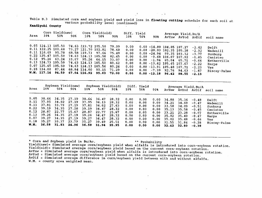
• I
Table B.3 Simulated corn and soybean yield and yield loss in floating cutting schedule for each soil at various probability level (continued) Kandiyohi County
Corn Yield(new) Corn Yield(old) Diff. Yield Average Yield,Bu/A Area 10% 50% 90% 10% 50% 90% 10% 50% 90% AvYnw AvYod AvDif soil name
0.05 124.13 105.50 74.63 123.72 105.50 79.99 0.00 0.00 -14.80 104.85 107.27 -2.42 Delft 0.11 122.25 100.68 73.27 121. 70 102.81 78.68 0.00 0.00 -20.03 102.35 105.28 -2.92 Wadenill 0.11 116. 69 95. 78 68.58 119. 73 97.66 75.49 0.00 0.00 -24.94 99.35 103.12 -3.7'J Sunburg 0.22 125.47 105.50 74.63 124.13 105.50 82.45 0.00 0.00 -9.68 106.07 107.92 -1. 85 Canisteo 0.12 95.26 63.24 33.07 95.26 64.15 33.07 0.00 0.00 -1. 94 65.04 65.71 -0.66 Estherville 0.13 124.73 105.50 74.63 124 .13 105.50 80.62 0.00 0.00 -13.62 105.45 107.67 -2.22 Harps 0.07 125.65 105.50 74.63 124 .13 105.56 80.24 0.00 0.00 -13.91 105.48 107. 71 -2.23 Ves 0.18 114. 00 87.44 68.84 114.00 90.15 71. 29 0.00 0.00 -7.39 92.76 94.63 -1. 87 Biscay-Palms W.M. 117.14 94.59 67.04 116.92 95.63 72.00 o.oo o.oo -12.18 96.42 98.55 -2.13
Soybean Yield(new) Soybean Yield(old) Diff. Yield Average Yield,Bu/A Area 10% 50% 90% 10% 50% 90% 10% 50% 90% AvYnw AvYod AvDif soil name
0.05 38.66 34. 35 27.19 38.66 34.47 ·28.32 0.00 o.oo 0.00 34.88 35.36 -0.48 Delft 0.11 37.95 34.02 27.19 37.95 34.13 28.32 0.00 0.00 0.00 34.21 34.69 -0.47 Wadenill 0.11 37.81 33.79 27.19 37.81 34.02 27.63 0.00 0.00 0.00 33.58 34.09 -0.51 Sunburg 0.22 39.19 34.35 27.28 39.19 34.47 28.32 0.00 0.00 0.00 35.13 35.58 -0.45 Canisteo 0.12 28.87 22.77 15.67 28.87 22.77 15.67 0.00 o.oo 0.00 23.21 23.28 -0.07 Estherville 0.13 39.26 34.35 27.19 39.26 34.47 28.32 0.00 o.oo 0.00 35.02 35.49 -0.47 Harps 0.07 39.27 34.35 27.19 39.27 34. 47 28.32 0.00 0.00 o.oo 35.02 35.48 -0.46 Ves 0.18 35.27 30.37 23.79 35.27 30.49 25.51 0.00 o.oo o.oo 31. 55 31. 84 -0.28 Biscay-Palms W.M. 36.58 31.83 24.96 36.58 31.94 25.95 o.oo o.oo o.oo 32.42 32.80 -0.38
* Corn and Soybean yield in Bu/Ac. ** Probability Yield(new)= Simulated average corn/soybean yield when alfalfa is introduced into corn-soybean rotation. Yield(old)= Simulated average corn/soybean yield based on the current corn-soybean rotation. AvYnw = Simulated average corn/soybean yield when alfalfa is introduced into corn-soybean rotation. AvYod = Simulated average corn/soybean yield based on the current corn-soybean rotation. AvDif = Simulated average difference in corn/soybean yield between with and without alfalfa. W.M. = county area weighted mean.
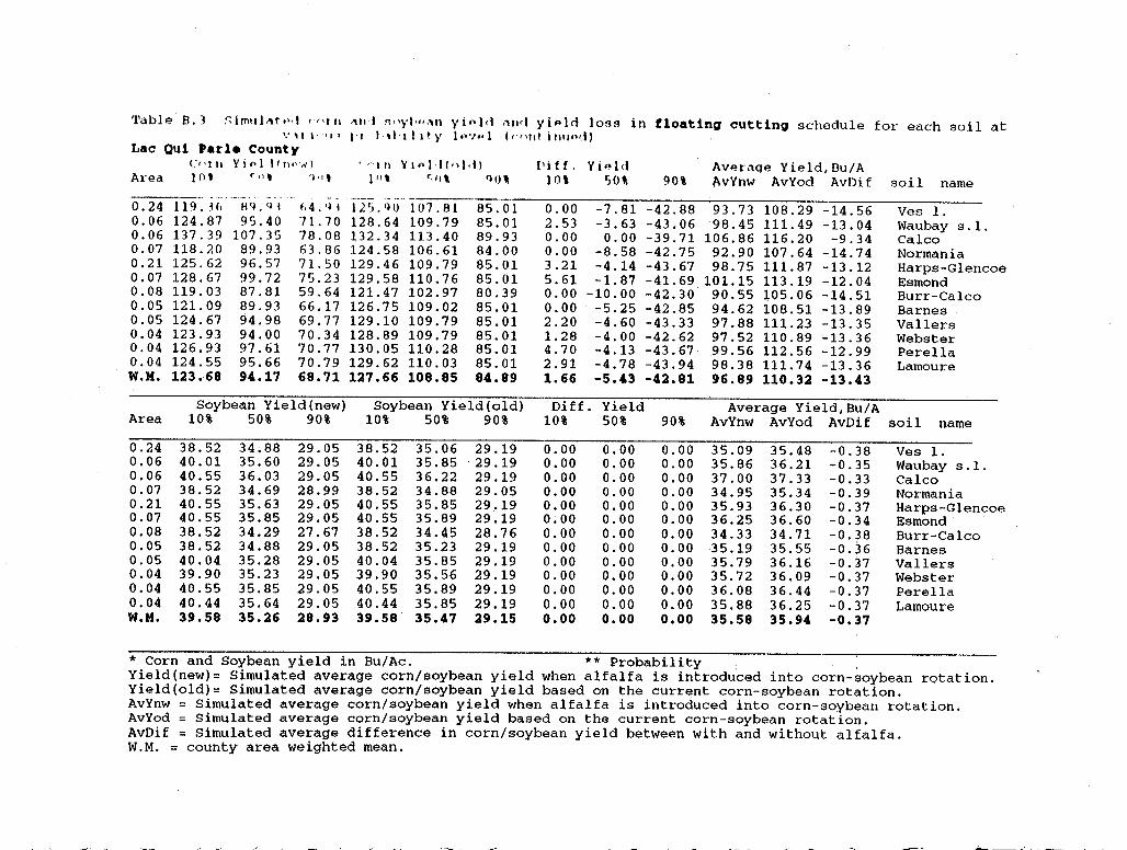
Table B.3 ;,imtll1't••·I 1·n111 Ml I ~nyl·••,,n yi<'ld ,,nrl y i P ld lo~rn in floating cutting schedule for each soil at \' , t l, ' 1 I 1 ,., 1,t·ll1t;• 1 ... , •.• 1 (1·n11t i111101.I)
Lac Qui Parle County C<' t 11 Y i " I 11 n ··""' I ''In Y1"l·lf<>l.tl ! 1 i ff. YiP.ld Aver~qe Yield,Bu/A
Area l 0 t r qt 'l <1' '"' r,q \ 'l()' 10\ 50\ 90\ AvYnw AvYod AvDif soil name ...
·~··-- ·- ·--· -0.24 119. Hi H4. QI 1,4. QI 12 '). (} () 107.Bl 85.01 0.00 -7.81 -42.88 93.73 108.29 -14.56 Ves 1. 0.06 124.87 95.40 71. 70 128.64 109.79 85.01 2.53 -3.63 -43.06 98.45 111. 49 -13.04 Waubay s. l. 0.06 137.39 107.35 78.08 132. 34 113. 40 89.93 0.00 0.00 -39.71 106.86 116. 20 -9.34 Calco 0.07 118. 20 89.93 63.86 124.58 106.61 84.00 0.00 -8.58 -42.75 92.90 107.64 -14.74 Normania 0.21 125.62 96.57 71. 50 129.46 109.79 85.01 3.21 -4.14 -43.67 98.75 111. 87 -13.12 Harps-Glencoe 0.07 128.67 99.72 75.23 129.58 110.76 85.01 5.61 -1. 87 -41. 69 101.15 113 .19 -12.04 Esmond 0.08 119. 03 87.81 59.64 121. 47 102.97 80.39 0.00 -10.00 -42.30 90.55 105.06 -14.51 Burr-Calco 0.05 121. 09 89.93 66.17 126.75 109.02 85.01 0.00 -5.25 -42.85 94.62 108.51 -13.89 Barnes 0.05 124.67 94.98 69.77 129.10 109.79 85.01 2.20 -4.60 -43.33 97.88 111. 23 -13.35 Vallers 0.04 123.93 94.00 70.34 128.89 109.79 85.01 1. 28 -4.00 -42.62 97.52 110. 89 -13.36 Webster 0.04 126.93 97.61 70.77 130.05 110. 28 85.01 4.70 -4.13 -43.67 99.56 112. 56 -12.99 Perella 0.04 124.55 95.66 70.79 129.62 110. 03 85.01 2.91 -4.78 -43.94 98.38 111. 74 -13.36 Lamoure W.M. 123.68 94.17 68.71 127.66 108.85 84.89 1.66 -5.43 -42.81 96.89 110.32 -13.43
Soybean Yield(new) Soybean Yield(old) Diff. Yield Average Yield,Bu/A Area 10% 50% 90% 10% 50% 90% 10% 50% 90% AvYnw AvYod AvDif soil name
0.24 38.52 34.88 29.05 38.52 35.06 29.19 0.00 0.00 0.00 35.09 35.48 -0.38 Ves 1. 0.06 40.01 35.60 29.05 40.01 35.85 ·29.19 0.00 0.00 0.00 35.86 36.21 -0.35 Waubay s.l. 0.06 40.55 36.03 29.05 40.55 36.22 29.19 0.00 0.00 0.00 37.00 37.33 -0.33 Calco 0.07 38.52 34.69 28.99 38.52 34.88 29.05 o.oo 0.00 0.00 34.95 35.34 -0.39 Normania 0.21 40.55 35.63 29.05 40.55 35.85 29.19 o.oo 0.00 0.00 35. 93 36.30 -0.37 Harps-Glencoe 0.07 40.55 35.85 29.05 40.55 35.89 29.19 o.oo 0.00 0.00 36.25 36.60 -0.34 Esmond 0.08 38.52 34.29 27.67 38.52 34.45 28.76 0.00 0.00 0.00 34.33 34. 71 -0.38 Burr-Calco 0.05 38.52 34.88 29.05 38.52 35.23 29.19 0.00 0.00 0.00 35.19 35.55 -0.36 Barnes 0.05 40.04 35.28 29.05 40.04 35.85 29.19 0.00 0.00 o.oo 35. 79 36.16 -0.37 Vallers 0.04 39.90 35.23 29.05 39.90 35.56 29.19 0.00 o.oo 0.00 35. 72 36.09 -0.37 Webster 0.04 40.55 35.85 29.05 40.55 35.89 29.19 0.00 0.00 0.00 36.08 36.44 -0.37 Perella 0.04 40.44 35.64 29.05 40.44 35.85 29.19 0.00 0.00 0.00 35.88 36.25 -0.37 Lamoure W.M. 39.58 35.26 28.93 39.58 35.47 29.15 o.oo o.oo o.oo 35.58 35.94 -0.37
* Corn and Soybean yield in Bu/Ac. ** Probability . . Yield(new)= Simulated average corn/soybean yield when alfalfa is introduced into corn-soybean rotation. Yield(old)= simulated average corn/soybean yield based on the current corn-soybean rotation. AvYnw = Simulated average corn/soybean yield when alfalfa is introduced into corn-soybean rotation. AvYod = Simulated average corn/soybean yield based on the current corn-soybean rotation. AvDif = Simulated average difference in corn/soybean yield between with and without alfalfa. W.M. = county area weighted mean.
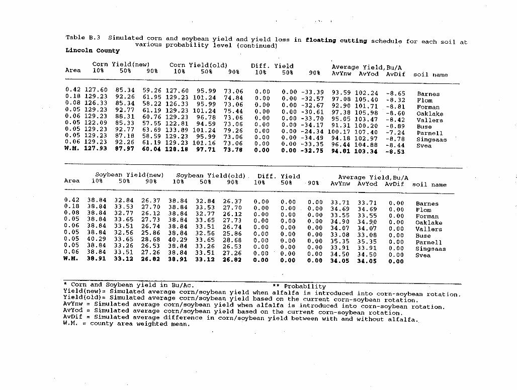
Table 8.3 Simulated corn and soybean yield and yield loss in floating cutting schedule for each soil at various probability level (continued) Lincoln County
Corn Yield(new) Corn Yield(old) Diff. Yield Average Yield,Bu/A Area 10% 50% 90% 10% 50% 90% 10% 50% 90% AvYnw AvYod AvDif soil name
0.42 127.60 85.34 59.26 127.60 95.99 73 .06 o.oo 0.00 -33.39 93.59 102.24 -8.65 Barnes 0.18 129.23 92.26 61. 95 129.23 101. 24 74.84 o.oo o.oo -32.57 97.08 105.40 -8.32 Flom 0.08 126. 33 85.34 58.22 126.33 95.99 73.06 0.00 0.00 -32. 67 92.90 101. 71 -8.81 Forman 0.05 129.23 92.77 61.19 129.23 101. 24 75.44 0.00 0.00 -30.61 97.38 105.98 -8.60 Oak lake 0.06 129.23 88.31 60.76 129.23 96.78 73.06 0.00 o.oo -33.70 95.05 103.47 -8.42 Vallers 0.05 122.09 85.33 57. 55 122.81 94.59 73.06 o.oo 0.00 -34.17 91. 31 100.20 -8.89 Buse 0.05 129.23 92.77 63.69 133.89 101. 24 79.26 0.00 0.00 -24.34 100.17 107.40 -7.24 Parnell 0.05 129.23 87.18 58.59 129.23 95.99 73.06 0.00 o.oo -34.49 94.18 102.97 -8.78 Singsaas 0.06 129.23 92.26 61.19 129.23 101.16 73.06 0.00 0.00 -33.35 96.44 104.88 -8.44 Svea W.M. 127.93 87.97 60.04 128.18 97.71 73.78 o.oo o.oo -32.75 94.81 103.34 -8.53
Soybean Yield(new) Soybean Yield(old) Diff. Yield Average Yield,Bu/A Area 10% 50% 90% 10% 50% 90% 10% 50% 90% AvYnw AvYod AvDif soil name
0.42 38.84 32.84 26.37 38.84 32.84 26.37 0.00 0.00 0.00 33.71 33. 71 0.00 Barnes 0.18 38.84 33.53 27.70 38.84 33.53 27.70 0.00 o.oo 0.00 34.69 34.69 0.00 Flom 0.08 38.84 32.77 26.12 38.84 32.77 26.12 0.00 o.oo 0.00 33.55 33.55 0.00 Forman 0.05 38.84 33.65 27.73 38.84 33.65 27.73 0.00 o.oo 0.00 34.90 34.9,0 0.00 Oak lake 0.06 38.84 33.51 26.74 38.84 33.51 26.74 0.00 o.oo 0.00 34.07 34.07 0.00 Vallers 0.05 38.84 32.56 25.86 38.84 32.56 25.86 0.00 0.00 o.oo 33.08 33.08 0.00 Buse 0.05 40.29 33.65 28.68 40.29 33.65 28.68 0.00 0.00 o.oo 35.35 35.35 0.00 Parnell 0.05 38.84 33.26 26.53 38.84 33.26 26.53 o.oo o.oo o.oo 33.91 33. 91 0.00 Singsaas 0.06 38.84 33.51 27.26 38.84 33.51 27.26 0.00 0.00 0.00 34.50 34. 50 0.00 Svea W.M. 38.91 33.12 26.82 38.91 33.12 26.82 o.oo o.oo o.oo 34.05 34.05 o.oo
* Corn and Soybean yield in Bu/Ac. ** Probability Yield(new)= Simulated average corn/soybean yield when alfalfa is introduced into corn-soybean rotation. Yield(old)= Simulated average corn/soybean yield based on the current corn-soybean rotation. AvYnw = Simulated average corn/soybean yield when alfalfa is introduced into corn-soybean rotation. AvYod = Simulated average corn/soybean yield based on the current corn-soybean rotation. AvDif = Simulated average difference in corn/soybean yield between with and without alfalfa. W.M. = county area weighted mean.
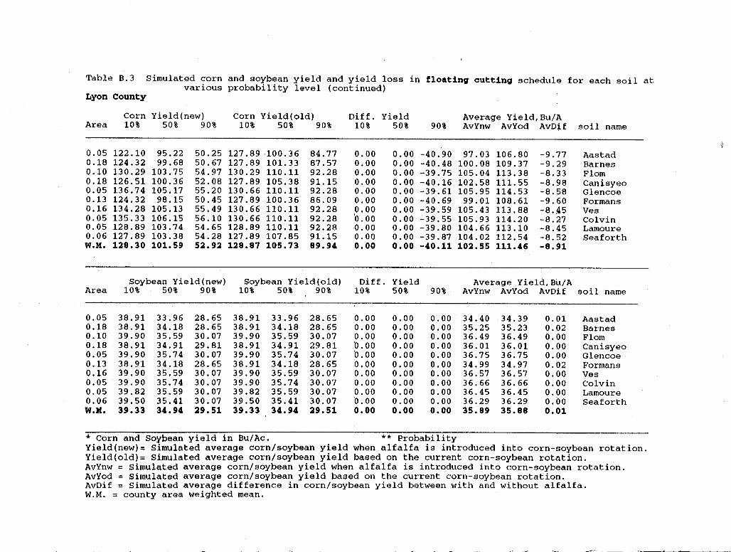
Table B.3 Simulated corn and soybean yield and yield loss in floating cutting schedule for each soil at various probability level (continued)
Lyon County
Corn Yield(new) Corn Yield(old) Diff. Yield Average Yield,Bu/A Area 10% 50% 90% 10% 50% 90% 10% 50% 90% AvYnw AvYod AvD:j.f soil name
0.05 122.10 95.22 50.25 127.89 100.36 84.77 0.00 0.00 -40.90 97.03 106.80 -9.77 Aastad 0.18 124.32 99.68 50. 67 127.89 101.33 87.57 0.00 0.00 -40.48 100.08 109.37 -9.29 Barnes 0.10 130.29 103.75 54.97 130.29 110 .11 92.28 0.00 0.00 -39.75 105.04 113. 38 -8.33 Flom 0.18 126.51 100.36 52.08 127.89 105.38 91.15 0.00 0.00 -40.16 102.58 111. 55 -8.98 Canisyeo 0.05 136.74 105.17 55.20 130.66 110 .11 92.28 0.00 0.00 -39.61 105.95 114. 53 -8.58 Glencoe 0.13 124.32 98.15 50.45 127.89 100.36 86.09 0.00 0.00 -40.69 99.01 108.61 -9.60 Formans 0.16 134.28 105.13 55.49 130.66 110 .11 92.28 0.00 o.oo -39.59 105.43 113. 88 -8.~5 Ves 0.05 135.33 106.15 56.10 130.66 110 .11 92.28 'o. oo o.oo -39.55 105.93 114.20 -8.27 Colvin 0.05 128.89 103.74 54.65 128.89 110 .11 92.28 0.00 0.00 -39.80 104.66 113 .10 -8.45 Lamoure 0.06 127.89 103.38 54.28 127.89 107.85 91.15 0.00 0.00 -39.87 104.02 112. 54 -8.52 Seaforth W.M. 128.30 101.59 52.92 128.87 105.73 89.94 o.oo o.oo -40.11 102.55 111.46 -8.91
Soybean Yield(new) Soybean Yield(old) Di ff. Yield Average Yield,Bu/A Area 10% 50% 90% 10% 50% 90% 10% 50% 90% AvYnw AvYod AvDif soil name
0.05 38.91 33.96 28.65 38.91 33.96 28.65 0.00 0.00 0. 00 .. 34.40 34.39 0.01 Aastad 0.18 38.91 34.18 28.65 38.91 34.18 28.65 0.00 0.00 0.00 35.25 35.23 0.02 Barnes 0.10 39.90 35.59 30.07 39.90 35.59 30.07 0.00 0.00 0.00 36.49 36.49 0.00 Flom 0.18 38.91 34.91 29.81 38.91 34.91 29.81 ·o. oo 0.00 0.00 36.01 36.01 0.00 Canisyeo 0.05 39.90 35.74 30.07 39.90 35.74 30.07 ·o. oo 0.00 0.00 36.75 36. 75 0.00 Glencoe 0.13 38.91 34.18 28.65 38.91 34.18 28.65 o.oo 0.00 0.00 34.99 34.97 0.02 Formans 0.16 39.90 35.59 30. 07 39.90 35.59 30.07 0.00 0.00 0.00 36.57 36.57 0.00 Ves 0.05 39.90 35.74 30.07 39.90 35. 74 30.07 o.oo 0.00 0.00 36.66 36.66 0.00 Colvin 0.05 39.82 35.59 30.07 39.82 35.59 30.07 0.00 0.00 0.00 36.45 36.45 0.00 Lamoure 0.06 39.50 35.41 30. 07 39.50 35.41 30.07 ·o. oo 0.00 0.00 36.29 36.29 0.00 Seaforth W.M. 39.33 34.94 29.51 39.33 34.94 29.51 o.oo o.oo 0.00 35.89 35.88 0.01
* Corn and Soybean yield in Bu/Ac. ** Probability Yield(new)= Simulated average corn/soybean yield when alfalfa is introduced into corn-soybean rotation. Yield(old)= Simulated average corn/soybean yield based on the current corn-soybean rotation. AvYnw = Simulated average corn/soybean yield when alfalfa is introduced into corn-soybean rotation. AvYod = Simulated average corn/soybean yield based on the current corn-soybean rotation. AvDif = Simulated average difference in corn/soybean yield between with and without alfalfa. W.M. = county area weighted mean.
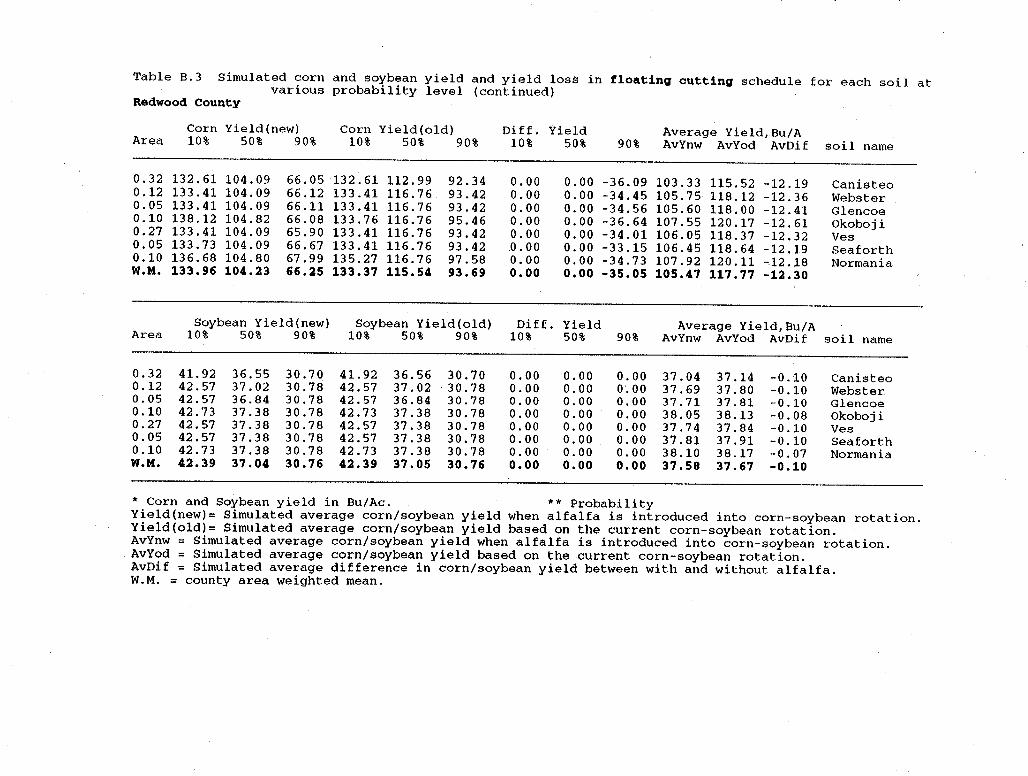
Table B.3 Simulated corn and soybean yield and yield loss in floating cutting schedule for each soil at various probability level (continued)
Redwood County
Corn Yield(new) Corn Yield(old) Diff. Yield Average Yield,Bu/A Area 10% 50% 90% 10% 50% 90% 10% 50% 90% AvYnw AvYod AvDif soil name
0.32 132. 61 104.09 66.05 132. 61 112. 99 92.34 0.00 0.00 -36.09 103.33 115. 52 -12.19 Canisteo 0.12 133. 41 104.09 66.12 133. 41 116. 76 93.42 0.00 0.00 -34.45 105.75 118 .12 -12.36 Webster 0.05 133.41 104.09 66.11 133. 41 116.76 93.42 0.00 0.00 -34.56 105.60 118. 00 -12.41 Glencoe 0.10 138 .12 104.82 66.08 133. 76 116.76 95.46 0.00 0.00 -36.64 107.55 120.17 -12.61 Okoboji 0.27 133.41 104.09 65.90 133. 41 116.76 93.42 0.00 0.00 -34.01 106.05 118. 37 -12.32 Ves 0.05 133.73 104.09 66.67 133. 41 116. 76 93.42 .0. 00 0.00 -33.15 106.45 118. 64 -12.19 Seaforth 0.10 136.68 104.80 67.99 135. 27 116.76 97.58 0.00 0.00 -34.73 107.92 120 .11 -12.18 Normania W.M. 133.96 104.23 66.25 133.37 115.54 93.69 o.oo o.oo -35.05 105.47 117.77 -12.30
Soybean Yield(new) Soybean Yield(old) Di ff. Yield Average Yield,Bu/A Area 10% 50% 90% 10% 50% 90% 10% 50% 90% AvYnw AvYod AvDif soil name
0.32 41.92 36.55 30. 70 41. 92 36.56 30.70 0.00 0.00 0.00 37.04 37.14 -0.10 Canisteo 0.12 42.57 37.02 30.78 42.57 37.02 30.78 o.oo 0.00 0.00 37.69 37.80 -0.10 Webster 0.05 42.57 36.84 30.78 42. 57 36.84 30.78 0.00 0.00 0.00 37. 71 37.81 -0.10 Glencoe 0.10 42.73 37.38 30. 78 42.73 37.38 30.78 0.00 0.00 0.00 38.05 38.13 -0.08 Okoboji 0.27 42.57 37.38 30.78 42.57 37.38 30.78 0.00 0.00 0.00 37.74 37.84 -0.10 Ves 0.05 42.57 37.38 30. 78 42.57 37.38 30.78 0.00 0.00 0.00 37.81 37.91 -0.10 Seaforth 0.10 42.73 37.38 30. 78 42.73 37.38 30.78 0.00 0.00 0.00 38.10 38.17 -0.07 Normania W.M. 42.39 37.04 30.76 42.39 37.05 30.76 o.oo o.oo o.oo 37.58 37.67 -0.10
* Corn and Soybean yield in Bu/Ac. ** Probability Yield(new)= Simulated average corn/soybean yield when alfalfa is introduced into corn-soybean rotation. Yield(old)= Simulated average corn/soybean yield based on the current corn-soybean rotation. AvYnw = Simulated average corn/soybean yield when alfalfa is introduced into corn-soybean rotation. AvYod = Simulated average corn/soybean yield based on the current corn-soybean rotation. AvDif = Simulated average difference in corn/soybean yield between with and without alfalfa. W.M. = county area weighted mean.
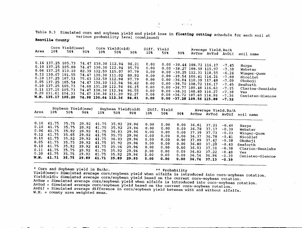
Table B. 3 Simulated corn and soybean yield and yield loss in floating cutting schedule for each soil at various probability level (cont,inued) Renville County
Corn Yield(new) Corn Yield(old) Diff. Yield Average Yield,Bu/A Area 10% 50% 90% 10% 50% 90% 10% 50% 90% AvYnw AvYod AvDif soil name
0.16 137. 25 105.73 74.47 130.30 112. 94 96.21 0.00 0.00 -38.44 108.72 116 .17 -7.45 Harps 0.10 137. 25 105.08 74.47 130.30 112. 94 95. 70 0.00 0.00 -38.27 108.59 115.97 -7.38 Webster 0.06 137. 25 110 .10 82.39 132.59 115. 07 97.79 o.oo 0.00 -30.25 112. 31 118. 55 -6.24 Winger-Quam 0.12 130.67 101. 55 74.47 130.30 111. 02 89.92 0.00 o.oo -39.54 106.41 114. 21 -7.80 Nicollet 0.10 137. 25 107.51 75.63 132.59 112.94 97.79 0.00 0.00 -36.04 110. 39 117. 48 -7.09 Okoboji 0.05 137.25 105.54 74.47 130.30 112. 94 96.62 0.00 0.00 -38.70 108. 72 116 .17 -7.45 Seaforth 0.10 137.25 105.73 74.68 131.28 112. 94 96.15 0.00 0.00 -36.77 109.48 116. 63 -7.15 Clarion-Swanlake 0.11 137.25 105.73 74.47 130.30 112. 94 96.55 o.oo o.oo -38.31 108.89 116.27 -7.38 Ves 0.20 131.61 104.33 74.47 130.30 111. 20 92.27 o.oo 0.00 -36.72 107.60 114. 96 -7.36 Canisteo-Glencoe W.M. 135.17 105.20 74.98 130.64 112.36 94.81 o.oo o.oo -37.28 108.56 115.88 -7.32
Soybean Yield(new) Soybean Yield(old) Diff, Yield Average Yield,Bu/A Area 10% 50% 90% 10% 50% 90% 10% 50% 90% AvYnw AvYod AvDif so~l name
0.16 41. 75 35.75 29.92 41. 75 35.92 '29.96 0.00 0.00 0.00 36.81 37.21 -0.40 Harps 0.10 41. 75 35.75 29. 92 41. 75 35.92 29.96 0.00 o.oo 0.00 36.78 37.17 -0.39 Webster 0.06 41.75 35. 92 29.92 41. 75 36.03 29.96 o.oo o.oo 0.00 37.39 37.73 -0.33 Winger-Quam 0.12 41. 75 35.65 29.92 41. 75 35.75 29.96 0.00 0.00 o.oo 36.37 36.78 -0.41 Nicollet 0.10 41. 75 35.92 29.92 41. 75 36.03 29.96 0.00 0.00 0.00 37. 09 37.47 -0.38 Okoboji 0.05 41. 75 35.75 29.92 41. 75 35, 92 29.96 0.00 0.00 0.00 36.80 37.20 -0.40 Seaforth 0.10 41. 75 35.92 29.92 41. 75 35. 96 29.96 0.00 o.oo o.oo 36.93 37.31 -0.38 Clarion-Swan lake 0.11 41. 75 35.75 29.92 41. 75 35.92 29.96 p.oo 0.00 0.00 36.82 37.22 -0.40 Ves 0.20 41. 75 35.75 29. 92 41. 75 35.92 29.96 P.00 o.oo 0.00 36.56 36.96 -0.39 Canisteo-Glencoe W.M. 41.71 35.75 29.89 41. 71 35.89 29.93 o.oo o.oo o.oo 36.74 37.13 -0.39
* Corn and Soybean yield in Bu/Ac. ** Probability Yield(new)= Simulated average corn/soybean yield when alfalfa is introduced into corn-soybean rotation. Yield(old)= Simulated average corn/soybean yield based on the current corn-soybean rotation. AvYnw = Simulated average corn/soybean yield when alfalfa is introduced into corn-soybean rotation. AvYod = Simulated average corn/soybean yield based on the current corn-soybean rotation. AvDif = Simulated average difference in corn/soybean yield between with and without alfalfa. W.M. = county area weighted mean.
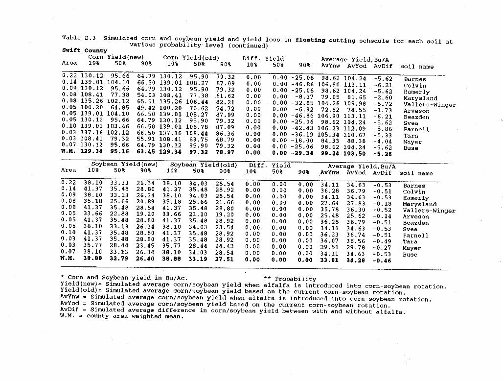
Table B.3 Simulated corn and soybean yield and yield loss in floating cutting schedule for each soil at various probability level (continued) Swift County
Corn Yield(new) Corn Yield(old) Diff. Yield Average Yield,Bu/A Area 10% 50% 90% 10% 50% 90% 10% 50% 90% AvYnw AvYod AvDif soil name 0.22 130 .12 95.66 64.79 130.12 95.90 79.32 0.00 0.00 -25.06 98.62 104.24 -5.62 Barnes 0.14 139. 01 104.10 66.50 139. 01 108.27 87.09 0.00 0.00 -46.86 106.90 113 .11 -6.21 Colvin 0.09 130 .12 95.66 64.79 130 .12 95.90 79.32 0.00 0.00 -25.06 98.62 104.24 -5.62 Hamerly 0.08 108.41 77 .38 54.03 108.41 77 .38 61. 62 0.00 0.00 -8.17 79.05 81. 65 -2.60 Marysland 0.08 135.26 102.12 65.51 135.26 106.44 82.21 0.00 0.00 -32.85 104.26 109.98 -5. 72 Vallers-Winger 0.05 100.20 64.85 49.42 100.20 70.62 54. 72 0.00 0.00 -6.92 72.82 74.55 -1. 73 Arveson 0.05 139. 01 104.10 66.50 139. 01 108.27 87.09 0.00 0.00 -46.86 106.90 113 .11 -6.21 Beazden 0.05 130.12 95.66 64.79 130.12 95.90 79.32 0.00 0.00 -25.06 98.62 104.24 -5.62 Svea 0.10 139. 01 103.46 66.50 139. 01 106.78 87.09 0.00 o.oo -42.43 106.23 112. 09 -5.86 Parnell 0.03 137 .16 102.12 66.50 137.16 106.44 86.36 o.oo 0.00 -36.19 105.34 110. 67 -5.33 Tara 0.03 108.41 79.32 55. 91 108.41 83.75 68.79 0.00 0.00 -18.00 84.33 88.38 -4.04 Mayer 0.07 130 .12 95.66 64.79 130.12 95.90 79.32 o.oo 0.00 -25.06 98.62 104.24 -5.62 Buse W.M. 129.34 95.16 63.45 129.34 97.32 78.97 o. 00 . o.oo -29.34 98.24 103.50 -5.26
Soybean Yield(new) Soybean Yield(old) Diff. Yield Average Yield,Bu/A Area 10% 50% 90% 10% 50% 90% 10% 50% 90% AvYnw AvYod AvDif soil name 0.22 38.10 33.13 26.34 38.10 34.03 28.54 0.00 0.00 0.00 34.11 34.63 -0.53 Barnes 0.14 41. 37 35.48 28.80 41. 37 35.48 . 28. 92 0.00 o.oo 0.00 36.28 36.79 -0.51 Colvin 0.09 38.10 33.13 26.34 38.10 34.03 28.54 0.00 0.00 0.00 34.11 34.63 -0.53 Hamerly 0.08 35.18 25.66 20.89 35.18 25.66 21. 66 0.00 0.00 0.00 27.64 27.83 -0.18 Marysland 0.08 41.37 35.48 28.54 41.37 35.48 28.80 0.00 0.00 0.00 35.78 36.30 -0.52 Vallers-Winger 0.05 33.66 22.88 19.20 33.66 23.10 19.20 0.00 0.00 0.00 25.48 25.62 -0.14 Arveson 0.05 41. 37 35.48 28.80 41. 37 35.48 28.92 0.00 0.00 0.00 36.28 36.79 -0.51 Beazden 0.05 38.10 33.13 26.34 38.10 34.03 28.54 0.00 o.oo 0.00 34.11 34.63 -0.53 Svea 0.10 41. 37 35.48 28.80 41. 37 35.48 28.92 0.00 0.00 0.00 36.23 36.74 -0.51 Parnell 0.03 41.37 35.48 28.80 41.37 35.48 28.92 0.00 0.00 0.00 36.07 36.56 -0.49 Tara 0.03 35. 77 28.44 23.45 35.77 28.44 24.42 0.00 0.00 0.00 29.51 29.78 -0.27 Mayer 0.07 38.10 33.13 26. 34 38.10 34.03 28.54 0.00 0.00 0.00 34.11 34.63 -0.53 Buse W.M. 38.88 32.79 26.40 38.88 33.19 27.51 o.oo o.oo o.oo 33.81 34.28 -0.46
* Corn and soybean yield in Bu/Ac. ** Probability Yield(new)= Simulated average corn/soybean yield when alfalfa is introduced into corn-soybean rotation. Yield(old)= simulated average corn/soybean yield based on the current corn-soybean rotation. AvYnw = simulated average corn/soybean yield when alfalfa is introduced into corn-soybean rotation. AvYod = simulated average corn/soybean yield based on the current corn-soybean rotation. AvDif = simulated average difference in corn/soybean yield between with and without alfalfa. W.M. = county area weighted mean.
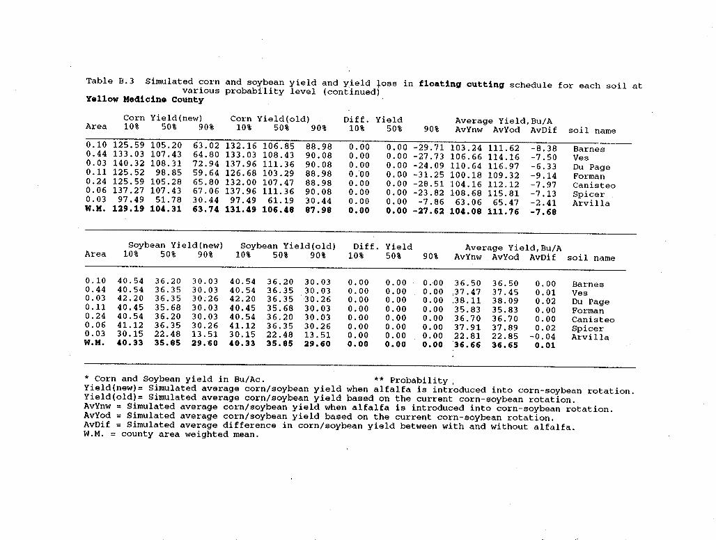
Table B.3 Simulated corn and soybean yield and y_ield ioss in floating cutting schedule for each soil at various probability level (continued) Yellow Medicine County
Corn Yield(new) Corn Yield(old) Diff. Yield Average Yield,Bu/A Area 10% 50% 90% 10% 50% 90% 10% 50% 90% AvYnw AvYod AvDif soil name
0.10 125.59 105.20 63.02 132.16 106.85 88.98 0.00 0.00 -29.71 103.24 111. 62 -8. 38 Barnes 0.44 133.03 107.43 64.80 133. 03 108.43 90.08 0.00 0.00 -27.73 106.66 114.16 -7.50 Ves 0.03 140.32 108.31 72.94 137. 96 111. 36 90.08 0.00 0.00 -24.09 110. 64 116. 97 -6.33 Du Page 0.11 125.52 98.85 59.64 126.68 103.29 88.98 0.00 0.00 -31. 25 100.18 109.32 -9.14 Forman 0.24 125.59 105.28 65.80 132. 00 107.47 88.98 0.00 0.00 -28.51 104.16 112 .12 -7.97 Canisteo 0.06 137. 27 107.43 67.06 137. 96 111. 36 90.08 0.00 0.00 -23.82 108.68 115.81 -7 .13 Spicer 0.03 97.49 51. 78 30.44 97.49 61.19 30.44 0.00 0.00 -7.86 63.06 65.47 -2.41 Arvilla W.M. 129.19 104.31 63.74 131.49 106.48 87.98 o.oo o.oo -27.62 104.08 111.76 -7.68
Soybean Yield(new) Soybean Yield(old) Diff. Yield Average Yield,Bu/A Area 10% 50% 90% 10% 50% 90% 10% 50% 90% AvYnw AvYod AvDif soil name
0.10 40.54 36.20 30.03 40.54 36.20 30.03 0.00 0.00 0.00 36.50 36.50 0.00 Barnes 0.44 40.54 36.35 30.03 40.54 36.35 30.03 0.00 0.00 0.00 )7 .47 37.45 0.01 Ves 0.03 42.20 36.35 30.26 42.20 36.35 30.26 0.00 0.00 0.00 .38.11 38.09 0.02 Du Page 0.11 40.45 35.68 30.03 40.45 35.68 30.03 0.00 0.00 0.00 35.83 35.83 0.00 Forman 0.24 40.54 36.20 30.03 40.54 36.20 30.03 o.oo 0.00 0.00 36.70 36.70 o.oo Canisteo 0.06 41.12 36.35 30.26 41.12 36.35 30.26 0.00 0.00 o.oo 37.91 37.89 0.02 Spicer 0.03 30.15 22.48 13. 51 30.15 22.48 13. 51 0.00 0.00 0.00 22.81 22.85 -0.04 Arvilla W.M. 40.33 35.85 29.60 40.33 35.85 29.60 o.oo o.oo o.oo 36.66 36.65 0.01
* Corn and Soybean yield in Bu/Ac. ** Probability , Yield(new)= Simulated average corn/soybean yield when alfalfa is introduced into corn-soybean rotation. Yield(old)= Simulated average corn/soybean yield based on the current corn-soybean rotation. AvYnw = Simulated average corn/soybean yield when alfalfa is introduced into corn-soybean rotation. AvYod = Simulated average corn/soybean yield based on the current corn-soybean rotation. AvDif = Simulated average difference in corn/soybean yield between with and without alfalfa. W.M. = county area weighted mean.
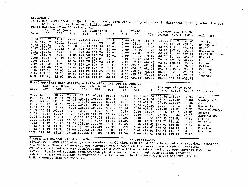
Appendix B Table B.4 Simulated Lac Qui Parle county's corn yield and yield loss in different cutting schedules for each soil at various probability level. Pixed Cutting (June 20 and Aug 31)
Corn Yield(new) Corn Yield(old) Diff. Yield Average Yield,Bu/A Area 10% 50% 90% 10% 50% 90% 10% 50% 90% AvYnw AvYod AvDif soil name 0.24 110. 07 79.91 45.97 125.90 107.81 85.01 0.00 -24.47 -61. 84 81.65 108.29 -26.63 Ves 1. 0.06 112 .17 85.01 50.68 128.64 109.79 85.01 0.00 -25.17 -61. 99 85.78 111.49 -25.71 Waubay s.l. 0.06 119. 70 90.25 60.18 132. 34 113. 40 89.93 0.00 -13.19 -52.48 94.75 116. 20 -21. 45 Calco 0.07 110. 07 78.42 45.81 124.58 106.61 84.00 o.oo -25.35 -61. 41 80.93 107.64 -26.71 Normania 0.21 112. 31 85.01 50.17 129.46 109.79 85.01 0.00 -25.24 -62.50 86.01 111. 87 -25.86 Harps-Glencoe 0.07 113. 38 85.01 53.05 129.58 110.76 85.01 0.00 -25.12 -59.62 88.24 113 .19 -24.95 Esmond 0.08 110. 07 78.08 45.37 121. 47 102.97 80.39 o.oo -25.29 -56.56 79.36 105.06 -25.69 Burr-Calco 0.05 110. 07 81.11 48.54 126. 75 109.02 85.01 0.00 -22.09 -60.48 82.64 108.51 -25.87 Barnes 0.05 112. 30 84.72 49.19 129.10 109.79 85.01 0.00 -25.24 -63.48 ,85.20 111. 23 -26.03 Vallers 0.04 110 .86 85.01 49.95 128.89 109.79 85.01 o.oo -24.40 -62.71 84.95 110. 89 -25.94 Webster 0.04 112. 34 85.01 51.15 130.05 110.28 85.01 0.00 -25.24 -62.63 86.75 112. 56 -25.81 Perella 0.04 113. 21 84. 72 49.52 129.62 110. 03 85.01 0.00 -25.50 -63.14 85.71 111. 74 -26.03 Lamoure W.M. 111.84 82.92 49.23 127.66 108.85 84.89 o.oo -24.13 -60.95 84.56 110.32 -25.76 Pixed cuttings with killing alfalfa after lat cut on June 20 Corn Yield(new) Corn Yield(old) Diff. ~ield Average Yield,Bu/A Area 10% 50% 90% 10% 50% 90% '10% 50% 90% ·AvYnw AvYod AvDif soil name 0.24 131.19 98.27 75.99 125.90 107.81 85.01 1'5 .14 0.00 -40.54 100.24 108.29 -8.04 Ves 1. 0.06 131. 64 99.72 78.08 128.64 109.79 85.01 11. 20 0.00 -43.06 103.67 111. 49 -7.82 Waubay s.l. 0.06 144.05 109.79 78.08 132.34 113. 40 89.93 o.oo 0.00 -39.71 109.84 116.20 -6.36 Calco 0.07 131.19 96.61 75.22 124.58 106.61 84.00 14.21 0.00 -40.24 99.61 107.64 -8.03 Normania 0.21 131. 64 99.72 78.08 129.46 109.79 85.01 10.14 0.00 -43.67 103.88 111. 87 -7.99 Harps-Glencoe 0.07 131. 64 102.40 78.08 129.58 110. 76 85.01 5.63 0.00 -41.69 105.66 113 .19 -7.53 Esmond 0.08 131.19 91. 57 75.38 121. 47 102.97 80.39 11. 37 0.00 -36.79 97.95 105.06 -7.10 Burr-Calco 0.05 131.19 98.34 78.08 126.75 109.02 85.01 16.85 0.00 -39.58 100.95 108.51 -7.56 Barnes 0.05 131.19 99.72 78.08 129.10 109.79 85.01 11. 85 0.00 -43.33 103.25 111. 23 -7.98 Vallers 0.04 131. 42 99.72 78.08 128.89 109.79 85.01 12.45 0.00 -42.62 103.02 110. 89 -7.87 Webster 0.04 131. 64 99.74 78.08 130. 05 110. 28 85.01 8.19 0.00 -43.67 104.46 112. 56 -8.10 Perella 0.04 131.19 99.72 78.08 129.62 110. 03 85.01 11.17 0.00 -43.94 103.61 111.74 -8.13 Lamoure W.M. 132.16 99.27 77.18 127.66 108.85 84.89 11.30 o.oo -41.49 102.ss 110.32 -7.78 * Corn and Soybean yield in Bu/Ac. ** Probability Yield(new)= Simulated average corn/soybean yield when alfalfa is introduced into corn-soybean rotation. Yield(old)= Simulated average corn/soybean yield based on the current corn-soybean rotation. AvYnw = Simulated average corn/soybean yield when alfalfa is introduced into corn-soybean rotation. AvYod = Simulated average corn/soybean yield based on the current corn-soybean rotation. AvDif = Simulated average difference in corn/soybean yield between with and without alfalfa. W.M. = county area weighted mean.
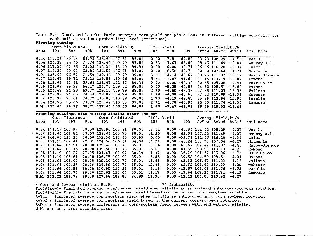
Table B.4 Simulated Lac Qui Parle county's corn yield and yield loss in different cutting schedules for each soil at various probability level (continued).
Floating Cutting Corn Yield(new) Corn Yield(old) Diff. Yield Average Yield,Bu/A
Area 10% 50% 90% 10% 50% 90% .10% 50% 90% AvYnw AvYod AvDif soil name
0.24 119.36 89.93 64.93 125.90 107.81 85.01 0.00 -7.81 -42.88 93.73 108.29 -14.56 Ves 1. 0.06 124.87 95.40 71. 70 128.64 109.79 85.01 ·2. 53 -3.63 -43.06 98.45 111. 49 -13.04 Waubay s.l. 0.06 137.39 107.35 78.08 132.34 113. 40 89.93 0.00 o.oo -39.71 1-06.86 116. 20 -9.34 Calco 0.07 118.20 89.93 63.86 124.58 106.61 84.00 0.00 -8.58 -42.75 92.90 107.64 -14.74 Normania 0.21 125.62 96.57 71. 50 129.46 109.79 85.01 3.21 -4.14 -43.67 98.75 111. 87 -13 .12 Harps-Glencoe 0.07 128.67 99.72 75.23 129.58 110. 76 85.01 5.61 -1. 87 -41. 69 101.15 113 .19 -12.04 Esmond 0.08 119. 03 87.81 59.64 121. 47 102.97 80.39 0.00 -10.00 -42.30 90.55 105.06 -14.51 Burr-Calco 0.05 121. 09 89.93 66.17 126.75 109.02 85.01 0.00 -5.25 -42.85 94.62 108.51 -13.89 Barnes 0.05 124.67 94.98 69. 77 129.10 109.79 85.01 2.20 -4.60 -43.33 97.88 111. 23 -13.35 Vallers 0.04 123.93 94.00 70.34 128.89 109.79 85.01 1.28 -4.00 -42.62 97.52 110. 89 -13.36 Webster 0.04 126.93 97.61 70. 77 130.05 110. 28 85.01 4.70 -4.13 -43.67 99.56 112. 56 -12.99 Perella 0.04 124.55 95.66 70.79 129.62 110. 03 85.01 2.91 -4.78 -43.94 98.38 111. 74 -13.36 Lamoure W.M. 123.68 94.17 68.71 127.66 108.85 84.89 1.66 -5.43 -42.81 96.89 110.32 -13.43
Floating cuttings with killing alfalfa after lat cut Corn Yield(new) Corn Yield(old) Oiff. Yield Average Yield,Bu/A
Area 10% 50% 90% 10% 50% 90% 10% 50% 90% AvYnw AvYod AvDif soil name
0.24 131.19 102.97 78.08 125.90 107.81 85.01 15.14 0.00 -40.54 104.02 108.29 -4.27 Ves 1. 0.06 131. 64 105. 54 78.08 128.64 109.79 85.01 11.20 0.00 -43.06 107.22 111. 49 -4.27 Waubay s.l. 0.06 144. 05 110. 28 78.08 132.34 113. 40 89.93 0.00 0.00 -39.71 111. 86 116. 20 -4.34 Calco 0.07 131.19 102. 44 77.81 124.58 106.61 84.00 14.21 0.00 -40.24 103.37 107.64 -4.27 Normania 0.21 131.64 105.91 78.08 129.46 109.79 85.01 10.14 0.00 -43.67 io7.47 111. 87 -4.40 Harps-Glencoe 0.07 131.64 106.75 78.08 129.58 110. 76 85.01 5.63 0.00 -41. 69 108.93 113 .19 -4.26 Esmond 0.08 131.19 102.27 77 .25 121. 47 102.97 80.39 11.37 0.00 -36.79 101. 32 105.06 -3.73 Burr-Calco 0.05 131.19 103.61 78.08 126. 75 109.02 85.01 16.85 0.00 -39.58 104.50 108.51 -4.01 Barnes 0.05 131. 64 105.04 78.08 129.10 109.79 85.01 11. 85 0.00 -43.33 106.87 111.23 -4.36 Vallers 0.04 131.64 104.17 78.08 128.89 109.79 85.01 12.45 0.00 -42.62 106.60 110. 89 -4.29 Webster 0.04 131.64 105.91• 78.08 130. 05 110. 28 85.01 8.19 0.00 -43.67 108.03 112. 56 -4.53 Perella 0.04 131.64 105.76 78.08 129.62 110. 03 85.01 11.17 0.00 -43.94 107.24 111. 74 -4.49 Lamoure W.M. 132.21 104.77 78.00 127.66 108.85 84.89 11.30 o.oo -41.49 106.05 110.32 -4.27
* Corn and Soybean yield in Bu/Ac. ** Probability Yield(new)= Simulated average corn/soybean yield when aifalfa is introduced into corn-soybean rotation. Yield(old)= Simulated average corn/soybean yield based on the current corn-soybean rotation. AvYnw = Simulated average corn/soybean yield when alfalfa is introduced into corn-soybean rotation. AvYod = Simulated average corn/soybean yield based on the current corn-soybean rotation. AvDif = Simulated average difference in corn/soybean yield between with and without alfalfa. W.M. = county area weighted mean.
----- -·--------------~----"--------------
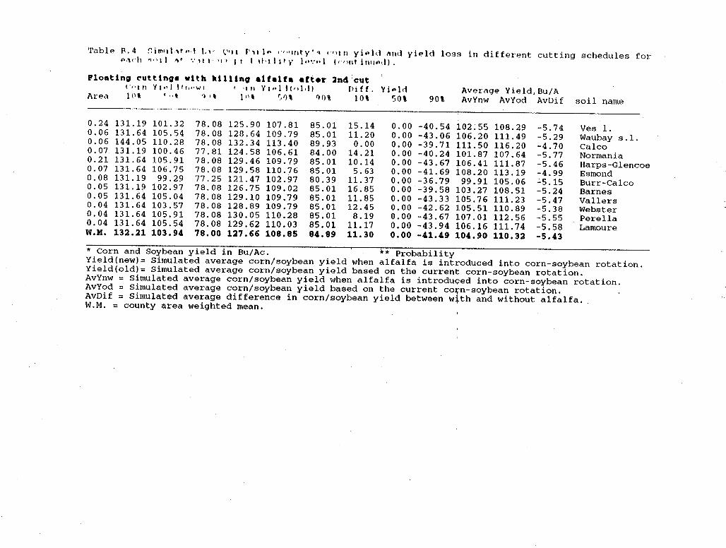
Table ~.4 ;.i1T11d.,t•>·I l.l· !,.''Ii l'H I" "" 1 111ty·~ <">Ill yi .. ld l'llld yield loss in different cutting schedules for <'·l<"h '1"11 ,... ·:111·'1'• 11 I ll•llit;• l"':"l (11>nti1111,.d).
Floating cutting• with killing alfalfa after 2nd:cut ("•I II YI•• I I I l1•·w I ' • t " Yt••l !(r,J.t) ()1ff. Vi,. ld AVP-t~ge Vield,Bu/A Are,1 l () t . ". ') I\ 1 •)' r,1)\ 1Hl\ 10\ 50\ 90\ AvYnw AvYod AvDif soil name --- .. --· - ··--···----- ·-·.
0.24 131.19 101.32 78.08 125.90 107. 81 85.01 15.14 0.00 -40.54 102.55 108.29 -5.74 Ves 1. 0.06 131.64 105.54 78.08 128.64 109.79 85.01 11. 20 0.00 -43.06 106.20 111. 49 -5.29 Waubay s .1. 0.06 144.05 110. 28 78.08 132.34 113. 40 89.93 0.00 o.oo -39.71 111. 50 116. 20 -4.70 Calco 0.07 131.19 100.46 77.81 124.58 106.61 84.00 14.21 0.00 -40.24 101. 87 107.64 -5. 77 Normania 0.21 131.64 105.91 78.08 129.46 109.79 85.01 10.14 0.00 -43.67 106.41 111. 87 -5.46 Harps-Glencoe 0.07 131. 64 106.75 78.08 129.58 110.76 85.01 5.63 0.00 -41. 69 io0.20 113 .19 -4.99 Esmond 0.08 131.19 99.29 77.25 121. 47 102.97 80.39 11. 37 0.00 -36.79 99.91 105.06 -5.15 Burr-Calco 0.05 131.19 102.97 78.08 126.75 109.02 85.01 16.85 0.00 -39.58 103.27 108.51 -5.24 Barnes 0.05 131. 64 105.04 78.08 129.10 109.79 85.01 11. 85 0.00 -43.33 105.76 111. 23 -5.47 Vallers 0.04 131. 64 103.57 78.08 128.89 109.79 85.01 12.45 0.00 -42.62 105.51 110. 89 -5.38 Webster 0.04 131. 64 105.91 78.08 130.05 110. 28 85.01 8.19 0.00 -43.67 107.01 112.56 -5.55 Perella 0.04 131. 64 105.54 78.08 129.62 110. 03 85.01 11.17 0.00 -43.94 106.16 111. 74 -5.58 Lamoure W.M. 132.21 103.94 78.00 127.66 108.85 84.89 11.30 o.oo -41.49 104.90 110.32 -5.43
* Corn and Soybean yield in Bu/Ac. ** Probability Yield(new)= Simulated average corn/soybean yield when alfalfa is introduced into corn-soybean rotation. Yield(old)= Simulated average corn/soybean yield based on the current corn-soybean rotation. AvYnw = simulated average corn/soybean yield when alfalfa is introduced into corn-soybean rotation. AvYod = Simulated average corn/soybean yield based on the current co~n-soybean rotation. AvDif = Simulated average difference in corn/soybean yield between with and without alfalfa. W.M. = county area weighted mean.
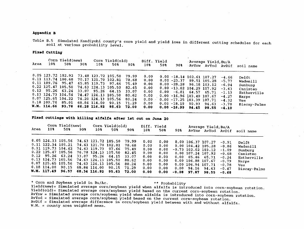
Appendix B
Table B.5 Simulated Kandiyohi county's corn yield and yield loss in different cutting schedules for each soil at various probability level.
Fixed cutting
Corn Yield(new) Corn Yield(old) Diff. Yield ·Average Yield,Bu/A Area 10% 50% 90% 10% 50% 90% 10% 50% 90% ,AvYnw AvYod AvDif soil name
0.05 123.72 102.92 73.48 123. 72 105.50 79.99 0.00 0.00 -18.14 102.61 107.27 -4.66 Delft 0.11 113. 74 100.68 70.17 121. 70 102.81 78.68 0.00 o.oo -23.37 99.51 105.28 -5.77 Wadenill 0.11 109.76 95.47 65.85 119. 73 97.66 75.49 0.00 0.00 -28.28 96.18 103.12 -6.94 Sunburg 0.22 125.47 105.50 74.63 124 .13 105.50 82.45 0.00 0.00 -13.02 104.29 107.92 -3.63 Canisteo 0.12 95.26 63.24 33.07 95.26 64.15 33.07 0.00 0.00 -6.81 64.57 65. 71 -1.13 Estherville 0.13 124.73 104.54 74.47 124 .13 105.50 80.62 0.00 0.00 -16.96 103.40 107.67 -4.27 Harps 0.07 125.65 104.22 74.20 124 .13 105.56 80.24 0.00 0.00 -17.25 103.39 107. 71 -4.32 Ves 0.18 109.76 85.01 68.84 114. 00 90.15 71.29 0.00 0.00 -18.19 90.93 94.63 -3.70 Biscay-Palms W.M. 114 .66 93.78 66.28 116.92 95.63 72.00 o.oo o.oo -16.99 94.45 98.55 -4.10
Pixed cuttings with killing alfalfa after 1st cut on June 20
Corn Yield(new) Corn Yield(old) Diff. Yield Average Yield,Bu/A Area 10% 50% 90% 10% 50% 90% 10% 50% 90% AvYnw AvYod AvDif soil name
0.05 124 .13 105.56 74.63 123. 72 105.50 79.99 0.00 o.oo 0.00 106.37 107.27 -0.91 Delft 0.11 122.34 105.21 74.63 121. 70 102.81 78.68 o.oo 0.00 0.00 104.42 105.28 -0.86 Wadenill 0.11 119. 73 104.42 74.63 119. 73 97.66 75.49 0.00 0.00 -0.73 102.02 103.12 -1. 09 Sunburg 0.22 125.47 105.56 76. 78 124.13 105.50 82.45 0.00 0.00 0.00 107.24 107.92 -0.68 Canisteo 0.12 95.26 63.24 33.07 95.26 64.15 33.07 0.00 0.00 0.00 65.46 65. 71 -0.24 Estherville 0.13 124.73 105.56 74.63 124.13 105.50 80.62 0.00 o.oo 0.00 106.88 107.67 -0.79 Harps 0.07 125.65 105.56 74.63 124.13 105.56 80.24 0.00 0.00 o.oo 106.94 107.71 -0.78 Ves 0.18 114. 00 90.15 68.84 114. 00 90.15 71.29 0.00 0.00 0.00 94.16 94.63 -0.47 Biscay-Palms W.M. 117.49 96.57 68.34 116.92 95.63 72.00 o.oo o.oo -0.08 97.87 98.55 -0.68
* Corn and Soybean yield in Bu/Ac. ** Probability Yield(new)= Simulated average corn/soybean yield when alfalfa is introduced into corn-soybean rotation. Yield(old)= Simulated average corn/soybean yield based on the current corn-soybean rotation. AvYnw = Simulated average corn/soybean yield when alfalfa is introduced into corn-soybean rotation. AvYod = Simulated average corn/soybean yield based on the current corn-soybean rotation. AvDif = Simulated average difference in corn/soybean yield between with and without alfalfa. W.M. = county area weighted mean.
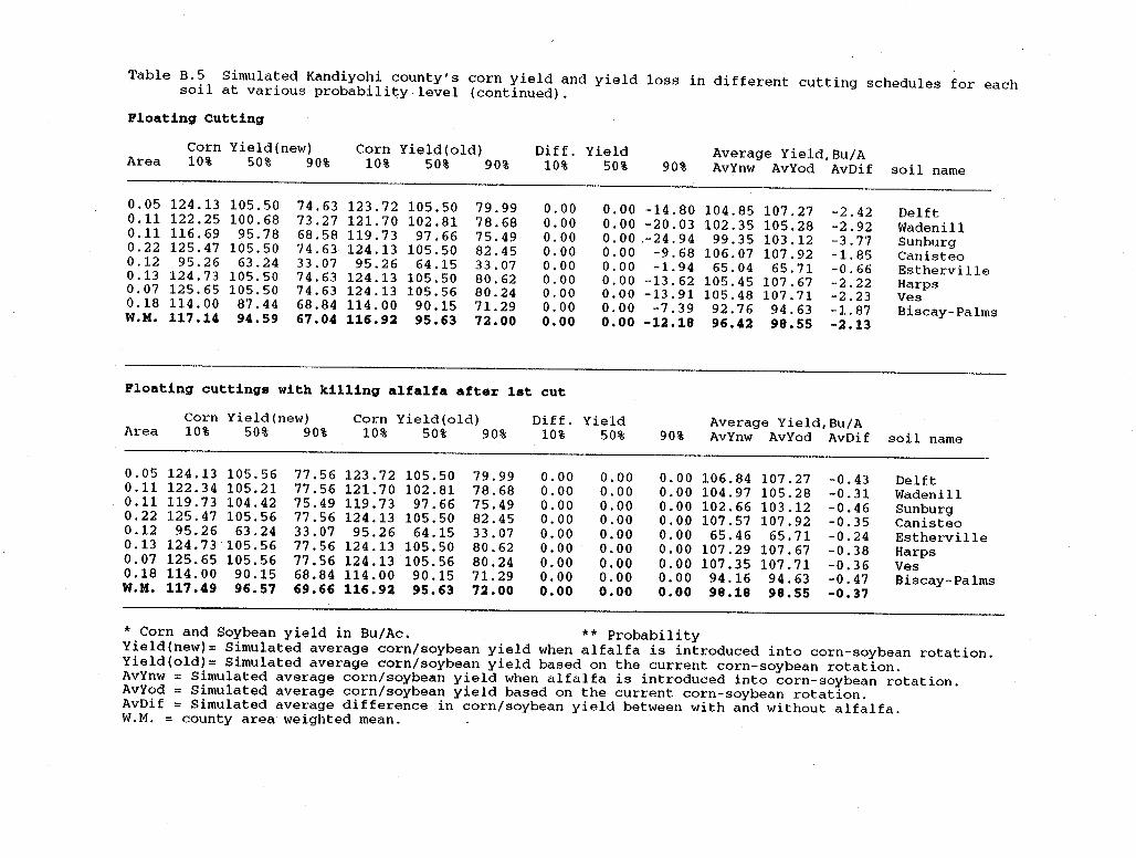
Table B.5 Simulated Kandiyohi county's corn yield and yield loss in different cutting schedules for each soil at various probability level (continued).
Floating Cutting
Corn Yield(new) Corn Yield(old) Diff. Yield Average Yield,Bu/A Area 10% 50% 90% 10% 50% 90% 10% 50% 90% AvYnw AvYod AvDif soil name
0.05 124.13 105.50 74.63 123.72 105.50 79.99 0.00 0.00 -14.80 104.85 107.27 -2.42 Delft 0.11 122.25 100.68 73.27 121. 70 102.81 78.68 0.00 o.oo -20.03 102.35 105.28 -2.92 Wadenill 0.11 116. 69 95.78 68.58 119. 73 97.66 75.49 0.00 0.00 .-24.94 99.35 103.12 -3.77 Sunburg 0.22 125.47 105.50 74.63 124.13 105.50 82.45 0.00 0.00 -9.68 106.07 107.92 -1. 85 Canisteo 0.12 95.26 63.24 33.07 95.26 64.15 33.07 0.00 0.00 -1. 94 65.04 65.71 -0.66 Estherville 0.13 124.73 105.50 74.63 124.13 105.50 80.62 0.00 0.00 -13.62 105.45 107.67 -2.22 Harps 0.07 125.65 105.50 74.63 124 .13 105.56 80.24 0.00 o.oo -13.91 105.48 107.71 -2.23 Ves 0.18 114. 00 87.44 68.84 114. 00 90.15 71.29 0.00 0.00 -7.39 92.76 94.63 -1.87 Biscay-Palms W.M. 117.14 94.59 67.04 116.92 95.63 72.00 o.oo o.oo -12.18 96.42 98.55 -2.13
Floating cuttings with killing alfalfa after 1st out
Corn Yield(new) Corn Yield(old) Diff. Yield Average Yield,Bu/A Area 10% 50% 90% 10% 50% 90% 10% 50% 90% AvYnw AvYod AvDif soil name
0.05 124 .13 105.56 77 .56 123.72 105.50 79.99 0.00 0.00 0.00 106.84 107.27 -0.43 Delft 0.11 122.34 105.21 77 .56 121. 70 102.81 78.68 0.00 0.00 0.00 104.97 105.28 -0.31 Wadenill 0.11 119.73 104.42 75.49 119. 73 97.66 75.49 0.00 o.oo 0.00 102.66 103.12 -0.46 Sunburg 0.22 125.47 105.56 77.56 124.13 105.50 82.45 0.00 0.00 0.00 107.57 107.92 -0.35 Canisteo 0.12 95.26 63.24 33.07 95.26 64.15 33.07 0.00 o.oo 0.00 65.46 65. 71 -0.24 Estherville 0.13 124.73 105.56 77. 56 124 .13 105.50 80.62 0.00 0.00 0.00 107.29 107.67 -0.38 Harps 0.07 125.65 105.56 77.56 124.13 105.56 80.24 0.00 0.00 0.00 107.35 107.71 -0.36 Ves 0.18 114.00 90.15 68.84 114. 00 90.15 71.29 0.00 0.00 0.00 94.16 94.63 -0.47 Biscay-Palms W.M. 117.49 96.57 69.66 116.92 95.63 72.00 o.oo o.oo o.oo 98.18 98.55 -0.37
* Corn and Soybean yield in Bu/Ac. ** Probability Yield(new)= Simulated average corn/soybean yield when alfalfa is introduced into corn-soybean rotation. Yield(old)= Simulated average corn/soybean yield based on the current corn-soybean rotation. AvYnw = Simulated average corn/soybean yield when alfalfa is introduced into corn-soybean rotation. AvYod = Simulated average corn/soybean yield based on the current corn-soybean rotation. AvDif = Simulated average difference in corn/soybean yield between with and without alfalfa. W.M. = county area weighted mean.
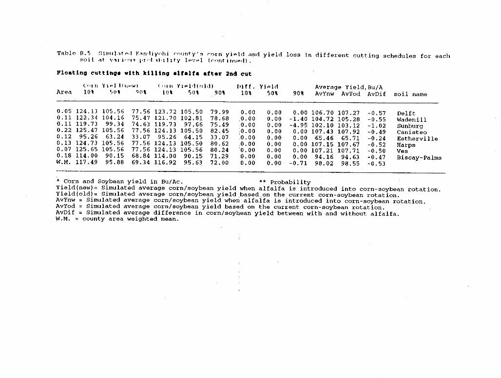
Table B.5 Sin>11htnd l'·itl'liynhi cn1inty''l nnn yiPld iltld yield loss in different cutting schedules for each 80i l .,t v.,r ir'"l'l J•l "l·1l,1l1ty l .. v .. l (cnnt in111>dl.
Ploatlno cuttlno• wlth kllllno alfalfa after 2nd cut
("'I II YI••) H11••W) f •'I fl Y11>)rl(ol1tl [lift. YiPld Average Yield,Bu/A Area 10\ r,1.1 \ '10\ 10\ ')()\ 90\ 10\ 50% 90% Av'lnw Av'lod AvDif soil name
0.05 124 .13 105.56 77.56 123.72 105.50 79.99 0.00 0.00 0.00 106.70 107.27 -0.57 Delft 0.11 122.34 104.16 75.47 121. 70 102.81 78.68 .o. 00 0.00 -1. 40 104.72 105.28 -0.55 Wadenill 0.11 119. 73 99.34 74.63 119. 73 97.66 75.49 0.00 0.00 -4.95 102.10 103.12 -1. 02 Sunburg 0.22 125.47 105.56 77. 56 124 .13 105.50 82.45 .o. 00 0.00 0.00 107.43 107.92 -0.49 Canisteo 0.12 95.26 63.24 33.07 95.26 64.15 33.07 .0. 00 0.00 0.00 65.46 65.71 -0.24 Estherville 0.13 124.73 105.56 77.56 124 .13 105.50 80.62 .0. 00 0.00 0.00 107.15 107.67 -0.52 Harps 0.07 125.65 105.56 77. 56 124.13 105.56 80.24 ·o. oo 0.00 o.oo 107.21 107.71 -0.50 Ves 0.18 114. 00 90.15 68.84 114. 00 90.15 71.29 0.00 0.00 0.00 94.16 94.63 -0.47 Biscay-Palms W.M. 117. 49 95.88 69.34 116.92 95.63 72.00 o.oo 0.00 -0.71 98.02 98.55 -0.53
* Corn and Soybean yield in Bu/Ac. ** Probability Yield(new)= Simulated average corn/soybean yield when alfalfa is introduced into corn-soybean rotation. Yield(old)= Simulated average corn/soybean yield .based .. on the current corn-soybean rotation. AvYnw = Simulated average corn/soybean yield when alfalfa is introduced into corn-soybean rotation. AvYod = Simulated average corn/soybean yield based on the current corn-soybean rotation. AvDif = Simulated average difference in corn/soyQean yield between with and without alfalfa. W.M. = county area weighted mean.
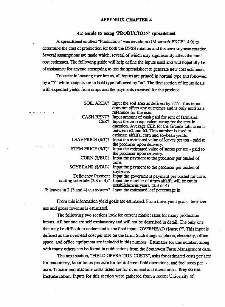
APPENDIX CHAPTER 4
4.2 Guide to using "PRODUCTION" spreadsheet
A spreadsheet entitled "Production" was developed (Microsoft EXCEL 4.0) to
determine the cost of production for lx>th the DFSS rotation and the com-soybean rotation .
. . Several assumptions are made which, several of which may significantly affect the total
cost estimates. The following guide will help define the inputs used and will hopefully be
of assistance for anyone attempting to use the spreadsheet to generate new cost estimates.
To assist in locating user inputs, all inputs are printed in normal type and followed
by a'"?" while outputs are in bold type followed by "=". The first section of inputs deals
with expected yields from crops and the payments received for the produce.
SOIL AREA?
CASHRENT? CER?
LEAF PRICE ($ff)?
S1EM PRICE ($ff)?
CORN ($/BU)?
SOYBEANS ($/BU)?
Deficiency Payment cutting schedule (2,3 or 4)?
% leaves in 2 (3 and 4) cut system?
Input the soil area as defined by ???? . This input does not affect any outcomes and is only used as a reference for the user. Input amount of cash paid for rent of farmland. Input the crop equivalent rating for the area in question. Average CER for the Granite falls area is between 62 and 65. This number is used to estimate alfalfa, corn and soybean yields. Input the estimated value of leaves per ton - paid to the producer upon delivery. Input the estimated value of stems per ton - paid to the producer upon delivery. Input the payment to the producer per bushel of com. Input the payment to the producer per bushel of soybeans Input th~ government payment per bushel for corn. Input the number of times alfalfa will be cut in establishment years. (2,3 or 4) Input the estimated leaf percentage in
From this information yield goals are estimated. From these yield goals, fertilizer
use and gross revenue is estimated.
The following two sections look for cmrent market rates for many production
inputs. All but one are self explanatory and will not be described in detail. The only one
that may be difficult to understand is the final input "OVERHEAD ($/acre)?". This input is
defined as the overhead cost per acre on the farm. Such things as phone, electricity, office
space, and office equipment are included in this number. Estimates for this number, along
with many others can be found in publications from the Southwest Farm Management data.
The next section, "FIEI.D OPERATION COSTS", asks for estimated costs per acre
for machinery, labor hours per acre for for different field operations, and fuel costs per .
acre. Tractor and machine costs listed are for overhead and direct costs, they do not
indude labor. Inputs for this section were gathered from a recent University of
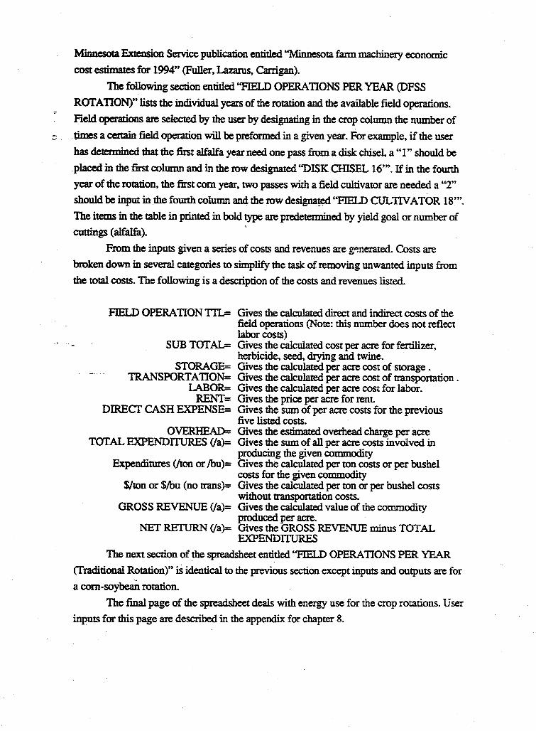
Minnesota Extension Service publication entitled ''Minnesota farm machinery economic cost estimates for 1994" (Fuller, Laz.arus, Carrigan).
The following section entitled ''FIELD OPERATIONS PER YEAR (DFSS ROTATION)" lists the individual years of the rotation and the available field operations. Field operations are selected by the user by designating in the crop column the number of . times a certain field operation will be preformed in a given year. For example, if the user has determined that the first alfalfa year need one pass from a disk chisel, a "l" should be .placed in the first column and in the row designated "DISK CEilSEL 16"'. If in the founh year of the rotation, the first com year, two passes with a field cultivator are needed a "2" should be input in the fourth column and the row designa~ ''FIELD CULTIVATOR 18"'. The items in the table in printed in bold type are predetermined by yield goal or number of cuttings (alfalfa).
From the inputs given a series of costs and revenues are g~nerated. Costs are broken down in several categories to simplify the task of removing unwanted inputs from the total costs. The following is a description of the costs and revenues listed.
FIELD OPERATION TI'L= Gives the calculated direct and indirect costs of the field operations (Note: this number does not reflect labor costs)
SUB TOTAL= Gives the calculated cost per acre for fertilizer, herbicide, seed, drying and twine.
STORAGE= Gives the calculated per acre cost of storage . TRANSPORTATION= Gives the calculated per acre cost of transportation.
LABOR= Gives the calculated per acre cost for labor. RENT= Gives the price per acre for rent.
DIRECT CASH EXPENSE= Gives the sum of per acre costs for the previous five listed costs.
OVERHEAD= Gives the estimated overhead charge per acre TOTAL EXPENDITURES (/a)= Gives the sum of all per acre costs involved in
producing the given commodity Expenditures (/ton or /bu)= Gives the calculated per ton costs or per bushel
costs for the given commodity $/ton or $/bu (no trans)= Gives the calculated per ton or per bushel costs
without transportation costs. GROSS REVENUE (/a)= Gives the calculated value of the commodity
produced per acre. NET RETURN (/a)= Gives the GROSS REVENUE minus TOTAL
EXPENDITURES The next section of the spreadsheet entitled ''FIELD OPERA TIO NS PER YEAR
(Traditional Rotation)" is identical to the previous section except inputs and outputs are for ·--
a com-soybean rotation.
The final page of the spreadsheet deals with energy use for the crop rotations. User inputs for this page are described in the appendix for chapter 8.
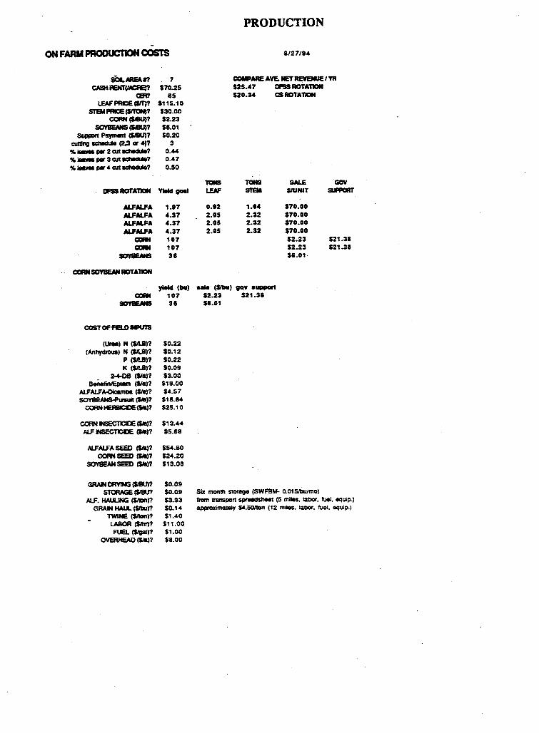
ON FARM PRODUCTION COSTS
sOLNEA.lf'I CASH fEN1'(MCAE)?
ClR1 LEAF PRICE ($11')?
STEM PRICE (SITDN)? CORN (MU)?
SOYBEANS (MU)? SUppon Payll*lt ($1BU)?
CUlllng ICll9dlM C2.3 « 4)? "4 ._ par 2 an ldledule? "4 i.- par 3 an ldledule? "4 .._ par 4 an ldledule?
7 $70.25
85 $115.10 $30.00 $2.23 $8.01 so.20
3 0.44 0.47 0.50
DFSS ROTAlJON Yield pl
ALFALFA 1.17 ALFALFA ,.37 ALFALFA ,.37 ALFALFA '-37
CCRN 107 CCRN 107
SOY1EMS 31
CCANSOYBEANAOTAlJON
0.12 2.05 2.05 2.05
PRODUCTION
8/27/94
COMPARE AVE. NET REVENUE I YR $25.,7 DFSSAOTATIDN $20.U CS ROTAllON
1aNS SALE Sl'EM SIUNIT
1.°' $70.00 2.32 $70.00 2.32 $70.00 2.32 $70.00
$2.23 $2.23 $6.01·
$21.38 $21.38
yield (bu) .... (SllMI) gov •upport CCRN 1 07 $2.23 $21 .38
SOYllEANS 31 $&.01
CCSTOF FE.D INPUIS
(Uraa) N ($1'l8)? (Anhydrous) N ($/LS)?
p ($/LS)? K ($/LS)?
2-+0B ($la)? ~($la)?
ALFALFA-Dlcllm• (Sia)? SOYBEANS-Pursuit ($Al)?
CORN HERBICIOE ($ltl)?
CORN NlECT1Cl:lE (SM)? ALF INSECTICIDE (SM)?
ALFALFA SEED ($1&)? C<HI SEED (Sia)?
SOYBEAN SEED 1$Aa)?
GRMI CRYING CMIUI? STORAGE (SIBU?
Mr. HAULING ($/llln)? GRAIN HAU. (Sl'bl)?
TWINE ($11Dnl? LABOR ($Inf)? FUEL (S/gal)?
OVERHEAD ($1&)?
$0.22 so.12 $0.22 S0.09 $3.00
$19.00 $4.57
$18.84 $25.10
$13.44 $5.68
$54.60 $24.20 $13.08
$0.09 $0.09 $3.93 $0.14 $1.40
$11.00 $1.00 $8.00
Six mon1ll storage (SW~M- 0.015Jbulmo)
from iranspon sprllllClshMt (5 miles. latlor. fuel. equip.) appraximatllly $4.50/t0n (12 miles. labor. fuel. equip.)
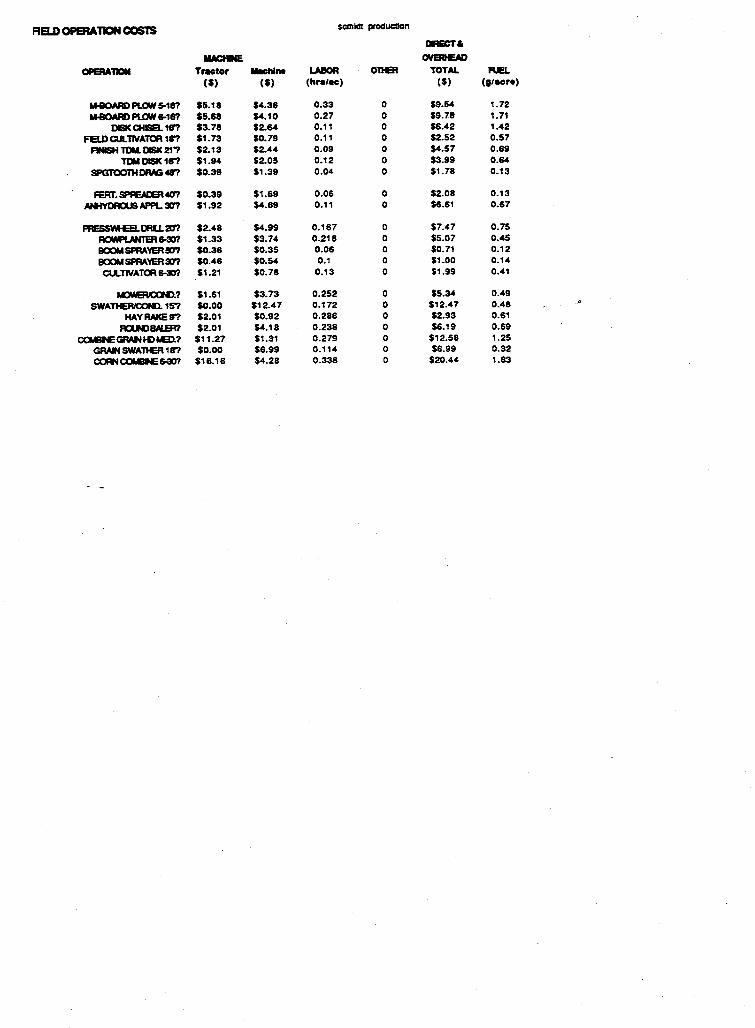
RB..D OPERATION COSTS scmldt produellon
DflECT&
IUCllNE OVERtEAD
OPEAATIQN Tractor u.clllne LABOR onEA TOTAL REL ($) ($) (hratac) ($) (gtacre)
M«>NID PLOW ~18? $5.18 $4.36 0.33 0 $9.54 1.72
M«>NID PLOW 8-18? $5.68 $4.10 0.27 0 $9.78 1.71 DISK a.ISEI.. 18'? $3.78 $2.64 0.11 0 $6.42 1.42
FELD CULTIVATOR 18'? $1.73 $0.79 0.11 0 $2.52 0.57
FINISH TOM. DISIC 21'? $2.13 $2.44 0.09 0 $4.57 0.69 TOM DISK 18'? $1.94 $2.05 0.12 0 $3.99 0.64
SPGTOOTHDMG 48'? $0.39 $1.39 0.04 0 $1.78 0.13
FERr. SPff1ACER«I? $0.39 $1.69 0.06 0 $2.08 0.13
ANHYDROUS APPL SI? $1.92 $4.69 0.11 0 $6.61 0.67
PRESSWH:B..0Rll 2Cf? $2.48 $4.99 0.167 0 $7.47 0.75
ROWPl.ANlER &30? $1.33 $3.74 0.218 0 $5.07 0.45
BOOM SPRAYER 50'? $0.36 $0.35 0.06 0 $0.71 0.12
BOOM SPRAYERS!? $0.46 $0.54 0.1 0 $1.00 0.14
CUlTIVATa:l 8-30? $1.21 $0.78 0.13 0 $1.99 0.41
MOWER.aH>.? $1.61 $3.73 0.252 0 $5.34 0.49 SWATHER/CON). 15'? so.co $12.47 0.172 0 $12.47 0.48
HAYRAKE9'? $2.01 $0.92 0.286 0 $2.93 0.61 FICLN)M,ER? $2.01 $4.18 0.238 0 $6.19 0.69
ca&EGRANK>ae>.? $11.27 $1.31 0.279 0 $12.58 1.25
GRAIN SWATl-ER 18'? $0.00 $6.99 0.114 0 $6.99 0.32
CORN COMBIE &30? $16.16 $4.28 0.338 0 $20.44 1.83
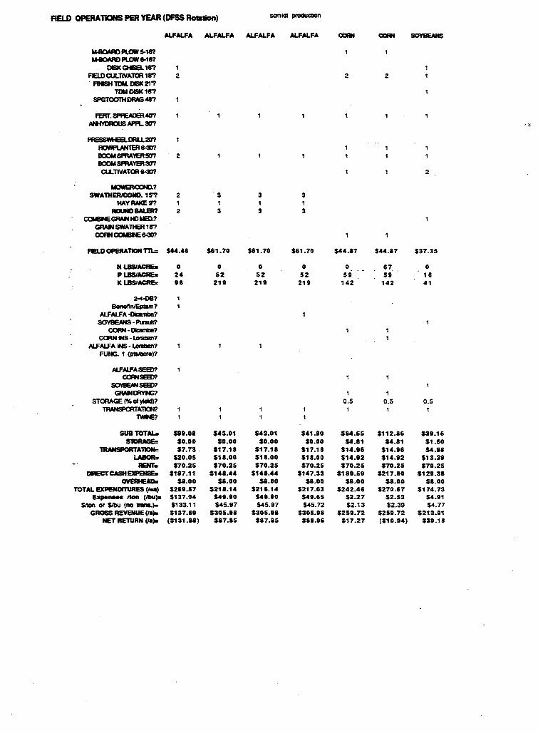
FIELD OPERA11CNS PER YEAR (DFSS Rotation) scmicll produc:lion
ALFALFA ALFALFA ALFALFA ALFALFA aat CXRf SOYBEANS
~PLOW~18? M«:WI) Pl.OW 6-18?
DISK CHISEL 18'? 1 FELDCUL.TIVATa:l 18'? 2 2 2
FINISH TDM. DISK 21'? TDU DISK 18'?
SPGTOOlHDRIG 48'?
~.SPFEAIB40?
ANMlROUSAPPL.31? .....
I RESSWI Ea.a.1..20'? RCMPlANtER &30? BCOMSPRAVERSI? 2 BCOMSPRAVER31? CU.TIVATOR &SO? 2
MCl!NB'llCCN).? SWA1HERICOND.15"? 2 ·3 3 3
HAYRAl<Erl 1 1 1 1 ACUNDULEA? 2 3 3 3
ca&EGRMIH>~?
GRAl\I SWAllER 16'? COANCClaE&-301
FELD OPERAllDN Tn..:: $U.'6 $61.70 $61.70 $61.70 $44.87 $44.87 $37.35
NLBSIACR&s 0 0 0 0 0 67 0 PLBSfACREs 2' 52 52 52 59 · - 59 16 KLBSIACR& 98 219 219 219 142 142 41
M-08? Beneftn/Eplam?
AJ.rAl.rA-Dicllmba? SOYBEANS. Plnuit?
COAN -OlcllmlB? CORN ..S -Lostan?
N.IAl.rA INS· Lonlban? FUNG. 1 (plBlaenl)?
MJ!/11.iASEED? ccr..sa:D?
SO'llEIHSEED? GRMID'IVN3? , ,
STORAGE (%of ylald)? 0.5 0.5 0.5 ~AllCN?
lWIE?
SUBTOTAl.z $99.08 $43.01 $43.01 $41.90 $84.65 $112.86 $39.16 S'10RAGE= $0.00 $0.00 $0.00 $0.00 $4.81 $4.81 $1.60
lRANSPORTA~ $7.73 $17.18 $17.18 $17.18 $14.96 $14.96 $4.98 LA80Ra $20.05 $18.00 $18.00 $18.00 $14.92 $14.92 $13.39
RENT• $70.25 $70.25 $70.25 $70.25 $70.25 $70.25 $70.25 DIECJ'CASHEJPENS& $197.11 $148.44 $148.44 $147.33 $189.59 $217.80 $129.38
OVERHEADs $8.00 $8.00 $8.00 $8.00 $8.00 $8.00 $8.00 TOTAL EXPENDITURES (hoa) $261.57 $218.14 $218.14 $217.03 $242.46 $270.67 $174.73
ExJi•- /loft (lbu)o: $137.04 $49.90 $49.90 $49.65 $2.27 $2.53 $4.91 $/Ion or $lbu (no 118n&.)s $133.,, $45.97 $45.97 $45.72 $2.13 $2.39 $4.77
GROSS REVENUE (/a)a $137.69 $305.98 $305.98 $305.H $259.72 $2511.72 $213.111 NET RETURN (la). ($131.88) $87.85 $87.85 $88.96 $17.27 ($10.114) $39.18
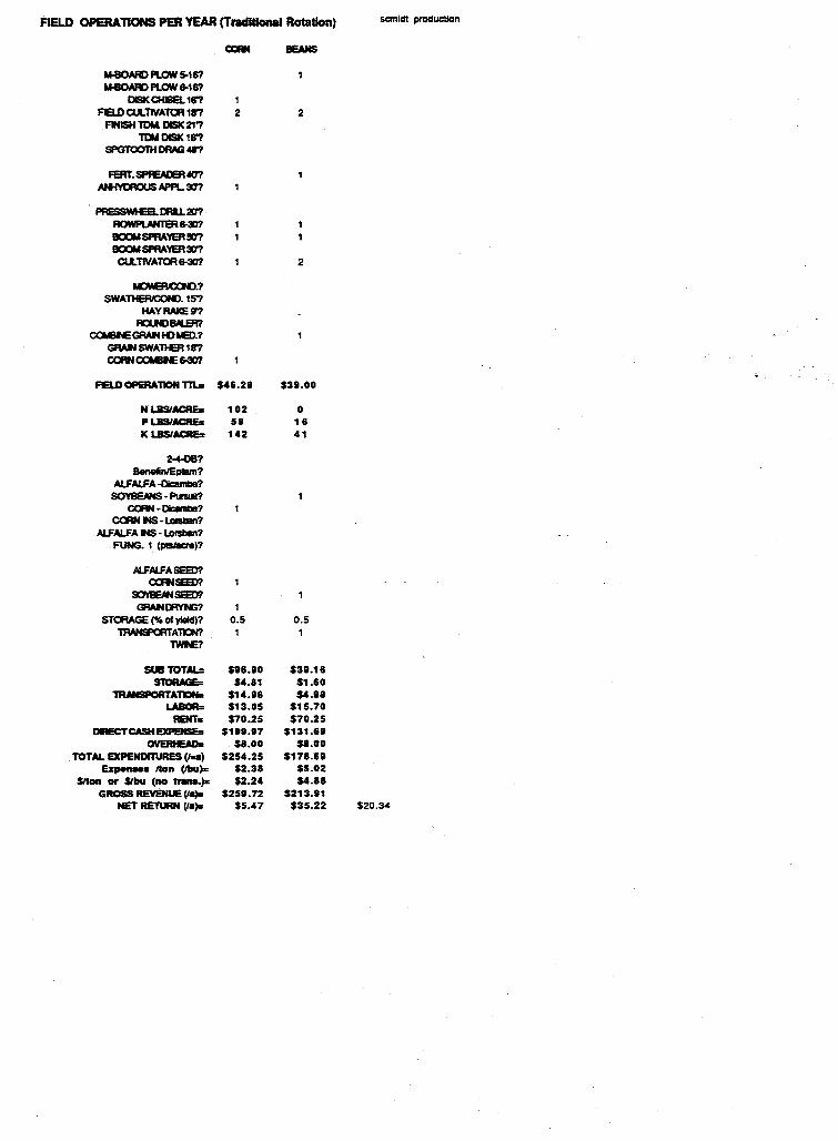
FIELD OPERATIONS PER YEAR (Traditional Rotation) scmidt production
CCAN BEANS
M-80NID Pl.OW S.16? M-BOARD Pl.OW &-16?
DISK ailSEI.. 1f1? 1 FELD CULTIVATOR 111? 2 2
FINISH TOM. DISK 21'? TOM DISK 16'?
SPGTOOTHOMG48?
FEAT. SPRENJER40"? ANM:lROUSAPPL~
PRESSWI £El.DRU.2f1? ROWPLAN1ER 6-30? BOOMSPRA'1ER~
BOOMSPRA'1ERS17 CU.TIVATOR &-30? 2
MO\'l&llCQD.? SWATHER/CON). 15'?
HAYRAl<Efl? RClN>MLER1
caelEGRAftf K>a.ED.? ~SWAllER1tl?
CORNOOMBN:&OO?
FELD OPERATION TTL= $4&.28 $311.00
NLBSIACRE: 102 0 PUISIACRE: 511 1& K LBSIACRE:: 1'2 41
2-4-08? Benefin/Epllun?
AJ.FAJ.FA-Olc:amlla? SOYBEANS- Plftuit?
CORN· Oic81nm? COAN Nl • l.ol&tal?
NJ=AJ..FA INS- Lorstlan? FUNG. 1 (p!S/acr8)?
NJ=AU'A SEED? <XAIS&D?
SCMEANSEED? GRANIJ'IYN3? ,
STORAGE ('lfo of yield)? 0.5 0.5 TPNISPORTATlON'l
1WIE?
SUBTOTAL= $1&.90 $39.1& S10RAGE= $4.81 $1.&0
1RANSPORTA110N= $14.96 $4.98 LABOR: $13.05 $15.70
RENT: $70.25 $70.25 DRECTCASH EXFSISE::: $11111.97 $131.&9
OVERHEADa $8.00 $8.00 TOTAL EXPENDnURES (/all) $254.25 $178.&9
ExJlenM• /ton (lbu)s $2.38 $5.02 $ltoa or $/bu (no trMa.)s $2.24 $4.88
GROSS REVENUE (fa)s $251.72 $213.111 NET RETURN (ta)a $5.47 $35.22 $20.34
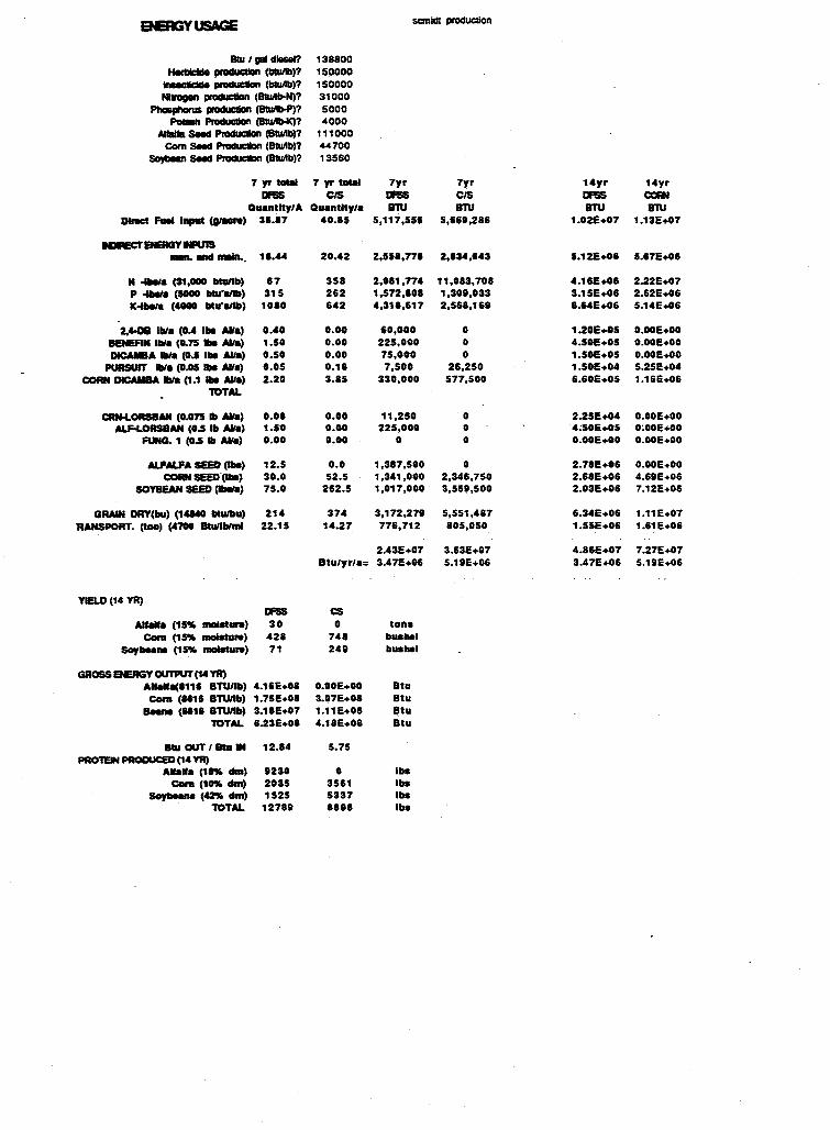
BERGYUSAGE scsnlelt produelion
Blu I gal diesel? 138800 Herlllclde pradllClilln (blullb)? 150000
"'-dc'dt praduc1lon (bluAb)? 150000 Nlnlgell praduCllon (Btull!Hij? 31000
PhospllofuS praducllon ~? 5000 Po..n Praduclloll (81ullb-K)? 4000
Alflllfa Seed Pnicluc:llon (Bill/lb)? 111000 Corn Seed Proc1uc:11on (BIUlll>)? 44700
SOyb8an Seed Producllon (BIUlll>)? 13560
7 yr teal 7 yr taeal 7yr 7yr 14yr 14yr DFSS CJS DFSS CJS DP.IS CXRI
Quantity/A Quantity/a B1U B1U B1U B1U Dll'Kt Fuel Input (glacre) 31.17 '°·85 5,117,551 5,1611,286 1.02E+07 1.13E+07
NJIECl'BEAGYINPU19
- ancl nwin.. 18.44 20.42 2,558,778 2,834,843 5.12£+08 5.67E+OI
N olllela (31,000 lltullb) 87 358 2,081,774 11,083,708 4.16E+08 2.22E+07 p -Ille/a (5000 btu'allb) 315 262 1,572,808 1,3011,033 3.15E+08 2.62E+06 K-llle/a (4000 lltu'allb) 1080 642 4,318,617 2,568,1611 8.&4E+06 5.14E+06
U-OS Ill/a (0.4 Ille Alla) 0.40 o.oo 60,000 0 1.20E+05 O.OOE+OO BENEFIN Ill/a (0.75 .. Al/a) 1.50 o.oo 225,000 0 4.50E+05 O.OOE+OO DICAIBA !Illa (0.5 Ille Alla) 0.50 o.oo 75,000 0 1.50E+05 O.OOE+OO
PURSUIT Illa (O.OS 1118 Alla) 0.05 0.18 7,500 26,250 1.50E+04 5.25E+04 CORN DlCAM8A 111111 (1.1 Ille .U.) 2.20 3.85 330,000 577,500 6.60E+05 1.16E+06
TOTAL
CRtM..ORS8AN (O.o75 lb .U.) 0.08 o.oo 11,250 0 2.25E+04 O.OOE+OO ALF-L.ORS8AH (0.5 lb .U.) 1.50 0.00 225,000 0 ·4;50£+0'5 O;OOE+OO
FUNG. 1 (0.5 lb Alfa) 0.00 0.00 0 0 O.OOE+OO O.OOE+OO
AJ;AJ.iA SEED (Illa) 12.5 0.0 1,387,500 0 2.78E+06 O.OOE+OO COAN SEED"(llls) 30.0 52.5 1,341,000 2,346,750 2.68E+06 4.611E+06
SOYBEAN SEED (Iba/a) 75.0 262.5 1,017,000 3,5511,500 2.03E+06 7.12E+06
GRAIN DRY(bll) (14840 lltUlllU) 214 374 3,172,2711 5,551,487 6.34E+06 1.11E+07 'RANSPORT. (ton) (4700 Btllillllml 22.15 14.27 776,712 805,050 1.55E+06 1.61E+06
2.43E+07 3.63E+07 4.86E+07 7.27E+07 Btulyrla= 3.47E+06 5.111E+06 3.47E+06 S.111E+06
YIELD (14 YR) DFSS cs
Alfalfa (15'% .......... , 30 0 tons Com (15% mol8turw) 428 748 bushel
SoJllHM (15% mol8turw) 71 2411 bushel
GROSS ENERGY OUTPUT (14 YR) AHallll(8118 BTUnb) 4.16E+08 O.OOE+OO Btu Com (8818 BTWlb) 1.75£+08 3.07E+08 Btu S- (8818 BTWlb) 3.18E+07 1.11E+08 Btu
TOTAL 6.23E+08 4.18E+08 Btu
Btu OUT I 8lu 91 12.84 5.75 PR0'1EIN PRODUCED (14 YR)
Allalfa (18"' elm) 11230 0 Iba earn (1CW. elm) 2035 3561 Iba
Soylleana (42"Xt elm) 1525 5337 Iba TOTAL 127811 88118 Iba
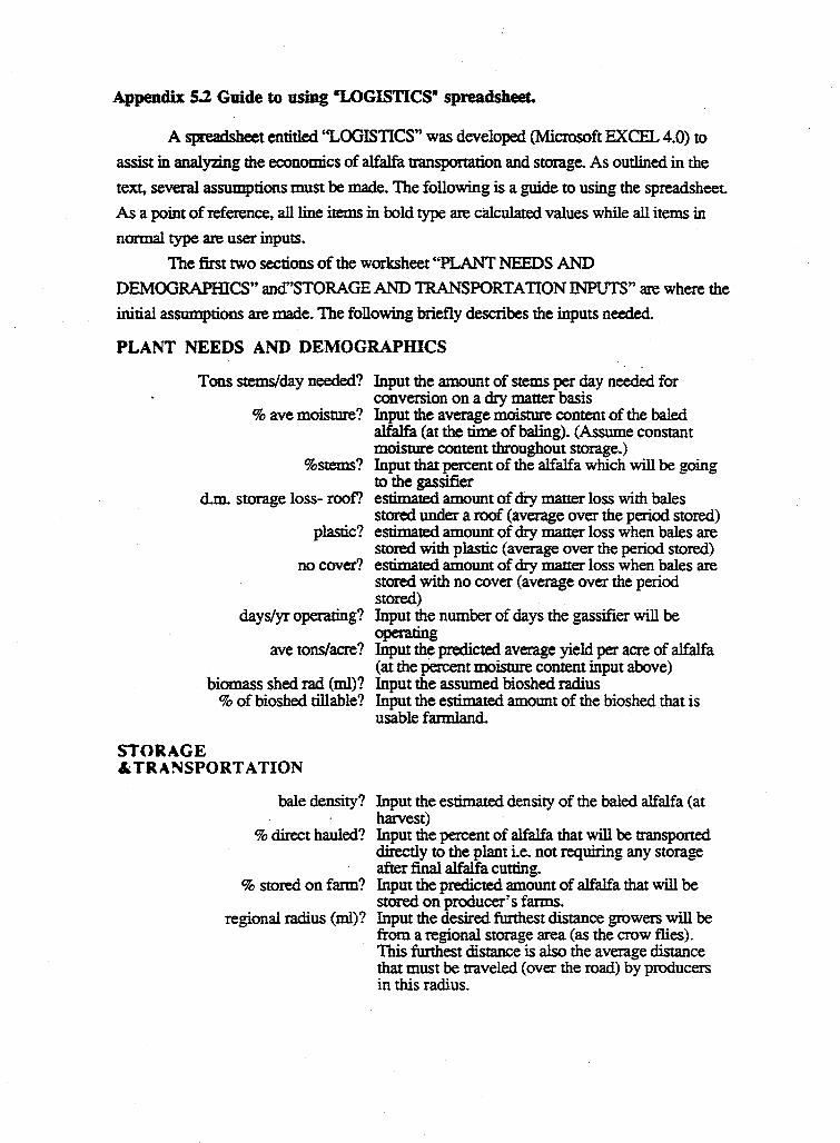
Appendix 5.2 Guide to using •LOGISTICS• spreadsheet.
A spreadsheet entitled ''LOOISTICS" was developed (Microsoft EXCEL 4.0) to
assist in analyzing the economics of alfalfa transportation and storage. As outlined in the
text, several assumptions must be made. The following is a guide to using the spreadsheet.
As a point of reference, all line items in bold type are calculated values while all items in
normal type are user inputs.
The first two sections of the worksheet ''PLANT NEEDS AND
DEMOGRAPHICS" and"STORAGE AND TRANSPORTATION INPUTS" are where the
initial assumptions are made. The following briefly describes the inputs needed.
PLANT NEEDS AND DEMOGRAPHICS
Tons stems/day needed? Input the amount of stems per day needed for conversion on a dry matter basis
% ave moisture? Input the average moisture content of the baled alfalfa (at the time of baling). (Assume constant moisture content throughout storage.)
%stems? Input that percent of the alfalfa which will be going to the gassifier
d.m. storage loss- roof? estimated amount of dry matter loss with bales stored under a roof (average over the period stored)
plastic? estimated amount of dry matter loss when bales are stored with plastic (average over the period stored)
no cover? estimated amount of dry matter loss when bales are stored with no cover (average over the period stored)
days/yr operating? Input the number of days the gassifier will be operating
ave tons/acre? Input the predicted average yield per acre of alfalfa (at the percent moisture content input above)
biomass shed rad (ml)? Input the assumed bioshed radius % of bioshed tillable? Input the estimated amount of the bioshed that is
usable farmland.
STORAGE &TRANSPORTATION
bale density? Input the estimated density of the baled alfalfa (at harvest)
% direct hauled? Input the percent of alfalfa that will be transponed directly to the plant i.e. not requiring any storage after final alfalfa cutting.
% stored on farm? Input the predicted amount of alfalfa that will be stored on producer's farms.
regional radius (ml)? Input the desired funhest distance growers will be from a regional storage area (as the crow flies). This funhest distance is also the average distance that must be traveled (over the road) by producers in this radius.
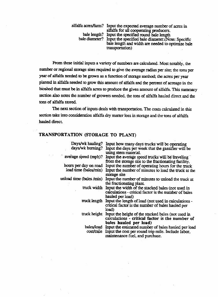
alfalfa acres/farm? Input the expected average number of acres in alfalfa for all cooperating producers.
bale length? Input the specified round bale length bale diameter? Input the specified bale diameter.(Note: Specific
bale length and width are needed to optimize bale transportation)
From these initial inputs a variety of numbers are calculated. Most notably, the number or regional storage sites required to give the average radius per site; the tons per year of alfalfa needed to be grown as a function of storage method; the acres per year planted in alfalfa needed to grow this amount of alfalfa and the percent of acreage in the bioshed that must be in alfalfa acres to prcxluce the given amount of alfalfa. This summary
section also notes the number of growers needed, the tons of alfalfa hauled direct and the
tons of alfalfa stored.
The next section of inputs deals with transportation. The costs calculated in this section take into consideration alfalfa dry matter loss in storage and the -tons of alfalfa
hauled direct.
TRANSPORTATION (STORAGE TO PLANT)
Days/wk hauling? days/wk bmning?
.. average sPeed (inph)?
hours per day on road load time (bales/min)
unload time (bales /min)
truck width
truck length
truck height
bales/load cost/mile
Input how many days trucks· will be operating Input the days per week that the gassifier will be using stem material. Input the average speed' i:i:iickS .WillbC traveling .. from the storage site to the fractionating facility. Input the number of operating hours for the truck Input the number of minutes to load the truck at the storage site Input the number of minutes to unload the truck at the fractionating plant Input the width of the stacked bales (not used in calculations - critical factor is the number of bales hauled per load) Input the length of load (not used in calculations -critical factor is the number of bales hauled per load) Input the height of the stacked bales (not used in calculations - critical factor is the number of bales hauled per load) Input the estimated number of bales hauled per load Input the cost per round trip mile. Include labor, maintenance fuel, and purchase.
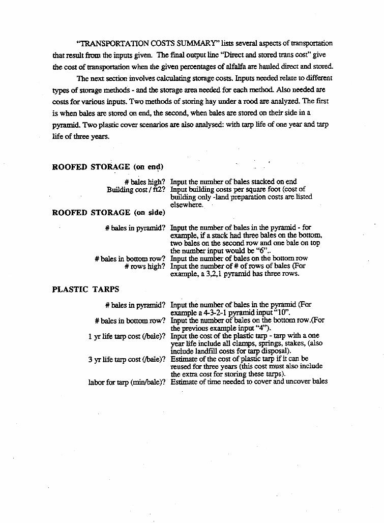
"TRANSPORTATION COSTS SUMMARY" lists several aspects of transportation
that result from the inputs given. The final output line ''Direct and stored trans cost" give
the cost of transportation when the given percentages of alfalfa are hauled direct and stored.
The next section involves calculating storage costs. Inputs needed relate to different
types of storage methods - and the storage area needed for each method. Also needed are
costs for various inputs. Two methods of storing hay under a rood are analyzed. The first
is when bales are stored on end, the second, when bales are stored on their side in a
pyramid Two plastic cover scenarios are also analysed: with tarp life of one year and tarp
life of three years.
ROOFED STORAGE (on en~)
# bales high? Input the number of bales stacked on end Building cost I ft2? Input building costs per square foot (cost of
building only -land preparation costs are listed elsewhere. ·
ROOFED STORAGE (on side)
# bales in pyramid? Input the number of bales in the pyramid - for example, if a stack had three bales on the bottom, two bales on the second row and one bale on top the number input would be "6" ..
# bales in bottom row? Input the number of bales on the bottom row # rows high? Input the number of# of rows of bales (For
example, a 3,2,l pyramid has three rows.
PLASTIC TARPS
# bales in pyramid?
#bales in bottom row?
1 yr life tarp cost (/bale)?
3 yr life tarp cost (/bale)?
labor for tarp (min/bale)?
Input the number of bales in the pyramid (For example a 4-3-2-1 pyramid input "l O". Input the number of bales on the bottom row .(For the previous example input "4"). Input the cost of the plastic tarp - tarp with a one year life include all clamps, springs, stakes, (also include landfill costs for tarp disposal). Estimate of the cost of plastic tarp if it can be reused for three years (this cost must also include the extra cost for storing these tarps). Estimate of time needed to cover and uncover bales
ADDITIONAL INFORMATION
labor cost ($/hr)? land value (/acre/yr)?
additional land needed?
land preparation cost ($/acre)?
Loader?:
equip-testing, weighing, etc?
DIR.TI?
Input the cost of labor - include all benefits Input land rental rate Input the percent increase in land that is needed at the storage site for driveways, buffer strips, par.king, etc .. Input the cost of preparing the site for storage. This price involves land leveling, removing topsoil, and hauling in and leveling gravel base. Input the purchase price of a loader - for unloading and loading bales at the remote site. Input the cost of additional equipment needed at each site. This cost includes office equipment, bale testing equipment, weigh scales, computers, bar coding equipment, etc. Depreciation, interest, repairs, taxes, and insurance on all capital expenditures.
Outputs given from this set of input include estimated total costs of storage as a
function of storage method and a breakdown of these costs. Also included are estimated costs per storage site.
The following section of the worksheet deals with equipment needs. As it turns out,
the number of sets of equipment needed dictates the optimum number of storage sites. The
equipment needed is a function of the peak rate at which alfalfa will be brought to storage.
If indeed bales are to be stored under plastic or under a roof, it is critical that these bales are
unloaded and stored in a timely manner. If bales are to be stored outside the rapid rate of
bale stacking is not needed, thus reducing equipment needs.
CALCULATING EQt:IPMENT NEEDS
hauling equipment? Input the cost of to transport alfalfa from the field to the storage site. This number includes direct and overhead costs, i.e., cost of purchase, maintenance and fuel. but no labor.
Ave # of bales per load? Input the average number of bales on a load coming from the field
average mph? Input the average miles per hour for transportation from the field to the storage site. (Include field travel, gravel road travel and highway travel)
·.. loading time min/bale? Input the anticipated time to pick up and load a bale at the production site. Typically the bales will be in the field.
% 1st cutting? Input the amount of alfalfa that will be coming in during the peak harvest season
#days allowed to store? Input the number of days that are included in the peak season (For example if the peak season is estimated at 33% of total alfalfa production for the year will be done in 15 days: % first cutting will be '33' and# days to store will be '15').
Storage site hours/day? Input the hours of operation the storage site will be operating during peak season
Processing time/bale? Input the estimated number of minutes it will take to process one bale of alfalfa. (This processing time includes bale testing, weighing, unloading and stacking).
These inputs are used to calculate the sets of equipment needed, the number of
equipment per site (for the given amount of sites), and the costs to transport alfalfa from the
production site to the storage site.
The final page of the worksheet is a summary page. All information given has been
calculated oo prior pages. The only input needed is the price paid to producers for their
alfalfa. This is needed to determine the true cost of alfalfa as it enters the fractionation
facility. This "Paid to producer" input could be a preselected value or a the cost of
producing alfalfa as determined by the alfalfa production spreadsheet
As stated previously, there are many assumptions made in this worksheet Many of
which could dramatically effect the final cost of alfalfa at the fractionation facility.
·-.
LOGISTICS
ALFALFA STORAGE AND TRANSPORTATION WORKSHEET
PlANT NEEDS AND DEMOGRAPHICS 8/25/94
tons stems/dy needed? 99'2 dry 'l. ave. masn.e? 15
tons Items neededs 1167 at moisture overage moisture content specifleid 'l.stem? 55
tons hay needed= 2122 d.m. store IOss roof ('I.)? 2
plastic ('I.)? 5 no cover ('I.)? 10
days/yr operatng? 300 ave. tons/acre? 4 at 15" moisture
biomass shed rad (ml)? .!I) "of bloshed tllable? 80
STORAGE 1RANSPORl'ATION INPUTS
bale density b/ft3? 10
" c:lrect hauled? 40 'l. stored on farm? 0 region region % stontd regional= 60 sides (miles) sq miles #regions region radius (ml)? 4.0 8.0 64 78.54
olfolfa oaes/farm? 200 bole length? 4.00
bale dlometer? 6.00 bale volume= 113.10 cubic feet/bale bale wt. (lbs)= 1131 before loss
SUMMARY INFORMATION
no cover plasllc root no loss tons/year= 679,016 656,680 644,372 636.578
acres needed= 178,688 172,811 169,572 167,520 bales/year= 1,200,765 1,161,266 1,139,501 1, 125,717
% acres In bloshed= 6.94 6.71 6.59 6.51 (acres in alfalfa)
STORAGE STATIS11CS DIRECT HAUL
no cover plastic rooted #cfgroweis= 893 864 848
acres clrect haul= 67,008 67,008 67,008 tons clrect haul= 254,631 254.631 254.631
TOTAL TO STORAGE no cover plastic root
acres stored= 111,680 105,802 102,564 tons stored= 424,385 402,049 389,741
PER REGION TOTALS
DIRECT HAULED AND Sl'ORED
acres of alala clrect= acres ol alf. to stolage=
tons clrect= tons stored=
Sl'ORAGE PER REGION
NO COVER 853
1,422 3,242 5,403
% on fann = . o.oo
on fann acres= on fann Ions= at ... acres=
at site Ions=
NO COVER 0 0
1,422 5,403
PLASTIC 853
1,347 3,242 5,119
ROOFED 853
1,306 3,242 4,962
% at site= 100.00
PLASTIC 0 0
1,347 - . • S;U9-~,· ..
ROOFED 0 0
l,306.,. 4,962
TRANSPORTATION (STORAGE TO PLANT)
DayS/week hauling? days/week buming?
average speed (mph)? hours/day on road?
:id time (minutes/bOle)? :id time (minutes/bOle)?
truck width (ft)? truck length (ft)? truck height (ft)?
boles /load? cost per mile? cu ft per load=
6 7
40 16
0.50 0.33
9 48 9
30 $1.50 3,393
lRANSPORl'A.TION COS1S SUMMA.RY
(Includes store loss) lons/lrUClc = tons per day needed to haul=
trucks per day= time per load (his) = • loads/lrUCk/day = ~needed=
miesJtruck/day = miles/yr/hUCk=
transport ccst= trans cost•(%) method=
Direct and stored trans ccst=
15.0 minutes per load 9.9 minutes per load
not used in calculations but should match boles per load notusedlncolculotions not used in colculotions
cost per loaded mile - overhead ond direct includes labor bole volume
NO COVER PLASTIC ROOF DIRECT HA.UL 15.3 16.1 16.6 17.0 2476 2476 2476 2476
162.14 153.61 148.90 145.93 2.42 2.42 2.42 2.42 6.63 6.63 6.63 6.63
24.47 23.18 22.48 22.03 530.02 530.02 530.02 530.02 136,291 136,291 ~36,291 136,291
$2,501,591 $2,369,929 $2,297,380 $2,251,432 $1,500,955 $1,421,957 $1,378,428 $900,573
$2,401,528 $2,322,530 $2,279,001 $2,251,432
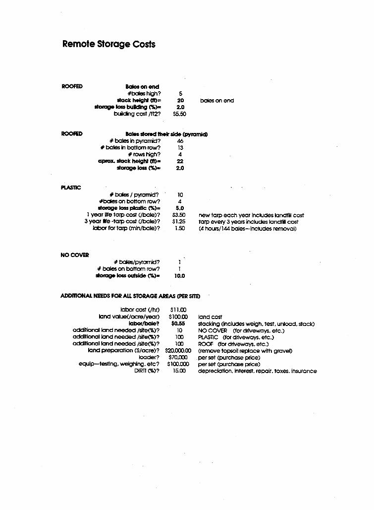
Remote Storage Costs
ROOFED Bales on end #bales high?
stack height (ft)= storage loss bulding (%)=
building cost /ft2.?
5 20 2.0
$5.50
boles on end
ROOFED Bales stored their side (pyramid)
PLAS11C
#boles in pyramid? 46 #boles In bottom row? 13
#rows high? 4 aprox. stack height (ft)= 22
storage loss (%)= 2.0
#boles I pyramid? #boles on bottom row? stotage loss plastic (%)=
l yeor life tarp cost Ubole)? 3 yeor lfe ·tarp cost Ubole)?
labor for tarp (min/bole)?
10 4
5.0 $3.50 Sl.25 1.50
NO COVER #boles/pyramid? 1
# bales on bottom row? 1 stocage loss outside (%)= 10.0
new torp eoch yeor includes landfiU cost torp every 3 years includes landfill cost (4 hours/144 boles-includes removal)
ADDmONAL NEEDS FOR ALL STORAGE AREAS <PER SITE)
labor cost Uhr) land valueC/acre/yeor)
labor/bale? adcfitional land needed /site(.%)? addltional land needed /site(.%)? odditional land needed /site(.%)?
land preparation CS/acre)? looder?
equip-testing, weighing. etc? DIRTI (%)?
Sl 1.00 $100.00 $0.55
10 100 100
S20,00J.OO $70.000
$100.000 15.00
land cost stocking (includes weigh, test. unload. stock) NO COVER (for driveways. etc.) PLASllC (for driveways. etc.) ROOF (for driveways. etc.) (remove topsoil replace with gravel) per set (purchase price) per set (purchase price) depreciation. interest. repair. taxes. insurance
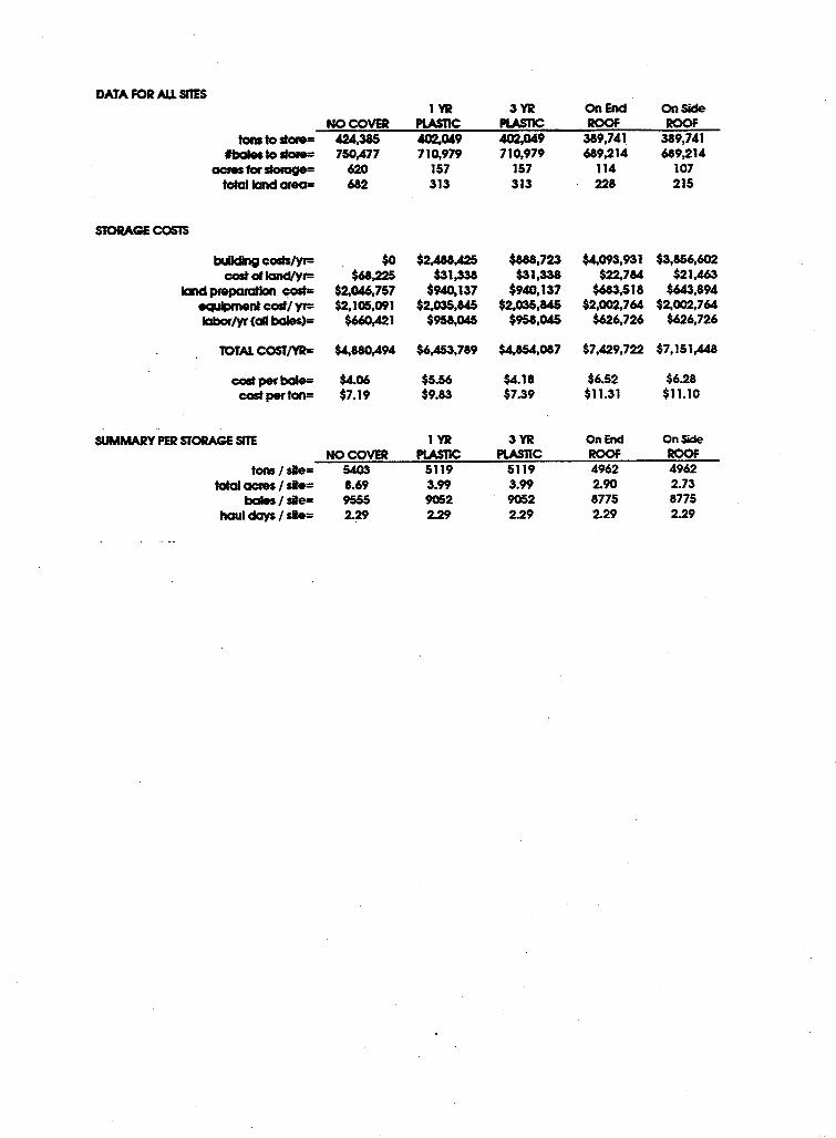
DATA FOR AU. Sl1ES 1 YR 3YR On Encl OnSide
NO COVER PLASTIC PLASTIC ROOF ROOF tons to store= 424,385 402,049 402,049 389,741 389,741
fiXlles to dote= 750,477 710,979 710,979 689,214 689,214 acres tor storage= 620 157 157 114 107
total land area= 682 313 313 228 215
STORAGE COS1S
~ colits/yr= $0 $2,488,425 $888,723 $4,093,931 $3,856,602 cost cl land/Yr= $68,225 $31,338 $31,338 $22,784 $21,463
land preparation cost= $2,046,757 $940,137 $940,137 $683,518 $643,894 equipment CW/ yr= $2,105,091 $2,035,845 $2,035,845 $2,002,764 $2,002,764 labor/yr (all bales)= $660,421 $958,045 $958,045 $626,726 $626,726
TOTAL COST/YR= $4,880,494 $6,453,789 $4,854,087 $7,429,722 $7,151,448
cost per bale= $4.06 $5.56 $4.18 $6.52 $6.28 cost per ton= $7.19 $9.83 $7.39 $11.31 $11.10
SUMMARY PER STORAGE SITE 1 YR 3YR On End On Side NO COVER PLASTIC PLASTIC ROOF ROOF
tons/sie= 5403 5119 5119 4962 4962 total acres I sie= 8.69 3.99 3.99 2.90 2.73
bales I site= 9555 9052 9052 8775 8775 haul days I sie= 2.29 2.29 2.29 2.29 2.29
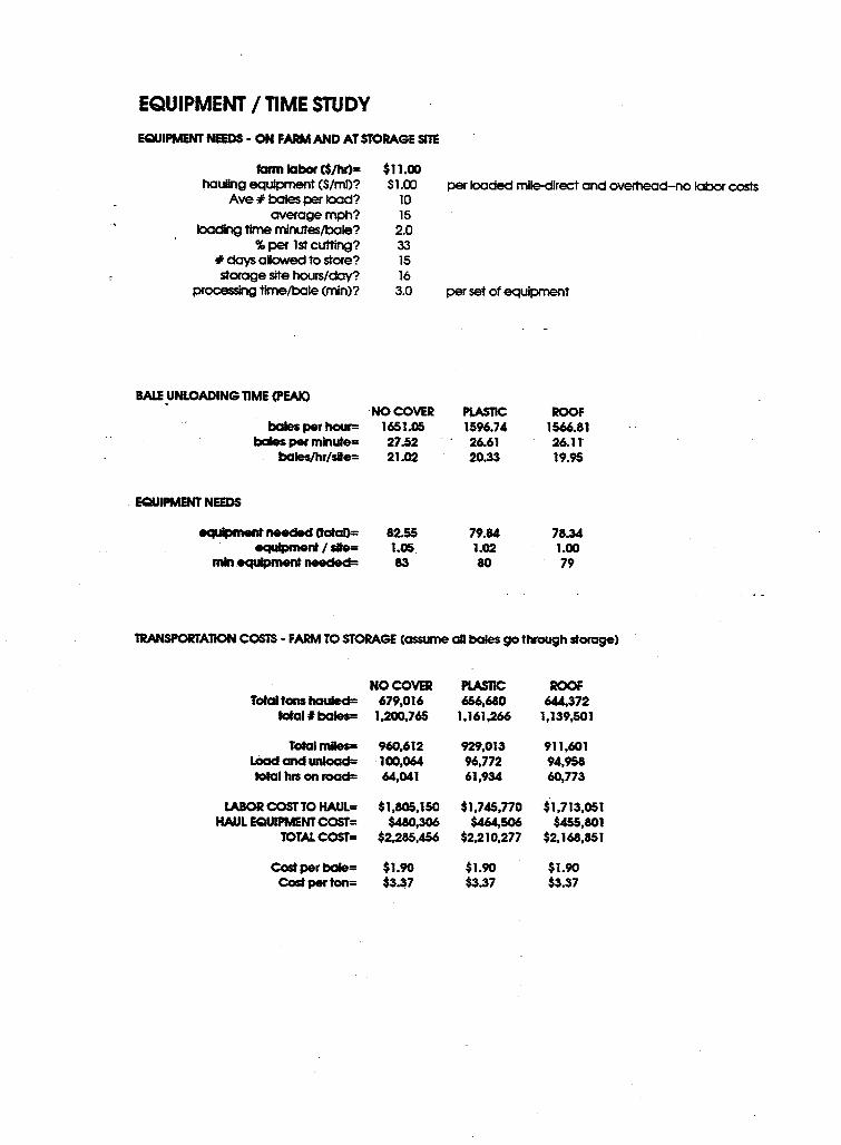
EQUIPMENT I TIME STUDY
EQUIPMENT NEEDS - ON FARM AND AT STORAGE SITE
farm labor ($/hr)= hauling equipment ($/mO?
Ave# boles per load? overage mph?
loading time minutes/bole? ,. per lst cutting?
#days allowed to store? storage site hours/day?
processing time/bole (min)?
BALEUNLOADINGTIME~EAIO
bales per hour= bales per minute=
bales/hr/site=
EQUIPMENT NEEDS
equipment needed (totaD= 9qU!pment Isle=
rnh equipment needed=
$11.00 $1.00
10 15 20 33 15 16 3.0
·NO COVER 1651.05 27.52 21.02
82.55 1.05 83
per loaded mile-direct end overhead-no labor costs
per set of equipment
PLASTIC ROOF 1596.74 1566.81 26.61 26.H 20.33 19.95
79.84 78.34 1.02 1.00 80 79
TRANSPORTATION COSTS - FARM TO STORAGE (assume aa bales go through storage)
NO COVER PLASTIC ROOF Total tons hauled= 679,016 656,680 644.372
fetal I bales= 1,200,765 1,161,266 1,139,501
Total miles= 960,612 929,013 911,601 Load and unload= 100,064 96,772 94,958 total tus on road= 64,041 61,934 60,773
LABOR COST TO HAUL= $1,805,150 $1,745,770 $1,713,051 HAUL EQUIPMENT COST= $480,306 $464,506 $455,801
TOTAL COST= $2,285,456 $2,210,277 $2,168,851
Cost per bale= $1.90 $1.90 $1.90 Cost per ton= $3.37 $3.37 $3.37
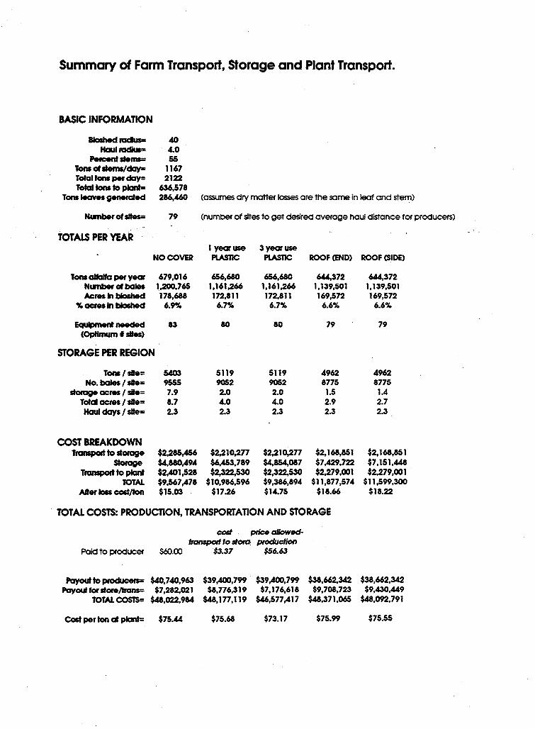
Summary of Fann Transport, Storage and Plant Transport.
BASIC INFORMATION
Bicshed radius= 40 Haul radius= 4.0
Percent Items= 55 Tons ot Items/day= 1167 Total tons per day= 2122 Total tons to plant= 636,578
Tons leaves genecated 286,460 (assumes dry matter losses ore the some in leaf and stem)
Nwnber of sites= 79 (number of sites to get desired average haul distance for producers)
-TOTALS PER YEAR
1 year use 3yearuse NO COVER PLASTIC PLASTIC ROOF(END) ROOF(SIOE}
Tons allalfa per year 679,016 656,680 656,680 644.372 644.372 Nwnber ot bales 1,200,765 1,161,266 1,161,266 1,139,501 1, 139,501 Acres In bloshed 178,688 172,811 172,811 169,572 169,572
% acres In bloshed 6.9% 6.7% 6.7% 6.6% 6.6%
Equipment needed 83 80 80 79 79 (Optinun • sites)
STORAGE PER REGION
Tons/lie= 5403 5119 5119 4962 4962 No. bales I site= 9555 9052 9052 8775 8775
storage acres I sie= 7.9 2.0 2.0 1.5 1.4 Total acres I sle= 8.7 4.0 4.0 2.9 2.7 Haul days Isle= 2.3 2.3 2.3 2.3 2.3
COST BREAKDOWN Transport to storage $2,285,456 $2,210,277 $2,210,277 $2,168,851 $2,168,851
storage $4,880,494 $6,453,789 $4,854,087 $7,429,722 $7,151,448 Transport to plant $2,401,528 $2,322,530 $2,322,530 $2,279,001 $2,279,001
TOTAL $9,567,478 $10,986,596 $9,386,894 $11,877,574 $11,599,300 Alter loss cost/ton $15.03 $17.26 $14.75 $18.66 $18.22
TOTAL COSTS: PRODUCTION, TRANSPORTATION AND STORAGE
cost price allowed-transpod to s#OICI: produclion
Paid to producer $60.00 $3.37 $56.63
Payout to producers= $40,740,963 $39,400,799 $39,400,799 $38,662,342 $38,662,342 Payout for store/tranS= $7,282,021 $8,776,319 $7,176,618 $9,708,723 $9,430,449
TOTAL COS'IS= $48,022,984 $48, 177, 119 $46,577,417 $48,371,065 $48,092,791
COst per ton at plant= $75.44 $75.68 $73.17 $75.99 $75.55
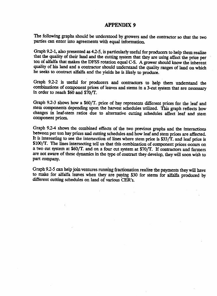
APPENDIX 9
The following graphs should be understood by growers and the contractor so that the two parties can enter into agreements with equal information.
Graph 9.2-1, also presented as 4.2-5, is particularly useful for producers to help them realize that the quality of their land and the cutting system that they are using affect the price per ton of alfalfa that makes the DFSS rotation equal C-S. A grower should know the inherent quality of his land and a contractor should understand the quality ranges of land on which he seeks to contract alfalfa and the yields he is likely to produce.
Graph 9.2-2 is useful for producers and contractors to help them understand the combinations of component prices of leaves and stems in a 3-cut system that are necessary in order to reach $60 and $70/T.
Graph 9.2-3 shows how a $60/T. price of hay represents different prices for the leaf and stem components depending upon the harvest schedules utilized. This graph reflects how changes in leaf-stem ratios due to alternative cutting schedules affect leaf and stem component prices.
Graph 9.2-4 shows the combined effects of the two previous graphs and the interactions between per ton hay prices and cutting schedules and how leaf and stem prices are affected. It is interesting to see the intersection of lines where stem price is $33 /T. and leaf price is $100/T. The lines intersecting tell us that this combination of component prices occurs on a two cut system at $60/T. and on a four cut system at $70/T. H contractors and farmers are not aware of these dynamics in the type of contract they develop, they will soon wish to part company.
Graph 92-5 can help join ventures running fra~onation realize the payments they will have to make for alfalfa leaves when they are paying $30 for stems for alfalfa produced by different cutting schedules on land of various CER's.
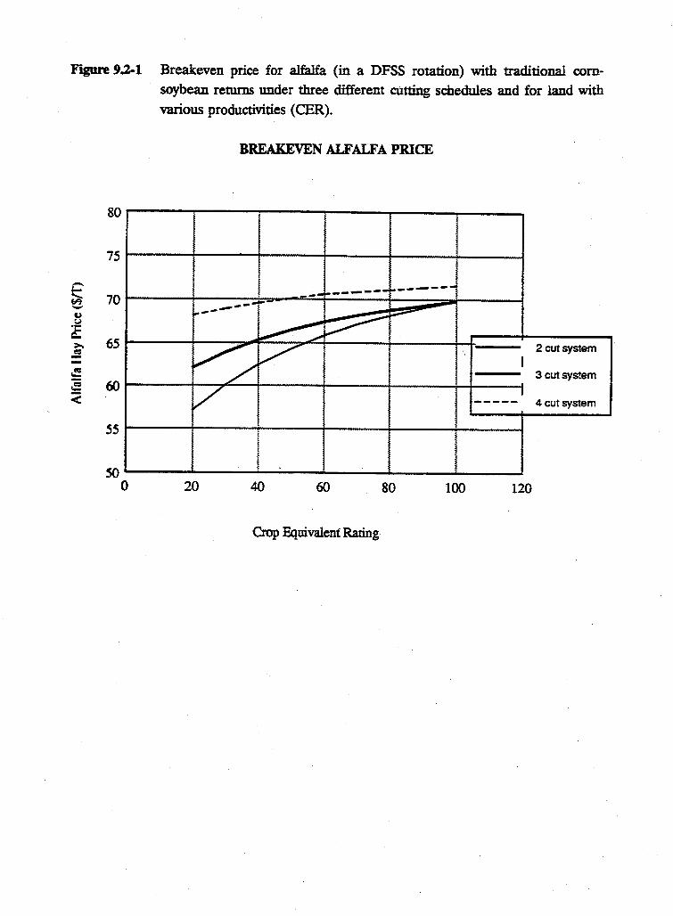
Figure 9.2-1 Breakeven price for alfalfa (in a DFSS rotation) with traditional comsoybean returns under three different cutting schedules and for land with various productivities (CER).
-£::: ~ -u ~ a: >. = --~ ~
<
80
75
70
65
60
SS
so 0
BREAKEVEN ALFALFA PRICE
-------- -------__ .. ---~---
.. -....----- ~-~ v- 2cutsystem
/ I
3cutsystem
/ I ----- 4 cut system
20 40 60 80 100 120
Crop :Equivalent Rating
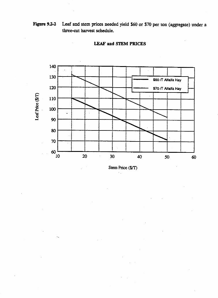
Figure 9.2-2 Leaf and stem prices needed yield $60 or $70 per ton (aggregate) under a three-cut harvest schedule.
-~ -~ CJ
~ 'ii ~
140
130
120
110
100
90
80
70
60 10
-
LEAF and STEM PRICES
-
""""" $60 fT Alfalfa Hay -
~ ~
$70 IT Alfalfa Hay -""--
~ '- ~
~
~ l ,.~
............ . ......
' ....._ .
I ...........
' I 20 30 40 50 60
Stem Price (Sm
Figure 9..2-3 Leaf and stem prices needed to yield $60 per ton (aggregate) under a two-, three-, or four-cut harvest· schedule.
s -«.> t.)
~ '-;; ~
130
120
110
100
90
80
70
60 10
LEAF and STEM PRICES
"' I 2cutsystem
~ 3cutsystem I'...
""" ""' ----- 4cutsystem
"-.... "" i. ... ~" '""·"' ......... ~ ... ...... .....
"""'
" ~ .........
!-..., ........ !'....
.._. .............
"""""" ~ ...... ........ ...
20 30 40 50 60
Stem Price ($ff)
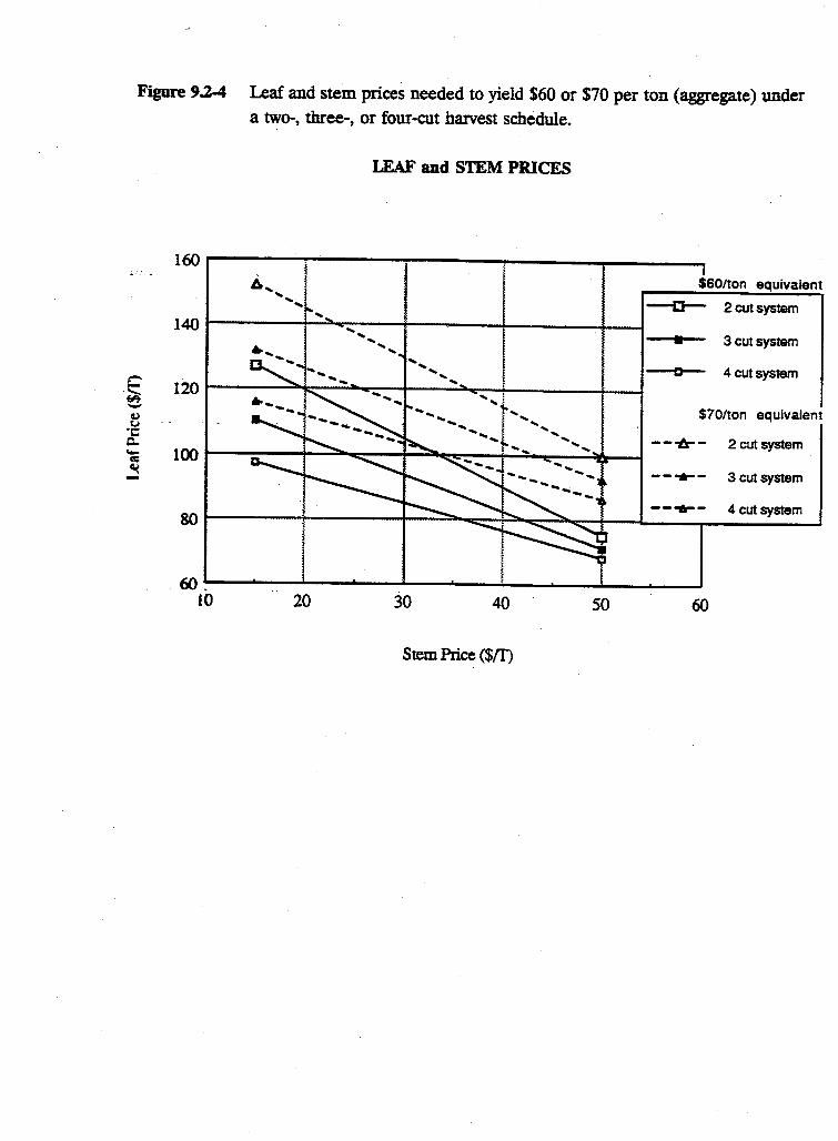
Figure 9.2-4 Leaf and stem prices needed to yield $60 or $70 per ton (aggregate) under a two-, three-, or four-cut harvest schedule.
E ~ -u tJ ·c c.. ._ ci: '( -
LEAF and STEM PRICES
I60r-------~--------:--------~----------------.
...
120
100
80
$60/ton equivalent
-0-- 2 cut system
3 cut system
D 4 cut system
$70/ton equivalent
- - -tr- - 2 cut system
- - ...- - 3 cut system
- - -ll- - 4 cut system
60~.------...... __ __.. __________ i..-________ .._ __ ....... ____ ..1-__ __...__ __ _i
10 20 30 40 50 60
Stem Price ($nJ
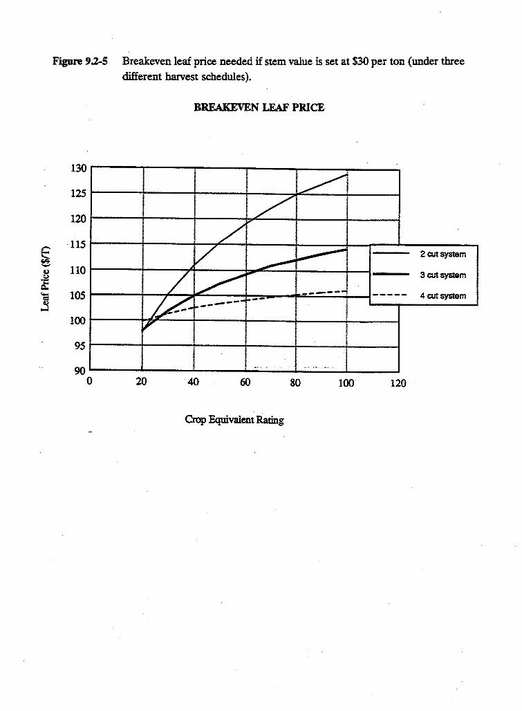
Figure 9.2-5 Breakeven leaf price needed if stem value is set at $30 per ton (under three different harvest schedules).
BREAKEVEN LEAF PRICE
130
125
120
s 115 2cutsystem - 110 a.>
~ 3 cut system
~ ~ 105 = 4 cut system
~ 100
95
90 0 20 40 60 80 100 120
Crop Equivalent Rating
APPENDIX 10.1 Guide to using-PRODUCTION' spreadsheet for energy balance.
A spreadsheet entitled -Froduction• was used to determine the cost of
production for both the DFSS rotation and the com-soybean rotation. The guide
to using the spreadsheet can be found in appendix 4.2. The final page of the
spreadsheet calculates the energy used in the various rotations. Energy use is a
function of field operations and fertilizer and chemical inputs. Field operations
are determined by crop rotatio~ chemical inputs are determined by both crop
rotation and yield goal. Because of this dependency on yield goal, the energy
balance varies between soil types. In real life, energy inputs also depend on
individual equipment and soil types. The fuel used for field operations is an
average theoretical fuel use. Therefore, the energy inputs given are merely
attempts at estimating true energy inputs.
The section of the spreadsheet -PRODUCT" entitled -Energy Usage•
requires user inputs. The inputs used for this analysis are documented in Chapter
10.1. The user is allowed to input values for the energy needed for production of
fertilizer, herbicides, insecticides and seeds. The values for these numbers vary
quite widely in published literature. Because of this the user is given these input
options.
Energy inputs are calculated in bo~ gallons of diesel fuel and Btu. Totals
are given as an average per year, and 7 and 14 year totals. Also listed as outputs
are the lbs or bushels of crop output, the gross energy of the output and the
protein produced by the output.
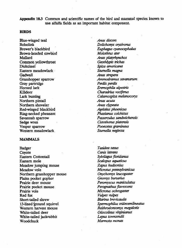
Appendix 10.3 Common and scientific names of the bird and mammal species known to use alfalfa fields as an important habitat component.
BIRDS
Blue-winged teal Bobolink Brewer's blackbird Brown-headed cowbird Mallard Common yellowthroat Dickcissel Eastern meadowlark· Gadwall Grasshopper sparrow Gray partridge Homed lark Killdeer Lark bunting Northern pintail Northern shoveler Red-winged blackbird Ring-necked pheasant Savannah sparrow Sedge wren Vesper sparrow Western meadowlark
MAMMALS
Badger Coyote Eastern Cottontail Eastern mole Meadow jumping mouse Meadow vole Northern grasshopper mouse Plains pocket gopher Prairie deer mouse Prairie pocket mouse Prairie vole Red fox Short-tailed shrew 13-lined tround squirrel Western harvest mouse White-tailed deer White-tailed jackrabbit Woodchuck
Anas discors Dolicho1l)'X oryzivorus Euphagus cyanocephal.us Molothrus ater Anas platyrhynchos Geothlypis trichas Spiza americana Stuinelli:z magna Anas strepera Ammodramus savanarum Perdix perdix Eremophil.a alpestris Charadrius vociferus Calamospiza melanocorys Anas acuta Anas clypeata Agelaius phoenicus Phasianus colchicus Passerculus sandwichensis Cistothorus platensis Pooecetes gramineus Stumella neglecta
Taxidea tams Canis latrans Sylvilagus floridanus Scalopus aquaticus Zapus hudsonius Microtus pennsylvanicus Onychomys leucogaster Geomys bursarius Peromyscus maniculatus Perognathus flavescens Microtus ochrogaster Vulpes vulpes Blarina brevicauda Spermophilus tridecemlineatus Reithrodontomys megalotis Odocoileus virginianus Lepus townsendil Marmota monax
BIBLIOGRAPHY
Allen, D.L. (ed.). 1956. Pheasants in North America. Wildl. Manage. Inst., Washington, D.C. 490pp.
Baker, D.G. and R. Keiit Crookston, 199L An Agronomic Look at the Climate and Weather of Minnesota.p.9-32. In R.K.Crookston ( ed): Com and soybean management in Minnesota. University of Minnesota, Minneapolis, MN
Baker, D.G., Ruschy, S. Evans, W.W. Nelson, J. Lamb, G. Randall, G. Spoden, and J. Zandlo. 1990. Climate and climatology, 1990. A report on filed research in soils, Miscellaneous Publication 62-1990. MAES, University of Minnesota, St.Paul, MN
Baskett, T .S. 1947. Nesting and production of the ring-necked pheasant in north-central Iowa. Ecol Monogr. 17(1):1-30.
Bauder, J. W., A Bauer, J.M. Ramirez, and D. K. Cassel 1978. Alfalfa water use and production on dryland and irrigated sandy loam. Agron. J. 70:95-99.
Baxter, W.L., and C.W. Wolfe. 1973. Life history and ecology of the ring-necked pheasant in Nebraska. Nebraska Game and Parks Comm. 58pp.
Baxter, W .L. Wildlife Biologist, Nebraska Game & Parks, Lincoln, NB. "Personal Communications·.
Bemer, A H. 1988. Federal pheasants-impacts of federal agriculture programs on pheasant habitat, 1934-1985. Pages 46-93 in D. L. Hallett, W.R. Edwards, and G. V. Burger (eds.) Pheasants: symptoms of wildlife problems on agriculture lands. North Central Section, The Wildlife Society, Bloomington, IN. 345pp.
Birney, E. Mammologist, Department of Ecology, Evolution and Behavior and Curator of The Bell Museum of Natural History, Univ. of Minnesota, St Paul, MN. "Personal Communications".
Bollinger, E. K., and TA Gavin. 1989. Eastern bobolink populatiom: Ecology and conservation in an agricultural landscape. Pages 497-505 in Symposium on Neotropical Birds, Manomet Observatory.
Bollinger, E.K., P.B. Bollinger, and TA Gavin. 1990. Effects of hay-cropping on eastern populations of the bobolink. Wtldl. Soc. Bull. 18:142-150.
Broder, J.M., K.C. Schneeberger, J.G. Beierlein. 1982. Energy and economic efficiency for off-site processing of selected oilseeds. In Vegeteble Oil Fuels. Proceedings of the International Conference on Plant and Vegetable Oils as Fuels. pp. 24-32. St Joseph, Michigan: American Society of Agricultural Engineers
Case, N.A, and O.H. Hewitt. 1963. Nesting and productivity of the red-winged blackbird in relation to habitat. Living Bird 2:7-20.
Cervinka, Va. 1980. Fuel and energy effiency. In Handbook of energy utilization in agriculture, edited by D.
Pimental, pp. 15-21. Boca Raton, Florida: CRC Press.
Collins, M., W.H. Paulson, M.F. Fmner, MA Jorgensen, C.R. Keuler. 1987. Moisture and storage effects on
dry matter and quality losses of alfalfa in round bales. Transactions of the ASAE. 30(4):913-917.
Dolbeer, RA 1976. Reproductive rate and temporal spacing of nesting of red-winged blackbirds in upland
habitat. Auk 93:343-355.
Dumke, R.T., and C.M. Pils. 1973. Mortality of radio-tagged pheasants on the Waterloo Wildlife Area.
WlSCOJlSin. Dept. of Nat. Resour. Tech. Bull. No. 72. 52pp.
Etter, S.E. Wildlife Biologist, Illinois Department of Conservation, Gibson City, IL. "Personal
Communications.•
Farris, AL., ED. Klonglan, and R.C. Nomsen. 1977. The ring-necked pheasant in Iowa. Iowa Conserv. Comm.
147pp.
Fluck, R.C; 1992. Energy of human labor. In In Energy in World Agriculture Vol 6: Energy in Farm
Production edited by R.C. Fluck, pp 31-36. New York: Elsevier.
Frawley, BJ., and L.B. Best. 1991. Effects of mowing on breeding bird abundance and species composition in
alfalfa fields. Wild!. Soc. Bull. 19:135-142
Frydendall, M. Mammologist, Mankato State University, Department of Biology, Mankato, MN. "Personal
Communications".
Galbreath, D.S. 1973. Pheasant population studies and pheasant losses from alfalfa mowing operations in the
Columbia Basin of Central Washington. Proc. West. Assoc. of State Fish and Game Comm. 53:326-
335.
Gates, J.M. 1965. Duck nesting and production on WJSCOnsin farmlands. J. Wtldl. Manage. 29(3):515-523.
Gates, J.M., E. J. Frank, and E.E. Woehler. 1970. Management of pheasant nesting cover on upland sites in
relation to cropland diversion programs. Wisconsin. Dept. of Nat. Resour.
Res. Rep. No.48. 22pp.
Gates, J.M., and J.B. Hale. 1975. Reproduction of an east central WJSCOnsin pheasant population. WJSCOnsin.
Dept. of Nat. Resour. Tech. Bull. No. 85. 70pp.
Ginting, D., J. F. Moncrief. S. C. Gupta and S. Evans. 1993. Tillage and manure interactions on sediment and
P-loss in surface runoff. Agronomy Abstract, 1993 Annual Meetings, Cincinnati, Ohio, p 32
Graber, R.R., and J.W. Graber. 1963. A comparative study of bird populations in Illinois, 1906-1909 and 1956-1958. Ill. Nat Hist Surv. Bull. 28:378-528.
Griffith, D.R., S.D. Parsons 1983. Energy requirements for various tillage-planting systems. North Central Regional Extension Publication #'2112.
Hanks, R. J.1983. Yield and water-use relationships: An over view. p 390-411. In Taylor et al. (eds.) I imitations to efficient water use in crop production. Amer. Soc. Agron.
Harmeson, J.P. 1974. Breeding ecology of the dickcissel Auk 91:348-359.
Heichel, G.H. 1978. Stabilizing agricultural energy needs: role of-forages, rotations, and nitrogen fixation. J. Soil Water Conservation 33:279-282. ·
Heichel, G.H., N.P. Martin. 1980. Alfalfa. In Handbook of energy utilization in agriculture, edited by D . . Pimentel, pp.155-161. Boca Raton, Florida: CRC Press.
Heichel, G.H.. 1980. Assessing the fossil energy costs of propagating agricultural crops. In Handbook of energy utilization in agriculture, edited by D. Pimentel, pp. 27-33. Boca Raton, Florida: CRC Press.
Higgins, K.F. 1977. Duck nesting in intensively farmed areas of North Dakota. J. Wtldl. Manage. 41(2):232-242.
Hill, D., and P. Robertson. 1988. The pheasant: ecology, management and conservation. BSP Professional Books, Oxford, England. 281pp.
Hobbs, J. A 1953. Replenishment of soil moisture supply following the growth of alfalfa. Agron. J. 45: 490-493.
Holt, R. F., D.R. Timmons, W. B. Voorhees and CA Van Doren.1964. Importance of stored soil moisture to the growth of com in the dry to moist subhumid climatic zone. Agron. J. 56: 82-85.
· · Huhnke, R.L. 1993~ ·Ro1ind bale orientation effects on alfalfa hay storage. Applied Engineering in Agriculture. 9(4):349-351.
Jackson, H.T. 1961. Mammals of WJSCODSin. Univ. of WJSCOnsin Press, Madison. 504pp.
Janssen, R.B. 1987. Birds in Minnesota. Univ. of Minnesota Press, Minneapolis.
Jarvis, R.L., and S.W. Harris. 1971. Land-use patterns and duck production at Malheur National Wildlife Refuge. J. Wtldl. Manage. 35(4):767-773.
Johnsgard, P.A. 1979. Birds of the Great Plains. University of Nebraska Press, Lincoln. 539pp.
Johnson, R.G., and S.T. Temple. 1990. Nest predation and brood parasitism of tallgrass prairie birds. J. W'tldl.
Manage. 54(1):106-111.
Jones Jr., J .K., and E.C. Birney. 1988. Handbook of mammaJs of the north-central states. Univ. of Minnesota
Press, Minneapolis. 346pp.
Kantrud, H.A., and K.F. Higgjns. 1992. Nest and nest site characteristics of ground-nesting, non-passerine birds
of northern grasslands. Prairie Naturalist 24(2):67-84.
Kirsch, L.M., H.F. Duebbert, and AD. Kruse. 1978. Grazing and haying effects on habitats of upland nesting
birds. Trans. N. Am. Wildl. Nat. Resour. Conf. 43:486-497.
Labisky, R.F. 1957. Relation of hay harvesting to duck nesting under a refuge-permittee system. J. W'tldl.
Manage. 21(2):194-200.
Lanyon, W .E. 1957. The comparative biology of meadowlarks (Stumella) in W'w:onsin. Nuttall Ornithol Oub
1:1-67.
Long, C.A., C.F. Long, J. Knops, and D.H. Matulioois. 1965. Reproduction in the dickcissel W'Jlson Bull.
n:zsl-256.
Martz, G.F. 1967. Effects of nesting cover removal on breeding pudcile
ducks. J. W'tldl. Manage. 31(2):236-247.
Minnesota State Government issues. 1986. Nonpoint source pollution issues team report. Presented to
energy/environment/resources subcabinet pp 56.
Minnesota Waste Control Commission.1990. Annual Report Non-point Source Program (Program 6000). Report
No. QC-90-182. pp 86.
Minnesota Waste Control Commission. 1991. Annual Report Non-point Source Program (Program 6000). Report
No. QC-91-221. pp 152.
Minnesota Waste Control Commission. 1994. Water quality analysis of the Lower Minnesota River and selected
tributaries: River (1976-1991) and non-point source (1989-1992) monitoring. Volume 1. Report No. QC
CJ3-'}f,7. pp 142.
Morey, R. V., J. R. Gilley, F. G. Bergmid, L. R. Dirkzwager. 1980. Yield response of com related to soil
moisture. Trans. ASAE, 23(2):1165-1170.
Morris, D., I Ahmed. 1992. How much energy does it take to make a gallon of ethanol? Publication of the
Institute for Local Self-Reliance, Minneapolis, MN.
Olsen, D.W., and J.P. Leatham. 1980. A manual for pheasant habitat management on private lands in Utah. Utah Division of Wddl. Resour. Puhl No. 80-4. 37pp.
Pimentel, D. 1991. Ethanol fuels: energy security, economics and the environment. Journal of Agricultural and Environmental Ethics 2:1-lL
Pimentel, D., M. Burgess. 1980. Energy inputs in com produdion. In Handbook of energy utilization in agriculture, edited by D. Pimentel, pp. 67-84. Boca Raton, Florida: CRC Press.
Pimentel, D. 1980. Energy used for transporting supplies to the farm. In Handbook of energy utilization in agriculture, edited by D. Pimentel, pp. 55. Boca Raton, Florida: CRC Press.
Pimentel, D. 1980. Energy inputs for the produdion, formulation, packaging, and transport fo various pesticides. In Handbook of energy utili7.ation in agriculture, edited by D. Pimentel, pp. 45-48. Boca Raton, Florida: CRC Press.
Pitt, R.E. 1990. Silage and hay preservation. NRAES-5.
Power, J. F. 1983. Soil management for efficient water use: Soil fertility. 461-470. In Taylor et al. (eds.) Limitations to efficient water use in crop production. Amer. Soc. Agron., Madison, WI.
Riley, T. Wddlife Biologist, Midwest Field Representative for the Wddlife Management Institute, Washington, D.C. "Personal Communications".
Riley, S. Wddlife Biologist, South Dakota Department of Game, Fish & Parks, Pierre, SD. Personal Communications".
Robertson Jr., W .B. 1958. Investigations of ring-necked pheasants in Illinois. Illinois Dept. of Conserv. Tech. Bull. No. 1. 137pp.
Rodgers, R. Wildlife Biologist, Kansas Department of Wddlife & Parks, Hays, KS. "Personal Communications".
Roseberry, JL., and W.D. Klimstra. 1970. The nesting ecology and reproductive performance of the eastern meadowlark. Wdson Bull. 82:243-267.
Rotz, CA., RJ. Davis, D.R. Bnckmaster, M.S. Allen. 1991. Preservation of alfalfa hay with propionic acid. Applied Engineering in Agriculture 7:7(1):33-40.
Sample, D.W. Wddlife Biologist, WJSCOnsin Department of Natural Resources, Madison, WI. "Personal ·-. Communications".
Sample, D.W. 1989. Grassland birds in southern WJSCOnsin: Habitat preference, population trends, and response to land use changes. M.S. Thesis, Univ. of Wisconsin, Madison. 588pp.
Schick, C. 1952. A study of pheasants on the 9,000-acre prairie farm in Saginaw county, Michigan. Michigan
Dept. of Conserv. P-R Proj. 7-R. Game Div. Bull. 134pp.
Schulz, J.H. 1982. Mortality and movements of white-tailed deer (Odocoileus virginianus Zimmerman) fawns
in southeastern Minnesota. M.S. Thesis, Mankato State University,
Mankato. 56pp.
Scott, W., J.Krummel 1980. Energy used in producing soybeans. In Handbook of energy utilization in agriadture,
edited by D. Pimentel, pp. 117-121. Boca Raton, Florida: CRC Pr~
Seeley, M. W. and G. Spoden.1982. CAW~. Part2: Background of crop water use models. Special Report
100.
Sharratt, B. S., D. G. Baker and C. C. Sheaffer.1987. Environmental guide to alfalfa growth, water use and yield
in Minnesota. Minnesota Agri. Experiment Station Bulletin 581. p20.
Singh, R.P. 1986. Energy accounting of food processing operations. InEner.gy in WorldA.griadture Vol 1: Ener.gy
in Food Processing, edited by R.P. Singh, pp 19-68. New York: Elsevier.
Smika, D. E., H. A Haas, and J. F. Power. 1965. Effects of soil moisture and nitrogen fertilizer on growth and
water use by native grass. Agron. J. 57: 753-764.
Soil Conservation Service. 1993. Minnesota River assessment project (MNRAP) level II land Use analysis. Soil
Conservation Service, St. Paul, MN. pp 84.
Stegman, E. C. 1989. Soybean yields as influenced by timing of ET deficits. Trans. ASAE 32:551-557.
Technical Release (TR 20). 1983. Computer program for project formulation. Hydrology. Revised by Northeast
National Technical Center and Hydrology Unit, Soil Conservation Service.
Trautman, C.G. 1982. History, ecology and management of the ring-necked pheasant in South Dakota. South
Dakota Dept. of Game, FJSh and Parks. Wddl Res. Bull. No. 7. 118pp.
Voorhees, W. B. and R. F. Holt. 1969. Management of alfalfa to conserve soil moisture. Agricultural Experiment
Station, Station Bulletin 494, University of Minnesota, plO.
Voss, R. D. and W. D. Shrader. 1984. Rotation effects and legume sources of nitrogen for corn. In Bezdiced et
al (eds.) Organic farming: Current technology and its role in a sustainable agriculture. p 61-68.
Wagner, F.H., C.D. Besadny and C. Kabat. Population ecology and management of W°JSCOnsin pheasants.
Wisconsin Conserv. Dept. Tech. Bull. No. 34. 168pp.
Warnert R. Wtldlife Ecol~ Associate Profes.sor of Natural Resources Ecologyt Wildlife Ecology and AgroEcology, Dept. of Forestryt and Assistant Director of the Illinois Agricultural Experiment Station, Univ. of Illinois, Urbana, Il... "Personal Communications•.
Warner, R.E., and S.E. Etter. 1989. Hay cutting and the survival of pheasants· A long-term perspective. J. Wildl. Manage. 53:455-461.
Zimmerman, JL. 1982. Nesting success of dickcissels (Spiza americana) in preferred and less preferred habitats. Auk 99:292-298.
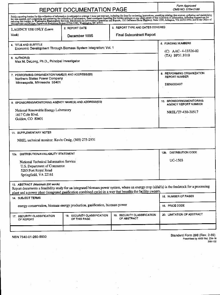
REPORT DOCUMENTATION PAGE Form Approved
OMB NO. 0704-0188
Public reporti~ burden for this collection of information is estimated to avera~e 1 hour p<r response, including the time for reviewing instructions, searching existi~ daUI sources, gathering and maintaining
the data need and co~lcting and reviewing the colledion of information. end comments regarding this burden estimate or any other aspect of this collection of information. including suggestions for
reducing this burden. to ashington H~ Services, Directorate for Information ~lions and Reports, 1215 Jefferson Davis Bigliway, Suite 1204, Arlington. VA 222024302, and to the Office of
Manaeement and Bud•"' Pan...workRedtictionProiect 10704-0188). Washlnotnn DC 20 03. _
l.AGENCY USE ONLY (Leave 2. REPORT DATE 3. REPORT TYPE AND DATES COVERED
blank) December 1995 Final Subcontract Report
4. TITLE AND SUBTITLE 5. FUNDING NUMBERS
Economic Development Through Biomass System Integration: Vol. 1 (C) AAC- 4-13326-02
6. AUTHOR(S) (TA) BP51.1010
Max M. Delong, Ph.D., Principal Investigator
7. PERFORMING ORGANIZATION NAME(S) AND ADDRESS(ES) 8. PERFORMING ORGANIZATION
Northern States Power Company REPORT NUMBER
Minneapolis, Minnesota 55401 DE96000497
9. SPONSORING/MONITORING AGENCY NAME(S) AND ADDRESS(ES) 10. SPONSORING/MONITORING AGENCY REPORT NUMBER
National Renewable Energy Laboratory NRELtrP-430-20517
1617 Cole Blvd. Golden, CO 80401
11. SUPPLEMENTARY NOTES
NREL technical monitor: Kevin Craig, (303) 275-2931
12a. DISTRIBUTION/AVAILABILITY ST A TEMENT 12b. DISTRIBUTION CODE
National Technical Information Service UC-1503
U.S. Department of Commerce
5285 Port Royal Road Springfield, VA 22161
13. ABSTRACT (Maximum 200 words)
Report documents a feasibility study for an integrated biomass power system. where an energy crop (alfalfa) is the feedstock for a processing
nlant and a vower nlant (integrated gasification combined cvcle) in a wav that benefits the facilitv owners.
14. SUBJECT TERMS
energy conservation, biomass energy production, gasification, biomass power
17. SECURITY CLASSIFICATION 18. SECURITY CLASSIFICATION 19. SECURITY CLASSIFICATION
OF REPORT OF THIS PAGE OF ABSTRACT
NSN 7540-01-280-5500
15.
16.
20.
NUMBER OF PAGES
PRICE CODE
LIMITATION OF ABSTRACT
Standard Form 298 (Rev. 2-89) Prescribed by ANSI Std. Z39-18
298-102
Related Documents