Economic Book Content: Name of Topics Name of the Topics 1. Prospectus & Study Guide 2. Mathematical Economics 3. Short Notes on Microeconomics 4. Short Notes on Macroeconomics 5. Growth Models 6. Indian Economic Issues

Welcome message from author
This document is posted to help you gain knowledge. Please leave a comment to let me know what you think about it! Share it to your friends and learn new things together.
Transcript

Economic Book
Content:
Name of Topics Name of the Topics
1. Prospectus & Study Guide 2. Mathematical Economics
3. Short Notes on Microeconomics 4. Short Notes on Macroeconomics
5. Growth Models 6. Indian Economic Issues

CTANUJIT CLASSES OF MATHEMATICS &
STATISTICS & ECONOMICS
Prospectus of Economics
ECONOMICS EDUCATION IN INDIA
Good Places for B.Sc in Economics(H) in India:-
1. Delhi University: There are many popular colleges, namely St. Stephen’s
College, Ramjas College where they provide rigorous training in Economics with
strong teaching of Mathematics, Statistics.
2. Presidency University: As this is the college where Nobel Laureate Dr.
Amartya Sen studied so it has a very good department with good faculties.
3. Calcutta University: Notable colleges are St. Xaviers College, Narrendrapur
Ramkrishna Mission, Bellur Vidyamandira, Scotish Charch College, Asutosh
College.
4. Jadavpur University: One of the good place to have B.Sc in Economics.
5. Madras School Of Economics: In collaboration with Central University of
Tamil Nadu they started B.Sc Economics which is good in nature.
Eligibility: 10+2 with Mathematics as a subject.
Good Places for M.Sc in Economics in India:-
Eligibility: Bachelors Degree with Mathematics/Statistics/Economics as a subject
or B.Tech Degree.
Places are:
1. Indian Statistical Institute: MSQE is offered in Delhi & Kolkata, undoubtedly
the Best Masters program in Economics in India.
2. Delhi School of Economics: Delhi University is among the top places offereing
MA in Economics.

3. Jawaharlal Nehru University: Offers MA in Economics & the program is
highly rigorous.
4. Indira Gandhi Institute of Development Research: An RBI Institute in
Mumbai offers M.Sc Economics.
5. Centre for Development Studies, Kerala: Applied Economics Institute under
JNU offers MA in Applied Economics.
6. Madras School of Economics:
7. Gokhale Institute of Politics & Economics
8. Jamia Millia Islamia
9. University of Hyderabad
10. TERI University
Good Places for Ph.D in Economics:
Indian Statistical Institute (Delhi, Kolkata)
Delhi School Of Economics (Delhi)
Indira Gandhi Institute of Development Research (Mumbai)
Jawaharlal Nehru University (Delhi)
Centre For Development Studies (Kerala)
Career Options after M.Sc in Economics in India:
1. INDIAN ECONOMIC SERVICES (IES)
2. RESERVE BANK OF INDIA (Economic Research Officer)
3. Economic Advisor in SEBI (Security Exchange Board of India)
4. RESEARCHER OR PROFESSORS IN COLLEGES & UNIVERSITIES
5. Economical Advisor in Nationalized Banks, namely SBI, UBI
6. Business Analyst: The leading job in modern times is the job of data
analysis. A good knowledge of SAS, SPSS can help you to get this type of
job with a marginal ability in the fields of Statistics.
7. Econometrician: There is also an another option to be an Econometrician
with good knowledge in Statistics, Time Series analysis, Economics.
Reference Books for MA/MSc/MPhil Economics Entrance Exams:
MICROECONOMICS (1) Intermediate Microeconomics by Varian 7th edition and workouts
(2) Microeconomics by Pyndick and Rubinfield 6th edition
(3) Fundamentals of Microeconomics by Nicholson and Snyder (high level)
MACROECONOMICS
(1) Macroeconomics by Abel and Bernanke (conceptual)
(2) Macroeconomics by Olivier Blanchard
(3) Macroeconomics by Branson(Mathematical)
MATHEMATICS Mathematics for Economic Analysis by Sydsaeter and Hammond
STATISTICS Fundamentals of Mathematical Statistics by S.C. Gupta and V.K. Kapoor
ECONOMETRICS Basic Econometrics by Damodar Gujarati
Prepared By,
Ctanujit Classes of Mathematics, Statistics & Economics,
Website:www.ctanujit.weebly.com Blog: www.ctanujit.in
Call: +918420253573 Mail:[email protected]

MICROECONOMICS
Intermediate Microeconomics by
Varian 7th edition and workouts
Microeconomics by Pyndick and
Rubinfield 6th edition Fundamentals of Microeconomics by Nicholson and Snyder (high level)
Unit 1 - Consumer
Behavior The Market Mathematics for Microeconomics
Budget Constraint
Preferences and Utility
Preferences
Utility Max and Choice
Utility
Income and Substitution Effects
Choice
Demand
Revealed Preference
Slutsky Equation
Buying and Selling
Intertemporal Choice
Consumer Surplus
Market Demand
Equilibrium
Unit 2 - Producer and
Game Theory Technology Production Production Functions
Profit Max The cost of Production Cost Functions
Cost Min Profit Max and Perfect Competition Profit Max
Cost curves
Market Power: Monopoly and its
Pricing The Partial Equilibrium Competitive Model
Firm Supply
Monopolistic Competition and
Oligopoly
Monopoly
Monopoly Behavior
Oligopoly
Game Theory
Game Applications
Unit - 3 General
Equilibrium Exchange
General Equilibrium and Economic
Efficiency
Production
Welfare

Unit - 4 Market Failure Externalities
Public Goods
Asymmetric Information
Unit-5 Labor Market Factor Markets
Price and Employment of Factor
Inputs
MACROECONOMICS Macroeconomics by Abel and Bernanke (conceptual) Macroeconomics by Olivier Blanchard
Unit 1 - Labor Market Productivity, Output and Employment The Labor Market
Unit 2 - Asset Market The Asset Market, Money and Prices
Unit 3 - IS-LM, AD-AS
(closed eco) The IS-LM/AD-AS model- A General Framework Putting all Markets Together-the AS-AD model
Classical Business Cycle Analysis
Macroeconomics of Wage and Price Rigidity
Unit 4 - Inflation and
Unemployment Unemployment and Inflation The Natural Rate of Unemployment and Phillips Curve
Inflation, Activity and Nominal Money Growth
Unit 5 - Open economy
Macroeconomics Savings and Investment in the Open Economy Openness in Goods and Financial Markets
*also chap no. 12 Macroeconomic Dimensions of International The Goods Market in Open Economy
Finance from International Finance by Maurice D. Levi Output, Interest Rate and Exchange rate
Exchange Rate Regimes
Unit 6 - Consumption
and Investment Consumption, Savings and Investment
*Also to be done from Macroeconomics by Mankiw
Unit-7 Economic
Growth *The Basic Solow Model from Charles I Jones
Macroeconomics by
Branson(Mathematical) chap-1 to chap-9

MATHEMATICS
Fundamentals of Mathematical
Economics by AC Chiang
Mathematics for Economic Analysis by
Sydsaeter and Hammond
Topics From 11-12 class RD Sharma Mathematics (without Trigonometry)
Chap-1 to Chap-12 (3rd edition)
limits, continuity and Differentiability
Chap-1 to Chap-13 (4th edition)
Only Practice questions of Complete
Book Differeciation and Integration
Relations and Functions
Also go through the maths material of Actuarial Entrance (ACET)
Examination Matrices and Determinants
STATISTICS Mathematical Statistics and Applications by John E. Freund Fundamentals of Mathematical Statistics by S.C. Gupta and V.K. Kapoor
Probability (Practice Illustrations and back questions - very imp)
Probability Distributions and Probability Densities Descriptive Measures
Mathematical Expectation Probability 1 and 2
Special Probability Distributions Random Variables and Distribution Functions
Special Probability Densities Mathematical Expectation
Functions of Random Variables Special Discrete Probability Distributions
Sampling Distributions Special Continuous Probability Distributions
Point Estimation Correlation
Interval Estimation Linear and Curvilinear Regression
Hypothesis Testing *For Concept of Hypothesis refer to chap-5 of Applied Statistics for
Tests of Hypothesis: Means, Variance and Proportions Economists by Karmel and Polasik
Correlation and Regression
Also go through the stats material of Actuarial Entrance (ACET)
Examination
ECONOMETRICS Basic Econometrics by Damodar Gujarati Prepared by Akshay Jain
Chap1 to Chap-9 (up to Dummy Variable)(Practice Back Questions also) E-mail: [email protected]

STUDY NOTES ON MATHEMATICAL ECONOMICS & APPLICATIONS
Contents Page No. Chapter 1 Static Economic Models and The Concept of Equilibrium....... 1 Chapter 2 Matrix Algebra .......................................................................... 5 Chapter 3 Vector Space and Linear Transformation................................. 10 Chapter 4 Determinant, Inverse Matrix, and Cramer’s rule .....................16 Chapter 5 Differential Calculus and Comparative Statics.......................... 25 Chapter 6 Comparative Statics – Economic applications.......................... 36 Chapter 7 Optimization............................................................................... 44 Chapter 8 Optimization–multivariate case................................................. 61 Chapter 9 Optimization with equality constraints and Nonlinear Programming ...............................................................................................74 Chapter 10 General Equilibrium and Game Theory................................... 89
1
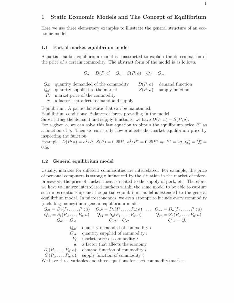
1 Static Economic Models and The Concept of Equilibrium
Here we use three elementary examples to illustrate the general structure of an eco-nomic model.
1.1 Partial market equilibrium model
A partial market equilibrium model is constructed to explain the determination ofthe price of a certain commodity. The abstract form of the model is as follows.
Qd = D(P ; a) Qs = S(P ; a) Qd = Qs,
Qd: quantity demanded of the commodity D(P ; a): demand functionQs: quantity supplied to the market S(P ; a): supply functionP : market price of the commoditya: a factor that affects demand and supply
Equilibrium: A particular state that can be maintained.Equilibrium conditions: Balance of forces prevailing in the model.Substituting the demand and supply functions, we have D(P ; a) = S(P ; a).For a given a, we can solve this last equation to obtain the equilibrium price P ∗ asa function of a. Then we can study how a affects the market equilibrium price byinspecting the function.
Example: D(P ; a) = a2/P , S(P ) = 0.25P . a2/P ∗ = 0.25P ∗ ⇒ P ∗ = 2a, Q∗d = Q∗
s =0.5a.
1.2 General equilibrium model
Usually, markets for different commodities are interrelated. For example, the priceof personal computers is strongly influenced by the situation in the market of micro-processors, the price of chicken meat is related to the supply of pork, etc. Therefore,we have to analyze interrelated markets within the same model to be able to capturesuch interrelationship and the partial equilibrium model is extended to the generalequilibrium model. In microeconomics, we even attempt to include every commodity(including money) in a general equilibrium model.Qd1 = D1(P1, . . . , Pn; a)Qs1 = S1(P1, . . . , Pn; a)
Qd1 = Qs1
Qd2 = D2(P1, . . . , Pn; a)Qs2 = S2(P1, . . . , Pn; a)
Qd2 = Qs2
. . . Qdn = Dn(P1, . . . , Pn; a)Qsn = Sn(P1, . . . , Pn; a)
Qdn = Qsn
Qdi: quantity demanded of commodity iQsi: quantity supplied of commodity iPi: market price of commodity ia: a factor that affects the economy
Di(P1, . . . , Pn; a): demand function of commodity iSi(P1, . . . , Pn; a): supply function of commodity i
We have three variables and three equations for each commodity/market.

2
Substituting the demand and supply functions, we have
D1(P1, . . . , Pn; a)− S1(P1, . . . , Pn; a) ≡ E1(P1, . . . , Pn; a) = 0D2(P1, . . . , Pn; a)− S2(P1, . . . , Pn; a) ≡ E2(P1, . . . , Pn; a) = 0
......
Dn(P1, . . . , Pn; a)− Sn(P1, . . . , Pn; a) ≡ En(P1, . . . , Pn; a) = 0.
For a given a, it is a simultaneous equation in (P1, . . . , Pn). There are n equationsand n unknown. In principle, we can solve the simultaneous equation to find theequilibrium prices (P ∗
1 , . . . , P ∗n).
A 2-market linear model:D1 = a0 + a1P1 + a2P2, S1 = b0 + b1P1 + b2P2, D2 = α0 + α1P1 + α2P2, S2 =β0 + β1P1 + β2P2.
(a0 − b0) + (a1 − b1)P1 + (a2 − b2)P2 = 0(α0 − β0) + (α1 − β1)P1 + (α2 − β2)P2 = 0.
1.3 National income model
The most fundamental issue in macroeconomics is the determination of the nationalincome of a country.
C = a + bY (a > 0, 0 < b < 1)I = I(r)Y = C + I + GS = Y − C.
C: Consumption Y : National incomeI: Investment S: SavingsG: government expenditure r: interest rate
a, b: coefficients of the consumption function.
To solve the model, we substitute the first two equations into the third to obtainY = a + bY + I0 + G ⇒ Y ∗ = (a + I(r) + G)/(1− b).
1.4 The ingredients of a model
We set up economic models to study economic phenomena (cause-effect relation-ships), or how certain economic variables affect other variables. A model consists ofequations, which are relationships among variables.
Variables can be divided into three categories:Endogenous variables: variables we choose to represent different states of a model.Exogenous variables: variables assumed to affect the endogenous variables but arenot affected by them.Causes (Changes in exogenous var.) ⇒ Effects (Changes in endogenous var.)Parameters: Coefficients of the equations.
3
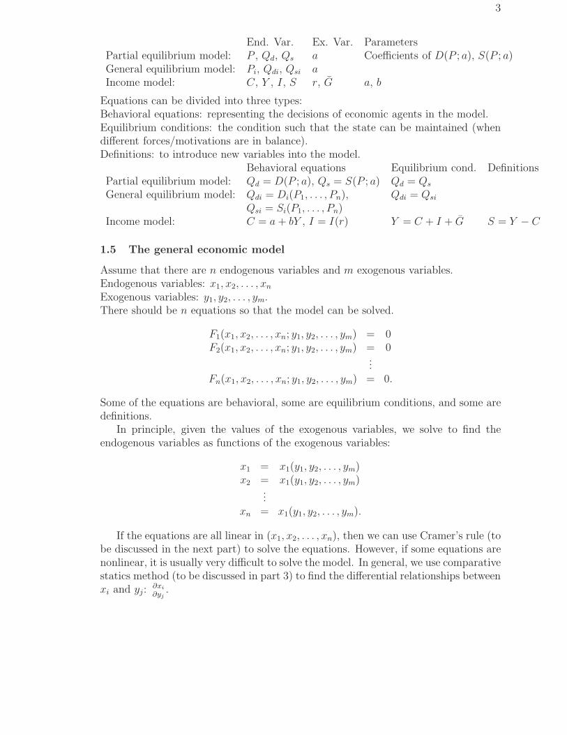
End. Var. Ex. Var. ParametersPartial equilibrium model: P , Qd, Qs a Coefficients of D(P ; a), S(P ; a)General equilibrium model: Pi, Qdi, Qsi aIncome model: C, Y , I, S r, G a, b
Equations can be divided into three types:Behavioral equations: representing the decisions of economic agents in the model.Equilibrium conditions: the condition such that the state can be maintained (whendifferent forces/motivations are in balance).Definitions: to introduce new variables into the model.
Behavioral equations Equilibrium cond. DefinitionsPartial equilibrium model: Qd = D(P ; a), Qs = S(P ; a) Qd = Qs
General equilibrium model: Qdi = Di(P1, . . . , Pn), Qdi = Qsi
Qsi = Si(P1, . . . , Pn)Income model: C = a + bY , I = I(r) Y = C + I + G S = Y − C
1.5 The general economic model
Assume that there are n endogenous variables and m exogenous variables.Endogenous variables: x1, x2, . . . , xn
Exogenous variables: y1, y2, . . . , ym.There should be n equations so that the model can be solved.
F1(x1, x2, . . . , xn; y1, y2, . . . , ym) = 0F2(x1, x2, . . . , xn; y1, y2, . . . , ym) = 0
...Fn(x1, x2, . . . , xn; y1, y2, . . . , ym) = 0.
Some of the equations are behavioral, some are equilibrium conditions, and some aredefinitions.
In principle, given the values of the exogenous variables, we solve to find theendogenous variables as functions of the exogenous variables:
x1 = x1(y1, y2, . . . , ym)x2 = x1(y1, y2, . . . , ym)
...xn = x1(y1, y2, . . . , ym).
If the equations are all linear in (x1, x2, . . . , xn), then we can use Cramer’s rule (tobe discussed in the next part) to solve the equations. However, if some equations arenonlinear, it is usually very difficult to solve the model. In general, we use comparativestatics method (to be discussed in part 3) to find the differential relationships betweenxi and yj:
∂xi
∂yj.
4
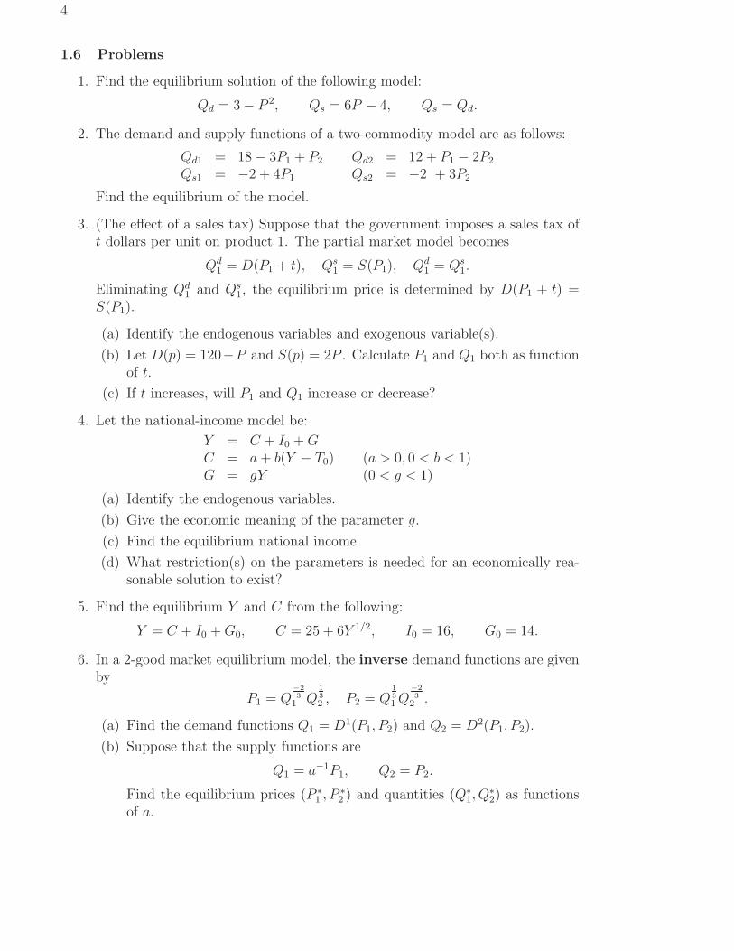
1.6 Problems
1. Find the equilibrium solution of the following model:
Qd = 3− P 2, Qs = 6P − 4, Qs = Qd.
2. The demand and supply functions of a two-commodity model are as follows:
Qd1 = 18− 3P1 + P2 Qd2 = 12 + P1 − 2P2
Qs1 = −2 + 4P1 Qs2 = −2 + 3P2
Find the equilibrium of the model.
3. (The effect of a sales tax) Suppose that the government imposes a sales tax oft dollars per unit on product 1. The partial market model becomes
Qd1 = D(P1 + t), Qs
1 = S(P1), Qd1 = Qs
1.
Eliminating Qd1 and Qs
1, the equilibrium price is determined by D(P1 + t) =S(P1).
(a) Identify the endogenous variables and exogenous variable(s).
(b) Let D(p) = 120−P and S(p) = 2P . Calculate P1 and Q1 both as functionof t.
(c) If t increases, will P1 and Q1 increase or decrease?
4. Let the national-income model be:
Y = C + I0 + GC = a + b(Y − T0) (a > 0, 0 < b < 1)G = gY (0 < g < 1)
(a) Identify the endogenous variables.
(b) Give the economic meaning of the parameter g.
(c) Find the equilibrium national income.
(d) What restriction(s) on the parameters is needed for an economically rea-sonable solution to exist?
5. Find the equilibrium Y and C from the following:
Y = C + I0 + G0, C = 25 + 6Y 1/2, I0 = 16, G0 = 14.
6. In a 2-good market equilibrium model, the inverse demand functions are givenby
P1 = Q−2
3
1 Q1
3
2 , P2 = Q1
3
1 Q−2
3
2 .
(a) Find the demand functions Q1 = D1(P1, P2) and Q2 = D2(P1, P2).
(b) Suppose that the supply functions are
Q1 = a−1P1, Q2 = P2.
Find the equilibrium prices (P ∗1 , P ∗
2 ) and quantities (Q∗1, Q
∗2) as functions
of a.
5
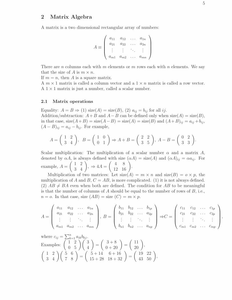
2 Matrix Algebra
A matrix is a two dimensional rectangular array of numbers:
A ≡
a11 a12 . . . a1n
a21 a22 . . . a2n...
.... . .
...am1 am2 . . . amn
There are n columns each with m elements or m rows each with n elements. We saythat the size of A is m× n.If m = n, then A is a square matrix.A m× 1 matrix is called a column vector and a 1× n matrix is called a row vector.A 1× 1 matrix is just a number, called a scalar number.
2.1 Matrix operations
Equality: A = B ⇒ (1) size(A) = size(B), (2) aij = bij for all ij.Addition/subtraction: A+B and A−B can be defined only when size(A) = size(B),in that case, size(A+B) = size(A−B) = size(A) = size(B) and (A+B)ij = aij + bij ,(A− B)ij = aij − bij . For example,
A =
(
1 23 4
)
, B =
(
1 00 1
)
⇒ A + B =
(
2 23 5
)
, A− B =
(
0 23 3
)
.
Scalar multiplication: The multiplication of a scalar number α and a matrix A,denoted by αA, is always defined with size (αA) = size(A) and (αA)ij = αaij. For
example, A =
(
1 23 4
)
, ⇒ 4A =
(
4 812 16
)
.
Multiplication of two matrices: Let size(A) = m × n and size(B) = o × p, themultiplication of A and B, C = AB, is more complicated. (1) it is not always defined.(2) AB 6= BA even when both are defined. The condition for AB to be meaningfulis that the number of columns of A should be equal to the number of rows of B, i.e.,n = o. In that case, size (AB) = size (C) = m× p.
A =
a11 a12 . . . a1n
a21 a22 . . . a2n...
.... . .
...am1 am2 . . . amn
, B =
b11 b12 . . . b1p
b21 b22 . . . a2p...
.... . .
...bn1 bn2 . . . anp
⇒C =
c11 c12 . . . c1p
c21 c22 . . . c2p...
.... . .
...cm1 cm2 . . . cmp
,
where cij =∑n
k=1 aikbkj .
Examples:
(
1 20 5
)(
34
)
=
(
3 + 80 + 20
)
=
(
1120
)
,(
1 23 4
)(
5 67 8
)
=
(
5 + 14 6 + 1615 + 28 18 + 32
)
=
(
19 2243 50
)
,

6
(
5 67 8
)(
1 23 4
)
=
(
5 + 18 10 + 247 + 24 14 + 32
)
=
(
23 3431 46
)
.
Notice that
(
1 23 4
)(
5 67 8
)
6=(
5 67 8
)(
1 23 4
)
.
2.2 Matrix representation of a linear simultaneous equation system
A linear simultaneous equation system:
a11x1 + . . . + a1nxn = b1...
...an1x1 + . . . + annxn = bn
Define A ≡
a11 . . . a1n...
. . ....
an1 . . . ann
, x ≡
x1...
xn
and b ≡
b1...bn
. Then the equation
Ax = b is equivalent to the simultaneous equation system.
Linear 2-market model:
E1 = (a1 − b1)p1 + (a2 − b2)p2 + (a0 − b0) = 0E2 = (α1 − β1)p1 + (α2 − β2)p2 + (α0 − β0) = 0
⇒(
a1 − b1 a2 − b2
α1 − β1 α2 − β2
)(
p1
p2
)
+
(
a0 − b0
α0 − β0
)
=
(
00
)
.
Income determination model:
C = a + bYI = I(r)
Y = C + I⇒
1 0 −b0 1 01 1 −1
CIY
=
aI(r)0
.
In the algebra of real numbers, the solution to the equation ax = b is x = a−1b.In matrix algebra, we wish to define a concept of A−1 for a n × n matrix A so thatx = A−1b is the solution to the equation Ax = b.
2.3 Commutative, association, and distributive laws
The notations for some important sets are given by the following table.N = nature numbers 1, 2, 3, . . . I = integers . . . ,−2,−1, 0, 1, 2, . . .Q = rational numbers m
nR = real numbers
Rn = n-dimensional column vectors M(m, n) = m× n matricesM(n) = n× n matrices
A binary operation is a law of composition of two elements from a set to form athird element of the same set. For example, + and × are binary operations of realnumbers R.Another important example: addition and multiplication are binary operations of ma-trices.
7
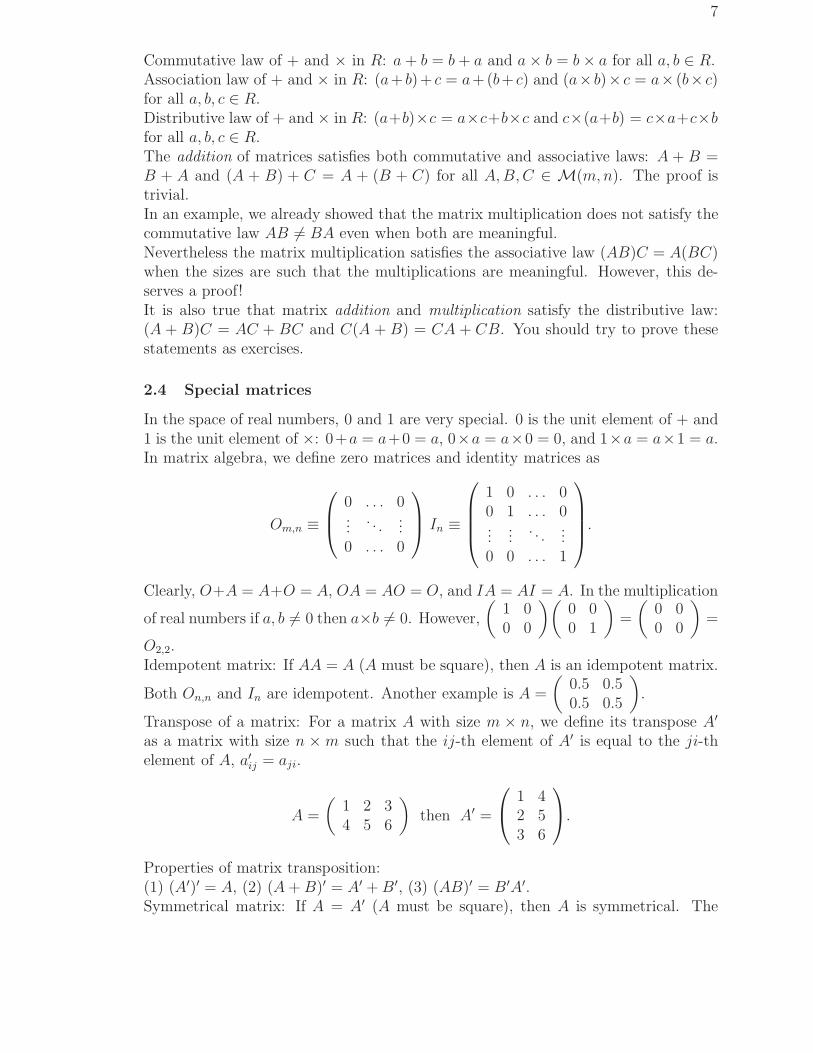
Commutative law of + and × in R: a + b = b + a and a× b = b× a for all a, b ∈ R.Association law of + and × in R: (a+ b)+ c = a+(b+ c) and (a× b)× c = a× (b× c)for all a, b, c ∈ R.Distributive law of + and × in R: (a+b)×c = a×c+b×c and c×(a+b) = c×a+c×bfor all a, b, c ∈ R.The addition of matrices satisfies both commutative and associative laws: A + B =B + A and (A + B) + C = A + (B + C) for all A, B, C ∈ M(m, n). The proof istrivial.In an example, we already showed that the matrix multiplication does not satisfy thecommutative law AB 6= BA even when both are meaningful.Nevertheless the matrix multiplication satisfies the associative law (AB)C = A(BC)when the sizes are such that the multiplications are meaningful. However, this de-serves a proof!It is also true that matrix addition and multiplication satisfy the distributive law:(A + B)C = AC + BC and C(A + B) = CA + CB. You should try to prove thesestatements as exercises.
2.4 Special matrices
In the space of real numbers, 0 and 1 are very special. 0 is the unit element of + and1 is the unit element of ×: 0+a = a+0 = a, 0×a = a×0 = 0, and 1×a = a×1 = a.In matrix algebra, we define zero matrices and identity matrices as
Om,n ≡
0 . . . 0...
. . ....
0 . . . 0
In ≡
1 0 . . . 00 1 . . . 0...
.... . .
...0 0 . . . 1
.
Clearly, O+A = A+O = A, OA = AO = O, and IA = AI = A. In the multiplication
of real numbers if a, b 6= 0 then a×b 6= 0. However,
(
1 00 0
)(
0 00 1
)
=
(
0 00 0
)
=
O2,2.Idempotent matrix: If AA = A (A must be square), then A is an idempotent matrix.
Both On,n and In are idempotent. Another example is A =
(
0.5 0.50.5 0.5
)
.
Transpose of a matrix: For a matrix A with size m × n, we define its transpose A′
as a matrix with size n ×m such that the ij-th element of A′ is equal to the ji-thelement of A, a′ij = aji.
A =
(
1 2 34 5 6
)
then A′ =
1 42 53 6
.
Properties of matrix transposition:(1) (A′)′ = A, (2) (A + B)′ = A′ + B′, (3) (AB)′ = B′A′.Symmetrical matrix: If A = A′ (A must be square), then A is symmetrical. The

8
condition for A to be symmetrical is that aij = aji. Both On,n and In are symmetrical.
Another example is A =
(
1 22 3
)
.
Projection matrix: A symmetrical idempotent matrix is a projection matrix.Diagonal matrix: A symmetrical matrix A is diagonal if aij = 0 for all i 6= j. Both
In and On,n are diagonal. Another example is A =
λ1 0 00 λ2 00 0 λ3
2.5 Inverse of a square matrix
We are going to define the inverse of a square matrix A ∈M(n).Scalar: aa−1 = a−1a = 1⇒ if b satisfies ab = ba = 1 then b = a−1.Definition of A−1: If there exists a B ∈ M(n) such that AB = BA = In, then wedefine A−1 = B.Examples: (1) Since II = I, I−1 = I. (2) On,nB = On,n ⇒ O−1
n,n does not exist. (3)
If A =
(
a1 00 a2
)
, a1, a2 6= 0, then A−1 =
(
a−11 00 a−1
2
)
. (4) If a1 = 0 or a2 = 0,
then A−1 does not exist.Singular matrix: A square matrix whose inverse matrix does not exist.Non-singular matrix: A is non-singular if A−1 exists.
Properties of matrix inversion:Let A, B ∈M(n), (1) (A−1)−1 = A, (2) (AB)−1 = B−1A−1, (3) (A′)−1 = (A−1)′.
2.6 Problems
1. Let A = I −X(X ′X)−1X ′.(a) If the dimension of X is m× n, what must be the dimension of I and A.(b) Show that matrix A is idempotent.
2. Let A and B be n× n matrices and I be the identity matrix.(a) (A + B)3 = ?(b) (A + I)3 = ?
3. Let B =
((
0.5 0.50.5 0.5
))
, U = (1, 1)′, V = (1,−1)′, and W = aU + bV , where
a and b are real numbers. Find BU , BV , and BW . Is B idempotent?
4. Suppose A is a n× n nonsingular matrix and P is a n× n idempotent matrix.Show that APA−1 is idempotent.
5. Suppose that A and B are n×n symmetric idempotent matrices and AB = B.Show that A− B is idempotent.
6. Calculate (x1, x2)
(
3 22 5
)(
x1
x2
)
.
9
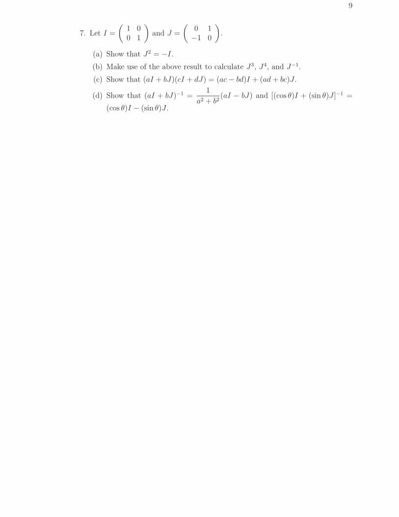
7. Let I =
(
1 00 1
)
and J =
(
0 1−1 0
)
.
(a) Show that J2 = −I.
(b) Make use of the above result to calculate J3, J4, and J−1.
(c) Show that (aI + bJ)(cI + dJ) = (ac− bd)I + (ad + bc)J .
(d) Show that (aI + bJ)−1 =1
a2 + b2(aI − bJ) and [(cos θ)I + (sin θ)J ]−1 =
(cos θ)I − (sin θ)J .

10
3 Vector Space and Linear Transformation
In the last section, we regard a matrix simply as an array of numbers. Now we aregoing to provide some geometrical meanings to a matrix.(1) A matrix as a collection of column (row) vectors(2) A matrix as a linear transformation from a vector space to another vector space
3.1 Vector space, linear combination, and linear independence
Each point in the m-dimensional Euclidean space can be represented as a m-dimensional
column vector v =
v1...
vm
, where each vi represents the i-th coordinate. Two points
in the m-dimensional Euclidean space can be added according to the rule of matrixaddition. A point can be multiplied by a scalar according to the rule of scalar multi-plication.
Vector addition:
v1...
vm
+
w1...
wm
=
v1 + w1...
vm + wm
.
Scalar multiplication: α
v1...
vm
=
αv1...
αvm
.
✲x1
✻x2
✑✑✑✑✑✑✸
v1✡✡✡✡✡✡✡✣
✡✡✡✡✡✡✡✣
v2
✒ v1 + v2
✲x1
✻x2
✒v ✒
2v
With such a structure, we say that the m-dimensional Euclidean space is a vec-tor space.
11
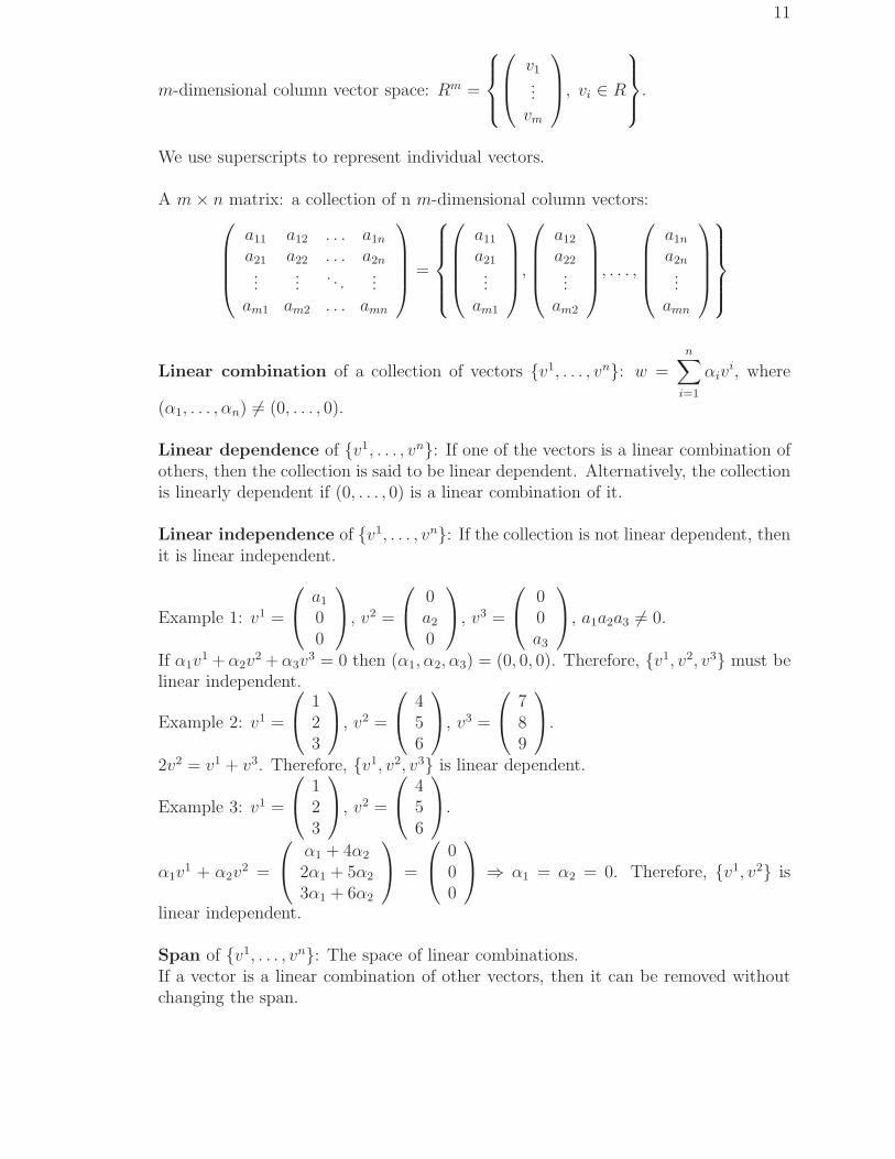
m-dimensional column vector space: Rm =
v1...
vm
, vi ∈ R
.
We use superscripts to represent individual vectors.
A m× n matrix: a collection of n m-dimensional column vectors:
a11 a12 . . . a1n
a21 a22 . . . a2n...
.... . .
...am1 am2 . . . amn
=
a11
a21...
am1
,
a12
a22...
am2
, . . . ,
a1n
a2n...
amn
Linear combination of a collection of vectors {v1, . . . , vn}: w =
n∑
i=1
αivi, where
(α1, . . . , αn) 6= (0, . . . , 0).
Linear dependence of {v1, . . . , vn}: If one of the vectors is a linear combination ofothers, then the collection is said to be linear dependent. Alternatively, the collectionis linearly dependent if (0, . . . , 0) is a linear combination of it.
Linear independence of {v1, . . . , vn}: If the collection is not linear dependent, thenit is linear independent.
Example 1: v1 =
a1
00
, v2 =
0a2
0
, v3 =
00a3
, a1a2a3 6= 0.
If α1v1 + α2v
2 + α3v3 = 0 then (α1, α2, α3) = (0, 0, 0). Therefore, {v1, v2, v3} must be
linear independent.
Example 2: v1 =
123
, v2 =
456
, v3 =
789
.
2v2 = v1 + v3. Therefore, {v1, v2, v3} is linear dependent.
Example 3: v1 =
123
, v2 =
456
.
α1v1 + α2v
2 =
α1 + 4α2
2α1 + 5α2
3α1 + 6α2
=
000
⇒ α1 = α2 = 0. Therefore, {v1, v2} is
linear independent.
Span of {v1, . . . , vn}: The space of linear combinations.If a vector is a linear combination of other vectors, then it can be removed withoutchanging the span.

12
Rank
v11 . . . v1n...
. . ....
vm1 . . . vmn
≡ Dimension(Span{v1, . . . , vn}) = Maximum # of indepen-
dent vectors.
3.2 Linear transformation
Consider a m × n matrix A. Given x ∈ Rn, Ax ∈ Rm. Therefore, we can define alinear transformation from Rn to Rm as f(x) = Ax or
f : Rn→Rm, f(x) =
y1...
ym
=
a11 . . . a1n...
. . ....
am1 . . . amn
x1...
xn
.
It is linear because f(αx + βw) = A(αx + βw) = αAx + βAw = αf(x) + βf(w).
Standard basis vectors of Rn: e1 ≡
10...0
, e2 ≡
01...0
, . . . , en ≡
00...1
.
Let vi be the i-th column of A, vi =
a1i...
ami
.
vi = f(ei):
a11
. . .am1
=
a11 . . . a1n...
. . ....
am1 . . . amn
1...0
⇒ v1 = f(e1) = Ae1, etc.
Therefore, vi is the image of the i-th standard basis vector ei under f .Span{v1, . . . , vn} = Range space of f(x) = Ax ≡ R(A).Rank(A) ≡ dim(R(A)).Null space of f(x) = Ax: N(A) ≡ {x ∈ Rn, f(x) = Ax = 0}.dim(R(A)) + dim(N(A)) = n.
Example 1: A =
(
1 00 2
)
. N(A) =
{(
00
)}
, R(A) = R2, Rank(A) = 2.
Example 2: B =
(
1 11 1
)
. N(B) =
{(
k−k
)
, k ∈ R
}
, R(B) =
{(
kk
)
, k ∈ R
}
,
Rank(B) = 1.
The multiplication of two matrices can be interpreted as the composition of twolinear transformations.
f : Rn→Rm, f(x) = Ax, g : Rp→Rn, g(y) = By, ⇒ f(g(x)) = A(By), f◦g : Rp→Rm.
13
The composition is meaningful only when the dimension of the range space of g(y)is equal to the dimension of the domain of f(x), which is the same condition for thevalidity of the matrix multiplication.
Every linear transformation f : Rn→Rm can be represented by f(x) = Ax forsome m× n matrix.
3.3 Inverse transformation and inverse of a square matrix
Consider now the special case of square matrices. Each A ∈ M(n) represents a lineartransformation f : Rn→Rn.The definition of the inverse matrix A−1 is such that AA−1 = A−1A = I. If we re-gard A as a linear transformation from Rn→Rn and I as the identity transformationthat maps every vector (point) into itself, then A−1 is the inverse mapping of A. Ifdim(N(A)) = 0, then f(x) is one to one.If dim(R(A)) = n, then R(A) = Rn and f(x) is onto.⇒ if Rank(A) = n, then f(x) is one to one and onto and there exits an inverse mappingf−1 : Rn→Rn represented by a n×n square matrix A−1. f−1f(x) = x⇒ A−1Ax = x.⇒ if Rank(A) = n, then A is non-singular.if Rank(A) < n, then f(x) is not onto, no inverse mapping exists, and A is singular.
Examples: Rank
a1 0 00 a2 00 0 a3
= 3 and Rank
1 4 72 5 83 6 9
= 2.
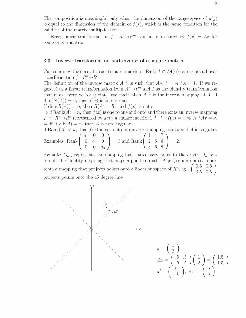
Remark: On,n represents the mapping that maps every point to the origin. In rep-resents the identity mapping that maps a point to itself. A projection matrix repre-
sents a mapping that projects points onto a linear subspace of Rn, eg.,
(
0.5 0.50.5 0.5
)
projects points onto the 45 degree line.
✲x1
✻x2
❅❅❅❅❅❅❅❅■
❅❅❅❅❅❅❅❅❘
❅❅❘
x
Ax
x =
(
12
)
Ax =
(
.5 .5
.5 .5
)(
12
)
=
(
1.51.5
)
x′ =
(
k−k
)
, Ax′ =
(
00
)
14
3.4 Problems
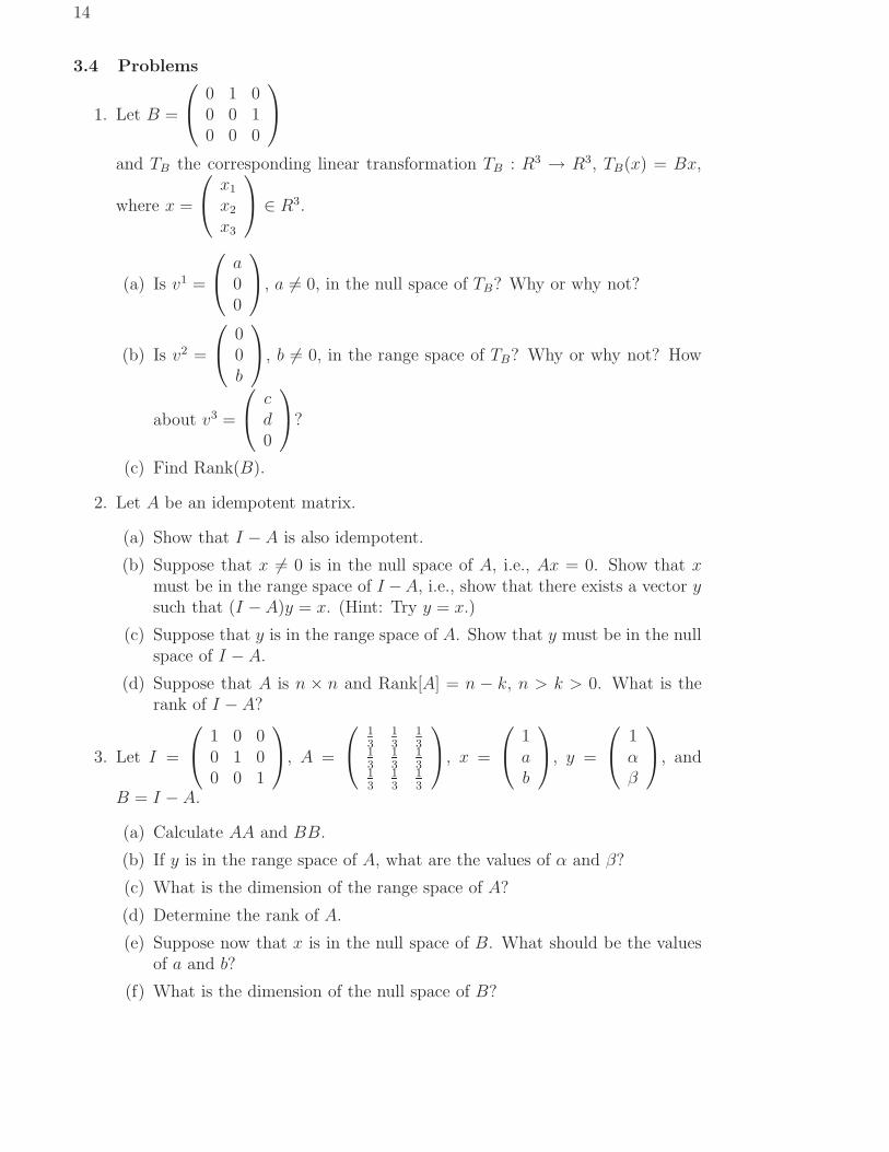
1. Let B =
0 1 00 0 10 0 0
and TB the corresponding linear transformation TB : R3 → R3, TB(x) = Bx,
where x =
x1
x2
x3
∈ R3.
(a) Is v1 =
a00
, a 6= 0, in the null space of TB? Why or why not?
(b) Is v2 =
00b
, b 6= 0, in the range space of TB? Why or why not? How
about v3 =
cd0
?
(c) Find Rank(B).
2. Let A be an idempotent matrix.
(a) Show that I − A is also idempotent.
(b) Suppose that x 6= 0 is in the null space of A, i.e., Ax = 0. Show that xmust be in the range space of I −A, i.e., show that there exists a vector ysuch that (I −A)y = x. (Hint: Try y = x.)
(c) Suppose that y is in the range space of A. Show that y must be in the nullspace of I − A.
(d) Suppose that A is n × n and Rank[A] = n − k, n > k > 0. What is therank of I − A?
3. Let I =
1 0 00 1 00 0 1
, A =
13
13
13
13
13
13
13
13
13
, x =
1ab
, y =
1αβ
, and
B = I − A.
(a) Calculate AA and BB.
(b) If y is in the range space of A, what are the values of α and β?
(c) What is the dimension of the range space of A?
(d) Determine the rank of A.
(e) Suppose now that x is in the null space of B. What should be the valuesof a and b?
(f) What is the dimension of the null space of B?
15
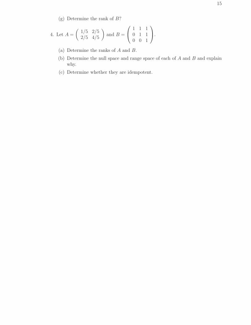
(g) Determine the rank of B?
4. Let A =
(
1/5 2/52/5 4/5
)
and B =
1 1 10 1 10 0 1
.
(a) Determine the ranks of A and B.
(b) Determine the null space and range space of each of A and B and explainwhy.
(c) Determine whether they are idempotent.

16
4 Determinant, Inverse Matrix, and Cramer’s rule
In this section we are going to derive a general method to calculate the inverse ofa square matrix. First, we define the determinant of a square matrix. Using theproperties of determinants, we find a procedure to compute the inverse matrix. Thenwe derive a general procedure to solve a simultaneous equation.
4.1 Permutation group
A permutation of {1, 2, . . . , n} is a 1-1 mapping of {1, 2, . . . , n} onto itself, written as
π =
(
1 2 . . . ni1 i2 . . . in
)
meaning that 1 is mapped to i1, 2 is mapped to i2, . . ., and
n is mapped to in. We also write π = (i1, i2, . . . , ın) when no confusing.
Permutation set of {1, 2, . . . , n}: Pn ≡ {π = (i1, i2, . . . , in) : π is a permutation}.P2 = {(1, 2), (2, 1)}.P3 = {(1, 2, 3), (1, 3, 2), (2, 1, 3), (2, 3, 1), (3, 1, 2), (3, 2, 1)}.P4: 4! = 24 permutations.
Inversions in a permutation π = (i1, i2, . . . , in): If there exist k and l such thatk < l and ik > il, then we say that an inversion occurs.N(i1, i2, . . . , ın): Total number of inversions in (i1, i2, . . . , in).Examples: 1. N(1, 2) = 0, N(2, 1) = 1.
2. N(1, 2, 3) = 0, N(1, 3, 2) = 1, N(2, 1, 3) = 1,N(2, 3, 1) = 2, N(3, 1, 2) = 2, N(3, 2, 1) = 3.
4.2 Determinant
Determinant of A =
a11 a12 . . . a1n
a21 a22 . . . a2n...
.... . .
...an1 an2 . . . ann
:
|A| ≡∑
(i1,i2,...,in)∈Pn
(−1)N(i1,i2,...,in)a1i1a2i2 . . . anin .
n = 2:
∣
∣
∣
∣
a11 a12
a21 a22
∣
∣
∣
∣
= (−1)N(1,2)a11a22 + (−1)N(2,1)a12a21 = a11a22 − a12a21.
n = 3:
∣
∣
∣
∣
∣
∣
a11 a12 a13
a21 a22 a23
a31 a32 a33
∣
∣
∣
∣
∣
∣
=
(−1)N(1,2,3)a11a22a33 + (−1)N(1,3,2)a11a23a32 + (−1)N(2,1,3)a12a21a33 +(−1)N(2,3,1)a12a23a31 + (−1)N(3,1,2)a13a21a32 + (−1)N(3,2,1)a13a22a31
= a11a22a33 − a11a23a32 − a12a21a33 + a12a23a31 + a13a21a32 − a13a22a31.

17
a11 a12
a21 a22
❅❅❘ ✒n = 2:
a11 a12 a13 a11 a12
a21 a22 a23 a21 a22
a31 a32 a33 a31 a32
❅❅❘
❅❅❘
❅❅❘
❅❅❘
❅❅❘
❅❅❘
✒
✒
✒
✒
✒
✒
n = 3:
4.3 Properties of determinant
Property 1: |A′| = |A|.Proof: Each term of |A′| corresponds to a term of |A| of the same sign.By property 1, we can replace “column vectors” in the properties below by “row vec-tors”.Since a n × n matrix can be regarded as n column vectors A = {v1, v2, . . . , vn}, wecan regard determinants as a function of n column vectors |A| = D(v1, v2, . . . , vn),D : Rn×n→R.By property 1, we can replace “column vectors” in the properties below by “row vec-tors”.
Property 2: If two column vectors are interchanged, the determinant changes sign.Proof: Each term of the new determinant corresponds to a term of |A| of oppositesign because the number of inversion increases or decreases by 1.
Example:
∣
∣
∣
∣
1 23 4
∣
∣
∣
∣
= 1× 4− 2× 3 = −2,
∣
∣
∣
∣
2 14 3
∣
∣
∣
∣
= 2× 3− 1× 4 = 2,
Property 3: If two column vectors are identical, then the determinant is 0.Proof: By property 2, the determinant is equal to the negative of itself, which ispossible only when the determinant is 0.
Property 4: If you add a linear combination of other column vectors to a columnvector, the determinant does not change.Proof: Given other column vectors, the determinant function is a linear function ofvi: D(αvi + βwi; other vectors ) = αD(vi; other vectors ) + βD(wi; other vectors ).
Example:
∣
∣
∣
∣
1 + 5× 2 23 + 5× 4 4
∣
∣
∣
∣
=
∣
∣
∣
∣
1 23 4
∣
∣
∣
∣
+
∣
∣
∣
∣
5× 2 25× 4 4
∣
∣
∣
∣
=
∣
∣
∣
∣
1 23 4
∣
∣
∣
∣
+ 5 ×∣
∣
∣
∣
2 24 4
∣
∣
∣
∣
=∣
∣
∣
∣
1 23 4
∣
∣
∣
∣
+ 5× 0.
Submatrix: We denote by Aij the submatrix of A obtained by deleting the i-throw and j-th column from A.Minors: The determinant |Aij| is called the minor of the element aij .Cofactors: Cij ≡ (−1)i+j|Aij | is called the cofactor of aij .

18
Property 5 (Laplace theorem): Given i = i, |A| =n∑
j=1
aijCij.
Given j = j, |A| = ∑ni=1 aijCij.
Proof: In the definition of the determinant of |A|, all terms with aij can be put to-gethere to become aijCij.
Example:
∣
∣
∣
∣
∣
∣
1 2 34 5 67 8 0
∣
∣
∣
∣
∣
∣
= 1×∣
∣
∣
∣
5 68 0
∣
∣
∣
∣
− 2×∣
∣
∣
∣
4 67 0
∣
∣
∣
∣
+ 3×∣
∣
∣
∣
4 57 8
∣
∣
∣
∣
.
Property 6: Given i′ 6= i,n∑
j=1
ai′jCij = 0.
Given j′ 6= j, =∑n
i=1 aij′Cij = 0.Therefore, if you multiply cofactors by the elements from a different row or column,you get 0 instead of the determinant.Proof: The sum becomes the determinant of a matrix with two identical rows (columns).
Example: 0 = 4×∣
∣
∣
∣
5 68 0
∣
∣
∣
∣
− 5×∣
∣
∣
∣
4 67 0
∣
∣
∣
∣
+ 6×∣
∣
∣
∣
4 57 8
∣
∣
∣
∣
.
4.4 Computation of the inverse matrix
Using properties 5 and 6, we can calculate the inverse of A as follows.
1. Cofactor matrix: C ≡
C11 C12 . . . C1n
C21 C22 . . . C2n...
.... . .
...Cn1 Cn2 . . . Cnn
.
2. Adjoint of A: Adj A ≡ C ′ =
C11 C21 . . . Cn1
C12 C22 . . . Cn2...
.... . .
...C1n C2n . . . Cnn
.
3. ⇒ AC ′ = C ′A =
|A| 0 . . . 00 |A| . . . 0...
.... . .
...0 0 . . . |A|
⇒ if |A| 6= 0 then 1|A|C
′ = A−1.
Example 1: A =
(
a11 a12
a21 a22
)
then C =
(
a22 −a21
−a12 a11
)
.
A−1 =1
|A|C′ =
1
a11a22 − a12a21
(
a22 −a12
−a21 a11
)
; if |A| = a11a22 − a12a21 6= 0.
Example 2: A =
1 2 34 5 67 8 0
⇒ |A| = 27 6= 0 and
C11 =
∣
∣
∣
∣
5 68 0
∣
∣
∣
∣
= −48, C12 = −∣
∣
∣
∣
4 67 0
∣
∣
∣
∣
= 42, C13 =
∣
∣
∣
∣
4 57 8
∣
∣
∣
∣
= −3,
19
C21 = −∣
∣
∣
∣
2 38 0
∣
∣
∣
∣
= 24, C22 =
∣
∣
∣
∣
1 37 0
∣
∣
∣
∣
= −21, C23 = −∣
∣
∣
∣
1 27 8
∣
∣
∣
∣
= 6,
C31 =
∣
∣
∣
∣
2 35 6
∣
∣
∣
∣
= −3, C32 = −∣
∣
∣
∣
1 34 6
∣
∣
∣
∣
= 6, C33 =
∣
∣
∣
∣
1 24 5
∣
∣
∣
∣
= −3,
C =
−48 42 −324 −21 6−3 6 −3
, C ′ =
−48 24 −342 −21 6−3 6 −3
, A−1 =1
27
−48 24 −342 −21 6−3 6 −3
.
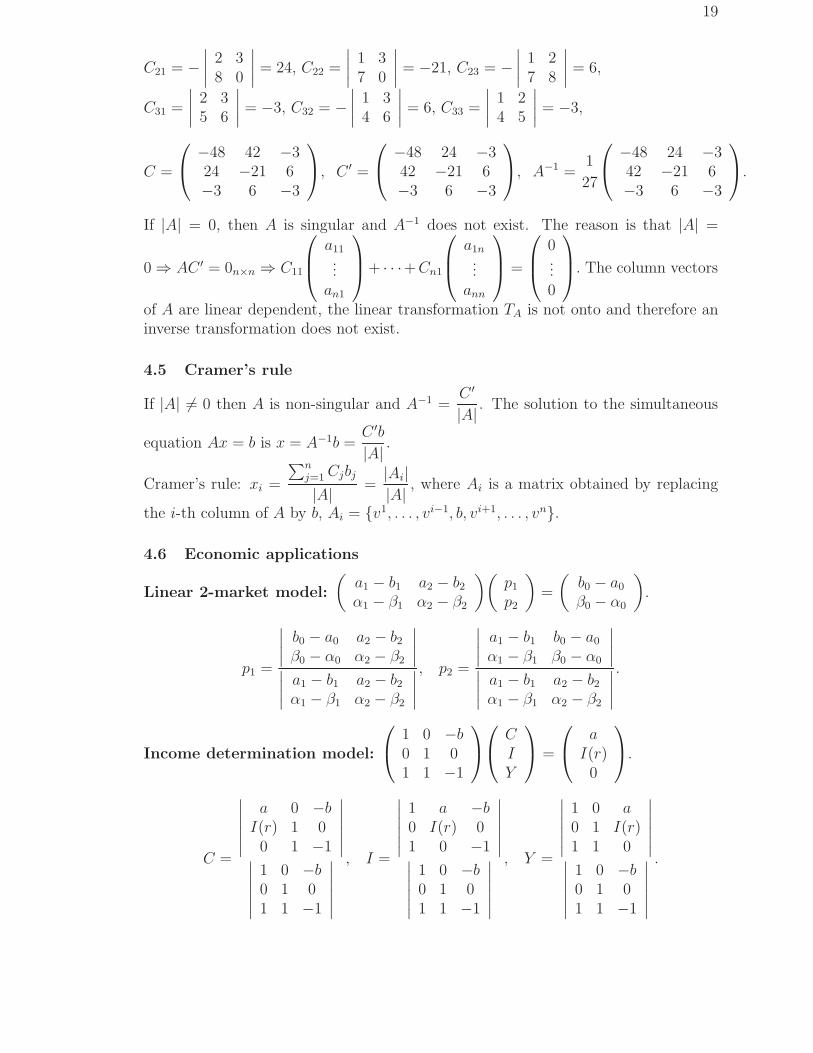
If |A| = 0, then A is singular and A−1 does not exist. The reason is that |A| =
0⇒ AC ′ = 0n×n ⇒ C11
a11...
an1
+ · · ·+Cn1
a1n...
ann
=
0...0
. The column vectors
of A are linear dependent, the linear transformation TA is not onto and therefore aninverse transformation does not exist.
4.5 Cramer’s rule
If |A| 6= 0 then A is non-singular and A−1 =C ′
|A| . The solution to the simultaneous
equation Ax = b is x = A−1b =C ′b
|A| .
Cramer’s rule: xi =
∑nj=1 Cjbj
|A| =|Ai||A| , where Ai is a matrix obtained by replacing
the i-th column of A by b, Ai = {v1, . . . , vi−1, b, vi+1, . . . , vn}.
4.6 Economic applications
Linear 2-market model:
(
a1 − b1 a2 − b2
α1 − β1 α2 − β2
)(
p1
p2
)
=
(
b0 − a0
β0 − α0
)
.
p1 =
∣
∣
∣
∣
b0 − a0 a2 − b2
β0 − α0 α2 − β2
∣
∣
∣
∣
∣
∣
∣
∣
a1 − b1 a2 − b2
α1 − β1 α2 − β2
∣
∣
∣
∣
, p2 =
∣
∣
∣
∣
a1 − b1 b0 − a0
α1 − β1 β0 − α0
∣
∣
∣
∣
∣
∣
∣
∣
a1 − b1 a2 − b2
α1 − β1 α2 − β2
∣
∣
∣
∣
.
Income determination model:
1 0 −b0 1 01 1 −1
CIY
=
aI(r)0
.
C =
∣
∣
∣
∣
∣
∣
a 0 −bI(r) 1 00 1 −1
∣
∣
∣
∣
∣
∣
∣
∣
∣
∣
∣
∣
1 0 −b0 1 01 1 −1
∣
∣
∣
∣
∣
∣
, I =
∣
∣
∣
∣
∣
∣
1 a −b0 I(r) 01 0 −1
∣
∣
∣
∣
∣
∣
∣
∣
∣
∣
∣
∣
1 0 −b0 1 01 1 −1
∣
∣
∣
∣
∣
∣
, Y =
∣
∣
∣
∣
∣
∣
1 0 a0 1 I(r)1 1 0
∣
∣
∣
∣
∣
∣
∣
∣
∣
∣
∣
∣
1 0 −b0 1 01 1 −1
∣
∣
∣
∣
∣
∣
.
20
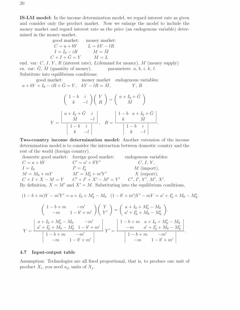
IS-LM model: In the income determination model, we regard interest rate as givenand consider only the product market. Now we enlarge the model to include themoney market and regard interest rate as the price (an endogenous variable) deter-mined in the money market.
good market: money market:C = a + bY L = kY − lRI = I0 − iR M = M
C + I + G = Y M = Lend. var: C, I, Y , R (interest rate), L(demand for money), M (money supply)ex. var: G, M (quantity of money). parameters: a, b, i, k, l.Substitute into equilibrium conditions:
good market: money market endogenous variables:a + bY + I0 − iR + G = Y , kY − lR = M , Y , R
(
1− b ik −l
)(
YR
)
=
(
a + I0 + GM
)
Y =
∣
∣
∣
∣
a + I0 + G iM −l
∣
∣
∣
∣
∣
∣
∣
∣
1− b ik −l
∣
∣
∣
∣
, R =
∣
∣
∣
∣
1− b a + I0 + Gk M
∣
∣
∣
∣
∣
∣
∣
∣
1− b ik −l
∣
∣
∣
∣
.
Two-country income determination model: Another extension of the incomedetermination model is to consider the interaction between domestic country and therest of the world (foreign country).domestic good market: foreign good market: endogenous variables:C = a + bY C ′ = a′ + b′Y ′ C, I, Y ,I = I0 I ′ = I ′0 M (import),M = M0 + mY M ′ = M ′
0 + m′Y ′ X (export),C + I + X −M = Y C ′ + I ′ + X ′ −M ′ = Y ′ C ′, I ′, Y ′, M ′, X ′.
By definition, X = M ′ and X ′ = M . Substituting into the equilibrium conditions,
(1− b + m)Y −m′Y ′ = a + I0 + M ′0 −M0 (1− b′ + m′)Y ′ −mY = a′ + I ′0 + M0 −M ′
0.
(
1− b + m −m′
−m 1− b′ + m′
)(
YY ′
)
=
(
a + I0 + M ′0 −M0
a′ + I ′0 + M0 −M ′0
)
.
Y =
∣
∣
∣
∣
a + I0 + M ′0 −M0 −m′
a′ + I ′0 + M0 −M ′0 1− b′ + m′
∣
∣
∣
∣
∣
∣
∣
∣
1− b + m −m′
−m 1− b′ + m′
∣
∣
∣
∣
Y ′ =
∣
∣
∣
∣
1− b + m a + I0 + M ′0 −M0
−m a′ + I ′0 + M0 −M ′0
∣
∣
∣
∣
∣
∣
∣
∣
1− b + m −m′
−m 1− b′ + m′
∣
∣
∣
∣
.
4.7 Input-output table
Assumption: Technologies are all fixed proportional, that is, to produce one unit ofproduct Xi, you need aji units of Xj .
21
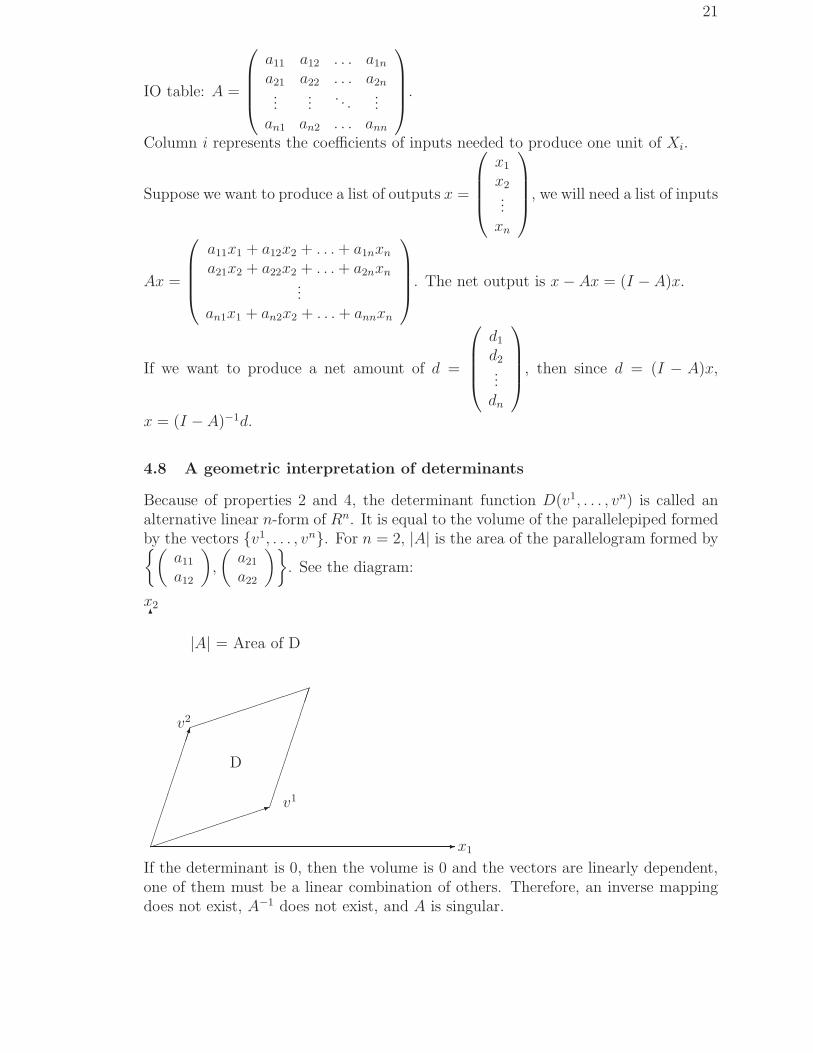
IO table: A =
a11 a12 . . . a1n
a21 a22 . . . a2n...
.... . .
...an1 an2 . . . ann
.
Column i represents the coefficients of inputs needed to produce one unit of Xi.
Suppose we want to produce a list of outputs x =
x1
x2...
xn
, we will need a list of inputs
Ax =
a11x1 + a12x2 + . . . + a1nxn
a21x2 + a22x2 + . . . + a2nxn...
an1x1 + an2x2 + . . . + annxn
. The net output is x−Ax = (I − A)x.
If we want to produce a net amount of d =
d1
d2...
dn
, then since d = (I − A)x,
x = (I −A)−1d.
4.8 A geometric interpretation of determinants
Because of properties 2 and 4, the determinant function D(v1, . . . , vn) is called analternative linear n-form of Rn. It is equal to the volume of the parallelepiped formedby the vectors {v1, . . . , vn}. For n = 2, |A| is the area of the parallelogram formed by{(
a11
a12
)
,
(
a21
a22
)}
. See the diagram:
✲x1
✻x2
✂✂✂✂✂✂✂✂✂✂✍
v2
✏✏✏✏✏✏✏✏✏✶ v1
|A| = Area of D
D
✏✏✏✏✏✏✏✏✏
✂✂✂✂✂✂✂✂✂✂
If the determinant is 0, then the volume is 0 and the vectors are linearly dependent,one of them must be a linear combination of others. Therefore, an inverse mappingdoes not exist, A−1 does not exist, and A is singular.

22
4.9 Rank of a matrix and solutions of Ax = d when |A| = 0
Rank(A) = the maximum # of independent vectors in A = {v1, . . . , vn} = dim(RangeSpace of TA).Rank(A) = the size of the largest non-singular square submatrices of A.
Examples: Rank
(
1 23 4
)
= 2. Rank
1 2 34 5 67 8 9
= 2 because
(
1 24 5
)
is non-
singular.Property 1: Rank(AB) ≤ min{Rank(A), Rank(B)}.Property 2: dim(Null Space of TA) + dim(Range Space of TA) = n.
Consider the simultaneous equation Ax = d. When |A| = 0, there exists a row ofA that is a linear combination of other rows
and Rank(A) < n. First, form the augmented matrix M ≡ [A...d] and calculate
the rank of M . There are two cases.
Case 1: Rank(M) = Rank (A).In this case, some equations are linear combinations of others (the equations are de-pendent) and can be removed without changing the solution space. There will bemore variables than equations after removing these equations. Hence, there will beinfinite number of solutions.
Example:
(
1 22 4
)(
x1
x2
)
=
(
36
)
. Rank(A) = Rank
(
1 22 4
)
= 1 = Rank(M) =
Rank
(
1 2 32 4 6
)
.
The second equation is just twice the first equation and can be discarded. The so-
lutions are
(
x1
x2
)
=
(
3− 2kk
)
for any k. On x1-x2 space, the two equations are
represented by the same line and every point on the line is a solution.
Case 2: Rank(M) = Rank(A) + 1.In this case, there exists an equation whose LHS is a linear combination of the LHSof other equations but whose RHS is different from the same linear combination ofthe RHS of other equations. Therefore, the equation system is contraditory and therewill be no solutions.
Example:
(
1 22 4
)(
x1
x2
)
=
(
37
)
. Rank(A) = Rank
(
1 22 4
)
= 1 < Rank(M) =
Rank
(
1 2 32 4 7
)
= 2.
Multiplying the first equation by 2, 2x1 + 4x2 = 6, whereas the second equation
says 2x1 + 4x2 = 7. Therefore, it is impossible to have any
(
x1
x2
)
satisfying both
equations simultaneously. On x1-x2 space, the two equations are represented by twoparallel lines and cannot have any intersection points.

23
4.10 Problems
1. Suppose v1 = (1, 2, 3)′, v2 = (2, 3, 4)′, and v3 = (3, 4, 5)′. Is {v1, v2, v3} linearlyindependent? Why or why not?
2.. Find the inverse of A =
[
6 58 7
]
.
3. Given the 3 × 3 matrix A =
2 1 65 3 48 9 7
,
(a) calculate the cofactors C11, C21, C31,(b) use Laplace expansion theorem to find |A|,(c) and use Cramer’s rule to find X1 of the following equation system:
2 1 65 3 48 9 7
X1
X2
X3
=
123
.
(Hint: Make use of the results of (a).)4. Use Cramer’s rule to solve the national-income model
C = a + b(Y − T ) (1)
T = −t0 + t1Y (2)
Y = C + I0 + G (3)
5. Let A =
0 1 00 0 10 0 0
.
(a) Find AA and AAA.(b) Let x = (1, 2, 3)′, compute Ax, AAx, and AAAx.(c) Find Rank[A], Rank[AA], and Rank[AAA].
6. Let X =
1 −11 01 1
.
(a) Find X ′X and (X ′X)−1.(b) Compute X(X ′X)−1X ′ and I −X(X ′X)−1X ′.(c) Find Rank[X(X ′X)−1X ′] and Rank[I −X(X ′X)−1X ′].
7. A =
[
1 23 6
]
, B =
[
1 2 13 6 1
]
, and C =
[
1 2 43 6 12
]
.
(a) Find the ranks of A, B, and C.(b) Use the results of (a) to determine whether the following system has any solution:
[
1 23 6
] [
X1
X2
]
=
[
11
]
.
(c) Do the same for the following system:[
1 23 6
] [
X1
X2
]
=
[
412
]
.

24
8. Let A =
(
3 21 2
)
, I the 2× 2 identity matrix, and λ a scalar number.
(a) Find |A− λI|. (Hint: It is a quadratic function of λ.)(b) Determine Rank(A − I) and Rank(A − 4I). (Remark: λ = 1 and λ = 4 are theeigenvalues of A, that is, they are the roots of the equation |A− λI| = 0, called thecharacteristic equation of A.)(c) Solve the simultaneous equation system (A − I)x = 0 assuming that x1 = 1.(Remark: The solution is called an eigenvector of A associated with the eigenvalueλ = 1.)(d) Solve the simultaneous equation system (A− 4I)y = 0 assuming that y1 = 1.(e) Determine whether the solutions x and y are linearly independent.

25
5 Differential Calculus and Comparative Statics
As seen in the last chapter, a linear economic model can be represented by a matrixequation Ax = d(y) and solved using Cramer’s rule, x = A−1d(y). On the other hand,a closed form solution x = x(y) for a nonlinear economic model is, in most applica-tions, impossible to obtain. For general nonlinear economic models, we use differentialcalculus (implicit function theorem) to obtain the derivatives of endogenous variables
with respect to exogenous variables∂xi
∂yj
:
f1(x1, . . . , xn; y1, . . . , ym) = 0...
fn(x1, . . . , xn; y1, . . . , ym) = 0
⇒
∂f1
∂x1
. . .∂f1
∂xn...
. . ....
∂fn
∂x1
. . .∂fn
∂xn
∂x1
∂y1. . .
∂x1
∂ym...
. . ....
∂xn
∂y1
. . .∂xn
∂ym
= −
∂f1
∂y1. . .
∂f1
∂ym...
. . ....
∂fn
∂y1
. . .∂fn
∂ym
.
⇒
∂x1
∂y1
. . .∂x1
∂ym...
. . ....
∂xn
∂y1. . .
∂xn
∂ym
= −
∂f1
∂x1. . .
∂f1
∂xn...
. . ....
∂fn
∂x1. . .
∂fn
∂xn
−1
∂f1
∂y1
. . .∂f1
∂ym...
. . ....
∂fn
∂y1. . .
∂fn
∂ym
.
Each∂xi
∂yjrepresents a cause-effect relationship. If
∂xi
∂yj> 0 (< 0), then xi will increase
(decrease) when yj increases. Therefore, instead of computing xi = xi(y), we want to
determine the sign of∂xi
∂yj
for each i-j pair. In the following, we will explain how it
works.
5.1 Differential Calculus
x = f(y)⇒ f ′(y∗) =dx
dy
∣
∣
∣
∣
y=y∗≡ lim
∆y→0
f(y∗ + ∆y)− f(y∗)
∆y.
On y-x space, x = f(y) is represented by a curve and f ′(y∗) represents the slope ofthe tangent line of the curve at the point (y, x) = (y∗, f(y∗)).Basic rules:
1. x = f(y) = k,dx
dy= f ′(y) = 0.
2. x = f(y) = yn,dx
dy= f ′(y) = nyn−1.
3. x = cf(y),dx
dy= cf ′(y).

26
4. x = f(y) + g(y),dx
dy= f ′(y) + g′(y).
5. x = f(y)g(y),dx
dy= f ′(y)g(y) + f(y)g′(y).
6. x = f(y)/g(y),dx
dy=
f ′(y)g(y)− f(y)g′(y)
(g(y))2.
7. x = eay,dx
dy= aeay. x = ln y,
dx
dy=
1
y.
8. x = sin y,dx
dy= cos y. x = cos y,
dx
dy= − sin y.
Higher order derivatives:
f ′′(y) ≡ d
dy
(
d
dyf(y)
)
=d2
dy2f(y), f ′′′(y) ≡ d
dy
(
d2
dy2f(y)
)
=d3
dy3f(y).
5.2 Partial derivatives
In many cases, x is a function of several y’s: x = f(y1, y2, . . . , yn). The partialderivative of x with respect to yi evaluated at (y1, y2, . . . , yn) = (y∗1, y
∗2, . . . , y
∗n) is
∂x
∂yi
∣
∣
∣
∣
(y∗1,y∗
2,...,y∗n)
≡ lim∆yi→0
f(y∗1, . . . , y∗i + ∆yi, . . . , y
∗n)− f(y∗1, . . . , y
∗i , . . . , y
∗n)
∆yi,
that is, we regard all other independent variables as constant (f as a function of yi
only) and take derivative.
9.∂xn
1xm2
∂x1= nxn−1
1 xm2 .
Higher order derivatives: We can define higher order derivatives as before. For thecase with two independent variables, there are 4 second order derivatives:
∂
∂y1
∂x
∂y1=
∂2x
∂y21
,∂
∂y2
∂x
∂y1=
∂2x
∂y2∂y1,
∂
∂y1
∂x
∂y2=
∂2x
∂y1∂y2,
∂
∂y2
∂x
∂y2=
∂2x
∂y22
.
Notations: f1, f2, f11, f12, f21, f22.
∇f ≡
f1...
fn
: Gradient vector of f .
H(f) ≡
f11 . . . f1n...
. . ....
fn1 . . . fnn
: second order derivative matrix, called Hessian of f .
Equality of cross-derivatives: If f is twice continously differentiable, then fij = fji
and H(f) is symmetric.
5.3 Economic concepts similar to derivatives
Elasticity of Xi w.r.t. Yj: EXi,Yj≡ Yj
Xi
∂Xi
∂Yj
, the percentage change of Xi when Yj
increases by 1 %. Example: Qd = D(P ), EQd,P =P
Qd
dQd
dP
27
Basic rules: 1. EX1X2,Y = EX1,Y + EX2,Y , 2. EX1/X2,Y = EX1,Y − EX2,Y ,3. EY,X = 1/EX,Y .
Growth rate of X = X(t): GX ≡ 1
X
dX
dt, the percentage change of X per unit of
time.
5.4 Mean value and Taylor’s Theorems
Continuity theorem: If f(y) is continuous on the interval [a, b] and f(a) ≤ 0, f(b) ≥ 0,then there exists a c ∈ [a, b] such that f(c) = 0.Rolle’s theorem: If f(y) is continuous on the interval [a, b] and f(a) = f(b) = 0, thenthere exists a c ∈ (a, b) such that f ′(c) = 0.
Mean value theorem: If f(y) is continously differentiable on [a, b], then there exists ac ∈ (a, b) such that
f(b)− f(a) = f ′(c)(b− a) orf(b)− f(a)
b− a= f ′(c).
Taylor’s Theorem: If f(y) is k + 1 times continously differentiable on [a, b], then foreach y ∈ [a, b], there exists a c ∈ (a, y) such that
f(y) = f(a)+f ′(a)(y−a)+f ′′(a)
2!(y−a)2 + . . .+
f (k)(a)
k!(y−a)k +
f (k+1)(c)
(k + 1)!(y−a)k+1.
5.5 Concepts of differentials and applications
Let x = f(y). Define ∆x ≡ f(y + ∆y)− f(y), called the finite difference of x.
Finite quotient:∆x
∆y=
f(y + ∆y)− f(y)
∆y⇒ ∆x =
∆x
∆y∆y.
dx, dy: Infinitesimal changes of x and y, dx, dy > 0 (so that we can divid somethingby dx or by dy) but dx, dy < a for any positive real number a (so that ∆y→dy).Differential of x = f(y): dx = df = f ′(y)dy.
Chain rule: x = f(y), y = g(z) ⇒ x = f(g(z)),
dx = f ′(y)dy, dy = g′(z)dz ⇒ dx = f ′(y)g′(z)dz.dx
dz= f ′(y)g′(z) = f ′(g(z))g′(z).
Example: x = (z2 + 1)3 ⇒ x = y3, y = z2 + 1 ⇒ dx
dz= 3y22z = 6z(z2 + 1)2.
Inverse function rule: x = f(y), ⇒ y = f−1(x) ≡ g(x),
dx = f ′(y)dy, dy = g′(x)dx⇒ dx = f ′(y)g′(x)dx.dy
dx= g′(x) =
1
f ′(y).
Example: x = ln y ⇒ y = ex ⇒ dx
dy=
1
ex=
1
y.

28
5.6 Concepts of total differentials and applications
Let x = f(y1, y2). Define ∆x ≡ f(y1 + ∆y1, y2 + ∆y2) − f(y1, y2), called the finitedifference of x.
∆x = f(y1 + ∆y1, y2 + ∆y2)− f(y1, y2)
= f(y1 + ∆y1, y2 + ∆y2)− f(y1, y2 + ∆y2) + f(y1, y2 + ∆y2)− f(y1, y2)
=f(y1 + ∆y1, y2 + ∆y2)− f(y1, y2 + ∆y2)
∆y1
∆y1 +f(y1, y2 + ∆y2)− f(y1, y2)
∆y2
∆y2
dx = f1(y1, y2)dy1 + f2(y1, y2)dy2.
dx, dy =
dy1...
dyn
: Infinitesimal changes of x (endogenous), y1, . . . , yn (exogenous).
Total differential of x = f(y1, . . . , yn):
dx = df = f1(y1, . . . , yn)dy1+. . .+fn(y1, . . . , yn)dyn = (f1, . . . , fn)
dy1...
dyn
= (∇f)′dy.
Implicit function rule:In many cases, the relationship between two variables are defined implicitly. Forexample, the indifference curve U(x1, x2) = U defines a relationship between x1 and
x2. To find the slope of the curvedx2
dx1, we use implicit function rule.
dU = U1(x1, x2)dx1 + U2(x1, x2)dx2 = dU = 0⇒;dx2
dx1= −U1(x1, x2)
U2(x1, x2).
Example: U(x1, x2) = 3x131 + 3x
132 = 6 defines an indifference curve passing through
the point (x1, x2) = (1, 1). The slope (Marginal Rate of Substitution) at (1, 1) can becalculated using implicit function rule.
dx2
dx1= −U1
U2= −x
− 2
3
1
x− 2
3
2
= −1
1= −1.
Multivariate chain rule:
x = f(y1, y2), y1 = g1(z1, z2), y2 = g2(z1, z2), ⇒ x = f(g1(z1, z2), g2(z1, z2)) ≡ H(z1, z2).
We can use the total differentials dx, dy1, dy2 to find the derivative∂x
∂z1
.
dx = (f1, f2)
(
dy1
dy2
)
= (f1, f2)
(
g11 g1
2
g21 g2
2
)(
dz1
dz2
)
= (f1g11+f2g
21, f1g
12+f2g
22)
(
dz1
dz2
)
.
29
⇒ ∂x
∂z1=
∂H
∂z1= f1g
11 + f2g
21,
∂x
∂z2=
∂H
∂z2= f1g
12 + f2g
22.
Example: x = y61y
72, y1 = 2z1 + 3z2, y2 = 4z1 + 5z2,
∂x
∂z1
= 6y51y
72(2) + 7y6
1y62(4).
Total derivative:
x = f(y1, y2), y2 = h(y1), x = f(y1, h(y1)) ≡ g(y1),
⇒ dx = f1dy1 + f2dy2 = f1dy1 + f2h′dy1 = (f1 + f2h
′)dy1.
Total derivative:dx
dy1
∣
∣
∣
∣
y2=h(y1)
= f1 + f2h′.
Partial derivative (direct effect of y1 on x):∂x
∂y1=
∂f
∂y1= f1(y1, y2).
Indirect effect through y2:∂x
∂y2
dy2
dy1
= f2h′.
Example: Given the utility function U(x1, x2) = 3x131 + 3x
132 , the MRS at a point
(x1, x2) is m(x1, x2) =dx2
dx1
= −U1(x1, x2)
U2(x1, x2)= −x
− 2
3
1
x− 2
3
2
. The rate of change of MRS
w.r.t. x1 along the indifference curve passing through (1, 1) is a total derivative
dm
dx1
∣
∣
∣
∣
3x1/3
1+3x
1/3
2=6
(
=d2x2
dx21
∣
∣
∣
∣
3x1/3
1+3x
1/3
2=6
)
=∂m
∂x1+
∂m
∂x2
dx2
dx1=
∂m
∂x1+
∂m
∂x2
(
−x− 2
3
1
x− 2
3
2
)
.
5.7 Inverse function theorem
In Lecture 3, we discussed a linear mapping x = Ay and its inverse mapping y = A−1xwhen |A| 6= 0.
(
x1
x2
)
=
(
a11 a12
a21 a22
)(
y1
y2
) (
y1
y2
)
=
(
a22
|A|−a12
|A|−a21
|A|a11
|A|
)
(
x1
x2
)
.
Therefore, for a linear mapping with |A| 6= 0, an 1-1 inverse mapping exists and thepartial derivatives are given by the inverse matrix of A. For example, ∂x1/∂y1 = a11
where∂y1/∂x1 = a22
|A| etc. The idea can be generalized to nonlinear mappings.
A general nonlinear mapping from Rn to Rn, y =
y1...
yn
→ x =
x1...
xn
, is
represented by a vector function
x =
x1...
xn
=
f 1(y1, . . . , yn)...
fn(y1, . . . , yn)
≡ F (y).

30
Jacobian matrix: JF (y) ≡
∂x1
∂y1. . .
∂x1
∂yn...
. . ....
∂xn
∂y1. . .
∂xn
∂yn
=
f 11 . . . f 1
n...
. . ....
fn1 . . . fn
n
.
Jacobian:∂(x1, . . . , xn)
∂(y1, . . . , yn)≡ |JF (y)|.
Inverse function theorem: If x∗ = F (y∗) and |JF (y∗)| 6= 0 (JF (y∗) is non-singular),then F (y) is invertible nearby x∗,
that is, there exists a function G(x) ≡
g1(x1, . . . , xn)...
gn(x1, . . . , xn)
such that y = G(x) if
x = F (y). In that case, JG(x∗) = (JF (y∗))−1.Reasoning:
dx1...
dxn
=
f 11 . . . f 1
n...
. . ....
fn1 . . . fn
n
dy1...
dyn
⇒
dy1...
dyn
=
g11 . . . g1
n...
. . ....
gn1 . . . gn
n
dx1...
dxn
=
f 11 . . . f 1
n...
. . ....
fn1 . . . fn
n
−1
dx1...
dxn
Example:
(
x1
x2
)
= F (r, θ) =
(
r cos θr sin θ
)
. JF (r, θ) =
(
cos θ −r sin θsin θ r cos θ
)
.
J = |JF | = r(cos2 θ + sin2 θ) = r > 0, ⇒ r =√
x21 + x2
2, θ = tan−1 x2
x1and
JG = (JF )−1. When r = 0, J = 0 and the mapping is degenerate, i.e., the whole set{r = 0,−π ≤ θ < π} is mapped to the origin (0, 0), just like the case in Lecture 3when the Null space is a line.
Notice that g11 6= 1/(f 1
1 ) in general.
5.8 Implicit function theorem and comparative statics
Linear model: If all the equations are linear, the model can be represtned in matrixform as
Ax+By = c ⇔
a11 · · · a1n...
. . ....
an1 · · · ann
x1...
xn
+
b11 · · · b1m...
. . ....
bn1 · · · anm
y1...
ym
−
c1...cn
=
0. . .
0
.
If |A| 6= 0, then the solution is given by x = −A−1(By + c). The derivative matrix[∂xi/∂yj]ij = A−1B. Using total differentials of the equations, we can derive a similarderivative matrix for general nonlinear cases.

31
We can regard the LHS of a nonlinear economic model as a mapping from Rn+m
to Rn:
f1(x1, . . . , xn; y1, . . . , ym) = 0...
fn(x1, . . . , xn; y1, . . . , ym) = 0
⇔ F (x; y) = 0.
Jacobian matrix: Jx ≡
f 11 . . . f 1
n...
. . ....
fn1 . . . fn
n
.
Implicit function theorem: If F (x∗; y∗) = 0 and |Jx(x∗; y∗)| 6= 0 (Jx(x
∗; y∗) isnon-singular), then F (x; y) = 0 is solvable nearby (x∗; y∗), that is, there exists a
function x =
x1...
xn
= x(y) =
x1(y1, . . . , ym)...
xn(y1, . . . , ym)
such that x∗ = x(y∗) and
F (x(y); y) = 0. In that case,
∂x1
∂y1. . .
∂x1
∂ym...
. . ....
∂xn
∂y1
. . .∂xn
∂ym
= −
f 11 . . . f 1
n...
. . ....
fn1 . . . fn
n
−1
∂f 1
∂y1. . .
∂f 1
∂ym...
. . ....
∂fn
∂y1
. . .∂fn
∂ym
.
Reasoning:
df 1
...dfn
=
0...0
⇒
f 11 . . . f 1
n...
. . ....
fn1 . . . fn
n
dx1...
dxn
+
∂f 1
∂y1. . .
∂f 1
∂ym...
. . ....
∂fn
∂y1. . .
∂fn
∂ym
dy1...
dym
= 0
⇒
dx1...
dxn
= −
f 11 . . . f 1
n...
. . ....
fn1 . . . fn
n
−1
∂f 1
∂y1. . .
∂f 1
∂ym...
. . ....
∂fn
∂y1
. . .∂fn
∂ym
dy1...
dym
.
Example: f 1 = x21x2 − y = 0, f 2 = 2x1 − x2 − 1 = 0, When y = 1, (x1, x2) = (1, 1)
is an equilibrium. To calculatedx1
dyand
dx2
dyat the equilibrium we use the implicit
function theorem:
dx1
dydx2
dy
= −
(
f 11 f 1
2
f 21 f 2
2
)−1
∂f 1
∂y∂f 2
∂y
= −(
2x1x2 x21
2 −1
)−1( −10
)
= −(
2 12 −1
)−1( −10
)
=
(
1/41/2
)
.

32
5.9 Problems
1. Given the demand function Qd = (100/P )− 10, find the demand elasticity η.
2. Given Y = X21X2 + 2X1X
22 , find ∂Y/∂X1, ∂2Y/∂X2
1 , and ∂2Y/∂X1∂X2, andthe total differential DY .
3. Given Y = F (X1, X2)+f(X1)+g(X2), find ∂Y/∂X1, ∂2Y/∂X21 , and ∂2Y/∂X1∂X2.
4. Given the consumption function C = C(Y − T (Y )), find dC/dY .
5. Given that Q = D(q ∗ e/P ), find dQ/dP .
6. Y = X21X2, Z = Y 2 + 2Y − 2, use chain rule to derive ∂Z/∂X1 and ∂Z/∂X2.
7. Y1 = X1 +2X2, Y2 = 2X1 +X2, and Z = Y1Y2, use chain rule to derive ∂Z/∂X1
and ∂Z/∂X2.
8. Let U(X1, X2) = X1X22 + X2
1X2 and X2 = 2X1 + 1, find the partial derivative∂U/∂X1 and the total derivative dU/dX1.
9. X2 + Y 3 = 1, use implicit function rule to find dY/dX.
10. X21 + 2X2
2 + Y 2 = 1, use implicit function rule to derive ∂Y/∂X1 and ∂Y/∂X2.
11. F (Y1, Y2, X) = Y1 − Y2 + X − 1 = 0 and G(Y1, Y2, X) = Y 21 + Y 2
2 + X2 − 1 = 0.use implicit function theorem to derive dY1/dX and dY2/dX.
12. In a Cournot quantity competition duopoly model with heterogeneous products,the demand functions are given by
Q1 = a− P1 − cP2, Q2 = a− cP1 − P2; 1 ≥ c > 0.
(a) For what value of c can we invert the demand functions to obtain P1 andP2 as functions of Q1 and Q2?
(b) Calculate the inverse demand functions P1 = P1(Q1, Q2) and P2 = P2(Q1, Q2).
(c) Derive the total revenue functions TR1(Q1, Q2) = P1(Q1, Q2)Q1 and TR2(Q1, Q2) =P2(Q1, Q2)Q2.
13. In a 2-good market equilibrium model, the inverse demand functions are givenby
P1 = A1Qα−11 Qβ
2 , P2 = A2Qα1 Qβ−1
2 ; α, β > 0.
(a) Calculate the Jacobian matrix
(
∂P1/∂Q1 ∂P1/∂Q2
∂P2/∂Q1 ∂P2/∂Q2
)
and Jacobian∂(P1, P2)
∂(Q1, Q2).
What condition(s) should the parameters satisfy so that we can invert thefunctions to obtain the demand functions?
(b) Derive the Jacobian matrix of the derivatives of (Q1, Q2) with respect to
(P1, P2),
(
∂Q1/∂P1 ∂Q1/∂P2
∂Q2/∂P1 ∂Q2/∂P2
)
.
33
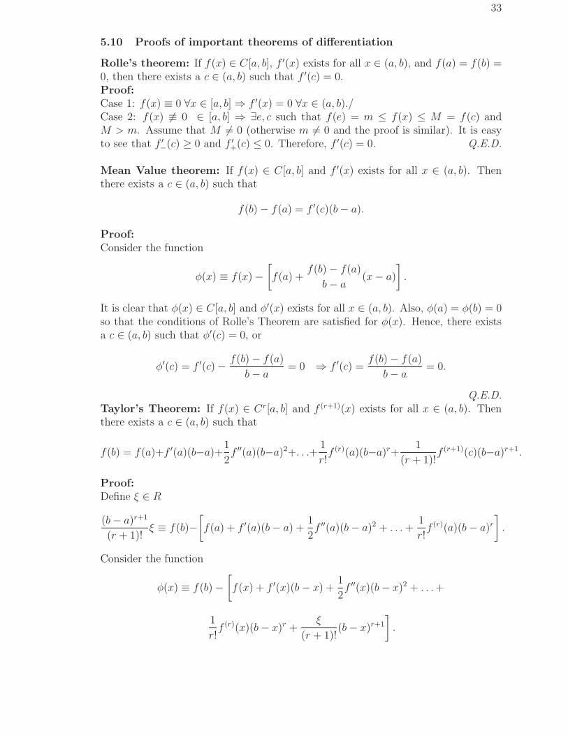
5.10 Proofs of important theorems of differentiation
Rolle’s theorem: If f(x) ∈ C[a, b], f ′(x) exists for all x ∈ (a, b), and f(a) = f(b) =0, then there exists a c ∈ (a, b) such that f ′(c) = 0.Proof:Case 1: f(x) ≡ 0 ∀x ∈ [a, b] ⇒ f ′(x) = 0 ∀x ∈ (a, b)./Case 2: f(x) 6≡ 0 ∈ [a, b] ⇒ ∃e, c such that f(e) = m ≤ f(x) ≤ M = f(c) andM > m. Assume that M 6= 0 (otherwise m 6= 0 and the proof is similar). It is easyto see that f ′−(c) ≥ 0 and f ′+(c) ≤ 0. Therefore, f ′(c) = 0. Q.E.D.
Mean Value theorem: If f(x) ∈ C[a, b] and f ′(x) exists for all x ∈ (a, b). Thenthere exists a c ∈ (a, b) such that
f(b)− f(a) = f ′(c)(b− a).
Proof:Consider the function
φ(x) ≡ f(x)−[
f(a) +f(b)− f(a)
b− a(x− a)
]
.
It is clear that φ(x) ∈ C[a, b] and φ′(x) exists for all x ∈ (a, b). Also, φ(a) = φ(b) = 0so that the conditions of Rolle’s Theorem are satisfied for φ(x). Hence, there existsa c ∈ (a, b) such that φ′(c) = 0, or
φ′(c) = f ′(c)− f(b)− f(a)
b− a= 0 ⇒ f ′(c) =
f(b)− f(a)
b− a= 0.
Q.E.D.
Taylor’s Theorem: If f(x) ∈ Cr[a, b] and f (r+1)(x) exists for all x ∈ (a, b). Thenthere exists a c ∈ (a, b) such that
f(b) = f(a)+f ′(a)(b−a)+1
2f ′′(a)(b−a)2+. . .+
1
r!f (r)(a)(b−a)r+
1
(r + 1)!f (r+1)(c)(b−a)r+1.
Proof:Define ξ ∈ R
(b− a)r+1
(r + 1)!ξ ≡ f(b)−
[
f(a) + f ′(a)(b− a) +1
2f ′′(a)(b− a)2 + . . . +
1
r!f (r)(a)(b− a)r
]
.
Consider the function
φ(x) ≡ f(b)−[
f(x) + f ′(x)(b− x) +1
2f ′′(x)(b− x)2 + . . . +
1
r!f (r)(x)(b− x)r +
ξ
(r + 1)!(b− x)r+1
]
.

34
It is clear that φ(x) ∈ C[a, b] and φ′(x) exists for all x ∈ (a, b). Also, φ(a) = φ(b) = 0so that the conditions of Rolle’s Theorem are satisfied for φ(x). Hence, there existsa c ∈ (a, b) such that φ′(c) = 0, or
φ′(c) =ξ − f (r+1)(c)
r!= 0 ⇒ f (r+1)(c) = ξ.
Q.E.D.
Inverse Function Theorem: Let E ⊆ Rn be an open set. Suppose f : E → Rn
is C1(E), a ∈ E, f(a) = b, and A = J(f(a)), |A| 6= 0. Then there exist open setsU, V ⊂ Rn such that a ∈ U , b ∈ V , f is one to one on U , f(U) = V , and f−1 : V → Uis C1(U).Proof:(1. Find U .) Choose λ ≡ |A|/2. Since f ∈ C1(E), there exists a neighborhood U ⊆ Ewith a ∈ U such that ‖J(f(x))−A‖ < λ.(2. Show that f(x) is one to one in U .) For each y ∈ Rn define φy on E byφy(x) ≡ x + A−1(y − f(x)). Notice that f(x) = y if and only if x is a fixed point of
φy. Since J(φy(x)) = I − A−1J(f(x)) = A−1[A− J(f(x))] ⇒ ‖J(φy(x))‖ <1
2on U .
Therefore φy(x) is a contraction mapping and there exists at most one fixed point inU . Therefore, f is one to one in U .(3. V = f(U) is open so that f−1 is continuous.) Let V = f(U) and y0 = f(x0) ∈ Vfor x0 ∈ U . Choose an open ball B about x0 with radius ρ such that the closure[B] ⊆ U . To prove that V is open, it is enough to show that y ∈ V whenever‖y − y0‖ < λρ. So fix y such that ‖y − y0‖ < λρ. With φy defined above,
‖φy(x0)− x0‖ = ‖A−1(y − y0)‖ < ‖A−1‖λρ =ρ
2.
If x ∈ [B] ⊆ U , then
‖φy(x)− x0‖ ≤ ‖φy(x)− φy(x0)‖+ ‖φy(x0)− x0‖ <1
2‖x− x0‖+
ρ
2≤ ρ.
That is, φy(x) ∈ [B]. Thus, φy(x) is a contraction of the complete space [B] into itself.Hence, φy(x) has a unique fixed point x ∈ [B] and y = f(x) ∈ f([B]) ⊂ f(U) = V .(4. f−1 ∈ C−1.) Choose y1, y2 ∈ V , there exist x1, x2 ∈ U such that f(x1) = y1,f(x2) = y2.
φy(x2)− φy(x1) = x2 − x1 + A−1(f(x1)− f(x2)) = (x2 − x1)−A−1(y2 − y1).
⇒ ‖(x2−x1)−A−1(y2−y1)‖ ≤1
2‖x2−x1‖ ⇒
1
2‖x2−x1‖ ≤ ‖A−1(y2−y1)‖ ≤
1
2λ‖y2−y1‖
or ‖x2 − x1‖ ≤1
λ‖y2 − y1‖. It follows that (f ′)−1 exists locally about a. Since
f−1(y2)− f−1(y1)− (f ′)−1(y1)(y2 − y1) = (x2 − x1)− (f ′)−1(y1)(y2 − y1)
= −(f ′)−1(y1)[−f ′(x1)(x2 − x1) + f(x2)− f(x1)],

35
We have
‖f−1(y2)− f−1(y1)− (f ′)−1(y1)(y2 − y1)‖‖y2 − y1‖
≤ ‖(f′)−1‖λ
‖f(x2)− f(x1)− f ′(x1)(x2 − x1)‖‖x2 − x1‖
.
As y2→y1, x2→x1. Hence (f 1−)′(y) = {f ′[f−1(y)]} for y ∈ V . Since f−1 is differ-entiable, it is continuous. Also, f ′ is continuous and its inversion, where it exists, iscontinuous. Therefore (f−1)′ is continuous or f−1 ∈ C1(V ). Q.E.D.
Implicit Function Theorem: Let E ⊆ R(n+m) be an open set and a ∈ Rn, b ∈ Rm,(a, b) ∈ E. Suppose f : E → Rn is C1(E) and f(a, b) = 0, and J(f(a, b)) 6= 0. Thenthere exist open sets A ⊂ Rn and B ⊂ Rm a ∈ A and b ∈ B, such that for eachx ∈ B, there exists a unique g(x) ∈ A such that f(g(x), x) = 0 and g : B → A isC1(B).Proof:Defining F : Rn+m→Rn+m by F (x, y) ≡ (x, f(x, y)). Note that since
J(F (a, b)) =
(
∂xi
∂xj
)
1≤i,j≤n
(
∂xi
∂xn+j
)
1≤i≤n,1≤j≤m(
∂fi
∂xj
)
1≤i≤m,1≤j≤n
(
∂fi
∂xn+j
)
1≤i,j≤m
=
(
I ON M
)
,
|J(F (a, b))| = |M | 6= 0. By the Inverse Function Theorem there exists an open setV ⊆ Rn+m containing F (a, b) = (a, 0) and an open set of the form A × B ⊆ Econtaining (a, b), such that F : A × B→V has a C1 inverse F−1 : V→A × B. F−1
is of the form F−1(x, y) = (x, φ(x, y)) for some C1 function φ. Define the projectionπ : Rn+m→Rm by π(x, y) = y. Then π ◦ F (x, y) = f(x, y). Therefore
f(x, φ(x, y)) = f ◦F−1(x, y) = (π ◦F ) ◦F−1(x, y) = π ◦ (F ◦F−1)(x, y) = π(x, y) = y
and f(x, φ(x, 0)) = 0. So, define g : A→B by g(x) = φ(x, 0). Q.E.D.
36
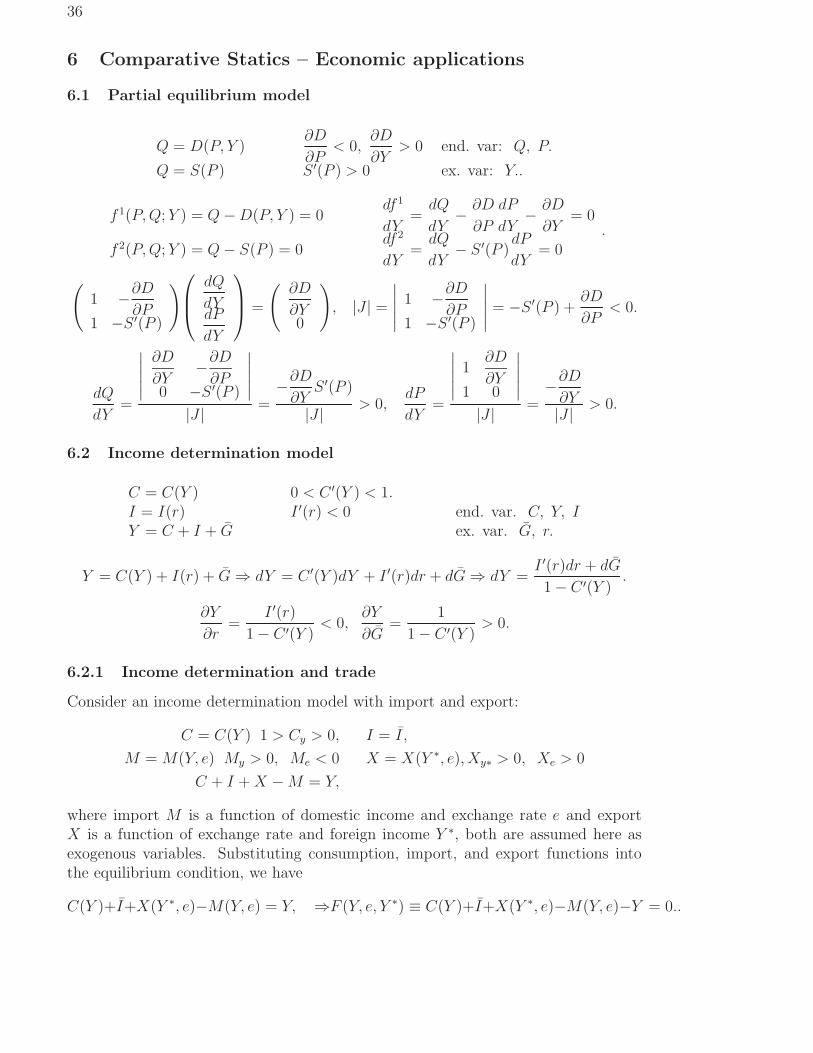
6 Comparative Statics – Economic applications
6.1 Partial equilibrium model
Q = D(P, Y )∂D
∂P< 0,
∂D
∂Y> 0 end. var: Q, P.
Q = S(P ) S ′(P ) > 0 ex. var: Y..
f 1(P, Q; Y ) = Q−D(P, Y ) = 0df 1
dY=
dQ
dY− ∂D
∂P
dP
dY− ∂D
∂Y= 0
f 2(P, Q; Y ) = Q− S(P ) = 0df 2
dY=
dQ
dY− S ′(P )
dP
dY= 0
.
(
1 −∂D
∂P1 −S ′(P )
)
dQ
dYdP
dY
=
(
∂D
∂Y0
)
, |J | =∣
∣
∣
∣
∣
1 −∂D
∂P1 −S ′(P )
∣
∣
∣
∣
∣
= −S ′(P ) +∂D
∂P< 0.
dQ
dY=
∣
∣
∣
∣
∣
∂D
∂Y−∂D
∂P0 −S ′(P )
∣
∣
∣
∣
∣
|J | =−∂D
∂YS ′(P )
|J | > 0,dP
dY=
∣
∣
∣
∣
∣
1∂D
∂Y1 0
∣
∣
∣
∣
∣
|J | =−∂D
∂Y|J | > 0.
6.2 Income determination model
C = C(Y ) 0 < C ′(Y ) < 1.I = I(r) I ′(r) < 0 end. var. C, Y, IY = C + I + G ex. var. G, r.
Y = C(Y ) + I(r) + G ⇒ dY = C ′(Y )dY + I ′(r)dr + dG⇒ dY =I ′(r)dr + dG
1− C ′(Y ).
∂Y
∂r=
I ′(r)
1− C ′(Y )< 0,
∂Y
∂G=
1
1− C ′(Y )> 0.
6.2.1 Income determination and trade
Consider an income determination model with import and export:
C = C(Y ) 1 > Cy > 0, I = I ,
M = M(Y, e) My > 0, Me < 0 X = X(Y ∗, e), Xy∗ > 0, Xe > 0
C + I + X −M = Y,
where import M is a function of domestic income and exchange rate e and exportX is a function of exchange rate and foreign income Y ∗, both are assumed here asexogenous variables. Substituting consumption, import, and export functions intothe equilibrium condition, we have
C(Y )+I+X(Y ∗, e)−M(Y, e) = Y, ⇒F (Y, e, Y ∗) ≡ C(Y )+I+X(Y ∗, e)−M(Y, e)−Y = 0..
37
Use implicit function rule to derive∂Y
∂Iand determine its sign:
∂Y
∂I= −FI
Fy
=1
1− C ′(Y ) + My
.
Use implicit function rule to derive∂Y
∂eand determine its sign:
∂Y
∂e= −Fe
Fy=
Xe −Me
1− C ′(Y ) + My.
Use implicit function rule to derive∂Y
∂Y ∗ and determine its sign:
∂Y
∂Y ∗ = −Fy∗
Fy=
Xy∗
1− C ′(Y ) + My.
6.2.2 Interdependence of domestic and foreign income
Now extend the above income determination model to analyze the joint dependenceof domestic income and foreign income:
C(Y ) + I + X(Y ∗, e)−M(Y, e) = Y C∗(Y ∗) + I∗ + X∗(Y, e)−M∗(Y ∗, e) = Y ∗,
with a similar assumption on the foreigner’s consumption function: 1 > C∗y∗ > 0.
Since domestic import is the same as foreigner’s export and domestic export is for-eigner’s import, X∗(Y, e) = M(Y, e) and M∗(Y ∗, e) = X(Y ∗, e) and the system be-comes:
C(Y ) + I + X(Y ∗, e)−M(Y, e) = Y C∗(Y ∗) + I∗ + M(Y, e)−X(Y ∗, e) = Y ∗,
Calculate the total differential of the system (Now Y ∗ becomes endogenous):
(
1− C ′ + My −Xy∗−My 1− C∗′ + Xy∗
)(
dYdY ∗
)
=
(
(Xe −Me)de + dI(Me −Xe)de + dI∗
)
,
|J | =∣
∣
∣
∣
1− C ′ + My −Xy∗−My 1− C∗′ + Xy∗
∣
∣
∣
∣
= (1−C ′ + My)(1−C∗′ + My∗)−MyXy∗ > 0.
Use Cramer’s rule to derive∂Y
∂eand
∂Y ∗
∂eand determine their signs:
dY =
∣
∣
∣
∣
(Xe −Me)de + dI −Xy∗(Me −Xe)de + dI∗ 1− C∗′ + Xy∗
∣
∣
∣
∣
|J |
=(Xe −Me)(1− C∗′ + Xy∗ −Xy∗)de + (1− C∗′ + Xy∗)dI + Xy∗dI∗
|J | ,

38
dY ∗ =
∣
∣
∣
∣
1− C ′ + My (Xe −Me)de + dI−My (Me −Xe)de + dI∗
∣
∣
∣
∣
|J |
=−(Xe −Me)(1− C ′ + My −My)de + (1− C ′ + My)dI∗ + XydI
|J | .
∂Y
∂e=
(Xe −Me)(1− C∗′)
|J | > 0,∂Y ∗
∂e=−(Xe −Me)(1− C ′)
|J | < 0.
Derive∂Y
∂Iand
∂Y ∗
∂Iand determine their signs:
∂Y
∂I= −1− C∗′ + My∗
|J | > 0,∂Y ∗
∂I=
My
|J | < 0.
6.3 IS-LM model
C = C(Y ) 0 < C ′(Y ) < 1 Md = L(Y, r)∂L
∂Y> 0,
∂L
∂r< 0
I = I(r) I ′(r) < 0 Ms = MY = C + I + G Md = Ms.
end. var: Y , C, I, r, Md, Ms. ex. var: G, M .
Y − C(Y )− I(r) = GL(Y, r) = M
⇒(1− C ′(Y ))dY − I ′(r)dr = dG
∂L
∂YdY +
∂L
∂rdr = dM
(
1− C ′ −I ′
LY Lr
)(
dYdr
)
=
(
dGdM
)
, |J | =∣
∣
∣
∣
1− C ′ −I ′
LY Lr
∣
∣
∣
∣
= (1−C ′)Lr+I ′LY < 0.
dY =
∣
∣
∣
∣
dG −I ′
dM Lr
∣
∣
∣
∣
|J | =LrdG + I ′dM
|J | , dr =
∣
∣
∣
∣
1− C ′ dGLY dM
∣
∣
∣
∣
|J | =−LY dG + (1− C ′)dM
|J |∂Y
∂G=
Lr
|J | > 0,∂Y
∂M=
I ′
|J | > 0,∂r
∂G= −LY
|J | > 0,∂r
∂M=
(1− C ′)
|J | < 0.
6.4 Two-market general equilibrium model
Q1d = D1(P1, P2) D11 < 0, Q2d = D2(P1, P2) D2
2 < 0, D21 > 0.
Q1s = S1 Q2s = S2(P2) S ′2(P2) > 0Q1d = Q1s Q2d = Q2s
end. var: Q1, Q2, P1, P2. ex. var: S1.
D1(P1, P2) = S1 ⇒ D11dP1 + D1
2dP2 = dS1
D2(P1, P2)− S2(P2) = 0 D21dP1 + D2
2dP2 − S ′2dP2 = 0.

39
(
D11 D1
2
D21 D2
2 − S ′2
)(
dP1
dP2
)
=
(
dS1
0
)
, |J | =∣
∣
∣
∣
D11 D1
2
D21 D2
2 − S ′2
∣
∣
∣
∣
= D11(D
22−S ′2)−D1
2D21.
Assumption: |D11| > |D1
2| and |D22| > |D2
1| (own-effects dominate), ⇒ |J | > 0.
dP1
dS1
=D2
2 − S ′2|J | < 0,
dP2
dS1
=−D2
1
|J | < 0
From Q1s = S1,∂Q1
∂S1
= 1. To calculate∂Q2
∂S1
, we have to use chain rule:
∂Q2
∂S1
= S ′2dP2
dS1
< 0.
6.4.1 Car market
Suppose we want to analyze the effect of the price of used cars on the market ofnew cars. The demand for new cars is given by Qn = Dn(Pn; Pu), ∂Dn/∂Pn < 0∂Dn/∂Pu > 0, where Qn is the quantity of new cars and Pn (Pu) the price of a new(used) car. The supply function of new cars is Qn = S(Pn), S ′(Pn) > 0.
end. var: Pn, Qn. ex. var: Pu.
Dn(Pn; Pu) = S(Pn); ⇒ ∂Dn
∂PndPn +
∂Dn
∂PudPu = S ′(Pn)dPn.
dPn
dPu=
∂Dn/∂Pu
S ′(Pn)− ∂Dn/∂Pn> 0,
dQn
dPu= S ′(Pn)
dPn
dPu=
S ′(Pn)∂Dn/∂Pu
S ′(Pn)− ∂Dn/∂Pn> 0.
The markets for used cars and for new cars are actually interrelated. The demandfor used cars is Qu = Du(Pu, Pn), ∂Dn/∂Pu < 0, ∂Dn/∂Pn > 0. In each period,the quantity of used cars supplied is fixed, denoted by Qu. Instead of analyzing theeffects of a change in Pu on the new car market, we want to know how a change inQu affects both markets.
end. var: Pn, Qn, Pu, Qu. ex. var: Qu.
Qn = Dn(Pn, Pu), Qn = S(Pn); Qu = Du(Pu, Pn), Qu = Qu
⇒ Dn(Pn, Pu) = S(Pn), Du(Pu, Pn) = Qu; DnndPn+Dn
udPu = S ′dPn, DundPn+Du
udPu = Q(
Dnn − S ′ Dn
u
Dun Du
u
)(
dPn
dPu
)
=
(
0dQu
)
, |J | =∣
∣
∣
∣
Dnn − S ′ Dn
u
Dun Du
u
∣
∣
∣
∣
= (Dnn−S ′)Du
u−DnuDu
n.
Assumption: |Dnn| > |Dn
u | and |Duu| > |Du
n| (own-effects dominate), ⇒ |J | > 0.
dPn
dQu
=−Dn
u
|J | < 0,dPu
dQu
=Dn
n − S ′
|J | < 0.
From Qu = Qu,∂Qu
∂Qu
= 1. To calculate∂Qn
∂Qu
, we have to use chain rule:∂Qn
∂Qu
=
S ′dPn
dQn
< 0.
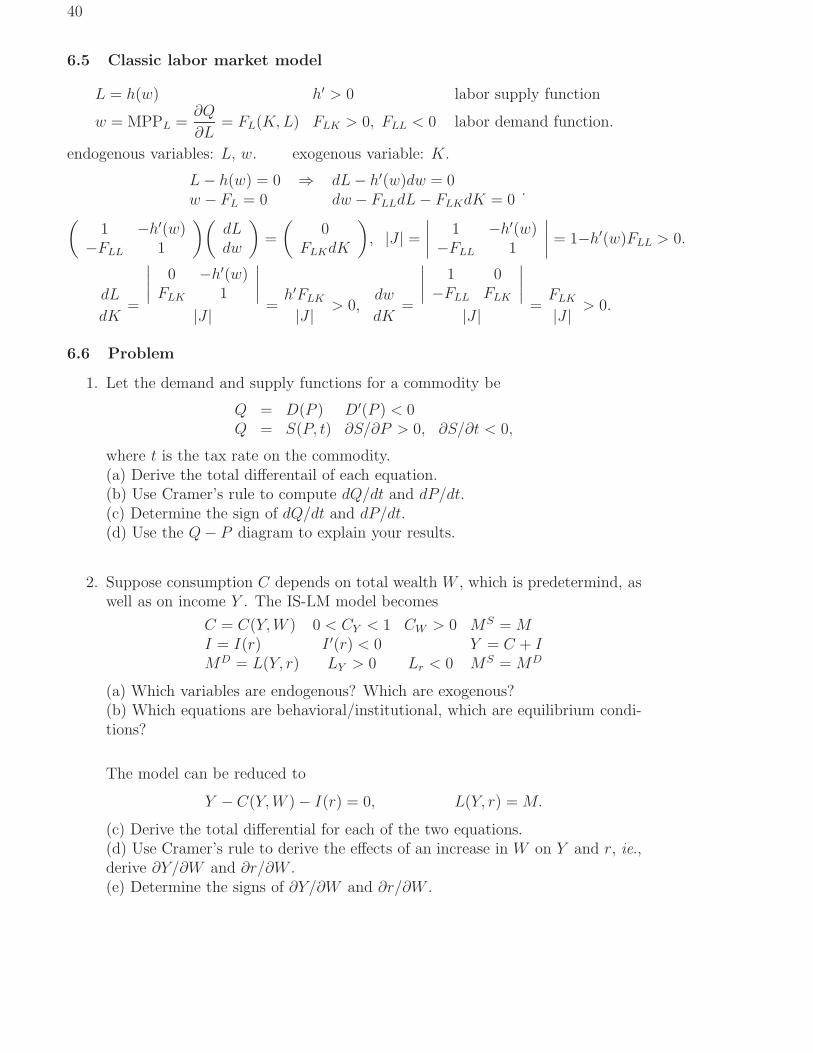
40
6.5 Classic labor market model
L = h(w) h′ > 0 labor supply function
w = MPPL =∂Q
∂L= FL(K, L) FLK > 0, FLL < 0 labor demand function.
endogenous variables: L, w. exogenous variable: K.
L− h(w) = 0 ⇒ dL− h′(w)dw = 0w − FL = 0 dw − FLLdL− FLKdK = 0
.
(
1 −h′(w)−FLL 1
)(
dLdw
)
=
(
0FLKdK
)
, |J | =∣
∣
∣
∣
1 −h′(w)−FLL 1
∣
∣
∣
∣
= 1−h′(w)FLL > 0.
dL
dK=
∣
∣
∣
∣
0 −h′(w)FLK 1
∣
∣
∣
∣
|J | =h′FLK
|J | > 0,dw
dK=
∣
∣
∣
∣
1 0−FLL FLK
∣
∣
∣
∣
|J | =FLK
|J | > 0.
6.6 Problem
1. Let the demand and supply functions for a commodity be
Q = D(P ) D′(P ) < 0Q = S(P, t) ∂S/∂P > 0, ∂S/∂t < 0,
where t is the tax rate on the commodity.(a) Derive the total differentail of each equation.(b) Use Cramer’s rule to compute dQ/dt and dP/dt.(c) Determine the sign of dQ/dt and dP/dt.(d) Use the Q− P diagram to explain your results.
2. Suppose consumption C depends on total wealth W , which is predetermind, aswell as on income Y . The IS-LM model becomes
C = C(Y, W ) 0 < CY < 1 CW > 0 MS = MI = I(r) I ′(r) < 0 Y = C + IMD = L(Y, r) LY > 0 Lr < 0 MS = MD
(a) Which variables are endogenous? Which are exogenous?(b) Which equations are behavioral/institutional, which are equilibrium condi-tions?
The model can be reduced to
Y − C(Y, W )− I(r) = 0, L(Y, r) = M.
(c) Derive the total differential for each of the two equations.(d) Use Cramer’s rule to derive the effects of an increase in W on Y and r, ie.,derive ∂Y/∂W and ∂r/∂W .(e) Determine the signs of ∂Y/∂W and ∂r/∂W .
41
3. Consider a 2-industry (e.g. manufacturing and agriculture) general equilibriummodel. The demand for manufacturing product consists of two components:private demand D1 and goverment demand G. The agricultural products haveonly private demand D2. Both D1 and D2 depend only on their own prices.Because each industry requires in its production process outputs of the other,the supply of each commodity depends on the price of the other commodity aswell as on its own price. Therefore, the model may be written as follows:
Qd1 = D1(P1) + G D′
1(P1) < 0,Qd
2 = D2(P2) D′2(P2) < 0,
Qs1 = S1(P1, P2) S1
1 > 0, S12 < 0, S1
1 > |S12 |,
Qs2 = S2(P1, P2) S2
1 < 0, S22 > 0, S2
2 > |S21 |,
Qd1 = Qs
1,Qd
2 = Qs2.
(a) Which variables are endogenous? Which are exogenous?(b) Which equations are behavioral? Which are definitional? Which are equi-librium conditions?
4. The model can be reduced to
S1(P1, P2) = D1(P1) + G S2(P1, P2) = D2(P2)
(c) Compute the total differential of each equation.(d) Use Cramer’s rule to derive ∂P1/∂G and ∂P2/∂G.(e) Determine the signs of ∂P1/∂G and ∂P2/∂G.(f) Compute ∂Q1/∂G and ∂Q2/∂G. (Hint: Use chain rule.)(g) Give an economic interpretation of the results.
5. The demand functions of a 2-commodity market model are:
Qd1 = D1(P1, P2) Qd
2 = D2(P1, P2).
The supply of the first commodity is given exogenously, ie., Qs1 = S1. The
supply of the second commodity depends on its own price, Qs2 = S2(P2). The
equilibrium conditions are:
Qd1 = Qs
1, Qd2 = Qs
2.
(a) Which variables are endogenous? Which are exogenous?(b) Which equations are behavioral? Which are definitional? Which are equi-librium conditions?
The model above can be reduced to :
D1(P1, P2)− S1 = 0 D2(P1, P2)− S2(P2) = 0
42
Suppose that both commodities are not Giffen good (hence, Dii < 0, i = 1, 2),
that each one is a gross substitute for the other (ie., Dij > 0, i 6= j), that
|Dii| > |Di
j |, and that S ′2(P2) > 0.(c) Calculate the total differential of each equation of the reduced model.(d) Use Cramer’s rule to derive ∂P1/∂S1 and ∂P2/∂S1.(e) Determine the signs of ∂P1/∂S1 and ∂P2/∂S1.(f) Compute ∂Q1/∂S1 and ∂Q2/∂S1 and determine their signs.
6. The demand functions for fish and chicken are as follows:
QdF = DF (PF − PC), D′
F < 0
QdC = DC(PC − PF ), D′
C < 0
where PF , PC are price of fish and price of chicken respectively. The supplyof fish depends on the number of fishermen (N) as well as its price PF : Qs
F =F (PF , N), FPF
> 0, FN > 0. The supply of chicken depends only on its pricePC : Qs
C = C(PC), C ′ > 0. The model can be reduced to
DF (PF − PC) = F (PF , N)DC(PC − PF ) = C(PC)
(a) Find the total differential of the reduced system.(b) Use Cramer’s rule to find dPF/dN and dPC/dN .(c) Determine the signs of dPF /dN and dPC/dN . What is the economic mean-ing of your results?(d) Find dQC/dN .
7. In a 2-good market equilibrium model, the inverse demand functions are givenby
P1 = U1(Q1, Q2), P2 = U2(Q1, Q2);
where U1(Q1, Q2) and U2(Q1, Q2) are the partial derivatives of a utility functionU(Q1, Q2) with respect to Q1 and Q2, respectively.
(a) Calculate the Jacobian matrix
(
∂P1/∂Q1 ∂P1/∂Q2
∂P2/∂Q1 ∂P2/∂Q2
)
and Jacobian∂(P1, P2)
∂(Q1, Q2).
What condition(s) should the parameters satisfy so that we can invert thefunctions to obtain the demand functions?
(b) Derive the Jacobian matrix of the derivatives of (Q1, Q2) with respect to
(P1, P2),
(
∂Q1/∂P1 ∂Q1/∂P2
∂Q2/∂P1 ∂Q2/∂P2
)
.
(c) Suppose that the supply functions are
Q1 = a−1P1, Q2 = P2,
and Q∗1 and Q∗
2 are market equilibrium quantities. Find the comparative
staticsdQ∗
1
daand
dQ∗2
da. (Hint: Eliminate P1 and P2.)

43
8. In a 2-good market equilibrium model with a sales tax of t dollars per unit onproduct 1, the model becomes
D1(P1 + t, P2) = Q1 = S1(P1), D2(P1 + t, P2) = Q2 = S2(P2).
Suppose that Dii < 0 and S ′i > 0, |Di
i| > |Dij|, i 6= j, i, j = 1, 2.
(a) Calculate dP2/dt.
(b) Calculate dQ2/dt.
(c) Suppose that Dij > 0. Determine the signs of dP2/dt and dQ2/dt.
(d) Suppose that Dij < 0. Determine the signs of dP2/dt and dQ2/dt.
(e) Explain your results in economics.
44
7 Optimization
A behavioral equation is a summary of the decisions of a group of economic agentsin a model. A demand (supply) function summarizes the consumption (production)decisions of consumers (producers) under different market prices, etc. The derivativeof a behavioral function represents how agents react when an independent variablechanges. In the last chapter, when doing comparative static analysis, we alwaysassumed that the signs of derivatives of a behavioral equation in a model are known.For example, D′(P ) < 0 and S ′(P ) > 0 in the partial market equilibrium model,C ′(Y ) > 0, I ′(r) < 0, Ly > 0, and Lr < 0 in the IS-LM model. In this chapter, weare going to provide a theoretical foundation for the determination of these signs.
7.1 Neoclassic methodology
Neoclassic assumption: An agent, when making decisions, has an objective functionin mind (or has well defined preferences). The agent will choose a feasible decisionsuch that the objective function is maximized.A consumer will choose the quantity of each commodity within his/her budget con-straints such that his/her utility function is maximized. A producer will choose tosupply the quantity such that his profit is maximizaed.Remarks: (1) Biological behavior is an alternative assumption, sometimes more ap-propriate, (2) Sometimes an agent is actually a group of people with different per-sonalities like a company and we have to use game theoretic equilibrium concepts tocharacterize the collective behavior.
Maximization ⇒ Behavioral equationsGame equilibrium ⇒ Equilibrium conditions
x1, . . . , xn: variables determined by the agent (endogenous variables).y1, . . . , ym: variables given to the agent (exogenous variables).Objective function: f(x1, . . . , xn; y1, . . . , ym).Opportunity set: the agent can choose only (x1, . . . , xn) such that (x1, . . . , xn; y1, . . . , ym) ∈A ⊂ Rn+m. A is usually defined by inequality constriants.
maxx1,...,xn
f(x1, . . . , xn; y1, . . . , ym) subject to
g1(x1, . . . , xn; y1, . . . , ym) ≥ 0...
gk(x1, . . . , xn; y1, . . . , ym) ≥ 0.
Solution (behavioral equations): xi = xi(y1, . . . , ym), i = 1, . . . , n (derived from FOC).∂xi/∂yj: derived by the comparative static method (sometimes its sign can be deter-mined from SOC).
Example 1: A consumer maximizes his utility function U(q1, q2) subject to thebudget constraint p1q1 + p2q2 = m ⇒ demand functions q1 = D1(p1, p2, m) andq2 = D2(p1, p2, m).
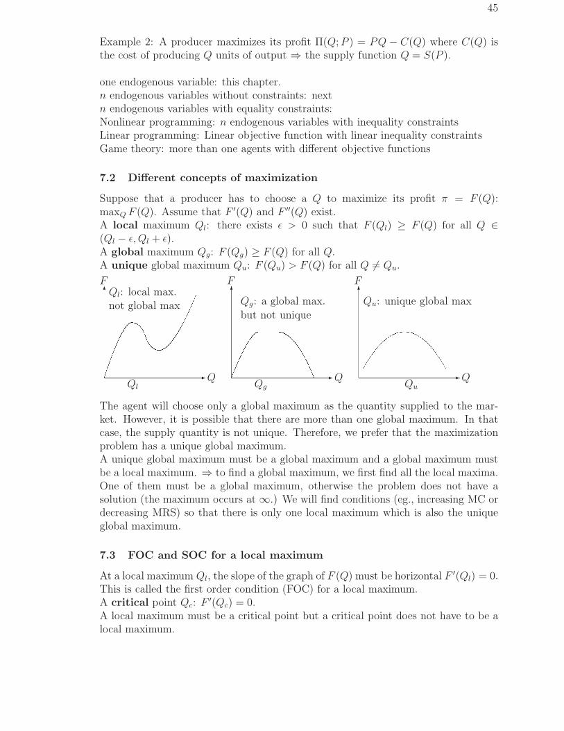
45
Example 2: A producer maximizes its profit Π(Q; P ) = PQ − C(Q) where C(Q) isthe cost of producing Q units of output ⇒ the supply function Q = S(P ).
one endogenous variable: this chapter.n endogenous variables without constraints: nextn endogenous variables with equality constraints:Nonlinear programming: n endogenous variables with inequality constraintsLinear programming: Linear objective function with linear inequality constraintsGame theory: more than one agents with different objective functions
7.2 Different concepts of maximization
Suppose that a producer has to choose a Q to maximize its profit π = F (Q):maxQ F (Q). Assume that F ′(Q) and F ′′(Q) exist.A local maximum Ql: there exists ǫ > 0 such that F (Ql) ≥ F (Q) for all Q ∈(Ql − ǫ, Ql + ǫ).A global maximum Qg: F (Qg) ≥ F (Q) for all Q.A unique global maximum Qu: F (Qu) > F (Q) for all Q 6= Qu.
✲Q
✻F
Ql
Ql: local max.not global max
✲Q
✻F
Qg: a global max.
but not unique
Qg
✲Q
✻F
Qu: unique global max
Qu
The agent will choose only a global maximum as the quantity supplied to the mar-ket. However, it is possible that there are more than one global maximum. In thatcase, the supply quantity is not unique. Therefore, we prefer that the maximizationproblem has a unique global maximum.A unique global maximum must be a global maximum and a global maximum mustbe a local maximum. ⇒ to find a global maximum, we first find all the local maxima.One of them must be a global maximum, otherwise the problem does not have asolution (the maximum occurs at ∞.) We will find conditions (eg., increasing MC ordecreasing MRS) so that there is only one local maximum which is also the uniqueglobal maximum.
7.3 FOC and SOC for a local maximum
At a local maximum Ql, the slope of the graph of F (Q) must be horizontal F ′(Ql) = 0.This is called the first order condition (FOC) for a local maximum.A critical point Qc: F ′(Qc) = 0.A local maximum must be a critical point but a critical point does not have to be alocal maximum.

46
✲Q
✻F
F ′′(Qc) < 0
local max.
Qc
✲Q
✻F
F ′′(Qc) > 0
local min.
Qc
✲Q
✻F
F ′′(Qc) = 0
degenerate
Qc
A degenerate critical point: F ′(Q) = F ′′(Q) = 0.A non-degenerate critical point: F ′(Q) = 0, F ′′(Q) 6= 0.A non-degenerate critical point is a local maximum (minimum) if F ′′(Q) < 0 (F ′′(Q) >0).
FOC: F ′(Ql) = 0 SOC: F ′′(Ql) < 0
Example: F (Q) = −15Q+9Q2−Q3, F ′(Q) = −15+18Q−3Q2 = −3(Q−1)(Q−5).There are two critical points: Q = 1, 5. F ′′(Q) = 18 − 6Q, F ′′(1) = 12 > 0, andF ′′(5) = −12 < 0. Therefore, Q = 5 is a local maximum. It is a global maximum for0 ≤ Q <∞.
Remark 1 (Degeneracy): For a degenerate critical point, we have to check higherorder derivatives. If the lowest order non-zero derivative is of odd order, then it is areflect point; eg., F (Q) = (Q−5)3, F ′(5) = F ′′(5) = 0 and F ′′′(5) = 6 6= 0 and Q = 5is not a local maximum. If the lowest order non-zero derivative is of even order andnegative (positive), then it is a local maximum (minimum); eg., F (Q) = −(Q− 5)4,F ′(5) = F ′′(5) = F ′′′(5) = 0, F (4)(5) = −24 < 0 and Q = 5 is a local maximum.Remark 2 (Unboundedness): If limQ→∞ F (Q) =∞, then a global maximum does notexist.Remark 3 (Non-differentiability): If F (Q) is not differentiable, then we have to useother methods to find a global maximum.Remark 4 (Boundary or corner solution): When there is non-negative restrictionQ ≥ 0 (or an upper limit Q ≤ a), it is possible that the solution occurs at Q = 0 (orat Q = a). To take care of such possibilities, FOC is modified to become F ′(Q) ≤ 0,QF ′(Q) = 0 (or F ′(Q) ≥ 0, (a−Q)F ′(Q) = 0).
7.4 Supply function of a competitive producer
Consider first the profit maximization problem of a competitive producer:
maxQ
Π = PQ− C(Q), FOC ⇒ ∂Π
∂Q= P − C ′(Q) = 0.
The FOC is the inverse supply function (a behavioral equation) of the producer: P= C ′(Q) = MC. Remember that Q is endogenous and P is exogenous here. To find
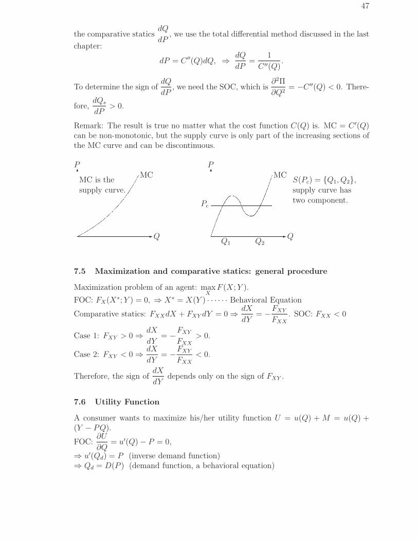
47
the comparative staticsdQ
dP, we use the total differential method discussed in the last
chapter:
dP = C ′′(Q)dQ, ⇒ dQ
dP=
1
C ′′(Q).
To determine the sign ofdQ
dP, we need the SOC, which is
∂2Π
∂Q2= −C ′′(Q) < 0. There-
fore,dQs
dP> 0.
Remark: The result is true no matter what the cost function C(Q) is. MC = C ′(Q)can be non-monotonic, but the supply curve is only part of the increasing sections ofthe MC curve and can be discontinuous.
✲Q
✻P
MCMC is the
supply curve.
✲Q
✻P
MC
Q1 Q2
Pc
S(Pc) = {Q1, Q2},supply curve hastwo component.
7.5 Maximization and comparative statics: general procedure
Maximization problem of an agent: maxX
F (X; Y ).
FOC: FX(X∗; Y ) = 0, ⇒ X∗ = X(Y ) · · · · · · Behavioral Equation
Comparative statics: FXXdX + FXY dY = 0 ⇒ dX
dY= −FXY
FXX. SOC: FXX < 0
Case 1: FXY > 0 ⇒ dX
dY= −FXY
FXX> 0.
Case 2: FXY < 0 ⇒ dX
dY= −FXY
FXX
< 0.
Therefore, the sign ofdX
dYdepends only on the sign of FXY .
7.6 Utility Function
A consumer wants to maximize his/her utility function U = u(Q) + M = u(Q) +(Y − PQ).
FOC:∂U
∂Q= u′(Q)− P = 0,
⇒ u′(Qd) = P (inverse demand function)⇒ Qd = D(P ) (demand function, a behavioral equation)
48
∂2U
∂Q∂P= UPQ = −1 ⇒ dQd
dP= D′(P ) < 0, the demand function is a decreasing
function of price.
7.7 Input Demand Function
The production function of a producer is given by Q = f(x), where x is the quantityof an input employed. Its profit is Π = pf(x) − wx, where p (w) is the price of theoutput (input).The FOC of profit maximization problem is pf ′(x)− w = 0⇒ f ′(x) = w/p (inverse input demand function)⇒ x = h(w/p) (input demand function, a behavioral equation)
∂2Π
∂x∂(w/p)= −1 ⇒ dx
d(w/p)= h′(w/p) < 0, the input demand is a decreasing func-
tion of the real input pricew
p.
7.8 Envelope theorem
Define the maximum function M(Y ) ≡ maxX F (X, Y ) = F (X(Y ), Y ) then the totalderivative
dM
dY= M ′(Y ) =
∂F (X, Y )
∂Y
∣
∣
∣
∣
X=X(Y )
.
Proof: M ′(Y ) = FXdX
dY+ FY . At the maximization point X = X(Y ), FOC implies
that the indirect effect of Y on M is zero.
In the consumer utility maximization problem, V (P ) ≡ U(D(P )) + Y − PD(P )is called the indirect utility function. The envelope theorem implies that V ′(P ) =dU
dP
∣
∣
∣
∣
Qd=D(P )
≡ −D(P ), this is a simplified version of Roy’s identity.
In the input demand function problem, π(w, p) ≡ pf(h(w/p))−wh(w/p) is the profitfunction. Let p = 1 and still write π(w) ≡ f(h(w))− wh(w). The envelope theorem
implies that π′(w) =dΠ
dw
∣
∣
∣
∣
x=h(w)
= −h(w), a simplified version of Hotelling’s lemma.
Example: The relationships between LR and SR cost curvesSTC(Q; K) = C(Q, K), K: firm size. Each K corresponds to a STC.LTC(Q) = minK C(Q, K), ⇒ K = K(Q) is the optimal firm size.LTC is the envelope of STC’s. Each STC tangents to the LTC (STC = LTC) at thequantity Q such that K = K(Q). Notice that the endogenous variable is K and theexogenous is Q here.By envelope theorem, LMC(Q) = dLTC(Q)/dQ = ∂C(Q, K(Q))/∂Q =SMC(Q; K(Q)).That is, when K = K(Q) is optimal for producing Q, SMC=LMC.

49
Since LAC(Q) =LTC(Q)/Q and SAC(Q) =STC(Q)/Q, LAC is the envelope of SAC’sand each SAC tangents to the LAC (SAC = LAC) at the quantity Q such thatK = K(Q).
7.9 Effect of a Unit Tax on Monopoly Output (Samuelson)
Assumptions: a monopoly firm, q = D(P ) ⇐⇒ P = f(q), (inverse functions),C = C(q), t = unit tax
maxπ(q) = Pq − C(q)− tq = qf(q)− C(q)− tq
q: endogenous; t: exogenousFOC: ∂π/∂q = f(q) + qf ′(q)− C ′(q)− t = 0.The FOC defines a relationship between the monopoly output q∗ and the tax rate tas q∗ = q(t) (a behavioral equation). The derivative dq∗/dt can be determined by thesign of the cross derivative:
∂2π
∂q∂t= −1 < 0
Therefore, we have dq∗/dt < 0.The result can be obtained using the q–pdiagram. FOC ⇐⇒ MR = MC + t.Therefore, on q–p space, an equilibrium is determined by the intersection point ofMR and MC + t curves.
Case 1: MR is downward sloping and MC is upward sloping:When t increases, q∗ decreases as seen from the left diagram below.
✲ q
✻P
MC
MC+t
MR< ✲ q
✻P
MC
MC+t
MR<
Case 2: Both MR and MC are downward sloping and MR is steeper. MC decreasing;MR decreasing more ⇒ t ↑ q ↓.
Case 3: Both MR and MC are downward sloping, but MC is steeper. The diagramshows that dq∗/dt > 0. It is opposite to our comparative statics result. Why?MR = MC + t violates SOC < 0, therefore, the intersection of MR and MC + tis not a profit maximizing point.
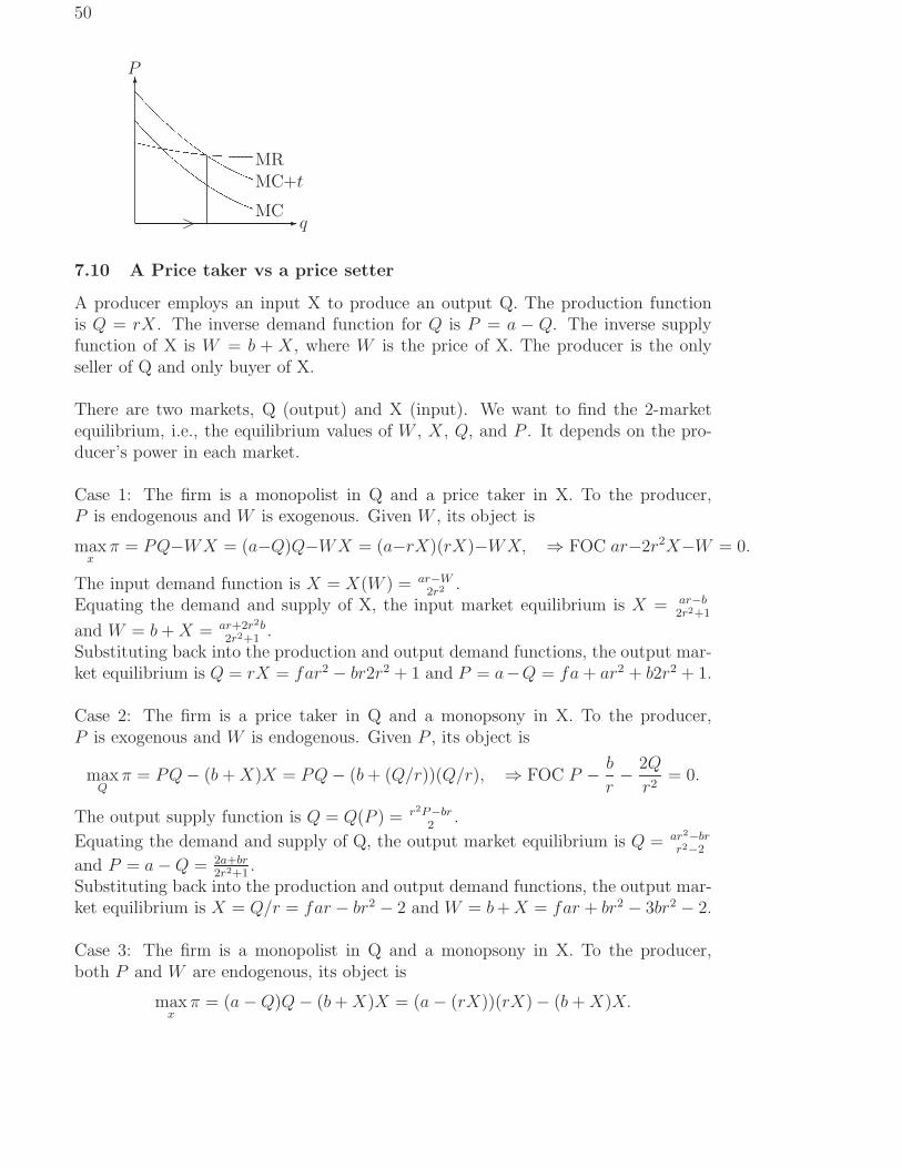
50
✲ q
✻P
MC
MC+tMR
>
7.10 A Price taker vs a price setter
A producer employs an input X to produce an output Q. The production functionis Q = rX. The inverse demand function for Q is P = a − Q. The inverse supplyfunction of X is W = b + X, where W is the price of X. The producer is the onlyseller of Q and only buyer of X.
There are two markets, Q (output) and X (input). We want to find the 2-marketequilibrium, i.e., the equilibrium values of W , X, Q, and P . It depends on the pro-ducer’s power in each market.
Case 1: The firm is a monopolist in Q and a price taker in X. To the producer,P is endogenous and W is exogenous. Given W , its object is
maxx
π = PQ−WX = (a−Q)Q−WX = (a−rX)(rX)−WX, ⇒ FOC ar−2r2X−W = 0.
The input demand function is X = X(W ) = ar−W2r2 .
Equating the demand and supply of X, the input market equilibrium is X = ar−b2r2+1
and W = b + X = ar+2r2b2r2+1
.Substituting back into the production and output demand functions, the output mar-ket equilibrium is Q = rX = far2 − br2r2 + 1 and P = a−Q = fa + ar2 + b2r2 + 1.
Case 2: The firm is a price taker in Q and a monopsony in X. To the producer,P is exogenous and W is endogenous. Given P , its object is
maxQ
π = PQ− (b + X)X = PQ− (b + (Q/r))(Q/r), ⇒ FOC P − b
r− 2Q
r2= 0.
The output supply function is Q = Q(P ) = r2P−br2
.
Equating the demand and supply of Q, the output market equilibrium is Q = ar2−brr2−2
and P = a−Q = 2a+br2r2+1
.Substituting back into the production and output demand functions, the output mar-ket equilibrium is X = Q/r = far − br2 − 2 and W = b + X = far + br2 − 3br2 − 2.
Case 3: The firm is a monopolist in Q and a monopsony in X. To the producer,both P and W are endogenous, its object is
maxx
π = (a−Q)Q− (b + X)X = (a− (rX))(rX)− (b + X)X.
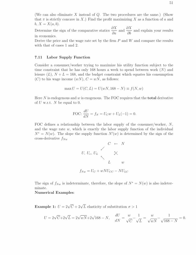
51
(We can also eliminate X instead of Q. The two procedures are the same.) (Showthat π is strictly concave in X.) Find the profit maximizing X as a function of a andb, X = X(a, b).
Determine the sign of the comparative statics∂X
∂aand
∂X
∂band explain your results
in economics.Derive the price and the wage rate set by the firm P and W and compare the resultswith that of cases 1 and 2.
7.11 Labor Supply Function
Consider a consumer/worker trying to maximize his utility function subject to thetime constraint that he has only 168 hours a week to spend between work (N) andleisure (L), N + L = 168, and the budget constraint which equates his consumption(C) to his wage income (wN), C = wN , as follows:
maxU = U(C, L) = U(wN, 168−N) ≡ f(N, w)
Here N is endogenous and w is exogenous. The FOC requires that the total derivativeof U w.r.t. N be equal to 0.
FOC:dU
dN= fN = UCw + UL(−1) = 0.
FOC defines a relationship between the labor supply of the consumer/worker, N ,and the wage rate w, which is exactly the labor supply function of the individualN∗ = N(w). The slope the supply function N ′(w) is determined by the sign of thecross-derivative fNw
U, Uc, UL
C ← Nւ
ւտտ
L w
fNw = UC + wNUCC −NULC
The sign of fNw is indeterminate, therefore, the slope of N∗ = N(w) is also indeter-minate.Numerical Examples:
Example 1: U = 2√
C + 2√
L elasticity of substitution σ > 1
U = 2√
C+2√
L = 2√
wN+2√
168−N,dU
dN=
w√C− 1√
L=
w√wN
− 1√168−N
= 0.

52
Therefore, the inverse labor supply function is w = N/(168 − N), which ispositively sloped.
✲N
✻w
σ > 1
✲N
✻w
σ < 1
Example 2: U = CLC+L
elasticity of substitution σ < 1
U =CL
C + L=
wN(168−N)
wN + 168−N,
dU
dN=
wL2 − C2
(C + L)2= 0.
Therefore, the inverse labor supply function is w = [(168 − N)/N ]2, which isnegatively sloped.
Example 3: U = CL Cobb-Douglas( σ = 1)
U = CL = wN(168−N)dU
dN= w(168− 2N) = 0
The labor supply function is a constant N = 84 and the curve is vertical.
✲N
✻w
σ = 1
✲N
✻w
Backward-bending Labor Supply Curve: It is believed that the labor supplycurve can be backward-bending.
7.12 Exponential and logarithmic functions and interest compounding
Exponential function f(x) = ex is characterized by f(0) = 1 and f(x) = f ′(x) =f ′′(x) = . . . = f (n)(x). The Taylor expansion of the exponential functionat x = 0becomes
ex = 1 + x + x2/2! + · · ·+ xn/n! + . . .
Some Rules:d
dx(ex) = ex,
d
dxeax = aeax,
d
dxef(x) = f ′(x)ef(x).
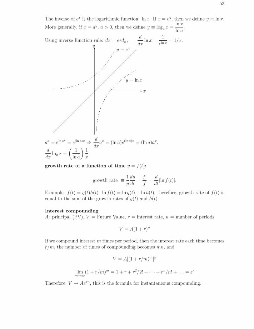
53
The inverse of ex is the logarithmic function: lnx. If x = ey, then we define y ≡ lnx.
More generally, if x = ay, a > 0, then we define y ≡ loga x =ln x
ln a.
Using inverse function rule: dx = eydy,d
dxln x =
1
eln x= 1/x.
✲x
✻y
y = ex
y = ln x
ax = eln ax
= e(ln a)x ⇒ d
dxax = (ln a)e(ln a)x = (ln a)ax.
d
dxlna x =
(
1
ln a
)
1
x
growth rate of a function of time y = f(t):
growth rate ≡ 1
y
dy
dt=
f ′
f=
d
dt[ln f(t)].
Example: f(t) = g(t)h(t). ln f(t) = ln g(t) + ln h(t), therefore, growth rate of f(t) isequal to the sum of the growth rates of g(t) and h(t).
Interest compoundingA: principal (PV), V = Future Value, r = interest rate, n = number of periods
V = A(1 + r)n
If we compound interest m times per period, then the interest rate each time becomesr/m, the number of times of compounding becomes mn, and
V = A[(1 + r/m)m]n
limm→∞
(1 + r/m)m = 1 + r + r2/2! + · · ·+ rn/n! + . . . = er
Therefore, V → Aern, this is the formula for instantaneous compounding.

54
7.13 Timing: (when to cut a tree)
t: number of years to wait, A(t) present value after t years
V (t) = Ke√
t: the market value of the tree after t years
A(t) = Ke√
te−rt is the present valueWe want to find the optimal t such that the present value is maximized.
maxt
A(t) = Ke√
te−rt.
The FOC is
A′ =
(
1
2√
t− r
)
A(t) = 0
Because A(t) 6= 0, FOC implies:1
2√
t− r = 0, t∗ = 1/(4r2)
For example, if r = 10%, t = 25, then to wait 25 years before cutting the tree is theoptimum.Suppose that A(t) = ef(t)
FOC becomes: A′(t)/A(t) = f ′(t) = r, ⇒ f ′(t) is the instantaneous growth rate (orthe marginal growth rate) at t, ⇒ at t = 25, growth rate = 10% = r, at t = 26,growth rate < 10%. Therefore, it is better to cut and sell the tree at t = 25 and putthe proceed in the bank than waiting longer.SOC: It can be shown that A′′ < 0.
7.14 Problems
1. Suppose the total cost function of a competitive firm is C(Q) = eaQ+b. Derivethe supply function.
2. The input demand function of a competitive producer, X = X(W ), can bederived by maximizing the profit function Π = F (X) −WX with respect toX, where X is the quantity of input X and W is the price of X. Derive thecomparative statics dX/dW and determine its sign.
3. The utility function of a consumer is given by U = U(X) + M , where X is thequantity of commodity X consumed and M is money. Suppose that the totalincome of the consumer is $ 100 and that the price of X is P . Then the utilityfunction become U(X) + (100−XP ).
(a) Find the first order condition of the utility maximization problem.
(b) What is the behavior equation implied by the first order condition?
(c) Derive dX/dP and determine its sign. What is the economic meaning ofyour result?
4. The consumption function of a consumer, C = C(Y ), can be derived by max-imizing the utility function U(C, Y ) = u1(C) + u2(Y − C), where u′1(C) > 0,u′2(Y −C) > 0 and u1”(C) < 0, u2”(Y −C) < 0. Derive the comparative staticsdC/dY and determine its sign.

55
5. Consider a duopoly market with two firms, A and B. The inverse demand func-tion is P = f(QA + QB), f ′ < 0, f” < 0. The cost function of firm A is TCA
= C(QA), C ′ > 0, C” > 0. The profit of firm A is ΠA = PQA − TCA =QAf(QA +QB)−C(QA). For a given output of firm B, QB, there is a QA whichmaximizes firm A’s profit. This relationship between QB and QA is called thereaction function of firm A, QA = RA(QB).
(a) Find the slope of the reaction function R′A = dQA
dQB.
(b) When QB increases, will firm A’s output QA increase or decrease?
6. The profit of a monopolistic firm is given by Π = R(x) − C(x, b), where x isoutput, b is the price of oil, R(x) is total revenue, and C(x, b) is the total costfunction. For any given oil price b, there is an optimal
output which maximizes profit, that is, the optimal output is a function of oilprice, x = x(b). Assume that Cbx = ∂2C/∂b∂x > 0, that is, an increase in oilprice will increase marginal cost. Will an increase in oil price increase output,that is, is dx/db > 0?
7. Consider a monopsony who uses a single input, labor (L), for the production of acommodity (Q), which he sells in a perfect competition market. His productionfunction is Q = F (L), (f ′(L) > 0). The labor supply function is L = L(w), ormore convenient for this problem, w = L−1(L) = W (L). Given the commodityprice p, there is an optimal labor input which maximizes the monopsonist’stotal profit Π = pf(L)−W (L)L. In this problem, you are asked to derive therelation between L and p.
(a) State the FOC and the SOC of the profit maximization problem.
(b) Derive the comparative statics dL/dp and determine its sign.
8. Suppose that a union has a fixed supply of labor (L) to sell, that unemployedworkers are paid unemployment insurance at a rate of $u per worker, and thatthe union wishes to maximize the sum of the wage bill plus the unemploymentcompensation S = wD(w) + u(L−D(w)), where w is wage per
worker, D(w) is labor demand function, and D′(w) < 0. Show that if u in-creases, then the union should set a higher w. (Hint: w is endogenous and u isexogenous.)
9. The production function of a competitive firm is given by Q = F (L, K). whereL is variable input and K is fixed input. The short run profit function is givenby Π = pQ−wL−rK, where p is output price, w is wage rate, and r is the rentalrate on capital. In the short run, given the quantity of fixed input K,there is aL which maximizes Π. Hence, the short run demand for L can be regarded asa function of K. Assume that FLK > 0.
(a) State the FOC and SOC of the profit maximization problem.
(b) Derive the comparative statics dL/dK and determine its sign.

56
7.15 Concavity and Convexity
The derivation of a behavioral equation X = X(Y ) from the maximization problemmaxx F (X; Y ) is valid only if there exists a unique global maximum for every Y . Ifthere are multiple global maximum, then X = X(Y ) has multiple values and thecomparative static analysis is not valid. Here we are going to discuss a condition onF (X; Y ) so that a critical point is always a unique global maximum and the compar-ative static analysis is always valid.
Convex setsA is a convex set if ∀X0, X1 ∈ A and 0 ≤ θ ≤ 1, Xθ ≡ (1 − θ)X0 + θX1 ∈ A. (IfX0, X1 ∈ A then the whole line connecting X0 and X1 is in A.)
✲x1
✻x2
❅❅
some convex sets
✣✢✤✜
✲ x1
✻x2
✒✑✓✏✧✦★✥
some non-convex sets
(1) If A1 and A2 are convex, then A1 ∩ A2 is convex but A1 ∪ A2 is not necessar-ily convex. Also, the empty set itself is a convex set.(2) The convex hull of A is the smallest convex set that contains A. For example, theconvex hull of {X0} ∪ {X1} is the straight line connecting X0 and X1.
Convex and concave functionsGiven a function F (X), we define the sets
G+F ≡ {(x, y)| y ≥ F (x), x ∈ R}, G−
F ≡ {(x, y)| y ≤ F (x), x ∈ R}, G+F , G−
F ⊂ R2.
If G+F (G−
F ) is a convex set, then we say F (X) is a convex function (a concave func-tion). If F (X) is defined only for nonnegative values X ≥ 0, the definition is similar.
✲X
✻
F (X)
G−F
G+F
G−F is a convex set ⇒ F (X) is concave
✲X
✻ F (X)
G−F
G+F
G+F is a convex set ⇒ F (X) is convex
Equivalent Definition: Given X0 < X1, 0 ≤ θ ≤ 1, denote F 0 = F (X0),F 1 = F (X1). Define Xθ ≡ (1 − θ)X0 + θX1, F (Xθ) = F ((1 − θ)X0 + θX1). Also
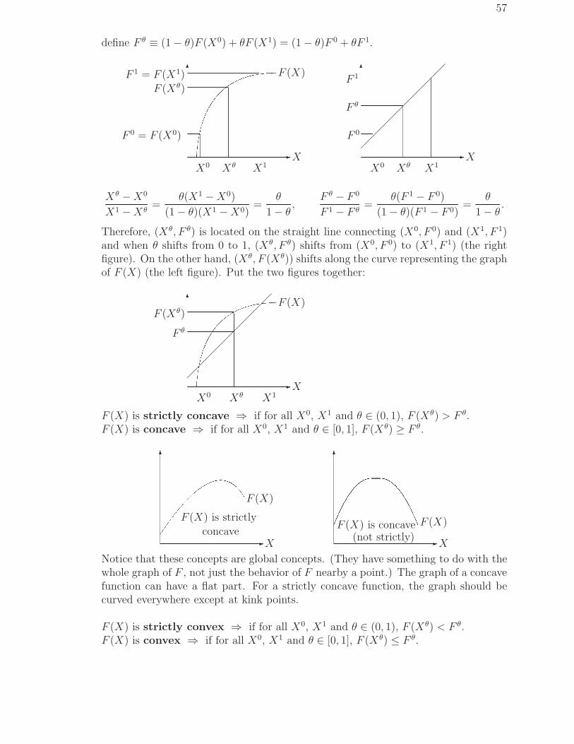
57
define F θ ≡ (1− θ)F (X0) + θF (X1) = (1− θ)F 0 + θF 1.
✲X
✻ F (X)
X0 Xθ X1
F 0 = F (X0)
F (Xθ)
F 1 = F (X1)
✲X
✻
X0 Xθ X1
F 0
F θ
F 1
Xθ −X0
X1 −Xθ=
θ(X1 −X0)
(1− θ)(X1 −X0)=
θ
1− θ,
F θ − F 0
F 1 − F θ=
θ(F 1 − F 0)
(1− θ)(F 1 − F 0)=
θ
1− θ.
Therefore, (Xθ, F θ) is located on the straight line connecting (X0, F 0) and (X1, F 1)and when θ shifts from 0 to 1, (Xθ, F θ) shifts from (X0, F 0) to (X1, F 1) (the rightfigure). On the other hand, (Xθ, F (Xθ)) shifts along the curve representing the graphof F (X) (the left figure). Put the two figures together:
✲X
✻ F (X)
X0 Xθ X1
F θ
F (Xθ)
F (X) is strictly concave ⇒ if for all X0, X1 and θ ∈ (0, 1), F (Xθ) > F θ.F (X) is concave ⇒ if for all X0, X1 and θ ∈ [0, 1], F (Xθ) ≥ F θ.
✲X
✻
F (X)
F (X) is strictly
concave✲X
✻
F (X)F (X) is concave(not strictly)
Notice that these concepts are global concepts. (They have something to do with thewhole graph of F , not just the behavior of F nearby a point.) The graph of a concavefunction can have a flat part. For a strictly concave function, the graph should becurved everywhere except at kink points.
F (X) is strictly convex ⇒ if for all X0, X1 and θ ∈ (0, 1), F (Xθ) < F θ.F (X) is convex ⇒ if for all X0, X1 and θ ∈ [0, 1], F (Xθ) ≤ F θ.

58
✲X
✻F
F (X) is strictly
convex
✲X
✻F
❍
F (X) is convex
(not strictly)
Remark 1: A linear function is both concave and convex since F θ ≡ F (Xθ).
✲X
✻F
✟✟✟✟✟✟✟✟✟
✲X
✻F
✂✂✂✂✂✂✂ ✘✘✘
✘
a concavepiecewise-linearfunction
✲X
✻F
✏✏✏ ✂✂✂✂✂✂✂
a convexpiecewise-linearfunction
Remark 2: A piecewise-linear function consists of linear components; for example,the income tax schedule T = f(Y ) is a piecewise-linear function. Other examples are
concave F (X) =
{
2X X ≤ 11 + X X > 1
convex F (X) =
{
X X ≤ 12X − 1 X > 1
In the following theorems, we assume that F ′′(X) exists for all X.
Theorem 1: F (X) is concave, ⇔ F ′′(X) ≤ 0 for all X.F ′′(X) < 0 for all X ⇒ F (X) is strictly concave.Proof: By Taylor’s theorem, there exist X0 ∈ [X0, Xθ] and X1 ∈ [Xθ, X1] such that
F (X1) = F (Xθ) + F ′(Xθ)(X1 −Xθ) +1
2F ′′(X1)(X1 −Xθ)2
F (X0) = F (Xθ) + F ′(Xθ)(X0 −Xθ) +1
2F ′′(X0)(X0 −Xθ)2
⇒ F θ = F (Xθ) +1
2θ(1− θ)(X1 −X0)2[F ′′(X0) + F ′′(X1)].
Theorem 2: If F (X) is concave and F ′(X0) = 0, then X0 is a global maximum.If F (X) is strictly concave and F ′(X0) = 0, then X0 is a unique global maximum.Proof: By theorem 1, X0 must be a local maximum. If it is not a global maximum,then there exists X1 such that F (X1) > F (X0), which implies that F (Xθ) > F (X0)for θ close to 0. Therefore, X0 is not a local maximum, a contradiction.
Remark 1 (boundary/corner solution): The boundary or corner condition F ′(X) ≤ 0,
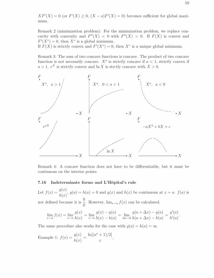
59
XF ′(X) = 0 (or F ′(X) ≥ 0, (X − a)F ′(X) = 0) becomes sufficient for global maxi-mum.
Remark 2 (minimization problem): For the minimization problem, we replace con-cavity with convexity and F ′′(X) < 0 with F ′′(X) > 0. If F (X) is convex andF ′(X∗) = 0, then X∗ is a global minimum.If F (X) is strictly convex and F ′(X∗) = 0, then X∗ is a unique global minimum.
Remark 3: The sum of two concave functions is concave. The product of two concavefunction is not necesarily concave. Xa is strictly concave if a < 1, strictly convex ifa > 1. eX is strictly convex and ln X is strctly concave with X > 0.
✲X
✻F
Xa, a > 1
✲X
✻F
Xa, 0 < a < 1
✲X
✻F
Xa, a < 0
✲X
✻F
eaX
✲X
✻F
ln X✲X
✻F
−aX2 + bX + c
Remark 4: A concave function does not have to be differentiable, but it must becontinuous on the interior points.
7.16 Indeterminate forms and L’Hopital’s rule
Let f(x) =g(x)
h(x), g(a) = h(a) = 0 and g(x) and h(x) be continuous at x = a. f(a) is
not defined because it is0
0. However, limx→a f(x) can be calculated.
limx→a
f(x) = limx→a
g(x)
h(x)= lim
x→a
g(x)− g(a)
h(x)− h(a)= lim
∆x→0
g(a + ∆x)− g(a)
h(a + ∆x)− h(a)=
g′(a)
h′(a).
The same procedure also works for the case with g(a) = h(a) = ∞.
Example 1: f(x) =g(x)
h(x)=
ln[(ax + 1)/2]
x,

60
g(0) = h(0) = 0, h′(x) = 1, g′(x) =(ln a)ax
ax + 1.
⇒ h′(0) = 1 and g′(0) =ln a
2, ⇒ limx→0 f(x) =
ln a
2.
Example 2: f(x) =g(x)
h(x)=
x
ex, h′(x) = ex, g′(x) = 1.
⇒ h′(∞) =∞ and g′(∞) = 1, ⇒ limx→∞ f(x) =1
∞ = 0.
Example 3: f(x) =g(x)
h(x)=
ln x
x, h′(x) = 1, g′(x) =
1
x.
⇒ limx→0+ h′(x) = 1 and limx→0+ g′(x) = ∞, ⇒ limx→0+ f(x) =1
∞ = 0.
7.17 Newton’s method
We can approximate a root x∗ of a nonlinear equation f(x) = 0 using an algorithmcalled Newton’s method.
✲x
✻
xn xn+1 x∗
f(xn)❙❙❙❙❙
f ′(xn) =f(xn)
xn − xn+1
Recursive formula: xn+1 = xn −f(xn)
f ′(xn).
If f(x) is not too strange, we will have limn→∞ xn = x∗. Usually, two or threesteps would be good enough.
Example: f(x) = x3 − 3, f ′(x) = 3x2, xn+1 = xn −x3 − 3
3x2= xn −
x
3+
1
x2.
Starting x0 = 1, x1 = 1− 1
3+ 1 =
5
3≈ 1.666. x2 =
5
3− 5
9+
9
25=
331
225≈ 1.47. The
true value is x∗ = 3√
3 ≈ 1.44225.

61
8 Optimization–Multivariate Case
Suppose that the objective function has n variables: maxx1,...,xn
F (x1, . . . , xn) = F (X).
A local maximum X∗ = (x∗1, . . . , x∗n): ∃ǫ > 0 such that F (X∗) ≥ F (X) for all X
satisfying xi ∈ (x∗i − ǫ, x∗i + ǫ) ∀i.A critical point Xc = (xc
1, . . . , xcn):
∂F (Xc)
∂xi
= 0 ∀i.A global maximum X∗: F (X∗) ≥ F (X) ∀X.A unique global maximum X∗: F (X∗) > F (X) ∀X 6= X∗.The procedure is the same as that of the single variable case. (1) Use FOC to findcritical points; (2) use SOC to check whether a critical point is a local maximum, orshow that F (X) is concave so that a critical point must be a global maximum.
If we regard variables other than xi as fixed, then it is a single variable maximizationproblem and, therefore, we have the necessary conditions
FOC:∂F
∂xi= 0 and SOC:
∂2F
∂x2i
< 0, i = 1, . . . , n.
However, since there are n×n second order derivatives (the Hessian matrix H(F )) andthe SOC above does not consider the cross-derivatives, we have a reason to suspectthat the SOC is not sufficient. In the next section we will provide a counter-exampleand give a true SOC.
8.1 SOC
SOC of variable-wise maximization is wrongExample: max
x1,x2
F (x1, x2) = −x21 + 4x1x2 − x2
2.
FOC: F1 = −2x1 + 4x2 = 0, F2 = 4x1 − 2x2 = 0, ⇒ x1 = x2 = 0.SOC? F11 = F22 = −2 < 0.
✲x1
✻x2
✄✄✄✄✄✄✄✄✄✄✄✄✄✄✄✄✄✄✄✄
✘✘✘✘✘✘
✘✘✘✘✘✘
✘✘✘✘✘✘
✘✘
4
1
4
1
-4-1
-4-1
(0,0) isa saddle point.
✲xi
✻F
When xj = 0,xi = 0 is
a maximum.
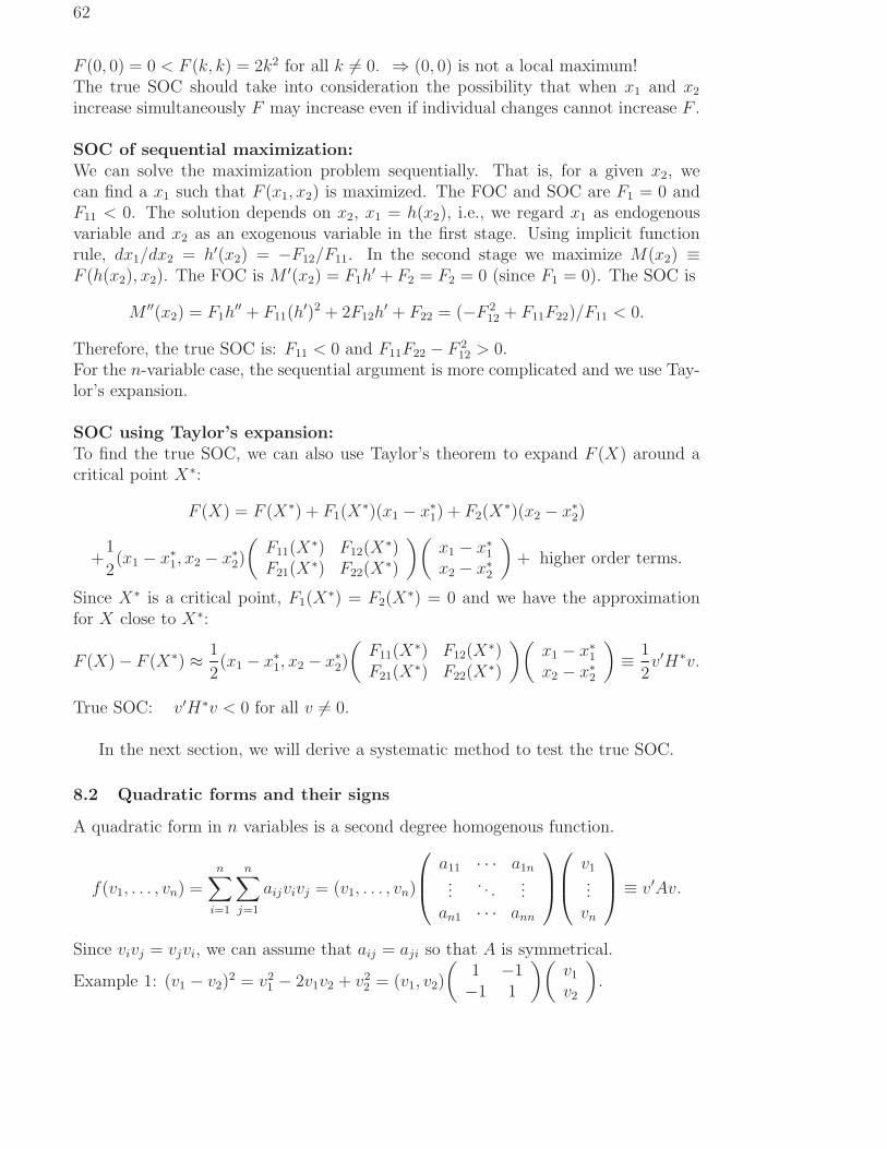
62
F (0, 0) = 0 < F (k, k) = 2k2 for all k 6= 0. ⇒ (0, 0) is not a local maximum!The true SOC should take into consideration the possibility that when x1 and x2
increase simultaneously F may increase even if individual changes cannot increase F .
SOC of sequential maximization:We can solve the maximization problem sequentially. That is, for a given x2, wecan find a x1 such that F (x1, x2) is maximized. The FOC and SOC are F1 = 0 andF11 < 0. The solution depends on x2, x1 = h(x2), i.e., we regard x1 as endogenousvariable and x2 as an exogenous variable in the first stage. Using implicit functionrule, dx1/dx2 = h′(x2) = −F12/F11. In the second stage we maximize M(x2) ≡F (h(x2), x2). The FOC is M ′(x2) = F1h
′ + F2 = F2 = 0 (since F1 = 0). The SOC is
M ′′(x2) = F1h′′ + F11(h
′)2 + 2F12h′ + F22 = (−F 2
12 + F11F22)/F11 < 0.
Therefore, the true SOC is: F11 < 0 and F11F22 − F 212 > 0.
For the n-variable case, the sequential argument is more complicated and we use Tay-lor’s expansion.
SOC using Taylor’s expansion:To find the true SOC, we can also use Taylor’s theorem to expand F (X) around acritical point X∗:
F (X) = F (X∗) + F1(X∗)(x1 − x∗1) + F2(X
∗)(x2 − x∗2)
+1
2(x1 − x∗1, x2 − x∗2)
(
F11(X∗) F12(X
∗)F21(X
∗) F22(X∗)
)(
x1 − x∗1x2 − x∗2
)
+ higher order terms.
Since X∗ is a critical point, F1(X∗) = F2(X
∗) = 0 and we have the approximationfor X close to X∗:
F (X)− F (X∗) ≈ 1
2(x1 − x∗1, x2 − x∗2)
(
F11(X∗) F12(X
∗)F21(X
∗) F22(X∗)
)(
x1 − x∗1x2 − x∗2
)
≡ 1
2v′H∗v.
True SOC: v′H∗v < 0 for all v 6= 0.
In the next section, we will derive a systematic method to test the true SOC.
8.2 Quadratic forms and their signs
A quadratic form in n variables is a second degree homogenous function.
f(v1, . . . , vn) =n∑
i=1
n∑
j=1
aijvivj = (v1, . . . , vn)
a11 · · · a1n...
. . ....
an1 · · · ann
v1...vn
≡ v′Av.
Since vivj = vjvi, we can assume that aij = aji so that A is symmetrical.
Example 1: (v1 − v2)2 = v2
1 − 2v1v2 + v22 = (v1, v2)
(
1 −1−1 1
)(
v1
v2
)
.
63
Example 2: 2v1v2 = (v1, v2)
(
0 11 0
)(
v1
v2
)
.
Example 3: x21 + 2x2
2 + 6x1x3 = (x1, x2, x3)
1 0 30 2 03 0 0
x1
x2
x3
.
v′Av is called negative semidefinite if v′Av ≤ 0 for all v ∈ Rn.v′Av is called negative definite if v′Av < 0 for all v 6= 0.v′Av is called positive semidefinite if v′Av ≥ 0 for all v ∈ Rn.v′Av is called positive definite if v′Av > 0 for all v 6= 0.
(1) −v21 − 2v2
2 < 0, if v1 6= 0 or v2 6= 0⇒ negative.(2) −(v1 − v2)
2 ≤ 0, = 0 if v1 = v2 ⇒ negative semidefinite.(3) (v1 + v2)
2 ≥ 0, = 0 if v1 = −v2 ⇒ positive semidefinite.(4) v2
1 + v22 > 0, if v1 6= 0 or v2 6= 0⇒ positive.
(5) v21 − v2
2
><
0 if |v1|><|v2| ⇒ neither positive nor negative definite.
(6) v1v2><
0 if sign(v1)=6= sign(v2) ⇒ neither positive nor negative definite.
Notice that if v′Av is negative (positive) definite then it must be negative (positive)semidefinite.Testing the sign of a quadratic form:
n = 2: v′Av = (v1, v2)
(
a11 a12
a21 a22
)(
v1
v2
)
= a11v21 + 2a12v1v2 + a22v
22 =
a11
(
v21 + 2
a12
a11v1v2 +
a212
a211
v22
)
+
(
−a212
a11+ a22
)
v22 = a11
(
v1 +a12
a11v2
)2
+
∣
∣
∣
∣
a11 a12
a21 a22
∣
∣
∣
∣
a11v22 .
Negative definite ⇔ a11 < 0 and
∣
∣
∣
∣
a11 a12
a21 a22
∣
∣
∣
∣
= a11a22 − a212 > 0.
Positive definite ⇔ a11 > 0 and
∣
∣
∣
∣
a11 a12
a21 a22
∣
∣
∣
∣
= a11a22 − a212 > 0.
For negative or positive semidefinite, replace strict inequalities with semi-inequalities.The proofs for them are more difficult and discussed in Lecture 13.
Example 1: F (v1, v2) = −2v21 + 8v1v2 − 2v2
2 = (v1, v2)
(
−2 44 −2
)(
v1
v2
)
, a11 =
−2 < 0 but
∣
∣
∣
∣
−2 44 −2
∣
∣
∣
∣
= −12 < 0 ⇒ neither positive nor negative. The matrix is
the Hessian of F of the counter-example in section 1. Therefore, the counter-exampleviolates the SOC.
64
General n: v′Av = (v1, . . . , vn)
a11 · · · a1n...
. . ....
an1 · · · ann
v1...
vn
= a11(v1 + · · ·)2
+
∣
∣
∣
∣
a11 a12
a21 a22
∣
∣
∣
∣
a11(v2+· · ·)2+
∣
∣
∣
∣
∣
∣
a11 a12 a13
a21 a22 a23
a31 a32 a33
∣
∣
∣
∣
∣
∣
∣
∣
∣
∣
a11 a12
a21 a22
∣
∣
∣
∣
(v3+· · ·)2+· · ·+
∣
∣
∣
∣
∣
∣
∣
a11 · · · a1n...
. . . · · ·an1 · · · ann
∣
∣
∣
∣
∣
∣
∣
∣
∣
∣
∣
∣
∣
∣
a11 · · · a1(n−1)...
. . ....
a(n−1)1 · · · a(n−1)(n−1)
∣
∣
∣
∣
∣
∣
∣
v2n.
k-th order principle minor of A: A(k) ≡
a11 · · · a1k...
. . ....
ak1 · · · akk
, k = 1, . . . , n.
Negative definite ⇔ A(1) = a11 < 0,|A(2)||A(1)| < 0,
|A(3)||A(2)| < 0, . . .,
|A(n)||A(n−1)| < 0.
Positive definite ⇔ A(1) = a11 > 0,|A(2)||A(1)| > 0,
|A(3)||A(2)| > 0, . . .,
|A(n)||A(n−1)| > 0.
Negative definite ⇔ |A(1)| = a11 < 0, |A(2)| =
∣
∣
∣
∣
a11 a12
a21 a22
∣
∣
∣
∣
> 0, |A(3)| =
∣
∣
∣
∣
∣
∣
a11 a12 a13
a21 a22 a23
a31 a32 a33
∣
∣
∣
∣
∣
∣
< 0, · · ·, (−1)n|A(n)| = (−1)n
∣
∣
∣
∣
∣
∣
∣
a11 · · · a1n...
. . ....
an1 · · · ann
∣
∣
∣
∣
∣
∣
∣
> 0.
Positive definite ⇔ |A(1)| = a11 > 0, |A(2)| =
∣
∣
∣
∣
a11 a12
a21 a22
∣
∣
∣
∣
> 0, |A(3)| =
∣
∣
∣
∣
∣
∣
a11 a12 a13
a21 a22 a23
a31 a32 a33
∣
∣
∣
∣
∣
∣
> 0, · · ·, |A(n)| =
∣
∣
∣
∣
∣
∣
∣
a11 · · · a1n...
. . ....
an1 · · · ann
∣
∣
∣
∣
∣
∣
∣
> 0.
The conditions for semidefinite are more complicated and will be discussed in Lecture13 using the concept of eigenvalues of a square matrix.
8.3 SOC again
From the last two sections, the SOC for a local maximum can be summarized as:
SOC: v′HF (X∗)v is negative definite ⇒ F11(X∗) < 0,
∣
∣
∣
∣
F11(X∗) F12(X
∗)F21(X
∗) F22(X∗)
∣
∣
∣
∣
=
F11F22 − F 212 > 0,
∣
∣
∣
∣
∣
∣
F11(X∗) F12(X
∗) F13(X∗)
F21(X∗) F22(X
∗) F23(X∗)
F31(X∗) F32(X
∗) F33(X∗)
∣
∣
∣
∣
∣
∣
< 0, . . .
Example: maxF (x1, x2) = 3x1 + 3x1x2 − 3x21 − x3
2. (A cubic function in 2 vari-ables.)

65
FOC: F1 = 3 + 3x2 − 6x1 = 0 and F2 = 3x1 − 3x22 = 0.
Two critical points:
(
x1
x2
)
=
1
4
−1
2
and
(
11
)
.
Hessian matrix: H(x1, x2) =
(
F11(X) F12(X)F21(X) F22(X)
)
=
(
−6 33 −6x2
)
; |H1(X)| =
F11(X) = −6 < 0, |H2(X)| =∣
∣
∣
∣
−6 33 −6x2
∣
∣
∣
∣
= 36x2 − 9.
|H2(1
4,−1
2)| = −27 < 0 ⇒
1
4
−1
2
is not a local max.
|H2(1, 1)| = 27 > 0 ⇒(
11
)
is a local max. F (1, 1) = 2. It is not a global maximum
because F→∞ when x2→−∞.
Remark 1: F11 < 0 and F11F22 − F 212 > 0 together implies F22 < 0.
Remark 2: If |Hk(X∗)| = 0 for some 1 ≤ k ≤ n then X∗ is a degenerate critical point.Although we can still check whether v′Hv is negative semidefinite, it is insufficient fora local maximum. We have to check the third or higher order derivatives to determinewhether X∗ is a local maximum. It is much more difficult than the single variablecase with F ′′ = 0.
8.4 Joint products
A competitive producer produces two joint products. (eg., gasoline and its by prod-ucts or cars and tructs, etc.)Cost function: C(q1, q2).Profit function: Π(q1, q2; p1, p2) = p1q1 + p2q2 − C(q1, q2).FOC: Π1 = p1 − C1 = 0, Π2 = p2 − C2 = 0; or pi = MCi.
SOC: Π11 = −C11 < 0,
∣
∣
∣
∣
−C11 −C12
−C21 −C22
∣
∣
∣
∣
≡ ∆ > 0.
Example: C(q1, q2) = 2q21 + 3q2
2 − q1q2
FOC: p1 − 4q1 + q2 = 0, p2 + q1 − 6q2 = 0 ⇒ supply functions q1 = (6p1 + p2)/23and q2 = (p1 + 4p2)/23.
SOC: −C11 = −4 < 0,
∣
∣
∣
∣
−C11 −C12
−C21 −C22
∣
∣
∣
∣
=
∣
∣
∣
∣
−4 11 −6
∣
∣
∣
∣
= 23 > 0.
Comparative statics:
Total differential of FOC:
(
C11 C12
C21 C22
)(
dq1
dq2
)
=
(
dp1
dp2
)
⇒
∂q1
∂p1
∂q1
∂p2∂q2
∂p1
∂q2
∂p2
=
1
∆
(
C22 −C12
−C21 C11
)
.
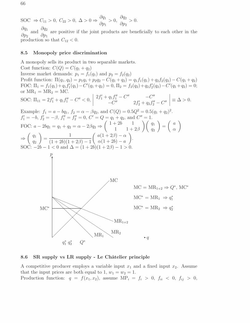
66
SOC ⇒ C11 > 0, C22 > 0, ∆ > 0 ⇒ ∂q1
∂p1> 0,
∂q2
∂p2> 0.
∂q1
∂p2
and∂q2
∂p1
are positive if the joint products are beneficially to each other in the
production so that C12 < 0.
8.5 Monopoly price discrimination
A monopoly sells its product in two separable markets.Cost function: C(Q) = C(q1 + q2)Inverse market demands: p1 = f1(q1) and p2 = f2(q2)Profit function: Π(q1, q2) = p1q1 + p2q2−C(q1 + q2) = q1f1(q1)+ q2f2(q2)−C(q1 + q2)FOC: Π1 = f1(q1)+q1f
′1(q1)−C ′(q1+q2) = 0, Π2 = f2(q2)+q2f
′2(q2)−C ′(q1 +q2) = 0;
or MR1 = MR2 = MC.
SOC: Π11 = 2f ′1 + q1f′′1 − C ′′ < 0,
∣
∣
∣
∣
2f ′1 + q1f′′1 − C ′′ −C ′′
−C ′′ 2f ′2 + q2f′′2 − C ′′
∣
∣
∣
∣
≡ ∆ > 0.
Example: f1 = a− bq1, f2 = α− βq2, and C(Q) = 0.5Q2 = 0.5(q1 + q2)2.
f ′1 = −b, f ′2 = −β, f ′′1 = f ′′2 = 0, C ′ = Q = q1 + q2, and C ′′ = 1.
FOC: a− 2bq1 = q1 + q2 = α− 2βq2 ⇒(
1 + 2b 11 1 + 2β
)(
q1
q2
)
=
(
aα
)
⇒(
q1
q2
)
=1
(1 + 2b)(1 + 2β)− 1
(
a(1 + 2β)− αα(1 + 2b)− a
)
.
SOC: −2b− 1 < 0 and ∆ = (1 + 2b)(1 + 2β)− 1 > 0.
✲ q
✻p
MC
❅❅❅❅❅❅❅❅❅❅MR1
◗◗◗◗◗◗◗◗◗◗◗◗◗◗◗MR2
❛❛❛❛❛❛❛❛❛❛❛❛❛❛❛MR1+2
Q∗q∗2q∗1
MC∗
MC = MR1+2 ⇒ Q∗, MC∗
MC∗ = MR1 ⇒ q∗1
MC∗ = MR2 ⇒ q∗2
8.6 SR supply vs LR supply - Le Chatelier principle
A competitive producer employs a variable input x1 and a fixed input x2. Assumethat the input prices are both equal to 1, w1 = w2 = 1.Production function: q = f(x1, x2), assume MPi = fi > 0, fii < 0, fij > 0,
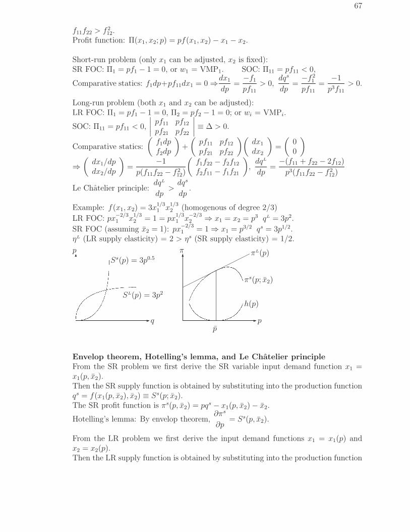
67
f11f22 > f 212.
Profit function: Π(x1, x2; p) = pf(x1, x2)− x1 − x2.
Short-run problem (only x1 can be adjusted, x2 is fixed):SR FOC: Π1 = pf1 − 1 = 0, or w1 = VMP1. SOC: Π11 = pf11 < 0,
Comparative statics: f1dp+pf11dx1 = 0⇒dx1
dp=−f1
pf11
> 0,dqs
dp=−f 2
1
pf11
=−1
p3f11
> 0.
Long-run problem (both x1 and x2 can be adjusted):LR FOC: Π1 = pf1 − 1 = 0, Π2 = pf2 − 1 = 0; or wi = VMPi.
SOC: Π11 = pf11 < 0,
∣
∣
∣
∣
pf11 pf12
pf21 pf22
∣
∣
∣
∣
≡ ∆ > 0.
Comparative statics:
(
f1dpf2dp
)
+
(
pf11 pf12
pf21 pf22
)(
dx1
dx2
)
=
(
00
)
⇒(
dx1/dpdx2/dp
)
=−1
p(f11f22 − f 212)
(
f1f22 − f2f12
f2f11 − f1f21
)
,dqL
dp=−(f11 + f22 − 2f12)
p3(f11f22 − f 212)
Le Chatelier principle:dqL
dp>
dqs
dp.
Example: f(x1, x2) = 3x1/31 x
1/32 (homogenous of degree 2/3)
LR FOC: px−2/31 x
1/32 = 1 = px
1/31 x
−2/32 ⇒ x1 = x2 = p3 qL = 3p2.
SR FOC (assuming x2 = 1): px−2/31 = 1⇒ x1 = p3/2 qs = 3p1/2.
ηL (LR supply elasticity) = 2 > ηs (SR supply elasticity) = 1/2.
✲ q
✻p
Ss(p) = 3p0.5
SL(p) = 3p2
✲ p
✻π
✟✟✟✟✟✟✟✟✟✟
πL(p)
πs(p; x2)
h(p)
p
Envelop theorem, Hotelling’s lemma, and Le Chatelier principleFrom the SR problem we first derive the SR variable input demand function x1 =x1(p, x2).Then the SR supply function is obtained by substituting into the production functionqs = f(x1(p, x2), x2) ≡ Ss(p; x2).The SR profit function is πs(p, x2) = pqs − x1(p, x2)− x2.
Hotelling’s lemma: By envelop theorem,∂πs
∂p= Ss(p, x2).
From the LR problem we first derive the input demand functions x1 = x1(p) andx2 = x2(p).Then the LR supply function is obtained by substituting into the production function
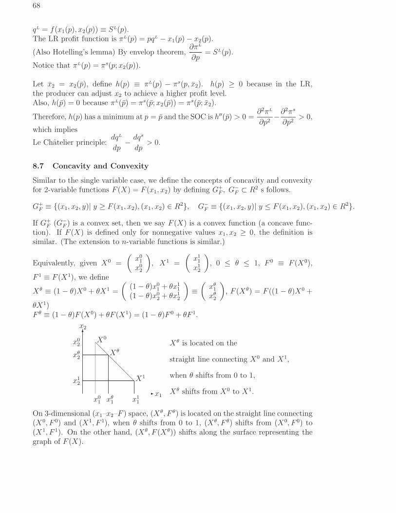
68
qL = f(x1(p), x2(p)) ≡ SL(p).The LR profit function is πL(p) = pqL − x1(p)− x2(p).
(Also Hotelling’s lemma) By envelop theorem,∂πL
∂p= SL(p).
Notice that πL(p) = πs(p; x2(p)).
Let x2 = x2(p), define h(p) ≡ πL(p) − πs(p, x2). h(p) ≥ 0 because in the LR,the producer can adjust x2 to achieve a higher profit level.Also, h(p) = 0 because πL(p) = πs(p; x2(p)) = πs(p; x2).
Therefore, h(p) has a minimum at p = p and the SOC is h′′(p) > 0 =∂2πL
∂p2−∂2πs
∂p2> 0,
which implies
Le Chatelier principle:dqL
dp− dqs
dp> 0.
8.7 Concavity and Convexity
Similar to the single variable case, we define the concepts of concavity and convexityfor 2-variable functions F (X) = F (x1, x2) by defining G+
F , G−F ⊂ R2 s follows.
G+F ≡ {(x1, x2, y)| y ≥ F (x1, x2), (x1, x2) ∈ R2}, G−
F ≡ {(x1, x2, y)| y ≤ F (x1, x2), (x1, x2) ∈ R2}.
If G+F (G−
F ) is a convex set, then we say F (X) is a convex function (a concave func-tion). If F (X) is defined only for nonnegative values x1, x2 ≥ 0, the definition issimilar. (The extension to n-variable functions is similar.)
Equivalently, given X0 =
(
x01
x02
)
, X1 =
(
x11
x12
)
, 0 ≤ θ ≤ 1, F 0 ≡ F (X0),
F 1 ≡ F (X1), we define
Xθ ≡ (1− θ)X0 + θX1 =
(
(1− θ)x01 + θx1
1
(1− θ)x02 + θx1
2
)
≡(
xθ1
xθ2
)
, F (Xθ) = F ((1− θ)X0 +
θX1)F θ ≡ (1− θ)F (X0) + θF (X1) = (1− θ)F 0 + θF 1.
✲x1
✻x2
❅❅❅❅❅❅
X0
Xθ
X1
x01 xθ
1 x11
x02
xθ2
x12
Xθ is located on the
straight line connecting X0 and X1,
when θ shifts from 0 to 1,
Xθ shifts from X0 to X1.
On 3-dimensional (x1–x2–F ) space, (Xθ, F θ) is located on the straight line connecting(X0, F 0) and (X1, F 1), when θ shifts from 0 to 1, (Xθ, F θ) shifts from (X0, F 0) to(X1, F 1). On the other hand, (Xθ, F (Xθ)) shifts along the surface representing thegraph of F (X).
69
F (X) is strictly concave ⇒ if for all X0, X1 and θ ∈ (0, 1), F (Xθ) > F θ.F (X) is concave ⇒ if for all X0, X1 and θ ∈ [0, 1], F (Xθ) ≥ F θ.F (X) is strictly convex ⇒ if for all X0, X1 and θ ∈ (0, 1), F (Xθ) < F θ.F (X) is convex ⇒ if for all X0, X1 and θ ∈ [0, 1], F (Xθ) ≤ F θ.
Example: 9x1/31 x
1/32 .
Assume that F is twice differentiable.Theorem 1: F (X) is concave, ⇔ v′HF v is negative semidefinite for all X.v′HFv is negative definite for all X ⇒ F (X) is strictly concave.Proof: By Taylor’s theorem, there exist X0 ∈ [X0, Xθ] and X1 ∈ [Xθ, X1] such that
F (X1) = F (Xθ) +∇F (Xθ)(X1 −Xθ) +1
2(X1 −Xθ)′HF (X1)(X1 −Xθ)
F (X0) = F (Xθ) +∇F (Xθ)(X0 −Xθ) +1
2(X0 −Xθ)′HF (X0)(X0 −Xθ)
⇒ F θ = F (Xθ) +θ(1− θ)
2(X1 −X0)′[HF (X0) + HF (X1)](X1 −X0).
Theorem 2: If F (X) is concave and ∇F (X0) = 0, then X0 is a global maximum.If F (X) is strictly concave and ∇F (X0) = 0, then X0 is a unique global maximum.Proof: By theorem 1, X0 must be a local maximum. If it is not a global maximum,then there exists X1 such that F (X1) > F (X0), which implies that F (Xθ) > F (X0)for θ close to 0. Therefore, X0 is not a local maximum, a contradiction.
Remark 1 (boundary or corner solution): The boundary or corner condition Fi(X) ≤0, xiFi(X) = 0 (or Fi(X) ≥ 0, (xi − ai)Fi(X) = 0) becomes sufficient for globalmaximum.Remark 2 (minimization problem): For the minimization problem, we replace con-cavity with convexity and negative definite with positive definite. If F (X) is convexand ∇F (X∗) = 0, then X∗ is a global minimum.If F (X) is strictly convex and ∇F (X∗) = 0, then X∗ is a unique global minimum.
8.8 Learning and utility maximization
Consumer B’s utility function is
U = u(x, k) + m− h(k), x, m, k ≥ 0,
where x is the quantity of commodity X consumed, k is B’s knowledge regard-ing the consumption of X, m is money, u(x, k) is the utility obtained, ∂2u
∂x2 < 0,∂2u∂x∂k
> 0 (marginal utility of X increases with k), and h(k) is the disutility of acquir-ing/maintaining k, h′ > 0, h′′ > 0. Assume that B has 100 dollar to spend and theprice of X is Px = 1 so that m = 100− x and U = u(x, k) + 100− x− h(k). Assume

70
also that k is fixed in the short run. The short run utility maximization problemis
maxx
u(x, k) + 100− x− h(k), ⇒ FOC:∂u
∂x− 1 = 0, SOC:
∂2u
∂x2< 0.
The short run comparative static dxdk
is derived from FOC as
dx
dk= − ∂2u/∂x2
∂2u/∂x∂k> 0,
that is, consumer B will consume more of X if B’s knowledge of X increases.
In the long run consumer B will change k to attain higher utility level. The long runutility maximization problem is
maxx,k
u(x, k) + 100− x− h(k), ⇒ FOC:∂u
∂x− 1 = 0,
∂u
∂k− h′(k) = 0.
The SOC is satisfied if we assume that u(x, k) is concave and h(k) is convex (h′′(k) >0), because F (x, k) ≡ u(x, k) + 100− x− h(k), x, k ≥ 0 is strictly concave then.
Consider now the specific case when
u(x, k) = 3x2/3k1/3 and h(k) = 0.5k2.
1. Calculate consumer B’s short run consumption of X, xs = x(k). (In this part,you may ignore the nonnegative constraint m = 100−x ≥ 0 and the possibilityof a corner solution.)x = 1/(8k).
2. Calculate the long run consumption of X, xL.x = 32
3. Derive the short run value function V (k) ≡ u(x(k), k) + 100− x(k)− h(k).
4. Solve the maximization problem maxk V (k).k = 4.
5. Explain how the SOC is satisfied and why the solution is the unique globalmaximum.
(demand functions) Consider now the general case when Px = p so that
U = 3x2/3k1/3 + 100− px− 0.5k2.
1. Calculate consumer B’s short run demand function of X, xs = x(p; k). (Warn-ing: There is a nonnegative constraint m = 100 − px ≥ 0 and you have toconsider both interior and corner cases.)xs(p) = 8kp−3 (100/p) if p ≤
√2k/5 (p <
√2k/5).
2. Calculate the long run demand function of X, xL(p). and the optimal level ofK, kL(p). (Both interior and corner cases should be considered too.)xL(p) = 32p−5 (100/p) if p > (8/25)1/4 (p < (8/25)1/4), kL(p) = [xL(p)]2/5.
71
8.9 Homogeneous and homothetic functions
A homogeneous function of degree k is f(x1, . . . , xn) such that
f(hx1, . . . , hxn) = hkf(x1, . . . , xn) ∀h > 0.
If f is homogeneous of degree k1 and g homogeneous of degree k2, then fg is homoge-
neous of degree k1 + k2,f
gis homogeneous of degree k1− k2, and fm is homogeneous
of degree mk1.
If Q = F (x1, x2) is homogeneous of degree 1, then Q = x1F (1,x2
x1) ≡ x1f
(
x2
x1
)
. If
m = H(x1, x2) is homogeneous of degree 0, then m = H(1,x2
x1) ≡ h
(
x2
x1
)
.
Euler theorem: If f(x1, . . . , xn) is homogeneous of degree k, then
x1f1 + . . . + xnfn = kf
If f is homogeneous of degree k, then fi is homogenous of degree k − 1.
Examples: 1. Cobb-Douglas function Q = Axα1 xβ
2 is homogeneous of degree α + β.
2. CES function Q = {axρ1 + bxρ
2}kρ is homogenous of degree k.
3. A quadratic form x′Ax is homogeneous of degree 2.4. Leontief function Q = min {ax1, bx2} is homogeneous of degree 1.
Homothetic functions: If f is homogeneous and g = H(f), H is a monotonicincreasing function, then g is called a homothetic function.
Example: Q = α ln x1 + β ln x2 = ln(
xα1 xβ
2
)
is homothetic.
The MRS of a homothetic function depends only on the ratiox2
x1
.
8.10 Problems
1. Use Newton’s method to find the root of the nonlinear equation X3+2X+2 = 0accurate to 2 digits.
2. Find (a) limX→0
1− 2−X
X, (b) lim
X→0+
1− e−aX
X, (c) lim
X→0
e2X − eX
X.
3. Given the total cost function C(Q) = eaQ+b, use L’hopital’s rule to find theAVC at Q = 0+.
4. Let z = x1x2 + x21 + 3x2
2 + x2x3 + x23.
(a) Use matrix multiplication to represent z.(b) Determine whether z is positive definite or negative definite.(c) Find the extreme value of z. Check whether it is a maximum or a minimum.

72
5. The cost function of a competitive producer is C(Q; K) =Q3
3K+ K, where K
is, say, the plant size (a fixed factor in the short run).
(a) At which output level, the SAC curve attains a minimum?
(b) Suppose that the equilibrium price is p = 100. The profit is Π = 100Q−Q3
3K− K. For a given K, find the supply quantity Q(K) such that SR
profit is maximized.
(c) Calculate the SR maximizing profit π(K).
(d) Find the LR optimal K = K∗ to maximize π(K).
(e) Calculate the LR supply quantity Q∗ = Q(K∗).
(f) Now solve the 2-variable maximization problem
maxQ,K≥0
Π(Q, K) = pQ− C(Q) = 100Q− Q3
3K−K.
and show that Π(Q, K) is concave so that the solution is the unique globalmaximum.
6. A competitive firm produces two joint products. The total cost function isC(q1, q2) = 2q2
1 + 3q22 − 4q1q2.
(a) Use the first order conditions for profit maximization to derive the supplyfunctions.(b) Check that the second order conditions are satisfied.
7. Check whether the function f(x, y) = ex+y is concave, convex, or neither.
8. (a) Check whether f(x, y) = 2 lnx+3 ln y−x−2y is concave, convex, or neither.(Assume that x > 0 and y > 0.)(b) Find the critical point of f .(c) Is the critical point a local maximum, a global maximum, or neither?
9. Suppose that a monopoly can produce any level of output at a constant marginalcost of $c per unit. Assume that the monopoly sells its goods in two differentmarkets which are separated by some distance. The demand curve in the firstmarket is given by Q1 = exp[−aP1] and the curve in the second market is givenby Q2 = exp[−bP2]. If the monopolist wants to maximize its total profits, whatlevel of output should be produced in each market and what price will prevail ineach market? Check that your answer is the unique global maximum. (Hints: 1.P1 = −(1/a) ln Q1 and P2 = −(1/b) ln Q2. 2. Π = P1Q1 + P2Q2− (Q1 + Q2)c =−(1/a)Q1 ln Q1 − (1/b)Q2 ln Q2 − (Q1 + Q2)c is strictly concave.)
10. The production function of a competitive firm is given by q = f(x1, x2) =
3x1
3
1 x1
3
2 , where x1 is a variable input and x2 is a fixed input. Assume that theprices of the output and the fixed input are p = w2 = 1. In the short run,the amount of the fixed input is given by x2 = x2. The profit function of thecompetitive firm is given by π = f(x1, x2)− w1x1 − x2.
73
(a) State the FOC for the SR profit maximization and calculate the SR input
demand function xS1 = xS
1 (w1) and the SR input demand elasticity w1
xS1
∂xS1
∂w1.
(b) Now consider the LR situation when x2 can be adjusted. State the FOCfor LR profit maximization and calculate the LR input demand funtion
xL1 = xL
1 (w1) and the LR input demand elasticity w1
xL1
∂xL1
∂w1.
(c) Verify the Le Chatelier principle:∣
∣
∣
w1
xL1
∂xL1
∂w1
∣
∣
∣>∣
∣
∣
w1
xS1
∂xS1
∂w1
∣
∣
∣.
(d) Show that the LR profit is a strictly concave function of (x1, x2) for x1, x2 >0 and therefore the solution must be the unique global maximum.
11. Let U(x, y) = xay + xy2, x, y, a > 0.
(a) For what value(s) of a U(x, y) is homogeneous?.
(b) For what value(s) of a U(x, y) is homothetic?
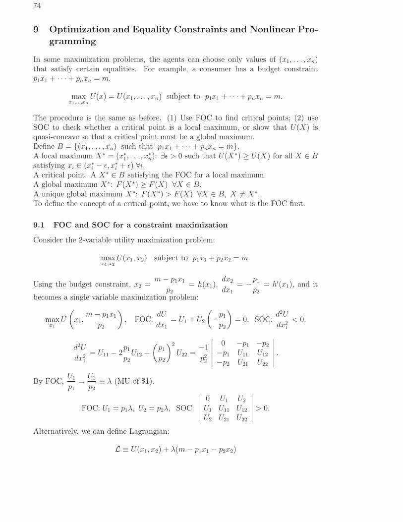
74
9 Optimization and Equality Constraints and Nonlinear Pro-gramming
In some maximization problems, the agents can choose only values of (x1, . . . , xn)that satisfy certain equalities. For example, a consumer has a budget constraintp1x1 + · · ·+ pnxn = m.
maxx1,...,xn
U(x) = U(x1, . . . , xn) subject to p1x1 + · · ·+ pnxn = m.
The procedure is the same as before. (1) Use FOC to find critical points; (2) useSOC to check whether a critical point is a local maximum, or show that U(X) isquasi-concave so that a critical point must be a global maximum.Define B = {(x1, . . . , xn) such that p1x1 + · · ·+ pnxn = m}.A local maximum X∗ = (x∗1, . . . , x
∗n): ∃ǫ > 0 such that U(X∗) ≥ U(X) for all X ∈ B
satisfying xi ∈ (x∗i − ǫ, x∗i + ǫ) ∀i.A critical point: A X∗ ∈ B satisfying the FOC for a local maximum.A global maximum X∗: F (X∗) ≥ F (X) ∀X ∈ B.A unique global maximum X∗: F (X∗) > F (X) ∀X ∈ B, X 6= X∗.To define the concept of a critical point, we have to know what is the FOC first.
9.1 FOC and SOC for a constraint maximization
Consider the 2-variable utility maximization problem:
maxx1,x2
U(x1, x2) subject to p1x1 + p2x2 = m.
Using the budget constraint, x2 =m− p1x1
p2
= h(x1),dx2
dx1
= −p1
p2
= h′(x1), and it
becomes a single variable maximization problem:
maxx1
U
(
x1,m− p1x1
p2
)
, FOC:dU
dx1= U1 + U2
(
−p1
p2
)
= 0, SOC:d2U
dx21
< 0.
d2U
dx21
= U11 − 2p1
p2
U12 +
(
p1
p2
)2
U22 =−1
p22
∣
∣
∣
∣
∣
∣
0 −p1 −p2
−p1 U11 U12
−p2 U21 U22
∣
∣
∣
∣
∣
∣
.
By FOC,U1
p1=
U2
p2≡ λ (MU of $1).
FOC: U1 = p1λ, U2 = p2λ, SOC:
∣
∣
∣
∣
∣
∣
0 U1 U2
U1 U11 U12
U2 U21 U22
∣
∣
∣
∣
∣
∣
> 0.
Alternatively, we can define Lagrangian:
L ≡ U(x1, x2) + λ(m− p1x1 − p2x2)

75
FOC: L1 =∂L∂x1
= U1 − λp1 = 0, L2 =∂L∂x2
= U2 − λp2 = 0, Lλ =∂L∂λ
=
m− p1x1 − p2x2 = 0.
SOC:
∣
∣
∣
∣
∣
∣
0 −p1 −p2
−p1 L11 L12
−p2 L21 L22
∣
∣
∣
∣
∣
∣
> 0.
general 2-variable with 1-constraint case:
maxx1,x2
F (x1, x2) subject to g(x1, x2) = 0.
Using the constraint, x2 = h(x1),dx2
dx1= −g1
g2= h′(x1), and it becomes a single
variable maximization problem:
maxx1
F (x1, h(x1)) FOC:dF
dx1
= F1 + F2h′(x1) = 0, SOC:
d2F
dx21
< 0.
d2F
dx21
=d
dx1
(F1 + F2h′) = F11 + 2h′F12 + (h′)
2F22 + F2h
′′
h′′ =d
dx1
(
−g1
g2
)
=−1
g2
[
g11 + 2g12h′ + g22(h
′)2]
.
⇒ d2F
dx21
=
(
F11 −F2
g2
g11
)
+ 2
(
F12 −F2
g2
g12
)
h′ +
(
F22 −F2
g2
g22
)
(h′)2
= −
∣
∣
∣
∣
∣
∣
∣
∣
∣
∣
0 −h′ 1
−h′ F11 −F2
g2g11 F12 −
F2
g2g12
1 F21 −F2
g2
g21 F22 −F2
g2
g22
∣
∣
∣
∣
∣
∣
∣
∣
∣
∣
=−1
g22
∣
∣
∣
∣
∣
∣
∣
∣
∣
∣
0 g1 g2
g1 F11 −F2
g2g11 F12 −
F2
g2g12
g2 F21 −F2
g2
g21 F22 −F2
g2
g22
∣
∣
∣
∣
∣
∣
∣
∣
∣
∣
By FOC,F1
g1
=F2
g2
≡ λ (Lagrange multiplier).
Alternatively, we can define Lagrangian:
L ≡ F (x1, x2)− λg(x1, x2)
FOC: L1 =∂L∂x1
= F1−λg1 = 0, L2 =∂L∂x2
= F2− λg2 = 0, Lλ =∂L∂λ
= −g(x1, x2) =
0.
SOC:
∣
∣
∣
∣
∣
∣
0 g1 g2
g1 L11 L12
g2 L21 L22
∣
∣
∣
∣
∣
∣
> 0.
n-variable 1-constraint case:
maxx1,...,xn
F (x1, . . . , xn) subject to g(x1, . . . , xn) = 0.
L ≡ F (x1, . . . , xn)− λg(x1, . . . , xn)

76
FOC: Li =∂L∂xi
= Fi − λgi = 0, i = 1, . . . , n, Lλ =∂L∂λ
= −g(x1, . . . , xn) = 0.
SOC:
∣
∣
∣
∣
0 −g1
−g1 L11
∣
∣
∣
∣
< 0,
∣
∣
∣
∣
∣
∣
0 −g1 −g2
−g1 L11 L12
−g2 L21 L22
∣
∣
∣
∣
∣
∣
> 0
∣
∣
∣
∣
∣
∣
∣
∣
0 −g1 −g2 −g3
−g1 L11 L12 L13
−g2 L21 L22 L23
−g3 L31 L32 L33
∣
∣
∣
∣
∣
∣
∣
∣
< 0, etc.
9.2 Examples
Example 1: maxF (x1, x2) = −x21 − x2
2 subject to x1 + x2 = 1.L = −x2
1 − x22 + λ(1− x1 − x2).
FOC: L1 = −2x1 − λ = 0, L2 = −2x2 − λ = 0 and Lλ = 1− 2x1 − 2x2 = 0.
Critical point:
(
x1
x2
)
=
1
21
2
, λ = −1.
SOC:
∣
∣
∣
∣
∣
∣
0 1 11 −2 01 0 −2
∣
∣
∣
∣
∣
∣
= 4 > 0.
⇒(
1/21/2
)
is a local maximum.
✲x1
✻x2
❅❅❅❅❅❅
r✲x1
✻x2
❅❅❅❅❅❅
❅❅❅❅❅❅
❅❅❅❅❅❅
❅❅❅❅❅❅
❅❅❅❅❅❅
r
r
Example 2: maxF (x1, x2) = x1 + x2 subject to x21 + x2
2 = 1.L = x1 + x2 + λ(1− x2
1 − x22).
FOC: L1 = 1− 2λx1 = 0, L2 = 1− 2λx2 = 0 and Lλ = 1− x21 − x2
2 = 0.Two critical points: x1 = x2 = λ = 1/
√2 and x1 = x2 = λ = −1/
√2.
SOC:
∣
∣
∣
∣
∣
∣
0 −2x1 −2x2
−2x1 −2λ 0−2x2 0 −2λ
∣
∣
∣
∣
∣
∣
= 8λ(x21 + x2
2).
⇒ x1 = x2 = λ = 1/√
2 is a local maximum and x1 = x2 = λ = −1/√
2 is a localminimum.

77
9.3 Cost minimization and cost function
min C(x1, x2; w1, w2) = w1x1 + w2x2 subject to xa1x
1−a2 = q, 0 < a < 1.
L = w1x1 + w2x2 + λ(q − xa1x
1−a2 ).
FOC: L1 = w1−aλxa−11 x1−a
2 = 0, L2 = w2− (1−a)λxa1x−a2 = 0, Lλ = q−xa
1x1−a2 = 0.
⇒ w1
w2
=ax2
(1− a)x1
⇒ x1 = q
[
aw2
(1− a)w1
]1−a
, x2 = q
[
(1− a)w1
aw2
]a
.
SOC:∣
∣
∣
∣
∣
∣
0 −axa−11 x1−a
2 −(1− a)xa1x−a2
−axa−11 x1−a
2 a(1− a)λxa−21 x1−a
2 −a(1− a)λxa−11 x−a
2
−(1− a)xa1x−a2 −a(1− a)λxa−1
1 x−a2 a(1− a)λxa
1x−a−12
∣
∣
∣
∣
∣
∣
= −a(1− a)q3λ
(x1x2)2< 0.
⇒ x1 = q
[
aw2
(1− a)w1
]1−a
, x2 = q
[
(1− a)w1
aw2
]a
is a local minimum.
The total cost is C(w1, w2, q) = q
[
(
a
1− a
)1−a
+
(
1− a
a
)a]
wa1w
1−a2 .
9.4 Utility maximization and demand function
maxU(x1, x2) = a ln x1 + b ln x2 subject to p1x1 + p2x2 = m.L = a ln x1 + b ln x2 + λ(m− p1x1 − p2x2).
FOC: L1 =a
x1− λp1 = 0, L2 =
b
x2− λp2 = 0 and Lλ = m− p1x1 − p2x2 = 0.
⇒ a
b
x2
x1=
p1
p2⇒ x1 =
am
(a + b)p1, x2 =
bm
(a + b)p2
SOC:
∣
∣
∣
∣
∣
∣
∣
∣
∣
0 −p1 −p2
−p1−a
x21
0
−p2 0−b
x22
∣
∣
∣
∣
∣
∣
∣
∣
∣
=ap2
2
x21
+bp2
1
x22
> 0.
⇒ x1 =am
(a + b)p1
, x2 =bm
(a + b)p2
is a local maximum.
9.5 Quasi-concavity and quasi-convexity
As discussed in the intermediate microeconomics course, if the MRS is strictly de-creasing along an indifference curve (indifference curve is convex toward the origin),then the utility maximization has a unique solution. A utility function U(x1, x2)
is quasi-concave if MRS (=U1
U2) is decreasing along every indifference curve. In
case MRS is strictly decreasing, the utility function is strictly quasi-concave. IfU(x1, x2) is (strictly) quasi-concave, then a critical point must be a (unique) globalmaximum.
Two ways to determine whether U(x1, x2) is quasi-concave: (1) the set {(x1, x2) ∈R2 U(x1, x2) ≥ U} is convex for all U . (Every indifference curve is convex toward the
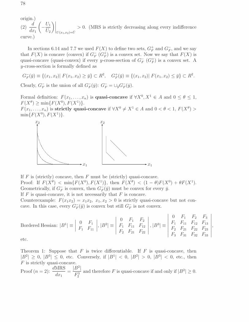
78
origin.)
(2)d
dx1
(
−U1
U2
)∣
∣
∣
∣
U(x1,x2)=U
> 0. (MRS is strictly decreasing along every indifference
curve.)
In sections 6.14 and 7.7 we used F (X) to define two sets, G+F and G−
F , and we saythat F (X) is concave (convex) if G−
F (G+F ) is a convex set. Now we say that F (X) is
quasi-concave (quasi-convex) if every y-cross-section of G−F (G+
F ) is a convex set. Ay-cross-section is formally defined as
G−F (y) ≡ {(x1, x2)| F (x1, x2) ≥ y} ⊂ R2, G+
F (y) ≡ {(x1, x2)| F (x1, x2) ≤ y} ⊂ R2.
Clearly, G−F is the union of all G−
F (y): G−F = ∪yG
−F (y).
Formal definition: F (x1, . . . , xn) is quasi-concave if ∀X0, X1 ∈ A and 0 ≤ θ ≤ 1,F (Xθ) ≥ min{F (X0), F (X1)}.F (x1, . . . , xn) is strictly quasi-concave if ∀X0 6= X1 ∈ A and 0 < θ < 1, F (Xθ) >min{F (X0), F (X1)}.
✲x1
✻x2
✲x1
✻x2
❅❅❅❅❅
❅
If F is (strictly) concave, then F must be (strictly) quasi-concave.Proof: If F (Xθ) < min{F (X0), F (X1)}, then F (Xθ) < (1 − θ)F (X0) + θF (X1).Geometrically, if G−
F is convex, then G−F (y) must be convex for every y.
If F is quasi-concave, it is not necessarily that F is concave.Counterexample: F (x1x2) = x1x2, x1, x2 > 0 is strictly quasi-concave but not con-cave. In this case, every G−
F (y) is convex but still G−F is not convex.
Bordered Hessian: |B1| ≡∣
∣
∣
∣
0 F1
F1 F11
∣
∣
∣
∣
, |B2| ≡
∣
∣
∣
∣
∣
∣
0 F1 F2
F1 F11 F12
F2 F21 F22
∣
∣
∣
∣
∣
∣
, |B3| ≡
∣
∣
∣
∣
∣
∣
∣
∣
0 F1 F2 F3
F1 F11 F12 F13
F2 F21 F22 F23
F3 F31 F32 F33
∣
∣
∣
∣
∣
∣
∣
∣
,
etc.
Theorem 1: Suppose that F is twice differentiable. If F is quasi-concave, then|B2| ≥ 0, |B3| ≤ 0, etc. Conversely, if |B1| < 0, |B2| > 0, |B3| < 0, etc., thenF is strictly quasi-concave.
Proof (n = 2):dMRS
dx1=|B2|F 3
2
and therefore F is quasi-concave if and only if |B2| ≥ 0.
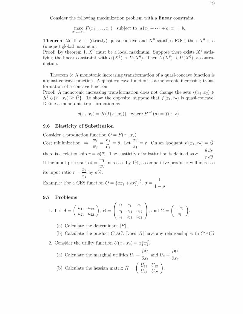
79
Consider the following maximization problem with a linear constraint.
maxx1,...,xn
F (x1, . . . , xn) subject to a1x1 + · · ·+ anxn = b.
Theorem 2: If F is (strictly) quasi-concave and X0 satisfies FOC, then X0 is a(unique) global maximum.Proof: By theorem 1, X0 must be a local maximum. Suppose there exists X1 satis-fying the linear constraint with U(X1) > U(X0). Then U(Xθ) > U(X0), a contra-diction.
Theorem 3: A monotonic increasing transformation of a quasi-concave function isa quasi-concave function. A quasi-concave function is a monotonic increasing trans-formation of a concave function.Proof: A monotonic increasing transformation does not change the sets {(x1, x2) ∈R2 U(x1, x2) ≥ U}. To show the opposite, suppose that f(x1, x2) is quasi-concave.Define a monotonic transformation as
g(x1, x2) = H(f(x1, x2)) where H−1(g) = f(x, x).
9.6 Elasticity of Substitution
Consider a production function Q = F (x1, x2).
Cost minimization ⇒ w1
w2=
F1
F2≡ θ. Let
x2
x1≡ r. On an isoquant F (x1, x2) = Q,
there is a relationship r = φ(θ). The elasticity of substitution is defined as σ ≡ θ
r
dr
dθ.
If the input price ratio θ =w1
w2increases by 1%, a competitive producer will increase
its input ratio r =x2
x1by σ%.
Example: For a CES function Q = {axρ1 + bxρ
2}kρ , σ =
1
1− ρ.
9.7 Problems
1. Let A =
(
a11 a12
a21 a22
)
, B =
0 c1 c2
c1 a11 a12
c2 a21 a22
, and C =
(
−c2
c1
)
.
(a) Calculate the determinant |B|.(b) Calculate the product C ′AC. Does |B| have any relationship with C ′AC?
2. Consider the utility function U(x1, x2) = xα1 xβ
2 .
(a) Calculate the marginal utilities U1 =∂U
∂x1and U2 =
∂U
∂x2.
(b) Calculate the hessian matrix H =
(
U11 U12
U21 U22
)
.

80
(c) Calculate the determinant of the matrix B =
0 U1 U2
U1 U11 U12
U2 U21 U22
.
(d) Let C =
(
−U2
U1
)
. Calculate the product C’HC.
3. Use the Lagrangian multiplier method to find the critical points of f(x, y) =x+y subject to x2 +y2 = 2. Then use the bordered Hessian to determine whichpoint is a maximum and which is a minimum. (There are two critical points.)
4. Determine whether f(x, y) = xy is concave, convex, quasiconcave, or quasicon-vex. (x > 0 and y > 0.)
5. Let U(x, y), U, x, y > 0, be a homogenous of degree 1 and concave function withUxy 6= 0.
(a) Show that V (x, y) = [U(x, y)]a is strictly concave if 0 < a < 1 and V (x, y)is strictly quasi-concave for all a > 0. Hint: UxxUyy = [Uxy]
2.
(b) Show that F (x, y) =(
xβ + yβ)a/β
, x, y > 0 and −∞ < β < 1 is homoge-nous of degree 1 and concave if a = 1.
(c) Determine the range of a so that F (x, y) is strictly concave.
(d) Determine the range of a so that F (x, y) is strictly quasi-concave.

81
9.8 Nonlinear Programming
The general nonlinear programming problem is:
maxx1,...,xn
F (x1, . . . , xn) subject to
g1(x1, . . . , xn) ≤ b1...
gm(x1, . . . , xn) ≤ bm
x1, . . . , xn ≥ 0.
In equality constraint problems, the number of constraints should be less than thenumber of policy variables, m < n. For nonlinear programming problems, there is nosuch a restriction, m can be greater than or equal to n. In vector notation,
maxx
F (x) subject to g(x) ≤ b, x ≥ 0.
9.9 Kuhn-Tucker condition
Define the Lagrangian function as
L(x, y) = F (x) + y(b− g(x)) = F (x1, . . . , xn) +m∑
j=1
yj(bj − gj(x1, . . . , xn)).
Kuhn-Tucker condition: The FOC is given by the Kuhn-Tucker conditions:
∂L
∂xi
=∂F
∂xi
−m∑
j=1
yj∂gj
∂xi
≤ 0, xi∂L
∂xi
= 0 xi ≥ 0, i = 1, . . . , n
∂L
∂yj= bj − gj(x) ≥ 0, yj
∂L
∂yj= 0 yj ≥ 0, j = 1, . . . , m
Kuhn Tucker theorem: x∗ solves the nonlinear programming problem if (x∗, y∗)solves the saddle point problem:
L(x, y∗) ≤ L(x∗, y∗) ≤ L(x∗, y) for all x ≥ 0, y ≥ 0,
Conversely, suppose that f(x) is a concave function and gj(x) are convex func-tions (concave programming) and the constraints satisfy the constraint qualifi-cation condition that there is some point in the opportunity set which satisfiesall the inequality constraints as strict inequalities, i.e., there exists a vectorx0 ≥ 0 such that gj(x0) < bj , j = 1, . . . , m, then x∗ solves the nonlinear pro-gramming problem only if there is a y∗ for which (x∗, y∗) solves the saddle pointproblem.
If constraint qualification is not satisfied, it is possible that a solution does not satisfythe K-T condition. If it is satisfied, then the K-T condition will be necessary. Forthe case of concave programming, it is also sufficient.

82
In economics applications, however, it is not convenient to use K-T condition tofind the solution. In stead, we first solve the equality constraint version of the problemand then use K-T condition to check or modify the solution when some constraintsare violated.
The K-T condition for minimization problems: the inequalities reversed.
9.10 Examples
Example 1. (Joint product profit maximization) The cost function of a competitiveproducer producing 2 joint products is c(x1, x2) = x2
1 +x1x2 +x22. The profit function
is given by π(p1, p2) = p1x1 + p2x2 − (x21 + x1x2 + x2
2).
maxx1≥0,x2≥0
f(x1, x2) = p1x1 + p2x2 − (x21 + x1x2 − x2
2)
K-T condition: f1 = p1 − 2x1 − x2 ≤ 0, f2 = p2 − x1 − 2x2 ≤ 0, xifi = 0, i = 1, 2.Case 1. p1/2 < p2 < 2p1.x1 = (2p1 − p2)/3, x2 = (2p2 − p1)/3.
Case 2. 2p1 < p2.x1 = 0, x2 = p2/2.
Case 3. 2p2 < p1.x1 = p1/2, x2 = 0.
Example 2. The production function of a producer is given by q = (x1+1)(x2+1)−1.For q = 8, calculate the cost function c(w1, w2).
minx1≥0,x2≥0
w1x1 + w2x2 subject to − [(x1 + 1)(x2 + 1)− 1] ≥ −8
Lagrangian function: L = w1x1 + w1x2 + λ[(x1 + 1)(x2 + 1)− 9].K-T conditions: L1 = w1−λ(x2−1) ≥ 0, L2 = w2−λ(x2−1) ≥ 0, xiLi = 0, i = 1, 2,and Lλ = (x1 + 1)(x2 + 1)− 9 ≥ 0, λLλ = 0.
Case 1. w1/9 < w2 < 9w1.x1 =
√
9w2/w1 − 1, x2 =√
9w1/w2 − 1 and c(w1, w2) = 6√
w1w2 − w1 − w2.
Case 2. 9w1 < w2.x1 = 8, x2 = 0, and c(w1, w2) = 8w1.
Case 3. 9w2 < w1.x1 = 0, x2 = 8, c(w1, w2) = 8w2.

83
Example 3. The utility function of a consumer is U(x1, x2) = x1(x2+1). The marketprice is p1 = p2 = 1 and the consumer has $11. Therefore the budget constraint isx1 + x2 ≤ 11. Suppose that both products are under rationing. Besides the moneyprice, the consumer has to pay ρi rationing points for each unit of product i consumed.Assume that ρ1 = 1 and ρ2 = 2 and the consumer has q rationing points. Therationing point constraint is x1 +2x2 ≤ q. The utility maximization problem is givenby
maxx1,x2
U(x1, x2) = x1(x2 +1) subject to x1 +x2 ≤ 11, x1 +2x2 ≤ q, x1, x2 ≥ 0.
Lagrangian function: L = x1(x2 + 1) + λ1(11− x1 − x2) + λ2(q − x1 − 2x2).K-T conditions: L1 = x2 +1−λ1−λ2 ≤ 0, L2 = x1−λ1−2λ2 ≤ 0, xiLi = 0, i = 1, 2,and Lλ1
= 11− x1 − x2 ≥ 0, Lλ2= q − x1 − 2x2 ≥ 0 λiLλi
= 0.
Case 1: q < 2.x1 = q, x2 = 0, λ1 = 0, and λ2 = 1.
Case 2: 2 ≤ q ≤ 14.x1 = (q + 2)/2, x2 = (q − 2)/4, λ1 = 0, and λ2 = (q + 2)/4.
Case 3: 14 < q ≤ 16.x1 = 22− q, x2 = q − 11, λ1 = 3(q − 14), and λ2 = 2(16− q).
Case 4: 16 < q.x1 = 6, x2 = 5, λ1 = 6, and λ2 = 0.
9.11 Problems
1. Given the individual utility function U(X, Y ) = 2√
X + Y ,a) show that U is quasi-concave for X ≥ 0 and Y ≥ 0,b) state the Kuhn-Tucker conditions of the following problem:
maxX≥0, Y≥0
2√
X + Y
s. t. PXX + PY Y ≤ I,
c) derive the demand functions X(PX , PY , I) and Y (PX , PY , I) for the case I ≥ P 2Y
PX,
check that the K-T conditions are satisfied,
d) and do the same for I <P 2
Y
PX.
e) Given that I = 1 and PY = 1, derive the ordinary demand function X = D(PX).f) Are your answers in (c) and (d) global maximum? Unique global maximum? Why

84
or why not?
2. A farm has a total amount of agricultural land of one acre. It can produce twocrops, corn (C) and lettuce (L), according to the production functions C = NC andL = 2
√NL respectively, where NC (NL) is land used in corn (lettuce) production.
The prices of corn and lettuce are p and q respectively. Thus, if the farm uses NC
of land in corn production and NL in lettuce production, (NC ≥ 0, NL ≥ 0, andNC + NL ≤ 1) its total revenue is pNC + 2q
√NL.
a) Suppose the farm is interested in maximizing its revenue. State the revenue max-imization problem and the Kuhn-Tucker conditions.b) Given that q > p > 0, how much of each output will the farm produce? Checkthat the K-T conditions are satisfied.c) Given that p ≥ q > 0, do the same as (b).
3. Suppose that a firm has two activities producing two goods “meat” (M) and“egg” (E) from the same input “chicken” (C) according to the production functions
M = CM and E = C1/2E , where CM (respectively CE) ≥ 0 is the q. Suppose in the
short run, the firm has C units of chicken that it must take as given and suppose thatthe firm faces prices p > 0, q > 0 of meat and egg respectively.a) Show that the profit function π = pCM + qC0.5
E is quasi-concave in (CM , CE).b) Write down the short run profit maximization problem.c) State the Kuhn-Tucker conditions.d) Derive the short run supply functions. (There are two cases.)e) Is your solution a global maximum? Explain.
4. State the Kuhn-Tucker conditions of the following nonlinear programming problem
max U(X, Y ) = 3 lnX + ln Ys. t. 2X + Y ≤ 24
X + 2Y ≤ 24X ≥ 0, Y ≥ 0.
Show that X = 9, Y = 6, λ1 = 1/6, and λ2 = 0 satisfy the Kuhn-Tucker conditions.What is the economic interpretations of λ1 = 1/6 and λ2 = 0 if the first constraint isinterpreted as the income constraint and the second constraint as the rationing pointconstraint of a utility maximization problem?
9.12 Linear Programming – A Graphic Approach
Example 1 (A Production Problem). A manufacturer produces tables x1 anddesks x2. Each table requires 2.5 hours for assembling (A), 3 hours for buffing (B),and 1 hour for crating (C). Each desks requires 1 hour for assembling (A), 3 hoursfor buffing (B), and 2 hours for crating (C). The firm can use no more than 20 hoursfor assembling, 30 hours for buffing, and 16 hours for crating each week. Its profitmargin is $3 per table and $4 per desk.

85
max Π = 3x1 + 4x2 (4)
subject to 2.5x1 + x2 ≤ 20 (5)
3x1 + 3x2 ≤ 30 (6)
x1 + 2x2 ≤ 16 (7)
x1, x2 ≥ 0. (8)
extreme point: The intersection of two constraints.extreme point theorem: If an optimal feasible value of the objective function exists,it will be found at one of the extreme points.
In the example, There are 10 extreme points, but only 5 are feasible: (0 ,0), (8,0), (62
3, 31
3), (4, 6), and (0, 8), called basic feasible solutions. At (4, 6), Π = 36 is the
optimal.
✲x1
✻x2
▲▲▲▲▲▲▲▲▲▲▲▲▲▲▲▲▲▲▲▲▲
❅❅❅❅❅❅❅❅❅❅
❍❍❍❍❍❍❍❍❍❍❍❍❍❍❍❍
q❩
❩❩
❩❩
❩❩
❩❩
❩❩
❩
(4,6)
✲ y
✻y2
❆❆❆❆❆❆❆❆❆❆❆❆❆❆
❅❅❅❅❅❅❅❅❅❅❅❅
PPPPPPPPPPPPPPPPPP
q❍
❍❍
❍❍
❍❍
❍❍
❍❍
❍❍
❍❍
(9,3)
Example 2 (The Diet Problem). A farmer wants to see that her herd gets theminimum daily requirement of three basic nutrients A, B, and C. Daily requirementsare 14 for A, 12 for B, and 18 for C. Product y1 has 2 units of A and 1 unit each ofB and C; product y2 has 1 unit each of A and B and 3 units of C. The cost of y1 is$2, and the cost of y2 is $4.
min c = 2y1 + 4y2 (9)
subject to 2y1 + y2 ≥ 14 (10)
y1 + y2 ≥ 12 (11)
y1 + 3y2 ≥ 18 (12)
y1, y2 ≥ 0. (13)

86
Slack and surplus variables: To find basic solutions, equations are needed. This isdone by incorporating a separate slack or surplus variable si into each inequality.In example 1, the system becomes
2.5x1 + x2 + s1 = 20 3x1 + 3x2 + s2 = 30 x1 + 2x2 + s3 = 16.
In matrix for,
2.5 1 1 0 03 3 0 1 01 2 0 0 1
x1
x2
s1
s2
s3
=
203016
.
In example 2, the inequalities are ”≥” and the surplus variables are substracted:
2y1 + y2 − s1 = 14 y1 + y2 − s2 = 12 y1 + 3y2 − s3 = 18.
In matrix for,
2 1 −1 0 01 1 0 −1 01 3 0 0 −1
y1
y2
s1
s2
s3
=
141218
.
For a system of m equations and n variables, where n > m, a solution in which atleast n −m variables equal to zero is an extreme point. Thus by setting n −mandsolving the m equations for the remaining m variables, an extreme point can be found.There are n!/m!(n−m)! such solutions.
9.13 Linear programming – The simplex algorithm
The algorithm moves from one basic feasible solution to another, always improvingupon the previous solutions, until the optimal solution is reached. In each step, thosevariables set equal to zero are called not in the basis and those not set equal to zeroare called in the basis. Let use example one to illustrate the procedure.
1. The initial Simplex Tableau
x1 x2 s1 s2 s3 Constant2.5 1 1 0 0 203 3 0 1 0 301 2 0 0 1 16-3 -4 0 0 0 0
The first basic feasible solution can be read from the tableau as x1 = 0, x2 = 0,s1 = 20, s2 = 30, and s3 = 16. The value of Π is zero.
2. The Pivot Element and a change of Basis
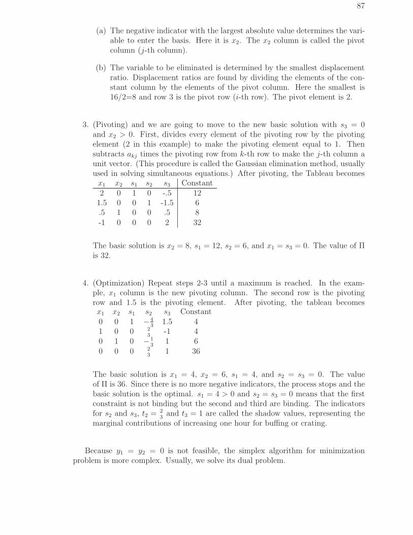
87
(a) The negative indicator with the largest absolute value determines the vari-able to enter the basis. Here it is x2. The x2 column is called the pivotcolumn (j-th column).
(b) The variable to be eliminated is determined by the smallest displacementratio. Displacement ratios are found by dividing the elements of the con-stant column by the elements of the pivot column. Here the smallest is16/2=8 and row 3 is the pivot row (i-th row). The pivot element is 2.
3. (Pivoting) and we are going to move to the new basic solution with s3 = 0and x2 > 0. First, divides every element of the pivoting row by the pivotingelement (2 in this example) to make the pivoting element equal to 1. Thensubtracts akj times the pivoting row from k-th row to make the j-th column aunit vector. (This procedure is called the Gaussian elimination method, usuallyused in solving simultaneous equations.) After pivoting, the Tableau becomesx1 x2 s1 s2 s3 Constant2 0 1 0 -.5 12
1.5 0 0 1 -1.5 6.5 1 0 0 .5 8-1 0 0 0 2 32
The basic solution is x2 = 8, s1 = 12, s2 = 6, and x1 = s3 = 0. The value of Πis 32.
4. (Optimization) Repeat steps 2-3 until a maximum is reached. In the exam-ple, x1 column is the new pivoting column. The second row is the pivotingrow and 1.5 is the pivoting element. After pivoting, the tableau becomesx1 x2 s1 s2 s3 Constant0 0 1 −4
31.5 4
1 0 0 23
-1 40 1 0 −1
31 6
0 0 0 23
1 36
The basic solution is x1 = 4, x2 = 6, s1 = 4, and s2 = s3 = 0. The valueof Π is 36. Since there is no more negative indicators, the process stops and thebasic solution is the optimal. s1 = 4 > 0 and s2 = s3 = 0 means that the firstconstraint is not binding but the second and third are binding. The indicatorsfor s2 and s3, t2 = 2
3and t3 = 1 are called the shadow values, representing the
marginal contributions of increasing one hour for buffing or crating.
Because y1 = y2 = 0 is not feasible, the simplex algorithm for minimizationproblem is more complex. Usually, we solve its dual problem.
88
9.14 Linear programming – The dual problem
To every linear programming problem there corresponds a dual problem. If the orig-inal problem, called the primal problem, is
maxx
F = cx subject to Ax ≤ b, x ≥ 0
then the dual problem is
miny
G = yb subject to yA ≥ c, y ≥ 0
where
A =
a11 . . . a1n...
. . ....
am1 . . . amn
, x =
x1...
xn
, b =
b1...
bm
, c = (c1, . . . , cn), y = (y1, . . . , ym).
Existence theorem: A necessary and sufficient condition for the existence of a so-lution is that the opportunity sets of both the primal and dual problems arenonempty.Proof: Suppose x, y are feasible. Then Ax ≤ b, yA ≥ c. It follows thatF (x) = cx ≤ yAx and G(y) = yb ≥ yAx. Therefore, F (x) ≤ G(y).
Duality theorem: A necessary and sufficient condition for a feasible vector to rep-resent a solution is that there exists a feasible vector for the dual problem forwhich the values of the objective functions of both problems are equal.
Complementary slackness theorem: A necessary and sufficient condition for fea-sible vectors x∗ , y∗ to solve the dual problems is that they satisfy the comple-mentary slackness condition:
(c− y∗A)x∗ = 0 y∗(b− Ax∗) = 0.
Proof: Use Kuhn-Tucker theorem.
Dual of the Diet Problem
max c∗ = 14x1 + 12x2 + 18x3 (14)
subject to 2x1 + x2 + x1 ≤ 2 (15)
x1 + x2 + 3x3 ≤ 4 (16)
x1, x2, x3 ≥ 0. (17)
x1, x2, x3, is interpreted as the imputed value of nutrient A, B, C, respectively.
89
10 General Equilibrium and Game Theory
10.1 Utility maximization and demand function
A consumer wants to maximize his utility function subject to his budget constraint:
maxU(x1, . . . , xn) subj. to p1x1 + · · ·+ pnxn = I.
Endogenous variables: x1, . . . , xn
Exogenous variables: p1, . . . , pn, I (the consumer is a price taker)Solution is the demand functions xk = Dk(p1, . . . , pn, I), k = 1, . . . , n
Example: maxU(x1, x2) = a ln x1 + b ln x2 subject to p1x1 + p2x2 = m.L = a ln x1 + b ln x2 + λ(m− p1x1 − p2x2).
FOC: L1 =a
x1
− λp1 = 0, L2 =b
x2
− λp2 = 0 and Lλ = m− p1x1 − p2x2 = 0.
⇒ a
b
x2
x1=
p1
p2⇒ x1 =
am
(a + b)p1, x2 =
bm
(a + b)p2
SOC:
∣
∣
∣
∣
∣
∣
∣
∣
∣
0 −p1 −p2
−p1−a
x21
0
−p2 0−b
x22
∣
∣
∣
∣
∣
∣
∣
∣
∣
=ap2
2
x21
+bp2
1
x22
> 0.
⇒ x1 =am
(a + b)p1, x2 =
bm
(a + b)p2is a local maximum.
10.2 Profit maximization and supply function
A producer’s production technology can be represented by a production functionq = f(x1, . . . , xn). Given the prices, the producer maximizes his profits:
max Π(x1, . . . , xn; p, p1, . . . , pn) = pf(x1, . . . , xn)− p1x1 − · · · − pnxn
Exogenous variables: p, p1, . . . , pn (the producer is a price taker)Solution is the supply function q = S(p, p1, . . . , pn) and the input demand functions,xk = Xk(p, p1, . . . , pn) k = 1, . . . , n
Example: q = f(x1, x2) = 2√
x1 + 2√
x2 and Π(x1, x2; p, p1, p2) = p(2√
x1 + 2√
x2)−p1x1 − p2x2,
maxx1.x2
p(2√
x1 + 2√
x2)− p1x1 − p2x2
FOC:∂Π
∂x1=
p√x1− p1 = 0 and
∂Π
∂x2=
p√x2− p2 = 0.
⇒ x1 = (p/p1)2, x2 = (p/p2)
2 (input demand functions) andq = 2(p/p1) + 2(p/p2) = 2p( 1
p1+ 1
p2) (the supply function)
90
Π = p2( 1p1
+ 1p2
)SOC:
∂2Π
∂x21
∂2Π
∂x1∂x2
∂2Π
∂x1∂x2
∂2Π
∂x21
=
−p
2x3/21
0
0−p
2x3/22
is negative definite.
10.3 Transformation function and profit maximization
In more general cases, the technology of a producer is represented by a transformationfunction: F j(yj
1, . . . , yjn) = 0, where (yj
1, . . . , yjn) is called a production plan, if yj
k > 0(yj
k) then k is an output (input) of j.
Example: a producer produces two outputs, y1 and y2, using one input y3. Itstechnology is given by the transformation function (y1)
2 + (y2)2 + y3 = 0. Its profit
is Π = p1y1 + p2y2 + p3y3. The maximization problem is
maxy1,y2,y3
p1y1 + p2y2 + p3y3 subject to (y1)2 + (y2)
2 + y3 = 0.
To solve the maximization problem, we can eliminate y3: x = −y3 = (y1)2 +(y2)
2 > 0and
maxy1,y2
p1y1 + p2y2 − p3[(y1)2 + (y2)
2].
The solution is: y1 = p1/(2p3), y2 = p2/(2p3) (the supply functions of y1 and y2), andx = −y3 = [p1/(2p3)]
2 + [p2/(2p3)]2 (the input demand function for y3).
10.4 The concept of an abstract economy and a competitive equilibrium
Commodity space: Assume that there are n commodities. The commodity space isRn
+ = {(x1, . . . , xn); xk ≥ 0}
Economy: There are I consumers, J producers, with initial endowments of com-modities ω = (ω1, . . . , ωn).Consumer i has a utility function U i(xi
1, . . . , xin), i = 1, . . . , I.
Producer j has a production transformation function F j(yj1, . . . , y
jn) = 0,
A price system: (p1, . . . , pn).
A private ownership economy: Endowments and firms (producers) are owned byconsumers.Consumer i’s endowment is ωi = (ωi
1, . . . , ωin),
∑Ii=1 ωi = ω.
Consumer i’s share of firm j is θij ≥ 0,∑I
i=1 θij = 1.
An allocation: xi = (xi1, . . . , x
in), i = 1, . . . , I, and yj = (yj
1, . . . , yjn), j = 1, . . . , J .
91
A competitive equilibrium:A combination of a price system p = (p1, . . . , pn) and an allocation ({xi}i=1,...,I , {yj}j=1,...,J)such that1.
∑
i xi = ω +
∑
j yj (feasibility condition).
2. yj maximizes Πj, j = 1, . . . , J and xi maximizes U i, subject to i’s budget con-straint p1x
i1 + . . . + pnxi
n = p1ω11 + . . . + pnωi
n + θi1Π1 + . . . + θiJΠJ .
Existence Theorem:Suppose that the utility functions are all quasi-concave and the production transfor-mation functions satisfy some theoretic conditions, then a competitive equilibriumexists.
Welfare Theorems: A competitive equilibrium is efficient and an efficient allocationcan be achieved as a competitive equilibrium through certain income transfers.
Constant returns to scale economies and non-substitution theorem:Suppose there is only one nonproduced input, this input is indispensable to produc-tion, there is no joint production, and the production functions exhibits constantreturns to scale. Then the competitive equilibrium price system is determined by theproduction side only.

92
10.5 Multi-person Decision Problem and Game Theory
In this chapter, we consider the situation when there are n > 1 persons with differentobjective (utility) functions; that is, different persons have different preferences overpossible outcomes. There are two cases:1. Game theory: The outcome depends on the behavior of all the persons involved.Each person has some control over the outcome; that is, each person controls certainstrategic variables. Each one’s utility depends on the decisions of all persons. Wewant to study how persons make decisions.
2. Public Choice: Persons have to make decision collectively, eg., by voting.We consider only game theory here.
Game theory: the study of conflict and cooperation between persons with differ-ent objective functions.
Example (a 3-person game): The accuracy of shooting of A, B, C is 1/3, 2/3, 1,respectively. Each person wants to kill the other two to become the only survivor.They shoot in turn starting A.Question: What is the best strategy for A?
10.6 Ingredients and classifications of games
A game is a collection of rules known to all players which determine what playersmay do and the outcomes and payoffs resulting from their choices.The ingredients of a game:
1. Players: Persons having some influences upon possible income (decision mak-ers).
2. Moves: decision points in the game at which players must make choices betweenalternatives (personal moves) and randomization points (called nature’s moves).
3. A play: A complete record of the choices made at moves by the players andrealizations of randomization.
4. Outcomes and payoffs: a play results in an outcome, which in turn determinesthe rewords to players.
Classifications of games:
1. according to number of players:2-person games – conflict and cooperation possibilities.n-person games – coalition formation possibilities in addition.infinite-players’ games – corresponding to perfect competition in economics.
2. according to number of strategies:finite – strategy (matrix) games, each person has a finite number of strategies,

93
payoff functions can be represented by matrices.infinite – strategy (continuous or discontinuous payoff functions) games likeduopoly games.
3. according to sum of payoffs:0-sum games – conflict is unavoidable.non-zero sum games – possibilities for cooperation.
4. according to preplay negotiation possibility:non-cooperative games – each person makes unilateral decisions.cooperative games – players form coalitions and decide the redistribution ofaggregate payoffs.
10.7 The extensive form and normal form of a game
Extensive form: The rules of a game can be represented by a game tree.The ingredients of a game tree are:1. Players2. Nodes: they are players’ decision points (personal moves) and randomizationpoints (nature’s moves).3. Information sets of player i: each player’s decision points are partitioned intoinformation sets. An information set consists of decision points that player i can notdistinguish when making decisions.4. Arcs (choices): Every point in an information set should have the same number ofchoices.5. Randomization probabilities (of arcs following each randomization points).6. Outcomes (end points)7. Payoffs: The gains to players assigned to each outcome.A pure strategy of player i: An instruction that assigns a choice for each informationset of player i.Total number of pure strategies of player i: the product of the numbers of choices ofall information sets of player i.
Once we identify the pure strategy set of each player, we can represent the gamein normal form (also called strategic form).
1. Strategy sets for each player: S1 = {s1, . . . , sm}, S2 = {σ1, . . . , σn}.
2. Payoff matrices: π1(si, σj) = aij , π2(si, σj) = bij . A = [aij ], B = [bij ].
Normal form:II
I ❅❅
❅
σ1 . . . σn
s1 (a11, b11) . . . (a1n, b1n)...
.... . .
...sm (am1, bm1) . . . (amn, bmn)
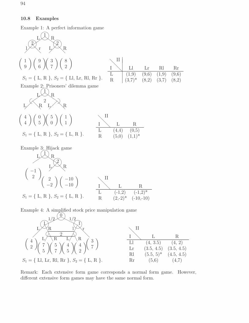
94
10.8 Examples
Example 1: A perfect information game
✑✑✑
◗◗◗✒✑✓✏1
L R
❅❅✒✑✓✏2
l r ❅❅✒✑✓✏2
L R
(
19
)(
96
)(
37
)(
82
)
S1 = { L, R }, S2 = { Ll, Lr, Rl, Rr }.
II
I ❅❅
❅
Ll Lr Rl RrL (1,9) (9,6) (1,9) (9,6)R (3,7)* (8,2) (3,7) (8,2)
Example 2: Prisoners’ dilemma game
✑✑✑
◗◗◗✒✑✓✏1
L R
❅❅
❅❅
☛✡ ✟✠2L R L R
(
44
)(
05
)(
50
)(
11
)
S1 = { L, R }, S2 = { L, R }.
II
I ❅❅
❅
L RL (4,4) (0,5)R (5,0) (1,1)*
Example 3: Hijack game
✑✑✑
◗◗◗✒✑✓✏1
L R
❅❅✒✑✓✏
2L R
(
−12
)
(
2−2
)(
−10−10
)
S1 = { L, R }, S2 = { L, R }.
II
I ❅❅
❅
L RL (-1,2) (-1,2)*R (2,-2)* (-10,-10)
Example 4: A simplified stock price manipulation game
✟✟✟✟
❍❍❍❍✒✑✓✏0
1/2 1/2
❆❆✒✑✓✏1
L R ✁✁❅❅❅
✒✑✓✏
1l r
✁✁❆❆
✁✁❆❆
☛✡ ✟✠2L R L R(
42
)
(
75
)(
57
)(
45
)(
42
)
(
37
)
S1 = { Ll, Lr, Rl, Rr }, S2 = { L, R }.
II
I ❅❅❅
L RLl (4, 3.5) (4, 2)Lr (3.5, 4.5) (3.5, 4.5)Rl (5.5, 5)* (4.5, 4.5)Rr (5,6) (4,7)
Remark: Each extensive form game corresponds a normal form game. However,different extensive form games may have the same normal form.

95
10.9 Strategy pair and pure strategy Nash equilibrium
1. A Strategy Pair: (si, σj). Given a strategy pair, there corresponds a payoff pair(aij , bij).
2. A Nash equilibrium: A strategy pair (si∗, σj∗) such that ai∗j∗ ≥ aij∗ and bi∗j∗ ≥bi∗j for all (i, j). Therefore, there is no incentives for each player to deviate fromthe equilibrium strategy. ai∗j∗ and bi∗j∗ are called the equilibrium payoff.
The equilibrium payoffs of the examples are marked each with a star in the normalform.
Remark 1: It is possible that a game does no have a pure strategy Nash equilib-rium. Also, a game can have more than one Nash equilibria.Remark 2: Notice that the concept of a Nash equilibrium is defined for a normal formgame. For a game in extensive form (a game tree), we have to find the normal formbefore we can find the Nash equilibria.
10.10 Subgames and subgame perfect Nash equilibria
1. Subgame: A subgame in a game tree is a part of the tree consisting of all thenodes and arcs following a node that form a game by itself.
2. Within an extensive form game, we can identify some subgames.
3. Also, each pure strategy of a player induces a pure strategy for every subgame.
4. Subgame perfect Nash equilibrium: A Nash equilibrium is called subgameperfect if it induces a Nash equilibrium strategy pair for every subgame.
5. Backward induction: To find a subgame perfect equilibrium, usually we workbackward. We find Nash equilibria for lowest level (smallest) subgames andreplace the subgames by its Nash equilibrium payoffs. In this way, the size ofthe game is reduced step by step until we end up with the equilibrium payoffs.
All the equilibria, except the equilibrium strategy pair (L,R) in the hijack game, aresubgame perfect.Remark: The concept of a subgame perfect Nash equilibrium is defined only for anextensive form game.
10.10.1 Perfect information game and Zemelo’s Theorem
An extensive form game is called perfect information if every information set consistsonly one node. Every perfect information game has a pure strategy subgame perfectNash Equilibrium.
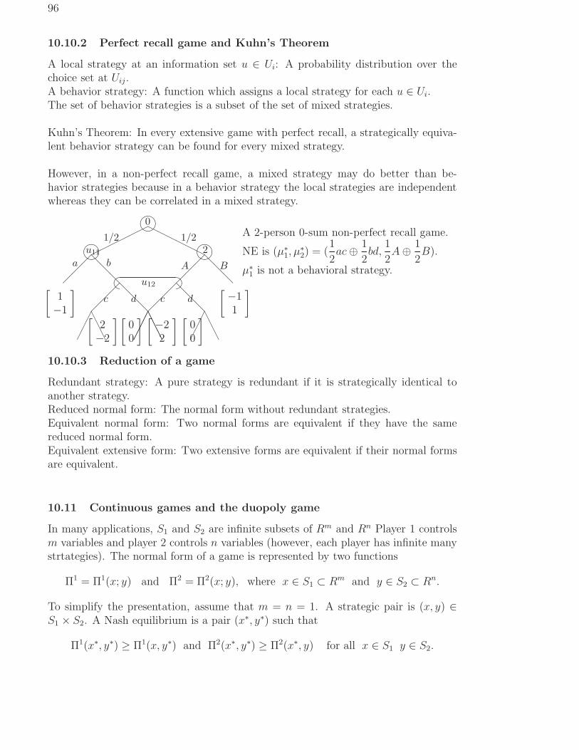
96
10.10.2 Perfect recall game and Kuhn’s Theorem
A local strategy at an information set u ∈ Ui: A probability distribution over thechoice set at Uij .A behavior strategy: A function which assigns a local strategy for each u ∈ Ui.The set of behavior strategies is a subset of the set of mixed strategies.
Kuhn’s Theorem: In every extensive game with perfect recall, a strategically equiva-lent behavior strategy can be found for every mixed strategy.
However, in a non-perfect recall game, a mixed strategy may do better than be-havior strategies because in a behavior strategy the local strategies are independentwhereas they can be correlated in a mixed strategy.
✟✟✟✟✟✟
❍❍❍❍❍❍
❅❅❅
❅❅❅
❅❅❅
✁✁✁
❆❆❆
✁✁✁
❆❆❆
❅❅❅
✁✁✁
❆❆❆
✁✁✁
❆❆❆
✍✌✎☞0✍✌✎☞u11 ✍✌✎☞2☛✡ ✟✠u12
1/2 1/2
a b A B
c d c d
[
1−1
] [
−11
]
[
2−2
][
00
] [
−22
] [
00
]
A 2-person 0-sum non-perfect recall game.
NE is (µ∗1, µ∗2) = (
1
2ac⊕ 1
2bd,
1
2A⊕ 1
2B).
µ∗1 is not a behavioral strategy.
10.10.3 Reduction of a game
Redundant strategy: A pure strategy is redundant if it is strategically identical toanother strategy.Reduced normal form: The normal form without redundant strategies.Equivalent normal form: Two normal forms are equivalent if they have the samereduced normal form.Equivalent extensive form: Two extensive forms are equivalent if their normal formsare equivalent.
10.11 Continuous games and the duopoly game
In many applications, S1 and S2 are infinite subsets of Rm and Rn Player 1 controlsm variables and player 2 controls n variables (however, each player has infinite manystrtategies). The normal form of a game is represented by two functions
Π1 = Π1(x; y) and Π2 = Π2(x; y), where x ∈ S1 ⊂ Rm and y ∈ S2 ⊂ Rn.
To simplify the presentation, assume that m = n = 1. A strategic pair is (x, y) ∈S1 × S2. A Nash equilibrium is a pair (x∗, y∗) such that
Π1(x∗, y∗) ≥ Π1(x, y∗) and Π2(x∗, y∗) ≥ Π2(x∗, y) for all x ∈ S1 y ∈ S2.

97
Consider the case when Πi are continuously differentiable and Π1 is strictly concavein x and Π2 strictly concave in y (so that we do not have to worry about the SOC’s).
Reaction functions and Nash equilibrium:To player 1, x is his endogenous variable and y is his exogenous variable. For each ychosen by player 2, player 1 will choose a x ∈ S1 to maximize his objective functionΠ1. This relationship defines a behavioral equation x = R1(y) which can be obtainedby solving the FOC for player 1, Π1
x(x; y) = 0. Similarly, player 2 regards y as en-dogenous and x exogenous and wants to maximize Π2 for a given x chosen by player1. Player 2’s reaction function (behavioral equation) y = R2(x) is obtained by solvingΠ2
y(x; y) = 0. A Nash equilibrium is an intersection of the two reaction functions.The FOC for a Nash equilibrium is given by Π1
x(x∗; y∗) = 0 and Π2
y(x∗; y∗) = 0.
Duopoly game:There are two sellers (firm 1 and firm 2) of a product.The (inverse) market demand function is P = a−Q.The marginal production costs are c1 and c2, respectively.Assume that each firm regards the other firm’s output as given (not affected by hisoutput quantity).The situation defines a 2-person game as follows: Each firm i controls his own outputquantity qi. (q1, q2) together determine the market price P = a− (q1 + q2) which inturn determines the profit of each firm:
Π1(q1, q2) = (P−c1)q1 = (a−c1−q1−q2)q1 and Π2(q1, q2) = (P−c2)q2 = (a−c2−q1−q2)q2
The FOC are ∂Π1/∂q1 = a− c1 − q2 − 2q1 = 0 and ∂Π2/∂q2 = a− c2 − q1 − 2q2 = 0.The reaction functions are q1 = 0.5(a− c1 − q2) and q2 = 0.5(a− c2 − q1).The Cournot Nash equilibrium is (q∗1 , q
∗2) = ((a− 2c1 + c2)/3, (a− 2c2 + c1)/3) with
P ∗ = (a + c1 + c2)/3. (We have to assume that a− 2c1 + c2, a− 2c2 + c1 ≥ 0.)
10.11.1 A simple bargaining model
Two players, John and Paul, have $ 1 to divide between them. They agree to spendat most two days negotiating over the division. The first day, John will make an offer,Paul either accepts or comes back with a counteroffer the second day. If they cannotreach an agreement in two days, both players get zero. John (Paul) discounts payoffsin the future at a rate of α (β) per day.
A subgame perfect equilibrium of this bargaining game can be derived using back-ward induction.1. On the second day, John would accept any non-negative counteroffer made byPaul. Therefore, Paul would make proposal of getting the whole $ 1 himself and Johnwould get $ 0.2. On the first day, John should make an offer such that Paul gets an amount equiv-alent to getting $ 1 the second day, otherwise Paul will reject the offer. Therefore,John will propose of 1− β for himself and β for Paul and Paul will accept the offer.
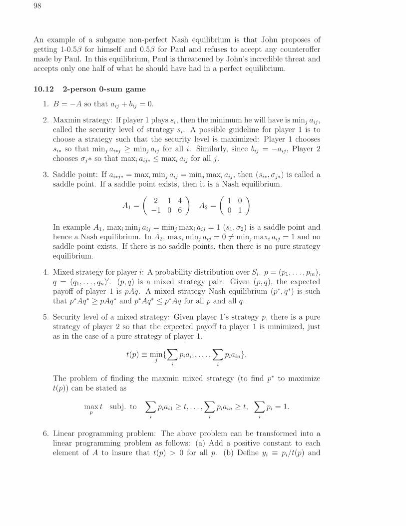
98
An example of a subgame non-perfect Nash equilibrium is that John proposes ofgetting 1-0.5β for himself and 0.5β for Paul and refuses to accept any counteroffermade by Paul. In this equilibrium, Paul is threatened by John’s incredible threat andaccepts only one half of what he should have had in a perfect equilibrium.
10.12 2-person 0-sum game
1. B = −A so that aij + bij = 0.
2. Maxmin strategy: If player 1 plays si, then the minimum he will have is minj aij ,called the security level of strategy si. A possible guideline for player 1 is tochoose a strategy such that the security level is maximized: Player 1 choosessi∗ so that minj ai∗j ≥ minj aij for all i. Similarly, since bij = −aij , Player 2chooses σj∗ so that maxi aij∗ ≤ maxi aij for all j.
3. Saddle point: If ai∗j∗ = maxi minj aij = minj maxi aij, then (si∗, σj∗) is called asaddle point. If a saddle point exists, then it is a Nash equilibrium.
A1 =
(
2 1 4−1 0 6
)
A2 =
(
1 00 1
)
In example A1, maxi minj aij = minj maxi aij = 1 (s1, σ2) is a saddle point andhence a Nash equilibrium. In A2, maxi minj aij = 0 6= minj maxi aij = 1 and nosaddle point exists. If there is no saddle points, then there is no pure strategyequilibrium.
4. Mixed strategy for player i: A probability distribution over Si. p = (p1, . . . , pm),q = (q1, . . . , qn)′. (p, q) is a mixed strategy pair. Given (p, q), the expectedpayoff of player 1 is pAq. A mixed strategy Nash equilibrium (p∗, q∗) is suchthat p∗Aq∗ ≥ pAq∗ and p∗Aq∗ ≤ p∗Aq for all p and all q.
5. Security level of a mixed strategy: Given player 1’s strategy p, there is a purestrategy of player 2 so that the expected payoff to player 1 is minimized, justas in the case of a pure strategy of player 1.
t(p) ≡ minj{∑
i
piai1, . . . ,∑
i
piain}.
The problem of finding the maxmin mixed strategy (to find p∗ to maximizet(p)) can be stated as
maxp
t subj. to∑
i
piai1 ≥ t, . . . ,∑
i
piain ≥ t,∑
i
pi = 1.
6. Linear programming problem: The above problem can be transformed into alinear programming problem as follows: (a) Add a positive constant to eachelement of A to insure that t(p) > 0 for all p. (b) Define yi ≡ pi/t(p) and

99
replace the problem of max t(p) with the problem of min 1/t(p) =∑
i yi. Theconstraints become
∑
i yiai1 ≥ 1, . . . ,∑
i yiain ≥ 1.
miny1,...,ym≥0
y1 + . . . + ym subj. to∑
i
yiai1 ≥ 1, . . . ,∑
i
yiain ≥ 1
7. Duality: It turns out that player 2’s minmax problem can be transformed sim-ilarly and becomes the dual of player 1’s linear programming problem. Theexistence of a mixed strategy Nash equilibrium is then proved by using theduality theorem in linear programming.
Example (tossing coin game): A =
(
1 00 1
)
.
To find player 2’s equilibrium mixed strategy, we solve the linear programming prob-lem:
maxx1,x2≥0
x1 + x2 subj. to x1 ≤ 1 x2 ≤ 1.
The solution is x1 = x2 = 1 and therefore the equilibrium strategy for player 2 isq∗1 = q∗2 = 0.5.
✲x1
✻x2
❅❅❅❅❅❅❅❅
1
1 r✲ y1
✻y2
❅❅❅❅❅❅❅❅
1
1 r
Player 1’s equilibrium mixed strategy is obtained by solving the dual to the linearprogramming problem:
miny1,y2≥0
y1 + y2 subj. to y1 ≥ 1 y2 ≥ 1.
The solution is p∗1 = p∗2 = 0.5.
10.13 Mixed strategy equilibria for non-zero sum games
The idea of a mixed strategy equilibrium is also applicable to a non-zero sum game.Similar to the simplex algorism for the 0-sum games, there is a Lemke algorism.
Example (Game of Chicken)

100
✑✑✑
◗◗◗✒✑✓✏1
S N
❅❅
❅❅
☛✡ ✟✠2S N S N
(
00
)(
−33
)(
3−3
)(
−9−9
)
S1 = { S, N }, S2 = { S, N }.
II
I ❅❅❅
Swerve Don’tSwerve (0,0) (-3,3)*Don’t (3,-3)* (-9,-9)
There are two pure strategy NE: (S, N) and (N, S).There is also a mixed strategy NE. Suppose player 2 plays a mixed strategy (q, 1−q).If player 1 plays S, his expected payoff is Π1(S) = 0q + (−3)(1 − q). If he playsN , his expected payoff is Π1(N) = 3q + (−9)(1 − q). For a mixed strategy NE,Π1(S) = Π1(N), therefore, q = 2
3.
The mixed strategy is symmetrical: (p∗1, p∗2) = (q∗1, q
∗2) = (2
3, 1
3).
Example (Battle of sex Game)
✑✑✑
◗◗◗✒✑✓✏1
B O
❅❅
❅❅
☛✡ ✟✠2B O B O
(
54
)(
00
) (
00
) (
45
)
S1 = { B, O }, S2 = { B, O }.
II
I ❅❅❅
Ball game OperaBall game (5,4)* (0,0)Opera (0,0) (4,5)*
There are two pure strategy NE: (B, B) and (O, O).There is also a mixed strategy NE. Suppose player 2 plays a mixed strategy (q, 1−q).If player 1 plays B, his expected payoff is Π1(B) = 5q + (0)(1− q). If he plays O, hisexpected payoff is Π1(O) = 0q+(4)(1−q). For a mixed strategy NE, Π1(B) = Π1(O),therefore, q = 4
9.
The mixed strategy is: (p∗1, p∗2) = (5
9, 4
9) and (q∗1 , q
∗2) = (4
9, 5
9).
10.14 Cooperative Game and Characteristic form
2-person 0-sum games are strictly competitive. If player 1 gains $ 1, player 2 will loss$ 1 and therefore no cooperation is possible. For other games, usually some coopera-tion is possible. The concept of a Nash equilibrium is defined for the situation whenno explicit cooperation is allowed. In general, a Nash equilibrium is not efficient (notPareto optimal). When binding agreements on strategies chosen can be contractedbefore the play of the game and transfers of payoffs among players after a play of thegame is possible, players will negotiate to coordinate their strategies and redistributethe payoffs to achieve better results. In such a situation, the determination of strate-gies is not the key issue. The problem becomes the formation of coalitions and thedistribution of payoffs.

101
Characteristic form of a game:The player set: N = {1, 2, . . . , n}.A coalition is a subset of N : S ⊂ N .A characteristic function v specifies the maximum total payoff of each coalition.Consider the case of a 3-person game. There are 8 subsets of N = {1, 2, 3}, namely,φ, (1), (2), (3), (12), (13), (23), (123).Therefore, a characteristic form game is determined by 8 values v(φ), v(1), v(2), v(3), v(12), v(13), v(23Super-additivity: If A ∩B = φ, then v(A ∪ B) ≥ v(A) + v(B).An imputation is a payoff distribution (x1, x2, x3).Individual rationality: xi ≥ v(i).Group rationality:
∑
i∈S xi ≥ v(S).Core C: the set of imputations that satisfy individual rationality and group rational-ity for all S.
Marginal contribution of player i in a coalition S ∪ i: v(S ∪ i)− v(S)Shapley value of player i is an weighted average of all marginal contributions
πi =∑
S⊂N
|S|!(n− |S| − 1)!
n![v(S ∪ i)− v(S)].
Example: v(φ) = v(1) = v(2) = v(3) = 0, v(12) = v(13) = v(23) = 0.5, v(123) = 1.C = {(x1, x2, x3), xi ≥ 0, xi + xj ≥ 0.5, x1 + x2 + x3 = 1}. Both (0.3, 0.3, 0.4) and(0.2, 0.4, 0.4) are in C.The Shapley values are (π1, π2, π3) = (1
3, 1
3, 1
3).
Remark 1: The core of a game can be empty. However, the Shapley values areuniquely determined.Remark 2: Another related concept is the von-Neumann Morgenstern solution. SeeCH 6 of Intriligator’s Mathematical Optimization and Economic Theory for the mo-tivations of these concepts.
10.15 The Nash bargaining solution for a nontransferable 2-person coop-erative game
In a nontransferable cooperative game, after-play redistributions of payoffs are im-possible and therefore the concepts of core and Shapley values are not suitable. Forthe case of 2-person games, the concept of Nash bargaining solutions are useful.Let F ⊂ R2 be the feasible set of payoffs if the two players can reach an agreementand Ti the payoff of player i if the negotiation breaks down. Ti is called the threatpoint of player i. The Nash bargaining solution (x∗1, x
∗2) is defined to be the solution
to the following problem:

102
✲x1
✻x2
T1
T2
x∗1
x∗2
max(x1,x2)∈F
(x1 − T1)(x2 − T2)
See CH 6 of Intriligator’s book for the motivations of the solution concept.
10.16 Problems
1. Consider the following two-person 0-sum game:I \ II σ1 σ2 σ3
s1 4 3 -2s2 3 4 10s3 7 6 8
(a) Find the max min strategy of player I smax min and the min max strategyof player II σmin max.
(b) Is the strategy pair (smax min, σmin max) a Nash equilibrium of the game?
(c) What are the equilibrium payoffs?
2. Find the maxmin strategy (smax min) and the minmax strategy (σmin max) of thefollowing two-person 0-sum game:
I \ II σ1 σ2
s1 -3 6s2 8 -2s3 6 3
Is the strategy pair (smax min, σmin max) a Nash equilibrium? If not, use simplexmethod to find the mixed strategy Nash equilibrium.
3. Find the (mixed strategy) Nash Equilibrium of the following two-person game:I \ II H T
H (-2, 2) (2, -1)T (2, -2) (-1,2)
4. Suppose that two firms producing a homogenous product face a linear demandcurve P = a−bQ = a−b(q1+q2) and that both have the same constant marginalcosts c. For a given quantity pair (q1, q2), the profits are Πi = qi(P − c) =qi(a − bq1 − bq2 − c), i = 1, 2. Find the Cournot Nash equilibrium output ofeach firm.
5. Suppose that in a two-person cooperative game without side payments, if thetwo players reach an agreement, they can get (Π1, Π2) such that Π2
1 + Π2 = 47

103
and if no agreement is reached, player 1 will get T1 = 3 and player 2 will getT2 = 2.
(a) Find the Nash solution of the game.
(b) Do the same for the case when side payments are possible. Also answerhow the side payments should be done?
6. A singer (player 1), a pianist (player 2), and a drummer (player 3) are offered$ 1,000 to play together by a night club owner. The owner would alternativelypay $ 800 the singer-piano duo, $ 650 the piano drums duo, and $ 300 the pianoalone. The night club is not interested in any other combination. Howeover,the singer-drums duo makes $ 500 and the singer alone gets $ 200 a night in arestaurant. The drums alone can make no profit.
(a) Write down the characteristic form of the cooperative game with side pay-ments.
(b) Find the Shapley values of the game.
(c) Characterize the core.

1
Short Notes
On
Microeconomics
In
Mathematical Approach

Contents
1 The Market 4
2 Budget Constraint 8
3 Preferences 10
4 Utility 14
5 Choice 18
6 Demand 24
7 Revealed Preference 27
8 Slutsky Equation 30
9 Buying and Selling 33
10 Intertemporal Choice 37
12 Uncertainty 39
14 Consumer Surplus 43
15 Market Demand 46
18 Technology 48
19 Profit Maximization 52
20 Cost Minimization 54
21 Cost Curves 57
22 Firm Supply 59
23 Industry Supply 62
24 Monopoly 64
2

25 Monopoly Behavior 67
26 Factor Market 72
27 Oligopoly 76
28 Game Theory 80
30 Exchange 85
3

Ch. 1. The Market
I. Economic model: A simplified representation of reality
A. An example
– Rental apartment market in Shinchon: Object of our analysis
– Price of apt. in Shinchon: Endogenous variable
– Price of apt. in other areas: Exogenous variable
– Simplification: All (nearby) Apts are identical
B. We ask
– How the quantity and price are determined in a given allocation mechanism
– How to compare the allocations resulting from different allocation mechanisms
II. Two principles of economics
– Optimization principle: Each economic agent maximizes its objective (e.g. utility, profit,
etc.)
– Equilibrium principle: Economic agents’ actions must be consistent with each other
III. Competitive market
A. Demand
– Tow consumers with a single-unit demand whose WTP’s are equal to r1 and r2 (r1 < r2)
r2
r1
p
Q1 2
– Many people
4

Q
p
Q
p
4 consumers ∞ consumers
B. Supply
– Many competitive suppliers
– Fixed at Q in the short-run
C. Equilibrium
– Demand must equal supply
Q Q′
p
Q
p
p∗
p′
→ Eq. price (p∗) and eq. quantity (Q)
D. Comparative statics: Concerns how endogenous variables change as exogenous variables
change
–
{
Comparative: Compare two eq’a
Statistics: Only look at eq’a, but not the adjustment process
– For instance, if there is exogenous increase in supply, Q→ Q′, then p∗ → p′
5

III. Other allocation mechanisms
A. Monopoly
p
p∗p′
B. Rent control: Price ceiling at p < p∗ → Excess demand → Rationing (or lottery)
IV. Pareto efficiency: Criterion to compare different economic allocations
A. One allocation is a Pareto improvement over the other if the former makes some people
better off without making anyone else worse off, compared to the latter.
B. An allocation is called Pareto efficient(PE) if there is no Pareto improvement.
Otherwise, the allocation is called Pareto inefficient
C. Example: Rent control is not PE
– Suppose that there are 2 consumers, A and B, who value an apt at rA and rB > rA.
– As a result of pricing ceiling and rationing, A gets an apt and B does not
6
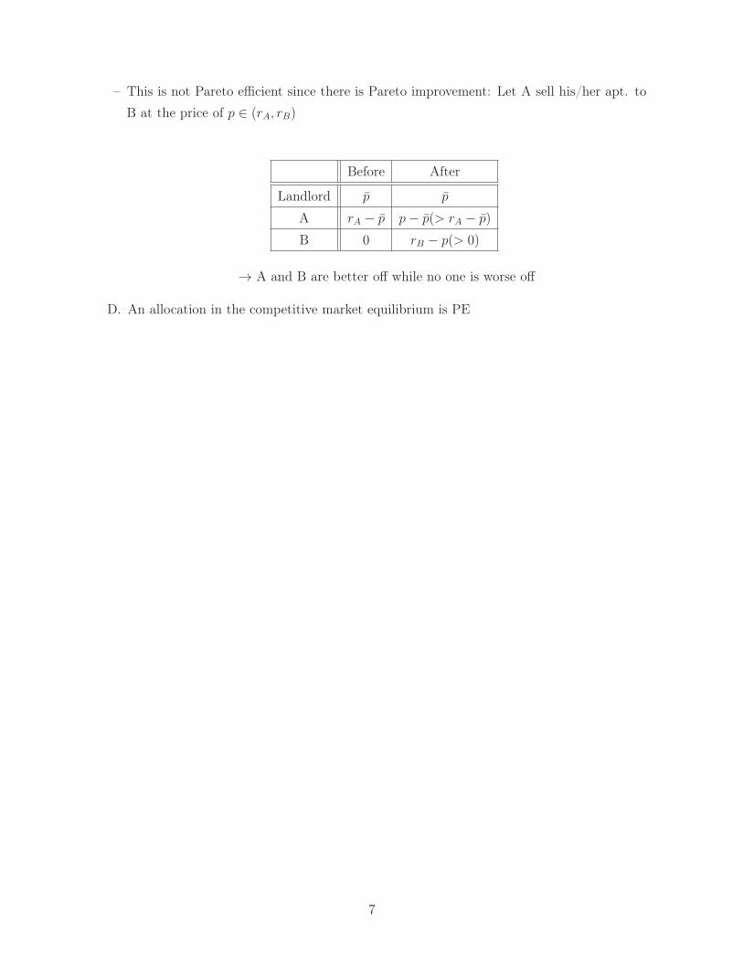
– This is not Pareto efficient since there is Pareto improvement: Let A sell his/her apt. to
B at the price of p ∈ (rA, rB)
Before After
Landlord p p
A rA − p p− p(> rA − p)
B 0 rB − p(> 0)
→ A and B are better off while no one is worse off
D. An allocation in the competitive market equilibrium is PE
7
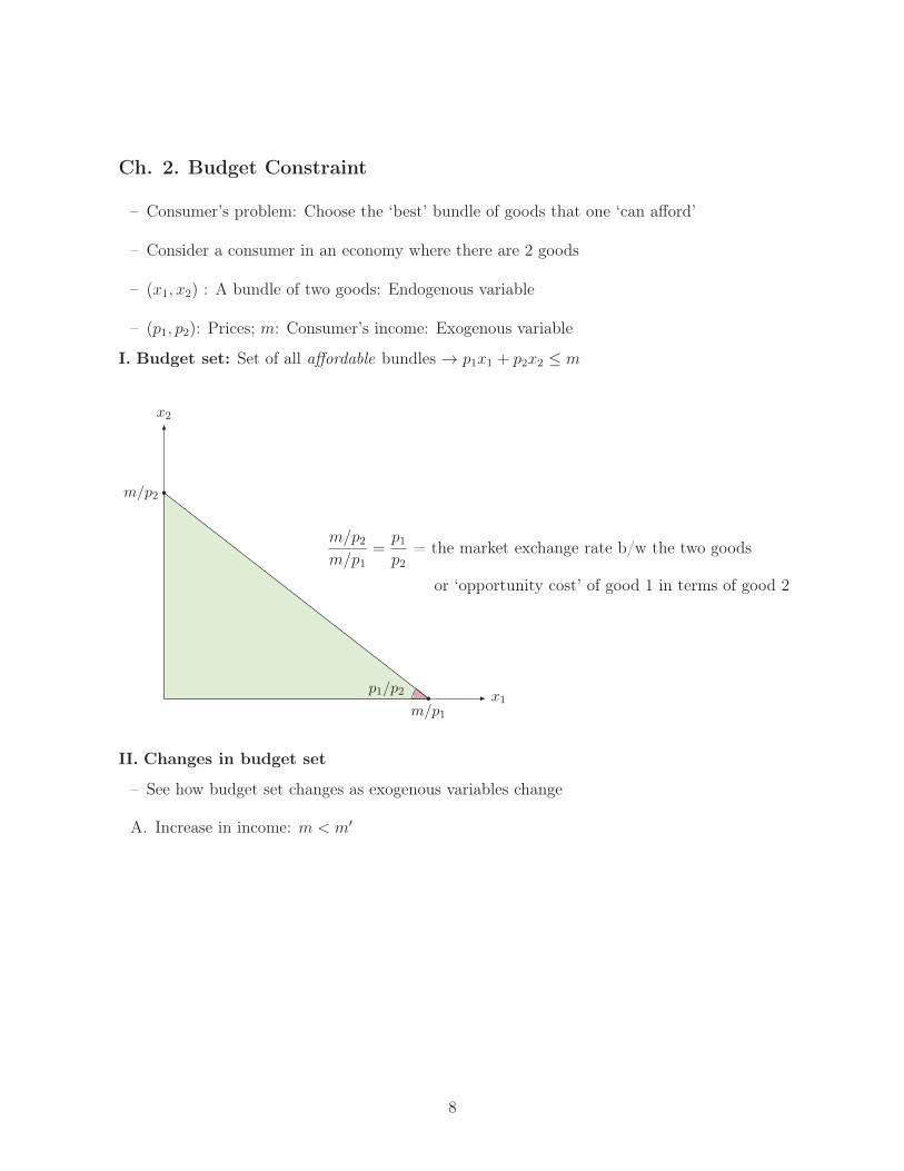
Ch. 2. Budget Constraint
– Consumer’s problem: Choose the ‘best’ bundle of goods that one ‘can afford’
– Consider a consumer in an economy where there are 2 goods
– (x1, x2) : A bundle of two goods: Endogenous variable
– (p1, p2): Prices; m: Consumer’s income: Exogenous variable
I. Budget set: Set of all affordable bundles → p1x1 + p2x2 ≤ m
x2
x1
m/p2
m/p1
p1/p2
m/p2m/p1
=p1p2
= the market exchange rate b/w the two goods
or ‘opportunity cost’ of good 1 in terms of good 2
II. Changes in budget set
– See how budget set changes as exogenous variables change
A. Increase in income: m < m′
8

B. Increase in the price of one good: p1 < p′1
C. Proportional increase in all prices and income: (p1, p2,m)→ (tp1, tp2, tm)
※ Numeraire: Let t = 1p1→ x1 +
p2p1x2 =
mp1
that is, the price of good 1 is 1
III. Application: Tax and subsidy
A. Quantity tax: Tax levied on each unit of, say, good 1 bought
– Given tax rate t, p′1 = p1 + t
B. Value tax: Tax levied on each dollar spent on good 1
– Given tax rate τ , p′1 = p1 + τp1 = (1 + τ)p1
C. Subsidy: Negative tax
Example. s = Quantity subsidy for the consumption of good 1 exceeding x1
9

Ch. 3. Preferences
I. Preference: Relationship (or rankings) between consumption bundles
A. Three modes of preference: Given two Bundles, x = (x1, x2) and y = (y1, y2)
1. x ≻ y: x ‘is (strictly) preferred to’ y
2. x ∼ y: x ‘is indifferent to’ y
3. x � y: x ‘is weakly preferred to’ y
Example. (x1, x2) � (y1, y2) if x1 + x2 ≥ y1 + y2
B. The relationships between three modes of preference
1. x � y ⇔ x ≻ y or x ∼ y
2. x ∼ y ⇔ x � y and y � x
3. x ≻ y ⇔ x � y but not y � x
C. Properties of preference �
1. x � y or y � x
2. Reflexive: Given any x, x � x
3. Transitive: Given x, y, and z, if x � y and y � z, then x � z
Example. Does the preference in the above example satisfy all 3 properties?
※ If � is transitive, then ≻ and ∼ are also transitive: For instance, if x ∼ y and y ∼ z,
then x ∼ z
D. Indifference curves: Set of bundles which are indifferent to one another
10

0 2 4 6 8 10 120
2
4
6
8
10
12
A
B
x1
x2
※ Two different indifferent curves cannot intersect with each other
※ Upper contour set: Set of bundles weakly preferred to a given bundle x
II. Well-behaved preference
A. Monotonicity: ‘More is better’
– Preference is monotonic if x � y for any x and y satisfying x1 ≥ y1, x2 ≥ y2
– Preference is strictly monotonic if x ≻ y for any x and y satisfying x1 ≥ y1, x2 ≥ y2, and
x 6= y
Example. Monotonicity is violated by the satiated preference:
B. Convexity: ‘Moderates are better than extremes’
– Preference is convex if for any x and y with y � x, we have
tx+ (1− t)y � x for all t ∈ [0, 1]
11

x2
x1
Convex Preference
x2
x1
Non-convex Preference
tx+ (1− t)y
x
y
tx+ (1− t)y
x
y
→ Convex preference is equivalent to the convex upper contour set
– Preference is strictly convex if for any x and y with y � x, we have
tx+ (1− t)y ≻ x for all t ∈ (0, 1)
III. Examples
A. Perfect substitutes: Consumer likes two goods equally so only the total number of goods
matters → 2 goods are perfectly substitutable
Example. Blue and Red pencil
B. Perfect complement: One good is useless without the other → It is not possible to sub-
stitute one good for the other
Example. Right and Left shoe
12

C. Bads: Less of a ‘bad’ is better
Example. Labor and Food
※ This preference violates the monotonicity but there is an easy fix: Let ‘Leisure = 24
hours − Labor’ and consider two goods, Leisure and Food.
IV. Marginal rate of substitution (MRS): MRS at a given bundle x is the marginal
exchange rate between two goods to make the consumer indifferent to x.
→ (x1, x2) ∼ (x1 −∆x1, x2 +∆x2)
→ MRS at x = lim∆x1→0
∆x2
∆x1= slope of indifference curve at x
→ MRS decreases as the amount of good 1 increases
13
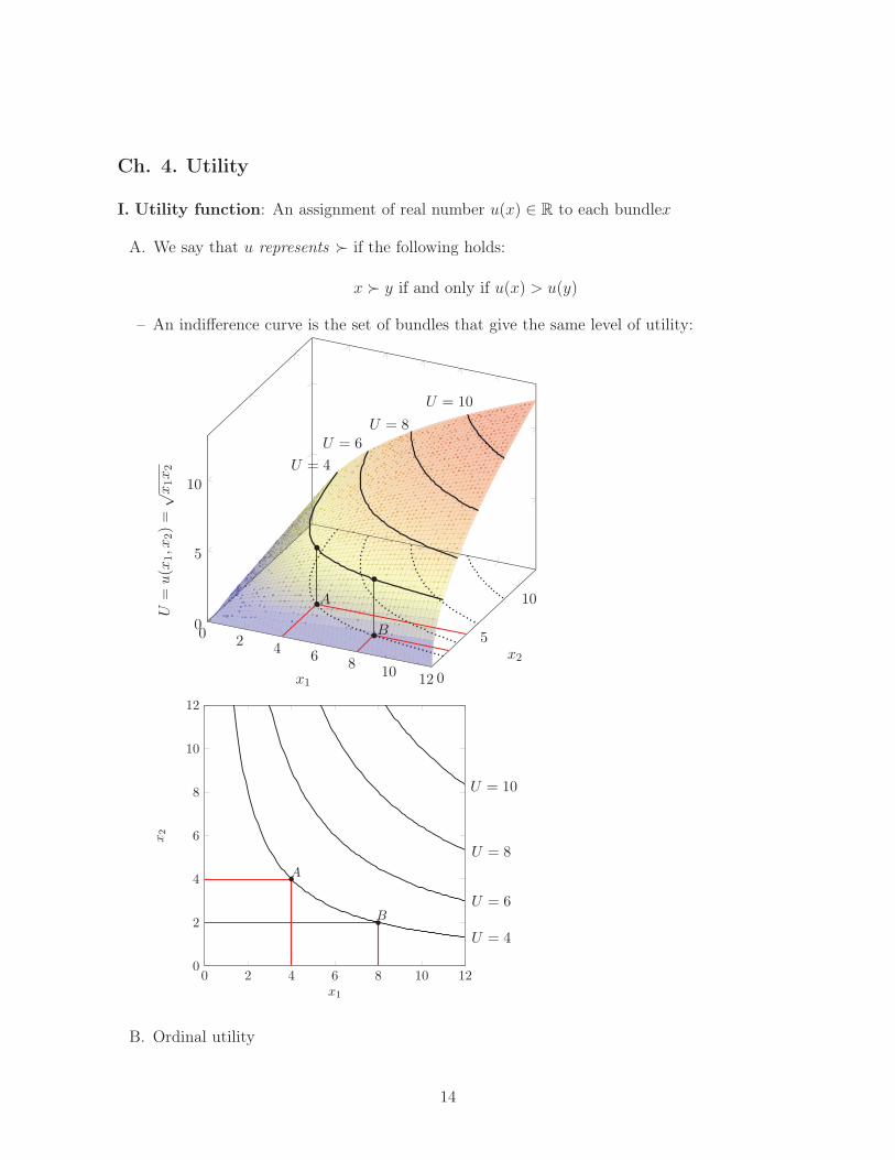
Ch. 4. Utility
I. Utility function: An assignment of real number u(x) ∈ R to each bundlex
A. We say that u represents ≻ if the following holds:
x ≻ y if and only if u(x) > u(y)
– An indifference curve is the set of bundles that give the same level of utility:
02
46
810
12 0
5
10
0
5
10
B
A
U = 4
U = 6U = 8
U = 10
x1
x2
U=
u(x
1,x
2)=√x1x2
0 2 4 6 8 10 120
2
4
6
8
10
12
A
B
x1
x2
U = 6
U = 4
U = 8
U = 10
B. Ordinal utility
14

– Only ordinal ranking matters while absolute level does not matter
Example. Three bundles x, y, and z, and x ≻ y ≻ z → Any u(·) satisfying u(x) > u(y) >
u(z) is good for representing ≻
– There are many utility functions representing the same preference
C. Utility function is unique up to monotone transformation
– For any increasing function f : R → R, a utility function v(x) ≡ f(u(x)) represents the
same preference as u(x) since
x ≻ y ⇔ u(x) > u(y)⇔ v(x) = f(u(x)) > f(u(y)) = v(y)
D. Properties of utility function
– A utility function representing a monotonic preference must be increasing in x1 and x2
– A utility function representing a convex preference must satisfy: For any two bundles x
and y,
u(tx+ (1− t)y) ≥ min{u(x), u(y)} for all t ∈ [0, 1]
II. Examples
A. Perfect substitutes
1. Red & blue pencils
→ u(x) = x1 + x2 or v(x) = (x1 + x2)2 (∵v(x) = f(u(x)), where f(u) = u2)
2. One & five dollar bills
→ u(x) = x1 + 5x2
3. In general, u(x) = ax1 + bx2
→ Substitution rate: u(x1 −∆x1, x2 +∆x2) = u(x1, x2) → ∆x2
∆x1= a
b
B. Perfect complements
1. Left & right shoes
→ u(x) =
{
x1 if x2 ≥ x1
x2 if x1 ≥ x2
or u(x) = min{x1, x2}
2. 1 spoon of coffee & 2 spoons of cream
→ u(x) =
{
x1 if x1 ≤ x2
2x2
2if x1 ≥ x2
2
or u(x) = min{x1,x2
2} or u(x) = min{2x1, x2}
3. In general, u(x) = min{ax1, bx2}, where a, b > 0
15

C. Cobb-Douglas: u(x) = xc1x
d2, where c, d > 0
→ v(x1, x2) = (xc1c
d2)
1
c+d = xc
c+d
1 xd
c+d
2 = xa1x
1−a2 , where a ≡ c
c+d
III. Marginal utility (MU) and marginal rate of substitution (MRS)
A. Marginal utility: The rate of the change in utility due to a marginal increase in one good
only
– Marginal utility of good 1: (x1, x2)→ (x1 +∆x1, x2)
MU1 = lim∆x1→0
∆U1
∆x1
= lim∆x1→0
u(x1 +∆x1, x2)− u(x1, x2)
∆x1
(→ ∆U1 = MU1 ×∆x1)
– Analogously,
MU2 = lim∆x2→0
∆U2
∆x2
= lim∆x2→0
u(x1, x2 +∆x2)− u(x1, x2)
∆x2
(→ ∆U2 = MU2 ×∆x2)
– Mathematically, MUi =∂u∂xi
, that is the partial differentiation of utility function u
B. MRS ≡ lim∆x1→0
∆x2
∆x1
for which u(x1, x2) = u(x1 −∆x1, x2 +∆x2)
→ 0 = u(x1 −∆x1, x2 +∆x2)− u(x1, x2)
= [u(x1 −∆x1, x2 +∆x2)− u(x1, x2 +∆x2)] + [u(x1, x2 +∆x2)− u(x1, x2)]
= − [u(x1, x2 +∆x2)− u(x1 −∆x1, x2 +∆x2)] + [u(x1, x2 +∆x2)− u(x1, x2)]
= −∆U1 +∆U2 = −MU1∆x1 +MU2∆x2
→ MRS =∆x2
∆x1
=MU1
MU2
=∂u/∂x1
∂u/∂x2
Example. u(x) = xa1x
1−a2
→ MRS =MU1
MU2
=axa−1
1 x1−a2
xa1(1− a)x−a2
=ax2
(1− a)x1
C. MRS is invariant with respect to the monotone transformation: Let v(x) ≡ f(u(x)) and
then∂v/∂x1
∂v/∂x2
=f ′(u) · (∂u/∂x1)
f ′(u)·(∂u/∂x2)=
∂u/∂x1
∂u/∂x2
.
Example. An easier way to get MRS for the Cobb-Douglas utility function
u(x) = xa1x
1−a2 → v(x) = a ln x1 + (1− a) ln x2
So, MRS = MU1
MU2= a/x1
(1−a)/x2= ax2
(1−a)x1
※ An alternative method for deriving MRS: Implicit function method
16
– Describe the indifference curve for a given utility level u by an implicit function x2(x1)
satisfying
u(x1, x2(x1)) = u
– Differentiate both sides with x1 to obtain
∂u(x1, x2)
∂x1
+∂u(x1, x2)
∂x2
∂x2(x1)
∂x1
= 0,
which yields
MRS =
∣∣∣∣
∂x2(x1)
∂x1
∣∣∣∣=
∂u(x1, x2)/∂x1
∂u(x1, x2)/∂x2
17
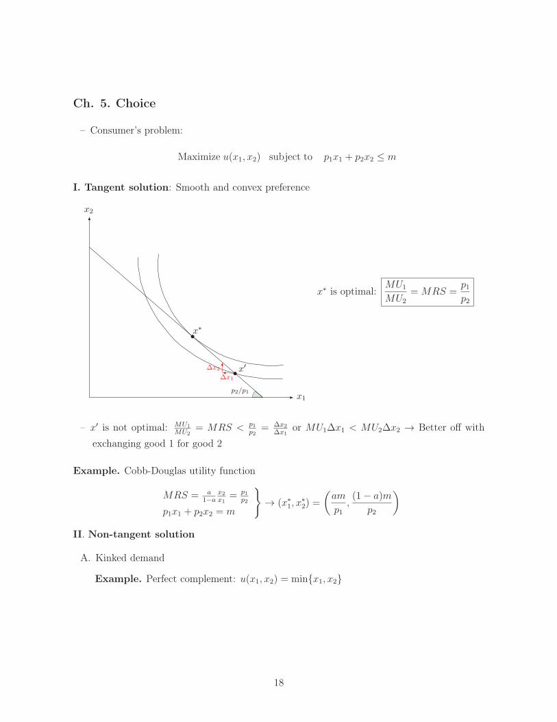
Ch. 5. Choice
– Consumer’s problem:
Maximize u(x1, x2) subject to p1x1 + p2x2 ≤ m
I. Tangent solution: Smooth and convex preference
x1
x2
p2/p1
∆x1
∆x2
x∗
x′
x∗ is optimal:MU1
MU2
= MRS =p1p2
– x′ is not optimal: MU1
MU2= MRS < p1
p2= ∆x2
∆x1or MU1∆x1 < MU2∆x2 → Better off with
exchanging good 1 for good 2
Example. Cobb-Douglas utility function
MRS = a1−a
x2
x1= p1
p2
p1x1 + p2x2 = m
}
→ (x∗1, x∗2) =
(am
p1,(1− a)m
p2
)
II. Non-tangent solution
A. Kinked demand
Example. Perfect complement: u(x1, x2) = min{x1, x2}
18

x1 = x2
p1x1 + p2x2 = m
}
→ x∗1 = x∗2 =m
p1 + p2
B. Boundary optimum
1. No tangency:
m/p2
x1
x2
x∗
x′′
x′∆x1
∆x2
∆x1
∆x2
At every bundle on the budget line,
MRS < p1p2or ∆x1 ·MU1 < ∆x2 ·MU2
→ x∗ = (0,m/p2)
Example. u(x1, x2) = x1 + ln x2, (p1, p2,m) = (4, 1, 3)
MRS = x2 <p1p2
= 4 → ∴ x∗ = (0, 3)
2. Non-convex preference: Beware of ‘wrong’ tangency
Example. u(x) = x21 + x2
2
3. Perfect substitutes:
19
→ (x∗1, x∗2) =
(m/p1, 0) if p1 < p2
any bundle on the budget line if p1 = p2
(0,m/p2) if p1 > p2
C. Application: Quantity vs. income tax
Quantity tax : (p1 + t)x1 + p2x2 = mUtility max.−−−−−−−→ (x∗1, x
∗2) satisfying p1x
∗1 + p2x
∗2 = m− tx∗1
Income tax : p1x1 + p2x2 = m−RSet R=tx∗
1−−−−−−→ p1x1 + p2x2 = m− tx∗1
→ Income tax that raises the same revenue as quantity tax is better for consumers
20
Appendix: Lagrangian Method
I. General treatment (cookbook procedure)
– Let f and gj, j = 1, · · · , J be functions mapping from Rn and R.
– Consider the constrained maximization problem as follows:
maxx=(x1,···xn)
f(x) subject to gj(x) ≥ 0, j = 1, · · · , J. (A.1)
So there are J constraints, each of which is represented by a function gj.
– Set up the Lagrangian function as follows
L(x, λ) = f(x) +J∑
j=1
λjgj(x).
We call λj, j = 1, · · · , J Lagrangian multipliers.
– Find a vector (x∗, λ∗) that solves the following equations:
∂L(x∗,λ∗)∂xi
= 0 for all i = 1, · · · , nλ∗jgj(x
∗) = 0 and λ∗j ≥ 0 for all j = 1, · · · , J.(A.2)
– Kuhn-Tucker theorem tells us that x∗ is the solution of the original maximization problem
given in (A.1), provided that some concavity conditions hold for f and gj, j = 1, · · · J. (Fordetails, refer to any textbook in the mathematical economics.)
II. Application: Utility maximization problem
– Set up the utility maximization problem as follows:
maxx=(x1,x2)
u(x)
subject to
m− p1x1 − p2x2 ≥ 0
x1 ≥ 0 and x2 ≥ 0.
– The Lagrangian function corresponding to this problem can be written as
L(x, λ) = u(x) + λ3(m− p1x1 − p2x2) + λ1x1 + λ2x2
A. Case of interior solution: Cobb-Douglas utility, u(x) = a ln x1 + (1− a) ln x2, a ∈ (0, 1)
21
– The Lagrangian function becomes
L(x, λ) = a ln x1 + (1− a) ln x2 + λ3(m− p1x1 − p2x2) + λ1x1 + λ2x2
– Then, the equations in (A.2) can be written as
∂L(x∗, λ∗)
∂x1
=a
x∗1− λ∗3p1 + λ∗1 = 0 (A.3)
∂L(x∗, λ∗)
∂x2
=1− a
x∗2− λ∗3p2 + λ∗2 = 0 (A.4)
λ∗3(m− p1x∗1 − p2x
∗2) = 0 and λ∗3 ≥ 0 (A.5)
λ∗1x∗1 = 0 and λ∗1 ≥ 0 (A.6)
λ∗2x∗2 = 0 and λ∗2 ≥ 0 (A.7)
1) One can easily see that x∗1 > 0 and x∗2 > 0 so λ∗1 = λ∗2 = 0 by (A.6) and (A.7).
2) Plugging λ∗1 = λ∗2 = 0 into (A.3), we can see λ∗3 =a
p1x∗
1
> 0, which by (A.5) implies
m− p1x∗1 − p2x
∗2 = 0. (A.8)
3) Combining (A.3) and (A.4) with λ∗1 = λ∗2 = 0, we are able to obtain
ax∗2(1− a)x∗1
=p1p2
(A.9)
4) Combining (A.8) and (A.9) yields the solution for (x∗1, x∗2) = (am
p1, (1−a)m
p2), which we have
seen in the class.
B. Case of boundary solution: Quasi-linear utility, u(x) = x1 + ln x2.
– Let (p1, p2,m) = (4, 1, 3)
– The Lagrangian becomes
L(x, λ) = x1 + ln x2 + λ3(3− 4x1 − x2) + λ1x1 + λ2x2
– Then, the equations in (A.2) can be written as
∂L(x∗, λ∗)
∂x1
= 1− 4λ∗3 + λ∗1 = 0 (A.10)
∂L(x∗, λ∗)
∂x2
=1
x∗2− λ∗3 + λ∗2 = 0 (A.11)
λ∗3(3− 4x∗1 − x∗2) = 0 and λ∗3 ≥ 0 (A.12)
λ∗1x∗1 = 0 and λ∗1 ≥ 0 (A.13)
λ∗2x∗2 = 0 and λ∗2 ≥ 0 (A.14)
22
1) One can easily see that x∗2 > 0 so λ∗2 = 0 by (A.14).
2) Plugging λ∗2 = 0 into (A.11), we can see λ∗3 =1x∗
2
> 0, which by (A.12) implies
3− 4x∗1 − x∗2 = 0. (A.15)
3) By (A.10),
λ∗1 = 4λ∗3 − 1 =4
x∗2− 1 > 0 (A.16)
since x∗2 ≤ 3 due to (A.15).
4) Now, (A.16) and (A.13) imply x∗1 = 0, which in turn implies x∗2 = 3 by (A.15).
23
Ch. 6. Demand
– We studied how the consumer maximizes utility given p and m
→ Demand function: x(p,m) = (x1(p,m), x2(p,m))
– We ask here how x(p,m) changes with p and m?
I. Comparative statics: Changes in income
A. Normal or inferior good: ∂xi(p,m)∂m
> 0 or < 0
B. Income offer curves and Engel curves
C. Homothetic utility function
– For any two bundles x and y, and any number α > 0,
u(x) > u(y)⇔ u(αx) > u(αy).
– Perfect substitute and complements, and Cobb-Douglas are all homothetic.
– x∗ is a utility maximizer subject to p1x1 + p2x2 ≤ m if and only tx∗ is a utility maximizer
subject to p1x1 + p2x2 ≤ tm for any t > 0.
– Income offer and Engel curves are straight lines
24

D. Quasi-linear utility function: u(x1, x2) = x1 + v(x2), where v is a concave function, that
is v′ is decreasing.
– Define x∗2 to satisfy
MRS =1
v′(x2)=
p1p2
(1)
– If m is large enough so that m ≥ p2x∗2, then the tangent condition (1) can be satisfied.
→ The demand of good 2, x∗2, does not depend on the income level
– If m < p2x∗2, then the LHS of (1) is always greater than the RHS for any x2 ≤ m
p2
→ Boundary solution occurs at x∗ = (0, mp2).
Example. Suppose that u(x1, x2) = x1 + ln x2, (p1, p2) = (4, 1). Draw the income offer
and Engel curves.
II. Comparative statics: Changes in price
A. Ordinary or Giffen good: ∂xi(p,m)∂pi
< 0 or >0
B. Why Giffen good?
p1 ր −→
Relatively more expensive good 1 : x1 ց
Reduced real income
{
normal good: x1 ցinferior good: x1 ր
So, a good must be inferior in order to be Giffen
C. Price offer curves and demand curves
25

D. Complements or substitutes: ∂xi(p,m)∂pj
< 0 or > 0
26
Ch. 7. Revealed Preference
I. Revealed preference: Choice (observable) reveals preference (unobservable)
– Consumer’s observed choice:
{
(x1, x2) chosen under price (p1, p2)
(y1, y2) chosen under price (q1, q2)
A. ‘Directly revealed preferred ’ (d.r.p.)
(x1, x2) is d.r.p. to (y1, y2)⇔ p1x1 + p2x2 ≥ p1y1 + p2y2
B. ‘Indirectly revealed preferred ’ (i.r.p.)
(x1, x2) is i. r. p. to (z1, z2)
C. ‘Revealed preferred ’ (r.p.) = ‘d.r.p. or i.r.p.’
II. Axioms of revealed preference:
A. Weak axiom of reveal preference (WARP):
– If (x1, x2) is d.r.p. to (y1, y2) with (x1, x2) 6= (y1, y2), then (y1, y2) must not be d.r.p. to (x1, x2)
⇔ If p1x1 + p2x2 ≥ p1y1 + p2y2 with (x1, x2) 6= (y1, y2), then it must be that q1y1 + q2y2 <
q1x1 + q2x2
27

B. How to check WARP
– Suppose that we have the following observations
Observation Prices Bundle
1 (2,1) (2,1)
2 (1,2) (1,2)
3 (2,2) (1,1)
– Calculate the costs of bundles
Price \ Bundle 1 2 3
1 5 4∗ 3∗
2 4∗ 5 3∗
3 6 6 4
→ WARP is violated since bundle 1 is d.r.p. to bundle 2 under price 1 while bundle 2 is
d.r.p. to bundle 1 under price 2.
C. Strong axiom of revealed preference (SARP) If (x1, x2) is r.p. to (y1, y2) with (x1, x2) 6=(y1, y2), then (y1, y2) must not be r.p. to (x1, x2)
III. Index numbers and revealed preference
– Enables us to measure consumers’ welfare without information about their actual prefer-
ences
– Consider the following observations
{
Base year : (xb1, x
b2) under (p
b1, p
b2)
Current year : (xt1, x
t2) under (p
t1, p
t2)
A. Quantity indices: Measure the change in “average consumptions”
– Iq =ω1x
t1 + ω2x
t2
ω1xb1 + ω2xb
2
, where ωi is the weight for good i = 1, 2
– Using prices as weights, we obtain
{
Passhe quantity index (Pq) if (ω1, ω2) = (pt1, pt2)
Laspeyres quantity index (Lq) if (ω1, ω2) = (pb1, pb2)
B. Quantity indices and consumer welfare
– Pq =pt1x
t1 + pt2x
t2
pt1xb1 + pt2x
b2
> 1 : Consumer must be better off at the current year
– Lq =pb1x
t1 + pb2x
t2
pb1xb1 + pb2x
b2
< 1 : Consumer must be worse off at the current year
28
C. Price indices: Measure the change in “cost of living”
– Ip =x1p
t1 + x2p
t2
x1pb1 + x2pb2, where (x1, x2) is a fixed bundle
– Depending on what bundle to use, we obtain
{
Passhe price index (Pp) : (x1, x2) = (xt1, x
t2)
Laspeyres price index (Lp) : (x1, x2) = (xb1, x
b2)
– Laspeyres price index is also known as “consumer price index (CPI)”: This has problem
of overestimating the change in cost of living
29

Ch. 8. Slutsky Equation
– Change of price of one good: p1 → p′1 with p′1 > p1
→{
Change in relative price (p1/p2)→ Substitution effect
Change in real income→ Income effect
I. Substitution and income effects:
– Aim to decompose the change ∆x1 = x1(p′1, p2,m)− x1(p1, p2,m) into the changes due to
the substitution and income effects.
– To obtain the change in demand due to substitution effect,
(1) compensate the consumer so that the original bundle is affordable under (p′1, p2)
→ m′ = p′1x1(p1, p2,m) + p2x2(p1, p2,m)
(2) ask what bundle he chooses under (p′1, p2,m′) → x1(p
′1, p2,m
′)
(3) decompose ∆x1 as follows:
∆x1 = x1(p′1, p2,m)− x1(p1, p2,m)
= [x1(p′1, p2,m
′)− x1(p1, p2,m)]︸ ︷︷ ︸
∆xs1 : Change due to
substitution effect
+ [x1(p′1, p2,m)− x1(p
′1, p2,m
′)]︸ ︷︷ ︸
∆xn1 : Change due to
income effect
p′1x1 + p2x2 = m′
∆xs1: Substitution
effect
∆xn1 : Income
effect Total effect
O
x2
x1
A
B
A′
C ′ D C
30

∆xs1: Substitution
effect∆xn1 : Income
effect Total effect
O
x2
x1
A
B
A′
C ′D C
– Letting ∆p1 ≡ p′1 − p1,
Substitution Effect :∆xs
1
∆p1< 0
Income Effect
{∆xn
1
∆p1< 0 if good 1 is normal
∆xn1
∆p1> 0 if good 1 is inferior
→ In case of inferior good, if the income effect dominates the substitution effect, then
there arises a Giffen phenomenon.
Example. Cobb-Douglas with a = 0.5, p1 = 2, & m = 16→ p′1 = 4
Remember x1(p,m) = amp1
so
x1(p1, p2,m) = 0.5× (16/2) = 4, x1(p′1, p2,m) = 0.5× (16/4) = 2
m′ = m+ (m′ −m) = m+ (p′1 − p1)x1(p1, p2,m) = 16 + (4− 2)4 = 24
x1(p′1, p2,m
′) = 0.5× (24/4) = 3
∴ ∆xs1 = x1(p
′1, p2,m
′)− x1(p1, p2,m) = 3− 4 = −1∆xn
1 = x1(p′1, p2,m)− x1(p
′1, p2,m
′) = 2− 3 = −1
II. Slutsky equation
– Letting ∆m ≡ m′ −m, we have ∆m = m′ −m = (p′1 − p1)x1(p,m) = ∆p1x1(p,m)
A. For convenience, let ∆xm1 ≡ −∆xn
1 . Then,
∆x1
∆p1=
∆xs1
∆p1− ∆xm
1
∆p1=
∆xs1
∆p1− ∆xm
1
∆mx1(p,m)
B. Law of demands (restated): If the good is normal, then its demand must fall as the price
rises
31
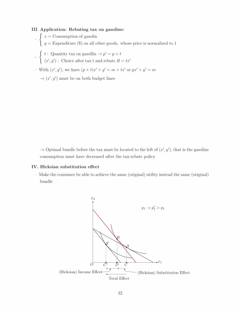
III. Application: Rebating tax on gasoline:
–
{
x = Consumption of gasolin
y = Expenditure ($) on all other goods, whose price is normalized to 1
–
{
t : Quantity tax on gasollin→ p′ = p+ t
(x′, y′) : Choice after tax t and rebate R = tx′
– With (x′, y′), we have (p+ t)x′ + y′ = m+ tx′ or px′ + y′ = m
→ (x′, y′) must be on both budget lines
→ Optimal bundle before the tax must be located to the left of (x′, y′), that is the gasoline
consumption must have decreased after the tax-rebate policy
IV. Hicksian substitution effect
– Make the consumer be able to achieve the same (original) utility instead the same (original)
bundle
(Hicksian) Substitution Effect(Hicksian) Income Effect
Total Effect
p1 → p′1 > p1
O
x2
x1
A
B
A′
C ′ D C
32

Ch. 9. Buying and Selling
– Where does the consumer’s income come from? → Endowment= (ω1, ω2)
I. Budget constraint
A. Budget line: p1x1 + p2x2 = p1ω1 + p2ω2 → Always passes through (ω1, ω2)
B. Change in price: p1 : (x1, x2)→ p′1 : (x′1, x
′2) with p′1 < p1
→ Consumer welfare
x1 − ω1 > 0→ x′1 − ω1 > 0 : Better off
x1 − ω1 < 0
⟨
x′1 − ω1 < 0 : Worse off
x′1 − ω1 > 0 : ?
II. Slutsky equation
– Suppose that p1 increases to p′1 > p1
A. Endowment income effect
– Suppose that the consumer chooses B under p1 and B′ under p′1
AA1A2 A′
x1
x2
E
B
B1
B2
B′
33
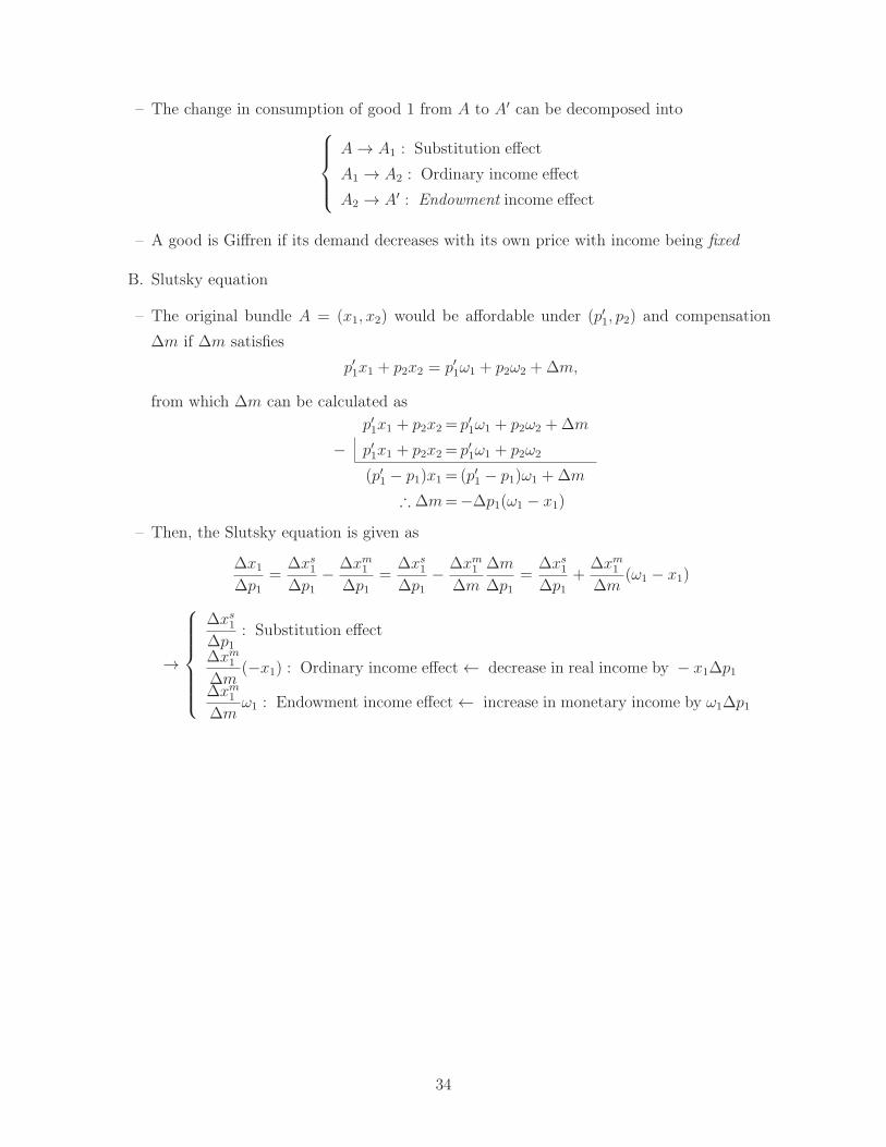
– The change in consumption of good 1 from A to A′ can be decomposed into
A→ A1 : Substitution effect
A1 → A2 : Ordinary income effect
A2 → A′ : Endowment income effect
– A good is Giffren if its demand decreases with its own price with income being fixed
B. Slutsky equation
– The original bundle A = (x1, x2) would be affordable under (p′1, p2) and compensation
∆m if ∆m satisfies
p′1x1 + p2x2 = p′1ω1 + p2ω2 +∆m,
from which ∆m can be calculated as
p′1x1 + p2x2 = p′1ω1 + p2ω2 +∆m
− p′1x1 + p2x2 = p′1ω1 + p2ω2
(p′1 − p1)x1 =(p′1 − p1)ω1 +∆m
∴ ∆m=−∆p1(ω1 − x1)
– Then, the Slutsky equation is given as
∆x1
∆p1=
∆xs1
∆p1− ∆xm
1
∆p1=
∆xs1
∆p1− ∆xm
1
∆m
∆m
∆p1=
∆xs1
∆p1+
∆xm1
∆m(ω1 − x1)
→
∆xs1
∆p1: Substitution effect
∆xm1
∆m(−x1) : Ordinary income effect← decrease in real income by − x1∆p1
∆xm1
∆mω1 : Endowment income effect← increase in monetary income by ω1∆p1
34

III. Application: labor supply
–
C : Consumption good
p : Price of consumption good
ℓ : Leisure time; L : endowment of time
w : Wage = price of leisure
M : Non-labor income
C ≡M/P : Consumption available when being idle
– U(C, ℓ): Utility function, increasing in both C and ℓ
– L = L− ℓ, labor supply
A. Budget constraint and optimal labor supply
pC = M +wL⇔M = pC−wL = pC−w(L− ℓ)⇔ pC+wl = M +wL = pC + wL︸ ︷︷ ︸
value of endowment
e.g.) Assume U(C, l) = Caℓ1−a, 0 < a < 1, M = 0, and L = 16, and derive the labor
supply curve
B. Changes in wage: w < w′
35

– Note that the leisure is not Giffen since the increase in its price (or wage increase) makes
income increase also
– Backward bending labor supply curve: Labor supply can be decreasing as wage increases
36

Ch. 10. Intertemporal Choice
– Another application of buy-and-selling model
– Choice problem involving saving and consuming over time
I. Setup
– A consumer who lives for 2 periods, period 1 (today) and period 2 (tomorrow)
– (c1, c2): Consumption plan, ci = consumption in period i
– (m1,m2): Income stream, mi = income in period i
– r: interest rate, that is saving $1 today earns $(1 + r) tomorrow
– Utility function: U(c1, c2) = u(c1) + δu(c2), where δ < 1 is discount rate, and u is concave
(that is u′ is decreasing)
II. Budget constraint
– s ≡ m1 − c1: saving(+) or borrowing(−) in period 1
– Budget equation: c2 = m2 + (1 + r)s = m2 + (1 + r)(m1 − c1), from which we obtain
c1 +1
1 + rc2
︸ ︷︷ ︸
present valueof consumptionplan (c1, c2)
= m1 +1
1 + rm2
︸ ︷︷ ︸
present valueof income
stream (m1,m2)
※ Present value
– Present value (PV) of amount x in t periods from now = x(1+r)t
37

– PV of a job that will earn mt in period t = 1, · · · , T
=m1
1 + r+
m2
(1 + r)2+ · · ·+ mT
(1 + r)T=
T∑
t=1
mt
(1 + r)t
– PV of a consol that promises to pay $x per year for ever
=∞∑
t=1
x
(1 + r)t=
x1+r
1− 11+r
=x
r
III. Choice
– Maximize u(c1) + δu(c2) subject to c1 +1
1+rc2 = m1 +
11+r
m2
– Tangency condition:
u′(c1)
δu′(c2)=
MU1
MU2
= slope of budget line =1
1/(1 + r)= 1 + r
oru′(c1)
u′(c2)= δ(1 + r)
→
c1 = c2 if (1 + r) = 1/δ
c1 > c2 if (1 + r) < 1/δ
c1 < c2 if (1 + r) > 1/δ
38

Ch. 12. Uncertainty
– Study the consumer’s decision making under uncertainty
– Applicable to the analysis of lottery, insurance, risky asset, and many other problems
I. Insurance problem
A. Contingent consumption: Suppose that there is a consumer who derives consumption
from a financial asset that has uncertain value:
– Two states
{
bad state, with prob. π
good state, with prob. 1− π
– Value of asset
{
mb in bad state
mg in good state→ Endowment
– Contingent consumption
{
consumption in bad state ≡ cb
consumption in good state ≡ cg
– Insurance
{
K : Amount of insurance purchased
γ : Premium per dollar of insurance
– Purchasing $K of insurance, the contingent consumption is given as
cb = mb +K − γK (2)
cg = mg − γK (3)
B. Budget constraint
– Obtaining K = mg−cgγ
from (3) and substituting it in (2) yields
cb = mb + (1− γ)K = mb + (1− γ)mg − cg
γ
or cb +(1− γ)
γcg = mb +
(1− γ)
γmg
39
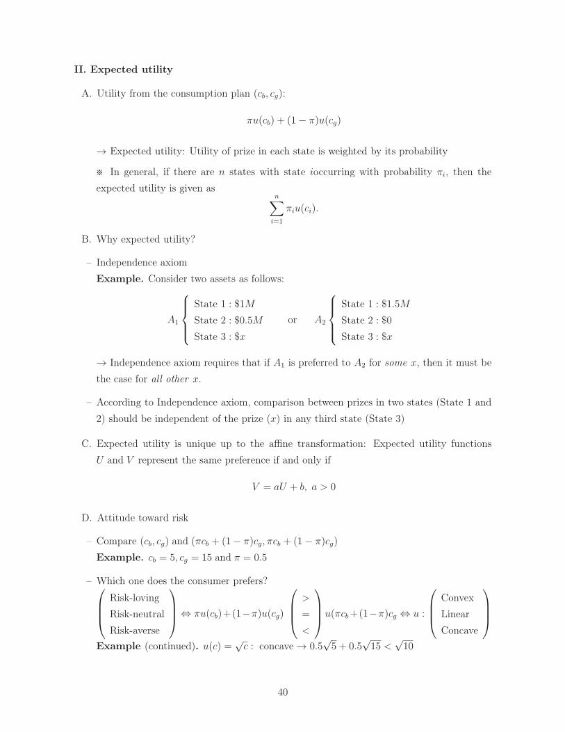
II. Expected utility
A. Utility from the consumption plan (cb, cg):
πu(cb) + (1− π)u(cg)
→ Expected utility: Utility of prize in each state is weighted by its probability
※ In general, if there are n states with state ioccurring with probability πi, then the
expected utility is given asn∑
i=1
πiu(ci).
B. Why expected utility?
– Independence axiom
Example. Consider two assets as follows:
A1
State 1 : $1M
State 2 : $0.5M
State 3 : $x
or A2
State 1 : $1.5M
State 2 : $0
State 3 : $x
→ Independence axiom requires that if A1 is preferred to A2 for some x, then it must be
the case for all other x.
– According to Independence axiom, comparison between prizes in two states (State 1 and
2) should be independent of the prize (x) in any third state (State 3)
C. Expected utility is unique up to the affine transformation: Expected utility functions
U and V represent the same preference if and only if
V = aU + b, a > 0
D. Attitude toward risk
– Compare (cb, cg) and (πcb + (1− π)cg, πcb + (1− π)cg)
Example. cb = 5, cg = 15 and π = 0.5
– Which one does the consumer prefers?
Risk-loving
Risk-neutral
Risk-averse
⇔ πu(cb)+(1−π)u(cg)
>
=
<
u(πcb+(1−π)cg ⇔ u :
Convex
Linear
Concave
Example (continued). u(c) =√c : concave→ 0.5
√5 + 0.5
√15 <
√10
40
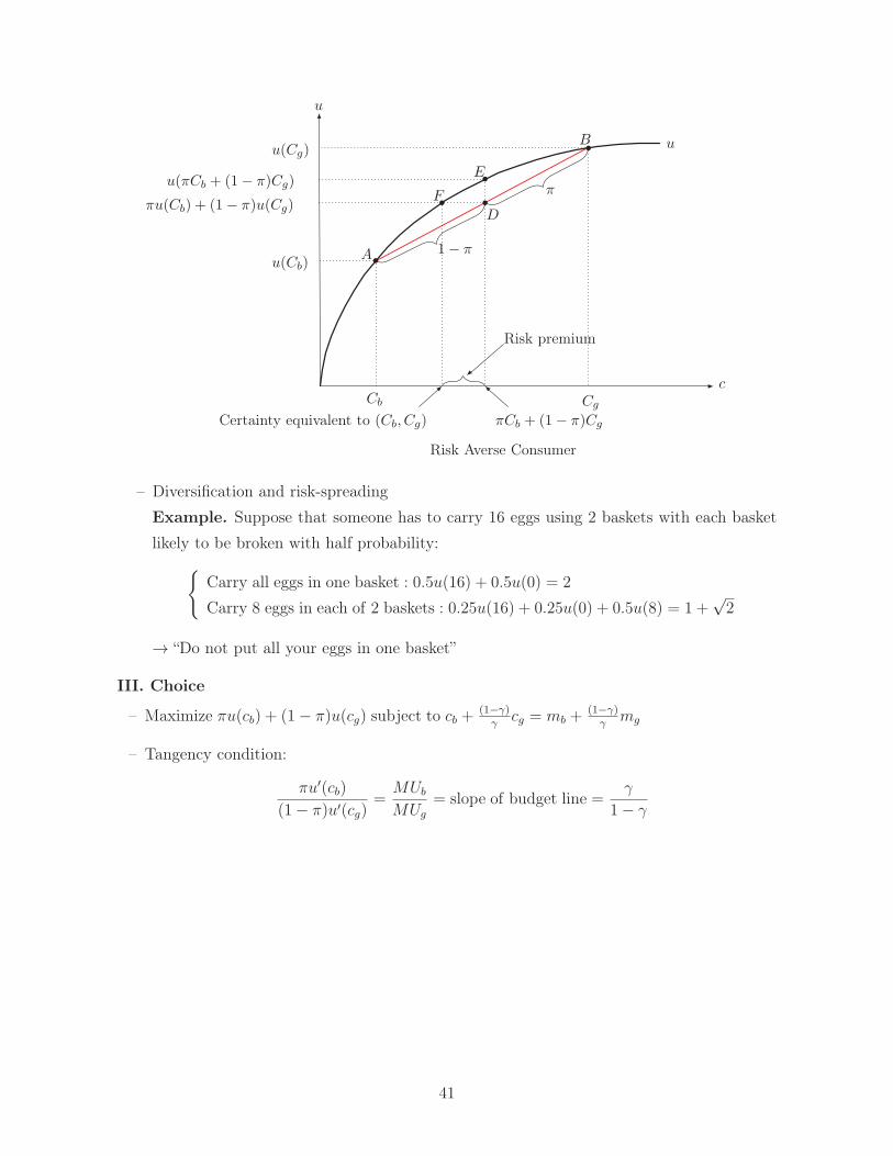
u
Cb Cg
πu(Cb) + (1− π)u(Cg)
u(πCb + (1− π)Cg)
u(Cg)
u(Cb)
u
c
A 1− π
π
B
D
E
Certainty equivalent to (Cb, Cg) πCb + (1− π)Cg
F
Risk premium
Risk Averse Consumer
– Diversification and risk-spreading
Example. Suppose that someone has to carry 16 eggs using 2 baskets with each basket
likely to be broken with half probability:
{
Carry all eggs in one basket : 0.5u(16) + 0.5u(0) = 2
Carry 8 eggs in each of 2 baskets : 0.25u(16) + 0.25u(0) + 0.5u(8) = 1 +√2
→ “Do not put all your eggs in one basket”
III. Choice
– Maximize πu(cb) + (1− π)u(cg) subject to cb +(1−γ)
γcg = mb +
(1−γ)γ
mg
– Tangency condition:
πu′(cb)
(1− π)u′(cg)=
MUb
MUg
= slope of budget line =γ
1− γ
41
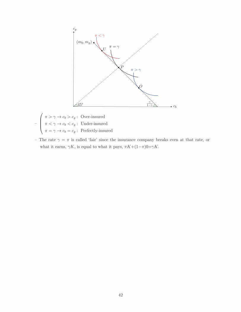
π < γ
π = γ
π > γ
cg
cb
(mb,mg)
P
U
O
γ1−γ45◦
–
π > γ → cb > cg : Over-insured
π < γ → cb < cg : Under-insured
π = γ → cb = cg : Perfectly-insured
– The rate γ = π is called ‘fair’ since the insurance company breaks even at that rate, or
what it earns, γK, is equal to what it pays, πK+(1−π)0=γK.
42

Ch. 14. Consumer Surplus
I. Measuring the change in consumer welfare
A. Let ∆CS ≡ change in the consumer surplus due to the price change p1 → p′1 > p1
– This is a popular method to measure the change in consumer welfare
– The idea underlying this method is that the demand curves measures the consumer’s
willingness to pay.
B. This works perfectly in case of the quasi linear utility: u(x1, x2) = v(x1) + x2
– Letting p2 = 1 and assuming a tangent solution,
v′(x1) = MRS = p1 ⇒ x1(p1) : demand function
– So the demand curve gives a correct measure of the consumer’s WTP and thus ∆CS
measures the change in the consumer welfare due to the price change.
– To verify, let x1 ≡ x1(p1) and x′1 = x1(p′1),
∆CS = (p′1 − p1)x′1 +
∫ x1
x′
1
[v′(s)− p1]ds
= (p′1 − p1)x′1 + v(x1)− v(x′1)− p1(x1 − x′1)
= [v(x1) +m− p1x1]− [v(x′1) +m− p′1x′]
– However, this only works with the quasi linear utility.
C. Compensating and equivalent variation (CV and EV)
– Idea: How much income would be needed to achieve a given level utility for consumer
under difference prices?
43

– Let
{
po ≡ (p1, 1), xo ≡ x(po,m), and uo ≡ u(xo)
pn ≡ (p′1, 1), xn ≡ x(pn,m), and un ≡ u(xn)
– Calculate m′ = income needed to attain uo under pn, that is uo = u(x(po,m′))
→ define CV ≡ |m − m′| and say that consumer becomes worse(better) off as much as
CV if m < (>)m′.
– Calculate m′′ = income needed to attain un under po, that is un = u(x(po,m′′))
→ define EV ≡ |m −m′′| and say that consumer becomes worse(better) off as much as
EV if m > (<)m′′.
p1p′1
m
m′
p2 = 1
p1 → p′1 > p1
x2
x1
xoxn
xCV
CV
m
m′′
p2 = 1
p1 → p′1 > p1
x2
x1
xoxn
p′1 p1
xEV
EV
Example.
{
po = (1, 1)
pn = (2, 1), m = 100, u(x1, x2) = x
1/21 x
1/22 →
{
u0= u(50, 50) = 50
un = u(50, 25) = 25√2
(i) pn = (2, 1)&m′ → (m′
4, m
′
2), u(m
′
4, m
′
2) = m′
2√2= 50, so m′ ≈ 141
(ii) po = (1, 1)&m′′ → (m′′
2, m
′′
2), u(m
′′
2, m
′′
2) = m′′
2= 25
√2, so m′′ ≈ 70
44
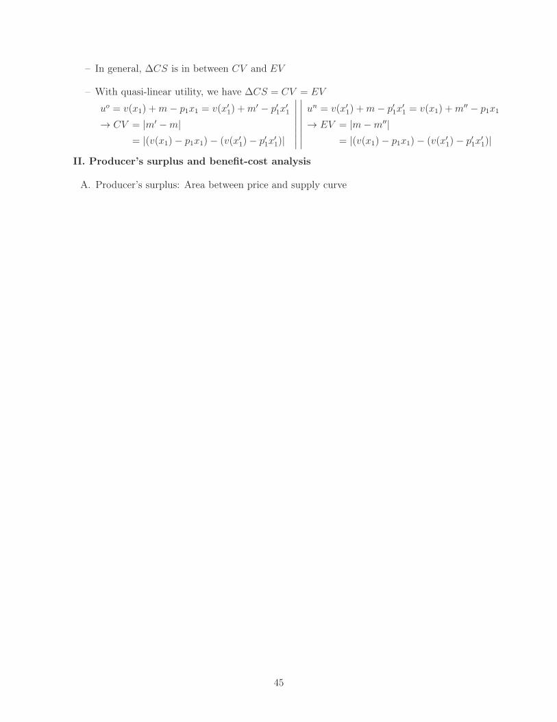
– In general, ∆CS is in between CV and EV
– With quasi-linear utility, we have ∆CS = CV = EV
uo = v(x1) +m− p1x1 = v(x′1) +m′ − p′1x′1
→ CV = |m′ −m|= |(v(x1)− p1x1)− (v(x′1)− p′1x
′1)|
∣∣∣∣∣∣∣∣
∣∣∣∣∣∣∣∣
un = v(x′1) +m− p′1x′1 = v(x1) +m′′ − p1x1
→ EV = |m−m′′|= |(v(x1)− p1x1)− (v(x′1)− p′1x
′1)|
II. Producer’s surplus and benefit-cost analysis
A. Producer’s surplus: Area between price and supply curve
45
Ch. 15. Market Demand
I. Individual and market demand
– n consumers in the market
– Consumer i’s demand for good k: xik(p,mi)
– Market demand for good k: Dk(p,m1, · · · ,mn) =∑n
i=1 xik(p,mi)
Example. Suppose that there are 2 goods and 2 consumers who have demand for good 1
as follows: With p2,m1, and, m2 being fixed,
x11(p1) = max{20− p1, 0} and x2
1(p1) = max{10− 2p1, 0}
II. Demand elasticity
A. Elasticity (ε): Measures a responsiveness of one variable y to another variable x
ε =∆y/y
∆x/x=
% change of y variable
% change of x variable
B. Demand elasticity: εp = −∆D(p)/D(p)∆p/p
= −∆D(p)∆p
pD(p)
, where ∆D(p) = D(p+∆p)−D(p)
– As ∆p→ 0, we have εp = −dD(p)dp
pD(p)
= −pD′(p)D(p)
, (point elasticity)
Example. Let D(p) = Ap−b, where A, b > 0 → εp = b or constant
C. Demand elasticity and marginal revenue:
– Revenue: R = D(p)p = D−1(q)q, where q = D(p)
– Marginal revenue: Rate of change in revenue from selling an extra unit of output
46
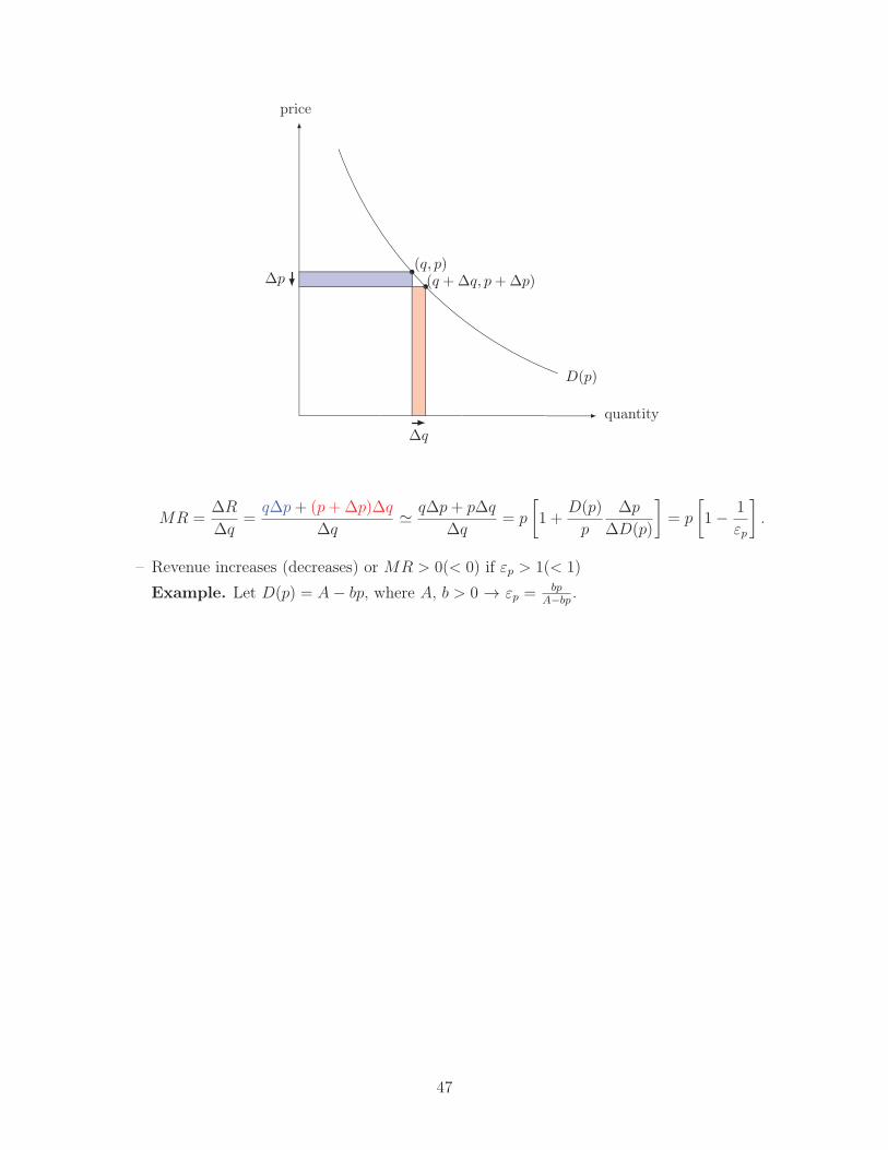
D(p)
price
quantity
(q, p)(q +∆q, p+∆p)∆p
∆q
MR =∆R
∆q=
q∆p+ (p+∆p)∆q
∆q≃ q∆p+ p∆q
∆q= p
[
1 +D(p)
p
∆p
∆D(p)
]
= p
[
1− 1
εp
]
.
– Revenue increases (decreases) or MR > 0(< 0) if εp > 1(< 1)
Example. Let D(p) = A− bp, where A, b > 0 → εp =bp
A−bp .
47
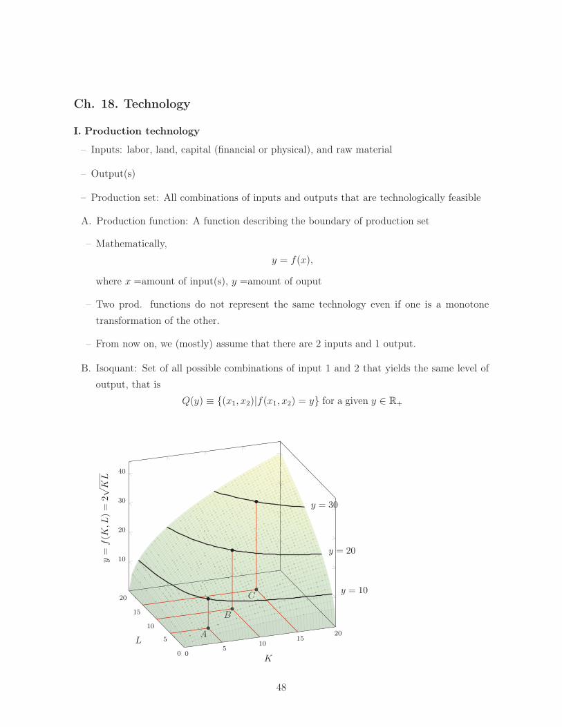
Ch. 18. Technology
I. Production technology
– Inputs: labor, land, capital (financial or physical), and raw material
– Output(s)
– Production set: All combinations of inputs and outputs that are technologically feasible
A. Production function: A function describing the boundary of production set
– Mathematically,
y = f(x),
where x =amount of input(s), y =amount of ouput
– Two prod. functions do not represent the same technology even if one is a monotone
transformation of the other.
– From now on, we (mostly) assume that there are 2 inputs and 1 output.
B. Isoquant: Set of all possible combinations of input 1 and 2 that yields the same level of
output, that is
Q(y) ≡ {(x1, x2)|f(x1, x2) = y} for a given y ∈ R+
05
1015
20
0
5
10
15
20
10
20
30
40
A
B
CCCCCCCCCCCCCCCCCCCCCCCCCCCCCCCCCCCCCCCCCCCCCCCCCCCCCCCCCCCCCCCCCCCCCCCCCCCCCCCCCC
BBBBBBBBBBBBBBBBBBBBBBBBBBBBBBBBBBBBBBBBBBBBBBBBBBBBBBBBBBBBBBBBBBBBBBBBBBBBBBBBBBBBBBBBB
AAAAAAAAAAAAAAAAAAAAAAAAAAAAAAAAAAAAAAAAAAAAAAAAAAAAAAAAAAAAAAAAAAAAAAAAAAAAA
K
L
y=
f(K
,L)=
2√KL
y = 10
y = 20
y = 30
48
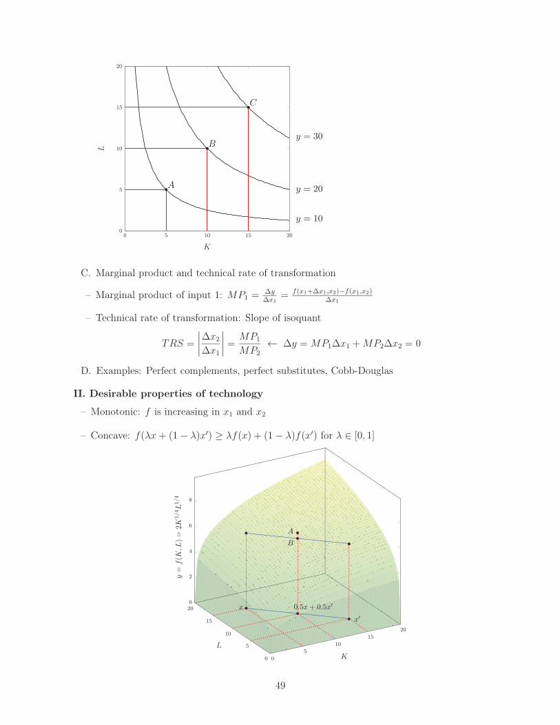
0 5 10 15 200
5
10
15
20
K
L
y = 20
y = 10
y = 30
A
B
C
C. Marginal product and technical rate of transformation
– Marginal product of input 1: MP1 =∆y∆x1
= f(x1+∆x1,x2)−f(x1,x2)∆x1
– Technical rate of transformation: Slope of isoquant
TRS =
∣∣∣∣
∆x2
∆x1
∣∣∣∣=
MP1
MP2
← ∆y = MP1∆x1 +MP2∆x2 = 0
D. Examples: Perfect complements, perfect substitutes, Cobb-Douglas
II. Desirable properties of technology
– Monotonic: f is increasing in x1 and x2
– Concave: f(λx+ (1− λ)x′) ≥ λf(x) + (1− λ)f(x′) for λ ∈ [0, 1]
0
5
10
15
20
0
5
10
15
200
2
4
6
8
A
B
x
x′0.5x+ 0.5x′
K
L
y=
f(K
,L)=
2K1/4L1/4
49
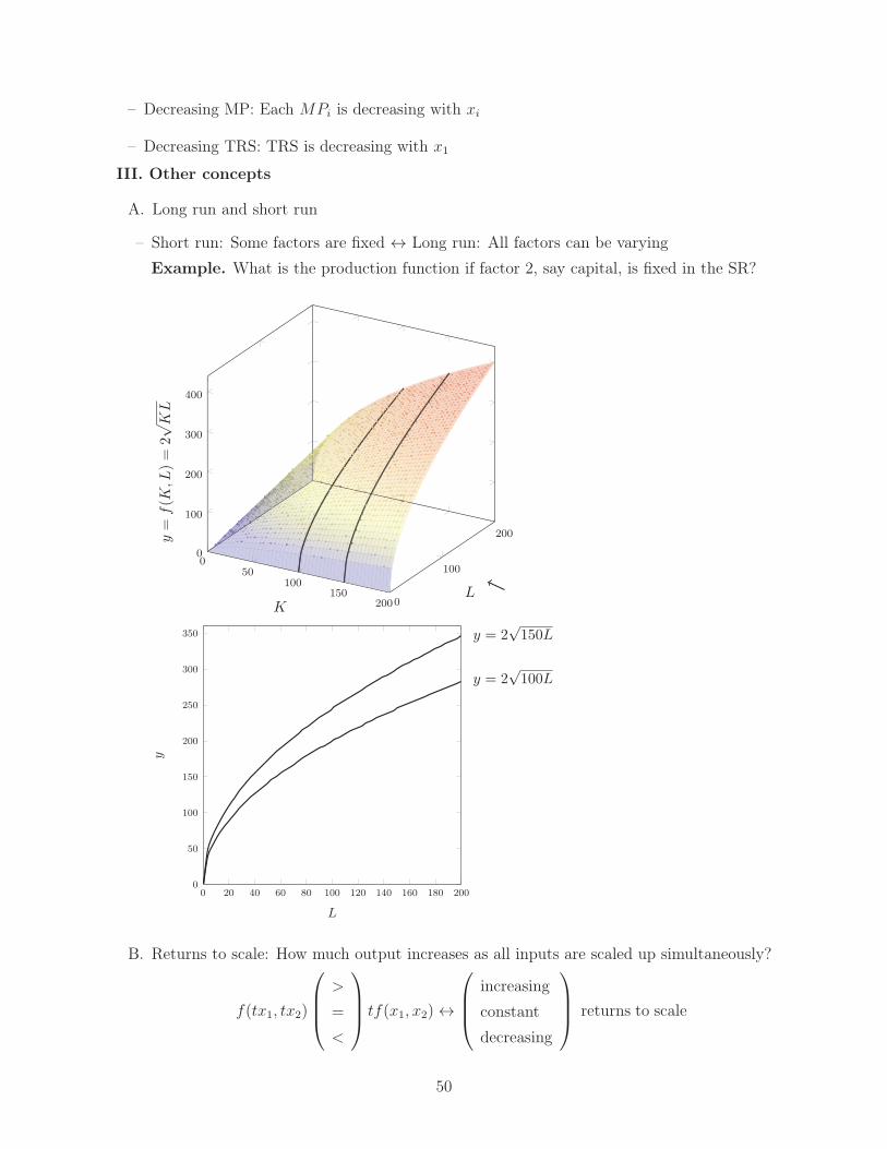
– Decreasing MP: Each MPi is decreasing with xi
– Decreasing TRS: TRS is decreasing with x1
III. Other concepts
A. Long run and short run
– Short run: Some factors are fixed ↔ Long run: All factors can be varying
Example. What is the production function if factor 2, say capital, is fixed in the SR?
050
100150
2000
100
200
0
100
200
300
400
KL
y=
f(K
,L)=
2√KL
0 20 40 60 80 100 120 140 160 180 2000
50
100
150
200
250
300
350
L
y
y = 2√100L
y = 2√150L
B. Returns to scale: How much output increases as all inputs are scaled up simultaneously?
f(tx1, tx2)
>
=
<
tf(x1, x2)↔
increasing
constant
decreasing
returns to scale
50

Example.
IRS : f(x) = x1x2
CRS : f(x) = min{x1, x2}DRS : f(x) =
√x1 + x2
What about f(x) = Kxa1x
b2?
51
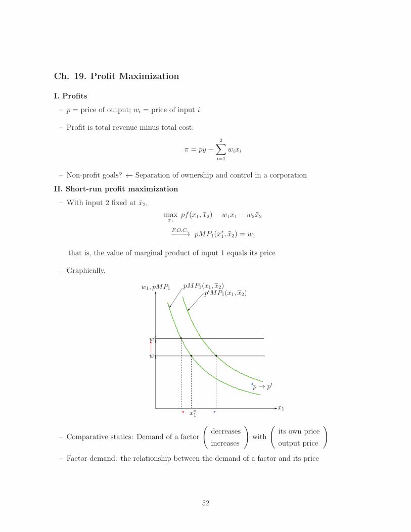
Ch. 19. Profit Maximization
I. Profits
– p = price of output; wi = price of input i
– Profit is total revenue minus total cost:
π = py −2∑
i=1
wixi
– Non-profit goals? ← Separation of ownership and control in a corporation
II. Short-run profit maximization
– With input 2 fixed at x2,
maxx1
pf(x1, x2)− w1x1 − w2x2
F.O.C.−−−−→ pMP1(x
∗1, x2) = w1
that is, the value of marginal product of input 1 equals its price
– Graphically,
pMP1(x1, x2)p′MP1(x1, x2)
w1
w′1
p→ p′
x∗1
w1, pMP1
x1
– Comparative statics: Demand of a factor
(
decreases
increases
)
with
(
its own price
output price
)
– Factor demand: the relationship between the demand of a factor and its price
52

III. Long-run profit maximization
– All inputs are variable
maxx1,x2
pf(x1, x2)− w1x1 − w2x2
F.O.C.−−−−→
{
pMP1(x∗1, x
∗2) = w1
pMP2(x∗1, x
∗2) = w2
– Comparative statics: (y, x1, x2) chosen under (p, w1, w2)→ (y′, x′1, x′2) chosen under (p
′, w′1, w′2)
1) Profit maximization requires
py − w1x1 − w2x2≥ py′ − w1x′1 − w2x
′2
+ p′y′ − w′1x′1 − w′2x
′2≥ p′y − w′1x1 − w′2x2
(p′ − p)(y′ − y)− (w′1 − w1)(x′1 − x2)− (w′2 − w2)(x
′2 − x2) ≥ 0
→ ∆p∆y −∆w1∆x1 −∆w2∆x2 ≥ 0
2) ∆w1 = ∆w2 = 0 → ∆p∆y ≥ 0, or the supply of output increases with its price
3) ∆p = ∆w2 = 0 → ∆w1∆x1 ≤ 0, or the demand of input decreases with its price
53

Ch. 20. Cost Minimization
I. Cost minimization: Minimize the cost of producing a given level of output y
minx1,x2
w1x1 + w2x2 subject to (x1, x2) ∈ Q(y) (i.e. f(x1, x2) = y)
A. Tangent solution: Consider iso-cost line for each cost level C, w1x1+w2x2 = C ; and find
the lowest iso-cost line that meets the isoquant curve
w1
w2
w1
w2
w1
w2
y = f(x1, x2)
costdecreases
x1(w, y)
x2(w, y)
x2
x1
→ TRS = MP1
MP2= w1
w2
→
{
x1(w, y), x2(w, y) : Conditional factor demand function
c(w, y) = w1x1(w, y) + w2x2(w, y) : Cost function
B. Examples
– Perfect complement: y = min{x1, x2}
→ x1(w, y) = x2(w, y) = y
c(w, y) = w1x1(w, y) + w2x2(w, y) = (w1 + w2)y
– Perfect substitutes: y = x1 + x2
→ x(w, y) =
{
(y, 0) if w1 < w2
(0, y) if w2 < w1
c(w, y) = min{w1, w2}y
– Cobb-Douglas: y = Axa1x
b2 →
{
TRS = ax2
bx1= w1
w2
y = Axa1x
b2
→ c(w, y) = Kwa
a+b
1 wb
a+b
2 y1
a+b , where K is a constant depending on a, b, and A
54

II. Comparative statics: (x1, x2) under (w1, w2, y)→ (x′1, x′2) under (w
′1, w
′2, y)
– Cost minimization requires: Letting ∆x1 ≡ x′1 − x1 and so on,
w1x′1 + w2x
′2≥w1x1 + w2x2
+ w′1x1 + w′2x2≥w′1x′1 + w′2x
′2
−(w′1 − w1)(x′1 − x2)− (w′2 − w2)(x
′2 − x2) ≥ 0 → ∆w1∆x1 +∆w2∆x2 ≤ 0
– Setting ∆w2 = 0, we obtain ∆w1∆x1 ≤ 0, or the conditional demand of an input falls as
its price rises
III. Average cost and returns to scale
– Average cost: AC(y) =c(w1, w2, y)
y, that is per-unit-cost to produce y units of output
– Assuming DRS technology, consider two output levels y0 and y1 = ty0 with t > 1: For any
x ∈ Q(y1),
tf(x
t
)
> f(
tx
t
)
or f(x
t
)
>f(x)
t=
y1
t= y0,
which implies
c(w, y0) < w1x1
t+ w2
x2
t=
1
t( w1x1 + w2x2 ) for all x ∈ Q(y1) .
So
c(w, y0) <1
tc(w, y1) =
y0
y1c(w, y1) or
AC(y0) =c(w, y0)
y0<
c(w, y1)
y1= AC(y1)
– Applying a similar argument to IRS or CRS technology, we obtain
DRS : AC(y) is increasing
IRS : AC(y) is decreasing
CRS : AC(y) is constant → AC(y) = c(w1, w2) or c(w, y) = c(w1, w2)y
IV. Long run and short run cost
– Suppose that input 2 is fixed at x2 in the SR
A. Short run demand and cost
– SR demand: xs1(w, y, x2) satisfying f(xs
1(w, y, x2), x2) = y
– SR cost: cs(w, y, x2) = w1xs1(w, y, x2) + w2x2
55

– Envelope property: c(w, y) = cs(w, y, x2(w, y)) = minx2
cs(w, y, x2) ≤ cs(w, y, x2)
x1
x2
LR expansion path
x2(w, y) SR expansion
path
xs1(w, y, x2)
x2
xs1(w, y, x′2)
x′2
B
A
C
D E
y′′
y′y
cs(w, y, x2(w, y))
A′D′ B′
C ′
E′
B′
y′ y′′y
c(w, y)
c
y
c
y
Example. f(x) = x1x2
→ xs1 =
yx2
and cs = w1xs1 + w2x2 = w1
yx2
+ w2x2
→ c(w, y) = minx2
w1yx2
+ w2x2
56
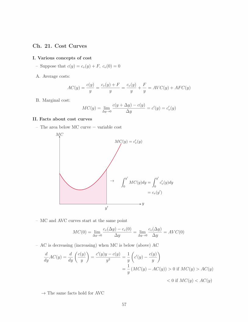
Ch. 21. Cost Curves
I. Various concepts of cost
– Suppose that c(y) = cv(y) + F, cv(0) = 0
A. Average costs:
AC(y) =c(y)
y=
cv(y) + F
y=
cv(y)
y+
F
y= AV C(y) + AFC(y)
B. Marginal cost:
MC(y) = lim∆y→0
c(y +∆y)− c(y)
∆y= c′(y) = c′v(y)
II. Facts about cost curves
– The area below MC curve = variable cost
MC
y
MC(y) = c′v(y)
∫ y′
0MC(y)dy =
∫ y′
0c′v(y)dy
= cv(y′)
→
y′
– MC and AVC curves start at the same point
MC(0) = lim∆y→0
cv(∆y)− cv(0)
∆y= lim
∆y→0
cv(∆y)
∆y= AV C(0)
– AC is decreasing (increasing) when MC is below (above) AC
d
dyAC(y) =
d
dy
(c(y)
y
)
=c′(y)y − c(y)
y2=
1
y
(
c′(y)−c(y)
y
)
=1
y(MC(y)− AC(y)) > 0 if MC(y) > AC(y)
< 0 if MC(y) < AC(y)
→ The same facts hold for AVC
57

– As a result, we have
y
MC,AC,AVC
MC(y)AC(y)
AV C(y)
– Example: c(y) = 13y3 − y2 + 2y + 1
→
MC(y) = y2 − 2y + 2
AV C(y) = 13y2 − y + 2
AC(y) = 13y2 − y + 2 + 1
y
58
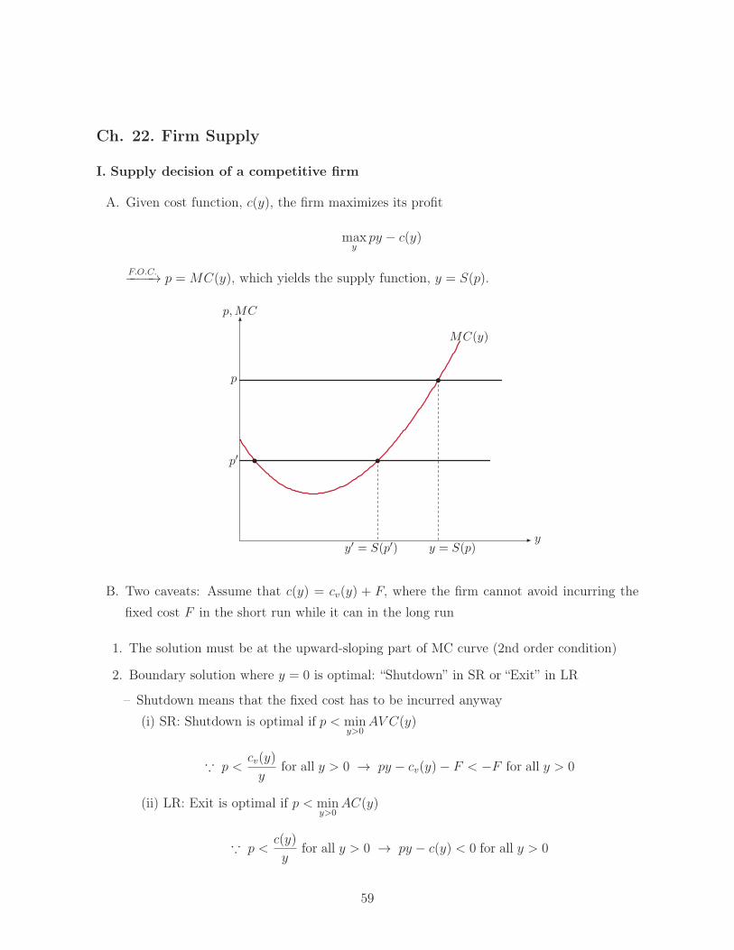
Ch. 22. Firm Supply
I. Supply decision of a competitive firm
A. Given cost function, c(y), the firm maximizes its profit
maxy
py − c(y)
F.O.C.−−−−→ p = MC(y), which yields the supply function, y = S(p).
p′
p
y = S(p)y′ = S(p′)
p,MC
y
MC(y)
B. Two caveats: Assume that c(y) = cv(y) + F, where the firm cannot avoid incurring the
fixed cost F in the short run while it can in the long run
1. The solution must be at the upward-sloping part of MC curve (2nd order condition)
2. Boundary solution where y = 0 is optimal: “Shutdown” in SR or “Exit” in LR
– Shutdown means that the fixed cost has to be incurred anyway
(i) SR: Shutdown is optimal if p < miny>0
AV C(y)
∵ p <cv(y)
yfor all y > 0 → py − cv(y)− F < −F for all y > 0
(ii) LR: Exit is optimal if p < miny>0
AC(y)
∵ p <c(y)
yfor all y > 0 → py − c(y) < 0 for all y > 0
59

3. Supply curves
y
MC(y)AC(y)
AV C(y)
shutdown in SR
exit in LR
– PS: Accumulation of extra revenue minus extra cost from producing extra unit of output
or
PS =
∫ y∗
0
(p−MC(y))dy = py∗ −
∫ y∗
0
MC(y)dy = py∗ − cv(y∗)
– Thus,
Profit = py∗ − c(y∗) = py∗ − cv(y∗)− F = PS− F
– Graphically,
p
y∗y
p
MC(y)
AV C(y)
y′
Dotted area (=producer’s surplus)
= Red area (=area b/w supply curve and price)
∵ Gray area (= y′ × AV C(y′))
= Stroked area (= cv(y′))
C. Long-run and short-run firm supply
60

– Assume more generally that the SR cost is given as cs(w, y, x2) and the LR cost as c(w, y).
– The envelope property implies that the marginal cost curve is steeper in the LR than in
the SR → The firm supply responds more sensitively to the price change in the LR than
in the SR.
cs(w, y, x2)
c(w, y)
c
y
c
y
MC
y
SR MC
LR MC
SR response
LR response
p
p′
p
61

Ch. 23. Industry Supply
I. Short run industry supply
– Let Si(p) denote firm i’s supply at price p. Then, the industry supply is given as
S(p) =n∑
i=1
Si(p).
→ Horizontal sum of individual firms’ supply curves
II. Long run industry supply
– Due to free entry,
{
profit → entry of firms → lower price → profit disappears
loss → exit of firms → higher price → loss disappears
D′
D′′
D′′′
D′′′′
y∗ 2y∗ 3y∗ 4y∗ y∗
p
y
S1 S2
S3
S4
MC
AC
y
p
E1
E2
E3
D
→ LR supply curve is (almost) horizontal
– LR equilibrium quantity y∗ must satisfy MC(y∗) = p = AC(y∗)
– # of firms in the LR depends on the demand side
III. Fixed factors and economic rent
– No free entry due to limited resources (e.g. oil) or legal restrictions (e.g. taxicab license)
– Consider a coffee shop at downtown, earning positive profits even in the LR.
→ py∗ − c(y∗) ≡ F > 0, which is the amount people would pay to rent the shop.
→ Economic profit is 0 since F is the economic rent (or opportunity cost)
IV. Application
62

A. Effects of quantity tax in SR and LR
L
yLySy′L
t
pL + t
pL
firms exit in LR
B. Two-tier oil pricing
– Oil crisis in 70’s: Price control on domestic oil
→{
domestic oil at $5/barell : MC1(y)
imported oil at $15/barell : MC2(y) = MC1(y) + 10
– y = the maximum amount of gasoline that can be produced using the domestic oil
– Due to the limited amount of domestic oil, the LR supply curve shifts up from MC1(y)
to MC2(y) as y exceeds y
63

Ch. 24. Monopoly
– A single firm in the market
– Set the price (or quantity) to maximize its profit
I. Profit maximization
A. Given demand and cost function, p(y) and c(y), the monopolist solves
maxy
p(y)y − c(y) = r(y)− c(y), where r(y) ≡ p(y)y
F.O.C.−−−−→ MR(y∗) = r′(y∗) = c′(y∗) = MC(y∗)
⇔ p(y∗) + yp′(y∗) = c′(y∗)
⇔ p(y∗)[
1 + dpdy
y∗
p(y∗)
]
= c′(y∗)
⇔ p(y∗)[
1− 1ε(y∗)
]
= c′(y∗) > 0
So, ε(y∗) > 1, that is monopoly operates where the demand is elastic.
B. Mark-up pricing:
p(y∗) =MC(y∗)
1− 1/ε(y∗)> MC(y∗), where 1− 1/ε(y∗) : mark-up rate
C. Linear demand example: p = a− by →MR(y) = ddy
(ay − 2by2) = a− 2by
MC
Deadweight loss
p
yyc
Surplus from y-th unit
yy∗
p∗
MR Demand
64
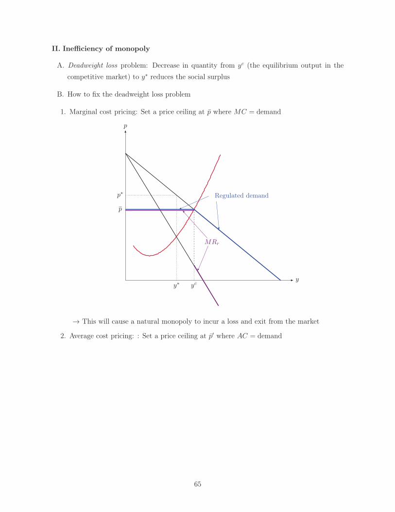
II. Inefficiency of monopoly
A. Deadweight loss problem: Decrease in quantity from yc (the equilibrium output in the
competitive market) to y∗ reduces the social surplus
B. How to fix the deadweight loss problem
1. Marginal cost pricing: Set a price ceiling at p where MC = demand
MRr
Regulated demand
p
yycy∗
p∗
p
→ This will cause a natural monopoly to incur a loss and exit from the market
2. Average cost pricing: : Set a price ceiling at p′ where AC = demand
65
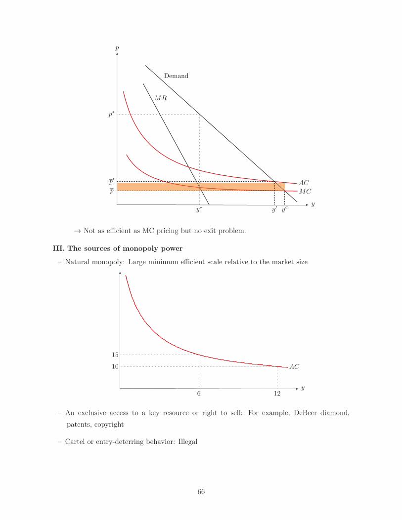
p
yy∗
p∗
p
p′
ycy′
MR
Demand
AC
MC
→ Not as efficient as MC pricing but no exit problem.
III. The sources of monopoly power
– Natural monopoly: Large minimum efficient scale relative to the market size
15
10
6 12y
AC
– An exclusive access to a key resource or right to sell: For example, DeBeer diamond,
patents, copyright
– Cartel or entry-deterring behavior: Illegal
66

Ch. 25. Monopoly Behavior
– So far, we have assumed that the monopolist charges all consumers the same uniform price
for each unit they purchase.
– However, it could charge
{
Different prices to different consumers (e.g. movie tickets)
Different per-unit-prices for different units sold (e.g. bulk discount)
– Assume MC = c(constant) and no fixed cost.
I. First-degree price discrimination (1◦ PD)
– The firm can charge different prices to different consumers and for different units.
– Two types of consumer with the following WTP (or demand)
A
K K
c
y y
WTPWTP
A′
y∗1 y∗2
– Take-it-or-leave offer: Bundle (y∗1, A+K) to type 1; bundle (y∗2, A′ +K ′) to type 2
→ No quantity distortion and no deadweight loss
→ Monopolist gets everything while consumers get nothing
– The same outcome can be achieved via “Two-Part Tariff”: For type 1, for instance, charge
A as an “entry fee” and c as “price per unit”.
II. Second-degree discrimination: Assume c = 0 for simplicity
– Assume that the firm cannot tell who is what type
– Offer a menu of two bundles from which each type can self select
67
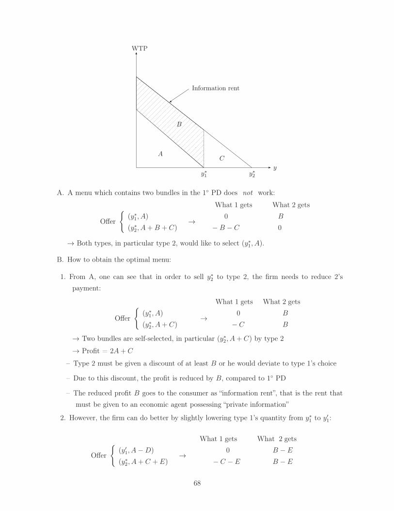
A
B
C
WTP
yy∗1 y∗2
Information rent
A. A menu which contains two bundles in the 1◦ PD does not work:
What 1 gets What 2 gets
Offer
{
(y∗1, A)
(y∗2, A+B + C)→ 0 B
− B − C 0
→ Both types, in particular type 2, would like to select (y∗1, A).
B. How to obtain the optimal menu:
1. From A, one can see that in order to sell y∗2 to type 2, the firm needs to reduce 2’s
payment:
What 1 gets What 2 gets
Offer
{
(y∗1, A)
(y∗2, A+ C)→ 0 B
− C B
→ Two bundles are self-selected, in particular (y∗2, A+ C) by type 2
→ Profit = 2A+ C
– Type 2 must be given a discount of at least B or he would deviate to type 1’s choice
– Due to this discount, the profit is reduced by B, compared to 1◦ PD
– The reduced profit B goes to the consumer as “information rent”, that is the rent that
must be given to an economic agent possessing “private information”
2. However, the firm can do better by slightly lowering type 1’s quantity from y∗1 to y′1:
What 1 gets What 2 gets
Offer
{
(y′1, A−D)
(y∗2, A+ C + E)→ 0 B − E
− C − E B − E
68

A
B
C
WTP
yy∗1 y∗2
E
D
y′1
→ Two bundles are self selected, (y′1, A−D) by 1 and (y∗2, A+ C + E) by 2
→ Profit = 2A+ C + (E −D) > 2A+ C
– Compared to the above menu, the discount (or information rent) for type 2 is reduced
by E, which is a marginal gain that exceeds D, the marginal loss from type 1
3. To obtain the optimal menu, keep reducing 1’s quantity until the marginal loss from 1
equals the marginal gain from 2
Offer
{
(ym1 , Am)
(y∗2, Am + Cm)
69
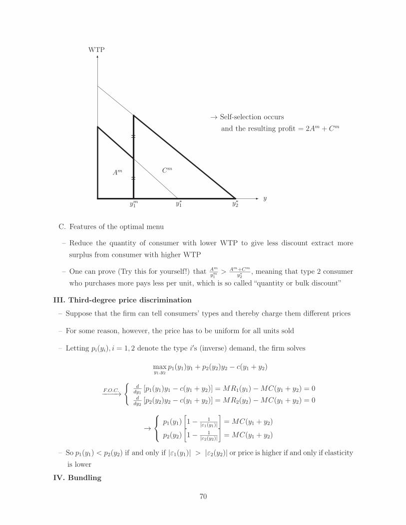
WTP
yy∗1 y∗2
Am Cm
ym1
→ Self-selection occurs
and the resulting profit = 2Am + Cm
C. Features of the optimal menu
– Reduce the quantity of consumer with lower WTP to give less discount extract more
surplus from consumer with higher WTP
– One can prove (Try this for yourself!) that Am
ym1
> Am+Cm
y∗2
, meaning that type 2 consumer
who purchases more pays less per unit, which is so called “quantity or bulk discount”
III. Third-degree price discrimination
– Suppose that the firm can tell consumers’ types and thereby charge them different prices
– For some reason, however, the price has to be uniform for all units sold
– Letting pi(yi), i = 1, 2 denote the type i′s (inverse) demand, the firm solves
maxy1,y2
p1(y1)y1 + p2(y2)y2 − c(y1 + y2)
F.O.C.−−−−→{
ddy1
[p1(y1)y1 − c(y1 + y2)] = MR1(y1)−MC(y1 + y2) = 0d
dy2[p2(y2)y2 − c(y1 + y2)] = MR2(y2)−MC(y1 + y2) = 0
→
p1(y1)[
1− 1|ε1(y1)|
]
= MC(y1 + y2)
p2(y2)[
1− 1|ε2(y2)|
]
= MC(y1 + y2)
– So p1(y1) < p2(y2) if and only if |ε1(y1)| > |ε2(y2)| or price is higher if and only if elasticityis lower
IV. Bundling
70

– Suppose that there are two consumer, A and B, with the following willingness-to-pay:
Type of consumer WTP
Word Excel
A 100 60
B 60 100
→ Maximum profit from selling separately=240
→ Maximum profit from selling in a bundle=320
– Bundling is good when values for two goods are negatively correlated
V. Monopolistic competition
– Monopoly + competition: Goods that are not identical but similar
→ Downward-sloping demand curve + free entry
– The demand curve will shift in until each firm’s maximized profit gets equal to 0
71
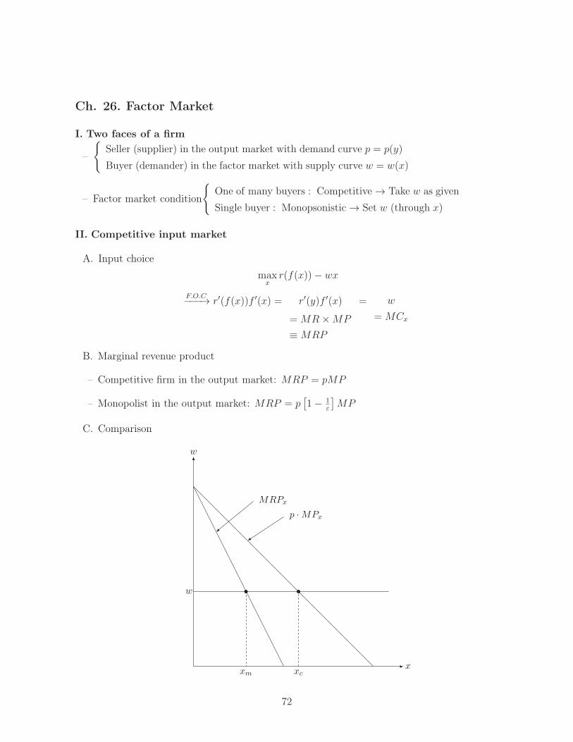
Ch. 26. Factor Market
I. Two faces of a firm
–
{
Seller (supplier) in the output market with demand curve p = p(y)
Buyer (demander) in the factor market with supply curve w = w(x)
– Factor market condition
{
One of many buyers : Competitive→ Take w as given
Single buyer : Monopsonistic→ Set w (through x)
II. Competitive input market
A. Input choice
maxx
r(f(x))− wx
F.O.C−−−→ r′(f(x))f ′(x) = r′(y)f ′(x)
= MR×MP
≡MRP
= w
= MCx
B. Marginal revenue product
– Competitive firm in the output market: MRP = pMP
– Monopolist in the output market: MRP = p[1− 1
ε
]MP
C. Comparison
w
w
x
MRPx
p ·MPx
xm xc
72
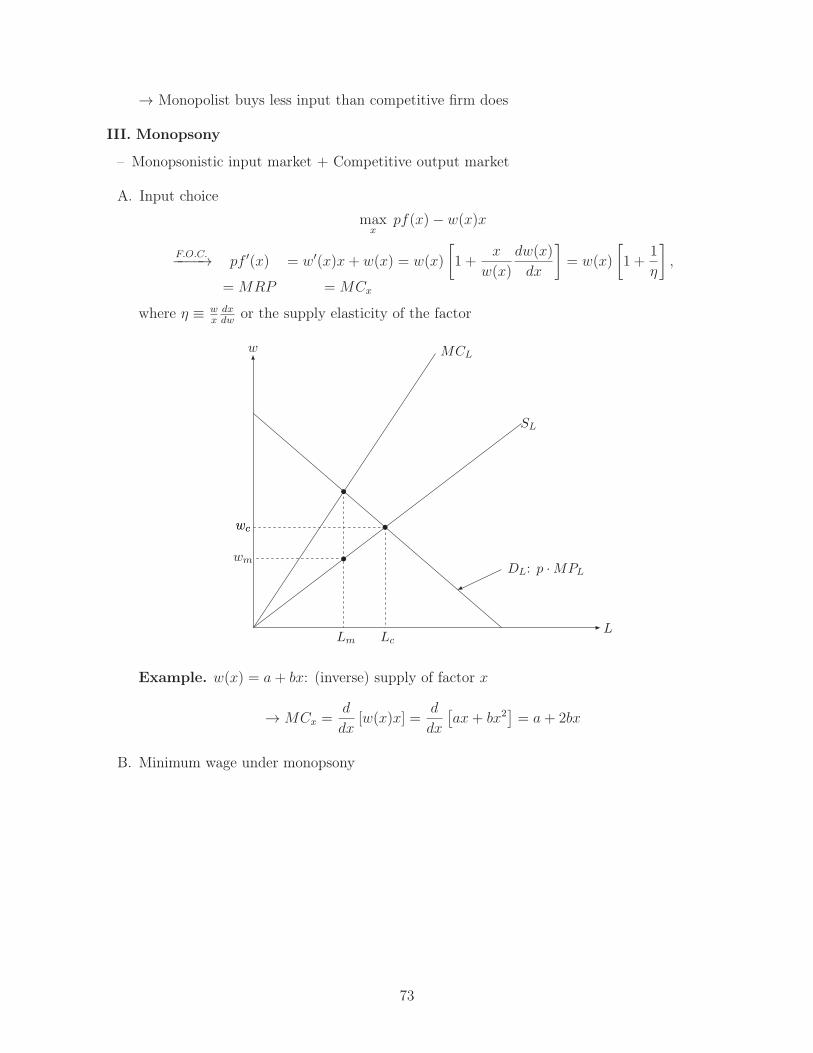
→ Monopolist buys less input than competitive firm does
III. Monopsony
– Monopsonistic input market + Competitive output market
A. Input choice
maxx
pf(x)− w(x)x
F.O.C.−−−−→ pf ′(x)
= MRP
= w′(x)x+ w(x)
= MCx
= w(x)
[
1 +x
w(x)
dw(x)
dx
]
= w(x)
[
1 +1
η
]
,
where η ≡ wx
dxdw
or the supply elasticity of the factor
MCL
SL
Lm Lc
wm
wc
DL: p ·MPL
wc
w
L
Example. w(x) = a+ bx: (inverse) supply of factor x
→MCx =d
dx[w(x)x] =
d
dx
[ax+ bx2
]= a+ 2bx
B. Minimum wage under monopsony
73
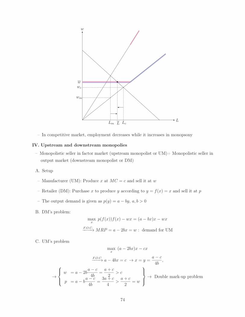
Lm LcL
wm
wc
w
w
L
– In competitive market, employment decreases while it increases in monopsony
IV. Upstream and downstream monopolies
– Monopolistic seller in factor market (upstream monopolist or UM)+ Monopolistic seller in
output market (downstream monopolist or DM)
A. Setup
– Manufacturer (UM): Produce x at MC = c and sell it at w
– Retailer (DM): Purchase x to produce y according to y = f(x) = x and sell it at p
– The output demand is given as p(y) = a− by, a, b > 0
B. DM’s problem:
maxx
p(f(x))f(x)− wx = (a− bx)x− wx
F.O.C.−−−−→MRP = a− 2bx = w : demand for UM
C. UM’s problem
maxx
(a− 2bx)x− cx
F.O.C−−−→ a− 4bx = c → x = y =a− c
4b,
→
w = a− 2ba− c
4b=
a+ c
2> c
p = a− ba− c
4b=
3a+ c
4>
a+ c
2= w
→ Double mark-up problem
74
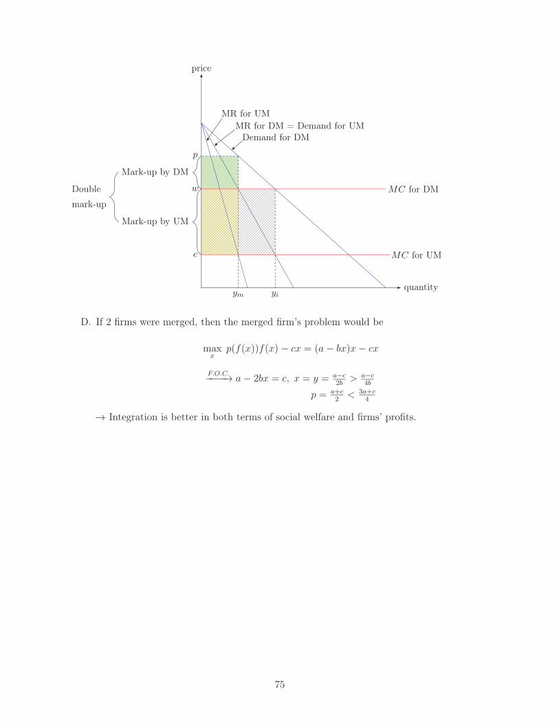
c MC for UM
w MC for DM
p
price
quantityym yi
Demand for DMMR for DM = Demand for UM
MR for UM
Mark-up by DM
Mark-up by UM
Double
mark-up
D. If 2 firms were merged, then the merged firm’s problem would be
maxx
p(f(x))f(x)− cx = (a− bx)x− cx
F.O.C.−−−−→ a− 2bx = c, x = y = a−c2b
> a−c4b
p = a+c2
< 3a+c4
→ Integration is better in both terms of social welfare and firms’ profits.
75
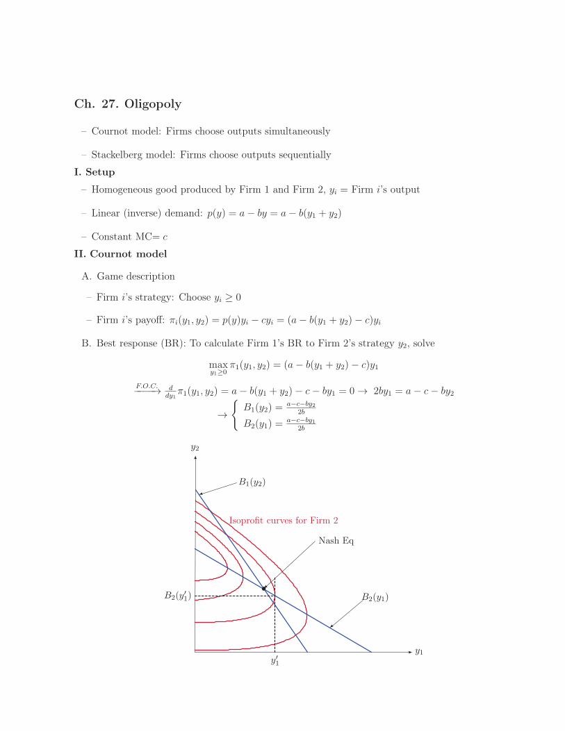
Ch. 27. Oligopoly
– Cournot model: Firms choose outputs simultaneously
– Stackelberg model: Firms choose outputs sequentially
I. Setup
– Homogeneous good produced by Firm 1 and Firm 2, yi = Firm i’s output
– Linear (inverse) demand: p(y) = a− by = a− b(y1 + y2)
– Constant MC= c
II. Cournot model
A. Game description
– Firm i’s strategy: Choose yi ≥ 0
– Firm i’s payoff: πi(y1, y2) = p(y)yi − cyi = (a− b(y1 + y2)− c)yi
B. Best response (BR): To calculate Firm 1’s BR to Firm 2’s strategy y2, solve
maxy1≥0
π1(y1, y2) = (a− b(y1 + y2)− c)y1
F.O.C.−−−−→ ddy1
π1(y1, y2) = a− b(y1 + y2)− c− by1 = 0→ 2by1 = a− c− by2
→{
B1(y2) =a−c−by2
2b
B2(y1) =a−c−by1
2b
y2
y1
Isoprofit curves for Firm 2
B2(y1)
y′1
B2(y′1)
B1(y2)
Nash Eq

C. Nash equilibrium: Letting yci denote i’ equilibrium quantity,
→{
B1(yc2) = yc1
B2(yc1) = yc2
→{
yc1 = yc2 = yc ≡ a−c3b
πc = (a− 2byc − c)yc = (a−c)29b
D. Comparison with monopoly
– Monopolist’s solution:
ym = a−c2b
πm = (a−c)24b
}
→{
ym < 2yc
πm > 2πc
– Collusion with each firm producing ym
2is not sustainable
B2(y1)
B1(y2)
y1 + y2 = ym: Joint profit is maximized
and equal to the monopoly level
ym/2
ym/2
ym
ym
C
D
y2
y1
E. Oligopoly with n firms
– Letting y ≡∑n
i=1 yi, Firm i solves
maxyi
(p(y)− c)yi = (a− b(y1 + · · ·+ yi + · · ·+ yn)− c) yi
F.O.C−−−→ − byi + (a− by − c) = 0.
– Since firms are symmetric, we have y1 = y2 = · · · = yn = yc, with which the F.O.C
becomes
−byc + (a− nbyc − c) = 0
→ yc =a− c
(n+ 1)b, y = nyc =
n
n+ 1
a− c
b→ a− c
bas n→∞
– Note that a−cb
is the competitive quantity. So the total quantity increases toward the
competitive level as there are more and more firms in the market.
77

III. Stackelberg model
A. Game description
– Firm 1 first chooses y1, which Firm 2 observes and then chooses y2
→ Firm 1: (Stackelberg) leader, Firm 2: follower
– Strategy
1) Firm 1: y1
2) Firm 2: r(y1), a function or plan contingent on what Firm 1 has chosen
B. Subgame perfect equilibrium
– Backward induction: Solve first the profit maximization problem of Firm 2
1) Given Firm 1’s choice y1, Firm 2 chooses y2 = r(y1) to solve
maxy2
π2(y1, y2)
F.O.C.−−−−→ r(y1) =a−c−by1
2b, which is the same as B2(y1).
2) Understanding that Firm 2 will respond to y1 with quantity r(y1), Firm 1 will choose y1
to solve
maxy1
π1(y1, r(y1)) = (a− b(y1 + r(y1))− c)y1 =1
2(a− c− by1)y1
F.O.C−−−→ (a− c− by1)− by1 = 0→ ys1 =a− c
2b, ys2 = r(ys1) =
a− c
4b< ys1
B2(y1)
B1(y2)
Isoprofit curves for firm 1
Stackelberg equilibrium
y2
y1
IV. Bertrand model
78

A. Game description
– Two firms compete with each other using price instead quantity
– Whoever sets a lower price takes the entire market (equally divide the market if prices
are equal)
B. Nash equilibrium: p1 = p2 = c is a unique NE where both firm split the market and get
zero profit, whose proof consists of 3 steps:
1. p1 = p2 = c constitutes a Nash equilibrium
– If, for instance, Firm 1 deviates to p1 > c, it continues to earn zero profit
– If Firm 1 deviates to p1 < c, it incurs a loss
– Thus, p1 = c is a Firm 1’s best response to p2 = c
2. There is no Nash equilibrium where min{p1, p2} < c
– At least one firm incurs a loss
3. There is no Nash equilibrium where max{p1, p2} > c
– p1 = p2 > c: Firm 1, for instance, would like to slightly lower the price to take the entire
market rather than a half, though the margin gets slightly smaller
– p1 > p2 > c : Firm 1 would like to cut its price slightly below p2 to take the entire
market and enjoy some positive, instead zero, profit
79
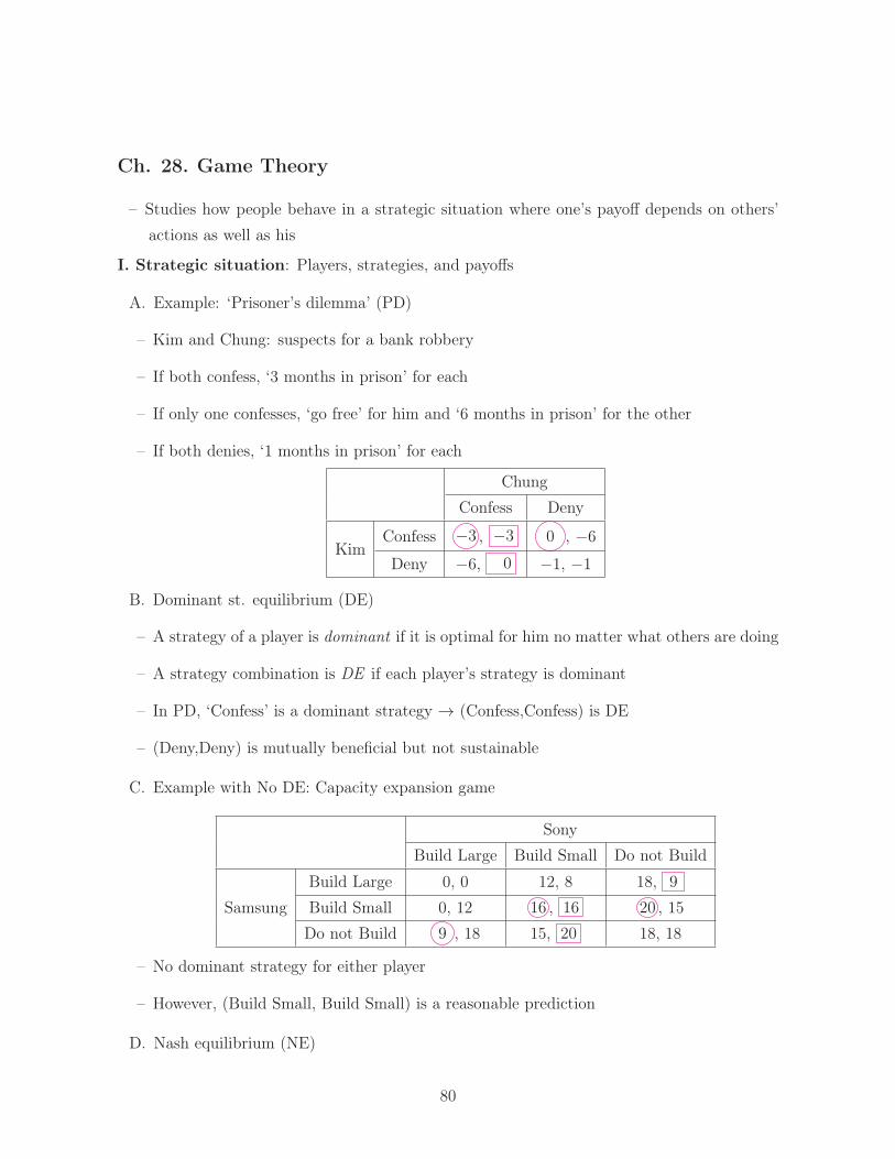
Ch. 28. Game Theory
– Studies how people behave in a strategic situation where one’s payoff depends on others’
actions as well as his
I. Strategic situation: Players, strategies, and payoffs
A. Example: ‘Prisoner’s dilemma’ (PD)
– Kim and Chung: suspects for a bank robbery
– If both confess, ‘3 months in prison’ for each
– If only one confesses, ‘go free’ for him and ‘6 months in prison’ for the other
– If both denies, ‘1 months in prison’ for each
Chung
Confess Deny
KimConfess −3 , −3 0 , −6Deny −6, 0 −1, −1
B. Dominant st. equilibrium (DE)
– A strategy of a player is dominant if it is optimal for him no matter what others are doing
– A strategy combination is DE if each player’s strategy is dominant
– In PD, ‘Confess’ is a dominant strategy → (Confess,Confess) is DE
– (Deny,Deny) is mutually beneficial but not sustainable
C. Example with No DE: Capacity expansion game
Sony
Build Large Build Small Do not Build
Samsung
Build Large 0, 0 12, 8 18, 9
Build Small 0, 12 16 , 16 20 , 15
Do not Build 9 , 18 15, 20 18, 18
– No dominant strategy for either player
– However, (Build Small, Build Small) is a reasonable prediction
D. Nash equilibrium (NE)
80

– A strategy combination is NE if each player’s strategy is optimal given others’ equilibrium
strategies
– In the game of capacity expansion, (Build Small, Build Small) is a NE
– Example with multiple NE: Battle of sexes game
Sheila
K1 Soap Opera
BobK1 2 , 1 0, 0
Soap Opera 0, 0 1 , 2
→ NE: (K1, K1) and (Soap opera, Soap opera)
E. Location game
1. Setup
– Bob and Sheila: 2 vendors on the beach [0, 1]
– Consumers are evenly distributed along the beach
– With price being identical and fixed, vendors choose locations
– Each consumer prefers a shorter walking distance
2. Unique NE: (1/2,1/2)
3. Socially optimal locations: (1/4,3/4)
4. Applications: Product differentiation, majority voting and median voter
5. NE with 3 vendors → no NE!
II. Sequential games
A. Example: A sequential version of battle of sexes
– Bob moves first to choose between ‘K1’ and ‘Soap opera’
– Observing Bob’s choice, Sheila chooses her strategy
B. Game tree
81

Bob
Sheila
(1,2)SO
(0,0)K1
SO
Sheila
(0,0)SO
(2,1)K1
K1
C. Strategies
{
Bob’s strategy: K1, SO
Sheila’s strategy: K1 ·K1, K1 · SO, SO ·K1, SO · SO
Sheila
K1·K1 K1·SO SO·K1 SO·SO
BobK1 2 1 2 1 0 0 0 0
SO 0 0 1 2 0 0 1 2
→ All NE: (K1,K1 ·K1), (SO, SO · SO), and (K1,K1 · SO)
D. All other NE than (K1,K1 · SO) are problematic
– For instance, (SO, SO · SO) involves an incredible threat
– In both (SO, SO · SO)and (K1,K1 ·K1), Sheila is not choosing optimally when Bob (un-
expectedly) chooses a non-equilibrium strategy.
E. Subgame perfect equilibrium (SPE)
– Requires that each player chooses optimally whenever it is his/her turn to move.
– Often, not all NE are SPE: (K1,K1 · SO) is the only SPE in the above game.
– SPE is also called a backward induction equilibrium.
– In sum, not all NE is an SPE while SPE must always be an NE.
F. Another example: Modify the capacity expansion game to let Samsung move first
82

Samsung
Sony
(18,18)Do not build
(15,20)Build small
(9,18)Build large
Do not build
Sony
(20,15)Do not build
(16,16)Build small
(8,12)Build large
Build small
Sony
(18,9)Do not build
(12,8)Build small
(0,0)Build large
Build large
– Unique SPE strategy: Sony chooses
{
Do not build if Samsung chooses Build large
Build small otherwise
}
while Samsung chooses Build large
→ SPE outcome: (Build large,Do not build)
– There exists NE that is not SPE: For instance, Sony chooses ‘always Build small’ while
Samsung chooses ‘Build small’
III. Repeated games: A sequential game where players repeatedly face the same strategic
situation
– Can explain why people can cooperate in games like prisoner’s dilemma
A. Infinite repetition of PD
– Play the same PD every period r
– Tomorrow’s payoff is discounted by discount rate= δ < 1
→ higher δ means that future payoffs are more important
B. Equilibrium strategies sustaining cooperation:
(i) Grim trigger strategy: I will deny as long as you deny while I will confess forever once
you confess
Deny today : − 1 + δ(−1) + δ2(−1) + · · · = −11− δ
Confess today : 0+δ(−3) + δ2(−3) + · · · = −3δ1− δ
83

So if δ > 13, ‘Confess’ is better
(ii) Tit-for-tat strategy: I will deny (confess) tomorrow if you deny (confess) today →Most popular in the lab. experiment by Axerlod
C. Application: enforcing a cartel (airline pricing)
D. Finitely or infinitely repeated?
84

Ch. 30. Exchange
– Partial equilibrium analysis: Study how price and output are determined in a single market,
taking as given the prices in all other markets.
– General equilibrium analysis: Study how price and output are simultaneously determined
in all markets.
I. Exchange Economy
A. Description of the economy
– Two goods, 1 and 2, and two consumers, A and B.
– Initial endowment allocation: (ω1i , ω
2i ) for consumer i = A or B.
– Allocation: (x1i , x
2i ) for consumer i = A or B.
– Utility: ui(x1i , x
2i ) for consumer i = A or B.
B. Edgeworth box
– Allocation is called feasible if the total consumption is equal to the total endowment:
x1A + x1
B = ω1A + ω1
B
x2A + x2
B = ω2A + ω2
B.
- All feasible allocations can be illustrated using Edgeworth box
endowmentpoint
ω1A ω1
B
ω2B
ω2A
OB
OA
85
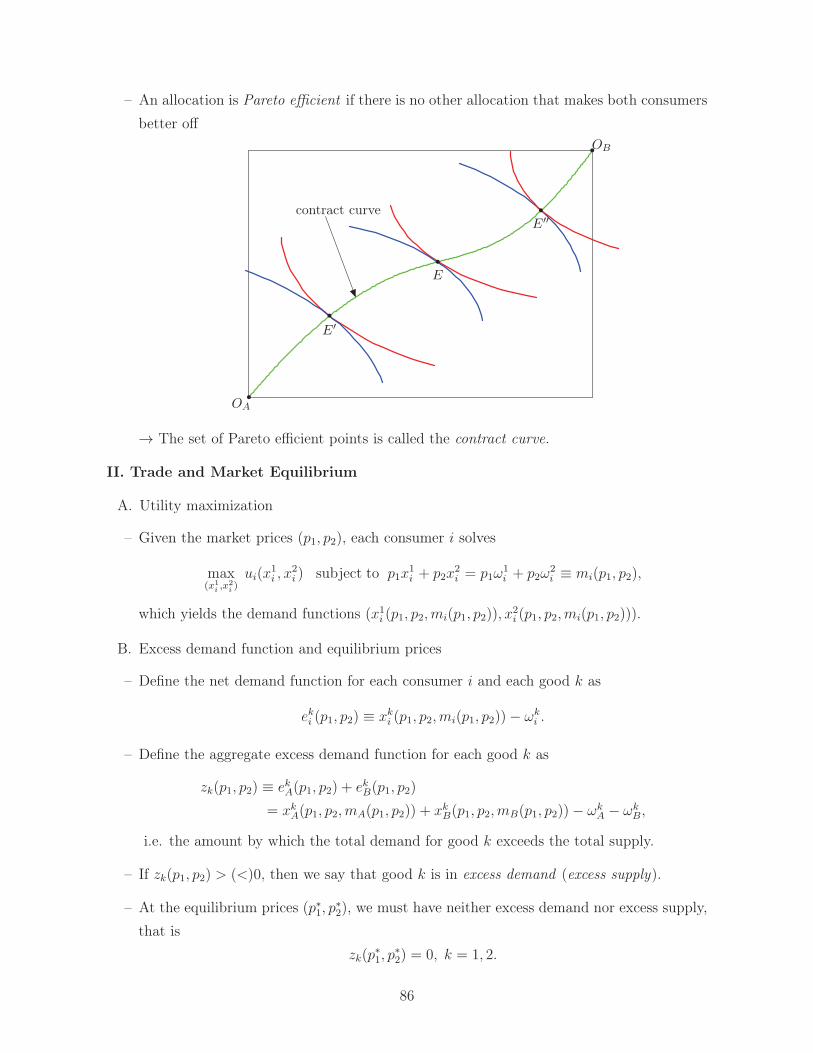
– An allocation is Pareto efficient if there is no other allocation that makes both consumers
better off
contract curve
OA
OB
E′
E
E′′
→ The set of Pareto efficient points is called the contract curve.
II. Trade and Market Equilibrium
A. Utility maximization
– Given the market prices (p1, p2), each consumer i solves
max(x1
i ,x2i )
ui(x1i , x
2i ) subject to p1x
1i + p2x
2i = p1ω
1i + p2ω
2i ≡ mi(p1, p2),
which yields the demand functions (x1i (p1, p2,mi(p1, p2)), x
2i (p1, p2,mi(p1, p2))).
B. Excess demand function and equilibrium prices
– Define the net demand function for each consumer i and each good k as
eki (p1, p2) ≡ xki (p1, p2,mi(p1, p2))− ωk
i .
– Define the aggregate excess demand function for each good k as
zk(p1, p2) ≡ ekA(p1, p2) + ekB(p1, p2)
= xkA(p1, p2,mA(p1, p2)) + xk
B(p1, p2,mB(p1, p2))− ωkA − ωk
B,
i.e. the amount by which the total demand for good k exceeds the total supply.
– If zk(p1, p2) > (<)0, then we say that good k is in excess demand (excess supply).
– At the equilibrium prices (p∗1, p∗2), we must have neither excess demand nor excess supply,
that is
zk(p∗1, p
∗2) = 0, k = 1, 2.
86
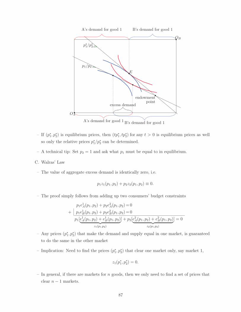
endowmentpoint
p∗1/p∗2
p1/p2
excess demand
A’s demand for good 1 B’s demand for good 1
A’s demand for good 1 B’s demand for good 1
E
OA
OB
– If (p∗1, p∗2) is equilibrium prices, then (tp∗1, tp
∗2) for any t > 0 is equilibrium prices as well
so only the relative prices p∗1/p∗2 can be determined.
– A technical tip: Set p2 = 1 and ask what p1 must be equal to in equilibrium.
C. Walras’ Law
– The value of aggregate excess demand is identically zero, i.e.
p1z1(p1, p2) + p2z2(p1, p2) ≡ 0.
– The proof simply follows from adding up two consumers’ budget constraints
p1e1A(p1, p2) + p2e
2A(p1, p2)= 0
+ p1e1B(p1, p2) + p2e
2B(p1, p2)= 0
p1[e1A(p1, p2) + e1B(p1, p2)︸ ︷︷ ︸
z1(p1,p2)
] + p2[e2A(p1, p2) + e2B(p1, p2)︸ ︷︷ ︸
z2(p1,p2)
] = 0
– Any prices (p∗1, p∗2) that make the demand and supply equal in one market, is guaranteed
to do the same in the other market
– Implication: Need to find the prices (p∗1, p∗2) that clear one market only, say market 1,
z1(p∗1, p
∗2) = 0.
– In general, if there are markets for n goods, then we only need to find a set of prices that
clear n− 1 markets.
87
D. Example: uA(x1A, x
2A) = (x1
A)a(x2
A)1−a
and uB(x1B, x
2B) = (x1
B)b(x2
B)1−b
– From the utility maximization,
x1A(p1, p2,m) = amA(p1,p2)
p1= a
p1ω1A+p2ω2
A
p1
x1B(p1, p2,m) = bmB(p1,p2)
p1= b
p1ω1B+p2ω2
B
p1
– So,
z1(p1, 1) = ap1ω
1A + ω2
A
p1+ b
p1ω1B + ω2
B
p1− ω1
A − ω1B.
– Setting z1(p1, 1) = 0 yields
p∗1 =aω2
A + bω2B
(1− a)ω1A + (1− b)ω1
B
.
III. Equilibrium and Efficiency: The First Theorem of Welfare Economics
– First Theorem of Welfare Economics: Any eq. allocation in the competitive market must
be Pareto efficient.
– While this result should be immediate from a graphical illustration, a more formal proof is
as follows:
(i) Suppose that an eq. allocation (x1A, x
2A, x
1B, x
2B) under eq. prices (p
∗1, p
∗2) is not Pareto
efficient, which means there is an alternative allocation (y1A, y2A, y
1B, y
2B) that is feasible
y1A + y1B = ω1A + ω1
B
y2A + y2B = ω2A + ω2
B
(4)
and makes both consumers better off
(y1A, y2A) ≻A (x1
A, x2A)
(y1B, y2B) ≻B (x1
B, x2B).
(ii) The fact that (x1A, x
2A) and (x1
B, x2B) solve the utility maximization problem implies
p∗1y1A + p∗2y
2A > p∗1ω
1A + p∗2ω
2A
p∗1y1B + p∗2y
2B > p∗1ω
1B + p∗2ω
2B.
(5)
(iii) Sum up the inequalities in (5) side by side to obtain
p∗1(y1A + y1B) + p∗2(y
2A + y2B) > p∗1(ω
1A + ω1
B) + p∗2(ω2A + ω2
B),
which contradicts with equations in (4).
88
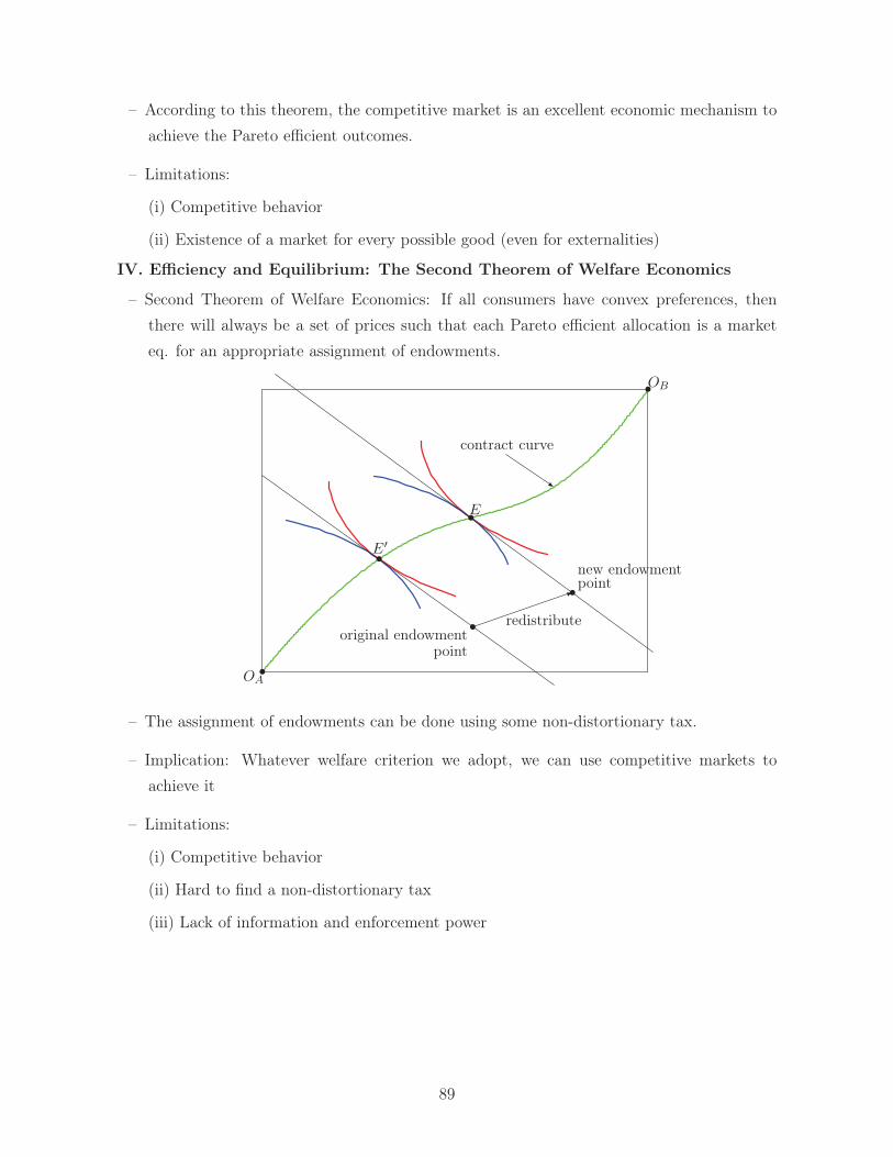
– According to this theorem, the competitive market is an excellent economic mechanism to
achieve the Pareto efficient outcomes.
– Limitations:
(i) Competitive behavior
(ii) Existence of a market for every possible good (even for externalities)
IV. Efficiency and Equilibrium: The Second Theorem of Welfare Economics
– Second Theorem of Welfare Economics: If all consumers have convex preferences, then
there will always be a set of prices such that each Pareto efficient allocation is a market
eq. for an appropriate assignment of endowments.
contract curve
redistribute
OA
E′
OB
E
original endowmentpoint
new endowmentpoint
– The assignment of endowments can be done using some non-distortionary tax.
– Implication: Whatever welfare criterion we adopt, we can use competitive markets to
achieve it
– Limitations:
(i) Competitive behavior
(ii) Hard to find a non-distortionary tax
(iii) Lack of information and enforcement power
89

Study Materials On Macroeconomics
Content :
1. Macroeconomics - Introduction
2. System of National Accounts
3. The goods market
4. Financial markets
5. The IS-LM Model
6. The Labor market
7. The three markets jointly : AS and AD
8. The Phillips curve
9. The open economy

1 Macroeconomics
Macroeconomics (Greek makro = ‘big’) describes and explains economic
processes that concern aggregates. An aggregate is a multitude of economic
subjects that share some common features. By contrast, microeconomics
treats economic processes that concern individuals.
Example: The decision of a Þrm to purchase a new o ce chair from com-
pany X is not a macroeconomic problem. The reaction of Austrian house-
holds to an increased rate of capital taxation is a macroeconomic problem.
Why macroeconomics and not only microeconomics? The whole
is more complex than the sum of independent parts. It is not possible to de-
scribe an economy by forming models for all Þrms and persons and all their
cross-e!ects. Macroeconomics investigates aggregate behavior by imposing
simplifying assumptions (“assume there are many identical Þrms that pro-
duce the same good”) but without abstracting from the essential features.
These assumptions are used in order to build macroeconomic models. Typi-
cally, such models have three aspects: the ‘story’, the mathematical model,
and a graphical representation.
Macroeconomics is ‘non-experimental’: like, e.g., history, macro-
economics cannot conduct controlled scientiÞc experiments (people would
complain about such experiments, and with a good reason) and focuses on
pure observation. Because historical episodes allow diverse interpretations,
many conclusions of macroeconomics are not coercive.
Classical motivation of macroeconomics: politicians should be ad-
vised how to control the economy, such that speciÞed targets can be met
optimally.
policy targets: traditionally, the ‘magical pentagon’ of good economic
growth, stable prices, full employment, external equilibrium, just distribution
1

of income; according to the EMU criteria, focus on inßation (around 2%),
public debt, and a balanced budget; according to Blanchard, focus on low
unemployment (around 5%), good economic growth, and inßation (0—3%).
In all speciÞcations, aim is meeting several conßicting targets simultaneously.
Examples for further typical questions to macroeconomics: what
causes business cycles (episodes of stronger and weaker economic growth)?
can an increase in the monetary supply by the central bank cause real e!ects?
what is responsible for long-run economic growth? should the exchange rate
of a currency be kept at a Þxed level? can one decrease unemployment, if
one accepts an increase in inßation?
A survey of world economics: three large economic blocks (Eu-
rope, USA+Canada, Japan+Far East) with di!erent problems, the remain-
der mostly developing countries.
1. USA: good growth, low inßation, tolerable unemployment rate, per-
sistent external deÞcit, increasing income inequality.
2. EU: moderate growth, low inßation, in some countries high unem-
ployment, inconspicuous external balance (total EU active, in Austria
recently turned active), for some countries large public debt, currently
important uniÞcation process, convergence and heterogeneity of indi-
vidual countries. ‘Richest’ EU countries Luxembourg, Denmark, then
‘mid-Þeld’ with Austria, IRL, B, NL, UK, D, F, FIN, I, S; slightly be-
low E, GR, SLO, P. Last come most ‘new’ (2004 accession) countries
(from Malta down to Latvia). Very ‘rich’ non-EU countries Norway,
Iceland, and Switzerland.
3. Japan: recently weak growth, large external surplus, deßationary ten-
dencies.
2
2 System of National Accounts
Basic idea (not the deÞnition): Summary of all economic activities within
a country’s territory and within a given time range (e.g., a year or quarter)
yields the gross domestic product (GDP). The value of all goods and ser-
vices is determined at market prices (Þnal prices, purchasers’ prices). System
for compilation of data and bookkeeping of all positions is called the System
of National Accounts (SNA). In Europe, compilation of the SNA conforms
to the ESA (European System of Accounts) standard.
Economic activity is mainly measured by transactions. Phrases from
text books: diversiÞcation of labor (not complete self-subsistence) causes
transactions, exchange of money for goods or services, exchange of an asset
or liability for a di!erent asset or liability, etc. The transactions take place on
markets. Money makes transactions easier than direct exchange of goods for
goods, which may require ‘double coincidence’ (hungry tailor meets freezing
baker).
Purpose of money: apart from payment and storage of value primarily
unit of measurement (numeraire). In economic text books, usually dollar
($), monetary unit (MU), or euro.
gross: many activities serve to repair or replace worn or damaged ma-
chines and objects (‘depreciation’), therefore it is not the total GDP that
contributes to the accumulation of aggregate wealth. In the SNA, ‘gross’
usually means ‘inclusive of depreciation’, ‘net’ often contains taxes, though
no depreciation.
Consumption of Þxed capital (in economics, depreciation) of SNA is the
estimated wear and tear of produced means of production (this ‘depreciation’
should not be confused with positions in tax declarations or with changes in
the currency exchange rate).
3
Capital stock is the stock of Þxed capital (machines, buildings, ...) in
enterprises and in the general government sector. This must be distinguished
carefully from the informal usage of the word ‘capital’ as ‘money, liquid
wealth’. By deÞnition, capital contains all produced means of production.
The separation of capital such as machinery from intermediate consumption
such as raw materials can be di cult.
economic activities: only market activities can be fully accounted for.
Therefore, private exchange and domestic services pass by unnoticed. By de-
Þnition, however, legitimacy of a transaction should not play a role. There-
fore, the shadow economy (moonlighting) and illegal drug production are
part of the GDP, but such activities are di cult to measure. A consequence
of this measurement problem is an exaggerated wedge between developing
countries and OECD countries (with the per capita GDP of Angola you can-
not survive in Austria). Interest focuses on transactions–bilateral (requited)
transactions (purchase etc.) and unilateral (unrequited) transactions (trans-
fers)–while value changes of existing objects are not accounted fully.
value added : deÞnition of GDP as the sum of values added in the produc-
tion process (ore metal screw motor part video recorder) avoids
multiple counts. Problems in the valuation of public services.
market prices: in principle, all goods and services are valued at market
prices, that is, inclusive of all taxes. If data is collected at the net value
(without taxes), taxes must be added.
economic agents: Resident ‘institutional units’ are classiÞed with regard
to their distinctive characteristics. Types of institutional units are: pri-
vate households, general government, Þnancial and non-Þnancial corpora-
tions (comprises most so called Þrms or enterprises), non-proÞt institutions
serving households. Foreign (non-resident) units are summarized as the ‘rest
4

of the world’, provided there are transactions with resident units. The same
person can be part of a private household and of an enterprise (rents out an
apartment, or even only uses his/her own condo but is assumed to rent it
out to him/herself).
resident is an institutional unit that is situated on a country’s territory.
Citizenship is not the criterion for residence. However, foreign students or
short-term foreign workers are not viewed as resident.
private households: produce and invest relatively little, consume, obtain
wage and proÞt income from corporations and from the government. As
self-employed persons, they obtain ‘mixed income’, though the separation of
households from corporations is occasionally di cult. Small (non-corporate)
Þrms and farms are counted as private households.
general government (‘public sector’): receives taxes from enterprises and
from private households, provides public goods (‘consumes them by itself’
according to SNA), no intention of proÞt.
corporations: produce and invest, do not consume, intention of proÞt.
Corporations, not the government sector, comprise also Þrms in public prop-
erty, if they cover 50% of their costs from sales. Because depreciation is now
called ‘consumption of Þxed capital’, it represents a kind of consumption of
corporations. Corporations are either Þnancial (banks etc.) or non-Þnancial.
non-proÞt institutions serving households (NPIsH): institutions (such as
schools, churches) that cover less than 50% of their production costs from
sales; idea: no intention of proÞt. A small sector, for simpliÞcation often
added to households.
rest of the world : consumes goods and services produced by residents
(exports) and produces goods and services consumed by residents (imports).
imports of services: includes travels abroad by residents
5

exports of services: includes consumption of foreign tourists on the terri-
tory of the economy (imputed based on valuta purchases etc.)
sectors: the activities of individuals of a similar kind are added up (ag-
gregated). The aggregate of all households forms the household sector etc.,
whereby transactions within the sector disappear. This ‘consolidation’ elim-
inates the exchange between households, as it does not increase collective
wealth. Recorded are the production of capital within the Þrms, the pro-
duction by private households, public consumption, which by deÞnition is
produced and consumed by the general government itself.
ex post : SNA records only after the economic processes have already
occurred, therefore only limited validity for the assessment of future reactions
in the economy. ex ante would be a task for economic theory.
ßows and stocks: SNA mainly records ßows of goods and services within a
time period (for example, the consumption of Austrian households in the Þrst
half-year of 1996). Sometimes, also stocks are of interest (wealth, number
of unemployed persons, central bank money, capital stock on July 31, 1996)
at a Þxed time point. Changes of stocks are ßows (bath tub: water level at
time point 1 = water level at time point 0 + inßow — outßow; inßow and
outßow are ßows; water level is a stock)
stocks: also short for ‘common stocks’ (shares) and occasionally for ‘in-
ventories’ (beware of the possibility of confusion)
2.1 Matrix of transactions between sectors
The new SNA convention a!ects this traditional presentation (followingHas-
linger), though it remains instructive and valid in principle. The NPIsH
sector is omitted here, an artiÞcial sector ‘value changes’ completes the trans-
action matrix.
6

Diagram of monetary ßows (payments) from the row sectors to the column
sectors, grossly simpliÞed, goods ßows partly in the opposite direction:
Þrms government householdsnon-
residents
value
changes
Þrms Tdir,F + Tind WF + d Im und,net
government subv + IP CP WP + trH SP
households C Tdir,H SH
non-residents X Im!X
value changes IF,net IP,netnames (notation as used in economics, not necessarily in SNA):
C . . . (private) consumption of households
CP . . .public consumption
IF . . . investment of corporations (enterprises, Þrms)
IP . . . investment of general government (public investment)
(‘investment’ always concerns means of production, not purchases of as-
sets)
Inet . . . investment without depreciation (wear and tear of the capital
stock)
WF . . .wage payments of Þrms to households
WP . . .wage payments in the public sector
trH . . . transfers to households (pensions, beneÞts, superscript indicates
direction ‘to households’; ‘transfers’=unilateral transactions without coun-
terpart)
SH , SP . . . saving (public sector often negative)
subv. . . . subsidies to enterprises
T . . . taxes etc.
Tind . . . indirect taxes are deductions before the calculation of income
7

(mainly value added tax) including customs, o cially production taxes.
Tdir . . .direct taxes are deductions from earned income (wage tax, income
tax etc.), including contributions to social security
und . . .undistributed proÞts
d . . .distributed proÞts (dividends etc.)
X . . . exports
Im . . . imports
Economic circuit: row sums = column sums (inßow=outßow), nothing
is lost, often graphical presentation with arrows. (metaphorical analogy wa-
ter: sector Atmosphere with input evaporation and output rain, sector Conti-
nents with input rain and output evaporation from inland water and outßow
at estuaries, sector Oceans with input at estuaries and output evaporation
from seas; earth is a closed circuit, amount of water is globally preserved)
open and closed circuit: without value changes, the economic circuit
is open, for example at X > Im more payments would ßow to Austria than
from Austria to non-residents. The hypothetical value changes sector (global
bank?) loses X ! Im and closes the circuit.
2.2 Accounts of the SNA
The new SNA consists of a sequence of several accounts, in which many
single positions are recorded, while others result as balancing items (bold
type in the accounts). These accounts are calculated for all sectors (Þnancial
and non-Þnancial corporations, public households, private households and
NPIsH, rest of the world) and for the total economy.
8

2.2.1 Sectorial accounting
The accounts that are decomposed according to sectors (Þnancial and non-
Þnancial corporations, public households, private households and NPIsH) are
primarily income accounts, which focus on the contributions of individual
sectors to national income. Point of departure is the production account.
Gross output (all production at basic prices, i.e. without value added tax and
customs) is booked on the credit side of this account. To this correspond,
as uses, the intermediate consumption and the depreciation (consumption of
Þxed capital). The balancing item is net value added. The columns ‘resources’
and ‘uses’ correspond to the bookkeeping terms ‘credit’ and ‘debit’.
Uses Resources
intermediate consumption gross output
depreciation
net value added
In the generation of income account, the balancing item of the production
account is transferred to the Resources. From the net value added, salaries
and wages (workers’ compensation) and some (so called ‘other’) production
taxes (e.g. payroll tax) are paid. The position ‘other subsidies received’
represents negative taxes, only the di!erence is of concern. The balancing
item of this account is called ‘operating surplus and mixed income’, where the
households and NPIsH earn mixed income, while the Þrms and government
9

receive an operating surplus:
Uses Resources
wages paid net value added
other taxes on production paid
— other subsidies received
operating surplus, net
mixed income, net
In the account of primary income allocation, the generation of income is
turned on its head. It yields, as a balancing item, the income of the sector.
For the total economy, the net value is slightly modiÞed relative to the sum
of single sectors, as primary income may also cross borders and also because
of the hypothetical position ‘Þnancial services indirectly measured’ (FISIM).
The relative contributions by the positions di!er widely across sectors. Thus,
only the general government receives production taxes, while only households
receive wages. The meaning of a primary income is that it is generated
completely in the production process. By contrast, the secondary income is
income after its redistribution through unilateral transfers. Correspondingly,
production taxes (indirect taxes) show up in the primary account, but not
the ‘direct’ taxes.
Uses Resources
property income paid operating surplus, net
mixed income, net
wages received
production taxes received
— subsidies paid
property income received
primary income, net FISIM
10

In the account of secondary income distribution, Þscal authorities show their
power. Neither corporations nor private households receive direct taxes,
while other transfers re-distribute income ßows among all sectors. As a bal-
ancing item, this account yields the so called disposable income, i.e. the
amount of income that is actually disposable for the sector’s expenditures
(or to the economy’s expenditures for the aggregate account)
Uses Resources
current taxes on income and wealth
paidprimary income, net
social contributions paidcurrent taxes on income and wealth
received
monetary social beneÞts paid social contributions received
other current transfers paid monetary social beneÞts received
disposable income, net other current transfers received
In the use of income account, all sectors except the corporations consume
out of their disposable income. The balancing item is the saving of the
sector, with a small correction because of contributions to pension funds,
which we would like to ignore. The quotient of saving and disposable income
in the household sector is called the household saving rate and represents an
important economic quantity. In Austria, this saving rate has dropped in
recent years from double-digit percentages to around 8%. Occasionally, also
the total saving rate is reported, which rather is a balancing item against the
non-resident sector.
Uses Resources
consumer expenditures disposable income, net
saving, net
11
In the capital account, saving serves as a resource for investment. After
deduction of a few lesser items, the net position of lending and borrowing
evolves as a balancing item. Gross Þxed investment is called ‘gross’, as it
comprises depreciation. It is called Þxed investment to distinguish it from
inventory investment, which is also seen as an investment. Fixed investment
can be broken up into residential construction, other construction investment
(buildings and structures, i.e. factories, streets, tunnels, ...), and equipment
investment (machines, vehicles, ...). Gross Þxed investment minus deprecia-
tion is called net Þxed investment.
Uses Resources
gross Þxed investment net saving
— depreciation capital transfers received, net
changes in inventories
net acquisition of valuables
net acquisition of non-produced
assets
net position of lending and borrowing
2.2.2 SNA for the total economy
Parallel to sectorial SNA, there is an accounting for the total economy, in
which the main emphasis is on production accounts rather than on income.
In these total accounts, we Þnd the primary target variable of SNA, the
gross domestic product (GDP). The GDP is distinct from the income items,
as it relates to the production by resident units rather than to the income
of residents. For production, all activities count that are performed on the
territory of an economy. For income, we are rather interested in activities
that are exercised by residents with permanent residence on this territory,
12
whether these activities take place at home or abroad. For disposable income,
one is more interested in the persons who earn the income. For the GDP,
it is more important, where production occurs. Even for disposable income,
however, residents are not deÞned by their citizenship. Longer-term guest
workers in Austria are counted as Austrians, while some border workers,
foreign students etc. are not counted as residents.
Again there is a production account, which departs from gross output,
which is recorded without goods taxes. Goods taxes are those indirect taxes
that depend on the quantity of production, i.e. primarily value added tax
(VAT) and customs. GDP should however also include these, thus they are
added, before intermediate consumption is subtracted. The balancing item is
GDP. Net of depreciation, this variable is called net domestic product (NDP).
GDP and NDP should correspond to the row sums across the values added
of all sectors.
Uses Resources
intermediate consumption gross output
gross domestic product goods taxes — goods subsidies
depreciation
net domestic product
In the sequence of accounts, the balancing item of exports and imports ac-
cording to SNA is recorded in a separate account as external balance of goods
and services. Otherwise, the generation of income account follows, whose
balancing item is again the operating surplus and mixed income. Note that
the previously added goods taxes are subtracted here just like other taxes,
such that the sectorial income accounts are comparable to the total. All
subsidies are minus positions (minus items), what really matters is the net
13

position of taxes minus subsidies.
Uses Resources
wages paid net domestic product
goods taxes paid
other production taxes paid
goods subsidies received
other subsidies received
operating surplus and
mixed income, net
In analogy to the sectorial account, an account of primary income alloca-
tion follows here, which yields the so-called net national income (NNI) as
a balancing item. The NNI should correspond to the sum of primary in-
comes net across all resident sectors. In the sequence of corrections in the
last two accounts (generation of income and primary distribution), the di!er-
ence between resident production and resident income disappears, such that
the resulting NNI again expresses the income of residents, which is indicated
by the word ‘national’. Before all, the net position of border-crossing prop-
erty income can be sizeable, while the net position of border-crossing wages
and subsidies is comparatively small. In order to calculate ‘gross national
income’ (GNI), one must add depreciation to net national income. GNI ap-
proximately corresponds to the historical ‘gross national product’ (GNP).
The name ‘income’ for this item is better than ‘product’, as it describes the
income of residential population and not their production.
14

Uses Resources
property income paidoperating surplus and
mixed income, net
wages received
production taxes received
— subsidies paid
net national income property income received
By way of the account of secondary income distribution, we obtain the dispos-
able income of the total economy. The positions in this account are relatively
small, as only few direct taxes and social contributions cross borders and their
net position is even smaller:
Uses Resources
income and property taxes paid net national income
social contributions paid income and property taxes received
monetary social beneÞts paid social contributions received
other current transfers paid monetary social beneÞts received
disposable income net other current transfers received
Like households, also the total economy consumes out of its disposable in-
come. Mainly, the household and the government sectors contribute to this
consumption. After an above mentioned small correction due to the change
in pension funds, the saving of the economy results as a balancing item. In a
parallel account for the non-resident sector, this use of income account also
shows the external position ‘external balance of current transactions’. This
is important insofar, as this ‘SNA current balance’ is available to an open
15

economy to Þnance its investment, apart from its saving.
Uses Resources
consumption expenditure disposable income net
saving net
The capital account has again the form that was described above. Finally,
the net position of lending and borrowing should correspond to the current
external balance. Due to measurement errors, there is no exact correspon-
dence. Therefore, there is the possibility of a ‘statistical di!erence’ on the
debit side. In total, however, the net position of lending and borrowing for
the total economy should be the negative value of the external balance.
Uses Resources
gross Þxed investment net saving
— depreciation capital transfers net
inventory changes
net acquisition of valuables
net acquisition of non-produced assets
net lending/borrowing
2.3 Variants of GDP
Once more the most important current and historical (partly still used) def-
initions
• Gross national income (GNI, formerly ‘gross national product’):
GDP plus primary income of residents from the rest of the world minus
primary income of non-residents from the economy; a GDP according
to the concept of residency of income earners instead of residency of
production units. International mobility (work abroad) confuses the
16
concept (extreme examples Luxemburg, Kuwait). Persons with per-
manent residence in Austria are always counted as residents!
• Gross social product: obsolete expression for gross national income
(GNI).
• Net domestic product: GDP minus depreciation.
• Net domestic product at factor costs: Net domestic product with-
out all production taxes (minus Tind plus subv).
• Net national income (formerly ‘net national product’): gross na-
tional income minus depreciation.
• Net disposable income of the economy: net national income (at
market prices, i.e. including all production taxes) plus balancing item
of border-crossing transfers. Should be a future main indicator of the
economy.
• GDP (etc.) at basic prices: Intermediate stage between the calcu-
lation at market prices (i.e. including all production taxes) and the
calculation at producer prices (i.e. excluding all production taxes).
Here, only goods taxes (comprises as its most important parts the value
added tax and customs) minus goods subsidies are subtracted. Only
after the further subtraction of ‘other production taxes minus other
subsidies’ (e.g., payroll tax), the value at producer prices is obtained.
According to convention, the original gross output is compiled at ‘basic
prices’, GDP and NNI are then shown at market prices.
Factor costs: the compensation paid to the production factors capital
(machinery and buildings) and labor, by proÞts and wages, without taxes
(net minus subsidies).
17
Primary income: deÞned as income earned by direct participation in
the production process. Labor and property income. Formerly ‘factor in-
come’.
2.4 SNA=3 national accounts
In many countries, GDP was formerly calculated three times
• from production
• from its Þnal uses
• from income
Particularly in the UK, three slightly di!erent GDP variants were com-
puted. According to SNA convention today, the Þrst of the three deÞnes
the proper GDP. As already described, GDP is computed by adding ‘goods
taxes minus goods subsidies’ to gross output and subtracting intermediate
consumption. There is also a break-down according to di!erent production
sectors (mining, agriculture, manufacturing etc.), which is not of central in-
terest in macroeconomics. An important component of this break-down is
industrial production, which is computed on a monthly basis and serves as a
fast business indicator.
Of fundamental interest in macroeconomics is the break-down of GDP
according to Þnal uses
GDP = C + CP + I +X ! Im . (1)
which is collected in a separate SNA account (Account 0, in economics
GDP is denoted by the letter Y and government consumption by the letter
G). Note that, from the outlined sequence of accounts you obtain C from
18
the consumer expenditure of households (including NPIsH), Cp from the
consumer expenditure of general government, I from the capital account,
X! Im from the external account as an external balance. In order to obtain
an exact match of the left side (from production) and the right side (from
uses), one should observe:
• the changes in inventories (conceptually seen as investment: inventory
investment)
• the change in the stock of valuables (purchases of objects of art etc.)
and similar small positions
• a statistical di!erence (formerly often added to the smaller aggregates
as ‘inventory changes and statistical di!erence’)
Sometimes, the private consumption C is broken down in:
• consumption of durable goods (cars, video recorders, ...)
• consumption of non-durable goods (clothing, food, books and journals,
...): proximity of purchase and utilization
• consumption of services (dining out, Þtness studio, ...): not storable
Public consumption CP is broken down into:
• Collective consumption: indivisible utilization (e.g., street lighting)
• Individual consumption: can be allocated to individual persons (e.g.,
free education)
According to the concept of the new SNA, individual public consump-
tion and private consumption are summarized in the aggregate ‘individual
consumption’. The economic meaning of this convention is questionable.
19

Gross Þxed investment I (‘gross’=includes depreciation, ‘Þxed’=no
inventory investment; also comprises public investment; in SNA: gross Þxed
capital formation) is broken down into:
• investment in equipment (machinery, vehicles, ...)
• investment in construction (buildings and structures, includes residen-
tial construction)
The meaning of the distribution of income account for the determination
of disposable income etc. was already explained. By contrast to many
other parts of the SNA accounts, which exist in real terms (adjusted for in-
ßation, at constant prices, in the public sector di cult!) and also in nominal
terms (at current prices), the income distribution is calculated in nominal
terms only. An important derived quantity of the distribution accounts is
the wage quota, i.e. the share of compensation for labor in national income.
The disposable income of households YD serves as the basis for the cal-
culation of the household saving rate
qSH =YD ! C
YD.
In Austria, this quotient currently is around 8-9%.
2.5 Other statistics that are related to SNA
Wealth is a stock variable and notoriously di cult to compile (human cap-
ital, unknown value of assets etc.). Household wealth can be estimated from
consumer expenditures on durables and assumptions about the depreciation
of these durable goods. Data on monetary wealth is provided by banks
(checking accounts, saving accounts, bonds, shares). The capital stock
(stock of produced means of production) results from depreciation rates for
20

Figure 1: Main components of the SNA (from Dudley Jackson, The New
National Accounts).
21

types of capital goods and from gross Þxed investment. The stock of in-
ventories results from inventory changes etc.
Input-output (IO) tables are large matrix tables that report the ßows
of goods and services among subsectors of an economy, admit detailed in-
formation about intermediary consumption, which is necessary for Þnal pro-
duction in a certain sub-sector.
The balance of payments registers all transactions of goods, services,
payments across borders. Because of di!erent concepts, it does not match
the SNA balances exactly:
1. goods balance (only goods, in Austria approximately neutral net posi-
tion)
2. services balance (primarily tourism, in Austria positive net position,
and also other services)
3. external balance of primary income (compensation of border workers,
primarily border-crossing property income, in Austria passive)
4. external balance of transfers (transactions without counterpart, in Aus-
tria passive)
Positions 1—2 together are the so-called ‘trade balance’, Position 1—4 yield
the current accounts balance. The current accounts balance should match,
with inverted sign, the balance of capital ßows (capital accounts balance,
short- and long-run capital ßows; note the usage of the word ‘capital’ that
does not denote produced means of production here). A di!erence of the two
positions may stem from the change in reserves of currency and gold in the
central bank, and from diverse statistical discrepancies. All balances together
22

are called the balance of payments. Therefore, there cannot be a deÞcit in
the balance of payments, while there may be a current account deÞcit.
Price indexes (deßators) must be calculated for the GDP and for all of
its demand-side components (durable consumption, total private consump-
tion, construction investment etc.)
Traditionally, deßators followed the concept of the Paasche index
pt+1t =
Pj pj,t+1xj,t+1Pj pj,txj,t+1
(2)
(what would the goods now demanded have cost one year ago?). After select-
ing a special base year, in which real (‘at constant prices’) and nominal (‘at
current prices’) variables (e.g., GDP) coincide, a current price index evolves
from
Pt = ptt 1p
t 1t 2 . . . p
t0+1t0
Pt0 ,
where Pt is 1 (or 100) in the base year t0.
Alternatively, basket indexes are calculated according to the concept of
the Laspeyres index
pt+1t =
Pj pj,t+1xj,0Pj pj,txj,0
(3)
(by how much did the price of a Þxed basket of goods and services increase
over the last year?). The basket is modiÞed partly continuously, partly in
base years, as goods are continuously replaced by other comparable goods.
It is common to standardize the Laspeyres index in the base year at 100,
though this standardization plays no role. The most important Laspeyres-
type index is the consumer price index (CPI), which, e.g., determines the
increases of rents and wages.
Since 2004, SNA deßators are no more calculated as Paasche indexes but
rather as geometric averages of Paasche and Laspeyres indexes (chaining).
23

A consequence is that identities–such as the important Account 0 identity–
do not hold exactly for real quantities any more.
What distinguishes de facto the consumption deßator and the consumer
price index? With the Laspeyres index, the households stand no chance
to substitute goods that have become more expensive by relatively cheaper
ones (e.g., books by computer software), therefore the CPI usually increases
faster.
hedonic prices: technical products (cars, computers) develop fast. Some
experts argue that these should not be valued at the market price, but at the
price of their inner characteristics (fuel consumption, speed of calculation).
This concept often yields a general decrease in the price of such goods by
increase in quality, though the problem remains whether the customers are
forced to consume an additional and relatively cheap ‘quality’ of such goods
(tinted car windows, automatically installed software). The concept is partly
used by statistical agencies for the calculation of all indexes.
The rate of inßation is the percentage change of a price index Pt, i.e.
100Pt ! Pt 1Pt 1
where Pt, e.g., may denote the consumer price index. As long as price inßa-
tion remains ‘normal’, the logarithmic rate 100(logPt ! logPt 1) is a conve-
nient approximation and is often preferred for technical reasons.
Labor market statistics provide the important unemployment rate
on a monthly basis. According to the traditional (‘Austrian’) deÞnition
unemployment rate =registered unemployed
employed + registered unemployed(4)
where the denominator is called the (dependent) labor force. Here, self-
employed persons do not count as employed. In contrast, the o cial un-
employment rate (‘international deÞnition’, ESA rate) relies on census mea-
24
surement, as registering at employment agencies is not a good indicator for
unemployment (no registration, when there is no chance of obtaining beneÞts
or if search is hopeless; fake registration of persons working in the shadow
economy) in many countries. According to this convention, self-employed
persons are included. In Austria, the ‘international’ concept leads to a lower
rate; in Spain, it leads to a higher rate.
2.6 Critique of National Accounts
1. SNA measures incorrectly
(a) Measurement and numbers are bad: Critique of reducing the real
world to data (atypical for a quantitative science, such as eco-
nomics)
(b) SNA does not measure welfare social indicators, questionnaires
etc. (borderline to sociology)
(c) SNA measures ßows, whereas true wealth is expressed by stocks
of property and possessions.
2. SNA measures too much
(a) regrettable necessities should not be measured, such as road acci-
dents, criminal activity, expenditures for longer commute to work,
as these do not increase welfare: deÞnition of boundaries is di -
cult, strong consequences for international and intertemporal com-
parisons unlikely (military goods even now only contribute, if they
can also be used for civilian purposes)
(b) damage to health and the environment should be subtracted. Throw-
away goods should not increase wealth slower growth if such
25

concepts are considered tentatively (Nordhaus/Tobin: measure
of economic welfare MEW instead of GDP)
3. SNA measures too little
(a) economic activities, which do not touch o cial markets (house-
hold work, so-called shadow economy), are not compiled accu-
rately (household work is deliberately excluded, as: (1) it is dif-
Þcult to measure, (2) externalizing of services in principle even
now an indicator of welfare, (3) household services as component
of GDP would destroy the di!erentiation between unemployment
and employment; shadow economy is included in o cial GDP, al-
though its assessment is concededly di cult; illegal production is
by deÞnition a part of GDP!)
(b) quality of life, leisure, creation of national parks, cleaning of air
and water are not valued su ciently, as these are not market goods
and do not have market prices (task for environmental economics)
26
3 The goods market
Wherever necessary, it is assumed that households and Þrms are identical
and produce and consume only one good. This good serves as a consump-
tion good as well as an investment good. Demand is assumed to be satisÞed
immediately by supply at a given and Þxed price. The decomposition (Ac-
count 0) of national income Y (or GDP, these are assumed as equal in what
follows) according to uses
Y = C + I +G+X ! Im (5)
(consumption C, investment I, government expenditure G loosely corre-
sponds to the CP from SNA, exports X, imports Im) simpliÞes to
Y = C + I +G (6)
in a closed economy, which does not communicate with the rest of the
world by means of imports or exports (as opposed to an open economy). At
Þrst, it will be assumed that the economy is closed.
Consumption C: households consume out of their disposable income,
we write
C = C(YD)
+
This is a (for the moment, not exactly speciÞed) consumption function.
The sign ‘+’ indicates that consumption rises with increasing income and
falls with decreasing income, i.e. it reacts ‘positively’. A simple functional
form is the linear speciÞcation
C = c0 + c1YD (7)
27
with c1 > 0 and typically also c0 > 0. This so-called Keynes consumption
function contains two parameters c0, c1, i.e. not directly observable, Þxed
constants. As a behavioral equation, it describes the action of households
as depending on their income. By contrast, the simplifying relation
YD = Y ! T (8)
with taxes T is not a behavioral equation, but rather a deÞnitional equa-
tion (identity). In more detail, the variable T may be identiÞed with ‘in-
come taxes minus transfers from government to households’ and may even
be thought to comprise social contributions and beneÞts.
‘Lump sum’: except for some exercise examples, taxes T are assumed
to be independent of income. Each identical household pays a Þxed amount
to the government, a ‘lump sum’.
The parameter c0 is the autonomous consumption of the economy.
Because the households are all alike, c0 is the sum of all expenditures of all
households that is necessary for their survival, if these do not receive any
income.
The parameter c1 is the marginal propensity to consume and de-
scribes, by how much consumption rises, if households receive an increase in
their income by, e.g., one euro. In this case, they increase consumption by
c1 euro. It makes sense to require c1 < 1, i.e. c1 " (0, 1). One also writes
c1 = C
YD(9)
Unlike c1, the average propensity to consume
C
YD=c0YD
+ c1 (10)
is not a constant, but falls with increasing income. C/YD answers the ques-
tion, how much out of the total income is consumed, not out of a ‘marginal’
28
additional income. Falling average, but constant marginal propensity to con-
sume was one of the famous Keynes axioms.
Investment I, government expenditure G, taxes T : are kept Þxed
and are, as ‘exogenous’ variables, not determined in the model; no relation-
ship between G and T ; exogenous (determined outside the model) variables
act like parameters, though, unlike those, they are observed directly. For-
mally, one writes:
I = I (11)
G = G (12)
T = T (13)
The behavioral equation (7), the deÞnitional equation (8), and the three iden-
tities that express exogeneity (11), (12), (13) describe the aggregate demand
in the simple closed economy.
The supply results from the quantity of the produced good Y .
Equilibrium on the goods market, i.e. a cleared goods market, in which
there are no increasing inventories and no unsatisÞed and hungry consumers,
means that Y and aggregate demand Z = C + I +G are equal, i.e. Y = Z,
or
Y = c0 + c1YD + I + G
= c0 + c1(Y ! T ) + I + G
and thus
Y =1
1! c1(c0 + I + G! c1T )
Thought experiments
29

1. We increase government expenditure G by 1 euro. This increases na-
tional income Y by 1/(1 ! c1) euro. Because c1 " (0, 1), for example
c1 = 0.9, Y increases by more than one euro, for example by 10 euro.
2. We increase investment I by 1 euro. Again Y increases by 1/(1 ! c1)
euro, in the numerical example by 10 euro.
3. We increase autonomous consumption c0, for example by a campaign
of optimism. Again, Y increases by 1/(1! c1) euro.
4. We increase taxes by 1 Euro. Now Y falls by c1/(1! c1) euro.
The important value 1/(1 ! c1) is called the (Þscal) multiplier, as it
multiplies the increase of an exogenous input in the aggregate output. This
multiplier e!ect is caused by the following mechanism: additional consumer
demand leads to an increase in total aggregate demand Z, which is satisÞed
by the Þrms immediately, whereby Y increases once more, as income equals
production, etc.
Saving propensity and multiplier: If YD!C is interpreted as house-
hold saving SH , then 1!c1 is the (marginal) saving propensity of house-
holds, if c1 is a propensity to consume, as
SH = YD ! C = YD ! (c0 + c1YD) = !c0 + (1! c1)YD
The bigger the saving propensity, i.e. the smaller the propensity to consume,
the smaller is the multiplier, and vice versa. At a saving propensity of 1,
the multiplier becomes 1, i.e. it does not multiply anything. At a saving
propensity of 0, the multiplier becomes #. This would be nonsense and
must be ruled out.
Empirical evidence (Figure 2): in line with the theoretical concept, the
propensity to consume appears to be slightly less than 1. A statistical re-
30
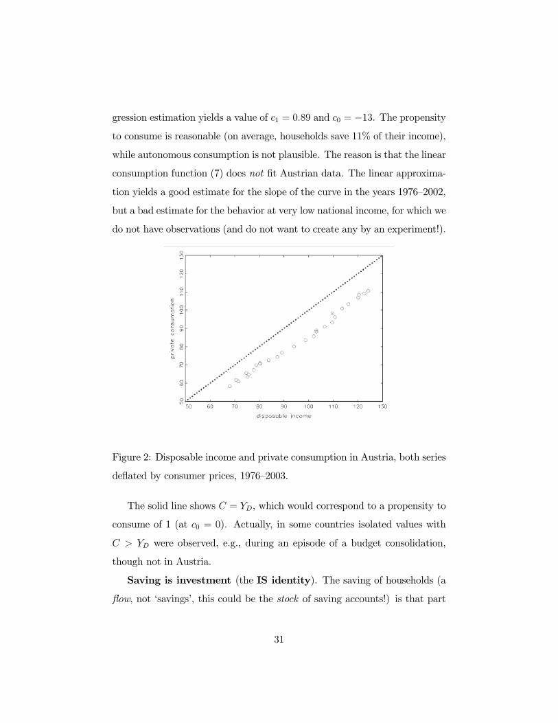
gression estimation yields a value of c1 = 0.89 and c0 = !13. The propensity
to consume is reasonable (on average, households save 11% of their income),
while autonomous consumption is not plausible. The reason is that the linear
consumption function (7) does not Þt Austrian data. The linear approxima-
tion yields a good estimate for the slope of the curve in the years 1976—2002,
but a bad estimate for the behavior at very low national income, for which we
do not have observations (and do not want to create any by an experiment!).
Figure 2: Disposable income and private consumption in Austria, both series
deßated by consumer prices, 1976—2003.
The solid line shows C = YD, which would correspond to a propensity to
consume of 1 (at c0 = 0). Actually, in some countries isolated values with
C > YD were observed, e.g., during an episode of a budget consolidation,
though not in Austria.
Saving is investment (the IS identity). The saving of households (a
ßow, not ‘savings’, this could be the stock of saving accounts!) is that part
31
of income that is not consumed
SH = YD ! C = Y ! T ! C (14)
Noting that Y = C + I +G we obtain
SH = I +G! T. (15)
If government runs a balanced budget, then its expenditure G equals taxes
T , G = T . This implies SH = I, “saving equals investment”. If government
runs a budget surplus (at the expense of the rest of the economy), then T > G
and therefore I > SH . If government consumes more than its revenues (a
budget deÞcit), then T < G and therefore I < SH . If one views T ! G as
‘government saving’ SP , then
SH + SP = I (16)
Thus, investment equals saving of households plus government saving. Typ-
ically, SP will be negative.
Where is the saving of Þrms? The saving of enterprises corresponds
to undistributed proÞts. In this simple model, it is assumed that (8) holds,
households receive the total income minus taxes. In this model, the saving
of Þrms is therefore 0.
Is saving good or bad? (Schoolchildren often learn that saving is
a good thing) In the short run, saving has a contractionary e!ect, i.e., a
negative e!ect on output. Lower c0 decreases aggregate income by c0/(1!c1).
Lower c1 has an even stronger negative e!ect. Because a contractionary e!ect
of saving appears to be a ‘paradox’, this is sometimes called the saving
paradox (paradox of thrift, Þrst implication). It can also be shown that,
in the model, a decrease of c0 or c1 implies such a strong decrease in Y
that SH (which depends on Y ) does not change at all (Exercise, paradox of
32

thrift, second implication). In the long run, the saving paradox disappears,
as saving increases the growth potential of the economy, causes the interest
rate to fall, and increases investment. These mechanisms are absent in the
simple model with I = I. (16) is only an identity and does not describe
economic behavior.
Is it preferable to increase government expenditure or to de-
crease taxes? In the model, a 1 billion euro increase in G at c1 = 0.9 yields
an additional income of 10 billion euro, while a decrease of T by the same
amount only yields 9 billion euro. G directly a!ects aggregate income, while
T only a!ects the disposable income and household consumption, whereby
saving annihilates a part 1! c1.
4 Financial markets
Many possibilities are available to a household who has to allocate its income.
The largest part of the disposable income is consumed, the remainder (7—
12%) is ‘saved’. For saving, the following ‘assets’ can be used:
1. narrow-sense money (cash, currency): originally promissory notes
on the central bank. Universally accepted for transactions, but bears
no interest. Liquidity is maximal, interest rate is 0.
2. checking accounts (demand deposits): short-run assets at banks.
Increasingly used for transactions (Quick Cash, Debit Card), very low
interest. Liquidity is high, interest rate nearly 0. Included even in
narrow-sense money (M1).
3. saving accounts (and time deposits): longer-run assets at banks.
Must be exchanged for money to enable transactions (limited liquidity),
33
but bear interest. Fast exchange for cash with small and standardized
transaction costs, therefore included in wide-sense money (M3).
4. bonds (risk-free securities with Þxed interest): promissory notes at
good debtors, can be purchased at banks (brokers). Better interest,
must be sold for transactions.
5. shares: certiÞcates of shared ownership at corporations. Uncertain,
though often good interest (return, dividends). Usually purchased via
banks (brokers) at a stock exchange and sold at variable prices.
6. real estate, stamps, antiques: uncertain interest, low liquidity (sta-
tistically, partly consumption!).
The aggregate stock of these assets is the wealth of households. Note that
household wealth does not contain the stock of consumer durables (cars and
dishwashers) with their negative rate of interest due to depreciation. Wealth
and its components are stocks, which increase by adding the ßow variable
‘income’ and diminish by subtracting the ßow variable ‘consumption’.
Assumption: in the closed economy there are only money and bonds.
The problem of households consists in distributing their wealth optimally
among money (M) and bonds (B), i.e. to Þnd M and B such that M +
B = $W . The symbol ‘$W ’ indicates that wealth and its components are
measured at current prices (in nominal terms).
4.1 Demand for money and bonds
Demand for money (Md for money demand). Money serves for trans-
actions, whose amount is proportional to national income ($Y for nominal
national income). High income means many transactions. When interest i
34

on bonds is high, households do not want to forego the additional income
out of interest and keep little money. One writes
Md = Md($Y, i)
+ !
or, more speciÞcally and simpler
Md = $Y · L(i)
with the function L(i), which falls in its argument i. The letter L is for
‘liquidity’. At an interest rate of 0, i = 0, all wealth is kept as money. At a
high interest rate, relatively little money is kept. Thus, one has i $ 0 and
L(i) > 0.
For Þxed income $Y , one sees a falling function (Fig. 3), which is drawn
with i on its y axis (ordinate axis) and with M on its x axis (abscissa axis),
for technical reasons. The higher $Y , the more do the curves move to their
right. At every interest rate i, more money is demanded.
Demand for bonds Bd. This results from the budget constraint and
from money demand as
Bd = $W !Md
= $W ! $Y L(i)
Larger wealth causes an increased demand for bonds, higher interest also
raises the demand for bonds. Higher income increases the stock of wealth
but also decreases money demand. In the short run, we assume that $W is
exogenous, therefore an increase in income will cause a fall in the demand
for bonds.
Empirical evidence for Austria. Figures 4 and 5 show the develop-
ment of the variablesM/$Y and i during 1970—2004. The theoretical concept
35

Figure 3: Money demand curves
of a function L(i) would imply a negative relationship, which is partly sup-
ported by the time-series graph and by the scatter diagram. There is no
convincing evidence on a long-run fall in the ratio M/$Y , which is reported
for the USA. Such a long-run fall may be plausible, as today less cash money
(including checking accounts?) is used than some time ago. This feature
would imply that the inverse ratio $Y/M , the so-called ‘velocity of money’,
increases.
4.2 Equilibrium in the money market
(Money market is an older expression for the Þnancial market) obtains when
money demand equals money supply. Assuming the money supply to be
Þxed and to be determined exogenously by the central bank, equilibrium
36
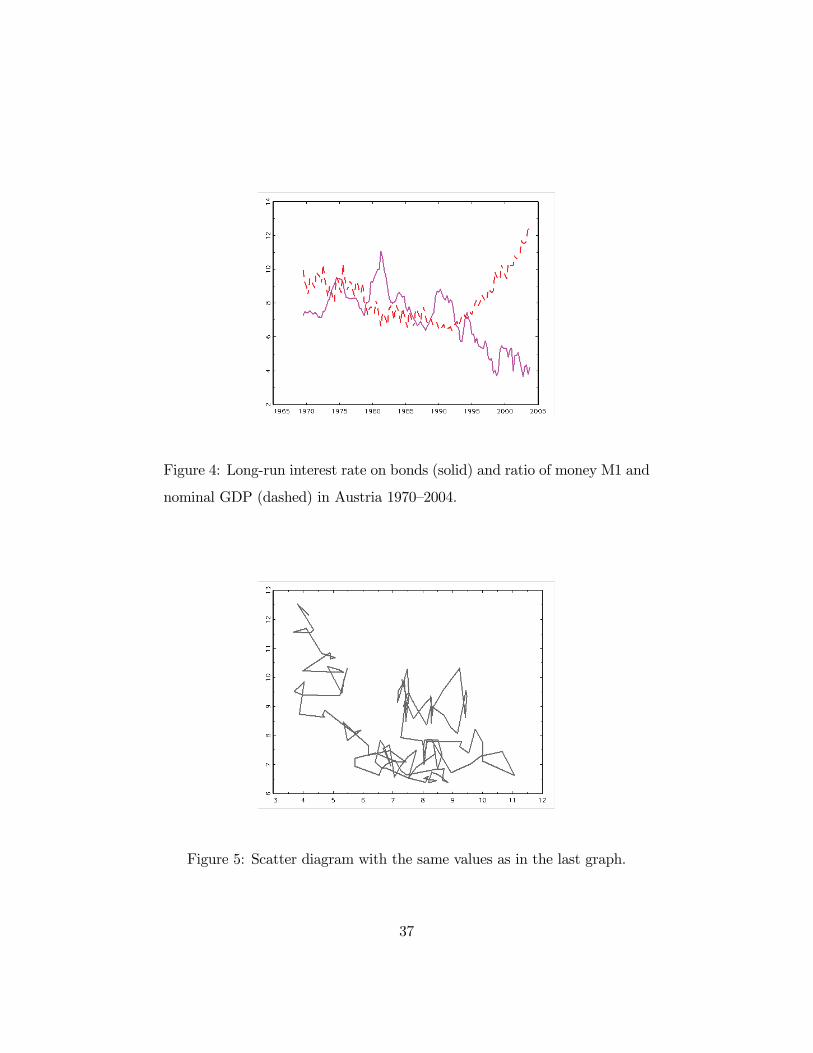
Figure 4: Long-run interest rate on bonds (solid) and ratio of money M1 and
nominal GDP (dashed) in Austria 1970—2004.
Figure 5: Scatter diagram with the same values as in the last graph.
37

means
Ms = M
Md = $Y L(i)
Ms = Md
Graphically, the vertical line Ms = M intersects the money demand curve
at a unique point, which determines the interest rate i. Thus, a given M
determines i uniquely. The equation M = $Y L(i) is called LM identity,
which is for ‘liquidity is money’ and is the counterpart to the IS identity
‘investment is saving’. If both the LM and the IS identity hold, there is
equilibrium in the goods market and in the money market.
Experiments:
1. The nominal income $Y is increased exogenously, for example by in-
creasing government expenditure. M is set by the central bank and
does not budge. The money demand curve shifts outward, the equilib-
rium interest rate i rises.
2. The central bank increases the money supply Ms = M . The vertical
line shifts to the right, the money demand curve does not move. The
equilibrium interest rate i falls.
How does the central bank do it? The central bank can use three
di!erent tools: open-market operations, reserve requirements, discount rate.
In open market operations, the central bank buys or sells bonds or other
assets and pays or receives money. It thus increases or decreases the amount
of money in circulation. Tightening the reserve requirements leads to tight-
ening of money, similar to an increase of the discount rate. Currently, the
most important instrument is open-market policy.
38

Reserve requirements. Obligatory reserves of banks that are held
at the central bank. Formerly, the central bank paid no interest on such
monetary reserves. The original intention was to guarantee the banks’ savings
accounts, today reserve requirements are just means of controlling the money
supply. Today, reserves have become interest-bearing (~2%). Thus, this
interest rate be used as another instrument of controlling the money supply.
Discount rate. An interest rate for transactions between the central
bank and banks. A higher discount rate does not automatically imply a
higher interest rate in the money market, though some positive inßuence is
reasonable to assume.
4.3 Price of bonds and interest rate
In real-world Þnancial markets, the interest rate of a bond is not determined
directly, but indirectly via the bond price. Assume that a bond is in circula-
tion at time point t, while its owner receives at maturity t+1 a value of 100.
That is, assume that ‘100’ and the maturity date are printed on the bond.
Then, the price of the bond in t, PBt, determines the interest because of
it =100! PBtPBt
,
i.e. not in percentage points, e.g., it = 0.07. Conversely, if i is given, the
bond price can be calculated as
PB =100
1 + i.
Because i > 0, it must hold that PB < 100 .
39
4.4 The money multiplier
The stock of printed money H (high-powered money) is called monetary
base and is partly stocked at the commercial banks, partly it is circulating:
H = CU +R
R denotes the reserves of banks, CU for ‘currency’ (cash money). Today,
usually ‘money supply’ is deÞned as M1, the sum of currency and demand
deposits:
M = CU +D
The banks can create money far beyond the monetary base. They face two
restrictions:
1. The minimum reserves required by the central bank, which are kept by
the banks at low or no interest, lock the ratio ! = R/D from below.
2. The economic agents determine their own (street-corner shop, newspa-
pers) cash demand coe cient c = CU/M .
From the relations, we obtain for demand deposit money D
D =M ! CU = (1! c)M
and therefore for the monetary base
H = CU +R = cM + !D = (c
1! c+ !)D =
c+ !(1! c)
1! cD
and thus by inverting the ratio for demand deposit money
D =1! c
c+ !(1! c)H
40
and for total ‘money’
M =1
1! cD =
1
c+ !(1! c)H .
The value 1/{c + !(1 ! c)} is called the money multiplier, as it indicates,
by how much the money supply increases, if the central bank prints one
additional unit of money. For small c and small !, the multiplier becomes
particularly large.
Example. Blanchard assumes ! = 0.1, we further assume that c =
0.05 (compare this to your own private allocation between cash and demand
deposits!). Then, the purchase of a bond for 1000 euro by the central bank
against emission of ten 100 euro notes causes the bond seller to increase his
demand deposit by 950 euro, while 50 euro of cash remain in the trouser
pocket. The bank keeps 95 euro as reserve and buys bonds for 855 euro from
a di!erent bond seller. This bond seller keeps 42.75 euro in cash in the pocket
of her jacket, while she increases her demand deposit by 855-42.75=812. 25
euro. Even now, money M1 has almost doubled, but the chain continues and
Þnally leads to 1/(0.05+0.1*0.95) euro, i.e. around 7000 euro, therefore to a
sevenfold increase according to the above formula.
How is household wealth really allocated in Austria? Most Aus-
trians do not own shares or stocks, the largest part is still kept in saving
accounts. The wide-sense deÞnition of money (M3) comprises cash money,
demand deposits and also saving accounts. The graph (Figure 6) shows
how the shares of these components have developed during the most recent
decades.
41

Figure 6: Development of monetary wealth components for the years 1962—
2004 in Austria.
42
5 The IS-LM model
If one looks at the goods and Þnancial markets jointly, then both the equilib-
rium condition on the goods market (IS) and on the Þnancial market (LM)
should hold. In the tradition of Keynes and Hicks, the emphasis is on the
behavior of income Y and of the interest rate i. For this purpose, the model
needs a reaction to interest rates on the goods market. Such a reaction is
most likely in investment behavior.
5.1 Investment function
The simple assumption I = I is now replaced by a useful investment function.
Investors react to two important variables:
1. expected sales should a!ect investment plans. These are not known,
though observed output Y should be a good indicator for expected
sales.
2. the interest rate determines the costs of loans that are required to
execute investment plans.
It follows that one may depart from an investment function such as
I = I(Y, i)
(+,!)
A functional form will, however, not be speciÞed.
Empirical evidence. A systematic negative reaction of gross Þxed in-
vestment to interest rates is di cult to establish empirically. The graphs
show scatter diagrams of the investment ratio I/Y and of its real growth
rate against a (nominal) interest rate and only vaguely indicate a negative
43
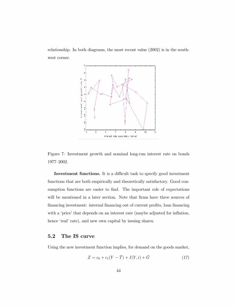
relationship. In both diagrams, the most recent value (2002) is in the south-
west corner.
Figure 7: Investment growth and nominal long-run interest rate on bonds
1977—2002.
Investment functions. It is a di cult task to specify good investment
functions that are both empirically and theoretically satisfactory. Good con-
sumption functions are easier to Þnd. The important role of expectations
will be mentioned in a later section. Note that Þrms have three sources of
Þnancing investment: internal Þnancing out of current proÞts, loan Þnancing
with a ‘price’ that depends on an interest rate (maybe adjusted for inßation,
hence ‘real’ rate), and new own capital by issuing shares.
5.2 The IS curve
Using the new investment function implies, for demand on the goods market,
Z = c0 + c1(Y ! T ) + I(Y, i) + G (17)
44
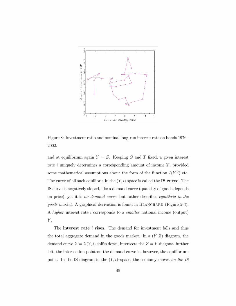
Figure 8: Investment ratio and nominal long-run interest rate on bonds 1976—
2002.
and at equilibrium again Y = Z. Keeping G and T Þxed, a given interest
rate i uniquely determines a corresponding amount of income Y , provided
some mathematical assumptions about the form of the function I(Y, i) etc.
The curve of all such equilibria in the (Y, i) space is called the IS curve. The
IS curve is negatively sloped, like a demand curve (quantity of goods depends
on price), yet it is no demand curve, but rather describes equilibria in the
goods market. A graphical derivation is found in Blanchard (Figure 5-3).
A higher interest rate i corresponds to a smaller national income (output)
Y .
The interest rate i rises. The demand for investment falls and thus
the total aggregate demand in the goods market. In a (Y,Z) diagram, the
demand curve Z = Z(Y, õ) shifts down, intersects the Z = Y diagonal further
left, the intersection point on the demand curve is, however, the equilibrium
point. In the IS diagram in the (Y, i)—space, the economy moves on the IS
45

curve leftward, i increases and Y falls.
The interest rate i falls. The economy moves on the IS curve to the
right, i falls, while Y increases.
Taxes T are increased. The demand curve Z = Z(Y ) shifts down,
without i changing. One obtains a lower demand Y at the same i, the whole
IS curve shifts left, as one obtains a lower output Y for every given i.
Government expenditure G is increased. The IS curve shifts right,
as for every interest rate i there is a higher demand Y .
The autonomous consumption c0 rises. Again, the IS curve shifts
right.
Autonomous demand. Because investment depends on Y and the
functional form I () is left unspeciÞed, the positivity of autonomous demand
c0 + I(0, i) + G! c1T is not guaranteed, at least not for high interest rates.
Blanchard argues that positive autonomous demand is the typical case.
5.3 The LM curve
Equilibrium in the Þnancial market obtains if Ms =Md. For money demand
Md we assume Md = $Y L(i), the money supply is Þxed exogenously by the
central bank , i.e. Ms = M . Because the goods market is presented in real
terms (deßated, i.e. at constant prices), it is useful to present the Þnancial
market likewise. Division by the price level P yields real money supply
Ms
P=M
P(18)
and real money demand
Md
P= Y L(i). (19)
Like all simple ‘Keynesian’ models, our model assumes Þxed prices in the
short run, i.e. P = P , therefore there is no change relative to the nominal
46
presentation. The left side of the equations M/P is called real money. In a
(M/P, i) diagram, the supply curve is a vertical line. The real money demand
curve is a downward sloping curve, at a higher interest rate i less money is
demanded. The intersection point of the vertical supply line and falling
demand curve yields the equilibrium interest rate i. On the money demand
curve, Y is kept constant. If Y falls, then the money demand curve shifts
left, the equilibrium interest rate i falls. This implies a curve of equilibria
in the Þnancial market in the (Y, i) space, the LM curve. The LM curve is
positively sloped, like a supply curve (supplied quantity of goods dependent
on price). It is, however, no supply curve, but rather describes equilibria in
the Þnancial market.
[observe four graphs: supply and demand in the goods market (Keynesian
cross), IS curve, supply and demand in the Þnancial market (money market
cross), LM curve]
The interest rate i rises. On the LM curve in the (Y, i) space, one
moves to the right, therefore the equilibrium income Y increases. In the
money market cross, one observes the following. If i increases, a wedge of
disequilibrium opens, as less money is demanded than supplied. Only if
income (output) Y increases, the money demand curve shifts to the right
until equilibrium is again obtained.
Money is printed. The increase of money supply shifts the money
supply vertical to the right, the equilibrium interest rate i falls, without any
change in Y . Because for every Y there is now a lower i , the LM curve shifts
to the right.
The price level P rises. This implies a fall in real money supply, ex-
pressed by the vertical line Ms = M . For every Y this yields a higher i, and
therefore the LM—curve shifts left. The reaction is easier to see from a nomi-
47

nal (M, i) diagram. The vertical money supply line remains Þxed, the money
demand curve shifts right, as $Y rises. Therefore, a higher i corresponds to
the same real income Y .
5.4 Fiscal policy in the IS-LM model
Fiscal policy is any economic policy by the government that concerns a
change in government expenditure G or in government revenues T . In order
to reduce a budget deÞcit (consolidation), either G can be lowered (less
expenditures, di cult) or T can be increased (tax increase, introduction of
new taxes, less di cult). Both cases are summarized as restrictive Þscal
policy. In order to stimulate demand, the government may decrease taxes
or increase expenditures. This is called expansionary Þscal policy. The
expression ‘restrictive’ is more neutral than ‘contractionary’, as occasionally
a restrictive policy may avoid contractionary e!ects on output.
In its narrow sense, the IS-LM model is the cross that consists of the
IS and LM curves in the (Y, i) plain. A change in the exogenous variables
or in the parameters shifts one or both curves, and a new equilibrium is
generated for both markets, a new point (Y, i). Typically, interest focuses
on the question whether the change has resulted in a rise or fall of i or Y
(comparative statics). More complex is the answer to the question, how
the economy moves from the old to the new equilibrium and how long it
takes (dynamics).
Government raises taxes T . The IS curve shifts left, as described
before. The LM curve does not budge, as T does not occur in the money
market model. Therefore, a new equilibrium to the left and below the old one
is obtained. Y and i must both fall. Comparative statics is clear. One can
only surmise the dynamics. With regard to Y , the immediate e!ect runs via
48
the consumption of households C = c0+ c1(Y T ) and lowers Y somewhat.
Only then do the investors adjust I = I(Y, i) to the decreased Y and the
consumers will also decrease C. During this episode, the Þnancial markets
should be quick enough to adjust to all changes immediately. Therefore, one
may assume, that the economy moves on the LM curve to its new equilibrium.
From the beginning, the investors do not only react to the lower Y , but also
to the low i. These e!ects are partly ambiguous, though one may assume
that, on the whole, a contraction will lower the goods demand curve. A
summary of the steps:
1. Government raises T and lowers disposable income YD.
2. Households decrease consumer spending C, aggregate income Y drops.
3. Money demand curve shifts, interest rate i falls.
4. Investors show ambiguous reaction, as i is lower, but so is Y . Con-
sumers feel lower YD, as Y has dropped, and reduce consumption C.
Aggregate income (aggregate demand) Y falls again.
5. Steps 3 and 4 are repeated, until the new equilibrium is obtained.
Critique. It could be that the contractive Þscal policy generates addi-
tional investment demand, as Þrms substitute the activities of government
(crowding-in and crowding-out). This e!ect does not show in the model and
could mitigate the leftward shift of the IS curve.
5.5 Monetary policy in the IS-LM model
Monetary policy is the policy of the central bank, which by law acts sepa-
rately from the government and, for example, may increase the money supply
49
(expansionary monetary policy) or may decrease it (restrictive or contractive
monetary policy). The question whether monetary policy or Þscal policy is
more important (more e cient), used to be one of the more controversial
topics of economics.
The central bank increases money supply. The LM curve shifts to
the right, as described. The IS curve remains Þxed, as our goods market
model does not contain the money M . A new equilibrium is created, at a
lower interest rate i and a higher output Y . Thus, the comparative statics is
obvious. Regarding dynamics, one could imagine the following steps:
1. The central bank increaseMs and thusM/P . The interest rate i reacts
strongly and falls, as Y does not react immediately.
2. Firms increase their investment I(Y, i), and aggregate demand Y in-
creases.
3. Money demand increases and therefore the interest rate rises, but less
strongly than it dropped before.
4. The higher aggregate demand Y increases consumer expenditure and
investment.
5. Steps 3 and 4 continue to the new equilibrium.
This mechanism would lead to a movement from a curved path from the
old to the new equilibrium beneath the IS curve. However, if all market
participants know the new equilibrium, it could be that the economy really
moves along the IS curve, just as it is depicted in the text book. This shows
that expectations of market participants can play an important role.
Mix of monetary and Þscal policy. A smart government could, in
agreement with the central bank, use both instruments simultaneously, for ex-
50

ample a restrictive Þscal policy and an expansionary monetary policy. Then
both the IS and the LM curve shift, with clever coordination an unchanged
output Y may be obtained at a lower interest rate i. The literature calls this
a policy mix.
Does the policy mix really work so well? If the same output is
obtained at a lower interest rate, there is a danger of inßation, as in the
longer run P is no more exogenous and constant. The central bank, which
by law is obliged to be concerned about inßation, could refuse to execute an
expansionary monetary policy.
Empirical examples. Blanchard considers US economic policy in the
1990s, when restrictive Þscal policy and expansionary monetary policy led
to a balanced budget and good economic growth, but also German economic
policy during re-uniÞcation, when expansionary Þscal policy and restrictive
monetary policy caused a recession.
51
6 The labor market
Together with the goods and Þnancial markets, the labor market, as a third
market, completes the (open or closed) economy. While inventories in the
goods market are often kept deliberately and Þnancial markets move to their
equilibria quickly, the labor market seems to be in a state of persistent dise-
quilibrium, as there are unemployed persons who, though willing to supply
labor, do not Þnd a corresponding demand.
Supply and demand: Contrary to the goods and Þnancial markets,
where supply comes from the mighty Þrms or the powerful central bank and
the demand side are the small households, in the labor market the suppliers
are the households and demand comes from the Þrms (and the government).
In more detail, supply of labor comes from all persons in the labor force (labor
supply, work force). The share of the labor force in the active population
(deÞnitions vary, e.g., resident population from 15/18 and 65) is called the
(labor) participation rate. The narrow-sense labor force (dependent labor
force) is determined by the total labor force minus the self-employed workers.
The quotient of unemployed (=labor force minus employed persons) and labor
force is the unemployment rate, which today is mostly measured by census
methods. The wage is the price of the good ‘labor’ on the labor market.
Austria. The unemployment rate amounts to, according to various meth-
ods of measurement, around 4—7% and presently appears to be relatively con-
stant after a long and steady increase. A stock of around 200,000 unemployed
(in winter more, in summer less) corresponds to a ßow of 40,000—50,000 per-
sons, who become unemployed within every month or (while hitherto unem-
ployed) Þnd an employment (or reach the age of retirement, though these
are relatively few). For the USA, the share of ‘ßuctuation’ (inßow, outßow)
in the unemployed is higher (>1/3). If the Austrian participation rate is
52

measured only from the dependent labor force, then it shows a long-run in-
creasing trend and is higher than in the European south, though lower than
in the north Europe. Since 1954, it has increased from 49% to 63%. There
are several conßicting trends: increasing participation by women, decreasing
participation due to longer education, and formerly ‘self-employed’ farmers
joining the dependent labor force. Inclusive of the self-employed, participa-
tion has remained almost constant at slightly above 70%.
The economically active population (some older statistics use the slightly
misleading wording ‘able-bodied population’, though fortunately most handi-
capped are also economically active) amounts to around 5.3 million persons.
Thereof, almost 3.8 million persons belong to the labor force. After subtract-
ing 380,000 self-employed, 3.4 millions remain for the proper (dependent)
labor force, out of which more than 3 million are employed in dependent
labor. Not all persons in the resulting di!erence are unemployed, however,
as around 100,000 must be subtracted as soldiers or on leave for childcare
etc., in order to calculate the unemployment rate. According to Austrian
deÞnition, this rate evolves from dividing the around 230,000 unemployed by
the labor force.
6.1 Wages
The assumption that all workers are equal (the labor force is homogeneous)
is unrealistic, though it is helpful in macroeconomic theory. The wage (com-
pensation for labor) is determined from the bargaining power of labor, which
is weakened by unemployment (excess supply of labor) and possibly strength-
ened by membership in trade unions (unionization) and unemployment in-
surance. Because workers want to use their wage to consume goods from the
goods market at market prices, they are not so much interested in a high
53

Figure 9: Austrian unemployment rate according to its traditional deÞnition.
Figure 10: Inßows to and outßows from the stock of job vacancies in Austria
indicate the inßows and outßows from the stock of unemployed.
54

nominal wage W (money wage) as in a high real wage W/P .
The reservation wage is a wage rate, below which an unemployed per-
son is not willing to supply labor (a person unwilling to supply labor is not
necessarily just lazy; consider the Þxed costs of employment, such as disci-
pline, clothing, costs of commute etc.). Even for a homogeneous work force,
Þrms often tend to pay higher wages than the reservation wage or a legally
determined minimum wage, in order to tie workers to the Þrm, to avoid
search costs, to enjoy the production e!ects of Þrm-speciÞc training costs,
and to prevent shirking (sloppy work, bad workers’ morale). Such wages are
also called e ciency wages.
E ciency wages. Blanchard’s deÞnition of e ciency wages is a bit
unclear, as he introduces them as ‘linking wages to productivity’, which
is a general characteristic of all wages, as will be visible from the price-
determination mechanism below. The point is that workers’ productivity is
assumed to depend positively on their wages. This could explain why employ-
ers in some industries pay workers more than employers in other industries
do, even if the workers have apparently comparable qualiÞcations and jobs.
[from a web dictionary]
As a wage function, one could use
W = P eF (u, z) (20)
where P e denotes the expected price level in the goods market, u is the unem-
ployment rate, z is used for ‘other inßuential variables in the labor market’
(Blanchard’s catchall variable), and the function F represents bargaining
power. The catchall z summarizes various e!ects. For example, increased
ßuctuation to and from unemployment reduces the fear of unemployment,
even at rather high u, as it appears to be easier to Þnd a job. Similarly,
unionization and unemployment insurance are expressed in z. Because the
55
wage is Þxed in negotiations for a considerable time span (there is no contin-
uous bargaining process), W/P e is the expected real wage for the immediate
future. The function F is falling in u (unemployment weakens bargaining
power).
6.2 Prices
In Keynesian short-run models, prices are Þxed and exogenous. If wages are
set, we must also be able to determine prices. If there is competition, a main
role is played by the production function, which indicates which amount
of input of production factors generate which amount of output. At Þrst,
Blanchard uses the simple production function
Y = AN , (21)
where N is the labor input (‘employment’) and A is labor productivity.
A = Y/N indicates, how much output can be produced with one input unit
of labor. In the last 100 years, the ratio A has increased by a multiple. In
order to simplify the calculation, one may set A = 1 in the following, for
example by re-deÞning the unit of produced goods.
At perfect competition (microeconomics), it is known that prices and
wages must correspond to the marginal product of labor Y/ N = A. From
this one may derive that W = AP (per capita wage = price per unit of
output × goods produced by one worker) or W/P = A (real wage = labor
productivity) or even P = W/A (price = wage per unit of output). In real-
life economies, however, producers succeed in adding a mark up µ to wage
costs, such that
P = (1 + µ)W/A .
56

Here, W/A would be the wage rate per unit of produced good at competition,
as a worker produces A goods. µ can be viewed as a measure for the ‘market
power’ of Þrms, or as a compensation for other ‘production factors’ (capital,
energy, land). The simplifying assumption that A = 1 yields P = (1+ µ)W .
6.3 Prices and wages in equilibrium
In a (u,W/P )—diagram, one can draw the solution curve for the wage deter-
mination equation
W
P= F (u, z)
for exogenous (Þxed) z and for the assumption P = P e (price expectations
are fulÞlled!). As already explained, this is a falling curve (in fact, it is a labor
supply function, which is positively sloped but drawn as negatively sloped,
as instead of employment the x—axis shows the unemployment rate u). In
this (u,W/P ) diagram, the price determination equation
W
P=
A
1 + µ
appears as a horizontal line (in principle, a labor demand function, which
should be negatively sloped or, in our diagram, positively sloped, but due to
the very simple production function with constant ‘returns to scale’ is ßat).
The intersection of both curves implies an equilibrium real wage and an
equilibrium unemployment rate un. This unemployment rate is called the
natural unemployment rate, though it is no constant of nature, but is
rather determined by variables and parameters that express market power
or the technology, such as z and µ. Although wages and prices are in their
equilibrium, there is unemployment, i.e. the labor market does not ‘clear’.
Natural employment Nn is given by
Nn = L(1 un)
57

if L denotes the labor force. Because of Y = AN , there is also a natural
output Yn, determined from
F (un, z) = F (1 N
L, z) = F (1
YnAL, z) =
A
1 + µ
or, using the simplifying assumption A = 1
F (1 YnL, z) =
1
1 + µ,
which determines Yn implicitly. Therefore, the natural output is that out-
put, at which there is natural unemployment and wages and prices are in
equilibrium.
Is there an equilibrium in the labor market? In the interpreta-
tion of Blanchard’s textbook, the labor market is in equilibrium whenever
price and wage determination coincide and when there is natural unemploy-
ment. Thus, in the short run the labor market is in a disequilibrium, in
the medium run it tends to its equilibrium. Alternatively, one might deÞne
short-run equilibria at unemployment rates di!erent from the natural rate,
or one may argue that the market is in equilibrium only when there is no
unemployment, excepting short episodes of job search. The text book uses a
possible compromise.
Does labor productivity A a!ect the natural unemployment
rate? In the price determination equation, higher A clearly raises the real
wage that Þrms are willing to pay. If the function F (u, z) remains constant,
u will decrease and the real wage increases. However, it is likely that A af-
fects the bargaining function, as workers demand for their share in the added
value of the productivity increase. In this case, un will re-increase, maybe
right to its former value. However, this is not a coercive consequence of the
model, as F (u, z) has been introduced simply as bargaining power and not
as labor supply.
58
Which economic variables a!ect the natural unemployment rate?
Remembering that un is deÞned implicitly as the solution of
F (un, z) =A
1 + µ,
we see that un is determined by: the markup µ, the catchall for factors
determining bargaining power z, the form of the bargaining-power function
F , and possibly productivity A. Conversely, no other economic variables
appear in this condition, such as: Þscal policy, monetary policy, consumer
sentiment, inßation and prices. The natural rate un is immune to any change
in any of these macroeconomic conditions.
59
7 The three markets jointly: AS and AD
Idea: The IS-LM model describes the short-run equilibrium on the goods
market and Þnancial market, which presupposes that prices P are Þxed and
that the short-run demand for goods creates its supply at current prices
(Y = Z). In the longer run, prices may move. The short-run equilibrium
Y of the nominal IS-LM model in the (Y, i) diagram need not coincide with
the ‘natural output’ Yn of the labor market. In the longer run, falling or
rising prices cause Y to converge to Yn. Blanchard calls the stage that is
attained in this section the ‘medium run’, in order to reserve the name ‘long
run’ for growth models.
In detail, Blanchard’s models use four di!erent time horizons:
1. In the shortest run, prices P are Þxed and thee price and wage deter-
mination in the labor market plays no role. Demand creates its own
supply, the narrow-sense IS-LM scheme holds.
2. In the short run, prices, wages, and employment may move but do not
necessarily coincide with their expectations P e. This time horizon is
treated by the AS-AD scheme. The goods supply is ßexible, though
not entirely ‘endogenous’.
3. In the medium run, all expectations regarding prices are fulÞlled. Nat-
ural employment and natural (potential) output determine an invariant
equilibrium. The goods supply is Þxed.
4. In the long run, all determinants for the natural output are changeable.
This long run is the subject of growth theory, which, e.g., wants to
explain growth and welfare di!erentials between OECD and developing
countries.
60
7.1 The aggregate supply: the AS curve
AS is for aggregate supply. In the labor market, equilibrium is deÞned by
W = P eF (u, z)
P = W (1 + µ)
(A = 1 is retained). Inserting the Þrst into the second equation yields
P = (1 + µ)P eF (u, z) = (1 + µ)P eF (1 Y
L, z) (22)
For Þxed µ, P e, z, L (and A), this deÞnes a functional relation between P and
Y . For general A, one obtains
P =1 + µ
AP eF (1
Y
AL, z) .
Is this function increasing or decreasing?
If Y rises, there will also be higher employment N = Y (or, for the more
general form Y = AN analogously N = Y/A), therefore the unemployment
rate u falls, hence the functional value F (u, z) increases, as F is a falling
function of u (bargaining power). Thus, P rises. The function deÞned in
(22) is also increasing in a (Y, P ) diagram. It bears the name AS curve and
describes short-run equilibria in the labor market. It can, however, also be
interpreted as the quantity that is produced and supplied at a given price P
using the required amount of labor, when it is read inversely, with Y as a
function of P . Therefore, it is a genuine supply curve.
Attention: the AS curve derived here contains characteristics of imper-
fect markets, such as unsatisÞed price expectations and mark-ups. Without
these characteristics, the equilibrium output would not depend on price and
the AS—curve would be vertical. Some economists think that the long-run
(Blanchard: medium-run) AS curve indeed is vertical. This ‘long-run AS
61
curve’ corresponds to the line Y = Yn. It will be shown that this is the only
longer-run equilibrium indeed.
The natural unemployment solves the AS curve for P = P e. If
prices equal their expectations, it holds that
P =1 + µ
APF (1
Y
AL, z)
or
F (1 Y
AL, z) =
A
1 + µ,
which was the deÞnition of natural output Yn. Similarly, 1 Yn/(AL) deÞnes
the natural unemployment rate. The point (Yn, Pe) lies on the AS curve for
exogenously givens P e. From this and the positive slope of the AS curve, it
follows that:
1. If Y > Yn, then P > P e, or vice versa. Therefore, an ‘unnaturally’ large
output can be attained only when prices are higher than expected.
2. If Y < Yn, then P < P e, or vice versa. Therefore, an ‘unnaturally’ low
output occurs if prices are lower than expected.
7.2 The aggregate demand: the AD curve
The IS-LM model
Y = C(Y T ) + I(Y, i) +G
M
P= Y L(i)
implies, for a given price P , a uniquely deÞned Y . If one increases P , then
the LM curve shifts leftward (already shown), such that higher prices imply
a higher i and a lower Y . Higher P therefore implies less output Y , as the
62

increased interest rate negatively a!ects investment demand and, by way of
the multiplier e!ects, decreases Y even further. Conversely, lower P means
higher output Y , due to the stronger investment and the multiplier e!ect.
In summary, one gets a falling curve in the (Y, P ) diagram, the AD curve
(aggregate demand). It is a genuine demand curve, as it describes (seen
inversely) the quantity in the goods market that is demanded at a given
price.
The negative slope of the AD curve is unequivocally accepted among
economists. For a given functional form and under certain assumptions, it
is mathematically feasible to solve the LM identity for the interest rate, to
substitute i in the IS function and then to solve for Y . In short, this implies
Y = Y (M
P,G, T ) ,
+ +
as it is used by Blanchard. The prices are inßuential only by way of the
real money M/P . As M/P has a positive inßuence on Y , the price level in
the denominator has a negative e!ect on output, just as it should be.
7.3 Movements in the AS-AD world
What happens if Y at the intersection point of AS and AD exceeds
Yn? The labor market is not in its medium-run equilibrium, as u is less
than the natural un. The price expectations are not fulÞlled, P > P e. By
a mechanism that is not described in the model, price expectations adapt to
actual prices. In the diagram, the AS curve experiences an upward shift.
(A possibility for a formal derivation would be the speciÞcation P et = Pt 1
suggested by Blanchard.) In the model, one might assume the following
sequence of events: higher wages are demanded; higher wages imply higher
63
prices via the markup (‘wage-price spiral’). An upward movement occurs on
the AD curve. Output has fallen, prices have risen. The game continues,
until Yn has been attained. There, the labor market is, at P = P e, in its
medium-run equilibrium.
What happens if an expansive monetary policy is pursued? We
know that this leads to a lower i and a higher output Y . Because a higher
output is implied at every P , the AD curve shifts to the right. Therefore, in
the AS-AD diagram, output and prices increase. Because of Yn < Y , there is
a pressure on the labor market to further increase wages and prices, and thus
formally to shift up the AS curve. As in the previous point, this development
stops when Y = Yn. Prices have, however, risen permanently, in 2 phases.
What happens if an expansive Þscal policy is pursued? Just the
same, except that, at Þrst (in Phase 1), the interest rate rises instead of
falling. This ‘washes out’ private investment, and this feature continues to
work in Phase 2, when the AS curve shifts and prices increase once more.
Output Þnishes again at Yn, though with lower investment and higher G. A
similar e!ect is achieved by expansive Þscal policy via a tax cut, because of
the reaction of interest rates. Finally, output is at the same level as before
the tax cut, but investment has fallen and private consumption has increased,
and so has the price level.
What happens at restrictive Þscal policy? For example, assume
that government lowers its expenditure G. At Þrst, this causes a contraction,
leading to lower Y at lower interest rate i. In the AS-AD diagram, the AD
curve has shifted left, P and Y have fallen. Because Y < Yn, there is higher
unemployment than un, wages and prices are reduced, the AS curve shifts
down. Wages and prices fall, until Y = Yn is attained. A lower price level
is obtained, at lower government expenditure. G has been substituted by
64

investment, which has increased because of the lower interest rate .
Conclusion. Expansionary policy can only be successful in the short run.
In the longer run, both Þscal and monetary policy are neutral with respect
to income. Contractive Þscal policy can have beneÞcial longer-run e!ects,
such as balancing the government budget and creating positive incentives for
private investment. How long it takes, until the economy will return to its
‘natural output’, cannot be stated exactly, a cycle of several years appears
to be realistic. During that phase, an expansive policy causes output to be
actually higher than natural output, thus economic policy has real e!ects.
Exogenous change of supply parameters. Both Þscal and monetary
policy cause, at Þrst, shifts in the AD curve, which are neutralized in a 2.
phase by an opposite movement of the AS curve. As an example for an
autonomous shift of the AS curve, Blanchard names the OPEC shocks of
the 1970s, which he interprets as an increase in the markup µ. The upward
shift of the AS curve yields a decrease in Y at increasing prices. The graph
tells us that Y has not su ciently fallen to match the new and much lower
natural output Yn. The disequilibrium in the labor market leads to a further
reduction of output at increasing prices, until Y = Yn.
For an exogenous change of price expectations P e or of the bargaining
position of labor suppliers z, one should be able to see similar movements.
In this case, the natural output changes, permanent e!ects occur.
Business cycles (business cycles, brit. also trade cycles) are ßuctuations
in output that may be caused by diverse ‘shocks’ to aggregate supply or
demand. The idea is that output moves from peak to trough (‘recession’,
red light) and then from trough to peak (‘recovery’, green light), around an
unknown equilibrium or potential output. Contrary to their name, these
ßuctuations are irregular rather than strictly cyclical.
65

8 The Phillips curve
In 1958, the economist Phillips drew, for British data, a (u,!w)—diagram
with wage inßation on the y—axis. The diagram showed a strong negative
correlation. Historically, the Þrst report on such statistical relationships is
ascribed to Irving Fisher. Instead of wage inßation !w, later authors used
price inßation ! and obtained similar patterns. Such a negative relation can
be derived from the AS curve
P = (1 + µ)P eF (u, z)
where, e.g., P e = Pt 1, i.e. expected prices equal those of the previous period
(of last year). We know that F (u, z)/ u < 0. By way of several mathemat-
ical approximation steps, one may derive that
!t = µ+ zt "ut
with " > 0, or, at positive inßationary expectations !et , also
!t = !et + µ+ zt "ut (23)
[The original Phillips curve was no linear function; Phillips did not se-
riously consider this possibility!] Such functions are also called ‘modiÞed
Phillips curves’, more exactly ‘expectations-augmented Phillips curves’.
Derivation by linearization: Putting F (u, z) = 1 + z "u yields for
P et = Pt 1
PtPt 1
= (1 + µ)(1 + zt "ut) ,
!t =Pt Pt 1Pt 1
ú= µ+ zt "ut .
Here it is assumed that µ, z,"u are ‘small’, such that all products of such
terms can be ignored, which justiÞes the approximative ‘ ú=’ For general P et ,
66
one has analogously
PtPt 1
=P etPt 1
(1 + µ)(1 + zt "ut) ,
!t ú= !et + µ+ zt "ut .
Here the expected rate of inßation !et is deÞned by (P et Pt 1)/Pt 1, i.e. by
the inßation that is expected in t 1 for t. In the following ‘ ú=’ will simply
be replaced by ‘=’, which is justiÞed, as the form F (u, z) = 1 + z "u was
assumed arbitrarily.
Conclusion: The rate of inßation !t tends to rise at higher inßationary
expectations, as the wage earners demand for a higher wage rise, to com-
pensate the price increases; it also rises at a higher markup, as then Þrms
will even add more to wages; it falls with higher unemployment, as the
bargaining power of workers drops; many more factors z a!ect this relation.
Evidence: While, for many years, the curve appeared to Þt the data
well, it broke down in the 1970s (at least, this is what the text books say).
Friedman explained this disappearance by several factors :
1. The OPEC price shock led to additional inßation that was not rooted in
the price-wage spiral of the home economy. This implied high inßation
at rather high unemployment.
2. A closer view of the modiÞed Phillips curve reveals that a negative
relationship is only possible when !et 6= !t. For ‘rational’ inßationary
expectations Et 1 !t = !et , !t and !et only di!er by an unsystematic
error, the values of u cluster around a ‘natural unemployment rate’,
notwithstanding the level of the (on average, correctly expected) inßa-
tion. Trade unions, Þrms, wage earners learn sooner or later, how to
form expectations rationally.
67
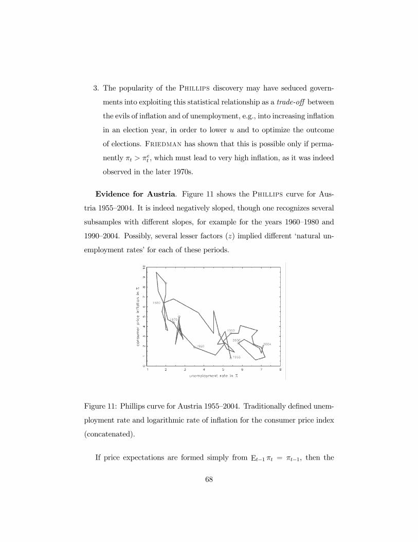
3. The popularity of the Phillips discovery may have seduced govern-
ments into exploiting this statistical relationship as a trade-o between
the evils of inßation and of unemployment, e.g., into increasing inßation
in an election year, in order to lower u and to optimize the outcome
of elections. Friedman has shown that this is possible only if perma-
nently t > et , which must lead to very high inßation, as it was indeed
observed in the later 1970s.
Evidence for Austria. Figure 11 shows the Phillips curve for Aus-
tria 1955—2004. It is indeed negatively sloped, though one recognizes several
subsamples with di erent slopes, for example for the years 1960—1980 and
1990—2004. Possibly, several lesser factors (z) implied di erent ‘natural un-
employment rates’ for each of these periods.
Figure 11: Phillips curve for Austria 1955—2004. Traditionally deÞned unem-
ployment rate and logarithmic rate of inßation for the consumer price index
(concatenated).
If price expectations are formed simply from Et 1 t = t 1, then the
68
(modiÞed) Phillips curve implies the relationship
t = t 1 + µ+ zt !ut
and one obtains a relation between changes in the rate of inßation and un-
employment rate
t t 1 = µ+ zt !ut (24)
This function, which is in the focus of the text book and which is called the
‘accelerating Phillips-curve’, is not satisfactory either, as a long-run stable
variable (u) is equated with the growth rate of inßation. Then the rate of
inßation would behave like a ‘random walk’, i.e. like a stock price, which is
not plausible. If one trusts in (24), one sees that there is a value of u, for
which the right side equals 0. Because price expectations are satisÞed for
the natural unemployment rate un, it must also hold that t 1 = t and
therefore u must equal un. Therefore, un is also called the NAIRU (non-
accelerating inßation rate of unemployment), as for this value the inßation
does not accelerate. In theory, the form of the accelerating Phillips-curve
implies a NAIRU of
un =µ+ z
!.
Because, however, z is only a catchall variable without known numerical
value, one cannot really calculate the NAIRU from this formula. Adepts
of this speciÞcation can explain changes in the NAIRU by changes in the
mark-up µ or in the bargaining power of workers z.
Note. The NAIRU formula un = (µ + z)/! coincides with the natural
rate un as determined from F (u, z) = 1/(1+µ), if one uses the approximation
1 µ = 1/(1 + µ), which is valid for a small mark-up µ.
69

Empirical evidence. For Austria, the accelerating Phillips curve
leaves a rather sad impression. A systematic negative relationship is not
visible. Note the year 1984, when the rate of inßation experienced a strong
short-term increase because of an increase in the value added tax rate on
luxury goods. A medium-run constant NAIRU cannot be calculated from
such data. Some economists assume stronger ßuctuations in the NAIRU (in
the Blanchard model, such ßuctuations would follow from changes in µ
and z), which however weakens the signiÞcance of the whole concept.
Figure 12: Accelerating variant of the Phillips curve for Austria during the
years 1955—2004.
A compromise. If price expectations are assumed to follow the speciÞ-
cation et = " t 1, one obtains the modiÞed Phillips curve
t = " t 1 + µ+ zt !ut .
In this model, there is a trade-o between inßation and unemployment, which
is however much weaker than in the classical Phillips curve. Blanchard
interprets the disappearance of the US Phillips curve as an increase in "
70
from nearly 0 to nearly 1. A statistical regression estimation for Austrian
data yields a " of around 0.6. A di erent interpretation of " views this para-
meter as the share or intensity of indexed wage contracts. Such indexation
plays a strong role during episodes of hyperinßation: if wages are indexed to
the current rate of inßation, then " can be greater 1. Others see in " t 1 a
‘core inßation’, which does not necessarily coincide with et .
Summary: Out of the AS—curve, which plots prices against output (or
the unemployment rate), Phillips created the Phillips curve, which plots
price inßations against u, even later followed a variant of the Phillips-curve,
which plots growth rates of price inßation against u. In summary, a deviation
from the natural rate un, or the NAIRU, can only be achieved, if prices
increase more strongly than it was assumed by workers who negotiate their
wages and thus their targeted real wage is not satisÞed, such that workers
are cheated upon. This is, of course, not systematically possible.
8.1 Okun’s law
Apart from the Phillips curve, another empirical relationship enjoys great
popularity among empirical macroeconomists, the so-called Okun’s law. There
is an exact one-one correspondence between natural output Yn and the nat-
ural unemployment rate un because of un = 1 Yn/L. Therefore, it would
be interesting to know how strongly deviations from natural output are re-
ßected in deviations from the natural unemployment rate. A formula due to
the economist Okun was
3(un u) =Y YnYn
(25)
Both sides are measured in percentages (%). If the unemployment rate is one
percentage point below the NAIRU, then output will be 3% above natural
71
output (or potential output).
Today, this function is usually presented in a modiÞed form:
ut ut 1 = #(gt gn) (26)
Here, gt denotes the actual growth rate of real output, while gn is its ‘natural’
growth rate. The equation assumes that, instead of ‘natural output’, there
is a natural growth rate gn, which should be around 2-3%. If output grows
at g > gn, then the unemployment rate falls. If the unemployment rate in
t 1 exactly matches the NAIRU, then it falls below the NAIRU in t. If
output (the real GDP) grows slower than gn, then the unemployment rate
rises above the NAIRU. Most authors Þnd that # > 0 is around 0.4.
Where does # come from? At low ßexibility of the labor market, at
high costs of hiring and Þring (adaptation costs), it may be rational for the
Þrms to meet an increased demand for goods with overtime work instead of
new hirings of workers and, conversely, to ‘hoard’ workers if demand is low.
Then, # will be low. If the costs of labor mobility decrease, # will rise. Many
economists Þnd that # has increased in the last 20-30 years.
Where does the natural growth rate come from? From the growth
of labor productivity. If the same input of labor can produce more goods,
output must increase more strongly, if it should generate an additional de-
mand for labor.
Evidence for Austria: For Austria, the evidence on the existence of
Okun’s law, in the above indicated form, remains unconvincing (see Figure
13). Whereas, on average, years with good economic performance indeed
have lower unemployment than years of economic slump, the autonomous
developments in the labor market dominate: the decline in the work force of
the Austrian industry, or rather a strong surge in labor productivity, 1980—
1990, and the stabilization of unemployment in the following years in spite of
72
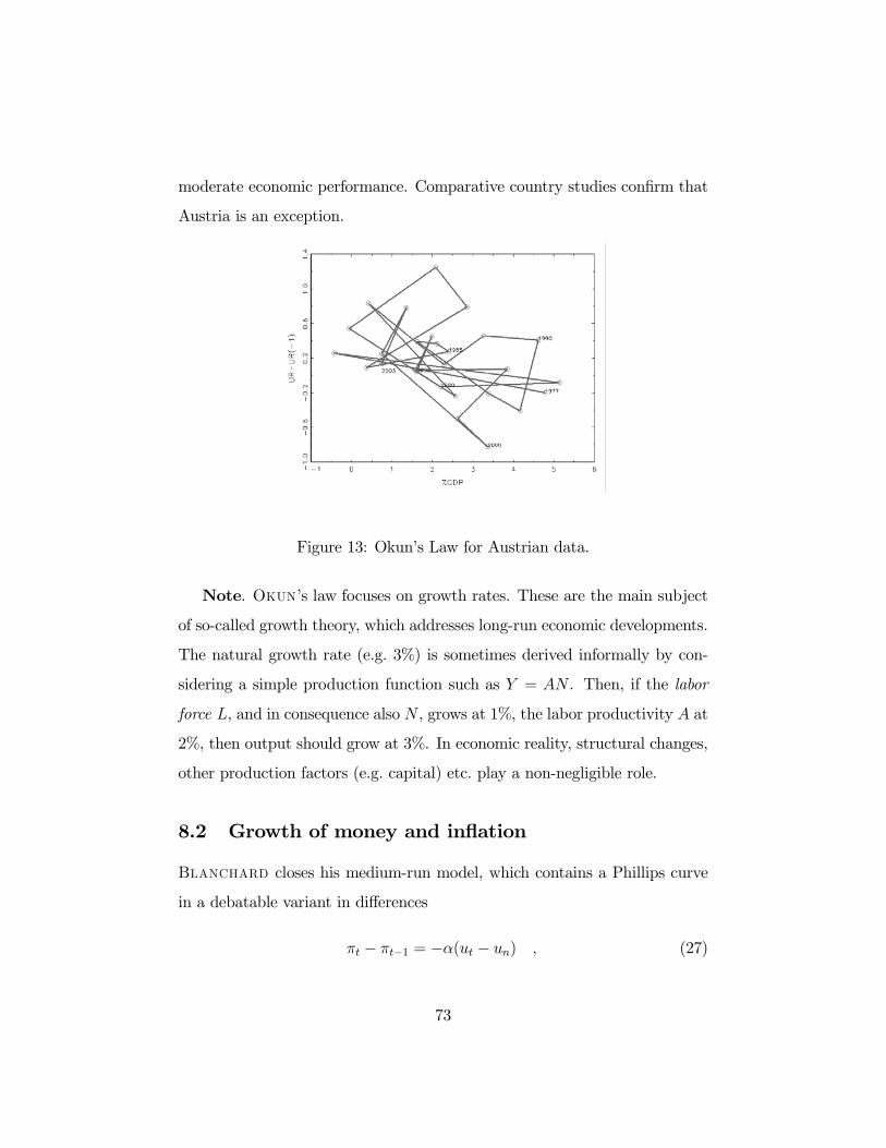
moderate economic performance. Comparative country studies conÞrm that
Austria is an exception.
Figure 13: Okun’s Law for Austrian data.
Note. Okun’s law focuses on growth rates. These are the main subject
of so-called growth theory, which addresses long-run economic developments.
The natural growth rate (e.g. 3%) is sometimes derived informally by con-
sidering a simple production function such as Y = AN . Then, if the labor
force L, and in consequence also N , grows at 1%, the labor productivity A at
2%, then output should grow at 3%. In economic reality, structural changes,
other production factors (e.g. capital) etc. play a non-negligible role.
8.2 Growth of money and inßation
Blanchard closes his medium-run model, which contains a Phillips curve
in a debatable variant in di erences
t t 1 = !(ut un) , (27)
73

and an Okun’s law
ut ut 1 = #(gt gn) , (28)
by a third equation that relates growth rates. This equation is derived from
the AD curve
Y = Y (M
P,G, T )
by simpliÞcation
Y = Y (M
P)
and by using a linear functional speciÞcation
Y = $M
P.
This yields, for constant $, the relationship among growth rates
gY,t = gM,t gP,t = gM,t t , (29)
as growth rates obey the same rules as logarithms. Here, is the growth of
prices, i.e. inßation. The growth rate of Y is written in a clearer notation as
gY , while it is denoted by g in Okun’s law.
From the three relationships, one sees that an equilibrium is obtained if
ut = un and gt = gn. Then not does not change any more, the level of
inßation is determined by the expansion path of money supply. In theory,
one could choose gM = gt and thus achieve simply = 0.
Growth rates and logarithms. If it holds that
Z = XY ,
then this implies that
logZ = logX + log Y .
74
If the 3 variables depend on time, this equation can be di erenced with
respect to time t:
d logZ
dt=
d logX
dt+d log Y
dtdZ/dt
Z=
dX/dt
X+dY/dt
Y(30)
These would be growth rates in ‘continuous time’, i.e. if time passes contin-
uously, not in jumps or intervals. For the usual discrete-time growth rates
gZ,t =Zt Zt 1Zt 1
, (31)
the formula gZ = gX + gY holds approximately only. In the longer run,
however, the time interval from t to t+1 is comparatively small, so one may
work with the approximation.
Usage of the dynamic model. The three-equations model can be used
to describe a process of disinßation. Starting from an equilibrium situation
with u = un and g = gn and therefore gM = gn + h for some h, political
forces–obviously forces in power of the money supply and therefore rather
central banks than government agencies–wish to reduce to a lower level l.
In order to do so, they reduce gM . An option would be gM = gn + l, which
can be adopted immediately and, in consequence, yields high unemployment
and low growth for a while, until eventually the new equilibrium is attained,
which is characterized by u = un, g = gn, and = l. Alternatively, one
could decrease gM gradually. Blanchard demonstrates that the sacriÞce
ratio, i.e. the ratio of additional unemployment beyond un (measured in ac-
cumulated percentage points and years) divided by the disinßation h l is
independent of whether the policy is gradual or immediate. This theorem is
true for most variants of these dynamic linear models, though not for all of
them.
75

9 The open economy
Contrary to the closed economy, the open economy communicates with the
rest of the world. It does so on three markets:
1. goods market (foreign trade): goods and (primarily touristic) ser-
vices are exported and imported. The idea that exports are good while
imports however are bad, insinuates restricting the free trade across
borders. Customs correspond to indirect taxes (goods taxes) on im-
ported goods and increase their prices (relative to domestic produc-
tion), quotas (rationing) limit the imported quantity of certain goods.
International tendency toward abolition of all restrictions on goods
trade.
2. Þnancial market (capital mobility): bonds, shares, and other do-
mestic securities are bought by non-residents, then interest and div-
idends are paid to non-residents. Austrians buy, e.g., foreign shares
and receive dividends from abroad. Increasing international tendency
toward abolition of all restrictions on such action.
3. labor market: international wage di erentials cause migration (im-
migration = inward migration, emigration = outward migration) and
the re-allocation of productive capital to countries with a low wage
level. In the EU-15 area (in theory) no restriction, worldwide strict
limits on migration.
The increasing openness of economies has advantages (higher welfare by
international division of labor) and disadvantages (loss of national auton-
omy, above all, of economic policy, ‘exposure’ to international crises). Most
economists agree that advantages dominate by far.
76

9.1 Stylized facts of the open goods market
Import ratio (imports/GDP) and export ratio (exports/GDP) increase
over time in most countries. Both ratios develop roughly in parallel move-
ments (Reasons: tendency toward a balanced current account, increase of
transit-like ßows: imported goods are re-exported after minor modiÞcations).
Because only net exports X Im contribute to GDP, import and export
ratios may exceed 1 and do so in some trade-oriented small economies (Sin-
gapore).
Figure 14: Import and export ratios for Austria 1976—2004.
The Austrian ratios are close to 50% now. In the longer run, exports and
imports increase faster than GDP, the share of imported durable consumer
goods and of imported investment goods for equipment investment is par-
ticularly high (and rising). Non-durable consumer goods are imported less
intensely, goods for construction investment the least.
Main trading partner of Austria is Germany (around 42% of exports
and imports), followed by Italy (more than 8%). Further important partners
77

are Switzerland, France, the USA, the United Kingdom, and Hungary (each
3—5%). Minor ßuctuations of trade shares are mainly due to changes in the
exchange rate. Major shifts often have other explanations. For example,
from Figure 15, note the drastic fall of the UK share in the 1970s, which may
be due to the British switch to the European Community from a common
economic area with Austria in the EFTA, and the fall of the Japanese share
in the 1990s, when Austria joined the European Union. By contrast, note
from Figure 16 that the German trade share is subject to minor ßuctuations
only.
Figure 15: Shares of selected countries in Austrian imports for the time range
1960—2004. Annual data.
78

Figure 16: Share of Germany in Austrian imports 1964—2004. Monthly data.
9.2 Nominal and real exchange rates
One currency does not have an exchange rate, this word is always related to
two currencies, e.g., euro and US dollar. From the viewpoint of the domes-
tic economy (Austria), the nominal exchange rate (E) is deÞned as the
quantity of dollars that is paid for one euro. The larger this value, the more
dollars must be paid and the higher is the value of the euro and the lower
is the value of the dollar. [Pure convention; this corresponds to the current
o!cial euro rates that are quoted in newspapers. You may remember Þgures
like 12 and 18 from the schilling era, which denoted the amount of schilling
that buy one dollar; this is exactly the reverse idea 1/E. In case you use
an older edition of Blanchard’s book, note that the convention di ered in
editions #1 to #3.]
The real exchange rate (%) tries to measure the exchange rate ßuctu-
79

ations on the basis of a Þxed good or basket of goods in ‘real’ terms. This
is only a theoretical variable, as there are, in the real world, many di erent
goods with diverse price movements (indexes in the domestic and in the for-
eign economy contain di erent goods and di erent weights). Formally, % is
deÞned by
% =EP
P !, (32)
where P denotes the domestic price level, P ! the foreign price level (formally,
in foreign currency). The numerator EP and the denominator P ! represent
prices that are both measured in the foreign currency (e.g., dollars or sterling
in Austria). Alternatively, you may consider P and P !/E, both priced in
the domestic currency.
If the price of the domestic currency decreases in the foreign currency, i.e.
if the nominal exchange rate falls, this is called a (nominal) depreciation. If
the price of foreign goods in domestic currency P !/E increases faster than
the price of domestic goods, this is a real depreciation. Thus, at low
inßation in Austria and higher inßation on the ‘world market’ there is a real
depreciation, even if the nominal exchange rate is constant.
If the price of the domestic currency increases, i.e. the nominal exchange
rate rises, this is called a (nominal) appreciation. A relatively high inßation
in Austria or a price reduction on the world market and constant nominal
exchange rate would imply a real appreciation. [There is a di erence be-
tween deliberate exchange rate changes as a policy instrument, devaluation
and revaluation, and normal market ßuctuations, depreciation and appre-
ciation. Note the ambiguity of ‘depreciation’ as exchange rate change and
consumption of Þxed capital]
real e ective exchange rate: a weighted average that is formed over
all real exchange rates of an open economy (with all trading partners), with
80

all weights determined by the share in the trade volume (average of export
and import), yields the real e ective exchange rate. Currently, two variants
are reported: one index uses consumer prices for basket deßators P ! and P ,
the other one uses labor costs.
Figure 17: Nominal and real exchange rates for Austria. Exchange rate
measured in US dollar per 100 euros or equivalent in Austrian schillings.
Is a real appreciation good or bad? Real appreciation implies a
stronger rise of domestic prices than of world market prices or a nominal
appreciation. This makes exporting more di!cult and decreases the price
competitiveness. On the other hand does an increase of export prices (not
of domestic prices per se) indicate that exporters are able to sell their goods
at a high price because of the high quality of their products. A real apprecia-
tion may indicate an increased non-price competitiveness of the domestic
economy. In any case does a real appreciation exert an incentive for qual-
ity improvement and rationalization (productivity increases) in the exporting
sector of the economy. [For a real depreciation, the opposite arguments hold.]
81
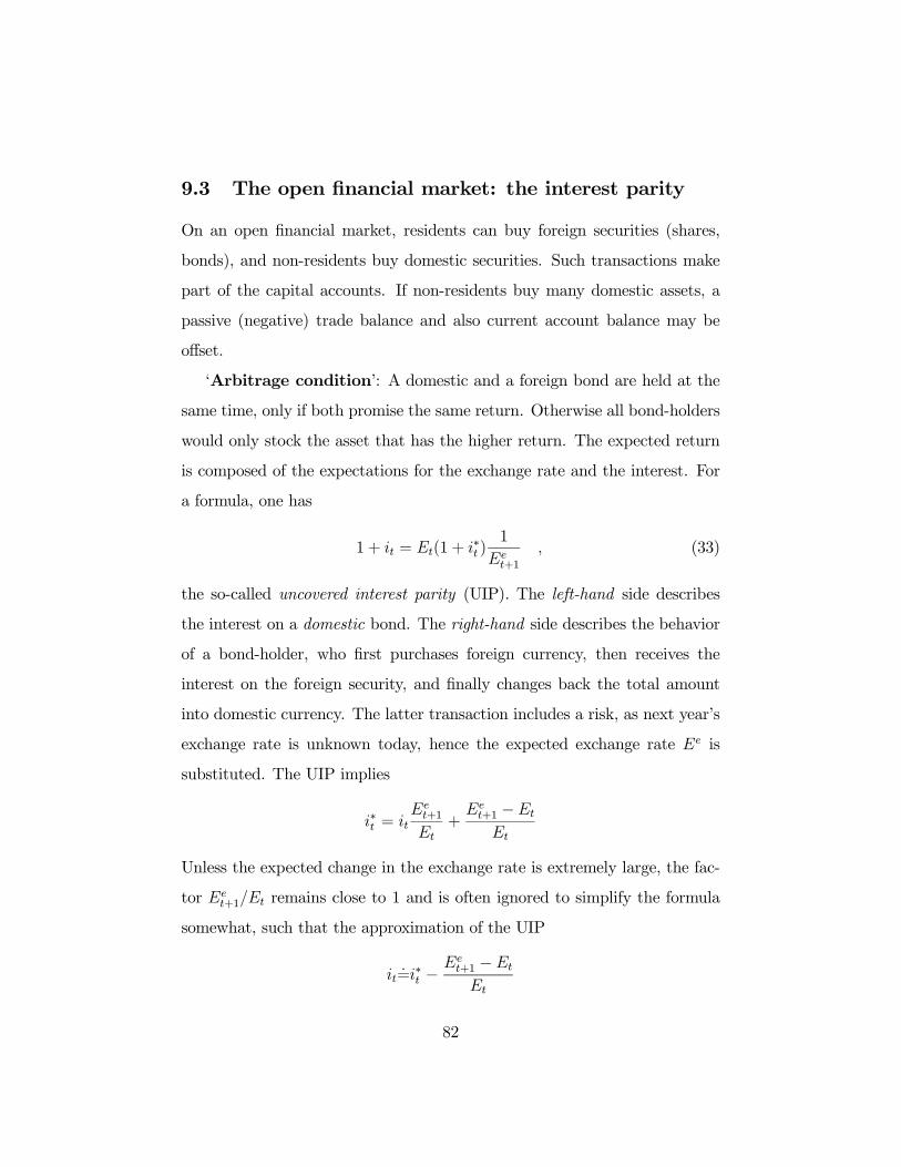
9.3 The open Þnancial market: the interest parity
On an open Þnancial market, residents can buy foreign securities (shares,
bonds), and non-residents buy domestic securities. Such transactions make
part of the capital accounts. If non-residents buy many domestic assets, a
passive (negative) trade balance and also current account balance may be
o set.
‘Arbitrage condition’: A domestic and a foreign bond are held at the
same time, only if both promise the same return. Otherwise all bond-holders
would only stock the asset that has the higher return. The expected return
is composed of the expectations for the exchange rate and the interest. For
a formula, one has
1 + it = Et(1 + i
t )1
Eet+1, (33)
the so-called uncovered interest parity (UIP). The left-hand side describes
the interest on a domestic bond. The right-hand side describes the behavior
of a bond-holder, who Þrst purchases foreign currency, then receives the
interest on the foreign security, and Þnally changes back the total amount
into domestic currency. The latter transaction includes a risk, as next year’s
exchange rate is unknown today, hence the expected exchange rate Ee is
substituted. The UIP implies
i t = itEet+1Et
+Eet+1 Et
Et
Unless the expected change in the exchange rate is extremely large, the fac-
tor Eet+1/Et remains close to 1 and is often ignored to simplify the formula
somewhat, such that the approximation of the UIP
it ú=i
t Eet+1 Et
Et
82

is often used.
Expected depreciation of the domestic currency causes a negative ratio
(Eet+1 Et)/Et and thus a relatively higher interest in the domestic economy,
expected appreciation means a higher interest abroad. In some countries
with a strong expectation of depreciation, the relation is seemingly violated,
as there an even higher return must be o ered to compensate for the high
risk of such bonds.
9.4 The open goods market
In an open economy, the demand for domestic goods is given by
Z = C + I +G Im / +X (34)
with exports X and imports Im. The correction factor 1/ indicates that
foreign goods in imports Im di er from domestic goods in their value. In the
National Accounts, of course, Im / is booked as ‘real imports’.
Domestic demand C + I +G follows the hitherto used pattern
C(YD) + I(Y, r) + G (35)
The import function (import demand)
Im = Im(Y, ) (36)
(+,+)
lets imports depend positively on domestic demand, without decomposition
into imports by particular demand categories, and positively on the real
exchange rate. The latter reaction stems from the fact that, at a higher ,
foreign goods are relatively cheaper and tend to substitute domestic goods.
83

The export function (export demand)
X = X(Y , ) (37)
(+, )
lets exports depend positively on foreign demand Y (demand on the world
market), and negatively on the real exchange rate, as a real depreciation
makes exported goods cheaper and more competitive.
Note that imports depend positively on income, while exports do not
react to Y . Therefore, at low Y net exports NX = X Im / are positive,
and at high Y net exports are negative. Therefore, to every given there
is an income YTB, at which the trade balance is exactly equalized. This
YTB need not correspond to the equilibrium on the domestic goods market.
For example, it seems that the US goods market is in its equilibrium at a
passive trade balance, i.e. the domestic economy demands more than YTB
NX(YTB). Currently, the Austrian foreign trade may be balanced.
Thought experiment 1: Increase of demand.
1. Increase of G (expansionary Þscal policy) raises imports Im / , how-
ever not by not the same amount. Therefore, higher Y results, with
multiplier e ects in I and C likewise reßected in imports. Y increases,
X does not change, Im / increases, while NX falls. Therefore, the
trade balance becomes more passive. A part of the multiplier e ect is
satisÞed by imported goods.
2. Increase of foreign demand Y raises exports X. Although the addi-
tional demand in NX and thus in Y is satisÞed partly by imports,
there remains a positive net e ect. The trade balance becomes more
active, income increases.
84
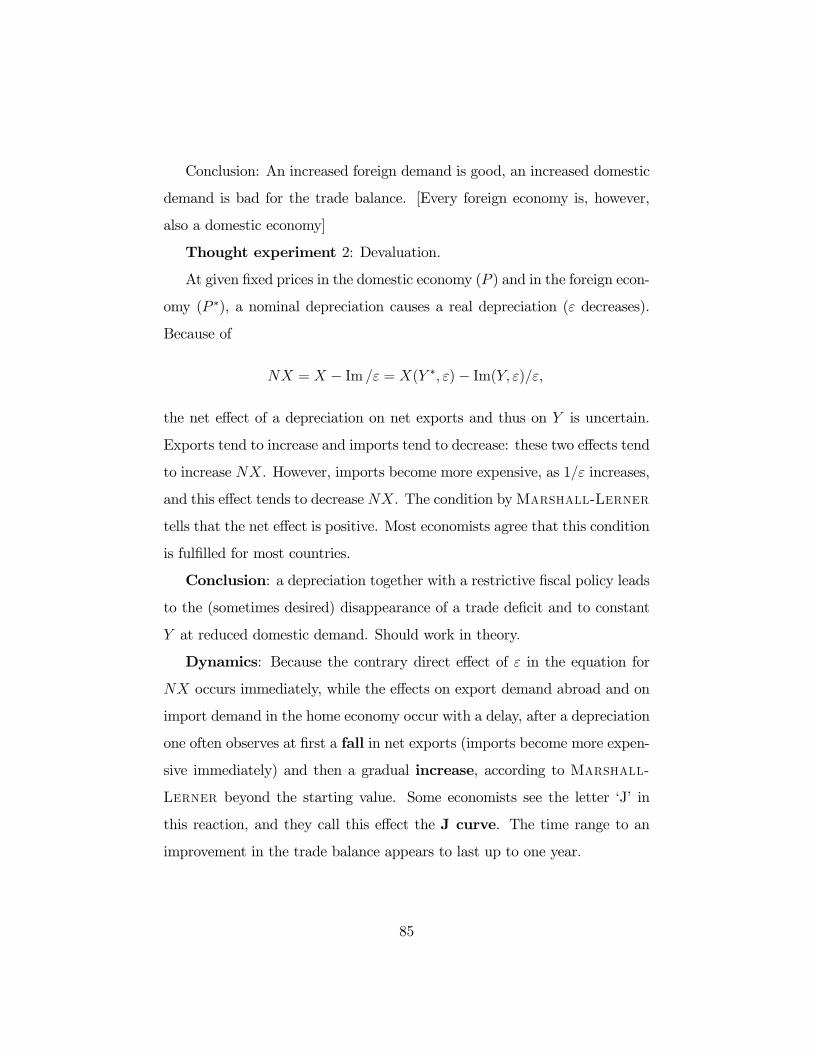
Conclusion: An increased foreign demand is good, an increased domestic
demand is bad for the trade balance. [Every foreign economy is, however,
also a domestic economy]
Thought experiment 2: Devaluation.
At given Þxed prices in the domestic economy (P ) and in the foreign econ-
omy (P ), a nominal depreciation causes a real depreciation ( decreases).
Because of
NX = X Im / = X(Y , ) Im(Y, )/ ,
the net e ect of a depreciation on net exports and thus on Y is uncertain.
Exports tend to increase and imports tend to decrease: these two e ects tend
to increase NX. However, imports become more expensive, as 1/ increases,
and this e ect tends to decrease NX. The condition byMarshall-Lerner
tells that the net e ect is positive. Most economists agree that this condition
is fulÞlled for most countries.
Conclusion: a depreciation together with a restrictive Þscal policy leads
to the (sometimes desired) disappearance of a trade deÞcit and to constant
Y at reduced domestic demand. Should work in theory.
Dynamics: Because the contrary direct e ect of in the equation for
NX occurs immediately, while the e ects on export demand abroad and on
import demand in the home economy occur with a delay, after a depreciation
one often observes at Þrst a fall in net exports (imports become more expen-
sive immediately) and then a gradual increase, according to Marshall-
Lerner beyond the starting value. Some economists see the letter ‘J’ in
this reaction, and they call this e ect the J curve. The time range to an
improvement in the trade balance appears to last up to one year.
85

9.5 Investment and saving in an open economy
In a closed economy, the simple identities SH + T G = I or SH + SP = I
hold. In an open economy, it follows from the identity
Y = C + I +G Im / +X
after subtraction of C + T on both sides that
Y C T = SH = I +G T Im / +X
or
SH + SP NX = I .
Investment equals the sum of 3 positions: household saving, government
saving, and the negative trade balance. The third position expresses Þnancing
of investment by net imports and therefore by foreign debt.
Conclusion: Countries with a high household-saving rate and budget
surplus either have a positive trade balance or invest very much. A higher
budget deÞcit is either compensated by more household saving, less invest-
ment, or a deÞcit in the trade balance.
Even this identity is an ex post—identity only and does not describe a
behavioral mechanism. For example, it is not recognizable that a depreciation
or appreciation indeed a ect the trade balance, although it seems that NX
is deÞned by SH + SP I. The change of implies a change in demand and
a ects both SH and I.
9.6 The IS-LM—model in the open economy
Mundell-Fleming model. The analysis of economic policy in an open
economy on the basis of the IS-LM diagram with the cases of ßexible and Þxed
86

exchange rates is due to Mundell (Nobel prize) and Fleming. Besides the
usual (Y, i) diagram, one often uses (not in Blanchard) the representation
in the (Y,E)—world.
While the LM equation of the closed economy
M
P= Y L(i)
continues to hold in the open economy, there are important changes to the
IS equation for equilibria in the goods market (for simpliÞcation, written in
the nominal interest rate i, i.e. for !e = 0)
Y = C(Y T ) + I(Y, i) +G+NX(Y, Y , )
and there is the interest parity (in the exact form)
Et =1 + it1 + i t
Eet+1
At a given expected exchange rate Eet+1 = Ee, one may express E as
E =1 + it1 + i t
Ee. (38)
Assuming additionally that, at least in the short run, P and P do not move,
one may substitute this expression for the (nominal) exchange rate instead
of the real exchange rate in the IS equation:
Y = C(Y T ) + I(Y, i) +G+NX(Y, Y ,1 + i
1 + i Ee)
and one obtains a negatively sloped IS curve in the (Y, i) diagram. Because
a higher interest rate negatively a ects both investment and net exports (i
is in the numerator of the last expression, E and therefore increases and
thus NX falls by ‘appreciation’), one may think that the curve would be
‘ßatter’ than in a closed economy and monetary policy would have stronger
87

e ects. The intersection of the LM and IS curve does not only determine an
equilibrium pair (Y, i), but also an equilibrium exchange rate.
Þscal policy in the open economy. The change in public demand
causes a shift of the IS curve at a rigid LM curve. For example, expan-
sionary Þscal policy. Both Y and i rise. The higher interest rate causes an
appreciation because of (38), i.e. E increases. In summary, private consump-
tion increases (depends directly on Y ), while the behavior of investment is
uncertain (higher Y , but also higher i), and net exports fall (Marshall-
Lerner). In other words, the trade balance deteriorates.
Monetary policy in the open economy. The change in the money
supply causes a shift of the LM curve at rigid IS curve. For example, expan-
sionary monetary policy. Y rises, but i falls. The lower interest rate causes
a depreciation, E falls. Private consumption, investment, and net exports
increase. This apparently ideal case includes, of course, the risk of inßation.
Fixed exchange rate. For diverse reasons, e.g., to eliminate exchange
rate risk, it may seem attractive to keep the nominal exchange rate E Þxed.
The UIP determines the interest rate i uniquely, as i and Ee are exogenous.
Therefore, at a Þxed exchange rate there is no independent monetary policy
any more, this policy instrument is no more available. Because E and Ee
must coincide in the longer run, one sees from the UIP that i = i must
hold, i.e. there is only one ‘international’ interest rate. The advantages of a
Þxed exchange rate, such as easing of border-crossing trade with its welfare-
increasing e ect, must be gauged against the disadvantage of abandoning
monetary policy as an instrument of economic policy.
Narrow-sense model cases of Mundell-Fleming. While in the
Blanchard variant with ßexible exchange rate, the expected exchange rate
Ee is exogenous and Þxed, which entails certain logical problems, Mundell-
88
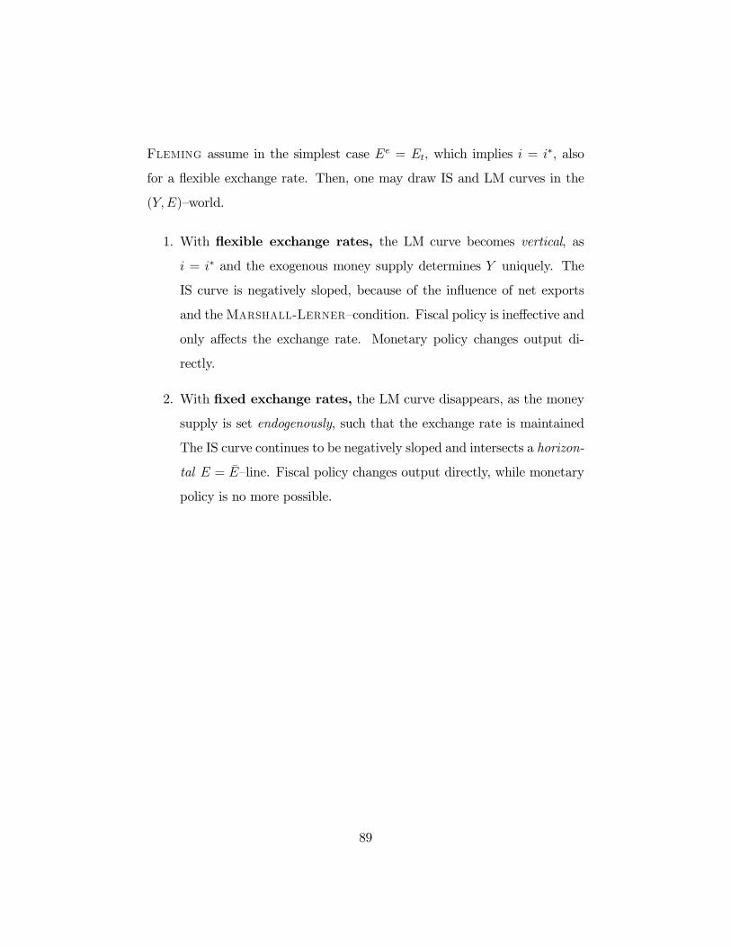
Fleming assume in the simplest case Ee = Et, which implies i = i , also
for a ßexible exchange rate. Then, one may draw IS and LM curves in the
(Y,E)—world.
1. With ßexible exchange rates, the LM curve becomes vertical, as
i = i and the exogenous money supply determines Y uniquely. The
IS curve is negatively sloped, because of the inßuence of net exports
and theMarshall-Lerner—condition. Fiscal policy is ine ective and
only a ects the exchange rate. Monetary policy changes output di-
rectly.
2. With Þxed exchange rates, the LM curve disappears, as the money
supply is set endogenously, such that the exchange rate is maintained
The IS curve continues to be negatively sloped and intersects a horizon-
tal E = E—line. Fiscal policy changes output directly, while monetary
policy is no more possible.
89
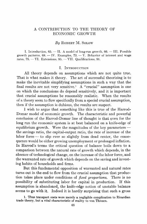
A CONTRIBUTION TO THE THEORY OF ECONOMIC GROWTH
By ROBERT M. SOLOW
I. Introduction, 65. - II. A model of long-run growth, 66. - III. Possible growth patterns, 68. - IV. Examples, 73. - V. Behavior of interest and wage rates, 78. - VI. Extensions, 85. - VIT. Qualifications, 91.
I. INTRODUCTION
All theory depends on assumptions which are not quite true. That is what makes it theory. The art of successful theorizing is to make the inevitable simplifying assumptions in such a way that the final results are not very sensitive.' A "crucial" assumption is one on which the conclusions do depend sensitively, and it is important that crucial assumptions be reasonably realistic. When the results of a theory seem to flow specifically from a special crucial assumption, then if the assumption is dubious, the results are suspect.
1 wish to argue that something like this is true of the Harrod- Domar model of economic growth. The characteristic and powerful conclusion of the Harrod-Domar line of thought is that even for the long run the economic system is at best balanced on a knife-edge of equilibrium growth. Were the magnitudes of the key parameters the savings ratio, the capital-output ratio, the rate of increase of the labor force - to slip ever so slightly from dead center, the conse- quence would be either growing unemployment or prolonged inflation. In Harrod's terms the critical question of balance boils down to a comparison between the natural rate of growth which depends, in the absence of technological change, on the increase of the labor force, and the warranted rate of growth which depends on the saving and invest- ing habits of households and firms.
But this fundamental opposition of warranted and natural rates turns out in the end to flow from the crucial assumption that produc- tion takes place under conditions of fixed proportions. There is no possibility of substituting labor for capital in production. If this assumption is abandoned, the knife-edge notion of unstable balance seems to go with it. Indeed it is hardly surprising that such a gross
1. Thus transport costs were merely a negligible complication to Ricardian trade theory, but a vital characteristic of reality to von Thunen.
65

66 QUARTERLY JOURNAL OF ECONOMICS
rigidity in one part of the system should entail lack of flexibility in another.
A remarkable characteristic of the Harrod-Domar model is that it consistently studies long-run problems with the usual short-run tools. One usually thinks of the long run as the domain of the neo- classical analysis, the land of the margin. Instead Harrod and Domar talk of the long run in terms of the multiplier, the accelerator, "the" capital coefficient. The bulk of this paper is devoted to a model of long-run growth which accepts all the Harrod-Domar assumptions except that of fixed proportions. Instead I suppose that the single composite commodity is produced by labor and capital under the standard neoclassical conditions. The adaptation of the system to an exogenously given rate of increase of the labor force is worked out in some detail, to see if the Harrod instability appears. The price-wage- interest reactions play an important role in this neoclassical adjust- ment process, so they are analyzed too. Then some of the other rigid assumptions are relaxed slightly to see what qualitative changes result: neutral technological change is allowed, and an interest-elastic savings schedule. Finally the consequences of certain more "Keynes- ian" relations and rigidities are briefly considered.
II. A MODEL OF LONG-RUN GROWTH
There is only one commodity, output as a whole, whose rate of production is designated Y(t). Thus we can speak unambiguously of the community's real income. Part of each instant's output is consumed and the rest is saved and invested. The fraction of output saved is a constant s, so that the rate of saving is sY(t). The com- munity's stock of capital K(t) takes the form of an accumulation of the composite commodity. Net investment is then just the rate of
increase of this capital stock dK/dt or K, so we have the basic identity at every instant of time: (1) K = sY.
Output is produced with the help of two factors of production, capital and labor, whose rate of input is L(t). Technological possi- bilities are represented by a production function
(2) Y = F(K,L).
Output is to be understood as net output after making good the depre- ciation of capital. About production all we will say at the moment is

THE THEORY OF ECONOMIC GROWTH 67
that it shows constant returns to scale. Hence the production func- tion is homogeneous of first degree. This amounts to assuming that there is no scarce nonaugmentable resource like land. Constant returns to scale seems the natural assumption to make in a theory of growth. The scarce-land case would lead to decreasing returns to scale in capital and labor and the model would become more Ricardian.2
Inserting (2) in (1) we get
(3) K = sF(K,L).
This is one equation in two unknowns. One way to close the system would be to add a demand-for-labor equation: marginal physical productivity of labor equals real wage rate; and a supply-of-labor equation. The latter could take the general form of making labor supply a function of the real wage, or more classically of putting the real wage equal to a conventional subsistence level. In any case there would be three equations in the three unknowns K, L, real wage.
Instead we proceed more in the spirit of the Harrod model. As a result of exogenous population growth the labor force increases at a constant relative rate n. In the absence of technological change n is Harrod's natural rate of growth. Thus:
(4) L(t) = Loent.
In (3) L stands for total employment; in (4) L stands for the available supply of labor. By identifying the two we are assuming that full employment is perpetually maintained. When we insert (4) in (3) to get (5) K sFE(K,Loee )
we have the basic equation which determines the time path of capital accumulation that must be followed if all available labor is to be employed.
Alternatively (4) can be looked at as a supply curve of labor. It says that the exponentially growing labor force is offered for employ- ment completely inelastically. The labor supply curve is a vertical
2. See, for example, Haavelmo: A Study in the Theory of Economic Evolution (Amsterdam, 1954), pp. 9-11. Not all "underdeveloped" countries are areas of land shortage. Ethiopia is a counterexample. One can imagine the theory as applying as long as arable land can be hacked out of the wilderness at essentially constant cost.

68 QUARTERLY JOURNAL OF ECONOMICS
line which shifts to the right in time as the labor force grows according to (4). Then the real wage rate adjusts so that all available labor is employed, and the marginal productivity equation determines the wage rate which will actually rule.3
In summary, (5) is a differential equation in the single variable K(t). Its solution gives the only time profile of the community's capital stock which will fully employ the available labor. Once we know the time path of capital stock and that of the labor force, we can compute from the production function the corresponding time path of real output. The marginal productivity equation determines the time path of the real wage rate. There is also involved an assumption of full employment of the available stock of capital. At any point of time the pre-existing stock of capital (the result of previous accumula- tion) is inelastically supplied. Hence there is a similar marginal productivity equation for capital which determines the real rental per unit of time for the services of capital stock. The process can be viewed in this way: at any moment of time the available labor supply is given by (4) and the available stock of capital is also a datum. Since the real return to factors will adjust to bring about full employment of labor and capital we can use the production function (2) to find the current rate of output. Then the propensity to save tells us how much of net output will be saved and invested. Hence we know the net accumulation of capital during the current period. Added to the already accumulated stock this gives the capital available for the next period, and the whole process can be repeated.
III. POSSIBLE GROWTH PATTERNS
To see if there is always a capital accumulation path consistent with any rate of growth of the labor force, we must study the differen- tial equation (5) for the qualitative nature of its solutions. Naturally without specifying the exact shape of the production function we can't hope to find the exact solution. But certain broad properties are surprisingly easy to isolate, even graphically.
K To do so we introduce a new variable r _ -, the ratio of capital
to labor. Hence we have K = rL = rLoent. Differentiating with respect to time we get
K = Loentr + nrLoen
3. The complete set of three equations consists of (3), (4) and ()= w. oL

THE THEORY OF ECONOMIC GROWTH 69
Substitute this in (5):
(r + nr)Loe"t = sF(K,Loe't).
But because of constant returns to scale we can divide both variables in F by L = Loent provided we multiply F by the same factor. Thus
(r' + nr)Loent = sLbentF ( Loet ' 1)
and dividing out the common factor we arrive finally at
(6) r = sF(r,1) - nr.
Here we have a differential equation involving the capital-labor ratio alone.
This fundamental equation can be reached somewhat less K
formally. Since r = -, the relative rate of change of r is the difference
between the relative rates of change of K and L. That is:
r K L r K L
Now first of all L = n. Secondly K = sF(K,L). Making these sub- L
stitutions: - sF(K,L) r-=r -nr.
K
Now divide L out of F as before, note that L= 1 and we get (6) again. K r
The function F(r, 1) appearing in (6) is easy to interpret. It is the total product curve as varying amounts r of capital are employed with one unit of labor. Alternatively it gives output per worker as a function of capital per worker. Thus (6) states that the rate of change of the capital-labor ratio is the difference of two terms, one representing the increment of capital and one the increment of labor.
When i = 0, the capital-labor ratio is a constant, and the capital stock must be expanding at the same rate as the labor force, namely n.

70 QUARTERLY JOURNAL OF ECONOMICS
(The warranted rate of growth, warranted by the appropriate real rate of return to capital, equals the natural rate.) In Figure I, the ray through the origin with slope n represents the function nr. The other curve is the function sF(r,l). It is here drawn to pass through the origin and convex upward: no output unless both inputs are positive, and diminishing marginal productivity of capital, as would be the case, for example, with the Cobb-Douglas function. At the point of intersection nr = sF(r,l) and r = 0. If the capital-labor ratio r* should ever be established, it will be maintained, and capital and labor will grow thenceforward in proportion. By constant returns to
or~~~~~~~~~~~~~~~~ r
s F(rI1)
r* FIGURE I
scale, real output will also grow at the same relative rate n, and out- put per head of labor force will be constant.
But if r $ r*, how will the capital-labor ratio develop over time? To the right of the intersection point, when r > r*, nr > sF(r, 1) and from (6) we see that r will decrease toward r*. Conversely if initially r < r*, the graph shows that nr < sF(r,l), r > 0, and r will increase toward r*. Thus the equilibrium value r* is stable. Whatever the initial value of the capital-labor ratio, the system will develop toward a state of balanced growth at the natural rate. The time path of capital and output will not be exactly exponential except asymptoti- cally.4 If the initial capital stock is below the equilibrium ratio,
4. There is an exception to this. If K = 0, r = 0 and the system can't get started; with no capital there is no output and hence no accumulation. But this
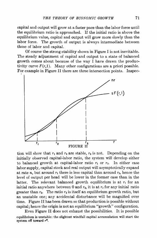
THE THEORY OF ECONOMIC GROWTH 71
capital and output will grow at a faster pace than the labor force until the equilibrium ratio is approached. If the initial ratio is above the equilibrium value, capital and output will grow more slowly than the labor force. The growth of output is always intermediate between those of labor and capital.
Of course the strong stability shown in Figure I is not inevitable. The steady adjustment of capital and output to a state of balanced growth comes about because of the way I have drawn the produc- tivity curve F(r,1). Many other configurations are a priori possible. For example in Figure II there are three intersection points. Inspec-
nr
s F (r, i)
/~~~~r r - 1 1~~~-
r, F2 F3 r FIGURE II
tion will show that ri and r3 are stable, r2 is not. Depending on the initially observed capital-labor ratio, the system will develop either to balanced growth at capital-labor ratio ri or r3. In either case labor supply, capital stock and real output will asymptotically expand at rate n, but around ri there is less capital than around r3, hence the level of output per head will be lower in the former case than in the latter. The relevant balanced growth equilibrium is at ri for an initial ratio anywhere between 0 and r2, it is at r3 for any initial ratio greater than r2. The ratio r2 is itself an equilibrium growth ratio, but an unstable one; any accidental disturbance will be magnified over time. Figure II has been drawn so that production is possible without capital; hence the origin is not an equilibrium "growth" configuration.
Even Figure II does not exhaust the possibilities. It is possible equilibrium is unstable: the slightest windfall capital accumulation will start the system off toward r*.

72 QUARTERLY JOURNAL OF ECONOMICS
that no balanced growth equilibrium might exist.5 Any nondecreasing function F(r,1) can be converted into a constant returns to scale production function simply by multiplying it by L; the reader can construct a wide variety of such curves and examine the resulting solutions to (6). In Figure III are shown two possibilities, together
r s, F'(r, I)
n r
S 2F2(r,1)
FIGURE III
with a ray nr. Both have diminishing marginal productivity through- out, and one lies wholly above nr while the other lies wholly below.6 The first system is so productive and saves so much that perpetual full employment will increase the capital-labor ratio (and also the output per head) beyond all limits; capital and income both increase
5. This seems to contradict a theorem in R. M. Solow and P. A. Samuelson: "Balanced Growth under Constant Returns to Scale," Econometrica, XXI (1953), 412-24, but the contradiction is only apparent. It was there assumed that every commodity had positive marginal productivity in the production of each com- modity. Here capital cannot be used to produce labor.
6. The equation of the first might be s1F1(r,1) = nr + Vr], that of the second
s2F2(r,1) =r rur1
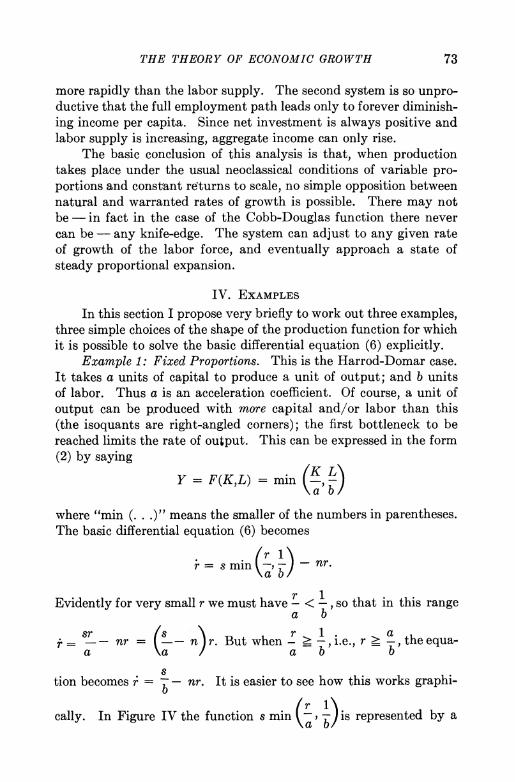
THE THEORY OF ECONOMIC GROWTH 73
more rapidly than the labor supply. The second system is so unpro- ductive that the full employment path leads only to forever diminish- ing income per capita. Since net investment is always positive and labor supply is increasing, aggregate income can only rise.
The basic conclusion of this analysis is that, when production takes place under the usual neoclassical conditions of variable pro- portions and constant retturns to scale, no simple opposition between natural and warranted rates of growth is possible. There may not be -in fact in the case of the Cobb-Douglas function there never can be - any knife-edge. The system can adjust to any given rate of growth of the labor force, and eventually approach a state of steady proportional expansion.
IV. EXAMPLES
In this section I propose very briefly to work out three examples, three simple choices of the shape of the production function for which it is possible to solve the basic differential equation (6) explicitly.
Example 1: Fixed Proportions. This is the Harrod-Domar case. It takes a units of capital to produce a unit of output; and b units of labor. Thus a is an acceleration coefficient. Of course, a unit of output can be produced with more capital and/or labor than this (the isoquants are right-angled corners); the first bottleneck to be reached limits the rate of output. This can be expressed in the form (2) by saying
Y = F(KL) = min L
where "min (. . .)" means the smaller of the numbers in parentheses. The basic differential equation (6) becomes
r 1 r=s min -- Jnr.
Evidently for very small r we must have - , so that in this range a b
-- nr (L-n ')a r = sr _ Or = (--n~r. But when?r _ 1 > i.e._ r > -, theequa-
a a a b
tion becomes i = b- nr. It is easier to see how this works graphi-
cally. In Figure IV the function s min (-, -)is represented by a
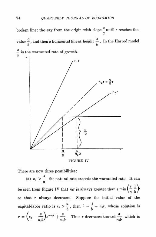
74 QUARTERLY JOURNAL OF ECONOMICS
broken line: the ray from the origin with slope -until r reaches the a
value -, and then a horizontal line at height -. In the Harrod model b b
8 is the warranted rate of growth.
a r
n, r
i ~ ~ ~ ~~~~~~~~ / l2r =-
/ X ~~~~~~~n3r
/
-a sr b n
FIGURE IV
There are now three possibilities: 8
(a) ni > -, the natural rate exceeds the warranted rate. It can a
be seen from Figure IV that nir is always greater than s min (-' !)' so that r always decreases. Suppose the initial value of the
a .
capital-labor ratio is ro > - then r = - - nor, whose solution is b ~~~b
r = (ro --) ni +t Thus r decreases toward which is nib nib nib

THE THEORY OF ECONOMIC GROWTH 75
in turn less than -. At an easily calculable point of time tj, r reaches
a . s Na (:'n ) (t-t b From then on r = (--nl} r, whose solutionis r = - e a 1 1).
8 a Since - < ni, r will decrease toward zero. At time ti, when r = -
a b
the labor supply and capital stock are in balance. From then on as the capital-labor ratio decreases labor becomes redundant, and the extent of the redundancy grows. The amount of unemployment can be calculated from the fact that K = rLoent remembering that, when
capital is the bottleneck factor, output is - and employment is b K
a a
(b) n2 =-, the warranted and natural rates are equal. If initially a
a a r > - so that labor is the bottleneck, then r decreases to - and stays
b Ib
there. If initially r < - then r remains constant over time, in a sort
of neutral equilibrium. Capital stock and labor supply grow at a common rate n2; whatever percentage redundancy of labor there was initially is preserved.
(c) n3 <-, the warranted rate exceeds the natural rate. For- a
mally the solution is exactly as in case (a) with n3 replacing ni.
There is a stable equilibrium capital output ratio at r = -. But
here capital is redundant as can be seen from the fact that the mar- ginal productivity of capital has fallen to zero. The proportion of
the capital stock actually employed in equilibrium growth is-
But since the capital stock is growing (at a rate asymptotically equal to n3) the absolute amount of excess capacity is growing, too. This appearance of redundancy independent of any price-wage move- ments is a consequence of fixed proportions, and lends the Harrod- Domar model its characteristic of rigid balance.
At the very least one can imagine a production function such
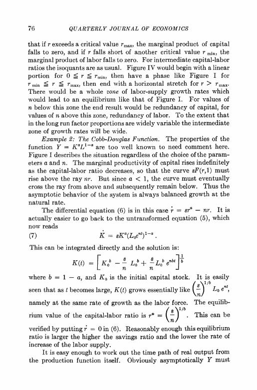
76 QUARTERLY JOURNAL OF ECONOMICS
that if r exceeds a critical value rmax, the marginal product of capital falls to zero, and if r falls short of another critical value r mi, the marginal product of labor falls to zero. For intermediate capital-labor ratios the isoquants are as usual. Figure IV would begin with a linear portion for 0 < r ? r then have a phase like Figure I for rmin _ r _ rmax, then end with a horizontal stretch for r > rmax There would be a whole zone of labor-supply growth rates which would lead to an equilibrium like that of Figure I. For values of n below this zone the end result would be redundancy of capital, for values of n above this zone, redundancy of labor. To the extent that in the long run factor proportions are widely variable the intermediate zone of growth rates will be wide.
Example 2: The Cobb-Douglas Function. The properties of the function Y = KaLl-a are too well known to need comment here. Figure I describes the situation regardless of the choice of the param- eters a and n. The marginal productivity of capital rises indefinitely as the capital-labor ratio decreases, so that the curve sF(r,1) must rise above the ray nr. But since a < 1, the curve must eventually cross the ray from above and subsequently remain below. Thus the asymptotic behavior of the system is always balanced growth at the natural rate.
The differential equation (6) is in this case r=sra - nr. It is actually easier to go back to the untransformed equation (5), which now reads
(7) K = sKa(Loent)l-a.
This can be integrated directly and the solution is:
K~t) = SKb _ b + S L b enbt] b n n
where b = 1 - a, and K0 is the initial capital stock. It is easily
seen that as t becomes large, K(t) grows essentially like -
Lo en',
namely at the same rate of growth as the labor force. The equilib-
rium value of the capital-labor ratio is r* = (-). This can be
verified by putting r = 0 in (6). Reasonably enough this equilibrium ratio is larger the higher the savings ratio and the lower the rate of increase of the labor supply.
It is easy enough to work out the time path of real output from the production function itself. Obviously asymptotically Y must
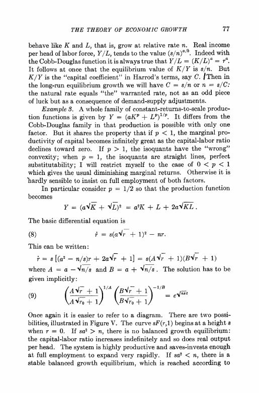
THE THEORY OF ECONOMIC GROWTH 77
behave like K and L, that is, grow at relative rate n. Real income per head of labor force, Y/L, tends to the value (s/f)a/b. Indeed with the Cobb-Douglas function it is always true that Y/L = (K/L)' = ra. It follows at once that the equilibrium value of K/ Y is s/n. But K/Y is the "capital coefficient" in Harrod's terms, say C. /Then in the long-run equilibrium growth we will have C = s/n or n = s/C: the natural rate equals "the" warranted rate, not as an odd piece of luck but as a consequence of demand-supply adjustments.
Example S. A whole family of constant-returns-to-scale produc- tion functions is given by Y = (aKP + LP)11P. It differs from the Cobb-Douglas family in that production is possible with only one factor. But it shares the property that if p < 1, the marginal pro- ductivity of capital becomes infinitely great as the capital-labor ratio declines toward zero. If p > 1, the isoquants have the "wrong" convexity; when p = 1, the isoquants are straight lines, perfect substitutability; I will restrict myself to the case of 0 < p < 1 which gives the usual diminishing marginal returns. Otherwise it is hardly sensible to insist on full employment of both factors.
In particular consider p = 1/2 so that the production function becomes
Y = (alK + jfL)2 = a2K + L + 2alKL.
The basic differential equation is
(8) r = s(alr + 1)2 -nr.
This can be written:
= s [(a -n/s)r + 2at'r + 1] = s(AV'r + 1)(B lr + 1)
where A = a -Vn/s and B = a + 'n/s . The solution has to be
given implicitly:
(9) ( VAi + 1/ /r + 1/ =et
\A 1ro + 1/ B-Vro + 12
Once again it is easier to refer to a diagram. There are two possi- bilities, illustrated in Figure V. The curve sF(r, 1) begins at a height s when r = 0. If sa2 > n, there is no balanced growth equilibrium: the capital-labor ratio increases indefinitely and so does real output per head. The system is highly productive and saves-invests enough at full employment to expand very rapidly. If sa2 < n, there is a stable balanced growth equilibrium, which is reached according to
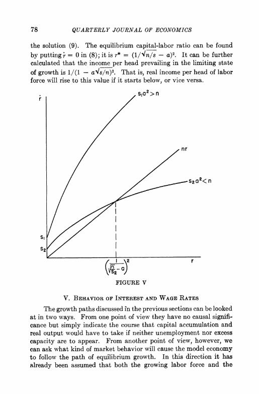
78 QUARTERLY JOURNAL OF ECONOMICS
the solution (9). The equilibrium capital-labor ratio can be found
by putting ' = 0 in (8); it is r* = (1/-Vn/s - a)2. It can be further calculated that the income per head prevailing in the limiting state
of growth is 1/(1 - als/n)2. That is, real income per head of labor force will rise to this value if it starts below, or vice versa.
sIo2> n r
nr
S20 2< n
St
/ 2 r
FIGURE V
V. BEHAVIOR OF INTEREST AND WAGE RATES
The growth paths discussed in the previous sections can be looked at in two ways. From one point of view they have no causal signifi- cance but simply indicate the course that capital accumulation and real output would have to take if neither unemployment nor excess capacity are to appear. From another point of view, however, we can ask what kind of market behavior will cause the model economy to follow the path of equilibrium growth. In this direction it has already been assumed that both the growing labor force and the

THE THEORY OF ECONOMIC GROWTH 79
existing capital stock are thrown on the market inelastically, with the real wage and the real rental of capital adjusting instantaneously so as to clear the market. If saving and investment decisions are made independently, however, some additional marginal-efficiency- of-capital conditions have to be satisfied. The purpose of this section is to set out the price-wage-interest behavior appropriate to the growth paths sketched earlier.
There are four prices involved in the system: (1) the selling price of a unit of real output (and since real output serves also as capital this is the transfer price of a unit of capital stock) p(t); (2) the money wage rate w(t); (3) the money rental per unit of time of a unit of capital stock q(t); (4) the rate of interest i(t). One of these we can eliminate immediately. In the real system we are working with there is nothing to determine the absolute price level. Hence we can take p(t), the price of real output, as given. Sometimes it will be convenient to imagine p as constant.
In a competitive economy the real wage and real rental are determined by the traditional marginal-productivity equations:
(10) OF w OL p
and
(11) OF q AK p
Note in passing that with constant returns to scale the marginal pro- ductivities depend only on the capital-labor ratio r, and not on any scale quantities.7
7. In the polar case of pure competition, even if the individual firms have U-shaped average cost curves we can imagine changes in aggregate output taking place solely by the entry and exit of identical optimal-size firms. Then aggregate output is produced at constant cost; and in fact, because of the large number of relatively small firms each producing at approximately constant cost for small variations, we can without substantial error define an aggregate production func- tion which will show constant returns to scale. There will be minor deviations since this aggregate production function is not strictly valid for variations in output smaller than the size of an optimal firm. But this lumpiness can for long- run analysis be treated as negligible.
One naturally thinks of adapting the model to the more general assumption of universal monopolistic competition. But the above device fails. If the indus- try consists of identical firms in identical large-group tangency equilibria then, subject to the restriction that output changes occur only via changes in the num- ber of firms, one can perhaps define a constant-cost aggregate production function. But now this construct is largely irrelevant, for even if we are willing to overlook

80 QUARTERLY JOURNAL OF ECONOMICS
The real rental on capital q/p is an own-rate of interest - it is the return on capital in units of capital stock. An owner of capital can by renting and reinvesting increase his holdings like compound
f tq/pdt interest at the variable instantaneous rate q/p, i.e., like e . Under conditions of perfect arbitrage there is a well-known close relationship between the money rate of interest and the commodity own-rate, namely
q(t) k(t) (12) p(t) p(t)
If the price level is in fact constant, the own-rate and the interest rate will coincide. If the price level is falling, the own-rate must exceed the interest rate to induce people to hold commodities. That the exact relation is as in (12) can be seen in several ways. For example, the owner of $1 at time t has two options: he can lend the money for a short space of time, say until t + h and earn approximately i(t)h in interest, or he can buy i/p units of output, earn rentals of (q/p)h and then sell. In the first case he will own 1 + i(t)h at the end of the period; in the second case he will have (q(t)/p(t))h + p(t + h)/p(t). In equilibrium these two amounts must be equal
1 + i(t)h = q(t) h + p (t + h)
p t) p(t) or
(t)h =q(t) h p(t + h) - p(t)
Dividing both sides by h and letting h tend to zero we get (12). Thus this condition equalizes the attractiveness of holding wealth in the form of capital stock or loanable funds.
Another way of deriving (12) and gaining some insight into its role in our model is to note that p(t), the transfer price of a unit of capital, must equal the present value of its future stream of net
its discontinuity and treat it as differentiable, the partial derivatives of such a function will not be the marginal productivities to which the individual firms respond. Each firm is on the falling branch of its unit cost curve, whereas in the competitive case each firm was actually producing at locally constant costs. The difficult problem remains of introducing monopolistic competition into aggrega- tive models. For example, the value-of-marginal-product equations in the text would have to go over into marginal-revenue-product relations, which in turn would require the explicit presence of demand curves. Much further experimenta- tion is needed here, with greater realism the reward.

THE THEORY OF ECONOMIC GROWTH 81
rentals. Thus with perfect foresight into future rentals and interest rates:
00 u
p(t) = f q(u)e-f(z)dz du.
Differentiating with respect to time yields (12). Thus within the narrow confines of our model (in particular, absence of risk, a fixed average propensity to save, and no monetary complications) the money rate of interest and the return to holders of capital will stand in just the relation required to induce the community to hold the
K K = r* L
/ 2P
FIGURE VI L
capital stock in existence. The absence of risk and uncertainty shows itself particularly in the absence of asset preferences.
Given the absolute price level p(t), equations (10)-(12) deter- mine the other three price variables, whose behavior can thus be calculated once the particular growth path is known.
Before indicating how the calculations would go in the examples of section IV, it is possible to get a general view diagrammatically, particularly when there is a stable balanced growth equilibrium. In Figure VI is drawn the ordinary isoquant map of the production function F(K,L), and some possible kinds of growth paths. A given capital-labor ratio r* is represented in Figure VI by a ray from the origin, with slope r*. Suppose there is a stable asymptotic ratio r*; then all growth paths issuing from arbitrary initial conditions approach the ray in the limit. Two such paths are shown, issuing from initial

82 QUARTERLY JOURNAL OF ECONOMICS
points Pi and P2. Since back in Figure I the approach of r to r* was monotonic, the paths must look as shown in Figure VI. We see that if the initial capital-labor ratio is higher than the equilibrium value, the ratio falls and vice versa.
Figure VII corresponds to Figure II. There are three "equilib- rium" rays, but the inner one is unstable. The inner ray is the dividing line among initial conditions which lead to one of the stable rays and those which lead to the other. All paths, of course, lead upward and to the right, without bending back; K and L always
K r3
FIGURE VII L
increase. The reader can draw a diagram corresponding to Figure III, in which the growth paths pass to steeper and steeper or to flatter and flatter rays, signifying respectively r --* or r -O 0. Again I remark that K and L and hence Y are all increasing, but if r -. 0, Y/L will decline.
Now because of constant returns to scale we know that along a ray from the origin, the slope of the isoquants is constant. This expresses the fact that marginal products depend only on the factor ratio. But in competition the slope of the isoquant reflects the ratio of the factor prices. Thus to a stable r* as in Figure VI corresponds an equilibrium ratio w/q. Moreover, if the isoquants have the normal
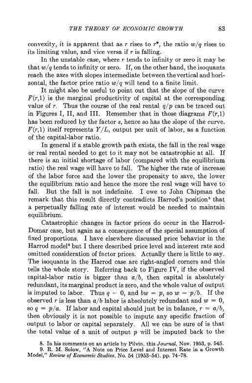
THE THEORY OF ECONOMIC GROWTH 83
convexity, it is apparent that as r rises to r*, the ratio w/q rises to its limiting value, and vice versa if r is falling.
In the unstable case, where r tends to infinity or zero it may be that w/q tends to infinity or zero. If, on the other hand, the isoquants reach the axes with slopes intermediate between the vertical and hori- zontal, the factor price ratio w/q will tend to a finite limit.
It might also be useful to point out that the slope of the curve F(r,1) is the marginal productivity of capital at the corresponding value of r. Thus the course of the real rental q/p can be traced out in Figures I, II, and III. Remember that in those diagrams F(r,1) has been reduced by the factor s, hence so has the slope of the curve. F(r,1) itself represents Y/L, output per unit of labor, as a function of the capital-labor ratio.
In general if a stable growth path exists, the fall in the real wage or real rental needed to get to it may not be catastrophic at all. If there is an initial shortage of labor (compared with the equilibrium ratio) the real wage will have to fall. The higher the rate of increase of the labor force and the lower the propensity to save, the lower the equilibrium ratio and hence the more the real wage will have to fall. But the fall is not indefinite. I owe to John Chipman the remark that this result directly contradicts Harrod's position' that a perpetually falling rate of interest would be needed to maintain equilibrium.
Catastrophic changes in factor prices do occur in the Harrod- Domar case, but again as a consequence of the special assumption of fixed proportions. I have elsewhere discussed price behavior in the Harrod model9 but I there described price level and interest rate and omitted consideration of factor prices. Actually there is little to say. The isoquants in the Harrod case are right-angled corners and this tells the whole story. Referring back to Figure IV, if the observed capital-labor ratio is bigger than a/b, then capital is absolutely redundant, its marginal product is zero, and the whole value of output is imputed to labor. Thus q =_ 0, and bw = p, so w = p/b. If the observed r is less than a/b labor is absolutely redundant and w = 0, so q = p/a. If labor and capital should just be in balance, r = a/b, then obviously it is not possible to impute any specific fraction of output to labor or capital separately. All we can be sure of is that the total value of a unit of output p will be imputed back to the
8. In his comments on an article by Pilvin, this Journal, Nov. 1953, p. 545. 9. R. M. Solow, "A Note on Price Level and Interest Rate in a Growth
Model," Review of Economic Studies, No. 54 (1953-54), pp. 74-78.
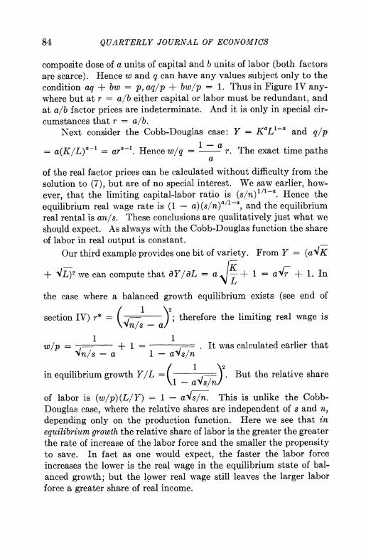
84 QUARTERLY JOURNAL OF ECONOMICS
composite dose of a units of capital and b units of labor (both factors are scarce). Hence w and q can have any values subject only to the condition aq + bw = p, aq/p + bw/p = 1. Thus in Figure IV any- where but at r = a/b either capital or labor must be redundant, and at a/b factor prices are indeterminate. And it is only in special cir- cumstances that r = a/b.
Next consider the Cobb-Douglas case: Y = K'Ll' and q/p
=a(K/L)a1 = aral. Hence w/q = a r. The exact time paths a
of the real factor prices can be calculated without difficulty from the solution to (7), but are of no special interest. We saw earlier, how- ever, that the limiting capital-labor ratio is (s/n) 1/1-a. Hence the equilibrium real wage rate is (1 - a)(s/n)a/1-a, and the equilibrium real rental is an/s. These conclusions are qualitatively just what we should expect. As always with the Cobb-Douglas function the share of labor in real output is constant.
Our third example provides one bit of variety. From Y = (a'IK
+ IlL)2 we can compute that OY/OL = a 4L + 1 = a-Jr + 1. In
the case where a balanced growth equilibrium exists (see end of
section IV) r* = a ); therefore the limiting real wage is
1 1 w/p= -a+ 1 - a It was calculated earlier that
_~n/s -a 1 atlsn
in equilibrium growth Y/L = ( -1) . But the relative share
of labor is (w/p) (L/Y) = 1- a4s/n. This is unlike the Cobb- Douglas case, where the relative shares are independent of s and n, depending only on the production function. Here we see that in equilibrium growth the relative share of labor is the greater the greater the rate of increase of the labor force and the smaller the propensity to save. In fact as one would expect, the faster the labor force increases the lower is the real wage in the equilibrium state of bal- anced growth; but the lower real wage still leaves the larger labor force a greater share of real income.

THE THEORY OF ECONOMIC GROWTH 85
VI. EXTENSIONS
Neutral Technological Change. Perfectly arbitrary changes over time in the production function can be contemplated in principle, but are hardly likely to lead to systematic conclusions. An especially easy kind of technological change is that which simply multiplies the production function by an increasing scale factor. Thus we alter (2) to read
(13) Y = A(t)F(K,L).
The isoquant map remains unchanged but the output number attached to each isoquant is multiplied by A (t). The way in which the (now ever-changing) equilibrium capital-labor ratio is affected can 1 e seen on a diagram like Figure I by "blowing up" the function sF(r,1).
The Cobb-Douglas case works out very simply. Take A (t) = eat and then the basic differential equation becomes
K - seat~a(Loent)l-a = sKaLo1-ae(n(1-a)+g)t
whose solution is
K(t) = [Kob_ bs b bs 1b(nb+g)t 11b
nb + g nb + i
where again b = 1 - a. In the long run the capital stock increases at the relative rate n + g/b (compared with n in the case of no techno- logical change). The eventual rate of increase of real output is n + ag/b. This is not only faster than n but (if a > 1/2) may even be faster than n + g. The reason, of course, is that higher real output means more saving and investment, which compounds the rate of growth still more. Indeed now the capital-labor ratio never reaches an equilibrium value but grows forever. The ever-increasing investment capacity is, of course, not matched by any speeding up of the growth of the labor force. Hence K/L gets bigger, eventually growing at the rate g/b. If the initial capital-labor ratio is very high, it might fall initially, but eventually it turns around and its asymptotic behavior is as described.
Since the capital-labor ratio eventually rises without limit, it follows that the real wage must eventually rise and keep rising. On the other hand, the special property of the Cobb-Douglas func- tion is that the relative share of labor is constant at 1 - a. The

86 QUARTERLY JOURNAL OF ECONOMICS
other essential structural facts follow from what has already been said: for example, since Y eventually grows at rate n + ag/b and K at rate n + g/b, the capital coefficient K/Y grows at rate n + g/b - n - ag/b = g.
The Supply of Labor. In general one would want to make the supply of labor a function of the real wage rate and time (since the labor force is growing). We have made the special assumption that L = Loen', i.e., that the labor-supply curve is completely inelastic with respect to the real wage and shifts to the right with the size of the labor force. We could generalize this somewhat by assuming that whatever the size of the labor force the proportion offered depends on the real wage. Specifically
(14) L = Loe )
Another way of describing this assumption is to note that it is a scale blow-up of a constant elasticity curve. In a detailed analysis this particular labor supply pattern would have to be modified at very high real wages, since given the size of the labor force there is an upper limit to the amount of labor that can be supplied, and (14) does not reflect this.
Our old differential equation (6) for the capital-labor ratio now becomes somewhat more complicated. Namely if we make the price level constant, for simplicity:
(6a) r = sF(r, 1) - nr -h . w
To (6a) we must append the marginal productivity condition (10)
_ = w. Since the marginal product of labor depends only on r, aL p we can eliminate w.
But generality leads to complications, and instead I turn again to the tractable Cobb-Douglas function. For that case (10) becomes
W a
- = (1 - a). r
and hence
w r
THE THEORY OF ECONOMIC GROWTH 87
After a little manipulation (6a) can be written
= (sF(r,1) - nr) (I + ah
which gives some insight into how an elastic labor supply changes
things. In the first place, an equilibrium state of balanced growth still exists, when the right-hand side becomes zero, and it is still
stable, approached from any initial conditions. Moreover, the equi- librium capital-labor ratio is unchanged; since r becomes zero exactly
where it did before. This will not always happen, of course; it is a
consequence of the special supply-of-labor schedule (14). Since r
behaves in much the same way so will all those quantities which depend only on r, such as the real wage.
The reader who cares to work out the details can show that over
the long run capital stock and real output will grow at the same rate n as the labor force.
If we assume quite generally that L = G(t,w/p) then (6) will
take the form r aG aG\
(6b) = sF(r,1) - - + ,(W)).
If r= 0, then uJ = 0, and the equilibrium capital-labor ratio is
determined by
sF(r, 1) = r-- G at
Unless 1/G OG/Ot should happen always to equal n, as in the case
with (14), the equilibrium capital-labor ratio will be affected by the
introduction of an elastic labor supply. Variable Saving Ratio. Up to now, whatever else has been
happening in the model there has always been growth of both labor
force and capital stock. The growth of the labor force was exoge-
nously given, while growth in the capital stock was inevitable because
the savings ratio was taken as an absolute constant. As long as real
income was positive, positive net capital formation must result. This
rules out the possibility of a Ricardo-Mill stationary state, and sug-
gests the experiment of letting the rate of saving depend on the yield
of capital. If savings can fall to zero when income is positive, it
becomes possible for net investment to cease and for the capital stock,
88 QUARTERLY JOURNAL OF ECONOMICS
at least, to become stationary. There will still be growth of the labor force, however; it would take us too far afield to go wholly classical with a theory of population growth and a fixed supply of land.
The simplest way to let the interest rate or yield on capital influence the volume of savings is to make the fraction of income saved depend on the real return to owners of capital. Thus total savings is s(q/p) Y. Under constant returns to scale and competition, the real rental will depend only on the capital-labor ratio, hence we can easily convert the savings ratio into a function of r.
Everyone is familiar with the inconclusive discussions, both abstract and econometrical, as to whether the rate of interest really has any independent effect on the volume of saving, and if so, in what direction. For the purposes of this experiment, however, the natural assumption to make is that the savings ratio depends posi- tively on the yield of capital (and hence inversely on the capital-labor ratio).
For convenience let me skip the step of passing from q/p to r via marginal productivity, and simply write savings as s(r) Y. Then the only modification in the theory is that the fundamental equation (6) becomes
(6c) r= s(r)F(r,1) - nr.
The graphical treatment is much the same as before, except that we must allow for the variable factor s(r). It may be that for suffi- ciently large r, s(r) becomes zero. (This will be the case only if, first, there is a real rental so low that saving stops, and second, if the production function is such that a very high capital-labor ratio will drive the real return down to that critical value. The latter condi- tion is not satisfied by all production functions.) If so, s(r)F(r,1) will be zero for all sufficiently large r. If F(O,1) = 0, i.e., if no pro- duction is possible without capital, then s(r)F(r,1) must come down to zero again at the origin, no matter how high the savings ratio is. But this is not inevitable either. Figure VIIJ gives a possible picture. As usual r*, the equilibrium capital-labor ratio, is found by putting r = G in (6c). In Figure VIII the equilibrium is stable and eventually capital and output will grow at the same rate as the labor force.
In general if s(r) does vanish for large r, this eliminates the possi- bility of a runaway indefinite increase in the capital-labor ratio as in Figure III. The savings ratio need not go to zero to do this, but if it should, we are guaranteed that the last intersection with nr is a stable one.

THE THEORY OF ECONOMIC GROWTH 89
If we compare any particular s(r) with a constant saving ratio, the two curves will cross at the value of r for which s(r) equals the old constant ratio. To the right the new curve will lie below (since I am assuming that s(r) is a decreasing function) and to the left it will lie above the old curve. It is easily seen by example that the equilibrium r* may be either larger or smaller than it was before. A wide variety of shapes and patterns is possible, but the net effect tends to be stabilizing: when the capital-labor ratio is high, saving is cut down; when it is low, saving is stimulated. There is still no possibility of a stationary state: should r get so high as to choke off
r nr
r* r
FIGURE VIII
saving and net capital formation, the continual growth of the labor force must eventually reduce it.
Taxation. My colleague, E. C. Brown, points out to me that all the above analysis can be extended to accommodate the effects of a personal income tax. In the simplest case, suppose the statelevies a proportional income tax at the rate t. If the revenues are directed wholly into capital formation, the savings-investment identity (1) becomes
k = s(l - t)Y + tY = (s(l - t) + t)Y.
That is, the effective savings ratio is increased from s to s + t(l - s). If the proceeds of the tax are directly consumed, the savings ratio is decreased from s to s(1 - t). If a fraction v of the tax proceeds is invested and the rest consumed, the savings ratio changes to
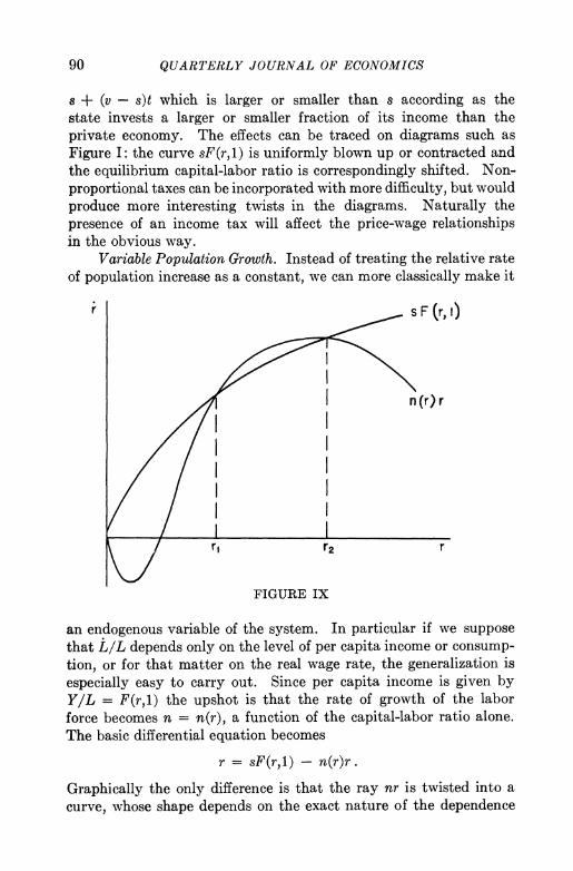
90 QUARTERLY JOURNAL OF ECONOMICS
s + (v - s)t which is larger or smaller than s according as the state invests a larger or smaller fraction of its income than the private economy. The effects can be traced on diagrams such as Figure I: the curve sF(r,1) is uniformly blown up or contracted and the equilibrium capital-labor ratio is correspondingly shifted. Non- proportional taxes can be incorporated with more difficulty, but would produce more interesting twists in the diagrams. Naturally the presence of an income tax will affect the price-wage relationships in the obvious way.
Variable Population Growth. Instead of treating the relative rate of population increase as a constant, we can more classically make it
r s F (rX 1)
n(r)r
FIGURE IX
an endogenous variable of the system. In particular if we suppose that L/L depends only on the level of per capita income or consump- tion, or for that matter on the real wage rate, the generalization is especially easy to carry out. Since per capita income is given by Y/L = F(r,l) the upshot is that the rate of growth of the labor force becomes n = n(r), a function of the capital-labor ratio alone. The basic differential equation becomes
r = sF(r,l) - n(r)r.
Graphically the only difference is that the ray nr is twisted into a curve, whose shape depends on the exact nature of the dependence

THE THEORY OF ECONOMIC GROWTH 91
between population growth and real income, and between real income and the capital-labor ratio.
Suppose, for example, that for very low levels of income per head or the real wage population tends to decrease; for higher levels of income it begins to increase; and that for still higher levels of income the rate of population growth levels off and starts to decline. The result may be something like Figure IX. The equilibrium capital-labor ratio ri is stable, but r2 is unstable. The accompanying levels of per capita income can be read off from the shape of F(r,1). If the initial capital-labor ratio is less than r2, the system will of itself tend to return to ri. If the initial ratio could somehow be boosted above the critical level r2, a self-sustaining process of increasing per capita income would be set off (and population would still be grow- ing). The interesting thing about this case is that it shows how, in the total absence of indivisibilities or of increasing returns, a situa- tion may still arise in which small-scale capital accumulation only leads back to stagnation but a major burst of investment can lift the system into a self-generating expansion of income and capital per head. The reader can work out still other possibilities.
VII. QUALIFICATIONS
Everything above is the neoclassical side of the coin. Most especially it is full employment economics - in the dual aspect of equilibrium condition and frictionless, competitive, causal system. All the difficulties and rigidities which go into modern Keynesian income analysis have been shunted aside. It is not my contention that these problems don't exist, nor that they are of no significance in the long run. My purpose was to examine what might be called the tightrope view of economic growth and to see where more flexible assumptions about production would lead a simple model. Under- employment and excess capacity or their opposites can still be attrib- uted to any of the old causes of deficient or excess aggregate demand, but less readily to any deviation from a narrow "balance."
In this concluding section I want merely to mention some of the more elementary obstacles to full employment and indicate how they impinge on the neoclassical model.'
Rigid Wages. This assumption about the supply of labor is just the reverse of the one made earlier. The real wage is held at some
1. A much more complete and elegant analysis of these important problems is to be found in a paper by James Tobin in the Journal of Political Economy, LXII (1955), 103-15.
92 QUARTERLY JOURNAL OF ECONOMICS
arbitrary level (T). The level of employment must be such as to
keep the marginal product of labor at this level. Since the marginal productivities depend only on the capital-labor ratio, it follows that fixing the real wage fixes r at, say, F. Thus K/L = i. Now there is no point in using r as our variable so we go back to (3) which in view of the last sentence becomes
r = sF rL,L),
or
L = F(F,1). L -r
This says that employment will increase exponentially at the rate (s/r)F(4, 1). If this rate falls short of n, the rate of growth of the labor force, unemployment will develop and increase. If s/rF(-r,1) > n, labor shortage will be the outcome and presumably the real wage will eventually become flexible upward. What this boils down to is that if (ib/p) corresponds to a capital-labor ratio that would nor- mally tend to decrease (r < 0), unemployment develops, and vice versa. In the diagrams, s/rF(-r,1) is just the slope of the ray from the origin to the sF(r, 1) curve at i. If this slope is flatter than n, unemployment develops; if steeper, labor shortage develops.
Liquidity Preference. This is much too complicated a subject to be treated carefully here. Moreover the paper by Tobin just men- tioned contains a new and penetrating analysis of the dynamics con- nected with asset preferences. I simply note here, however crudely, the point of contact with the neoclassical model.
Again taking the general price level as constant (which is now an unnatural thing to do), the transactions demand for money will depend on real output Y and the choice between holding cash and holding capital stock will depend on the real rental q/p. With a given quantity of money this provides a relation between Y and q/p or, essentially, between K and L, e.g.,
(15) M = Q (Y. ) = Q(F(K,L), FK(K,L))
where now K represents capital in use. On the earlier assumption of full employment of labor via flexible wages, we can put L = Loent,
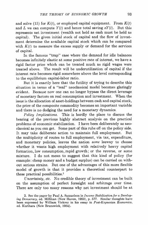
THE THEORY OF ECONOMIC GROWTH 93
and solve (15) for K(t), or employed capital equipment. From K(t) and L we can compute Y(t) and hence total saving sY(t). But this represents net investment (wealth not held as cash must be held as capital). The given initial stock of capital and the flow of invest- ment determine the available capital stock which can be compared with K(t) to measure the excess supply or demand for the services of capital.
In the famous "trap" case where the demand for idle balances becomes infinitely elastic at some positive rate of interest, we have a rigid factor price which can be treated much as rigid wages were treated above. The result will be underutilization of capital if the interest rate becomes rigid somewhere above the level corresponding to the equilibrium capital-labor ratio.
But it is exactly here that the futility of trying to describe this situation in terms of a "real" neoclassical model becomes glaringly evident. Because now one can no longer bypass the direct leverage of monetary factors on real consumption and investment. When the issue is the allocation of asset-holdings between cash and capital stock, the price of the composite commodity becomes an important variable and there is no dodging the need for a monetary dynamics.
Policy Implications. This is hardly the place to discuss the bearing of the previous highly abstract analysis on the practical problems of economic stabilization. I have been deliberately as neo- classical as you can get. Some part of this rubs off on the policy side. It may take deliberate action to maintain full employment. But the multiplicity of routes to full employment, via tax, expenditure, and monetary policies, leaves the nation some leeway to choose whether it wants high employment with relatively heavy capital formation, low consumption, rapid growth; or the reverse, or some mixture. I do not mean to suggest that this kind of policy (for example: cheap money and a budget surplus) can be carried on with- out serious strains. But one of the advantages of this more flexible model of growth is that it provides a theoretical counterpart to these practical possibilities.
Uncertainty, etc. No credible theory of investment can be built on the assumption of perfect foresight and arbitrage over time. There are only too many reasons why net investment should be at
2. See the paper by Paul A. Samuelson in Income Stabilization for a Develop- ing Democracy, ed. Millikan (New Haven, 1953), p. 577. Similar thoughts have been expressed by William Vickrey in his essay in Post-Keynesian Economics, ed. Kurihara (New Brunswick, 1954).

94 QUARTERLY JOURNAL OF ECONOMICS
times insensitive to current changes in the real return to capital, at other times oversensitive. All these cobwebs and some others have been brushed aside throughout this essay. In the context, this is perhaps justifiable.
ROBERT M. SOLOW.
MASSACHUSETTS INSTITUTE OF TECHNOLOGY

Brief Notes On Indian Economy &
Current Issues
Content :
1. The Indian Economy Since Independence
2. The Overview Of Indian Economy
3. Some Important Short Notes

1
The Indian Economy Since Independence India Wins Freedom On 14 August 1947, Nehru had declared: “Long years ago we made a tryst with
destiny, and now the time comes when we shall redeem our pledge. The achievement we
celebrate today is but a step, an opening of opportunity, to the great triumph and
achievments that await us.” He reminded the country that the tasks ahead included “the
ending of poverty and ignorance and disease and inequality of opportunity”. These were the
basic foundations on which India embarked upon its path of development since gaining
independence in 1947. The purpose of this talk is to analyze how much has India really
achieved in the last 55 years in fulfilling the aspirations on which it was founded.
Indian Planning process The objective of India’s development strategy has been to establish a socialistic
pattern of society through economic growth with self-reliance, social justice and alleviation
of poverty. These objectives were to be achieved within a democratic political framework
using the mechanism of a mixed economy where both public and private sectors co-exist.
India initiated planning for national economic development with the establishment of the
Planning Commission. The aim of the First Five Year Plan (1951-56) was to raise domestic
savings for growth and to help the economy resurrect itself from colonial rule. The real
break with the past in planning came with the Second Five Year Plan (Nehru-Mahalanobis
Plan). The industrialization strategy articulated by Professor Mahalanobis placed emphasis
on the development of heavy industries and envisaged a dominant role for the public sector
in the economy. The entrepreneurial role of the state was evoked to develop the industrial
sector. Commanding heights of the economy were entrusted to the public sector. The
objectives of industrial policy were: a high growth rate, national self-reliance, reduction of
foreign dominance, building up of indigenous capacity, encouraging small scale industry,
bringing about balanced regional development, prevention of concentration of economic
power, reduction of income inequalities and control of economy by the State. The planners

2
and policy makers suggested the need for using a wide variety of instruments like state
allocation of investment, licensing and other regulatory controls to steer Indian industrial
development on a closed economy basis.
The strategy underlying the first three plans assumed that once the growth process
gets established, the institutional changes would ensure that benefits of growth trickle down
to the poor. But doubts were raised in the early seventies about the effectiveness of the
‘trickle down’ approach and its ability to banish poverty. Further, the growth itself
generated by the planned approach remained too weak to create adequate surpluses- a
prerequisite for the ‘trickle down’ mechanism to work. Public sector did not live upto the
expectations of generating surpluses to accelerate the pace of capital accumulation and help
reduce inequality. Agricultural growth remained constrained by perverse institutional
conditions. There was unchecked population growth in this period. Though the growth
achieved in the first three Five Year Plans was not insignificant, yet it was not sufficient to
meet the aims and objectives of development. These brought into view the weakness of
economic strategy. We discuss the failure of the planning process in more detail in the next
section.
A shift in policy was called for. The Fifth Plan (1974-79) corrected its course by
initiating a program emphasizing growth with redistribution. To accelerate the process of
production and to align it with contemporary realities, a mild version of economic
liberalization was started in the mid 1980s. Three important committees were set up in the
early 1980s. Narsimhan Committee on the shift from physical controls to fiscal controls,
Sengupta Committee on the public sector and the Hussain Committee on trade policy. The
result of such thinking was to reorient our economic policies. As a result there was some
progress in the process of deregulation during the 1980s. Two kinds of delicencing activity
took place. First, thirty two groups of industries were delicensed without any investment
limit. Second, in 1988, all industries were exempted from licensing except for a specified
negative list of twenty six industries. Entry into the industrial sector was made easier but
exit still remained closed and sealed.
Hence, the roots of the liberalization program were started in the late 80’s when
Rajiv Gandhi was the Prime Minister of India, but the reach and force of the reform

3
program was rather limited. There were political reasons as to why this program could not
be enhanced which we talk about later.
The Failure of the Planning Process
While the reasons for adopting a centrally directed strategy of development were
understandable against the background of colonial rule, it, however soon became clear that
the actual results of this strategy were far below expectations. Instead of showing high
growth, high public savings and a high degree of self-reliance, India was actually showing
one of the lowest rates of growth in the developing world with a rising public deficit and a
periodic balance of payment crises. Between 1950 and 1990, India’s growth rate averaged
less than 4 per cent per annum and this was at a time when the developing world, including
Sub-Saharan Africa and other least developed countries, showed a growth rate of 5.2 % per
annum.
An important assumption in the choice of post-independence development strategy
was the generation of public savings, which could be used for higher and higher levels of
investment. However, this did not happen, and the public sector-instead of being a
generator of savings for the community’s good- became, over time, a consumer of
community’s savings. This reversal of roles had become evident by the early seventies, and
the process reached its culmination by the early eighties. By then, the government began to
borrow not only to meet its own revenue expenditure but also to finance public sector
deficits and investments. During 1960-1975, total public sector borrowings averaged 4.4 %
of GDP. These increased to 6 % of GDP by 1980-81, and further to 9 % by 1989-90. Thus,
the public sector, which was supposed to generate resources for the growth of the rest of the
economy, gradually became a net drain on the society as a whole.
I will now try to give some reasons for the deterioration of the public sector in India.
1) The legal system in India is such that it provides full protection to the private
interests of the so called ‘public servant’, often at the expense of the public that he
or she is supposed to serve. In addition to complete job security, any group of public
servants in any public sector organization can go on strike in search of higher
wages, promotions and bonuses for themselves, irrespective of the costs and

4
inconvenience to the public. Problems have become worse over time and there is
little or no accountability of the public servant to perform the public duty.
2) The ‘authority’ of governments, at both center and states, to enforce their decisions
has eroded over time. Government can pass orders, for example, for relocation of
unauthorized industrial units or other structures, but implementation can be delayed
if they run counter to private interests of some (at the expense of the general public
interest).
3) The process and procedures for conducting business in government and public
service organizations, over time, have become non-functional. There are
multiplicity of departments involved in the simplest of decisions, and administrative
rules generally concentrate on the process rather than results. There is very little
decentralization of decision-making powers, particularly financial powers. Thus,
while local authorities have been given significant authority in some states for
implementing national programmes, their financial authority is limited.
Hence during early 90’s it was imperative for India to correct its clearly faulty
developmental process. There have been several reasons put forward for the failure of the
developmental path which necessitated the reforms of Manmohan Singh in 1991. The way I
would approach the analysis is through the approach of comparing and contrasting the
viewpoints of two of the most prominent Indian economists of our times.
The Bhagwati-Sen debate
Jagdish Bhagwati and Amartya Sen, probably the two most influential voices
amongst Indian economists, represent the two divergent ways of thinking about the
development path. Though formally no such debates exists, apart from occasional jibes
against Sen in the writings of Bhagwati, I believe by scrutinizing their positions a lot of
introspection can be done. As Bhagwati says “my view as to what went wrong with Indian
planning is completely at odds with that of Prof Sen”. My objective in this section is bring

5
out the intellectual divergence amongst these two great minds and possibly to learn
something from that.
Let us start with the points on which they agree. I think the fact that India needs an
egalitarian development path is quite well acknowledged by both of them. The Nehruvian
dream of an egalitarian growth process was what both of them would endorse. As Bhagwati
says “I have often reminded the critics of Indian strategy, who attack it from the perspective
of poverty which is juxtaposed against growth, that it is incorrect to think that the Indian
planners got it wrong by going for growth rather than attacking poverty: they confuse
means with ends. In fact, the phrase “minimum income” and the aim of providing it to
India’s poor were very much part of the lexicon and at the heart of our thinking and
analysis when I worked at the Indian Planning Commission in the early 1960’s”. The key
strategy that defined the resulting developmental effort was the decision to target efforts at
accelerating the growth rate. Given the immensity of the poverty, the potential of simple
redistribution was considered to be both negligible in its immediate impact and of little
sustained value. Accelerated growth was thus regarded as an instrumental variable; a policy
outcome that would in turn reduce poverty. He goes on to argue “Those intimately
associated in India’s plans fully understood, contrary to many recent assertions, the need
for land reforms, for attention to the possibility of undue concentration of economic power
and growth in inequality. These ‘social tasks’, which of course also can redound to
economic advantage, were attended to and endlessly debated in the ensuing years, with
reports commissioned (such as the Mahalanobis Committee report on income distribution
in 1962) and policies continually revised and devised to achieve these social outcomes”.
If we follow the writings of Sen on the other hand, in his recent book “Development
As Freedom”, Sen argues that “the usefulness of wealth lies in the things that it allows us to
do- the substantive freedoms it helps us to achieve….an adequate conception of
development must go much beyond the accumulation of wealth and the growth of gross
national product and other income-related variables. Without ignoring the importance of
economic growth, we must look well beyond it”. I don’t think that there is any divergence
of view on this front with that of what Bhagwati says. It is worth mentioning at this
juncture that this has been a common misconception amongst economists about the
divergence of two different developmental paths. It is often misunderstood that Bhagwati’s
6
view stresses just on economic growth while Sen argues against economic growth and the
importance of markets. The above paragraphs reveal that this is certainly not the case. Both
of them is sufficiently concerned with economic growth as well as the basic issues of
poverty, health and social issues.
The points of divergence
I believe the real disparity concerns the means of achieving these common goals.
Bhagwati’s arguments can be summarized as follows. The development process consists of
two steps. As a first step, a growth accelerated strategy would generate enhanced
investments and whose objective was to jolt the economy up into a higher investment mode
that would generate a much higher growth rate. The planning framework rested on two
legs. First, it sought to make the escalated growth credible to private investors so that they
would proceed to invest on an enhanced basis in a self-fulfilling prophecy. Second, it aimed
at generating the added savings to finance the investments so induced. His argument
crucially rested on the following logical theory. For the higher growth rate to achieve it is
very important for the economy concerned to be open. If the effective exchange rate for
exports over the effective exchange rate for imports (signifying the relative profitability of
the foreign over the home market), ensured that the world markets were profitable to aim
for, guaranteeing in turn that the inducement to invest was no longer constrained by the
growth of the domestic market. It is worthwhile to recount India’s performance as far as the
public sector savings is concerned, which was considered a major hindrance towards the
success of the Indian plans. Continuing with the argument, the generation of substantial
export earnings enabled the growing investment to be implemented by imports of
equipment embodying technical change. If the Social Marginal Product of this equipment
exceeded the cost of its importation, there would be a ‘surplus’ that would accrue as an
income gain to the economy and boost the growth rate.
The role of literacy and education comes at the next stage. The productivity of the
imported equipment would be greater with a workforce that was literate and would be
further enhanced if many had even secondary education. Now his argument is based on the
fact that the enhanced growth would demand and lead to a more educated workforce. Thus

7
he considers that primary education and literacy plays an enhancing, rather than initiating
role in the developmental process.
Sen on the other hand considers a larger view of development. He believes that
questions such as whether certain political or social freedoms, such as the liberty of
political participation and dissent, or opportunities to receive basic education, are or not
“conducive to development” misses the important understanding that these substantive
freedoms are among the constituent components of development. Their relevance for
development does not have to be freshly established through their indirect contribution to
the growth of GNP or to the promotion of industrialization. While the causal relation, that
these freedoms and rights are also very effective in contributing to economic progress, the
vindication of freedoms and rights provided by this causal linkage is over and above the
directly constitutive role of these freedoms in development.
I think that it is precisely at this point where some of Sen’s writings on economics
and philosophy should be considered. According to Sen, economics as a discipline has
tended to move away from focusing on the value of freedoms to that of utilities, incomes
and wealth. This narrowing of focus leads to an underappreciation of the full role of the
market mechanism. For example, take the example of the most important finding on the
theory of the markets- the Arrow-Debreu equilibrium. That theorem shows that a
competitive economic system can achieve a certain type of efficiency (Pareto efficiency to
be precise) which a centralized system cannot achieve, and this is due to reasons of
incentives and information problems. But if we suppose that no such imperfections do exist
and the same competitive equilibrium can be brought about by a dictator who announces
the production and allocation decision, then are these two outcomes the same? In a much
celebrated paper, Sen brings out the distinction between “culmination outcomes” (that is,
the only final outcomes without taking any note of the process of getting there) and
“comprehensive outcomes” (taking note of the process through which the culmination
outcomes come about). Along these lines we can argue that Sen would disagree with
Bhagwati’s point of view in that it does not consider the “comprehensive outcomes”.
Though the outcomes may be the same if we bring about a simultaneous increase in
investments in education, health and other social activities, with that of growth, as against a
8
framework where growth brings about a derived demand for those activities (a la
Bhagwati), these are not the same thing.
So as we can see, the primary difference in the approach is that Bhagwati argues
that poverty and social dimensions can be taken care of in the second step of the
development process while Sen argues that social opportunity is a constitutive element in
the developmental process. In this respect it is helpful to scrutinize the East Asian case,
where countries like Japan, South Korea, Taiwan (so called Asian Tigers) achieved
phenomenal rates of growth in the 80’s and much of the early 90’s. The interesting fact
about these countries is that they achieved this with a significant high record on the social
dimensions. Both Bhagwati and Sen has commented directly on the achievement of these
countries. As Bhagwati states “The East Asian investment rate began its take-off to
phenomenal levels because East Asia turned to the Export promotion (EP) strategy. The
elimination of the ‘bias against exports’, and indeed a net excess of the effective exchange
rate for exports over the effective exchange rate for imports (signifying the relative
profitability of the foreign over the domestic market), ensured that the world markets were
profitable to aim for, guaranteeing in turn that the inducement to invest was no longer
constrained by the growth of the domestic market as in the IS strategy”.
I personally think that there is nothing disputable in this analysis but it does not
strengthen his argument that the social achievements in these countries followed their phase
of growth. In fact the pioneering example of enhancing economic growth through social
opportunity, especially in basic education, is Japan. Japan had a higher rate of literacy than
Europe even at the time of the Meiji restoration in the mid nineteenth century, when
industrialization had not yet occurred there but had gone on for many decades in Europe.
The East Asian experience was also based on similar connections. The contrasts between
India and China are also important in this aspect. The governments of both China and India
has been making efforts for sometime now to move toward a more open, internationally
active, market-oriented economy. While Indian efforts have slowly met with some access,
the kind of massive results that China has seen has failed to occur in India. An important
factor in this contrast lies in the fact that from a social preparedness standpoint, China is a
great deal ahead of India in being able to make use of the market economy. While pre-
reform China was deeply skeptical of markets, it was not skeptical of basic education and

9
widely shared health care. When China turned to marketization in 1979, it already had a
highly literate people, especially the young, with good schooling facilities across the bulk
of the country. In this respect, China was not very far from the basic educational situation
in South Korea or Taiwan, where too an educated population had played a major role in
seizing the economic opportunities offered by a supported market system.
Indeed it is often argued that it is a mistake to worry about the discord between
income achievements and survival chances-in general- the statistical connection between
them is observed to be quite close. It is interesting, in this context, to refer to some
statistical analyses that have recently been presented by Sudhir Anand and Martin
Ravallion. On the basis of intercountry comparisons, they find that life expectancy does
indeed have a significantly positive correlation with GNP per head, but that this
relationship works primarily through the impact of GNP on (I) the incomes specifically of
the poor and (2) public expenditure particularly in health care. In fact, once these two
variables are included on their own in the statistical exercise, little extra explanation can be
obtained from including GNP per head as an additional causal influence. The basic point is
that the impact of economic growth depends much on how the fruits of economic growth
are used.
Sen argues that a focus on issues on basic education, basic health care and land
reforms made widespread economic participation easier in many of the East Asian and
Southeast Asian economies in a way it has not been possible in, say, Brazil or India, where
the creation of social opportunities has been much slower and that slowness has acted as a
barrier to economic development. I believe that one has to take note of the examples of say,
Sri Lanka, the Indian State of Kerala or pre-reform China where on the contrary, impressive
high life expectancy, low fertility, high literacy and so on, have failed to translate into high
economic growth. I would like to see a theory which explains this. But to elucidate Sen’s
view, he would rather prefer a situation of that of Kerala or Sri Lanka than that of Brazil or
India.
I would suggest that what one needs is such critical studies which would illuminate
the failure of Brazil on one hand as against Sri Lanka on the other, to illustrate the fact that
why an egalitarian growth process was not successfully implemented in these cases. We
will have useful lessons to learn in that case for the future of development. The debate

10
between Bhagwati and Sen (or rather the created debate in this paper) gives rise to such an
agenda.
The Reforms of Manmohan Singh
At the beginning of 90’s the reform process was started by the then Finance
Minsiter of India, Manmohan Singh. The way I will organize this section is the following:
First, I will give a short summary of the reform process , in the sense what were its general
goals and ideas. Then I will mention some aspects of the reforms which I think are very
encouraging. After that I will scrutinize the reforms more stringently in order to assess
whether there is real cause for such jubilation that we tend to observe regarding India.
(i) The Background: India’s economic reforms began in 1991 under the Narsimha
Rao Government. By that time the surge in oil prices triggered by the Gulf War
in 1990 imposed a severe strain on a balance of payments already made fragile
by several years of large fiscal deficits and increasing external debt as was
discussed before. Coming at a time of internal political instability, the balance-
of-payments crises quickly ballooned into a crisis of confidence which
intensified in 1991 even though oil prices quickly normalized. Foreign exchange
reserves dropped to $1.2 billion in 1991, barely sufficient for two weeks of
imports and a default on external payments appeared inevitable. The shortage of
foreign exchange forced tightening of import restrictions, which in turn led to a
fall in industrial output.
A digression: The politics of reforms
In a very engaging article on the politics of reforms Ashutosh Varshney has raised
an extremely important question as to why was India’s minority government in 1991
successful in introducing economic reforms, whereas a much stronger government, with
a three-fourth majority in parliament, was unable to do so in 1985 (under the Prime
Ministership of Rajiv Gandhi)? His argument draws a distinction between mass politics
and elite politics. He believes that “this distinction has not been adequately appreciated

11
in the voluminous literature on the politics of economic reforms. Scholars of economic
reforms have generally assumed that reforms are, or tend to become, central to politics.
Depending on what else is making demands on the energies of the electorate and
politicians- ethnic and religious strife, political order and stability, corruption and
crimes of the incumbents- the assumption of reforms centrality may not be right”. In the
largest ever survey of mass political attitudes in India conducted between April-July
1996, only 19 percent of the electorate reported any knowledge of economic reforms,
even though reforms had been in existence since July 1991. Of the rural electorate, only
about 14 per cent had heard of reforms, whereas the comparable proportion in the cities
was 32 per cent. Further nearly 66 percent of the graduates were aware of the dramatic
changes in economic policy, compared to only 7 per cent of the poor, who are mostly
illiterate. In contrast, close to three-fourths of the electorate – both literates and
illiterates, poor and rich, urban and rural- were aware of the 1992 mosque demolition in
Ayodhya; 80 per cent expressed clear opinions about whether the country should have a
uniform civil code or religiously prescribed and separate laws for marriage, divorce,
and property inheritance; and 87 per cent took a stand on caste-based affirmative action.
Thus according to Varshney, elite politics is typically expressed in debates and
struggles within the institutionalized settings of a bureaucracy, of a parliament or a
cabinet. Mass politics takes place primarily on the streets. In democracies, especially
poor democracies, mass politics can redefine elite politics, for an accumulated
expression of popular sentiments and opinions inevitably exercises a great deal of
pressure on elected politicians. The economic reform’s during 1991 kept progressing
because the political context had made Hindu-Muslim relations and caste animosities
the prime determinant of political coalitions. The reforms were crowded out of mass
politics by issues that aroused greater passion, and anxiety about the nation. And hence
the reforms could go as far as they did.
(ii) The Reforms in a Nutshell: The reforms had two broad objectives. One was the
reorientation of the economy from a statist, centrally directed and highly
controlled economy to what is referred to in the current jargon as a ‘market-
friendly economy’. A reduction direct controls and physical planning was
expected to improve the efficiency of the economy. It was to be made more

12
‘open’ to trade and external flows through a reduction in trade barriers and
liberalization of foreign investment policies. A second objective of the reform
measures was macro-economic stabilization. This was to be achieved by
substantially reducing fiscal deficits and the government’s draft on society’s
savings.
(iii) Results: Compared with the historical trend, the impact of these policies has
been positive and significant. The growth rate of the economy during 1992-93 to
1999-2000 was close to 6.5 per cent per annum. The balance of payments
position has also substantially improved. Despite several external developments,
including the imposition of sanctions in 1998 and sharp rise in oil prices in
2000-01, foreign exchange reserves are at a record level. Current account
deficits have been moderate, and India’s external debt (as a percentage of GDP)
and the debt servicing burden have actually come down since the early nineties.
There is also evidence of considerable restructuring in the corporate sector with
attention being given to cost-competitiveness and financial viability. The rate of
inflation has also come down sharply.
(iv) A Closer Scrutiny: When we talk about GDP growth we talk about the
aggregate figures. Let us closely look at the sectoral composition. If we look at
the growth rates with respect to different sectors we find that the growth rates of
agricultural and industrial production have not increased at all in the nineties,
compared with the eighties. The increase in overall growth in the 1990’s is
overwhelmingly driven by accelerated growth of the ‘service’ sector. The
service sector includes some very dynamic fields, such as uses of information
technology and electronic servicing, in both of which India has made
remarkable progress. This was largely a result of the liberalization policies
initiated by Manmohan Singh. Similar comments apply to the phenomenal
expansion of software-related export services. Now the relevant question is,
what is wrong in the fact that the services sector is driving the growth process in
India? What is a bit disturbing is the fact that it is not clear as to the extent to
which the rapid growth of the service sector as a whole contributes to the
generation of widely-shared employment, the elimination of poverty, and the

13
enhancement of the quality of life. And also employment in the service sector is
often inaccessible to those who lack the required skills or education. The current
restructuring to the Indian economy towards this skill and education-intensive
sector reinforces the resources to a certain section of the society.
How has the Reforms been successful in creating a widely shared developmental process?
The issue as to whether the reforms have been successful in eliminating poverty to a
greater extent than say in the 80’s is a contentious issue. Experience prior to the 1990s
suggests that economic growth in India has typically reduced poverty. Using data from
1958 to 1991, Ravallion and Datt (1996) find that the elasticity of the incidence of poverty
with respect to net domestic product per capita was –0.75 and that with respect to private
consumption per capita it was –0.9. However, the 1990s are more contentious. Some
observers have argued that poverty has fallen far more rapidly in the 1990s than previously
(for example, Bhalla, 2000). Others have argued that poverty reduction has stalled and that
the poverty rate may even have risen (for example, Sen, 2001). The basic question of
measuring India’s poverty rate has turned out to be harder to answer than it needed to be
because of difficulties with coverage and comparability of the survey data. Correcting for
all those, Datt and Ravallion in a recent study find that India has probably maintained its
1980s rate of poverty reduction in the 1990s, though they do not find any convincing
evidence of an acceleration in the decline of poverty. It is probably apt to remark here that
oftentimes the public rhetoric fails to take the incomparability problems in the surveys from
which the poverty estimates are calculated and try to interpret the estimates to reinforce
their particular arguments. Even the Finance Minister’s ‘budget speech’ of Feb 2001
concluded firmly that ‘poverty has fallen from 36 percent in 1993-4 to 26 percent or less
now’. It is worth noting that even if one were to endorse the official 1999-2000 headcount
ratio of 26 per cent, which is known to be biased downwards, one would find that poverty
reduction in the 90s has proceeded at a similar rates as in the earlier decades, in spite of a
significant acceleration in the economic growth rate. As things stand, this is the most
optimistic reading of the available evidence.
All of the estimates were made with respect to head-count indexes. I think it is
necessary to move away from this narrow index and to consider a broader range of social
14
indicators. Much of the debate in this area has focused on what has happened to
expenditure on social sector development in the post reform period. Dev and Mooji (2002)
find that central government expenditure toward social services and rural development
increased from 7.6 per cent of total expenditure in 1990-91 to 10.2 percent in 2000-01.
During the first two years of the reforms when the fiscal stabilization constraints were
dominant it dipped a little, but after that it increased. However, expenditure trends in the
states, which accounts for 80 percent of total expenditures in this area, show a definite
decline as a percentage of GDP in the post-reform period. Taking central and state
expenditures together, social sector expenditure has remained more or less constant as a
percentage of GDP.
Starting with areas of concern, the decline of infant mortality appears to have
slowed down in recent years. During the 80s India achieved a reduction of 30 per cent in
the infant mortality rate – from 114 to 80 between 1980 and 1990. During the 90s,
however, the infant mortality rate declined by only 12.5 per cent- from 80 to 70.
Similarly, the growth rate of real agricultural wages fell from over 5 percent per
year in the 1980’s to 2.5 percent or so in the 1990s. Given the close association between
real agricultural wages and rural poverty, this pattern is consistent with the belief that
poverty has continued to decline in the 90s, but perhaps at a slower rate than in the 80s.
At the same time it is worth noting that literacy has greatly improved during the
reforms. The literacy rate increased from 52 percent in 1991 to 65 percent in 2001, a faster
increase in the 1990s than in the previous decade, and the increase has been particularly
high in some of the low literacy states such as Bihar, Madhya Pradesh, Uttar Pradesh and
Rajasthan.
Lastly it is important to note the rising economic inequalities of the 90s. Two
aspects are well established. First, inter state economic disparities have risen in the 90s,
when states that were already comparatively advanced (notably in the western and southern
regions) grew particularly fast. Second, there is also strong evidence of rising rural-urban
disparities in the 90s, as one might have expected given the sectoral imbalances discussed
earlier. As Datt and Ravallion comment “We find large differences across states in the
poverty impact of any given rate of growth in nonagricultural output. States with relatively
low levels of initial rural development and human capital development were not well suited

15
to reduce poverty in response to economic growth. Our results are thus consistent with the
view that achieving higher aggregate economic growth is only one element of an effective
strategy for poverty reduction in India. The sectoral and geographic composition of growth
is also important, as is the need to redress existing inequalities in human resource
development and between rural and urban areas.”
Conclusion
Let us go back to Bhagwati-Sen debate which was used as a theoretical
underpinning for my analyses on the developmental process since Independence. As
Bhagwati argues, “India had a major setback in her planning process when she turned
inwards following the balance of payments crises in 1956-57. The explicit strategy of an IS
strategy (Import Substitution) was desired then, reflecting the economic logic of elasticity
pessimism that characterized the thinking of Indian planners. The result was that the
inducement to invest in the economy was constrained by the growth of demand from the
agricultural sector and the public sector savings. But agriculture has grown nowhere by
more than 4 per cent per annum over a sustained period of over a decade. And we discussed
the issue of public sector savings earlier. By contrast, the East Asian investment rate began
its take-off to phenomenal levels because East Asia turned to the Export Promotion
strategy. In that case, the world markets were profitable to aim for, guaranteeing in turn that
the inducement to invest was no longer constrained by the growth of the domestic market
as in the IS strategy.” Hence the liberalization program of Manmohan Singh in 1991 was a
welcome step towards achieving the logic which has been argued by Bhagwati.
Unfortunately, the second step of the developmental process, that of derived demand for
education and other social issues, have been far from being realized atleast a decade after
the reform process.
On the other hand, Sen’s contention that the planning process failed was because of
the government’s complete neglect throughout of issues on literacy, health and other social
indicators. The fact that the reform process did actually achieve a higher growth rate in the
90’s with the opening up of the economy is actually received quite encouragingly by Sen
(as against some assertions made on the contrary). But I personally believe that he is critical
of the fact, that inspite the achievement in the growth rate, the governmental neglect on the

16
above mentioned issues still continues. In fact during the 90’s the concerns have become
more stark in some sense, whereas India has achieved a respectable growth rate while on
the other hand problems on literacy, health, living conditions continue to exist at an
increasing rate. So he would argue that the reform process is largely an incomplete work.
While I agree to Sen’s views I think there is one issue that he often ignores in his
writings. It’s a kind of counterfactual reasoning but nonetheless it is important. The
situation that India faced in the early 90’s (which led to the reform process in the first
place) was an extreme situation. Hence Manmohan Singh’s initial years as Finance
Minister was trying to cope up with this crises in some sense. Given budget constraint
considerations it was impossible for Dr Singh to allocate more resources into those
neglected issues. According to Dr Singh, the government had planned more resources for
health, education and social sectors after the economy recovered from the crises.
Unfortunately the Congress government had to leave soon given the rise of BJP and its
subsequent control of the Parliament. Hence I think, that Manmohan Singh’s achievements
have to be evaluated in this light given the initial conditions from which he started. It would
have been likely that India would have fallen into a situation such as that of Argentina in
the current years, if not because of the timely reform process. In this aspect I think Prof Sen
often ignores the feasibility issue and the conditions in which the reform process started.
Nonetheless, given the rhetoric of the ‘market economy’ being so loosely used in a
lot a contexts, a voice like Amartya Sen is extremely important. Otherwise we would be left
gloating in our achievements without sufficient introspection in the neglected dimensions
of our economy.

AN OVERVIEW OF INDIAN
ECONOMY As citizens of India, it is very important for all of you to know about the economy
of India. As you also know from history that India became an independent nation
on August 15, 1947.Prior to that the Indian subcontinent was under the British rule
for nearly two centuries which is a very long period to sufficiently influence every
aspect of the country such as- politics, culture, social system, economy etc. We
will only concentrate on the study of economy of India here.
STATE OF THE INDIAN ECONOMY AT THE
TIME OF INDEPENDENCE
India inherited the economy from the British who were ruling this country for their
gain. The British were never interested in the development of India or its citizens.
Their aim was to exploit the resources of India and take away as much as possible
to England. This is the reason why railway lines were laid so that things can be
transported to port areas for shipment to England. Even if construction of railways
was a positive contribution, it was mostly used to serve the British interest.
At the end of British period some notable economic features were as follows:
(i)Decline of handicrafts industry (ii) Production of cash crops
(iii) Famines and food shortage (iv) Rise of intermediaries in agriculture
Let us discuss these points one by one.
Decline of Handicraft Industry
Before the British came to India, Emperors and kings were ruling this land. They
promoted the interest of local artisans, carpenters, artists, weavers etc. who were
very good at making beautiful paintings, decorating walls, designing textiles and
jewelry, tailoring, making furniture, toys and idols of stones and metals etc. These
people were using their labour and local skills to create these things. A lot of
concentration and long time was required to create such things. The Kings’ courts
in various parts of the country were full of decorative items of various types made
of different materials. But when the British came they defeated the Kings and took
over their kingdoms. Towns were destroyed and with this the handicraft industry
was also faced closure. An important part of Indian handicraft were the textile
handicrafts. In the latter half 19th century England was experiencing changes in
production technology. Machine was replacing human labour to produce goods.
Producing goods at large scale was becoming easier. More factories were coming
up. The British could bring their machine made textiles and sell in India at a

cheaper price and also in large quantities. The British government also made
policies to help the British producers only. So Indian handicraft suffered.
Production of Cash Crops
As said above, England was under going change in terms of industrialization so
factories there were in need of raw materials to produce goods. In order to make
textiles raw cotton was needed. Similarly indigo was in high demand to make
prints on textiles. Also jute, sugarcane, ground nuts were all in great demand in
England as they were all needed in factories there. Since these were all cultivated
in India, the British offered money to poor farmers of India to raise these crops so
that they could send them to England. Since these crops are used in factories as
raw materials to produce goods, they are called cash crops. Attracted by money,
Indian farmers grew these cash crops for the British who supplied them to factories
in England. The factory made goods were sent for sale in the Indian market. Now
the British sold these goods to Indian people and made profit.
Famines and Shortage of Food
The worst part of British rule in India had been the frequent occurrences of
famines. Famine is a situation wherein many people do not get food to eat and die
from hunger and diseases. Famine occurred nearly 33 times during whole British
period. The most devastating famine was the Bengal famine of 1943, just four
years before independence. More than 1.5 million people died at this time due to
lack of food. Some reasons for occurrence of famines were as follows:
(i) Bad rainfall upsetting food grain production since irrigation facilities were not
available. Agriculture was dependent on rainfall.
(ii) British government kept on exporting food grains to its native country England
and elsewhere even if there was local need for these things. British government
was only interested in earning revenue for itself by exporting food grains to other
countries. It also used food grains to feed its soldiers who were fighting wars in
different parts of the world. You know that the British had not only captured India,
but also many other countries of the world. So they were sending food from India
to these countries where their soldiers were fighting to capture territories.
(iii) Poor people had not enough money to purchase food grains from the market.
(iv) As said above, Indian farmers were encouraged to produce cash crops on their
fields. This led to fall in production of food grains because less area was available
for their cultivation.
Intermediaries in Agriculture

Agriculture was major occupation of people of India during British rule .More than
70 percent of the population was dependent on agriculture. So it was the major
source of revenue for the government. The British introduced two types of land
revenue, such as:
(i) Permanent settlement under which land revenue to be collected was
permanently
fixed.
(ii) Temporary settlement under which land revenue was changed after 25-30 years
of time.
In order to collect revenue the British appointed Zamindars in eastern part of India,
Mahalwari in western part and Ryotwari in south India. These persons were called
intermediaries because they used to act between British Government and common
people. Their job was to collect revenue in the form of rent, tax etc from the
villagers, farmers and other households and submit that revenue with the
government. Over the years these people became exploiters of common people as
they mercilessly collected revenue without considering their poor status. Similarly
no mercy was shown even during poor harvest due to bad rain fall or floods. Out of
the total revenue collected from the villagers these intermediaries used to keep a
part of it before depositing with the British government. Besides collection of land
revenue the British government also depended on them for running the
administration. In this way the Zamindars, Mahalwaris and Ryotwaris became mini
rulers in their respective areas. They used force to take away belongings of persons
who failed to give revenue. This way these intermediaries became rich and
powerful at the cost of common man and with the blessings of British government.
CHANGES IN THE FEATURES OF INDIAN
ECONOMY AFTER INDEPENDENCE
A new era began in India’s history after its independence. Obviously so, because
the governance of India became the responsibility of its people. Unlike the British
government, the aim of the government of India was to take India towards the
higher levels of development and achieve welfare for all its citizens. By the year
2010, the government of India has completed more than sixty years of governing
India. This is long enough time to make an evaluation and accordingly describe the
major features of Indian economy which are as follows Low level of per capita
income, slow growth of per capita income, Heavy population pressure, Existence

of Poverty, Dependence on agriculture and Planning for Development Let us
discuss them one by one in the following way.
Low level of per capita income
Per capita income is calculated by dividing national income by population. Income
of an individual is a major indicator of his or her standard of living. Per capita
income gives the idea of income earned on an average by an individual in the
economy in a year. India’s per capita income for the year 2009-10 was Rs. 33731.
This comes out to be around Rs 2811 per month. (i.e. 33731/12 = 2811). This
amount is very low to lead a decent life. A person needs a room to live, cloths
and dress materials to wear and food to eat. All these things have to be purchased
from the market by paying some price. Even if a person has his or her parental
house to stay where he / she does not pay rent, still he / she needs to buy clothes
and food for him / herself. Since price of food grains, vegetables, clothes etc. are
high so you think Rs.2811 is sufficient to meet these expenditures?
Slow growth of per capita income
India’s per capita income is not only low but also growing very slowly. Growth
refers to increase over time. Why we want our income to increase every year?
There are a few reasons for it . First, our wants are increasing, as we grow over
time. In order to satisfy the extra wants, we need more income. Take for example
your own case. Don’t you want to watch a movie in a cinema hall; don’t you want
to wear nice dresses; don’t you want to eat in a hotel; don’t you want to watch IPL
cricket match in a stadium; don’t you want to study in a college; don’t you want a
mobile phone for yourself etc. The list could go endless. But these things are not
available free of cost. So you need more income than before to satisfy these wants.
Second, another reason for earning more income is that the prices of goods you
buy in the market are also increasing. So you may have to pay more money for the
same goods and services you consume. Recently the prices of petrol and diesel
were increased. In Delhi the price was increased by around Rs 5 per litre. Suppose
a person runs a truck from Delhi to Shimla carrying shoes. He sells shoes in
Shimla market at the rate of Rs.300 per pair. His expenditure on diesel before the
rise in price was around is Rs.3100 per trip. But because of price rise his
expenditure on diesel increased to ,say, Rs.3700. How he will manage this extra
Rs.600? One way is to increase the price of a pair of shoes from Rs.300 to say
Rs.325. If you are staying at Shimla and buying shoes then you have to pay Rs.25
more for a pair than before. Where from you get this extra money of Rs.25? Your
income must increase to adjust this increase in expenditure. Since you spend on

other goods as well and prices of others goods are also increasing in a similar
fashion, your income must increase even faster. But ironically, the per capita
income in India has not increased in the desired manner. We just told that India’s
per capita income was Rs.33,731 in the year 2009-2010. Do you know what was
the amount in the preceding year. 2008-9?It was Rs.31,801. This means, income of
an individual was increased by only Rs.1930. What is the increase per month? It
was around Rs.160 per month. Is this amount sufficient for you to meet the extra
expenditure on various goods due to rise in prices? Remember that you have to pay
extra Rs.25 for shoes only. These are so many other things you need for which you
have to pay more. So increase of Rs.160 is not just enough to satisfy your existing
wants, what to talk of satisfying increase in wants? We reproduce the data on per
capita income in the table below given economic survey.
Table: Per capita income of India
Year per capita income (Rs) Growth (Rs)
2008-09 31801 –
2009-10 33731 160
Third, finally we want our income to grow because we may want to help each
other at times of needs or to please each other. Let us not forget that we live in a
society with our relatives, friends and others. We need each others help and
cooperation all the time. Have you ever helped a friend who was in need? You may
want to help a poor person who wants food to eat? You may want to purchase a
book for your needy friend? You may want to buy chocolates for your little brother
or sister? In all these cases you need more money after taking care of your own
needs But if we are not able earn more for ourselves to satisfy our own increase in
wants, then how can we help others which we want to do?
Heavy population pressure
India’s economy is over populated. It has grown by more than three times in last
60 years. At the time of independence in 1947 the population was 350 million.
According to 2011 census, India’s population stands at 1.21 billion. It is second
only to China in the world and may even over take China in future. Why are we
worried about high population? Very simple. More people means more mouths to
eat. This implies that more food grains to be produced. Since population is
increasing every year, more food grains must be produced every year. This is not
an easy task. Because the land area meant for cultivation is not increasing
proportionately. So if food production does not match with increase in population

then availability of food grain per head or per capita supply of food grain will fall.
Taking the hole of India as one family, this further means that, each member of the
family will have less food to eat. Is it not alarming? Besides food, more population
mean more clothes, more expenditure in education and health services, more
houses, roads and what not? Who will provide it? Is our government bestowed
with sufficient resources to provide all these facilities? May be not. Otherwise
there would not have been slums in cities and beggars on the streets. The positive
thing about India’s population is that the number of young people is very high as
compared to other nations in the world. About half of India’s population is in
the age group of 0 to 25 years. Around 78.5 crore out of 121 crore people belong
to below 35 years of age. What does it mean? Youth are full of energy and strength
and expected to perform better as they have the ability to work more. It also
indicates low dependency ratio. In fact total of India’s population almost equals the
combined population of USA, Japan, Indonesia, Pakistan and Bangladesh.
Existence of Poverty
Nearly one third of world’s poor live in India. See the beggars on the streets, the
slums in towns and cities, children working on the fields or in the street side
dhabas or employed in houses or in factories etc. These are visuals of poverty in
the country . More than 30 crores of India’s population suffer from poverty which
is about 27.5 percent of the total population. Out of these, more than 22 crores live
in rural areas. The rest live in urban areas i.e. towns and cities. Among various
states of India, Odisha is the most affected by poverty. Because the percentage of
poor people out of its total population is 46 which is highest among all the states. It
is followed by Chhatisgarh, then Bihar. In terms of number of poor people, UP has
the maximum number of poor people. Look at Punjab, Haryana and Andhra
Pradesh. They are among the least affected by poverty because, percentage of poor
people in these states is lower as compared to Odisha, Bihar and Uttar Pradesh.
Table : Poverty situation in some states in India
State % of Poor People Total number of Poor People (Lakh)
Odisha 46 179
Chhatisgarh 41 91
Bihar 41 369
Uttar Pradesh 35 590
Andhra Pradesh 16 126
Haryana 14 32
Punjab 08 22
All India 27.5 3017

In an economy people pursue various activities to earn their livelihood, such as,
agriculture, industry and services.(we will study this in detail in lesson-20).Indian
economy has been traditionally based on agriculture. In 1951, at the beginning of
first plan, more than 70 percent of the population were engaged in agriculture and
related activities. Even if this has come down, still around 60 percent of the
population is still dependent on agriculture at the beginning of the 21st. century i.e
year 2001.
Planning for Development
A major feature of Indian economy after independence has been its consistent
effort to achieve development through the process of economic planning. This is a
very positive phenomena going on for the past 60 years. The government of India
adopted five year plans beginning with the first five year plan in 1951. The
duration of this plan was 1951 to 1956. Accordingly the second five year plan
began in the year 1956 and ended in 1961. And so on. See the table -4 below to
know the time period of different plans in India.
Plans Plan Periods in India
First 1951-1956
Second 1956-1961
Third 1961-1966
Annual Plan 1966-1967, 1967-68,
1968-69
Fourth 1969-1974
Fifth 1974-79
Annual Plan 1979-80
Sixth 1980-1985
Seventh 1985-1990
Annual Plans 1990-91 and 1991-92
Eighth 1992-1997
Ninth 1997-2002
Tenth 2002-2007
Eleventh 2007-2012
SOME IMPORTANT SHORT NOTES
1. Gini Coefficient: An inequality indicator. The Gini coefficient measures the
inequality of income distribution within a country. It varies from zero, which
indicates perfect equality, with every household earning exactly the same, to
one, which implies absolute inequality, with a single household earning a
country's entire income. Latin America is the world's most unequal region,
with a Gini coefficient of around 0.5; in rich countries the figure is closer to
0.3.
2. Purchasing Power Parity (PPP): A method for calculating the correct
value of a currency, which may differ from its current market value. It is
helpful when comparing living standards in different countries, as it
indicates the appropriate exchange rate to use when expressing incomes and
prices in different countries in a common currency. By correct value,
economists mean the exchange rate that would bring demand and supply of a
currency into equilibrium over the long-term. The current market rate is only
a short-run equilibrium. Purchasing power parity (PPP) says that goods and
services should cost the same in all countries when measured in a common
currency.
3. Game theory : Game theory is a technique for analysing how people, firms
and governments should behave in strategic situations (in which they must
interact with each other), and in deciding what to do must take into account
what others are likely to do and how others might respond to what they do.
For instance, competition between two firms can be analysed as a game in
which firms play to achieve a long-term competitive advantage (perhaps
even a monopoly). The theory helps each firm to develop its optimal strategy
for, say, pricing its products and deciding how much to produce; it can help
the firm to anticipate in advance what its competitor will do and shows how
best to respond if the competitor does something unexpected.
4. Nash Equilibrium : An important concept in game theory, a Nash
equilibrium occurs when each player is pursuing their best possible strategy
in the full knowledge of the strategies of all other players. Once a Nash
equilibrium is reached, nobody has any incentive to change their strategy. It
is named after John Nash, a mathematician and Nobel prize-winning
economist.

5. Negative income tax : A way of building redistribution into the taxation
system by taking money from people with high incomes and paying it to
people with low incomes. Because it takes place automatically through the
tax system, it may attach less stigma to the receipt of financial help than
some other forms of welfare assistance. However, it may also discourage
recipients from working to increase their income , which is why some
countries have introduced a form of negative income tax that is available
only to the working poor. In the United States, this is known as the earned
income tax credit.
6. Welfare Economics: Welfare economics is a branch of economics that uses
microeconomic techniques to simultaneously determine the allocational
efficiency within an economy and the income distribution associated with it.
It attempts to achieve social welfare by examining the economic activities of
the individuals that comprise society. Welfare economics is concerned with
the welfare of individuals, as opposed to groups, communities, or societies
because it assumes that the individual is the basic unit of measurement. It
also assumes that individuals are the best judges of their own welfare, that
people prefer greater welfare to less welfare, and that welfare can be
adequately measured either in monetary terms or as a relative preference.
7. Human Development Index (HDI) : The Human Development Index
(HDI) is a comparative measure of life expectancy, literacy, education, and
standard of living for countries worldwide. It is a standard means of
measuring well-being, especially child welfare. It is used to determine and
indicate whether a country is a developed, developing, or underdeveloped
country and also to measure the impact of economic policies on quality of
life.
8. International Finance Corporation (IFC): IFC is a member of the World
Bank Group and is headquartered in Washington, DC. IFC promotes
sustainable private sector investment in developing countries as a way to
reduce poverty and improve people's lives.Established in 1956, IFC is the
largest multilateral source of loan and equity financing for private sector
projects in the developing world. It promotes sustainable private sector
development primarily by:
1. Financing private sector projects located in the developing world.
2. Helping private companies in the developing world mobilize financing in
international financial
markets.
3. Providing advice and technical assistance to businesses and governments.
9. Hot money: Money that is held in one currency but is liable to switch to
another currency at a moment’s notice in search of the highest available
returns, thereby causing the first currency’s exchange rate to plummet. It is
often used to describe the money invested in currency markets by
speculators.
10. Alternative minimum tax: An IRS mechanism created to ensure that high-
income individuals,corporations, trusts, and estates pay at least some
minimum amount of tax, regardless of deductions, credits or exemptions. It
operates by adding certain tax-preference items back into adjusted gross
income. While it was once only important for a small number of high-
income individuals who made extensive use of tax shelters and deductions,
more and more people are being affected by it. The AMT is triggered when
there are large numbers of personal exemptions on state and local taxes paid,
large numbers of miscellaneous itemized deductions or medical expenses, or
by Incentive Stock Option (ISO) plans.
11. Bretton Woods: An international monetary system operating from 1946-
1973. The value of the dollar was fixed in terms of gold, and every other
country held its currency at a fixed exchange rate against the dollar; when
trade deficits occurred, the central bank of the deficit country financed the
deficit with its reserves of international currencies. The Bretton Woods
system collapsed in 1971 when the US abandoned the gold standard.
12. Call money: Price paid by an investor for a call option. There is no fixed
rate for call money. It depends on the type of stock, its performance prior to
the purchase of the call option, and the period of the contract. It is an interest
bearing band deposits that can be withdrawn on 24 hours notice.
13. Classical economics: The economics of Adam Smith, David Ricardo,
Thomas Malthus, and later followers such as John Stuart Mill. The theory
concentrated on the functioning of a market economy, spelling out a

rudimentary explanation of consumer and producer behaviour in particular
markets and postulating that in the long term the economy would tend to
operate at full employment because increases in supply would create
corresponding increases in demand.
14. Countervailing duties: duties (tariffs) that are imposed by a country to
counteract subsidies provided to a foreign producer Current account: Part of
a nation's balance of payments which includes the value of all goods and
services imported and exported, as well as the payment and receipt of
dividends and interest. A nation has a current account surplus if exports
exceed imports plus net transfers to foreigners. The sum of the current and
capital accounts is the overall balance of payments.
15. Currency appreciation: An increase in the value of one currency relative
to another currency. Appreciation occurs when, because of a change in
exchange rates; a unit of one currency buys more units of another currency.
Opposite is the case with currency depreciation.
16. Double taxation: Corporate earnings taxed at both the corporate level and
again as a stockholder dividend Economic growth: Quantitative measure of
the change in size/volume of economic activity, usually calculated in terms
of gross national product (GNP) or gross domestic product (GDP).
17. Fiscal deficit is the gap between the government's total spending and the
sum of its revenue receipts and non-debt capital receipts. It represents the
total amount of borrowed funds required by the government to completely
meet its expenditure.
18. Gross national product (GNP) is the value of all final goods and services
produced within a nation in a given year, plus income earned by its citizens
abroad, minus income earned by foreigners from domestic production. The
Fact book, following current practice, uses GDP rather than GNP to measure
national production. However, the user must realize that in certain countries
net remittances from citizens working abroad may be important to national
well being. GNP equals GDP plus net property income from abroad.
Globalisation: The process whereby trade is now being conducted on ever

widening geographical boundaries. Countries now trade across continents
and companies also trade all over the world.
19. Imperfect market A market where the theoretical assumptions of perfect
competition are violated by the existence of, for example, a small number of
buyers and sellers, barriers to entry, nonhomogeneity of products, and
incomplete information. The three imperfect markets commonly analyzed in
economic theory are monopoly, oligopoly, and monopolistic competition.
20. Money supply: The total stock of money in the economy; currency held by
the public plus money in accounts in banks. It consists primarily currency in
circulation and deposits in savings and checking accounts. Too much money
in relation to the output of goods tends to push interest rates down and push
inflation up; too little money tends to push rates up and prices down, causing
unemployment and idle plant capacity. The central bank manages the money
supply by raising and lowering the reserves banks are required to hold and
the discount rate at which they can borrow money from the central bank.
The central bank also trades government securities (called repurchase
agreements) to take money out of the system or put it in. There are various
measures of money supply, including M1, M2, M3 and L; these are referred
to as monetary aggregates.
21. Capital flight: When capital flows rapidly out of a country, usually because
something happens which causes investors suddenly to lose confidence in its
economy (Strictly speaking, the problem is not so much the money leaving,
but rather that investors in general suddenly lower their valuation of all the
assets of the country.) This is particularly worrying when the flight capital
belongs to the country’s own citizens. This is often associated with a sharp
fall in the exchange rate of the abandoned country’s currency.
22. Soft loan: A loan provided at below the market INTEREST RATE. Soft
loans are used by international agencies to encourage economic activity in
DEVELOPING COUNTRIES and to support non-commercial activities.
23. Import substitution A deliberate effort to replace major consumer imports
by promoting the emergence and expansion of domestic industries such as

textiles, shoes, and household appliances. Import substitution requires the
imposition of protective tariffs and quotas to get the new industry started.
24. Income inequality The existence of disproportionate distribution of total
national income among households whereby the share going to rich persons
in a country is far greater than that going to poorer persons (a situation
common to most LDCs). This is largely due to differences in the amount of
income derived from ownership of property and to a lesser extent the result
of differences in earned income. Inequality of personal incomes can be
reduced by progressive income taxes and wealth taxes.
25. Monetary policy: The regulation of the money supply and interest rates by
a central bank in order to control inflation and stabilize currency. If the
economy is heating up, the central bank (such as RBI in India) can withdraw
money from the banking system, raise the reserve requirement or raise the
discount rate to make it cool down. If growth is slowing, it can reverse the
process - increase the money supply, lower the reserve requirement and
decrease the discount rate. The monetary policy influences interest rates and
money supply.
26. Repo rate: This is one of the credit management tools used by the Reserve
Bank to regulate liquidity in South Africa (customer spending). The bank
borrows money from the Reserve Bank to cover its shortfall. The Reserve
Bank only makes a certain amount of money available and this determines
the repo rate. If the bank requires more money than what is available, this
will increase the repo rate - and vice versa.]
27. Revenue expenditure: This is expenditure on recurring items, including the
running of services and financing capital spending that is paid for by
borrowing. This is meant for normal running of governments' maintenance
expenditures, interest payments, subsidies and transfers etc. It is current
expenditure which does not result in the creation of assets. Grants given to
State governments or other parties are also treated as revenue expenditure
even if some of the grants may be meant for creating assets. Subsidy :
Financial assistance (often from the government) to a specific group of
producers or consumers.

28. Revenue receipts: Additions to assets that do not incur an obligation that
must be met at some future date and do not represent exchanges of property
for money. Assets must be available for expenditures. These include
proceeds of taxes and duties levied by the government, interest and dividend
on investments made by the government, fees and other receipts for services
rendered by the government.
29. Subsidy: A payment by the government to producers or distributors in an
industry to prevent the decline of that industry (e.g., as a result of continuous
unprofitable operations) or an increase in the prices of its products or simply
to encourage it to hire more labor (as in the case of a wage subsidy).
Examples are export subsidies to encourage the sale of exports; subsidies on
some foodstuffs to keep down the cost of living, especially in urban areas;
and farm subsidies to encourage expansion of farm production and achieve
self reliance in food production.
30. Devaluation: Devaluation is a reduction in the value of a currency with
respect to other monetary units. In common modern usage, it specifically
implies an official lowering of the value of a country's currency within a
fixed exchange rate system, by which the monetary authority formally sets a
new fixed rate with respect to a foreign reference currency. In contrast,
(currency) depreciation is most often used for the unofficial decrease in the
exchange rate in a floating exchange rate system. The opposite of
devaluation is called revaluation.
31. Countervailing duties: duties (tariffs) that are imposed by a country to
counteract subsidies provided to a foreign producer Current account: Part of
a nation's balance of payments which includes the value of all goods and
services imported and exported, as well as the payment and receipt of
dividends and interest. A nation has a current account surplus if exports
exceed imports plus net transfers to foreigners. The sum of the current and
capital accounts is the overall balance of payments.
32. Phillips curve: In 1958, an economist from New Zealand, A.W.H. Phillips ,
proposed that there was a trade-off between inflation and unemployment.
The lower the unemployment rate, the higher was the rate of inflation.
Governments simply had to choose the right balance between the two evils.

He drew this conclusion by studying nominal wage rates and jobless rates in
the UK between 1861 and 1957, which seemed to show the relationship of
unemployment and inflation as a smooth curve.
33. Stagflation: Term coined in the 1970s for the twin economic problems of
stagnation and rising inflation. Until then, these two economic blights had
not appeared simultaneously. Indeed, policymakers believed the message of
the Phillips curve: that unemployment and inflation were alternatives.
34. Money illusion: When people are misled by inflation into thinking that they
are getting richer, when in fact the value of money is declining. Whether,
and how much, people are fooled by inflation is much debated by
economists. Money illusion, a phrase coined by KEYNES, is used by some
economists to argue that a small amount of inflation may not be a bad thing
and could even be beneficial, helping to ―grease the wheels‖ of the
economy. Because of money illusion, workers like to see their nominal
wages rise, giving them the illusion that their circumstances are improving,
even though in real (inflation-adjusted) terms they may be no better off.
During periods of high inflation double-digit pay rises (as well as, say, big
increases in the value of their homes) can make people feel richer even if
they are not really better off. When inflation is low, growth in real incomes
may hardly register.
35. Dumping : Selling something for less than the cost of producing it. This
may be used by a dominant firm to attack rivals, a strategy known to
antitrust authorities as predatory pricing participants in international trade
are often accused of dumping by domestic firms charging more than rival
imports. Countries can slap duties on cheap imports that they judge are being
dumped in their markets. Often this amounts to thinly disguised
protectionism against more efficient foreign firms. In practice, genuine
predatory pricing is rare – certainly much rarer than anti-dumping actions –
because it relies on the unlikely ability of a single producer to dominate a
world market. In any case, consumers gain from lower prices; so do
companies that can buy their supplies more cheaply abroad.]
36. Transfer Pricing: The Prices assumed, for the purposes of calculating tax
liability, to have been charged by one unit of a multinational company when

selling to another (foreign) unit of the same firm. FIRMS spend a fortune on
advisers to help them set their transfer prices so that they minimise their total
tax bill. For instance, by charging low transfer prices from a unit based in a
high-tax country that is selling to a unit in a low-tax country, a firm can
record a low profit in the first country and a high profit in the second. In
theory, however, transfer prices are supposed to be set according to the
arm’s-length principle: that they should be the same as would be charged if
the sale was to a business unconnected in any way to the selling firm. But
when there is no genuinely independent market with which to compare
transfer prices, what an arm’s length price would be can be a matter of great
debate and an opportunity for firms that want to lower their tax bill.
37. Laissez faire: It is an economic system where there is no government
intervention and economic activities are organized by the private sector
through markets. Classical economist is proponents of laissez faire.
38. International Development Association (IDA): The International
Development Association (IDA) created on September 24, 1960, is the part
of the World Bank that helps the world’s poorest countries. It complements
the World Bank's other lending arm—the International Bank for
Reconstruction and Development (IBRD)—which serves middle-income
countries with capital investment and advisory services. The International
Development Association (IDA) is responsible for providing long-term
interest-free loans to the world's 81 poorest countries, 40 of which are in
Africa. IDA provides grants and credits, with repayment periods of 35 to 40
years and no interest. Since its inception, IDA credits and grants have totaled
$161 billion, averaging $7–$9 billion a year in recent years and directing the
largest share, about 50 percent, to Africa. IDA is part of the World Bank
Group based in Washington, D.C.
39. Amartya Sen: Amartya Kumar Sen, is an Indian economist, philosopher,
and a winner of the Bank of Sweden Prize in Economic Sciences (Nobel
Prize for Economics) in 1998, for his work on famine, human development
theory, welfare economics, the underlying mechanisms of poverty, and
political liberalism. Among his many contributions to development
economics, Sen has produced work on gender inequality. He is currently the
Lamont University Professor at Harvard University.
Related Documents