Economic and environmental implications of demand-side management options

An assessment of household electricity load curves and correspondingCO2 marginal abatement cost curves for Gujarat state, India

Amit Garg a,n, P.R. Shukla b, Jyoti Maheshwari c, Jigeesha Upadhyay d

a Wing 16B, Indian Institute of Management Ahmedabad, Vastrapur, Ahmedabad 380015, Indiab Wing 3G, Indian Institute of Management Ahmedabad, Vastrapur, Ahmedabad 380015, Indiac Wing 1A, Indian Institute of Management Ahmedabad, Vastrapur, Ahmedabad 380015, Indiad CEPT University, University Road, Ahmedabad 380009, India

H I G H L I G H T S

� Residential sector provides focused mitigation opportunities.� Energy efficient space cooling is the main technology transition required.� Almost 26% residential load could be reduced by DSM measures.� Myriad barriers limit penetration of negative marginal cost efficient options.

a r t i c l e i n f o

Article history:Received 3 May 2013Accepted 29 October 2013

Keywords:Load researchMarginal Abatement Cost (MAC)CO2 mitigation

a b s t r a c t

Gujarat, a large industrialized state in India, consumed 67 TWh of electricity in 2009–10, besidesexperiencing a 4.5% demand–supply short-fall. Residential sector accounted for 15% of the totalelectricity consumption. We conducted load research survey across 21 cities and towns of the state toestimate residential electricity load curves, share of appliances by type and usage patterns for all types ofhousehold appliances at utility, geographic, appliance, income and end-use levels. The results indicatethat a large scope exists for penetration of energy efficient devices in residential sector. MarginalAbatement Cost (MAC) curves for electricity and CO2 were generated to analyze relative attractiveness ofenergy efficient appliance options. Results indicate that up to 7.9 TWh of electricity can be saved per yearwith 6.7 Mt-CO2 emissions mitigation at negative or very low CO2 prices of US$ 10/t-CO2. Despite suchoptions existing, their penetration is not realized due to myriad barriers such as financial, institutional orawareness and therefore cannot be taken as baseline options for CO2 emission mitigation regimes.

& 2013 Elsevier Ltd. All rights reserved.

1. Introduction

Energy has strong socio-economic and environmental linkages,with associated greenhouse gas (GHG) emissions being among thenegative externalities. Enhancing energy efficiency and makingenergy less GHG intensive are therefore two prime movers ofmodern energy services and businesses. India, the fifth largestprimary energy consumer in the world, is an emerging economyundergoing rapid economic growth and structural transitionswhich are driving rapid rise in energy demand. Energy elasticityof Indian GDP is over one (Shukla et al., 2004), but is decliningsince the last decade. Per capita total primary energy consumptionin India is still very low in comparison with most of the developingcountries (IEP, 2011). During 2012–13, residential sector accounted

for 25.87% of electricity demand in India (CEA, 2013a). Averagehousehold electricity consumption, though, is projected toincrease five fold during 2000–2020 (Deshmukh, 2010). TotalIndian residential energy use is expected to increase by around65–75% in 2050 compared to 2005, but residential carbon emis-sions may increase by up to 9–10 times the 2005 level, mainly dueto rural households moving to fossil fuels from traditional biomass(Van Ruijven et al., 2011). Substantial progress in improvingenergy efficiency has contributed to reducing energy intensity ofIndian GDP (MJ per PPP$ at constant prices) to the tune of 25%during 1980–2007 (Balachandra et al., 2010). In terms of energyintensity of GDP (MJ/PPP$), India has a relatively high ninthposition from top among the 30 highest energy consumingcountries of the world during 2007 (Balachandra et al., 2010).

India has a federal structure and the states play a vital role inimplementing federal energy efficiency policies as well as theirown state policies. Gujarat, a large industrialized state in India,consumed 67 TWh of electricity in 2009–10, besides experiencinga 4.5% demand–supply short-fall. Gujarat state recorded 13% GDP

Contents lists available at ScienceDirect

journal homepage: www.elsevier.com/locate/enpol

Energy Policy

0301-4215/$ - see front matter & 2013 Elsevier Ltd. All rights reserved.http://dx.doi.org/10.1016/j.enpol.2013.10.068

n Corresponding author. Tel.:þ91 79 6632 4952; fax: þ91 79 6632 6896.E-mail addresses: [email protected] (A. Garg),

[email protected] (P.R. Shukla), [email protected] (J. Maheshwari),[email protected] (J. Upadhyay).

Please cite this article as: Garg, A., et al., An assessment of household electricity load curves and corresponding CO2 marginal abatementcost curves for Gujarat state, India. Energy Policy (2013), http://dx.doi.org/10.1016/j.enpol.2013.10.068i

Energy Policy ∎ (∎∎∎∎) ∎∎∎–∎∎∎

growth in 2009–10 fiscal year, the highest among Indian states(Invest in India, 2012) while it moderated to around 8.5% in 2011–12 (DNA, 2013). Per capita consumption of electricity in Gujaratwas 1491 kWh in 2009–10 (SER Gujarat, 2012), and 1642 kWh in2011–12, nearly twice the India average (SER Gujarat, 2013).

The paper analyzes ownership and usage patterns of efficient andrelatively less efficient electric appliances in residential sector ofGujarat, and tries to assess relative cost benefit of various efficienttechnologies. We conducted residential load and appliance usesurvey for Gujarat state. The information is also used in this paperto create Marginal Abatement Cost (MAC) curves for electricity andCO2 emissions under alternate scenarios to assess cost efficientenergy and CO2 transition pathways in residential sector.

2. Methodology

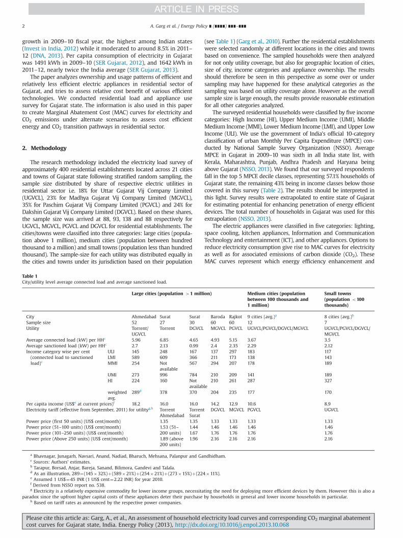
The research methodology included the electricity load survey ofapproximately 400 residential establishments located across 21 citiesand towns of Gujarat state following stratified random sampling, thesample size distributed by share of respective electric utilities inresidential sector i.e. 18% for Uttar Gujarat Vij Company Limited(UGVCL), 23% for Madhya Gujarat Vij Company Limited (MGVCL),35% for Paschim Gujarat Vij Company Limited (PGVCL) and 24% forDakshin Gujarat Vij Company Limited (DGVCL). Based on these shares,the sample size was arrived at 88, 93, 138 and 88 respectively forUGVCL, MGVCL, PGVCL and DGVCL for residential establishments. Thecities/towns were classified into three categories: large cities (popula-tion above 1 million), medium cities (population between hundredthousand to a million) and small towns (population less than hundredthousand). The sample-size for each utility was distributed equally inthe cities and towns under its jurisdiction based on their population

(see Table 1) (Garg et al., 2010). Further the residential establishmentswere selected randomly at different locations in the cities and townsbased on convenience. The sampled households were then analyzedfor not only utility coverage, but also for geographic location of cities,size of city, income categories and appliance ownership. The resultsshould therefore be seen in this perspective as some over or undersampling may have happened for these analytical categories as thesampling was based on utility coverage alone. However as the overallsample size is large enough, the results provide reasonable estimationfor all other categories analyzed.

The surveyed residential households were classified by five incomecategories: High Income (HI), Upper Medium Income (UMI), MiddleMedium Income (MMI), Lower Medium Income (LMI), and Upper LowIncome (ULI). We use the government of India’s official 10-categoryclassification of urban Monthly Per Capita Expenditure (MPCE) con-ducted by National Sample Survey Organization (NSSO). AverageMPCE in Gujarat in 2009–10 was sixth in all India state list, withKerala, Maharashtra, Punjab, Andhra Pradesh and Haryana beingabove Gujarat (NSSO, 2013). We found that our surveyed respondentsfall in the top 5 MPCE decile classes, representing 57.1% households ofGujarat state, the remaining 43% being in income classes below thosecovered in this survey (Table 2). The results should be interpreted inthis light. Survey results were extrapolated to entire state of Gujaratfor estimating potential for enhancing penetration of energy efficientdevices. The total number of households in Gujarat was used for thisextrapolation (NSSO, 2013).

The electric appliances were classified in five categories: lighting,space cooling, kitchen appliances, Information and CommunicationTechnology and entertainment (ICT), and other appliances. Options toreduce electricity consumption give rise to MAC curves for electricityas well as for associated emissions of carbon dioxide (CO2). TheseMAC curves represent which energy efficiency enhancement and

Table 1City/utility level average connected load and average sanctioned load.

Large cities (population 41 million) Medium cities (populationbetween 100 thousands and1 million)

Small towns(population o100thousands)

City Ahmedabad Surat Surat Baroda Rajkot 9 cities (avg.)a 8 cities (avg.)b

Sample size 52 27 30 60 60 12 7Utility Torrent/

UGVCLTorrent DGVCL MGVCL PGVCL UGVCL/PGVCL/DGVCL/MGVCL UGVCL/PGVCL/DGVCL/

MGVCLAverage connected load (kW) per HHc 5.96 6.85 4.65 4.93 5.15 3.67 3.5Average sanctioned load (kW) per HHc 2.7 2.13 0.99 2.4 2.35 2.29 2.12Income category wise per cent(connected load to sanctionedload)c

ULI 145 248 167 137 297 183 117LMI 589 609 366 211 173 138 143MMI 254 Not

available567 294 207 178 189

UMI 273 996 784 210 209 141 189HI 224 160 Not

available210 261 287 327

weightedavg.

289d 378 370 204 235 177 170

Per capita income (US$e at current prices)f 18.2 16.0 16.0 14.2 12.9 10.6 8.9Electricity tariff (effective from September, 2011) for utilityg,h Torrent

AhmedabadTorrentSurat

DGVCL MGVCL PGVCL UGVCL

Power price (first 50 units) (US$ cent/month) 1.35 1.35 1.33 1.33 1.33 1.33Power price (51–100 units) (US$ cent/month) 1.53 (51–

200 units)1.44 1.46 1.46 1.46 1.46

Power price (101–250 units) (US$ cent/month) 1.67 1.76 1.76 1.76 1.76Power price (Above 250 units) (US$ cent/month) 1.89 (above

200 units)1.96 2.16 2.16 2.16 2.16

a Bhavnagar, Junagarh, Navsari, Anand, Nadiad, Bharuch, Mehsana, Palanpur and Gandhidham.c Sources: Authors’ estimates.b Tarapur, Borsad, Anjar, Bareja, Sanand, Bilimora, Gandevi and Talala.d As an illustration, 289¼(145�32%)þ(589�21%)þ(254�21%)þ(273�15%)þ(224�11%).e Assumed 1 US$¼45 INR (1 US$ cent¼2.22 INR) for year 2010.f Derived from NSSO report no. 538.g Electricity is a relatively expensive commodity for lower income groups, necessitating the need for deploying more efficient devices by them. However this is also a

paradox since the upfront higher capital costs of these appliances deter their purchase by households in general and lower income households in particular.h Based on tariff rates as announced by the respective power companies.

A. Garg et al. / Energy Policy ∎ (∎∎∎∎) ∎∎∎–∎∎∎2

Please cite this article as: Garg, A., et al., An assessment of household electricity load curves and corresponding CO2 marginal abatementcost curves for Gujarat state, India. Energy Policy (2013), http://dx.doi.org/10.1016/j.enpol.2013.10.068i

therefore CO2 reduction measures save the most resources. It con-denses complicated data into a graph showing cost effectiveness andmagnitude of carbon saved (NHS SDU, 2011).

Load research is an essential tool and a prerequisite for DemandSide Management (DSM) initiatives, involving systematic collectionand analysis of customers’ electricity consumption as well as demandrequirements by time-of-day, month, season and year; consumptionpatterns; socio-economic and demographic influencing factors; andwillingness-to-pay for electricity (Elkarmi, 2008). Analyses from loadresearch studies assist utilities and power companies to manage andimprove the performance of power systems. Zhao et al. (2012) appliedthe Logarithmic Mean Divisia Index (LMDI) method to a decomposi-tion of China’s urban Residential Energy Consumption (REC) for theperiod 1998–2007 at disaggregated product/activity level. The resultsshow an extensive structure change towards an energy-intensivehousehold consumption with high-quality and cleaner energy.Although China's price reforms in the energy sector contributed to areduction of REC, increased urban population and income levels hadresulted in rapid growth of REC. Feng et al. (2011) used Grey model tocompare the relationship between energy consumption, consumptionexpenditure and CO2 emissions in China. Direct energy consumptionand CO2 emissions were increasing faster for urban households. Thestructural difference for different income levels was significant forindirect energy consumption and CO2 emissions. Mcneil and Letschert(2010) studied the diffusion of refrigerators, washing machines,televisions and air conditioners in the residential sector using linearregression model including many developing countries. In anotherstudy, Ouyang et al. (2010) found a high rebound effect of 30–50% inthe household energy efficiency in China. The paper suggesteddeploying an integrated policy to mitigate the rebound effect, suchas developing renewable energy resources, increasing energy prices,improving energy efficiency, building rational energy prices system,and improving consumer behavior. Marzal and Heiselberg (2011)studied the Life Cycle Cost (LCC) to estimate a cost effective relationbetween energy efficiency measures and renewable energy technol-ogies for a new multi-storey residential Net Zero Energy Building(ZEB) in Denmark. Al-Monsour (2011) captured energy efficiencyimprovement trends in manufacturing, transport and residentialsector in Slovenia for the period from 1997 to 2008.

3. Survey results

3.1. Consumer profile

This section presents city and utility wise average connectedload, average sanctioned load for different income households andslab wise electricity tariff structure for various utilities. It alsoincludes various indicators such as average number of occupants,average energy consumption in summer and winter seasons,

average number of air conditioners for households of differentincome categories.

Table 1 presents city and utility wise average actual load andaverage sanctioned load in residential sector.1 The actual load(average) is two to three times higher than the sanctioned load(average) in about 90% of cities covered in load research survey(Table 1 and Fig. 1). The reason for this variation may be utilityofficials not surveying the residential establishments to verifyactual load connectivity and low penalty for violations. Althoughall the connected devices in a household are not under simulta-neous operation, appliance overload raise concerns about loadmanagement and planning of distribution networks in cities.

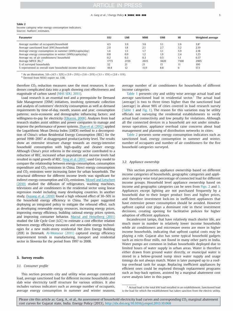
Table 2 presents some energy consumption indicators such assanctioned load, energy consumption in summer and winter,number of occupants and number of air conditioners for the fivehousehold categories surveyed.

3.2. Appliance ownership

This section presents appliance ownership based on differentincome categories of households, geographic categories and appli-ance category wise total percentage of connected load for differentincome groups. Household level appliance ownership based onincome and geographic categories can be seen from Figs. 2 and 3.Appliances except lighting are not purchased frequently by ahousehold due to their longer product lives and higher prices,and therefore investment lock-ins in inefficient appliances thathave extensive power consumption should be avoided. Howeverupfront capital cost plays a dominant role in these investmentdecisions, creating opening for facilitative policies for higheradoption of efficient appliances.

Incandescent lamps, that have relatively much shorter life, aremuch more in number in relatively lower income householdswhile air conditioners and microwave ovens are more in higherincome households, indicating that upfront capital costs may beplaying a role. Gujarat also has some typical household gadgetssuch as micro-flour mills, not found in many other parts in India.Water pumps are common in Indian households deployed due tolimited hours of water supply in urban areas. Water is thereforeeither drawn from ground water directly, or municipal water isstored in a below-ground sump since water supply and usagetimings do not always match. Water is later pumped up to a roof-top overhead tank for usage. Replacing inefficient appliances byefficient ones could be explored through replacement programssuch as buy-back options, assisted by a marginal abatement costcurve analysis later in this paper.

Table 2Income category wise energy consumption indicators.Sources: Authors' estimates.

Parameter ULI LMI MMI UMI HI Weighted average

Average number of occupants/household 4.5 3.9 3.6 3.1 2.6 3.8a

Average sanctioned load (kW)/household 2.0 1.8 2.1 2.7 3.2 2.19Average energy consumption in summer (kWh/capita/day) 1.4 1.5 1.7 3.1 5.9 2.18Average energy consumption in winter (kWh/capita/day) 0.8 0.9 1.2 1.9 2.4 1.23Average no. of air conditioners/ household 0.2 0.3 0.3 0.5 1.1 0.37Average MPCE (Rs.)b 1773 2159 2615 3820 7100 2905% of surveyed households 32 21 21 15 11 100% represented in overall state household income deciles classes 18.4 12 11.9 8.8 6 57.1

a As an illustration, 3.8¼(4.5�32%)þ(3.9�21%)þ(3.6�21%)þ(3.1�15%)þ(2.6�11%).b Derived from NSSO report no. 538.

1 Actual load is the total kW load installed in an establishment. Sanctioned loadis the load for which the establishment has taken sanction from the electric utility.

A. Garg et al. / Energy Policy ∎ (∎∎∎∎) ∎∎∎–∎∎∎ 3

Please cite this article as: Garg, A., et al., An assessment of household electricity load curves and corresponding CO2 marginal abatementcost curves for Gujarat state, India. Energy Policy (2013), http://dx.doi.org/10.1016/j.enpol.2013.10.068i

Large cities show higher ownership of extensive power consum-ing gadgets such as air conditioners, geysers, washing machines andmicrowave ovens. Even computers and laptops find a higherpenetration in households of large cities. These ownership patterns

may be due to higher per household incomes, lifestyles, or eventrends. Penetration of at least one CFL per household was found veryhigh (up to 80–90%) in residential sector irrespective of income orgeographic category. Though the incandescent lamp load is only 12%

8

6.2

4.1

4.0

3.7

2.7 3.

1 3.4

5.3

3.0 3.

5

4.5

6.0

7.8

1.4

1.3

1.1

0.5

0.2 0.

7

0.6

0.3

0.3

0.1

2.2

2.3

2.3

2.3

1.4

2.0

2.1

2.2

2.1

0.8

1.6

1.7

4.4

5.2

0

3

6

9

Torr

ent S

EC

Torr

ent A

EC

PGV

CL

MG

VC

L

DG

VC

L

UG

VC

L

Smal

l citi

es

Med

ium

citi

es

Larg

e ci

ties

ULI

LMI

MM

I

UM

I

HI

Oth

ers

Kitc

hen

appl

ianc

es

Spac

e co

olin

g

ICT

& e

nter

tain

men

t

Ligh

ting

Air

cond

ition

er

Elec

tric

geys

er

Was

hing

mac

hine

Cei

ling

fan

Frid

ge

Utility Geographical Income category End-use categorisation Appliance

kW/H

ouse

hold

Connected load

Sanctioned load

Fig. 1. Category wise average connected and sanctioned loads. Note: There is no appliance and end-use category wise sanctioned load.Sources: Authors' estimates.

0%

20%

40%

60%

80%

100%

CFL Incandescent lamp

Air conditioner

Electric geyser Washing machine

Computer & Laptop

Flour mill Microwave

% o

f Hou

seho

lds

ULI LMI MMI UMI HI

Fig. 2. Income category wise appliance ownership.Sources: Authors' estimates.

0%

20%

40%

60%

80%

100%

CFL Incandescent lamp

Air conditioner

Electric geyser Washing machine

Computer & Laptop

Flour mill Microwave

% o

f Hou

seho

lds

Small cities Medium cities Large cities

Fig. 3. Geographic category wise appliance ownership.Sources: Authors' estimates.

A. Garg et al. / Energy Policy ∎ (∎∎∎∎) ∎∎∎–∎∎∎4

Please cite this article as: Garg, A., et al., An assessment of household electricity load curves and corresponding CO2 marginal abatementcost curves for Gujarat state, India. Energy Policy (2013), http://dx.doi.org/10.1016/j.enpol.2013.10.068i

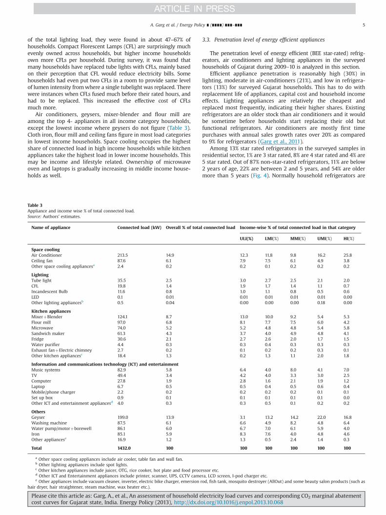
of the total lighting load, they were found in about 47–67% ofhouseholds. Compact Florescent Lamps (CFL) are surprisingly muchevenly owned across households, but higher income householdsown more CFLs per household. During survey, it was found thatmany households have replaced tube lights with CFLs, mainly basedon their perception that CFL would reduce electricity bills. Somehouseholds had even put two CFLs in a room to provide same levelof lumen intensity fromwhere a single tubelight was replaced. Therewere instances when CFLs fused much before their rated hours, andhad to be replaced. This increased the effective cost of CFLsmuch more.

Air conditioners, geysers, mixer-blender and flour mill areamong the top 4- appliances in all income category households,except the lowest income where geysers do not figure (Table 3).Cloth iron, flour mill and ceiling fans figure in most load categoriesin lowest income households. Space cooling occupies the highestshare of connected load in high income households while kitchenappliances take the highest load in lower income households. Thismay be income and lifestyle related. Ownership of microwaveoven and laptops is gradually increasing in middle income house-holds as well.

3.3. Penetration level of energy efficient appliances

The penetration level of energy efficient (BEE star-rated) refrig-erators, air conditioners and lighting appliances in the surveyedhouseholds of Gujarat during 2009–10 is analyzed in this section.

Efficient appliance penetration is reasonably high (30%) inlighting, moderate in air-conditioners (21%), and low in refrigera-tors (13%) for surveyed Gujarat households. This has to do withreplacement life of appliances, capital cost and household incomeeffects. Lighting appliances are relatively the cheapest andreplaced most frequently, indicating their higher shares. Existingrefrigerators are an older stock than air conditioners and it wouldbe sometime before households start replacing their old butfunctional refrigerators. Air conditioners are mostly first timepurchases with annual sales growth rates over 20% as comparedto 9% for refrigerators (Garg et al., 2011).

Among 13% star rated refrigerators in the surveyed samples inresidential sector, 1% are 3 star rated, 8% are 4 star rated and 4% are5 star rated. Out of 87% non-star-rated refrigerators, 11% are below2 years of age, 22% are between 2 and 5 years, and 54% are oldermore than 5 years (Fig. 4). Normally household refrigerators are

Table 3Appliance and income wise % of total connected load.Source: Authors' estimates.

Name of appliance Connected load (kW) Overall % of total connected load Income-wise % of total connected load in that category

ULI(%) LMI(%) MMI(%) UMI(%) HI(%)

Space coolingAir Conditioner 213.5 14.9 12.3 11.8 9.8 16.2 25.8Ceiling fan 87.6 6.1 7.9 7.5 6.1 4.9 3.8Other space cooling appliancesa 2.4 0.2 0.2 0.1 0.2 0.2 0.2

LightingTube light 35.5 2.5 3.0 2.7 2.5 2.1 2.0CFL 19.8 1.4 1.9 1.7 1.4 1.1 0.7Incandescent Bulb 11.6 0.8 1.0 1.1 0.8 0.5 0.6LED 0.1 0.01 0.01 0.01 0.01 0.01 0.00Other lighting appliancesb 0.5 0.04 0.00 0.00 0.00 0.18 0.00

Kitchen appliancesMixerþBlender 124.1 8.7 13.0 10.0 9.2 5.4 5.3Flour mill 97.0 6.8 8.1 7.7 7.5 6.0 4.2Microwave 74.0 5.2 5.2 4.8 4.8 5.4 5.8Sandwich maker 61.3 4.3 3.7 4.0 4.9 4.8 4.1Fridge 30.6 2.1 2.7 2.6 2.0 1.7 1.5Water purifier 4.4 0.3 0.3 0.4 0.3 0.3 0.3Exhaust fanþElectric chimney 2.7 0.2 0.1 0.2 0.2 0.3 0.1Other kitchen appliancesc 18.4 1.3 0.2 1.3 1.1 2.0 1.8

Information and communications technology (ICT) and entertainmentMusic systems 82.9 5.8 6.4 4.0 8.0 4.1 7.0TV 49.4 3.4 4.2 4.0 3.3 3.0 2.5Computer 27.8 1.9 2.8 1.6 2.1 1.9 1.2Laptop 6.7 0.5 0.5 0.4 0.5 0.6 0.4Mobile/phone charger 2.2 0.2 0.2 0.2 0.2 0.1 0.1Set up box 0.9 0.1 0.1 0.1 0.1 0.1 0.0Other ICT and entertainment appliancesd 4.0 0.3 0.3 0.5 0.1 0.2 0.2

OthersGeyser 199.0 13.9 3.1 13.2 14.2 22.0 16.8Washing machine 87.5 6.1 6.6 4.9 8.2 4.8 6.4Water pump/motorþborewell 86.1 6.0 6.7 7.0 6.1 5.9 4.0Iron 85.1 5.9 8.3 7.6 4.0 4.8 4.6Other appliancese 16.9 1.2 1.3 0.5 2.4 1.4 0.3

Total 1432.0 100 100 100 100 100 100

a Other space cooling appliances include air cooler, table fan and wall fan.b Other lighting appliances include spot lights.c Other kitchen appliances include juicer, OTG, rice cooker, hot plate and food processor etc.d Other ICT and Entertainment appliances include printer, scanner, UPS, CCTV camera, LCD screen, I-pod charger etc.e Other appliances include vacuum cleaner, inverter, electric bike charger, emersion rod, fish tank, mosquito destroyer (AllOut) and some beauty salon products (such as

hair dryer, hair straightener, steam machine, wax heater etc.).

A. Garg et al. / Energy Policy ∎ (∎∎∎∎) ∎∎∎–∎∎∎ 5

Please cite this article as: Garg, A., et al., An assessment of household electricity load curves and corresponding CO2 marginal abatementcost curves for Gujarat state, India. Energy Policy (2013), http://dx.doi.org/10.1016/j.enpol.2013.10.068i

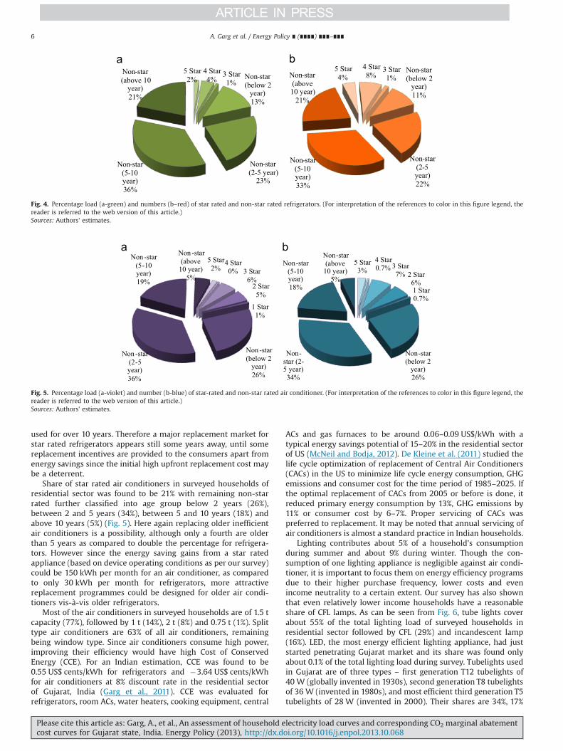
used for over 10 years. Therefore a major replacement market forstar rated refrigerators appears still some years away, until somereplacement incentives are provided to the consumers apart fromenergy savings since the initial high upfront replacement cost maybe a deterrent.

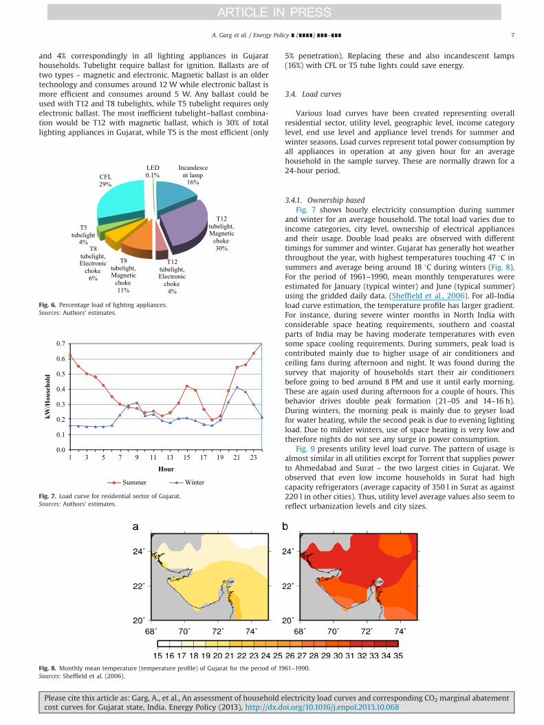
Share of star rated air conditioners in surveyed households ofresidential sector was found to be 21% with remaining non-starrated further classified into age group below 2 years (26%),between 2 and 5 years (34%), between 5 and 10 years (18%) andabove 10 years (5%) (Fig. 5). Here again replacing older inefficientair conditioners is a possibility, although only a fourth are olderthan 5 years as compared to double the percentage for refrigera-tors. However since the energy saving gains from a star ratedappliance (based on device operating conditions as per our survey)could be 150 kWh per month for an air conditioner, as comparedto only 30 kWh per month for refrigerators, more attractivereplacement programmes could be designed for older air condi-tioners vis-à-vis older refrigerators.

Most of the air conditioners in surveyed households are of 1.5 tcapacity (77%), followed by 1 t (14%), 2 t (8%) and 0.75 t (1%). Splittype air conditioners are 63% of all air conditioners, remainingbeing window type. Since air conditioners consume high power,improving their efficiency would have high Cost of ConservedEnergy (CCE). For an Indian estimation, CCE was found to be0.55 US$ cents/kWh for refrigerators and �3.64 US$ cents/kWhfor air conditioners at 8% discount rate in the residential sectorof Gujarat, India (Garg et al., 2011). CCE was evaluated forrefrigerators, room ACs, water heaters, cooking equipment, central

ACs and gas furnaces to be around 0.06–0.09 US$/kWh with atypical energy savings potential of 15–20% in the residential sectorof US (McNeil and Bodja, 2012). De Kleine et al. (2011) studied thelife cycle optimization of replacement of Central Air Conditioners(CACs) in the US to minimize life cycle energy consumption, GHGemissions and consumer cost for the time period of 1985–2025. Ifthe optimal replacement of CACs from 2005 or before is done, itreduced primary energy consumption by 13%, GHG emissions by11% or consumer cost by 6–7%. Proper servicing of CACs waspreferred to replacement. It may be noted that annual servicing ofair conditioners is almost a standard practice in Indian households.

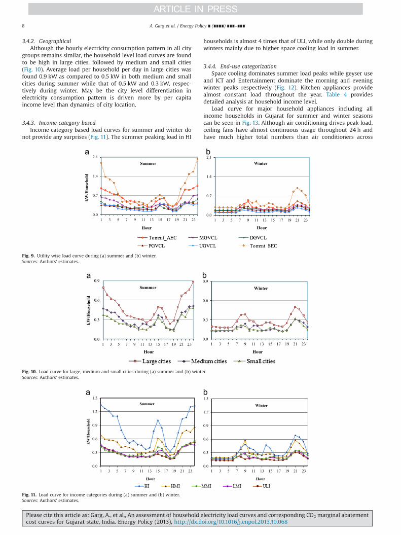
Lighting contributes about 5% of a household’s consumptionduring summer and about 9% during winter. Though the con-sumption of one lighting appliance is negligible against air condi-tioner, it is important to focus them on energy efficiency programsdue to their higher purchase frequency, lower costs and evenincome neutrality to a certain extent. Our survey has also shownthat even relatively lower income households have a reasonableshare of CFL lamps. As can be seen from Fig. 6, tube lights coverabout 55% of the total lighting load of surveyed households inresidential sector followed by CFL (29%) and incandescent lamp(16%). LED, the most energy efficient lighting appliance, had juststarted penetrating Gujarat market and its share was found onlyabout 0.1% of the total lighting load during survey. Tubelights usedin Gujarat are of three types – first generation T12 tubelights of40 W (globally invented in 1930s), second generation T8 tubelightsof 36 W (invented in 1980s), and most efficient third generation T5tubelights of 28 W (invented in 2000). Their shares are 34%, 17%

5 Star2%

4 Star4%

3 Star1%

Non-star (below 2

year)13%

Non-star (2-5 year)

23%

Non-star (5-10 year)36%

Non-star (above 10

year)21%

5 Star4%

4 Star8%

3 Star1%

Non-star (below 2

year)11%

Non-star (2-5 year)22%

Non-star (5-10 year)33%

Non-star (above 10 year)

21%

Fig. 4. Percentage load (a‐green) and numbers (b–red) of star rated and non-star rated refrigerators. (For interpretation of the references to color in this figure legend, thereader is referred to the web version of this article.)Sources: Authors' estimates.

5 Star2%

4 Star0% 3 Star

6%2 Star5%

1 Star1%

Non -star (below 2

year)26%

Non -star (2-5 year)36%

Non -star (5-10 year)19%

Non -star (above

10 year)5%

5 Star3%

4 Star0.7% 3 Star

7% 2 Star6%1 Star0.7%

Non-star (below 2

year)26%

Non-star (2-5 year)34%

Non-star (5-10 year)18%

Non-star (above

10 year)5%

Fig. 5. Percentage load (a‐violet) and number (b‐blue) of star-rated and non-star rated air conditioner. (For interpretation of the references to color in this figure legend, thereader is referred to the web version of this article.)Sources: Authors' estimates.

A. Garg et al. / Energy Policy ∎ (∎∎∎∎) ∎∎∎–∎∎∎6

Please cite this article as: Garg, A., et al., An assessment of household electricity load curves and corresponding CO2 marginal abatementcost curves for Gujarat state, India. Energy Policy (2013), http://dx.doi.org/10.1016/j.enpol.2013.10.068i

and 4% correspondingly in all lighting appliances in Gujarathouseholds. Tubelight require ballast for ignition. Ballasts are oftwo types – magnetic and electronic. Magnetic ballast is an oldertechnology and consumes around 12 W while electronic ballast ismore efficient and consumes around 5 W. Any ballast could beused with T12 and T8 tubelights, while T5 tubelight requires onlyelectronic ballast. The most inefficient tubelight–ballast combina-tion would be T12 with magnetic ballast, which is 30% of totallighting appliances in Gujarat, while T5 is the most efficient (only

5% penetration). Replacing these and also incandescent lamps(16%) with CFL or T5 tube lights could save energy.

3.4. Load curves

Various load curves have been created representing overallresidential sector, utility level, geographic level, income categorylevel, end use level and appliance level trends for summer andwinter seasons. Load curves represent total power consumption byall appliances in operation at any given hour for an averagehousehold in the sample survey. These are normally drawn for a24-hour period.

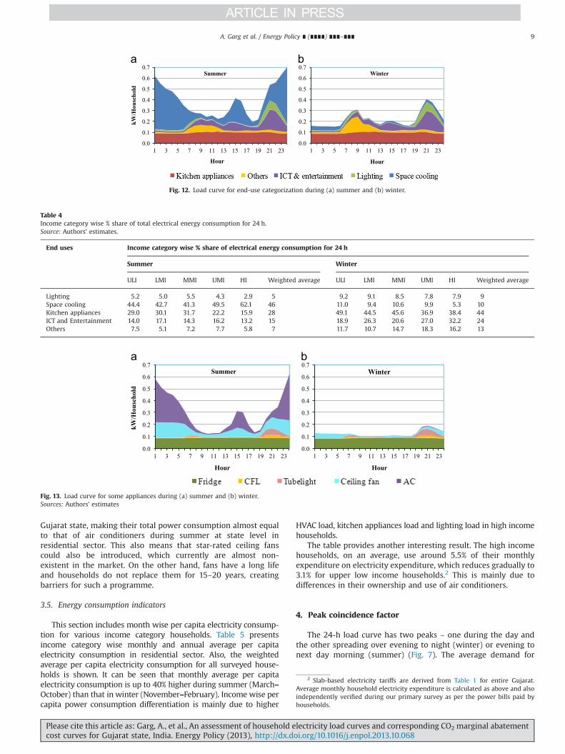
3.4.1. Ownership basedFig. 7 shows hourly electricity consumption during summer

and winter for an average household. The total load varies due toincome categories, city level, ownership of electrical appliancesand their usage. Double load peaks are observed with differenttimings for summer and winter. Gujarat has generally hot weatherthroughout the year, with highest temperatures touching 47 1C insummers and average being around 18 1C during winters (Fig. 8).For the period of 1961–1990, mean monthly temperatures wereestimated for January (typical winter) and June (typical summer)using the gridded daily data. (Sheffield et al., 2006). For all-Indiaload curve estimation, the temperature profile has larger gradient.For instance, during severe winter months in North India withconsiderable space heating requirements, southern and coastalparts of India may be having moderate temperatures with evensome space cooling requirements. During summers, peak load iscontributed mainly due to higher usage of air conditioners andceiling fans during afternoon and night. It was found during thesurvey that majority of households start their air conditionersbefore going to bed around 8 PM and use it until early morning.These are again used during afternoon for a couple of hours. Thisbehavior drives double peak formation (21–05 and 14–16 h).During winters, the morning peak is mainly due to geyser loadfor water heating, while the second peak is due to evening lightingload. Due to milder winters, use of space heating is very low andtherefore nights do not see any surge in power consumption.

Fig. 9 presents utility level load curve. The pattern of usage isalmost similar in all utilities except for Torrent that supplies powerto Ahmedabad and Surat – the two largest cities in Gujarat. Weobserved that even low income households in Surat had highcapacity refrigerators (average capacity of 350 l in Surat as against220 l in other cities). Thus, utility level average values also seem toreflect urbanization levels and city sizes.

0.0

0.1

0.2

0.3

0.4

0.5

0.6

0.7

1 3 5 7 9 11 13 15 17 19 21 23

kW/H

ouse

hold

Hour

Summer Winter

Fig. 7. Load curve for residential sector of Gujarat.Sources: Authors' estimates.

Fig. 8. Monthly mean temperature (temperature profile) of Gujarat for the period of 1961–1990.Sources: Sheffield et al. (2006).

Incandescent lamp

16%

T12 tubelight, Magnetic

choke30%

T12 tubelight, Electronic

choke4%

T8 tubelight, Magnetic

choke11%

T8 tubelight, Electronic

choke6%

T5 tubelight

4%

CFL29%

LED0.1%

Fig. 6. Percentage load of lighting appliances.Sources: Authors' estimates.

A. Garg et al. / Energy Policy ∎ (∎∎∎∎) ∎∎∎–∎∎∎ 7

Please cite this article as: Garg, A., et al., An assessment of household electricity load curves and corresponding CO2 marginal abatementcost curves for Gujarat state, India. Energy Policy (2013), http://dx.doi.org/10.1016/j.enpol.2013.10.068i

3.4.2. GeographicalAlthough the hourly electricity consumption pattern in all city

groups remains similar, the household level load curves are foundto be high in large cities, followed by medium and small cities(Fig. 10). Average load per household per day in large cities wasfound 0.9 kW as compared to 0.5 kW in both medium and smallcities during summer while that of 0.5 kW and 0.3 kW, respec-tively during winter. May be the city level differentiation inelectricity consumption pattern is driven more by per capitaincome level than dynamics of city location.

3.4.3. Income category basedIncome category based load curves for summer and winter do

not provide any surprises (Fig. 11). The summer peaking load in HI

households is almost 4 times that of ULI, while only double duringwinters mainly due to higher space cooling load in summer.

3.4.4. End-use categorizationSpace cooling dominates summer load peaks while geyser use

and ICT and Entertainment dominate the morning and eveningwinter peaks respectively (Fig. 12). Kitchen appliances providealmost constant load throughout the year. Table 4 providesdetailed analysis at household income level.

Load curve for major household appliances including allincome households in Gujarat for summer and winter seasonscan be seen in Fig. 13. Although air conditioning drives peak load,ceiling fans have almost continuous usage throughout 24 h andhave much higher total numbers than air conditioners across

0.0

0.3

0.6

0.9

1 3 5 7 9 11 13 15 17 19 21 23

Hour

Winter

0.0

0.3

0.6

0.9

1 3 5 7 9 11 13 15 17 19 21 23

kW/H

ouse

hold

Hour

Summer

Fig. 10. Load curve for large, medium and small cities during (a) summer and (b) winter.Sources: Authors’ estimates.

0.0

0.3

0.6

0.9

1.2

1.5

1 3 5 7 9 11 13 15 17 19 21 23

kW/H

ouse

hold

Hour

Summer

0.0

0.3

0.6

0.9

1.2

1.5

1 3 5 7 9 11 13 15 17 19 21 23

Hour

Winter

Fig. 11. Load curve for income categories during (a) summer and (b) winter.Sources: Authors’ estimates.

0.0

0.7

1.4

2.1

1 3 5 7 9 11 13 15 17 19 21 23

kW/H

ouse

hold

Hour

Summer

0.0

0.7

1.4

2.1

1 3 5 7 9 11 13 15 17 19 21 23

Hour

Winter

Fig. 9. Utility wise load curve during (a) summer and (b) winter.Sources: Authors’ estimates.

A. Garg et al. / Energy Policy ∎ (∎∎∎∎) ∎∎∎–∎∎∎8

Please cite this article as: Garg, A., et al., An assessment of household electricity load curves and corresponding CO2 marginal abatementcost curves for Gujarat state, India. Energy Policy (2013), http://dx.doi.org/10.1016/j.enpol.2013.10.068i

Gujarat state, making their total power consumption almost equalto that of air conditioners during summer at state level inresidential sector. This also means that star-rated ceiling fanscould also be introduced, which currently are almost non-existent in the market. On the other hand, fans have a long lifeand households do not replace them for 15–20 years, creatingbarriers for such a programme.

3.5. Energy consumption indicators

This section includes month wise per capita electricity consump-tion for various income category households. Table 5 presentsincome category wise monthly and annual average per capitaelectricity consumption in residential sector. Also, the weightedaverage per capita electricity consumption for all surveyed house-holds is shown. It can be seen that monthly average per capitaelectricity consumption is up to 40% higher during summer (March–October) than that in winter (November–February). Income wise percapita power consumption differentiation is mainly due to higher

HVAC load, kitchen appliances load and lighting load in high incomehouseholds.

The table provides another interesting result. The high incomehouseholds, on an average, use around 5.5% of their monthlyexpenditure on electricity expenditure, which reduces gradually to3.1% for upper low income households.2 This is mainly due todifferences in their ownership and use of air conditioners.

4. Peak coincidence factor

The 24-h load curve has two peaks – one during the day andthe other spreading over evening to night (winter) or evening tonext day morning (summer) (Fig. 7). The average demand for

Table 4Income category wise % share of total electrical energy consumption for 24 h.Source: Authors’ estimates.

End uses Income category wise % share of electrical energy consumption for 24 h

Summer Winter

ULI LMI MMI UMI HI Weighted average ULI LMI MMI UMI HI Weighted average

Lighting 5.2 5.0 5.5 4.3 2.9 5 9.2 9.1 8.5 7.8 7.9 9Space cooling 44.4 42.7 41.3 49.5 62.1 46 11.0 9.4 10.6 9.9 5.3 10Kitchen appliances 29.0 30.1 31.7 22.2 15.9 28 49.1 44.5 45.6 36.9 38.4 44ICT and Entertainment 14.0 17.1 14.3 16.2 13.2 15 18.9 26.3 20.6 27.0 32.2 24Others 7.5 5.1 7.2 7.7 5.8 7 11.7 10.7 14.7 18.3 16.2 13

0.0

0.1

0.2

0.3

0.4

0.5

0.6

0.7

1 3 5 7 9 11 13 15 17 19 21 23

Hour

Winter

0.0

0.1

0.2

0.3

0.4

0.5

0.6

0.7

1 3 5 7 9 11 13 15 17 19 21 23

kW/H

ouse

hold

Hour

Summer

Fig. 13. Load curve for some appliances during (a) summer and (b) winter.Sources: Authors’ estimates

0.0

0.1

0.2

0.3

0.4

0.5

0.6

0.7

1 3 5 7 9 11 13 15 17 19 21 23

kW/H

ouse

hold

Hour

Summer

0.0

0.1

0.2

0.3

0.4

0.5

0.6

0.7

1 3 5 7 9 11 13 15 17 19 21 23

Hour

Winter

Fig. 12. Load curve for end-use categorization during (a) summer and (b) winter.

2 Slab-based electricity tariffs are derived from Table 1 for entire Gujarat.Average monthly household electricity expenditure is calculated as above and alsoindependently verified during our primary survey as per the power bills paid byhouseholds.

A. Garg et al. / Energy Policy ∎ (∎∎∎∎) ∎∎∎–∎∎∎ 9

Please cite this article as: Garg, A., et al., An assessment of household electricity load curves and corresponding CO2 marginal abatementcost curves for Gujarat state, India. Energy Policy (2013), http://dx.doi.org/10.1016/j.enpol.2013.10.068i

electricity by individual households is higher during these peakhours due to use of more appliances. The overall timings of thesepeaks vary. Electricity supply costs during peaks are generallyhigher for a utility as a whole as the marginal cost of supplying thelast unit of electricity is higher as the electricity demand rises. Theutility may or may not be able to transfer these higher costs tohouseholds due to the presence or absence of time-of-day pricingrespectively. In Gujarat presently there is no time-of-day pricingfor households, but only a monthly slab pricing. The householdstherefore do not get a price signal on daily peaks. However utilityhas to supply power at higher costs during the peaks, whichreduces its overall margins. It is therefore desirable, primarily forutilities in the present situation, to understand the contribution byvarious appliances to load peaking in order to suggest policies forreducing the peaks. If a time-of-day pricing is introduced in futurefor households, this analysis would become more relevant forhouseholds as the utility may then be able to transfer the higherpeaking costs to households. Peak coincidence factor is a tool toanalyze peaks and how various appliances contribute to it. It is aratio, expressed as a numerical value or as a percentage, of thesimultaneous maximum demand of a group of electrical appli-ances or consumers within a specified period, to the sum of theirindividual maximum demands within the same period (EEP, 2010).Coincidence factor is usually less than one.

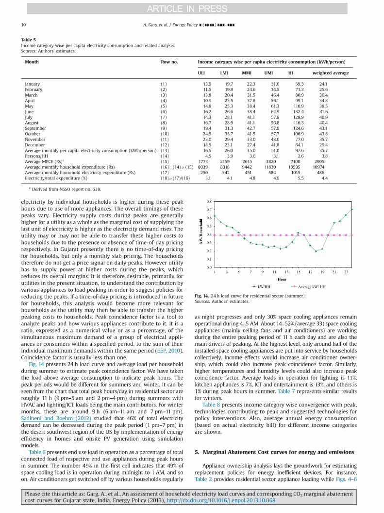
Fig. 14 presents 24 h load curve and average load per householdduring summer to estimate peak coincidence factor. We have takenthe load above average consumption to indicate peak hours. Thepeak periods would be different for summers and winter. It can beseen from the chart that total peak hours/day in residential sector areroughly 11 h (9 pm–5 am and 2 pm–4 pm) during summers withHVAC and lighting/ICT loads being the main contributors. For wintermonths, these are around 9 h (6 am–11 am and 7 pm–11 pm).Sadineni and Boehm (2012) studied that 46% of total electricitydemand can be decreased during the peak period (1 pm–7 pm) inthe desert southwest region of the US by implementation of energyefficiency in homes and onsite PV generation using simulationmodels.

Table 6 presents end use load in operation as a percentage of totalconnected load of respective end use appliances during peak hoursin summer. The number 49% in the first cell indicates that 49% ofspace cooling load is in operation during midnight to 1 AM, and soon. Air conditioners get switched off by various households regularly

as night progresses and only 30% space cooling appliances remainoperational during 4–5 AM. About 14–52% (average 33) space coolingappliances (mainly ceiling fans and air conditioners) are workingduring the entire peaking period of 11 h each day and are also themain drivers of peaking. At the highest level, only around half of theinstalled space cooling appliances are put into service by householdscollectively. Income effects would increase air conditioner owner-ship, which could also increase peak coincidence factor. Similarly,higher temperatures and humidity levels could also increase peakcoincidence factor. Average loads in operation for lighting is 11%,kitchen appliances is 7%, ICT and entertainment is 13%, and others is1% during peak hours in summer. Table 7 represents similar resultsfor winters.

Table 8 presents income category wise convergence with peak,technologies contributing to peak and suggested technologies forpolicy interventions. Also, average annual energy consumption(based on actual electricity bill) for different income categoriesare shown.

5. Marginal Abatement Cost curves for energy and emissions

Appliance ownership analysis lays the groundwork for estimatingreplacement policies for energy inefficient devices. For instance,Table 2 provides residential sector appliance loading while Figs. 4–6

Table 5Income category wise per capita electricity consumption and related analysis.Sources: Authors’ estimates.

Month Row no. Income category wise per capita electricity consumption (kWh/person)

ULI LMI MMI UMI HI weighted average

January (1) 13.9 19.7 22.3 31.0 59.3 24.1February (2) 11.5 19.9 24.6 34.5 71.3 25.6March (3) 13.8 20.4 31.5 46.4 80.9 30.4April (4) 10.9 23.5 37.8 56.1 99.1 34.8May (5) 14.8 25.3 38.4 61.3 110.9 38.5June (6) 16.2 26.6 38.4 62.9 132.4 41.6July (7) 14.3 28.1 41.1 57.9 128.9 40.9August (8) 16.7 28.9 41.1 56.8 116.3 40.4September (9) 19.4 31.3 42.7 57.9 124.6 43.1October (10) 24.5 35.7 41.5 57.7 106.9 43.8November (11) 23.0 29.4 33.0 48.0 77.0 35.7December (12) 18.5 23.1 27.4 41.8 64.1 29.4Average monthly per capita electricity consumption (kWh/person) (13) 16.5 26.0 35.0 51.0 97.6 35.7Persons/HH (14) 4.5 3.9 3.6 3.1 2.6 3.8Average MPCE (Rs)a (15) 1773 2159 2615 3820 7100 2905Average monthly household expenditure (Rs) (16)¼(14)� (15) 8039 8318 9442 11830 18595 10974Average monthly household electricity expenditure (Rs) (17) 250 342 451 584 1015 486Electricity/total expenditure (%) (18)¼(17)/(16) 3.1 4.1 4.8 4.9 5.5 4.4

a Derived from NSSO report no. 538.

0.0

0.1

0.2

0.3

0.4

0.5

0.6

0.7

0.8

1 3 5 7 9 11 13 15 17 19 21 23

kW/H

ouse

hold

Hour

kW/HH Average kW/ HH

Fig. 14. 24 h load curve for residential sector (summer).Sources: Authors’ estimates.

A. Garg et al. / Energy Policy ∎ (∎∎∎∎) ∎∎∎–∎∎∎10

Please cite this article as: Garg, A., et al., An assessment of household electricity load curves and corresponding CO2 marginal abatementcost curves for Gujarat state, India. Energy Policy (2013), http://dx.doi.org/10.1016/j.enpol.2013.10.068i

provide ownerships for air conditioners, refrigerators and lightingloads. These results could be used to design programmes for higherpenetration of energy efficient appliances using myriad instrumentssuch as energy efficiency standards and labels, subsidies, tax incen-tives, price rebates, and carbon credits. For instance, air conditionerstake 16.4% of total residential sector sanctioned load, of which around76% load is accounted for by non-star rated ACs. Utilities may launchreplacement programmes in collaboration with star-rated AC manu-facturers wherein cash incentives may be provided to the buyers ofstar rated ACs. Also, utilities may launch buy back policy for replace-ment of old, non-star rated refrigerator with star rated refrigerators byproviding good rebates to the consumers. Similar scope exists forlaunching energy efficient lighting programmes. Buy back policy couldbe developed for replacement of magnetic ballast with electronicballast with reasonable rates. Also, new purchase for tube lights couldbe promoted for T5 tubelights. Utilities, appliance manufacturers andconsumers all gain by such programmes. Consumers’ power billsreduce, manufacturers sell more products, and utilities reduce theirpeak load requirements thus releasing generation capacity whileavoiding buying of very high rate peak power from the grid to meetthese loads.

There are similar suggestions by other authors in literature. Forinstance, Abhyankar and Phadke (2012) examined the impacts onutility finances and consumer tariffs by various scenarios such as(a) incentive mechanisms for mitigating the financial risk of utilities,(b) utilities fund the EE programs only partially, (c) utilities sell the

conserved electricity into spot markets and (d) the level of powershortages utilities are facing. The average tariff was increased by 2.2%for consumers participating in EE programs and the utility incentivemechanisms mitigate their risk of losing long- term returns. Also, thecash flow risk was amplified (up to 57% of annual returns of utilities)in case of power shortages. Amstalden et al. (2007) studied theeconomic potential of energy efficient retrofitting in the Swissbuilding sector using the discounted cash flowmethod with differentenergy price expectations, policy instruments such as subsidies,income tax deduction, a carbon tax, and decrease in cost of energyefficiency measures. Expecting higher energy prices in future,energy-efficient retrofitting would be an attractive investmentopportunity. Kesicki (2012) studied the CO2 abatement potentialand costs in the residential sector of UK from a systems perspectivein order to capture interactions and interdependencies in the energysector using UK MARKAL model. Ashina and Nakata (2008) studiedthat CO2 emission in the residential sector of Iwate prefecture inJapan can be decreased from 0.726 Mt-CO2 (2003) to 0.674 Mt-CO2 inthe year 2020 if half of the households use EE appliances, providedgovernment financially supports the purchasers of EE appliances.Kesicki (2013) studied the MAC curve for the UK energy system usingUK MARKAL model. The results indicated that a system-wide CO2 taxof around d100/t-CO2 in 2030 would be necessary to cut UKemissions by 60% in 2030 compared with 1990 levels.

Marginal abatement cost (MAC) curves are a commonly usedpolicy tool indicating emission abatement potential and associated

Table 6End use loads in operation as a percentage of total connected load of respective end use during peak hours in summer.Source: Authors’ estimates.

End uses End use loads in operation as a percentage of total connected load of respective end use during peak hours in summer

0–1 1–2 2–3 3–4 4–5 14–15 15–16 20–21 21–22 22–23 23–24

Space cooling (%) 49 42 38 36 30 22 21 14 19 36 52Lighting (%) 4 4 4 4 4 1 1 40 33 20 10Kitchen appliances (%) 7 7 7 7 7 8 8 8 7 7 7ICT and entertainment (%) 3 2 2 2 2 16 12 36 35 24 10Others (%) 1 1 1 1 1 1 1 2 2 1 1

Table 7End use load in operation as a percentage of total connected load of respective end use during peak hours in winter.Source: Authors’ estimates.

End uses End use loads in operation as a percentage of total connected load of respective end use during peak hours in winter

6–7 7–8 8–9 9–10 10–11 19–20 20–21 21–22 22–23

Space cooling (%) 6 3 2 1 1 2 4 5 6Lighting (%) 3 6 6 2 1 7 16 18 14Kitchen appliances (%) 4 4 4 4 5 4 5 4 4ICT and entertainment (%) 1 1 3 4 3 3 7 14 13Others (%) 2 10 16 18 9 2 2 2 2

Table 8Income category wise convergence with peak, technologies contributing to peak and technologies of intervention (summer).Source: Authors’ estimates.

Incomecategories

Convergence with peak(9 pm–5 am, 2 pm–4 pm)

Annual average electricityconsumption (kWh)

Technologies contributingto peak

Technologies of interventions

ULI 5 h (9 pm–2 am) 891 Lighting and ICT and entertainment CFLs, T5 tube lights, EE fans, EE refrigeratorsLMI 5 h (9 pm–2 am) 1217 Lighting and ICT and entertainment CFLs, T5 tubelights, EE fans, EE refrigeratorsMMI 6 h (9 pm–1 am, 2 pm–4 pm) 1512 HVAC, lighting EE ACs, EE fans, T5 tube lights, EE refrigerators,

solar water geyser (winter)UMI 10 h (9 pm–5 am, 2 pm–4 pm) 1897 HVAC, and lighting EE ACs, EE fans, T5 tube lights, EE refrigerators,

solar water geyser (winter)HI 10 h (9 pm–5 am, 2 pm–4 pm) 3045 HVAC and lighting

A. Garg et al. / Energy Policy ∎ (∎∎∎∎) ∎∎∎–∎∎∎ 11

Please cite this article as: Garg, A., et al., An assessment of household electricity load curves and corresponding CO2 marginal abatementcost curves for Gujarat state, India. Energy Policy (2013), http://dx.doi.org/10.1016/j.enpol.2013.10.068i

abatement costs. They have been extensively used for variousenvironmental issues in different countries and are increasinglyapplied to climate change policy (Kesicki and Strachan, 2013). Wehave used MAC curves as a tool for grading various technologyreplacement options on the basis of effective costs and expectedsavings, through net present value estimation. Energy savings thusaccrued could also be converted into CO2 emission savings forplotting MAC curves. However co-benefits of reduction in otherpollution loads are not included in the analysis. We consideredtwo scenarios.

� Scenario A- Replacing existing inefficient but operational appli-ances with more energy efficient appliances where the full costof the new appliances is to be paid by the consumer. She willhowever receive a salvage value for the replaced inefficientappliances, along with energy savings but no money receivedfor the CO2 saved due to this replacement.

� Scenario B- Similar to scenario-A plus CO2 money receipts.

The Marginal Abatement Cost (MAC) for an appliance isestimated using the following equation:

MAC ¼ NPVifðEiþRCiÞ�CCig=CO2i

where, MAC is the Marginal Abatement Cost, NPVi is the NetPresent Value of appliance i estimated over its entire life, Ei is thePrice of electricity saved per year, RCi is the Revenue from CO2

saved/year, CCi is the Capital cost of appliance i and CO2i is the CO2

saved over entire life of the appliance i.The CO2 price is assumed to be US$ 5 per ton-CO2 for 2011-13,

increasing by US$ 2.5/t-CO2 per year until 2019. It is subsequentlytaken as US$ 25/t-CO2 per year. Similar levels of CO2 prices havebeen projected in other studies (STCM, 2012, CTM, 2012 and PointCarbon, 2011).We also carried out sensitivity analysis for CO2

prices ranging to twice these prices. Higher CO2 prices (andrevenues) make a few more technology transitions financiallymore attractive for each income category. We have assumedweighted average emission factor of 0.88 kg of CO2 per kWh forwestern regional grid of India (CEA, 2013b). The MAC curves areprepared for a range of discount rates: 6, 8, 10, 12, 16, 20 and 25%

as a sensitivity analysis and also since different income groups facedifferent discount rates in reality. For instance, capital is scarcer forlower income groups and may have sub sustenance level alternateuses. Micro finance institutions charge around 26% (max.) averageannual interests from lower income households in India (RBI,2012). Replacing energy inefficient appliances therefore shouldmake sense to them provided their returns from such replace-ments are more than their high cost of capital. For higher incomegroups, discount rates are much lower and taken closer to thoseused for project evaluation including inflation (CERC, 2011). Wadaet al. (2012) had also indicated that the rate of uptake of energyefficiency measures is slow as the discount rate reflects actualconsumer behavior. Lower income households require muchhigher discount rates than high income households to investmentsin energy efficiency in the real world economy.

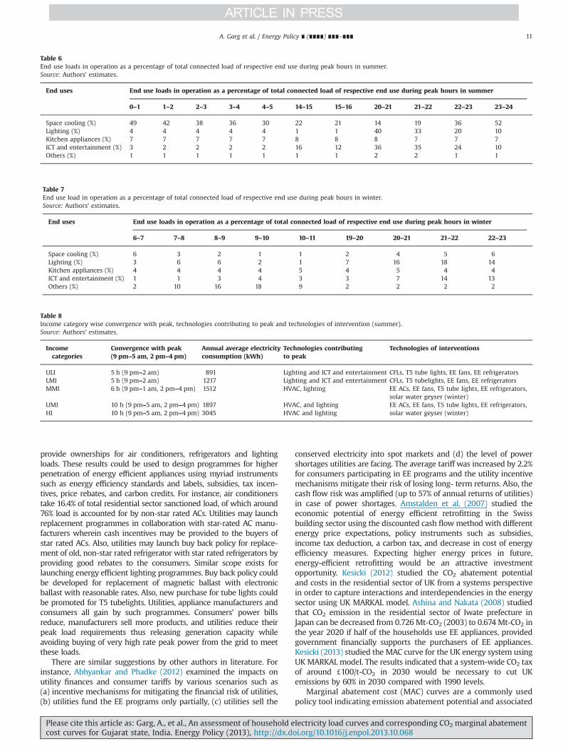
Figs. 15 and 16 present MAC curves for low, medium and highincome households in Gujarat for scenarios A and B, respectively.3

It can be seen from all these figures that MAC curves for highincome households appear on right side due to their highermitigation potential which in turn is due to more number ofappliances coupled by their higher usage. The negative MAC valuesin all the three figures indicate technology replacement choicesthat should be implemented anyway as it represents direct benefitto the consumers besides carbon benefits to the society. Howeverdespite having a negative cost, these options are not generallychosen by households due to myriad barriers, such as high upfrontcost of efficient technologies, high cost of capital, lack of aware-ness, perception about reliability of new technologies, unreliableand low quality electricity supply making appliance efficiency

Fig. 15. MAC curve for Scenario-A (Low income: 20% discount rate, Medium income: 16% discount rate, High income: 12% discount rate).Sources: Authors’ estimates.

3 These 3 categories subsume the earlier 5 categories for ease of representationin the figures. High in Figs. 15 and 16 encompasses High Income and UMI of Table 2,similarly Medium encompasses MMI and LMI, and Low encompasses ULI. Oursensitivity analysis and individual 5-category analysis support this reducedrepresentation. Five category analysis places the categories in the same ascendingorder in the figures, while increasing the complexity with 5 lines having marginalvariation in discount rates for each line. The 3 category representation in thissection therefore does not result in any loss of information and captures the maininsights as derived from MAC curves.

A. Garg et al. / Energy Policy ∎ (∎∎∎∎) ∎∎∎–∎∎∎12

Please cite this article as: Garg, A., et al., An assessment of household electricity load curves and corresponding CO2 marginal abatementcost curves for Gujarat state, India. Energy Policy (2013), http://dx.doi.org/10.1016/j.enpol.2013.10.068i

gains ineffective, path dependencies of supporting infrastructure,behavioral lock-ins etc. Multiple policy and market based initia-tives such as consumer awareness, easy information access such asthrough labeling and initial support for developing infrastructuregeared to new appliances are needed to realize the full potential ofthese negative or near-zero cost mitigation actions. Even technol-ogies with positive MAC value, such as solar geysers, may requireadequate CO2 prices and/or government support for adaptation.Reducing import tariffs, technology R&D incentives, subsidies toconsumers, incentives to producers, and enhancing economies ofscale and learning are some options for making these technologiesmarket ready.

Almost 26% residential load can be reduced by deployingenergy efficient DSM measures with negative MAC values. Underscenario A, the positive MAC for low income households occurs forthe following technology transitions - Incandescent lamp to CFL,T12 to T8 tubelight (with and without ballast replacement), T12 toT5 tubelight (with and without ballast replacement), T8 to T5tubelight (with and without ballast replacement), non star AC (agebelow 10 years) to 2/5 star AC, non star fridge (any age) to 4/5 starfridge, non-star TV to 4 star TV and electric geyser to gas geyser/solar geyser. For medium income households it occurs for T12 toT8/T5 (without ballast replacement), T8 to T5 tube light (with andwithout ballast replacement), non-star fridge to 4/5 star fridge,non-star AC (age between 5 and 10 years) to 2 star AC, non-star ACto 2/5 star AC, non-star TV to 4 star TV and electric geyser to gasgeyser/solar geyser. For high income households if occurs for T8 toT5 tube light (without ballast replacement), non-star TV to 4 starTV and electric geyser to solar geyser (Fig. 15). The time-of-daybased differential electricity tariff in the residential sector is notavailable in India presently and is therefore not able to correctconsumer behavior on deploying more energy efficient appliances.Table 9 presents annual energy savings, CO2 savings over life and

MAC results for Scenario A and Scenario B for some of theappliance replacements.

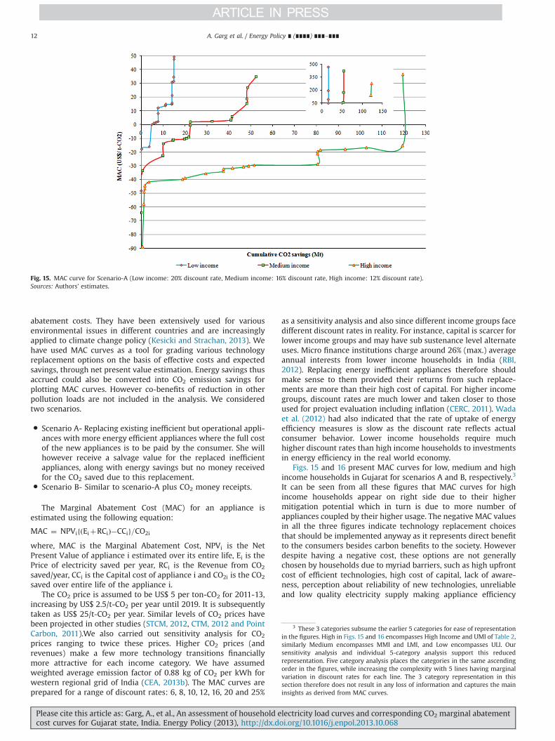
Under scenario B, the positive MAC for low income householdsoccurs for the technology transitions: non star AC (between 5 and 10years of age) to 2/5 star AC, incandescent lamp to CFL, T12 to T8 or T5tubelights (with and without ballast replacement), T8 to T5 tubelight(with and without ballast replacement), non-star AC to 2/5 star AC,non star TV to 4 star TV, and electric geyser to gas geyser/solargeyser. For medium income households it occurs for the T12 to T8/T5tubelights (without ballast replacement), non-star AC to 2/5 star AC,T8 to T5 tubelight (without ballast replacement), non star TV to4 star TV, and electric geyser to gas geyser/solar geyser. For highincome households, it occurs for the same technology transitions asthose under scenario-A (Fig. 16). Lower income households facemore barriers for many simple technology transitions that occur forhigher income households at negative or near-zero costs. Penetra-tion of solar geysers is an expensive proposition for all incomegroups currently. This market is to be expanded in India and may-beeconomies of scales would bring down the technology costs.

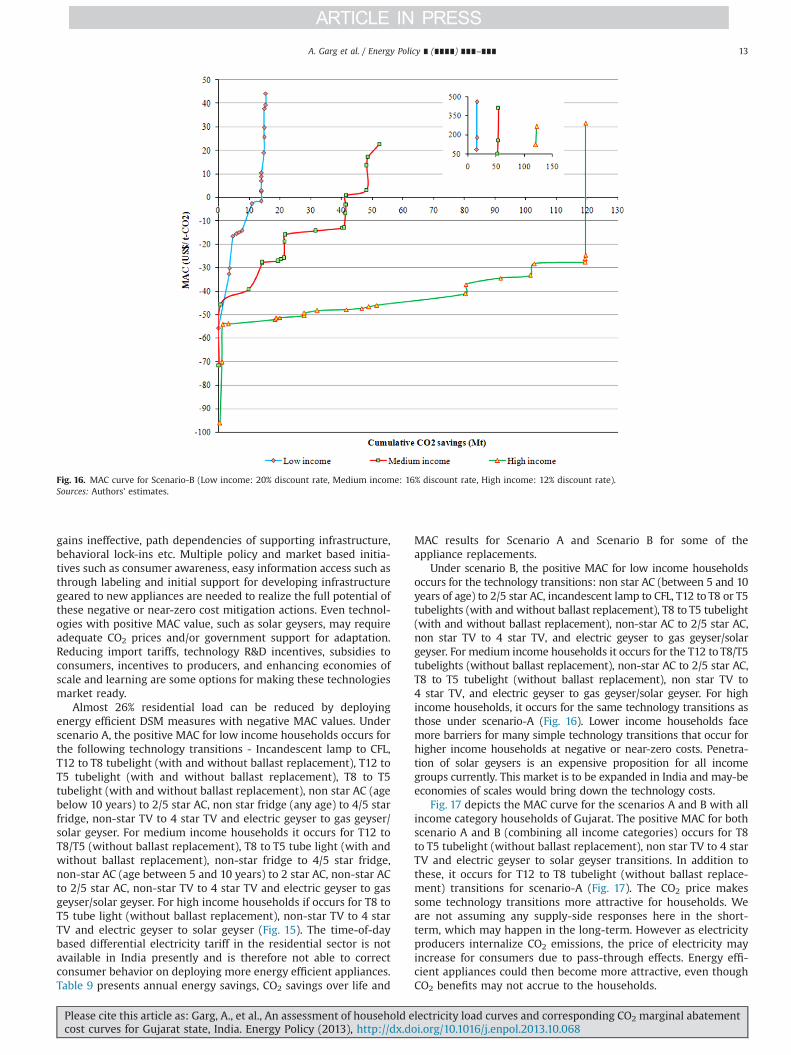
Fig. 17 depicts the MAC curve for the scenarios A and B with allincome category households of Gujarat. The positive MAC for bothscenario A and B (combining all income categories) occurs for T8to T5 tubelight (without ballast replacement), non star TV to 4 starTV and electric geyser to solar geyser transitions. In addition tothese, it occurs for T12 to T8 tubelight (without ballast replace-ment) transitions for scenario-A (Fig. 17). The CO2 price makessome technology transitions more attractive for households. Weare not assuming any supply-side responses here in the short-term, which may happen in the long-term. However as electricityproducers internalize CO2 emissions, the price of electricity mayincrease for consumers due to pass-through effects. Energy effi-cient appliances could then become more attractive, even thoughCO2 benefits may not accrue to the households.

Fig. 16. MAC curve for Scenario-B (Low income: 20% discount rate, Medium income: 16% discount rate, High income: 12% discount rate).Sources: Authors’ estimates.

A. Garg et al. / Energy Policy ∎ (∎∎∎∎) ∎∎∎–∎∎∎ 13

Please cite this article as: Garg, A., et al., An assessment of household electricity load curves and corresponding CO2 marginal abatementcost curves for Gujarat state, India. Energy Policy (2013), http://dx.doi.org/10.1016/j.enpol.2013.10.068i

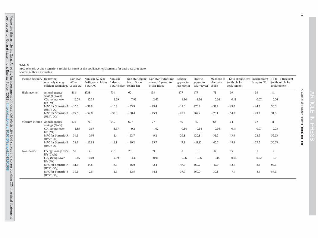
Table 9MAC scenario-A and scenario-B results for some of the appliance replacements for entire Gujarat state.Source: Authors' estimates.

Income category Deployingrelatively energyefficient technology

Non starAC to2 star AC

Non star AC (age5–10 years old) to5 star AC

Non starfridge to4 star fridge

Non star ceilingfan to 5 starceiling fan

Non star fridge (ageabove 10 years) to5 star fridge

Electricgeyser togas geyser

Electricgeyser tosolar geyser

Magnetic toelectronicchoke

T12 to T8 tubelight(with chokereplacement)

Incandescentlamp to CFL

T8 to T5 tubelight(without chokereplacement)

High income Annual energysavings (GWh)

1884 1738 734 601 198 177 177 73 69 39 14

CO2 savings overlife (Mt)

16.58 15.29 9.69 7.93 2.62 1.24 1.24 0.64 0.18 0.07 0.04

MAC for Scenario-A(US$/t-CO2)

�15.3 �39.8 �16.8 �33.9 �29.4 �18.6 276.9 �57.9 �49.0 �44.3 36.6

MAC for Scenario-B(US$/t-CO2)

�27.5 �52.0 �33.3 �50.4 �45.9 �28.2 267.2 �70.1 �54.0 �49.3 31.6

Medium income Annual energysavings (GWh)

438 76 649 697 77 49 49 64 54 37 11

CO2 savings overlife (Mt)

3.85 0.67 8.57 9.2 1.02 0.34 0.34 0.56 0.14 0.07 0.03

MAC for Scenario-A(US$/t-CO2)

34.9 �0.63 3.4 �22.7 �9.2 26.8 420.81 �33.5 �13.9 �22.5 55.63

MAC for Scenario-B(US$/t-CO2)

22.7 �12.88 �13.1 �39.2 �25.7 17.2 411.12 �45.7 �18.9 �27.5 50.63

Low income Energy savings overlife (GWh)

52 4 219 261 69 8 8 17 15 11 2

CO2 savings overlife (Mt)

0.45 0.03 2.89 3.45 0.91 0.06 0.06 0.15 0.04 0.02 0.01

MAC for Scenario-A(US$/t-CO2)

51.5 14.8 14.9 �16.0 2.4 47.6 469.7 �17.9 12.1 8.1 92.6

MAC for Scenario-B(US$/t-CO2)

39.3 2.6 �1.6 �32.5 �14.2 37.9 460.0 �30.1 7.1 3.1 87.6

A.G

arget

al./Energy

Policy∎(∎∎∎∎)

∎∎∎–∎∎∎

14Pleasecite

thisarticle

as:Garg,A

.,etal.,A

nassessm

entofh

ouseh

oldelectricity

loadcu

rvesan

dcorresp

ondingCO2margin

alabatemen

tcost

curves

forGujarat

state,India.En

ergyPolicy

(2013),http

://dx.d

oi.org/10.1016/j.enpol.2013.10.068i

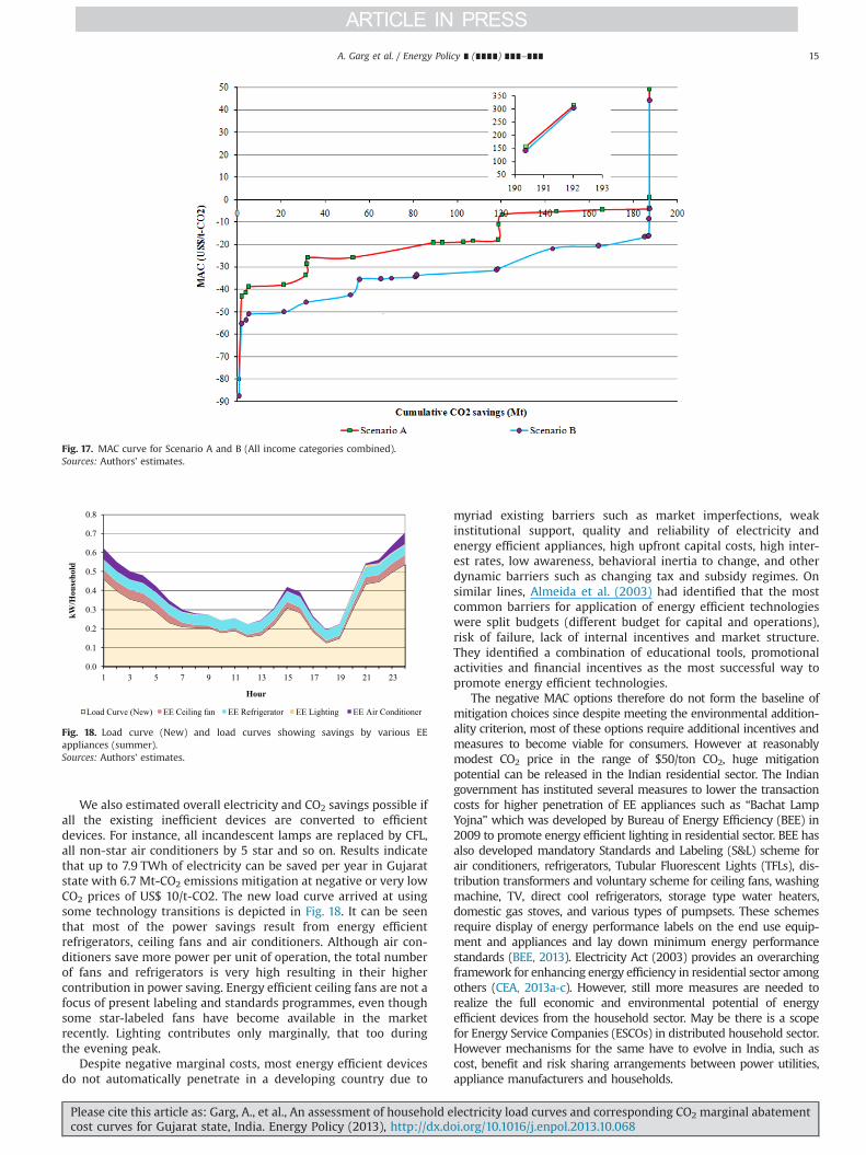
We also estimated overall electricity and CO2 savings possible ifall the existing inefficient devices are converted to efficientdevices. For instance, all incandescent lamps are replaced by CFL,all non-star air conditioners by 5 star and so on. Results indicatethat up to 7.9 TWh of electricity can be saved per year in Gujaratstate with 6.7 Mt-CO2 emissions mitigation at negative or very lowCO2 prices of US$ 10/t-CO2. The new load curve arrived at usingsome technology transitions is depicted in Fig. 18. It can be seenthat most of the power savings result from energy efficientrefrigerators, ceiling fans and air conditioners. Although air con-ditioners save more power per unit of operation, the total numberof fans and refrigerators is very high resulting in their highercontribution in power saving. Energy efficient ceiling fans are not afocus of present labeling and standards programmes, even thoughsome star-labeled fans have become available in the marketrecently. Lighting contributes only marginally, that too duringthe evening peak.

Despite negative marginal costs, most energy efficient devicesdo not automatically penetrate in a developing country due to

myriad existing barriers such as market imperfections, weakinstitutional support, quality and reliability of electricity andenergy efficient appliances, high upfront capital costs, high inter-est rates, low awareness, behavioral inertia to change, and otherdynamic barriers such as changing tax and subsidy regimes. Onsimilar lines, Almeida et al. (2003) had identified that the mostcommon barriers for application of energy efficient technologieswere split budgets (different budget for capital and operations),risk of failure, lack of internal incentives and market structure.They identified a combination of educational tools, promotionalactivities and financial incentives as the most successful way topromote energy efficient technologies.

The negative MAC options therefore do not form the baseline ofmitigation choices since despite meeting the environmental addition-ality criterion, most of these options require additional incentives andmeasures to become viable for consumers. However at reasonablymodest CO2 price in the range of $50/ton CO2, huge mitigationpotential can be released in the Indian residential sector. The Indiangovernment has instituted several measures to lower the transactioncosts for higher penetration of EE appliances such as “Bachat LampYojna” which was developed by Bureau of Energy Efficiency (BEE) in2009 to promote energy efficient lighting in residential sector. BEE hasalso developed mandatory Standards and Labeling (S&L) scheme forair conditioners, refrigerators, Tubular Fluorescent Lights (TFLs), dis-tribution transformers and voluntary scheme for ceiling fans, washingmachine, TV, direct cool refrigerators, storage type water heaters,domestic gas stoves, and various types of pumpsets. These schemesrequire display of energy performance labels on the end use equip-ment and appliances and lay down minimum energy performancestandards (BEE, 2013). Electricity Act (2003) provides an overarchingframework for enhancing energy efficiency in residential sector amongothers (CEA, 2013a-c). However, still more measures are needed torealize the full economic and environmental potential of energyefficient devices from the household sector. May be there is a scopefor Energy Service Companies (ESCOs) in distributed household sector.However mechanisms for the same have to evolve in India, such ascost, benefit and risk sharing arrangements between power utilities,appliance manufacturers and households.

Fig. 17. MAC curve for Scenario A and B (All income categories combined).Sources: Authors’ estimates.

0.0

0.1

0.2

0.3

0.4

0.5

0.6

0.7

0.8

1 3 5 7 9 11 13 15 17 19 21 23

kW/H

ouse

hold

Hour

Load Curve (New) EE Ceiling fan EE Refrigerator EE Lighting EE Air Conditioner

Fig. 18. Load curve (New) and load curves showing savings by various EEappliances (summer).Sources: Authors’ estimates.

A. Garg et al. / Energy Policy ∎ (∎∎∎∎) ∎∎∎–∎∎∎ 15

Please cite this article as: Garg, A., et al., An assessment of household electricity load curves and corresponding CO2 marginal abatementcost curves for Gujarat state, India. Energy Policy (2013), http://dx.doi.org/10.1016/j.enpol.2013.10.068i

6. Conclusions

This is a broad assessment and may be first of its kind for alarge state in India. The results provide an initial analysis onownership and usage patterns of various appliances in residentialsector for different income categories, cities and seasons. Theconsumer base representation in the sample survey was highincome class with 26% share, medium income class at 42%, andlow income class at 32% which together represented upper5 deciles classes of Gujarat’s income category households. Theaverage electricity consumption of the household indicates that14% consume less than 100 units (kWh) per month, 77% consume100–250 units and 9% using more than 250 units per month.Electricity expenditure is between 3.1 to 5.5% of monthly house-hold expenditure, with 4.4% being overall average. Higher incomehouseholds have higher ratio, mainly due to higher ownership anduse of more energy intensive appliances such as air conditioners.The ownership of appliances shows the affluent status of theresidential consumers of all utilities with 95% owning refrigera-tors, 37% owning air conditioners, 43% owning washing machines,and 30% owning computers. More than 22% also own electricwater geysers. Thus, the overall electricity consumption of thesehouseholds is on the higher side relatively. During summer, spacecooling load, in particular air conditioners, are the highest con-tributors to total load, followed by refrigerators, ceiling fan andlighting load (FTLs, CFLs etc.). While in winters, refrigeratorscontribute the most to the total load, followed by ceiling fansand lighting equipments (FTLs, CFLs etc.) as air conditioning andeven space heating loads are negligible in winter in this part of theworld. Climate change effects and also income effects may alterboth these dynamics as more and more requirements may be feltfor higher space cooling and heating in the coming years.

Another interesting policy insight is on the switch over toefficient appliances in refrigeration and space cooling domains.Efficient lighting is only a marginal contributor to peak loadreduction. Utilities could thus use our results to design DSMprogrammes in their jurisdictions to target income categoriesand appliances. Manufacturers could also use these results tounderstand the market potential for their products. Energy effi-cient ceiling fans are one potential area where current efforts arenot focused. There is also good possibility of a follow up researchin this direction. The methodology and analysis of this type couldalso be deployed for other states in India.

We have also created marginal abatement cost curves forvarious technology transitions to replace existing inefficient appli-ances with efficient appliances. This analysis deployed two sce-narios combining appliance costs, salvage value of replacedappliance, electricity savings, and carbon revenue. These coveredvarious income classifications, covering a sensitivity analysis ondiscount rates and CO2 prices. The analysis highlighted technologytransitions that have a negative MAC. Lower income householdshave lower possibility of technology transitions due to incomeeffects. It may be noted here that although many negative costmitigation options do exist in the residential sector, they facemyriad barriers for higher penetration such as quality and relia-bility of electricity and energy efficient appliances, high upfrontcapital costs, high interest rates, low awareness, and behavioralinertia to change, and therefore cannot be taken as baselineoptions for any CO2 related mitigation regime.

Acknowledgements

This work was partially supported by the Department ofScience and Technology, Government of India under US-IndiaCenter for Building Energy Research and Development (CBERD)

project, administered by Indo-US Science and Technology Forum(IUSSTF). We also acknowledge ECO-3 project for supporting someportions of the load survey.

References

Abhyankar, N., Phadke, A., 2012. Impact of large-scale energy efficiency programson utility finances and consumer tariffs in India. Energy Policy 43, 308–326.

Almeida, A.T., Fonseca, P., Bertoldi, P., 2003. Energy-efficient motor systems in theindustrial and in the services sectors in the European Union: characterisation,potentials, barriers and policies. Energy 28 (7), 673–690.

Al-Monsour, F., 2011. Energy efficiency trends and policy in Slovenia. Energy 36,1868–1877.

Amstalden, R.W., Kost, M., Nathani, C., Imboden, D.M., 2007. Economic potential ofenergy efficient retrofitting in the Swiss residential building sector: The effectsof policy instruments and energy price expectations. Energy Policy 35 (3),1819–1829.

Ashina, S., Nakata, T., 2008. Quantitative analysis of energy-efficiency strategy oncarbon emissions in the residential sector in Japan—Case study of Iwateprefecture. Appl. Energy 85 (4), 204–217.

Balachandra, P., Ravindranath, D., Ravindranath, N.H., 2010. Energy efficiency inIndia: assessing the policy regimes and their impacts. Energy Policy 38 (11),6428–6438.

Bureau of Energy Efficiency (BEE), 2013. BEE Schemes, BEE, A statutory body underMinistry of Power, Government of India, India. ⟨http://www.beeindia.in/schemes/schemes.php⟩.

Carbon Trading Magazine (CTM), 2012. Carbon Trading Magazine, December 2012/January 2013 online. ⟨http://www.carbon-tradingmagazine.com/articles/dec-2012jan-2013-online/⟩.

Central electricity Authority (CEA), 2013a. National Electricity Plan, Generation(volume 1), Jan 2012, CEA, Ministry of Power, Government of India, India.⟨http://www.cea.nic.in/reports/powersystems/nep2012/generation_12.pdf⟩.

Central electricity Authority (CEA), 2013b. CO2 Baseline Database for the IndianPower Sector User Guide (version 2), June 2007, CEA, Ministry of Power,Government of India, India. ⟨http://www.cea.nic.in/reports/planning/cdm_co2/user_guide_ver2.pdf⟩.

Central electricity Authority (CEA), 2013c. The Electricity Act 2003, CEA, Ministry ofPower, Government of India, India. ⟨http://www.cea.nic.in/reports/electricity_act2003.pdf⟩.

Central Electricity Regulatory Commission (CERC), 2011. Explanation for thenotification on escalation rates dated March 31, 2008, CERC, India. ⟨http://www.cercind.gov.in/Escalation-rate/Explanation_Notification_31-03-08.pdf⟩.

De Kleine, R.D., Keolein, G.A., Kelly, J.C., 2011. Optimal replacement of residential airconditioning equipment to minimize energy, greenhouse gas emissions, andconsumer cost in the US. Energy Policy 39 (6), 3144–3153.

Deshmukh, A., 2010. The Case for Residential Energy Benchmarking (ppt). USAIDECO-3 Project, International Resource Group, India. ⟨http://eco3.org/news/Benchmarking%2014lujy2010/Session%202/Session%202-Aalok%20Deshmukh%20(P).pdf⟩.

DNA, 2013. Gujarat's GDP Growth Dips to 8.5% from 10%, Thursday, February 21,2013, DNA Ahmedabad Daily, Gujarat, India. ⟨http://www.dnaindia.com/ahmedabad/1802446/report-gujarat-s-gdp-growth-dips-to-8-5pct-from-10pct⟩.

Elkarmi, F., 2008. Load research as a tool in electric power system planning,operation, and control—the case of Jordon. Energy Policy 36, 1757–1763.

Europe's Energy Portal (EEP), 2010. EEP, Belgium, Europe. ⟨http://www.energy.eu/dictionary/data/271.html⟩.

Feng, Z., Zou, L., Wei, Y., 2011. The impact of household consumption on energy useand CO2 emissions in China. Energy 36, 656–670.

Garg, A., Maheshwari, J., Mahapatra, D., Kumar, S., 2011. Economic and environ-mental implications of demand-side management options. Energy Policy 39,3076–3085.

Garg, A., Maheshwari, J., Upadhyay, J., 2010. Load Research for Residential andCommercial Establishments in Gujarat. Research (survey) Report Eco-3-1024.New Delhi, India. ⟨http://eco3.org/news/Benchmarking%2014lujy2010/Session%202/Session%202-Aalok%20Deshmukh%20(P).pdf⟩.

India Energy Portal (IEP), 2011. Per capita Energy Consumption (Table E.1c). IEP,Government of India, India. ⟨http://www.indiaenergyportal.org/overview_detail.php⟩.

Invest in India, 2012. Gujarat Posted an Impressive 12.99% Gross State DomesticProduct Growth. Invest in India, India. ⟨http://www.investinindia.com/state/gujrat/gujarat-posted-impressive-1299-gross-state-domestic-product-growth⟩.

Kesicki, F., 2012. Costs and potentials of reducing CO2 emissions in the UK domesticstock from a systems perspective. Energy Build. 51, 203–211.

Kesicki, F., 2013. What are the key drivers of MAC curves? A partial-equilibriummodeling approach for the UK. Energy Policy 58, 142–151.

Kesicki, F., Strachan, N., 2013. Marginal abatement cost (MAC) curves: confrontingtheory and practice. Environ. Sci. Policy 14, 1195–1204.

Marzal, A.J., Heiselberg, P., 2011. Life cycle cost analysis of a multi-storey residentialNet Zero Building in Denmark. Energy 36 (9), 5600–5609.

McNeil, M.A., Bodja, N., 2012. Cost-effectiveness of high-efficiency appliances in theU.S. residential sector: a case study. Energy Policy 45, 33–42.

McNeil, M.A., Letschert, V.E., 2010. Modeling diffusion of electrical appliances in theresidential sector. Energy Build. 42 (6), 783–790.

A. Garg et al. / Energy Policy ∎ (∎∎∎∎) ∎∎∎–∎∎∎16

Please cite this article as: Garg, A., et al., An assessment of household electricity load curves and corresponding CO2 marginal abatementcost curves for Gujarat state, India. Energy Policy (2013), http://dx.doi.org/10.1016/j.enpol.2013.10.068i

National Sample Survey Office (NSSO), 2013. Level and Pattern of ConsumerExpenditure 2009–10, NSS Report no. 538. NSS 66th Round, NSSO, NationalStatistical Organization, Ministry of Statistics and Programme Implementation,Government of India, India. ⟨http://mospi.nic.in/Mospi_New/upload/NSS_Report_538.pdf⟩.

NHS Sustainable Development Unit (NHS SDU), 2011. MAC Curves, NHS SDU,Cambridge, UK. ⟨http://www.sdu.nhs.uk/publications-resources/10/MAC-Curves/⟩.

Ouyang, J., Long, E., Hokao, K., 2010. Rebound effect in Chinese household energyefficiency and solution for mitigating it. Energy 35, 5269–5276.

Point Carbon, 2011. Carbon 2011 Tvinnereim, E. et al., published at Point Carbon's7th Annual Conference, Carbon Market Insights 201, Amsterdam, Netherlands.⟨http://www.pointcarbon.com/polopoly_fs/1.1545244!Carbon%202011_web.pdf⟩.

Reserve Bank of India (RBI), 2012. Monetary Policy Statement 2011–12 byDr. D. Subbarao (Governer), RBI, India. ⟨http://rbi.org.in/scripts/NotificationUser.aspx?Id=6376&Mode=0⟩.

Sadineni, S.B., Boehm, R.F., 2012. Measurements and simulations for peak electricalload reduction in cooling dominated climate. Energy 37 (1), 689–697.

Sheffield, J., Goteti, G., Wood, E.F., 2006. Development of a 50-yr high resolutionglobal dataset of meteorological forcings for land surface modeling. J. Clim. 19(13), 3088–3111.

Shukla, P.R., Rana, A., Garg, A., Kapshe, M.M., Nair, R., 2004. Climate PolicyAssessment for India: Applications of Asia-Pacific Integrated Model (AIM).Universities Press (India) Pvt. Ltd., Hyderabad, India.

Socio-Economic Review (SER) Gujarat, 2012. SER Gujarat State. Budget publicationNo. 34, February, 2012. Directorate of Economics and Statistics, Government ofGujarat, India. ⟨http://gujecostat.gujarat.gov.in/wp-content/uploads/Publication/ser1112e.pdf⟩.

Socio-Economic Review (SER) Gujarat, 2013. SER Gujarat State. Budget publication No.34, February, 2013. Directorate of Economics and Statistics, Government of Gujarat,India. ⟨http://financedepartment.gujarat.gov.in/budget13_14_pdf/34_Socio_Economic_Review_English.pdf⟩.

State & Trends of Carbon Market (STCM), 2012. State & Trends of Carbon Market2012, Washington DC, USA. ⟨http://siteresources.worldbank.org/INTCARBONFINANCE/Resources/State_and_Trends_2012_Web_Optimized_19035_Cvr&Txt_LR.pdf⟩.

Van Ruijven, B.J., Van Vuuren, D.P., De vries, B.J.M., Issac, M., Van der Sluijs, J.P.,Lucas, P.L., Balachandra, P., 2011. Model projections for household energy use inIndia. Energy Policy 39 (12), 7747–7761.

Wada, K., Akimoto, K., Sano, F., Oda, J., Homma, T., 2012. Energy efficiencyopportunities in the residential sector and their feasibility. Energy 48 (1), 5–10.

Zhao, X., Li, N., Ma, C., 2012. Residential energy consumption in urban China: adecomposition analysis. Energy Policy 41, 644–653.

A. Garg et al. / Energy Policy ∎ (∎∎∎∎) ∎∎∎–∎∎∎ 17

Please cite this article as: Garg, A., et al., An assessment of household electricity load curves and corresponding CO2 marginal abatementcost curves for Gujarat state, India. Energy Policy (2013), http://dx.doi.org/10.1016/j.enpol.2013.10.068i