Economic Analysis of Building and Construction Industry Productivity: 2012 Report This report was prepared for Master Builders Australia 27 February 2012 This report has been produced for Master Builders Australia Ltd (MBA) according to their terms of reference for the project. Independent Economics makes no representations to, and accepts no liability for, reliance on this report by any person or organisation other than the MBA. Any person, other than the MBA, who uses this report does so at their own risk and agrees to indemnify Independent Economics for any loss or damage arising from such use.

Welcome message from author
This document is posted to help you gain knowledge. Please leave a comment to let me know what you think about it! Share it to your friends and learn new things together.
Transcript

Economic Analysis of Building and
Construction Industry Productivity:
2012 Report This report was prepared for Master Builders Australia
27 February 2012
This report has been produced for Master Builders Australia Ltd (MBA) according to their terms of
reference for the project. Independent Economics makes no representations to, and accepts no liability
for, reliance on this report by any person or organisation other than the MBA. Any person, other than the
MBA, who uses this report does so at their own risk and agrees to indemnify Independent Economics for
any loss or damage arising from such use.

Independent Economics is an independent provider of economic modelling services to support economic
policy analysis and forecasting. We are strongly committed to independent modelling that provides robust
analysis and real solutions to meet client needs. In Australia, we provide services to government and
industry, and we also provide services internationally.
© 2012 Econtech Pty Ltd trading as Independent Economics. All rights reserved.
Postal Address:
Independent Economics PO Box 4129 KINGSTON ACT 2604 AUSTRALIA
Street Address:
Independent Economics Unit 4 4 Kennedy Street KINGSTON ACT 2604 AUSTRALIA
Phone: +61 2 6295 8884
Email: [email protected]
Web-site: www.independenteconomics.com.au
Entity: Econtech Pty Ltd (ACN 056 645 197) trading as Independent Economics

Master Builders Australia Economic Analysis of Construction Industry Productivity: 2012 Update
27 February 2012
Contents Executive Summary ........................................................................................................................................... i
1. Introduction .............................................................................................................................................. 1
2. Productivity comparisons in the Construction industry .......................................................................... 3
2.1 Year-to-year comparisons ................................................................................................................ 4
2.1.1 Labour productivity ................................................................................................................... 4
2.1.2 Multifactor productivity ........................................................................................................... 5
2.1.3 Total factor productivity ........................................................................................................... 7
2.2 Commercial versus domestic residential comparison ..................................................................... 8
2.3 Individual project comparisons and other supporting studies ..................................................... 12
2.4 Days lost to industrial action .......................................................................................................... 14
2.5 Summary – the impact of improved workplace practices on building and construction industry productivity ................................................................................................................................................. 15
3. Modelling the impact of improved workplace practices ....................................................................... 18
3.1 Previous studies .............................................................................................................................. 18
3.2 Scenarios ......................................................................................................................................... 19
3.3 Model inputs ................................................................................................................................... 19
3.4 The Independent CGE model .......................................................................................................... 20
4. Economic impact of improved workplace practices .............................................................................. 23
4.1 Building and construction industry effects .................................................................................... 23
4.2 Wider industry effects .................................................................................................................... 28
4.3 National Macroeconomic effects ................................................................................................... 31
Appendix A: Independent CGE Model ........................................................................................................... 33
A.1 General features ............................................................................................................................. 33
A.2 Trade and demand .......................................................................................................................... 34
A.3 Industry production ........................................................................................................................ 36
A.4 Households ...................................................................................................................................... 38
A.5 Government .................................................................................................................................... 39
A.6 The foreign sector ........................................................................................................................... 40
A.7 Baseline scenario and validation .................................................................................................... 40
References ....................................................................................................................................................... 42

Master Builders Australia Economic Analysis of Construction Industry Productivity: 2012 Update
27 February 2012
i
Executive Summary Introduction
In 2007, Econtech Pty Ltd (now trading as Independent Economics) was commissioned by the Office of the
Australian Building and Construction Commissioner (ABCC) to prepare a report on construction industry
productivity. The 2007 Econtech Report estimated the effects of improved workplace practices on
productivity in the building and construction industry, and the flow-on effects to the wider economy.
The first stage of the 2007 report analysed the contribution of improved workplace practices and other
factors in driving construction industry productivity. The contribution to productivity was analysed for
improved workplace practices associated with the following: the Australian Building and Construction
Commission (ABCC); its predecessor, the Building Industry Taskforce (the Taskforce); and industrial
relations reforms in the years to 2006. The second stage of the 2007 report took the estimated gain in
productivity from improved workplace practices and estimated its economy-wide impacts using a
Computable General Equilibrium (CGE) model.
This is the fourth update of the 2007 report on construction industry productivity. Since this initial report in
2007, the analysis has been updated in 2008, 2009 and 2010. Each report incorporated up-to-date
information on construction industry productivity from the Australian Bureau of Statistics, the Productivity
Commission, quantity surveyor data, case studies and other related research. Importantly, the data analysed
for each update continues to support the findings of our initial report; that there has been a productivity
outperformance in the building and construction industry compared to other sectors of the economy and its
historical productivity performance prior to the implementation of improved workplace practices.
For this 2012 update, we have fully adjusted our 2008 update for the latest data. We have also cross-checked
our results against the 2010 update report that was published by Master Builders Australia. This 2012 update
was undertaken in the same two stages as the original 2007 report. This first stage, released in January,
analyses the contribution of improved workplace practices and other factors in driving construction industry
productivity. The second stage of the update uses the findings of stage one to estimate the flow-on benefits
to the wider economy from the lift in construction industry productivity attributed to improved workplace
practices. This report incorporates both the first and second stage analysis.
Methodology
The first stage involves reviewing the latest data on construction industry productivity from a variety of
sources to provide an up-to-date analysis of trends in construction industry productivity and the factors
driving these trends.
An analysis of the various indicators of construction industry productivity suggests that productivity in the
construction industry has outperformed productivity in the wider economy. Following the identification of
this productivity outperformance, the contribution of improved workplace practices to the recent productivity
outperformance in the construction industry is examined. In line with earlier reports, three types of
productivity indicators are assessed. The productivity indicators and motivation for why they were chosen
are detailed below.

Master Builders Australia Economic Analysis of Construction Industry Productivity: 2012 Update
27 February 2012
ii
Year-to-year comparisons of construction industry productivity are made using data from the
Australian Bureau of Statistics (ABS), the Productivity Commission and recently published
academic research to determine whether there was any shift in construction industry productivity
following the implementation of improved workplace practices.
The non-residential building sector and multi-unit residential sector (i.e. commercial construction)
have been the focus of improved workplace practices because this is traditionally the more regulated
side of the building and construction industry. Historically, the housing construction (domestic
construction) sector of the industry can complete the same construction tasks at lower cost than the
commercial construction sector. We use Rawlinsons data on construction costs to determine
whether improved workplace practices have narrowed the cost gap between commercial
construction and domestic construction. This is to help determine whether improved workplace
practices have boosted productivity in commercial construction.
Case studies of individual projects, completed in earlier reports by Econtech Pty Ltd and other
sources, compare projects completed before and after improved workplace practices to provide
information on the impact of improved workplace practices on the productivity performance of
individual projects.
For each comparison, the timing of improvements in construction industry productivity is compared with the
timing of improved workplace practices to assess the contribution of improved workplace practices to the
industry’s productivity outperformance. The identified boost to productivity from improved workplace
practices is then introduced into an economy-wide model to estimate the impacts of improved workplace
practices on the construction industry and the Australian economy as a whole.
The economy-wide modelling is undertaken using Independent Economics’ newly-developed Computable
General Equilibrium model, the Independent CGE model. The economy-wide modelling provides estimates
of the permanent long-term gains in activity in the construction industry and other industries from having a
more productive construction industry. It also estimates the permanent, long-term flow-on benefits to
consumers from lower costs in the construction industry, which take the form of lower prices and lower
taxes.
The economy-wide modelling in this report continues to increase the degree of modelling sophistication used
to estimate the flow-on benefits of building and construction improved workplace practices. Hence, the
estimates of the economy-wide impact of improved workplace practices presented in this report are even
more robust than those presented in earlier reports.
The Independent CGE model has the following features that are important for this report.
The model separately identifies four sectors within the building and construction industry: residential
building; non-residential building; engineering construction; and construction trade services. This
distinction is of particular importance because improved workplace practices have been concentrated
on non-residential construction and multi-unit residential building. The more detailed breakdown of
the building and construction industry means that the model can better trace the economy-wide
impact of improved workplace practices.

Master Builders Australia Economic Analysis of Construction Industry Productivity: 2012 Update
27 February 2012
iii
The model uses the most up-to-date Input-Output (IO) tables from the Australian Bureau of Statistics
(ABS). Specifically, the 2007/08 IO tables released by the ABS in late 2011 are used. The IO tables
provide the most detailed information that is available on the structure of the Australian economy.
While the data underlying the model is based on the structure of the Australian economy in 2007/08,
the model has been uprated to provide a snapshot of the economy in a normalised 2011/12. This
includes allowing for growth in wages, prices, productivity, population and commodity prices since
2007/08.
The model uses the most up-to-date ABS industry classification, ANZSIC 2006, and distinguishes
111 industries.
The production process in each of the 111 industries distinguishes two types of capital: buildings and
structures; and other types of capital (such as machinery and equipment). This is of particular
importance in this project, as it allows for a more robust estimate of the flow-on effects of reform in
the building and construction industry, which produces dwellings and building and structures. The
model also captures the reliance of the housing services sector on the supply of land for housing.
The model provides for a robust measure of consumer welfare derived from the consumption of
goods and services. Consumer welfare is the key measure for assessing the merits of economic
policies, such as the improved workplace practices considered in this report.
The impact of improved workplace practices on construction industry productivity
Each of the productivity indicators listed above shows that improved workplace practices has been
responsible for a part of the construction industry’s outperformance. This is consistent with the findings of
the original Econtech report and earlier updates. The analysis supporting this conclusion is outlined below.
Year-to-Year Comparisons
ABS data shows that, from 2002 to 2010 (the latest data available), construction industry labour
productivity has outperformed by 12.4 per cent. This productivity outperformance is identified after
controlling for factors driving productivity in the economy as a whole and trends in construction
industry productivity prior to 2002 (the year improved workplace practices began).
The Productivity Commission’s analysis of ABS data has found that multifactor productivity in the
construction industry was no higher in 2000-01 than 20 years earlier1. In contrast, the latest ABS
data on productivity shows that construction industry multifactor productivity accelerated to rise by
14.5 per cent in the nine years to 2010-11.
Recently published research on total factor productivity shows that productivity in the construction
industry grew by 13.2 per cent, between 2003 and 2007, whereas productivity grew by only
1.4 per cent between 1998 and 2002.
1 Productivity Commission, Productivity Estimates to 2005-06, December 2006.

Master Builders Australia Economic Analysis of Construction Industry Productivity: 2012 Update
27 February 2012
iv
While the productivity indicators listed above are not directly comparable, they all indicate that the
timing of improvements in construction industry coincides with the timing of improved workplace
practices; the Taskforce was established in late 2002 and the ABCC was established in late 2005.
Commercial versus domestic
Rawlinsons data to January 2012 shows that the cost penalty for completing the same tasks in the
same region for commercial construction compared to domestic construction has continued to shrink.
The narrowing in the cost gap coincides with improved workplace practices in commercial
construction. The boost to productivity in the commercial construction sector, as estimated by the
narrowing in the cost gap, is conservatively estimated at 11.8 per cent between 2004 and 2012. This
estimate is considerably higher once other factors are taken into account.
Individual Projects
Case studies undertaken as part of the original 2007 Econtech report found that improved workplace
practices have led to better management of resources in the building and construction industry. This,
in turn, has boosted productivity in the building and construction industry.
Other studies considered in earlier updates, including those assessing the impact of improved
workplace practices on major engineering construction projects, also find improvements in building
and construction industry productivity as a result of improved workplace practices. The gain in
productivity as a result of improved workplace practices is estimated at 10 per cent.
All of this evidence confirms the findings of the original 2007 Econtech report and earlier updates, that there
has been significant gain in construction industry productivity. What remains is to identify whether
improved workplace practices have contributed to this productivity outperformance. The data sources above
indicate that significant productivity gains in construction industry productivity developed from 2002-03
onwards. This supports the interpretation that it was the activities of the Taskforce (from 2002) and the
ABCC (from 2005) that have made a major difference.
Thus, the productivity and cost difference data suggest that effective monitoring and enforcement of the
general industrial relations reforms and those that relate specifically to the building and construction sector
were necessary before the reforms could lead to labour productivity improvements. As such, it is considered
that separate attribution of labour productivity improvements to the ABCC and industrial relations reforms is
not possible, because they both need to operate together to be effective.
The latest data to February 2012 continue to point to improved workplace practices leading to a significant
productivity gain in the construction industry. That is, the data shows that construction industry productivity
has outperformed other sectors of the economy as a result of improved workplace practices. As reported
above, the estimated gain ranges between 10 and 14.5 per cent, depending on the measure and the source of
information that is used. Notably, the latest data indicates that the productivity outperformance of the
construction industry has strengthened. Based on data available to July 2010, the 2010 report estimated the
gain in construction industry productivity to be between 7.7 per cent and 14.8 per cent.
Earlier reports found that the data continued to support an estimated gain in construction industry labour
productivity, as a result of the ABCC and related industrial relations reforms, of 9.4 per cent. While not all

Master Builders Australia Economic Analysis of Construction Industry Productivity: 2012 Update
27 February 2012
v
of the productivity measures are strictly comparable, and the magnitude of the estimated gain varies across
measures, the most recent data generally shows some strengthening of the productivity outperformance of
the construction industry, as noted above. The latest available data could justify an increase in the estimate
of the gain in construction industry productivity from improved workplace practices. However, we continue
to use a 9.4 per cent gain in productivity to estimate the economy-wide impact of improved workplace
practices for several reasons. Firstly, the same gain in productivity is used for comparability across reports.
Secondly, it avoids placing too much weight on data for any single year. Finally, it avoids any possible
overestimation of the productivity outperformance of the construction industry as a result of improved
workplace practices.
Economic impact of improving productivity in the Building and Construction
industry
The Independent CGE model of the Australian economy is used to estimate the long-term economy-wide
impact of improved workplace practices. The following two scenarios were developed through model
simulations:
a “Baseline Scenario”, which is a snapshot of the Australian economy without improved workplace
practices; and
an “Improved Workplace Practices Scenario”, which is a snapshot of the Australian economy with
improved workplace practices.
The results of both scenarios were analysed and the long-run impact of improved workplace practices on key
economic aggregates were estimated as the difference between the results of the Improved Workplace
Practices (alternative) and Baseline scenarios. The results of this analysis are summarised in the diagram
below.

Master Builders Australia Economic Analysis of Construction Industry Productivity: 2012 Update
27 February 2012
vi
Diagram A: National macro-economic effects of improved workplace practices (deviations from baseline)
0.7%
0.3%
0.7%0.8%6.3
-4
-2
0
2
4
6
8
-0.5%
0.0%
0.5%
1.0%
Householdwelfare
($b 2011/12)
Realconsumption
Consumer realwages
Consumer realafter-tax
wages
GDP
Source: the Independent CGE model estimates
Note: The results refer to permanent effects on the levels, not growth rates, of indicators relative to what they otherwise would be.
For example, the Improved Workplace Practices Scenario shows a gain of 0.8% in the level of GDP relative to what it would
otherwise be, and not its annual growth rate.
The modelling results suggest that the improvements in labour productivity outlined in the Improved
Workplace Practices Scenario have lowered construction costs, relative to what they would otherwise be.
This in turn reduces costs across the economy, as both the private and government sectors are significant
users of commercial building or engineering construction.
In the private sector, the cost savings to each industry from lower costs for buildings and engineering
construction flows through to households in the form of lower consumer prices. This is reflected in the gain
of 0.3 per cent in consumer real wages seen in Diagram A.
In the government sector, the budget saving from the lower cost of public investment in schools, hospitals,
roads and other infrastructure is assumed to be passed on to households in the form of a cut in personal
income tax. This boosts the gain in consumer real wages from 0.3 per cent on a pre-tax basis, to 0.7 per cent
on a post-tax basis, as seen in Diagram A.
This gain in consumer real after-tax wages is reflected in higher living standards. Hence, Diagram A shows
that, due to improved workplace practices, consumers are better off by $6.3 billion on an annual basis, in
current (2011/12) dollars.
After allowing for economic growth over the last two years, this is very similar to the consumer gain
estimated in the 2010 report of approximately $5.9 billion in 2009/10 terms. The estimate of consumer gains
is similar across reports, since each report has consistently modelled a productivity gain of the same

Master Builders Australia Economic Analysis of Construction Industry Productivity: 2012 Update
27 February 2012
vii
magnitude (9.4 per cent) and from the same source (improved workplace practices in the building and
construction industry).
Policies should be assessed on the basis of their impact on households. Consumer welfare, as opposed to
GDP, is the most robust way of measuring how households are affected by various policies. The findings of
this report are consistent with the original 2007 Econtech report and earlier updates and continue to support
the argument that improved workplace practices in the building and construction industry is in the public
interest.
The Improved Workplace Practices Scenario confirms that higher productivity in the construction industry
lowers its costs, leading to lower prices for new construction. This stimulates demand for new construction,
leading to a significant permanent gain in construction activity of 1.5 per cent. This comprises a gain of 1.2
per cent for residential construction, 1.9 per cent for non-residential building construction, 1.6 per cent for
engineering construction and 1.6 per cent for construction trade services. Here engineering construction and
non-residential building construction are separately identified, whereas in the original 2007 Econtech report
and earlier updates they were combined in a broader non-residential construction sector. The gain in non-
residential building and engineering construction underpins a long term lift in buildings and structures
investment of 2.4 per cent. Diagram B summarises these effects.
Diagram B: Effect of improved workplace practices on the building and construction industry
(% deviations from baseline)
-1.1%
1.2%0.7%
-2.9%
1.9%
-8.4%
-3.7%
1.6%
-10.9%
-3.1%
1.6%
-3.9%-3.0%
2.4%
-12%
-10%
-8%
-6%
-4%
-2%
0%
2%
4%
cost ofconstruction
investment price -bldgs & structures
investment - bldgs& structures
real value added employment
Residential Building Construction Non-Residential Building Construction
Engineering Construction Construction Services
Source: the Independent CGE model estimates
At the same time, the reforms cause some shifting of jobs away from construction and towards other
industries compared to the situation in the absence of the reforms. Higher labour productivity reduces labour
demand in construction and this effect is only partly offset by an increase in labour demand from higher
construction activity. Overall, as shown in Diagram C (on the following page), employment in construction

Master Builders Australia Economic Analysis of Construction Industry Productivity: 2012 Update
27 February 2012
viii
is estimated to be 4.7 per cent lower than in the Baseline. However, this loss in employment in construction
is offset by gains in employment in other industries. Further, this loss is relative to a Baseline Scenario
without reform and does not mean that there is a fall in construction employment from one year to the next.
Indeed, construction employment grew strongly during the improved workplace practices process. This
reallocation of employment means a more efficient allocation of labour between industries, underpinning the
permanent gains to consumers from improved workplace practices.
Diagram C: Effect of improved workplace practices on employment in selected industries (% deviations
from baseline)
-4.7%
0.7%
0.4%
0.8%
0.4%
0.0%
-7% -5% -3% -1% 1%
Construction
Transport, postal and warehousing
Communication services
Admin. and support services
Other industries
Total
Source: the Independent CGE model estimates

Master Builders Australia Economic Analysis of Construction Industry Productivity: 2012 Update
27 February 2012
1
1. Introduction In 2007, Econtech Pty Ltd (now trading as Independent Economics) was commissioned by the Office of the
Australian Building and Construction Commissioner (ABCC) to prepare a report on construction industry
productivity. The 2007 Econtech Report estimated the effects of improved workplace practices on
productivity in the building and construction industry, and the flow-on effects to the wider economy.
This is the fourth update of the 2007 report on construction industry productivity. Since this initial report in
2007, the analysis has been updated in 2008, 2009 and 2010. Each report incorporated up-to-date
information on construction industry productivity from the Australian Bureau of Statistics, the Productivity
Commission, quantity surveyor data, case studies and other related research.
This study, like the original 2007 study, was undertaken in two stages. In the first stage, the contribution to
productivity is analysed for improved workplace practices associated with the following: the Australian
Building and Construction Commissioner (ABCC); its predecessor, the Building Industry Taskforce; and
industrial relations reforms in the years to 2006. The second stage takes the estimated gain in productivity
from improved workplace practices and estimates its economy-wide impacts using a Computable General
Equilibrium (CGE) model.
Since this initial report in 2007, the analysis has been updated in 2008, 2009 and 2010. Each report
incorporated up-to-date information on construction industry productivity from the Australian Bureau of
Statistics, the Productivity Commission, quantity surveyor data, case studies and other related research.
Importantly, the data analysed for each update continues to support the findings of our initial report; that
there has been a productivity outperformance in the building and construction industry compared to other
sectors of the economy and its historical productivity performance prior to the implementation of improved
workplace practices.
In each report, the boost to construction industry productivity, driven by improved workplace practices, is
introduced into an economy-wide model to estimate the impacts of gains in construction industry
productivity on the wider economy. The modelling results suggest that improvements in labour productivity
have lowered construction costs, relative to what they would otherwise have been. This in turn reduces costs
across the economy, as both the private and government sectors are significant users of commercial building
or engineering construction. Lower business costs mean lower consumer prices and government budget
savings from the lower cost of public investment lead to tax cuts. These two effects combine to boost the
real after-tax wage for consumers. Furthermore, the reports found that, due to improved workplace
practices, consumers are better off by about $6 billion in 2009-10 terms on an annual basis.
It has been over one year since the economic analysis in the 2010 report was updated and new data has been
released since the 2010 report was finalised. This 2012 update is completed in two stages. The first stage
analysed the contribution of improved workplace practices and other factors in driving construction industry
productivity. The findings of the first stage of the analysis were released in January. The second stage of the
update uses the findings of Stage one to estimate the flow-on benefits to the wider economy from a lift in
construction industry productivity. This report incorporates both the first and second stage analysis.
For this 2012 update, we have fully adjusted our 2008 update for the latest data. We have also cross-checked
our results against the 2010 update report that was published by Master Builders Australia. The analysis in
this 2012 report fully updates, and therefore supersedes, the economic analysis contained in the 2010 report.

Master Builders Australia Economic Analysis of Construction Industry Productivity: 2012 Update
27 February 2012
2
The new data factored into this report include the following.
Rawlinsons Australian Construction Handbooks for 2011 and 2012, containing data on the costs of
construction tasks on the commercial and domestic construction sides of the building industry.
Australian Bureau of Statistics (ABS) national accounts and employment data (released in December
2011).
The latest published estimates of total factor productivity (released in September 2010).
ABS data on the number of working days lost from industrial disputes in the construction industry
and the economy as a whole (released in December 2011).
This report is structured as follows.
Section 2 analyses productivity in the construction industry by undertaking a range of productivity
comparisons. It compares construction industry productivity between different years, between the
commercial and domestic construction sides of the industry and between individual projects
completed before and after improved workplace practices. It then assesses the extent to which
productivity changes can be attributed to improved workplace practices and other sources.
Section 3 describes the Independent CGE model, its main assumptions, and the scenarios that are
modelled.
Section 4 outlines the impact of productivity gains in the building and construction industry that is
attributable to improved workplace practices, on the Australian economy of productivity.
While all care, skill and consideration has been used in the preparation of this report, the findings refer to the
terms of reference of Master Builders Australia Ltd and are designed to be used only for the specific purpose
set out below. If you believe that your terms of reference are different from those set out below, or you wish
to use this report or information contained within it for another purpose, please contact us.
The specific purpose of this 2012 report is to update the first stage of the economic analysis performed in the
2007, 2008, 2009 and 2010 reports for new developments since July 2010.
The findings in this report are subject to unavoidable statistical variation. While all care has been taken to
ensure that the statistical variation is kept to a minimum, care should be taken whenever using this
information. This report only takes into account information available to Independent Economics up to the
date of this report and so its findings may be affected by new information. Should you require clarification
of any material, please contact us.

Master Builders Australia Economic Analysis of Construction Industry Productivity: 2012 Update
27 February 2012
3
2. Productivity comparisons in the
Construction industry This section provides an analysis of productivity trends in the construction industry. Firstly, the focus is in
determining whether productivity in the construction industry has outperformed productivity in the wider
economy. Secondly, an analysis of the sources of any identified productivity outperformance is completed.
Similar to earlier reports, we perform several types of productivity comparisons.
Year-to-year comparisons of construction industry productivity are made using data from the
Australian Bureau of Statistics (ABS), the Productivity Commission and recently published
academic research to determine whether there was any shift in construction industry productivity
following the implementation of improved workplace practices.
The non-residential building sector and multi-unit residential sector (i.e. commercial construction)
have been the focus of improved workplace practices because this is traditionally the more regulated
side of the building and construction industry. Historically, the housing construction (domestic
construction) sector of the industry can complete the same construction tasks at lower cost than the
commercial construction sector. We use Rawlinsons data on construction costs to determine
whether improved workplace practices have narrowed the cost gap between commercial
construction and domestic construction. That is, whether improved workplace practices have
boosted productivity in commercial construction.
Case studies of individual projects, completed in earlier reports by Econtech Pty Ltd and other
sources, compare projects completed before and after improved workplace practices to provide
information on the impact of improved workplace practices on the productivity performance of
individual projects.
This section first provides an explanation of differences in productivity measures. Following this
explanation, each of the different types of productivity comparisons (listed above) is then discussed in turn.
That is, subsection 2.1 examines year-to-year comparisons and subsection 2.2 compares commercial and
domestic construction productivity. Subsection 2.3 reviews studies comparing the productivity of individual
building and construction projects completed before and after improved workplace practices. Subsection 2.4
analyses the impact of improved workplace practices on working days lost to industrial action. In subsection
2.5, an assessment of the extent to which construction productivity outperformance is attributable to
improved workplace practices is presented.
Differences in productivity measures
There are a number of alternative approaches to measuring industry productivity. The most common
measures are labour productivity, capital productivity, multifactor productivity and total factor productivity.
For ease of exposition, the discussion on these four productivity measures is included below and follows the
discussion outlined in the original 2007 Econtech Pty Ltd report.

Master Builders Australia Economic Analysis of Construction Industry Productivity: 2012 Update
27 February 2012
4
Labour Productivity. Labour productivity is the ratio of real output produced to the quantity of
labour employed. Labour productivity is typically measured as output per person employed or per
hour worked. Changes in labour productivity can be attributed to labour where they reflect
improvements in education levels, labour efficiency or technology that makes labour more
productive. Changes in labour productivity can also reflect changes in capital and intermediate
inputs, in technical and organisational efficiency, as well as the influence of economies of scale and
varying degrees of capacity utilisation.
Capital Productivity. Capital productivity is measured as output per unit of capital. This ratio shows
the time profile of how productively capital is used to generate output. Capital productivity reflects
the joint influence of capital, labour, intermediate inputs, technical change, efficiency change,
economies of scale and capacity utilisation.
Multifactor Productivity (MFP). MFP is defined as the ratio of output to combined inputs of labour
and capital. In principle, MFP is a more comprehensive productivity measure because it identifies
the contribution of both capital and labour to output. In practice, labour input can be measured more
accurately than capital input. Reflecting these competing considerations, both labour productivity
and MFP continue to be used as measures of productivity.
Total Factor Productivity (TFP). TFP is the ratio of output to the combined inputs of labour, capital
and intermediate inputs (such as fuel, electricity and other material purchases). While this measure
is the most comprehensive, often it cannot be calculated because there is insufficient data.
2.1 Year-to-year comparisons
This section reviews trends in productivity in the construction industry over a number of years for each of
the three productivity measures outlined above. It begins by analysing the aggregate construction industry
labour productivity data from the ABS. The section then reviews and extends an analysis of multifactor
productivity trends in the construction industry undertaken by the Productivity Commission. Finally, the
section analyses total factor productivity in the construction industry, using the latest published research.
For each productivity indicator, the analysis is completed for data up to and including 2002, covering the
period prior to the establishment of the Taskforce/ABCC and then for data post-2002.
2.1.1 Labour productivity
An analysis of the latest ABS data on building and construction industry labour productivity is presented in
this section. Specifically, construction industry output and employment data are used to make year-to-year
comparisons of construction industry labour productivity. Diagram 2.1 shows actual productivity in the
construction industry compared to predictions based on historical performance.
Master Builders Australia Economic Analysis of Construction Industry Productivity: 2012 Update
27 February 2012
5
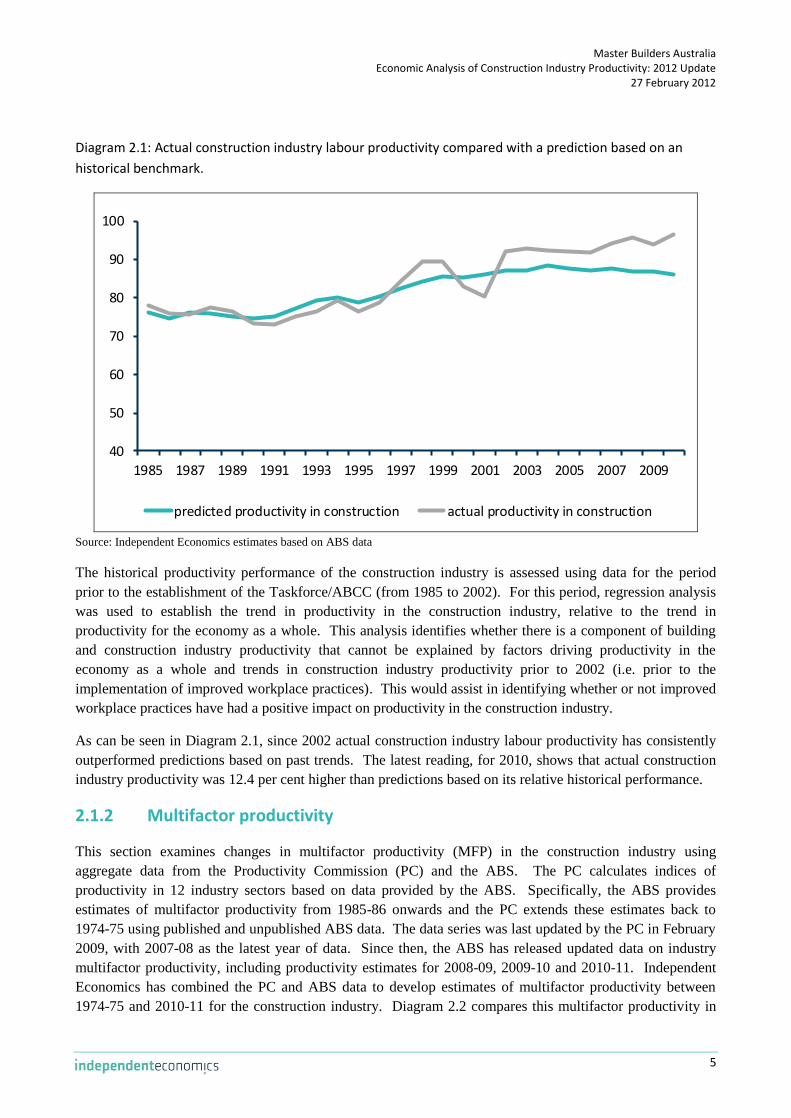
Diagram 2.1: Actual construction industry labour productivity compared with a prediction based on an
historical benchmark.
40
50
60
70
80
90
100
1985 1987 1989 1991 1993 1995 1997 1999 2001 2003 2005 2007 2009
predicted productivity in construction actual productivity in construction
Source: Independent Economics estimates based on ABS data
The historical productivity performance of the construction industry is assessed using data for the period
prior to the establishment of the Taskforce/ABCC (from 1985 to 2002). For this period, regression analysis
was used to establish the trend in productivity in the construction industry, relative to the trend in
productivity for the economy as a whole. This analysis identifies whether there is a component of building
and construction industry productivity that cannot be explained by factors driving productivity in the
economy as a whole and trends in construction industry productivity prior to 2002 (i.e. prior to the
implementation of improved workplace practices). This would assist in identifying whether or not improved
workplace practices have had a positive impact on productivity in the construction industry.
As can be seen in Diagram 2.1, since 2002 actual construction industry labour productivity has consistently
outperformed predictions based on past trends. The latest reading, for 2010, shows that actual construction
industry productivity was 12.4 per cent higher than predictions based on its relative historical performance.
2.1.2 Multifactor productivity
This section examines changes in multifactor productivity (MFP) in the construction industry using
aggregate data from the Productivity Commission (PC) and the ABS. The PC calculates indices of
productivity in 12 industry sectors based on data provided by the ABS. Specifically, the ABS provides
estimates of multifactor productivity from 1985-86 onwards and the PC extends these estimates back to
1974-75 using published and unpublished ABS data. The data series was last updated by the PC in February
2009, with 2007-08 as the latest year of data. Since then, the ABS has released updated data on industry
multifactor productivity, including productivity estimates for 2008-09, 2009-10 and 2010-11. Independent
Economics has combined the PC and ABS data to develop estimates of multifactor productivity between
1974-75 and 2010-11 for the construction industry. Diagram 2.2 compares this multifactor productivity in

Master Builders Australia Economic Analysis of Construction Industry Productivity: 2012 Update
27 February 2012
6
the construction industry with multifactor productivity in the market sector as a whole from 1974-75 to
2010-11.
Diagram 2.2: Construction industry multifactor productivity, 1974-75 to 2010-11 (2009-10 = 100).
70
80
90
100
110
1974-75 1979-80 1984-85 1989-90 1994-95 1999-00 2004-05 2009-10
Construction Market Sector
Source: Productivity Commission 2009, “Productivity Estimates and Trends”, ABS Cat No. 5260.0.55.002, ABS Cat No. 5204.0 and
Independent Economics estimates.
While productivity in the market sector has followed a fairly steady upward trend, productivity in the
construction industry was fairly flat through the 1980s and 1990s. The PC found that multifactor
productivity in the construction industry was no higher in 2000-01 than 20 years earlier2. As shown in
Diagram 2.2, construction industry productivity is below the level seen in 1980-81 during several periods,
including between 1988-89 and 1996-97.
However, construction industry productivity then strengthened considerably to achieve a higher level for the
nine years from 2002-03 to 2010-11. The data shows construction industry productivity rising by 14.5 per
cent in the nine years to 2010-11 (starting from a value of 90 in 2001-02 and escalating to 103.09 in 2010-
11). In contrast, in the nine years prior to the implementation of improved workplace practices (i.e. the nine
years from 1993-94 to 2001-02), construction industry productivity increased by 9.6 per cent. In addition,
between 2002-03 and 2010-11 the productivity performance of the construction industry outpaced that of the
market sector; within this period multifactor productivity in the market sector fell by 3.3 per cent. This
confirms the strong construction industry productivity outperformance of recent years already seen using
labour productivity in Diagram 2.1.
A study by the Grattan Institute has also noted that construction is one of only three industries that have
enjoyed faster labour and multifactor productivity growth in the 2000s compared to the 1990s3
.
2 Productivity Commission, Productivity Estimates to 2005-06, December 2006
3 Eslake, Saul and Walsh, Marcus, Australia’s Productivity Challenge, The Grattan Institute, Melbourne, February 2011

Master Builders Australia Economic Analysis of Construction Industry Productivity: 2012 Update
27 February 2012
7
Administration and support services and arts and recreation services are the other two industries whose
productivity performance has improved in the 2000s.
2.1.3 Total factor productivity
Recently, estimates of total factor productivity for the Australian construction industry have been developed
and published in the Construction and Management Economics journal4. This section reviews the findings
of this research.
The estimates of total factor productivity presented in the paper are developed using ABS data for the
construction industry. Productivity indices are estimated for each state and territory and cover the period
between 1990 and 2007. This time period was chosen by the authors based on data availability.
The diagram below compares growth in total factor productivity in the five years to 2002 and the five years
to 2007. The growth rate for each state and territory is calculated separately from the published data and
then weighted to develop an aggregate growth rate for Australia. The weights are based on the value of
construction work done in each state and territory. The construction work done data is also sourced from the
ABS.
Diagram 2.3: Growth in Construction industry total factor productivity (per cent).
-20%
-10%
0%
10%
20%
30%
40%
50%
ACT NSW VIC QLD SA WA TAS NT AUS
1998 to 2002 2003 to 2007
Source: Li and Liu (2010) and Independent Economics calculations.
Similar to the analysis performed using labour productivity and multi factor productivity, growth in total
factor productivity is faster in the five years to 2007 compared to growth in the five years to 2002.
4 Yan Li and Chunlu Liu, Malmquist indices of total factor productivity changes in the Australian construction industry,
Construction Management and Economics, 28:9, September 2010

Master Builders Australia Economic Analysis of Construction Industry Productivity: 2012 Update
27 February 2012
8
Specifically, between 2003 and 2007, total factor productivity in the Australian construction industry grew
by 13.2 per cent, whereas productivity grew by only 1.4 per cent between 1998 and 2002.
2.2 Commercial versus domestic residential comparison
Improved workplace practices (consisting of the establishment of the Taskforce, the ABCC and supporting
industrial relations reforms) are expected to have their main impact on the non-house building side of the
construction industry, rather than on the house building side. This is because the ABCC’s jurisdiction does
not cover housing construction of four dwellings or less (as well as the extraction of minerals, oil and gas).
The ABCC’s mandate is on the non-house building side of this industry because this is where, traditionally,
there were more industrial disputes and higher costs for specific tasks. The house building side, on the other
hand, is considered to be more flexible – reflecting the involvement of many small, independent operators
and the extensive use of piece rates for work performed.
So another way of testing the impact of the ABCC is by examining whether it has led to any improvement in
productivity on the non-house building side of the industry compared with the house building side. This can
be assessed at a detailed level by comparing how the ABCC has affected the relative performance of the two
sides of the industry in undertaking the same tasks.
Changes in the relative performance of the two sides of the industry can be assessed using quantity surveyors
data. This data is used to investigate how the ABCC has affected the cost comparison between the two sides
of the industry for the same building tasks in the same locations. This report updates the analysis of the
earlier reports by including the latest (January 2012) data available from Rawlinsons.
The cost comparison involves the following analysis. The Rawlinsons data is used to investigate movements
in recent years in the cost comparison between commercial building and domestic residential building for the
same building tasks in the same locations.
In making this comparison, the first point to clarify is the definitions of the two sides of the industry that are
used in the Rawlinsons data. Commercial building includes larger-multi-unit dwellings, offices, retail,
industrial and other buildings besides domestic residential buildings. It excludes engineering construction
(roads, bridges, rail, telecommunications and other infrastructure). Domestic residential building includes all
dwellings except larger multi-unit dwellings.
The building tasks used in this cost comparison of commercial building with domestic residential building
are as follows:
concrete to suspended slab;
formwork to suspended slab;
10mm plasterboard wall;
painting (sealer and two coats);
hollow core door; and

Master Builders Australia Economic Analysis of Construction Industry Productivity: 2012 Update
27 February 2012
9
carpentry wall.
Table 2.1 shows the cost penalties for commercial building compared with domestic residential building for
completing the same tasks, in the same states, for each year.
Table 2.1: Difference between the costs of tasks in commercial building and the same tasks in domestic
residential building, in the same state, 2004 – 2012 (per cent).
2004 2005 2006 2007 2008 2009 2010 2011 2012Change
since 2004
SA 9.2 7.3 6.6 6.6 6.1 6.1 5.2 5.1 5.0 -4.2
Qld 23.9 20.8 21.7 22.4 22.7 24.8 21.7 16.5 17.4 -6.4
Vic. 22.7 24.0 21.8 15.1 15.7 15.7 15.2 14.2 14.2 -8.5
WA 15.5 11.3 10.4 10.5 12.0 11.6 10.2 9.4 9.3 -6.2
NSW 16.2 14.7 12.6 12.4 12.3 12.5 11.3 11.0 11.2 -4.9
Aust. Average 19.0 17.3 16.1 14.8 15.2 15.7 14.2 12.4 12.7 -6.3Source: Rawlinsons Australian Construction Handbook, 2004 – 20125
Notes: (1) Aust. Average is weighted according to turnover on a state-by-state basis.
(2) Dates indicate beginning of each calendar year, for example 2004 refers to January 2004.
As outlined in the introduction, this report follows the same methodology as was employed in the earlier
reports since 2008. The analysis has simply been updated to incorporate the January 2011 and January 2012
Rawlinsons data. Specifically, Rawlinsons data is used to compare cost gaps between commercial and
domestic construction in 2012 with the same cost gaps in 2004 to see whether the cost penalty in commercial
construction has shrunk as a result of improved workplace practices6. The base year was chosen because the
Taskforce was established in October 2002 and the ABCC was established in 2005. The base year was also
chosen to remove the effects of an apparent break in some of the data series. Hence, a narrowing of the cost
gap between this period would indicate that improved workplace practices has had a positive effect on
productivity
Table 2.1 confirms that, similar to the findings of the original 2007 Econtech report and earlier updates, the
average costs of completing the same tasks in the same states have been generally higher in the commercial
building sector than in the domestic residential building sector. However, as noted above, our interest is in
whether this cost penalty for commercial building has shrunk since the introduction of improved workplace
practices.
The final column of Table 2.1 shows that the cost penalty for commercial building compared with domestic
residential building has fallen in all mainland states, suggesting that the improved workplace practices have
been effective. The biggest fall is in Victoria, where it is down from about 23 per cent to about 14 per cent.
Victoria is the state where restrictive work practices in commercial building were generally acknowledged to
be most pervasive7. In line with this, between 2004 and 2010, the cost gap in Queensland has remained
relatively stable and restrictive work practices in commercial building were generally acknowledged to be
less pervasive in Queensland.
5 Rawlinsons is a construction cost consultancy in Australia and New Zealand. The Rawlinsons Australian Construction Handbook is
the leading authority on construction costs in Australia. 6 Survey data refers to January of each year.
7 Wilcox, Transition to Fair Work Australia for the Building and Construction Industry, April 2009

Master Builders Australia Economic Analysis of Construction Industry Productivity: 2012 Update
27 February 2012
10
The cost gap in Queensland shrunk substantially in 2011 to 16.5 per cent. While it is likely that the cost gap
has shrunk further in 2011, the narrowing of the gap for this particular year is likely to be overstated.
Indeed, for 2012, the cost gap in Queensland rose to 17.4 per cent. One driver of the narrowing gap in 2011
is a substantial cost increase in domestic residential building compared to commercial building. This spike
in costs may be attributed to rebuilding efforts following natural disasters in Queensland during late 2010
and early 2011. According to a construction cost consultant report, price pressures will be greater in the
residential sector compared to others as a result of the lift in demand for materials and labour8. The report
notes that these price pressures are likely to be temporary given the one-off nature of the boost in demand.
Table 2.1 also presents cost penalties for Australia as a whole, calculated as weighted averages of the cost
penalties for individual states. These Australian cost penalties are also displayed in Diagram 2.4. Table 2.1
and Diagram 2.4 show that, since the introduction of the Taskforce9, across Australia, the cost penalty for
commercial building compared with domestic residential building has fallen. The cost penalty was around
19 per cent in 2004, but has declined over the past six years to be 12.7 per cent in 2012, or a fall of 6.3
percentage points.
Diagram 2.4: Average cost differences between commercial building and domestic residential building for
the same tasks for five states, 2004 – 2012 (per cent).
0%
2%
4%
6%
8%
10%
12%
14%
16%
18%
20%
2004 2005 2006 2007 2008 2009 2010 2011 2012
Source: Independent Economics estimates.
Many possible explanations for the fall in the cost penalty are ruled out by the close nature of the comparison
used in estimating the penalty. In particular, the cost penalty is calculated for performing the same building
tasks in the same locations. The only major aspect that is varied in the calculation is whether a task is
8 Davis Langdon, The Impact of the Queensland Floods and Cyclone Yasi on Construction Costs, March 2011.
9 The Taskforce was established in October 2002 but it is reasonable to expect a lag before its activities started to make an impact.
The data also relate to January of each year so that for 2004, the data relates to January 2004.

Master Builders Australia Economic Analysis of Construction Industry Productivity: 2012 Update
27 February 2012
11
undertaken as part of a commercial building project or as part of a domestic residential building project.
Both types of projects pay similar costs for materials.
This leaves a fall in the labour cost penalty (for commercial building) as the most plausible explanation for
the fall in the total cost penalty. On this interpretation, Table 2.2 uses the fall in the total cost penalty for
commercial building to estimate the fall in the labour cost penalty. It does this conversion using the average
share of labour in total costs for the six building tasks. Labour cost shares for each type of building task
listed earlier in this section are combined and come to approximately 53 per cent10
. The result is an
estimated fall from 2004 to 2012 in the labour cost penalty for commercial building of 11.8 percentage
points, as shown in the table below.
Table 2.2: Average labour cost differences between commercial building and domestic residential building,
2004 – 2012 (per cent or percentage points).
2004 2005 2006 2007 2008 2009 2010 2011 2012Change
since 2004
Total Cost Gap 19.0 17.3 16.1 14.8 15.2 15.7 14.2 12.4 12.7 6.3
Labour Cost Gap 35.8 32.6 30.4 27.8 28.7 29.6 26.7 23.4 24.0 11.8Source: Independent Economics estimates.
Estimates of the labour cost gap shown in the table above are conservative. This is because Rawlinson’s
estimate total costs do not include off-site overheads or profit. In other words, it does not include returns to
capital in its measure of total cost. Once allowing for returns to capital, the labour share of total cost would
be well below 53 per cent. This implies that the labour cost penalty is likely to be higher than the
11.8 per cent estimated using 2012 data.
In principle, this fall in the labour cost penalty for commercial building compared with domestic residential
building could be due either to movements in relative productivity or wages between the two sectors. These
two possible explanations are considered in turn.
Relative wages in commercial building compared with domestic residential building could have moved for
two reasons. First, site allowances associated with non-residential construction have been restricted by the
ABCC. However, site allowances are not included in the data for the costs of building tasks and so do not
explain the fall in the cost penalty. Second, enterprise bargaining may have affected relative wages.
However, enterprise bargaining easily predates our cost comparison, which begins in 2004.
This leaves post-2004 improvements in labour productivity in commercial building compared with domestic
residential building as the most likely explanation for the fall in the commercial building labour cost penalty.
The timing of improvements is in line with activities of the Taskforce/ABCC in improving work practices
and enforcing general industrial relations reforms in commercial building.
This leaves the conclusion is that there has been a recent improvement in labour productivity in commercial
building compared with domestic residential building of 11.8 per cent as a result of improved workplace
practices. However, as Mitchell points out in his comment on the 2007 report11
, using the Rawlinsons
10
Information on labour cost shares are sourced from Rawlinsons. 11 Mitchell, An examination of the cost differentials methodology used in ‘Economic Analysis of Building and Construction Industry
Productivity’ – the Econtech Report, August 2007.

Master Builders Australia Economic Analysis of Construction Industry Productivity: 2012 Update
27 February 2012
12
domestic construction data “blurs the distinction [between commercial building and domestic construction
categories] by including small-scale construction within domestic construction”. To the extent that the
classification blurs the desired distinction in categories, the cost gap and its movements will be understated.
As noted earlier, the ABCC’s jurisdiction includes housing construction of four dwellings or more.
However, this type of small-scale commercial construction is included in the definition of domestic
construction used by Rawlinsons. This means that a small sector of domestic construction would have also
benefited from improved workplace practices and associated labour productivity boost. The inclusion of
small-scale construction in the domestic construction category means that the cost gap would have narrowed
further had this not been the case.
In summary, the simple estimate of the gain in productivity of 11.8 per cent is likely to be understated by two
factors. Firstly, Rawlinson’s exclude returns to capital in its estimate of construction costs. Secondly, a
component of domestic construction (small scale construction) also benefits from a productivity boost.
Domestic residential building is less useful as a cost benchmark for engineering construction, which largely
involves other, unrelated tasks. However, as noted in our earlier reports, a previous study has estimated that
there is a similar cost advantage for engineering construction projects by comparing the construction of
EastLink to CityLink. Specifically, a previous study showed a significant “advantage to EastLink by
operating under the post-WorkChoices/ABCC environments” of 11.8 per cent (see Table 2.3 for more
details)12
. Thus it is reasonable to assume that the engineering cost improvement is likely to be at least equal
to the estimate of the improvement in commercial building costs.
Hence, based on the evidence above, the relative labour productivity gain for the non-residential construction
sector as a whole is conservatively estimated at 11.8 per cent. If the estimate was adjusted to incorporate the
cost of capital in determining the labour share of construction costs and if small-scale construction was
excluded from the definition of domestic construction, then the estimated boost in productivity would be
greater.
2.3 Individual project comparisons and other supporting studies
So far in this section it has been established that labour productivity in commercial construction has
increased in recent years, both relative to its historical trend and relative to domestic residential construction.
To help understand the sources of the recent productivity gains, Econtech undertook a number of case
studies as part of its original 2007 report. The case studies allow an examination of particular experiences
across different companies in the construction industry.
Several other research reports confirm the findings of the original 2007 report and earlier updates; that there
has been a boost to building and construction productivity as a result of improved workplace practices. The
table below from the 2010 report summarises the findings of the case studies completed in 2007 and other
supporting studies. A more detailed discussion of the case studies and other supporting studies can be found
in the 2008 and 2009 reports.
12 Phillips, Ken (2006), “Industrial Relations and the Struggle to Build in Victoria”, Institute of Public Affairs Briefing Paper,
November 2006

Master Builders Australia Economic Analysis of Construction Industry Productivity: 2012 Update
27 February 2012
13
Table 2.3: Summary of other supporting studies.
Study Findings Estimated gain in productivity
Econtech case studiesProjects undertaken post-ABCC activity have fewer project days
lost per year than projects undertaken pre-ABCC activity
$2.71 million in cost saving from
reduction in days lost to
industrial dispute
The Allen Consulting Group
The report examined multifactor productivity in the non-
residential construction industry and found that there had been a
gain in productivity in the five years to 2007
12.2 per cent gain in multifactor
productivity over 5 years
Ken Phillips
Comparison of two major construction projects in Victoria, the
EastLink project and the CityLink project. The study found that
there would have been additional costs for EastLink had it been
constructed under industrial agreements outside of the ABCC and
Workchoices environment.
$295 million in direct cost saving
and toll revenue or 11.8 per cent
of the total construction cost
BHP Billiton
Provided industry-wide observations and on-the-ground examples
of changes that have occurred in their business. The business
noted that there has been an improvement in industrial relations
since the establishment of the ABCC. N/A
Grocon
Provided industry-wide observations and on-the-ground examples
of changes that have occurred in their business. The business
noted that there was a fall in the number of days lost to industrial
disputes following the introduction of the ABCC. N/A
John Holland Group
The construction industry has enjoyed an "unprecendented
increase in productivity" since the completion of the Cole Royal
Commission. 10% productivity dividend
Source: KPMG Econtech (2010)

Master Builders Australia Economic Analysis of Construction Industry Productivity: 2012 Update
27 February 2012
14
2.4 Days lost to industrial action
The previous sections outlined the impact of improved workplace practices on productivity indicators for the
building and construction industry. This section analyses the impact of improved workplace practices on
another general performance indicator, the number of work days lost to industrial action. Specifically, since
improved workplace practices have been implemented, the building and construction industry has
outperformed other sectors of the economy in reducing in the number of work days lost. This improvement
can be shown at two different levels, using aggregate ABS data and using individual project data. This
subsection focuses on aggregate ABS data. The analysis of individual project data can be found in the 2008
report.
Diagram 2.5 shows ABS data on the number of working days lost in the construction industry due to
industrial disputes. The average number of working days lost each year for the period 1996 to 2002 was
164,000. In contrast, the diagram shows that since 2003 the number of days lost in the industry has been
decreasing. 2003 was the full first year of operation of the Taskforce, which started operations in October
2002. The ABCC started its operations in October 2005. After five years of operation of the ABCC, the
annual number of working days lost in the building and construction industry due to industrial disputes has
fallen dramatically to only 31,000 in 2010 (or 19 per cent of the 1996-2002 average).
As a comparison, an analysis of working days lost to industrial disputes in other sectors of the economy is
also presented in Diagram 2.5. Similar to the case for the productivity indicators, compared to other sectors
of the economy, the construction industry has lowered the number of working days lost by a greater amount.
In 2010, construction working days lost are at only 19 per cent of earlier levels (as noted above). This
compares favourably with the same figure for all other industries, 26 per cent. That is, in 2010, working
days lost in the construction were a mere 81 per cent than the industry’s 1996-2002 average. Other
industries reduced their number of working days lost to only 74 per cent lower than their 1996-2002 average.
For 2011, data is available for the March, June and September quarter. An estimate for the December
quarter has been calculated by taking the average of the December quarter value over the last five years, for
both the construction industry and the economy in aggregate. The number of industrial disputes in 2011 was
relatively high, for both the construction industry and the rest of the economy, compared with recent history.
Specifically, in 2011, an estimated 52,000 working days was lost in the construction industry as a result of
industrial disputes; the corresponding figure for all other industries is estimated at 172,000 working days.
However, similar to the data for 2010, the latest data shows that the construction industry continues to
outperform other industries in reducing the number of working days lost to industrial disputes. In the
construction industry, the number of working days lost are only 32 per cent of the industry’s 1996-2002
average, while for other industries it is 46 per cent of the 1996-2002 average.

Master Builders Australia Economic Analysis of Construction Industry Productivity: 2012 Update
27 February 2012
15
Diagram 2.5: Working days lost in construction due to industrial disputes (‘000)
335
108
211
165
109 121102
123 12089
15 7 14 24 3152
594
426
316
485
360
272
158
316
260
139118
43
183
109 96
172
0
100
200
300
400
500
600
700
construction all other industries
Source: ABS Cat No. 6321.0.55.001
Note: Independent Economics’ estimate for December 2011 is included in the data for 2011.
2.5 Summary – the impact of improved workplace practices on
building and construction industry productivity
As shown in the previous subsections, each of the updated productivity indicators finds significant
improvements in labour productivity since the implementation of improved workplace practices. This is
consistent with the findings of the original 2007 Econtech report and earlier updates.
ABS data shows that, in 2010 (the latest data available), construction industry labour productivity
has outperformed predictions based on its historical performance relative to other industries by 12.4
per cent. That is, a productivity outperformance is identified after allowing for factors driving
productivity in the economy as a whole and trends in construction industry productivity prior to 2002
(the year improved workplace practices began).
The Productivity Commission’s analysis of ABS data has found that multifactor productivity in the
construction industry was no higher in 2000-01 than 20 years earlier13
. In contrast, the latest ABS
data on productivity shows that construction industry multifactor productivity accelerated to rise by
14.5 per cent in the nine years to 2010-11.
13
Productivity Commission, Productivity Estimates to 2005-06, December 2006.

Master Builders Australia Economic Analysis of Construction Industry Productivity: 2012 Update
27 February 2012
16
Recently published research on total factor productivity shows that productivity in the construction
industry grew by 13.2 per cent, between 2003 and 2007, whereas productivity grew by only
1.4 per cent between 1998 and 2002.
While the productivity indicators listed above are not directly comparable, they all indicate that the
timing of improvements in construction industry coincides with the timing of improved workplace
practices; the Taskforce was established in late 2002 and the ABCC was established in late 2005.
Rawlinsons data to January 2012 shows that the cost penalty for completing the same tasks in the
same region for commercial construction compared to domestic construction has continued to shrink.
The narrowing in the cost gap coincides with improved workplace practices in commercial
construction. The boost to productivity in the commercial construction sector, as estimated by the
narrowing in the cost gap, is conservatively estimated at 11.8 per cent between 2004 and 2012. This
estimate is considerably higher once other factors are taken into account.
Case studies undertaken as part of the original 2007 Econtech report found that improved workplace
practices have led to better management of resources in the building and construction industry. This,
in turn, has boosted productivity in the building and construction industry.
All of this evidence continues to support the conclusion of the original 2007 Econtech report and earlier
updates, that there has been significant gain in construction industry productivity. The question then
becomes to what extent has improved workplace practices contributed to this improvement.
Before the impact of improved workplace practices on building and construction industry productivity can be
determined, it is useful to review the key regulatory changes that have occurred in the industry and
importantly, the timing of these changes. The Taskforce was established in October 2002 but it lacked
enforcement powers . The ABCC was established in October 2005; and amendments to the Workplace
Relations Act were implemented on the 27 March 2006.
The ABCC relies on two acts as a platform for prosecution; Building and Construction Industry
Improvement Act 2005 (BCII Act) and the Fair Work Act 2009 (FW Act). The BCII Act is the main
legislation used by the ABCC, though the FW Act has also been used in a number of cases since it was fully
implemented on 1 January 2010.
The majority of regulatory changes listed above are industry specific. However, general industrial relations
reforms have also supported the effectiveness of the ABCC. For example, significant industrial relations
reforms to encourage enterprise bargaining were introduced in 1993. Further changes were introduced in
1996 to reinforce the incentive for enterprise bargaining as well as reduce the scope for industrial action.
These industrial relations reforms provided a more productivity-friendly environment.
However, these changes did not appear to have any effect in terms of improving construction industry
productivity until after the Taskforce was put in place in October 2002. The data sources above indicate that
the significant productivity gains in construction industry productivity appear around 2002/03. This supports
the interpretation that it was the activities of the Taskforce and, more importantly, the ABCC (given its
enforcement powers) when it was established in October 2005 that made a major difference.

Master Builders Australia Economic Analysis of Construction Industry Productivity: 2012 Update
27 February 2012
17
Thus, the productivity and cost difference data suggest that effective monitoring and enforcement of the
general industrial relations reforms and those that related specifically to the building and construction sector
were necessary before the reforms could lead to labour productivity improvements. As such, it is considered
that separate attribution of labour productivity improvements to the ABCC and industrial relations reforms is
not possible, because they both need to operate together to be effective.
The latest data up to February 2012, continues to point to improved workplace practices contributing to a
significant productivity gain in the construction industry. That is, the construction industry’s productivity
has outperformed other sectors of the economy as a result of improved workplace practices. As reported
above, the estimated gain ranges between 10 and 14.5 per cent, depending on the measure and the source of
information that is used. Notably, the latest data indicates that the productivity outperformance of the
construction industry has strengthened. Based on data available to July 2010, the 2010 report estimated the
gain in construction industry productivity to be between 7.7 per cent and 14.8 per cent.
Earlier reports found that the data continued to support an estimated gain in construction industry labour
productivity, as a result of the ABCC and related industrial relations reforms, of 9.4 per cent. While not all
of the productivity measures are strictly comparable, and the magnitude of the estimated gain varies across
measures, the most recent data generally shows some strengthening of the productivity outperformance of
the construction industry, as noted above. The latest available data could justify an increase in the estimate
of the gain in construction industry productivity from improved workplace practices. However, we continue
to use a 9.4 per cent gain in productivity to estimate the economy-wide impact of improved workplace
practices for several reasons. Firstly, the same gain in productivity is used for comparability across reports.
Secondly, it avoids placing too much weight on data for any single year. Finally, it avoids any possible
overestimation of the productivity outperformance of the construction industry as a result of improved
workplace practices.
Changes to the regulation of the building and construction industry are expected in the near future. The
Building and Construction Industry Improvement Amendment (Transition to Fair Work) Bill 2011 was
introduced to the House of Representatives in November 2011 and is currently the subject of a Senate
inquiry. Under this bill, the building and construction industry will be regulated by the Office of the Fair
Work Building Inspectorate instead of the ABCC. The bill will also repeal or amend several of the
provisions under the BCII Act and renames the act to the Fair Work (Building Industry) Act 201114
. The
effect of this regulatory change on building and construction industry productivity will need to be analysed
following its implementation.
14
Parliamentary Library, Bills Digest No.80: Building and Construction Industry Improvement Amendment (Transition to Fair
Work) Bill 2011, November 2011

Master Builders Australia Economic Analysis of Construction Industry Productivity: 2012 Update
27 February 2012
18
3. Modelling the impact of improved
workplace practices This section provides details of the modelling approach used to estimate the economy-wide impacts of
improved workplace practices. The section is structured as follows. Section 3.1 summarises Econtech’s
previous studies in this area. Section 3.2 outlines the scenarios that were simulated using the Independent
CGE model to quantify the economic contribution of improved workplace practices. Section 3.3 outlines the
main data inputs that are used to build the alternative scenario and describes how these inputs were derived.
Section 3.4 discusses the main features of the economic model (the Independent CGE model) that was used
to estimate the economic contribution of improved workplace practices.
3.1 Previous studies
In 2003, Econtech prepared a study for the, then, Department of Employment and Workplace Relations
(DEWR) that analysed the cost differences for the same standard building tasks between commercial
buildings and domestic residential buildings. This report and its conclusions (outlined below) on building
and construction industry productivity were accepted by DEWR
The report, using Rawlinson’s data, showed that building tasks – such as laying a concrete slab,
building a brick wall, painting and carpentry work – cost more for commercial buildings than for
domestic residential housing. The difference was mainly attributed to differences in work practices
between the commercial and domestic residential building sector.
The productivity performance of Australia’s building and construction industry lags behind
international best practice. If the cost gap between commercial and domestic construction were
removed, Australia’s performance would still be behind international benchmarks.
The 2003 Econtech Report went on to model the economy-wide benefits of reducing the cost gap through
reform to work practices in the commercial building sector.
While the 2003 Report estimated the potential productivity gains from workplace reform in the construction
industry, by 2007/08 the reform process was well established. Hence in 2007 the ABCC commissioned
Econtech to estimate the actual productivity gains that can be attributed to the activities of the ABCC and its
predecessor the Taskforce. This 2007 report was then updated in 2008, 2009 and 2010.
Each report consistently showed that there had been a gain in construction industry productivity of about
10 per cent, due to the activities of the Taskforce and the ABCC in conjunction with related industrial
relations reforms. Similar to the 2003 report, each subsequent report modelled the economy-wide benefits of
this gain in construction industry productivity from improved workplace practices.
The 2008, 2009 and 2010 reports considered the impact of workplace reform on construction industry
productivity from three different angles. It compared construction industry productivity between different

Master Builders Australia Economic Analysis of Construction Industry Productivity: 2012 Update
27 February 2012
19
years, between the non-residential and residential sides of the building industry, and between individual
projects undertaken before and after the establishment of the ABCC.
This report updates the economic analysis in the earlier reports to incorporate the latest data and other studies
completed in the intervening time on building and construction industry productivity. In addition, this report
also updates the economy-wide modelling initially undertaken in 2007, using Independent Economics’
newly-developed Computable General Equilibrium model, the Independent CGE model. While a new model
is used to estimate these impacts, the estimates developed by this new model are consistent with the
estimates presented in earlier reports; this is discussed further in section 4.
This section presents the methodology and model used to estimate the economic impacts of improved
workplace practices within the building and construction industry.
3.2 Scenarios
The Independent CGE model of the Australian economy is used to estimate the long-term economy-wide
impact of improved workplace practices. To do this, the following two scenarios were developed:
a “Baseline Scenario”, which provides a snapshot of the Australian economy without improved
workplace practices; and
an “Improved Workplace Practices Scenario”, which provides a snapshot of the Australian economy
with improved workplace practices.
The results of both scenarios were analysed and the impact of improved workplace practices on key
economic aggregates were estimated as the difference between the results of the Improved Workplace
Practices and Baseline scenarios.
The main inputs for each of the scenarios are discussed in detail below.
3.3 Model inputs
As explained in Section 2, the latest data continues to point to a significant productivity outperformance in
the construction industry, due to improved workplace practices. Indeed, the latest data suggest that the
building and construction industry’s outperformance has strengthened. . As discussed in section 2.5, while
there is justification to lift the estimate of the gain in construction industry productivity from improved
workplace practices, we continue to use a 9.4 per cent gain in productivity to estimate the economy-wide
impact of improved workplace practices.
This gain is concentrated to the sectors where the ABCC has jurisdiction, non-residential building
construction, engineering construction and multi-unit residential building. This is consistent with the
modelling input used in the original 2007 Econtech report and earlier updates. The estimated gains in labour
productivity for the various sub sectors of the building and construction industry are shown in Table 3.1.
Specifically, combining a gain of 12 per cent in non-residential construction, and a 4.2 per cent in residential

Master Builders Australia Economic Analysis of Construction Industry Productivity: 2012 Update
27 February 2012
20
construction (to reflect the productivity gain in multi-unit residential building) leads to an overall industry
productivity gain of 9.4 per cent.
Table 3.1: Simulated gains in labour productivity (per cent)
2 sectors 3 sectors 4 sectors
Non-residential building 12.0% 18.4%
Engineering construction 17.0%
Other non-residential building 21.0%
Residential building 4.2% 0.0% 0.0%
Construction services 6.5% 6.5%
Total building and construction 9.4% 9.4% 9.4%
Reform Scenario
Source: Independent Economics estimates based on total estimated productivity improvements and current labour cost relativities
between the construction sub-sectors.
The Independent CGE model uses the ABS’ latest industrial classification, ANZSIC 2006. Thus the model
separately identifies four sub sectors of the construction industry: engineering construction, non-residential
building construction, residential construction and construction trade services. In the models utilised in
original 2007 Econtech report and earlier updates, engineering construction was combined with non-
residential building construction in the broader non-residential construction sector.
The productivity gains must be disaggregated, in a consistent manner, into the four construction subsector
identified in the model. The disaggregated gains across the four sectors are outlined in Table 3.1. That is, a
17 per cent productivity gain in engineering construction; a 21 per cent gain in non-residential construction;
no direct gain in residential construction and 6.5 per cent in construction services is consistent with an
overall productivity gain of 9.4 per cent and reflects the ABCC’s jurisdiction. This disaggregation allows for
the importance of construction trade services as a production input into residential, non-residential and
engineering construction. For example, while there is no direct productivity gain in residential construction,
the sector benefits from the productivity gain in construction services. This indirect benefit is equivalent to a
4.2 per cent gain in productivity for the residential construction industry.
3.4 The Independent CGE model
The economy-wide contributions of improved workplace practices were estimated using the Independent
CGE model. It is a long-term model of the Australian economy that models a long-run equilibrium
(approximately 5 to 10 years). In other words, it estimates the long-term impacts of improved workplace
practices after the economy has fully adjusted to the reform.
The Independent CGE model has the following features that are important for this report.
The model separately identifies four sectors within the building and construction industry: residential
building, non-residential building, engineering construction and construction trade services. In
original 2007 Econtech report and earlier updates, engineering construction was combined with non-

Master Builders Australia Economic Analysis of Construction Industry Productivity: 2012 Update
27 February 2012
21
residential building in a broader non-residential construction industry. This distinction is of
particular importance because improved workplace practices have been concentrated on non-
residential construction and multi-unit residential building. A more detailed breakdown of the
building and construction industry means that the model can better trace the economy-wide impact
of improved workplace practices. For example, a separate engineering construction sector means
that the technology used in the sector is separately identified from the broader non-residential
construction sector. That is, the model allows for the fact that the engineering construction sector
and the non-residential building construction sector have quite different production technologies.
The model uses the latest information available, including the latest detailed Input-Output (IO) tables
from the Australian Bureau of Statistics (ABS). Specifically, the 2007/08 IO table released by the
ABS in late 2011 is used. This means that the analysis presented in this report is based on the most
up-to-date detailed picture of the structure of the Australian economy.
While the data underlying the model is based on the structure of the Australian economy in 2007/08,
the model has been uprated to provide a snapshot of the economy in a normalised 2011/12. This
includes allowing for growth in wages, prices, productivity, employment and commodity prices
since 2007/08.
The model uses the most up-to-date ABS industry classification, ANZSIC 2006.
Each industry in the model uses labour, two types of capital and a fixed factor, whereas in a basic
CGE model only labour and one type of capital are used. Importantly, building and structures and
dwellings are separately identified from other types of capital (which includes items such as motor
vehicles, machinery and computers). Each industry’s mix of primary factors is separately chosen
depending on relative prices and the industry’s production technology. This is of particular
importance in this project, as would allow for a more robust estimate of the impact of reform on the
building and construction industry, which produces building and structures and dwellings. In
addition, the model accounts for the use of fixed factors in production, such as residential land in the
provision of housing services.
Consumer welfare (household living standards) is estimated robustly, based on the equivalent
variation measure used in welfare economics. A robust measure of welfare is of particular
importance as policies should be assessed based on their impact on households.
As noted above, the model estimates the long-term effects of improved workplace practices, after the
economy has fully responded. The merit of economic policies should be judged on their long-term, as
opposed to short-term, impacts. The long-term assumptions of the Independent CGE model are as follows.
Profit maximisation: the representative business in each industry chooses how to produce (primary
factors, intermediate inputs) and how much to produce to maximise profit subject to constraints such
as prices and a production function.
Utility maximisation: A representative household chooses a consumption bundle to maximise utility,
which depends on the consumption of products, subject to a budget constraint.

Master Builders Australia Economic Analysis of Construction Industry Productivity: 2012 Update
27 February 2012
22
Labour market equilibrium: in the long term the labour market is assumed to clear, so that an
economic shock will have no lasting effects on employment.
External balance: in the long term, external balance is assumed to be achieved by adjustment of the
exchange rate, so that trade shocks have no lasting effect on external balance.
Budget balance: the budget is balanced because in the long run fiscal policy must be sustainable.
The policy instrument which adjusts to ensure the budget is balanced, otherwise known as the swing
policy instrument, is labour income tax.
Private saving: in the long run the level of private sector saving and associated asset accumulation
must be sustainable.

Master Builders Australia Economic Analysis of Construction Industry Productivity: 2012 Update
27 February 2012
23
4. Economic impact of improved workplace
practices The previous section described the scenarios that were simulated using the Independent CGE model,
outlined the main data inputs that Independent Economics used to build the scenarios and described how
these inputs were derived. This section provides the results of modelling the economic impacts of improved
workplace practices at three different levels, as follows.
Section 4.1 describes the detailed economic impacts on the building and construction industry.
Section 4.2 describes the wider industry impacts of reform in the building and construction industry.
Section 4.3 presents the economy-wide impacts of reform in the building and construction industry.
Importantly, the results presented in this section refer to permanent effects on the levels, not growth rates, of
indicators relative to what they would otherwise be. This means, for example, that a gain of 0.8 per cent in
the level of GDP is interpreted as the increase in GDP relative to what it would otherwise be, and not the
annual growth rate. That is it compares the level of GDP at a point in time under the baseline scenario with
the level of GDP at the same point in time under the alternative (improved workplace practices) scenario.
4.1 Building and construction industry effects
This section presents the economic impacts on the building and construction industry of labour productivity
gains in the industry stemming from improved workplace practices.
In considering the effects on the construction industry itself of higher construction productivity due to
improved workplace practices, it is important to distinguish between residential construction, non-residential
building construction, engineering construction and construction services. Notably, the industry-level
impacts outlined below, particularly for non-residential construction, are not directly comparable to the
industry-level results presented in the 2010 report. The industry structure presented in this report is in line
with the industry structure presented in the latest Input-Output table from the ABS (which uses the most up-
to-date industry classification). That is, engineering construction is no longer combined with non-residential
building construction; in the 2010 report these sectors were combined in a broader non-residential
construction sector.
Diagram 4.1 shows the estimated long-term effects on residential construction. These effects are driven
mainly by the assumed indirect gain in labour productivity in residential construction, stemming from its use
of construction trade services. That is, construction services are an important input into the production of
dwellings in the latest ABS input-output tables and thus the residential construction sector benefits from
having a more productive construction services sector.

Master Builders Australia Economic Analysis of Construction Industry Productivity: 2012 Update
27 February 2012
24
Diagram 4.1: Effect of improved workplace practices on residential construction (% deviation from baseline)
1.2%0.7%
-1.1%-0.6%
-8%
-4%
0%
4%
real value added employment cost of residentialconstruction
price of housingservices
Source: the Independent CGE model simulations
The boost in efficiency in construction services reduces the costs of production in the residential construction
sector relative to what they would otherwise be. This leads to an overall cost reduction of 1.1 per cent for
residential building, as shown in Diagram 4.1. The flows through to a smaller percentage reduction in the
price of housing services of 0.6 per cent, consistent with the fact that production of housing services relies
not only on residential buildings, but also on residential land and intermediate inputs.
Lower prices for housing services leads to an increase in the derived demand for residential buildings,
boosting residential construction activity. Indeed, Diagram 4.1 shows a long-term increase in residential
construction activity of 1.2 per cent relative to what it would otherwise be. This is a similar production
response to that in the 2010 report. The lift in activity leads to a gain in employment in residential
construction of 0.7 per cent.
The effects on the non-residential side of the building industry are shown in Diagram 4.2. As shown in
Table 3.1, these effects are based mainly on an assumed increase in direct labour efficiency of 21 per cent for
non-residential building construction in the long-term, relative to the situation in the absence of the reforms.
In addition, since construction services are an important input into the production of non-residential
buildings, the sector enjoys further costs savings from having a more productive construction services sector.

Master Builders Australia Economic Analysis of Construction Industry Productivity: 2012 Update
27 February 2012
25
Diagram 4.2: Effect of increased efficiency on non-residential building construction (% deviation from
baseline)
1.9%
-8.4%
-2.9% -3.0%
2.4%
-9%
-6%
-3%
0%
3%
real value added employment cost of construction investment price -bldgs & structures
investment - bldgs& structures
Source: the Independent CGE model simulations
The direct gain in labour efficiency means that the cost reduction for non-residential building construction is
larger than for residential building construction, 2.9 per cent compared to 1.1 per cent.
Cheaper non-residential building construction costs, together with cheaper engineering construction costs,
combine to lower the overall cost of business investment in buildings and structures by 3 per cent (as seen in
Diagram 4.2). As discussed later in this subsection, the reduction in engineering construction costs, like the
reduction in non-residential building costs, is a result of higher labour productivity from improved workplace
practices.
Cheaper building and structures stimulates a lift in real investment by business in this type of capital of 2.4
per cent. Even assuming that there is no response by general government in its level of investment in
building and structures, the business response results in a long-term gain in total non-residential building
construction activity of 1.9 per cent, as seen in Diagram 4.2.
Employment in non-residential building construction is affected by three separate factors.
The assumed gain in labour efficiency of 21 per cent reduces employment by a similar percentage,
for an unchanged level of activity (“labour saving effect”).
The rise in activity of 1.9 per cent adds a similar percentage to employment (“output effect”).
The gain in labour efficiency makes labour cheaper, inducing some substitution of labour for capital
and land (“substitution effect”).

Master Builders Australia Economic Analysis of Construction Industry Productivity: 2012 Update
27 February 2012
26
The negative effect on employment from the labour saving effect dominates the positive effects of the output
and substitution effects, leaving a net loss of 8.4 per cent in non-residential building employment in the long-
term. Importantly, while there are offsetting employment effects in other sectors of the economy, there
would be short-term adjustment costs from job shifting from non-residential building construction to other
industries, but there is no long-term loss in national employment.
As outlined in section 3, in comparison to earlier modelling, the Independent CGE model identifies an
additional sector to the construction industry, by dividing non-dwelling construction into non-dwelling
building and engineering construction. Similar to the non-residential building construction industry, the
engineering construction industry enjoys a direct labour productivity boost of 17 per cent as well as
benefiting from the productivity gain in construction services. The flow-on impacts of this gain in efficiency
are show in Diagram 4.3 below.
Diagram 4.3: Effect of increased efficiency on engineering construction (% deviation from baseline)
1.6%
-10.9%
-3.7%-3.0%
2.4%
-12%
-8%
-4%
0%
4%
real value added employment cost ofconstruction
investment price- bldgs &
structures
investment -bldgs &
structures
Source: the Independent CGE model simulations
Similar to non-residential building construction, this gain in efficiency leads to a reduction in engineering
construction costs of 3.7 per cent. As noted earlier, lower engineering construction costs, combined with
lower non-residential building construction costs, lower the overall cost of business investment in buildings
and structures by 3 per cent. As also noted earlier, cheaper building and structures, in turn, stimulates a lift
in real investment by business in this type of capital of 2.4 per cent. It is assumed that there is no response
by general government in its level of investment in engineering construction. Even so, the business response
results in a long-term gain in engineering construction activity of 1.6 per cent, as seen in Diagram 4.3. This
is a permanent gain in engineering construction activity compared to the situation without improved
workplace practices.
Similar to non-residential building construction, higher labour efficiency in engineering construction affects
employments in three separate ways (labour saving, output and substitution effects) and the positive output

Master Builders Australia Economic Analysis of Construction Industry Productivity: 2012 Update
27 February 2012
27
and substitution effects offset only part of the negative labour saving effect. This leaves net employment
losses on 10.9 per cent in engineering construction, which are offset in other sectors of the economy.
Construction trade services include businesses engaged in land development and site preparation services,
building structure services, building installation services, building completion services and other
construction services15
. The industry is a large supplier of services to the other three construction industries.
That is, construction services is an important intermediate input into the production of residential, non-
residential building and engineering construction. The analysis of productivity gains from improved
workplace practices in section 2 indicated that the productivity gains are concentrated in the multi-unit, non-
residential building and engineering construction side of the construction industry. This analysis is
consistent with an efficiency gain in construction trade services of 6.5 per cent.
Diagram 4.4: Effect of increased efficiency on construction services (% deviation from baseline)
1.6%
-3.9%
-3.1%
-8%
-4%
0%
4%
real value added employment cost of construction services
Source: the Independent CGE model simulations
The productivity boost from improved workplace practices leads to lower prices for construction services,
specifically 3.1 per cent lower. Lower prices stimulate demand and activity in construction services is
l.6 per cent greater than would otherwise be the case. In addition, the gains in activity for the three types of
construction also lift demand for construction services. Both of these effects combine to lift activity in
construction services by 1.6 per cent.
Employment in this subsector is reduced by 3.9 per cent and this is because the negative labour saving effect
overshadows the positive output and substitution effects. As noted earlier, this fall in employment is offset
by gains in employment in other sectors of the economy, so that there is no change in the total level of
employment across all industries, but is also accompanied by short term adjustment costs as workers move to
the other industries.
15
Australian Bureau of Statistics, Catalogue No. 1292.0

Master Builders Australia Economic Analysis of Construction Industry Productivity: 2012 Update
27 February 2012
28
Overall, the productivity boost in the building and construction industry as a result of improved workplace
practices is positive and boosts activity. However, the lift in activity varies across the four subsectors of the
construction industry in the following way:
1.2 per cent for residential building;
1.9 per cent for non-residential building;
1.6 per cent for engineering construction; and
1.6 per cent for construction services.
At the same time, these permanent long-term gains in construction activity will have been accompanied by
short-term adjustment costs, due to job shifting from construction to other industries.
Note that the losses in construction industry employment are relative to a Baseline Scenario without reform.
This does not mean that there has been a fall in construction employment during the reform process. Indeed,
construction employment has grown strongly in most years during the reform process and is now higher than
it was in 2001/02 (the start of the reform process).
4.2 Wider industry effects
The change in activity in the building and construction industry is expected to affect activity in other
industries. This section outlines the simulated production impacts on other industries of improved workplace
practices in the building and construction industry. These effects, which put more precisely refer to real
value added, are presented in Diagram 4.5 on the following page.
As discussed in Section 4.1, higher labour productivity flows through to reduce the price of dwellings by
around 0.6 per cent (also shown in Diagram 4.5). This stimulates a long-term rise in demand for housing
services (“ownership of dwellings”) of 0.9 per cent, relative to what it otherwise would be, as also shown in
Diagram 4.5.
The detailed effects within the construction industry itself were discussed in Section 4.1. These effects add
up to an average fall in construction costs of 2.6 per cent and a rise in construction activity of 1.5 per cent, as
shown in Diagram 4.5. These are average effects only. As explained above, the percentage gains in
production are lower for residential building and higher for non-residential building.
As discussed in the previous section, the price falls for construction flowing from productivity gains reduce
the overall cost of investment in buildings and structures by 3 per cent. This is of particular benefit to
sectors that are large users of buildings and structures. Diagram 4.5 shows that electricity, gas, water &
waste, communication services, and transport, postal and warehousing receive cost savings that reduce prices
by 1.1, 0.6 and 0.6 per cent respectively. Because of the price-sensitive nature of demand for
communication services and transport, postal and warehousing, these price reductions lead to significant
production gains. In contrast, because the demand for utilities is largely inelastic or not as responsive to
price changes, this means that the production gain is more muted.

Master Builders Australia Economic Analysis of Construction Industry Productivity: 2012 Update
27 February 2012
29
Diagram 4.5: Effect of increased efficiency in the construction industry on real value added in other
industries (% deviation from baseline)
0.5%
0.7%
0.8%
0.9%
1.5%
0.8%
0.7%
0.9%
1.3%
1.0%
0.5%
1.2%
0.7%
0.9%
0.1%
0.2%
0.2%
0.7%
0.7%
0.9%
0.8%
-0.3%
-0.4%
-0.4%
-1.1%
-2.6%
-0.4%
-0.3%
-0.4%
-0.6%
-0.6%
0.3%
-0.7%
-0.2%
-0.3%
-0.4%
-0.2%
-0.2%
-0.4%
-0.3%
-0.6%
-0.6%
-3% -2% -1% 0% 1% 2%
Agriculture, forestry and fishing
Mining
Manufacturing
Electricity, gas, water and waste
Construction
Wholesale trade
Retail trade
Accommodation and food services
Transport, postal and warehousing
Communication services
Finance and insurance
Rental and real estate services
Professional and technical services
Admin. and support services
Public administration and safety
Education and training
Health care and social assistance
Arts and recreation services
Other services
Ownership of dwellings
Total
activity prices
Source: the Independent CGE model simulations
For the economy as a whole, production costs are down 0.6 per cent, while production volumes are up
0.8 per cent, relative to what they would otherwise be. The long-term production gains are widespread but
are largest in the transport, postal and warehousing industry and the construction industry itself.
Diagram 4.6 shows the pattern of industry job shifting induced by higher productivity in the construction
sector. While employment in construction is down, the effect of this on national employment is offset by
employment gains in other industries.

Master Builders Australia Economic Analysis of Construction Industry Productivity: 2012 Update
27 February 2012
30
Diagram 4.6: Effect of increased efficiency in the construction industry on employment in other industries
(% deviation from baseline)
0.4%
0.6%
0.6%
0.0%
-4.7%
0.6%
0.5%
0.6%
0.7%
0.4%
0.6%
0.5%
0.6%
0.8%
-0.1%
0.1%
0.1%
0.3%
0.6%
0.0%
-7% -6% -5% -4% -3% -2% -1% 0% 1% 2%
Agriculture, forestry and fishing
Mining
Manufacturing
Electricity, gas, water and waste
Construction
Wholesale trade
Retail trade
Accommodation and food services
Transport, postal and warehousing
Communication services
Finance and insurance
Rental and real estate services
Professional and technical services
Admin. and support services
Public administration and safety
Education and training
Health care and social assistance
Arts and recreation services
Other services
Total
Source: the Independent CGE model simulations
One of the biggest employment gains is in the transport, postal and warehousing industry, where
employment is higher by 0.7 per cent. This is a direct effect of the gains in production in the industry of
1.3 per cent, as discussed above. The highest percentage gain is a 0.8 per cent rise in employment in the
Administrative and Support Services industry, which is also a result of the boost in production in this
industry (shown in Diagram 4.5 above).
As discussed in Section 4.1, employment in the construction industry itself is expected to be lower than
otherwise, with the negative labour saving effect only partly offset by the positive output and substitution
effects in this industry. Minor reductions are also expected in employment in the public administration and
safety industry as government substitute away from labour towards relatively cheaper capital.

Master Builders Australia Economic Analysis of Construction Industry Productivity: 2012 Update
27 February 2012
31
Diagram 4.6 also shows that, overall, there is no change in the level of employment in the economy. As
explained in Section 3.4, national employment is assumed to be unchanged, as in the long-term the labour
market clears.
4.3 National Macroeconomic effects
As explained in the previous sections, higher construction productivity leads to lower construction prices.
This flows through to savings in production costs across the economy, because all industries are reliant on
construction to some extent as part of their business investment. As shown in Diagram 4.5, the average
saving in production costs is reflected in a reduction in production prices of 0.6 per cent.
This cost saving is shared across the economy, as both the private and government sectors are significant
users of commercial building or engineering construction. Importantly, consumers reap the benefits of this
through a gain in their real after-tax wage. This gain is distributed through two channels, a lift in the real
wage and cut to personal income tax rates.
Diagram 4.7: National macro-economic effects of improved workplace practices (deviation from baseline)
0.7%
0.3%
0.7%0.8%6.3
-4
-2
0
2
4
6
8
-0.5%
0.0%
0.5%
1.0%
Householdwelfare
($b 2011/12)
Realconsumption
Consumer realwages
Consumer realafter-tax
wages
GDP
Source: the Independent CGE model simulations
In the private sector, the cost savings to each industry from lower costs for buildings and engineering
construction flows through to households in the form of lower consumer prices. This is reflected in the gain
of 0.3 per cent in consumer real wages seen in Diagram 4.7.
In the government sector, lower construction costs mean that the same level of public investment in schools,
hospitals, roads and other infrastructure can be provided at a lower cost. This budget saving is assumed to be
passed on to households in the form of a cut in personal income tax, which is the model’s swing fiscal policy

Master Builders Australia Economic Analysis of Construction Industry Productivity: 2012 Update
27 February 2012
32
instrument, as discussed in section 3.4. This tax cut boosts the gain in consumer real wages from 0.3 per
cent on a pre-tax basis, to 0.7 per cent on a post-tax basis, as seen in Diagram 4.7.
In short, there is a lift in the real consumer after-tax wage, because labour in the construction industry has
become more productive as a result of improved workplace practices, and this productivity boost flows
through to the wider economy and ultimately to consumers.
Diagram 4.7 also shows the effects of higher construction productivity on other economy-wide indicators.
The gain of 0.7 per cent in consumer real after-tax wages leads to a gain in real private consumption of 0.7
per cent. That is, a higher real wage leads to higher living standards.
This gain in living standards is more rigorously measured as an annual gain in consumer welfare. The
Independent CGE model provides estimates of the change in annual economic welfare by using the
compensating variation and equivalent variation methodology from welfare economics. These are
alternative measures of the gain in real consumption. Diagram 4.7 shows the higher construction
productivity leads to an increase in consumer living standards (the annual economic welfare gain) of $6.3
billion in current (2011/12) dollars.
After allowing for economic growth over the last two years, this is similar to the consumer gain estimated in
the 2010 report of $5.9 billion in 2009/10 terms. The estimate of consumer gains is similar across reports,
since each report has consistently modelled a productivity gain of the same magnitude (9.4 per cent) and
from the same source (improved workplace practices in the building and construction industry).
Policies should be assessed on the basis of their impact on households. Consumer welfare, as opposed to
GDP, is the most robust way of measuring how households are affected by various policies. Thus, the
findings of this report are consistent with the original 2007 Econtech report and earlier updates and continue
to support the argument that improved workplace practices in the building and construction industry is in the
public interest.
Diagram 4.7 also shows a 0.8 per cent increase in the level of GDP in the long-term, relative to what it
otherwise would have been in the absence of the reforms. This gain was reported earlier in Diagram 4.5 as
the gain in real value added for all industries added together. Activity gains for individual industries can be
seen in the same diagram.

Master Builders Australia Economic Analysis of Construction Industry Productivity: 2012 Update
27 February 2012
33
Appendix A: Independent CGE Model Computable General Equilibrium (CGE) models provide a powerful tool for simulating the economic
impacts of changes in government economic policies, industry developments, and the world economy. They
show impacts on economic activity, employment, trade and investment at the level of individual industries,
impacts on households and impacts on the economy as a whole.
The Independent CGE Model is Independent Economics’ completely new CGE model of the Australian
economy. It includes a number of notable features that set it apart from other models of the Australian
economy.
The model uses the latest information available. The starting point was calibrating the model to the
2007/08 Input-Output (IO) tables from the Australian Bureau of Statistics (ABS), which were
released in late 2011. The model is then uprated in the baseline scenario to a normalised version of
the Australian economy in 2011/12. This includes allowing for growth in wages, prices,
productivity, employment and commodity prices from 2007/08 to 2011/12.
The model is based on the most up-to-date ABS industry classification, ANZSIC 2006, which
replaces ANZSIC 1993. Specifically, it distinguishes the 111 industries under the IOIG (2009)
classification, which maps directly to the ANZSIC 2006 classification.
The model incorporates a sophisticated modelling of production in each industry. Production in a
standard CGE involves at least three factors of production - labour, capital and intermediate inputs.
The Independent CGE model extends this to distinguish two types of capital, namely structures and
equipment. It also introduces a fixed factor to capture land and other economic rents. The model
also allows for different degrees of substitutability between different factors.
The model provides a valid measure of changes in consumer welfare or living standards based on the
equivalent variation, so that policy changes can be correctly evaluated in terms of the public interest.
This appendix explains the main features of the Independent CGE Model, starting with its general features,
which are common to most long-run CGE models. Then, the overall structure of the model is described,
including the different sources of supply and the end users in the model. Following this, the behaviour of
each of the agents in the model is outlined – industries, households, government and then the foreign sector.
The final section explains the baseline scenario and validation procedures undertaken in ensuring that the
model meets high professional standards.
A.1 General features
The Independent CGE Model makes a number of general assumptions that are consistent with its long-term
time horizon. Many of these features are shared with other long-run CGE models.

Master Builders Australia Economic Analysis of Construction Industry Productivity: 2012 Update
27 February 2012
34
Long-term model
The Independent CGE Model is a long-term model, meaning that results refer to the ongoing effects on the
economy after it has fully adjusted to economic shocks. In keeping with this, all markets are assumed to
have reached equilibrium. This includes key markets such as the labour market, where the real wage adjusts
so that labour demand from industries is equal to labour supply from households. In addition, the behaviour
of households and government is consistent with the inter-temporal budget constraints that they face. This
involves levels of household saving and foreign capital inflow that are consistent with stocks of financial
assets growing at the same rate as GDP.
The long-term time horizon is fitting because economic policies should be judged against their lasting effects
on the economy, not just their effects in the first one or two years.
Optimising behaviour
Industries and households in the Independent CGE Model choose the best possible outcome, while still
remaining within the constraints of their budgets.
Profit maximisation: the representative business in each industry chooses how to produce (with a
mix of primary factors and intermediate inputs) and how much to produce to maximise its profit
subject to the prices of its inputs and outputs.
Utility maximisation: A representative household chooses their consumption levels of each of the
goods and services in a way that maximises their well-being (or utility), subject to a budget
constraint.
Budget constraints
In a sustainable equilibrium, governments and households must meet their budget constraints. For
simplicity, we assume that the government budget is balanced in the long run. Given its expenditure
requirement, the government chooses its level of taxation consistent with achieving this outcome. In the
private sector, a sustainable outcome is one in which household saving is sufficient to generate growth in
household assets in line with growth in GDP.
A.2 Trade and demand
This section discussed the overall structure of the Independent CGE Model. The connection between total
use and total demand is shown in Diagram A.1.

Master Builders Australia Economic Analysis of Construction Industry Productivity: 2012 Update
27 February 2012
35
Diagram A.1 Trade and demand for each product
Note: GFCF is Gross Fixed Capital Formation, or investment.
As shown in Diagram A.1, total supply in the Independent CGE Model is made up of locally produced and
imported varieties of each good. Local production competes with imports so that if imports become cheaper
relative to the locally-produced equivalent, domestic users will purchase more imports and less locally
produced goods and services. This substitution is modelled using a Constant Elasticity of Substitution (CES)
function, where the elasticity of substitution has been set at 3.0. That is, if the price of imports relative to
local production is 1 percent lower, then the quantity used of imports relative to local production will be
3.0 percent higher.
The value of 3.0 for the elasticity has been chosen after considering the economic literature for Australia.
For example, Zhang and Verikios have estimated the elasticity of substitution between locally produced and
imported goods for a number of countries, including Australia, using data from 1997, 1998 and 2002. Their
estimates for this elasticity in industries for which Australia is a large importer suggest an overall
substitutability of around 3.0.
Total supply must equal total demand in a long-run equilibrium. In the Independent CGE Model, local
production and imports supply the seven different categories of demand that are shown in Diagram A.1.
Industries demand intermediate inputs.
Industries also make decisions on their three capital stocks – including stocks of capital equipment,
dwellings structures and non-dwellings structures. In turn, these capital stocks determine the gross
fixed capital formation (or investment) required to maintain sustainable growth in these assets.
Households demand consumption goods and services.
The general government sector demands final goods and services on behalf of households.
local production
imports
3.0
general government final demand
household consumption
exports
capital equipment
GFCF
non-dwelling structures
GFCF
dwelling structures
GFCF
industry intermediate
supply
total use
total demand

Master Builders Australia Economic Analysis of Construction Industry Productivity: 2012 Update
27 February 2012
36
The foreign sector demands exports from Australia.
The following sections describe the behaviour of each of these agents in the model – industries, households,
the government and the foreign sector.
A.3 Industry production
Production in each of the 111 industries in the Independent CGE Model is modelled in a sophisticated way
that identifies a large set of inputs used by industries.
It is standard practice in a CGE model to at least distinguish labour and capital as primary factors.
Krusell et al. (1997) go further and distinguish between capital structures and capital equipment, as well as
between skilled labour and unskilled labour. They argue this is important for understanding the upward
trend in both the relative quantities and prices of skilled labour to unskilled labour. In the Independent CGE
model, we adopt their idea of distinguishing between capital equipment and capital structures, while we
leave the issue of disaggregation of labour to further research. This means that the Independent CGE model
recognises that the relative important of structures and equipment as capital inputs varies between industries,
leading to a more accurate picture of the industry pattern of cost savings from productivity gains in the
construction industry.
Fraser and Waschik (2010) note that the GTAP7 Dataset distinguishes the primary factors of land, skilled
labour, unskilled labour, capital and natural resources. Hertel et al. (2008) discuss land use in CGE models.
Land and natural resources can be regarded as industry-specific, fixed factors earning economic rents, setting
them apart from mobile, variable factors such as labour and capital. For simplicity, in each industry in the
Independent CGE model, land, natural resources and any other industry-specific fixed factors are combined
as a single industry-specific factor in fixed supply.
Therefore, each industry (other than dwelling services) in the Independent CGE model uses the four primary
factors of labour, capital equipment, capital structures and a fixed factor. It combines these primary factors
with intermediate inputs purchased from other industries. The structure of the production decisions is shown
in Diagram A.2.
Each industry can change the mix of primary factors that it uses as their relative prices change. Some types
of primary factors are more substitutable with other factors, and other types of primary factors are less
substitutable. To reflect this, the nesting structure of production decisions in the Independent CGE Model is
set up in a way that allows for maximum flexibility.
As shown in Diagram A.2, labour and capital equipment (which includes capital such as computers and
machinery) are modelled to be relatively substitutable with each other. As capital equipment becomes more
expensive, an industry may choose to use more labour instead. The elasticity of substitution for labour and
capital equipment measures the per cent change in the ratio of labour to capital equipment for a 1 percent
decrease in the ratio of their prices. Gunning et al. (2007) review the CGE modelling literature, showing that
the consensus for this elasticity appears to be between 0.7 and 1.0. Following this, we set the elasticity of
substitution between labour and capital equipment at 0.9.

Master Builders Australia Economic Analysis of Construction Industry Productivity: 2012 Update
27 February 2012
37
Diagram A.2 Production in each industry
An additional type of capital, capital structures, is included in the model. This type of capital includes
commercial buildings and engineering structures, such as roads and bridges. Compared with capital
equipment, capital structures is less substitutable for labour. That is, it is easier to substitute machinery for
labour than it is to substitute structures for labour. Therefore, the second tier of the production decision
shown in Diagram A.2 separately models the choice between capital structures and the bundle of labour and
capital equipment. The elasticity of substitution between these two factors is set as 0.7, below the elasticity
for labour and capital equipment.
The third tier in each industry’s production decision models the choice between variable factors and fixed
factors. Variable factors are the composite of capital structures and labour & equipment, the use of which
can be varied over the long-run. Fixed factors are inputs that are fixed in supply, such as land and natural
resources. Each industry uses a different type of fixed factor. For example, each industry within the mining
sector will use a different type of natural resource – the coal industry requires coal resources and the iron-ore
industry requires iron-ore resources. Variable factors and fixed factors are modelled to be less substitutable
with each other. This is because, in the long term, adding more variable factors to a fixed coal deposit will
increase production by a relatively moderate large amount. Therefore, the elasticity chosen for the third tier
of the production function is 0.5.
Finally, each industry combines the bundle of their primary factors, or value added, with intermediate inputs,
which are the goods and services it purchases from other industries. Industries are assumed to use
0.5
0.9
0.7
labour capital
equipment
labour & equipment
capital structures
fixed factors
variable factors
value added
intermediate inputs
local production

Master Builders Australia Economic Analysis of Construction Industry Productivity: 2012 Update
27 February 2012
38
intermediate inputs and value added in fixed proportions. For example, for every can of tomatoes, a factory
requires a certain amount of tomatoes and a certain amount of primary factors.
The Dwellings sector in the Independent CGE Model follows a similar structure as other industries, but uses
primary factors specific to the industry – dwelling structures and dwelling land. The production technology
for the Dwellings sector is shown in Diagram A.3 below, which reflects the more limited range of inputs that
are used in this sector.
The structures used in the Dwelling industry are a different type of capital to the structures used in all other
industries in the Independent CGE Model. Specifically, dwelling structures are produced by the Residential
Construction industry, whereas the capital structures used by other industries are produced by another two
industries – the Non-residential Building Construction industry and the Heavy and Civil Engineering
Construction industry. This means that changes that affect dwelling structures can be modelled separately to
changes that affect the capital structures used in the rest of the economy.
Diagram A.3 Production of Dwelling services
As shown in Diagram A.3, the elasticity of substitution between dwelling structures and dwelling land is 0.5.
This is based on the literature survey and assessment of Zhao (2010, p. 31-32, 51).
A.4 Households
Households in the Independent CGE Model derive well-being (or utility) from their consumption of the 111
different goods and services included in the model. However, as described in section A.1, households cannot
spend more than their income. After paying tax and saving at a sustainable rate, households spend the
remainder of their income on consumption, choosing the mix of goods and services that gives them the
maximum possible level of utility. This behaviour is explained below.
Household income is made up of the income earned from supplying labour and the income earned from the
assets they own.
0.5
dwelling land
dwelling structures
value added
intermediate inputs
dwelling services

Master Builders Australia Economic Analysis of Construction Industry Productivity: 2012 Update
27 February 2012
39
Households are willing to supply a fixed amount of labour. Over the long run, the labour market is
in equilibrium, and the real wage can adjust so that all labour is fully employed. Therefore, the wage
that industries are willing to pay determines labour income.
Households own a certain amount of assets in the form of capital equipment, business capital
structures, dwelling structures and fixed factors. Households are able to earn the rates of return
demanded by global capital markets on these assets.
Out of this income, households must pay tax. The amount of tax paid depends on the tax rate on labour
income imposed by the government (all other taxes are built into the price of goods and services).
Household saving must be enough to maintain sustainable growth in the assets owned by households i.e. the
domestically-owned capital stock. This sustainable rate of growth is the same as the long-run GDP growth
rate. This is consistent with the long-run time horizon of the Independent CGE Model.
After subtracting tax on labour income as well as sustainable saving, households spend the remainder of their
income on the consumption of goods and services. The Independent CGE Model uses a Constant Elasticity
of Substitution (CES) utility function to describe the utility that households derive from their consumption
bundle. This means that households make price-sensitive decisions when they choose their consumption
mix. If the price of goods from one industry becomes higher relative to the price of others, then households
will substitute away from consuming that good. The elasticity of substitution governs how readily
households would be willing to substitute between the goods when their relative prices change. The
elasticity of substitution in consumption in the Independent CGE Model is 0.6.
Since household decisions are modelled using a consistent utility function, the Independent CGE Model is
able to provide valid measures of changes in consumer welfare, or living standards. The measure used is the
equivalent variation, from welfare economics. This is the income transfer that would need to be given to
households before the economic shock or policy change to enable the same level of utility as they would
have after the change.
A.5 Government
Given the policy choices of the government, it will have certain expenditure requirements. These
expenditure requirements are assumed to be exogenous – that is, the real general government final demand is
fixed in the Independent CGE Model. However, if prices change, then nominal government expenditure
would change accordingly.
The government collects tax revenue to finance its expenditure. In the Independent CGE model, it collects
indirect taxes and personal income tax in the form of a tax on labour income.
In the long-run, the government must have a sustainable budget position. For simplicity, in the model it is
assumed that the government has a balanced budget.
When an economic shock is applied to the model, the government’s budget position is affected, as changes
in economic activity and prices affect government expenditure requirements and tax collections. Therefore,
a swing fiscal policy instrument must be nominated, which adjusts so that the budget is always in balance.
In the Independent CGE Model, the tax rate on labour income is used for this purpose.

Master Builders Australia Economic Analysis of Construction Industry Productivity: 2012 Update
27 February 2012
40
A.6 The foreign sector
The modelling of Australia’s relationship with the foreign sector recognises Australia’s position as a small
economy. This is the case for both trade and capital flows, which are now considered in turn.
Australia is a price taker for imports, meaning that changes in the Australian economy do not influence the
foreign-currency price of imports. Likewise, Australia is also close to being a price taker for exports, with a
standard value for the export price elasticity of demand of -10.
Net foreign investment in Australia is assumed to take the form of equity capital. Under the small country
assumption, Australia can access the world market for funds, so long as the rate of return that is achieved
matches the given rate required on the world capital market. That is, the required rate of return on capital is
determined overseas and is not influenced by changes in the domestic economy.
Australian ownership of the capital stocks is determined by their initial asset holdings. As discussed in
section A.4, the rate of growth in Australian-owned assets is assumed to be fixed, at a rate that implies
sustainable growth in the initial locally-owned asset stock. Since foreign investors are willing to invest
funds as long as the rate of return is at a given level, any change in the capital stock is met by a change in
foreign-owned capital.
Foreign ownership of the capital stock must also be in a sustainable long-run equilibrium. The annual inflow
of investment funds, recorded on the capital account in the balance of payments, is an amount that ensures
that the foreign-owned capital stock grows at a sustainable rate – the long-run rate of GDP growth. The
payments to service this borrowing, an outflow on the current account, is equal to the required return on the
foreign-owned assets.
Together, the inflow on the capital account and the outflow on the current account imply a certain trade
balance if external balance is to be achieved. Exchange rate adjustments ensure that this balance occurs.
A.7 Baseline scenario and validation
The model uses the latest information available, including the latest detailed Input-Output (IO) tables from
the ABS, giving the model the most up-to-date detailed picture of the Australian economy. Specifically, the
2007/08 IO tables released in late 2011 are used, which means that the model also uses the contemporary
ABS industry classification, ANZSIC 2006. The model is calibrated so that it exactly reproduces this
2007/08 data.
The next step is to simulate a baseline scenario for use as a point of reference. This involves two aspects,
uprating the economy from 2007/08 to 2011/12 and normalising the economy to a sustainable position. That
is, the baseline scenario provides a normalised, or sustainable, version of the 2011/12 economy.
Uprating the economy from 2007/08 to 2011/12 involves simulating the model after adjusting the model’s
inputs for the effects of economic developments from 2007/08 to 2011/12. This includes allowing for
growth in wages, prices, productivity, employment and commodity prices from 2007/08 to 2011/12. Part of
the growth in commodity prices was discounted, on the assumption that real commodity prices are not
sustainable at the very high levels of 2011/12.

Master Builders Australia Economic Analysis of Construction Industry Productivity: 2012 Update
27 February 2012
41
Normalising the economy involves taking into account the differences between the structure of the economy
in 2007/08, compared to an economy in a long-run sustainable equilibrium.
In 2007/08 capital inflow was well above a sustainable level, as the share of foreign liabilities in the
capital stock was on the rise. In the normalised economy, capital inflow is set at the sustainable
level, so that foreign liabilities grow at the same rate as the economy. This external balance is
achieved through flexible adjustment of the exchange rate, as described in section A.6.
In 2007/08 business investment was well above a sustainable level (reaching a peak as a share of
GDP), as capital-output ratios were on the rise. In the normalised economy, business investment is
set so that the stocks of capital structures and capital equipment grow at the same rate as GDP.
The model has also been tested to ensure that it observes a number of widely-accepted balance and neutrality
properties for CGE models.
GDP by expenditure (the sum of household consumption, gross fixed capital formation, general
government final demand and exports, less imports) always equals GDP by income (the sum of
value added across all industries). This is true for both nominal and real GDP in all simulations,
which is a useful check on the consistency of the model’s coding.
Walras’ Law states that if all but one market is in equilibrium, then the last market must also be in
equilibrium. This is the case in the Independent CGE Model. All markets other than the labour
market are in equilibrium because the model equations are set up to achieve this. On the other hand,
equilibrium in the labour market is not explicitly modelled. Rather, the balance between labour
demand and supply is monitored in simulation results. Exact balance is always achieved, meaning
that Walras’ Law holds precisely, which is an important test of the internal consistency of a CGE
model.
The Independent CGE Model observes price neutrality. In all CGE models, one price must be fixed
exogenously as the numeraire, to provide an anchor for the price level. This is because the price
level is usually considered to be determined by monetary policy, which is outside of the scope of a
CGE model. Just as it is argued that the real economy should be neutral to monetary policy in the
long run, real outcomes from CGE models should be unaffected by a shock to level of the numeraire.
The numeraire in the Independent CGE model is the wage. When it is increased by one per cent, all
prices in the model increase by exactly one per cent, and all real variables are unaffected, in
accordance with the expected price neutrality property.
The Independent CGE Model also observes real neutrality. This means that when all of the
exogenous real variables are 1 per cent higher, all of the endogenous real variables are also 1 per
cent higher. The exogenous real variables in the Independent CGE Model are: employment; real
general government final demand; the fixed factors available to each industry; the real assets owned
by the household sector; and the size of the economy in the rest of the world.

Master Builders Australia Economic Analysis of Construction Industry Productivity: 2012 Update
27 February 2012
42
References Fraser, Iain; and Waschik, Robert (2010), ‘The Double Dividend Hypothesis in a CGE Model: Specific
Factors and Variable Labour Supply’, LaTrobe University, mimeo.
Gunning, Timothy; Diamond, J.; Zodrow, G; (2007), ‘Selecting Parameter Values for General Equilibrium
Model Simulations’, National Tax Association Proceedings from the 100th Annual Conference in Columbus,
Ohio, 2007.
Hertel, Thomas; Rose, Steven; and Tol, Richard (2008), ‘Land Use in Computable General Equilibrium
Models: An Overview’, GTAP Working Paper No. 39.
Krusell, Per; Ohanian, Lee; Rios-Rull, Jose-Victor; and Violante, Giovanni (1997), ‘Capital-Skill
Complementarity and Inequality: a Macroeconomic Analysis’, Federal Reserve Bank of Minneapolis
Research Department Staff Report 239, 1997.
Zhang, Xiao-guang; and Verikios, G; ‘Armington Parameter Estimation for a Computable General
Equilibrium Model: a database consistent approach’,
http://www.animals.uwa.edu.au/__data/assets/pdf_file/0005/99257/06_10_Verikios.pdf
Zhao, Xingshuo, ‘Market Forces and Urban Spatial Structure: Evidence from Beijing, China’, PhD
dissertation, University of Maryland, 2010.
Related Documents