Econometric ridge regression models of risk-sensitive ...

Arq. Bras. Med. Vet. Zootec., v.73, n.5, p.1159-1170, 2021

Econometric ridge regression models of risk-sensitive sunflower yield

[Modelos economométricos de regressão de rendimento de girassol sensível ao risco]

M.I. Slozhenkina1 , I.F. Gorlov1 , O.A. Kholodov2 , M.A. Kholodova3 , O.P. Shakhbazova4 ,

D.A. Mosolova1 , O.A. Knyazhechenko1

1Volga Region Research Institute of Manufacture and Processing of Meat-and-Milk Production,

Volgograd, Russian Federation 2Rostov State University of Economics, Rostov-on-Don, Russian Federation

3Federal Rostov Agrarian Scientific Center, Rostov-on-Don, Russian Federation 4Don State Agrarian University, Rostov-on-Don, Russian Federation

ABSTRACT

The article considers econometric ridge regression models of the risk-sensitive sunflower yield on the

example of an export-oriented agricultural crop. In particular, we have proved that despite the functional

mulcollinearity of the predictors in the sunflower yield model with respect to risk caused by the algorithm

peculiarities of the hierarchy analysis methods, the ridge regression procedure makes it possible to obtain

its complete specification and provide biased but stable estimates of the forecast parameters in the case of

uncertain input variables. It has been substantiated that the rational value of the displacement parameters is

expedient to be established using a graphical interpretation of the ridge wake as the border of fast and slow

fluctuations in the estimates of the ridge regression coefficients. Econometric models were calculated using

SPSS Statistics, Mathcad and FAR-AREA 4.0 software. The empirical basis for forecast calculations was

the assessment of trends in sunflower production in all categories of farms in the Rostov region of Russia

for the period of 2008-2018. The calculation results of econometric models made it possible to develop

three author's scenarios for the sunflower production in the region, namely, inertial, moderate, and

optimistic ones that consider the export-oriented strategy of the agro-industrial complex.

Keywords: forecasting, agricultural production, export-oriented strategy, econometric models, ridge

regression

RESUMO

O artigo considera modelos econométricos de regressão de rendimento de girassol sensível ao risco sobre

o exemplo de uma cultura agrícola orientada para a exportação. Em particular, provamos que apesar da

multicolinearidade funcional dos preditores no modelo de rendimento de girassol com relação ao risco

causado pelas peculiaridades dos algoritmos dos métodos de análise hierárquica, o procedimento de

regressão de cristas permite obter sua especificação completa e fornecer estimativas tendenciosas, mas

estáveis dos parâmetros de previsão no caso de variáveis de entrada incertas. Foi comprovado que o valor

racional dos parâmetros de deslocamento é conveniente de ser estabelecido usando uma interpretação

gráfica da esteira da crista como fronteira das flutuações rápidas e lentas nas estimativas dos coeficientes

de regressão da crista. Os modelos econométricos foram calculados usando o software SPSS Statistics,

Mathcad e FAR-AREA 4.0. A base empírica para os cálculos de previsão foi a avaliação das tendências

da produção de girassol em todas as categorias de fazendas na região de Rostov na Rússia para o período

de 2008-2018. Os resultados dos cálculos dos modelos econométricos permitiram desenvolver três

cenários de autor para a produção de girassol na região, a saber, os cenários inercial, moderado e otimista

que consideram a estratégia orientada à exportação do complexo agroindustrial.

Palavras-chave: previsão, produção agrícola, estratégia orientada à exportação, modelos econométricos,

regressão de rendimento

Corresponding author: [email protected]

Submitted: March 15, 2021. Accepted: June 8, 2021.

https://orcid.org/0000-0001-9542-5893

https://orcid.org/0000-0002-8683-8159

https://orcid.org/0000-0002-3629-8086

https://orcid.org/0000-0001-9808-8263

https://orcid.org/0000-0001-9810-0162

https://orcid.org/0000-0002-5579-6726

https://orcid.org/0000-0003-1508-2179

Editora

Carimbo

ELIANA SILVA

Texto digitado

http://dx.doi.org/10.1590/1678-4162-12367

Slozhenkina et al.

1160 Arq. Bras. Med. Vet. Zootec., v.73, n.5, p.1159-1170, 2021

INTRODUCTION

Currently, economic forecasting is a scientific

prediction of possible trends in development of

the economy and a tool for valid substantiating

agricultural policy both at the federal and regional

levels. The relevance of a reliable forecasting for

the agrarian sector and the national economy in

general has increased in terms of an emerging

trend of strengthened state regulation of socio-

economic processes. However, to understand the

agricultural sector of national economy and

export-oriented strategies implemented, new

analytical approaches are required. Science-based

forecasting econometric models serve as the most

important tool in the study.

The previously available (until 1990) forecasting

methodology has lost both its practical and

scientific value due to a new system of strategic

planning of the national economy of Russia and

trends in the new economic reality. In this regard,

it was important to adapt the methodology and

forecasting procedures to interpret the laws of the

modern national economy that has an unsteady-

state path.

METHODS

The methodological basis of the study was the

methods of economic and mathematical

modeling, i.e. trend, regression, and simulation

modeling.

Trend calculations of the economic processes

under study applied linear, logarithmic, power,

and exponential models; their functions were

- linear: 𝑌 = 𝑎 + 𝑏𝑥;

(1)

- exponential: 𝑌𝑡 = 𝑎𝑏𝑡; (2)

- power: 𝑌 = 𝑎0𝑥1𝑛; and (3)

- logarithmic: 𝑌 = 𝑏 = 𝑎 𝑙𝑛 𝑥. (4)

However, extrapolation of time series reflecting

trends in crop yields cannot always ensure the

significance of the indicators predicted; therefore,

to assess the trend parameters, several

methodological approaches, including regression

and simulation modeling (Kuznetsov et al., 2006;

Derunova, 2019), should be used simultaneously.

When constructing an econometric model, it was

assumed that the independent variables affect the

dependent variable in isolation, i.e. the influence

of a single variable on the effective trait is not

related to the influence of other variables. In

reality, all phenomena are connected to any

extent; therefore, to achieve this assumption is

practically impossible. The relationship between

independent variables evidences the need to

assess its impact on the results of correlation and

regression analysis.

The investigation has proved that the input

variables multicollinearity makes the multiple

linear regression models based on predictors,

having a high strength of correlation between

main components, significantly change the

estimated regression parameters and determine

their incomplete and ambiguous specification.

Estimates in particular can have great standard

errors and be of low significance, while the model

as a whole is adequate (high R2 value). The

assumption that multicollinearity of regression

models can be eliminated or reduced, using ridge

regression methods, has been substantiated

(Ivanov et al., 2020; Pokrovsky, 2012).

It was substantiated that the rational value of

displacement parameters is expedient to be

established using a graphical interpretation of the

ridge wake as the border of fast and slow

fluctuations in the estimates of the ridge

regression coefficients.

The predicted indicator was the sunflower yield.

The results of trend and regression modeling were

evaluated with respect to in terms of the studied

variables and economic, mathematical, and

statistical criteria of reliability and accuracy.

RESULTS AND DISCUSSION

The export of processed products is a factor that

positively affects economic relations between

agricultural and processing industries. The largest

share in the export of food processing industry in

the Rostov region belongs to vegetable sunflower

oil (13.0%). The data of the Federal Customs

Service of the Russian Federation indicated that

the export of sunflower oil in the Rostov region

for the period of 2016-2018 made 2861.7

thousand tons to a value of $ 2047.7mln, with the

share of sunflower oil produced in the Rostov

Region being 30% of the regional exports, which

indicated a developed export infrastructure of the

RF constituent entity and growth opportunities for

the product sold to other countries.

Econometric ridge…

Arq. Bras. Med. Vet. Zootec., v.73, n.5, p.1159-1170, 2021 1161

In 2018, the Rostov region was ranked 2nd in the

production of refined vegetable oil (specific

weight of 14.9% in the total RF volume) and 3rd

in the production of unrefined vegetable oil

(specific weight of 10.6% in the total RF volume)

in the Russian Federation (Kholodov, 2020;

Goncharov, 2019).

The oil and fat industry of the Rostov region is

represented by a number of large oil extraction

plants and medium and small enterprises. The

main producers of vegetable oil in the Rostov

Region are LLC MEZ Yug Rusi and JSC Aston;

their combined share in the regional production is

more than 80.0%.

On a mid-term horizon, there is a need to assess

the commercial opportunities of sunflower

processing in the region with respect to the

objectives of implemented export-oriented

agricultural strategy and substantiate the predicted

values based on the econometric models that

consider current indices of production of this

vitally important type of food in the region up to

2023 (Pechenevsky and Snegirev 2018;

Gurnovich, 2018; Poluskina, 2013; Kabanov,

2020).

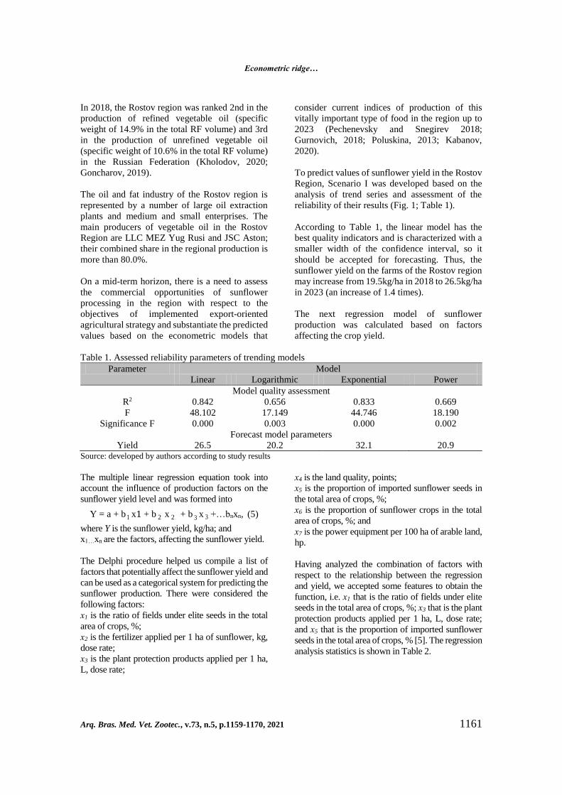
To predict values of sunflower yield in the Rostov

Region, Scenario I was developed based on the

analysis of trend series and assessment of the

reliability of their results (Fig. 1; Table 1).

According to Table 1, the linear model has the

best quality indicators and is characterized with a

smaller width of the confidence interval, so it

should be accepted for forecasting. Thus, the

sunflower yield on the farms of the Rostov region

may increase from 19.5kg/ha in 2018 to 26.5kg/ha

in 2023 (an increase of 1.4 times).

The next regression model of sunflower

production was calculated based on factors

affecting the crop yield.

Table 1. Assessed reliability parameters of trending models

Parameter Model

Linear Logarithmic Exponential Power

Model quality assessment

R2 0.842 0.656 0.833 0.669

F 48.102 17.149 44.746 18.190

Significance F 0.000 0.003 0.000 0.002

Forecast model parameters

Yield 26.5 20.2 32.1 20.9 Source: developed by authors according to study results

The multiple linear regression equation took into

account the influence of production factors on the

sunflower yield level and was formed into

Y = a + b x1 + b x + b x +…bnxn, (5)

where Y is the sunflower yield, kg/ha; and

x1…xn are the factors, affecting the sunflower yield.

The Delphi procedure helped us compile a list of

factors that potentially affect the sunflower yield and

can be used as a categorical system for predicting the

sunflower production. There were considered the

following factors:

х1 is the ratio of fields under elite seeds in the total

area of crops, %;

х2 is the fertilizer applied per 1 ha of sunflower, kg,

dose rate;

х3 is the plant protection products applied per 1 ha,

L, dose rate;

х4 is the land quality, points;

х5 is the proportion of imported sunflower seeds in

the total area of crops, %;

х6 is the proportion of sunflower crops in the total

area of crops, %; and

х7 is the power equipment per 100 ha of arable land,

hp.

Having analyzed the combination of factors with

respect to the relationship between the regression

and yield, we accepted some features to obtain the

function, i.e. х1 that is the ratio of fields under elite

seeds in the total area of crops, %; х3 that is the plant

protection products applied per 1 ha, L, dose rate;

and х5 that is the proportion of imported sunflower

seeds in the total area of crops, % [5]. The regression

analysis statistics is shown in Table 2.

1 2 2 3 3

Slozhenkina et al.


Figure 1. Trend models to forecast sunflower yield in farms of all categories in the Rostov region.

Source: developed by authors according to study results

Table 2. Matrix of statistical data for regression analysis of sunflower yield in farms of all categories of the

Rostov region

Year Y Baseline data

х1 х3 х5

2012 13.00 2.7 0.49 50.2

2013 15.00 2.8 0.52 56.7

2014 14.80 2.9 0.59 60.03

2015 15.70 3.0 0.61 74.95

2016 21.40 3.3 0.78 87.7

2017 20.50 3.1 0.83 82.16

2018 19.50 3.2 0.80 77.02 Source: compiled by authors according to the Ministry of Agriculture of the Rostov Region

Linear model Logarithmic model

Exponential model Power model

2023202220212020201920182017201620152014201320122011201020092008

Год

30

20

10

0

95% UCL for

ур_подсо from

CURVEFIT, MOD_13

LINEAR

95% LCL for


CURVEFIT, MOD_13

LINEAR

Fit for ур_подсо from

CURVEFIT, MOD_13

LINEAR

Урожайность

подсолнечника, ц/га

2023202220212020201920182017201620152014201320122011201020092008

Год

30

25

20

15

10

5

0

95% UCL for


CURVEFIT, MOD_15

LOGARITHMIC

95% LCL for


CURVEFIT, MOD_15

LOGARITHMIC


CURVEFIT, MOD_15

LOGARITHMIC



2023202220212020201920182017201620152014201320122011201020092008

Год

50

40

30

20

10

0

95% UCL for


CURVEFIT, MOD_17

EXPONENTIAL

95% LCL for


CURVEFIT, MOD_17

EXPONENTIAL


CURVEFIT, MOD_17

EXPONENTIAL



2023202220212020201920182017201620152014201320122011201020092008

Год

35

30

25

20

15

10

5

95% UCL for


CURVEFIT, MOD_18

POWER

95% LCL for


CURVEFIT, MOD_18

POWER


CURVEFIT, MOD_18

POWER



sunflower

yield, hundredwei

ght / ha

sunflower

yield, hundredwei

ght / ha

year

year

year

year

sunflower yield, hundredweight / ha

sunflower yield, hundredweight / ha



The relationship between the sunflower yield and

main influencing factors was presented as a

regression model:

𝑌 = −5.7 + 3.72𝑥1 + 13.32𝑥3 + 0.04𝑥5.

The multiple regression coefficient R=0.97

indicated a close relationship between the whole

set of factors and result. The multiple

determination coefficient R2=0.95 suggested that

95.0% of the variation in sunflower yield was

explained by the variation of factors in the model.

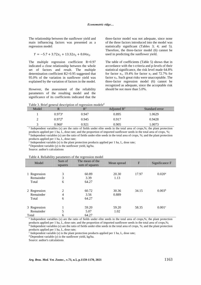
However, the assessment of the reliability

parameters of the resulting model and the

significance of its coefficients indicated that the

three-factor model was not adequate, since none

of the three factors introduced into the model was

statistically significant (Tables 3; 4; and 5).

Therefore, the three-factor model (6) cannot be

used in predicting the sunflower yield.

The table of coefficients (Table 5) shows that in

accordance with the t-criteria and p-levels of their

statistical significance, the risk level made 64.8%

for factor x1, 19.4% for factor x2 and 72.7% for

factor x3. Such great risks were unacceptable. The

three-factor regression model (6) cannot be

recognized as adequate, since the acceptable risk

should be not more than 5.0%.

Table 3. Brief general description of regression modelsd

Model R R2 Adjusted R2 Standard error

1 0.973a 0.947 0.895 1.0629

2 0.972b 0.945 0.917 0.9428

3 0.960c 0.921 0.905 1.0073 a Independent variables (x) are the ratio of fields under elite seeds in the total area of crops,%; the plant protection

products applied per 1 ha, L, dose rate; and the proportion of imported sunflower seeds in the total area of crops, %; b Independent variables (x) are the ratio of fields under elite seeds in the total area of crops, %; and the plant protection

products applied per 1 ha, L, dose rate; c Independent variable (x) is the plant protection products applied per 1 ha, L, dose rate; d Dependent variable (y) is the sunflower yield, kg/ha.

Source: author's calculations

Table 4. Reliability parameters of the regression model

Model Sum of

squares

The mean of the

sum of squares Mean spread F Significance F

1 Regression

Remainder

Total

3

3

6

60.89

3.39

64.27

20.30

1.13

17.97

0.020a

2 Regression

Remainder

Total

2

4

6

60.72

3.56

64.27

30.36

0.889

34.15

0.003b

3 Regression

Remainder

Total

1

5

6

59.20

5.07

64.27

59.20

1.02

58.35

0.001с

a Independent variables (x) are the ratio of fields under elite seeds in the total area of crops,%; the plant protection

products applied per 1 ha, L, dose rate; and the proportion of imported sunflower seeds in the total area of crops,%; b Independent variables (x) are the ratio of fields under elite seeds in the total area of crops, %; and the plant protection

products applied per 1 ha, L, dose rate; c Independent variable (x) is the plant protection products applied per 1 ha, L, dose rate; d Dependent variable (y) is the sunflower yield, kg/ha.


Slozhenkina et al.


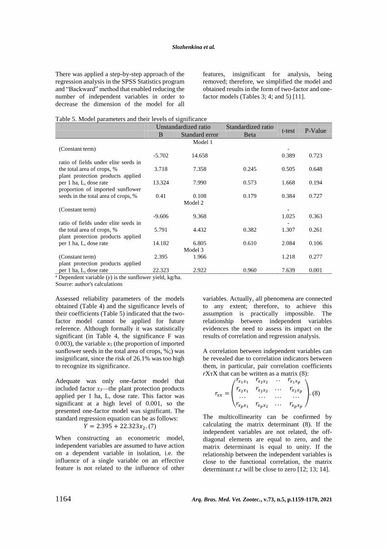
There was applied a step-by-step approach of the

regression analysis in the SPSS Statistics program

and “Backward” method that enabled reducing the

number of independent variables in order to

decrease the dimension of the model for all

features, insignificant for analysis, being

removed; therefore, we simplified the model and

obtained results in the form of two-factor and one-

factor models (Tables 3; 4; and 5) [11].

Table 5. Model parameters and their levels of significance

Unstandardized ratio Standardized ratio t-test Р-Value

В Standard error Beta Model 1

(Constant term)

-5.702 14.658

-

0.389 0.723

ratio of fields under elite seeds in

the total area of crops, % 3.718 7.358 0.245 0.505 0.648

plant protection products applied

per 1 ha, L, dose rate 13.324 7.990 0.573 1.668 0.194

proportion of imported sunflower

seeds in the total area of crops, % 0.41 0.108 0.179 0.384 0.727

Model 2

(Constant term)

-9.606 9.368

-

1.025 0.363

ratio of fields under elite seeds in

the total area of crops, % 5.791 4.432 0.382

-

1.307 0.261


per 1 ha, L, dose rate 14.182 6.805 0.610 2.084 0.106

Model 3

(Constant term) 2.395 1.966 1.218 0.277


per 1 ha, L, dose rate 22.323 2.922 0.960 7.639 0.001 a Dependent variable (y) is the sunflower yield, kg/ha.


Assessed reliability parameters of the models

obtained (Table 4) and the significance levels of

their coefficients (Table 5) indicated that the two-

factor model cannot be applied for future

reference. Although formally it was statistically

significant (in Table 4, the significance F was

0.003), the variable x5 (the proportion of imported

sunflower seeds in the total area of crops, %;) was

insignificant, since the risk of 26.1% was too high

to recognize its significance.

Adequate was only one-factor model that

included factor х3—the plant protection products

applied per 1 ha, L, dose rate. This factor was

significant at a high level of 0.001, so the

presented one-factor model was significant. The

standard regression equation can be as follows:

𝑌 = 2.395 + 22.323𝑥2. (7)

When constructing an econometric model,

independent variables are assumed to have action

on a dependent variable in isolation, i.e. the

influence of a single variable on an effective

feature is not related to the influence of other

variables. Actually, all phenomena are connected

to any extent; therefore, to achieve this

assumption is practically impossible. The

relationship between independent variables

evidences the need to assess its impact on the

results of correlation and regression analysis.

A correlation between independent variables can

be revealed due to correlation indicators between

them, in particular, pair correlation coefficients

rXтX that can be written as a matrix (8):

𝑟𝑥𝑥 = (

𝑟𝑥1𝑥1 𝑟𝑥2𝑥2 . . 𝑟𝑥1𝑥𝑝𝑟𝑥2𝑥1 𝑟𝑥2𝑥2 . . . 𝑟𝑥2𝑥𝑝. . . . . . . . . . . .𝑟𝑥𝑝𝑥1 𝑟𝑥𝑝𝑥2 . . . 𝑟𝑥𝑝𝑥𝑝

). (8)

The multicollinearity can be confirmed by

calculating the matrix determinant (8). If the

independent variables are not related, the off-

diagonal elements are equal to zero, and the

matrix determinant is equal to unity. If the

relationship between the independent variables is

close to the functional correlation, the matrix

determinant rxr will be close to zero [12; 13; 14].



According to Table 1, the matrix of predictor

intercorrelation was as follows (9):

𝒓𝒙𝒙 = (1 0,916 0,955

0,916 1 0,9080,955 0,908 1

) (9)

The matrix determinant was 0.013, which was less

than 1. Nevertheless, the determinant was

different from zero, so it was necessary to apply

other features of multicollinearity. Variables are

considered to be included in the model, if relations

(10) are satisfied, i.e. the strength of the

relationship between response and explicative

variables is greater than the strength of the

relationship between explicative variables.

{𝑟𝑦𝑥𝑖⟩𝑟𝑥𝑖𝑥𝑗 ,

𝑟𝑦𝑥𝑗⟩ 𝑟𝑥𝑖𝑦𝑗 ,𝑖 ≠ 𝑗.

(10)

We used the data in Table 2 and obtained r (yx1)

= 0.941; r (yx2) = 0.960; and r (yx3) = 0.933.

Given the data in matrix (10), we have (11); (12);

and (13).

{𝑟𝑦𝑥1 = 0.941⟩𝑟𝑥1𝑥2 = 0.916,

𝑟𝑦𝑥2 = 0.960⟩ 𝑟𝑥1𝑦2 = 0.916,𝑖 ≠ 𝑗; (11)

Therefore, variables x1 and x2 can be included in

the model

{𝑟𝑦𝑥2 = 0.960⟩𝑟𝑥1𝑥3 = 0.955,

𝑟𝑦𝑥3 = 0.933⟨𝑟х1х30.955,𝑖 ≠ 𝑗; (12)

and variable x3 together with variable x2 cannot be

included in the model.

{𝑟𝑦𝑥1 = 0.941⟨𝑟𝑥1𝑥3 = 0.955,

𝑟𝑦𝑥3 = 0.933⟨𝑟х1х30.955,𝑖 ≠ 𝑗. (13)

therefore, the variable x3 together with the variable

x1 cannot be included in the model.

Another method to measure multicollinearity

resulted from the analysis of the standard error

formula for the regression coefficient (14):

𝑆𝜎𝑖 =𝜎𝑦

𝜎𝑥𝑗√

1−𝑅2𝑦𝑥1...𝑥𝑝

(1−𝑅2𝑥𝑗𝑥1...𝑥𝑗−1,...хр)(𝑛−𝑚−1). (14)

As follows from this formula, the larger is the

standard error, the smaller is the value of the

variance inflation factor (VIF) (15):

𝑉𝐼𝐹𝑥𝑗 =1

(1−𝑅2𝑥𝑗𝑥1...𝑥𝑗−1...𝑥𝑝), (15)

where R2xjx1…xj-1…xp is the determination

coefficient found in the stimulus-response

equation for variable xj that depends on other

variables x1…xp in the considered multiple

regression model [12, 13].

Value R2xjx1…xj-1…xp reflects the strength of the

relationship between variable xj and other

explicative variables and, in fact, characterizes

multicollinearity with respect to variable xj. If the

relationship is absent, the VIFx indicator is equal

(or closes) to unity; strengthening relationship

makes this indicator tend to infinity. If VIFx>3 for

each variable, the multicollinearity occurs.

𝑉𝐼𝐹𝑥1 =1

(1−0.925)=

1

0.075= 13.3; (16)


(1−0.851)=

1

0.149= 6.7; (17)


(1−0.825)=

1

0.175= 5.7.

(18)

Calculations (16); (17); and (18) evidenced that

the indices exceeded the significance point of

three. Therefore, when constructing a model, the

relationships between independent variables

cannot be neglected.

This can be confirmed by following arguments.

The State Program on Agribusiness Development

envisages subsidizing the purchase of elite seeds

until 2025 and guarantees the development of this

sector. In the structure of sunflower production

costs of agricultural producers, the costs of plant

protection products enhanced from 10.0% in 2013

to 14.1% in 2018. Given this trend, as well as the

technological need to actively use chemicals at

intensive sunflower production, we predicted an

increase in the cost of protection products, which

indicated the ability of this factor to have an

impact on the crop yield in the medium term. It

should be noted that in the Rostov Region from

2012 to 2018, the share of imported seeds

increased from 55.2% to 77.02%. Thus, more than

half of sunflower crops in the region depend on

imported seeds that are highly germinated,

resistant to diseases, and yielding. This fact is also

in favor of the feature under consideration

(Kholodov, 2020).

Consequently, the empirical basis we have

considered for constructing a risk-sensitivity

regression model of the sunflower yield was

characterized by multicollinearity.

The presented multiple regression models

contained input variables as predictors, most

closely correlated with the yield value and had

Slozhenkina et al.


satisfactory quality characteristics. The factorial

analysis results did not allow assessing the impact

of all risk factors in the analysis on the sunflower

yield; moreover, their specification was not

unambiguous.

In this case, the list of independent variables

cannot be changed; therefore, one of the methods

for eliminating multicollinearity must be applied.

For example, after correcting the model using the

ridge regression equation procedure, the found

parameter estimates will be biased (19)

(Pechenevsky and Snegirev, 2018; Plis and

Slivina, 1999; Pokrovsky, 2012):

B = (ХТХ + kI)-

1Х

ТY. (19)

When building ridge regression, it is

recommended to convert independent variables

according to formula (20) and the response

variable according to formula (21):

𝑥𝑖𝑗 =𝑥𝑗−𝑥𝑗

√∑(𝑥𝑗−𝑥𝑗)2 ; (20)

𝑦𝜏 = 𝑦 × 𝑦𝜏. (21)

Having evaluated the parameters (22), we found

the regression of the initial variables, using

relations (23):

𝑎𝑗 = (𝑋𝜏𝑇𝑋𝜏 + 𝜏𝐼)−1𝑋𝜏

𝑇𝑌𝜏; (22)

𝑎𝑗 =𝑎𝑖𝑗

√∑(𝑥𝑗−𝑥𝑗)2, j=1.2…,p; 𝑎0 = 𝑦;∑ 𝑎𝑗𝑥𝑗𝑗 .

(23)

Regression parameters estimated by formula (23)

were biased. However, since the matrix

determinant (ХТХ+τI) was greater than the matrix

determinant (XTX), the variance of the regression

parameters estimates decreased and positively

affected predicted properties of the model.

Thus, the task of our study resolves itself into this:

using the same data set as when constructing

Model 2, it is necessary to estimate the parameters

of the ridge regression model that excludes the

influence of multicollenarity and contains a full

set of predictors.

In accordance with the above, the dependence of

the parameters’ estimates of the ridge-regression

model on its values was initially studied. The

empirical basis was the data in Table 2. The

Mathcad package was used as a computational

and analytical research tool. Taking into account

the recommendations on the bias parameter value

and the ridge regression results, the k parameter

varied in the range from 0.25 to 3.0, with the

values of the determinant of the information ХТХ

matrix being calculated together with the

regression coefficients. To increase the accuracy

of calculations, the factors were centered and

normalized; the response was also centered

(Pokrovsky, 2012).

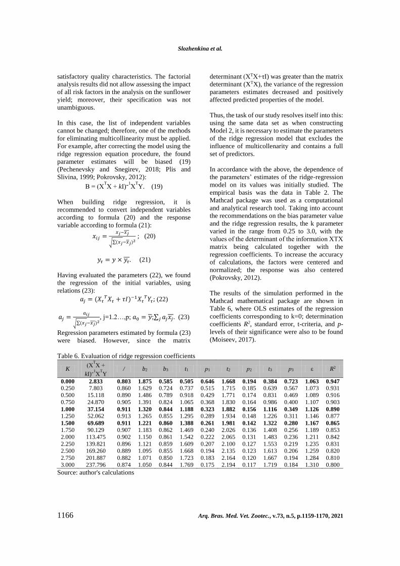
The results of the simulation performed in the

Mathcad mathematical package are shown in

Table 6, where OLS estimates of the regression

coefficients corresponding to k=0; determination

coefficients R2, standard error, t-criteria, and p-

levels of their significance were also to be found

(Moiseev, 2017).

Table 6. Evaluation of ridge regression coefficients

K (Х

ТХ +

kI)-1Х

ТY

/ b2 b3 t1 р1 t2 р2 t3 р3 ε R2

0.000 2.833 0.803 1.875 0.585 0.505 0.646 1.668 0.194 0.384 0.723 1.063 0.947

0.250 7.803 0.860 1.629 0.724 0.737 0.515 1.715 0.185 0.639 0.567 1.073 0.931

0.500 15.118 0.890 1.486 0.789 0.918 0.429 1.771 0.174 0.831 0.469 1.089 0.916

0.750 24.870 0.905 1.391 0.824 1.065 0.368 1.830 0.164 0.986 0.400 1.107 0.903

1.000 37.154 0.911 1.320 0.844 1.188 0.323 1.882 0.156 1.116 0.349 1.126 0.890

1.250 52.062 0.913 1.265 0.855 1.295 0.289 1.934 0.148 1.226 0.311 1.146 0.877

1.500 69.689 0.911 1.221 0.860 1.388 0.261 1.981 0.142 1.322 0.280 1.167 0.865

1.750 90.129 0.907 1.183 0.862 1.469 0.240 2.026 0.136 1.408 0.256 1.189 0.853

2.000 113.475 0.902 1.150 0.861 1.542 0.222 2.065 0.131 1.483 0.236 1.211 0.842

2.250 139.821 0.896 1.121 0.859 1.609 0.207 2.100 0.127 1.553 0.219 1.235 0.831

2.500 169.260 0.889 1.095 0.855 1.668 0.194 2.135 0.123 1.613 0.206 1.259 0.820

2.750 201.887 0.882 1.071 0.850 1.723 0.183 2.164 0.120 1.667 0.194 1.284 0.810

3.000 237.796 0.874 1.050 0.844 1.769 0.175 2.194 0.117 1.719 0.184 1.310 0.800




According to Table 6, centering and normalizing

of the factors did not change the accuracy

characteristics of the regression coefficients

according to the “standard” OLS method (k=0).

The only difference was that due to centering of

the response variable, the Y-intercept of the model

was equal to zero, and some differences in p-

values of the regression coefficients were

explained by calculation errors.

The regression equation (6) was presented in

centered and normalized forms (24):

𝑌 = 0.803𝑥1 + 1.875𝑥3 + 0.585𝑥5. (24)

The determination coefficient of this model was

0.947; Fisher's test of 17.965 was significant at

0.020; and the standard approximation error was

1.06. Moreover, all factors were insignificant.

In practical estimation procedures, the initial

decision-making methods for obtaining estimates

of the regression coefficients are graphs, showing

relationship between the variance in the

coefficient estimates and changes in the bias

parameter k (ridge graphs). This parameter is

usually not worth of considering. It is

recommended to consider k less than 0.5 and set a

small step, for example, of 0.02. This

recommendation, however, contradicts the results

of ridge regression modeling presented in the

Draper and Smith’s classical work on the

regression analysis, where the bias parameter

value of 0.013 turned out to be the best according

to the ridge graphs. The obtained value

corresponded to the transition from the site of a

strong change in the regression coefficients to the

site of their slow change (Draper, Smith, 1987). In

other works, the parameter values were greater,

i.e. k=10 (Moiseev, 2017).

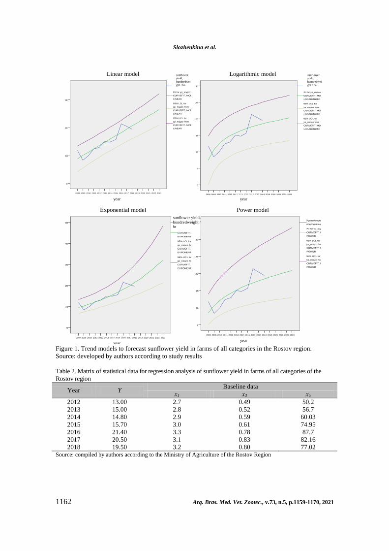
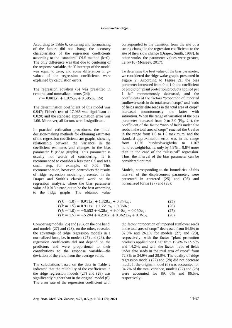
To determine the best value of the bias parameter,

we considered the ridge wake graphs presented in

Figure 2. According to Figure 2a, the bias

parameter increased from 0 to 1.0, the coefficient

of predictor “plant protection products applied per

1 ha” monotonously decreased, and the

coefficients of the factors “proportion of imported

sunflower seeds in the total area of crops” and “ratio

of fields under elite seeds in the total area of crops”

increased monotonously, the latter with

saturation. When the range of variation of the bias

parameter increased from 0 to 3.0 (Fig. 2b), the

coefficient of the factor “ratio of fields under elite

seeds in the total area of crops” reached the k value

in the range from 1.0 to 1.5 maximum, and the

standard approximation error was in the range

from 1.026 hundredweight/ha to 1.167

hundredweight/ha, i.e. only by 5.9% ... 9.8% more

than in the case of the “classical” regression.

Thus, the interval of the bias parameter can be

considered optimal.

Models, corresponding to the boundaries of this

interval of the displacement parameter, were

presented in centered (25) and (26) and

normalized forms (27) and (28):

𝑌(𝑘 = 1.0) = 0.911𝑥1 + 1.320𝑥3 + 0.844𝑥5; (25)

𝑌(𝑘 = 1.5) = 0.911𝑥1 + 1.221𝑥3 + 0.8605; (26)

𝑌(𝑘 = 1.0) = −5.652 + 4.28𝑥1 + 9.040𝑥3 + 0.060𝑥5; (27)

𝑌(𝑘 = 1.5) = −5.284 + 4.218𝑥1 + 8.3621𝑥3 + 0.0615. (28)

Comparing models (25) and (26), on the one hand,

and models (27) and (28), on the other, revealed

the advantage of ridge regression models in a

normalized form, i.e. in models (27) and (28), the

regression coefficients did not depend on the

predictors and were proportional to their

contributions to the response variable—the

deviation of the yield from the average value.

The calculations based on the data in Table 2

indicated that the reliability of the coefficients in

the ridge regression models (27) and (28) was

significantly higher than in the original model (6).

The error rate of the regression coefficient with

the factor “proportion of imported sunflower seeds

in the total area of crops” decreased from 64.6% to

32.3% and 26.1% for models (27) and (28),

respectively; with the factor “plant protection

products applied per 1 ha” from 19.4% to 15.6 %

and 14.2%; and with the factor “ratio of fields

under elite seeds in the total area of crops” from

72.3% to 34.9% and 28.0%. The quality of ridge

regression models (27) and (28) did not decrease

much. If the original model (6) was accounted for

94.7% of the total variance, models (27) and (28)

were accounted for 89, 0% and 86.5%,

respectively.

Slozhenkina et al.


Figure 2. Relationship between ridge regression coefficients of sunflower yield and bias parameter in the

range of a) from 0 to 1.0; and b) from 0 to 3.0.


The conducted statistical analysis substantiated

the econometric ridge regression models (27) and

(28) to be useful for forecasting the sunflower

yield for 2023. In order to increase the reliability,

we used the average results for models (27) and

(28) as predictive estimates.

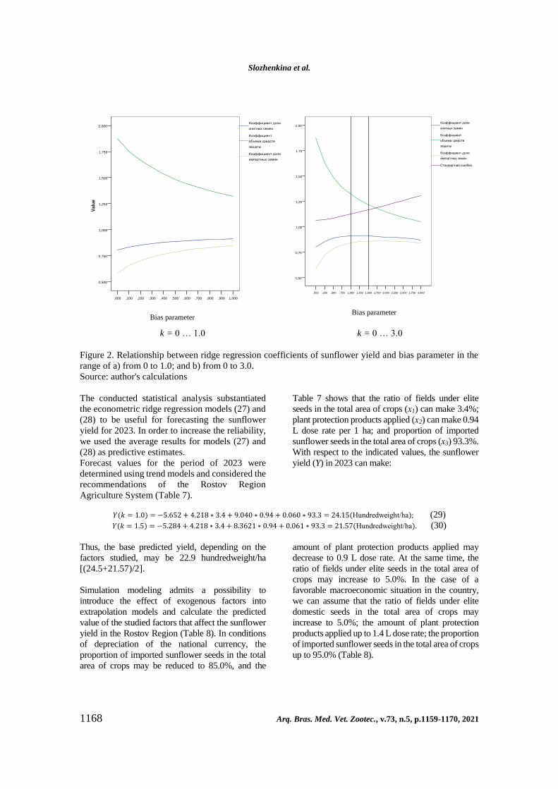
Forecast values for the period of 2023 were

determined using trend models and considered the

recommendations of the Rostov Region

Agriculture System (Table 7).

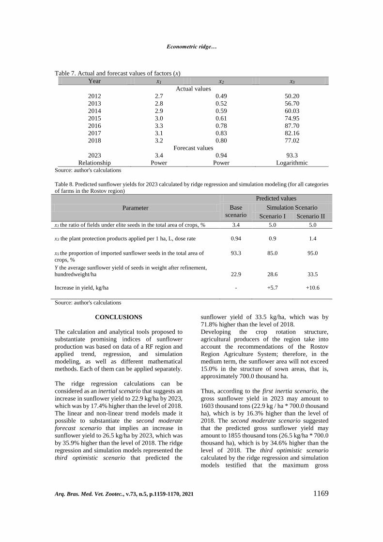
Table 7 shows that the ratio of fields under elite

seeds in the total area of crops (х1) can make 3.4%;

plant protection products applied (х2) can make 0.94

L dose rate per 1 ha; and proportion of imported

sunflower seeds in the total area of crops (х3) 93.3%.

With respect to the indicated values, the sunflower

yield (Y) in 2023 can make:

𝑌(𝑘 = 1.0) = −5.652 + 4.218 ∗ 3.4 + 9.040 ∗ 0.94 + 0.060 ∗ 93.3 = 24.15(Hundredweight/ha);

(29)

𝑌(𝑘 = 1.5) = −5.284 + 4.218 ∗ 3.4 + 8.3621 ∗ 0.94 + 0.061 ∗ 93.3 = 21.57(Hundredweight/ha). (30)

Thus, the base predicted yield, depending on the

factors studied, may be 22.9 hundredweight/ha

[(24.5+21.57)/2].

Simulation modeling admits a possibility to

introduce the effect of exogenous factors into

extrapolation models and calculate the predicted

value of the studied factors that affect the sunflower

yield in the Rostov Region (Table 8). In conditions

of depreciation of the national currency, the

proportion of imported sunflower seeds in the total

area of crops may be reduced to 85.0%, and the

amount of plant protection products applied may

decrease to 0.9 L dose rate. At the same time, the

ratio of fields under elite seeds in the total area of

crops may increase to 5.0%. In the case of a

favorable macroeconomic situation in the country,

we can assume that the ratio of fields under elite

domestic seeds in the total area of crops may

increase to 5.0%; the amount of plant protection

products applied up to 1.4 L dose rate; the proportion

of imported sunflower seeds in the total area of crops

up to 95.0% (Table 8).

k = 0 … 1.0 k = 0 … 3.0

1,000,900,800,700,600,500,400,300,200,100,000

Параметр смещения

2,000

1,750

1,500

1,250

1,000

0,750

0,500

Va

lue

Коэффициент доли

импортных семян

Коэффициент

объема средств

защиты


элитных семян

3,0002,7502,5002,2502,0001,7501,5001,2501,000,750,500,250,000

Параметр смещения

2,00

1,75

1,50

1,25

1,00

0,75

0,50

Стандартная ошибка


импортных семян

Коэффициент

объема средств

защиты


элитных семян

Bias parameter

Bias parameter



Table 7. Actual and forecast values of factors (x)

Year х1 х2 х3

Actual values

2012 2.7 0.49 50.20

2013 2.8 0.52 56.70

2014 2.9 0.59 60.03

2015 3.0 0.61 74.95

2016 3.3 0.78 87.70

2017 3.1 0.83 82.16

2018 3.2 0.80 77.02

Forecast values

2023 3.4 0.94 93.3

Relationship Power Power Logarithmic Source: author's calculations

Table 8. Predicted sunflower yields for 2023 calculated by ridge regression and simulation modeling (for all categories

of farms in the Rostov region)

Parameter

Predicted values

Base

scenario

Simulation Scenario

Scenario I Scenario II

х1 the ratio of fields under elite seeds in the total area of crops, % 3.4 5.0 5.0

х3 the plant protection products applied per 1 ha, L, dose rate 0.94 0.9 1.4

х5 the proportion of imported sunflower seeds in the total area of

crops, %

93.3 85.0 95.0

Y the average sunflower yield of seeds in weight after refinement,

hundredweight/ha

22.9

28.6

33.5

Increase in yield, kg/ha - +5.7 +10.6


CONCLUSIONS

The calculation and analytical tools proposed to

substantiate promising indices of sunflower

production was based on data of a RF region and

applied trend, regression, and simulation

modeling, as well as different mathematical

methods. Each of them can be applied separately.

The ridge regression calculations can be

considered as an inertial scenario that suggests an

increase in sunflower yield to 22.9 kg/ha by 2023,

which was by 17.4% higher than the level of 2018.

The linear and non-linear trend models made it

possible to substantiate the second moderate

forecast scenario that implies an increase in

sunflower yield to 26.5 kg/ha by 2023, which was

by 35.9% higher than the level of 2018. The ridge

regression and simulation models represented the

third optimistic scenario that predicted the

sunflower yield of 33.5 kg/ha, which was by

71.8% higher than the level of 2018.

Developing the crop rotation structure,

agricultural producers of the region take into

account the recommendations of the Rostov

Region Agriculture System; therefore, in the

medium term, the sunflower area will not exceed

15.0% in the structure of sown areas, that is,

approximately 700.0 thousand ha.

Thus, according to the first inertia scenario, the

gross sunflower yield in 2023 may amount to

1603 thousand tons (22.9 kg / ha * 700.0 thousand

ha), which is by 16.3% higher than the level of

2018. The second moderate scenario suggested

that the predicted gross sunflower yield may

amount to 1855 thousand tons (26.5 kg/ha * 700.0

thousand ha), which is by 34.6% higher than the

level of 2018. The third optimistic scenario

calculated by the ridge regression and simulation

models testified that the maximum gross

Slozhenkina et al.


sunflower yield in the Rostov Region may reach

2345 thousand tons (33.5 t/ha * 700.0 thousand

ha), which is by 70.1% higher than the level of

2018.

Using the example of forecasting the sunflower

yield, it was substantiated that despite the

functional multicollinearity of the predictors in

the risk-sensitive yield model that is conditioned

by the algorithm of the hierarchy analysis method

used in the case of uncertainty of input variables,

it was possible to provide a complete specification

of the model and get biased but stable estimates of

its parameters, using the ridge regression

procedure. The rational value of the parameters

was proposed to determine according to the ridge

wake graphs as the border of fast and slow

changes in the estimates of the ridge regression

coefficients.

ACKNOWLEDGMENTS

This work was performed under RF President

grant to support leading scientific schools, НШ-

2542.2020.11.

REFERENCES

DERUNOVA, E.A. Toolkit for assessing and

predicting the dynamics of innovation and

competitiveness of agricultural products. Econ.

Agric. Proc. Enterprises, v.1, p.65-70, 2019.

DRAPER, N.; SMITH, H. Applied regression

analysis. Part 2. Moscow: Finance and statistics,

1987.

GONCHAROV, V.D. Production of rapeseed oil

in Russia: problems of development Econ. Agric.

Proc. Enterprises, v.2, p.54-58, 2019.

GURNOVICH, T.G.; AGARKOVA, L.V.;

OSTAPENKO, E.A.; USENKO, L.N. Increasing

competitiveness of the agrarian sector of the

heregional russian economy Russia. Int. J. Eng.

Technol., v.7, p.201-211, 2018.

IVANOV, E.E.; SHUSTOV, D.A.;

PERESHIVKIN, S.A. Multivariable statistical

methods. Multiple regression analysis. Ridge

regression method. 2020. Available in:

http://ecocyb.narod.ru/513/MSM/msm3_2.htm.

Accessed in: 15 Oct. 2020.

KABANOV, S.V. Using the Statistica

5.0 package for statistical processing of

experimental data. 2020. Available in:

http://www.exponenta.ru/educat/systemat/kabano

v/literatura.asp. Accessed in: 15 Oct. 2020.

KHOLODOV, O.A. Development of industrial

and economic relations between agricultural

producers and processing enterprises. Fund. Appl.

Res. Studies Econ. Coop. Sector, v.1, 2020.

KUZNETSOV, V.V.; TARASOV, A.N.;

DUNAEV, V.L. et al. Improved forecasting of the

regional agribusiness development based on

economic and mathematical modeling. Rostov on

Don: Vniiein, 2006.

MOISEEV, N.A. Comparative analysis of

methods for eliminating multicollinearity. Acc.

Sta., v.2, p.62-73, 2017.

PECHENEVSKY, V.F.; SNEGIREV, O.I.

Forecasting the location of livestock production in

the region. Econ. Agric. Proc. Enterprises, v.11,

p.43-47, 2018.

PLIS, A.I.; SLIVINA, N.A. Mathcad:

mathematical workshop for economists and

engineers: a study guide. Moscow: Finance and

Statistics, 1999.

POKROVSKY, A.M. Econometric models of

sensitivity of innovative projects to risk factors

based on ridge regression. Innovative Econ.Inf.

Anal. Forecasts, v.3, p.10-13, 2012.

POLUSKINA, T.M. Modern Russia agrarian

polity in the context of globalization. World Sci.

Discov., v.1, p.105-115, 2013.

Econometric ridge regression models of risk-sensitive ...

Documents