ALMA MATER STUDIORUM UNIVERSITA’ DI BOLOGNA Department of Statistics Doctor of Philosophy Thesis in STATISTICAL METHODOLOGY FOR SCIENTIFIC RESEARCH XIX Cycle ECONOMETRIC MODELS FOR THE ANALYSIS OF ELECTRICITY MARKETS Carlo Fezzi Supervisor: Coordinator: Chiar.mo Prof. Attilio Gardini Chiar.ma Prof.ssa Daniela Cocchi Disciplinary sector: SECS-P/05

Welcome message from author
This document is posted to help you gain knowledge. Please leave a comment to let me know what you think about it! Share it to your friends and learn new things together.
Transcript

ALMA MATER STUDIORUM
UNIVERSITA’ DI BOLOGNA
Department of Statistics
Doctor of Philosophy Thesis in
STATISTICAL METHODOLOGY FOR SCIENTIFIC RESEARCH
XIX Cycle
ECONOMETRIC MODELS
FOR THE ANALYSIS OF ELECTRICITY
MARKETS
Carlo Fezzi
Supervisor: Coordinator:
Chiar.mo Prof. Attilio Gardini Chiar.ma Prof.ssa Daniela Cocchi
Disciplinary sector: SECS-P/05
i
Contents
List of Figures iii
List of Tables v
1 Introduction 1
2 The electricity sector and the reconstruction process 5
2.1 The electricity sector . . . . . . . . . . . . . . . . . . . . . . . . . . . . . . . 62.2 The liberalisation process . . . . . . . . . . . . . . . . . . . . . . . . . . . . 82.3 Wholesale electricity markets . . . . . . . . . . . . . . . . . . . . . . . . . . 11
2.3.1 The UK market evolution . . . . . . . . . . . . . . . . . . . . . . . . 132.3.2 The California Crisis . . . . . . . . . . . . . . . . . . . . . . . . . . . 142.3.3 The PJM market . . . . . . . . . . . . . . . . . . . . . . . . . . . . . 152.3.4 The NordPool . . . . . . . . . . . . . . . . . . . . . . . . . . . . . . . 162.3.5 The Italian power exchange . . . . . . . . . . . . . . . . . . . . . . . 17
3 Time series analysis of electricity market outcomes 19
3.1 Quantity dynamics . . . . . . . . . . . . . . . . . . . . . . . . . . . . . . . . 203.1.1 Determinants of quantity dynamics . . . . . . . . . . . . . . . . . . . 213.1.2 Short term forecasting models . . . . . . . . . . . . . . . . . . . . . . 24
3.2 Price dynamics . . . . . . . . . . . . . . . . . . . . . . . . . . . . . . . . . . 323.2.1 Determinants of price dynamics . . . . . . . . . . . . . . . . . . . . . 333.2.2 The stationarity issue . . . . . . . . . . . . . . . . . . . . . . . . . . 373.2.3 Price modelling and forecasting . . . . . . . . . . . . . . . . . . . . . 48
4 Electricity wholesale markets behaviour 52
4.1 The price formation process . . . . . . . . . . . . . . . . . . . . . . . . . . . 534.2 Competition and market power . . . . . . . . . . . . . . . . . . . . . . . . . 604.3 The demand elasticity dilemma . . . . . . . . . . . . . . . . . . . . . . . . . 65
5 Structural analysis of high-frequency electricity demand and supply in-
teractions 72
5.1 Preliminary data analysis . . . . . . . . . . . . . . . . . . . . . . . . . . . . 75
ii
5.1.1 Descriptive analysis of PJM electricity market outcomes . . . . . . . 765.1.2 Unit root and stationarity analysis . . . . . . . . . . . . . . . . . . . 84
5.2 A static economic model of electricity aggregated demand and supply . . . 875.2.1 Stylization of the supply and demand curves . . . . . . . . . . . . . 885.2.2 The empirical specification . . . . . . . . . . . . . . . . . . . . . . . 91
5.3 Econometrics methodologies for non-stationary data . . . . . . . . . . . . . 945.3.1 The spurious regression problem . . . . . . . . . . . . . . . . . . . . 955.3.2 Error-correction models and cointegration . . . . . . . . . . . . . . . 975.3.3 Further issues on cointegration . . . . . . . . . . . . . . . . . . . . . 1035.3.4 The asymmetric error-correction model . . . . . . . . . . . . . . . . 106
5.4 The dynamic econometric specification . . . . . . . . . . . . . . . . . . . . . 1085.5 The empirical analysis . . . . . . . . . . . . . . . . . . . . . . . . . . . . . . 1155.6 Conclusions . . . . . . . . . . . . . . . . . . . . . . . . . . . . . . . . . . . . 129
6 Conclusions 134
Bibliography 138

iii
List of Figures
2.1 Wholesale and retail competition model . . . . . . . . . . . . . . . . . . . . 11
2.2 California power exchange hourly prices, from 01/01/2000 to 31/12/2000 . 15
3.1 Periodogram of UK electricity half-hourly load data (1st of january 2004 -23rd of january 2006) . . . . . . . . . . . . . . . . . . . . . . . . . . . . . . 22
3.2 Hourly average load in California in MWh (straigh line, 01/01/1999 - 31/12/1999)and Spain (dotted line, 01/01/1998 - 31/12/2003) . . . . . . . . . . . . . . . 23
3.3 Hourly loads in Italy, from 19/12/2004 to 29/12/2004. . . . . . . . . . . . . 24
3.4 Daily average load in Spain, 1 January 1998 - December 1999, seasonal cyclesuperimposed . . . . . . . . . . . . . . . . . . . . . . . . . . . . . . . . . . . 25
3.5 Structure of a MLP neural network: input variables (Xs), neurons (circles),output variables (Y) and weights (w and u). . . . . . . . . . . . . . . . . . . 29
3.6 Hourly electricity price in Italy, from 19/12/2004 to 29/12/2004. . . . . . . 34
3.7 APX (Netherlands) daily price, weekdays, from 01/01/2001 to 31/12/2002 . 35
3.8 Electricity (euro / MWh) and gas (c / therm) daily price in UK, from01/01/2004 to 14/12/2005 . . . . . . . . . . . . . . . . . . . . . . . . . . . . 36
3.9 Autocorrelation function: UK half-hourly loads, from january 2004 to may2006 . . . . . . . . . . . . . . . . . . . . . . . . . . . . . . . . . . . . . . . . 43
4.1 Daily load duration curve, Spain, 1st of January 1998 - 31st of December 1999 55
4.2 Break-even analysis, straight line = least cost solution . . . . . . . . . . . . 57
4.3 Marginal cost supply function for the optimisation example in table 4.1 . . 58
4.4 Shift in the supply curve when some plants (shaded area) are not availableto produce, with two different demand curves (baseload and peak) . . . . . 59
5.1 Quantity (MWh) and price ($/MWh) traded on the PJM market, from the1st of April, 2002 to the 31st of August, 2003. . . . . . . . . . . . . . . . . . 76
5.2 Scatter plot between PJM average quantity (MWh) and atmospheric tem-perature (F0), from the 1st of April, 2002 to the 31st of August, 2003. . . . 78
5.3 Quantity (straight line, MWh) and price (dotted line, $/MWh) traded onthe PJM market, from the 26th of February, 2002 to the 5th of March„ 2003. 79

iv
5.4 Hourly means (straight line) and standard deviations (dotted line), PJMclearing quantity (left) and price (right), working days only. . . . . . . . . . 80
5.5 Hourly clearing prices and quantities, PJM day-ahead market, hour 19 andhour 24. Atmospheric temperature, excess capacity, coal (Pennsylvania in-dex) and gas (Henry Hub) prices. Time span: 01/04/2002 — 31/08/2003. . . 83
5.6 Autocorrelation plot for hour 24 price and quantity, working days only. . . . 845.7 Actual and fidded values, and standardized residuals, in hour 24. . . . . . . 1275.8 Actual and fitted values, and standardized residuals, in hour 19. . . . . . . 1285.9 Simulated effect of a gas price shock on electricity traded quantity and price
in hour 24 . . . . . . . . . . . . . . . . . . . . . . . . . . . . . . . . . . . . . 130
v
List of Tables
4.1 Technology choice in a simple example . . . . . . . . . . . . . . . . . . . . 564.2 Assumed demand elasticities in articles analysing market power and strategic
interaction of firms in electricity markets . . . . . . . . . . . . . . . . . . . . 68
5.1 Descriptive Statistics . . . . . . . . . . . . . . . . . . . . . . . . . . . . . . . 815.2 Unit Root and Stationarity Tests . . . . . . . . . . . . . . . . . . . . . . . . 855.3 Hour 24 VAR descriptive statistics and diagnostic tests, series in natural
logarithms . . . . . . . . . . . . . . . . . . . . . . . . . . . . . . . . . . . . . 1165.4 Hour 19 VAR descriptive statistics and diagnostic tests, series in natural
logarithms . . . . . . . . . . . . . . . . . . . . . . . . . . . . . . . . . . . . . 1175.5 Cointegration tests and eigenvalues . . . . . . . . . . . . . . . . . . . . . . . 1195.6 Cointegrating vectors and loading factors, with LR significance tests . . . . 1205.7 Cointegrating vectors and loading factors, with LR significance tests . . . . 1215.8 Cointegrating vectors with coal, gas and capacity as weakly exogenous . . . 1225.9 Simultaneous equations estimates and specification tests, hour 24 . . . . . . 1245.10 Simultaneous equations estimates and specification tests, hour 19 . . . . . 125

vi
Acknowledgments
Many people have provided advice and support throughout this research, without whom
I doubt it would have been possible. Firstly, many thanks to my supervisor, Attilio Gar-
dini, for his support and advice, and to Michele Costa, for his suggestions, kindness and
for always having time. I am sincerely grateful to Derek Bunn, for his fundamental con-
tribution and guidance, which I have been fortunate to appreciate from the very first day
I arrived at LBS. I am indebt to all the members of the Energy Markets Group, and
all the other LBS PhD students and staff with whom I shared my research interests, my
doubts, or simply my free-time. Among them, particular thanks to Sirio Aramonte and
Stefano Sacchetto, for their enthusiasm and friendship. I have also benefit from the helpful
comments of Giuseppe Cavaliere, Luca Fanelli and of the participants to the 29th Inter-
national Conference the International Association for Energy Economics (IAEE), Berlin,
the 3rd International Conference European Electricity Markets EEM 06, Warsaw, and the
5th Conference of the British Institute of Energy Economics (BIEE), Oxford. I am very
grateful to all of them, but they are of course, absolved from any responsibility from
the views expressed in this book. Any errors that may remain are mine own. Finally,
I am greatly indebts to my parents and friends (both in Italy and in London) for their
support and encouragement in the hard and in the joyful moments of these three years.
Bologna, March 2007 Carlo Fezzi

1
Chapter 1
Introduction
Since the invention of the incandescent light bulb by Thomas Edison in 1879, elec-
tricity revolutionised our way of life. Electricity is so important for social and economic
development that a recent report1 of the International Monetary Found and of the World
Bank has pointed out how 1.6 billions of people do not have access to electricity and how
“poor people without access to modern energy suffer from health effects of indoor air pol-
lution; are constrained from engaging in productive activities; and suffer from poor health
and education services”. This “is responsible of 1.5 millions of death per year”. Until
recently, electricity was thought to be a typical example of natural monopoly: an indivis-
ible, capital intensive product totally dependent upon a network structure which requires
a perfect synchronization between production and instantaneous consumption. Therefore,
electric industry management has historically been entrusted to state-owned, monopolistic
companies.
Nevertheless, over the last decade, a wave of reconstruction interested the electric
1Development Commitee (2006)

2
industry in many countries and the liberalisation of the power sector became one of the
major issues worldwide. In the early 1990s this phenomenon started in a few countries across
the world (among others United Kingdom, Norway and Australia) and in the following years
it gradually diffused in the European Union as well as in the United States. Ownership
in the electric sector has become private rather than public, and competive markets have
been introduced in many countries to boost wholesale trading. The scope was to rely
on competitive forces to encourage investment and efficiency, with benefits for the overall
economy.
Liberalisation also introduced new elements of risk; the major one being without
a doubt electricity price volatility. Under regulation, in fact, price variation was minimal
and under the strict control of public-owned commissions, which determined tariffs on the
basis of average production costs. In this controlled environment the attention was focused
on demand forecasting. In particular, the most sophisticated statistical techniques have
been proposed to achieve satisfactory short-run predictions. On the other hand, under
deregulation, price formation was delegated to the law of supply and demand. Because of
the distinct characteristics of electricity, in liberalised markets price volatility has increased
far beyond those of any other commodity or financial asset. Therefore, great interest has
been placed on developing accurate price forecasting models. Nevertheless, the results
achieved in demand forecasting are still far to be accomplished for price. The main reasons
are the peculiar dynamics of electricity price, characterised by a huge volatility and by
the presence of sudden, unexpected changes. The contributions in this area have mainly
focused on identifying the stochastic properties of electricity prices and on proposing models

3
to describe the time-series behaviour of price conditional mean and variance. Still at the
earliest steps in this area is the study of models which are statistically accurate and also
grounded in economic theory. This thesis is one of the first attempts in trying to fill this
significant research gap.
The contribution of the thesis is twofold. First, it illustrates the main results
achieved in the last decade in the statistical analysis of electricity markets outcomes, with
special attention to the aspects which are still debated among academics and practitioners.
Therefore, it proposes a novel econometric approach which ensures clear-cut inference on
the price and quantity formation process in wholesale electricity markets. This model is
structural, in the sense that each parameter has a clear economic interpretation, and can
provide important insights on many of the unresolved aspects illustrated previously. This
work has benefited from an extensive collaboration with the Energy Markets Group, and in
particular with Professor Derek Bunn, started during a visiting period at London Business
School.
This thesis is organised as follows. In chapter 2, the stylised facts concerning the
electricity market liberalisation process are illustrated. The structure of wholesale markets
is introduced, drawing examples from the arrangements actually existing in many countries
across the world. The outcomes (price and quantity) of those markets are then analysed in
the following sections.
In chapter 3, the statistical methods proposed to model electricity quantity and
price are presented. The main focus is on high-frequency, time-series models, since in

4
this context the most advanced methodologies are required and, therefore, have been devel-
oped. Quantity dynamics have been subject to extensive research since many decades before
deregulation, whereas models to describe and forecast price are a new and expanding area
of research. As showed in this chapter, some characteristics of electricity price dynamics
are still unresolved. For instance, it is still debated if those time series should be considered
stationary or with unit root for modelling purposes.
Since the aim of the thesis is to develop models with clear economic interpreta-
tion, in chapter 4 the micro-economic issues that characterise wholesale electricity markets
behaviour are illustrated. An important potential pitfall of deregulation is the presence of
market power from the generators side and a huge amount of research has been dedicated
to its study. Nevertheless, there is still a great uncertainty regarding a parameter which
is crucial for those analyses: the elasticity of demand. Therefore, this “demand elasticity
dilemma” is introduced.
In chapter 5 a dynamic, structural econometric model is proposed to analyse
simultaneously quantity and price in hourly wholesale electricity markets. The methodology
is novel since it is grounded in economic theory and provides valid empirical inference
regarding the parameters of the electricity supply and demand functions, distinguishing
between short and long run. This analysis provides new insights on a well-established but
unresolved aspect concerning the extent of demand elasticity to price. Chapter 6 concludes.

5
Chapter 2
The electricity sector and the
reconstruction process
Over the last decade, the liberalisation process in the electricity sector has spread
worldwide. In the early 1990s the phenomenon started in a few countries across the world
(among the others United Kingdom, Norway and Australia) and in the following years
it gradually diffused in the European Union (for instance in Spain, Germany and Italy)
as well as in the USA. This wide diffusion was founded upon the belief in the ability of
competitive forces to deliver innovation and efficiency gains for the whole economy (Bunn
2003, Popova 2004). Competition transformed completely the structure of the market, with
strong reflections in the dynamics of price. Before deregulation they were fixed by public
commissions and their change over time was minimal, related to long-run pruduction costs
considerations. Electricity price in liberalised markets, on the contrary, shows a tremendous
volatility, higher than any other commodity or financial asset, and other peculiar features

6
(on this point see section 3.2). As showed in the next chapters, these characteristics require
the design of specifically dedicated modelling techniques. Since the scope of this thesis
is to develop structural econometric models (i.e., as defined by the Cowles Commission,
models where parameters have clear, direct, economic interpretation1) for the analysis of
the newly developed electric sector, it is necessary to initially present briefly the electric
industry (section 2.1 ), the restructuring process and its potential pitfalls (section 2.2 ) and
the structure of wholesale electricity markets, drawing examples from the actual state of
the market in some countries (section 2.3 ).
2.1 The electricity sector
Electricity is a fundamental input for the production process in any industrialised
country. “Price raises, which are tolerated in other sectors, quickly become regional and
national issues of concern. Similarly, any prospects of power shortages become major social
and economic threat” (Bunn, 2003). For this reasons, not surprisingly, until very recent
times the management of the all the electric sector (tariff designs, investment decisions and
so on) was regulated by public commissions and tariffs were kept fixed over long periods
of time. In this traditional structure, electricity firms were vertically integrated across the
five major components (or functions) of electricity production: generation, transmission,
distribution, retail and system operator.
Generation can take place through a variety of technologies, from steam power
stations (using, for instance coal or natural gas) to hydroelectric ones, from nuclear to
1See, for example, Johnston 1984, chapter 11.

7
solar and wind. Each technology has different marginal and fixed costs, and no one clearly
dominates the others (the only exception is probably hydropower as showed in Knittel,
2003). For this reason, in every market in the world a wide diversity of plants are operating
at the same time (see also the technical analysis in section 4.1).
The transmission network transfers electricity over long distances, using the al-
ternating current (AC) system invented by Tesla at the end of the XIX century. In this
system, transformers are used to step up, or increase, the voltage that leaves the power
plant. This enables electricity to travel over long-distance wires. When electricity reaches
its destination, another transformer would then step down, or decrease, the voltage so that
power could be used in homes and factories. This last phase is called distribution function.
All the firms entitled to provide electricity to households and other small consumers form
the retail function. The crucial feature of electricity is the impossibility of storing it in
an economically feasible way. Therefore, production and consumption must be perfectly
synchronised, in order to not compromise the structure of the electric grid. Furthermore,
end-users treat electricity as a service at their convenience. The task of the system operator,
therefore, is to continuously monitor the system and to call on those generators which have
the technical and economical capability to respond quickly to the fluctuations of demand.
Until 15 years ago those functions were all regulated and subjected to the control
of the central government. In the last decade, the ownership in the electricity sector started
to become private rather then public, and the industry has been split up into the differ-
ent functions. As showed in the next section, the liberalisation process presents common
features in all nations, but also distinct aspects that characterise each country.

8
2.2 The liberalisation process
Transition from state-owned monopolies to competitive markets has not always
been smooth, and skepticism and concerns have been raised in many countries. The Cali-
fornia market collapse is probably the most exposed case (see Borenstein et al. 2002, Wolak
2003, and section 2.3.2), but also “blackouts in North America, Italy and Scandinavia have
been used to argue that the electricity market liberalisation is a failed concept” (Stridbaek,
2006). Nevertheless, there are also many successful experiences, such as UK, Australia,
NordPool and the PJM market (International Energy Agency, 2005).
As illustrated in the previous chapter, the electricity industry can be divided into
five functions: generation, retail, system operations, transmission and distribution. Even
under deregulation, the last three functions have remained monopolies, because, for their
structure, no one could provide competing services in those sectors (Hunt, 2002). Fur-
thermore these are “essential facilities” and all competitors in the other functions need
nondiscriminatory access to them. For instance, one independent system operator is re-
quired to ensure the reliability of the electric system, and to continuously keep in balance
demand and supply. Transmission and distribution networks are considered to be natural
monopolies and access to them must be granted in order to ensure that generators have a
way to reach their consumers. Nevertheless, it is important to provide incentives to the con-
struction of new connections and transmission lines. In particular, in the European Union
the long term aim is to constitute “a competitive single EU electricity market” (European
Commission, 2005).
The main issues in the deregulation process can be identified as:
9
• eliminate as far as possible any conflict of interest between the competitive entities
(retailers and generators) and the providers of the essential facilities (distribution,
transmission, system operator), escluding any opportunity to discriminate;
• ensure that the market prices are settled in a truly competitive environment (see also
chapter 4.2 on market power in wholesale markets);
• maintain the reliability of the system, i.e. grant short-term stability, adequate invest-
ment in both production plants and in transmission units;
Considering those points, Hunt (2002) identifies four models that represent the
industry sector, each one in turn more deregulated than the previous one. Each one of
these model is operating somewhere in the world. The first model is a vertically integrated
monopoly. There is no competition, and all the function are bundled together and regulated.
This model served the industry well for 100 years, and is still adopted in many countries
across the world.
The first step towards liberalisation, adopted in the United States in the late
70s and now widely adopted in many Asian countries, is the single buyer model. In this
framework the vertically integrated monopolist is allowed to buy electricity from many small
competing independent power producers (IPP). The price at which IPPs sell is not settled
by a short-term market, but rather regulated through a sort of auction, in which the utility
signs long-term life-of-plant contracts with the regulator. Compared to a fully liberalised
market, this situation limits the effectivness of competition, which often achieves efficiency
by finding new technologies, fuels and locations.
The third model is wholesale competition. In a wholesale market, distribution

10
companies and large industrial consumers buy electricity from a fully competitive generating
sector. The retail function is still a monopoly. This is the structure of the US gas industry,
and also the first step in the UK restructuring in 1999 and the first phase of the Italian one,
in the period 2004-2007. In wholesale markets the level of electricity price is delegated to
the law of demand and supply. The peculiar aspects of this commodity (among others the
istantaneous nature of the product and the low demand elasticity) reflect in the dynamics
of price which, as showed in chapter 3, present distinctive features and requires modelling
techniques specifically dedicated. As illustrated in the next section (see also section 4.2) if
the wholesale market is not truly competitive the overall economy of the system can face
severe losses. The main problem with this model is how the distribution companies provide
power to small consumer, over which they have a full monopoly. The retailers, in fact, could
fully pass-through the cost of electricity to their clients or sell to them at a fixed price, but
their choices must be closely checked since they have complete market power over their
clients.
This issue is resolved, at least in theory, with the last model: wholesale and retail
competition, represented in figure 2.1. This framework is now in place in most countries
across the world: United States (PJM), United Kingdom, New Zeland, Australia, Nordic
countries and Spain. A retail market pulls the benefits of having a competitive market
down to the very small consumers. The big drawback of this system are its settlement
costs: small consumers need to be educated and a metering and billing system need to be
installed in every house.
Moving from one model to another needs a good amount of structural change

11
Figure 2.1: Wholesale and retail competition model
Generator GeneratorGeneratorGenerator
Large industry RetailerRetailer
Consumer ConsumerConsumerConsumer
WHOLESALE
MARKETPLACE
RETAIL MARKETPLACE
Generator GeneratorGeneratorGenerator
Large industry RetailerRetailer
Consumer ConsumerConsumerConsumer
WHOLESALE
MARKETPLACE
RETAIL MARKETPLACE
and rearrangement in the electric industry. Existing monopolistic companies must be split
to ensure competition. Some institutions need to be unbundled because of the potential
conflicts of interest, in particular transmission and system operation with generation (model
3) and retail with distribution (model 4). Finally, given the importance of electricity for
the whole economy, one of the crucial issues is to ensure that the wholesale market is truly
competitive (see section 4.2). For this reason the generation function is often required to
divest during the first stages of reconstruction.
2.3 Wholesale electricity markets
The liberalisation process (see model 3 and model 4 in the previous section) has
created the need for organised markets in which electricity can be traded between generators,

12
industrial consumers and retailers. Those markets have been called power exchanges, or
simply wholesale electricity markets. Participation to the exchange can be mandatory or
voluntary; in the last case electricity trading is allowed also through bilateral contracts (as
in Italy).
Wholesale markets are organised as auctions, in which generators submit their
offers based on the prices at which they are willing to run their plants, and retailer and
industrial consumers present their demand bids2 regarding the price at which they are
willing to purchase electricity (which, in turn, is determined by the forecasted demand
of electricity by the small consumers, see section 3.1). Those bids are aggregated by an
independent system operator in order to construct the aggregated electricity supply and
demand curves, which determine the market clearing price and quantity. In chapter 3 the
dynamics of those two variables are analysed using specifically dedicated time series models.
In general, in wholesale markets electricity is traded on hourly basis the day before
the delivery, since the transmission system operator needs advanced notice to verify that
the schedule is feasible and lies within the transmission constraints. In most markets (Italy,
Spain, PJM and many others) electricity for the subsequent day is traded in 24 contem-
poraneous hourly auctions. As showed in the next section, this framework has inspired
modelling techniques based on considering each hour of the day as a separate time series.
Nevertheless, in some markets electricity is traded closer to the delivery and each period at
a time. This is the case of UK where electricity is traded by half-hours and of the Ontario
wholesale market, in which electricity price is settled every five-minutes through an auction.
2In the first phase of wholesale market operation, the demand side has often been kept regulated and anUnique Buyer has kept the responsability of purchasing power in the market for the consumer sector. Thisstructure have been operating, for instance, in Italy, until the end of 2005.

13
Thereafter a few examples of market structures are briefly illustrated. These examples will
provide an idea of the main issues that the design of liberalised markets has raised in many
countries across the world.
2.3.1 The UK market evolution
The England and Wales (from April 2005 extended to include Scotland) electricity
market began operating in 1990 and it is the oldest one in Europe. Therefore, not surpris-
ingly, it was subject of extensive research (among others Green and Newbery 1992, Green
1996, Wolak and Patrick 1997, Wolfram 1999, Bunn 2003, Karakatsani and Bunn 2005a,
2005b). During its 15 years history it experimented a series of reforms3, which transformed
the compulsory day-ahead auction market in a bilateral trading system with a power ex-
change (UKPX) in which only the marginal load (around 1.5% of the total, source Weron
2006) is traded, on half-hourly basis.
The UK system is an interesting example of market evolution. The initial alloca-
tion of the British electricity market split the state owned monopoly into three companies,
with only two of them, National Power (50% of share) and Powergen (30%) able to set
the price (the third company was providing baseload, nuclear power, which, as showed in
section 4.2, is essentially price-taking). After two years of low electricity prices, the average
price began to rise slowly, inducing the regulatory body to impose an average price cap
of 24£/MWh in the years 1994-96. “The price indeed averaged exactly at 24£/MWh over
these two years, [. . . ] hardly reflecting competitive market forces in action” (Bunn, 2003).
Nevertheless, generators divestment happened during the following years, and indeed the
3The most significant in March 2001, called New Electricity Trading Arrangements (NETA).

14
wholesale price fell. In 1999, with the introduction of NETA and the liberalisation of the
retail sector, electric utilities had become vertical integrated companies, with balanced mar-
ket share both in generation and retail. Therefore, despite a decline in wholesale prices,
electric companies were not worse off because most of the value had migrated into the retail
business.
Nowadays the UK market is one of the most competitive, and it shows a strong
linkage between price and market fundamentals (Karakatsani and Bunn 2005a, 2005b). In
particular, during the winter peak period, the relationship between electricity and fuel prices
is rather strong (see, for instance, plot 3.8 in the next section).
2.3.2 The California Crisis
The crisis that involved the Californian electric sector in 2001 is probably the most
cited example of failure of a liberalised electricity market. California was one of the first
US states to launch a liberalised power market, which started in 1998. It was organised
as a day-ahead auction on hourly basis. The design was similar to model 3, in the sense
that the retail revenues were fixed at regulated rates. The flawless of this system showed
up in 2000-01, when electricity prices begun to rise above historical peak levels, as showed
in figure 2.2. Some utilities began to lose a lot of money, since they were buying at the
spot price (around 120 $/MWh) and selling at fixed rates (60 $/MWh). Many concurrent
causes made wholesale price to rise, among others (1) an increase in gas prices, (2) an
increase of the (inelastic) demand, (3) rising prices of NOx emission credits, (4) market
power problems (Borenstein et al. 2002, Wolak 2003) (5) absence of long-term contracts or
vertical arrangements (Bushnell et al., 2004).
15
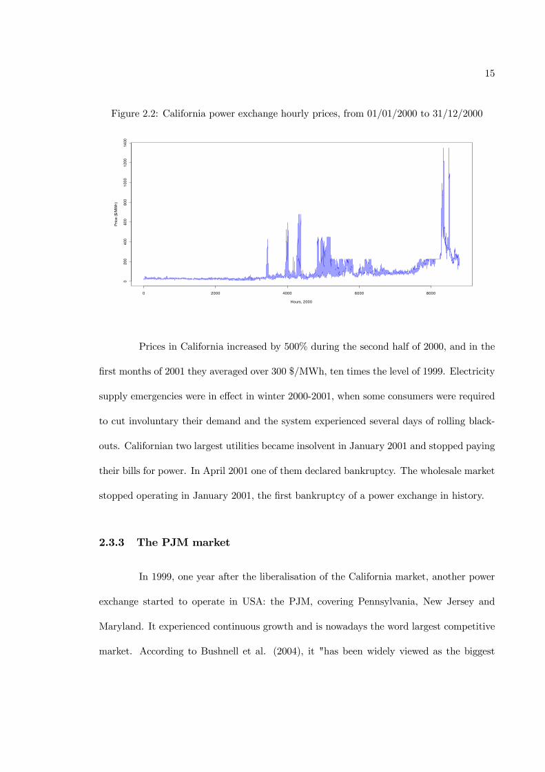
Figure 2.2: California power exchange hourly prices, from 01/01/2000 to 31/12/2000
0 2000 4000 6000 8000
0200
400
60
08
00
100
01
200
14
00
Hours, 2000
Price (
$/M
Wh
)
Prices in California increased by 500% during the second half of 2000, and in the
first months of 2001 they averaged over 300 $/MWh, ten times the level of 1999. Electricity
supply emergencies were in effect in winter 2000-2001, when some consumers were required
to cut involuntary their demand and the system experienced several days of rolling black-
outs. Californian two largest utilities became insolvent in January 2001 and stopped paying
their bills for power. In April 2001 one of them declared bankruptcy. The wholesale market
stopped operating in January 2001, the first bankruptcy of a power exchange in history.
2.3.3 The PJM market
In 1999, one year after the liberalisation of the California market, another power
exchange started to operate in USA: the PJM, covering Pennsylvania, New Jersey and
Maryland. It experienced continuous growth and is nowadays the word largest competitive
market. According to Bushnell et al. (2004), it "has been widely viewed as the biggest

16
success amongst US markets". In the PJM market electricity is bought and sold in two
different markets: (1) a day-ahead one, in which most of the quantity is traded, and a (2)
real time, balancing market which operates at the margin.
PJM consists of approximately 76000 MWh of capacity, including coal, oil, natural
gas, nuclear and hydroelectric. Given its large dimensions, it is divided into different zones.
This means that, when bottlenecks are present in the transmission system, the market splits
into two or more sub-markets, with distinct supply and demand functions. In such cases,
the price in the separated markets may be different. PJM market outcomes will be the
subject of the empirical analysis in section 5.1 and 5.5.
2.3.4 The NordPool
The electricity reform in the Nordic European countries started in 1992, with the
Norwegian Energy Act, which opened the way for the subsequent deregulation. In the
following years Sweden (1996), Finland (1998) and Denmark (2000) joined the market,
called NordPool, in which is traded about 40% of the quantity consumed in those four
countries. There are nowadays over 400 participants in the market, including generators,
retailers, traders, industrial consumers and financial institutions. Furthermore, the Pool
administers an established market of power derivatives.
The NordPool is a market with unique characteristics, because of its high per-
centage of hydropower (55% in total, but almost 100% in Norway). This feature originates
peculiar price dynamics, which have been subject of ad-hoc analyses in the recent years (see
Hjalmarsson 2002, Johnsen et al. 2004, Haldrup and Nielsen 2006a, 2006b). In particular,
price is very sensitive to the atmospheric conditions and, even though in general is lower

17
than in the rest of the European countries, it may rise accordingly to unexpected water
shortages. A well known case it is the “drought in 2002/03, which put the Nordic electricity
market under tremendous pressure” (Stridbaek, 2006), with subsequent increase in price.
The market responded in several ways: exploiting all existing Nordic power plants, increas-
ing imports and also through demand reduction. Interesting the retail contract system
influenced the reactions of small consumers to the increased price. In Sweden, one / two
years contracts were the standard for residential consumers, thus there was no pass-through
of high-prices into more expensive electricity bills. Therefore, no demand reduction was
observable in the residential sector. Norwegian households, on the contrary, had short-term
contracts linked to the spot price, which stimulated a cut in consumes. Nevertheless, the
market recovered from the crisis and now it is widely seen as one of the most successful
cases of liberalisation in the world.
2.3.5 The Italian power exchange
The Italian electricity market is one of the youngest in Europe and in this country
the electric industry is still experiencing major changes. In particular, in 2007-08 it is
expected the liberalisation of the retail market. The Italian power exchange (Ipex) started
operating at the beginning of 2004 and, almost immediately, registered the highest average
prices in Europe. The main reason is the shortage of generating capacity that historically
affects the peninsula, which has to import 15% of its electricity consumes from France,
Switzerland, Austria and Slovenia. Furthermore, the recent increase in the price of natural
gas heavily affected the highly gas-dependent Italian electric sector.
The Ipex is divided into three markets: (1) a day-ahead market (MGP), in which

18
is traded most of the quantity in 24 concurrent auctions, (2) the adjustment market (MA),
which takes place immediately after the MGP closes and where utilities can adjust their
schedules selling and buying electricity, and (3) a balancing market (MSD). As showed in
detail the next section, electricity price is often characterised by a huge volatility. Interest-
ingly, the presence of two day-ahead markets (MGP and MA) pushes most of the variability
in the market closest to the delivery (MA), leaving the market where most of the quantity
is traded (MGP) relatively calm compared to the other European power exchanges.
The Italian electricity market is facing major challenges in the next years, among
others (1) investing in cross-border transmission lines, to facilitate import from other coun-
tries, (2) investing in new generation capacity, (3) encourage divestment of the incumbent
ENEL to reduce its potential market power (CESI, 2005).

19
Chapter 3
Time series analysis of electricity
market outcomes
As illustrated in the previous chapter, the original monopoly structure which has
characterised the electricity sector for more than a century has been replaced in many
countries by deregulated, competitive markets. Furthermore, to facilitate trading in these
new markets, power exchanges have been organised. In these structures electricity is bought
and sold like any other commodity, in both spot and derivative contracts. For this reason,
electric utilities, power producers and marketers are now facing two fundamental sources
of variability and, hence, of risk: quantity and price. As showed in this chapter, their
time series present peculiar characteristics which differ from those of other commodities or
financial assets and, therefore, require modelling strategies specifically dedicated.
Quantity (load) modelling and forecasting was foundamental for the electricity
market management also during regulation. In the short term it was important for ensuring

20
the reliability and security of supply and in the long term for planning and investing in
new generation capacity. Electricity quantity peculiar features and the related short term
forecasting methods are presented in section 3.1.
Before liberalisation, electricity price was regulated by appropriate public com-
mission and its variability was minimal and associated with long term fuels cost variations.
With deregulation, price volatility has skyrocketed, and a 30% average change on daily
basis is common in most markets (Huisman, 2003). For this reason price modelling and
forecasting has become an essential input for energy companies decision making and strate-
gic development in the last decade. Electricity price time series present distinctive features,
which are illustrated in section 3.2. Particular emphasis is placed on the stationarity issue
(section 3.2.4) and on the modelling techniques proposed in literature (section 3.2.5).
3.1 Quantity dynamics
Developing models able to describe and forecast the dynamics of electricity quan-
tity (which it is often indicated with the term “load” in technical papers) has been pursued
since many years before the deregulation process began. Early reviews are the work of
Moghram and Rahman (1989) and the collection of papers in Bunn and Farmer (1985).
Short term load forecasting (in general on hourly or half-hourly basis for a daily or weekly
horizon) is the task in which the most advanced techniques have been developed and im-
plemented. For this reason, and for congruency with the general scope of this thesis, in
this section I will focus only on short-term forecasting methods. For a review of long and
medium term approaches see, among others, Gellings (1996).

21
Accurate short-term forecasts are fundamental for a sensible operation of the elec-
tric system, contributing to an economical efficient and secure electric supply. In Bunn and
Farmer (1985) has been estimated that a 1% increase in the forecasting error would cause an
increase of 10 M pounds in operating costs per year in the UK. In fact, short-term planning
of electricity load allows the determination of which devices shall operate and which shall
not in a given period, in order to achieve the requested production at the fewest cost and
to help scheduling generators maintenance routines. In a liberalised market, accurate load
forecasts also lead to stipulate better contracts (Weron, 2006).
In section 3.1.1 the distinctive features of electricity load dynamics are presented,
with emphasis on the multi-level seasonality and the strong relation with the atmospheric
conditions, particularly temperature. In section 3.1.2 the most recognised short-term mod-
elling and forecasting techniques are illustrated, including time series models, linear regres-
sions and artificial neural networks.
3.1.1 Determinants of quantity dynamics
The strong seasonal component is probably the most evident feature of electricity
load dynamics. Cycles with annual, weekly and daily periodicity characterise every power
sector across the world. The daily cycle encompasses the highest part of variability (see
the periodogram in figure 3.1) and follows the working habits of the population. As showed
in figure 3.2, this cycle can be different from market to market, and may present one
(California) or two (Spain) peaks per day, according to the atmospheric conditions and the
living habits of the population. Night hours present a low demand, which starts increasing
roughly around 6.00-7.00 a.m., when population awakes and the workday begins. In figure

22
Figure 3.1: Periodogram of UK electricity half-hourly load data (1st of january 2004 - 23rdof january 2006)
W E E K LY
0 0.01 0 .02
10
20
D A ILY
A N N U A L12 H O U R S
frequency
W E E K LY
0 0.01 0 .02
10
20
D A ILY
A N N U A L12 H O U R S
W E E K LY
0 0.01 0 .02
10
20
D A ILY
A N N U A L12 H O U R S
0 0.01 0 .02
10
20
D A ILY
A N N U A L12 H O U R S
frequency
3.2, Californian load reaches his peak around 17 p.m., and then decreases gradually until 1
a.m. On the other hand, Spanish load presents two peaks per day, at 13 a.m. and at 10 p.m.
In any case, however, a strong daily cycle is always a fundamental feature of the electricity
load patters. For this reason in wholesale electricity markets electricity is traded on hourly
basis (see section 2.3). Has been even argued that electricity traded in different hours
should be treated as different commodities for modelling purposes (Guthrie and Videbeck,
2002). As showed in the next section, the approach of developing a separate model for each
hour of the day, introduced in Ramanathan et al. (1997), has became rather established in
forecasting demand.
In general, the weekly cycle encompasses a small portion of variance, and it is
originated by the working cycle of the population as well. Sunday and Saturday load
profiles, in fact, are systematically lower than weekdays ones. This feature causes also
a particular steep increasing of electricity generation in the early hours of Monday, and
a steep decreasing in the late Friday. This variation often reflects in prices, which are

23
Figure 3.2: Hourly average load in California in MWh (straigh line, 01/01/1999 -31/12/1999) and Spain (dotted line, 01/01/1998 - 31/12/2003)
5 10 15 20
1800
0200
00
22
00
02
40
00
164
96
17
91
7.2
51
933
8.5
20
75
9.7
52
218
1
particularly unstable in those two weekdays. A ‘weekend effect’ takes also place during
national holidays, when working activities are partially suspended and, hence, electricity
consumption is lower. During those days electricity load forecasting is particularly difficult,
and it is often based on the personal experience of the operators more than on sophisticated
statistical modelling. See, for instance, the peculiar patters of the Italian electricity load
during the Christmas holidays 2004 plotted in figure 3.3.
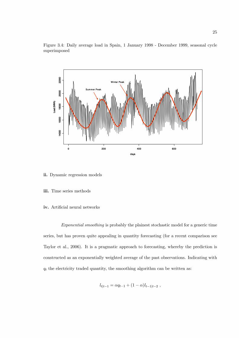
The third seasonal factor, the annual cycle, is connected with the smooth variation
of temperature through the whole year. Electricity, in fact, can be used for both heating
and air-conditioning purposes creating in many markets two peaking seasons (winter and
summer) and two low demand seasons (spring and fall). This behaviour is evident in the
Spanish demand time series presented in figure 3.4. In Italy the heating system is mainly

24
Figure 3.3: Hourly loads in Italy, from 19/12/2004 to 29/12/2004.
0 5 0 1 0 0 1 5 0 2 0 0 2 5 0
25
00
03
00
00
35
00
04
00
00
45
00
05
00
00
h o u rs
Lo
ad
(M
Wh
) Sunday
Christmas
0 5 0 1 0 0 1 5 0 2 0 0 2 5 0
25
00
03
00
00
35
00
04
00
00
45
00
05
00
00
h o u rs
Lo
ad
(M
Wh
) Sunday
Christmas
gas based and demand reaches its peak during the summer. In general, however, electricity
load and atmospheric temperature are characterised by a strong non-linear relationships,
which has been illustrated, among others, in Engle et al. (1986) and Henley and Peirson
(1997). Atmospheric conditions not only originate the yearly cycle, but also explain short-
term changes in electricity consumption. As showed in the next section, these are the most
important exogenous variables when developing short-term load forecasting models.
3.1.2 Short term forecasting models
Short-term load forecasting has been widely studied in literature. Since the 70s,
many techniques have been proposed and compared without the establishment of a clear
winner. However, those studies enhanced sensibly quantity forecasting, achieving a predic-
tions error of 1-2% on hourly basis (Bunn, 2000). Among the most recognised methods one
may cite:
i. Exponential smoothing
25
Figure 3.4: Daily average load in Spain, 1 January 1998 - December 1999, seasonal cyclesuperimposed
0 200 400 600
14000
16000
18000
20000
22000
days
Load (M
Wh)
Summer Peak
W inter Peak
0 200 400 600
14000
16000
18000
20000
22000
days
Load (M
Wh)
Summer Peak
W inter Peak
ii. Dynamic regression models
iii. Time series methods
iv. Artificial neural networks
Exponential smoothing is probably the plainest stochastic model for a generic time
series, but has proven quite appealing in quantity forecasting (for a recent comparison see
Taylor et al., 2006). It is a pragmatic approach to forecasting, whereby the prediction is
constructed as an exponentially weighted average of the past observations. Indicating with
qt the electricity traded quantity, the smoothing algorithm can be written as:
lt|t−1 = αqt−1 + (1− α)lt−1|t−2 ,
26
where lt|t−1 is the smoothed series at time t calculated using the information available at
time t-1. Applying recursively the algorithm, each prediction (i.e. each smoothed value)
is obtained as the weighted average of the current observation and the previous smoothed
value. In addition to simple exponential smoothing, more advanced models based on the
same priciple have been developed, in order to accommodate series with seasonality and
trend. Among others, the Holt-Winter’s method (see, for a discussion, Bowerman and
O’Connell, 1979), which has been implemented in Taylor (2003) and Taylor et al. (2006),
divides the series into three component:
lt = α(qt − St−s) + (1− α)(lt−1 + Tt−1) ,
Tt = β(lt − lt−1) + (1− β)Tt−1 ,
St = γ(qt − lt) + (1− γ)St−s ,
where Tt is the trend, St the seasonality and the prediction can be obtained as an additive
or multiplicative interaction of the three components Tt, St and lt.
The dynamic regression modelling approach assumes that the quantity traded on
the market can be decomposed in a base level (the intercept) and a component which is
linearly dependent to a set of explanatory (exogenous) variables, like atmospheric conditions
(such as temperature and air humidity) or the past values of quantity. Indicating with zt
the explanatory variables, the model can be written as:
qt = b0 + b1zt1 + b2zt2 + ...+ b3zt3 + ut , (3.1)

27
with ut residual component, with mean zero and assumed, in general, Gaussian white
noise. Forecasts based on more than one equation (3.1) can also be developed as, for
instance, it has been done in Papalexopulos and Hesterberg (1990). Their model produces
an initial peak demand forecast based on a set of explanatory variables such as forecasted
temperature, day of the week and lagged temperature and load. This estimate is then
modified using the hourly forecast obtained with another regression through an exponential
smoothing procedure. Hyde and Hodnett (1997) proposed an adaptable regression model for
day-ahead forecast, which identifies weather-insensitive and sensitive demand components.
Linear regression on historical load and weather data is used to estimate the parameters of
the two components. Others relevant contributions in this area are, for instance, Ruzic et
al. (2003) and Ramanathan et al. (1997).
Time series processes are probably one of the most established modelling tech-
niques for electricity demand, when the focus is on the forecasting performances. A review
of this methodology is beyond the scope of this thesis; for an extensive illustration of time
series analysis I suggest to refer to the wide literature available (among others Box and
Jenkins 1970, Hamilton 1994, Dagum 2002). The most popular stochastic processes applied
to electricity demand modelling are the ARIMA and the transfer function models. The
generic ARIMA process, indicating with B the backshift operator, can be written as:
φ(B)∇dqt = θ(B)ut ,
where:
φ(B) = 1− φ1B − φ2B2 − ...− φpB
p is the autoregressive component (AR);

28
θ(B) = 1− θ1B − θ2B2 − ...− θqB
q is the moving average component (MA);
∇qt = qt − qt−1 = (1−B)qt is the differencing operator (I) to achive stationarity1;
ut is the residual component assumed to be white noise and Gaussian.
The parameters φ(B) and θ(B) can be estimated through Maximum Likelihood.
The process can be augmented including also a seasonal component (SARIMA). In this
technique (as in the exponential smoothing) the only information used to forecast electricity
demand is the one embedded in the historical values of the series itself.
The classical ARIMA approach has been applied to electricity load forecasting also
introducing a few changes. For instance, Nowicka-Zagrajek and Weron (2002) include an
hyperbolic specification for the error component, which provides a better fit in the data
they analysed. A non-Gaussian ARIMA model for short-term load forecasting is proposed
also in Huang and Shin (2003). Furthermore, Huang (1997) implements a threshold autore-
gressive model, a class of processes introduced by Tong (1983). The underlying idea is to
fit a non-linear process identifying some thresholds in which the process can be effectively
approximated with linear functions.
Using the transfer function method one can also incorporate exogenous or de-
terministic variables in the model. For instance, atmospheric temperature (temp) can be
included as explanatory variable obtaining:
qt =ω(B)
σ(B)tempt−s + nt , (3.2)
with:1For a primer on stationarity see section 3.2.2.
29
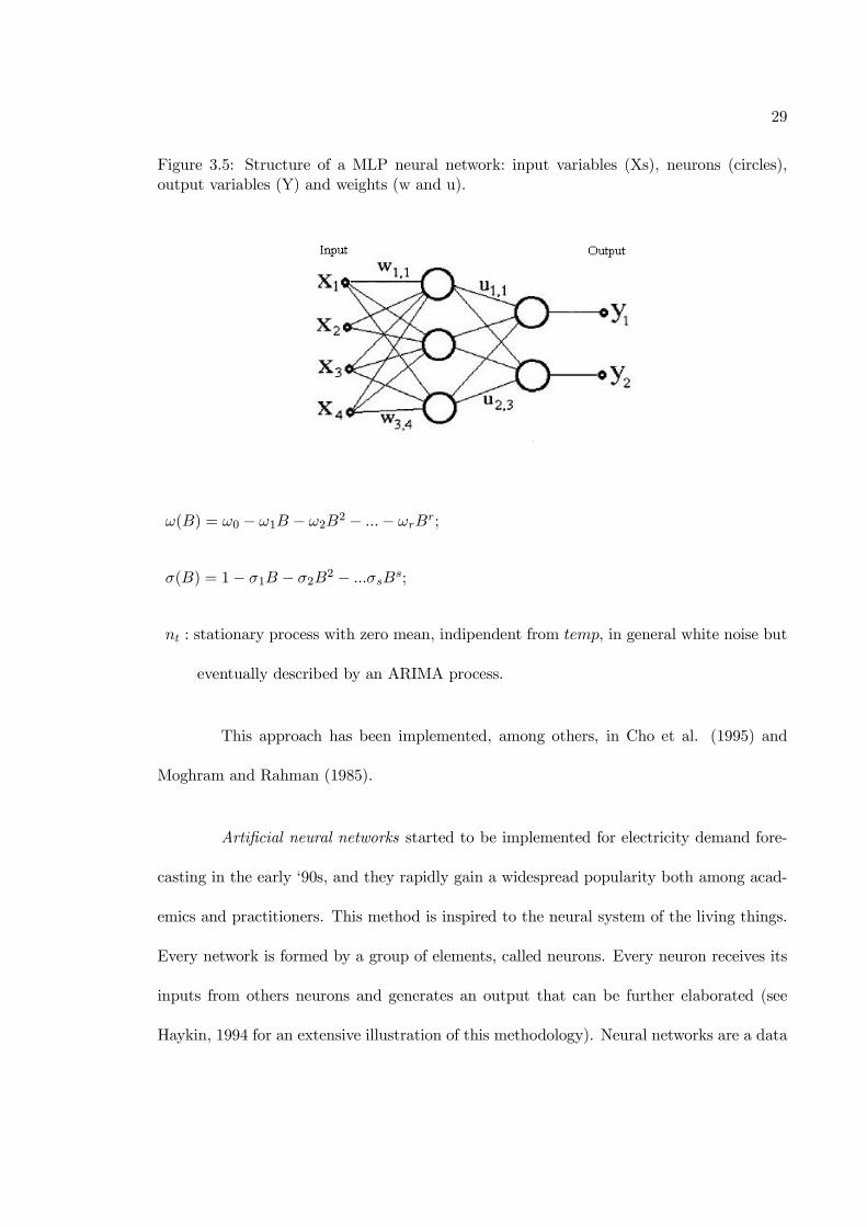
Figure 3.5: Structure of a MLP neural network: input variables (Xs), neurons (circles),output variables (Y) and weights (w and u).
ω(B) = ω0 − ω1B − ω2B2 − ...− ωrBr;
σ(B) = 1− σ1B − σ2B2 − ...σsB
s;
nt : stationary process with zero mean, indipendent from temp, in general white noise but
eventually described by an ARIMA process.
This approach has been implemented, among others, in Cho et al. (1995) and
Moghram and Rahman (1985).
Artificial neural networks started to be implemented for electricity demand fore-
casting in the early ‘90s, and they rapidly gain a widespread popularity both among acad-
emics and practitioners. This method is inspired to the neural system of the living things.
Every network is formed by a group of elements, called neurons. Every neuron receives its
inputs from others neurons and generates an output that can be further elaborated (see
Haykin, 1994 for an extensive illustration of this methodology). Neural networks are a data

30
driven approach since they require that the researcher formulates only a few initial assump-
tions. For this reason they are particularly suited when a lot of data are available, but
the relations among the variables are not clear a priori, as it often happens for electricity
markets outcomes. Furthermore, they are able to approximate every continuous function
with extreme precision (Zhang, 1998). On the other hand, they behave like “black boxes”
and the results often lack of interpretability. Among the first application of neural net-
works to electricity load forecasting is the work by Park et al. (1991), in which a multilayer
perceptron (MLP) network is used to predict peak and total daily load. In figure 3.5 is
represented the structure of a MLP, probably the most established neural network type.
In each neuron, called perceptron, the output is produced applying a non-linear function
(called activity function) to a linear combination of the inputs:
ouj = h(n∑
i=1
wiini − k) , (3.3)
with:
ouj = output signal;
ini = input singnal, which can be initial input or other neurons output;
w = weights;
k = intercept;
h(.) = activity function.
Activity functions can be any functional form, in general non linear (the most
diffused are the sigmoid functions or the hyperbolic tangent). For more information one can
refer to Haykin (1994). MLP are often applied by electric utilities and system operators to
31
produce their official short-term forecasts. Examples are the model proposed in Khontazad
et al. (1998), in which various systems of neural networks are combined to produce optimal
predictions. Other interesting contributions are, for instance, Mohammed et al. (1995),
Asar and McDonald (1994) and Czernichow et al. (1996). For a review see Hippert (2001).
In the last decade, a modelling approach which can be implemented alongside
with any of those methodologies gained growing recognition and diffusion. It consists in
developing a separate model for each of the hour of the day (or half-hours, if this is the
trading unit of the market of interest). This technique was first introduced in Ramanathan
et al. (1997) to compete in a forecasting contest organised by the Puget Sound and Light
System Company (an electric utility company based in New York). This approach is inspired
by the idea that each of the 24 hours presents specific demand characteristics (see section
3.1.1) which are not shared by the other hours of the same day. For instance, the hour 17
(peak) loads of the same week are likely to be much more similar among them that the
hourly loads from hour 11 to 17 of the same day. Given the large amount of data which
is generally available, it is often a sensible option to reduce this heterogeneity defining 24
separate hourly time series from the original one. This choice often proves quite appealing
for forecasting purposes. The model proposed in Ramanathan et al. (1997), for instance,
was simply a dynamic regression using past load and temperature as exogenous regressors.
Nevertheless, it outperformed all the others, much more complex, approaches (for instance,
the time-varying spline of Harvey and Koopman, 1993, and the neural network of Brace et
al., 1993) and the own company experts predictions.

32
After this first contribution, many researchers followed the path indicated by Ra-
manathan et al. (1997), and developing separate models for each hour of the day become
a rather established procedure. It has been used, for instance, with ARIMA and SARIMA
models (Soares and Sousa 2003, Soares and Medeiros 2005) and neural networks (Khon-
tazad et al. 1998). With the birth of liberalised markets, it has also gradually been adopted
for forecasting electricity prices (see, for instance, section 3.2.3 or Karakatsani and Bunn,
2005a). Also the model proposed in chapter 5, even though not developed for forecasting
purposes, is based on this approach.
As showed in section 2.3, in deregulated markets, price and quantity are determined
simultaneously. In this framework, it is significant to analyse the extent in which electricity
demand is affected by the level of price (i.e. if electricity demand is price elastic) or if
price can be helpful to predict future traded quantity (i.e. if electricity quantity is price
responsive). This issue is still debated (see section 4.3) and the model presented in chapter
5 can give, inter alia, important insights on this point. Nevertheless, price has already
been used to improve quantity forecasts in Chen et al. (2001). On the other hand, load is
extensively used to improve price forecasting models, as showed in the next sections.
3.2 Price dynamics
An evident consequence of the electricity markets liberalisation is the increase in
the uncertainty of electricity prices. Spot prices present an extremely high volatility and,
therefore, modelling and forecasting electricity prices in the short term assumes critical
importance for trading, derivative evaluation and risk hedging. Even though forecasting

33
electricity loads has reached a comfortable state of performance (Bunn, 2000), achieving
the same results for prices seem still a long way to go. The task in fact has proven to be
quite challenging to several researchers because of the peculiar characteristics of electricity
prices, which differ dramatically from those of other commodities.The distinctive feature
of electricity is indeed the instantaneous nature of the product. In fact, across the grid,
production and consumption are perfectly synchronised, without any capability of storage.
For this reason inventories cannot be used to arbitrage prices over time and, when demand
is higher than supply, prices can rise more than proportionally such that high and mean-
reverting spikes may occur.
In section 3.2.1 the distinctive features of electricity price are illustrated, section
3.2.2 discuss to the stationarity issue, which is still debated for these time series, whereas
section 3.2.3 reviews the modelling techniques proposed in literature.
3.2.1 Determinants of price dynamics
Not surprisingly, the most important factor affecting price is indeed the demand
dynamic. Since the short term elasticity of demand is very low (see section 4.3) electricity
price profiles appear to be often driven by the load ones. Therefore, electricity price dynamic
inherits some of the distinctive features of demand, such as the multi-level seasonality. As
showed in section 3.1.1, load is characterised by three seasonal cycles: yearly, weekly and
daily. The same behaviour is evident in electricity prices time series, as showed in picture
3.6.
On the other hand, price time series are much more variable than load ones (see
for example the coefficient of variations computed in section 5.1.1). Comparing electricity

34
Figure 3.6: Hourly electricity price in Italy, from 19/12/2004 to 29/12/2004.
0 50 100 150 200 250
50
100
15
0
hour
Pri
ce (
eu
ro /
MW
h)
demand (figure 3.3) and electricity price (figure 3.6) in the same days, in fact, it is clear how
the latter displays a structure which is much more complicated than a simple functional
rescaling of demand. A number of salient features of price dynamics have been analysed in
literature; an extensive illustration can be found in Knittel and Roberts (2005). Among oth-
ers, high volatility with evidence of heteroskedasticity and the presence of sudden jumps are
probably the most noticeable. The first one refers to the presence of low volatility clusters
followed by unstable periods (Escribano et al. 2001) and it is typical of financial assets time
series. This aspect has been widely modeled using Arch and Garch processes (Engle 1982,
Bollerslev 1986) in Goto and Karolyi (2004), Leon and Rubia (2004), Worthington and
Higgs (2004), Knittel and Roberts (2005) and Misiorek et al. (2006), among others. The
second one (spikes) is a peculiar characteristic of electricity prices, which originates from
the impossibility of storing electricity in an economic feasible way. Furthermore, supply
and demand must be balanced continuously to prevent the network from collapsing. Hence,
since shocks cannot be smoothed through inventories, some extremely and unexpected high

35
Figure 3.7: APX (Netherlands) daily price, weekdays, from 01/01/2001 to 31/12/2002
0 100 200 300 400 500
05
01
00
15
02
00
25
0
d ays
Pri
ce
(e
uro
/ M
Wh
)
prices may occur. Those events are evident from the plot in figure 3.7.
There are a number of market structure elements, which help to explain these un-
usual time series characteristics (see section 4.1 for an extensive illustration). The simplest
observation is that with a diversity of plants, of different technologies and fuel efficiencies on
the system, at different levels of demand, different plants will be setting the market-clearing
price. For this reason, an important variable for determining price is the amount of power
plants available to produce in each day (i.e. the available capacity on the system which, in
technical papers, is often called "margin"). As showed in detail section 4.1, if some power
plant bids are missing the aggregate supply curve shifts upwards. This feature is not sub-
stantial when demand is low (i.e. in the baseload) but will affect price considerably in the
peak and it is one of the reasons which may determine the above mentioned spikes.
Furthermore, since the price-setting power plant is often a fuel burning one (par-
ticularly during the peak) electricity price is particularly sensitive to fuel price movements.
36
Figure 3.8: Electricity (euro / MWh) and gas (c / therm) daily price in UK, from 01/01/2004to 14/12/2005
0 100 200 300 400 500
50
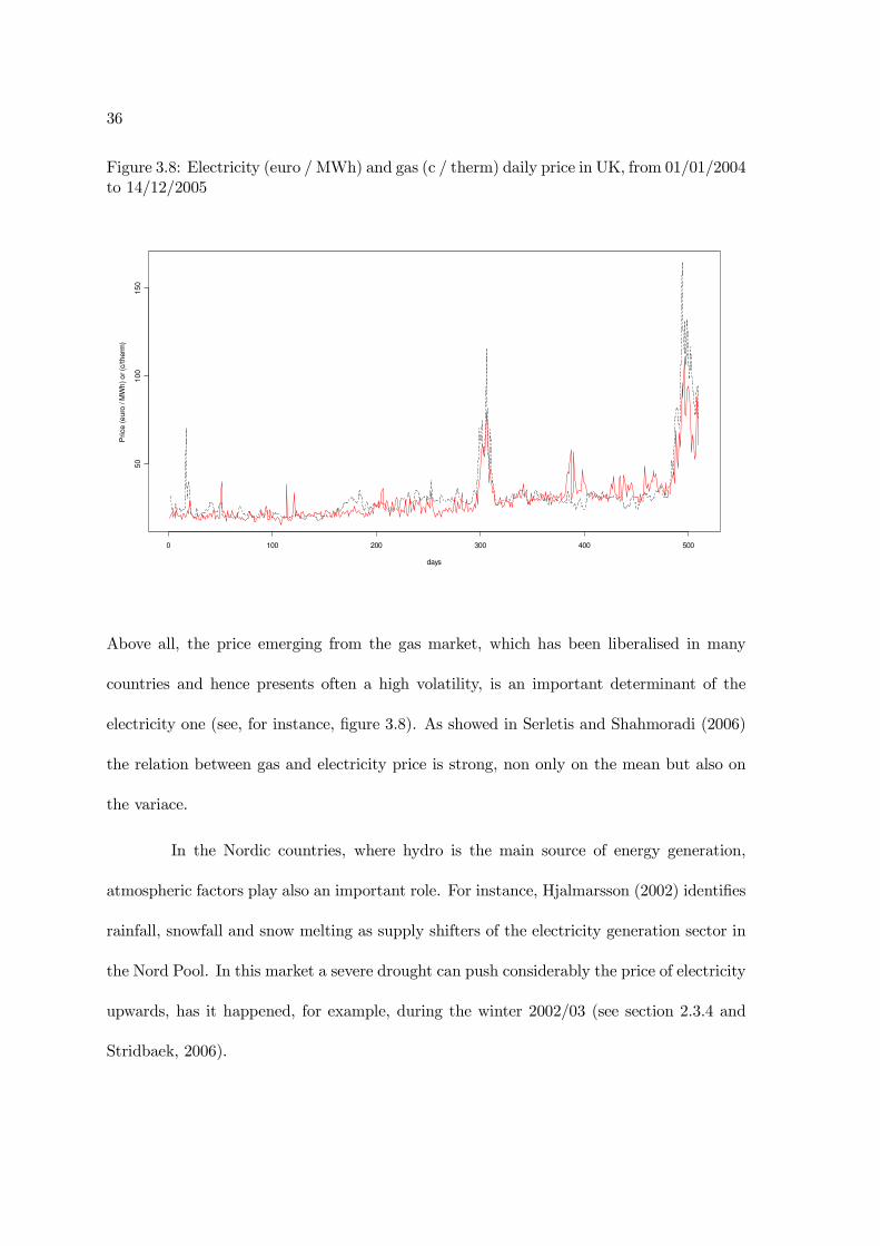
10
01
50
days
Price
(e
uro
/ M
Wh
) o
r (c
/th
erm
)
Above all, the price emerging from the gas market, which has been liberalised in many
countries and hence presents often a high volatility, is an important determinant of the
electricity one (see, for instance, figure 3.8). As showed in Serletis and Shahmoradi (2006)
the relation between gas and electricity price is strong, non only on the mean but also on
the variace.
In the Nordic countries, where hydro is the main source of energy generation,
atmospheric factors play also an important role. For instance, Hjalmarsson (2002) identifies
rainfall, snowfall and snow melting as supply shifters of the electricity generation sector in
the Nord Pool. In this market a severe drought can push considerably the price of electricity
upwards, has it happened, for example, during the winter 2002/03 (see section 2.3.4 and
Stridbaek, 2006).

37
From these findings, it is clear how the complex relations and dynamics which
characterise electricity prices require modelling techniques specifically dedicated. On the
other hand, the birth of liberalised market is a recent phenomenon (see section 2.2) and
the research in this field is still at its first steps. Reaching the performance achieved in
load forecasting is still a long way to go and, according to some researchers (Weron and
Misiorek, 2005) may turn out to be unfeasible. In the next sections the most established
modelling approaches are reviewed and illustrated. Before doing so I will present an issue
which is still an open question in the analysis of electricity markets outcomes time series
and which deserves a careful examination.
3.2.2 The stationarity issue
In the literature and among practitioners there is an overall agreement on the
high frequency electricity prices features that have been presented in the previous section
(seasonality, heteroskedasticity and the presence of sudden jumps). On the contrary, a
crucial element as the stationarity of electricity prices is still an open question. When
discussing time series analysis, investigating the stationarity of the data generating process
is frequently a key aspect of the modelling procedure. As discussed in Dixit and Pindyck
(1994) and Baker, Mayfield and Parsons (1998), for instance, modelling energy price time
series as trend mean-reverting or as random walk may have very different implication for
investment decision and option pricing. This issue has been extensively analysed in Pindyck
(1999) using 120 years of coal, oil and gas prices, showing that non-stationary processes best
describe the data. Also in the context of empirical electricity price modelling, this issue
should be carefully examined, in particular if, as in the model proposed in chapter 5, is

38
given to the estimated parameters an economic interpretation.
A stationary variable is a variable in which mean and variance do not evolve over
time. More formally, indicating with yt the price of electricity at a given hour t, this time
series is defined weakly stationary if its first two moments are constant over time, and so:
E[yt] = µ ,
E[(yt − µ)2] = σ2 ,
E[(yt − µ)(yt−s − µ)] = γ(s) ,
where µ, σ2 and γ(s) are finite and independent of t2. One the basis of classical economet-
ric theory is the fact that the variables involved in the analysis are stationary (Hendry and
Juselius, 2000). Under this condition, classical statistical inference is valid, whilst assuming
this assumption when it doesn’t hold can induce serious statistical mistakes. In fact, mod-
elling non stationary variables as they would be stationary invalidates in the most cases all
the inference procedures leading to a problem known in literature as spurious regression or
“nonsense correlation”, with extremely high correlation often found between variables for
which there is no causal explanation.
In such conditions many statistical inference tools such as the Student’s t, the F
test and the R2 are no longer valid. A complete illustration of this topic is beyond the
purpose of this text, for a detailed and extensive analysis I suggest to refer to the wide
literature available, for example: Granger and Newbold (1974), Hendry (1980), Phillips
(1986) and Hendry and Juselius (2000).
2A variable is defined as “strict stationary” when the entire joint distribution is constant over time.
39
In most paper focused on empirical electricity price modelling (see, for instance,
De Vany and Walls 1999, Atkins and Chen 2002, Goto and Karolyi 2004, Haldrup and
Nielsen 2004, Karakatsani and Bunn 2005a, Knittel and Roberts 2005) the issue of non
stationarity is investigated through standard procedures like the augmented Dickey Fuller
test and the Phillips Perron test. The first one is probably the most popular unit root test
and refers to the work by Dickey and Fuller (1979), in which the null hypothesis that a
series yt contains a unit root (i.e., it is non-stationary) is tested against the alternative of
stationarity through the following regression:
yt = φyt−1 + ut ,
or, the more common:
∆yt = (φ− 1)yt−1 + ut , (3.4)
with ut residual component i.i.d. Gaussian with zero mean. The null hypothesis of non
stationarity (i.e. of unit root) is thus H0:φ = 1 against the alternative H1: φ < 1. In fact,
a process defined as:
yt = yt−1 + ut = y0 +t−1∑
j=0
ut−j
does not converge to a mean value over time, nor presents constant variance since V [yt] =
tσ2u. This process is called random walk, or integrated of order one I(1), since it needs to
be differentiated ones to achieve stationarity. Stationary processes, on the other hand, are
called integrated of order zero, or I(0). The autocorrelation function of processes with a
unit root is very persistent whereas in I(0) processes it decays exponentially to zero.

40
The hypothesis of unit root can be tested using a standard t-ratio test on the
parameter φ. However, under non-stationarity the statistic computed does not follow the
standard Student’s t distribution but rather a Dickey-Fuller distribution, whose critical val-
ues has been computed using Monte Carlo techniques in Dickey and Fuller (1979). Equation
(3.4) shows the simplest form of the test. This has been subsequently modified to account
for an overall process mean different from zero, a trend and an autocorrelated error term.
This leads to the augmented Dickey — Fuller (ADF) test (Dickey et al., 1984 and 1986):
∆yt = φyt−1 +
p∑
i=1
ψi∆yt−1 + µ+ γt+ ut ,
where the number p of lagged differences is chosen long enough to capture autocorrelated
omitted variables that would, otherwise, enter in the error term, and, therefore, to ensure
that ut is approximately white noise. The choice of the appropriate lag-length is crucial
since too few lags may result in over-rejecting the null when it is true (affecting the size of
test), while too many lags may reduce the power of test (and so its ability of rejecting the
null when it is false). For some guidelines and for a further discussion of this topic see, for
example Banerjee et al. (1993).
An alternative approach to take into account serial correlation in the residual com-
ponent is the one proposed by Phillips and Perron (1988). Rather then adding lagged dif-
ferences of the dependent variable in the regression equation they propose a non-parametric
correction of the test statistic which considers the effect that autocorrelated errors have on
the results. This methodology is based on the intuition that in presence of autocorrelated
residuals the variance of the stochastic component in the population:

41
σ2 = limT→∞
E[T−1S2T ] (3.5)
(with ST =∑tj=1 uj) differs from the variance of the residuals in the regression equation:
σ2u = limT→∞
T−1T∑
t=1
E(u2t ) . (3.6)
Indicating with S2u and S2T� consistent estimators of the quantities in equation (3.5) and
equation (3.6) (see Phillips and Perron, 1988 and Banerjee et al., 1993 for a comprehensive
discussion of the topic), the PP Z-statistic for the null hypothesis of φ = 1 (for a process
with mean but no trend) is defined as:
Z(φ) = T (φ− 1)−1
2(S2u − S
2T�)
[
T−2T∑
t=2
(yt−1 − y−1)2
]−1.
The corresponding statistics for a process with zero mean or with mean and trend are
reported in Perron (1988). The critical values are the same as for the DF test.
An alternative approach is to construct a test under the null hypothesis of station-
arity as proposed by Kwiatkowski, Phillips, Schmidt, and Shin (1992) and implemented in
analysis of electricity spot price in Atkins and Chen (2002) and Haldrup and Nielsen (2004).
The KPSS test derivation starts with the model:
yt = βtDt + µt + ut ,
µt = µt−1 + εt εt ∼ i.i.d.(0, σ2ε) ,
where Dt contains the deterministic components (mean, trend or seasonal dummies as
showed in Jin and Phillips, 2002) and ut is I(0) and may be heteroskedastic. The null

42
hypothesis that yt is I(0) is formulated as H0: σ2ε = 0, which implies that µt is a constant.
The KPSS statistics is the Lagrange multiplier (LM) or score statistics for testing σ2ε = 0
against the alternative σ2ε > 0, and it is given by:
KPSS =
(
T−2T∑
t=1
S2t
)
/S2T� ,
where S2t and S2T� defined as previously. Kwiatkowski et al. (1992) showed that under the
null the statistic converges to a function of a standard Brownian motion that depends on
the form of the deterministic terms Dt but not on the coefficient values β. Critical values
for this distribution have been calculated with simulation methods.
One must remember that results from any unit root test must be taken carefully,
in particular when, as in the case of electricity price (or load) time series, the alternative
is a very persistent stationary process. In fact, as showed in Campbell and Perron (1991),
in finite samples “any trend-stationary process can be approximated arbitrary well by a
unit root process (in the sense that the autocovariance structure will be arbitrarily close)”,
and the reverse is also true. For this reason there is a trade off between size and power
in unit root test (Blough, 1992), and there is an high probability of falsely not reject the
null when the true data generating process is a nearly stationary process. Furthermore, in
the case of electricity markets spot prices these results are even weaker, considering that
the strong seasonality and the presence of sudden mean-reverting spikes affect the power
and size of the standard unit root tests (Cavaliere, 2004). The autocorrelation function of
electricity markets outcomes is indeed persistent, and strongly reflects the daily seasonality.
As an example, figure 3.9 plots the autocorrelation function computed using UK half hourly

43
Figure 3.9: Autocorrelation function: UK half-hourly loads, from january 2004 to may 2006
0 200 400 600 800 1000
0.0
0.2
0.4
0.6
0.8
1.0
Lag
AC
F
Autocorrelation
quantity in the years 2004-2006. Autocorrelation is still very high after 1000 lags, and the
daily and weekly seasonal patters are both evident in the graph. Trying to overcome these
issues, Escribano et al. (2002) propose an unit root test studied to account for the presence
of outliers (spikes) and heteroskedastic errors. Through this procedure they refuse the null
hypothesis of unit root for some electricity price series (Argentina, Australia, New Zealand,
Nordpool and Spain).
Nevertheless, the stationarity of electricity price (and quantity) time series cannot
be assumed as a general rule. Stevenson (2002) for instance, identifies a unity root in the
Australian market prices and decides to use the differentiated series to obtain a stationary
mean. The same approach is followed by Contreras et al. (2003) and Conejo et al. (2004)
for California, Spain and PJM interconnection (Pennsylvania, New Jersey and Maryland)
data. Goto and Karolyi (2004) decide to treat USA, Nord Pool and Australian electricity
prices as stationary, even if they stress that the tests they apply (ADF and PP) do not show

44
robust stationarity evidence, in particular for the Nord Pool. Weron et al. (2003) analyse
the stationarity issue in the latter market using the Average Wavelet Coefficient (AWC)
method of Simonsen et al. (1998) finding contrasting results (i.e. they find that using data
with different time frequency leads to different conclusions). Haldrup and Nielsen (2004)
test stationarity via the PP and the KPSS test, refusing the null hypothesis in both cases.
For this reason they argue that neither an I(1) nor an I(0) description of the Nord Pool
time series is appropriate. On this basis they propose a fractionally integrated process: a
process that is on the border between stationarity and non stationarity, presenting both
long memory and mean reversion (for a complete illustration about long memory processes
see, for example, Geweke and Porter-Hudak 1983, Beran 1994, Baille 1996). Atkins and
Chen (2002) reach the same conclusion analysing a different market, and derive an ARFIMA
(autoregressive fractionally integrated) model for Alberta hourly electricity prices. On the
contrary, it must be noticed that in many papers (for example Karakatsani and Bunn
2005a, Knittel and Roberts 2005) non-stationarity is tested, rejected and electricity prices
are treated as a stationary and mean-reverting process.
As illustrated in section 3.2.1 seasonal patterns are one of the most important de-
terminants of electricity price dynamic behaviour. As showed in Maddala and Kim (1998),
strong seasonality can influence the power and the size of the standard unit root tests.
According to the different source of seasonality, it is possible to distinguish between deter-
ministic and stochastic seasonality. The first one can be modeled inserting a deterministic
component in the equation, such as seasonal dummy variables or sinusoids. This kind of
seasonality is perfectly predictable and never changes in shape. The second one is generated

45
by a stochastic process and can vary with time.
As showed in section 3.1.1, the strong seasonal variation of load and prices on
the daily horison inspired the development of empirical approaches based on modelling
separately each hour. This choice is able to rule out all the seasonal variation on the daily
cycle, but leaves in the series the weekly one. The remaining weakly seasonal process can
be written, for example, as:
yt = φ7yt−1 + ut .
In this case if φ7 < 1 the process is stationary and its seasonal mean and variance are
stable over time, otherwise, if φ7 = 1 the process is said to be seasonally integrated or to
have seasonal unit root (Hylleberg at al., 1990). Such processes cannot be captured using
deterministic seasonal dummies since the seasonal components can drift substantially over
time. Stationarity can be achieved using the seasonal differencing operator, as advocated
by Box and Jenkins (1970), and indicated by ∆d = (1−Bd), with d seasonal periodicity.
Rubia (2001) extends to the weekly case the HEGY seasonal unit root test (Hylle-
berg et al., 1990) in order to check the necessity and the validity of the application of
the seasonal differencing operator in the case of electricity demand data modelling. An-
gel and Rubia (2004) use a similar methodology and find evidence of seasonal unit root
in the Spanish electricity daily prices. The HEGY test (Hylleberg et al., 1990) is based
on the factorisation of the weekly differencing polynomial (1 − B7) in (1 − B)S(B), with
S(B) = (1+B+ . . .+B6). Therefore, the null hypothesis of unit root at seasonal frequency
can be expressed in a unit root at zero frequency and three pairs of complex roots at the

46
seasonal frequency k/, with k = 1, 2, 3 and / = 2π/7. Referring to Rubia (2001) for the
technical aspects involved, the test can be derived as:
∆7yt = α+ βt+7∑
j=2
αjDjt +7∑
j=2
γjDjtt+7∑
j=2
πjzj,t−1 +
p∑
r=1
φr∆7yt−r + ut , (3.7)
where each of the regressors zj,t are defined on the seasonal frequencies k/ as follows:
z1,t =7∑
j=1
cos(0j)Bj−1yt = S(B)yt ,
z2k,t =7∑
j=1
cos(kj/)Bj−1yt ,
z2k+1,t = −7∑
j=1
sin(kj/)Bj−1yt .
This specification is the most general, and includes a drift (µ), a linear time trend (β),
deterministic seasonal dummies (Djt) or seasonal drifts (γt) and it is estimated through
Ordinary Least Squares (OLS). As in the ADF test (Dickey and Fuller 1979, Dickey et al.,
1986) a number of lags p of the dependent variable are included in order to achieve zero
autocorrelation.
Compared to other techniques (see for example Dickey et al., 1984) the HEGY
approach has the remarkable feature that one can test for unit roots at some frequencies
without assuming that there are unit roots at some or all of the other frequencies. In fact,
in equation (3.7), each on of the regressors is defined on a specific angular frequency (k/)
by a linear filter that removes all the unit roots from yt except the one associated with the
specific frequency of the regressor. To check for unit root at zero frequency one can test
the null hypothesis of π1 = 0 with an unilateral t statistics, comparing the empirical value

47
with the same critical values reported in Dickey and Fuller (1979). Unit root hypotheses
at the seasonal frequencies k/ (k = 1, 2, 3) imply that both statistics associated with the
same frequencies are zero (π2k = π2k+1 = 0). This can be tested using two sequential
t-statistics or a joint F -statistics that, according to Ghysels et al. (1994), presents better
statistical properties. Critical values for both the approaches, calculated by a Monte Carlo
experiment, are reported in Rubia (2001).
From these findings it can be concluded that stationarity (both at zero and at sea-
sonal frequencies) cannot be considered a general feature of all electricity markets outcomes
time series and, on the contrary, must be considered carefully case-by-case before under-
taking any empirical analysis. Furthermore, there is not yet an acknowledged methodology
to handle (i.e. test) this issue in the electricity markets framework, due to the presence
of many specific aspects (seasonality, heteroskedasticity, mean-reverting spikes) that affect
the standard procedures and create an unique environment for the researcher. In this sit-
uation a preferred strategy would be to consider the process as non-stationary until it is
not verified a strong evidence in the other sense, since doing the opposite is potentially
more harmful from a statistical point of view (Hendry and Jusielius, 2000). The choice is
indeed rather controversial, and must follow economic theory as well as statistical validity.
It can be stated that the preference should depend at least on two key elements: first of
all the structure and the behaviour of the market investigated and second, but not less
important, the time frequency and the time span selected for the analysis. This aspect is
further considered in the modelling approach proposed in chapter 5.

48
3.2.3 Price modelling and forecasting
With the liberalisation of the electric sector, accurate load forecasts are no longer
sufficient for the electric utilities. In order to bid optimally into the power pool and to
efficaciously engage in bilateral contracts, market participants need also sensible price fore-
casts. Furthermore, accurate price modelling is fundamental for derivates evaluation and
risk hedging. This activities are crucial in the context of electricity markets, given the
high volatility which characterise the dynamic of the price of this commodity (see previous
section and, among others, Misiorek and Weron 2006). This task proves quite challenging
since, as showed previously, electricity price displays characteristics which differ completely
from those of other commodities. For instance, a recent issue of Studies in Nonlinear Dy-
namics and Econometrics (2006) has been dedicated to the "nonlinear analysis of electricity
prices". The contributions include regime-switching models (Haldrup and Nielsen 2006, Mi-
siorek et al. 2006, De Jong 2006), wavelets (Stevenson et al., 2006) and spectral analysis
(Hinich and Serletis, 2006).
One of the features that have caught the attention of many modelers is the presence
of sudden spikes (figure 3.7). This characteristic is common in most markets, and it is
connected with the attributes of the commodity electricity. Specifically, there are at least
two factors which may determine those high and mean-reverting prices: the impossibility
of economically storing electricity and the low short-term elasticity of demand. These
two conditions may allow strategic bidding by some of the producers which can result in
producing extremely high prices for very short periods of time (like one or two hours).
This behaviour does not necessarily imply presence of market power and, on the contrary,
49
can even produce beneficial effects on the sector, boosting investment in new generation
capacity, as it is showed in Stridbaek (2006) for the Australian market.
Price spikes have been modelled primarily with jump-diffusion processes, for in-
stance in Deng (2000) and Knittel and Roberts (2005). As showed, among others, in
Hamilton (1994) a jump-diffusion process can be written as a mixture of two normal distri-
butions. Indicating with pt the price of electricity at time t and with λ the probability of
observing a spike, one can write the conditional (to the first observation) likelihood function
that correspond to an AR(1) jump diffusion model as:
L(θ) =T∏
t=2
[(1− λ)N (pt − [α+ φpt−1];σ) + λN (pt − [α+ φpt−1 + µ];σ + δ)] ,
with:
N(.): normal density probability function;
α+ φpt−1: conditional expected value if there is no spike (probability 1− λ);
α+ φpt−1 + µ: conditional expected value if there is a spike event (prob. λ);
δ: change in variance when there is a spike;
θ = [λ, φ, α, σ, δ, µ] parameters that can be estimated, for instance, through maximum
likelihood.
The main problem of this specification is that it does not consider that in the
electricity price dynamics the jump effect dies out rather quickly and does not lead to

50
sustainable high price levels. One may therefore expect that a sudden jump will be shortly
followed by a down-jump. This feature is taken into account in the model proposed by
Huisman and Mahieu (2003). They propose a regime-switching model with three regimes:
(1) normal price, (2) initial jump and (3) post-jump reversion towards the normal level.
Regimes (2) and (3) can last only one period. On the other hand, as pointed out in De
Jong (2006), this approach has the drawback of not allowing for multiple consecutive spikes,
which are sometimes observed in electricity markets. For this reason, building on De Jong
and Huisman (2003) he proposes a model with two indipendent regimes, a ’normal’ mean
reverting regime and a spike regime Poisson process. In this specification, price does not
need to be "pulled down" after a spike simply because the two regimes are indipendent.
The switching probability λ can also be specified as a function of the market
fundamentals, such as load generated on the system and available excess capacity (see
section 4.1 for more information on this), as it has been done in Mount et al. (2006).
They show that this information is crucial to correctly evaluate the switching probability,
and can be used in order to effectively predict the spike component. On this point it is
important to note that producing accurate load and particularly margin day-ahead forecasts
is a necessary input for the analysis.
Load and margin have been used also to develop econometric models in order to
describe price dynamics (Karakatsani and Bunn, 2005a) and price volatility (Karakatsani
and Bunn, 2005b). The model proposed in the first paper, in particular, contains a detailed
non-linear specification of the effects of load on price, including six variables derived from
the original traded quantity (namely linear and quadratic polynomials of demand, demand

51
slope and curvature, demand variation, demand volatility). Since the model is constituted
by a single equation, the implicit assumption is the weak exogeneity (according to Engle
et al. 1983) of the traded quantity. This postulation is still controversial and would imply
a perfectly inelastic demand curve, at least in the short term. This ‘demand elasticity
dilemma’ is fully uncovered in section 4.3, whereas the model presented in chapter 5 is be
used, inter alia, to give new insights on the issue.
Numerous models have been proposed and tested for price forecasting. The main-
stream approach has been to extend the techniques developed for load forecasting (see sec-
tion 3.1.2) to the price time series. A comparison of different methodologies can be found
in Bunn and Karakatsani (2003), Conejo et al. (2005) or in the textbook by Weron (2006).
Surprisingly, the best predictions are in general obtained with rather simple models, such as
ARIMA, ARIMAX (Contreras et al. 2003, Zhou et al. 2006) and transfer function models
(Conejo et al. 2004). The explanatory variables considered are in general load or forecasted
load and margin (excess capacity). This choice implicitly assumes the strong exogeneity
of these variables, allowing the researcher to develop a single equation model without any
loss of relevant information (see Engle et al. 1983). Indeed, it looks that inserting load
and margin in the model equation is likely to improve the forecasting performance of time
series models (see Weron and Misiorek 2005, Conejo et al. 2004, Misiorek et al. 2006, for
some comparisons). Still uncertain is if those performances could be improved even more
relaxing the strong exogeneity assumption and designing multi-equation models for price
and quantity. The model presented in chapter 5 is a first attempt in this direction, even
though its forecasting ability is not tested here.

52
Chapter 4
Electricity wholesale markets
behaviour
In the previous section, wholesale electricity markets outcomes have been analysed
using time series techniques, and some models have been proposed to study their dynamics.
Nevertheless, the scope of this thesis is to develop structural model on time series data,
i.e. models which embed economic theory and therefore may be used not only for short-
run forecasting but also to derive policy relevant conclusions. Following this intent, in this
chapter I will first illustrate the economic and technical grounds which ultimately cause
the peculiar dynamics showed in the previous chapter. With this purpose, section 4.1
presents an analysis of the price formation process in wholesale electricity markets from a
micro-economic point of view, focusing on the structure of the supply function.
Section 4.2 introduces the competition issue in power markets, and in particular
the analysis of market power from the supply side. Given the strategic value of electricity

53
in the production chain, and the transformation of state-owned monopolies into liberalised
markets (see section 2.2), the deregulation process raised particular concern on this point.
This issue has been, without any doubt, one of the most fertile area of research in energy
economics during the last decade. Nevertheless, some questions are still debated. In par-
ticular, a controversial issue, which is also crucially relevant for developing dynamic models
(section 3.2.6) for prices, is the elasticity of the aggregated demand function. As showed
in section 4.3, this is a fundamental point in both theoretical models and in empirical ap-
plications. Nevertheless, few attempts have been made to measure it and its value is still
and unresolved dilemma. The model illustrated in chapter 5 is designed, inter alia, to give
significant insights on this issue.
4.1 The price formation process
As introduced in chapter 2.3, the deregulation process has boosted the introduction
of wholesale markets: physical and financial exchange points, where electricity is traded both
in spot and future contracts . Nevertheless, as showed in the previous chapter, electricity
prices are quite different in their behaviour and properties to those in other financial and
commodity markets and need specifically dedicated modelling techniques. In this chapter I
will illustrate why electricity prices are so different.
The crucial feature of the price formation process in spot markets is the instanta-
neous nature of the product (Bunn, 2003). The physical laws that determine the delivery
of power across a transmission grid require a synchronised and continuous energy balance
between production and consumption, without any capability of storage. Furthermore, end-

54
users treat this product as a service at their convenience. The task of the grid operator,
therefore, is to continuously monitore demand and to call on those generators who have the
technical capability and the capacity to respond quickly to its fluctuations. In figure 3.2 it
was showed the annual range of daily demand profiles for California and Spain. Through
a mixture of good short-term forecasting (section 3.1.2) and scheduling, instantaneous pro-
duction also follows these demand paths. Indeed, the average variation of production on the
daily horizon is quite significant and around the 25%. This variation is even larger if one
takes into account the yearly cycle (figure 3.4). Therefore, it is clear that throughout the
day and throughout the year, a wide variety of plant will be in action and therefore setting
the price at different times. Furthermore, one would expect a diversity of plant on the
system for at least two reasons. The obvious one is obsolescence. The more subtle is, again,
due to the impossibility of storing electricity in an economically sensible way. The most
efficient power plants, with the lowest marginal costs (typically nuclear) operate most of
the time, but during the peak hours some of the high marginal costs power plants (typically
gas and small coal plants) are necessary to balance the increase in demand. These plants
may be operating for only a few hours, and the recovery of their capital cost may have to be
achieved setting high prices. Indeed, if one would like to optimise his stock of power plants,
he would invest is some capital-intensive, low operating cost plants to serve the baseload
and some relatively expensive to run plants, available for the peaks. This is the generation
structure one observes in real power markets, with the consequence that prices are much
higher during demand peaks.
The reason for this diversity of plants can be better illustrated deriving a load
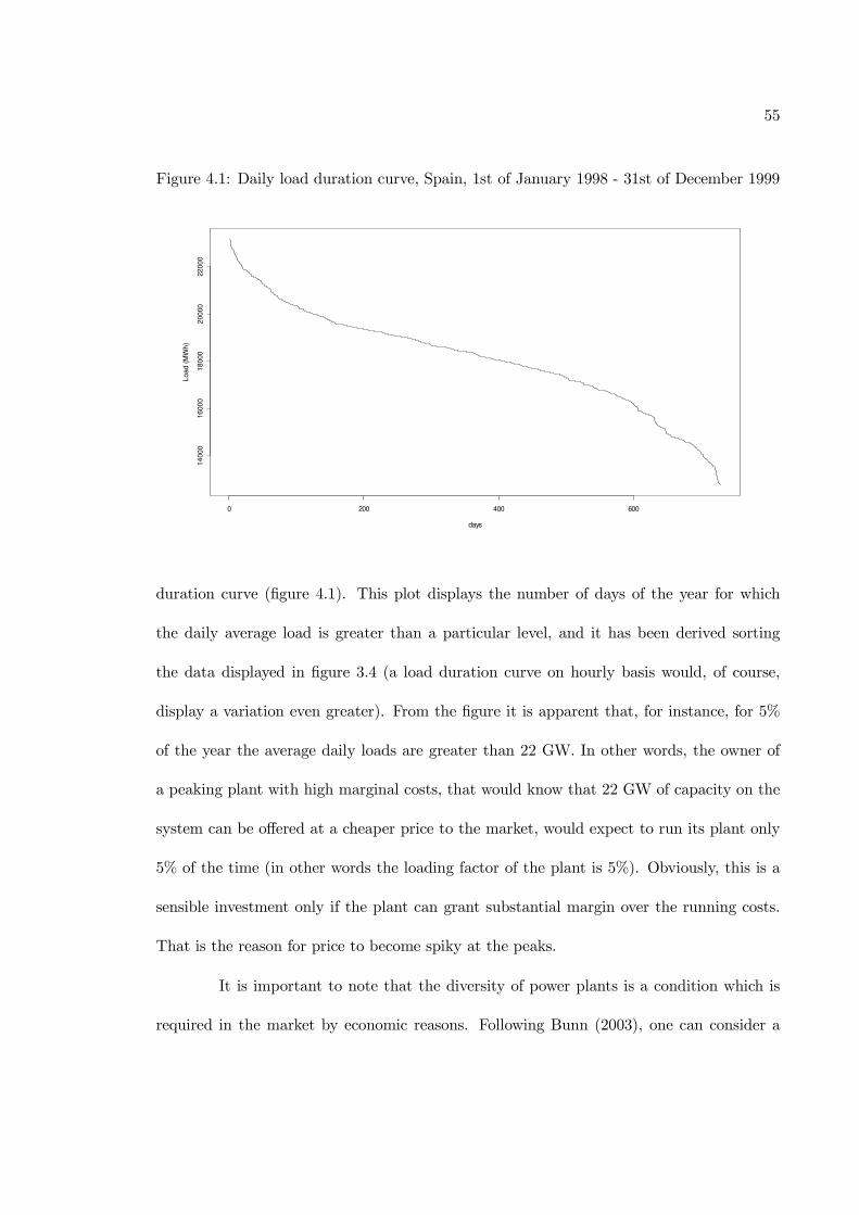
55
Figure 4.1: Daily load duration curve, Spain, 1st of January 1998 - 31st of December 1999
0 200 400 600
14
00
01
60
00
18
000
20
00
022
00
0
days
Lo
ad
(M
Wh
)
duration curve (figure 4.1). This plot displays the number of days of the year for which
the daily average load is greater than a particular level, and it has been derived sorting
the data displayed in figure 3.4 (a load duration curve on hourly basis would, of course,
display a variation even greater). From the figure it is apparent that, for instance, for 5%
of the year the average daily loads are greater than 22 GW. In other words, the owner of
a peaking plant with high marginal costs, that would know that 22 GW of capacity on the
system can be offered at a cheaper price to the market, would expect to run its plant only
5% of the time (in other words the loading factor of the plant is 5%). Obviously, this is a
sensible investment only if the plant can grant substantial margin over the running costs.
That is the reason for price to become spiky at the peaks.
It is important to note that the diversity of power plants is a condition which is
required in the market by economic reasons. Following Bunn (2003), one can consider a

56
Investment cost p.y. Marginal Production Cost(e/KW) (e/MWh)
Nuclear 90 2Coal 45 10Gas 20 30
Table 4.1: Technology choice in a simple example
simple example with a set of three technologies with different investment (fixed) cost and
operating (marginal) cost. Assuming that the cost of the investment can be spread over
the life of the power plant, one can calculate the investment costs per year as reported in
table 4.1 and derive the break-even function showed in figure 4.2. According to this simple
structure, the nuclear plant needs to run more than 5600 hours per year to be a better
investment than the coal one, and only more than 2500 to be a better investment than a
gas fired power plant.
In order to find the optimal mix of technology for the Spanish power market, one
can just project the break-even analysis onto the load duration curve in figure 4.1. In this
situation, nuclear would provide baseload, with 17500 MWh installed, coal power plants
would have a capacity of 3000 MWh, and peak load would be covered by gas, for a total
capacity of 3500 MWh1. Of course a real power system would require some more capacity
to secure electricity supply in case of extraordinary peaks of demand or temporary plant
outages. From this example one could also derive the supply function offered on the power
market, i.e. the stack of marginal costs for each capacity. “The shape of the supply function
is one of the most important fundamentals in understanding the behaviour of electricity
1For ease of illustration the optimal installed capacity is calculated here using the daily load durationcurve. A proper analysis would require at least an hourly load duration curve, which is in general muchsteeper. In this case the optimal installed capacity for gas and coal would increase, whereas there would bea decrease in the nuclear one.

57
Figure 4.2: Break-even analysis, straight line = least cost solution
prices” (Bunn, 2003). It is typically a step function, which displays the marginal cost of
producing electricity at a particular level of demand2.
Figure 4.3 plots the marginal cost supply function for the example introduced in
table 4.1. Taking into account the high demand variation during the day, the resulting
price volatility would be even higher, considering the amplification effect that the steeply-
increasing supply function produces (see also the examples in section 3.2 and the empirical
analysis in section 5.1.1). In a real system the supply function would present many more
steps (for instance, many different technologies, with different investment and marginal costs
can be available to produce electricity from gas) and, as a result, it would appear much
smoother, but the key features remain the same ones. There are also technical reasons
that justify a diversity of plants on the system and, as a consequence, of marginal costs.
2This definition assumes perfect competition. The issue of imperfect competition and market power fromthe supply side is analysed in the next chapter.

58
Figure 4.3: Marginal cost supply function for the optimisation example in table 4.1
Capacity (GW)10 20
Co
st(e
uro
\MW
h)
15
30
Nuclear
Coal
Gas
Capacity (GW)10 20
Co
st(e
uro
\MW
h)
15
30
Nuclear
Coal
Gas
In fact, some technologies can respond to changes in demand quicker than others. For
instance nuclear plants need to run at a constant pace. Small gas and coal plants can, on
the contrary, follow the load path more rapidly.
Another fundamental aspect to consider when analysing electricity market out-
comes is the excess capacity available on the system, i.e. the amount of power plants
willing to produce (and bidding into the market) in a specific hour or day. This is often
indicated with the term "margin" and can vary a lot during the year, according to the
maintenance schedule of power plants but also to the strategic interaction of the suppliers
(see next chapter, Borenstein and Bushnell, 1999 and Borenstein et al. 1999). The impact
of the variation of margin on prices is substantial. As showed in figure 5.3, for instance, the
same quantity produced can be mapped into very different clearing prices on the market.
In fact, as showed in figure 4.4, when some power plant bids are missing (represented by the

59
Figure 4.4: Shift in the supply curve when some plants (shaded area) are not available toproduce, with two different demand curves (baseload and peak)
S2 S1
p
q
Dpeak
Dbase
S2 S1
p
q
Dpeak
Dbase
S2 S1
p
q
Dpeak
Dbase
shaded area) the overall supply curve shifts upwards. This effect is, in general, particularly
relevant in peak hours.
Although a substantial amount of electricity is generated from hydro and nuclear
sources in various part of the world, the dominant production process is still thermal con-
version of fossil fuels, such as gas, oil and coal. This is a very capital intensive process, with
surprisingly few workers actually being employed at the power plant (Bunn, 2003). Thus,
as electricity is often traded on exchanges one day (or even one hour) before the delivery
(see section 2.3), the variable cost of power generation is essentially the fuel cost. With the
liberalisation of the gas sector, and the introduction of trading hubs where this commodity
is traded on daily basis, also gas volatility has increased rapidly. Recent events have showed
how gas price in Europe may be sensible to external factors or simply how it may increase
in a very cold winter, when the supply-demand balance is tight. Since an important part

60
of the electricity supply stack is provided by gas-burning power plants, these variations are
likely to be passed-through in the power sector. As showed in figure 3.8, the gas-electricity
price relation is already strong in the UK market, probably the most mature energy market
in Europe.
It is important to note that differences may arise between the marginal cost supply
function and the actual market supply function, given by the aggregation of the supply bids
offered into the market. Strategic interactions and market power are still present in some
markets across the world, and strong regulatory intervention is sometimes necessary to
keep prices close to competitive levels. The issue of market power has indeed raised a great
interest in the context of electricity markets, particularly because the deregulation process
is still at a young stage in many countries (among others also in Italy) and because of the
strategic importance of the commodity electricity. The issue of generators market power is
the focus of the next section.
4.2 Competition and market power
Until recently, electricity was a monopoly in most countries, often owned by the
government, and, if not, highly regulated. During the 90s, ownership has generally become
private rather than public and the whole sector has been interested by the process of lib-
eralisation (see section 2.2). The generation sector, in particular, has been progressively
deregulated and public-owned companies split in a sufficient number of private firms in
order to ensure competition. The main reason for the broad diffusion of this process is
that policy makers believed that liberalisation would impose market discipline, encouraging

61
market entry and thus lead to lower production costs, more efficient investments and lower
consumer prices.
Unfortunately “the promises of restructuring have not always been realised” (Mansur,
2003). In liberalised markets, price variation has skyrocketed: as illustrated in section 3 a
30% variation on the daily horizon is the average in many markets. As showed in the previ-
ous section, this huge price volatility is not necessary a symptom of market malfunctioning.
On the contrary, it is often present even in the most competive markets and is connected
with the inner structure of the electric system. In particular it is due to (1) the impossibil-
ity of storing electricity in a economically feasible way, (2) the continuous demand-supply
balance, (3) the presence of different production technologies. Nevertheless, the potential to
exercise market power is often present from the supply side. Initiatives to mitigate market
power and pursue market efficiency are indeed among the most delicate and debated issues
concerning the deregulation process in many countries. This issue is particularly interesting
because the exploitation of market power can significantly erode the consumer benefits that
would be expected to result from the transition from regulated to competitive markets for
electricity generation. The importance of electricity for the whole economy, therefore, moti-
vated the huge amount of research dedicated to this topic in the last decade. As illustrated
in the next pages, the novel modelling approach proposed in chapter 5 can give important
insight also in this branch of literature.
As introduced in section 2.3.2, the Californian market collapse is probably the
most exposed case of market failure. Beginning in summer 2000, the electricity price in
California began to rise, reaching peaks of 800 $/MWh, threatening the financial stability

62
of the state and ultimately leading to the closure of the Californian Power Exchange. The
extent to which this huge increase could be attributed to market fundamentals (such as
growing production costs or scarcity of generation capacity) or to market power is a crucial
issue in order to design better policies and avoid the replication of such cases. On this point,
Borenstein et al. (2002) and Wolak (2003), analysing detailed input and production costs,
find that at least 50% of the electricity prices in California could be attributed to market
power.
Unfortunately, despite its importance for regulatory purposes (for instance to eval-
uate merging or acquisitions proposals), evaluating market power in electricity markets ex-
ante it is not an easy task. In fact, the general concentration measures (like the Henfindahl-
Hirschman index3) implemented in classical industrial economics and traditional measures
of price-costs mark-up (for instance the Lerner index4) may be inappropriate in the elec-
tricity market context (Borenstein et al. 1999, Bower 2004). Indeed, Stoft (2002) argues
against applying the HHI to the electricity industry because it ignores some key factors
that are crucial in this context: (1) demand elasticity, (2) style of competition, (3) forward
contracting, (4) vertical integration of firms, (5) geographical structure. Furthermore, as
noted in Borenstein et al. (2002) and Fabra and Toro (2005), given the non-storability of
electricity, market power can exhibit huge inter-temporal variations.
The main techniques proposed to measure the potential for suppliers to exercise
market power in electricity markets can be divided into three main approaches (Knittel
and Roberts, 2005). The first one relays on simulating through a game-theoretical model
3The HHI is defined as: HHI =
n∑
i=1
(si)2, with si market share of the firm i.
4The Lerner index is the typical measure of price - costs markups and it is defined as: (Pt −mct)/Pt.

63
the strategic behaviour of the firms and compare the outcomes with perfectly competitive
prices. The most diffuse models have been Cournot oligopoly (Andersson and Bergman
1995, Borenstein and Bushnell 1999, Borenstein et al. 1999, Lise et al. 2003) and supply
function equilibrium model (Green and Newbury 1992, Green 1996, Baldik et al. 2004).
In both approaches, the price is determined by the intersection between the (simulated)
supply and the demand curves. As showed in the chapter 4.3, specifying the demand curve
in electricity markets is not an easy task, due to the low short-run elasticity. Indeed, often
the results of these analyses are presented under different assumption for the price elasticity
of demand.
A second, more direct, approach is to compare hourly engineering marginal costs
with actual market clearing prices. Wolfram (1999), for instance, compares market prices to
marginal costs for the restructured UK market finding that prices, even though higher than
in a perfect competitive regime, are lower than implied by game theoretical models. Possible
explanations are that firms are facing regulatory constraints and the threat of entry. Other
contributions are Borenstein et al. (2002) and Joskow and Kahn (2002), where California
electricity market prices are compared to marginal costs. Both papers find that mark-ups
over marginal cost increased during the summer 2000 crisis period. Again, these analyses
often rely on assumptions regarding the elasticity of demand to price. Furthermore, as
pointed out in Mansur (2003), in these approaches it is important to consider that electricity
generating units often are subject to production constraints. After taking into account cost
non-convexities (such as power plants start up costs) he shows that PJM prices in the years
1998-99 were, on average, only 3% above perfectly competitive levels (and not 12,5% higher

64
as one would conclude ignoring production constraints).
The third methodology studies the dynamic interactions of agents by simulating
market behaviour at a microscopic instead of at an aggregated market level. These agent-
based models allow for heterogeneous utility functions, non-linear trading rules, learning
modes and detailed representation of the market environment. They often focus on agent
interactions after a regulatory intervention to the market, such as the introduction of new
trading arrangements (Bower and Bunn 2001, Bunn and Oliveira 2002) or CO2-emission
trading and the intensified application of renewable energy sources (Veit et al., 2004). In
this ex-ante framework, the models derive acting recommendations for market participants
as well as political and regulatory authorities. Nevertheless, the parameter validation and
the results’ sensitivity to them are two substantial sources of complexity.
There have also been a few studies implementing econometric approaches to es-
timate, on time series data, the actual level of market power. Hjalmarsson (2000), for
instance, extends to the dynamic case the static Bresnahan-Lau (Bresnahan 1982, Lau
1982) model for the identification of market power. This method leads to estimate a pa-
rameter, which varies between 0 (perfect competition) and 1 (monopoly) and encompasses
how far the actual price is from a perfectly competitive situation. As showed in detail
in the next section, also this approach requires rather subtle assumptions on the shape of
the demand curve. According to this study, the hypothesis of no market power for the
Nord Pool (years 1996-1999) cannot be rejected at any reasonable significance level. On the
other hand, Fabra and Toro (2005) find substantial evidence of time-varying market power
in the Spanish power sector. Accounting for changes in demand and cost conditions (which

65
reflect changes in input costs, capacity availability and hydro power) they show that the
time-series of prices is characterised by two significantly different levels. They explain these
findings with the possible collusive behaviour of the two Spanish market leaders: Endesa
and Iberdrola.
As illustrated, the ex-ante assessment of potential for market power and the actual
measure of market power on market outcomes have been subject to extensive research which
reflects the crucial importance of these issues on the policy makers agenda. Nevertheless,
the results of most of these studies are sensitive to some of the assumptions, particularly
regarding the shape of the demand curve. In the next section, the “elasticity dilemma” which
characterise the electricity demand function is fully illustrated. This section is particularly
significant since the model proposed in chapter 5 is designed to estimate, inter alia, this
parameter, using wholesale markets outcomes time series.
4.3 The demand elasticity dilemma
The elasticity of demand to price is a subtle issue in the research on electricity
markets. Electricity is produced as a commodity, but it is consumed as a service and often
end-use consumers do not have incentives to change their consumption patterns according
to the short-term variations of price, because not directly exposed to it. On the other
hand, recent empirical research (Callaway and Weale, 2005) showed that large industrial
consumers can indeed temporarily reduce production or switch to their own back up gen-
erators (in both case reducing the overall demand on the market) if electricity prices are
perceived as too high.

66
As pointed out in Borenstein (2004): “electricity demand elasticities are subject to
a nearly endless contention”. Nevertheless, investigating this issue is extremely important
in the context of electricity markets. In fact, it is a fundamental information for developing
theoretical models to address, for instance, market power potentials (section 4.2) and also
for designing accurate statistical models for prices (section 3.2.3). Furthermore, demand
responsiveness to high prices has been proposed as an effective way to mitigate market
power (Borenstein and Bushnell 1999, Borenstein et al. 2002b, Borenstein 2004).
As showed in chapter 3.2, many high frequency empirical models of prices have
established relationships with various market fundamentals (i.e. the quantity traded on the
market, the available capacity, the fuel prices) to develop conditional models in a single
equation framework (see Karakatsani and Bunn 2005a, 2005b, Weron and Misiorek 2005,
Mount et al., 2006). Doing so, the quantity traded on the market has been explicitly
considered as fixed (i.e. exogenous), assuming a perfectly inelastic demand curve, at least
in the short run for high frequency hourly analysis.
For instance, in Karakatsani and Bunn (2005a), high-frequency price dynamics
are analysed as a process conditioned to some explanatory variables, among others demand
and excess capacity available on the system. The model is used to asses if wholesale British
NETA prices were cost reflective during the low prices period 2001-2002. Hence, a structural
meaning is given to the parameters of the model. The validity of this inference strongly
relies on the assumption of a non-elastic demand curve, as the two Authors acknowledge
declaring that: “such regression would be invalid, if demand would not be exogenous”. On
the same assumption are founded the models proposed in Karakatsani and Bunn (2005b)

67
in order to analyse electricity price volatility. They found that including covariates in
the variance specification is able to capture the ‘Arch effect’ commonly observed in price
dynamics (see, for instance, Duffie et al. 1998, Knittel and Roberts 2005 and chapter 3.2.1)
and that a relevant source of risk in electricity price dynamics is connected with demand
movements. Again, they note, these results are valid only if “demand is perceived as an
exogenous variable, because of the negligible elasticity in the short term”. In another study
on volatility, Goto and Karoly (2004) find significant Garch effect in the dynamics of PJM,
NordPool and Austrialian market. Including in the equation of the conditional mean the
quantity traded on the market, they implicitly assume an inelastic demand.
Quantity is included as a deterministic regressor also in the forecasting models
proposed in Contreras et al. (2003), Conejo et al. (2004), Rodriguez and Anders (2004),
Mount et al. (2006), Weron and Misiorek (2005). In these contributions, the performance
of various forecasting methods is compared in performing short term predictions of dif-
ferent power market price series (for instance PJM, Spain, California and Ontario). Not
surprisingly, the information included in the quantity time series proves to be fundamental
in order to achieve adequate performances. Indeed, according to these studies, the most
promising results seems to be the one achieved applying time series techniques such as trans-
fer function methods, ARIMAX and dynamic regression models (section 3.2). These single
equation approaches are efficient for forecasting only if the variables on which the equa-
tion is conditioned (in this case quantity and other market fundamentals) are, according to
the terminology introduced in Engle et al. (1983), strongly exogenous. This assumption
is violated if the demand function is not perfectly inelastic, i.e. it is influenced by price

68
Article Market Demand Elasticity
Borenstein et al. (1999) California from 0.1 to 0.4Borenstein and Bushnell (1999) California from 0.1 to 1.0Borenstein et al. (2002) California zeroGreen and Newbury (1992) United Kingdom from 0.1 to 0.5Green (1996) United Kingdom 0.25Hjalmarsson (2002) NordPool elasticJohnsen et al. (2004) NordPool elasticLise et al. (2004) Germany 0.4Mansur (2003) PJM zeroWolfram (1999) United Kingdom 0.17
Table 4.2: Assumed demand elasticities in articles analysing market power and strategicinteraction of firms in electricity markets
dynamics.
In contrast with those contributions, as showed in section 4.2, often an elastic
demand has been assumed in order to analyse the firms strategic interactions and their
implications for price and social welfare (in particular measuring the extent of market
power). Nevertheless, as showed in table 4.2, there is not an overall agreement regarding
the value of this parameter. Furthermore, demand elasticity is almost always a crucial
factor and the outcomes of these models are often presented under different assumption
regarding its value. For instance, Borenstein et al. (1999) consider the amount of potential
market power in the Californian electricity market developing measures which differ from
the commonly implemented concentration indexes (like the HHI). Simulating the strategic
behaviour of firms as a Cournot oligopoly they found that demand elasticity is a crucial
parameter in the electricity price formation process, and that the equilibrium price is much
higher when the assumed demand elasticity is lower (they compare a range of values from
0.1 to 0.4). These results are confirmed by the analysis of the restructured Californian
electricity market in Borenstein and Bushnell (1999). They show how one of the most

69
important factors in determining the extent of market power is indeed the elasticity of the
aggregated demand.
Market power is also analysed in Green and Newbury (1992) using a supply func-
tion equilibrium model. Assuming different elasticities of demand (from 0.1 to 0.5) they
found that the duopoly implemented during the first years of deregulation in Britain was
leaving considerable market power to the two incumbents. An examination of possible
policies devoted to address this issue is presented in Green (1996). Using a linear supply
function model (with demand elasticity equal to 0.25), the Author finds that the regula-
tor chosen policy (partial divestiture), would lead to a substantial reduction in deadweight
losses.
Wolfram (1999) examines electricity prices in the British market, empirically es-
timating price-costs markups to measure the presence of market power from the supply
side and estimating a Lerner index of 0.24. However, much of the Lerner index could be
explained by the low elasticity of demand (assumed equal to 0.17) and, after controlling for
this factor5 the average adjusted Lerner index is around 0.05. The results imply that prices,
even though higher than marginal costs, where not as high as implied by some theoretical
economic models (like, for instance, the ones proposed in Borenstein and Bushnell, 1999 and
in Green and Newbury, 1992). Possible explanations are that firms are facing regulatory
constraints and the threat of entry.
Also in the econometric study of Hjalmarsson (2000), based on a dynamic Bresnahan-
5The elasticity adjusted Lerner index controls for cross-sectional or time series deviations between pricesand marginal costs driven by differences in the elasticity of demand. It is defined as (Pt −mct)ηt/Pt, whereηt is the elasticity of demand at time t. As a convenient benchmark, the elasticity adjusted Lerner indexfor a symmetric Cournot game with N firms is 1/N. Therefore, Wolfram (1999) results suggest the marketis acting as if there are 20 symmetric firms, whereas there were three major firms, one of which dominatedthe market with 52% of capacity.

70
Lau (Bresnahan 1982, Lau 1982) model for the identification of market power, the shape
of the demand curve plays a fundamental role. In this framework, in order to identify the
market power parameter, not only an elastic demand is required but also variables able to
rotate the demand curve (i.e. alter the elasticity) have to be included in the model. With
this purpose Hjalmarsson (2002) considers the interactions among price and the demand
curve shifters (like the atmospheric conditions) and finds no significant presence of mar-
ket power in the NordPool. This result is not supported by the analysis of Johnsen et al.
(2004), which evidence that Nordic market prices are higher when demand in less elastic.
Also according to Borenstein et al. (1999) when demand is less elastic, the possibility to
exercise market power from the supply side is higher. Hence, Johnsen et al. (2004) are
able to identify price markups comparing the market prices in different periods, specifically
when marginal costs are the same and demand elasticity varies. They evidence that some
firms have incentives to withhold capacity when transmission constraints bind and hence
increase the price. Lise et al. (2003) address the impact on the environment of the elec-
tricity liberalisation process in Germany. This study, based on a large simulation model in
which demand elasticity is assumed constant and equal to 0.4, shows that, when firms act
strategically, the environment is better of at the cost of higher electricity prices.
Even though in most paper belonging to this branch of the literature demand is
assumed elastic, there are also notable exceptions. For instance, Borenstein et al. (2002)
analyse the presence of market inefficiencies in the Californian restructured electricity mar-
ket assuming a short term inelastic demand. On the same assumption is founded also the
empirical study on market inefficiencies of the PJM market of Mansur (2003). The paper,

71
based on a detailed description of the cost faced by the producers in this market, finds a
rather competitive environment. Some of the equations of the econometric set up, in order
to maintain structural meaning, require the assumption of a “completely inelastic demand”.
Despite the clear importance of this issue, few attempts have been made to directly
measure the value of electricity demand elasticity. Some contributions on demand response
to price have focused upon micro survey data, at the company or individual level, (see
Patrick and Wolak, 2001, Callaway and Weale, 2005). They found that day-ahead demand
elasticity estimates vary substantially by time-of-day, industry, and firms within industries;
with sample mean averages ranging from essentially zero to 0.86 in absolute value. Despite
clearly giving behavioural insights, these do not help directly in specifying elasticities for
the spot and forward trading markets. In contrast, in the next chapter, I seek to addresses
this question from the perspective of publicly-available, wholesale day-ahead market data,
specifying a dynamic econometric model that encompasses the short-term interactions of
electricity price and quantity. This approach allows to directly estimate on time-series
data the value of the elasticity of the aggregated demand, and understand in a dynamic
framework how quantity reacts to price changes.

72
Chapter 5
Structural analysis of
high-frequency electricity demand
and supply interactions
In the previous sections has been illustrated how the assumptions on electricity
demand elasticity have been fundamental to at least two lines of research on energy markets.
At an initial prospect, unfortunately, these assumptions may appear difficult to conciliate.
In fact, developers of dynamic, stochastic models devoted to describe and forecast market
price have often assumed an inelastic demand. On the contrary, in economic models, used,
for instance, to measure market efficiency or to identify the presence of market power,
demand elasticity is often set as different from zero and its value is almost always crucial
for the analysis. Nevertheless, few attempts have been made to empirically measure this
parameter and no one at all using high-frequency wholesale market data. Therefore, this

73
chapter presents a model that allows to identify and empirically estimate the demand and
the supply curves in electricity markets. It can be used, inter alia, to give valuable insights
on the demand elasticity dilemma, directly estimating this parameter.
The proposed approach is novel, since it is based on high-frequency, public-available,
wholesale day-ahead market data. I also advocate that simplifying the complex dynamic
response of electricity demand to price into one unique elasticity parameter can lead to
misleading conclusions. In the model proposed here, I identify three different ways in which
demand may react to a change in price: instantaneously, in terms of an econometrically
estimated equilibrium and through an error-correction mechanism. Furthermore, I consider
the possibility of asymmetries in the demand response, i.e. demand may react differently
to an increase or to a decrease in prices. This feature is consistent with the intuition that,
in the short run, large industrial consumers may shut down machineries or switch to their
own back-up generators if the electricity price is too high, but may not, under normal cir-
cumstances, alter their production patterns substantially if price is lower than expected.
The econometric model is specified in a dynamic, simultaneous equation, error-correction
form and presents both statistical soundness and economic foundation. The first one is se-
cured because the approach followed in this work is inspired by the methodology advocated
in Hendry and Mizon (1993), Johansen and Juselius (1994), Hendry (1995) and Johansen
(1996). In other words data are initially analysed developing a well-defined statistical model,
and then a downward testing procedure is implemented, in order to derive the structural
specification. The economic grounds are preserved since the restrictions are inspired by a
general theoretical economic model.

74
This chapter is organised as follows: in section 5.1 a preliminary data analysis
is presented, with particular focus on the hypothesis of stationarity which, as showed in
section 3.2.2, in the context of electricity markets is still debated and may rise subtle issues
of specification. In this analysis, for instance, stationarity is not supported by empiri-
cal evidence and the variables are modelled as I(1). Section 5.2 illustrates a theoretical
economic model describing the price-formation process in wholesale electricity market (see
section 4.1), where the aggregated supply and demand curves are approximated with con-
tinuous functions. Thereafter, the model is translated into an empirically feasible, linear
specification. In section 5.3 the statistical methodology devoted to the analysis of I(1)
variables is briefly illustrated. The error-correction model and the cointegration method-
ology (Johansen, 1996) are presented, focusing in particular on the asymmetric case, on
the identification problem and on the weak exogeneity test. In section 5.4 the dynamic
version of the model developed in section 5.2 is specified as an asymmetric, error-correction
simultaneous system of equations including price and quantity. Synthetically, this model
gives us the opportunity to:
i. obtain a robust inference on the relationships among supply and demand securing against
the risks of spurious regression and endogeneity;
ii. test structural hypotheses on the supply and demand function and specifically analyse
how quantity reacts to price dynamics and vice versa, both in the long and in the
short run;
iii. analyse all these features on high frequency (hourly) data, comparing the structural
differences that characterise distinctive hours of the day.
75
In section 5.5 the model is empirically estimated on the electricity wholesale mar-
ket data analysed previously. Section 5.6 concludes.
5.1 Preliminary data analysis
The methodology proposed in this chapter is empirically estimated on PJM (Penn-
sylvania, New Jersey and Maryland) hourly day-ahead market data, spanning a period from
1st of April, 2002 to the 30th of August, 2003. This market, which is one of the most es-
tablished worldwide, is described in section 2.3.3. As stated in Bushnell et al. (2004), “the
PJM market has been widely viewed as the biggest success amongst US markets”. Fur-
thermore, most market data are public available, and can be easily accessed on the internet
site of the independent system operator: www.pjm.com. For these reasons this market has
been subject of extensive research (see, among the most recent contributions, Mansur 2003,
Longstaff and Wang 2004, Wolak 2004, Conejo et al. 2005, Mount et al. 2006). In the PJM
day-ahead market are currently active more than 300 entities, which mainly operate both
as buyers and as sellers. This framework ensures the system a good level of competitiveness
and reliability (Market Monitoring Unit, 2004). In the period considered in the analysis the
generation capacity consisted of approximately 76.000 MW, including hydro, nuclear, coal,
natural gas and oil. Nuclear and coal plants provided baseload generation, producing most
of the quantity, whereas gas and oil plants were active mainly in the peak periods.
Given its large dimensions, the market has been divided into different zones imple-
menting a zonal price system. For this reason, when transmission constraints are present,
the marginal price can differ among zones. Nevertheless, in this analysis it is considered

76
Figure 5.1: Quantity (MWh) and price ($/MWh) traded on the PJM market, from the 1stof April, 2002 to the 31st of August, 2003.
0 2000 4000 6000 8000 10000 12000
2000
03
0000
40
000
500
00
60000
observation
ho
urly d
em
and (
MW
h)
0 2000 4000 6000 8000 10000 12000
050
100
150
200
observation
hou
rly p
rice (
$/M
Wh)
only the price on the market as a whole, i.e. the weighted average of the hourly zonal prices.
In section 5.1.1 is presented a descriptive analysis of the data used to empirically estimate
the model proposed later in this chapter, in section 5.2.2 particular emphasis is placed on
the stationarity hypothesis which, as showed in section 3.2.5, is a subtle issue in the context
of electricity markets outcomes time series.
5.1.1 Descriptive analysis of PJM electricity market outcomes
Electricity market outcomes and their peculiar dynamic properties have been pre-
sented in chapter 3. In this section it is showed how PJM day-ahead market results display
the distinct features of electricity markets price and quantity time series. Therefore, this

77
data represent a good framework to empirically estimate and evaluate the model proposed
in the next sections. Market outcomes (quantity and price) high-frequency time series are
showed in figure 5.1.
The quantity series displays the typical annual seasonality, with two peaks per
year (winter and summer). As illustrated in section 3.1.1, these dynamics are related to
the atmospheric conditions, that in general exhibit a smooth variation all through the year.
Nevertheless, quantity dynamics are different in the two peak periods. In fact, the summer
peak is characterised by a high variability (its peak is higher and its dip is lower than the
winter ones) whereas in the winter peak the increasing in electricity consumption is not
followed by an increasing in the variance. This difference reflects how the marginal drivers
of electricity consumption (cooling and heating) are inherently different in the two peaks.
The strong relationship among electricity usage and temperature can be showed
also through a scatter-plot, as the one reported in figure 5.2. The relation among quantity
and temperature is ‘V’ shaped with the two intercepting lines presenting different slopes.
Hence, electricity consumption increases differently with cold or warm temperature. This
feature implies that, approximating this relation with a second degree polynomial, (which
implies symmetry) is probably not the most appropriate choice. This issue is further con-
sidered in developing the empirical specification of the model (section 5.2).
Going back to figure 5.1, it can be noticed how electricity price dynamics are
strongly linked with quantity movements. High-prices are more frequent during the summer,
whereas, when demand is lower, (typically in spring and autumn) prices are more stable
and constantly under the 100$/MWh threshold. Price dynamics are not always mimicking

78
Figure 5.2: Scatter plot between PJM average quantity (MWh) and atmospheric tempera-ture (F0), from the 1st of April, 2002 to the 31st of August, 2003.
20 40 60 80
30
00
035
00
040
000
450
00
500
00
temperature (F degrees)
qua
ntit
y (
MW
h)
quantity ones, but also present distinctive characteristics, as can be noticed observing figure
5.3. In the picture are showed in detail the hourly prices and quantities during 9 days of
trading, from the 26th of February to the 5th of March 2003. To the highest price in the
graph (147 $/MWh) corresponds a moderate quantity, which is about one third lower than
the highest quantities in the sample (which are traded at lower price, around 115$/MWh).
The reason for those large differences cannot be ascribed to the demand elasticity since, as
illustrated in sections 4.1 and 4.3, its value is too low to cause such a disparity. As showed
in section 4.1 and 4.2 not only demand but also supply shocks play a fundamental role in the
price formation mechanism. For instance, when the available capacity (margin) is different,
the same amount of electricity can be traded on the market at completely different prices.
The situation showed in figure 5.3 is a typical example of such cases.

79
Figure 5.3: Quantity (straight line, MWh) and price (dotted line, $/MWh) traded on thePJM market, from the 26th of February, 2002 to the 5th of March„ 2003.
0 50 100 150 200
3000
035
000
4000
045
000
28.3
57.9
7587
.65
117.
325
147
In the plot it is also evident the seasonality characterising market outcomes on
the weekly and on the daily cycle. As illustrated in section 3.1.1, both seasonalities are
connected with the working and living habits of the population. As showed in the following
sections, in this context the weekly cycle can be eliminated with no significant loss of
information simply dropping the weekends from the analysis (the same approach has also
been implemented, for instance, in Ramanathan et al. 1997).
Daily seasonality is quite relevant: for both series strong differences subsist among
distinct hours, as can be noticed comparing hourly means and standard deviations in figure
5.4. As expected, the difference on daily basis is substantial: a 30% variation for quantity
and a 150% one for price. The reason for this high price variation has been illustrated in
section 4.1. Since electricity demand presents usually a high variability on the daily horizon,
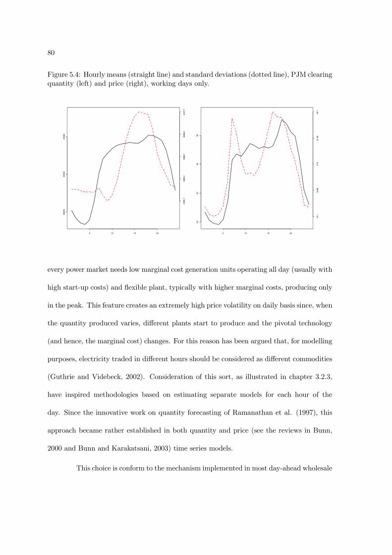
80
Figure 5.4: Hourly means (straight line) and standard deviations (dotted line), PJM clearingquantity (left) and price (right), working days only.
5 10 15 20
3000
03500
040000
3789.7
4389.2
4988.7
5588.2
6187.7
5 10 15 20
20
30
40
50
10
.113
.85
17
.621.3
525
.1
every power market needs low marginal cost generation units operating all day (usually with
high start-up costs) and flexible plant, typically with higher marginal costs, producing only
in the peak. This feature creates an extremely high price volatility on daily basis since, when
the quantity produced varies, different plants start to produce and the pivotal technology
(and hence, the marginal cost) changes. For this reason has been argued that, for modelling
purposes, electricity traded in different hours should be considered as different commodities
(Guthrie and Videbeck, 2002). Consideration of this sort, as illustrated in chapter 3.2.3,
have inspired methodologies based on estimating separate models for each hour of the
day. Since the innovative work on quantity forecasting of Ramanathan et al. (1997), this
approach became rather established in both quantity and price (see the reviews in Bunn,
2000 and Bunn and Karakatsani, 2003) time series models.
This choice is conform to the mechanism implemented in most day-ahead wholesale

81
x σ CV skew. kurt.
Quantity H24 (MWh) 33415 4442 0.133 0.26 2.18Quantity H19 (MWh) 40772 6352 0.156 0.49 2.71Price H24 ($/MWh) 25.17 11.16 0.443 2.42 11.65Price H19 ($/MWh) 52.87 24.24 0.458 1.20 4.89
Table 5.1: Descriptive Statistics
markets across the world (among others in PJM), where electricity is traded in separate
and concurrent auctions for each hour of the subsequent day (see section 2.3 for some
examples). Following these considerations, in the next sections the empirical estimation of
the econometric model will be implemented considering market outcomes of different hours
as separate time series.
In order to evaluate the model in two distinct contexts, a baseload (hour 24) and
a peak hour (hour 19) are selected. The baseload hour is characterised by lower price
variability and by marginal generating plants constituted primarily by nuclear and large
coal plants. On the contrary, the selected peak hour presents the highest volatility of the
sample and has gas-fired power station as typical marginal generating units. The descriptive
statistics of market outcomes time series in the two hours are reported in table 5.11.
The difference between the two hours is substantial, even though there is a consis-
tent overlap between the quantity densities, due to the strong yearly seasonality. A move-
ment in quantities echoes amplified in prices, as can be noticed comparing the coefficients of
variations. This feature is not surprising since, as illustrated in section 3.2, electricity prices
present a high volatility and sometimes show idiosyncratic and unexpected movements. For
1Shewness defined as the third standardised moment: skew = µ3/σ3, where µ
3is the third moment
about the mean and σ is the standard deviation. Kurtosis defined as the fourth standardised moment:kurt = µ
4/σ4, where µ
4is the fourth moment about the mean.

82
these reasons this time series is, by far, more difficult to predict than the quantity one.
Moreover, price distributions are quite distant from the Gaussian one, a problem which, in
the rest of the analysis, is somehow reduced applying the logarithmic transformation.
All the time series used in the empirical specification of the model, presented
in the next sections, are plotted in figure 5.5. These include available excess capacity,
electricity prices and quantities for hour 19 and 24, downloaded from the internet site of
the PJM Interconnector, atmospheric temperature (measured as the daily average between
the Pittsburgh and the Philadelphia ones) provided by the University of Daytona Archive,
gas price (traded on the Henry Hub) available on DataStream and coal price (Pennsylvania
coal price index) available on Bloomberg. Discarding the weekends, the total amount of
observations for each series is 370. PJM day-ahead market results present the same drifting
behaviour observable on the complete series in figure 5.1, i.e. a smooth yearly seasonality
connected with the variation of temperature. These dynamics are even more evident when
the daily and weekly seasonalities have been filtered from the data, eliminating the weekends
and selecting only one hour of the day. The two fuel prices present complete different
dynamics. Coal price is quite stable during the all sample, whilst gas price is characterised
by a high spike during the end of February 2003. This feature was caused by a conjuncture
of low supply and high demand, originated by a particularly cold winter.
As in general it happens when electricity market data are analysed, observing
those graphs it is not easy to decide regarding a delicate issue like the stationarity of the
time series. This feature can be investigated also observing the autocorrelation plot of the
market outcomes in hour 24, plotted in figure 5.62. The autocorrelations are quite persistent
2The autocorrelation function for the market outcomes in hour 19 is extremely similar and therefore not

83
Figure 5.5: Hourly clearing prices and quantities, PJM day-ahead market, hour 19 and hour24. Atmospheric temperature, excess capacity, coal (Pennsylvania index) and gas (HenryHub) prices. Time span: 01/04/2002 — 31/08/2003.

84
Figure 5.6: Autocorrelation plot for hour 24 price and quantity, working days only.
0 5 10 15 20 25
0.0
0.2
0.4
0.6
0.8
1.0
hou
rly p
rice (
$/M
Wh)
Autocorre la tion function
0 5 10 15 20 25
0.0
0.2
0.4
0.6
0.8
1.0
hourly q
uan
tity (
MW
h)
and do not show the weekly seasonality which has been successfully removed discarding the
weekends. The autocorrelation paths are consistent with a process with long memory, either
stationary or with unit root. The next section is devoted to the evaluation of this issue.
5.1.2 Unit root and stationarity analysis
In this section the hypothesis of stationarity of the time series modelled in the
following parts is empirically evaluated. As illustrated in section 3.2.2, despite its impor-
tance for modeling purposes3, the stationarity of electricity prices and quantities is still an
reported here.3One of the bases of classical econometric theory is the stationarity of the variables considered in the
analysis (Hendry and Juselius, 2000). Under this condition classical statistical inference is valid, whileassuming this postulation when it doesn’t hold can induce serious statistical mistakes, invalidating in most

85
ADF KPSS
LevelsQ19 -2.40 0.323P19 -2.80* 1.14***Q24 -2.47 0.383P24 -3.08** 1.31***C -3.86** 0.219Pgas -1.84 3.80***Pcoal -1.09 2.56***Temp -1.14 0.978***
First differencesQ19 -12.42*** 0.035P19 -12.61*** 0.017Q24 -6.48*** 0.038P24 -8.03*** 0.016C -19.56*** 0.034Pgas -9.03*** 0.050Pcoal -19.14*** 0.178Temp -3.93*** 0.099
Table 5.2: Unit Root and Stationarity Tests
open issue in the literature. In most analyses (Escribano et al. 2002, Huisman and Mahieu
2003, Karakatsani and Bunn 2005a) price and quantity are modelled as stationary, but
there exists notable exception. For instance, Stevenson’s (2002) analysis of the Australian
electricity prices and the works by Contreras et al. (2003) and Conejo et al. (2005), on
PJM. Has also been argued that, for some electricity price time series, neither an I(1) nor
an I(0) description is appropriate. On this point Haldrup and Nielsen (2006) develop a
fractionally integrated process describing NordPool price dynamics. The proposed process
is on the border between stationarity and non stationarity, presenting both long memory
and mean reversion.
cases all the inference procedures and leading to a problem known as “spurious regression”. See section3.2.5 for an illustration in the context of electricity markets. For a detailed and extensive analysis refer tothe wide literature available, for example, Granger and Newbold (1974), Hendry (1980), Phillips (1986) andHendry and Juselius (2000).

86
Here the hypothesis of non-stationarity for all the series considered in the analy-
sis is evaluated through the ADF unit root tests (Said and Dickey, 1984) and the KPSS
stationarity test (Kwiatkowski, Phillips, Schmidt and Shin, 1992)4. The results, reported
in table 5.25, do not give a clear indication in favour of one of the two hypotheses since,
for some series, the two tests show opposite results. For the two prices, for instance, the
two null hypotheses of unit root and of stationarity are both refused. For fuel prices and
temperature, on the other hand, the hypothesis of unit root is not refused. On this point
one has always to remember that results from any unit root test must be taken carefully,
in particular when the alternative is a stationary but very persistent process (in this case
the unit root test presents poor size and power properties). Observing the autocorrelation
function in figure 5.6 this seems to be the case.
On these grounds it is rather difficult to draw general conclusion regarding the
stationarity or the non-stationarity of the electricity time series analysed. Rather, unit root
tests are used here to assess “whether the finite sample data used exhibits stationary or
non-stationary attributes”, as advocated in Harris (1995). As Cochrane (1991) argues, the
important question is not weather there exists a unit root and to classify time series into
the unit root category or not, but to outline the appropriate inferential procedure. On this
point, there seems to be strong evidence that the differentiated series are stationary. For
this reason, even if the support in favour of a unit root is not strong, in the next sections the
series are considered I(1), in order to avoid the risk of spurious regression. In this sense I
follow the advice of Hendry and Juselius (2000). They suggest that “even though a variable
4Number of lags for the ADF selected with the AIC criterion, with 5 seasonal dummies and interceptincluded. Number of lags for the KPSS fixed as 4*(T/100)^1/4.
5In this table and in all the following tables: * = 10% significance level; ** = 5% significance level; ***= 1% significance level;

87
is stationary, but with unit root close to unity [. . . ] it is often a good idea act as if there
are unit roots to obtain robust statistical inference”.
5.2 A static economic model of electricity aggregated de-
mand and supply
In this section an economic model describing the supply and the demand functions
in wholesale electricity markets is presented. The proposed model is static, since it describes
the market with theoretical equilibrium relations and does not consider any dynamic in-
teractions among the variables involved in the system. Nevertheless, it provides a general
description, grounded in economic theory, of the interactions between the variables consid-
ered in the analysis. Therefore, this is the first step to ensure that the parameters of the
dynamic econometric model proposed in the next sections are based on a solid theory and
therefore assume clear economic interpretations (i.e. to ensure that the model is structural,
in the sense of the Cowless Commission; see Johnston 1984).
It is worth to note that the theoretical model proposed in this section is appropriate
for every electricity wholesale market which is organised as an auction, i.e. for most day-
ahead power markets across the world (see section 2.3). In section 5.2.1 the theoretical
economic model is presented, whereas in section 5.2.2 an empirically feasible specification
is derived.

88
5.2.1 Stylization of the supply and demand curves
In wholesale electricity markets (see section 2.3) an independent system operator
(ISO) receives supply and demand bids from the market participants and sets the clear-
ing price and quantity at the intersection of the resulting aggregate supply and demand
curves, subject perhaps to some operational constraints6. In this section the clearing mech-
anism is described approximating the aggregate electricity demand and supply curves with
continuous functions.
As showed in section 3.1 the aggregated demand for electricity is strongly related
to the working activities of the population and to the atmospheric conditions (particularly
temperature). The non-linear relationship with these variables generates the recognised
multi-level (annual, weakly and daily) seasonality of electricity demand. In contrast, as
illustrated in section 4.3, a crucial aspect like the demand elasticity to price is still an
open question. Briefly, in empirical models describing price dynamics (see, for instance,
Karakatsani and Bunn 2005a, Weron and Misiorek 2005, Mount et al. 2006) the demand
curve is typically assumed as completely inelastic, and the quantity cleared on the market
is included in the model as exogenous. On the contrary, in theoretical economic models,
demand elasticity is almost always assumed to be different from zero and its value is crucial
for the analysis. It has been used, for instance, to identify potential market inefficiencies
(Borenstein et al. 1999, Growitsch and Wein 2005) or to estimate the amount of market
power (Wolfram 1999, Johnsen et al. 2004). Nevertheless, assuming a plausible value for the
6The System Operator ultimately needs to balance demand a supply in real-time, and will generallyoperate some kind of a continuous balancing market after the day-ahead auction, or power exchange, hasclosed. In doing so, various operational plant characteristics as well as transmission constraints will have tobe met. A few markets, however, include some of these system contraints in the day ahead auction pricesetting.
89
short term demand elasticity has remained an open and crucial question in these analyses.
As showed by recent empirical work (Callaway and Weale, 2005) large industrial consumers
can indeed respond to high wholesale prices switching to their own backup generators or
temporarily shut down production
The model proposed here can be used, inter alia, to test hypotheses on the demand
elasticity. For this reason I consider a demand function with constant elasticity. Population
activities and atmospheric conditions are identified as shifters of the demand function, which
can be written as:
Q(P, a, b, vd) = Pλ1φ(a, b)vd , (5.1)
with Q = electricity quantity traded on the market, P = electricity clearing price, a =
atmospheric conditions, b = behaviour of the population (working and living habits), vd
= residual random component, λ1 price elasticity of demand and φ(.) functional form that
takes into account the non-linear features that characterise the relationships between tem-
perature, working activities and electricity demand.
In competitive7 electricity markets the aggregated supply curve reflects the stack
of increasing marginal costs offered by different power plants in order to produce electricity.
The supply is affected by three sources of variability: fuel prices, plant outages and technical
rationale. The first one reflects that the marginal plant (i.e. the plant that is setting the
price in the auction market) is often a fossil-fuel burning one, particularly during the peak
7Even though market power can be present from the generation side, the aggregate supply curve in well-behaving, established electricity markets is typically not too far from competitive levels. Even though thisfeature can vary from one market to another, the main reasons are vertical integration of firms (Mansur2003, Karakatsani and Bunn 2005a), regulatory constraints, and the threat of entry that suppliers are facing(Wolfram, 1999). In any case, the usual way to exercise market power is to alter the production patters,reducing the amount of power plants available to produce (Borenstein et al., 1999). I directly account forthis effect in the model, since one of the relevant variables considered here is the available excess capacity.

90
periods (the only notable exception at the moment is the NordPool, which, as illustrated
in section 2.3.4, is dominated by hydropower). The second accounts that, according to
technical, or, as many studies (see, for instance, Borenstein and Bushnell 1999, Borenstein
et al. 1999) seem to evidence, strategical reasons, the amount of power plants available to
produce (i.e. bidding into the market) can vary considerably from day to day. As showed in
section 4.1, if some power plants bids are missing the aggregate supply curve shifts upwards.
This feature is not substantial when demand is low (i.e. in the baseload) but will affect price
considerably in the peak. The third factor affecting the supply curve is connected to the
technical management of power plants. Starting or varying production of electricity requires
costs and time. For this reason the cost faced by a power plant in order to produce the
same amount of electricity can be different. This feature explains why wholesale prices are
generally higher in the hours in which production is rapidly changing. Assuming constant
elasticities the aggregate supply function can be written as:
P (Q, pf , c, tr, vs) = β0Qβ1p
β2f cβ3η(tr)vs , (5.2)
with pf = fuel prices, c = excess capacity available on the system (margin), tr = technical
rationale, vs random component incorrelated with vd, β0 constant term depending, for
instance, on the set of technologies present on the market and on the competition level; β1,
β2 and β3 = quantity, fuel prices and excess capacity elasticities and η(.) is a non linear
function representing the effect of technical constraints on the aggregated supply.

91
5.2.2 The empirical specification
The previous paragraph describes the electricity market supply and demand func-
tions from a static, theoretical point of view. In this section an empirically tractable, linear
specification of the two curves is derived from equations (5.1)-(5.2). This requires some
assumptions on the non-linear functions φ(a, b) and η(tr).
Considering electricity demand, one can observe that most of the variability in the
activity of the population is regulated on seasonal cycles with daily and weekly periodicity
(see the description in section 5.1 and section 3.1.1). As previously introduced, in this
analysis the daily cycle is encompassed developing a separate model for each hour of the
day. As illustrated in section 3.1.2 and 3.2.3 this choice is rather established in electricity
quantity and price modelling. Furthermore, the weekly cycle is handled discarding the
weekends and inserting a centred dummy for each remaining day of the week. Demand for
electricity is also significantly lower than usual in national festivities days. I account for this
effect inserting a dummy equal to one when the day is a national feast, and zero otherwise.
Among the atmospheric variables that influence electricity demand, only temper-
ature, which is by far the most important determinant, is considered here. As showed in
section 5.1, the link between electricity demand and temperature is analogous to an asym-
metric “V”. This relationship cannot be linearised with a second degree polynomial (which
implies symmetry) but must be handled defining two different variables from the original
temperature. A threshold (see figure 5.2) that corresponds to the lowest demand of elec-
tricity (i.e. the sum of electricity demand for heating and cooling purposes is minimum)
is selected. Consequently, I define cold temperature (tcold) all the temperature below the

92
threshold (electricity demand is mainly for heating purposes) and hot temperature (thot)
all the temperature above the threshold (demand for cooling and air conditioning needs).
Hence, the functional form that describes the influence of temperature and population be-
haviour on electricity demand can be written as:
φ(a, b) = λ0(λdff
5∏
i=1
λdii )(λdtt exp[λctcol d + λhthot) , (5.3)
where the population behaviour effect is encompassed in the first round brackets, the at-
mospheric conditions (temperature) effect in the second ones, and df is a dummy variable
taking value 1 when the day is a national holiday and 0 otherwise, di, i = 1, 2, . . . , 5 are
dummy variables identifying each day of the week; tcold (thot) is equal to the atmospheric
temperature when temperature is lower (higher) than the threshold and set equal to 0
otherwise and dt is a dummy variable that takes value 1 when temperature is above the
threshold and 0 otherwise. All the parameters have direct economic meaning: λ0 is the
constant term (depending, for instance, on the level of market liquidity), λf is the variation
of the constant when the day is a national feast, λi are daily multiplicators capturing the
seasonal behaviour on the weekly cycle, λc and λh are the semi-elasticities of demand to
cold and hot temperature and λt is the variation of the constant when temperature is hot.
Substituting (5.3) in (5.1) and applying the logarithmic transformation, one obtains the
following double-log specification of the demand curve:
ln(Q) = λ1 ln(P )+ln(λ0)+df ln(λf )+5∑
i=1
di ln(λi)+dt ln(λt)+λctcol d+λhthot+ln(vd). (5.4)
The choice of conducting a separate analysis for each hour of the day encompasses
also most of the technical rationale η(tr) influencing the supply function on daily basis.
93
In fact, the aggregate production path follows the same dynamics from day to day and
the technical constraints that power plants are facing are similar among the same hours
of distinct days. The weekly effect is captured inserting a centered dummy for each day
of the week and the remaining influence is included in the error-term. Hence, substituting
η(tr) =∏5
i=1βdii and applying the logarithmic transformation to equation (5.2) I derive
the double-log representation of the supply function:
ln(P ) = ln(β0) + β1 ln(Q) + βf ln(pf ) + β3 ln(c) +5∑
i=1
di ln(βi) + ln(vs). (5.5)
Equation (5.4) and (5.5) describe the aggregate demand and supply function sub-
mitted for a generic hour in wholesale electricity markets. Both curves are specified in
a double-log form and therefore can be empirically estimated as a system of linear equa-
tions. This representation does not include any dynamic relationship between the variables
involved in the system, but considers only simultaneous effects. Nevertheless, electricity
markets can also be characterised by dynamic relations. For example, if the supply func-
tion shifts upwards (and hence, the clearing price increases), the reduction of the quantity
cleared on the market can be instantaneous or take place with some delay, because demand
can require time to adjust to the shock. On the other hand, the effect of an impulse can
be completely absorbed only after many lags. A suitable short-term empirical specification
cannot avoid encompassing all these aspects. Furthermore, the estimation method must
take into account that, as showed in section 5.1.2, the hypothesis of stationarity for the
time series considered in this analysis is not supported by empirical evidence.
In the next section the statistical methodology developed to ensure correct infer-
ence when analysing non-stationary variables is introduced, considering also the possibility

94
of asymmetric effects. Building on these tools, in section 5.4 a dynamic version of the
system (5.4)-(5.5) is specified, and a methodology is proposed for its empirical estimation.
5.3 Econometrics methodologies for non-stationary data
As showed in section 3.2., the hypothesis of stationarity may raise subtle issue of
specification also in electricity prices and quantities time series modelling and, therefore, it
must be carefully evaluated. In section 5.1.2 unit root and stationarity tests are implemented
on the time series considered in this analysis, and it is showed how the hypothesis of
stationarity is not sustained by empirical evidence. On the contrary, the first difference
of all the series appear to be stationary. For this reason the variables should be considered
I(1) for modelling purposes. ‘Classical’ statistical inference procedures assume that observed
data comes from a stationary process, i.e. a process where means and variances are constant
over time. A huge number of different methods have been proposed in order to test this
hypothesis; they can be divided into unit root and stationarity tests (for an extensive review
see Phillips and Xiao, 1998, for a review of the applications in the context of electricity
market outcomes see section 3.2).
This section consists in a brief overview of the methodologies developed to estimate
models on unit root variables. A complete illustration of those techniques is beyond the
scope of this text, and for an extensive description I suggest to refer to the wide literature
available (see, among others, the textbooks by Banerjee et al. 1993, Johansen 1996, Maddala
and Kim 1998). In section 5.3.1 the problems that may arise when estimating regressions on
non stationary variables are presented, in section 5.3.2 the methodologies (error-correction
95
models and cointegration) developed to handle such situations are illustrated. Section 5.3.3
covers some of the advanced issues on cointegration that will be useful in the following
parts of the analysis. In section 5.3.4 asymmetric error-correction models are presented,
since asymmetric relations may play an important role in the electricity price formation
process.
5.3.1 The spurious regression problem
The literature on unit root time series testing and modelling presented a tremen-
dous growth in the recent years. However, the problems connected with regressing a non
stationary variable8 on another have been already pointed out long time ago. Yule (1926)
was the first one to formalise it, calling ‘nonsense correlation’ the situation where extremely
high correlation is found between variables for which there is no causal explanation. He
found that the coefficient of correlation between two variables xt and yt (indicated with ρxy)
is almost normally distributed when the variables are stationary, but becomes nearly uni-
formly distributed when the variables contain a unit root. Yule’s nonsense correlation can
be illustrated defining two unit root I(1) processes, for instance electricity traded quantity
and clearing price:
∆yt = εt where εt ∼ IN[0, σε] , (5.6)
∆xt = vt where vt ∼ IN[0, σv] ,
and:
E[εtvs] = 0 ∀t, s .
8For the definitions of stationary and non-stationary variable, and further issues on stationarity and unitroot testing on electricity market outcomes see section 3.2.2

96
The model of interest is:
yt = b0 + b1xt + ut . (5.7)
The estimate of b1 with OLS wrongly postulates that ut is an IID process independent to
xt. Under this assumption, a significance test on the parameter b1, based on the Student’s
t distribution, can be written as the ratio:
b1
s.e[b1], (5.8)
where:
b1 =[∑
(xt − x)2]−1 [∑
(xt − x)(yt − y)], and
s.e[b1] =σu√∑(xt − x)2
.
If ut is autocorrelated, the ratio (5.8) does no longer follows a Student’s t distrib-
ution. In particular, if ut is I(1), according to the Monte Carlo experiments in Hendry and
Juselius (2000), a critical value of 14.8 is needed to define a 5% rejection frequency under
the null (instead of a value around 2). This large distortion occurs because, even though b1
is an unbiased estimator of b1, the calculated standard error underestimates its true value.
The main reason is that the sum of squares∑
(xt − x)2 is not an appropriate measure of
the variance of x, since x (instead of xt−1) is a poor ‘reference line’ when xt has a stochastic
trend. As illustrated, for instance, in the simulation study of Granger and Newbold (1974),
not only the t-statistic, but also other classical statistical tools, such as the F -test and the

97
R2, are no longer valid in presence of non stationary variables. Hendry (1980), for instance,
constructed a nonsense regression using cumulative rainfall to provide a better explanation
of price inflation than did the money stock in the UK. Typical features of these spurious
regressions are the high R2, the low Durbin-Watson (1951) statistic on the levels and, on
the other hand, an R2 close to zero and a DW near 2 on the first differences. A complete
technical analysis of these results is presented in Phillips (1986).
In summary, there is often a problem of falsely concluding that a relationship
exists between two unrelated non-stationary series. Furthermore, even though this relation
is present, valid empirical inference cannot be based on the standard tools developed by
the classical statistical theory (which is founded on the hypothesis of stationarity). The
error-correction models and the cointegration method, developed to address this problem,
are presented in the next section.
5.3.2 Error-correction models and cointegration
As showed in section 3.2.5, a process which requires to be differentiated ones to
achieve stationarity is called integrated of order one, or I(1). Examples of I(1) processes
are yt and xt as defined in equations (5.6). In general, any linear combination of these two
series will also be I(1). Statistical inference on the relations between I(1) variables cannot
be conducted on the levels but must be accomplished on the differentiated variables (which
are I(0)). Nevertheless, the differencing operator may rule out important information which
is encompassed in the series on the levels. However, there are situations in which “there are
other ways to achieve stationary other than blanket differencing” (Hendry and Anderson,
1977).

98
This intuition is formalized in Engle and Granger (1987), building on Davidson et
al. (1978) and Granger (1981). They showed that, given two or more I(1) variables, there
is the possibility that, for a given scalar (or, when considering more than two variables, a
vector) β, their linear combination:
ut = yt − βxt (5.9)
would be stationary. In such cases the series are called co-integrated. Hence, even though
the series considered individually are non-stationary, they will nevertheless move closely
together over time, according to an equilibrium relation which remains constant. Thus, the
idea of co-integration mimics the economic concept of ‘long run’ equilibrium, to which the
economic system will converge. In other words, the variables cannot diverge indefinitely
from the equilibrium state but, from some point in time, they will be re-attracted towards
it. The reason is that the economic relations will hold the variables ‘linked together’ over
time. Hence, in statistical terms, the disequilibrium in the system (represented by the
term ut in (5.9)) is a stationary variable. Citing Benerjee et al. (1993): “Co-integration
may be viewed as the statistical expression of the nature of such [economic] equilibrium
relationships”. For instance, since electricity can be obtained as a conversion of natural gas,
one might expect that a relationship would hold ultimately, keeping those two commodity
prices linked togheter over time.
Co-integrated variables are characterised by having an error-correction representa-
tion, that is, the relationship among the variables may be expressed in a way that combines
the advantages of modelling both levels and first differences. In error-correction models, in

99
fact, the dynamics of both short-run (changes) and long-run (levels) are modelled simul-
taneously. In the bivariate case, the error-correction representation can be derived from a
general ADL model:
yt = b0 + b1yt−1 + b2xt + b3xt−1 + εt , (5.10)
where yt and xt are both I(1), xt is weakly exogenous according to Hendry et al. (1983),
and εt is IID and Gaussian. Equation (5.10) can be reformulated subtracting yt−1 from
both sides and subtracting and adding b2xt−1 from the right side obtaining:
∆yt = α0 + α1∆xt − α2[yt−1 − β0 − β1xt−1] + εt , (5.11)
where α1 = b2, α2 = (1 − b1), β1 = (b2 + b3)/(1 − b1), and α0 + α2β0 = b0. If yt and xt
are co-integrated, all the variables that appear in equation (5.11) are stationary. In this
representation the variation of yt depends on the variation of the exogenous variable xt
and also to the disequilibrium that is present in the system at time t − 1, encompassed in
the term yt−1 − β0 − β1xt−1. Thus, the value of −α2 provides information on the speed
of adjustment of the variable yt towards its equilibrium value β0 + β1xt. For instance, if
previous electricity price (yt−1) is too high compared to its equilibrium value (β′xt−1, with
xt−1 containg, for instance, the quantity produced and the fuel prices), then actual price
will correct downwards, and vice versa. To allow this error-correction dynamic, the value
of the parameter α2 must lie between 0 (no adjustment) and 1 (perfect adjustment in one
period).
Many methodologies have been proposed to estimate model (5.11) and a review of

100
those techniques is beyond the scope of this text. Among the most popular approaches see
Engle and Granger (1987), Phillips and Hansen (1990), Stock and Watson (1993), Davidson
(1998), Bruggemann and Lutkepohl (2005). Nevertheless, the methodology which became
the reference point in this literature, and the one applied also in the analysis in the next sec-
tions, is the approach proposed in Johansen (1988, 1991) and further developed in Johansen
(1995, 1996) and Johansen and Juselius (1994).
The Johansen technique has the strong advantage of starting with an unrestricted
VAR, a system in which all variables are modelled as endogenous. VAR models have been
introduced by Sims (1980) as a way to estimate dynamic relationships among economic
variables without imposing strong a priori restrictions. A VAR system can be written as:
xt = A1xt−1 +A2xt−2 + ...+Akxt−k + µ+ ψDt + ut , (5.12)
with xt (h x 1) vector of endogenous I(1) variables, Dt vector of dummy variables (for
instance seasonal dummies), ut error term distributed as IIDN(0,Σ) andA1, ..., Ak matrixes
of parameters (h x h). As analogous to equations (5.10)-(5.11), one can derive the error-
correction form of the system (5.12) as:
∆xt = Πxt−1 + Γ1∆xt−1 + ...+ Γk−1∆xt−k+1 + µ+ ψDt + ut , (5.13)
where Π = A1+A2...+Ak− I and Γi = −(Ai+1+Ai+2...+Ak). This specification contains
information on both the short run (Γi) and the long run (Π) relations among the variables.
Following Johansen (1988), the test of cointegration can be performed as a test of reduced
rank on the matrix Π. In fact, one can rewrite Π = αβ′, where the vector α represents the

101
speed of adjustment of each variable towards the equilibrium vectors β′. In this framework,
the term β′xt−1 embeds the disequilibrium present in the system at time t− 1. According
to the rank r of Π three situations are possible:
r = h : the variables modelled in the VAR system are stationary, and any linear combi-
nation of them would also be stationary. In this case there is no problem of spurious
regression and one can estimate the VAR (5.12) in levels;
r = 0 : the variables are I(1) but they are not cointegrated, hence there are no linear
combination of them that are stationary. The best modelling strategy, in this case, is
a VAR on the first differences;
0 < r ≤ h − 1 : the variables considered individually are I(1) but there exist r linear
combinations of them which are stationary. In other words there are r cointegrating
vectors, which are embedded in the matrix β. In this case Π has reduced rank equal
to r.
From these considerations the test for cointegration (and for the number of cointe-
grating vectors) can be implemented as a test on the rank of Π. Johansen (1988) proposes
two tests: the trace test and max-eigenvalue value test. Both tests are likelihood ratio (LR)
tests and are based on the eigenvalues of the matrix Π. As showed in Johansen (1988),
the number of eigenvalues which are significantly different from zero corresponds to the
number of cointegrating relationships. Hence, the null hypothesis that there are at most r
cointegrating vectors becomes:
H0 : λi = 0 i = r + 1, ..., h , (5.14)
102
where only the first r eigenvalues are non-zero. The trace test for the null hypothesis in
(5.14) can be written as:
λtrace = −2 log(Q) = −Th∑
i=r+1
log(i− λi) ,
where Q = (restricted ML/unrestricted ML). The maximal-eigenvalue test uses the same
principle, and it is based on the significance of the largest non-zero eigenvalue:
λmax = −T log(1− λr+1) .
This tests that there are r cointegrating vectors against the alternative that r + 1 exist.
Asymptotic critical values for both tests are reported in Johansen and Juselius (1990)
and Johansen (1996). The two tests are implemented in section 5.5 to investigate the
cointegration rank of the system considered in the analysis. However, it is worth mentioning
that the choice of the cointegration rank cannot be based on a blind use of any testing
procedure, but must consider as much information as possible, including a priori economic
theory. On this point see, among others, Doornik et al. (1998) and Hendry and Juselius
(2001).
In discussing the formulation of the dynamic model (5.13), an important question
is whether an intercept or a trend should enter the short and/or the long run model. Since
the variables considered in the analysis do not present a trend, only this situation is consid-
ered here9. In this case the constant µ is restricted to lie in the cointegration space, in fact
an absence of trend in the model on the levels (5.12) translates in an absence of the constant
9For a complete illustration of the topic see, among others: Johansen and Juselius (1990), Johansen(1996), Hendry and Juselius (2001).

103
in the model on the first differences (5.13), hence E(∆xt) = 0. The only deterministic com-
ponent (except the dummies) in the model are the intercepts in the cointegrating relations,
implying that some equilibrium means are different from zero. Therefore, the estimates of
the parameters β and α in model (5.13) are obtained through a maximum likelihood (ML)
procedure as illustrated in Johansen (1988, 1996).
The cointegration methodology raised a great interest in literature and it would
be impossible to even only cite here all the relevant aspects of this topic. On the contrary,
in the next sections, I will focus on three issues which are the most relevant for the analysis
in section 5.4 and 5.5: weakly exogenous variables, the identification of the cointegrating
relations and the asymmetric error-correction model.
5.3.3 Further issues on cointegration
This section illustrates two features of the cointegration methodology which are
intitled of particular emphasis in the analysis presented in section 5.4 and 5.5: the iden-
tification of the cointegrating relations and how to test weak exogeneity and estimating
error-correction models including weakly exogenous variables.
The identification problem is particularly important, since the Johansen approach
only provides information regarding how many vectors span the cointegration space, but
requires restrictions motivated by economic theory to obtain unique vectors. This issue
is analysed in Johansen and Juselius (1994) and Johansen (1995). The restrictions are
similar to Cowless Commission type restrictions (for instance, a particular variable does
not appear in one equation) but apply only in the long run, getting around Sims (1980)
critique regarding the use of restrictions on the short-run dynamics in simultaneous systems

104
of equations.
In general, just identification can be achieved imposing the appropriate normal-
isation and r − 1 restrictions on each cointegrating vector βi (hence, if there is only one
cointegrating vector, normalisation is sufficient for identification). These restrictions do not
change the likelihood function, hence no tests are involved. When the vectors are identi-
fied, over-identifying restrictions on the parameters βij can be tested through a LR test, as
showed in Johansen (1991) and Johansen and Juselius (1994).
It is worth mentioning that, even though the VAR system (5.12) is a reduced form,
the identified long run relations (i.e. the cointegrating vectors) are in a structural form. On
this regard Davidson (1998) defines the structural cointegrating vectors as: "simply, para-
meters/relations which have a direct economic interpretation", such as "supply and demand
elasticities, propensity to consume or save, etc.". Hence, if the identification procedure is
grounded in economic theory, the cointegrating vectors assume the meaning of long run,
equilibrium relationships, with direct economic behavioural meaning. On this point see also
Pesaran and Smith (1998).
The second issue regards how to test and model cointegrating relationships includ-
ing weakly exogenous variables. The definition of weak exogeneity has been introduced in
Engle, Hendry and Richard (1983). According to EHR a variable is weakly exogenous when
it can be considered ’as given’ without losing information for inferential modelling purposes.
In this case, the analysis can be conducted developing a model conditioned on the weakly
exogenous variables without losing relevant information for the parameter estimation. This
feature is satisfied if two conditions are valid. Indicating with θ1 the parameter of the
105
conditional model and with θ2 the parameter of the marginal density of zt, zt is weakly
exogenous if and only (1) if the parameters of interest (i.e. the parameters on which in-
ference is conducted) can be written as a function of θ1 and (2) if θ1 and θ2 are variation
free (there are no cross-restrictions between them). In the cointegration framework, if the
interest is placed on the long run parameters β, the concept of weak exogeneity is related
to the significance of the parameter α. Consider equation (5.13) in the bivariate case, with
xt = [yt, zt]. Conditioning on zt, with number of lags h = 1 and no dummy variables, the
system (5.13) can be re-written as:
∆yt = γ∆zt + α1β′xt−1 + ε1t ,
∆zt = α2β′xt−1 + ε2t .
In this representation zt is weak exogenous for β if α2 = 0. In that case, zt, even though
being present in the cointegrating relation, does not adjust towards the equilibrium. Hence,
it marginal density contains no additional information concerning the parameter β and
efficient inference can be conducted by considering only the conditional system.
There are at least two potential advantages from estimating a model having condi-
tioned on the weakly exogenous variables (Urbain, 1995). First, if the exogenous variables
exhibit all the ’problematic’ data features (such as non-normality, presence of outliers, het-
eroskedasticity and similar) than conditioning on those variables will usually ensure that the
rest of the system presents ’better’ stochastic properties. Second, the number of parameters
to be estimated is reduced. The test for weak exogeneity can be conducted, as illustrated
in Johansen and Juselius (1990) as a LR test:

106
−2 log(Q) = Tr∑
i=1
log
(1− λ
∗i
1− λi
)
,
with λ∗i eigenvalues of the restricted model. For further discussion on testing weak exogene-
ity in cointegration analysis see, among others, Johansen and Juselius (1990), Johansen
(1992) and Ericsson (1992).
However, it is not unfrequent the situation in which some variables can be assumed
as weakly exogenous a priori. This is the case of atmospheric temperature in the model
presentend in the next section. In such cases the model (5.12) becomes:
∆yt = Λ∆zt +Πxt−1 +Γ1∆xt−1 + ...+ Γk−1∆xt−k+1 + µ+ ψDt + ut , (5.15)
where xt cointains both the endogenous yt and the exogenous zt variables. In this situation,
the critical values for the cointegration test computed in Johansen and Juselius (1990) are
no longer valid. This issue is analysed in Pesaran et al. (2000), where the asymptotic and
the small samples (by Monte Carlo simulation) critical values for both tests are provided.
5.3.4 The asymmetric error-correction model
Asymmetric relations may play an important role in the electricity markets clear-
ing process. For example, if electricity price becomes higher than a threshold, industrial
consumer may temporarily reduce production and hence the overall electricity demand
(Callaway and Weale, 2005), whereas low electricity prices are not likely to influence the
production patterns to the same extent in the short term. Asymmetric price transmission in
energy commodities has also been subject of considerable attention, in particular regarding
the pass-trough of oil shocks into and gasoline price (see, among others, Borenstein et al.

107
1997, and Chen et al. 2005).
In the asymmetric error-correction model the speed of adjustment of each variable
towards the equilibrium (represented by the matrix α) may vary accordingly with the sign
of disequilibrium. In the extreme case, adjustment will happen only if disequilibrium is
positive or negative. This class of models was presented for the first time in Granger and
Lee (1989), as a generalisation of the methodology introduced in Engle and Granger (1987),
and further developed in Enders and Granger (1998) and Enders and Siklos (2001). The
single equation asymmetric error-correction model can be written as:
∆yt = µ+ Itα+β′xt−1 + (1− It)α
−β′xt−1 +k∑
i=1
Γi∆xt−i + ut , (5.16)
with β′xt−1 disequilibrium in the system at time t − 1, α− adjustment coefficient when
disequilibrium is negative, α+ adjustment coefficient when the disequilibrium is positive, It
indicator variable equal to 1 when the disequilibrim is negative and 0 otherwise, k number
of lags chosen ot ensure absence of autocorrelation in the residual ut. Equation (5.16) can
be generalised allowing also the effect of the lagged variables to change with the sign of the
disequilibrium.
As showed in Krolzig (1997) and Saikkonen and Luukkonen (1997), the Johansen
(1991, 1996) ML methodology originally developed to estimate the cointegrating relations
in linear, Gaussian systems, can be implemented even when the short-term dynamics are
subject to regime-switching. This result has been used to estimate the long-run, equilibrium
relationships in Markow-switching vector error correction models (MS-VECM) with the
standard Johansen (1996) methodology, and to estimate the regime-dependent, short-run

108
parameters only in a second step (Krolzig et al. 2002, Clarida et al. 2003, Tillmann 2004).
Following these considerations, since asymmetric responses can be viewed as a special case of
the MS-VECM, in the multivariate generalisation of (5.16) one can estimate the equilibrium
relationships with the Johansen methodology as illustrated in the previous sections, and
estimate the short term parameters in a second step, with FIML or IV. This approach is
indeed proposed to estimate the model introduced in the next section.
5.4 The dynamic econometric specification
This section is devoted to the dynamic specification of the supply and demand
system developed in section 5.2. The static model (5.4)-(5.5) assumes that the variables
are affected only by simultaneous interactions. Nevertheless, empirical evidence shows that
dynamics play a foundamental role in determining electricity markets outcomes. As illus-
trated in section 5.1.2, the autocorrelation functions of the series considered in the analysis
are quite persistent, and the hypothesis of stationarity is not supported by statistical ev-
idence. For this reason the variables are modelled as I(1). Hence, the model (5.4)-(5.5)
implies the presence of two cointegrating vectors and can be sensibly specified including the
dynamic interactions in an error-correction form. As showed in the previous section, this
specification allows to encompass both short and long run relations in the same model.
On this point it is important to emphasize that in this framework the concept of
‘long run’ has to be interpreted in a ’short window’ context. In fact, since the analysis
is based on hourly data covering approximately one year and a half of time span, one
cannot assume as variable all the inputs of production. Indeed, most of the investment

109
decisions in power markets require a time span of several years, and for this reason these
must be considered as fixed in this framework. Thereafter, with ‘long-run’ relations I will
indicate static equilibrium conditions with direct economic meaning towards which the
system will converge in absence of perturbations, conditional upon all the price drivers (eg.
market structure changes) that need more than the elapsed time to adapt being considered
fixed. In this sense, all the factors of production that need more than the time covered
by the analysis to be changed must be considered as fixed in order to correctly interpret
the results. Furthermore, asymmetric responses may be present in the short-term, high-
frequency, interactions among demand and supply. To evaluate this potential asymmetry in
the demand price response and to encompass both short and long run relations in the same
framework, I specify the following asymmetric vector-error correction model (A-VECM)10:
∆pt = θ11∆qt + δ11∆ct + δ12∆pf + IStα+SpβSwS,t−1 + (1− ISt)α
−SpβSwS,t−1 +
+IDtα+DpβDwD,t−1 + (1− IDt)α
−DpβDwD,t−1 + φdj,t +
p∑
i=1
ϑ′i∆wS,t−i + uSt
(5.17)
∆qt = θ21∆pt + δ21∆tcol d + δ22∆thot + IStα+SqβSwS,t−1 + (1− ISt)α
−SqβSwS,t−1 +
+IDtα+DqβDwD,t−1 + (1− IDt)α
−DqβDwD,t−1 + ϕdj,t +
k∑
i=1
ς ′i∆wD,t−i + uDt
with:
pt : logarithm of the clearing price;
qt : logarithm of the traded quantity;
10Also a more general specification, embedding asymmetric effects of the lagged variables, has been con-sidered. Its coefficients did not show any significant asymmetry and therefore only the asymmetric error-correction version is presented here.

110
ct : logarithm of the available capacity;
pf : logarithm of the fuel prices;
tcold and thot : atmospheric temperature variables defined as in (5.3)11;
dj : vector of dummy variables containing both di and df ;
wS = [pt, qt, ct, pf , 1] a vector containing only the variables embedded in the supply fuction;
wD = [q,t pt, thot, tcold, dt, 1] a vector containing only the variables embedded the demand
function;
ISt(IDt) : indicator variable for positive disquilibrium in the supply (demand) side, equal
to 1 when βSwS,t−1 > 0 (βDwD,t−1 > 0) and to 0 otherwise;
p and k : number of lags selected to assure serial incorrelation in the Gaussian residual
components uDt and uSt.
In this representation clearing prices and quantities traded on the market react
to the short term dynamics of the supply and demand shifters and also are attracted to-
wards the long-run equilibrium vectors through an error-correction mechanism . All the
variables of the system are stationary, since they are first difference of I(1) variables or
their stationary linear combination. In fact the vectors β’s are such that β′wt ∼ I(0), i.e.
they are cointegrating vectors. As showed in section 5.3, from a pure statistical point of
11The two variables ∆tcold and ∆thot are not simply the first differences of tcold and thot. In fact, in orderto linearise a relation in the first difference, one has to consider that if during the intra-period variation thetemperature crosses the threshold the relationship with quantity is reverted. To overcome this problem Idefine as ∆thot all the variation of the temperature that occurs above the threshold and as ∆tcold all thevariation that occurs below. If, for instance, the threshold is 60oF and temperature drops from 63oF to55oF , the variable ∆thot will take value -3 and the variable ∆tcold will be defined as -5.

111
view the cointegrating vectors have to be interpreted as equilibrium states: “to which the
system is attracted, other things being equal” (Banerjee et al., 1993). Furthermore, if the
restrictions introduced to identify them are based on economic theory, one can interpret the
cointegrating relations as long-run behavioural relationships, with direct economic meaning
(Johansen 1995). For this reason they have been defined as "structural" (Davidson, 1998).
Model (5.17) is consistent with a cointegration rank r = 2, where the cointegrating vectors
are identified as the electricity aggregate supply and demand function imposing the appro-
priate restrictions based on equations (5.4)-(5.5). The first equation in model (5.17) is a
short run supply function, in which the clearing price react to the short term dynamics of
the supply shifters (fuel prices and excess capacity) and also corrects towards the ‘long-run’
equilibrium supply and demand curves through an error-correction mechanism. The second
equation is a short run demand function, in which the quantity traded on the markets is
influenced by the demand shifters (temperature and working habits) and corrects toward
the equilibrium curves with two error-correction terms. Additionally, the effects of disequi-
librium in both the supply and demand side can be different if the disequilibrium is positive
or negative.
Hence, all the parameters of this model have structural interpretation. The coin-
tegrating vectors βS and βD cointain the long run supply and demand elasticities. The
error-correction terms βSwt−1 and βDwt−1 describe the disequilibrium of the system in the
period t−1 compared with the long run supply and demand functions. The adjustment co-
efficients αSp, αDp and αSq, αDq represent the speed of adjustment of the clearing quantity
and price to past disequilibrium in the supply and demand functions. Finally, θ11 and θ21

112
are the short run elasticities of the supply function to quantity and of the demand function
to price, whereas δ11, δ12, δ21 and δ22 are short run elasticities and semi-elasticities and φ
and ϕ embody the effects of festivities and of the weekly cycle.
When α+Sq �= α−Sq demand responds differently to a positive or to a negative dise-
quilibrium in the supply side. If, on the other hand, α+Sq = α−Sq = θ21 = βD1 = 0, demand
is perfectly inelastic and the quantity cleared on the market does not react at all to price
dynamics but is only determined by temperature and consumer behaviour. Moreover, if
α+Sq = α−Sq = 0 a partial system analysis based only on the first equation in (5.17) is effi-
cient to estimate the long run supply curve (i.e. quantity is weakly exogenous for the long
run parameters). If, on the contrary, at least one between αSq and αSq is different from zero,
demand is still inelastic in the short run (θ11 = 0) and in the long run (βD1 = 0), but the
quantity traded on the market reacts to a system price higher or lower than the equilibrium
level through the error correction term. In this case a single equation framework does no
longer contains all the information available on the long run parameters (i.e. quantity is no
longer exogenous). Finally, if βD1 �= 0, demand is still inelastic in the short run but has a
significant long run elasticity (i.e. price enters in the long run demand function).
As showed in section 5.3, the equilibrium vectors βD and βS can be estimated
starting from a general VARmodel, as introduced in Johansen (1996). This choice allows the
modeling approach to begin with a general specification and test successively the structural
economic model as a reduction of the statistical model describing the data. This ‘data based’
approach is advocated, among others, in Hendry and Mizon (1993), Johansen and Juselius
(1994) and Hendry (1995). Furthermore, as illustrated in section 5.3.4, this approach is still
113
valid even though the short-run dynamics present non-linearities.
Hence, in order to estimate the cointegrating relations, I start from a reduced
form VAR model considering all the variables as endogenous ‘a priori’ (with the exception
of the temperature, which is introduced as weakly exogenous) and only in a second step I
insert the non-linearities in the model. Defining y′t = [pt, qt, ct, pf ], z′t = [thot,t, tcold,t, dt,t]
and x′t = [y′t, z′t] the VAR system in which is nested model (5.17), and corresponding to the
reduced form, dynamic version of equations (5.4)-(5.5) can be written as:
yt = B0zt +A1xt−1 + ...+Akxk−1 + µ+Cdj,t + ut , (5.18)
with k number of lags selected long enough to assure absence of autocorrelation in the
residual component ut, assumed to be Gaussian, uncorrelated and homoskedastic; µ vector
of constant terms; dj,t vector of dummies defined as previously. All variables, except tem-
perature, are expressed in their natural logarithms. If the VAR model is correctly specified,
the test for cointegration can be implemented with the technique based on the reduced
rank regression introduced in Johansen (1991). Since the VAR model contains exogenous
regressors the asymptotic critical values presented in Johansen (1991) are no longer valid.
For this reason I use the asymptotic critical values provided in Pesaran et al. (2000). For
a fixed cointegration rank, the error-correction representation of equation (5.18) can be
written as:
∆yt = /∆zt + αβ′xt−1 + Γ1∆xt−1 + ...+ Γ∆xt−k+1 +Cdj,t + ut , (5.19)
where the vector β′s, as in (5.17), are such that β′xt ∼ I(0). As stressed in Johansen (1995)
one has to impose r−1 restrictions on each of the cointegrating vectors in order to identify

114
the system. In this framework, when r = 2, the identifying restriction can be imposed
following equations (5.4)-(5.5). This ensures that the cointegrating relations preserve a
clear economic interpretation.
When the cointegrating vectors are identified as the ‘long run’ supply and demand
functions, one can test the hypotheses of weak exogeneity of fuel prices and excess capacity
simply performing a test on the adjustment coefficients (see section 5.3)12. If the hypotheses
are not rejected, a partial system analysis involving only the demand and the supply equa-
tions is efficient to estimate the long run parameters of the two curves (i.e. the marginal
distribution of capacity and fuel price does not contain any additional relevant information).
Furthermore, after estimating the cointegrating vectors β′s, the short term dynamics can
be investigated estimating the structural model (5.17) with FIML, assuming the residual
component uSt and uDt, normodistributed, homoskedastic and serially uncorrelated.
Synthetically, the steps involved in the empirical estimation of (5.17), following a
‘data based’ approach which starts with estimating a proper statistical models describing
data dynamics and then derives the structural economic model can be summerised as follows:
1. estimate with OLS (equivalent to ML) the reduced form VAR (5.18) with all the
variables (except temperature) included as endogenous;
2. test for the cointegration rank r using the trace and the max-eigenvalue tests;
3. if r = 2, identify the cointegrating vectors as the ‘long run’ supply and demand
functions imposing the restrictions following equations (5.4)-(5.5);
12I assume symmetry in the response of fuel prices and excess capacity to supply disequilibrium. Sincethe focus of this section is on the electricity demand response, this is not likely to be a crucial weakness.
115
4. test the hypothesis of weak exogeneity of the excess capacity and the fuel prices;
5. if this the hypotheses of weak exogeneity are not refused re-estimate a partial VAR
system where quantity and price are modeled conditional on temperature, excess
capacity and fuel price and estimate the cointegrating vectors with r = 2.
6. estimate with FIML the error-correction model describing the short run relationships
between price and quantity, keeping fixed the cointegration vectors at the values esti-
mated at the previous step.
This procedure ensures that the error-correction model (5.17) estimated at the last
step is both founded on strong statistical grounds and on economic theory. Furthermore, it
provides inference which is robust against the risk of spurious regression and endogeneity of
the regressors, since the estimation procedure is based on the cointegration methodology and
starts with a reduced form VAR in which all the variables are modeled as endogenous. The
model can be used, inter alia, to give significant insights regarding the ‘elasticity dilemma’
(see section 4.3) since it contains the estimates of both the short run and the ’long run’
demand elasticities. In addition, it encompasses not only instantaneous relationships, but
also dynamic interactions, which play a fundamental role in the electricity market price
formation process. Finally, the possibility of an asymmetric response in the short-run
electricity demand function is considered and embedded in the model. Given its generality,
it can be applied to most wholesale markets across the world.

116
5.5 The empirical analysis
In this section the modelling strategy presented previously is implemented on
PJM wholesale electricity market data. As introduced in section 5.1 and 5.3, the different
hours of the day are modelled separately. To evaluate the modelling technique in two
distinct contexts, a baseload period (hour 24) and a peak period (hour 19) are selected.
The descriptive analysis for both hours is reporeted in section 5.1. As showed in section
5.1.2, since the data do not support the hypothesis of stationarity, the variables involved
in the system (5.18) are assumed I(1), and therefore modelled through the cointegration
methodology (Johansen 1991, Johansen and Juselius 1994 and section 5.3.2).
System (5.18) is estimated separately for both hours via OLS, with number of lags
(selected with the AIC criterion) k = 2. In the vector dj,t are included also six variables to
encompass the “gas price spike” represented in figure 5.5. In table 5.3 and 5.4 are reported
the descriptive statistics13 of the endogenous variables involved in the model (5.18) and the
specification tests conducted on the VAR residuals.
The main problem of this specification is the strongly rejection of the normality
assumption for some of the equations random components, in particular for the coal price
and for the excess capacity ones. This feature, related to the step-function dynamic of the
two series (see figure 5.3) cannot be modelled in a parsimonious way but would require
the inclusion of many dummy variables. Since the choice of two lags leaves no sign of
significative residual autocorrelation, we carry on the analysis with this model, bearing in
13Normality test computed as in Doornik and Hansen (1994); AR LM test computed regressing theresiduals on the original variables and lagged residuals as in Doornik and Hendry (1997); Arch LM testcomputed regressing the squared residuals on the lagged squared residuals, as in Lütkepohl H., Krätzing M.(2004). These definitions are valid for all the section if not otherwise specified.

117
Pt qt ct pgas pcoalx 3.15 10.41 7.39 1.49 3.50s 0.36 0.13 0.30 0.28 0.12xskew 0.99 0.04 -0.72 0.60 -0.93xkurt 0.84 -0.91 -0.02 1.60 -0.44Norm χ2(2) 71.82 12.85 32.33 61.91 56.71
Residualsεsd 0.17 0.04 0.12 0.03 0.004εskew 0.31 0.13 -0.26 0.05 -2.69εkurt 4.09 4.52 23.99 3.47 39.67
TestsAR LM 1-4 0.695 2.15 1.12 0.538 0.486F(4,330) [0.596] [0.07] [0.345] [0.701] [0.746]Arch LM 1-4 2.21 1.57 0.09 1.92 0.13F(4,326) [0.07] [0.177] [0.985] [0.106] [0.971]Normal 16.65 35.1 919 3.76 495χ2(2) [0.000] [0.000] [0.000] [0.152] [0.000]
Table 5.3: Hour 24 VAR descriptive statistics and diagnostic tests, series in natural loga-rithms
Pt qt ct pgas pcoalx 3.87 10.60 7.39 1.49 3.50s 0.44 0.15 0.30 0.28 0.12xskew 0.03 0.17 -0.72 0.60 -0.93xkurt -0.48 -0.58 -0.02 1.60 -0.44Norm χ2(2) 9.20 3.66 32.33 61.91 56.71
Residualsεsd 0.20 0.05 0.12 0.03 0.005εskew -0.38 0.01 -0.24 0.013 -2.58εkurt 4.61 4.11 23.41 3.47 41.09
TestsAR LM 1-4 0.498 0.95 0.59 0.877 0.42F(4,330) [0.737] [0.433] [0.669] [0.477] [0.795]Arch LM 1-4 1.38 2.09 0.105 1.88 0.162F(4,326) [0.24] [0.082] [0.981] [0.113] [0.958]Normal 27.67 24.61 881 4.23 597χ2(2) [0.000] [0.000] [0.000] [0.101] [0.000]
Table 5.4: Hour 19 VAR descriptive statistics and diagnostic tests, series in natural loga-rithms
118
mind the non-normality drawback14. On this point Gonzalo (1994) showed that the finite
sample properties of the Johansen (1991) cointegration methodology are consistent with
the asymptotic results even though the residuals are non-Gaussian. Hence, even though
strong, the non-normality of the residuals is not likely to be a crucial specification weak-
ness. In addition, some non-normality can be expected considering the non-linearities that
may characterise in the short run dynamics. Anyway, the choice of the cointegration rank
cannot be based only on the cointegration tests, since the critical values for the model with
exogenous regressors (Pesaran et al., 2000) are founded on the normality assumption and
can be altered by the presence of dummy variables.
However, even though these critical values must be considered only as indicative,
both the trace and the max-eigenvalue tests, presented in table 5.515, support the choice of
a cointegration rank equal to 2. The magnitudes of the eigenvalues sustain this choice, since
the first two appear to be significantly bigger than the others. Furthermore, two cointegrat-
ing relationships are consistent with the structural model (5.17). For these reasons, basing
the choice on both statistical evidence and economic theory, I select a cointegration rank
r = 2 and identify the cointegrating vectors with the long-run demand and supply functions
imposing the suitable restrictions according to model (5.4)-(5.5). Hence, the cointegrating
vectors assume structural economic meaning, as showed in Johansen and Juselius (1994)
and Davidson (1998). The estimates of the cointegrating vectors and of the adjustment
coefficients are reported in table 5.6 and 5.7.
14I compared the Johansen ML estimation results with the ones obtained through an alternative method,namely the 2SLS advocated by Davidson (1994) and Hsiao (1997). This approach relies mainly on economic‘a priori’ information and requires less stringent statistical assumption. The results, available under request,are essentially the same and therefore not reported here.15The critical values (5% and 10%) in table 5.5 are taken from table 6.2 in Pesaran et al. (2000), specifi-
cation with 3 exogenous variables.

119
TRACE TESTH0 r p-r Hour 24 Hour 19 5% 10%
0 5 157.21*** 157.06*** 108.6 103.61 4 76.38* 76.76* 81.25 76.692 3 33.64 33.28 56.28 52.713 2 16.66 16.72 35.46 32.384 1 4.88 3.91 17.80 15.68
MAX-EIGENVALUE TESTH0 r p-r Hour 24 Hour 19 5% 10%
0 5 80.83*** 80.29*** 43.62 40.861 4 42.74** 43.48** 37.83 35.082 3 16.98 16.56 31.56 28.833 2 11.78 12.81 24.97 22.544 1 4.88 3.91 17.80 15.68
EIGENVALUES1 2 3 4 5
Hour 24 0.1996 0.1111 0.0457 0.0319 0.0134Hour 19 0.1984 0.1129 0.0446 0.0347 0.0107
Table 5.5: Cointegration tests and eigenvalues
The supply curves in both hours present a strong elasticity to quantity, a result
which is consistent with the price formation process in wholesale markets, as illustrated in
section 4.1. As expected, the supply curves in the different hours are differently affected by
the two fuel prices. Coal price is an important determinant of the baseload supply curve,
whilst in the peak the coefficient presents a sign that is even the opposite of the one implied
by economic theory (even though insignificant). This feature is explained considering that
coal is a marginal fuel only during the baseload, whereas in the peak hours marginal plants
are mainly gas-fired ones. For this reason the coal coefficient is restricted to be zero in the
peak hour analysis.
Comparing the loading factors one can notice that the ones of capacity, coal
price and gas price seem to be quite small, particularly for the peak hour. Testing the

120
Hour 24
supply demand
β χ(1) β χ(1)Price 1 — -0.128 3.18Quantity -1.429 13.54*** 1 —Capacity 0.071 1.42 0 —Coal price -1.832 6.51** 0 —Gas price -0.397 22.23*** 0 —Temp. hot 0 — -0.017 24.6***Temp. cold 0 — 0.008 35.01***Dummy temp. 0 — 1.507 28.77***Constant 18.002 11.26*** -10.330 8.13**
Loading factorsαsup αdem χ(2)
Price -0.577 -1.410 51.43***Quantity -0.126 -0.464 41.36***Capacity 0.056 0.177 1.05Coal price 0.003 0.002 5.75Gas price 0.005 0.095 5.5
Weak exogeneity testsαcoal = αgas = αcap = 0 χ(6) = 10.88 [0.092]
Table 5.6: Cointegrating vectors and loading factors, with LR significance tests
joint significance of those adjustment coefficients does not refuse the null hypothesis for
both hours. This result implies that the three supply curve shifters are weakly exoge-
nous (see section 5.3.2). Therefore, model (5.18) can be re-specified as a partial VAR
system where hourly quantities and prices are modeled conditional on temperature, ca-
pacity and fuel prices. The system is equivalent to equation (5.15) with yt = [pt, qt] and
xt = [pgas, pcoal, ct, thot,t, tcold,t, dt]. The estimates of the cointegrating vectors resulting from
this model are reported in table 5.8.
All the coefficients present the sign implied by economic theory. As expected,
(see figure 5.2) the effect of temperature on demand changes when temperature crosses
the threshold. Not only the sign is reversed, but also the magnitude of the coefficient is

121
Hour 19
supply demand
β χ(1) β χ(1)Price 1 — -0.066 0.51Quantity -1.777 7.96** 1 —Capacity 0.071 0.34 0 —Coal price 1.420 1.79 0 —Gas price -0.618 14.93*** 0 —Temp. hot 0 — -0.022 12.34***Temp. cold 0 — 0.008 20.04***Dummy temp. 0 — 1.873 14.98***Constant 10.565 4.17* -10.639 9.71**
Loading factorsαsup αdem χ(2)
Price -0.444 -1.307 42.08***Quantity -0.082 -0.418 27.02***Capacity 0.021 0.125 0.73Coal price 0.000 -0.003 0.41Gas price -0.004 0.055 2.36
Weak exogeneity testsαcoal = αgas = αcap = 0 χ(6) = 2.97 [0.81]
Table 5.7: Cointegrating vectors and loading factors, with LR significance tests
different. In fact, for each degree above the threshold, electricity response is almost double
than for each degree lower than the threshold (i.e., βtemp.hot 2βtemp. col d). This feature
justifies the choice of not modelling this relationship with a quadratic polynomial, which
would restrict the two coefficients to be the same.
Supply elasticities in both hours are quite high, reflecting two steep supply func-
tions. On the contrary, the two demand curve elasticities are not significantly different
from zero. One can conclude that the long-run level of demand is not significantly affected
by the level of price. As stressed before, in this context one has to bear in mind that a
relative ‘long run’ is considered here. The time span on which it is estimated the model, in
fact, does not allow long run investments to take place. Therefore, the effect of potential
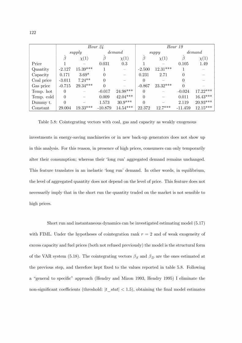
122
Hour 24 Hour 19supply demand suppy demand
β χ(1) β χ(1) β χ(1) β χ(1)Price 1 — 0.031 0.3 1 — 0.105 1.49Quantity -2.127 15.39*** 1 — -2.500 12.31*** 1 —Capacity 0.171 3.69* 0 — 0.231 2.71 0 —Coal price -3.011 7.24** 0 — 0 — 0 —Gas price -0.715 29.34*** 0 — -0.867 23.32*** 0 —Temp. hot 0 — -0.017 24.98*** 0 — -0.024 17.22***Temp. cold 0 — 0.009 42.04*** 0 — 0.011 16.43***Dummy t. 0 — 1.573 30.9*** 0 — 2.119 20.93***Constant 29.004 19.33*** -10.879 14.54*** 22.372 12.7*** -11.459 12.15***
Table 5.8: Cointegrating vectors with coal, gas and capacity as weakly exogenous
investments in energy-saving machineries or in new back-up generators does not show up
in this analysis. For this reason, in presence of high prices, consumers can only temporarily
alter their consumption; whereas their ‘long run’ aggregated demand remains unchanged.
This feature translates in an inelastic ‘long run’ demand. In other words, in equilibrium,
the level of aggregated quantity does not depend on the level of price. This feature does not
necessarily imply that in the short run the quantity traded on the market is not sensible to
high prices.
Short run and instantaneous dynamics can be investigated estimating model (5.17)
with FIML. Under the hypotheses of cointegration rank r = 2 and of weak exogeneity of
excess capacity and fuel prices (both not refused previously) the model is the structural form
of the VAR system (5.18). The cointegrating vectors βS and βD are the ones estimated at
the previous step, and therefore kept fixed to the values reported in table 5.8. Following
a “general to specific” approach (Hendry and Mizon 1993, Hendry 1995) I eliminate the
non-significant coefficients (threshold: |t_stat| < 1.5), obtaining the final model estimates

123
Quantity PriceVariable Coefficient t-stat. Variable Coefficient t-stat.EC sup(+) -0.085 -5.83 EC supply -0.196 -5.48EC dem(+) -0.210 -3.25 ∆ct -0.134 -2.02EC dem(-) -0.485 -8,74 ∆qt 3.43 12.6∆thot,t 0.014 13.2∆tcol d,t -0.0043 -6.60 ∆pgas,t−1 0.677 4.96∆qt−1 -0.076 -1.52 ∆pt−1 -0.072 -1.85∆thot,t -0.0022 -2.14∆tcol d,t 0.0013 2.16 df,t 0.129 2.09df,t -0.064 -4.25 d1,t 0.001 0.02d1,t -0.016 -2.141 d2,t 0.025 0.86d2,t -0.034 -4.79 d3,t 0.079 2.65d3,t -0.031 -4.48 d4,t 0.081 2.61d4,t -0.046 -6.62
σu = 0.0427 εskew = 0.19 σu = 0.169 εskew = −0.23R2 = 0.45 εkurt = 4.6 R2 = 0.51 εkurt = 3.2Arch 1-4 (LM): F(4,353) = 1.70 [0.150] Arch 1-4 (LM): F(4,353) = 3.51 [0.008]
Test for vector-autocorrelation: F(16,696) = 1.36 [0.155]Test of vector-arch (LM test) Chi (36) = 84.24 [0.000]Test for over-identifying restrictions, Chi (19) = 18.77 [0.471]
Table 5.9: Simultaneous equations estimates and specification tests, hour 24
reported in table 5.9-5.10. The over-identifying restrictions are not rejected according to the
likelihood ratio, Chi-squared test (with p-values 0.47 and 0.70). The models appear to be
well specified in both hours, even though the residuals are still non-normal. Nevertheless,
the model fitting seems to be quite satisfactory for both hours, as showed in figure 5.7 and
5.8. Observing the plots, the model seems to be able to capture the few spikes present in
the series, with perhaps the exception of the firsts two in the hour 19 prices. Except for
those two cases (which, in fact, present the highest values for the standardized residuals),
the residuals look quite small and well-behaving. The R2s are particularly high, considering
that I am modelling first differenced series characterised by elevated variability.
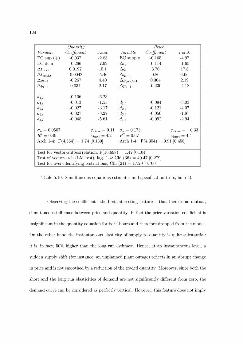
124
Quantity PriceVariable Coefficient t-stat. Variable Coefficient t-stat.EC sup (+) -0.037 -2.83 EC supply -0.165 -4.97EC dem -0.266 -7.92 ∆ct -0.114 -1.65∆thot,t 0.0197 15.1 ∆qt 3.70 17.8∆tcol d,t -0.0042 -5.46 ∆qt−1 0.86 4.06∆qt−1 -0.267 4.40 ∆pgas,t−1 0.304 2.19∆pt−1 0.034 2.17 ∆pt−1 -0.230 -4.18
df,t -0.106 -6.23d1,t -0.013 -1.55 d1,t -0.094 -3.03d2,t -0.027 -3.17 d2,t -0.121 -4.07d3,t -0.027 -3.27 d3,t -0.056 -1.87d4,t -0.048 -5.61 d4,t -0.092 -2.94
σu = 0.0507 εskew = 0.11 σu = 0.173 εskew = −0.33R2 = 0.49 εkurt = 4.2 R2 = 0.67 εkurt = 4.4Arch 1-4: F(4,354) = 1.74 [0.139] Arch 1-4: F(4,354) = 0.91 [0.458]
Test for vector-autocorrelation: F(16,698) = 1.47 [0.104]Test of vector-arch (LM test), lags 1-4: Chi (36) = 40.47 [0.279]Test for over-identifying restrictions, Chi (21) = 17.20 [0.700]
Table 5.10: Simultaneous equations estimates and specification tests, hour 19
Observing the coefficients, the first interesting feature is that there is no mutual,
simultaneous influence between price and quantity. In fact the price variation coefficient is
insignificant in the quantity equation for both hours and therefore dropped from the model.
On the other hand the instantaneous elasticity of supply to quantity is quite substantial:
it is, in fact, 50% higher than the long run estimate. Hence, at an instantaneous level, a
sudden supply shift (for instance, an unplanned plant outage) reflects in an abrupt change
in price and is not smoothed by a reduction of the traded quantity. Moreover, since both the
short and the long run elasticities of demand are not significantly different from zero, the
demand curve can be considered as perfectly vertical. However, this feature does not imply

125
that the quantity traded on the market is not price-responsive, since it significantly reacts
to past disequilibrium in the long run supply function through the error-correction term.
Furthermore, the demand response to disequilibrium on the supply side is asymmetric: when
supply disequilibrium is negative there is no significant short-term reaction in demand (the
α−Sq coefficients were not significant and therefore dropped from the models), whereas when
price is higher than in the equilibrium, demand shows a significant reduction. Hence the
demand function, even though vertical, does adjust to past high prices shifting to the left
according to the adjustment coefficients (-0.085 and -0.037, for base and peak respectively)
relative to the long run supply function disequilibrium.
This behaviour is consistent with the empirical findings in Callaway and Weale
(2005), where it is showed that industrial consumers can temporarily reduce their demand
for electricity (shutting down production or using their own back-up generators) when
prices are perceived as too high. According to this analysis, the response does not take
place instantaneously but only after one period. On the other hand, low prices do not alter
the short-run production patterns. Consequently, to correctly analyse short run electricity
demand response to price, asymmetries play a fundamental role and cannot be ignored.
Interestingly demand reaction is faster for the baseload hour than for the peak. It may well
be that the demand side has a better perception of where the supply function “equilibrium”
(“focal point”) should be at baseload and/or that a greater proportion of the baseload is
industrial with its higher characteristic price-responsiveness.
On the other hand, in the two supply equations there is no significant asymmetry;
therefore the adjustment coefficients for positive and negative disequilibrium were restricted

126
Figure 5.7: Actual and fidded values, and standardized residuals, in hour 24.
0 100 200 300
20
40
60
80
10
0 fitted and actual values (price)
pri
ce
($
/MW
h)
0 100 200 300
-3-2
-10
12
3
sd. residuals (price)
0 100 200 300
25
00
03
00
00
35
00
04
00
00
45
00
0 fitted and actual values (load)
loa
d (
MW
h)
0 100 200 300
-4-2
02
4
sd. residuals (load)
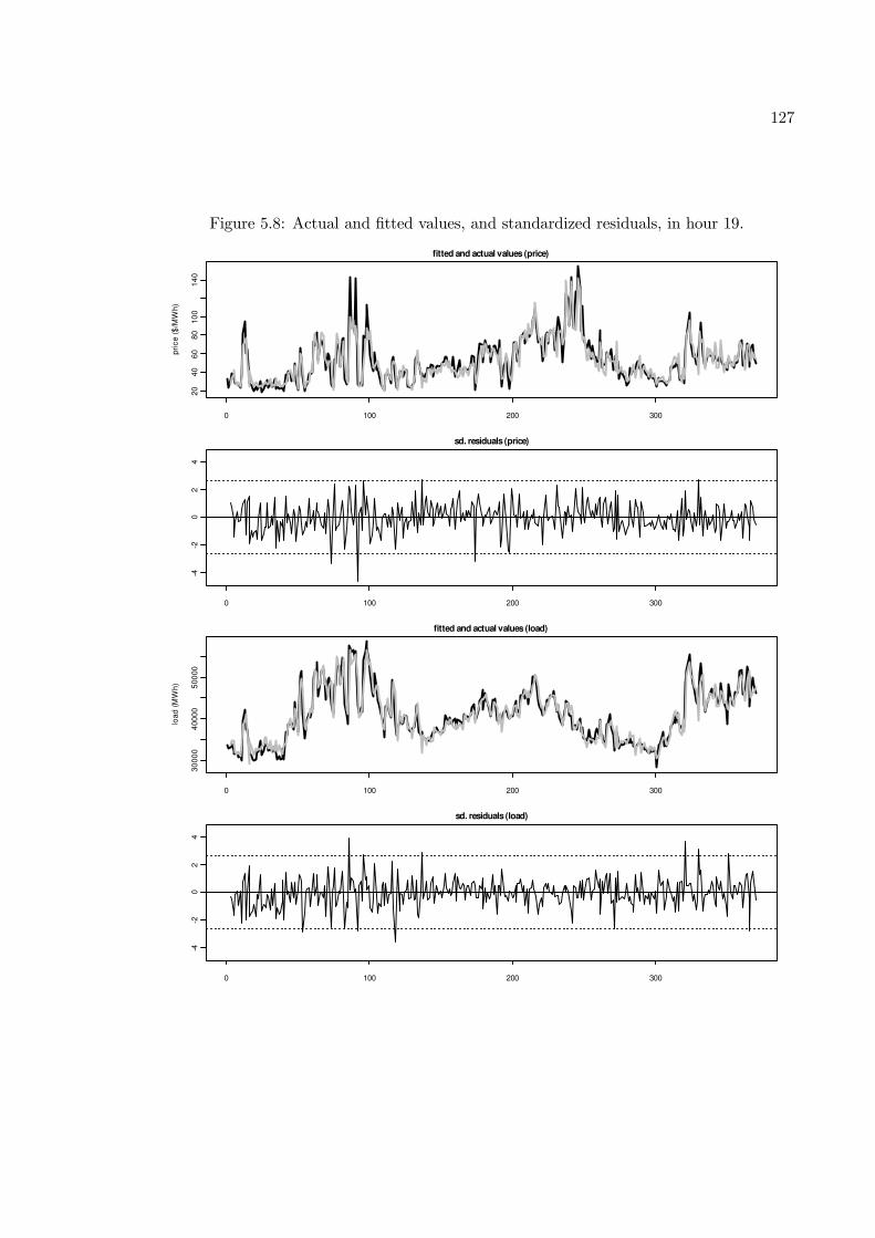
127
Figure 5.8: Actual and fitted values, and standardized residuals, in hour 19.
0 100 200 300
20
40
60
80
10
01
40
fitted and actual values (price)
pri
ce
($
/MW
h)
0 100 200 300
-4-2
02
4
sd. residuals (price)
0 100 200 300
30
00
04
00
00
50
00
0
fitted and actual values (load)
loa
d (
MW
h)
0 100 200 300
-4-2
02
4
sd. residuals (load)

128
to be equal. Moreover, there is no reaction to demand disequilibrium, i.e. quantity effects
the supply curves simply through the long-run and the short-run elasticities. Interestingly,
in the short run the supply curve is affected by the lagged gas price and not by the current
gas price. This feature may be due to a lack of synchronisation between the two markets:
PJM receives bids for the day-ahead market until 12.00 a.m. of the previous day, whereas
the Henry Hub day-ahead gas price closing time is at 1.00 p.m. Finally, festivity day
dummies are significant in both hours, showing that during holidays there is a consistent
reduction in electricity demand, both for baseload and peak.
As a final illustration, I use the model to simulate the reaction of the market to
a shock on the gas price, similar to the one which took place in February 2003. I keep
fixed all the other determinants (capacity, temperature and coal price) and start from a
situation of equilibrium in both the supply and the demand side. Then, I assume that
the gas price moves from 5.75 $/MMBtu to 12.2 $/MMBtu for 4 days to then goes back
to its initial level. The dynamic response of price and quantity are showed in figure 5.7.
At the beginning electricity price is lower than the level implied by the ‘long run’ supply
function and it gradually increases adjusting towards the equilibrium. Quantity is not
affected because, as long as price is lower than the equilibrium, industrial consumers do not
have incentives to change their short-run production patterns. When gas price decreases
again the electricity price is, for one day, higher than the equilibrium. Hence, demand is
temporarily reduced. In the ‘long run’ (which, in this framework, is a matter of a few days)
both quantity and price return to their previous equilibrium levels.
129
Figure 5.9: Simulated effect of a gas price shock on electricity traded quantity and price inhour 24
5.6 Conclusions
In this chapter a dynamic, structural econometric model that allows the identi-
fication and estimation of the supply and demand curves in electricity markets has been
illustrated and estimated on high frequency wholesale data. The approach proposed diverges
from the empirical dynamic models in the literature (see, for instance, Huisman and Mahieu
2003, Karakatsani and Bunn, 2005a, 2005b, and section 3.3.6). In fact, instead of focus-
ing only on price dynamics in a single equation framework, it considers price and quantity
interactions in a simultaneous system of equations. The identification procedure is based
on a theoretical economic model which describes supply and demand function in electricity
wholesale markets and, consequently, can be applied to the majority of the power markets

130
across the world. Therefore, the model is constructed to be estimated on high-frequency
(hourly) wholesale market data, which are public available in most of the countries in which
the electricity sector has been liberalised. Furthermore, the estimation method is robust
against the risk of spurious regression, since it is based on the cointegration methodology
introduced in Johansen (1991).
The model is founded on strong theoretical grounds and provides valid inference
regarding the parameters of the electricity supply and demand curves. In the empirical
application (on PJM market data), it is showed that an inelastic demand does not imply
that the quantity traded on the market is exogenous for the parameters of the long-run
supply function. Even when demand is completely inelastic to price, in fact, the quantity
traded on the market responds to past disequilibrium in the supply function. This effect is
significant and asymmetric, since demand reacts if price is higher than the equilibrium but
does not show any significant feedback if price is lower.
The first implication of this analysis is that the quantity cleared on the market
can be assumed as exogenous only if the interest is focused on its instantaneous influence
on price. It has been proven how this effect may significantly improve price forecasting (see,
among others, Conejo et al. 2005, Weron and Misiorek 2005) in a single equation framework,
but it remains an open question whether those predictions can be improved even more by
including quantity as endogenous. This seems to be the case in our framework, where
demand is influenced by positive disequilibrium on the supply side. On this point, lagged
prices have been already used to improve quantity forecasts (Chen et al., 2001).
The second implication is that, if the interest is on the structural relations that

131
characterise the supply side (i.e. the equilibrium supply function parameters) quantity needs
to be modelled as endogenous, at least in the market considered here. In those analyses
I observed through a unit root testing that more emphasis should be placed on the non-
stationarity issue, in order to restrict potential problems of spurious regression over the
time spans considered. Thirdly, the model shows how the reaction of consumers to high
prices can take place not only instantaneously (as considered, for instance, in Borenstein et
al. 2002b, Johnsen et al. 2004) but also after some delay. This feature assumes particular
relevance considering that demand side responsiveness to high prices has been proposed as
an effective way to mitigate market power (see Borenstein and Bushnell 1999, Borenstein
et al. 2002b, Borenstein 2004 and section 4.2). In this analysis, considering inter-temporal
effects (in particular the error-correction terms) would appear to be fundamental in order
to correctly determine the price-demand dynamic in the daily wholesale electricity market.
Fourth, the model gives also valuable insights for the developers of theoretical
models in a static framework. Particular attention in those cases has to be imposed on the
time horizon for which the model is designed and accordingly choose an appropriate value
of elasticity. In long-run models it seems sensible to approximate the dynamic effect of price
on quantity imposing a (small) significant elasticity in the static demand curve.
Fifth, significant differences have been identified between the baseload and the
peak hour. As expected, different marginal fuels characterise the two hours, but also the
effect of the available excess capacity and the semi-elasticity to temperature of demand are
diverse. These results bring additional support to the modelling philosophy entailing the
estimation of separate models for each hour of the day.

132
Sixth, it is worth mentioning that the application of cointegration techniques to
high-frequency data is not frequent in the literature. Examples are Baille and Bollerslev
(1989) and Diebold et al. (1994). This analysis shows the potential advantages of this
method in the context of electricity market.
Aspects of further development are not absent. In particular, since the model
analyses separately each hour of the day, it does not embed the possibility of intra-daily
effects among different hourly prices and quantities. This aspect is not likely to be sub-
stantial in many wholesale markets (like PJM or Italy), where electricity quantities for all
the hours of the following day are traded in contemporaneous auctions, but deserves careful
examination. In particular, it may be significant in markets where electricity is traded each
period at a time, like in UK or Ontario (see section 2.3). The results in this analysis suggest
that a panel cointegrating approach can potentially give important insights on this issue.

133
Chapter 6
Conclusions
Liberalisation has been interesting the power sector for almost two decades. Never-
theless, in competitive electricity markets, price formation and dynamics are only partially
understood. In particular the non-storability of electricity, episodes of market power abuse
and constraints of the market design create a peculiar environment which ultimately gen-
erates a dynamic behaviour which differs completely from those of other commodities.
Although research on electricity markets is diverse and extensive, it has mainly fo-
cused on (1) the idiosyncratic statistical properties of price and quantity (chapter 3) and on
(2) general equilibrium properties used, under certain assumption of agent’s behaviour and
market structure, to evaluate market efficiency and in particular the potential market power
from the supply side (chapter 4.2). However, few attempts have been made to test those
assumptions on high-frequency, real market data, and crucial issues like the elasticity of the
aggregated demand are still unresolved (chapter 4.3). On the other hand, existing dynamic
models for day-ahead electricity prices present some limitation: (i) they are primarily con-

134
strained to autoregressive effects, seasonal and climate factors which, although important,
are insufficient to explain price formation, (ii) they lack of economic interpretability and are,
in general, reduced form equations in which quantity and margin are assumed exogenous a
priori.
To address open research issues on price formation in day-ahead, wholesale elec-
tricity markets, this thesis defines an original econometric methodology which combines
statistical accuracy with economic interpretability. This approach provides valid empirical
inference on the supply and demand curves in high-frequency (hourly) day-ahead electricity
markets. Through a detailed specification of the response of demand to price, the model is
used (chapter 5) to give important insights on the debated demand elasticity issue, directly
estimating this parameter on wholesale market data.
In terms of methodology, this approach enlightens the benefits of extending a mod-
elling strategy historically implemented in a macroeconomic framework to micro-economic,
high-frequency data. The first step is, in fact, a reduced-form VAR, in which all the vari-
ables (quantity, price, fuel prices and excess capacity) are jointly modelled as endogenous.
Therefore, after rejecting the stationarity of the time series considered, the variables are
tested for co-integration and, through an in-depth testing procedure, the structural model
is derived as a parsimonious reduction of the statistical model describing the data. This
data-based, general to specific approach is advocated, among others, in Hendry and Mizon
(1993), Johansen and Juselius (1994) and Hendry (1995).
The final model is an asymmetric, structural, vector error-correction model (A-
VECM) which directly estimates on day-ahead, hourly wholesale market data the aggre-

135
gated demand and supply curves, distinguishing between short and long-run. Consequently,
the model can be used to simulate the dynamic effects of a variation of the underlying pro-
duction costs (for instance, fuel prices) on the electricity traded quantity and price. From a
modelling specification perspective this reveals that the traded quantity cannot be consid-
ered as exogenous (neither weakly, nor strongly) a priori even for the short-run parameters.
On the contrary, this assumption must be carefully evaluated since it may lead to inefficient
parameter estimation and sub-optimal forecasting performances. In the empirical applica-
tion on PJM market data (chapter 5.5), in fact, it is showed that an inelastic demand does
not imply that the quantity traded on the market is exogenous for the parameters of the
long-run supply function.
From an quantitative economic viewpoint, this thesis shows how the response
of electricity demand to price can take place through a complex mechanism that can be
hardly summarised using only one elasticity parameter. In this analysis I identify three
different ways in which demand may react to a supply shock: instantaneously, in terms of
an econometrically estimated equilibrium and through an error-correction mechanism. Even
though instantaneously demand is essentially inelastic to price, the quantity traded on the
market does responds to past disequilibrium in the supply function (i.e. to prices different
from their “equilibrium values”) through an error-correction mechanism. This effect is
significant and asymmetric, since demand reacts if price is higher than the equilibrium but
do not show any significant feedback if price is lower. This behaviour is consistent with
the empirical findings in Callaway and Weale (2005), where it is showed that industrial
consumers can temporarily reduce their demand for electricity (shutting down production

136
or using their own back-up generators) when prices are perceived as too high. Furthermore,
it is showed how different hours of the day are characterised by substantial heterogeneity.
This reflects the variation of demand characteristics, and particularly the differences in the
marginal plant fuels, which is mainly coal in the baseload and almost always natural gas
during the peak. Without imposing any a priori, this intuition is reflected in the model
estimates.
Overall, this thesis suggests that a comprehensive econometric model, specified at
high-frequency level, can represent adequately the complexities and subtleties of the price
formation process in wholesale electricity markets, achieving both an adequate statistical
representation of the idiosyncratic price dynamics and a structural, economic interpretabil-
ity.

137
Bibliography
[1] Andersson B., Bergman L. (1995) Market structure and the price of electricity: an ex
ante analysis of the deregulated Swedish electricity market, The Energy Journal, vol.
16, No. 2, 1995, pp. 97-130
[2] Asar A., McDonald J.R. (1994) A specification of neural network applications in the
load forecasting problem, IEEE Transaction on Control System Technology, vol. 2, No.
2, June 1994, pp. 134-141
[3] Atkins F.J., Chen J. (2002) Some statistical properties of deregulated electricity prices
in Alberta, working paper, 2002-06, University of Calgary
[4] Baker M.P., Mayfield S., Parsons J.E. (1998) Alternative models of uncertain com-
modity price for use with modern asset pricing methods, The Energy Journal, vol. 19,
No. 1, 1999, pp. 115-148
[5] Baille, R. T. (1996) Long memory processes and fractional integration in econometrics,
Journal of Econometrics, vol. 73, 1996, pp. 5-59
[6] Baillie R.T., Bollerslev T. (1989) Common stochastic trends in a system of exchange
rates, Journal of Finance, vol. 44, n. 1, pp. 167-181
138
[7] Baldik R., Grant R., Kahn E. (2004) Theory and application of linear supply equilib-
rium function in electricity markets, Journal of Regulatory Economics, vol. 25, No.
2, 2004, pp. 143-167
[8] Banerjee A., Dolado J.J., Galbraith J.W., Hendry D.F. (1993) Co-integration, error-
correction and the econometric analysis of non-stationary data, Advanced Text in
Econometrics, Oxford University Press
[9] Beran J. (1994) Statistics for long memory processes, Chapman and Hall, London,1994
[10] Blough S.R. (1992) The relationship between power and level for generic unit root test
in finite samples, Journal of Applied Econometrics, vol. 7, pp. 295-308
[11] Bollerslev, T. (1986) Generalised Autoregressive Conditional Heteroskedasticity, Jour-
nal of Econometrics, vol. 31, 307-327
[12] Borenstein S. (2004) The long-run effects of real-time electricity pricing, CSEMWork-
ing Paper No. 133, University of California Energy Institute
[13] Borenstein S., Bushnell J. (1999) An empirical analysis of the potential for market
power in California’s electricity market, Journal of Industrial Economics, vol. 47, n.
3, 1999, pp. 285-323
[14] Borenstein S., Bushnell J., Knittel C.R. (1999) Market power in electricity markets:
beyond concentration measures, The Energy Journal, vol. 20, n. 4, 1999, pp. 65-88
[15] Borenstein S., Bushnell J., F. A. Wolak (2002a) Measuring market inefficiencies in
139
California’s restructured wholesale electricity market, American Economic Review,
vol. 92, n. 5, 2002, pp. 1376-1405
[16] Borenstein S., Jaske M., Rosenfeld A. (2002b) Dynamic pricing, advanced metering
and demand response in electricity markets, CSEMWorking Paper No. 105, University
of California Energy Institute
[17] Borenstein S., Cameron A.C., Gilbert R. (1997) Do gasoline prices respond asymmet-
rically to crude oil price changes?, Quarterly Journal of Economics, vol. 112, 1997,
pp. 305-339
[18] Bower J. (2004) Price impact of horizontal mergers in the British generation market,
in Modelling prices in competitive electricity markets, in (ed.: D.W. Bunn) Modelling
prices in competitive electricity markets, Wiley & Sons, Chichester, pp. 99-126
[19] Bower J., Bunn D.W. (2001) Experimental analysis of the efficiency of uniform-price
versus discriminatory auctions in the England and Wales electricity market, Journal
of Economic Dynamics and Control, vol. 25, 2001, pp. 561-92
[20] Bowerman B. L., O’Connell R.T. (1979) Time Series and Forecasting: An Applied
Approach, Duxbury Press
[21] Box G.E.P., Jenkins G.M. (1970) Time series analysis, forecasting and control,
Holdey-Day, San Francisco, California
[22] Brace M.C., Bui-Nguyen V., Schmidt J. (1993) Another look at forecast accuracy of
neural networks, Second International Forum on the Application of Neural Networks
to Power Systems, April 19-22, 1993, Yokohama, Japan
140
[23] Bresnahan T.F., (1982)The oligopoly solution concept is identified, Economics Letters,
vol. 10, 1982, pp. 87-92
[24] Bunn D.W. (2003) Structural and behavioural foundations of competitive electricity
prices, in (ed.: D.W. Bunn) Modelling prices in competitive electricity markets, Wiley
& Sons, Chichester, pp. 1-17
[25] Bunn D.W., Farmer E.D. (1985) Comparative models for electrical load forecasting,
Belfast, John Wiley & Sons, 1985
[26] Bunn D.W., Oliveira F. (2001) Agent-based simulation: an application to the New
Electricity Trading Arrangements of England and Wales, IEEE Transactions on Evo-
lutionary Computation, vol. 5, No. 5, October 2001, pp. 493-503
[27] Bushnell J., Mansur E.T., Saravia C. (2004) Market structure and competition: a
cross-market analysis of U.S. electricity deregulation, CSEM Working Paper No. 126,
University of California Energy Institute
[28] Campbell J.Y., Perron P. (1991) Pitfalls and opportunities: what macroeconomist
should know about unit roots, in Blanchard O.J., Fisher S., NBER Economics Annual
1991, MIT Press
[29] Callaway M., Weale G. (2005) Estimation of industrial buyers’ potential demand re-
sponse to short period of high gas and electricity prices, Global Insight report for DTI
and OFGEM, 2005
[30] Cavaliere G. (2004) Unit root tests under time-varying variances, Econometric Re-
views, Vol. 23, No. 4, 2004, pp. 259-292

141
[31] CESI (2005) Indagine conoscitiva sullo stato della liberalizzazione nel settore
dell’energia elettrica, 2005, Milan (in Italian)
[32] Chen H., Canizares C.A., Singh A. (2001) ANN-based short term load forecasting in
electricity markets, IEEE Power Engineering Society Transmission and Distribution
Conference, 2001, pp. 411-415
[33] Chen L.-H., Finney M., Lai K.-S. (2005) A threshold cointegration analysis of asym-
metric transmission from crude oil to gasoline prices, Economics Letters, vol. 89,
2005, pp. 233-239
[34] Cho M.Y., Hwang J.C., Chen C.S. (1995) Customer short term load forecasting by
using ARIMA transfer function model, Proceedings of the international conference on
energy management and power delivery, vol.1, 1995, pp. 317-322
[35] Clarida, R. H., L. Sarno, M. P. Taylor, and G. Valente (2003) The out-of-sample
success of term structure models as exchange rate predictors: a step beyond, Journal
of International Economics, vol. 60, 2003, pp. 61-83.
[36] Cochrane J.H. (1991) A critique of the application of unit root tests, Journal of Eco-
nomic Dynamics and Control, vol. 15, 1991, pp. 275-284
[37] Conejo A.J., Contreras J., Espinola R, Plazas M.A. (2005) Forecasting electricity
prices for a day-ahead pool-based electric energy market, International Journal of Fore-
casting, vol. 21, 2005, pp. 435-462
[38] Contreras J., Espinola R., Nogales F.J., Conejo A.J. (2003) ARIMA models to predict
142
next-day electricity prices, IEEE Transaction on Power Systems, vol. 18, No. 3, August
2003, pp. 1014-1020
[39] Czernichow T., Piras A., Imhof K., Caire P., Jaccard Y., Dorizzi B., Germond A.
(1996) Short term electrical load forecasting with artificial neural networks, Engineer-
ing Intelligent Systems, vol. 2, 1996, pp. 85-89
[40] Dagum E. B. (2002) Analisi delle serie storiche: modellistica, previsione e scompo-
sizione (in Italian), Springer, 2002, Milan.
[41] Davidson, J. (1994) Identifying cointegrating regressions by the rank condition, Oxford
Bulletin of Economics and Statistics, vol. 56, 1994, pp. 105-110
[42] Davidson J. (1998) Structural relations, cointegration and identification: some simple
results and their application, Journal of Econometrics, vol. 87, 1998, pp. 87-113
[43] Davidson J.E.H., Hendry D.F., Srba F., Yeo J.S. (1978) Econometric modelling of the
aggregate time-series relationship between consumers’ expenditure and income in the
United Kingdom, Economic Journal, vol. 88, pp. 661-692. Reprinted in Hendry D.F.
(1993) Econometrics: Alchemy or Science? Blackwell Publishers, Oxford.
[44] De Jong C. (2006) The nature of power spikes: a regime-switch approach, Studies in
Nonlinear Dynamics and Econometrics, vol. 10, n. 3, 2006, article 3
[45] De Jong C., Huisman R. (2003) Option pricing for power prices with spikes, Energy
Power Risk Managment, vol. 7, 2003, pp. 12-16
[46] Deng S. (2000) Stochastic models of energy commodity prices and their applications:
143
mean reversion with jumps and spikes, Power Working Paper No. 073, University of
California Energy Institute.
[47] De Vany A.S., Walls W.D. (1999) Cointegration analysis of spot electricity prices:
insight on transmission efficiency in the western US, Energy Economics, vol. 21, pp.
435-448
[48] Development Committee (2006) An investment framework for clean energy and de-
velopment: a progress report, September 2006.
[49] Diebold F.X., Gardeazabal J., Yilmaz K. (1994) On cointegration and exchange rate
dynamics, The Journal of Finance, vol. 49, n. 2, pp. 727-735
[50] Dickey D.A., Bell W.R., Miller R.B (1986) Unit root in time series models: tests and
implications, The American Statistician, vol. 40, 1986, pp. 12-26.
[51] Dickey D. A., Fuller W. A. (1979) Distribution of the estimator for autoregressive
time series with a unit root, Journal of the American Statistical Association , vol. 74,
1979, pp. 427— 31.
[52] Dickey D.A., Hasza D.P., Fuller W.A (1984) Testing for unit roots in seasonal time
series, Journal of the American Statistical Association, vol. 79, pp. 355-367.
[53] Dixit A. K., Pindyck R. S. (1994) Investment under uncertanty, Princeton, New Jer-
sey, Princeton University Press
[54] Doornik J.A., Hansen H. (1994) An omnibus test for univariate and multivariate
normality, Working Paper, Nuffield College, Oxford.

144
[55] Doornik J.A., Hendry D.F. (1997) Modelling dynamic systems using PcFiml 9.0 for
Windows, International Thomson Business Press, 1997, London.
[56] Duffie D., Gray S., Hoang, P. (1998) Volatility in energy prices, in Managing Energy
Price Risk, Risk Publications, 1998, London.
[57] Durbin J., Watson G.S. (1951) Testing for serial correlation in least squares regression
II, Biometrika, vol. 38, 1951, pp. 159-178
[58] Enders W., Granger C.W.J. (1998)Unit-root tests and asymmetric adjustment with an
example using the term structure of interest rates, Journal of Business and Economics
Statistics, vol. 16, 1998, pp. 304-311
[59] Enders W., Siklos P.L. (2001) Cointegration and threshold adjustment, Journal of
Business and Economic Statistics, vol. 19, 2001, pp. 166-176
[60] Engle, R.F. (1982) Autoregressive Conditional Heteroskedasticity with Estimates of
the Variance of U.K. Inflation, Econometrica, vol. 50, 987-1008.
[61] Engle R.F., Granger C.W.J (1987) Co-integration and error correction: representa-
tion, estimation and testing, Econometrica, vol. 55, No. 2, 1987, pp. 251-276
[62] Engle R. F., Granger C. W. J., Rice J. Weiss A. (1986) Semiparametric estimates of
the relation between weather and electricity sales, Journal of the American Statistical
Association, vol. 81, 1986, pp. 310-320
[63] Engle R.F., Hendry D.F., Richard J.F. (1983) Exogeneity, Econometrica, vol. 51, n.
2, 1983, pp. 277-304

145
[64] Ericsson N.R. (1992) Cointegration, exogeneity, and policy analysis: an overview,
Journal of Policy Modelling, vol. 14, n. 3, 1992, pp. 251-280
[65] Escribano A., Pena J.I., Villaplana P. (2002)Modeling electricity prices: international
evidence, working paper, 02-27, University Carlos III, Madrid
[66] European Commission (2005) Directive concerning measures to safeguard security of
electricity supply and infrastructure investment, May 2005.
[67] Fabra N., Toro J. (2005) Price war and collusion in the Spanish electricity market,
International Journal of Industrial Organization, vol. 23, No. 3-4, 2005, pp. 155-181
[68] Gellings C.W. (1996) Demand forecasting for electric utilities, Fairmont Press, Lil-
burn, GA, 1996
[69] Geweke J., Porter-Hudak S. (1983) The estimation and application of long memory
time series models, Journal of time series analysis, vol. 4, 1983, pp. 221-238
[70] Ghysels E., Lee H.S., Noh J. (1994) Testing for unit roots in seasonal time series,
Journal of Econometrics, vol. 62, pp. 415-422
[71] Gonzalo J. (1994) Five alternative methods of estimating long-run equilibrium rela-
tionships, Journal of Econometrics, vol. 60, No. 1, 1994, pp. 203-233
[72] Goto M., Karolyi G., (2004) Understanding electricity price volatility within and
across markets, working paper, Ohio University
[73] Granger C.W.J. (1981) Some properties of time series data and their use in econo-
metric model specification, Journal of Econometrics, vol. 16, pp. 121-130

146
[74] Granger C.W.J., Lee T.H. (1989) Investigation of production, sales and inventory rela-
tionships using multicointegration and non-symmetric error correction models, Journal
of Applied Econometrics, vol. 4, 1989, pp.145-159
[75] Granger C.W.J., Newbold p. (1974) Spurious regression in econometrics, Journal of
Econometrics, vol. 2, 1974, pp. 111-120
[76] Green R.J. (1996) Increasing competition in the British electricity spot market, Journal
of Industrial Economics, vol. 44, No 2, 1996, pp. 205-216.
[77] Green R.J., Newbery D.M. (1992) Competition in the British electricity spot market,
Journal of Political Economy, vol. 100, No. 5, 1992, pp. 929-953
[78] Growitsch C., Wein T. (2005) Network access charges, vertical integration, and prop-
erty rights structure—experiences from the German electricity markets, Energy Eco-
nomics, vol. 27(2), 2005, pp. 257-278
[79] Guthrie G., Videbeck S. (2002) High frequency electricity spot price dynamics: an
intra-day approach, Working Paper, New Zeland Institute for the study of competition
and regulation, 2002.
[80] Haldrup N., Nielsen M.O. (2006a) A regime switching long memory model for elec-
tricity prices, Journal of Econometrics, 2006, vol. 135, issue 1-2, 2006, pages 349-376.
[81] Haldrup N., Nielsen M.O. (2006b) Directional congestion and regime switching in a
long memory model for electricity prices, Studies in Nonlinear Dynamics and Econo-
metrics, vol. 10, n. 3, 2006, article 1
147
[82] Harvey A., Koopman S.J. (1993) Forecasting hourly electricity demand using time-
varying splines, Journal of the American Statistical Association, vol. 88, 1993, pp.
1228-1236
[83] Haykin S. (1994) Neural networks, a comprehensive foundation, New York, MacMillan
College Publ. Co.b, 1994
[84] Hendry D.F. (1980) Econometrics: Alchemy or Science?, Economica, vol. 47, 1980,
pp. 387-406. Reprinted in Hendry D.F: (1993) Econometrics: Alchemy or Science?,
Oxford, Blackwell Publishers
[85] Hendry D.F. (1995) Dynamic Econometrics, Oxford University Press, 1995, Oxford.
[86] Hendry D.F., Anderson G.J. (1977) Testing dynamic specification in small simulta-
neous system: an application to a model of building society behaviour in the United
Kingdom, in Intriligator, M.D. (ed.), Frontiers in Quantitative Economics, vol. 3, pp.
361-383, North Hollad, Amsterdam. Reprinted in Hendry D.F. (1993), Econometrics:
Alchemy or Science? Blackwell Publishers, Oxford.
[87] Hendry D.F., Mizon G.E. (1993) Evaluating dynamic models by encompassing the
VAR, in P.C.B. Phillips ed.: Models, methods, and applications of econometrics,
Blackwell, Oxford, 1993, pp. 272-300
[88] Hendry D.F., Juselius K. (2000) Explaining cointegration analysis: Part I, The Energy
Journal, vol. 21, 2000, pp. 1-42
[89] Hendry D.F., Juselius K. (2001) Explaining cointegration analysis: Part II, The En-
ergy Journal, vol. 22, 2001, pp. 75-120

148
[90] Henley A., Peirson J. (1997) Non-linearities in electricity demand and temperature:
parametric versus non-parametric methods, Oxford Bulletin of Economics and Statis-
tics, vol. 59, No. 1, 1997, pp. 149-162
[91] Hinich M.J., Serletis A. (2006) Randomly modulated periodic signals in Alberta’s elec-
tricity market, Studies in Nonlinear Dynamics and Econometrics, vol. 10, n. 3, 2006,
article 5
[92] Hippert H., Pedreira C., Souza R. (2001) Neural networks for short-term load fore-
casting: A review and evaluation, IEEE Transaction on Power System, vol. 16, No. 1,
2001, pp. 44-55
[93] Hjalmarsson E. (2002) Nord Pool: a power market without market power, Working
Paper in Economics n. 28, 2002, Göteborg University
[94] Hsiao C. (1997) Cointegration and dynamic simultaneous equations model, Economet-
rica, vol. 65, 1997, pp. 647-670
[95] Huang, S. R. (1997) Short term load forecasting using threshold autoregressive models,
IEE Proceedings on Generation, Transmission and Distribution, vol. 144, No. 5, 1997,
pp. 477-481
[96] Huang S.J., Shih K.R. (2003) Short-term load forecasting via ARMA model identi-
fication including non-Gaussian process consideration, IEEE Transaction on Power
Systems, vol. 18, n.2, 2003, pp. 673-679
[97] Huisman R., Mahieu R. (2003) Regime jumps in electricity prices, Energy Economics,
vol. 25, 2003, pp. 425-434

149
[98] Hunt S. (2002) Making competition work in electricity, John Wiley and Sons, New
York
[99] Hyde O., Hodnett P.F. (1997) An adaptable automated procedure for short-term elec-
tricity load forecasting, IEEE Transactions on Power System, vol. 13, n. 3, 1998, pp.
1115-1120
[100] Hylleberg S., Engle R.F., Granger C.W.J, Yoo B.S. (1990) Seasonal integration and
cointegration, Journal of Econometrics, vol. 44, 1990, pp. 215-238
[101] Karakatsani N., Bunn D.W. (2005a) Structural and dynamic properties of the low
British electricity wholesale prices 2001—2002, Working Paper, London Business
School
[102] Karakatsani N., Bunn D.W. (2005b)Modelling stochastic volatility in high-frequencies
spot electricity prices, Working Paper, London Business School
[103] Kim D.W., Knittel C.R. (2004) Biases in static oligopoly models? Evidence from the
California electricity market, CSEM Working Paper No. 131, University of California
Energy Institute.
[104] Khotanzad A., Afkhami-Rohani T.L., Maratukulam D. (1998) ANNSTLF - Artificial
neural network short-term load forecaster - generation three, IEEE Transaction on
Power System, vol. 13, No. 4, Novembre 1998, pp. 1413-1422
[105] Knittel C. (2003) Market structure and the pricing of electricity and natural gas,
Journal of Industrial Economics, vol. 51, n. 2, 2003, pp. 167-191
150
[106] Knittel C.R., Roberts M.R (2005) An empirical examination of restructured electricity
prices, Energy Economics, vol. 27, 2005, pp. 791-817
[107] Krolzig H.-M. (1997) Markov switching vector autoregressions. Modelling, Statistical
inference and application to business cycle analysis, Springer, 1997, Berlin.
[108] Krolzig H.-M., Marcellino M., Mizon G.E. (2002), A Markov-switching vector equilib-
rium correction model of the UK labour market, Empirical Economics, vol. 27, 2002,
pp. 233-254.
[109] Kwiatkowski D., Phillips P.C.B, Schmidt P., Shin Y. (1992) Testing the null hypothesis
of stationarity against the alternative of a unit root, Journal of Econometrics, vol. 54,
1992, pp. 159-178
[110] Jin S., Phillips C.B. (2002) The KPSS test with seasonal dummies, Cowles Foundation
Discussion Paper No 1373, 2002, Yale University
[111] Johansen S. (1988) Statistical analysis of cointegration vectors, Journal of Economic
Dynamics and Control, vol. 12, 1988, n. 231-254
[112] Johansen S. (1991) Estimation and hypothesis testing of cointegration vectors in
Gaussian vector autoregressive models, Econometrica, vol. 59, No. 6, 1991, pp. 1551-
1580
[113] Johansen S. (1992) Testing weak exogeneity and the order of cointegration in UK
money demand data, Journal of Policy Modelling, vol. 14, n. 3, 1992, pp. 313-334
151
[114] Johansen S. (1995) Identifying restriction of linear equations with applications to si-
multaneous equations and cointegration, Journal of Econometrics, vol. 69, pp. 111-132
[115] Johansen S. (1996) Likelihood-based inference in cointegrated vector autoregressive
models, Oxford University Press, Oxford
[116] Johansen S., Juselius K. (1990)Maximum likelihood estimation and inference on coin-
tegration, with application to the demand for money, Oxford Bulletin of Economics
and Statistics, vol. 52, n. 2, 1990, pp. 169-210
[117] Johansen S., Juselius K. (1994) Identification of the long-run and short-run structure.
An application to the IS-LM model, Journal of Econometrics, vol. 63, 1994, pp. 7-36
[118] Johnsen A., Verma S.K., Wolfram C. (2004) Zonal pricing and demand-side respon-
siveness in the Norwegian electricity market, Power Working Paper 063, 2004
[119] Johnston J. (1984) Econometric methods, 3rd edition, Mc Graw Hill, 1984, New York
[120] Joskow P.L., Kahn E. (2002) A quantitative analysis of pricing behaviour in Califor-
nia’s wholesale electricity market during summer 2000, The Energy Journal, vol. 23,
pp. 1—35.
[121] International Energy Agency (2005) Lessons from liberalised electricity markets,
IEA/OECD, 2005, Paris
[122] Lau L.J. (1982) On identifying the degree of competitiveness from industry price and
output data, Economics Letters, vol. 10, 1982, pp. 93-99.
152
[123] Leon A., Rubia A. (2004) Forecasting time-varying covariance matrices in the in-
tradaily spot market of Argentina, in (ed.: D.W. Bunn) Modelling prices in competi-
tive electricity markets, Wiley & Sons, Chichester, pp. 177-189
[124] Leon A., Rubia A. (2004) Testing for weekly seasonal unit roots in the Spanish power
pool, in (Bunn D.) Modelling prices in competitive electricity markets, John Wiley
and Sons, Chichester, pp. 131-145.
[125] Lise W., Kemfert C., Tol R.S.J. (2003) Strategic actions in the liberalised German
electricity market, Fondazione Eni Enrico Mattei Working Paper 3.2003, 2003.
[126] Longstaff F.A., Wang A.W. (2004) Electricity forward prices: a high-frequency em-
pirical analysis, Journal of Finance, vol. 59, No. 4, 2004, pp. 1877-1900
[127] Lütkepohl H., Krätzing M. (2004) Applied time series econometrics, Cambridge Uni-
versity Press, 2004, Cambridge.
[128] Maddala G.S., Kim I.M. (1998) Unit roots, cointegration and structural change, Cam-
bridge University Press, Cambridge.
[129] Mansur (2003)Vertical integration in restructured electricity markets: measuring mar-
ket efficiency and firm conduct, Yale School of Management, Working Paper No. 32,
2003.
[130] Market Monitoring Unit (2004) PJM: 2003 state of the market report, PJM MMU,
2004.
153
[131] Misiorek A., Weron R. (2006) Interval forecasting for spot electricity prices, Proceed-
ings of the EEM-06 International Conference, Warsaw, 2006, pp. 212-220
[132] Misiorek A., Trueck S., Weron R. (2006) Point and interval forecasting of spot elec-
tricity prices: linear vs. non-linear time series models, Studies in Nonlinear Dynamics
and Econometrics, vol. 10, n. 3, 2006, article 2
[133] Moghram I., Rahman S.(1989) Analysis and evaluation of five short term load fore-
casting techniques, IEEE Transactions on Power System, vol. 4, No. 4, Ottobre 1989,
pp. 1484-1491
[134] Mohammed O., Park D., Merchant R., Dinh T., Tong C., Azeem A., Farah J., Drake
C. (1995) Practical experiences with an adaptive neural network short-term load fore-
casting system, IEEE Transactions on Power Systems, Vol. 10, No. 1, February 1995,
pp. 254 - 265
[135] Mount D.T., Ning Y., Cai X. (2006) Predicting price spikes in electricity markets using
a regime-switching model with time-varying parameters, Energy Economics, vol. 28,
n. 1, 2006, pp. 62-80
[136] Nowicka-Zagrajek J., Weron R. (2002)Modeling electricity loads in California: ARMA
models with hyperbolic noise, Signal Processing, vol. 82, 2002, pp. 1903-1915
[137] Papalexopoulos A. D., Hesterberg T.C. (1990) A regression based approach to short
system load forecasting, IEEE Transaction on Power Systems, vol. 5, No. 4, Novembre
1990, pp. 1535-1547

154
[138] Park D.C., El-Sharkawi M.A., Marks R.J., Atlas L.E., Damborg M.J. (1991) Electric
load forecasting using an artificial neural network, IEEE Trans. Power Systems, vol.
6, n. 2, 1991, pp. 442-449.
[139] Patrick R.H., Wolak F.A. (2001) Estimating the consumer level demand for electricity
under real-time market prices, NBER working paper n. 8213, 2001
[140] Perron P. (1988) Trends and random walks in macroeconomic time series: further
evidence from a new approach, Journal of Economics, Dynamics and Control, vol. 12,
pp. 297-332
[141] Pesaran M.H., Smith R.P. (1998) Structural analysis of cointegrating VARs, Journal
of Economic Surveys, vol. 12, n. 5, 1998, pp. 471-505
[142] Pesaran M.H., Shin Y., Smith R.P. (2000) Structural analysis of vector error-
correction models with exogenous I(1) variables, Journal of Econometrics, vol. 97,
2000, pp. 293-343.
[143] Phillips P.C.B. (1986) Understanding spurious regression in econometrics, Journal of
Econometrics, vol. 33, 1986, pp. 331-340
[144] Phillips P.C.B., Hansen B.E. (1990) Statistical inference in instrumental variables
regression with I(1) processes, The Review of Economic Studies, vol. 57, pp. 99-125
[145] Phillips P.C.B, Perron P. (1988) Testing for a unit root in time series regression,
Biometrika, vol. 75, 1988, pp. 335-346
155
[146] Phillips P.C.B., Xiao Z. (1998) A primer on unit root testing, Journal of Economic
Surveys, vol. 12, No. 5, 1998, pp. 423-469
[147] Pindyck R.S. (1999) The long run evolution of energy prices, The Energy Journal,
vol. 20, No. 2, 1999, pp. 1-27
[148] Popova J. (2004) Spatial patterns in modelling electricity prices: evidence from the
PJM market, Working Paper, West Virginia University
[149] Ramanathan R., Engle R., Granger C.W.J., Vahid-Araghi F. (1997) Short-run fore-
casts of electricity loads and peaks, International Journal of Forecasting, vol. 13, 1997,
pp. 161-174
[150] Rodriguez C.P., Anders G.J. (2004) Energy price forecasting in the Ontario competi-
tive power system market, IEEE Transaction on Power Systems, vol. 19, No. 1, 2004,
pp. 366-374
[151] Rubia A. (2001) Testing for seasonal unit roots in daily electricity demand: evidence
from deregulated markets, Instituto Valenciano de Investigaciones Economicas, WP-
EC 2001-21
[152] Ruzic S., Vuckovic A., Nikolic N. (2003)Weather sensitive method for short-term load
forecasting in electric power utility of Serbia, IEEE Transaction on Power Systems,
vol. 18, 2003, pp. 1581-1586
[153] Said S.E., Dickey D.A. (1984) Testing for unit roots in autoregressive moving average
models of unknown order, Biometrika, vol. 71, 1984, pp. 599-608

156
[154] Saikkonen P., Luukkonen R. (1997) Testing cointegration in infinite order vector au-
toregressive processes, Journal of Econometrics, vol. 81, 1997, pp. 93-126.
[155] Sims (1980) Macroeconomics and reality, Econometrica, vol. 48, pp. 1-48.
[156] Simonsen I., Hansen A., Nes O. (1998) Determination of the Hurst exponent by use
of wavelet transforms, Physical Review E, vol. 58, 1998, pp. 2779-2787
[157] Soares L. J., Medeiros M.C. (2005) Modelling and forecasting short-term electricity
load: a two step methodology, working paper, University of Rio De Janeiro
[158] Soares L. J., Souza L.R. (2003) Forecasting electricity demand using generalized long
memory, working paper, EPGE
[159] Stevenson M. (2002) Filtering and forecasting spot electricity prices in the Australian
electricity market, working paper, University of Technology, Sydney
[160] Stevenson M., Do Amaral L.F., Peat M. (2006) Risk management and the role of
spot price predictions in the Australian retail electricity market, Studies in Nonlinear
Dynamics and Econometrics, vol. 10, n. 3, 2006, article 4
[161] Stock J., Watson M.W. (1993) A simple estimator of cointegrating vectors in higher
order integrated systems, Econometrica, vol. 61, pp. 783-820
[162] Stoft S. (2002) Power system economics: designing markets for electricity, IEEE
Press, Piscataway, Wiley Interscience
[163] Stridbaek U. (2006) Lessons from liberalised electricity markets in IEA member coun-

157
tries, in (Mielczarski W.) Complex Electricity Markets, collection of the invited papers
of the EEM-06 International Conference, Warsaw, 2006, pp. 21-45
[164] Taylor J.W. (2003) Short-term electricity demand forecasting using double seasonal
exponential smoothing, Journal of Operational Research Society, vol. 54, 2003, pp.
799-805
[165] Taylor J.W., De Menezes L., McSharry P.E. (2006) A comparison of univariate meth-
ods of forecasting energy demand up to a day ahead, International Journal of Fore-
casting, 2006 (forthcoming)
[166] Tillmann P. (2004) Cointegration and regime-switching risk premia in the US term
structure of interest rates, Proc. of the Econometric Society 2004 North American
Summer Meetings 26, Econometric Society.
[167] Tong H. (1983) Threshold models in non-linear time series analysis, 1983, Springer-
Verlag, New York
[168] Urbain J.P. (1995) Partial versus full system modelling of cointegrated system: an
empirical illustration, Journal of Econometrics, vol. 69, 1995, pp. 177-210
[169] Veit D., Fichtner W., Ragwitz M. (2004) Agent-based computational economics in
power markets — multi-agent based simulation as a tool for decision support, in (ed: J.
Andrysek, M. Karny, J. Kracik): Multiple participant decision making, International
Series on Advanced Intelligence, vol. 9, Advanced Knowledge International, Adelaide,
Australia, 2004.

158
[170] Weron R. (2006) Modelling and forecasting electricity loads and prices: a statistical
approach, 2006, Wiley & Sons
[171] Weron R., Misiorek A. (2005) Forecasting spot electricity prices with time series mod-
els, Proceedings of the European Electricity Market Conference, Lodz, Poland, May
2005, pp. 123-130
[172] Weron R., Simonsen I., Wilman P. (2004) Modeling highly volatile and seasonal mar-
kets: evidence from the Nord Pool electricity market, in: The Application of Econo-
physics, (ed.: H. Takayasu), Springer, Tokyo, pp. 182—191.
[173] Wolak F.A. (2003)Measuring unilateral market power in wholesale electricity markets:
the California Market 1998-2003, American Economic Review, vol. 93, No. 2, 2003,
pp. 425-430
[174] Wolak F. (2004) Lessons from international experience with electricity markets mon-
itoring, CSEM Working Paper No. 134, University of California Energy Institute
[175] Wolak F., Patrick R. (1997) The impact of market rules and market structure on the
price determination proces in he England and Wales electrcity market, CSEMWorking
Paper, University of California Energy Institute
[176] Wolfram C.D. (1999) Measuring duopoly power in the British electricity spot market,
American Economic Review, vol. 89, No. 4, 1999, pp. 805-826
[177] Worthington A.C., Higgs H. (2004) Transmission of price and volatility in the Aus-
tralian electricity spot markets, in (ed.: D.W. Bunn) Modelling prices in competitive
electricity markets, Wiley & Sons, Chichester, pp. 217-229

159
[178] Zhang G., Patuwo B.E., Hu M.Y. (1998) Forecasting with artificial neural networks:
the state of the art, International Journal of Forecasting, Vol. 14, 1998, pp. 35-62
[179] Zhou M., Yan Z., Ni Y.X., Li G., Nie Y. (2006) Electricity price forecasting with
confidence-interval estimation through an extended ARIMA approach, IEEE Proc. in
Generation, Transmission and Distribution, vol. 153, n. 2, 2006, pp. 187-195.
Related Documents