Econometric Methods for Policy Evaluation By Joan Llull *, § CEMFI. Winter 2016 I. Motivation: Structural vs Treatment Effect Approaches The evaluation of public (and private) policies is very important for efficiency, and ultimately to improve welfare. There is a vast literature in economics, mostly in public economics, but also in development economics and labor economics, devoted to the evaluation of different programs. Examples include training pro- grams, welfare programs, wage subsidies, minimum wage laws, taxation, Medicaid and other health policies, school policies, feeding programs, microcredit, and a va- riety of other forms of development assistance. These analyses aim at quantifying the effects of these policies on different outcomes, and ultimately on welfare. The classic approach to quantitative policy evaluation is the structural ap- proach. This approach specifies a class of theory-based models of individual choice, chooses the one within the class that best fits the data, and uses it to evaluate policies through simulation. This approach has the main advantage that it allows both ex-ante and ex-post policy evaluation, and that it permits evaluat- ing different variations of a similar policy without need to change the structure of the model or reestimate it (out of sample simulation). The main critique to this approach, though, is that there is a host of untestable functional form as- sumptions that undermine the force of the structural evidence because they have unknown implications for the results, give researchers too much discretion, and its complexity often affects transparency and replicability. Some people has argued that this approach puts too much emphasis on external validity at the expense of a more basic internal validity. During the last two decades, the treatment effect approach has established itself as an important competitor that has introduced a different language, dif- ferent priorities, techniques, and practices in applied work. This approach has changed the perception of evidence-based economics among economists, public opinion, and policy makers. The main goal of this approach is to evaluate (ex- * Departament d’Economia i Hist` oria Econ` omica. Universitat Aut` onoma de Barcelona. Fac- ultat d’Economia, Edifici B, Campus de Bellaterra, 08193, Cerdanyola del Vall` es, Barcelona (Spain). E-mail: joan.llull[at]movebarcelona[dot]eu. URL: http://pareto.uab.cat/jllull. § These materials are based on earlier materials from the course by Manuel Arellano, available at http://www.cemfi.es/∼arellano. 1

Welcome message from author
This document is posted to help you gain knowledge. Please leave a comment to let me know what you think about it! Share it to your friends and learn new things together.
Transcript

Econometric Methods for Policy Evaluation
By Joan Llull∗,§
CEMFI. Winter 2016
I. Motivation: Structural vs Treatment Effect Approaches
The evaluation of public (and private) policies is very important for efficiency,
and ultimately to improve welfare. There is a vast literature in economics, mostly
in public economics, but also in development economics and labor economics,
devoted to the evaluation of different programs. Examples include training pro-
grams, welfare programs, wage subsidies, minimum wage laws, taxation, Medicaid
and other health policies, school policies, feeding programs, microcredit, and a va-
riety of other forms of development assistance. These analyses aim at quantifying
the effects of these policies on different outcomes, and ultimately on welfare.
The classic approach to quantitative policy evaluation is the structural ap-
proach. This approach specifies a class of theory-based models of individual
choice, chooses the one within the class that best fits the data, and uses it to
evaluate policies through simulation. This approach has the main advantage that
it allows both ex-ante and ex-post policy evaluation, and that it permits evaluat-
ing different variations of a similar policy without need to change the structure
of the model or reestimate it (out of sample simulation). The main critique to
this approach, though, is that there is a host of untestable functional form as-
sumptions that undermine the force of the structural evidence because they have
unknown implications for the results, give researchers too much discretion, and its
complexity often affects transparency and replicability. Some people has argued
that this approach puts too much emphasis on external validity at the expense of
a more basic internal validity.
During the last two decades, the treatment effect approach has established
itself as an important competitor that has introduced a different language, dif-
ferent priorities, techniques, and practices in applied work. This approach has
changed the perception of evidence-based economics among economists, public
opinion, and policy makers. The main goal of this approach is to evaluate (ex-
∗ Departament d’Economia i Historia Economica. Universitat Autonoma de Barcelona. Fac-ultat d’Economia, Edifici B, Campus de Bellaterra, 08193, Cerdanyola del Valles, Barcelona(Spain). E-mail: joan.llull[at]movebarcelona[dot]eu. URL: http://pareto.uab.cat/jllull.§ These materials are based on earlier materials from the course by Manuel Arellano, available
at http://www.cemfi.es/∼arellano.
1

post) the impact of an existing policy by comparing the distribution of a chosen
outcome variable for individuals affected by the policy (the treatment group), with
the distribution of unaffected individuals (control group). The main challenge of
this approach is to find a way to perform the comparison in such a way that the
distribution of outcome for the control group serves as a good counterfactual for
the distribution of the outcome for the treated group in the absence of treatment.
The main focus of this approach is in the understanding of the sources of variation
in data with the objective of identifying the policy parameters, even though these
parameters are formally not valid representations of the outcomes of implement-
ing the same policy in an alternative environment, or of implementing variations
of the policy even to the same environment. Thus, this approach helps in the
assessment of future policies in a more informal way.
The main advantage of this approach is that, given its focus on internal validity,
the exercise gives transparent and credible identification. The main disadvantage
is that estimated parameters are not useful for welfare analysis because they are
not deep parameters (they are reduced-forms instead), and as a result, they are
not policy-invariant (Lucas, 1976; Heckman and Vytlacil, 2005). In that respect,
a treatment effect exercise is less ambitious.
The deep differences between the two approaches has split the economics profes-
sion into two camps whose research programs have evolved almost independently
despite focusing on similar questions (Chetty, 2009). However, recent develop-
ments have changed this trend, as researchers realized about the important com-
plementarity between the two. The survey articles by Chetty (2009) and Todd and
Wolpin (2010) review the progress made along those lines and point to avenues
for future developments.
In this part of the course we will review the main designs for policy evaluation
under the treatment effect approach. In the second part (with Pedro) you will
review structural approaches. And by the end of this part, if time permits, I will
introduce some bridges between the two, which will serve as an introduction to
the second part.
II. Potential Outcomes and Causality: Treatment Effects
A. Potential outcomes and treatment effects
Consider the population of individuals that are susceptible of a treatment. Let
Y1i denote the outcome for an individual i if exposed to the treatment (Di = 1),
and let Y0i be the outcome for the same individual if not exposed (Di = 0). The
treatment effect for individual i is thus Y1i − Y0i. Note that Y1i and Y0i are
2

potential outcomes in the sense that we only observe Yi = Y1iDi + Y0i(1−Di).
This poses the main challenge of this approach, as the treatment effect can not
be computed for a given individual. Fortunately, our interest is not in treatment
effects for specific individuals per se, but, instead, in some characteristics of their
distribution.
For most of the time, we will focus on two main parameters of interest. The
first one is the average treatment effect (ATE):
αATE ≡ E[Y1 − Y0], (1)
and the second one is average treatment effect on the treated (TT):
αTT ≡ E[Y1 − Y0|D = 1]. (2)
As noted, the main challenge is that we only observe Y . The standard measure
of association between Y and D (the regression coefficient) is:
β ≡ E[Y |D = 1]− E[Y |D = 0]
= E[Y1 − Y0|D = 1]︸ ︷︷ ︸αTT
+ (E[Y0|D = 1]− E[Y0|D = 0]), (3)
which differs from αTT unless the second term is equal to zero. The second term
indicates the difference in potential outcomes when untreated for individuals that
are actually treated and individuals that are not. A nonzero difference may result
from a situation in which treatment status is the result of individual decisions
where those with low Y0 choose treatment more frequently than those with high Y0.
From a structural model of D and Y , one could obtain the implied average
treatment effects. Instead, here, they are defined with respect to the distribution
of potential outcomes, so that, relative to the structure, they are reduced-form
causal effects. Econometrics has conventionally distinguished between reduced
form effects, uninterpretable but useful for prediction, and structural effects, as-
sociated with rules of behavior. The treatment effects provide this intermediate
category between predictive and structural effects, in the sense that recovered
parameters are causal effects, but they are uninterpretable in the same sense as
reduced form effects.
An important assumption of the potential outcome representation is that the
effect of the treatment on one individual is independent of the treatment received
by other individuals. This excludes equilibrium or feedback effects, as well as
strategic interactions among agents. Hence, the framework is not well suited
3

to the evaluation of system-wide reforms which are intended to have substantial
equilibrium effects.
Sample analogs for αATE and αTT are:
αSATE ≡1
N
N∑i=1
(Y1i − Y0i) (4)
αSTT ≡1∑N
i=1Di
N∑i=1
Di(Y1i − Y0i). (5)
If factual and counterfactual potential outcomes were observed, these quantities
could be estimated without error. However, since they are not, the distinction is
not very useful on practical grounds. Importantly, though, depending on whether
we estimate population (α) or sample (αS) average treatment effects, standard
errors will be different, so we should take this into account when computing con-
fidence intervals. The sample average version of β is given by:
βS ≡ YT − YC
≡ 1
N1
N∑i=1
YiDi −1
N0
N∑i=1
(1−Di)Yi, (6)
where N1 ≡∑N
i=1Di is the number of treated individuals, and N0 ≡ N − N1 is
the number of untreated.
B. Identification of treatment effects under different assumptions
The identification of the treatment effects depends on the assumptions we can
make on the relation between potential outcomes and the treatment. The easiest
case is when the distribution of the potential outcomes is independent of the
treatment:
(Y1, Y0) ⊥ D. (7)
This situation is typical in randomized experiments, where individuals are assigned
to treatment or control in a random manner. When this happens, F (Y1|D =
1) = F (Y1), and F (Y0|D = 0) = F (Y0), which implies that E[Y1] = E[Y1|D =
1] = E[Y |D = 1] and E[Y0] = E[Y0|D = 0] = E[Y |D = 0], and, as a result,
αATE = αTT = β. In this case, an unbiased estimate of αATE is given by the
difference between the average outcomes for treatments and controls:
αATE = YT − YC = βS. (8)
4

In this context, there is no need to “control” for other covariates, unless there is
direct interest in their marginal effects, or in effects for specific groups.
A less restrictive assumption is conditional independence:
(Y1, Y0) ⊥ D|X, (9)
where X is a vector of covariates. This situation is known as matching, as for
each “type” of individual (i.e. each value of covariates) we can match treated
and control individuals, so that the latter act as counterfactuals for the former.
Conditional independence implies E[Y1|X] = E[Y1|D = 1, X] = E[Y |D = 1, X]
and E[Y0|X] = E[Y0|D = 0, X] = E[Y |D = 0, X], and, as a result:
αATE = E[Y1 − Y0] =
∫E[Y1 − Y0|X]dF (X)
=
∫(E[Y |D = 1, X]− E[Y |D = 0, X])dF (X), (10)
or, in words, compute the difference in average observed outcomes of treated and
controls for each value of X, and integrate over the distribution of X. For the
treatment effect on the treated:
αTT =
∫E[Y1 − Y0|D = 1, X]dF (X|D = 1)
=
∫E[Y − E[Y0|D = 1, X]|D = 1, X]dF (X|D = 1)
=
∫E[Y − µ0(X)|D = 1, X]dF (X|D = 1), (11)
where µ0(X) ≡ E[Y |D = 0, X], and we use the fact that E[Y |D = 0, X] =
E[Y0|X] = E[Y0|D = 1, X]. The function µ0(X) is used as an imputation for Y0.
Finally, sometimes we cannot assume conditional independence:
(Y1, Y0) 6⊥ D|X. (12)
In this case, we will need some variable Z that constitutes an exogenous source
of variation in D, in the sense that it satisfies the independence assumption:
(Y1, Y0) ⊥ Z|X, (13)
and the relevance condition:
Z 6⊥ D|X. (14)
As we discuss below, in this context we are only going to be able to identify an
average treatment effect for a subgroup of individuals, and we call the resulting
parameter a local average treatment effect.
5

III. Social Experiments
In the treatment effect approach, a randomized field trial is regarded as the ideal
research design. Observational studies are seen as more speculative attempts
to generate the force of evidence of experiments. In a controlled experiment,
treatment status is randomly assigned by the researcher, which by construction,
ensures independence. Thus, as noted above, αATE = αTT = β.
There is a long history of randomized field trials in social welfare in the U.S.,
beginning in the 1960s (see Moffitt (2003) for a review). Early experiments had
many flaws due to the lack of experience in designing them, and in data analysis.
During the 1980s, the U.S. Federal Government started to encourage states to
use experimentation, eventually becoming almost mandatory. The analysis of the
1980s experimental data consisted of simple treatment-control differences. The
force of the results had a major influence on the 1988 legislation. In spite of these
developments, randomization encountered resistance from many U.S. states on
ethical grounds. Even more so in other countries, where treatment groups have
often been formed by selecting areas for treatment instead of individuals.
One example of this is the National Supported Work program (NSW), which
was designed in the U.S. in the mid 1970s to provide training and job opportu-
nities to disadvantaged workers, as part of an experimental demonstration. Ham
and LaLonde (1996) looked at the effects of the NSW on women that volunteered
for training. NSW guaranteed to treated participants 12 months of subsidized
employment (as trainees) in jobs with gradual increase in work standards. Eli-
gibility requirements were to be unemployed, a long-term AFDC recipient, and
have no preschool children. Participants were randomly assigned to treatment
and control groups in 1976-1977. The experiment took place in 7 cities. Ham and
LaLonde analyze data for 275 women in the treatment group and 266 controls.
All volunteered in 1976.
Thanks to randomization, a simple comparison between employment rates of
treatments and controls gives an unbiased estimate of the effect of the program
on employment at different horizons. Figure 1 from Ham and LaLonde (1996)
shows the effects. Initially, by construction there is a mechanical effect from the
fact that treated women are offered a subsidized job. As apparent from the figure,
compliance with the treatment is decreasing over time, as women can decide to
drop from the subsidized job. The employment growth for controls is just a
reflection of the program’s eligibility criteria. Importantly, after the program
ends, a 9 percentage points difference in employment rates is sustained in the
6
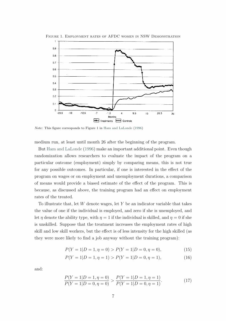
Figure 1. Employment rates of AFDC women in NSW Demonstration
Note: This figure corresponds to Figure 1 in Ham and LaLonde (1996)
medium run, at least until month 26 after the beginning of the program.
But Ham and LaLonde (1996) make an important additional point. Even though
randomization allows researchers to evaluate the impact of the program on a
particular outcome (employment) simply by comparing means, this is not true
for any possible outcomes. In particular, if one is interested in the effect of the
program on wages or on employment and unemployment durations, a comparison
of means would provide a biased estimate of the effect of the program. This is
because, as discussed above, the training program had an effect on employment
rates of the treated.
To illustrate that, let W denote wages, let Y be an indicator variable that takes
the value of one if the individual is employed, and zero if she is unemployed, and
let η denote the ability type, with η = 1 if the individual is skilled, and η = 0 if she
is unskilled. Suppose that the treatment increases the employment rates of high
skill and low skill workers, but the effect is of less intensity for the high skilled (as
they were more likely to find a job anyway without the training program):
P (Y = 1|D = 1, η = 0) > P (Y = 1|D = 0, η = 0), (15)
P (Y = 1|D = 1, η = 1) > P (Y = 1|D = 0, η = 1), (16)
and:
P (Y = 1|D = 1, η = 0)
P (Y = 1|D = 0, η = 0)>P (Y = 1|D = 1, η = 1)
P (Y = 1|D = 0, η = 1). (17)
7

This implies that the frequency of low skill will be greater in the group of employed
treatments than in the employed controls:
P (η = 0|Y = 1, D = 1) > P (η = 0|Y = 1, D = 0), (18)
which is a way to say that η, which is unobserved, is not independent of D given
Y = 1, although, unconditionally, η ⊥ D. For this reason, a direct comparison
of average wages between treatments and controls will tend to underestimate the
effect of treatment on wages. In particular, consider the conditional effects:
∆0 ≡ E[W |Y = 1, D = 1, η = 0]− E[W |Y = 1, D = 0, η = 0], (19)
∆1 ≡ E[W |Y = 1, D = 1, η = 1]− E[W |Y = 1, D = 0, η = 1]. (20)
Our effect of interest is:
∆ATE = ∆0P (η = 0) + ∆1P (η = 1), (21)
whereas the comparison of average wages between treatments and controls deliv-
ers:
∆W = E[W |Y = 1, D = 1]− E[W |Y = 1, D = 0]. (22)
In general, we shall have ∆W < ∆ATE. Indeed, it may not be possible to construct
an experiment to measure the effect of training the unemployed on subsequent
wages, i.e. it does not seem possible to experimentally undo the conditional
correlation between D and η.
A similar problem would occur with the comparison of exit rates from employ-
ment or unemployment:
P (T = τ |T ≥ τ,D = 1)− P (T = τ |T ≥ τ,D = 0) (23)
6= P (T = τ |T ≥ τ,D = 1, η)− P (T = τ |T ≥ τ,D = 0, η).
In particular, D is correlated with η given T = τ for various reasons (the argu-
ment is analogous to the classical discussion state dependence versus unobserved
heterogeneity that you probably discuss in the Microeconometrics course).
IV. Matching
A. Selection based on observables and matching
There are many situations where experiments are too expensive, unfeasible,
or unethical. A classical example is the analysis of the effects of smoking on
8

mortality. In these situations, we have to rely on observational data, which is
unlikely to satisfy independence. In some situations, we can arguably defend the
assumption of conditional independence. We say that there is selection into
treatment when the independence assumption is not satisfied. When we assume
conditional independence, we say that we are assuming that there is selection
based on observables.
As discussed above, when there is selection based on observables, the simple
comparison of treatment and control averages does deliver our treatment effects
of interest. The problem is that the controls are not a counterfactual of treated in
the absence of treatment, because the two groups differ in characteristics that are
correlated with the outcome. However, Equations (11) and (11) delivers useful
representations. For example, for the ATE:
αATE =
∫(E[Y |D = 1, X]− E[Y |D = 0, X])dF (X), (24)
What the above expression does is to compare average outcomes for individuals
with the same characteristics, and then integrate over the distribution of char-
acteristics. This is called matching, as it links each group of individuals in the
treatment group with their counterparts in the control group. Provided that the
selection is based on observables, for a given X, the assignment to treatment
and control groups is random, and the above expression provides an unbiased
computation of αATE. Similar arguments follow the expression for αTT .
B. The common support condition
Note that an essential condition for matching is that, for each possible value
of X, there are individuals in the treatment and control group for which we can
average outcomes. This requirement is called as the common support condi-
tion. Suppose, for the sake of the argument, that X is a single covariate whose
support lies in the range (Xmin, Xmax). Suppose also that the support for the
subpopulation of treated (D = 1) is (Xmin, X1), and the support of the controls
(D = 0) is (X0, Xmax), with X0 < X1. In that case:
P (D = 1|X) =
1 if Xmin ≤ X < X0
p ∈ (0, 1) if X0 ≤ X ≤ X1
0 if X1 < X ≤ Xmax
. (25)
The implication is that E[Y |D = 1, X] is only identified for values of X in the
range (Xmin, X1), and E[Y |D = 0, X] is only identified for values of X in the range
(X0, Xmax). Thus, we can only calculate the difference E[Y |D = 1, X]−E[Y |D =
9

0, X] for values of X in the intersection range (X0, X1), which implies that αATE
(and αTT ) is not identified. The bottom line is that the necessary condition
to ensure identification, in addition to conditional independence, is the common
support assumption, that can be stated as:
0 < P (D = 1|X) < 1 for all X in its support. (26)
C. Estimation methods
Let us start from the discrete case. Suppose that X is discrete and takes on J
possible values {xj}Jj=1, and we have a sample of N observations {Xi}Ni=1. Let N j
be the number of observations in cell j, N j` be the number of observations in cell j
with D = `, and Y j` be the mean outcome in cell j for D = `. With this notation,
Y j1 − Y
j0 is the sample counterpart of E[Y |D = 1, X = xj]− E[Y |D = 0, X = xj],
which can be used to get the following estimates:
αATE =J∑j=1
(Y j1 − Y
j0
) N j
N(27)
αTT =J∑j=1
(Y j1 − Y
j0
) N j1
N1
. (28)
Note that the formula for αTT can also be written in the form:
αTT =1
N1
∑Di=1
(Yi − Y j(i)
0
), (29)
where j(i) indicates the cell of Xi. Thus, αTT matches the outcome of each
treated unit with the mean of untreated units in the same cell, which is a way
of imputing the missing outcome for the treated individuals, and compute the
average treatment effect for them. Note that this expression is the sample analog
of Equation (11).
In the continuous case, a matching estimator can be regarded as a way of con-
structing imputations for missing potential outcomes in a similar way, so that
gains Y1i − Y0i can be estimated for each unit. In the discrete case:
Y0i = Yj(i)0 ≡
∑k∈(D=0)
1{Xk = Xi}Yk∑`∈(D=0) 1{X` = Xi}
, (30)
and now we can generalize it to:
Y0i =∑
k∈(D=0)
w(i, k)Yk, (31)
10

and different estimators will use different weighting schemes. For example, near-
est neighbor matching uses the following weighting function:
w(i, k) = 1{Xk = mini||Xk −Xi||}, (32)
sometimes restricting the sample to cases in which mini ||Xk−Xi|| < ε for some ε.
This method is typically applied to compute αTT , but it is also applicable to αATE.
An alternative weighting is given by kernel matching :
w(i, k) =κ(Xk−Xi
γN0
)∑
`∈(D=0) κ(X`−Xi
γN0
) , (33)
where κ(.) is a kernel that downweights distant observations, and γN0 us a band-
width parameter.
Finally, a popular method for matching is the propensity score matching.
Rosenbaum and Rubin (1983) defined the propensity score as:
π(x) ≡ P (D = 1|X), (34)
and proved that if (Y1, Y0) ⊥ D|X then:
(Y1, Y0) ⊥ D|π(X), (35)
provided that 0 < π(X) < 1:
P (D = 1|Y1, Y0, π(X)) = E[D|Y0, Y1, π(X)]
= E[E[D|Y0, Y1, X]|Y0, Y1, π(X)]
= E[E[D|X]|Y0, Y1, π(X)]
= E[P (D = 1|X)|Y0, Y1, π(X)]
= E[π(X)|Y0, Y1, π(X)]
= π(X), (36)
which proves the result in (35).
This result suggests two-step procedures to estimate the treatment effects where
first we estimate the propensity score, and then create the appropriate weighting.
To do so, let us rewrite αATE in terms of the propensity score. Under unconditional
independence, we could write:
αATE = E[Y |D = 1]− E[Y |D = 0] =E[DY ]
P (D = 1)− E[(1−D)Y ]
P (D = 0). (37)
11

Thus, under conditional independence we can write:
E[Y1 − Y0|X] = E[Y |D = 1, X]− E[Y |D = 0, X]
=E[DY |X]
P (D = 1|X)− E[(1−D)Y |X]
P (D = 0|X)
=E[DY |X]
π(X)− E[(1−D)Y |X]
1− π(X), (38)
which implies:
αATE = E[E[DY
π(X)− (1−D)Y
1− π(X)
∣∣∣∣X]]= E
[Y
D − π(X)
π(X)[1− π(X)]
]. (39)
Based on the sample analog of the above expression, Hirano, Imbens and Ridder
(2003) propose the following estimator:
αATE =1
N
N∑i=1
Yi
(D − π(Xi)
π(Xi)[1− π(Xi)]
). (40)
Note that is estimator is of the matching type described above, where the expres-
sion in parenthesis is the corresponding weight.
D. Advantages and disadvantages of matching
Given conditional independence one could alternatively estimate the treatment
effect by means of a regression of the observed outcome Y on the treatment dummy
D and the controls X. Controlling for X, D would be uncorrelated with the error
term by assumption, and the coefficient of D would be a consistent estimate
of αATE (if the assumption holds). Thus, it is natural to compare the two.
The main advantages of matching are that it avoids functional form assumptions
and it emphasizes the common support condition. Matching focuses on a single
parameter at a time, which is obtained through explicit aggregation. On the
downside, matching works under the presumption that for X = x there is random
variation in D, so that we can observe both Y0 and Y1. Hence, it fails if D is a
deterministic function of X, that is, if π(X) is either 0 or 1. Additionally, there
is a tension between the thought that if X is good enough then there may not be
within-cell variation in D, and the suspicion that seeing enough variation in D
given X is an indication that exogeneity is at fault.
12

E. Example: monetary incentives and schooling in the UK
As an illustration, Dearden, Emmerson, Frayne and Meghir (2009) analyze the
effect of a conditional cash transfer on school participation in the UK. They par-
ticipated in the design of the pilot and did the evaluation. The program was called
Education Maintenance Allowance (EMA), and its pilot implementation started
in September 2009. EMA paid youths aged 16-18 that continued in full time edu-
cation (after 11 compulsory grades) a weekly stipend of £30 to £40, plus bonuses
for good results up to £140. Eligibility (and amounts paid) depends on household
characteristics. Eligible for full payments were households with annual income
under £13,000; those above £30,000 were not eligible. For political reasons, there
were no experimental design, but treatment and control areas were defined, both
rural and urban.
The main question asked is whether more education results from this policy.
The worry is that families fail to decide optimally due to liquidity constraints
or missinformation. To address it, the authors use propensity scores. The rea-
son is that, given that individuals in treatment and control areas can differ in
characteristics, the unconditional independence may not hold.
To implement the matching approach, the authors estimate π(X) using a Probit
with family, local, and school characteristics. For each treated observation they
construct a counterfactual mean using kernel regression and bootstrap standard
errors. They find that EMA increased participation in grade 12 by 5.9% for eligible
individuals, and by 3.7% for the whole population. They find estimated effects to
be significantly different from zero only for full-payment recipients.
V. Instrumental Variables (IV)
A. Identification of causal effects in IV settings
Suppose that (Y1, Y0) 6⊥ D|X, but we have an exogenous source of variation
in D so that (Y1, Y0) ⊥ Z|X that satisfies the relevance condition Z 6⊥ D|X.
In that situation, we can use the variation in Z to identify αATE under certain
circumstances. Matching can be regarded as a special case in which Z = D,
i.e. all the variation in D is exogenous given X. For simplicity, we do most of
the analysis below considering a single binary instrument Z, and we abstract from
including other covariates. We consider two different cases, depending on whether
the treatment effects are homogeneous across individuals or not.
13

Homogeneous treatment effects. In this case, the causal effect is the same
for every individual:
Y1i − Y0i = α. (41)
In this case, the availability of an instrumental variable allows us to identify α.
This is the traditional situation in econometric models with endogenous explana-
tory variables (IV regression). To see it, note that:
Yi = Y0i + (Y1i − Y0i)Di = Y0i + αDi. (42)
Taking into account that Y0i ⊥ Zi:
α =E[Yi|Zi = 1]− E[Yi|Zi = 0]
E[Di|Zi = 1]− E[Di|Zi = 0], (43)
which is derived from:
α =Cov(Yi, Zi)
Cov(Di, Zi)
=E[YiZi]− E[Yi]E[Zi]
E[DiZi]− E[Di]E[Zi]
=E[Yi|Zi = 1]P (Zi = 1)− {E[Yi|Zi = 1]P (Zi = 1) + E[Yi|Zi = 0]P (Zi = 0)}P (Zi = 1)
E[Di|Zi = 1]P (Zi = 1)− {E[Di|Zi = 1]P (Zi = 1) + E[Di|Zi = 0]P (Zi = 0)}P (Zi = 1)
=E[Yi|Zi = 1]P (Zi = 1)(1− P (Zi = 1))− E[Yi|Zi = 0]P (Zi = 0)P (Zi = 1)
E[Di|Zi = 1]P (Zi = 1)(1− P (Zi = 1))− E[Di|Zi = 0]P (Zi = 0)P (Zi = 1)
=E[Yi|Zi = 1]P (Zi = 1)P (Zi = 0)− E[Yi|Zi = 0]P (Zi = 0)P (Zi = 1)
E[Di|Zi = 1]P (Zi = 1)P (Zi = 0)− E[Di|Zi = 0]P (Zi = 0)P (Zi = 1)
=E[Yi|Zi = 1]− E[Yi|Zi = 0]
E[Di|Zi = 1]− E[Di|Zi = 0]. (44)
An alternative way to see it is that, given Y0i ⊥ Zi:
E[Yi|Zi = 1] = E[Y0i] + αE[Di|Zi = 1]
E[Yi|Zi = 0] = E[Y0i] + αE[Di|Zi = 0]
}⇒ α =
E[Yi|Zi = 1]− E[Yi|Zi = 0]
E[Di|Zi = 1]− E[Di|Zi = 0]. (45)
Identification obviously requires that E[Di|Zi = 1] − E[Di|Zi = 0] 6= 0, which is
the relevance condition. All in all, we are getting the effect of D on Y through
the effect of Z because Z only affects Y through D (exclusion restriction).
14

Heterogeneous effects. In the heterogeneous case, the availability of instru-
mental variables is not sufficient to identify a causal effect (e.g. αATE). An
additional assumption that helps identification of causal effects is the following
monotonicity condition : any person that was willing to treat if assigned to
the control group would also be prepared to treat if assigned to the treatment
group. The plausibility of this assumption depends on the context of the applica-
tion. Under monotonicity, the IV coefficient coincides with the average treatment
effect for those whose value of D would change when changing the value of Z,
which is known as the local average treatment effect (LATE).
Let D0 denote D when Z = 0, and let D1 denote D when Z = 1. As we only
observe D`, for ` either equal to one or to zero, the combination of treatment and
instrument define four observable groups. However, using a potential outcome
interpretation, we have eight potential groups, depending on the value of the
unobserved treatment status D−`:
Obs. type Z D D0 D1 Latent type
Type 1 0 0 00
1
Never-taker
Complier
Type 2 0 1 10
1
Defier
Always-taker
Type 3 1 00
10
Never-taker
Defier
Type 4 1 10
11
Complier
Always-taker
To illustrate this classification, consider the following example. We are inter-
ested in the effect of going to college (treatment) on wages (outcome). Because
individuals with higher ability may be more likely to go to college and, with a
given educational level, to earn higher wages, independence does not hold neither
conditionally nor unconditionally. Hence, to be able to identify a causal effect of
college on wages, we need an instrument. We consider proximity to a college as
an exogenous source of variation: it is associated with the cost of education, but
plausibly uncorrelated with later outcomes. To make it dichotomous, we distin-
guish between being far and close from school. A complier is an individual that
goes to school if she lives close to school, but would have not gone had she lived
far, or one that does not go to school because she leaves far, but would have gone
had she lived close. An individual that goes to school whether she lives close or
far is an always-taker, and one that does not go to school whether she lives close
15

or far is a never-taker. Defiers are those individuals that go to school being far,
but would have not gone had they been close, or those who do not go being close,
but would have gone had they been far.
To see that the availability of an instrumental variable is not enough to iden-
tify causal effects, consider the second derivation of the treatment effect for the
homogeneous effects descried in Equation (45). Now we have:
E[Y |Z = 1] = E[Y0] + E[(Y1 − Y0)D1]
E[Y |Z = 0] = E[Y0] + E[(Y1 − Y0)D0],(46)
which implies:
E[Y |Z = 1]− E[Y |Z = 0] = E[(Y1 − Y0)(D1 −D0)]
= E[Y1 − Y0|D1 −D0 = 1]P (D1 −D0 = 1) (47)
− E[Y1 − Y0|D1 −D0 = −1]P (D1 −D0 = −1).
Thus, E[Y |Z = 1] − E[Y |Z = 0] could be negative and yet the causal effect be
positive for everyone, as long as the probability of defiers is sufficiently large.
One possibility is that we assume an eligibility rule of the form:
P (D = 1|Z = 0) = 0, (48)
that is, individuals with Z = 0 are denied treatment (observable types 2, 3B, and
4B are ruled out). This situation is not implausible, as, in some designs treatment
is offered to a subpopulation who endogenously select whether to comply with the
treatment or not. In this case:
E[Y |Z = 1] = E[Y0] + E[(Y1 − Y0)D|Z = 1]
= E[Y0] + E[Y1 − Y0|D = 1, Z = 1]P (D = 1|Z = 1), (49)
and, since P (D = 1|Z = 0) = 0:
E[Y |Z = 0] = E[Y0] + E[(Y1 − Y0)D|Z = 0]
= E[Y0] + E[Y1 − Y0|D = 1, Z = 0]P (D = 1|Z = 0)
= E[Y0]. (50)
Therefore:
αTT = E[Y1 − Y0|D = 1]
= E[Y1 − Y0|D = 1, Z = 1]
=E[Y |Z = 1]− E[Y |Z = 0]
P (D = 1|Z = 1), (51)
16
where the second equality is the result of the fact that P (Z = 1|D = 1) = 1. Thus,
if the eligibility condition in Equation (48) holds, the IV coefficient coincides with
the treatment effect on the treated.
B. Local average treatment effects (LATE)
If we rule out defiers (which implies monotonicity), that is P (D1−D0 = −1) = 0,
Equation (47) reduces to:
E[Y |Z = 1]− E[Y |Z = 0] = E[Y1 − Y0|D1 −D0 = 1]P (D1 −D0 = 1), (52)
and:
E[D|Z = 1]− E[D|Z = 0] = E[D1 −D0] = P (D1 −D0 = 1). (53)
Thus, the causal effect that we can identify is:
αLATE ≡ E[Y1 − Y0|D1 −D0 = 1] =E[Y |Z = 1]− E[Y |Z = 0]
E[D|Z = 1]− E[D|Z = 0]. (54)
Imbens and Angrist (1994) called this parameter the local average treatment ef-
fect, because it is the average treatment effects on the subsample of compliers.
Importantly, different instrumental variables lead to different parameters, even
under instrument validity, which is counter to standard GMM thinking. This
concept changed radically the way we think of and understand IV.
As noted, the identified coefficient is the average treatment effect for compliers.
Thus, when selecting an instrument, on top of thinking about relevance and or-
thogonality conditions, the researcher needs to think about the potential group of
compliers selected by the instrument. Most relevant LATEs are those based on
instruments that are policy variables (e.g. college fee policies or college creation).
Thus, in our example above on the returns to college, the identified effect is not
going to be a good measurement of the average return to education in the overall
population, but it would be a very good measure of how outcomes would react to
a college subsidy.
As a final remark, what happens if there are no compliers? In the absence
of defiers, the probability of compliers satisfies P (D1 − D0 = 1) = E[D|Z =
1]−E[D|Z = 0], so the lack of compliers implies lack of instrument relevance, and,
hence, underidentification. This is natural, because if the population is formed of
never-takers and always-takers, there is no role to be played by the instrument.
17

C. Conditional estimation with instrumental variables
So far we abstracted from the fact that the validity of the instrument may only
be conditional on X: it may be that (Y0, Y1) 6⊥ Z, but the following does:
(Y0, Y1) ⊥ Z|X (conditional independence)
Z 6⊥ D|X (conditional relevance) .(55)
For example, in the analysis of the returns to college, Z is an indicator of proximity
to college. The problem is that Z is not randomly assigned but chosen by parents,
and this choice may depend on characteristics that subsequently affect wages. The
validity of Z may be more credible if we can condition on family background, X.
In the linear version of the problem we can estimate using a two-stage procedure:
first regress D on Z and X, so that we get D, and in the second stage we regress
Y on D and X. In general, we now have a conditional LATE given X:
γ(X) ≡ E[Y1 − Y0|D1 −D0 = 1, X], (56)
and a conditional IV estimator:
β(X) ≡ E[Y |Z = 1, X]− E[Y |Z = 0, X]
E[D|Z = 1, X]− E[D|Z = 0, X]. (57)
To get an aggregate effect, we proceed differently depending on whether the effects
are homogeneous or heterogeneous. In the homogeneous case:
Y1 − Y0 = β(X). (58)
In the heterogeneous case, it makes sense to consider an average treatment effect
for the overall subpopulation of compliers:
βC ≡∫β(X)
P (compliers|X)
P (compliers)dF (X)
=
∫{E[Y |Z = 1, X]− E[Y |Z = 0, X]} 1
P (compliers)dF (X), (59)
where:
P (compliers) =
∫{E[D|Z = 1, X]− E[D|Z = 0, X]} dF (X). (60)
Therefore:
βC =
∫{E[Y |Z = 1, X]− E[Y |Z = 0, X]} dF (X)∫{E[D|Z = 1, X]− E[D|Z = 0, X]} dF (X)
, (61)
which can be estimated as a ratio of matching estimators (Frolich, 2003).
18

D. Relating LATE to parametric models of the potential outcomes
The endogenous dummy explanatory variable probit model. The model
as usually written in terms of observables is:
Y = 1{β0 + β1D + U ≥ 0}D = 1{π0 + π1Z + V ≥ 0}
(U
V
) ∣∣∣∣Z ∼ N ((0
0
),
(1 ρ
ρ 1
))(62)
In this model D is an endogenous explanatory variable as long as ρ 6= 0. D is
exogenous if ρ = 0. In this model, there are only two potential outcomes:
Y1 = 1{β0 + β1 + U ≥ 0} (63)
Y0 = 1{β0 + U ≥ 0}.
The ATE is given by:
θ = E[Y1 − Y0] = Φ(β0 + β1)− Φ(β0). (64)
In less parametric specifications, E[Y1 − Y0] may not be point identified, but we
may still be able to estimate a LATE.
The index model for the treatment equation already imposes monotonicity. For
example, consider the case in which Z is binary, so that there are only two potential
values of D:
D1 = 1{π0 + π1 + V ≥ 0} (65)
D0 = 1{π0 + V ≥ 0}.
Suppose, without loss of generality, that π1 ≥ 0. Then, we can distinguish three
subpopulations depending on an individual’s value of V :
Group Conditon Probability mass
Never-takers V < −π0 − π1 ⇒ D1 = 0, D0 = 0 1− Φ(π0 + π1)
Compliers −π0 − π1 ≤ V ≤ −π0 ⇒ D1 = 1, D0 = 0 Φ(π0 + π1)− Φ(π0)
Always-takers V ≥ −π0 ⇒ D1 = 1, D0 = 1 Φ(π0)
We can obtain the average treatment effect for the subpopulation of compliers:
θLATE = E[Y1 − Y0|D1 −D0 = 1] = E[Y1 − Y0| − π0 − π1 ≤ V < −π0]. (66)
We have:
E[Y1| − π0 − π1 ≤ V < −π0] = P (β0 + β1 + U ≥ 0| − π0 − π1 ≤ V < −π0)
= 1− P (U ≤ −β0 − β1, V ≤ −π0)− P (U ≤ −β0 − β1, V ≤ −π0 − π1)P (V ≤ −π0)− P (V ≤ −π0 − π1)
, (67)
19

and similarly:
E[Y0| − π0 − π1 ≤ V < −π0] = P (β0 + U ≥ 0| − π0 − π1 ≤ V < −π0)
= 1− P (U ≤ −β0, V ≤ −π0)− P (U ≤ −β0, V ≤ −π0 − π1)P (V ≤ −π0)− P (V ≤ −π0 − π1)
. (68)
Finally:
θLATE =
{[Φ2(−β0 − β1,−π0 − π1; ρ)− Φ2(−β0 − β1,−π0; ρ)]
− [Φ2(−β0,−π0 − π1; ρ)− Φ2(−β0,−π0; ρ)]
}Φ(−π0)− Φ(−π0 − π1)
, (69)
where Φ2(r, s; ρ) ≡ P (U ≤ r, V ≤ s) is the standard normal bivariate probability.
The nice thing about θLATE is that it is identified also in the absence of joint nor-
mality. In fact, it does not even require monotonicity in the relationship between
Y and D.
Models with additive errors: switching regressions. Consider the following
switching regression model with endogenous switch:
Yi = β0 + β1iDi + Ui
Di = 1{γ0 + γ1Zi + εi ≥ 0}. (70)
The potential outcomes are:
Y1i = β0 + β1i + Ui ≡ µ1 + V1i
Y0i = β0 + Ui ≡ µ0 + V0i, (71)
so that the treatment effect β1i = Y1i − Y0i is heterogeneous. Traditional models
assume β1i is constant or that it varies only with observable characteristics. In
these models, D may be exogenous (independent of U) or endogenous (correlated
with U), but in either case Y1 − Y0 is constant, at least given controls. In our
model, β1i may depend on unobservables and Di may be correlated with both Ui
and β1i. We assume the exclusion restriction holds, in the sense that (V1i, V0i, εi)
or (Ui, β1i.εi) are independent of Zi.
In terms of the alternative notation:
Yi = µ0 + (Y1i − Y0i)Di + V0i = µ0 + (µ1 − µ0)Di + [V0i + (V1i − V0i)Di], (72)
and we can write the ATE as β1 ≡ µ1−µ0, and ξi ≡ V1i−V0i, so that β1i = β1+ξi.
Thus:
E[Yi|Zi] = µ0 + (µ1 − µ0)E[Di|Zi] + E[V1i − V0i|Di = 1, Zi]E[Di|Zi]. (73)
20

If β1i is mean independent of Di, then E[V1i − V0i|Di = 1, Zi] = 0 and:
E[Yi|Zi] = µ0 + (µ1 − µ0)E[Di|Zi], (74)
so that β1 = Cov(Z, Y )/Cov(Z,D), which is the IV coefficient. Otherwise, β1
does not coincide with the IV coefficient. A special case of mean independence of
β1i with respect to Di occurs when β1i is constant.
The failure of IV can be seen as the result of a missing variable. The model can
be written as:
Yi = β0 + β1Di + ϕ(Zi)Di + ζi, (75)
where ϕ(Zi) ≡ E[V1i − V0i|Di = 1, Zi]. Note that E[ζi|Zi] = 0. When we are
doing IV estimation we are not taking into account the variable ϕ(Zi)Di. In the
example of returns to education, ϕ(z) is the average excess return for college-
educated people with Zi = z. If Zi = 1 if the individual leaves near to college, we
would expect ϕ(1) ≤ ϕ(0).
The average treatment effect on the treated and the LATE are respectively:
αTT = E[Y1i − Y0i|Di = 1] = β1 + E[V1i − V0i|Di = 1] (76)
αLATE = E[Y1i − Y0i|D1i −D0i = 1] = β1 + E[V1i − V0i| − γ0 − γ1 ≤ εi ≤ −γ0].
The model is completed with the assumption:V1iV0iεi
∣∣∣∣Zi ∼ N0
0
0
,
σ21 σ10 σ1ε
σ20 σ0ε
1
. (77)
In this case, we have a parametric likelihood model that can be estimated by ML.
We can also consider a variety of two-step methods. Note that:
E[V1i − V0i|Di = 1, Zi] = (σ1ε − σ0ε)λi, (78)
where λi ≡ λ(γ0 + γ1Zi) and λ(.) is the inverse Mills ratio, so that we can do IV
estimation in:
Yi = β0 + β1Di + (σ1ε − σ0ε)λiDi + ζi, (79)
or OLS estimation in:
Yi = β0 + β1Φi + (σ1ε − σ0ε)φi + ζ∗i . (80)
The current model can be regarded as the combination of two generalized selec-
tion models; therefore, the identification result for that model applies. Namely,
21

with a continuous exclusion restriction, E[Y1i|Xi] and E[Y0i|Xi] are identified up
to a constant (Xi denotes controls that so far we omitted for simplicity). However,
the constants are important because they determine the average treatment effect
of D on Y . Unfortunately, they require an identification at infinity argument.
Willis and Rosen (1979) provide an illustration for this model. In their pa-
per, the authors propose a switching regression model, where individuals decide
whether to engage in college education or stay with high school. There are deter-
minants of the costs, like distance to college, tuition fees, availability of scholar-
ships, opportunity costs or borrowing constraints which are potential instruments.
E. Continuous instruments: marginal treatment effects (MTE)
When the support of Z is not binary, there is a multiplicity of causal effects.
Then, the question is which of these causal effects are relevant for evaluating a
given policy. The natural experiment literature has been satisfied with identify-
ing “causal effects” in a a broad sense, without paying much attention to their
relevance. But the reality is that some causal effects are more informative than
others.
If Z is continuous, we can define a different LATE parameter for every pair (z, z′):
αLATE(z, z′) ≡ E[Y |Z = z]− E[Y |Z = z′]
E[D|Z = z]− E[D|Z = z′]. (81)
The multiplicity is even higher when there is more than one instrument.
For a general instrument vector Z, there are as many potential treatment status
indicators Dz as possible values z of the instrument. The IV assumptions become:
(Y0, Y1, Dz) ⊥ Z (independence)
P (D = 1|Z = z) ≡ P (z) is a nontrivial function of z (relevance) .(82)
The monotonicity assumption for general Z can be expressed as follows. For any
pair of values (z, z′), all units in the population satisfy either:
Dzi ≥ Dz′i or Dzi ≤ Dz′i. (83)
Alternatively, we can postulate an index model for Dz:
Dz = 1{µ(z)− U > 0} and U ⊥ Z, (84)
which can be a useful way of organizing different LATEs (Heckman and Vytlacil,
2005). Note that the observed D is D = Dz. Monotonicity and index model
assumptions are equivalent (Vytlacil, 2002). This result connects LATE thinking
22

with econometric selection models. Without loss of generality, we can set µ(z) =
P (z), and take U as uniformly distributed in the (0, 1) interval. To see this,
note that:
1{µ(z) > U} = 1{FU(µ(z)) > FU(U)} = 1{P (z) > U}, (85)
where U is uniformly distributed.
To connect with the earlier discussion, if Z is a 0-1 scalar instrument, there are
only two values of the propensity score P (0) and P (1). Suppose that P (0) < P (1).
Always-takers have U < P (0), compliers have U between P (0) and P (1), and
never-takers have U > P (1). A similar argument can be made for any pair (z, z′)
in the case of a general Z. Therefore, under monotonicity we can always invoke an
index equation and imagine each member of the population as having a particular
value of the unobserved variable U .
Using the propensity score P (Z) ≡ P (D = 1|Z) as instrument, LATE becomes:
αLATE(P (z), P (z′)) =E[Y |P (Z) = P (z)]− E[Y |P (Z) = P (z′)]
P (z)− P (z′). (86)
If Z is binary, this is equivalent to what we had in the first place, but if Z is
continuous, taking limits as z→ z′, we get a limiting form of LATE, which we
refer to as marginal treatment effect (MTE):
αMTE(P (z)) =∂ E[Y |P (Z) = P (z)]
∂P (z). (87)
αLATE(P (z), P (z′)) gives the ATE for individuals who would change schooling
status from changing P (Z) from P (z) to P (z′):
αLATE(P (z), P (z′)) = E[Y1 − Y0|P (z′) < U < P (z)]. (88)
Similarly, αMTE(P (z)) gives the ATE for individuals who would change schooling
status following a marginal change in P (z) or, in other words, who are indifferent
between schooling choices at P (Z) = P (z). Using the error term in the index
model, we can say that:
αMTE(P (z)) = E[Y1 − Y0|U = P (z)]. (89)
Integrating αMTE(U) over different ranges of U we can get other ATE measures.
For example:
αLATE(P (z), P (z′)) =
∫ P (z)
P (z′)
αMTE(u)du
P (z)− P (z′), (90)
23

and:
αATE =
∫ 1
0
αMTE(u)du, (91)
which makes it clear that to be able to identify αATE we need identification of
αMTE(u) over the entire (0, 1) range.
Constructing suitably integrated marginal treatment effects, it may be possible
to identify policy relevant treatment effects. LATE gives the per capita effect
of the policy in those induced to change by the policy when the instrument is
precisely an indicator of the policy change (e.g. policies that change college fees
or distance to school, under the assumption that the policy change affects the
probability of participation but not the gain itself).
Heckman and Vytlacil (2005) suggest to estimate MTE by estimating the deriva-
tive of the conditional mean E[Y |P (Z) = P (z), X = x] using kernel-based local
linear regression techniques. Hence, in this context, the propensity score plays a
very different role to matching.
Homogeneity (or absence of self-selection) can be tested by testing linearity
of the conditional mean outcome on the propensity score. To see it, use Y =
Y0 + (Y1 − Y0)D and write:
E[Y |P (Z)] = E[Y0|P (Z)] + E[(Y1 − Y0)D|P (Z)]
= E[Y0|P (Z)] + E[Y1 − Y0|P (Z), D = 1]P (Z). (92)
The quantity E[Y1 − Y0|P (Z), D = 1] is constant under homogeneity, so that the
conditional mean is linear in P (Z).
F. Some remarks about unobserved heterogeneity in IV settings
Applied researchers are often concerned about the implications of unobserved
heterogeneity. The balance between observed and unobserved heterogeneity de-
pends on how detailed information on agents is available, which ultimately is an
empirical issue. The worry for IV-based identification of treatment effects is not
heterogeneity per se, but the fact that heterogeneous gains may affect program
participation.
In the absence of an economic model or a clear notional experiment, it is often
difficult to interpret what IV estimates estimate. Knowing that IV estimates can
be interpreted as averages of heterogeneous effects is not very useful if under-
standing the heterogeneity itself is first order. This is clearly a drawback of the
approach.
24
Heterogeneity of treatments may be more important. For example, the literature
has found significant differences in returns to different college majors. A problem
of aggregating educational categories is that returns are less meaningful. Some-
times education outcomes are aggregated into just two categories, because some
techniques are only well developed for binary explanatory variables. A method-
ological emphasis may offer new opportunities but also impose constraints.
G. Some examples
Example 1: Non-compliance in randomized trials. In a classic exam-
ple, Z indicates assignments to treatment in an experimental design. Therefore,
(Y0, Y1) ⊥ Z. However, the “actual treatment” D differs from Z because some
individuals in the treatment group decide not to treat (non-compliers). Z and D
will be correlated by construction. We mentioned this example to illustrate the
plausibility of the eligibility rule that allows us to identify αTT .
Assignment to treatment is not a valid instrument in the presence of external-
ities that benefit members of the treatment group, even if they are not treated
themselves. In such case, the exclusion restriction fails to hold. An example of
this situation arises in a study of the effect of deworming on school participation
in Kenya using school-level randomization (Miguel and Kremer, 2004).
Example 2: Ethnic Enclaves and Immigrant Outcomes. Edin, Fredriksson
and Aslund (2003) are interested in the effect of living in highly concentrated
ethnic area on labor success. In Sweden, 11% of the population was born abroad.
Of those, more than 40% live in an ethnic enclave. The question is, then, whether
they perform worse than the other immigrants because they live in an enclave.
The causal effect is ambiguous ex-ante. Residential segregation lowers the ac-
quisition rate of local skills, preventing access to good jobs, but enclaves act as
opportunity-increasing networks by disseminating information to new immigrants.
Immigrants in ethnic enclaves have 5% lower earnings, after controlling for age,
education, gender, family background, country of origin, and year of immigration.
But this association may not be causal if the decision to live in an enclave depends
on expected opportunities. As a result, the authors use an exogenous source of
variation as an instrument. Motivated by the belief that dispersing immigrants
promotes integration, Swedish governments of 1985-1991 assigned initial areas of
residence to refugee immigrants. Let Z indicate initial assignment (8 years before
measuring the ethnic enclave indicator D). Edin, Fredriksson and Aslund (2003)
assume that Z is independent of potential earnings Y0 and Y1. IV estimates
imply a 13% gain for low-skill immigrants associated with one standard deviation
25
increase in ethnic concentration. For high-skill immigrants, there was no effect.
Example 3: Vietnam veterans and civilian earnings. Did military service
in Vietnam have a negative effect on earnings? This is the question analyzed by
Angrist (1990). In this example, he uses draft lottery eligibility as the instrumental
variable, Veteran status as treatment variable, and log earnings as the outcome.
He uses administrative records for 11,637 white men born in 1950-1953 linked
with March CPS of 1979 and 1981-1985.
This lottery was conducted annually during 1970-1974. It assigned numbers
from 1 to 365 to dates of birth in the cohorts being drafted. Men with lowest
numbers were called up to a ceiling determined every year by the department
of defense. The fact that draft eligibility affected the probability of enrollment
along with its random nature makes this variable a good candidate to instrument
“veteran status”. The need for instrumentation is because there was a strong
selection process in the military during the Vietnam period: some volunteered,
while others avoided enrollment using student or job deferments. Presumably,
enrollment was influenced by future potential earnings.
VI. Regression Discontinuity (RD)
A. The fundamental RD assumption
In the matching context we make the conditional exogeneity assumption (Y1, Y0) ⊥D|X whereas in the IV context we assume (Y1, Y0) ⊥ Z|X (orthogonality of the
instrument) and D 6⊥ Z|X (relevance). The relevance condition can also be
expressed as saying that for some z 6= z′, the following inequality is satisfied:
P (D = 1|Z = z) 6= P (D = 1|Z = z′). In regression discontinuity we con-
sider a situation where there is a continuous variable Z that is not necessarily a
valid instrument (it does not satisfy the exogeneity assumption), but such that
treatment assignment is a discontinuous function of Z. The basic asymmetry
on which identification rests is discontinuity in the dependence of D on Z but
continuity in the dependence of (Y1, Y0) on Z. RD methods have much potential
in economic applications because geographic boundaries or program rules (e.g.
eligibility thresholds) often create usable discontinuities.
More formally, discontinuity in treatment assignment but continuity in potential
outcomes means that there is at least a known value z = z0 such that:
limz→ z+0
P (D = 1|Z = z) 6= lim→ z−0
P (D = 1|Z = z) (93)
limz→ z+0
P (Yj ≤ r|Z = z) = limz→ z−0
P (Yj ≤ r|Z = z) (j = 0, 1) (94)
26

Implicit regularity conditions are: (i) the existence of the limits, and (ii) that
Z has positive density in a neighborhood of z0. We abstract from conditioning
covariates for the time being for simplicity.
Early RD literature in Psychology (Cook and Campbell, 1979) distinguishes be-
tween sharp and fuzzy designs. In the former, D is a deterministic function of Z:
D = 1{Z ≥ z0}, (95)
whereas in the latter is not. The sharp design can be regarded as a special case
of the fuzzy design, but one that has different implications for identification of
treatment effects. In the sharp design:
limz→ z+0
E[D|Z = z] = 1
limz→ z−0
E[D|Z = z] = 0.(96)
B. Homogeneous treatment effects
Like in the IV setting, the case of homogeneous treatment effects is useful to
present the basic RD estimator. Suppose that α = Y1 − Y0 is constant, so that:
Yi = αDi + Y0i (97)
Taking conditional expectations given Z = z and left- and right-side limits:
limz→ z+0
E[Y |Z = z] = α limz→ z+0
E[D|Z = z] + limz→ z+0
E[Y0|Z = z]
limz→ z−0
E[Y |Z = z] = α limz→ z−0
E[D|Z = z] + limz→ z−0
E[Y0|Z = z],(98)
which leads to the consideration of the following RD parameter:
αRD =
limz→ z+0
E[Y |Z = z]− limz→ z−0
E[Y |Z = z]
limz→ z+0
E[D|Z = z]− limz→ z−0
E[D|Z = z], (99)
which is determined provided the relevance condition in Equation (93) is satisfied,
and equals α provided the independence condition in Equation (94) holds.
In the case of a sharp design, the denominator is unity so that:
αRD = limz→ z+0
E[Y |Z = z]− limz→ z−0
E[Y |Z = z], (100)
which can be regarded as a matching-type situation, in the same way that the
general case can be regarded as an IV-type situation. So the basic idea is to obtain
27

a treatment effect by comparing the average outcome left of the discontinuity with
the average outcome to the right of discontinuity, relative to the difference between
the left and right propensity scores. Intuitively, considering units within a small
interval around the cutoff point is similar to a randomized experiment at the
cutoff point.
C. Heterogeneous treatment effects
Now suppose that:
Yi = αiDi + Y0i (101)
In the sharp design since D = 1{Z ≥ z0} we have:
E[Y |Z = z] = E[α|Z = z]1{z ≥ z0}+ E[Y0|Z = z]. (102)
Therefore, the situation is one of selection on observables. That is, letting:
k(z) ≡ E[Y0|Z = z] + {E[α|Z = z]− E[α|Z = z0]}1{z ≥ z0} (103)
we have:
E[Y |Z = z] = E[α|Z = z0]1{z ≥ z0}+ k(z) (104)
where k(z) is continuous at z = z0. Therefore, the OLS population coefficient on
D in the equation:
Y = αRDD + k(z) + w (105)
coincides with αRD, which in turn equals E[α|Z = z0]. The control function
k(z) is nonparametrically identified. To see this, first note that αRD is identified
from Equation (102). Then k(z) is identifiable as the nonparametric regression
E[Y − αRDD|Z = z]. Note that if the treatment effect is homogeneous, k(z)
coincides with E[Y0|Z = z], but not in general.
If µ(z) ≡ E[Y0|Z = z] was known (e.g. using data from a setting in which no
program was present) then we could consider a regression of Y on D and µ(z). It
turns out that the coefficient on D in such a regression is E[α|z ≥ z0].
In the fuzzy design, D not only depends on 1{Z ≥ z0}, but also on other unob-
served variables. Thus, D is an endogenous variable in Equation (105). However,
we can still use 1{Z ≥ z0} as an instrument for D in such equation to identify
αRD, at least in the homogeneous case. The connection between the fuzzy de-
sign and the instrumental variables perspective was first made explicit in van der
Klaaw (2002).
28

Next, we discuss the interpretation of αRD in the fuzzy design with heteroge-
neous treatment effects, under two different assumptions. Let us first consider the
weak conditional independence assumption:
D ⊥ (Y0, Y1)|Z = z (106)
for z near z0, i.e. for z = z0±e, where e is an arbitrarily small positive number, or:
P (Yj ≤ r|D = 1, Z = z0 ± e) = P (Yj ≤ r|Z = z0 ± e) (j = 0, 1). (107)
That is, we are assuming that treatment assignment is exogenous in the neigh-
borhood of z0. An implication is:
E[αD|Z = z0 ± e] = E[α|Z = z0 ± e]E[D|Z = z0 ± e]. (108)
Proceeding as before, we have:
limz→ z+0
E[Y |Z = z] = limz→ z+0
E[α|Z = z]E[D|Z = z] + limz→ z+0
E[Y0|Z = z]
limz→ z−0
E[Y |Z = z] = limz→ z−0
E[α|Z = z]E[D|Z = z] + limz→ z−0
E[Y0|Z = z].(109)
Noting that limz→ z+0E[α|Z = z] = limz→ z−0
E[α|Z = z] = E[α|Z = z0], subtract-
ing one equation from the other, and rearranging the terms we obtain:
E[α|Z = z0] = E[Y1 − Y0|Z = z0]
=
limz→ z+0
E[Y |Z = z]− limz→ z−0
E[Y |Z = z]
limz→ z+0
E[D|Z = z]− limz→ z−0
E[D|Z = z]= αRD. (110)
That is, the RD parameter can be interpreted as the average treatment effect at z0.
Hahn, Todd and van der Klaaw (2001) also consider an alternative LATE-type of
assumption. Let Dz be the potential assignment indicator associated with Z = z,
and for some ε > 0 and any pair (z0 − ε, z0 + ε) with 0 < ε < ε suppose the local
monotonicity assumption:
Dz0+ε ≥ Dz0−ε for all units in the population. (111)
An example is a population of cities where Z denotes voting share and Dz is
an indicator of party control when Z = z. In this case the local conditional
independence assumption could be problematic but the monotonicity assumption
is not. In such case, it can be shown that αRD identifies the local average treatment
effect at z = z0:
αRD = limε→ 0+
E[Y1 − Y0|Dz0+ε −Dz0−ε = 1] (112)
29

that is, the ATE for the units for whom treatment changes discontinuously at z0.
If the policy is a small change in the threshold for program entry, the LATE pa-
rameter delivers the treatment effect for the subpopulation affected by the change,
so that in that case it would be the parameter of policy interest.
D. Estimation strategies
There are parametric and semiparametric estimation strategies. Hahn, Todd
and van der Klaaw (2001) suggested the following local estimator. Let Si ≡1{z0 − h < Zi < z0 + h} where h > 0 denotes the bandwidth, and consider the
subsample such that Si = 1. The proposed estimator is the IV regression of Yi on
Di using Wi ≡ 1{z0 < Zi < z0 + h} as an instrument, applied to the subsample
with Si = 1:
αRD =E[Yi|Wi = 1, Si = 1]− E[Yi|Wi = 0, Si = 1]
E[Di|Wi = 1, Si = 1]− E[Di|Wi = 0, Si = 1]. (113)
This estimator has nevertheless a poor boundary performance. An alternative
suggested by Hahn, Todd and van der Klaaw (2001) is a local linear regression
method. Suppose:
E[D|Z] = g(Z) + δ 1{Z ≥ z0} (114)
and:
E[Y0|Z] = k(Z). (115)
A control function regression-based approach is based in the control function
augmented equation that replaces D by the propensity score E[D|Z]:
Y = αRD E[D|Z] + k(Z) + w (116)
In a parametric approach, we assume functional forms for g(Z) and k(Z). van der
Klaaw (2002) considered a semiparametric approach using a power series approxi-
mation for k(Z). If g(Z) = k(Z), then we can do 2SLS using as instrumental vari-
ables 1{Z ≥ z0} and g(Z), where g(Z) is the included instrument and 1{Z ≥ z0}is the excluded instrument. These methods of estimation, which are not local to
data points near the threshold, are implicitly predicated on the assumption of
homogeneous treatment effects.
E. Conditioning on covariates
Even if the RD assumption is satisfied unconditionally, conditioning on covari-
ates may mitigate the heterogeneity in treatment effects, hence contributing to
30

the relevance of RD estimated parameters. Covariates may also make the lo-
cal conditional exogeneity assumption more credible. This would also be true of
within-group estimation in a panel data context (see application in Hoxby, 2000).
F. Examples
Effect of class size on test scores. Angrist and Lavy (1999) analyze the effect
of class size on test scores using the “Maimonides’ rule” in Israel. The Maimonides
rule divides students in classes of less than a given maximum number of students
(40). Maimonides’ rule allows enrollment cohorts of 1-40 to be grouped in a single
class, but enrollment groups of 41-80 are split into two classes of average size 20.5-
40, enrollment groups of 81-120 are split into three classes of average size 27-40,
etc. (in practice, the rule was not exact: class size predicted by the rule differed
from actual size). Angrist and Lavy (1999) use this discontinuity to analyze the
effect of class size on school outcomes. Their outcome variable is the average test
score at a class i in school s, the treatment variable (not binary) is the size of class
i, and the instrument is the total enrollment at the beginning of an academic year
at school s.
Effect of financial aid offers on students’ enrollment decisions. This is
the interest of van der Klaaw (2002). His outcome of interest is the decision of
student i to enroll in college a given college (binary), the treatment is the amount
of financial aid offer to student i, and the instrument is the index that aggregates
SAT score and high school GPA: applicants for aid were divided into four groups
on the basis of the interval the index Z fell into. Average aid offers as a function of
Z contained jumps at the cutoff points for the different ranks, with those scoring
just below a cutoff point receiving much less on average than those who scored
just above the cutoff.
VII. Differences-in-Differences (DID)
In this section, we start straight from the example. In March 1992 the state of
New Jersey increased the legal minimum wage by 19%, whereas the bordering state
of Pennsylvania kept it constant. Card and Krueger (1994) evaluate the effect of
this change on the employment of low wage workers. In a competitive model the
result of increasing the minimum wage is to reduce employment. They conducted
a survey to some 400 fast food restaurants from the two states just before the NJ
reform, and a second survey to the same outlets 7-8 months after. Characteristics
of fast food restaurants: (i) a large source of employment for low-wage workers; (ii)
they comply with minimum wage regulations (especially franchised restaurants);
31
(iii) fairly homogeneous job, so good measures of employment and wages can be
obtained; (iv) easy to get a sample frame of franchised restaurants (yellow pages)
with high response rates (response rates 87% and 73% —less in Pennsylvania,
because the interviewer was less persistent).
The DID coefficient is:
β = {E[Y2|D = 1]− E[Y1|D = 1]} − {E[Y2|D = 0]− E[Y1|D = 0]}, (117)
where Y1 and Y2 denote employment before and after the reform, D = 1 denotes
a store in New Jersey (treatment group) and D = 0 denotes one in Pennsylvania
(control group).
β measures the difference between the average employment change in New Jersey
and the average employment change in Pennsylvania. The key assumption in
giving a causal interpretation to β is that the temporal effect in the two states is
the same in the absence of intervention.
It is possible to generalize the comparison in several ways, for example con-
trolling for other variables. Card and Krueger found that rising the minimum
wage increased employment in some of their comparisons but in no case caused
an employment reduction. This article originated much economic and political
debate. DID estimation has become a very popular method of obtaining causal
effects, especially in the US, where the federal structure provides cross state vari-
ation in legislation.
If we observe outcomes before and after treatment, we could use the treated
before treatment as controls for the treated after treatment. The problem of this
comparison is that it can be contaminated by the effect of events other than the
treatment that occurred between the two periods. Suppose that only a fraction
of the population is exposed to treatment. In such a case, we can use the group
that never receives treatment to identify the temporal variation in outcomes that
is not due to exposure to treatment. This is the basic idea of the DID method.
To see identification more formally, consider the two-period potential outcomes
representation with treatment in t = 2:
Y1 = Y0(1)
Y2 = (1−D)Y0(2) +DY1(2) (118)
The fundamental identifying assumption is that the average changes in the two
groups are the same in the absence of treatment:
E[Y0(2)− Y0(1)|D = 1] = E[Y0(2)− Y0(1)|D = 0]. (119)
32

Y0(1) is always observed but Y0(2) is counterfactual for units with D = 1. Under
such identification assumption, the DID coefficient coincides with the average
treatment effect for the treated. To see this note that the DID parameter in
general is equal to:
β = {E[Y2|D = 1]− E[Y1|D = 1]} − {E[Y2|D = 0]− E[Y1|D = 0]} (120)
= {E[Y1(2)|D = 1]− E[Y0(1)|D = 1]} − {E[Y0(2)|D = 0]− E[Y0(1)|D = 0]}.
Now, adding and subtracting E[Y0(2)|D = 1]:
β = E[Y1(2)− Y0(2)|D = 1] + {E[Y0(2)− Y0(1)|D = 1]− E[Y0(2)− Y0(1)|D = 0]},(121)
which as long as the last term vanishes it equals:
β = E[Y1(2)− Y0(2)|D = 1]. (122)
There are some relevant comments to make. β can be obtained as the coeffi-
cient of the interaction term in a regression of outcomes on treatment and time
dummies. To obtain the DID parameter we do not need panel data (except if e.g.
we regard the Card-Krueger data as an aggregate panel with two units and two
periods), just cross-sectional data for at least two periods. With panel data, we
can estimate β from a regression of outcome changes on the treatment dummy.
This is convenient for accounting for dependence between the two periods.
This approach has also caveats. β is obtained from differences in averages
in the two periods and two groups. If the composition of the cross-sectional
populations change over time, estimates will be biased (especially problematic
if not using panel data). Still, the fundamental assumption might be satisfied
conditionally given certain covariates, but identification vanishes if some of them
are unobservable.
VIII. Distributional Effects and Quantile Treatment Effects
A. Distributional effects. Matching
Most of the literature focused on average effects, but the results seen in previ-
ous sections also hold for distributional comparisons. First consider conditional
independence. Under conditional independence, the full marginal distributions of
Y1 and Y0 can be identified. To see this, first note that we can identify not just
αATE but also E[Y1] and E[Y0]:
E[Y1] =
∫E[Y1|X]dF (X) =
∫E[Y |D = 1, X]dF (X) (123)
33

and similarly for E[Y0]. Next, we can equally identify the expected value of any
function of the outcomes E[h(Y1)] and E[h(Y0)]:
E[h(Y1)] =
∫E[h(Y1)|X]dF (X) =
∫E[h(Y1)|D = 1, X]dF (X) (124)
Thus, setting h(Y1) = 1{Y1 ≤ r} we get:
E[1{Y1 ≤ r}] = P (Y1 ≤ r) =
∫[P (Y ≤ r|D = 1, X)dF (X), (125)
and similarly for P (Y0 ≤ r). Given identification of the cdfs we can also identify
quantiles of Y1 and Y0. Quantile treatment effects are differences in the marginal
quantiles of Y1 and Y0. More substantive objects are the joint distribution of
(Y1, Y0) or the distribution of gains Y1, Y0, but their identification requires stronger
assumptions.
Firpo (2007) proposes a quantile treatment effects under the matching assump-
tions. Let (Y1, Y0) be potential outcomes with marginal cdfs F1(r) and F0(r), and
quantile functions Q1τ = F−11 (τ) and Q0τ = F−10 (τ). The QTE is defined to be:
ατ ≡ Q1τ −Q0τ (126)
Under conditional exogeneity Fj(r) = P (Y ≤ r|D = j,X)dG(X) for j = 0, 1.
Moreover, Q1τ and Q0τ satisfy the moment conditions:
E[
Dπ(X)
1{Y ≤ Q1τ} − τ]
= 0
E[
1−D1−π(X)
1{Y ≤ Q0τ} − τ]
= 0,(127)
and
Q1τ = arg minq E[
Dπ(X)
ρτ (Y − q)]
Q0τ = arg minq E[
1−D1−π(X)
ρτ (Y − q)],
(128)
where ρτ (u) ≡ [τ − 1{u < 0}]u is the “check” function. Firpo’s method is a
two-step weighting procedure in which the propensity score π(X) is estimated in
a first stage.
B. Instrumental Variables
Imbens and Rubin (1997) show that if conditional independence does not hold,
but valid instruments that satisfy monotonicity are available, not only the average
treatment effect for compliers is identified but also the entire marginal distribu-
tions of Y0 and Y1 for them. Abadie (2002) gives a simple proof that suggests a
34

similar calculation to the one done for average treatment effects. For any function
h(.) consider:
W ≡ h(Y )D =
{W1 ≡ h(Y1) if D = 1
W0 ≡ 0 if D = 0(129)
Because (W1,W0, D1, D0) are independent of Z, we can apply the LATE formula
to W and get:
E[W1 −W0|D1 −D0 = 1] =E[W |Z = 1]− E[W |Z = 0]
E[D|Z = 1]− E[D|Z = 0], (130)
or substituting:
E[h(Y1)|D1 −D0 = 1] =E[h(Y )D|Z = 1]− E[h(Y )D|Z = 0]
E[D|Z = 1]− E[D|Z = 0], (131)
If we choose h(Y ) = 1{Y ≤ r}, the previous formula gives as an expression for
the cdf of Y1 for the compliers. Similarly, if we consider:
V ≡ h(Y )(1−D) =
{V1 ≡ h(Y0) if 1−D = 1
V0 ≡ 0 if 1−D = 0(132)
then:
E[V1 − V0|D1 −D0 = 1] =E[V |Z = 1]− E[V |Z = 0]
E[D|Z = 1]− E[D|Z = 0], (133)
or:
E[h(Y0)|D1 −D0 = 1] =E[h(Y )(1−D)|Z = 1]− E[h(Y )(1−D)|Z = 0]
E[D|Z = 1]− E[D|Z = 0], (134)
from which we obtain the cdf of Y0 for the compliers setting h(Y ) = 1{Y ≤ r}.To see the intuition, suppose D is exogenous (Z = D), then the cdf of Y |D = 0
coincides with the cdf of Y0, and the cdf of Y |D = 1 coincides with the cdf of Y1.
If we regress h(Y )D on D, the OLS regression coefficient is:
E[h(Y )D|D = 1]− E[h(Y )D|D = 0] = E[h(Y1)], (135)
which for h(Y ) = 1{Y ≤ r} gives us the cdf of Y1. Similarly, if we regress
h(Y )(1−D) on (1−D), the regression coefficient is:
E[h(Y )(1−D)|1−D = 1]− E[h(Y )(1−D)|1−D = 0] = E[h(Y0)]. (136)
In the IV case, we are running similar IV (instead of OLS) regressions using Z as
instrument and getting expected h(Y1) and h(Y0) for compliers.
35

What does this parameter tell us? Consider, again the college example. We
want to disentangle what is the effect of increasing college on the distribution of
wages. Using again a binary indicator of distance as an instrument, our quantile
comparison of interest is not between the distribution of wages for individuals who
effectively attended college and the one of individuals who did not, but, instead,
the distribution of wages of individuals that went to college because it was close
to home, but that would have not gone if it had been further away, and that of
individuals that did not go because it was far, but would have gone if it had been
close. This comparison is what we can identify using this instrument.
Abadie (2003) suggests a weighting procedure that is useful to estimate IV quan-
tile treatment effects. If our instrument Z satisfies the standard assumptions given
X, for any measurable function of (Y,X,D) with finite expectation, h(Y,X,D):
E[h(Y,X,D)|D1 −D0 = 1] =E[κh(Y,X,D)]
E[κ], (137)
where:
κ = 1− D(1− Z)
1− P (Z = 1|X)− (1−D)Z
P (Z = 1|X). (138)
The main idea is that the operator κ “finds compliers”, given that:
E[κ|Y,X,D] = Pr(D1 −D0 = 1|Y,X,D). (139)
The intuition behind this is that individuals with D(1−Z) = 1 are always-takers
as D0 = 1 for them; similarly, individuals with (1−D)Z = 1 are never-takers, as
D1 = 0 for them; hence, the left-out are the compliers.
Given this result, Abadie et al. (2002) developed the IV quantile treatment
effects estimator as the sample analog to:
(ατ , Q0τ ) = arg min(a,q)
E [ρτ (Y − aD − q)|D1 −D0 = 1] = arg min(a,q)
E [κρτ (Y − aD − q)]
(140)
There are several aspects that worth a mention. First is that κ needs to be es-
timated (and standard errors should take this into account —bootstrapped stan-
dard errors (including the estimation of κ in the bootstrapping) will). Second, κ
is negative when D 6= Z (instead of zero), which makes the regression minimand
non-convex. To solve this problem, we can apply the law of iterated expectations,
so that we transform the problem into:
(ατ , Q0τ ) = arg min(a,q)
E [E[κ|Y,X,D]ρτ (Y − aD − q)] (141)
36

this solves the problem provided that E[κ|Y,X,D] = P (D1 −D0 = 1|Y,X,D) is
a probability and, hence, lies between zero and one.
This later trick makes indeed the problem very easy to implement in practice.
Note that:
E[κ|Y,X,D] = 1− D(1− E[Z|Y,X,D = 1])
1− P (Z = 1|X)− (1−D)E[Z|Y,X,D = 0]
Pr(Z = 1|X). (142)
A very simple two-stage method consists of the following two steps:
1) Estimate E[Zi|Yi, Xi, Di] with a Probit of Zi on Yi and Xi separately for
Di = 0 and Di = 1 subsamples, and P (Zi = 1|Xi) with a Probit of Zi on
Xi with the whole sample. Construct E[κi|Yi, Xi, Di] using the fitted values
from the previous expressions.1
2) Estimate the quantile regression model with the standard procedure using
these predicted kappas as weights.
One should then compute the correct standard errors taking into account that the
weights are estimated instead of the true weights as we discussed above.
C. Regression discontinuity
For some function h(.), consider the outcome:
W ≡ h(Y )D =
{W1 ≡ h(Y1) if D = 1
W0 ≡ 0 if D = 0(143)
as defined above. Using h(Y ) = 1{Y ≤ r} the RD parameter for the outcome
W (r) = 1{Y ≤ r}D delivers:
P (Y1 ≤ r|Z = z0) =
limz→ z+0
E[W (r)|Z = z]− limz→ z−0
E[W (r)|Z = z]
limz→ z+0
E[D|Z = z]− limz→ z−0
E[D|Z = z], (144)
under the local conditional independence assumption. A similar strategy can be
followed to obtain P (Y0 ≤ r|Z = z0). In that case we consider:
V ≡ h(Y )(1−D) =
{V1 ≡ h(Y0) if 1−D = 1
V0 ≡ 0 if 1−D = 0,(145)
1 It may happen that, for some observations, the predicted value goes below 0 or above 1;in this case, replace the values below 0 by 0 and the values above 1 by 1.
37

and the RD parameter for the outcome V (r) = 1{Y ≤ r}(1−D) delivers:
P (Y0 ≤ r|Z = z0) =
limz→ z+0
E[V (r)|Z = z]− limz→ z−0
E[V (r)|Z = z]
limz→ z+0
E[D|Z = z]− limz→ z−0
E[D|Z = z], (146)
Comparing the two, we obtain the distributional treatment effects.
IX. A Bridge Between Structural and Reduced Form Methods
A. Ex-post and ex-ante policy evaluation
Ex-post policy evaluation happens after the policy has been implemented. This
is the context in which we typically implement the techniques seen so far in the
course. Specifically, the evaluation makes use of existing policy variation; exper-
imental and non-experimental methods are used. Ex-ante evaluation concerns
interventions which have not taken place. These include treatment levels outside
those in the range of existing programs, other modifications to existing programs,
or new programs altogether. Ex-ante evaluation requires an extrapolation from
(i) existing policy or (ii) policy-relevant variation. Extrapolation requires a model
(structural or nonstructural). In this section we draw from Todd and Wolpin
(2006), Wolpin (2007), and Chetty (2009).
Consider the ex-ante evaluation of a school attendance subsidy program in a
development country. Consider the following two possible situations:
1) School tuition p varies exogenously across countries in the range (p, p).
2) Schools are free: p = 0.
In case 1) it is possible to estimate a relationship between school attendance s
and tuition cost p, but in case 2) it is not. Suppose that s also depends on a set
of observed factors X and it is possible to estimate non-parametrically:
s = f(p,X) + v. (147)
Then it is possible to estimate the effect of the subsidy b on s for all households
i in which tuition net of the subsidy pi − b is in the support of p. Because some
values of net tuition must be outside of the support, it is not possible to estimate
the entire response function, or to obtain population estimates of the impact of
the subsidy in the absence of a parametric assumption.
In case 2), we need to look at the opportunity cost of school. Consider a
household with one child making a decision about whether to send the child to
38

school or to work. Suppose the household chooses to have the child attend school
(s = 1) if w is below some reservation wage w∗, where w∗ represents the utility
gain for the household if the child goes to school:
w < w∗ (148)
If w∗ ∼ N (α, σ2), we get a standard probit model:
P (s = 1) = 1− P (w∗ < w) = Φ
(α− wσ
)(149)
To obtain separate estimates of α and σ we need to observe child wage offers (not
only the wages of children who work). Under the school subsidy the child goes
to school if w < w∗ + b so that the probability that a child attends school will
increase by:
Φ
(b+ α− w
σ
)− Φ
(α− wσ
). (150)
The conclusion is that variation in the opportunity cost of attending school (the
child market wage) serves as a substitute for variation in the tuition cost of school-
ing.
B. Combining experiments and structural estimation
In an influential paper, Todd and Wolpin (2006) evaluate the effects of the
PROGRESA school subsidy program on schooling of girls in rural Mexico. The
Mexican government conducted a randomized social experiment between 1997 and
1999, in which 506 rural villages were randomly assigned to either treatment (320)
or control groups (186). Parents of eligible treatment households were offered
substantial payments contingent on their children’s regular attendance at school.
The benefit levels represented about 1/4 of average family income. The subsidy
increased with grade level up to grade 9 (age 15). Eligibility was determined on
the basis of a poverty index.
Experimental treatment effects on school attendance rates one year after the
program showed large gains, ranging from about 5 to 15 percentage points de-
pending on age and sex. These effects, however, assessed the impact only of
the particular subsidy that was implemented. From the PROGRESA experiment
alone it is not possible to determine the size and structure of the subsidy that
achieves the policy goals at the lowest cost, or to assess alternative policy tools
to achieve the same goals.
39

Todd and Wolpin use a structural model of parental fertility and schooling
choices to compare the efficacy of the PROGRESA program with that of alterna-
tive policies that were not implemented. They estimate the model using control
households only, exploiting child wage variation and, in particular, distance to the
nearest big city for identification. They use the treatment sample for model vali-
dation and presumably also for model selection. The model specifies choice rules
to determine pregnancies and school choices of parents for their children from the
beginning of marriage throughout mother’s fertile period and children until aged
15. These rules come from intertemporal expected utility maximization. Parents
are uncertain about future income (both their own and their children) and their
own future preferences for schooling.
The response functions lack a closed form expression, so that the model needs
to be solved numerically. They estimate the model by maximum likelihood. The
model is further complicated by including unobserved household heterogeneity
(discrete types). The downside of their model is the numerical complication. The
advantage is the interpretability of its components, even if some of them may be
unrealistic such as the specification of household uncertainty.
They emphasize that social experiments provide an opportunity for out-of-
sample validation of models that involve extrapolation outside the range of exist-
ing policy variation. This is true of both structural and nonstructural estimation.
C. Model selection: data mining and Bayesian estimation
Once the researcher has estimated a model, she can perform diagnostics, like
tests of model fit and tests of overidentifying restrictions. If the model does not
provide a good fit, the researcher will change the model in the directions in which
the model poorly fits the data. Formal methods of model selection are no longer
applicable because the model is the result of repeated pretesting. Estimating a
fixed set of models and employing a model selection criterion (like AIC) is also
unlikely to help because models that result from repeated pretesting will tend to
be very similar in terms of model fit.
Imagine a policy maker concerned on how best to use the data (experimental
program data on control and treatment households) for an ex ante policy evalua-
tion. The policy maker selects several researchers, each of whose task is to develop
a model for ex ante evaluation. One possibility is to give the researcher all the
data. The other possibility is to hold out the post-program treatment households,
so that the researcher only has access to control households. Is there any gain in
holding out the data on the treated households? That is, is there a gain that com-
40

pensates for the information loss from estimating the model on a smaller sample
with less variation?
The problem is that after all the pre-testing associated with model building it is
not a viable strategy to try to discriminate among models on the basis of within-
sample fit because all the models are more or less indistinguishable. So we need
some other criterion for judging the relative success of a model. One is assessing
a model’s predictive accuracy for a hold out sample.
Weighting models on the basis of posterior model probabilities in a Bayesian
framework in principle seems the way to go because posterior model probabilities
carry an automatic penalty for overfitting. This is proposed by Schorfheide and
Wolpin (2012). The odd posterior ratio between two models is given by the odd
prior ratio times the likelihood ratio:
P (Mj|y)
P (M`|y)=P (Mj)f(y|Mj)
P (M`)f(y|M`), (151)
where f(y|Mj) =∫f(y|θj,Mj)π(θj|Mj)dθj. The Schwarz approximation to the
marginal ratio contains a correction factor for the difference in the number of
parameters:
f(y|Mj)
f(y|M`)≈ f(y|θj,Mj)
f(y|θj,Mj)×N−[dim(θj)−dim(θ`)]/2. (152)
The overall posterior distribution of a treatment effect or predictor ∆ is:
P (∆|y) =∑j
P (∆|y,Mj)P (Mj|y) (153)
where P (∆|y,Mj) is the posterior density of ∆ calculated under model Mj.
From a Bayesian perspective the use of holdout samples is suboptimal because
the computation of posterior probabilities should be based on the entire sample y
and not just a subsample. Schorfheide and Wolpin argue that the problem with
the Bayesian perspective is that the set of models under consideration is not only
incomplete but that the collection of models that are analyzed is data dependent.
That is, the researcher will start with some model, inspect the data, reformulate
the model, consider alternative models based on the previous data inspection and
so on. This is a process of data mining (e.g. the Smets and Wouters (2007) DSGE
model widely used in macro policy evaluation).
The problem with such data mining is the prior distribution is shifted towards
models that fit the data well whereas other models that fit slightly worse are
forgotten. So these data dependent priors produce marginal likelihoods that (i)
41

overstate the fit of the reported model and also (ii) the posterior distribution
understates the parameter uncertainty. There is no viable commitment from the
modelers not to look at data that are stored on their computers!
Schorfheide and Wolpin (2012, 2014) develop a principal-agent framework to
address this trade-off. Data mining generates an impediment for the implementa-
tion of the ideal Bayesian analysis. In their analysis there is a policy maker (the
principal) and two modelers (the agents). The modelers can each fit a structural
model to whatever data they get from the policy maker and provide predictions
of the treatment effect. The modelers are rewarded based on the fit of the model
that they are reporting. So they have an incentive to engage in data mining.
In the context of a holdout sample, modelers are asked by the policy maker
to predict features of the sample that is held out for model evaluation. If the
modelers are rewarded such that their payoff is proportional to the log of the
reported predictive density for ∆, then they have an incentive to reveal their
subjective beliefs truthfully (i.e. to report the posterior density of ∆ given their
model and the data available to them). They provide a formal rationale for holding
out samples in situations where the policy maker is unable to implement the full
Bayesian analysis.
D. Sufficient statistics
There is a third alternative to evaluate public policies: the sufficient statis-
tics approach, reviewed in Chetty (2009). This approach provides a middle
ground between more structural and reduced form approaches. These papers
develop sufficient-statistic formulas that combine the advantages of reduced-form
empirics (transparent and credible identification) with an important advantage of
structural models (the ability to make precise statements about welfare). The idea
is to derive formulas for the welfare consequences of policies that are functions of
high-level elasticities rather than deep primitives. Even though there are multiple
combinations of primitives that are consistent with the inputs to the formulas, all
these combinations have the same welfare implications (Chetty, 2009).
For example, in our school subsidy example, it can be that the increase in welfare
produced by the subsidy can be expressed purely in terms of the elasticity of school
enrollment to changes in tuition (and maybe some other elasticity), despite the
fact that the subsidy can affect later decisions of the individual in terms of future
education and employment, as well as parent’s fertility decisions.
Provided that the program-evaluation estimates can provide a value to these
elasticities, this approach allows to give economic meaning to what might other-
42
wise be viewed as atheoretical statistical estimates.
X. Concluding Remarks
Empirical papers have become more central to economics than they used to.
This reflects the new possibilities afforded by technical change in research and is
a sign of scientific maturity of Economics. In an empirical paper the econometric
strategy is often paramount, i.e. what aspects of data to look at and how to
interpret them. This typically requires a good understanding of both relevant
theory and sources of variation in data. Once this is done there is usually a more
or less obvious estimation method available and ways of assessing statistical error.
Statistical issues like quality of large sample approximations or measurement
error may or may not matter much in a particular problem, but a characteristic
of a good empirical paper is the ability to focus on the econometric problems that
matter for the question at hand. The quasi-experimental approach is also having
a contribution to reshaping structural econometric practice. It is increasingly
becoming standard fare a reporting style that distinguishes clearly the roles of
theory and data in getting the results.
Experimental and quasi-experimental approaches have an important but limited
role to play in policy evaluation. There are relevant quantitative policy questions
that cannot be answered without the help of economic theory. In Applied Mi-
croeconomics there has been a lot of excitement in recent years in empirically
establishing causal impacts of interventions (from field and natural experiments
and the like). This is understandable because in principle causal impacts are more
useful for policy than correlations. However, there is an increasing awareness of
the limitations due to heterogeneity of responses and interactions and dynamic
feedback. Addressing these matters require more theory. A good thing of the
treatment effect literature is that it has substantially raised the empirical credi-
bility hurdle.
A challenge for the coming years is to have more theory-based or structural em-
pirical models that are structural not just because the author has written down
the model as derived from a utility function but because he/she has been able to
establish empirically invariance to a particular class of interventions, which there-
fore lends credibility to the model for ex ante policy evaluation within this class.
REFERENCES
Abadie, Alberto, “Bootstrap Tests for Distributional Treatment Effects in In-
strumental Variable Models,” Journal of the American Statistical Association,
43

March 2002, 97 (457), 284–292.
, “Semiparametric Instrumental Variable Estimation of Treatment Response
Models,” Journal of Econometrics, April 2003, 113 (2), 231–263.
, Joshua D. Angrist, and Guido W. Imbens, “Instrumental Variables Es-
timates of the Effect of Subsidized Training on the Quantiles of Trainee Earn-
ings,” Econometrica, January 2002, 70 (1), 91–117.
Angrist, Joshua D., “Lifetime Earnings and the Vietnam Era Draft Lottery:
Evidence from Social Security Administrative Records,” American Economic
Review, June 1990, 80 (3), 313–336.
and Victor Lavy, “Using Maimonides’ Rule to Estimate the Effect of Class
Size on Scholastic Achievement,” Quarterly Journal of Economics, May 1999,
114 (2), 533–575.
Card, David E. and Alan B. Krueger, “Minimum Wages and Employment:
A Case Study of the Fast-Food Industry in New Jersey and Pennsylvania,”
American Economic Review, September 1994, 84 (4), 772–293.
Chetty, Raj, “Sufficient Statistics for Welfare Analysis: A Bridge Between Struc-
tural and Reduced-Form Methods,” Annual Review of Economics, September
2009, 1 (1), 451–488.
Cook, Thomas D. and Donald T. Campbell, Quasi-Experimentation: Design
& Analysis Issues for Field Settings, Chicago: Rand McNally College Pub. Co.,
1979.
Dearden, Lorraine, Carl Emmerson, Christine Frayne, and Costas
Meghir, “Conditional Cash Transfer and School Dropout Rates,” Journal of
Human Resources, Fall 2009, 44 (4), 827–857.
Edin, Per-Anders, Peter Fredriksson, and Olof Aslund, “Ethnic Enclaves
and the Economic Success of Immigrants — Evidence from a Natural Experi-
ment,” Quarterly Journal of Economics, February 2003, 118 (1), 329–357.
Firpo, Sergio, “Efficient Semiparametric Estimation of Quantile Treatment Ef-
fects,” Econometrica, January 2007, 75 (1), 259–276.
Frolich, Markus, Program Evaluation and Treatment Choice, Berlin-Heidelberg:
Springer-Verlag, 2003.
Hahn, Jinyong, Petra E. Todd, and Wilbert van der Klaaw, “Identi-
fication and Estimation of Treatment Effects with a Regression-Discontinuity
Design,” Econometrica, January 2001, 69 (1), 201–209.
44

Ham, John C. and Robert J. LaLonde, “The Effect of Sample Selection and
Initial Conditions in Duration Models: Evidence from Experimental Data on
Training,” Econometrica, January 1996, 64 (1), 175–205.
Heckman, James J. and Edward Vytlacil, “Structural Equations, Treatment
Effects, and Econometric Policy Evaluation,” Econometrica, May 2005, 73 (3),
669–738.
Hirano, Keisuke, Guido W. Imbens, and Geert Ridder, “Efficient Esti-
mation of Average Treatment Effects Using the Estimated Propensity Score,”
Econometrica, July 2003, 71 (4), 1161–1189.
Hoxby, Caroline M., “The Effects of Class Size on Student Achievement: New
Evidence from Population Variation,” Quarterly Journal of Economics, Novem-
ber 2000, 115 (4), 1239–1285.
Imbens, Guido W. and Donald B. Rubin, “Estimating Outcome Distribu-
tions for Compliers in Instrumental Variables Models,” Review of Economic
Studies, October 1997, 64 (4), 555–574.
and Joshua D. Angrist, “Identification and Estimation of Local Average
Treatment Effects,” Econometrica, March 1994, 62 (2), 467–475.
Lucas, Robert E., “Econometric Policy Evaluation: A Critique,” Carnegie-
Rochester Conference Series on Public Policy, 1976, 1, 16–46.
Miguel, Edward and Michael Kremer, “Worms: Identifying Impacts on Ed-
ucation and Health in the Presence of Treatment Externalities,” Econometrica,
January 2004, 72 (1), 159–217.
Moffitt, Robert A., Means-Tested Transfer PProgram in the United States,
Chicago: The University of Chicago Press, 2003.
Rosenbaum, Paul R. and Donald B. Rubin, “The Central Role of the
Propensity Score in Observational Studies for Causal Effects,” Biometrika, April
1983, 70 (1), 41–55.
Schorfheide, Frank and Kenneth I. Wolpin, “On the Use of Houldout Sam-
ples for Model Selection,” American Economic Review, May 2012, 102 (3),
477–481.
and , “To Hold Out or Not to Hold Out,” NBER Working Paper N. 16565,
July 2014.
Smets, Frank and Rafael Wouters, “Shocks and Frictions in US Business
Cycles: A Bayesian DSGE Approach,” American Economic Review, June 2007,
97 (3), 586–606.
45

Todd, Petra E. and Kenneth I. Wolpin, “Assessing the Impact of a School
Subsidy Program in Mexico: Using a Social Experiment to Validate a Dynamic
Behavioral Model of Child Schooling and Fertility,” American Economic Re-
view, December 2006, 96 (5), 1384–1417.
and , “Structural Estimation and Policy Evaluation in Developing Coun-
tries,” Annual Review of Economics, September 2010, 2 (1), 21–50.
van der Klaaw, Wilbert, “Estimating the Effect of Financial Aid Offers on
College Enrollment: A Regression-Discontinuity Approach,” International Eco-
nomic Review, November 2002, 43 (4), 1249–1287.
Vytlacil, Edward, “Independence, Monotonicity, and Latent Index Models: An
Equivalence Result,” Econometrica, January 2002, 70 (1), 331–341.
Willis, Robert J. and Sherwin Rosen, “Education and Self-Selection,” Jour-
nal of Political Economy, October 1979, 87 (5), S7–S36.
Wolpin, Kenneth I., “Ex Ante Policy Evaluation, Structural Estimation and
Model Selection,” American Economic Review, May 2007, 97 (2), 48–52.
46
Related Documents