Econometric Forecasts Package: Short-Run Forecasting Models for

Econometric Forecasts Package: Short-RunForecasting Models for the Current Analysis of the

Canadian Economy¤

Frédérick Demersy Philippe Marcilz

Research DepartmentBank of Canada

May 2005 (not for quotation)

AbstractTo improve the monitoring of the Canadian economy, a new forecasts package is

introduced: the Econometric Forecasts Package (EFP). The EFP makes use of di¤erentindicator models or reduced-form speci…cations that were originally developed by thesta¤ at the Bank of Canada. This document provides a comprehensive view of themodels currently available for near-term forecasting of various economic indicatorssuch as GDP and in‡ation. It also provides the Bank’s sta¤ with a new forecastingstrategy where econometric models are being used in a systematic framework. Forecastsare reported in tables every week, incorporating up-to-date information, with weeklyupdates. A wide variety of models are used, including sophisticated non-linear modelssuch as Markov-Switching. The EFP will be a useful and stimulating tool for theBank’s Sta¤, making the BoC a leading institution in terms of developing and usingeconometric models for the purpose of timely short-run forecasting.

Bank classi…cation: Current Analysis, Econometric and Statistical Methods.

¤This work is the result of long standing research in model building by past and current economists at theBank of Canada. Without these past works, our actual project would have been impossible to realize. Wealso wish to thank Richard Dion, Jamie Armour, Michel Laurence, Sylvain Martel, John Murray, Don Coletti,Paul Fenton, and Bob Amano for their comments and suggestions, and other participants at seminars held atthe Bank of Canada and the University of Ottawa. We are also grateful to colleagues in other central banksfor fruitful conversations and for sharing on their experience in short-run forecasting when participating tothe Bank of Canada Workshop on Monitoring and Forecasting, held in Ottawa on October 22nd and 23rd,2004. The views expressed herein and any remaining errors are those of the authors. No responsibility forthem should be attributed to the Bank of Canada. Internal reference: RM-04-011 (December 2004).

yCorresponding author: Research Department, Bank of Canada, 234 Wellington St., Ottawa, Ontario,K1A OG9, Canada ([email protected]).

zFormally at the Bank of Canada.

An Important question in econometric model-building

is how useful econometric models are likely to be for

short-run forecasting purposes.

Ray C. Fair, 1974

1 Introduction

As part of a larger strategy aimed at developing and using more econometric forecastingmodels to help monitor the Canadian economy in the short-run, whether it be the GDPas a whole, or its various components such as consumption or investment in inventories forinstance, we introduce a new Econometric Forecasts Package (hereafter EFP) for currentanalysis. This document incorporates a large collection of models previously developed atthe Bank of Canada. The challenges of monitoring a modern economy are tremendousgiven the plethora of times series that are available to analysts and the frequency at whichcertain economic indicators are updated. For instance, the sta¤ of the Current AnalysisDivision of the Research Department monitors nearly 250 Canadian economic indicators ona monthly or quarterly basis1 , in general for an horizon of up to two quarters. In this context,producing accurate assessment of the current stance of the economy is never easy, even whenthe quarter is complete. This new package should therefore provide additional informationon which direction the economy is heading.

For a transparent central bank like the Bank of Canada, achieving reasonably accurateshort-run forecasts is paramount in maintaining a credible image in the public. This is par-ticularly true when monetary policy decisions are taken in the context of in‡ation targetingas the primary objective, as it is the case in Canada, Australia, New Zealand, and the Eu-ropean monetary union, to name a few, where forward-looking central banks need to have asolid view of where the economy is going in the near- and medium-term.

The EFP provides a comprehensive view of the various short-run forecasts that are gen-erated by the econometric models available to the Bank’s sta¤. As stated in the Bank ofEngland’s (1999, p. v) document on their economic models, the approach adopted hereis also “pragmatic and pluralist”, combining economic models and pure atheoretical time-series models in a deliberate attempt to improve forecast accuracy as a complement to currentpractices.2 It is important to emphasize the fact that the main purpose of this package is toprovide econometric forecasts for the very near-term, namely one or two quarters ahead. Ofcourse, forecasts for any given horizon are generally trivial to generate – although they areplagued with a higher degree of uncertainty –, this is why the tables in which the forecastsare tabulated also report forecasts for up to eight quarters ahead. Furthermore, this toolkit gives an extra value-added to some of the applied research by making a systematic useof their output and by making it readily available across the Bank for consultation. By

1For the price of commodities, monitoring is done on a weekly basis.2See also their September 2000 update.

1

constructing economic forecasts in a dynamic mechanical fashion, our approach shares somecommonality with the recent trend in econometrics of generating automated forecasts, atrend largely in‡uenced by the work of David Hendry. Given its nature, the EFP is obvi-ously a work-in-progress type of project, where the potential for improvements is virtuallyunlimited.

As Fair (1974) argued, it is important to produce econometric forecasts that are free ofjudgement, whatever the outcome is, remembering meanwhile that even the best econometricmodels should produce bad forecasts about …ve per cent of the times. Finally, letting thedata and the models speak freely will allow us to adequately evaluate the performance ofeach model over time, although the current framework does not allow to properly evaluatethe consequences of forecasting using real-time data. Since the second quarter of 2004, wehave begun collecting the EFP’s real-time forecasts for in‡ation and GDP growth. Hence,in the coming years we will be in a position to evaluate real-time forecasts and to comparethem with actual Sta¤’s forecasts.

Large-scale macroeconomic modelling is well documented at the Bank of Canada.3 Largemacro models are generally well suited for policy and shock analysis as well as for long-runforecasting. However, large models often require a forecast-based starting-point. Whilethey are designed to handle policy changes in a structural fashion, they can sometimes havemore di¢culties in handling unusual temporary shocks (e.g., SARS, ESB, September-11th,etc), whereas small models might run through them with less di¢culties (for an excellentdiscussion on this issue, see, e.g., Hendry, 2000, and Hendry and Mizon, 2004). At theBank of Canada, the Quarterly Projection Model (QPM) uses two quarters of monitoringto initiate the projection.4 Good initial conditions are therefore crucial for the projectionmodel to generate useful and sensible projections.

To warrant a sound and practical application of the EFP, it has been designed to beeasily updated, basically requiring a push of only a few keys on the computer such that themarginal cost of producing timely forecasts is virtually zero. Today’s computer processingspeed also makes this project manageable while estimating a very large amount of modelswhich sometimes necessitate intensive processing capacity.5 This also allows us to reestimatethe models every time the package is updated so that they re‡ect data revisions and the

3See, e.g., Côté, Kuszczak, Lam, Liu, and St-Amant (2003), and Coletti (2005). For a historical review,see Duguay and Longworth (1998).

4This will also be true of the new projection model, TOTEM.5The models introduced so far necessitate just under 40 minutes times to run the complete sequence

of codes on a SunBlade150R° machine. The software used so far are: Rats

R°; GaussR° , and, for data

management, FAMER°

.

2

addition of new data every time they are published. Essentially, this project follows apragmatic approach to the problem of forecasting, which, combined with experts’ judgment,we hope will improve the sta¤’s assessment of current and near-term economic conditions.This new package is updated every Wednesday morning by 9:30 using data available up tothat time. Upon the publication of some important economic indicator, however, the EFPis easily updated so that up-to-date forecasts are available to the sta¤.

While most models described in this document are based on economic theory or onleading-indicator properties, we also consider autoregressive and threshold autoregressiveclass of models to produce forecasts. Because it is well known that the pooling of variousforecasts is often found to outperform any single forecast, we also take the simple averageof all the forecasts for a particular time series. Further work on pooling of forecasts isanticipated in the year 2005 and 2006.

We are convinced that this new package will prove to be a useful and stimulating tool.We also hope that more models will be added and that the currently available models willbe improved as we go along. The collection of various models will allow us to keep track ofthe period-to-period forecast performance.

The rest of this paper is divided as follows. Section 2 reviews the main objectives of thisproject. Section 3 discusses some theoretical and practical issues in economic forecasting.Section 4 discusses the operating framework in which the EFP was elaborated, while section5 discusses some of the important issues in designing a systematic forecast package. Section6 presents the forecasting models and very brie‡y discusses the updated empirical results.Section 7 presents the methodology employed to obtain forecasts from time-series models.Section 8 discusses the combination of forecasts. Section 9 presents the tables in which theforecasts are presented whereas section 10 concludes with some remarks and suggests someinteresting directions for future research.

2 Main Objectives of the EFP

The main purpose of this project is to have model-based and judgment-free econometricforecasts of the various Canadian economic indicators monitored by the Bank of Canada’ssta¤. Although econometric modelling and forecasting has a long tradition at the Bank ofCanada (hereafter BoC), it has been used mostly in an ad-hoc fashion, at irregular frequency,often on a need-to-know basis, and seldomly for pure short-run considerations. With this newpackage, however, forecasts are produced systematically, following a ‡exible but consistentstrategy which will be further discussed in the next sections.

3

While a few models were used either regularly or occasionally, they were not reestimatedfrequently, nor were they analyzed to ensure their relevance in the context of importantdata revisions and of the uncertainty regarding the constancy of the relations the models aresupposed to characterize. On the contrary, apart from a few exceptions, the fully automatedpackage that we have developed reestimates the models every time it is ran. Furthermore,some automated model selection is done (i.e., lag selection), allowing for some of the speci-…cations to (partially) adjust to the ever changing stochastic properties of the time series athand.6 Maintaining a high degree of automation is one of the key elements for the successof the EFP as it will quickly become large and computer intensive.

Another important aspect of this project is that some of the research material producedby the Bank’s sta¤, which is often published in the Bank’s Working Paper series, will be putto use more than ever before. In particular, recent research e¤orts in the Current AnalysisDivision have been directly oriented at short-run forecasting and, most importantly, theprojects were developed with the clear intention of developing models and tools that canbe applied on a regular basis, as it is done in the EFP. This, we feel, is a key contributionwhich will make some research more useful by having their product contributing directly tothe short-run monitoring of the Canadian economy.

As explained by the ECB, “[...] relying on a single forecast would be unwise [...]” in aworld of uncertainty (The Monetary Policy of the ECB, 2004, p. 57). Furthermore, economicmodels often display di¤erent responses to shocks, thereby generating di¤erent forecasts. Inthis context, it becomes clear that using a pluralist approach such as the one we are proposingcan help to better evaluate economic conditions and balance the risks to the outlook.

Lastly, the dynamic nature of this ambitious project will help the Bank’s sta¤ develop itsexpertise in econometric modelling for short-run forecasting. While well-established modelshave been introduced in the EFP, day-to-day experience will also lead us to investigategenuine alternative approaches that work well in practice, in particular for assessing thecurrent economic conditions with the highest degree of precision possible.

6 Ideally, we would use a general-to-speci…c approach where a set of variables would be tested for itsrelevance, but this is kept for future extensions of this project.

4

3 Economic Forecasting: From Theory to Practice

“To deliver relevant conclusions about macroeconomic forecasting, analyses mustbe based on assumptions pertinent to the economies to be forecast. This forcesthe analysis to contend with non-constant, evolving process for which estimatedeconometric models are far from being facsimiles.” Clements and Hendry (1999).

Economic forecasting has greatly evolved during the past two decades. Apart from themassive theoretical developments that econometric analysis has witnessed, it is probablythe plethora of economic indicators and the continuous progress of computers that havehelped the most to contribute to better economic forecasting. In many ways, the approachadopted here comes within the scope of the so-called ‘automated’ econometric methods,a topic to which the in‡uential Econometric Theory devoted its 20th anniversary specialedition (Econometric Theory, 2005, vol. 21, No. 1).

For central banks – or any policy institution –, the notion of forecasting is not necessarilythe same as what one would …nd in usual textbooks. In fact, it is important to distinguishbetween two notions, namely: forecasts and projections or, equivalently, as unconditionalversus conditional forecasts (Coletti, 2005). While a number of central banks do not explic-itly acknowledge it, others, such as the European Central Bank, certainly make sure that the‘public’ understands the grounds upon which its so-called forecasts – which are in fact projec-tions – are formed (A Guide to Eurosystem Sta¤ Macroeconomic Projection Exercises, ECB,2001). In the case of in‡ation-targeting central banks, it becomes obvious that coherencyrequires model-based projections of in‡ation to show in‡ation converging towards the in‡a-tion target within an acceptable lapse of time, usually within two years. Else, the projectionexercise would not ful…ll its purpose of providing relevant policy analysis and guidance onhow an in‡ation-targeting central bank can achieve its policy objective of keeping in‡ationat target.

Typically, projection exercises involve large-scale macroeconomic models, dominated to-day by the DSGE family of models. While the new generations of models are far morecomplex and exhibit greater ‡exibility in their capacity to represent economies (e.g., Smetsand Wouters, 2003), forecast accuracy is subject to remain limited if the models are not ca-pable of closely matching historical data. Although it is widely acknowledged that good toolsfor policy analysis are critical for the formulation of monetary policy, it is also acknowledgedthat the forecasting ability of policy models is rather limited. Typically, good policy-analysisproperties come as a trade-o¤ against good forecast accuracy. Hence, these policy-analysisand forecasting models should not be seen as competitors, but complements (Pagan, 2003;

5

Hendry and Mizon, 2004; and Coletti, 2005). Reasons for the limited forecasting ability ofeconometrics models, whether large or small, is that, as mentioned above in the quote byClements and Hendry (1999), we know virtually nothing about the true generating process ofthe data. At best, we formulate some hypothetical speci…cations based on economic theoryand experimentation.

A good illustration of this problem faced when forecasting are the speci…cations of corein‡ation in Canada for which various studies have shown that the data do not admit muchpersistence since the introduction of the in‡ation target and that the response to output gapshocks has virtually vanished (Demers, 2003; Khalaf and Kichian, 2003). Such behaviourfor the Canadian in‡ation data poses serious challenges to forecast models developed alongthe well established theories of high in‡ation inertia and the output-in‡ation trade-o¤. Italso poses a challenge to the conventional output-in‡ation relation often expressed by theBoC when reporting that in‡ationary pressures are building up as the economy is in excessdemand as we no longer observe any causal link in the data. In brief, as Hendry and Mizon(2004) put it: “Unless the model coincides with the generating mechanism, one cannot evenprove that causal variables will dominate non-causal variables in forecasting.”

At the other end of the spectrum of forecasting models, simple reduced-form modelsand time-series models have a well established reputation for providing very competitiveforecasts. Similar approaches to the one advocated here have also been elaborated by Schi¤and Phillips (2000) for the New Zealand economy and by Klein and Ozmucur (2004) forthe U.S. economy. Noteworthy also is the Bank of England’s work on a ‘suite of forecastingmodels’ with the aim to combine various sources of information and models, ranging fromVAR, regime-switching and factor models, among others, in an optimal way (see, inter alia,Kapetanios, Labhard and Schleicher, 2005; Kapetanios, Labhard and Price, 2005).7 Theapproach elaborated by Klein and Ozmucur (2004) comprises an impressive amount of smallmodels aimed at maximizing the usefulness of high-frequency macroeconomic indicators. Inspirit, our approach is also related to the automated methods proposed by Hendry andKrolzig (2001) in the sense that some ‡exibility in the DGP is allowed.

Of course, evaluating and selecting models based on forecast performance is plaguedwith caveats, and it is quite common to …nd that the best forecasting model will often bea less meaningful or interesting device than some preferred structural model (White, 2000;Clement, 2002; Hendry, 2002; Hendry and Mizon, 2004). Although the reasons why this isobserved in practice are numerous, one should not forget however that the forecast accuracy– in- and out-of-sample – of a model is intrinsically linked to its ability to replicate the

7We are grateful to colleagues from the Bank of England for sharing on their forecasting practices.

6

generating process of the data.Despite the mentioned caveat, the fact remains that “[...] forecasting models should

remain distinct from policy models [...]” (Hendry and Mizon, 2004).

4 Forecasts Accuracy, Timeliness, and Monetary Policy

Since December of 2000, monetary policy at the BoC is conducted in the context of having…xed dates each year for announcing its policy decisions. The schedule of the Fixed ActionDates (FAD) framework is based upon eight pre-speci…ed dates per year which are coordi-nated with National Accounts data ‡ow. Policy decisions and the views of the GoverningCouncil are explained to the public in the bi-annual publication Monetary Policy Report(MPR), with bi-annual updates as well. Gradually, during the middle of the 1990’s, theBank began publishing short-horizon forecasts of output and in‡ation in the MPR. Today,the Governing Council reveals the broad lines of its view regarding near-term (i.e., currentand next year) economic activity and prices. Although the Governing Council avoids dis-closing detailed forecasts, it nevertheless provides the public with point forecasts for bothGDP growth and in‡ation over selected periods. Less formally, the Governing Council oftencommunicates some uncertainty assessment.

In the context of the FAD, the sta¤ produces full economic projections four times ayear to help conduct monetary policy. For most of this projection exercise, large-scalemacroeconomic models are used to construct an appropriate economic projection, which willserve as the basis for the sta¤’s monetary policy recommendation. For most economic datathat enter into the models, two initial quarters are used to initialize the projection. A soundevaluation of the current and near-term economic conditions is therefore crucial for accuratelyprojecting the path of the economy. As argued by Bernanke, Laubach, Mishkin and Posen(1999, ch. 6 and 11) the BoC now has solidly established a reputation of e¤ectiveness inpursuing monetary policy by means of transparency and of communicating to the publicin a clear fashion its views on the prospects of in‡ation and output. But despite thosee¤orts in raising their accountability, the credibility of transparent central banks such as theBoC or the Bank of England, among others, not only depends upon their communicationskills, but, most importantly, it depends upon a reasonable accuracy of their views aboutthe future, particularly for the near future, where the central bank’s assessment of globaleconomic activity often becomes subject to headline news. In practice, the BoC’s view canbe summarized as follows:

7

“The transmission mechanism is complex and evolves over long and variablelags—the impact on in‡ation from changes in policy rates is usually spread oversix to eight quarters.” Monetary Policy Report, October 2004.

Under such a framework where the central bank is explicitly forward-looking, havingrelatively accurate in‡ation and output forecasts, particularly for the current quarter, canhelp the central bank maintain its credibility. Of course, some rare and important eventsremain virtually unpredictable. While monetary policy acts upon economic activity witha certain lag, it is always crucial to have a solid view of near-term developments and tounderstand adequately the recent trends in the data.

While large scale economic projections are produced every quarter, various economicindicators, such as monthly GDP estimates, employment, consumer prices, etc, are releasedalmost every week. The Bank’s sta¤ provides an update of the economic outlook to themanagement every Friday, with forecasts o¢cially revised (or re-stated) at a two week periodinterval. It is therefore important for the sta¤ to have at hand a variety of forecasting modelswhich can be both used in a timely fashion and, at the same time, provide reliable short-runforecasts.

With the high ‡ow of data and the limited time and human resources available for mon-itoring economic developments, timeliness and low operational costs are the most importantfactors that guide our approach to forecasting. As such, no single model whatsoever canpretend to be able to capture the various aspects of the economy. Our pluralistic approachtherefore has the advantage of using both low- and high-frequency macroeconomic data toproduce timely forecasts to help the sta¤ better understand past developments and, ulti-mately, provide the most accurate forecasts possible.

Insofar, the EFP includes mostly quarterly models. Currently, however, various projectswhere monthly data will be used to improve our quarterly forecasts of key indicators such asconsumption, GDP growth, and investment in residential investment are in progress. Theadditional models should be available sometimes in 2005.

5 Forecasting Strategies and Issues

5.1 Parameter constancy

An important question for practitioners is what kind of decision rule should one followin producing timely forecasts in an automated framework. Given that some models wereoriginally designed over ten years ago, that the stochastic properties of the data may notbe constant, and that the models are a mere approximation of the data generating process,

8

‡exibility is most certainly warranted in practice. For some models, it is possible to havequarterly data that go back to 1961. In most situations, the relationship used to forecast anindicator is assumed to remain constant over time. Of course, even for non-linear models thisis a very strict assumption which, as discussed in Clements and Hendry (1999) and Hendryand Mizon (2004), may have severe consequences on forecasts accuracy.

Our current approach is to use a sample size that begins at the same time the modelwas originally developed; in other words, we follow an expanding window approach. But acareful analysis of the forecasts accuracy where the window is rolling instead is warranted.This way, we can possibly achieve better forecasts accuracy by not imposing the relations tobe entirely …xed over time.

5.2 Speci…cation constancy

Similarly, another related issue has to do with dynamic models, for which the lag order needsto be inferred from the data following some strategy, based upon information criteria or bytesting for restrictions on parameters, following, for instance, a general-to-speci…c approach.When researchers analyze data in the context of a research project aimed for publication,a particular data set is used and, for data such as GDP, which can be revised a number oftimes before being declared as …nal estimates, the empirical results will then be conditionalupon the vintage of their release by the statistical agency. In this regard, using a constant lagstructure over time could lead to the selection of a model over another one simply becauseof a particular data vintage.

In the case of forecasting in‡ation using information based on the output gap, Cayenand van Norden (2001) have shown that not only are output-gap estimates sensitive to the…nite sample properties of the particular methodologies used to obtain a measure of theoutput gap, but revisions to GDP account for a considerable amount of the variance of thein‡ation-forecast error. As a practical solution to improve forecasting accuracy, using datathat are less sensitive to measurement issues – such as the output gap – and that are not –or less – revised should therefore be given special attention. In this sense, an evaluation ofthe patterns in data revisions which would try to identify which macroeconomic indicatorsare most a¤ected by revisions could be very useful in helping us develop forecasting models.

To deal with the issue of model selection constancy, we have set the estimation procedure,for some models only, so as to reevaluate the lag structure according to some selectioncriteria. For linear models, this is quite simple, but for non-linear models reevaluating thelag selection is still problematic given the high computational costs and the great sensitivitythat some highly non-linear models often exhibit. There is therefore room for further work

9

and improvement on this front.Furthermore, in the case of non-linear models (e.g., Markov-Switching, Smooth-Transition,

etc), there are sometimes di¢culties encountered when re-estimating these models usingnewly released and revised data. While the numerical optimization of the likelihood func-tion is an important problem, the economic quality of the results is also a major concernwhen one needs to communicate the forecasts. As for the di¢culties with the numericaloptimization, a simple solution consists in constraining the parameter space to lie within adesired region, stationarity, for instance, and when the constraints are detected to be active,then the function is re-evaluated from another initial point to attempt optimizing the func-tion without active constraints – i.e., without having parameters lying on the boundaries.Similarly, when optimization simply fails for some other reason, further attempts are thenmade. The coding implemented in the EFP currently allows for up to ten attempts on alikelihood function. After ten unsuccessful attempts, depending on the situation, forecastsare either produced with active constraints or the model simply uses the old parameter esti-mates – from the last time the model was successfully estimated – with a warning messagereminding us to carefully investigate the current speci…cation so that we can assess the va-lidity of the parameters from an economic point of view.8 With respect to the potentialpresence of multiple maxima for the likelihood function, we have not addressed this issueformally yet.9

In general, when models cannot be reevaluated in a dynamic fashion, we adopt thestrategy of quickly revisiting the empirical results to ensure that the models still have bothgood economic and statistical properties. Ensuring that models satisfy some selected criteriais thus one of the key challenges we face in this project.

5.3 Scenario for the exogenous variables

Since most of the models used in the EFP are simple reduced-form relations, we need to havea scenario for the exogenous variables that are used as leading indicators and explanatoryvariables. Although the EFP is producing forecasts for a wide range of economic indicatorsthat are often used as exogenous variables in other forecasting models, the monitoring andthe Sta¤ projection scenario, which re‡ect a consensus formed with a combination of modelevaluation and best judgment, are used when available. The main reason behind this choiceis that we want to ensure consistency in our forecasts and avoid producing forecasts that

8For parameters estimates to be in line with the economics, our only criteria is the sign, while we ignorethe magnitude.

9So far, in practice, this question does not appear to be a major source of concern.

10

depend upon highly questionable scenarios. Interest rate variables, which re‡ect the stanceof monetary policy, and other variables which are exogenous in the models are thereforetaken as given. One of the most signi…cant exception is the scenario for the exchange rate.In other less critical situations where we also need a scenario for the exogenous variables,our approach is explained in details below.

5.3.1 Scenario for the exchange rate

A di¢cult macroeconomic variable to forecast, is, above all, the exchange rate, for which itis often found that the random walk can be a challenging model to outperform in terms ofout-of-sample forecasts accuracy. Moreover, there is no formal forecasting of the exchangerate between quarterly economic projections and this sometime causes important deviationsbetween the last projected values and the observed path. The strategy adopted here issimple: we let the exchange rate follow a random walk and we extrapolate on coming weeksby taking the last weekly value as the future value of the exchange rate.

Obviously, the frequency at which we update this data and how it is done has an impor-tant impact on the forecasts the models are producing. Updating the information set on aweekly basis was motivated mostly by the idea of incorporating up-to-date information in arapidly changing foreign-exchange environment. Of course, given the high level of volatilityobserved in the nominal Canada-U.S. exchange rate, the approach adopted here introducesa certain amount of volatility in our weekly forecast updates.10

5.4 Other Practical Issues

Since some models were originally designed over ten years ago, a brief analysis of the resultswas performed to ensure that they are still relevant, and, when necessary, small adjustmentswere made to adapt them to the current data. For instance, since 2001, the de…nition ofcore in‡ation in Canada has changed from the CPI excluding food and energy prices and thee¤ect of changes in indirect taxes, to the current de…nition of core which excludes from CPIthe eight most volatile components and the e¤ect of changes in indirect taxes. Wheneverpossible, we attempted to remain as close as possible to the original work.

Because the main objective of this document is to compile and present a body of someearlier research done at the Bank for the purpose of forecasting, statistical inference is there-fore very limited, if not totally absent: as little as possible was done. Similarly, resultanalysis is almost entirely absent from this document since the updated empirical results are

10While this is true for longer horizons, this issue does not apply when forecasting one-quarter ahead,which is by far the most important objective here.

11

broadly comparable to those reported in their original publication. For a detailed analysis ofthe models, interested readers are strongly encouraged to consult the original papers citedbelow.

For the remaining of this paper, ¢ will be referred to as the di¤erencing operator; thelevel of all series is expressed in logarithm, except for interest rate variables. The frequenciesare denoted as follows: quarterly data are denoted with a single digit, e.g., 2004:2, for thesecond quarter of 2004; whereas data expressed at the monthly frequency are denoted as,e.g., 2004:04, for April of 2004.

6 Forecasting Models

M1. Duguay (1994)

Duguay estimated an IS-curve for Canada augmented of commodity prices to forecastCanadian GDP growth (¢yt). The …nal model he suggested includes the following variables:

et : 12-quarter moving-average of the (Canada-U.S.) real exchange rate11

ct : 12-quarter moving-average of the real commodity prices 12

yUSt : U.S. GDP

rt : 8-quarter moving-average of the real interest rates

Using data for the period 1975:1 until 2004:2, the following estimation results are ob-tained:

¢yt = 0:132 + 0:365¢yUSt + 0:374¢yUSt¡1 ¡ 0:256¢rt¡1 + 0:147¢et¡1 + 0:056¢ct¡1 + utR2 = 0:46:

Demers and Marcil (2004) suggested an updated version of this model which is augmentedof a lag of the GDP growth and a lag of the change in the consumer con…dence index (cct).The regression results for this model are the following:

¢yt = 0:076 + 0:228¢yt¡1 +0:312¢yUSt +0:298¢yUSt¡1 ¡ 0:227¢rt¡1+ 0:106¢et¡1+0:057¢ct¡1 + 0:020¢cct + ut

R2 = 0:49:

Compared to the original estimates, the model has a relatively better R2.11Expressed as year-over-year growth.12De‡ated using the GDP chained implicit price index.

12

M2. Murchison, 2001; a.k.a. NAOMI13

Murchison introduced a model where the important relations of a small open economylike Canada are nicely modelled. His model is commonly referred to as NAOMI (NorthAmerican Open economy Macroeconomic Integrated model). Although NAOMI can providea comprehensive set of forecasts for other key economic variables (e.g., real commodity prices,interest rates, etc), it is mainly used at the Bank to forecast GDP growth, so the detailsof the other equations of the model are omitted from this paper and the interested readershould consult Murchison (2001) for further details.

The following variables are used to forecast the output gap (yGt ):

et : 5-quarter moving-average of the (Canada-U.S.) real exchange rate14

ct : 3-quarter moving-average of real non-energy commodity prices15

yPt : Potential level of Canadian GDP

yGt ´ yt ¡ yPtyUSt : U.S. GDP

yUSGt ´ ¢yUSt ¡ ¢yPtst : Weighted average of the spread gap16

gt : Governement balances17

Using data from 1981:2 until 2004:1, the following results are obtained:

yGt = 1:089yGt¡1 + (1¡ 1:089)yGt¡2 + 0:419yUSGt +0:280st¡2 + 0:055¢ct¡3

+0:125¢et¡2 +0:214¢gt + ut

R2 = 0:56:

The GDP forecast is then constructed from the simple identity yt ´ yGt + yPt .13This model was originally developed at the Department of Finance Canada. The version that is currently

in use at the Bank, although modi…ed, is largely based on the original version.14Expressed as year-over-year growth and such that an appreciation translates into a decrease of et .15De‡ated using the GDP chained implicit price index.16The spread is simply de…ned as the di¤erence between short and long rates, and a constant term (his-

torical average of st) is also added. The weights are …xed at 0 for time t ¡ 1, 0.35 for t ¡ 2 and t ¡ 3, 0.2 fort ¡ 4, and 0.1 for t ¡ 5.

17Expressed such that an increase in the surplus translates into a decrease of gt. For details on theconstruction of this particular variable, the interested reader should consult Murchison (2001).

13

M3. Murchison (2004)

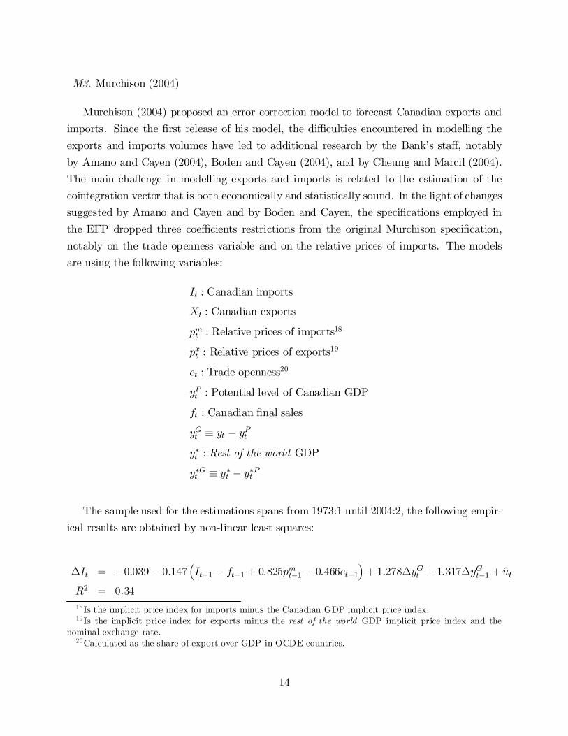
Murchison (2004) proposed an error correction model to forecast Canadian exports andimports. Since the …rst release of his model, the di¢culties encountered in modelling theexports and imports volumes have led to additional research by the Bank’s sta¤, notablyby Amano and Cayen (2004), Boden and Cayen (2004), and by Cheung and Marcil (2004).The main challenge in modelling exports and imports is related to the estimation of thecointegration vector that is both economically and statistically sound. In the light of changessuggested by Amano and Cayen and by Boden and Cayen, the speci…cations employed inthe EFP dropped three coe¢cients restrictions from the original Murchison speci…cation,notably on the trade openness variable and on the relative prices of imports. The modelsare using the following variables:

It : Canadian imports

Xt : Canadian exports

pmt : Relative prices of imports18

pxt : Relative prices of exports19

ct : Trade openness20

yPt : Potential level of Canadian GDP

ft : Canadian …nal sales

yGt ´ yt ¡ yPty¤t : Rest of the world GDP

y¤Gt ´ y¤t ¡ y¤Pt

The sample used for the estimations spans from 1973:1 until 2004:2, the following empir-ical results are obtained by non-linear least squares:

¢It = ¡0:039¡ 0:147³It¡1 ¡ ft¡1 + 0:825pmt¡1 ¡ 0:466ct¡1

´+1:278¢yGt + 1:317¢yGt¡1 + ut

R2 = 0:3418 Is the implicit price index for imports minus the Canadian GDP implicit price index.19 Is the implicit price index for exports minus the rest of the world GDP implicit price index and the

nominal exchange rate.20Calculated as the share of export over GDP in OCDE countries.

14

¢Xt = 2:844 ¡ 0:204³Xt¡1 ¡ y¤t¡1 +0:359pxt¡1 ¡ 0:731ct¡1

´+ 1:352¢y¤Gt + 0:869¢y¤Gt¡1 + ut

R2 = 0:44:

The empirical results obtained here di¤er from those obtained in Murchison and in Bodenand Cayen. For the imports equation, the trade openness coe¢cient is far from its originalrestriction of one and the lagged e¤ect of the Canadian output gap is now stronger. Forexports, the coe¢cient on trade openness is close to its original restriction of one, whereasthe lagged e¤ects of the rest of the world output gap and the error correction term arerespectively slightly stronger and slower.

M4. Cheung and Marcil (2004)

Cheung and Marcil used an error-correction model based on Murchison’s (2004) equa-tion to model the volume of imports using a trade-weighted activity measure as the maindeterminants for the Canadian demand of imported goods. The variables used are:

It : Canadian import

pmt : Relative prices of imports21

ct : Trade openness22

at : Trade-weighted activity measure for imports23

Using data from 1973:1 until 2004:2, the following empirical results are obtained:

¢It = 0:908¡ 0:147³It¡1 + pmt¡1 ¡ 0:798at¡1 ¡ 0:549ct¡1

´+ 0:901¢at + 0:113¢at¡1 + ut

R2 = 0:46:

21 Is the implicit price index for imports minus the Canadian GDP implicit price index.22 It is calculated as the share of exports over GDP in country member of the OCDE.23For more detail on this measure, see Cheung and Marcil (2004).

15

M5. Fillion and Léonard (1997)

In Fillion and Léonard (FL), core in‡ation is modelled as a Phillips-curve augmentedwith lags of imported in‡ation, lags of changes in the indirect tax rate, lags of the change inthe growth rate of real oil prices, and lags of changes in the real exchange rate. Furthermore,they take into account possible structural changes in the in‡ation process by adding dummyvariables to the model such that the mean and the persistence change over time. They alsospecify the measure of imported in‡ation to vary according to the stationarity of in‡ation,which is allowed to change across regimes. The model we use is an adjusted version of Eq.1.3 in FL which re‡ects the current measure of core in‡ation by the Bank.

The variables used are:

¼t : In‡ation excluding the eight most volatile components and changes in indirect taxes24

yt : Output gap25

¼¤t : 8-quarter moving-average of the real exchange rate26

¿ t : Indirect tax rate27

Ot : West Texas Intermediate crude oil price28

D1t = 1 when t = 1968:1; :::; 1973:4; else D1t = 0

D2t = 1 when t = 1974:1; :::; 1981:4; else D2t = 0

D3t = 1 when t = 1984:1; :::; 1991:2; else D3t = 0

D4t = 1 when t = 1993:1; :::; present, else D4t = 0

As in the original paper, the least square estimates are obtained with the constraint thatduring the 1974:1–1981:1 period in‡ation followed an integrated process. For some variables,holes in the lag window are allowed so that the number of parameters to estimate is reduced.Estimation results for the updated FL model are reported below using data up to 2004:3:

24For details, see Macklem (2001).25For technical details on this measure, see Butler (1996).26Expressed as year-over-year growth.27For the out-of-sample forecast, a value of zero is assumed unless changes in indirect taxes are announced

by governement authorities28Expressed in Canadian dollars.

16

¼t = 3:390D1t + 0:120D2t +3:791D3t + 1:794D4t + 0:1661yt¡1

+0:5732X

j=1¢¿t¡j + 0:006

2X

j=1¢2Ot¡j + 0:042¼¤t¡1

+0:638

0@

3X

j=1¼t¡jD1t

1A + 1:00

0@

3X

j=1¼t¡jD2t

1A + ut

R2 = 0:83:

Overall, the results from this updated model are somewhat similar to those reported in FL.

M6. Chacra and Kichian (2004)

Chacra and Kichian modelled inventory investment (It) using an error correction modelwhere It is a function of the following variables:

xt : Ratio of the computer and software prices over the IPPI29

st : Spread between long and short rates30

ft : Final sales

¾t : Volatility of …nal sales31

rt : Ratio of the BCPI over the CPI32

pt : CPI

All variables except for st and ¾t are expressed in log. To obtain the necessary futurevalues of xt to forecast It, xt+h was simply …xed to its average growth over the last twelvequarters since no forecast is formally available for xt.

Compared to the original work of Chacra and Kichian, two modi…cations were requiredto make their suggested model fully operational. First, BCPI is now de‡ated with the CPIinstead of the IPPI because no forecasts are available for IPPI at the Bank. Second, and mostimportantly, the inventory series (It) used in the original work is based on an unpublisheddata from Statistics Canada, whereas we now accumulate the National Account inventory

29 IPPI: Industrial Producers Price Index.30 i.e., the di¤erence between the 10 year yield on governement bonds and the 90 day rate on commercial

papers .31The rolling volatility measure, ¾t , is calculated using an average of four quarters.32BCPI: Bank of Canada Commodity Price Index; CPI, Consumer Price Index.

17

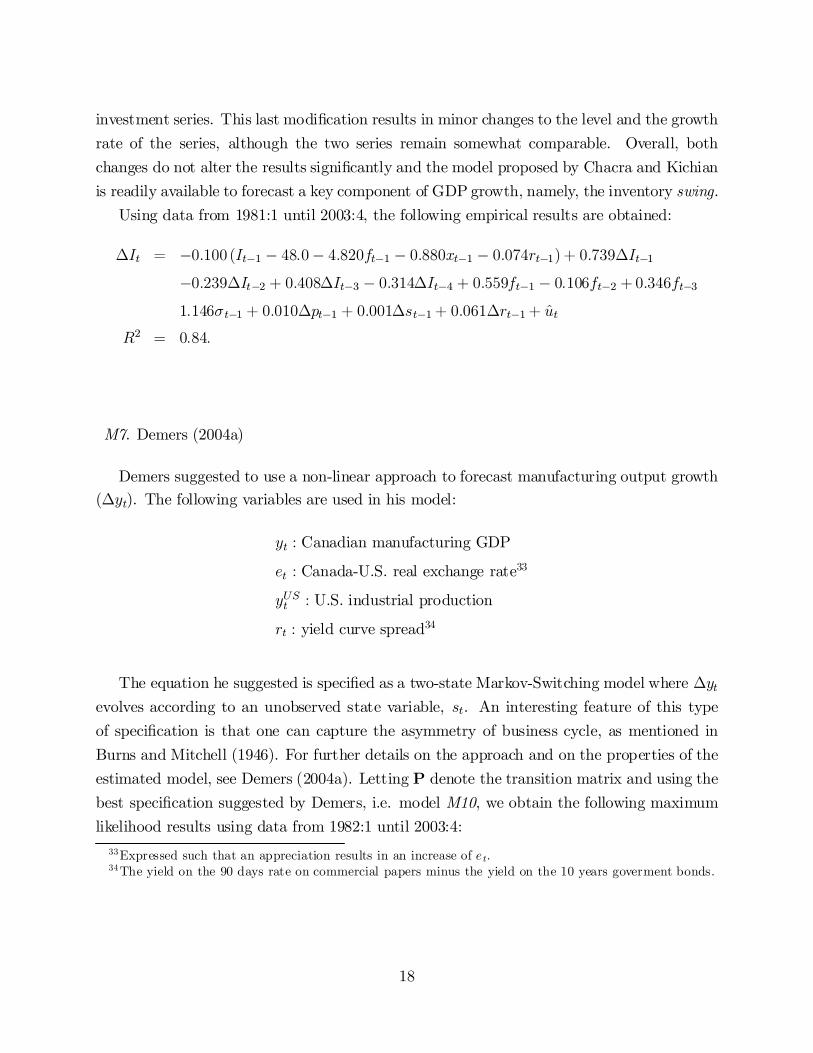
investment series. This last modi…cation results in minor changes to the level and the growthrate of the series, although the two series remain somewhat comparable. Overall, bothchanges do not alter the results signi…cantly and the model proposed by Chacra and Kichianis readily available to forecast a key component of GDP growth, namely, the inventory swing.

Using data from 1981:1 until 2003:4, the following empirical results are obtained:

¢It = ¡0:100 (It¡1 ¡ 48:0¡ 4:820ft¡1 ¡ 0:880xt¡1 ¡ 0:074rt¡1) + 0:739¢It¡1

¡0:239¢It¡2 + 0:408¢It¡3 ¡ 0:314¢It¡4 + 0:559ft¡1 ¡ 0:106ft¡2 +0:346ft¡3

1:146¾t¡1 + 0:010¢pt¡1 + 0:001¢st¡1+ 0:061¢rt¡1+ utR2 = 0:84:

M7. Demers (2004a)

Demers suggested to use a non-linear approach to forecast manufacturing output growth(¢yt). The following variables are used in his model:

yt : Canadian manufacturing GDP

et : Canada-U.S. real exchange rate33

yUSt : U.S. industrial production

rt : yield curve spread34

The equation he suggested is speci…ed as a two-state Markov-Switching model where ¢ytevolves according to an unobserved state variable, st. An interesting feature of this typeof speci…cation is that one can capture the asymmetry of business cycle, as mentioned inBurns and Mitchell (1946). For further details on the approach and on the properties of theestimated model, see Demers (2004a). Letting P denote the transition matrix and using thebest speci…cation suggested by Demers, i.e. model M10, we obtain the following maximumlikelihood results using data from 1982:1 until 2003:4:

33Expressed such that an appreciation results in an increase of et.34The yield on the 90 days rate on commercial papers minus the yield on the 10 years goverment bonds.

18

¢yt =

8>>>>>>>>>>><>>>>>>>>>>>:

8>><>>:

¡1:510+ 0:617(4:62)

¢yt¡1¡ 0:400(¡3:67)

rt¡1+ 0:824(3:55)

¢yust¡1

¡ 0:704(¡7:43)

¢et¡1¡ 0:460(¡4:14)

¢et¡2¡ 0:417(¡3:61)

¢et¡3¡ 0:673(¡6:34)

¢et¡4 + u1;t; st = 0

8>><>>:

0:855(5:73)

¡ 0:134(¡1:55)

¢yt¡1¡ 0:544(¡8:42)

rt¡1+ 0:333(2:57)

¢yust¡1

¡ 0:104(¡1:65)

¢et¡1+ 0:028(0:50)

¢et¡2+ 0:363(6:39)

¢et¡3+ 0:148(2:46)

¢et¡4 + u2;t; st = 1

P =

0BB@

0:813(15:14)

0:650

0:187 0:350(3:15)

1CCA ; R2 = 0:61 u » i:i:d:N (0; ¾2):

Demers also estimated the same model using least squares, from which we obtain the follow-ing empirical results:

M3a : yt = ¡ 0:064(¡0:28)

¡ 0:354(¡3:04)

rt¡1+ 0:333(1:41)

yust¡1+ 0:308(2:22)

yt¡1

¡ 0:035(¡0:77)

et¡1 + ut

R2 = 0:43:

The forecasts from both models are presented in the table.

M8. Demers and De Champlain (2005)

Demers and De Champlain (hereafter DDC) suggested to use disaggregated CPI datato forecast monthly and quarterly core in‡ation. Compared to DDC’s original work, aslightly di¤erent scheme to aggregate the data was used since some subaggregate indicesare not available before 1997. To make the DDC models fully compatible with the currentdisaggregation scheme used to monitor in‡ation at the Bank, the models developed by DDCwere thus modi…ed accordingly. Although this is an important change with respect to thestarting date of the sample considered by DDC, this truncation is still coherent with theirmost important …ndings: disaggregated models which allowed for a structural break generallyprovide the most accurate forecasts. In e¤ect, structural breaks were detected in the …rsthalf of the 1990’s.

DDC showed that using monthly disaggregated data helps improve the quarterly forecasts(at least for one-quarter-ahead). Here, only monthly forecasts are used to obtain quarterlyforecasts; and therefore the quarterly models studied in DDC are not used in this document.DDC also considered two levels of disaggregation in addition to aggregate data. The …rst

19

level of disaggregation is based on building six sub-aggregates, whereas the second level isbased upon building twenty one sub-aggregates. In this package, all three sets of monthlyforecasts are presented.

The explanatory variables they use are simply the growth rate of the real Canada-U.S.exchange rate and the QPM output-gap measure. Because the method they employ producesa large amount of estimation results, the updated estimation results of the micro-relationsare not presented here and the reader should therefore consult DDC for detailed empiricalresults and analysis.

The table also reports the forecasts from disaggregated AR(p) models.

M9. Chacra (2002)

Chacra modelled real gasoline, heating oil, and natural gas CPI components using anerror-correction approach. The following variables are used in his forecast models:

Gt : CPI of Gasoline35

Ht : CPI of Heating oil

Nt : CPI of Natural gas

Wt : West Texas Intermediate price for crude oil36

yt : U.S. output gap37

Dt : Dummy variable for the period 1973:4 to 1985:2

Controlling for seasonal e¤ects (St = 1 for the fourth quarter, else St = 0), using datafrom 1971:1 until 2004:2 and non-linear squares, the following empirical results are obtained:

¢Gt = ¡0:164 (Gt¡1 ¡ 0:924 ¡ 0:313Dt¡1 ¡ 0:813Wt¡1) + 0:240¢Wt¡1 ¡ 0:102¢Wt¡2

+0:022¢Wt¡3 ¡ 0:030St + ut

R2 = 0:3235Changes in gasoline taxes have been removed from this series.36Expressed in canadian dollars.37For technical details on this measure, see Gosselin and Lalonde (2002).

20

¢Ht = ¡0:078 (Ht¡1 ¡ 1:559 ¡ 0:313Dt¡1 ¡ 0:895Wt¡1) + 0:227¢Wt¡1 +0:053¢Wt¡3

+0:027St + ut

R2 = 0:44

¢Nt = ¡0:094 (Nt¡1 ¡ 0:812¡ 0:497Dt¡1 ¡ 1:164Wt¡1) + 0:006yt¡1 ¡ 0:015yt¡2 + 0:013yt¡3

+0:150¢Nt¡1 + 0:147¢Nt¡2 +0:029St + utR2 = 0:23:

Again, the empirical results are very close to those originally reported in Chacra (2002),with a reasonably fast speed of adjustment for the gasoline equation, whereas they are muchslower for the heating oil and natural gas equations.

M10. Marcil (2004)

Marcil modelled monthly consumer expenditures in energy and Canadian utilities’ outputusing temperature series. The following variables are used in his forecast models:

ct : Canadian consumer expenditures in energy excluding gasoline

yt : Canadian utilities GDP

ht : Seasonally adjusted heating degree day38

ct : Seasonally adjusted cooling degree day

mt : Canadian manufacturing GDP

Dt = 1 when t > 1992:02, else Dt = 0

St : Dummy variable controlling for various exogenous shock39

The estimation sample for the …rst model run from 1987:02 until 2004:04, whereas forthe second model the sample goes from 1981:02 until 2004:04. Using maximum likelihood,

38An elaborate desrciption of heating degree day and of cooling degree day, including the seasonal adjust-ment process used, can be found in Marcil (2004).

39 It is a trinary dummy variable (i.e., +1,0,-1). A complete list of shocks can be found in Marcil (2004).

21

the following empirical results are obtained:

¢ct = 0:0009 + 0:270Dt +0:0004¢ht + 0:00058¢ct + ut ¡ 0:33ut¡1

R2 = 0:61

¢yt = 0:0006 + 0:044St + 0:00024¢ht + 0:00059¢ct + 0:320¢mt + ut ¡ 0:22ut¡1

R2 = 0:66:

6.1 Forthcoming forecasting models

M11. Cheung and Laurence (2005)

Disaggregate models of exports and imports volumes.

M12. Ko (2005)

Disaggregate models of exports and imports price de‡ators.

M13. Demers (2005)

Forecasting models for housing investment.

M14. Demers and Macdonald (2005)

Markov-Switching models to predict GDP growth and business cycle turning-points.

M15. Zheng and Rossiter (2005)

Indicators models to predict current-quarter GDP growth using monthly information.

7 Other Models

In the spirit of Box and Jenkins (1970), simple autoregressive (AR) models are also usedto forecast the time series of interest. AR(p) models are easy to estimate and operate,with well-known properties. They also have a long history of providing decent and oftenvery competitive forecasts in all sorts of contexts. Hence, the EFP incorporates forecasts

22

from AR(p) models. We adopted (by choice) the iterative forecasting methodology for thesemodels, although the direct method could easily be implemented.40

The lag selection is done by Akaike’s information criteria, based on a comparison ofthe results from speci…cations with up to six lags. To limit the perverse e¤ects from thepossibility that parameters are unstable over time, the AR(p) models are reestimated usinga rolling window of ten years of data (the lag selection is also updated).

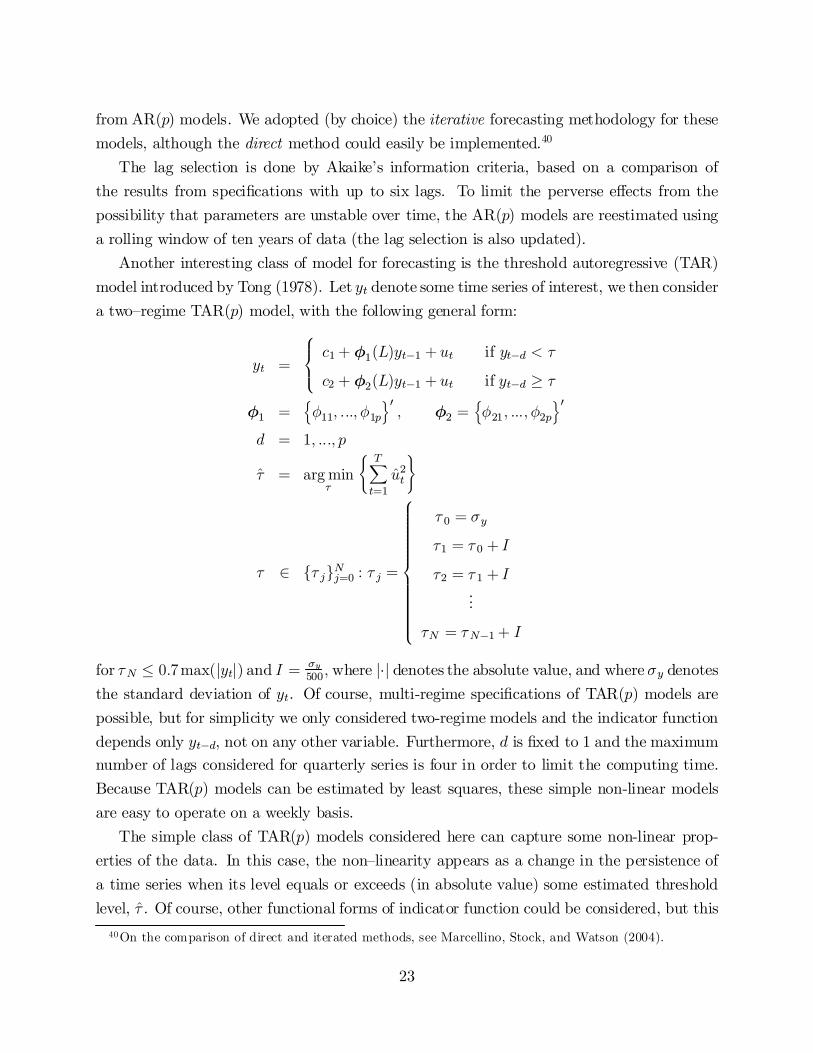
Another interesting class of model for forecasting is the threshold autoregressive (TAR)model introduced by Tong (1978). Let yt denote some time series of interest, we then considera two–regime TAR(p) model, with the following general form:

yt =

8><>:c1+ Á1(L)yt¡1 + ut if yt¡d < ¿

c2 + Á2(L)yt¡1 + ut if yt¡d ¸ ¿Á1 =

nÁ11; :::; Á1p

o0; Á2 =

nÁ21; :::; Á2p

o0

d = 1; :::; p

¿ = arg min¿

( TX

t=1u2t

)

¿ 2 f¿ jgNj=0 : ¿ j =

8>>>>>>>>>>>><>>>>>>>>>>>>:

¿ 0 = ¾y

¿1 = ¿ 0 + I

¿2 = ¿ 1 + I...

¿N = ¿N¡1+ I

for ¿N · 0:7max(jytj) and I = ¾y500; where j¢j denotes the absolute value, and where ¾y denotes

the standard deviation of yt. Of course, multi-regime speci…cations of TAR(p) models arepossible, but for simplicity we only considered two-regime models and the indicator functiondepends only yt¡d, not on any other variable. Furthermore, d is …xed to 1 and the maximumnumber of lags considered for quarterly series is four in order to limit the computing time.Because TAR(p) models can be estimated by least squares, these simple non-linear modelsare easy to operate on a weekly basis.

The simple class of TAR(p) models considered here can capture some non-linear prop-erties of the data. In this case, the non–linearity appears as a change in the persistence ofa time series when its level equals or exceeds (in absolute value) some estimated thresholdlevel, ¿ . Of course, other functional forms of indicator function could be considered, but this

40On the comparison of direct and iterated methods, see Marcellino, Stock, and Watson (2004).

23

is left for future research.41

8 Forecasts Combination

Many techniques are available to combine forecasts (see, e.g., Granger and Ramanathan,1984; Fuchun and Tkacz, 2001; Elliot and Timmermann, 2004; Hendry and Clements, 2002).Given that we are still in the early stages of this ambitious project, we have only beenable to use the easiest methods of all, that is, the simple arithmetic mean of all forecastsfor a certain indicator. Because such a method to pool forecasts does not ensure that thepooled-forecast errors will be unbiased, the pooled forecasts are adjusted using the averagepooled forecast errors of the last twelve quarters. Although this simple method is known tooften perform very well, this area certainly has substantial potential for future research inempirically investigating what are the best methods to combine the available forecasts.

9 Presenting the Forecasts

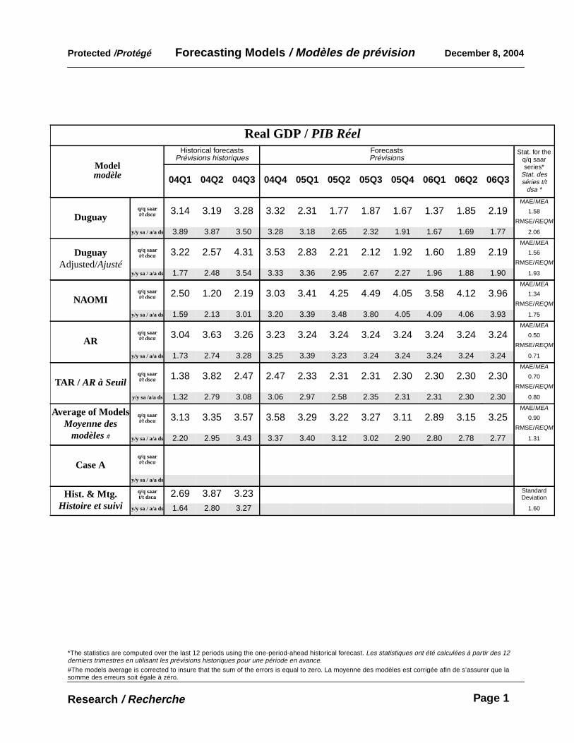
To communicate to both the sta¤ in charge of assessing current economic developments andof forecasting and to the management, who subsequently briefs the Governing Council, it isimportant for us to report the suggested model-based forecasts in appropriate tables. Anexample is shown in the appendix. The tables are reporting forecasts for an horizon of up toeight quarters or months, with three quarters or months also of history and past forecasts.

Past forecasts are genuine one-step-ahead forecasts in the sense that they are based oniterative estimation and forecasts using the most recent data releases. Eventually, it couldbe possible to base our past forecasts on real-time information, thereby allowing for easycomparison with the sta¤’s forecasts. It should be noted however that the computer codehas been written such that we are able to collect real-time output and in‡ation quarterlyforecasts such that comparisons with the o¢cial base-case scenario are possible. Of course,we have only a few observations so far, but as time goes by it will be interesting to see howthe sta¤’s forecasts compare with the models.42

In addition to reporting forecasts for the three previous period, the tables also reportsome statistics to assess the recent forecasting accuracy. The two statistics reported are theroot mean standard forecasts error (RMSE) and the mean absolute forecasts error (MAE)based on the most recent (revised) 20 quarterly forecasts and 24 monthly forecasts.

41To keep the package manageable, we also need to consider the processing time constraint.42Of course, the sta¤ has the advantage of knowing the model-based forecasts before …nalizing its view.

24

It is important to recall that one of the main challenges in forecasting macroeconomictime series is that we try, at best, to …nd reduced-forms which are able to characterize witha certain degree of accuracy the properties of the data. As mentioned above, these forms aremere approximations of the DGP, such that the level of uncertainty regarding the validity ofa particular reduced-form or indicator model can vary substantially over time. It is thereforeimportant to adopt a dynamic approach in evaluating the relative forecast accuracy of thevarious competing models at hand. The rolling estimates of the accuracy metrics as well asthe three most recent forecasts should prove useful in this regard.

10 Conclusion: Where to Next?

This document provides a comprehensive view and catalogue of the models currently avail-able in the EFP for forecasting near-term economic indicators in Canada such as GDP andin‡ation. It also provides the Bank’s sta¤ with a new forecasting strategy where econometricmodels are being used in a systematic framework, with judgement-free forecasts reported intables every week, incorporating up-to-date information. This document will also serve as aguide in developing forecast models at the Bank of Canada.

Since 2003, the research strategy in the Current Analysis Division has been largely ori-ented towards the developments of the EFP and of short-run forecasting models. Oldermodels have been revamped and, sometimes, modi…ed in order to adjust them to currentneeds and data. Meanwhile, a number of models have been developed and we now covera wide spectrum of Canadian economic indicators. But given the plethora of economic in-dicators that are published in Canada, there is still a large amount of work ahead of us.Furthermore, each indicator can potentially be modelled in various ways, thereby creatinginteresting research avenues.

Currently, the Current Analysis Division is exploring challenging topics. One is related tothe usefulness of monthly indicators to forecast quarterly indicators such as GDP. Anothertopic is related to combining forecasts using time-varying or state-dependent weights. Asmentioned above, such projects can be carried using state-of-the-art econometric techniques,providing us with sometimes very di¤erent and interesting outcomes and forecasting devices.

Given the number of models that will be available to forecast some of the key Canadianeconomic variables, namely GDP growth and in‡ation, an interesting project would be to doa comparative analysis of their forecasting capability using appropriate tests. In this sense,further work on forecasts pooling will most surely be promising in improving the forecastaccuracy of the models comprised in the EFP. Another avenue for future research will be

25

to try to combine forecasts from various indicator models for subaggregates of, say, GDP,with bridge equations in the spirit of the bottom-up approach, applied, among others, byRünstler and Sédillot (2003) and by Klein and Ozmucur (2004).

An important point that needs to be addressed in a near future is the uncertainty whichsurrounds these point forecasts. Measuring and reporting forecasts uncertainty is a crucialaspect of forecasting as one can assess the degree to which certain critical outcomes suchas recessions or surges in in‡ation are likely or not. The work of Wallis (2003) is a goodexample of what could be done in future research. Similarly, regime-switching models such asMarkov-Switching models could be use to build business cycle turning-point indicators (e.g.,Ba¢gi and Basanetti, 2004; and Diebold and Rudebusch, 1999). This could be particularlyuseful for forecasting recessions, which are virtually unpredictable (Demers, 2004b).

To assess the risks to the in‡ation outlook, the ECB reported in its March 2005 MonthlyBulletin (p. 20) a chart showing the range (maximum, minimum and median) of in‡ationforecasts obtained from leading indicator models. We also plan to produce similar charts inthe near future.

26

References

Amano, B. and J.-P. Cayen. 2004. “An Evaluation of a Model of Long-Run CanadianImport.” Bank of Canada, RN-04–178.

Bank of England. 1999. Economic Models at the Bank of England. London: Bank ofEngland.

Bank of England. 2000. Economic Models at the Bank of England. (September 2000Update) London: Bank of England.

Ba¢gi, A. and Basanetti, A. 2004. “Turning-point Indicators from Business Surveys: Real-time Detection for the Euro Area and its Major Member Countries.” Bank of Italy,Working Paper No. 500.

Bernanke, B.S., T. Laubach, F.S. Mishkin, and A.S. Posen. 1999. In‡ation Targeting.Princeton, N.-J.: Princeton University Press.

Box, G.E.P. and G.M. Jenkins. 1970. Time Series Analysis, Forecasting, and Control. SanFrancisco: Holden–Day.

Butler, L. 1996. A Semi-Structural Method to Estimate Potential Output: Combining Eco-nomic Theory with a Time–Series Filter. Technical Report No. 77. Ottawa: Bank ofCanada.

Burns, A., and W.C. Mitchell. 1946. Measuring Business Cycles, New York: NBER.

Boden, G.M. and Cayen, J.-P. 2004. ”Les exportations nettes: les perspectives d’un modèleà correction d’erreurs.” Bank of Canada, RN-04-101.

Cayen, J.-P. and S. van Norden. 2001. “La …abilité des estimations de l’écart de produc-tion.”Bank of Canada, Working Paper No. 2002–10.

Chacra, M. 2002. “Oil-Price Shocks and Retail Energy Prices in Canada.” Bank of Canada,Working paper 2002–38.

Chacra, M. and M. Kichian. 2004. “A Forecasting Model of Inventory Investment.” Bankof Canada, Working Paper No. 2004–39.

Cheung, C. and Marcil, P. 2004. “Net Exports: An Update on the Equilibrium Gap.” Bankof Canada, RN-04-159.

27

Cheung, C. and M. Laurence. 2005. “Model of Canadian International Trade Flows: ADisaggregate Approach.” Bank of Canada, forthcoming.

Clements, M.P. et D.F. Hendry. 1998. Forecasting Economic Time Series. Cambridge,Mass.: Cambridge University Press.

Coletti, D. 2005. “Constructing the Sta¤ Economic Projection at the Bank of Canada.”In: Proceedings of Practical Experience with In‡ation Targeting, held at the CzechNational Bank May 13-14.

Côté, D., J. Kuszczak, J.–P. Lam, Y. Liu, and P. St-Amant. 2003. A Comparison of TwelveMacroeconomic Models of the Canadian Economy. Technical Report No. 94. Ottawa:Bank of Canada.

Demers, F. 2005. “Modeling and Forecasting Housing Investment: the Case of Canada.”Bank of Canada, forthcoming.

Demers, F. 2004a. “Prévisions et analyse de la croissance de la production manufacturière:comparaison de modèles linéaires et non-linéaires.” Bank of Canada, Working PaperNo. 2004–40.

Demers, F. 2004b. “Comparaison de modèles de prévision pour la croissance du PIB cana-dien.” Bank of Canada, RN-04–172.

Demers, F. and A. De Champlain. 2005. “Forecasting Core In‡ation: Should we Forecastthe Aggregate or the Components? Some Empirical Evidence From Canada.” Bankof Canada, forthcoming.

Demers, F. and Marcil, P. 2004. “Prévisions de la croissance du PIB canadien: quelquesnouveautés pour l’équation de la courbe IS de Duguay.” Bank of Canada, RN–04–168.

Demers, F. and R. Macdonald. 2005. “Are Nonlinearities Important When Predicting GDPGrowth in Canada?” Bank of Canada, forthcoming.

Diebold, F.X. and G.D. Rudebusch. 1999. Business Cycles: Durations, Dynamics, andForecasting. Princeton, N.-J.: Princeton University Press.

Duguay, P. 1994. Empirical Evidence on the Strength of the Monetary Transmission Mech-anism in Canada.” Journal of Monetary Economics 33: 39–61.

28

Duguay, P. and D. Longworth. 1998. “Macroeconomic models and policymaking at theBank of Canada.” Economic Modelling 15: 357–75.

European Central Bank. 2001. A Guide to Eurosystem Sta¤ Macroeconomic ProjectionExercises. Frankfurt: ECB.

European Central Bank. 2004. The Monetary Policy of the ECB. 2nd edition. Frankfurt:ECB.

Elliot, G. and A. Timmermann. 2002. “Optimal Forecast Combinations Under RegimeSwitching.” University of California San Diego, mimeo.

Elliot, G. and A. Timmermann. 2004. “Optimal Forecast Combinations Under GeneralLoss Functions and Forecast Error Distributions.” Journal of Econometrics 122: 47–79.

Fair, R.C. 1974. “An Evaluation of a Short-Run Forecasting Model.” International Eco-nomic Review 15: 285–303.

Fillion, J.-F. and A. Léonard. 1997. “La courbe de Phillips au Canada: un examen dequelques hypothèses.” Bank of Canada, Working Paper No. 97–3.

Fuchun, L. and G. Tkacz. 2001. “Evaluating Linear and Non-Linear Time-Varying Forecast–Combination Methods.” Bank of Canada, Working Paper No. 2001–12.

Gosselin, M.-A. and R. Lalonde 2002. “Une approche éclectique d’estimation du PIBpotentiel américain.” Bank of Canada, Working Paper No. 2002–36.

Granger, C.W.J. and R. Ramanathan. 1984. “Improved Methods of Combining Forecasts.”Journal of Forecasting 3: 197–204.

Hendry, D.F. 2002. “Forecast Failure, Expectations Formations, and the Lucas Critique.”In Econometrics of Policy Evaluation, Special Issue of Annales d’Économie et de Sta-tistique 66-67: 21–40.

Hendry, D.F. and M.P. Clements. 2002. “Pooling of Forecasts.” Econometric Journal 5:1–26.

Hendry, D.F. and H.-M. Krolzig. 2001. Automatic Econometric Model Selection. Timber-lake Consultants Press.

29

Hendry, D.F. and G.E. Mizon. 2004. “Forecasting in the Presence of Structural Breaksand Policy Regime Shifts.” In Identi…cation and Inference in Econometric Models:Festschrift in Honor of T.J. Rothenberg, eds. by D.W. Andrews, J.L. Powell, P.A.Ruud and J. Stock, Cambridge University Press. Forthcoming.

Kapetanios, G., V. Labhard and C. Schleicher. 2005. “Conditional Model Con…dence Setswith an Application to Forecasting Models.” Bank of England, mimeo.

Kapetanios, G., V. Labhard and S. Price. 2005. “Forecasting using Bayesian and Informa-tion Theoretic Model Averaging: An Application to UK In‡ation.” Bank of England,mimeo.

Khalaf, L. and M. Kichian. 2003. “Exact Testing of the Phillips Curve.” Bank of Canada,Working Paper No. 2003–7.

Klein, L.R. and S. Ozmucur. 2004. The University of Pennsylvania Models for High-Frequency Modeling. University of Pennsylvania, mimeo.

Ko, N. 2005. “A Forecast Model for Canadian Export and Import Prices: Exchange RatePass-through and the E¤ect of Commodity Price Shocks on the Terms of Trade.” Bankof Canada, forthcoming.

Macklem, T. 2001. “A New Measure of Core In‡ation.” Bank of Canada Review (Autumn):3–12.

Marcellino, M., J.H. Stock, and M.W. Watson. 2004. “A Comparison of Direct and It-erated Multistep AR Methods for Forecasting Macroeconomic Time Series.” HarvardUniversity, mimeo.

Marcil, P. 2004. “La météo comme outil de prévision.” Bank of Canada, RN-04-160.

Murchison, S. 2001. “A New Quarterly Forecasting Model. Part II: A Guide to CanadianNAOMI.” Department of Finance Canada, Working Paper No. 2001–25.

Murchison. 2004. “Net Exports in December Case A: Are we Underestimating the Re-bound?” Bank of Canada, RN-04-013.

Pagan, A. 2003. Report on Modelling and Forecasting at the Bank of England. London:Bank of England.

30

Rünstler, G. and F. Sédillot. 2003. “Short-term estimates of euro area real GDP by meansof monthly data.” European Central Bank, Working Paper No. 276.

Schi¤, A.F. and P.C.B. Phillips. 2000. “Forecasting New Zealand’s Real GDP.” ReserveBank of New Zealand, mimeo.

Smets, F. and R. Wouters. 2003. “An Estimated Stochastic General Equilibrium Model ofthe Euro Area.” European Central Bank, Working Paper No. 171.

Tong, H. 1978. “On a Threshold Model.” In Chen, C.H. (eds.). Pattern Recognition andSignal Processing, Amsterdam: Sijho¤ & Noordo¤.

Wallis, K.F. 2003. “Forecast Uncertainty, its Representation and Evaluation.” BoletinIn‡acion y Analisis Macroeconomico, Universidad Carlos III de Madrid, Special IssueNo. 100: 89–98.

White, H. 2000. “A Reality Check for Data Snooping.” Econometrica 68: 1097–1126.

Zheng, I.Y. and J. Rossiter. 2005. “Using Monthly Indicators to Predict Quarterly In‡a-tion.” Bank of Canada, forthcoming.

31

Page 1

Protected /Protégé Forecasting Models / Modèles de prévision December 8, 2004

Research / Recherche

*The statistics are computed over the last 12 periods using the one-period-ahead historical forecast. Les statistiques ont été calculées à partir des 12derniers trimestres en utilisant les prévisions historiques pour une période en avance.#The models average is corrected to insure that the sum of the errors is equal to zero. La moyenne des modèles est corrigée afin de s’assurer que lasomme des erreurs soit égale à zéro.

Real GDP / PIB Réel

Modelmodèle

Historical forecastsPrévisions historiques

ForecastsPrévisions

Stat. for theq/q saarseries*

Stat. desséries t/t

dsa *04Q1 04Q2 04Q3 04Q4 05Q1 05Q2 05Q3 05Q4 06Q1 06Q2 06Q3

Duguayq/q saart/t dsca 3.14 3.19 3.28 3.32 2.31 1.77 1.87 1.67 1.37 1.85 2.19

MAE/MEA

1.58

RMSE/REQM

y/y sa / a/a ds 3.89 3.87 3.50 3.28 3.18 2.65 2.32 1.91 1.67 1.69 1.77 2.06

DuguayAdjusted/Ajusté

q/q saart/t dsca 3.22 2.57 4.31 3.53 2.83 2.21 2.12 1.92 1.60 1.89 2.19

MAE/MEA

1.56

RMSE/REQM

y/y sa / a/a ds 1.77 2.48 3.54 3.33 3.36 2.95 2.67 2.27 1.96 1.88 1.90 1.93

NAOMIq/q saart/t dsca 2.50 1.20 2.19 3.03 3.41 4.25 4.49 4.05 3.58 4.12 3.96

MAE/MEA

1.34

RMSE/REQM

y/y sa / a/a ds 1.59 2.13 3.01 3.20 3.39 3.48 3.80 4.05 4.09 4.06 3.93 1.75

ARq/q saart/t dsca 3.04 3.63 3.26 3.23 3.24 3.24 3.24 3.24 3.24 3.24 3.24

MAE/MEA

0.50

RMSE/REQM

y/y sa / a/a ds 1.73 2.74 3.28 3.25 3.39 3.23 3.24 3.24 3.24 3.24 3.24 0.71

TAR / AR à Seuilq/q saart/t dsca 1.38 3.82 2.47 2.47 2.33 2.31 2.31 2.30 2.30 2.30 2.30

MAE/MEA

0.70

RMSE/REQM

y/y sa /a/a ds 1.32 2.79 3.08 3.06 2.97 2.58 2.35 2.31 2.31 2.30 2.30 0.80

Average of ModelsMoyenne des

modèles#

q/q saart/t dsca 3.13 3.35 3.57 3.58 3.29 3.22 3.27 3.11 2.89 3.15 3.25

MAE/MEA

0.90

RMSE/REQM

y/y sa / a/a ds 2.20 2.95 3.43 3.37 3.40 3.12 3.02 2.90 2.80 2.78 2.77 1.31

Case Aq/q saart/t dsca

y/y sa / a/a ds

Hist. & Mtg.Histoire et suivi

q/q saart/t dsca 2.69 3.87 3.23 Standard

Deviation

y/y sa / a/a ds 1.64 2.80 3.27 1.60

Page 2




Exports of goods and services /Exportations de biens et de services

Modelmodèle





dsa04Q1 04Q2 04Q3 04Q4 05Q1 05Q2 05Q3 05Q4 06Q1 06Q2 06Q3

Murchisonq/q saart/t dsca 12.80 11.20 9.42 9.87 7.73 6.70 6.59 6.30 6.78 7.23 7.07

MAE/MEA

11.02

RMSE/REQM

y/y sa / a/ads 3.53 5.55 10.10 7.22 8.17 5.48 7.71 6.83 6.59 6.73 6.85 11.56

ARq/q saart/t dsca 5.30 8.41 3.69 3.88 4.79 4.93 4.95 4.96 4.96 4.96 4.96

MAE/MEA

5.89

RMSE/REQM

y/y sa / a/ads 1.76 4.88 8.63 5.73 5.93 2.87 4.64 4.91 4.95 4.96 4.96 7.05


MAE/MEA

5.56

RMSE/REQM

y/y sa / a/ads 2.45 4.83 8.71 5.78 5.76 2.45 3.96 3.91 3.91 3.91 3.91 6.61


modèles#

q/q saart/t dsca 6.53 7.04 3.48 3.72 3.25 2.95 2.93 2.83 2.99 3.14 3.09

MAE/MEA

4.91

RMSE/REQM

y/y sa / a/ads 2.03 4.53 8.59 5.69 6.06 3.05 4.88 4.66 4.60 4.64 4.68 6.06


y/y sa / a/ads


q/q saart/t dsca 3.99 17.99 -1.97 Standard

Deviation

y/y sa / a/ads 1.45 7.12 7.11 7.35

Page 3




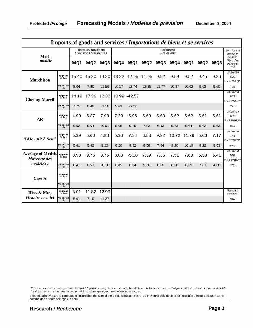
Imports of goods and services /Importations de biens et de services

Modelmodèle





dsa04Q1 04Q2 04Q3 04Q4 05Q1 05Q2 05Q3 05Q4 06Q1 06Q2 06Q3

Murchisonq/q saart/t dsca 15.40 15.20 14.20 13.22 12.95 11.05 9.92 9.59 9.52 9.45 9.86

MAE/MEA

6.29

RMSE/REQM

y/y sa / a/ads 8.04 7.90 11.56 10.17 12.74 12.55 11.77 10.87 10.02 9.62 9.60 7.36

Cheung-Marcilq/q saart/t dsca 14.19 17.36 12.32 10.99 -42.57

MAE/MEA

5.78

RMSE/REQM

y/y sa / a/ads 7.75 8.40 11.10 9.63 -5.27 7.44

ARq/q saart/t dsca 4.99 5.87 7.98 7.20 5.96 5.69 5.63 5.62 5.62 5.61 5.61

MAE/MEA

6.70

RMSE/REQM

y/y sa / a/ads 5.52 5.64 10.01 8.68 9.45 7.92 6.12 5.73 5.64 5.62 5.62 8.17


MAE/MEA

7.41

RMSE/REQM

y/y sa / a/ads 5.61 5.42 9.22 8.20 9.32 8.58 7.84 9.20 10.19 9.22 8.53 8.49


modèles#

q/q saart/t dsca 8.90 9.76 8.75 8.08 -5.18 7.39 7.36 7.51 7.68 5.58 6.41

MAE/MEA

5.57

RMSE/REQM

y/y sa / a/ads 6.41 6.53 10.16 8.85 6.24 9.36 8.26 8.28 8.29 7.83 4.68 7.25


y/y sa / a/ads



Deviation

y/y sa / a/ads 5.01 7.10 11.27 9.67

Page 4




Swing in Inventories Investment /Changement des investissements en inventaire

Modelmodèle





dsa04Q1 04Q2 04Q3 04Q4 05Q1 05Q2 05Q3 05Q4 06Q1 06Q2 06Q3

Chacra-Kichian

q/q saart/t dsca 6.87 -6.19 5.57 -11.77 -5.55 0.74 -7.83 -0.27 4.80 -0.44 2.43

MAE/MEA

8.13

RMSE/REQM

Stocks toSales /

inven. survente

0.61 0.59 0.59 0.55 0.55 0.56 0.55 0.56 9.38

ARq/q saart/t dsca 0.08 0.06 -0.44 -5.06 2.31 3.43 -7.45 2.76 0.53 -2.72 4.17

MAE/MEA

6.61

RMSE/REQM

8.23

TAR / AR à Seuilq/q saart/t dsca 1.70 -0.53 -4.72 11.33 -7.04 -1.46 -5.96 -8.35 0.34 0.89 2.31

MAE/MEA

7.83

RMSE/REQM

9.79


modèles#

q/q saart/t dsca 3.33 -1.77 0.59 -1.38 -2.98 1.35 -6.63 -1.51 2.34 -0.31 3.42

MAE/MEA

6.43

RMSE/REQM

7.57


q/q saart/t dsca -7.45 -0.48 14.68 Standard

Deviation

Stocks toSales /

inven. survente

0.67 0.65 0.66 8.69

Page 5




GDP at Basic Prices : Manufacturing /PIB aux prix de base : Manufucturier

Modelmodèle





dsa04Q1 04Q2 04Q3 04Q4 05Q1 05Q2 05Q3 05Q4 06Q1 06Q2 06Q3

Demerslinear/ linéaire

q/q saart/t dsca 6.78 -0.41 -1.33 6.67 4.34 6.11 6.24 5.73 4.93 4.84 4.64

MAE/MEA

6.84

RMSE/REQM

y/y sa / a/ads 1.75 2.05 4.11 6.16 6.80 6.38 5.84 5.60 5.75 5.43 5.03 5.17

Demersmarkov

switching

q/q saart/t dsca -9.50 15.26 22.16 -9.99 -17.34 -17.92 -20.65 -20.59 -9.81 -1.21 1.56

MAE/MEA

5.30

RMSE/REQM

y/y sa / a/ads -2.37 5.84 9.82 1.74 -3.43 -9.79 -16.56 -19.14 -17.36 -13.44 -7.93 7.25

ARq/q saart/t dsca 7.59 8.50 3.71 3.61 5.61 3.33 1.75 3.31 2.56 3.23 4.33

MAE/MEA

3.83

RMSE/REQM

y/y sa / a/ads 3.43 5.53 4.61 5.38 6.35 5.23 3.57 3.49 2.74 2.71 3.35 4.24

TAR / AR à Seuilq/q saart/t dsca 2.83 4.15 0.72 0.77 4.73 1.09 -0.49 3.72 1.11 3.05 4.60

MAE/MEA

4.02

RMSE/REQM

y/y sa / a/ads 2.59 4.04 3.69 4.65 5.39 3.71 1.51 2.24 1.34 1.83 3.11 4.56


modèles#

q/q saart/t dsca 1.59 6.54 5.98 -0.07 -1.00 -2.18 -3.62 -2.29 -0.64 2.14 3.45

MAE/MEA

2.53

RMSE/REQM

y/y sa / a/ads 1.39 4.40 5.60 4.52 3.82 1.43 -1.37 -1.91 -1.84 -0.83 0.93 3.37



Deviation

y/y sa / a/ads 0.55 4.09 6.60 5.77

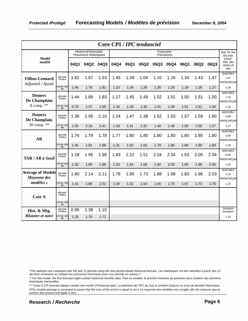
Page 6



*The statistics are computed over the last 12 periods using the one-period-ahead historical forecast. Les statistiques ont été calculées à partir des 12derniers trimestres en utilisant les prévisions historiques pour une période en avance.7** For this model, the first forecast might contain historical monthly data. Pour ce modéle, le premier trimestre de prévision peut contenir des donnéeshistoriques mensuelles.*** Case A CPI forecast always contain one month of historical data. La prévision de l’IPC du Cas A contient toujours un mois de donnée historicque.#The models average is corrected to insure that the sum of the errors is equal to zero. La moyenne des modèles est corrigée afin de s’assurer que lasomme des erreurs soit égale à zéro.

Core CPI / IPC tendanciel

Modelmodèle





dsa04Q1 04Q2 04Q3 04Q4 05Q1 05Q2 05Q3 05Q4 06Q1 06Q2 06Q3

Fillion-LeonardAdjusted /Ajusté

q/q saart/t dsca 1.82 1.67 1.53 1.45 1.39 1.04 1.10 1.26 1.34 1.43 1.47

MAE/MEA

1.07

RMSE/REQM

y/y sa / a/ads 1.46 1.78 1.81 1.23 1.34 1.26 1.25 1.20 1.19 1.28 1.37 1.35

DemersDe Champlain

8 comp. **

q/q saart/t dsca 1.44 1.89 1.83 1.17 1.45 1.49 1.52 1.51 1.50 1.51 1.50

MAE/MEA

1.03

RMSE/REQM

y/y sa / a/ads 0.79 1.37 1.55 1.16 1.29 1.32 1.41 1.49 1.51 1.51 1.50 1.19

DemersDe Champlain

20 comp. **

q/q saart/t dsca 1.36 1.95 2.10 1.24 1.47 1.38 1.52 1.53 1.57 1.59 1.60

MAE/MEA

0.99

RMSE/REQM

y/y sa / a/ads 1.55 2.16 2.41 1.18 1.31 1.31 1.40 1.48 1.50 1.55 1.57 1.17

ARq/q saart/t dsca 1.76 1.79 1.78 1.77 1.80 1.80 1.80 1.80 1.80 1.80 1.80

MAE/MEA

0.99

RMSE/REQM

y/y sa / a/ads 1.45 1.81 1.88 1.31 1.52 1.63 1.79 1.80 1.80 1.80 1.80 1.09


MAE/MEA

0.94

RMSE/REQM

y/y sa / a/ads 1.30 1.85 1.89 1.33 1.64 1.68 1.90 2.03 1.85 1.99 2.06 1.05


modèles#

q/q saart/t dsca 1.80 2.14 2.11 1.78 1.95 1.73 1.88 1.98 1.83 1.96 2.03

MAE/MEA

1.03

RMSE/REQM

y/y sa / a/ads 1.41 1.89 2.01 1.34 1.52 1.54 1.65 1.70 1.67 1.73 1.76 1.15


y/y sa / a/ads



Deviation

y/y sa / a/ads 1.25 1.70 1.72 1.33

Page 7



*The statistics are computed over the last 18 periods using the one-period-ahead historical forecast. Les statistiques ont été calculées à partir des18derniers mois en utilisant les prévisions historiques pour une période en avance.#The models average is corrected to insure that the sum of the errors is equal to zero. La moyenne des modèles est corrigée afin de s’assurer que lasomme des erreurs soit égale à zéro.

Monthly Core CPI / IPC tendanciel mensuel

Modelmodèle



Stat. for them/m saarseries*

Stat. desséries m/m

dsaAug Sep Oct Nov Dec Jan Feb Mar Apr May Jun

DemersDe Champlain

aggregated / agrégé

m/m saarm/m dsca 1.39 1.40 1.01 1.85 1.69 1.70 1.70 1.70 1.70 1.70 1.70

MAE/MEA

1.88

RMSE/REQM

y/y sa / a/ads 1.97 1.39 1.36 1.19 1.09 1.23 1.46 1.52 1.50 1.48 1.47 2.48

DemersDe Champlain

8 comp.

m/m saarm/m dsca 1.80 1.86 1.40 1.08 1.37 1.58 1.51 1.51 1.48 1.48 1.52

MAE/MEA

1.45

RMSE/REQM

y/y sa / a/ads 2.01 1.43 1.39 1.13 1.00 1.13 1.34 1.39 1.35 1.31 1.28 1.83

DemersDe Champlain

20 comp.

m/m saarm/m dsca 1.94 2.09 1.11 1.35 1.47 1.65 1.32 1.31 1.41 1.38 1.53

MAE/MEA

1.55

RMSE/REQM

y/y sa / a/ads 2.02 1.45 1.37 1.15 1.03 1.17 1.36 1.39 1.35 1.30 1.27 1.92

ARm/m saarm/m dsca 1.73 2.02 1.61 1.57 1.74 1.77 1.66 1.57 1.57 1.61 1.64

MAE/MEA

1.57

RMSE/REQM

y/y sa / a/ads 2.00 1.45 1.41 1.17 1.07 1.22 1.44 1.49 1.46 1.44 1.41 1.91


modèles#

m/m saarm/m dsca 1.65 1.78 1.22 1.40 1.51 1.61 1.48 1.46 1.48 1.48 1.53

MAE/MEA

2.31

RMSE/REQM

y/y sa / a/ads 1.99 1.43 1.38 1.15 1.04 1.18 1.39 1.44 1.41 1.38 1.35 2.41


m/m saarm/m dsca -1.91 2.93 1.05 Standard

Deviation

y/y sa / a/ads 1.69 1.52 1.36 1.98

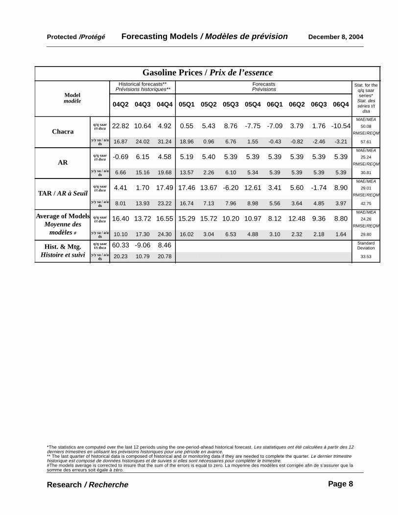
Page 8



*The statistics are computed over the last 12 periods using the one-period-ahead historical forecast. Les statistiques ont été calculées à partir des 12derniers trimestres en utilisant les prévisions historiques pour une période en avance.** The last quarter of historical data is composed of historical and or monitoring data if they are needed to complete the quarter. Le dernier trimestrehistorique est composé de données historiques et de suivies si elles sont nécessaires pour compléter le trimestre.#The models average is corrected to insure that the sum of the errors is equal to zero. La moyenne des modèles est corrigée afin de s’assurer que lasomme des erreurs soit égale à zéro.

Gasoline Prices /Prix de l’essence

Modelmodèle

Historical forecasts**Prévisions historiques**




dsa04Q2 04Q3 04Q4 05Q1 05Q2 05Q3 05Q4 06Q1 06Q2 06Q3 06Q4

Chacraq/q saart/t dsca 22.82 10.64 4.92 0.55 5.43 8.76 -7.75 -7.09 3.79 1.76 -10.54

MAE/MEA

50.08

RMSE/REQM

y/y sa / a/ads 16.87 24.02 31.24 18.96 0.96 6.76 1.55 -0.43 -0.82 -2.46 -3.21 57.61

ARq/q saart/t dsca -0.69 6.15 4.58 5.19 5.40 5.39 5.39 5.39 5.39 5.39 5.39

MAE/MEA

25.24

RMSE/REQM

y/y sa / a/ads 6.66 15.16 19.68 13.57 2.26 6.10 5.34 5.39 5.39 5.39 5.39 30.81

TAR / AR à Seuilq/q saart/t dsca 4.41 1.70 17.49 17.46 13.67 -6.20 12.61 3.41 5.60 -1.74 8.90

MAE/MEA

29.01

RMSE/REQM

y/y sa / a/ads 8.01 13.93 23.22 16.74 7.13 7.96 8.98 5.56 3.64 4.85 3.97 42.75


modèles#

q/q saart/t dsca 16.40 13.72 16.55 15.29 15.72 10.20 10.97 8.12 12.48 9.36 8.80

MAE/MEA

24.26

RMSE/REQM

y/y sa / a/ads 10.10 17.30 24.30 16.02 3.04 6.53 4.88 3.10 2.32 2.18 1.64 29.80


q/q saart/t dsca 60.33 -9.06 8.46 Standard

Deviation

y/y sa / a/ads 20.23 10.79 20.78 33.53

Page 9



*The statistics are computed over the last 12 periods using the one-period-ahead historical forecast. Les statistiques ont été calculées à partir des 12derniers trimestres en utilisant les prévisions historiques pour une période en avance.** The last quarter of historical data is composed of historical and or monitoring data if they are needed to complete the quarter. Le dernier trimestrehistorique est composé de données historiques et de suivies si elles sont nécessaires pour compléter le trimestre.#The models average is corrected to insure that the sum of the errors is equal to zero. La moyenne des modèles est corrigée afin de s’assurer que lasomme des erreurs soit égale à zéro.

Miscellaneous /DiversModelmodèle

Historical forecasts**Prévisions historiques**


Statictics*Statistique*

Production of Utilities / Production de service publicsJul Aug Sep Oct Nov Dec

Marcilm/m saarm/m dsca 0.29 -0.38 0.08 -3.64 3.32 1.38 RMSE/REQM

y/y sa / a/ads 3.49 -4.45 0.95 -35.88 48.00 17.87 1.32


m/m saarm/m dsca 0.92 1.34 0.36 Standard

Deviationy/y sa / a/a

ds 11.67 17.28 4.43 2.08

Consumption of Energy excl. gasoline /Consommation d’énergie excl. l’essenceJul Aug Sep Oct Nov Dec

Marcilm/m saarm/m dsca -0.38 -0.07 -0.17 -6.09 5.97 2.04 RMSE/REQM

y/y sa / a/ads -4.43 -0.83 -2.00 -52.97 100.44 27.48 3.42


m/m saarm/m dsca -0.45 0.65 -0.94 Standard


ds -5.24 8.09 -10.69 3.42

Heating Oil Prices /Prix de l’huile à chauffage04Q2 04Q3 04Q4 05Q1 05Q2 05Q3 05Q4 06Q1 06Q2 06Q3 06Q4

Chacraq/q saart/t dsca 10.57 11.68 28.44 19.15 -3.43 -2.81 5.63 4.93 -7.70 -7.82 3.21 RMSE/REQM

y/y sa / a/ads 8.17 14.79 26.61 25.49 24.43 20.70 4.25 0.99 -0.14 -1.46 -2.02 48.89


q/q saart/t dsca -0.08 9.77 89.79 Standard


ds 5.46 14.29 39.60 51.72

Natural Gas Prices /Prix du gaz naturel04Q2 04Q3 04Q4 05Q1 05Q2 05Q3 05Q4 06Q1 06Q2 06Q3 06Q4

Chacraq/q saart/t dsca -14.87 -6.76 6.71 9.00 -0.41 -7.15 5.08 4.87 -7.97 -8.65 2.00 RMSE/REQM

y/y sa / a/ads -11.44 -7.08 4.85 10.55 5.59 -1.87 1.45 0.47 -1.49 -1.89 -2.62 49.70


q/q saart/t dsca 19.66 24.49 -8.00 Standard


ds -3.57 -0.12 1.04 50.62

Page 10



*Data with a star are based on monitoring and Case-A forecast. For the other variables, they are held constant at their latest historical value. Les donnéesavec une étoile sont basées sur le suivi et le Cas-A. Pour les autres variables, elles sont maintenues à leur derniére valeur.** Nominal series. Série nominale.#The models average is corrected to insure that the sum of the errors is equal to zero. La moyenne des modèles est corrigée afin de s’assurer que lasomme des erreurs soit égale à zéro.

Forecasting Scenario /Scénario de prévision04Q1 04Q2 04Q3 04Q4 05Q1 05Q2 05Q3 05Q4 06Q1 06Q2 06Q3

Exchange RateTaux de change**

U.S.$/Can$

Interest RateTaux d’intérêt

30 daysé-jour

BCPI / ICPB ** q/q saart/t dsca

Can. GDP Defl.dégonfl. PIB

q/q saart/r sdca

Can. Output Gapécart au potentiel

% of pot.gdp

% du pibpot.

U.S. GDP / PIB q/q saart/r sdca

U.S. G.D.P. Defl.dégonfl. PIB

q/q saart/r sdca

U.S. Output Gap/écart au potentiel

% of pot.gdp

% du pibpot.

U.S. IIP / IPI q/q saart/r sdca

Rest of the worldOutput Gap/ écart aupotentiel du reste du

monde

% of pot.gdp

% du pibpot.

Crude Oil Prices /Prix du pétrole

brute

In US$/en $US

Jul Aug Sep Oct Nov Dec Jan Feb Mar Apr May

Manufacturing sec-tor / Secteur manu-

facturier

m/m sam/m ds

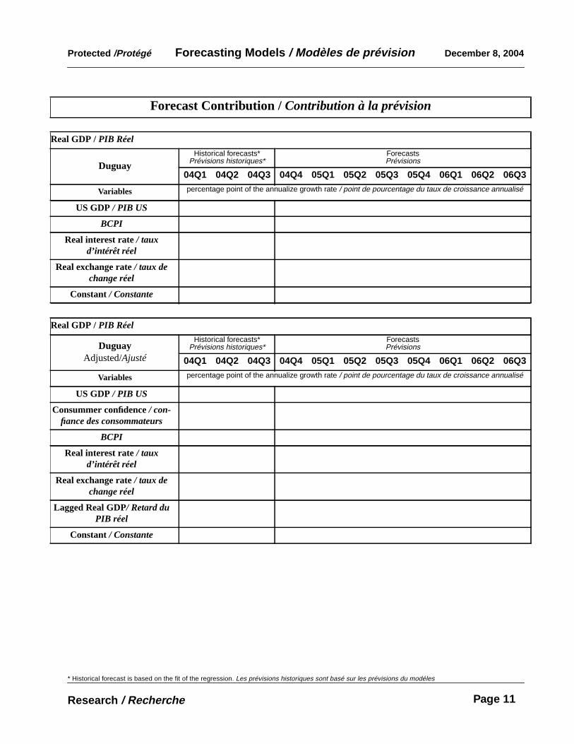
Page 11



* Historical forecast is based on the fit of the regression. Les prévisions historiques sont basé sur les prévisions du modéles

Forecast Contribution / Contribution à la prévision


DuguayHistorical forecasts*

Prévisions historiques*ForecastsPrévisions

04Q1 04Q2 04Q3 04Q4 05Q1 05Q2 05Q3 05Q4 06Q1 06Q2 06Q3

Variables percentage point of the annualize growth rate / point de pourcentage du taux de croissance annualisé

US GDP / PIB US

BCPI

Real interest rate/ tauxd’intérêt réel

Real exchange rate/ taux dechange réel

Constant / Constante


DuguayAdjusted/Ajusté

Historical forecasts*Prévisions historiques*


04Q1 04Q2 04Q3 04Q4 05Q1 05Q2 05Q3 05Q4 06Q1 06Q2 06Q3


US GDP / PIB US

Consummer confidence/ con-fiance des consommateurs

BCPI

Real interest rate/ tauxd’intérêt réel


Lagged Real GDP/ Retard duPIB réel


Page 12



* Historical forecast is based on the fit of the regression. Les prévisions historiques sont basé sur les prévisions du modéles

Forecast Contribution / Contribution à la prévision

Core CPI / IPC tendanciel

Fillion-LeonardAdjusted /Ajusté

Historical forecasts*Prévisions historiques*


04Q1 04Q2 04Q3 04Q4 05Q1 05Q2 05Q3 05Q4 06Q1 06Q2 06Q3


Canadian Ouput Gap/Écart au potentiel canadian

Real crude oil prices/ Prix dupétrole brut réel



Econometric Forecasts Package: Short-Run Forecasting Models for

Documents