ECOLOGY AND MANAGEMENT OF SUPERABUNDANT FISH POPULATIONS by Nathaniel T. Stewart A THESIS Presented to the Faculty of The Graduate College at the University of Nebraska In Partial Fulfillment of Requirements For the Degree of Master of Science Major: Natural Resource Sciences Under the Supervision of Professor Kevin L. Pope and Professor Christopher J. Chizinski Lincoln, Nebraska May 2015

Welcome message from author
This document is posted to help you gain knowledge. Please leave a comment to let me know what you think about it! Share it to your friends and learn new things together.
Transcript

ECOLOGY AND MANAGEMENT OF SUPERABUNDANT
FISH POPULATIONS
by
Nathaniel T. Stewart
A THESIS
Presented to the Faculty of
The Graduate College at the University of Nebraska
In Partial Fulfillment of Requirements
For the Degree of Master of Science
Major: Natural Resource Sciences
Under the Supervision of Professor Kevin L. Pope and Professor Christopher J. Chizinski
Lincoln, Nebraska
May 2015

ECOLOGY AND MANAGEMENT OF SUPERABUNDANT FISH POPULATIONS
Nathaniel Thomas Stewart, M.S.
University of Nebraska, 2015
Advisors: Kevin L. Pope and Christopher J. Chizinski
Fish population biomasses can reach extreme levels; we term these populations
superabundant fish populations. Superabundant fish populations may negatively affect
aquatic communities and anglers, necessitating the effective management of the
superabundant fish populations. However, there are gaps in our understanding of these
populations. The gaps in our understanding hamper our ability to predict effects on
valuable sportfisheries and to effectively manage superabundant fish populations. The
overall goal of my thesis research is to provide further insight into the ecology of
superabundant fish populations and to provide information that will aid in their effective
management. First, we described a new method for estimating abundances and
biomasses of superabundant fish populations in lentic systems using generalized N-
mixture models with data from consumer-grade sonar, vertical gillnets, and a boat
electrofisher. These open population models use point-count data with covariates to
estimate site-specific abundances and detection probabilities. I used this method to
estimate that there were 1.1-1.4 million white perch (Morone americana) and 0.5-1.1
million gizzard shad (Dorosoma cepedianum) in Branched Oak Lake, Nebraska. Second,
we determined how the spatial distributions of superabundant white perch populations
related to the spatial distributions of gizzard shad populations present in the same
waterbodies by using the site-specific abundances estimated with the generalized N-
mixture models. White perch and gizzard shad spatial distributions were positively

related in Branched Oak Lake and Pawnee Reservoir, Nebraska. We suspect that large
population sizes and similar diets contributed to the observed relationship. Third, we
evaluated the effect of a low-dose-rotenone application on white perch and gizzard shad
populations in Pawnee Reservoir, Nebraska. The low-dose rotenone application in
Pawnee Reservoir led to a large reduction (83%) in the white perch population biomass
and extirpated, or nearly extirpated, gizzard shad from the reservoir. By filling in the
gaps in our knowledge of superabundant populations we can more effectively manage
them for the good of our fisheries resources and their users by improving growth and
abundance of sportfish.

iv
Acknowledgements
There are numerous people who have contributed to getting me here and I thank
them all. I thank my family for their love, moral support, and patience. Specifically I
thank my parents Jeffery and Karen Stewart for providing an environment that allowed
me to develop a strong mental and spiritual base, for all of the advice over the years, and
for being excellent role models. I thank my brothers Ian and Will Stewart for moral
support and comic relief. I also thank both of my grandmothers for all of the cookies
they baked over the years and both of my grandfathers for teaching me to fish and for
providing examples of solid work ethics, honesty, and putting family first.
I thank my advisers Dr. Kevin Pope and Dr. Christopher Chizinski. I thank you
both for challenging me, for all of the time and ink spent editing, and for maintaining an
environment to foster learning, exploration, and constructive criticism. Specifically I
thank Kevin for helping me to think at more of a systems level rather than just about the
components that make up systems and for helping me improve my critical thinking skills.
I also thank you for all of the enthusiasm that you brought to our meetings and the project
as a whole. I thank Chris for all of the help with R, with population modeling, and for
challenging me to think beyond the standard fisheries approaches to data analysis. Thank
you also for all of your patience as I learned R and worked through the population models
for this project.
I thank the rest of my other committee members Dr. Larkin Powell, Dr. Mark
Pegg, Dr. Richard Holland, and Jeffery Jackson for all of their insight and interest in my

v
graduate education. I thank Dr. Larkin Powell for all of his assistance trouble shooting
our population models. I thank Dr. Mark Pegg for helping me think about the big picture
and for bringing a riverine perspective to our meetings. I thank Dr. Richard Holland for
always asking questions and for pushing me to look further into what my results meant. I
thank Jeffery Jackson for always bringing a management perspective to the table and for
his cooperation with my field sampling.
I thank my fellow graduate students in the Nebraska Cooperative Fish and
Wildlife Research Unit and Mark Pegg’s lab for feedback on presentations, writing, and
for discussions of my project. Specifically I thank Christopher Wiley, Dustin Martin,
Robert Kill, Kelly Turek, William Smith, Lucas Kowalewski, Brian Harmon, Danielle
Haak, Alexis Fedele, Nick Cole, Conner Chance-Ossowski, Nathan Bieber, and Stephen
Siddons for assistance with fieldwork. I especially thank Lucas Kowalewski for all of his
assistance with fieldwork, assistance designing sampling gear, and for all of the
discussions we had about my project while out on the boat. You helped get my graduate
school career off to a good start. I thank Kelly Turek for all of the assistance with
fieldwork during the fall of 2014. I also thank Valerie Egger and Caryl Cashmere for all
of their help with the logistics of graduate school. Without their help I would have had a
lot more trouble getting field equipment, traveling as part of my master’s program, and
getting to and from my field sites.
I thank the Nebraska Game and Parks Commission for funding my research. I
thank all of the Nebraska Game and Parks fisheries staff for their interest in and

vi
contributions to my research. I especially thank the southeast district fisheries staff for
always being willing to discuss my project when I stopped by.
Finally I thank the fisheries professionals who got me into fisheries and who
convinced me to pursue a graduate education. I think Jana Prey for showing me that you
could actually make a career out of working in fisheries. I thank Jason Spaeth for
introducing me to fieldwork in fisheries. I thank Dr. Daniel Isermann and Dr. Justin
Sipiorski for providing me opportunities to conduct research as an undergraduate student.
I thank Ryan Doorenbos for encouraging me to pursue a graduate education.
This project was funded by Federal Aid in Sport Fish Restoration, project F-193-
R, administered by the Nebraska Game and Parks Commission. Reference to trade names
does not imply endorsement by the author or any U.S. government. The Nebraska
Cooperative Fish and Wildlife Research Unit is jointly supported by the U.S. Geological
Survey, the Nebraska Game and Parks Commission, the University of Nebraska, the U.S.
Fish and Wildlife Service, and the Wildlife Management Institute. Portions of this work
were completed utilizing the Holland Computing Center of the University of Nebraska.

vii
Table of Contents
Chapter 1. Introduction ....................................................................................................... 1
Thesis goal and outline ....................................................................................................... 4
References ........................................................................................................................... 5
Chapter 2 Defining superabundant populations and challenges in estimating their size .... 8
Study Reservoirs ............................................................................................................... 14
Branched Oak Lake ................................................................................................... 14
Pawnee Reservoir ...................................................................................................... 14
Methods............................................................................................................................. 15
Sampling Design ....................................................................................................... 15
Approach: Water Depths > 2 m ................................................................................. 16
Approach: Water Depths ≤ 2 m ................................................................................. 18
Analysis ..................................................................................................................... 19
Application: Branched Oak Lake ............................................................................. 24
Application: Pawnee Reservoir ................................................................................ 26
Results ............................................................................................................................... 28
Sonar validation ......................................................................................................... 28
Branched Oak Lake ................................................................................................... 28
Pawnee Reservoir ...................................................................................................... 35
Discussion ......................................................................................................................... 38
References ......................................................................................................................... 46
Chapter 3 Seasonal distribution patterns of white perch and gizzard shad in reservoirs 107
Study Reservoirs ............................................................................................................. 110
Branched Oak Lake ................................................................................................. 110
Pawnee Reservoir .................................................................................................... 111
Methods........................................................................................................................... 111
Results ............................................................................................................................. 113

viii
Branched Oak Lake ................................................................................................. 113
Pawnee Reservoir .................................................................................................... 115
Discussion ....................................................................................................................... 116
References ....................................................................................................................... 120
Chapter 4. Controlling superabundant fish populations ................................................. 139
Methods........................................................................................................................... 142
Study Site................................................................................................................. 142
Application .............................................................................................................. 142
Abundance estimation and analysis ......................................................................... 143
Non-target effects .................................................................................................... 144
Results ............................................................................................................................. 145
Non-target effects .................................................................................................... 146
Discussion ....................................................................................................................... 147
References ....................................................................................................................... 152
Chapter 5 Conclusions, management recommendations, and research needs ................ 176
Management needs .................................................................................................. 178
Research questions .................................................................................................. 179
Conclusions ..................................................................................................................... 183
References ....................................................................................................................... 185
Appendix A. Diel distribution of white perch and gizzard shad in a flood-control
reservoir .......................................................................................................................... 186
Methods........................................................................................................................... 188
Study Site................................................................................................................. 188
Sampling Design ..................................................................................................... 188
Approach Water Depths > 2 m ................................................................................ 189
Approach Water Depths ≤ 2 m ................................................................................ 190
Analysis ................................................................................................................... 190
Results ............................................................................................................................. 192

ix
Discussion ....................................................................................................................... 194
References ....................................................................................................................... 197
Appendix B. Striped bass diet and condition .................................................................. 207
Reference ........................................................................................................................ 212

x
List of Tables
Table 2-1. Methods that fisheries scientists can use to estimate fish abundance and each
method’s advantages. ........................................................................................................ 50
Table 2-2. Candidate generalized N-mixture models used to estimate white perch and
gizzard shad abundances on Branched Oak Lake and Pawnee Reservoir, Nebraska. Data
were collected with a consumer grade sonar unit used in conjunction with vertical gillnets
(SN) and with a boat electrofisher (EF). In each model, λ is site and specific abundance,
γ is site and time specific recruitment, Ω is site and time specific apparent survival, and p
is site and time specific detection probability. The covariates in the models are the mean
depth of cells (D), whether the mean slope was < 1% or ≥ 1 % (S), the period in which a
sample was taken (P), whether the cell was adjacent to shore and whether the adjacent
shoreline had rip rap (H), and presence or absence of timber (T). ................................... 51
Table 2-3. Generalized N-mixture models ranked with AIC used to model white perch
abundance on Branched Oak Lake, Nebraska during 2013 (K: number of model
parameters, AIC: Akaike Information Criterion score, ΔAIC: difference between AIC
score for the specified model and for the top model, AICwt: AIC weight, cumwt:
cumulative AIC weight). Count data were collected with a consumer grade sonar unit
used in conjunction with vertical gillnets (SN) in waters with total depths ≥ 2 m and a
boat electrofisher (EF) used to electrify points in water with total depths < 2 m. In each
model, λ is site and time specific abundance, γ is site and time specific recruitment, Ω is
site and time specific apparent survival, and p is site and time specific detection
probability. The covariates in the models are the mean depth of cells (D), whether the
mean slope was < 1 % or ≥ 1 % (S), the period in which a sample was taken (P), whether
the cell was adjacent to shore and whether the adjacent shoreline had rip rap (H), and
presence or absence of timber (T). .................................................................................... 53
Table 2-4. Parameter estimates for generalized N-mixture model used to estimate white
perch abundance and biomass on the north arm of Branched Oak Lake, Nebraska during
2013. We collected data using a combination of sonar and vertical gillnets. In the model,
λ is site and time specific abundance (log scale), γ is site and time specific recruitment
(log scale), Ω is site and time specific apparent survival (logit scale), and p is site and
time specific detection probability (logit scale). Covariates were Depth (the mean depth
of cells), Slope (mean bottom slope in a cell; category 1: <1% slope, category 2: ≥1%
slope), and Period (the period in, which sampling took place; category A: June 25,
category B: July 31, and category B: October 16). This model also included dispersion
parameter that is a measure of how much overdispersion the model was relative to a
Poisson model. .................................................................................................................. 55

xi
Table 2-5. Parameter estimates for generalized N-mixture model used to estimate white
perch abundance and biomass on the north arm of Branched Oak Lake, Nebraska during
2013. We collected data using a boat electrofisher. In the model, λ is site and time
specific abundance (log scale), γ is site and time specific recruitment (log scale), Ω is site
and time specific apparent survival (logit scale), and p is site and time specific detection
probability (logit scale). Covariates were Depth (the mean depth of cells), Slope (mean
bottom slope in a cell; category 1: <1% slope, category 2: ≥1% slope), Shore (whether or
not a cell was adjacent to shore and whether or not that shore had rip rap; category 1:
offshore, category 2: adjacent to shore, category 3: adjacent to rip-rapped shore), Timber
(whether or not a sampling cell contained flooded timber; category 0: timber absent and
category 1: timber present) and Period (the period in, which sampling took place;
category A: June 25, category B: July 31, and category B: October 16). This model
contains a zero-inflation term, which provided a measure of how zero inflated the data
were. .................................................................................................................................. 57
Table 2-6. Parameter estimates for generalized N-mixture model used to estimate white
perch abundance and biomass on the south arm of Branched Oak Lake, Nebraska during
2013. We collected data using a combination of sonar and vertical gillnets. In the model,
λ is site and time specific abundance (log scale), γ is site and time specific recruitment
(log scale), Ω is site and time specific apparent survival (logit scale), and p is site and
time specific detection probability (logit scale). Covariates were Depth (the mean depth
of cells), Slope (mean bottom slope in a cell; category 1: <1% slope, category 2: ≥1%
slope), and Period (the period in, which sampling took place; category A: June 25,
category B: July 31, and category B: October 16). This model also included dispersion
parameter that is a measure of how much overdispersion the model allowed relative to a
Poisson model. .................................................................................................................. 59
Table 2-7. Generalized N-mixture models ranked with AIC used to model white perch
abundance on Branched Oak Lake, Nebraska during 2014 (K: number of model
parameters, AIC: Akaike Information Criterion score, ΔAIC: difference between AIC
score for the specified model and for the top model, AICwt: AIC weight, cumwt:
cumulative AIC weight). Count data were collected with a consumer grade sonar unit
used in conjunction with vertical gillnets (SN) in waters with total depths ≥ 2 m and a
boat electrofisher (EF) used to electrify points in water with total depths < 2 m during.
In each model, λ is abundance, γ is recruitment, Ω is apparent survival, and p is detection
probability. The covariates in the models are depth (D), slope (S), sampling period (P),
and shoreline habitat (H). .................................................................................................. 61
Table 2-8. Parameter estimates for generalized N-mixture model used to estimate white
perch abundance and biomass on the north arm of Branched Oak Lake, Nebraska during
2014. We collected data using a combination of sonar and vertical gillnets. In the model,
λ is site and time specific abundance (log scale), γ is site and time specific recruitment
(log scale), Ω is site and time specific apparent survival (logit scale), and p is site and

xii
time specific detection probability (logit scale). Covariates were Depth (the mean depth
of cells), Slope (mean bottom slope in a cell; category 1: <1% slope, category 2: ≥1%
slope), and Period (the period in, which sampling took place; category A: April 1,
category B: July 7, and category B: October 13). This model also included dispersion
parameter that is a measure of how much overdispersion the model allowed relative to a
Poisson model. .................................................................................................................. 63
Table 2-9. Parameter estimates for generalized N-mixture model used to estimate white
perch abundance and biomass on the north arm of Branched Oak Lake, Nebraska during
2014. We collected data using a boat electrofisher. In the model, λ is site and time
specific abundance (log scale), γ is site and time specific recruitment (log scale), Ω is site
and time specific apparent survival (logit scale), and p is site and time specific detection
probability (logit scale). Covariates were Depth (the mean depth of cells), Slope (mean
bottom slope in a cell; category 1: <1% slope, category 2: ≥1% slope), Shore (whether or
not a cell was adjacent to shore and whether or not that shore had rip rap; category 1:
offshore, category 2: adjacent to shore, category 3: adjacent to rip-rapped shore), Timber
(whether or not a sampling cell contained flooded timber; category 0: timber absent and
category 1: timber present) and Period (the period in, which sampling took place;
category A: April 1, category B: July 7, and category B: October 13). This model
contains a zero-inflation term, which provided a measure of how zero inflated the data
were. .................................................................................................................................. 65
Table 2-10. Parameter estimates for generalized N-mixture model used to estimate white
perch abundance and biomass on the south arm of Branched Oak Lake, Nebraska during
2014. We collected data using a combination of sonar and vertical gillnets. In the model,
λ is site and time specific abundance (log scale), γ is site and time specific recruitment
(log scale), Ω is site and time specific apparent survival (logit scale), and p is site and
time specific detection probability (logit scale). Covariates were Depth (the mean depth
of cells), Slope (mean bottom slope in a cell; category 1: <1% slope, category 2: ≥1%
slope), and Period (the period in, which sampling took place; category A: April 1,
category B: July 7, and category B: October 13). This model also included dispersion
parameter that is a measure of how much overdispersion the model allowed relative to a
Poisson model. .................................................................................................................. 67
Table 2-11. Parameter estimates for generalized N-mixture model used to estimate white
perch abundance and biomass on the south arm of Branched Oak Lake, Nebraska during
2014. We collected data using a boat electrofisher. In the model, λ is site and time
specific abundance (log scale), γ is site and time specific recruitment (log scale), Ω is site
and time specific apparent survival (logit scale), and p is site and time specific detection
probability (logit scale). Covariates were Depth (the mean depth of cells), Slope (mean
bottom slope in a cell; category 1: <1% slope, category 2: ≥1% slope), Shore (whether or
not a cell was adjacent to shore and whether or not that shore had rip rap; category 1:
offshore, category 2: adjacent to shore, category 3: adjacent to rip-rapped shore), Timber

xiii
(whether or not a sampling cell contained flooded timber; category 0: timber absent and
category 1: timber present) and Period (the period in, which sampling took place;
category A: April 1, category B: July 7, and category B: October 13). This model
contains a zero-inflation term, which provided a measure of how zero inflated the data
were. .................................................................................................................................. 69
Table 2-12. Generalized N-mixture models ranked with AIC used to model gizzard shad
abundance on Branched Oak Lake, Nebraska during 2013 (K: number of model
parameters, AIC: Akaike Information Criterion score, ΔAIC: difference between AIC
score for the specified model and for the top model, AICwt: AIC weight, cumwt:
cumulative AIC weight). Count data were collected with a consumer grade sonar unit
used in conjunction with vertical gillnets (SN) in waters with total depths ≥ 2 m and a
boat electrofisher (EF) used to electrify points in water with total depths < 2 m. In each
model, λ is abundance, γ is recruitment, Ω is apparent survival, and p is detection
probability. The covariates in the models are depth (D), slope (S), sampling period (P),
and shoreline habitat (H). .................................................................................................. 71
Table 2-13. Parameter estimates for generalized N-mixture model used to estimate
gizzard shad abundance and biomass on the north arm of Branched Oak Lake, Nebraska
during 2013. We collected data using a combination of sonar and vertical gillnets. In the
model, λ is site and time specific abundance (log scale), γ is site and time specific
recruitment (log scale), Ω is site and time specific apparent survival (logit scale), and p is
site and time specific detection probability (logit scale). Covariates were Depth (the
mean depth of cells), Slope (mean bottom slope in a cell; category 1: <1% slope, category
2: ≥1% slope), and Period (the period in, which sampling took place; category A: June
25, category B: July 31, and category B: October 16). This model also included
dispersion parameter that is a measure of how much overdispersion the model allowed
relative to a Poisson model. .............................................................................................. 72
Table 2-14. Parameter estimates for generalized N-mixture model used to estimate
gizzard shad abundance and biomass on the north arm of Branched Oak Lake, Nebraska
during 2013. We collected data using a boat electrofisher. In the model, λ is site and
time specific abundance (log scale), γ is site and time specific recruitment (log scale), Ω
is site and time specific apparent survival (logit scale), and p is site and time specific
detection probability (logit scale). Covariates were Depth (the mean depth of cells),
Slope (mean bottom slope in a cell; category 1: <1% slope, category 2: ≥1% slope),
Shore (whether or not a cell was adjacent to shore and whether or not that shore had rip
rap; category 1: offshore, category 2: adjacent to shore, category 3: adjacent to rip-rapped
shore), Timber (whether or not a sampling cell contained flooded timber; category 0:
timber absent and category 1: timber present) and Period (the period in, which sampling
took place; category A: June 25, category B: July 31, and category B: October 16). This
model contains a zero-inflation term, which provided a measure of how zero inflated the
data were. .......................................................................................................................... 74

xiv
Table 2-15. Parameter estimates for generalized N-mixture model used to estimate
gizzard shad abundance and biomass on the south arm of Branched Oak Lake, Nebraska
during 2013. We collected data using a combination of sonar and vertical gillnets. In the
model, λ is site and time specific abundance (log scale), γ is site and time specific
recruitment (log scale), Ω is site and time specific apparent survival (logit scale), and p is
site and time specific detection probability (logit scale). Covariates were Depth (the
mean depth of cells), Slope (mean bottom slope in a cell; category 1: <1% slope, category
2: ≥1% slope), and Period (the period in, which sampling took place; category A: June
25, category B: July 31, and category B: October 16). This model also included
dispersion parameter that is a measure of how much overdispersion the model allowed
relative to a Poisson model. .............................................................................................. 76
Table 2-16. Generalized N-mixture models ranked with AIC used to model gizzard shad
abundance on Branched Oak Lake, Nebraska during 2014 (K: number of model
parameters, AIC: Akaike Information Criterion score, ΔAIC: difference between AIC
score for the specified model and for the top model, AICwt: AIC weight, cumwt:
cumulative AIC weight). Count data were collected with a consumer grade sonar unit
used in conjunction with vertical gillnets (SN) in waters with total depths ≥ 2 m and a
boat electrofisher (EF) used to electrify points in water with total depths < 2 m. In each
model, λ is abundance, γ is recruitment, Ω is apparent survival, and p is detection
probability. The covariates in the models are depth (D), slope (S), sampling period (P),
and shoreline habitat (H). .................................................................................................. 78
Table 2-17. Parameter estimates for generalized N-mixture model used to estimate
gizzard shad abundance and biomass on the north arm of Branched Oak Lake, Nebraska
during 2014. We collected data using a combination of sonar and vertical gillnets In the
model, λ is site and time specific abundance (log scale), γ is site and time specific
recruitment (log scale), Ω is site and time specific apparent survival (logit scale), and p is
site and time specific detection probability (logit scale). Covariates were Depth (the
mean depth of cells), Slope (mean bottom slope in a cell; category 1: <1% slope, category
2: ≥1% slope), and Period (the period in, which sampling took place; category A: April 1,
category B: July 7, and category B: October 13). This model also included dispersion
parameter that is a measure of how much overdispersion the model allowed relative to a
Poisson model. .................................................................................................................. 80
Table 2-18. Parameter estimates for generalized N-mixture model used to estimate
gizzard shad abundance and biomass on the north arm of Branched Oak Lake, Nebraska
during 2014. We collected data using a boat electrofisher. In the model, λ is site and
time specific abundance (log scale), γ is site and time specific recruitment (log scale), Ω
is site and time specific apparent survival (logit scale), and p is site and time specific
detection probability (logit scale). Covariates were Depth (the mean depth of cells),
Slope (mean bottom slope in a cell; category 1: <1% slope, category 2: ≥1% slope),
Shore (whether or not a cell was adjacent to shore and whether or not that shore had rip

xv
rap; category 1: offshore, category 2: adjacent to shore, category 3: adjacent to rip-rapped
shore), Timber (whether or not a sampling cell contained flooded timber; category 0:
timber absent and category 1: timber present) and Period (the period in, which sampling
took place; category A: April 1, category B: July 7, and category B: October 13). This
model contains a zero-inflation term, which provided a measure of how zero inflated the
data were. .......................................................................................................................... 82
Table 2-19. Parameter estimates for generalized N-mixture model used to estimate
gizzard shad abundance and biomass on the south arm of Branched Oak Lake, Nebraska
during 2014. We collected data using a combination of sonar and vertical gillnets. In the
model, λ is site and time specific abundance (log scale), γ is site and time specific
recruitment (log scale), Ω is site and time specific apparent survival (logit scale), and p is
site and time specific detection probability (logit scale). Covariates were Depth (the
mean depth of cells), Slope (mean bottom slope in a cell; category 1: <1% slope, category
2: ≥1% slope), and Period (the period in, which sampling took place; category A: April 1,
category B: July 7, and category B: October 13). This model also included dispersion
parameter that is a measure of how much overdispersion the model allowed relative to a
Poisson model. .................................................................................................................. 84
Table 2-20. Parameter estimates for generalized N-mixture model used to estimate
gizzard shad abundance and biomass on the south arm of Branched Oak Lake, Nebraska
during 2014. We collected data using a boat electrofisher. In the model, λ is site and
time specific abundance (log scale), γ is site and time specific recruitment (log scale), Ω
is site and time specific apparent survival (logit scale), and p is site and time specific
detection probability (logit scale). Covariates were Depth (the mean depth of cells),
Slope (mean bottom slope in a cell; category 1: <1% slope, category 2: ≥1% slope),
Shore (whether or not a cell was adjacent to shore and whether or not that shore had rip
rap; category 1: offshore, category 2: adjacent to shore, category 3: adjacent to rip-rapped
shore), Timber (whether or not a sampling cell contained flooded timber; category 0:
timber absent and category 1: timber present) and Period (the period in, which sampling
took place; category A: April 1, category B: July 7, and category B: October 13). This
model contains a zero-inflation term, which provided a measure of how zero inflated the
data were. .......................................................................................................................... 86
Table 2-21. Abundance and biomass with 95% confidence intervals estimated for white
perch (WHP) and gizzard shad (SHAD) in Branched Oak Lake (BOL) and Pawnee
Reservoir (PWR), Nebraska. Estimates were made using generalized N-mixture models
with data collected with a consumer-grade sonar unit, vertical gillnets, and a boat
electrofisher....................................................................................................................... 88
Table 2-22. Generalized N-mixture models ranked with AIC used to estimate white perch
abundance and biomass on Pawnee Reservoir, Nebraska (K: number of model
parameters, AIC: Akaike Information Criterion score, ΔAIC: difference between AIC
score for the specified model and for the top model, AICwt: AIC weight, cumwt:

xvi
cumulative AIC weight). Count data were collected with a consumer grade sonar unit
used in conjunction with vertical gillnets (SN) in waters with total depths ≥ 2 m and a
boat electrofisher (EF) used to electrify points in water with total depths < 2 m. In each
model, λ is abundance, γ is recruitment, Ω is apparent survival, and p is detection
probability. The covariates in the models are depth (D), slope (S), sampling period (P),
and shoreline habitat (H). .................................................................................................. 89
Table 2-23. Parameter estimates for generalized N-mixture model used to estimate white
perch abundance and biomass in Pawnee Reservoir, Nebraska during 2013. We collected
data using a combination of sonar and vertical gillnets. In the model, λ is site and time
specific abundance (log scale), γ is site and time specific recruitment (log scale), Ω is site
and time specific apparent survival (logit scale), and p is site and time specific detection
probability (logit scale). Covariates were Depth (the mean depth of cells), Slope (mean
bottom slope in a cell; category 1: <1% slope, category 2: ≥1% slope), and Period (the
period in, which sampling took place; category A: June 17, category B: July 25, category
C: September 9, category D: October 8). This model also included dispersion parameter
that is a measure of how much overdispersion the model allowed relative to a Poisson
model................................................................................................................................. 90
Table 2-24. Parameter estimates for generalized N-mixture model used to estimate white
perch abundance and biomass in Pawnee Reservoir, Nebraska during 2013. We collected
data using a boat electrofisher. In the model, λ is site and time specific abundance (log
scale), γ is site and time specific recruitment (log scale), Ω is site and time specific
apparent survival (logit scale), and p is site and time specific detection probability (logit
scale). Covariates were Depth (the mean depth of cells), Slope (mean bottom slope in a
cell; category 1: <1% slope, category 2: ≥1% slope), Shore (whether or not a cell was
adjacent to shore and whether or not that shore had rip rap; category 1: offshore, category
2: adjacent to shore, category 3: adjacent to rip-rapped shore), Timber (whether or not a
sampling cell contained flooded timber; category 0: timber absent and category 1: timber
present) and Period (the period in, which sampling took place; category A: June 17,
category B: July 25, category C: September 9, category D: October 8). This model
contains a zero-inflation term, which provided a measure of how zero inflated the data
were. .................................................................................................................................. 92
Table 2-25. Parameter estimates for generalized N-mixture model used to estimate white
perch abundance and biomass in Pawnee Reservoir, Nebraska during 2014. We collected
data using a combination of sonar and vertical gillnets. In the model, λ is site and time
specific abundance (log scale), γ is site and time specific recruitment (log scale), Ω is site
and time specific apparent survival (logit scale), and p is site and time specific detection
probability (logit scale). Covariates were Depth the mean depth of cells (the mean depth
of cells), Slope (mean bottom slope in a cell; category 1: <1% slope, category 2: ≥1%
slope), and Period (the period in, which sampling took place; category A: May 2,
category B: May 14, category C: May 21, category D: June 20, category E: September

xvii
18, category F: October 7). This model also included dispersion parameter that is a
measure of how much overdispersion the model allowed relative to a Poisson model. ... 94
Table 2-26. Parameter estimates for generalized N-mixture model used to estimate white
perch abundance and biomass in Pawnee Reservoir, Nebraska during 2014. We collected
data using a boat electrofisher. In the model, λ is site and time specific abundance (log
scale), γ is site and time specific recruitment (log scale), Ω is site and time specific
apparent survival (logit scale), and p is site and time specific detection probability (logit
scale). Covariates were Depth (the mean depth of cells), Slope (mean bottom slope in a
cell; category 1: <1% slope, category 2: ≥1% slope), Shore (whether or not a cell was
adjacent to shore and whether or not that shore had rip rap; category 1: offshore, category
2: adjacent to shore, category 3: adjacent to rip-rapped shore), Timber (whether or not a
sampling cell contained flooded timber; category 0: timber absent and category 1: timber
present) and Period (the period in, which sampling took place; category A: May 2,
category B: May 14, category C: May 21, category D: June 20, category E: September
18, category F: October 7). This model contains a zero-inflation term, which provided a
measure of how zero inflated the data were...................................................................... 96
Table 2-27. Generalized N-mixture models ranked with AIC used to model gizzard shad
abundance on Pawnee Reservoir, Nebraska during 2013 (K: number of model
parameters, AIC: Akaike Information Criterion score, ΔAIC: difference between AIC
score for the specified model and for the top model, AICwt: AIC weight, cumwt:
cumulative AIC weight). Count data were collected with a consumer grade sonar unit
used in conjunction with vertical gillnets (SN) in waters with total depths of 2 m or more
and a boat electrofisher (EF) used to shock points in water with total depths < 2 m. In
each model, λ is abundance, γ is recruitment, Ω is apparent survival, and p is detection
probability. The covariates in the models are depth (D), slope (S), sampling period (P),
and shoreline habitat (H). .................................................................................................. 98
Table 2-28. Parameter estimates for generalized N-mixture model used to estimate
gizzard shad abundance and biomass in Pawnee Reservoir, Nebraska during 2013 We
collected data using a combination of sonar and vertical gillnets. In the model, λ is site
and time specific abundance (log scale), γ is site and time specific recruitment (log scale),
Ω is site and time specific apparent survival (logit scale), and p is site and time specific
detection probability (logit scale). Covariates were Depth (the mean depth of cells),
Slope (mean bottom slope in a cell; category 1: <1% slope, category 2: ≥1% slope), and
Period (the period in, which sampling took place; category A: June 17, category B: July
25, category C: September 9, category D: October 8). This model also included
dispersion parameter that is a measure of how much overdispersion the model allowed
relative to a Poisson model. .............................................................................................. 99
Table 2-29. Parameter estimates for generalized N-mixture model used to estimate
gizzard shad abundance and biomass in Pawnee Reservoir, Nebraska during 2013. We
collected data using a boat electrofisher. In the model, λ is site and time specific

xviii
abundance (log scale), γ is site and time specific recruitment (log scale), Ω is site and
time specific apparent survival (logit scale), and p is site and time specific detection
probability (logit scale). Covariates were Depth (the mean depth of cells), Slope (mean
bottom slope in a cell; category 1: <1% slope, category 2: ≥1% slope), Shore (whether or
not a cell was adjacent to shore and whether or not that shore had rip rap; category 1:
offshore, category 2: adjacent to shore, category 3: adjacent to rip-rapped shore), Timber
(whether or not a sampling cell contained flooded timber; category 0: timber absent and
category 1: timber present) and Period (the period in, which sampling took place;
category A: June 17, category B: July 25, category C: September 9, category D: October
8). This model contains a zero-inflation term, which provided a measure of how zero
inflated the data were. ..................................................................................................... 101
Table 4-1. Species-specific rotenone toxicity estimates with standard error if available as
reported in the literature; (* rough estimates of LC 100). .............................................. 155
Table 4-2. Generalized N-mixture models ranked with AIC used to model white perch
abundance on Pawnee Reservoir, Nebraska prior to (pre) and following (post) a low-dose
rotenone treatment during November 2013 (K: number of model parameters, AIC:
Akaike Information Criterion score, ΔAIC: difference between AIC score for the
specified model and for the top model, AICwt: AIC weight, cumwt: cumulative AIC
weight). Count data were collected with a consumer grade sonar unit used in conjunction
with vertically set gillnets (SN) in waters with total depths ≥ 2 m and a boat electrofisher
(EF) used to electrify points in water with total depths < 2 m. In each model, λ is
abundance, γ is recruitment, Ω is apparent survival, and p is detection probability. The
covariates in the models are depth (D), slope (S), sampling period (P), and shoreline
habitat (H). ...................................................................................................................... 157
Table 4-3. Parameter estimates for generalized N-mixture model used to estimate white
perch abundance and biomass in Pawnee Reservoir, Nebraska during 2013. We collected
data using a combination of sonar and vertical gillnets. In the model, λ is site and time
specific abundance (log scale), γ is site and time specific recruitment (log scale), Ω is site
and time specific apparent survival (logit scale), and p is site and time specific detection
probability (logit scale). Covariates were Depth (the mean depth of cells), Slope (mean
bottom slope in a cell; category 1: <1% slope, category 2: ≥1% slope), and Period (the
period in, which sampling took place; category A: June 17, category B: July 25, category
C: September 9, category D: October 8). This model also included dispersion parameter
that is a measure of how much overdispersion the model allowed relative to a Poisson
model............................................................................................................................... 158
Table 4-4. Parameter estimates for generalized N-mixture model used to estimate white
perch abundance and biomass in Pawnee Reservoir, Nebraska during 2013. We collected
data using a boat electrofisher. In the model, λ is site and time specific abundance (log
scale), γ is site and time specific recruitment (log scale), Ω is site and time specific
apparent survival (logit scale), and p is site and time specific detection probability (logit

xix
scale). Covariates were Depth (the mean depth of cells), Slope (mean bottom slope in a
cell; category 1: <1% slope, category 2: ≥1% slope), Shore (whether or not a cell was
adjacent to shore and whether or not that shore had rip rap; category 1: offshore, category
2: adjacent to shore, category 3: adjacent to rip-rapped shore), and Period (the period in,
which sampling took place; category A: June 17, category B: July 25, category C:
September 9, category D: October 8). This model contains a zero-inflation term, which
provided a measure of how zero inflated the data were. ................................................. 160
Table 4-5. Parameter estimates for generalized N-mixture model used to estimate white
perch abundance and biomass in Pawnee Reservoir, Nebraska during 2014. We collected
data using a combination of sonar and vertical gillnets. In the model, λ is site and time
specific abundance (log scale), γ is site and time specific recruitment (log scale), Ω is site
and time specific apparent survival (logit scale), and p is site and time specific detection
probability (logit scale). Covariates were Depth (the mean depth of cells), Slope (mean
bottom slope in a cell; category 1: <1% slope, category 2: ≥1% slope), and Period (the
period in, which sampling took place; category A: May 2, category B: May 14, category
C: May 21, category D: June 20, category E: September 18, category F: October 7). This
model also included dispersion parameter that is a measure of how much overdispersion
the model allowed relative to a Poisson model. .............................................................. 162
Table 4-6. Parameter estimates for generalized N-mixture model used to estimate white
perch abundance and biomass in Pawnee Reservoir, Nebraska during 2014. We collected
data using a boat electrofisher. In the model, λ is site and time specific abundance (log
scale), γ is site and time specific recruitment (log scale), Ω is site and time specific
apparent survival (logit scale), and p is site and time specific detection probability (logit
scale). Covariates were Depth (the mean depth of cells), Slope (mean bottom slope in a
cell; category 1: <1% slope, category 2: ≥1% slope), Shore (whether or not a cell was
adjacent to shore and whether or not that shore had rip rap; category 1: offshore, category
2: adjacent to shore, category 3: adjacent to rip-rapped shore), and Period (the period in,
which sampling took place; category A: May 2, category B: May 14, category C: May 21,
category D: June 20, category E: September 18, category F: October 7). This model
contains a zero-inflation term, which provided a measure of how zero inflated the data
were. ................................................................................................................................ 164
Table 4-7. Generalized N-mixture models ranked with AIC used to model gizzard shad
abundance on Pawnee Reservoir Nebraska prior to a low-dose rotenone treatment during
November 2013 (K: number of model parameters, AIC: Akaike Information Criterion
score, ΔAIC: difference between AIC score for the specified model and for the top
model, AICwt: AIC weight, cumwt: cumulative AIC weight). Count data were collected
with a consumer grade sonar unit (SN) used in conjunction with vertically set gillnets in
waters with total depths of 2 m or more and a boat electrofisher (EF) used to shock points
in water with total depths less than 2 m. In each model, λ is abundance, γ is recruitment,

xx
Ω is apparent survival, and p is detection probability. The covariates in the models are
depth (D), slope (S), sampling period (P), and shoreline habitat (H). ............................ 166
Table 4-8. Parameter estimates for generalized N-mixture model used to estimate gizzard
shad abundance and biomass in Pawnee Reservoir, Nebraska during 2013. We collected
data using a combination of sonar and vertical gillnets. In the model, λ is site and time
specific abundance (log scale), γ is site and time specific recruitment (log scale), Ω is site
and time specific apparent survival (logit scale), and p is site and time specific detection
probability (logit scale). Covariates were Depth (the mean depth of cells), Slope (mean
bottom slope in a cell; category 1: <1% slope, category 2: ≥1% slope), and Period (the
period in, which sampling took place; category A: June 17, category B: July 25, category
C: September 9, category D: October 8). This model also included dispersion parameter
that is a measure of how much overdispersion the model allowed relative to a Poisson
model............................................................................................................................... 167
Table 4-9. Parameter estimates for generalized N-mixture model used to estimate gizzard
shad abundance and biomass in Pawnee Reservoir, Nebraska during 2013. We collected
data using a boat electrofisher. In the model, λ is site and time specific abundance (log
scale), γ is site and time specific recruitment (log scale), Ω is site and time specific
apparent survival (logit scale), and p is site and time specific detection probability (logit
scale). Covariates were Depth (the mean depth of cells), Slope (mean bottom slope in a
cell; category 1: <1% slope, category 2: ≥1% slope), Shore (whether or not a cell was
adjacent to shore and whether or not that shore had rip rap; category 1: offshore, category
2: adjacent to shore, category 3: adjacent to rip-rapped shore), and Period (the period in,
which sampling took place; category A: June 17, category B: July 25, category C:
September 9, category D: October 8). This model contains a zero-inflation term, which
provided a measure of how zero inflated the data were. ................................................. 169
Table 4-10. Daily observed mortality of non-target fish species counted along seven, 10-
m sections of shoreline 2, 3, 5, and 7 days post low-dose rotenone application on Pawnee
Reservoir, Nebraska. ....................................................................................................... 171
Table A-1. The order of polynomial used to remove global trends and mean prediction
error for universal kriging analysis carried out using geostatistical analyst tools in
ArcGIS10 to assess changes in fish spatial distribution in Branched Oak Lake during diel
cycles between August 11 and 29 of 2014. Data were collected using a consumer grade
sonar unit. ........................................................................................................................ 199
Table A-2. Comparisons of the number of fish captured with a boat electrofisher between
periods over diel cycles in Branched Oak Lake, Nebraska from August 11to 29, 2014.
Analyses were carried out using generalized linear models for data with negative
binomial distribution. ...................................................................................................... 200

xxi
Table A-3. Results of comparisons of number of fish targets identified using consumer-
grade sonar between periods within depth layers. Data were collected between August 11
and 29, 2014 in Branched Oak Lake, Nebraska. Analyses were carried out using
generalized linear models for data with negative binomial distribution. ........................ 201
Table A-4. Results of comparisons of number of fish captured with vertical gillnets in the
top 4 meters of the water column between periods. Data were collected between August
11 to 29, 2014 in Branched Oak Lake, Nebraska. Analyses were carried out using
generalized linear models for data with negative binomial distribution. ........................ 202
Table B-2. Length, weight, relative weight (Wr), and gut content information for striped
bass (Morone saxatilis) captured in Branched Oak Lake, Nebraska during 2014. Effort
consisted of 288, 1-2 h vertical gillnet sets (VG), 15, 1-24 h horizontal gillnet sets (GN),
and 26,731 seconds of electrofishing (EF) during 2014. Fish from October were captured
in Nebraska Game and Parks Commission standardized gillnets and trapnets (TN).
Parameters for estimating relative weight from Brown and Murphy 1991. ................... 211

xxii
List of Figures
Figure 1-1. Conceptual model of differences in population biomass regulation between
organisms that exhibit limited growth plasticity such as mammals or birds (left) and
organisms that exhibit growth plasticity such as fish (right). Box number denotes the
number of individuals and box width denotes the size of the individual; biomasses in all
populations are the same. .................................................................................................... 7
Figure 2-1. Stratification system and sampling sites (with adjustments for sites moved
because they were unsampleable) for estimating white perch and gizzard shad
abundances, biomasses, and spatial distributions in Branched Oak Lake, Nebraska. .... 103
Figure 2-2. Stratification system and sampling sites for estimating white perch and
gizzard shad abundances, biomasses, and spatial distributions in Pawnee Reservoir,
Nebraska. ........................................................................................................................ 104
Figure 2-3. Electric field map for a 5.5- m boat electrofisher with a Smith-Root® 5.0
GPP control box. The effective edge of the electric field was estimated to be where
power density was < 84 µW/cc. ...................................................................................... 105
Figure 2-4. Relationships between vertical gillnet catch and fish density estimated using
consumer grade sonar in Branched Oak Lake (top) and Pawnee Reservoir, Nebraska
(bottom) during spring, summer, and fall of 2013 and 2014. ......................................... 106
Figure 3-1. Conceptual models of hypothetical white perch ( ) and gizzard shad ( )
distributions in two habitats ( and ) within the same waterbody. The top panels
represents no relationship between spatial distributions, the second panels represents both
species sharing the same habitats, the third panels represents each species using different
habitat, and the fourth panel represents white perch using all habitats and gizzard shad
selecting one habitat. ....................................................................................................... 122
Figure 3-2. Estimates of white perch relative abundances (percent of population per
sampling cell) in Branched Oak Lake, Nebraska. Data were collected during July and
October of 2013 and during April, July, and October of 2014 with consumer-grade sonar,
vertical gillnets, and a boat electrofisher and analyzed using generalized N-mixture
models. ............................................................................................................................ 124
Figure 3-3. Estimates of white perch detection probability in Branched Oak Lake,
Nebraska. Data were collected during July and October of 2013 and during April, July,
and October of 2014 with consumer-grade sonar, vertical gillnets, and a boat electrofisher
and analyzed using generalized N-mixture models. ....................................................... 126
Figure 3-4. Estimates of gizzard shad relative abundances (percent of population per
sampling cell) in Branched Oak Lake, Nebraska. Data were collected during July and

xxiii
October of 2013 and during April, July, and October of 2014 with consumer-grade sonar,
vertical gillnets, and a boat electrofisher and analyzed using generalized N-mixture
models. ............................................................................................................................ 128
Figure 3-5. Estimates of gizzard shad detection probability in Branched Oak Lake,
Nebraska. Data were collected during July and October of 2013 and during April, July,
and October of 2014 with consumer-grade sonar, vertical gillnets, and a boat electrofisher
and analyzed using generalized N-mixture models. ....................................................... 130
Figure 3-6. Estimates of white perch relative abundances (percent of population per
sampling cell) in Pawnee Reservoir, Nebraska. Data were collected during June and
October of 2013 and during May, June, and October of 2014 with consumer-grade sonar,
vertical gillnets, and a boat electrofisher and analyzed using generalized N-mixture
models. ............................................................................................................................ 132
Figure 3-7. Estimates of white perch detection probability in Pawnee Reservoir,
Nebraska. Data were collected during June and October of 2013 and during May, June,
and October of 2014 with consumer-grade sonar, vertical gillnets, and a boat electrofisher
and analyzed using generalized N-mixture models. ....................................................... 133
Figure 3-8. Estimates of gizzard shad relative abundances (percent of population per
sampling cell) in Pawnee Reservoir, Nebraska. Data were collected during June and
October of 2013 with consumer-grade sonar, vertical gillnets, and a boat electrofisher and
analyzed using generalized N-mixture models. .............................................................. 135
Figure 3-9. Estimates of gizzard shad detection probability in Pawnee Reservoir,
Nebraska. Data were collected during June and October of 2013 with consumer-grade
sonar, vertical gillnets, and a boat electrofisher and analyzed using generalized N-mixture
models. ............................................................................................................................ 137
Figure 4-1. Length distributions of white perch captured in Pawnee Reservoir, Nebraska
with a boat electrofisher and vertical gillnets during September 2013 (top) and September
2014 (bottom).................................................................................................................. 172
Figure 4-2. Observed mortality of grass carp (●) and largemouth bass (○) from a Florida
Lake over a 24-h period as a function of rotenone concentrations (Colle et al. 1978). .. 173
Figure 4-3. Rotenone toxicity (LC 50 µg/L) as a function of exposure time for green
sunfish in a laboratory setting (Marking and Bills 1976). .............................................. 174
Figure 4-4. Rotenone resistance (48 h LC 50 with standard error) of golden shiner in
Connecticut ponds increasing with repeated applications of rotenone between 1957 and
1974 (Orciari 1979)......................................................................................................... 175

xxiv
Figure A-1. Sampling used to estimating changes in fish spatial distribution in Branched
Oak Lake, Nebraska over diel cycles between August 11 and 29, 2014. ....................... 203
Figure A-2. Fish distribution during four periods (dawn 2 h before to 2 h after sunrise,
day 11:00-15:00, dusk 2 h before to 2 h after sunset, night 23:00-03:00) in three depth
layers of Branched Oak Lake, Nebraska during the week of August 11, 2014. Data were
collected using a consumer grade sonar unit and maps were generated using universal
kriging. ............................................................................................................................ 204
Figure A-3. Fish distribution during three periods (dawn 2 h before to 2 h after sunrise,
day 11:00-15:00, and dusk 2 h before to 2 h after sunset) in three depth layers of
Branched Oak Lake, Nebraska during the week of August 18, 2014. Data were collected
using a consumer grade sonar unit and maps were generated using universal kriging. . 205
Figure A-4. Fish distribution during three periods (dawn 2 h before to 2 h after sunrise,
day 11:00-15:00, and dusk 2 h before to 2 h after sunset) in three depth layers of
Branched Oak Lake, Nebraska during the week of August 25, 2014. Data were collected
using a consumer grade sonar unit and maps were generated using universal kriging. . 206

1
Chapter 1. Introduction
1. How can we estimate size of superabundant fish populations?
2. What are the ecological consequences of superabundant fish populations?
3. How can we reduce sizes of superabundant fish populations?
Maximum size in many fish species varies due to growth plasticity. Biotic and
abiotic conditions in the environment influence fish growth (Sebens 1987; Ylikarjula et
al. 1999). For example, fish growth rates increase when resources become more
available, decrease when fish reach maturity and divert energy to reproduction, and
decrease in less than optimal temperatures (Sebens 1987; Mommsen 2001). Both
organismal abundance and the body size of individuals that comprise a population
interact to determine the biomass of the population (Pagel et al. 1991). Organisms with
little growth plasticity, such as mammals and birds, have population biomasses
determined primarily by abundance of organisms because little variation in individual
body size (Weatherby 1990) (Figure 1-1). In contrast, organisms that exhibit growth
plasticity, such as fish, have biomasses regulated by abundance and body size because of
the larger variation among individuals in body size. Thus, fish populations can
theoretically have the same biomass in multiple ways (Figure 1-1). Fish populations can
exist along a continuum from a few, large individual to numerous, small individuals. In
populations that are termed stunted, resource limitations due to intraspecific competition
reduce individual growth and along with earlier maturity, lead to a large number of

2
individuals of small size (Swingle and Smith 1942; Scheffer et al. 1995; Ylikarjula et al.
1999). In some cases, as a result of growth plasticity, fish biomasses can obtain extreme
levels (herein termed superabundant fish populations, Chapter 2).
Superabundant fish populations have consequences for aquatic communities and
the anglers who utilize those communities. Superabundant fish populations may lead to
trophic cascades altering aquatic communities through predation on lower trophic levels
and competition with early life stages of organisms at higher trophic levels (Carpenter et
al. 1985; Stein et al. 1995; Strock et al. 2013). For example, reduction in abundance due
to reduced recruitment was observed in the Lake Erie population of white bass (Morone
chrysops) in the presence of large numbers of white perch (Morone americana) during
the 1980s (Madenjian et al. 2000). The hours spent angling for white bass in several
Lake Erie tributaries also fell sharply following the 1980s (Ohio Division of Wildlife
2014). Superabundant fish populations may be stunted in any waterbody they inhabit
making the individuals in the populations of little value to anglers who generally prefer to
catch a few larger fish over many smaller fish (Petering et al. 1995).
To achieve management goals for superabundant populations, such as increased
individual growth, large reductions in biomasses are often necessary. For example, for a
severely stunted white perch population in Nebraska, fisheries scientists need to remove
90% of the biomass to increase maximum individual length by 50% (Chizinski et al.
2010). Superabundant populations will disperse throughout a waterbody because prime
habitats will be occupied forcing portions of the populations into sub-prime habitats

3
(Morris 1987; Shepherd and Litvak 2004). This forced dispersion limits the control
techniques that can be used to manage these populations. Some common control
techniques, such as commercial seining used to remove common carp (Cyprinus carpio)
(Bajer et al. 2011), are most effective when effort can be concentrated in a relatively
small area (i.e., aggregated distribution). Furthermore, broader, less targeted control
techniques need to account for the potential effects on fish communities. Attempts to
control superabundant fish populations may lead to trophic cascades (Carpenter et al.
1985) that negatively affect fisheries, as observed in some gizzard shad (Dorosoma
cepedianum) and threadfin shad (Dorosoma petenense) removal efforts (DeVries and
Stein 1990). In addition, freeing up energetic resources could open the door to other
invasive or nuisance species (Zavaleta et al. 2001). Fisheries scientists will need to
repeat control efforts to maintain systems in desired states, unless mangers eliminate
superabundant species from systems or discover and alter the conditions that led the
populations to become superabundant (Meronek 1996).
There are gaps in our understanding of superabundant fish populations. The gaps
in our understanding of these populations hinder our ability to predict effects on valuable
fisheries and our ability to effectively manage superabundant fish populations. We need
to better understand superabundant fish populations, what they are, how they interact
with other populations in aquatic systems, and how we can effectively monitor and
manage them.

4
Thesis goal and outline
The overall goal of my thesis research is to provide further insight into the
ecology of superabundant fish populations and to provide information that will aid in
their effective management. I define superabundant fish populations and describe
methodology for estimating population size (Chapter 2). I investigate the spatial ecology
of superabundant populations (Chapter 3). I evaluate the effectiveness of a control effort
designed to reduce the size of superabundant populations of white perch and gizzard shad
(Chapter 4). I provide a direction for future research on superabundant populations
(Chapter 5).

5
References
Bajer, P. G., C. J. Chizinski, and P. W. Sorensen. 2011. Using the Judas technique to
locate and remove wintertime aggregations of invasive common carp. Fisheries
Management and Ecology 18:497-505.
Carpenter, S. R., J. F. Kitchell, and J. R. Hodgson. 1985. Cascading trophic interactions
and lake productivity. BioScience 35:634-639.
Chizinski, C. J., K. L. Pope, and G. R. Wilde. 2010. A modeling approach to evaluate
potential management actions designed to increase growth of white perch in a
high-density population. Fisheries Management and Ecology 17:262-271.
DeVries, D. R., and R. A. Stein. 1990. Manipulating shad to enhance sport fisheries in
North America: an assessment. North American Journal of Fisheries Management
10:209-223.
Madenjain, C. P., R. L. Knight, M. T. Bur, and J. L. Froney. 2000. Reduction in
recruitment of white bass in Lake Erie after invasion of white perch. Transactions
of the American Fisheries Society 129:1340-1353.
Meronek, T. G., P. M. Bouchard, E. R. Buckner, T. M. Burri, K. K. Demmerly, D. C.
Hateli, R. A. Klumb, S. H. Schmidt, and D. W. Coble. 1996. A review of fish
control projects. North American Journal of Fisheries Management 16:63-74.
Mommsen, T. P. 2001. Paradigms of growth in fish. Comparitive Biochemistry and
Physiology Part B 129:207-219.
Morris, D. W. 1987. Density dependent habitat selection in a patchy environment.
Ecological Monographs 57:269-281.
Ohio Division of Wildlife. 2014. Ohio’s Lake Erie fisheries 2013, Project F-69-P, Annual
Status Report. Ohio Department of Natural Resources, Division of Wildlife, Lake
Erie Fisheries Units, Fairport and Sandusky, Ohio.
Pagel, M. D., P. H. Harvey, and H. C. J. Godfray. 1991. Species-abundance, biomass, and
resource-use distributions. American Naturalist 138:836-850.
Petering R. W., G. L. Isbell, and R. L. Miller. 1995. A survey method for determining
angler preference for catches of various fish length and number combinations
15:732-735.

6
Scheffer, M., J. M. Baveco, D. L. DeAngelis, E. H. R. R. Lammens, and B. Shuter. 1995.
Stunted growth and stepwise die-off in animal cohorts. The American Naturalist
145:376-388.
Sebens, K. P. 1987. The ecology of indeterminate growth in animals. Annual Review of
Ecology and Systematics 18:371-407.
Shepherd, T. D., and M. K. Litvak. 2004. Density-dependent habitat selection and the
ideal free distribution in marine fish spatial dynamics: considerations and
cautions. Fish and Fisheries 5:141-152.
Stein, R. A., D. R. DeVries, and J. M. Dettmers. 1995. Food-web regulation by a
planktivore: exploring the generality of the trophic cascade hypothesis. Canadian
Journal of Fisheries and Aquatic Science 52:2518-2526.
Strock, K. E., J. E. Saros, K. S. Simon, S. McGowan, and M. T. Kinnison. 2013.
Cascading effects of generalist fish introduction in oligotrophic lakes.
Hydrobiologia 71:99-113.
Swingle, H. S., and E. V. Smith. 1942. The management of ponds with stunted fish
populations. Transactions of the American Fisheries Society 71:102-105.
Weatherly, A. H. 1990. Approaches to understanding fish growth. Transactions of the
American Fisheries Society 119:662-672.
Ylikarjula, J., M. Heino, and U. Dieckmann. 1999. Ecology and adaptation of stunted
growth in fish. Evolutionary Ecology 13:433-453.
Zavaleta, E. S., R. J. Hobbs, and H. A. Mooney. 2001. Viewing invasive species removal
in a whole-ecosystem context. Trends in Ecology and Evolution 16:454-459.

7
Figure 1-1. Conceptual model of differences in population biomass regulation between
organisms that exhibit limited growth plasticity such as mammals or birds (left) and
organisms that exhibit growth plasticity such as fish (right). Box number denotes the
number of individuals and box width denotes the size of the individual; biomasses in all
populations are the same.

8
Chapter 2 Defining superabundant populations and challenges
to estimating their size
A sound understanding of organism abundance is crucial to the understanding of
ecology. Without an understanding of this metric, it is impossible to understand how the
environment affects populations, how populations interact with each other, and how
populations change through time. Effective natural resource management, in particular
fishery management, necessitates an understanding of organism abundance (Hubert and
Fabrizo 2007). Fisheries scientists need effective methods to estimate organism true
abundance.
Within ecology and natural resource management, a variety of methods to
estimate organism abundance have been developed that are applicable to fisheries (Table
2-1). Habitat and population characteristics affect the applicability of a specific method.
For example, in some cases we can assume population closure whereas in others, we
cannot. Whether we can make the assumption of population closure determines what
statistical methods we can use to estimate true abundance (Hayes et al. 2007). The size
of the population whose abundance we are trying to estimate also influences the
applicable methods (Table 2-1).
With increased awareness of endangered species and the importance of diversity,
researchers have focused much effort on developing methods to estimate presence or
abundance of rare and elusive species. Occupancy modeling is one of the most

9
commonly used methods to monitor rare species. Occupancy modeling involves repeated
sampling of the same area to determine the presence of species by incorporating detection
probability (MacKenzie et al. 2002). From these data, fisheries scientists can then get an
estimate of how species are spatially distributed across sampled habitats (MacKenzie
2006). In their most basic form, occupancy models do not estimate abundance, but trends
in spatial distribution can be used to track trends in abundance (Holt et al. 2002; Joseph et
al. 2006). Occupancy models have been extended to estimate abundance using repeated-
count data with covariates to estimate detection probability (Royle and Nichols 2003;
Royle 2004).
For populations of relatively abundant individuals, there are two primary methods
used to estimate abundance, mark recapture and depletion sampling. For mark-recapture
techniques, fisheries scientists must capture a large portion of the fish population, mark
the individuals in a distinguishable manner, release them back into the waterbody, and
resample the population noting the number of recaptures (Otis et al. 1978). In the
simplest form of mark recapture, the ratio of marked fish to unmarked fish during the
recapture event is used to estimate abundance. Depletion sampling involves removing
fish from a waterbody during each sampling period until the catch decreases. Fisheries
scientists can then plot catch against cumulative catch and fit a line to these data; the
value where the line intersects the axis for cumulative catch is the estimated true
abundance (Leslie and Davis 1937).

10
Fisheries scientists can also use hydroacoustic data to estimate population sizes of
abundant fish. These data are collected with sonar equipment that sends out a pulse of
sound, then retrieves and records the sound that is reflected back by any objects in the
water column such as fish. These recordings can then be used to count the number of fish
in the water column. Sampling generally involves mounting the sonar equipment to a
boat, navigating the boat along some arrangement of transects, and recording sonar data.
These data are then processed to estimate the total number of fish in the volume of water
sampled (Brandt 1996). To estimate total fish abundance in a waterbody or over a
predetermined area, the estimates of the number of fish sampled can be extrapolated
either using area expansion or geostatistics (Brandt 1996; Rivoirard et al. 2000).
We term fish populations that are abundant and for which traditional means of
sampling are ineffective superabundant fish populations. These populations can form in
situations where population sizes are not naturally controlled such as species invasions or
releases from predation. The methods used to estimate abundance of rare and common
fish are ineffective for these populations. For occupancy modeling to effectively track
trends in organism abundance, there must be sites where the organism is present and sites
where the organisms is absent so that trends in the number of sites containing the species
can be observed (Holt et al. 2002). If the fish species of interest is present in all or nearly
all sites, changes in abundance may not result in changes in the number of occupied sites,
but rather in changes in the number of individuals at sites. Changes in detection
probability may track these changes, but with superabundant populations, fisheries

11
scientists will detect organisms in nearly all sites and thus may not provide an index of
abundance with this method (Holt et al. 2002). To get precise estimates of abundance
using mark-recapture methods, fisheries scientists need to mark a large proportion of the
population, a difficult task if the population numbers in the millions. For example,
Robson and Regier (1964) suggested that for an expected population size of 1 million
individuals with a confidence interval of ± 25%, 8,500 organisms need to be marked and
8,500 need to be captured in subsequent sampling. To increase precision, many more
fish would need to be sampled. Another method commonly used by fisheries scientists to
estimate fish abundance is depletion sampling. Using depletion methods on
superabundant fish populations, it may be difficult to exert enough effort to witness a
decline in catch because of sheer population size unless depletion can be carried out at a
small spatial scale. Additionally, this method is susceptible to the problem of
hyperstability because this method assumes that catchability remains constant between
capture events (DeLury 1947; Zippin 1958). Hyperstability occurs when catchability
increases as true abundance decreases leading to artificially stable catches (Hilborn and
Walters 1992). Fish redistributing to occupy prime habitats and gear saturation can both
cause hyperstability (Rose and Kulka 1999; Hubert and Fabrizo 2007; Ward et al. 2013).
If hyperstability occurred then fisheries scientists would overestimate abundance with
this method. Hydoracoustic data can be used on large fish populations and does not
require the capture of large portions of the fish population being studied. However, the
methods used to estimate abundance with these data generally do not account for

12
imperfect detection (Brandt 1996). We know that detection with hydroacoustic
equipment is not always perfect due to differences in acoustic returns depending how the
fish are oriented in the acoustic beam (Tušer et al. 2014) and due to fish avoidance of the
boats carrying the acoustic equipment (Draštík and Kubečka 2005). Abundance
estimates from hydroacoustic data are at best conservative because of this imperfect
detection that is unaccounted.
Wildlife scientists have developed point-count methods such as N-mixture models
to estimate organism abundance that overcome some of the challenges presented by
superabundant populations. N-mixture models build on occupancy models by using
repeated point counts to estimate site-specific detection probabilities and abundances
(Royle and Nichols 2003; Royle 2004). These models treat total abundance as a random
variable that is assumed to have some prior statistical distribution (i.e. Poisson, negative
binomial, zero-inflated Poisson) (Royle 2004). Maximum likelihood methods can be
used to estimate site-specific detection probabilities (the estimated proportion of the
individuals at a site that are sampled) based on trends in count data and the prior
distribution of abundance if total abundance is integrated out of the likelihood. The
estimated detection probabilities along with the counts can be used to estimate site-
specific abundances. Covariate data can also be included to account for non-random
patterns in detection or site abundances (Royle 2004). N-mixture models assume site
closure throughout sampling; however, generalized N-mixture models have been
developed for open populations (Dail and Madsen 2011). Generalized N-mixture models

13
relax the closure assumption by incorporating a parameter for recruitment (i.e. new
organisms added to a site through births or immigration) and a parameter for apparent
survival (i.e. organisms leaving a site through mortality or emigration) into the
calculation. These models are ideal for superabundant populations because they do not
rely on capturing a large portion of the population as both mark recapture and depletion
methods do and they account for imperfect detection. However, the application of these
methods to aquatic systems by fisheries scientists has been limited to small lotic
(Yoichiro et al. 2014) and lentic (Kowalewski 2014) systems.
The goal of this study was to provide fisheries scientists with a tool for estimating
abundances and biomasses of superabundant fish populations in lentic systems to
improve management and understanding of these populations. To do this, I describe a
new technique to estimate population sizes of superabundant fish in lentic waterbodies
using generalized N-mixture models (Royle 2004; Dail and Madsen 2011). I then apply
this technique to estimate the abundances and biomasses of four superabundant fish
populations in two southeastern Nebraska reservoirs, Branched Oak Lake and Pawnee
Reservoir. These two reservoirs were selected because they both contained populations
of superabundant white perch (Morone americana) and gizzard shad (Dorosoma
cepedianum). As of 2007 Branched Oak Lake contained a severely stunted population of
white perch and a large population of gizzard shad (Chizinski 2007; Gosch 2008). In
2007, Pawnee Reservoir contained a superabundant population of white perch that was
transitioning to a stunted state but did not contain gizzard shad; between 2007 and 2013,

14
gizzard shad established a superabundant population in Pawnee Reservoir (Chizinski
2007; Gosch 2008).
Study Reservoirs
Branched Oak Lake
Branched Oak Lake is a 728 ha flood-control reservoir located approximately 24
km northwest of Lincoln, Nebraska in the Salt Creek Watershed. Oak Creek and Middle
Oak Creek flow into the reservoir forming two reservoir arms. Fish species present in the
reservoir include white perch, gizzard shad, walleye, freshwater drum (Aplodinotus
grunniens), hybrid striped bass (Morone chrysops x Morone saxatilis), bluegill (Lepomis
macrochirus), green sunfish (Lepomis cyanellus), largemouth bass (Micropterus
salmoides), black crappie (Pomoxis nigromaculatus), white crappie (Pomoxis annularis),
flathead catfish (Pylodictis olivaris), channel catfish (Ictaluris punctatus), blue catfish
(Ictalurus furcatus) brook silverside (Labidesthes sicculus), common carp (Cyprinus
carpio), and striped bass (Morone saxatilis).
Pawnee Reservoir
Pawnee Reservoir is a 299 ha flood-control reservoir located in the Salt Creek
Watershed. The reservoir is located 14 km south of Branched Oak Lake, and is 17 km
west of Lincoln, Nebraska. Like Branched Oak Lake, Pawnee Reservoir is part of a state
recreation area providing water recreation opportunities for area residents. Pawnee
reservoir was formed by damming Middle Creek, which enters the reservoir on the

15
northwest end. Fish present in Pawnee Reservoir include white perch, gizzard shad,
walleye, freshwater drum, bluegill, green sunfish, largemouth bass, black crappie, white
crappie, channel catfish, flathead catfish, common carp, and bigmouth buffalo (Ictiobus
cyprinellus).
Methods
Sampling Design
We divided our sampling into three seasons (spring, summer, and fall). We
defined spring from April 1 to June 13, summer from June 14 to October 3, and fall from
October 4 to November 30. Within each season, we organized our sampling into
rotations (a period when we sampled all sites once in each reservoir); each rotation took
approximately one month to complete. During each year, we completed at least one
sampling rotation in each reservoir during each season except for spring of 2013. We
used spring of 2013 to test field equipment and finalize the sampling design.
Prior to sampling we stratified reservoirs based on longitudinal differences in
water depth (areas with depths of 0.00-2.00, 2.01-4.00, 4.01-6.00, and >6.00 m) and areas
perceived to be important for management (Figures 2-1 and 2-2). Within each strata, we
selected two sampling transects with the exception of the deepest strata on Branched Oak
Lake where we selected six transects (Figures 2-1 and 2-2). We oriented transects to run
across the reservoir and up bays connected to the main reservoir (Figures 2-1 and 2-2).

16
Approach: Water Depths > 2 m
The primary sampling gear used to sample water depths >2 m was a consumer-
grade sonar unit (Lowrance©
HDS-9 Gen2 Touch) operating at 455 kHz. With this unit,
we recorded sonar logs that consisted of sonar images, depth soundings, and associated
geospatial data. Data were collected along transects on which we navigated a boat at
speeds between 4.8 and 8.0 km/h; sonar logs were saved for later analysis. Surface
disturbance prevented enumeration of fish in the top 1.5 m of the water column, this
prevented us from effectively sampling with this gear in water ≤ 2 m deep.
To estimate the volume of water sampled we estimated the field of view of the
sonar. We fixed ping-pong balls (Dahl and Mathisen 1983) to a weighted line at 1-m
intervals; we then jigged this line at 0.5 m intervals moving away from the transducer. At
each interval, we tallied the ping-pong balls that were visible and recorded their depths.
From these data, we estimated the field of view based on what depth intervals were
visible at varying distances from the transducer. For the 455 kHz beam, we estimated the
field of view to be approximately 90°. We used this information along with image
lengths to estimate the sampled volume; we used the volume estimates to account for
differences in sampling effort due to differences in water depth.
To evaluate the species composition of fish signatures observed with the sonar,
we set vertical gillnets in conjunction with sonar transects. We constructed vertical
gillnets based on designs described by Lackey (1968) and Kohler et al. (1979). Nets
were 2-m wide and 10-m high. We used 19, 25, 32, or 38-mm bar-mesh monofilament

17
netting with 7.9-mm polypropylene rope around the edge to construct the nets. During
construction, we marked the side ropes at 1-m intervals so that we could record depths
(nearest m) that fish were captured. We fixed the polypropylene rope at the bottom of the
net to a length of metal pipe to hold the bottom of the net in place when set. To provide
floatation, a method for storage, and for easy deployment, we attached an axle. One
anchor was set off each side of the net to hold the net in place. A buoy was set in
conjunction with each net to warn boaters of the net’s presence. Halfway down each net
we attached a spreader bar to ensure that the net remained open. When setting, the net
was extended to the bottom and 0.5 m of extra net was extended to allow the axle and
floatation to move up and down freely in waves.
Three sites were selected along each transect: 1) at a transect end (generally 2-m
depth-contour, the end where this site was located was randomly selected on each
transect), 2) center of the transect, 3) halfway between the center and end of the transect
(on the end opposite the transect end where the net was set). Two nets were set at each
site, a 19-mm net and a randomly selected without replacement 25, 32, or 38-mm bar-
mesh net. The second net was selected such that in addition to three 19-mm nets, each
transect had one net of each other mesh size. Nets were set at the sites along the transect
immediately following the sonar recording. Once set, we allowed each net to soak for
between 1 and 2 h before retrieval. Following retrieval, we recorded the vertical position
of each fish caught per 1-m depth. We removed and enumerated all fish from the net.
Within each 1-m-depth bin, we recorded total length (TL; nearest mm) and wet weight

18
(nearest g) from 10 white perch and 10 gizzard shad; we counted all white perch and
gizzard shad.
The gillnet data were also used to provide validation for the sonar unit. On each
waterbody, we calculated the mean fish density estimated with the sonar (fish/10 m3) and
the gillnet catch (fish/m of net) within each transect. We then log transformed these data
and compared counts using separate Pearson correlations within each waterbody (α =
0.05).
Approach: Water Depths ≤ 2 m
To sample areas with depths ≤ 2-m, we used a point-electrofishing approach. We
selected sites off the ends of sonar transects and in upper reaches of the reservoirs that
were at least 24 m apart to allow adequate spacing between the electric fields and for
GPS error (Burkhardt and Gutreuter 1995). For each sampling event, we randomly
selected the starting site and sampling direction. During each sampling event at each
point, we applied power for 60 seconds using a boat electrofisher, and captured all fish
with a dip net. We standardized power density during each sampling event in an attempt
to maintain a constant sampling effectiveness (Temple 2009). We counted and released
all non-target organisms at each site. We recorded TL (nearest mm) and wet weight
(nearest g) for up to 50 white perch and 50 gizzard shad at each site. For our analysis, we
did not included young of the year fish (white perch <100 mm TL, gizzard shad during
2013 <115 mm TL, and gizzard shad during 2014 <160 mm TL) because catches of these
fish were extremely variable and they were not vulnerable to gillnetting.

19
We estimated the effective field size for our boat electrofisher under
standardized power density by taking measurements of voltage gradients with a Smith-
Root® electric field probe at location in front of and off the sides of our electrofishing
boat. To predict power density at unmeasured locations, we used inverse distance
weighting in ArcMap 10’s geostatistical analyst tools (ESRI 2012). Miranda (2005)
estimated that a power density of 60 µW/cc needs to be applied to a fish to stun it. With
water conductivity at the time of field mapping (Cs = 361 µS/cm) and assuming fish
conductivity to be 115 µS/cm (Miranda and Dolan 2003), we defined the edge of our
field as where measured power density declined below 84 µW/cc (Figure 2-3). Starting
during the summer of 2014, we measured the distance that the boat drifted during the 60
seconds of sampling to the nearest m with a handheld GPS unit on the front of the boat
electrofisher, these data were used to correct the field size based on median drift distance
across all samples for a waterbody before the site specific counts and estimates of volume
were input into the models.
Analysis
We randomly selected 100-m long sonar images within each transect for analysis
such that selected images were not adjacent, the number of images selected varied by
transect length with more images selected on longer transects. In each image, we filtered
out noise using the threshold filter for black and white images (filter range 10-114) in
ImageJ (Abramoff, et al. 2004). We used the particle analysis function in ImageJ
(Abramoff, et al. 2004) with target size parameters generated based on a set of test

20
images known to contain white perch and gizzard shad based on net sampling occurring
at the same time and location (3-50 pixels). After the particle analysis function identified
targets, we visually inspected the image to separate fish from noise and tallied the
number of fish. For schools of fish too tightly packed for the particle analyzer to identify
individuals, we measured the total area of the image occupied by each school and divided
this area by the median of the range of the target size parameters (27 pixels) to estimate
the number of fish in schools.
We estimated the species composition of the fish in each image using data from
the vertical gillnets set immediately following the collection of the sonar sample. We
scaled gillnet catch within each transect such that each mesh size was equally represented
(divided the catch in 19-mm mesh nets by 3). The proportional composition of each
species in the gillnet catch across the entire transect was multiplied by the number of fish
signatures observed in each image from that transect to get an estimate of the number of
each species present in the volume of water sampled.
To estimate abundance we input repeated counts into species-specific and gear-
specific generalized N-mixture models (Dail and Madsen 2011). These models included
four parameters, cell-specific abundance of white perch or gizzard shad (this is equivalent
to cell specific density (fish/m3) of white perch or gizzard shad because we took into
account differences in sampling volume) (λ), recruitment (new white perch or gizzard
shad added to a cell through births or immigration from one sampling period to another)
(γ), apparent survival (proportion of white perch or gizzard shad remaining in a cell from

21
one sampling period to another) (Ω), and detection probability (the estimated proportion
of the white perch or gizzard shad in the area sampled that we captured or observed
during a specific sampling event so detection of 0.5 means that we sampled 50% of the
white perch or gizzard shad in the area we sampled) (p). The count data used in these
models were offset by sampling volume thereby accounting for differences in sampling
volume and in effect converting the results to density that could then be scaled up with
cell volumes. We set up these models in R version 3.0.1 (R Development Core Team
2013) with the package unmarked (Fiske and Chandler 2011). For all sonar models, we
used negative binomial prior distributions, we selected this distribution because it is well
suited for count data with few zeros and because our sonar counts were highly variable
and this distribution allows variance to be greater than the mean (Hilborn and Mangel
1997). For electrofishing models, we used zero-inflated Poisson prior distributions to
deal with the large number of zeros in the count data.
Models incorporated environmental covariates that we hypothesized to influence
the model parameters (Table 2-2). To spatially link covariates and count data, we
established grid cells. Grid cells were 100 x 200 m for water depths > 2 m and 50 x 50 m
for water depths ≤ 2 m. We used rectangular cells for the water depths > 2 m with the
long axis of the cell oriented approximately perpendicular to the sonar transect to allow
for more positional error in that direction. Covariates included water depth (m), bottom
slope (% rise), timber, shore habitat, sampling period, and the interaction between water
depth and sampling period. Water depth was a continuous variable based on the mean-

22
water depth (m) in the grid cell at conservation pool. Bottom slope was a categorical
variable based on the mean slope of the reservoir bottom in percent rise within the grid
cell with categories of slopes < 1 % and slopes ≥ 1 %. Timber was a categorical variable
based on the presence or absence of flooded trees or brush in a grid cell that we used only
for the electrofishing models. Shore habitat was a categorical variable used in
electrofishing models and was based on whether or not a sampling cell intersected the
shore and whether the intersected shoreline had rip rap. Period was a categorical variable
based on the rotation in which we collected each sample.
From these covariates we constructed sets of candidate models (Table 2-2). We
did not construct model sets of all possible combinations of covariates because many
combinations did not allow the data to behave in a biologically reasonable manner such
as forcing γ and Ω to be constant rates through time and because the size and
computational demands of these models prevented running all combinations of
covariates. We hypothesized that the covariates affecting γ and Ω would be the same so
these two parameters had the same covariates within models (Table 2-2). We included an
interaction between depth and period on γ and Ω because this allowed the relationship
with depth to change through time. We included depth and period as covariates on p.
Depth as a covariate on p allowed p to change with depth but held it constant through
time. Period as a covariate on p held p constant across space but allowed it to change
through time. Models with both depth and period or the interaction between the two were
too complex to converge and thus were not included in the model sets. We were able to

23
include an interaction term for p in the electrofishing models because the maximum
counts (which determine computational difficulty) were lower than for sonar. Timber
was a covariate used in electrofishing models on Branched Oak Lake but not Pawnee
Reservoir because flooded timber habitat is very limited on Pawnee Reservoir. Within
these conditions, we built the most complex models that were biologically reasonable and
that we could get to converge with the data we collected. We then progressively
simplified the models from there. Finally, all model sets also included a null model.
We selected the most parsimonious model using Akaike’s Information Criterion
(Akaike 1976). Akaike’s Information Criterion attempts to balance the ability to explain
the pattern observed in the data with model simplicity by measuring how well the model
fits the data and then penalizing the model based on the number of parameters (models
with more parameters are more severely penalized). The model with the greatest weight
is the most parsimonious model meaning it does the best job of explaining the data
without being overly complex. We had challenges getting convergence on all parameters
of our models. To increase the number of models that completely converged, we scaled
some of the data on gizzard shad in Branched Oak Lake, we focused on simple models
that were biologically reasonable, and we used a zero-inflated Poisson distribution for the
electrofishing data. Only models that had estimates of standard error for all covariates
were included in the model sets with the exception of the electrofishing models for
gizzard shad in Branched Oak Lake during 2014. We then used the model with the
greatest AIC weight to predict abundance using area expansion (Royle 2004). We

24
included the volume of the top 1.5 m of the water column in the area expansion thereby
estimating total abundance by assuming that densities of fish in the top 1.5 m of the water
column were similar to the densities throughout the remainder of the water column. We
calculated the confidence interval about the abundance estimate using the delta method
(Powell 2007). To estimate biomass, we multiplied mean masses of white perch and
gizzard shad captured by total abundance and estimated the variance using the method
described by Goodman (1960).
Application: Branched Oak Lake
In Branched Oak Lake, strata were bays, upper arms with water depths 0.0-2.0 m,
middle arms with depths 2.1-4.0 m, lower arms with water depths 4.1-6.0 m, and deep
water with water depths > 6.1 m (Figures 2-1). One transect was established in each of
the bays in Branched Oak Lake running along their long axis (Figure 2-1). Four transects
(2 in each arm of the reservoir) were established in the middle-arms and an additional
four were established in lower arms (Figure 2-1). Six transects were established (three
perpendicular to each arm) in the deep-water in Branched Oak Lake (Figure 2-1). The
sequences that strata and transects were sampled using the sonar were randomly selected
within each reservoir arm.
Starting during the fall 2013, we collected three sets of sonar logs within each
rotation of sampling in Branched Oak Lake. We recorded one set of logs for all sonar
transects over a 24-h period. Another set of sonar logs was recorded over a period of
several weeks and had vertical gillnets set along each transect. We recorded a final set of

25
sonar logs over a 24-h period following all of the other sampling conducted during that
rotation. The before and after sonar logs were not processed for use in the analyses, but
were used observationally to estimate the direction of any movement during the sampling
period, we observed movement during the 2013 and 2014 fall samples.
We established electrofishing sites to estimate white perch and gizzard shad
abundance and biomass in water < 2 m deep. Shore electrofishing sites were selected on
both ends of each transect to evaluate if shoreline habitat was used by white perch or
gizzard shad. We randomly selected one additional site on each transect end between the
shore and the 2-m contour except where depth increased rapidly close to shore. In the
deep-water stratum, we established electrofishing sites on the ends of transects that
intersected the shoreline (Figure 2-1). Sites were moved in instances where transects
ended on beaches to avoid swimmers. We established fourteen electrofishing sites in the
upper end of each reservoir arm (Figure 2-1). We also selected four sites in the ends of
each of the bays in Branched Oak Lake (Figure 2-1).
We conducted analyses separately for 2013 and 2014 to account for any large
changes in abundance from one year to the next. One of the assumptions of the
generalizes N-mixture model is that any movement that occurs during a sampling period
is random. If the movement was not random, that would have biased the estimates of
abundance either high or low depending on whether the movement leads to double
counting or undercounting. By minimizing the duration of sampling periods, the chances
of violating this assumption can be minimized. To minimize our chances of violating this

26
assumption, we analyzed data from each arm of Branched Oak Lake separately reducing
computing time and the risk of violating the assumption of closure by dealing with
approximately 1.5 weeks of sampling at a time rather than 3 weeks at a time. The gizzard
shad models were too large to run efficiently on a standard desktop computer, so data and
sampling volumes were scaled (halved) and run on the Crane supercomputer at the
University of Nebraska-Lincoln’s Holland Computing Center. During 2013, sampling
took place between June 25 and November 6 with sampling periods beginning on June 25
(period A), July 31(period B), and October 16 (period C). During 2014, sampling took
place between April 1 and November 7 with sampling periods beginning on April 1
(period A), July 7 (period B), and October 13 (period C).
Application: Pawnee Reservoir
In Pawnee Reservoir, strata were bays, upper reservoir with water depths 0.0-2.0
m, middle reservoir with depths 2.1-4.0 m, and lower reservoir with water depths > 4.0 m
(Figures 2-2). No transects were established in the bays in Pawnee Reservoir. Two
transects were established in the middle-reservoir strata and an additional two were
established in the lower-reservoir strata (Figure 2-2). The sequence in which the strata
and transects within strata were sampled were randomly selected.
Starting during fall of 2013, we collected two sets of sonar logs within each
rotation in Pawnee Reservoir. One set of sonar logs were recorded over the period of
approximately a week and had associated vertical gillnets set along each transect; these
data were fed into the models to estimate abundance. Another set collected over a 24-h

27
period following the other sampling was not used in the analyses, but was used
observationally to estimate the direction of movement during the sampling period; we did
observe movement during 2013 and 2014 fall samples.
We established electrofishing sites off the ends of transects, in the upper end of
the reservoir and in the bays to estimate white perch and gizzard shad use of these areas.
A shore electrofishing site was selected on both ends of each sonar transect to evaluate if
shoreline habitat was used by white perch and gizzard shad. One additional site was
randomly selected on each sonar transect end between the shore and the 2-m contour
except where depth increased rapidly close to shore. We selected fourteen electrofishing
sites in the upper end of the reservoir (Figure 2-2). We selected four sites in the northern
bay and one in the southern bay (Figure 2-2).
We analyzed data separately for 2013 and 2014 on Pawnee Reservoir because a
low-dose-rotenone treatment was carried out during November 2013 that drastically
altered white perch and gizzard shad abundances in the waterbody (see Chapter 4 for
details). During 2013, sampling took place between June 17 and October 17 with
sampling periods beginning on June 17 (period A), July 25 (period B), September 9
(period C), and October 8 (period D). During 2014, sampling took place between May 2
and October 10 with sampling periods beginning May 2 (period A), May 14 (period B),
May 21 (period C), June 20 (period D), September 18 (period E), and October 7 (period
F).

28
Results
Sonar validation
Overall, sonar density estimates were positively correlated with vertical-gillnet
catches. On Branched Oak Lake, the correlation coefficient was 0.32 (t = 3.35, df = 94, p
= 0.001) (Figure 2-4). On Pawnee Reservoir, the correlation coefficient was 0.41 (t =
2.80, df = 38, p =0.008) (Figure 2-4).
Branched Oak Lake
White perch sonar model, north arm 2013
The top model for sonar sampling data used to estimate white perch abundance on
the north arm of Branched Oak Lake during 2013 had 100% of the AIC weight (Table 2-
3). In the top model for depths > 2-m, λ decreased with depth and that it was greater for
sites with slopes ≥ 1% (Table 2-4). Detection probability decreased from June 25 (period
A) to July 31 (period B) and then increased from July 31 (period B) to October 16 (period
C) and the dispersion parameter was significant (Table 2-4). We estimated mean
detection probability to be 0.53 (s.e. = 0.02) with the sonar during July 2013.
White perch electrofishing model, north arm 2013
The top model for electrofishing data used to estimate white perch abundance on
the north arm of Branched Oak Lake during 2013 had 100% of the AIC weight (Table 2-
3). In the top model for depths ≤ 2-m, λ decreased with depth and was greater at sites

29
with submerged trees (Table 2-5). Detection probability increased from June 25 (period
A) to July 31 (period B) and then decreased from July 31 (period B) to October 16
(period C), detection probability increased with depth, decreased where submerged
timber was present, and there was a positive interaction between depth and period (Table
2-5). The zero-inflation parameter was not significant (Table 2-5). We estimated mean
detection probability to be 0.36 (s.e. = 0.11) with the boat electrofisher during June 2013
(period A).
White perch sonar model, south arm 2013
The top model for sonar sampling used to estimate white perch abundance and
biomass on the south arm of Branched Oak Lake during 2013 had 100% of the AIC
weight (Table 2-3). In the top model for depths > 2-m, λ decreased with depth and that it
was greater for sites with slopes ≥ 1% (Table 2-6). Detection probability decreased with
depth and the dispersion parameter was not significant (Table 2-6). We estimated mean
detection probability to be 0.65 (s.e. = 0.01) with the sonar during July 2013 (period A).
White perch sonar model, north arm 2014
The top model for sonar sampling data used to estimate white perch abundance
and biomass on the north arm of Branched Oak Lake during 2014 had 100% of the AIC
weight (Table 2-7). In the top model for depths > 2-m, λ decreased with depth and that it
was greater for sites with slopes < 1% (Table 2-8). Detection probability increased from
April 1 (period A) to July 1 (period B) then decreased from July 1 (period B) to October

30
13 (period C) and the dispersion parameter was significant (Table 2-8). We estimated
mean detection probability to be 0.09 (s.e. = < 0.01) with the sonar during April 2014
(period A).
White perch electrofishing model, north arm 2014
The top model for electrofishing data used to estimate white perch abundance and
biomass on the north arm of Branched Oak Lake during 2014 had 100% of the AIC
weight (Table 2-7). In the top model for depths ≤ 2-m, λ decreased with depth and was
less at sites adjacent to shore (Table 2-9). Detection probability decreased from April 1
(period A) to October 13 (period C), detection probability decreased with depth and there
was a negative interaction between depth and period (Table 2-9). The zero-inflation
parameter was not significant (Table 2-9). We estimated mean detection probability to be
0.47 (s.e. = 1.0) with the boat elecrofisher during April 2014 (period A).
White perch sonar model, south arm 2014
The top model for sonar sampling data used to estimate white perch abundance
and biomass on the south arm of Branched Oak Lake during 2014 had 100% of the AIC
weight (Table 2-7). In the top model for depths > 2-m, λ decreased with depth and was
greater for sites with slopes ≥ 1% (Table 2-10). Detection probability increased from June
25 (period A) to July 31 (period B) then decreased from July 31 (period B) to October 16
(period C) and the dispersion parameter was significant (Table 2-10). We estimated

31
mean detection probability to be 0.05 (s.e. = 0.01) with the sonar during April 2014
(period A).
White perch electrofishing model, south arm 2014
The top model for electrofishing used to estimate white perch abundance and
biomass on the south arm of Branched Oak Lake during 2014 had 94% of the AIC weight
(Table 2-7). In the top model for depths ≤ 2-m, λ decreased with depth and was greater at
sites along the shore (Table 2-11). Detection probability increased from June 25 (period
A) to July 31 (period B) and then decreased from July 31 (period B) to October 16
(period B), detection probability decreased with depth, and there was a negative and a
positive interaction between depth and period (Table 2-11). The zero-inflation parameter
was not significant (Table 2-11). We estimated mean detection probability to be 0.99
with the boat elecrofisher during April 2014 (period A).
Gizzard shad sonar model, north arm 2013
The top model for sonar sampling data used to estimate gizzard shad abundance
and biomass on the north arm of Branched Oak Lake during 2013 had 95% of the AIC
weight (Table 2-12). In the top model for depths > 2-m, λ decreased with depth (Table 2-
13). Detection probability increased with depth and the dispersion parameter was
significant (Table 2-13). We estimated mean detection probability to be 0.34 (s.e. = 0.02)
with the sonar during July 2013.

32
Gizzard shad electrofishing model, north arm 2013
The top model for electrofishing used to estimate gizzard shad abundance and
biomass on the north arm of Branched Oak Lake during 2013 had 88% of the AIC weight
(Table 2-12). In the top model for depths ≤ 2-m, λ decreased with depth and was greater
at sites with submerged trees (Table 2-14). Detection probability decreased from June 25
(period A) to October 16 (period C), detection probability decreased with depth,
decreased where submerged timber was present, and there was a negative interaction
between depth and period (Table 2-14). The zero-inflation parameter was not significant
(Table 2-14). We estimated mean detection probability to be 0.10 (s.e. = 0.08) with the
boat elecrofisher during June 2013 (period A).
Gizzard shad sonar model, south arm 2013
The top models for sonar sampling used to estimate gizzard shad abundance and
biomass on the south arm of Branched Oak Lake during 2013 had 100% of the AIC
weight (Table 2-12). In the top model for depths > 2-m, λ decreased with depth (Table 2-
15). Detection probability decreased from June 25 (period A) to July 31 (period B) then
increased from July 31 (period B) to October 16 (period C) and the dispersion parameter
was significant (Table 2-15). We estimated mean detection probability to be 0.16 (s.e. =
0.02) with the sonar during June of 2013 (period A).
Gizzard shad sonar model, north arm 2014

33
The top model for sonar sampling data used to estimate gizzard shad abundance
and biomass on the north arm of Branched Oak Lake during 2014 had 100% of the AIC
weight (Table 2-16). In the top model for depths > 2-m, λ decreased with depth (Table 2-
17). Detection probability increased through time, and the dispersion parameter was
significant (Table 2-17). We estimated mean detection probability to be 0.08 (s.e. = 0.01)
with the sonar during April 2014 (period A).
Gizzard shad electrofishing model, north arm 2014
The top model for sonar sampling data used to estimate gizzard shad abundance
and biomass on the north arm of Branched Oak Lake during 2014 had 67% of the AIC
weight (Table 2-16). In the top model for depths ≤ 2-m, λ increased with depth and was
greater at sites with submerged trees (Table 2-18). Detection probability increased from
April 1 (period A) to July 1 (period B), detection probability increased with depth,
decreased where submerged timber was present, and there was a positive interaction
between depth and period (Table 2-18). The model was unable to estimate the effect of
the third sampling period or the interaction between the third sampling period and depth
on detection probability (Table 2-18). We estimated mean detection probability to be 0.43
(s.e. = 0.36) with the boat electrofisher during April 2014 (period A).
Gizzard shad sonar model, south arm 2014

34
The top model for sonar sampling data used to estimate gizzard shad abundance
and biomass on the south arm of Branched Oak Lake during 2014 had 100% of the AIC
weight (Table 2-16). In the top model for depths > 2-m λ decreased with depth and that it
was greater for sites with slopes < 1% (Table 2-19). Detection probability increased with
depth, and the dispersion parameter was not significant (Table 2-19). We estimated mean
detection probability to be 0.38 (s.e. = 0.02) with the sonar during April 2014 (period A).
Gizzard shad electrofishing model, south arm 2014
The top model electrofishing used to estimate gizzard shad abundance and
biomass on the south arm of Branched Oak Lake during 2014 had 59% of the AIC weight
(Table 2-16). In the top model for depths ≤ 2-m, λ decreased with depth and was greater
at sites without submerged trees (Table 2-20). Detection probability increased from April
1 (period A) to July 1 (period B) then decreased from July 1 (period B) to October 13
(period C), detection probability increased with depth, decreased where submerged
timber was present, and there was a negative interaction between depth and period (Table
2-20). The zero-inflation parameter was not significant (Table 2-20). We estimated
mean detection probability to be 0.58 (s.e. = 1.0) with the boat electrofisher during April
2014 (period A).

35
Overall abundance
In total, we estimated that there were 1,195,571 (95% CI: 1,135,337– 1,255,804;
63 kg/ha 95% CI: 1-125 kg/ha) white perch present in Branched Oak Lake during July
2013 (period A) (Table 2-21). During April 2014 (period A), we estimated that there
were 1,195,213 (95% CI: 1,123,831–1,266,595; 58 kg/ha 95% CI: 8-108 kg/ha) white
perch present (Table 2-21). We estimated that there were 906,287 (95% CI: 774,438–
1,038,136; 109 kg/ha 95% CI: 1-232 kg/ha) gizzard shad present in Branched Oak Lake
during July 2013 (period A) (Table 2-21). During April 2014 (period A), we estimated
that there were 698,018 (95% CI: 540,961– 855,076; 143 kg/ha 95% CI: 35-250 kg/ha)
gizzard shad present (Table 2-21).
Pawnee Reservoir
White perch sonar 2013
The top models for the sonar sampling data used to estimate white perch
abundance and biomass during 2013 had 100% of the AIC weight (Table 2-22). In the
top model for depths > 2-m, λ decreased with depth and that it was greater for sites with
slopes ≥ 1% (Table 2-23). Detection probability increased with depth, and the dispersion
parameter was significant (Table 2-23). We estimated detection probability to be 0.81
(s.e. = 0.01) with the sonar during June of 2013 (period A).

36
White perch electrofishing 2013
The top models for the electrofishing used to estimate white perch abundance and
biomass during 2013 had 100% of the AIC weight (Table 2-22). In the top model for
depths ≤ 2-m, λ decreased with depth (Table 2-24). Detection probability increased from
June 17 (period A) to September 9 (period B) then decreased from September 9 (period
B) to October 8 (period C), detection probability increased with depth, and there was a
negative interaction between depth and period (Table 2-24). We estimated detection
probability to be 0.64 (s.e. = 0.05). The zero-inflation parameter was not significant
(Table 2-24).
White perch sonar 2014
The top model for the sonar sampling data used to estimate white perch
abundance and biomass during 2014 had 100% of the AIC weight (Table 2-22). In the
top model for depths > 2-m, λ increased with depth and that it was greater for sites with
slopes < 1% (Table 2-25). Detection probability increased from May 2 (period A) to
June 20 (period D), decreased from June 20 (period D) to September 18 (period E), then
increased from September 18 (period E) to October 7 (period F), and the dispersion
parameter was significant (Table 2-25). We estimated detection probability to be 0.15
(s.e. = 0.03) with the sonar during May of 2014 (period A).

37
White perch electrofishing 2014
The top model for the electrofishing used to estimate white perch abundance and
biomass during 2014 had 100% of the AIC weight (Table 2-22). In the top model for
depths ≤ 2-m, λ was greater for sites with slopes < 1% (Table 2-26). Detection
probability decreased from May 2 (period A) to June 20 (period D), increased from June
20 (period D) to September 18 (period E), then decreased from September 18 (period E)
to October 7 (period F), and the zero-inflation parameter was significant (Table 2-26).
We estimated detection probability to be 0.63 (s.e. = 0.22) with the boat electrofisher
during May 2014 (period A).
Gizzard shad sonar 2013
The top models for the sonar sampling data used to estimate gizzard shad
abundance prior to the application had 100% of the AIC weight (Table 2-27). In the top
model for depths > 2-m, λ decreased with total depth and that it was greater for sites with
slopes ≥ 1% (Table 2-28). We estimated detection probability to be 0.64 (s.e. = 0.05)
with the sonar during June 2013 (period A).
Gizzard shad electrofishing 2013
The top models for the electrofishing used to estimate gizzard shad abundance
prior to the application had 100% of the AIC weight (Table 2-27). The top model for
depths ≤ 2-m, indicated that λ decreased with depth (Table 2-29). Detection probability

38
increased from June 17 (period A) to September 9 (period C) and then decreased from
September 9 (period C) to October 8 (period D), and there was a negative interaction
between depth and period (Table 2-29). The zero-inflation parameter was significant
(Table 2-29). We estimated detection probability to be 0.15 (s.e. = 0.04) with the boat
electrofisher during June 2013 (period A).
Overall abundance
During June 2013 (period A) we estimated that there were 1,589,537 (95% CI:
1,487,757– 1,691,317; 146 kg/ha 95% CI: 74-218 kg/ha) white perch present in Pawnee
Reservoir (Table 2-21). We estimated the white perch population size to be 273,105
(95% CI: 232,751– 313,459; 26 kg/ha 95% CI: 15-37 kg/ha) during May 2014 (period A)
(Table 2-21). During June 2013 (period A), we estimate the gizzard shad total abundance
to be 638,819 (95% CI: 593,202– 684,435; 101 kg/ha 95% CI: 35-168 kg/ha) in Pawnee
Reservoir (Table 2-21).
Discussion
We attempted to provide some validation for the sonar we were using by
comparing it to vertical-gillnet catches. We found significant positive correlations
between the two gears in both reservoirs. The noise in correlations could be related to
many factors, in particular these two gears collect data on different scales (number per m3
for sonar and number per m for gillnets) and have different selectivities (Murphy and
Willis 1996). This does provide some rudimentary support for the use of our consumer-

39
grade sonar unit to assess fish abundance. However, further assessment to provide
validation for the sonar unit would strengthen the support and should be a part of any
future projects using this gear. This did not provide any validation for our approach as a
whole because it did not consider any of the population modeling that was part of our
abundance estimation.
The method for sampling abundance that we described provides fishery scientists
with a new tool for estimating the size of superabundant fish populations in lentic
waterbodies. We were able to apply this method to white perch and gizzard shad
populations to generate estimates of abundance and biomass. In Branched Oak Lake, we
estimated there were 1,195,571 (95% CI: 1,135,337– 1,255,804) white perch along with
906,287 (95% CI: 774,438– 1,038,136) gizzard shad in 2013 and 1,241,922 (95% CI:
1,155,653–1,328,191) white perch along with 698,018 (95% CI: 540,961– 855,076)
gizzard shad during 2014. In Pawnee Reservoir, we estimated that there were 1,589,537
(95% CI: 1,487,757– 1,691,317) white perch along with 269,327 (95% CI: 228,982–
309,671) gizzard shad during 2013 and 638,819 (95% CI: 593,202– 684,435) white perch
along with zero gizzard shad during 2014.
Our total biomass estimates fall within the range observed in other lakes and
reservoirs. Our greatest biomass estimate for white perch was 146 kg/ha in Pawnee
Reservoir during 2013 and our greatest estimate for gizzard shad was 143 kg/ ha in
Branched Oak Lake during 2014. Over a four-year period on Acton Lake, Ohio
researchers documented gizzard shad biomasses up to 400 kg/ha (Schaus et al. 2002).

40
Northern pike (Esox lucius) biomasses among 11 lakes and reservoirs worldwide, the
greatest biomass was 51 kg/ha (Craig 1996). In an assessment of fish production in 38
lakes worldwide, largemouth (Micropterus salmoides) biomass was up to 129 kg/ha and
bluegill (Lepomis macrochirus) biomass was up to 771 kg/ha (Downing and Plante
1993). In Australia, biomasses of common carp in lakes have been observed as great as
690 kg/ha (Smith 2005). Our biomasses fall within this range but even combined do not
approach the maximum observed for single species in some other systems meaning that
in certain circumstances, fish biomasses can be even more extreme than what we
observed.
We observed some general patterns among model covariates in Branched Oak
Lake and Pawnee Reservoir. Among most models, λ decreased with total depth. This
pattern held among both species, both waterbodies, and both gears. However, the
exception was for white perch in Pawnee Reservoir during 2014 in water >2 m deep,
where abundance significantly increased with depth total depth. This may be due to
changes in white perch distribution because of reduced abundance following a low-dose-
rotenone application. The application was carried out during November 2013 and
resulted in an approximately 83% reduction in white perch biomass and extirpated or
nearly extirpated gizzard shad from the waterbody (Chapter 4), either of which could
have influenced white perch spatial distribution. Slope also had effects on λ, but there
was no overarching pattern to these effects, in some cases, abundance was greater in cells
with high slope and in other cases, it was greater in cells with lower slopes. For both

41
recruitment and apparent survival, there were no overarching patterns in the covariates
that were significant. We often had large amounts of uncertainty for both of these model
components, which likely contributed to the lack of a pattern. Sampling period, depth,
and the interaction between sampling period and depth all appeared in detection models.
However, there was no overarching pattern in how the detection probabilities changed
with these covariates. Detection probability was consistently greater for white perch than
for gizzard shad. This is due to greater variability in gizzard shad counts possibly caused
by greater short-term movement of the species. Sonar detection probabilities were
greater for both species in both waterbodies for the 2013 samples used to estimate
abundance than for the 2014 samples. The pattern reversed for electrofishing with
detection probabilities higher during the 2014 samples than during the 2013 samples. A
possible cause of this relationship is that during 2013 the first sample occurred during
summer when water temperatures were warmer whereas during 2014 the samples
occurred during spring. This may have affected our ability to detect fish with the sonar
because fish were more dispersed throughout the water column where we could better
detect them during summer, but during spring were mostly near the bottom where they
are difficult to detect (Brandt 1996). For electrofishing, warmer temperatures may have
allowed more fish to escape the electric field during 2013 thereby reducing our detection
probabilities (Reynolds 1996). The detection portion of the model for gizzard shad
abundance in the north arm of Branched Oak Lake during 2014 based on the
electrofishing data (Table 2-16) returned nulls for the standard error for the sampling

42
period that began on October 13 and for the interaction between depth and sampling
period that began on October 13. During this period, we only captured gizzard shad at
four of the 38 sites sampled; the small number of sites sampled with gizzard shad is the
most likely cause of the nulls in the model. There was a large amount of variability in the
estimates of detection probability for sonar. A number of factors could have contributed
to this variability including physical factors such as water temperature or wind speed and
direction, which contributed to the amount of noise in the sonar data. Biological factors
such as large numbers of phytoplankton or zooplankton could also have contributed to
the variation in detection probabilities by increasing the amount of noise in the data.
Random or systematic variation in counts could also have driven the drastic swings in
detection probabilities. We suspect that movement during sampling periods led to
increased variation in counts for white perch and reductions in detection probability
during certain periods. We suspect that random variation in counts led to the swings in
detection probabilities.
One advantage of the approach we used is that the spatial distribution of fish can
be estimated at the same time and with the same data used to estimate abundance. This is
possible because these models generate abundance estimates that are site specific. When
we map these site-specific estimates across the waterbody, we get an estimate of
organism spatial distribution. It is possible to get site-specific abundance estimates
during each sampling period using the γ and Ω parameters (Chapter 3), and thus how the
spatial distribution of the species changes through time can also be assessed. Also,

43
through the use of covariates in the models, insight can be gained into how the site
abundance of a species is related to specific habitat conditions. By estimating how
organisms are spatially distributed, how these distributions change through time, and how
site abundances are related to habitat covariates, we can better understand how
superabundant populations interact with their environment, interact with other
populations, and suggest approaches to better manage superabundant fish populations
(Chapter 3).
One disadvantage is that these methods are computationally intensive. In our
experience, the largest individual count determines the speed at which the models run,
with larger counts leading to greater run times. We had several data sets with maximum
counts between 500 and 600; on a 64-bit desktop computer with 8 GB of ram, each
model in a set took approximately eight days to run. We eventually scaled the data for
these models (division by 2) and ran them on the Crane supercomputer at the University
of Nebraska—Lincoln’s Holland Computing Center (http://hcc.unl.edu/). If fisheries
scientists have counts greater than 500 and do not have access to a supercomputer they
will need to take steps to simplify the data such as scaling or to simplify the models such
as reducing the number of covariates used so that they can be assessed on a desktop
computer.
We made several assumptions in the process of estimating abundance of both
white perch and gizzard shad. The first assumption made was that any changes in fish
spatial distribution within a sampling period were random and consistent throughout the

44
waterbody. If this assumption was violated, it may have led to abundances that are
biased high if the fish moved from sites sampled early in the period to sites sampled later
in the period due to double counting. If fish moved in the opposite pattern that would
lead to undercounting and abundance estimates biased low. Based on what we observed
in the before and after sonar logs, during fall 2013 on Branched Oak Lake and spring
2014 on Pawnee Reservoir, fish moved from sites sampled early in the period to sites
sampled late in the period possibly leading to double counting and abundance estimates
that were biased high. We assumed that the densities of fish in the top 1.5 m of the water
column were similar to the densities throughout the remainder of the water column
because we were not able to sample the top 1.5 m with our sonar unit. A violation of this
assumption could bias abundance estimates either positively or negatively.
Observationally based on our gillnet data and additional sampling during late summer of
2014 (Appendix A), fish were not distributed uniformly through the water column.
During spring and fall, catches tended to be greater near the bottom, during summer
catches tended to be greater in the midsection of the water-column and near the surface.
This assumption could be further tested with high intensity gillnet data, trawl data, or
with side scanning sonar. We assumed no fright bias from the boat carrying the sonar or
from the electrofishing boat. A violation of this assumption could bias abundance
estimates low; however, accounting for detection probability reduces the effect of any
violation of this assumption. Finally we assumed that vertical-gillnet catch was a
representative proportion of the species present along each transect. A violation of this

45
assumption would not lead to a bias in our abundance across species but may have led to
biases of abundance estimates within a species.
We have described a method for using generalized N-mixture models to estimate
fish abundance in lentic systems. Despite the challenges presented by this approach, it is
a new tool for fisheries scientists to estimate abundance in cases where other method are
not effective. This approach also provides spatial information that can further our
understanding of species ecology. However, further research is needed to extend the
applicability of this approach. Superabundant fish populations also occur in lotic
systems; Asian carp (Hypophthalmichthys spp.) populations are an example of this. A
sampling scheme needs to be designed to collect point-count data from all available lotic
habitats so that generalized N-mixture models can be applied to populations occupying
lotic systems. Evaluation of this approach and of consumer-grade sonar relative to other
methods would also be beneficial. Further research in this area would improve our
ability to sample and manage superabundant fish populations wherever they occur.

46
References
Abràmoff, M. D., P. J. Magalhães, and S. J. Ram. 2004. Image processing with ImageJ.
Biophotics International. Available: http://igitur-archive.library.uu.nl/med/2011-
0512-200507/ImageJ.pdf (August 2013)
Akaike, H. 1976. An information criterion (AIC). Math Science 14:5-9.
Brandt, S. B. 1996. Acoustic assessment of fish abundance and distributioin. Pages 385-
432 in B. R. Murphy, and D. W. Willis, editors. Fisheries techniques, 2nd
edition. American Fisheries Society, Bethesda, Maryland.
Burkhardt, R. W., and S. Gutreuter. 1995. Improving electrofishing catch consistency by
standardizing power. North American Journal of Fisheries Management 15:375-
381.
Chizinski, C. J. 2007. Variation in life-history traits and morphology of stunted and non-
stunted fish. Doctoral dissertation. Texas Tech University, Lubbock.
Craig, J. F. 1996. Population dynamics, predation and role in the community. Pages 201-
217 in J. F. Craig, editor. Pike Biology and Exploitation. Chapman and Hall,
London, England.
Dahl, P. H., and O. A. Mathisen. 1983. Measurement of fish target strength and
associated directivity at high frequencies. Journal of the Acoustic Society of
America 73:1205-1210.
Dail, D., and L. Madsen. 2011. Models for estimating abundance from repeated counts of
an open metapopulation. Biometrics 67:1-11.
DeLury, D. B. 1947. On the estimation of biological populations. Biometrics 3:145-167.
Draštík, V., and J. Kubečka. 2005. Fish avoidance of acoustic survey boat in shallow
waters. Fisheries Research 72:219-228.
Downing, J. A. and C. Plante. 1993. Production of fish populations in lakes. Canadian
Journal of Fisheries and Aquatic Science 50:110-120.
ESRI, 2012. ArcGIS help library. ESRI, Redlands, California. Available:
http://help.arcgis.com/en/arcgisdesktop/10.0/help/ (February 2013).
Fiske I., and R. Chandler. 2011. unmarked: an r package for fitting hierarchical models of
wildlife occurrence and abundance. Journal of Statistical Software, 43(10), 1-23.
Available: http://www.jstatsoft.org/v43/i10/ (February 2014).

47
Goodman, L. A. 1960. On the exact variance of products. Journal of the American
Statistical Association 55:708-713.
Gosch, N. J. C. 2008. Predation as a mechanism for the control of white perch: an
investigation of food habits in two Nebraska reservoirs. Master’s thesis.
University of Nebraska Lincoln.
Hayes, D .B., J. R. Bence, T. J. Kwak, and B. E. Thompson. 2007. Abundance, biomass,
and production. Pages 327-374 in C. S. Guy and M. L. Brown, editors. Analysis
and interpretation of freshwater fisheries data. American Fisheries Society,
Bethesda, Maryland.
Hilborn, R., and M. Mangel. 1997. The ecological detective: confronting models with
data. Princeton University Press, Princeton, New Jersey.
Hilborn, R., and C. J. Waters, editors. 1992. Quantitative fisheries stock assessment:
choice, dynamics and uncertainty. Springer Science & Business Media, New
York, New York.
Holt, A. R., K. J. Gaston, and F. He. 2002. Occupancy-abundance relationships and
spatial distribution: a review. Basic and Applied Ecology 3:1-13.
Hubert, W. A., and M. C. Fabrizio. 2007. Relative abundance and catch per unit effort.
Pages 279-325 in C. S. Guy and M. L. Brown, editors. Analysis and interpretation
of freshwater fisheries data. American Fisheries Society, Bethesda, Maryland.
Joseph, L. N., S. A. Field, C. Wilcox, and H. P. Possingham. 2006. Presence-absence
versus abundance data for monitoring threatened species. Conservation Biology
20:1679-1687.
Kohler, C. C., J. J. Ney, and A. A. Nigro. 1979. Compact, portable vertical gill net
system. The Progressive Fish-Culturist 41:34-35.
Kowalewski, L. K. 2014. Accuracy or precision: implications of sample design and
methodology on abundance estimation. Master’s Thesis. University of Nebraska
Lincoln.
Lackey, R. T. 1968. Vertical gill nets for studying depth distribution of small fish.
Transactions of the American Fisheries Society 97:296-299.
Leslie, P. H., and D. H. S. Davis. 1937. An attempt to determine the absolute number of
rats on a given area. Journal of Animal Ecology 8:94-113.
MacKenzie, D. I., J. D. Nichols, G. B. Lachman, S. Droege, J. A. Royale, and C. A.
Langtimm. 2002. Estimating site occupancy rates when detection probabilities are
less than one. Ecology 83:2248-2255.

48
MacKenzie, D. I. editor. 2006. Occupancy estimation and modeling: inferring patterns
and dynamics of species occurrence. Academic Press, Waltham, Massachusetts.
Miranda, L. E. and C. R. Dolan. 2003. Test of a power transfer model for standardizing
electrofishing. Transactions of the American Fisheries Society 132:1179-1185.
Miranda, L. E. 2005. Refining boat electrofishing equipment to improve consistency and
reduce harm to fish. North American Journal of Fisheries Management 25:609-
618.
Morris, D. W. 1987. Tests of density dependent habitat selection in a patchy
environment. Ecological Monographs 57:269-281.
Murphy, B. R., and D. W. Willis, editors. 1996. Fisheries techniques, 2nd edition.
American Fisheries Society, Bethesda, Maryland.
Otis, D. L., K. P. Burnham, G.C. White, and D.R. Anderson. 1978. Statistical inference
from capture data on closed animal populations. Wildlife Monographs 62:3-135.
Powell, L. A. 2007. Approximating variance of demographic parameters using the delta
method: a reference for avian biologists. The Condor 109:949-954.
R Development Core Team. 2013. R: a language for statistical computing, USA:R
Foundation for Statistical Computing. Available: www.R-project.org (August
2013)
Reynolds, J. B. 1996. Electrofishing. Pages 221-253 in B. R. Murphy, and D. W. Willis,
editors. Fisheries techniques, 2nd edition. American Fisheries Society, Bethesda,
Maryland.
Rivoirard, J., J. Simmonds, K. G. Foote, P. Fernandez, and N. Bez. 2000. Geostatistics
for estimating fish abundance. Blackwell Science, Oxford, UK.
Robson, D. S. and H. A. Regier. 1964. Sample size in Petersen mark–recapture
experiments. Transactions of the American Fisheries Society 93:215-226.
Rose, G. A. and D. W. Kulka. 1999. Hyperaggregation of fish and fisheries: how catch-
per-unit effort increased as the northern cod (Gadus morhua) declined. Canadian
Journal of Aquatic Science 56:118-127.
Royle, J. A. and J. D. Nichols. 2003. Estimating abundance from repeated presence-
absence data or point counts. Ecology 84:777-790.
Royle, J. A. 2004. N-mixture models for estimating population size from spatially
replicated counts. Biometrics 60:108-115.

49
Schaus, M. H., M. J. Vanni, and T. E. Wissing. 2002. Biomass-dependent diet shifts in
omnivorous gizzard shad: implications for growth, food web, and ecosystem
effects. Transactions of the American Fisheries Scoiety 131:40-54.
Smith, B. 2005. The state of the art: a synopsis of information on common carp (Cyprinus
carpio) in Australia final technical report. SARDI Research Report Series No. 77.
Temple, A. J. 2009. An Introduction to Electrofishing with Power v1.4.U.S. Fish and
Wildlife Service National Conservation Training Center. Available:
http://electrofishing.net/2009/09/electrofishing-with-power-v141/ (June 2013).
Tušer, M., J. Frouzová, H. Balk, M. Muška, T. Mrkvička, and J. Kubečka. 2014.
Evaluation of potential bias in observing fish with a DIDSON acoustic camera.
Fisheries Research 155:114-121.
Ward, H. G. M., P. J. Askey, and J. R. Post. 2013. A mechanistic understanding of
hyperstability in catch per unit effort and density-dependent catchability in a
multistock recreational fishery. Canadian Journal of Fisheries and Aquatic
Sciences 70:1542-1550.
Yoichiro, K., B. H. Letcher, J. C. Vokoun, and E. F. Zipkin. 2014. Spatial variability in
adult brook trout (Salvelinus fontinalis) survival within two intensively sampled
headwater stream networks. Canadian Journal of Fisheries and Aquatic Sciences
71:1010-1019.
Zippin, C. 1958. The removal method of population estimation. The Journal of Wildlife
Management 22:82-90.

50
Table 2-1. Methods that fisheries scientists can use to estimate fish abundance and each
method’s advantages.
Method
Occupancy
models
Mark
recapture Depletion
Hydroacoustics with
geostatistics
N-mixture
models
Work for
large
populations
x x
Account for
catchability x x x
x
Resistant to
hyperstability x x
x
No marking x
x x x
No removal x x
x x
Single field
effort x
Simple
computation x x x
Spatial
distribution x x x

51
Table 2-2. Candidate generalized N-mixture models used to estimate white perch and
gizzard shad abundances on Branched Oak Lake and Pawnee Reservoir, Nebraska. Data
were collected with a consumer grade sonar unit used in conjunction with vertical gillnets
(SN) and with a boat electrofisher (EF). In each model, λ is site and specific abundance,
γ is site and time specific recruitment, Ω is site and time specific apparent survival, and p
is site and time specific detection probability. The covariates in the models are the mean
depth of cells (D), whether the mean slope was < 1% or ≥ 1 % (S), the period in which a
sample was taken (P), whether the cell was adjacent to shore and whether the adjacent
shoreline had rip rap (H), and presence or absence of timber (T).

52
Waterbody Gear Models
Branched Oak Lake S λ: D+S, γ: D*P+S, Ω: D*P+S, p: P
λ: D+S, γ: D*P+S, Ω: D*P+S, p: D
λ: D, γ: D*P, Ω: D*P, p: P
λ: D, γ: D*P, Ω: D*P, p: D
λ: 1, γ: 1, Ω: 1, p: 1
EF λ: D+SH+T, γ: D*P+SH+T, Ω: D*P+SH+T, p: D+P
λ: D+T, γ: D*P+T, Ω: D*P+T, p: D+P+T
λ: D+SH, γ: D*P+SH, Ω: D*P+SH p: D+P
λ: D, γ: D*P, Ω: D*P, p: D*P
λ: D+S, γ: D*P+S, Ω: D*P+S, p: D
λ: S, γ: S+P, Ω: S+P, p: P
λ: 1, γ: 1, Ω: 1, p: 1
Pawnee Reservoir S λ: D+S, γ: D*P+S, Ω: D*P+S, p: P
λ: D+S, γ: D*P+S, Ω: D*P+S, p: D
λ: D, γ: D*P, Ω: D*P, p: P
λ: D, γ: D*P, Ω: D*P, p: D
λ: 1, γ: 1, Ω: 1, p: 1
EF λ: D+SH, γ: D*P+SH, Ω: D*P+SH p: D+P
λ: D, γ: D*P, Ω: D*P, p: D*P
λ: D+S, γ: D*P+S, Ω: D*P+S, p: D
λ: S, γ: S+P, Ω: S+P, p: P
λ: 1, γ: 1, Ω: 1, p: 1

53
Table 2-3. Generalized N-mixture models ranked with AIC used to model white perch
abundance on Branched Oak Lake, Nebraska during 2013 (K: number of model
parameters, AIC: Akaike Information Criterion score, ΔAIC: difference between AIC
score for the specified model and for the top model, AICwt: AIC weight, cumwt:
cumulative AIC weight). Count data were collected with a consumer grade sonar unit
used in conjunction with vertical gillnets (SN) in waters with total depths ≥ 2 m and a
boat electrofisher (EF) used to electrify points in water with total depths < 2 m. In each
model, λ is site and time specific abundance, γ is site and time specific recruitment, Ω is
site and time specific apparent survival, and p is site and time specific detection
probability. The covariates in the models are the mean depth of cells (D), whether the
mean slope was < 1 % or ≥ 1 % (S), the period in which a sample was taken (P), whether
the cell was adjacent to shore and whether the adjacent shoreline had rip rap (H), and
presence or absence of timber (T).

54
Arm Gear Model K AIC ΔAIC AICwt cumwt
North SN λ: D+S, γ: D*P+S, Ω: D*P+S, p: P 17 1978 0 1.00 1.00
λ: D+S, γ: D*P+S, Ω: D*P+S, p: D 16 2024 46 0.00 1.00
λ: D, γ: D*P, Ω: D*P, p: D 13 2289 311 0.00 1.00
λ: 1, γ: 1, Ω: 1, p: 1 5 4618 2640 0.00 1.00
EF λ: D+T, γ: D*P+T, Ω: D*P+T, p: D+P+T 21 247 0 1.00 1.00
λ: D+H+T, γ: D*P+H+T, Ω: D*P+H+T,
p: D+P
26 282 35 0.00 1.00
λ: D+S, γ: D*P+S, Ω: D*P+S, p: D 16 306 59 0.00 1.00
λ: D, γ: D*P, Ω: D*P, p: D*P 17 306 59 0.00 1.00
λ: S, γ: S+P, Ω: S+P, p: P 12 331 84 0.00 1.00
λ: 1, γ: 1, Ω: 1, p: 1 5 387 140 0.00 1.00
South SN λ: D+S, γ: D*P+S, Ω: D*P+S, p: D 16 2222 0 1.00 1.00
λ: D, γ: D*P, Ω: D*P, p: D 13 2948 726 0.00 1.00
λ: D, γ: D*P, Ω: D*P, p: P 14 3276 1054 0.00 1.00
λ: 1, γ: 1, Ω: 1, p: 1 5 4016 1794 0.00 1.00

55
Table 2-4. Parameter estimates for generalized N-mixture model used to estimate white
perch abundance and biomass on the north arm of Branched Oak Lake, Nebraska during
2013. We collected data using a combination of sonar and vertical gillnets. In the model,
λ is site and time specific abundance (log scale), γ is site and time specific recruitment
(log scale), Ω is site and time specific apparent survival (logit scale), and p is site and
time specific detection probability (logit scale). Covariates were Depth (the mean depth
of cells), Slope (mean bottom slope in a cell; category 1: <1% slope, category 2: ≥1%
slope), and Period (the period in, which sampling took place; category A: June 25,
category B: July 31, and category B: October 16). This model also included dispersion
parameter that is a measure of how much overdispersion the model was relative to a
Poisson model.

56
Component Variable Estimate SE Z p
λ Intercept - 2.92 0.12 - 24.23 <0.001
Depth - 0.70 0.10 - 7.31 <0.001
Slope 2 0.34 0.23 1.46 0.143
γ Intercept - 2.67 0.56 - 4.72 <0.001
Period B 2.01 0.59 3.40 0.001
Depth 2.72 0.38 7.18 <0.001
Slope 2 3.12 0.16 19.31 <0.001
Period B*Depth 0.30 0.36 0.81 0.418
Ω Intercept 42.90 31.20 1.37 0.170
Period B - 43.20 31.20 - 1.38 0.166
Depth - 44.80 33.70 - 1.33 0.183
Slope 2 - 58.40 39.40 -1.48 0.139
Period B*Depth 45.00 33.70 1.34 0.181
p Intercept 0.14 0.08 1.69 0.092
Period B - 0.48 0.07 - 7.09 <0.001
Period C 1.32 1.36 0.98 0.330
Dispersion 1.02 0.23 4.47 <0.001

57
Table 2-5. Parameter estimates for generalized N-mixture model used to estimate white
perch abundance and biomass on the north arm of Branched Oak Lake, Nebraska during
2013. We collected data using a boat electrofisher. In the model, λ is site and time
specific abundance (log scale), γ is site and time specific recruitment (log scale), Ω is site
and time specific apparent survival (logit scale), and p is site and time specific detection
probability (logit scale). Covariates were Depth (the mean depth of cells), Slope (mean
bottom slope in a cell; category 1: <1% slope, category 2: ≥1% slope), Shore (whether or
not a cell was adjacent to shore and whether or not that shore had rip rap; category 1:
offshore, category 2: adjacent to shore, category 3: adjacent to rip-rapped shore), Timber
(whether or not a sampling cell contained flooded timber; category 0: timber absent and
category 1: timber present) and Period (the period in, which sampling took place;
category A: June 25, category B: July 31, and category B: October 16). This model
contains a zero-inflation term, which provided a measure of how zero inflated the data
were.

58
Component Variable Estimate SE Z p
λ Intercept - 3.04 0.34 - 8.97 <0.001
Depth - 0.34 0.25 - 1.32 0.185
Timber 1 2.50 0.44 5.63 <0.001
γ Intercept 0.58 0.25 2.32 0.020
Period B - 2.18 0.97 - 2.25 0.025
Depth - 0.80 0.27 - 3.01 0.003
Timber 1 - 0.96 0.53 - 1.82 0.068
Period B*Depth - 1.28 0.80 - 1.60 0.109
Ω Intercept 6.08 2.46 2.47 0.014
Period B 0.10 5.59 0.02 0.985
Depth - 6.91 3.26 -2.12 0.034
Timber 1 - 5.07 1.83 - 2.77 0.006
Period B*Depth - 17.98 25.56 - 0.70 0.482
p Intercept 1.50 1.38 1.09 0.277
Period B 12.40 5.69 2.18 0.029
Period C 0.37 1.68 0.22 0.823
Depth 0.24 0.75 0.32 0.751
Timber 1 - 5.66 1.57 - 3.60 <0.001
Period B*Depth 9.44 4.27 2.21 0.027
Period C*Depth 4.02 1.39 2.90 0.004
Zero-inflation 0.29 0.47 0.62 0.536

59
Table 2-6. Parameter estimates for generalized N-mixture model used to estimate white
perch abundance and biomass on the south arm of Branched Oak Lake, Nebraska during
2013. We collected data using a combination of sonar and vertical gillnets. In the model,
λ is site and time specific abundance (log scale), γ is site and time specific recruitment
(log scale), Ω is site and time specific apparent survival (logit scale), and p is site and
time specific detection probability (logit scale). Covariates were Depth (the mean depth
of cells), Slope (mean bottom slope in a cell; category 1: <1% slope, category 2: ≥1%
slope), and Period (the period in, which sampling took place; category A: June 25,
category B: July 31, and category B: October 16). This model also included dispersion
parameter that is a measure of how much overdispersion the model allowed relative to a
Poisson model.

60
Component Variable Estimate SE Z p
λ Intercept - 3.49 0.19 - 18.03 <0.001
Depth - 0.47 0.19 - 2.52 0.012
Slope 2 0.83 0.38 2.17 <0.001
γ Intercept 3.25 0.06 53.88 <0.001
Period B 0.26 0.07 3.93 <0.001
Depth 0.01 0.05 0.10 0.923
Slope 2 0.36 0.05 7.12 <0.001
Period B*Depth 1.09 0.07 16.25 <0.001
Ω Intercept - 239.70 249.30 - 0.96 0.336
Period B 227.20 244.00 0.93 0.352
Depth - 162.00 172.70 - 0.94 0.348
Slope 2 52.90 48.90 1.08 0.279
Period B*Depth 218.40 245.20 0.89 0.373
p Intercept 1.23 0.17 7.04 <0.001
Depth - 2.36 0.15 - 15.26 <0.001
Dispersion 0.22 0.25 0.88 0.377

61
Table 2-7. Generalized N-mixture models ranked with AIC used to model white perch
abundance on Branched Oak Lake, Nebraska during 2014 (K: number of model
parameters, AIC: Akaike Information Criterion score, ΔAIC: difference between AIC
score for the specified model and for the top model, AICwt: AIC weight, cumwt:
cumulative AIC weight). Count data were collected with a consumer grade sonar unit
used in conjunction with vertical gillnets (SN) in waters with total depths ≥ 2 m and a
boat electrofisher (EF) used to electrify points in water with total depths < 2 m during.
In each model, λ is abundance, γ is recruitment, Ω is apparent survival, and p is detection
probability. The covariates in the models are depth (D), slope (S), sampling period (P),
and shoreline habitat (H).

62
Arm Gear Model K AIC ΔAIC AICwt cumwt
North SN λ: D+S, γ: D*P+S, Ω: D*P+S, p: P 17 1957 0 1.00 1.00
λ: D, γ: D*P, Ω: D*P, p: P 14 2134 177 0.00 1.00
λ: D+S, γ: D*P+S, Ω: D*P+S, p: D 16 2160 203 0.00 1.00
λ: D, γ: D*P, Ω: D*P, p: D 13 2690 733 0.00 1.00
EF λ: D+H, γ: D*P+H, Ω: D*P+H, p: D+P 23 163 0 1.00 1.00
λ: D+T, γ: D*P+T, Ω: D*P+T,
p: D+P+T
21 174 11 0.00 1.00
λ: D, γ: D*P, Ω: D*P, p: D*P 17 183 20 0.00 1.00
λ: D+S, γ: D*P+S, Ω: D*P+S, p: D 16 188 25 0.00 1.00
λ: 1, γ: 1, Ω: 1, p: 1 5 197 34 0.00 1.00
South SN λ: D+S, γ: D*P+S, Ω: D*P+S, p: P 17 1575 0 1.00 1.00
λ: D, γ: D*P, Ω: D*P, p: P 14 1718 143 0.00 1.00
λ: D+S, γ: D*P+S, Ω: D*P+S, p: D 16 1995 420 0.00 1.00
λ: D, γ: D*P, Ω: D*P, p: D 13 2016 441 0.00 1.00
λ: 1, γ: 1, Ω: 1, p: 1 5 3480 1905 0.00 1.00
EF λ: D+H, γ: D*P+H, Ω: D*P+H, p: D+P 23 144 0 0.94 0.94
λ: D+T, γ: D*P+T, Ω: D*P+T,
p: D+P+T
21 150 6 0.05 0.99
λ: S, γ: S+P, Ω: S+P, p: P 12 153 9 0.01 1.00
λ: 1, γ: 1, Ω: 1, p: 1 5 168 24 0.00 1.00
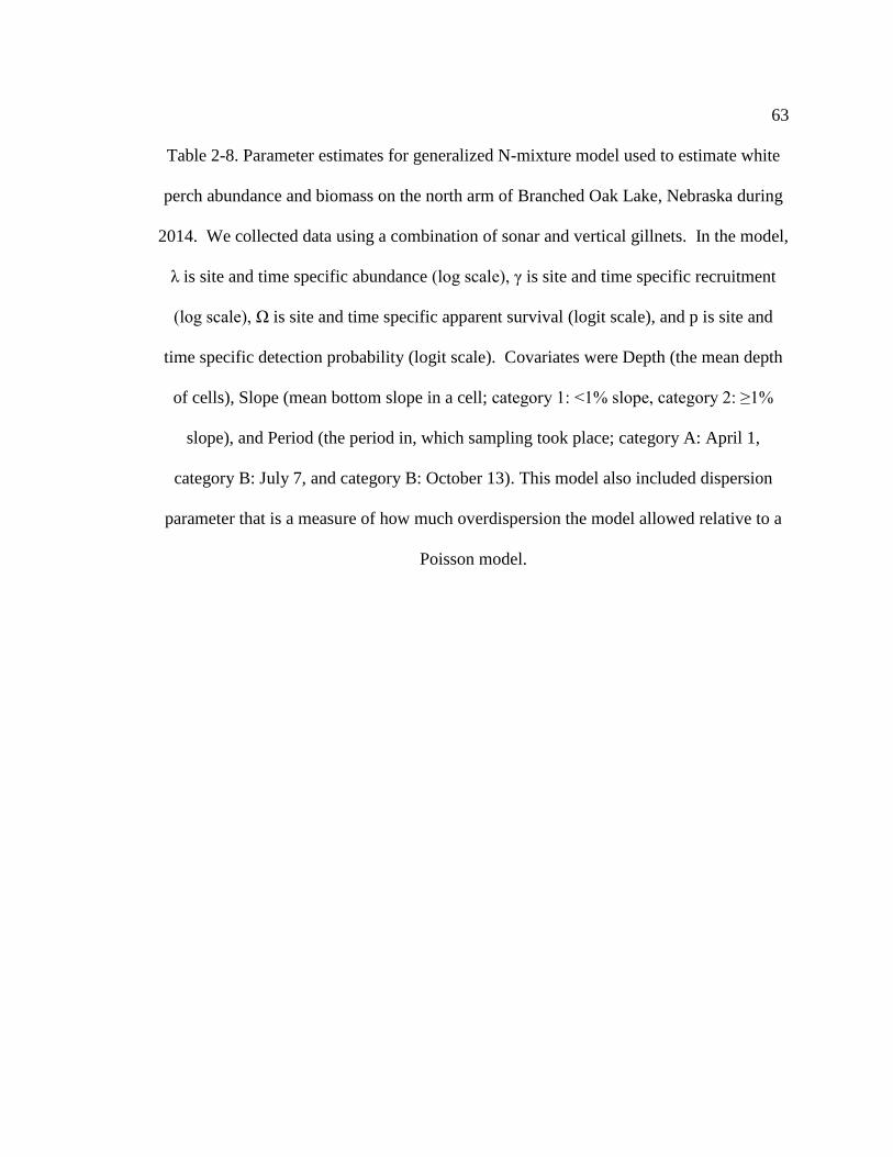
63
Table 2-8. Parameter estimates for generalized N-mixture model used to estimate white
perch abundance and biomass on the north arm of Branched Oak Lake, Nebraska during
2014. We collected data using a combination of sonar and vertical gillnets. In the model,
λ is site and time specific abundance (log scale), γ is site and time specific recruitment
(log scale), Ω is site and time specific apparent survival (logit scale), and p is site and
time specific detection probability (logit scale). Covariates were Depth (the mean depth
of cells), Slope (mean bottom slope in a cell; category 1: <1% slope, category 2: ≥1%
slope), and Period (the period in, which sampling took place; category A: April 1,
category B: July 7, and category B: October 13). This model also included dispersion
parameter that is a measure of how much overdispersion the model allowed relative to a
Poisson model.

64
Component Variable Estimate SE Z p
λ Intercept - 2.86 0.12 - 24.04 <0.001
Depth - 0.29 0.11 - 2.65 0.008
Slope 2 - 0.06 0.25 - 0.23 0.816
γ Intercept - 2.30 1.90 - 1.21 0.227
Period B 5.56 1.90 2.93 0.003
Depth - 2.42 1.42 - 1.70 0.089
Slope 2 0.35 0.14 2.45 0.014
Period B*Depth 3.10 1.42 2.18 0.030
Ω Intercept 2.83 0.13 21.77 <0.001
Period B - 3.46 0.29 - 11.78 <0.001
Depth - 1.04 0.09 - 11.79 <0.001
Slope 2 - 1.87 0.12 - 16.07 <0.001
Period B*Depth 1.55 0.21 7.31 <0.001
p Intercept - 2.30 0.06 - 38.35 <0.001
Period B 17.55 193.78 0.09 0.928
Period C 1.69 0.30 5.66 <0.001
Dispersion 1.00 0.278 3.61 <0.001

65
Table 2-9. Parameter estimates for generalized N-mixture model used to estimate white
perch abundance and biomass on the north arm of Branched Oak Lake, Nebraska during
2014. We collected data using a boat electrofisher. In the model, λ is site and time
specific abundance (log scale), γ is site and time specific recruitment (log scale), Ω is site
and time specific apparent survival (logit scale), and p is site and time specific detection
probability (logit scale). Covariates were Depth (the mean depth of cells), Slope (mean
bottom slope in a cell; category 1: <1% slope, category 2: ≥1% slope), Shore (whether or
not a cell was adjacent to shore and whether or not that shore had rip rap; category 1:
offshore, category 2: adjacent to shore, category 3: adjacent to rip-rapped shore), Timber
(whether or not a sampling cell contained flooded timber; category 0: timber absent and
category 1: timber present) and Period (the period in, which sampling took place;
category A: April 1, category B: July 7, and category B: October 13). This model
contains a zero-inflation term, which provided a measure of how zero inflated the data
were.

66
Component Variable Estimate SE Z p
λ Intercept - 1.92 5.98 -0.32 0.748
Depth - 1.96 2.56 -0.77 0.442
Shore1 - 1.85 3.51 -0.53 0.597
Shore2 - 3.76 3.66 -1.03 0.304
γ Intercept 2.30 0.46 5.05 <0.001
Period B - 3.40 0.86 -3.98 <0.001
Depth 0.25 0.36 0.69 0.492
Shore1 - 2.89 0.85 -3.41 0.001
Shore2 - 2.72 1.10 -2.47 0.014
Period B*Depth 1.61 1.96 0.82 0.411
Ω Intercept - 65.80 1414.00 -0.05 0.963
Period B - 28.60 759.00 -0.04 0.970
Depth - 53.80 1389.00 -0.04 0.969
Shore1 44.20 749.00 0.06 0.953
Shore2 - 77.30 4549.00 -0.02 0.986
Period B*Depth - 27.00 1393.00 -0.02 0.985
p Intercept - 0.14 6.33 -0.02 0.983
Period B - 0.80 5.22 -0.15 0.878
Period C - 2.11 6.34 -0.33 0.739
Depth 30.89 199.93 0.15 0.877
Period B*Depth - 0.42 5.25 -0.08 0.936
Period C*Depth - 56.89 416.92 -0.14 0.891
Zero-inflation 0.51 0.52 0.98 0.330

67
Table 2-10. Parameter estimates for generalized N-mixture model used to estimate white
perch abundance and biomass on the south arm of Branched Oak Lake, Nebraska during
2014. We collected data using a combination of sonar and vertical gillnets. In the model,
λ is site and time specific abundance (log scale), γ is site and time specific recruitment
(log scale), Ω is site and time specific apparent survival (logit scale), and p is site and
time specific detection probability (logit scale). Covariates were Depth (the mean depth
of cells), Slope (mean bottom slope in a cell; category 1: <1% slope, category 2: ≥1%
slope), and Period (the period in, which sampling took place; category A: April 1,
category B: July 7, and category B: October 13). This model also included dispersion
parameter that is a measure of how much overdispersion the model allowed relative to a
Poisson model.

68
Component Variable Estimate SE Z p
λ Intercept - 3.34 0.21 - 16.01 <0.001
Depth - 0.48 0.20 - 2.41 0.016
Slope 2 0.73 0.54 1.36 0.175
γ Intercept 2.35 0.12 19.93 <0.001
Period B 0.35 0.14 2.55 0.011
Depth 2 0.65 0.09 6.87 <0.001
Slope 2 - 12.66 160.39 - 0.08 0.940
Period B*Depth 0.04 0.11 0.35 0.726
Ω Intercept 5.93 1.29 4.61 <0.001
Period B - 8.55 1.68 - 5.07 <0.001
Depth 2 - 7.80 1.72 - 4.55 <0.001
Slope 2 2.26 0.48 4.73 <0.001
Period B*Depth 7.87 1.73 4.56 <0.001
p Intercept - 2.94 0.11 - 26.33 <0.001
Period B 13.32 46.46 0.29 0.774
Period C 11.61 77.14 0.15 0.880
Dispersion 0.02 0.31 0.06 0.951

69
Table 2-11. Parameter estimates for generalized N-mixture model used to estimate white
perch abundance and biomass on the south arm of Branched Oak Lake, Nebraska during
2014. We collected data using a boat electrofisher. In the model, λ is site and time
specific abundance (log scale), γ is site and time specific recruitment (log scale), Ω is site
and time specific apparent survival (logit scale), and p is site and time specific detection
probability (logit scale). Covariates were Depth (the mean depth of cells), Slope (mean
bottom slope in a cell; category 1: <1% slope, category 2: ≥1% slope), Shore (whether or
not a cell was adjacent to shore and whether or not that shore had rip rap; category 1:
offshore, category 2: adjacent to shore, category 3: adjacent to rip-rapped shore), Timber
(whether or not a sampling cell contained flooded timber; category 0: timber absent and
category 1: timber present) and Period (the period in, which sampling took place;
category A: April 1, category B: July 7, and category B: October 13). This model
contains a zero-inflation term, which provided a measure of how zero inflated the data
were.

70
Component Variable Estimate SE Z p
λ Intercept - 3.36 0.70 - 4.82 <0.001
Depth - 0.26 0.67 - 0.39 0.697
Shore1 1.45 0.72 2.02 0.044
Shore2 0.55 0.74 0.75 0.452
γ Intercept - 1.31 1.34 - 0.97 0.331
Period B 0.57 0.96 0.59 0.556
Depth 0.13 0.81 0.16 0.872
Shore1 - 8.01 185.03 - 0.04 0.966
Shore2 2.18 1.41 1.55 0.122
Period B*Depth 1.58 0.74 2.13 0.033
Ω Intercept - 0.16 1.72 -0.09 0.928
Period B - 23.91 7968.80 0.00 0.998
Depth - 1.16 2.12 -0.54 0.586
Shore1 12.20 351.48 0.03 0.972
Shore2 - 9.93 148.27 - 0.07 0.947
Period B*Depth -4.64 4867.47 0.00 0.999
p Intercept - 0.90 0.82 -1.10 0.270
Period B 5.47 5.40 1.01 0.311
Period C - 143.17 11900.00 - 0.01 0.990
Depth - 0.08 0.75 - 0.11 0.914
Period B*Depth 4.09 3.77 1.09 0.277
Period C*Depth -152.86 13000.00 - 0.01 0.991
Zero-inflation - 11.50 144.00 - 0.08 0.936

71
Table 2-12. Generalized N-mixture models ranked with AIC used to model gizzard shad
abundance on Branched Oak Lake, Nebraska during 2013 (K: number of model
parameters, AIC: Akaike Information Criterion score, ΔAIC: difference between AIC
score for the specified model and for the top model, AICwt: AIC weight, cumwt:
cumulative AIC weight). Count data were collected with a consumer grade sonar unit
used in conjunction with vertical gillnets (SN) in waters with total depths ≥ 2 m and a
boat electrofisher (EF) used to electrify points in water with total depths < 2 m. In each
model, λ is abundance, γ is recruitment, Ω is apparent survival, and p is detection
probability. The covariates in the models are depth (D), slope (S), sampling period (P),
and shoreline habitat (H).
Arm Gear Model K AIC ΔAIC AICwt cumwt
North SN λ: D, γ: D*P, Ω: D*P, p: D 13 1443 0 0.95 1.00
λ: D+S, γ: D*P+S, Ω: D*P+S, p: D 16 1449 6 0.05 1.00
λ: 1, γ: 1, Ω: 1, p: 1 5 1958 515 0.00 1.00
EF λ: D+T, γ: D*P+T, Ω: D*P+T,
p: D+P+T
21 188 0 0.88 0.88
λ: D+S, γ: D*P+S, Ω: D*P+S, p: D 16 192 4 0.12 0.99
λ: D, γ: D*P, Ω: D*P, p: D*P 17 198 10 0.01 1.00
λ: 1, γ: 1, Ω: 1, p: 1 5 414 226 0.00 1.00
South SN λ: D, γ: D*P, Ω: D*P, p: P 14 512 0 1.00 1.00
λ: D+S, γ: D*P+S, Ω: D*P+S, p: P 17 1189 677 0.00 1.00
λ: D+S, γ: D*P+S, Ω: D*P+S, p: D 16 1511 999 0.00 1.00
λ: D, γ: D*P, Ω: D*P, p: D 13 1833 1321 0.00 1.00
λ: 1, γ: 1, Ω: 1, p: 1 5 2816 2304 0.00 1.00

72
Table 2-13. Parameter estimates for generalized N-mixture model used to estimate
gizzard shad abundance and biomass on the north arm of Branched Oak Lake, Nebraska
during 2013. We collected data using a combination of sonar and vertical gillnets. In the
model, λ is site and time specific abundance (log scale), γ is site and time specific
recruitment (log scale), Ω is site and time specific apparent survival (logit scale), and p is
site and time specific detection probability (logit scale). Covariates were Depth (the
mean depth of cells), Slope (mean bottom slope in a cell; category 1: <1% slope, category
2: ≥1% slope), and Period (the period in, which sampling took place; category A: June
25, category B: July 31, and category B: October 16). This model also included
dispersion parameter that is a measure of how much overdispersion the model allowed
relative to a Poisson model.

73
Component Variable Estimate SE Z p
λ Intercept - 3.44 0.30 - 11.60 <0.001
Depth - 1.05 0.29 - 3.66 <0.001
γ Intercept - 3.78 2.10 - 1.80 0.070
Period B 6.84 2.09 3.27 <0.001
Depth - 6.36 1.59 - 4.01 <0.001
Period B*Depth 6.65 1.59 4.18 <0.001
Ω Intercept 1.90 0.49 3.85 <0.001
Period B - 61.18 202.47 - 0.30 0.763
Depth - 2.13 0.35 - 6.10 <0.001
Period B*Depth 58.75 188.78 0.31 0.756
p Intercept - 0.86 0.11 - 7.69 <0.001
Depth 1.29 0.11 11.92 <0.001
Dispersion - 1.11 0.27 - 4.10 <0.001

74
Table 2-14. Parameter estimates for generalized N-mixture model used to estimate
gizzard shad abundance and biomass on the north arm of Branched Oak Lake, Nebraska
during 2013. We collected data using a boat electrofisher. In the model, λ is site and
time specific abundance (log scale), γ is site and time specific recruitment (log scale), Ω
is site and time specific apparent survival (logit scale), and p is site and time specific
detection probability (logit scale). Covariates were Depth (the mean depth of cells),
Slope (mean bottom slope in a cell; category 1: <1% slope, category 2: ≥1% slope),
Shore (whether or not a cell was adjacent to shore and whether or not that shore had rip
rap; category 1: offshore, category 2: adjacent to shore, category 3: adjacent to rip-rapped
shore), Timber (whether or not a sampling cell contained flooded timber; category 0:
timber absent and category 1: timber present) and Period (the period in, which sampling
took place; category A: June 25, category B: July 31, and category B: October 16). This
model contains a zero-inflation term, which provided a measure of how zero inflated the
data were.

75
Component Variable Estimate SE Z p
λ Intercept - 2.74 0.65 - 4.21 <0.001
Depth - 1.14 0.52 - 2.18 0.029
Timber 1 1.75 0.62 2.83 0.005
γ Intercept 0.92 0.52 1.79 0.073
Period B - 21.17 6557.00 0.00 0.997
Depth 1.25 0.36 3.50 <0.001
Timber 1 - 0.78 0.78 - 1.00 0.318
Period B*Depth 7.69 4021.83 0.00 0.998
Ω Intercept - 105.60 447.97 - 0.24 0.814
Period B 50.00 214.20 0.23 0.816
Depth 3.10 4.66 0.67 0.505
Timber 1 109.30 447.95 0.24 0.807
Period B*Depth - 77.80 327.20 - 0.24 0.812
p Intercept - 1.92 0.80 - 2.40 0.016
Period B 0.00 0.61 0.00 0.998
Period C - 0.51 0.80 - 0.64 0.522
Depth - 0.37 0.68 - 0.54 0.590
Timber 1 - 0.63 0.72 - 0.88 0.379
Period B*Depth - 1.12 0.79 - 1.42 0.155
Period C*Depth - 3.76 1.61 - 2.34 0.019
Zero-inflation 0.43 0.47 0.93 0.352

76
Table 2-15. Parameter estimates for generalized N-mixture model used to estimate
gizzard shad abundance and biomass on the south arm of Branched Oak Lake, Nebraska
during 2013. We collected data using a combination of sonar and vertical gillnets. In the
model, λ is site and time specific abundance (log scale), γ is site and time specific
recruitment (log scale), Ω is site and time specific apparent survival (logit scale), and p is
site and time specific detection probability (logit scale). Covariates were Depth (the
mean depth of cells), Slope (mean bottom slope in a cell; category 1: <1% slope, category
2: ≥1% slope), and Period (the period in, which sampling took place; category A: June
25, category B: July 31, and category B: October 16). This model also included
dispersion parameter that is a measure of how much overdispersion the model allowed
relative to a Poisson model.

77
Component Variable Estimate SE Z p
λ Intercept - 3.18 0.48 - 6.69 <0.001
Depth - 0.96 0.46 - 2.09 0.036
γ Intercept 1.04 0.24 4.34 <0.001
Period B - 17.25 1104.29 - 0.02 0.988
Depth - 0.14 0.25 - 0.56 0.576
Period B*Depth - 4.35 823.05 - 0.01 0.996
Ω Intercept 5.68 5.85 0.97 0.331
Period B 17.76 16.90 1.05 0.294
Depth - 0.09 2.12 - 0.04 0.967
Period B*Depth 17.90 12.31 1.45 0.146
p Intercept - 1.64 0.16 - 10.49 <0.001
Period B - 0.27 0.16 - 1.61 0.107
Period C - 0.22 0.17 - 1.26 0.206
Dispersion - 1.87 0.34 - 5.50 <0.001

78
Table 2-16. Generalized N-mixture models ranked with AIC used to model gizzard shad
abundance on Branched Oak Lake, Nebraska during 2014 (K: number of model
parameters, AIC: Akaike Information Criterion score, ΔAIC: difference between AIC
score for the specified model and for the top model, AICwt: AIC weight, cumwt:
cumulative AIC weight). Count data were collected with a consumer grade sonar unit
used in conjunction with vertical gillnets (SN) in waters with total depths ≥ 2 m and a
boat electrofisher (EF) used to electrify points in water with total depths < 2 m. In each
model, λ is abundance, γ is recruitment, Ω is apparent survival, and p is detection
probability. The covariates in the models are depth (D), slope (S), sampling period (P),
and shoreline habitat (H).

79
Arm Gear Model K AIC ΔAIC AICwt cumwt
North SN λ: D, γ: D*P, Ω: D*P, p: P 14 890 0 1.00 1.00
λ: D+S, γ: D*P+S, Ω: D*P+S, p: P 17 986 96 0.00 1.00
λ: D+S, γ: D*P+S, Ω: D*P+S, p: D 16 1427 537 0.00 1.00
λ: D, γ: D*P, Ω: D*P, p: D 13 1499 609 0.00 1.00
λ: 1, γ: 1, Ω: 1, p: 1 5 1651 761 0.00 1.00
EF λ: D+T, γ: D*P+T, Ω: D*P+T,
p: D+P+T
21 92 0 0.67 0.67
λ: D, γ: D*P, Ω: D*P, p: D*P 17 94 2 0.24 0.91
λ: D+S, γ: D*P+S, Ω: D*P+S, p: D 16 96 4 0.09 1.00
λ: S, γ: S+P, Ω: S+P, p: P 12 148 56 0.00 1.00
λ: 1, γ: 1, Ω: 1, p: 1 5 193 101 0.00 1.00
South SN λ: D+S, γ: D*P+S, Ω: D*P+S, p: D 16 1321 0 1.00 1.00
λ: D, γ: D*P, Ω: D*P, p: P 14 1545 224 0.00 1.00
λ: 1, γ: 1, Ω: 1, p: 1 5 2917 1596 0.00 1.00
EF λ: D+T, γ: D*P+T, Ω: D*P+T,
p: D+P+T
21 80 0 0.59 0.59
λ: D+H, γ: D*P+H, Ω: D*P+H,
p: D+P
23 80 1 0.41 1.00
λ: S, γ: S+P, Ω: S+P, p: P 12 94 14 0.00 1.00
λ: 1, γ: 1, Ω: 1, p: 1 5 95 15 0.00 1.00

80
Table 2-17. Parameter estimates for generalized N-mixture model used to estimate
gizzard shad abundance and biomass on the north arm of Branched Oak Lake, Nebraska
during 2014. We collected data using a combination of sonar and vertical gillnets In the
model, λ is site and time specific abundance (log scale), γ is site and time specific
recruitment (log scale), Ω is site and time specific apparent survival (logit scale), and p is
site and time specific detection probability (logit scale). Covariates were Depth (the
mean depth of cells), Slope (mean bottom slope in a cell; category 1: <1% slope, category
2: ≥1% slope), and Period (the period in, which sampling took place; category A: April 1,
category B: July 7, and category B: October 13). This model also included dispersion
parameter that is a measure of how much overdispersion the model allowed relative to a
Poisson model.

81
Component Variable Estimate SE Z p
λ Intercept - 3.40 0.23 - 14.71 <0.001
Depth 0.00 0.23 - 0.02 0.983
γ Intercept 0.40 0.48 0.83 0.407
Period B - 8.96 9.01 - 0.99 0.320
Depth - 1.14 0.38 - 3.03 0.002
Period B*Depth - 0.44 22.82 - 0.02 0.985
Ω Intercept 40.60 24.00 1.69 0.091
Period B - 40.20 24.00 - 1.67 0.094
Depth - 21.10 12.30 - 1.72 0.086
Period B*Depth 22.10 12.30 1.80 0.072
p Intercept - 2.48 0.14 - 17.94 <0.001
Period B 0.09 0.17 0.55 0.581
Period C 11.55 18.35 0.63 0.529
Dispersion - 0.25 0.34 - 0.73 0.466

82
Table 2-18. Parameter estimates for generalized N-mixture model used to estimate
gizzard shad abundance and biomass on the north arm of Branched Oak Lake, Nebraska
during 2014. We collected data using a boat electrofisher. In the model, λ is site and
time specific abundance (log scale), γ is site and time specific recruitment (log scale), Ω
is site and time specific apparent survival (logit scale), and p is site and time specific
detection probability (logit scale). Covariates were Depth (the mean depth of cells),
Slope (mean bottom slope in a cell; category 1: <1% slope, category 2: ≥1% slope),
Shore (whether or not a cell was adjacent to shore and whether or not that shore had rip
rap; category 1: offshore, category 2: adjacent to shore, category 3: adjacent to rip-rapped
shore), Timber (whether or not a sampling cell contained flooded timber; category 0:
timber absent and category 1: timber present) and Period (the period in, which sampling
took place; category A: April 1, category B: July 7, and category B: October 13). This
model contains a zero-inflation term, which provided a measure of how zero inflated the
data were.

83
Component Variable Estimate SE Z p
λ Intercept - 13.26 11.31 - 1.17 0.241
Depth 5.06 7.47 0.68 0.498
Timber 1 0.95 2.88 0.33 0.741
γ Intercept - 4.01 0.72 - 5.60 <0.001
Period B - 34.35 9.46 - 3.63 <0.001
Depth - 2.11 0.40 - 5.27 <0.001
Timber 1 4.19 0.71 5.92 <0.001
Period B*Depth 28.10 5.96 4.71 <0.001
Ω Intercept - 6.72 32.10 - 0.21 0.834
Period B - 13.71 11969.70 0.00 0.999
Depth - 16.41 58.00 - 0.28 0.777
Timber 1 36.18 125.40 0.29 0.773
Period B*Depth 3.78 6760.40 0.00 1.000
p Intercept 15.61 3502.00 0.00 0.996
Period B 18.37 3490.00 0.01 0.996
Period C - 1.58 NA NA NA
Depth 6.36 2630.00 0.00 0.998
Timber 1 - 35.60 232.00 - 0.15 0.878
Period B*Depth 6.42 2630.00 0.00 0.998
Period C*Depth - 4.94 NA NA NA
Zero-inflation - 8.36 147.00 - 0.06 0.955

84
Table 2-19. Parameter estimates for generalized N-mixture model used to estimate
gizzard shad abundance and biomass on the south arm of Branched Oak Lake, Nebraska
during 2014. We collected data using a combination of sonar and vertical gillnets. In the
model, λ is site and time specific abundance (log scale), γ is site and time specific
recruitment (log scale), Ω is site and time specific apparent survival (logit scale), and p is
site and time specific detection probability (logit scale). Covariates were Depth (the
mean depth of cells), Slope (mean bottom slope in a cell; category 1: <1% slope, category
2: ≥1% slope), and Period (the period in, which sampling took place; category A: April 1,
category B: July 7, and category B: October 13). This model also included dispersion
parameter that is a measure of how much overdispersion the model allowed relative to a
Poisson model.
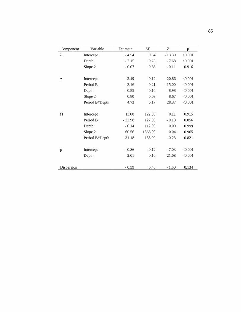
85
Component Variable Estimate SE Z p
λ Intercept - 4.54 0.34 - 13.39 <0.001
Depth - 2.15 0.28 - 7.68 <0.001
Slope 2 - 0.07 0.66 - 0.11 0.916
γ Intercept 2.49 0.12 20.86 <0.001
Period B - 3.16 0.21 - 15.00 <0.001
Depth - 0.85 0.10 - 8.98 <0.001
Slope 2 0.80 0.09 8.67 <0.001
Period B*Depth 4.72 0.17 28.37 <0.001
Ω Intercept 13.08 122.00 0.11 0.915
Period B - 22.98 127.00 - 0.18 0.856
Depth - 0.14 112.00 0.00 0.999
Slope 2 60.56 1365.00 0.04 0.965
Period B*Depth -31.18 138.00 - 0.23 0.821
p Intercept - 0.86 0.12 - 7.03 <0.001
Depth 2.01 0.10 21.08 <0.001
Dispersion - 0.59 0.40 - 1.50 0.134

86
Table 2-20. Parameter estimates for generalized N-mixture model used to estimate
gizzard shad abundance and biomass on the south arm of Branched Oak Lake, Nebraska
during 2014. We collected data using a boat electrofisher. In the model, λ is site and
time specific abundance (log scale), γ is site and time specific recruitment (log scale), Ω
is site and time specific apparent survival (logit scale), and p is site and time specific
detection probability (logit scale). Covariates were Depth (the mean depth of cells),
Slope (mean bottom slope in a cell; category 1: <1% slope, category 2: ≥1% slope),
Shore (whether or not a cell was adjacent to shore and whether or not that shore had rip
rap; category 1: offshore, category 2: adjacent to shore, category 3: adjacent to rip-rapped
shore), Timber (whether or not a sampling cell contained flooded timber; category 0:
timber absent and category 1: timber present) and Period (the period in, which sampling
took place; category A: April 1, category B: July 7, and category B: October 13). This
model contains a zero-inflation term, which provided a measure of how zero inflated the
data were.

87
Component Variable Estimate SE Z p
λ Intercept - 4.59 0.59 - 7.85 <0.001
Depth - 0.82 0.41 - 1.98 0.048
Timber 1 - 9.16 209.80 - 0.04 0.965
γ Intercept - 4.78 2.79 - 1.71 0.087
Period B - 38.71 10.87 - 3.56 <0.001
Depth 0.79 1.85 0.43 0.668
Timber 1 6.92 2.58 2.68 0.007
Period B*Depth 26.50 6.56 4.04 <0.001
Ω Intercept - 13.01 46.00 - 0.28 0.777
Period B - 16.31 45.60 - 0.36 0.721
Depth - 20.74 66.90 - 0.31 0.756
Timber 1 27.18 81.60 0.33 0.739
Period B*Depth 2.78 17.40 0.16 0.873
p Intercept - 27.90 96.80 - 0.29 0.773
Period B 35.10 109.50 0.32 0.748
Period C 34.50 109.40 0.32 0.753
Depth 20.70 71.10 0.29 0.770
Timber 1 - 10.50 51.20 - 0.21 0.837
Period B*Depth - 21.30 71.10 - 0.30 0.765
Period C*Depth - 21.40 71.10 - 0.30 0.763
Zero-inflation - 11.00 203.00 - 0.05 0.957

88
Table 2-21. Abundance and biomass with 95% confidence intervals estimated for white
perch (WHP) and gizzard shad (SHAD) in Branched Oak Lake (BOL) and Pawnee
Reservoir (PWR), Nebraska. Estimates were made using generalized N-mixture models
with data collected with a consumer-grade sonar unit, vertical gillnets, and a boat
electrofisher.
Biomass
Waterbody Species Year
Abundance
(millions)
Mean mass
(g) kg (thousands) kg/ha
BOL WHP 2013 1.20(1.14-1.26) 38(1-76) 45.99(0.93-91.05) 63(1-125)
2014 1.20(1.12-1.27) 35(5-66) 42.38(6.10-78.66) 58(8-108)
SHAD 2013 0.91(0.77-1.04) 87(0-485) 79.46(0.00-168.54) 109(0-232)
2014 0.70(0.54-0.86) 149(42-257) 103.83(25.76-181.90) 143(35-250)
PWR WHP 2013 1.59(1.49-1.69) 28(14-41) 43.71(22.16-65.26) 146(74-218)
2014 0.27(0.23-0.31) 28(17-39) 7.64(4.35-10.93) 26(15- 37)
SHAD
2013
2014
0.64(0.59-0.68)
0
47(16-79)
0
30.33(10.39-50.27)
0.00
101(35-168)
0

89
Table 2-22. Generalized N-mixture models ranked with AIC used to estimate white perch
abundance and biomass on Pawnee Reservoir, Nebraska (K: number of model
parameters, AIC: Akaike Information Criterion score, ΔAIC: difference between AIC
score for the specified model and for the top model, AICwt: AIC weight, cumwt:
cumulative AIC weight). Count data were collected with a consumer grade sonar unit
used in conjunction with vertical gillnets (SN) in waters with total depths ≥ 2 m and a
boat electrofisher (EF) used to electrify points in water with total depths < 2 m. In each
model, λ is abundance, γ is recruitment, Ω is apparent survival, and p is detection
probability. The covariates in the models are depth (D), slope (S), sampling period (P),
and shoreline habitat (H).
Period Gear Model K AIC ΔAIC AICwt cumwt
2013 SN λ: D+S, γ: D*P+S, Ω: D*P+S, p: D 20 1468 0 1.00 1.00
λ: D, γ: D*P, Ω: D*P, p: D 17 1607 139 0.00 1.00
λ: D, γ: D*P, Ω: D*P, p: P 19 1741 273 0.00 1.00
λ: 1, γ: 1, Ω: 1, p: 1 5 2729 1261 0.00 1.00
EF λ: D, γ: D*P, Ω: D*P, p: D*P 23 838 0 1.00 1.00
λ: S, γ: S+P, Ω: S+P, p: P 15 921 83 0.00 1.00
λ: 1, γ: 1, Ω: 1, p: 1 5 1098 260 0.00 1.00
2014 SN λ: D+S, γ: D*P+S, Ω: D*P+S, p: P 32 1070 0 1.00 1.00
λ: D, γ: D*P, Ω: D*P, p: D 25 1128 58 0.00 1.00
λ: D, γ: D*P, Ω: D*P, p: P 29 1146 76 0.00 1.00
λ: D+S, γ: D*P+S, Ω: D*P+S, p: D 28 1210 140 0.00 1.00
λ: 1, γ: 1, Ω: 1, p: 1 5 2569 1499 0.00 1.00
EF λ: S, γ: S+P, Ω: S+P, p: P 21 341 0 1.00 1.00
λ: 1, γ: 1, Ω: 1, p: 1 5 360 19 0.00 1.00

90
Table 2-23. Parameter estimates for generalized N-mixture model used to estimate white
perch abundance and biomass in Pawnee Reservoir, Nebraska during 2013. We collected
data using a combination of sonar and vertical gillnets. In the model, λ is site and time
specific abundance (log scale), γ is site and time specific recruitment (log scale), Ω is site
and time specific apparent survival (logit scale), and p is site and time specific detection
probability (logit scale). Covariates were Depth (the mean depth of cells), Slope (mean
bottom slope in a cell; category 1: <1% slope, category 2: ≥1% slope), and Period (the
period in, which sampling took place; category A: June 17, category B: July 25, category
C: September 9, category D: October 8). This model also included dispersion parameter
that is a measure of how much overdispersion the model allowed relative to a Poisson
model.

91
Component Variable Estimate SE Z p
λ Intercept - 1.56 0.14 - 11.34 <0.001
Depth - 0.81 0.11 - 7.51 <0.001
Slope 2 0.08 0.24 0.33 0.742
γ Intercept 3.80 0.07 52.31 <0.001
Period B - 0.70 0.10 - 6.86 <0.001
Period C - 1.19 0.11 - 10.92 <0.001
Depth - 0.28 0.07 - 4.31 <0.001
Slope 2 - 0.90 0.10 - 8.58 <0.001
Period B*Depth - 0.91 0.10 - 9.42 <0.001
Period C*Depth 0.11 0.12 0.91 0.362
Ω Intercept - 4.12 0.82 - 5.00 <0.001
Period B - 45.12 35.99 - 1.25 0.210
Period C - 9.95 1.86 - 5.36 <0.001
Depth 0.16 0.08 1.87 0.061
Slope 2 3.31 0.81 4.07 <0.001
Period B*Depth - 70.03 52.03 - 1.35 0.178
Period C*Depth - 8.51 1.62 - 5.26 <0.001
p Intercept 3.83 0.33 11.60 <0.001
Depth 3.85 0.25 15.50 <0.001
Dispersion 1.50 0.32 4.68 <0.001

92
Table 2-24. Parameter estimates for generalized N-mixture model used to estimate white
perch abundance and biomass in Pawnee Reservoir, Nebraska during 2013. We collected
data using a boat electrofisher. In the model, λ is site and time specific abundance (log
scale), γ is site and time specific recruitment (log scale), Ω is site and time specific
apparent survival (logit scale), and p is site and time specific detection probability (logit
scale). Covariates were Depth (the mean depth of cells), Slope (mean bottom slope in a
cell; category 1: <1% slope, category 2: ≥1% slope), Shore (whether or not a cell was
adjacent to shore and whether or not that shore had rip rap; category 1: offshore, category
2: adjacent to shore, category 3: adjacent to rip-rapped shore), Timber (whether or not a
sampling cell contained flooded timber; category 0: timber absent and category 1: timber
present) and Period (the period in, which sampling took place; category A: June 17,
category B: July 25, category C: September 9, category D: October 8). This model
contains a zero-inflation term, which provided a measure of how zero inflated the data
were.

93
Component Variable Estimate SE Z p
λ Intercept - 0.29 0.26 - 1.13 0.257
Depth - 0.79 0.21 - 3.77 <0.001
γ Intercept 1.51 0.23 6.72 <0.001
Period B - 26.30 6.57 - 4.00 <0.001
Period C - 4.99 1.62 - 3.09 0.002
Depth 1.49 0.31 4.86 <0.001
Period B*Depth - 16.68 3.73 - 4.47 <0.001
Period C*Depth - 4.58 1.03 - 4.44 <0.001
Ω Intercept 1.06 0.56 1.89 0.059
Period B 2.62 1.26 2.09 0.037
Period C 1.71 11.71 0.15 0.884
Depth 1.76 0.41 4.26 <0.001
Period B*Depth 3.38 1.66 2.04 0.041
Period C*Depth 29.66 203.01 0.15 0.884
p Intercept - 0.83 0.45 - 1.84 0.066
Depth 0.58 0.38 1.54 0.124
Period B 1.04 0.43 2.45 0.014
Period C 1.38 0.44 3.11 0.002
Period D - 0.60 0.65 - 0.92 0.355
Period B*Depth - 2.47 0.58 - 4.28 <0.001
Period C*Depth - 3.55 0.64 - 5.52 <0.001
Period D*Depth - 4.64 1.42 - 3.26 0.001
Zero-inflation - 0.27 0.37 - 0.73 0.465

94
Table 2-25. Parameter estimates for generalized N-mixture model used to estimate white
perch abundance and biomass in Pawnee Reservoir, Nebraska during 2014. We collected
data using a combination of sonar and vertical gillnets. In the model, λ is site and time
specific abundance (log scale), γ is site and time specific recruitment (log scale), Ω is site
and time specific apparent survival (logit scale), and p is site and time specific detection
probability (logit scale). Covariates were Depth the mean depth of cells (the mean depth
of cells), Slope (mean bottom slope in a cell; category 1: <1% slope, category 2: ≥1%
slope), and Period (the period in, which sampling took place; category A: May 2,
category B: May 14, category C: May 21, category D: June 20, category E: September
18, category F: October 7). This model also included dispersion parameter that is a
measure of how much overdispersion the model allowed relative to a Poisson model.

95
Component Variable Estimate SE Z p
λ Intercept - 3.62 0.24 - 15.02 <0.001
Depth 0.28 0.14 1.98 0.048
Slope 2 - 0.03 0.24 - 0.11 0.912
γ Intercept 1.47 0.51 2.87 0.004
Period B 1.10 0.53 2.09 0.037
Period C 1.38 0.52 2.68 0.007
Period D - 9.14 5.56 - 1.65 0.100
Period E - 0.06 0.53 - 0.11 0.911
Depth 0.44 0.28 1.59 0.112
Slope 2 - 0.12 0.07 - 1.70 0.089
Period B*Depth 0.25 0.29 0.86 0.392
Period C*Depth - 0.17 0.28 - 0.62 0.534
Period D*Depth 5.26 3.22 1.63 0.103
Period E*Depth - 0.83 0.31 - 2.72 0.006
Ω Intercept 11.80 6.44 1.84 0.066
Period B - 23.40 11.04 - 2.12 0.034
Period C 188.00 98.87 1.90 0.057
Period D 100.70 567.61 0.18 0.859
Period E - 22.30 10.96 - 2.04 0.042
Depth - 12.40 6.06 - 2.05 0.040
Slope 2 10.00 4.58 2.18 0.029
Period B*Depth 10.50 6.15 1.70 0.089
Period C*Depth 272.60 140.79 1.94 0.053
Period D*Depth - 81.70 452.98 - 0.18 0.857
Period E*Depth 13.00 6.06 2.15 0.031
p Intercept - 1.72 0.24 - 7.29 <0.001
Period B 2.02 0.41 4.99 <0.001
Period C 12.47 238.00 0.05 0.958
Period D 1.98 0.27 7.34 <0.001
Period E - 0.99 0.27 - 3.63 <0.001
Period F 19.08 23800.00 0.00 0.999
Dispersion 1.90 0.61 3.13 0.002

96
Table 2-26. Parameter estimates for generalized N-mixture model used to estimate white
perch abundance and biomass in Pawnee Reservoir, Nebraska during 2014. We collected
data using a boat electrofisher. In the model, λ is site and time specific abundance (log
scale), γ is site and time specific recruitment (log scale), Ω is site and time specific
apparent survival (logit scale), and p is site and time specific detection probability (logit
scale). Covariates were Depth (the mean depth of cells), Slope (mean bottom slope in a
cell; category 1: <1% slope, category 2: ≥1% slope), Shore (whether or not a cell was
adjacent to shore and whether or not that shore had rip rap; category 1: offshore, category
2: adjacent to shore, category 3: adjacent to rip-rapped shore), Timber (whether or not a
sampling cell contained flooded timber; category 0: timber absent and category 1: timber
present) and Period (the period in, which sampling took place; category A: May 2,
category B: May 14, category C: May 21, category D: June 20, category E: September
18, category F: October 7). This model contains a zero-inflation term, which provided a
measure of how zero inflated the data were.

97
Component Variable Estimate SE Z p
λ Intercept - 0.52 0.49 - 1.08 0.282
Slope 2 - 1.30 0.39 - 3.37 0.001
γ Intercept - 2.88 1.55 - 1.86 0.063
Period B 3.24 68.21 0.05 0.962
Period C 1.34 1.64 0.82 0.414
Period D - 5.21 27.20 - 0.19 0.848
Period E 3.70 1.66 2.23 0.026
Slope 2 1.25 0.74 1.68 0.092
Ω Intercept - 9.58 59.70 - 0.16 0.873
Period B - 9.25 86.70 - 0.11 0.915
Period C - 11.52 57.20 - 0.20 0.840
Period D - 0.52 19.30 - 0.03 0.979
Period E 3.60 67.30 0.05 0.957
Slope 2 13.30 61.90 0.21 0.830
p Intercept 0.53 0.95 0.56 0.576
Period B - 1.62 0.91 - 1.77 0.076
Period C - 3.68 71.11 - 0.05 0.959
Period D 0.14 2.52 0.06 0.954
Period E 3.31 32.05 0.10 0.918
Period F - 4.62 1.31 - 3.52 <0.001
Zero-inflation 0.93 0.42 2.20 0.028

98
Table 2-27. Generalized N-mixture models ranked with AIC used to model gizzard shad
abundance on Pawnee Reservoir, Nebraska during 2013 (K: number of model
parameters, AIC: Akaike Information Criterion score, ΔAIC: difference between AIC
score for the specified model and for the top model, AICwt: AIC weight, cumwt:
cumulative AIC weight). Count data were collected with a consumer grade sonar unit
used in conjunction with vertical gillnets (SN) in waters with total depths of 2 m or more
and a boat electrofisher (EF) used to shock points in water with total depths < 2 m. In
each model, λ is abundance, γ is recruitment, Ω is apparent survival, and p is detection
probability. The covariates in the models are depth (D), slope (S), sampling period (P),
and shoreline habitat (H).
Gear Model K AIC ΔAIC AICwt cumwt
SN λ: D+S, γ: D*P+S, Ω: D*P+S, p: D*P 20 1058 0 1.00 1.00
λ: D, γ: D*P, Ω: D*P, p: D*P 17 1112 54 0.00 1.00
λ: 1, γ: 1, Ω: 1, p: 1 5 1346 288 0.00 1.00
EF λ: D, γ: D*P, Ω: D*P, p: D*P 23 483 0 1.00 1.00
λ: D+H, γ: D*P+H, Ω: D*P+H p: D+P 30 517 34 0.00 1.00
λ: D+S, γ: D*P+S, Ω: D*P+S, p: D 20 520 37 0.00 1.00
λ: 1, γ: 1, Ω: 1, p: 1 5 549 66 0.00 1.00
λ: S, γ: S+P, Ω: S+P, p: P 15 551 68 0.00 1.00

99
Table 2-28. Parameter estimates for generalized N-mixture model used to estimate
gizzard shad abundance and biomass in Pawnee Reservoir, Nebraska during 2013 We
collected data using a combination of sonar and vertical gillnets. In the model, λ is site
and time specific abundance (log scale), γ is site and time specific recruitment (log scale),
Ω is site and time specific apparent survival (logit scale), and p is site and time specific
detection probability (logit scale). Covariates were Depth (the mean depth of cells),
Slope (mean bottom slope in a cell; category 1: <1% slope, category 2: ≥1% slope), and
Period (the period in, which sampling took place; category A: June 17, category B: July
25, category C: September 9, category D: October 8). This model also included
dispersion parameter that is a measure of how much overdispersion the model allowed
relative to a Poisson model.

100
Component Variable Estimate SE Z p
λ Intercept - 2.77 0.20 - 13.71 <0.001
Depth - 0.76 0.16 - 4.91 <0.001
Slope 2 0.08 0.33 0.26 0.799
γ Intercept 2.28 0.17 13.49 <0.001
Period B - 0.48 0.20 - 2.40 0.016
Period C - 0.89 0.27 - 3.34 <0.001
Depth 0.15 0.10 1.48 0.1390
Slope 2 1.15 0.15 7.50 <0.001
Period B*Depth - 0.09 0.15 - 0.61 0.545
Period C*Depth 0.07 0.19 0.39 0.70
Ω Intercept - 1.96 0.40 - 4.88 <0.001
Period B 4.42 0.83 5.32 <0.001
Period C 2.07 0.50 4.17 <0.001
Depth 1.53 0.26 5.99 <0.001
Slope 2 - 2.07 0.42 - 4.93 <0.001
Period B*Depth - 3.01 0.59 - 5.11 <0.001
Period C*Depth - 1.73 0.37 - 4.65 <0.001
p Intercept 0.62 0.17 3.57 <0.001
Period B 0.49 0.18 2.68 0.007
Dispersion 0.83 0.32 2.61 0.009

101
Table 2-29. Parameter estimates for generalized N-mixture model used to estimate
gizzard shad abundance and biomass in Pawnee Reservoir, Nebraska during 2013. We
collected data using a boat electrofisher. In the model, λ is site and time specific
abundance (log scale), γ is site and time specific recruitment (log scale), Ω is site and
time specific apparent survival (logit scale), and p is site and time specific detection
probability (logit scale). Covariates were Depth (the mean depth of cells), Slope (mean
bottom slope in a cell; category 1: <1% slope, category 2: ≥1% slope), Shore (whether or
not a cell was adjacent to shore and whether or not that shore had rip rap; category 1:
offshore, category 2: adjacent to shore, category 3: adjacent to rip-rapped shore), Timber
(whether or not a sampling cell contained flooded timber; category 0: timber absent and
category 1: timber present) and Period (the period in, which sampling took place;
category A: June 17, category B: July 25, category C: September 9, category D: October
8). This model contains a zero-inflation term, which provided a measure of how zero
inflated the data were.

102
Component Variable Estimate SE Z p
λ Intercept - 0.59 0.23 - 2.53 0.012
Depth - 0.36 0.30 - 1.22 0.222
γ Intercept - 1.21 0.96 - 1.27 0.206
Period B 0.70 1.06 0.66 0.509
Period C 1.21 1.04 1.16 0.245
Depth 1.82 0.89 2.05 0.040
Period B*Depth - 1.90 1.02 - 1.86 0.063
Period C*Depth - 0.54 1.11 - 0.49 0.627
Ω Intercept - 1.63 0.46 - 3.57 <0.001
Period B - 231.51 6823.12 - 0.03 0.973
Period C 2.84 1.55 1.84 0.066
Depth 2.31 0.82 2.82 0.005
Period B*Depth 329.95 9700.55 0.03 0.973
Period C*Depth - 1.61 1.54 - 1.05 0.294
p Intercept - 1.52 0.31 - 4.90 <0.001
Depth 0.00 0.39 - 0.01 0.994
Period B 4.09 1.20 3.41 0.001
Period C 2.72 1.56 1.74 0.082
Period D 13.98 8.99 1.56 0.120
Period B*Depth - 5.13 1.41 - 3.63 <0.001
Period C*Depth - 1.91 1.17 - 1.63 0.103
Period D*Depth - 21.85 13.13 - 1.66 0.096
Zero-inflation - 1.22 0.49 - 2.52 0.012

103
Figure 2-1. Stratification system and sampling sites (with adjustments for sites moved
because they were unsampleable) for estimating white perch and gizzard shad
abundances, biomasses, and spatial distributions in Branched Oak Lake, Nebraska.

104
Figure 2-2. Stratification system and sampling sites for estimating white perch and
gizzard shad abundances, biomasses, and spatial distributions in Pawnee Reservoir,
Nebraska.

105
Figure 2-3. Electric field map for a 5.5- m boat electrofisher with a Smith-Root® 5.0
GPP control box. The effective edge of the electric field was estimated to be where
power density was < 84 µW/cc.

106
Figure 2-4. Relationships between vertical gillnet catch and fish density estimated using
consumer grade sonar in Branched Oak Lake (top) and Pawnee Reservoir, Nebraska
(bottom) during spring, summer, and fall of 2013 and 2014.

107
Chapter 3 Seasonal distribution patterns of white perch and
gizzard shad in reservoirs
To understand the ecology of a fish species, a sound understanding of spatial
distribution is crucial. Spatial distributions are influenced by heterogeneity in habitat
quality and by the distributions of other fish populations within a waterbody. Several
possible relationships exist among spatial distributions of co-occurring fish populations.
One possibility is that the spatial distributions are not related, which could occur if both
species use different resources that occur with some spatial overlap. For example,
bluegill (Lepomis macrochirus) and black crappie (Pomoxis nigromaculatus) may both
use the same patches of coarse woody debris, but in addition to these areas bluegill use
shallow areas with macrophytes whereas black crappie use deeper habitats (Becker
1983). From a distribution standpoint, this would appear as little similarity between the
populations (Figure 3-1). In this instance, we would expect no significant relationship
between the distributions.
Another possibility is that the distributions will be positively related, which could
occur if the behavior of one species benefits the other species, or if both species use the
same resources. For example, bluegill and redbreasted sunfish (Lepomis auritus) use
similar littoral habitats with physical structure in southern reservoirs (Barwick 2004).
From a distribution standpoint, this would appear as nearly identical distributions of the

108
two species (Figure 3-1). In this instance, we would expect a positive relationship
between the distributions.
Spatial distributions could be exclusionary if species utilize dissimilar habitats.
For example, cisco (Coregonus artedi) need cooler water and open areas whereas bluegill
prefer warmer water and littoral habitats; when both species occur in the same waterbody
there is little overlap in their habitats (Jacobson et al. 2002). This scenario could also
occur if one species forces another out of certain habitats. For example, bluegill shift
their distribution from vegetated areas when green sunfish (Lepomis cyanellus) are
present in large numbers because of the competitive advantage that green sunfish have in
vegetated habitats (Werner and Hall 1976; Werner and Hall 1977). From a spatial
distribution standpoint, either of these scenarios would appear as opposite or completely
separate distributions for the two species (Figure 3-1). In this instance, we would expect
a negative relationship between the distributions.
Another possibility is that the distribution of one species may overlap completely
with the other and spill over into suboptimal habitats, which could occur if one species
only uses a specific habitat and the other is more of a generalist. For example, in
Wisconsin streams specialist species such as brook trout (Salvelinus fontinalis) only exist
in cold-water streams whereas white sucker (Catosyomus commersonii) span the gradient
from degraded cold-water streams to warm-water streams (Lyons et al. 1996). Spatially
this would appear as some type of concentrated distribution for the specialist species and

109
more of a uniform distribution for the generalist species (Figure 3-1). In this instance, we
would expect no significant relationship between the distributions.
A better understanding of the spatiotemporal distributions of co-occurring
superabundant fish populations (Chapter 2) and how they are related could provide
insight into the ecological interactions occurring between the populations. The presence
of a superabundant fish population in a waterbody is ideal for study because it should
lead to intense competition for food and space, exacerbating patterns in distribution.
Some waterbodies in southeastern Nebraska are ideal systems to study these
relationships. These waterbodies contain superabundant populations of white perch
(Morone americana) and gizzard shad (Dorosoma cepedianum). We assume that both
species follow an ideal-free distribution in which organisms distribute to maximize
fitness (the relative amount of an organisms genetic material passed on to the next
generation) based on the interaction of habitat quality and organism density over a
relatively small spatial scale (area that fish can easily access with minimal movement
costs) (Morris 1987; Shepherd and Litvak 2004). We hypothesized that there would be a
significant positive relationship between the spatial distributions due to the large sizes of
these populations (Chapter 2). Also, these species are suspected of causing declines in
angler use of Nebraska reservoirs and as a result reductions in their abundances are
necessary. An understanding of the spatial ecology of these species would aid in
designing management actions to reduce abundance of these species.

110
Our goal was to determine how the spatial distribution of a superabundant white
perch population related to the spatial distributions of a gizzard shad population in the
same waterbody. Thus, we estimated the spatial distributions of both species seasonally
across all available habitats. We then compared these distributions to determine which
within-waterbody relationship (described above) likely exists between white perch and
gizzard.
Study Reservoirs
Branched Oak Lake
Branched Oak Lake is a 728 ha, flood-control reservoir located approximately 24
km northwest of Lincoln, Nebraska in the Salt Creek Watershed. Oak Creek and Middle
Oak Creek flow into the reservoir forming two reservoir arms. Fish species present in the
reservoir include white perch, gizzard shad, walleye (Sander vitreus), freshwater drum
(Aplodinotus grunniens), hybrid striped bass (Morone chrysops x Morone saxatilis),
bluegill, green sunfish, largemouth bass (Micropterus salmoides), black crappie, white
crappie (Pomoxis annularis), flathead catfish (Pylodictis olivaris), channel catfish
(Ictaluris punctatus), blue catfish (Ictalurus furcatus) brook silverside (Labidesthes
sicculus), common carp (Cyprinus carpio), and striped bass.

111
Pawnee Reservoir
Pawnee Reservoir is a 299 ha flood-control reservoir located in the Salt Creek
Watershed. The reservoir is located 14 km south of Branched Oak Lake, and is 17 km
west of Lincoln, Nebraska. Like Branched Oak Lake, Pawnee Reservoir is part of a state
recreation area providing water recreation opportunities for area residents. Pawnee
reservoir was formed by damming Middle Creek, which enters the reservoir on the
northwest end. Fish present in Pawnee Reservoir include white perch, gizzard shad,
walleye, freshwater drum, bluegill, green sunfish, largemouth bass, black crappie, white
crappie, channel catfish, flathead catfish, common carp, and bigmouth buffalo (Ictiobus
cyprinellus).
Methods
We estimated the spatial distributions of white perch and gizzard shad by
expanding the models described in chapter 2. Briefly, we input data collected using a
consumer-grade sonar unit, vertical gillnets, and a boat electrofisher into generalized N-
mixture models to estimate site-specific abundance for both species. We selected the top
model from a set of candidate models using AIC model selection procedures. The top
model output provided us with an estimate of abundance within each cell for the first
sampling event. The models also output estimates of detection probability in each cell for
each sampling event, a recruitment term that incorporated immigration and recruitment in
each cell (for all but the final sampling event) as well as an apparent survival term that

112
incorporated emigration and survival in each cell (Fiske and Chandler 2011). The model
estimates of recruitment and apparent survival were used to step the estimates of
abundance forward in time with the relationship,
Nt = Ω*Nt-1 + γ
where Nt is abundance at time t, Ω is survival and emigration, Nt-1 is abundance during
the previous time step, and γ is immigration and recruitment (Dail and Mathisen 2011).
Through this process, we generate estimates of abundances in each cell during the second
sampling event. We then relativized these estimates by dividing each estimate by the
total abundance and multiplying that by 100. We plotted these relative abundance values
in ArcMap 10 (ESRI 2012) to generate an estimated spatial distribution. We repeated the
process for each sampling event.
We used Spearman rank correlations (α = 0.05) to compare the spatial
distributions of white perch and gizzard shad. Specifically we compared cell-specific
abundances of white perch to cell-specific abundances of gizzard shad during each
sampling period. We used non-parametric bootstrapping to estimate 95% confidence
intervals about the correlation coefficients. This analysis was carried out in R version
3.0.1(R Development Core Team 2013) with the package boot (Davison and Hinkley,
1997).

113
Results
Branched Oak Lake
In July 2013, white perch were distributed throughout the reservoir with
the greatest abundances in the middle sections of the reservoir arms (Figure 3-2). In the
north arm at this time, detection probability was relatively uniform in water with depths >
2 m, in the south arm, detection probability increased as we moved up the reservoir
(Figure 3-3). Gizzard shad abundance was greatest in the mid-sections of the reservoir
arms (Figure 3-4). Detection probability was greater in the north arm of the reservoir
than in the south arm of the reservoir at this time (Figure 3-5). There was a positive
correlation between site abundances of white perch and gizzard shad with a correlation
coefficient of 0.94 (95% CI: 0.94 to 0.95).
In October 2013, most of the white perch in the north arm were near the middle of
the arm and most of the white perch in the south arm were near the bottom of the arm or
in the main basin of the reservoir (Figure 3-2). Detection probability in the north arm
generally increased as we moved offshore and in the south arm increased as we moved up
the reservoir arm (Figure 3-3). Gizzard shad abundance increased as we moved down the
north arm of the reservoir, gizzard shad abundance was greatest in the upper portion of
the south arm of the reservoir (Figure 3-4). Detection probability was greater in the north
arm of the reservoir than in the south arm of the reservoir at this time (Figure 3-5). There
was a positive correlation between site abundances of white perch and gizzard shad with
a correlation coefficient of 0.53 (95% CI: 0.48 to 0.59).

114
In April 2014, white perch abundance was greatest in the middle and lower
portions of the north arm and the creek channel in the south arm (Figure 3-2). Across the
reservoir, detection probability was greater onshore than offshore (Figure 3-3). Gizzard
shad abundance increased in the north arm of the reservoir as we moved down reservoir
and was also high in the midsection of the south arm (Figure 3-4). Detection probability
was uniform and low in the north arm of the reservoir and peaked in the bottom of the
south arm and on shore in the south arm (Figure 3-5). There was a positive correlation
between site abundances of white perch and gizzard shad with a correlation coefficient of
0.09 (95% CI: 0.03 to 0.14).
In July 2014, white perch were dispersed throughout the reservoir (Figure 3-2).
Across the reservoir detection probability was uniform and low (Figure 3-3). Gizzard
shad abundance increased in the north arm of the reservoir as we moved down reservoir
and was also high in the midsection of the south arm (Figure 3-4). Detection probability
was uniform and low in the north arm of the reservoir and peaked in the bottom of the
south arm and on shore in the south arm (Figure 3-5). There was a positive correlation
between site abundances of white perch and gizzard shad with a correlation coefficient of
0.23 (95% CI: 0.18 to 0.28).
In November 2014, white perch aggregated in the deeper portions of the north
arm with numbers increasing from up reservoir to down reservoir and in the creek
channel of the south arm (Figure 3-2). Detection probability increased slightly as we
moved onshore in the north arm of the reservoir and increased as we moved offshore in

115
the south arm (Figure 3-3). Gizzard shad abundance increased in the north arm of the
reservoir as we moved down reservoir and was also high in the midsection of the south
arm (Figure 3-4). Detection probability was uniform and low in the north arm of the
reservoir and peaked in the bottom of the south arm and on shore in the south arm (Figure
3-5). There was a negative correlation between site abundances of white perch and
gizzard shad with a correlation coefficient of -0.27 (95% CI: -0.32 to -0.22).
Pawnee Reservoir
In June 2013, white perch abundance was greatest in the midsection of the
reservoir, but with large numbers of white perch also present in the lower portion of the
reservoir (Figure 3-6). Detection probability was high and greatest in water >2 m deep
(Figure 3-7). Gizzard shad abundance was greatest in the midsection of the reservoir
(Figure 3-8). Detection probability was uniform and high (Figure 3-9). There was a
positive correlation between site abundances of white perch and gizzard shad with a
correlation coefficient of 0.95 (95% CI: 0.94 to 0.97).
In October 2013, white perch abundance was greatest near shore and in the upper
portion of the reservoir (Figure 3-6). Detection probability increased as we moved
offshore (Figure 3-7). Gizzard shad were still distributed throughout the reservoir
(Figure 3-8). Detection probability increased with water depth (Figure 3-9). There was a
significant positive correlation between site abundances of white perch and gizzard shad
with a correlation coefficient of 0.45 (95% CI: 0.36 to 0.54).

116
In April of 2014, white perch abundance was greatest in the lower portion of the
reservoir (Figure 3-6). Detection probability decreased as we moved offshore (Figure 3-
7). In July of 2014, white perch were distributed throughout the reservoir with a few
larger groups in the midsection of the reservoir (Figure 3-6). Detection probability
decreased as we moved offshore (Figure 3-7). In October of 2014, white perch
abundance was greatest in the midsection of the reservoir and near shore (Figure 3-6).
Detection probability increased as we moved offshore (Figure 3-8). During 2014 no
gizzard shad were sampled in Pawnee Reservoir.
Discussion
As we hypothesized, there was a significant positive relationship in the spatial
(within-waterbody) distributions of these two species. Both of these species occupy a
wide range of habitats in other waterbodies so we would expect some overlap in their
distributions. Further, we suspect that diets of these two species may have contributed to
the relationship between their spatial distributions. Adult white perch consume benthic
invertebrates, crustaceans, fish, and fish eggs in freshwater habitats (Zuerlein 1981;
Schaeffer and Margraf 1987). In Branched Oak Lake and Pawnee Reservoir, Gosch et al.
(2010) observed that white perch populations consume cladocera and diptera larvae year
round and other items seasonally. Depending on fish size, food availability and
population density, gizzard shad can either consume zooplankton or filter detritus
(Maynard et al. 2002). Gizzard shad < 30 mm total length consume zooplankton (Yako
et al. 1996). Gizzard shad ≥ 30 mm will continue to consume zooplankton if population

117
density is low. If adult gizzard shad were consuming zooplankton in these systems, they
would be using similar resources to white perch. This could result in a positive
relationship between the distributions.
It is possible that the relationship we observed was in part influenced by our
sampling scheme. Our sampling occurred over a relatively coarse spatial scale (sampling
cells were 100 x 200 m for water > 2-m deep and were 50x50 m for water ≤ 2-m deep).
It is possible within sampling cells that the distributions of white perch and gizzard shad
related in a different manner. Also, our analysis did not assess the vertical distributions
of the two species, it is possible that there was some vertical separation between the
species. However, during our gillnet sampling, white perch and gizzard shad were
frequently captured together. To understand how distributions are related at this smaller
spatial scale, further sampling would be needed including telemetry for both species and
an assessment of vertical distribution.
Detection probabilities for our models were quite variable and in Branched Oak
Lake, this variability sometimes resulted in detection probabilities that differed between
reservoir arms. The reason for these differences computationally was that separate
models were fit for each arm. Variation in the count data input into the model determines
detection probability, with higher variation leading to lower detection probability.
Several factors could be causing differences in the variation of counts between the arms.
One factor is fish movement within a sampling period. If there was non-random fish
movement during a sampling period in one arm and not the other, this could lead to

118
differences in count variation and differences in detection probability. We suspect this
was the case for the white perch model during fall 2014 (Figure 3-2). We sampled the
north arm while white perch were moving down the reservoir and the south arm after
they had finished moving leading to lower detection probabilities in the north arm than
the south arm. Random variation in the counts could also lead to differences in detection
probability between the reservoir arms. We suspect that this is the case for gizzard shad
because they do not have strong associations with any of the habitat covariates we used
as white perch did and because they are extremely mobile.
In addition to providing insight into how white perch and gizzard shad
distributions overlap spatially, our research provides insight into how these species
individually distribute at high abundances. For white perch, we also provide information
on how they distribute in Midwestern waterbodies that they have invaded. These pieces
of information can aid fisheries scientists in controlling these species by providing
information on when and where control efforts should be targeted for each species to
maximize the numbers of fish removed per unit effort. Further research on fine-scale
distribution and resource partitioning between these two species would aid in our
understanding of the ecology and management of superabundant fish populations. Also,
other environmental variables that may influence white perch and gizzard shad spatial
distributions should be explored such as wind speed, wind direction, boat activity, and
vertical position in the water column. By exploring these variables we may be better able

119
to map the distributions of these species thereby improving our understanding of their
ecology and our ability to manage them.

120
References
Barwick, D. H. 2004. Species richness and centrarchid abundance in littoral habitats of
three southern U.S. reservoirs. North American Journal of Fisheries Management
24:76-81.
Becker, G. C. 1983. Fishes of Wisconsin. The University of Wisconsin Press, Madison,
Wisconsin.
Dail, D., and L. Madsen. 2011. Models for estimating abundance from repeated counts of
an open metapopulation. Biometrics 67:1-11.
Davison, A. C., and D.V. Hinkley. 1997. Bootstrap Methods and Their Applications.
Cambridge University Press, Cambridge, UK.
ESRI, 2012. ArcGIS help library. ESRI, Redlands, California. Available:
http://help.arcgis.com/en/arcgisdesktop/10.0/help/ (February 2013).
Fiske I., and R. Chandler. 2011. unmarked: an r package for fitting hierarchical models of
wildlife occurrence and abundance. Journal of Statistical Software, 43(10), 1-23.
Available: http://www.jstatsoft.org/v43/i10/ (February 2014).
Gosch, N. J. C., J. R. Stittle, and K. L. Pope. 2010. Food habits of stunted and non-
stunted white perch Morone Americana. Journal of Freshwater Ecology 25:31-36.
Jacobson, P. C., H. G. Stefan, and D. L. Pereira. 2002. Coldwater fish oxythermal habitat
in Minnesota lakes: influence of total phosphorous, July air temperature, and
relative depth. Canadian Journal of Aquatic Science 67:2002-2013.
Lyons, J., L. Wang, and T. D. Simson. 1996. Development and validation of an index of
biotic integrity for coldwater streams in Wisconsin. North American Journal of
Fisheries Management 16:241-256.
Maynard, H. S., M .J. Vanni, and T. E. Wissing. 2002. Biomass dependent diet shifts in
omnivorous gizzard shad: implications for growth, food web, and ecosystem
effects. Transactions of the American Fisheries Society 131:40-50.
Morris, D. W. 1987. Density dependent habitat selection in a patchy environment.
Ecological Monographs 57:269-281.
R Development Core Team. 2013. R: a language for statistical computing, USA:R
Foundation for Statistical Computing. Available: www.R-project.org (August
2013).

121
Schaeffer, J. S., and F. J. Margraf. 1987. Predation on fish eggs by white perch, Morone
americana in western Lake Erie. Environmental Biology of Fishes 18:77-80.
Shepherd, T. D. and M. K. Litvak. 2004. Density-dependent habitat selection and the
ideal free distribution in marine fish spatial dynamics: considerations and
cautions. Fish and Fisheries 5141-152.
Werner, E. E., and D. J. Hall. 1976. Niche shifts in sunfishes: experimental evidence and
significance. Science 191:404-406.
Werner, E. E., and D. J. Hall. 1977. Competition and habitat shift in tow sunfishes
(Centrarchidae). Ecology 58:869-876.
Yako, L. A., J. M. Dettmers, and R. A. Stein. 1996. Feeding preferences of omnivorous
gizzard shad as influenced by fish size and zooplankton density. Transactions of
the American Fisheries Society 125:753-759.
Zuerlein, G. 1981. The white perch in Nebraska. Nebraska Technical Series No. 8.

122
Figure 3-1. Conceptual models of hypothetical white perch ( ) and gizzard shad ( )
distributions in two habitats ( and ) within the same waterbody. The top panels
represents no relationship between spatial distributions, the second panels represents both
species sharing the same habitats, the third panels represents each species using different
habitat, and the fourth panel represents white perch using all habitats and gizzard shad
selecting one habitat.

123

124
Figure 3-2. Estimates of white perch relative abundances (percent of population per
sampling cell) in Branched Oak Lake, Nebraska. Data were collected during July and
October of 2013 and during April, July, and October of 2014 with consumer-grade sonar,
vertical gillnets, and a boat electrofisher and analyzed using generalized N-mixture
models.

125

126
Figure 3-3. Estimates of white perch detection probability in Branched Oak Lake,
Nebraska. Data were collected during July and October of 2013 and during April, July,
and October of 2014 with consumer-grade sonar, vertical gillnets, and a boat electrofisher
and analyzed using generalized N-mixture models.

127

128
Figure 3-4. Estimates of gizzard shad relative abundances (percent of population per
sampling cell) in Branched Oak Lake, Nebraska. Data were collected during July and
October of 2013 and during April, July, and October of 2014 with consumer-grade sonar,
vertical gillnets, and a boat electrofisher and analyzed using generalized N-mixture
models.

129

130
Figure 3-5. Estimates of gizzard shad detection probability in Branched Oak Lake,
Nebraska. Data were collected during July and October of 2013 and during April, July,
and October of 2014 with consumer-grade sonar, vertical gillnets, and a boat electrofisher
and analyzed using generalized N-mixture models.

131

132
Figure 3-6. Estimates of white perch relative abundances (percent of population per
sampling cell) in Pawnee Reservoir, Nebraska. Data were collected during June and
October of 2013 and during May, June, and October of 2014 with consumer-grade sonar,
vertical gillnets, and a boat electrofisher and analyzed using generalized N-mixture
models.

133

134
Figure 3-7. Estimates of white perch detection probability in Pawnee Reservoir,
Nebraska. Data were collected during June and October of 2013 and during May, June,
and October of 2014 with consumer-grade sonar, vertical gillnets, and a boat electrofisher
and analyzed using generalized N-mixture models.

135

136
Figure 3-8. Estimates of gizzard shad relative abundances (percent of population per
sampling cell) in Pawnee Reservoir, Nebraska. Data were collected during June and
October of 2013 with consumer-grade sonar, vertical gillnets, and a boat electrofisher and
analyzed using generalized N-mixture models.

137

138
Figure 3-9. Estimates of gizzard shad detection probability in Pawnee Reservoir,
Nebraska. Data were collected during June and October of 2013 with consumer-grade
sonar, vertical gillnets, and a boat electrofisher and analyzed using generalized N-mixture
models.

139
Chapter 4. Controlling superabundant fish populations
The goal of managing superabundant fish populations, which we defined in
chapter 2 is to minimize the effects they have on sportfish populations through predation
and competition. To reach this goal, population size needs to be drastically reduced
thereby restoring balance to the systems. A variety of methods have been used to reduce
the abundances of nuisance fish populations, one of the most common is the application
of the chemical rotenone to eradicate fish from the waterbody.
Rotenone, a plant derived toxin that inhibits aerobic respiration in organisms with
gills, has been used to sample and control fish populations since the 1930s (Krumholz
1948). To sample with rotenone, fisheries scientists block off coves of waterbodies with
nets, apply rotenone to the cove, and then collect the fish (Bettoli and Maceina 1996).
When using rotenone to control fish populations, fisheries scientists generally apply
sufficient concentrations (> 50 µg/L) to kill all fish in a waterbody (Krumholz 1948;
Bettoli and Maceina 1996). Toxicity of rotenone varies among species (Colle et al. 1978;
Marking and Bills 1981; Amberg et al. 2012), and among life stages within a species
(Libey and Allen 1980; Bills et al. 1988); application of a certain dosage may affect
certain species more than others (Krumholz 1948; Colle et al. 1978; Wisener 2004)
(Table 4-1). Fisheries scientists in Indiana have reduced gizzard shad (Dorosoma
cepedianum) populations using rotenone doses of 5.0-6.5 µg/L without eliminating the
sportfish communities that included largemouth bass (Micropterus salmoides), bluegill
(Lepomis macrochirus), yellow bass (Morone mississippiensis), and crappie (Pomoxis

140
sp.) from the waterbody (Wisener 2004). Fisheries scientists in Kentucky applied a
rotenone dose of 5.0 µg/L to eliminate gizzard shad from Kentucky Lake without
eliminating the fish community that included largemouth bass, bluegill, crappie, bullhead
(Ameiurue sp.), and freshwater drum (Aplodinotus grunniens) (Bowers 1955). The effect
of rotenone on fish is dependent on concentration and exposure time. In laboratory tests,
white perch (Morone americana) mortality occurred in less time than white sucker
(Catosyomus commersonii), lake chub (Couesius plumbeus), and banded killifish
(Fundulus diaphanus) at rotenone doses ranging from 6 to 60 µg/L (Smith 1940). In lab
and field-tests rotenone doses as low as 2.5 µg/L were sufficient to kill white perch in
soft-water (hardness 50 mg/L) ponds (Wujtewicz et al. 1997).
White perch is an invasive species in the Midwest of the U.S.A. where their
populations can reach superabundant levels (Hergenrader and Bliss 1971; Zuerlien 1981;
Hodkin 2001; Chapter 2). Researchers have linked declines in sportfish populations
(Hergenrader and Bliss 1971; Wong et al. 1999; Harris 2006) to the establishment of
white perch in Nebraska, North Carolina, and Virginia reservoirs. Harris (2006)
documented a significant decline in white bass (Morone chrysops) relative abundance
following the introduction of white perch in Kerr Reservoir, Virginia. Gosch (2008)
documented diet overlap between white perch and juvenile sportfish such as walleye
(Sander vitreus), largemouth bass, black and white crappie, and flathead catfish
(Pylodictis olivaris) in two southeastern Nebraska flood-control reservoirs that may lead
to competition. Schaffer and Margraf (1987) observed predation by white perch on

141
walleye and white bass eggs in Lake Erie tributaries and hypothesized that this predation
could become problematic as white perch abundance increased. Madenjian et al. (2000)
investigated declines in white bass catch-per-unit effort in Lake Erie due to a reduction in
recruitment and concluded that the most probable cause of the reduction in recruitment
was an increase in white perch abundance that resulted in greater predation on white bass
eggs.
Fisheries managers with the Nebraska Game and Parks Commission are interested
in increasing angler use by improving the sportfisheries in reservoirs with white perch
and thus are seeking strategies to control white perch populations. Population models
indicate that there needs to be a 90% reduction of the white perch biomass to increase
white perch maximum size by 50%, this was the objective for control efforts (Chizinski
et al. 2010). Previous attempts using predator management have met little success
(Gosch 2008). One possible reason for this lack of success is the presence of gizzard
shad in some reservoirs, which may serve as a preferred prey to introduced predators due
to a lack of spines (Wahl and Stein 1988; Gosch 2008) and high caloric content (Pope et
al. 2001).
The goal of this research project was to evaluate the effects of a low-dose-
rotenone application intended to control white perch in a small Great Plains flood-control
reservoir. The first objective was to estimate the proportion of the white perch biomass
removed by the low-dose-rotenone application to determine if the application achieved
the white-perch-biomass-reduction target of 90% (Chizinski et al. 2010) for eastern

142
Nebraska flood-control reservoirs. The second objective was to document potential
mortality of non-target-fish species caused by the low-dose-rotenone application.
Methods
Study Site
Pawnee Reservoir is a 299-ha hypereutrophic flood-control reservoir located in
the Salt Creek watershed 17 km west of Lincoln, Nebraska. The long axis of the
reservoir was oriented generally north to south and winds keep the reservoir well mixed
throughout most of the summer and autumn. Pawnee Reservoir had an estimated volume
of 964 ha-m when at conservation pool in 2001 (NDEQ 2001). Pawnee Reservoir is the
second largest waterbody in southeastern Nebraska, which along with the reservoir’s
proximity to the population centers of Lincoln and Omaha make this reservoir popular for
water-based recreation. White perch, gizzard shad, and common carp (Cyprinus carpio)
dominated the fish community in the reservoir. Other fish present in Pawnee Reservoir
included walleye, freshwater drum, black crappie (Pomoxis nigromaculatus), white
crappie (Pomoxis annularis), bluegill, green sunfish (Lepomis cyanellus), largemouth
bass, channel catfish (Ictaluris punctatus), and flathead catfish (Pylodictis olivaris).
Application
Fisheries managers applied rotenone on 13 November 2013, when the water
temperature was 4.4° C. Managers selected this temperature because rotenone degrades
slower at colder water temperatures (Siegler and Pillsbury 1946; Gilderhus et al. 1988;

143
Finlayson et al. 2000) and remained lethal to white perch for a longer period. Managers
drew down the reservoir 0.6 m to a volume of 724 ha-m to reduce the quantity of
rotenone needed in the application. During the two days prior to application, managers
applied a full dose of rotenone (> 50 mg/L) to 1.6 km of stream above the reservoir.
Managers treated the stream in an attempt to eliminate any white perch that may have
been present immediately above the reservoir and to eliminate this area as a possible
refuge site. For the application on the reservoir itself, a concentration of 6.0 µg/L was
applied. In total managers applied 1317 L of 4.75% rotenone to the reservoir and inlet
stream. The concentrated rotenone was diluted prior to application to the waterbody by
combining approximately 11 L of rotenone solution with 462 L of reservoir water in
tanks. Managers further diluted the chemical using a venturi system to pump the
chemical from the tanks into the water. Following the application managers collected a
water sample and it was analyzed to determine the actual concentration of rotenone
applied.
Abundance estimation and analysis
We estimated white perch and gizzard shad abundances and biomasses prior to
and following the application of rotenone to evaluate the effectiveness of the treatment.
We used the same data collection methods and analyses as described in chapter 2 to
estimate abundance. Briefly, we input data collected using a consumer-grade sonar unit,
vertical gillnets, and a boat electrofisher into generalized N-mixture models to estimate
site-specific abundance for both species. We then totaled the site specific abundance

144
estimates to get total abundance. We estimated biomass by multiplying the mean mass of
fish captured by the total abundance. We estimated pre-application abundance and
biomass based on data collected during summer and fall 2013 and we estimated post-
application estimates based on data collected during the spring, summer, and fall 2014.
During 2013, sampling took place between June 17 and October 17 with sampling
periods beginning on June 17, July 25, September 9, and October 8. During 2014,
sampling took place between May 2 and October 10 with sampling periods beginning
May 2, May 14, May 21, June 20, September 18, and October 7.
Non-target effects
We randomly selected seven 10-m segments in areas of the shoreline that we
could access on foot. On each segment, we collected all fish on the shore and within 2 m
of shore. Once we collected the fish, we identified them to species and counted the
number of each species present. We removed fish from the area and marked them by
slicing the stomachs to prevent double counting. We collected these data 2, 3, 5, and 7
days after the application. The nature of the data collected, particularly the lack of
available pre-rotenone population estimates for species other than white perch and
gizzard shad, prevented us from estimating mortality rates. However, we used these data
to describe the species affected by the rotenone and the time it took to observe the effects.
For the purposes of this study, we treated the data as observational when we used it to
assess what non-target species experienced mortality because of the low-dose-rotenone
application.

145
Results
The top models for the sonar sampling data and for the electrofishing data to
estimate white perch abundance and biomass prior to the rotenone application both had
100% of the AIC weights (Table 4-2). The top model for sonar sampling included water
depth and sampling period as covariates (Table 4-3). The top model for electrofishing
included water depth, shore habitat, and period as covariates (Table 4-4). Prior to the
application of the rotenone, we estimated that there were 1,589,537 (1,487,757–
1,691,317) white perch present in the reservoir. White perch captured during this
sampling had a mean mass of 28 g (14 – 41 g). Based on the population abundance and
individual masses, we estimate that there was 43,712 kg (22,162– 65,263 kg; 74– 218
kg/ha) of white perch present in Pawnee Reservoir.
The top models for the sonar sampling data and for the electrofishing data to
estimate white perch abundance and biomass following the rotenone application both had
100% of the AIC weights (Table 4-2). The top model for sonar sampling included water
depth, bottom slope, and sampling period as covariates (Table 4-5). The top model for
electrofishing included water depth, shore habitat, and period as covariates (Table 4-6).
During spring following application, we estimated the white perch population size to be
273,105 (232,751– 313,459). Individuals captured during this sampling had mass of 28 g
(17 – 39 g). We estimated that following the rotenone application the total biomass of
white perch was 7,641kg (4,354– 10,929 kg; 15 – 37 kg/ha). We estimated that a total of
36,071 kg of white perch were eliminated by the low-dose-rotenone application.

146
The top model for the sonar sampling data to estimate gizzard shad abundance
prior to the rotenone application had 100% of the AIC weight and the top model for
electrofishing data had 60% of the AIC weight (Table 4-7). The top model for the sonar
sampling data included water depth, bottom slope, and sampling period as covariates
(Table 4-8). The top model for electrofishing data also included water depth, bottom
slope, and sampling period as covariates (Table 4-9). Prior to the rotenone application,
we estimated the gizzard shad total abundance to be 638,819 (593,202– 684,435)
individuals with a mean mass of 47 g (16 – 79 g). The total biomass estimate was
30,331 kg (10,391– 50,271 kg; 35 – 168 kg/ha). Following the application, we did not
sample any gizzard shad, so our estimates of gizzard shad abundance and biomass were
0. However, the Nebraska Game and Parks Commission did capture six gizzard shad
during fall 2014 electrofishing surveys. Based on this information, either gizzard shad
were not extirpated from the waterbody by the application or they were extirpated and
then recolonized following the application; in either case, the low-dose-rotenone
application nearly eliminated gizzard shad from Pawnee Reservoir.
Non-target effects
We observed 10 species in counts on days 2, 3, 5, and 7 (Table 4-10). The most
common species observed during this period were common carp, freshwater drum, and
white crappie. In addition to fish mortality, we observed large numbers of dead
chironomids washed up on the shoreline, while conducting shoreline counts of dead fish.

147
Discussion
The goal of managing superabundant fish populations is to minimize the effects
on desirable fish populations by controlling the size of the superabundant fish population.
The low-dose rotenone application in Pawnee Reservoir lead to a large reduction (83%)
in the white perch population biomass. This reduction was similar to the biomass-
removal target of 90% as prescribed by Chizinski et al. (2010). The estimates from
Chizinski et al. (2010) predicted that a reduction of this magnitude would increase white
perch maximum size by 50%. We observed an increase in the mean length of white
perch captured from 132 ±2 mm in September of 2013 to 195 ± 4 mm (47% increase) in
September 2014 (Figure 1). The removal target assumed no reduction in gizzard shad
abundance; the application nearly extirpated gizzard shad from the waterbody. A
biomass reduction that falls slightly short of the 90% target for white perch accompanied
by substantial reductions in gizzard shad biomass may lead to 50% increases in
maximum length of white perch in Branched Oak Lake given that gizzard shad may have
competed with white perch or served as an alternate prey source for predators in the
system (Gosch 2008).
We did observe mortality of non-target species, but the application did not
eliminate the sportfish community from the reservoir. Some of the species for which we
documented mortality, such as common carp, have rotenone tolerances well below the
applied concentration of 6.0 µg/L (Table 4-1), but were not eliminated from the reservoir.
Other species, such as black bullhead (Ameiurus melas), that have tolerances well above

148
the applied concentrations also experienced some mortality following the application
(Tables 4-1 and 4-10). This means that for the species with lower tolerances, we did not
apply a concentration great enough to cause 100% mortality and for the species with
higher tolerances that the dose was high enough to cause some mortality. This highlights
the challenge in selecting a dose that effects the target species without causing mortality
on non-target species.
The low-dose-rotenone application on Pawnee Reservoir reduced white perch
abundance, but did not eliminate them from the waterbody. In the future, the white perch
population in Pawnee Reservoir may become superabundant again necessitating future
management actions to reduce white perch population size. Low-effort-control methods
such as predator stocking may lengthen the time before managers need to take further
actions. Fisheries scientists need to define measureable action thresholds such as growth
and catch-per-unit effort values. When white perch populations reach these action
thresholds, management actions to reduce white perch abundance need to be taken.
Monitoring on Pawnee Reservoir should focus on determining where the population is in
relation to these action thresholds.
When planning a low-dose-rotenone application fisheries scientists need to
consider the toxicity of rotenone to both target and non-target species. There are
toxicities published for a variety of fish species (Table 4-1). However, many species do
not have published toxicities and thus require further research to determine the toxicity of
rotenone to these species. Generally, the toxicity reported in the literature is the LC 50,

149
which is the concentration that will kill 50% of the populations in a specified time; often
these values are reported with temperature, water hardness, or ph all of, which may have
an effect on toxicity (Meadows 1973; Marking and Bills 1976; Wujtewicz et al. 1997).
Fisheries scientists will want to apply a concentration that kills the entire target species
(LC 100) so will need to apply a dose greater than LC 50. Future research on toxicity of
rotenone should report LC 99 or LC 100 values in addition to LC 50 values because LC
99 and LC 100 values are more applicable to the use of rotenone. Ideally, fisheries
scientists will be able to select a toxicity that affects the target species without affecting
the non-target species; however, it is unlikely that managers will be able to find a
concentration that results in 100% mortality of the target species with no mortality of
non-target species. For example, to achieve 100% mortality of grass carp in a Florida
Lake, the concentration applied resulted of 40% mortality in largemouth bass (Figure 4-
2) (Colle et al. 1978).
Managers attempting to apply this technique need to take into account logistical
constraints. Mixing and uniform application are important considerations for any
rotenone treatment (Krumholz 1948). With low-dose-rotenone applications, these
considerations are even more important because of the small amounts being applied.
Rotenone applied on the water’s surface can penetrate to between 4.6 and 7.6 m if there is
no stratification (Foye 1956). Meaning that if there is stratification or if the waterbody is
deeper than 7.6 m rotenone will need to be pumped down into the water column in order
to get a uniform application.

150
Fisheries scientists also need to consider season when planning low-dose
applications. As water temperature increases so does the detoxification rate of rotenone
(Siegler and Pillsbury 1946; Gilderhus et al. 1988; Finlayson et al. 2000). In the case of
low-dose-rotenone applications, fisheries scientists need to consider the exposure time in
addition to the concentration applied. As exposure time increases, the lethal
concentration decreases. For example, 3 h LC 50 for green sunfish is 19.45±1.45 µg/L as
compared to the 96 h LC 50 of 7.05±0.69 µg/L (Figure 4-3) (Marking and Bills 1976).
If fisheries scientists apply at lower water temperatures, they can use a lower dose
because exposure time increases. If fisheries scientists apply rotenone at a higher water
temperature, they will need to apply a higher dose because the rotenone will detoxify
quicker and exposure time will be shorter.
The development of tolerance to rotenone is something that fisheries scientists
need to consider if prior applications have occurred in a waterbody. Rotenone is also a
pesticide used in agriculture, and agricultural pests such as Mexican bean beetle
(Epilachna varivestis) can become resistant to rotenone after repeated application (Brett
and Brubaker 1955). Fish can develop resistance to heavy metal pollution such as has
been observed with methyl mercury and killifish (Fundulus heteroclitus) in several New
York creeks (Weis et al. 1981). Researchers have also documented resistance to rotenone
in a number of fish species. Orciari (1979) observed up to 7-fold increases in rotenone
tolerance of golden shiner (Notemigonus crysoleucas) from a pond that managers had
treated with rotenone six times when compared to golden shiner from untreated ponds

151
(Figure 4-4). Orciari (1979) also observed approximately a two-fold increase in rotenone
tolerance when comparing golden shiner from a pond that managers had treated once to
golden shiner from untreated ponds (Figure 4-4). In Mississippi, researchers discovered
resistant populations of mosquito fish (Gambusia affinis) that had twice the tolerance for
rotenone compared to non-resistant populations. The researchers suspected that these
populations developed resistance to rotenone following exposure to organochlorine
insecticides (Fabacher 1972). If the initial low-dose rotenone application does not
eradicate the targeted population, future applications may need to be at increasingly
greater concentrations and the effects on non-target species may change if different
species develop tolerances at different rates. Further research on the development of
rotenone resistance in fish and whether this resistance differs by species should be
conducted before low-dose rotenone applications are carried out on a large scale.
Based on our assessment, low doses of rotenone applied to reservoirs may be an
effective method for reducing abundance of white perch or other superabundant fish,
depending on rotenone tolerance. Low doses of rotenone however, are unlikely to be a
one-time solution to superabundant fish populations and may ultimately lead to rotenone
resistant fish. In our case, we did not eliminate white perch from the waterbody; thus,
population monitoring needs to continue and managers will likely need to take further
actions to control abundance in the future. To allow for use of this management
technique to control other superabundant populations, managers need further information
on the chemical tolerances of other species.

152
References
Amberg, J. J., T. M. Schreier, and M. P. Gaikowski. 2012. Molecular responses differ
between sensitive silver carp and tolerant bighead carp and bigmouth buffalo
exposed to rotenone. Fish Physiology and Biochemistry 38:1379-1391.
Becker, G. C. 1983. Fishes of Wisconsin. The University of Wisconsin Press, Madison,
Wisconsin.
Bettoli, P. W., and M. J. Maceina. 1996. Sampling with toxicants. Pages 303-333 in B. R.
Murphy, and D. W. Willis, editors. Fisheries techniques, 2nd edition. American
Fisheries Society, Bethesda, Maryland.
Bills, T. F., J. J. Rach, and L. L. Marking. 1988. Toxicity of rotenone to developing
rainbow trout. U.S. Fish and Wildlife Service, Investigations in fish control 93,
Washington, D.C.
Bowers, C. C. 1955. Selective poisoning of gizzard shad with rotenone. The Progressive
Fish -Culturist 17:134-135.
Brett, C. H. and R. W. Brubaker. 1955. Rotenone resistance in the Mexican bean beetle.
Journal of Economic Entomology 48:343.
Chizinski, C. J., K. L. Pope, G. R. Wilde. 2010. A modeling approach to evaluate
potential management actions designed to increase growth of white perch in a
high-density population. Fisheries Management and Ecology 17:262-271.
Colle, D. E., J. V. Shireman, R. D. Gasaway, R. L. Stetler, and W. T. Haller. 1978.
Utilization of selective removal of grass carp (Ctenopharyngodon idella) from
and 80-hectare Florida lake to obtain a population estimate. Transactions of the
American Fisheries Society 107:724-729.
Fabacher, D. L. 1972. Rotenone tolerance in mosquitofish. Environmental Pollution.
3:139-141.
Finlayson, B. J., R. A. Schnick, R. L. Cailteux, L. DeMong, W. D. Horton, W. McClay,
C. W. Thompson, and G. W. Tichacek. 2000. Rotenone use in fisheries
management: administrative and technical guidelines manual. American Fisheries
Society, Bethesda, Maryland.
Foye, R. E. 1956. Reclamation of potential trout ponds in Maine. The Journal of Wildlife
Management 20:389-398.

153
Gilderhus, P. A., V. K. Dawson, and J. L. Allen. 1988. Deposition and persistence of
rotenone in shallow ponds during cold and warm seasons. U.S. Fish and Wildlife
Service, Investigations in fish control 95, Washington, D.C.
Gosch, N. J. C. 2008. Predation as a mechanism for the control of white perch: an
investigation of food habits in two Nebraska reservoirs. Master’s thesis.
University of Nebraska Lincoln.
Harris, J. L. 2006. Impacts of the invasive white perch on fish assemblage of Kerr
Reservoir, Virginia. Master’s Thesis. Virginia Polytechnic Institute and State
University, Blacksburg.
Hergenrader, G. L., and Q. P. Bliss. 1971. The white perch in Nebraska. Transactions of
the American Fisheries Society 100:734-738.
Hodkin, C. E. 2001. Population characteristics and food habits of white perch (Morone
americana) in Branched Oak Lake, Nebraska. Master’s Thesis. University of
Nebraska Lincoln.
Krumholz, L. A. 1948. The use of rotenone in fisheries research. The Journal of Wildlife
Management 12:305-317.
Lazur, A., S. Early, J. M. Jacobs. 2006. Acute toxicity of 5% rotenone to northern
snakehead. North American Journal of Fisheries Management 26:628-630.
Libey G. S., and L. E. Holland. 1980. The use of periodic light applications of rotenone
as a management technique for small impoundments. Purdue University Water
Resources Research Center. Technical Report 132. West Lafayette, Indiana.
Madenjian, C. P., R. L. Knight, M. T. Bur, and J. L. Forney. 2000. Reduction in
recruitment of white bass in Lake Erie after invasion of white perch. Transactions
of the American Fisheries Society 129:1340-1353.
Marking, L. L., and T. D. Bills. 1976. Toxicity of rotenone to fish in standardized
laboratory tests. United States Department of the Interior Fish and Wildlife
Service. Investigations in Fish Control 72. Washington D.C.
Marking, L. L., and T. D. Bills. 1981. Sensitivity of four carp to selected fish toxicants.
North American Journal of Fisheries Management 1:51-54.
Meadows, B. S. 1973. Toxicity of rotenone to some species of coarse fish and
invertebrates. Journal of Fish Biology 5:155-163.
NDEQ (Nebraska Department of Environmental Quality). 2001. Total maximum daily
load for Pawnee Reservoir-Lancaster County, Nebraska. Nebraska Department of
Environmental Quality, Lincoln.

154
Orciari, R. D. 1979. Rotenone resistance of golden shiners from a periodically reclaimed
pond. Transactions of the American Fisheries Society 108:641-645.
Pope, K. L., M. L. Brown, W. G. Duffy, and P. H. Michaletz. 2001. A caloric-based
evaluation of diet indices for largemouth bass. Environmental Biology of Fishes
61:329-339.
Schaeffer, J. S., and F. J. Margraf. 1987. Predation on fish eggs by white perch, Morone
americana in western Lake Erie. Environmental Biology of Fishes 18:77-80.
Siegler, H. R., and H. W. Pillsbury. 1946. Use of derris to reclaim ponds for game fish.
The Journal of Wildlife Management 10:308-316.
Smith, M. W. 1940. Copper sulfate and rotenone as fish poisons. Transactions of the
American Fisheries Society 69:141-157.
Wahl, D. H., and R. A. Stein. 1988. Selective predation by three esocids: the role of prey
behavior and morphology. Transactions of the American Fisheries Society
117:142-152.
Weis, J. S., P. Weis, M. Heber, and S. Vaidya. 1981. Methylmercury tolerance of killifish
(Fundulus heteroclitus) embryos from a polluted vs non-polluted environment.
Marine Biology 65:283-287.
Wisner, R. J. 2004. Glenn Flint Lake gizzard shad selective 2004 fish management
report. Fisheries Section Indiana Department of Natural Resources Division of
Fish and Wildlife.
Wong, R. K., R. L. Noble, J. R. Jackson, and S. V. Horn. 1999. white perch invasion of
B. Everett Jordan Reservoir, North Carolina. Proceedings of the Annual
Conference of Southeastern Association of Fish and Wildlife Agencies 52:162-
169.
Wujtewicz, D., B. R. Petrosky, D.L. Petrosky. 1997. Acute toxicity of 5% non-synergized
emulsifiable rotenone to white river crayfish Procambarus acutus and white perch
Morone americana. Journal of the World Aquaculture Society 28:249-259.
Zuerlein, G. 1981. The white perch in Nebraska. Nebraska Technical Series No. 8,
Lincoln.

155
Table 4-1. Species-specific rotenone toxicity estimates with standard error if available as
reported in the literature; (* rough estimates of LC 100).

156

157
Table 4-2. Generalized N-mixture models ranked with AIC used to model white perch
abundance on Pawnee Reservoir, Nebraska prior to (pre) and following (post) a low-dose
rotenone treatment during November 2013 (K: number of model parameters, AIC:
Akaike Information Criterion score, ΔAIC: difference between AIC score for the
specified model and for the top model, AICwt: AIC weight, cumwt: cumulative AIC
weight). Count data were collected with a consumer grade sonar unit used in conjunction
with vertically set gillnets (SN) in waters with total depths ≥ 2 m and a boat electrofisher
(EF) used to electrify points in water with total depths < 2 m. In each model, λ is
abundance, γ is recruitment, Ω is apparent survival, and p is detection probability. The
covariates in the models are depth (D), slope (S), sampling period (P), and shoreline
habitat (H).
Period Gear Model K AIC ΔAIC AICwt cumwt
Pre SN λ: D+S, γ: D*P+S, Ω: D*P+S, p: D 20 1468 0 1.00 1.00
λ: D, γ: D*P, Ω: D*P, p: D 17 1607 139 0.00 1.00
λ: D, γ: D*P, Ω: D*P, p: P 19 1741 273 0.00 1.00
λ: 1, γ: 1, Ω: 1, p: 1 5 2729 1261 0.00 1.00
EF λ: D, γ: D*P, Ω: D*P, p: D*P 23 838 0 1.00 1.00
λ: S, γ: S+P, Ω: S+P, p: P 15 921 83 0.00 1.00
λ: 1, γ: 1, Ω: 1, p: 1 5 1098 260 0.00 1.00
Post SN λ: D+S, γ: D*P+S, Ω: D*P+S, p: P 32 1070 0 1.00 1.00
λ: D, γ: D*P, Ω: D*P, p: D 25 1128 58 0.00 1.00
λ: D, γ: D*P, Ω: D*P, p: P 29 1146 76 0.00 1.00
λ: D+S, γ: D*P+S, Ω: D*P+S, p: D 28 1210 140 0.00 1.00
λ: 1, γ: 1, Ω: 1, p: 1 5 2569 1499 0.00 1.00
EF λ: S, γ: S+P, Ω: S+P, p: P 21 341 0 1.00 1.00
λ: 1, γ: 1, Ω: 1, p: 1 5 360 19 0.00 1.00

158
Table 4-3. Parameter estimates for generalized N-mixture model used to estimate white
perch abundance and biomass in Pawnee Reservoir, Nebraska during 2013. We collected
data using a combination of sonar and vertical gillnets. In the model, λ is site and time
specific abundance (log scale), γ is site and time specific recruitment (log scale), Ω is site
and time specific apparent survival (logit scale), and p is site and time specific detection
probability (logit scale). Covariates were Depth (the mean depth of cells), Slope (mean
bottom slope in a cell; category 1: <1% slope, category 2: ≥1% slope), and Period (the
period in, which sampling took place; category A: June 17, category B: July 25, category
C: September 9, category D: October 8). This model also included dispersion parameter
that is a measure of how much overdispersion the model allowed relative to a Poisson
model.

159
Component Variable Estimate SE Z p
λ Intercept - 1.56 0.14 - 11.34 <0.001
Depth - 0.81 0.11 - 7.51 <0.001
Slope 2 0.08 0.24 0.33 0.742
γ Intercept 3.80 0.07 52.31 <0.001
Period B - 0.70 0.10 - 6.86 <0.001
Period C - 1.19 0.11 - 10.92 <0.001
Depth - 0.28 0.07 - 4.31 <0.001
Slope 2 - 0.90 0.10 - 8.58 <0.001
Period B*Depth - 0.91 0.10 - 9.42 <0.001
Period C*Depth 0.11 0.12 0.91 0.362
Ω Intercept - 4.12 0.82 - 5.00 <0.001
Period B - 45.12 35.99 - 1.25 0.210
Period C - 9.95 1.86 - 5.36 <0.001
Depth 0.16 0.08 1.87 0.061
Slope 2 3.31 0.81 4.07 <0.001
Period B*Depth - 70.03 52.03 - 1.35 0.178
Period C*Depth - 8.51 1.62 - 5.26 <0.001
p Intercept 3.83 0.33 11.60 <0.001
Depth 3.85 0.25 15.50 <0.001
Dispersion 1.50 0.32 4.68 <0.001

160
Table 4-4. Parameter estimates for generalized N-mixture model used to estimate white
perch abundance and biomass in Pawnee Reservoir, Nebraska during 2013. We collected
data using a boat electrofisher. In the model, λ is site and time specific abundance (log
scale), γ is site and time specific recruitment (log scale), Ω is site and time specific
apparent survival (logit scale), and p is site and time specific detection probability (logit
scale). Covariates were Depth (the mean depth of cells), Slope (mean bottom slope in a
cell; category 1: <1% slope, category 2: ≥1% slope), Shore (whether or not a cell was
adjacent to shore and whether or not that shore had rip rap; category 1: offshore, category
2: adjacent to shore, category 3: adjacent to rip-rapped shore), and Period (the period in,
which sampling took place; category A: June 17, category B: July 25, category C:
September 9, category D: October 8). This model contains a zero-inflation term, which
provided a measure of how zero inflated the data were.

161
Component Variable Estimate SE Z p
λ Intercept - 0.29 0.26 - 1.13 0.257
Depth - 0.79 0.21 - 3.77 <0.001
γ Intercept 1.51 0.23 6.72 <0.001
Period B - 26.30 6.57 - 4.00 <0.001
Period C - 4.99 1.62 - 3.09 0.002
Depth 1.49 0.31 4.86 <0.001
Period B*Depth - 16.68 3.73 - 4.47 <0.001
Period C*Depth - 4.58 1.03 - 4.44 <0.001
Ω Intercept 1.06 0.56 1.89 0.059
Period B 2.62 1.26 2.09 0.037
Period C 1.71 11.71 0.15 0.884
Depth 1.76 0.41 4.26 <0.001
Period B*Depth 3.38 1.66 2.04 0.041
Period C*Depth 29.66 203.01 0.15 0.884
p Intercept - 0.83 0.45 - 1.84 0.066
Depth 0.58 0.38 1.54 0.124
Period B 1.04 0.43 2.45 0.014
Period C 1.38 0.44 3.11 0.002
Period D - 0.60 0.65 - 0.92 0.355
Period B*Depth - 2.47 0.58 - 4.28 <0.001
Period C*Depth - 3.55 0.64 - 5.52 <0.001
Period D*Depth - 4.64 1.42 - 3.26 0.001
Zero-inflation - 0.27 0.37 - 0.73 0.465

162
Table 4-5. Parameter estimates for generalized N-mixture model used to estimate white
perch abundance and biomass in Pawnee Reservoir, Nebraska during 2014. We collected
data using a combination of sonar and vertical gillnets. In the model, λ is site and time
specific abundance (log scale), γ is site and time specific recruitment (log scale), Ω is site
and time specific apparent survival (logit scale), and p is site and time specific detection
probability (logit scale). Covariates were Depth (the mean depth of cells), Slope (mean
bottom slope in a cell; category 1: <1% slope, category 2: ≥1% slope), and Period (the
period in, which sampling took place; category A: May 2, category B: May 14, category
C: May 21, category D: June 20, category E: September 18, category F: October 7). This
model also included dispersion parameter that is a measure of how much overdispersion
the model allowed relative to a Poisson model.

163
Component Variable Estimate SE Z p
λ Intercept - 3.62 0.24 - 15.02 <0.001
Depth 0.28 0.14 1.98 0.048
Slope 2 - 0.03 0.24 - 0.11 0.912
γ Intercept 1.47 0.51 2.87 0.004
Period B 1.10 0.53 2.09 0.037
Period C 1.38 0.52 2.68 0.007
Period D - 9.14 5.56 - 1.65 0.100
Period E - 0.06 0.53 - 0.11 0.911
Depth 0.44 0.28 1.59 0.112
Slope 2 - 0.12 0.07 - 1.70 0.089
Period B*Depth 0.25 0.29 0.86 0.392
Period C*Depth - 0.17 0.28 - 0.62 0.534
Period D*Depth 5.26 3.22 1.63 0.103
Period E*Depth - 0.83 0.31 - 2.72 0.006
Ω Intercept 11.80 6.44 1.84 0.066
Period B - 23.40 11.04 - 2.12 0.034
Period C 188.00 98.87 1.90 0.057
Period D 100.70 567.61 0.18 0.859
Period E - 22.30 10.96 - 2.04 0.042
Depth - 12.40 6.06 - 2.05 0.040
Slope 2 10.00 4.58 2.18 0.029
Period B*Depth 10.50 6.15 1.70 0.089
Period C*Depth 272.60 140.79 1.94 0.053
Period D*Depth - 81.70 452.98 - 0.18 0.857
Period E*Depth 13.00 6.06 2.15 0.031
p Intercept - 1.72 0.24 - 7.29 <0.001
Period B 2.02 0.41 4.99 <0.001
Period C 12.47 238.00 0.05 0.958
Period D 1.98 0.27 7.34 <0.001
Period E - 0.99 0.27 - 3.63 <0.001
Period F 19.08 23800.00 0.00 0.999
Dispersion 1.90 0.61 3.13 0.002

164
Table 4-6. Parameter estimates for generalized N-mixture model used to estimate white
perch abundance and biomass in Pawnee Reservoir, Nebraska during 2014. We collected
data using a boat electrofisher. In the model, λ is site and time specific abundance (log
scale), γ is site and time specific recruitment (log scale), Ω is site and time specific
apparent survival (logit scale), and p is site and time specific detection probability (logit
scale). Covariates were Depth (the mean depth of cells), Slope (mean bottom slope in a
cell; category 1: <1% slope, category 2: ≥1% slope), Shore (whether or not a cell was
adjacent to shore and whether or not that shore had rip rap; category 1: offshore, category
2: adjacent to shore, category 3: adjacent to rip-rapped shore), and Period (the period in,
which sampling took place; category A: May 2, category B: May 14, category C: May 21,
category D: June 20, category E: September 18, category F: October 7). This model
contains a zero-inflation term, which provided a measure of how zero inflated the data
were.

165
Component Variable Estimate SE Z p
λ Intercept - 0.52 0.49 - 1.08 0.282
Slope 2 - 1.30 0.39 - 3.37 0.001
γ Intercept - 2.88 1.55 - 1.86 0.063
Period B 3.24 68.21 0.05 0.962
Period C 1.34 1.64 0.82 0.414
Period D - 5.21 27.20 - 0.19 0.848
Period E 3.70 1.66 2.23 0.026
Slope 2 1.25 0.74 1.68 0.092
Ω Intercept - 9.58 59.70 - 0.16 0.873
Period B - 9.25 86.70 - 0.11 0.915
Period C - 11.52 57.20 - 0.20 0.840
Period D - 0.52 19.30 - 0.03 0.979
Period E 3.60 67.30 0.05 0.957
Slope 2 13.30 61.90 0.21 0.830
p Intercept 0.53 0.95 0.56 0.576
Period B - 1.62 0.91 - 1.77 0.076
Period C - 3.68 71.11 - 0.05 0.959
Period D 0.14 2.52 0.06 0.954
Period E 3.31 32.05 0.10 0.918
Period F - 4.62 1.31 - 3.52 <0.001
Zero-inflation 0.93 0.42 2.20 0.028

166
Table 4-7. Generalized N-mixture models ranked with AIC used to model gizzard shad
abundance on Pawnee Reservoir Nebraska prior to a low-dose rotenone treatment during
November 2013 (K: number of model parameters, AIC: Akaike Information Criterion
score, ΔAIC: difference between AIC score for the specified model and for the top
model, AICwt: AIC weight, cumwt: cumulative AIC weight). Count data were collected
with a consumer grade sonar unit (SN) used in conjunction with vertically set gillnets in
waters with total depths of 2 m or more and a boat electrofisher (EF) used to shock points
in water with total depths less than 2 m. In each model, λ is abundance, γ is recruitment,
Ω is apparent survival, and p is detection probability. The covariates in the models are
depth (D), slope (S), sampling period (P), and shoreline habitat (H).
Gear Model K AIC ΔAIC AICwt cumwt
SN λ: D+S, γ: D*P+S, Ω: D*P+S, p: D*P 20 1058 0 1.00 1.00
λ: D, γ: D*P, Ω: D*P, p: D*P 17 1112 54 0.00 1.00
λ: 1, γ: 1, Ω: 1, p: 1 5 1346 288 0.00 1.00
EF λ: D, γ: D*P, Ω: D*P, p: D*P 23 483 0 1.00 1.00
λ: D+H, γ: D*P+H, Ω: D*P+H p: D+P 30 517 34 0.00 1.00
λ: D+S, γ: D*P+S, Ω: D*P+S, p: D 20 520 37 0.00 1.00
λ: 1, γ: 1, Ω: 1, p: 1 5 549 66 0.00 1.00
λ: S, γ: S+P, Ω: S+P, p: P 15 551 68 0.00 1.00

167
Table 4-8. Parameter estimates for generalized N-mixture model used to estimate gizzard
shad abundance and biomass in Pawnee Reservoir, Nebraska during 2013. We collected
data using a combination of sonar and vertical gillnets. In the model, λ is site and time
specific abundance (log scale), γ is site and time specific recruitment (log scale), Ω is site
and time specific apparent survival (logit scale), and p is site and time specific detection
probability (logit scale). Covariates were Depth (the mean depth of cells), Slope (mean
bottom slope in a cell; category 1: <1% slope, category 2: ≥1% slope), and Period (the
period in, which sampling took place; category A: June 17, category B: July 25, category
C: September 9, category D: October 8). This model also included dispersion parameter
that is a measure of how much overdispersion the model allowed relative to a Poisson
model.

168
Component Variable Estimate SE Z p
λ Intercept - 2.77 0.20 - 13.71 <0.001
Depth - 0.76 0.16 - 4.91 <0.001
Slope 2 0.08 0.33 0.26 0.799
γ Intercept 2.28 0.17 13.49 <0.001
Period B - 0.48 0.20 - 2.40 0.016
Period C - 0.89 0.27 - 3.34 <0.001
Depth 0.15 0.10 1.48 0.1390
Slope 2 1.15 0.15 7.50 <0.001
Period B*Depth - 0.09 0.15 - 0.61 0.545
Period C*Depth 0.07 0.19 0.39 0.70
Ω Intercept - 1.96 0.40 - 4.88 <0.001
Period B 4.42 0.83 5.32 <0.001
Period C 2.07 0.50 4.17 <0.001
Depth 1.53 0.26 5.99 <0.001
Slope 2 - 2.07 0.42 - 4.93 <0.001
Period B*Depth - 3.01 0.59 - 5.11 <0.001
Period C*Depth - 1.73 0.37 - 4.65 <0.001
p Intercept 0.62 0.17 3.57 <0.001
Depth 0.49 0.18 2.68 0.007
Dispersion 0.83 0.32 2.61 0.009

169
Table 4-9. Parameter estimates for generalized N-mixture model used to estimate gizzard
shad abundance and biomass in Pawnee Reservoir, Nebraska during 2013. We collected
data using a boat electrofisher. In the model, λ is site and time specific abundance (log
scale), γ is site and time specific recruitment (log scale), Ω is site and time specific
apparent survival (logit scale), and p is site and time specific detection probability (logit
scale). Covariates were Depth (the mean depth of cells), Slope (mean bottom slope in a
cell; category 1: <1% slope, category 2: ≥1% slope), Shore (whether or not a cell was
adjacent to shore and whether or not that shore had rip rap; category 1: offshore, category
2: adjacent to shore, category 3: adjacent to rip-rapped shore), and Period (the period in,
which sampling took place; category A: June 17, category B: July 25, category C:
September 9, category D: October 8). This model contains a zero-inflation term, which
provided a measure of how zero inflated the data were.

170
Component Variable Estimate SE Z p
λ Intercept - 0.59 0.23 - 2.53 0.012
Depth - 0.36 0.30 - 1.22 0.222
γ Intercept - 1.21 0.96 - 1.27 0.206
Period B 0.70 1.06 0.66 0.509
Period C 1.21 1.04 1.16 0.245
Depth 1.82 0.89 2.05 0.040
Period B*Depth - 1.90 1.02 - 1.86 0.063
Period C*Depth - 0.54 1.11 - 0.49 0.627
Ω Intercept - 1.63 0.46 - 3.57 <0.001
Period B - 231.51 6823.12 - 0.03 0.973
Period C 2.84 1.55 1.84 0.066
Depth 2.31 0.82 2.82 0.005
Period B*Depth 329.95 9700.55 0.03 0.973
Period C*Depth - 1.61 1.54 - 1.05 0.294
p Intercept - 1.52 0.31 - 4.90 <0.001
Depth 0.00 0.39 - 0.01 0.994
Period B 4.09 1.20 3.41 0.001
Period C 2.72 1.56 1.74 0.082
Period D 13.98 8.99 1.56 0.120
Period B*Depth - 5.13 1.41 - 3.63 <0.001
Period C*Depth - 1.91 1.17 - 1.63 0.103
Period D*Depth - 21.85 13.13 - 1.66 0.096
Zero-inflation - 1.22 0.49 - 2.52 0.012

171
Table 4-10. Daily observed mortality of non-target fish species counted along seven, 10-
m sections of shoreline 2, 3, 5, and 7 days post low-dose rotenone application on Pawnee
Reservoir, Nebraska.
Days post treatment
Species 2 3 5 7
Common carp (Cyprinus carpio) 39 164 19 86
Freshwater drum (Aplodinotus grunniens) 129 39 31 29
White crappie (Pomoxis annularus) 20 8 2 3
Bluegill (Lepomis macrochirus) 9 4 2 1
Channel catfish (Ictalurus punctatus) 1 2 1 0
Flathead catfish (Pylodictis olivaris) 1 0 1 1
Golden shiner (Notemigonus crysoleucas) 0 0 0 0
Black bullhead (Ameiurus melas) 0 2 0 0
Walleye (Sander vitreus) 1 0 0 0
Black crappie (Pomoxis nigromaculatus) 0 0 0 0
Green sunfish (Lepomis cyanellus) 1 0 0 0
Bigmouth buffalo (Ictiobus cyprinellus) 0 0 0 1

172
Figure 4-1. Length distributions of white perch captured in Pawnee Reservoir, Nebraska
with a boat electrofisher and vertical gillnets during September 2013 (top) and September
2014 (bottom).
n = 26
n = 168

173
Figure 4-2. Observed mortality of grass carp (●) and largemouth bass (○) from a Florida
Lake over a 24-h period as a function of rotenone concentrations (Colle et al. 1978).

174
Figure 4-3. Rotenone toxicity (LC 50 µg/L) as a function of exposure time for green
sunfish in a laboratory setting (Marking and Bills 1976).

175
Figure 4-4. Rotenone resistance (48 h LC 50 with standard error) of golden shiner in
Connecticut ponds increasing with repeated applications of rotenone between 1957 and
1974 (Orciari 1979).

176
Chapter 5 Conclusions, management recommendations, and
research needs
Our research provided information to guide white perch (Morone americana) and
gizzard shad (Dorosoma cepedianum) management in eastern Nebraska reservoirs. In
these systems, Chizinski et al. (2010) prescribed a removal of 90% of the white perch
biomass to increase white perch maximum size by 50%. Based on our estimates of the
white perch population size in Branched Oak Lake, managers need to remove
approximately 40,500 kg or 1,000,000 white perch from this system to achieve a 50%
increase in maximum size. During 2013 in Pawnee Reservoir, approximately 39,341 kg
or 1,430,000 white perch would have needed to be removed. However, the removal
target assumed no change in gizzard shad abundance; it may be possible to get the 50%
increase in white perch maximum size with less than a 90% reduction in biomass by also
reducing gizzard shad biomass.
The advantage of the abundance data over relative abundance data is that the
abundance values can be used directly to set control targets, whereas relative abundance
values are more difficult to use in setting control targets because they are not directly
translatable to a number of fish. Also, relative abundance is susceptible to hyperstability,
which may mask changes in true abundance, because abundance estimates account for
catchability in most cases, they are generally resistant to this. One disadvantage of
abundance estimators in relation to relative abundance is that it takes much longer to
collect the data.

177
Ideally, managers could target aggregations of these species rather than the entire
waterbody. The overall pattern in spatial distributions of white perch and gizzard shad in
eastern Nebraska reservoirs was that in general both species occupied deep water (> 4 m)
in the spring, dispersed in the summer, and then move back into deep water (> 4 m) late
in the fall. However, there was a large amount of noise in this pattern. White perch and
gizzard shad are most aggregated late in the fall and early in the spring. The aggregations
occur in the lower reaches of the reservoir in water > 4 m deep. These aggregations
cover large areas of the reservoirs making them difficult to target. From late spring until
early fall, they disperse throughout the reservoir. However, our models have a lot of
uncertainty in predicting spatial distributions.
With information on how many white perch we need to remove and information
on how white perch distribute spatially, the next step is to determine the best control
method. The size of these populations limits us to methods that remove large numbers of
fish per unit effort, taking methods such as fyke netting off the table. To date, predator
management efforts have not lead to sufficient reductions in abundance; alone, this
method is inadequate. A targeted approach such as a commercial seine may be
applicable because white perch do appear to aggregate during the early spring and late
fall. However, these aggregations cover large areas making them difficult to target. The
low-dose-rotenone application on Pawnee Reservoir lead to an 83% reduction in white
perch abundance and eliminated or nearly eliminated gizzard shad from the waterbody.
This type of approach has the benefit of not needing to be targeted, but may be
logistically difficult to accomplish on a waterbody the size of Branched Oak Lake. Also,
further research is needed on fish developing resistance to this chemical. If fish do

178
develop resistance, subsequent low-dose-rotenone applications will need to use greater
concentrations of rotenone. A combined approach with commercial seines or rotenone
followed by predator management is the most likely to be effective. Regardless to the
method used, it is unlikely that white perch or gizzard shad will be eliminated from these
systems permanently so managers will need to repeat control efforts to achieve
management goals.
Management needs
1. Clear objectives for white perch management designed from a system standpoint.
White perch control efforts need a clear objective. The present objective is to increase
angler trips to Branched Oak Lake back to levels seen in the 1980s. This objective is
good in that it provides a target; however, I believe it has some shortcomings. First, I do
not believe that the target of increasing angling to 1980s levels is realistic. The landscape
has changed such that anglers now have more waterbodies to go to distributing effort.
Second, the objective does not take into account angler specialization. Branched Oak
Lake currently provides unique angling opportunities within the Salt Valley to target
hybrid striped bass (Morone chrysops x Morone saxatilis) and large flathead catfish
(Pylodictis olivaris). Controlling white perch may increase the number of anglers for
species such as bluegill (Lepomis macrochirus), but those gains may come with a loss of
wiper and flathead catfish angling opportunities.
2. Thorough evaluation of any management actions taken on white perch.
Evaluations of any management actions are important because they provide an
opportunity to learn so that we are more effective in the future. Evaluation is particularly

179
important for white perch management because it is unlikely that they will be
permanently eliminated from the Salt Valley. I recommend that an adaptive management
approach be adopted for white perch control. This would involve first developing clear
measureable objectives for management. Then collecting data to assess the state of the
population specifically related to the objective prior to taking a management action. A
management action should then be taken. Following the management action data on the
state of the population should again be collected, this data should then be compared back
to the data collected prior to the management action to determine the effect of the action.
The information on the effect of the management action should then be used to improve
future management actions.
3. Develop Action thresholds.
It is unlikely that white perch will ever be eliminated from the Salt Valley; control efforts
will likely need to be repeated. Managers should develop some measurable population
thresholds to determine when it is necessary to conduct further control efforts. These
thresholds could include some form of growth metric, condition metric, or relative
abundance. Monitoring efforts then need to focus on measuring the selected metric to
determine when it is necessary to carry out control efforts on that population.
Research questions
1. What ecological mechanisms drive the patterns in white perch and gizzard shad
distributions that we observed?
Our research documented shifts in white perch and gizzard shad distributions seasonally
(Chapter 3). However, we did not explore the mechanisms behind or the ecological

180
consequences of these distributions. An understanding of the mechanisms behind these
distributions would improve our understanding of their consequences and improve our
ability to predict distributions in other waterbodies.
2. What will the effects of white perch control efforts be on other fisheries in the
same waterbodies?
Hybrid striped bass and flathead catfish were introduced as part of white perch control
efforts in Branched Oak Lake. These species now provide angling opportunities in this
waterbody and rely on white perch and gizzard shad as their prey base. White perch
control efforts may lead to declines in these fish populations by reducing their prey base.
Research should be conducted to determine if there is a way to control white perch
populations without crashing these fisheries.
3. What are the effects of white perch on angler use of the Salt Valley and what will
the effects of white perch control efforts be on angler use in the Salt Valley?
The ultimate goal of white perch control efforts is to increase the number of angler trips
to waterbodies such as Branched Oak Lake by improving the sportfishery. However, we
do not have a good understanding of how white perch populations affect angler use of the
Salt Valley or how control efforts will affect angler distribution. If the goal of white
perch control efforts is increased angler trips, an understanding of these relationships
would benefit control efforts.

181
4. How can we apply the methods for estimating abundance described in chapter 2
to lotic systems?
We were able to apply the method we described in Chapter 2 to estimate abundance
superabundant populations in reservoirs. However, superabundant fish populations also
exist in lotic systems. An example of this are asian carp (Hypophthalmichthys spp.)
populations found in rivers. Lotic environments present a challenge to our method
because in many cases the gears we employed such as gillnets and the point
electrofishing approach we used will not be effective because of flowing water. The
modeling approach we used would be applicable to these habitats if the data could be
collected. A new sampling scheme should be designed to collect data that can be used in
generalized N-mixture models.
5. What determines if a fish population becomes superabundant?
Through our research we have defined a superabundant fish population (Chapter 2) and
explored some of the ecological interactions between superabundant fish populations
(Chapter 3). A next step in furthering our understanding of these populations would be to
gain a better understanding of what factors lead to the formation of these populations.
We know that events such as species invasions and predator removals can play a part.
However, some species tend to be more prone to becoming superabundant; an
understanding of what makes these species prone to superabundance and what local
conditions contribute to this would allow us to better predict and prevent the formations
of these populations.

182
6. What is the toxicity of rotenone to fish species?
In chapter 4, we evaluated the use of low-dose-rotenone applications to control white
perch. The application we evaluated resulted in a large reduction in white perch
abundance in this system. To effectively carry out this type of control effort a knowledge
of species specific rotenone tolerance is necessary. Some rotenone tolerances have been
published (see Marking and Bills 1976). However, these concentrations are generally
concentrations that will kill 50% of the populations (LC 50); estimates of LC 99s would
be much more useful for applications in fisheries. Also, the list of species for which
toxicities have been published is far from complete. Future research to expand the
number of species with published rotenone toxicities would allow for a broader use of
low-dose-rotenone applications to control superabundant fish populations.
7. What species of fish can develop resistance to rotenone, and what is the
mechanism behind this resistance?
The low-dose-rotenone application that we evaluated (Chapter 4) did not eliminate the
superabundant fish from the waterbody; future control efforts and possibly future
applications of rotenone may be needed. There is some evidence that fish can develop a
resistance to rotenone either through repeated exposure (Orciari 1979) or possibly
through exposure to other pesticides (Fabacher 1972). Research on this phenomenon is
limited in terms of the species that can be developed resistance and the mechanism by
which they develop resistance.

183
Conclusions
There are five crucial pieces of information needed to understand and manage
superabundant fish populations. First, we need to know what superabundant fish
populations are. We define superabundant fish populations as populations of organisms
that are abundant and for which traditional means estimating abundance are ineffective
(Chapter 2). With a definition, we can now begin to categorize fish populations to aid in
understanding their ecology and effective management.
Second, we need to understand how large these populations are. Methods
commonly used in fisheries to estimate population size are ineffective on these
populations because they are so large. We described a new method to estimate the sizes
of superabundant fish populations and applied it to superabundant fish populations in
eastern Nebraska Reservoirs (Chapter 2). With information on abundance, we can set
management objectives, evaluate management actions, and gain a better understanding of
the ecology of these populations.
Third, we need an understanding of the ecology of these populations. Even basic
ecological information such as diet and spatial distribution can provide insight into the
mechanisms behind the superabundant populations. We estimated the spatio-temporal
distributions of superabundant fish populations in eastern Nebraska reservoirs and
compared these distributions between species (Chapter 3). With this information, we can
also provide guidance for management efforts.
Fourth, we need an understanding of management and sampling options. There
are many different approaches to reducing fish abundance, each with benefits and
drawbacks — there is no one perfect management technique for all scenarios. For

184
example, the large abundance of white perch in eastern Nebraska reservoirs makes
removal with fyke nets or gillnets ineffective, but because of the low tolerance of this
species to rotenone, low doses of rotenone may provide and effective control method.
Managers need to select the best option for a given situation.
Fifth, we need information on the effectiveness of management actions.
Assessment of management actions is crucial to effective long-term management.
Without assessment, we cannot learn from previous management actions to make future
actions more effective. We assessed a low-dose-rotenone application designed to control
superabundant fish populations in a Nebraska reservoir (Chapter 4). The knowledge we
gained through this assessment can be used to improve future control efforts in these
systems.
Superabundant populations of organisms currently present us with serious
challenges to management. Our knowledge about these populations is limited, which
hampers our ability to manage them. A better understanding of these populations will
allow us to more effectively monitor and manage them if necessary for the good of our
natural resources and their users.

185
References
Chizinski, C. J., K. L. Pope, G. R. Wilde. 2010. A modeling approach to evaluate
potential management actions designed to increase growth of White Perch in a
high-density population. Fisheries Management and Ecology 17:262-271.
Fabacher, D. L. 1972. Rotenone tolerance in mosquitofish. Environmental Pollution.
3:139-141.
Marking, L. L., and T. D. Bills. 1976. Toxicity of rotenone to fish in standardized
laboratory tests. United States Department of the Interior Fish and Wildlife
Service. Investigations in Fish Control 72. Washington D.C.
Orciari, R. D. 1979. Rotenone resistance of golden shiners from a periodically reclaimed
pond. Transactions of the American Fisheries Society 108:641-645.

186
Appendix A. Diel distribution of white perch and gizzard shad
in a flood-control reservoir
Aquatic organisms live in a 3-dimensional environment in which they can shift
their distribution. Aquatic organisms can move closer to or further from shore, as Gibson
et al. (1998) described for the fish community in a bay on the coast of Sweden. In
addition to being able to move in to shore, aquatic organisms in lotic environments can
move up and down stream; many species of sturgeon migrate within river systems to
reach spawning grounds (Auer 1996). Organisms can also move vertically in many lentic
systems, as was observed in kokanee salmon (Oncorhynchus nerka) in some lakes and
reservoirs (Finnell and Reed 1969).
Fish do not always move independently, but may move in response to other
organisms. Some species such as grass carp (Ctenopharyngodon idella) can alter
environmental conditions by modifying habitat structure (Dibble and Kovalenko 2009)
resulting in possible changes in spatial distribution of other species. Other species may
force changes in the spatial distribution of a fish species by changing resource availability
through competition (Taniguchi and Nakano 2000) or by changing risk across the habitat
through predation (He and Kitchell 1990). Further, if one species gains benefits from
another or competes for resources, their distributions may shift together. When
populations are large and their distributions change in conjunction with each other, this
may result in large spatial shifts in fish biomass over relatively short temporal scales.
White perch (Morone americana), an invasive species in U.S.A. Midwestern
waterbodies (Zuerlein 1981), and gizzard shad (Dorosoma cepedianum) can be extremely

187
abundant in Midwestern reservoirs and may share a common food resource possibly
resulting in distributions that change in conjunction with each other if distributions of
their food change. In some Nebraskan waterbodies white perch constituted greater than
90% of all fish caught in samples in certain years (Hodkin 2001) on top of already large
populations of gizzard shad. In these waterbodies white perch consume cladocera and
diptera larvae year-round and other seasonally available items (Gosch et al. 2010).
Gizzard shad consume zooplankton such as cladocera when they are available in
sufficient numbers, and when zooplankton are not available in sufficient numbers they
filter detritus (Yako et al. 1996; Maynard et al. 2002). Based on similarities in the diet of
the two species there is reason to believe that the distributions of these two species will
change with each other. Zooplankton are known to exhibit shifts in distribution over diel
cycles, particularly shifts in vertical distribution (Ringelberg 1995), which could lead to a
shift in fish biomass over a diel cycle in systems that contain white perch and gizzard
shad.
The spatial distribution of fish biomass is unknown in systems containing both
white perch and gizzard shad. A better understanding of how the spatial distribution of
fish biomass changes temporally would provide a starting point for further research on
the interactions between white perch and gizzard shad. My goal was to describe how fish
spatial distribution changed over a diel cycle in an eastern Nebraska flood-control
reservoir. My objective was to estimate spatial distribution of fish during four periods
(dawn, day, dusk, and night) within a diel cycle.

188
Methods
Study Site
Branched Oak Lake is a polymictic flood-control reservoir with an area of 728 ha
located approximately 24 km northwest of Lincoln, Nebraska in the Salt Creek
Watershed. Oak Creek and Middle Oak Creek flow into the reservoir forming two
reservoir arms. Our study was limited to the south arm of the reservoir. Fish species
present in the reservoir include white perch, gizzard shad, walleye (Sander vitreus),
freshwater drum (Aplodinotus grunniens), hybrid striped bass (Morone chrysops x
Morone saxatilis), bluegill (Lepomis macrochirus), green sunfish (Lepomis cyanellus),
largemouth bass (Micropterus salmoides), black crappie (Pomoxis nigromaculatus),
white crappie (Pomoxis annularus), flathead catfish (Pylodictis olivaris), channel catfish
(Ictalurus punctatus), blue catfish (Ictalurus furcatus), brook silverside (Labidesthes
sicculus), common carp (Cyprinus carpio), and striped bass (Morone saxatilis).
Sampling Design
Diel sampling was conducted using a combination of sonar, vertical gillnets, and a
boat electrofisher. Sampling took place during four periods; daylight hours (1100-1500),
nighttime hours (2300-0300), at sunrise (2 hours before sunrise to 2 hours after sunrise),
and at sunset (2 hours before sunset to 2 hours after sunset. We characterized the spatial
distribution of the fish community during each period using all of the gears. Three
separate samples (one sample a week) were collected between the 11 - 29 August 2014.

189
Approach Water Depths > 2 m
We sampled sonar transects organized in a box pattern that we established on the
reservoir in water depths >2 m (Figure A-1) (Murphy and Willis 1996). The corner
where each sampling event began and the direction of sampling were randomly selected
for each period within a sampling event. We collected sonar data using a Lowrance©
HDS-9 Gen2 Touch sonar operating at 200 kHz. We used a frequency of 200 kHz
because it resulted in the best separation between fish targets and large amounts of noise
observed in the water column. To estimate the field of view for this sonar frequency we
jigged ping-ping balls, an object sometimes used to calibrate sonars (Dahl and Mathisen
1983) spaced at 1 m intervals along a weighted line at distance increments of 0.5 m from
the transducer and observing what ping-pong balls were visible at each distance
increment. We estimated the field of view to be approximately 60° based on the results
of this test. Data were collected along the transect; the boat was navigated at speeds
between 4.8 and 8.0 km/h. We saved sonar logs for later analysis.
Prior to running the sonar transect, four vertical gillnets each made up of 19-mm
bar mesh monofilament netting were set along the long axis of the reservoir (Figure A-1)
to evaluate whether large numbers of fish were moving into the top two meters of the
water column where they would not be visible with sonar. 19-mm bar mesh nets were
used because the time constraints limited the number of nets that could be set to four and
because based on previous sampling, this size of net captured the most fish. Gillnets
were 2-m wide and 10-m high constructed based on the designs described by Lackey
(1968) and Kohler et al. (1979). At each site, the gillnet was unrolled such that
approximately 0.5 m of excess net was let out then the side ropes were secured to the

190
float and the net was anchored in place. Following the sonar sampling we retrieved each
net and recorded the vertical position of each fish in the net to the nearest meter.
Approach Water Depths ≤ 2 m
We electrofished in waters with depths of ≤ 2 m where sonar transects would not
be effective to assess fish distribution. In total 10 samples were collected during each
period, 1 in each of 10 zones. Prior to sampling, we randomly selected the centers of
each zone in open-water areas and in areas with submerged trees in areas with water
depths ≤ 2 m based on the availability of each habitat. We defined each zone as the area
within a 100-m radius of the center point with depth ≤ 2 m. Within each zone, we
randomly selected 4 points with a minimum spacing of 24 m so that electric fields did not
overlap (Figure A-1) (Burkhardt and Gutreuter 1995). In an attempt to minimize bias
between diel sampling events we standardized power density to differences in
conductivity (Temple 2009).
During each period, we randomly selected the zone and point within the zone
where sampling would begin and the direction sampling would proceed. We sampled
each point once during a complete set of diel data collection. During a sampling event,
we electrified the point for 60 seconds and collected all fish using a dip net. At each site,
we tallied the total number of fish by species and then released fish.
Analysis
Sonar data were analyzed to determine if there were large lateral or longitudinal
shifts in fish distribution in water with depths >2 m. The sonar transect was divided into
300-m segments and images of each segment were extracted. We used ImageJ to analyze

191
the extracted images (Abramoff, et al. 2004). Images were first filtered using a threshold
filter with parameters based on test images of ping-pong balls and dispersed fish. To
identify targets we used the particle analysis function in the software with parameters
estimated from test images of ping-pong balls and dispersed fish. We overlaid the image
with lines denoting the depth layers (2.1-4.0 m, 4.1-6.0 m, and > 6.0 m) and targets were
counted separately within each depth layer. When fish were in schools too tightly packed
for the particle analyzer to separate, they were counted visually if there was enough
separation to distinguish individuals, or if there was not enough separation to distinguish
individuals and the school was separated from large patches of noise, the area occupied
by the school was measured and divided by midpoint of the range of the target size
parameters to estimate the number of fish in the school. When there was not adequate
separation between individuals in the school and no separation from noise, we estimated
the number of fish in the school visually based on distinct fish visible in the image and
the size of the school. We then analyzed the data using geostatistical analyst tools in
ArcMap 10 (ESRI 2012) for each depth within the four periods. Prior to running the
analysis we created semivariograms to better understand spatial dependency in the data.
We also assessed the data for trends, and checked for outliers. We detected global trends
in the data, we removed these trends in the kriging process using first or second order
polynomials to produce more accurate maps, the order or polynomial used in the trend
removal was determined based on diagnostic plots generated before the data were
analyzed (Table A-1). One outlier was removed from the data prior to analysis because it
was characteristic of a relatively small habitat and not representative of the general

192
habitat of the area. We visually compared spatial distributions to determine if there were
lateral or longitudinal shifts.
Data from the sonar and vertical gillnets were analyzed to determine if there were
any vertical shifts in distribution. Counts from the sonar were compared between periods
within each depth layer (2.1-4.0 m, 4.1-6.0 m, and > 6.0 m) using generalized linear
models for data with a negative binomial distribution blocked by sampling event (α =
0.05). Counts for gillnets were compared between periods within depth layers using
generalized linear models for data with a negative binomial distribution with repeated
measures (α = 0.05). We carried out the analysis in R version 3.1.2 (R Development
Core Team 2014) using the package MASS (Venables and Ripley 2002).
Data from the boat electrofisher were analyzed to determine if there were any
shifts in fish distribution into or out of water with total depths of < 2 m. Catches were
compared between periods using a generalized-linear-mixed model for data with a
negative binomial distribution for multiple occasions blocked by habitat type (α = 0.05).
We carried out the analysis in R version 3.1.2 (R Development Core Team 2014) using
the package lme4 (Bates et al. 2014).
Results
During the three weeks of sampling, we collected sonar data for 10 out of the
possible 12 periods, which we used to assess if there were changes in fish distribution
laterally and longitudinally within the sample site. During the first week of sampling, we
collected sonar data during all four periods. We observed increasing densities of fish
from up reservoir to down reservoir, but no differences across the four periods in this
sample (Figure A-2, A-3, and A-4). During the second and third weeks of sampling, we

193
collected sonar data during dawn, day, and dusk; we did not collect a night sample either
week due to thunderstorms. We observed the same trend in density as the first sample
with no lateral or longitudinal differences across the sampling periods in both the second
and third samples (Figures A-2, A-3, and A-4).
Based on our analysis there was only weak evidence that there were significant
movements of fish into or out of habitats with depths < 2 m. We captured significantly
more fish in these habitats at dusk than at dawn (Table A-2). However, there were no
significant differences in catch between any other periods (Table A-2).
Based on our assessment of the sonar and vertical gillnet data there were likely
shifts in fish vertical distribution across diel cycles. Across all three-depth layers, we
detected significantly more fish at dawn and during the day than at dusk or during the
night (Table A-3). We detected significantly more fish at dawn in the 2.1-4.0 m depth
layer than during the day, but there were no significant differences in the numbers of fish
detected between dawn and day for either of the other two depth layers. There were no
significant differences in the number of fish detected between dusk and night in any of
the depth layers (Table A-3). Gillnet data could only be assessed for the two uppermost
depth layers (0.0-2.0 m and 2.1-4.0 m) due to data limitations for the two deeper layers
(4.1-6.0 m and >6 m). In the uppermost depth layer (0.0-2.0 m) there were no significant
differences in catch across periods (Table A-4). In the second depth layer (2.1-4.0 m) we
captured significantly more fish during the day than at night, but there were no significant
differences for any other periods (Table A-4).

194
Discussion
The distribution of fish in Branched Oak Lake did not change in the lateral or
longitudinal dimensions over diel cycles during August 2014. Based on the sonar data
and the data collected by the boat electrofisher there was not strong evidence for
substantial onshore to offshore movements of fish during our sampling. There were
vertical changes in distribution during our sampling. Based on our sonar data fish appear
to move out of water depths greater than 2 meters at dusk and then return at dawn. We
captured significantly greater numbers of fish between 2.1 and 4.0 m during the day than
during the night corroborating our finding (Table A-4). Our gillnets did not detect any
significant change in the numbers of fish present in the top 2 m of the water column.
We detected significant decreases in the numbers of fish in depths > 2 m, but did
not detect any significant increases in the numbers of fish in any other areas; there are
several possible reasons that could explain this. One possibility is that the decrease
detected by the sonar was a false positive; this is unlikely because the change was
detected across all three depth layers, appears to be consistent through the three weeks of
sampling, and was corroborated in the 2.1-4.0 depth layer where we had sufficient gillnet
data to make comparisons. Another possibility is that the fish moved into water with
depths < 2 m and we did not detect the change with our boat electrofisher. Researchers
have documented that electrofishing catchability is greater at night than during the day so
it is possible that our results are biased (Murphy and Willis 1996). In this case, we
should have captured more fish at night and been more likely to detect an increase in
abundance in water with depths < 2 m, thus it is improbable that large numbers of fish
moved into these habitats. We only sampled the south arm of the reservoir, so it is

195
possible that the fish moved to the north arm of the reservoir at night and then returned to
the south arm at dawn; this is unlikely because the habitat is similar between the two
arms such that there is little incentive for fish to migrate between arms, they may
however, move back and forth at random. The final possibility is that fish moved into the
top 2 m of the water column at night and we did not detect the difference with our
gillnets. We believe that this is the most likely explanation; catches in passive gears such
as gillnets can be highly variable (Murphy and Willis 1996) and our sample size was
small because we were only able to collect one night sample - the combination of these
factors limited our statistical power.
We observed a distribution shift that differs from what has been documented in
the literature for white perch and gizzard shad. White perch typically move into shallow
water at night to feed and then move back to deeper water during the day in waters along
the east coast of the U.S.A. (Webster 1943; McGarth and Austin 2009). Gizzard shad
distributions are similar between day and night in Lake Texoma (Vondracek and Degan
1995). In other systems white perch predominately eat benthos along with fish eggs, but
in Branched Oak Lake zooplankton are large components of white perch diet (Zuerlein
1981; Schaeffer and Margraf 1987; Gosch et al. 2010). Gizzard shad prefer to consume
zooplankton when enough are available (Yako et al. 1996; Maynard et al. 2002). During
our sampling we observed a large amount of what appeared to be noise that moved up in
the water column at dusk and then moved back down at dawn. We suspect that this may
have been large numbers of zooplankton going through diel-vertical migration, a
movement well documented for these organisms (Ringelberg 1995); this may be what
caused the distribution shift we observed.

196
Our study provided insight into the movement of fish over diel cycles in a system
containing superabundant white perch and abundant gizzard shad, but was not able to
determine the movement of specific species over this time scale. Further research,
specifically into how each species distributes over this time scale would provide insight
into interactions between white perch and gizzard shad and their influence on aquatic
systems. Research of this nature would also further our understanding of how
superabundant fish populations behave and how they interact within fish communities,
improving our ability to manage them and our understanding of their effects on fish
communities.

197
References
Abràmoff, M. D., P. J. Magalhães, and S.J. Ram. 2004. Image processing with ImageJ.
Biophotics International. Available: http://igitur-archive.library.uu.nl/med/2011-
0512-200507/ImageJ.pdf (August 2013).
Auer, N.A. 1996. Importance of habitat and migration to sturgeons with emphasis on lake
sturgeon. Canadian Journal of Aquatic Science 53:152-160.
Bates D., M. Maechler, B.M. Bolker, and S. Walker. 2014. lme4: linear mixed-effects
models using Eigen and S4.” ArXiv e-print; submitted to Journal of Statistical
Software, http://arxiv.org/abs/1406.5823.
Burkhardt, R. W., and S. Gutreuter. 1995. Improving electrofishing catch consistency by
standardizing power. North American Journal of Fisheries Management 15:375-
381.
Dahl, P.H. and O.A. Mathisen. 1983. Measurement of fish target strength and associated
directivity at high frequencies. Journal of the Acoustic Society of America
73:1205-1210.
Dibble, E.D. and K. Kovalenko. 2009. Ecological impact of grass carp: a review of the
available data. Journal of Aquatic Plant Management 47:1-15.
ESRI, 2012. ArcGIS help library. ESRI, Redlands, California. Available:
http://help.arcgis.com/en/arcgisdesktop/10.0/help/ (February 2013).
Finnell, L.M. and E.B. Reed. 1969. The diel vertical movements of kokanee salmon,
Oncorhynchus nerka, in Grandy Reservoir, Colorado. Transactions of the
American Fisheries Society 98:245-252.
Gibson, R.N., L. Pihl, M.T. Burrows, J. Modin. H. Wennhage, and L. A. Nickell. 1998.
Diel movements of juvenile plaice Pleuronectes platessa in relation to predators,
competitors, food availability and abiotic factors on a microtidal nursery ground.
Marine Ecology Progress Series 165:145-159.
Gosch, N.J.C., J.R. Stittle, and K.L. Pope. 2010. Food habits of stunted and non-stunted
white perch Morone Americana. Journal of Freshwater Ecology 25:31-36.
He, X. and J.F. Kitchell. 1990. Direct and indirect effects of predation on a fish
community: a whole-lake experiment. Transactions of the American Fisheries
Society 119:825-835.
Hodkin, C.E. 2001. Population characteristics and food habits of white perch (Morone
americana) in Branched Oak Lake, Nebraska. Master’s Thesis. University of
Nebraska Lincoln.
Kohler, C. C., J. J. Ney, and A. A. Nigro. 1979. Compact, portable vertical gill net
system. The Progressive Fish-Culturist 41:34-35.

198
Lackey, R. T. 1968. Vertical gill nets for studying depth distribution of small fish.
Transactions of the American Fisheries Society 97:296-299.
Maynard, H.S., M.J. Vanni, and T.E. Wissing. 2002. Biomass dependent diet shifts in
omnivorous gizzard shad: implications for growth, food web, and ecosystem
effects. Transactions of the American Fisheries Society 131:40-50.
McGrath, P., and H.A. Austin. 2009. Site fidelity, home range, and tidal movements of
white perch during the summer in two small tributaries of the York River,
Virginia. Transactions of the American Fisheries Society 138:966-974.
Murphy, B. R., and D. W. Willis, editors. 1996. Fisheries techniques, 2nd edition.
American Fisheries Society, Bethesda, Maryland.
R Development Core Team. 2014. R: a language for statistical computing, USA:R
Foundation for Statistical Computing. Available: www.R-project.org (January
2015)
Ringelberg, J. 1995. Changes in light intensity and diel vertical migration: a comparison
of marine and freshwater environments. Journal of the Marine Biological
Association of the United Kingdom 75:15-25.
Schaeffer, J.S., and F.J. Margraf. 1987. Predation on fish eggs by white perch, Morone
americana in western Lake Erie. Environmental Biology of Fishes 18:77-80.
Temple, A. J. 2009. An Introduction to Electrofishing with Power v1.4.U.S. Fish and
Wildlife Service National Conservation Training Center. Available:
http://electrofishing.net/2009/09/electrofishing-with-power-v141/ (June 2013).
Taniguchi, Y. and S. Nakano. 2000. Condition-specific competition: implications for the
altitudinal distribution of stream fishes. Ecology 81:2027-2039.
Venables, W. N. and B. D. Ripley. 2002 Modern Applied Statistics with S. Fourth
Edition. Springer, New York.
Vondracek, B., and D.J. Degan. 1995. Among- and within-transect variability in
estimates of shad abundance made with hydroacoustics. North American Journal
of Fisheries Management 15:933-939.
Webster, D.A. 1943. Food progression in young white perch Morone americana (Gmelin)
from Bantam Lake, Connecticut. Transactions of the American Fisheries Society
72:136-144.
Yako, L.A., J.M. Dettmers, and R.A. Stein. 1996. Feeding preferences of omnivorous
gizzard shad as influenced by fish size and zooplankton density. Transactions of
the American Fisheries Society 125:753-759.
Zuerlein, G. 1981. The white perch in Nebraska. Nebraska Technical Series No. 8.

199
Table A-1. The order of polynomial used to remove global trends and mean prediction
error for universal kriging analysis carried out using geostatistical analyst tools in
ArcGIS10 to assess changes in fish spatial distribution in Branched Oak Lake during diel
cycles between August 11 and 29 of 2014. Data were collected using a consumer grade
sonar unit.
Depth layer (m)
2.1-4.0
4.1-6.0
>6
Sample Period
Order of
trend
removal
Mean
prediction
error
Order
of trend
removal
Mean
prediction
error
Order of
trend
removal
Mean
prediction
error
1 Dawn 2 -0.026
1 0.153
1 0.037
Day 2 -0.143
1 -0.172
1 -0.082
Dusk 2 0.184
1 -0.028
2 0.016
Night 2 0.058
1 -0.023
1 -0.020
2 Dawn 2 -0.011
1 0.035
2 -3.085
Day 2 -0.016
1 -0.044
1 -0.030
Dusk 2 -0.108
1 -0.049
2 0.016
3 Dawn 2 0.424
1 -0.162
2 0.004
Day 2 0.316
0 -0.025
2 3.540
Dusk 2 -0.020 0 0.022 2 -0.034

200
Table A-2. Comparisons of the number of fish captured with a boat electrofisher between
periods over diel cycles in Branched Oak Lake, Nebraska from August 11to 29, 2014.
Analyses were carried out using generalized linear models for data with negative
binomial distribution.
Period comparison t df p
Dawn v. day -1.322 105 0.186
Dawn v. dusk -2.946 105 0.003
Dawn v. night -1.803 105 0.071
Day v. dusk 1.832 105 0.067
Day v. night 0.708 105 0.479
Dusk v. night -0.188 105 0.271
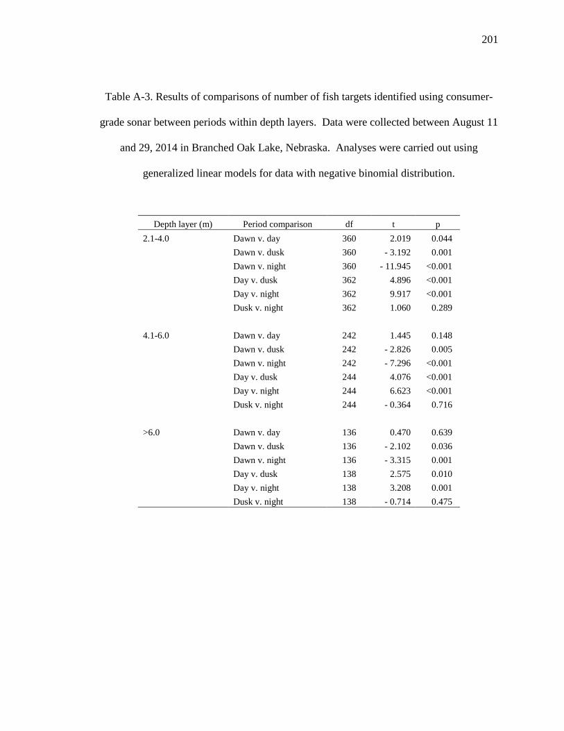
201
Table A-3. Results of comparisons of number of fish targets identified using consumer-
grade sonar between periods within depth layers. Data were collected between August 11
and 29, 2014 in Branched Oak Lake, Nebraska. Analyses were carried out using
generalized linear models for data with negative binomial distribution.
Depth layer (m) Period comparison df t p
2.1-4.0 Dawn v. day 360 2.019 0.044
Dawn v. dusk 360 - 3.192 0.001
Dawn v. night 360 - 11.945 <0.001
Day v. dusk 362 4.896 <0.001
Day v. night 362 9.917 <0.001
Dusk v. night 362 1.060 0.289
4.1-6.0 Dawn v. day 242 1.445 0.148
Dawn v. dusk 242 - 2.826 0.005
Dawn v. night 242 - 7.296 <0.001
Day v. dusk 244 4.076 <0.001
Day v. night 244 6.623 <0.001
Dusk v. night 244 - 0.364 0.716
>6.0 Dawn v. day 136 0.470 0.639
Dawn v. dusk 136 - 2.102 0.036
Dawn v. night 136 - 3.315 0.001
Day v. dusk 138 2.575 0.010
Day v. night 138 3.208 0.001
Dusk v. night 138 - 0.714 0.475

202
Table A-4. Results of comparisons of number of fish captured with vertical gillnets in the
top 4 meters of the water column between periods. Data were collected between August
11 to 29, 2014 in Branched Oak Lake, Nebraska. Analyses were carried out using
generalized linear models for data with negative binomial distribution.
Depth layer (m) Period comparison df t p
0.0-2.0 Dawn v. day 32 -0.503 0.615
Dawn v. dusk 32 1.404 0.160
Dawn v. night 32 0.204 0.838
Day v. dusk 34 -1.895 0.058
Day v. night 34 -1.027 0.304
Dusk v. night 34 1.281 0.200
2.1-4.0 Dawn v. day 32 0.133 0.894
Dawn v. dusk 32 -0.194 0.846
Dawn v. night 32 0.000 1.000
Day v. dusk 34 0.333 0.739
Day v. night 34 1.974 0.048
Dusk v. night 34 1.449 0.147

203
Figure A-1. Sampling used to estimating changes in fish spatial distribution in Branched
Oak Lake, Nebraska over diel cycles between August 11 and 29, 2014.

204
Figure A-2. Fish distribution during four periods (dawn 2 h before to 2 h after sunrise,
day 11:00-15:00, dusk 2 h before to 2 h after sunset, night 23:00-03:00) in three depth
layers of Branched Oak Lake, Nebraska during the week of August 11, 2014. Data were
collected using a consumer grade sonar unit and maps were generated using universal
kriging.

205
Figure A-3. Fish distribution during three periods (dawn 2 h before to 2 h after sunrise,
day 11:00-15:00, and dusk 2 h before to 2 h after sunset) in three depth layers of
Branched Oak Lake, Nebraska during the week of August 18, 2014. Data were collected
using a consumer grade sonar unit and maps were generated using universal kriging.

206
Figure A-4. Fish distribution during three periods (dawn 2 h before to 2 h after sunrise,
day 11:00-15:00, and dusk 2 h before to 2 h after sunset) in three depth layers of
Branched Oak Lake, Nebraska during the week of August 25, 2014. Data were collected
using a consumer grade sonar unit and maps were generated using universal kriging.

207
Appendix B. Striped bass condition and diet
Introduction
In an attempt to reduce white perch (Morone americana) abundance in Branched
Oak Lake, the Nebraska Game and Parks Commission stocked striped bass (Morone
saxatilis). Striped bass were selected for stocking because they are a predator of white
perch in their native range and because they tend to consume smaller prey (Walters and
Austin 2003; Gosch 2008). In October 2013, 8,000 striped bass were stocked at a total
length of 76 mm along with 2,400 striped bass at a total length of 89 mm. During May
2014, 8,524 striped bass were stocked at a total length of 203 mm. Our goal was to
evaluate these stockings in terms of striped bass condition and diet.
Methods
We recorded any striped bass captured during 2014 on Branched Oak Lake while
sampling to estimate abundance (Chapter 2) and to estimate how fish distributions
changed over diel cycles (Appendix A) we recorded any striped bass captured. In
addition to this sampling, we electrofished specifically for striped bass during June 2014,
September 2014, and April 2015. The Nebraska Game and Parks Commission also
electrofished for striped bass during April 2015. This sampling was conducted during
daylight hours using a boat electrofisher and targeted at areas low in the reservoir near
water > 4 m deep such as the jetties on the bay mouths and the face of the dam. We also
set gillnets during April 2014 and August 2014. These nets were made up of fish 10-m
monofilament panels, two 19-mm bar mesh panels and one each of 25-, 32-, and 38-mm

208
bar mesh panels; all panels were 2-m high and were arranged in a random sequence.
During April 2014, two gillnets were set in water > 7 m deep low in the reservoir to
target aggregations of white perch and gizzard shad; these nets were retrieved 24 h after
setting. During August 2014, 13 gillnets were set to specifically target striped bass; these
nets were distributed throughout the reservoir and 7 were set as floating gillnets by
attaching buoys to the float line at 5-m intervals thereby keeping the float line within 15
cm of the water’s surface; these nets were retrieved 1-2 h after setting.
When striped bass were captured, total length (mm) and mass (g) were recorded
in the field. Striped bass were then frozen and returned to the laboratory. In the
laboratory, the fish were thawed and we removed the stomach from each fish. All items
in the stomach were removed and all fish contained in striped bass stomachs were
identified to species if possible. Relative weight was calculated for each fish (Brown and
Murphy 1991).
Results and discussion
In total, we captured 12 striped bass (Table B-1). Three striped bass were
captured in vertical gillnets during July 2014, one striped bass was captured in a standard
set gillnet during August 2014 (Table B-1), and eight striped bass were captured
electrofishing along the jetties at the bay mouths during September (Table B-1). In
addition to the striped bass that we captured, the Nebraska Game and Parks Commission
captured two striped bass in standardized gillnets and two in standardized frame nets
during October. We captured the most striped bass by electrofishing the jetties at the bay
mouths during September.

209
Condition of striped bass captured was poor with relative weights ranging from 58
to 87 (Table B-2). Relative weight of fish captured decreased from July through
September then slightly increased from September to October (Table B-2). Seven of the
16 (44%) fish examined had empty stomachs. Two striped bass had small amounts of
digested material in their stomachs (Table B-2). Three striped bass contained fish
material that could not be identified (Table B-2). Four striped bass contained gizzard
shad (Dorosoma cepedianum) (Table B-2). Thus some of the stocked striped bass grew
to a size where they were able to consume young of the year gizzard shad by October.
No white perch were identified in any of the striped bass stomachs.
Future research should focus on understanding striped bass ecology in Branched
Oak Lake as it relates to the effect on the white perch population. Survival of the stocked
striped bass should be assessed to determine the best manner in which to stock them and
to determine if they can survive long term in this system. Prey selection and
bioenergetics data would be beneficial for determining if white perch are a substantial
portion of striped bass diet in Branched Oak Lake and to predict their effect on the white
perch population in this waterbody. Finally, an understanding of how striped bass
spatially distribute in this system would allow us to determine what habitats are critical
for the success of this species in this system and what the carrying capacity of this system
is in terms of striped bass. Once we understand this, we may be able to manipulate the
habitat to increase the carrying capacity for striped bass possibly with greater effects on
the white perch population in Branched Oak Lake.

210
Table B-1. Sampling effort (N) and catch of striped bass (Morone saxatilis) in Branched
Oak Lake, Nebraska. Sampling gears were vertical gillnets (VG; number of sets), a boat
electrofisher (EF; seconds of on time), and horizontal gillnets (GN; number of sets).
Month Gear N Striped bass
April 2014 VG 96 0
EF 3540 0
GN 2 0
June 2014 EF - 0
July 2014 VG 96 3
EF 4320 0
August 2014 GN 13 1
EF 6600 0
September 2014 EF 4575 8
October 2014 VG 66 0
EF 4500 0
November 2014 VG 30 0
April 2015 EF 9771 0

211
Table B-2. Length, weight, relative weight (Wr), and gut content information for striped
bass (Morone saxatilis) captured in Branched Oak Lake, Nebraska during 2014. Effort
consisted of 288, 1-2 h vertical gillnet sets (VG), 15, 1-24 h horizontal gillnet sets (GN),
and 26,731 seconds of electrofishing (EF) during 2014. Fish from October were captured
in Nebraska Game and Parks Commission standardized gillnets and trapnets (TN).
Parameters for estimating relative weight from Brown and Murphy 1991.
Month Gear
Length
(mm)
Weight
(g) Wr Stomach
July VG 201 87 87 4 spinal columns
VG 174 57 88 Empty
VG 161 45 87 1 gizzard shad 1 spinal column
August GN 193 56 63 Empty
September EF 261 150 68 1 unidentified fish
EF 246 135 73 1 spinal column
EF 252 139 70 Empty
EF 263 157 70 Empty
EF 246 135 73 Empty
EF 199 64 66 Empty
EF 230 100 66 Small amount digested material
EF 248 122 65 Small amount digested material
October GN 282 216 78 2 gizzard shad 1 spinal column
GN 274 220 86 2 gizzard shad
TN 271 196 79 1 gizzard shad
TN 250 112 58 Empty

212
References
Brown, M. L., and B. R. Murphy. 1991. Standard weights (Ws) for striped bass, white
bass, and hybrid striped bass. North American Journal of Fisheries Management
11:451-467.
Gosch, N. J. C. 2008. Predation as a mechanism for the control of white perch: an
investigation of food habits in two Nebraska reservoirs. Master’s thesis.
University of Nebraska Lincoln.
Walters, J. F., and H. M. Austin. 2003. Diet composition of large striped bass (Morone
saxatilis) in Chesapeake Bay. Fishery Bulletin 101:414-423.
Related Documents