Eco-Driving in Urban Traffic Networks Using Traffic Signals ...

HAL Id: hal-01297629https://hal-ifp.archives-ouvertes.fr/hal-01297629v2

Submitted on 7 Jan 2016

HAL is a multi-disciplinary open accessarchive for the deposit and dissemination of sci-entific research documents, whether they are pub-lished or not. The documents may come fromteaching and research institutions in France orabroad, or from public or private research centers.

L’archive ouverte pluridisciplinaire HAL, estdestinée au dépôt et à la diffusion de documentsscientifiques de niveau recherche, publiés ou non,émanant des établissements d’enseignement et derecherche français ou étrangers, des laboratoirespublics ou privés.

Eco-Driving in Urban Traffic Networks Using TrafficSignals Information

Giovanni de Nunzio, Carlos Canudas de Wit, Philippe Moulin, Domenico DiDomenico

To cite this version:Giovanni de Nunzio, Carlos Canudas de Wit, Philippe Moulin, Domenico Di Domenico. Eco-Drivingin Urban Traffic Networks Using Traffic Signals Information. International Journal of Robust andNonlinear Control, Wiley, 2016, Special issue : Recent Trends in Traffic Modelling and Control, 26(6), pp.1307-1324. 10.1002/rnc.3469. hal-01297629v2

Eco-Driving in Urban Traffic Networks Using TrafficSignals Information

Giovanni De Nunzio∗1,2, Carlos Canudas de Wit2, Philippe Moulin1, andDomenico Di Domenico1

1IFP Energies Nouvelles, Department of Control Signal and Systems, 1&4 avenue de Bois-Préau, 92852,

Rueil-Malmaison, France.2NeCS team, Inria Grenoble Rhône-Alpes, 655 Avenue de l’Europe, 38334 Montbonnot Saint-Martin, France.

Abstract

The problem of eco-driving is analyzed for an urban traffic network in presence ofsignalized intersections. It is assumed that the traffic lights timings are known and avail-able to the vehicles via infrastructure-to-vehicle (I2V) communication. This work pro-vides a solution to the energy consumption minimization, while traveling through a se-quence of signalized intersections and always catching a green light. The optimal controlproblem is non-convex due to the constraints coming from the traffic lights, therefore asub-optimal strategy to restore the convexity and solve the problem is proposed. Firstly,a pruning algorithm aims at reducing the optimization domain, by considering only theportions of the traffic lights green phases that allow to drive in compliance with the cityspeed limits. Then, a graph is created in the feasible region, in order to approximate theenergy consumption associated with each available path in the driving horizon. Lastly,after the problem convexity is recovered, a simple optimization problem is solved on theselected path to calculate the optimal crossing times at each intersection. The optimalspeeds are then suggested to the driver. The proposed sub-optimal strategy is comparedto the optimal solution provided by Dynamic Programming, for validation purposes. It isalso shown that the low computational load of the presented approach enables robustnessproperties, and results very appealing for online use.

Keywords — Eco-driving, nonlinear optimization, speed advisory, trajectory planning.

1 IntroductionPollution reduction and energy consumption optimization are becoming more and more crit-ical. Over the last years the number of vehicles demanding access to the road infrastructurehas increased exponentially. Governments along with scientific community aim at reducingboth environmental impact and costs of transportation. In particular the European Union hasset binding legislation to cut emissions by 20% with respect to 1990 levels by the end of

∗IFPen, 1&4 avenue de Bois-Préau, 92852, Rueil-Malmaison, France. E-mail: [email protected]

1

2020 [1]. Traffic congestion and idling time at signalized intersections are among the maincauses of energy consumption. Congestion in 2010 has been calculated to cost to US driversabout 101 billions of dollars [2]. Transportation is responsible for a substantial fraction oftotal green-house gas emissions (GHG), around a quarter in the European Union, making itthe second biggest GHG emitting sector after energy production. However, while emissionsfrom other sectors are generally decreasing, those from transportation have increased since1990 (by 36% in the European Union). In [3], experiments showed that the concentration offine particles in the air at traffic lights during stops is 29-times higher as compared to free-flow conditions. Also, though the delay time at intersections represents only a minor portionof the entire commuting time, it may contribute up to about 25% of the total trip emissions.

Extensive study and experimentation of several adaptive traffic control systems have beenconducted over the past three decades. Strategies such as SCOOT [4], which reduces trafficdelay by about 20% in urban areas, SCATS and TUC [5] have been employed all over theworld proving actual benefits in terms of congestion and emissions reduction. However, thesestrategies present some limitations in terms of traffic conditions responsiveness and sensorfailure robustness.

The state of the art in wireless communication, the deployment of dedicated communica-tion protocols for Vehicular Ad-hoc Networks (VANETs), and the decreasing price of GPSreceivers, allow more and more to rely on communication between the different agents ofan urban traffic network for the design of robust and efficient traffic control strategies [6].Specifically, Infrastructure-to-Vehicle (I2V) and Vehicle-to-Vehicle (V2V) communicationattracted the attention of many due to their potential to enable fast and cheap advanced drivingassistance systems (ADAS). Several international projects and groups (Drive C2X, iTetris,COMeSafety2, PATH), involving both automotive manufacturers and research centers, havebeen working on the setup of the communication infrastructure and on the assessment of theeffect of this technology on traffic management and energy consumption.

Speed advisory for the urban environment was already proposed in the ’80s [7][8] as avery energy-efficient traffic management strategy and as a pioneer for the modern ADAS. Therather simple initial idea of placing a roadside sign upstream from an intersection, indicatingthe travel speed to catch a green light, nowadays can be substantially improved thanks to theroad communication networks.

Knowledge of the traffic lights signal timings has been proved to be significantly ben-eficial in terms of energy efficiency in urban traffic. Green lights optimal speed advisory(GLOSA), with different penetration rate of the technology, has shown promising advantagesin terms of fuel consumption and average idling time [9]. Vehicles energy consumption isstrictly related to the accelerations in driving profiles. Soft decelerations to traffic lights onred, using advanced wireless-transmitted information, have been proved to be more energyefficient than sudden stops, allowing a reduction of both fuel consumption and emissions[10]. In general, it is possible to reduce energy consumption by preventing a vehicle fromcoming to a full stop at the intersections and by advising cruising velocities in order to catchas many green lights as possible. This goal could be achieved in different ways. In [11],authors developed an algorithm to minimize the acceleration profile while driving through asequence of signalized intersections, simulating scenarios with stochastically varied param-eters and showing a systematic reduction of fuel consumption, emissions and travel time.Interesting results on eco-driving with probabilistic signal phase and timing (SPAT) infor-mation are shown in [12], where a comparison between an uninformed driver and a driverwith different information levels (full horizon and short-term) is conducted using Dynamic

2

Programming (DP). An innovative solution to the velocity advisory problem, in proximity toa traffic light, was proposed in [13], where smartphones make use of their cameras to builda SPAT map of every intersection by relying only on V2V communication, without directlyinteracting with the infrastructure. This approach may enable GLOSA service and adaptiveroute change (ARC). Predictive cruise control (PCC) in traffic networks with signalized in-tersections was extensively treated in [14]. The objective is to penalize the braking actionto indirectly reduce energy consumption and travel time, and to discourage deviations froma suggested speed that allows to cross intersections without stopping. Somewhat similar ap-proach was used in [15]. A preliminary algorithm determines the arrival times at each trafficlight, by assuming that the closest trajectory to the one of the unconstrained case (i.e. notraffic lights) is the most energy-efficient. Then an analytical and numerical solution to thefuel consumption minimization problem is proposed, for a scenario with three traffic lightsover a driving horizon of nine kilometers. In [16] only one traffic light is considered andaccelerations upstream and downstream from the intersection are varied to find sub-optimalvalues for the fuel consumption minimization problem. In [17] DP is used to find the mini-mum energy solution, for a driving horizon enclosing up to two traffic lights. An approachto the multi-segment speed advisory is presented in [18]. The fuel consumption is indirectlyminimized by penalizing speed variations between adjacent road sections. The strategy ac-counts for multiple intersections and shows how such optimization yields better results withrespect to the single-segment approach. However nothing is stated about the computationtime and online applicability of the algorithm.

Assuming I2V communication, and therefore full knowledge of the traffic lights timings,the goal of this work is to analyze the driving horizon and compute an energy-efficient speedadvisory for the driver. As in previous works, stops at a red traffic light are to be avoided. Thenovelty of this work is summarized as follows. Given a set of green traffic light phases, thereexist different driving profiles to reach a given destination at a given final time in compliancewith traffic lights constraints (i.e. always catching the green light) and city speed limits. Thepresented strategy is capable of an a priori identification of the most energy-efficient veloc-ity trajectory, by approximating the available paths and their energy cost with an orientedweighted graph. The computational complexity of the graph creation has been reduced inthis work from exponential [19] to polynomial, thanks to the introduction of the line graph.The computation time has been consequently significantly reduced. Only after this prelimi-nary stage of path selection, a formal optimization problem is solved in order to calculate theoptimal arrival times at each intersection, by explicitly minimizing the energy consumptionof the vehicle. This approach qualifies as a pre-trip eco-driving ADAS, since the speed advi-sory is provided to the driver at the beginning of the driver horizon. However, given the verylittle computation time required by the algorithm, it may be employed online thus enablingin-trip assistance features. This allows to respond dynamically to traffic perturbations and/ordeviations from the speed advisory, and to increase the robustness and the applicability ofthe strategy in a realistic environment. Simulations in a microscopic traffic simulator demon-strate that the proposed strategy is able to deal online with perturbations coming from trafficand to reduce the overall energy consumption without affecting travel time.

Section 2 introduces the vehicle model and formulates the optimization problem. In Sec-tion 3 the applied methodology for the sub-optimal solution of the problem is explained indetail. In Section 4 the algorithm is validated against the true energy consumption calculatedvia DP, and robustness capabilities are shown. Concluding remarks are given in Section 5.

3

2 Problem FormulationThis work has as objective the minimization of the energy consumed by vehicles in a trafficnetwork to travel from an initial to a final point, in presence of signalized intersections inthe driving horizon. Clearly this problem is not trivial because the travel time, and moreimportantly the acceleration and velocity profiles of a vehicle, are affected by other agents ofthe traffic network (i.e. traffic lights), whose actions and priorities may conflict with the timeconstraints of the vehicles.

The analysis is carried out for a simplified urban traffic network with vehicles in freeflow, with no constraints coming from other users of the infrastructure. However, we willshow that the algorithm may be employed also in more realistic scenarios where the presenceof multiple vehicles requires the speed advisories to be updated dynamically.

I2V communication is assumed, and the vehicles have full knowledge of the n trafficlights timings in the driving horizon.

From a mathematical point of view, a constrained optimization problem can be cast. En-ergy consumption over the trip horizon is to be minimized, subject to the vehicle dynamicalmodel, and time constraints to impose arrivals at the intersections during a green phase.

2.1 Vehicle ModelVehicles equipped with electric motors will be considered in this work. The equivalent circuitmodel of a DC motor gives [20]:

Va = iaRa + e

e = κωm (1)Tm = κia

where Va is the armature voltage, ia is the armature current, Ra is the armature resistance,e is the back electromotive force, κ is the speed constant, ωm is the rotational speed of themotor, Tm is the electromagnetic motor torque. The motor power supply is converted intomechanical power and electric power loss due to heating of the armature coil, as follows:

P = Vaia = ωmTm +Ra

κ2T 2m (2)

where Vaia is the electric power supplied to the armature, ωmTm is the actual mechanicalpower developed by the armature, and Ra

κ2T 2m is the electric power wasted in the armature.

The control input u is represented by the motor torque:

u = Tm (3)

The vehicle longitudinal dynamical model may be generally written as:

mdv

dt= Ft − Faero − Ffriction − Fslope (4)

where Ft is the traction force at the wheels, Faero the aerodynamic force, Ffriction the rollingresistance force, Fslope the gravity force.

4

In the following we assume that there are no losses in the transmission, no slip at thewheels, and that the road slope does not vary in space. In particular, the road slope could beapproximated by an average value. Therefore, the vehicle model shall be written as:

x = v

mv = uRt

r− 1

2ρaAfcdv

2 −mgcr −mg sin(α)(5)

where Rt is the transmission ratio, r is the wheel radius, m is the vehicle mass, ρa is theexternal air density, Af is the vehicle frontal area, cd is the aerodynamic drag coefficient, cris the rolling resistance coefficient, α is the road slope, and g is the gravity.

The sum of the aerodynamic and rolling frictions can be approximated as a second orderpolynomial in the velocity v:

Fres = Faero + Ffriction = a0 + a1v + a2v2 (6)

where a0, a1 and a2 are parameters identified in previous works [21, 22].Under these assumptions the vehicle model can be simplified as follows:

x = v

v = h1u− h2v2 − h3v − h0

(7)

withh1 =

Rt

mr, h2 =

a2

m, h3 =

a1

m, h0 =

a0

m+ g sin(α) (8)

Therefore, the power demand can be expressed as:

P = b1uv + b2u2 (9)

whereb1 =

Rt

r, b2 =

Ra

κ2(10)

2.2 Traffic Lights TimingsIn this study the traffic lights are not actuated, therefore cycle time, phase time and offset aredeterministic and given. It is possible to formulate mathematically the state evolution of thetraffic lights as follows:

si(τ) =

1, kT < τ − θi 6 kT + Tgr

0, kT + Tgr < τ − θi 6 (k + 1)T(11)

where si is the state of the i-th traffic light, k ∈ Z is the number of cycles, T is thecycle time, Tgr is the duration of the green phase, and θi ∈ [0, T ) is the traffic light offset atintersection i, for i ∈ 1, . . . , n.

5

2.3 Optimal Control ProblemFinally, the optimization problem may be stated as follows:

minu

J =

tf∫t0

b1uv + b2u2 dt

s.t. x = v

v = h1u− h2v2 − h3v − h0

x(t0) = d0, x(tf ) = dn+1

x(ti) = di ∧ si(ti) = 1

v(t0) = v0, v(tf ) = vf

vmin ≤ v ≤ vmax

umin ≤ u ≤ umax

(12)

where (t0, d0) are the vehicle coordinates at the origin of the driving horizon, (tf , dn+1) arethe coordinates of the destination of the driving horizon, ti is the crossing time at the i-thintersection, di is the position of the i-th intersection, for i ∈ 1, . . . , n, v0 and vf are thedesired initial and final velocities.

A solution to a simpler problem, with no traffic lights and a simplified vehicle model, wasfound analytically in [20]. In the case under analysis, the traffic lights introduce an additionalcomplexity to the problem, expressed mathematically by the constraint:

x(ti) = di ∧ si(ti) = 1 (13)

Equation (13) imposes a non-stop requirement at the signalized intersection, by specifyingthat the vehicle has to be at the intersection di at time ti, when the traffic light si is green.This constraint may result in disjoint sets due to the presence of multiple available greenphases at each intersection, and may affect the convexity of the problem. In other wordsthe constraint (13) defines a non-convex set, and the nonlinear objective function, because ofsuch discontinuity in the constraints, assumes multiple local minima. Therefore, the solutionto this optimal control problem has to be sought in a sub-optimal way, by use of algorithmsthat simplify the control envelope, recover the convexity of the constraints set and solve theoptimization advising the driver on the velocity to track.

The problem can be solved in a local optimal way by the DP, provided that the selectionof the green phases to be traversed is made a priori. In order to obtain a global optimum,DP should be run extensively on all the possible paths to find the one with minimum cost.However its high computational load is clearly not suitable for online uses. In the following,the results obtained via DP will be used as a benchmark for validation and evaluation of theemployed sub-optimal strategy.

3 Optimization AlgorithmThe original optimal control problem (12) will be now divided into sub-problems for thesimplification of constraint (13) and the formulation of a convex optimization problem. Theidea is to identify the best green phase at each intersection, in order to finally optimize over asingle path from origin to destination.

6

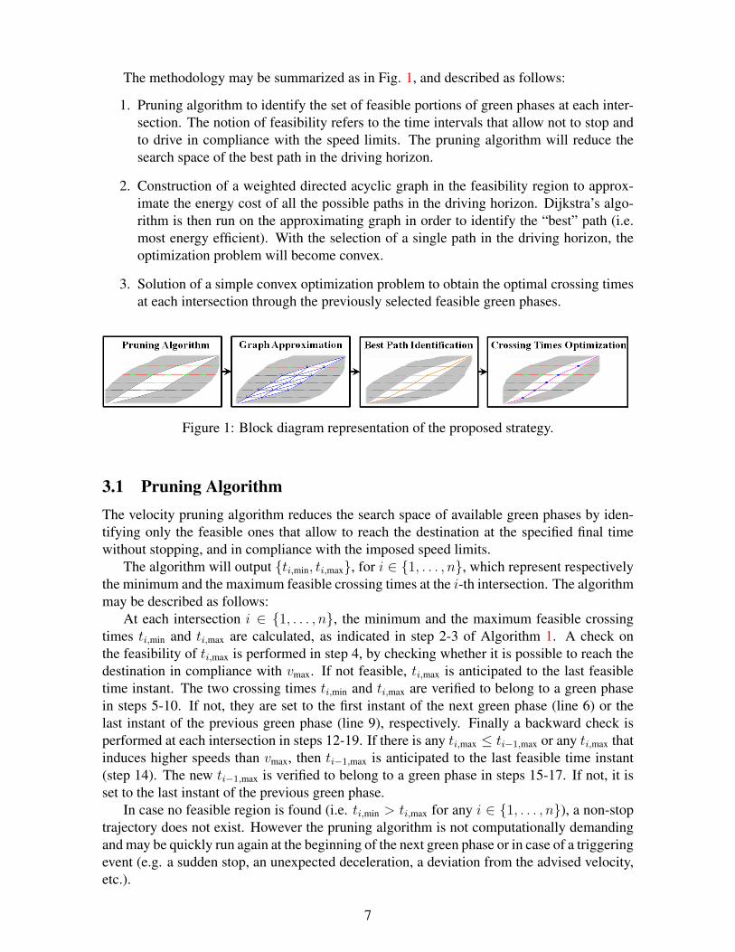
The methodology may be summarized as in Fig. 1, and described as follows:

1. Pruning algorithm to identify the set of feasible portions of green phases at each inter-section. The notion of feasibility refers to the time intervals that allow not to stop andto drive in compliance with the speed limits. The pruning algorithm will reduce thesearch space of the best path in the driving horizon.

2. Construction of a weighted directed acyclic graph in the feasibility region to approx-imate the energy cost of all the possible paths in the driving horizon. Dijkstra’s algo-rithm is then run on the approximating graph in order to identify the “best” path (i.e.most energy efficient). With the selection of a single path in the driving horizon, theoptimization problem will become convex.

3. Solution of a simple convex optimization problem to obtain the optimal crossing timesat each intersection through the previously selected feasible green phases.

Figure 1: Block diagram representation of the proposed strategy.

3.1 Pruning AlgorithmThe velocity pruning algorithm reduces the search space of available green phases by iden-tifying only the feasible ones that allow to reach the destination at the specified final timewithout stopping, and in compliance with the imposed speed limits.

The algorithm will output ti,min, ti,max, for i ∈ 1, . . . , n, which represent respectivelythe minimum and the maximum feasible crossing times at the i-th intersection. The algorithmmay be described as follows:

At each intersection i ∈ 1, . . . , n, the minimum and the maximum feasible crossingtimes ti,min and ti,max are calculated, as indicated in step 2-3 of Algorithm 1. A check onthe feasibility of ti,max is performed in step 4, by checking whether it is possible to reach thedestination in compliance with vmax. If not feasible, ti,max is anticipated to the last feasibletime instant. The two crossing times ti,min and ti,max are verified to belong to a green phasein steps 5-10. If not, they are set to the first instant of the next green phase (line 6) or thelast instant of the previous green phase (line 9), respectively. Finally a backward check isperformed at each intersection in steps 12-19. If there is any ti,max ≤ ti−1,max or any ti,max thatinduces higher speeds than vmax, then ti−1,max is anticipated to the last feasible time instant(step 14). The new ti−1,max is verified to belong to a green phase in steps 15-17. If not, it isset to the last instant of the previous green phase.

In case no feasible region is found (i.e. ti,min > ti,max for any i ∈ 1, . . . , n), a non-stoptrajectory does not exist. However the pruning algorithm is not computationally demandingand may be quickly run again at the beginning of the next green phase or in case of a triggeringevent (e.g. a sudden stop, an unexpected deceleration, a deviation from the advised velocity,etc.).

7

0 20 40 60 80 100 120 140 160 180 2000

200

400

600

800

1000

1200

1400

1600

1800

2000

time [s]

dis

tan

ce

[m

]

14 5.66

14 6.618

14 14

14 14

8.581 14

6 12.86

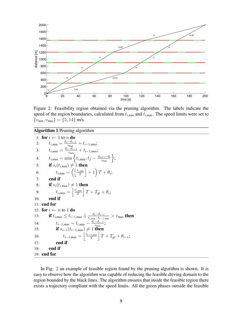
Figure 2: Feasibility region obtained via the pruning algorithm. The labels indicate thespeed of the region boundaries, calculated from ti,min and ti,max. The speed limits were set tovmin, vmax = 5, 14 m/s.

Algorithm 1 Pruning algorithm1: for i← 1 to n do2: ti,min = di−di−1

vmax+ ti−1,min;

3: ti,max = di−di−1

vmin+ ti−1,max;

4: ti,max = minti,max, tf − dn+1−di

vmax

;

5: if si(ti,min) 6= 1 then6: ti,min =

(⌊ti,minT

⌋+ 1)T + θi;

7: end if8: if si(ti,max) 6= 1 then9: ti,max =

⌊ti,maxT

⌋T + Tgr + θi;

10: end if11: end for12: for i← n to 1 do13: if ti,max ≤ ti−1,max || di−di−1

ti,max−ti−1,max> vmax then

14: ti−1,max = ti,max − di−di−1

vmax;

15: if si−1(ti−1,max) 6= 1 then16: ti−1,max =

⌊ti−1,maxT

⌋T + Tgr + θi−1;

17: end if18: end if19: end for

In Fig. 2 an example of feasible region found by the pruning algorithm is shown. It iseasy to observe how the algorithm was capable of reducing the feasible driving domain to theregion bounded by the black lines. The algorithm ensures that inside the feasible region thereexists a trajectory compliant with the speed limits. All the green phases outside the feasible

8

0 20 40 60 80 100 120 140 160 180 2000

200

400

600

800

1000

1200

1400

1600

1800

2000

time [s]

dis

tan

ce

[m

]

1

2 3

4 5 6

7 8 9

10 11 12

13 14

15

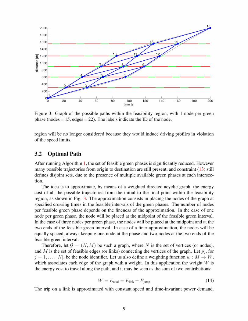
Figure 3: Graph of the possible paths within the feasibility region, with 1 node per greenphase (nodes = 15, edges = 22). The labels indicate the ID of the node.

region will be no longer considered because they would induce driving profiles in violationof the speed limits.

3.2 Optimal PathAfter running Algorithm 1, the set of feasible green phases is significantly reduced. Howevermany possible trajectories from origin to destination are still present, and constraint (13) stilldefines disjoint sets, due to the presence of multiple available green phases at each intersec-tion.

The idea is to approximate, by means of a weighted directed acyclic graph, the energycost of all the possible trajectories from the initial to the final point within the feasibilityregion, as shown in Fig. 3. The approximation consists in placing the nodes of the graph atspecified crossing times in the feasible intervals of the green phases. The number of nodesper feasible green phase depends on the fineness of the approximation. In the case of onenode per green phase, the node will be placed at the midpoint of the feasible green interval.In the case of three nodes per green phase, the nodes will be placed at the midpoint and at thetwo ends of the feasible green interval. In case of a finer approximation, the nodes will beequally spaced, always keeping one node at the phase and two nodes at the two ends of thefeasible green interval.

Therefore, let G = (N,M) be such a graph, where N is the set of vertices (or nodes),and M is the set of feasible edges (or links) connecting the vertices of the graph. Let pj , forj = 1, . . . , |N |, be the node identifier. Let us also define a weighting function w : M → W ,which associates each edge of the graph with a weight. In this application the weight W isthe energy cost to travel along the path, and it may be seen as the sum of two contributions:

W = Etotal = Elink + Ejump (14)

The trip on a link is approximated with constant speed and time-invariant power demand.

9

Therefore, the associated energy consumption is defined as:

Elink = ∆T(b1uivi + b2u

2i

)(15)

where vi = di−di−1

∆Tis the constant velocity on the edge, and ui = 1

h1(h2v

2i + h3vi + h0) from

(7), for i ∈ 1, . . . , n+ 1. The link travel time is defined as ∆T = τpl − τpj , for every edge(pj, pl) ∈ M , and pj, pl ∈ N , with τ being the crossing time associated with the relativevertex.

The energy consumption associated with the change of velocity at a node between twoedges is defined as:

Ejump =

∫ tjump

0

b1u(t)v(t) + b2u(t)2 dt (16)

where u(t) = 1h1

(v(t) + h2v(t)2 + h3v(t) + h0) from (7), and v(t) is the time-varying ve-locity in every transient linearly modeled as v(t) = vin ± a · t, with a being a constant fixedacceleration, vin the constant velocity on the incoming edge to the node. The speed change isassumed to be performed in tjump = |vout−vin|

a, with vout being the constant velocity on the out-

going edge from the node. Note that regenerative braking is not considered in this analysis,therefore Ejump is not negative.

The main challenge of such graph approximation is represented by the weight assignmentto the edges. Every node of the graph with two or more incoming edges is critical because vin

is not unique, and this generates multiple contributions Ejump for the outgoing edge. There-fore, the critical nodes need to be “decoupled” in order to have a correct weight assignment.

One option to deal with this problem is to transform the directed acyclic graph into thetree of all the possible paths [19]. This approach has an exponential complexity and itscomputational load might increase significantly with the size of the approximating graph.

A more efficient solution, in terms of memory allocation and computational load, is pro-posed in this work, and it is represented by the extension of the original graph into a linedigraph [23].

The line graph, L(G) of a graph G has as vertices the edges of G, and two vertices ofL(G) are adjacent whenever the corresponding edges of G are adjacent. The in-degree id(pj)of a vertex pj is the number of edges incident to pj (the inlines at pj), while its out-degreeod(pj) is the number of edges leaving pj (the outlines at pj). A point with no inlines is asource, one with no outlines is a sink.

Let G = (N,M) be the graph with N nodes and M edges as before. Then in L(G) =(N∗,M∗), the number of nodes is |N∗| = |M | and the number of edges is:

|M∗| =|N |∑j=1

id(pj) · od(pj)

The adoption of the line graph allows to solve the criticality of the original graph byintrinsically decoupling the nodes with multiple incoming edges. The problem boils down toassigning to each edge of the line graph a weight corresponding to the sum of Elink relativeto the edge indicated in the identifier of the destination node, and Ejump relative to the speedchange when coming from the link indicated in the origin node (see Fig. 4). Furthermore,the size of L(G) is smaller than the size of the tree of all the possible paths [19]. The numberof nodes in the expanded tree grows with an exponential law, whereas the number of nodesof the line graph grows with a polynomial law (namely quadratic).

10

1−2 1−3

2−4 2−5 3−5 3−6

4−7 4−8 5−8 5−9 6−9

7−10 7−11 8−11 8−12 9−12

10−13 11−13 11−14 12−14

13−15 14−15

D

S

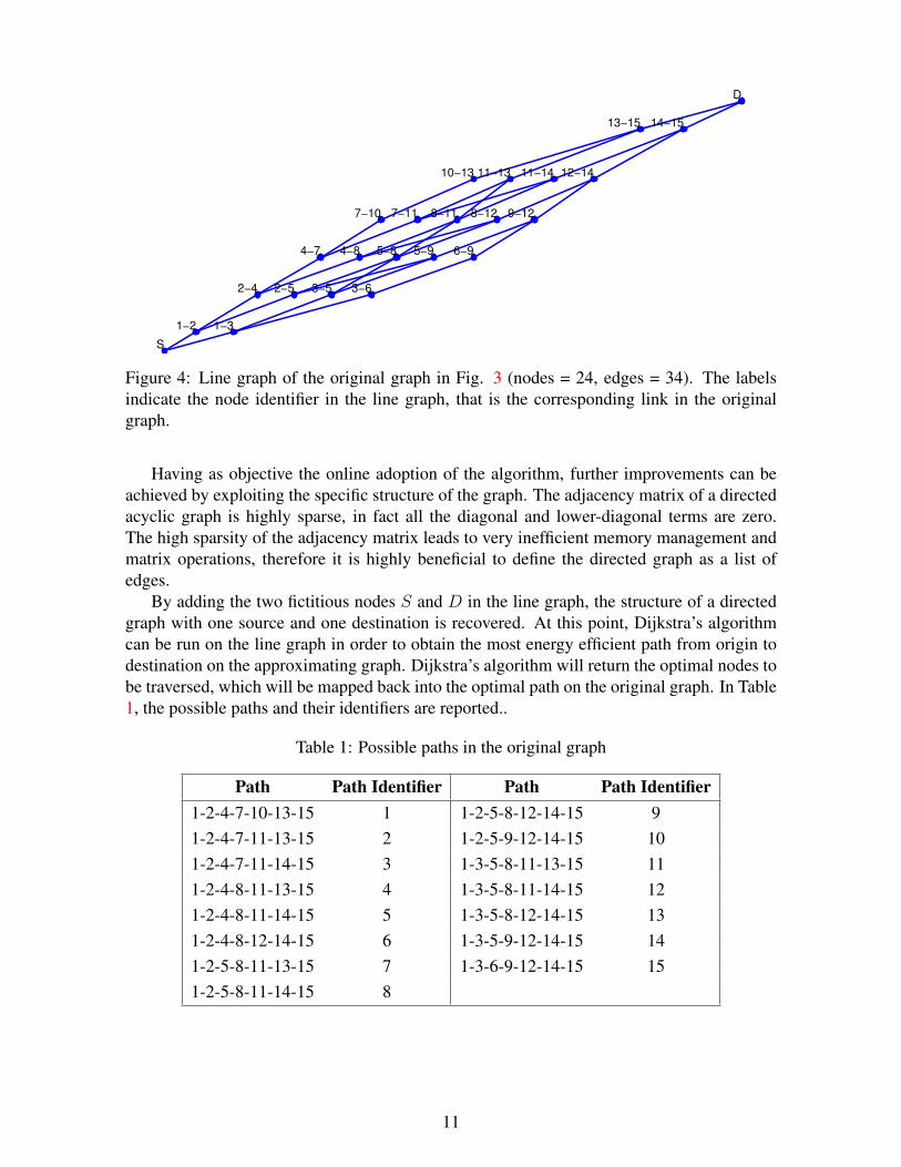
Figure 4: Line graph of the original graph in Fig. 3 (nodes = 24, edges = 34). The labelsindicate the node identifier in the line graph, that is the corresponding link in the originalgraph.

Having as objective the online adoption of the algorithm, further improvements can beachieved by exploiting the specific structure of the graph. The adjacency matrix of a directedacyclic graph is highly sparse, in fact all the diagonal and lower-diagonal terms are zero.The high sparsity of the adjacency matrix leads to very inefficient memory management andmatrix operations, therefore it is highly beneficial to define the directed graph as a list ofedges.

By adding the two fictitious nodes S and D in the line graph, the structure of a directedgraph with one source and one destination is recovered. At this point, Dijkstra’s algorithmcan be run on the line graph in order to obtain the most energy efficient path from origin todestination on the approximating graph. Dijkstra’s algorithm will return the optimal nodes tobe traversed, which will be mapped back into the optimal path on the original graph. In Table1, the possible paths and their identifiers are reported..

Table 1: Possible paths in the original graph

Path Path Identifier Path Path Identifier1-2-4-7-10-13-15 1 1-2-5-8-12-14-15 91-2-4-7-11-13-15 2 1-2-5-9-12-14-15 101-2-4-7-11-14-15 3 1-3-5-8-11-13-15 111-2-4-8-11-13-15 4 1-3-5-8-11-14-15 121-2-4-8-11-14-15 5 1-3-5-8-12-14-15 131-2-4-8-12-14-15 6 1-3-5-9-12-14-15 141-2-5-8-11-13-15 7 1-3-6-9-12-14-15 151-2-5-8-11-14-15 8

11

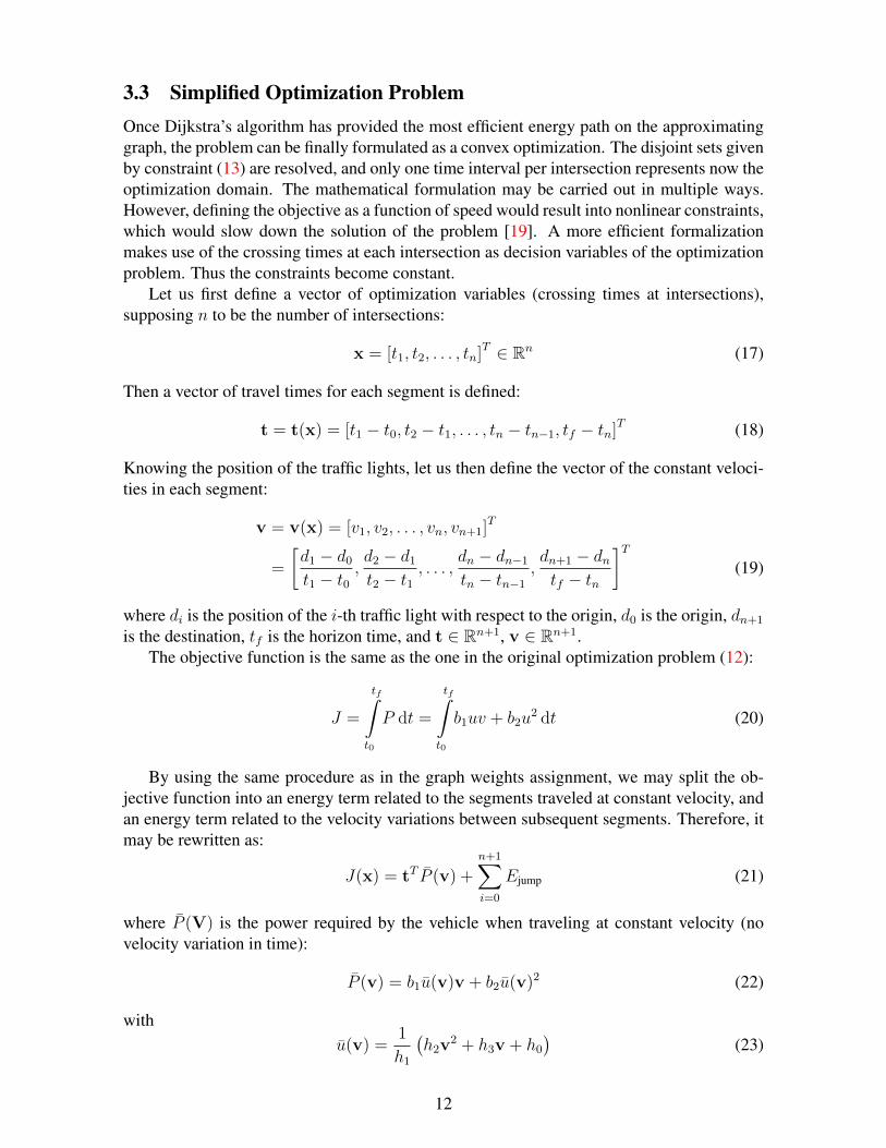
3.3 Simplified Optimization ProblemOnce Dijkstra’s algorithm has provided the most efficient energy path on the approximatinggraph, the problem can be finally formulated as a convex optimization. The disjoint sets givenby constraint (13) are resolved, and only one time interval per intersection represents now theoptimization domain. The mathematical formulation may be carried out in multiple ways.However, defining the objective as a function of speed would result into nonlinear constraints,which would slow down the solution of the problem [19]. A more efficient formalizationmakes use of the crossing times at each intersection as decision variables of the optimizationproblem. Thus the constraints become constant.

Let us first define a vector of optimization variables (crossing times at intersections),supposing n to be the number of intersections:

x = [t1, t2, . . . , tn]T ∈ Rn (17)

Then a vector of travel times for each segment is defined:

t = t(x) = [t1 − t0, t2 − t1, . . . , tn − tn−1, tf − tn]T (18)

Knowing the position of the traffic lights, let us then define the vector of the constant veloci-ties in each segment:

v = v(x) = [v1, v2, . . . , vn, vn+1]T

=

[d1 − d0

t1 − t0,d2 − d1

t2 − t1, . . . ,

dn − dn−1

tn − tn−1

,dn+1 − dntf − tn

]T(19)

where di is the position of the i-th traffic light with respect to the origin, d0 is the origin, dn+1

is the destination, tf is the horizon time, and t ∈ Rn+1, v ∈ Rn+1.The objective function is the same as the one in the original optimization problem (12):

J =

tf∫t0

P dt =

tf∫t0

b1uv + b2u2 dt (20)

By using the same procedure as in the graph weights assignment, we may split the ob-jective function into an energy term related to the segments traveled at constant velocity, andan energy term related to the velocity variations between subsequent segments. Therefore, itmay be rewritten as:

J(x) = tT P (v) +n+1∑i=0

Ejump (21)

where P (V) is the power required by the vehicle when traveling at constant velocity (novelocity variation in time):

P (v) = b1u(v)v + b2u(v)2 (22)

withu(v) =

1

h1

(h2v

2 + h3v + h0

)(23)

12

Finally the optimization problem may be formulated as:minx

J(x)

maxt−i , ti,min

≤ ti ≤ min

t+i , ti,max

(24)

where t−i and t+i are constants and represent the end times of the selected green phase at eachintersection i ∈ 1, . . . , n, and ti,min and ti,max are the minimum and the maximum feasiblecrossing times returned by the pruning algorithm.

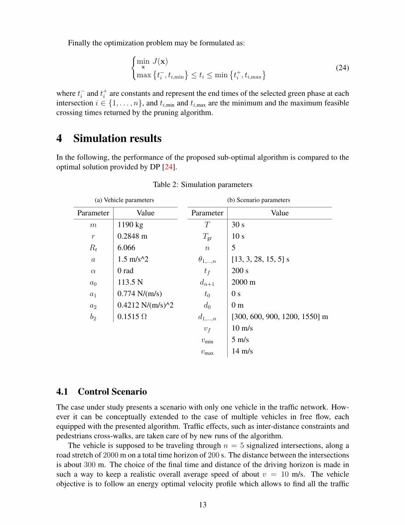
4 Simulation resultsIn the following, the performance of the proposed sub-optimal algorithm is compared to theoptimal solution provided by DP [24].

Table 2: Simulation parameters

(a) Vehicle parameters

Parameter Valuem 1190 kgr 0.2848 mRt 6.066a 1.5 m/s^2α 0 rada0 113.5 Na1 0.774 N/(m/s)a2 0.4212 N/(m/s)^2b2 0.1515 Ω

(b) Scenario parameters

Parameter ValueT 30 sTgr 10 sn 5

θ1,...,n [13, 3, 28, 15, 5] stf 200 sdn+1 2000 mt0 0 sd0 0 m

d1,...,n [300, 600, 900, 1200, 1550] mvf 10 m/svmin 5 m/svmax 14 m/s

4.1 Control ScenarioThe case under study presents a scenario with only one vehicle in the traffic network. How-ever it can be conceptually extended to the case of multiple vehicles in free flow, eachequipped with the presented algorithm. Traffic effects, such as inter-distance constraints andpedestrians cross-walks, are taken care of by new runs of the algorithm.

The vehicle is supposed to be traveling through n = 5 signalized intersections, along aroad stretch of 2000 m on a total time horizon of 200 s. The distance between the intersectionsis about 300 m. The choice of the final time and distance of the driving horizon is made insuch a way to keep a realistic overall average speed of about v = 10 m/s. The vehicleobjective is to follow an energy optimal velocity profile which allows to find all the traffic

13

1 2 3 4 5 6 7 8 9 10 11 12 13 14 150

0.1

0.2

0.3

0.4

0.5

0.6

0.7

0.8

0.9

1

v0 = 9 m/s

Path ID

Energ

y C

onsum

ption

1 2 3 4 5 6 7 8 9 10 11 12 13 14 150

0.1

0.2

0.3

0.4

0.5

0.6

0.7

0.8

0.9

1

v0 = 10 m/s

Path ID

Energ

y C

onsum

ption

DP

Proposed Optimization

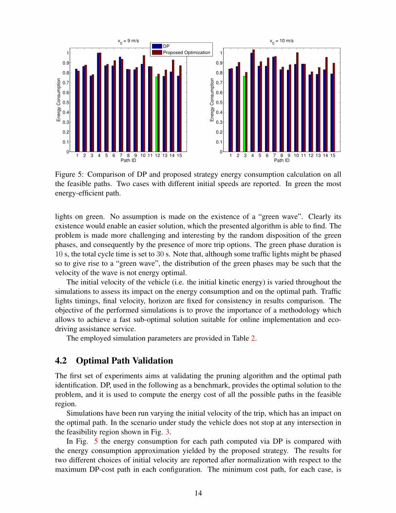
Figure 5: Comparison of DP and proposed strategy energy consumption calculation on allthe feasible paths. Two cases with different initial speeds are reported. In green the mostenergy-efficient path.

lights on green. No assumption is made on the existence of a “green wave”. Clearly itsexistence would enable an easier solution, which the presented algorithm is able to find. Theproblem is made more challenging and interesting by the random disposition of the greenphases, and consequently by the presence of more trip options. The green phase duration is10 s, the total cycle time is set to 30 s. Note that, although some traffic lights might be phasedso to give rise to a “green wave”, the distribution of the green phases may be such that thevelocity of the wave is not energy optimal.

The initial velocity of the vehicle (i.e. the initial kinetic energy) is varied throughout thesimulations to assess its impact on the energy consumption and on the optimal path. Trafficlights timings, final velocity, horizon are fixed for consistency in results comparison. Theobjective of the performed simulations is to prove the importance of a methodology whichallows to achieve a fast sub-optimal solution suitable for online implementation and eco-driving assistance service.

The employed simulation parameters are provided in Table 2.

4.2 Optimal Path ValidationThe first set of experiments aims at validating the pruning algorithm and the optimal pathidentification. DP, used in the following as a benchmark, provides the optimal solution to theproblem, and it is used to compute the energy cost of all the possible paths in the feasibleregion.

Simulations have been run varying the initial velocity of the trip, which has an impact onthe optimal path. In the scenario under study the vehicle does not stop at any intersection inthe feasibility region shown in Fig. 3.

In Fig. 5 the energy consumption for each path computed via DP is compared withthe energy consumption approximation yielded by the proposed strategy. The results fortwo different choices of initial velocity are reported after normalization with respect to themaximum DP-cost path in each configuration. The minimum cost path, for each case, is

14

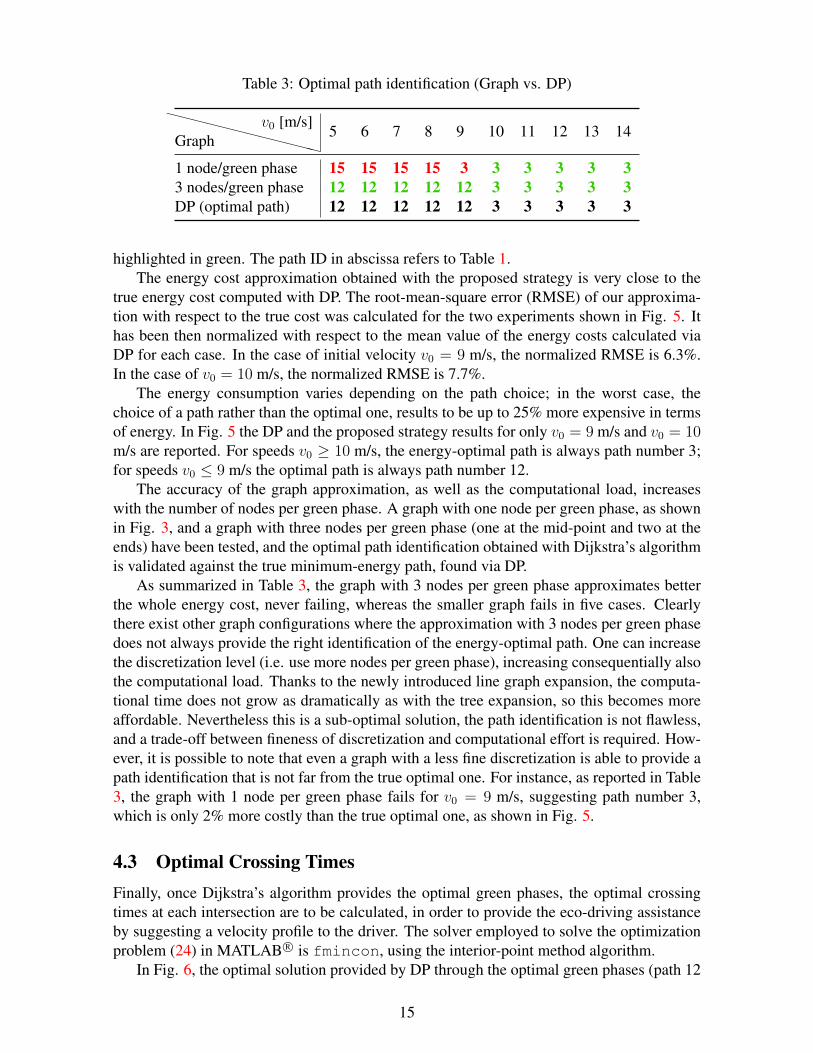
Table 3: Optimal path identification (Graph vs. DP)

XXXXXXXXXXXXGraphv0 [m/s]

5 6 7 8 9 10 11 12 13 14

1 node/green phase 15 15 15 15 3 3 3 3 3 33 nodes/green phase 12 12 12 12 12 3 3 3 3 3DP (optimal path) 12 12 12 12 12 3 3 3 3 3

highlighted in green. The path ID in abscissa refers to Table 1.The energy cost approximation obtained with the proposed strategy is very close to the

true energy cost computed with DP. The root-mean-square error (RMSE) of our approxima-tion with respect to the true cost was calculated for the two experiments shown in Fig. 5. Ithas been then normalized with respect to the mean value of the energy costs calculated viaDP for each case. In the case of initial velocity v0 = 9 m/s, the normalized RMSE is 6.3%.In the case of v0 = 10 m/s, the normalized RMSE is 7.7%.

The energy consumption varies depending on the path choice; in the worst case, thechoice of a path rather than the optimal one, results to be up to 25% more expensive in termsof energy. In Fig. 5 the DP and the proposed strategy results for only v0 = 9 m/s and v0 = 10m/s are reported. For speeds v0 ≥ 10 m/s, the energy-optimal path is always path number 3;for speeds v0 ≤ 9 m/s the optimal path is always path number 12.

The accuracy of the graph approximation, as well as the computational load, increaseswith the number of nodes per green phase. A graph with one node per green phase, as shownin Fig. 3, and a graph with three nodes per green phase (one at the mid-point and two at theends) have been tested, and the optimal path identification obtained with Dijkstra’s algorithmis validated against the true minimum-energy path, found via DP.

As summarized in Table 3, the graph with 3 nodes per green phase approximates betterthe whole energy cost, never failing, whereas the smaller graph fails in five cases. Clearlythere exist other graph configurations where the approximation with 3 nodes per green phasedoes not always provide the right identification of the energy-optimal path. One can increasethe discretization level (i.e. use more nodes per green phase), increasing consequentially alsothe computational load. Thanks to the newly introduced line graph expansion, the computa-tional time does not grow as dramatically as with the tree expansion, so this becomes moreaffordable. Nevertheless this is a sub-optimal solution, the path identification is not flawless,and a trade-off between fineness of discretization and computational effort is required. How-ever, it is possible to note that even a graph with a less fine discretization is able to provide apath identification that is not far from the true optimal one. For instance, as reported in Table3, the graph with 1 node per green phase fails for v0 = 9 m/s, suggesting path number 3,which is only 2% more costly than the true optimal one, as shown in Fig. 5.

4.3 Optimal Crossing TimesFinally, once Dijkstra’s algorithm provides the optimal green phases, the optimal crossingtimes at each intersection are to be calculated, in order to provide the eco-driving assistanceby suggesting a velocity profile to the driver. The solver employed to solve the optimizationproblem (24) in MATLAB R© is fmincon, using the interior-point method algorithm.

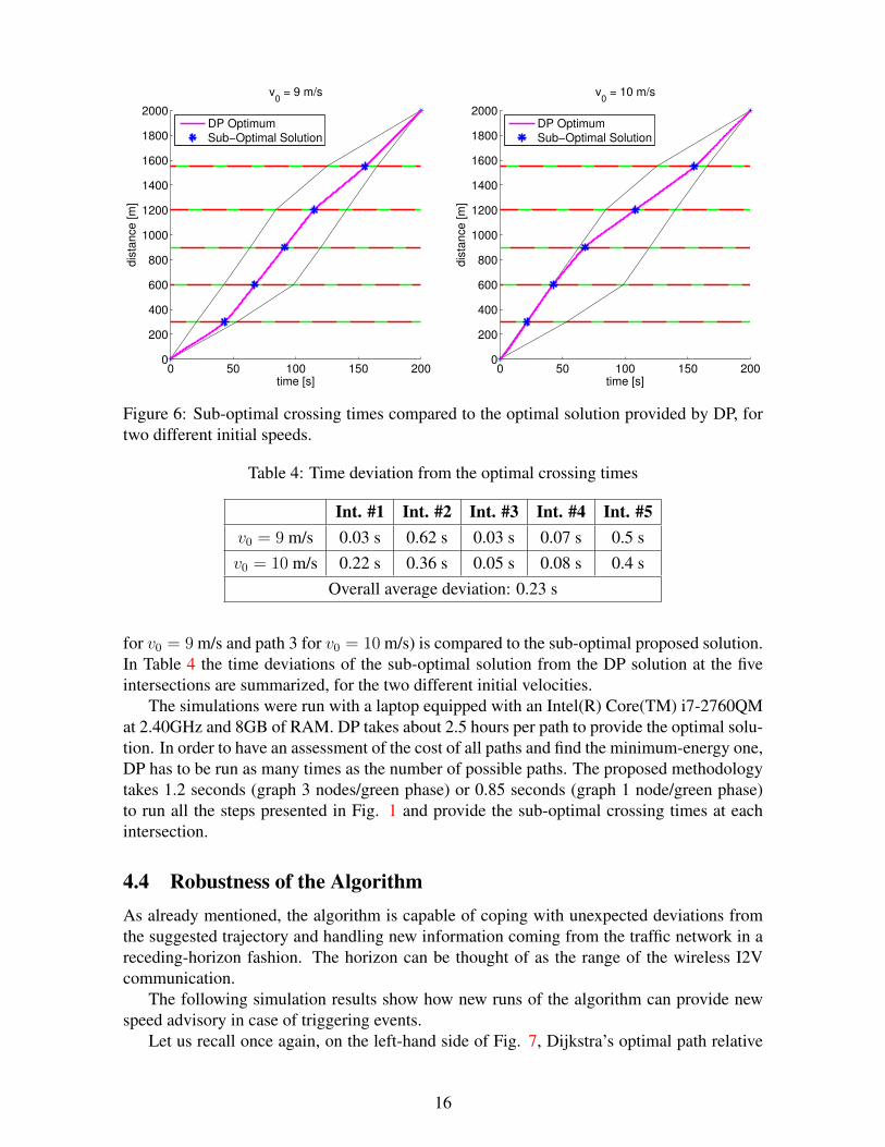
In Fig. 6, the optimal solution provided by DP through the optimal green phases (path 12

15

0 50 100 150 2000

200

400

600

800

1000

1200

1400

1600

1800

2000

time [s]

dis

tan

ce

[m

]

v0 = 9 m/s

DP Optimum

Sub−Optimal Solution

0 50 100 150 2000

200

400

600

800

1000

1200

1400

1600

1800

2000

time [s]

dis

tan

ce

[m

]

v0 = 10 m/s

DP Optimum

Sub−Optimal Solution

Figure 6: Sub-optimal crossing times compared to the optimal solution provided by DP, fortwo different initial speeds.

Table 4: Time deviation from the optimal crossing times

Int. #1 Int. #2 Int. #3 Int. #4 Int. #5v0 = 9 m/s 0.03 s 0.62 s 0.03 s 0.07 s 0.5 sv0 = 10 m/s 0.22 s 0.36 s 0.05 s 0.08 s 0.4 s

Overall average deviation: 0.23 s

for v0 = 9 m/s and path 3 for v0 = 10 m/s) is compared to the sub-optimal proposed solution.In Table 4 the time deviations of the sub-optimal solution from the DP solution at the fiveintersections are summarized, for the two different initial velocities.

The simulations were run with a laptop equipped with an Intel(R) Core(TM) i7-2760QMat 2.40GHz and 8GB of RAM. DP takes about 2.5 hours per path to provide the optimal solu-tion. In order to have an assessment of the cost of all paths and find the minimum-energy one,DP has to be run as many times as the number of possible paths. The proposed methodologytakes 1.2 seconds (graph 3 nodes/green phase) or 0.85 seconds (graph 1 node/green phase)to run all the steps presented in Fig. 1 and provide the sub-optimal crossing times at eachintersection.

4.4 Robustness of the AlgorithmAs already mentioned, the algorithm is capable of coping with unexpected deviations fromthe suggested trajectory and handling new information coming from the traffic network in areceding-horizon fashion. The horizon can be thought of as the range of the wireless I2Vcommunication.

The following simulation results show how new runs of the algorithm can provide newspeed advisory in case of triggering events.

Let us recall once again, on the left-hand side of Fig. 7, Dijkstra’s optimal path relative

16

0 50 100 150 2000

200

400

600

800

1000

1200

1400

1600

1800

2000

time [s]

dis

tan

ce

[m

]

Dijkstra’s optimal path

0 50 100 150 2000

200

400

600

800

1000

1200

1400

1600

1800

2000

time [s]

dis

tan

ce

[m

]

Dijkstra’s optimal path

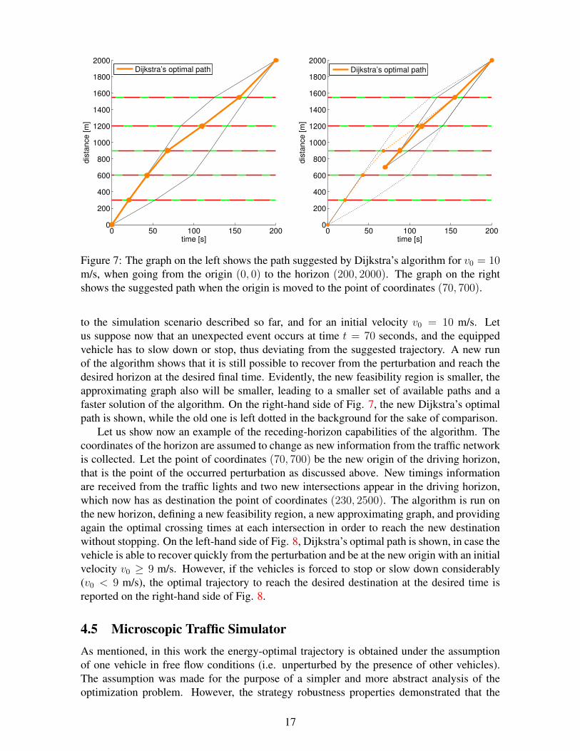
Figure 7: The graph on the left shows the path suggested by Dijkstra’s algorithm for v0 = 10m/s, when going from the origin (0, 0) to the horizon (200, 2000). The graph on the rightshows the suggested path when the origin is moved to the point of coordinates (70, 700).

to the simulation scenario described so far, and for an initial velocity v0 = 10 m/s. Letus suppose now that an unexpected event occurs at time t = 70 seconds, and the equippedvehicle has to slow down or stop, thus deviating from the suggested trajectory. A new runof the algorithm shows that it is still possible to recover from the perturbation and reach thedesired horizon at the desired final time. Evidently, the new feasibility region is smaller, theapproximating graph also will be smaller, leading to a smaller set of available paths and afaster solution of the algorithm. On the right-hand side of Fig. 7, the new Dijkstra’s optimalpath is shown, while the old one is left dotted in the background for the sake of comparison.

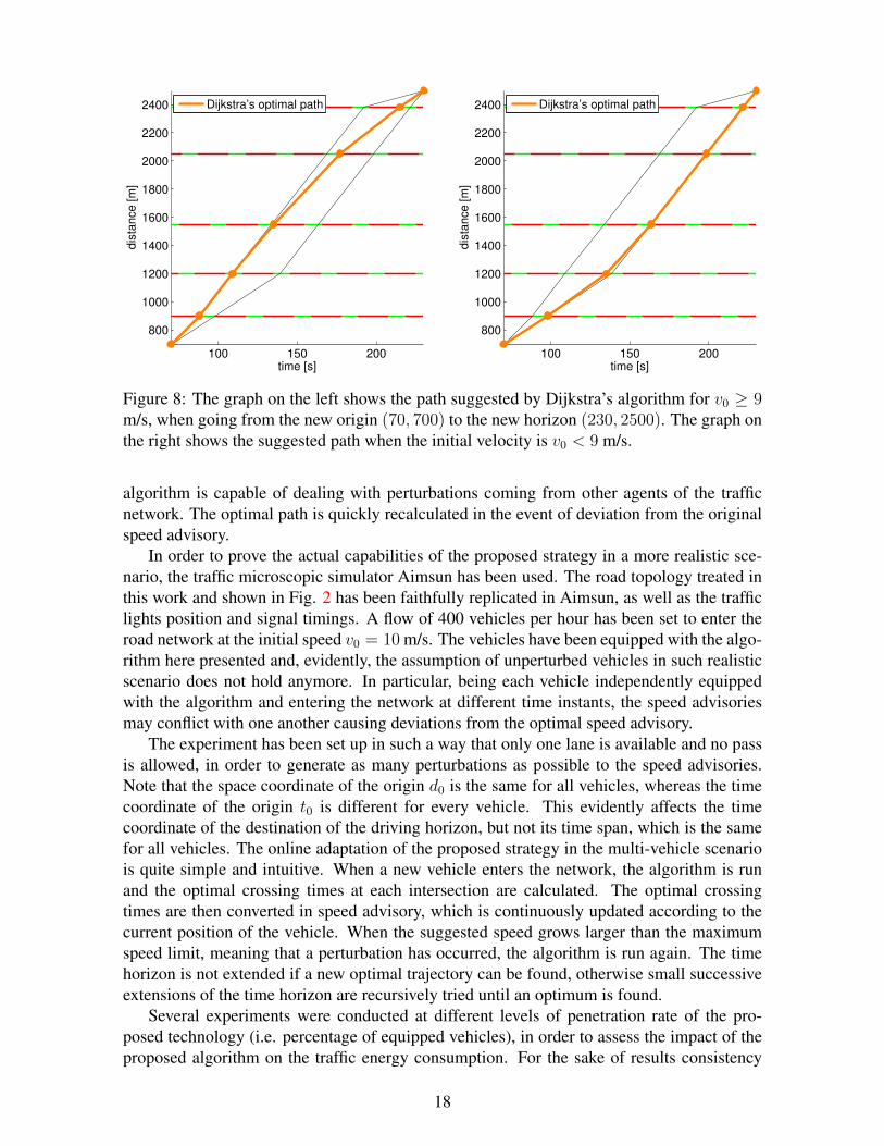
Let us show now an example of the receding-horizon capabilities of the algorithm. Thecoordinates of the horizon are assumed to change as new information from the traffic networkis collected. Let the point of coordinates (70, 700) be the new origin of the driving horizon,that is the point of the occurred perturbation as discussed above. New timings informationare received from the traffic lights and two new intersections appear in the driving horizon,which now has as destination the point of coordinates (230, 2500). The algorithm is run onthe new horizon, defining a new feasibility region, a new approximating graph, and providingagain the optimal crossing times at each intersection in order to reach the new destinationwithout stopping. On the left-hand side of Fig. 8, Dijkstra’s optimal path is shown, in case thevehicle is able to recover quickly from the perturbation and be at the new origin with an initialvelocity v0 ≥ 9 m/s. However, if the vehicles is forced to stop or slow down considerably(v0 < 9 m/s), the optimal trajectory to reach the desired destination at the desired time isreported on the right-hand side of Fig. 8.

4.5 Microscopic Traffic SimulatorAs mentioned, in this work the energy-optimal trajectory is obtained under the assumptionof one vehicle in free flow conditions (i.e. unperturbed by the presence of other vehicles).The assumption was made for the purpose of a simpler and more abstract analysis of theoptimization problem. However, the strategy robustness properties demonstrated that the

17

100 150 200

800

1000

1200

1400

1600

1800

2000

2200

2400

time [s]

dis

tance [m

]

Dijkstra’s optimal path

100 150 200

800

1000

1200

1400

1600

1800

2000

2200

2400

time [s]

dis

tance [m

]

Dijkstra’s optimal path

Figure 8: The graph on the left shows the path suggested by Dijkstra’s algorithm for v0 ≥ 9m/s, when going from the new origin (70, 700) to the new horizon (230, 2500). The graph onthe right shows the suggested path when the initial velocity is v0 < 9 m/s.

algorithm is capable of dealing with perturbations coming from other agents of the trafficnetwork. The optimal path is quickly recalculated in the event of deviation from the originalspeed advisory.

In order to prove the actual capabilities of the proposed strategy in a more realistic sce-nario, the traffic microscopic simulator Aimsun has been used. The road topology treated inthis work and shown in Fig. 2 has been faithfully replicated in Aimsun, as well as the trafficlights position and signal timings. A flow of 400 vehicles per hour has been set to enter theroad network at the initial speed v0 = 10 m/s. The vehicles have been equipped with the algo-rithm here presented and, evidently, the assumption of unperturbed vehicles in such realisticscenario does not hold anymore. In particular, being each vehicle independently equippedwith the algorithm and entering the network at different time instants, the speed advisoriesmay conflict with one another causing deviations from the optimal speed advisory.

The experiment has been set up in such a way that only one lane is available and no passis allowed, in order to generate as many perturbations as possible to the speed advisories.Note that the space coordinate of the origin d0 is the same for all vehicles, whereas the timecoordinate of the origin t0 is different for every vehicle. This evidently affects the timecoordinate of the destination of the driving horizon, but not its time span, which is the samefor all vehicles. The online adaptation of the proposed strategy in the multi-vehicle scenariois quite simple and intuitive. When a new vehicle enters the network, the algorithm is runand the optimal crossing times at each intersection are calculated. The optimal crossingtimes are then converted in speed advisory, which is continuously updated according to thecurrent position of the vehicle. When the suggested speed grows larger than the maximumspeed limit, meaning that a perturbation has occurred, the algorithm is run again. The timehorizon is not extended if a new optimal trajectory can be found, otherwise small successiveextensions of the time horizon are recursively tried until an optimum is found.

Several experiments were conducted at different levels of penetration rate of the pro-posed technology (i.e. percentage of equipped vehicles), in order to assess the impact of theproposed algorithm on the traffic energy consumption. For the sake of results consistency

18

0% 10% 20% 30% 40% 50% 60% 70% 80% 90% 100%0.7

0.75

0.8

0.85

0.9

0.95

1

Penetration Rate

Energ

y C

onsum

ption

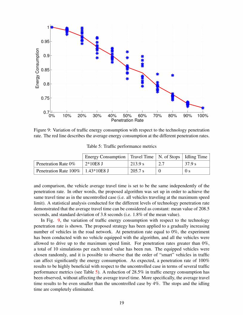
Figure 9: Variation of traffic energy consumption with respect to the technology penetrationrate. The red line describes the average energy consumption at the different penetration rates.

Table 5: Traffic performance metrics

Energy Consumption Travel Time N. of Stops Idling TimePenetration Rate 0% 2*10E8 J 213.9 s 2.7 37.9 sPenetration Rate 100% 1.43*10E8 J 205.7 s 0 0 s

and comparison, the vehicle average travel time is set to be the same independently of thepenetration rate. In other words, the proposed algorithm was set up in order to achieve thesame travel time as in the uncontrolled case (i.e. all vehicles traveling at the maximum speedlimit). A statistical analysis conducted for the different levels of technology penetration ratedemonstrated that the average travel time can be considered as constant: mean value of 208.5seconds, and standard deviation of 3.8 seconds (i.e. 1.8% of the mean value).

In Fig. 9, the variation of traffic energy consumption with respect to the technologypenetration rate is shown. The proposed strategy has been applied to a gradually increasingnumber of vehicles in the road network. At penetration rate equal to 0%, the experimenthas been conducted with no vehicle equipped with the algorithm, and all the vehicles wereallowed to drive up to the maximum speed limit. For penetration rates greater than 0%,a total of 10 simulations per each tested value has been run. The equipped vehicles werechosen randomly, and it is possible to observe that the order of “smart” vehicles in trafficcan affect significantly the energy consumption. As expected, a penetration rate of 100%results to be highly beneficial with respect to the uncontrolled case in terms of several trafficperformance metrics (see Table 5). A reduction of 28.5% in traffic energy consumption hasbeen observed, without affecting the average travel time. More specifically, the average traveltime results to be even smaller than the uncontrolled case by 4%. The stops and the idlingtime are completely eliminated.

19

One may argue that a global deployment of the proposed strategy would be difficult toachieve in a close future. A penetration rate of 40% is more realistic and results to be alreadyappealing in terms of energy consumption, yielding an average reduction of about 10%.

5 ConclusionsThe exchange of information between the infrastructure and the vehicles (I2V) has beenproved in literature to be beneficial in terms of traffic energy consumption. This workfocuses on the possibility of further improvements when information about many succes-sive signalized intersections is available. The presented algorithm is capable of finding theenergy-efficient path among all the available ones, and returning the speed advisory to thedrivers, in a sub-optimal way. The length of the optimization horizon can be arbitrarily long.The only limitations come from the I2V communication range and/or online execution con-straints. However, for the already complex scenario analyzed in this study, the computationtime required by the algorithm is very appealing for online implementation purposes. Therobustness capabilities of the algorithm have been also presented, by showing how perturba-tions and deviations from the suggested trajectory are handled. In particular, experiments ina microscopic traffic simulator demonstrated that, even in presence of multiple vehicles, theproposed algorithms is able to cope with perturbations and to drastically reduce the trafficenergy consumption without affecting travel time.

The experiments in the microscopic traffic simulator highlighted the fact that a perfor-mance improvement is achievable even though the vehicles are independently equipped withthe proposed algorithm and do not exchange information among them. Further improvementscould be achieved by exploiting V2V communication and by sharing information among thevehicles about their own optimal trajectory. Moreover, if the traffic flow grows larger, con-gestion and queues become inevitable. More sophisticated methods would be required, suchas macroscopic models for the estimation of the queue length. In such a situation the problemof eco-driving changes its nature, and a different analysis would be necessary. Lastly, an en-ergy consumption model for electric vehicles was considered in this work. Different energyand/or emissions models could be introduced into the problem, without any loss of generalityfor the proposed strategy.

References[1] What Is the EU Doing about Climate Change? URL http://ec.europa.eu/

clima/policies/brief/eu/.

[2] Schrank D, Eisele B, Lomax T. TTI’s 2012 Urban Mobility Report. Technical Report,Texas A\&M Transportation Institute 2012.

[3] Goel A, Kumar P. Characterisation of Nanoparticle Emissions and Exposure at Traf-fic Intersections through Fast–Response Mobile and Sequential Measurements. Atmo-spheric Environment 2015; .

[4] Hunt PB, Robertson DI, Bretherton RD, Winton RI. SCOOT - A Traffic ResponsiveMethod of Co-Ordinating Signals. Technical Report, TRRL Laboratory Report 10141981.

20

[5] Diakaki C. Integrated Control of Traffic Flow in Corridor Networks. PhD Thesis, Tech-nical University of Crete 1999.

[6] Hartenstein H, Laberteaux KP. A Tutorial Survey on Vehicular Ad Hoc Networks. IEEECommunications Magazine 2008; .

[7] Trayford RS, Doughty BW, Wooldridge MJ. Fuel Saving and Other Benefits of DynamicAdvisory Speeds on a Multi-Lane Arterial Road. Transportation Research Part A 1984;18(5-6).

[8] Trayford RS, Doughty BW, van der Touw JW. Fuel Economy Investigation of DynamicAdvisory Speeds from an Experiment in Arterial Traffic. Transportation Research PartA 1984; 18.

[9] Katsaros K, Kernchen R, Dianati M, Rieck D. Performance Study of a Green LightOptimized Speed Advisory (GLOSA) Application Using an Integrated Cooperative ITSSimulation Platform. International Wireless Communications and Mobile ComputingConference, 2011.

[10] Li M, Boriboonsomsin K, Wu G, Zhang WB, Barth M. Traffic Energy and EmissionReductions at Signalized Intersections: A Study of the Benefits of Advanced DriverInformation. International Journal of ITS Research 2009; 7(1):49–58.

[11] Mandava S, Boriboonsomsin K, Barth M. Arterial Velocity Planning Based on Traf-fic Signal Information under Light Traffic Conditions. IEEE Conference on IntelligentTransportation Systems, 2009.

[12] Mahler G, Vahidi A. Reducing Idling at Red Lights Based on Probabilistic Predictionof Traffic Signal Timings. IEEE American Control Conference, 2012.

[13] Koukoumidis E, Martonosi M, Peh LS. Leveraging Smartphone Cameras for Collabo-rative Road Advisories. IEEE Transactions on mobile computing 2012; 11(5):707–723.

[14] Asadi B, Vahidi A. Predictive Cruise Control: Utilizing Upcoming Traffic Signal Infor-mation for Improving Fuel Economy and Reducing Trip Time. IEEE Transactions onControl Systems Technology 2011; 19(3):707–714.

[15] Ozatay E, Ozguner U, Filev D, Michelini J. Analytical and Numerical Solutions forEnergy Minimization of Road Vehicles with the Existence of Multiple Traffic Lights.IEEE Conference on Decision and Control, 2013.

[16] Rakha H, Kamalanathsharma RK. Eco-Driving at Signalized Intersections Using V2ICommunication. IEEE Conference on Intelligent Transportation Systems, 2011.

[17] Miyatake M, Kuriyama M, Takeda Y. Theoretical Study on Eco-Driving Technique foran Electric Vehicle Considering Traffic Signals. IEEE Conference on Power Electronicsand Drive Systems, 2011.

[18] Seredynski M, Mazurczyk W, Khadraoui D. Multi-Segment Green Light Optimal SpeedAdvisory. IEEE 27th International Symposium on Parallel and Distributed ProcessingWorkshops and PhD Forum, 2013.

21

[19] De Nunzio G, Canudas De Wit C, Moulin P, Di Domenico D. Eco-Driving in UrbanTraffic Networks Using Traffic Signal Information. IEEE Conference on Decision andControl, 2013.

[20] Petit N, Sciarretta A. Optimal Drive of Electric Vehicles Using an Inversion-Based Tra-jectory Generation Approach. IFAC World Congress, 2011.

[21] Dib W, Chasse A, Moulin P, Sciarretta A, Corde G. Optimal Energy Management foran Electric Vehicle in Eco-Driving Applications. Control Engineering Practice 2014;29:299–307.

[22] Dib W, Chasse A, Di Domenico D, Moulin P, Sciarretta A. Evaluation of the EnergyEfficiency of a Fleet of Electric Vehicle for Eco-Driving Application. Oil & Gas Scienceand Technology – Rev. IFP Energies nouvelles 2012; 67(4):589–599.

[23] Harary F, Norman RZ. Some Properties of Line Digraphs. Rendiconti del CircoloMatematico di Palermo 1960; 9(2):161–168.

[24] Sundström O, Guzzella L. A Generic Dynamic Programming Matlab Function. IEEEInternational Conference on Control Applications, 2009.

22