ecn.sandia.gov · Web viewUse of volatile, gasoline fuels. Injection pressures lower than 500 bar. Ambient density and temperatures typical of gasoline engines, …

ECN6 – GASOLINE SPRAY (SPRAY G) SUBMISSION GUIDELINES

Unified guidelines for:

Topic 9, Internal and near-nozzle flow

David Schmidt (UMass Amherst)

[email protected]

Topic 10, Evaporative Spray G

Tommaso Lucchini (Polimi)

[email protected]

Topic 11, Spray G in engines

Joaquin de la Morena (CMT)

[email protected]

IntroductionWe are motivated to understand the fuel-air mixing process in gasoline, direct-injection engines where spray evolution is characterized by:

Use of volatile, gasoline fuels Injection pressures lower than 500 bar Ambient density and temperatures typical of gasoline engines, ranging from intake (possibly sub-

atmospheric) throughout the compression stroke Multi-hole and injector geometry interactions

Over the years, ECN efforts in this topic were dedicated to: definition of the injector (ECN1 and ECN2), initial experiments and modeling of the “reference” condition (ECN3), detailed characterization of the spray morphology (ECN4), careful internal geometry characterization, and air entrainment and plume interaction effects (ECN5). Please refer to past proceedings (https://ecn.sandia.gov/ecn-workshop/search-presentations/) to understand the findings and context for current work.

ObjectivesECN6 will expand upon past work, specifically focused on the target Spray G condition. The main objectives will be to:

Understand mixing under flash-boiling conditions Expand generality of modeling to a wider range of ambient conditions Compare injection in engines (with intake flow) to quiescent spray chambers Study the effectiveness of multiple injections with new experiments and modeling

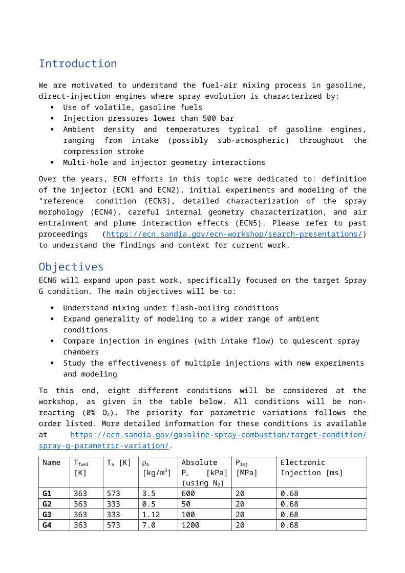
To this end, eight different conditions will be considered at the workshop, as given in the table below. All conditions will be non-reacting (0% O2). The priority for parametric variations follows the order listed. More detailed information for these conditions is available at https://ecn.sandia.gov/gasoline-spray-combustion/target-condition/spray-g-parametric-variation/.

Name Tfuel [K] Ta [K] a [kg/m3] Absolute Pa

[kPa] (using N2)Pinj [MPa] Electronic Injection [ms]

G1 363 573 3.5 600 20 0.68G2 363 333 0.5 50 20 0.68G3 363 333 1.12 100 20 0.68G4 363 573 7.0 1200 20 0.68G7 363 800 9.0 2150 20 0.68G-M1 363 573 3.5 600 20 0.68 / 1 (dwell) / 0.186*G1-cold

298 298 3.5 315 20 0.68

G2-cold

363 298 0.6 50 20 0.68

* Electronic settings for #28

Note that the target conditions will be reached in EITHER spray chambers OR engines, where the charge-gas conditions in engines are those at the time of injection, particularly for G1, G2, G3 conditions. No specification is given for the engine flowfield. Engine experiments and simulations are encouraged both before and after injection to understand the fate of mixing on the given flowfield.

Although conditions are listed to establish their priority, this does not imply that an institution has to provide data for ALL conditions and requests. Institutions are encouraged to submit any number of

contributions (big or small), with the objective of filling the gaps between all contributors. Simulations are encouraged that span internal and near-nozzle flow (Topic 9) towards vaporization (Topic 10) and spray-flow interactions in engines (Topic 11). Having identified the main objectives and conditions, there are also specific activities and objectives particular to both experimental and modeling work.

Experimental objectivesExperimental techniques that provide both global behavior and detailed in-situ quantification are encouraged. ECN6 will focus on:

- Detailed data release, analysis, and comparison of the flash-boiling G2 condition by multiple institutions for the first time

- Evaluation of the self-consistency of mixing, velocity, and penetration data as a whole to identify the most effective experimental techniques

- Evaluation and (re-evaluation) of vapor and liquid envelopes, concentration, and plume direction using new liquid-extinction experiments and analysis

- Development of quantitative diagnostics in mixed (liquid and vapor) regions of the spray - Further standardization of experimental techniques and derived metrics- Archival release of well-documented datasets to the ECN website

Modeling objectivesTo advance the capability of computational methodology to describe the internal flow, countersunk hole geometry interaction, and charge-gas thermodynamic conditions and flow on spray mixing and evaporation. In particular:

- Transients of needle opening and closing- Realistic geometry and surface roughness of the injector- Internal flow and near-field mixing that leads to predictive plume dispersion, rather than tuned

spreading angle- Spray collapse and plume-interaction under high ambient temperature or low ambient pressure

(flash boiling) conditions- Spray-gas interactions with variation of gas velocity and turbulence- How spray evaporation is affected by fuel properties, spray breakup and coalescence- Methods for utilizing less expensive simulations (RANS) to establish reliable input for more

expensive simulations (VOF, LES)

Spray modeling approaches with different resolution, cost, and structure (Eulerian-Lagrangian, Eulerian-Eulerian) using both RANS and LES are encouraged to bridge the gap between high-fidelity and engineering level simulations.

Deadline for submissions1st July 2018

Nomenclature and boundary condition definitionsGeometrySimulation and experimental submissions will follow the ECN coordinate system convention for Spray G, as described in https://ecn.sandia.gov/gasoline-spray-combustion/target-condition/spray-g-plume-orientation/ . The injector nozzle with the holes numbered, and coordinate system axis, are shown. The SAE J2715 standard orientation convention has been used by the ECN Spray G community with z = 0, y = 0, x = 0 defined as the tip of the nozzle, NOT the flat of the injector (see Fig. 2).

Fig. 1. Hole numbering and coordinate system convention of Spray G

Note that the tip protrudes past the hole exit, meaning that the plumes begin at negative z values. Conventions for describing the drill angle and derived plume geometry are given below. Another coordinate system z´, colinear with the hole drill angle and beginning at the exit of the inner hole (z´ = 0), is introduced for use with internal flow simulations and experiments.

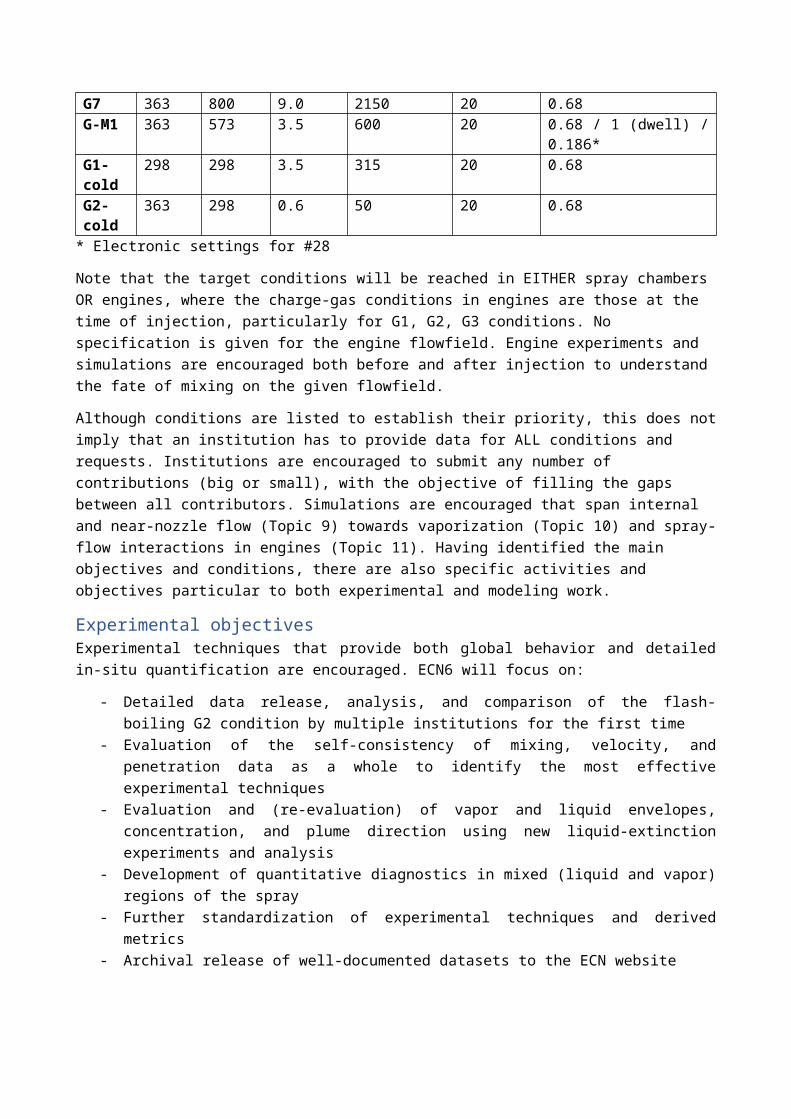
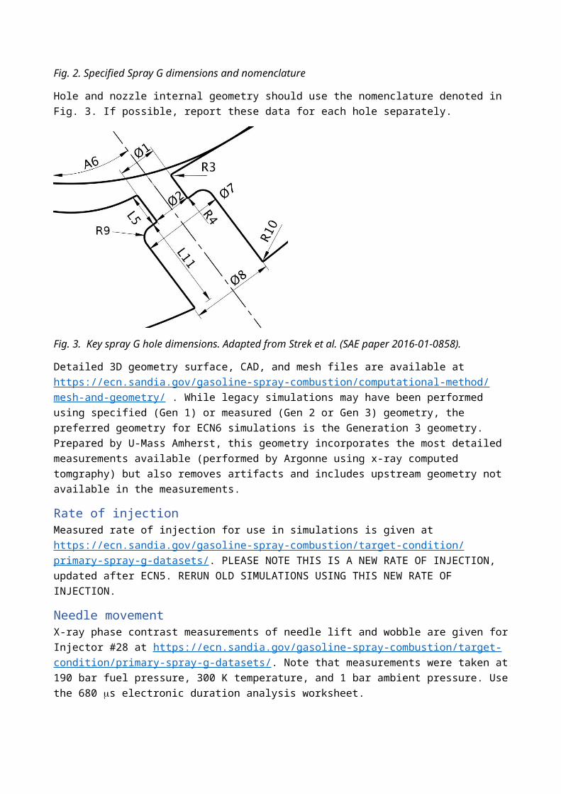
Fig. 2. Specified Spray G dimensions and nomenclature

Hole and nozzle internal geometry should use the nomenclature denoted in Fig. 3. If possible, report these data for each hole separately.

Fig. 3. Key spray G hole dimensions. Adapted from Strek et al. (SAE paper 2016-01-0858).

Detailed 3D geometry surface, CAD, and mesh files are available at https://ecn.sandia.gov/gasoline-spray-combustion/computational-method/mesh-and-geometry/ . While legacy simulations may have been performed using specified (Gen 1) or measured (Gen 2 or Gen 3) geometry, the preferred geometry for ECN6 simulations is the Generation 3 geometry. Prepared by U-Mass Amherst, this geometry incorporates the most detailed measurements available (performed by Argonne using x-ray computed tomgraphy) but also removes artifacts and includes upstream geometry not available in the measurements.

Rate of injectionMeasured rate of injection for use in simulations is given at https://ecn.sandia.gov/gasoline-spray-combustion/target-condition/primary-spray-g-datasets/. PLEASE NOTE THIS IS A NEW RATE OF INJECTION, updated after ECN5. RERUN OLD SIMULATIONS USING THIS NEW RATE OF INJECTION.

Needle movementX-ray phase contrast measurements of needle lift and wobble are given for Injector #28 at https://ecn.sandia.gov/gasoline-spray-combustion/target-condition/primary-spray-g-datasets/. Note that measurements were taken at 190 bar fuel pressure, 300 K temperature, and 1 bar ambient pressure. Use the 680 s electronic duration analysis worksheet.

TemperatureFuel temperature, nozzle temperature, and gas temperature are as specified at the start of injection. For engine simulations, state assumptions for representative gas temperature and pressure (or density). Specifying non-adiabatic wall conditions is encouraged.

Initial dissolved non-condensable gas contentSimulations will be performed with no non-condensable gas addition.

Initial ambient gas motionFor engine simulations, the characteristics of air flow at the simulation start are to be given in terms of tumble ratio and/or swirl ratio.

Submission of experimental and modeling results Using the defined coordinate system, all experiments and simulations will provide data relative to the start of injection. Start of injection is defined as the time of emergence of first liquid out of the counterbore section of the hole. Needle movement occurs earlier.

Experimental submissions from past workshops are listed in Appendix A. Expectations for experimental and modeling submissions for ECN6 are listed in Appendix B. We encourage archiving experimental submissions with documentation for each variable, as described at https://ecn.sandia.gov/gasoline-spray-combustion/experimental-data-search/ .

Submissions will include several processed indicators of spray penetration and growth as a function of time, as well as detailed 2D cut-plane or projection data at specific locations and timings.

Data formatRaw numeric data is required. Simple time-resolved may be returned in delimited format. 2D data may be binary, provided a reader program or script is provided. One option is to use standard image format (.png, or .tif) without truncating or changing the range of the data in time. By providing the pixel dimensions, and the minimum and maximum quantities, the image data is easily converted to numeric quantities, as shown in Appendix 3.

For a time-resolved, global quantity, please use the naming format QuantityvsTime.txt, e.g., “ROI_hole1vsTIME.txt”. For a 2D binary data please use “QuantityLocationTime.png”, e.g., LVFz2mm0600.png for z = 2 mm data at 0.600 ms after start of injection.

Global and Time-Resolved Spray IndicatorsThese are quantities describing the overall spray behavior, resolved in time.

Vapor penetration:ExperimentalSchlieren or other diagnostics sensitive to fuel vapor are utilized in either the primary or secondary orientation. Penetration is defined as the maximum axial penetration of ANY plume, as described in https://ecn.sandia.gov/gasoline-spray-combustion/experimental-diagnostics/gasoline-jet-penetration/ .

ModelingDefined as the farthest axial distance where mixture fraction is less than 0.001.

Liquid-phase penetration:To assess the vaporization characteristics of the spray, we define a threshold for axial (or radial) liquid penetration. Past work has shown inconsistency when using a Mie-scatter diagnostic and other difficulties if using a liquid-volume fraction criteria, as explained by the ECN5.9 slides and recording given by Pickett, accessible at https://ecn.sandia.gov/gasoline-spray-combustion/experimental-diagnostics/liquid-penetration-length/ . The parameter for comparison will be the “projected liquid-volume” defined as

where LVF is the local liquid volume fraction (i.e. units of mm3 liquid / mm3) and y is the cross-stream direction (x could be exchanged for y for Spray G if appropriate for the experiment).

Experimental method to derive projected liquid volumeLaser extinction or diffused backlit imaging (DBI) with sufficient radiance and collection angles to eliminate beam-steering are required to perform these experiments, as detailed in the above links and presentations.

∫− y∞

y∞

LVF ∙dy (1)

Past datasets which show beamsteering may be analyzed and offset to account for beam-steering, while documenting all assumptions. Note that G2 and G3 conditions may exhibit little beam-steering artifacts because of the lower ambient density and cooler ambient temperature, making it possible to analyze the data quantitatively. Extinction measurement provide the optical thickness of liquid objects along the beam path, where the transmitted intensity I normalized by the baseline light intensity I0 is related to by

and the optical thickness is related to extinction along the path due to liquid with

where d is droplet diameter and C ext¿ is the extinction cross-section from Mie-theory, depending upon

droplet size, wavelength, and collection angle (the * superscript designates collection with a finite collection angle, rather than complete extinction). If one assumes a monodisperse droplet size distribution, Equation 3 becomes

Allowing the measured optical thickness and estimates for droplet optical properties . For the sake of consistency, we will assume a droplet size of 7 m, based upon SMD measurements performed by Scott Parrish (GM) at the periphery of the plume (see https://ecn.sandia.gov/gasoline-spray-combustion/target-condition/primary-spray-g-datasets/) and a refractive index of 1.391 for iso-octane. Under these assumptions, Mie-scatter theory (recommend use of http://www.philiplaven.com/mieplot.htm) with a detector collection angle of 225 mrad at 633 nm yields C ext

¿ =44.6 ∙10−6mm2 . The left-hand side of Equation 3 may therefore be evaluated (for this example) to estimate the projected liquid volume.

Liquid-extinction lengthBecause of the need to explore sensitivities in models and experiments, two different thresholds are required:

.

The maximum axial position (of any plume) with liquid-volume projection less than these “low” and “high” thresholds will be referrred to as “liquid-extinction” length.

Liquid-extinction widthAt an axial position of z = 15 mm, the radial width at these two thresholds is defined as the “liquid-extinction” width.

Both the liquid-extinction width and liquid-extintion length will be returned with respect to time. In the next section, 2D datasets for liquid-volume projection will also be requested for further analysis at particular time steps.

Spatial- (and time-) resolved variablesRequested 2D binary data (see Data Format above) are to be provided on different cut planes (Fig. 4). Provide data from 0.1 – 2 ms (or max) in 0.1 ms time-steps.

Axial (x-y) cut planes: z = 1, 2, 10, 15 mm Axial cut plane normal to the drill angle (z’, Fig. 2): z´ = -0.1, 0, 0.1, 1.0 mm

II 0

=e−τ (2)

τ=∫− y∞

y∞

Cext¿ LVFπ d3 /6

dy (3)

τ π d3 /6Cext

¿ =∫− y∞

y∞

LVF ∙dy , (3)

∫− y∞

y∞

LVF ∙dy=0.2 ∙10−3mm3 liquidmm2

∧2.0∙10−3 mm3liquidmm2

The central x-z cut plane (z = -2 to 40 mm) in primary position The “secondary” x’-z cut plane (z = -2 to 40 mm, rotated about z by 22.5 degrees)

Fig. 4. Illustration of 2D cut planes for data analysis (see Duke et al. Experimental Thermal and Fluid Science 88:608-621, 2017).

The 2D binary data requested include:

3 component gas and liquid velocities (m/s) total liquid and vapor fuel mixture fraction (mass of liquid fuel and vapor fuel/mass of all mixture) mass liquid fuel / volume (not liquid fuel density, kg fuel / m3) liquid volume fraction (volume liquid / volume) fuel vapor volume fraction (volume fuel vapor / volume) non-condensible gas (nitrogen) volume fraction (volume nitrogen / volume) total mixture density (fuel and all other gases / volume) projected liquid volume (x-z plane, integrated in y direction, mm3 liquid /mm2) temperature (K) sauter mean diameter droplet size (m)

Description of the simulationRather than a prose submission, descriptions will be submitted for all simulations using the following numbered items:

1. The name of the phase-change model and a seminal reference where interested readers can learn more about the details. A sentence or two about the basic phenomena captured by this model is also expected.

2. An explanation of how fluid properties were calculated or tabulated. This may be a reference to a database or an equation of state.

3. Does the internal simulation couple to an external spray simulation? If so, how?4. What turbulence closure is used?

5. What is the initial gas and liquid velocity and turbulence distribution at the time of injection?6. What form of the energy equation is used, if any. How was the wall treatment determined? Were

walls treated as adiabatic, isothermal, or other?7. Were any special phenomena were considered? Examples are compressibility, dissolved gas,

nucleation8. Did you specify ROI, or another variable such as needle position or injection pressure? 9. What needle lift was used, fixed or variable? If a fixed needle lift was used, what was the value?

Also, was wobble included?10. For moving needle cases, how was the beginning and end of injection treated? Were baffles

removed or inserted to stop flow? Does the algorithm automatically seal the injector needle to the seat or must some model be employed? If a static need was used, leave this blank.

11. What geometry was used? Please provide as much information about the provenance of the geometry as possible. See https://ecn.sandia.gov/gasoline-spray-combustion/computational-method/mesh-and-geometry/ for generation 1 and 2 geometries.

12. What mesh paradigm was used? Please indicate the basic meshing strategy and the number of cells. If the number of cells varied during the simulation, please explain. For moving needle computations, explain how the mesh was morphed or topologically altered. The submission should include a saggital plane snapshot of the mesh at full needle lift. Avoid slices that cut through individual cells, but rather give a crinkle-cut slice if possible.

13. What interface treatment was used? This should be several sentences. For example, it is not sufficient to say “VOF” but rather explain whether a geometric interface construction was used or some interfacial compression scheme was employed with flux limiting. If a diffuse interface treatment was used, be sure to provide a reference that describes the governing equations.

14. Provide a table of boundary conditions that was used for each equation.

Specific requests for topic 9 internal flow simulationsNote that the time datum for internal injection calculations needs to be adjusted to match the defined start of injection. Time 0 is the time of the first passage of liquid out of the hole counterbore for any one of the eight holes. Internal simulations submissions should include the following:

1. Predicted mass rate of injection in g/s versus time in ms. This should be submitted as a plain text ASCII file with time as the first column and ROI as the second.

2. Predicted mass rate of injection of each hole in g/s versus time in ms. ROI should be measured at the small-hole exit. This should be submitted as a plain text ASCII file with time as the first column and ROI as the second. This should be a nine column table where the first column is time in ms and the subsequent eight columns correspond to the mass flow of each hole.

3. Provide the liquid fuel ROI, fuel-vapor ROI and non-condensible gas ROI similar to the total fuel ROI in item #2.

4. Time average 2D data requested above for the quasi-steady state, i.e., the period of near-maximum needle lift from 0.4 to 0.6 ms ASOI. Use the naming recommended above, i.e. “QuantityLocationTime.png”, e.g., LVFz2mm0400-0600.png for z = 2 mm data at 0.600 ms after start of injection.

Specific requests for topic 10 evaporative spray1. Priority list of conditions to be simulated: G, G2, G3, G4, G7, G1-cold, G2-cold 2. Provide results with your “best practice” 3. In order to make a consistent comparison between codes, independently from the used spray

model, provide simulation results for spray G conditions with: a. No spray sub-models;b. Injected droplet size from a Rosin-Rammler distribution with SMD = 9.5 m;

c. Cone angle for the different plumes: 15°d. Plume direction: 34°e. Area contraction coefficient (Ca): 0.7 and 1.0, using Dnozzle as the 1 denoted above in Fig. 3.

Ca is defined as:

Ca=A jetAnozzle

=D jet2

Dnozzle2

For the same injection mass flow rate, a reduction of Ca will produce an increase of the jet velocity and will affect the air-entrainment process. Practically, reducing Ca in Lagrangian simulations means that the simulation is initialized with a smaller nozzle diameter with respect to the actual nozzle size:

D jet=√Ca⋅Dnozzle

Specific requests for topic 11 Spray G in engines evaporative spray1. Combustion chamber layout: due to the characteristics of Spray G injector, preferred configuration

would be spray guided with central injector location. 2. To avoid complex interactions between the flow field from the intake ducts and the piston shape, a

flat piston configuration is recommended (but not required). 3. Intake pressure (or even compression ratio) and injection timing should be adjusted, if possible, to

match as close as possible the target conditions defined above at start of injection (SOI). 4. Preferred engine speeds should range between 1500 and 2000 rpm to have significant flow

structures that can affect the spray propagation characteristics. Slower engine speeds can be also considered to achieve a more direct comparison with quiescent chambers.

5. For simulation activities, researchers are encouraged to perform complete simulations including both intake and compression strokes, so that 3-dimensional intake flow features are reproduced. To do so, the following information should be made available from experimental activities:

a. Air mass flowb. Measured in-cylinder pressure and intake pressure resolved inc. Complete intake and in-cylinder geometryd. Intake valve timing and lift profiles

Appendix 1: AVAILABLE Experimental DataAvailable data is found at https://ecn.sandia.gov/gasoline-spray-combustion/target-condition/primary-spray-g-datasets/ . Details have been presented at ECN workshops and monthly webex meetings. You may search past presentations at https://ecn.sandia.gov/ecn-workshop/search-presentations/ .

A summary of available data, not all posted to the ECN website, as of Mar 2018 is shown below.

Liquid-extinction Penetration, Vapor Penetration, and Spray Width.Institution Source Pos Condition ReferenceMelbourne

DBI and MIESchlieren

1 G1, G2, G3

Sandia DBI and Mie

1 &

G1, G4, G5, G6, G7, G-M1 ECN websiteSAE 2015-01-1894

Schlieren 2CMT DBI

Schlieren1 G1, G2, G3, G4, G5, G6, G7, G-M1

parametric variations:1 to 9 kg/m3, 300 to 800K, 680-1200us, 100-200 bar (120 conditions)

Payri et al., Applied Therm. Eng. 2016ECN5

Ist. Motori MIESchlieren

1 G1, G2 (cold), G3 (cold)Cold = Ambient temp.

IFPEn MIESchlieren

1 G1, G7 SAE 2015-01-1902

GM MIESchlieren

1 G1, G-M1 SAE 2015-01-1894

Illinois DBISchlieren

1 G1, G2, G3 ECN 5.7

1: primary orientation (0 deg), 2: secondary orientation (22.5 deg) Check orientation

Velocity, density, concentration, mixture fraction. Ins Data Source Condition Notes Argonne Fuel density / volume x-ray CT G1-cold, G2-cold z = 2 mmGM Liquid velocity and SMD PDI

Phase Doppler Interferometry

Spray G Radial and transverse at 15mm from nozzle tip.

IFPen Fuel mass concentrationTemperature fields

p-DFB LIF two color LIF

Spray G3.5 kg/m3 673K 6kg/m3 700K 9kg/m3 800K

Iso-octane + 0.03% vol. DFB Primary orientation

Sandia Gas velocity fields between plumes 13 – 20 mm downstream

PIV G1, G4, G7, G-M1Longer injections

Secondary orientation

Appendix 2: Gasoline spray committee -- participants for ECN6

Inst Contact Type Topic Notes Argonne Chris Powell Experiment 9

10 Needle lift, geometry, fuel densityG2-cold radiography

GM Scott Parrish Experiment 9 Microscopy inside counterboreSandia Lyle Pickett Experiment 9

10Microscopy of spray, geometryVelocity, liquid volume

ORNL Martin Wissink Experiment 9 Needle motion, neutron imagingArgonne Zongyu Yu,

Kaushik SahaSimulation 9

10VOF at G1-coldELSA, one-way, Lagrangian

Chalmers Michael Oevermann Simulation 9 G2 presented at ECN5.8Siemens Samir Muzaferija Simulation 9UMass/GM David Schmidt Simulation 9CMT Daniel Vaquerizo

Joaquin de la MorenaExperiment 10

11Illinois Wayne Chang Experiment 10 G2

Ist Motori A. Montanaro Experiment 10Melbourne Joshua Lacey Experiment 10 G2 GM Scott Parrish Experiment 10 G1, G-M1IFPEN Gilles Bruneaux Experiment 10 G1Chalmers Petter Dahlander Experiment 10 G2, PDI plansPoliMi Davide Paredi Simulation 10

11UW Randy Hessel Simulation 10KAUST-UW-Aramco

Hongjiang Li Simulation 10

Darmstadt Christian Hasse Simulation 10Illinois Chia-Fon Li Simulation 10Michigan Margaret Wooldridge Experiment 11Duisburg- Essen

Sebastian Kaiser Experiment 11

Darmstadt Benjamin Boehm Experiment 11

Appendix 3: Example to convert binary image data to floating-point data This example Matlab script shows how to read an 8 bit grayscale image on the current ECN website, converting it to floating point liquid volume fraction data with inputs for image range. Image scale is also given, providing actual spatial dimensions.

%example for accepting grayscale .png file (binary) and using for analysis %(1) download "data" .png file for Spray A liquid volume fraction at %https://ecn.sandia.gov/wp-content/uploads/2015/06/s675x0.1tox3z0a.pngim = imread('s675x0.1tox3z0a.png');%im is grayscale 8 bit with 301 x 1550 pixels%(2) get maximum and minimum for image range: % given at https://ecn.sandia.gov/wp-content/uploads/2015/06/s675x0.1tox3z0ag.pngimMin = 0; imMax = 1.04; nPixy = 301; nPixx = 1550;%(3) get scale of pixels, and reference: %given at https://ecn.sandia.gov/wp-content/uploads/2015/06/s675x0.1y_column.csvdPix = 0.002; % 2 um per pixelpixNoz = 151; % pixel 151 is center of nozzley = ([nPixy:-1:1]-pixNoz).*dPix; % given vector for y axisx = 0.1+ ([1:1:nPixx]-1).*dPix; % given vector for x axisLVF = imMin + single(im)./256*(imMax-imMin); %image data now converted to quantitative liquid volume fraction %% show data in Matlab "jet" colormapfigure(4), imshow(LVF,[imMin imMax]); colormap(gca,jet); %% get cool-to-warm colormap at http://www.kennethmoreland.com/color-advice/% dowload byte map 256m = dlmread('smooth-cool-warm-table-byte-0256.csv',',',1,0);coolWarmMap = m(:,2:4)./256;% show data in cool-to-warm colormapfigure(5), imshow(LVF,[imMin imMax]); %show cool-to-warm imagecolormap(gca,coolWarmMap); %% most importantly, use data quantitatively

% examine LVF profile at certain axial distanceaxd = 1; %data at x = 1 mma = find(x>axd,1,'first');figure(6), plot(y,LVF(:,a));ylabel('Liquid volume fraction [au]');xlabel('Radial position [mm]');text(-0.2,0.8,'x = 1.0 mm','fontsize',16);