Efficient creation of multipartite entanglement for superconducting quantum computers Johannes Ferber M¨ unchen 2005

Welcome message from author
This document is posted to help you gain knowledge. Please leave a comment to let me know what you think about it! Share it to your friends and learn new things together.
Transcript

Efficient creation of multipartiteentanglement for superconducting
quantum computers
Johannes Ferber
Munchen 2005

Efficient creation of multipartiteentanglement for superconducting
quantum computers
Johannes Ferber
Diplomarbeitan der Fakultat fur Physik
der Ludwig–Maximilians–UniversitatMunchen
vorgelegt vonJohannes Ferber
aus Munchen
Munchen, den 23.8.2005

Erstgutachter: PD Frank K. Wilhelm
Zweitgutachter: Prof. Dr. Harald Weinfurter
Contents
0 Overview 1
1 Introduction 31.1 Quantum computation . . . . . . . . . . . . . . . . . . . . . . . . . . . . . . . 31.2 Implementation schemes . . . . . . . . . . . . . . . . . . . . . . . . . . . . . . 31.3 Superconducting qubits . . . . . . . . . . . . . . . . . . . . . . . . . . . . . . 41.4 Flux qubit . . . . . . . . . . . . . . . . . . . . . . . . . . . . . . . . . . . . . . 61.5 Decoherence . . . . . . . . . . . . . . . . . . . . . . . . . . . . . . . . . . . . . 91.6 Coherent manipulation . . . . . . . . . . . . . . . . . . . . . . . . . . . . . . . 91.7 Coupling of three qubits . . . . . . . . . . . . . . . . . . . . . . . . . . . . . . 101.8 Measurement . . . . . . . . . . . . . . . . . . . . . . . . . . . . . . . . . . . . 10
2 Coupling strength 112.1 Coupling via a common loop . . . . . . . . . . . . . . . . . . . . . . . . . . . 112.2 Coupling via shared junctions–qubit triangle . . . . . . . . . . . . . . . . . . 162.3 Measurement design . . . . . . . . . . . . . . . . . . . . . . . . . . . . . . . . 19
3 Eigenstates of the system 213.1 Hamiltonian . . . . . . . . . . . . . . . . . . . . . . . . . . . . . . . . . . . . . 213.2 No coupling . . . . . . . . . . . . . . . . . . . . . . . . . . . . . . . . . . . . . 233.3 Weak antiferromagnetic coupling . . . . . . . . . . . . . . . . . . . . . . . . . 253.4 Strong antiferromagnetic coupling . . . . . . . . . . . . . . . . . . . . . . . . 28
4 Preparing states in the degenerate subspaces 314.1 Quantizing the electromagnetic field and the
interaction Hamiltonian . . . . . . . . . . . . . . . . . . . . . . . . . . . . . . 324.2 Preparing given states in the degenerate subspaces . . . . . . . . . . . . . . . 33
5 Entanglement properties 395.1 Tripartite entanglement . . . . . . . . . . . . . . . . . . . . . . . . . . . . . . 405.2 Bell inequalities . . . . . . . . . . . . . . . . . . . . . . . . . . . . . . . . . . . 445.3 Robustness to limited measurement fidelity . . . . . . . . . . . . . . . . . . . 46
6 Pulse shaping 516.1 Laplace transform . . . . . . . . . . . . . . . . . . . . . . . . . . . . . . . . . 526.2 LTI-Systems and transfer functions . . . . . . . . . . . . . . . . . . . . . . . . 526.3 Circuit synthesis theory . . . . . . . . . . . . . . . . . . . . . . . . . . . . . . 54
v
vi Contents
6.4 Approximation and results . . . . . . . . . . . . . . . . . . . . . . . . . . . . . 57
Conclusions 61
Acknowledgments 63
A Three-spin basis 65
B Eigenenergies and eigenstates of the doublets 67
C Structure of the eigenstates 69
D Entanglement measures 73D.1 3-tangle . . . . . . . . . . . . . . . . . . . . . . . . . . . . . . . . . . . . . . . 73D.2 Global entanglement . . . . . . . . . . . . . . . . . . . . . . . . . . . . . . . . 73
E Driving propagators 75
F Network synthesis 77F.1 Important time functions and their Laplace transforms . . . . . . . . . . . . . 77F.2 Construction of networks . . . . . . . . . . . . . . . . . . . . . . . . . . . . . 77
G Publication 81
List of Figures 87
List of Tables 89
Bibliography 91

Chapter 0
Overview
We propose a design based on flux qubits which is capable of creating tripartite entanglementin a natural, controllable and stable way.
In chapter 1, we describe the basic concepts of quantum computation and superconductingqubit devices. After having determined the character and the strength of the interactionbetween the flux qubits in our design in chapter 2, we concentrate on the properties of theeigenstates in chapter 3. Besides their natural benefits of easy preparation and stability topure dephasing processes, the eigenstates are found to exhibit strong tripartite entanglementfor an appropriate choice of parameters. Moreover, symmetries of the system lead to theformation of energetically degenerate subspaces that show a particular robustness. In chapter4, we demonstrate the preparation of given, maximally entangled states in these subspacesby means of external microwave fields. In chapter 5, we cover the entanglement propertiesin more detail and identify both generic kinds of tripartite entanglement –the W type andthe GHZ type entanglement– among the eigenstates. We furthermore discuss the violation ofBell inequalities in this system and present the impact of a limited measurement fidelity onthe detection of entanglement and quantum nonlocality.
Chapter 6 finally features an approach to the shaping of short pulse sequences by filter net-works of passive circuit elements. Its application is not limited to the presented flux-qubitdesign but also complies to the requirements of other solid state systems, as shown for theexample of a quantum gate implementation in a system of two coupled charge qubits.
1

2 0 Overview
Chapter 1
Introduction
1.1 Quantum computation
Unlike classical computers, quantum computers store and process information representedby quantum variables. Typically, these variables consist of two-state quantum systems (al-though in principle, larger Hilbert spaces can be used), called quantum bits or qubits. Dif-ferent from a classical bit, such a qubit can be prepared in a superposition of its basis states|ψ〉 = α|0〉 + β|1〉. Moreover, interactions between qubits provide other intrinsic quantummechanical resources unknown in classical physics and information technology such as en-tanglement. States of composite systems are called entangled if they are not separable intothe states of the subsystems, such as |ψ〉 = (1/
√2)(|0〉|1〉 + |1〉|0〉). Performing operations
on these variables and making use of these resources while preserving the quantum characterof the system allows for the solution of computational tasks practically infeasible for anyconventional information technology. Various quantum algorithms have been developed thatprovide significant speedups over classical computation schemes [1, 2, 3, 4].Crucial properties of a quantum computer are the capability to prepare the qubits in a desiredinitial state, the coherent manipulation of the states, and the possibility to couple qubits witheach other, as well as read out their state at the end of the operation [5]. For the coherentmanipulation, the qubits have to be isolated well enough to keep them free from interactionsthat induce noise and decoherence.
1.2 Implementation schemes
A number of possible two-state systems has been examined both theoretically and experimen-tally, and qubits have been physically implemented in a variety of systems as different as ionsin an electromagnetic trap [6], nuclear spins, optical photon [7], and solid state realizations.All these efforts aim at developing a highly coherent and scalable set of quantum bits whichcan be isolated, controlled, coupled and measured. Realizations based on Nuclear MagneticResonance (NMR) [8, 9, 10] have been used to carry out small quantum algorithms [11],thereby proving the feasibility of a working quantum computer.Although qubits based on NMR and other microscopic systems are the most advanced exper-imental realization available nowadays, it can hardly be imagined how to scale these systemsup to large sizes, where quantum computers would beat conventional computers in real-worldapplications. Solid state implementations [12, 13] such as quantum dots or superconducting
3
4 1 Introduction
qubits on the other hand side can –due to the available advanced lithographic methods de-veloped in the context of conventional integrated electronics– be scaled up easily. Moreover,the layout of these system and the values of the parameters and couplings are determinedby the designer. Along with this great flexibility, however, one has to deal with fabricationdrawbacks, uncertain tolerances and the problem of decoherence. Whereas microscopic qubitssuch as ions are identical by nature, the manufacturing variability in artificial systems mustbe taken into account and being compensated for.Here, we want to focus on superconducting designs.
1.3 Superconducting qubits
When quantizing the electromagnetic field, one finds that flux and charge are canonicallyconjugate variables [12]
[Φ, Q] = i~ . (1.1)
Both charge and flux quantization effects arise in superconducting circuits, both being capableof letting the system act as qubit. By tuning the system near a degeneracy point of the twobasis states of the chosen degree of freedom (gate charge ng = 1/2 for a charge qubit, externalflux Φx = Φ0/2 for a flux qubit), we can have the coupling mix the basis states and modifythe energy of the eigenstates, Fig. 1.5. In the vicinity of these points the system effectivelyreduces to a two-state quantum system and quantum computation can be performed. Thebasis states in qubits based on the charge degree of freedom differ in the number of Cooperpairs on an island (|n〉 ≡ |0〉, |n + 1〉 ≡ |1〉), while the states in flux qubits exhibit oppositelycirculating supercurrents (and therefore two different fluxes).Experimental investigations have demonstrated several quantum phenomena in both designs.On flux qubits, Rabi, Ramsey and echo-type sequences have been successfully performed[14, 15, 16], whereas in charge qubits even a CNOT gate has been realized [17, 18].In the following, we describe the basic building blocks of superconducting qubits. Besides thefact that dissipation, meaning electrical resistance, should be avoided, and therefore use ofsuperconductors is made, the phenomena associated with the quantum nature of supercon-ductivity provide more interesting features for the design of such a qubit.
1.3.1 Josephson junction
A Josephson junction consists of two pieces of superconductor separated by a small insulatingbarrier. Cooper pairs on the superconducting electrodes on either side of the junction cantunnel through the barrier.According to the first Josephson equation, the supercurrent through the barrier is given by[19]
IS = IC sinϕ , (1.2)
where IC is the critical current through the junction and ϕ the phase difference between theCooper pair wavefunctions left and right
ΨL = |Ψ1| eiϕ1 , ΨR = |Ψ2| eiϕ2
1.3 Superconducting qubits 5
ϕ
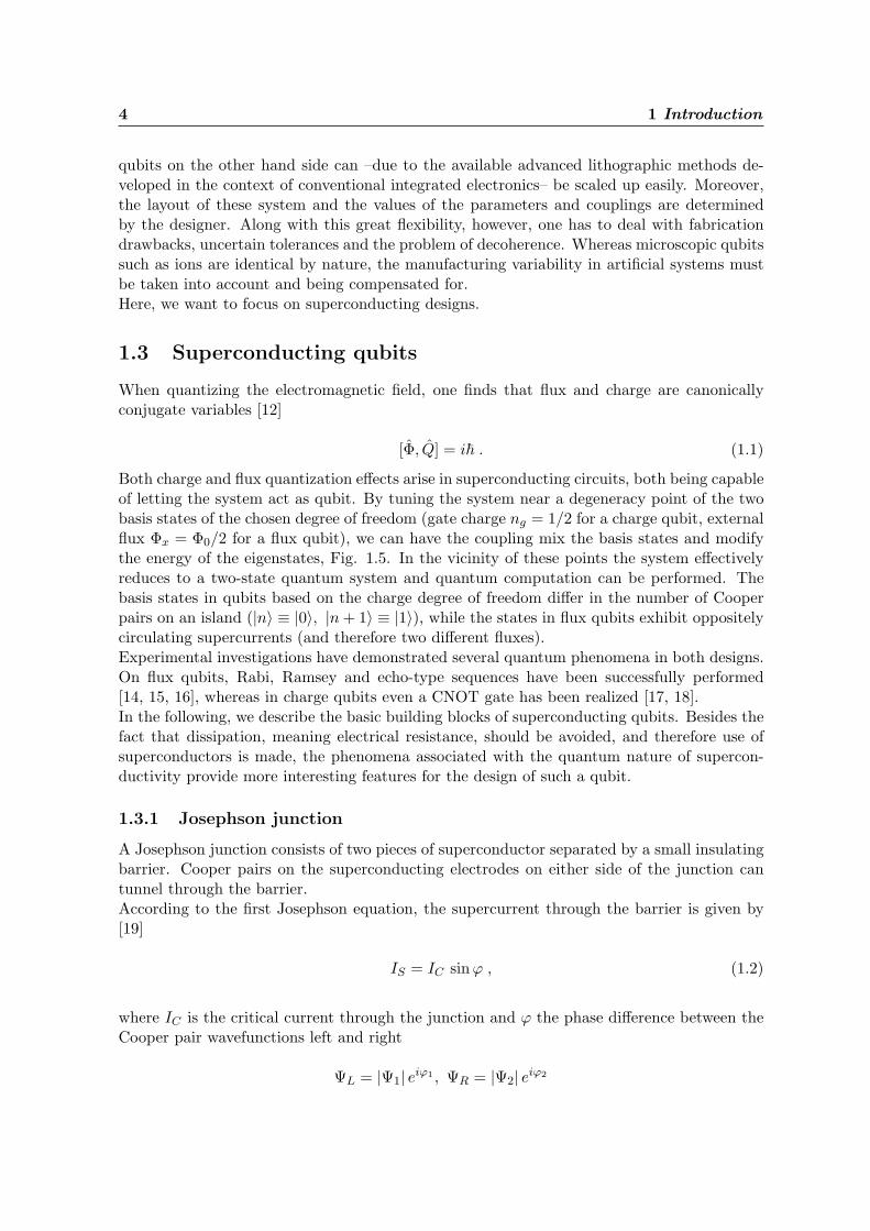
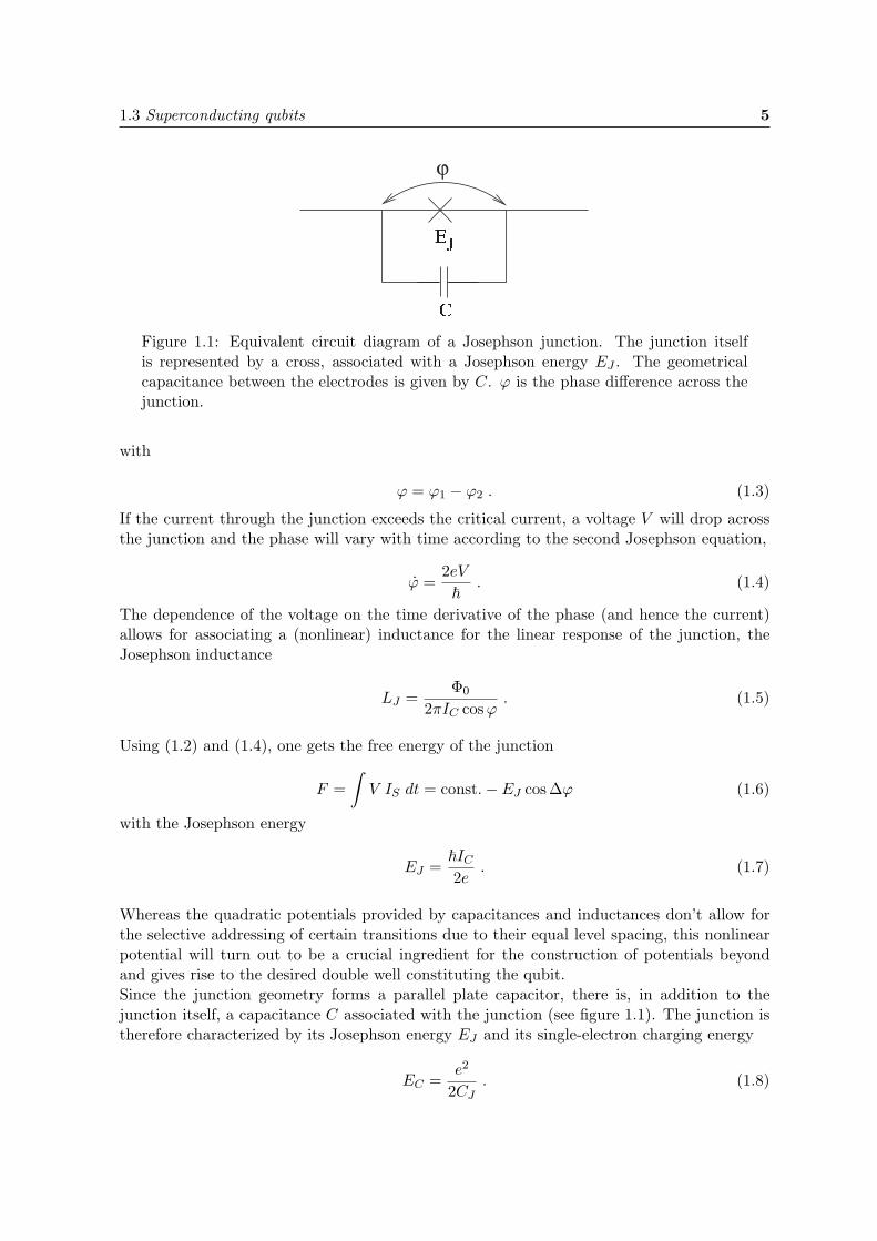
Figure 1.1: Equivalent circuit diagram of a Josephson junction. The junction itselfis represented by a cross, associated with a Josephson energy EJ . The geometricalcapacitance between the electrodes is given by C. ϕ is the phase difference across thejunction.
with
ϕ = ϕ1 − ϕ2 . (1.3)
If the current through the junction exceeds the critical current, a voltage V will drop acrossthe junction and the phase will vary with time according to the second Josephson equation,
ϕ =2eV
~. (1.4)
The dependence of the voltage on the time derivative of the phase (and hence the current)allows for associating a (nonlinear) inductance for the linear response of the junction, theJosephson inductance
LJ =Φ0
2πIC cosϕ. (1.5)
Using (1.2) and (1.4), one gets the free energy of the junction
F =∫
V IS dt = const.− EJ cos∆ϕ (1.6)
with the Josephson energy
EJ =~IC
2e. (1.7)
Whereas the quadratic potentials provided by capacitances and inductances don’t allow forthe selective addressing of certain transitions due to their equal level spacing, this nonlinearpotential will turn out to be a crucial ingredient for the construction of potentials beyondand gives rise to the desired double well constituting the qubit.Since the junction geometry forms a parallel plate capacitor, there is, in addition to thejunction itself, a capacitance C associated with the junction (see figure 1.1). The junction istherefore characterized by its Josephson energy EJ and its single-electron charging energy
EC =e2
2CJ. (1.8)
6 1 Introduction
1.3.2 Fluxoid quantization
If we put superconductors and Josephson junctions into a closed loop, the magnetic fluxthrough the area enclosed by the loop is restricted. This is a result the single-valuedness ofthe Cooper pair wavefunction phase γ after one circulation around the loop,
γ =∑
i
ϕi +2π
Φ0
∮A ds . (1.9)
Here, A denotes the vector potential of the magnetic field, the sum goes over all junctions,and the line integral goes once around the loop. By applying Stokes theorem we obtain
∑
i
ϕi +2πΦtot
Φ0= 0 . (1.10)
This relation is called fluxoid quantization [19]. The magnetic flux quantum in a supercon-ductor reads
Φ0 =h
2e. (1.11)
1.4 Flux qubit
We want to describe qubits based on the flux degree of freedom, called flux qubits or persistentcurrent qubits.In order to make persistent, dissipationless currents possible, we consider superconductingring geometries. In addition, these rings shall be intersected by one or more Josephsonjunctions. The simplest design is a RF-SQUID, formed by a loop with one junction. Fluxoidquantization relates the phase across the junction to the magnetic flux enclosed by the loop,ϕ = −2πΦtot
Φ0. The Hamiltonian includes the charging energy of the junction and its Josephson
energy as well as the energy contained in the magnetic field created by the current in the loop[12],
H =Q2
2CJ− EJ cos
(2π
Φtot
Φ0
)+
(Φtot − Φx)2
2L, (1.12)
where L is the self-inductance of the loop, and Φx is the externally applied bias flux. For abias Φx ≈ (n + 1/2)Φ0, the cosine potential and the quadratic potential of the third termcan form a double well potential. The states in the bottoms of the two wells then correspondto two Φ expectation values Φ = nΦ0 and Φ = (n + 1)Φ0. The first term depends on thecharge Q, the canonically conjugate variable of Φ and can therefore be considered to be thekinetic energy of the particle in the double well with mass CJ . However, in order to forma suitable double well potential, the Josephson energy EJ of the junction as well as the selfinductance L of the loop have to be large. The first restriction requires a large junction witha large capacitance CJ , which suppresses tunneling. A high self inductance calls for largeloops, making the system very sensitive to external noise.
1.4 Flux qubit 7
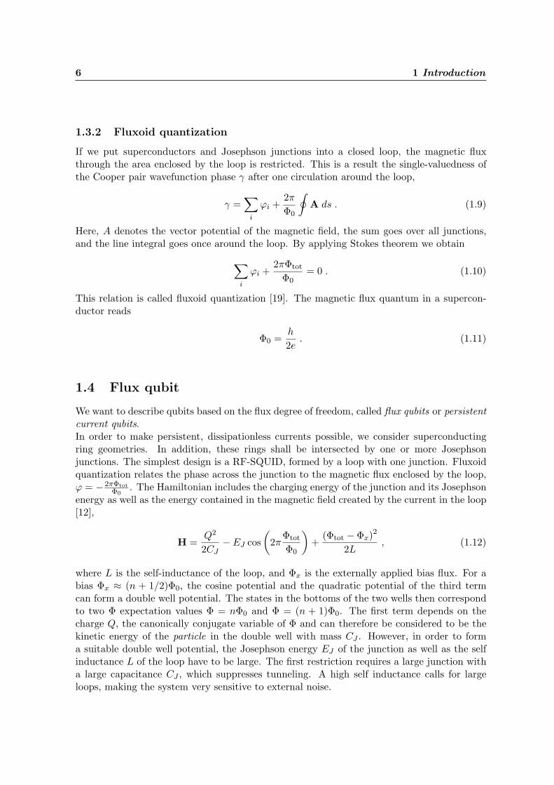
These shortcomings can be overcome by using a smaller loop with three junctions [20], seefigure 1.2 and 1.3.
pI
ϕ2
ϕ1
ϕ3
Figure 1.2: Circuit diagram of a three-junction flux qubit. Junction 3 isslightly smaller than the junctions 1and 2.
Figure 1.3: SEM picture of a three-junction flux qubit. The Joseph-son junctions are thin insulating oxidebarriers between the superconductingelectrodes [21].
The flux in this low-inductance circuit remains –as opposed to the design above– close to theexternally applied field Φtot ≈ Φx and fluxoid quantization takes the form
ϕ1 + ϕ2 + ϕ3 +2πΦx
Φ0= 0 . (1.13)
Moreover, one of the junctions (here junction 3) is slightly smaller than the other two,EJ,3/EJ,2 = EJ,3/EJ,1 = α ≈ 0.8.Writing down the Hamiltonian of the loop [20] yields
H =3∑
i=1
Q2i
2CJ,i−EJ
(cosϕ1 + cosϕ2 + α cos
(2πΦΦ0
− ϕ1 − ϕ2
))+
(Φ− Φx)2
2L. (1.14)
Due to the small inductance of the loop, Φ ≈ Φx holds, and the term expressing the magneticenergy is small. The phase across junction 3 in (1.14) is expressed by the phases ϕ1 and ϕ2
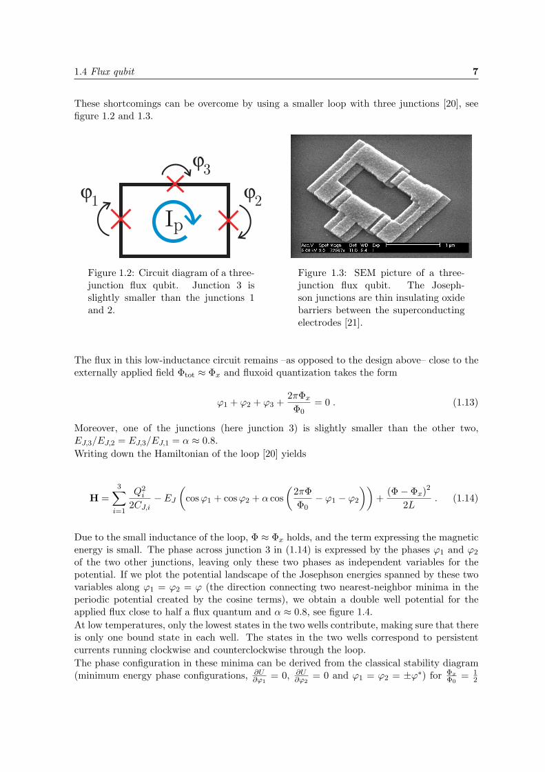
of the two other junctions, leaving only these two phases as independent variables for thepotential. If we plot the potential landscape of the Josephson energies spanned by these twovariables along ϕ1 = ϕ2 = ϕ (the direction connecting two nearest-neighbor minima in theperiodic potential created by the cosine terms), we obtain a double well potential for theapplied flux close to half a flux quantum and α ≈ 0.8, see figure 1.4.At low temperatures, only the lowest states in the two wells contribute, making sure that thereis only one bound state in each well. The states in the two wells correspond to persistentcurrents running clockwise and counterclockwise through the loop.The phase configuration in these minima can be derived from the classical stability diagram(minimum energy phase configurations, ∂U
∂ϕ1= 0, ∂U
∂ϕ2= 0 and ϕ1 = ϕ2 = ±ϕ∗) for Φx
Φ0= 1
2
8 1 Introduction
Φ/Φ0= 0.5α = 0.8
-1 0 1
ϕ
1
1.5
2
2.5
U/EJ
α = 0.7
α = 0.8
α = 0.9
-1 0 1
ϕ
1
1.5
2
2.5
U/EJ
Φ/Φ0= 0.48
Φ/Φ0= 0.5
Φ/Φ0= 0.52
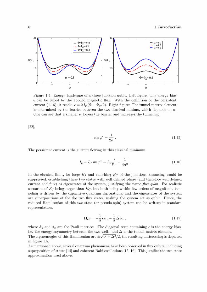
Figure 1.4: Energy landscape of a three junction qubit. Left figure: The energy biasε can be tuned by the applied magnetic flux. With the definition of the persistentcurrent (1.16), it reads: ε = 2 Ip (Φ− Φ0/2). Right figure: The tunnel matrix elementis determined by the barrier between the two classical minima, which depends on α.One can see that a smaller α lowers the barrier and increases the tunneling.
[22],
cosϕ∗ =12α
. (1.15)
The persistent current is the current flowing in this classical minimum,
Ip = IC sinϕ∗ = IC
√1− 1
4α2. (1.16)
In the classical limit, for large EJ and vanishing EC of the junctions, tunneling would besuppressed, establishing these two states with well defined phase (and therefore well definedcurrent and flux) as eigenstates of the system, justifying the name flux qubit. For realisticscenarios of EJ being larger than EC , but both being within few orders of magnitude, tun-neling is driven by the capacitive quantum fluctuations, and the eigenstates of the systemare superpositions of the the two flux states, making the system act as qubit. Hence, thereduced Hamiltonian of this two-state (or pseudo-spin) system can be written in standardrepresentation,
Heff = −12
ε σz − 12
∆ σx , (1.17)
where σz and σx are the Pauli matrices. The diagonal term containing ε is the energy bias,i.e. the energy asymmetry between the two wells, and ∆ is the tunnel matrix element.The eigenenergies of this Hamiltonian are ±√ε2 + ∆2/2, the resulting anticrossing is depictedin figure 1.5.As mentioned above, several quantum phenomena have been observed in flux qubits, includingsuperposition of states [14] and coherent Rabi oscillations [15, 16]. This justifies the two-stateapproximation used above.

1.5 Decoherence 9
0.495 0.4975 0.5 0.5025 0.505
Φ/Φ0
-0.01
0
0.01
E/EJ
Figure 1.5: The energies of the two localized persistent-current states are indicatedwith the dashed lines. At the degeneracy point Φ = Φ0/2, the quantum levels (solidlines) are symmetric and antisymmetric superpositions of the two persistent-currentstates and an anticrossing occurs. The expectation value of the current in the loop iszero at the degeneracy point and approaches the persistent current ±Ip far away fromthe degeneracy point.
1.5 Decoherence
Among the design requirements for a quantum computer, the sufficient long timescale overwhich the quantum coherence needs to be kept, is particulary hard to meet for solid statesystems. The relatively strong coupling of the qubits to the many fluctuating, uncontrolledenvironmental degrees of freedom causes quick decoherence, i.e. dephasing and relaxation.Dephasing describes the process of vanishing correlations between the states, ending up in astatistical mixture as opposed to a quantum mechanical superposition. The correlations aregiven by the off-diagonal terms of the density operator. The dephasing time is the character-istic time on which these terms turn to zero. In the flux qubit design, among other sources,flux noise causes the energy splitting of the qubit to fluctuate, resulting in dephasing.Relaxation is the process of approaching the thermal equilibrium. The relaxation time isthe characteristic time on which the diagonal elements of the density matrix go towards thevalues given by the Boltzmann factors.Recent measurements on relaxation and dephasing times in flux qubits have yielded timescalesof approximately 100 ns for both processes [23].The coupling of the system to a dissipative environment and the resulting decoherence effectsare often modelled by the Spin-Boson model [24]. Here, the qubits are described by spin-1/2 particles and the environment is taken as a bath of harmonic oscillators. This way, allGaussian noise sources can be reproduced by appropriately chosen spectral functions. On theother hand, non-Gaussian noise such as 1/f noise can not be treated by this method.
1.6 Coherent manipulation
Quantum operations in solid state devices are performed by applying electromagnetic fields.To implement given operations, two components of the effective magnetic field need to becontrolled. However, for flux qubits, usually only control over the energy bias ε can be gained
10 1 Introduction
by means of an external magnetic field, whereas the tunnel element ∆ remains fixed. Apossible solution is resonant driving, known from NMR [8]. One induces Rabi oscillationsbetween different states of the qubit by resonant pulses, i.e. AC pulses with frequency closeto the qubit’s level spacing, and lets the system evolve at this degeneracy point for a certaintime. By this, arbitrary one-qubit operations are possible, but the evolution under the internalsystem Hamiltonian puts physical limits on the minimum time required to prepare the targetstate.
1.7 Coupling of three qubits
A two-qubit operation is in general induced by turning on the corresponding coupling betweenthe qubits. For flux qubits placed close to each other, the natural interaction is mediatedby the magnetic fluxes and always turned on, however, switchable [20] or even tunable [25]coupling schemes based on SQUIDs have been proposed. But even for fixed coupling schemesas the ones presented in the following, full control can be gained and all quantum gatescan be realized. However, we want to concentrate on the possibility of creating tripartiteentanglement. It will be shown that the coupling schemes proposed in chapter 2 give riseto pairwise coupling between the qubits of the type σ
(i)z ⊗ σ
(j)z . We will see that this can
lead to superpositions of macroscopically distinct states. Besides the fundamental interestin this kind of macroscopic quantum behavior, these states will turn out to have interestingentanglement properties.
1.8 Measurement
Besides the controlled manipulations of the qubits, measurements have to be performed toread out the final state of the system. The ideal projective measurement with the collapseof the wavefunction is just an approximation of this process, since the measurement deviceis a quantum system by its own, coupled to the measured system. In case of flux qubits,the measurement devices are DC-SQUIDs [20, 21, 26], the coupling is given by the mutualinductance between the qubit and the DC-SQUID. By sending a current through the SQUIDone can determine the switching current, i.e. the critical current where the SQUID switchesto the finite voltage state. This is a measure for the flux enclosed by the SQUID, and therebyfor the state of the qubit. However, the flux fluctuations produced by the SQUID currentitself cause decoherence in the qubit. Moreover, this switching is a statistical process, givinga spread in the switching currents. No perfect correlation of the measurement result withthe state of the qubit can be achieved, in contrast to the ideal von Neumann measurement.Recently developed measurement schemes like dispersive readout [27] or the non-dissipativemeasurement of the change in the Josephson inductance of the SQUID [28, 29] in contrast tothe dissipative switching scheme outlined above can avoid some of these limitations. We willdiscuss this in more detail in section 2.3, where we propose a measurement geometry for ourthree-qubit design.
Chapter 2
Coupling strength
Two designs for a coupled 3-qubit system with two different coupling schemes have beeninvestigated, namely inductive coupling via mutually induced fluxes and coupling via theJosephson inductances of shared junctions. It will turn out that of both these mechanismscan be treated by introducing extra phases, which incorporate the couplings and add uplinearly to the total coupling strength.
2.1 Coupling via a common loop
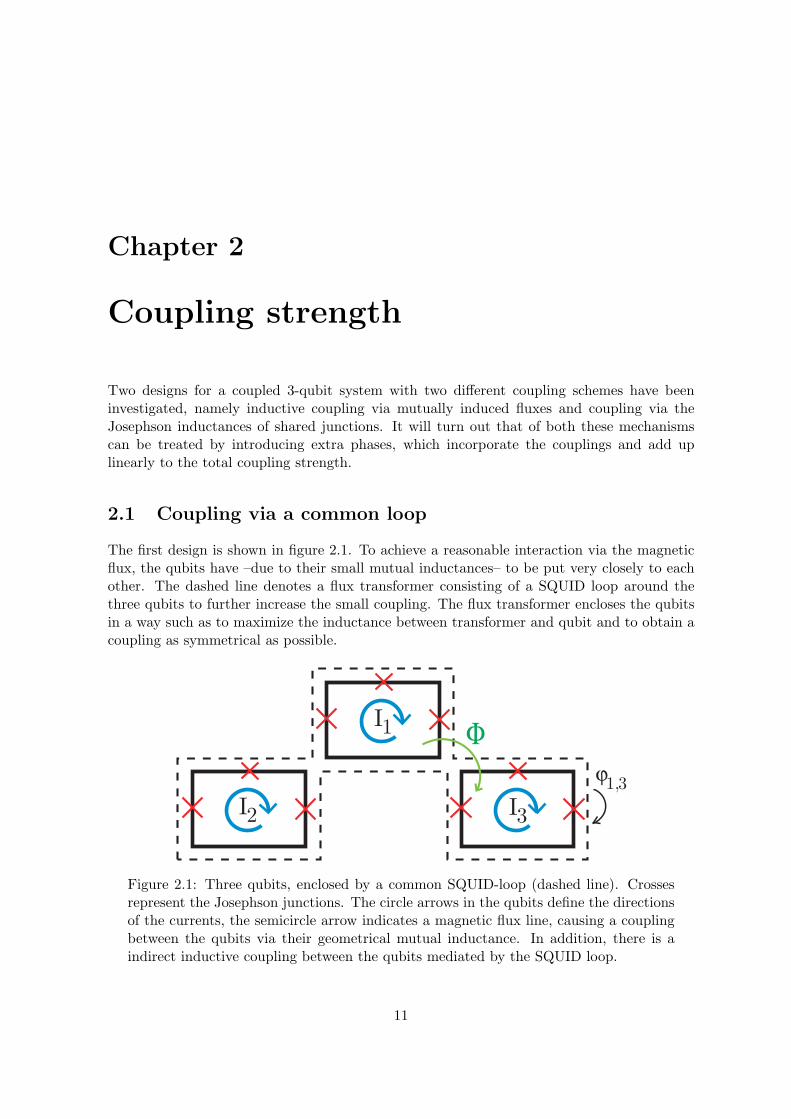
The first design is shown in figure 2.1. To achieve a reasonable interaction via the magneticflux, the qubits have –due to their small mutual inductances– to be put very closely to eachother. The dashed line denotes a flux transformer consisting of a SQUID loop around thethree qubits to further increase the small coupling. The flux transformer encloses the qubitsin a way such as to maximize the inductance between transformer and qubit and to obtain acoupling as symmetrical as possible.
1I
2I 3I
ϕ1,3
Φ
Figure 2.1: Three qubits, enclosed by a common SQUID-loop (dashed line). Crossesrepresent the Josephson junctions. The circle arrows in the qubits define the directionsof the currents, the semicircle arrow indicates a magnetic flux line, causing a couplingbetween the qubits via their geometrical mutual inductance. In addition, there is aindirect inductive coupling between the qubits mediated by the SQUID loop.
11
12 2 Coupling strength
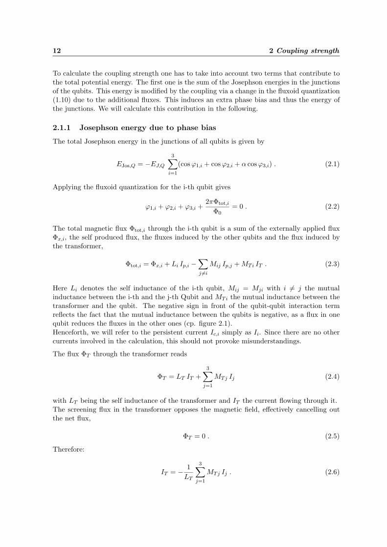
To calculate the coupling strength one has to take into account two terms that contribute tothe total potential energy. The first one is the sum of the Josephson energies in the junctionsof the qubits. This energy is modified by the coupling via a change in the fluxoid quantization(1.10) due to the additional fluxes. This induces an extra phase bias and thus the energy ofthe junctions. We will calculate this contribution in the following.
2.1.1 Josephson energy due to phase bias
The total Josephson energy in the junctions of all qubits is given by
EJos,Q = −EJ,Q
3∑
i=1
(cos ϕ1,i + cosϕ2,i + α cosϕ3,i) . (2.1)
Applying the fluxoid quantization for the i-th qubit gives
ϕ1,i + ϕ2,i + ϕ3,i +2πΦtot,i
Φ0= 0 . (2.2)
The total magnetic flux Φtot,i through the i-th qubit is a sum of the externally applied fluxΦx,i, the self produced flux, the fluxes induced by the other qubits and the flux induced bythe transformer,
Φtot,i = Φx,i + Li Ip,i −∑
j 6=i
Mij Ip,j + MTi IT . (2.3)
Here Li denotes the self inductance of the i-th qubit, Mij = Mji with i 6= j the mutualinductance between the i-th and the j-th Qubit and MTi the mutual inductance between thetransformer and the qubit. The negative sign in front of the qubit-qubit interaction termreflects the fact that the mutual inductance between the qubits is negative, as a flux in onequbit reduces the fluxes in the other ones (cp. figure 2.1).Henceforth, we will refer to the persistent current Ic,i simply as Ii. Since there are no othercurrents involved in the calculation, this should not provoke misunderstandings.
The flux ΦT through the transformer reads
ΦT = LT IT +3∑
j=1
MTj Ij (2.4)
with LT being the self inductance of the transformer and IT the current flowing through it.The screening flux in the transformer opposes the magnetic field, effectively cancelling outthe net flux,
ΦT = 0 . (2.5)
Therefore:
IT = − 1LT
3∑
j=1
MTj Ij . (2.6)
2.1 Coupling via a common loop 13
For convenience purposes and for later generalizing the results, we introduce an extra phase,
φi =2π
Φ0
Li Ii −
∑
j 6=i
Mij Ij − 1LT
MTi
3∑
j=1
MTj Ij
. (2.7)
This phase φi incorporates the coupling effects and enters into the fluxoid quantization (2.2),
ϕ1,i + ϕ2,i + ϕ3,i + φi +2πΦx,i
Φ0= 0 . (2.8)
Since the fluxes induced by the other parts of the system are small compared to the fluxquantum, φi can be considered to be small as well (φi ≈ 7 · 10−4).
Expressing the phase across the smaller junction in terms of the other phases gives
α cosϕ3,i = α cos(
2πΦx,i
Φ0+ ϕ1,i + ϕ2,i + φi
)=
= α cos(
2πΦx,i
Φ0+ ϕ1,i + ϕ2,i
)· cosφi −
−α sin(
2πΦx,i
Φ0+ ϕ1,i + ϕ2,i
)· sinφi . (2.9)
The discussion of the individual terms yields:
• cosφi ≈ 1, since φi is small.
• sin(
2πΦx,i
Φ0+ ϕ1,i + ϕ2,i
)≈ sin (π + ϕ1,i + ϕ2,i) = − sin (ϕ1,i + ϕ2,i).
The minima of the potential landscape of a single qubit are located at ϕ1 = ϕ2 = ±ϕ∗
where cosϕ∗ = 12α [22].
Therefore: − sin (ϕ1,i + ϕ2,i) ≈ −2 sin ϕ∗ cosϕ∗ = − 1α
IiIC,Q
.
• sinφi ≈ φi.
α cosϕ3,i = α cos(
2πΦx,i
Φ0+ ϕ1,i + ϕ2,i
)+
Ii
IC,Qφi . (2.10)
With the definitions of φi (2.7), EJos,Q (2.1) and Φ0 (1.11), we arrive at
EJos,Q =3∑
i=1
EJos,uncp − EJ,Q
IC,Q
3∑
i=1
Ii φi =
=3∑
i=1
EJos,uncp −3∑
i=1
Li Ii2 +
3∑
i=1
∑
j 6=i
Mij Ii Ij +1
LT
∑
ij
MTi MTj Ii Ij . (2.11)
14 2 Coupling strength
for the Josephson energies of the qubit junctions. Here EJos,uncp denotes the Josephsonjunction energies of a single qubit without couplings,
EJos,uncp = −EJ,Q
3∑
i=1
(cosϕ1,i + cosϕ2,i + α cos
(2πΦx,i
Φ0+ ϕ1,i + ϕ2,i
)). (2.12)
We now separate the sums into single qubit energies and interaction terms. Note that
3∑
i=1
∑
j 6=i
cij = 23∑
i=1
∑
j>i
cij , if cij = cji ∀ i, j .
EJos,Q =3∑
i=1
EJos,uncp +3∑
i=1
(MTi
2
LT− Li
)Ii
2 + 23∑
i=1
∑
j>1
(Mij +
MTi MTj
LT
)Ii Ij . (2.13)
This coupling, expressed by the last term in (2.13), is antiferromagnetic, giving an energyadvantage for an antiparallel configuration of the currents.
2.1.2 Energy stored in the magnetic field
The second contribution is the energy stored in the joint magnetic field [30]. It is given by
Emag =12
3∑
i=1
Li Ii2 −
3∑
i=1
∑
j>i
Mij Ii Ij +3∑
i=1
MTi IT Ii +12LT IT
2 . (2.14)
Insert (2.6) and split again into single qubit terms and interactions:
Emag =12
3∑
i=1
Li Ii2 −
3∑
i=1
∑
j>i
Mij Ii Ij − 12
1LT
∑
ij
MTi MTj Ii Ij =
= −12
3∑
i=1
(MTi
2
LT− Li
)Ii
2 −3∑
i=1
∑
j>i
(Mij +
MTi MTj
LT
)Ii Ij (2.15)
We see that this contribution gives a ferromagnetic coupling with half the strength of theJosephson term. The sign of the interaction can be understood by looking at the two partsof the expression Mij + MTi MTj
LT. First, the direct qubit-qubit interaction, represented by
Mij , has to be ferromagnetic owing to the negative mutual inductance between the qubits.Comparing the direction of the flux line in Fig. 2.1, one recognizes that for a parallel alignmentof the magnetic fluxes, each qubit reduces the flux in the other qubits and thereby the energyof the joint magnetic field, yielding an energy advantage for a parallel alignment. Second, thescreening of the magnetic flux in the transformer, as described above, gives rise to a secondferromagnetic contribution. The two mutual inductances showing up in the transformercoupling part 1
LTMTi MTj can be considered as the links in the interaction chain first qubit
↔ flux transformer ↔ second qubit.
2.1 Coupling via a common loop 15
2.1.3 Coupling strength
Adding up the two contributions gives
E = EJos,Q + Emag =
=3∑
i=1
EJos,uncp +12
3∑
i=1
(MTi
2
LT− Li
︸ ︷︷ ︸Li′
)Ii
2 +3∑
i=1
∑
j>i
(Mij +
MTi MTj
LT︸ ︷︷ ︸Kij
)Ii Ij .(2.16)
Li′ is the modified self inductance of the i-th qubit. As pointed out in the introduction, the
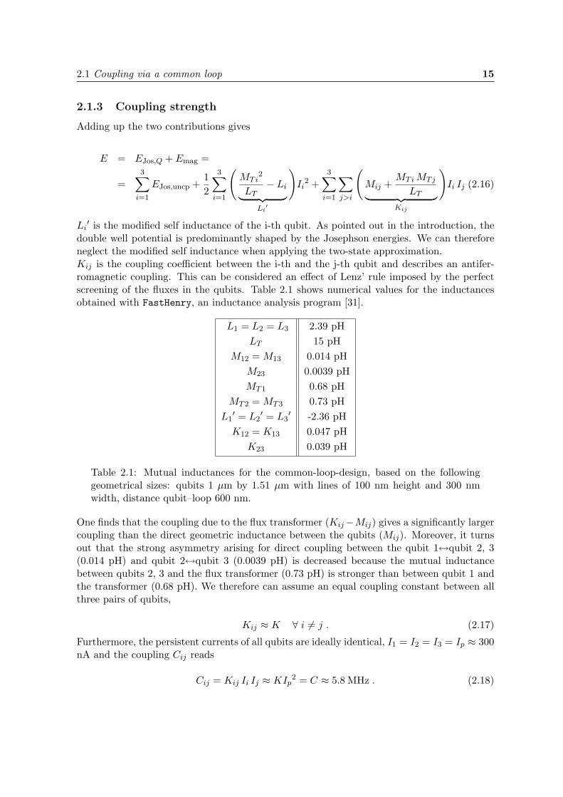
double well potential is predominantly shaped by the Josephson energies. We can thereforeneglect the modified self inductance when applying the two-state approximation.Kij is the coupling coefficient between the i-th and the j-th qubit and describes an antifer-romagnetic coupling. This can be considered an effect of Lenz’ rule imposed by the perfectscreening of the fluxes in the qubits. Table 2.1 shows numerical values for the inductancesobtained with FastHenry, an inductance analysis program [31].
L1 = L2 = L3 2.39 pHLT 15 pH
M12 = M13 0.014 pHM23 0.0039 pHMT1 0.68 pH
MT2 = MT3 0.73 pHL1
′ = L2′ = L3
′ -2.36 pHK12 = K13 0.047 pH
K23 0.039 pH
Table 2.1: Mutual inductances for the common-loop-design, based on the followinggeometrical sizes: qubits 1 µm by 1.51 µm with lines of 100 nm height and 300 nmwidth, distance qubit–loop 600 nm.
One finds that the coupling due to the flux transformer (Kij−Mij) gives a significantly largercoupling than the direct geometric inductance between the qubits (Mij). Moreover, it turnsout that the strong asymmetry arising for direct coupling between the qubit 1↔qubit 2, 3(0.014 pH) and qubit 2↔qubit 3 (0.0039 pH) is decreased because the mutual inductancebetween qubits 2, 3 and the flux transformer (0.73 pH) is stronger than between qubit 1 andthe transformer (0.68 pH). We therefore can assume an equal coupling constant between allthree pairs of qubits,
Kij ≈ K ∀ i 6= j . (2.17)
Furthermore, the persistent currents of all qubits are ideally identical, I1 = I2 = I3 = Ip ≈ 300nA and the coupling Cij reads
Cij = Kij Ii Ij ≈ KIp2 = C ≈ 5.8 MHz . (2.18)

16 2 Coupling strength
2.2 Coupling via shared junctions–qubit triangle
In this section the design shown in figure 2.2 will be discussed. The three qubits are pairwisesharing a common line with an extra Josephson junction inserted in it. Every pair of qubitssends its currents through the joint junction and therefore imposes a phase ϕi,S across it.
1I
3I
2Iϕ2,S
ϕ1,S
ϕ3,S
ϕ3,2
Figure 2.2: The design of the flux qubit triangle. The three qubits are formed by thethree small isosceles triangles, the round arrows in the qubits defining the directionsof the currents. Small crosses represent the Josephson junctions in the individualqubits, large crosses the coupling junctions (big Josephson energy—small Josephsoninductance).
As in section 2.1, two energies are associated with this coupling. The first one is again thesum of the Josephson energies in the qubit junctions. The phases across the shared junctionsinfluence fluxoid quantization in the individual qubits and thus change the Josephson energiesof their junctions. We will first calculate this effect.
2.2.1 Josephson energy due to phase bias
The total Josephson energies in the qubit junctions is again given by
EJos,Q = −EJ,Q
3∑
i=1
(cos ϕ1,i + cosϕ2,i + α cosϕ3,i) . (2.19)
When applying fluxoid quantization, we take the additional phases ϕi,S of the shared junctionsinto account (here exemplarily for qubit 1, in analogy for qubits 2 and 3):
ϕ11 + ϕ12 + ϕ13 + ϕ1,S − ϕ2,S +2πΦtot,1
Φ0= 0 (2.20)
The coupling junctions are large compared to the qubit junctions and their critical currentsare far above the persistent currents in the qubits. Hence, their phases are small and behavenearly classical (the fluctuations in the phases are small, and phases can therefore be expressedin terms of the classical flowing currents). In this regime, the nonlinear inductance discussedin chapter 1 can be assumed to be linear, having the same effect as the mutual inductances in

2.2 Coupling via shared junctions–qubit triangle 17
section 2.1. Moreover, we assume the critical currents of these junctions to be equal (which canbe achieved in an actual experiment, because critical currents can be tuned very accurately[16]). According to the directions of currents (cp. Figure 2.2), we get
ϕ1,S = arcsinI1 − I2
IC,S≈ I1 − I2
IC,S, (2.21)
ϕ2,S ≈ I3 − I1
IC,S, (2.22)
ϕ3,S ≈ I2 − I3
IC,S. (2.23)
Adding up the phases for the fluxoid quantization rules (2.20) in each qubit consistently, weagain define extra coupling phases (cp. (2.7)), namely
φ1 = ϕ1,S − ϕ2,S ≈ 2 I1 − I2 − I3
IC,S, (2.24)
φ2 = ϕ3,S − ϕ1,S ≈ 2 I2 − I1 − I3
IC,S, (2.25)
φ3 = ϕ2,S − ϕ3,S ≈ 2 I3 − I1 − I2
IC,S. (2.26)
Moreover, the coupling mediated by the geometrical inductance will turn out to be muchsmaller than the one due to the shared junctions. Therefore, we neglect the additional fluxesinduced by the other qubits and set Φtot,i ≈ Φx,i.
The rewritten fluxoid quantization
ϕ1,i + ϕ2,i + ϕ3,i + φi +2πΦx,i
Φ0= 0 (2.27)
then looks the same as (2.8).
Applying the same reasoning as in section 2.1.1, we get in analogy to (2.11)
EJos,Q =3∑
i=1
EJos,uncp − EJ
IC,Q
3∑
i=1
Ii φi . (2.28)
Putting in (2.24),(2.25) and (2.26) and using (1.7) and (1.11) yields
EJos,Q =3∑
i=1
EJos,uncp +Φ0
2πIC,S2
−
3∑
i=1
Ii2 +
3∑
i=1
∑
j>i
Ii Ij
. (2.29)
We can express this in terms of the Josephson inductance of the shared junctions LJ,S (1.5),
LJ,S ≈ Φ0
2πIC,S, (2.30)
18 2 Coupling strength
EJos,Q =3∑
i=1
EJos,uncp − 2LJ,S
3∑
i=1
Ii2 + 2 LJ,S
3∑
i=1
∑
j>i
Ii Ij . (2.31)
We find that the coupling due to the phase bias is antiferromagnetic, as in section 2.1.1. TheJosephson inductance of the shared junctions here plays the role of the mutual inductancemediating the interaction between the qubits. It depends on the size of the junctions, witha bigger junction resulting in a smaller inductance and a smaller coupling. This can beunderstood by considering that the same current imposes a smaller phase difference across alarger junction modifying the fluxoid quantization less violently.
2.2.2 Josephson energy of the shared junctions
The second energy associated with the inserted junctions is their own Josephson energy. Weexpand and get
EJos,S = −EJ,S
3∑
i=1
cosϕi,S ≈ −EJ,S
3∑
i=1
(1− ϕi,S
2
2
). (2.32)
By putting in (2.21), (2.22), (2.23) and using the definition of the Josephson inductance(2.30), we obtain
EJos,S = −3EJ,S + LJ,S
3∑
i=1
Ii2 − LJ,S
3∑
i=1
∑
j>i
Ii Ij . (2.33)
2.2.3 Coupling strength
The total potential energy reads
E = EJos,Q + EJos,S =
=3∑
i=1
EJos,uncp − 3EJ,S − LJ,S
3∑
i=1
Ii2 + LJ,S
3∑
i=1
∑
j>i
Ii Ij . (2.34)
Therefore:
Kij = K = LJ,S ∀ i 6= j (2.35)
Using the same values as in section 2.1.3, I1 = I2 = I3 = Ip ≈ 300 nA, we arrive at thecoupling
Cij = Kij Ii Ij ≈ LJ,SIp2 = C . (2.36)
This type of coupling allows for great flexibility, a typical and achievable coupling strengthfor later discussions is C=700 MHz (corresponding to LJ,S ≈ 5 pH).
2.3 Measurement design 19
2.2.4 Smaller contributions
In addition to the strong coupling provided by the junctions, there are still smaller contribu-tions from the geometrical inductance (as described in section 2.1) and the kinetic inductanceof the shared lines [16]. All these coupling add up linearly to the total coupling
Ctot =∑
n
Cn . (2.37)
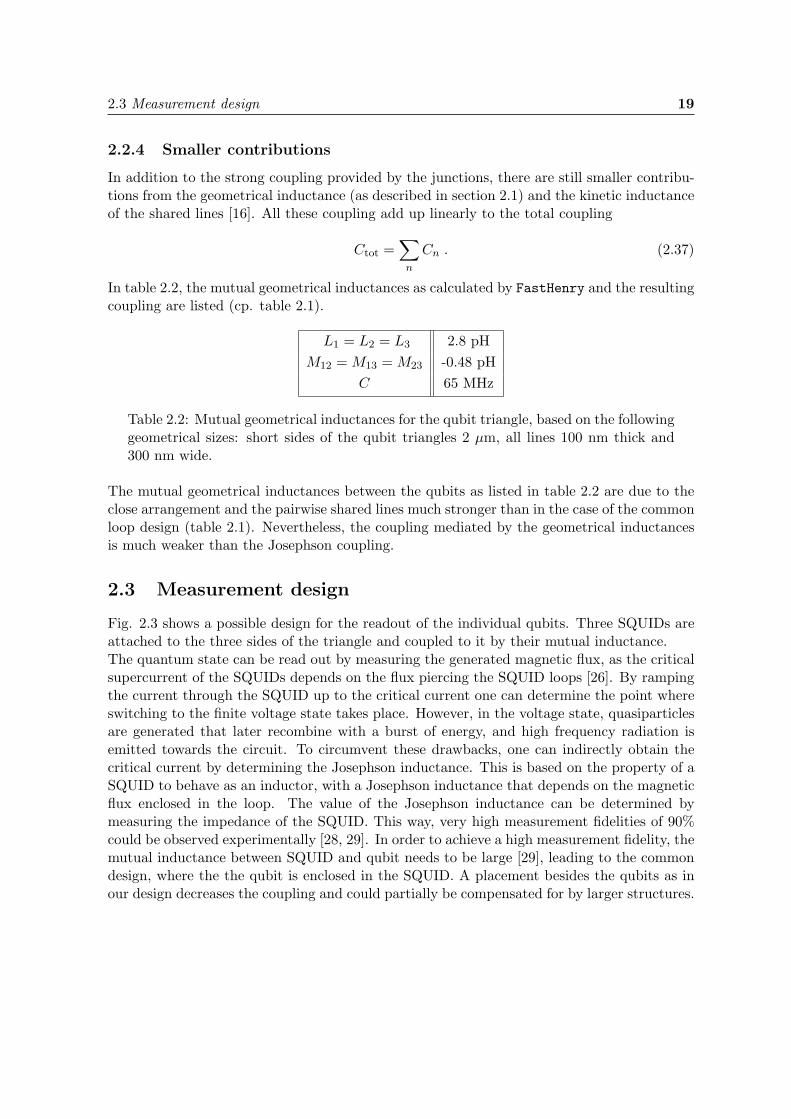
In table 2.2, the mutual geometrical inductances as calculated by FastHenry and the resultingcoupling are listed (cp. table 2.1).
L1 = L2 = L3 2.8 pHM12 = M13 = M23 -0.48 pH
C 65 MHz
Table 2.2: Mutual geometrical inductances for the qubit triangle, based on the followinggeometrical sizes: short sides of the qubit triangles 2 µm, all lines 100 nm thick and300 nm wide.
The mutual geometrical inductances between the qubits as listed in table 2.2 are due to theclose arrangement and the pairwise shared lines much stronger than in the case of the commonloop design (table 2.1). Nevertheless, the coupling mediated by the geometrical inductancesis much weaker than the Josephson coupling.
2.3 Measurement design
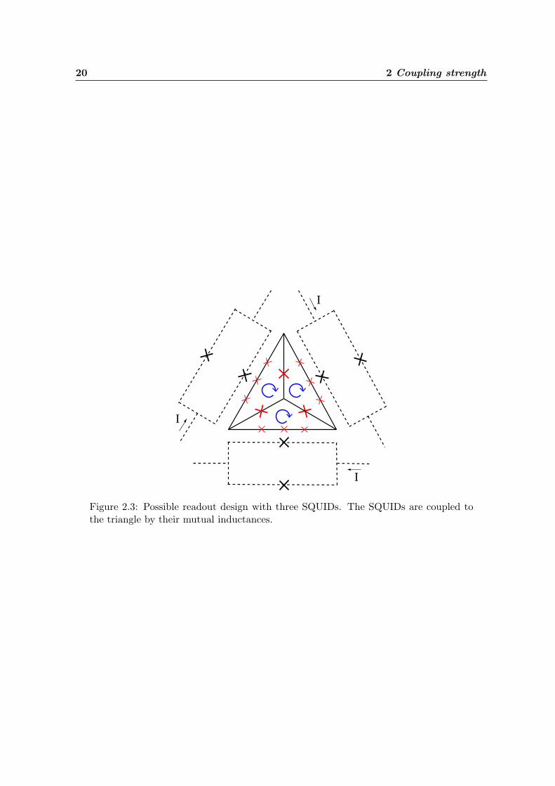
Fig. 2.3 shows a possible design for the readout of the individual qubits. Three SQUIDs areattached to the three sides of the triangle and coupled to it by their mutual inductance.The quantum state can be read out by measuring the generated magnetic flux, as the criticalsupercurrent of the SQUIDs depends on the flux piercing the SQUID loops [26]. By rampingthe current through the SQUID up to the critical current one can determine the point whereswitching to the finite voltage state takes place. However, in the voltage state, quasiparticlesare generated that later recombine with a burst of energy, and high frequency radiation isemitted towards the circuit. To circumvent these drawbacks, one can indirectly obtain thecritical current by determining the Josephson inductance. This is based on the property of aSQUID to behave as an inductor, with a Josephson inductance that depends on the magneticflux enclosed in the loop. The value of the Josephson inductance can be determined bymeasuring the impedance of the SQUID. This way, very high measurement fidelities of 90%could be observed experimentally [28, 29]. In order to achieve a high measurement fidelity, themutual inductance between SQUID and qubit needs to be large [29], leading to the commondesign, where the the qubit is enclosed in the SQUID. A placement besides the qubits as inour design decreases the coupling and could partially be compensated for by larger structures.
20 2 Coupling strength
I
I
I
Figure 2.3: Possible readout design with three SQUIDs. The SQUIDs are coupled tothe triangle by their mutual inductances.
Chapter 3
Eigenstates of the system
We aim for preparing tripartite entangled states in a preferably easy and stable way. Bothdemands are naturally met by the eigenstates of a system, as eigenstates are easy to prepare byπ-pulse driving on the one hand side and stable to pure dephasing processes on the other handside. Since the dephasing time T2 is usually the shorter timescale compared to the relaxationtime T1 [23], this is particulary desirable. We start with writing down the Hamiltonian in aappropriate basis, taking into account the coupling derived in chapter 2 and continue withinvestigating the eigenenergies and eigenstates for different coupling strengths and in differentregimes of the energy bias ε.
3.1 Hamiltonian
By adding up the single qubit Hamiltonians of the individual qubits as introduced in (1.17)and the coupling term derived in chapter 2, we arrive at the total Hamiltonian. The currentsin the qubits are quantum mechanically associated with σz operators and the Hamiltonianreads in terms of the Pauli spin matrices1
H =3∑
i=1
(−1
2εi σ
(i)z − 1
2∆i σ
(i)x
)+ C(σ(1)
z σ(2)z + σ(1)
z σ(3)z + σ(2)
z σ(3)z ) . (3.1)
1The superscript indices here have the meaning of being applied to the qubit with the corresponding indexwhile unity is applied to the qubits with the missing indices (e.g. σ
(3)z ≡ 1l2⊗ 1l2⊗ σz, σ
(1)z σ
(2)z ≡ σz ⊗ σz ⊗ 1l2).
21

22 3 Eigenstates of the system
Writing H down in the standard basis (see A.2) yields
H = −12
ε1+ε2+ε3−6C ∆3 ∆2 0 ∆1 0 0 0
∆3 ε1+ε2−ε3+2C 0 ∆2 0 ∆1 0 0
∆2 0 ε1−ε2+ε3+2C ∆3 0 0 ∆1 0
0 ∆2 ∆3 ε1−ε2−ε3+2C 0 0 0 ∆1
∆1 0 0 0 −ε1+ε2+ε3+2C ∆3 ∆2 0
0 ∆1 0 0 ∆3 −ε1+ε2−ε3+2C 0 ∆2
0 0 ∆1 0 ∆2 0 −ε1−ε2+ε3+2C ∆3
0 0 0 ∆1 0 ∆2 ∆3 −ε1−ε2−ε3−6C
.
(3.2)
We want to assume the qubits to be identical (∆1 = ∆2 = ∆3 = ∆, ε1 = ε2 = ε3 = ε). Wealready introduced this approximation implicitly by setting the coupling C equal for all threepairs of qubits.In the following, we choose a collective quartet-doublet basis, reflecting the nature of thesystem as a system of three coupled (pseudo-) spin-1/2 particles (see appendix A.4 for thedefinition of this basis). This will simplify many arguments related to the symmetries of thesystem. The Hamilton rewritten in the collective basis is (as from now, operators and statesexpressed in the collective basis carry a tilde, see also appendix A)
H = −12
3ε− 6C√
3∆ 0 0 0 0 0 0√
3 ∆ ε + 2C 2∆ 0 0 0 0 0
0 2 ∆ ε + 2C√
3∆ 0 0 0 0
0 0√
3∆ −3ε− 6C 0 0 0 0
0 0 0 0 ε + 2C ∆ 0 0
0 0 0 0 ∆ −ε + 2C 0 0
0 0 0 0 0 0 ε + 2C ∆
0 0 0 0 0 0 ∆ −ε + 2C
.
(3.3)As can be see from 3.3, the Hamiltonian is block diagonal in the doublet and quartet subspaces.In the following, |E1〉–|E8〉 denote the eigenstates of the system (E1–E8 are the associatedeigenenergies), where |E1〉–|E4〉 correspond to the upper four by four matrix (the quartet),|E5〉 and |E6〉 to the first doublet, |E7〉 and |E8〉 to the second one. Apparently, due to theidentical form of the two doublets, there are two pairs of degenerate eigenstates, |E5〉 and|E7〉 as well as |E6〉 and |E8〉. The eigenenergies and eigenstates of the doublet blocks can befound in appendix B.
3.2 No coupling 23
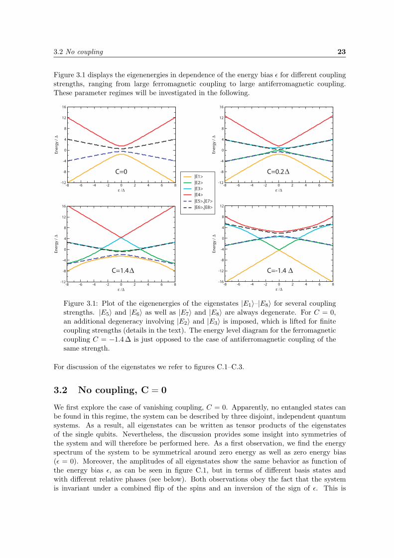
Figure 3.1 displays the eigenenergies in dependence of the energy bias ε for different couplingstrengths, ranging from large ferromagnetic coupling to large antiferromagnetic coupling.These parameter regimes will be investigated in the following.
|E3>
|E4>
|E2>
|E1>
|E6>,|E8>
|E5>,|E7>
∆C=0 C=0.2
∆C=1.4 ∆C=-1.4
-8 -6 -4 -2 0 2 4 6 8
ε /∆
-12
-8
-4
0
4
8
12
16
Ene
rgy
/∆
-8 -6 -4 -2 0 2 4 6 8
ε /∆
-12
-8
-4
0
4
8
12
16
Ene
rgy
/∆
-8 -6 -4 -2 0 2 4 6 8
ε /∆
-16
-12
-8
-4
0
4
8
12
Ene
rgy
/∆
-8 -6 -4 -2 0 2 4 6 8
ε /∆
-12
-8
-4
0
4
8
12
16
Ene
rgy
/∆
Figure 3.1: Plot of the eigenenergies of the eigenstates |E1〉–|E8〉 for several couplingstrengths. |E5〉 and |E6〉 as well as |E7〉 and |E8〉 are always degenerate. For C = 0,an additional degeneracy involving |E2〉 and |E3〉 is imposed, which is lifted for finitecoupling strengths (details in the text). The energy level diagram for the ferromagneticcoupling C = −1.4∆ is just opposed to the case of antiferromagnetic coupling of thesame strength.
For discussion of the eigenstates we refer to figures C.1–C.3.
3.2 No coupling, C = 0
We first explore the case of vanishing coupling, C = 0. Apparently, no entangled states canbe found in this regime, the system can be described by three disjoint, independent quantumsystems. As a result, all eigenstates can be written as tensor products of the eigenstatesof the single qubits. Nevertheless, the discussion provides some insight into symmetries ofthe system and will therefore be performed here. As a first observation, we find the energyspectrum of the system to be symmetrical around zero energy as well as zero energy bias(ε = 0). Moreover, the amplitudes of all eigenstates show the same behavior as function ofthe energy bias ε, as can be seen in figure C.1, but in terms of different basis states andwith different relative phases (see below). Both observations obey the fact that the systemis invariant under a combined flip of the spins and an inversion of the sign of ε. This is
24 3 Eigenstates of the system
obvious as ε is (due to the missing coupling) the only parameter that determines the spinalignment (and hence the energy of a certain configuration), favoring spins aligned parallelto the applied magnetic field and giving an energy disadvantage to the opposite aligned ones.We also find that for the same reason the ground state maps onto the highest excited state byjust a global spin flip. We will refer to these general considerations when looking at the caseof finite coupling and will now explicitly write down the form of the some of the eigenstatesin standard notation.
3.2.1 No energy bias, ε = 0
Without energy bias, for zero coupling as well as for finite coupling (see below), no σz spinalignment in either direction is preferred, therefore all states will yield zero expectation valuefor σz, 〈σ(1)
z 〉 = 〈σ(2)z 〉 = 〈σ(3)
z 〉 = 〈σ(1)z + σ
(2)z + σ
(3)z 〉 = 0. The single qubit Hamiltonian (1.17)
then reduces to H = −12 ∆ σx with the two well-known eigenstates |ψG〉 = 1/
√2(|↓〉 + |↑〉)
(ground state) and |ψex〉 = 1/√
2(|↓〉−|↑〉) (excited state). The ground state of the compositethree-qubit system |E1〉 is the direct product of the σx eigenstates with the lower energy(crossing point of the curves in the first plot of figure C.1),
|ψG〉 = |E1〉 =1√8(|↓〉+ |↑〉)A ⊗ (|↓〉+ |↑〉)B ⊗ (|↓〉+ |↑〉)C , (3.4)
whereas the highest excited state reads (crossing point in the fourth plot)
|ψex〉 = |E4〉 =1√8(|↓〉 − |↑〉)A ⊗ (|↓〉 − |↑〉)B ⊗ (|↓〉 − |↑〉)C . (3.5)
Reflecting the symmetry of the system under exchange of qubits, the other six eigenenergiessplit up in two 3-fold degenerate subspaces, the corresponding states being |E2〉, |E5〉, |E7〉(first excitation above the ground state) and |E3〉, |E6〉, |E8〉 (second excitation above theground state). These subspaces contain states with different properties, including non-zeroentanglement. However, we make here a physical choice for the basis states, taking intoaccount that the system physically consists of three disjoint subsystems.The basis states spanning the low-energy subspace for ε = 0 then read
|E2〉 := (|↓〉+ |↑〉)A ⊗ (|↓〉+ |↑〉)B ⊗ (|↓〉 − |↑〉)C ,
|E5〉 := (|↓〉+ |↑〉)A ⊗ (|↓〉 − |↑〉)B ⊗ (|↓〉+ |↑〉)C ,
|E7〉 := (|↓〉 − |↑〉)A ⊗ (|↓〉+ |↑〉)B ⊗ (|↓〉+ |↑〉)C (3.6)
and for the high-energy subspace
|E3〉 := (|↓〉 − |↑〉)A ⊗ (|↓〉 − |↑〉)B ⊗ (|↓〉+ |↑〉)C ,
|E6〉 := (|↓〉 − |↑〉)A ⊗ (|↓〉+ |↑〉)B ⊗ (|↓〉 − |↑〉)C ,
|E8〉 := (|↓〉+ |↑〉)A ⊗ (|↓〉 − |↑〉)B ⊗ (|↓〉 − |↑〉)C . (3.7)
The basis states are composed of the low-energy eigenvalues with respect to two of the qubitsand a high-energy eigenvalue with respect to the third one for the low-energy subspace, andoppositely for the high-energy subspace.One can see that all eigenstates occurring at zero energy bias are superpositions of all basisstates, where all basis states are equal in amplitude, only varying in their relative phases.Particulary, all eigenstates contain contributions from the two totally aligned states |↑↑↑〉 and|↓↓↓〉. As we will see in section 3.3 and 3.4, this is not true for finite coupling.

3.3 Weak antiferromagnetic coupling 25
3.2.2 High energy bias
With increasing (positive) energy bias, the energy degeneracy between spin up and spin downstates expressed by their equal amplitudes is lifted. For the ground state |E1〉, spins alignedantiparallel to the magnetic field increasingly get suppressed, with the totally misaligned state|↓↓↓〉 decaying quickest. In the limit of large energy bias, only the totally aligned componentof the ground state is left,
|ψG〉 = |E1〉 = |↑↑↑〉 . (3.8)
The highest state in analogy looks like
|ψex〉 = |↓↓↓〉 . (3.9)
These are the classical states of the system for large energy bias (no superposition).For the states spanning the degenerate subspaces we get classical, frustrated states with σz
expectation values of 〈σ(1)z + σ
(2)z + σ
(3)z 〉 = 1
2 for the low-energy subspace,
|E2〉 = |↑↑↓〉 , |E5〉 = |↓↑↑〉 , |E7〉 = |↑↓↑〉 , (3.10)
and 〈σ(1)z + σ
(2)z + σ
(3)z 〉 = −1
2 for the high-energy subspace,
|E3〉 = |↓↓↑〉 , |E6〉 = |↓↑↓〉 , |E8〉 = |↑↓↓〉 . (3.11)
3.3 Weak antiferromagnetic coupling, C = 0.2∆
Introducing a σz ⊗ σz coupling into the system for small energy bias lifts the three-folddegeneracies described above into two-fold degeneracies. Thus, the states |E2〉, |E5〉, |E7〉,|E3〉, |E6〉 and |E8〉 do not have a direct counterpart for zero coupling and only the groundstate |E1〉 and the highest excited state |E4〉 can be directly compared to the case of C = 0.
3.3.1 Ground state and highest excited state
The antiferromagnetic coupling energetically favors frustrated states. For ε = 0, the groundstate |E1〉 therefore contains a larger contribution of frustrated states and a smaller contribu-tion of aligned states compared to the case of vanishing coupling. The highest excited state|E4〉 shows the opposite behavior. For large energy bias, the states converge to the states forzero coupling and the plots look the same.
3.3.2 The degenerate subspaces
As already mentioned, the three-fold degeneracies for C = 0 are for finite coupling lifted intotwo-fold degeneracies. This can be understood by looking at the collective basis in appendixA. We want to point out the situation for zero energy bias.Again the expectation value for the total σz component of the states will be zero, 〈σtot
z 〉 =〈σ(1)
z + σ(2)z + σ
(3)z 〉 = 0. This results in equal superpositions of states with opposite σz expec-
tation values. We can construct a state with 〈σz〉 = 0 by a superposition of |v5〉 and |v6〉, |v7〉and |v8〉, as well as |v2〉 and |v3〉 (note that the second quantum number in the notation ofthe collective basis states as in appendix A gives the σz expectation value). An equal super-position of |v1〉 and |v4〉 also yields 〈σz〉 = 0; however, due to the antiferromagnetic coupling,

26 3 Eigenstates of the system
this aligned state is energetically raised compared to the frustrated states. Moreover, it turnsout that a superposition of |v2〉 and |v3〉 is not an eigenstate of the system. The remainingsuperpositions span the two subspaces2.The low-energy subspace is spanned by
|ψL1 〉 = x |v5〉+
√1− x2 |v6〉 ,
|ψL2 〉 = x |v7〉+
√1− x2 |v8〉 , (3.12)
the high-energy subspace by
|ψH1 〉 = x′ |v5〉 −
√1− x′2 |v6〉 ,
|ψH2 〉 = x′ |v7〉 −
√1− x′2 |v8〉 . (3.13)
For zero energy bias x and x′ read (for the general form of x and x′ see appendix B)
x = x′ =1√2
. (3.14)
All four states are superpositions of states with 〈σz〉 = ±12 , i.e. frustrated states. The
application of the operator representing the coupling to any frustrated state |f〉 yields(σ(1)
z σ(2)z + σ(1)
z σ(3)z + σ(2)
z σ(3)z
)|f〉 = −|f〉 . (3.15)
All frustrated states are thus eigenstates of the coupling for any arbitrary coupling strength.Therefore, |ψL
1 〉, |ψL2 〉, |ψH
1 〉, |ψH2 〉 do not depend on the coupling strength. Formally, this is
expressed by the coupling C being located as factor in front of the doublet matrices.
Low-energy subspace
|ψL〉 = A |ψL1 〉+ eiϕ
√1−A2 |ψL
2 〉 (3.16)
is an arbitrary state in the low-energy subspace. In chapter 4, the topic will be covered howto prepare given states, with respect to the relative amplitudes as well as phases, in thesedegenerate subspaces. Here, we take a look at –in terms of entanglement– significant resultingstates.
For quantifying entanglement, we use so-called global entanglement here, addressed in chapter5 and appendix D.2. The amplitude A and phase ϕ of the states |E5〉 and |E7〉 displayed infigures C.2 and C.3 are chosen such as to maximize (the state displayed in box 5), respectivelyminimize (displayed in Box 7) the global entanglement. Remarkably, the optimal choice forA and ϕ does not depend on the energy bias.
We obtain maximal entanglement for the state
|ψLmax〉 =
1√2(|ψL
1 〉+ i |ψL2 〉) := |E5〉 , (3.17)
2These are the eigenstates of the 2 × 2 block matrices (the doublets) of the coupled Hamiltonian (cp.appendix B)
3.3 Weak antiferromagnetic coupling 27
and minimal entanglement for
|ψLmin〉 =
1√2(|ψL
1 〉+ |ψL2 〉) := |E7〉 . (3.18)
The global entanglement for |ψLmax〉 is 8
9 , equal to the so-called W (Werner) state
|W 〉 =1√3(|↑↑↓〉+ |↑↓↑〉+ |↓↑↑〉) . (3.19)
For zero energy bias, the state |ψLmax〉 transformed into the standard basis has the form
|ψLmax〉 = S†|ψL
max〉 =
=1
2√
6
2(|↑↑↓〉+ |↓↓↑〉)− (1− i
√3)(|↑↓↑〉+ |↓↑↓〉)− (1 + i
√3)(|↑↓↓〉+ |↓↑↑〉)
.
(3.20)
In fact, as suggested by the equal value for the global entanglement, |ψLmax〉 can be transferred
onto a W state by a unitary operator UL composed of purely local operations,
UL |ψLmax〉 = |W 〉 (3.21)
with
UL = e−iπ/3 Ry(π/2)(1) ⊗ Rz(2π/3) Ry(π/2)(2) ⊗ Rz(−2π/3) Ry(π/2)(3) , (3.22)
where Rz(θ) (Ry(θ)) rotates the qubit by an angle θ around the z-axis (y-axis),
Rz(θ) = e−i θ2
σz , Ry(θ) = e−i θ2
σy . (3.23)
Since UL is a tensor product of operations acting on the individual qubits (subsystems),whereas entanglement is a resource reflecting correlations between subsystems, U does notchange the entanglement properties of the state. In this sense, |ψL
max〉 and |W 〉 are calledlocally equivalent3.
High-energy subspace
The same considerations employed for the low-energy subspace also apply to the high-energysubspace. The plots in box 6 and box 8 in figures C.2 and C.3 are again –with respect tothe entanglement– the maximized and minimized superpositions of the basis states |ψH
1 〉 and|ψH
2 〉; optimal amplitude and phase are identical to (3.17) and (3.18):
|ψHmax〉 =
1√2(|ψH
1 〉+ i |ψH2 〉) := |E6〉 (3.24)
|ψHmin〉 =
1√2(|ψH
1 〉+ |ψH2 〉) := |E8〉 (3.25)
3U belongs to a general class of operations called LOCC (local operations and classical communication).

28 3 Eigenstates of the system
Again we write for zero energy bias the explicit form of |ψHmax〉 in the standard basis,
|ψHmax〉 = S†|ψH
max〉 =
=1
2√
6
2(|↑↑↓〉+ |↓↓↑〉) + (1− i
√3)(|↑↓↑〉 − |↓↑↓〉) + (1 + i
√3)(|↑↓↓〉 − |↓↑↑〉)
,
(3.26)
and can find a local transformation rotating this state onto the W state,
UH = e−iπ/3 H(1) ⊗ Rz(2π/3) H(2) ⊗ Rz(−2π/3) H(3) , (3.27)
where H denotes the Hadamard gate,
H =1√2
(1 11 −1
). (3.28)
3.4 Strong antiferromagnetic coupling, C = 1.4∆
In this regime due to the large coupling, frustrated alignment of spins is strongly favored.
3.4.1 Ground state and the highest excited states
The arguments provided in 3.3.1 concerning the ground state and the highest excited statefor the weak antiferromagnetic coupling apply even more intensively to the case of strongantiferromagnetic coupling.The ground state for zero energy bias takes the form
|ψG〉 = |E1〉 =1√
6 + 2 δ2(|↑↑↓〉+ |↑↓↑〉+ |↑↓↓〉+ |↓↑↑〉+ |↓↓↑〉+ |↓↑↓〉+ δ(|↑↑↑〉+ |↓↓↓〉)) ,
(3.29)where δ is small (δ → 0 for C →∞, δ ≈ 0.2 for C = 1.4∆), i.e. the aligned states |↑↑↑〉 and|↓↓↓〉 are strongly suppressed.The two highest excited states |E3〉 (box 3 in figure C.3) and |E4〉 (box 4 in figure C.3),however, show an interesting behavior. In a small range for the energy bias ε around zero,|E3〉 and |E4〉 are superpositions of the maximally unfavorable states in terms of energy, i.e.of the states |↑↑↑〉 and |↓↓↓〉.For zero energy bias we obtain
|E3〉 =1√
2 + 6 δ′ 2(|↑↑↑〉+ |↓↓↓〉 − δ′(|↑↑↓〉+ |↑↓↑〉+ |↑↓↓〉+ |↓↑↑〉+ |↓↓↑〉+ |↓↑↓〉))
with δ′ ≈ 0.07 , therefore |E3〉 ≈ 1√2(|↑↑↑〉+ |↓↓↓〉) . (3.30)
|E4〉 =1√
2 + 6 δ′′ 2(−|↑↑↑〉+ |↓↓↓〉+ δ′′(|↑↑↓〉+ |↑↓↑〉 − |↑↓↓〉+ |↓↑↑〉 − |↓↓↑〉 − |↓↑↓〉))
with δ′′ ≈ 0.1 , therefore |E4〉 ≈ 1√2(|↓↓↓〉 − |↑↑↑〉) . (3.31)
3.4 Strong antiferromagnetic coupling 29
Despite the antiferromagnetic coupling, |E3〉 and |E4〉 are for small energy bias close tosuperpositions that contain only the macroscopically distinct states |↑↑↑〉 and |↓↓↓〉 with equalamplitude. Such states are called GHZ (Greenberger-Horne-Zeilinger) states. The interestingentanglement properties of GHZ states are covered in chapter 5.
3.4.2 The degenerate subspaces
As emphasized above, the form of the states in the degenerate subspaces does not dependon the coupling strength, the coupling only shifts the states in energy (cp. appendix B and(3.15)). Therefore, all statements made in 3.3.2 apply without modification. In the nextchapter, we will show how to prepare arbitrary states –i.e. arbitrary superpositions of |ψL
1 〉and |ψL
2 〉 (|ψH1 〉 and |ψH
2 〉, respectively)– in these subspaces by means of external driving.Due to the particular stability of these states with respect to the coupling, the results are notlimited to a particular design scheme or coupling.

30 3 Eigenstates of the system
Chapter 4
Preparing states in the degeneratesubspaces
We aim for preparing arbitrary states in the degenerate subspaces introduced in 3.3.2, i.e. wewant to apply a π-pulsing scheme in order to fully depopulate the ground state and populatethe desired subspace with an arbitrary superpositions of |ψL
1 〉 and |ψL2 〉 (|ψH
1 〉 and |ψH2 〉,
respectively),
|ψL(H)〉 = A |ψL(H)1 〉+ eiϕ
√1−A2 |ψL(H)
2 〉 . (4.1)
This is different from ordinary π-pulse driving for the fact that two degenerate states abovethe ground state need to be populated in parallel with a given amplitude ratio and relativephase. We investigate this situation by the use of a dressed state approach. Note thatanalogous results can be obtained by the use of Floquet states and classical driving [32].
We consider driving of the system by means of external radiofrequency (rf ) pulses. The ap-plied oscillating flux couples in via the energy bias εi to the σz component of the Hamiltonian,given by
εi′(t) = 2 Ip,i
(Φtot,i(t)− Φ0
2
)= 2 Ip,i
(Φi + Φrf,i(t)− Φ0
2
)= εi + δεi(t) . (4.2)
Here, we consider individual microwave amplitudes for the qubits. The Hamiltonians for theindividual qubits have the form
Hi = −12
εi′(t) σ(i)
z − 12
∆i σ(i)x = −1
2εi σ(i)
z − 12
∆i σ(i)x − 1
2δεi(t) σ(i)
z , (4.3)
where δεi(t) = δεi cosωt is a periodic perturbation.
The total Hamiltonian of the system can then be written as
H = H0 + V (t) . (4.4)
H0 is the unperturbed Hamiltonian of the system as given in (3.1) and V (t) is the periodicperturbation
V (t) = −12
δε1 σ(1)
z + δε2 σ(2)z + δε3 σ(3)
z︸ ︷︷ ︸V0
cosωt . (4.5)
31
32 4 Preparing states in the degenerate subspaces
We choose a parametrization in polar coordinates in order to make sure that the maximaltransition rate does not depend on the ratio of the relative amplitudes driving the individualqubits (given by κ1 and κ2), but only on a global driving amplitude κ,
V0 =κ
3
111
+ κ1
10
−1
+ κ2
1−1
0
σ(1)z
σ(2)z
σ(3)z
with 0 ≤ κ1, κ2 ≤ 1 (4.6)
4.1 Quantizing the electromagnetic field and theinteraction Hamiltonian
The electromagnetic field can be written quantum mechanically as a sum over all modes of thefield, each one corresponding to a harmonic oscillator. However, by driving with a laser, we canachieve the situation of a near-monochromatic field, i.e. a field with a dominating mode anda narrow line width. Therefore, we want to treat it (in the ideal limit) as a monochromatic,single mode quantum field, disregarding all modes except the one being resonant with thedesired transition of the system [33].The Hamilton of the field mode with frequency ω reads
HF = ~ω(
a†a +12
)(4.7)
with a† and a being the creation and annihilation operators, whose effect on number states|n〉 is given by
a†|n〉 =√
n + 1 |n + 1〉 , (4.8)a|n〉 =
√n |n− 1〉 , (4.9)
a†a|n〉 = n |n〉 . (4.10)
At the coordinate origin, the magnetic field vector can be written as
~B = i~εB0 (a + a†) . (4.11)
Here, B0 is the field strength and ~ε is the polarization of the field.To lowest order, the interaction is a dipole-dipole interaction between the field and the dipolemoment of the qubits, which is aligned along σz, and we obtain the interaction between thefield and a qubit,
HI = gI σz (a† + a) . (4.12)
gI is the coupling constant which describes the strength of the interaction. It depends ondetails of the experimental realization.Adding up the system Hamiltonian H0, the Hamiltonian of the field mode HF and the inter-action HI (rewritten in terms of V0 as introduced above), we arrive at the total Hamiltonian,
H = H0 + ~ω(
a†a +12
)+ gI V0 (a† + a) . (4.13)

4.2 Preparing given states in the degenerate subspaces 33
In what follows we assume that the mean number of photons 〈n〉 (which will simply bereferred to as n in the following) is large. In 4.2 we will calculate expectation values of thecreation and annihilation operators, scaling with
√n. These expectation values are affected
by a fluctuation δn in the number of photons as
√n + δn−√n√
n=√
n√n
(√1 +
δn
n− 1
)≈ 1
2δn
n, (4.14)
where in the last step a Taylor approximation was applied.For large n, however, the width δn in the distribution of the number of photons is smallcompared to n. For example for a coherent state holds δn =
√n [33], yielding
limn→∞
√n + δn−√n√
n= lim
n→∞1
2√
n= 0 . (4.15)
This results in the system being subjected to the same field intensity during the experiment.
4.2 Preparing given states in the degenerate subspaces
We first disregard the coupling expressed by HI. The state of the composite system consistingof the qubits and the electromagnetic field can be written as |ψ, n〉, where the labels in theket are |qubits, field〉, i.e. qubits in the state |ψ〉, and n being the number of photons.For propagating the system from the ground state to one of the excited two-fold degeneratesubspaces, we choose the frequency of the mode to be resonant with the transition frequencyfrom the ground state to the excited level (the indices ’e’ and ’g’ stand for the ground stateand the excited states, respectively),
~ω = Ee −Eg . (4.16)
Consider the three states
|g, n〉 , |e1, n− 1〉 , |e2, n− 1〉 , (4.17)
where |e1〉 and |e2〉 are two arbitrary states in the degenerate subspace.The three states in (4.17) are energetically degenerate eigenstates of the uncoupled Hamilto-nian
(H0 + HF
),
(H0 + HF
) |g, n〉 = H0 |g, n〉+ ~ω(a†a + 1/2
) |g, n〉 =Eg + ~ω(n + 1/2)
|g, n〉(H0 + HF
) |e1, n− 1〉 =Ee + ~ω(n− 1 + 1/2)
|e1, n− 1〉 =Eg + ~ω(n + 1/2)
|e1, n− 1〉(H0 + HF
) |e2, n− 1〉 =Ee + ~ω(n− 1 + 1/2)
|e2, n− 1〉 =Eg + ~ω(n + 1/2)
|e2, n− 1〉 .
(4.18)
We can now introduce the couplings between the field and the qubits. The couplings cor-respond to absorption (|g, n〉 → |e1, n− 1〉, |g, n〉 → |e2, n− 1〉) and stimulated emission(|e1, n− 1〉 → |g, n〉, |e2, n− 1〉 → |g, n〉) processes.
34 4 Preparing states in the degenerate subspaces
We first note that the transition matrix elements between the states |e1, n− 1〉 and |e2, n− 1〉vanish,
〈e1, n− 1|(a† + a)|e2, n− 1〉 = 〈e1, n− 1|√n + 1 |e2, n− 2〉+ 〈e1, n− 1|√n |e2, n〉 = 0 ,(4.19)
since the number states are orthogonal, 〈n|m〉 = δnm.The elements between the ground state and the excited states, however, are non-zero,
〈g, n|gI V0(a† + a)|e1, n− 1〉 = gI
√n 〈g, n|V0|e1, n〉 , (4.20)
〈g, n|gI V0(a† + a)|e2, n− 1〉 = gI
√n 〈g, n|V0|e2, n〉 . (4.21)
We write down the matrix representing the reduced perturbation in the tree-fold degeneratesubspace, spanned by the states in (4.17). The basis states are numbered as
|g, n〉 =
100
, |e1, n− 1〉 =
010
, |e2, n− 1〉 =
001
. (4.22)
With this choice for the basis, the reduced perturbation takes the form
V red0 = gI
√n
0 〈g|V0|e1〉 〈g|V0|e2〉〈e1|V0|g〉 0 0〈e2|V0|g〉 0 0
. (4.23)
4.2.1 Driving the low-energy subspace
For convenience purposes, we calculate V red0 in the coupled basis introduced in appendix A,
V red0 = gI
√n
0 〈g|V0|e1〉 〈g|V0|e2〉〈e1|V0|g〉 0 0〈e2|V0|g〉 0 0
. (4.24)
As pointed out in chapter 3.3.2 and explicitly written down in appendix B, the lower energysubspace is spanned by |ψL
1 〉 and |ψL2 〉, which are superpositions of |v5〉 and |v7〉 (|v6〉 and |v8〉,
respectively), whereas the ground state |E4〉 is a superposition of |v1〉, . . . , |v4〉. Moreover,the state vectors have only real entries (the Hamiltonian is purely real). This enables us–without further knowledge about the structure of the states– to write
|g〉 = |E4〉 =
g1
g2
g3
±√
1− g21 − g2
2 − g23
0000
, |e1〉 = |ψL1 〉 =
0000e√
1− e2
00
, |e2〉 = |ψL2 〉 =
000000e√
1− e2
.
(4.25)
4.2 Preparing given states in the degenerate subspaces 35
We obtain
V red0 = −
√23gI
√n (e g2 +
√1− e2 g3)
0√
3κ1 κ1 + 2κ2√3κ1 0 0
κ1 + 2κ2 0 0
=
= ~
0 ω1 ω2
ω1 0 0ω2 0 0
. (4.26)
Here, all the constants1 have been substituted by the Rabi frequencies ω1 and ω2.
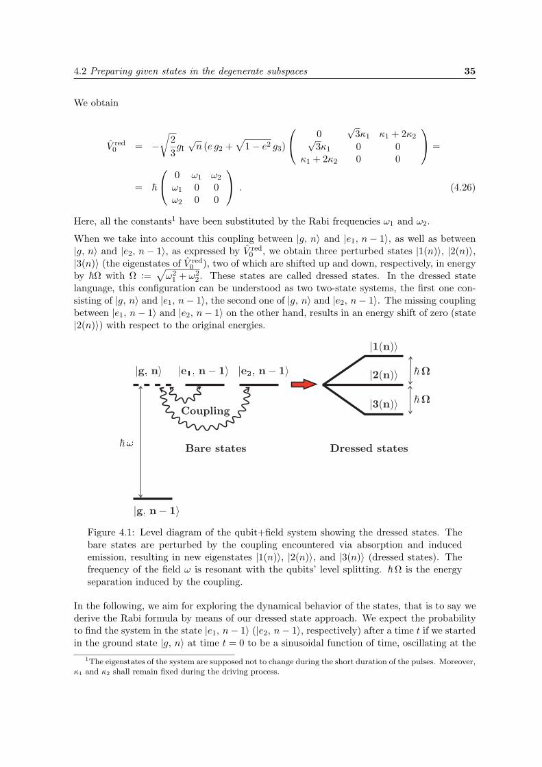
When we take into account this coupling between |g, n〉 and |e1, n− 1〉, as well as between|g, n〉 and |e2, n− 1〉, as expressed by V red
0 , we obtain three perturbed states |1(n)〉, |2(n)〉,|3(n)〉 (the eigenstates of V red
0 ), two of which are shifted up and down, respectively, in energyby ~Ω with Ω :=
√ω2
1 + ω22. These states are called dressed states. In the dressed state
language, this configuration can be understood as two two-state systems, the first one con-sisting of |g, n〉 and |e1, n− 1〉, the second one of |g, n〉 and |e2, n− 1〉. The missing couplingbetween |e1, n− 1〉 and |e2, n− 1〉 on the other hand, results in an energy shift of zero (state|2(n)〉) with respect to the original energies.
Figure 4.1: Level diagram of the qubit+field system showing the dressed states. Thebare states are perturbed by the coupling encountered via absorption and inducedemission, resulting in new eigenstates |1(n)〉, |2(n)〉, and |3(n)〉 (dressed states). Thefrequency of the field ω is resonant with the qubits’ level splitting. ~Ω is the energyseparation induced by the coupling.
In the following, we aim for exploring the dynamical behavior of the states, that is to say wederive the Rabi formula by means of our dressed state approach. We expect the probabilityto find the system in the state |e1, n− 1〉 (|e2, n− 1〉, respectively) after a time t if we startedin the ground state |g, n〉 at time t = 0 to be a sinusoidal function of time, oscillating at the
1The eigenstates of the system are supposed not to change during the short duration of the pulses. Moreover,κ1 and κ2 shall remain fixed during the driving process.

36 4 Preparing states in the degenerate subspaces
Bohr frequency Ω associated with the perturbed levels [33]. For resonant coupling as in ourcase, the Rabi frequency equals the Bohr frequency.
In the interaction picture, the time evolution of the system is governed by the perturbationand the Schrodinger equation reads
i~∂
∂t|ψ(t)〉 = V red
0 |ψ(t)〉 . (4.27)
V red0 is time independent (as a result of the used dressed state approach), and we can solve
(4.27) by
|ψ(t)〉 = U(t, t0)|ψ(t0)〉 = e−i~ V red
0 (t−t0) |ψ(t0)〉 . (4.28)
Our objective is to calculate the propagator U(t, t0). The dressed states together with thecorresponding eigenvalues read
|1(n)〉 =1√2Ω
Ωω1
ω2
, |2(n)〉 =
1Ω
0−ω2
ω1
, |3(n)〉 =
1√2Ω
−Ωω1
ω2
(4.29)
λ1 = ~Ω , λ2 = 0 , λ3 = −~Ω . (4.30)
We get (in the following we set t0 = 0 without loss of generality)
U(t) = T
e−iΩt 0 00 1 00 0 eiΩt
T † with T =
(|1(n)〉 |2(n)〉 |1(n)〉
). (4.31)
The explicit form of U(t) can be found in appendix E.
Consider we start with a fully occupied ground state without any population in the excitedlevels. The effect of the propagator onto this initial state then looks like
|ψ(t)〉 = U(t)
100
=
cosΩt
−iω1sinΩt
Ω
−iω2sinΩt
Ω
. (4.32)
We obtain the expected sinusoidal behavior mentioned above. Complete depopulation of theground state can be achieved by applying a π-pulse of length
tπ =π
2Ω, (4.33)
yielding the final state (disregarding a global phase)
|ψ(tπ)〉 =1Ω
0ω1
ω2
. (4.34)
By choosing the amplitudes of the sources κ1 and κ2 (and thereby the Rabi frequencies ω1
and ω2) appropriately, we can completely depopulate the ground state and prepare stateswith arbitrary amplitude ratio (in a given basis) in the degenerate subspace. Note that this
4.2 Preparing given states in the degenerate subspaces 37
could not be achieved by a symmetric driving in ε (ε1(t) = ε2(t) = ε3(t)); the HamiltonianH0 in (3.1) has no transition matrix elements between the ground state (living in the upper4× 4 block) and the degenerate subspaces (living in the lower 2× 2 blocks).
We now want to enhance this scheme by additionally introducing a relative phase, that ispreparing a target state
|ψtarget〉 =1Ω
0ω1
ω2 eiϕ
. (4.35)
4.2.2 Introducing a relative phase
We assume the two microwave sources, so far just characterized by their amplitudes κ1 andκ2, to be independent not only in amplitude but also in their relative phase. However, bothsources shall be kept on resonance, as expressed by the condition (4.16), oscillating on thesame frequency,
~B1(t) = ~εB1 cosωt = ~εB112
(eiωt + e−iωt
),
~B2(t) = ~εB2 cos (ωt + θ) = ~εB212
(eiθeiωt + e−iθe−iωt
). (4.36)
Quantization of the field introduces the creation and annihilation operators, whereas theexponentials e±iωt disappear for a single-mode field (in the interaction representation) [34],
~B1 = ~εB1 (a + a†) ,
~B2 = ~εB2 (eiθa + e−iθa†) . (4.37)
The interaction Hamiltonian then takes the form
HI = gIκ
3
111
+ κ1
10
−1
~σ(a + a†) + κ2
1−1
0
~σ
(eiθa + e−iθa†
) (4.38)
and the reduced perturbation operator reads (cp. (4.26))
V red0 = −
√23
gIκ
3√
n (e g2 +√
1− e2 g3)
0√
3κ1 κ1 + 2κ2 e−iθ√3κ1 0 0
κ1 + 2κ2 eiθ 0 0
=
= ~
0 ω1 ω2 e−iϕ
ω1 0 0ω2 eiϕ 0 0
. (4.39)
The operator can still be written in terms of the two frequencies ω1 and ω2 and in additiona phase ϕ; however, note that in general, ω2 as in (4.39) is different from ω2 as in (4.26).

38 4 Preparing states in the degenerate subspaces
Determining the propagator U(t) = e−i~ V red
0 t in the same way as above and applying it to theinitial ground state gives
|ψ(t)〉 = U(t)
100
=
cosΩt
−iω1sinΩt
Ω
−iω2sinΩt
Ω eiϕ
. (4.40)
The explicit form of U(t) can again be found in appendix E.
For a π-pulse of the same length as in (4.33) and disregarding a global phase we get a finalstate
|ψ(tπ)〉 =1Ω
0ω1
ω2 eiϕ
. (4.41)
We obtain the delighting result that amplitude as well as phase can be controlled by amplitudeand phase of the applied pulses. This enables us to prepare arbitrary states in the subspace.By an optimal choice of ω1, ω2 and ϕ, states with maximized entanglement can be created(see appendix D.2). We will concentrate on these states in the following.
Chapter 5
Entanglement properties
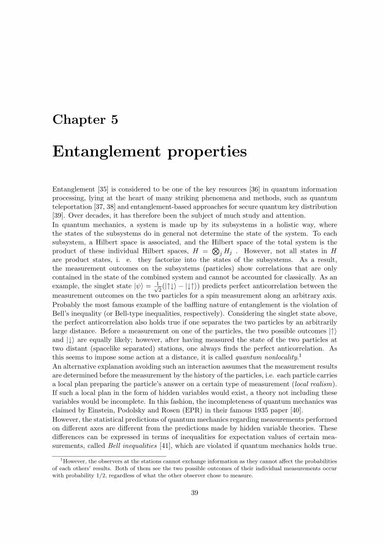
Entanglement [35] is considered to be one of the key resources [36] in quantum informationprocessing, lying at the heart of many striking phenomena and methods, such as quantumteleportation [37, 38] and entanglement-based approaches for secure quantum key distribution[39]. Over decades, it has therefore been the subject of much study and attention.In quantum mechanics, a system is made up by its subsystems in a holistic way, wherethe states of the subsystems do in general not determine the state of the system. To eachsubsystem, a Hilbert space is associated, and the Hilbert space of the total system is theproduct of these individual Hilbert spaces, H =
⊗j Hj . However, not all states in H
are product states, i. e. they factorize into the states of the subsystems. As a result,the measurement outcomes on the subsystems (particles) show correlations that are onlycontained in the state of the combined system and cannot be accounted for classically. As anexample, the singlet state |ψ〉 = 1√
2(|↑↓〉 − |↓↑〉) predicts perfect anticorrelation between the
measurement outcomes on the two particles for a spin measurement along an arbitrary axis.Probably the most famous example of the baffling nature of entanglement is the violation ofBell’s inequality (or Bell-type inequalities, respectively). Considering the singlet state above,the perfect anticorrelation also holds true if one separates the two particles by an arbitrarilylarge distance. Before a measurement on one of the particles, the two possible outcomes |↑〉and |↓〉 are equally likely; however, after having measured the state of the two particles attwo distant (spacelike separated) stations, one always finds the perfect anticorrelation. Asthis seems to impose some action at a distance, it is called quantum nonlocality.1
An alternative explanation avoiding such an interaction assumes that the measurement resultsare determined before the measurement by the history of the particles, i.e. each particle carriesa local plan preparing the particle’s answer on a certain type of measurement (local realism).If such a local plan in the form of hidden variables would exist, a theory not including thesevariables would be incomplete. In this fashion, the incompleteness of quantum mechanics wasclaimed by Einstein, Podolsky and Rosen (EPR) in their famous 1935 paper [40].However, the statistical predictions of quantum mechanics regarding measurements performedon different axes are different from the predictions made by hidden variable theories. Thesedifferences can be expressed in terms of inequalities for expectation values of certain mea-surements, called Bell inequalities [41], which are violated if quantum mechanics holds true.
1However, the observers at the stations cannot exchange information as they cannot affect the probabilitiesof each others’ results. Both of them see the two possible outcomes of their individual measurements occurwith probability 1/2, regardless of what the other observer chose to measure.
39
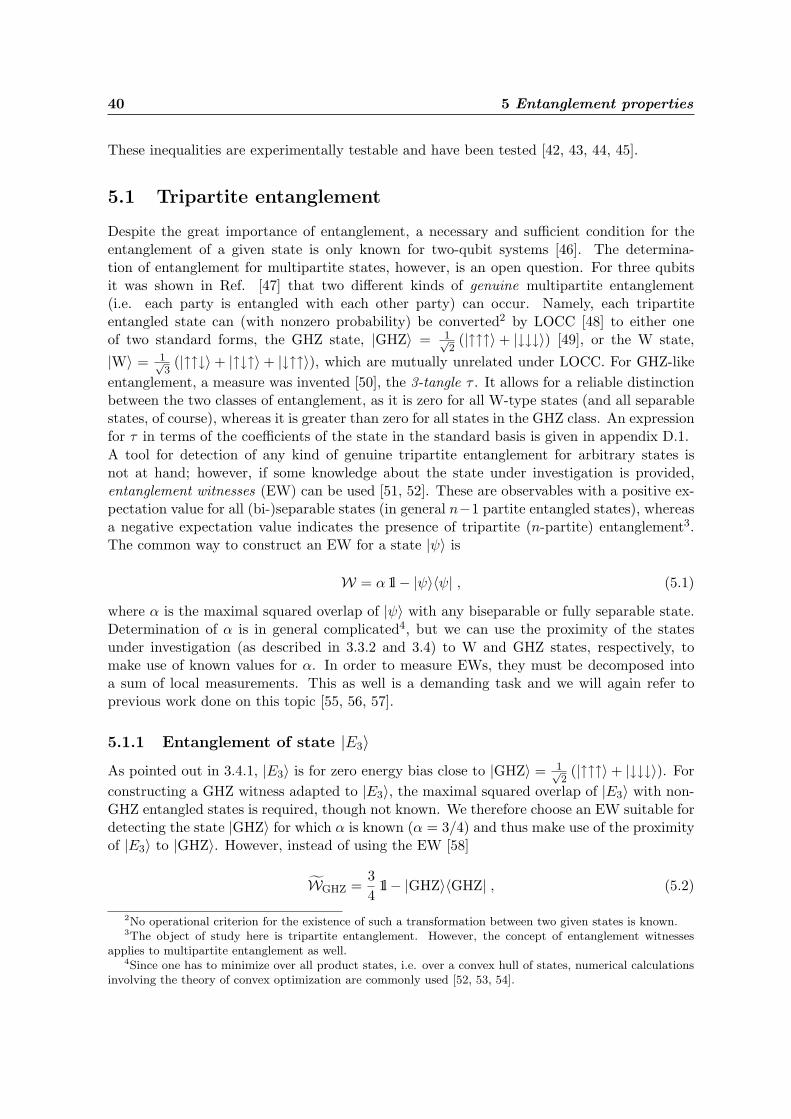
40 5 Entanglement properties
These inequalities are experimentally testable and have been tested [42, 43, 44, 45].
5.1 Tripartite entanglement
Despite the great importance of entanglement, a necessary and sufficient condition for theentanglement of a given state is only known for two-qubit systems [46]. The determina-tion of entanglement for multipartite states, however, is an open question. For three qubitsit was shown in Ref. [47] that two different kinds of genuine multipartite entanglement(i.e. each party is entangled with each other party) can occur. Namely, each tripartiteentangled state can (with nonzero probability) be converted2 by LOCC [48] to either oneof two standard forms, the GHZ state, |GHZ〉 = 1√
2(|↑↑↑〉+ |↓↓↓〉) [49], or the W state,
|W〉 = 1√3(|↑↑↓〉+ |↑↓↑〉+ |↓↑↑〉), which are mutually unrelated under LOCC. For GHZ-like
entanglement, a measure was invented [50], the 3-tangle τ . It allows for a reliable distinctionbetween the two classes of entanglement, as it is zero for all W-type states (and all separablestates, of course), whereas it is greater than zero for all states in the GHZ class. An expressionfor τ in terms of the coefficients of the state in the standard basis is given in appendix D.1.A tool for detection of any kind of genuine tripartite entanglement for arbitrary states isnot at hand; however, if some knowledge about the state under investigation is provided,entanglement witnesses (EW) can be used [51, 52]. These are observables with a positive ex-pectation value for all (bi-)separable states (in general n−1 partite entangled states), whereasa negative expectation value indicates the presence of tripartite (n-partite) entanglement3.The common way to construct an EW for a state |ψ〉 is
W = α 1l− |ψ〉〈ψ| , (5.1)
where α is the maximal squared overlap of |ψ〉 with any biseparable or fully separable state.Determination of α is in general complicated4, but we can use the proximity of the statesunder investigation (as described in 3.3.2 and 3.4) to W and GHZ states, respectively, tomake use of known values for α. In order to measure EWs, they must be decomposed intoa sum of local measurements. This as well is a demanding task and we will again refer toprevious work done on this topic [55, 56, 57].
5.1.1 Entanglement of state |E3〉As pointed out in 3.4.1, |E3〉 is for zero energy bias close to |GHZ〉 = 1√
2(|↑↑↑〉+ |↓↓↓〉). For
constructing a GHZ witness adapted to |E3〉, the maximal squared overlap of |E3〉 with non-GHZ entangled states is required, though not known. We therefore choose an EW suitable fordetecting the state |GHZ〉 for which α is known (α = 3/4) and thus make use of the proximityof |E3〉 to |GHZ〉. However, instead of using the EW [58]
WGHZ =34
1l− |GHZ〉〈GHZ| , (5.2)
2No operational criterion for the existence of such a transformation between two given states is known.3The object of study here is tripartite entanglement. However, the concept of entanglement witnesses
applies to multipartite entanglement as well.4Since one has to minimize over all product states, i.e. over a convex hull of states, numerical calculations
involving the theory of convex optimization are commonly used [52, 53, 54].
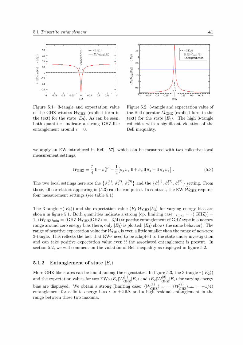
5.1 Tripartite entanglement 41
-1 -0.75 -0.5 -0.25 0 0.25 0.5 0.75 1
ε /∆
-0.6
-0.4
-0.2
0
0.2
0.4
0.6
0.8
1
Figure 5.1: 3-tangle and expectation valueof the GHZ witness WGHZ (explicit form inthe text) for the state |E3〉. As can be seen,both quantities indicate a strong GHZ-likeentanglement around ε = 0.
-1 -0.75 -0.5 -0.25 0 0.25 0.5 0.75 1
ε /∆
0
0.5
1
1.5
2
2.5
3
3.5
4
Local prediction
Figure 5.2: 3-tangle and expectation value ofthe Bell operator MGHZ (explicit form in thetext) for the state |E3〉. The high 3-tanglecoincides with a significant violation of theBell inequality.
we apply an EW introduced in Ref. [57], which can be measured with two collective localmeasurement settings,
WGHZ =74
1l− σ⊗3x − 1
2[σz σz 1l + σz 1l σz + 1l σz σz
]. (5.3)
The two local settings here are theσ
(1)x , σ
(2)x , σ
(3)x
and the
σ
(1)z , σ
(2)z , σ
(3)z
setting. From
these, all correlators appearing in (5.3) can be computed. In contrast, the EW WGHZ requiresfour measurement settings (see table 5.1).
The 3-tangle τ(|E3〉) and the expectation value 〈E3|WGHZ|E3〉 for varying energy bias areshown in figure 5.1. Both quantities indicate a strong (cp. limiting case: τmax = τ(|GHZ〉) =1, 〈WGHZ〉min = 〈GHZ|WGHZ|GHZ〉 = −3/4) tripartite entanglement of GHZ type in a narrowrange around zero energy bias (here, only |E3〉 is plotted, |E4〉 shows the same behavior). Therange of negative expectation value forWGHZ is even a little smaller than the range of non-zero3-tangle. This reflects the fact that EWs need to be adapted to the state under investigationand can take positive expectation value even if the associated entanglement is present. Insection 5.2, we will comment on the violation of Bell inequality as displayed in figure 5.2.
5.1.2 Entanglement of state |E2〉More GHZ-like states can be found among the eigenstates. In figure 5.3, the 3-tangle τ(|E2〉)and the expectation values for two EWs 〈E2|W(1)
GHZ|E2〉 and 〈E2|W(2)
GHZ|E2〉 for varying energy
bias are displayed. We obtain a strong (limiting case: 〈W(1)
GHZ〉min = 〈W(2)
GHZ〉min = −1/4)
entanglement for a finite energy bias ε ≈ ±2.6∆ and a high residual entanglement in therange between these two maxima.
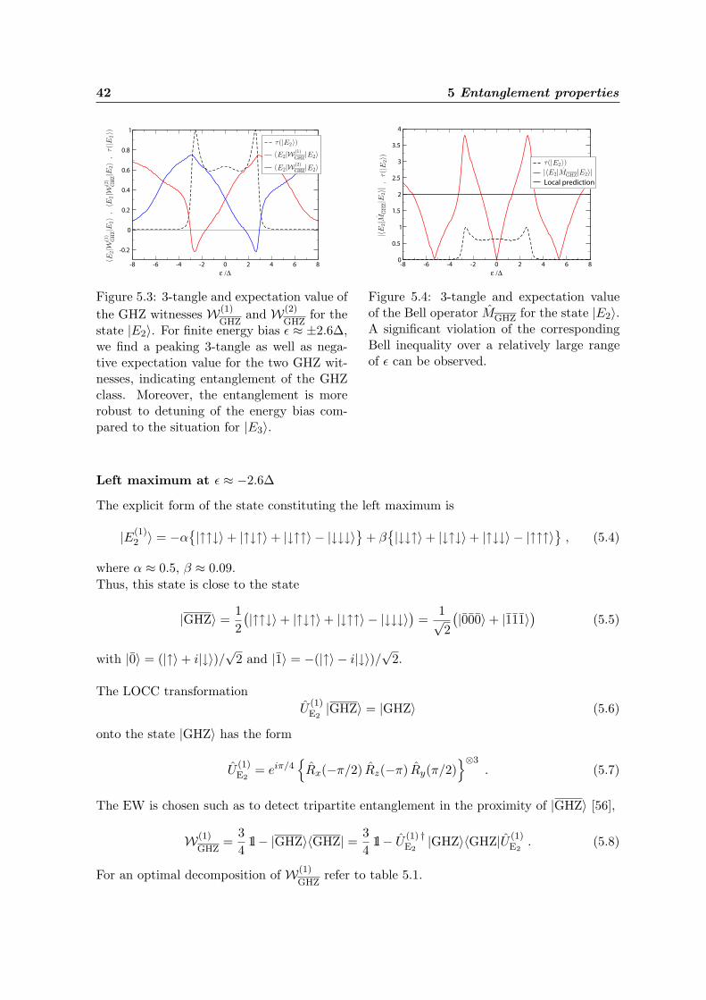
42 5 Entanglement properties
-8 -6 -4 -2 0 2 4 6 8
ε /∆
-0.2
0
0.2
0.4
0.6
0.8
1
Figure 5.3: 3-tangle and expectation value ofthe GHZ witnesses W(1)
GHZand W(2)
GHZfor the
state |E2〉. For finite energy bias ε ≈ ±2.6∆,we find a peaking 3-tangle as well as nega-tive expectation value for the two GHZ wit-nesses, indicating entanglement of the GHZclass. Moreover, the entanglement is morerobust to detuning of the energy bias com-pared to the situation for |E3〉.
-8 -6 -4 -2 0 2 4 6 8
ε /∆
0
0.5
1
1.5
2
2.5
3
3.5
4
Local prediction
Figure 5.4: 3-tangle and expectation valueof the Bell operator MGHZ for the state |E2〉.A significant violation of the correspondingBell inequality over a relatively large rangeof ε can be observed.
Left maximum at ε ≈ −2.6∆
The explicit form of the state constituting the left maximum is
|E(1)2 〉 = −α
|↑↑↓〉+ |↑↓↑〉+ |↓↑↑〉 − |↓↓↓〉 + β|↓↓↑〉+ |↓↑↓〉+ |↑↓↓〉 − |↑↑↑〉 , (5.4)
where α ≈ 0.5, β ≈ 0.09.Thus, this state is close to the state
|GHZ〉 =12(|↑↑↓〉+ |↑↓↑〉+ |↓↑↑〉 − |↓↓↓〉) =
1√2
(|000〉+ |111〉) (5.5)
with |0〉 = (|↑〉+ i|↓〉)/√2 and |1〉 = −(|↑〉 − i|↓〉)/√2.
The LOCC transformationU
(1)E2|GHZ〉 = |GHZ〉 (5.6)
onto the state |GHZ〉 has the form
U(1)E2
= eiπ/4
Rx(−π/2) Rz(−π) Ry(π/2)⊗3
. (5.7)
The EW is chosen such as to detect tripartite entanglement in the proximity of |GHZ〉 [56],
W(1)
GHZ=
34
1l− |GHZ〉〈GHZ| = 34
1l− U(1) †E2
|GHZ〉〈GHZ|U (1)E2
. (5.8)
For an optimal decomposition of W(1)
GHZrefer to table 5.1.

5.1 Tripartite entanglement 43
Right maximum at ε ≈ 2.6∆
For the state in the right maximum we find
|E(2)2 〉 = α
|↓↓↑〉+ |↓↑↓〉+ |↑↓↓〉 − |↑↑↑〉− β|↑↑↓〉+ |↑↓↑〉+ |↓↑↑〉 − |↓↓↓〉 (5.9)
with α and β as above. |E(2)2 〉 is the totally flipped counterpart to |E(1)
2 〉 and therefore showsthe same behavior after being flipped back by Rx(−π)⊗3,
U(2)E2|E(2)
2 〉 ≈ |GHZ〉 with U(2)E2
= U(1)E2
Rx(−π)⊗3 . (5.10)
The corresponding EW looks like
W(2)
GHZ= Rx(π)⊗3W(1)
GHZRx(−π)⊗3 . (5.11)
The optimal decomposition of W(2)
GHZcan again be looked up in table 5.1.
Whereas the behavior of the highest excited states |E3〉 and |E4〉 for vanishing energy bias asdescribed above was expected, we make the surprising observation –referring to figure 5.3–of the existence of GHZ entangled states also in the parameter regime of finite energy bias.Moreover, the entanglement shown by |E2〉 is more stable to deviations from the optimal en-ergy bias than the one of |E3〉, overcoming a major drawback caused by the antiferromagneticnature of the coupling.
5.1.3 Entanglement in the degenerate subspaces
-8 -6 -4 -2 0 2 4 6 8
ε /∆
-0.4
-0.3
-0.2
-0.1
0
0.1
0.2
,
Figure 5.5: 3-tangle and expectation valueof the W witness WW (explicit form in thetext) for the state |ψL
max〉. The vanishing3-tangle excludes entanglement of the GHZtype, whereas the negative expectation valueof the W witness indicates a W type entan-glement.
-8 -6 -4 -2 0 2 4 6 8
ε /∆
0
0.5
1
1.5
2
2.5
3
3.5
Local prediction
Figure 5.6: 3-tangle and expectation valueof the Bell operator MW (explicit form inthe text) for the state |ψL
max〉. The maxi-mal violation of the Bell inequality for theW-equivalent state is not as high as for theGHZ-equivalent states above, however, theviolation persists over a large range of ε.
In figure 5.5, the 3-tangle and the expectation value of the EW 〈ψLmax|WW|ψL
max〉 for the max-imally entangled superposition |ψL
max〉 in the low-energy subspace is displayed (correspondingbehavior for |ψH
max〉—not shown separately).
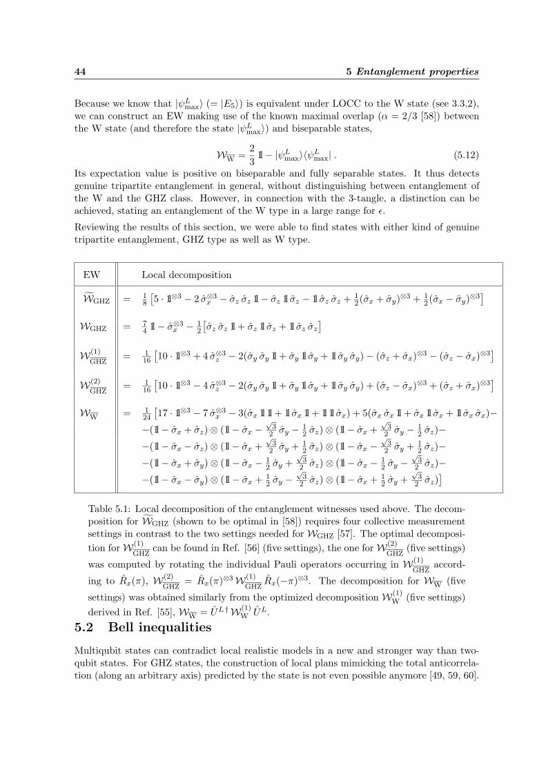
44 5 Entanglement properties
Because we know that |ψLmax〉 (= |E5〉) is equivalent under LOCC to the W state (see 3.3.2),
we can construct an EW making use of the known maximal overlap (α = 2/3 [58]) betweenthe W state (and therefore the state |ψL
max〉) and biseparable states,
WW =23
1l− |ψLmax〉〈ψL
max| . (5.12)
Its expectation value is positive on biseparable and fully separable states. It thus detectsgenuine tripartite entanglement in general, without distinguishing between entanglement ofthe W and the GHZ class. However, in connection with the 3-tangle, a distinction can beachieved, stating an entanglement of the W type in a large range for ε.
Reviewing the results of this section, we were able to find states with either kind of genuinetripartite entanglement, GHZ type as well as W type.
EW Local decomposition
WGHZ = 18
[5 · 1l⊗3 − 2 σ⊗3
x − σz σz 1l− σz 1l σz − 1l σz σz + 12(σx + σy)⊗3 + 1
2(σx − σy)⊗3]
WGHZ = 74 1l− σ⊗3
x − 12
[σz σz 1l + σz 1l σz + 1l σz σz
]
W(1)
GHZ= 1
16
[10 · 1l⊗3 + 4 σ⊗3
z − 2(σy σy 1l + σy 1l σy + 1l σy σy)− (σz + σx)⊗3 − (σz − σx)⊗3]
W(2)
GHZ= 1
16
[10 · 1l⊗3 − 4 σ⊗3
z − 2(σy σy 1l + σy 1l σy + 1l σy σy) + (σz − σx)⊗3 + (σz + σx)⊗3]
WW = 124
[17 · 1l⊗3 − 7 σ⊗3
x − 3(σx 1l 1l + 1l σx 1l + 1l 1l σx) + 5(σx σx 1l + σx 1l σx + 1l σx σx)−−(1l− σx + σz)⊗ (1l− σx −
√3
2 σy − 12 σz)⊗ (1l− σx +
√3
2 σy − 12 σz)−
−(1l− σx − σz)⊗ (1l− σx +√
32 σy + 1
2 σz)⊗ (1l− σx −√
32 σy + 1
2 σz)−−(1l− σx + σy)⊗ (1l− σx − 1
2 σy +√
32 σz)⊗ (1l− σx − 1
2 σy −√
32 σz)−
−(1l− σx − σy)⊗ (1l− σx + 12 σy −
√3
2 σz)⊗ (1l− σx + 12 σy +
√3
2 σz)]
Table 5.1: Local decomposition of the entanglement witnesses used above. The decom-position for WGHZ (shown to be optimal in [58]) requires four collective measurementsettings in contrast to the two settings needed for WGHZ [57]. The optimal decomposi-tion for W(1)
GHZcan be found in Ref. [56] (five settings), the one for W(2)
GHZ(five settings)
was computed by rotating the individual Pauli operators occurring in W(1)
GHZaccord-
ing to Rx(π), W(2)
GHZ= Rx(π)⊗3W(1)
GHZRx(−π)⊗3. The decomposition for WW (five
settings) was obtained similarly from the optimized decomposition W(1)W (five settings)
derived in Ref. [55], WW = UL †W(1)W UL.
5.2 Bell inequalities
Multiqubit states can contradict local realistic models in a new and stronger way than two-qubit states. For GHZ states, the construction of local plans mimicking the total anticorrela-tion (along an arbitrary axis) predicted by the state is not even possible anymore [49, 59, 60].

5.2 Bell inequalities 45
The concept of locality therefore breaks down at an earlier stage, giving rise to a refutationby quantum mechanics that is no longer statistical but can rather be accomplished by a sin-gle run, i.e. the explanation required by the data accumulated by a series of experiments isnot refuted by the statistics of the data obtained in another long series of runs but by theoutcome of a single crucial run [60]. However, the actual data obtained by a realistic experi-ment with realistic detectors would reveal less than perfect correlations, making the originalGHZ reasoning not feasible for an experimental verification. To face this problem, N -particleBell inequalities have been proposed [61, 62, 63], which involve pairs of settings at each ofthe measurement stations. These works have shown that the predictions made by quantummechanics for the GHZ state violate these inequalities by a factor that grows exponentiallywith N . Thereby systems capable of showing entanglement of the GHZ type might providean interesting way to test the hypothesis of local hidden variables5.
5.2.1 State |E3〉We use a Bell operator similar to one proposed by Mermin [61],
MGHZ =12i
3∏
j=1
(σjy + iσj
x)−3∏
j=1
(σjy − iσj
x)
= σy σy σx + σy σx σy + σx σy σy − σx σx σx .
(5.13)The Bell inequality, i.e. the local prediction for 〈MGHZ〉 reads
〈ψ|MGHZ|ψ〉 ≤ 2 ∀ |ψ〉 , (5.14)
whereas quantum mechanics states a maximal value of
〈GHZ|MGHZ|GHZ〉 = 4 . (5.15)
In Fig. 5.2, the violation of (5.14) by |E3〉 is displayed. Again, we find the violation to occuronly in a small range around zero energy bias, however the height of the violation confirmsthe almost perfect overlap of |E3〉 (at ε = 0) with the ideal GHZ state.
5.2.2 State |E2〉Making use of the equivalency of |E(1, 2)
2 〉 with |GHZ〉 mediated by U(1, 2)E2
, we use a modifiedBell operator,
MGHZ = U(2) †E2
MGHZ U(2)E2
= σx σx σz + σx σz σx + σz σx σx − σz σz σz . (5.16)
We again find (Fig. 5.4) a significant violation of the local prediction located at the points ofmaximal 3-tangle (and minimal expectation value of the EW). Although being not as strongas for |E3〉, this violation might –due to its smaller sensitivity to energy bias deviations– bemore promising in terms of feasibility of preparation and measurement.
5Obviously, quantum nonlocality can only arise in the entanglement of remote systems. The violation ofBell inequalities as sign for non-classical correlations is nevertheless highly substantial as an ingredient toquantum information processing.

46 5 Entanglement properties
5.2.3 Degenerate subspace
We again aim for investigating the properties of |ψLmax〉. For constructing an appropriate Bell
operator MW, we first need the Bell operator MW for the common representation of the Wstate |W〉 and then adapt it by applying the local operation UL.In general, Bell inequalities for three qubits are constructed from the correlator
E(a,b, c) = 〈ψ|(a · ~σ)⊗ (b · ~σ)⊗ (c · ~σ)|ψ〉 . (5.17)
a, b, c are real three-dimensional normalized vectors, which define a rotation of the Paulimatrices ~σ = (σx, σy, σz). A Bell operator is then given by
M = E(a,b, c′) + E(a,b′, c) + E(a′,b, c)−E(a′,b′, c′) . (5.18)
In order to obtain an optimal Bell operator for a given state, one can optimize over the six unitvectors a, a′, b, b′, c and c′ [64, 65]. The two Bell operators MGHZ and MGHZ introducedabove are in this sense optimal choices for the states |GHZ〉 and |GHZ〉.The optimal values as obtained by a numerical optimization for MW adapted the state |W〉are listed in table 5.2.
a1 0.318053 a′1 -0.635515 b1 0.635515 b′1 0.318052 c1 0.635515 c′1 0.318053a2 0.250811 a′2 -0.501155 b2 0.501155 b′2 0.250810 c2 0.501154 c′2 0.250810a3 0.914296 a′3 -0.587337 b3 -0.587336 b′3 0.914296 c3 -0.587338 c′3 0.914296
Table 5.2: Entries of the vectors a, a′, b, b′, c and c′ for the Bell operator MW [66].In connection with (5.17) and (5.18), the explicit form of MW can be determined.
The Bell operator for the state |ψLmax〉 then reads
MW = UL † MW UL . (5.19)
The violation of the Bell inequality as displayed in Fig. 5.6 approaches for ε = 0 the theoreticalmaximum for a W state of 〈MW〉 ≈ 3.05. Moreover, it persists over a large range of ε whicheven noticeably exceeds the observed range for |E2〉.
5.3 Robustness to limited measurement fidelity
Any experimental test of tripartite entanglement or the violation of Bell inequalities involvingthree qubits will be more fragile than a two particle test and will be put in jeopardy bydetector imperfections (as three-party correlations need to be measured in either case, themeasurement fidelity enters –roughly spoken– with the power of three) and fabricational issuesof the sample preparation. However, concerning Bell inequalities, the stronger violation thatis possible with three particles might compensate for that. We will investigate the effect of alimited measurement fidelity f < 1 on the expectation values of the EWs and Bell operatorsintroduced above and compare the results to a representative two-particle case. We modela non-perfect measurement of a spin component σi by the perfect measurement of a spin

5.3 Robustness to limited measurement fidelity 47
component σ′i which yields the correct measurement result with a probability f , whereas a’1’ is measured otherwise,
σ′i = f σi + (1− f) 1l . (5.20)
In the following, the results for the aforementioned parameter regimes are plotted.
-0.2 -0.15 -0.1 -0.05 0 0.05 0.1 0.15
ε /∆
-0.6
-0.4
-0.2
0
0.2
0.4
0.6
0.8
1
f=1
f=0.95
f=0.9
f=0.85
f=0.8
0.70.750.80.850.90.951
Fidelity f
-0.6
-0.4
-0.2
0
0.2
0.4
Figure 5.7: Left: Expectation value of GHZ witness WGHZ for several measurementfidelities for |E3〉. Right: Minimal expectation value of WGHZ vs. fidelity. The absolutelower limit for the measurement fidelity in order to detect tripartite entanglement withWGHZ is fmin ≈ 84.3%.
-0.2 -0.15 -0.1 -0.05 0 0.05 0.1 0.15
ε /∆
0
0.5
1
1.5
2
2.5
3
3.5
4
f=1
f=0.95
f=0.9
f=0.85
f=0.8Local bound
0.70.750.80.850.90.951
Fidelity f
1
1.5
2
2.5
3
3.5
4
Local bound
Figure 5.8: Left: Expectation value of Bell operator MGHZ for several measurementfidelities for |E3〉. Right: Maximal violation of Bell inequality vs. fidelity. The absolutelower limit for the measurement fidelity in order to detect nonlocality with MGHZ isfmin ≈ 81.4%.
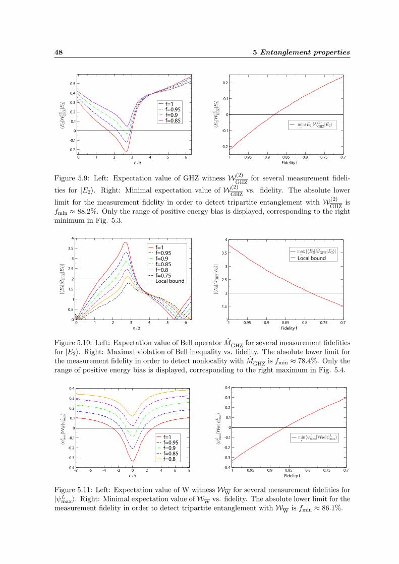
48 5 Entanglement properties
0 1 2 3 4 5 6
ε /∆
-0.2
-0.1
0
0.1
0.2
0.3
0.4
0.5
f=1
f=0.95
f=0.9
f=0.85
0.70.750.80.850.90.951
Fidelity f
-0.2
-0.1
0
0.1
0.2
Figure 5.9: Left: Expectation value of GHZ witness W(2)
GHZfor several measurement fideli-
ties for |E2〉. Right: Minimal expectation value of W(2)
GHZvs. fidelity. The absolute lower
limit for the measurement fidelity in order to detect tripartite entanglement with W(2)
GHZis
fmin ≈ 88.2%. Only the range of positive energy bias is displayed, corresponding to the rightminimum in Fig. 5.3.
0 1 2 3 4 5 6
ε /∆
0
0.5
1
1.5
2
2.5
3
3.5
4
f=1
f=0.95
f=0.9
f=0.85
f=0.8
f=0.75Local bound
0.70.750.80.850.90.951
Fidelity f
1
1.5
2
2.5
3
3.5
4
Local bound
Figure 5.10: Left: Expectation value of Bell operator MGHZ for several measurement fidelitiesfor |E2〉. Right: Maximal violation of Bell inequality vs. fidelity. The absolute lower limit forthe measurement fidelity in order to detect nonlocality with MGHZ is fmin ≈ 78.4%. Only therange of positive energy bias is displayed, corresponding to the right maximum in Fig. 5.4.
-8 -6 -4 -2 0 2 4 6 8
ε /∆
-0.4
-0.3
-0.2
-0.1
0
0.1
0.2
0.3
0.4
f=1
f=0.95
f=0.9
f=0.85
f=0.8
0.70.750.80.850.90.951
Fidelity f
-0.4
-0.3
-0.2
-0.1
0
0.1
0.2
0.3
0.4
Figure 5.11: Left: Expectation value of W witness WW for several measurement fidelities for|ψL
max〉. Right: Minimal expectation value of WW vs. fidelity. The absolute lower limit for themeasurement fidelity in order to detect tripartite entanglement with WW is fmin ≈ 86.1%.

5.3 Robustness to limited measurement fidelity 49
-8 -6 -4 -2 0 2 4 6 8
ε /∆
0
0.5
1
1.5
2
2.5
3
3.5
4
f=1
f=0.95
f=0.9
f=0.85
f=0.8Local bound
0.70.750.80.850.90.951
Fidelity f
1.6
1.8
2
2.2
2.4
2.6
2.8
3
3.2
Local bound
Figure 5.12: Left: Expectation value of Bell operator MW for several measurementfidelities for |ψL
max〉. Right: Maximal violation of Bell inequality vs. fidelity. Theabsolute lower limit for the measurement fidelity in order to detect nonlocality withMW is fmin ≈ 81.2%.
In Tab. 5.3, the minimal detector fidelities for the detection of tripartite entanglement orviolation of Bell inequalities using the aforementioned operators are compared. Moreover,the required fidelity for the violation of the CHSH inequality (named after Clauser-Horne-Shimony-Holt [67]) by a bell pair |ψ〉 = 1√
2(|↑↓〉 − |↓↑〉) is listed. Evidently, the fidelity
needed to detect nonlocal three-party correlations via the Bell inequalities introduced abovelies even slightly below the one required for falsifying the CHSH inequality. The requestedmeasurement fidelity is already available for charge qubits, where significant progress hasrecently been achieved with dispersive readout6 inside a cavity, providing a visibility of morethan 90% [27]. A similar design has been proposed for flux qubits [68]. Moreover, otherexperiments based on Josephson junction technology indicating similar fidelities have beenperformed [28, 29, 69, 70].
Operator fmin Operator fmin
WGHZ 84.3% MGHZ 81.4%W(2)
GHZ88.2% MGHZ 78.4%
WW 86.1% MW 81.2%MCHSH
21+√
2≈ 82.8%
Table 5.3: Minimal detector fidelities for the detection of tripartite entanglement orviolation of Bell inequalities, respectively.
6i.e. the shift in resonance frequency of a resonator coupled to the system

50 5 Entanglement properties
Chapter 6
Pulse shaping
In the previous chapters, properties of the eigenstates of the system were discussed. Althoughthe system will naturally occupy its ground state after some time, the population of higherexcited eigenstates can be achieved by applying resonant π-pulses. Here, the relevant param-eter is the area under the pulse in the time domain. A higher pulse amplitude leads to a largerRabi frequency, thereby transferring the system to the desired state more quickly (4.33). Inthis driving scheme, the shape of the pulses –i.e. the envelope of the amplitude– is in principleirrelevant (as long as the rotating wave approximation is still valid, i.e. the linewidth is muchsmaller than the transition frequency). However, facing the challenges given by the short de-coherence times in solid state systems, short pulse times are crucial to preserve the quantumproperties of the system over the duration of the pulses. In addition, whenever one has todeal with additional time scales, as –for example– given by the coupling between qubits in therealization of quantum gates or the preparation of arbitrary non-eigenstates, simple amplifi-cation of the (single-qubit) pulses does not yield the desired propagator anymore. It rathercreates a mismatch between the evolution of the individual qubits on their local Bloch spheresand the evolution governed by the coupling which acts in parallel. To achieve a time optimalpropagation from the the initial state into the final state, one has to take this coupling intoaccount and shape the pulses optimally [8, 71]. Other boundary conditions requiring complexpulse shapes might be the avoidance of certain Fourier components in the pulse to preventthe excitation of leakage levels [72] or the optimization of the shape with respect to otherparameters.
The need for complex pulses in order to achieve the desired behavior of the system is accompa-nied by the need to actually shape these pulses with available technology. As mentioned above,decoherence and coupling eventually require this shaping to act on very short timescales, not(yet) reached by waveform generators.
In this chapter, we discuss pulse shaping by networks of passive electronic elements. Thiswork stands in the context of the time-optimal implementation of a CNOT gate in a systemof two coupled charge qubits (see the corresponding publication in appendix G). The task isto find an approximation for the optimal pulses that can be implemented by a passive circuitnetwork and yields a high fidelity of the gate operation. Moreover, we will find that thenumber of elements needed to obtain a good approximation of the pulse provides a measureof its complexity.
51
52 6 Pulse shaping
6.1 Laplace transform
There are two equivalent descriptions of a signal: the description in the time domain asexpressed by a function f(t) or the description as spectrum written as F (s). We want to dealwith the spectrum as obtained by the one-side Laplace transform
F (s) = Lf(t) =∫ ∞
t=0f(t) e−st dt . (6.1)
s is a complex variable and can be considered to be a complex frequency. The necessary andsufficient condition for the existence of the spectrum of a function f(t) is that the integral onthe right hand side remains finite.We restrict ourselves to the discussion of rational functions with real coefficients, F (s) =P (s)Q(s) , where P (s) denotes the polynomial in the numerator and Q(s) the polynomial in thedenominator. We will see that rational functions play an outstanding role in network synthesistheory. Moreover, the restriction to rational functions is not a strong limitation, because manyof the most important time-domain functions (the Dirac delta function, the trigonometricfunctions etc., see table F.1 in appendix F) yield a spectrum that is in fact a rational function.
By dividing P (s) by Q(s) we obtain
F (s) =P (s)Q(s)
= ansn + an−1sn−1 + . . . + a1s + a0 +
P1(s)Q(s)
. (6.2)
This allows for finding the corresponding time function for every individual term (after pos-sibly rewriting P1(s)
Q(s) as sum of partial fractions) by reverse lookup in table F.1.We list two properties of the Laplace transform, which will be made use of later:
• The spectrum of the function f(t−t0) shifted by a time t0 = 0 is related to the spectrumof the unshifted function f(t) via
Lf(t− t0) = e−st0 Lf(t) . (6.3)
• The spectrum of the first derivative dfdt of a function f(t) is related to the spectrum of
the function f(t) via
L
df
dt
= sLf(t) − f(0) . (6.4)
6.2 LTI-Systems and transfer functions
We are looking for a system which is capable of shaping a complex output pulse p(t) out ofa simple input pulse q(t),
p(t) = Trq(t) , (6.5)
where Trq(t) is the transformation performed by the system on the input signal.
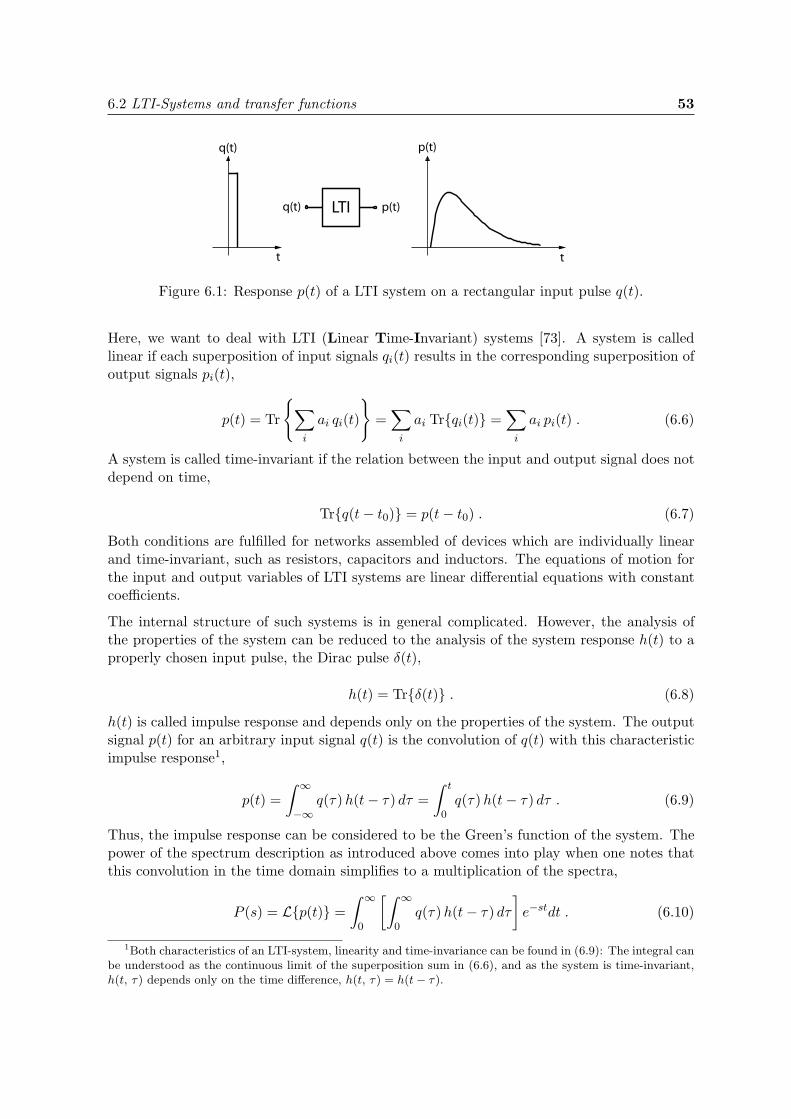
6.2 LTI-Systems and transfer functions 53
q(t)
t t
p(t)
q(t) p(t)LTI
Figure 6.1: Response p(t) of a LTI system on a rectangular input pulse q(t).
Here, we want to deal with LTI (Linear Time-Invariant) systems [73]. A system is calledlinear if each superposition of input signals qi(t) results in the corresponding superposition ofoutput signals pi(t),
p(t) = Tr
∑
i
ai qi(t)
=
∑
i
ai Trqi(t) =∑
i
ai pi(t) . (6.6)
A system is called time-invariant if the relation between the input and output signal does notdepend on time,
Trq(t− t0) = p(t− t0) . (6.7)
Both conditions are fulfilled for networks assembled of devices which are individually linearand time-invariant, such as resistors, capacitors and inductors. The equations of motion forthe input and output variables of LTI systems are linear differential equations with constantcoefficients.
The internal structure of such systems is in general complicated. However, the analysis ofthe properties of the system can be reduced to the analysis of the system response h(t) to aproperly chosen input pulse, the Dirac pulse δ(t),
h(t) = Trδ(t) . (6.8)
h(t) is called impulse response and depends only on the properties of the system. The outputsignal p(t) for an arbitrary input signal q(t) is the convolution of q(t) with this characteristicimpulse response1,
p(t) =∫ ∞
−∞q(τ) h(t− τ) dτ =
∫ t
0q(τ) h(t− τ) dτ . (6.9)
Thus, the impulse response can be considered to be the Green’s function of the system. Thepower of the spectrum description as introduced above comes into play when one notes thatthis convolution in the time domain simplifies to a multiplication of the spectra,
P (s) = Lp(t) =∫ ∞
0
[∫ ∞
0q(τ) h(t− τ) dτ
]e−stdt . (6.10)
1Both characteristics of an LTI-system, linearity and time-invariance can be found in (6.9): The integral canbe understood as the continuous limit of the superposition sum in (6.6), and as the system is time-invariant,h(t, τ) depends only on the time difference, h(t, τ) = h(t− τ).
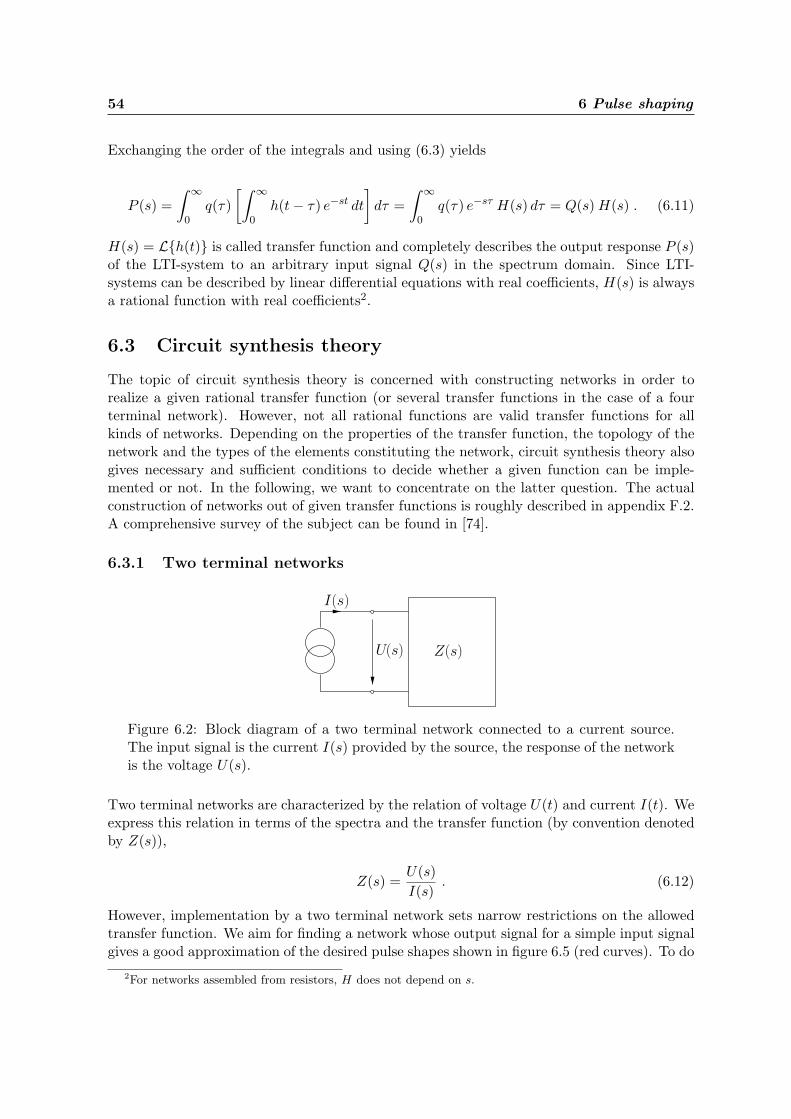
54 6 Pulse shaping
Exchanging the order of the integrals and using (6.3) yields
P (s) =∫ ∞
0q(τ)
[∫ ∞
0h(t− τ) e−st dt
]dτ =
∫ ∞
0q(τ) e−sτ H(s) dτ = Q(s) H(s) . (6.11)
H(s) = Lh(t) is called transfer function and completely describes the output response P (s)of the LTI-system to an arbitrary input signal Q(s) in the spectrum domain. Since LTI-systems can be described by linear differential equations with real coefficients, H(s) is alwaysa rational function with real coefficients2.
6.3 Circuit synthesis theory
The topic of circuit synthesis theory is concerned with constructing networks in order torealize a given rational transfer function (or several transfer functions in the case of a fourterminal network). However, not all rational functions are valid transfer functions for allkinds of networks. Depending on the properties of the transfer function, the topology of thenetwork and the types of the elements constituting the network, circuit synthesis theory alsogives necessary and sufficient conditions to decide whether a given function can be imple-mented or not. In the following, we want to concentrate on the latter question. The actualconstruction of networks out of given transfer functions is roughly described in appendix F.2.A comprehensive survey of the subject can be found in [74].
6.3.1 Two terminal networks
Figure 6.2: Block diagram of a two terminal network connected to a current source.The input signal is the current I(s) provided by the source, the response of the networkis the voltage U(s).
Two terminal networks are characterized by the relation of voltage U(t) and current I(t). Weexpress this relation in terms of the spectra and the transfer function (by convention denotedby Z(s)),
Z(s) =U(s)I(s)
. (6.12)
However, implementation by a two terminal network sets narrow restrictions on the allowedtransfer function. We aim for finding a network whose output signal for a simple input signalgives a good approximation of the desired pulse shapes shown in figure 6.5 (red curves). To do
2For networks assembled from resistors, H does not depend on s.

6.3 Circuit synthesis theory 55
so, we proceed to the more general case of four terminal networks, making use of the greatervariety of valid transfer functions.
6.3.2 Four terminal networks
Figure 6.3: Block diagram of a four terminal network. Here, the case R1 = R2 = ∞ istreated, i.e. an ideal current source connected to the input and a system with infiniteworking resistance connected to the output. In this case, we only need to specify Z21(s),whereas the other transfer functions remain to be chosen according to the conditionsimposed by the desired realization.
As only one equation –and one transfer function– is required to describe a two terminalnetwork, we need two equations –and four transfer functions– to characterize the relationsbetween the input and output voltages and currents U1(s), I1(s), U2(s) and I2(s) of a fourterminal network,
(U1(s)U2(s)
)=
(Z11(s) Z12(s)Z21(s) Z22(s)
)(I1(s)I2(s)
). (6.13)
The behavior of the network is now completely described by the four coefficients (transferfunctions) Z11(s), Z12(s), Z21(s) and Z22(s).
What restrictions apply to the poles and zeros of a four pole transfer function? Consider atransfer function Z(s) in the form
Z(s) =P (s)Q(s)
=am sm + · · ·+ a1 s + a0
bn sn + · · ·+ b1 s + b0, (6.14)
where Z(s) denotes any of the above transfer functions constituting the four pole. In conse-quence of P (s) and Q(s) having only real coefficients, complex zeros and poles can only occuras pairs of complex conjugates.Moreover, we want to take a look at the time domain behavior of the input and output signals.
Stability
Let p(t) be the time domain function of the output and q(t) of the input signal. Eq. (6.14)corresponds to the differential equation
bndnp(t)dtn
+ . . . + b1dp(t)dt
+ b0 p(t) = amdmq(t)dtm
+ . . . + a1dq(t)dt
+ a0 q(t) , (6.15)
as one can obtain (6.14) by applying (6.4) to (6.15).
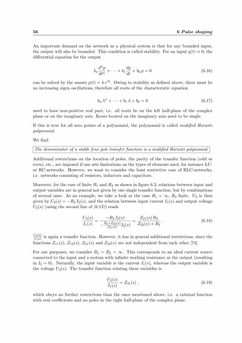
56 6 Pulse shaping
An important demand on the network as a physical system is that for any bounded input,the output will also be bounded. This condition is called stability. For an input q(t) ≡ 0, thedifferential equation for the output
bndnp
dtn+ · · ·+ b1
dp
dt+ b0 p = 0 (6.16)
can be solved by the ansatz p(t) = k eλt. Owing to stability as defined above, there must beno increasing eigen oscillations, therefore all roots of the characteristic equation
bn λn + · · ·+ b1 λ + b0 = 0 (6.17)
need to have non-positive real part, i.e. all roots lie on the left half-plane of the complexplane or on the imaginary axis. Roots located on the imaginary axis need to be single.
If this is true for all zero points of a polynomial, the polynomial is called modified Hurwitzpolynomial.
We find:
The denominator of a stable four pole transfer function is a modified Hurwitz polynomial.
Additional restrictions on the location of poles, the parity of the transfer function (odd oreven), etc., are imposed if one sets limitations on the types of elements used, for instance LC-or RC-networks. However, we want to consider the least restrictive case of RLC-networks,i.e. networks consisting of resistors, inductors and capacitors.
Moreover, for the case of finite R1 and R2 as shown in figure 6.3, relations between input andoutput variables are in general not given by one single transfer function, but by combinationsof several ones. As an example, we take a look at the case R1 = ∞, R2 finite. U2 is thengiven by U2(s) = −R2 I2(s), and the relation between input current I1(s) and output voltageU2(s) (using the second line of (6.13)) reads
U2(s)I1(s)
=−R2 I2(s)
−R2+Z22(s)Z21(s)
I2(s)=
Z21(s) R2
Z22(s) + R2. (6.18)
U2(s)I1(s) is again a transfer function. However, it has in general additional restrictions, since thefunctions Z11(s), Z12(s), Z21(s) and Z22(s) are not independent from each other [74].
For our purposes, we consider R1 = R2 = ∞. This corresponds to an ideal current sourceconnected to the input and a system with infinite working resistance at the output (resultingin I2 = 0). Naturally, the input variable is the current I1(s), whereas the output variable isthe voltage U2(s). The transfer function relating these variables is
U2(s)I1(s)
= Z21(s) , (6.19)
which obeys no further restrictions than the ones mentioned above, i.e. a rational functionwith real coefficients and no poles in the right half-plane of the complex plane.

6.4 Approximation and results 57
6.4 Approximation and results
We want to move on to the actual issue. In figure 6.5, the time course of the desired outputpulses δng,C(t) for the gate voltage of the control qubit and δng,T(t) for the target qubit (redcurves) in a system of two charge qubits along with the approximations by our filter networks(blue curves) are shown.We first state that the input pulse is arbitrary and should be kept simple, however, it hasto contain enough spectral weight at the dominating harmonics of the output pulse. Here,we start for both output pulses with a rectangular input current pulse of length τr = 1.1 ps.The short duration of the pulse guarantees a broad frequency spectrum. These time scalesare already accessible by the application of well established optoelectronic techniques to thegeneration and detection of terahertz (THz) pulses [75] used in the field of femtochemistryfor the investigation of the dynamics of chemical reactions [76].The time courses for the optimal pulses in figure 6.5 actually show the interpolating envelopeof 50 discrete data points resulting from the numerical optimization. Since the Laplacetransform can only be applied to continuous functions, the pulses were written as a sum of6 (for the pulse on the control qubit, 7 for the target pulse, respectively) harmonic functionsobtained by discrete-time Fourier transform. The transfer function for the control pulse (thetarget pulse) then looks like
H(s)C(T) =LFtn, δng,C(T)(tn)
LΘ(t)Θ(−t + τr) =LFtn, δng,C(T)(tn)
(1− e−s τr) /s(6.20)
with Θ(t)Θ(−t+τr) making up the rectangular pulse of length τr (Θ(t) denotes the Heavisidefunction), and Ftn, δng,C(T)(tn) being the Fourier transform of the discrete set of pulseamplitudes δng,C(T)(tn) of the control qubit (the target qubit).
We aim for determining a four-pole transfer function Z21(s) with the restrictions pointedout above, approximating H(s). The used algorithm finds rational functions f(x), whichinterpolate a set of data points xi, yi –in our case a finite number of sampling points of H(s)–by a rational function with given degrees for the nominator and denominator polynomial. AsH(s) turns out to approach a finite value for s → ±∞, the degrees of the nominator and thedenominator need to be equal.
As expected, a small degree results in an inaccurate approximation with the inverse Laplacetransform L−1 LΘ(t)Θ(−t + τr) Z21(s) of the shaped output pulse showing large devia-tions from the desired pulse (see figure 6.4).For higher degrees, the rational interpolation is in increasingly good agreement with thedesired pulses. Figure 6.5 shows the approximation achieved by two transfer functions withthe degree 14 for the control qubit and 18 for the target qubit, respectively. The higher degreeof the network shaping the pulse for the target qubit is consistent with the higher numberof harmonics contained in the pulse (see above) and confirms the usability of the networkcomplexity as measure for the complexity of the pulse.
For the same filter networks, a characterization showing the location of the poles with thecorresponding residue is displayed in figure 6.6. According to the constructional methodsdescribed in appendix F.2, each pole on the negative real axis corresponds to a RC-filter,a pair of complex conjugate poles yields a LCR-filter. The pulse for the control qubit canthereby be approximated with 6 LCR filters and 2 RC filters, the pulse for the target qubit

58 6 Pulse shaping
with 8 LCR filters and 2 RC-filters. The fidelity of the gate operation, i.e. the overlap of theideal CNOT propagator with the propagator (refer to publication, appendix G) induced bythe approximated pulses is higher than 94%. In reality, first the parameters of the sample haveto be determined spectroscopically before adapting the filter network accordingly. Moreover,the pulse arriving at the sample will be distorted by the transmission through the leads etc.(which can be again modelled by the corresponding transfer function), which needs to becompensated.
0 10 20 30 40 50
time (ps)
-0.2
-0.1
0
0.1
δ n
g,C
Optimal pulse
Pulse shaped by LCR-filter
0 10 20 30 40 50
time (ps)
-0.2
-0.1
0
0.1
δ n
g,C
Optimal pulse
Pulse shaped by LCR-filter
Figure 6.4: Time course of the desired output pulse for the control qubit and itsapproximation shaped by filter networks of varying complexity. Left: Approximationby a transfer function with degree 6. Right: Approximation by a transfer function withdegree 11. The increasing quality of the approximation with increasing degree of thetransfer function allows for measuring the pulse complexity in terms of complexity ofthe transfer function.
0 10 20 30 40 50
time (ps)
-0.2
-0.1
0
0.1
δ n
g,C
Optimal pulse
Pulse shaped by LCR-filter
0 10 20 30 40 50
time (ps)
-0.2
-0.1
0
0.1
0.2
0.3
δ n
g,T
Optimal pulse
Pulse shaped by LCR-filter
Figure 6.5: Time course of the desired output and the pulses shaped by the filternetworks. Left: Control qubit pulse, approximated by a transfer function with degree14. Right: Target qubit pulse approximated by a transfer function with degree 18.
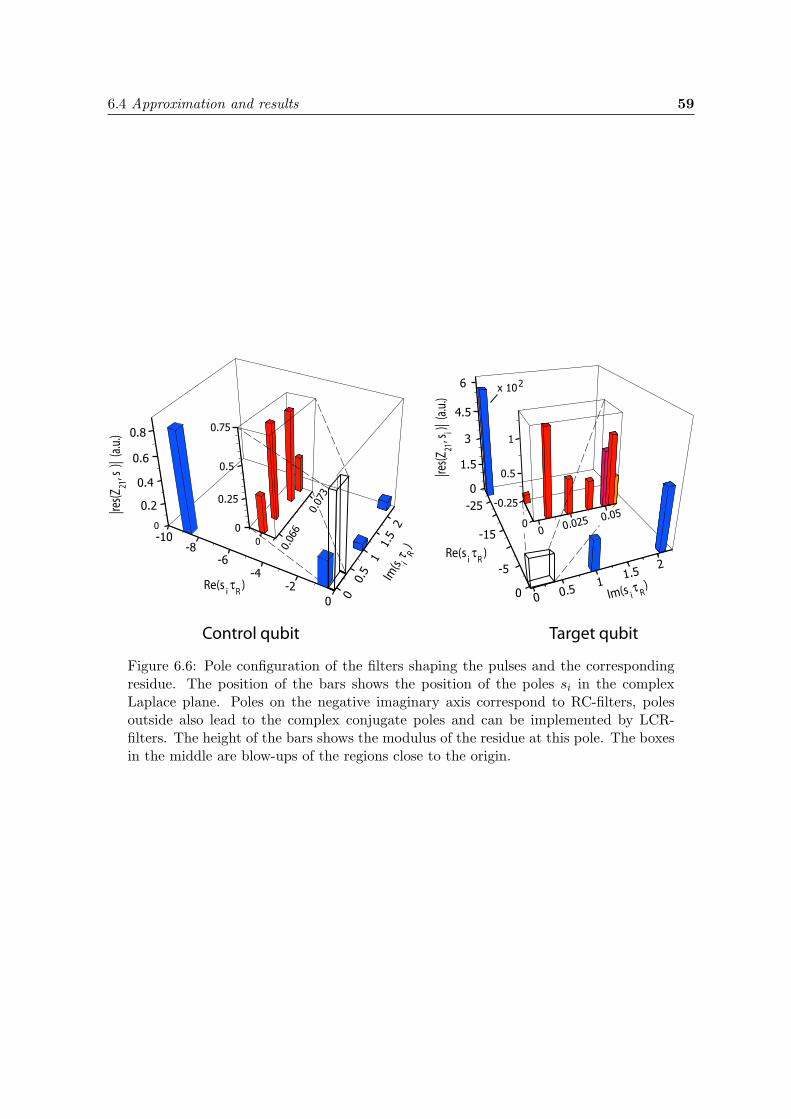
6.4 Approximation and results 59
0
-5
-15
-25
0
1.5
3
4.5
6
0.5
1
0
-0.25
00.5
11.5
2
00.025
0.05
|res
(Z21
, si)|
(a.u
.)
Re(siτ
R)
Im(s iτ R
)
x 10 2
0.8
0.6
0.4
0.2
0
0
0.5
11.5
2
0.0
73
0.25
0.5
0.75
0
0
0
-2
-10
0.0
66
-8
-6
-4
|res
(Z21
, s)|
(a.u
.)
Re(siτ
R)
Im(s i
τ R)
Control qubit Target qubit
Figure 6.6: Pole configuration of the filters shaping the pulses and the correspondingresidue. The position of the bars shows the position of the poles si in the complexLaplace plane. Poles on the negative imaginary axis correspond to RC-filters, polesoutside also lead to the complex conjugate poles and can be implemented by LCR-filters. The height of the bars shows the modulus of the residue at this pole. The boxesin the middle are blow-ups of the regions close to the origin.

60 6 Pulse shaping
Conclusions
In this work, we showed the suitability of a system of three coupled flux qubits to exhibitstrong tripartite entanglement for a realistic and approachable set of parameters as well asthe feasibility to prepare, detect and identify this entanglement by available technology.
In chapter 2, we discussed the types and the strengths of the interactions between the qubitsfor two possible designs, an arrangement of the three qubits next to each other with an addi-tional joint SQUID-loop acting as flux transformer (Fig. 2.1) and a triangle geometry (Fig.2.2), providing the coupling mainly via the Josephson inductances of shared junctions placedin shared lines between the qubits. Both of these designs cause a pairwise antiferromagneticIsing type coupling σ
(i)z ⊗ σ
(j)z , where the coupling in the triangle design is found to be much
stronger and takes –depending on the size of the shared junctions– values of approx. 1.4∆ (∆is the tunnel matrix element of the qubits). In section 2.3, we proposed a readout geometryconsisting of three SQUIDs attached to the sides of the triangle.
In chapter 3, the properties of the eigenstates of the system were investigated for differentcoupling strengths and in different regimes of the energy bias ε. Due to the antiferromagneticcoupling, the ground state is a superposition of frustrated states (3.29), whereas the highestexcited states are for strong coupling close to GHZ states in a small range around zero energybias (3.31). Moreover, by writing down the Hamiltonian in an appropriate collective basis(3.3), we found two degenerate pairs of eigenstates forming two subspaces. Among the statescontained in these degenerate subspaces, we identified states with maximal entanglement,which are equivalent to the W state (3.19) under local unitary operations, see (3.21) and(3.27).
The preparation of these maximally entangled states in the subspaces by application of ex-ternal microwave fields is covered in chapter 4. By means of a dressed state approach weshowed that preparation of arbitrary superpositions of the basis states is possible by pulsingthe qubits individually.
In chapter 5, we addressed the detection of tripartite entanglement and violation of Bellinequalities in more detail. We used the 3-tangle [50] and entanglement witnesses (5.1) astools to identify tripartite entanglement. We detected GHZ type entanglement in the regimeof zero energy bias mentioned above (Fig. 5.1) and –in a more robust manner– in a regimeof finite energy bias (Fig. 5.3). The W type entanglement in the degenerate subspaces wasinvestigated in 5.1.3 and was found to persist over a large range of the energy bias (Fig. 5.5).Moreover, we observed significant violations of adapted, optimized Bell type inequalities inall these regimes (Fig. 5.2, 5.4, 5.6).Starting from the local decompositions of the Bell operators and the entanglement witnesses,we discussed the effect of a limited measurement fidelity in section 5.3. The required fidelities
61

62 6 Pulse shaping
are almost identical and even slightly lower than for the case of two qubits (table 5.3) andwere shown to be approachable with recently developed measurement techniques. Thus, theproposed design is indeed suitable for demonstrating tripartite entanglement.
In chapter 6, we presented an approach to the shaping of short pulse sequences by filternetworks of passive circuit elements. This was done for the example of a quantum gateimplementation in a system of two coupled charge qubits, where an accurate approximationof an optimal pulse sequence (Fig. 6.5) could be achieved with a small number of filterelements (Fig. 6.6), yielding an overlap with the ideal gate propagator of more than 94%. Wealso outlined the connection between the complexity of the desired pulse on the one hand sideand the complexity of the filter network on the other hand side, which allows for estimatingand measuring the pulse complexity in terms of properties of the required network (6.4).

Acknowledgments
This diploma thesis and the associated year of work would not have been possible withouthelp and support of many others and even if it would have been possible, it would have beena pain.
I would like to thank Prof. Dr. Jan von Delft for giving me the opportunity to join his group.The environment and atmosphere in the group, professionally as well as personally made iteasy to enjoy this time and to learn a lot.
I would particulary like to thank my supervisor PD Dr. Frank Wilhelm, for his advice andhelp concerning physical and non-physical aspects, his support and discussions in form of’intellectual pressure fuelling’.
I want to thank Markus Storcz for his continuous support, help and devotion in all kinds ofaspects, this has been very helpful and a good example.
Thank goes to Dr. Thomas Schulte-Herbruggen and Andreas Sporl of the group of Prof. Dr.Steffen Glaser for the fruitful collaboration and the stimulating, intense discussions. I alsothank John Clarke and Birgitta Whaley for inviting me to visit their groups in Berkeley. Ivery much look forward to it.
Thanks to my officemates Michael and Henryk for tolerating my presence for one whole yearand for being open to all kinds of questions, to physical, philosophical and profane discussions.The same holds for all the other people at the chair for theoretical condensed matter physics,it was a pleasure to me.
Thanks to my friends, especially Moritz, Ferdinand and Lukas, for their company and muchmore. Speaking of the last year, I also don’t want to forget our common friend Jack, see youagain!
I would like to thank my girlfriend Blanca. Be it her understanding for many of my ideas orbe it the lack of understanding for some others, it has always been the right call.
Last, but in no way least thanks to my parents and my brothers for their support anddedication over all these many years. You cannot choose your family but I am definitelylucky.
63

64 Acknowledgements

Appendix A
Three-spin basis
The standard basis is given by the eigenstates of the tensor product of the z-components ofthe individual spins si
z = 12 σi
z,
(s1z ⊗ s2
z ⊗ s3z
) |m1s m2
s m3s〉 = m1
s m2s m3
s |m1s m2
s m3s〉 , (A.1)
where mis = ±1/2 corresponds to |mi
s〉 = |↑〉 (|↓〉, respectively).
|↑↑↑〉 = (1, 0, 0, 0, 0, 0, 0, 0)T = |v1〉|↑↑↓〉 = (0, 1, 0, 0, 0, 0, 0, 0)T = |v2〉|↑↓↑〉 = (0, 0, 1, 0, 0, 0, 0, 0)T = |v3〉|↑↓↓〉 = (0, 0, 0, 1, 0, 0, 0, 0)T = |v4〉|↓↑↑〉 = (0, 0, 0, 0, 1, 0, 0, 0)T = |v5〉|↓↑↓〉 = (0, 0, 0, 0, 0, 1, 0, 0)T = |v6〉|↓↓↑〉 = (0, 0, 0, 0, 0, 0, 1, 0)T = |v7〉|↓↓↓〉 = (0, 0, 0, 0, 0, 0, 0, 1)T = |v8〉 (A.2)
We aim for finding a collective basis, i.e. a basis of eigenstates of the total spin and itsz-component rather than of the individual z-components. To do so, we use the well knownsinglet-triplet basis, say for the qubits denoted by 1 and 2, |m1
s m2s〉 −→ |s12 m12
s 〉 and couplea third spin 1/2 particle to it,
|m1s m2
s m3s〉 −→ |stot mtot
s s12〉 . (A.3)
The third quantum number s12 denotes the total spin of the qubits 1 and 2 combined (possiblevalues being 1 or 0) and has to be carried along to exclude ambiguities (e.g. between the states|12 1
2 0〉 and |12 12 1〉). We express these states in terms of the uncoupled basis and determine
the Clebsch-Gordan coefficients C(stot mtots s12, m1
s m2s m3
s) = 〈stot mtots s12 |m1
s m2s m3
s〉 by thecommon method of iteratively applying the lowering operator, starting from the state |32 3
2 1〉,as described in Ref. [77]. We arrive at:
65
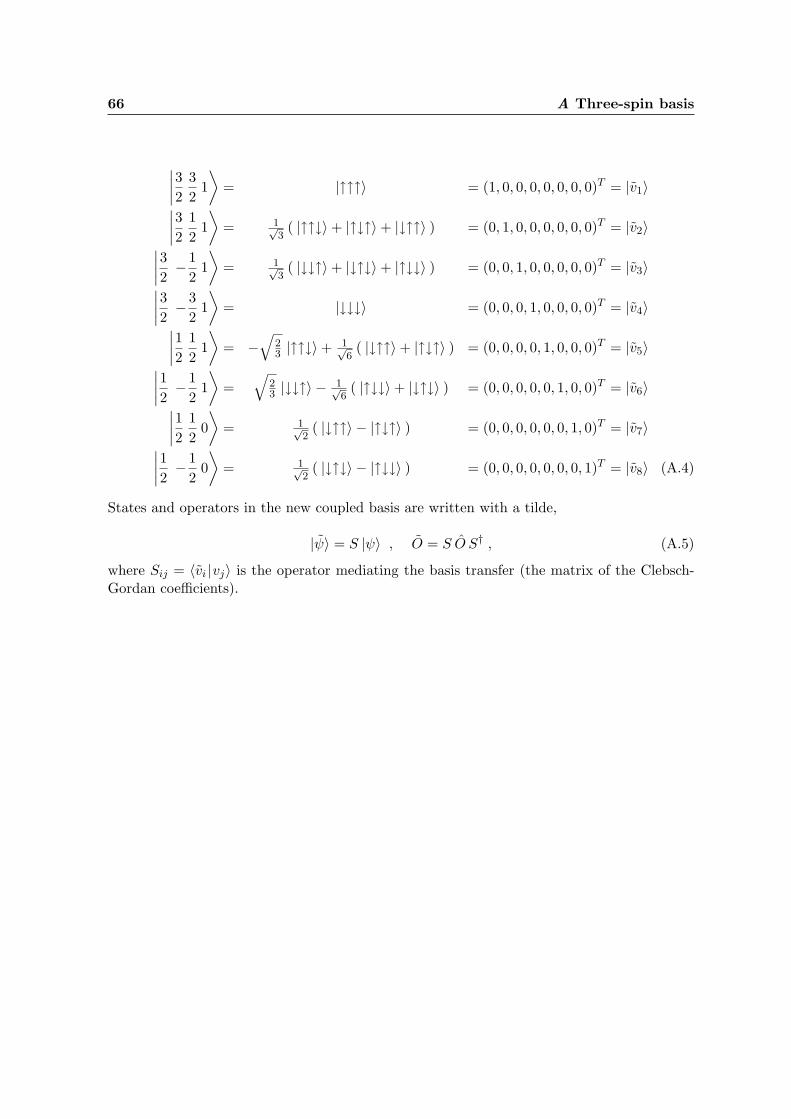
66 A Three-spin basis
∣∣∣∣32
32
1⟩
= |↑↑↑〉 = (1, 0, 0, 0, 0, 0, 0, 0)T = |v1〉∣∣∣∣32
12
1⟩
= 1√3( |↑↑↓〉+ |↑↓↑〉+ |↓↑↑〉 ) = (0, 1, 0, 0, 0, 0, 0, 0)T = |v2〉
∣∣∣∣32− 1
21⟩
= 1√3( |↓↓↑〉+ |↓↑↓〉+ |↑↓↓〉 ) = (0, 0, 1, 0, 0, 0, 0, 0)T = |v3〉
∣∣∣∣32− 3
21⟩
= |↓↓↓〉 = (0, 0, 0, 1, 0, 0, 0, 0)T = |v4〉∣∣∣∣12
12
1⟩
= −√
23 |↑↑↓〉+ 1√
6( |↓↑↑〉+ |↑↓↑〉 ) = (0, 0, 0, 0, 1, 0, 0, 0)T = |v5〉
∣∣∣∣12− 1
21⟩
=√
23 |↓↓↑〉 − 1√
6( |↑↓↓〉+ |↓↑↓〉 ) = (0, 0, 0, 0, 0, 1, 0, 0)T = |v6〉
∣∣∣∣12
12
0⟩
= 1√2( |↓↑↑〉 − |↑↓↑〉 ) = (0, 0, 0, 0, 0, 0, 1, 0)T = |v7〉
∣∣∣∣12− 1
20⟩
= 1√2( |↓↑↓〉 − |↑↓↓〉 ) = (0, 0, 0, 0, 0, 0, 0, 1)T = |v8〉 (A.4)
States and operators in the new coupled basis are written with a tilde,
|ψ〉 = S |ψ〉 , O = S O S† , (A.5)
where Sij = 〈vi |vj〉 is the operator mediating the basis transfer (the matrix of the Clebsch-Gordan coefficients).

Appendix B
Eigenenergies and eigenstates of thedoublets
The doublet Hamiltonian reads
H = −12
ε + 2C ∆
∆ −ε + 2C
. (B.1)
The eigenenergies and corresponding eigenstates in the quartet/doublet basis read
E5, E7 = −C − Λ2
,
E6, E8 = −C +Λ2
. (B.2)
|ψL1 〉 =
1√2Λ(Λ + ε)
0000−∆
ε + Λ00
, |ψH1 〉 =
1√2Λ(Λ− ε)
0000−∆
ε− Λ00
|ψL2 〉 =
1√2Λ(Λ + ε)
000000−∆
ε + Λ
, |ψH2 〉 =
1√2Λ(Λ− ε)
000000−∆
ε− Λ
(B.3)
with Λ =√
∆2 + ε2.
67

68 B Eigenenergies and eigenstates of the doublets

Appendix C
Structure of the eigenstates
We plot the projection of the eigenstates |E1〉–|E8〉 onto the states of the standard basis. Thediscussion of the properties of the eigenstates in chapter 3 is mainly based on these plots.
69
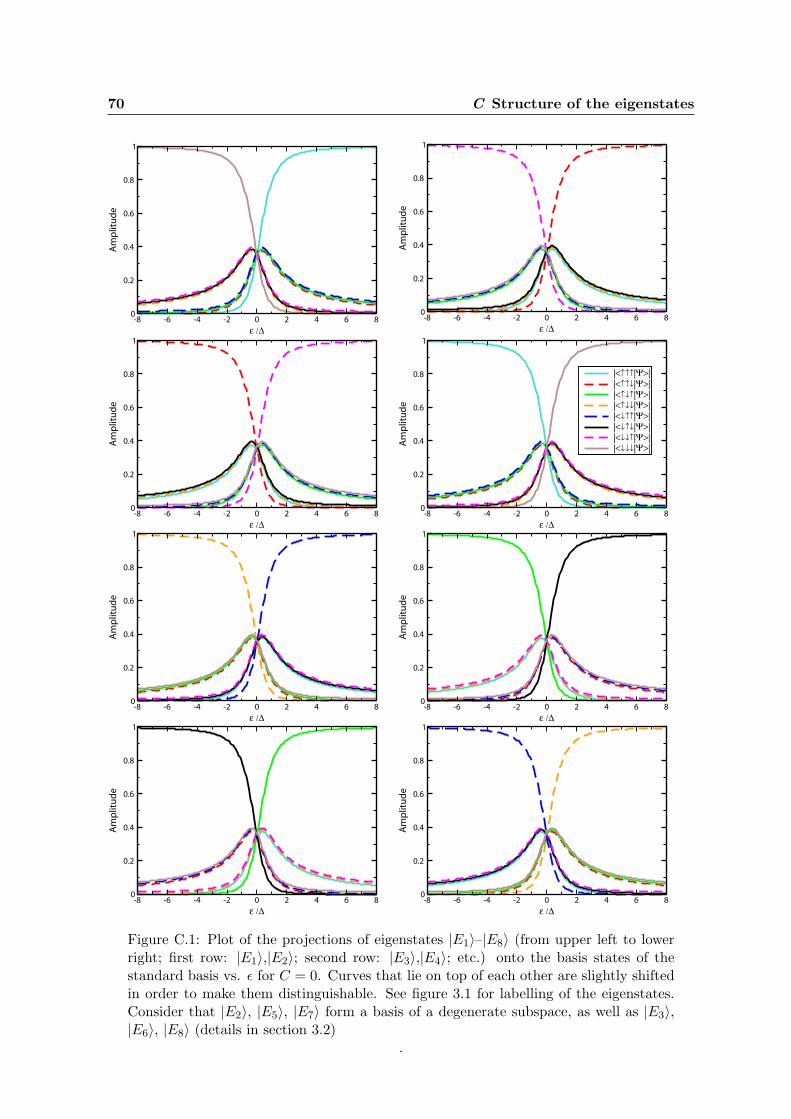
70 C Structure of the eigenstates
-8 -6 -4 -2 0 2 4 6 8
ε /∆
0
0.2
0.4
0.6
0.8
1
Am
pli
tud
e
-8 -6 -4 -2 0 2 4 6 8
ε /∆
0
0.2
0.4
0.6
0.8
1
Am
pli
tud
e
-8 -6 -4 -2 0 2 4 6 8
ε /∆
0
0.2
0.4
0.6
0.8
1
Am
pli
tud
e
-8 -6 -4 -2 0 2 4 6 8
ε /∆
0
0.2
0.4
0.6
0.8
1
Am
pli
tud
e
-8 -6 -4 -2 0 2 4 6 8
ε /∆
0
0.2
0.4
0.6
0.8
1
Am
pli
tud
e
-8 -6 -4 -2 0 2 4 6 8
ε /∆
0
0.2
0.4
0.6
0.8
1
Am
pli
tud
e
-8 -6 -4 -2 0 2 4 6 8
ε /∆
0
0.2
0.4
0.6
0.8
1
Am
pli
tud
e
-8 -6 -4 -2 0 2 4 6 8
ε /∆
0
0.2
0.4
0.6
0.8
1
Am
pli
tud
e
|<↑↑↑|Ψ>||<↑↑↓|Ψ>||<↑↓↑|Ψ>||<↑↓↓|Ψ>||<↓↑↑|Ψ>||<↓↑↓|Ψ>||<↓↓↑|Ψ>||<↓↓↓|Ψ>|
Figure C.1: Plot of the projections of eigenstates |E1〉–|E8〉 (from upper left to lowerright; first row: |E1〉,|E2〉; second row: |E3〉,|E4〉; etc.) onto the basis states of thestandard basis vs. ε for C = 0. Curves that lie on top of each other are slightly shiftedin order to make them distinguishable. See figure 3.1 for labelling of the eigenstates.Consider that |E2〉, |E5〉, |E7〉 form a basis of a degenerate subspace, as well as |E3〉,|E6〉, |E8〉 (details in section 3.2)
.

71
-8 -6 -4 -2 0 2 4 6 8
ε /∆
0
0.2
0.4
0.6
0.8
1
Am
pli
tud
e
-8 -6 -4 -2 0 2 4 6 8
ε /∆
0
0.2
0.4
0.6
0.8
1
Am
pli
tud
e
-8 -6 -4 -2 0 2 4 6 8
ε /∆
0
0.2
0.4
0.6
0.8
1
Am
pli
tud
e
-8 -6 -4 -2 0 2 4 6 8
ε /∆
0
0.2
0.4
0.6
0.8
1
Am
pli
tud
e
|<↑↑↑|Ψ>||<↑↑↓|Ψ>||<↑↓↑|Ψ>||<↑↓↓|Ψ>||<↓↑↑|Ψ>||<↓↑↓|Ψ>||<↓↓↑|Ψ>||<↓↓↓|Ψ>|
-8 -6 -4 -2 0 2 4 6 8
ε /∆
0
0.2
0.4
0.6
0.8
1
Am
pli
tud
e
-8 -6 -4 -2 0 2 4 6 8
ε /∆
0
0.2
0.4
0.6
0.8
1
Am
pli
tud
e
-8 -6 -4 -2 0 2 4 6 8
ε /∆
0
0.2
0.4
0.6
0.8
1
Am
pli
tud
e
-8 -6 -4 -2 0 2 4 6 8
ε /∆
0
0.2
0.4
0.6
0.8
1
Am
pli
tud
e
Figure C.2: Plot of the projections of eigenstates |E1〉–|E8〉 (from upper left to lowerright; first row: |E1〉,|E2〉; second row: |E3〉,|E4〉; etc.) onto the basis states of thestandard basis vs. ε for C = 0.2∆. Curves that lie on top of each other are slightlyshifted in order to make them distinguishable. See figure 3.1 for labelling of the eigen-states. Consider that |E5〉 and |E7〉 form a basis of a degenerate subspace, as well as|E6〉 and |E8〉(details in section 3.3)
.
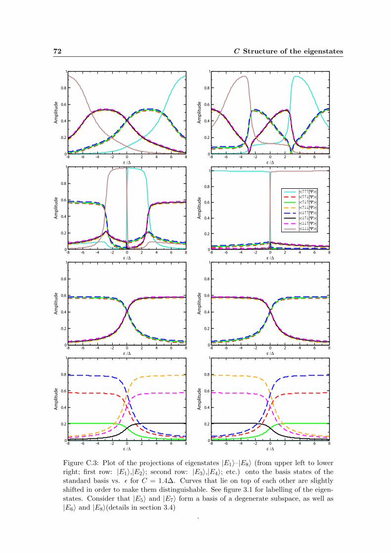
72 C Structure of the eigenstates
-8 -6 -4 -2 0 2 4 6 8
ε /∆
0
0.2
0.4
0.6
0.8
1
Am
pli
tud
e
-8 -6 -4 -2 0 2 4 6 8
ε /∆
0
0.2
0.4
0.6
0.8
1
Am
pli
tud
e
-8 -6 -4 -2 0 2 4 6 8
ε /∆
0
0.2
0.4
0.6
0.8
1
Am
pli
tud
e
-8 -6 -4 -2 0 2 4 6 8
ε /∆
0
0.2
0.4
0.6
0.8
1
Am
pli
tud
e
-8 -6 -4 -2 0 2 4 6 8
ε /∆
0
0.2
0.4
0.6
0.8
1
Am
pli
tud
e
-8 -6 -4 -2 0 2 4 6 8
ε /∆
0
0.2
0.4
0.6
0.8
1
Am
pli
tud
e
-8 -6 -4 -2 0 2 4 6 8
ε /∆
0
0.2
0.4
0.6
0.8
1
Am
pli
tud
e
-8 -6 -4 -2 0 2 4 6 8
ε /∆
0
0.2
0.4
0.6
0.8
1
Am
pli
tud
e
|<↑↑↑|Ψ>||<↑↑↓|Ψ>||<↑↓↑|Ψ>||<↑↓↓|Ψ>||<↓↑↑|Ψ>||<↓↑↓|Ψ>||<↓↓↑|Ψ>||<↓↓↓|Ψ>|
Figure C.3: Plot of the projections of eigenstates |E1〉–|E8〉 (from upper left to lowerright; first row: |E1〉,|E2〉; second row: |E3〉,|E4〉; etc.) onto the basis states of thestandard basis vs. ε for C = 1.4∆. Curves that lie on top of each other are slightlyshifted in order to make them distinguishable. See figure 3.1 for labelling of the eigen-states. Consider that |E5〉 and |E7〉 form a basis of a degenerate subspace, as well as|E6〉 and |E8〉(details in section 3.4)
.
Appendix D
Entanglement measures
The quantification of entanglement is a long standing problem in quantum information theory.An entanglement measure does not need to be an observable, however, it has to satisfy certainconditions. In particular, it has to be an entanglement monotone [78], i.e. it must notincrease on average under stochastic local operations and classical communication (SLOCC)[47, 79]. An important measure is the entanglement of formation [80, 81, 82], which gives thenumber of Einstein-Podolsky-Rosen pairs asymptotically required to prepare a given state. Byinvestigating the entanglement properties of mixed bipartite states, a measure for tripartitepure states could be derived, the 3-tangle [50].
D.1 3-tangle
The 3-tangle τ can be expressed in terms of the coefficients aijk of the state in the standardbasis, |ψ〉 =
∑ijk aijk |ijk〉, by
τ = 4 |d1 − 2d2 + 4d3| , (D.1)
where
d1 = a2000 a2
111 + a2001 a2
110 + a2010 a2
101 + a2100 a2
011
d2 = a000 a111 a011 a100 + a000 a111 a101 a010 + a000 a111 a110 a001 +
+a011 a100 a101 a010 + a011 a100 a110 a001 + a101 a010 a110 a001
d3 = a000 a110 a101 a011 + a111 a001 a010 a100 . (D.2)
D.2 Global entanglement
D.2.1 Definition
The global entanglement Q is given by
Q(|ψ〉) = 2
[1− 1
n
n∑
1
Tr ρ2k
](D.3)
73
74 D Entanglement measures
with ρk being the density matrix reduced to a single qubit k.For the special case of three qubits, this can be rewritten as [64]
Q =23
(C2
12 + C213 + C2
23
)+ τ , (D.4)
where τ is the 3-tangle and Cij the 2-qubit concurrence between qubit i and qubit j [81]. Theglobal entanglement thus measures the sum of different entanglement contributions.
D.2.2 Choice of |E5〉 and |E7〉We look for superpositions of |ψL(H)
1 〉 and |ψL(H)2 〉 (the states spanning the degenerate sub-
spaces, see 3.3.2 and appendix B) with maximal (respectively minimal) entanglement and usethe global entanglement introduced above as a measure.
For the global entanglement of an arbitrary state
|ψL(H)〉 = A |ψL(H)1 〉+ eiϕ
√1−A2 |ψL(H)
2 〉 (D.5)
in the low-energy (high-energy) subspace, we obtain (independent from the energy bias)
Q(A, ϕ) =89
(cos2 ϕ− 1
) (A4 −A2
)+
23
, (D.6)
which leads to the choice of A and ϕ for maximal (minimal) entanglement as
A =1√2
, ϕ =π
2
(A =
1√2
, ϕ = 0)
. (D.7)
This results in in |ψL(H)max 〉 (|ψL(H)
min 〉) with maximized (minimized) Q,
|ψL(H)max 〉 =
1√2(|ψL(H)
1 〉+ i |ψL(H)2 〉) := |E5(6)〉 , (D.8)
|ψL(H)min 〉 =
1√2(|ψL(H)
1 〉+ |ψL(H)2 〉) := |E7(8)〉 . (D.9)

Appendix E
Driving propagators
Referring to chapter 4, we write down the explicit form of the propagator U(t) for the evolutionof a state in the interaction picture under the driving Hamiltonian.
For two microwave sources radiating towards the qubits with individual amplitudes κ1 andκ2 as expressed by (4.6), the propagator reads (for the connection of ω1, ω2 and Ω to κ1 andκ2, refer to chapter 4)
U(t) =1Ω
Ωcos Ωt −iω1 sinΩt −iω2 sinΩt
−iω1 sinΩtω2
2+ω21 cosΩtΩ
ω1ω2(cosΩt−1)Ω
−iω2 sinΩt ω1ω2(cosΩt−1)Ω
ω21+ω2
2 cosΩtΩ
. (E.1)
As we assume the initial state to be the ground state written as (1, 0, 0)T in the basis intro-duced in (4.22), the evolution is given by the first column in the matrix representing U(t).
If the two sources are also shifted by an independent relative phase, the propagator reads
U(t) =1Ω
Ωcos Ωt −iω1 sin Ωt −iω2 sinΩt e−iϕ
−iω1 sinΩtω2
2+ω21 cosΩtΩ
ω1ω2(cosΩt−1)Ω e−iϕ
−iω2 sinΩt eiϕ ω1ω2(cosΩt−1)Ω eiϕ ω2
1+ω22 cosΩtΩ
. (E.2)
75

76 E Driving propagators
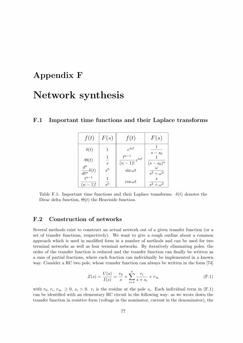
Appendix F
Network synthesis
F.1 Important time functions and their Laplace transforms
f(t) F (s) f(t) F (s)
δ(t) 1 es0t 1s− s0
Θ(t)1s
tn−1
(n− 1)!es0t 1
(s− s0)n
dn
dtnδ(t) sn sinωt
ω
s2 + ω2
tn−1
(n− 1)!1sn
cosωts
s2 + ω2
Table F.1: Important time functions and their Laplace transforms. δ(t) denotes theDirac delta function, Θ(t) the Heaviside function.
F.2 Construction of networks
Several methods exist to construct an actual network out of a given transfer function (or aset of transfer functions, respectively). We want to give a rough outline about a commonapproach which is used in modified form in a number of methods and can be used for twoterminal networks as well as four terminal networks. By iteratively eliminating poles, theorder of the transfer function is reduced and the transfer function can finally be written asa sum of partial fractions, where each fraction can individually be implemented in a knownway. Consider a RC two pole, whose transfer function can always be written in the form [74]
Z(s) =U(s)I(s)
=r0
s+
n∑
i=1
ri
s + si+ r∞ (F.1)
with r0, ri, r∞ ≥ 0, si > 0. ri is the residue at the pole si. Each individual term in (F.1)can be identified with an elementary RC circuit in the following way: as we wrote down thetransfer function in resistive form (voltage in the nominator, current in the denominator), the
77
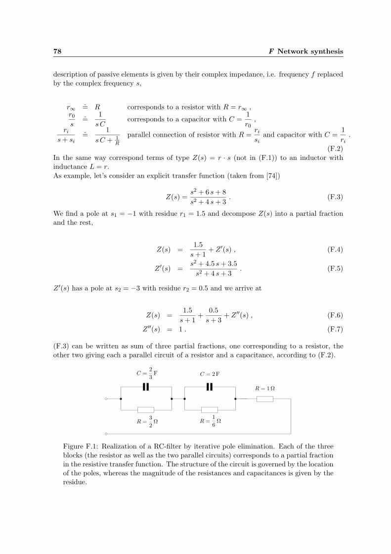
78 F Network synthesis
description of passive elements is given by their complex impedance, i.e. frequency f replacedby the complex frequency s,
r∞ = R corresponds to a resistor with R = r∞ ,r0
s=
1sC
corresponds to a capacitor with C =1r0
,
ri
s + si=
1sC + 1
R
parallel connection of resistor with R =ri
siand capacitor with C =
1ri
.
(F.2)In the same way correspond terms of type Z(s) = r · s (not in (F.1)) to an inductor withinductance L = r.As example, let’s consider an explicit transfer function (taken from [74])
Z(s) =s2 + 6 s + 8s2 + 4 s + 3
. (F.3)
We find a pole at s1 = −1 with residue r1 = 1.5 and decompose Z(s) into a partial fractionand the rest,
Z(s) =1.5
s + 1+ Z ′(s) , (F.4)
Z ′(s) =s2 + 4.5 s + 3.5
s2 + 4 s + 3. (F.5)
Z ′(s) has a pole at s2 = −3 with residue r2 = 0.5 and we arrive at
Z(s) =1.5
s + 1+
0.5s + 3
+ Z ′′(s) , (F.6)
Z ′′(s) = 1 . (F.7)
(F.3) can be written as sum of three partial fractions, one corresponding to a resistor, theother two giving each a parallel circuit of a resistor and a capacitance, according to (F.2).
Figure F.1: Realization of a RC-filter by iterative pole elimination. Each of the threeblocks (the resistor as well as the two parallel circuits) corresponds to a partial fractionin the resistive transfer function. The structure of the circuit is governed by the locationof the poles, whereas the magnitude of the resistances and capacitances is given by theresidue.
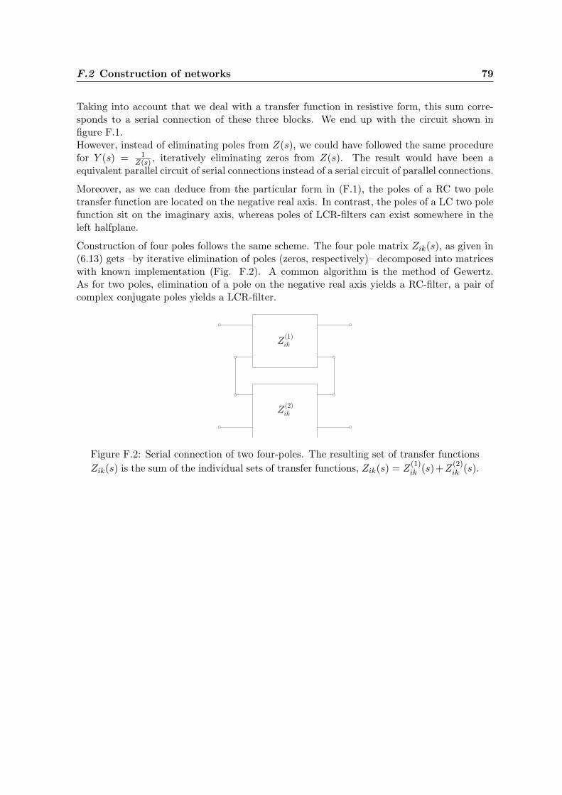
F.2 Construction of networks 79
Taking into account that we deal with a transfer function in resistive form, this sum corre-sponds to a serial connection of these three blocks. We end up with the circuit shown infigure F.1.However, instead of eliminating poles from Z(s), we could have followed the same procedurefor Y (s) = 1
Z(s) , iteratively eliminating zeros from Z(s). The result would have been aequivalent parallel circuit of serial connections instead of a serial circuit of parallel connections.
Moreover, as we can deduce from the particular form in (F.1), the poles of a RC two poletransfer function are located on the negative real axis. In contrast, the poles of a LC two polefunction sit on the imaginary axis, whereas poles of LCR-filters can exist somewhere in theleft halfplane.
Construction of four poles follows the same scheme. The four pole matrix Zik(s), as given in(6.13) gets –by iterative elimination of poles (zeros, respectively)– decomposed into matriceswith known implementation (Fig. F.2). A common algorithm is the method of Gewertz.As for two poles, elimination of a pole on the negative real axis yields a RC-filter, a pair ofcomplex conjugate poles yields a LCR-filter.
Figure F.2: Serial connection of two four-poles. The resulting set of transfer functionsZik(s) is the sum of the individual sets of transfer functions, Zik(s) = Z
(1)ik (s)+Z
(2)ik (s).

80 F Network synthesis
Appendix G
Publication
The attached paper has been submitted to Physical Review Letters and is available online,quant-ph/0504202; the ASC (Arnold Sommerfeld Center for Theoretical Physics) preprintnumber is LMU-ASC 38/05.
81
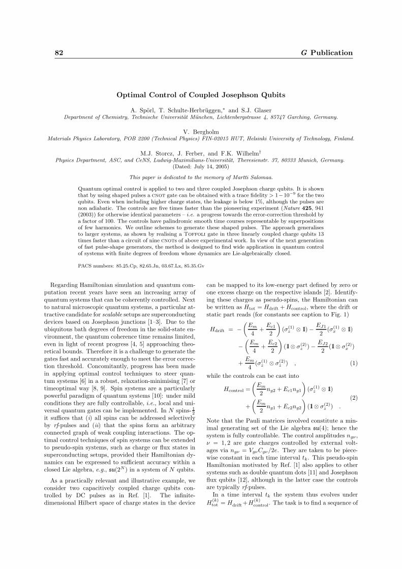
82 G Publication
Optimal Control of Coupled Josephson Qubits
A. Sporl, T. Schulte-Herbruggen,∗ and S.J. GlaserDepartment of Chemistry, Technische Universitat Munchen, Lichtenbergstrasse 4, 85747 Garching, Germany.
V. BergholmMaterials Physics Laboratory, POB 2200 (Technical Physics) FIN-02015 HUT, Helsinki University of Technology, Finland.
M.J. Storcz, J. Ferber, and F.K. Wilhelm†
Physics Department, ASC, and CeNS, Ludwig-Maximilians-Universitat, Theresienstr. 37, 80333 Munich, Germany.(Dated: July 14, 2005)
This paper is dedicated to the memory of Martti Salomaa.
Quantum optimal control is applied to two and three coupled Josephson charge qubits. It is shownthat by using shaped pulses a cnot gate can be obtained with a trace fidelity > 1−10−9 for the twoqubits. Even when including higher charge states, the leakage is below 1%, although the pulses arenon adiabatic. The controls are five times faster than the pioneering experiment (Nature 425, 941(2003)) for otherwise identical parameters – i.e. a progress towards the error-correction threshold bya factor of 100. The controls have palindromic smooth time courses representable by superpositionsof few harmonics. We outline schemes to generate these shaped pulses. The approach generalisesto larger systems, as shown by realising a Toffoli gate in three linearly coupled charge qubits 13times faster than a circuit of nine cnots of above experimental work. In view of the next generationof fast pulse-shape generators, the method is designed to find wide application in quantum controlof systems with finite degrees of freedom whose dynamics are Lie-algebraically closed.
PACS numbers: 85.25.Cp, 82.65.Jn, 03.67.Lx, 85.35.Gv
Regarding Hamiltonian simulation and quantum com-putation recent years have seen an increasing array ofquantum systems that can be coherently controlled. Nextto natural microscopic quantum systems, a particular at-tractive candidate for scalable setups are superconductingdevices based on Josephson junctions [1–3]. Due to theubiquitous bath degrees of freedom in the solid-state en-vironment, the quantum coherence time remains limited,even in light of recent progress [4, 5] approaching theo-retical bounds. Therefore it is a challenge to generate thegates fast and accurately enough to meet the error correc-tion threshold. Concomitantly, progress has been madein applying optimal control techniques to steer quan-tum systems [6] in a robust, relaxation-minimising [7] ortimeoptimal way [8, 9]. Spin systems are a particularlypowerful paradigm of quantum systems [10]: under mildconditions they are fully controllable, i.e., local and uni-versal quantum gates can be implemented. In N spins- 1
2it suffices that (i) all spins can be addressed selectivelyby rf-pulses and (ii) that the spins form an arbitraryconnected graph of weak coupling interactions. The op-timal control techniques of spin systems can be extendedto pseudo-spin systems, such as charge or flux states insuperconducting setups, provided their Hamiltonian dy-namics can be expressed to sufficient accuracy within aclosed Lie algebra, e.g., su(2N ) in a system of N qubits.
As a practically relevant and illustrative example, weconsider two capacitively coupled charge qubits con-trolled by DC pulses as in Ref. [1]. The infinite-dimensional Hilbert space of charge states in the device
can be mapped to its low-energy part defined by zero orone excess charge on the respective islands [2]. Identify-ing these charges as pseudo-spins, the Hamiltonian canbe written as Htot = Hdrift + Hcontrol, where the drift orstatic part reads (for constants see caption to Fig. 1)
Hdrift = −
(
Em
4+
Ec1
2
)
(σ(1)z ⊗ 1l) −
EJ1
2(σ(1)
x ⊗ 1l)
−
(
Em
4+
Ec2
2
)
(1l ⊗ σ(2)z ) −
EJ2
2(1l ⊗ σ(2)
x )
+Em
4(σ(1)
z ⊗ σ(2)z ) , (1)
while the controls can be cast into
Hcontrol =
(
Em
2ng2 + Ec1ng1
)
(σ(1)z ⊗ 1l)
+
(
Em
2ng1 + Ec2ng2
)
(1l ⊗ σ(2)z ) .
(2)
Note that the Pauli matrices involved constitute a min-imal generating set of the Lie algebra su(4); hence thesystem is fully controllable. The control amplitudes ngν ,ν = 1, 2 are gate charges controlled by external volt-ages via ngν = VgνCgν/2e. They are taken to be piece-wise constant in each time interval tk. This pseudo-spinHamiltonian motivated by Ref. [1] also applies to othersystems such as double quantum dots [11] and Josephsonflux qubits [12], although in the latter case the controlsare typically rf-pulses.
In a time interval tk the system thus evolves under
H(k)tot = Hdrift+H
(k)control. The task is to find a sequence of

83
2
FIG. 1: (Colour online) Fastest gate charge controls obtainedfor realising a cnot-gate on two coupled charge qubits (leftpart: control qubit, right part: working qubit). The totalgate charges for the qubits are ngν = n0
gν + δngν with ν =1, 2. Here, n0
g1 = 0.24, n0g2 = 0.26 and the qubit energies
Ec1/h = 140.2 GHz, Ec2/h = 162.2 GHz, EJ1/h = 10.9 GHz,EJ2/h = 9.9 GHz, and Em/h = 23.0 GHz were taken from theexperimental values in [1]. The 50 piecewise constant controlsare shown as bars (uniform width ∆ = tk = 1.1 ps); the trace
fidelity is 1
2N
˛
˛trU†targetUT
˛
˛ > 1 − 10−9. Red lines give theanalytic curves in Eqn. 3; the blue ones superimposed show apulse synthesised by an LCR-filter (see below and Fig. 3).
control amplitudes for the intervals t1, t2, . . . , tk, . . . , tMsuch as to maximise a quality function, here the over-lap with the desired quantum gate or element of analgorithm Utarget. Moreover, for the decomposition of
UT = e−itM HM
e−itM−1HM−1
· · · e−itkHk
· · · e−it1H1
intoavailable controls H
(k)ν to be timeoptimal, T :=
∑M
k=1 tk has to be minimal. The gate fidelity is
unity, if ||UT − Utarget||22 = 0 = ||UT ||
22 + ||Utarget||
22 −
2Re trU †targetUT . Maximising Re trU †
targetUT can
be solved by optimal control: set h(
U(tk))
:=Re trλ†(tk)(−i(Hd +
∑
uνHν))U(tk) with theLagrange-type adjoint system λ(t) following the equa-tion of motion λ(t) = −i(Hd +
∑
uνHν)λ(t). Pon-tryagin’s maximum principle requires ∂h/∂uν ≡Re trλ†(−iHν)U = 0 thus allowing to implementa gradient-flow based recursion. For the amplitudeof the νth control in iteration r + 1 at time intervaltk one finds with ε as a suitably chosen step size
n(r+1)gν (tk) = n
(r)gν (tk) + ε ∂h(r)(tk)
∂n(r)gν (tk)
as explained in more
detail in Refs. [13, 14]. T is the shortest fixed final timeallowing for a given fidelity to be obtained numerically.
Throughout the work, we take the parameters from theexperiment [1]. Fig. 1 shows the fastest decompositionsobtained by numerical optimal control for the cnot gateinto evolutions under available controls (Eqns. 1 and 2).In contrast to the 255 ps in Ref. [1], T = 55 ps suffice toget ||UT − Utarget||2 = 5.3464× 10⁻⁵ corresponding to a
trace fidelity of 12N
∣
∣trU †targetUT
∣
∣ > 1 − 10−9.
The supplementary material illustrates how the se-quence of controls (Fig. 1) acts on specific input statesby representing the quantum evolution on local Bloch
spheres complemented by showing the coupling evolu-tion in the Weyl chamber. These pictures trigger phys-ical insight: for a cnot, the duration T = 55 ps hasto accomodate at least a π
2 rotation under the couplingHamiltonian ( 1
2σz ⊗ σz) lasting 21.7 ps concomitant to
two π2 x-rotations under the drift component ( 1
2σ(2)x ) each
requiring 25.3 ps. This is in contrast to NMR, wherethe coupling interactions are some 100 times slower thanthe local ones, so timeoptimal controls can be envis-aged as Riemannian geodesics in the symmetric spaceG/K = SU(4)/SU(2)⊗2 [8]. However, in our chargequbit system, the time scales of local and non-local inter-actions are comparable, and the local drifts in K gener-ated by σx are even time-limiting, while phase shifts gen-erated by σz via the gate charge are fast (cf. Eqns. 1-2).Assuming in a limiting simplification that two π
2 x-pulsesare required, the total length cannot be shorter than 50.6ps. A sigmoidal phase distortion from a geodesic state in-version is cheap timewise. While the duration of T = 55ps of our controls is close to the simplifying infimum of50.6 ps, the controls in Ref. [1] last 255 ps; they entailseveral closed great circles on the Bloch sphere and arefar from geodesic (details in the supplement).
Note that the time course of controls in chargequbits turns out palindromic (Fig. 1). Self-inversegates (U2
gate = 1l) relate to the more general time-and-phase-reversal symmetry (TPR) observed in the con-trol of spin systems [15]: for example, any sequencee−itxσxe−ityσye−itzσz is inverted by transposition con-comitant to time reversal tν 7→ −tν and σy 7→ −σy.Since the Hamiltonians in Eqns. 1-2 are real and sym-metric, they will give the same propagator, no matterwhether read forward or backward.
The pulses are not very complicated, as the time courseof the controls on either qubit (ν = 1, 2) can be writtenwith high accuracy as a sum of 6(7) harmonic functions(coefficients in Tab. 1 of the supplement)
ngν(t) =
5(6)∑
j=0
aν(j) cos(
2πων(j)t
T+ φν(j)
)
. (3)
The limited bandwidth allows to maintain high fidelityeven if leakage levels formed from higher charge states ofthe qubit system are taken into account: we now explic-itly apply the pulses to the extended system obtainedby mapping the full Hamiltonian [1] to the subspaces of−1, . . . , 2 extra charges per island. The two-qubit cnot
gate is thus embedded into the group SU(16), still thefull propagator generated by the above controls projectsonto the cnot gate giving a trace fidelity > 0.99. Eventhe time courses starting with any of the four canonicaltwo-qubit basis vectors hardly ever leave the state spaceof the working qubits: at no time do the projections ontothe leakage space exceed 0.6 %. Clearly, optimisation in-cluding explicit leakage levels would improve the qualityeven further as in other systems [16].
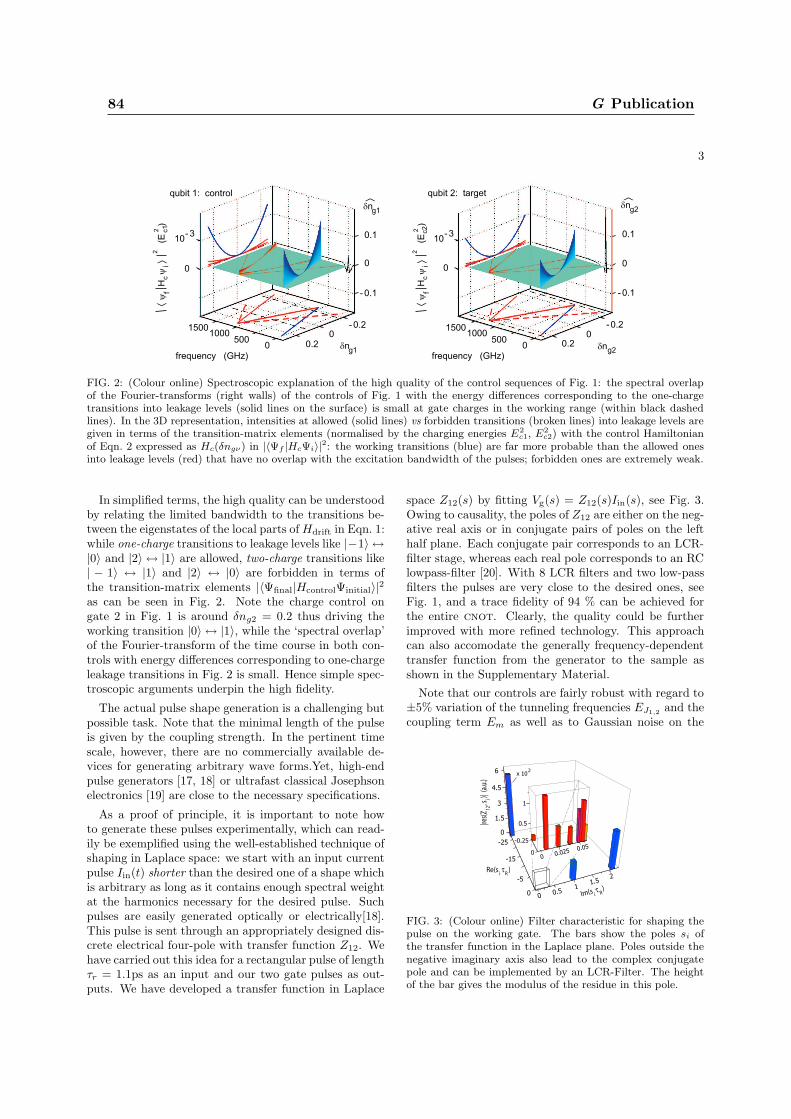
84 G Publication
3
FIG. 2: (Colour online) Spectroscopic explanation of the high quality of the control sequences of Fig. 1: the spectral overlapof the Fourier-transforms (right walls) of the controls of Fig. 1 with the energy differences corresponding to the one-chargetransitions into leakage levels (solid lines on the surface) is small at gate charges in the working range (within black dashedlines). In the 3D representation, intensities at allowed (solid lines) vs forbidden transitions (broken lines) into leakage levels aregiven in terms of the transition-matrix elements (normalised by the charging energies E
2
c1, E2
c2) with the control Hamiltonianof Eqn. 2 expressed as Hc(δngν) in |〈Ψf |HcΨi〉|
2: the working transitions (blue) are far more probable than the allowed onesinto leakage levels (red) that have no overlap with the excitation bandwidth of the pulses; forbidden ones are extremely weak.
In simplified terms, the high quality can be understoodby relating the limited bandwidth to the transitions be-tween the eigenstates of the local parts of Hdrift in Eqn. 1:while one-charge transitions to leakage levels like |−1〉 ↔|0〉 and |2〉 ↔ |1〉 are allowed, two-charge transitions like| − 1〉 ↔ |1〉 and |2〉 ↔ |0〉 are forbidden in terms ofthe transition-matrix elements |〈Ψfinal|HcontrolΨinitial〉|
2
as can be seen in Fig. 2. Note the charge control ongate 2 in Fig. 1 is around δng2 = 0.2 thus driving theworking transition |0〉 ↔ |1〉, while the ‘spectral overlap’of the Fourier-transform of the time course in both con-trols with energy differences corresponding to one-chargeleakage transitions in Fig. 2 is small. Hence simple spec-troscopic arguments underpin the high fidelity.
The actual pulse shape generation is a challenging butpossible task. Note that the minimal length of the pulseis given by the coupling strength. In the pertinent timescale, however, there are no commercially available de-vices for generating arbitrary wave forms.Yet, high-endpulse generators [17, 18] or ultrafast classical Josephsonelectronics [19] are close to the necessary specifications.
As a proof of principle, it is important to note howto generate these pulses experimentally, which can read-ily be exemplified using the well-established technique ofshaping in Laplace space: we start with an input currentpulse Iin(t) shorter than the desired one of a shape whichis arbitrary as long as it contains enough spectral weightat the harmonics necessary for the desired pulse. Suchpulses are easily generated optically or electrically[18].This pulse is sent through an appropriately designed dis-crete electrical four-pole with transfer function Z12. Wehave carried out this idea for a rectangular pulse of lengthτr = 1.1ps as an input and our two gate pulses as out-puts. We have developed a transfer function in Laplace
space Z12(s) by fitting Vg(s) = Z12(s)Iin(s), see Fig. 3.Owing to causality, the poles of Z12 are either on the neg-ative real axis or in conjugate pairs of poles on the lefthalf plane. Each conjugate pair corresponds to an LCR-filter stage, whereas each real pole corresponds to an RClowpass-filter [20]. With 8 LCR filters and two low-passfilters the pulses are very close to the desired ones, seeFig. 1, and a trace fidelity of 94 % can be achieved forthe entire cnot. Clearly, the quality could be furtherimproved with more refined technology. This approachcan also accomodate the generally frequency-dependenttransfer function from the generator to the sample asshown in the Supplementary Material.
Note that our controls are fairly robust with regard to±5% variation of the tunneling frequencies EJ1,2
and thecoupling term Em as well as to Gaussian noise on the
0
-5
-15
-25
0
1.5
3
4.5
6
0.5
1
0
-0.25
00.5
11.5
2
00.0250.05
|res
(Z12
, si)|
(a.u
.)
Re(siτ
R)
Im(s iτ R
)
x 10 2
FIG. 3: (Colour online) Filter characteristic for shaping thepulse on the working gate. The bars show the poles si ofthe transfer function in the Laplace plane. Poles outside thenegative imaginary axis also lead to the complex conjugatepole and can be implemented by an LCR-Filter. The heightof the bar gives the modulus of the residue in this pole.
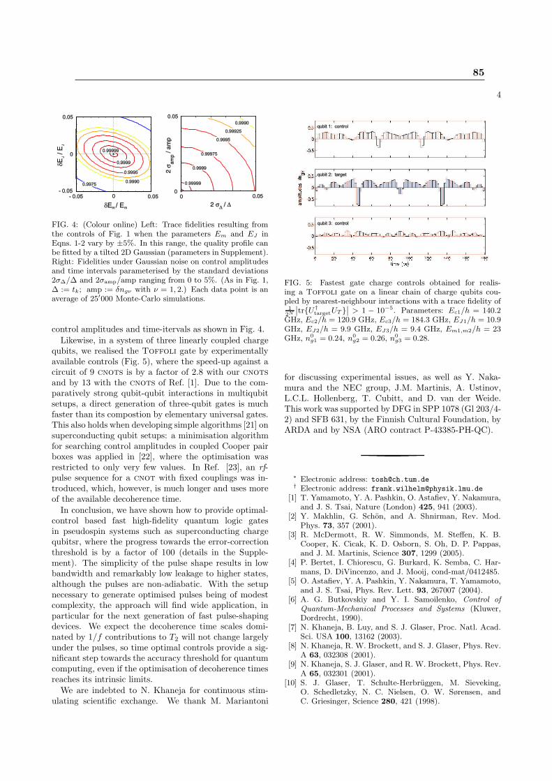
85
4
FIG. 4: (Colour online) Left: Trace fidelities resulting fromthe controls of Fig. 1 when the parameters Em and EJ inEqns. 1-2 vary by ±5%. In this range, the quality profile canbe fitted by a tilted 2D Gaussian (parameters in Supplement).Right: Fidelities under Gaussian noise on control amplitudesand time intervals parameterised by the standard deviations2σ∆/∆ and 2σamp/amp ranging from 0 to 5%. (As in Fig. 1,∆ := tk; amp := δngν with ν = 1, 2.) Each data point is anaverage of 25′000 Monte-Carlo simulations.
control amplitudes and time-itervals as shown in Fig. 4.
Likewise, in a system of three linearly coupled chargequbits, we realised the Toffoli gate by experimentallyavailable controls (Fig. 5), where the speed-up against acircuit of 9 cnots is by a factor of 2.8 with our cnots
and by 13 with the cnots of Ref. [1]. Due to the com-paratively strong qubit-qubit interactions in multiqubitsetups, a direct generation of three-qubit gates is muchfaster than its compostion by elementary universal gates.This also holds when developing simple algorithms [21] onsuperconducting qubit setups: a minimisation algorithmfor searching control amplitudes in coupled Cooper pairboxes was applied in [22], where the optimisation wasrestricted to only very few values. In Ref. [23], an rf-pulse sequence for a cnot with fixed couplings was in-troduced, which, however, is much longer and uses moreof the available decoherence time.
In conclusion, we have shown how to provide optimal-control based fast high-fidelity quantum logic gatesin pseudospin systems such as superconducting chargequbitsr, where the progress towards the error-correctionthreshold is by a factor of 100 (details in the Supple-ment). The simplicity of the pulse shape results in lowbandwidth and remarkably low leakage to higher states,although the pulses are non-adiabatic. With the setupnecessary to generate optimised pulses being of modestcomplexity, the approach will find wide application, inparticular for the next generation of fast pulse-shapingdevices. We expect the decoherence time scales domi-nated by 1/f contributions to T2 will not change largelyunder the pulses, so time optimal controls provide a sig-nificant step towards the accuracy threshold for quantumcomputing, even if the optimisation of decoherence timesreaches its intrinsic limits.
We are indebted to N. Khaneja for continuous stim-ulating scientific exchange. We thank M. Mariantoni
FIG. 5: Fastest gate charge controls obtained for realis-ing a Toffoli gate on a linear chain of charge qubits cou-pled by nearest-neighbour interactions with a trace fidelity of1
2N
˛
˛trU†targetUT
˛
˛ > 1 − 10−5. Parameters: Ec1/h = 140.2GHz, Ec2/h = 120.9 GHz, Ec3/h = 184.3 GHz, EJ1/h = 10.9GHz, EJ2/h = 9.9 GHz, EJ3/h = 9.4 GHz, Em1,m2/h = 23GHz, n0
g1 = 0.24, n0g2 = 0.26, n0
g3 = 0.28.
for discussing experimental issues, as well as Y. Naka-mura and the NEC group, J.M. Martinis, A. Ustinov,L.C.L. Hollenberg, T. Cubitt, and D. van der Weide.This work was supported by DFG in SPP 1078 (Gl 203/4-2) and SFB 631, by the Finnish Cultural Foundation, byARDA and by NSA (ARO contract P-43385-PH-QC).
∗ Electronic address: [email protected]† Electronic address: [email protected]
[1] T. Yamamoto, Y. A. Pashkin, O. Astafiev, Y. Nakamura,and J. S. Tsai, Nature (London) 425, 941 (2003).
[2] Y. Makhlin, G. Schon, and A. Shnirman, Rev. Mod.Phys. 73, 357 (2001).
[3] R. McDermott, R. W. Simmonds, M. Steffen, K. B.Cooper, K. Cicak, K. D. Osborn, S. Oh, D. P. Pappas,and J. M. Martinis, Science 307, 1299 (2005).
[4] P. Bertet, I. Chiorescu, G. Burkard, K. Semba, C. Har-mans, D. DiVincenzo, and J. Mooij, cond-mat/0412485.
[5] O. Astafiev, Y. A. Pashkin, Y. Nakamura, T. Yamamoto,and J. S. Tsai, Phys. Rev. Lett. 93, 267007 (2004).
[6] A. G. Butkovskiy and Y. I. Samoilenko, Control of
Quantum-Mechanical Processes and Systems (Kluwer,Dordrecht, 1990).
[7] N. Khaneja, B. Luy, and S. J. Glaser, Proc. Natl. Acad.Sci. USA 100, 13162 (2003).
[8] N. Khaneja, R. W. Brockett, and S. J. Glaser, Phys. Rev.A 63, 032308 (2001).
[9] N. Khaneja, S. J. Glaser, and R. W. Brockett, Phys. Rev.A 65, 032301 (2001).
[10] S. J. Glaser, T. Schulte-Herbruggen, M. Sieveking,O. Schedletzky, N. C. Nielsen, O. W. Sørensen, andC. Griesinger, Science 280, 421 (1998).
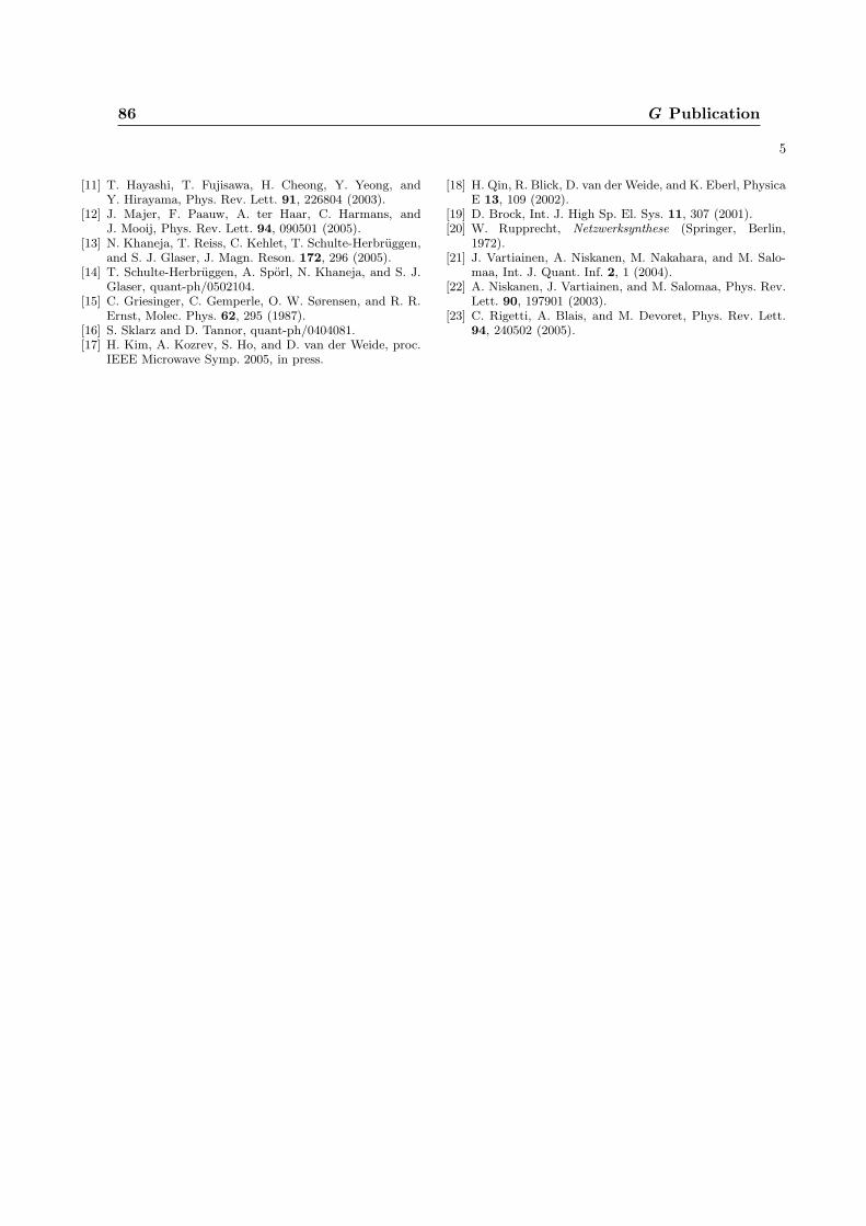
86 G Publication
5
[11] T. Hayashi, T. Fujisawa, H. Cheong, Y. Yeong, andY. Hirayama, Phys. Rev. Lett. 91, 226804 (2003).
[12] J. Majer, F. Paauw, A. ter Haar, C. Harmans, andJ. Mooij, Phys. Rev. Lett. 94, 090501 (2005).
[13] N. Khaneja, T. Reiss, C. Kehlet, T. Schulte-Herbruggen,and S. J. Glaser, J. Magn. Reson. 172, 296 (2005).
[14] T. Schulte-Herbruggen, A. Sporl, N. Khaneja, and S. J.Glaser, quant-ph/0502104.
[15] C. Griesinger, C. Gemperle, O. W. Sørensen, and R. R.Ernst, Molec. Phys. 62, 295 (1987).
[16] S. Sklarz and D. Tannor, quant-ph/0404081.[17] H. Kim, A. Kozrev, S. Ho, and D. van der Weide, proc.
IEEE Microwave Symp. 2005, in press.
[18] H. Qin, R. Blick, D. van der Weide, and K. Eberl, PhysicaE 13, 109 (2002).
[19] D. Brock, Int. J. High Sp. El. Sys. 11, 307 (2001).[20] W. Rupprecht, Netzwerksynthese (Springer, Berlin,
1972).[21] J. Vartiainen, A. Niskanen, M. Nakahara, and M. Salo-
maa, Int. J. Quant. Inf. 2, 1 (2004).[22] A. Niskanen, J. Vartiainen, and M. Salomaa, Phys. Rev.
Lett. 90, 197901 (2003).[23] C. Rigetti, A. Blais, and M. Devoret, Phys. Rev. Lett.
94, 240502 (2005).
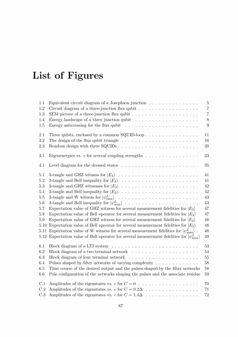
List of Figures
1.1 Equivalent circuit diagram of a Josephson junction . . . . . . . . . . . . . . . 51.2 Circuit diagram of a three-junction flux qubit . . . . . . . . . . . . . . . . . . 71.3 SEM picture of a three-junction flux qubit . . . . . . . . . . . . . . . . . . . . 71.4 Energy landscape of a three junction qubit . . . . . . . . . . . . . . . . . . . 81.5 Energy anticrossing for the flux qubit . . . . . . . . . . . . . . . . . . . . . . 9
2.1 Three qubits, enclosed by a common SQUID-loop . . . . . . . . . . . . . . . . 112.2 The design of the flux qubit triangle . . . . . . . . . . . . . . . . . . . . . . . 162.3 Readout design with three SQUIDs . . . . . . . . . . . . . . . . . . . . . . . . 20
3.1 Eigenenergies vs. ε for several coupling strengths . . . . . . . . . . . . . . . . 23
4.1 Level diagram for the dressed states . . . . . . . . . . . . . . . . . . . . . . . 35
5.1 3-tangle and GHZ witness for |E3〉 . . . . . . . . . . . . . . . . . . . . . . . . 415.2 3-tangle and Bell inequality for |E3〉. . . . . . . . . . . . . . . . . . . . . . . . 415.3 3-tangle and GHZ witnesses for |E2〉 . . . . . . . . . . . . . . . . . . . . . . . 425.4 3-tangle and Bell inequality for |E2〉. . . . . . . . . . . . . . . . . . . . . . . . 425.5 3-tangle and W witness for |ψL
max〉 . . . . . . . . . . . . . . . . . . . . . . . . 435.6 3-tangle and Bell inequality for |ψL
max〉 . . . . . . . . . . . . . . . . . . . . . . 435.7 Expectation value of GHZ witness for several measurement fidelities for |E3〉 475.8 Expectation value of Bell operator for several measurement fidelities for |E3〉 475.9 Expectation value of GHZ witness for several measurement fidelities for |E2〉 485.10 Expectation value of Bell operator for several measurement fidelities for |E2〉 485.11 Expectation value of W witness for several measurement fidelities for |ψL
max〉 . 485.12 Expectation value of Bell operator for several measurement fidelities for |ψL
max〉 49
6.1 Block diagram of a LTI system . . . . . . . . . . . . . . . . . . . . . . . . . . 536.2 Block diagram of a two terminal network . . . . . . . . . . . . . . . . . . . . 546.3 Block diagram of four terminal network . . . . . . . . . . . . . . . . . . . . . 556.4 Pulses shaped by filter networks of varying complexity . . . . . . . . . . . . . 586.5 Time course of the desired output and the pulses shaped by the filter networks 586.6 Pole configuration of the networks shaping the pulses and the associate residue 59
C.1 Amplitudes of the eigenstates vs. ε for C = 0 . . . . . . . . . . . . . . . . . . 70C.2 Amplitudes of the eigenstates vs. ε for C = 0.2∆ . . . . . . . . . . . . . . . . 71C.3 Amplitudes of the eigenstates vs. ε for C = 1.4∆ . . . . . . . . . . . . . . . . 72
87

88 List of Figures
F.1 Realization of a RC-filter by iterative pole elimination . . . . . . . . . . . . . 78F.2 Serial connection of two four-poles . . . . . . . . . . . . . . . . . . . . . . . . 79
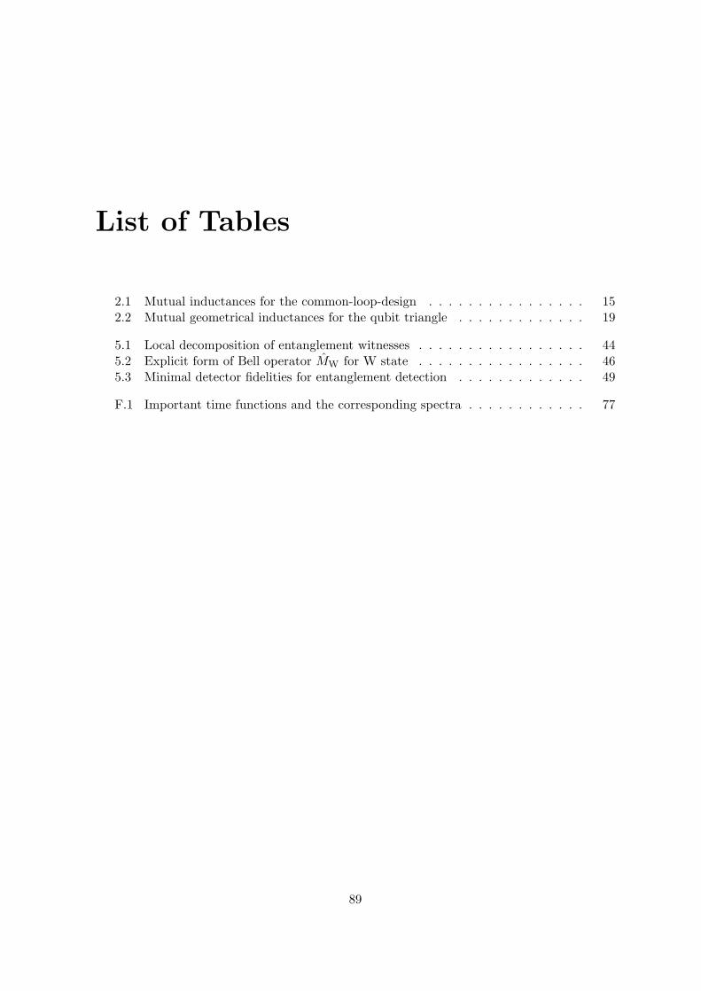
List of Tables
2.1 Mutual inductances for the common-loop-design . . . . . . . . . . . . . . . . 152.2 Mutual geometrical inductances for the qubit triangle . . . . . . . . . . . . . 19
5.1 Local decomposition of entanglement witnesses . . . . . . . . . . . . . . . . . 445.2 Explicit form of Bell operator MW for W state . . . . . . . . . . . . . . . . . 465.3 Minimal detector fidelities for entanglement detection . . . . . . . . . . . . . 49
F.1 Important time functions and the corresponding spectra . . . . . . . . . . . . 77
89

90 List of Tables

Bibliography
[1] D. Deutsch, Quantum Theory, the Church-Turing Principle and the Universal QuantumComputer, Proc. Roy. Soc. Lond. A 400, 97 (1985).
[2] P. W. Shor, in Proc. 35nd Annual Symposium on the Foundations of Computer Science,edited by S. Goldwasser (IEEE Computer Society Press, 1994), pp. 124–134.
[3] C. Bennett and D. P. DiVincenzo, Quantum Computing—Towards an engineering era?,Nature 377, 389 (1995).
[4] L. K. Grover, Quantum Mechanics Helps in Searching for a Needle in a Haystack, Phys.Rev. Lett. 79, 325 (1997).
[5] D. P. DiVincenzo, Quantum Computation, Science 270, 255 (1995).
[6] F. Schmidt-Kaler, H. Haffner, M. Riebe, S. Gulde, G. P. T. Lancaster, T. Deuschle,C. Becher, C. F. Roos, J. Eschner, and R. Blatt, Realization of the Cirac-Zoller controlled-NOT quantum gate, Nature 422, 408 (2003).
[7] E. Knill, R. Laflamme, and G. J. Milburn, A scheme for efficient quantum computationwith linear optics, Nature 409, 46 (2001).
[8] L. M. K. Vandersypen and I. L. Chuang, Nmr techniques for quantum control and com-putation, Rev. Mod. Phys. 76, 1037 (2004).
[9] S. J. Glaser, T. Schulte-Herbruggen, M. Sieveking, O. Schedletzky, N. C. Nielsen, O. W.Sørennsen, and C. Griesinger, Unitary Control in Quantum Ensembles, Maximising Sig-nal Intensity in Coherent Spectroscopy, Science 280, 421 (1998).
[10] S. J. Glaser, NMR Quantum Computing, Angew. Chem. Int. Ed. 40, 147 (2001).
[11] L. M. K. Vandersypen, M. Steffen, G. Breyta, C. S. Yannoni, M. H. Sherwood, and I. L.Chuang, Experimental realization of Shor’s quantum factoring algorithm using nuclearmagnetic resonance, Nature 414, 883 (2001).
[12] Y. Makhlin, G. Schon, and A. Shnirman, Quantum-state engineering with Josephson-junction devices, Rev. Mod. Phys. 73, 357 (2001).
[13] V. Cerletti, W. A. Coish, O. Gywat, and D. Loss, Recipes for spin-based quantum com-puting, Nanotechnology 16, R27 (2005).
91
92 BIBLIOGRAPHY
[14] C. H. van der Wal, A. ter Haar, F. Wilhelm, R. Schouten, C. Harmans, T. Orlando,S. Lloyd, and J. Mooij, Quantum Superposition of Macroscopic Persistent-Current States,Science 290, 773 (2000).
[15] I. Chiorescu, Y. Nakamura, C. Harmans, and J. Mooij, Coherent Quantum Dynamics ofa Superconducting Flux Qubit, Science 299, 1869 (2003).
[16] A. C. J. ter Haar, PhD thesis, TU Delft (2005).
[17] Y. A. Pashkin, T. Yamamoto, O. Astafiev, Y. Nakamura, D. V. Averin, and J. S. Tsai,Quantum oscillations in two coupled charge qubits, Nature 421, 823 (2003).
[18] T. Yamamoto, Y. A. Pashkin, O. Astafiev, Y. Nakamura, and J. S. Tsai, Demonstra-tion of conditional gate operation using superconducting charge qubits, Nature 425, 941(2003).
[19] M. Tinkham, Introduction to Superconductivity (McGraw-Hill, 1996).
[20] J. E. Mooij, T. P. Orlando, L. Levitov, L. Tian, C. H. van der Wal, and S. Lloyd,Josephson Persistent-Current Qubit, Science 285, 1036 (1999).
[21] C. H. van der Wal, PhD thesis, TU Delft (2001).
[22] T. P. Orlando, J. E. Mooij, L. Tian, C. H. van der Wal, L. S. Levitov, S. Lloyd, and J. J.Mazo, Superconducting persistent-current qubit, Phys. Rev. B 60, 15398 (1999).
[23] P. Bertet, I. Chiorescu, G. Burkard, K. Semba, C. Harmans, D. DiVincenzo, and J. Mooij,Relaxation and dephasing in a flux qubit, cond-mat/0412485 (2004).
[24] A. J. Leggett, S. Chakravarty, A. T. Dorsey, M. P. A. Fisher, A. Garg, and W. Zwerger,Dynamics of the dissipative two-state system, Rev. Mod. Phys. 59, 1 (1987).
[25] B. L. T. Plourde, J. Zhang, K. B. Whaley, F. K. Wilhelm, T. L. Robertson, T. Hime,S. Linzen, P. A. Reichardt, C.-E. Wu, and J. Clarke1, Entangling flux qubits with abipolar dynamic inductance, PRB 70, 140501 (2004).
[26] J. Clarke and A. I. Braginski, The SQUID Handbook, Vol.1 : Fundamentals and Tech-nology of SQUIDs and SQUID Systems (John Wiley & Sons Inc, 2004).
[27] A. Wallraff, D. I. Schuster, A. Blais, L. Frunzio, J. Majer, M. H. Devoret, S. M. Girvin,and R. J. Schoelkopf, Approaching Unit Visibility for Control of a Superconducting Qubitwith Dispersive Readout, Phys. Rev. Lett. 95, 060501 (2005).
[28] A. Lupascu, C. J. Verwijs, R. N. Schouten, C. J. P. Harmans, and J. E. Mooij, Nonde-structive Readout for a Superconducting Flux Qubit, Phys. Rev. Lett. 93, 177006 (2004).
[29] A. Lupascu, C. J. P. Harmans, and J. E. Mooij, Quantum state detection of a supercon-ducting flux qubit using a dc-SQUID in the inductive mode, Phys. Rev. B 71, 184506(2005).
[30] J. David Jackson, Klassische Elektrodynamik (De Gruyter, 2002).
[31] Fasthenry, URL http://www.wrcad.com/ftp/pub/fasthenry-3.0wr.tar.gz.

BIBLIOGRAPHY 93
[32] M. Grifoni and P. Hanggi, Driven quantum tunneling, Phys. Reports 304, 229 (1998).
[33] C. Cohen-Tannoudji, J. Dupont-Roc, and G. Grynberg, Atom–Photon Interactions (Wi-ley, 1998).
[34] D. Walls and G. Milburn, Qantum Optics (Springer, 1994).
[35] E. Schrodinger, Proc. Cambridge Philos. Soc 31, 555 (1935).
[36] S. Popescu and D. Rohrlich, in Introduction to Quantum Computation and Information(World Scientific, 1998).
[37] C. H. Bennett, G. Brassard, C. Crepeau, R. Jozsa, A. Peres, and W. K. Wootters,Teleporting an unknown quantum state via dual classical and Einstein-Podolsky-Rosenchannels, Phys. Rev. Lett. 70, 1895 (1993).
[38] M. Riebe, H. Haffner, C. F. Roos, W. Hansel, J. Benhelm, G. P. T. Lancaster, T. W.Korber, C. Becher, F. Schmidt-Kaler, D. F. V. James, et al., Deterministic quantumteleportation with atoms, Nature 429, 734 (2004).
[39] A. Ekert, Quantum Cryptography Based on Bell’s Theorem, Phys. Rev. Lett. 67, 661(1991).
[40] A. Einstein, B. Podolsky, and N. Rosen, Can Quantum-Mechanical Description of RealityBe Considered Complete?, Phys. Rev. 41, 777 (1935).
[41] J. Bell, On the Einstein-Podolsky-Rosen Paradox, Physics 1, 195 (1964).
[42] S. J. Freedman and J. F. Clauser, Experimental Test of Local Hidden-Variable Theories,Phys. Rev. Lett. 28, 938 (1972).
[43] C. Bennett and D. P. DiVincenzo, Experimental Test of Bell’s Inequalities Using Time-Varying Analyzers, Phys. Rev. Lett. 49, 1804 (1982).
[44] G. Weihs, T. Jennewein, C. Simon, H. Weinfurter, and A. Zeilinger, Violation of Bell’sInequality under Strict Einstein Locality Conditions, Phys. Rev. Lett. 81, 5039 (1998).
[45] M. A. Rowe, D. Kielpinsky, V. Meyer, C. A. Sacket, W. M. Itano, C. Monroe, and D. J.Wineland, Experimental violation of a Bell’s inequality with efficient detection, Nature409, 791 (2001).
[46] A. Peres, Separability Criterion for Density Matrices, Phys. Rev. Lett. 77, 1413 (1996).
[47] W. Dur, G. Vidal, and J. Cirac, Three qubits can be entangled in two inequivalent ways,Phys. Rev. A 62, 062314 (2000).
[48] I. C. M. A. Nielsen, Quantum Computation and Quantum Information (Cambridge Uni-versity Press, 2000).
[49] D. M. Greenberger, M. Horne, and A. Zeilinger, in Bell’s Theorem, Quantum Theoryand Conceptions of the Universe (Kluver Academic, 1989).
[50] V. Coffman, J. Kundu, and W. K. Wootters, Distributed entanglement, Phys. Rev. A61, 052306 (2000).
94 BIBLIOGRAPHY
[51] B. M. Terhal, Bell inequalities and the separability criterion, Phys. Lett. A 271, 319(2000).
[52] M. Lewenstein, B. Kraus, J. I. Cirac, and P. Horodecki, Optimization of entanglementwitnesses, Phys. Rev. A 62, 052310 (2000).
[53] J. Eisert, P. Hyllus, O. Guhne, and M. Curty, Complete hierarchies of efficient approxi-mations to problems in entanglement theory, Phys. Rev. A 70, 062317 (2004).
[54] F. G. S. L. B. ao, Quantifying entanglement with witness operators, Phys. Rev. A 72,022310 (2005).
[55] O. Guhne and P. Hyllus, Investigating Three Qubit Entanglement With Local Measure-ments, Int. J. Theor. Phys. 42, 1001 (2003).
[56] M. Bourennane, M. Eibl, C. Kurtsiefer, S. Gaertner, H. Weinfurter, O. Guhne, P. Hyl-lus, D. Bruß, M. Lewenstein, and A. Sanpera, Experimental Detection of MultipartiteEntanglement using Witness Operators, Phys. Rev. Lett. 92, 087902 (2004).
[57] G. Toth and O. Guhne, Detecting Genuine Multipartite Entanglement with Two LocalMeasurements, Phys. Rev. Lett. 94, 060501 (2005).
[58] A. Acın, D. Bruß, M. Lewenstein, and A. Sanpera, Classification of Mixed Three-QubitStates, Phys. Rev. Lett. 87, 040401 (2001).
[59] D. M. Greenberger, M. A. Horne, A. Shimony, and A. Zeilinger, Bell’s theorem withoutinequalities, Am. J. Phys. 58, 1131 (1990).
[60] N. D. Mermin, Quantum mysteries revisited, Am. J. Phys. 58, 731 (1990).
[61] N. D. Mermin, Extreme Quantum Entanglement in a Superposition of MacroscopicallyDistinct States, Phys. Rev. Lett. 65, 1838 (1990).
[62] A. V. Belinskii and D. N. Klyshko, Interference of light and Bell’s theorem, Phys. Usp.36, 653 (1993).
[63] D. N. Klyshko, The Bell and GHZ theorems: a possible three-photon interference exper-iment and the question of nonlocality, Phys. Lett. A 172, 399 (1993).
[64] J. Endrejat and H. Buttner, Characterization of entanglement of more than two qubitswith Bell inequalities and global entanglement, Phys. Rev. A 71, 012305 (2005).
[65] C. Emary and C. W. J. Beenakker, Relation between entanglement measures and Bellinequalities for three qubits, Phys. Rev. A 69, 032317 (2004).
[66] J. Endrejat (2005), priv. comm.
[67] J. F. Clauser, M. A. Horne, A. Shimony, and R. A. Holt, Proposed Experiment to TestLocal Hidden-Variable Theories, Phys. Rev. Lett. 23, 880 (1969).
[68] M. J. Storcz, PhD thesis, LMU Munchen (2005).

BIBLIOGRAPHY 95
[69] I. Siddiqi, R. Vijay, F. Pierre, C.M.Wilson, M. Metcalfe, C. Rigetti, L. Frunzio, andM. H. Devoret, RF-Driven Josephson Bifurcation Amplifier for Quantum Measurement,Phys. Rev. Lett. 93, 20702 (2004).
[70] O. Astafiev, Y. A. Pashkin, T. Yamamoto, Y. Nakamura, and J. S. Tsai, Single-shotmeasurement of the Josephson charge qubit, Phys. Rev. B 69, 180507 (2004).
[71] N. Khaneja, T. Reiss, C. Kehlet, T. Schulte-Herbruggen, and S. J. Glaser, Optimal controlof coupled spin dynamics: design of NMR pulse sequences by gradient ascent algorithms,J. Magn. Reson. 172, 296 (2005).
[72] R. Fazio, G. M. Palma, and J. Siewert, Fidelity and Leakage of Josephson Qubits, Phys.Rev. Lett. 83, 5385 (1999).
[73] Ohm and Luke, Signalubertragung (Springer, 2004).
[74] W. Rupprecht, Netzwerksynthese (Springer, 1972).
[75] B. Ferguson and X.-C. Zhang, Materials for terahertz science and technology, NatureReview Article 1, 26 (2002).
[76] A. Zewail, in Nobel Lectures, Chemistry 1996-2000, edited by I. Grenthe (World ScientificPublishing Co., 2003).
[77] T. Fließbach, Quantenmechanik (Spekrum Verlag, 1995).
[78] G. Vidal, Entanglement monotones, J. Mod. Opt. 47, 355 (2000).
[79] C. H. Bennett, S. Popescu, D. Rohrlich, J. A. Smolin, and A. V. Thapliyal, Exact andasymptotic measures of multipartite pure-state entanglement, Phys. Rev. A 63, 012307(2001).
[80] C. H. Bennett, D. P. DiVincenzo, J. A. Smolin, and W. K. Wootters, Mixed-state entan-glement and quantum error correction, Phys. Rev. Lett. 54, 3824 (1996).
[81] S. Hill and W. K. Wootters, Entanglement of a Pair of Quantum Bits, Phys. Rev. Lett.78, 5022 (1997).
[82] W. K. Wootters, Entanglement of Formation of an Arbitrary State of Two Qubits, Phys.Rev. Lett. 80, 2245 (1998).
Related Documents