Efficient cost allocation ∗ Korok Ray McDonough School of Business Georgetown University Washington, DC 20057 e-mail: [email protected] Maris Goldmanis Department of Economics University of Chicago 1101 E. 58th Street Chicago, IL 60637 phone: 773-955-1891 e-mail: [email protected] Abstract Firms routinely allocate the costs of common corporate resources down to divisions. The main insight of this paper is that any efficient allocation rule must reflect the firm’s underlying cost structure. We propose a new allocation rule (the polynomial rule), which achieves efficiency and approximate budget balance. We also examine conditions under which simple allocation rules induce efficiency. Finally, we show that welfare losses due to linear allocation rules increase with firm size. Thus polynomial allocation rules should be preferred to linear rules for larger firms. JEL Classification codes: D21, D82, M41. Keywords: Cost allocation, cost sharing, mechanism design, teams, efficiency. * All correspondence should be directed to Maris Goldmanis. We would like to thank Canice Prendergast, Madhav Rajan, Stefan Reichelstein, and participants of the Chicago Accounting brown bag for helpful comments and suggestions. Alex Frankel provided outstanding research assistance. University of Chicago GSB provided generous financial support.

Welcome message from author
This document is posted to help you gain knowledge. Please leave a comment to let me know what you think about it! Share it to your friends and learn new things together.
Transcript
Efficient cost allocation∗
Korok Ray
McDonough School of Business
Georgetown University
Washington, DC 20057
e-mail: [email protected]
Maris Goldmanis
Department of Economics
University of Chicago
1101 E. 58th Street
Chicago, IL 60637
phone: 773-955-1891
e-mail: [email protected]
Abstract
Firms routinely allocate the costs of common corporate resources down to divisions.
The main insight of this paper is that any efficient allocation rule must reflect the firm’s
underlying cost structure. We propose a new allocation rule (the polynomial rule), which
achieves efficiency and approximate budget balance. We also examine conditions under
which simple allocation rules induce efficiency. Finally, we show that welfare losses due to
linear allocation rules increase with firm size. Thus polynomial allocation rules should be
preferred to linear rules for larger firms.
JEL Classification codes: D21, D82, M41.
Keywords: Cost allocation, cost sharing, mechanism design, teams, efficiency.
∗All correspondence should be directed to Maris Goldmanis. We would like to thank Canice Prendergast,
Madhav Rajan, Stefan Reichelstein, and participants of the Chicago Accounting brown bag for helpful comments
and suggestions. Alex Frankel provided outstanding research assistance. University of Chicago GSB provided
generous financial support.

1 Introduction
The multiple divisions within a firm often share a variety of common resources, such as informa-
tion technology, legal services, human resource management, executive time, etc. Managerial
accounting textbooks (Horngren et al. (2005), Zimmerman (2006)) and surveys of company
practice (Fremgen and Liao (1981), Atkinson (1987), Ramadan (1989), Dean et al. (1991)) doc-
ument the widespread practice of common cost allocation to induce appropriate consumption
of corporate resources. For example, if divisions were not allocated any corporate costs, they
may have adverse incentives to overconsume such common resources. The objective of this
paper is to examine cost allocation rules that solve this free-rider problem, i.e. induce efficient
resource use by divisions acting simultaneously and independently.
We demonstrate that the main feature of any efficient allocation is that it must reflect the
firm’s underlying costs. While this point may seem obvious, the linear rules used in practice
make allocations without regard to the shape of the firm’s cost function, and this keeps such
rules from achieving efficiency. The reason for this failure is straightforward: charging for each
unit of common resource used at the same constant rate (whether an actual average cost or a
budgeted per-unit overhead rate) ignores the fact that the actual marginal cost of each unit
of resource used may depend on the total amount of resources used (for example, if the firm’s
cost function is highly convex, it is much more costly for the firm to acquire an additional unit
of the resource if it already has a hundred than if it only had one). Consequently, under such
cost allocation schemes, the price that a division pays for an additional unit of resource (the
private cost to the division) differs from the actual marginal cost to the firm, which causes
inefficient resource consumption decisions by the division.
The analysis here operates in environments that more closely resemble real-world settings,
with the aim of recommending cost allocations that will be practically useful to managers.
First, we depart from formal mechanism design theory (such as Green and Laffont (1979)) in
that we assume that the private information of the divisional managers is too complex to be em-
bedded within the firm’s contracts. Therefore, the firm cannot perfectly obtain the manager’s
entire private information through a complex reporting game and through contracts that de-
pend on announcements of private information. While formal mechanism design has spawned
an enormous literature on incentives, it requires a large amount of information (knowledge of
all production and utility functions, rich contract spaces, etc.). Thus it has been unable to
provide concrete advice to actual managers, since it relies on menus of contracts that enjoy
nice theoretical properties but are rarely adopted in practice (see Rogerson (2003) and Wilson
(1987) for a fully articulated critique). Instead, we propose a world where private informa-
tion is sufficiently complex, communication is sufficiently costly, and contracts are sufficiently
2
incomplete that the Revelation Principle no longer applies. Divisional managers have private
information on their divisional production functions, but cannot perfectly communicate this
information to the central office via a complex menu of contracts.
The class of efficient cost allocations turns out to be large. However, the class of efficient
cost allocations to be used in practice can be narrowed down by imposing additional desirable
properties on these allocations. In line with our main goal of capturing a more realistic firm
environment, we require cost allocation rules to satisfy certain properties of actual allocation
methods used in practice. Like the early cooperative cost allocation literature, we impose
certain axioms on allocation rules and explore when some or all of these axioms can be satisfied.
In particular, an allocation is budget balancing if the sum of the allocated costs equals total
cost; an allocation is fair if a division pays nothing if it consumes none of the resource; and an
allocation is simple if it can be written as a ratio. Linear allocation rules commonly used in
practice satisfy all three properties, though they are not efficient. Requiring these properties
constrains the set of possible efficient allocation rules. For example, the firm could easily charge
every division the full corporate cost. While this would achieve efficiency for each division, it
would grossly break the budget. The question we set out to answer is whether it is possible to
construct efficient cost allocation rules that possess any of these additional desirable properties.
We show that it is possible to construct allocations that are efficient and approximately
budget balancing. This allocation rule (called the polynomial allocation) induces efficient
resource levels, but may exhibit a small budget imbalance. For firms with more divisions, this
budget imbalance shrinks, eventually vanishing altogether. Numerical simulations show that
for a firm with as few as four divisions, these imbalances are a small fraction of total cost.
We give an explicit algorithm for calculating the polynomial allocation from the firm’s cost
function: first, fit a polynomial to the firm’s cost function, and then use the coefficients of that
polynomial to construct the allocation rule (specifically, use the coefficients to determine the
transfers to different divisions). This illustrates the main message that an efficient allocation
must reflect the firm’s cost function. In fact, the firm can use this explicit algorithm even if it
does not know its cost function exactly, but must estimate its cost function from internal cost
data. This makes the polynomial allocation useful in practice, as it reduces the informational
requirements of the allocation.
In addition to the result discussed above, we also show that it is possible to construct
allocations that are efficient, budget balancing, and simple if one of two special cases holds:
either all divisions have the same production function (i.e., are equally productive), or the firm
knows the relative efficient resource use levels (i.e., for each pair of divisions, i and j, the firm
knows that in an equilibrium division i will consume α times as much of the common resource
as division j will). However, it is generally not possible to construct cost allocations that, in
3
addition to efficiency and budget balance, also satisfy fairness.
Even though the linear rules used in practice are in general not efficient, they are widely
used in practice. Therefore, we conclude our analysis by exploring the welfare losses of linear
rules. In particular, we show that these welfare losses increase with the number of divisions.
Intuitively, linear rules are inefficient because they do not reflect the firm’s underlying costs,
and therefore do not adjust to changes in the firm’s cost function. The linear rule is a blunt
instrument to control managerial behavior compared to the efficient rule, which varies with
the firm’s underlying costs. An increase in the number of divisions aggravates the free-rider
problem, and linear rules are less capable of resolving this problem compared to efficient rules.
The existing literature on cost allocation spans both accounting and economics, and relies
on both cooperative and non-cooperative games. The older cooperative game theory approach
began with Shubik (1962), who suggested that the Shapley value of a game can be used to
allocate accounting costs. Subsequent papers have expanded on the Shapley allocation by in-
corporating notions of equity (Hughes and Scheiner (1980)), bargaining between agents (Roth
and Verrecchia (1979)), and even variations on the Shapley allocation closer to actual prac-
tice (Moriarity (1975), Louderback (1976), Gangolly (1981), Balachandran and Ramakrishnan
(1981)). The main problem with the cooperative approach is not only an inability to consider
agent-level incentives, but also the severe informational requirements of the cost function. In
cooperative models the cost function is defined on all subsets of agents, and this information
is necessary when forming the allocation. For these reasons, recent analytical work in cost
allocation has shifted into the non-cooperative realm.
Agency models of cost allocation take place in single-agent and multiple agent settings.
Single agent settings consider a principal who must compensate and possibly allocate costs
to an agent. For example, Baiman and Noel (1985) show that allocating costs can assist in
dynamic performance measurement. Magee (1988) shows that the agent’s optimal contract
can include a cost component based on activity levels to better control his unobservable effort
levels. Demski (1981) also takes a performance measurement approach and argues that cost
allocation is valuable if it provides additional information for contracting purposes. Because
these papers involve only a single agent, they do not consider issues of common cost allocation,
i.e., cost allocation across multiple divisions.
Some papers consider multiple agents. Suh (1987) shows that the principal may want to
include non-controllable costs in order to discourage collusion between the agents. Yet that
model does not explicitly speak to the form of the allocation rule, and instead asks whether
the compensation should or should not include non-controllable costs. Therefore Suh (1987)
is more a paper on whether you should allocate costs instead of how you should allocate
costs. Rajan (1992) shows that cost allocation schemes can serve a coordination purpose when
4
multiple agents have correlated private information. Baldenius et al. (2006) find that a cost
allocation based on hurdle rates of divisional reports to a central office is an optimal mechanism
in a multiple division, multiperiod setting. These last two papers both allow communication
between the agents and the principal and assume the principal can commit to a menu of
contracts. We do not make these assumptions on communication and commitment here.
There has been a recent surge of interest in simple and robust mechanism design. All such
papers begin with the observation that real-life mechanisms are much simpler than the complex
mechanisms articulated in theory. A handful of papers seek to calculate the welfare losses from
simple, common mechanisms used in practice. For example, Rogerson (2003) examines fixed-
price cost reimbursement contracts in the defense industry, McAfee (2002) considers matching
and rationing problems using only two priority classes, and Satterthwaite and Williams (2002)
explore the double auction as a simple trading mechanism. All three papers show that simple
mechanisms fare quite well, despite small efficiency losses. Hansen and Magee (2003) show
that linear allocation rules are robust in a model of a single decision-maker who must allocate
capacity to multiple products. In particular, as the number of products grows, linear allocation
rules become optimal because the expected benefit per unit of capacity is set equal across
project types. Another cluster of papers responds to the Wilson critique of mechanism design
(Wilson (1987)). Wilson argues that the main problem with complex mechanisms is that they
assume the mechanism designer knows the game that is played. Bergemann and Morris (2005)
and Arya et al. (2005) consider mechanisms that are robust to small perturbations in the
environment.
Like much of the prior cost allocation literature, this paper has several normative messages.
First and foremost, we show that, in order to achieve efficiency, the cost allocation rule must
reflect the firm’s underlying cost structure. Second, we take as given certain properties of
allocation rules which may reflect exogenous constraints, such as ease of accounting (budget
balance), bounded rationality (simplicity), and equity (fairness). We then explore when it is
possible to achieve efficiency subject to these constraints. The polynomial and simple allocation
rules proposed in this paper are intended for actual implementation in real-world environments,
the former when the firm has a large number of diverse divisions having private information
about their production functions, the latter when the firm is small and simplicity is paramount.
Both these recommended allocations share the feature that they reflect the firm’s underlying
costs, and show that embedding such costs into the allocation itself will bring the divisional
resources closer to efficient levels.
The paper is organized as follows. Section 2 provides a motivating example; Section 3
presents the main model and explores efficient allocation rules; Section 4 investigates budget
balance and constructs the efficient polynomial allocation rule that (approximately) imple-
5
ments it; Section 5 addresses the additional requirement of fairness; Section 6 examines simple
allocation rules; Section 7 investigates the welfare losses from linear allocation rules, and Sec-
tion 8 concludes.
2 A Motivating Example
To fix ideas, consider the following simple example of corporate cost allocation, as taught in
textbooks, classrooms, and as practiced in corporations. Imagine a firm that consists of two
divisions, labeled 1 and 2. Each division selects a resource consumption level for its own plant.
Each plant requires information technology (IT) support that the firm provides to all divisions.
The corporate IT department has both variable costs (number of computers per plant, number
of IT support engineers dedicated to each division) as well as fixed costs (overhead for the
IT division, salary of the IT department manager, general administrative costs of running the
department). The firm allocates these IT costs to each division to induce the efficient use of
corporate IT resources. Assume that plant resource level drives IT costs: as plant resource
level increases, so do corporate IT costs. Suppose division 1 consumes one unit of the resource
and division 2 consumes two units. This generates $9m of corporate IT costs for the firm.
Since plant resource consumption is the cost driver for IT costs, the firm will allocate IT costs
to each division based on its own resource level relative to total resource consumption. Thus
the allocated costs to each division are:
(
1
1 + 2
)
$9M = $3M for division 1,
(
2
1 + 2
)
$9M = $6M for division 2.
More generally, let x be division 1’s resource level, y be division 2’s resource level, and let
Si(x, y) be the share of corporate IT costs allocated to division i, for i = 1, 2. Then, allocating
costs according to relative resource levels is an allocation rule of
S1(x, y) =x
x + yand S2(x, y) =
y
x + y.
Call this allocation rule the linear rule. Observe that the linear rule satisfies budget balance,
or S1(x, y)+S2(x, y) = 1 for all x, y. For any set of resource levels, this rule always allocates all
costs down to the divisions, presumably to ease accounting calculations. Second, observe that
each division pays nothing if it consumes nothing, or S1(0, y) = 0 for all y and S2(x, 0) = 0 for
all x. This seems to satisfy some notion of equity or fairness, since a division is not charged if
6
it produces nothing. Finally, observe that the linear rule is simple in the sense that it can be
written as a ratio of each division’s activity level (resource level).
We take as given that these three properties of the linear allocation rule are a reduced-form
expression for the underlying economic environment of the firm. For example, perhaps making
accounting calculations is a time consuming activity and therefore budget balanced allocation
rules reduce these computing costs, or perhaps managers can more easily understand allocation
rules that are written as a simple ratio, or perhaps interdivisional conflict is a serious drain
on productivity and fair allocation rules reduce such conflict. Whatever the reasons, these
three properties represent the environment of the firm, and therefore set the stage for the
forthcoming analysis. The linear allocation rule certainly satisfies all three properties but it
is not efficient, as shown later. But is it possible to find an efficient allocation rule that also
satisfies any or all of the three properties? To get traction on this question, it is necessary to
articulate the model more precisely and define efficiency accordingly.
3 The Model
Consider a firm with n divisions and a central office. The firm has a decentralized structure:
each division acts as a profit center and therefore each divisional manager’s goal is to maximize
the profit of his or her division. Each division simultaneously selects a resource level ki. These
resources are assets such as plants, machines, human capital, etc. The production of the firm
is given by Φ, which is a function of all divisions’ resource levels, k1 through kn. We assume
that Φ(0, . . . , 0) = 0 and that the marginal productivity of division i takes the form
∂Φ
∂ki(k1, . . . , kn) = z(n)φi(ki)
for all i, where φi are positive-valued, strictly decreasing functions and z is a positive-valued,
strictly increasing function. In words, we assume that the marginal productivity of division
i decreases in its resource use, but increases in the size of the firm. This allows us to model
synergies in production, at the same time keeping the production function separable in the
production levels of individual divisions. We believe that this is a simple, reduced-form way to
model synergies between multiple divisions. As the number of divisions grows, these synergies
increase, and therefore each division’s marginal productivity increases. We now denote division
i’s production function by fi(ki) ≡∫ ki
0 z(n)φi(x)dx. Note that our assumptions on φi imply
that fi is strictly increasing and strictly concave for any i. Also notice that fi(ki)/z(n) would
give the production of a firm consisting of just division i. Lemma 1 in the Appendix shows that
Φ(k1, . . . , kn) =∑n
i=1 fi(ki), i.e., the production function is separable in individual divisions’
productions, as claimed above.
7
All divisions of the firm make use of a common, firm-wide resource, such as information
technology, corporate human resources, executive time, etc. The cost to the firm of the use
of this common resource given each division’s resource level is C(k1 + · · · + kn), where C
is strictly increasing, weakly convex, continuous, and twice continuously differentiable.1 Let
k = (k1, . . . , kn) be the resource vector, and let k−i = (k1, . . . , ki−1, ki+1, . . . kn) be the resource
vector for all divisions other than i. Furthermore, let K = k1 + . . . + kn be the total resource
level and K−i =∑
j 6=i kj , the total resource level for all divisions except i. We assume that the
feasible resource level set for each division i is bounded above by ki, so that k ∈∏n
i=1[0, ki]
and K ∈ [0, K], where K =∑n
i=1 ki.
The firm’s total profit isn∑
i=1
fi (ki) − C (K) .
Let k∗ ≡ {k∗i }
ni=1 denote the first-best efficient resource levels, i.e., the resource levels that
maximize the firm’s total profit. The first-order conditions for a maximum require that (for
all i) f ′i(k
∗i ) = C ′ (K∗), where K∗ =
∑
k∗j is the efficient total resource level.2 The production
functions fi are private information of the respective divisions, but resource level decisions
ki, current production levels fi(ki) and costs C(·) are common knowledge.3 This stands in
contrast to many agency models where effort is unobservable but utility functions are common
knowledge. While it is plausible that effort is legitimately unobservable, it is hard to believe
that resource consumption is unobservable. Internal accounting records document resource
levels, as the firm must use such numbers for budgeting and compensation purposes.
Contracts within the firm are incomplete, and so the firm cannot perfectly obtain the di-
visional manager’s private information through a complex menu of contracts and incentive
constraints. In this setting, the Revelation Principle does not apply. Contractual incomplete-
ness reflects the high costs of including complex private information within the contracts of
divisional managers. Indeed, while menus of contracts exhibit nice theoretical properties, they
are rarely observed in practice, and certainly not to the extent and complexity as predicted
by theory. One reason for this is that either the agents or the mechanism designer does not
perfectly know the game that is being played, and therefore simple and incomplete contracts
1The resource level ki is measured in units (plants, machines, factories) while the cost of these resources is
measured in dollars.2The assumptions on C and fi guarantee that the second-order conditions for a maximum are met, and
Lemma 2 in the Appendix shows that the solution k∗ is unique.3That is, each division (and the central office of the firm) observes the current production of the other
divisions, but it does not observe the other divisions’ full production functions: everybody sees what each
division produces at its current resource level, but only the division itself knows what it would produce if its
resource level were to change.
8
are robust to this uncertainty, as modeled in Bergemann and Morris (2005) and Arya et al.
(2005).
Even though resource levels are observable, the private information of the divisions prevents
the firm from implementing first-best resource levels through a forcing contract, i.e., a contract
that pays each division a positive amount if it selects the first-best resource level, and zero
otherwise. A forcing contract is impossible because the firm does not even know the first best
resource levels. The firm can, however, induce first-best resource levels through an appropriate
cost allocation rule. Suppose that the firm charges Ai(k1 . . . kn) to division i, based on the
resource levels of all divisions.4 Let Si be the proportion of common costs charged to division
i, so Si = Ai/C. Each division then maximizes
Πi = fi(ki) − Si(ki, k−i) · C(k1 + · · · + kn).
Thus the agency problem here is the classic free-rider problem. Each division’s resource
consumption generates common costs for the firm, and thus imposes negative externalities on
other divisions. The objective of the firm is to choose the allocation rule to induce the selection
of efficient resource levels. For example, if the firm does not allocate any of these common
costs (Si = 0), then each division will select a resource level that maximizes its own private
return without considering its effect on other divisions. This will lead other divisions to over-
consume; in other words, they will select a privately optimal resource level that exceeds the
socially optimal (efficient) level.
Casting the common cost allocation problem in terms of implementing efficient resource
levels gives guidance on what the “right” allocation rule is. The incentive effects of cost
allocations have been known in the accounting literature at least dating back to Zimmerman
(1979) and are now acknowledged by most modern accounting textbooks (such as Horngren
et al. (2005) or Garrison et al. (2004)); see in particular the discussion of cost allocations as a
system for taxing excessive consumption in Zimmerman (2006, Chapter 7C). Nonetheless, the
exact form of incentive-optimal cost allocations has not been studied extensively, particularly
in an environment with incomplete contracts. In this paper, we seek to fill this gap.
3.1 Efficient Allocation Rules
Each division chooses its resource level simultaneously; therefore it is necessary to solve for the
Nash equilibrium of the resource level selection game. Let ki denote the equilibrium resource
4This includes charging each division a capital charge rate for its resource level, in which case Ai(k) = µiki
for some µi > 0. Of course, Ai can be much more general than this.
9

level actually chosen by division i. These actual resource levels will be determined by the
system of n first-order conditions from the individual divisions’ optimization problems:
f ′i(ki) = Si(ki, k−i)C
′(K) + C(K)∂Si(ki, k−i)
∂ki,
where k−i is the equilibrium resource levels of all divisions other than i, and K is the equi-
librium total resource level. Thus in equilibrium, the marginal return to additional resource
consumption equals the marginal cost. Observe that there are in fact two marginal costs of
resource consumption. For every dollar’s worth of resources, the division bears not only the
direct marginal cost from use of the common resource, but also the marginal change in the
allocation rule; these are the first and second terms on the right-hand side in the equation
above. This shows that cost allocations indeed have incentive effects. If the firm allocates
costs according to certain activity levels (such as resource levels), then the manager will select
his activity level depending on the actual allocation rule. The firm can therefore control the
actual resource levels by choosing the appropriate cost allocation rules.5
We take the position that the single most important goal the firm must consider in designing
cost allocation rules is efficiency. That is, the rules should work as a tool for aligning the
interests of divisional decision makers with those of the firm as a whole, inducing the individual
managers to use resources in a way that maximizes overall firm profit. We now formalize this
notion. Let S ≡ {Si}ni=1 be a set of cost allocation rules.
Definition 1 S is efficient if, for any set of production functions, ki = k∗i for all i.
In other words, a set of cost allocation rules S is efficient if each allocation rule Si induces
efficient resource levels for every division. Let S∗i denote an efficient allocation rule and S∗ the
corresponding set of efficient allocation rules. Since the firm does not know the individual pro-
duction functions, it can only ensure efficiency if it induces ki = k∗i for all possible production
functions. The differential equations given by the first-order conditions for the first best and
for the individual divisions’ problems immediately yield a straightforward characterization of
efficient allocation rules (all proofs are in the Appendix):
Proposition 1 S is efficient if and only if there exist transfers ri : Rn−1 → R such that, for
all i and all (k1, . . . kn),
S∗i (ki, k−i) = 1 −
ri(k−i)
C (K). (1)
5Zimmerman (1979) first articulated the incentive effects of cost allocations. In particular, he argued that
the firm can use cost allocations to tax undesirable or excessive investment, thus controlling divisional managers’
behavior. This model formalizes Zimmerman’s early insight.
10
Therefore the firm can implement efficiency (i.e., induce first-best resource levels) by setting
an allocation rule with an appropriate transfer scheme ri(k−i), which constitutes a payment
between division i and the central office. The intuition behind this result becomes apparent if
we rewrite (1) by multiplying through by C(K): A(ki, k−i) = C(K) − ri(k−i). We can thus
imagine the cost allocation as a two-step process. Each division first pays the full cost of the
firm (C(K)) and then receives a refund in the form of a transfer that depends only on the other
divisions’ resource choices (ri(k−i)). The first step (paying the full common cost) makes each
division’s perceived cost move one-to-one with the firm’s common cost (i.e., it equates each
division’s individual marginal cost of resource consumption to that of the firm), thus inducing
the division to select the optimal resource level. The second step (the transfer) allows the
firm to actually charge each division less than the total common cost without distorting the
incentives of the division. This is because the transfer to each division does not depend on that
division’s decisions: the division cannot affect its own transfer by manipulating its resource
level.
To see the logic in the proposition above, note that, under efficiency, the allocation to
division i (Ai(ki, k−i)) as a function of ki must be a parallel shift of the total cost (C(K) =
C(ki + k−i)). This is because the division equates it marginal benefit f ′i(ki) to its private
marginal cost ∂∂ki
Ai(ki, k−i), whereas efficiency requires that the same marginal benefit be
equated to the firm’s overall marginal cost ∂∂ki
C(ki + k−i) = C ′(K). Thus, if the division’s
decision is to coincide with the efficient decision, its private marginal cost must equal the
overall marginal cost, i.e., ∂∂ki
Ai(ki, k−i) = C ′(K). Put differently, the functions Ai(ki, k−i)
and C(ki, k−i) must have the same slope at every value of ki, which means that one must be a
parallel shift of the other: the two functions can differ only by a term independent of ki. This
term is the transfer ri(k−i) in the expression above. Note that, as far as efficiency is concerned,
the transfer can be any function of k−i: after receiving the payment C(K) from each division,
the firm can pay back as much or as little of it as it pleases, as long as the transfer given back
to each division is independent of that division’s own resource use. The transfers therefore act
as an instrument that the firm can use to adjust its budget balance without creating incorrect
incentives.
That the transfer for division i depends only on k−i bears similarity to the Groves scheme
in direct revelation mechanisms (Groves (1973)); hence also the term “transfer.” However, the
efficient rule S∗i in Proposition 1 is not a Groves mechanism, since the game played here is not
a direct revelation game, i.e., the transfers do not depend on announcements of the private
information of the divisions. Nonetheless, the essential logic of the Groves scheme applies here.
Division i’s transfer, being independent of division i’s actions, allows the mechanism designer,
in this case, the firm, to adjust the total payment by division i without negatively affecting
11
the division’s incentives.
The class of efficient rules is quite large: any allocation is efficient, as long as it satisfies (1)
and the transfer to each division does not depend on that division’s resource level. Observe
that the proposition does not require these transfers to take any specific form, only that they
do not depend on the target division’s resource level. Nonetheless, the efficient rule in (1) does
include the common cost function, and therefore any allocation rule that does not include the
common cost function cannot be efficient.
An allocation rule commonly used in practice is the linear rule SLi (k1, . . . , kn) = ki/K,
where each division is allocated costs based on its relative resource level. The linear rule does
not include the common cost function, and therefore it is not efficient (for more discussion on
linear rules, see Section 7). Nonetheless, the linear rule satisfies some convenient and intuitive
properties. For example, the shares in the linear rule all sum to one, and if any division
selects zero resources, it bears none of the common cost. Therefore, we now consider more
general allocation rules that also satisfy these properties. Take these constraints on the class of
allocation rules as reduced-form expressions for complexity of the environment or a desire for
equity among different parties within the firm. The question we ask is whether these additional
properties are compatible with our key criterion of efficiency. In the next section, we explore
the notion of budget balance, while Sections 5 and 6 address the concepts of fairness and
simplicity, respectively.
4 Budget Balance
In this section, we explore the implications of the additional requirement of budget balance,
namely, the idea that the cost shares allocated should sum up to one. We begin by defining
this notion precisely.
Definition 2 S is budget balancing (BB) if, for all (k1, . . . kn),
n∑
i=1
Si(ki, k−i) = 1.
Budget balance simply requires the allocations to sum to one, or the sum of the allocated
costs to exactly equal total costs.6 The equality must hold at all values of (k1, . . . kn) (not just
at the equilibrium), because the firm does not know the production functions and therefore
does not know the equilibrium nor efficient resource levels.
6Demski (1981) called allocations that sum to one “tidy.” We use the term “budget balance,” following the
extensive literature on public decisions and cost-sharing (Groves (1973), Green and Laffont (1979), Moulin and
Shenker (1992), Moulin and Sprumont (2005)).
12
In practice, firms do not always allocate all of their common costs. For example, firms
may not allocate corporate legal expenses to individual divisions, as it is difficult to determine
which individual divisions generate firm-wide legal costs. However, firms do desire budget
balance within those common costs the firms do decide to allocate. Thus, a firm that decides
to allocate its information technology costs to various divisions often desires budget balance
among all IT costs. In other words, the common costs considered here are those costs that the
firm does decide to allocate.
With this qualification, the requirement of budget balance is an intuitive and natural
one, and typically satisfied by actual cost allocation rules used in practice. In particular,
budget balance is satisfied by the linear rule. Textbook examples of cost allocations (such
as Zimmerman, 2006, Chapter 7) are also budget balancing: the identified common costs are
fully distributed among cost objects (such as divisions of a firm), based on some allocation
base (such as hours of resource use). Even when allocations are made prospectively, based
on budgeted, rather than actual, numbers (as in Zimmerman, 2006, Chapter 9C), a form of
budget balance is used: namely, the budgeted allocations equal the budgeted common costs.
Furthermore, budget balance also has normative appeal: it simplifies accounting and allows the
firm to cover the full costs incurred without putting undue stress on the individual divisions’
budgets (which would not be the case if the allocations exceeded the total cost). In addition,
if budget balance were not satisfied, divisional performance measurement in a decentralized
organization could become meaningless, since the sum of individual divisional profits could be
far from the total firm profits.
In general, budget balance constrains the set of efficient allocation rules. This section
investigates conditions under which efficient and budget balancing allocation rules exist. While
Section 4.1 gives the somewhat discouraging result that exact budget balance is compatible
with efficiency only for a particular class of cost functions, we go on in Section 4.2 to construct
an efficient rule that is approximately budget balancing for any cost function. While this
constructed allocation rule cannot be expressed as a ratio and therefore is not a simple rule
(in the sense defined precisely in Section 6), it is not difficult to imagine a firm constructing
this allocation rule from its cost data. In fact, it can be constructed without knowledge of the
cost function, as Section 4.3 shows.
4.1 Exact Budget Balance
When do efficient and budget balancing allocation rules exist in general? The following example
shows that the search is not futile, even with strictly convex costs and zero fixed costs.
Example. Let n = 3 and let C(K) = K2. Our goal is to create an efficient and budget
13
balancing cost allocation.
Recall from Proposition 1 that efficiency requires the allocations to take the form
Ai(ki, k−i) = C(K) − ri(k−i).
Therefore all three allocations together sum to
A1(k1, k−1) + A2(k2, k−2) + A3(k3, k−3) = 3C(K) − r1(k−1) − r2(k−2) − r3(k−3).
Budget balance requires that this total allocated cost be equal to the total common cost, i.e.,
3C(K) − r1(k−1) − r2(k−2) − r3(k−3) = C(K), or
r1(k−1) + r2(k−2) + r3(k−3) = 2C(K).
Expanding
C(K) = K2 = (k1 + k2 + k3)2 = k2
1 + k22 + k2
3 + 2k1k2 + 2k1k3 + 2k2k3
and plugging into the expression for the sum of the transfers above yields
r1(k−1) + r2(k−2) + r3(k−3) = 2k21 + 2k2
2 + 2k23 + 4k1k2 + 4k1k3 + 4k2k3.
To obtain the individual transfers, we now just have to regroup the terms in the sum above,
making sure that ri does not contain any terms containing ki for any i. One (symmetric) way
to do this is to write
r1(k−1) = k22 + k2
3 + 4k2k3;
r2(k−2) = k21 + k2
3 + 4k1k3;
r3(k−3) = k21 + k2
2 + 4k1k2.
Letting Ai(ki, k−i) = C(K)− ri(k−i) for all i now yields our desired efficient, budget balancing
solution. �
Notice that in the three-division example above the third derivative of the cost function
was zero. The following proposition shows that this is no coincidence:
Proposition 2 An efficient and budget balancing allocation rule exists if and only if the nth
derivative of C is identically 0.
This completely characterizes the set of efficient and budget balancing allocation rules. The
main insight is that every efficient rule must satisfy (1) from Proposition 1, and the allocations
must sum to one. This reduces to the expression:
1
n − 1
n∑
i=1
ri(k−i) = C(K).
14
In words, the average transfer must equal the total cost.
Differentiating both sides of the equation above n times with respect to k1, . . . , kn shows
that the nth derivative of C is 0. Thus a necessary condition for an efficient and budget
balancing allocation is that the n-th derivative of the cost function be zero. Moreover, any
cost function whose nth derivative is 0 must be a polynomial of degree less than or equal to
n− 1. The proof of Proposition 2 shows that it is possible to construct a set of transfers based
on the coefficients of that polynomial such that the equation above holds. Therefore, C(n) ≡ 0
is also a sufficient condition for an efficient and budget balancing allocation. The algorithm for
the construction of this rule, given a cost function with C(n) ≡ 0, is a simple algebraic exercise
based on the multinomial expansion theorem. This is unsurprising, since the only role of the
transfer scheme here is to mechanically ensure budget balance; the scheme has no incentive
effects. For details of the algorithm, refer to the proof in the Appendix. The construction there
might appear quite complex at first glance. However, the algorithm can easily be implemented
on a computer and it is not important that the users of the algorithm understand its every
detail.
To illustrate the algorithm, consider the special case when n = 3 (this is a generalization
of the motivating example at the beginning of this section). We know from Proposition 2 that
when n = 3, an efficient and budget balancing allocation rule exists if and only if C(3) ≡ 0,
that is, if and only if the cost function can be written as
C(K) = a0 + a1K + a2K2
for some constants a0, a1, and a2. By the argument above, the efficient and budget balancing
rule satisfies Ai(k1, k2, k3) = C(K) − ri(k−i), where 1n−1
∑ni=1 ri(k−i) = C(K).
The construction of the actual transfers proceeds similarly to the construction in the ex-
ample at the beginning of this section. Recall that in that example we expanded out the
expression 2C(K) = 2(k1 +k2 +k3)2 and then regrouped the terms in the expression so that ri
did not depend on ki. The construction in the general case follows the same lines. We expand
all the powers of K = k1 + . . . + kn according to the multinomial expansion theorem and then
group them so that ri is independent of ki for all i.
We begin by constructing the sets P ji from the proof of the proposition. For the n = 3
case, each of these sets consists of vectors with three elements, where the first corresponds to a
power of k1, the second to a power of k2 and the third to a power of k3. For example, (1, 2, 0)
would correspond to k1k22k
03 = k1k
22. The set P j
i simply lists all the terms in the expansion of
(k1 + k2 + k3)j that do not contain ki. For example, (0, 2, 0), which corresponds to k2
2, is in
P 21 , but neither in P 2
2 (because it contains k2) nor in P 11 (because the expansion of K1 does
15
not contain any square terms). For our n = 3 case, all of the sets are as follows:
P 11 = {(0, 1, 0), (0, 0, 1)}; P 2
1 = {(0, 2, 0), (0, 0, 2), (0, 1, 1)};
P 12 = {(1, 0, 0), (0, 0, 1)}; P 2
2 = {(2, 0, 0), (0, 0, 2), (1, 0, 1)};
P 13 = {(1, 0, 0), (0, 1, 0)}; P 2
3 = {(2, 0, 0), (0, 2, 0), (1, 1, 0)}.
The first step above accomplished two tasks: it enumerated all the terms in the expansions of
all the relevant powers of K and it grouped together the terms that can be used for ri (i.e.,
terms that do not contain ki). All that remains to be done to complete the calculation of the
ris is to multiply each of the terms from each P ji by an appropriate constant (coming from the
multinomial expansion theorem), so that all the terms from P j1 , P j
2 and P j3 sum to 2Kj . We
also need to multiply all these terms by aj (since Kj is multiplied by that coefficient in C(K)).
The resulting expressions are the βji from the proof of the theorem (βj
i is the contribution to
ri that comes from the expansion of Kj). In our case, they are as follows (shown here only for
i = 1; the other cases can easily be obtained by symmetry):
β01 =
2
3a0; β1
1 = a12
2·
1
1 · 1 · 1(k2 + k3); β2
1 = a2
(
2
2·
2
2 · 1 · 1(k2
2 + k23) +
2
1·
2
1 · 1 · 1k2k3
)
.
Finally, we obtain the transfers ri = β0i + β1
i + β2i :
r1 =2
3a0 + a1(k2 + k3) + a2(k
22 + k2
3 + 4k2k3);
r2 =2
3a0 + a1(k1 + k3) + a2(k
21 + k2
3 + 4k1k3);
r3 =2
3a0 + a1(k1 + k2) + a2(k
21 + k2
2 + 4k1k2). (2)
Observe that the transfer to each division i (ri) depends only on the resource levels of the other
divisions (kj for j 6= i). Once we have chosen the transfers, we are effectively done. Set the
final allocations Ai(k1, k2, k3) = C(K)−ri(k−i) for each division. Note that this rule is efficient
by Proposition 1 and budget balancing, because 12(r1 + r2 + r3) = a0 + a1K + a2K
2 = C(K),
as is easy to check.
The result of Proposition 2 makes a theoretical link between the number of divisions of the
firm and its cost function. As long as there are more divisions in the firm than the degree of
the cost function, then there will exist an efficient and budget balancing allocation rule. For
example, suppose the cost function is the quadratic cost function C(K) = γK2. The third
derivative of this function is 0, so any firm with three or more divisions can use the allocation
rule constructed in the proof of Proposition 2. This allocation rule is efficient and budget
balancing.
One implication is that it is easier to achieve efficiency and budget balance in firms with
many divisions. These firms allow for cost functions with large degrees, as the high number
16
of divisions permits a class of increasingly fine polynomials. And even though the allocation
in Proposition 2 cannot be written as a ratio, it is easy to calculate using modern computing
technology. If the firm knows its cost function, as assumed at the outset, and this cost function
is a polynomial with degree less than the number of divisions in the firm, then Proposition 2
provides an algorithm for constructing an efficient and budget balancing allocation rule.
4.2 Approximate Budget Balance with Known Cost Function
Of course, Proposition 2 begs the question of what happens if the cost function is not a
polynomial, as some cost functions do not satisfy this property for any n (consider, for example,
C(K) = eK). However, recalling the basic result from real analysis that every measurable
function can be arbitrarily well approximated by polynomials (which do satisfy the property
above for a finite n), it is possible to construct efficient rules that are approximately budget
balancing, as long as the number of divisions is sufficiently large. Furthermore, the rules get
closer and closer to budget balancing as the number of divisions increases, eventually achieving
exact budget balance. To make this notion more precise, consider the following definition.
Definition 3 Let{
{Sni }
ni=1
}∞
n=1be a sequence of sets of allocation rules. The sequence con-
verges to budget balance in n if
limn→∞
maxk
∣
∣
∣
∣
∣
n∑
i=1
Sni (ki, k−i) − 1
∣
∣
∣
∣
∣
= 0.
Thus, a sequence of sets of allocation rules converges to budget balance in n if, as the
number of divisions increases, the maximum possible deviation from budget balance (over all
possible equilibrium values of k) gets arbitrarily small. The reason we focus on the maximum
possible deviation over all k is that firm does not known the production functions of the
individual divisions in advance and hence also does not know the equilibrium values of k.
Since any k is a possible equilibrium (as shown in Lemma 3 in the Appendix), the firm must
design the cost allocation rule so as to guarantee that the deviation from budget balance will
be small, no matter what the equilibrium k turns out to be.
The idea that the firm aims to minimize the maximum possible deviation is akin to the
concept of minimax in game theory. Now, bounding this maximum possible deviation be-
comes easier as the firm becomes larger, because the set of cost functions that allow the exact
implementation of efficient and budget balancing allocation rules becomes larger (as per Propo-
sition 2), and consequently better and better approximations of arbitrary cost functions can be
found in this set. Convergence to budget balance simply requires that the worst-case deviation
from budget balance decreases with the number of divisions so much that this deviation be-
comes negligible when the number of divisions becomes sufficiently large. Thus, if an allocation
17
rule converges to budget balance and the firm that uses this rule has many divisions, we can
rest assured that, no matter what the true production functions of the divisions are and no
matter what resource levels are selected at the equilibrium, the deviation from budget balance
will be close to zero. This is indeed the case for the efficient allocation rules constructed in the
proof of Proposition 2:
Proposition 3 There always exists a sequence of efficient allocation rules that converges to
budget balance in n.
Call the allocation rule constructed in Proposition 3 the “polynomial allocation,” as the
allocation itself is built from a Chebyshev polynomial approximation of the cost function (other
approximation methods might be used; the Chebyshev approximation was chosen because of
its superior convergence properties). The idea behind the polynomial allocation is simple: we
know from Proposition 2 how to construct an efficient and budget balancing rule when the cost
function is a polynomial. When the cost function is not a polynomial, we can approximate the
function by a polynomial and construct the allocation rule from this approximated function,
instead of the true one. By construction, the rule will still be efficient. Furthermore, the
allocations will sum to the approximated cost function. This will result in a budget imbalance.
However, as the quality of the approximation improves, the approximated function (and hence
also the sum of the allocations) will be closer and closer to the true cost function. Now,
as the number of divisions grows, higher and higher order polynomials can be used in the
approximation (recall that we can use polynomials of order at most n− 1). Consequently, the
quality of the approximation improves, and the budget imbalance gradually vanishes.
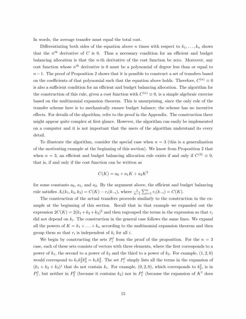
As an example, consider the case C(K) = eK and let K = 5 (so that K is restricted
to the interval (0, 5]). To construct the polynomial allocation, an n-division firm begins by
approximating the cost function using Chebyshev least squares approximation of degree n− 1
over the interval (0, K] (this purely numerical exercise can easily be completed by a computer
program). For example, if the firm has three divisions, it will use the degree-2 approximation,
which in this case turns out to be C(K) = 9.86−25.23K+9.95K2. If the firm has five divisions,
it will use the degree-4 approximation; in the C(K) = eK case, C(K) = 1.66−5.14K+9.28K2−
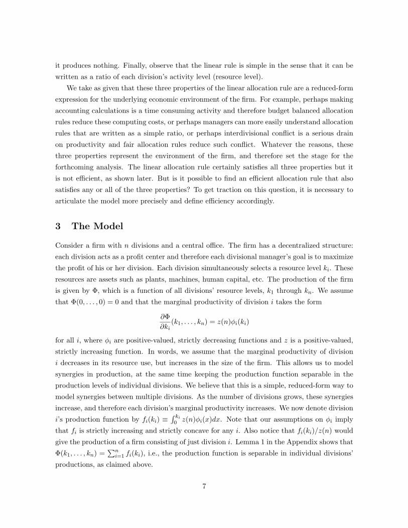
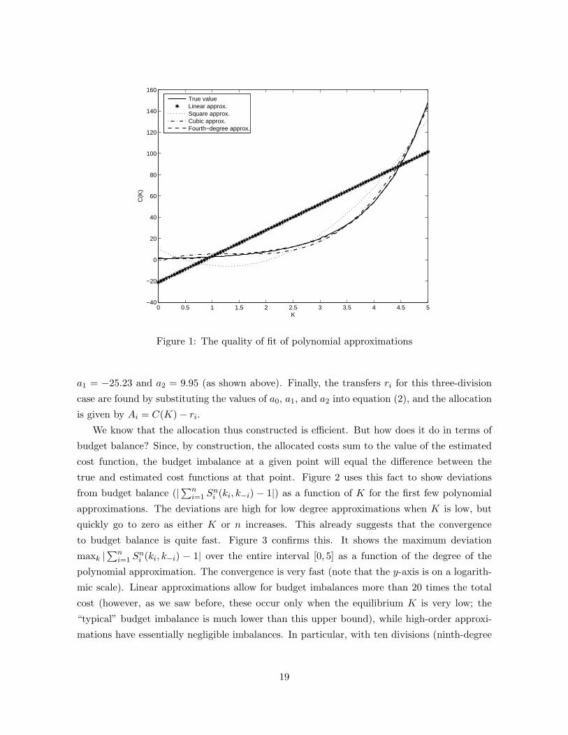
3.93K3 + 0.69K4. The first five polynomial approximations are shown in Figure 1. We see
that the approximated cost functions are quite close to the true C starting already at the
square approximation, which corresponds to n = 3, and the fit improves as the order of the
polynomial increases. Once the cost function has been approximated by a polynomial, the firm
uses the coefficients of the polynomial obtained to calculate the cost allocations according to
the algorithm in the proof of Proposition 2. For example, if the firm has three divisions, it
uses the degree-2 approximation C(K) = a0 + a1K + a2K; in the C(K) = eK case, a0 = 9.86,
18
0 0.5 1 1.5 2 2.5 3 3.5 4 4.5 5−40
−20
0
20
40
60
80
100
120
140
160
K
C(K
)
True valueLinear approx.Square approx.Cubic approx.Fourth−degree approx.
Figure 1: The quality of fit of polynomial approximations
a1 = −25.23 and a2 = 9.95 (as shown above). Finally, the transfers ri for this three-division
case are found by substituting the values of a0, a1, and a2 into equation (2), and the allocation
is given by Ai = C(K) − ri.
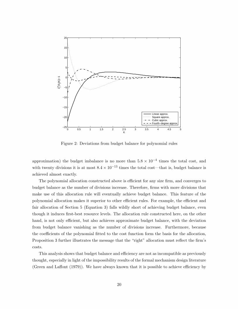
We know that the allocation thus constructed is efficient. But how does it do in terms of
budget balance? Since, by construction, the allocated costs sum to the value of the estimated
cost function, the budget imbalance at a given point will equal the difference between the
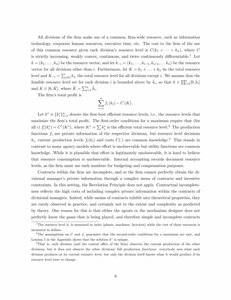
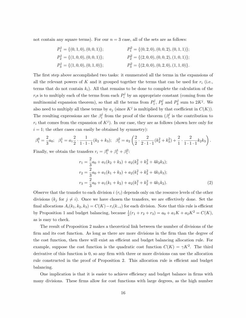
true and estimated cost functions at that point. Figure 2 uses this fact to show deviations
from budget balance (|∑n
i=1 Sni (ki, k−i) − 1|) as a function of K for the first few polynomial
approximations. The deviations are high for low degree approximations when K is low, but
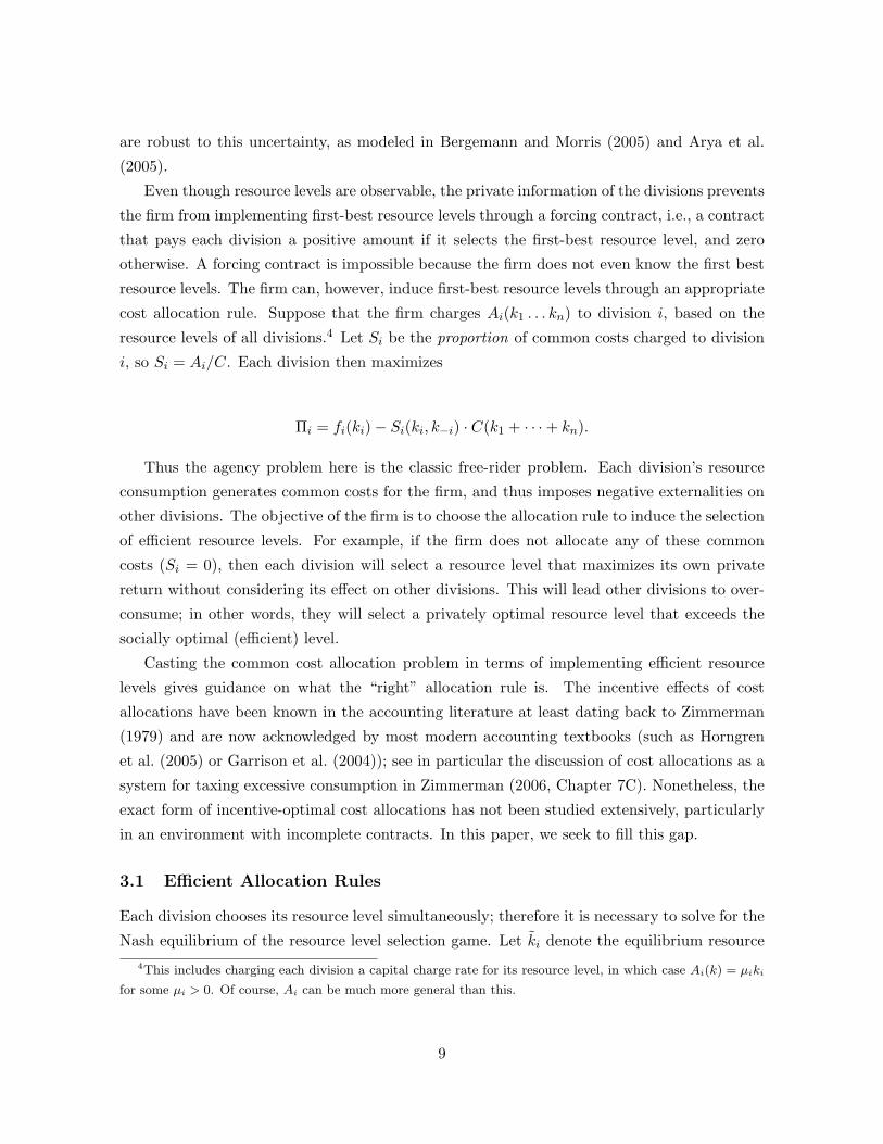
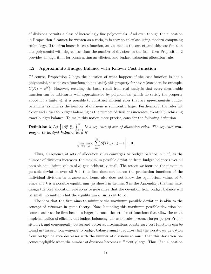
quickly go to zero as either K or n increases. This already suggests that the convergence
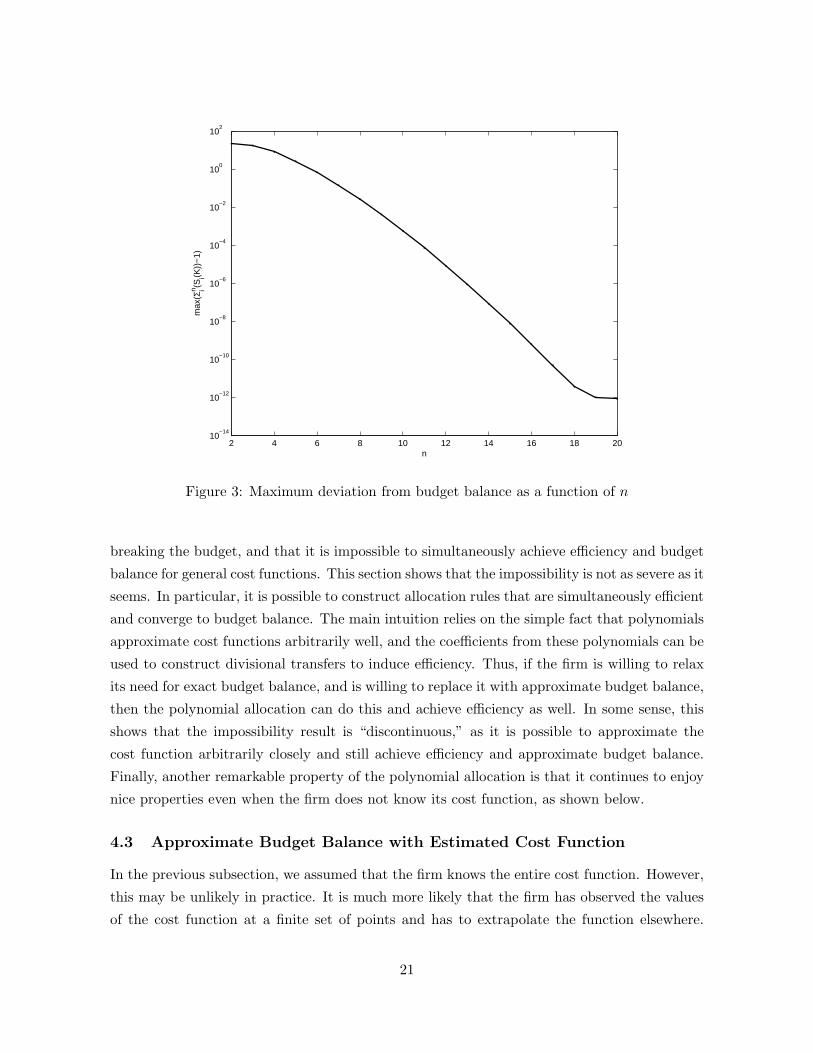
to budget balance is quite fast. Figure 3 confirms this. It shows the maximum deviation
maxk |∑n
i=1 Sni (ki, k−i) − 1| over the entire interval [0, 5] as a function of the degree of the
polynomial approximation. The convergence is very fast (note that the y-axis is on a logarith-
mic scale). Linear approximations allow for budget imbalances more than 20 times the total
cost (however, as we saw before, these occur only when the equilibrium K is very low; the
“typical” budget imbalance is much lower than this upper bound), while high-order approxi-
mations have essentially negligible imbalances. In particular, with ten divisions (ninth-degree
19
0 0.5 1 1.5 2 2.5 3 3.5 4 4.5 5−25
−20
−15
−10
−5
0
5
10
15
20
K
Σ in (Si(K
))−
1
Linear approx.Square approx.Cubic approx.Fourth−degree approx.
Figure 2: Deviations from budget balance for polynomial rules
approximation) the budget imbalance is no more than 5.8 × 10⁻⁴ times the total cost, and
with twenty divisions it is at most 8.4× 10⁻¹³ times the total cost—that is, budget balance is
achieved almost exactly.
The polynomial allocation constructed above is efficient for any size firm, and converges to
budget balance as the number of divisions increase. Therefore, firms with more divisions that
make use of this allocation rule will eventually achieve budget balance. This feature of the
polynomial allocation makes it superior to other efficient rules. For example, the efficient and
fair allocation of Section 5 (Equation 3) falls wildly short of achieving budget balance, even
though it induces first-best resource levels. The allocation rule constructed here, on the other
hand, is not only efficient, but also achieves approximate budget balance, with the deviation
from budget balance vanishing as the number of divisions increase. Furthermore, because
the coefficients of the polynomial fitted to the cost function form the basis for the allocation,
Proposition 3 further illustrates the message that the “right” allocation must reflect the firm’s
costs.
This analysis shows that budget balance and efficiency are not as incompatible as previously
thought, especially in light of the impossibility results of the formal mechanism design literature
(Green and Laffont (1979)). We have always known that it is possible to achieve efficiency by
20
2 4 6 8 10 12 14 16 18 2010
−14
10−12
10−10
10−8
10−6
10−4
10−2
100
102
n
max
(Σin (S
i(K))
−1)
Figure 3: Maximum deviation from budget balance as a function of n
breaking the budget, and that it is impossible to simultaneously achieve efficiency and budget
balance for general cost functions. This section shows that the impossibility is not as severe as it
seems. In particular, it is possible to construct allocation rules that are simultaneously efficient
and converge to budget balance. The main intuition relies on the simple fact that polynomials
approximate cost functions arbitrarily well, and the coefficients from these polynomials can be
used to construct divisional transfers to induce efficiency. Thus, if the firm is willing to relax
its need for exact budget balance, and is willing to replace it with approximate budget balance,
then the polynomial allocation can do this and achieve efficiency as well. In some sense, this
shows that the impossibility result is “discontinuous,” as it is possible to approximate the
cost function arbitrarily closely and still achieve efficiency and approximate budget balance.
Finally, another remarkable property of the polynomial allocation is that it continues to enjoy
nice properties even when the firm does not know its cost function, as shown below.
4.3 Approximate Budget Balance with Estimated Cost Function
In the previous subsection, we assumed that the firm knows the entire cost function. However,
this may be unlikely in practice. It is much more likely that the firm has observed the values
of the cost function at a finite set of points and has to extrapolate the function elsewhere.
21
For example, the firm has chosen certain resource levels in the past and this has generated
certain common costs. As a result, the firm has a finite amount of observations from its prior
activities. It knows the values of its cost function at the points that correspond to its prior
choices and must use this information to estimate the costs that it would incur if it were to
make a resource choice that is different from those of the past.
In this case, the firm can obtain a polynomial approximation of the cost function by running
an OLS regression of observed cost function values on observed resource levels. The firm can
then use the polynomial allocation rule with polynomial coefficients from the OLS regression
instead of those from the Chebyshev approximation (the latter is unavailable for an unknown
cost function). However, it is not immediately obvious that the resulting rule will approach
budget balance, even when both the number of divisions and the number of sample points is
high; for each n, the OLS regression used suffers from omitted variable bias (due to truncating
the series of powers of K at n−1), which usually does not vanish as sample size goes to infinity.
Fortunately, the special structure of the regressor matrix, along with the convergence result
from the previous subsection, guarantees that in this particular case the bias does disappear
and the rule does become budget balancing as both the number of divisions and the sample
size for each number of divisions increase. We now turn to stating this result more formally.
Let an n-division firm have data on cost function values at m points. The data consist of
a vector Kn,m of m observed total resource levels and a vector yn,m of the corresponding cost
levels:
Kn,m = (Kn,m1 , Kn,m
2 , . . . , Kn,mm )′ and
yn,m = (C(Kn,m1 ), C(Kn,m
2 ), . . . , C(Kn,mm ))′.
The firm constructs an allocation rule in two steps as follows:
1. Run an OLS regression of yn,m on the first n − 1 powers of Kn,m and a constant to
estimate the cost function by C:
C(K) = cn,m0 + cn,m
1 K + · · · + cn,mn−1K
n−1,
where cn,m = (cn,m0 , cn,m
1 , . . . cn,mn−1)
′ is the vector of estimated coefficients from the OLS
regression.
2. Construct the cost allocation rules {Sn,mi }n
i=1 as outlined in the proof of Proposition 3,
with cn,mi in place of ci.
Call this the estimated polynomial allocation rule. Before stating the approximate budget
balance result for this case, it is necessary to expand the definition of budget balance to the
case of estimated cost functions:
22
Definition 4 Let{
{Sn,mi }n
i=1
}∞
n=1be a sequence of sets of allocation rules. The sequence
converges to budget balance in n and m if
limn→∞
limm→∞
maxk
∣
∣
∣
∣
∣
n∑
i=1
Sn,mi (ki, k−i) − 1
∣
∣
∣
∣
∣
= 0.
That is, the sharing rules converge to budget balance in n and m if the deviation from budget
balance becomes negligible when the firm estimates its cost functions from large samples and
the number of divisions becomes large. The intuition for this definition is essentially the same as
that for convergence to budget balance in n alone (from the case of known cost functions). The
only difference is that in the case of estimated cost functions, one additional variable influences
the quality of the approximation and hence also the maximum deviation from budget balance.
This variable is sample size: the more observations of the cost function the firm has made in
the past, the better it is able to estimate the cost function. An allocation rule converges to
budget balance if the maximum possible deviation from budget balance goes to zero as the
number of divisions and the number of cost function sample points grow.
Intuitively, this happens for two reasons. First, for any firm with a given number of
divisions, the estimated cost function becomes closer and closer to the true cost function as
the number of cost function observations (m) grows (this is the inner limit in the definition
above). Second, just as in Section 4.2, the allocation rule guarantees that the maximum
possible deviation from budget balance diminishes as the number of divisions (n) grows (this
is the outer limit in the definition). Consequently, if a large firm with a large number of prior
observations of the cost function implements cost allocation rules that converge to budget
balance, it can be certain that the deviation from budget balance will be small, regardless of
the shapes of the divisions’ production functions.
It turns out that, as long as the firms’ samples are sufficiently well dispersed over the range
of feasible resource levels, the estimated polynomial allocation rule does indeed converge to
budget balance:
Proposition 4 The estimated polynomial allocation rule converges to budget balance in n and
m, if for each n and i, limm→∞
(
Km,ni − K
mi)
= 0.
Before we move to a specific numerical example, let us take a moment to summarize the
algorithm that the firm uses to construct the estimated polynomial allocation.
1. The firm has observed its total resource use, K, and its corresponding total cost C(K)
on m previous occasions. The observed values are stored in a dataset containing two
variables/ columns, K and C, and m observations/ rows.
23
2. Auxiliary variables K2, K3, . . . , Kn−1 are computed, where Ki corresponds to the ith
power of K.
3. Ordinary least squares (OLS) regression is run with C as the dependent variable and K
through Kn−1 as the regressors. The coefficient estimates are a0 through an−1, where a0
is the constant; a1 is the coefficient on K, and a2 through an−1 are the coefficients on
K2 through Kn−1.
4. Cost allocations are calculated by a computer program using the algorithm in the proof
of Proposition 2.
Thus, the algorithm for the estimated polynomial rule differs from that for the simple poly-
nomial rule described in the previous section only in the way the cost function is approximated
by a polynomial: the simple polynomial rule uses the Chebyshev least squares approximation,
while the estimated polynomial rule relies on OLS regression on a set of previously observed
values. The simple polynomial rule requires exact knowledge of the cost function, whereas the
estimated rule uses random samples of values of the function.
Let us return to our earlier example C(K) = eK for K ∈ [0, 5]. Suppose the firm has
a sample of m observations of the values of the cost function. As described above, the firm
runs OLS regression on these observations to obtain a polynomial approximation of the cost
function and then proceeds to construct the cost allocation, as described in the examples in
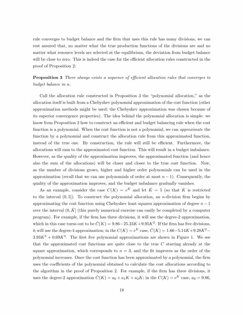
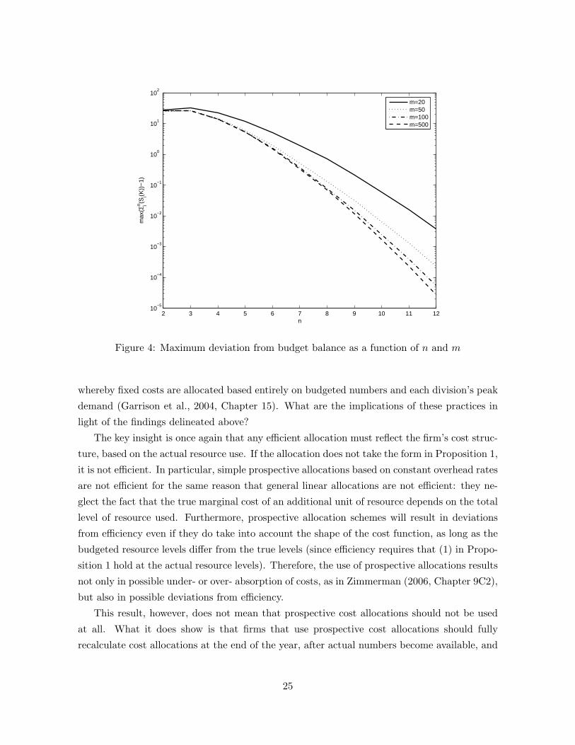
the previous two sections. Figure 4 illustrates the speed of convergence to budget balance.
Each line corresponds to a sample size. We see that for each sample size the budget imbalance
decreases as the number of divisions grows and that the budget imbalance for any given number
of divisions is smaller, the larger the sample size. We see that with a sample size of 100 the
deviation from budget balance is less than ten percent (10−1) for firms with more than seven
divisions, less than one percent (10−2) for firms with more than eight divisions and less than
one-hundredth of one percent (10−4) for firms with twelve or more divisions.
4.4 Prospective Cost Allocation
Note that the cost allocation rules defined above are based on actual resource levels consumed
by all divisions; that is, these allocations are retrospective or ex post. In practice, most firms
define their cost allocation rules prospectively, on the basis of a combination of actual and
budgeted numbers. Typically, an overhead rate is computed at the beginning of a year based
on budgeted resource use, and during the year each division is charged this budgeted rate
times that division’s actual resource use (Zimmerman, 2006, Chapter 9C). In addition, when a
clear dichotomy between fixed and variable costs exists, a two-step scheme is sometimes used,
24
2 3 4 5 6 7 8 9 10 11 1210
−5
10−4
10−3
10−2
10−1
100
101
102
n
max
(Σin (S
i(K))
−1)
m=20m=50m=100m=500
Figure 4: Maximum deviation from budget balance as a function of n and m
whereby fixed costs are allocated based entirely on budgeted numbers and each division’s peak
demand (Garrison et al., 2004, Chapter 15). What are the implications of these practices in
light of the findings delineated above?
The key insight is once again that any efficient allocation must reflect the firm’s cost struc-
ture, based on the actual resource use. If the allocation does not take the form in Proposition 1,
it is not efficient. In particular, simple prospective allocations based on constant overhead rates
are not efficient for the same reason that general linear allocations are not efficient: they ne-
glect the fact that the true marginal cost of an additional unit of resource depends on the total
level of resource used. Furthermore, prospective allocation schemes will result in deviations
from efficiency even if they do take into account the shape of the cost function, as long as the
budgeted resource levels differ from the true levels (since efficiency requires that (1) in Propo-
sition 1 hold at the actual resource levels). Therefore, the use of prospective allocations results
not only in possible under- or over- absorption of costs, as in Zimmerman (2006, Chapter 9C2),
but also in possible deviations from efficiency.
This result, however, does not mean that prospective cost allocations should not be used
at all. What it does show is that firms that use prospective cost allocations should fully
recalculate cost allocations at the end of the year, after actual numbers become available, and
25
make the necessary adjustments from the prospective allocation. If the divisional managers
know that such recalculation will be made, they will make their resource choices based on the
expected final, not the tentative budgeted allocations. Consequently, as long as the recalculated
allocations are in the form of (1) in Proposition 1, the induced resource use will be efficient.
In addition, if the recalculation follows the polynomial scheme discussed above, the allocations
will be approximately budget balancing.
Thus, our results suggest that whenever prospective allocations are used, a two-step process
should be followed: firms should be charged according to the prospectively determined rate
during the course of the year, but an adjustment should be made at the end of the year. We
recommend that the polynomial rule be used in the calculation of the adjusted allocation,
resulting in efficiency and approximate budget balance.
5 Fair Allocation Rules
In the previous section, we analyzed conditions under which cost allocation rules are budget
balancing. In this section, we look at fairness: an additional property that, like budget balance,
is also satisfied by our motivating example, the linear rule. We begin by defining fairness and
finding conditions under which efficient cost allocation rules are fair and then proceed to ask
whether fairness is compatible with budget balance (under efficiency).
Definition 5 S is fair if Si(0, k−i) = 0 for all i and all k−i.
Fair allocation rules neither reward nor penalize divisions for producing zero output.7 Just
like budget balance, we take fairness as an exogenous constraint on the class of feasible allo-
cation rules. Combining efficiency (Proposition 1) and fairness yields the following (unique)
allocation rule:
Si(ki, k−i) = 1 −C(K−i)
C (K). (3)
Fairness implies that ri(k−i) = C(K−i): each division pays the additional costs that it
incurs. In particular, the efficient, fair allocation above allocates to each division its relative
incremental contribution to total cost. Specifically, this is its incremental contribution to
total cost, C(K)−C(K−i), divided by the total cost C(K). Charging each division its relative
incremental contribution to total cost induces each division to consume resources at the efficient
level.
7This “fairness” property of allocation rules has appeared elsewhere. For example, Baldenius et al. (2006)
call this the “no play no pay” condition.
26
Recall that any efficient rule must include the common cost function of the firm. This
is essential to obtain efficiency and is a key distinction between efficient allocation rules and
linear allocation rules. To illustrate the differences between linear and efficient allocation rules,
let us consider a particular example. Let C(K) = F + Km, pick one division (labeled i), and
fix the total resource use of all other divisions at K−i = 1. We want to compare the share of
total costs allocated to division i (as function of ki) under the two allocation rules: the linear
allocation, SLi = ki
K, and the efficient and fair allocation, given in equation (3). Figure 5 graphs
the share allocated to division i according to the linear rule and according to the efficient and
fair rule under two different scenarios: highly convex C (F = 0, m = 2.5) and high fixed costs
with linear variable costs (F = 1, m = 1).
Suppose that the cost function C is highly convex. Therefore, additional resources for any
division are highly costly for the firm. The firm would like to discourage such resource use,
and can do this by increasing the share of allocated costs. In particular, for any given resource
level ki, the firm will allocate more of the common cost under the fair and efficient rule than
under the linear rule. Essentially, the firm adjusts its allocation to respond to its highly convex
cost function. Figure 5 shows that for the cost function C(K) = F +Km, the fair and efficient
rule lies above the linear rule if costs are sufficiently convex (if m is sufficiently high).8 The
efficient rule essentially accelerates the cost allocation for any given resource level.
Similarly, suppose that the firm’s cost function has a high fixed component but a low vari-
able component. In this case, the marginal effect of additional resource use by any division on
the total resource level will be small. The firm would like to encourage additional resource use,
and can do so by reducing the share of allocated cost for any given resource level. Therefore,
the efficient and fair allocation will lie below the linear allocation rule, as shown in Figure 5.
The efficient and fair rule essentially decelerates the cost allocation for any given resource level,
compared to the linear rule. Unlike the linear rule, the efficient and fair rule varies as the firm’s
cost function varies. Efficiency forces the allocation to reflect the underlying costs; linear rules
do not.
A natural question to ask is whether efficient, budget balancing, and fair allocation rules
even exist. For example, linear rules are budget balancing and fair, but not necessarily efficient.
The polynomial rule constructed in the previous section is efficient and (approximately) budget
balancing, but not necessarily fair. The efficient, fair allocation rule in (3) does not always
balance the budget. Unfortunately, these examples are not a coincidence: for virtually any
commonly used cost function (except for constant marginal cost with zero fixed cost), allocation
rules that satisfy all three of the criteria above (efficiency, budget balance, and fairness) do
not exist, as the following proposition shows:
8See Corollary 1 in the Appendix for a derivation of this result.
27

0 0.5 1 1.5 2 2.5 3 3.5 4 4.5 50
0.1
0.2
0.3
0.4
0.5
0.6
0.7
0.8
0.9
1
Division i’s investment
Div
isio
n i’s
allo
cate
d sh
are
Efficient and fair rule, strongly convex costsLinear ruleEfficient and fair rule, high fixed costs
Figure 5: Efficient versus linear allocation rules
Proposition 5 An efficient, budget balancing, and fair allocation rule exists if and only if
C(K) ≡ αK, for some α ∈ R+.
Any efficient and fair allocation rule must satisfy (3), or in words, must allocate to each
division its relative incremental contribution to total cost. But budget balance constrains these
allocations to one. Said differently, budget balance requires that the sum of each division’s
incremental contribution to total cost exactly equals total cost:
n∑
i=1
(C(K) − C(K−i)) = C(K) = C
(
n∑
i=1
(K − K−i)
)
.
The only cost function that satisfies this condition for all (k1 . . . kn) is the constant-
marginal-cost function with no fixed cost (C(K) = αK). Intuitively, the linearity of the
variable costs (constant marginal cost), along with the absence of fixed costs, allows us to
exchange the C and∑
in the equation above. Moreover, no other cost function permits this.
This proposition shows that satisfying all three of the target conditions for cost allocation
rules is in general impossible. Once again, there is a connection with the literature on public
decisions. Green and Laffont (1979) show that it is impossible to find mechanisms that satisfy
ex post efficiency, budget balance, and implementation in dominant strategies. Of course, their
setting is different from here because they invoke the Revelation Principle, allow contracts and
28
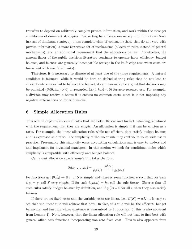
transfers to depend on arbitrarily complex private information, and work within the stronger
equilibrium of dominant strategies. Our setting here uses a weaker equilibrium notion (Nash
instead of dominant-strategy), a less complete class of contracts (those that do not vary with
private information), a more restrictive set of mechanisms (allocation rules instead of general
mechanisms), and an additional requirement that the allocations be fair. Nonetheless, the
general flavor of the public decisions literature continues to operate here: efficiency, budget
balance, and fairness are generally incompatible (except in the knife-edge case when costs are
linear and with zero fixed costs).
Therefore, it is necessary to dispose of at least one of the three requirements. A natural
candidate is fairness: while it would be hard to defend sharing rules that do not lead to
efficient outcomes or fail to balance the budget, it can reasonably be argued that divisions may
be punished (Si(0, k−i) > 0) or rewarded (Si(0, k−i) < 0) for zero resource use. For example,
a division may receive a bonus if it creates no common costs, since it is not imposing any
negative externalities on other divisions.
6 Simple Allocation Rules
This section explores allocation rules that are both efficient and budget balancing, combined
with the requirement that they are simple. An allocation is simple if it can be written as a
ratio. For example, the linear allocation rule, while not efficient, does satisfy budget balance
and is expressed as a ratio. The simplicity of the linear rule may contribute to its wide use in
practice. Presumably this simplicity eases accounting calculations and is easy to understand
and implement for divisional managers. In this section we look for conditions under which
simplicity is compatible with efficiency and budget balance.
Call a cost allocation rule S simple if it takes the form
Si(k1, . . . , kn) =gi(ki)
g1(k1) + · · · + gn(kn)
for functions gi : [0, ki] → R+. If S is simple and there is some function g such that for each
i, gi = g, call S very simple. If for each i, gi(ki) = ki, call the rule linear. Observe that all
such rules satisfy budget balance by definition, and if gi(0) = 0 for all i, then they also satisfy
fairness.
If there are no fixed costs and the variable costs are linear, i.e., C(K) = αK, it is easy to
see that the linear rule will achieve first best. In fact, this rule will be the efficient, budget
balancing, and fair rule whose existence is guaranteed by Proposition 5 (this is also apparent
from Lemma 4). Note, however, that the linear allocation rule will not lead to first best with
general affine cost functions incorporating non-zero fixed cost. This is also apparent from
29
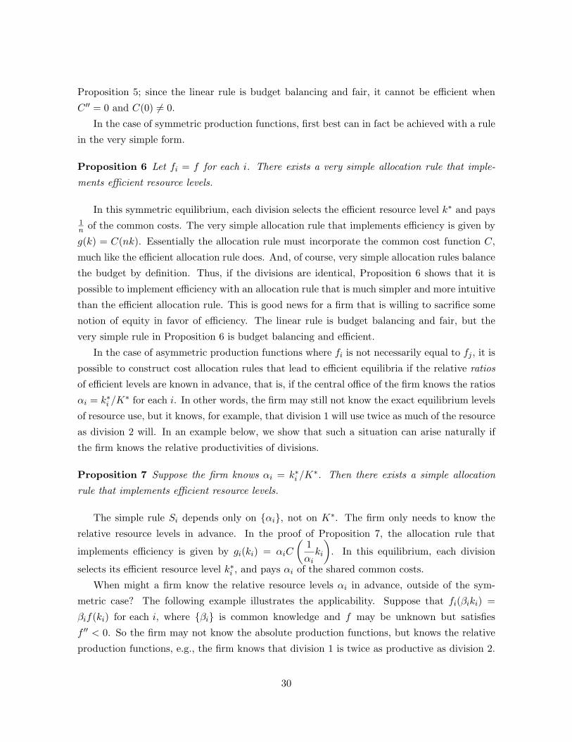
Proposition 5; since the linear rule is budget balancing and fair, it cannot be efficient when
C ′′ = 0 and C(0) 6= 0.
In the case of symmetric production functions, first best can in fact be achieved with a rule
in the very simple form.
Proposition 6 Let fi = f for each i. There exists a very simple allocation rule that imple-
ments efficient resource levels.
In this symmetric equilibrium, each division selects the efficient resource level k∗ and pays1n
of the common costs. The very simple allocation rule that implements efficiency is given by
g(k) = C(nk). Essentially the allocation rule must incorporate the common cost function C,
much like the efficient allocation rule does. And, of course, very simple allocation rules balance
the budget by definition. Thus, if the divisions are identical, Proposition 6 shows that it is
possible to implement efficiency with an allocation rule that is much simpler and more intuitive
than the efficient allocation rule. This is good news for a firm that is willing to sacrifice some
notion of equity in favor of efficiency. The linear rule is budget balancing and fair, but the
very simple rule in Proposition 6 is budget balancing and efficient.
In the case of asymmetric production functions where fi is not necessarily equal to fj , it is
possible to construct cost allocation rules that lead to efficient equilibria if the relative ratios
of efficient levels are known in advance, that is, if the central office of the firm knows the ratios
αi = k∗i /K∗ for each i. In other words, the firm may still not know the exact equilibrium levels
of resource use, but it knows, for example, that division 1 will use twice as much of the resource
as division 2 will. In an example below, we show that such a situation can arise naturally if
the firm knows the relative productivities of divisions.
Proposition 7 Suppose the firm knows αi = k∗i /K∗. Then there exists a simple allocation
rule that implements efficient resource levels.
The simple rule Si depends only on {αi}, not on K∗. The firm only needs to know the
relative resource levels in advance. In the proof of Proposition 7, the allocation rule that
implements efficiency is given by gi(ki) = αiC
(
1
αiki
)
. In this equilibrium, each division
selects its efficient resource level k∗i , and pays αi of the shared common costs.
When might a firm know the relative resource levels αi in advance, outside of the sym-
metric case? The following example illustrates the applicability. Suppose that fi(βiki) =
βif(ki) for each i, where {βi} is common knowledge and f may be unknown but satisfies
f ′′ < 0. So the firm may not know the absolute production functions, but knows the relative
production functions, e.g., the firm knows that division 1 is twice as productive as division 2.
30
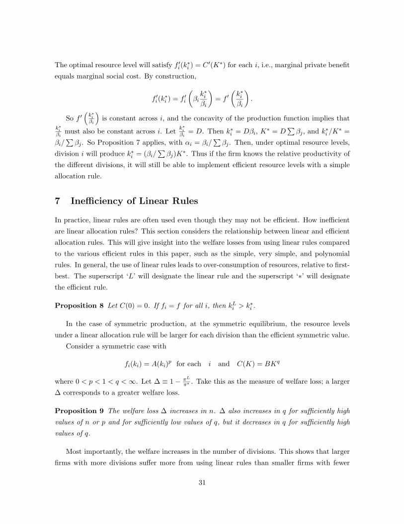
The optimal resource level will satisfy f ′i(k
∗i ) = C ′(K∗) for each i, i.e., marginal private benefit
equals marginal social cost. By construction,
f ′i(k
∗i ) = f ′
i
(
βik∗
i
βi
)
= f ′
(
k∗i
βi
)
.
So f ′(
k∗
i
βi
)
is constant across i, and the concavity of the production function implies that
k∗
i
βimust also be constant across i. Let
k∗
i
βi= D. Then k∗
i = Dβi, K∗ = D∑
βj , and k∗i /K∗ =
βi/∑
βj . So Proposition 7 applies, with αi = βi/∑
βj . Then, under optimal resource levels,
division i will produce k∗i = (βi/
∑
βj)K∗. Thus if the firm knows the relative productivity of
the different divisions, it will still be able to implement efficient resource levels with a simple
allocation rule.
7 Inefficiency of Linear Rules
In practice, linear rules are often used even though they may not be efficient. How inefficient
are linear allocation rules? This section considers the relationship between linear and efficient
allocation rules. This will give insight into the welfare losses from using linear rules compared
to the various efficient rules in this paper, such as the simple, very simple, and polynomial
rules. In general, the use of linear rules leads to over-consumption of resources, relative to first-
best. The superscript ‘L’ will designate the linear rule and the superscript ‘∗’ will designate
the efficient rule.
Proposition 8 Let C(0) = 0. If fi = f for all i, then kLi > k∗
i .
In the case of symmetric production, at the symmetric equilibrium, the resource levels
under a linear allocation rule will be larger for each division than the efficient symmetric value.
Consider a symmetric case with
fi(ki) = A(ki)p for each i and C(K) = BKq
where 0 < p < 1 < q < ∞. Let ∆ ≡ 1 − πL
π∗. Take this as the measure of welfare loss; a larger
∆ corresponds to a greater welfare loss.
Proposition 9 The welfare loss ∆ increases in n. ∆ also increases in q for sufficiently high
values of n or p and for sufficiently low values of q, but it decreases in q for sufficiently high
values of q.
Most importantly, the welfare increases in the number of divisions. This shows that larger
firms with more divisions suffer more from using linear rules than smaller firms with fewer
31
divisions. Combined with Proposition 3, this gives a general prediction on efficient cost al-
location and the size of firms. If n is small, then Proposition 9 shows that the welfare loss
from using the linear rule is small, and so small firms can use linear rules with few efficiency
losses. But if n is big, not only do the welfare losses from the linear rules increase, but the
benefits of the polynomial allocation also increase, since the polynomial allocation converges
to budget balance for large n. Therefore, this paper gives an explicit recommendation on allo-
cation practices depending on the number of divisions in the firm: small firms can use linear
rules, while large firms should use non-linear rules (such as the polynomial allocation). This
recommendation from the model is consistent with the normative flavor of much of the cost
allocation literature.
8 Conclusion
Cost allocations have incentive effects. They determine how a division is charged for use of
a common resource, and thus become an instrument for the firm to indirectly control the
behavior of its decentralized divisions. For example, suppose a firm allocates its information
technology (IT) costs based on IT headcount, i.e., the number of corporate IT employees
assigned to different divisions. On the margin, this gives incentives for the divisions to reduce
resource levels that require a high volume of IT support. Knowing that divisions respond in
such a manner, the firm can choose an allocation rule to induce divisional resource levels that
are optimal for the firm as a whole.
The cost allocation method that dominates time in cost accounting classrooms, space in
cost accounting textbooks, and the energy of corporate financial officers is the linear allocation
rule. This rule satisfies certain key features that reflect the underlying economic and managerial
environment of the firm, such as budget balance, fairness, and simplicity. That it satisfies these
three properties possibly explains its wide use in teaching and practice. However, the linear
rule is not efficient in that it does not solve the firm’s free-rider problem of multiple divisions
simultaneously and independently making resource selection decisions. When is it possible to
satisfy the three properties of budget balance, simplicity, and fairness, as well as efficiency?
Like much of the prior literature in cost allocation, the aim here has been normative: to
recommend allocation rules that bring the firm closer to efficiency but also are feasible for the
firm, by virtue of satisfying some or all of the three aforementioned properties. We propose a
new allocation—the polynomial allocation—that achieves efficiency and converges to budget
balance, as the number of divisions in the firm increases. We also show that if the firm
knows the relative efficient investment levels (and, in particular, if all divisions have the same
production function), a simple, budget balancing allocation rule can achieve efficiency.
32
The main message is that any efficient allocation will reflect the firm’s underlying costs.
As the cost of a common resource increases, the firm would like to discourage use of the
common resource (to mitigate the negative externalities of resource consumption) and therefore
will accelerate the allocation, relative to the linear rule. Similarly, if the cost of a common
resource decreases, the firm can afford to encourage more use of the resource, and therefore will
decelerate the allocation, relative to the linear rule. The efficient rule will thus vary with the
firm’s cost structure. This drives home the broader point that an efficient accounting system
will reflect the firm’s underlying economic environment.
Collecting all the results in the paper, another message from the analysis is that linear rules
“should” be used for small, not large, firms. First, the welfare loss of linear rules increases
as the number of divisions grows, as this exacerbates the free-rider problem. And second,
the polynomial allocation converges to budget balance as the number of divisions grows. For
firms with sufficiently many divisions, the polynomial allocation is efficient and exactly budget
balancing. Large, multi-divisional firms may experience significant negative externalities from
incorrect cost allocation; therefore getting the allocation “right” in terms of achieving efficiency
is perhaps more important for large, rather than small, firms.
Future research in this area will proceed in similar manner by examining what firms ac-
tually do and making explicit, concrete recommendations for changes to practice. While it is
true that the contracts and mechanisms observed in practice are much simpler than those ar-
ticulated in the formal mechanism design theory, it is still possible to strike a balance halfway
between theory and practice. This requires more careful observation of real life mechanisms,
a better understanding of what constraints those mechanisms satisfy, and analyzing optimal
mechanisms subject to those constraints.
9 Appendix
Lemma 1 Φ(k1, . . . , kn) =∑n
i=1 fi(ki).
Proof of Lemma 1
Φ(k1, . . . , kn) = Φ(k1, . . . , kn) − Φ(0, . . . , 0) =
[Φ(k1, . . . , kn) − Φ(k1, . . . , kn−1, 0)] + [Φ(k1, . . . , kn−1, 0) − Φ(k1, . . . , kn−2, 0, 0)]
+ · · · + [Φ(k1, 0, . . . , 0) − Φ(0, . . . , 0)]
33
=
∫ kn
0
∂Φ
∂kn(k1, k2, . . . , kn−1, x)dx +
∫ kn−1
0
∂Φ
∂kn−1(k1, . . . , kn−2, x, 0)dx
+ · · · +
∫ k1
0
∂Φ
∂k1(x, 0, . . . , 0)dx
=n∑
i=1
fi(ki).
�
Lemma 2 Given C and the set of production functions (f1, . . . , fn), there is a single vector of
resource levels (k∗1, . . . , k
∗n) satisfying the first-best conditions f ′
i(k∗i ) = C ′(
∑
i k∗i ) = 0 for all i.
Proof of Lemma 2 Suppose that ka = (ka1 , ..., ka
n) and kb = (kb1, ..., k
bn) both satisfy
f ′i(k
ji ) = C ′(Kj) for j ∈ {a, b}, where Kj ≡
∑ni=1 kj
i . First, suppose Ka 6= Kb. Without loss
of generality, Ka < Kb. Then
f ′i(k
ai ) = C ′(Ka) < C ′(Kb) = f ′
i(kbi ).
This implies that kai > kb
i for each i, since f ′′i < 0. So Ka =
∑
kai >
∑
kbi = Kb. Contradiction.
Therefore, Ka = Kb = K∗. And because f ′i(k
ji ) = C ′(K∗), it must also hold that ka
i =
kbi = k∗
i for each i. �
Lemma 3 For any vector (k1, . . . , kn) there is a vector of production functions (f1, . . . , fn)
that leads to optimal resource levels k∗i = ki for each i.
Proof of Lemma 3 Let the function fα(x) ≡ αx1
2 . Then fα′(x) =α
2x1
2
. So for each i, let
fi = fαi for αi = 2k1
2
i C ′(n∑
i=1
ki).
These production functions generate our desired optimal resource levels. �
Proof of Proposition 1 We will prove the equivalent statement that a set of cost allo-
cations induces k∗i = ki for all i and all {fi}
ni=1 if and only if there exist ri : R
n−1 → R such
that, for all i and all (k1, . . . kn), Ai(ki, k−i) = C(∑n
i=1 ki) − ri(k−i).
Recall that, for a given set of production functions, k∗i and ki are defined by the first-order
conditions for the firm’s and the individual divisions’ optimization problems, respectively:
f ′i(k
∗i ) = C ′(
n∑
i=1
k∗i ) and f ′
i(ki) =∂Ai
∂ki(ki, k−i).
34
Therefore, k∗i = ki for all i if and only if
C ′(n∑
i=1
k∗i ) =
∂Ai
∂ki(k∗
i , k∗−i).
This completes the proof of the “if” part of Proposition 1: if Ai(ki, k−i) = C(∑n
i=1 ki) −
ri(k−i), then C ′(∑n
i=1 ki) = ∂Ai
∂ki(ki, k−i) at all (k1, . . . , kn) and thus also at (k∗
1, . . . k∗n).
The “only if” part requires some more work, because, for a given set of production functions,
the relationship C ′ = ∂Ai
∂kimust hold only at one point, namely, at the corresponding first-best
resource vector. This precludes us from determining a global relationship between A and C
directly. However, the fact that we must ensure k∗i = ki for arbitrary production functions
guarantees that the relationship will hold at every point (k1, . . . , kn), as Lemma 3 shows.
Since every vector (k1, . . . , kn) is first-best for some set of production functions, the rela-
tionship
C ′(n∑
i=1
ki) =∂Ai
∂ki(ki, k−i)
must hold at all (k1, . . . , kn). Holding k−i fixed and integrating with respect to ki, we readily
obtain
Ai(ki, k−i) = C(n∑
i=1
ki) − ri(k−i).
�
Corollary 1 Let C(K) = F +Km. Let SLi and S∗
i denote the “linear” and “fair and efficient”
allocation rules, respectively. For any i and k−i,
1. S∗i (ki, k−i) > SL
i (ki, k−i) for sufficiently high m.
2. S∗i (ki, k−i) < SL
i (ki, k−i) for sufficiently high F .
Proof of Corollary 1 Observe SLi (ki, k−i) = ki/K and S∗
i (ki, k−i) = 1 − C(K−i)C(K) .
So S∗i (ki, k−i) > SL
i (ki, k−i) if and only if
K−i
K>
C(K−i)
C(K)=
F + (K−i)m
F + Km≡ D.
Observe that
D =1
1 + Km
F
+
(
K−i
K
)m
FKm + 1
→ 0 as m → ∞
.
35
Both terms vanish as m → ∞ since K−i < K. This proves part one.
Observe that
D =1 +
Km−i
F
1 + Km
F
→ 1 as F → ∞,
since K−i/K < 1. This proves part two. �
Proof of Proposition 2
=⇒: Suppose an efficient and budget balancing allocation rule does exist. By efficiency,
there are functions (r1, . . . , rn) satisfying
Si(ki, k−i) = 1 −ri(k−i)
C (∑n
i=1 ki).
Summing over all divisions and applying the (BB) condition yields
n∑
i=1
ri(k−i) = (n − 1)C
(
n∑
i=1
ki
)
.
Apply∂n
∂k1 · · · ∂knto both sides to get
0 = (n − 1)C(n)
(
n∑
i=1
ki
)
.
⇐=: If C(n) is identically 0, then C must be a polynomial of degree less than or equal to
n − 1:
C(K) = an−1Kn−1 + · · · + a1K + a0.
We will now define some helpful terminology. First define the sets
P j ≡{
p = (p1, ..., pn)∣
∣ pl a nonnegative integer, (n∑
l=1
pl) = j}
P ji ≡
{
p ∈ P j∣
∣ pi = 0}
for j = 1, ..., n−1; i = 1, ..., n. Next, for p ∈ P j , let G(p) be the number of nonzero coordinates
of p: G(p) ≡∣
∣
{
l∣
∣ pl 6= 0}∣
∣. Note that G(p) is at most j. Finally, define
(
j
p
)
≡ j!p1!···pn! .
By the multinomial expansion theorem, it holds that
(k1 + · · · + kn)j =∑
p∈P j
(
j
p
)
kp1
1 · · · kpnn .
36
Now we will define a series of βji for j = 0, ..., n − 1; i = 1, ..., n:
β0i = a0
n − 1
n
βji = aj
∑
p∈Pji
n − 1
n − G(p)
(
j
p
)
kp1
1 · · · kpnn for j = 1, ..., n − 1.
Observe that for a given vector p ∈ P j , p is in P ji for n − G(p) values of i. Therefore
n∑
i=1
βji = aj(n − 1)(k1 + · · · + kn)j = aj(n − 1)Kj .
By construction, βji is independent of ki for each j. So now let
ri(k−i) =n−1∑
j=0
βji
and define
Si(ki, k−i) = 1 −ri(k−i)
C (K).
By Proposition 1, this rule is efficient. Furthermore, it satisfies budget balance, because
n∑
i=1
ri(k−i) =n∑
i=1
n−1∑
j=0
βji =
n−1∑
j=0
n∑
i=1
βji =
n−1∑
j=0
aj(n − 1)Kj = (n − 1)C(K).
�
Proof of Proposition 3 For each n ≥ 2, let Cn−1 be the Chebyshev least squares approx-
imation of C over the interval (0, K]. Note that, by definition, Cn−1 is a polynomial of degree
n − 1,
Cn−1(K) = cn−1Kn−1 + · · · + c1K + c0.
Construct the sets of allocation rules as in the proof of Proposition 2. That is, let
β0i = c0
n − 1
n
βji = cj
∑
p∈Pji
n − 1
n − G(p)
(
j
p
)
kp1
1 · · · kpnn for j = 1, ..., n − 1,
where P ji and G(p) are as defined in the proof of Proposition 2, and let
Sni (ki, k−i) = 1 −
rni (k−i)
C (K),
37
where
rni (k−i) =
n−1∑
j=0
βji .
As before, the rule is efficient by Proposition 1, and
n∑
i=1
rni (k−i) =
n∑
i=1
n−1∑
j=0
βji =
n−1∑
j=0
n∑
i=1
βji =
n−1∑
j=0
cj(n − 1)Kj = (n − 1)Cn−1(K).
Therefore, for a given k ∈∏n
i=1[0, ki],∣
∣
∣
∣
∣
n∑
i=1
Sni (ki, k−i) − 1
∣
∣
∣
∣
∣
=n − 1
C(K)|C(K) − Cn−1(K)|.
Since C is C2, the standard results on the convergence of Chebyshev approximations apply
(see, e.g., Judd (1998), pages 210–215). In particular, there exists a B < ∞ such that |C(K)−
Cn−1(K)| ≤ B ln(n)n2 for all K ∈ (0, K]. Therefore, for each K,
∣
∣
∣
∣
∣
n∑
i=1
Sni (ki, k−i) − 1
∣
∣
∣
∣
∣
≤B
C(K)
ln(n)
n→ 0,
as n → ∞, because C(K) > 0 for K > 0. �
Proof of Proposition 4 In what follows, we will omit the superscript m, n for visual
clarity. Thus, we will use K, y, and c to denote Km,n, ym,n, and cm,n, respectively.
Let
K =
1 K1 (K1)2 . . . (K1)
n−1
1 K2 (K2)2 . . . (K2)
n−1
. . . . . . . . . . . . . . . . . . . . . . . . . . . . . . .
1 Km (Km)2 . . . (Km)n−1
.
Estimating the polynomial coefficients by OLS, we obtain
c = (K′K)−1K′y.
Recall that we construct the estimated polynomial sharing rule by using c instead of c in the
algorithm outlined in the proof of Proposition 3. That proof then shows that the budget
imbalance arising from using this rule when total resource level is K is
n − 1
C(K)
∣
∣
∣C(K) − C(K)
∣
∣
∣,
where C(K) = c0 + c1K + · · · + cn−1Kn−1. Our goal is therefore to show that (for any K)
limn→∞
limm→∞
n − 1
C(K)
∣
∣
∣C(K) − C(K)
∣
∣
∣= 0.
38
Now, let C be the (n − 1)st-degree Chebyshev least squares approximation of C, and let δ
be the residual, δ(K) = C(K) − C(K). Recall that δ(K) = O( ln nn2 ) (where O(·) denotes the
asymptotic operator “of order no more than”). We can now write
yi = C(Ki) = C(Ki) + δ(Ki) =(
1 Ki (Ki)2 . . . (Ki)
n−1)
c + δ(Ki),
so that y = Kc + ∆, where ∆ =(
δ(K1) δ(K2) . . . δ(Km))′
. Now,
C(K) =(
1 K K2 . . . Kn−1)
c
=(
1 K K2 . . . Kn−1)
(K′K)−1K′(
Kc + ∆)
= C(K) +(
1 K K2 . . . Kn−1)(
(K′K)−1K′∆)
.
Now, given our assumption that limm→∞
(
Ki −Km
i)
= 0, we know that
limm→∞
K = limm→∞
1 Km
(
Km
)2. . .
(
Km
)n−1
1 2 Km
(
2 Km
)2. . .
(
2 Km
)n−1
. . . . . . . . . . . . . . . . . . . . . . . . . . . . . . . .
1 K(
K)2
. . .(
K)n−1
= limm→∞
V D,
where V is the rectangular (n, m) Vandermonde matrix on integer nodes (Vij = ij−1) and
D = diag(
1 Km
. . .(
Km
)n−1)
. Therefore, for each n,
limm→∞
(
1 K K2 . . . Kn−1)(
K′K)−1K′∆)
= limm→∞
(
1 K K2 . . . Kn−1)
D−1V +∆,
where V + is the Moore-Penrose pseudo-inverse of V , V + = (V ′V )−1V ′.
Using the factorization in Eisinberg et al. (2001), we can write V + = SM, where S is an
n × n upper-triangular matrix whose entries do not depend on m and M is given by
Mi,j =n∑
t=1
n∑
k=1
(−1)t
(
j − 1
t − 1
)
(
i+k−2i−1
)(
m−im−k
)(
t+k−2t−1
)(
m−tm−k
)
(
2k−2k−1
)(
m+k−12k−1
) .
Now,(
j−1t−1
)
≤(
m−1t−1
)
= Θ(mt−1), where Θ denotes the asymptotic operator “of the same
order as”. Similarly,(
m−im−k
)
= Θ(mk−i),(
m−tm−k
)
= Θ(mk−t), and(
2k−2k−1
)(
m+k−12k−1
)
= Θ(m2k−1).
Consequently, each term in the finite summation for Mij (and therefore Mij itself) is
O(mt−1+k−i+k−t−(2k−1)) = O(m−i),
where O denotes the asymptotic operator “of order no more than.” Finally, the (i, j) element
of D−1V + = D−1SM is(
D−1V +)
i,j=
n∑
l=1
(m
K
)i−1Si,lMl,j .
39
Since Ml,j = O(m−l), all terms are O(mi−l−1). Noting that Si,l = 0 when i > l we see that
i− l− 1 ≤ −1 for all non-zero terms, so that each element of(
D−1V +)
i,jis decreasing at rate
at least m−1. Hence, for any n,
limm→∞
(
1 K K2 . . . Kn−1)
D−1V +∆ = 0,
so that
limm→∞
C(K) = C(K).
Now,
limm→∞
n − 1
C(K)
∣
∣
∣C(K) − C(K)
∣
∣
∣=
n − 1
C(K)
∣
∣
∣C(K) − C(K)
∣
∣
∣=
n − 1
C(K)|δ(K)| = O
(
ln(n)
n
)
,
so that
limn→∞
limm→∞
n − 1
C(K)
∣
∣
∣C(K) − C(K)
∣
∣
∣= 0.
�
Proof of Proposition 5
1. A set of allocation rules is efficient, budget balancing, and fair if and only if the following
three conditions hold for all i and all (k1, . . . , kn):
Si(ki, k−i) = 1 −ri(k−i)
C (∑n
i=1 ki);
n∑
i=1
Si(ki, k−i) = 1;
Si(0, k−i) = 0.
The first and the third condition (efficiency and fairness) together are equivalent to
Si(ki, k−i) = 1 −C(
∑
j 6=i kj
)
C (∑n
i=1 ki).
Combining this with budget balance yields
n −
∑ni=1 C
(
∑
j 6=i kj
)
C (∑n
i=1 ki)= 1,
that is,
C
(
n∑
i=1
ki
)
=1
n − 1
n∑
i=1
C
∑
j 6=i
kj
. (4)
We therefore see that a set of efficient, budget balancing, and fair allocation rules exists
if and only if (4) holds for all k ∈∏n
i=1[0, ki].
40
2. Now, pick any k1 ∈ R and take k = (k1, 0, . . . , 0). By (4), if an efficient, budget balancing
and fair allocation rule exists, then C(k1) = 1n−1(C(0)+(n−1)C(k1)), that is, C(0) = 0.
3. Next, suppose that C is strictly convex and an efficient, budget balancing and fair allo-
cation rule exists. Let K ≡∑n
i=1 ki and let K−i ≡∑
j 6=i kj .
Now, observe that
C(K−i) = C
(
K−i
K· K +
ki
K· 0
)
<K−i
KC(K) +
ki
KC(0) =
K−i
KC(K) (5)
for all i, where the inequality follows by the convexity of C and C(0) = 0 as shown above.
Therefore,
n∑
i=1
C(K−i) <n∑
i=1
K−i
KC(K) =
C(K)
K
n∑
i=1
K−i
=C(K) · (n − 1)K
K= (n − 1)C(K),
which contradicts (4).
4. Therefore, we see that if an efficient, budget balancing and fair allocation rule exists,
C must not be strictly convex and must have C(0) = 0. That is, the only candidate
functions are the linear cost functions C(K) = αK. It is also easy to see that this family
of functions satisfies (4):
1
n − 1
n∑
i=1
C(K−i) =1
n − 1
αn∑
i=1
∑
j 6=i
kj
= αK = C(K),
which completes the proof.
�
Lemma 4 Take S = (S1, . . . , Sn) in the simple form Si(k1, . . . , kn) = gi(ki)g1(k1)+···+gn(kn) . Then
S will imply an efficient equilibrium if and only if (for each i)
C(K∗)
C ′(K∗)=
∑
j gj(k∗j )
g′i(k∗i )
.
Proof of Lemma 4 From the firm’s objective function, we see that k∗i is defined by the
FOC
f ′i(k
∗i ) − C ′(K∗) = 0 (6)
41
Division i maximizes fi(ki) − Si(k1, . . . , kn) · C(K). Let ∂iSi denote the derivative of
Si(k1, . . . , kn) with respect to ki. With an arbitrary allocation rule S, we get the first order
condition for division i’s problem,
f ′i(ki) − ∂iSi(k1, ..., kn) · C(K) − Si(k1, ..., kn) · C ′(K) = 0. (7)
Combining (6) and (7), we see that k∗i = ki for each i if and only if
C ′(K∗) = ∂iSi(k∗1, ..., k
∗n) · C(K∗) + Si(k
∗1, ..., k
∗n) · C ′(K∗). (8)
By assumption, Si(k1, . . . , kn) = gi(ki)∑
j gj(kj), so
∂iSi =(∑
j gj(kj)) · g′i(ki) − gi(ki) · g
′i(ki)
(∑
j gj(kj))2
=g′i(ki) ·
∑
j 6=i gj(kj)
(∑
j gj(kj))2.
Plugging this and Si into (8) and simplifying gives us the desired result,
C(K∗)
C ′(K∗)=
∑
j gj(k∗j )
g′i(k∗i )
. (9)
�
Proof of Proposition 6
By Lemma 4 it suffices to check that (9) holds. k∗i is determined by (7) and all values of
k∗i are equal to some k∗. So K = nk∗. Thus,
∑
j gj(k∗j )
g′i(k∗i )
=ng(k∗)
g′(k∗)=
nC(nk∗)
nC ′(nk∗)=
C(K∗)
C ′(K∗).
�
Proof of Proposition 7
To show that an equilibrium is generated, by Lemma 4 it suffices to check that (9) holds:
∑
j gj(k∗j )
g′i(k∗i )
=
∑
j αjC( 1αj
αjK∗)
1αi
αiC ′( 1αi
αiK∗)=
C(K∗)
C ′(K∗).
So optimal resource levels are an equilibrium. And in this equilibrium, division i pays
Si =αiC(K∗)
∑
j αjC(K∗)= αi.
�
42
Proof of Proposition 8. Fix K−i. Let kLci be the resource levels induced by the linear
cost allocation rule for division i, conditional on K−i, and let k∗ci be the conditional efficient
resource level.
Given K−i, we see from (6) that the conditional efficient k∗ci will satisfy
f ′i(k
∗ci ) = C ′(K−i + k∗c
i ).
The linear rule will have
SLi (k) =
k
K−i + k, SL′
i (k) =K−i
(K−i + k)2,
and so from (7), the linear kLci will satisfy
f ′i(k
Lci ) =
K−i
(K−i + kLci )2
· C(K−i + kLci ) +
kLci
K−i + kLci
· C ′(K−i + kLci ).
And, because C is convex,
C(x) < x · C ′(x) + C(0). (10)
We have assumed C(0) = 0, so plug this back in with x = K−i + kLci :
f ′i(k
Lci ) <
K−i(K−i + kLci )
(K−i + kLci )2
· C ′(K−i + kLci ) +
kLci
K−i + kLci
· C ′(K−i + kLci ) = C ′(K−i + kLc
i ).
Because f ′i(k) is decreasing in k and C ′(K−i + k) is increasing in k, we have that
f ′i(k
Lci ) < C ′(K−i + kLc
i )
and f ′i(k
∗ci ) = C ′(K−i + k∗c
i )
iff kLci > k∗c
i . If production is symmetric, k∗i = k∗ for each i. Let k∗c
i (K−i) be the optimal
conditional resource levels for a given K−i. k∗ci (K−i) satisfies f ′(k∗c
i (K−i)) − C ′(k∗ci (K−i) +
K−i) = 0, so we can implicitly differentiate and see that
dk∗ci (K−i)
dK−i=
C ′′
f ′′ − C ′′< 0.
At any symmetric equilibrium, K−i = (n−1)k and K = nk. Now kLci (K−i) > k∗c
i (K−i) for
any K−i. Also, for K−i ≤ K∗−i, the above differentiation shows that k∗c
i (K−i) ≥ k∗ci (K∗
−i) = k∗.
So assume that KL ≤ K∗. Then, KL−i ≤ K∗
−i for all i, and therefore
kLi = kLc
i (KL−i) > k∗c
i (KL−i) ≥ k∗.
But this implies that KL > K∗. Contradiction. So KL > K∗ and kL > k∗. �
43
Lemma 5 If fi(ki) = A(ki)p for each i and C(K) = BKq for 0 < p < 1 < q < ∞ then
k∗ =
(
Ap
Bqn1−q
) 1
q−p
kL =
(
Apn2−q
B(n − 1 + q)
)1
q−p
πL
π∗= n
p
q−p
(
q
n − 1 + q
)p
q−p
(
1 − npn−1+q
1 − pq
)
.
Proof: In the respective symmetric equilibria, k∗i = k∗
j and kLi = kL
j , so we will drop the
subscripts from these quantities in the following proof. The optimal production k∗ solves (6),
so
Ap(k∗)p−1 = q B(nk∗)q−1
(k∗)q−p =Ap
Bqn1−q
k∗ =
(
Ap
Bqn1−q
) 1
q−p
.
And kL solves (7), so
Ap(kL)p−1 −(n − 1)kL
n2(kL)2B(nkL)q −
1
nBq(nkL)q−1 = 0
Ap(kL)p−1 = nq−2(kL)q−1[B(n − 1 + q)]
kL =
(
Apn2−q
B(n − 1 + q)
)1
q−p
.
Now, π(k) = nAkp − B(nk)q for a symmetric output level k, so
π∗ = An
(
Ap
Bqn1−q
)p
q−p
− B
(
nq−p Ap
Bqn1−q
)q
q−p
= nq−pq
q−p
[
A
(
Ap
Bq
)p
q−p
− B
(
Ap
Bq
)q
q−p
]
= Anq−pq
q−p
(
Ap
Bq
)p
q−p(
1 −p
q
)
.
And
πL = An
(
Ap
B(n − 1 + q)n2−q
)p
q−p
− B
(
nq−p Ap
B(n − 1 + q)n2−q
)q
q−p
= Anq+p−qp
q−p
(
Ap
B(n − 1 + q)
)p
q−p(
1 −np
n − 1 + q
)
.
44
So
πL
π∗=
Anq+p−qp
q−p
(
ApB(n−1+q)
)p
q−p(
1 − npn−1+q
)
Anq−pq
q−p
(
ApBq
)p
q−p(
1 − pq
)
= np
q−p
(
q
n − 1 + q
)p
q−p
(
1 − npn−1+q
1 − pq
)
.
�
Proof of Proposition 9
Note ∆ = 1 − πL/π∗, where πL/π∗ is calculated in Lemma 5.
Without calculations, it is clear that∂∆
∂A=
∂∆
∂B= 0. Now
∂∆
∂n=
(n − 1)np
q−p−1
p(q − 1)2q(
qn+q−1
)p
q−p
(q − p)2(n + q − 1)2> 0.
∂∆
∂p=
1
(p − q)3
(
np
q−p
( q
n − 1 + q
)q
q−p·
(
(n − 1)(p − q)(q − 1) + q(n − np + q − 1) log(nq
n − 1 + q))
)
.
So ∂∆∂p
has the opposite sign of (n − 1)(p − q)(q − 1) + q(n − np + q − 1) log( nqn−1+q
). Plugging
in the inequality log(x) ≤ x − 1,
(n − 1)(p − q)(q − 1) + q(n − np + q − 1) log(nq
n − 1 + q)
≤ (n − 1)(p − q)(q − 1) + q(n − np + q − 1)
(
nq
n − 1 + q− 1
)
= −(n − 1)2p(q − 1)2
n − 1 + q
< 0.
Thus, ∂∆∂p
> 0. Now
∂∆
∂q=
1
(p − q)3(n − 1 + q)2
(
np
q−p pq( q
n − 1 + q
)p
q−p·
(
(n − 1)(q − p)(q − 1) − (q − 1 + n − np)(n − 1 + q) log(nq
n − 1 + q))
)
45

So ∂∆∂q
has the opposite sign of
(n − 1)(q − p)(q − 1) − (q − 1 + n − np)(n − 1 + q) log( nqn−1+q
).
In other words, ∂∆∂q
has the sign of
log(nq
n − 1 + q) −
(n − 1)(q − p)(q − 1)
(n − 1 + q)(n − np + q − 1).
As n −→ ∞, this goes to log(q) − 0 = log(q) > 0. So for n large enough holding other
parameters fixed, ∂∆∂q
> 0.
As q −→ ∞, this goes to log(n) − (n − 1) which is strictly less than 0 for n ≥ 2. So for q
large enough, ∂∆∂q
< 0.
As q −→ 1, we can find the sign by dividing through by the fraction and applying
L’Hopital’s rule to the limit. This has the sign of n − 1 > 0, so for q small enough, ∂∆∂q
> 0.
As p −→ 1, the expression goes to log( nqn−1+q
)− (n−1)(q−1)n−1+q
. Applying the inequality log(x) ≤
x − 1, we get log( nqn−1+q
) ≤ (n−1)(q−1)n−1+q
. So ∂∆∂p
< 0 for p large enough, when other parameters
are held constant. �
46
References
Arya, A., Demski, J., Glover, J., Liang, P., 2005. Quasi-robust multiagent contracts. Mimeo,
Ohio State University.
Atkinson, A., 1987. Intrafirm cost and resource allocations: Theory and practice. Monograph,
Society of Management Accountants of Canada and Canadian Academic Accounting Asso-
ciation Research, Hamilton, Canada.
Baiman, S., Noel, J., 1985. Noncontrollable costs and responsibility accounting. Journal of
Accounting Research 23 (2), 486–501.
Balachandran, B., Li, L., Magee, R., 1987. On the allocation of the fixed and variable costs
from service departments. Contemporary Accounting Research, 164–185.
Balachandran, B., Ramakrishnan, R., 1981. Joint cost allocation: A unified approach. The
Accounting Review 56 (1), 85–96.
Balakrishnan, R., Sivaramakrishnan, K., 2002. A critical overview of the use of full-cost data
for planning and pricing. Journal of Management Accounting Research 14, 3–31.
Baldenius, T., Dutta, S., Reichelstein, S., September 2006. Cost allocation for capital budgeting
decisions. Working paper, Stanford University.
Bergemann, D., Morris, S., 2005. Robust mechanism design. Econometrica 73 (6), 1771–1813.
Biddle, G. C., Steinberg, R., 1984. Allocations of joint and common costs. Journal of Account-
ing Literature 3, 1–45.
Bower, A., 1993. Procurement policy and contracting efficiency. International Economic Review
34 (4), 873–901.
Chen, Y., Sep 2003. An experimental study of serial and average cost pricing mechanisms.
Journal of Public Economics 87 (9), 2305–2335.
Cohen, S. I., Loeb, M., 1982. Public goods, common inputs, and the efficiency of full cost
allocations. The Accounting Review 57, 336–347.
Dean, G., Joye, M., Blayney, P., 1991. Strategic management accounting survey. Tech. rep.,
Sydney, Australia.
Demski, J. S., 1981. Cost allocation games. In: Moriarity, S. (Ed.), Joint Cost Allocations.
University of Oklahoma Press, Norman, OK, pp. 142–173.
47
Dopuch, N., 1981. Some perspectives on cost allocations. In: Moriarity, S. (Ed.), Joint Cost
Allocations. University of Oklahoma Press, Norman, OK, pp. 1–7.
Eisinberg, A., Pugliese, P., Salerno, N., 2001. Vandermonde matrices on integer nodes: The
rectangular case. Numerische Mathematik 87 (4), 663–674.
Fremgen, J., Liao, S., 1981. The allocation of corporate indirect costs. Tech. rep., National
Association of Accountants, NY.
Gangolly, J. S., 1981. On joint cost allocation: Independent cost, proportional scheme and its
properties. Journal of Accounting Research 19 (2), 299–312.
Garrison, R. H., Noreen, E., Brewer, P. C., 2004. Managerial Accounting, 11th Edition.
McGraw-Hill/Irwin, New York, NY.
Gasmi, F., Laffont, J. J., Sharkey, W. W., 1999. Empirical evaluation of regulatory regimes in
local telecommunications markets. Journal of Economics and Management Strategy 8 (1),
61–93.
Green, J., Laffont, J. J., 1977. Characterization of satisfactory mechanisms for the revelation
of preferences for public goods. Econometrica 45, 427–438.
Green, J., Laffont, J. J., 1979. Incentives in public decision making. In: Studies in Public
Economics, Vol. 1. North-Holland, Amsterdam.
Groves, T., 1973. Incentives in teams. Econometrica 41 (4), 617–631.
Groves, T., Loeb, M., 1975. Incentives and public inputs. Journal of Public Economics 4,
211–226.
Hamlen, S. S., Hamlen Jr., W. A., Tschirhart, J., 1980. The use of the generalized Shapley
allocation in joint cost allocation. The Accounting Review 55 (2), 269–287.
Hansen, S. C., Magee, R. P., 2003. Capacity cost and capacity allocation. Contemporary
Accounting Research 9 (2), 635–660.
Horngren, C., Datar, S., Foster, G., 2005. Cost Accounting: A Managerial Emphasis, 12th
Edition. Prentice Hall, Englewood Cliffs, NJ.
Hughes, J. S., Scheiner, J. H., 1980. Efficiency properties of mutually satisfactory cost alloca-
tions. The Accounting Review 55 (1), 85–95.
Judd, K., 1998. Numerical Methods in Economics. The MIT Press, Cambridge, MA.
48
Kaplan, R. S., 1981. The impact of management accounting research on policy and practice.
In: Buckley, J. (Ed.), Proceedings of the Arthur Young Professor’s Roundtable. Council of
Arthur Young Professors.
Louderback, J. G., 1976. Another approach to allocating joint costs: A comment. The Ac-
counting Review 51, 683–685.
Magee, R. P., 1988. Cost allocation in a principal/agent setting. The Accounting Review 63 (1),
42–54.
McAfee, R. P., 2002. Coarse matching. Econometrica 70 (5), 2025–2034.
Melumad, N. D., Reichelstein, S., 1987. Centralization versus delegation and the value of
communication. Journal of Accounting Research 25, 1–18.
Miller, B. L., Buckman, A. G., 1987. Cost allocation and opportunity costs. Management
Science 33 (5), 626–639.
Moriarity, S., 1975. Another approach to allocating joint cost. The Accounting Review 49,
791–795.
Moulin, H., Sep 1987. Equal or proportional division of a surplus, and other methods. Inter-
national Journal of Game Theory 16 (3), 161–186.
Moulin, H., 1994. Serial cost-sharing of excludable public goods. Review of Economic Studies
61, 305–325.
Moulin, H., 2005. The price of anarchy of serial cost sharing and other methods. Mimeo, Rice
University.
Moulin, H., Shenker, S., 1992. Serial cost sharing. Econometrica 60 (5), 1009–1037.
Moulin, H., Shenker, S., 2001. Strategyproof sharing of submodular costs: Budget balance
versus efficiency. Economic Theory 18 (3), 511–533.
Moulin, H., Sprumont, Y., 2005. On demand responsiveness in additive cost sharing. Journal
of Economic Theory 125 (1), 1–35.
Rajan, M. V., 1992. Cost allocation in multiagent settings. The Accounting Review 67 (3),
527–545.
Ramadan, S., Winter 1989. The rationale for cost allocation: A study of U.K. divisionalized
companies. Tech. rep., Accounting and Business Research.
49
Reichelstein, S., 1992. Constructing incentive schemes for government contracts, an application
of agency theory. The Accounting Review 67 (4), 712–731.
Rogerson, W. P., 2003. Simple menus of contracts in cost-based procurement and regulation.
The American Economic Review 93 (3), 919–926.
Roth, A. E., Verrecchia, R. E., 1979. The Shapley value as applied to cost allocation: A
reinterpretation. Journal of Accounting Research 17 (1), 295–302.
Satterthwaite, M. A., Williams, S. R., 2002. The optimality of a simple market mechanism.
Econometrica 70 (5), 1841–1863.
Serizawa, S., Jan 1999. Strategy-proof and symmetric social choice functions for public good
economies. Econometrica 67 (1), 121–145.
Shubik, M., 1962. Incentives, decentralized control, the assignment of joint costs and internal
pricing. Management Science 8, 325–343.
Suh, Y. S., 1987. Collusion and noncontrollable cost allocation. Journal of Accounting Research
25, 22–46.
Verrecchia, R. E., 1981. A question of equity: Use of the Shapley value to allocate state and
local income and franchise taxes. In: Moriarity, S. (Ed.), Joint Cost Allocations. University
of Oklahoma Press, Norman, OK, pp. 14–40.
Verrecchia, R. E., 1982. An analysis of two cost allocation cases. The Accounting Review 57,
579–593.
Walker, M., Sep 1980. On the nonexistence of a dominant strategy mechanism for making
optimal public decisions. Econometrica 48 (6), 1521–1540.
Wilson, R., 1987. Game-theoretic analyses of trading processes. In: Bewley, T. (Ed.), Advances
in Economic Theory, 5th World Congress. Cambridge University Press, pp. 33–70.
Young, H. P., 1985. Producer incentives in cost allocation. Econometrica 53, 757–765.
Zimmerman, J., 1979. The costs and benefits of cost allocations. The Accounting Review 54 (3),
504–521.
Zimmerman, J. L., 2006. Accounting for Decision Making and Control, 5th Edition. McGraw-
Hill/Irwin, New York, NY.
50
Related Documents