Ecient computation of the Tikhonov regularization parameter by goal oriented adaptive discretization

IOP PUBLISHING INVERSE PROBLEMS

Inverse Problems 24 (2008) 025025 (20pp) doi:10.1088/0266-5611/24/2/025025

Efficient computation of the Tikhonov regularizationparameter by goal-oriented adaptive discretization

Anke Griesbaum1, Barbara Kaltenbacher2 and Boris Vexler3

1 University of Heidelberg, Heidelberg, Germany2 University of Stuttgart, Stuttgart, Germany3 RICAM Linz, Austrian Academy of Sciences, Linz, Austria

Received 30 October 2007, in final form 13 February 2008Published 14 March 2008Online at stacks.iop.org/IP/24/025025

AbstractParameter identification problems for partial differential equations (PDEs)often lead to large-scale inverse problems. For their numerical solution itis necessary to repeatedly solve the forward and even the inverse problem, as itis required for determining the regularization parameter, e.g., according to thediscrepancy principle in Tikhonov regularization. To reduce the computationaleffort, we use adaptive finite-element discretizations based on goal-orientederror estimators. This concept provides an estimate of the error in a so-calledquantity of interest, which is a functional of the searched for parameter q and thePDE solution u. Based on this error estimate, the discretizations of q and u arelocally refined. The crucial question for parameter identification problems isthe choice of an appropriate quantity of interest. A convergence analysis of theTikhonov regularization with the discrepancy principle on discretized spacesfor q and u provides a possible answer: it shows, that in order to determine thecorrect regularization parameter, one has to guarantee sufficiently high accuracyin the squared residual norm—which is therefore our quantity of interest—whereas q and u themselves need not be computed precisely everywhere. Thisfact allows for relatively low dimensional adaptive meshes and hence for aconsiderable reduction of the computational effort. In this paper, we study anefficient inexact Newton algorithm for determining an optimal regularizationparameter in Tikhonov regularization according to the discrepancy principle.With the help of error estimators we guide this algorithm and control theaccuracy requirements for its convergence. This leads to a highly efficientmethod for determining the regularization parameter.

(Some figures in this article are in colour only in the electronic version)

0266-5611/08/025025+20$30.00 © 2008 IOP Publishing Ltd Printed in the UK 1

Inverse Problems 24 (2008) 025025 A Griesbaum et al

1. Introduction

In this paper, we consider inverse problems for partial differential equations and develop anefficient algorithm for determining the regularization parameter for Tikhonov regularization.The proposed method is based on the discrepancy principle on the one hand and on exploitingadaptive finite-element discretizations on the other hand.

Driven by efficiency requirements for the solution of increasingly large-scale inverseproblems, adaptivity has recently been attracting more and more interest in the inverse problemscommunity. For instance, we point to [1], where refinement and coarsening indicators areextracted from Lagrange multipliers for the misfit functional with constraints incorporatinglocal changes of the discretization. Moreover, we refer to [15, 22], where sloppily speakingthe magnitude of gradients is used as a criterion for local refinement. Also, we would like torefer to very interesting ideas on ‘a priori’ adaptivity in [8].

Inverse problems for partial differential equations such as parameter identification orinverse boundary value problems can usually be written as operator equations, where theforward operator is the composition

F = C ◦ S

of a parameter-to-solution map for a PDE

S : Q → V

q �→ u

with some measurement operator

C : V → G

u �→ g,

where Q,V,G are appropriate Hilbert spaces. Throughout the paper we denote by ‖·‖Q thenorm and by (·, ·)Q the inner product in Q. Similar notation is used for V and G.

Here, we will write the underlying (possibly nonlinear) PDE in its weak form

u ∈ V : A(q, u)(v) = f (v) ∀ v ∈ V, (1)

where u denotes the solution of the forward (state) equation (1), q some searched for parameteror boundary function and f ∈ V ∗ some given right-hand side. We will assume that the forwardequation (1) and especially also its linearization at (q, u) is uniquely and stably solvable, i.e.

A′u(q, u)−1 ∈ L(V ∗, V ). (2)

As a matter of fact, parameter identification problems often lead to nonlinear equations

F(q) = g (3)

where F is a nonlinear operator between Hilbert spaces Q and G. Still, there are also manylinear inverse problems for PDEs such as certain inverse source or inverse boundary valueproblems, thus in this paper we will mainly consider the linear case of (3)

T q = g, (4)

and refer to the forthcoming paper [13] for the fully nonlinear case.Since we are interested in the situation that the solution of (4) does not depend continuously

on the data and we are only given noisy data gδ with noise level δ according to

‖gδ − g‖G � δ, (5)

it is necessary to apply regularization methods for their stable solution. When applying oneof the well-known regularization methods such as Tikhonov regularization

Minimize jα(q) = ‖F(q) − gδ‖2G + α‖q‖2

Q over q ∈ Q, (6)

2

Inverse Problems 24 (2008) 025025 A Griesbaum et al

or with F = C ◦ S equivalently

Minimize Jα(q, u) = ‖C(u) − gδ‖2G + α‖q‖2

Q over q ∈ Q, u ∈ V,

under the constraints A(q, u)(v) = f (v) ∀ v ∈ V,

it is essential to choose some regularization parameter (here α > 0) in an appropriate way.A both theoretically and practically well-established method for doing so a posteriori amongothers (see, e.g., [12, 17, 18] as well as a remark in section 5) is the discrepancy principle: theparameter α∗ is determined by∥∥F

(qδ

α∗

) − gδ∥∥

G= τδ (7)

with some constant τ � 1, where qδα denotes a (global) minimizer of (6) for given regularization

parameter α. We introduce the reciprocal of the regularization parameter β = 1/α and definea function i: R+ → R describing the squared residual norm as a function of β:

i(β) = ∥∥F(qδ

α

) − gδ∥∥2

G, α = 1

β. (8)

Then, an optimal value of regularization parameter has to be computed as a solution to theone-dimensional nonlinear equation

i(β) = τ 2δ2. (9)

Newton’s iteration can be applied to (9) and is known to be fast and in the linear case (4)globally convergent (cf, e.g., chapter 9 in [11]). However, this iteration can be numericallyvery expensive, since the evaluation of i(β) for the current iterate β requires the solution ofthe optimization problem (6). In addition, the derivative i ′(β) has to be computed in eachNewton step. To reduce the computational effort, we will use adaptive finite elements for thediscretization of (6) guided by specially designed a posteriori error estimators. The underlyingmeshes should on the one hand be as coarse as possible to save computational effort and on theother hand locally fine enough to preserve global and fast convergence of Newton’s methodas well as sufficient accuracy in the solution of (9).

For this purpose, we use the concept of goal-oriented error estimators as introduced in[6, 7] for optimization problems with partial differential equations based on the approach from[5]. These a posteriori error estimators allow us to assess the discretization error betweenthe solution of the optimization problem (6) and its discrete counterpart obtained by a finite-element discretization. The discretization error can be estimated with respect to a givenquantity of interest I (q, u) which may depend on the parameter (control) q as well as the statevariable u. On the basis of these error estimators finite-element meshes are locally refined inorder to achieve given accuracy requirements on the quantity of interest in an efficient way.

A crucial question that we have to answer beforehand is the choice of an appropriatequantity of interest. Note that in the identification of a distributed parameter one mightthink of having infinitely many quantities of interest, namely the values of the parameterfunction in each point, which would obviously be practically useless for the definition of anefficient refinement strategy, though. However, considering Tikhonov regularization with thediscrepancy principle as well as Newton’s method for solving (7), it is intuitively clear thatthe value of the Tikhonov functional jα(q), the squared residual norm i(β) and its derivativewith respect to the regularization parameter i ′(β) are important quantities. As a matter offact, our analysis shows that these quantities are sufficient for guaranteeing convergence andoptimal convergence rates of Tikhonov regularization as well as fast convergence of Newton’smethod for (9). It is an essential result of this paper to provide this link between the analysis inthe sense of regularization methods and the requirements on the adaptive discretization. Ourmain contributions are the derivation of the necessary error estimates, their efficient evaluation

3

Inverse Problems 24 (2008) 025025 A Griesbaum et al

as well as the fast computation of i ′(β) required for the Newton method. With all theseingredients we obtain an efficient algorithm for choosing the regularization parameter and forsolving the underlying inverse problem.

The paper is organized as follows: in section 2 we introduce the concept of goal-orientederror estimators and apply it in the context of Tikhonov regularization to estimate the error injα(q), i(β) and i ′(β). Moreover, we provide easy to evaluate expressions for i ′(β) and eventhe second derivative i ′′(β). The next section deals with computation of the regularizationparameter by Newton’s method as well as the accuracy requirements for this purpose. Also,convergence and optimal convergence rates for the Tikhonov minimizer with so computedregularization parameter are proven. Section 4 shows the results of numerical experimentsbased on the proposed methodology that demonstrate its efficiency. In section 5 we summarizeand give an outlook.

2. Goal-oriented error estimators

We start this section by formulating the optimization problem for Tikhonov regularizationand corresponding optimality conditions explicitly taking into account the dependence on theregularization parameter. To make the discrepancy principle, equation (7), less nonlinear, wewill use the reciprocal β of the parameter α, cf [11]. The optimization problem for a fixedβ ∈ R+ is formulated as follows:

Minimize J (β, q, u) = ‖C(u) − gδ‖2G +

1

β‖q‖2

Q, q ∈ Q,u ∈ V (10)

subject to

A(q, u)(v) = f (v) ∀ v ∈ V. (11)

To formulate necessary optimality conditions we introduce the Lagrange functional:

L: R × X → R, L(β, q, u, z) = J (β, q, u) + f (z) − A(q, u)(z),

where we have used the notation X = Q × V × V and z ∈ V will denote the adjoint state.Using these notation the necessary optimality conditions can be formulated as follows:

L′x(β, x)(dx) = 0 ∀ dx ∈ X, (12)

where x = (q, u, z).

Remark 1. The solution x depends on the noise level δ and the regularization parameter β.In some cases we will therefore write xδ

β = (qδ

β, uδβ, zδ

β

)to stress this dependence. In this

section, however, we suppress the notation for this dependence for better readability.

To discretize (10), (11) we use a Galerkin-type discretization based on finite-dimensionalsubspaces Qh ⊂ Q,Vh ⊂ Vh. For standard construction of finite elements spaces we refer,e.g., to [9, 10]. The discrete counterpart of (10), (11) is given as

Minimize J (β, qh, uh), qh ∈ Qh, uh ∈ Vh (13)

subject to

A(qh, uh)(vh) = f (vh) ∀ vh ∈ Vh. (14)

The discrete optimality system for fixed β ∈ R has the form

L′x(β, xh)(dxh) = 0 ∀ dxh ∈ Xh, (15)

where xh = (qh, uh, zh) and Xh = Qh × Vh × Vh.

4

Inverse Problems 24 (2008) 025025 A Griesbaum et al

2.1. Error estimator for the error in the cost functional

Following [5] we provide an error estimator for the discretization error with respect to the costfunctional (for fixed β ∈ R), i.e. for the error

J (β, q, u) − J (β, qh, uh),

where (q, u) is a solution of (10), (11) and (qh, uh) is the solution of the discretized problem(13), (14). There holds the following error representation [5]:

Proposition 1. Let for fixed β ∈ R+, (q, u) be a solution of (10), (11) and (qh, uh) a solutionof (13), (14). Then there holds

J (β, q, u) − J (β, qh, uh) = 12L

′x(β, xh)(x − xh) + R,

where xh ∈ Xh is arbitrary and R is a third-order remainder term given by

R = 1

2

∫ 1

0L′′′

xxx(β, x + sex)(ex, ex, ex) · s · (s − 1) ds

with ex = x − xh.

In order to turn the above error representation into a computable error estimator, we proceedas follows. First we choose xh = ihx with a suitable interpolation operator ih: X → Xh, thenthe interpolation error is approximated using an operator π : Xh → Xh, with Xh = Xh, suchthat x − πxh has a better local asymptotical behavior than x − ihx. Then we approximate

J (β, q, u) − J (β, qh, uh) ≈ ηJ = 12L

′x(β, xh)(πhxh − xh).

Such an operator can be constructed for example by the interpolation of the computed bilinearfinite-element solution in the space of biquadratic finite elements on patches of cells. For thisoperator the improved approximation property relies on local smoothness of the solution andsuper-convergence properties of the approximation xh. The use of such ‘local higher-orderapproximations’ is observed to work very successfully in the context of a posteriori errorestimation, see, e.g., [5, 6].

2.2. Error estimation for the error in the squared residual

In [6, 7] an approach for error estimation with respect to a given quantity of interest is presented.To control the accuracy within the Newton algorithm for solving (9) we first choose the squaredresidual

I (u) = ‖C(u) − gδ‖2G

as a quantity of interest. As introduced in (8), i(β) denotes the value of I (u) if (q, u) is thesolution of (10), (11). On the discrete level we define the function ih: R+ → R by

ih(β) = I (uh), where (qh, uh) is the solution of (13), (14) . (16)

Our aim is now to estimate the error with respect to I, i.e.,

I (u) − I (uh) = i(β) − ih(β).

To this end, we introduce an auxiliary Lagrange functional

M: R × X2 → R, M(β, x, x1) = I (u) + L′x(β, x)(x1).

We abbreviate y = (x, x1) and x1 = (q1, u1, z1). Then similarly to proposition 1 an errorrepresentation for the error in I can be formulated using continuous and discrete stationarypoints of M, cf [6, 7].

5

Inverse Problems 24 (2008) 025025 A Griesbaum et al

Proposition 2. Let y = (x, x1) ∈ X2 be stationary point of M, i.e.,

M′y(β, y)(dy) = 0 ∀ dy ∈ X2,

and let yh = (xh, x1,h) ∈ X2h be a discrete stationary point, i.e.,

M′y(β, yh)(dyh) = 0 ∀ dyh ∈ X2

h,

then there holds

I (u) − I (uh) = i(β) − ih(β) = 12M

′y(β, yh)(y − yh) + R1,

where yh ∈ X2h is arbitrary and the remainder term is given as

R1 = 1

2

∫ 1

0M′′′

y (β, y + sey)(ey, ey, ey) · s · (s − 1) ds

with ey = y − yh.

Again, in order to turn this error identity into a computable error estimator, we neglect theremainder term R1 and approximate the interpolation error using a suitable approximation ofthe interpolation error leading to

I (u) − I (uh) = i(β) − ih(β) ≈ ηI = 12M

′y(β, yh)(πhyh − yh).

For a concrete form of this error estimator consisting of some residuals we refer to [6, 7].A crucial question is of course how to compute the discrete stationary point yh of M

required for this error estimator. At the first glance it seems that the solution of the stationarityequation for M leads to coupled system of double size compared with the optimality systemfor (10), (11). However, solving this stationarity equation can be easily done using thealready computed stationary point x = (q, u, z) of L and exploiting existing structures. Thefollowing proposition shows that the computation of auxiliary variables x1,h = (q1,h, u1,h, z1,h)

is equivalent to one step of an SQP method, which is often applied for solving (10), (11). Thecorresponding equation can also be solved by a Schur complement technique reducing theproblem to the control space, cf, e.g., [19].

Proposition 3. Let x = (q, u, z) and xh = (qh, uh, zh) be continuous and discrete stationarypoints of L. Then y = (x, x1) is a stationary point of M if and only if

L′′xx(β, x)(dx, x1) = −I ′(u)(du) ∀ dx = (dq, du, dz) ∈ X.

Moreover, yh = (xh, x1,h) is a discrete stationary point of M if and only if

L′′xx(β, xh)(dxh, x1,h) = −I ′(uh)(duh) ∀ dxh = (dqh, duh, dzh) ∈ Xh.

Proof. There holds for dy = (dx, dx1) ∈ X2

M′y(β, y)(dy) = I ′(u)(du) + L′′

xx(β, x)(dx, x1) + L′x(β, x)(dx1).

The last term vanishes due to the fact that x is a stationary point of L. This completes theproof. �

6

Inverse Problems 24 (2008) 025025 A Griesbaum et al

2.3. Derivative of the squared residual with respect to the regularization parameter

The derivative of the squared residual with respect to the regularization parameter β, i.e. i ′(β),as well as its discrete counterpart i ′h(β) is required for the Newton algorithm for solving (9).In the next proposition we show that once yh = (xh, x1,h) is computed for the error estimationwith respect to i, we can also use these quantities—with almost no additional effort—forevaluation of i ′h(β). Similar results for evaluation of sensitivity derivatives of a quantity ofinterest with respect to some parameters can be found in [7, 14].

Proposition 4. Let y = (q, u, z, q1, u1, z1) and yh = (qh, uh, zh, q1,h, u1,h, z1,h) becontinuous and discrete stationary points of M. Then there holds

i ′(β) = − 2

β2(q, q1)Q and i ′h(β) = − 2

β2(qh, q1,h)Q.

Proof. Due to the fact that x = (q, u, z) and xh = (qh, uh, zh) are continuous and discretestationary points of L we have by definition of M

i(β) = I (u) = M(β, y) and ih(β) = I (uh) = M(β, yh).

Denoting here the dependence y = y(β) explicitly we obtain

i ′(β) = d

dβM(β, y(β)) = M′

β(β, y(β)) + M′y(β, y(β))(y ′(β)).

The last term vanishes due to the stationarity of y. The expression for i ′(β) is then calculatedtaking the partial derivative of M with respect to β leading to

i ′(β) = M′β(β, y) = − 2

β2(q, q1)Q.

The corresponding result on the discrete level is obtained in the same way. �

Remark 2. The above proof uses the existence of directional derivatives of y with respect toβ. Sufficient conditions for the existence of this sensitivity derivative can be found in [14].

2.4. Error estimator for the error in the derivative of the squared residual

For the control of the Newton method for solving (9) not only the value of i(β) but also thevalue of its derivative i ′(β) has to be computed with certain accuracy. Therefore we willestimate the error between i ′(β) and i ′h(β) for fixed value of β. To this end, we introducea new error functional (quantity of interest) motivated by the expression for i ′(β) fromproposition 4:

K: R × Q2 → R, K(β, q, q1) = − 2

β2(q, q1)Q.

The aim of this subsection is to derive an error estimator for the error

i ′(β) − i ′h(β) = K(β, q, q1) − K(β, qh, q1,h).

To this end, we introduce an additional Lagrange functional N : R × X4 → R of the samestructure as M:

N (β, x, x1, x2, x3) = K(β, q, q1) + M′x(β, x, x1)(x2) + M′

x1(β, x, x1)(x3),

where we have introduced additional variables x2 = (q2, u2, z2) and x3 = (q3, u3, z3).Additionally, we introduce a new abbreviation y = (x2, x3) and can rewrite the definitionof N as

N (β, y, y) = K(β, q, q1) + M′y(β, y)(y).

7

Inverse Problems 24 (2008) 025025 A Griesbaum et al

With this notation we obtain an error representation for the error with respect to K using thesame approach as in the previous section.

Proposition 5. Let (y, y) = (x, x1, x2, x3) ∈ X4 be a stationary point of N , i.e.,

N ′y(β, y, y)(dy) = 0 ∀ dy ∈ X2 and N ′

y (β, y, y)(dy) = 0 ∀ dy ∈ X2,

and let (yh, yh) = (xh, x1,h, x2,h, x3,h) ∈ X4h be a discrete stationary point of N , i.e.,

N ′y(β, yh, yh)(dyh) = 0 ∀ dyh ∈ X2

h and N ′y (β, yh, yh)(dyh) = 0 ∀ dyh ∈ X2

h,

then there holds

K(β, q, q1) − K(β, qh, q1,h) = 12N

′y(β, yh, yh)(y − yh) + 1

2N′y (β, yh, yh)(y − yh) + R2,

where yh, yh ∈ X2h are arbitrary and R2 is a third-order remainder term.

This error representation is again turned into a computable error estimate by

i ′(β) − i ′h(β) ≈ ηK = 12N

′y(β, yh, yh)(πhy − yh) + 1

2N′y (β, yh, yh)(πhy − yh).

As in the previous section the main question here is how to compute auxiliary variablesyh = (x2,h, x3,h). The system to be solved for yh has double size compared with the systemfor x1,h. However, this system can be decoupled leading to two systems, and each of themcan be solved using the existing structure. The numerical effort is equivalent to two steps ofan SQP method for the original problem or to two steps of the Newton method reduced to thecontrol space. The required decoupling is given in the following proposition.

Proposition 6. Let y = (x, x1) and yh = (xh, x1,h) be continuous and discrete stationarypoints of M, cf proposition 3. Then (y, y) = (x, x1, x2, x3) is a stationary point of N if andonly if y = (x2, x3) ∈ X2 fulfils the following two equations:

L′′xx(β, x)(x2, dx1) = −K ′

q1(β, q, q1)(dq1) ∀ dx1 ∈ X,

L′′xx(β, x)(x3, dx) = −K ′

q(β, q, q1)(dq) − I ′′uu(u)(u2, du) − L′′′

xxx(β, x)(x1, x2, dx)

∀ dx ∈ X.

Moreover, (yh, yh) = (xh, x1,h, x2,h, x3,h) is a discrete stationary point of N if and only if thediscrete counterparts of the above equations are fulfilled for yh = (x2,h, x3,h) ∈ X2

h.

Proof. There holds by the stationarity of y with respect to M:

N ′y (β, y, y)(dy) = M′

y(β, y)(dy) = 0.

For the derivative with respect to y we obtain

N ′y(β, y, y)(dy) = K ′

q(β, q, q1)(dq) + K ′q1

(β, q, q1)(dq1) + M′′yy(β, y)(y, dy).

The last term can be explicitly rewritten as

M′′yy(β, y)(y, dy) = I ′′

uu(u)(u2, du) + L′′xx(β, x)(x2, dx1)

+L′′xx(β, x)(x3, dx) + L′′′

xxx(β, x)(x1, x2, dx).

Separating the terms with dx = (dq, du, dz) and dx1 = (dq1, du1, dz1) we obtain the desiredequations for x2 and x3. The argumentation for the discrete solutions is analog. �

8

Inverse Problems 24 (2008) 025025 A Griesbaum et al

2.5. Second derivative of the squared residual with respect to the regularization parameter

In section 2.3, we have shown that the quantities x1,h = (q1,h, u1,h, z1,h) computed for theerror estimation of the error in I (u) can be directly used for the evaluation of i ′h(β). Similarly,once the quantities x2,h = (q2,h, u2,h, z2,h) and x3,h = (q3,h, u3,h, z3,h) are computed for theestimation of the error in K(β, q, q1), one can evaluate the second derivative i ′′h(β) almostwithout extra numerical effort. Although this second derivative is not required in Newton’smethod, it can be useful for other purposes, e.g., one can easily check the correct computationof x2,h and x3,h by comparing i ′′h(β) with difference quotients. In the next proposition weprovide expressions for i ′′(β) and i ′′h(β).

Proposition 7. Let (y, y) = (x, x1, x2, x3) be a stationary point of N as in proposition 6.Then the following representation for i ′′(β) holds:

i ′′(β) = 4

β3(q, q1)Q − 2

β2(q2, q1)Q − 2

β2(q, q3)Q.

A similar representation holds on the discrete level for i ′′h(β).

Proof. Due to the fact that y = (x, x1) is a stationary point of M we have

i ′(β) = K(β, q, q1) = N (β, y, y).

We differentiate totally with respect to β, use the fact that (y, y) is a stationary point of N andobtain

i ′′(β) = N ′β(β, y, y).

Calculating the partial derivative of N with respect to β completes the proof. �

3. Determination of the Tikhonov regularization parameter

In this section we will restrict ourselves to the linear case (4), where the minimizer of theTikhonov functional is given by

qδβ =

(T ∗T +

1

βI

)−1

T ∗gδ. (17)

This is the case if the solution operator S of the forward equation and the observation operatorC are both linear, i.e. T = C ◦ S. Throughout this section we assume that a solution to (4)exists and denote by q† the best approximate solution (i.e., the solution with minimal norm).Due to the linearity of T this solution is unique.

Our aim is to determine the regularization parameter β = β(gδ, δ) in such a way that thecorresponding recovered parameter converges to q† as δ tends to zero.

3.1. An inexact Newton method

To compute the regularization parameter we would like to apply Newton’s method to the one-dimensional equation (9). However, neither i(β) nor i ′(β) required for the Newton method areavailable. Rather approximations ih(β) and i ′h(β) can be evaluated for each fixed discretizationwith discrete spaces Vh,Qh, see the previous section. Therefore, we apply an inexact Newtonalgorithm, where we control and change the accuracy of discretizations in such a way that thealgorithm converges globally as well as quadratically to the solution β∗ of (9). Moreover, wewill derive a stopping criterion in such a way that the iterate βk∗ fulfilling this criterion leadsto convergence of qδ

βk∗ and qδh,βk∗ to q† as δ tends to zero. In the following we sketch this

9

Inverse Problems 24 (2008) 025025 A Griesbaum et al

multilevel inexact Newton algorithm, where the detailed form of the accuracy requirementsand the stopping criterion is given in theorem 1.

Multilevel Inexact Newton Method1. Choose initial guess β0 > 0, initial discretization Qh0 , Vh0 , set k = 02. Solve optimization problem (13)–(14), compute xhk

= (qhk

, uhk, zhk

)3. Evaluate ihk

(βk)

4. Compute x1,hk= (

q1,hk, u1,hk

, z1,hk

), see proposition 3

5. Evaluate i ′hk(βk), see proposition 4

6. Evaluate error estimator ηI , see proposition 27. Compute x2,hk

= (q2,hk

, u2,hk, z2,hk

)and x3,hk

= (q3,hk

, u3,hk, z3,hk

), see proposition 6

8. Evaluate error estimator ηK, see proposition 59. If the accuracy requirements for ηI , ηK are fulfilled, set

βk+1 = βk − ihk(βk) − τ 2δ2

i ′hk(βk)

10. else: refine discretization hk → hk+1 using local information from ηI , ηK

11. if stopping criterion is fulfilled: break12. else: Set k = k + 1 and go to 2.

For Newton’s method with exact evaluation of i(β) and i ′(β), one can show globalconvergence, see [11], provided gδ is not in the null space of T ∗, i.e. gδ ∈ N (T ∗). This factrelies on the following lemma.

Lemma 1. The function i: R+ → R defined by (8) satisfies for all β ∈ R+ the followinginequalities:

−2‖gδ‖G

β� i ′(β) � 0,

6‖gδ‖G

β2� i ′′(β) � 0, i ′′′(β) � 0.

If additionally gδ ∈ N (T ∗), then strict inequalities hold.

Proof. It is readily checked that

i(β) = ‖(βT T ∗ + I )−1gδ‖2G,

i ′(β) = −2‖(βT ∗T + I )−3/2T ∗gδ‖2G,

i ′′(β) = 6‖(βT T ∗ + I )−2T T ∗gδ‖2G,

i ′′′(β) = −24‖(βT ∗T + I )−5/2T ∗T T ∗gδ‖2G.

Using the fact that ‖(T T ∗ +β−1I )−1T T ∗‖G � 1, ‖(T T ∗ +β−1I )−1T T ∗‖G � β, for all β > 0(cf, e.g., [11]), we complete the proof. �

In the following theorem we derive the accuracy requirements for the inexact Newtonalgorithm presented above. For setting up the stopping criterion we exploit the fact that we donot need to reach τ 2δ2 in (9) exactly but only up to some accuracy τ 2δ2 for some τ < τ , seesubsection 3.2 for details.

Theorem 1. Let i ∈ C3(R+), i ′(β) < 0, i ′′(β) > 0, i ′′′(β) � 0 for all β > 0, and β∗ solve(9). Let moreover a sequence {βk} be defined by

βk+1 = βk − ikh − τ 2δ2

i ′kh, 0 < β0 � β∗, (18)

10

Inverse Problems 24 (2008) 025025 A Griesbaum et al

with ikh, i′kh satisfying

∣∣i(βk) − ikh

∣∣ � min

{c1

∣∣ikh − τ 2δ2∣∣, C2‖gδ‖2

G∣∣i ′kh∣∣2(βk)2

∣∣ikh − τ 2δ2∣∣2

}(19)

∣∣i ′(βk) − i ′kh∣∣ � min

{C3

∣∣i ′kh∣∣, C2‖gδ‖2G∣∣i ′kh∣∣(βk)2

∣∣ikh − τ 2δ2∣∣} (20)

for some constants c1, C2, C3 > 0, c1 < 1 independent of k. Let moreover k∗ be given as

k∗ = min{k ∈ N

∣∣ikh − (τ 2 + τ 2/2)δ2 � 0}

(21)

and the following conditions be fulfilled:

i ′kh < 0 for all k � k∗ − 1, (22)

∣∣i(βk∗−1) − ik∗−1h

∣∣ +

∣∣∣∣∣ ik∗−1h − τ 2δ2

i ′k∗−1h

∣∣∣∣∣ ∣∣i ′(βk∗−1) − i ′k∗−1h

∣∣ � τ 2δ2, (23)

∣∣i(βk∗) − ik∗h

∣∣ � τ 2

2δ2 (24)

for some τ < τ .Then k∗ is finite and there holds

βk+1 � βk ∧ βk � β∗ ∀ k � k∗ − 1, (25)

βk satisfies the local quadratic convergence estimate

|βk+1 − β∗| � C‖gδ‖2G

i ′(βk)(βk)2(βk − β∗)2 + O((βk − β∗)4) ∀ k � k∗ − 1 (26)

for some C > 0 independent of βk and k, and

(τ 2 − τ 2)δ2 � i(βk∗) � (τ 2 + τ 2)δ2. (27)

Proof. To show monotonicity up to k∗, note that the definition of k∗ and (19) imply that forall k � k∗ − 1

i(βk) − τ 2δ2 � ikh − τ 2δ2 − ∣∣i(βk) − ikh

∣∣ � (1 − c1)(ikh − τ 2δ2) > 0,

hence, by the strict monotonicity of i(β), βk � β∗. Moreover,

βk+1 − βk = ikh − τ 2δ2

−i ′kh� 0

by (22), hence we have shown (25).By Taylor expansion we obtain the following error decomposition:

βk+1 − β∗ = 1

i ′(βk)

(1

2i ′′(βk)(βk − β∗)2 + i(βk) − ikh − ikh − τ 2δ2

i ′kh

(i ′(βk) − i ′kh

)), (28)

where βk ∈ [βk, β∗]. Hence, by lemma 1, relation (25), and the fact that i ′′(β) is monotonicallydecreasing

i ′′(βk) � i ′′(βk) � 6‖gδ‖2G

(βk)2, (29)

11

Inverse Problems 24 (2008) 025025 A Griesbaum et al

the above error decomposition (28) implies (26) provided∣∣∣∣i(βk) − ikh − ikh − τ 2δ2

i ′kh

(i ′(βk) − i ′kh

)∣∣∣∣ � C‖gδ‖2G

(βk)2(βk − β∗)2 + O((βk − β∗)4) (30)

for some constant C can be guaranteed. The latter can be concluded from (19), (20), usingthe fact that

ikh − τ 2δ2 = ikh − i(βk) + i ′kh(βk − β∗) + (i ′(βk) − i ′kh)(β

k − β∗) − 12 i ′′(βk)(βk − β∗)2.

and therewith

r � e +∣∣i ′kh∣∣(βk − β∗) + e′(βk − β∗) +

3‖gδ‖2G

(βk)2(βk − β∗)2 (31)

for

r = ∣∣ikh − τ 2δ2∣∣, e = ∣∣i(βk) − ikh

∣∣, and e′ = ∣∣i ′(βk) − i ′kh∣∣.

Namely, with (19), (20), the estimate (31) implies

(1 − c1)e � c1

(∣∣i ′kh∣∣(βk − β∗) + e′(βk − β∗) +3‖gδ‖2

G

(βk)2(βk − β∗)2

)

� c1(1 + C3)∣∣i ′kh∣∣(βk − β∗) + c1

3‖gδ‖2G

(βk)2(βk − β∗)2.

Inserting this and (20) into (31) yields

r � 1

1 − c1

((1 + C3)

∣∣i ′kh∣∣(βk − β∗) +3‖gδ‖2

G

(βk)2(βk − β∗)2

)which by (19), (20) implies

max

{e,

r∣∣i ′kh∣∣e′}

� C2‖gδ‖2G∣∣i ′kh∣∣2

(βk)2r2

� 2C2(1 + C3)2

(1 − c1)2

‖gδ‖2G

(βk)2(βk − β∗)2 +

2C2

(1 − c1)2

9‖gδ‖6G∣∣i ′kh∣∣2

(βk)6(βk − β∗)4

� 2C2(1 + C3)2

(1 − c1)2

(‖gδ‖2G

(βk)2(βk − β∗)2 +

9‖gδ‖6G

|i ′(βk)|2(βk)6(βk − β∗)4

),

where we have used |i ′(βk)| � (1 + C3)∣∣i ′kh∣∣, and therewith (30).

Existence of k∗ < ∞ now follows from convergence of βk to a solution of i(β) = τ 2δ2

if (19), (20), (22) hold for all k ∈ N.To show the lower estimate in (27), we use (23), which implies

i(βk∗) − τ 2δ2 = i

(βk∗−1 − i

k∗−1h − τ 2δ2

i ′k∗−1h

)− τ 2δ2

= i(βk∗−1) − τ 2δ2 + i ′(βk∗−1)︸ ︷︷ ︸�i ′(βk∗−1)

ik∗−1h − τ 2δ2

−i ′k∗−1h︸ ︷︷ ︸

�0

� i(βk∗−1) − ik∗−1h +

ik∗−1h − τ 2δ2

−i ′k∗−1h

(i ′(βk∗−1) − i ′k∗−1

h

)� −τ 2δ2

12

Inverse Problems 24 (2008) 025025 A Griesbaum et al

where βk∗−1 ∈ [βk∗−1, βk∗ ]. The upper estimate in (27) directly follows from the definition ofk∗ and (24). �

Remark 3. Setting ikh = ih(βk) and i ′kh = i ′h(β

k) in theorem 1, we obtain the accuracyrequirements and the stopping criterion for the inexact Newton algorithm described above.The requirement (22) is fulfilled due to the discrete analog of lemma 1. Condition β0 � β∗on the starting value is natural and easy to satisfy: it means that we start with a sufficientlystrongly regularized problem such that the residual norm is still larger than τδ. (To see thelatter note that i is strictly monotone and hence β0 � β∗ equivalent to i(β0) � τ 2δ2.) Since nocloseness assumption to β∗ is made on β0, theorem 1 describes a globally convergent iteration.

Remark 4. A similar strategy for choosing accuracy requirements as in theorem 1 can beobtained for a secant method of the following type:

βk+1 = βk − ikh − τ 2δ2

ikh−ik−1h

βk−βk−1

.

3.2. Convergence of the discrete and the continuous Tikhonov minimizer

The stopping rule from theorem 1 for the multilevel inexact Newton method described in theprevious subsection leads to an approximation β = βk∗ of the solution β∗ of (9), such thatthe condition (27) is fulfilled. Following the lines of theorem 4.17 in [11], we will show thatthis condition allows for convergence and optimal convergence rates for the correspondingTikhonov minimizer qδ

βto q† as δ tends to zero. This result is given in the following proposition.

Proposition 8. Let q† be the minimal norm solution of (4) and u† the corresponding state. Letmoreover

(qδ

β, uδ

β

)be the minimizer of the Tikhonov functional with regularization parameter

β = β(δ, gδ) chosen in such a way that (27) is fulfilled with τ > 1, 0 < τ 2 < τ 2 − 1. Thenqδ

βconverges to q† in Q as δ tends to zero.

Proof. The lower inequality of (27) and the optimality of(qδ

β, uδ

β

)implies

(τ 2 − τ 2)δ2 + β−1∥∥qδ

β

∥∥2Q

� J(β, qδ

β, uδ

β

)� J (β, q†, u†) � δ2 + β−1‖q†‖2

Q.

Hence, by the conditions for τ, τ we have∥∥qδ

β

∥∥2Q

� β(1 − τ 2 + τ 2) + ‖q†‖2Q � ‖q†‖2

Q. (32)

Considering q(δ) = qδ

βas a sequence in δ, the boundedness (32) implies existence of a weakly

convergent subsequence q(δk). For an arbitrary weakly convergent subsequence q(δk) withweak limit q∗ it follows from the upper bound in (27) and weak continuity of the boundedlinear operator T that q∗ solves T q∗ = g and ‖q∗‖ � ‖q†‖. Since q† has minimal normamong all solutions to T q = g and is uniquely determined by this property, we can concludeq∗ = q†, which by a subsequence–subsequence argument implies weak convergence of thewhole sequence q(δ) = qδ

βto q† as δ → 0. Strong convergence follows as usual by the

following argument:∥∥qδ

β− q†∥∥2

Q= ∥∥qδ

β

∥∥2Q

+ ‖q†‖2Q − 2

(qδ

β, q†)

Q� 2‖q†‖2

Q − 2(qδ

β, q†)

Q→ 0,

where we have used (32) and the weak convergence of qδ

β. �

13

Inverse Problems 24 (2008) 025025 A Griesbaum et al

The proposed choice of β leads not only to convergence to q† but also to optimal convergencerates provided that a corresponding source condition is fulfilled.

Proposition 9. Let the conditions of proposition 8 be fulfilled. Let moreover, the followingsource condition hold:

q† ∈ R(f (T ∗T )), (33)

with f such that f 2 is strictly monotonically increasing on (0, ‖T ‖2], φ defined by φ−1(λ) =f 2(λ) is convex and ψ defined by ψ(λ) = f (λ)

√λ is strictly monotonically increasing on

(0, ‖T ‖2]. Then the following convergence rates with some C > 0 independent of δ areobtained: ∥∥qδ

β− q†∥∥

Q= O

(Cδ√

ψ−1(Cδ)

).

Note that using (27) we could directly conclude the assertion from [21], see also [20] for themore general situation of regularization in Hilbert scales. Nevertheless, we provide a proofhere which allows for an easy generalization to the nonlinear case, see [13]; for a convergencerate proof in the nonlinear case under different conditions on the forward operator than thoseused in [13] we refer to [23].

Proof. From the source condition we obtain the existence of v ∈ Q such that

q† = f (T ∗T )v.

Using the notation e = qδ

β− q† and Jensen’s inequality, that implies

‖f (T ∗T )e‖Q � ‖e‖Qf

(‖T e‖2

G

‖e‖2Q

)

(cf, e.g., [16]) we obtain by (32)

‖e‖2Q � 2‖q†‖2

Q − 2(qδ

α∗ , q†)

Q= −2(e, f (T ∗T )v)Q

= −2(v, f (T ∗T )e)Q � 2‖v‖Q‖e‖Qf

(‖T e‖2

G

‖e‖2Q

).

This implies√

τ 2 − τ 2 − 1

2‖v‖Q

δ � ‖T e‖G

2‖v‖Q

� ψ

(‖T e‖2

G

‖e‖2Q

)� ψ

((√

τ 2 + τ 2 + 1)2δ2

‖e‖2Q

),

hence

ψ−1

(√τ 2 − τ 2 − 1

2‖v‖Q

δ

)� (

√τ 2 + τ 2 + 1)2δ2

‖e‖2Q

,

from which the proposed assertion follows with C :=√

τ 2−τ 2−12‖v‖Q

. �

The following corollary provides convergence rates for typical source conditions:

Corollary 1. Let the assumptions of proposition 9 be satisfied and let the source condition(33) hold with

(a) f (λ) = λν for some ν ∈ (0, 1

2

]or

(b) f (λ) = (−ln λ)−p for some p > 0,

14

Inverse Problems 24 (2008) 025025 A Griesbaum et al

where in case (b) we additionally assume (without loss of generality, by appropriate scaling)that ‖T ‖2 � 1

e. Then optimal convergence rates∥∥qδ

β− q†∥∥

Q= O

(δ

2ν2ν+1

)in case (a),

∥∥qδ

β− q†∥∥

Q= O((−ln δ)−p) in case (b)

are obtained.

In proposition 8, proposition 9 and in the above corollary, the convergence behavior of qδ

β

is studied for δ → 0. Although β = βk∗ is directly computed by the inexact Newton algorithmpresented in the previous section, the solution of the continuous Tikhonov problem qδ

βis not

available. Rather the solution of the discrete Tikhonov problem qδ

h,βcan be computed. In

the next proposition we give an additional accuracy criterion which allows for convergence ofqδ

h,βto q† as δ → 0.

Proposition 10. Let the conditions of proposition 8 and (24) be fulfilled. Let moreover for thediscretization error with respect to the cost functional hold:∣∣J (

β, qδ

β, uδ

β

) − J(β, qδ

h,β, uδ

h,β

)∣∣ � σ 2δ2, (34)

where 0 � σ 2 � τ 2 − 32 τ 2 − 1. Then qδ

h,βconverges to q† in Q as δ → 0.

Proof. Similar as in the proof of proposition 8 we have, by (24) and (27),

ih(β) � i(β) − τ 2

2δ2 �

(τ 2 − 3τ 2

2

)δ2.

Therefore(τ 2 − 3τ 2

2

)δ2 + β−1

∥∥qδ

h,β

∥∥2Q

� J(β, qδ

h,β, uδ

h,β

)� J

(β, qδ

β, uδ

β

)+ σ 2δ2

� J (β, q†, u†) + σ 2δ2 = (1 + σ 2)δ2 + β−1‖q†‖2Q.

Hence, ∥∥qδ

h,β

∥∥2Q

� β

(1 + σ 2 − τ 2 +

3τ 2

2

)δ2 + ‖q†‖2

Q � ‖q†‖2Q.

The rest of the proof follows the lines of the proof of proposition 8. �

Once the regularization parameter β = βk∗ is computed, we check if the condition (34) isfulfilled on the current mesh. If it is not the case, the mesh is refined using the information fromthe corresponding error estimator ηJ , see proposition 1. Then on this new mesh a Tikhonovproblem for the already computed regularization parameter β is solved. This procedure isrepeated until the condition (34) is satisfied. Once, it is fulfilled, the accuracy of qδ

h,βis

satisfactory.

4. Numerical results

For illustrating the performance of the proposed method, we apply it to the problem ofidentifying the source term q in the elliptic boundary value problem

−�u = q in

u = 0 on ∂

15

Inverse Problems 24 (2008) 025025 A Griesbaum et al

(a) (b) (c)

Figure 1. Exact q for examples (a) Gaussian distribution, s = 0.05, (b) Gaussian distribution,s = 0.01 and (c) step function.

(a) (b) (c)

Figure 2. Exact u for examples (a) Gaussian distribution, s = 0.05, (b) Gaussian distribution,s = 0.01 and (c) step function.

on the unit square = (0, 1)2 ⊂ R2. We consider three configurations with different exact

sources q†: two types of Gaussian distributions and a step function

(a), (b) q†(x, y) = 1

2πs2exp

(−

(x − 5

11

)2+

(y − 5

11

)2

2s2

)

(c) q†(x, y) ={

1 x � 12

0 x > 12

where we set

(a) s = 0.05 and (b) s = 0.01.

Figures 1 and 2 show the exact parameters and states (computed on a very fine grid with morethan 106 nodes to avoid an inverse crime), respectively.

The measurements were defined by point functionals in nm = 100 uniformly distributedpoints {ξi} ⊂ and perturbed by uniformly distributed random noise at different percentages.The functional spaces are chosen as Q = L2( ), V = H 1

0 ( ) ∩ C( ) and G = Rnm . The

observation operator C: V → G is defined for our examples by

(C(v))i = v(ξi), i = 1, . . . , nm.

The algorithm consists of two main steps. First the computation of β = βk∗ within the inexactNewton algorithm described in section 3 according to theorem 1. Second, taking into account

16

Inverse Problems 24 (2008) 025025 A Griesbaum et al

(a) (b) (c)

Figure 3. Adaptively refined meshes for examples (a) Gaussian distribution, s = 0.05, (b) Gaussiandistribution, s = 0.01 and (c) step function, with noise level δ = 1%.

(a) (b) (c)

Figure 4. Reconstructed q for examples (a) Gaussian distribution, s = 0.05, (b) Gaussiandistribution, s = 0.01 and (c) step function, with noise level δ = 1%.

proposition 10, the accordant qδ

h,βis computed. Further parameters used in the computations

were

τ = 1.8, τ = 1, σ 2 = 0.24, β0 = 10.

All computations were carried out on a AMD Athlon64 3500+ (2 GB central memory) usingthe package RODOBO [4] for treating optimization problems governed by partial differentialequations and the finite-element library GASCOIGNE [2]. For visualization we used thevisualization tool VISUSIMPLE [3].

In tables 1–3 we show a comparison of the proposed adaptive refinement strategy versus auniform refinement for our three example configurations. For the uniform refinement we alsoused the error estimators derived in section 2 to control the error according to the requirementsgiven in theorem 1 and proposition 10. The noise level for these computations was chosenδ = 1%. The corresponding reconstructed sources qδ

h,βare shown in figure 4 and the finest

adaptive meshes in figure 3. Neither of the examples tested here required further refinementto guarantee condition (34) in proposition 10. In these examples we observe considerablesaving in degrees of freedom required for computation of the regularization parameter, if theproposed adaptive algorithm is used. Note that the corresponding algorithm on uniformlyrefined meshes can only be realized if the proposed error estimators are used.

17

Inverse Problems 24 (2008) 025025 A Griesbaum et al

Table 1. Adaptive versus uniform refinement for example (a) with noise level δ = 1%.

k No. of nodes βk k No. of nodes βk

(a) Adaptive refinement (b) Uniform refinement0 25 10 0 25 100 81 10 0 81 100 189 10 0 289 100 561 10 0 1089 100 1485 10 0 4225 100 4485 10 0 16641 101 4485 22.77 1 16641 22.772 4485 57.65 2 16641 57.633 4485 143.47 3 16641 143.374 4485 324.20 4 16641 323.965 4485 684.73 5 16641 684.196 4485 1352.15 6 16641 1351.177 4485 2456.35 7 16641 2454.938 4485 4007.33 8 16641 4005.779 4485 5670.76 9 16641 5669.44

10 4485 6761.25 10 16641 6760.3511 4485 7047.47 11 16641 7046.7711 9261 7047.47 11 66049 7046.77

Table 2. Adaptive versus uniform refinement for example (b) with noise level δ = 1%.

k No. of nodes βk k No. of nodes βk

(a) Adaptive refinement (b) Uniform refinement0 25 10 0 25 100 25 10 0 81 100 81 10 0 289 100 165 10 0 1089 100 525 10 0 4225 100 1373 10 0 16641 100 4041 10 1 16641 31.291 4041 31.29 2 16641 125.411 12413 31.29 3 16641 477.192 12413 125.40 3 66049 477.193 12413 476.80 4 66049 1592.594 12413 1591.70 5 66049 4084.305 12413 4083.29 6 66049 8365.456 12413 8365.15 7 66049 14888.707 12413 14890.09 8 66049 24046.198 12413 24050.74 9 66049 35451.469 12413 35461.69 10 66049 46650.69

10 12413 46670.03 11 66049 53403.9311 12413 53433.11 12 66049 54983.9912 12413 55017.36 12 263169 54983.9912 18021 55017.36

The convergence behavior of qδ

h,βfor δ → 0 for configurations (a) and (b) is demonstrated

in table 4. Although in both examples the solutions are sufficiently smooth to satisfy a sourcecondition with ν � 1

2 in the case of continuous measurements (up to zero boundary conditions

18

Inverse Problems 24 (2008) 025025 A Griesbaum et al

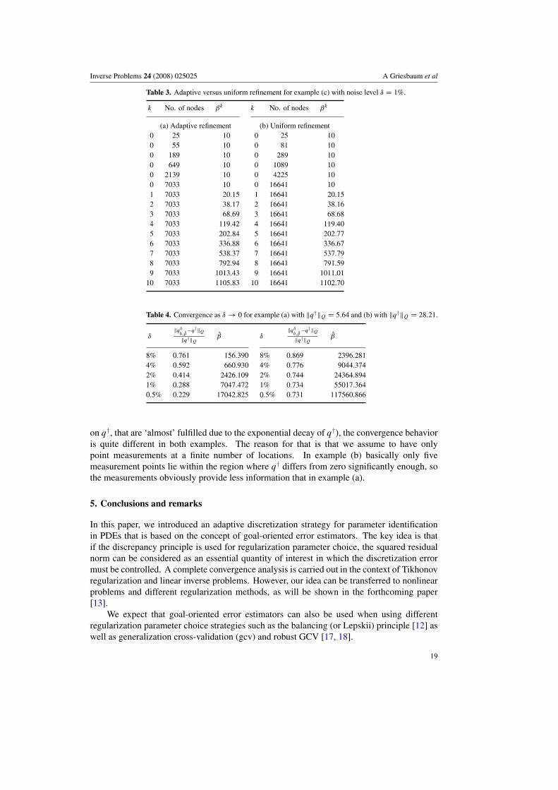
Table 3. Adaptive versus uniform refinement for example (c) with noise level δ = 1%.

k No. of nodes βk k No. of nodes βk

(a) Adaptive refinement (b) Uniform refinement0 25 10 0 25 100 55 10 0 81 100 189 10 0 289 100 649 10 0 1089 100 2139 10 0 4225 100 7033 10 0 16641 101 7033 20.15 1 16641 20.152 7033 38.17 2 16641 38.163 7033 68.69 3 16641 68.684 7033 119.42 4 16641 119.405 7033 202.84 5 16641 202.776 7033 336.88 6 16641 336.677 7033 538.37 7 16641 537.798 7033 792.94 8 16641 791.599 7033 1013.43 9 16641 1011.01

10 7033 1105.83 10 16641 1102.70

Table 4. Convergence as δ → 0 for example (a) with ‖q†‖Q = 5.64 and (b) with ‖q†‖Q = 28.21.

δ‖qδ

h,β−q†‖Q

‖q†‖Qβ δ

‖qδh,β

−q†‖Q

‖q†‖Qβ

8% 0.761 156.390 8% 0.869 2396.2814% 0.592 660.930 4% 0.776 9044.3742% 0.414 2426.109 2% 0.744 24364.8941% 0.288 7047.472 1% 0.734 55017.3640.5% 0.229 17042.825 0.5% 0.731 117560.866

on q†, that are ‘almost’ fulfilled due to the exponential decay of q†), the convergence behavioris quite different in both examples. The reason for that is that we assume to have onlypoint measurements at a finite number of locations. In example (b) basically only fivemeasurement points lie within the region where q† differs from zero significantly enough, sothe measurements obviously provide less information that in example (a).

5. Conclusions and remarks

In this paper, we introduced an adaptive discretization strategy for parameter identificationin PDEs that is based on the concept of goal-oriented error estimators. The key idea is thatif the discrepancy principle is used for regularization parameter choice, the squared residualnorm can be considered as an essential quantity of interest in which the discretization errormust be controlled. A complete convergence analysis is carried out in the context of Tikhonovregularization and linear inverse problems. However, our idea can be transferred to nonlinearproblems and different regularization methods, as will be shown in the forthcoming paper[13].

We expect that goal-oriented error estimators can also be used when using differentregularization parameter choice strategies such as the balancing (or Lepskii) principle [12] aswell as generalization cross-validation (gcv) and robust GCV [17, 18].

19

Inverse Problems 24 (2008) 025025 A Griesbaum et al

Acknowledgments

The research work leading to this paper was initiated during a stay of the second author atthe Radon Institute for Computational and Applied Mathematics (RICAM) in Linz; hencethe authors wish to express their thanks to the Austrian Academy of Sciences. Moreover, wewish to thank the referees for valuable comments. The first author is supported by the DFGpriority program 1251 ‘Optimization with Partial Differential Equations’. The third author hasbeen partially supported by the Austrian Science Fund FWF project P18971-N18 ‘Numericalanalysis and discretization strategies for optimal control problems with singularities’.

References

[1] Ameur H B, Chavent G and Jaffre J 2002 Refinement and coarsening indicators for adaptive parametrization tothe estimation of hydraulic transmissivities Inverse Problems 18 775–94

[2] Becker R, Braack M, Meidner D, Richter T, Schmich M and Vexler B 2005 The Finite Element Toolkit GASCOIGNE

[3] Becker R, Dunne T and Meidner D 2005 VISUSIMPLE: An interactive VTK-based visualization andgraphics/mpeg-generation program

[4] Becker R, Meidner D and Vexler B 2005 RODOBO: A C++ library for optimization with stationary andnonstationary PDEs with interface to GASCOIGNE [2]

[5] Becker R and Rannacher R 2001 An Optimal Control Approach to a-Posteriori Error Estimation in ActaNumerica 2001 ed A Iserles (Cambridge: Cambridge University Press) pp 1–102

[6] Becker R and Vexler B 2004 A posteriori error estimation for finite element discretizations of parameteridentification problems Numer. Math. 96 435–59

[7] Becker R and Vexler B 2005 Mesh refinement and numerical sensitivity analysis for parameter calibration ofpartial differential equations J. Comput. Phys. 206 95–110

[8] Borcea L and Druskin V 2002 Optimal finite difference grids for direct and inverse sturm liouville problemsInverse Problems 18 979–1001

[9] Braess D 2007 Finite Elements: Theory, Fast Solvers and Applications in Solid Mechanics (Cambridge:Cambridge University Press)

[10] Brenner S and Scott R 2002 The Mathematical Theory of Finite Element Methods (Berlin: Springer)[11] Engl H, Hanke M and Neubauer A 1996 Regularization of Inverse Problems (Dordrecht: Kluwer)[12] Goldenshluger A and Pereverzev S 2000 Adaptive estimation of linear functionals in Hilbert scales from indirect

white noise observations Probab. Theory Relat. Fields 118 169–86[13] Griesbaum A, Kaltenbacher B and Vexler B Goal oriented adaptive discretization for nonlinear ill-posed

problems, in preparation[14] Griesse R and Vexler B 2007 Numerical sensitivity analysis for the quantity of interest in PDE-constrained

optimization SIAM J. Sci. Comput. 29 22–48[15] Haber E, Heldmann S and Ascher U 2007 Adaptive finite volume methods for distributed non-smooth parameter

identification Inverse Problems 23 1659–76[16] Hohage T 2000 Regularization of exponentially ill-posed problems Numer. Funct. Anal. Optim. 21 439–64[17] Lukas M A 1998 Comparisons of parameter choice methods for regularization with discrete noisy data Inverse

Problems 14 161–84[18] Lukas M A 2006 Robust generalized cross-validation for choosing the regularization parameter Inverse

Problems 22 1883–902[19] Meidner D and Vexler B 2007 Adaptive space-time finite element methods for parabolic optimization problems

SIAM J. Control Optim. 46 116–42[20] Nair M, Pereverzev S and Tautenhahn U 2005 Regularization in Hilbert scales under general smoothing

conditions Inverse Problems 21 1851–69[21] Nair M, Schock E and Tautenhahn U 2003 Morozov’s discrepancy principle under general source conditions

Zeitschr Anal. Anw. 22 199–214[22] Neubauer A 2007 Solution of ill-posed problems via adaptive grid regularization: convergence analysis Numer.

Funct. Anal. Optim. 28 405–23[23] Tautenhahn U and Nian Jin Q 2003 Tikhonov regularization and a posteriori rules for solving nonlinear ill-posed

problems Inverse Problems 19 1–21

20