Eciency of Continuous Double Auctions under Individual Evolutionary Learning with Full or Limited Information

Efficiency of Continuous Double Auctions under Individual

Evolutionary Learning with Full or Limited Information ∗

Mikhail Anufriev a Jasmina Arifovic b Valentyn Panchenko c

February 2010

a CeNDEF, School of Economics, University of Amsterdam,

Roetersstraat 11, NL-1018 WB Amsterdam, Netherlands

b Department of Economics, Simon Fraser University,

Burnaby, B.C., Canada V5A 1S6

c School of Economics, University of New South Wales,

Sydney, NSW 2052, Australia

∗We thank the participants of the SCE-2009 conference in Sydney, the workshop “Evolution and marketbehavior in economics and finance” in Pisa and the seminars at the University of Amsterdam, University ofAuckland and University of Technology, Sydney, for useful comments on earlier drafts of this paper. JasminaArifovic acknowledges financial support from the Social Sciences and Humanities Research Council underthe Standard Research Grant Program. Mikhail Anufriev acknowledges the financial support by the EU7th framework collaborative project “Monetary, Fiscal and Structural Policies with Heterogeneous Agents(POLHIA)”, grant no.225408. Valentyn Panchenko acknowledges the support under Australian ResearchCouncil’s Discovery Projects funding scheme (project number DP0986718). Usual caveats apply.

1

Abstract

In this paper we explore how specific aspects of market transparency and agents

behavior affect the efficiency of the market outcome. In particular, we are interested

whether learning behavior with and without information about actions of other partici-

pants improves market efficiency. We consider a simple market for a homogeneous good

populated by buyers and sellers. The valuations of the buyers and the costs of the sellers

are given exogenously. Agents are involved in the consecutive trading sessions, which

are organized as a continuous double auction with electronic book. Using Individual

Evolutionary Learning mechanism agents submit price bids and offers, trying to learn

the most profitable strategy by looking at their realized and counterfactual or “foregone”

payoffs. We find that learning outcomes heavily depend on information treatments. Un-

der full information agents’ orders tend to be similar, while under limited information

agents submit their valuations/costs. This results in higher price volatility for the latter

treatment. We also find that learning improves allocative efficiency when compared with

the outcomes with Zero-Intelligence traders.

JEL codes: D83, C63, D44

Keywords: Allocative Efficiency, Continuous Double Auction, Individual Evolution-

ary Learning

2

1 Introduction

A question of “What makes markets allocatively efficient?” has attracted a lot of at-

tention in recent years. Methodology focusing on Zero Intelligent (ZI) agents initiated

in Gode and Sunder (1993) has led to the conclusion that the rules of the market and

not individual rationality are responsible for market’s allocative efficiency.1 ZI traders

do not have memory and do not behave strategically, submitting random orders subject

to budget constraints. Thus any effect on efficiency is attributed solely to the change

of market rules. Gode and Sunder (1993) find that market organized as a continuous

double auction (CDA) is highly efficient and in some cases allows ZI traders to extract

around 99% of possible surplus. This result has been criticized in the literature. Gode

and Sunder (1997) have found that a number of specific rules of the CDA is required to

guarantee this efficiency. LiCalzi and Pellizzari (2008) have shown that the allocative

efficiency of the CDA would drop substantially if every transaction did not force agents

to submit new orders. In their words, the high efficiency results in Gode and Sunder

(1993) are driven by order book “resampling”.

The results of experiments with human subjects starting with Smith (1962) show

quick convergence towards competitive equilibrium, also resulting in high allocative effi-

ciency of the CDA. A natural question arises about significance of individual rationality

for this outcome. Gjerstad and Shachat (2007) note that budget constraints of the

ZI agents, i.e., restrictions on submitting orders clearly resulting in losses, is a part of

agents’ individual rationality. The role of rationality is even more important in the

markets where the ZI agents do not extract a maximum possible surplus. With the

assumption of forward-looking, strategical, optimizing agents, a standard economic ap-

proach suggests solving for a rational expectations equilibrium under specified market

rules. Examples of such approach include Easley and Ledyard (1993), Friedman (1991)

and Gjerstad and Dickhaut (1998). In our opinion, the fully rational approach is not

completely satisfactory because of two reasons. First, given complexity of the CDA mar-

ket and the high dimension of strategy space results are obtained only under auxiliary

assumptions which limit either information or strategies available to participants or both.

Full solution is, perhaps, not feasible anyway. Second, and more importantly, behavioral

and experimental literature shows that people fail to optimize and behave strategically

even in more simple situations and that models with simple learning behavior fit observed

outcomes better, see, for example, Erev and Roth (1998).

In this paper, we follow an intermediate approach between ZI and full rationality.

More precisely, we analyze allocative efficiency in the market with boundedly rational

participants learning in a fixed environment. While the demand and supply schedules

are not changing from one trading session to another, the agents’ bidding behavior does.

We use the Individual Evolutionary Learning (IEL) algorithm, introduced in Arifovic

and Ledyard (2003). This algorithm builds on the framework introduced by Arifovic

1See Duffy (2006) and Ladley (2010) for recent reviews of the ZI-literature.

3

(1994) who examined genetic algorithms (GA) as a model of social as well as individual

learning of economic agents in the context of the cobweb model. For a recent application

of the GA to the CDA market with a large number of traders, see Fano, LiCalzi, and

Pellizzari (2010). According to the IEL algorithm agents select their strategies (limit

order prices) on the basis of their not only actual, but also counterfactual performance.

We distinguish between learning based on the information available in the open order

book and learning based only on aggregate market information, when the order book is

closed. Similar questions were recently analyzed in Arifovic and Ledyard (2007) for call

auction market, while we address them here for the CDA market. Openness of the order

book is related to the questions of the market design which recently draw attention in

the literature. For example, in January 2002 the NYSE introduced OpenBook system

which effectively opened the content of the limit order book to public. Boehmer, Saar,

and Yu (2005) find that this increasing transparency affected investors’ trading strategies

and resulted in decreased price volatility and increased liquidity. Alternatively, we may

think about use of information as a part of agents behavior, which maybe influenced by

market mechanism, e.g., via price of access or availability of access to the information.

We analyze whether and how learning affects the allocative efficiency and study what

kind of observable agents’ behavior emerges as an outcome of the learning process in two

different types of environments, Gode-Sunder (GS, henceforth, that corresponds to the

environment in Gode and Sunder, 1997) and Arifovic-Ledyard (AL, that corresponds to

the environment in Arifovic and Ledyard, 2007). We find that learning may result in

sizeable increase in efficiency. We also find that market transparency influences trading

strategies and results in different market outcomes. In particular, usage of the book in-

formation substantially decreases market volatility, consistently with empirical evidence.

In general, efficiency of the market is a joint outcome of market rules and agents’ ratio-

nality, as was previously stressed in models with heterogeneous agents of Bottazzi, Dosi,

and Rebesco (2005) and Anufriev and Panchenko (2009).

The rest of the paper is organized as follows. The market environment is explained

in Section 2, where we also recall the definition of allocative efficiency and derive a

benchmark for ZI traders. The model for learning behavior of agents is introduced in

Section 3 and its effects on market outcomes are discussed in Section 4. In Section 5 we

report various robustness tests which have been performed. Section 6 concludes.

2 Model

We start with describing environment and defining competitive equilibrium as a bench-

mark against which the outcomes under different learning rules will be compared. We

then proceed by explaining the continuous double auction mechanism. Finally, we study

the allocative efficiency under ZI trading.

4

2.1 Environment

Suppose we have a fixed number B + S market participants, B buyers and S sellers. At

the beginning of a trading session t ∈ {1, . . . , T}, each seller is endowed with one unit

of commodity and each buyer would like to consume one unit of commodity. The same

agents transact during T trading sessions. Throughout the paper index b ∈ {1, . . . , B}denotes the buyer and index s ∈ {1, . . . , S} denotes the seller.

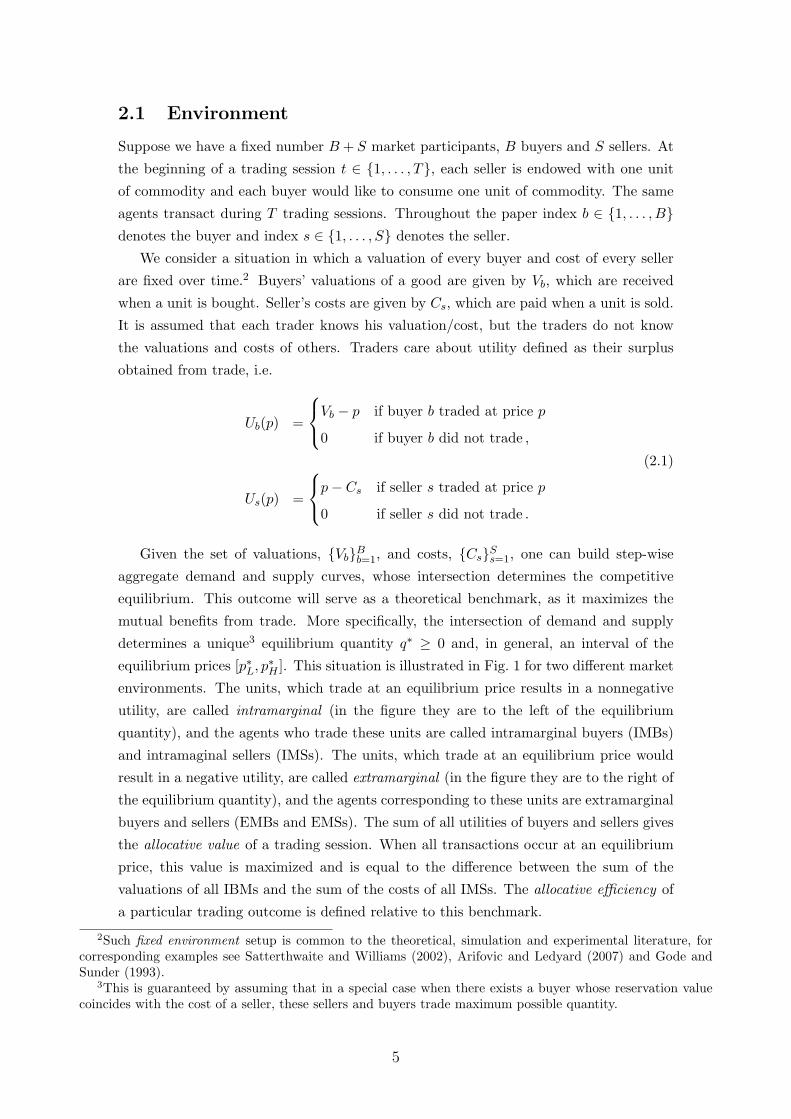
We consider a situation in which a valuation of every buyer and cost of every seller

are fixed over time.2 Buyers’ valuations of a good are given by Vb, which are received

when a unit is bought. Seller’s costs are given by Cs, which are paid when a unit is sold.

It is assumed that each trader knows his valuation/cost, but the traders do not know

the valuations and costs of others. Traders care about utility defined as their surplus

obtained from trade, i.e.

Ub(p) =

Vb − p if buyer b traded at price p

0 if buyer b did not trade ,

Us(p) =

p− Cs if seller s traded at price p

0 if seller s did not trade .

(2.1)

Given the set of valuations, {Vb}Bb=1, and costs, {Cs}Ss=1, one can build step-wise

aggregate demand and supply curves, whose intersection determines the competitive

equilibrium. This outcome will serve as a theoretical benchmark, as it maximizes the

mutual benefits from trade. More specifically, the intersection of demand and supply

determines a unique3 equilibrium quantity q∗ ≥ 0 and, in general, an interval of the

equilibrium prices [p∗L, p∗H ]. This situation is illustrated in Fig. 1 for two different market

environments. The units, which trade at an equilibrium price results in a nonnegative

utility, are called intramarginal (in the figure they are to the left of the equilibrium

quantity), and the agents who trade these units are called intramarginal buyers (IMBs)

and intramaginal sellers (IMSs). The units, which trade at an equilibrium price would

result in a negative utility, are called extramarginal (in the figure they are to the right of

the equilibrium quantity), and the agents corresponding to these units are extramarginal

buyers and sellers (EMBs and EMSs). The sum of all utilities of buyers and sellers gives

the allocative value of a trading session. When all transactions occur at an equilibrium

price, this value is maximized and is equal to the difference between the sum of the

valuations of all IBMs and the sum of the costs of all IMSs. The allocative efficiency of

a particular trading outcome is defined relative to this benchmark.

2Such fixed environment setup is common to the theoretical, simulation and experimental literature, forcorresponding examples see Satterthwaite and Williams (2002), Arifovic and Ledyard (2007) and Gode andSunder (1993).

3This is guaranteed by assuming that in a special case when there exists a buyer whose reservation valuecoincides with the cost of a seller, these sellers and buyers trade maximum possible quantity.

5

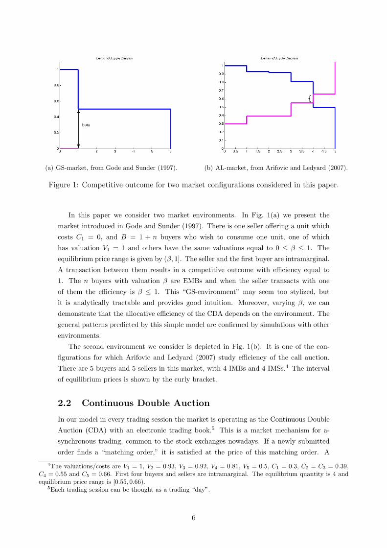
(a) GS-market, from Gode and Sunder (1997). (b) AL-market, from Arifovic and Ledyard (2007).

Figure 1: Competitive outcome for two market configurations considered in this paper.

In this paper we consider two market environments. In Fig. 1(a) we present the

market introduced in Gode and Sunder (1997). There is one seller offering a unit which

costs C1 = 0, and B = 1 + n buyers who wish to consume one unit, one of which

has valuation V1 = 1 and others have the same valuations equal to 0 ≤ β ≤ 1. The

equilibrium price range is given by (β, 1]. The seller and the first buyer are intramarginal.

A transaction between them results in a competitive outcome with efficiency equal to

1. The n buyers with valuation β are EMBs and when the seller transacts with one

of them the efficiency is β ≤ 1. This “GS-environment” may seem too stylized, but

it is analytically tractable and provides good intuition. Moreover, varying β, we can

demonstrate that the allocative efficiency of the CDA depends on the environment. The

general patterns predicted by this simple model are confirmed by simulations with other

environments.

The second environment we consider is depicted in Fig. 1(b). It is one of the con-

figurations for which Arifovic and Ledyard (2007) study efficiency of the call auction.

There are 5 buyers and 5 sellers in this market, with 4 IMBs and 4 IMSs.4 The interval

of equilibrium prices is shown by the curly bracket.

2.2 Continuous Double Auction

In our model in every trading session the market is operating as the Continuous Double

Auction (CDA) with an electronic trading book.5 This is a market mechanism for a-

synchronous trading, common to the stock exchanges nowadays. If a newly submitted

order finds a “matching order,” it is satisfied at the price of this matching order. A

4The valuations/costs are V1 = 1, V2 = 0.93, V3 = 0.92, V4 = 0.81, V5 = 0.5, C1 = 0.3, C2 = C3 = 0.39,C4 = 0.55 and C5 = 0.66. First four buyers and sellers are intramarginal. The equilibrium quantity is 4 andequilibrium price range is [0.55, 0.66).

5Each trading session can be thought as a trading “day”.

6

matching order is defined as an order stored in the opposite side of the book at whose

price the transaction with a newly arrived order is possible. If there are many orders

which match the incoming order, the matching order with which the trade occurs is

selected according to the price-time priority. If the submitted order does not find a

matching order, it is stored in the book.

We assume that every agent submits only one order (bid or ask depending on the

agent’s type) during a trading session.6 The agents determine their orders before the

session starts. Consequently, they cannot condition their order on the state of the book.

The sequence of traders’ arrival to the market is randomly permuted for every session. At

the end of each trading session the order book is cleared by removing all the unsatisfied

orders, so that the next session starts with an empty book.

For a given set of agents’ orders and their arrival sequence, the CDA mechanism

described above generates a (possible empty) sequence of transactions. The prices at

which buyer b and seller s traded during trading session t are denoted by pb,t and ps,t,

while their orders are given by bb,t and as,t, respectively. In case b traded with s, price

pb,t=ps,t is the price of this transaction. It is equal to bb,t if b arrived before s and

to as,t, otherwise. According to (2.1), buyer b who traded at price pb,t extracts utility

Vb − pb,t, while the buyer who did not trade over the session gets 0. Similarly, seller s

who succeeded in selling the unit at price ps,t receives utility ps,t − Cs, while the seller

who did not trade gets 0. Note that in the CDA market the utility of the traders depend

not only on their submitted orders but also on the sequence of their trades.

2.3 Market Efficiency with ZI-traders

A useful benchmark for efficiency of a market mechanism is given by its performance

when the traders are Zero Intelligent (ZI). Every trading period ZI traders submit random

orders, drawing them independently from a uniform distribution. Gode and Sunder

(1993) distinguish between constrained and unconstrained ZI traders. Unconstrained ZI

traders can draw orders from a whole interval [0, 1], while constrained traders are not

allowed to bid higher than their valuation or ask lower than their cost. Gjerstad and

Shachat (2007) attribute this restriction to the individual rationality (IR) in the order

submission, rather than a market rule. We follow their terminology and distinguish

between agents “with IR” and “without IR”. A buyer with IR cannot submit an order

higher than the valuation. A seller with IR cannot submit an order lower than the cost.

6This assumption implies that multiple rounds of bidding are excluded from the analysis of this paper.Gode and Sunder (1997) show that multiple rounds (until all possible transactions occur) result in higherefficiency due to absence of losses caused by absence of trade. We also do not clear and “resample” the bookafter every transaction. Resampling would increase efficiency of the market, because orders submitted far fromthe equilibrium range of price would have a chance to be corrected, see LiCalzi and Pellizzari (2008).

7

0.4

0.5

0.6

0.7

0.8

0.9

1

0 0.2 0.4 0.6 0.8 1

Eff

icie

ncy

β

En=10n=3

(a) Agents with IR.

0

0.2

0.4

0.6

0.8

1

0 0.2 0.4 0.6 0.8 1

Eff

icie

ncy

β

E with IRE without IR

n=10n=3

(b) Agents without IR.

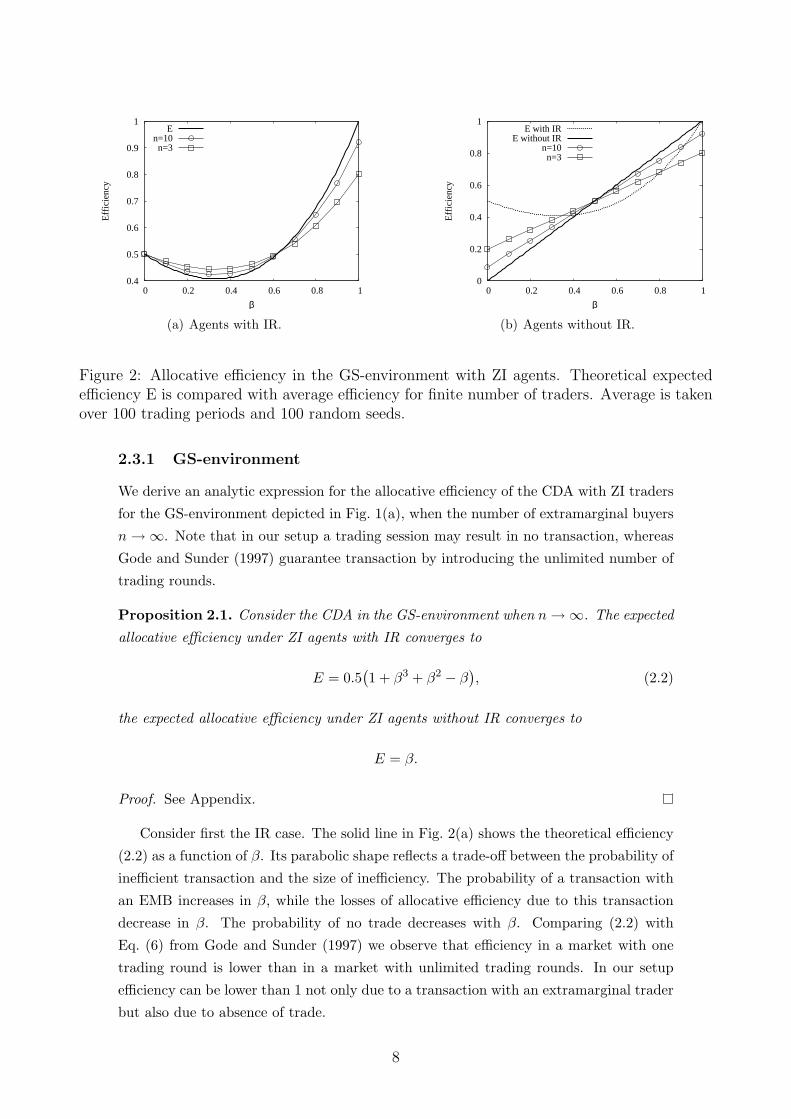
Figure 2: Allocative efficiency in the GS-environment with ZI agents. Theoretical expectedefficiency E is compared with average efficiency for finite number of traders. Average is takenover 100 trading periods and 100 random seeds.

2.3.1 GS-environment

We derive an analytic expression for the allocative efficiency of the CDA with ZI traders

for the GS-environment depicted in Fig. 1(a), when the number of extramarginal buyers

n→∞. Note that in our setup a trading session may result in no transaction, whereas

Gode and Sunder (1997) guarantee transaction by introducing the unlimited number of

trading rounds.

Proposition 2.1. Consider the CDA in the GS-environment when n→∞. The expected

allocative efficiency under ZI agents with IR converges to

E = 0.5(1 + β3 + β2 − β

), (2.2)

the expected allocative efficiency under ZI agents without IR converges to

E = β.

Proof. See Appendix.

Consider first the IR case. The solid line in Fig. 2(a) shows the theoretical efficiency

(2.2) as a function of β. Its parabolic shape reflects a trade-off between the probability of

inefficient transaction and the size of inefficiency. The probability of a transaction with

an EMB increases in β, while the losses of allocative efficiency due to this transaction

decrease in β. The probability of no trade decreases with β. Comparing (2.2) with

Eq. (6) from Gode and Sunder (1997) we observe that efficiency in a market with one

trading round is lower than in a market with unlimited trading rounds. In our setup

efficiency can be lower than 1 not only due to a transaction with an extramarginal trader

but also due to absence of trade.

8

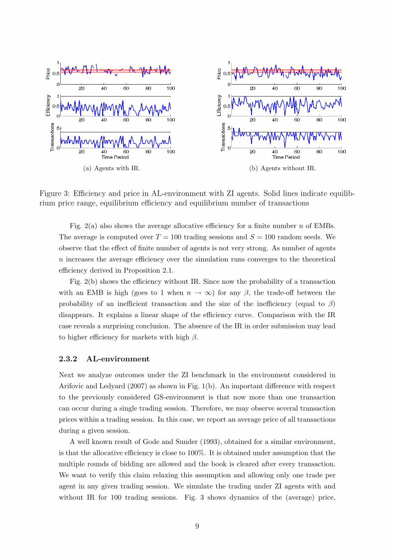
(a) Agents with IR. (b) Agents without IR.

Figure 3: Efficiency and price in AL-environment with ZI agents. Solid lines indicate equilib-rium price range, equilibrium efficiency and equilibrium number of transactions

Fig. 2(a) also shows the average allocative efficiency for a finite number n of EMBs.

The average is computed over T = 100 trading sessions and S = 100 random seeds. We

observe that the effect of finite number of agents is not very strong. As number of agents

n increases the average efficiency over the simulation runs converges to the theoretical

efficiency derived in Proposition 2.1.

Fig. 2(b) shows the efficiency without IR. Since now the probability of a transaction

with an EMB is high (goes to 1 when n → ∞) for any β, the trade-off between the

probability of an inefficient transaction and the size of the inefficiency (equal to β)

disappears. It explains a linear shape of the efficiency curve. Comparison with the IR

case reveals a surprising conclusion. The absence of the IR in order submission may lead

to higher efficiency for markets with high β.

2.3.2 AL-environment

Next we analyze outcomes under the ZI benchmark in the environment considered in

Arifovic and Ledyard (2007) as shown in Fig. 1(b). An important difference with respect

to the previously considered GS-environment is that now more than one transaction

can occur during a single trading session. Therefore, we may observe several transaction

prices within a trading session. In this case, we report an average price of all transactions

during a given session.

A well known result of Gode and Sunder (1993), obtained for a similar environment,

is that the allocative efficiency is close to 100%. It is obtained under assumption that the

multiple rounds of bidding are allowed and the book is cleared after every transaction.

We want to verify this claim relaxing this assumption and allowing only one trade per

agent in any given trading session. We simulate the trading under ZI agents with and

without IR for 100 trading sessions. Fig. 3 shows dynamics of the (average) price,

9

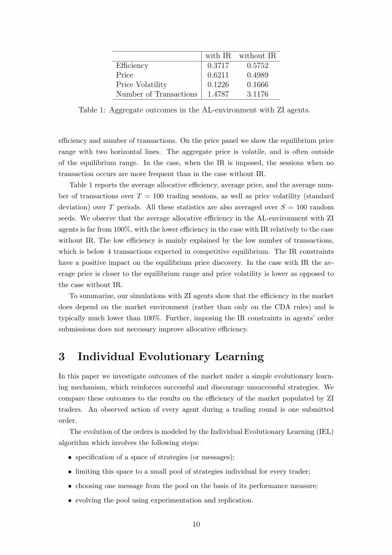
with IR without IREfficiency 0.3717 0.5752Price 0.6211 0.4989Price Volatility 0.1226 0.1666Number of Transactions 1.4787 3.1176

Table 1: Aggregate outcomes in the AL-environment with ZI agents.

efficiency and number of transactions. On the price panel we show the equilibrium price

range with two horizontal lines. The aggregate price is volatile, and is often outside

of the equilibrium range. In the case, when the IR is imposed, the sessions when no

transaction occurs are more frequent than in the case without IR.

Table 1 reports the average allocative efficiency, average price, and the average num-

ber of transactions over T = 100 trading sessions, as well as price volatility (standard

deviation) over T periods. All these statistics are also averaged over S = 100 random

seeds. We observe that the average allocative efficiency in the AL-environment with ZI

agents is far from 100%, with the lower efficiency in the case with IR relatively to the case

without IR. The low efficiency is mainly explained by the low number of transactions,

which is below 4 transactions expected in competitive equilibrium. The IR constraints

have a positive impact on the equilibrium price discovery. In the case with IR the av-

erage price is closer to the equilibrium range and price volatility is lower as opposed to

the case without IR.

To summarize, our simulations with ZI agents show that the efficiency in the market

does depend on the market environment (rather than only on the CDA rules) and is

typically much lower than 100%. Further, imposing the IR constraints in agents’ order

submissions does not necessary improve allocative efficiency.

3 Individual Evolutionary Learning

In this paper we investigate outcomes of the market under a simple evolutionary learn-

ing mechanism, which reinforces successful and discourage unsuccessful strategies. We

compare these outcomes to the results on the efficiency of the market populated by ZI

traders. An observed action of every agent during a trading round is one submitted

order.

The evolution of the orders is modeled by the Individual Evolutionary Learning (IEL)

algorithm which involves the following steps:

• specification of a space of strategies (or messages);

• limiting this space to a small pool of strategies individual for every trader;

• choosing one message from the pool on the basis of its performance measure;

• evolving the pool using experimentation and replication.

10

IEL is based on the individual (not social) evolutionary process. It is well suited for

applications in the environments with large strategy spaces (subsets of real line) such as

is our CDA environment.7

Messages

We assume that a message, εb,t(εs,t), represents a potential bid (or ask) order price

from buyer b (or seller s) at trading session t. In our base treatment we do not allow

a violation of the IR constraints, that is, we require εb,t ≤ Vb and εs,t ≥ Cs. Under

alternative treatments without IR constraints these restrictions will not be imposed and

we will let traders themselves to learn not to submit orders which lead to individual

losses. We assume that possible orders belong to the interval [0, 1].

Individual Pool

Even if there is a continuum of possible messages, every agent will be restricted at every

time to choose between a limited amount of them. The pool of messages (bids) available

for submission at time t by buyer b is denoted by Bb,t. The pool of messages (asks)

available for submission at time t by seller s is denoted by As,t. Every period the pool

of each agent is updated, but the number of messages in the pool is fixed and equals to

J . In the benchmark simulations J = 100. Some of the messages in the pool might be

identical, so that an agent may be choosing from J or less possible alternatives. Initially,

the individual pools contains J strategies drawn, independently for each agent, from the

uniform distribution on the interval [0, 1].

The pool used at time t is updated before the following trading session by subsequent

application of two algorithms, experimentation (or mutation) and replication. During

experimentation stage, any message from the old pool can be replaced with a small prob-

ability by some new message. In such a way for every buyer and seller the intermediate

pools are formed. More specifically, each message is removed from the pool with a small

probability of experimentation, ρ, or remains in the pool with probability 1− ρ. In case

that a message is removed, it is replaced by a new message drawn from a distribution,

P. In the benchmark simulations ρ = 0.03 and distribution P is uniform on the interval

[0, 1].

At the replication stage two randomly chosen messages from the just-formed (inter-

mediate) pool are compared one with another, and the best of them occupies a place in

a new pool, Bb,t+1, for a buyer or As,t+1 for a seller. For every agent such process is

independently repeated J times (with replacement), in order to fill all the places in the

new pool. The comparison is made according to a performance measure which is defined

below. During replication we, therefore, increase an amount of “successful” messages in

the pool at the expense of less successful messages.

7See Arifovic and Ledyard (2004) for a discussion of the advantages of IEL over other commonly usedmodels of individual learning, such as Reinforcement Learning and Experience-Weighted Attraction Learning,in the environments with large strategy spaces.

11

Calculating the Foregone Utilities

How good is a given message? To answer this questions, every agent applies some

counterfactual analysis. Indeed, only the message which has actually been used last

period delivers a known payoff given by (2.1). A learning agent would also like to infer a

foregone payoff from alternative strategies. Notice this is a boundedly rational reasoning,

since our agent ignores the analogous learning process of all the other agents.

The calculation of foregone payoff is also made according to (2.1), but the price of

transaction is notional and depends on the amount of information which is available

to the agent. We distinguish between two treatments which we call open book (OP)

and closed book (CL) information treatment. Under the OP treatment each agent uses

full information about all bids, offers and prices from the previous period. Only the

identity of bidders are not known preventing a direct access to the behavioral strategies

used by others. Under the CL treatment the agents are informed only about some price

aggregate, say, average price from the previous session, P avt . If no transaction occurred

during this session, P avt is set to an average price of the most recent past session for

which at least one transaction had occurred. Note that the availability and use of the

information from the book may be attributed either to market design, e.g. openness of

the market, costs of open book access, or to individual behavior, e.g. willingness to buy

information, possibility to process it, or both.

Let It denote the largest possible information set after the trading session t. It

includes the orders of all buyers and sellers as well as sequence in which they arrive at

the market. Under the CL treatment this whole set is not known to traders: they know

only their own bids and asks as well as an average price. Thus, under the CL treatment

the information sets of buyers and sellers in the end of session t are given as

ICLb,t =

{bb,t, P

avt } ∪ ICL

b,t−1 , ICLs,t =

{as,t, P

avt } ∪ ICL

s,t−1 .

The order book of the past period cannot be reconstructed with this information. Hence,

agent can use only average price of the previous session as an indication for possible

realized price given alternative message submitted.8 Under the CL treatment, agents’

foregone utilities are given by

Ub,t(εb|ICLb,t ) =

Vb − P avt if εb ≥ P av

t

0 otherwise,

Us,t(εs|ICLs,t ) =

P avt − Cs if εs ≤ P av

t

0 otherwise.

(3.1)

Under the OP treatment, an agent knows the state of the order book at every moment

8Other plausible possibility is to consider the closed price of the day. This modification does not influenceour results.

12

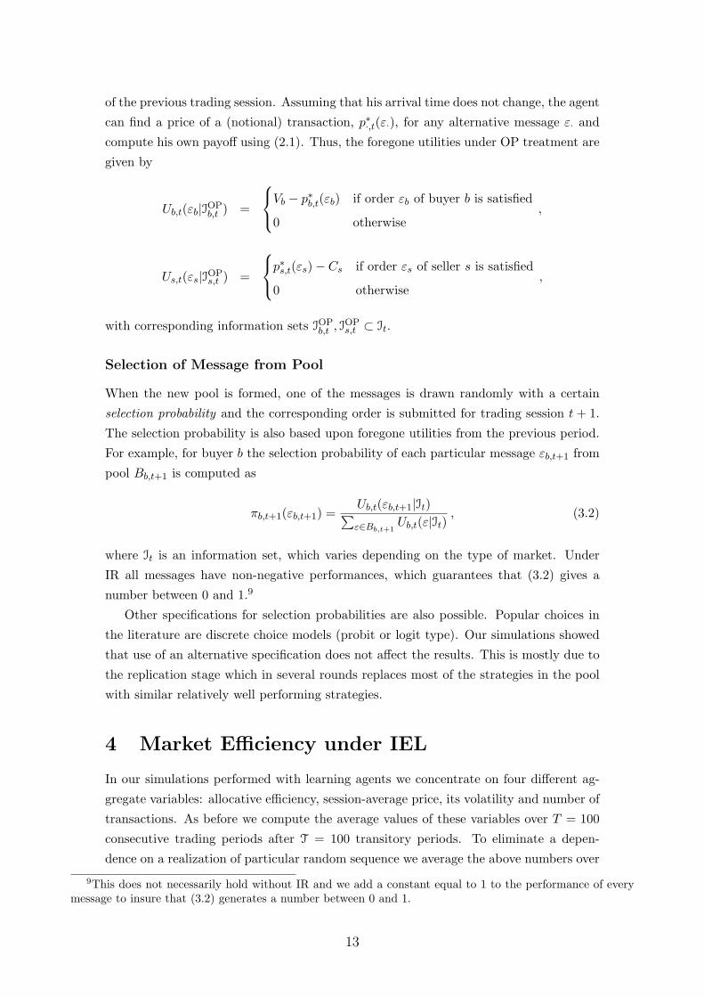
of the previous trading session. Assuming that his arrival time does not change, the agent

can find a price of a (notional) transaction, p∗·,t(ε·), for any alternative message ε· and

compute his own payoff using (2.1). Thus, the foregone utilities under OP treatment are

given by

Ub,t(εb|IOPb,t ) =

Vb − p∗b,t(εb) if order εb of buyer b is satisfied

0 otherwise,

Us,t(εs|IOPs,t ) =

p∗s,t(εs)− Cs if order εs of seller s is satisfied

0 otherwise,

with corresponding information sets IOPb,t , I

OPs,t ⊂ It.

Selection of Message from Pool

When the new pool is formed, one of the messages is drawn randomly with a certain

selection probability and the corresponding order is submitted for trading session t + 1.

The selection probability is also based upon foregone utilities from the previous period.

For example, for buyer b the selection probability of each particular message εb,t+1 from

pool Bb,t+1 is computed as

πb,t+1(εb,t+1) =Ub,t(εb,t+1|It)∑ε∈Bb,t+1

Ub,t(ε|It), (3.2)

where It is an information set, which varies depending on the type of market. Under

IR all messages have non-negative performances, which guarantees that (3.2) gives a

number between 0 and 1.9

Other specifications for selection probabilities are also possible. Popular choices in

the literature are discrete choice models (probit or logit type). Our simulations showed

that use of an alternative specification does not affect the results. This is mostly due to

the replication stage which in several rounds replaces most of the strategies in the pool

with similar relatively well performing strategies.

4 Market Efficiency under IEL

In our simulations performed with learning agents we concentrate on four different ag-

gregate variables: allocative efficiency, session-average price, its volatility and number of

transactions. As before we compute the average values of these variables over T = 100

consecutive trading periods after T = 100 transitory periods. To eliminate a depen-

dence on a realization of particular random sequence we average the above numbers over

9This does not necessarily hold without IR and we add a constant equal to 1 to the performance of everymessage to insure that (3.2) generates a number between 0 and 1.

13

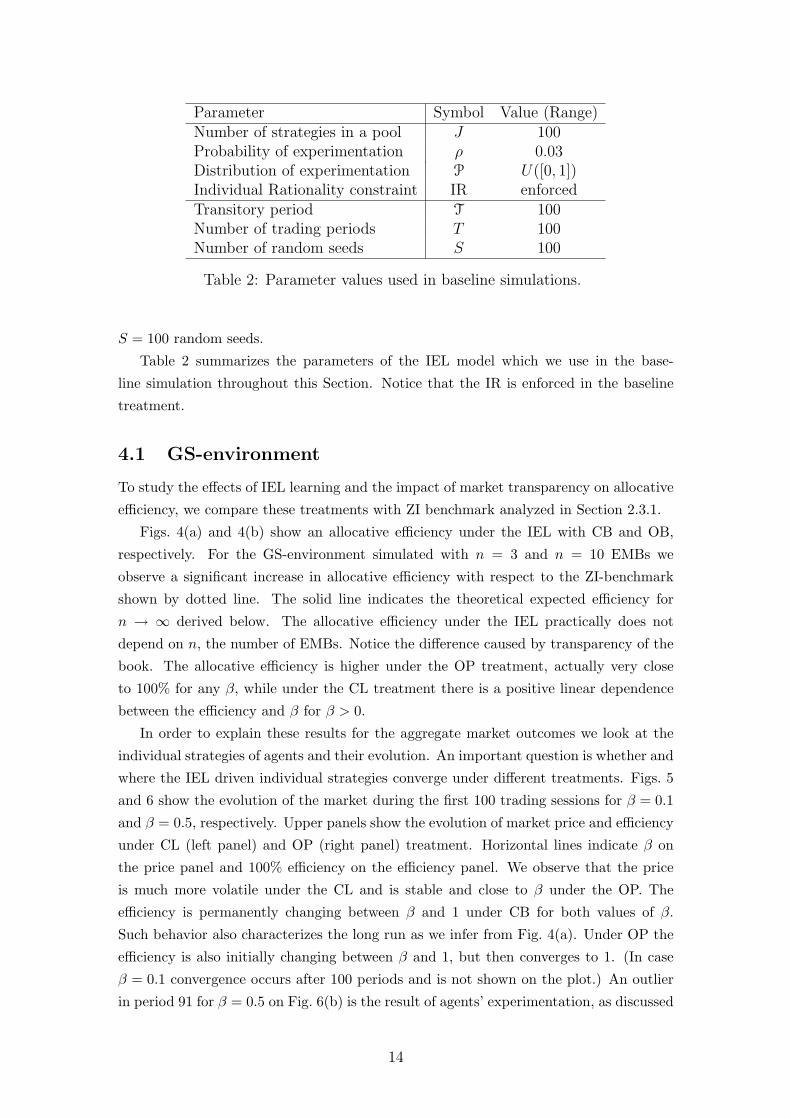
Parameter Symbol Value (Range)Number of strategies in a pool J 100Probability of experimentation ρ 0.03Distribution of experimentation P U([0, 1])Individual Rationality constraint IR enforcedTransitory period T 100Number of trading periods T 100Number of random seeds S 100

Table 2: Parameter values used in baseline simulations.

S = 100 random seeds.

Table 2 summarizes the parameters of the IEL model which we use in the base-

line simulation throughout this Section. Notice that the IR is enforced in the baseline

treatment.

4.1 GS-environment

To study the effects of IEL learning and the impact of market transparency on allocative

efficiency, we compare these treatments with ZI benchmark analyzed in Section 2.3.1.

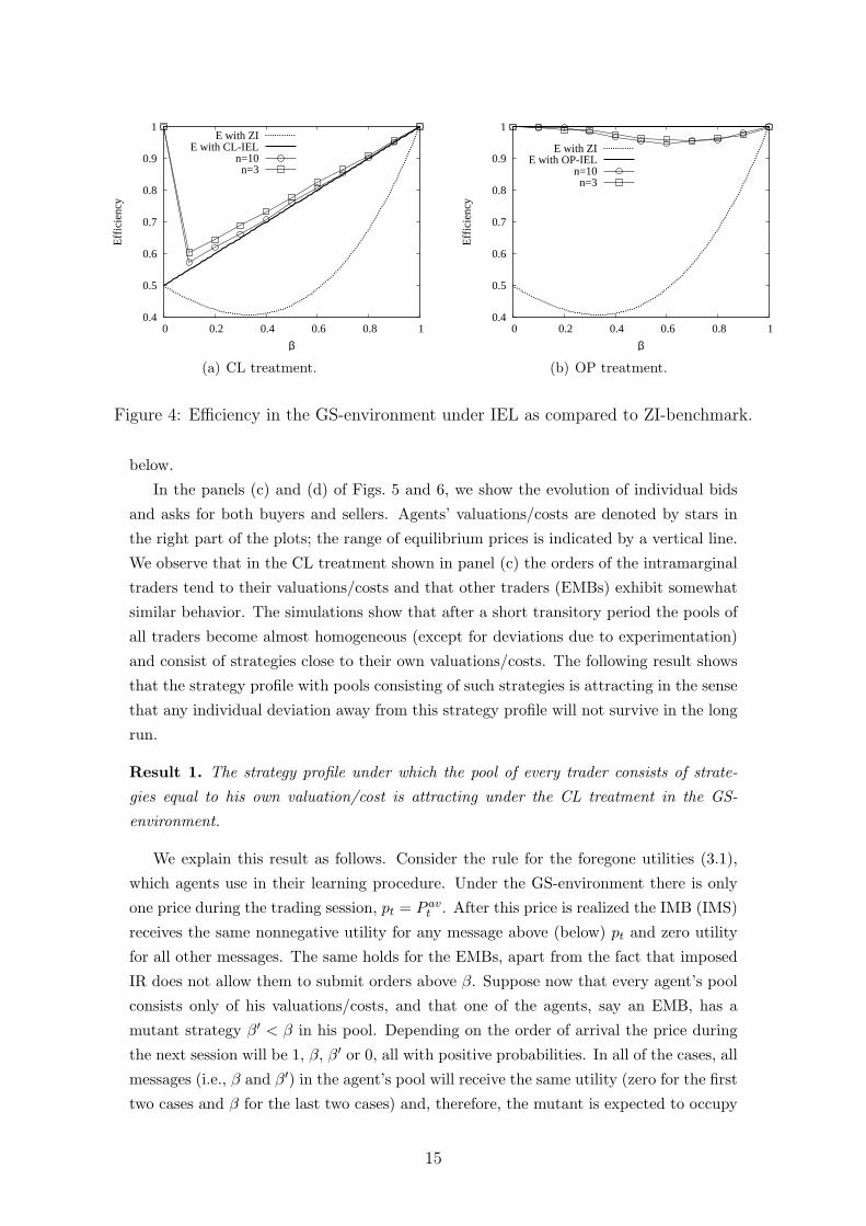
Figs. 4(a) and 4(b) show an allocative efficiency under the IEL with CB and OB,

respectively. For the GS-environment simulated with n = 3 and n = 10 EMBs we

observe a significant increase in allocative efficiency with respect to the ZI-benchmark

shown by dotted line. The solid line indicates the theoretical expected efficiency for

n → ∞ derived below. The allocative efficiency under the IEL practically does not

depend on n, the number of EMBs. Notice the difference caused by transparency of the

book. The allocative efficiency is higher under the OP treatment, actually very close

to 100% for any β, while under the CL treatment there is a positive linear dependence

between the efficiency and β for β > 0.

In order to explain these results for the aggregate market outcomes we look at the

individual strategies of agents and their evolution. An important question is whether and

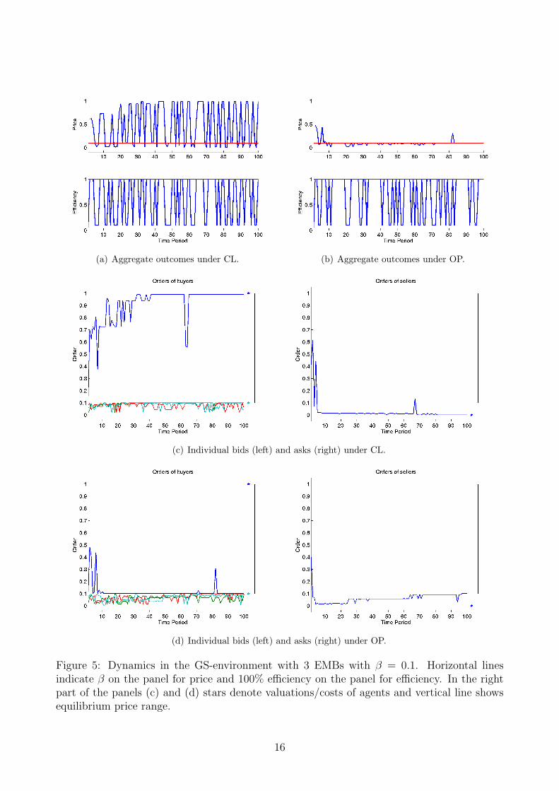
where the IEL driven individual strategies converge under different treatments. Figs. 5

and 6 show the evolution of the market during the first 100 trading sessions for β = 0.1

and β = 0.5, respectively. Upper panels show the evolution of market price and efficiency

under CL (left panel) and OP (right panel) treatment. Horizontal lines indicate β on

the price panel and 100% efficiency on the efficiency panel. We observe that the price

is much more volatile under the CL and is stable and close to β under the OP. The

efficiency is permanently changing between β and 1 under CB for both values of β.

Such behavior also characterizes the long run as we infer from Fig. 4(a). Under OP the

efficiency is also initially changing between β and 1, but then converges to 1. (In case

β = 0.1 convergence occurs after 100 periods and is not shown on the plot.) An outlier

in period 91 for β = 0.5 on Fig. 6(b) is the result of agents’ experimentation, as discussed

14

0.4

0.5

0.6

0.7

0.8

0.9

1

0 0.2 0.4 0.6 0.8 1

Eff

icie

ncy

β

E with ZIE with CL-IEL

n=10n=3

(a) CL treatment.

0.4

0.5

0.6

0.7

0.8

0.9

1

0 0.2 0.4 0.6 0.8 1

Eff

icie

ncy

β

E with ZIE with OP-IEL

n=10n=3

(b) OP treatment.

Figure 4: Efficiency in the GS-environment under IEL as compared to ZI-benchmark.

below.

In the panels (c) and (d) of Figs. 5 and 6, we show the evolution of individual bids

and asks for both buyers and sellers. Agents’ valuations/costs are denoted by stars in

the right part of the plots; the range of equilibrium prices is indicated by a vertical line.

We observe that in the CL treatment shown in panel (c) the orders of the intramarginal

traders tend to their valuations/costs and that other traders (EMBs) exhibit somewhat

similar behavior. The simulations show that after a short transitory period the pools of

all traders become almost homogeneous (except for deviations due to experimentation)

and consist of strategies close to their own valuations/costs. The following result shows

that the strategy profile with pools consisting of such strategies is attracting in the sense

that any individual deviation away from this strategy profile will not survive in the long

run.

Result 1. The strategy profile under which the pool of every trader consists of strate-

gies equal to his own valuation/cost is attracting under the CL treatment in the GS-

environment.

We explain this result as follows. Consider the rule for the foregone utilities (3.1),

which agents use in their learning procedure. Under the GS-environment there is only

one price during the trading session, pt = P avt . After this price is realized the IMB (IMS)

receives the same nonnegative utility for any message above (below) pt and zero utility

for all other messages. The same holds for the EMBs, apart from the fact that imposed

IR does not allow them to submit orders above β. Suppose now that every agent’s pool

consists only of his valuations/costs, and that one of the agents, say an EMB, has a

mutant strategy β′ < β in his pool. Depending on the order of arrival the price during

the next session will be 1, β, β′ or 0, all with positive probabilities. In all of the cases, all

messages (i.e., β and β′) in the agent’s pool will receive the same utility (zero for the first

two cases and β for the last two cases) and, therefore, the mutant is expected to occupy

15

(a) Aggregate outcomes under CL. (b) Aggregate outcomes under OP.

(c) Individual bids (left) and asks (right) under CL.

(d) Individual bids (left) and asks (right) under OP.

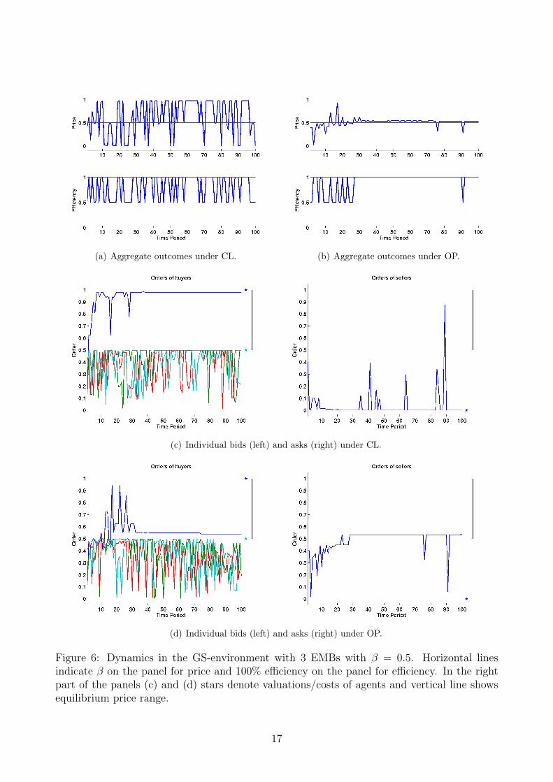
Figure 5: Dynamics in the GS-environment with 3 EMBs with β = 0.1. Horizontal linesindicate β on the panel for price and 100% efficiency on the panel for efficiency. In the rightpart of the panels (c) and (d) stars denote valuations/costs of agents and vertical line showsequilibrium price range.

16

(a) Aggregate outcomes under CL. (b) Aggregate outcomes under OP.

(c) Individual bids (left) and asks (right) under CL.

(d) Individual bids (left) and asks (right) under OP.

Figure 6: Dynamics in the GS-environment with 3 EMBs with β = 0.5. Horizontal linesindicate β on the panel for price and 100% efficiency on the panel for efficiency. In the rightpart of the panels (c) and (d) stars denote valuations/costs of agents and vertical line showsequilibrium price range.

17

only one place in the new pool after replication. In the next period a new mutant, β′′,

enters the pool during experimentation. If β′′ > β′ the new mutant dominates the old

mutant in the long-run because the expected utility of the new mutant is higher than

the expected utility of the old mutant. (If the trading price happens to be β′′, strategy

β′′ receives utility β while strategy β′ receives zero utility. For other possible prices 1, β,

β′ or 0, both strategies receive the same utility.) By the similar reasoning, if β′′ < β′ the

new mutant dominates the old mutant in the long-run. Hence, only mutations towards

attracting configuration of own valuations/costs will survive in the long run. The same

reasoning holds for other types of traders.

Corollary 1. Under the configuration in Result 1 the price oscillates in the range [0, 1],

and the expected efficiency is given by

ECL =1 + βn

(n+ 1)(n+ 2)+

1n+ 2

(1 + n

β + 12

). (4.1)

Proof. See Appendix.

When number of agents n → ∞ the expression (4.1) converges to (1 + β)/2, shown

by a solid line in 4(a).

In the market with the OP treatment the evolution of individual strategies is re-

markably different. In the Figs. 5(d) and 6(d) we observe that intramarginal traders are

able to coordinate on one price and submit the orders close to this price. We have the

following result.

Result 2. For any price p from the equilibrium price range (β, 1] the strategy profile

under which the pools of the IMB and the IMS consist of strategies equal to this price is

stable under the OP treatment in the GS-environment.

To explain this result, let us suppose that both intramarginal traders have homoge-

neous pools with strategies equal to p. Consider an arbitrary mutant strategy by the

IMB. If this strategy is larger than p then it will be dominated by incumbent strategies

in the sessions when the IMB arrives before the IMS (i.e., with probability 1/2) and will

have an equal chance to survive otherwise. If this strategy is smaller than p then the

IMB does not trade at all and the mutant is eliminated from the pool in any case. The

same reasoning holds for the IMS.

Corollary 2. Under the configuration in Result 2 the price is stable and the expected

efficiency is given by

EOP = 1

Proof. Since the strategy profiles of the IMB and the IMS are stable, the price is stable.

Given the price in the competitive equilibrium range the IMB trades with the IMS and

the maximum expected efficiency, EOP = 1, is obtained for any β.

18

The last result shows that in the OP treatment there are multiple equilibria with

any price within the equilibrium range. For example, in Fig. 6(d) the strategies of the

IMB and IMS converged to the same submitted orders approximately equal to 0.53. Of

course, the EMBs never trade in such a market and all their strategies in the pools have

equal probabilities, see the left panel. On the other hand, in Fig. 5(d) the strategies of

the IMB and IMS did converge to 0.1 only in the session t = 95. Before this period the

EMBs had their chances to trade and could learn to submit orders close to 0.1.

Even if Result 2 implies the 100% allocative efficiency, due to experimentation the

efficiency may drop in some periods. This happens around the period 91 in Fig. 6(d).

After previous trading round the seller’s pool was dominated by the orders equal to

0.53, which is the price at period 90. An experimentation adds a strategy 0.06 to the

seller’s pool, which survives replication stage. In fact, the price p90 was determined by

the buyer’s order (the seller at t = 90 arrived after the buyer) and so all the strategies

below p90 have the same hypothetical payoffs. Even if the strategy 0.06 belongs to the

seller’s pool at time 91, a probability to use this strategy as an order is only 1/J = 1/100.

Whenever such order is submitted, the price will be lower than previously observed 0.53.

In this particular case, p91 = 0.28 equal to the order of one of the EMB. Notice that

after this trading round, the seller will re-evaluates his strategies, and strategy 0.53 will

have higher hypothetical payoff than 0.06.

To summarize, the information used by the agents under the IEL shapes their strat-

egy pool in the long-run. This pool affects the aggregate dynamics, which feeds back

by providing a ground for selection of active strategies within the pool. When the book

is closed (CL treatment), agents react on commonly available signal (price of the trans-

action) and learn to submit their own valuation. This leads to higher opportunity of

trade, but also to larger price volatility, as we observed in Figs. 5(a) and 6(a). Instead,

when the book is open (OP treatment), agents can adapt to the stable strategies. Such

individual behavior results in a stable price behavior at the aggregate level.

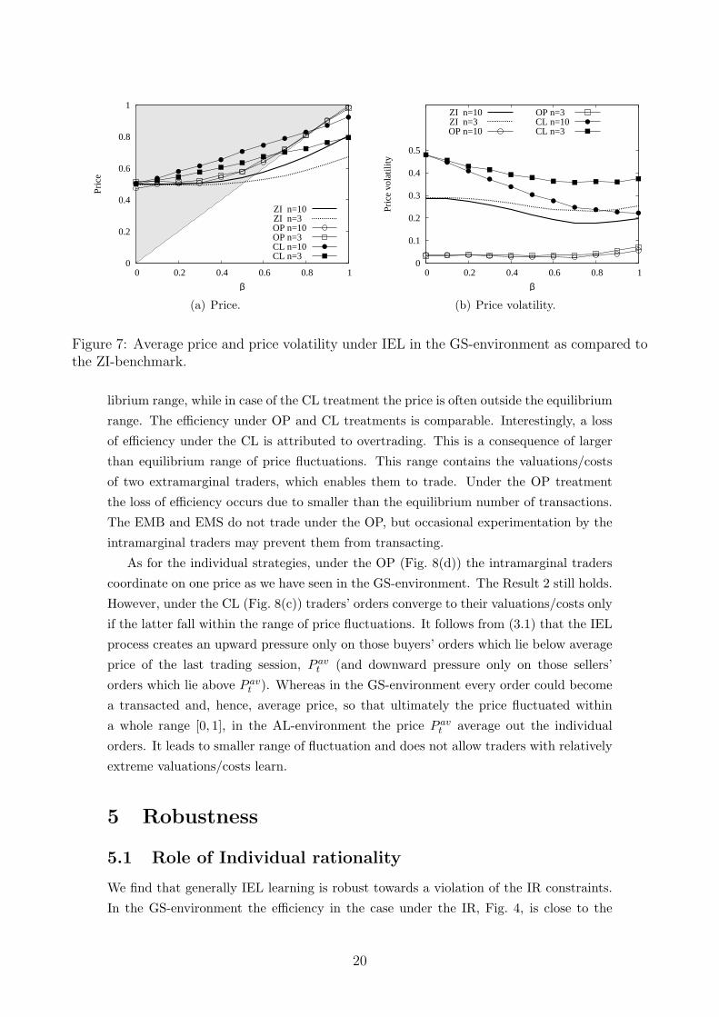
Fig. 7 shows the average price and price volatility and confirms the above finding. In

particular, we observe that under OP treatment the price is within the competitive price

range denoted by shaded area for any β. This is not the case for the CL and ZI. The

price volatility is at the lowest level for OP and the largest for CL with ZI in between.

4.2 AL-environment

Do the results about aggregate dynamics and individual behavior observed in the styl-

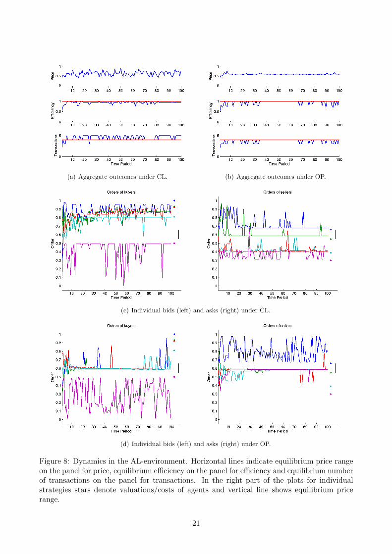
ized GS-environment also hold under alternative environments? Fig. 8 shows market

aggregates (price, efficiency and number of transactions), as well as evolution of the in-

dividual trading orders (bids/asks) over time for the AL-environment. Two horizontal

lines on the panel for price indicate equilibrium price range, while the line on the panel

for transactions shows the equilibrium number of transactions equal to 4.

As before, the price is less volatile under the OP treatment and lies within the equi-

19

0

0.2

0.4

0.6

0.8

1

0 0.2 0.4 0.6 0.8 1

Pric

e

β

ZI n=10ZI n=3 OP n=10OP n=3 CL n=10CL n=3

(a) Price.

0

0.1

0.2

0.3

0.4

0.5

0 0.2 0.4 0.6 0.8 1

Pric

e vo

latil

ity

β

ZI n=10ZI n=3 OP n=10

OP n=3 CL n=10CL n=3

(b) Price volatility.

Figure 7: Average price and price volatility under IEL in the GS-environment as compared tothe ZI-benchmark.

librium range, while in case of the CL treatment the price is often outside the equilibrium

range. The efficiency under OP and CL treatments is comparable. Interestingly, a loss

of efficiency under the CL is attributed to overtrading. This is a consequence of larger

than equilibrium range of price fluctuations. This range contains the valuations/costs

of two extramarginal traders, which enables them to trade. Under the OP treatment

the loss of efficiency occurs due to smaller than the equilibrium number of transactions.

The EMB and EMS do not trade under the OP, but occasional experimentation by the

intramarginal traders may prevent them from transacting.

As for the individual strategies, under the OP (Fig. 8(d)) the intramarginal traders

coordinate on one price as we have seen in the GS-environment. The Result 2 still holds.

However, under the CL (Fig. 8(c)) traders’ orders converge to their valuations/costs only

if the latter fall within the range of price fluctuations. It follows from (3.1) that the IEL

process creates an upward pressure only on those buyers’ orders which lie below average

price of the last trading session, P avt (and downward pressure only on those sellers’

orders which lie above P avt ). Whereas in the GS-environment every order could become

a transacted and, hence, average price, so that ultimately the price fluctuated within

a whole range [0, 1], in the AL-environment the price P avt average out the individual

orders. It leads to smaller range of fluctuation and does not allow traders with relatively

extreme valuations/costs learn.

5 Robustness

5.1 Role of Individual rationality

We find that generally IEL learning is robust towards a violation of the IR constraints.

In the GS-environment the efficiency in the case under the IR, Fig. 4, is close to the

20

(a) Aggregate outcomes under CL. (b) Aggregate outcomes under OP.

(c) Individual bids (left) and asks (right) under CL.

(d) Individual bids (left) and asks (right) under OP.

Figure 8: Dynamics in the AL-environment. Horizontal lines indicate equilibrium price rangeon the panel for price, equilibrium efficiency on the panel for efficiency and equilibrium numberof transactions on the panel for transactions. In the right part of the plots for individualstrategies stars denote valuations/costs of agents and vertical line shows equilibrium pricerange.

21

0.4

0.5

0.6

0.7

0.8

0.9

1

0 0.2 0.4 0.6 0.8 1

Eff

icie

ncy

β

E in ZI without IRE in CL

n=10n=3

(a) CL treatment.

0.4

0.5

0.6

0.7

0.8

0.9

1

0 0.2 0.4 0.6 0.8 1

Eff

icie

ncy

β

E in ZI without IRE in OP

n=10n=3

(b) OP treatment.

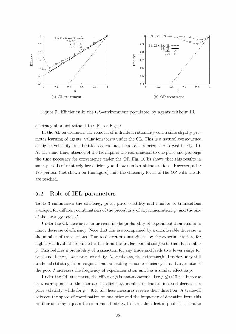
Figure 9: Efficiency in the GS-environment populated by agents without IR.

efficiency obtained without the IR, see Fig. 9.

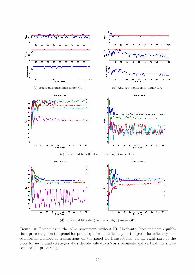
In the AL-environment the removal of individual rationality constraints slightly pro-

motes learning of agents’ valuations/costs under the CL. This is a natural consequence

of higher volatility in submitted orders and, therefore, in price as observed in Fig. 10.

At the same time, absence of the IR impairs the coordination to one price and prolongs

the time necessary for convergence under the OP. Fig. 10(b) shows that this results in

some periods of relatively low efficiency and low number of transactions. However, after

170 periods (not shown on this figure) unit the efficiency levels of the OP with the IR

are reached.

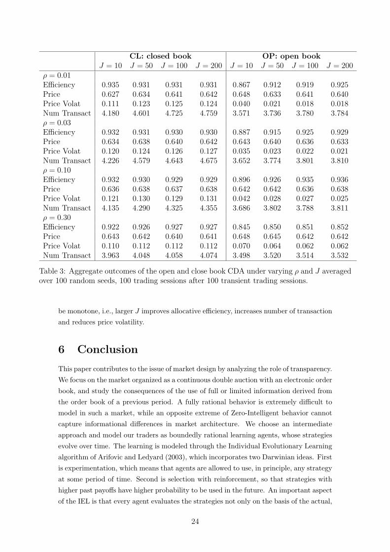
5.2 Role of IEL parameters

Table 3 summarizes the efficiency, price, price volatility and number of transactions

averaged for different combinations of the probability of experimentation, ρ, and the size

of the strategy pool, J .

Under the CL treatment an increase in the probability of experimentation results in

minor decrease of efficiency. Note that this is accompanied by a considerable decrease in

the number of transactions. Due to distortions introduced by the experimentation, for

higher ρ individual orders lie further from the traders’ valuations/costs than for smaller

ρ. This reduces a probability of transaction for any trade and leads to a lower range for

price and, hence, lower price volatility. Nevertheless, the extramarginal traders may still

trade substituting intramarginal traders leading to some efficiency loss. Larger size of

the pool J increases the frequency of experimentation and has a similar effect as ρ.

Under the OP treatment, the effect of ρ is non-monotone. For ρ ≤ 0.10 the increase

in ρ corresponds to the increase in efficiency, number of transaction and decrease in

price volatility, while for ρ = 0.30 all these measures reverse their direction. A trade-off

between the speed of coordination on one price and the frequency of deviation from this

equilibrium may explain this non-monotonicity. In turn, the effect of pool size seems to

22

(a) Aggregate outcomes under CL. (b) Aggregate outcomes under OP.

(c) Individual bids (left) and asks (right) under CL.

(d) Individual bids (left) and asks (right) under OP.

Figure 10: Dynamics in the AL-environment without IR. Horizontal lines indicate equilib-rium price range on the panel for price, equilibrium efficiency on the panel for efficiency andequilibrium number of transactions on the panel for transactions. In the right part of theplots for individual strategies stars denote valuations/costs of agents and vertical line showsequilibrium price range.

23

CL: closed book OP: open bookJ = 10 J = 50 J = 100 J = 200 J = 10 J = 50 J = 100 J = 200

ρ = 0.01Efficiency 0.935 0.931 0.931 0.931 0.867 0.912 0.919 0.925Price 0.627 0.634 0.641 0.642 0.648 0.633 0.641 0.640Price Volat 0.111 0.123 0.125 0.124 0.040 0.021 0.018 0.018Num Transact 4.180 4.601 4.725 4.759 3.571 3.736 3.780 3.784ρ = 0.03Efficiency 0.932 0.931 0.930 0.930 0.887 0.915 0.925 0.929Price 0.634 0.638 0.640 0.642 0.643 0.640 0.636 0.633Price Volat 0.120 0.124 0.126 0.127 0.035 0.023 0.022 0.021Num Transact 4.226 4.579 4.643 4.675 3.652 3.774 3.801 3.810ρ = 0.10Efficiency 0.932 0.930 0.929 0.929 0.896 0.926 0.935 0.936Price 0.636 0.638 0.637 0.638 0.642 0.642 0.636 0.638Price Volat 0.121 0.130 0.129 0.131 0.042 0.028 0.027 0.025Num Transact 4.135 4.290 4.325 4.355 3.686 3.802 3.788 3.811ρ = 0.30Efficiency 0.922 0.926 0.927 0.927 0.845 0.850 0.851 0.852Price 0.643 0.642 0.640 0.641 0.648 0.645 0.642 0.642Price Volat 0.110 0.112 0.112 0.112 0.070 0.064 0.062 0.062Num Transact 3.963 4.048 4.058 4.074 3.498 3.520 3.514 3.532

Table 3: Aggregate outcomes of the open and close book CDA under varying ρ and J averagedover 100 random seeds, 100 trading sessions after 100 transient trading sessions.

be monotone, i.e., larger J improves allocative efficiency, increases number of transaction

and reduces price volatility.

6 Conclusion

This paper contributes to the issue of market design by analyzing the role of transparency.

We focus on the market organized as a continuous double auction with an electronic order

book, and study the consequences of the use of full or limited information derived from

the order book of a previous period. A fully rational behavior is extremely difficult to

model in such a market, while an opposite extreme of Zero-Intelligent behavior cannot

capture informational differences in market architecture. We choose an intermediate

approach and model our traders as boundedly rational learning agents, whose strategies

evolve over time. The learning is modeled through the Individual Evolutionary Learning

algorithm of Arifovic and Ledyard (2003), which incorporates two Darwinian ideas. First

is experimentation, which means that agents are allowed to use, in principle, any strategy

at some period of time. Second is selection with reinforcement, so that strategies with

higher past payoffs have higher probability to be used in the future. An important aspect

of the IEL is that every agent evaluates the strategies not only on the basis of the actual,

24

but also counterfactual (foregone) utility.

We derive allocative efficiency for the benchmark case with the ZI traders and show

through simulations that IEL leads to a substantially higher efficiency. As for the trans-

parency issue we show that strategies learned by traders are remarkably different in the

treatments with fully available (“open”) order book and unavailable (“closed”) order

book. Traders, who systematically participate in the trade, learn to submit their own

valuations/costs under the closed book treatment, and the previously observed trading

price under the open book treatment. These individual differences result in differences

on the aggregate level: higher price volatility and overtrading under the closed book

relatively to the open book treatment. The allocative efficiency is comparable in both

cases, however the sources of the inefficiencies are different.

We show that our results are robust with respect to the market environments that

we consider. In addition, the results are robust with respect to changes in the values of

the parameters of the learning model, such as the rate of experimentation and the size

of the pool of strategies. We also find that the IEL algorithm is effective in wiping out

the strategies which contradict individual rationality constraint and result in a strictly

negative utility. This is an important property of the algorithm, suggesting that it can be

successfully applied in more sophisticated environments, where strategies with negative

performance cannot be easily identified and ruled out at the outset. Indeed, as experi-

ments in Kagel, Harstad, and Levin (1987) and Lei, Noussair, and Plott (2001) show, in

reality participants can occasionally violate the individual rationality requirement and

trade with clear losses. The learning model applied in this paper does not contradict

such experimental evidence.

In modeling agents’ behavior our approach is relatively simple in comparison to some

micro-structure studies attempting to model fully rational behavior. However, our be-

havioral assumptions fit better to the experimental evidence of human behavior in com-

plex environment that demonstrates that human subjects often use simple behavioral

rules (Hommes, Sonnemans, Tuinstra, and Velden, 2005). Based on such assumptions

our model predicts that volatility in the market should decrease as a result of higher

transparency. This is consistent with the study of Boehmer, Saar, and Yu (2005) for the

NYSE. Some of their finding (e.g., higher order splitting as a result of increasing market

transparency) cannot be replicated in this paper, because we do not allow individual

traders to buy or sell multiple units. Several other assumptions of this paper could also

be relaxed. Allowing for cancelation of some orders would bring us to a more realistic

setting, which lies in between of the two extremes: no-cancelation as in this paper and

cancelation of all remaining orders after every transaction as in Gode and Sunder (1993).

Submission of multiple orders would allow us to model a more realistic intermediate sit-

uation between the two extremes: one-order per agent in one trading session as here and

unbounded amount of multiple orders as in Gode and Sunder (1997). Finally, it would

be also interesting to consider endogenous dynamics for valuations and costs, explored in

heterogeneous agent models literature, see, e.g., Brock and Hommes (1998) and Anufriev

25

and Panchenko (2009).

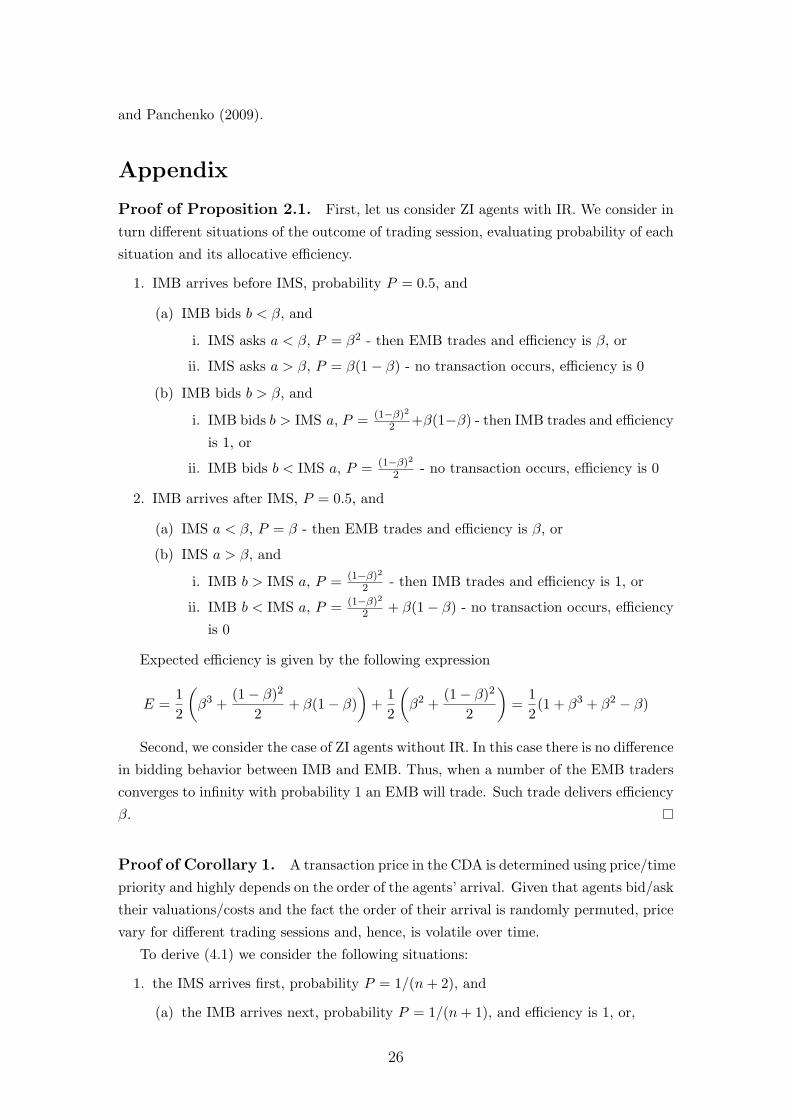
Appendix

Proof of Proposition 2.1. First, let us consider ZI agents with IR. We consider in

turn different situations of the outcome of trading session, evaluating probability of each

situation and its allocative efficiency.

1. IMB arrives before IMS, probability P = 0.5, and

(a) IMB bids b < β, and

i. IMS asks a < β, P = β2 - then EMB trades and efficiency is β, or

ii. IMS asks a > β, P = β(1− β) - no transaction occurs, efficiency is 0

(b) IMB bids b > β, and

i. IMB bids b > IMS a, P = (1−β)2

2 +β(1−β) - then IMB trades and efficiency

is 1, or

ii. IMB bids b < IMS a, P = (1−β)2

2 - no transaction occurs, efficiency is 0

2. IMB arrives after IMS, P = 0.5, and

(a) IMS a < β, P = β - then EMB trades and efficiency is β, or

(b) IMS a > β, and

i. IMB b > IMS a, P = (1−β)2

2 - then IMB trades and efficiency is 1, or

ii. IMB b < IMS a, P = (1−β)2

2 + β(1− β) - no transaction occurs, efficiency

is 0

Expected efficiency is given by the following expression

E =12

(β3 +

(1− β)2

2+ β(1− β)

)+

12

(β2 +

(1− β)2

2

)=

12

(1 + β3 + β2 − β)

Second, we consider the case of ZI agents without IR. In this case there is no difference

in bidding behavior between IMB and EMB. Thus, when a number of the EMB traders

converges to infinity with probability 1 an EMB will trade. Such trade delivers efficiency

β.

Proof of Corollary 1. A transaction price in the CDA is determined using price/time

priority and highly depends on the order of the agents’ arrival. Given that agents bid/ask

their valuations/costs and the fact the order of their arrival is randomly permuted, price

vary for different trading sessions and, hence, is volatile over time.

To derive (4.1) we consider the following situations:

1. the IMS arrives first, probability P = 1/(n+ 2), and

(a) the IMB arrives next, probability P = 1/(n+ 1), and efficiency is 1, or,

26

(b) the EMB arrives next, probability P = n/(n+ 1), and efficiency is β

In this situation the price is 0.

2. the IMB arrives first, probability P = 1/(n+2), and efficiency is 1. In this situation

the price is 1.

3. an EMB arrives first, probability P = n/(n+ 2), and

(a) the IMS arrives before the IMB, probability P = 1/2, and efficiency is β, in

this situation the price is β, or,

(b) the IMS arrives after the IMB, probability P = 1/2, and efficiency is 1, in this

situation the price is 1.

Summing the terms we obtain (4.1) for the efficiency.

References

Anufriev, M., and V. Panchenko (2009): “Asset Prices, Traders’ Behavior and

Market Design,” Journal of Economic Dynamics & Control, 33, 1073 – 1090.

Arifovic, J. (1994): “Genetic algorithm learning and the cobweb model,” Journal of

Economic Dynamics & Control, 18(1), 3–28.

Arifovic, J., and J. Ledyard (2003): “Computer testbeds and mechanism design:

application to the class of Groves-Ledyard mechanisms for the provision of public

goods,” manuscript.

(2007): “Call market book information and efficiency,” Journal of Economic

Dynamics and Control, 31(6), 1971–2000.

Boehmer, E., G. Saar, and L. Yu (2005): “Lifting the veil: An analysis of pre-trade

transparency at the NYSE,” Journal of Finance, 60(2), 783–815.

Bottazzi, G., G. Dosi, and I. Rebesco (2005): “Institutional Architectures and

Behavioral Ecologies in the Dynamics of Financial Markets: a Preliminary Investiga-

tion,” Journal of Mathematical Economics, 41, 197–228.

Brock, W. A., and C. H. Hommes (1998): “Heterogeneous Beliefs and Routes to

Chaos in a Simple Asset Pricing Model,” Journal of Economic Dynamics and Control,

22, 1235–1274.

Duffy, J. (2006): “Agent-Based Models and Human Subject Experiments,” in Hand-

book of Computational Economics Vol. 2: Agent-Based Computational Economics,

ed. by K. Judd, and L. Tesfatsion. Elsevier/North-Holland (Handbooks in Economics

Series).

27

Easley, D., and J. Ledyard (1993): “Theories of price formation and exchange

in double oral auctions,” in The double auction market: Institutions, theories, and

evidence, ed. by D. Friedman, and J. Rust, pp. 63–97. Perseus Books.

Erev, I., and A. E. Roth (1998): “Prediction how people play games: Reinforcement

learning in games with unique strategy equilibrium,” American Economic Review, 88,

848–881.

Fano, S., M. LiCalzi, and P. Pellizzari (2010): “Convergence of outcomes and evo-

lution of strategic behavior in double auctions,” Working Paper no. 196, Department

of Applied Mathematics, University of Venice.

Friedman, D. (1991): “A simple testable model of double auction markets,” Journal

of Economic Behavior & Organization, 15(1), 47–70.

Gjerstad, S., and J. Dickhaut (1998): “Price formation in double auctions,” Games

and Economic Behavior, 22(1), 1–29.

Gjerstad, S., and J. Shachat (2007): “Individual rationality and market efficiency,”

Working Papers no. 1204, Institute for research in the behavioral, economic, and

management sciences, Purdue University.

Gode, D., and S. Sunder (1993): “Allocative efficiency of markets with zero-

intelligence traders: Market as a partial substitute for individual rationality,” Journal

of Political Economy, pp. 119–137.

(1997): “What Makes Markets Allocationally Efficient?,” Quarterly Journal of

Economics, 112(2), 603–630.

Hommes, C., J. Sonnemans, J. Tuinstra, and H. v. d. Velden (2005): “Coordi-

nation of Expectations in Asset Pricing Experiments,” Review of Financial Studies,

18(3), 955–980.

Kagel, J., R. Harstad, and D. Levin (1987): “Information impact and allocation

rules in auctions with affiliated private values: A laboratory study,” Econometrica:

Journal of the Econometric Society, pp. 1275–1304.

Ladley, D. (2010): “Zero Intelligence in Economics and Finance,” Knowledge Engi-

neering Review, forthcoming.

Lei, V., C. Noussair, and C. Plott (2001): “Nonspeculative bubbles in experimen-

tal asset markets: lack of common knowledge of rationality vs. actual irrationality,”

Econometrica, pp. 831–859.

LiCalzi, M., and P. Pellizzari (2008): “Zero-Intelligence Trading Without Resam-

pling,” in Complexity and Artificial Markets, ed. by K. Schredelseker, and F. Hauser,

pp. 3–14. Springer.

28

Satterthwaite, M., and S. Williams (2002): “The optimality of a simple market

mechanism,” Econometrica, pp. 1841–1863.

Smith, V. L. (1962): “An Experimental Study of Competitive Market Behavior,” The

Journal of Political Economy, 70(2), 111–137.

29