Echo statistics associated with discrete scatterers: A tutorial on physics-based methods Timothy K. Stanton, Wu-Jung Lee, and Kyungmin Baik Citation: The Journal of the Acoustical Society of America 144, 3124 (2018); doi: 10.1121/1.5052255 View online: https://doi.org/10.1121/1.5052255 View Table of Contents: https://asa.scitation.org/toc/jas/144/6 Published by the Acoustical Society of America ARTICLES YOU MAY BE INTERESTED IN A mathematical model of bowel sound generation The Journal of the Acoustical Society of America 144, EL485 (2018); https://doi.org/10.1121/1.5080528 Macroscopic observations of diel fish movements around a shallow water artificial reef using a mid-frequency horizontal-looking sonar The Journal of the Acoustical Society of America 144, 1424 (2018); https://doi.org/10.1121/1.5054013 Multiplicative and min processing of experimental passive sonar data from thinned arrays The Journal of the Acoustical Society of America 144, 3262 (2018); https://doi.org/10.1121/1.5064458 Performance comparisons of array invariant and matched field processing using broadband ship noise and a tilted vertical array The Journal of the Acoustical Society of America 144, 3067 (2018); https://doi.org/10.1121/1.5080603 Putting Laurel and Yanny in context The Journal of the Acoustical Society of America 144, EL503 (2018); https://doi.org/10.1121/1.5070144 An Empirical Mode Decomposition-based detection and classification approach for marine mammal vocal signals The Journal of the Acoustical Society of America 144, 3181 (2018); https://doi.org/10.1121/1.5067389

Welcome message from author
This document is posted to help you gain knowledge. Please leave a comment to let me know what you think about it! Share it to your friends and learn new things together.
Transcript
Echo statistics associated with discrete scatterers: A tutorial on physics-basedmethodsTimothy K. Stanton, Wu-Jung Lee, and Kyungmin Baik
Citation: The Journal of the Acoustical Society of America 144, 3124 (2018); doi: 10.1121/1.5052255View online: https://doi.org/10.1121/1.5052255View Table of Contents: https://asa.scitation.org/toc/jas/144/6Published by the Acoustical Society of America
ARTICLES YOU MAY BE INTERESTED IN
A mathematical model of bowel sound generationThe Journal of the Acoustical Society of America 144, EL485 (2018); https://doi.org/10.1121/1.5080528
Macroscopic observations of diel fish movements around a shallow water artificial reef using a mid-frequencyhorizontal-looking sonarThe Journal of the Acoustical Society of America 144, 1424 (2018); https://doi.org/10.1121/1.5054013
Multiplicative and min processing of experimental passive sonar data from thinned arraysThe Journal of the Acoustical Society of America 144, 3262 (2018); https://doi.org/10.1121/1.5064458
Performance comparisons of array invariant and matched field processing using broadband ship noise and atilted vertical arrayThe Journal of the Acoustical Society of America 144, 3067 (2018); https://doi.org/10.1121/1.5080603
Putting Laurel and Yanny in contextThe Journal of the Acoustical Society of America 144, EL503 (2018); https://doi.org/10.1121/1.5070144
An Empirical Mode Decomposition-based detection and classification approach for marine mammal vocal signalsThe Journal of the Acoustical Society of America 144, 3181 (2018); https://doi.org/10.1121/1.5067389

Echo statistics associated with discrete scatterers:A tutorial on physics-based methods
Timothy K. Stantona)
Department of Applied Ocean Physics and Engineering, Woods Hole Oceanographic Institution,Mail Stop #11, Woods Hole, Massachusetts 02543, USA
Wu-Jung LeeApplied Physics Laboratory, University of Washington, 1013 Northeast 40th Street, Seattle,Washington 98105, USA
Kyungmin BaikCenter for Medical Convergence Metrology, Division of Chemical and Medical Metrology,Korea Research Institute of Standards and Science, Daejeon 34113, Republic of Korea
(Received 8 August 2017; revised 7 August 2018; accepted 11 August 2018; published online 6December 2018)
When a beam emitted from an active monostatic sensor system sweeps across a volume, the echoes
from scatterers present will fluctuate from ping to ping due to various interference phenomena and
statistical processes. Observations of these fluctuations can be used, in combination with models, to
infer properties of the scatterers such as numerical density. Modeling the fluctuations can also help
predict system performance and associated uncertainties in expected echoes. This tutorial focuses
on “physics-based statistics,” which is a predictive form of modeling the fluctuations. The modeling
is based principally on the physics of the scattering by individual scatterers, addition of echoes
from randomized multiple scatterers, system effects involving the beampattern and signal type, and
signal theory including matched filter processing. Some consideration is also given to environment-
specific effects such as the presence of boundaries and heterogeneities in the medium. Although the
modeling was inspired by applications of sonar in the field of underwater acoustics, the material is
presented in a general form, and involving only scalar fields. Therefore, it is broadly applicable to
other areas such as medical ultrasound, non-destructive acoustic testing, in-air acoustics, as well as
radar and lasers. VC 2018 Author(s). All article content, except where otherwise noted, is licensedunder a Creative Commons Attribution (CC BY) license (http://creativecommons.org/licenses/by/4.0/). https://doi.org/10.1121/1.5052255
[JFL] Pages: 3124–3171
TABLE OF CONTENTS
LINKS TO SOFTWARE USED TO CREATE
FIGURES. . . . . . . . . . . . . . . . . . . . . . . . . . . . . . . . . . . . . . 3125
I. INTRODUCTION . . . . . . . . . . . . . . . . . . . . . . . . . . . . 3126
II. KEY ELEMENTS OF ECHO STATISTICS . . . . . 3127
A. Interfering signals . . . . . . . . . . . . . . . . . . . . . . . 3128
B. Stochastic scattering from a single scatterer. 3128
C. Beampattern effects . . . . . . . . . . . . . . . . . . . . . 3129
III. EXPLOITING ECHO STATISTICS FOR
VARIOUS APPLICATIONS . . . . . . . . . . . . . . . . . 3129
A. Inferring information on scatterers. . . . . . . . . 3129
1. Inferring number of scatterers . . . . . . . . . . 3130
2. Discriminating between echo from
scatterer of interest and background. . . . . 3130
3. Removing beampattern effects to isolate
properties of resolved scatterer . . . . . . . . . 3130
4. Discriminating between different types
of aggregations of scatterers . . . . . . . . . . . 3131
5. Further considerations. . . . . . . . . . . . . . . . . 3131
a. Directionality of sensor beam
improves inference techniques. . . . . . . 3131
b. Noise and “tail” of echo PDF. . . . . . . 3131
B. Predicting error or uncertainty in signal
magnitude. . . . . . . . . . . . . . . . . . . . . . . . . . . . . . 3131
IV. KEY EQUATIONS FOR SCATTERING AND
ASSOCIATED STATISTICAL PROCESSES . . . 3131
A. Deterministic scattering . . . . . . . . . . . . . . . . . . 3131
1. Single scatterer . . . . . . . . . . . . . . . . . . . . . . 3132
2. Multiple scatterers . . . . . . . . . . . . . . . . . . . . 3132
B. Probability density function and related
quantities . . . . . . . . . . . . . . . . . . . . . . . . . . . . . . 3133
1. Definitions and equations. . . . . . . . . . . . . . 3133
2. Calculating PDFs: Directly and from
Monte Carlo simulations . . . . . . . . . . . . . . 3133
3. Non-uniform spacing of bins. . . . . . . . . . . 3134
4. Normalization. . . . . . . . . . . . . . . . . . . . . . . . 3134
a. Vertical scale. . . . . . . . . . . . . . . . . . . . . 3134
b. Horizontal scale. . . . . . . . . . . . . . . . . . . 3134
C. Fundamental statistical processes relevant
to echo statistics . . . . . . . . . . . . . . . . . . . . . . . . 3134
1. Randomizing the deterministic scattering
equations . . . . . . . . . . . . . . . . . . . . . . . . . . . . 3134a)Electronic mail: [email protected]
3124 J. Acoust. Soc. Am. 144 (6), December 2018 VC Author(s) 2018.0001-4966/2018/144(6)/3124/48

2. Function of a single random variable. . . . 3135
3. Function of two random variables . . . . . . 3135
4. Product of two random variables . . . . . . . 3136
5. Sum of random variables . . . . . . . . . . . . . . 3136
a. Method of characteristic functions. . . 3136
b. Monte Carlo simulations.. . . . . . . . . . . 3136
6. Sum of infinite number of random
variables (central limit theorem;
Rayleigh PDF) . . . . . . . . . . . . . . . . . . . . . . . 3137
V. IN-DEPTH TREATMENT OF ECHO
STATISTICS: OVERVIEW . . . . . . . . . . . . . . . . . . . 3137
A. How to use this material for realistic
signals/environments, and advanced signal/
beam processing . . . . . . . . . . . . . . . . . . . . . . . . 3138
B. Peak sampling, pulsed signals with
boundaries, and beyond . . . . . . . . . . . . . . . . . . 3138
VI. IN-DEPTH TREATMENT OF ECHO
STATISTICS: NO BEAMPATTERN EFFECTS 3138
A. Addition of random signals (generic
signals; not specific to scattering) . . . . . . . . . 3139
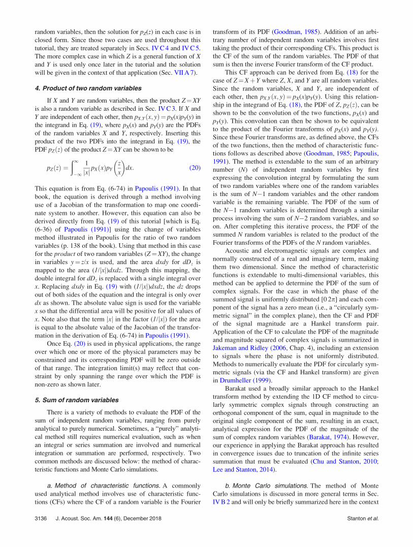
1. Arbitrary cases . . . . . . . . . . . . . . . . . . . . . . . 3139
2. Sine wave plus noise (Rice PDF) . . . . . . . 3139
3. Special distributions of N or ai (K PDF). 3140
4. Adding independent realizations of the
complex signal A . . . . . . . . . . . . . . . . . . . . . 3142
B. Complex scatterers with stochastic
properties . . . . . . . . . . . . . . . . . . . . . . . . . . . . . . 3142
1. Point scatterer . . . . . . . . . . . . . . . . . . . . . . . 3142
2. Rayleigh scatterer . . . . . . . . . . . . . . . . . . . . 3142
3. Randomized prolate spheroid . . . . . . . . . . 3142
a. Smooth boundary, fixed orientation. . 3142
b. Smooth boundary, random
orientation. . . . . . . . . . . . . . . . . . . . . . . . 3143
c. Rough boundary, random orientation. 3144
4. Randomly rough objects with full range of
roughness and circumferential/internal
waves . . . . . . . . . . . . . . . . . . . . . . . . . . . . . . . . 3145
a. Circumferential and internal waves
(smooth boundary). . . . . . . . . . . . . . . . . 3145
b. Front interface only: Small-to-
intermediate roughness, Rice PDF. . . 3145
c. Randomized circumferential and
internal waves added to front
interface echo; nulls and attenuation
effects.. . . . . . . . . . . . . . . . . . . . . . . . . . . 3146
VII. IN-DEPTH TREATMENT OF ECHO
STATISTICS: WITH BEAMPATTERN
EFFECTS . . . . . . . . . . . . . . . . . . . . . . . . . . . . . . . . . 3146
A. Single scatterer randomly located in beam. . 3147
1. Accounting for beampattern effects in
echo PDF . . . . . . . . . . . . . . . . . . . . . . . . . . . 3147
2. PDF of spatial distribution of scatterer . . 3147
3. Beampattern PDF for mainlobe only
(axisymmetric transducer, uniformly
distributed scatterer) . . . . . . . . . . . . . . . . . . 3148
a. Exact solution. . . . . . . . . . . . . . . . . . . . 3148
b. Power law approximation for
beampattern PDF. . . . . . . . . . . . . . . . . 3149
4. Beampattern PDF for entire beam
(axisymmetric transducer, uniformly
distributed scatterer) . . . . . . . . . . . . . . . . . . 3149
5. Beampattern PDF for 2D and 3D
distribution of scatterers . . . . . . . . . . . . . . . 3150
6. Echo PDF for different types of
individual scatterers in axisymmetric
beam . . . . . . . . . . . . . . . . . . . . . . . . . . . . . . . 3151
a. Point scatterer; main lobe only.. . . . . 3151
b. Rayleigh scatterer; mainlobe only. . . 3151
c. Complex scatterer; entire beam. . . . . 3152
7. Beampattern PDF for non-axisymmetric
beampattern, non-uniform distribution of
scatterer. . . . . . . . . . . . . . . . . . . . . . . . . . . . . 3152
a. Non-uniformly distributed scatterer. . 3153
b. Uniformly distributed scatterer.. . . . . 3153
B. Multiple identical scatterers randomly
located in beam . . . . . . . . . . . . . . . . . . . . . . . . . 3153
C. Multiple scatterers of different types and
sizes. . . . . . . . . . . . . . . . . . . . . . . . . . . . . . . . . . . 3156
1. Split aggregation of type A and B
scatterers—mixture PDF . . . . . . . . . . . . . . 3156
2. Interspersed aggregation of type A and B
scatterers—coherent phasor sum . . . . . . . . . 3157
3. Comparisons between echo PDFs from
split and interspersed two-type
aggregations . . . . . . . . . . . . . . . . . . . . . . . . . 3157
4. Many types of scatterers (general
formulations) . . . . . . . . . . . . . . . . . . . . . . . . 3157
VIII. SYSTEMS AND ENVIRONMENTS WITH
MORE COMPLEXITY. . . . . . . . . . . . . . . . . . . . . 3159
A. Pulsed signals (partially overlapping
echoes) . . . . . . . . . . . . . . . . . . . . . . . . . . . . . . . . 3160
B. Object near a rough boundary. . . . . . . . . . . . . 3161
C. Object(s) in a random waveguide. . . . . . . . . . 3162
1. Some simple formulations . . . . . . . . . . . . . 3163
2. Closed form solutions for limiting cases
involving a saturated waveguide. . . . . . . . 3164
a. Small patch of scatterers. . . . . . . . . . 3164
b. Extended patch of scatterers. . . . . . . 3165
IX. DISCUSSION AND CONCLUSIONS . . . . . . . . . 3165
ACKNOWLEDGMENTS . . . . . . . . . . . . . . . . . . . . . . . . 3165
APPENDIX: GENERIC OR COMMONLY USED
STATISTICAL FUNCTIONS . . . . . . . . . . . . . . . . . . . . 3166
1. Rayleigh PDF . . . . . . . . . . . . . . . . . . . . . . . . . . . 3168
2. Rice PDF. . . . . . . . . . . . . . . . . . . . . . . . . . . . . . . 3168
3. K PDF . . . . . . . . . . . . . . . . . . . . . . . . . . . . . . . . . 3168
4. Weibull PDF. . . . . . . . . . . . . . . . . . . . . . . . . . . . 3168
5. Log normal PDF . . . . . . . . . . . . . . . . . . . . . . . . 3168
6. Nakagami-m PDF (and related chi-squared
and gamma PDFs) . . . . . . . . . . . . . . . . . . . . . . . 3169
7. Generalized Pareto PDF . . . . . . . . . . . . . . . . . . 3169
LINKS TO SOFTWARE USED TO CREATE FIGURES
The software used to produce all predictions in the fig-
ures is in the supplementary material at https://doi.org/
J. Acoust. Soc. Am. 144 (6), December 2018 Stanton et al. 3125
10.1121/1.5052255. The software is also stored online (Lee
and Baik, 2018), where it is subject to future revisions.
I. INTRODUCTION
Echoes, as measured through the receiver of an active
monostatic sensor system, will typically fluctuate from ping
to ping as the beam emitted from the system scans across a
volume containing scatterers or as the scatterers in that vol-
ume move through the beam (Fig. 1). It is essential to under-
stand the echo statistics for accurate interpretation of the
scattering and for modeling system performance. Toward
that goal, understanding the underlying physical processes
that give rise to the fluctuations allows one to accurately pre-
dict and interpret the echo statistics. In the simplest case in
which the propagation medium is homogeneous and there
are no boundaries present (i.e., a “direct path” geometry),
the fluctuations are due to a combination of several statistical
processes: the interference between overlapping echoes
when multiple scatterers are present, the random nature of
the echoes from individual scatterers (not including beam-
pattern effects), and the modulation of the echo due to the
random location of the scatterer in the beam. Once the geom-
etry is further complicated by heterogeneities in the medium
and/or the presence of boundaries, the propagated signals
will become refracted and/or rescattered, giving rise to more
propagation paths that are potentially random and, in turn,
also contributing to the fluctuations. This tutorial presents
key concepts and formulations associated with predicting the
echo fluctuations over a wide range of scenarios in terms of
the physics of the scattering, system parameters, and signal
theory.
The statistical behavior of echoes is important across a
diverse range of active sensor systems and applications
involving the use of either acoustic waves (such as with
sonar, medical ultrasonics, or non-destructive testing) or
electromagnetic waves (such as with radar or light) to study
individual discrete scatterers, assemblages of scatterers, or
rough interfaces that cause scattering. Understanding echo
statistics has been integral in interpreting radar clutter
(Watts and Ward, 2010) and sonar reverberation and clutter
(Ol’shevskii, 1978; Gallaudet and de Moustier, 2003;
Abraham and Lyons, 2010), sonar classification of marine
life and objects on the seafloor (Stanton and Clay, 1986;
Medwin and Clay, 1998), medical ultrasound classification
of human tissue (Eltoft, 2006; Destrempes and Cloutier,
2010, 2013; Oelze and Mamou, 2016), and non-destructive
ultrasound testing of materials (Li et al., 1992). Within each
of these areas, echo statistics are used in the detection and
classification of scatterers, discriminating between scatterers
of interest from clutter (i.e., unwanted echoes), estimating
numerical density of scatterers, and determining the perfor-
mance of sensor systems for use in detection and classifica-
tion of scatterers. The studies of clutter involve
characterizing the statistics of unwanted echoes from fea-
tures or objects in the environment that have properties
resembling the target of interest. The clutter may be due to
the sea surface (radar/sonar/laser), marine life or seafloor
(sonar), human tissue (medical ultrasound), or grains in sol-
ids (non-destructive testing).
The above applications have many elements of statistical
theory in common. Those common elements are treated for-
mally in Goodman (1985) and Jakeman and Ridley (2006).
There are also notable differences between interpreting echoes
from acoustic and electromagnetic systems, such as the pres-
ence of shear waves and polarization, respectively, which are
summarized in Le Chevalier (2002). Differences in echo sta-
tistics between scalar fields (both acoustics and electromag-
netic, ignoring shear waves and polarization, respectively)
and those fields with polarization effects (electromagnetic
only) are summarized in Jakeman and Ridley (2006).
While there has been much work conducted in the area
of echo statistics, the focus has generally involved describing
the variability of echoes through use of generic statistical
functions whose parameters need to be determined from
experimental data. Here, “generic” refers to those functions
generally devoid of a physical basis and derived solely from
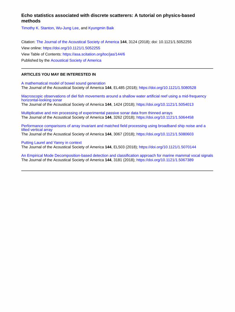
FIG. 1. Echoes fluctuate from ping to ping as the sensor beam scans across the scatterers. The resultant ensemble of echoes can be formed into a histogram,
related to the probability density function of the echo magnitude. A simple direct-path geometry involving a homogeneous medium with no boundaries is illus-
trated. Key elements to echo statistics are illustrated—stochastic scattering (fðiÞbs ) from a single scatterer, random angular location ðhi; /iÞ of scatterer within
the sensor beam causing random modulation of the echo due to the beampattern (b), and randomized interference caused by overlap of echoes from multiple
random phase scatterers (P� � �). The statistics is formed over M pings to form a histogram of echo magnitudes in the far right graph. All of these terms are
defined in Sec. IV.
3126 J. Acoust. Soc. Am. 144 (6), December 2018 Stanton et al.

random signal theory, such as a Gaussian process. These
generic functions include the Rayleigh, Rice, K, Weibull, log
normal, and Nakagami-m distributions (App). Only under a
narrow range of conditions can some of the generic functions
be connected to the physics. There has been a much smaller
set of studies in which the statistics were modeled from first
principles, and hence being predictive, through a combination
of the physics of scattering, sensor system parameters, and
signal theory. To date, there has been no text or tutorial with
a comprehensive coverage of physics-based phenomena.
This tutorial presents the fundamentals of echo statistics
associated with an active monostatic sensor system, written
in a manner that is readable by a wide audience. While much
of the material is motivated by the use of sonar in underwa-
ter applications, the material is broadly applicable to other
types of active acoustic systems used in various media
including air, solids, and biological tissue, as well as to radar
and lasers. Because of the generality of the treatment, the
system used to transmit waves and receive the echoes will
heretofore be referred to as a “sensor system” regardless of
application and whether it involves acoustic or electromag-
netic waves. The formulations describe scalar fields, which
can be directly applied to either acoustic or electromagnetic
signals in the absence of the presence of shear waves or
polarization effects, respectively. Only brief reference is
made to those latter effects.
The emphasis in this tutorial is on describing the statis-
tics of the magnitude of the complex echo (or echo enve-
lope) in terms of the physics of the scattering, sensor system
parameters, and signal processing. More specifically, the
emphasis is on physics-based methods, in contrast to the
generic approaches referenced above. The methods are
focused solely on “first-order statistics” which concern sta-
tistical properties of the signal at a single instant in time.
Also, the material can apply to single beam (fixed or scan-
ning) and multi-beam systems where the scatterer(s) in each
case are randomly located in each beam.
Since there are too many combinations of types of sys-
tems, signal processing, and environments to adequately
describe in a single paper, the material is focused on the fun-
damental aspects of echo statistics due to discrete scatterers
that are not specific to any particular system, signal process-
ing, or environment. The range of beamwidths, types of scat-
terers, and number of scatterers in the predictions illustrate
the corresponding range of statistical behavior of the echoes
from a wide range of system parameters and distributions of
scatterers. However, the formulations are completely limited
to (1) first-order statistics as described above, and are mostly
limited to (2) narrowband signals that are long enough so that
the echoes from the scatterers overlap significantly, (3) direct
path geometries where there are no boundaries present, and
(4) a homogeneous medium. Beyond those limited scenarios,
examples are presented of more complex cases involving
pulsed signals in which the echoes from the scatterers only
partially overlap and the presence of boundaries and/or heter-
ogeneities, including waveguide effects. There are also many
more important cases not covered explicitly, but that can be
described using these formulations as a basis, including
advanced signal processing and complex environments.
A common theme of the material involves predicting
the degree to which the statistics of the echo magnitude devi-
ate from the classic Rayleigh distribution (described in more
detail later), with a focus on the “tail” of the echo distribu-
tions. Experimental observations of echo statistics, particu-
larly in the limit of a large number of scatterers, tend toward
the Rayleigh distribution and deviations from that distribu-
tion contain information on the scatterers. The tail corre-
sponds to the highest values of echo magnitude and will
typically be the part of the echo that is detected above the
background noise or reverberation. This tail is shown to con-
tain valuable information as it is a function of the numerical
density of scatterers, type of scatterer, bandwidth, and
beamwidth.
The tutorial is organized as follows: Secs. II–IV provide
qualitative descriptions and illustrations of concepts that are
important to echo statistics, a summary of the range of appli-
cations that exploit echo statistics, and equations specific to
scattering and random processes (not specific to scattering)
that are common to many formulations in echo statistics.
Sections V–VIII draw from the material in Secs. II–IV in a
presentation of echo statistics formulations for a wide range
of important physical scenarios. These scenarios include
beampattern effects associated with main lobes of various
width, narrowband and broadband signals, completely over-
lapping echoes (long signal) and partially overlapping ech-
oes (short signal), single scatterers and mixed assemblages
of scatterers, elongated and randomized scatterers, and
geometries involving either a direct path and a homogeneous
medium or ones involving the presence of boundaries and/or
heterogeneities. Sections VI and VII include a progression of
cases, all involving a direct path geometry with a homoge-
neous medium using narrowband signals that are long
enough so that the echoes from the scatterers overlap signifi-
cantly. The two sections begin with the case involving no
beampattern effects (omni-directional beam) (Sec. VI), and
then later incorporating beampattern effects (directional
beam) (Sec. VII). Section V, besides providing an overview
of the material of the rest of the tutorial, outlines how the
results in Secs. VI and VII can be extended to more complex
cases, such as the ones given in Sec. VIII. Section VIII draws
from Secs. VI and VII for selected complex cases involving
partially overlapping echoes and the presence of boundaries
and/or heterogeneities. Although many details of the deriva-
tions are not given in Secs. VI–VIII, references to the con-
cepts and equations in Secs. II–IV are given, as well as
references to previously published papers.
II. KEY ELEMENTS OF ECHO STATISTICS
Fundamental to the echo statistics are the (1) various
types of interference between overlapping echoes from mul-
tiple scattering features from a single scatterer, multiple scat-
terers, and/or multiple propagation paths in a heterogeneous
medium or a medium containing boundaries, (2) stochastic
nature of scattering by individual scatterers (not including
sensor system effects), and (3) random modulation due to
random location of the scatterers in the sensor beampattern
(Fig. 1). These elements are first discussed qualitatively with
J. Acoust. Soc. Am. 144 (6), December 2018 Stanton et al. 3127

important aspects illustrated. Formal mathematical treat-
ments based on the physical processes, sensor system, and
signal types are presented later. All processes are described
quantitatively in terms of the probability density function
(PDF), which is the probability of occurrence of a random
variable for each of its values. The PDF and related quanti-
ties are defined formally in Sec. IV B 1.
A. Interfering signals
Echoes from one or more scatterers can be decomposed
into the sum of the echoes from multiple scattering high-
lights from each individual scatterer, echoes from multiple
scatterers when more than one scatterer is present, and ech-
oes from multiple propagation paths when the medium is
heterogeneous and/or there are one or more boundaries pre-
sent. Regardless of scenario, because of randomness gener-
ally associated with the scatterer or environment, the echoes
will tend to interfere randomly with each other, causing fluc-
tuations from ping to ping.
In order to understand this interference phenomenon, we
first examine the simple case of a single sinusoidal signal
whose amplitude (i.e., envelope) does not vary in time. This
signal corresponds to the echo from a point scatterer fixed in
the beam of a narrowband system. In this case, the amplitude
of the signal is constant [Fig. 2(a)]. The PDF describing this
single-valued quantity is the delta function [Fig. 2(a)]. Note
that when expressing the signal as a complex variable (which
is the case for most of this tutorial), then it is the magnitudeof the signal that is of interest which is equal to the ampli-
tude of the sine wave in this example.
The statistics change dramatically once another signal
with the same magnitude but of random phase is added. This
second signal corresponds to the echo from a second identi-
cal scatterer (or scattering feature or ray path) whose echo
overlaps with that of the first. Now, the PDF of the magni-
tude of the sum is spread over a range of values, depending
on whether the signals added constructively, destructively,
or something in between [Fig. 2(b)]. As more signals of
equal magnitude and random phase are added, the PDF con-
tinues to change and, in the limit of an infinite number of
signals of random phase, the PDF converges to the Rayleigh
PDF [Fig. 2(c)].
This example involved single-frequency signals of infi-
nite extent. This idealized signal can be used to approximate
pulsed (or “gated”) sine wave signals used in many sensor
systems where echoes from scatterers significantly overlap.
The same principles also apply, although with more com-
plexity, to pulsed signals (narrowband and broadband) of
much shorter extent where the multiple signals generally
overlap only partially as presented in Sec. VIII A.
B. Stochastic scattering from a single scatterer
The simplest of scatterers is a point scatterer, as it gives
the same echo regardless of orientation. In this case in which
effects from the sensor system are ignored (i.e., omnidirec-
tional beam) and when using a sinusoidal signal, the echo
magnitude from a single point scatterer is constant with a
delta function PDF [Fig. 3(a)]. For more realistic scatterers
of finite extent, such as elongated ones whose orientation
and/or shape may change in time, the echo magnitude will
vary from ping to ping. Now, the PDF is significantly broad-
ened and the echo statistics are more complex [Fig. 3(b)].
There is some correspondence between this and the for-
mer case involving sinusoidal signals. The echo from a point
FIG. 2. PDFs of magnitude of sums of random phase sinusoidal signals: (a)
The magnitude of one sine wave is single valued, which is described by the
delta function PDF; (b) two sine waves results in a PDF skewed toward the
value associated with complete constructive interference; and (c) the sum of
many sine waves tends to the Rayleigh PDF.
FIG. 3. Echo statistics of the magnitude of scattering amplitude for (a) a
simple point scatterer and (b) a randomly oriented irregular elongated scat-
terer. This does not account for beampattern effects of the sensor system.
The echo is shown to have a singular value for the point scatterer and is dis-
tributed over a range of values for the elongated scatterer.
3128 J. Acoust. Soc. Am. 144 (6), December 2018 Stanton et al.

scatterer corresponds to a single sine wave with a constant
magnitude. In some cases, an echo from an irregular finite-
sized scatterer can be decomposed into echoes from different
parts of the body of the scatterer, which corresponds to the
addition of multiple random-phased sinusoidal signals. Also,
there are conditions under which the echo PDF from a com-
plex scatterer can be the Rayleigh PDF, which corresponds
to the sum of an infinite number of randomly phased sine
waves.
C. Beampattern effects
The echo measured through the receiver of the sensor
system depends, in part, on the location of the scatterer in
the two-way beampattern. The beampattern will modulate
the echo according to the location, with stronger values
being associated with the scatterer being near the center of
the main lobe and weaker values corresponding to locations
well away from the center. For a randomly located scatterer,
the modulation will correspondingly be random, adding to
the variability of the echo. The distribution associated with
this random modulation is referred to as the “beampattern
PDF.”
The randomizing effects of the beampattern on the echo
from a randomly located object can be illustrated by varying
the solid angle within which the object is allowed to move
(Fig. 4). In this simple example, a circular piston transducer
is used to both send and receive the signal and the solid
angle is centered about the axis of symmetry of the trans-
ducer (which is the center of the main lobe). A point scat-
terer is allowed to move randomly within the solid angle at a
fixed distance from the transducer. In the first case, the solid
angle is 0 and the scatterer is restricted to remain fixed in the
center of the beam where the response is maximum [Fig.
4(a)]. The corresponding echo is single valued from ping to
ping and its PDF is the delta function [right panel of Fig.
4(a)]. As the solid angle increases from zero allowing the
scatterer to randomly move a greater amount across the
beam, the ping-to-ping variability in the echo increases cor-
respondingly [Figs. 4(b)–4(d)]. When only the portion of the
main lobe above the highest sidelobe is involved in the
motion [Figs. 4(a)–4(c)], then the echo PDF is either single
valued or approximately power-law-distributed. However,
once sidelobes are involved, then the echo PDF is more com-
plex, as a non-monotonic characteristic is present due to the
sidelobe structure [“spiky” section of curve in Fig. 4(d),
where values of echo are lower].
These effects will be shown in Sec. VII A 4 to be qual-
itatively similar over a wide range of beamwidths. In
essence, regardless of beamwidth (several degrees or sev-
eral tens of degrees), if the scatterer is randomly located
within a solid angle containing at least most of the main
lobe of the beampattern, then the echo will correspond-
ingly be modulated over a wide range of values of the
beampattern.
III. EXPLOITING ECHO STATISTICS FOR VARIOUSAPPLICATIONS
Understanding and quantifying the statistical variabil-
ity of a signal is useful in a diverse range of applications.
Below are described two common uses of echo statistics,
one in which the variability of the observed signal is used
to infer important information regarding the scatterers, and
the other in which the degree to which the signal varies for
a given scenario is predicted to understand the error or
uncertainty regarding the expected signal. Specific exam-
ples are given in Sec. III A where echo statistics are used as
an inference tool spanning use of sonar, radar, and medical
ultrasound.
A. Inferring information on scatterers
Regardless of the field and type of sensor system, one
can exploit properties of the variability of the echo to make
inferences of important quantities such as number of scatter-
ers, scatterer characteristics, discriminating between and
classifying different types of scatterers, and probability of
false alarm when detecting a scatterer of interest that is inter-
spersed with other unwanted scatterers. Key to the success
FIG. 4. PDF of echo magnitude from point scatterer in the sensor beam, ran-
domly and uniformly located within different solid angles and at constant
range. As illustrated in (a), the echo is delta-function-distributed when the
scatterer is fixed in the center of the beam. Once it is randomly distributed
across all angles as illustrated in (d), the trend of the echo PDF is roughly a
power-law, with some strong structure associated with the sidelobes. The
PDFs in (b) and (c) are monotonic functions and closely approximate a
power law (corresponding to contributions solely from the main lobe) and
are from segments of the near power law (monotonic) portion of the tail of
the PDF in (d). All curves reach a maximum value corresponding to the cen-
ter of the beam, as indicated by the vertical dashed line. The PDF is plotted
on a logarithmic-logarithmic scale to illustrate the near constant slope for
large echo values.
J. Acoust. Soc. Am. 144 (6), December 2018 Stanton et al. 3129

of the inference is using a model of the echo statistics whose
parameters can be linked to the physical properties of inter-
est. The description of such models is the focus of this
tutorial.
Once the statistics model is determined for the particular
application, there are numerous methods to infer parameters
of modeled echo statistics from data including use of least
squares, maximum likelihood estimators (MLE) (Azzalini,
1996), and method of moment estimators (MME) (Joughin
et al., 1993). Performance of an unbiased estimator can be
evaluated formally through the Cramer-Rao lower bound
(CRLB) method which estimates a lower bound of the vari-
ance of the estimator (Hogg and Craig, 1978). Abraham and
Lyons (2002b) provides an example of use of MLE, MME,
and CRLB for inference of modeled parameters from data
(Appendix B of that paper).
Many applications using echo statistics as an inference
tool are described in citations given in Sec. I. Selected exam-
ples spanning three types of sensor systems—sonar, radar,
and medical ultrasound—are briefly summarized below.
1. Inferring number of scatterers
The shape of the echo PDF can be used to infer the num-
ber of scatterers. This topic has especially seen much atten-
tion spanning many applications, with attempts to connect
parameters of either physics-based or generic PDFs, such as
the K PDF, to numerical density of scatterers. Stanton et al.(2015) used physics-based methods (such as described in
this tutorial in Sec. VII B) to relate the shape of the PDF of
the magnitude of the echo to the number of scatterers in a
sonar beam in the ocean. The inferences were conducted for
several different types of scatterers (“bottom-like,” “compact
stationary,” and “compact non-stationary”) that ranged in
densities from resolved to unresolved. Lee and Stanton
(2015) used similar physics-based methods with a sonar
beam to infer the numerical density of fish (more details on
this broadband method given in Sec. VIII A). Other studies
have related a parameter of a generic PDF to numerical den-
sity of scatterers. For example, Abraham and Lyons (2002b)
analytically related the shape parameter of the K PDF to
numerical density of scatterers (for certain conditions; gen-
eral and not specific to sonar) and applied the results to using
sonar to estimate numerical density of scatterers on the sea-
floor. Tunis et al. (2005) performed a controlled laboratory
experiment with various dilute solutions containing cancer-
ous cells (acute myeloid leukemia and prostate adenocarci-
noma) to empirically relate a parameter of the gamma
distribution of the medical ultrasound echo to numerical den-
sity of the cells.
For the general case in which there is a mixture of dif-
ferent sized scatterers, Lee and Stanton (2014) have formu-
lated the echo PDF based on various physical parameters—
sensor beampattern, scattering amplitudes, and numerical
density of each type of scatterer. This method is not specific
to any type of sensor system (and is described in Sec. VII C)
and the simulations demonstrated conditions under which
the number of scatterers (especially within the type that
dominated the echo) could be inferred (see Figs. 6 and 7 of
that paper).
2. Discriminating between echo from scattererof interest and background
For a single scatterer of interest interspersed within an
aggregation of other unwanted scatterers (in a volume or
on a surface), echoes from the scatterer of interest can be
discriminated from those containing only the surrounding
unwanted or “background” scatterers. Here, the echo con-
taining the scatterer of interest will also be contaminated
with echoes from the background. Ferrara et al. (2011)
conducted an experimental study on the ocean involving
use of radar to detect and classify echoes from ships and
oil rigs. In their data, there were echoes from two types of
regions containing (1) both the scatterers of interest (ships
or oil rigs; one at a time) and the sea surface and (2) only
the sea surface. The experimental radar-echo statistics
data were fit to the generalized K PDF. They demonstrated
that combinations of generalized K parameters (such as
ratios of the parameters) could be used to unambiguously
distinguish between echoes involving the scatterers of
interest (ships and oil rigs) and the background (sea sur-
face) scattering from those due to the surrounding sea sur-
face alone. There was only one false alarm out of 229
detected targets.
3. Removing beampattern effects to isolate propertiesof resolved scatterer
While the previous case in Sec. III A 2 involves classify-
ing a scatterer of interest when its echo is confounded with
that of the surrounding background, the case simplifies once
the echo is resolved from the background. This can occur
when the scatterer is suspended in the volume away from
any boundary or other neighboring scatterer. In this case,
through inversion methods, variability due to the scatterer’s
random location in the beampattern can be removed to iso-
late echo variability due to the target alone. The target echo
variability (with no beampattern effects) contains informa-
tion on the scatterer, such as its size and degree to which it is
elongated or rough.
For example, in Clay (1983), the PDF of the echo (as
described in Sec. VII A 1 of this tutorial), which is a function
of both the beampattern PDF and the PDF of the scattering
amplitude of the scatterer, is formulated in terms of a convo-
lution involving each of those individual PDFs. Through
knowledge of the beampattern properties, the effects of the
beampattern are removed from the echoes through deconvo-
lution, leaving only the PDF of the scattering amplitude. The
statistics of the scattering amplitude are then used to classify
the scatterer in terms of its size and type. Although the paper
was intended for use of sonar to detect and classify echoes
from fish, the equations are general and applicable to any
sensor system. Clay’s method was refined in Stanton and
Clay (1986).
3130 J. Acoust. Soc. Am. 144 (6), December 2018 Stanton et al.

4. Discriminating between different typesof aggregations of scatterers
Oelze and Mamou (2016) reviewed a number of previ-
ously published studies concerning use of medical ultra-
sound to detect and classify in vivo soft tissue. One such
study (Fig. 3 of that paper) combined the spectral content of
the broadband echo [to estimate effective scatterer diameter
(ESD)] with echo statistics data fit to the homodyned K dis-
tribution. The feature analysis plot of ESD versus two
parameters of the homodyned K distribution provided
strong discrimination (with no overlap) between echoes
from three different types of cancerous tumors (mammary)
in rodents (rat fibroadenomas, mouse carcinomas, and
mouse sarcomas).
5. Further considerations
In order for the echo statistics to best be exploited, there
are further considerations in using echo statistics as a tool
with a practical sensor system.
a. Directionality of sensor beam improves inference
techniques. The degree to which the echoes are non-
Rayleigh contains valuable information such as numbers of
scatterers that can be inferred, as summarized above. Once
the echoes are Rayleigh distributed, the amount of informa-
tion to be inferred is limited. The beampattern causes echoes
that may be otherwise Rayleigh-like to be non-Rayleigh
through reducing the effective number of scatterers that are
“seen” by the narrow mainlobe of the system. Furthermore,
echoes that are non-Rayleigh before beampattern effects will
deviate even more from the Rayleigh PDF once the beampat-
tern is accounted for. The process of inferring information
from the field of scatterers can therefore be enhanced or
even optimized through varying, when possible, the width of
the main lobe of the beampattern so that the echoes will be
non-Rayleigh over the range of expected values.
b. Noise and “ tail” of echo PDF. In any practical sensor
system, there will be various sources of noise (including
electronic noise) and background reverberation that will nor-
mally dominate the lower values of echoes. Thus, any infor-
mation to be inferred must generally come from the higher
portion of the echo PDF—that is, the “tail.” Many analyses
focus solely on properties of the tail that is above the detec-
tion threshold of the system.
B. Predicting error or uncertainty in signal magnitude
In many applications, it is desired to predict the magni-
tude of the signal after it has propagated through an environ-
ment. The applications can deal with ones such as those
described above in which one wishes to infer properties of
the environment or scatterers from the signal or other types
of applications in which the performance of the sensor sys-
tem is being studied. Ideally, one wants to know all key
parameters of the environment and scatterers so that the
properties of the signal that propagates through the environ-
ment can be known to 100% certainty. However, due to a
combination of the uncertainties of the values of the many
parameters of the environment [e.g., roughness of surface(s),
material properties, etc.] and scatterers (e.g., number, type,
orientation, etc.) as well as random variations of those same
quantities due to naturally occurring processes, the predicted
signal in a natural environment is normally a random
variable.
To quantify the degree to which the signal varies (that is,
predict what is commonly called its error or uncertainty), the
random variables associated with parameters of the environ-
ment and scatterers must first be estimated. Using these ran-
dom variables, the variability of the signal can then be
predicted through use of physics-based equations as described
below. Regardless of the approach used, there are different
degrees of variability. First, predicting the variability of the
signal due to random variations in the environment and scat-
terers from the expected mean properties. A higher order vari-
ability would be due to errors in those estimates of the
random variations in the environment and scatterers and asso-
ciated deviations from the predicted variability of the signal
(that is, an error in a prediction of a signal PDF).
Beyond the above considerations in which there is no
noise in the system, there is also uncertainty in the predic-
tions associated with random noise. This noise can be due to
a combination of ambient noise in the environment and elec-
trical system noise. Also, diffuse background reverberation
is sometimes considered to be part of the noise. Although
this topic is outside the scope of this tutorial, it is an impor-
tant consideration in modeling practical systems. The noise
can be accounted for through various methods which include
(1) modeling the noise as an additive random complex vari-
able to the (complex) echo signal (Jones et al., 2017) and (2)
modeling the echo magnitude PDF as a “mixture” PDF,
which is the sum of the noise-free echo magnitude PDF and
the noise-only PDF (Stanton and Chu, 2010; Abraham et al.,2011).
IV. KEY EQUATIONS FOR SCATTERING ANDASSOCIATED STATISTICAL PROCESSES
Fundamental equations are first given describing deter-
ministic scattering such as for a fixed location or orientation
of the scatterer. In order to describe the scattering for a ran-
domized case such as when the location or orientation vary
randomly, general equations describing statistical processes
that occur in such scenarios are given, which are then incor-
porated into the equations for deterministic scattering to
describe randomized scattering. All of the below equations
relate the echo and its fluctuations directly to the physical
properties of the scatterers and sensor system. This type of
treatment is referred to as “physics based.”
A. Deterministic scattering
The scattering described in this section is from a single
ping or statistical realization. This deterministic description
will then be randomized for use in predicting the statistics of
the echoes. The scattering geometry involves use of an
active monostatic sensor system where the transmitter and
receiver are collocated (Fig. 1). The scattering can involve
J. Acoust. Soc. Am. 144 (6), December 2018 Stanton et al. 3131

one or multiple scatterers. Also, all analyses involve scatter-
ers distributed within a thin shell of constant radius with the
sensor system at the center. The thickness of the shell is
much smaller than its radius.
This (shell) geometry is for modeling a long narrowband
signal in which echoes from all of the scatterers within the
shell completely overlap. For a sensor system that uses short
pulses to detect a more broadly distributed set of scatterers
(such as in many practical applications), the thickness of this
thin shell can be related approximately to the duration of the
pulse. A rigorous approach to modeling pulsed systems
where the echoes generally only partially overlap is given in
Sec. VIII A.
1. Single scatterer
The voltage Vs received by the sensor system due to the
echo from a single scatterer is
Vs ¼ VTGTGRr0
r2e�jxte2jkre�2arb h;/ð Þfbs; (1)
where VT is the voltage applied to the transducer, GT is the
transmitter response (conversion factor of applied voltage to
acoustic or electromagnetic field) which is equal to the
acoustic or electromagnetic signal, respectively, at reference
distance r0 per unit applied voltage VT , GR is the receiver
sensitivity (conversion of acoustic or electromagnetic field
to voltage) which is equal to the voltage signal at the output
of the transducer per unit acoustic or electromagnetic signal,
respectively, incident at the transducer, r is the distance
between the transducer and scatterer, j¼ffiffiffiffiffiffiffi�1p
, x is the
angular frequency of the sinusoidal signal, k is the acoustic
or electromagnetic wavenumber (¼ 2p/k, where k is the
wavelength), a is the absorption coefficient of the medium
so that e�2ar is the two-way loss due to absorption, and
bðh;/Þ is the two-way beampattern of the sensor system
whose values lie in the range [0,1]. The term bðh;/Þ is the
product of the beampatterns of the transmitter and receiver
and the terms h and / are the angular coordinates of the
scatterer. Specifically, bðh;/Þ ¼ bTðh;/Þbrðh;/Þ, where bT
and br are the transmitter and receiver beampatterns, respec-
tively. The term fbs is the backscattering amplitude of the
scatterer and is a complex variable.
In this formulation, the signal is assumed to be at a sin-
gle frequency (i.e., narrowband) of infinite temporal extent.
Also, the acoustic and electromagnetic fields associated with
GT and GR are assumed to be scalar quantities. For acoustics,
this scalar quantity is pressure, the compressional component
of the field, and assumes no shear component in the medium
(although conversion of compression to shear wave can take
place within the scatterer). For the electromagnetic field, the
scalar quantity is one polarization component of the electric
or magnetic field. This assumption in this latter case treats
each polarization component independently and ignores cou-
pling between the components [Chap. 4 of Goodman (1985);
Chap. 4 of Jakeman and Ridley (2006)].
The target strength of the scatterer can be expressed in
terms of the backscattering amplitude and differential back-
scattering cross section rbs as
TS ¼ 20 log jfbsj (2)
¼ 10 log rbs; (3)
where rbs¼ jfbsj2 and the units of fbs (m) and rbs (m2) are sup-
pressed. Note that the term rbs should not be confused with a
similar representation for backscattering cross section, r , that
is commonly used where r ¼ 4prbs and TS¼ 10 logðr =4pÞ:For simplicity in the analysis, all parameters of the sys-
tem and measurement are assumed to be constant and will be
suppressed in the following equation. From Eq. (1), the mag-
nitude of the echo voltage due to a single scatterer as
received through the monostatic active sensor system is now
given by
~e ¼ jfbsjbðh;/Þ; (4)
where VT , GT , GR, r; and a in Eq. (1) have been suppressed
and r0 ¼ 1m. Here, the magnitude of the signal is based sim-
ply on the absolute value of the signal.
2. Multiple scatterers
The voltage received by the sensor system due to the
echo from an aggregation of N scatterers is
Vs ¼ VTGTGRr0e�jxtXN
i¼1
e2jkri
r2i
e�2ari f ið Þbs b hi;/ið Þ; (5)
where ri, fðiÞbs , and ðhi; /iÞ are the range, backscattering
amplitude, and angular location of the ith scatterer, respec-
tively. As with Eq. (1), the signal is assumed to be at a single
frequency of infinite temporal extent. With this type of sig-
nal, there is 100% overlap between the echoes from all indi-
vidual scatterers. The simple summation of echoes from
individuals reflects the assumption that only single-order
scattering is being considered and higher-order scattering
(i.e., re-scattering of echoes between individuals) is assumed
to be negligible.
From Eq. (5), and suppressing the constants of the sys-
tem and measurement in a manner similar to that with the
individual scatterer described above, the magnitude of the
echo voltage due to N scatterers as received through the sen-
sor system is given by
~e ¼����XN
i¼1
~eiejDi
����; (6)
where the magnitude of the echo voltage from the ith scat-
terer as received through the sensor system is
~ei ¼ jf ðiÞbs jbðhi; /iÞ: (7)
The assumption that all parameters of the sensor system and
measurement are constant requires the range from the sensor
system to each scatterer to be approximately the same so
that the differences in losses due to spreading and absorption
in the r�2i and e�2ari terms, respectively, in Eq. (5) associated
with each scatterer are negligible (i.e., r�2i � r�2¼ constant
3132 J. Acoust. Soc. Am. 144 (6), December 2018 Stanton et al.
and e�2ari � e�2ar ¼ constant). Specifically, all scatterers are
assumed to be located within a thin shell whose thickness is
small compared with the radius of the shell. However, minor
differences in range within the shell can still lead to signifi-
cant changes in phase of the echo from individual scatterers,
especially when the acoustic or electromagnetic wavelength
is comparable to or smaller than the shell thickness. For sim-
plicity in the formulation, all phase shifts associated with the
ith scatterer are in the term Di, which includes phase shifts
due to differences in range within the shell (i.e., 2kri) and
due to the scatterer and beamformer. For acoustic/electro-
magnetic wavelengths that are small compared with the shell
thickness, Di will generally vary randomly and uniformly in
the range [0 2p] for randomly distributed scatterers.
B. Probability density function and related quantities
1. Definitions and equations
The statistics described herein involve the probability of
occurrence of random variables. This is in contrast to other
types of statistics such as statistical tests (e.g., the t- and
Kolmogorov-Smirnov tests). The principal statistical quanti-
ties used are the probability density function (PDF or p),
cumulative distribution function (CDF), and probability of
false alarm (PFA), which are interrelated from the following
expressions for one-dimensional continuous random varia-
bles (Ol’shevskii, 1978; Papoulis, 1991; and Goodman,
1985). Expressions involving multi-dimensional random var-
iables will appear later in context. While the below expres-
sions are general, the integration limits associated with echo
magnitude statistics later will reflect the fact that the magni-
tude (x) is always positive and p ¼ 0 for x < 0.
Note that the CDF is rigorously referred to as the
“distribution” or “distribution function.” However, the PDF
is also commonly referred to as a “distribution” as well as
“frequency function” throughout the literature. While
“PDF,” “distribution,” and “distribution function” are com-
monly interchanged with no change in meaning (in context),
the term “PDF” will be principally used herein.
The infinitesimal probability dPX of a random variable Xoccurring in the differential interval [x, xþ dx] is expressed in
terms of the probability density function pXðxÞ of X,
dPXðx � X � xþ dxÞ ¼ pXðxÞdx: (8)
For a finite interval ½a; b�, the probability is calculated
through the following integral:
PXða � X � bÞ ¼ðb
a
pXðxÞdx ðprobabilityÞ: (9)
Once a and b are extended to �1 and þ1, respectively, the
integral over all values of X is equal to unity.
The probability of a random variable occurring for all
values of X up to an arbitrary point x is determined from the
integral in Eq. (9) and is referred to as the cumulative distri-
bution function,
CDFXðxÞ ¼ðx
�1pXðuÞdu
ðcumulative distribution functionÞ: (10)
As stated above, once these equations are applied to echo
magnitude statistics, pXðuÞ ¼ 0 for u < 0, thus the lower
limit of this integral would be zero.
The PDF can be determined from the CDF simply by
taking the derivative of the above expression,
pX xð Þ ¼ d
dxCDFX xð Þ½ � probability density functionð Þ:
(11)
The probability of false alarm PFA is commonly used to
determine the probability of occurrence of a random variable
occurring for any value higher than an arbitrary value (Chap.
7 of Ol’shevskii, 1978). From Eq. (9), the PFA of X for all
values above x can be related to the integral of the probabil-
ity density function as
PFAXðxÞ ¼ð1
x
pXðuÞdu ðprobability of false alarmÞ:
(12)
Using the fact that the integral of the PDF over all values of
its argument is equal to unity, Eqs. (10) and (12) can be used
to express the PFA in terms of the CDF,
PFAXðxÞ ¼ 1� CDFXðxÞ: (13)
The PFA presented in this tutorial is mathematically equiva-
lent to the probability of detection (PD). The nomenclature
varies depending on the context of application. For example,
when the PDF is used to describe the unwanted background
echoes or “noise,” the PFA gives a measure of the probability
that the source of scattering is not from the target of interest.
Conversely, when the PDF is used to describe the anticipated
echo from a scatterer (or “target”) of interest, the PD gives a
measure of the probability of detecting the target of interest.
The limit, x, in Eq. (12) is the threshold above which the PFA
and PD are calculated (Chap. 7 of Ol’shevskii, 1978).
2. Calculating PDFs: Directly and from Monte Carlosimulations
Some PDFs are, conveniently, closed-form analytical
solutions that can be calculated directly. For example, the
Rayleigh and K PDFs given later, as well as the Gaussian
PDF are in a simple analytical form and are straight forward
to calculate. Other analytical solutions, such as those given
in integral form, are also straight forward to calculate
through numerical integration. However, PDFs for many
realistic cases are generally not in closed form and require
numerical simulations involving the scattering equations to
estimate them. For example, once parameters of the sensor
system and scatterers are specified, models of the echo at the
signal level (not PDF level) such as in Eq. (6) are simulated
to create the statistics of the echo.
A common method to estimate PDFs is through use of
Monte Carlo simulations which generally involves making
J. Acoust. Soc. Am. 144 (6), December 2018 Stanton et al. 3133

calculations of many statistical realizations of the signal to
form an ensemble from which the PDFs are estimated. For
example, in Eqs. (6) and (7), each ith scatterer will have a
distribution of scattering amplitudes fðiÞbs and locations
(hi; /i). Each realization involves randomly selecting one of
those scattering amplitudes and locations for each scatterer,
then calculating the signal using Eq. (6). The process is
repeated many times, with each selection of random values
being statistically independent (when independence is
required) from the other selections.
Use of Monte Carlo simulations tends to be more gen-
eral than analytical methods as there are fewer assumptions
and, hence, limitations. For example, the scatterers can be
arbitrarily correlated in space (such as being in a thin layer
or small patch) and can have arbitrary phase-shift distribu-
tions. While many analytical models are restricted to cases
involving independently distributed scatterers whose phases
are uniformly distributed over [0 2p], use of the Monte Carlo
simulations do not have such restrictions.
Once the many simulations have been completed, the PDF
is commonly estimated by putting the realizations of the signal
into “bins” to form a histogram. For an analysis of echo magni-
tude statistics in the example described above, the result of
each calculation is put into a magnitude bin (i.e., quantized
value of echo magnitude) so that a histogram can be formed.
These simulations require many realizations so that there can
be correspondingly many narrow bins in order to produce a his-
togram that is an accurate representation of the actual PDF.
This binning approach is intuitive and is a method used
in this paper, when appropriate, due to its simplicity.
Conditions under which this method are used depend upon a
combination of the type of structure in the PDF and corre-
sponding number of realizations required to model that struc-
ture. In some cases, such as for a smoothly varying PDF, the
computation time is reasonable. Calculations of PDFs for other
applications where there is structure such as the presence of
narrow peaks or nulls in the PDF curve may require more real-
izations and correspondingly significant computer time. When
making too few calculations in this latter case, there can be
artifacts in the result, such as smoothed or completely missed
peaks or nulls. Thus, when there is the presence of narrow
peaks or nulls in the PDF, a closed-form analytical method is
used in this paper to determine the PDF, when possible.
Beyond these approaches, the kernel density estimation (KDE)
method was used to reduce the number of realizations needed
to produce a reliable estimate of the echo PDF (Botev et al.,2010; Lee and Stanton, 2015; Scott, 1992). The calculations
illustrated in this paper typically involve 107 realizations.
Finally, for applications that extract information from
the tail of the PDF, estimation methods such as importance
sampling can be used to reduce the variance in the estimate
and to increase the efficiency of the Monte Carlo process
through selectively sampling the more desired (tail) samples
(Agapiou et al., 2017).
3. Non-uniform spacing of bins
Depending upon the types of features one is investigat-
ing in a PDF, the curves will either be plotted on a linear-
linear or logarithmic-logarithmic scale. While the former
scale may be more intuitive, the latter is especially useful
when examining the tail of the PDF which typically has low
values relative to the maximum. Choice of type of scale
influences how the bins are determined. For linear-linear
plots of PDFs, equally-spaced bins for the horizontal axis
are normally used. However, when plotting PDFs on a
logarithmic-logarithmic scale, the width of the bins should
be equal on a log scale, which is non-uniform on a linear
scale. Otherwise, if the bins were equal on a linear scale, but
plotted on a log scale, the density of points on the plots
would increase throughout the plot, and not fully character-
ize the shape of the PDF.
4. Normalization
a. Vertical scale. The probability of a variable occur-
ring over any of the values of the random value x over the
entire range is, by definition, unity. Therefore, the integral
over x of any PDF over all values is unity. PDFs are com-
monly derived with a constant factor introduced that is deter-
mined through normalizing the area under the PDF curve to
unity. From this property, it follows that the CDF will begin
at a value of 0 for the smallest value of x and reach its maxi-
mum value of unity at the largest value of x. Similarly, the
PFA will begin at unity and decrease to the value of 0 for the
corresponding smallest and largest values of x, respectively.
b. Horizontal scale. In some applications, it is also
important to normalize the (horizontal) scale associated with
the random variable. This can be the case when the calibra-
tion of the system is not known accurately, the propagation
loss of the signal in the medium is not known accurately, or
when only the shape of the PDF, CDF, and PFA are of inter-
est regardless of the echo strength. Through normalization,
only the relative values of the random variable will be con-
sidered. One convenient approach is to normalize the ran-
dom variable by its root-mean-square (rms) value hx2i1=2
and plot the PDF, CDF, and PFA versus the random variable
divided by hx2i1=2, where h� � �i is the average over a statisti-
cal ensemble of values. In this case, the area under the PDF
curve (with an argument normalized by hx2i1=2) is preserved
under the transformation and is unity.
Regardless of the type of scale (linear-linear or logarith-
mic-logarithmic) or uniformity of spacing of bins, all nor-
malizations are first calculated on a linear-linear scale. For
example, an equation such as Eq. (9) is on a linear-linear
scale and can be used to normalize the PDF to unity while
accounting for non-uniform spacing in the integral.
C. Fundamental statistical processes relevant to echostatistics
1. Randomizing the deterministic scattering equations
Random fluctuations of echoes involve several funda-
mental statistical processes. For example, in Eq. (1), the
beampattern is shown to be a function of the angular coor-
dinates. In general, the scatterer will be randomly located
in the beam, making the angular coordinates of the
3134 J. Acoust. Soc. Am. 144 (6), December 2018 Stanton et al.

scatterer random variables. Since the beampattern is a
function of the random angular coordinates, then the
beampattern function is, in turn, a random variable for a
randomly located scatterer. The scattering amplitude in
Eq. (1) is also generally a randomly variable due to the
random nature of the scatterer. Since the echo ~e in Eq. (4)
as measured through the receiver of the sensor system is
the product of the two random variables, the beampattern
function and scattering amplitude, then ~e is also a random
variable. Finally, once there are multiple scatterers in the
beam of the sensor system, the resultant echo ~e [Eq. (6)],
as measured through the receiver, will be the sum of the
random individual echoes [Eq. (7)] and will, in turn, be a
random variable.
These statistical processes—function of a random varia-
ble(s), multiplication of two random variables, and addition
of random variables—are of wide applicability, are not spe-
cific to sensor systems or scattering, and appear in standard
textbooks on statistics. Formulas summarizing these general
processes are given below for later reference in the scattering
problem. While only the simplest of cases involving one or
two random variables are given, formulas involving more
random variables are given in the references and/or later in
context of the application.
2. Function of a single random variable
If the function Z is a function of the random variable X,
then Z(X) is also a random variable. The formulations relat-
ing the PDF of Z to the PDF of X are based on the fundamen-
tal principle that the probability of occurrence of an event in
one space (X in this case) is the same as that in the trans-
formed space (Z in this case). The resultant PDF pZ(z) is
then given by one of two equations depending upon whether
Z(X) varies monotonically or non-monotonically with
respect to X. Specifically, Z(X) is monotonic with X if it
either solely increases or solely decreases over the range of
X such that for any value of Z, there is only one (unique)
value of X. Conversely, for the non-monotonic case, Z(X)
both increases and decreases over the range of X so that there
can be multiple values of X for a given value of Z [both of
these cases and the below equations are described on pp.
23–27 of Goodman (1985)].
For the case in which Z(X) varies monotonically with
respect to X over the entire range of X, then the following
expressions can be written where the differential probabili-
ties in the two spaces are equated to each other,
dPZðz � Z � zþ dzÞ ¼ dPX ðx � X � xþ dxÞðmonotonicÞ: (14)
From Eq. (8), this can be expressed in terms of the PDFs of
X and Z,
pZðzÞdz ¼ pXðxÞdx ðmonotonicÞ: (15)
Rearranging terms yields an expression for the PDF of Z in
terms of the PDF of X for this monotonic case,
pZ zð Þ ¼pX xð Þ���� @z
@x
���� jx zð Þ
monotonicð Þ; (16)
where the absolute value sign is used to keep the expression
for the PDF positive.
In the more complex case in which Z(X) varies non-monotonically with respect to X over the range of X, the PDF
is described by a similar equation, but summed over M con-
tiguous segments where Z(X) varies monotonically within
each segment,
pZ zð Þ ¼XM
m¼1
pX xmð Þ���� @z
@xm
���� jxm zð Þ
non-monotonicð Þ: (17)
Here, x(z) and xm(z) in Eqs. (16) and (17) are the inverse
functions z�1(x) and z�1(xm), respectively. In practice, these
inverse functions can be determined numerically from the
forward analytical function, plots, or tables of z(x) and z(xm).
3. Function of two random variables
The above analysis involving a function of one random
variable is extended to the case of a function of two random
variables. In this case, if the function Z is a function of the
random variables X and Y, then Z(X, Y) is also a random vari-
able. Relating the PDF of Z to the PDF(s) of X and Yinvolves the same process as in the previous case of one ran-
dom variable in which the probability of occurrence of an
event in one space is set equal to that of the other space. This
process generally involves first determining the Jacobian of
the transformation relating the two spaces, although that will
not be shown explicitly below (Papoulis, 1991).
From Eq. (6-35) of Papoulis (1991), the probability of Zoccurring for any value below z is given in terms of x and y as
PZðZ � zÞ¼ð ð
Dz
pX;Yðx; yÞdydx; (18)
where PZ (Z � z) is also the CDFZ. Here, pX;Yðx; yÞ is the joint
probability density function of the random variables X and Y,
and DZ is the region or regions in the xy plane containing val-
ues of x and y where Z(X,Y) � z (DZ is illustrated in Fig. 6-7 of
Papoulis, 1991). This equation for PZ (Z � z) is a two-
dimensional form of Eq. (10). The PDF of z can be expressed
by taking the differential of PZ (Z � z) above,
pZðzÞdz ¼ dPZðz � Z � zþ dzÞ ¼ð ð
dDz
pX;Yðx; yÞdydx;
(19)
where dDz is now the differential region or regions(s) in the
xy plane whereby the values of x and y are bounded by the
differential area determined by the range z � Z � zþ dz[Eq. (6-36) and Fig. 6-7 of Papoulis, 1991].
This equation is complex to solve and depends upon the
characteristics and form of pX;Yðx; yÞ: For simple forms such
as Z¼XY and Z¼XþY, where X and Y are independent
J. Acoust. Soc. Am. 144 (6), December 2018 Stanton et al. 3135
random variables, then the solution for pZ(z) in each case is in
closed form. Since those two cases are used throughout this
tutorial, they are treated separately in Secs. IV C 4 and IV C 5.
The more complex case in which Z is a general function of Xand Y is used only once later in the tutorial and the solution
will be given in the context of that application (Sec. VII A 7).
4. Product of two random variables
If X and Y are random variables, then the product Z¼XYis also a random variable as described in Sec. IV C 3. If X and
Y are independent of each other, then pX;Yðx; yÞ¼ pX(x)pY(y) in
the integrand in Eq. (19), where pX(x) and pY(y) are the PDFs
of the random variables X and Y, respectively. Inserting this
product of the two PDFs into the integrand in Eq. (19), the
PDF pZðzÞ of the product Z¼XY can be shown to be
pZ zð Þ ¼ð1�1
1
jxj pX xð ÞpYz
x
� �dx: (20)
This equation is from Eq. (6-74) in Papoulis (1991). In that
book, the equation is derived through a method involving
use of a Jacobian of the transformation to map one coordi-
nate system to another. However, this equation can also be
derived directly from Eq. (19) of this tutorial [which is Eq.
(6-36) of Papoulis (1991)] using the change of variables
method illustrated in Papoulis for the ratio of two random
variables (p. 138 of the book). Using that method in this case
for the product of two random variables (Z¼XY), the change
in variables y¼ z/x is used, and the area dxdy for dDz is
mapped to the area (1/jxj)dxdz. Through this mapping, the
double integral for dDz is replaced with a single integral over
x. Replacing dxdy in Eq. (19) with (1/jxj)dxdz, the dz drops
out of both sides of the equation and the integral is only over
dx as shown. The absolute value sign is used for the variable
x so that the differential area will be positive for all values of
x. Note also that the term jxj in the factor (1/jxj) for the area
is equal to the absolute value of the Jacobian of the transfor-
mation in the derivation of Eq. (6-74) in Papoulis (1991).
Once Eq. (20) is used in physical applications, the range
over which one or more of the physical parameters may be
constrained and its corresponding PDF will be zero outside
of that range. The integration limit(s) may reflect that con-
straint by only spanning the range over which the PDF is
non-zero as shown later.
5. Sum of random variables
There is a variety of methods to evaluate the PDF of the
sum of independent random variables, ranging from purely
analytical to purely numerical. Sometimes, a “purely” analyti-
cal method still requires numerical evaluation, such as when
an integral or series summation are involved and numerical
integration or summation are performed, respectively. Two
common methods are discussed below: the method of charac-
teristic functions and Monte Carlo simulations.
a. Method of characteristic functions. A commonly
used analytical method involves use of characteristic func-
tions (CFs) where the CF of a random variable is the Fourier
transform of its PDF (Goodman, 1985). Addition of an arbi-
trary number of independent random variables involves first
taking the product of their corresponding CFs. This product is
the CF of the sum of the random variables. The PDF of that
sum is then the inverse Fourier transform of the CF product.
This CF approach can be derived from Eq. (18) for the
case of Z¼Xþ Y where Z, X, and Y are all random variables.
Since the random variables, X and Y, are independent of
each other, then pX;Yðx; yÞ¼ pX(x)pY(y). Using this relation-
ship in the integrand of Eq. (18), the PDF of Z, pZðzÞ, can be
shown to be the convolution of the two functions, pX(x) and
pY(y). This convolution can then be shown to be equivalent
to the product of the Fourier transforms of pX(x) and pY(y).Since these Fourier transforms are, as defined above, the CFs
of the two functions, then the method of characteristic func-
tions follows as described above (Goodman, 1985; Papoulis,
1991). The method is extendable to the sum of an arbitrary
number (N) of independent random variables by first
expressing the convolution integral by formulating the sum
of two random variables where one of the random variables
is the sum of N�1 random variables and the other random
variable is the remaining variable. The PDF of the sum of
the N�1 random variables is determined through a similar
process involving the sum of N�2 random variables, and so
on. After completing this iterative process, the PDF of the
summed N random variables is related to the product of the
Fourier transforms of the PDFs of the N random variables.
Acoustic and electromagnetic signals are complex and
normally constructed of a real and imaginary term, making
them two dimensional. Since the method of characteristic
functions is extendable to multi-dimensional variables, this
method can be applied to determine the PDF of the sum of
complex signals. For the case in which the phase of the
summed signal is uniformly distributed [0 2p] and each com-
ponent of the signal has a zero mean (i.e., a “circularly sym-
metric signal” in the complex plane), then the CF and PDF
of the signal magnitude are a Hankel transform pair.
Application of the CF to calculate the PDF of the magnitude
and magnitude squared of complex signals is summarized in
Jakeman and Ridley (2006, Chap. 4), including an extension
to signals where the phase is not uniformly distributed.
Methods to numerically evaluate the PDF for circularly sym-
metric signals (via the CF and Hankel transform) are given
in Drumheller (1999).
Barakat used a broadly similar approach to the Hankel
transform method by extending the 1D CF method to circu-
larly symmetric complex signals through constructing an
orthogonal component of the sum, equal in magnitude to the
original single component of the sum, resulting in an exact,
analytical expression for the PDF of the magnitude of the
sum of complex random variables (Barakat, 1974). However,
our experience in applying the Barakat approach has resulted
in convergence issues due to truncation of the infinite series
summation that must be evaluated (Chu and Stanton, 2010;
Lee and Stanton, 2014).
b. Monte Carlo simulations. The method of Monte
Carlo simulations is discussed in more general terms in Sec.
IV B 2 and will only be briefly summarized here in the context
3136 J. Acoust. Soc. Am. 144 (6), December 2018 Stanton et al.

of adding random variables. This is a commonly used numeri-
cal approach that involves simulating a statistical ensemble of
a large number of realizations of the process of interest so
that the PDF can be formed. Performing Monte Carlo simula-
tions to evaluate the sum of random variables in predictions
of scattering will provide a stable and accurate solution (see,
for example, Stanton et al., 2015). When using this method to
simulate signals associated with a sensor system, random var-
iables are normally added through (1) a phasor addition in the
frequency domain of single frequency or narrowband signals
of long enough extent that the echoes are completely overlap-
ping [such as with Eq. (6)] or (2) addition in the time domain
of short signals when the echoes are only partially overlap-
ping and/or when broadband signals of any duration are used
(Sec. VIII A). In the case of phasor addition, the signals are
first represented in complex form and then the real and imagi-
nary components are added separately before being recom-
bined to calculate the signal magnitude.
6. Sum of infinite number of random variables (centrallimit theorem; Rayleigh PDF)
In the limit of the sum of an infinite number of indepen-
dent complex random variables, drawn from identical distri-
butions with uniformly distributed phases, each of the two
independent components of the sum tends to a Gaussian
PDF, with zero mean and equal variance. This is referred to
as the central limit theorem (CLT) and is integral to many
treatments of random variables (Goodman, 1985; Jakeman
and Ridley, 2006). The statistics of the magnitude of the sum
can be shown to be the Rayleigh PDF,
pRay xð Þ ¼ 2x
kRe�x2=kR ; x � 0 Rayleigh PDFð Þ: (21)
where kR ¼ hx2i is the mean square magnitude.
From Eqs. (10) and (13), the CDF and PFA associated
with the Rayleigh PDF are
CDFRayðxÞ ¼ 1� e�x2=kR ; x � 0 ðRayleigh CDFÞ;(22)
PFARayðxÞ ¼ e�x2=kR ; x � 0 ðRayleigh PFAÞ; (23)
where the lower bound in the integral in Eq. (10) is zero
since pRayðxÞ ¼ 0 for x < 0.
The Rayleigh PDF is widely used in describing echo sta-
tistics. It is commonly used as the “starting point” in describ-
ing the statistics of the echo magnitude, especially when there
are many scatterers or many highlights from an individual
scatterer contributing to the echo. When the statistics do not
follow the Rayleigh PDF, deviations of the statistics from the
Rayleigh PDF are frequently described. The deviations in the
higher values of the echo magnitude, i.e., the “tail” of the dis-
tributions, are of particular interest. The term “non-Rayleigh
statistics” is commonly associated with those distributions
that deviate from the Rayleigh PDF. The Rayleigh PDF and
associated CDF and PFA are illustrated (Fig. 5).
V. IN-DEPTH TREATMENT OF ECHO STATISTICS:OVERVIEW
As discussed in Sec. I, various important aspects of echo
statistics will now be examined in detail. The treatment will
draw from the concepts and equations given in Secs. II–IV.
Generally, deterministic equations for the echo magnitude
[Eqs. (4) and (6)], which are based on solutions to the wave
equation, are randomized with respect to various physical
quantities such as random location in beampattern and ran-
dom orientation of scatterer. They are randomized using fun-
damental statistics equations given in Sec. IV C. This
approach differs from other approaches such as first random-
izing parameters of the governing differential equation before
solving the equation [see, for example, the summary in Sec.
12.6 of Jakeman and Ridley (2006), and references therein].
In Sec. VI, the treatment begins with the simplest of
cases—single-frequency signals of infinite extent in which
echoes from all scatterers completely overlap and direct path
FIG. 5. Rayleigh PDF and associated CDF and PFA. The curves were calculated with the analytical solutions given in Eqs. (21), (22), and (23), respectively.
Each function is denoted by the term F . The functions are plotted on both linear-linear and logarithmic-logarithmic scales in (a) and (b), respectively. With
each function plotted on a normalized scale, the curves are independent of the mean square magnitude of the signal (also, there is no shape parameter). The
normalization of the horizontal scale here and throughout this paper involves dividing the argument (x) of the distribution by its rms level [hx2i1/2] where h…irepresents an average over an ensemble of values. The software used to produce this figure is in the supplementary material at https://doi.org/10.1121/
1.5052255. The software is also stored online (Lee and Baik, 2018), where it is subject to future revisions.
J. Acoust. Soc. Am. 144 (6), December 2018 Stanton et al. 3137

propagation in a homogeneous medium without the compli-
cating effects due to reflections from boundaries. These ide-
alized signals approximate gated sine waves where the
echoes overlap significantly. In addition, given the impor-
tance of the random modulation effect of the beampattern on
the echo when a scatterer is randomly located in the beam,
the echo statistics are first described without those effects.
This is equivalent to the sensor system having an omnidirec-
tional beam. In Sec. VII, beampattern effects are then incor-
porated into the analysis. In Sec. VIII, the work is further
extended into more realistic and complex cases involving
pulsed signals (narrowband and broadband) in which echoes
may only partially overlap, the presence of a boundary near
a scatterer, and propagation and scattering in a waveguide
with a heterogeneous medium.
A. How to use this material for realistic signals/environments, and advanced signal/beam processing
The number of combinations of types of systems, sig-
nals, signal processing and beamforming algorithms, and
environments is limitless and cannot be adequately described
within this tutorial. The material is therefore aimed toward
the more fundamental aspects of echo statistics that are not
specific to any particular system or environment, but that
many applications either have in common or could use as a
basis. For example, most material involves the following:
(1) Signal type: Long, narrowband signals are used in
which the echoes from all scatterers completely overlap (in
all cases in Secs. VI and VII, and some cases in Sec. VIII).
(2) Signal processing: The magnitude of the signal as mea-
sured at a single instant in time is measured—that is, “first-
order statistics” is modeled (in all cases in Secs. VI–VIII).
The instant in time may be fixed or randomly selected,
but it is not adaptively chosen according to a particular
echo magnitude. (3) Processing of beam data and/or beam-forming: Echoes from a single beam are modeled (fixed or
scanning; or one selected from a multi-beam system) in
which the scatterers are randomly distributed in space (in
all cases in Secs. VII and VIII). The echo is sampled from a
single beam for a random spatial distribution of scatterers
and the beam is not steered adaptively to select or focus
on a particular scatterer. (4) Environment: direct path
geometries in which the medium is homogeneous and there
are no reflecting boundaries (in Secs. VI and VII; and one
case in Sec. VIII).
The following cases for systems, signals, and environ-
ments of greater complexity are examined in Sec. VIII: (1)
Signal type and signal processing: pulsed signals are mod-
eled in one example in which the echoes from the scatterers
only partially overlap (Sec. VIII A). In Sec. VIII A, the pulse
is further shortened through use of matched filter processing.
(2) Environment: in two examples, geometries in which there
are one or more boundaries present and there are heterogene-
ities in the medium (Secs. VIII B and VIII C, which cover
boundary interaction and waveguide effects).
The several cases modeled in Sec. VIII, while far from
spanning the many possible complex scenarios, provide
examples for how the fundamental formulations involving
the more simple cases can be applied to the more complex
cases. For example, the case involving a pulsed signal shows
how a time series can be constructed due to the interference
between the partially overlapping echoes from the scatterers
(Sec. VIII A). The examples involving the presence of one or
more boundaries and/or heterogeneities in the medium show
the different types of effects associated with the boundaries
and medium heterogeneities. For a single boundary near a
scatterer, it can provide an added source of interference due
to the interaction of the incident signal and the boundary and
scatterer (Sec. VIII B). For two parallel boundaries and/or a
medium with a local minimum in wave speed, a waveguide
is formed and the signal can propagate along multiple paths
that are guided by the boundaries or local minimum (Sec.
VIII C). These multiple paths represent additional sources of
fluctuations in the echoes.
B. Peak sampling, pulsed signals with boundaries,and beyond
There are many more important cases not covered
explicitly in this tutorial, but that can be described using
these formulations. For example, there are systems that use
peak sampling signal processing, such as recording the maxi-
mum echo magnitude in a time window or adaptively steer-
ing a beam toward the scatterer with the largest echo. When
multiple scatterers are present, the process of peak sampling
in both cases (time and angle/space) will bias the statistics
toward higher values than the magnitudes modeled with
first-order statistics and a fixed beam. This process involves
“extremal” statistics (Stanton, 1985), which is outside the
scope of this tutorial. However, for the time-based peak sam-
pling, the method in Sec. VIII A that produces a time series
could then serve as a basis of the time series with which a
peak sampling algorithm could be applied. As shown in
Stanton (1985), the bias in this case increases with the ratio
of window duration to ping duration of the signal. For the
case of a scanning beam or multi-beam system adaptively
focusing on the peak echo in a field of multiple scatterers,
this extremal statistics formulation can be adapted from a
time series to a space series of echoes scanned across angles.
The bias here will increase as the angular window is
increased.
Another important case involves use of pulsed signals in
the presence of boundaries in which the echoes from the
scatterers are only partially overlapping. Here, the method
given in Sec. VIII A to produce a time series can be incorpo-
rated into the formulations in Secs. VIII B or VIII C that
involve the presence of boundaries. Furthermore, advanced
signal processing such as peak sampling can also be incorpo-
rated into this case as described above.
VI. IN-DEPTH TREATMENT OF ECHO STATISTICS: NOBEAMPATTERN EFFECTS
Given the complex effects of the beampattern on the
echo statistics (Fig. 4), fluctuations of the echoes without
the influence of the beampattern are first examined sepa-
rately. This is equivalent to a sensor system with an omni-
directional beam so that the echo value is the same
3138 J. Acoust. Soc. Am. 144 (6), December 2018 Stanton et al.
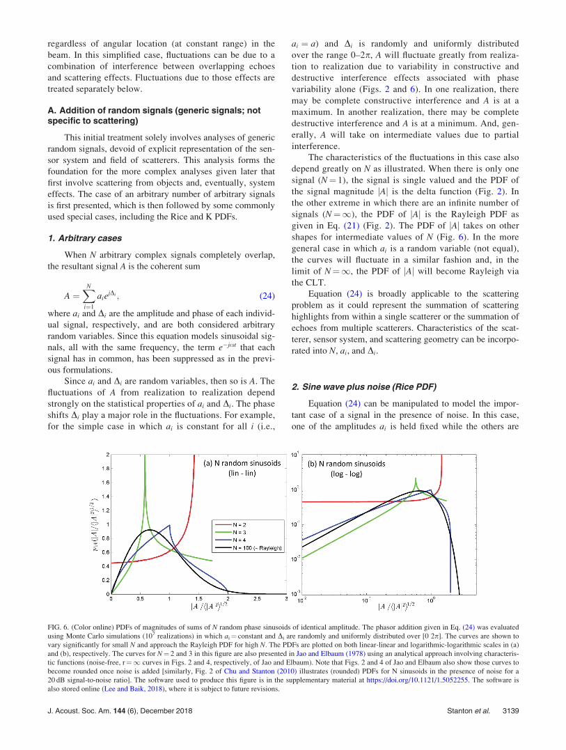
regardless of angular location (at constant range) in the
beam. In this simplified case, fluctuations can be due to a
combination of interference between overlapping echoes
and scattering effects. Fluctuations due to those effects are
treated separately below.
A. Addition of random signals (generic signals; notspecific to scattering)
This initial treatment solely involves analyses of generic
random signals, devoid of explicit representation of the sen-
sor system and field of scatterers. This analysis forms the
foundation for the more complex analyses given later that
first involve scattering from objects and, eventually, system
effects. The case of an arbitrary number of arbitrary signals
is first presented, which is then followed by some commonly
used special cases, including the Rice and K PDFs.
1. Arbitrary cases
When N arbitrary complex signals completely overlap,
the resultant signal A is the coherent sum
A ¼XN
i¼1
aiejDi ; (24)
where ai and Di are the amplitude and phase of each individ-
ual signal, respectively, and are both considered arbitrary
random variables. Since this equation models sinusoidal sig-
nals, all with the same frequency, the term e�jxt that each
signal has in common, has been suppressed as in the previ-
ous formulations.
Since ai and Di are random variables, then so is A. The
fluctuations of A from realization to realization depend
strongly on the statistical properties of ai and Di. The phase
shifts Di play a major role in the fluctuations. For example,
for the simple case in which ai is constant for all i (i.e.,
ai ¼ a) and Di is randomly and uniformly distributed
over the range 0–2p, A will fluctuate greatly from realiza-
tion to realization due to variability in constructive and
destructive interference effects associated with phase
variability alone (Figs. 2 and 6). In one realization, there
may be complete constructive interference and A is at a
maximum. In another realization, there may be complete
destructive interference and A is at a minimum. And, gen-
erally, A will take on intermediate values due to partial
interference.
The characteristics of the fluctuations in this case also
depend greatly on N as illustrated. When there is only one
signal (N¼ 1), the signal is single valued and the PDF of
the signal magnitude jAj is the delta function (Fig. 2). In
the other extreme in which there are an infinite number of
signals (N¼1), the PDF of jAj is the Rayleigh PDF as
given in Eq. (21) (Fig. 2). The PDF of jAj takes on other
shapes for intermediate values of N (Fig. 6). In the more
general case in which ai is a random variable (not equal),
the curves will fluctuate in a similar fashion and, in the
limit of N¼1, the PDF of jAj will become Rayleigh via
the CLT.
Equation (24) is broadly applicable to the scattering
problem as it could represent the summation of scattering
highlights from within a single scatterer or the summation of
echoes from multiple scatterers. Characteristics of the scat-
terer, sensor system, and scattering geometry can be incorpo-
rated into N, ai, and Di.
2. Sine wave plus noise (Rice PDF)
Equation (24) can be manipulated to model the impor-
tant case of a signal in the presence of noise. In this case,
one of the amplitudes ai is held fixed while the others are
FIG. 6. (Color online) PDFs of magnitudes of sums of N random phase sinusoids of identical amplitude. The phasor addition given in Eq. (24) was evaluated
using Monte Carlo simulations (107 realizations) in which ai¼ constant and Di are randomly and uniformly distributed over [0 2p]. The curves are shown to
vary significantly for small N and approach the Rayleigh PDF for high N. The PDFs are plotted on both linear-linear and logarithmic-logarithmic scales in (a)
and (b), respectively. The curves for N¼ 2 and 3 in this figure are also presented in Jao and Elbaum (1978) using an analytical approach involving characteris-
tic functions (noise-free, r¼1 curves in Figs. 2 and 4, respectively, of Jao and Elbaum). Note that Figs. 2 and 4 of Jao and Elbaum also show those curves to
become rounded once noise is added [similarly, Fig. 2 of Chu and Stanton (2010) illustrates (rounded) PDFs for N sinusoids in the presence of noise for a
20 dB signal-to-noise ratio]. The software used to produce this figure is in the supplementary material at https://doi.org/10.1121/1.5052255. The software is
also stored online (Lee and Baik, 2018), where it is subject to future revisions.
J. Acoust. Soc. Am. 144 (6), December 2018 Stanton et al. 3139

randomly varied. Pulling the fixed-amplitude signal out of
the summation, Eq. (24) is rewritten,
A ¼ aejD þXN
i¼1
aiejDi ; (25)
where the second term on the right-hand-side, representing
noise, is the sum of a large number of random amplitude,
random phase signals. The PDFs of the magnitudes of the
fixed amplitude and summed signals are the delta function
and Rayleigh PDF, respectively. Here, N must be sufficiently
large so that the magnitude of the summation converges to a
Rayleigh random variable. The PDF of jAj is the Rice PDF
(Rice, 1954),
pRice jAjð Þ¼2jAj 1þcð ÞhjAj2i
e� 1þcð ÞjAj2þchjAj2i½ �=hjAj2iI0 qð Þ
RicePDFð Þ;(26)
where
q � 2jAj c 1þ cð ÞhjAj2i
" #1=2
; (27)
and
c ¼ a2
r2n
: (28)
The term c is the ratio of the mean squared values of the sine
wave and noise (i.e., the power signal-to-noise ratio or SNR
where the “signal” is the sine wave in this context), rn is the
rms value of the noise term, hjAj2i is the mean square of the
sine wave plus noise [i.e., mean square of Eq. (25)], and I0 is
the zeroth-order modified Bessel function of the first kind.
Note that in the original derivation by Rice, the noise term in
Eq. (25) can also involve the summation of signals of differ-
ent frequencies as well (i.e., more general than the single fre-
quency case shown here).
The shape of the Rice PDF depends strongly on c (Fig. 7).
For example, in the limit as c approaches infinity, the PDF
is close to a Gaussian PDF. This corresponds to the limit of
high SNR where the signal is dominated by the constant
sine wave. In the other extreme, as c approaches zero, the
PDF approaches the Rayleigh PDF. This latter case corre-
sponds to the limit of low SNR where the signal is domi-
nated by the noise. The shape of the Rice PDF changes
smoothly for all intermediate values of c.
In addition to this formula being widely applicable in
modeling noisy signals, it can also be applied to scattering
problems where the “signal” [sine wave in Eq. (25)] is the
mean scattered field and the “noise” [summation term in Eq.
(25)] is the component of the scattered signal that fluctuates
about the mean (Stanton and Clay, 1986; Stanton and Chu,
1992). For example, it could be used to model the fluctua-
tions of the echo from a sphere near a rough interface where
the individual echoes from the sphere and rough interface
are delta-function- and Rayleigh-distributed, respectively.
Or, rather than a rough interface, the sphere could be sur-
rounded by a cloud of smaller scatterers whose individual
echoes are of random phase. If the constant sine wave in Eq.
(25) is considered to represent a single scatterer of interest
(such as the sphere) and the noise term represents the back-
ground reverberation (such as from the rough interface or
cloud of smaller scatterers), then the term c is the signal-to-
reverberation ratio.
3. Special distributions of N or ai (K PDF)
A more complex, but commonly occurring, case is when
N and/or ai in Eq. (24) are random variables. This can be
divided into two categories—one in which Di is randomly
and uniformly distributed over the range 0–2p, and the other
in which Di is non-uniformly distributed. The former
FIG. 7. (Color online) Rice PDF for various values of shape parameter c. The curves were calculated with the analytical solution given in Eq. (26). The PDF
approaches the Rayleigh and Gaussian distributions as c approaches 0 and 1, respectively. The PDFs are plotted on both linear-linear and logarithmic-
logarithmic scales in (a) and (b), respectively. With each function plotted on a normalized scale, the curves are independent of the mean square magnitude of
the signal and only depend upon c. The software used to produce this figure is in the supplementary material at https://doi.org/10.1121/1.5052255. The soft-
ware is also stored online (Lee and Baik, 2018), where it is subject to future revisions.
3140 J. Acoust. Soc. Am. 144 (6), December 2018 Stanton et al.
category will first be discussed. If N follows a negative bino-
mial PDF and its average value tends to infinity, the statistics
of jAj in Eq. (24) for arbitrary ai is described by the K PDF
(Jakeman and Pusey, 1976; Abraham and Lyons, 2002b),
pK jAjð Þ ¼ 4ffiffiffiffiffiffikK
pC aKð Þ
jAjffiffiffiffiffiffikK
p� �aK
KaK�1
2jAjffiffiffiffiffiffikK
p� �
K PDFð Þ;
(29)
where K is the modified Bessel function of the second kind
(and served in the naming of the PDF), C is the gamma func-
tion, aK is the shape parameter, and kK is a scale parameter
equal to the mean square of the signal divided by aK .
The K PDF has a single mode and varies smoothly with
jAj (Fig. 8). The distribution tends to the Rayleigh PDF in
the limit of high aK . Note that the function K also has other,
less common names, including the Basset function and the
modified Bessel function of the third kind.
The K PDF can also be derived in several other ways.
For example, it has been shown that for finite N and if ai fol-
lows an exponential PDF, then jAj is K-distributed (Abraham
and Lyons, 2002b). Beyond methods involving summing
sinusoidal signals, the K PDF has been shown to be due to the
product of two independent random variables: a Rayleigh-
distributed term and one that is chi distributed (Ward, 1981).
This product was later written in extended form as the product
of a Rayleigh-distributed term and the square root of a term
that is gamma distributed (Abraham and Lyons, 2002b). Here,
the square root of the gamma-distributed term is related to the
chi-distributed term through analytical continuation of the
integer number of summed terms in the chi distribution to a
non-integer number in the gamma distribution. In another der-
ivation, the K PDF has also been shown to result from a
Rayleigh PDF whose mean-square value is gamma distributed
(Jakeman and Tough, 1987). Both of these latter derivations
are referred to as a “compound representation.”
Equation (29) has been widely used to describe echo sta-
tistics in both acoustic and electromagnetic applications.
While there has generally not been a direct connection to the
physics of the scattering, the tail of the distribution has gen-
erally followed those from experimental data after an empiri-
cal fit. As discussed above, through the interpretation of
Abraham and Lyons (2002b), the number of scatterers has
been related to the shape parameter of the K PDF for the spe-
cific case in which the amplitudes ai of the individual echoes
are exponentially distributed. Since ai in this case is
observed through the receiver of the sensor system, the expo-
nential PDF includes the effects of both fluctuations from
the stochastic nature of the scatterer and the variability due
to the scatterer being randomly located in the beam. Details
of those effects are given in Sec. VII. Also, in his expression
of a K-distributed magnitude being due to the product of
Rayleigh- and chi-distributed random variables, Ward
(1981) attributed the Rayleigh term as being due to quickly
varying interference between scatterers (such as from phase
shift differences within a patch of scatterers) and the chi
term being due to slowly varying changes in the echo from
larger-scale variations in the “bunching” or patchiness of
scatterers.
The above K PDF involves signals who phases are uni-
formly and randomly distributed over [0 2p]. However,
when the distribution of phases is non-uniform, then jAj can
be described by the generalized K-distribution (not shown)
(Jakeman and Tough, 1987). This distribution is described
by three parameters—kK and aK as given above, plus a third
that describes the non-uniform phase distribution. In addi-
tion, the generalized K PDF in Jakeman and Tough (1987)
can also describe an n-dimensional random walk (general-
ized from the two-dimensional walk for the standard K
PDF). For the case of a non-uniform phase distribution, this
is a random walk with directional bias. Similar to the com-
pound representation of the K PDF above being a Rayleigh
PDF with its mean-square value being gamma distributed,
with this directional bias, the generalized K PDF can be
(compound) represented by a Rice PDF with the mean
square noise and constant amplitude signal components each
FIG. 8. (Color online) K PDF for various values of shape parameter aK . The curves were calculated with the analytical solution given in Eq. (29). With each
function plotted on a normalized scale, the curves are independent of the mean square magnitude of the signal and only depend upon aK . The PDFs are plotted
on both linear-linear and logarithmic-logarithmic scales in (a) and (b), respectively. The software used to produce this figure is in the supplementary material
at https://doi.org/10.1121/1.5052255. The software is also stored online (Lee and Baik, 2018), where it is subject to future revisions.
J. Acoust. Soc. Am. 144 (6), December 2018 Stanton et al. 3141
being gamma distributed in a correlated way (Jakeman and
Tough, 1987). The generalized K PDF can be applicable to
the case in which one or several scatterers dominate the scat-
tering from within a field of many scatterers, thus skewing
the distribution of phases into one that is non-uniform
(Ferrara et al., 2011).
Another generalization of the K PDF is the homodynedK-distribution (not shown). Like the generalized K PDF, it is
also a three-parameter distribution. And, like the generalized
K PDF, it can also be (compound) represented by a Rice
PDF, but with only the mean square noise component (but
not the constant amplitude component) being gamma distrib-
uted (Jakeman and Tough, 1987).
The properties and potential relations to scattering of
the K PDF, generalizations of the K PDF, and other generic
PDFs are summarized in Destrempes and Cloutier (2010).
4. Adding independent realizations of the complexsignal A
As discussed in Secs. IV C 6 and VI A 1, in the limiting
case of the sum of an infinite number of random complex vari-
ables, the PDF of the magnitude of the sum is Rayleigh distrib-
uted (as per the CLT). Specifically, for Eq. (24) where the
phase shifts Di are randomly and uniformly distributed over the
range 0–2p, in the limit of N¼1, jAj is Rayleigh distributed.
Now, consider the case in which there is an ensemble of statis-
tically independent realizations of the complex signal A (in the
limit of large N) where the magnitude of each realization of Ais Rayleigh distributed and with the same mean square value.
Then by extension of the CLT, the magnitude of the sum of
those realizations of A is likewise Rayleigh distributed, even
for a finite number of realizations. However, if each realization
of A is modulated by a multiplicative term with a magnitude
that is a random variable, the resultant magnitude of the sum of
a finite number of these (complex) signals can possibly be
strongly non-Rayleigh. As described in Sec. VI A 3, such a
modulation can be caused by patchiness of the scatterers,
resulting in echo PDFs that can be derived through a com-
pound representation. Also, when the scatterers are uniformly
distributed (i.e., no patchiness effects), there can also be modu-
lation caused by the beampattern where the echo from the scat-
terer is randomly modulated by its random location in the
beam, causing strongly non-Rayleigh echoes as described in
Secs. VII B and VII C.
B. Complex scatterers with stochastic properties
Scatterers can range in complexity from the simplest of
form, a point scatterer, in which the scattering amplitude is
constant for all orientations, to an arbitrarily shaped object
whose echo varies from orientation to orientation. In this sec-
tion, the statistics of scattering by an individual are examined
in a progression of complexity. The point scatterer, Rayleigh
scatterer (defined below), and smooth and rough prolate sphe-
roids with both fixed and random orientation are modeled. A
summary of scatterers with other complexities are given at the
end.
1. Point scatterer
The simplest case is the point scatterer or, more pre-
cisely, very small scatterer. The dimensions of this scatterer
are sufficiently small compared with an acoustic or electro-
magnetic wavelength that the echo is constant for all orienta-
tions. It is constant because there is only one scattering
highlight from this object and nothing else with which to
interfere. The PDF of the echo magnitude is the delta func-
tion [Figs. 2(a) and 3(a)].
2. Rayleigh scatterer
At the other extreme from a point scatterer is a scatterer
whose echo is Rayleigh distributed. This so-called “Rayleigh
scatterer” can be in many forms. For example, it could be a
small patch of many point scatterers, each with an echo
whose phase is randomly and uniformly distributed over the
range [0 2p]. Or, it could be a single spherical scatterer
whose surface is randomly rough and can be described as a
collection of many scattering highlights bounded by the sur-
face. The echo from each highlight has a phase that is ran-
domly and uniformly distributed over the range [0 2p]. In
each case, from the central limit theorem, the echo from the
patch or rough sphere is Rayleigh distributed [Fig. 2(c); Eq.
(21)]. The fluctuations occur from ping to ping as the patch
or rough sphere are rotated, or from realization to realization
of a randomized spatial distribution of scatterers in the patch
or randomized roughness of the rough sphere.
3. Randomized prolate spheroid
A sequence of formulations is presented, beginning with
the deterministic description of the scattering by a smooth
prolate spheroid at fixed orientation, then randomizing its ori-
entation, and then further randomizing the spheroid by rough-
ening its boundary. In contrast to the Rayleigh scatterer, the
echoes from the randomized prolate spheroid are generally
non-Rayleigh because of the elongated shape of the prolate
spheroid. The degree to which the echoes are non-Rayleigh
can be connected to various parameters of the scatterer
through the physics-based formulas given below. The formu-
las given below are adapted from Bhatia et al. (2015).
a. Smooth boundary, fixed orientation. We begin with a
deterministic description of the scattering by a smooth prolate
spheroid at fixed orientation. The spheroid is modeled as being
impenetrable (acoustically “hard” or “soft” or, with an electro-
magnetic signal, perfectly conducting). Also, the scattering is in
the “geometric optics” or high frequency limit where the acous-
tic or electromagnetic wavelength is much smaller than any
dimension of the spheroid. For simplicity, only echoes from the
front interface are analyzed and waves that travel around the
boundary (i.e., circumferential waves) are ignored. Using the
Kirchhoff approximation and the stationary phase approxima-
tion, the magnitude of the backscattering amplitude of the
spheroid is (Chap. 4 of Crispin and Siegel, 1968)
3142 J. Acoust. Soc. Am. 144 (6), December 2018 Stanton et al.

jfSSj ¼1
2cb1
2
b12 cos2bþ c 2 sin2b
smooth boundary; fixed orientationð Þ; (30)
where the “SS” subscript to the scattering amplitude refers
to “smooth spheroid” and b is the angle between the direc-
tion of the incident acoustic or electromagnetic wave and the
plane that is normal to the lengthwise axis of the prolate
spheroid [Fig. 9(a)]. Note that this equation is equivalent to
Eq. (7) of Bhatia et al. (2015), but is in a form in which no
terms have singularities. b¼ 0 and b¼ p=2 correspond to
broadside and end-on incidence, respectively, relative to the
incident wave. The terms c and b1 are the lengths of the
semimajor and semiminor axes of the prolate spheroid,
respectively (the length and width of the spheroid are 2cand 2b1, respectively). The spheroid is axisymmetric about
the length-wise axis, leading to only one unique value of
semiminor axis. The term b1 is not to be confused with the
beampattern b. The aspect ratio of the spheroid is defined to
be the ratio c=b1 (or, equivalently, length/width). The scat-
tering is a strong function of the aspect ratio and orientation
[Fig. 9(b)]. At broadside incidence, the above formula
reduces to
jfSSj ¼c
2: (31)
b. Smooth boundary, random orientation. We now ran-
domize the scattering by first randomizing the orientation.
This is done by making b a random variable with an associ-
ated PDF pbðbÞ. For simplicity, the prolate spheroid will
only rotate in a single plane about its minor axis in a plane
containing the direction vector of the incident plane wave
[Fig. 9(a)].
Since the scattering amplitude fss is a function of the
random variable b, then fss is a random variable as well.
Inserting jfSSj and pbðbÞ into Eq. (16), the PDF of the magni-
tude of the scattering amplitude of a randomly oriented
smooth prolate spheroid is
pSS jfSSjð Þ¼pb bð Þ����@jfSSj@b
����jb jfSSjð Þ
smoothboundary; randomorientationð Þ: (32)
Equation (16) was used because the scattering amplitude in
Eq. (30) varies monotonically over the entire range of orien-
tations. If the scattering amplitude varied non-
monotonically, then Eq. (17) would have been required to
calculate the echo PDF.
Inserting Eq. (30) into Eq. (32) gives the PDF of the
magnitude of the scattering amplitude of a randomly ori-
ented smooth prolate spheroid explicitly in terms of the
dimensions of the prolate spheroid,
pSS jfSSjð Þ ¼ pb bð Þ b12 cos2bþ c2 sin2b
� �2
cb12 c2 � b1
2ð Þj sin b cos bj
����b jfSSjð Þ
smooth boundary; random orientationð Þ: (33)
Calculation of the echo PDF requires knowledge of the ori-
entation distribution. For the simple case in which the angles
of rotation are uniformly and randomly distributed over the
range [0 2p], the PDF of b is
pb bð Þ ¼ 2
p; 0 � b � p
2rotation in one planeð Þ; (34)
FIG. 9. (Color online) Backscattering by an impenetrable prolate spheroid. (a) Scattering geometry. The term b is the angle between the direction of the incident
wave and the plane that is normal to the lengthwise axis of the prolate spheroid. For simplicity, this illustration is drawn in the plane containing the incident wave
vector and the lengthwise axis. (b) Magnitude of scattering amplitude (backscatter direction) versus angle of incidence b for smooth prolate spheroids. The curves
were calculated with the analytical solution given in Eq. (30). All spheroids, which span a range of aspect ratios from 1:1 (sphere) to 10:1 (most elongated), have
the same volume equal to that of a sphere of radius 0.1 m. Adapted from Bhatia et al. (2015). The software used to produce panel (b) of this figure is in the supple-
mentary material at https://doi.org/10.1121/1.5052255. The software is also stored online (Lee and Baik, 2018), where it is subject to future revisions.
J. Acoust. Soc. Am. 144 (6), December 2018 Stanton et al. 3143

where b only varies over the range 0–p/2 because of the
symmetry of the scattering over the other angles.
The echo PDF for the randomly oriented smooth prolate
spheroid is calculated for a range of aspect ratios (not includ-
ing the case of a sphere where the aspect ratio is unity) by
inserting Eq. (34) into Eq. (33) [Fig. 10(a)]. For each (non-
unity) aspect ratio, the echo PDF is characterized by a
smoothly varying function for most magnitudes, but with
strong narrow peaks at the end points. These peaks are attrib-
uted to the fact that the backscattering near broadside and
end-on incidence varies slowly with orientation angle, which
increases the probability of occurrence at those correspond-
ing echo values. The range of echo values as well as proba-
bility of occurrence are both shown to be a strong function
of aspect ratio of the spheroid. For the case of a sphere, the
echo is constant for all b and the echo PDF is a delta func-
tion [Fig. 10(a)].
c. Rough boundary, random orientation. We further
randomize the scattering by roughening the boundary of
the prolate spheroid, where the roughness here is the devia-
tion from the mean boundary. In this case, the boundary is
randomly rough throughout the entire surface of the spher-
oid. Furthermore, it is assumed to be sufficiently rough
compared with an acoustic or electromagnetic wavelength
such that for any orientation, the magnitude of the scatter-
ing amplitude is Rayleigh distributed. For the randomly
rough surface, the echoes are assumed to be independent
of each other from orientation to orientation (or realization
to realization). In this limiting case, we model the scatter-
ing by being equal to the product of the magnitude of the
scattering amplitude jfssj of the smooth prolate spheroid at
a particular orientation and an independent “modulation”
random variable that follows a Rayleigh PDF. This latter
modulation term has a unity rms and, for each orientation,
the term is statistically independent from its value at all
other orientations. For a randomly oriented prolate spher-
oid, jfssj is also a random variable. Thus, the magnitude of
the scattering amplitude for the randomly rough, randomly
oriented prolate spheroid is the product of two random var-
iables, jfssj and the Rayleigh-distributed modulation term.
The statistics of the echoes from randomly rough, ran-
domly oriented prolate spheroids can be described using
Eq. (20),
prs jfrsjð Þ ¼ðjfssjmax
jfssjmin
1
xpSS xð ÞpRay
jfrsjx
� �dx
randomly rough boundary; random orientationð Þ;(35)
where the subscript “rs” refers to rough (randomly oriented)
prolate spheroid and pRay is the Rayleigh PDF of the modu-
lation term [Eq. (21)]. The terms jfssjmin and jfssjmax are the
minimum and maximum values of the magnitude of the
scattering amplitude of the smooth prolate spheroid,
respectively, which correspond to end-on and broadside
incidence. Those two terms replaced the limits �1 and
þ1, respectively, in the integral in Eq. (20) to reflect the
fact that the magnitude of the scattering amplitude of the
smooth prolate spheroid is within the range [jfssjmin,
jfssjmax] and that the corresponding PDF pss is zero for val-
ues of its argument outside that range. Without the above
constraint, the integral still would have been constrained by
the Rayleigh PDF whose argument is limited to only posi-
tive values, which would have led to integral limits of zero
to infinity.
The resultant echo PDFs of the scattering by the ran-
domly rough, randomly oriented prolate spheroid are signifi-
cantly different from the smooth counterpart [Fig. 10(b)].
The curves for each aspect ratio are now smoothly varying,
have a mode, and do not have any singularities.
FIG. 10. (Color online) PDF of magnitude of backscattering amplitude for (a) smooth prolate spheroid and (b) rough prolate spheroid. Each spheroid is ran-
domly and uniformly oriented in a single plane. The axis of rotation (a minor axis of the spheroid) is the normal to this plane, which contains the omnidirec-
tional sensor system. Aspect ratio is varied from 1:1 (sphere) to 10:1 (most elongated). The curves in (a) (not including the sphere) and (b) are calculated using
the analytical solutions given in Eqs. (33) and (35), respectively. Equation (34) was used in each case for the orientation distribution. Equation (33) for pss is
used in the integrand in Eq. (35). The Rayleigh PDF [from Eq. (21)] in the integrand of Eq. (35) is normalized so that the rms amplitude is equal to unity.
From Bhatia et al. (2015). The software used to produce this figure is in the supplementary material at https://doi.org/10.1121/1.5052255. The software is also
stored online (Lee and Baik, 2018), where it is subject to future revisions.
3144 J. Acoust. Soc. Am. 144 (6), December 2018 Stanton et al.

4. Randomly rough objects with full range ofroughness and circumferential/internal waves
There are many more important complexities of the
scattering and associated echo statistics than described above
and they are summarized briefly below. The above example
involved the simplified case in which the boundary of the
prolate spheroid was impenetrable, only the echo from the
front interface was accounted for, and its roughness was suf-
ficiently large so that the echo was Rayleigh distributed for
any fixed orientation. However, it is not uncommon for an
object to have circumferential and internally refracted/
reflected waves and/or a boundary roughness that spans
small-to-intermediate levels relative to a wavelength of the
incident signal. Each of these latter cases can lead to statis-
tics of the echo that are significantly different than that of
the very rough impenetrable prolate spheroid discussed
above and must be accounted for.
Given the complexity of predicting the scattering by
objects with those various types of waves, the echo statistics
will be summarized below according to a progression of com-
plexity. In Sec. VI B 4 a, effects on the scattering due to cir-
cumferential and internal waves for smooth objects are briefly
reviewed. In Sec. VI B 4 b, the object is roughened, and the
statistics of the echoes from only the front interface are con-
sidered. This is similar to the case of the rough impenetrable
prolate spheroid above but with the added complexity of
accounting for small-to-intermediate roughness where the
echoes are non-Rayleigh. In Sec. VI B 4 c, circumferential/
internal waves associated with penetrable materials are incor-
porated with boundary roughness included.
a. Circumferential and internal waves (smooth
boundary). Objects with common material properties not
only produce a significant echo from the front interface, but
they also support various classes of circumferential and inter-
nally refracted/reflected waves due to incident signals (acous-tic: Hackman, 1993; Marston, 1992; Numrich and Uberall,
1992; Uberall, 1973; electromagnetic: Chen, 1998; Crispin
and Siegel, 1968; Moser et al., 1981; Murphy et al., 1980;
Newton, 1982; acoustic and electromagnetic: Bowman et al.,1987; Nussenzveig, 1969). For the case of impenetrable
objects, such as infinitely dense materials for acoustics appli-
cations and perfectly conducting materials for electromag-
netic applications, there is a weak signal that diffracts or
“creeps” around the boundary and reradiates in all directions
including back to the receiver. For the case of penetrable
objects, such as elastic materials for acoustics applications
and dielectric materials for electromagnetic applications,
those diffracted waves also exist. In addition, with elastic
objects, there can be strong surface elastic waves that are gen-
erated from the incident acoustic signal and will travel around
the boundary (in addition to the diffraction boundary wave).
Furthermore, other processes are also involved for the pene-
trable objects such as waves that refract into the interior of
the object and reflect internally. Because of these various
effects, the echo from a smooth symmetrical object such as a
sphere or cylinder will generally be composed of the sum of
echoes associated with the front-facing interface (sometimes
called the “specular” echo), internal transmission and reflec-
tions, and circumferential waves.
The total echo from these objects will vary according to
the constructive and destructive interference between the
individual echoes associated with each of the different scat-
tering phenomena described above. For a smooth object
such as a sphere or cylinder, the phase of the echo associated
with each phenomenon will vary strongly with signal fre-
quency (or more precisely, ka, where a is the radius of the
object). Because of these frequency dependences, which also
vary with each phenomenon, the pattern of echo vs fre-
quency will contain a series of peaks and strong nulls associ-
ated with the constructive and destructive interference,
respectively, between the different phenomena.
b. Front interface only: Small-to-intermediate rough-
ness, Rice PDF. The following discussion concerns the
echo from the front interface only, in isolation from the cir-
cumferential and internal waves.
When the roughness of the surface is smaller than the
wavelength of the incident signal or, more precisely, when
krB < 1, where rB is the standard deviation of the boundary
(or, equivalently, the rms deviation from the mean bound-
ary), the magnitude of the echo from the front-facing surface
of a rough object at normal incidence to that surface is gen-
erally not Rayleigh distributed. This is because the phases of
the echoes from the individual scattering features of the sur-
face are relatively narrowly distributed, in contrast to being
uniformly distributed [0 2p] such as in the above case of the
(very) rough spheroid. This effect has been studied mostly in
the context of scattering by rough planar interfaces and, to a
much lesser extent, for rough bounded objects. In either
case, in the limit of small roughness (i.e., krB 1), the echo
PDF will tend to the delta function. In the opposite limit
(i.e., krB 1), the echo PDF will tend to the Rayleigh PDF
(or at least be Rayleigh-like) as in the above example.
It has been shown that the echo statistics from the full
range of roughness at normal incidence of a planar boundary
can be described by the Rice PDF, as given above in Eq.
(26) (Stanton and Clay, 1986). In this formulation, the scat-
tered signal is decomposed into the sum of two components,
the coherent mean (constant amplitude) and fluctuation com-
ponent. The PDFs of the magnitudes of the two components
are the delta function and Rayleigh PDF, respectively. The
mean component is related to the reflection coefficient of the
interface modified by the term e�2k2r2B —a term originally
derived for rough planar interfaces by Eckart (1953). The
fluctuation term is related to the scattering phenomena that
cause deviations in the echo from this mean. These two scat-
tering terms, the constant amplitude and fluctuation compo-
nents, correspond to the sinusoidal signal and noise,
respectively, in the original Rice formulation.
The Rice PDF shape parameter has also been explicitly
connected to parameters of the roughness and sensor system
for rough planar interfaces (normal incidence), as summa-
rized in Stanton and Clay (1986). Parameters of the rough-
ness are the rms deviations (rB) from the normal to the mean
surface and the two-dimensional autocorrelation function
(along the surface) of the surface. Parameters of the sensor
J. Acoust. Soc. Am. 144 (6), December 2018 Stanton et al. 3145
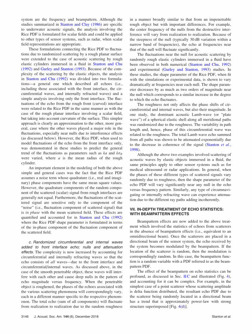
system are the frequency and beampattern. Although the
studies summarized in Stanton and Clay (1986) are specific
to underwater acoustic signals, the analysis involving the
Rice PDF is formulated for scalar fields and could be applied
to other types of sensor systems, such as radar, when scalar
field representations are appropriate.
These formulations connecting the Rice PDF to fluctua-
tions due to randomized scattering by a rough planar surface
were extended to the case of acoustic scattering by rough
elastic cylinders immersed in a fluid in Stanton and Chu
(1992) and Gurley and Stanton (1993). Because of the com-
plexity of the scattering by the elastic objects, the analysis
in Stanton and Chu (1992) was divided into two formula-
tions—a general one which described all echoes (i.e.,
including those associated with the front interface, the cir-
cumferential waves, and internally refracted waves) and a
simple analysis involving only the front interface. The fluc-
tuations of the echo from the rough front (curved) interface
were related to the Rice PDF in the same manner as with the
case of the rough planar interface involving a scalar field,
but taking into account curvature of the surface. This simpler
approach is clearly an approximation to the other, more gen-
eral, case where the other waves played a major role in the
fluctuations, especially near nulls due to interference effects
(as discussed below). However, the Rice PDF, when used to
model fluctuations of the echo from the front interface only,
was demonstrated in these studies to predict the general
trend of the fluctuations as parameters such as ka and krB
were varied, where a is the mean radius of the rough
cylinder.
An important element in the modeling of both the above
simple and general cases was the fact that the Rice PDF
assumes a noise term whose quadrature (i.e., real and imagi-
nary) phase components have the same mean square values.
However, the quadrature components of the random compo-
nent of the scattered (scalar) signal from rough interfaces are
generally not equal. Furthermore, the fluctuations of the scat-
tered signal are sensitive only to the component of the
“noise” (i.e., fluctuation component of scattered signal) that
is in phase with the mean scattered field. These effects are
quantified and accounted for in Stanton and Chu (1992)
where the Rice PDF shape parameter is formulated in terms
of the in-phase component of the fluctuation component of
the scattered field.
c. Randomized circumferential and internal waves
added to front interface echo; nulls and attenuation
effects. The complexity is now increased by accounting for
circumferential and internally refracting waves so that the
echo consists of all waves—due to the front interface and
circumferential/internal waves. As discussed above, in the
case of the smooth penetrable object, these waves will inter-
fere with each other and cause deep nulls in the pattern of
echo magnitude versus frequency. When the penetrable
object is roughened, the phases of the echoes associated with
the various scattering phenomena will correspondingly vary,
each in a different manner specific to the respective phenom-
enon. The total echo (sum of all components) will fluctuate
from realization to realization due to the random roughness
in a manner broadly similar to that from an impenetrable
rough object but with important differences. For example,
the center frequency of the nulls from the destructive inter-
ference will vary from realization to realization. Because of
the steepness of the null (typically 30 dB variation within a
narrow band of frequencies), the echo at frequencies near
that of the null will fluctuate significantly.
The fluctuations near the null for acoustic scattering by
randomly rough elastic cylinders immersed in a fluid have
been observed in both numerical (Stanton and Chu, 1992)
and experimental (Gurley and Stanton, 1993) studies. In
these studies, the shape parameter of the Rice PDF, when fit
with the simulations or experimental data, is shown to vary
dramatically at frequencies near each null. The shape param-
eter decreases by as much as two orders of magnitude near
the null which corresponds to a similar increase in the degree
to which the echo fluctuates.
The roughness not only affects the phase shifts of cir-
cumferential and internal waves, but also their magnitude. In
one study, the dominant acoustic Lamb-wave (or “plate
wave”) of a spherical elastic shell along all meridional paths
was randomized due to the roughness. The variability in path
length and, hence, phase of this circumferential wave was
related to the roughness. The total Lamb wave echo summed
from all paths was shown to be attenuated exponentially due
to the decrease in coherence of the signal (Stanton et al.,1998).
Although the above two examples involved scattering of
acoustic waves by elastic objects immersed in a fluid, the
same principles apply to other sensor systems such as for
medical ultrasound or radar applications. In general, when
the phases of these different types of scattered signals vary
randomly due to roughness, then the shape parameter of the
echo PDF will vary significantly near any null in the echo
versus frequency pattern. Similarly, any type of circumnavi-
gating or internally refracting wave can experience attenua-
tion due to the different ray paths adding incoherently.
VII. IN-DEPTH TREATMENT OF ECHO STATISTICS:WITH BEAMPATTERN EFFECTS
Beampattern effects are now added to the above treat-
ment which involved the statistics of echoes from scatterers
in the absence of beampattern effects (i.e., equivalent to an
omnidirectional beam). Once the scatterers are placed in a
directional beam of the sensor system, the echo received by
the system becomes modulated by the beampattern. If the
location of the scatterer is random, then the modulation is
correspondingly random. In this case, the beampattern func-
tion is a random variable with a PDF referred to as the beam-
pattern PDF.
The effect of the beampattern on echo statistics can be
profound, as discussed in Sec. II C and illustrated (Fig. 4),
and accounting for it can be complex. For example, in the
simplest case of a point scatterer whose scattering amplitude
is delta function distributed, the resultant echo PDF due to
the scatterer being randomly located in a directional beam
has a trend that is approximately power-law with strong
structure superimposed [Fig. 4(d)].
3146 J. Acoust. Soc. Am. 144 (6), December 2018 Stanton et al.

The below treatment begins with a general formula for
the echo PDF due to a single scatterer randomly distributed
in a beam. The properties of the scatterer, spatial distribu-
tion, and beampattern are all arbitrary in this formula.
Following the general formula is a progression of examples
beginning with the simplest of cases—a point scatterer ran-
domly and uniformly distributed within only the mainlobe of
the beam of an axisymmetric transducer (i.e., excluding side-
lobes). The analysis then extends to complex scatterers and
the entire beam (including sidelobes) and, finally, to the case
involving a beampattern from an arbitrary transducer in
which the beampattern is not axisymmetric and a spatial dis-
tribution of scatterers that is not uniform. After the treatment
of single scatterers, the echo statistics associated with multi-
ple scatterers in the beam is presented. In the first set of
examples, all scatterers are identical, which is then followed
by the more general case of assemblages of scatterers of
varying types.
The formulations can be applied to single beam (fixed
or scanning) and multi-beam systems, provided that the scat-
terer(s) are randomly located in the beam. The formulations
are general and are not specific to any particular system.
Although specific types of signal processing or adaptive
beamforming that some systems incorporate are not mod-
eled, the formulations presented herein can serve as a basis
for the modeling as discussed in Secs. V A and V B.
A. Single scatterer randomly located in beam
1. Accounting for beampattern effects in echo PDF
For the case in which a single scatterer is randomly
located in the beam of the sensor system at approximately
constant range, its angular coordinates ðh; /Þ are random
variables. Since the beampattern is a function of these ran-
dom variables, the beampattern function bðh; /Þ is also now
a random variable (Sec. IV C 3) and can be described by the
beampattern PDF, pbðbÞ. Consider now a scatterer whose
scattering properties are random (such as a randomly rough
and/or randomly oriented elongated scatterer). The scattering
amplitude is now a random variable and its magnitude can
be described by the PDF psðjfbsjÞ (Secs. II B and VI B). The
magnitude of the echo ~e received by the system is equal to
the product of the magnitude of the scattering amplitude jfbsjand the beampattern bðh; /Þ [Eq. (4)]. With both of these
latter two terms being random variables, then ~e is also a ran-
dom variable (Sec. IV C 4). Using Eq. (20), the PDF of ~e can
be written in terms of pS and pb as [Ehrenberg (1972)]
pe ~eð Þ ¼ð1
~e
1
xpS xð Þpb
~e
x
� �dx; 0 � b � 1; (36a)
where x is used to denote jfbsj. The term b (¼ ~e/x) is implic-
itly the argument of pb. Using the same procedure, peð~eÞ can
be expressed in an alternate, but equivalent form
pe ~eð Þ ¼ð1
0
1
bpb bð ÞpS
~e
b
� �db; 0 � b � 1: (36b)
where now jfbsj (¼ ~e/b) is implicitly the argument of pS.
Equations (36a) and (36b) are equivalent because of the
commutative nature of the product of the two random varia-
bles in Eq. (20). The limits of 61 in the integral in Eq. (20)
are reduced to the ranges [~e 1] and [0 1] in Eqs. (36a) and
(36b), respectively, since the values of the beampattern bonly span the range [0 1] and the corresponding beampattern
PDF pb is zero outside that range. Finally, the range
0 � b � 1 is used in each equation as they apply to the entirebeampattern, whereas some applications later will involve
only portions of the beampattern, such as for values of the
mainlobe only above the highest sidelobe. In those cases, the
limits in the integrals are modified accordingly.
These expressions, originally derived by Ehrenberg
(1972) [using Eq. (20)] for echo intensity with identical
form, are given for echo magnitude (i.e., not intensity) in
Ehrenberg et al. (1981) and are also described in reviews in
Stanton and Clay (1986) and Ehrenberg (1989). While use of
one form over the other [Eq. (36a) vs Eq. (36b)] was not
explained in the early papers, it is possible that one form
may be more conducive for evaluation, such as in numerical
integration (Bhatia et al., 2015).
The above integral relationship in Eqs. (36a) and (36b)
between the echo PDF peð~eÞ and the PDFs of the magnitude of
the scattering amplitude and beampattern function is
completely general, as it applies to an arbitrary stochastic scat-
terer that is randomly located (at approximately constant range)
in an arbitrary beampattern over an arbitrary spatial distribu-
tion. The constraint of the scatterers being at approximately
constant range is consistent with Eq. (4) as these equations
apply to the scatterers distributed within a thin shell at a nearly
constant distance from the sensor system. This eliminates the
range-dependent effects in analysis of the echo fluctuations.
2. PDF of spatial distribution of scatterer
The beampattern PDF depends not only on the beampat-
tern function bðh; /Þ, but also the PDF, ph;/ðh ;/Þ; of the
angular location of the scatterer in the beam. This probabil-
ity, in combination with the beampattern function, deter-
mines the degree to which the echo is randomly modulated
by the beampattern. For example, if the scatterer were fixed
in the center of the beam, then ph;/ is a delta function peaked
at ðh ;/Þ¼ (0, 0) and the echo is multiplied by unity for all
realizations [Fig. 4(a)]. In the other extreme, if the scatterer
were randomly located throughout the entire half-space, then
ph;/ is finite for all h and /: In this latter case, the echo is
randomly modulated by all values of the beampattern result-
ing in a wide range of echo values, even for a point scatterer
[Fig. 4(d)].
Two simple examples are treated here involving the
scatterer being randomly and uniformly distributed in a half-
plane (2D) and half-space (3D) at approximately a constant
range. The 2D and 3D cases apply to geometries in which
the sensor system is detecting scatterers that are distributed
throughout a thin semicircular arc and a thin hemispherical
shell, respectively. The 2D case may apply to geometries
where (1) the transducer is a line with a beampattern that
only varies in one plane, (2) the sensor system is located
within a thin layer of scatterers and is looking along the layer
J. Acoust. Soc. Am. 144 (6), December 2018 Stanton et al. 3147

from within that layer, or (3) the system is in a waveguide
and long-range echoes only vary with respect to one dimension
(such as in the plane parallel to the waveguide boundaries as
described in Sec. VIII C). In all of these cases, only a half-
plane or half-space are considered as the transducer is assumed
to be baffled sufficiently so that there is no “back” radiation.
In each example, ph;/ (which reduces to ph in some
cases) is calculated using Eq. (8), where pXðxÞ in that equa-
tion is used to represent the probability of occurrence of the
scatterer per unit volume at angular location ðh ;/Þ and xrepresents the volume V (Chap. 10 of Medwin and Clay,
1998). The term dPX ð¼ dPVÞ in Eq. (8) is the differential
probability of occurrence of the scatterer in the differential
volume dV at location ðh ;/Þ. For the case of the scatterers
being located within a thin hemispherical shell of constant
radius, which is the 3D geometry in most examples in this
tutorial, then dx¼ dV¼ r2sin hdhd/Dr, where r is the radius
of the hemispherical shell, h is the spherical polar angle, / is
the spherical azimuthal angle, and Dr is the thickness of the
shell. For the case of the scatterers being located within a
thin-shelled semi-circular arc of constant radius r, which is
the 2D geometry sometimes used in this tutorial, then
dx¼ dV¼ rdhDwDr, where Dw is the (thin) width of the cir-
cular arc (strip). The total volume of the thin shell in each of
these two cases is 2pr2Dr and prDwDr, respectively.
For a scatterer uniformly distributed within the volume,
then the differential probability of occurrence dPV per unit
differential volume dV is held constant (i.e., dPV=dV¼ pv
¼ constant). Using that constraint, and the fact that the inte-
gral of dPV over the total volume that the scatterer can
occupy is unity [and, hence, dPV=dV¼ pv¼ (total vol-
ume)�1], then pv¼ (prDwDr)�1 and pv¼ (2pr2Dr)�1 for the
2D and 3D cases, respectively. Through these changes in
variables, Eq. (8) becomes dPV ¼ phdh and dPV ¼ ph;/dhd/for these two cases, respectively, where expressions for ph
and ph;/ are given below.
For the 2D case in which the scatterer is randomly and
uniformly distributed in a half-plane at approximately con-
stant range, the probability density function of the angular
location of the scatterer in spherical coordinates is deter-
mined using the above approach,
ph ¼1
p; � p
2� h � p
2; fixed / 2D; half-planeð Þ:
(37)
There is no dependence upon h since, at approximately con-
stant range, the scatterer is uniformly distributed within a thin
arc of nearly constant radius in that plane. There is no depen-
dence upon / as it is fixed in this geometry. Note that
although the polar angle h is normally restricted to the range
0 � h � p=2, it is varied over the range �p=2 � h � p=2 for
fixed /. For the case of an axisymmetric beam centered at
h¼ 0 which is typically the major response axis (MRA) of
the beam, the expression ph ¼ 2=p for 0 � h � p=2 has been
used to eliminate redundant calculations (Bhatia et al., 2015).
For the 3D case in which the scatterer is randomly and
uniformly distributed in a half-space at approximately con-
stant range, the probability density function of its angular
location is determined using the above approach (Medwin
and Clay, 1998),
ph;/ ¼1
2psin h; 0 � h � p
2; 0 � / � 2p
3D; half- spaceð Þ: (38)
Although the scatterers are located throughout all values of
/, ph;/ still does not depend upon / (as in the 2D case
above). However, now ph;/ depends upon h because in this
3D polar-spherical coordinate system, the scatterer is ran-
domly and uniformly distributed within a thin hemispherical
shell in the range 0� h�p/2. Calculations in this coordinate
system involve annular rings (at constant spherical radius),
each located at some angle h with a width of dh and span-
ning all values of /: Since the scatterer is randomly and uni-
formly distributed across all values of / within each ring,
then the probability ph;/ only depends upon the area of each
ring, which is proportional to sin h (which appears in the
expression for dV above). Accounting for the uniform distri-
bution across all / [0, 2p] for a given value of h yields a fac-
tor (2p)�1 in Eq. (38).
For the case in which the beampattern is symmetrical
about the h ¼ 0 axis, ph;/ in Eq. (38) can be integrated over
all / [0, 2p] for the simplified result
ph ¼ sin h; 0 � h � p2
3D; half-space axisymmetric transducerð Þ: (39)
3. Beampattern PDF for mainlobe only (axisymmetrictransducer, uniformly distributed scatterer)
a. Exact solution. Calculating the PDF of the beampat-
tern function depends upon the complexity of the beam. The
FIG. 11. Diagram illustrating different conditions considered when calculat-
ing beampattern PDF. The portion of b greater than the highest sidelobe,
bSL, varies monotonically with h and Eq. (40) is used to calculate the PDF.
Once the entire beampattern is used, the beampattern varies non-
monotonically and Eq. (46) is used. For the arbitrary value of barb, the beam-
pattern takes on that value three times in this example (b1, b2, and b3 for
m¼ 1, 2, and 3, respectively, and, correspondingly h1, h2, and h3 which are
not shown). The vertical axis is on an arbitrary logarithmic scale to better
illustrate the sidelobe structure.
3148 J. Acoust. Soc. Am. 144 (6), December 2018 Stanton et al.

simplest case is first examined involving an axisymmetric
beam (i.e., due to a circular planar transducer) in which only
the portion of the mainlobe above the value of the highest side-
lobe is used [Figs. 4(c) and 11]. This results in the beampattern
only being dependent upon a single random variable (spherical
polar angle, hÞ and furthermore varying monotonically with
respect to this angle. Using only the values of the mainlobe
above that of the highest sidelobe is not only easier to calcu-
late, but it also generally relates to the highest values of the
echoes, which have a higher chance of being detectable above
the system noise levels. With these simplifications, Eq. (16)
can be used to describe the beampattern PDF for the case in
which the beampattern is monotonic and dependent upon only
a single random variable,
pb bð Þ ¼ ph hð Þ���� @b
@h
���� jh bð Þ
; bSL � b � 1; (40)
where bSL is the value of the highest sidelobe of the beam-
pattern and the notation phðhÞ represents ph;/ for this case
where the scatterer distribution does not depend upon /.
This corresponds to the scenario where a scatterer is uni-
formly and randomly distributed either in 2D or 3D as shown
in Sec. VII A 2, but with the restriction that �hSL � h � hSL
(fixed /) and 0 � h � hSL (all /) for the 2D and 3D cases,
respectively, where hSL corresponds to bSL [Figs. 4(c) and
11]. With this restriction, phðhÞ ¼ 1=ð2hSLÞ and phðhÞ¼ sin h=ð1� cos hSLÞ for the 2D and 3D cases, respectively.
These two latter expressions are calculated in a similar man-
ner as for Eqs. (37) and (39), respectively, except that they
involve use of a smaller volume, subtended by the angle hSL,
over which dPV is integrated for normalization.
The beampattern function for a circular planar trans-
ducer is (Kinsler et al., 2000)
b hð Þ ¼ 2J1 kaT sin hð ÞkaT sin h
� 2
; (41)
where aT is the radius of the transducer and J1 is the Bessel
function of the first kind of order 1. The square of the brackets
corresponds to the fact that this is a composite, or two-way
beampattern, being produced by the product of the transmit
and receive beampatterns which are identical to each other.
Using phðhÞ ¼ sin h=ð1� cos hSLÞ from above and Eq.
(41) in Eq. (40), the beampattern PDF for an axisymmetric
beam and associated with the values of the mainlobe above
the highest sidelobe is
pb bð Þ ¼ sin2h
4ffiffiffibp
cos h 1� cos hSLð ÞjJ2 kaT sin hð Þj
����h bð Þ;
bSL � b � 1; (42)
where J2 is the Bessel function of the first kind of order 2.
Here, the scatterers are assumed to be uniformly distributed
at approximately constant range within the mainlobe for
polar angles in the range 0 � h � hSL (all /) (i.e., a 3D
case).
b. Power law approximation for beampattern PDF. The
beampattern PDF, when plotted on a log-log scale, has been
shown to have a negative and nearly constant slope for the
higher values of beampattern (Ehrenberg, 1972) (Figs. 4 and
12 of this paper). This pattern corresponds to the portion of
the mainlobe higher than the highest sidelobe and also
occurs over a wide range of beamwidths (Ehrenberg, 1972).
Under these conditions, the beampattern PDF can be approx-
imated using the following equation (Ehrenberg et al.,1981):
pbðbÞ ¼ k0b�l; bSL � b � 1; (43)
where the normalization constant k0 ensures the integral of
Eq. (43) over b is unity and is given by
k0 ¼
1� lð Þbl�1SL
bl�1SL � 1
l 6¼ 1ð Þ;
� 1
ln bSLl ¼ 1ð Þ:
8>>>><>>>>:
(44)
Using Eq. (42) in the limit of b approaching unity or
kaT sin h approaching zero (that is, for angles near the center
of the beam), the exponent in Eq. (43) is (Chu and Stanton,
2010)
l ¼ 5
6þ 2
kaTð Þ2; b! 1 or kaT sin h! 0; (45)
which shows that the slope of the beampattern PDF on a log-
log plot varies only with kaT (related to beamwidth) and is
independent of b under these limiting conditions. This equa-
tion was derived under the assumption that the scatterers are
uniformly distributed at approximately constant range within
the mainlobe for polar angles in the range 0 � h � hSL (all
/) (i.e., a 3D case). Note that the power-law form in Eq. (43)
applies to both an intensity-based analysis (Ehrenberg, 1972;
Ehrenberg et al., 1981) and magnitude-based analysis such
as in this tutorial and in Chu and Stanton (2010).
4. Beampattern PDF for entire beam (axisymmetrictransducer, uniformly distributed scatterer)
Once the entire beampattern is accounted for in the echo
statistics, the sidelobes become a significant factor. In this
case, there can be more than one angle at which the beam-
pattern achieves a certain value [Figs. 4(d) and 11]. In this
non-monotonic case, Eq. (17) is now used to calculate the
beampattern PDF,
pb bð Þ ¼XM
m¼1
ph hmð Þ���� @b
@hm
���� jhm bð Þ
; 0 � b � 1: (46)
Now, the full range of polar angles is used
[�p=2 � h � p=2 (fixed /) and 0 � h � p=2 (all /) for the
2D and 3D cases, respectively]. The summand of this equa-
tion is the same as Eq. (40) which corresponds to the portion
of the mainlobe above the highest sidelobe level and which
J. Acoust. Soc. Am. 144 (6), December 2018 Stanton et al. 3149

is a monotonic function. With this summation over m in Eq.
(46), each value of m corresponds to a portion of the beam-
pattern that is monotonic and is associated with the structure
of the mainlobe and sidelobes (Fig. 11).
For a scatterer being uniformly distributed in a hemi-
spherical shell, Eq. (39) is used for its spatial distribution
phðhÞ. For the case of a circular planar transducer, Eqs. (39)
and (41) are inserted into Eq. (46) to obtain the beampattern
PDF for the entire beampattern,
pb bð Þ ¼ 1
4ffiffiffibpXM
m¼1
sin2 hm
cos hmjJ2 kaT sin hmð Þj
����hm bð Þ
;
0 � b � 1; (47)
The summand of this equation is similar to Eq. (42), which
describes the PDF of the portion of the mainlobe above the
highest sidelobe, and differs only by the term in Eq. (42) con-
taining hSL. By setting hSL¼ p=2 in Eq. (42), thus allowing
the polar angle to vary over the entire range 0 � h � p=2 (all
/), Eq. (42) becomes identical to the summand in Eq. (47).
With the sidelobes accounted for in Eq. (47), the beam-
pattern PDF has significant structure involving singularities
(Fig. 12). Each sharp peak in the PDF is associated with the
peak of a sidelobe, while the smoothly varying portion with
a nearly constant slope at the higher values of b is associated
with the portion of the mainlobe above the highest sidelobe
as discussed above. The beampattern PDF is also shown to
vary with beamwidth (i.e., different kaT). The narrower the
beam, the more sidelobes are present, which leads to corre-
spondingly more structure in the PDF. There is also some
similarity in the occurrence of the sharp peaks as beamwidth
is varied.
5. Beampattern PDF for 2D and 3D distributionof scatterers
For any distribution of scatterers containing at least
most of the main lobe of the beampattern, the beampattern
PDF will generally be qualitatively similar for all distribu-
tions of scatterers. Specifically, the PDF will generally have
a downward trend, such as with the (approximately) power
law illustrated in Figs. 4 and 12. Naturally, there will be
some differences associated with the different distributions.
As shown in Fig. 4, if the scatterers are only in the main lobe
of the beam and do not encounter sidelobes, then the
FIG. 12. Beampattern PDF associated with circular apertures of varying size and/or frequency (i.e., varying kaT, where aT is the radius of the aperture, k(¼2p/k) is the wavenumber, and k is the wavelength). The width of mainlobe (�3 to �3 dB; defined in Table I) of the composite (two-way) beampattern varies
from 1� to 10� (kaT¼ 132.74, 44.251, 26.556, and 13.291 for the widths of 1�, 3�, 5�, and 10�, respectively). The sharp peaks are associated with singularities
caused by the sidelobes, as indicated in (a). As kaT increases, the number of sidelobes and, hence, singularities, increases. The curves were calculated using
the analytical solution given in Eq. (46), where the numerator and denominator are evaluated separately, using Eqs. (39) and (41), respectively. These calcula-
tions assume the scatterer to be randomly and uniformly distributed in a thin hemispherical shell [as reflected in the use of Eq. (39)]. The software used to pro-
duce this figure is in the supplementary material at https://doi.org/10.1121/1.5052255. The software is also stored online (Lee and Baik, 2018), where it is
subject to future revisions.
3150 J. Acoust. Soc. Am. 144 (6), December 2018 Stanton et al.

beampattern PDF decreases monotonically with amplitude.
Once the sidelobes are encountered, then there is structure
superimposed on this decreasing trend. Furthermore, the
beampattern PDF will also vary depending upon whether or
not the scatterers reside in a half-plane containing the MRA
or the entire half space (Fig. 13). While the beampattern
PDF is shown to be generally similar between the two cases,
there is a singularity associated with the 2D case at the maxi-
mum value of amplitude.
Beampattern PDFs, such as those illustrated in Fig. 13,
for 2D (half plane) and 3D (half space) distributions of
scatterers at approximately constant range can be predicted
analytically using Eqs. (37) and (39), respectively, with Eq.
(41) used in Eq. (46). However, for the purpose of illustra-
tion and comparison with the analytical predictions in Fig.
12, the curves in Fig. 13 were produced through Monte
Carlo simulations of Eq. (41) in which random draws of h(fixed /) and (h, /) were made for the 2D and 3D cases,
respectively.
6. Echo PDF for different types of individual scatterersin axisymmetric beam
The above expressions for the beampattern PDF in Secs.
VII A 2–VII A 4 are now incorporated into the general
expression in Eq. (36) to calculate the effects of the beam-
pattern on the echo PDF. The examples below give a pro-
gression of simple to complex scatterers, located either in
the main lobe of the beam only or anywhere in the entire
beam (including sidelobes).
a. Point scatterer; main lobe only. In the simplest of
cases in which a single point scatterer with a constant scat-
tering amplitude (delta function PDF) is uniformly and ran-
domly distributed in 3D at approximately constant range and
its location is restricted to only the portion of the mainlobe
of the beam that is above the highest sidelobe, the echo PDF
is
peð~eÞ ¼k0jfpsjl�1~e–l; ~e � jfpsj;0; ~e > jfpsj
(
ðbSL � b � 1; point scatterer in mainlobe
above highest sidelobeÞ; (48)
where jfpsj is the magnitude of the scattering amplitude of
the point scatterer. The echo PDF was calculated by insert-
ing Eq. (43) for the beampattern PDF and the delta function
d(jfbsj�jfpsj) for the PDF of the scattering amplitude into Eq.
(36a) (where x denotes jfbsj) with the upper limit of the inte-
gral ~e=bSL, reflecting that the integral only involves values of
the beampattern above the highest sidelobe. The inequality
involving b given after Eq. (48) explicitly indicates the range
of b over which the equation applies, which also corresponds
to the range in polar angles, 0 � h � hSL (all /).
This simple example illustrates the significance of the
beampattern in echo statistics. With the simplest case of a
point scatterer with a constant scattering amplitude, the echo
received through the receiver of a directional sensor system
involving the main lobe only is approximately power lawdistributed as shown in Eq. (48) [Figs. 4(c) and 12(a)]. As
demonstrated below, the echo PDF is further complicated
once a more complex scatterer and the entire beampattern
(including sidelobes) are used.
b. Rayleigh scatterer; mainlobe only. The above exam-
ple is now extended by replacing the constant-amplitude
scatterer with a Rayleigh scatterer. As before, the scatterer is
randomly and uniformly distributed in 3D at approximately
constant range and its location is restricted to only the por-
tion of the mainlobe above the highest sidelobe. Inserting
Eq. (43) for the beampattern PDF and Eq. (21) for the PDF
of the Rayleigh scatterer into Eq. (36a) with the upper limit
of the integral ~e/bSL so that bSL � b � 1, the echo PDF is
pe ~eð Þ ¼ k0 kRl�1ð Þ=2 ~e�l
� Clþ 1
2;
~e2
kR
!� C
lþ 1
2;
~e2
b2SLkR
!24
35;
bSL � b � 1 Rayleigh scatterer in mainlobeð Þ;(49)
where C(ag, bg) is the upper incomplete gamma function,
which is related to the gamma function C(agÞ, but calculated
with the lower limit in the integral form of C(agÞ set equal to
bg, rather than 0. Equation (49) is a corrected version of
FIG. 13. Beampattern PDF associated with a circular aperture for 3D and
2D distributions of scatterers. The scatterers are randomly and uniformly
distributed within a thin hemispherical shell (half-space) in the 3D case and
within a thin arc of constant radius in the half-plane containing the MRA of
the beam in the 2D case. The curves were generated through Monte Carlo
simulations (108 realizations) of the two-way beampattern function given in
Eq. (41) with random draws of (h; /) and h (fixed /) for the 3D and 2D
cases, respectively. The width of mainlobe [�3 to �3 dB; as shown in Fig.
4(b) and defined in Table I] of the composite (two-way) beampattern is 3�,corresponding to a value of kaT¼ 44.2511. The numerically generated curve
for the 3D case in this figure is to be compared with the analytically gener-
ated curve in Fig. 12(c). The software used to produce this figure is in the
supplementary material at https://doi.org/10.1121/1.5052255. The software
is also stored online (Lee and Baik, 2018), where it is subject to future
revisions.
J. Acoust. Soc. Am. 144 (6), December 2018 Stanton et al. 3151

what appears in Ehrenberg et al. (1981) and has been con-
firmed with simulations over the entire range of echo magni-
tudes (not shown). The inequality involving b given after
Eq. (49) explicitly indicates the range of b over which the
equation applies, which also corresponds to the range in
polar angles, 0 � h � hSL (all /).
c. Complex scatterer; entire beam. The analysis is fur-
ther extended to more complex cases involving a point scat-
terer, Rayleigh scatterer, randomly oriented smooth prolate
spheroid, and randomly oriented rough prolate spheroid,
each randomly and uniformly located (one at a time) in a
half-plane at approximately constant range involving the
entire beam [mainlobe and all sidelobes; �p=2 � h � p=2
(fixed /)] (Fig. 14). For each of those cases, the PDF of the
magnitude of the scattering amplitude ps(jfbsj) using
d(jfbsj�jfpsj), Eq. (21), Eq. (33), and Eq. (35), respectively, is
inserted into Eq. (36a), where x denotes jfbsj. For the case of
using an axisymmetric beampattern due to a circular planar
piston transducer, the beampattern PDF given in Eq. (46) is
used in Eq. (36a) in which the entire beam is accounted for
(0 � b � 1), while using Eq. (41) for the beampattern func-
tion and Eq. (37) for the 2D distribution of scatterers. Also,
the prolate spheroids rotate in the plane and Eq. (34) is used
for their orientation distribution.
As in Sec. VI in which beampattern effects are not
included, predictions using these equations that now incor-
porate beampattern effects show dependence of echo PDF
[and now also PFA through use of Eq. (12)] with type of
scatterer (Fig. 14). However, the beampattern significantly
alters the shape of the echo PDF over the counterpart cases
not involving the beampattern: i.e., the delta function PDF
for a point scatterer, Rayleigh PDF for a Rayleigh scatterer,
and the PDFs associated with a randomized prolate spheroid
as illustrated in Fig. 10. Furthermore, the degree to which
the PDFs deviate from the Rayleigh PDF increases once the
beampattern is included. As with the examples excluding
beampattern effects, the more elongated the scatterers
become, the greater the degree to which the echo PDF is
non-Rayleigh. As with the PDFs, the slope of the tail of all
PFAs depends upon scatterer type. Note that these examples
in Fig. 14 which involve a 2D distribution of scatterers are
qualitatively similar to the corresponding examples involv-
ing 3D distributions in Sec. VII B for the single scatterer
(N¼ 1) cases.
7. Beampattern PDF for non-axisymmetric beampat-tern, non-uniform distribution of scatterer
The above cases involve the simpler examples in which
the beampattern is axisymmetric and the scatterer is randomly
and uniformly distributed in a half-plane or half-space at
approximately constant range. Those examples apply to many
important scenarios. However, there are also important cases
in which the beampattern may not be axisymmetric (such as a
rectangular transducer or mills cross array) and where the
location of the scatterer is non-uniformly distributed. In this
more general scenario, the beampattern is now a function of
two random variables—h and /. Furthermore, the PDF of the
angular location of the scatterer is now a function of both of
those variables. Below, the beampattern PDF for the most
general case of non-axisymmetric beampattern and non-
uniform distribution of scatterer is first given, which is fol-
lowed by the simplified case of a non-axisymmetric beampat-
tern with a uniformly distributed scatterer.
FIG. 14. (Color online) Distributions of magnitude of echo in backscatter direction received by system (including beampattern effects) for several types of
scatterers. The echo PDFs and PFAs are given in (a) and (b), respectively. The Rayleigh PDF and PFA are superimposed in those plots for comparison. The
beampattern is due to a circular aperture with kaT¼ 44.2511, where the width of mainlobe (�3 to �3 dB; defined in Table I) of the composite (two-way) beam-
pattern is 3�. The scatterers are randomly and uniformly distributed in a thin arc of constant radius in the plane containing the MRA of the beam (i.e., 2D
case). All curves were generated through evaluation of analytical solutions, not Monte Carlo simulations. All calculations involve use of Eq. (36a) and the
beampattern PDF (2D case) calculated with Eq. (46), with Eqs. (41) and (37). In addition, the following equations are used—point scatterer: Using a delta
function for the PDF, ps, of the magnitude of the scattering amplitude, Eq. (36a) reduces to the beampattern PDF; Rayleigh scatterer: ps in Eq. (36a) is the
Rayleigh PDF; smooth prolate spheroid: ps in Eq. (36a) is given by Eq. (33) [using Eq. (34) for the orientation distribution]; and rough prolate spheroid: ps in
Eq. (36a) is given by Eq. (35) [using Eq. (33) for pSS and Eq. (34) for the orientation distribution]. Both types of prolate spheroids (smooth and rough) are ran-
domly and uniformly oriented in a single plane. The axis of rotation is the normal to this plane which contains the sensor system. Aspect ratios of scatterers
are given. The software used to produce this figure is in the supplementary material at https://doi.org/10.1121/1.5052255. The software is also stored online
(Lee and Baik, 2018), where it is subject to future revisions.
3152 J. Acoust. Soc. Am. 144 (6), December 2018 Stanton et al.
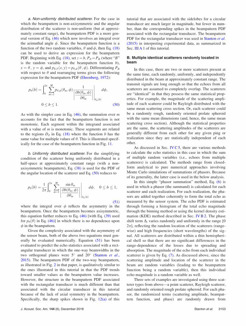
a. Non-uniformly distributed scatterer. For the case in
which the beampattern is non-axisymmetric and the angular
distribution of the scatterer is non-uniform (but at approxi-
mately constant range), the beampattern PDF is a more gen-
eral version of Eq. (46) which now involves an integral over
the azimuthal angle /: Since the beampattern function is a
function of the two random variables, h and /, then Eq. (18)
can be used to derive an expression for the beampattern
PDF. Beginning with Eq. (18), set z¼ b, PZ¼PB (where “B”
is the random variable for the beampattern function b),
x ¼ h ; y ¼ /, and pX;Yðx; yÞ¼ ph;/ðh ;/Þ. Differentiating PB
with respect to h and rearranging terms gives the following
expression for the beampattern PDF (Ehrenberg, 1972):
pb bð Þ ¼ð2p
0
XM
m¼1
ph;/ hm;/ð Þ 1����@b hm;/ð Þ@hm
���� jhm bð Þ
d/;
0� b� 1: (50)
As with the simpler case in Eq. (46), the summation over maccounts for the fact that the beampattern function is not
monotonic. Each segment within the integrand associated
with a value of m is monotonic. These segments are related
to the regions DZ in Eq. (18) where the function b has the
same value for multiple values of h. This is illustrated specif-
ically for the case of the beampattern function in Fig. 11.
b. Uniformly distributed scatterer. For the simplifying
condition of the scatterer being uniformly distributed in a
half-space at approximately constant range (with a non-
axisymmetric beampattern), Eq. (38) is used for the PDF of
the angular location of the scatterer and Eq. (50) reduces to
pb bð Þ ¼ 1
2p
ð2p
0
XM
m¼1
sin hm���� @b hm;/ð Þ@hm
���� jhm bð Þ
d/; 0 � b � 1;
(51)where the integral over / reflects the asymmetry in the
beampattern. Once the beampattern becomes axisymmetric,
this equation further reduces to Eq. (46) [with Eq. (39) used
for phðhÞ in Eq. (46)] in which there is no dependence upon
/ in the beampattern.
Given the complexity associated with the asymmetry of
the sensor beam, both of the above two equations must gen-
erally be evaluated numerically. Equation (51) has been
evaluated to predict the echo statistics associated with a rect-
angular transducer in which the one-way beamwidths in the
two orthogonal planes were 5� and 20� (Stanton et al.,2015). The beampattern PDF of the two-way beampattern,
as illustrated in Fig. 2 in that paper, is qualitatively similar to
the ones illustrated in this tutorial in that the PDF trends
toward smaller values as the beampattern value increases.
However, the structure in the beampattern PDF associated
with the rectangular transducer is much different than that
associated with the circular transducer in this tutorial
because of the lack of axial symmetry in the beampattern.
Specifically, the sharp spikes shown in Fig. 12(a) of this
tutorial that are associated with the sidelobes for a circular
transducer are much larger in magnitude, but fewer in num-
ber, than the corresponding spikes in the beampattern PDF
associated with the rectangular transducer. The beampattern
PDF for the rectangular transducer was used in Stanton et al.(2015) in interpreting experimental data, as summarized in
Sec. III A 1 of this tutorial.
B. Multiple identical scatterers randomly located inbeam
In this case, there are two or more scatterers present at
the same time, each randomly, uniformly, and independently
distributed in the beam at approximately constant range. The
transmit signals are long enough so that the echoes from all
scatterers are assumed to completely overlap. The scatterers
are “identical” in that they possess the same statistical prop-
erties. For example, the magnitude of the scattering ampli-
tude of each scatterer could be Rayleigh distributed with the
same mean scattering cross section. Or, each scatterer could
be a randomly rough, randomly oriented prolate spheroid
with the same mean dimensions (and, hence, the same mean
scattering cross section). Although the statistical properties
are the same, the scattering amplitudes of the scatterers are
generally different from each other for any given ping or
realization since they are statistically independent of each
other.
As discussed in Sec. IV C 5, there are various methods
to calculate the echo statistics in this case in which the sum
of multiple random variables (i.e., echoes from multiple
scatterers) is calculated. The methods range from closed-
form analytical to pure numerical approaches involving
Monte Carlo simulations of summations of phasors. Because
of its generality, the latter case is used in the below analysis.
In this simple “phasor summation” method, Eq. (6) is
used in which a phasor (the summand) is calculated for each
scatterer and each realization. For each realization, the pha-
sors are added together coherently to form the total echo as
measured by the sensor system. The echo PDF is estimated
through forming a histogram of the total echo magnitude
through the binning method or using the kernel density esti-
mation (KDE) method described in Sec. IV B 2. The phase
shift term Di varies randomly and uniformly in the range [0
2p], reflecting the random location of the scatterers (range-
wise) and high frequencies (short wavelengths) of the sig-
nal. All scatterers are distributed within a thin hemispheri-
cal shell so that there are no significant differences in the
range-dependence of the losses due to spreading and
absorption. The magnitude of the echo from each individual
scatterer is given by Eq. (7). As discussed above, since the
scattering amplitude and location of the scatterer in the
beam are random variables (leading to the beampattern
function being a random variable), then this individual
echo magnitude is a random variable as well.
Three sets of examples are investigated using three scat-
terer types from above—a point scatterer, Rayleigh scatterer,
and randomly oriented rough prolate spheroid. For each pha-
sor, the randomized terms (scattering amplitude, beampat-
tern function, and phase) are randomly drawn from
J. Acoust. Soc. Am. 144 (6), December 2018 Stanton et al. 3153
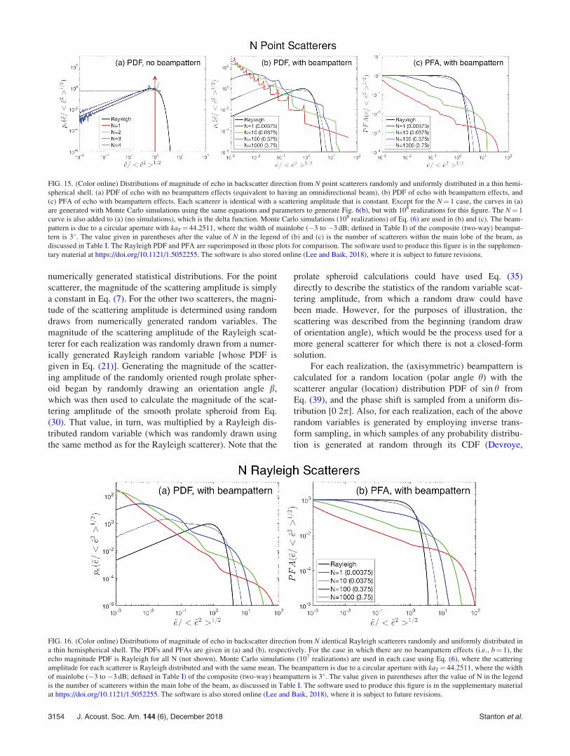
numerically generated statistical distributions. For the point
scatterer, the magnitude of the scattering amplitude is simply
a constant in Eq. (7). For the other two scatterers, the magni-
tude of the scattering amplitude is determined using random
draws from numerically generated random variables. The
magnitude of the scattering amplitude of the Rayleigh scat-
terer for each realization was randomly drawn from a numer-
ically generated Rayleigh random variable [whose PDF is
given in Eq. (21)]. Generating the magnitude of the scatter-
ing amplitude of the randomly oriented rough prolate spher-
oid began by randomly drawing an orientation angle b,
which was then used to calculate the magnitude of the scat-
tering amplitude of the smooth prolate spheroid from Eq.
(30). That value, in turn, was multiplied by a Rayleigh dis-
tributed random variable (which was randomly drawn using
the same method as for the Rayleigh scatterer). Note that the
prolate spheroid calculations could have used Eq. (35)
directly to describe the statistics of the random variable scat-
tering amplitude, from which a random draw could have
been made. However, for the purposes of illustration, the
scattering was described from the beginning (random draw
of orientation angle), which would be the process used for a
more general scatterer for which there is not a closed-form
solution.
For each realization, the (axisymmetric) beampattern is
calculated for a random location (polar angle h) with the
scatterer angular (location) distribution PDF of sin h from
Eq. (39), and the phase shift is sampled from a uniform dis-
tribution [0 2p]. Also, for each realization, each of the above
random variables is generated by employing inverse trans-
form sampling, in which samples of any probability distribu-
tion is generated at random through its CDF (Devroye,
FIG. 15. (Color online) Distributions of magnitude of echo in backscatter direction from N point scatterers randomly and uniformly distributed in a thin hemi-
spherical shell. (a) PDF of echo with no beampattern effects (equivalent to having an omnidirectional beam), (b) PDF of echo with beampattern effects, and
(c) PFA of echo with beampattern effects. Each scatterer is identical with a scattering amplitude that is constant. Except for the N¼ 1 case, the curves in (a)
are generated with Monte Carlo simulations using the same equations and parameters to generate Fig. 6(b), but with 108 realizations for this figure. The N¼ 1
curve is also added to (a) (no simulations), which is the delta function. Monte Carlo simulations (108 realizations) of Eq. (6) are used in (b) and (c). The beam-
pattern is due to a circular aperture with kaT¼ 44.2511, where the width of mainlobe (�3 to �3 dB; defined in Table I) of the composite (two-way) beampat-
tern is 3�. The value given in parentheses after the value of N in the legend of (b) and (c) is the number of scatterers within the main lobe of the beam, as
discussed in Table I. The Rayleigh PDF and PFA are superimposed in those plots for comparison. The software used to produce this figure is in the supplemen-
tary material at https://doi.org/10.1121/1.5052255. The software is also stored online (Lee and Baik, 2018), where it is subject to future revisions.
FIG. 16. (Color online) Distributions of magnitude of echo in backscatter direction from N identical Rayleigh scatterers randomly and uniformly distributed in
a thin hemispherical shell. The PDFs and PFAs are given in (a) and (b), respectively. For the case in which there are no beampattern effects (i.e., b¼ 1), the
echo magnitude PDF is Rayleigh for all N (not shown). Monte Carlo simulations (107 realizations) are used in each case using Eq. (6), where the scattering
amplitude for each scatterer is Rayleigh distributed and with the same mean. The beampattern is due to a circular aperture with kaT¼ 44.2511, where the width
of mainlobe (�3 to �3 dB; defined in Table I) of the composite (two-way) beampattern is 3�. The value given in parentheses after the value of N in the legend
is the number of scatterers within the main lobe of the beam, as discussed in Table I. The software used to produce this figure is in the supplementary material
at https://doi.org/10.1121/1.5052255. The software is also stored online (Lee and Baik, 2018), where it is subject to future revisions.
3154 J. Acoust. Soc. Am. 144 (6), December 2018 Stanton et al.

1986). Using these terms, the summand in Eq. (6) is calcu-
lated and summed over the N scatterers for each realization.
The process is repeated for millions of realizations (typically
107) and a histogram is formed representing the statistics of
the magnitude of the echo as received by the sensor system.
In each example, the echo PDFs are shown to vary sig-
nificantly with type and number of scatterers (Figs. 15–17).
As with the case of a single scatterer in the beam, the PDF is
significantly different than when beampattern effects are not
accounted for. As expected, as the number of scatterers
increases, the PDFs approach the Rayleigh PDF. In general,
for a small number of scatterers, the echo PDF deviates sig-
nificantly from the Rayleigh PDF, both in the small and large
echo magnitude regions of the PDF. Echo PFAs are also
illustrated, which also show significant dependences upon
type and number of scatterer. The degree to which the PDF
deviates from a Rayleigh PDF also varies with beamwidth
(Fig. 18). For a fixed number of scatterers, the narrower the
beam, the greater the deviation from a Rayleigh PDF. Note
that the “noisy” characteristic in portions of some of the
plots of PDF in Figs. 15–18 is due to the relatively low num-
ber of realizations in the Monte Carlo simulations that were
FIG. 17. (Color online) Distributions of magnitude of echo in backscatter direction from N randomly rough, randomly oriented prolate spheroids randomly
and uniformly distributed in a thin hemispherical shell. (a) PDF of echo with no beampattern effects (i.e., omnidirectional beam); (b) PDF of echo with beam-
pattern effects; (c) PFA of echo with beampattern effects. This geometry is fully 3D as the spheroids are distributed within the hemispherical shell and the
spheroid orientation varies randomly and uniformly in two planes of rotation of the spheroid. This is in contrast to Fig. 14 where the spheroid orientation fol-
lows a 2D distribution (spheroid distributed within thin arc and rotating in only one plane of rotation). The scatterers are identical in size and shape (10:1
aspect ratio), although statistically independent of each other. Monte Carlo simulations (107 realizations) are used in each case using Eq. (6), where the scatter-
ing amplitude for each scatterer is the product of Eq. (30) (smooth spheroid) and a Rayleigh distributed random variable (to simulate roughness effects). The
beampattern is due to a circular aperture with kaT¼ 44.2511, where the width of mainlobe (�3 to �3 dB; defined in Table I) of the composite (two-way) beam-
pattern is 3�. The beampattern b in Eq. (7) is set equal to unity in (a). The value given in parentheses after the value of N in the legend in (b) and (c) is the num-
ber of scatterers within the main lobe of the beam, as discussed in Table I. The software used to produce this figure is in the supplementary material at https://
doi.org/10.1121/1.5052255. The software is also stored online (Lee and Baik, 2018), where it is subject to future revisions.
FIG. 18. (Color online) PDF of magnitude of echo from 100 identical
Rayleigh scatterers that are randomly and uniformly distributed in thin
hemispherical shell. The beamwidth (�3 to �3 dB; defined in Table I) of
the composite (two-way) beampattern is varied from 1� to 20�. The beam-
pattern is due to a circular aperture. Monte Carlo simulations (107 realiza-
tions) are used in each case using Eq. (6), where the scattering amplitude
for each scatterer is Rayleigh distributed and with the same mean. The
numbers of scatterers within the main lobe for the different directional
beams are given in parentheses next to the corresponding beamwidth in
the legend. Those numbers, as well as the respective values of kaT, are
summarized in Table I. The software used to produce this figure is in the
supplementary material at https://doi.org/10.1121/1.5052255. The soft-
ware is also stored online (Lee and Baik, 2018), where it is subject to
future revisions.
TABLE I. Average number of scatterers within the entire main lobe of a cir-
cular transducer (i.e., within solid angle defined by the first null of the beam-
pattern) for various beamwidths and various total number of scatterers, N, in
the half space. The beampattern b (¼ bTbr) is the composite two-way beam-
pattern determined by the product of the transmit (bT) and receive (br) beam-
pattern as given in Eq. (41). The beamwidth (2h0) is the full width of the
beampattern between the �3 dB (half-power) points where b(h0)¼ 1/ffiffiffi2p
.
The parameters in this table correspond to various figures within this paper.
Beamwidth
(�3 to �3 dB) (deg.) kaT N (half space)
Average number
within mainlobe
1 132.74 100 0.0417
3 44.2511 1 0.00375
3 44.2511 10 0.0375
3 44.2511 25 0.0937
3 44.2511 100 0.375
3 44.2511 250 0.937
3 44.2511 1000 3.75
3 44.2511 2500 9.37
10 13.2907 100 4.13
20 6.6707 100 16.0
J. Acoust. Soc. Am. 144 (6), December 2018 Stanton et al. 3155

within those particular log-spaced magnitude bins (i.e., when
both pe and ~e=h~e2i1=2are low).
It is important to emphasize that the number of scatter-
ers N is distributed uniformly in a thin hemispherical shell in
a half-space. For a narrow beamwidth, the mainlobe occu-
pies just a small fraction of that half-space. Since the main-
lobe weights the echoes from the individual scatterers much
more than the sidelobes, the scatterers within the mainlobe
will generally contribute the most to the signal. In essence,
the signal will be dominated by the effective number of scat-
terers—those that are within the mainlobe. The average
number of scatterers within the mainlobe is indicated in
parentheses after the value of N in the legends to these and
later figures and are also given in Table I.
The echo statistics vary with beamwidth even though N is
constant because the effective number of scatterers varies with
beamwidth—that is, for fixed N, the number of scatterers
within the mainlobe that contributes to the higher values of the
scattering decreases with decreasing beamwidth (Fig. 18). For
example, for N¼ 100, the number of scatterers within a 1�-wide mainlobe is, on average, equal to 0.0417 (Table I). Before
beampattern effects are included, the sum of 100 independent,
random phase signals would be very close to Rayleigh distrib-
uted (Fig. 6). However, with such a narrow beam with only a
small fraction of the 100 scatterers within the mainlobe, the
resultant echo PDF will be strongly non-Rayleigh.
C. Multiple scatterers of different types and sizes
Once there is more than one type or size of scatterer present,
the echo PDF will not only depend upon the type and number of
scatterers, and sensor beamwidth, as in the above examples in
Sec. VII B which involved one type of scatterer at a time, but
will also depend upon the variability of values of mean scattering
cross section and variability of numbers of scatterers across the
different types of scatterers. Furthermore, the echo PDF will
depend upon the differences in spatial distributions of the differ-
ent types of scatterers. For example, consider two distinct cases:
(1) a split aggregation in which scatterers of only one type reside
in “monotype” patches and each echo contains contributions
from only one type of scatterer and (2) an interspersed aggrega-tion in which the different types of scatterers are uniformly
interspersed with each other so that each echo contains contribu-
tions from all of the types of scatterers (Fig. 19). In each case,
the beam is much narrower than both the patch and analysis win-
dow containing the scatterers and the echoes from many pings
or independent realizations are observed within each window
(Fig. 19). The echo statistics will generally be significantly dif-
ferent for the two distributions, even when the same set of scat-
terers of varying types are involved in each distribution (Lee and
Stanton, 2014). And, for each type of distribution, the echo PDF
will vary as the number and mean scattering cross section of
each scatterer type are varied.
Below, the echo PDF is formulated for each type of spa-
tial distribution—first for cases involving two types of scat-
terers, then generalizing to an arbitrary number of scatterer
types. For the split aggregation, a mixture PDF (to be defined
below) involving separate phasor summations for the mono-
type patches is used and, for the interspersed aggregation,
the phasor summation method is used to form the echo PDF
from the echoes from all types of scatterers within the analy-
sis window. Examples of echo PDFs from each type of dis-
tribution are given in Sec. VII C 3 for the simple case
involving two different sizes of scatterers, “weak” (type A)
and “strong” (type B), for a range of numbers and sizes of
scatterers. Both types of scatterers are Rayleigh scatterers,
but with different mean scattering cross sections.
1. Split aggregation of type A and Bscatterers—mixture PDF
Formulating the echo PDF for the split aggregation geom-
etry [Fig. 19(a)] for two types of scatterers is intuitive and is
done in two steps. First, the echo PDF is determined for each
homogeneous patch of identical scatterers—the type A and
type B patches. As discussed in Secs. IV C 5 and VII B, the
PDF can be determined for each patch using a variety of meth-
ods, including the phasor summation method which uses Eqs.
(6) and (7) for each patch separately. The patches are analyzed
separately since the echoes from the different types of scatter-
ers do not overlap in this case. Since the echo PDF from the
sensor system scanning all scatterers is based on echoes accu-
mulated from both patches, the echo PDF from the analysis
window is simply the weighted sum of the PDFs from the two
patches, which is known as a two-component “mixture” PDF,
peð~eÞ ¼ wApðAÞe ð~eÞ þ wBpðBÞe ð~eÞðmixture PDF; split aggregationÞ: (52)
Here, the weighting factors wA and wB represent the frac-
tional volume occupied by the type A and type B scatterers,
respectively. For example, if the patch of type A scatterers
occupies 60% of the analysis window and the patch of type
B scatterer occupies 40% of the window, then wA¼ 0.6 and
wB¼ 0.4. Since, by definition, the two patches collectively
occupy 100% of the analysis window, then wAþwB¼ 1 and
Eq. (52) can be simplified,
peð~eÞ ¼ wApðAÞe ð~eÞ þ ð1� wAÞpðBÞe ð~eÞðmixture PDF; split aggregationÞ: (53)
FIG. 19. Analysis windows involving two different spatial arrangements for
aggregations composed of more than one type of scatterer. (a) Split aggregation
where scatterers of different types are separated into their own sub-regions. (b)
Interspersed aggregation where scatterers of different types are uniformly inter-
spersed throughout the window. In each case, the resolution cell of the sensor
system is much smaller than the analysis window and, in case (a), it is also
much smaller than each sub-region. From Lee and Stanton (2014).
3156 J. Acoust. Soc. Am. 144 (6), December 2018 Stanton et al.

2. Interspersed aggregation of type A and Bscatterers—coherent phasor sum
In contrast to the above case of a split aggregation, the
echoes from the two types of scatterers in the interspersed
aggregation overlap with each other [Fig. 19(b)]. Predictions
of the echo PDF in this geometry therefore begins with a
coherent phasor summation involving both types of scatter-
ers. Calculating the echo statistics using the phasor sum
method is done the same way as described in Sec. VII B, but
by first rewriting Eqs. (6) and (7),
~e ¼����XN
i¼1
~eiAejDiA þXM
i¼1
~eiBejDiB
����ðphasor summation; interspersed aggregationÞ:
(54)
where the magnitude of the echo voltage from the ith scat-
terer of the kth type as received through the sensor system is
~eik ¼ jf ðikÞbs jbðhik; /ikÞ (55)
and Dik and ðhik; /ikÞ are the phase and angular locations of the
ith scatterer of the kth type, respectively. There are N and Mtype A and B scatterers, respectively. The term k corresponds to
type A or type B scatterer in this example. Once ~e is calculated
from Eq. (54) for many realizations, the echo PDF is formed.
3. Comparisons between echo PDFs from split andinterspersed two-type aggregations
Echo PDFs are calculated using Monte Carlo simulations
of Eq. (6) as described above for a range of parameters for
both the split and interspersed aggregations involving two
types of scatterers. Both types of scatterers are Rayleigh scat-
terers, but with two different mean scattering cross sections
denoted by “weak” (smaller mean scattering cross section)
and “strong” (larger mean scattering cross section). The dif-
ference of average scattering levels could be achieved through
either a difference in boundary conditions (a weak scatterer
with small contrast in material properties relative to surround-
ing medium and a strong scatterer with large contrast) or a
difference in size (a weak scatterer being smaller than a strong
scatterer). The ratio of rms magnitude of the scattering ampli-
tudes of the strong (“S”) to weak (“W”) scatterers is given by
rSW ¼kS
kW; (56)
where k is the rms magnitude of the scattering amplitude of
the denoted scatterer type [this notation is chosen to be con-
sistent with that of Lee and Stanton (2014) and is not to be
confused with kR of Eqs. (21)–(23) of this tutorial].
With the number of weak scatterers fixed at 2500, the num-
ber of strong scatterers is varied over the range 25–2500 for two
values of rSW (5 and 20). The resultant echo PDFs are shown to
vary in shape over all combinations of these parameters (Figs.
20 and 21). All PDFs deviate significantly from the Rayleigh
PDF. In each example, the tail of the PDF is elevated above the
Rayleigh PDF. The degree to which the tail is elevated is espe-
cially pronounced for the larger ratio of strong-to-weak scatter-
ing amplitude (rSW ¼ 20) in both types of aggregations and for
the cases involving fewer numbers of strong scatterers in the
interspersed aggregations. This is consistent with the intuition
that the strong scatterers dominate the echo and can cause the
echo to be non-Rayleigh when they are small in number. Also,
very importantly, the PDFs with the same parameters, but differ-
ent spatial distribution (split- and interspersed aggregation), are
significantly different from each other. Note that, as with some
of the previous simulations, the “noisy” characteristic in portions
of some of the plots of PDF in Figs. 20 and 21 are due to the rel-
atively low number of realizations in the Monte Carlo simula-
tions that were within those particular log-spaced magnitude
bins (i.e., when both pe and ~e=h~e2i1=2are low).
With the many model parameters in these formulations, it is
relatively easy to obtain a good fit to experimental data, even
when using the “wrong” theoretical PDF (“wrong” in that the
assumptions in the derivation of the theoretical PDF do not
match the physical scenario). This was explored in Lee and
Stanton (2014) where echoes from both split- and interspersed
aggregations were simulated numerically. While allowing all
parameters to vary freely, theoretical PDFs for each type of
aggregation were then “fit” to simulations from both the corre-
sponding appropriate aggregation and the other aggregation.
Excellent fits were obtained in most cases (i.e., for both the
“right” and “wrong” aggregations). For example, a mixture
model could not only be successfully fit to echoes from a split
aggregation (for which the mixture model is derived), but also
could be “successfully” fit to an interspersed aggregation (which
it was not derived for). However, when the theoretical PDF was
fit to the wrong aggregation, the inferred parameters (that is, the
ones required to obtain a good fit) were up to an order of magni-
tude in error [see Table I and Figs. 6 and 7 of Lee and Stanton
(2014)]. The conclusion was that for accurate inference of model
parameters from data, it is essential to model the spatial distribu-
tion of the scatterers appropriately, taking into account whether
or not they are split or interspersed.
4. Many types of scatterers (general formulations)
The above simple cases involving two types of scatter-
ers can easily be extended to the general case of K types of
scatterers (where K is an integer, not to be confused with the
K PDF). For the case in which each type of scatterer is parti-
tioned separately in its own patch within the analysis win-
dow, the echo PDF from the entire analysis window is
calculated using the following K-component mixture PDF:
peð~eÞ ¼XK
k¼1
wkpðkÞe ð~eÞ
ðmixture PDF; K types partitionedÞ: (57)
where pðkÞe ð~eÞ is the echo PDF of the patch associated with
the kth type of scatterer, wk is the weighting factor for the
kth patch, andPK
k¼1 wk ¼ 1.
For the case in which all types of scatterers are ran-
domly and uniformly interspersed within the analysis win-
dow, the phasor sum for a single realization of echo is
J. Acoust. Soc. Am. 144 (6), December 2018 Stanton et al. 3157

~e ¼����XK
k¼1
XNðkÞi¼1
~eikejDik
����ðphasor summation; K types interspersedÞ; (58)
where ~eik is given in Eq. (55) and N(k) is the number of scat-
terers of the kth type. The echo is calculated for a large
ensemble of independent realizations to form the echo PDF
of the analysis window for the interspersed aggregation.
FIG. 20. (Color online) PDF of echo magnitude from multiple Rayleigh scatterers in a split aggregation in which the larger scatterers are separated from the
smaller scatterers as illustrated in Fig. 19(a). The arrow in the lower right panel indicates an inflection in the PDF associated with having two types of scatter-
ers. The beampattern is due to a circular aperture with kaT¼ 44.2511, where the width of mainlobe (�3 to �3 dB; defined in Table I) of the composite (two-
way) beampattern is 3�. The number of strong and weak scatterers, NS and NW, respectively, randomly and uniformly distributed in a thin hemispherical shell
are given. Monte Carlo simulations (107 realizations) are used in each case using Eq. (6), where the scattering amplitude for each scatterer is Rayleigh distrib-
uted, but with different means, as indicated by the value of rSW. The volume within which the strong scatterers occupy is 5% of the total volume (that is,
wA¼ 0.05 in Eq. (53), where “A” and “B” denote the patches of strong and weak scatterers, respectively). The value given in parentheses after each value of
NS and NW is the corresponding number of strong and weak scatterers within the main lobe of the beam, as discussed in Table I. The software used to produce
this figure is in the supplementary material at https://doi.org/10.1121/1.5052255. The software is also stored online (Lee and Baik, 2018), where it is subject to
future revisions.
3158 J. Acoust. Soc. Am. 144 (6), December 2018 Stanton et al.

Finally, the above two equations can be used in concert to
describe more complex cases such as when multiple patches of
both monotype and interspersed aggregations are present.
VIII. SYSTEMS AND ENVIRONMENTS WITH MORECOMPLEXITY
All of the above involved relatively simple scenarios—
single-frequency signals that are long enough so that echoes
from all scatterers completely overlapped and direct path
geometries in which the medium is homogeneous and there
is no interference from neighboring boundaries. While the
results from these scenarios sufficiently approximate a wide
range of applications, there are factors in other applications
that sometimes must be accounted for in accurately predict-
ing echo statistics. For example, signals in sensor systems
are generally pulsed and the environments may be
FIG. 21. (Color online) PDF of echo magnitude from multiple Rayleigh scatterers in an interspersed aggregation in which both the larger and smaller scatter-
ers are uniformly and randomly interspersed throughout the analysis window as illustrated in Fig. 19(b). The inflections in these PDFs are less pronounced in
this type of aggregation than in the split aggregations as noted by the arrow in Fig. 20. As with Fig. 20, Monte Carlo simulations (107 realizations) are used in
each case using Eq. (6), where the scattering amplitude for each scatterer is Rayleigh distributed, but with different means, as indicated by the value of rSW.
All modeling parameters are the same as in Fig. 20 (except for wA, which is specific to a split aggregation) and are described in the caption to that figure. Each
type of scatterer occupies 100% of the volume with this case of interspersed aggregations. The software used to produce this figure is in the supplementary
material at https://doi.org/10.1121/1.5052255. The software is also stored online (Lee and Baik, 2018), where it is subject to future revisions.
J. Acoust. Soc. Am. 144 (6), December 2018 Stanton et al. 3159

heterogeneous and have boundaries. When pulsed signals
are used, echoes from individual scatterers will generally
partially overlap, or not overlap at all. The presence of a sin-
gle boundary near a scatterer will be an added source of
interference, and the presence of two parallel boundaries
and/or heterogeneities will not only cause more interference,
but also possibly waveguide effects.
The effects from these realistic conditions are described
below as well as recommendations for physics-based predic-
tions of the echo statistics.
A. Pulsed signals (partially overlapping echoes)
Once the signals are pulsed instead of continuous wave, the
echoes from individual scatterers in an aggregation may only
partially overlap or not overlap at all which can significantly
affect the echo statistics (Figs. 22 and 23). This effect, in
essence, translates to fewer effective scatterers in the main-
lobe of the beam, which will tend to make the statistics of
the pulsed signal more non-Rayleigh. Generally, the shorter
the signal, the fewer the effective scatterers and, hence, the
more non-Rayleigh the echo becomes. The signal can be
shortened either by reducing the gate duration of the signal,
or by increasing the bandwidth of the signal and applying
matched filter processing as described below.
The bandwidth of a pulsed signal emitted by a system is
inherently finite (i.e., non-zero bandwidth). The bandwidth
can be exploited to further reduce the signal duration through
signal processing such as matched filter processing where
the received echo is cross correlated with a replica signal
such as the transmitter waveform. This processing, which is
sometimes referred to as “pulse-compression” processing,
can shorten the duration of the processed echo down to the
FIG. 22. Modeling considerations and processing flow for echo statistics
associated with pulsed broadband signals. (a) Beamwidth that varies with
frequency within a broadband signal is illustrated as well as partially over-
lapping echoes due to short signal. (b) Flow diagram illustrating system
effects incorporated into echo statistics model. The echo time series shown
in the right of (a) and (b) is the envelope of the pulse-compressed signal
from match filter processing, which greatly increases temporal (range) reso-
lution and increases the probability that the echoes will only partially over-
lap. The circled “*” and “�” symbols represent the convolution and cross
correlation operations, respectively. From Lee and Stanton (2015), where
terms in the illustration specific to that paper, are described.
FIG. 23. (Color online) Comparisons between the PDFs of the echo magnitudes associated with long narrowband and short pulsed broadband signals with three
cases of multiple scatterers. The broadband signal has an octave bandwidth centered about the frequency of the narrowband signal. The spectrum of the broad-
band signal has a constant value within the band and is equal to zero outside the band. The N Rayleigh scatterers are identical with the same mean and are ran-
domly and uniformly distributed in a thin hemispherical shell. The narrowband signals are long enough so that the echoes completely overlap while, in contrast,
there is generally only partial overlap between the echoes from the short broadband signals. The echo from the broadband signal is temporally compressed
through matched filter processing so that its duration is approximately equal to the inverse of the bandwidth of the signal. Predictions for both the narrowband
and broadband cases involve Monte Carlo simulations (106 realizations) in the time domain as illustrated in Fig. 22 and given in detail in Lee and Stanton (2015).
In the simulations, the scattering amplitude of each scatterer (via Rayleigh PDF), time of return, and location in the beampattern are randomized. The beampattern
is due to a circular aperture with kaT¼ 44.2511 at the narrowband frequency and the center frequency of the broadband signal. The width of the mainlobe (�3 to
�3 dB; defined in Table I) of the composite (two-way) beampattern is 3.0� for kaT¼ 44.2511. The value given in parentheses after the value of N is the number
of scatterers within the main lobe of the 3.0� beam, as discussed in Table I. The width of the main lobe across all frequencies of the broadband signal varies from
2.1� to 4.2�. Note that these curves are qualitatively similar to the octave-band simulations in Fig. 3(b) of Lee and Stanton (2015) where the spectrum of the
broadband signal is non-uniform due to the non-uniform transducer response. The software used to produce this figure is in the supplementary material at https://
doi.org/10.1121/1.5052255. The software is also stored online (Lee and Baik, 2018), where it is subject to future revisions.
3160 J. Acoust. Soc. Am. 144 (6), December 2018 Stanton et al.

limit of the inverse bandwidth (Turin, 1960). In the common
case in which the transmitter waveform is used as a replica,
the cross-correlation between that signal and the echo (which
contains the response of the system and scatterer) normally
deviates from the autocorrelation function of the replica and
that theoretical limit is never fully achieved. Either way,
whether an ideal or practical waveform is used as a replica,
generally the broader the bandwidth, the shorter the proc-
essed echo and, correspondingly, the finer the along-range
resolution of the system becomes.
Because of the improvement in resolution of the com-
pressed pulse, there will generally be even fewer scatterers in
an aggregation contributing to a given (processed) echo than
in the original pulsed signal which, in turn, can further
increase the degree to which the echo is non-Rayleigh. This
effect is particularly relevant to operational systems, as band-
width is commonly increased in order to improve image reso-
lution and signal-to-noise ratio (Gillman, 1997; Abraham and
Lyons, 2002a,b; and Lee and Stanton, 2015).
Predicting the echo PDF for pulsed systems is complex.
Generally, the system response is nonuniform across the fre-
quency band, the transmitted signal is shaped in time and
further modulated by the system response, and the echoes
from the individual scatterers will only partially overlap, if
at all. And, as indicated above, the broader the bandwidth,
the less the echoes from the scatterers will overlap after
pulse-compression processing, adding to the challenge of
modeling the echo PDF.
Because of the complexity, treating the problem
through a numerical, rather than analytical, approach may
be best. In a recent study by Lee and Stanton (2015), a
broadband pulsed system was simulated (Fig. 22).
Parameters of the simulations were based on a known com-
mercial system. The bandwidth of the system was roughly
one octave (i.e., the upper frequency was approximately
twice the lower frequency) and the system response was
nonuniform (varying by more than 10 dB across the band).
The transmission signal was linear frequency modulated (a
“chirp”) across the band and the echoes were processed
with matched filter processing, using the signal applied to
the transmitter transducer as the replica. Key to the simula-
tions was numerically convolving the applied signal with
the system response (including frequency dependence of
transducer and frequency dependence of beampattern), con-
volving the resultant outgoing signal with the scatterer
response, and delaying the echo from each randomized scat-
terer by a time that was randomized. The envelope of the
matched filtered echo was sampled in the middle of the sam-
ple window (Fig. 22). The envelope was calculated using a
Hilbert transform. The results of those simulations are illus-
trated in Figs. 2–5 of Lee and Stanton (2015) where direct
comparisons are made between narrowband and broadband
effects (Rayleigh scatterers), Rayleigh scatterers and ran-
domly oriented rough prolate spheroids (broadband), and
monotype and mixed assemblages of different types of scat-
terers (broadband).
In this tutorial, some of the simulations in Lee and
Stanton (2015) are reproduced, but with the simplification of
replacing the signal and system response that was specific to
a particular commercial system with a simple octave-
bandwidth signal whose spectrum is uniform over the band.
A different set of number of scatterers is also used. The echo
PDFs illustrated in Fig. 23 of this tutorial are qualitatively
similar to those predicted in Fig. 3(b) in Lee and Stanton
(2015). Note that, as with some of the previous simulations,
the “noisy” characteristic in portions of some of the plots of
PDF in this figure are due to the relatively low number of
realizations in the Monte Carlo simulations that were within
those particular log-spaced magnitude bins (i.e., when both
pe and ~e=h~e2i1=2are low).
The results of both sets of simulations in Lee and
Stanton (2015) and this tutorial show that for any given set of
parameters, the echo PDF of the broadband pulsed signal
(after pulse-compression processing) deviates much more
from the Rayleigh PDF than the corresponding PDF associ-
ated with a long single-frequency signal whose frequency is
at the center of the spectrum of the broadband signal. This
increase in the non-Rayleigh nature of the pulsed signal is
due to the fact that the echoes are generally only partially
overlapping or not overlapping, which reduces the number of
effective scatterers whose echoes interfere with each other.
It is important to note that the echo was sampled in both
sets of simulations at a single fixed point since this is an
analysis involving first-order statistics, which is the focus of
this tutorial. The analysis presented in this tutorial for Fig.
23 maintains generality and is not specific to any particular
system or signal processing algorithm. For systems that
involve a sampling method more advanced than sampling a
single point, such as sampling a peak value within a sample
window, the results in this tutorial can serve as a basis for
modeling those methods, as discussed in Sec. V B.
B. Object near a rough boundary
When the scatterer of interest is close enough to a
boundary so that echoes from the object overlap with echoes
from the boundary, there will be interference between the
two sets of echoes. In addition, there will be signals (and
associated interference) involving secondary or “rescattered”
FIG. 24. Object near a rough boundary. The direction of propagation of the
incident signal is at a shallow grazing angle relative to the boundary.
Primary (1) and secondary (2) echoes are illustrated.
J. Acoust. Soc. Am. 144 (6), December 2018 Stanton et al. 3161

echoes following paths such as transmitter-boundary-scat-
terer-receiver and transmitter-scatterer-boundary-receiver
(Fig. 24) (Williams et al., 2010). Although some of the sig-
nal energy may be refracted into the boundary (for a penetra-
ble boundary), these secondary echoes can be of comparable
magnitude as the primary echoes that are directly from the
scatterer. Accounting for these effects is specific to the par-
ticular geometry. One simple model is given below involv-
ing a single scatterer near a rough boundary with more
complex solutions discussed.
The below treatment describes a simple model of the
scattering involving use of rays. The statistics can be mod-
eled by using an approximate ray-based method in which
components of the echo are rays either involving scattering
by the object (including object-boundary interaction) or by
the boundary alone (not involving the object). The ray-based
method is very intuitive and can lead to reasonable results over
a wide range of important conditions. However, in general, the
scattering in this complex geometry must be treated formally
through various approaches involving solutions to the wave
equation (Lim et al., 2000; Zampolli et al., 2008; Williams
et al., 2010). In those cases, the statistics can be formed
through Monte Carlo simulations of the formal solutions.
One important geometry involves shallow grazing angles
in which the incident signal is propagating in a direction
nearly parallel to a rough boundary and the echo from the
scatterer is comparable to or greater than that of the backscat-
tered echo from the rough boundary (Fig. 24). The echo
involving the object is the “signal” echo (i.e., echo of interest)
and the boundary-alone echo is the “background” or noise-
like echo. The magnitude of the total echo involves the coher-
ent sum of the echoes from both the object and boundary,
~e ¼����XN
i¼1
~eiejDi þ BejD
����; (59)
where N is the number of rays that either involve a direct
echo from the object or an echo involving interaction
between the object and boundary. The terms ~ei and Di are
the magnitude and phase shift, respectively, of the ith ray
associated with the object. The terms B and D are the magni-
tude and phase shift, respectively, of the echo from the
boundary only. Both ~ei and B depend upon the beampattern.
The term ~ei is given by Eq. (7) (except that it represents the
ith ray rather than the ith scatterer). The term B involves an
integral of the beampattern, at constant range, over the
boundary (Ogilvy, 1991).
All four of the terms in the right side of Eq. (59) are ran-
dom variables. Since B is associated with diffuse scattering by
the rough boundary, it is commonly assumed to be Rayleigh
distributed. However, there is no restriction on its distribution
and it could be, for example, K-distributed (Ferrara et al.,2011) or one that is derived based on the scattering physics.
For the very simple case of a point scatterer near a rough
boundary, an omnidirectional beam, no significant interac-
tions between the scatterer and boundary (N¼ 1), and a
Rayleigh distributed echo from the boundary, the statistics
of the echo magnitude in Eq. (59) can be described by the
Rice PDF given in Eq. (26). The generalized K PDF, which
is conceptually similar to the Rice in that it involves a ran-
dom signal with a preferred phase (such as due to the single
scatterer in the presence of background reverberation), may
also be used to approximate the echo statistics (Sec. VI A 3)
(Jakeman and Tough, 1987; Ferrara et al., 2011). For exam-
ple, the generalized K PDF has been successfully used in an
experimental study by Ferrara et al. (2011) to describe the
statistics of radar echoes from ships and oil rigs on the sea
surface (summary of their work in Sec. III A 2).
Beyond those simple scenarios with a closed-form solu-
tion such as the Rice and generalized K PDFs, the PDF of the
magnitude of the echo in Eq. (59) generally must be deter-
mined numerically using physics-based methods. For example,
once the directional characteristics of the beam are accounted
for and the scatterer is now of complex shape and is randomly
located in the beam, then the echo becomes a complex func-
tion of the sensor system and scatterer as described in Sec. VII
and the problem may not have a closed form solution. In that
case, the echoes from the rough boundary and scatterer are
each (separately) non-Rayleigh. For these more general scenar-
ios, the summation term in Eq. (59) can be determined through
the phasor summation method using a scattering model of the
rays associated with the object-boundary paths and the back-
ground term can be determined through a scattering model of
the boundary alone. The two terms can be summed coherently
for each realization, and an ensemble of realizations is calcu-
lated to form the echo PDF.
The method of characteristic functions, as described in
Sec. IV C 5, may also be useful, especially if one or both
terms in Eq. (59) has an assumed PDF. For example, it is
common to assume a known statistical function (such as the
Rayleigh or K PDF) for the echo from the boundary alone.
In this case, the PDF associated with the summation term in
Eq. (59) can still be determined using the phasor summation
method. Assuming that the two terms within the absolute
value sign in Eq. (59) are independent of each other and
have random phase, the problem is reduced to the sum of
two random complex independent variables whose individ-
ual PDFs (magnitude) are known.
C. Object(s) in a random waveguide
When a signal travels long enough distances, variability
in the environment can play a significant role in the
FIG. 25. Object in a waveguide. The signal propagates a long distance in the
waveguide due to any combination of interacting with the boundaries and
undulating about a minimum (when present) in wave speed. Although the
waveguide illustrated involves physical boundaries and wave speed mini-
mum, a similar scenario can occur without boundaries, but with the mini-
mum in wave speed remaining (and corresponding undulations) that “traps”
much of the signal energy within imaginary boundaries.
3162 J. Acoust. Soc. Am. 144 (6), December 2018 Stanton et al.

propagation. The presence of boundaries and heterogeneities
in the medium will redirect the signal through various reflec-
tion, refraction, and scattering processes. In the case involv-
ing two parallel planar boundaries of infinite extent, a
waveguide is formed, and a signal will naturally reflect
repeatedly within the two boundaries as it travels along the
length of the waveguide (Fig. 25). Under other conditions
and without the presence of boundaries, variations in the
medium can cause the signal to be “trapped” within an effec-tive waveguide. In this latter case, there would be a cross-
waveguide profile of wave speed that reaches a local mini-
mum and the signals will undulate about that minimum
through refraction (Snell’s Law) (Fig. 25). The space
between the imaginary boundaries within which the signal
undulates is also referred to as a waveguide. In some geome-
tries, the propagation in an effective waveguide is further
affected by the presence of one or more real boundaries and
there can be repeated interaction with at least one of the
boundaries every cycle of undulation (Fig. 25). Further com-
plicating the propagation in all of the above cases, random
variations of the surfaces (such as roughness) and of the
properties of the medium (such as wave speed) will tend to
randomize the phase of each ray. In general, in any wave-
guide, there are multiple rays due to multiple paths, and cor-
responding interference between the rays. Because of the
inherent randomness of the natural environment, this inter-
ference will vary, causing ping-to-ping fluctuations.
For the case in which one or more objects of interest are in
a waveguide (whether it involves real or imaginary boundaries),
description of the signals incident upon the object(s) and
receiver of the sensor system is quite complex. The signals will
generally be random variables due to the variable nature of the
waveguide that occurs naturally in the environment. There is a
vast literature on this topic concerning both acoustic and electro-
magnetic fields and, because of the complexity, will generally
require numerical modeling of both the random propagation and
scattering. For example, fluctuations of signals due these phe-
nomena, in general (any medium and type of field), are
described in Jakeman and Ridley (2006). Formulations specific
to sonar in the ocean and reviews of the literature are in Jones
et al. (2014) and Colosi (2016). Analyses specific to wave prop-
agation through the turbulent atmosphere (acoustics and electro-
magnetic) are given in Tatarski (1961). The modeling and
measurements of propagation and bistatic scattering of medical
ultrasound signals through tissue, treated as a continuous ran-
dom medium, are reviewed by Waag (1984).
1. Some simple formulations
Several simple examples adapted from Jones et al.(2014) are described below to illustrate some of the interfer-
ence phenomena associated with propagation and scattering
in a real or effective waveguide. For simplicity, all examples
are for long single-frequency signals (that is, echoes from all
scatterers completely overlap).
The one-way propagation of a signal through a “frozen”
waveguide due to a point source can be modeled through the
simple equation
SincðRÞ ¼ HðRÞSsource ðone–way propagationÞ; (60)
where SincðRÞ is the (complex) signal in the waveguide inci-
dent at a scatterer at a location R due to a source that is at the
origin (Fig. 25), HðRÞ is the transfer function of the waveguide
between the source and location R, and Ssource is the source
signal in the medium referenced to one meter from the source.
Here, the “signal” in the medium could be a pressure or elec-
tromagnetic wave associated with an acoustic or electromag-
netic sensor system, respectively. The term H is a function of
the waveguide properties which include spatial variability of
the wave speed and, when physical boundaries are present,
material properties of the boundaries relative to those of the
medium, and boundary roughness. Although generally the
properties of waveguides can change temporally, this wave-
guide is considered “frozen” for simplicity, in that any tempo-
ral changes are considered negligible during the time of two-
way propagation of the signal.
The transfer function can be written as the product of its
magnitude H0ðRÞ and an exponential term containing its
phase shift d,
HðRÞ ¼ H0ðRÞejd ðone–way waveguide responseÞ:(61)
For an arbitrary spatial distribution of N scatterers within the
waveguide at distances from the source much greater than
the thickness of the waveguide, the magnitude of the echo
received through two-way propagation due to a directional
sensor system is
~e ¼����XN
i¼1
H20ðRiÞjf ðiÞbs jbð/iÞejDi
����ðarbitrary distribution of scatterersÞ; (62)
where the thickness of the waveguide is defined as the separa-
tion between the boundaries or, in the case of an effective
waveguide with no physical boundaries, the amplitude of the
undulation of the signal. The source level from Eq. (60) has
been suppressed, as with all analyses earlier in this tutorial. In
this two-way propagation, the square of the one-way transfer
function is used due to the reciprocity of the waveguide. The
term b is the two-way composite beampattern due to the prod-
uct of the directivity of the co-located source and receiver. As
with Eq. (6), for simplicity in this formulation, all phase shifts
associated with the ith scatterer are in the term Di, which
includes those due to the two-way propagation of the signal,
the scatterer, and beamformer. For wavelengths of the acous-
tic/electromagnetic signal that are small compared with the
differences in the along-range distances between the scatter-
ers, Di will generally be randomly and uniformly distributed
in the range [0 2p] for randomly distributed scatterers.
At these great distances, generally only rays in a narrow
range of angles within the plane normal to the waveguide
boundaries (real or effective) and propagating nearly parallel
to the boundaries will contribute to the signal at location R. To
simplify the formulation, those contributing rays are accounted
for in the transfer function. As a result, the beampattern at
J. Acoust. Soc. Am. 144 (6), December 2018 Stanton et al. 3163
these great ranges varies only in the azimuthal direction (the
angle / varies in the plane parallel to the boundaries).
Because of the multiple rays that remain within the waveguide,
the signal still varies as a function of distance from a boundary
at these ranges. The scatterers described in Eq. (62) are arbi-
trarily distributed within the waveguide at arbitrary cross-
waveguide and along-waveguide distances and location in the
beampattern. In addition to being far from the source, the scat-
terers are assumed to be far enough from any boundary so that
the scattering process does not significantly involve the prox-
imity of a boundary (i.e., free field scattering is assumed).
Predicting the PDF of the echo for the arbitrary distribu-
tion of scatterers in Eq. (62) involves randomizing the loca-
tion, scattering amplitude (as discussed previously), location
in the beampattern, and phase. The resultant summed pha-
sors are calculated for an ensemble of realizations resulting
in the PDF for the magnitude of the echo.
At these large distances, the patch of scatterers may be
small enough so that they all occur within a narrow range of
azimuthal angles. In this geometry, the beampattern depen-
dence can be taken out of the summation,
~e ¼ bð/Þ����XN
i¼1
H20ðRiÞjf ðiÞbs jejDi
����ðpatch within narrow range of azimuthal anglesÞ:
(63)
The expression can be further simplified for patches that are
smaller than the correlation length of the waveguide. In this
case, the magnitude of the waveguide transfer function is
approximately constant within the small patch of scatterers
and the function can be taken out of the summation
~e ¼ bð/ÞH20ðRÞ
����XN
i¼1
jf ðiÞbs jejDi
����ðpatch smaller than correlation lengthÞ: (64)
The validity of the above phasor sum formulation to model
echo statistics associated with scatterer(s) in a waveguide has
been tested over a range of conditions in simulation and experi-
mental studies in Jones et al. (2014) and Jones et al. (2017),
respectively. In Jones et al. (2014), propagation and scattering
of sound in ocean waveguides of various complexities were sim-
ulated using the PE (parabolic equation) and compared with the
phasor summation method. In Jones et al. (2017), the analysis
was extended to experimental data involving use of a directional
long-range sonar to detect and classify aggregations of fish in an
ocean waveguide. In this latter experimental study, random
noise was added coherently to the phasor summation to simulate
system noise and background reverberation to fit the low magni-
tude portion of the PDFs of the experimental echo data. In both
studies, it was demonstrated that there was generally reasonable
agreement (but with some departures) between the predictions
of the echo magnitude PDF using the phasor summation and
both the PE simulations and experimental data as a function of
range in which there were both convergence and shadow zones
present, and as a function of number of scatterers present.
In Jones et al. (2014), it was noted that the transfer func-
tion H0ðRÞ of the waveguide should, in principal, be deter-
mined through numerical methods using formulations such
as the PE. However, all applications of the phasor summa-
tion method in both papers by Jones et al. used limiting
closed-form analytical forms of H0ðRÞ, which assumed the
waveguide to be fully saturated, as discussed below.
Although those solutions were based on a saturated wave-
guide, the phasor summation method using those limiting
forms were reasonably successful, as noted above, as a func-
tion of range where the waveguide was not saturated.
The echo magnitude PDFs modeled through use of the
phasor summation method were also shown to generally out-
perform the use of best-fit K PDFs (Figs. 15 and 16 of Jones
et al., 2014). A key element to the success of the phasor
summation method was its ability to predict effects due to
the directional sonar.
2. Closed form solutions for limiting cases involving asaturated waveguide
Regardless of simplification, calculation of the magni-
tude of the echo and its PDF will generally involve numeri-
cally determining the random phasors for an ensemble of
realizations. However, there are some important cases which
one can solve analytically or at least formulate into a closed-
form solution (Jones et al., 2014). For example, at suffi-
ciently large ranges and associated multiple paths within the
waveguide, the signal at location R is “saturated” in that it
can be described as the summation of many random phase [0
2p] signals. In this limit, the magnitude of the signal at loca-
tion R is Rayleigh distributed. Since the square of a
Rayleigh distributed signal is exponentially distributed, then
the square of the transfer function H20ðRÞ is exponentially
distributed.
In the case of the saturated waveguides, four examples
are given below involving patches of scatterers smaller or
larger than the correlation length of the waveguide and those
patches either being fixed at a constant azimuthal angle or
randomly distributed azimuthally across the entire beampat-
tern. As discussed previously, simulations applying the pha-
sor summation using these limiting solutions to signals in a
realistic waveguide as a function of range are given in vari-
ous figures in Jones et al. (2014) and Jones et al. (2017). The
limiting solutions for different scenarios are also summa-
rized in Table III of Jones et al. (2014).
a. Small patch of scatterers. For the case in which the
patch of scatterers is smaller than the correlation length of
the waveguide [Eq. (64)] and there are a large number of
scatterers, each with echoes that have a random phase [0
2p], the magnitude of the summed expression in Eq. (64) is
Rayleigh distributed. For a patch subtended by a narrow
range of azimuthal angles so that bð/Þ can be considered
approximately fixed, then the statistics of the echo magni-
tude are determined by the product of the two random varia-
bles, H20ðRÞ and the magnitude of the summed expression,
whose distributions are exponential and Rayleigh, respec-
tively. If that same patch is now randomly distributed
3164 J. Acoust. Soc. Am. 144 (6), December 2018 Stanton et al.

azimuthally, the product has a third random variable bð/ Þ as
a factor, whose statistics are described by the beampattern
PDF given previously. PDFs of the above products of ran-
dom variables can be derived using the closed-form expres-
sion in Sec. IV C 4.
b. Extended patch of scatterers. In another case when
the patch of scatterers is larger than the correlation distance
of the (saturated) waveguide, the transfer function remains
in the summation [Eq. (63)]. For a large number of scatter-
ers, each with echoes that have a random phase [0 2p], then
the magnitude of the summed term in Eq. (63) is Rayleigh
distributed. For the patch subtended by a narrow range of
azimuthal angles so that bð/Þ can be considered to be
approximately fixed, then the magnitude of the echo is
Rayleigh distributed. However, if the patch is randomly dis-
tributed azimuthally, then the echo is the product of the two
random variables, bð/Þ and the magnitude of the summed
term, whose distributions are the beampattern PDF and
Rayleigh PDF as described previously, respectively. Section
IV C 4, again, provides a closed form solution for the product
of these two random variables.
IX. DISCUSSION AND CONCLUSIONS
There has been much success over the years across vari-
ous types of sensor systems and applications in fitting
generic statistical models to experimental echo data.
However, since parameters of these models are not explicitly
related to parameters of the sensor system, environment, or
scattering process, the models are generally not predictive.
Thus, a model fitted to experimental data within one scenario
may not necessarily apply to another.
The use of physics-based models addresses this issue as
these models are derived from physical principles and are
predictive over a wide range of conditions. Parameters of the
echo statistics formulas derived from this approach are
explicitly related to parameters of the sensor system, envi-
ronment, and scattering process. For example, for a given
sensor system and scattering geometry, the shape parameter
of the echo PDF is shown to be a direct function of beam-
width, type of signal, type of scatterer, and number of scat-
terers. These relationships between parameters are useful
over a range of applications, from making inferences of scat-
terer characteristics from parameters of measured echo sta-
tistics data to understanding errors or uncertainties in
predictions of signals that propagate through, and scatter in,
a random or changing environment.
This tutorial presents many of the important concepts
and formulas associated with physics-based echo statistics
methods. Key formulas and illustrations of the major con-
cepts are given, beginning with simple deterministic equa-
tions describing the scattering physics and properties of the
sensor system. While all examples involved a sensor sys-
tem with an axisymmetric beampattern and a uniform dis-
tribution of scatterers, the formulations were general
enough (with some explicitly given) to accommodate a
non-axisymmetric beampattern and non-uniform distribu-
tion of scatterers. Also, while the material focused
principally on the simple direct-path geometry using
single-frequency signals that are long enough for signifi-
cantly overlapping echoes and a homogeneous medium,
cases were also presented involving short pulsed signals
(narrowband and broadband) in which the echoes would
only partially overlap, as well as geometries where the scat-
terer was near a boundary or in a waveguide and the
medium was heterogeneous. Finally, discussions are given
on how to extend these formulations to more complex envi-
ronments and signal processing.
All formulations involved scalar fields applicable to
both acoustic and electromagnetic phenomena. The general
concepts involving scalar fields presented herein can also be
applied or extended to cases involving elastic effects (shear
waves in acoustics) and polarization (electromagnetic signals
such as radar and laser).
An important aspect of the echo statistics is the degree
to which the statistics deviate from the commonly used
Rayleigh PDF. The non-Rayleigh nature of the statistics
was shown to depend strongly upon the beamwidth, type
of signal, type of scatterer, and number of scatterers. For
example, the echo would become more non-Rayleigh
under one or more of the following conditions: (1) the
beamwidth is decreased, (2) the signal is shortened, (3) the
number of scatterers is decreased, and/or (4) the type of
scatterer is changed from one type of scatterer to another
(such as from a point scatterer to a randomly oriented pro-
late spheroid).
In conclusion, regardless of complexity, the most accu-
rate and predictive approach in modeling echo statistics
requires beginning with a physical model of the sensor sys-
tem, environment, and scattering process. The random nature
of the parameters associated with the sensor system, environ-
ment, and scatterers can then be incorporated into the physi-
cal model and directly related to parameters of the statistical
model of the echoes. The approach presented here pro-
gressed from deterministic solutions of the wave equation,
randomizing the parameters of the solutions, to ultimately
predicting the statistical nature of the echo. Through this
physics-based approach, echo statistics can be predicted over
a wide range of important conditions, as illustrated in this
tutorial.
ACKNOWLEDGMENTS
The content of this work is based on research conducted
in the past from years of support from the U.S. Office of
Naval Research and the Woods Hole Oceanographic
Institution, Woods Hole, MA. Writing of the manuscript by
W.-J.L. was also supported by the Science and Engineering
Enrichment and Development Postdoctoral Fellowship from
the Applied Physics Laboratory, University of Washington,
WA. The authors are grateful to Dr. Benjamin A. Jones of
the Naval Postgraduate School, Monterey, CA for his
thoughtful suggestions on an early draft of the manuscript.
The authors are also grateful to the reviewer for the in-depth
and constructive recommendations. W.-J.L. and K.B.
contributed equally to this work.
J. Acoust. Soc. Am. 144 (6), December 2018 Stanton et al. 3165
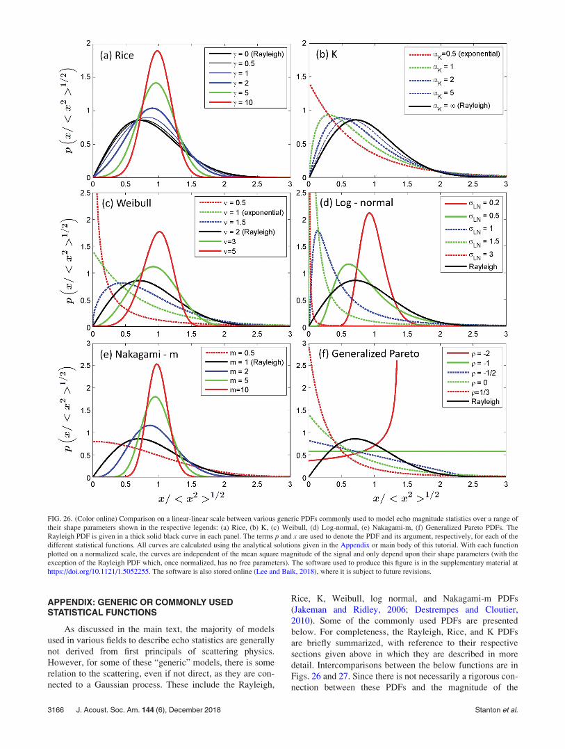
APPENDIX: GENERIC OR COMMONLY USEDSTATISTICAL FUNCTIONS
As discussed in the main text, the majority of models
used in various fields to describe echo statistics are generally
not derived from first principals of scattering physics.
However, for some of these “generic” models, there is some
relation to the scattering, even if not direct, as they are con-
nected to a Gaussian process. These include the Rayleigh,
Rice, K, Weibull, log normal, and Nakagami-m PDFs
(Jakeman and Ridley, 2006; Destrempes and Cloutier,
2010). Some of the commonly used PDFs are presented
below. For completeness, the Rayleigh, Rice, and K PDFs
are briefly summarized, with reference to their respective
sections given above in which they are described in more
detail. Intercomparisons between the below functions are in
Figs. 26 and 27. Since there is not necessarily a rigorous con-
nection between these PDFs and the magnitude of the
FIG. 26. (Color online) Comparison on a linear-linear scale between various generic PDFs commonly used to model echo magnitude statistics over a range of
their shape parameters shown in the respective legends: (a) Rice, (b) K, (c) Weibull, (d) Log-normal, (e) Nakagami-m, (f) Generalized Pareto PDFs. The
Rayleigh PDF is given in a thick solid black curve in each panel. The terms p and x are used to denote the PDF and its argument, respectively, for each of the
different statistical functions. All curves are calculated using the analytical solutions given in the Appendix or main body of this tutorial. With each function
plotted on a normalized scale, the curves are independent of the mean square magnitude of the signal and only depend upon their shape parameters (with the
exception of the Rayleigh PDF which, once normalized, has no free parameters). The software used to produce this figure is in the supplementary material at
https://doi.org/10.1121/1.5052255. The software is also stored online (Lee and Baik, 2018), where it is subject to future revisions.
3166 J. Acoust. Soc. Am. 144 (6), December 2018 Stanton et al.
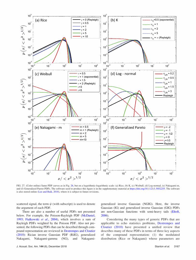
scattered signal, the term w (with subscript) is used to denote
the argument of each PDF.
There are also a number of useful PDFs not presented
below. For example, the Poisson-Rayleigh PDF (McDaniel,
1993; Fialkowski et al., 2004), which involves a sum of
Rayleigh PDFs weighted by the Poisson PDF. Also not pre-
sented, the following PDFs that can be described through com-
pound representation are reviewed in Destrempes and Cloutier
(2010): Rician inverse Gaussian PDF (RiIG), generalized
Nakagami, Nakagami-gamma (NG), and Nakagami-
generalized inverse Gaussian (NGIG). Here, the inverse
Gaussian (IG) and generalized inverse Gaussian (GIG) PDFs
are non-Gaussian functions with semi-heavy tails (Eltoft,
2006).
Considering the many types of generic PDFs that are
applicable to echo statistics problems, Destrempes and
Cloutier (2010) have presented a unified review that
describes many of these PDFs in terms of three key aspects
of the compound representation: (1) the modulated
distribution (Rice or Nakagami) whose parameters are
FIG. 27. (Color online) Same PDF curves as in Fig. 26, but on a logarithmic-logarithmic scale: (a) Rice, (b) K, (c) Weibull, (d) Log-normal, (e) Nakagami-m,
and (f) Generalized Pareto PDFs. The software used to produce this figure is in the supplementary material at https://doi.org/10.1121/1.5052255. The software
is also stored online (Lee and Baik, 2018), where it is subject to future revisions.
J. Acoust. Soc. Am. 144 (6), December 2018 Stanton et al. 3167

modulated by another distribution, (2) the modulating dis-
tribution (gamma, inverse Gaussian, or generalized inverse
Gaussian) that is used to modulate one or more of the
parameters of the modulated distribution, and (3) the mod-
ulated parameters (diffuse and/or coherent components) of
the modulated distribution. See, for example, Table 2 of
that paper that summarizes the three aspects for some of
the PDFs.
1. Rayleigh PDF
In the limit of an infinite number of random phase
sinusoids, the instantaneous amplitude (not magnitude) is
a complex Gaussian in which both the real and imaginary
components of the signal are Gaussian-distributed varia-
bles with the same variance. The magnitude of the instan-
taneous signal (i.e., its envelope) is Rayleigh distributed,
whose equation is given in Eq. (21). In addition to being
applied to modeling the statistics of white noise and, as
discussed in Sec. IV C 6, this distribution can also be
directly connected to the scattering physics in the case of a
high number of scattering features whose echoes overlap
and are of random phase (uniformly distributed [0 2p]).
The scattering features could be from multiple scatterers,
a rough boundary, or an object with a complex shape or
rough boundary.
2. Rice PDF
In the case of a single sinusoid of constant amplitude
added to a signal whose magnitude is Rayleigh distributed,
the magnitude of the instantaneous summed signal is
Rice distributed, as given in Eq. (26). While originally devel-
oped to describe the statistics of a signal in the presence of
white noise, it can also be directly related to the scattering
physics. For example, as discussed in Sec. VI A 2, the constant
signal could correspond to an individual scatterer of interest
whose echo remains constant and the Rayleigh-distributed
component could be the echo from a neighboring rough
boundary or cloud of scatterers. In the limit of the scattering
by the individual being strong or weak relative to the diffuse
background scattering, the echo (Rice) PDF approaches a
Gaussian or Rayleigh PDF, respectively.
3. K PDF
The K PDF, given in Eq. (29), can be derived several
ways. Two approaches involve sums of sinusoidal signals:
(a) when the number of sinusoids follows a negative bino-
mial PDF and with the average number tending to infinity
and (b) for a finite number of sinusoids whose amplitudes
follow an exponential PDF. Two other approaches involve
the “compound representation” that uses existing statistical
functions where the K PDF can be derived from (c) the prod-
uct of a Rayleigh-distributed random variable and a random
variable that is chi distributed and (d) a Rayleigh PDF whose
mean-square value is gamma distributed. Under certain lim-
ited conditions, the sinusoids in derivations (a) and (b) can
be rigorously and directly related to the scattering physics by
connecting the distribution of sinusoids to a corresponding
distribution of scatterers (whose echoes are convolved with
the beampattern of the sensor system).
As discussed in Sec. VI A 3, the original K PDF is a
two-parameter function and is associated with sinusoids with
phases that are randomly and uniformly distributed [0 2p].
The generalized K PDF (not shown) involves the more gen-
eral case when the distribution of phases is not uniform and
can be related to, for example, the echo from one or several
large scatterers in the presence of an extended diffuse scat-
terer such as a rough boundary. This latter distribution, and a
more restricted form (homodyned K PDF), have three
parameters. While all of these K-based PDFs can be rigor-
ously connected to the scattering physics under only a nar-
row range of conditions, these distributions have been
demonstrated to reasonably fit experimental echo statistics
data from objects and boundaries over a much wider range
of conditions.
4. Weibull PDF
The distribution of intensity IR (square of magnitude) of
a Rayleigh-distributed random variable is a negative expo-
nential PDF. Using the transformation IR¼ w�W yields the
Weibull PDF
pW wWð Þ ¼ �
kRw��1
W e�w�W=kR ; (A1)
where kR ¼ hIRi is the mean intensity of the original
Rayleigh random variable as given in Eq. (21) (Jakeman and
Ridley, 2006). This PDF for wW , whose derivation involves
a Gaussian process, has been used for both magnitude and
intensity statistics. The PDF becomes a negative exponential
(intensity-like) and Rayleigh PDF (magnitude-like) when �is equal to 1 and 2, respectively. Furthermore, since the K
PDF becomes a negative exponential when its shape parame-
ter aK in Eq. (29) is equal to 1/2, then the Weibull and K
PDFs become the same PDF (negative exponential) when �and aK are equal to 1 and 1/2, respectively.
5. Log normal PDF
The log normal PDF involves a variable whose loga-
rithm is Gaussian distributed. The magnitude wLN can be
written as wLN ¼ Cex where x is Gaussian distributed with a
mean and variance of zero and r2LN , respectively, and C is a
constant. It follows that the PDF of wLN is (Jakeman and
Ridley, 2006)
pLN wLNð Þ ¼ 1
wLN
ffiffiffiffiffiffiffiffiffiffiffiffiffi2pr2
LN
p e� ln wLN�ln Cð Þ2=2r2LN : (A2)
Although there is not a direct connection between this PDF
and backscattering, the signal of a propagating field some-
times decreases exponentially, with x being a negative quan-
tity in ex above. The term x can be related to absorption and
scattering-related loss of signal. The absorption and scatter-
ing may be variable, causing fluctuations or scintillation in
the forward-propagating signal which, in turn, will result in
fluctuations of the backscattered signal as it relates to the
3168 J. Acoust. Soc. Am. 144 (6), December 2018 Stanton et al.

local (fluctuating) value of the signal incident upon a scat-
terer. There will be additional fluctuations incurred in the
backscattered signal as it propagates back to the sensor sys-
tem. The PDF of intensity w2LN takes on the same functional
form as the above equation, but with different constant fac-
tors in the exponent (page 399 of Goodman, 1985).
6. Nakagami-m PDF (and related chi-squared andgamma PDFs)
The Nakagami-m, chi-squared, and gamma PDFs are
related to each other, as they all involve incoherent processes
in which the signal is composed of the incoherent addition
(sum of squares) of m independent, Rayleigh-distributed var-
iables. Or, equivalently, the signal is made up of the sum of
the squares of 2m independent Gaussian-distributed varia-
bles. Although this incoherent process does not directly
relate to a scattering process which involves the coherentsum of random variables (i.e., sum of complex signal), there
has been success in using these PDFs to model echo
statistics.
The Nakagami-m is concerned with the statistics of the
magnitude of the signal whereas the chi-squared and gamma
PDFs describe the PDF of the square (i.e., intensity) of the
signal. The chi-squared PDF relates to an integer number of
Rayleigh-distributed variables and the gamma PDF is an
analytical continuation of that PDF for non-integer numbers
of variables. The equations for all three PDFs have a similar
form and are expressed in terms of a gamma function. This
section will focus on the Nakagami-m PDF since it is most
relevant to the magnitude statistics in this paper.
In this model, the random variable wN is defined as the
square root of the sum of the squares of m independent
Rayleigh random variables. The resultant PDF of wN is the
Nakagami-m PDF (Nakagami, 1960; Karagiannidis et al.,2003; Eltoft, 2006)
pN wNð Þ ¼ 2mmw 2m�1ð ÞN
C mð ÞXm e�mw2N=X; (A3)
where C is the gamma function. The terms m and X are shape
and scaling parameters, respectively, where X ¼ hw2Ni. As
with the gamma PDF, through analytical continuation, the
term m can be a non-integer. And, as discussed above, while
the Nakagami-m PDF is used to model fluctuations of signal
magnitude, wN does not rigorously represent the magnitude of
the signal, as it is related to an incoherent (sum of squares),
rather than a coherent (sum of complex variables) process
associated with the scattering.
The Nakagami-m PDF reduces to the Rayleigh and
“one-sided” Gaussian PDFs for m¼ 1 and 1/2, respectively.
Here, the one-sided Gaussian is a Gaussian PDF with its
peak at an argument of zero and is only evaluated for non-
negative values of argument. The Nakagami-m PDF also
takes on qualitatively similar shapes to the Rice PDF for
higher values of m (Nakagami-m) and c (Rice) where both
curves are Gaussian-like (Figs. 26 and 27). For example the
Nakagami-m PDF, when calculated for the values m¼ 3,
3.9, and 5, looks similar to the Rice PDF when calculated for
the values c¼ 5, 6.9, and 9, respectively (not shown).
7. Generalized Pareto PDF
The generalized Pareto PDF is based on extreme value
theory, which focuses on either the minimum or maximum
values of a signal (Pickands, 1975; La Cour, 2004). In this
case, the generalized Pareto PDF has been derived to
describe the tails of the PDF (i.e., more than simply the max-
imum values). The generalized Pareto PDF is
pGP wGPð Þ ¼1þ qwGP
n
� �� 1=qð Þ�1
n; (A4)
where q and n are the shape and scale parameters, respec-
tively. While this PDF is not specific to magnitude or inten-
sity, this has been shown to successfully describe the tails of
the intensity of non-Rayleigh echoes (La Cour, 2004; Gelb
et al., 2010). Note that this PDF can only be normalized for
values of q < 1=2, otherwise the integration diverges. Also,
when q ¼ �2, the range of wGP is limited to prevent the
argument of the square root term from becoming negative
above a certain value of wGP.
Abraham, D. A., Gelb, J. M., and Oldag, A. W. (2011). “Background and
clutter mixture distributions for active sonar statistics,” IEEE J. Ocean.
Eng. 36(2), 231–247.
Abraham, D. A., and Lyons, A. P. (2002a). “Reverberation envelope statis-
tics and their dependence on sonar beamwidth and bandwidth,” in Impactof Littoral Environmental Variability on Acoustic Predictions and SonarPerformance, edited by N. G. Pace and F. B. Jensen (Kluwer Academic,
Dordrecht, the Netherlands), pp. 539–546.
Abraham, D. A., and Lyons, A. P. (2002b). “Novel physical interpretations
of K-distributed reverberation,” IEEE J. Ocean. Eng. 27(4), 800–813.
Abraham, D. A., and Lyons, A. P. (2010). “Special issue on non-Rayleigh
reverberation and clutter,” IEEE J. Ocean. Eng. 35(2), 233–356.
Agapiou, S., Papaspiliopoulos, O., Sanz-Alonso, D., and Stuart, A. M.
(2017). “Importance sampling: Intrinsic dimension and computational
cost,” Stat. Sci. 32(3), 405–431.
Azzalini, A. (1996). Statistical Inference Based on the Likelihood (Chapman
and Hall, London), Vol. 68, Chap. 3.
Barakat, R. (1974). “First-order statistics of combined random sinusoidal
waves with applications to laser speckle patterns,” Opt. Acta 21, 903–921.
Bhatia, S., Stanton, T. K., and Baik, K. (2015). “Non-Rayleigh scattering by
a randomly oriented elongated scatterer randomly located in a beam,”
IEEE J. Ocean. Eng. 40(1), 169–176.
Botev, Z. I., Grotowski, J. F., and Kroese, D. P. (2010). “Kernel density esti-
mation via diffusion,” Ann. Stat. 38(5), 2916–2957.
Bowman, J. J., Senior, T. B. A., and Uslenghi, P. L. E. (1987).
Electromagnetic and Acoustic Scattering by Simple Shapes (Hemisphere,
New York).
Chen, C.-C. (1998). “Electromagnetic resonances of immersed dielectric
spheres,” IEEE Trans. Ant. Propagat. 46(7), 1074–1083.
Chu, D., and Stanton, T. K. (2010). “Statistics of echoes from a directional
sonar beam insonifying finite numbers of single scatterers and patches of
scatterers,” IEEE J. Ocean. Eng. 35(2), 267–277.
Clay, C. S. (1983). “Deconvolution of the fish scattering PDF from the echo
PDF for a single transducer sonar,” J. Acoust. Soc. Am. 73, 1989–1994.
Colosi, J. A. (2016). Sound Propagation Through the Stochastic Ocean(Cambridge University Press, Cambridge).
Crispin, J. W., Jr., and Siegel, K. M. (1968). Methods of Radar Cross-Section Analysis (Academic Press, New York).
Destrempes, F., and Cloutier, G. (2010). “A critical review and uniformized
representation of statistical distributions modeling the ultrasound echo
envelope,” Ultrasound Med. Bio. 36(7), 1037–1051.
J. Acoust. Soc. Am. 144 (6), December 2018 Stanton et al. 3169

Destrempes, F., and Cloutier, G. (2013). “Review of envelope statistics
models for quantitative ultrasound imaging and tissue characterization,” in
Quantitative Ultrasound in Soft Tissues, edited by J. Mamou and M. Oelze
(Springer, Dordrecht, the Netherlands), pp. 219–274.
Devroye, L. (1986). “Inversion by numerical solution of F(X)¼U,” in Non-uniform Random Variable Generation (Springer-Verlag, New York), Sec.
2.2.
Drumheller, D. M. (1999). “Pad�e approximations to matched filter ampli-
tude probability functions,” IEEE Trans. Aerospace Electron. Syst. 35,
1033–1045.
Eckart, C. (1953). “The scattering of sound from the sea surface,” J. Acoust.
Soc. Am. 25, 566–570.
Ehrenberg, J. E. (1972). “A method for extracting the fish target strength
distribution from acoustic echoes,” Proc. Conf. Eng. Ocean Environ. 1,
61–64.
Ehrenberg, J. E. (1989). “A review of target strength estimation techniques,”
in Underwater Acoustic Data Processing, edited by Y. Chan (Kluwer,
Dordrecht, the Netherlands), pp. 161–175.
Ehrenberg, J. E., Carlson, T. J., Traynor, J. J., and Williamson, N. J. (1981).
“Indirect measurement of the mean acoustic backscattering cross section
of fish,” J. Acoust. Soc. Am. 69, 955–962.
Eltoft, T. (2006). “Modeling the amplitude statistics of ultrasonic images,”
IEEE Trans. Med. Mag. 25, 229–240.
Ferrara, G., Migliaccio, M., Nunziata, F., and Sorrentino, A. (2011).
“Generalized-K (GK)-based observation of metallic objects at sea in full-
resolution synthetic aperture radar (SAR) data: A multipolarization study,”
IEEE J. Ocean. Eng. 36, 195–204.
Fialkowski, J. M., Gauss, R. C., and Drumheller, D. M. (2004).
“Measurements and modeling of low-frequency near-surface scattering
statistics,” IEEE J. Ocean. Eng. 29, 197–214.
Gallaudet, T. C., and de Moustier, C. P. (2003). “High-frequency volume
and boundary acoustic backscatter fluctuations in shallow water,”
J. Acoust. Soc. Am. 114, 707–725.
Gelb, J. M., Heath, R. E., and Tipple, G. L. (2010). “Statistics of distinct
clutter classes in midfrequency active sonar,” IEEE J. Ocean. Eng. 35,
220–229.
Gillman, L. C. (1997). “First-order statistics of pulsed-sinusoid backscatter
from random media: Basic elements of an exact treatment,” IEEE Trans.
Ultrason. Ferroelectr. Freq. Control 44, 798–804.
Goodman, J. W. (1985). Statistical Optics, 1st ed. (Wiley-Interscience, New
York).
Gurley, J. V., and Stanton, T. K. (1993). “Sound scattering by rough elon-
gated elastic objects. III. Experiment,” J. Acoust. Soc. Am. 94,
2746–2755.
Hackman, R. H. (1993). “Acoustic scattering from elastic solids,” in
Physical Acoustics, edited by A. D. Pierce and R. N. Thurston (Academic,
New York), Vol. 22, pp. 1–194.
Hogg, R. V., and Craig, A. T. (1978). Introduction to MathematicalStatistics, 4th ed. (Macmillan, New York).
Jakeman, E., and Pusey, P. N. (1976). “A model for non-Rayleigh sea echo,”
IEEE Trans. Antennas Propag. 24(6), 806–814.
Jakeman, E., and Ridley, K. D. (2006). Modeling Fluctuations in ScatteredWaves (Taylor and Francis, New York).
Jakeman, E., and Tough, R. J. A. (1987). “Generalized K distribution: A sta-
tistical model for weak scattering,” J. Opt. Soc. Am. 4, 1764–1772.
Jao, J. K., and Elbaum, M. (1978). “First-order statistics of a non-Rayleigh
fading signal and its detection,” Proc. IEEE 66, 781–789.
Jones, B. A., Colosi, J. A., and Stanton, T. K. (2014). “Echo statistics of
individual and aggregations of scatterers in the water column of a random,
oceanic waveguide,” J. Acoust. Soc. Am. 136, 90–108.
Jones, B. A., Stanton, T. K., Colosi, J. A., Gauss, R. C., Fialkowski, J. M.,
and Jech, J. M. (2017). “Broadband classification and statistics of echoes
from aggregations of fish measured by long-range, mid-frequency sonar,”
J. Acoust. Soc. Am. 141, 4354–4371.
Joughin, I. R., Percival, D. B., and Winebrenner, D. P. (1993). “Maximum
likelihood estimation of K distribution parameters for SAR data,” IEEE
Trans. Geosci. Remote Sens. 31, 989–999.
Karagiannidis, G. K., Zogas, D. A., and Kotsopoulos, S. A. (2003). “On the
multivariate Nakagami-m distribution with exponential correlation,” IEEE
Trans. Commun. 51, 1240–1244.
Kinsler, L. E., Frey, A. R., Coppens, A. B., and Sanders, J. V. (2000).
Fundamentals of Acoustics, 4th ed. (Wiley, New York), Chap. 7.
La Cour, B. R. (2004). “Statistical characterization of active sonar reverber-
ation using extreme value theory,” IEEE J. Ocean. Eng. 29(2), 310–316.
Le Chevalier, F. (2002). Principles of Radar and Sonar Signal Processing(Artech House, Boston).
Lee, W.-J., and Baik, K. (2018). “leewujung/echo-stats-tutorial,” https://
doi.org/10.5281/zenodo.1313729.
Lee, W.-J., and Stanton, T. K. (2014). “Statistics of echoes from mixed
assemblages of scatterers with different scattering amplitudes and numeri-
cal densities,” IEEE J. Ocean. Eng. 39(4), 740–754.
Lee, W.-J., and Stanton, T. K. (2015). “Statistics of broadband echoes:
Application to acoustic estimates of numerical density of fish,” IEEE J.
Ocean. Eng. 41(3), 709–723.
Li, X., Xin, J.-Q., Donohue, K., and Bilgutay, N. M. (1992). “Rank determi-
nation of order statistic filters for ultrasonic flaw detection,” in Review ofProgress in Quantitative Nondestructive Evaluation, edited by D. O.
Thomson and D. E. Chimenti (Plenum Press, New York), pp. 943–950.
Lim, R., Williams, K. L., and Thorsos, E. I. (2000). “Acoustic scattering by
a three-dimensional elastic object near a rough surface,” J. Acoust. Soc.
Am. 107, 1246–1262.
Marston, P. L. (1992). “Geometrical and catastrophe optics methods in
scattering,” in Physical Acoustics, edited by A. D. Pierce and R. N.
Thurston (Academic, New York), Vol. 21, pp. 1–234.
McDaniel, S. T. (1993). “Sea-surface reverberation fluctuations,” J. Acoust.
Soc. Am. 94, 1551–1559.
Medwin, H., and Clay, C. S. (1998). Fundamentals of AcousticalOceanography (Academic, Boston).
Moser, P. J., Murphy, J. D., Nagl, A., and Uberall, H. (1981). “Resonances
and surface waves on conducting spheres with a dielectric coating,” Radio
Sci. 16(3), 279–288, https://doi.org/10.1029/RS016i003p00279.
Murphy, J. D., Moser, P. J., Nagl, A., and Uberall, H. (1980). “A surface
wave interpretation for the resonances of a dielectric sphere,” IEEE Trans.
Antennas Propagat. AP-28(6), 924–927.
Nakagami, M. (1960). “The m-distribution—A general formula of intensity
distribution of rapid fading,” in Statistical Methods in Radio WavePropagation, edited by W. C. Hoffman (Permagon, New York), pp. 3–36.
Newton, R. G. (1982). Scattering Theory of Waves and Particles (Springer-
Verlag, New York).
Numrich, S. K., and Uberall, H. (1992). “Scattering of sound pulses and
the ringing of target resonances,” in Physical Acoustics, edited by A. D.
Pierce and R. N. Thurston (Academic, New York), Vol. 21, pp.
235–318.
Nussenzveig, H. M. (1969). “High-frequency scattering by a transparent
sphere—Part I: Direct reflection and transmission, Part II: Theory of the
rainbow and the glory,” J. Math. Phys. 10, 82–176.
Oelze, M. L., and Mamou, J. (2016). “Review of quantative ultrasound:
Envelope statistics and backscatter coefficient imaging and contributions
to diagnostic ultrasound,” IEEE Trans. Ultrason. Ferroelectr. Freq.
Control 63, 336–351.
Ogilvy, J. A. (1991). Theory of Wave Scattering from Random RoughSurfaces (Adam Hilger, Bristol).
Ol’shevskii, V. V. (1978). Statistical Methods in Sonar (Consultants
Bureau, New York).
Papoulis, A. (1991). Probability, Random Variables, and StochasticProcesses (McGraw-Hill, New York).
Pickands, J., Jr. (1975). “Statistical inference using extreme order statistics,”
Ann. Statist. 3, 119–131.
Rice, S. O. (1954). “Mathematical analysis of random noise,” in SelectedPapers on Noise and Stochastic Processes, edited by N. Wax (Dover,
New York), pp. 133–294.
Scott, D. W. (1992). Multivariate Density Estimation: Theory, Practice, andVisualization (Wiley, New York).
Stanton, T. K. (1985). “Volume scattering: Echo peak PDF,” J. Acoust. Soc.
Am. 77, 1358–1366.
Stanton, T. K., and Chu, D. (1992). “Sound scattering by rough elongated
elastic objects: II. fluctuations of scattered field,” J. Acoust. Soc. Am. 92,
1665–1678.
Stanton, T. K., and Chu, D. (2010). “Non-Rayleigh echoes from resolved
individuals and patches of resonant fish at 2–4 kHz,” IEEE J. Ocean. Eng.
35(2), 152–163.
Stanton, T. K., Chu, D., Gelb, J. M., Tipple, G. L., and Baik, K. (2015).
“Interpreting echo statistics of three distinct clutter classes measured with
a midfrequency active sonar: Accounting for number of scatterers, scatter-
ing statistics, and beampattern effects,” IEEE J. Ocean. Eng. 40, 657–665.
Stanton, T. K., Chu, D., and Wiebe, P. H. (1998). “Sound scattering by sev-
eral zooplankton groups II: Scattering models,” J. Acoust. Soc. Am. 103,
236–253.
3170 J. Acoust. Soc. Am. 144 (6), December 2018 Stanton et al.

Stanton, T. K., and Clay, C. S. (1986). “Sonar echo statistics as a remote-
sensing tool: Volume and seafloor,” IEEE J. Ocean. Eng. 11(1), 79–96.
Tatarski, V. I. (1961). Wave Propagation in a Turbulent Medium, translated
by R. A. Silverman (McGraw-Hill, New York).
Tunis, A. S., Baddour, R. E., Czarnota, G. J., Giles, A., Worthington, A. E.,
Sherar, M. D., and Kolios, M. C. (2005). “Using high frequency ultra-
sound envelope statistics to determine scatterer number density in dilute
cell solutions,” in Proceedings to IEEE Ultrasonics Symposium, pp.
878–881.
Turin, G. L. (1960). “An introduction to matched filters,” IRE Trans. Inf.
Theory 6, 311–329.
Uberall, H. (1973). “Surface waves in acoustics,” in Physical Acoustics,
edited by W. B. Mason and R. N. Thurston (Academic, New York), Vol.
10, pp. 1–60.
Waag, R. C. (1984). “A review of tissue characterization from ultrasonic
scattering,” IEEE Trans. Biomed. Eng. BME-13, 884–893.
Ward, K. D. (1981). “Compound representation of high resolution sea
clutter,” Electron. Lett. 17(16), 561–563.
Watts, S., and Ward, K. (2010). “Special issue on radar clutter,” IET Radar
Sonar Nav. 4(2), 143–328.
Williams, K. L., Kargl, S. G., Thorsos, E. I., Burnett, D. S., Lopes, J. L.,
Zampolli, M., and Marston, P. L. (2010). “Acoustic scattering from a
solid aluminum cylinder in contact with a sand sediment:
Measurements, modeling, and interpretation,” J. Acoust. Soc. Am. 127,
3356–3371.
Zampolli, M., Tesei, A., and Canepa, G. (2008). “Computing the far field
scattered or radiated by objects inside layered fluid media using approxi-
mate Green’s functions,” J. Acoust. Soc. Am. 123, 4051–4058.
J. Acoust. Soc. Am. 144 (6), December 2018 Stanton et al. 3171
Related Documents