ECHO STATE NETWORK APPROACH FOR RADIO SIGNAL …

ECHO STATE NETWORK APPROACH FOR RADIO SIGNAL STRENGTH

PREDICTION APPLIED TO CELLULAR COMMUNICATION

FREQUENCY BANDS IN NORTHERN NAMIBIA

A THESIS SUBMITTED IN FULFILMENT

OF THE REQUIREMENTS FOR THE DEGREE OF

MASTER OF SCIENCE ELECTRONICS AND COMPUTER ENGINEERING

OF

THE UNIVERSITY OF NAMIBIA

BY

KENNETH GIDEON

(200813927)

OCTOBER 2017

Supervisor: Dr. C. Temaneh-Nyah, Co-supervisor: Dr. C.N. Nyirenda

i

PRELIM INARY

ABSTRACT

Reliance on mobile connectivity has led to demands for wireless spectrum capacity to

grow on a daily basis resulting to congested networks. Ensuring acceptable levels of

Quality of Service (QoS) for users in wireless communication systems, through

continuous wireless network analysis using simulation tools based on radio

propagation models has become increasingly prominent. To provide automated

analytical model building, the use of machine learning methods has been considered

to predict characteristics of the wireless channel. Thus, in this work, a method for

predicting radio signal strength using Echo State Networks (ESNs) is proposed and

applied to three different locations in Northern Namibia. This method aims at

providing a better approach for radio signal strength prediction, which leads to

improvements in wireless communication planning, design and analysis. Its

performance is compared with the Support Vector Regression (SVR) method

optimized for radio propagation modeling. Simulations are conducted in Python using

propagation data measured from the three locations based on the following four

performance metrics: goodness of fit criteria; error measures; computation

complexities; and F-Test for statistical model comparison. Simulation results show

that the ESN gives a better prediction accuracy in terms of the goodness of fit criteria

and the error measures (i.e. average R2 = 0.82 and average mean absolute error (MAE)

= 0.0312 for ESN compared to 0.648 and 0.0624 for SVR), but it is inferior to the SVR

in terms of computation complexities (i.e. average training complexity of 410 ms and

average testing complexity of 79.0 ms for ESN compared to 8.19 ms and 1.04 ms for

SVR). In addition, results from the F-Test also indicates that the ESN provides a

significantly better fit than the SVR.

ii

PUBLICATIONS

The following are the resulting peer reviewed publications from this study.

Conference Proceedings:

1. K. Gideon, C. Nyirenda, and C. Temaneh-Nyah, “Radio signal strength

prediction using echo state networks”, in The 7th International Symposium on

Computational Intelligence and Industrial Applications (ISCIIA2016), Beijing,

P. R. China, 2016.

Journal Article:

1. K. Gideon, C. Nyirenda, and C. Temaneh-Nyah, “Echo State Network based

Radio Signal Strength Prediction for Wireless Communication in Northern

Namibia,” IET Commun., vol. 11, no. 12, pp. 1920–1926, 2017.

iii

TABLE OF CONTENTS

PRELIMINARY .............................................................................................................................. I

ABSTRACT ........................................................................................................................................ I PUBLICATIONS ............................................................................................................................... II ACKNOWLEDGEMENT .................................................................................................................. V DEDICATION ................................................................................................................................... VI DECLARATIONS ............................................................................................................................ VII LIST OF ACRONYMS .................................................................................................................... VIII

CHAPTER 1: INTRODUCTION ................................................................................................... 1

1.1 ORIENTATION OF THE STUDY ................................................................................................. 1 1.2 PROBLEM STATEMENT........................................................................................................... 2 1.3 OBJECTIVES ........................................................................................................................... 4 1.4 RESEARCH QUESTION ............................................................................................................ 4 1.5 SIGNIFICANCE OF THE STUDY ................................................................................................ 5 1.6 SCOPE AND LIMITATION OF THE STUDY ................................................................................. 5 1.7 STRUCTURAL ORGANIZATION ............................................................................................... 5

CHAPTER 2: LITERATURE REVIEW ....................................................................................... 7

2.1 INTRODUCTION ...................................................................................................................... 7 2.2 CLASSICAL METHODS FOR RADIO PROPAGATION MODELING ............................................... 7

2.2.1 Empirical Methods ........................................................................................................... 9 2.2.2 Stochastic Methods ......................................................................................................... 10

2.3 MACHINE LEARNING METHODS .......................................................................................... 11 2.3.1 Multilayer Perceptrons ................................................................................................... 12 2.3.2 Support Vector Regression Concepts ............................................................................. 12 2.3.3 Echo State Network Principles ....................................................................................... 16

2.4 CHAPTER SUMMARY ........................................................................................................... 21

CHAPTER 3: METHODOLOGY ................................................................................................ 22

3.1 INTRODUCTION .................................................................................................................... 22 3.2 DATA ACQUISITION ............................................................................................................. 23 3.3 DATA PREPARATION ............................................................................................................ 27

3.3.1 Removal of Outliers ........................................................................................................ 27 3.3.2 Preprocessing ................................................................................................................. 27 3.3.3 Normalization ................................................................................................................. 32

3.4 SIMULATIONS ...................................................................................................................... 33 3.4.1 Data Partitioning ........................................................................................................... 35 3.4.2 Model Development and Optimization ........................................................................... 35 3.4.3 Model Performance Evaluation ..................................................................................... 38

3.5 DATA ANALYSIS .................................................................................................................. 40 3.5.1 The F Significance Test .................................................................................................. 40 3.5.2 The Analysis of Variance ................................................................................................ 41 3.5.3 Tukey’s HSD for Post-hoc Analysis ............................................................................... 41

3.6 CHAPTER SUMMARY ........................................................................................................... 41

iv

CHAPTER 4: RESULTS AND DISCUSSION ............................................................................ 43

4.1 INTRODUCTION .................................................................................................................... 43 4.2 GRAPHICAL PRESENTATION OF THE RESULTS...................................................................... 43

4.2.1 Actual and Predicted RSSI values .................................................................................. 43 4.2.2 Computation Complexity and MAE against Reservoir Size (N) ..................................... 45

4.3 STATISTICAL RESULTS ........................................................................................................ 52 4.4 STATISTICAL TESTS AND ANALYSIS OF VARIANCE.............................................................. 53

4.4.1 The F-Test for Statistical Model Comparison ................................................................ 53 4.4.2 Analysis of Variance ....................................................................................................... 53

CHAPTER 5: CONCLUSIONS AND RECOMMENDATIONS ................................................ 58

5.1 CONCLUSIONS ..................................................................................................................... 58 5.2 RECOMMENDATION FOR FUTURE WORK .............................................................................. 58

REFERENCES ............................................................................................................................. 59

APPENDICES ................................................................................................................................... 65

APPENDIX A: DATA PREPROCESSING – PART 1 ............................................................................ 65 APPENDIX B: DATA PREPROCESSING – PART 2 ............................................................................ 67 APPENDIX C: PYTHON SIMULATION CODES ................................................................................. 69 APPENDIX D: PYTHON CODES FOR DATA ANALYSIS .................................................................... 74 APPENDIX E: PYTHON CODES FOR ANOVA ................................................................................ 77

v

ACKNOWLEDGEMENT

This research was possible thanks to the cooperation and support of a number of

people. I am grateful to them all, and would like to express my appreciation to the

following people:

1. Dr. Clement Temaneh-Nyah, my research supervisor, for broadening my

understanding on radio propagation characterization.

2. Dr. C. N. Nyirenda, my research co-supervisor, for his guidance as well as his help

in selecting the right simulation tools throughout the whole research.

I would also like to express my appreciation to all the staff and colleagues in the

Electronics and Computer Engineering department for their full support and assistance

during this research.

vi

DEDICATION

This thesis is dedicated to my mother and brother, the two people who have inspired

me, helped me, and guided me through my life the most.

vii

DECLARATIONS

I, Kenneth Gideon, hereby declare that this study is my own work and is a true

reflection of my research, and that this work, or any part thereof has not been submitted

for a degree at any other institution.

No part of this thesis/dissertation may be reproduced, stored in any retrieval system,

or transmitted in any form, or by means (e.g. electronic, mechanical, photocopying,

recording or otherwise) without the prior permission of the author, or The University

of Namibia in that behalf.

I, Kenneth Gideon, grant The University of Namibia the right to reproduce this thesis

in whole or in part, in any manner or format, which The University of Namibia may

deem fit.

…………………………. …………………………. ………………………….

Name of Student Signature Date

…………………………. …………………………. ………………………….

Supervisor Signature Date

…………………………. …………………………. ………………………….

Co-Supervisor Signature Date

KENNETH GIDEON

DR. C. TEMANEH-NYAH

DR. C. N. NYIRENDA

viii

LIST OF ACRONYMS

3G Third Generation cellular technologies

AI Artificial Intelligence

ANN Artificial Neural Networks

ANOVA Analysis of Variance

API Application Programming Interface

BTS Base Transceiver Station

CAGR Compound Annual Growth Rate

CID Cell Identification

CTC Computation Time Complexity

dB Deci Bell

EDGE Enhanced Data rates for GSM Evolution

ESN Echo State Network

EURO-COST European Cooperation in Science and Technology

GPRS General Packet Radio Service

GPS Global Positioning System

GRNN Generalized Regression Neural Network

GSM Global System for Mobile communication

HSDPA High Speed Downlink Packet Access

HSPA High Speed Packet Access

HSPA+ Evolved High Speed Packet Access

HSUPA High Speed Uplink Packet Access

IDE Integrated Development Environment

ITU-R Recommendation for International

Telecommunication Union

LAC Location Area Code

MAE Mean Absolute Error

MCC Mobile Country Code

MDP Modular Data Processing

MHz Mega Hertz

ML Machine Learning

ix

MLP Multi-Layer Perceptron

MNC Mobile Network Code

MS Mobile Station

MSE Mean Square Error

Numpy Numerical Python

OGER Organic Environment for Reservoir computing

QoS Quality of Service

RBF Radial Basis Function

RC Reservoir Computing

RMSE Root Mean Square Error

RNN Recurrent Neural Networks

RSSI Received Signal Strength Indication

Rx Receiver

Scipy Scientific Python

SSE Residual Sum of Squares / Sum of Squared Errors

SST Total Sum of Squares

SVM Support Vector Machine

SVR Support Vector Regression

Tx Transmitter

UMTS Universal Mobile Telecommunication System

VNI Visual Networking Index

1

CHAPTER 1: INTRODUCTION

1.1 Orientation of the Study

Today, more than half of the world’s population rely on mobile connectivity, resulting

in high demands for wireless spectrum capacity and leading to congested networks [1].

Performing continuous network analysis is, therefore, very important in order to ensure

an acceptable level of Quality of Service (QoS) for users in a wireless communication

network [2]. Wireless network analysis can be performed either by conducting field

measurements or by using simulation tools which rely on modeling the radio

propagation environment. Since performing field measurements is tedious, time

consuming, and expensive, modeling the radio propagation environment has become

the suitable alternative. Network simulation tools are very crucial as they substantially

simplify and increase the effectiveness of mobile network design. An accurately

conforming propagation model is, therefore, essential for any wireless network

simulation tool. The challenges faced in radio propagation modeling occur due to the

wireless radio channel being characterized by various random parameters, such as the

distribution of the terrain obstructions. Hence, researchers are constantly searching for

more accurate ways of characterizing and quantifying the propagation scenarios in

different environments with more certainty.

2

1.2 Problem Statement

Classical methods for modeling the radio propagation environment, such as empirical

and stochastic methods come short in either computation power, accuracy, or good

representation of the propagation environment. Empirical methods [3], [4] have the

computation power but are less accurate since they do not consider certain propagation

phenomena and they require considerable assumptions for simplification. Stochastic

methods [5] omit crucial propagation parameters such as path azimuth and terrain

obstruction profiles in their computations, leading to a misrepresentation of the

propagation environment.

Alternatives to classical methods are methods based on machine learning (ML)

approaches such as Multilayer Perceptron (MLP) [6] and Support Vector Regression

(SVR) [7]. These methods have the ability to learn and make data-driven predictions

based on observed data [8], [9], making them potentially suitable for predicting signal

strength within a radio propagation environment. However, the drawback of these

methods is that MLP does not generalize a solution well to global minima [10], and

SVR may not deal well with discrete data [7], [11], [12]. Furthermore, previous work

[13]–[15] carried out using this methods omits the distribution of terrain obstructions,

which is a crucial factor affecting the propagation of radio signals. Another alternative

can be based on Reservoir Computing (RC) [16], which is a framework for

computation that is viewed as an extension of neural networks. Here, an input signal

is fed into a fixed (random) dynamical system called a reservoir and the dynamics of

the reservoir map the input to a higher dimension. A simple readout mechanism is

trained to read the state of the reservoir and map it to the desired output. The main

3

benefit is that the training is performed only at the readout stage and the reservoir is

fixed.

ESN is a RC method that provides a supervised learning architecture for Recurrent

Neural Networks (RNNs) [17]. It is biologically more plausible than other forms of

Artificial Neural Networks (ANN) [18] such as MLP, and its training process is

conceptually simple [17], [19]. Furthermore, to the best of our knowledge, there is no

approach in the literature that considers the use of ESNs to perform radio signal

strength predictions in Namibia.

Therefore, in this work, a method for predicting radio signal strength using Echo-State

Networks (ESNs) is proposed and applied to three different locations in Northern

Namibia. These three locations were chosen due to the fact that they are fast grow

towns experiencing low network Quality of Service (QoS). Moreover, as these towns

are extending, there is a need to predict the signal strength in the new extensions in

order to determine the network coverage area. These will enable the network planners

to decide whether there is a need for a new BTS within the added extensions. The

performance of the ESN is compared to the performance of the SVR method with the

Gaussian Radial Basis Function (RBF) kernel. This choice is motivated by the fact that

in [12] an SVR that uses the Gaussian RBF kernel, outperforms empirical and

stochastic methods.

In this study, the terrain information is limited to the heights and average height of 10

equidistant obstruction points within the propagation path from the transmitter to the

receiver.

4

1.3 Objectives

The main objective investigated in this thesis is the modeling of radio wave

propagation in a wireless mobile communication system using ESN method for the

purpose of predicting radio signal strength and comparing the performance of this

approach with the SVR method. The sub-objectives investigated in this thesis are

therefore:

i) To customize the ESN method in the modeling of radio wave propagation for

the purpose of radio signal strength prediction.

ii) To replicate the radio signal strength prediction by modeling radio wave

propagation using the SVR method adopted from [12].

iii) To perform simulations using the scikit-learn toolkit for SVR and the Organic

Environment for Reservoir computing (OGER) toolbox for ESN. (The scikit-

learn toolkit and the OGER toolbox are further discussed in Chapter 3).

iv) To evaluate and compare the performances of ESN and SVR based algorithms

in radio signal strength prediction.

1.4 Research Questions

In this study, the following research questions are considered:

i) How does the increase in the reservoir size (N) of the ESN influence its

predictive accuracy and computation complexities?

ii) Compare the proposed ESN approach and the SVR approach at a 95%

confidence level?

5

iii) Is the mean absolute error (MAE) of ESN homogeneous in various

propagation environments at a 95% confidence level?

1.5 Significance of the Study

The results of this thesis are expected to be better than the results obtained using the

existing methods for radio signal strength prediction, which can lead to improvements

in wireless communication planning, design and analysis.

1.6 Scope and Limitation of the Study

The study is delimited to mobile cellular communication systems based on GSM-900,

UMTS-2100, and LTE-1800 systems in the Northern Namibia. An LG Optimus G-Pro

handset with an installed GSM Field Test software [20] is used for data acquisition

instead of a handheld WSUB1G RF Explorer [21] or a Radio Spectrum Analyzer. The

GSM Field Test Software provides an in-built Global Positioning System (GPS) and

data logging capabilities.

1.7 Structural Organization

The rest of the thesis is structured as follow. Chapter 2 gives a comprehensive review

on the classical methods and some machine learning (ML) algorithms used for radio

propagation modeling. It also discusses the theoretical concepts of Support Vector

Regression (SVR) and the Echo State Network (ESN) principles.

Chapter 3 demonstrates the methods employed in this work with full reliance to

literature, including the methods for both data acquisition and data analysis.

Chapter 4 presents the simulation results as well as a comprehensive discussion of the

obtained results.

6

Chapter 5 lays out the conclusions and future perspectives.

7

CHAPTER 2: LITERATURE REVIEW

2.1 Introduction

Today, more than half of the world’s population have either smartphones or tablets

using mobile broadband [22]. According to the Cisco Visual Networking Index (VNI)

forecast [23], global mobile data traffic is expected to increase nearly eightfold

between the years 2015 and 2020, rising at a compound annual growth rate (CAGR)

of 53%, and reaching 30.6 exabytes per month by the year 2020. With this rapid

growth, it is critical that adequate spectrum capacity exists to meet the growing needs

of wireless consumers and the economy. Smartphones use 50 times the amount of

spectrum as a basic feature phone, while tablets use 120 times that amount [24]. With

insufficient spectrum, consumers will experience more dropped calls, failed

applications and other negative effects of congested networks. Therefore, it is very

crucial to ensure an acceptable level of Quality of Service (QoS) for consumers in a

wireless communication network, and this is done by performing constant network

analysis. Wireless network analysis using simulation tools that are based on radio

propagation models has become increasingly prominent [25]. Thus, in this chapter the

classical methods for radio propagation modeling are discussed in section 2.2, and in

section 2.3, the machine learning methods are dissertated.

2.2 Classical Methods for Radio Propagation Modeling

Radio propagation modeling is a way of quantifying and characterizing the behaviors

of transmitted radio waves at any point within the radio propagation environment [3],

[26]. Fig. 2.1 shows an illustration of a radio transmission system adopted from [27].

8

TX Antenna

RX Antenna

Transmitter Receiver

Propagation Path

Fig. 2.1. A simple illustration of a radio transmission system.

Given a radio transmission system, the received power 𝑃𝑟𝑥 at a point distant 𝑑 km from

the Base Transceiver Station (BTS), is defined by

𝑃𝑟𝑥 = 𝑃𝑡𝑥 + 𝐺𝑡𝑥(휃, 𝛿) + 𝐺𝑟𝑥(휃, 𝛿) − 𝐿 − 휂𝑡𝑥 − 𝜒 , (2.1)

where 𝑃𝑡𝑥 is the power transmitted by the BTS, 휃 and 𝛿 are the antenna azimuth angle

and the antenna tilt angle respectively, 𝐺𝑡𝑥(휃, 𝛿) is the antenna gain of the BTS,

𝐺𝑟𝑥(휃, 𝛿) is the antenna gain of the Mobile Station (MS), 𝐿 is the propagation path

loss, 휂𝑡𝑥 is the feeder loss of the BTS; 𝜒 denotes the loss (measured in dB) due to

antenna polarization [28] which can be defined as indicated in Table 2.1.

Table 2.1 The loss due to antenna polarization.

Transmitter

Horizontal Vertical Circular

Rec

eiver

Horizontal 0 -16 -3

Vertical -16 0 -3

Circular -3 -3 0

9

The azimuth angle 휃 is the horizontal orientation of the antenna of the BTS, and it is

measured in a clockwise manner with 0° pointing to the true north. The tilt angle 𝛿,

sometimes referred to as the elevation angle, is the vertical orientation of the antenna

of the BTS, and it is measured in a counter-clockwise manner with 0° being when the

antenna is facing to the ground.

The next sub-sections of this section review the empirical and stochastic methods used

for radio signal strength predictions.

2.2.1 Empirical Methods

Empirical methods use observations and measurements of vast amount of propagation

data, and employ empirical formulation to find the relationship between variables [29].

Examples of these methods are the Okumura-Hata and the COST 231 models.

The Okumura-Hata model is used for propagation environments that falls within the

frequency range of 150 MHz to 1500 MHz. It is formulated based on graphical path

loss data rendered by Okumura [30]. Its standard path-loss formula for urban

environments is defined as

𝐿(𝑑𝐵) = 69.55 + 26.16 𝑙𝑜𝑔10(𝑓𝑐) − 13.82 𝑙𝑜𝑔10(ℎ𝑏)– 𝑎 (ℎ𝑚)

+ (44.9 − 6.55 𝑙𝑜𝑔10 (ℎ𝑏))𝑙𝑜𝑔10(𝑑) , (2.2)

where 𝑓𝑐 is the carrier frequency (MHz), ℎ𝑏 is the BTS effective transmitter antenna

height (m), ℎ𝑚 is the effective mobile receiver antenna height (m), 𝑑 is the distance

between BTS and the Mobile Station (MS) in KM, and 𝑎 (ℎ𝑚) is the correction factor

for effective MS antenna height.

10

In April 1986, the European Cooperation in Science and Technology (EURO-COST)

formed the COST-231 committee, which developed the COST-231 model by April

1996. This model is suitable for medium and large cities where the base transiver

station (BTS) antenna height is above the surrounding buildings [31]. The COST-231

model is defined by

𝐿(𝑑𝐵) = 46.3 + 33.9 𝑙𝑜𝑔10 (𝑓𝑐) − 13.82 𝑙𝑜𝑔10(ℎ𝑏)– 𝑎 (ℎ𝑚)

+ (44.9 − 6.55 𝑙𝑜𝑔10 (ℎ𝑏))𝑙𝑜𝑔10 (𝑑) + 𝐶𝑚 , (2.3)

where 𝑎 (ℎ𝑚) is defined as:

𝑎(ℎ𝑚) = (1.1 𝑙𝑜𝑔10 (ℎ𝑚) − 0.7)ℎ𝑚 – (1.56 𝑙𝑜𝑔10 (𝑓𝑐) − 0.8)𝑑𝐵. (2.4)

The COST-231 model is restricted to the following range of parameters, 𝑓𝑐 is 1500

MHz to 2000 MHz, ℎ𝑏 is 30m to 200m, ℎ𝑚 is 1m to 10m and 𝑑 is 1km to 20km.

Empirical propagation modeling methods are computationally efficient, but t they do

not consider certain propagation phenomena [3], [4], such as the distribution of the

terrain obstructions, the percentage time and the distribution that the propagating

signal follows. Furthermore, these models do not hold for communication systems that

have a cell radius less than 1 km [3], which is the case in most UMTS networks in

urban and sub-urban environments.

2.2.2 Stochastic Methods

Stochastic methods describe phenomena that are unpredictable as a result of the

influence of some random variables, and employ the theory of probability to model

these phenomena [32]. In radio signal strength predictions, sparse data is applied to

interpolate the input data, and forms the estimate of the channel's impulse responses

11

via ray-based computations [33]. The probability distributions are modeled by

stochastic variables representing urban, suburban, or rural environments [34], and thus

omitting specific terrain data in the calculations. An example of a stochastic method is

the Recommendation ITU-R P.1546-5 [5],which uses the robust Monte-Carlo Analysis

technique. The Recommendation ITU-R P.1546-5 is based on interpolation and

extrapolation of empirically derived field strength curves as functions of distance,

antenna height, frequency and percentage time. Equation (2.5) depicts the ITU-R path-

loss model for urban and suburban environments for 50 % of time.

𝐿(𝑑𝐵) = 40 log(𝑑) + 30 log(𝑓𝑐) + 49 , (2.5)

where 𝐿 is the propagation path loss in dB, 𝑑 is the separation distance between the

BTS and the MS in km, and 𝑓𝑐 is the carrier frequency in MHz. This model is for non-

line of sight and describes worst case condition deviation of 10 dB for outdoor users.

The drawback of the ITU-R model is that it uses the absolute separation distance

between the transmitter (Tx) and the receiver (Rx) when computing the path loss, and

omitting crucial propagation parameters, such as the terrain obstruction profile, and

thus yielding an estimated received power level that may be less accurate.

2.3 Machine Learning Methods

Machine learning (ML) is a form of Artificial Intelligence (AI) that focuses on the

study and construction of algorithms that can learn and make data-driven predictions

based on observed data [8], [9]. It gives computers the ability to learn without being

explicitly programmed. In this section, ML algorithms for radio propagation modeling

are discussed. Section 2.3.1 dissertates the multilayer perceptron (MLP) neural

12

network, and in section 2.3.2, the SVR principles are discussed. Finally, in section

2.3.3, the concepts of the ESN are discussed.

2.3.1 Multilayer Perceptrons

The MLP is a type of artificial neural network belonging to the feed forward class, and

it is used for both regression and classification tasks [35].

A study by Anitzine, Argota and Fontán [36] followed an approach which combines

the use of an MLP and a ray-tracing method, in which the latter was used to identify

and parameterize the dominant path, and the former was used to carry out the

regression analysis focusing on an optimum selection of the training set.

The major fallback of the MLP, however, is that it may fail to generalize to global

minima and fall into local minima during the training phase [6], a problem addressed

by Mgbe, Mom and Igwue in [37]. Mgbe et al. proposed a Generalized Regression

Neural Network (GRNN) model, which is an extension to the standard MLP,

employing a smoothing factor in the training process of the ANN that alters the degree

of generalization of the network. Moreover, unlike the MLP, the GRNN does not

require an iterative training process, and thus making its training process

computationally inexpensive when compared to MLP. However, the GRNN model

omitted the distribution of the terrain profile in its calculations, which is a crucial factor

that affects radio signal propagation.

2.3.2 Support Vector Regression Concepts

Support Vector Machine (SVM) is a method that performs classification tasks by

constructing hyperplanes in a multidimensional space that separates cases of different

class labels [38], [39], [40]. SVM supports both regression and classification tasks and

13

can handle multiple continuous and categorical variables. To construct an optimal

hyperplane, SVM employs an iterative training algorithm, which is used to minimize

an error function. In SVR, one has to estimate the functional dependence of the

dependent variable 𝑦 ∈ ℝ𝑛 on a set of independent variables 𝑥𝑖 ∈ ℝ𝑝, 𝑖 = 1,… ,𝑁. It

assumes that the relationship between the independent and dependent variables is

given by

𝑦 = 𝑓(𝑥) + 𝛽 , (2.6)

where 𝑓 is a deterministic function, and 𝛽 is the additive noise. The task is then to find

a functional form for 𝑓 that can correctly predict new cases that the SVR has not been

presented with before . This can be achieved by training the SVR model on a sample

set, a process that involves the sequential optimization of an error function [41].

Section 2.3.2 (i) – (ii), discusses the underlying principles of two types of SVR models

differentiated by the definition of their error functions, (iii) and (iv) outlines the

different kernel functions and the advantages of SVR.

NB: In the text below, the notations “x” and “x*” refers to the two solutions from a

quadratic programming (QP) problem.

i) Epsilon-SVR

In epsilon-SVR [38], [42], [43], training involves the minimization of the error

function

𝐸 = min𝑤,𝑏,𝜁,𝜁∗

1

2𝑤𝑇𝑤 + 𝐶 ∑(휁𝑖 + 휁𝑖

∗)

𝑁

𝑖=1

, (2.7)

14

subject to

𝑦𝑖 − 𝑤𝑇𝜙(𝑥𝑖) − 𝑏 ≤ 휀 + 휁𝑖 ,

𝑤𝑇𝜙(𝑥𝑖) + 𝑏 − 𝑦𝑖 ≤ 휀 + 휁𝑖 ,

휁𝑖 , 휁𝑖∗ ≥ 0, 𝑖 = 1,… ,𝑁 ,

where 𝐸 denotes the error function, 𝐶 is the regularization parameter, 𝑤 is the vector

of coefficients, 𝑏 is a constant, and 휁𝑖 represents parameters for handling inseparable

inputs, and 휀 is the margin of tolerance (i.e. vector margin). The index 𝑖 labels the 𝑁

training cases; 𝑦 is the target vector; 𝑥𝑖 denotes the input vector; 𝜙 denotes the function

that implicitly maps the training vectors into higher dimensional space. This function

transforms the non-linear data from the input space into higher dimensional feature

space making the data in the feature space linear separable as shown in Fig. 2.2 below.

( )

Fig. 2.2. An illustration of data transformation using mapping function.

ii) Nu-SVR

In nu-SVR [38], [44], training involves the minimization of the error function

15

𝐸 = min𝑤,𝑏,𝜁,𝜁∗

1

2𝑤𝑇𝑤 − 𝐶 (𝑣휀 +

1

𝑁∑(휁𝑖 + 휁𝑖

∗)

𝑁

𝑖=0

) ,

(2.8) subject to

𝑦𝑖 − (𝑤𝑇𝜙(𝑥𝑖) + 𝑏) ≤ 휀 + 휁𝑖 ,(𝑤𝑇𝜙(𝑥𝑖) + 𝑏) − 𝑦𝑖 ≤ 휀 + 휁𝑖 ,

휁𝑖 , 휁𝑖∗ ≥ 0, 𝑖 = 1,… ,𝑁, 휀 ≥ 0 ,

where 𝐾(𝑥𝑖 , 𝑥𝑗) = 𝜙(𝑥𝑖)𝑇𝜙(𝑥𝑗) is the kernel.

iii) Kernel Functions

The kernel function, represents a dot product of the input data points mapped into the

higher dimensional feature space by the transformation function 𝜙, defined as

𝜙 = ∑(𝛼𝑖 − 𝛼𝑖∗)

𝑁

𝑖=1

𝐾(𝑥𝑖 , 𝑥𝑗) + 𝜌 , (2.9)

where 𝛼𝑖 and 𝛼𝑖∗, referred to as the dual coefficients, are the Lagrange multipliers for

the ith constraints, and 𝜌 is the intercept term of the optimal line that separates different

class labels in the feature space. There are a number of kernels that can be used in

Support Vector Regression. These includes Linear defined in equation (2.10),

Polynomial indicated in equation (2.11), Gaussian radial basis function (RBF) outlined

in equation (2.12) and Sigmoid specified in equation (2.13) [38].

𝐾(𝑋𝑖, 𝑋𝑗) = 𝑋𝑖 ∙ 𝑋𝑗 , (2.10)

𝐾(𝑋𝑖, 𝑋𝑗) = (𝛾𝑋𝑖 ∙ 𝑋𝑗 + 𝐶)𝑑 , (2.11)

𝐾(𝑋𝑖, 𝑋𝑗) = 𝑒𝑥𝑝 (−𝛾|𝑋𝑖 − 𝑋𝑗|2) , (2.12)

𝐾(𝑋𝑖, 𝑋𝑗) = tanh(𝛾𝑋𝑖 ∙ 𝑋𝑗 + 𝐶) , (2.13)

where 𝛾 > 0 is an adjustable parameter referred to as the kernel coefficient.

16

iv) Advantages

The advantages of using SVR is that it generalizes a solution to global minima and

offers a capacity control by optimizing the support vector margins [7]. It has been

proven in [12] that by using the Radial Basis Function (RBF) kernel defined in (2.11),

the SVR method outperforms empirical and stochastic methods and it gives similar

results as the MLP method.

2.3.3 Echo State Network Principles

Echo State Network (ESN) renders an architecture and a supervised learning principle

for Recurrent Neural Networks (RNNs) [45]–[48]. The main idea of ESN is:

a) To use an input signal to drive a reservoir in such a way that a nonlinear

response signal is induced in each neural node [46].

b) To combine a desired output signal with a trainable linear combination

of all the response signals.

The basic ESN equations are discussed in sub-section 2.3.3 (i), and the ESN training

mechanism are discussed in sub-section 2.3.3 (ii) of this section.

i) Basic ESN Equations

An ESN structure [16], [46] shown in Fig. 2.3, is a type of Recurrent Neural Network

(RNN) with a leaky integration. It constitutes a feedforward input layer, a non-

trainable recurrently connected reservoir and a linear readout layer. In an ESN, the

input weight vector denoted by 𝑾𝑖𝑛, the reservoir connection weight matrix denoted

by 𝑾, the output feedback matrix, denoted by 𝑾𝑓𝑏, and the initial state of the

reservoir, denoted by (0), are randomly generated. The synaptic connections,

denoted by 𝑾𝑜𝑢𝑡, from the reservoir to the readout neural nodes are adjusted using

supervised learning [49].

17

Fig. 2.3. An Echo State Network structure (Courtesy of [17]).

The succeeding state of the reservoir, denoted by (𝑛 + 1) at every time (𝑛 + 1), is

generated from the current state using the state update equation defined by

(𝑛 + 1) = 𝑓 (𝑾 (𝑛) + 𝑾𝑖𝑛𝒖(𝑛 + 1) + 𝑾𝑓𝑏 (𝑛)) , (2.14)

where (𝑛) is the N-dimensional reservoir state; 𝑓 is a sigmoid function (usually the

tanh function); 𝒖(𝑛) is the K dimensional input signal; and (𝑛) is the 𝐿-dimensional

output signal. In tasks where no output feedback is required, 𝑾𝑓𝑏 is nulled [50]. The

extended system state denoted by 𝒛(𝑛) = [ (𝑛); 𝒖(𝑛)] at time 𝑛 is the concatenation

of the reservoir and input states. The output is obtained from the extended system state

by

(𝑛) = 𝑔(𝑾𝑜𝑢𝑡𝒛(𝑛)) , (2.15)

where 𝑔 is an output activation function, typically the identity or a sigmoid.

ii) ESN Training Mechanism

The ESN training is done in two stages: (a) The Sampling stage (i.e. state harvesting),

and (b) The Weight Computation stage.

Sampling: During sampling / state harvesting, the ESN is driven by an input sequence

𝒖(1),… , 𝒖(𝑛𝑚𝑎𝑥), which yields a sequence 𝒛(1),… , 𝒛(𝑛𝑚𝑎𝑥) of extended system

d( )

( )

18

states using the system equations defined by equation (2.15) and (2.16). If the model

includes output feedback (i.e., nonzero 𝑾𝒇𝒃), then during the generation of the system

states, the correct outputs 𝒅(𝑛) are written into the output units a process referred to

as teacher forcing. The obtained extended system states are filed row-wise into a state

collection matrix 𝑺 of size 𝑛𝑚𝑎𝑥 × (𝑁 + 𝐾) . Usually some initial portion of the states

thus collected are discarded to accommodate for a washout of the arbitrary (random or

zero) initial reservoir state needed at time 1. A washout refers to a point in time during

training when the trained ESN approximates the desired output well after the

reservoir’s initial transient dynamics have been replaced, which are invoked by the

networks’ initial state. Similarly, the desired outputs 𝒅(𝑛) are sorted row-wise into a

teacher output collection matrix 𝑫 of size 𝑛𝑚𝑎𝑥 × 𝐿.

Weight Computation: The desired output weights 𝑾𝒐𝒖𝒕 are the linear regression

weights of the desired outputs 𝒅(𝑛) on the harvested extended states 𝒛(𝑛) [51]. Let

𝑹 = 𝑺𝑇𝑺 be the correlation matrix of the extended reservoir states, and let 𝑷 = 𝑺𝑇𝑫

be the cross-correlation matrix of the states against the desired outputs. Then, 𝑾𝒐𝒖𝒕 is

computed by invoking the Wiener-Hopf solution [52] defined as

𝑾𝑜𝑢𝑡 = (𝑹−1𝑷)𝑇 . (2.16)

iii) Echo state property

In order for the ESN principle to work, the reservoir must have the echo state property

(ESP), which relates asymptotic properties of the excited reservoir dynamics to the

driving signal [17]. Intuitively, the ESP states that the reservoir will asymptotically

wash out any information from initial conditions. The ESP is guaranteed for additive-

sigmoid neuron reservoirs, if the reservoir weight matrix (and the leaking rates) satisfy

19

certain algebraic conditions in terms of singular values. For such reservoirs with a

𝑡𝑎𝑛ℎ sigmoid, the ESP is violated for zero input if the spectral radius of the reservoir

weight matrix is larger than unity. Conversely, it is empirically observed that the ESP

is granted for any input if this spectral radius is smaller than unity [50].

iv) Tuning global controls and regularization

When using ESNs in practical nonlinear modeling tasks, the ultimate objective is to

minimize the test error. A standard method in machine learning to get an estimate of

the test error is to use only a part of the available training data for model estimation,

and monitor the model's performance on the withheld portion of the original training

data (the validation set). The question is, how can the ESN models be optimized in

order to reduce the error on the validation set? In the terminology of machine learning,

this boils down to the question on how the ESN models can be equipped with a task-

appropriate bias. With ESNs, there are three types of bias which can be adjusted [50].

The first kind of bias is to employ regularization [50], [51], [53]–[55]. Two standard

ways of doing this are: (1) Ridge regression, which modifies the linear regression in

equation (2.16) for the output weights to equation (2.17), and (2) State noise which

alters the reservoir state during sampling by adding a noise vector 𝒗(𝑛) as indicated

in equation (2.18).

𝑾𝑜𝑢𝑡 = (𝑹 + 𝑎2𝑰)−1𝑷 , (2.17)

(𝑛 + 1) = 𝑓 (𝑾 (𝑛) + 𝑾𝒊 𝒖(𝑛 + 1) + 𝑾𝒇𝒃 (𝑛)) + 𝒗(𝑛) , (2.18)

where 𝑎2 > 0 specifies the strength of the smoothing effect, and 𝑰 is the identity

matrix. Both methods lead to smaller output weights. Adding state noise is

20

computationally more expensive, but appears to have the additional benefit of

stabilizing solutions in models with output feedback [56], [57].

The second type of bias is effected by making the echo state network dynamically

similar to the system that is being modeled. This shaping of major dynamical

characteristics is realized by adjusting a small number of global control parameters:

a) The Spectral Radius

The spectral radius is the maximal absolute eigenvalue of the reservoir’s connection

matrix 𝑾, and it is defined as

𝜌(𝑾) = max1≤𝑖≤𝑛

|𝜆𝑖|, (2.19)

where 𝜆1, … , 𝜆𝑛 are the eigenvalues of 𝑾.

The spectral radius codetermines (1) the effective time constant of the echo state

network (larger spectral radius implies slower decay of impulse response) and (2) the

amount of nonlinear interaction of input components through time (larger spectral

radius implies longer-range interactions).

b) The input scaling

The input scaling, denoted by 𝑎, is the range of the interval [−𝑎; 𝑎] from which values

of 𝑾𝑖𝑛 are sampled. It codetermines the degree of nonlinearity of the reservoir

dynamics. In one extreme, with very small effective input amplitudes the reservoir

behaves almost like a linear medium, while in the other extreme, very large input

amplitudes drive the neurons to the saturation of the sigmoid and a binary switching

dynamics results.

21

c) The output feedback scaling

The output feedback scaling, denoted by 𝑏, is the range of the interval [−𝑏; 𝑏] from

which values of 𝑾𝑓𝑏 are sampled. It codetermines the extent to which the trained ESN

has an autonomous pattern generation component. ESNs without any output feedback

are the typical choice for purely input-driven dynamical pattern recognition and

classification tasks. Nonzero output feedback entails the danger of dynamical

instability.

Finally, a third type of bias is the reservoir size 𝑁. In the sense of statistical learning

theory, increasing the reservoir size is the most direct way of increasing the model

capacity [50].

2.4 Chapter Summary

In this Chapter, an outline of the different methods used for signal strength prediction

was given. The classical methods such as Okumura-Hata and Ericson fall short in

either computation power, accuracy, or good representation of the propagation

environment [12], and they are not suitable for systems with cell radius less than 1 km.

The ability of ML methods to learn and make data-driven predictions gives them an

advantage over the classical methods. SVR with RBF kernel outperforms classical

methods and yields similar results to MLP. In addition, these methods omit the

distribution of terrain obstructions. The next Chapter will discuss the methods

employed in performing this study, it will also illustrate how the distributions of terrain

obstructions was incorporated in this research work.

22

CHAPTER 3: METHODOLOGY

3.1 Introduction

This chapter illustrates the research methods applied in this work. As aforementioned,

the study investigates the use of Echo State Network (ESN) in modeling of radio wave

propagation for the purpose of predicting radio signal strength in a mobile wireless

communication network. The performance of the ESN based approach is compared

against the SVR approach using the actual measurements of received signal strength

indications(RSSIs) and the following four criteria: goodness of fit, error measures,

average computation complexities, and F-Test for statistical model comparison. The

research tools and instruments for this study are shown in Table 3.1, and the steps of

the research procedures are depicted in Fig. 3.1.

Table 3.1 Available research tools and instruments for this study.

Research Tools and instrument Purpose

LG Optimus G-Pro handset with an

installed GSM Field Test software Data acquisition and logging,

Python, a programming language for

scientific computing Simulations and data analysis,

Opencellid API To determine the GPS locations of the base

transceiver stations (BTS) or cell Towers.

Google Map Elevation API Provides access to elevation data,

Geographic Lib Provides access to geographic routines.

23

The diagram in Fig. 3.1 shows the flow chart of the steps in the research procedures.

START

DATA PREPARATION

END

SIMULATIONS

DATA ANALYSIS

DATA ACQUISITION

Fig. 3.1. A flow diagram of the steps in the research procedures.

3.2 Data Acquisition

Three different locations in Northern Namibia (i.e. Ongwediva, Eenhana and Ruacana)

shown on the map of Fig. 3.2 are chosen on the basis of their difference in topographic

characteristics and therefore represent different propagation environments namely:

plane terrain (Ongwediva), terrain with high vegetation (Eenhana and mountainous

terrain (Ruacana) respectively. A drive test is carried out by the Candidate according

to [12], [36] in each of the environment to obtain measurement in many data points.

Radio wave propagation measurements at carrier frequencies of 900 MHz, 1800 MHz,

and 2100 MHz in mobile communication networks are considered. A total of 5669

measurements comprising of 1282 (for Ongwediva), 1083 (for Eenhana), and 3304

(for Ruacana) data points are conducted at several points in the propagation

24

environments within the three locations by adopting a drive test method from [12],

[36].

RuacanaOngwediva

Eenhana

Fig. 3.2. The three locations on the map of Namibia where measurements were

conducted. (courtesy of http://www.maphill.com/)

Measurements are performed using an LG Optimus G-Pro handset with an installed

GSM Field Test software following the measurement setup indicated in Fig. 3.3. The

calibration of the measurements was performed automatically by the GSM Field Test

Software, and as such there was no need to calibrate the measurements manually.

25

BTS

Laptop

Cellphone

RSSI

LoggingOf NetworkParameters

Fig. 3.3. Drive Test Measurement Setup.

The GSM Field Test software logs a series of measurements while driving along the

routes depicted in Fig. 3.4. Here, the circles indicate the points at which measurement

were conducted and the red markers represent the location of the Base Transceiver

Stations (BTS). Table 1 describes the parameters that are obtained through

measurements at the aforementioned points.

26

Eenhana (6.88 km²)

Ongwediva (12.24 km²)

Ruacana (38.29 km²)

Fig. 3.4. Radio propagation measurements conducted using the drive test within

the three locations.

Table 3.3 The parameters obtained at each point of measurement.

Parameter Description

Latitude GPS Latitude Coordinates of the mobile station.

Longitude GPS Longitude Coordinates of the mobile station.

Accuracy GPS Triangulation accuracy, specified in meters.

RSSI The received signal strength indication.

LAC A location area is a set of base stations that are grouped together to

optimize signaling. To each location area, a unique number called a

27

Location Area Code (LAC) is assigned. The location area code is

broadcast by each base station at regular intervals.

CID A CID (cell id) is a unique number used for identifying each BTS or

sector of a BTS within a LAC if not within a GSM network.

MNC Denotes the Mobile Network Code, which identifies the mobile

operator.

MCC A Mobile Country Code is used in combination with a mobile network

code (MNC) to uniquely identify a mobile phone operator (carrier)

using the GSM, UMTS and LTE.

Network Type The type of network,

3.3 Data Preparation

3.3.1 Removal of Outliers

The outliers are identified using the three or more standard deviation rule [58]. Here,

data points that are three or more standard deviations from the mean are considered as

outliers and are removed.

3.3.2 Preprocessing

The first order parameters, namely: (i) the altitude of the data point, (ii) the BTS

Latitude coordinates and the BTS Longitude coordinates, and (iii) the BTS altitude

were derived using the measured parameters. The GPS location of the all the BTS were

obtained using the Opencellid API (http://wiki.opencellid.org/wiki/API), the altitudes

of all the BTS and of all the data points were obtained using the Google Maps

Elevation API (https://developers.google.com/maps/documentation/elevation/intro).

The propagation path distance was found by adopting the improved versions of the

Vincenty's formulae [59], using the python implementation of the geodesic routines in

28

GeographicLib (http://geographiclib.sourceforge.net/). Vincenty's formulae are two

related iterative methods used in Geodesy (i.e. a branch of geology that studies the

shape of the earth and the determination of the exact position of geographical points)

to calculate the distance between two points on the surface of a spheroid, developed

by Thaddeus Vincenty [60]. They are based on the assumption that the Earth is an

oblate spheroid (i.e. a shape generated by rotating an ellipse around its shorter axis)

[61], [62], and hence are more accurate than methods that assume a spherical Earth,

such as great-circle distance [63], [64]. The path azimuth angle was calculated using

𝐴𝑧𝑖𝑚 = 𝑎𝑡𝑎𝑛2([𝑠𝑖𝑛(𝐿𝑜𝑛1 − 𝐿𝑜𝑛2) × 𝑐𝑜𝑠 𝐿𝑎𝑡2], [cos(𝐿𝑎𝑡1) × sin(𝐿𝑎𝑡2)

− sin (𝐿𝑎𝑡1) × cos (𝐿𝑎𝑡2) × 𝑐𝑜𝑠(𝐿𝑜𝑛1 − 𝐿𝑜𝑛2)])

(3.1)

where 𝐴𝑧𝑖𝑚 is the path bearing, in degrees, between two points located

at 𝑝1(𝐿𝑎𝑡1, 𝐿𝑜𝑛1) and 𝑝2(𝐿𝑎𝑡2, 𝐿𝑜𝑛2) on the surface of a spheroid. To obtain the

elevation angle of the propagation path, in this study, the illustration of Fig. 3.5 is

considered.

𝑑𝑖𝑠𝑡

𝑃 𝑎

𝑡

15𝑚

1.5𝑚

𝑒𝑙𝑒𝑣 𝑃

𝐵

𝐵 𝑎

𝑡

Fig. 3.5. An illustration of computing the propagation path’s elevation angle.

Here, 𝑃 denotes the data point and 𝐵 denotes the base transceiver station. The

elevation angle, 𝑒𝑙𝑒𝑣, was found using

29

𝑒𝑙𝑒𝑣 = atan(𝑑𝑖𝑓𝑓( 𝑃ℎ𝑡 , 𝐵 ℎ𝑡)

𝑑𝑖𝑠𝑡) , (3.2)

where 𝑑𝑖𝑠𝑡 is the propagation path distance and 𝑑𝑖𝑓𝑓( 𝑃ℎ𝑡 , 𝐵 ℎ𝑡) is the height

difference between the BTS and the data point, and it is defined as

𝑑𝑖𝑓𝑓( 𝑃ℎ𝑡 , 𝐵 ℎ𝑡) = (𝐵 𝑎 𝑡 + 15𝑚) − ( 𝑃𝑎 𝑡 + 1.5𝑚) , (3.3)

where 𝐵 𝑎 𝑡 and 𝐵 𝑎 𝑡 are the ground level altitudes of the BTS and the data point

above sea level respectively, and the values 15 𝑚 and 1.5 𝑚 denotes the standard

heights of the BTS and the data point above the ground level [27]. To obtain the

average obstruction height, the illustration of Fig. 3.6 was considered to determine the

locations of points sampled along the propagation path between the data point denoted

by 𝑷𝟏 and the BTS denoted by 𝑷𝟐.

𝟏 𝟐

𝑷𝟏

( 𝒕𝟏, 𝒐 𝟏)

𝑷𝟐( 𝒕𝟐, 𝒐 𝟐)

𝑷

( 𝒕𝟏, 𝒐 𝟐)

𝒃

𝒃𝟏

𝒃𝟐

𝒃

Fig. 3.6. An illustration of computing the GPS coordinates of points along a path.

Given two points 𝑷𝟏(𝑙𝑎𝑡1, 𝑙𝑜𝑛1) and 𝑷𝟐(𝑙𝑎𝑡2, 𝑙𝑜𝑛2) with their respective GPS

coordinates, the relationship between the lines of latitude denoted by 𝑏 =

30

𝑏0, 𝑏1, 𝑏2, … , 𝑏𝑛 and the lines of longitude denoted by 𝑎 = 𝑎0, 𝑎1, 𝑎2, … , 𝑎𝑛 along the

path 𝑷𝟏 → 𝑷𝟐 can be found by assuming that the sampled points depicted by diamond

shapes in Fig. 3.6 are at equidistance 𝑥 along the 𝑙𝑎𝑡1 axis, and at equidistance 𝑦 along

the 𝑙𝑜𝑛2 axis defined as

𝑥 =𝑙𝑜𝑛2 − 𝑙𝑜𝑛1

𝑁 ,

(3.4)

𝑦 =𝑙𝑎𝑡2 − 𝑙𝑎𝑡1

𝑁 ,

where 𝑁 = 𝑛 + 1 is the number of points sampled along 𝑷𝟏 → 𝑷𝟐.

The individual lines of longitude and of latitude for the sampled points can be defined

using

𝑎0 = 𝑥 + 𝑙𝑜𝑛1, 𝑏0 = 𝑦 + 𝑙𝑎𝑡1, (3.5)

𝑎1 = 𝑥 + 𝑎0, 𝑏1 = 𝑦 + 𝑏0, (3.6)

𝑎2 = 𝑥 + 𝑎1, 𝑏2 = 𝑦 + 𝑏1, (3.7)

.

.

.

.

.

.

𝑎𝑛 = 𝑥 + 𝑎𝑛−1, 𝑏𝑛 = 𝑦 + 𝑏𝑛−1, (3.8)

Equation (3.5) – (3.8) can be reduced to

𝑎𝑖 = 𝑥(𝑖 + 1) + 𝑙𝑜𝑛1, (3.9)

𝑏𝑖 = 𝑦(𝑖 + 1) + 𝑙𝑎𝑡1, (3.10)

where 𝑖 = 0, 1, 2, … , 𝑛 is the position of the sampled point along 𝑷𝟏 → 𝑷𝟐. Hence,

(3.9) and (3.10) can be used to find the line of latitude and longitudes in order to

determine the positions of the sampled points. In this study, 10 equidistant sampled

points are considered along the propagation path between each data point and the BTS,

31

their elevations are determined using the Google Maps Elevation API, and thus

obtaining the maximum obstructing height, max (𝑂𝐻), and the average obstructing

height, 𝑎𝑣𝑔(𝑂𝐻).

The height difference 𝑑𝑖𝑓𝑓(𝐵 ℎ𝑡 , max (𝑂𝐻)) between BTS height (𝐵 ℎ𝑡) and the

maximum obstructing height, max (𝑂𝐻), along the propagation path profile as well as

the height difference 𝑑𝑖𝑓𝑓( 𝑃ℎ𝑡 , max (𝑂𝐻)) between the data point height, 𝑃ℎ𝑡,

and the maximum obstruction height are calculated according to the illustration in Fig.

3.7 by the equations (3.11) and (3.12) respectively.

𝑑𝑖𝑠𝑡 𝑃 , max(𝑂𝐻)

𝑃ℎ𝑡

max(𝑂𝐻)

𝐵 ℎ𝑡

Fig. 3.7. An illustration of obtaining the height differences.

𝑑𝑖𝑓𝑓(𝐵 ℎ𝑡 , max (𝑂𝐻)) = 𝐵 ℎ𝑡 − max(𝑂𝐻) , (3.11)

𝑑𝑖𝑓𝑓( 𝑃ℎ𝑡 , max (𝑂𝐻)) = max(𝑂𝐻) − 𝑃ℎ𝑡 . (3.12)

The distance between data point coordinate and the coordinate with the maximum obstructing

height along the propagation path profile is 𝑑𝑖𝑠𝑡( 𝑃 ,max (𝑂𝐻)). The parameters

constituting each data point after preprocessing are shown in Table 3.4.

32

Table 3.4 Preprocessed parameters in each of the data points.

Symbol Parameter Description

𝑃𝑎 𝑡 Data Point ground level altitude

𝑃𝑟𝑒𝑠𝑜 Resolution of the Data Point’s GPS coordinates

𝐵 𝑎 𝑡 BTS ground level altitude

𝑅 𝐼 Measured received signal strength indication

𝑁𝑒𝑡 𝑦𝑝𝑒 The type of network for which the parameters are

measured

𝑑𝑖𝑠𝑡(𝐵 , 𝑃) Propagation path distance, in meters, between the

BTS coordinates and the data point coordinates

max (𝑂𝐻)𝑎 𝑡 Maximum Obstructing Height ground level altitude

𝑎𝑣𝑔(𝑂𝐻) Average Obstructing Heights along the propagation

path between data point and BTS

𝑑𝑖𝑠𝑡( 𝑃 ,max (𝑂𝐻)) Distance between data point coordinates and

coordinates of the point with maximum obstructing

height along the propagation path between data point

and BTS

𝑑𝑖𝑓𝑓( 𝑃ℎ𝑡 ,max (𝑂𝐻)) Height Difference between data point height and

maximum obstructing height

𝑑𝑖𝑓𝑓(𝐵 ℎ𝑡 , max (𝑂𝐻)) Height Difference between BTS height and

Maximum Obstructing Height

𝑓𝑐 Radio transmission carrier frequency

𝐴𝑧𝑖𝑚 Path azimuth angle

𝑒𝑙𝑒𝑣 Path elevation angle

3.3.3 Normalization

The ESN and the SVR works with data that falls within the range of [0; 1], thus, to

prepare the data points to be used in the simulations, the features within each data point

were normalized as follow: The Net Type, which is a categorical feature, was

normalized by representing each network type with a decimal value as indicated in

Table 3.5.

33

Table 3.5 Decimal values considered in encoding the categorical feature

Network Type Code

UMTS 0.0

HSDPA 0.2

HSPA+ 0.4

GPRS 0.6

EDGE 0.8

LTE 1.0

The ordinal features were normalized using the min-max range scaling [65], which

scales the data to a fixed range of the interval [0; 1]. It is defined as

𝑋𝑖𝑛𝑜𝑟𝑚 =

𝑋𝑖 − min(𝑋)

max(𝑋) − min(𝑋) (3.13)

where min(𝑋) and max(𝑋) are the minimum and maximum values in the dataset 𝑋 ∈

ℝ, and 𝑋𝑖 ∈ ℝ is the 𝑖𝑡ℎ data point in the dataset, and 𝑋𝑖𝑛𝑜𝑟𝑚 ∈ ℝ is the scaled value

of the 𝑖𝑡ℎ data point.

3.4 Simulations

The simulations for the ESN are performed using the Organic Environment for

Reservoir computing (OGER) toolbox [66], and the simulations for the SVR are

conducted using the Support Vector Machine (SVM) library in scikit-learn [67]. Both

simulations are conducted in Python [68], [69], a programming language for scientific

computing. The hardware used is an HP-250 Laptop, with the system specifications

shown in Table 3.6.

34

Table 3.6 System Specifications

Specification Description

Processor Intel(R) Core (TM) i5-3230M CPU @ 2.60 GHz

Installed memory (RAM) 4.00 GB (3.89 GB usable)

System type 64-bit Operating System, x64-based processor

Operating System Windows 10 Pro

The diagram in Fig. 3.8 shows the steps of carrying out the simulation of the ESN and

SVR. The same steps are repeated using data from each propagation environment for

both ESN and SVR, yielding two simulations per environment and giving a total of 6

different simulations.

START

DATA PARTITIONING

MODEL DEVELOPMENT

MODEL PERFORMANCE

EVALUATION

END

Fig. 3.8. The diagram depicting the flow of a single simulation.

35

3.4.1 Data Partitioning

A random permutation is performed on the full dataset 𝑋 ∈ ℝ, by reordering the data

points within the dataset using the Knuth shuffle algorithm [70]. The Knuth shuffle

algorithm generates a permutation of 𝑛 items uniformly at random without retries, it

starts with any permutation and then go through the positions 𝑖 = 1,2,3, … , 𝑛 − 1, and

for each 𝑖𝑡ℎ position, the 𝑖𝑡ℎ data point is swapped with a randomly chosen data point

from position 𝑖 to 𝑛, inclusive. The shuffled dataset is then split into two equal datasets:

(i) 𝑋𝐷𝑒𝑣, which denotes the development dataset (constituting of 60% of the complete

dataset) that is used for model development and optimization (discussed in Section

3.4.2), and (ii) 𝑋𝑇𝑒𝑠𝑡, which specifies the test dataset (constituting of 40% of the

complete dataset) that is used for model performance evaluation (discussed in Section

3.4.3).

3.4.2 Model Development and Optimization

During model development, parameters that are not directly estimated from the

observed data are optimized or tuned by searching a parameter space for the best cross-

validation score. These type of parameters are referred to as hyper-parameters [67]. In

this work, the epsilon-SVR [42] with the Gaussian RBF kernel is considered. For this

approach, tuning involves optimizing the hyper-parameters: 𝐶, which denotes the

regularization factor, and 𝛾 > 0, which specifies the kernel coefficient. For ESN,

tuning implies optimizing the hyper-parameters: which denotes the input scaling,

𝜌(𝑾) which refers to the spectral radius of the reservoir’s connection matrix 𝑾, and

𝛼 which is the leaking rate of the dynamic reservoir. In this study, tuning is performed

by adopting a random search for hyper-parameter optimization [71], with cross-

36

validation using Optunity [72], [73], a Python library containing various optimizers

for hyper-parameter tuning. The advantage of using random search over the exhaustive

grid search is that a budget can be chosen independent of the number of parameters

and possible values [74]. The description of the random search for hyper parameter

optimization is given in part (i), and the cross-validation concept is discussed in part

(ii) of this section.

i) Random search for hyper-parameter optimization

The random search for hyper-parameter optimization performs a randomized search

over parameters, where each setting is sampled from a distribution over possible

parameter values [75]. Samples of 𝑛 candidates are randomly sampled from the

parameter space and for 𝑖 = 1, 2, 3, … , 𝑛, the hyper parameters in each 𝑖𝑡ℎ candidate

are applied in constructing their corresponding 𝑖𝑡ℎ models. These models are then

subjected to a cross-validation process using the development dataset 𝑋𝐷𝑒𝑣. The

parameters of the model yielding the best cross-validation score are returned as the

optimal hyper-parameters [76].

ii) Cross-validation

Cross-validation is a model validation technique for evaluating how well the results of

a statistical analysis will generalize to an independent data set [77]. A common type

of cross-validation is the K-fold cross-validation, mostly used for evaluating the model

accuracy [78]. To perform cross-validation, the development dataset 𝑋𝐷𝑒𝑣 is

partitioned into 𝑘 equal subsets referred to as folds, and for 𝑖 = 1, 2, 3, … , 𝑘, the 𝑖𝑡ℎ

fold is used as a validation set and the model is fit using the remaining (𝑘 − 1) folds

referred to as the training set. Fig. 3.9 depicts a k-fold cross-validation process.

37

…

…

…

… … …

1𝑠𝑡 𝑓𝑜𝑙𝑑

𝑖 = 1

𝑖 = 2

𝑖 = 𝑘

2𝑛𝑑 fold 𝑘𝑡ℎ 𝑓𝑜𝑙𝑑

Key: Training set Validation set

𝑅 𝐸1

𝑅 𝐸2

𝑅 𝐸

…

Fig. 3.9. An illustration of a K-fold Cross-Validation process.

For each iteration, the held-out subset in the 𝑖𝑡ℎ fold is predicted by the model, and a

root mean square error (𝑅 𝐸) defined by equation (3.14) is computed.

𝑅 𝐸(𝑦, �̂�) = √1

𝑛∑(𝑦𝑖 − �̂�𝑖)2

𝑛−1

𝑖=0

, (3.14)

Here �̂� denotes the predicted value and 𝑦 denotes the corresponding true value. At the

end of the process, a cross-validation score is calculated as the average 𝑅 𝐸 defined

as

𝑅 𝐸̅̅ ̅̅ ̅̅ ̅̅ (𝑦, �̂�) =1

𝑘∑ 𝑅 𝐸𝑖(𝑦, �̂�),

−1

𝑖=0

(3.15)

where 𝑘 is the number of folds. As a general rule, most authors, and empirical

evidence, suggest that the number of folds to use in a k-fold cross-validation should

be 𝑘 = 5 or 𝑘 = 10 [79], thus this work considered a twice-iterated k-fold cross-

validation with 𝑘 = 10. Table 3.7 shows the values of the optimal hyper-parameters

38

obtained after the random search for hyper-parameter optimization procedure for the

propagation environment of Eenhana, Ongwediva and Ruacana.

Table 3.7 Optimal hyper-parameters for Ongwediva, Eenhana and Ruacana for N = 214.

Hyper-parameter Ongwediva Eenhana Ruacana

log (𝐶) 0.412 0.122 0.999

log (𝛾) -0.0738 0.00772 0.0533

Leaking Rate (α) 0.658 0.628 0.644

Spectral Radius (𝜌) 0.991 0.970 0.815

Input Scaling (𝑠) 0.444 0.472 0.444

3.4.3 Model Performance Evaluation

To evaluate and quantify the quality of predictions of the optimal SVR model as well

as of the optimal ESN model given the test dataset 𝑋𝑇𝑒𝑠𝑡 = (𝑥 , 𝑦), where 𝑥 ∈ ℝ is a

set of observed input features and 𝑦 ∈ ℝ is set of observed target RSSI values, the

optimal model is tested using the test set 𝑥, and yields a set of corresponding

predictions �̂� ∈ ℝ. The predicted set �̂� of RSSI values is then employed together with

the actual set 𝑦 of RSSI values to measure the regression performance and test for the

goodness of fit based on the following metrics: the coefficient of determination (𝑅2),

the mean absolute error ( 𝐴𝐸), and the standard deviation (𝜎) of the absolute errors.

i) Coefficient of determination

The 𝑅2 score, provides a measure of how well future data points are likely to be

predicted by the model [80]. It ranges from 0.0 to 1.0, with 1.0 being the best possible

score. The 𝑅2 score estimated over 𝑛 data points, is used in this study to test for the

39

goodness of fit and quantitatively describe the accuracy of the SVR model’s output as

well as the ESN model’s output. It is defined as

𝑅2(𝑦, �̂�) = 1 −∑ (𝑦𝑖 − �̂�𝑖)

2𝑛−1𝑖=0

∑ (𝑦𝑖 − �̅�)2𝑛−1𝑖=0

, (3.16)

where: �̅� =1

𝑛∑ 𝑦𝑖

𝑛−1𝑖=0 is the mean of the observed RSSI values, �̂�𝑖 is the predicted RSSI

value of the 𝑖𝑡ℎ data point and 𝑦𝑖 is the corresponding observed true RSSI value.

ii) Mean absolute error

The mean absolute error ( 𝐴𝐸) is a risk metric corresponding to the expected value

of the absolute error loss or the L1–norm loss [81]. It is less sensitive to the occasional

very large error because it does not square the errors in the calculation, thus in this

study the 𝐴𝐸 estimated over 𝑛 data points, is used in obtaining the error measure in

the validation period. It is defined as

𝐴𝐸(𝑦, �̂�) =1

𝑛∑|𝑦𝑖 − �̂�𝑖|

𝑛−1

𝑖=0

, (3.17)

where: �̂�𝑖 is the predicted RSSI value of the 𝑖𝑡ℎ data point and 𝑦𝑖 is the corresponding

observed RSSI true value.

iii) Standard deviation

In this study, the standard deviation (σ) is used to measure and quantify the amount of

variation or dispersion of a set of predicted data values. A low standard deviation

indicates that the data points tend to be close to the mean of the set, while a high

standard deviation indicates that the data points are spread out over a wider range of

values. It is defined as

40

𝜎 = √∑(𝑥 − 𝜇)2

𝑁 , (3.18)

where 𝑥 represents each value in the population, 𝜇 is the mean value of the population,

𝛴 is the summation (or total), and 𝑁 is the number of values in the population.

3.5 Data Analysis

Data from the simulations is analyzed using the following three analysis methods: F

significance test; Analysis of variance; and Tukey’s HSD (Honestly Significant

Difference) for post-hoc analysis.

3.5.1 The F Significance Test

An F significance test (F-Test) is conducted in order to determine whether the ESN

model provides a significantly better fit than the SVR model at a 95% confidence level.

The F-test conforms to an F-distribution and can be used to compare statistical models

[82]. In this work, the test-statistic is calculated using

𝐹 = 𝑅𝐸𝑆𝑁

𝑅𝑆𝑉𝑅 , (3.18)

where 𝑅𝐸𝑆𝑁 is the sum of squared residuals for the ESN model and 𝑅𝑆𝑉𝑅 is the

sum of squared residuals for the SVR model. The SSR for each model is computed

using

𝑅 = ∑ (𝑦𝑖 − �̂�𝑖)2

𝑛−1

𝑖=0 (3.19)

where 𝑦𝑖 − ŷ𝑖, is the residual [83], [84], and the degree of freedom, both for the

numerator and for the denominator is obtained using

𝐹 = 𝑁 − 𝑉 , (3.20)

where 𝑁 is the number of data points and 𝑉 is the number of parameters being

estimated. The 𝑝-value is obtained using the 𝐹 cumulative distribution function

(FCDF) in the Python SciPy’s stats module [85], as follows:

41

𝑝 = 𝐹𝐶 𝐹(𝑥| 𝐹, 𝐹) = ∫Γ( 𝐹)

2Γ ( 𝐹2 )

𝑥

0

𝑡𝐷𝐹−2

2

(1 + 𝑡)𝐷𝐹𝑑𝑡 , (3.21)

where Γ(∙) is the Gamma function, 𝑡 denotes time, and 𝑝 is the probability that a single

observation from the F-distribution will fall in the interval [0 𝑥]. A value of 𝑝 less than

the significance level (i.e. 𝑝 < 0.05) indicates that the ESN model is statistically better

than the SVR model.

3.5.2 The Analysis of Variance

The Analysis of Variance (ANOVA) [86], [87], is performed in order to determine

whether the mean absolute errors (MAEs) of the ESN and of the SVR are

homogeneous in all three propagation environments at a 95% confidence level. This

will show whether the model’s predictive accuracy is more or less the same across

different propagation environments. The ANOVA is performed with the aid of the

python pivot tables [88]. A 𝑝 > 0.05, confirms with high confidence that the MAEs

of the simulation results from all three propagation environments are not significantly

different.

3.5.3 Tukey’s HSD for Post-hoc Analysis

In cases where the ANOVA indicates a significant difference in the MAEs, Tukey’s

Honestly Significant Difference (HSD) for post-hoc analysis [89] is conducted using

the Pivot Tables Library in Python. These was done in order to determine which means

are unequal and by how much they differed.

3.6 Chapter Summary

In this Chapter, the methods employed in performing the research is presented with

full reliance to literature. Simulations are conducted using measured propagation data

42

from three different locations in northern Namibia, using OGER toolbox for ESN and

scikit-learn toolkit for SVR. The next Chapter presents and gives a comprehensive

discussion of the results from the simulations and data analysis.

43

CHAPTER 4: RESULTS AND DISCUSSION

4.1 Introduction

In this chapter, the simulation results from the ESN and the SVR methods obtained by

following the procedures of Chapter 3, are presented. The graphical results are

discussed in Section 4.2, and the statistical results in Section 4.3, and finally in Section

4.4, the results from the statistical tests and the analysis of variance are discussed.

4.2 Graphical Presentation of the Results

4.2.1 Actual and Predicted RSSI values

Fig. 4.1 shows the actual measurements of the RSSI and the predicted RSSI

observed from the ESN and SVR models for the propagation environment of

Ongwediva. The values were normalized using the mi-max range scaling, with

the minimum value of -113 dBm, and the maximum value of -61 dBm. The

line of the ESN model provides a slightly better fit to the actual measurements

of RSSIs as compared to the fitted line of the SVR model. Furthermore, this

can also be noticed in Fig. 4.2 and Fig. 4.3 for Eenhana and Ruacana

respectively.

44

Fig. 4.1. A plot of actual and predicted values for a sample size of 20 randomly

selected data points from the validation data set for Ongwediva.

Fig. 4.2. A plot of actual and predicted values for a sample size of 20 randomly selected

data points from the validation data set for Eenhana.

0

0.1

0.2

0.3

0.4

0.5

0.6

0.7

0.8

0.9

1

1 2 3 4 5 6 7 8 9 10 11 12 13 14 15 16 17 18 19 20

No

rmal

ized

RSS

I

Data Points

Actual & Predicted RSSI for Ongwediva

ESN Norm SVR Norm Actual Norm

0

0.1

0.2

0.3

0.4

0.5

0.6

0.7

0.8

1 2 3 4 5 6 7 8 9 10 11 12 13 14 15 16 17 18 19 20

No

rmal

ized

RSS

I

Data Points

Actual & Predicted RSSI for Eenhana

ESN SVR Actual

45

Fig. 4.3. A plot of actual and predicted values for a sample size of 20 randomly selected

data points from the validation data set for Ruacana.

4.2.2 Computation Complexity and MAE against Reservoir Size (N)

i) Training complexity against reservoir size

Table 4.1 shows the training computation complexity tested at different reservoir sizes

for three repeated simulations, and the plot of the average training computation

complexity against the reservoir size is depicted in Fig. 4.4.

0.4

0.5

0.6

0.7

0.8

0.9

1

1 2 3 4 5 6 7 8 9 10 11 12 13 14 15 16 17 18 19 20

No

rmal

ize

d R

SSI

Data Points

Actual & Predicted RSSI for Ruacana

ESN SVR Actual

46

Table 4.1 Training complexity at different reservoir sizes for three repeated simulation runs.

Training Complexity (ms)

Reservoir size 1st run 2nd run 3rd run Average

50 201 57.7 63.0 107

75 88.2 201 71.8 120

100 123 102 101 109

125 111 114 115 114

150 138 133 131 134

175 176 154 155 162

200 188 199 177 188

225 249 243 219 238

250 261 273 266 267

275 542 502 518 521

300 647 630 662 646

325 763 780 796 780

350 921 981 879 927

375 1011 1072 996 1026

400 1285 1251 1262 1266

47

Fig. 4.4. A plot of average training computation complexity against the reservoir size.

It can be noted that as the reservoir size of the ESN grows from 50 to 400 neural nodes,

the average training computation complexity can be modeled with an accuracy of 𝑅2 =

0.989 by a polynomial form of the second order defined as

= 0.0139𝑁2 − 2.999𝑁 + 252.17 , (4.1)

where denotes the computation complexity in milliseconds and 𝑁 denotes the

reservoir size in neural nodes.

ii) Testing complexity against reservoir size

Table 4.2 shows the testing computation complexity measured at different reservoir

sizes for three repeated simulations, and the plot of the average testing computation

complexity against the reservoir size is depicted in Fig. 4.5.

-200

0

200

400

600

800

1000

1200

1400

25 75 125 175 225 275 325 375 425

Co

mp

uta

tio

n C

om

ple

xity

(m

s)

Reservoir Size (N)

Average Poly. (Average)

Expon. (Average) Linear (Average)

48

Table 4.2 Testing complexity at different reservoir sizes for three repeated simulation runs.

Testing Complexity (ms)

Reservoir size 1st run 2nd run 3rd run Average

50 26.1 26.1 32.8 28.3

75 35.9 47.4 31.9 38.4

100 38.4 34.3 46.8 39.8

125 34.6 44.8 42.9 40.7

150 38.6 46.1 37.4 40.7

175 45.4 48.8 46.7 46.9

200 45.3 48.7 43.6 45.9

225 46.0 42.8 44.8 44.5

250 48.3 52.0 48.5 49.6

275 53.9 55.2 60.4 56.5

300 67.8 54.0 54.1 58.6

325 60.2 54.3 52.5 55.7

350 57.6 61.4 50.6 56.5

375 61.7 68.6 56.7 62.3

400 67.1 72.1 71.6 70.3

49

Fig. 4.5. A plot of the average testing computation time complexity against the

reservoir size.

It can be noted that as the reservoir size of the ESN grows from 100 to 350 neural

nodes, the average testing computation complexity can be modeled with an accuracy

of 𝑅2 = 0.92, by a linear form defined as

𝐿𝑖𝑛𝑒𝑎𝑟 ( ) = 0.0939𝑁 + 27.879 (4.2)

iii) Error measure (MAE) against reservoir size

Table 4.3 shows the mean absolute errors (MAE) measured at different reservoir sizes

for three repeated simulations, and the plot of the average MAE against the reservoir

size is depicted in Fig. 4.6.

25

30

35

40

45

50

55

60

65

70

75

25 75 125 175 225 275 325 375 425

Co

mp

uta

tio

n C

om

ple

xity

(m

s)

Reservoir Size (N)

Average Expon. (Average) Linear (Average)

50

Table 4.3 MAE at different reservoir sizes for three repeated simulation runs.

Mean Absolute Error (MAE)

Reservoir size 1st run 2nd run 3rd run Average

50 0.0474 0.0491 0.0423 0.0462

75 0.0367 0.0451 0.0418 0.0412

100 0.0365 0.0369 0.0382 0.0372

125 0.0359 0.0367 0.0375 0.0367

150 0.0358 0.0354 0.0335 0.0349

175 0.0357 0.0332 0.0302 0.0330

200 0.0317 0.0345 0.0327 0.0329

225 0.0302 0.0329 0.0333 0.0321

250 0.0308 0.0319 0.0292 0.0306

275 0.0320 0.0328 0.03 0.0316

300 0.0332 0.0326 0.0325 0.0328

325 0.028 0.0326 0.0313 0.0306

350 0.0276 0.0297 0.0328 0.03

375 0.03 0.0290 0.0319 0.0304

400 0.0306 0.0295 0.0335 0.0312

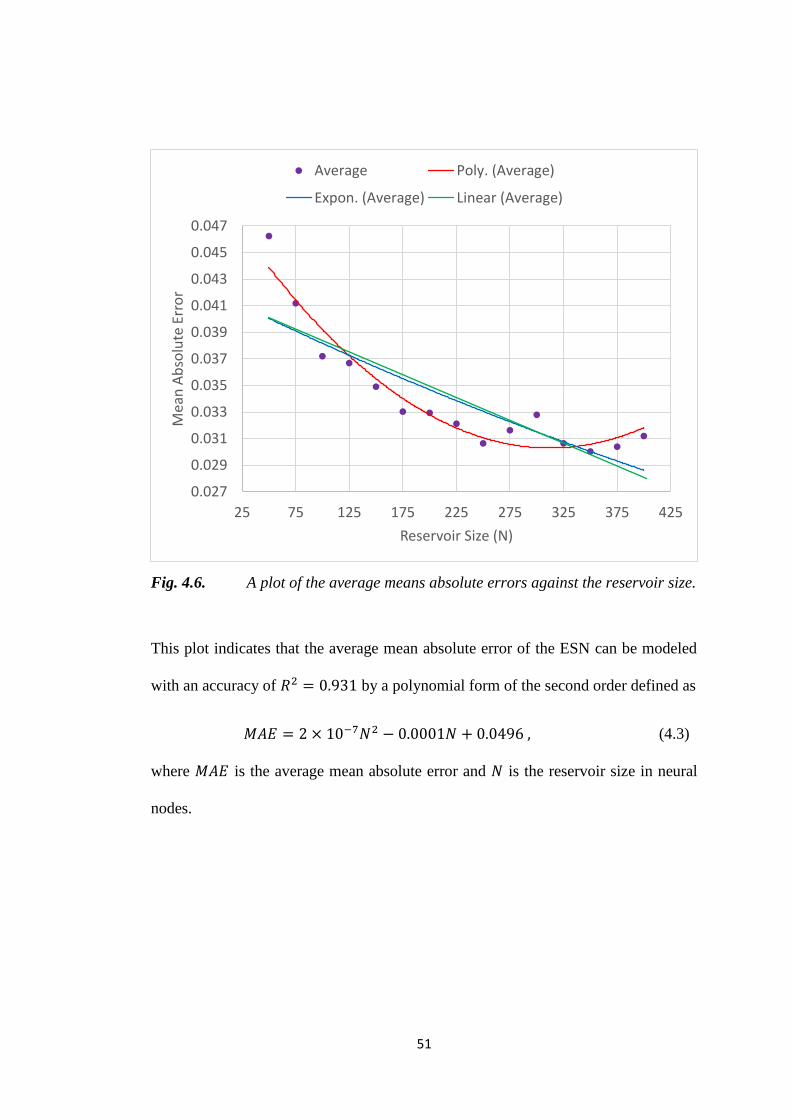
51

Fig. 4.6. A plot of the average means absolute errors against the reservoir size.

This plot indicates that the average mean absolute error of the ESN can be modeled

with an accuracy of 𝑅2 = 0.931 by a polynomial form of the second order defined as

𝐴𝐸 = 2 × 10−7𝑁2 − 0.0001𝑁 + 0.0496 , (4.3)

where 𝐴𝐸 is the average mean absolute error and 𝑁 is the reservoir size in neural

nodes.

0.027

0.029

0.031

0.033

0.035

0.037

0.039

0.041

0.043

0.045

0.047

25 75 125 175 225 275 325 375 425

Me

an A

bso

lute

Err

or

Reservoir Size (N)

Average Poly. (Average)

Expon. (Average) Linear (Average)

52

4.3 Statistical Results

Table 4.4 shows the statistical results of the SVR and ESN models for the radio

propagation environments of Eenhana, Ongwediva and Ruacana. Here, 𝜎 denotes the

standard deviation of the absolute errors. In places where the result is better, it has

been bolded.

Table 4.4 Statistical Comparison of the SVR and ESN model.

Ongwediva Eenhana Ruacana Average

ESN SVR ESN SVR ESN SVR ESN SVR

R2 0.932 0.874 0.714 0.413 0.812 0.658 0.819 0.648

MAE 0.0312 0.0578 0.0278 0.0623 0.0345 0.0672 0.0312 0.0624

σ 0.0428 0.0432 0.0469 0.0471 0.0522 0.0510 0.0473 0.0471

Training

Complexity

(ms)

208 12.9 939 10.1 82.7 1.14 410 8.19

Testing

Complexity

(ms)

49.3 1.37 182 1.25 6.03 0.499 79.0 1.04

The metrics indicate that the SVR model has a better performance in terms of

computation complexities with an average training complexity of 8.19 ms and an

average testing complexity of 1.04 ms, as compared to the ESN model which has an

average training complexity of 410 ms and an average testing complexity of 79.0 ms.

On the other hand, in terms of accuracy, the ESN model proves to be slightly more

accurate and gives the least error measure as it provides an overall average R2-score

of 0.819 and an overall MAE of 0.0312, as compared to an overall average R2-score

of 0.648 and an overall average MAE of 0.0624 yielded by the SVR model. In addition,

the F-Test discussed in section 4.4.1 confirms that the ESN model is statistically better

than the SVR model in terms of the goodness of fit.

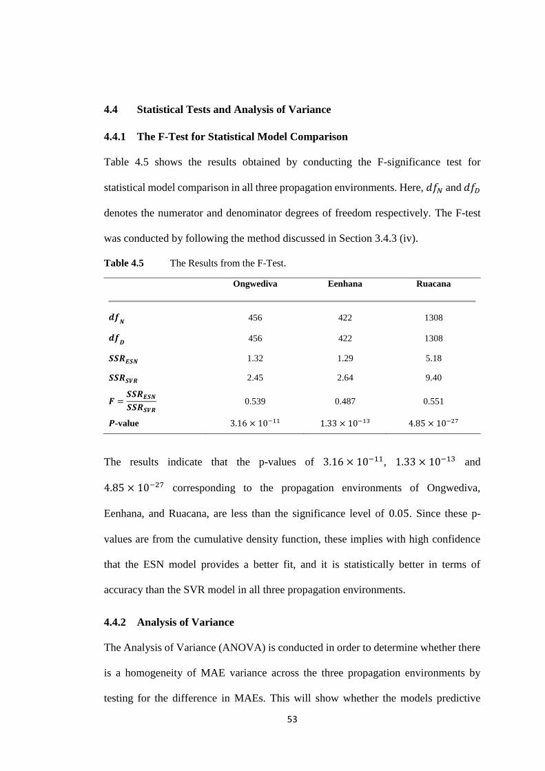
53

4.4 Statistical Tests and Analysis of Variance

4.4.1 The F-Test for Statistical Model Comparison

Table 4.5 shows the results obtained by conducting the F-significance test for

statistical model comparison in all three propagation environments. Here, 𝑑𝑓𝑁 and 𝑑𝑓𝐷

denotes the numerator and denominator degrees of freedom respectively. The F-test

was conducted by following the method discussed in Section 3.4.3 (iv).

Table 4.5 The Results from the F-Test.

Ongwediva Eenhana Ruacana

𝒅𝒇𝑵

456 422 1308

𝒅𝒇𝑫

456 422 1308

𝑺𝑺𝑹𝑬𝑺𝑵 1.32 1.29 5.18

𝑺𝑺𝑹𝑺𝑽𝑹 2.45 2.64 9.40

𝑭 =𝑺𝑺𝑹𝑬𝑺𝑵

𝑺𝑺𝑹𝑺𝑽𝑹

0.539 0.487 0.551

𝑷-value 3.16 × 10−11 1.33 × 10−13 4.85 × 10−27

The results indicate that the p-values of 3.16 × 10−11, 1.33 × 10−13 and

4.85 × 10−27 corresponding to the propagation environments of Ongwediva,

Eenhana, and Ruacana, are less than the significance level of 0.05. Since these p-

values are from the cumulative density function, these implies with high confidence

that the ESN model provides a better fit, and it is statistically better in terms of

accuracy than the SVR model in all three propagation environments.

4.4.2 Analysis of Variance

The Analysis of Variance (ANOVA) is conducted in order to determine whether there

is a homogeneity of MAE variance across the three propagation environments by

testing for the difference in MAEs. This will show whether the models predictive

54

accuracy is the same across different environments. The ANOVA results for the ESN

is discussed in sub-section (i) and that of the SVR is discussed in sub-section (ii) of

this section.

i) Single Factor ANOVA on ESN Absolute Errors

The summary of descriptive statistics for the absolute errors in Table 4.6 show that the

assumption of equality of variance in all the groups is met, and all three propagation

environments have an absolute error variance of 0.02.

Table 4.6 Statistical Summary of the absolute deviations for the ESN model.

Groups Counts Sum Average Variance

Eenhana 433 12.002 0.028 0.002

Ongwediva 433 13.314 0.031 0.002

Ruacana 433 14.491 0.033 0.002

This assumption was also confirmed by the O’Brien Test for homogeneity of variance

in Table 4.7, yielding a p-value of 0.838 which is much higher than the significance

level of 0.05.

Table 4.7 O'Brien Test for Homogeneity of Variance for ESN.

Source of Variation SS 𝐝𝐟 MS F P-value

Treatment 3.858 × 10−5 2 1.929

× 10−5

0.177 0.838

Error 0.141 1296 1.09 × 10−4

Total 0.141 1298

55

The single factor ANOVA on absolute errors results in Table 4.8 for the test of the

difference in MAEs of the ESN model in the propagation environments of Ongwediva,

Eenhana and Ruacana, yields a p-value of 0.172 which is greater than the significance

level of 0.05. This implies with high confidence that there is no significant difference

in the MAEs of the ESN model and therefore there is a homogeneity of MAEs across

the three propagation environments.

Table 4.8 ESN ANOVA Results for the difference in MAEs.

Source of Variation SS 𝐝𝐟 MS F P-value

Treatment 0.007 2 0.004 1.761 0.172

Error 2.635 1296 0.002

Total 2.642 1298

In addition, this fact is also confirmed by the results of the Turkey Honestly Significant

Difference (HSD) for Post-hoc analysis in Table 4.9. Here, it can be noted that all the

three q-statistics of 1.398, 2.652 and 1.254 corresponding to each pair are below the

q-critical value of 3.318, and thus implying that there is no significant difference at a

95% confidence level.

Table 4.9 Tukey HSD – Table of q-statistics for ESN model.

Eenhana Ongwediva Ruacana

Eenhana 0 1.398 2.652

Ongwediva 0 1.254

Ruacana 0

KEY: 𝑝 < 0.05 (𝑞 − 𝑐𝑟𝑖𝑡𝑖𝑐𝑎𝑙[3, 1296] = 3.31836468968)

56

ii) Single Factor ANOVA on SVR Absolute Errors

The summary of descriptive statistics in Table 4.10 does not clarify that the assumption

of equality of variance in all the groups is met. However, this assumption is confirmed

by the O’Brien Test for homogeneity of variance in Table 4.11, yielding a p-value of

0.361 which is higher than the significance level of 0.05.

Table 4.10 Statistical Summary of the absolute deviations for the SVR.

Groups Counts Sum Average Variance

Eenhana 433 26.970 0.062 0.002

Ongwediva 433 24.643 0.057 0.001

Ruacana 433 30.202 0.070 0.003

Table 4.11 O'Brien Test for Homogeneity of Variance for SVR.

Source of Variation SS 𝐝𝐟 MS F P-value

Treatment 6.109 × 10−4 2 3.054

× 10−4

1.021 0.361

Error 0.388 1296 2.992

× 10−4

Total 0.388 1298

In addition, the single factor ANOVA results in Table 4.12 yields a p-value of

4.036 × 10−4 which is much less than the significance level of 0.05.

57

Table 4.12 SVR ANOVA Results for the difference in MAEs.

Source of Variation SS 𝐝𝐟 MS F P-value

Treatment 0.036 2 0.018 7.862 4.036

× 10−4

Error 2.967 1296 0.002

Total 3.003 1298

This implies that there is a significant difference in the MAEs of at least two groups

(propagation environments), and it does not provide sufficient information in order to

identify which means are unequal. However, the results from the Tukey’s HSD for

post-hoc analysis in Table 4.13 show that the difference in the MAEs lies between the

propagation environments of Ongwediva and Ruacana, giving a q-statistic of 5.583

that is much greater than the q-critical value of 3.318 for the significance level of 0.05.

Table 4.13 Tukey HSD – Table of q-statistics for SVR model.

Eenhana Ongwediva Ruacana

Eenhana 0 2.337 3.246

Ongwediva 0 5.583

Ruacana 0

KEY: 𝑝 < 0.05 (𝑞 − 𝑐𝑟𝑖𝑡𝑖𝑐𝑎𝑙[3, 1296] = 3.31836468968)

58

CHAPTER 5: CONCLUSIONS AND RECOMMENDATIONS

5.1 Conclusions

In this thesis, a method for predicting radio signal strength using ESN is proposed and

applied to three different locations in Northern Namibia. The ESN’s performance is

compared with the SVR method adopted from literature and optimized for radio

propagation modeling. Simulation results show that the ESN method gives a better

prediction accuracy in terms of goodness of fit and error measure criteria, i.e. an

average R2 of 0.82 and average MAE of 0.0312 for ESN, as compared to 0.648 and

0.0624 for SVR respectively. However, the ESN approach is inferior to the SVR

method in terms of computation time complexities as the ESN yields an average

training complexity of 410 ms and an average testing complexity of 79.0 ms as

compared to an average of 8.19 ms and 1.04 ms for SVR respectively. In addition, the

results from the F-Test also indicates that the ESN method provides a significantly

better fit than the SVR method in all three propagation environments. Furthermore,

the results from the Analysis of Variance (ANOVA) on ESN absolute errors show that

there is a homogeneity of MAEs across all the propagation environments.

5.2 Recommendation for future work

The work discussed in this thesis did not consider the propagation channel’s time

varying property. Thus, further work can be conducted in order to determine the

distributions of the radio signal strength with respect to time for each data point. These

distributions can then be incorporated in conjunction with the ESN to make the

predictions of radio signal strength more accurate.

59

REFERENCES

[1] N. Gupta, “Introduction to Wireless Communication,” in Inside Bluetooth Low Energy,

N. Gupta, Ed. London: Artech House Mobile Communications, 2013.

[2] E. Ostlin, H.-J. Zepernick, and H. Suzuki, “Macrocell path-loss prediction using

artificial neural networks,” IEEE Trans. Veh. Technol., vol. 59, no. 6, pp. 2735–2747,

2010.

[3] V. Modi, “Radio Wave Propagation,” IOSR J. Electron. Commun. Eng., vol. 9, no. 1,

pp. 17–19, 2014.

[4] F. J. Oluwole and O. Y. Olajide, “MATLAB Graphical User Interface ( GUI ) for

Wireless Metropolitan Area Network Optimum Performance Okumura-Hata,” Int. J.

Sci. Technol., vol. 2, no. 6, pp. 429–432, 2013.

[5] Radiocommunication Sector of ITU, “Rec. ITU-R P.1546-5: Method for point-to-area

predictions for terrestrial services in the frequency range 30 MHz to 3000 MHz,”

Geneva, 2013.

[6] J. M. Mom, C. O. Mgbe, and G. A. Igwue, “Application of Artificial Neural Network

For Path Loss Prediction In Urban Macrocellular Environment,” Am. J. Eng. Res., vol.

3, no. 2, pp. 270–275, 2014.

[7] A. J. Smola, B. Sch, and B. Schölkopf, “A Tutorial on Support Vector Regression,”

Stat. Comput., vol. 14, no. 3, pp. 199–222, 2004.

[8] Y. Baştanlar and M. Ozuysal, “Introduction to machine learning.,” Methods Mol. Biol.,

vol. 1107, pp. 105–28, 2014.

[9] D. J. C. MacKay, Information Theory, Inference, and Learning Algorithms David J.C.

MacKay, vol. 100. 2005.

[10] L. Azpilicueta, M. Rawat, and K. Rawat, “A Ray Launching-Neural Network

Approach for Radio Wave Propagation Analysis in Complex Indoor Environments,”

IEEE Trans. Antennas Propag., vol. 62, no. 5, pp. 2777–2786, 2014.

[11] K. Shi, Z. Ma, R. Zhang, W. Hu, and H. Chen, “Support Vector Regression Based

Indoor Location in IEEE 802.11 Environments,” Mob. Inf. Syst., vol. Volume 201, no.

Article ID 295652, p. 14 pages, 2015.

[12] R. D. a Timoteo, D. C. Cunha, and G. D. C. Cavalcanti, “A Proposal for Path Loss

Prediction in Urban Environments using Support Vector Regression,” in Advanced

International Conference on Telecommunications, 2014, vol. 10, no. c, pp. 119–124.

[13] S. P. Sotiroudis, K. Siakavara, and J. N. Sahalos, “A Neural Network Approach to the

Prediction of the Propagation Path-loss for Mobile Communications Systems in Urban

Environments,” PIERS Online, vol. 3, no. 8, pp. 1175–1179, 2007.

[14] A. Sarka, S. Majumdar, and P. P. Bhattacharya, “Path Loss Estimation for a Wireless

Sensor Network for Application in Ship,” Int. J. Comput. Sci. Mob. Comput., vol. 2,

no. 6, pp. 87–96, 2013.

[15] L. Q. L. Qiu, D. J. D. Jiang, and L. Hanlen, “Neural network prediction of radio

propagation,” 2005 Aust. Commun. Theory Work., pp. 1–6, 2005.

60

[16] M. Lukoševičius, H. Jaeger, and B. Schrauwen, “Reservoir Computing Trends,” KI -

Künstliche Intelligenz, vol. 26, no. 4, pp. 365–371, 2012.

[17] M. Lukoševičius, “A practical guide to applying echo state networks,” in Neural

Networks: Tricks of the Trade, 2nd ed., vol. 7700, G. Montavon, G. B. Orr, and K.-R.

Müller, Eds. Berlin Heidelberg: Springer, 2012, pp. 659–686.

[18] M. Cernanský and P. Tino, “Predictive modeling with echo state networks,” Artif.

Neural Networks-ICANN 2008, no. 2, 2008.

[19] E. Rodriguez, “Training Echo State Networks with Short Segments of Motion Capture

Data,” Jacobs University Bremen, 2013.

[20] “Description of GSM Field Test,” 2011. [Online]. Available:

http://signalmonitoring.com/en/gsm-field-test-description. [Accessed: 16-Mar-2016].

[21] “RF Explorer.” [Online]. Available: http://j3.rf-explorer.com/. [Accessed: 16-Feb-

2016].

[22] Pew Research Center, “Smartphone Ownership and Internet Usage Continues to Climb

in Emerging Economies,” 2016.

[23] T. J. Barnett, A. Sumits, S. Jain, and U. Andra, “Cisco Visual Networking Index:

Global Mobile Data Traffic Forecast Update, 2015–2020 White Paper,” San Jose, CA,

2016.

[24] J. Zander, S.-L. Kim, M. Almgren, and O. Queseth, Radio Resource Management for

Wireless Networks. Norwood, MA, USA: Artech House, Inc., 2001.

[25] J. Burbank, W. Kasch, and J. Ward, “Modeling and Simulation for RF Propagation,”

An Introduction to Network Modeling and Simulation for the Practicing Engineer, no.

December. pp. 20–50, 2009.

[26] C. Phillips, D. Sicker, and D. Grunwald, “A Survey of Wireless Path Loss Prediction

and Coverage Mapping Methods,” IEEE Commun. Surv. Tutorials, vol. 15, no. 1, pp.

255–270, 2013.

[27] C. Temaneh-Nyah and J. Nepembe, “Determination of a Suitable Correction Factor to

a Radio Propagation Model for Cellular Wireless Network Analysis,” in 2014 5th

International Conference on Intelligent Systems, Modelling and Simulation, 2014, pp.

175–182.

[28] I. A. Vinter, N. I. Korolev, A. N. Krenev, N. I. Leshkov, V. A. Timofiev, and E. G.

Tseganov, “Geoinformation System of Planning and Analysis of Radio Networks.”

Yaroslave State University, p. 88c, 1999.

[29] A. Hrovat, G. Kandus, and T. Javornik, “A Survey of radio propagation modeling for

tunnels,” IEEE Commun. Surv. Tutorials, vol. 16, no. 2, pp. 658–669, 2014.

[30] S. A. Mawjoud, “Path Loss Propagation Model Prediction for GSM Network

Planning,” vol. 84, no. 7, pp. 30–33, 2013.

[31] J. Nepembe, “DETERMINING A CORRECTION FACTOR FOR A RADIO WAVE

PROPAGATION MODEL TO FIT HIDAS ( WINDHOEK , NAMIBIA ),” University

of Namibia, 2013.

61

[32] P. W. Glynn, “Introduction to Stochastic Modeling.” Stanford University, pp. 1–22,

2014.

[33] J. P. Kermoal, L. Schumacher, K. I. Pedersen, P. E. Mogensen, and F. Frederiksen, “A

Stochastic MIMO Radio Channel Model With Experimental Validation,” IEEE J. Sel.

Areas Commun., vol. 20, no. 6, pp. 1211–1226, 2002.

[34] G. K. Karagiannidis, N. C. Sagias, and P. T. Mathiopoulos, “N*Nakagami: A novel

stochastic model for cascaded fading channels,” IEEE Trans. Commun., vol. 55, no. 8,

pp. 1453–1458, 2007.

[35] Ž. Živković, I. Mihajlović, and Đ. Nikolić, “Artificial Neural Network Method Applied

On The Nonlinear Multivariate Problem,” Serbian J. Manag., vol. 4, no. 2, pp. 143–

155, 2009.

[36] I. Fernández Anitzine, J. A. Romo Argota, and F. P. Fontán, “Influence of training set

selection in artificial neural network-based propagation path loss predictions,” Int. J.

Antennas Propag., vol. 2012, pp. 1–7, 2012.

[37] C. O. Mgbe, J. M. Mom, and G. A. Igwue, “Performance Evaluation of Generalized

Regression Neural Network Path loss Prediction Model in Macrocellular

Environment,” J. Multidiscip. Eng. Sci. Technol., vol. 2, no. 2, pp. 204–208, 2015.

[38] “Support Vector Machines (SVM),” StatSoft, 2017. .

[39] C.-C. Chang and C.-J. Lin, “LIBSVM: A library for support vector machines,” ACM

Trans. Intell. Syst. Technol., vol. 2, no. 3, p. 27:1--27:27, 2011.

[40] D. Tomar and S. Agarwal, “Twin Support Vector Machine: A review from 2007 to

2014,” Egypt. Informatics J., vol. 16, no. 1, pp. 55–69, Mar. 2015.

[41] R.-E. Fan, P.-H. Chen, and C.-J. Lin, “Working Set Selection Using Second Order

Information for Training Support Vector Machines,” J. Mach. Learn. Res., vol. 6, pp.

1889–1918, 2005.

[42] Y.-J. Lee, W.-F. Hsieh, and C.-M. Huang, “epsilon-SSVR: A Smooth Support Vector

Machine for epsilon-Insensitive Regression,” IEEE Trans. Knowl. Data Eng., vol. 17,

no. 5, pp. 678–685, May 2005.

[43] W.-C. Hong, “A hybrid support vector machine regression for exchange rate

prediction,” Int. J. Inf. Manag. Sci., vol. 17, no. 2, pp. 19–32, 2006.

[44] P.-Y. Hao, “New support vector algorithms with parametric insensitive/margin

model.,” Neural Netw., vol. 23, no. 1, pp. 60–73, Jan. 2010.

[45] P. Voigtlaender, P. Doetsch, S. Wiesler, and R. Schl, “SEQUENCE-

DISCRIMINATIVE TRAINING OF RECURRENT NEURAL NETWORKS Human

Language Technology and Pattern Recognition , Computer Science Department ,

RWTH Aachen University , Aachen , Germany LIMSI CNRS , Spoken Language

Processing Group , Paris , France,” Icassp, no. 2, pp. 4565–4569, 2015.

[46] J. Schmidhuber, “Recurrent Neural Networks,” 2015. [Online]. Available:

http://people.idsia.ch/~juergen/rnn.html. [Accessed: 16-Feb-2016].

[47] B. Galbraith, “Spiking Neural Networks in Python (Part 1),” Neurdon, 2011. [Online].

Available: http://www.neurdon.com/2011/03/06/spiking-neural-networks-in-python-

part-1/comment-page-1/. [Accessed: 16-Feb-2016].

62

[48] D. Brezak, T. Bacek, and D. Majetic, “A comparison of feed-forward and recurrent

neural networks in time series forecasting,” in 2012 IEEE Conference on

Computational Intelligence for Financial Engineering & Economics (CIFEr), 2012,

pp. 1–6.

[49] M. Han and M. Xu, “Predicting Multivariate Time Series Using Subspace Echo State

Network,” Neural Process. Lett., vol. 41, no. 2, pp. 201–209, 2015.

[50] H. Jaeger, “Echo state network,” Scholarpedia, vol. 2, no. 9, p. 2330, 2007.

[51] P. Yu, L. Miao, and G. Jia, “Clustered complex echo state networks for traffic

forecasting with prior knowledge,” in Instrumentation and Measurement Technology

Conference (I2MTC), 2011 IEEE, 2011, pp. 1–5.

[52] J. Ho, “The Wiener-Hopf Method and Its Applications in Fluids,” The University of

Melbourne Department, 2007.

[53] X. Liu and C. Bao, “Audio Bandwidth Extension Based on Ensemble Echo State

Networks with Temporal Evolution,” IEEE/ACM Trans. Audio, Speech, Lang.

Process., vol. 24, no. 3, pp. 594–607, Mar. 2016.

[54] J. Bozsik and Z. Ilonczai, “Echo state network-based credit rating system,” in 2012 4th

IEEE International Symposium on Logistics and Industrial Informatics, 2012, pp. 185–

190.

[55] Z. Xu, J. Wan, F. Su, and Y. Xue, “Analysis of detecting target in sea clutter using

decoupled echo state network,” in 2012 IEEE International Conference on Computer

Science and Automation Engineering, 2012, pp. 492–495.

[56] A. Rodan and P. Tino, “Minimum complexity echo state network,” IEEE Trans. Neural

Networks, vol. 22, no. 1, pp. 131–144, 2011.

[57] M. J. A. Rabin, M. S. Hossain, M. S. Ahsan, M. A. S. Mollah, and M. T. Rahman,

“Sensitivity learning oriented nonmonotonic multi reservoir echo state network for

short-term load forecasting,” in International Conference on Informatics, Electronics

Vision (ICIEV), 2013, 2013, pp. 1–6.

[58] J. W. Osborne and A. Overbay, “The power of outliers (and why researchers should

always check for them),” Pract. Assessment, Res. Eval., vol. 9, no. 6, 2004.

[59] C. F. F. Karney, “Algorithms for geodesics,” J. Geod., vol. 87, no. 1, pp. 43–55, 2013.

[60] T. Vincenty, “Direct and Inverse Solutions of Geodesics on the Ellipsoid with

application of nested equations,” Surv. Rev., vol. 33, no. 176, pp. 88–93, 1975.

[61] C. F. F. Karney, “Geodesics on an ellipsoid of revolution,” J. Geod., p. 29, 2011.

[62] Y.-C. Lee, “The Accuracy Analysis of Methods to solve the Geodetic Inverse

Problem,” J. Korean Soc. Surv. Geod. Photogramm. Cartogr., vol. 29, no. 4, pp. 329–

341, 2011.

[63] C.-L. Chen, T.-P. Hsu, and J.-R. Chang, “A Novel Approach to Great Circle Sailings:

The Great Circle Equation,” J. Navig., vol. 57, no. 2, pp. 311–320, 2004.

[64] W.-K. Tseng and H.-S. Lee, “The Vector Function for Distance Travelled in Great

Circle Navigation,” J. Navig., vol. 60, no. 1, pp. 158–164, 2007.

63

[65] S. G. K. Patro and K. K. Sahu, “Normalization: A Preprocessing Stage,” arXiv Prepr.

arXiv1503.06462, 2015.

[66] D. Verstraeten, B. Schrauwen, S. Dieleman, P. Brakel, P. Buteneers, and D. Pecevski,

“Oger: Modular Learning Architectures For Large-Scale Sequential Processing,” J.

Mach. Learn. Res., vol. 13, p. 2995−2998, 2012.

[67] F. Pedregosa, G. Varoquaux, A. Gramfort, V. Michel, B. Thirion, O. Grisel, M.

Blondel, P. Prettenhofer, R. Weiss, V. Dubourg, J. Vanderplas, A. Passos, D.

Cournapeau, M. Brucher, M. Perrot, and É. Duchesnay, “Scikit-learn: Machine

Learning in Python,” J. Mach. Learn. Res., vol. 12, pp. 2825–2830, 2012.

[68] G. van Rossum, “Python Reference Manual.” PythonLabs, Virginia, USA, 2001.

[69] K. J. Millman and M. Aivazis, “Python for Scientists and Engineers,” Comput. Sci.

Eng., vol. 13, no. 2, pp. 9–12, Mar. 2011.

[70] M. C. Wilson, “Overview of Sattolo’s Algorithm,” in Algorithms Seminar 2002–2004,

2005, pp. 105–108.

[71] J. Bergstra and Y. Bengio, “Random Search for Hyper-Parameter Optimization,” J.

Mach. Learn. Res., vol. 13, pp. 281–305, 2012.

[72] M. Claesen, J. Simm, D. Popovic, Y. Moreau, and B. De Moor, “Easy Hyperparameter

Search Using Optunity,” arXiv Prepr. arXiv1412.1114, pp. 1–5, 2014.

[73] M. Claesen, B. L. R. De Moor, J. Simm, and D. Popovic, “Hyperparameter tuning in

Python using Optunity,” in Proceedings of the International Workshop on Technical

Computing for Machine Learning and Mathematical Engineering, 2014, pp. 6–7.

[74] M. Claesen and B. De Moor, “Hyperparameter Search in Machine Learning,” in 11th

Metaheuristics International Conference, 2015, pp. 10–14.

[75] J. Bergstra, R. Bardenet, Y. Bengio, and B. Kegl, “Algorithms for Hyper-Parameter

Optimization,” in 25th Annual Conference on Neural Information Processing Systems

(NIPS 2011), 2011, pp. 2546–2554.

[76] J. Bergstra, D. Yamins, and D. Cox, “Making a science of model search,” arXiv Prepr.

arXiv1209.5111, pp. 1–11, 2012.

[77] M. Browne, “Cross-Validation Methods.,” J. Math. Psychol., vol. 44, no. 1, pp. 108–

132, Mar. 2000.

[78] G. Seni and J. F. Elder, “Ensemble methods in data mining: improving accuracy

through combining predictions,” Synth. Lect. Data Min. Knowl. Discov., vol. 2, no. 1,

pp. 1–126, 2010.

[79] G. James, D. Witten, T. Hastie, and R. Tibshirani, An Introduction to Statistical

Learning, vol. 64, no. 9–12. Springer, 2013.

[80] J.-R. Kurz-Kim and M. Loretan, “On the properties of the coefficient of determination

in regression models with infinite variance variables,” J. Econom., vol. 181, no. 1, pp.

15–24, Jul. 2014.

[81] X. Peng, D. Xu, L. Kong, and D. Chen, “L1-norm loss based twin support vector

machine for data recognition,” Inf. Sci. (Ny)., vol. 340–341, pp. 86–103, May 2016.

64

[82] D. E. Ramirez, “The Generalized F Distribution,” J. Stat. Softw., vol. 5, no. 1, pp. 1–

14, 2000.

[83] L. Zhang, J. H. Gove, and L. S. Heath, “Spatial residual analysis of six modeling

techniques,” Ecol. Modell., vol. 186, no. 2, pp. 154–177, Aug. 2005.

[84] E. Deschepper, O. Thas, and J. P. Ottoy, “Regional residual plots for assessing the fit

of linear regression models,” Comput. Stat. Data Anal., vol. 50, no. 8, pp. 1995–2013,

Apr. 2006.

[85] A. Small, “Scientific Python for Both Expert and Novice Programmers,” Comput. Sci.

Eng., vol. 14, no. 2, pp. 6–7, Mar. 2012.

[86] H. R. Lindman, “Two-Way Analysis of Variance,” in Analysis of Variance in

Experimental Design, New York: Springer, 1992, pp. 93–125.

[87] M. G. Larson, “Analysis of variance,” Circulation, vol. 117, no. 1, pp. 115–121, 2008.

[88] J. Vanderplas, “Pivot Tables in Python,” in Python Data Science Handbook, O’Reilly

Media, 2015, p. 546.

[89] H. Abdi and L. J. Williams, “Tukey’s honestly significant difference (HSD) test,”

Encycl. Res. Des. Thousand Oaks, CA Sage, vol. 1, pp. 1–5, 2010.

65

APPENDICES

Appendix A: Data Preprocessing – Part 1

# -*- coding: utf-8 -*-

"""

Created on Mon Aug 08 05:37:02 2016

@author: kgideon

"""

import csv

import googlemaps

from geopy.distance import vincenty

google_api_key = 'AIzaSyBFZGIjqlvwEdwszjJQrt_Y0g_2m-G8oeM'

gmaps = googlemaps.Client(key= google_api_key)

def azimuth_angle(A, B):

from math import radians, degrees, cos, sin, atan2

lat_a, lon_a = A

lat_b, lon_b = B

dLon = radians(lon_b - lon_a)

lat1 = radians(lat_a)

lat2 = radians(lat_b)

y = sin(dLon) * cos(lat2)

x = cos(lat1)* sin(lat2) - sin(lat1) * cos(lat2)* cos(dLon)

return degrees(atan2(y, x))

def elevation_angle(dpalt, ctalt, d):

from math import atan, degrees

ctah = float(ctalt)

dpah = float(dpalt)

hd = ctah - dpah

return degrees(atan(hd/d))

with open('datasets/ongwediva_2016-09-18_raw.csv') as original_csvfile:

reader = csv.DictReader(original_csvfile)

with open('datasets/ongwediva_2016-09-18_processed.csv', 'w') as preprocessed_csvfile:

fieldnames = ['DPLat', 'DPLon', 'DPEl', 'DPRating', 'CTLat', 'CTLon', 'CTEl', 'RSSI', 'Type', 'Distance', 'ElevAngle',

'AzimAngle']

writer = csv.DictWriter(preprocessed_csvfile, fieldnames=fieldnames)

writer.writeheader()

i = 0

for row in reader:

LAC = row['LAC/TAC']

CID = row['Cell ID']

DPLat = row['DPLAT']

DPLon = row['DPLON']

CTLat = row['CTLAT']

CTLon = row['CTLON']

RSSI = row['RSSI']

Type = row['Type']

DPRating = row['Accuracy']

#find elevation of data point and of cell tower using Google Elevation API

elev_data = gmaps.elevation({(float(DPLat), float(DPLon)), (float(CTLat), float(CTLon))})

dp_elev_data = elev_data[0]

ct_elev_data = elev_data[1]

DPEl = 1.5 + dp_elev_data['elevation']

CTEl = 15.0 + ct_elev_data['elevation']

# Find propagation path distance, path elevation angle, and path azimuth angles

AzimAngle = azimuth_angle((float(DPLat), float(DPLon)), (float(CTLat), float(CTLon)))

66

Distance = vincenty((float(DPLat), float(DPLon)), (float(CTLat), float(CTLon))).meters

ElevAngle = elevation_angle(DPEl, CTEl, Distance)

i = i + 1

print 'writing row: ', i

writer.writerow({'DPLat': DPLat, 'DPLon': DPLon, 'DPEl': DPEl,'DPRating': DPRating, 'CTLat': CTLat,

'CTLon': CTLon, 'CTEl': CTEl,'RSSI': RSSI,'Type': Type, 'Distance': Distance,

'ElevAngle': ElevAngle, 'AzimAngle': AzimAngle})

67

Appendix B: Data Preprocessing – Part 2

# -*- coding: utf-8 -*-

"""

Created on Wed Aug 10 19:06:45 2016

@author: kgideon

"""

import csv

import googlemaps

from geopy.distance import vincenty

google_api_key_2 = "AIzaSyCgn0I4lpadd2aJXDN4Apnj4pKewFWSPwo"

gmaps = googlemaps.Client(key=google_api_key)

with open('datasets/ongwediva_2016-09-18_processed.csv') as original_csvfile:

reader = csv.DictReader(original_csvfile)

with open('datasets/ongwediva_2016-09-18_processed_full.csv', 'w') as preprocessed_csvfile:

fieldnames = ['DPLat', 'DPLon', 'DPALT', 'DPRating', 'CTLat', 'CTLon', 'CTALT', 'RSSI', 'Type', 'Distance', 'MOH',

'AOH', 'dOH', 'DPOH', 'CTOH', 'RCF', 'ElevAngle', 'AzimAngle']

writer = csv.DictWriter(preprocessed_csvfile, fieldnames=fieldnames)

writer.writeheader()

i = 0

for row in reader:

DPLat = row['DPLat']

DPLon = row['DPLon']

RSSI = row['RSSI']

Type = row['Type']

DPRating = row['DPRating']

CTLat = row['CTLat']

CTLon = row['CTLon']

DPALT = row['DPEl']

CTALT = row['CTEl']

AzimAngle = row['AzimAngle']

Distance = row['Distance']

ElevAngle = row['ElevAngle']

# Find the radio carier frequency

if Type == 'LTE':

RCF = '1800'

elif (Type == 'UMTS') or (Type == 'HSDPA') or (Type == 'HSPA') or (Type == 'HSPA+'):

RCF = '2100'

else:#if (Type == 'GPRS') or (Type == 'EDGE') or (Type == 'GSM'):

RCF = '900'

#

max_lat = 0 # lat value of the maximum obstructing height

max_lon = 0 # lon value of the maximum obstructing height

MOH = 0.0

AOH = 0.0

a_cor = {'a0': 0.0, 'a1': 0.0, 'a2': 0.0, 'a3': 0.0, 'a4': 0.0}

b_cor = {'b0': 0.0, 'b1': 0.0, 'b2': 0.0, 'b3': 0.0, 'b4': 0.0}

elevations = {'p0': 0.0, 'p1': 0.0, 'p2': 0.0, 'p3': 0.0, 'p4': 0.0}

N = 5 # number of sampled points

x = (float(CTLon) - float(DPLon)) / N # unit distance along the Lat1 axis

y = (float(CTLat) - float(DPLat)) / N # unit distance along the Lon2 axis

for j in [0,1,2,3,4]:

a_cor['a' + str(j)] = x*(i + 1) + float(DPLon)

b_cor['b' + str(j)] = y*(i + 1) + float(DPLat)

# Find MOH, AOH, gps coor of MOH

68

elev_data = gmaps.elevation({(b_cor['b0'], a_cor['a0']), (b_cor['b1'], a_cor['a1']),(b_cor['b2'], a_cor['a2']),

(b_cor['b3'], a_cor['a3']),(b_cor['b4'], a_cor['a4'])})

for j in [0,1,2,3,4]:

data = elev_data[0]

elevations['p' + str(j)] = data['elevation']

AOH = AOH + (data['elevation'] / N)

if data['elevation'] > MOH:

MOH = data['elevation']

max_lat = b_cor['b' + str(j)]

max_lon = a_cor['a' + str(j)]

# Find dOH, DPOH, and CTOH

dOH = vincenty((float(DPLat), float(DPLon)), (max_lat, max_lon)).meters

DPOH = float(DPALT) - MOH

CTOH = float(CTALT) - MOH

i = i + 1

print 'writing row: ', i

writer.writerow({'DPLat': DPLat, 'DPLon': DPLon, 'DPALT': DPALT,

'DPRating': DPRating, 'CTLat': CTLat, 'CTLon': CTLon, 'CTALT': CTALT,

'RSSI': RSSI,'Type': Type, 'Distance': Distance,

'MOH': MOH, 'AOH': AOH, 'dOH': dOH, 'DPOH': DPOH, 'CTOH': CTOH, 'RCF': RCF,

'ElevAngle': ElevAngle, 'AzimAngle': AzimAngle})

69

Appendix C: Python Simulation Codes

# -*- coding: utf-8 -*-

"""

Created on Wed Jun 01 09:36:11 2016

@author: kgideon

"""

######### Module Imports #########

import time

import csv

import numpy as np

#*************** ESN imports

import mdp

import Oger

import optunity

import optunity.metrics

#*************** SVR imports

from sklearn import svm

####********************* End of Module Imports ***************************####

#

#

#

########################## Functions definitions ################

# min max range scaling function for data normalization

def minMaxNorm(value, maxValue, minValue):

normVal = (value - minValue) / (maxValue - minValue)

return normVal;

# min max range rescaling function for data denormalization

def minMaxDenorm(value, maxValue, minValue):

denormVal = value*maxValue - value*minValue + minValue

return denormVal;

#*********** SVR Function definitions

def fix_svr_data(x_fixed, y_fixed):

@optunity.cross_validated(x=x_fixed, y=y_fixed, num_folds=10, num_iter=2)

def svr_cv(logC, logGamma, x_train, x_test, y_train, y_test):

model = svm.SVR(kernel='rbf', C=10 ** logC, gamma=10 ** logGamma).fit(x_train, y_train.ravel())

y_pred = model.predict(x_test)

return( optunity.metrics.mse(y_test.ravel(), y_pred))

return svr_cv

def getOptimalSVR_Model(optimal_pars, x_dev, y_dev):

model = svm.SVR(kernel='rbf', C=10 ** optimal_pars['logC'], gamma=10 ** optimal_pars['logGamma']).fit(x_dev,

y_dev.ravel())

return model;

#*********** ESN Function definitions

def fix_esn_data(x_fixed, y_fixed):

@optunity.cross_validated(x=x_fixed, y=y_fixed, num_folds=10, num_iter=2)

def esn_cv(N, spectral_radius, input_scaling, leak_rate, x_train, x_test, y_train, y_test):

reservoir = Oger.nodes.LeakyReservoirNode(output_dim = int(100 * N), spectral_radius=spectral_radius,

input_scaling=input_scaling, leak_rate=leak_rate)

readout = Oger.nodes.RidgeRegressionNode(0.001)

flow = mdp.Flow([reservoir, readout])

x_train_list = []

y_train_list = []

num_input_features = len(x_train[0:1 , 0:][0])

for i in range(len(x_train)):

70

x_train_list.append(x_train[i].reshape(1, num_input_features))

y_train_list.append(y_train[i].reshape(1, 1))

x_test_list = []

y_test_list = []

for i in range(len(x_test)):

x_test_list.append(x_test[i].reshape(1, num_input_features))

y_test_list.append(y_test[i].reshape(1, 1))

data = [[], zip(x_train_list, y_train_list)]

flow.train(data)

pred = []

for x in x_test_list:

pred.append(flow(x))

y_pred = np.array(pred)

return( optunity.metrics.mse(y_test, y_pred) )

return esn_cv

def getOptimalESN_Model(optimal_pars, x_dev, y_dev):

reservoir = Oger.nodes.LeakyReservoirNode(output_dim = int(100 * optimal_pars['N']),

spectral_radius=optimal_pars['spectral_radius'], input_scaling=optimal_pars['input_scaling'],

leak_rate=optimal_pars['leak_rate'])

readout = Oger.nodes.RidgeRegressionNode(0.001)

flow = mdp.Flow([reservoir, readout])

x_dev_list = []

y_dev_list = []

num_input_features = len(x_dev[0:1 , 0:][0])

for i in range(len(x_dev)):

x_dev_list.append(x_dev[i].reshape(1, num_input_features))

y_dev_list.append(y_dev[i].reshape(1, 1))

data = [[], zip(x_dev_list, y_dev_list)]

ESN_Training_start = time.clock();

flow.train(data)

ESN_Training_time = (time.clock() - ESN_Training_start );

return flow, float(ESN_Training_time);

#*********** Statistical Function definitions

def Residuals(y_true, y_pred):

e = y_true - y_pred

return e;

# Residual sum of squares

def SS_Residuals(y_true, y_pred):

e = y_true - y_pred

return sum(e**2);

def Adjusted_r_squared(y_true, y_pred, num_params):

p = num_params # no. of input features plus no. of target features

n = len(y_true) # number of data points

r_sq = optunity.metrics.r_squared(y_true, y_pred)

r_bar_sq = r_sq - (1 - r_sq)*((p - 1)/(n - p))

return r_bar_sq;

#

####************************ End of function Defs *************************####

#

71

#

#

########## Importing data #####################

data_path = 'ongwediva_data.csv'

results_path = 'simu_results/ongwediva_results.csv'

# load the data from a csv file into a python list

print "Loading the data from the csv file"

data_obj = open(data_path)

reader = csv.reader(data_obj)

data_list = list(reader)

# Normalizing the categorical variables

x = 0

for row in data_list:

if x != 0:

net_type = row[3]

if net_type == 'UMTS':

data_list[x][3] = 0.1

elif net_type == 'HSDPA':

data_list[x][3] = 0.3

elif net_type == 'HSPA+':

data_list[x][3] = 0.5

elif net_type == 'GPRS':

data_list[x][3] = 0.7

else: # if net_type == 'EDGE':

data_list[x][3] = 0.9

x = x + 1;

# convert the data list into a numpy array

print "converting the data list into a numpy array"

data_array = np.asarray(data_list[1:len(data_list)], dtype=np.float64, order=None)

# Nomalize the data using the min max range scaling

print("Nomalizing the data using the min max range scaling")

data_norm = np.zeros((len(data_array), len(data_array[0])))

for i in xrange(len(data_norm)):

for j in xrange(len(data_array[0])):

if j == 3:

data_norm[i][j] = data_array[i][j]

else:

data_norm[i][j] = minMaxNorm(value=data_array[i][j], maxValue=np.amax(data_array[0:, j: j + 1]),

minValue=np.amin(data_array[0:, j: j + 1]))

print("done")

# Shuffle the normalized dataset randomly

np.random.shuffle(data_norm)

num_input_features = len(data_array[0]) - 1

X_inputs = data_norm[0:, 0:num_input_features] # set of input features

Y_targets = data_norm[0:, num_input_features:] # set of target features

# Split into Development 60% and Testing 40% Datasets

dev_len = int(len(X_inputs) * 0.6)

X_Dev = X_inputs[0: dev_len]

Y_Dev = Y_targets[0: dev_len]

X_Test = X_inputs[dev_len: ]

Y_Test = Y_targets[dev_len: ]

test_arr = np.concatenate((X_Test, Y_Test), axis=1)

test_arr = sorted(test_arr, key=lambda a_entry: a_entry[4])

test_arr = np.array(test_arr)

72

####************************* End of data import **************************####

#

#

#

#############SVR Simulations ###################

print("Simulating using the Support Vector Regression method")

print("Searching for the best SVR hyperparameters")

svr_randomSearch = optunity.solvers.RandomSearch(logC=[-5, 2], logGamma=[-5, 1], num_evals=20)

svr_with_fixed_data = fix_svr_data(X_Dev, Y_Dev)

optimal_svr_pars, _ = svr_randomSearch.minimize(svr_with_fixed_data)

print("optimal hyperparameters: " + str(optimal_svr_pars))

print("Fit optimal SVR with the whole development data set...")

SVR_Training_start = time.clock();

optimalSVR = getOptimalSVR_Model(optimal_svr_pars, X_Dev, Y_Dev)

SVR_Training_time = (time.clock() - SVR_Training_start );

print("done.")

print("Validate optimal SVR with the test data set...")

SVR_Testing_start = time.clock() ;

Y_Pred_SVR = optimalSVR.predict(X_Test)

SVR_Testing_time = (time.clock() - SVR_Testing_start );

####*********************** End of SVR Simulations ************************####

#

#

#

################## ESN Simulations ########################

print("Simulating using the Echo State Network method")

Y_Pred_List = []

X_Test_List = []

for i in range(len(X_Test)):

X_Test_List.append(X_Test[i].reshape(1, len(X_Test[0])))

print("Searching for the best hyperparameters")

esn_randomSearch = optunity.solvers.RandomSearch(N=[1.5, 2.5], spectral_radius=[0.6, 1.3], input_scaling=[0.1,0.5],

leak_rate=[0.1,0.9], num_evals=20)

esn_with_fixed_data = fix_esn_data(X_Dev, Y_Dev)

optimal_esn_pars, _ = esn_randomSearch.minimize(esn_with_fixed_data)

print("optimal hyperparameters: " + str(optimal_esn_pars))

print("Fit optimal ESN with the whole development data set...")

optimalESN, ESN_Training_time = getOptimalESN_Model(optimal_esn_pars, X_Dev, Y_Dev)

print("done.")

print("Validate optimal ESN with the test data set...")

ESN_Testing_start = time.clock()

Y_Pred_List = optimalESN(X_Test_List)

ESN_Testing_time = (time.clock() - ESN_Testing_start );

Y_Pred_ESN = np.array(Y_Pred_List)

####*********************** End of ESN Simulations ************************####

#

Y_Pred_SVR_denorm = np.zeros((len(Y_Test), 1))

Y_Pred_ESN_denorm = np.zeros((len(Y_Test), 1))

Y_Test_denorm = np.zeros((len(Y_Test), 1))

rssi_ = data_array[0: , (len(data_array[0]) - 1):]

rssi_ = rssi_.ravel()

min_val = np.amin(rssi_)

max_val = np.amax(rssi_)

# sorting an array: --> a = ar[ar[:,2].argsort()]

73

# Creating the simulation results file

print "Creating the simulation results csv file"

with open(results_path, 'w') as results_csvfile:

fieldnames = ['DPALT', 'CTALT', 'Type', 'Distance', 'Tilt', 'Azimuth','ESN Norm', 'SVR Norm', 'Actual Norm', 'ESN',

'SVR', 'Actual']

writer = csv.DictWriter(results_csvfile, fieldnames=fieldnames)

writer.writeheader()

for i in xrange(len(Y_Test)):

Y_Pred_SVR_denorm[i] = minMaxDenorm(Y_Pred_SVR[i], max_val, min_val)

Y_Pred_ESN_denorm[i] = minMaxDenorm(Y_Pred_ESN[i], max_val, min_val)

Y_Test_denorm[i] = minMaxDenorm(Y_Test[i], max_val, min_val)

DPALT = X_Test[i][0]

CTALT = X_Test[i][2]

Type = X_Test[i][3]

Distance = X_Test[i][4]

Tilt = X_Test[i][11]

Azimuth = X_Test[i][12]

ESN_norm = np.float64(Y_Pred_ESN[i])

ESN = np.float64(Y_Pred_ESN_denorm[i])

SVR_norm = np.float64(Y_Pred_SVR[i])

SVR = np.float64(Y_Pred_SVR_denorm[i])

Actual_norm = np.float64(Y_Test[i])

Actual = np.float64(Y_Test_denorm[i])

writer.writerow({'DPALT': DPALT, 'CTALT': CTALT, 'Type': Type, 'Distance': Distance, 'Tilt': Tilt, 'Azimuth':

Azimuth,'ESN Norm': ESN_norm, 'SVR Norm': SVR_norm, 'Actual Norm': Actual_norm, 'ESN': ESN, 'SVR': SVR, 'Actual':

Actual})

####********************** End of Simulations ***********************####

74

Appendix D: Python Codes for Data Analysis

# -*- coding: utf-8 -*-

"""

Created on Wed Jun 01 09:36:11 2016

@author: kgideon

"""

########### Module Imports ######################

import csv

import numpy as np

from scipy.stats import f

import optunity

import optunity.metrics

import sklearn.metrics

from pyvttbl import DataFrame # for analysis of variance

#

####*********** End of Module Imports ***********####

#

#

############# Functions definitions #################

#*********** Statistical Function definitions

def Residuals(y_true, y_pred):

e = y_true - y_pred

return e;

# Residual sum of squares

def SS_Residuals(y_true, y_pred):

e = y_true - y_pred

return np.float64(sum(e**2));

def Adjusted_r_squared(y_true, y_pred, num_params):

p = num_params # no. of input features plus no. of target features

n = len(y_true) # number of data points

r_sq = optunity.metrics.r_squared(y_true, y_pred)

r_bar_sq = r_sq - (1 - r_sq)*((p - 1)/(n - p))

return np.float64(r_bar_sq);

#

####*********** End of function Defs **************####

#

#

############ Data imports ##############

#defining the paths

eenha_data_path = 'eenhana_results.csv'

ongwe_data_path = 'ongwediva_results.csv'

ruaca_data_path = 'ruacana_results.csv'

analysis_results_path = 'analysis.csv'

anova_file_path = 'data_for_anova.csv'

#defining the indices

dpalt, ctalt, Type, distance, tilt, azimuth = 0, 1, 2, 3, 4, 5

esn_norm, svr_norm, act_norm = 6, 7, 8

esn_den, svr_den, act_den = 9, 10, 11

#

#load eenhana data into a nympy MxN array

print "Loading simulation results data from Eenhana"

data_obj = open(eenha_data_path)

reader = csv.reader(data_obj)

eenha_data_list = list(reader)

# convert the data list into a numpy array

print "converting Eenhana data list into a numpy array"

75

eenha_arr = np.asarray(eenha_data_list[1:len(eenha_data_list)], dtype=np.float64, order=None)

#

#load Ongwediva data into a nympy MxN array

print "Loading simulation results data from Ongwediva"

data_obj = open(ongwe_data_path)

reader = csv.reader(data_obj)

ongwe_data_list = list(reader)

# convert the data list into a numpy array

print "converting Ongwediva data list into a numpy array"

ongwe_arr = np.asarray(ongwe_data_list[1:len(ongwe_data_list)], dtype=np.float64, order=None)

#

#load Ruacana data into a nympy MxN array

print "Loading simulation results data from Ruacana"

data_obj = open(ruaca_data_path)

reader = csv.reader(data_obj)

ruaca_data_list = list(reader)

# convert the data list into a numpy array

print "converting Ruacana data list into a numpy array"

ruaca_arr = np.asarray(ruaca_data_list[1:len(ruaca_data_list)], dtype=np.float64, order=None)

#

mean_esn_ = np.zeros((3,), dtype=np.float64)

sigma_esn_ = np.zeros((3,), dtype=np.float64)

mean_svr_ = np.zeros((3,), dtype=np.float64)

sigma_svr_ = np.zeros((3,), dtype=np.float64)

print "Creating the analysis results csv file"

with open(analysis_results_path, 'w') as analysis_csvfile:

fieldnames = ['SIGMA-S', 'RSQ-S', 'RBSQ-S', 'MAE-S', 'SSR-S', 'SIGMA-E', 'RSQ-E', 'RBSQ-E', 'MAE-E', 'SSR-E', 'F-

STAT','DF', 'P-VAL']

writer = csv.DictWriter(analysis_csvfile, fieldnames=fieldnames)

writer.writeheader()

#create a file to be used by anova

with open(anova_file_path, 'w') as anova_csvfile:

fieldnames = ['group', 'error_esn', 'error_svr']

awriter = csv.DictWriter(anova_csvfile, fieldnames=fieldnames)

awriter.writeheader()

group = ""

#

for i in np.arange(0,3,1):

if i == 0:

dat_arr = ongwe_arr

group = 'Ongwediva'

print 'Performing data analysis for Ongwediva'

elif i == 1:

dat_arr = eenha_arr

group = 'Eenhana'

print 'Performing data analysis for Eenhana'

else: # i == 2

dat_arr = ruaca_arr

group = 'Ruacana'

print 'Performing data analysis for Ruacana'

############# Data analysis ################

num_params = len(dat_arr[0:1 , 0:][0])

#Calculating the goodness of fit criteriors

R_sq_SVR = optunity.metrics.r_squared(dat_arr[0: , act_norm: act_norm + 1], dat_arr[0: , svr_norm: svr_norm +

1])

R_bar_sq_SVR = Adjusted_r_squared(dat_arr[0: , act_norm: act_norm + 1], dat_arr[0: , svr_norm: svr_norm + 1],

num_params)

76

R_sq_ESN = optunity.metrics.r_squared(dat_arr[0: , act_norm: act_norm + 1], dat_arr[0: , esn_norm: esn_norm +

1])

R_bar_sq_ESN = Adjusted_r_squared(dat_arr[0: , act_norm: act_norm + 1], dat_arr[0: , esn_norm: esn_norm + 1],

num_params)

#Calculating the error measures in the validation period

MAE_SVR = sklearn.metrics.mean_absolute_error(dat_arr[0: , act_norm: act_norm + 1], dat_arr[0: , svr_norm:

svr_norm + 1])

MAE_ESN = sklearn.metrics.mean_absolute_error(dat_arr[0: , act_norm: act_norm + 1], dat_arr[0: , esn_norm:

esn_norm + 1])

#Calculate the residuals

SVR_Residuals = Residuals(dat_arr[0: , act_norm: act_norm + 1], dat_arr[0: , svr_norm: svr_norm + 1])

ESN_Residuals = Residuals(dat_arr[0: , act_norm: act_norm + 1], dat_arr[0: , esn_norm: esn_norm + 1])

#Calculate the sum of squared residuals

SSR_SVR = SS_Residuals(dat_arr[0: , act_norm: act_norm + 1], dat_arr[0: , svr_norm: svr_norm + 1])

SSR_ESN = SS_Residuals(dat_arr[0: , act_norm: act_norm + 1], dat_arr[0: , esn_norm: esn_norm + 1])

#

#F Test to compare SVR and ESN for Eenhana

F_stat = SSR_ESN / SSR_SVR # Compute the F-statistic

# Compute Degree of Freedom:

# N - V, where N = no. of datapoints & V = no. of params being estimated

DF = len(dat_arr[0:]) - num_params

# Compute the p value

pVal = f.cdf(F_stat, DF, DF) # using Cumulative density function

mean_esn_[i] = np.mean(np.abs(ESN_Residuals))

mean_svr_[i] = np.mean(np.abs(SVR_Residuals))

#mean_esn_[i] = MAE_ESN

sigma_esn_[i] = np.std(np.abs(ESN_Residuals))

#mean_svr_[i] = MAE_SVR

sigma_svr_[i] = np.std(np.abs(SVR_Residuals))

mu_svr = np.mean(np.abs(SVR_Residuals))

sigma_svr = np.std(np.abs(SVR_Residuals))

mu_esn = np.mean(np.abs(ESN_Residuals))

sigma_esn = np.std(np.abs(ESN_Residuals))

# display the analysis results:

writer.writerow({'SIGMA-S': sigma_svr,'RSQ-S': np.float64(R_sq_SVR), 'RBSQ-S': R_bar_sq_SVR, 'MAE-S':

MAE_SVR, 'SSR-S': SSR_SVR, 'SIGMA-E': sigma_esn, 'RSQ-E': np.float64(R_sq_ESN), 'RBSQ-E': R_bar_sq_ESN, 'MAE-E':

MAE_ESN, 'SSR-E': SSR_ESN, 'F-STAT': F_stat,'DF': DF, 'P-VAL': pVal})

np.random.shuffle(ESN_Residuals)

np.random.shuffle(SVR_Residuals)

for j in np.arange(0, 433, 1):

#error_esn = np.float64(np.abs(ESN_Residuals[j]))

#error_svr = np.float64(np.abs(SVR_Residuals[j]))

error_esn = np.float64(ESN_Residuals[j])

error_svr = np.float64(SVR_Residuals[j])

awriter.writerow({'group': group, 'error_esn': np.abs(error_esn), 'error_svr': np.abs(error_svr)})

#

77

Appendix E: Python Codes for ANOVA

# -*- coding: utf-8 -*-

"""

Created on Fri Sep 02 10:34:31 2016

@author: kgideon

"""

from pyvttbl import DataFrame

datafile="data_for_anova.csv"

df=DataFrame()

df.read_tbl(datafile)

anova_esn = df.anova1way('error_esn', 'group')

anova_svr = df.anova1way('error_svr', 'group')

print anova_esn

print '#########################'

print anova_svr