ECEN 667 Power System Stability - Thomas Overbyeoverbye.engr.tamu.edu/wp-content/uploads/sites/146/2017/08/ECEN667...ECEN 667 Power System Stability 1 Lecture 15: PIDs, Governors,

ECEN 667

Power System Stability

1

Lecture 15: PIDs, Governors, Transient

Stability Solutions

Prof. Tom Overbye

Dept. of Electrical and Computer Engineering

Texas A&M University, [email protected]

Announcements

• Read Chapter 7

• Homework 5 is assigned today, due on Oct 31

2

PID Controllers

• Governors and exciters often use proportional-integral-

derivative (PID) controllers

– Developed in 1890’s for automatic ship steering by observing

the behavior of experienced helmsman

• PIDs combine

– Proportional gain, which produces an output value that is

proportional to the current error

– Integral gain, which produces an output value that varies with

the integral of the error, eventually driving the error to zero

– Derivative gain, which acts to predict the system behavior.

This can enhance system stability, but it can be quite

susceptible to noise

3

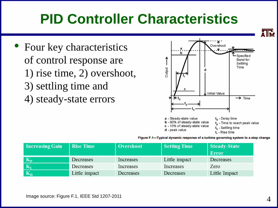
PID Controller Characteristics

• Four key characteristics

of control response are

1) rise time, 2) overshoot,

3) settling time and

4) steady-state errors

4Image source: Figure F.1, IEEE Std 1207-2011

PID Example: Car Cruise Control

• Say we wish to implement cruise control on a car by

controlling the throttle position

– Assume force is proportional to throttle position

– Error is difference between actual speed and desired speed

• With just proportional control we would never achieve

the desired speed because with zero error the throttle

position would be at zero

• The integral term will make sure we stay at the desired

point

• With derivative control we can improve control, but as

noted it can be sensitive to noise

5

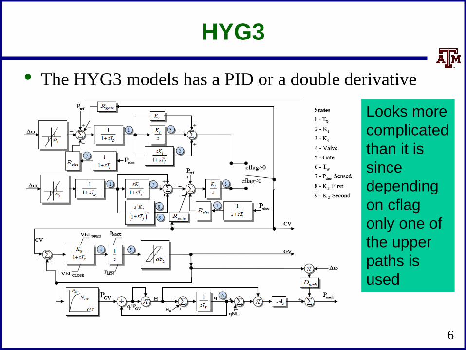
HYG3

• The HYG3 models has a PID or a double derivative

6

Looks more

complicated

than it is

since

depending

on cflag

only one of

the upper

paths is

used

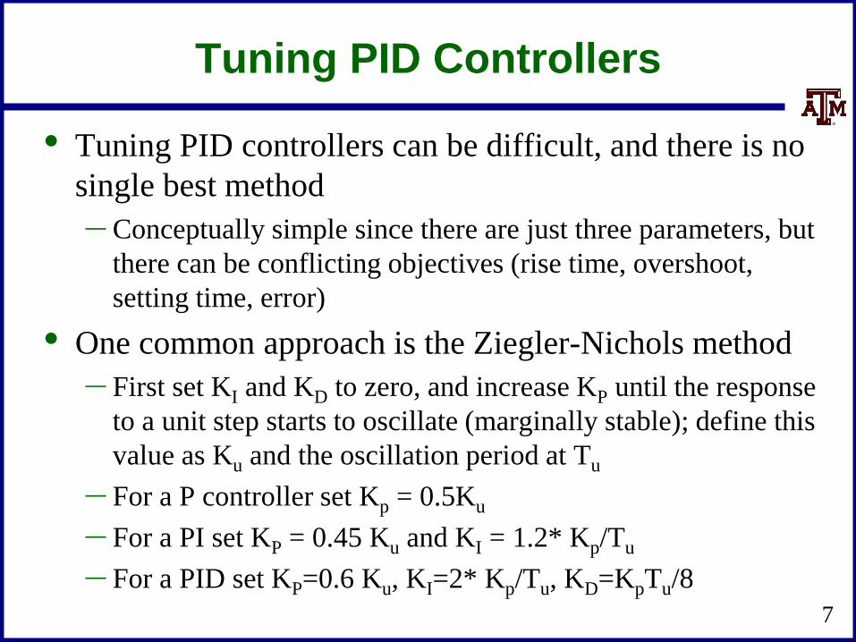
Tuning PID Controllers

• Tuning PID controllers can be difficult, and there is no

single best method

– Conceptually simple since there are just three parameters, but

there can be conflicting objectives (rise time, overshoot,

setting time, error)

• One common approach is the Ziegler-Nichols method

– First set KI and KD to zero, and increase KP until the response

to a unit step starts to oscillate (marginally stable); define this

value as Ku and the oscillation period at Tu

– For a P controller set Kp = 0.5Ku

– For a PI set KP = 0.45 Ku and KI = 1.2* Kp/Tu

– For a PID set KP=0.6 Ku, KI=2* Kp/Tu, KD=KpTu/8

7

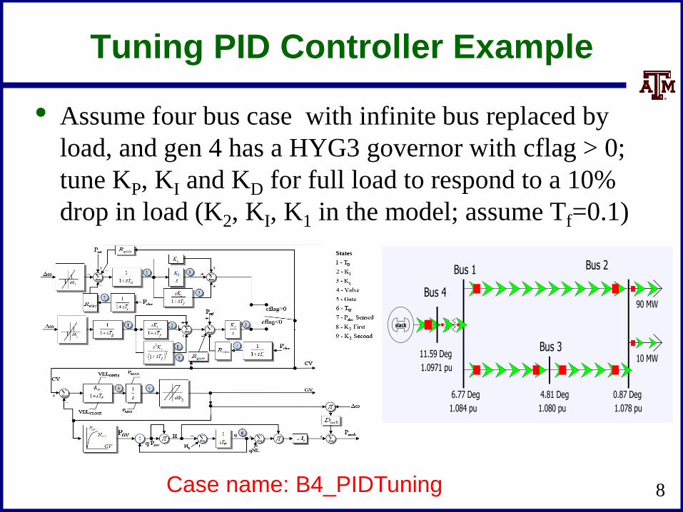
Tuning PID Controller Example

• Assume four bus case with infinite bus replaced by

load, and gen 4 has a HYG3 governor with cflag > 0;

tune KP, KI and KD for full load to respond to a 10%

drop in load (K2, KI, K1 in the model; assume Tf=0.1)

8

slack

Bus 1 Bus 2

Bus 3

0.87 Deg 6.77 Deg

Bus 4

11.59 Deg

4.81 Deg

1.078 pu 1.080 pu 1.084 pu

1.0971 pu

90 MW

10 MW

Case name: B4_PIDTuning

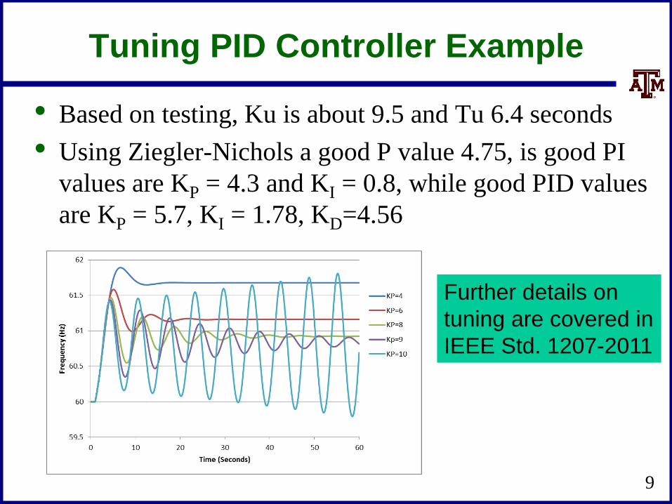
Tuning PID Controller Example

9

Further details on

tuning are covered in

IEEE Std. 1207-2011

• Based on testing, Ku is about 9.5 and Tu 6.4 seconds

• Using Ziegler-Nichols a good P value 4.75, is good PI

values are KP = 4.3 and KI = 0.8, while good PID values

are KP = 5.7, KI = 1.78, KD=4.56

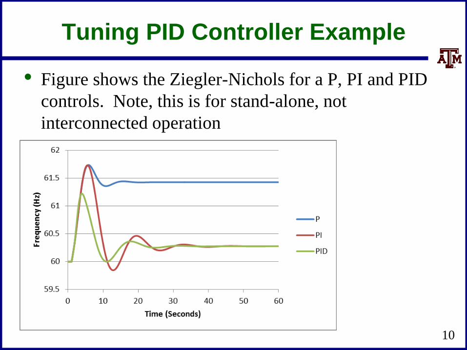
Tuning PID Controller Example

• Figure shows the Ziegler-Nichols for a P, PI and PID

controls. Note, this is for stand-alone, not

interconnected operation

10

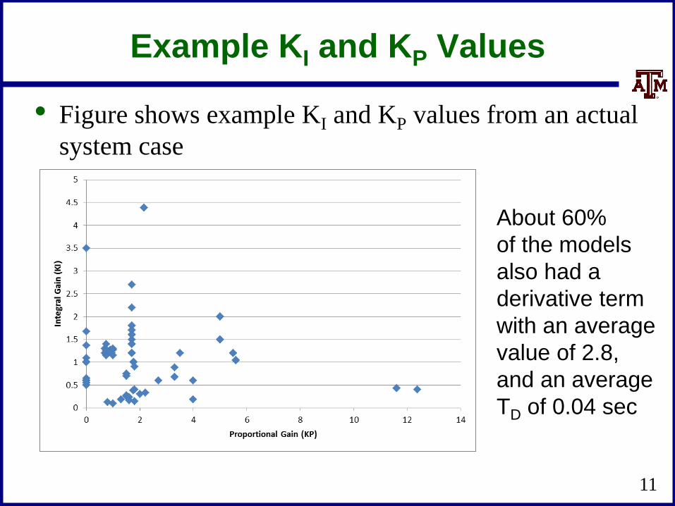
Example KI and KP Values

• Figure shows example KI and KP values from an actual

system case

11

About 60%

of the models

also had a

derivative term

with an average

value of 2.8,

and an average

TD of 0.04 sec

Non-windup Limits

• An important open question is whether the governor PI

controllers should be modeled with non-windup limits

– Currently models show no limit, but transient stability

verification seems to indicate limits are being enforced

• This could be an issue if frequency goes low, causing

governor PI to "windup" and then goes high (such as in

an islanding situation)

– How fast governor backs down depends on whether the limit

winds up

12

PI Non-windup Limits

• There is not a unique way to handle PI non-windup

limits; the below shows two approaches from IEEE Std

425.5

13

Another

common

approach

is to cap the

output and

put a non-

windup limit

on the

integratore

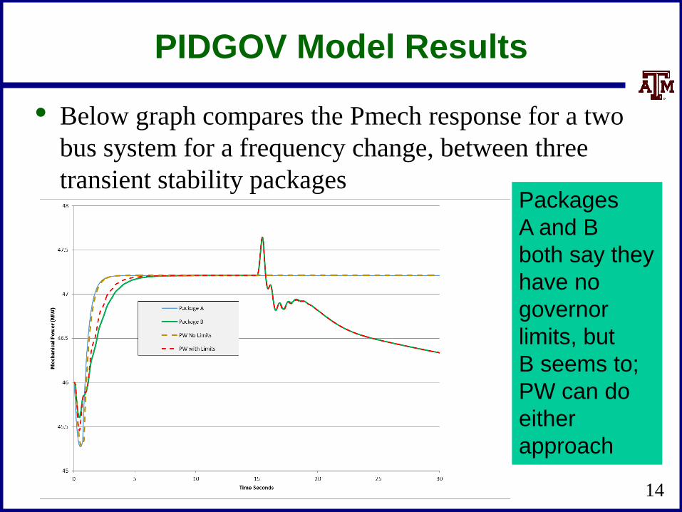
PIDGOV Model Results

• Below graph compares the Pmech response for a two

bus system for a frequency change, between three

transient stability packages

14

Packages

A and B

both say they

have no

governor

limits, but

B seems to;

PW can do

either

approach

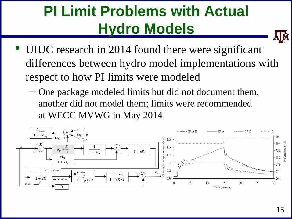
PI Limit Problems with Actual

Hydro Models

• UIUC research in 2014 found there were significant

differences between hydro model implementations with

respect to how PI limits were modeled

– One package modeled limits but did not document them,

another did not model them; limits were recommended

at WECC MVWG in May 2014

15

GGOV1

• GGOV1 is a newer governor model introduced in early

2000's by WECC for modeling thermal plants

– Existing models greatly under-estimated the frequency drop

– GGOV1 is now the most common WECC governor, used

with about 40% of the units

• A useful reference is L. Pereira, J. Undrill, D. Kosterev,

D. Davies, and S. Patterson, "A New Thermal Governor

Modeling Approach in the WECC," IEEE Transactions

on Power Systems, May 2003, pp. 819-829

16

GGOV1: Selected Figures from

2003 Paper

17

Fig. 1. Frequency recordings of the

SW and NW trips on May 18, 2001.

Also shown are simulations with

existing modeling (base case).

Governor model

verification—950-MW

Diablo generation trip on

June 3, 2002.

GGOV1 Block Diagram

18

Transient Stability

Multimachine Simulations

• Next, we'll be putting the models we've covered so far

together

• Later we'll add in new model types such as stabilizers,

loads and wind turbines

• By way of history, prior to digital computers, network

analyzers were used for system stability studies as far

back as the 1930's (perhaps earlier)

– For example see, J.D. Holm, "Stability Study of A-C Power

Transmission Systems," AIEE Transactions, vol. 61, 1942, pp.

893-905

• Digital approaches started appearing in the 1960's

19

Transient Stability

Multimachine Simulations

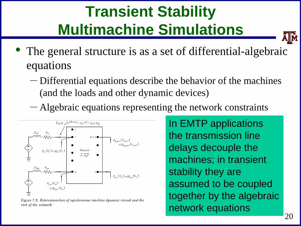
• The general structure is as a set of differential-algebraic

equations

– Differential equations describe the behavior of the machines

(and the loads and other dynamic devices)

– Algebraic equations representing the network constraints

20

In EMTP applications

the transmission line

delays decouple the

machines; in transient

stability they are

assumed to be coupled

together by the algebraic

network equations

General Form

• The general form of the problem is solving

21

( , , )

( , )

where is the vector of the state variables (such

as the generator 's), is the vector of the algebraic

variables (primarily the bus complex voltages), and

is the vector of contr

x f x y u

0 g x y

x

y

u ols (such as the exciter voltage

setpoints)

Transient Stability

General Solution

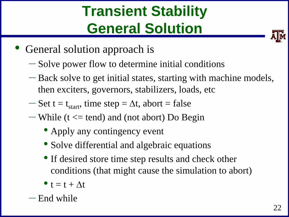
• General solution approach is

– Solve power flow to determine initial conditions

– Back solve to get initial states, starting with machine models,

then exciters, governors, stabilizers, loads, etc

– Set t = tstart, time step = Dt, abort = false

– While (t <= tend) and (not abort) Do Begin

• Apply any contingency event

• Solve differential and algebraic equations

• If desired store time step results and check other

conditions (that might cause the simulation to abort)

• t = t + Dt

– End while22

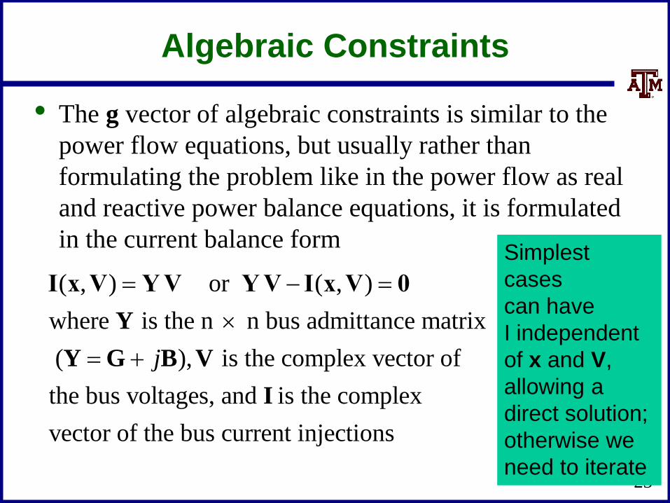
Algebraic Constraints

• The g vector of algebraic constraints is similar to the

power flow equations, but usually rather than

formulating the problem like in the power flow as real

and reactive power balance equations, it is formulated

in the current balance form

23

( , ) or ( , )

where is the n n bus admittance matrix

( ), is the complex vector of

the bus voltages, and is the complex

vector of the bus current injections

j

Ι x V YV YV Ι x V 0

Y

Y G B V

I

Simplest

cases

can have

I independent

of x and V,

allowing a

direct solution;

otherwise we

need to iterate

Why Not Use the

Power Flow Equations?

• The power flow equations were ultimately derived from

I(𝐱, 𝐕) = Y V

• However, the power form was used in the power flow

primarily because

– For the generators the real power output is known and either

the voltage setpoint (i.e., if a PV bus) or the reactive power

output

– In the quasi-steady state power flow time frame the loads can

often be well approximated as constant power

– The constant frequency assumption requires a slack bus

• These assumptions do not hold for transient stability

24

Algebraic Equations for

Classical Model

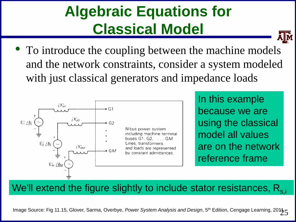
• To introduce the coupling between the machine models

and the network constraints, consider a system modeled

with just classical generators and impedance loads

25Image Source: Fig 11.15, Glover, Sarma, Overbye, Power System Analysis and Design, 5th Edition, Cengage Learning, 2011

In this example

because we are

using the classical

model all values

are on the network

reference frame

We'll extend the figure slightly to include stator resistances, Rs,i

Algebraic Equations for

Classical Model

• Replace the internal voltages and their impedances by

their Norton Equivalent

• Current injections at the non-generator buses are zero

since the constant impedance loads are included in Y

– We'll modify this later when we talk about dynamic loads

• The algebraic constraints are then I – Y V = 0

26

, , , ,

,i ii i

s i d i s i d i

E 1I Y

R jX R jX

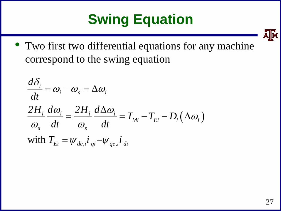
Swing Equation

• Two first two differential equations for any machine

correspond to the swing equation

27

, ,with

ii s i

i i i iMi Ei i i

s s

Ei de i qi qe i di

d

dt

2H d 2H dT T D

dt dt

T i i

D

D D

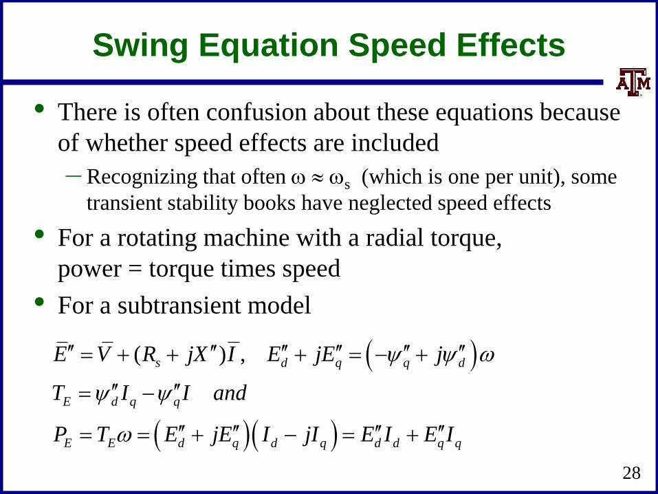
Swing Equation Speed Effects

• There is often confusion about these equations because

of whether speed effects are included

– Recognizing that often s (which is one per unit), some

transient stability books have neglected speed effects

• For a rotating machine with a radial torque,

power = torque times speed

• For a subtransient model

28

( ) ,s d q q d

E d q q

E E d q d q d d q q

E V R jX I E jE j

T I I and

P T E jE I jI E I E I

Classical Swing Equation

• Often in an introductory coverage of transient stability

with the classical model the assumption is s

so the swing equation for the classical model is given as

• We'll use this simplification for our initial example

29

with P

ii s i

i iMi Ei i i

s

Ei i i i i i i

d

dt

2H dP P D

dt

E E V Y

D

D D

As an example of this initial approach see Anderson and Fouad, Power System Control and Stability, 2nd Edition,

Chapter 2

Numerical Solution

• There are two main approaches for solving

– Partitioned-explicit: Solve the differential and algebraic

equations separately (alternating between the two) using an

explicit integration approach

– Simultaneous-implicit: Solve the differential and algebraic

equations together using an implicit integration approach

30

( , , )

( , )

x f x y u

0 g x y

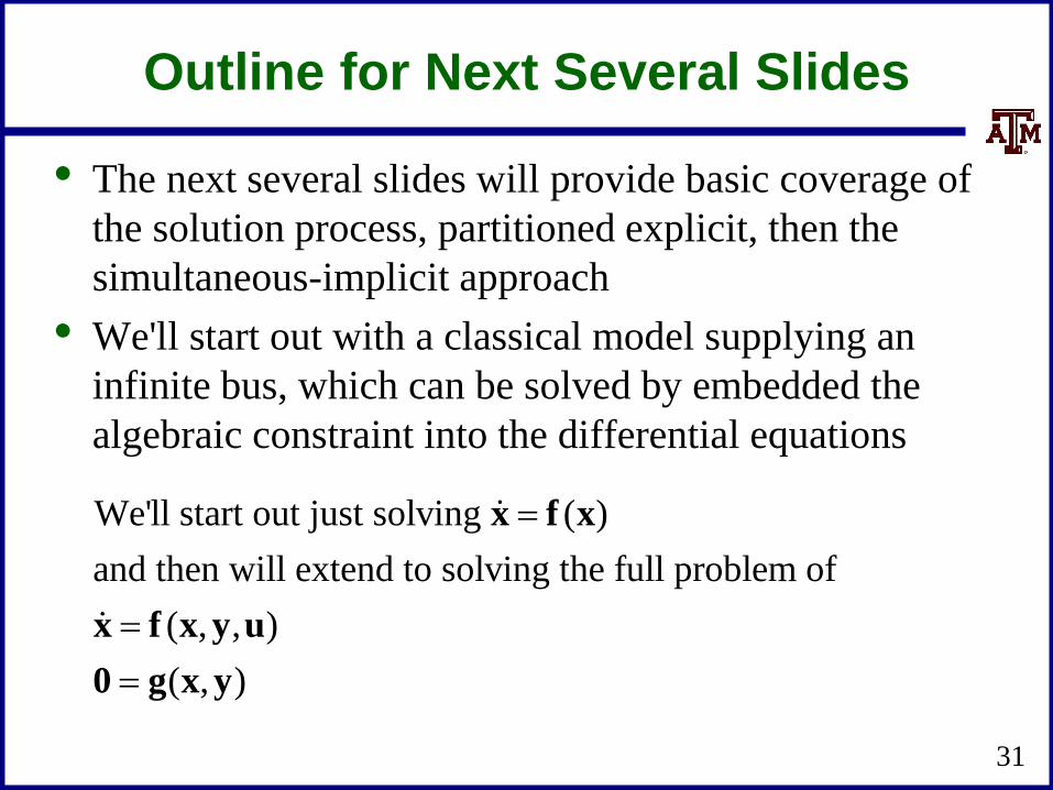
Outline for Next Several Slides

• The next several slides will provide basic coverage of

the solution process, partitioned explicit, then the

simultaneous-implicit approach

• We'll start out with a classical model supplying an

infinite bus, which can be solved by embedded the

algebraic constraint into the differential equations

31

We'll start out just solving ( )

and then will extend to solving the full problem of

( , , )

( , )

x f x

x f x y u

0 g x y

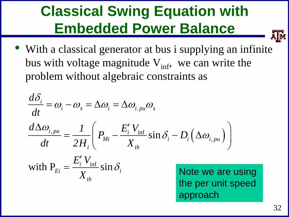
Classical Swing Equation with

Embedded Power Balance

• With a classical generator at bus i supplying an infinite

bus with voltage magnitude Vinf, we can write the

problem without algebraic constraints as

32

.

, inf,

inf

sin

with P sin

ii s i i pu s

i pu iMi i i i pu

i th

iEi i

th

d

dt

d E V1P D

dt 2H X

E V

X

D D

D D

Note we are using

the per unit speed

approach

Explicit Integration Methods

• As covered on the first day of class, there are a wide

variety of explicit integration methods

– We considered Forward Euler, Runge-Kutta, Adams-

Bashforth

• Here we will just consider Euler's, which is easy to

explain but not too useful, and a second order Runge-

Kutta, which is commonly used

33

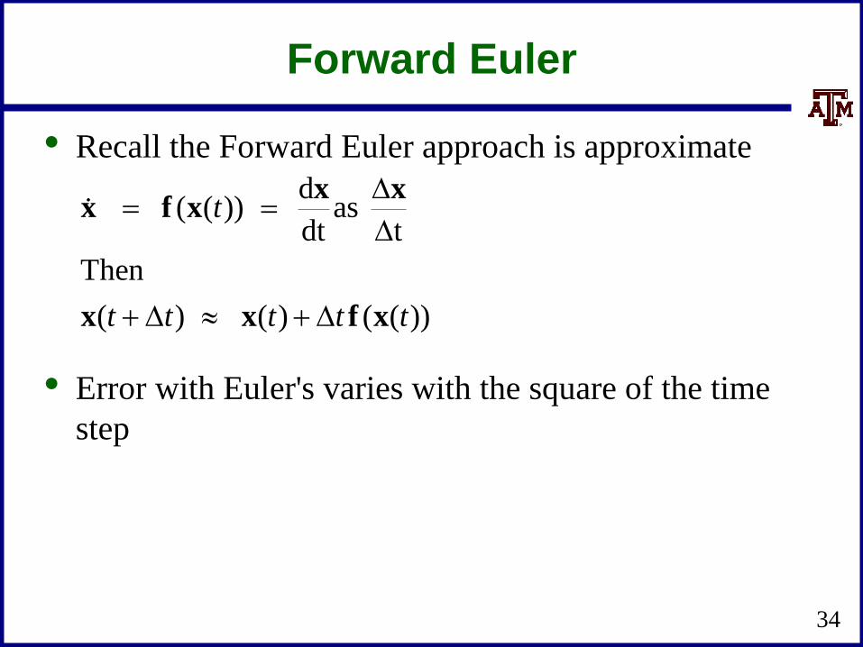
Forward Euler

• Recall the Forward Euler approach is approximate

• Error with Euler's varies with the square of the time

step

34

d( ( )) as

dt t

Then

( ) ( ) ( ( ))

t

t t t t t

D

D

D D

x xx f x

x x f x

Infinite Bus GENCLS Example

using the Forward Euler's Method

• Use the four bus system from before, except now gen 4

is modeled with a classical model with Xd'=0.3, H=3

and D=0; also we'll reduce to two buses with equivalent

line reactance, moving the gen from bus 4 to 1

35

Infinite Bus

slack

GENCLS

X=0.22

Bus 1

Bus 2

0.00 Deg 11.59 Deg

1.000 pu 1.095 pu

In this example Xth = (0.22 + 0.3), with the internal voltageത𝐸′1 = 1.281∠23.95° giving E'1=1.281 and 1= 23.95°

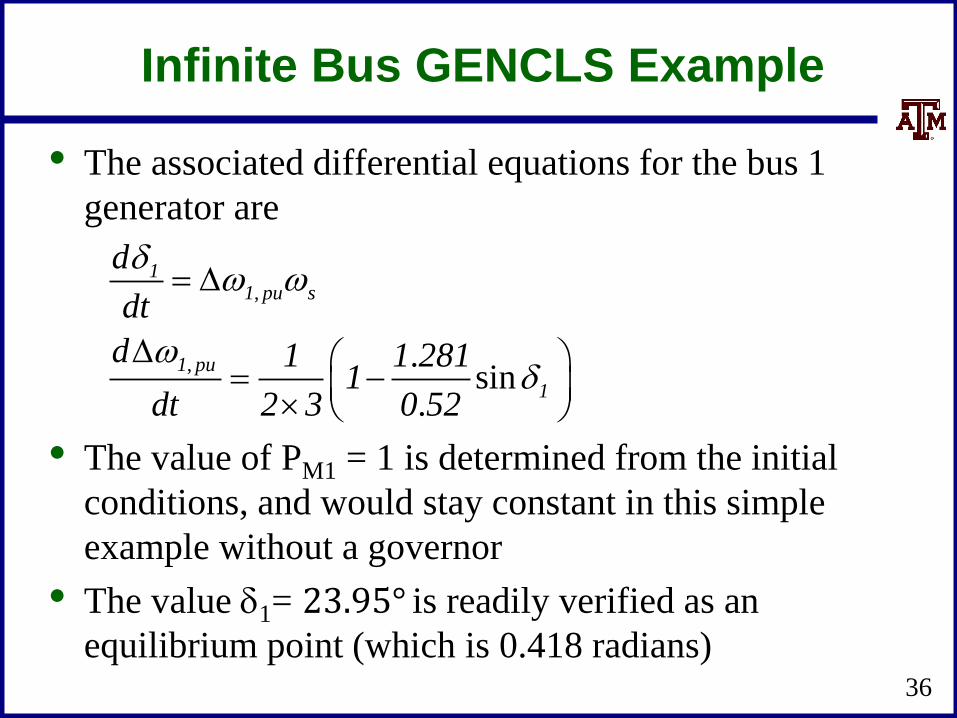
Infinite Bus GENCLS Example

• The associated differential equations for the bus 1

generator are

• The value of PM1 = 1 is determined from the initial

conditions, and would stay constant in this simple

example without a governor

• The value 1= 23.95° is readily verified as an

equilibrium point (which is 0.418 radians) 36

,

, .sin

.

11 pu s

1 pu

1

d

dt

d 1 1 2811

dt 2 3 0 52

D

D

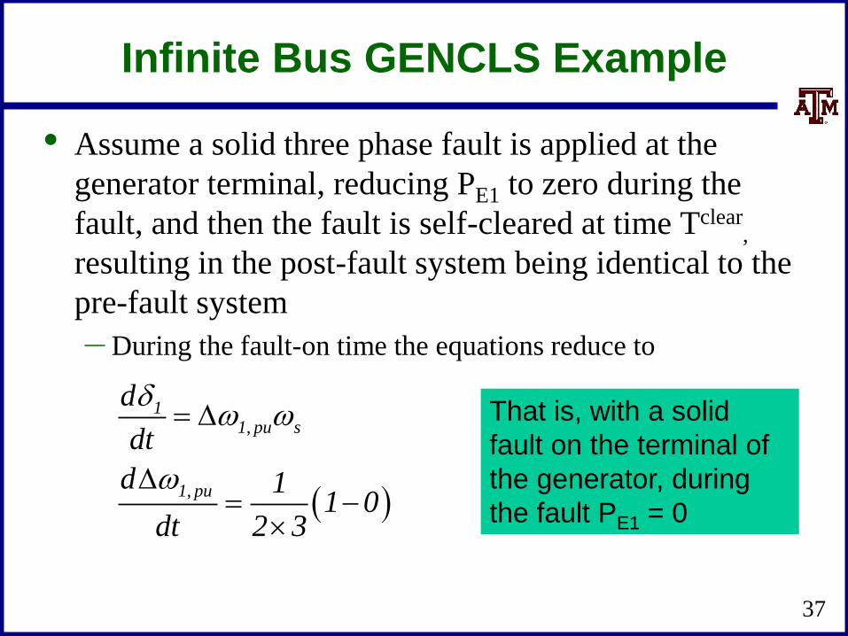
Infinite Bus GENCLS Example

• Assume a solid three phase fault is applied at the

generator terminal, reducing PE1 to zero during the

fault, and then the fault is self-cleared at time Tclear,

resulting in the post-fault system being identical to the

pre-fault system

– During the fault-on time the equations reduce to

37

,

,

11 pu s

1 pu

d

dt

d 11 0

dt 2 3

D

D

That is, with a solid

fault on the terminal of

the generator, during

the fault PE1 = 0

Euler's Solution

• The initial value of x is

• Assuming a time step Dt = 0.02 seconds, and a Tclear of

0.1 seconds, then using Euler's

• Iteration continues until t = Tclear

38

( ) .( )

( )pu

0 0 4180

0 0

x

. .( . ) .

. .

0 418 0 0 4180 02 0 02

0 0 1667 0 00333

x

Note Euler's

assumes

stays constant

during the first

time step

Euler's Solution

• At t = Tclear the fault is self-cleared, with the equations

changing to

• The integration continues using the new equations

39

.sin

.

pu s

pu

d

dt

d 1 1 2811

dt 6 0 52

D

D

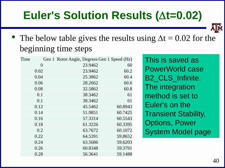
Euler's Solution Results (Dt=0.02)

• The below table gives the results using Dt = 0.02 for the

beginning time steps

40

Time Gen 1 Rotor Angle, Degrees Gen 1 Speed (Hz)

0 23.9462 60

0.02 23.9462 60.2

0.04 25.3862 60.4

0.06 28.2662 60.6

0.08 32.5862 60.8

0.1 38.3462 61

0.1 38.3462 61

0.12 45.5462 60.8943

0.14 51.9851 60.7425

0.16 57.3314 60.5543

0.18 61.3226 60.3395

0.2 63.7672 60.1072

0.22 64.5391 59.8652

0.24 63.5686 59.6203

0.26 60.8348 59.3791

0.28 56.3641 59.1488

This is saved as

PowerWorld case

B2_CLS_Infinite.

The integration

method is set to

Euler's on the

Transient Stability,

Options, Power

System Model page

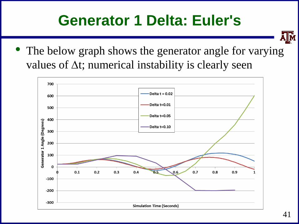
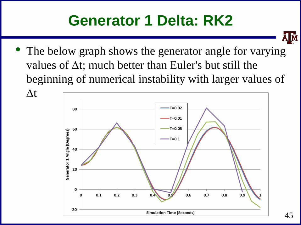
Generator 1 Delta: Euler's

• The below graph shows the generator angle for varying

values of Dt; numerical instability is clearly seen

41

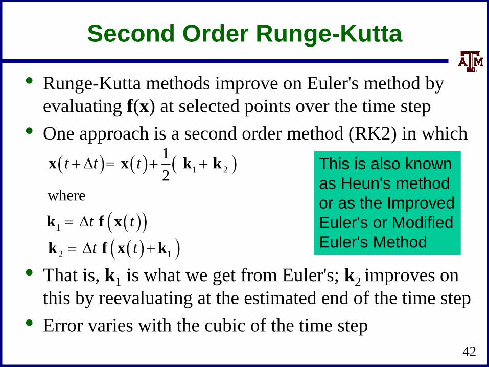
Second Order Runge-Kutta

42

• Runge-Kutta methods improve on Euler's method by

evaluating f(x) at selected points over the time step

• One approach is a second order method (RK2) in which

• That is, k1 is what we get from Euler's; k2 improves on

this by reevaluating at the estimated end of the time step

• Error varies with the cubic of the time step

1 2

1

2 1

1              

2

where   

t t t

t t

t t

D

D

D

x x k k

k f x

k f x k

This is also known

as Heun's method

or as the Improved

Euler's or Modified

Euler's Method

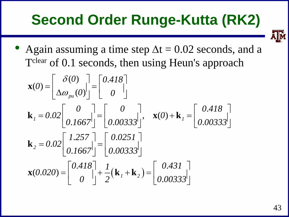
Second Order Runge-Kutta (RK2)

• Again assuming a time step Dt = 0.02 seconds, and a

Tclear of 0.1 seconds, then using Heun's approach

43

( ) .( )

( )

.. , ( )

. . .

. ..

. .

. .( . )

.

pu

1 1

2

1 2

0 0 4180

0 0

0 0 0 4180 02 0

0 1667 0 00333 0 00333

1 257 0 02510 02

0 1667 0 00333

0 418 0 43110 020

0 0 003332

D

x

k x k

k

x k k

RK2 Solution Results (Dt=0.02)

• The below table gives the results using Dt = 0.02 for the

beginning time steps

44

Time Gen 1 Rotor Angle, Degrees Gen 1 Speed (Hz)

0 23.9462 60

0.02 24.6662 60.2

0.04 26.8262 60.4

0.06 30.4262 60.6

0.08 35.4662 60.8

0.1 41.9462 61

0.1 41.9462 61

0.12 48.6805 60.849

0.14 54.1807 60.6626

0.16 58.233 60.4517

0.18 60.6974 60.2258

0.2 61.4961 59.9927

0.22 60.605 59.7598

0.24 58.0502 59.5343

0.26 53.9116 59.3241

0.28 48.3318 59.139

This is saved as

PowerWorld case

B2_CLS_Infinite.

The integration

method should be

changed to Second

Order Runge-Kutta

on the Transient

Stability, Options,

Power System Model

page

Generator 1 Delta: RK2

• The below graph shows the generator angle for varying

values of Dt; much better than Euler's but still the

beginning of numerical instability with larger values of

Dt

45

Adding Network Equations

• Previous slides with the network equations embedded in

the differential equations were a special case

• In general with the explicit approach we'll be alternating

between solving the differential equations and solving the

algebraic equations

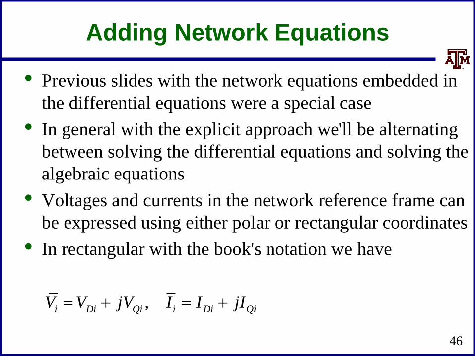
• Voltages and currents in the network reference frame can

be expressed using either polar or rectangular coordinates

• In rectangular with the book's notation we have

46

,i Di Qi i Di QiV V jV I I jI

Adding Network Equations

• Network equations will be written as Y V- I(x,V) = 0

– Here Y is as from the power flow, except augmented to

include the impact of the generator's internal impedance

– Constant impedance loads are also embedded in Y; non-

constant impedance loads are included in I(x,V)

• If I is independent of V then this can be solved directly:

V = Y-1

I(x)

• In general an iterative solution is required, which we'll

cover shortly, but initially we'll go with just the direct

solution

47

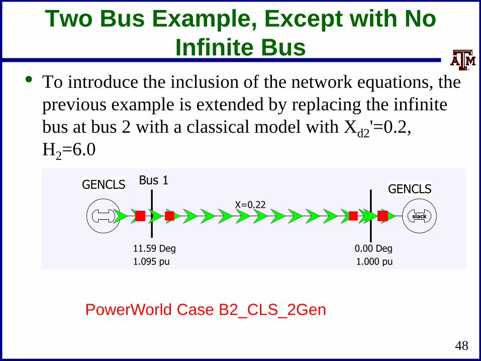
Two Bus Example, Except with No

Infinite Bus

• To introduce the inclusion of the network equations, the

previous example is extended by replacing the infinite

bus at bus 2 with a classical model with Xd2'=0.2,

H2=6.0

48

GENCLS

slack

GENCLS

X=0.22

Bus 1

Bus 2

0.00 Deg 11.59 Deg

1.000 pu 1.095 pu

PowerWorld Case B2_CLS_2Gen

Bus Admittance Matrix

• The network admittance matrix is

• This is augmented to represent the Norton admittances

associated with the generator models (Xd1'=0.3, Xd2'=0.2)

• In PowerWorld you can see this matrix by selecting

Transient Stability, States/Manual Control, Transient

Stability Ybus 49

. .

. .N

j4 545 j4 545

j4 545 j4 545

Y

. ..

. .

.

N

10

j7 879 j4 545j0 3

1 j4 545 j9 5450

j0 2

Y Y

Current Vector

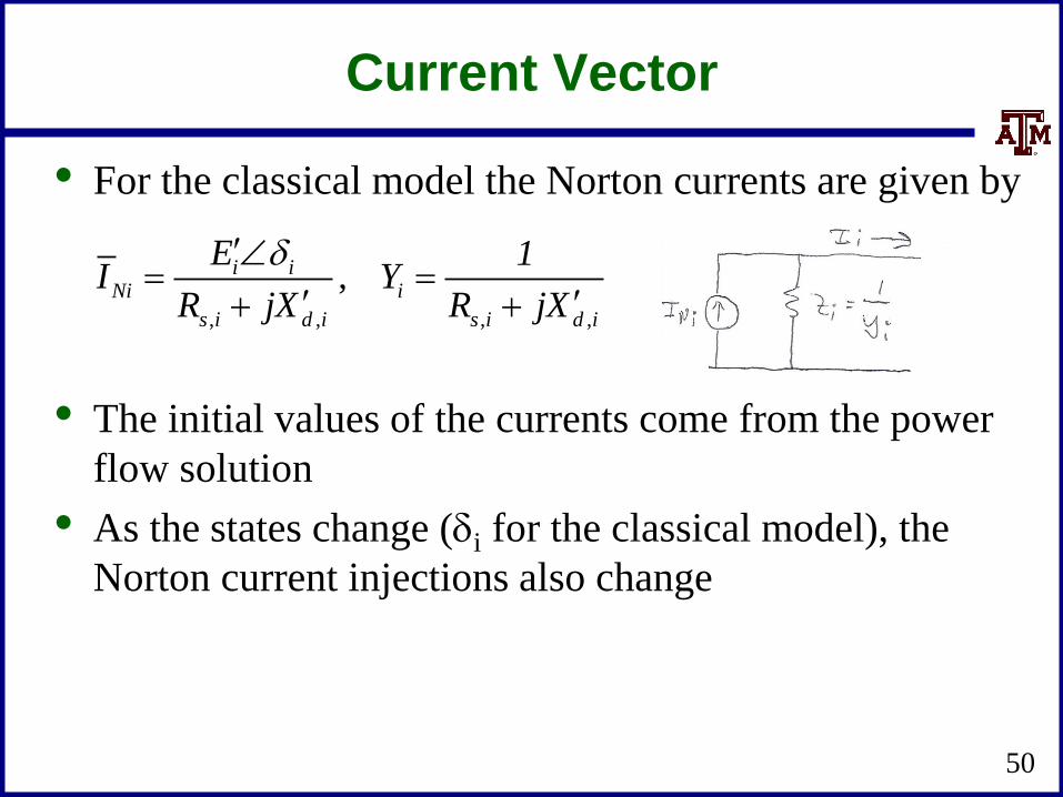
• For the classical model the Norton currents are given by

• The initial values of the currents come from the power

flow solution

• As the states change (i for the classical model), the

Norton current injections also change

50

, , , ,

,i iNi i

s i d i s i d i

E 1I Y

R jX R jX