ECE160 Spring 2007 Lecture 14 MPEG Audio Compression 1 ECE160 / CMPS182 Multimedia Lecture 14: Spring 2007 MPEG Audio Compression

ECE160 Spring 2007 Lecture 14 MPEG Audio Compression 1 ECE160 / CMPS182 Multimedia Lecture 14: Spring 2007 MPEG Audio Compression.
Dec 20, 2015
Welcome message from author
This document is posted to help you gain knowledge. Please leave a comment to let me know what you think about it! Share it to your friends and learn new things together.
Transcript
ECE160Spring 2007
Lecture 14MPEG Audio Compression
1
ECE160 / CMPS182
MultimediaLecture 14: Spring 2007
MPEG Audio Compression
ECE160Spring 2007
Lecture 14MPEG Audio Compression
2
Vocoders
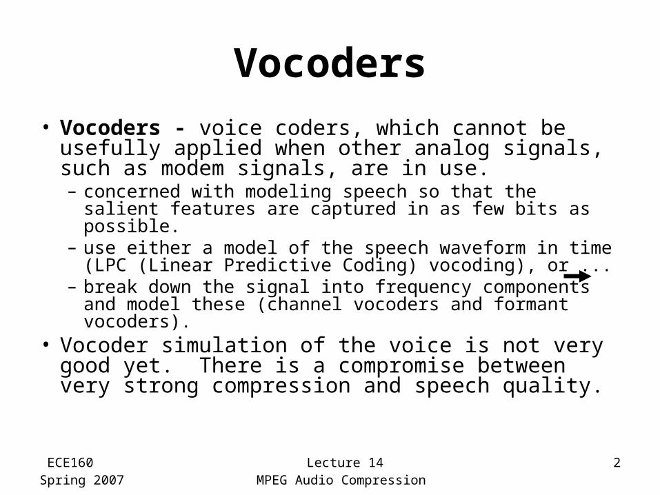
• Vocoders - voice coders, which cannot be usefully applied when other analog signals, such as modem signals, are in use.– concerned with modeling speech so that the salient
features are captured in as few bits as possible.– use either a model of the speech waveform in time
(LPC (Linear Predictive Coding) vocoding), or ... – break down the signal into frequency components and
model these (channel vocoders and formant vocoders).
• Vocoder simulation of the voice is not very good yet. There is a compromise between very strong compression and speech quality.
ECE160Spring 2007
Lecture 14MPEG Audio Compression
3
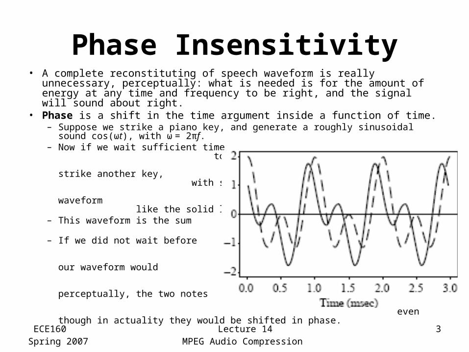
Phase Insensitivity• A complete reconstituting of speech waveform is really
unnecessary, perceptually: what is needed is for the amount of energy at any time and frequency to be right, and the signal will sound about right.
• Phase is a shift in the time argument inside a function of time.– Suppose we strike a piano key, and generate a roughly sinusoidal
sound cos(ωt), with ω = 2πf.– Now if we wait sufficient time
to generate a phase shift π/2 and then strike another key, with sound cos(2ωt + π/2), we generate a waveform like the solid line
– This waveform is the sum cos(ωt) + cos(2ωt + π/2).
– If we did not wait before striking the second note, then our waveform would be cos(ωt) + cos(2ωt). But perceptually, the two notes would sound the same sound, even though in actuality they would be shifted in phase.
ECE160Spring 2007
Lecture 14MPEG Audio Compression
4
Channel Vocoder
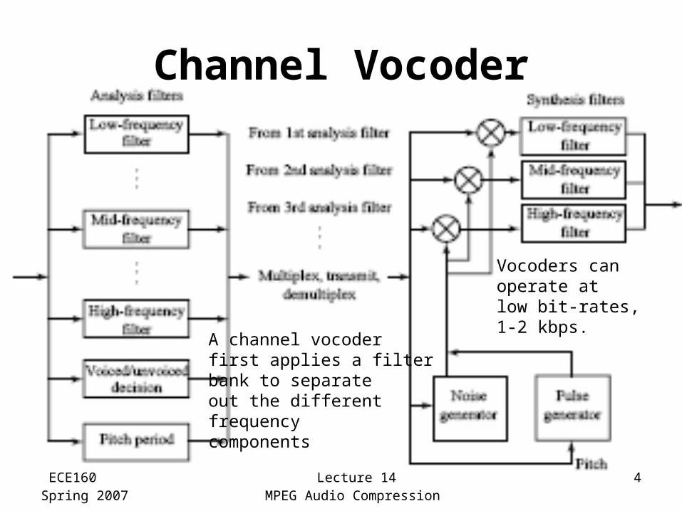
Vocoders canoperate atlow bit-rates,1-2 kbps.
A channel vocoderfirst applies a filterbank to separate out the differentfrequencycomponents
ECE160Spring 2007
Lecture 14MPEG Audio Compression
5
Channel Vocoder• A channel vocoder first applies a filter bank to separate
out the different frequency components.• Due to Phase Insensitivity (only the energy is important):
– The waveform is “rectified" to its absolute value.– The filter bank derives power levels for each frequency range.– A subband coder would not rectify the signal, and would use
wider frequency bands.
• A channel vocoder also analyzes the signal to determine the general pitch of the speech (low-bass, or high-tenor), and also the excitation of the speech.
• A channel vocoder applies a vocal tract transfer model to generate a vector of excitation parameters that describe a model of the sound, and also guesses whether the sound is voiced or unvoiced.
ECE160Spring 2007
Lecture 14MPEG Audio Compression
6
Formant Vocoder
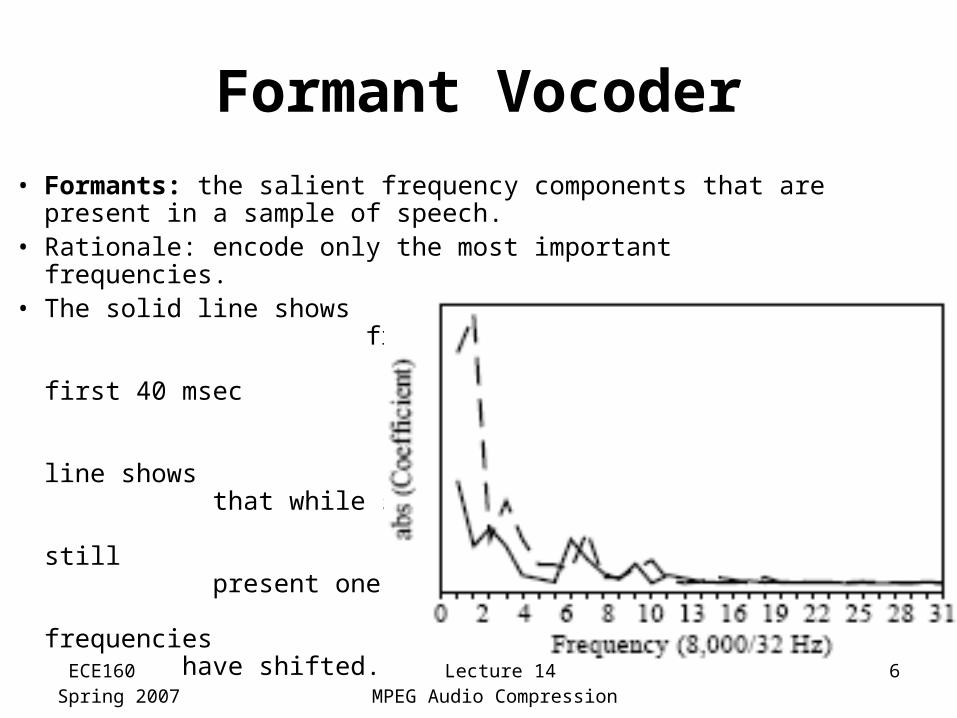
• Formants: the salient frequency components that are present in a sample of speech.
• Rationale: encode only the most important frequencies.• The solid line shows
frequencies present in the first 40 msec of a speech sample. The dashed line shows that while similar frequencies are still present one second later, these frequencies have shifted.
ECE160Spring 2007
Lecture 14MPEG Audio Compression
7
Linear Predictive Coding (LPC)
• LPC vocoders extract salient features of speech directly from the waveform, rather than transforming the signal to the frequency domain
• LPC Features:– uses a time-varying model of vocal tract sound generated from a
given excitation– transmits only a set of parameters modeling the shape and
excitation of the vocal tract, not actual signals or differences - small bit-rate
• About “Linear": The speech signal generated by the output vocal tract model is calculated as a function of the current speech output plus a second term linear in previous model coefficients
ECE160Spring 2007
Lecture 14MPEG Audio Compression
8
LPC Coding Process
LPC starts by deciding whether the current segment is voiced (vocal cords resonate) or unvoiced:
• For unvoiced: a wide-band noise generator creates a signal f(n) that acts as input to the vocal tract simulator
• For voiced: a pulse train generator creates signal f(n)
• Model parameters ai: calculated by using a least-squares set of equations that minimize the difference between the actual speech and the speech generated by the vocal tract model, excited by the noise or pulse train generators that capture speech parameters
ECE160Spring 2007
Lecture 14MPEG Audio Compression
9
LPC Coding Process
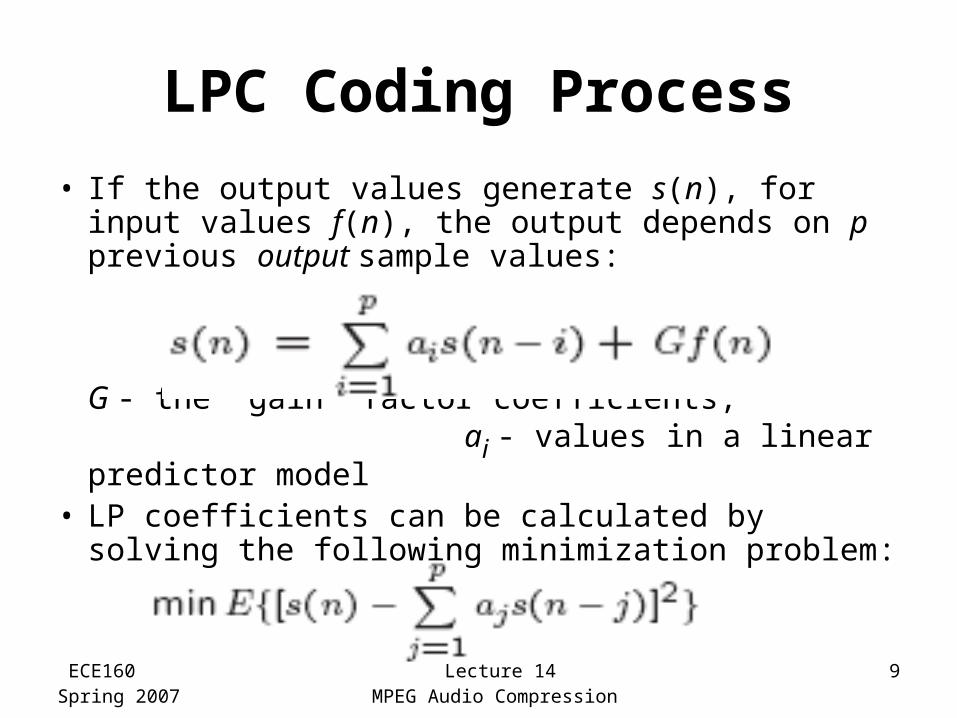
• If the output values generate s(n), for input values f(n), the output depends on p previous output sample values:
G - the “gain" factor coefficients; ai - values in a linear predictor model
• LP coefficients can be calculated by solving the following minimization problem:
ECE160Spring 2007
Lecture 14MPEG Audio Compression
10
Code Excited Linear Prediction (CELP)
• CELP is a more complex family of coders that attempts to mitigate the lack of quality of the simple LPC model
• CELP uses a more complex description of the excitation:– An entire set (a codebook) of excitation vectors is matched to
the actual speech, and the index of the best match is sent to the receiver
– The complexity increases the bit-rate to 4,800-9,600 bps– The resulting speech is perceived as being more similar and
continuous– Quality achieved this way is sufficient for audio conferencing
ECE160Spring 2007
Lecture 14MPEG Audio Compression
11
Psychoacoustics
• The range of human hearing is about 20 Hz to about 20 kHz
• The frequency range of the voice is typically only from about 500 Hz to 4 kHz
• The dynamic range, the ratio of the maximum sound amplitude to the quietest sound that humans can hear, is on the order of about 120 dB
ECE160Spring 2007
Lecture 14MPEG Audio Compression
12
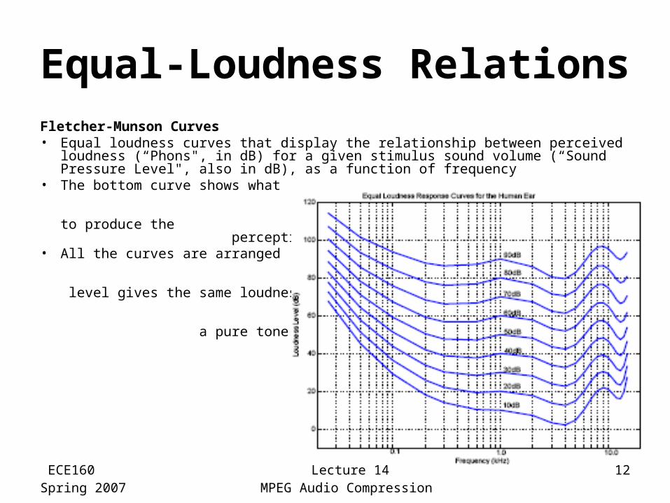
Equal-Loudness RelationsFletcher-Munson Curves• Equal loudness curves that display the relationship between perceived
loudness (“Phons", in dB) for a given stimulus sound volume (“Sound Pressure Level", also in dB), as a function of frequency
• The bottom curve shows what level of pure tone stimulus is required to produce the perception of a 10 dB sound
• All the curves are arranged so that the perceived loudness level gives the same loudness as for that loudness level of a pure tone at 1 kHz
ECE160Spring 2007
Lecture 14MPEG Audio Compression
13
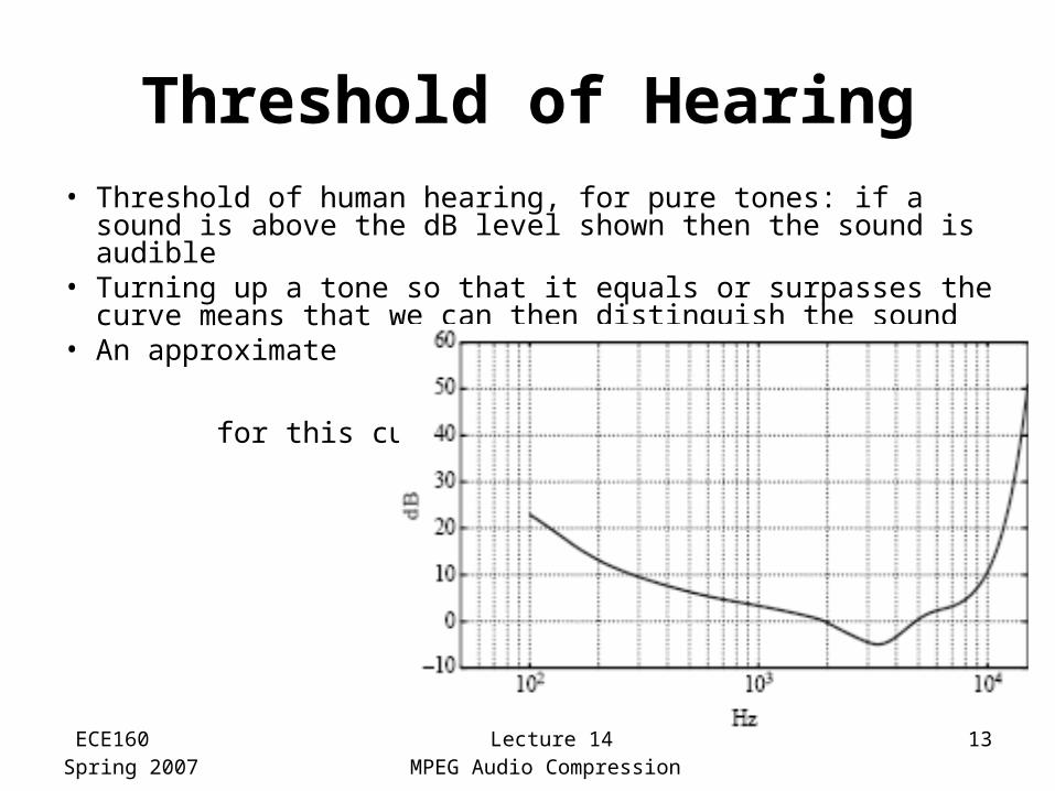
Threshold of Hearing• Threshold of human hearing, for pure tones: if a sound is
above the dB level shown then the sound is audible• Turning up a tone so that it equals or surpasses the
curve means that we can then distinguish the sound• An approximate
formula exists for this curve:
ECE160Spring 2007
Lecture 14MPEG Audio Compression
14
Frequency Masking
• Lossy audio data compression methods, such as MPEG/Audio encoding, do not encode some sounds which are masked anyway
• The general situation in regard to masking is as follows:1. A lower tone can effectively mask (make us unable to hear) a higher tone2. The reverse is not true - a higher tone does not mask a lower tone well3. The greater the power in the masking tone, the wider is its influence - the broader the range of frequencies it can mask.4. As a consequence, if two tones are widely separated in frequency then little masking occurs
ECE160Spring 2007
Lecture 14MPEG Audio Compression
15
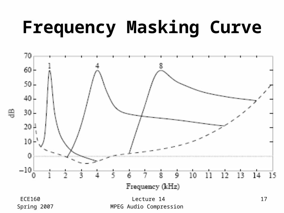
Frequency Masking Curves
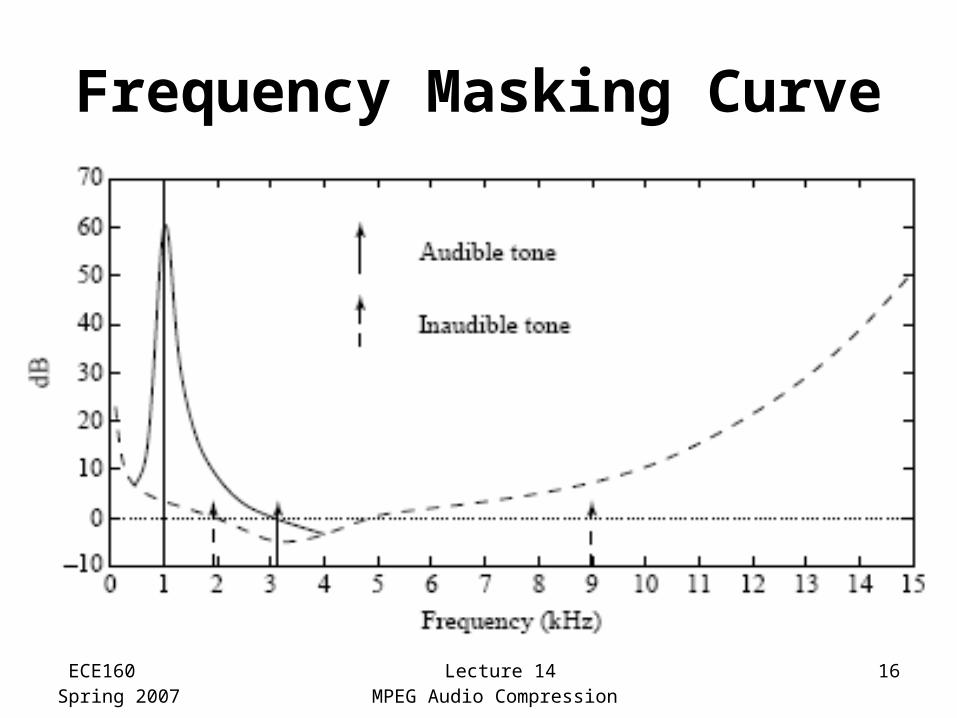
• Frequency masking is studied by playing a particular pure tone, say 1 kHz again, at a loud volume, and determining how this tone affects our ability to hear tones nearby in frequency– One would generate a 1 kHz masking tone, at a fixed
sound level of 60 dB, and then raise the level of a nearby tone, e.g., 1.1 kHz, until it is just audible
• The threshold plots the audible level for a single masking tone (1 kHz) and a single sound level
• The plot changes if other masking frequencies or sound levels are used.
ECE160Spring 2007
Lecture 14MPEG Audio Compression
16
Frequency Masking Curve
ECE160Spring 2007
Lecture 14MPEG Audio Compression
17
Frequency Masking Curve
ECE160Spring 2007
Lecture 14MPEG Audio Compression
18
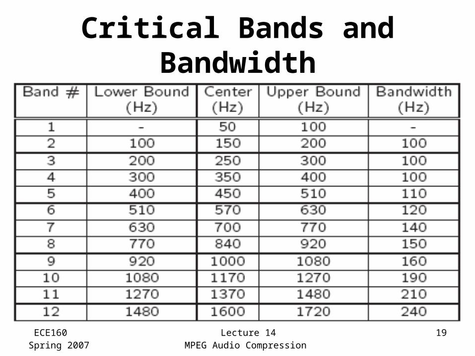
Critical Bands
• Critical bandwidth represents the ear's resolving power for simultaneous tones or partials– At the low-frequency end, a critical band is less than
100 Hz wide, while for high frequencies the width can be greater than 4 kHz
• Experiments indicate that the critical bandwidth:– for masking frequencies < 500 Hz: remains
approximately constant in width ( about 100 Hz)– for masking frequencies > 500 Hz: increases
approximately linearly with frequency
ECE160Spring 2007
Lecture 14MPEG Audio Compression
19
Critical Bands and Bandwidth
ECE160Spring 2007
Lecture 14MPEG Audio Compression
20
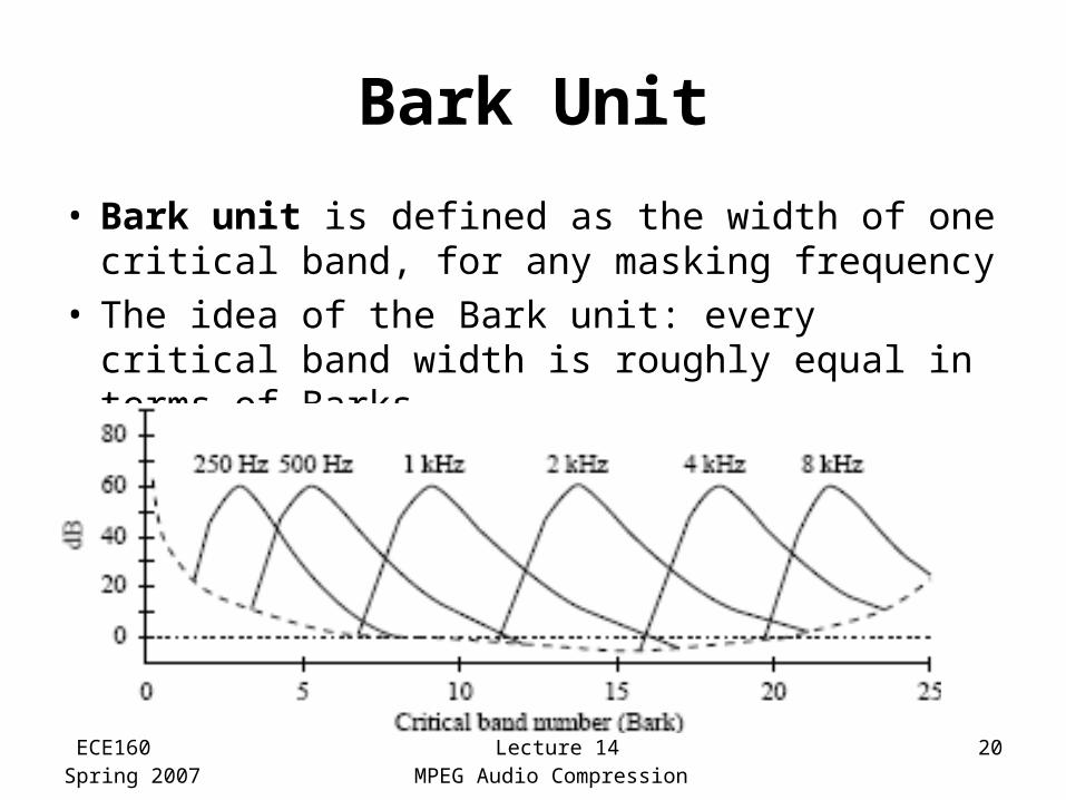
Bark Unit
• Bark unit is defined as the width of one critical band, for any masking frequency
• The idea of the Bark unit: every critical band width is roughly equal in terms of Barks
ECE160Spring 2007
Lecture 14MPEG Audio Compression
21
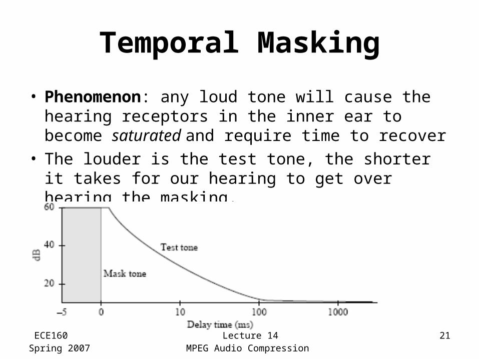
Temporal Masking
• Phenomenon: any loud tone will cause the hearing receptors in the inner ear to become saturated and require time to recover
• The louder is the test tone, the shorter it takes for our hearing to get over hearing the masking.
ECE160Spring 2007
Lecture 14MPEG Audio Compression
22
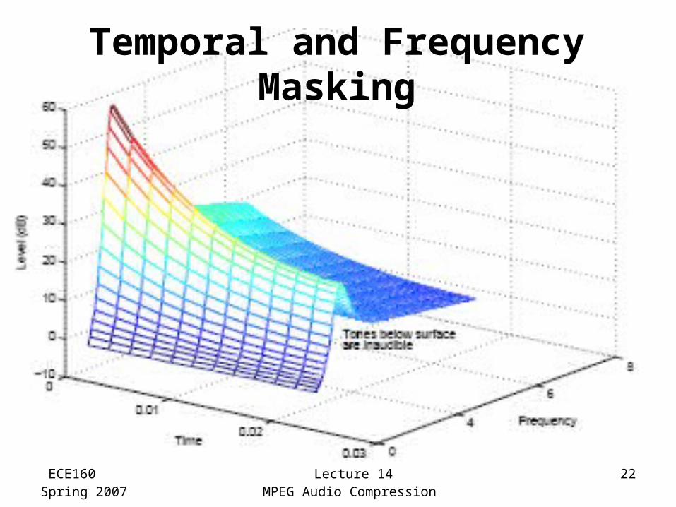
Temporal and Frequency Masking
ECE160Spring 2007
Lecture 14MPEG Audio Compression
23
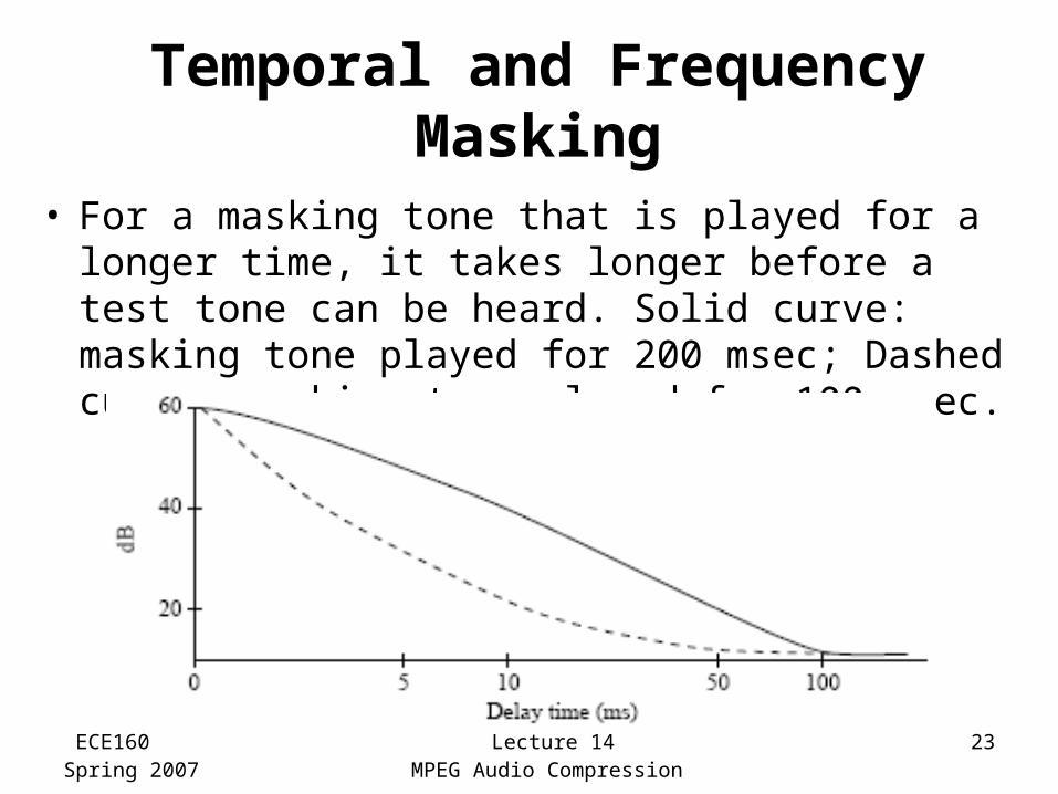
Temporal and Frequency Masking
• For a masking tone that is played for a longer time, it takes longer before a test tone can be heard. Solid curve: masking tone played for 200 msec; Dashed curve: masking tone played for 100 msec.
ECE160Spring 2007
Lecture 14MPEG Audio Compression
24
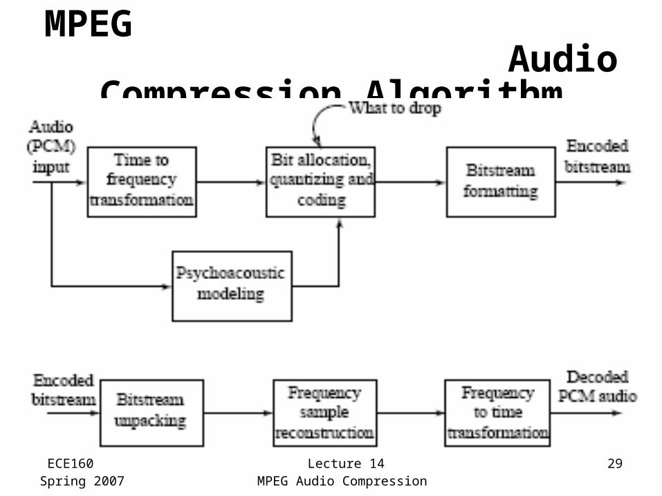
MPEG Audio
• MPEG audio compression takes advantage of psychoacoustic models, constructing a large multi-dimensional lookup table to transmit masked frequency components using fewer bits
• MPEG Audio Overview1. Applies a filter bank to the input to break it into its frequency components2. In parallel, a psychoacoustic model is applied to the data for bit allocation block3. The number of bits allocated are used to quantize the info from the filter bank - providing the compression
ECE160Spring 2007
Lecture 14MPEG Audio Compression
25
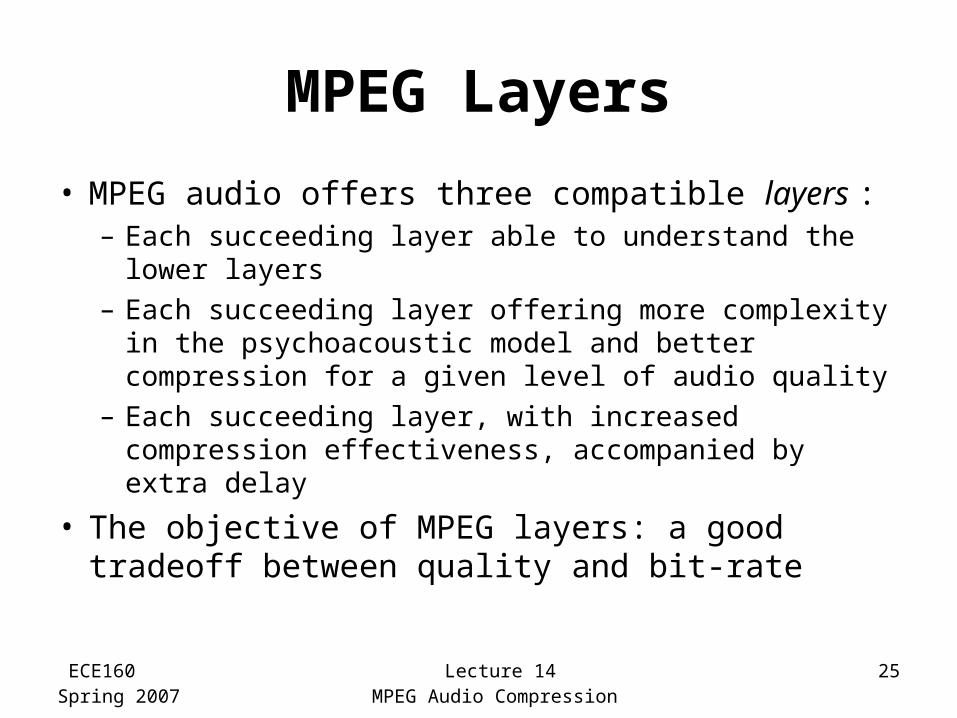
MPEG Layers
• MPEG audio offers three compatible layers :– Each succeeding layer able to understand the lower
layers– Each succeeding layer offering more complexity in the
psychoacoustic model and better compression for a given level of audio quality
– Each succeeding layer, with increased compression effectiveness, accompanied by extra delay
• The objective of MPEG layers: a good tradeoff between quality and bit-rate
ECE160Spring 2007
Lecture 14MPEG Audio Compression
26
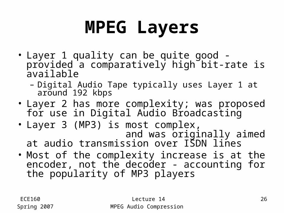
MPEG Layers
• Layer 1 quality can be quite good - provided a comparatively high bit-rate is available– Digital Audio Tape typically uses Layer 1 at around
192 kbps• Layer 2 has more complexity; was proposed for
use in Digital Audio Broadcasting• Layer 3 (MP3) is most complex,
and was originally aimed at audio transmission over ISDN lines
• Most of the complexity increase is at the encoder, not the decoder - accounting for the popularity of MP3 players
ECE160Spring 2007
Lecture 14MPEG Audio Compression
27
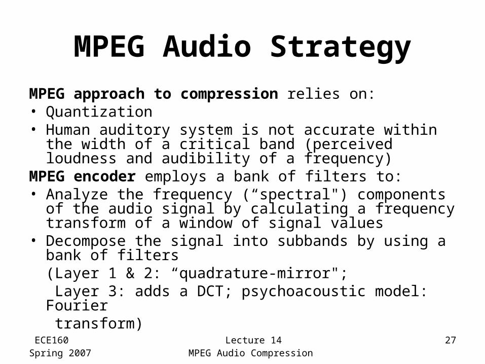
MPEG Audio Strategy
MPEG approach to compression relies on:• Quantization• Human auditory system is not accurate within the width
of a critical band (perceived loudness and audibility of a frequency)
MPEG encoder employs a bank of filters to:• Analyze the frequency (“spectral") components of the
audio signal by calculating a frequency transform of a window of signal values
• Decompose the signal into subbands by using a bank of filters(Layer 1 & 2: “quadrature-mirror"; Layer 3: adds a DCT; psychoacoustic model: Fourier transform)
ECE160Spring 2007
Lecture 14MPEG Audio Compression
28
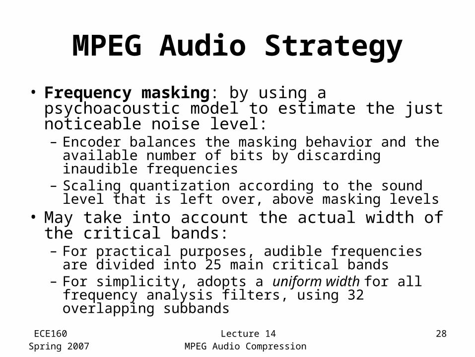
MPEG Audio Strategy
• Frequency masking: by using a psychoacoustic model to estimate the just noticeable noise level:– Encoder balances the masking behavior and the
available number of bits by discarding inaudible frequencies
– Scaling quantization according to the sound level that is left over, above masking levels
• May take into account the actual width of the critical bands:– For practical purposes, audible frequencies are
divided into 25 main critical bands – For simplicity, adopts a uniform width for all frequency
analysis filters, using 32 overlapping subbands
ECE160Spring 2007
Lecture 14MPEG Audio Compression
29
MPEG Audio Compression Algorithm
ECE160Spring 2007
Lecture 14MPEG Audio Compression
30
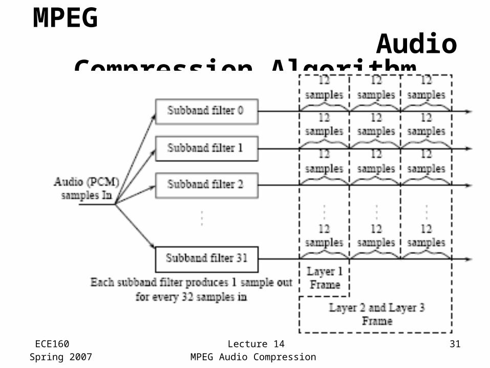
MPEG Audio Compression Algorithm
• The algorithm proceeds by dividing the input into 32 frequency subbands, via a filter bank– A linear operation taking 32 PCM samples, sampled
in time; output is 32 frequency coefficients• In the Layer 1 encoder, the sets of 32 PCM
values are first assembled into a set of 12 groups of 32s– An inherent time lag in the coder, equal to the time to
accumulate 384 (i.e., 12x32) samples• A Layer 2 or Layer 3, frame actually
accumulates more than 12 samples for each subband: a frame includes 1,152 samples
ECE160Spring 2007
Lecture 14MPEG Audio Compression
31
MPEG Audio Compression Algorithm
ECE160Spring 2007
Lecture 14MPEG Audio Compression
32
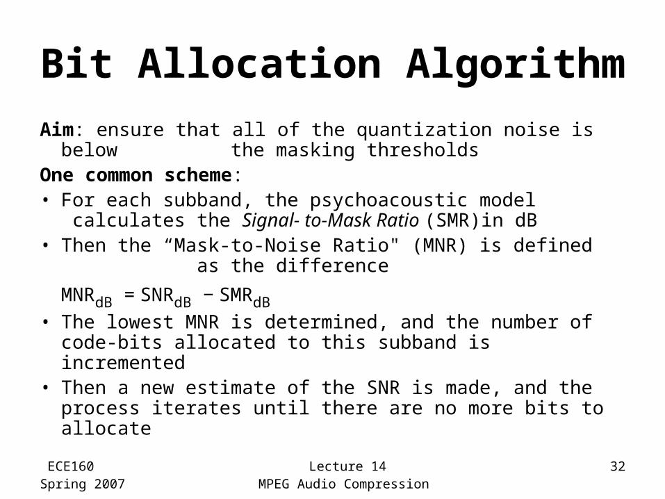
Bit Allocation Algorithm
Aim: ensure that all of the quantization noise is below the masking thresholds
One common scheme:• For each subband, the psychoacoustic model
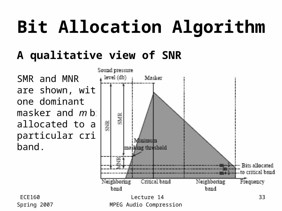
calculates the Signal- to-Mask Ratio (SMR)in dB• Then the “Mask-to-Noise Ratio" (MNR) is defined
as the difference
MNRdB = SNRdB − SMRdB
• The lowest MNR is determined, and the number of code-bits allocated to this subband is incremented
• Then a new estimate of the SNR is made, and the process iterates until there are no more bits to allocate
ECE160Spring 2007
Lecture 14MPEG Audio Compression
33
Bit Allocation Algorithm
A qualitative view of SNR
SMR and MNR are shown, with one dominant masker and m bits allocated to a particular critical band.
ECE160Spring 2007
Lecture 14MPEG Audio Compression
34
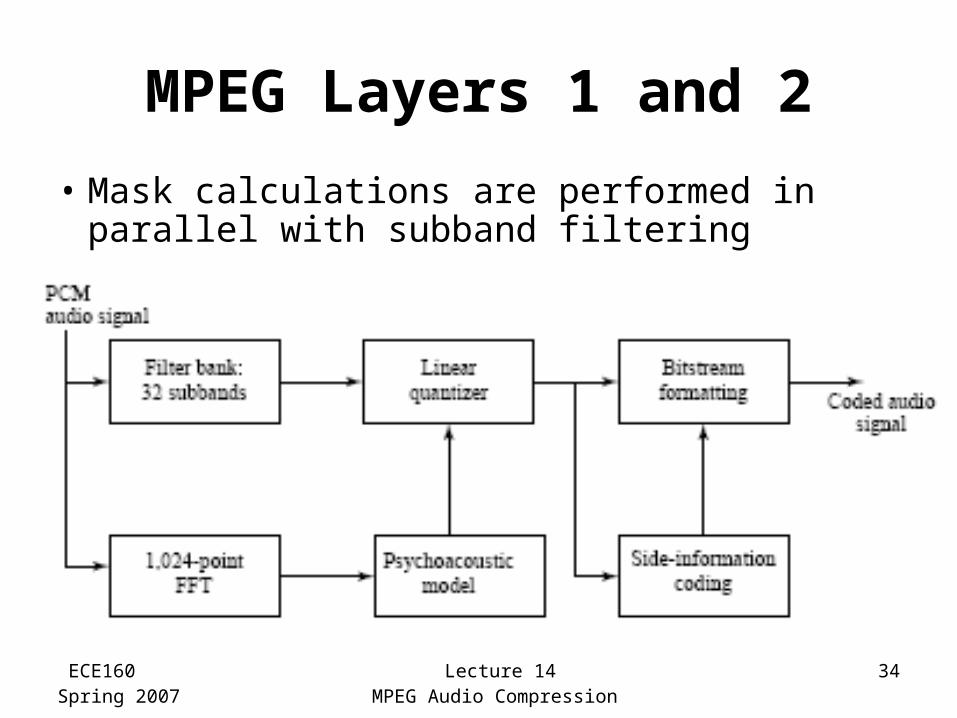
MPEG Layers 1 and 2
• Mask calculations are performed in parallel with subband filtering
ECE160Spring 2007
Lecture 14MPEG Audio Compression
35
Layer 2 of MPEG Audio
Main difference:• Three groups of 12 samples are encoded in
each frame and temporal masking is brought into play, as well as frequency masking
• Bit allocation is applied to window lengths of 36 samples instead of 12
• The resolution of the quantizers is increased from 15 bits to 16
Advantage:• a single scaling factor can be used
for all three groups
ECE160Spring 2007
Lecture 14MPEG Audio Compression
36
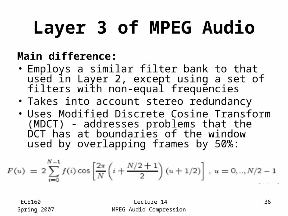
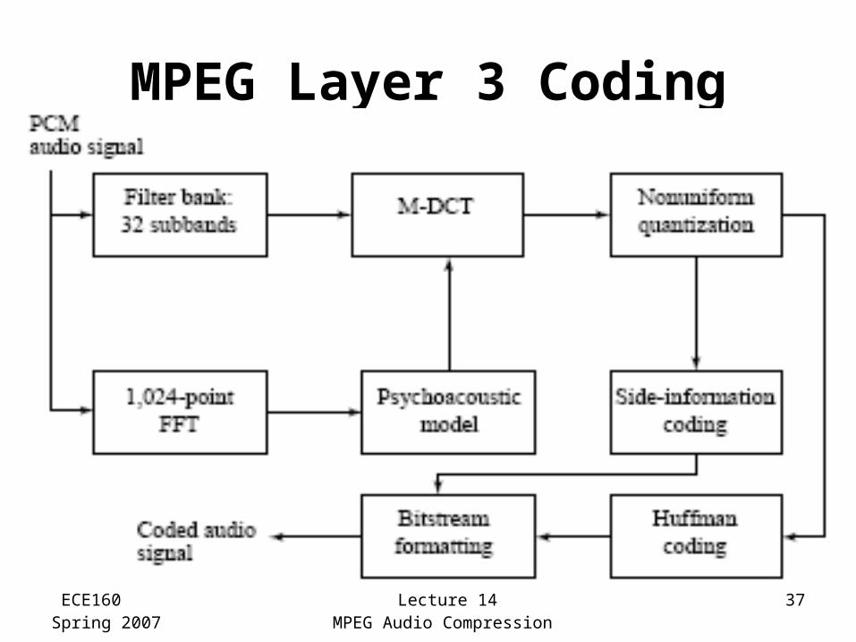
Layer 3 of MPEG Audio
Main difference:• Employs a similar filter bank to that used in
Layer 2, except using a set of filters with non-equal frequencies
• Takes into account stereo redundancy• Uses Modified Discrete Cosine Transform
(MDCT) - addresses problems that the DCT has at boundaries of the window used by overlapping frames by 50%:
ECE160Spring 2007
Lecture 14MPEG Audio Compression
37
MPEG Layer 3 Coding
ECE160Spring 2007
Lecture 14MPEG Audio Compression
38
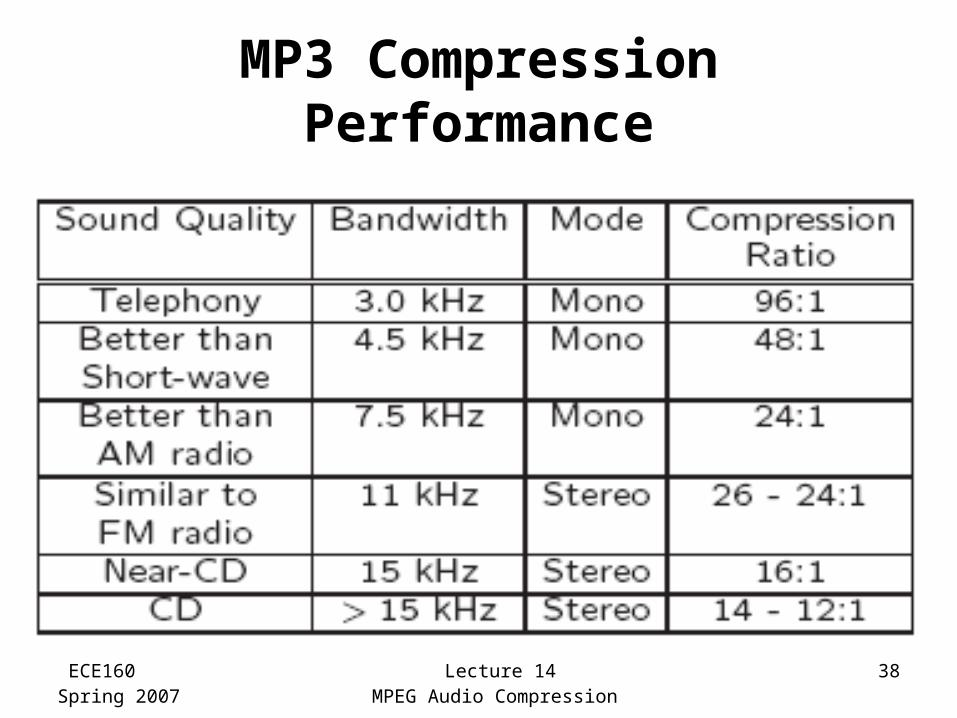
MP3 Compression Performance
ECE160Spring 2007
Lecture 14MPEG Audio Compression
39
MPEG-2 AAC (Advanced Audio Coding)
The standard vehicle for DVDs:• Audio coding technology for the DVD-Audio
Recordable (DVD-AR) format, also adopted by XM Radio
• Aimed at transparent sound reproduction for theaters
• Can deliver this at 320 kbps for five channels so that sound can be played from 5 different directions: – Left, Right, Center, Left-Surround, and Right-
Surround
ECE160Spring 2007
Lecture 14MPEG Audio Compression
40
MPEG-2 AAC
• Also capable of delivering high-quality stereo sound at bit-rates below 128 kbps
• Support up to 48 channels, sampling rates between 8 kHz and 96 kHz, and bit-rates up to 576 kbps per channel
• Like MPEG-1, MPEG-2, supports three different “profiles", but with a different purpose:– Main profile– Low Complexity(LC) profile– Scalable Sampling Rate (SSR) profile
ECE160Spring 2007
Lecture 14MPEG Audio Compression
41
MPEG-4 Audio
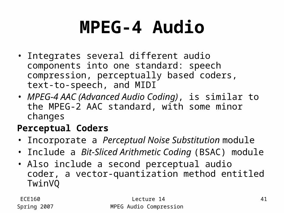
• Integrates several different audio components into one standard: speech compression, perceptually based coders, text-to-speech, and MIDI
• MPEG-4 AAC (Advanced Audio Coding), is similar to the MPEG-2 AAC standard, with some minor changes
Perceptual Coders• Incorporate a Perceptual Noise Substitution module• Include a Bit-Sliced Arithmetic Coding (BSAC) module• Also include a second perceptual audio coder, a vector-
quantization method entitled TwinVQ
ECE160Spring 2007
Lecture 14MPEG Audio Compression
42
MPEG-4 Audio
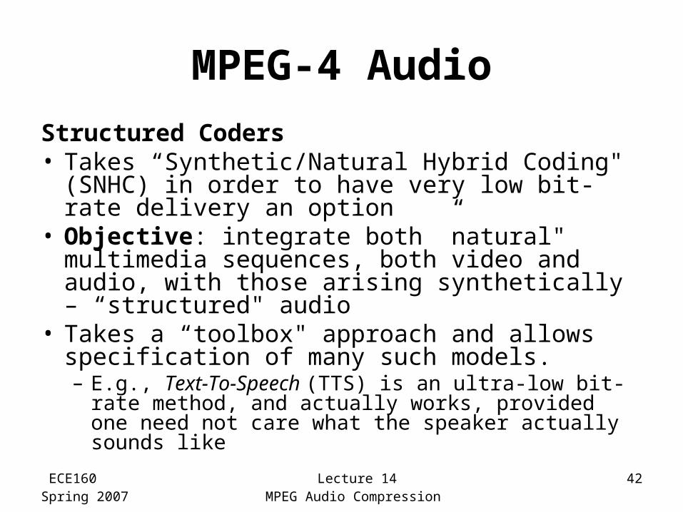
Structured Coders• Takes “Synthetic/Natural Hybrid Coding"
(SNHC) in order to have very low bit-rate delivery an option
• Objective: integrate both ”natural" multimedia sequences, both video and audio, with those arising synthetically – “structured" audio
• Takes a “toolbox" approach and allows specification of many such models.– E.g., Text-To-Speech (TTS) is an ultra-low bit-rate
method, and actually works, provided one need not care what the speaker actually sounds like
ECE160Spring 2007
Lecture 14MPEG Audio Compression
43
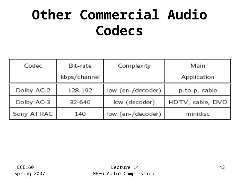
Other Commercial Audio Codecs
ECE160Spring 2007
Lecture 14MPEG Audio Compression
44
MPEG-7 and MPEG-21
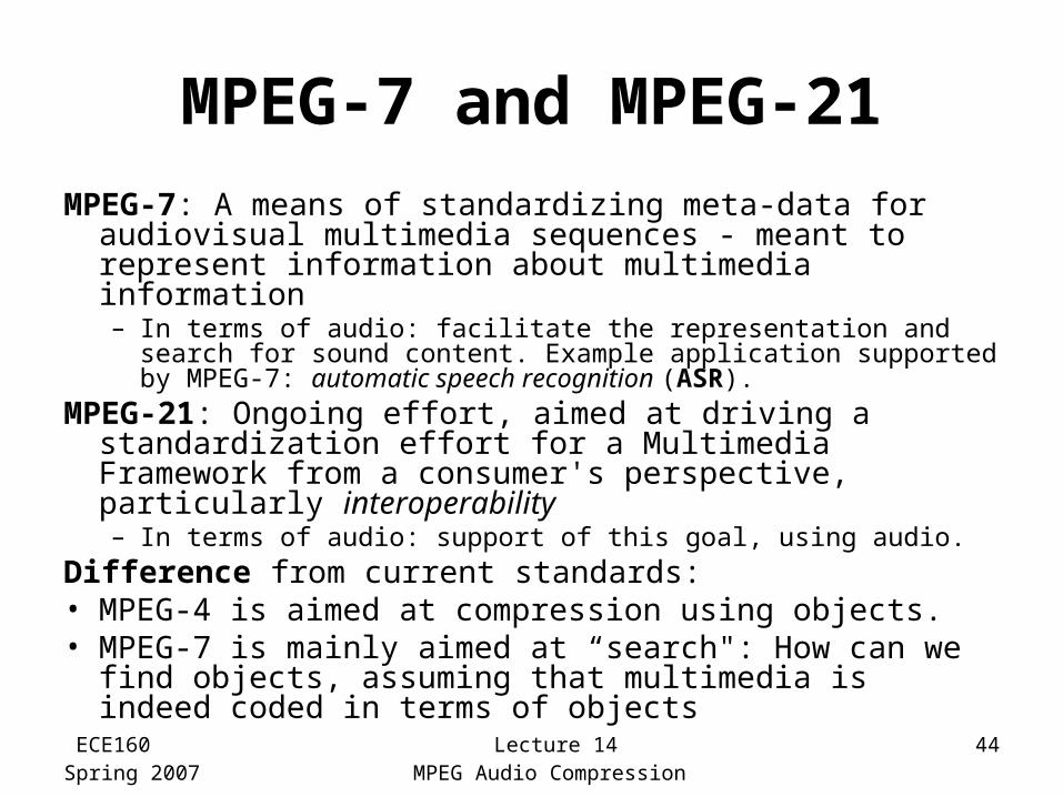
MPEG-7: A means of standardizing meta-data for audiovisual multimedia sequences - meant to represent information about multimedia information– In terms of audio: facilitate the representation and search for
sound content. Example application supported by MPEG-7: automatic speech recognition (ASR).
MPEG-21: Ongoing effort, aimed at driving a standardization effort for a Multimedia Framework from a consumer's perspective, particularly interoperability– In terms of audio: support of this goal, using audio.
Difference from current standards:• MPEG-4 is aimed at compression using objects.• MPEG-7 is mainly aimed at “search": How can we find
objects, assuming that multimedia is indeed coded in terms of objects
Related Documents