ECE 4680 DSP Laboratory 4: FIR Digital Filtersmwickert/ece5655/lecture_notes/ARM/FIR_Lab4.pdf · // Brute force 4-tap solution ... Of special interest for this lab Figure 2: The CMSIS-DSP

ECE 4680 DSP Laboratory 4:FIR Digital FiltersDue Date: ________________

Introduction

Finite Impulse Response Filter BasicsChapter 3 of the course text deals with FIR digital filters. In ECE 2610 considerable time wasspent with this class of filter. Recall that the difference equation for filtering input with filtercoefficient set , is

. (1)

The number of filter coefficients (taps) is (later denoted M_FIR) and the filter order is .The coefficients are typically obtained using filter design functions in scipy.signal, e.g. the cus-tom module of function in fir_design_helper.py, also utilized in the Jupyter notebook FIR Fil-ter Design and C Headers.ipynb or MATLAB’s filter design function, fdatool().

Notice that the calculation behind the FIR filter can be viewed as a sum-of-products or as a dotproduct between arrays/vectors containing the filter coefficients and the present and N past sam-ples of the input. For the Nth filter the computational burden is multiplications and additions.

The filter impulse response is obtained by setting as assuming zero initial con-ditions (the filter state array contains zeros)

(2)

The filter frequency response is obtained by Fourier transforming (DTFT) the impulse response

(3)

and the filter system function (z-domain representation) is the z-transform of

. (4)

From the system function it is clear why the filter order is N. The highest negative power of z is N.

x n b n n 0 N =

y n h k x n k– k 0=

N

=

N 1+ N

N 1+ N

x n n =x n x n 1– x n N–

h n h k n k– k 0=

N

=

H ej h k e jk–

k 0=

N

=

h n

H z h k z 1–

k 0=

N

h 0 h 1 z 1– h N z N–+ + += =

Introduction 1

ECE 4680 DSP Laboratory 4: FIR Digital Filters

Once a set of filter coefficients is available an FIR filter can make use of them. In Python/MATLAB code this is easy since we have the lfilter()/filter() function available. In Pythonsuppose x is an ndarray (1D array) input signal values that we want to filter and vector h containsthe FIR coefficients. We can obtain the filtered output array y via

>> y = lfilter(h,1,x);

In this lab we move beyond the use of Python (lfilter(b,a,x))/MATLAB (filter(b,a,x)) for fil-tering signals, and consider the real-time implementation of a sample-by-sample filter algorithmin C/C++. The Reay text [1], Chapter 3, is devoted FIR filters and implementation in C. Under thesrc folder of the ZIP package for Lab 4 you find the code module FIR_filters.c/FIR_filters.hfor implementing both floating-point and fixed-point FIR filters. Thirdly, FIR filters are also avail-able in the ARM CMSIS-DSP library (http://www.keil.com/pack/doc/CMSIS/DSP/html/index.html). Recall CMSIS is the ARM Cortex-M Software Interface Standard, freely availablefor use with the Cortex-M family of microcontrollers. In this lab you will get a chance to checkout the last two approaches, plus write simple filtering code right inside the ISR routine.

Real-Time FIR Filtering in CIn this section several FIR filter implementations are considered. All of the approaches fall backon the same sum-of-products concept, but in slightly different ways. At the end of this section theARM CMSIS-DSP functions are considered, but only at the interface level. The internal details arenot explored.

Sum-of-Products In-place Filtering

A simple sum-of-products FIR filtering routine is given in the Jupyter notebook ‘FIR Filter

Design and C Headers.ipynb’. This code was prototyped on the host PC using the GNU compil-ers (gcc and g++). The core filter code, that here runs inside a simulation loop over NSAMPLES is:

#define NSAMPLES 50float32_t x[NSAMPLES], y[NSAMPLES];float32_t state[M_FIR];float32_t accum;...// Filter Input array x and output array yfor (n = 0; n < NSAMPLES; n++) { accum = 0.0; state[0] = x[n]; // Filter (sum of products) for (i = 0; i < M_FIR; i++) { accum += h_FIR[i] * state[i]; } y[n] = accum; // Update the states for (i = M_FIR-1; i > 0; i--) { state[i] = state[i - 1]; }}

where M_FIR is a constant corresponding to the tap count, as declared via a #define in a header file

Introduction 2

http://www.keil.com/pack/doc/CMSIS/DSP/html/index.html



where the coefficients are listed. You will see later how this header file is obtained using a Pythonfunction that transfers digital filter coefficients from a Jupyter notebook to a .h file.

Brute Force Filtering for a Few Taps

Implementing, say a four tap moving average filter, can be done in a less formal way. Below xand y are float32_t values inside the FM4 ISR with x_old and state defined globally.

float32_t x_old[4] = {0, 0, 0, 0};float32_t state[4] = {0, 0, 0, 0};

...// Brute force 4-tap solutionx_old[0] = x;y = 0.25f*x_old[0] + 0.25f*x_old[1] + 0.25f*x_old[2] + 0.25f*x_old[3];x_old[3] = x_old[2];x_old[2] = x_old[1];

x_old[1] = x_old[0];

...

Using a Portable Filter Module

The code module FIR_filters.c/FIR_filters.h, found in the src folder for Lab 4, imple-ments both floating-point and fixed-point FIR filtering routines using portable ANSI C. Here wewill only explore the float32_t functions. The functions allow for sample-by-sample processingas well as frame-based processing, where a block of length Nframe samples are processed in onefunction call. The data structure shown below is used to organize the filter details:

struct FIR_struct_float32 { int16_t M_taps; float32_t *state; float32_t *b_coeff;

};

Pointers are used to manage all of the arrays, and ultimately the data structure itself, to insure thatfunction calls are fast and efficient. Recall in particular that in C an array name is actually theaddress to the first element of the array. This property is used by the functions FIR_init_-float32() and FIR_filt_float32() which interact with the FIR filter data structure to initializeand then filter signal samples, respectively. The four steps to FIR filtering using this module are:

1. Create an instance of the data structure:

struct FIR_struct_float32 FIR1;

where now FIR1 is essentially a filter object to be manipulated in code.

2. Have on hand two float32_t arrays of length M_FIR to hold the filter coefficients, e.g.,h_fir[], and the filter state, state[]. Note actual filter state is really just M_FIR-1, but oneelement is used to hold the present input.

3. Initialize FIR1 in main() using:

FIR_init_float32(&FIR1,state101,h_FIR,M_FIR);

where here state101 is the address to a float32_t array of length 101 elements used to hold

Introduction 3


the filter states and h_FIR is the address to a float32_t array holding 101 filter coefficients.The filter state array should be declared as a global. Often h_FIR will be filled using a headerfile, e.g.,

#include "remez_8_14_bpf_f32.h" // a 101 tap FIR

is a 101 tap FIR bandpass filter with passband from 8 to 14 kHz generated in a Jupyter note-book.

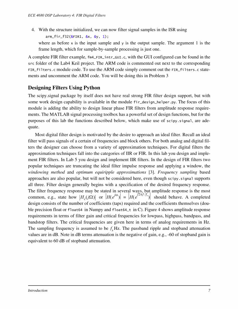
4. With the structure initialized, we can now filter signal samples in the ISR using

FIR_filt_float32(&FIR1,&x,&y,1);

where x is the input sample and y is the output sample. Notice again passing by address inthe event a frame of data is being filtered. The argument 1 is the frame length, which forsample-by-sample processing is just one. By sample-by-sample I mean that each time theISR runs a new sample has arrived at the ADC and a new filtered sample must returned tothe DAC.

The code behind FIR_filt_float32(), inside FIR_filters.c, is:

//Process each sample of the frame with this loop for (iframe = 0; iframe < Nframe; iframe++) { // Clear the accumulator/output before filtering accum = 0; // Place new input sample as first element in the filter state array FIR->state[0] = x_in[iframe]; //Direct form filter each sample using a sum of products

for (iFIR = 0; iFIR < FIR->M_taps; iFIR++) { accum += FIR->state[iFIR]*FIR->b_coeff[iFIR]; } x_out[iframe] = accum; // Shift filter states to right or use circular buffer for (iFIR = FIR->M_taps-1; iFIR > 0; iFIR--) { FIR->state[iFIR] = FIR->state[iFIR-1]; } }

}

All working variables are float32_t. The outer for loop processes each sample within the frame.The first of the inner for loops is in fact the sum-of-products represented by (1). The array FIR->state[] holds for (here M_taps is equivalent to in (1)). The sec-ond of the inner for loops updates the filter history by discarding the oldest input, , andsliding all the remaining samples to the left one position. The most recent input, , ends up inFIR->state[1] to make room for the new input being placed into FIR->state[0] on the next callof the ISR. A more efficient means of keep the state array updated is using circular buffer. Moreon that later.

A complete FIR filter example, fm4_FIR_intr_GUI.c, with the GUI configured can be found inthe src folder of the Lab4 Keil project. This project is configured to load a 101 tap bandpass filter.

x n k– k 0 N = N 1+x n N–

x n

Introduction 4


ARM CMSIS-DSP FIR Algorithms

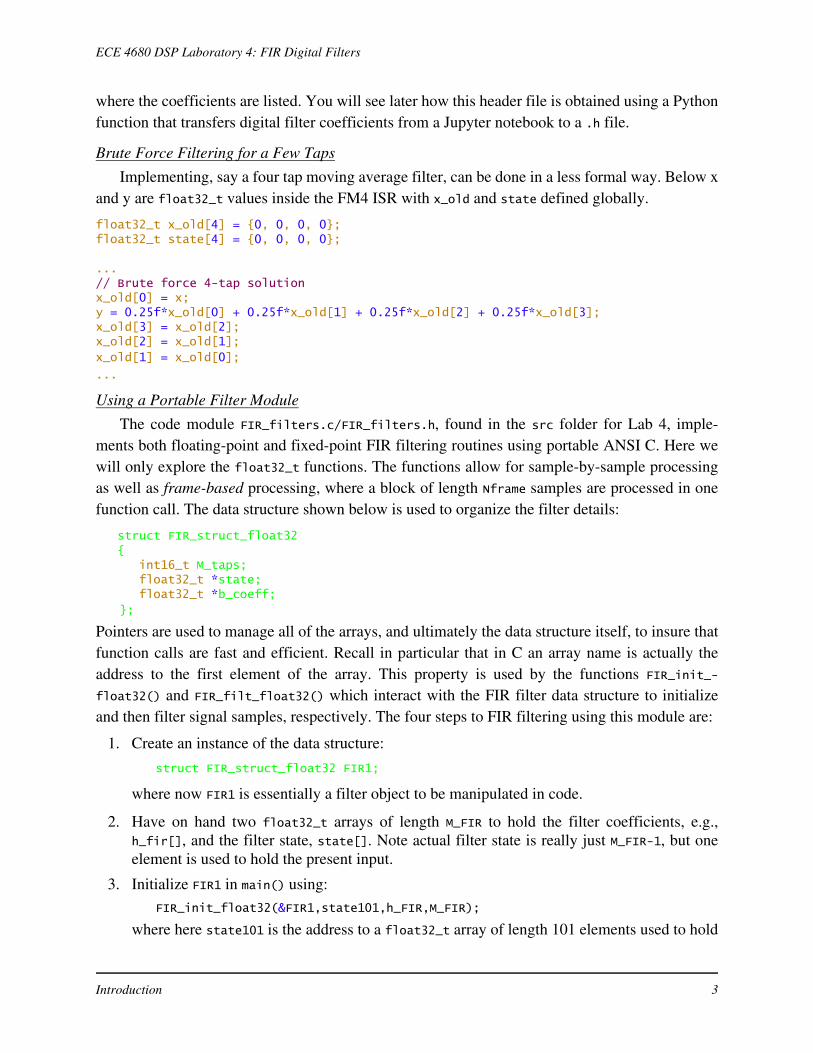
An important part of the Arm® Cortex®-M processor family is the Cortex microcontroller soft-ware interface standard (CMSIS) http://www.keil.com/pack/doc/CMSIS/General/html/

index.html of Figure 1. Of particular interest is the DSP library CMSIS-DSP of Figure 2. Fast and

efficient C data structure-based FIR filter algorithms are available in the library: http://www.keil.com/pack/doc/CMSIS/DSP/html/index.html. The DSP library is divided into 10 major

Figure 1: ARM® CMSIS the big picture showing where CMSIS-DSP resides.

Of special interest for this lab

Figure 2: The CMSIS-DSP library top level description.

Introduction 5


http://www.keil.com/pack/doc/CMSIS/General/html/index.html

http://www.keil.com/pack/doc/CMSIS/General/html/index.html


groups of algorithms. Other parts of CMSIS are at work in the FM4, for example CMSIS-DAPdefines the Debug Access Port interface.

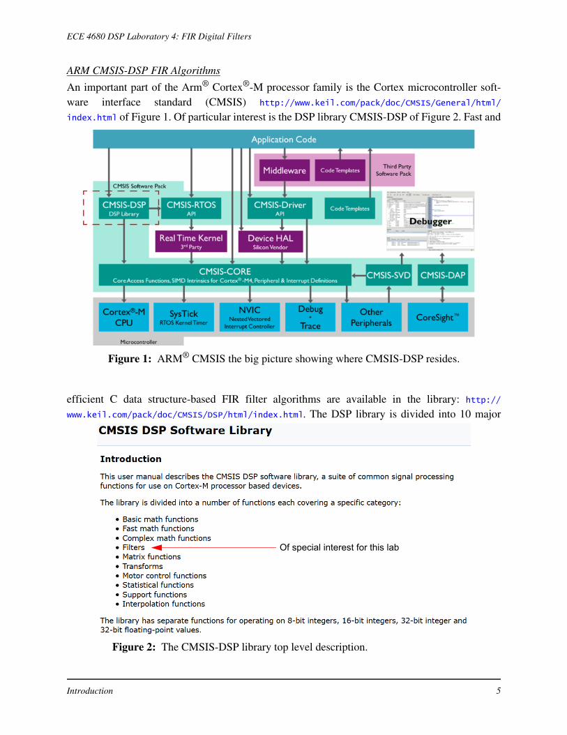
The documentation for the Filter Functions group com be expanded by clicking on Referencedisclosure triangle in the left navigation pane of the CMSIS-DSP Web Site as shown in Figure 3.A good introduction to the inner workings of CMSIS-DSP can be found in Yiu [2]. Within the fil-tering subheading you find FIR filters, and finally float32_t implementations that run on the M4with the floating-point hardware present. The functions arm_fir_init_f32() and arm_fit_f32()

perform functions similar to FIR_init_float32() and FIR_filt_float32() respectively, of theprevious subsection. The function calls are slightly different, but in the end take the same argu-ments, except in CMSIS-DSP the init function takes the frame length. The four steps to FIR fil-tering using this module are:

1. Create an instance of the data structure:arm_fir_instance_f32 FIR1;

where now FIR1 is essentially a filter object to be manipulated in code.

2. Again you need to have on hand two float32_t arrays of length M_FIR to hold the filter coef-ficients, e.g., h_fir[], and the filter state, state[]. Note actual filter state is really justM_FIR-1, but as before one element is used to hold the present input.

3. Initialize FIR1 in main() using:

IIR_sos_init_float32(&IIR1, STAGES, ba_coeff, IIRstate);

where as before state101 is the address to a float32_t array of length 101 elements used tohold the filter states and h_FIR is the address to a float32_t array holding 101 filter coeffi-cients. The final argument sets frame length (ARM terminology blockSize). Here it is justone for sample-by-sample processing.

Functions ofinterest here

Figure 3: CMSIS-DSP FIR float32_t filter detail.

Introduction 6


4. With the structure initialized, we can now filter signal samples in the ISR using

arm_fir_f32(&FIR1, &x, &y, 1);

where as before x is the input sample and y is the output sample. The argument 1 is theframe length, which for sample-by-sample processing is just one.

A complete FIR filter example, fm4_FIR_intr_GUI.c, with the GUI configured can be found in thesrc folder of the Lab4 Keil project. The ARM code is commented out next to the correspondingFIR_filters.c module code. To use the ARM code simply comment out the FIR_filters.c state-ments and uncomment the ARM code. You will be doing this in Problem 3

Designing Filters Using PythonThe scipy.signal package by itself does not have real strong FIR filter design support, but withsome work design capability is available in the module fir_design_helper.py. The focus of thismodule is adding the ability to design linear phase FIR filters from amplitude response require-ments. The MATLAB signal processing toolbox has a powerful set of design functions, but for thepurposes of this lab the functions described below, which make use of scipy.signal, are ade-quate.

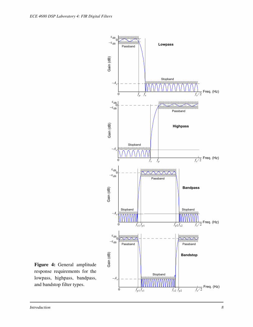
Most digital filter design is motivated by the desire to approach an ideal filter. Recall an idealfilter will pass signals of a certain of frequencies and block others. For both analog and digital fil-ters the designer can choose from a variety of approximation techniques. For digital filters theapproximation techniques fall into the categories of IIR or FIR. In this lab you design and imple-ment FIR filters. In Lab 5 you design and implement IIR filters. In the design of FIR filters twopopular techniques are truncating the ideal filter impulse response and applying a window, thewindowing method and optimum equiripple approximations [3]. Frequency sampling basedapproaches are also popular, but will not be considered here, even though scipy.signal supportsall three. Filter design generally begins with a specification of the desired frequency response.The filter frequency response may be stated in several ways, but amplitude response is the mostcommon, e.g., state how or should behave. A completeddesign consists of the number of coefficients (taps) required and the coefficients themselves (dou-ble precision float or float64 in Numpy and float64_t in C). Figure 4 shows amplitude responserequirements in terms of filter gain and critical frequencies for lowpass, highpass, bandpass, andbandstop filters. The critical frequencies are given here in terms of analog requirements in Hz.The sampling frequency is assumed to be Hz. The passband ripple and stopband attenuationvalues are in dB. Note in dB terms attenuation is the negative of gain, e.g., -60 of stopband gain isequivalent to 60 dB of stopband attenuation.

Hc j H ej H e

j2f fs =

fs

Introduction 7


–

As–

fsfp fs

–

As–

fsfpfs

–

As–

fsfpfs fsfp

–

As–

fsfp fs fs fp

Figure 4: General amplituderesponse requirements for thelowpass, highpass, bandpass,and bandstop filter types.

Introduction 8


There are 10 filter design functions and one plotting function available infir_design_helper.py. Four functions for designing Kaiser window based FIR filters and fourfunctions for designing equiripple based FIR filters. Of the eight just described, they all take inamplitude response requirements and return a coefficients array. Two filter functions are simplywrappers around the scipy.signal function signal.firwin() for designing filters of a specificorder with one (lowpass) or two (bandpass) critical frequencies are given. The wrapper functionsfix the window type to the firwin default of hann (hanning). The plotting function provides aneasy means to compare the resulting frequency response of one or more designs on a single plot.Display modes allow gain in dB, phase in radians, group delay in samples, and group delay in sec-onds for a given sampling rate. This function, freq_resp_list(), works for both FIR and IIRdesigns. Table 1 provides the interface details to the eight design functions where d_stop and

d_pass are positive dB values and the critical frequencies have the same unit as the sampling fre-quency f_s. These functions do not create perfect results so some tuning of of the design parame-ters may be needed, in addition to bumping the filter order up or down via N_bump.

Table 1: FIR filter design functions in fir_design_helper.py.

Type FIR Filter Design Functions

Kasier Window

Lowpass h_FIR = firwin_kaiser_lpf(f_pass, f_stop, d_stop, fs = 1.0, N_bump=0)

Highpass h_FIR = firwin_kaiser_hpf(f_stop, f_pass, d_stop, fs = 1.0, N_bump=0)

Bandpass h_FIR = firwin_kaiser_bpf(f_stop1, f_pass1, f_pass2, f_stop2, d_stop, fs = 1.0, N_bump=0)

Bandstop h_FIR = firwin_kaiser_bsf(f_stop1, f_pass1, f_pass2, f_stop2, d_stop, fs = 1.0, N_bump=0)

Equiripple Approximation

Lowpass h_FIR = fir_remez_lpf(f_pass, f_stop, d_pass, d_stop, fs = 1.0, N_bump=5)

Highpass h_FIR = fir_remez_hpf(f_stop, f_pass, d_pass, d_stop, fs = 1.0, N_bump=5)

Bandpass h_FIR = fir_remez_bpf(f_stop1, f_pass1, f_pass2, f_stop2, d_pass, d_stop, fs = 1.0, N_bump=5)

Bandstop h_FIR = fir_remez_bsf(f_pass1, f_stop1, f_stop2, f_pass2, d_pass, d_stop, fs = 1.0, N_bump=5)

The optional N_bump argument allows the filter order to be bumped up or down by an integer value in order to fine tune the design. Making changes to the stopband gain main also be helpful in fine tuning. Note also that the Kaiser bandstop filter order is constrained to be even (an odd number of taps).

Introduction 9


The frequency response plotting function, freqz_resp_list, interface is given below:

def freqz_resp_list(b,a=np.array([1]),mode = 'dB',fs=1.0,Npts = 1024,fsize=(6,4)): """ A method for displaying digital filter frequency response magnitude, phase, and group delay. A plot is produced using matplotlib

freq_resp(self,mode = 'dB',Npts = 1024)

A method for displaying the filter frequency response magnitude, phase, and group delay. A plot is produced using matplotlib

freqz_resp(b,a=[1],mode = 'dB',Npts = 1024,fsize=(6,4))

b = ndarray of numerator coefficients a = ndarray of denominator coefficents mode = display mode: 'dB' magnitude, 'phase' in radians, or 'groupdelay_s' in samples and 'groupdelay_t' in sec, all versus frequency in Hz Npts = number of points to plot; default is 1024 fsize = figure size; defult is (6,4) inches

To see how all of this works a couple of examples extracted from the sample Jupyter notebook areprovided below.

Lowpass Design

Figure 5: Lowpassdesign example;Kaiser vs optimalequal ripple.

Introduction 10


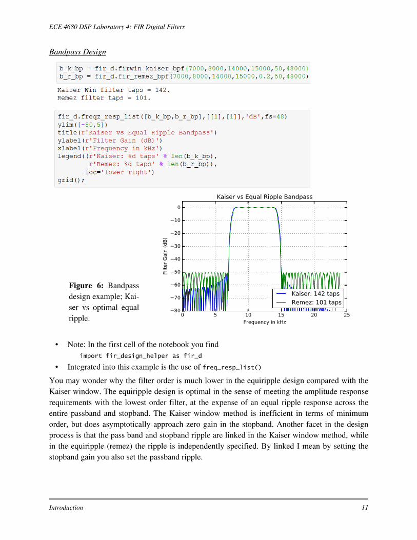
Bandpass Design

• Note: In the first cell of the notebook you findimport fir_design_helper as fir_d

• Integrated into this example is the use of freq_resp_list()

You may wonder why the filter order is much lower in the equiripple design compared with theKaiser window. The equiripple design is optimal in the sense of meeting the amplitude responserequirements with the lowest order filter, at the expense of an equal ripple response across theentire passband and stopband. The Kaiser window method is inefficient in terms of minimumorder, but does asymptotically approach zero gain in the stopband. Another facet in the designprocess is that the pass band and stopband ripple are linked in the Kaiser window method, whilein the equiripple (remez) the ripple is independently specified. By linked I mean by setting thestopband gain you also set the passband ripple.

Figure 6: Bandpassdesign example; Kai-ser vs optimal equalripple.

Introduction 11


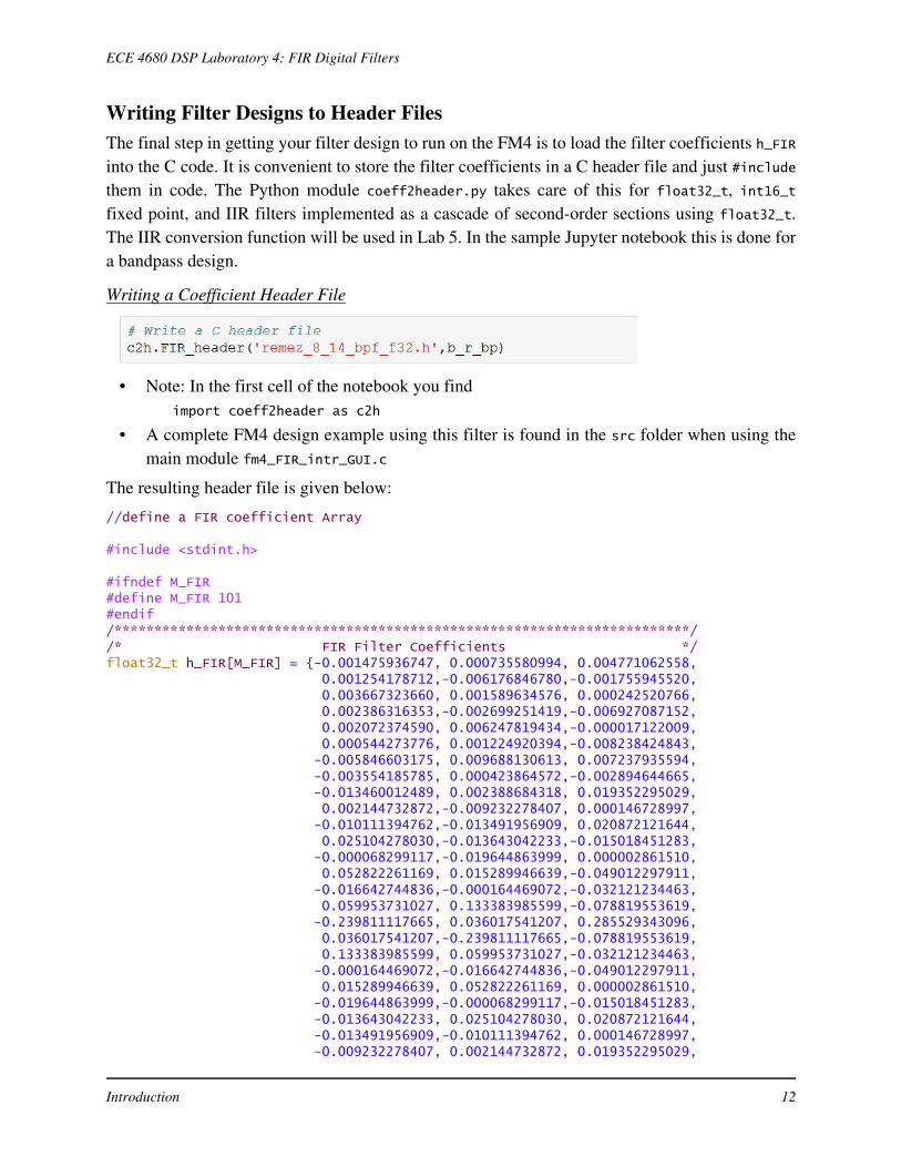
Writing Filter Designs to Header FilesThe final step in getting your filter design to run on the FM4 is to load the filter coefficients h_FIRinto the C code. It is convenient to store the filter coefficients in a C header file and just #includethem in code. The Python module coeff2header.py takes care of this for float32_t, int16_tfixed point, and IIR filters implemented as a cascade of second-order sections using float32_t.The IIR conversion function will be used in Lab 5. In the sample Jupyter notebook this is done fora bandpass design.

Writing a Coefficient Header File

• Note: In the first cell of the notebook you findimport coeff2header as c2h

• A complete FM4 design example using this filter is found in the src folder when using themain module fm4_FIR_intr_GUI.c

The resulting header file is given below:

//define a FIR coefficient Array

#include <stdint.h>

#ifndef M_FIR#define M_FIR 101#endif/************************************************************************//* FIR Filter Coefficients */float32_t h_FIR[M_FIR] = {-0.001475936747, 0.000735580994, 0.004771062558, 0.001254178712,-0.006176846780,-0.001755945520, 0.003667323660, 0.001589634576, 0.000242520766, 0.002386316353,-0.002699251419,-0.006927087152, 0.002072374590, 0.006247819434,-0.000017122009, 0.000544273776, 0.001224920394,-0.008238424843, -0.005846603175, 0.009688130613, 0.007237935594, -0.003554185785, 0.000423864572,-0.002894644665, -0.013460012489, 0.002388684318, 0.019352295029, 0.002144732872,-0.009232278407, 0.000146728997, -0.010111394762,-0.013491956909, 0.020872121644, 0.025104278030,-0.013643042233,-0.015018451283, -0.000068299117,-0.019644863999, 0.000002861510, 0.052822261169, 0.015289946639,-0.049012297911, -0.016642744836,-0.000164469072,-0.032121234463, 0.059953731027, 0.133383985599,-0.078819553619, -0.239811117665, 0.036017541207, 0.285529343096, 0.036017541207,-0.239811117665,-0.078819553619, 0.133383985599, 0.059953731027,-0.032121234463, -0.000164469072,-0.016642744836,-0.049012297911, 0.015289946639, 0.052822261169, 0.000002861510, -0.019644863999,-0.000068299117,-0.015018451283, -0.013643042233, 0.025104278030, 0.020872121644, -0.013491956909,-0.010111394762, 0.000146728997, -0.009232278407, 0.002144732872, 0.019352295029,

Introduction 12


0.002388684318,-0.013460012489,-0.002894644665, 0.000423864572,-0.003554185785, 0.007237935594, 0.009688130613,-0.005846603175,-0.008238424843, 0.001224920394, 0.000544273776,-0.000017122009, 0.006247819434, 0.002072374590,-0.006927087152, -0.002699251419, 0.002386316353, 0.000242520766, 0.001589634576, 0.003667323660,-0.001755945520, -0.006176846780, 0.001254178712, 0.004771062558, 0.000735580994,-0.001475936747};

/************************************************************************/

ExpectationsWhen completed, submit a lab report which documents code you have written and a summary ofyour results. Screen shots from the scope and any other instruments and software tools should beincluded as well. I expect lab demos of certain experiments to confirm that you are obtaining theexpected results and knowledge of the tools and instruments.

Problems

Measuring Filter Frequency Response Using the Network Analyzer1. The Comm/DSP lab has test equipment that be used to measure the frequency response of

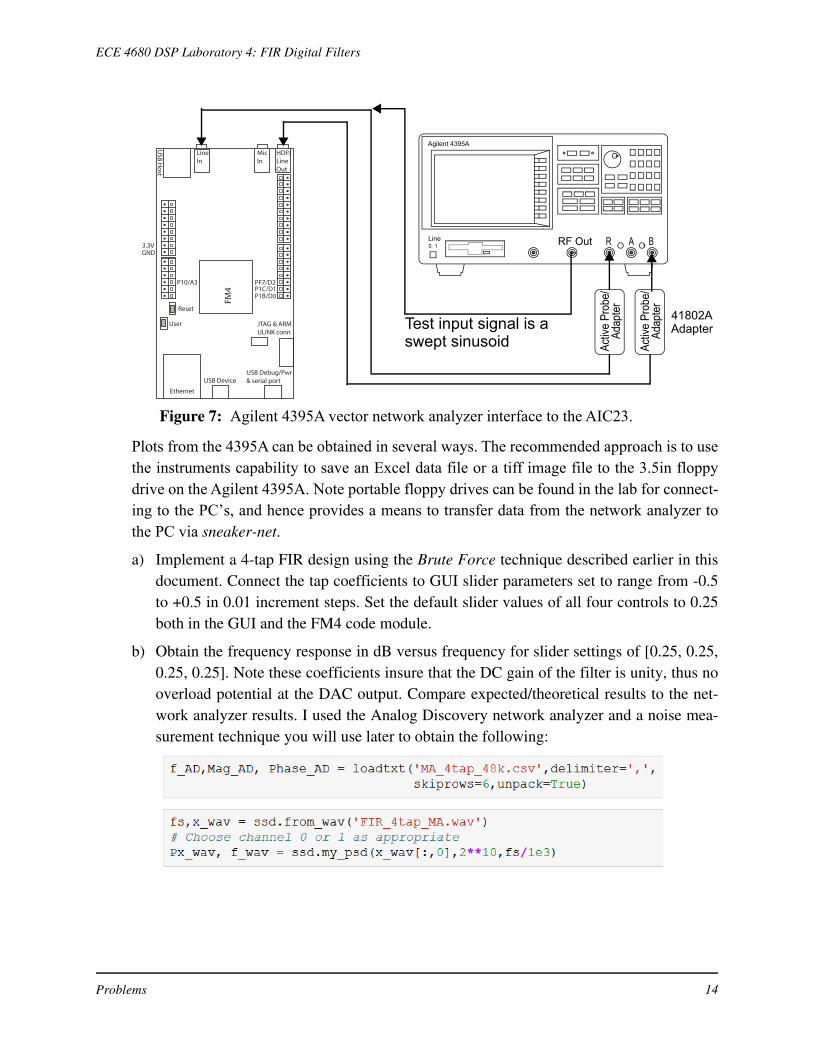
an analog filter. In particular, we can use this equipment to characterize the end-to-endresponse of a digital filter that sits inside of an A/D- -D/A processor, such as the FM4Pioneer Kit. The instructor will demonstrate how to properly use the Agilent 4395A vector/spectrum analyzer for taking frequency response measurements.

Turning to the vector network analyzer consider the block diagram of Figure 2. You use thevector network analyzer to measure the frequency response magnitude in dB as the ratio ofthe analog output over the analog input (say using analyzer ports B/R). The phase differenceformed as the output phase minus the input phase, the phase response, can also be measuredby the instrument, although that is not of interest presently. The frequency range you sweepover should be consistent with the sampling frequency. If you are sampling at 48 ksps whatshould the maximum frequency of interest be?

H z

Expectations 13


Plots from the 4395A can be obtained in several ways. The recommended approach is to usethe instruments capability to save an Excel data file or a tiff image file to the 3.5in floppydrive on the Agilent 4395A. Note portable floppy drives can be found in the lab for connect-ing to the PC’s, and hence provides a means to transfer data from the network analyzer tothe PC via sneaker-net.

a) Implement a 4-tap FIR design using the Brute Force technique described earlier in thisdocument. Connect the tap coefficients to GUI slider parameters set to range from -0.5to +0.5 in 0.01 increment steps. Set the default slider values of all four controls to 0.25both in the GUI and the FM4 code module.

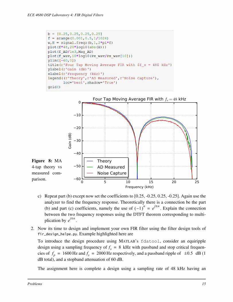
b) Obtain the frequency response in dB versus frequency for slider settings of [0.25, 0.25,0.25, 0.25]. Note these coefficients insure that the DC gain of the filter is unity, thus nooverload potential at the DAC output. Compare expected/theoretical results to the net-work analyzer results. I used the Analog Discovery network analyzer and a noise mea-surement technique you will use later to obtain the following:

FM4

P10/A3 PF7/D2P1C/D1P1B/D0

USB H

ost

MicIn

HDP/LineOut

LineIn

3.3VGND

Ethernet

Reset

User

USB Debug/Pwr& serial portUSB Device

JTAG & ARMULINK conn

Agilent 4395A

0 1 . . . .RF OutLine R BA

Act

ive

Pro

be/

Ada

pter

41802AAdapter

Act

ive

Pro

be/

Ada

pter

Test input signal is aswept sinusoid

Figure 7: Agilent 4395A vector network analyzer interface to the AIC23.

Problems 14


c) Repeat part (b) except now set the coefficients to [0.25, -0.25, 0.25, -0.25]. Again use theanalyzer to find the frequency response. Theoretically there is a connection be the part(b) and part (c) coefficients, namely the use of . Explain the connectionbetween the two frequency responses using the DTFT theorem corresponding to multi-plication by .

2. Now its time to design and implement your own FIR filter using the filter design tools offir_design_helpe.py. Example highlighted here are

To introduce the design procedure using MATLAB’s fdatool, consider an equirippledesign using a sampling frequency of kHz with passband and stop critical frequen-cies of Hz and Hz respectively, and a passband ripple of dB (1dB total), and a stopband attenuation of 60 dB.

The assignment here is complete a design using a sampling rate of 48 kHz having an

Figure 8: MA4-tap theory vsmeasured com-parison.

1– n ejn

=

ejn

fs 8=fp 1600= fs 2000= 0.5

Problems 15


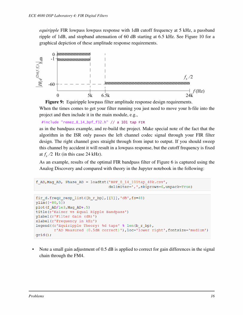
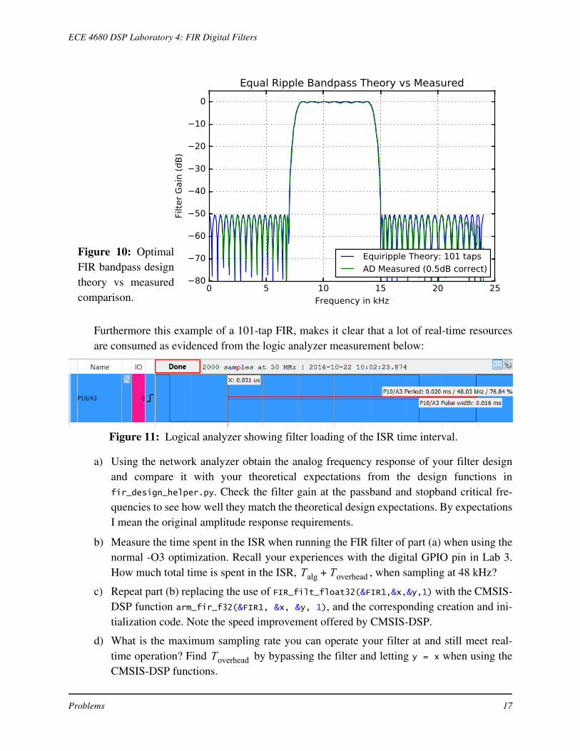
equiripple FIR lowpass lowpass response with 1dB cutoff frequency at 5 kHz, a passbandripple of 1dB, and stopband attenuation of 60 dB starting at 6.5 kHz. See Figure 10 for agraphical depiction of these amplitude response requirements.

When the times comes to get your filter running you just need to move your h-file into theproject and then include it in the main module, e.g.,

#include "remez_8_14_bpf_f32.h" // a 101 tap FIR

as in the bandpass example, and re-build the project. Make special note of the fact that thealgorithm in the ISR only passes the left channel codec signal through your FIR filterdesign. The right channel goes straight through from input to output. If you should sweepthis channel by accident it will result in a lowpass response, but the cutoff frequency is fixedat Hz (in this case 24 kHz).

As an example, results of the optimal FIR bandpass filter of Figure 6 is captured using theAnalog Discovery and compared with theory in the Jupyter notebook in the following:

• Note a small gain adjustment of 0.5 dB is applied to correct for gain differences in the signalchain through the FM4.

Hej2

f

f s

dB

0-1

-60

0 5k 6.5k 24kf (Hz)

fs 2

Figure 9: Equiripple lowpass filter amplitude response design requirements.

fs 2

Problems 16


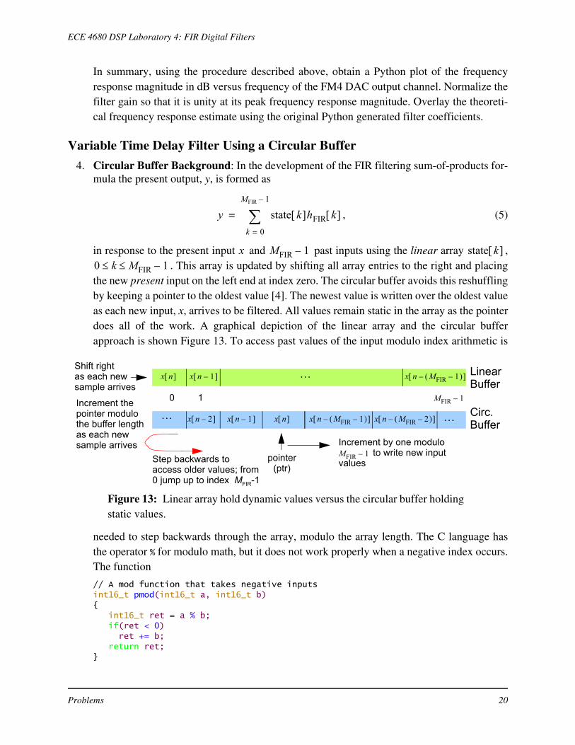
Furthermore this example of a 101-tap FIR, makes it clear that a lot of real-time resourcesare consumed as evidenced from the logic analyzer measurement below:

a) Using the network analyzer obtain the analog frequency response of your filter designand compare it with your theoretical expectations from the design functions infir_design_helper.py. Check the filter gain at the passband and stopband critical fre-quencies to see how well they match the theoretical design expectations. By expectationsI mean the original amplitude response requirements.

b) Measure the time spent in the ISR when running the FIR filter of part (a) when using thenormal -O3 optimization. Recall your experiences with the digital GPIO pin in Lab 3.How much total time is spent in the ISR, , when sampling at 48 kHz?

c) Repeat part (b) replacing the use of FIR_filt_float32(&FIR1,&x,&y,1) with the CMSIS-DSP function arm_fir_f32(&FIR1, &x, &y, 1), and the corresponding creation and ini-tialization code. Note the speed improvement offered by CMSIS-DSP.

d) What is the maximum sampling rate you can operate your filter at and still meet real-time operation? Find by bypassing the filter and letting y = x when using theCMSIS-DSP functions.

Figure 10: OptimalFIR bandpass designtheory vs measuredcomparison.

Figure 11: Logical analyzer showing filter loading of the ISR time interval.

Talg Toverhead+

Toverhead

Problems 17


e) Estimate the maximum number of FIR coefficients the present algorithm can supportwith kHz and still meet real-time. Show your work. You can assume that grows linearly with the number of coefficients, M_FIR. Again assume you are usingCMSIS-DSP.

Measuring Frequency Response Using White Noise Excitation

3. Rather than using the network analyzer as in Problems 1–2, this time you will use the PCdigital audio system to capture a finite record of DAC output as shown in Figure 12. Use the

same FIR filter as used in Problem 2. The software capture tool that is useful here is the

shareware program GoldWave1 (goldwave.zip on Web site). A 30 second capture at44.1 kHz seems to work well. Since the sampling rate is only 32 ksps.

To get this setup you first need to add a function to your code so that you can digitally gen-erate a noise source as the input to your filtering algorithm. Add the following uniform ran-dom number generator function to the ISR code module:

// Uniformly distributed noise generatorint32_t rand_int32(void){ static int32_t a_start = 100001;

a_start = (a_start*125) % 2796203;

return a_start;

}

1. https://www.goldwave.com/. An older version is available on the course Web Site.

fs 48= Talg

FM4

PCSoundCard

Capture 30 secondsusing >= 24.4 kHzsampling rate.

Save outputas a .wav file.

Import using

Apply psd()to createfrequencyresponseestimate.

f

|H(f)|dB

PCWorkstation

LineInput

Out

GoldwaveAudio

Capture

Run whitenoise codeas filterinput

ssd.from_wav('filename.wav')

Importwave file

intoJupyter

notebook

Figure 12: Waveform capture using the PC sound card and Goldwave.

Problems 18


Note the code is already in place in the project you extract from the Lab 4 zip file. Now youwill drive your filter algorithm with white noise generated via the function rand_int32(). Inyour filter code you will replace the read from the audio code with something like to follow-ing:

# Replace ADC with internal noise scaled//x = (float32_t) sample.uint16bit[LEFT];x = (float32_t) (rand_int32()>>4);

Once a record is captured in GoldWave it can be saved as a .wav file. The .wav file canthen be loaded into a Jupyter notebook using ssd.from_wav('filename.wav'). Note, Gold-Wave can directly display waveforms and their corresponding spectra, but higher qualityspectral analysis can be performed using the numpy function psd(). You need a version thatallows rescaling of the spectrum estimate. For this purpose use the wrapper function

Px_wav, f_wav = ssd.my_psd(x, NFFT, fs)

The spectral analysis function implements Welch’s method of averaged periodograms. Sup-pose that the .wav file is saved as FIR_4tap_MA.wav, then a plot of the frequency responsecan be created as follows:

fs,x_wav = ssd.from_wav('FIR_4tap_MA.wav')# Choose channel 0 or 1 as appropriatePx_wav, f_wav = ssd.my_psd(x_wav[:,0],2**10,fs/1e3)# Normalize using a reasobable value close to f = 0, but not zeroplot(f_wav,10*log10(Px_wav/Px_wav[10]))

One condition to watch out for is overloading of the PC sound card line input. Goldwave haslevel indicators to help with this however. Use the sound card line input found on the back ofthe PC Workstation. The software mixer application has a separate set of mixer gain settingsjust for recording. You will need to adjust the Line In volume (similar to Figure 11) andwatch the actual input levels on Goldwave.

Adjust This Slider

Figure 11: Controlling the input level to the PC sound card.

or similar to avoid

Select the appropriatesource, likelyinternal mic input;Here I used anexternal USBaudio card (iMic)

Deflection due toaudio input fromFM4

overload

Double-click

Problems 19


In summary, using the procedure described above, obtain a Python plot of the frequencyresponse magnitude in dB versus frequency of the FM4 DAC output channel. Normalize thefilter gain so that it is unity at its peak frequency response magnitude. Overlay the theoreti-cal frequency response estimate using the original Python generated filter coefficients.

Variable Time Delay Filter Using a Circular Buffer

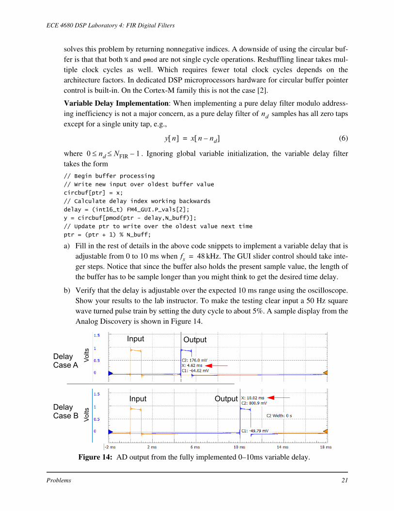
4. Circular Buffer Background: In the development of the FIR filtering sum-of-products for-mula the present output, y, is formed as

, (5)

in response to the present input and past inputs using the linear array ,. This array is updated by shifting all array entries to the right and placing

the new present input on the left end at index zero. The circular buffer avoids this reshufflingby keeping a pointer to the oldest value [4]. The newest value is written over the oldest valueas each new input, x, arrives to be filtered. All values remain static in the array as the pointerdoes all of the work. A graphical depiction of the linear array and the circular bufferapproach is shown Figure 13. To access past values of the input modulo index arithmetic is

needed to step backwards through the array, modulo the array length. The C language hasthe operator % for modulo math, but it does not work properly when a negative index occurs.The function

// A mod function that takes negative inputs int16_t pmod(int16_t a, int16_t b){ int16_t ret = a % b; if(ret < 0) ret += b; return ret;}

y state k hFIR k k 0=

MFIR 1–

=

x MFIR 1– state k 0 k MFIR 1–

x n x n 1– x n MFIR 1– –

x n x n 1–

Shift rightas each newsample arrives

Increment thepointer modulothe buffer lengthas each new sample arrives

pointer

x n MFIR 1– –

Increment by one moduloMFIR 1–

x n 2– x n MFIR 2– –

Step backwards toaccess older values; from0 jump up to index MFIR-1

to write new input values

0 1 MFIR 1–

Figure 13: Linear array hold dynamic values versus the circular buffer holdingstatic values.

LinearBuffer

Circ.Buffer

(ptr)

Problems 20


solves this problem by returning nonnegative indices. A downside of using the circular buf-fer is that that both % and pmod are not single cycle operations. Reshuffling linear takes mul-tiple clock cycles as well. Which requires fewer total clock cycles depends on thearchitecture factors. In dedicated DSP microprocessors hardware for circular buffer pointercontrol is built-in. On the Cortex-M family this is not the case [2].

Variable Delay Implementation: When implementing a pure delay filter modulo address-ing inefficiency is not a major concern, as a pure delay filter of samples has all zero tapsexcept for a single unity tap, e.g.,

(6)

where . Ignoring global variable initialization, the variable delay filtertakes the form

// Begin buffer processing

// Write new input over oldest buffer value

circbuf[ptr] = x;

// Calculate delay index working backwards

delay = (int16_t) FM4_GUI.P_vals[2];

y = circbuf[pmod(ptr - delay,N_buff)];

// Update ptr to write over the oldest value next time

ptr = (ptr + 1) % N_buff;

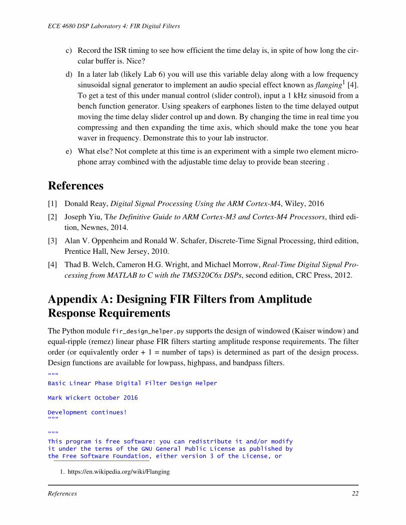
a) Fill in the rest of details in the above code snippets to implement a variable delay that isadjustable from 0 to 10 ms when kHz. The GUI slider control should take inte-ger steps. Notice that since the buffer also holds the present sample value, the length ofthe buffer has to be sample longer than you might think to get the desired time delay.

b) Verify that the delay is adjustable over the expected 10 ms range using the oscilloscope.Show your results to the lab instructor. To make the testing clear input a 50 Hz squarewave turned pulse train by setting the duty cycle to about 5%. A sample display from theAnalog Discovery is shown in Figure 14.

nd

y n x n nd– =

0 nd NFIR 1–

fs 48=

DelayCase A

DelayCase B

Input Output

OutputInput

Vol

tsV

olts

Figure 14: AD output from the fully implemented 0–10ms variable delay.

Problems 21


c) Record the ISR timing to see how efficient the time delay is, in spite of how long the cir-cular buffer is. Nice?

d) In a later lab (likely Lab 6) you will use this variable delay along with a low frequencysinusoidal signal generator to implement an audio special effect known as flanging1 [4].To get a test of this under manual control (slider control), input a 1 kHz sinusoid from abench function generator. Using speakers of earphones listen to the time delayed outputmoving the time delay slider control up and down. By changing the time in real time youcompressing and then expanding the time axis, which should make the tone you hearwaver in frequency. Demonstrate this to your lab instructor.

e) What else? Not complete at this time is an experiment with a simple two element micro-phone array combined with the adjustable time delay to provide bean steering .

References[1] Donald Reay, Digital Signal Processing Using the ARM Cortex-M4, Wiley, 2016

[2] Joseph Yiu, The Definitive Guide to ARM Cortex-M3 and Cortex-M4 Processors, third edi-tion, Newnes, 2014.

[3] Alan V. Oppenheim and Ronald W. Schafer, Discrete-Time Signal Processing, third edition,Prentice Hall, New Jersey, 2010.

[4] Thad B. Welch, Cameron H.G. Wright, and Michael Morrow, Real-Time Digital Signal Pro-cessing from MATLAB to C with the TMS320C6x DSPs, second edition, CRC Press, 2012.

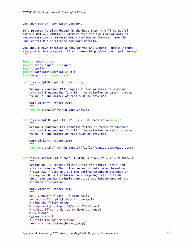
Appendix A: Designing FIR Filters from Amplitude Response RequirementsThe Python module fir_design_helper.py supports the design of windowed (Kaiser window) andequal-ripple (remez) linear phase FIR filters starting amplitude response requirements. The filterorder (or equivalently order + 1 = number of taps) is determined as part of the design process.Design functions are available for lowpass, highpass, and bandpass filters.

"""Basic Linear Phase Digital Filter Design Helper

Mark Wickert October 2016

Development continues!"""

"""This program is free software: you can redistribute it and/or modifyit under the terms of the GNU General Public License as published bythe Free Software Foundation, either version 3 of the License, or

1. https://en.wikipedia.org/wiki/Flanging

References 22


(at your option) any later version.

This program is distributed in the hope that it will be useful,but WITHOUT ANY WARRANTY; without even the implied warranty ofMERCHANTABILITY or FITNESS FOR A PARTICULAR PURPOSE. See theGNU General Public License for more details.

You should have received a copy of the GNU General Public Licensealong with this program. If not, see <http://www.gnu.org/licenses/>."""

import numpy as npimport scipy.signal as signalimport optfirimport matplotlib.pyplot as pltfrom matplotlib import pylab

def firwin_lpf(N_taps, fc, fs = 1.0): """ Design a windowed FIR lowpass filter in terms of passband critical frequencies f1 < f2 in Hz relative to sampling rate fs in Hz. The number of taps must be provided. Mark Wickert October 2016 """ return signal.firwin(N_taps,2*fc/fs)

def firwin_bpf(N_taps, f1, f2, fs = 1.0, pass_zero=False): """ Design a windowed FIR bandpass filter in terms of passband critical frequencies f1 < f2 in Hz relative to sampling rate fs in Hz. The number of taps must be provided.

Mark Wickert October 2016 """ return signal.firwin(N_taps,2*(f1,f2)/fs,pass_zero=pass_zero)

def firwin_kaiser_lpf(f_pass, f_stop, d_stop, fs = 1.0, N_bump=0): """ Design an FIR lowpass filter using the sinc() kernel and a Kaiser window. The filter order is determined based on f_pass Hz, f_stop Hz, and the desired stopband attenuation d_stop in dB, all relative to a sampling rate of fs Hz. Note: the passband ripple cannot be set independent of the stopband attenuation.

Mark Wickert October 2016 """ wc = 2*np.pi*(f_pass + f_stop)/2/fs delta_w = 2*np.pi*(f_stop - f_pass)/fs # Find the filter order M = np.ceil((d_stop - 8)/(2.285*delta_w)) # Adjust filter order up or down as needed M += N_bump N_taps = M + 1 # Obtain the Kaiser window beta = signal.kaiser_beta(d_stop)

Appendix A: Designing FIR Filters from Amplitude Response Requirements 23


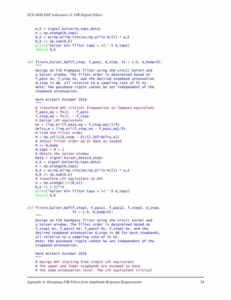
w_k = signal.kaiser(N_taps,beta) n = np.arange(N_taps) b_k = wc/np.pi*np.sinc(wc/np.pi*(n-M/2)) * w_k b_k /= np.sum(b_k) print('Kaiser Win filter taps = %d.' % N_taps) return b_k

def firwin_kaiser_hpf(f_stop, f_pass, d_stop, fs = 1.0, N_bump=0): """ Design an FIR highpass filter using the sinc() kernel and a Kaiser window. The filter order is determined based on f_pass Hz, f_stop Hz, and the desired stopband attenuation d_stop in dB, all relative to a sampling rate of fs Hz. Note: the passband ripple cannot be set independent of the stopband attenuation.

Mark Wickert October 2016 """ # Transform HPF critical frequencies to lowpass equivalent f_pass_eq = fs/2. - f_pass f_stop_eq = fs/2. - f_stop # Design LPF equivalent wc = 2*np.pi*(f_pass_eq + f_stop_eq)/2/fs delta_w = 2*np.pi*(f_stop_eq - f_pass_eq)/fs # Find the filter order M = np.ceil((d_stop - 8)/(2.285*delta_w)) # Adjust filter order up or down as needed M += N_bump N_taps = M + 1 # Obtain the Kaiser window beta = signal.kaiser_beta(d_stop) w_k = signal.kaiser(N_taps,beta) n = np.arange(N_taps) b_k = wc/np.pi*np.sinc(wc/np.pi*(n-M/2)) * w_k b_k /= np.sum(b_k) # Transform LPF equivalent to HPF n = np.arange(len(b_k)) b_k *= (-1)**n print('Kaiser Win filter taps = %d.' % N_taps) return b_k

def firwin_kaiser_bpf(f_stop1, f_pass1, f_pass2, f_stop2, d_stop, fs = 1.0, N_bump=0): """ Design an FIR bandpass filter using the sinc() kernel and a Kaiser window. The filter order is determined based on f_stop1 Hz, f_pass1 Hz, f_pass2 Hz, f_stop2 Hz, and the desired stopband attenuation d_stop in dB for both stopbands, all relative to a sampling rate of fs Hz. Note: the passband ripple cannot be set independent of the stopband attenuation.

Mark Wickert October 2016 """ # Design BPF starting from simple LPF equivalent # The upper and lower stopbands are assumed to have # the same attenuation level. The LPF equivalent critical



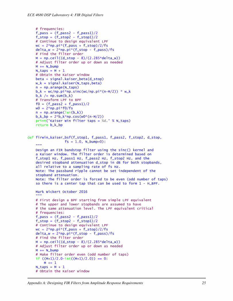
# frequencies: f_pass = (f_pass2 - f_pass1)/2 f_stop = (f_stop2 - f_stop1)/2 # Continue to design equivalent LPF wc = 2*np.pi*(f_pass + f_stop)/2/fs delta_w = 2*np.pi*(f_stop - f_pass)/fs # Find the filter order M = np.ceil((d_stop - 8)/(2.285*delta_w)) # Adjust filter order up or down as needed M += N_bump N_taps = M + 1 # Obtain the Kaiser window beta = signal.kaiser_beta(d_stop) w_k = signal.kaiser(N_taps,beta) n = np.arange(N_taps) b_k = wc/np.pi*np.sinc(wc/np.pi*(n-M/2)) * w_k b_k /= np.sum(b_k) # Transform LPF to BPF f0 = (f_pass2 + f_pass1)/2 w0 = 2*np.pi*f0/fs n = np.arange(len(b_k)) b_k_bp = 2*b_k*np.cos(w0*(n-M/2)) print('Kaiser Win filter taps = %d.' % N_taps) return b_k_bp

def firwin_kaiser_bsf(f_stop1, f_pass1, f_pass2, f_stop2, d_stop, fs = 1.0, N_bump=0): """ Design an FIR bandstop filter using the sinc() kernel and a Kaiser window. The filter order is determined based on f_stop1 Hz, f_pass1 Hz, f_pass2 Hz, f_stop2 Hz, and the desired stopband attenuation d_stop in dB for both stopbands, all relative to a sampling rate of fs Hz. Note: The passband ripple cannot be set independent of the stopband attenuation. Note: The filter order is forced to be even (odd number of taps) so there is a center tap that can be used to form 1 - H_BPF.

Mark Wickert October 2016 """ # First design a BPF starting from simple LPF equivalent # The upper and lower stopbands are assumed to have # the same attenuation level. The LPF equivalent critical # frequencies: f_pass = (f_pass2 - f_pass1)/2 f_stop = (f_stop2 - f_stop1)/2 # Continue to design equivalent LPF wc = 2*np.pi*(f_pass + f_stop)/2/fs delta_w = 2*np.pi*(f_stop - f_pass)/fs # Find the filter order M = np.ceil((d_stop - 8)/(2.285*delta_w)) # Adjust filter order up or down as needed M += N_bump # Make filter order even (odd number of taps) if ((M+1)/2.0-int((M+1)/2.0)) == 0: M += 1 N_taps = M + 1 # Obtain the Kaiser window



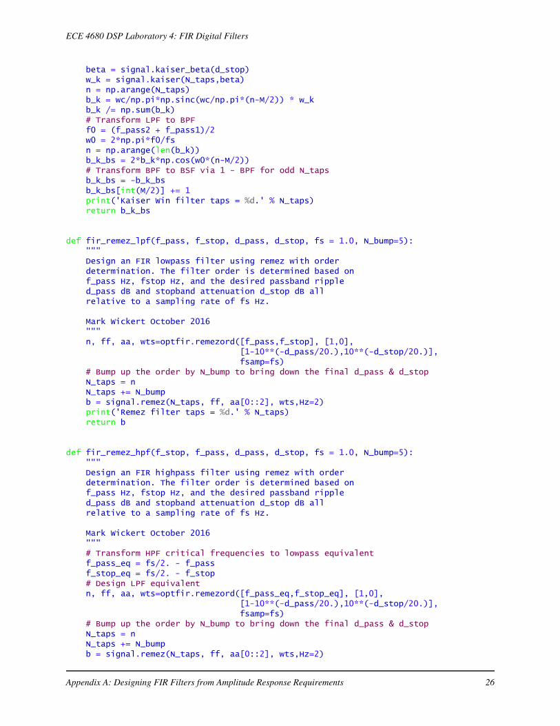
beta = signal.kaiser_beta(d_stop) w_k = signal.kaiser(N_taps,beta) n = np.arange(N_taps) b_k = wc/np.pi*np.sinc(wc/np.pi*(n-M/2)) * w_k b_k /= np.sum(b_k) # Transform LPF to BPF f0 = (f_pass2 + f_pass1)/2 w0 = 2*np.pi*f0/fs n = np.arange(len(b_k)) b_k_bs = 2*b_k*np.cos(w0*(n-M/2)) # Transform BPF to BSF via 1 - BPF for odd N_taps b_k_bs = -b_k_bs b_k_bs[int(M/2)] += 1 print('Kaiser Win filter taps = %d.' % N_taps) return b_k_bs

def fir_remez_lpf(f_pass, f_stop, d_pass, d_stop, fs = 1.0, N_bump=5): """ Design an FIR lowpass filter using remez with order determination. The filter order is determined based on f_pass Hz, fstop Hz, and the desired passband ripple d_pass dB and stopband attenuation d_stop dB all relative to a sampling rate of fs Hz.

Mark Wickert October 2016 """ n, ff, aa, wts=optfir.remezord([f_pass,f_stop], [1,0], [1-10**(-d_pass/20.),10**(-d_stop/20.)], fsamp=fs) # Bump up the order by N_bump to bring down the final d_pass & d_stop N_taps = n N_taps += N_bump b = signal.remez(N_taps, ff, aa[0::2], wts,Hz=2) print('Remez filter taps = %d.' % N_taps) return b

def fir_remez_hpf(f_stop, f_pass, d_pass, d_stop, fs = 1.0, N_bump=5): """ Design an FIR highpass filter using remez with order determination. The filter order is determined based on f_pass Hz, fstop Hz, and the desired passband ripple d_pass dB and stopband attenuation d_stop dB all relative to a sampling rate of fs Hz.

Mark Wickert October 2016 """ # Transform HPF critical frequencies to lowpass equivalent f_pass_eq = fs/2. - f_pass f_stop_eq = fs/2. - f_stop # Design LPF equivalent n, ff, aa, wts=optfir.remezord([f_pass_eq,f_stop_eq], [1,0], [1-10**(-d_pass/20.),10**(-d_stop/20.)], fsamp=fs) # Bump up the order by N_bump to bring down the final d_pass & d_stop N_taps = n N_taps += N_bump b = signal.remez(N_taps, ff, aa[0::2], wts,Hz=2)



# Transform LPF equivalent to HPF n = np.arange(len(b)) b *= (-1)**n print('Remez filter taps = %d.' % N_taps) return b

def fir_remez_bpf(f_stop1, f_pass1, f_pass2, f_stop2, d_pass, d_stop, fs = 1.0, N_bump=5): """ Design an FIR bandpass filter using remez with order determination. The filter order is determined based on f_stop1 Hz, f_pass1 Hz, f_pass2 Hz, f_stop2 Hz, and the desired passband ripple d_pass dB and stopband attenuation d_stop dB all relative to a sampling rate of fs Hz.

Mark Wickert October 2016 """ n, ff, aa, wts=optfir.remezord([f_stop1,f_pass1,f_pass2,f_stop2], [0,1,0], [10**(-d_stop/20.),1-10**(-d_pass/20.), 10**(-d_stop/20.)], fsamp=fs) # Bump up the order by N_bump to bring down the final d_pass & d_stop N_taps = n N_taps += N_bump b = signal.remez(N_taps, ff, aa[0::2], wts,Hz=2) print('Remez filter taps = %d.' % N_taps) return b

def fir_remez_bsf(f_pass1, f_stop1, f_stop2, f_pass2, d_pass, d_stop, fs = 1.0, N_bump=5): """ Design an FIR bandstop filter using remez with order determination. The filter order is determined based on f_pass1 Hz, f_stop1 Hz, f_stop2 Hz, f_pass2 Hz, and the desired passband ripple d_pass dB and stopband attenuation d_stop dB all relative to a sampling rate of fs Hz.

Mark Wickert October 2016 """ n, ff, aa, wts=optfir.remezord([f_pass1,f_stop1,f_stop2,f_pass2], [1,0,1], [1-10**(-d_pass/20.),10**(-d_stop/20.), 1-10**(-d_pass/20.)], fsamp=fs) # Bump up the order by N_bump to bring down the final d_pass & d_stop N_taps = n N_taps += N_bump b = signal.remez(N_taps, ff, aa[0::2], wts,Hz=2) print('Remez filter taps = %d.' % N_taps) return b

def freqz_resp_list(b,a=np.array([1]),mode = 'dB',fs=1.0,Npts = 1024,fsize=(6,4)): """ A method for displaying digital filter frequency response magnitude, phase, and group delay. A plot is produced using matplotlib







Mark Wickert, January 2015 """ if type(b) == list: # We have a list of filters N_filt = len(b) f = np.arange(0,Npts)/(2.0*Npts) for n in range(N_filt): w,H = signal.freqz(b[n],a[n],2*np.pi*f) if n == 0: plt.figure(figsize=fsize) if mode.lower() == 'db': plt.plot(f*fs,20*np.log10(np.abs(H))) if n == N_filt-1: plt.xlabel('Frequency (Hz)') plt.ylabel('Gain (dB)') plt.title('Frequency Response - Magnitude')

elif mode.lower() == 'phase': plt.plot(f*fs,np.angle(H)) if n == N_filt-1: plt.xlabel('Frequency (Hz)') plt.ylabel('Phase (rad)') plt.title('Frequency Response - Phase')

elif (mode.lower() == 'groupdelay_s') or (mode.lower() == 'groupdelay_t'): """ Notes -----

Since this calculation involves finding the derivative of the phase response, care must be taken at phase wrapping points and when the phase jumps by +/-pi, which occurs when the amplitude response changes sign. Since the amplitude response is zero when the sign changes, the jumps do not alter the group delay results. """ theta = np.unwrap(np.angle(H)) # Since theta for an FIR filter is likely to have many pi phase # jumps too, we unwrap a second time 2*theta and divide by 2 theta2 = np.unwrap(2*theta)/2. theta_dif = np.diff(theta2) f_diff = np.diff(f) Tg = -np.diff(theta2)/np.diff(w) # For gain almost zero set groupdelay = 0



idx = pylab.find(20*np.log10(H[:-1]) < -400) Tg[idx] = np.zeros(len(idx)) max_Tg = np.max(Tg) #print(max_Tg) if mode.lower() == 'groupdelay_t': max_Tg /= fs plt.plot(f[:-1]*fs,Tg/fs) plt.ylim([0,1.2*max_Tg]) else: plt.plot(f[:-1]*fs,Tg) plt.ylim([0,1.2*max_Tg]) if n == N_filt-1: plt.xlabel('Frequency (Hz)') if mode.lower() == 'groupdelay_t': plt.ylabel('Group Delay (s)') else: plt.ylabel('Group Delay (samples)') plt.title('Frequency Response - Group Delay') else: s1 = 'Error, mode must be "dB", "phase, ' s2 = '"groupdelay_s", or "groupdelay_t"'

print(s1 + s2)

Appendix B: Writing FIR Coefficient Header FilesThe Python module coef2header.py supports the writing of C style header files for use in the filterfunction of FIR_Filter.c/FIR_Filter.h and the ARM functions .

"""Digital Filter Coefficient Conversion to C Header Files

Mark Wickert January 2015 - October 2016

Development continues!"""

"""This program is free software: you can redistribute it and/or modifyit under the terms of the GNU General Public License as published bythe Free Software Foundation, either version 3 of the License, or(at your option) any later version.

This program is distributed in the hope that it will be useful,but WITHOUT ANY WARRANTY; without even the implied warranty ofMERCHANTABILITY or FITNESS FOR A PARTICULAR PURPOSE. See theGNU General Public License for more details.

You should have received a copy of the GNU General Public Licensealong with this program. If not, see <http://www.gnu.org/licenses/>."""

import numpy as npimport scipy.signal as signalimport matplotlib.pyplot as pltfrom matplotlib import pylab

def FIR_header(fname_out,h):

Appendix B: Writing FIR Coefficient Header Files 29


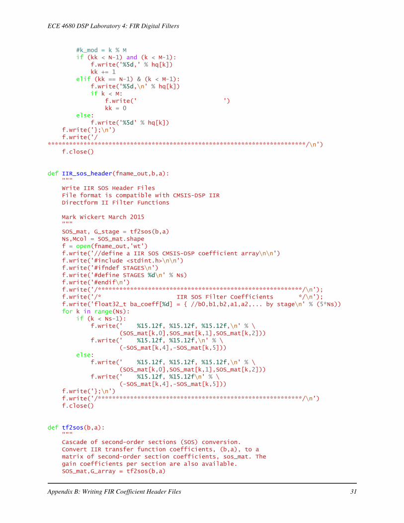
""" Write FIR Filter Header Files Mark Wickert February 2015 """ M = len(h) N = 3 # Coefficients per line f = open(fname_out,'wt') f.write('//define a FIR coefficient Array\n\n') f.write('#include <stdint.h>\n\n') f.write('#ifndef M_FIR\n') f.write('#define M_FIR %d\n' % M) f.write('#endif\n') f.write('/************************************************************************/\n'); f.write('/* FIR Filter Coefficients */\n'); f.write('float32_t h_FIR[M_FIR] = {') kk = 0; for k in range(M): #k_mod = k % M if (kk < N-1) and (k < M-1): f.write('%15.12f,' % h[k]) kk += 1 elif (kk == N-1) & (k < M-1): f.write('%15.12f,\n' % h[k]) if k < M: f.write(' ') kk = 0 else: f.write('%15.12f' % h[k]) f.write('};\n') f.write('/************************************************************************/\n') f.close()

def FIR_fix_header(fname_out,h): """ Write FIR Fixed-Point Filter Header Files Mark Wickert February 2015 """ M = len(h) hq = int16(rint(h*2**15)) N = 8 # Coefficients per line f = open(fname_out,'wt') f.write('//define a FIR coefficient Array\n\n') f.write('#include <stdint.h>\n\n') f.write('#ifndef M_FIR\n') f.write('#define M_FIR %d\n' % M) f.write('#endif\n') f.write('/************************************************************************/\n'); f.write('/* FIR Filter Coefficients */\n'); f.write('int16_t h_FIR[M_FIR] = {') kk = 0; for k in range(M):



#k_mod = k % M if (kk < N-1) and (k < M-1): f.write('%5d,' % hq[k]) kk += 1 elif (kk == N-1) & (k < M-1): f.write('%5d,\n' % hq[k]) if k < M: f.write(' ') kk = 0 else: f.write('%5d' % hq[k]) f.write('};\n') f.write('/************************************************************************/\n') f.close()

def IIR_sos_header(fname_out,b,a): """ Write IIR SOS Header Files File format is compatible with CMSIS-DSP IIR Directform II Filter Functions Mark Wickert March 2015 """ SOS_mat, G_stage = tf2sos(b,a) Ns,Mcol = SOS_mat.shape f = open(fname_out,'wt') f.write('//define a IIR SOS CMSIS-DSP coefficient array\n\n') f.write('#include <stdint.h>\n\n') f.write('#ifndef STAGES\n') f.write('#define STAGES %d\n' % Ns) f.write('#endif\n') f.write('/*********************************************************/\n'); f.write('/* IIR SOS Filter Coefficients */\n'); f.write('float32_t ba_coeff[%d] = { //b0,b1,b2,a1,a2,... by stage\n' % (5*Ns)) for k in range(Ns): if (k < Ns-1): f.write(' %15.12f, %15.12f, %15.12f,\n' % \ (SOS_mat[k,0],SOS_mat[k,1],SOS_mat[k,2])) f.write(' %15.12f, %15.12f,\n' % \ (-SOS_mat[k,4],-SOS_mat[k,5])) else: f.write(' %15.12f, %15.12f, %15.12f,\n' % \ (SOS_mat[k,0],SOS_mat[k,1],SOS_mat[k,2])) f.write(' %15.12f, %15.12f\n' % \ (-SOS_mat[k,4],-SOS_mat[k,5])) f.write('};\n') f.write('/*********************************************************/\n') f.close()

def tf2sos(b,a): """ Cascade of second-order sections (SOS) conversion. Convert IIR transfer function coefficients, (b,a), to a matrix of second-order section coefficients, sos_mat. The gain coefficients per section are also available. SOS_mat,G_array = tf2sos(b,a)



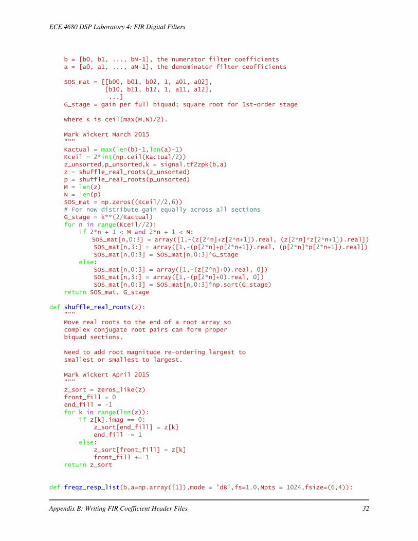
b = [b0, b1, ..., bM-1], the numerator filter coefficients a = [a0, a1, ..., aN-1], the denominator filter ceofficients

SOS_mat = [[b00, b01, b02, 1, a01, a02], [b10, b11, b12, 1, a11, a12], ...] G_stage = gain per full biquad; square root for 1st-order stage

where K is ceil(max(M,N)/2).

Mark Wickert March 2015 """ Kactual = max(len(b)-1,len(a)-1) Kceil = 2*int(np.ceil(Kactual/2)) z_unsorted,p_unsorted,k = signal.tf2zpk(b,a) z = shuffle_real_roots(z_unsorted) p = shuffle_real_roots(p_unsorted) M = len(z) N = len(p) SOS_mat = np.zeros((Kceil//2,6)) # For now distribute gain equally across all sections G_stage = k**(2/Kactual) for n in range(Kceil//2): if 2*n + 1 < M and 2*n + 1 < N: SOS_mat[n,0:3] = array([1,-(z[2*n]+z[2*n+1]).real, (z[2*n]*z[2*n+1]).real]) SOS_mat[n,3:] = array([1,-(p[2*n]+p[2*n+1]).real, (p[2*n]*p[2*n+1]).real]) SOS_mat[n,0:3] = SOS_mat[n,0:3]*G_stage else: SOS_mat[n,0:3] = array([1,-(z[2*n]+0).real, 0]) SOS_mat[n,3:] = array([1,-(p[2*n]+0).real, 0]) SOS_mat[n,0:3] = SOS_mat[n,0:3]*np.sqrt(G_stage) return SOS_mat, G_stage

def shuffle_real_roots(z): """ Move real roots to the end of a root array so complex conjugate root pairs can form proper biquad sections. Need to add root magnitude re-ordering largest to smallest or smallest to largest. Mark Wickert April 2015 """ z_sort = zeros_like(z) front_fill = 0 end_fill = -1 for k in range(len(z)): if z[k].imag == 0: z_sort[end_fill] = z[k] end_fill -= 1 else: z_sort[front_fill] = z[k] front_fill += 1 return z_sort

def freqz_resp_list(b,a=np.array([1]),mode = 'dB',fs=1.0,Npts = 1024,fsize=(6,4)):



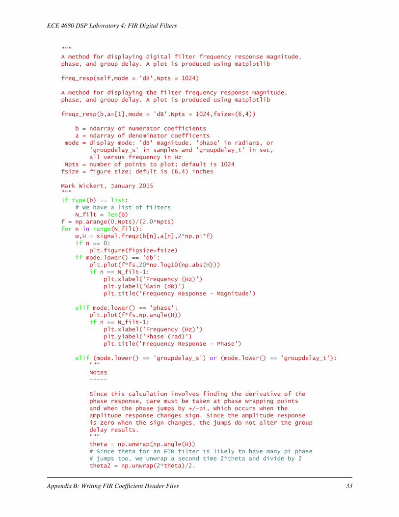
""" A method for displaying digital filter frequency response magnitude, phase, and group delay. A plot is produced using matplotlib





Mark Wickert, January 2015 """ if type(b) == list: # We have a list of filters N_filt = len(b) f = np.arange(0,Npts)/(2.0*Npts) for n in range(N_filt): w,H = signal.freqz(b[n],a[n],2*np.pi*f) if n == 0: plt.figure(figsize=fsize) if mode.lower() == 'db': plt.plot(f*fs,20*np.log10(np.abs(H))) if n == N_filt-1: plt.xlabel('Frequency (Hz)') plt.ylabel('Gain (dB)') plt.title('Frequency Response - Magnitude')

elif mode.lower() == 'phase': plt.plot(f*fs,np.angle(H)) if n == N_filt-1: plt.xlabel('Frequency (Hz)') plt.ylabel('Phase (rad)') plt.title('Frequency Response - Phase')

elif (mode.lower() == 'groupdelay_s') or (mode.lower() == 'groupdelay_t'): """ Notes -----

Since this calculation involves finding the derivative of the phase response, care must be taken at phase wrapping points and when the phase jumps by +/-pi, which occurs when the amplitude response changes sign. Since the amplitude response is zero when the sign changes, the jumps do not alter the group delay results. """ theta = np.unwrap(np.angle(H)) # Since theta for an FIR filter is likely to have many pi phase # jumps too, we unwrap a second time 2*theta and divide by 2 theta2 = np.unwrap(2*theta)/2.



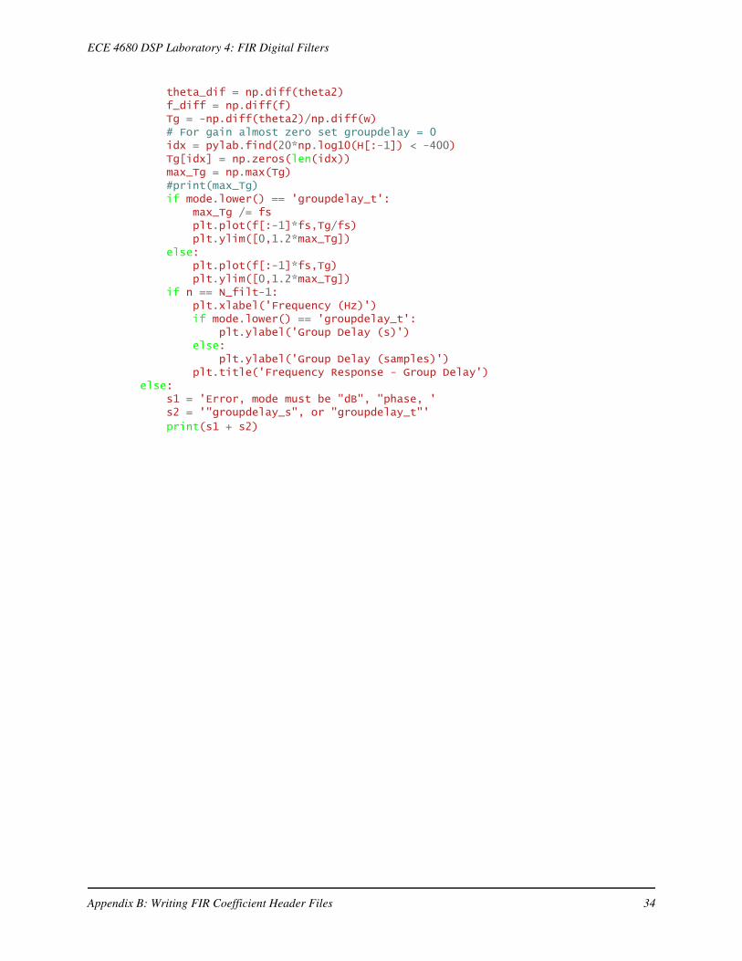
theta_dif = np.diff(theta2) f_diff = np.diff(f) Tg = -np.diff(theta2)/np.diff(w) # For gain almost zero set groupdelay = 0 idx = pylab.find(20*np.log10(H[:-1]) < -400) Tg[idx] = np.zeros(len(idx)) max_Tg = np.max(Tg) #print(max_Tg) if mode.lower() == 'groupdelay_t': max_Tg /= fs plt.plot(f[:-1]*fs,Tg/fs) plt.ylim([0,1.2*max_Tg]) else: plt.plot(f[:-1]*fs,Tg) plt.ylim([0,1.2*max_Tg]) if n == N_filt-1: plt.xlabel('Frequency (Hz)') if mode.lower() == 'groupdelay_t': plt.ylabel('Group Delay (s)') else: plt.ylabel('Group Delay (samples)') plt.title('Frequency Response - Group Delay') else: s1 = 'Error, mode must be "dB", "phase, ' s2 = '"groupdelay_s", or "groupdelay_t"'

print(s1 + s2)


ECE 4680 DSP Laboratory 4: FIR Digital Filtersmwickert/ece5655/lecture_notes/ARM/FIR_Lab4.pdf · // Brute force 4-tap solution ... Of special interest for this lab Figure 2: The CMSIS-DSP

Documents