Ec980X Stata Tutorial - Harvard Canvas

Ec980X Stata TutorialFall 2019

Downloading Stata

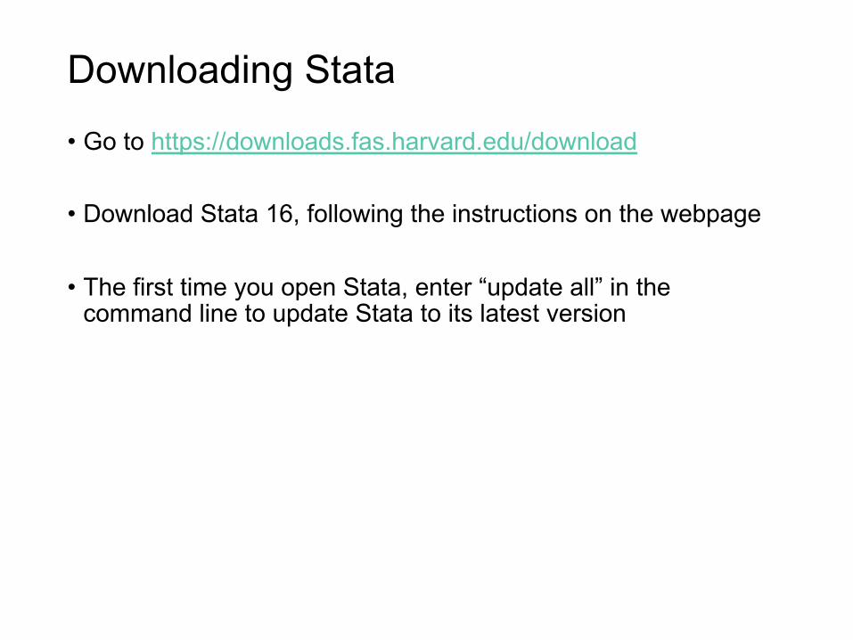
• Go to https://downloads.fas.harvard.edu/download

• Download Stata 16, following the instructions on the webpage

• The first time you open Stata, enter “update all” in the command line to update Stata to its latest version

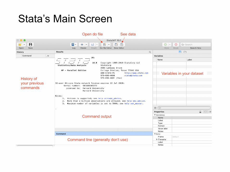
Stata’s Main Screen

Variables in your dataset

Command line (generally don’t use)

History of your previous commands

Command output

Open do file See data

Do File Editor

• Save and execute your commands from a .do file• Every .do file should look something like the following:

Include the name of the .do file, a brief description of what it does, and the date you last updated it. This will be helpful for when you come back to a project after taking a break from it.

These 4 lines of code will be at the top of every do file. The first 3 shouldn’t be changed and just make sure you’ve cleared everything, closed open log files, and don’t have to click enter after regressions. The last sets your directory.

Save do file Execute do file. Run selected lines by highlighting them

Open existing do file. Open new file by clicking File → New → Do-File. Can open multiple tabs at once.

Use asterisks (*) to comment new lines of code. Use asterisks plus slashes (/* block of text */) to comment sections of code (not shown).Use double slashes (//) to comment after a line of code (not shown).

If you have spaces in your file path, use quotes around the file path

Downloading Data

• On Canvas, see Files → Econ980x_DataSets for links to useful data sets

• These sources will generally give you relatively clean data ready for inputting into Stata

• We will go through examples of how to work with two common data sets for this class

• American Community Survey (ACS) or Current Population Survey (CPS) data downloaded from IPUMS

• National Longitudinal Survey of Youth (NLSY) data downloaded from the NLS Investigator

Working with IPUMS ACS or CPS

• ACS example, go to https://usa.ipums.org/usa/index.shtml• Click “Get Data” in middle of page• Select your variables

Click + to add variable

Click variable name to see important details

See years of variable availability

Click to select years in your sample

Click to view cart after finished selecting variables and samples

Selecting IPUMS ACS or CPS Samples

• Usually you just want the default sample for your years of interest in the ACS and Census

• In the CPS, click to the Supplements tab to get data from the fertility supplement, click ASEC to get detailed income data (can’t be used with other supplements), and click basic monthly to get demographic variables (should automatically be selected if you select supplement samples); note you need to select supplement samples before selecting variables in the CPS

ACS Sample Selection

CPS Sample Selection

Downloading IPUMS ACS or CPS Data

• After selecting your variables and samples, click “View Cart” • You will see your selected variables plus some preselected

variables; keep these variables and click “Create Data Extract”• Change your data format to Stata; otherwise, you will have an

added step of downloading a do file to convert the data• It will take IPUMS anywhere between a few minutes to a few

hours to create your extract, depending on the file size

Change this to StataUseful for seeing characteristics of child’s parents or adult’s spouse if living together

Note you need to be logged in to submit an extract; you will need to create a log in the first time you use IPUMS

Working with the NLSY

• Go to https://www.nlsinfo.org/investigator/pages/login.jsp• You’ll need a log in - this is easy to create• Select your survey of interest• Click variable search and browse for your variables of interest

Select your variables

Survey of interest

Download selected data

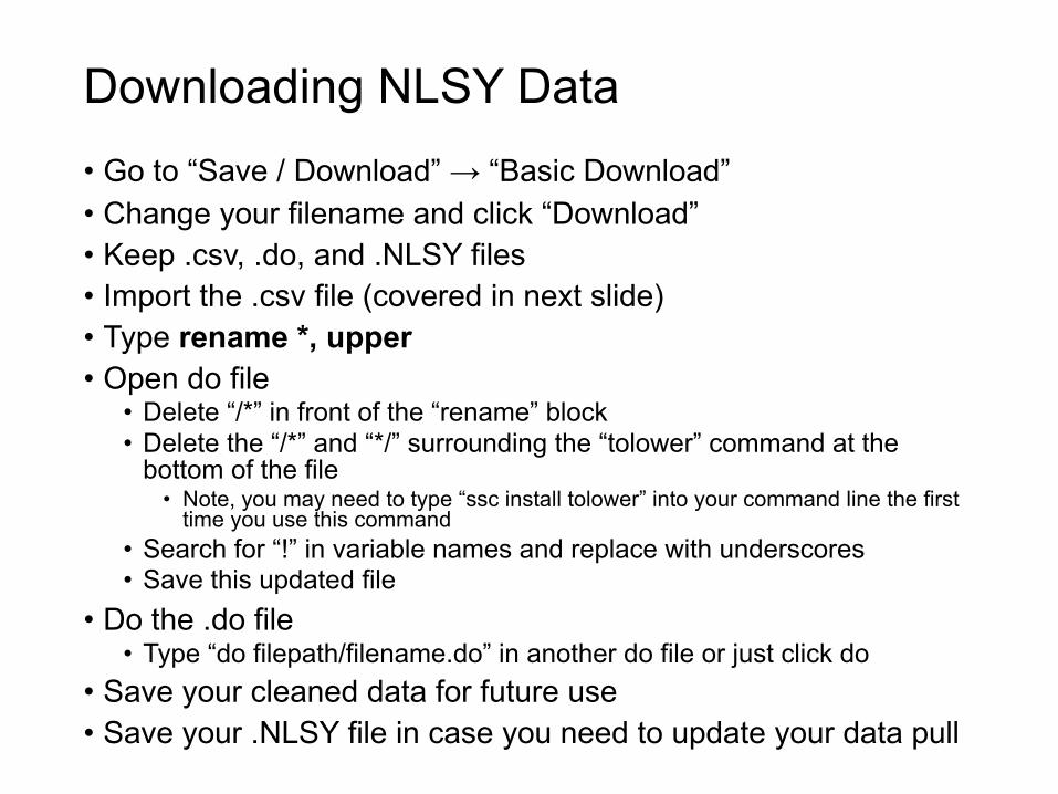
Downloading NLSY Data• Go to “Save / Download” → “Basic Download”• Change your filename and click “Download”• Keep .csv, .do, and .NLSY files• Import the .csv file (covered in next slide)• Type rename *, upper• Open do file

• Delete “/*” in front of the “rename” block • Delete the “/*” and “*/” surrounding the “tolower” command at the

bottom of the file• Note, you may need to type “ssc install tolower” into your command line the first

time you use this command• Search for “!” in variable names and replace with underscores• Save this updated file

• Do the .do file • Type “do filepath/filename.do” in another do file or just click do

• Save your cleaned data for future use• Save your .NLSY file in case you need to update your data pull

Importing Data into Stata

• If your data is in Stata format (.dta file), then simply use• use “filepath/filename.dta”, clear• This will be the case for data download from IPUMS or data you have

cleaned• If your data is in .csv format, use

• import delimited “filepath/filename.csv”, clear• This will be the case for data downloaded from the NLS Investigator

and various other sources• If your data is in excel format, use

• import excel “filepath/filename.xlsx”, sheet(“sheetname”) firstrowclear

• Drop the firstrow part if the first row doesn’t contain variable names

• To save cleaned data in Stata format, type • save “filepath/filename.dta”, replace

Troubleshooting Data Imports into Stata

• Make sure you have properly set your directory• cd /Users/name/desktop/ or whatever you have should correspond

with your main working directory• The file path for the data should be an extension of this directory; e.g, if

you have a data subfolder, you’d have use data/filename.dta• In the command line, type help import• On the main Stata page, go to File → Import → data type

• This will give you code that you should copy and paste into your do file

Manually enter in data here

Exploring Data in Stata

• To simply look at the data click a data editor icon on the main Stata page

• To browse select variables, type browse var1 var2• To get summary statistics, like mean and standard deviation, for

a variable, type summarize var1• To get detailed summary statistics like median and percentiles,

type summarize var1, d• To get summary statistics on multiple variables at once, type

summarize var1 var2

Exploring Data in Stata

• To see which values a variable takes on, use tabulate var1• Often, the data will have value labels which will be displayed

with the tabulate command, but these are not the true values of the variable that Stata observes; use tabulate var1, nolabel to view these

Cleaning Data in Stata Basics

• To drop or keep observations, use the commands drop and keep, for example

• drop if age>30 (use >= if you want to include 30)• keep if sex==1 (you need two equals here)

• To recode observations, use the recode or replace commands• recode mar_status_1996_10_xrnd -4=.• replace mar_status_1996_10_xrnd=. if

mar_status_1996_10_xrnd<0• Note that Stata observes a period “.” as a missing variable

• To generate a new variable, use the generate command• generate year_of_birth=year-age• generate age_squared=age^2• generate post_indicator=(year>=2009)• generate var2=(var1>=num) generates a variable that equals 1 when

var1>=num is true, and 0 when it isn’t true

Cleaning Data in Stata More Advanced

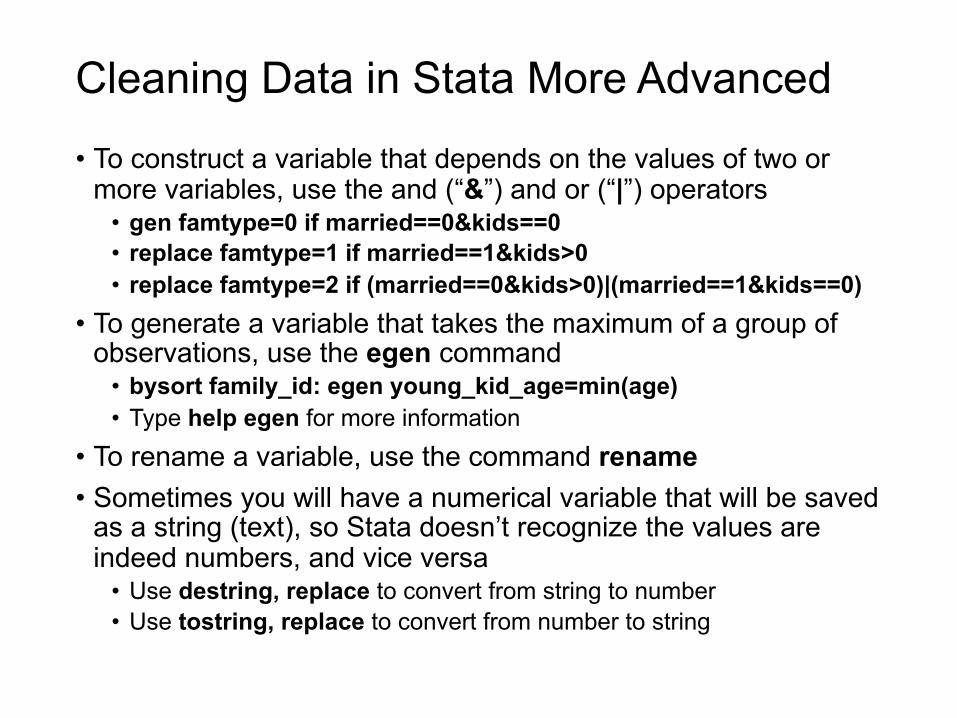
• To construct a variable that depends on the values of two or more variables, use the and (“&”) and or (“|”) operators

• gen famtype=0 if married==0&kids==0• replace famtype=1 if married==1&kids>0• replace famtype=2 if (married==0&kids>0)|(married==1&kids==0)

• To generate a variable that takes the maximum of a group of observations, use the egen command

• bysort family_id: egen young_kid_age=min(age)• Type help egen for more information

• To rename a variable, use the command rename• Sometimes you will have a numerical variable that will be saved

as a string (text), so Stata doesn’t recognize the values are indeed numbers, and vice versa

• Use destring, replace to convert from string to number• Use tostring, replace to convert from number to string

Other Advanced Commands

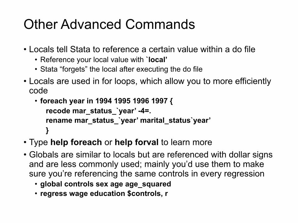
• Locals tell Stata to reference a certain value within a do file• Reference your local value with `local’• Stata “forgets” the local after executing the do file

• Locals are used in for loops, which allow you to more efficiently code

• foreach year in 1994 1995 1996 1997 {recode mar_status_`year’ -4=.rename mar_status_`year’ marital_status`year’}

• Type help foreach or help forval to learn more• Globals are similar to locals but are referenced with dollar signs

and are less commonly used; mainly you’d use them to make sure you’re referencing the same controls in every regression

• global controls sex age age_squared• regress wage education $controls, r

Transforming Data - Reshape

• You downloaded NLSY data that has a different variable (column) for each year, but you would like to have one variable and a different row for each year

• reshape long marital_status, i(pubid_1997) j(year)• You downloaded data that has a different row for each year, but

you’d like to have a different variable for each year• reshape wide unemp_rate, i(state) j(year)

Transforming Data - Collapse

• You downloaded individual data from the ACS or CPS but would like to have information at the household level, like the total household income by the age of the youngest kid

• collapse (min) age (sum) income, by(household_id)• Note that if you go from individual to state data, you will need to

add weights (see later slides)• Type help collapse to learn more

Merging Data

• Suppose you’d like to merge the state unemployment rate onto your individual data in the ACS or CPS

• Make sure that your state and year variables are named the same way in both files

• Then, when you have your ACS file open, use a many-to-one merge with merge m:1 state year using unemp_data.dta

• Alternatively, if you started with the unemployment rate data, you would use a one-to-many merge with merge 1:m

• If you were merging two state by year level datasets, you would use a one-to-one merge with merge 1:1

Merging Data Considerations• Never use a many-to-many merge; it doesn’t do what you think

it should• If you feel you need a many-to-many merge, you probably need

to use joinby• After you merge your data, Stata will give you output tell you

how successful your merge was• See whether this makes sense• You may have differences in variable values across files (e.g., “MA” in

one file and “Massachusetts” in another) that you will need to harmonize before successfully merging the data

• You may have some values in one file that you don’t in another (e.g., Puerto Rico in unemployment rate data but not in the ACS); you will want to drop these values using drop if _merge==1 or 2 depending on how you merged your data

• You will then need to drop _merge or rename _merge merge_name since you cannot merge again if _merge is in your dataset

Appending Data

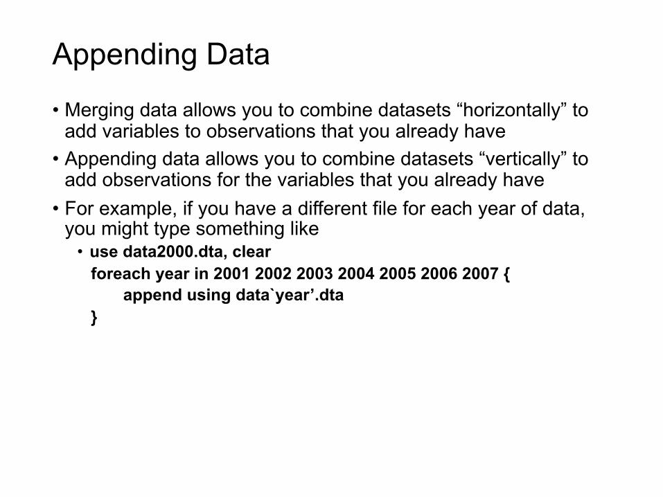
• Merging data allows you to combine datasets “horizontally” to add variables to observations that you already have

• Appending data allows you to combine datasets “vertically” to add observations for the variables that you already have

• For example, if you have a different file for each year of data, you might type something like

• use data2000.dta, clearforeach year in 2001 2002 2003 2004 2005 2006 2007 {

append using data`year’.dta}

Weights

• You will often be using national surveys that are “representative” of the population, but that doesn’t always mean that each individual is representative

• You typically need to use weights to get the sample to be truly representative of the population

• For summarize and collapse commands, you can simply use [weight=weight_var], and Stata will choose the correct weight

• For regressions, if you have individual data (as in the ACS, CPS, and NLSY), use pweight, and if you have aggregated data (like from school districts, counties, and states) for which you’d like a nationally representative estimate, use aweight,

• We won’t go into the details of the differences here, but this is a good rule of thumb to use

• If you have negative weights (occasionally show up in old CPS files), often just drop those observations

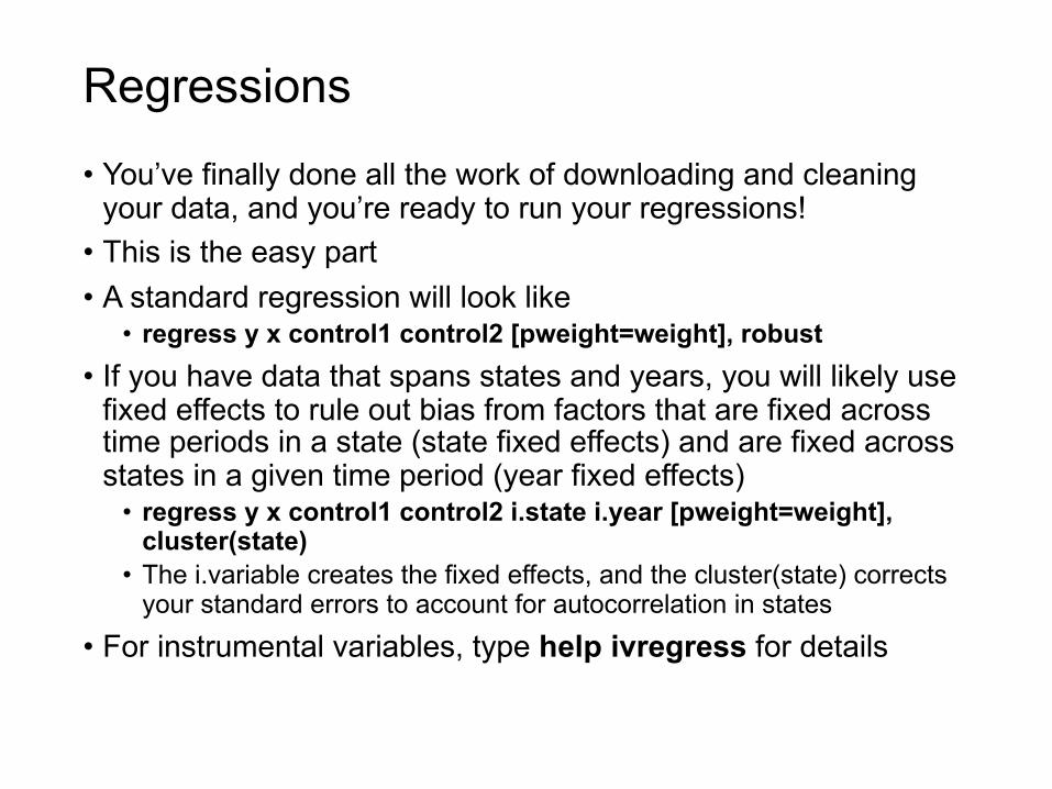
Regressions

• You’ve finally done all the work of downloading and cleaning your data, and you’re ready to run your regressions!

• This is the easy part• A standard regression will look like

• regress y x control1 control2 [pweight=weight], robust• If you have data that spans states and years, you will likely use

fixed effects to rule out bias from factors that are fixed across time periods in a state (state fixed effects) and are fixed across states in a given time period (year fixed effects)

• regress y x control1 control2 i.state i.year [pweight=weight], cluster(state)

• The i.variable creates the fixed effects, and the cluster(state) corrects your standard errors to account for autocorrelation in states

• For instrumental variables, type help ivregress for details

Outputting Regression Results

• A common command to output your regression results to Microsoft Excel is outreg2

• Right after estimating your regression, type• outreg2 [varlist] using filepath/filename.xls, replace or append• You can specify variables you’d like outputted where [varlist] is noted,

otherwise Stata will output all variables, which is also okay• You should use replace after the first regression you run and then

append for the next ones to get the results all in one file• If you use Latex, you can use the commands eststo and esttab

to output your results• Type help eststo and help esttab for more details• You may need to ssc install estout first

Figures

• A picture is worth a thousand words, and figures are often very helpful for making an argument in a paper

• One option for creating a figure is collapsing your dataset to what you need for the figure, using the export excel command, and creating the figure in Excel

• Another option is to use Stata’s graphing software• The advantage of using Stata to graph is that Stata makes it

easy to replicate and modify graphs• The disadvantage is that Stata’s defaults are somewhat

unattractive and it will take some work to create a nice figure• See the next two slides for some tips from Stata cheat sheets

referenced at the end of this presentation• Directly after creating your figure, you can save it by typing

graph export filepath/figure_name.png, as(png) replace

Figures Details

More Figures Details

List of Common Symbols In Stata• Missing: .• And: &• Or: |• Not: ~ or !• Wildcard: *• Global identifier: $• Local identifier: `text’• For loop opener and closer: { }• Command option indicator: ,• Commenting code: *, //, and /*text*/• Continuing command onto next line: ///• Standard arithmetic operations: +,-, *, /,^ • Standard equalities: ==, >, >=, <, <=

Tips for Data Management• Make sure you have an organized folder repository• Here’s an example

• /Data• /Raw• /Intermediate

• /Scripts• /Clean• /Tables• /Figures

• /Log• /Output

• /Tables• /Figures

• Use clear names for files and be consistent across file types e.g. name the .do file, .dta file, and .fig files consistently

• Use version control practices to ensure you are working with the latest versions of analysis, and that you don’t lose important information

Additional Tips for Data Management

• Keep a record of where raw data came from including the database, what variables you queried (if relevant), the years included, the website where the data was obtained, and the date you downloaded it. The last point is critical – datasets are often updated, and you need to keep track of what version of the data you are using

• Data should be cleaned once and then saved for subsequent analysis

• Variables should generally be created in the clean data file, unless they are specific to one piece of analysis

• Use clear names for variables that are understandable e.g. “Unemployment_Rate” rather than “V125”

• Use labels / notes / comments to explain what variables are and how they were created

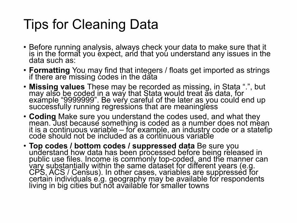
Tips for Cleaning Data • Before running analysis, always check your data to make sure that it

is in the format you expect, and that you understand any issues in the data such as:

• Formatting You may find that integers / floats get imported as strings if there are missing codes in the data

• Missing values These may be recorded as missing, in Stata “.”, but may also be coded in a way that Stata would treat as data, for example “9999999”. Be very careful of the later as you could end up successfully running regressions that are meaningless

• Coding Make sure you understand the codes used, and what they mean. Just because something is coded as a number does not mean it is a continuous variable – for example, an industry code or a statefipcode should not be included as a continuous variable

• Top codes / bottom codes / suppressed data Be sure you understand how data has been processed before being released in public use files. Income is commonly top-coded, and the manner can vary substantially within the same dataset for different years (e.g. CPS, ACS / Census). In other cases, variables are suppressed for certain individuals e.g. geography may be available for respondents living in big cities but not available for smaller towns

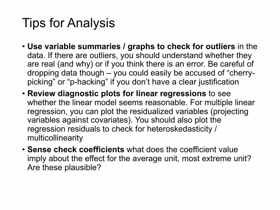
Tips for Analysis

• Use variable summaries / graphs to check for outliers in the data. If there are outliers, you should understand whether they are real (and why) or if you think there is an error. Be careful of dropping data though – you could easily be accused of “cherry-picking” or “p-hacking” if you don’t have a clear justification

• Review diagnostic plots for linear regressions to see whether the linear model seems reasonable. For multiple linear regression, you can plot the residualized variables (projecting variables against covariates). You should also plot the regression residuals to check for heteroskedasticity / multicollinearity

• Sense check coefficients what does the coefficient value imply about the effect for the average unit, most extreme unit? Are these plausible?

Additional resources

• You can always type help [command] to learn more about a Stata command

• Google is often helpful too

• There are some very helpful cheat sheets here: https://geocenter.github.io/StataTraining/portfolio/01_resource/

• The economics department hosts Stata office, described here: https://canvas.harvard.edu/courses/19323/pages/office-hours

• You are welcome to come to my office hours to get help with debugging code