SEMIGROUPS AND AUTOMATA SELECTA UNO KALJULAID (1941–1999)

Ebooksclub.org Semigroups and Automata SELECTA Uno Kaljulaid 1941 1999 Stand Alone
Dec 30, 2015
Semigroups
Welcome message from author
This document is posted to help you gain knowledge. Please leave a comment to let me know what you think about it! Share it to your friends and learn new things together.
Transcript

SEMIGROUPS AND AUTOMATA
SELECTA
UNO KALJULAID (1941–1999)


Semigroups and Automata
SELECTA
Uno Kaljulaid (1941–1999)
Edited by
Jaak Peetre
Lund, Sweden
and
Jaan Penjam
Tallinn, Estonia
Amsterdam • Berlin • Oxford • Tokyo • Washington, DC

© 2006 The authors.
All rights reserved. No part of this book may be reproduced, stored in a retrieval system,
or transmitted, in any form or by any means, without prior written permission from the publisher.
ISBN 1-58603-582-7
Library of Congress Control Number: 2005938840
Publisher
IOS Press
Nieuwe Hemweg 6B
1013 BG Amsterdam
Netherlands
fax: +31 20 687 0019
e-mail: [email protected]
Distributor in the UK and Ireland Distributor in the USA and Canada
Gazelle Books IOS Press, Inc.
Falcon House 4502 Rachael Manor Drive
Queen Square Fairfax, VA 22032
Lancaster LA1 1RN USA
United Kingdom fax: +1 703 323 3668
fax: +44 1524 63232 e-mail: [email protected]
LEGAL NOTICE
The publisher is not responsible for the use which might be made of the following information.
PRINTED IN THE NETHERLANDS

CONTENTS v
Contents
Preface. viiBiography of Uno Kaljulaid. J. Peetre xiBibliography of Uno Kaljulaid. xxi
Chapter I. Representations of semigroups and algebras 11. [K69a] On the cohomological dimension of some quasiprojective varieties. 32. [K77a] Triangular products of representations of semigroups and associativealgebras. 153. [K79a] Triangular products and stability of representations. Candidatedissertation. 194. [K79b] Triangular products and stability of representations. (Author review ofCandidate thesis in Physico-Mathematical Sciences). 1015. [K87a] Some remarks on Shevrin’s problem. 1116. [K90] Transferable elements in group rings. 1177. [K00] Ω-rings and their flat representations. Coauthor O. Sokratova 127
Chapter II. Automata theory 1411. Preamble. Editors 1432. Automata and their decomposition. 1453. [K97] On two algebraic constructions for automata. Coauthor J. Penjam 1834. [K98c] Revisiting wreath products, with applications to representations andinvariants. 203
Chapter III. Majorization 2051. Generalized majorization. Coauthor J. Peetre 2072. Van der Waerden’s conjecture and hyperbolicity. J. Peetre 2253. On generalized majorization. J. Peetre 233
Chapter IV. Combinatorics 2371. [K88a] On Stirling and Lah numbers. 2392. Letter (or draft of letter) c. 1991 from Uno Kaljulaid to Torbjörn Tambour. 2433. On Fibonacci numbers of graphs. 245
Chapter V. History of Mathematics 2511. Th. Molien, an innovator of algebra. 2532. [K87e] On the results of Molien about invariants of finite groups and theirrenaissance in contemporary mathematics. 2573. Theodor Molien, about his life and mathematical work as seen a century later.(A biographical sketch and a glimpse of his work). 2654. Notes on five 19th century Tartu mathematicians (Backlund, Kneser, Lindstedt,Molien, Weihrauch). 291
Chapter VI. Popularization of Mathematics 3251. [K68a] and [K69b] On the geometric methods of Diophantine Analysis. 327
vi CONTENTS
2. [K68b] Lenin prize for work in Diophantine geometry. 3513. [K69c] The history of solving equations. 3554. [K70] Additional remarks on groups. 3735. [K73a] Polynomials and formal series. 3896. [K75a] On Galois theory. 3997. [K75b] Theory of automata. Coauthor E. Tamme 4138. [K93c] Mordell’s problem. 4279. [K96] On two discrete models in connection with structures of mathematicsand language. 447
Index of Names 459
Subject Index 467

PREFACE vii
Preface
We have the pleasure to offer to the Mathematical Public the Selecta of the eminent,late Estonian algebraist Uno Kaljulaid. It contains mainly papers published in Kaljulaid’slifetime. Many of them were originally written in Russian, a few also in Estonian, andhave now been translated into English, mainly, by one of us, J. Peetre1.
Heritage. In addition to this published material, Kaljulaid left a large number ofmanuscripts in various states of completion. They are currently in the custody of theSenior Editor. For instance, there is an almost complete paper on right order groups, sur-veying the subject in its historical development, starting with D. Hilbert; some materialon Petri nets, etc., things that, apparently, occupied Kaljulaid in his last years. Hopefully,part of it can also be made public, at a later stage, perhaps in the form of Selecta II.
Let us now highlight some of the main items of the present Volume.
Contents. We offer here the English translation of Kaljulaid’s 1979 Tartu/MinskCandidate thesis [K79a], which originally was typewritten in Russian and manufacturedin not so many copies. The thesis was devoted to representation theory in the spirit ofhis thesis advisor B. I. Plotkin: representations of semigroups and algebras, especiallyextension to this situation, and application of the notion of triangular product of repre-sentations for groups introduced by Plotkin. We include also two summaries of the thesis[K77a] and [K79b].
Through representation theory, Kaljulaid became also interested in automata theory,which at a later phase became his main area of interest.
Another field of research concerns combinatorics.Besides being an outstanding and most dedicated mathematician Uno Kaljulaid was
also very much interested in the history of mathematics. In particular, he took a vividinterest in the life and work of the great 19th century Dorpat-Tartu algebraist Th. Molien(see Chapter V). Perhaps he saw in Molien a kindred soul, as neither of the two got quitethe recognition from their Alma Mater, which they for sure deserved; in Molien’s case,he had to go into voluntary exile in Tomsk, Siberia.
Kaljulaid was also very interested in the teaching and exposition, or populariza-tion of mathematics; he had several outstanding research students. Some of his morepopular-scientific papers were published in an Estonian language journal Matemaatikaja Kaasaeg (Mathematics and Our Age). Amongst there is a whole series of papersabout algebraic matters, culminating in a brilliant, elementary – although partly ratherphilosophical – essay devoted to Galois theory [K75a]. Another such series is his excel-lent essay of Diophantine Geometry [K68a,69b], in various installments, followed by hiséloge [K68b] to another of his teachers Yu. I. Manin. We believe that the inclusion ofthese papers here will make the Volume more interesting for beginners, and perhaps evencontribute to attracting young people to mathematics, in Estonia and elsewhere.
1Later on referred to as Senior Editor.

viii PREFACE
Presentation. The papers in the Volume are assembled in chapters according to thetheme.
Important matters or notions have often, with some consequence, been set in italics,sometimes upon their first appearance, or else where they are defined.
Rather rare quotes in other languages than English are usually followed by a trans-lation within parentheses.
References to items of Uno Kaljulaid come in the form [Kx], where x (a year) istaken modulo 1900, and refer to the bibliography. References to other mathematicianscome in the form [y], where y runs through 1, 2, 3 . . . , independently in each separatepaper.
In case of books translated into Russian, the Russian translation is often indicated,along with the original for the benefit of the Readers reading Russian or having access tothe Russian book. In transliterating the Cyrillic into English we use, with some conse-quence, the system in Mathematical Reviews, as set forth on p. 1–2 of the book [1].
Some facts about Estonia and Estonian mathematics. It should perhapsalso be recalled here that Estonia is the northern most of the three Baltic Republics, fac-ing the Finnish Gulf in the north, bordering to Latvia in the south and to Russia in theEast. Its population is about 1.3 million, most of them Estonians, many living in thecapital Tallinn; there is also a large Russian speaking minority. The Estonians speak alanguage somewhat affined to Finnish and not at all related to the language of their south-ern neighbors the Latvians and the Lithuanians. Estonians were mentioned already bythe Roman writer Tacitus (c. 55–117) who spoke of them as the Aestorum gentes. How-ever, around the beginning of the 13th century the Estonians were still among those fewpeople in Europe who had not accepted Christianity. In a devastating war (1208–1227),against German, Swedish and Danish Crusaders, the new religion was forced upon them.The last stronghold of the Estonians, the Castle of Valjala on the island of Saaremaa,was conquered by a Crusader’s army, coming from Pärnu and marching over the frozenarchipelago, in February, 1227. Then the Estonians became united, together with theLatvians, in a state ruled by the Order of the Brethren of the Sword, later known as theTeutonic Order, while the native population came to live, for centuries, in serfdom. Therule of the Order lasted until mid 16th century. At later times, Estonia was governed,alternatingly, by Swedes, Poles, and Russians. The situation of the indigenous deterio-rated ever more and was particularly low towards the end of the 18th century, farmerswere freely sold to the highest bidding landowner; one could even draw a parallel tothe Belgian Congo at a much later epoch. However, in the mid of the 19th century anational awakening took place. After hard struggles, the Estonians managed to form anindependent country of their own in 1918–20, in the aftermath of World War, when allempires collapsed, the Russian one included. In the advent of the Molotov-Ribbentroptreaty in August, 1939 it was annexed by the Soviet Union in June, 1940, and regainedits independence in 1991, during the fall of the Soviet empire.
For more details about the above, and also some information about mathematics inEstonia until 1940, with a tradition going back to the Academia Gustaviana in Tartu,founded by the Swedish King Gustavus Adolphus in 1632, closed down in 1656, whenthe city was captured by the Russians, and then followed by the Academia Carolina
PREFACE ix
(1690–1710)2, we refer to an article by Ülo Lumiste, nestor of Estonian mathematicians,in the book [2]. After a long interregnum the university was reopened in 1802, underthe auspices of czar Alexander I; Estonia was now a part of the Russian Empire, theuniversity’s official name being Kaiserliche Universität zu Dorpat, as the language ofteaching was German.
Acknowledgements. The appearance of the present compilation would not havebeen possible without the generous assistance of a large number of friends and col-leagues, students, secretaries, librarians, family members, etc. – from Novosibirsk inthe East to Iowa in the West. To all of them we express here our sincere thanks. Thefollowing list of names (in alphabetic order) comprises probably only a fraction of all:
Gert Almkvist, Marianne Blauert, Leonid Bokut, Kerstin Brandt,Michael Cwikel, Martina Eicheldinger, Miroslav Engliš, Jan Gus-tavsson, László Filep, Eila Ritva Jansson, Margreth Johnsson, KalleKaarli, Dan and Christer Kiselman, Andi Kivinukk, Richard Koch,Petr Krylov, Ruvim Lipyanskiı, Indrek Martinson, Caroline Myr-berg, Aleksandr Nikolskii, Inga-Britt Peetre, Jakob-Sebastian Peetre,Monika Perkmann, Ann-Christin Persson, Ulf Persson, Professor Pa-ter Anders Piltz O.P., Boris Plotkin, Olga Sokratova, Sven Spanne,Gunnar Sparr, Michael David Spivak, Annika Tallinn, Hellis Tamm,Marje Tamm, Enn Tamme, Erki Tammiksaar, Gunnar Traustason,Michael Tsfasman, Victor Ufanrovski, Aleksandr Zubkov.
Amongst institutions, we mention in particular the following:
Eesti Loodusuurijate Selts (Estonian Naturalists’ Society, Tartu, Es-tonia); Verlag Heyn (Klagenfurt, Austria).
We have had an invaluable aid from many libraries, amongst others:
Mathematical libraries of Lund, and the one of Uppsala (named theBeurling library); Lund University, Giesen, and Heidelberg; the li-brary of the Mittag-Leffler Institute; the library of the Institute ofCybernetics at Tallinn University of Technology.
Finally, we express our great esteem for the generosity of our sponsors, the Royal Physio-graphic Society of Lund, taking over all costs of publication and the European Union’sFifth Framework Programme project IST-2001-37592 (eVikings II) that partially sup-ported the editing of this book and the related visits of Jaan Penjam to Lund.
T h e E d i t o r s
References
[1] A., J. Lohwater. Russian-English Dictionary of the mathematical sciences. American Mathematical Soci-ety, Paris, 1961.
[2] Ü. Lumiste and J. Peetre. Edgar Krahn, A centenary volume 1894–1961. IOS Press, Providence, RhodeIsland, 1994.
2Probably, few mathematicians are aware of that the first ever to teach about Newton’s cosmology wasthe Swede Sven Dimberg in Tartu [3].

x PREFACE
[3] Ü. Lumiste and H. Piirimäe. Newton’s Principia in the curricula of the University of Tartu (Dorpat) inthe early 1690’s. In: R. Vihalemm (ed.), Estonian studies in the history and philosophy of science. KluwerAcademic Publishers, Dordrecht, Boston, New York and London, 2001, 1–18. Swedish translation, basedon enlaged 1981 Estonian version: J. Peetre – S. Rodhe, Normat (to appear).
BIOGRAPHY OF UNO KALJULAID xi
Biography of Uno Kaljulaidby J. Peetre
The following is mainly drawn from Uno Kaljulaid’s own curriculum vitae alongwith my personal recollections, as well as information obtained from his daughter Mrs. An-nika Tallinn, and some other persons.
Uno Kaljulaid was born on October 21, 1941 in Kõpu3 in the district of Viljandi insouth-western Estonia.
Primary education. In primary school in Kõpu Uno was supposedly a naughty boy,but he had never any problems in learning. Once even a question was raised of sendinghim to a special school. After finishing primary school his father, Elmar Kaljulaid wantedhim to become a tractor driver, but a relative (the husband of Uno’s sister) took care ofhim and so Uno moved to Pärnu, a nearby famous seaside resort on the Eastern side ofthe Riga bay.
Secondary education. So his secondary education young Uno got in Pärnu. Hegraduated the Pärnu First High School in 1959.
But even after Uno still did return to Kõpu. In summer time he used to help hismother with haymaking. But his great hobby was to go and pick cranberries in theswamps and morasses – a great part of Estonia consists of morasses. Early in the morn-ing off he went on his moped and returned only by midnight, when everybody at homealready was worried about him. But each time his rucksack was crammed with berries.In Kõpu he also wrote many of his mathematical papers, a special room having beenprepared as an office for him. After the death of his parents, however, the farm was sold.Then Uno began to spend his summers in Pärnu, where he rented a room in a house inToominga (Wild Cherry) Street at the beach area. He liked the arrangement very muchand spent at least five years there.
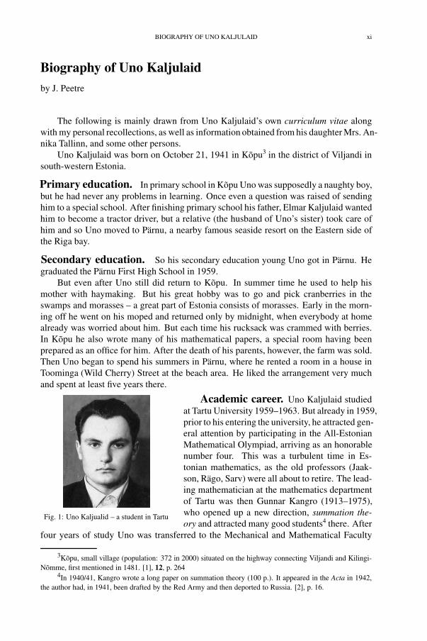
Fig. 1: Uno Kaljualid – a student in Tartu
Academic career. Uno Kaljulaid studiedat Tartu University 1959–1963. But already in 1959,prior to his entering the university, he attracted gen-eral attention by participating in the All-EstonianMathematical Olympiad, arriving as an honorablenumber four. This was a turbulent time in Es-tonian mathematics, as the old professors (Jaak-son, Rägo, Sarv) were all about to retire. The lead-ing mathematician at the mathematics departmentof Tartu was then Gunnar Kangro (1913–1975),who opened up a new direction, summation the-ory and attracted many good students4 there. After
four years of study Uno was transferred to the Mechanical and Mathematical Faculty
3Kõpu, small village (population: 372 in 2000) situated on the highway connecting Viljandi and Kilingi-Nõmme, first mentioned in 1481. [1], 12, p. 264
4In 1940/41, Kangro wrote a long paper on summation theory (100 p.). It appeared in the Acta in 1942,the author had, in 1941, been drafted by the Red Army and then deported to Russia. [2], p. 16.

xii BIOGRAPHY OF UNO KALJULAID
of Moscow University. He got his diploma in algebraic geometry, under the auspicesof Yuri Manin 1966, but he was never formally Manin’s “aspirant”, several applicationsby him being turned down (cf. below). Post-graduate studies again were done at TartuUniversity in 1968–1972. As follows to the comments by J.-E. Roos to his diploma work[K69a], some problems, then open, have been settled now.
The advisor of his Candidate thesis was Professor Boris Plotkin (at Riga, now inJerusalem). The defence took place, on March 11, 1979, at the Mathematical Instituteof the Belorussian Academy of Sciences in that country’s capital Minsk, with ZenonI. Borevich and Alex E. Zaleskiı as official opponents.
Fig. 2: Boris Isakovich Plotkin, supervisorof Uno Kaljulaid
Uno Kaljulaid taught at Tartu University from1972 on, first 1972–1974 as an Assistant Profes-sor and then 1974–1983 as an Associate Profes-sor. He was made a Docent in 1983. From 1993on he did scientific work and provided consulta-tive service at the Computer Science Institute ofthe Department of Mathematics of Tartu Univer-sity. Simultaneously, Kaljulaid was a part time se-nior research fellow at the Institute of Cyberneticsin Tallinn, where he carried out studies on com-positional theory of abstract state machines withmemory.
Scientific work. Teaching. Students. Uno Kaljulaid’s scientific output is,nominally, not large. Much is in the form of short papers, often merely research an-nouncements.
The bibliography below sets the number of items printed under Kaljulaid’s life timeto some 40. According to MathSciNet he has 27 reviewed papers in Mathematical Re-views. Searching there for Anywhere: Kalju∗ gave, somewhat surprisingly, 124 hits,indicating that Uno Kaljulaid, after all, was quite influential. To some extent this highfigure can be accounted for by the fact that it comprises also reviews written by Kaljulaid.On the other hand, MATH Database lists 14 items covered by Zentralblatt.
The first printed paper by Uno Kaljulaid seems to be [K69a] and visibly represents,although we are not explicitly told this, his diploma work at Moscow. It is about algebraicgeometry in a rather abstract style (Serre, Grothendieck), to wit about the cohomologicaldimension of algebraic varieties. This is what Professor Manin wrote to me when helearnt about the untimely death of Uno:
He was a student at the Algebra Chair of Moscow University. Forsome time, I was nominally his advisor, however, he always hadhis own scientific interests. I remember his mild smile and gentlespeech. He was deeply interested in mathematics and enthusiasticabout it. During the last decade or so I received a couple of lettersand postcards from him. He was explaining what he was doing math-ematically and usually added just a few words about life, which sodrastically changed for many of us. I will miss him.
Although Uno Kaljulaid was a dedicated mathematician and all absorbed by thissubject, he had also wide interests outside mathematics. We have already recorded his

BIOGRAPHY OF UNO KALJULAID xiii
with ballet.After his sojourn at Moscow University, Uno Kaljulaid did one year of military
service in the same city.
Fig. 3: Military service 1967
Having returned to Estonia, in1967, he worked some time with Pro-fessor Jaak Hion5 as supervisor.However, he soon was attracted tothe theory of representations, espe-cially of semigroups and algebras,and so his thesis advisor became, atleast unofficially, Professor Plotkin,at this time one of the leaders in thisarea. His Candidate thesis [K79a](in type script and written in Russian),is translated into English, and printedhere for the first time. An “author’sreview” of the thesis[K79b] is likewise included here.For a very brief overview we alsorefer to a note in Uspekhi Matema-ticheskikh Nauk [K77a]. Further-more, some preliminary results latercovered in [K79a] were presented inseparate publications prior et poste-
rior, see e.g. [K71b,71c,73c,76,77b,78a,78b,81,82a,82b, 83a,83e,85a], not reproducedhere).
The following lines were written, on my request, by Professor Plotkin about hiscontacts with Uno:
Uno Kaljulaid was not only my pupil but also a very close friend.Our contacts started in the end of 60-ties, when I used to come
to Tartu from Riga with talks and lectures. That time the mathemat-ical life in Tartu was rather active. One of the most popular activi-ties was Summer Mathematical Schools in Kääriku. In Kääriku therewas a base of Tartu University and mathematicians enjoyed this placewhere mathematical discussions could be combined with rest, beau-tiful nature and conversations. I remember that these conferenceswere made possible due to [Jaak] Hion, Mati Kilp, [Ülo] Lumisteand other mathematicians from Tartu.
At the beginning of 70-ties my interest was focused on the vari-eties of group representations. This topic attracted attention of Uno.Soon after he asked me to give him a problem for his [Candidate] the-sis. I recommended him to build a similar theory for representationsof semigroups. In this case I took into account that Uno [had] already
5Born in 1929, Hion got his Candidate degree in Moscow under A. G. Kurosh, an outstanding algebraistmainly known for his work in group theory, in 1955.
passion for the lovely Estonian cranberries. During his Moscow days he also fell in love

xiv BIOGRAPHY OF UNO KALJULAID
studied semigroups for a long time. Simultaneously I proposed himsome problems about group representations. Uno managed to prove aseries of significant results and in the end of the 70-ties he brilliantlydefended his [Candidate] thesis at the Institute of Mathematics inMinsk. His work was highly appreciated by the reviewers and theCouncil members.
Along with great results achieved by Uno, I should mention thathe had deep and wide mathematical background. Uno has gradu-ated from Moscow State University, where he got his education fromoutstanding teachers. For example, I know that during his univer-sity years he collaborated with Yu. I. Manin. I think Uno took greatadvantages from his education in Moscow University and the widestyle of mathematical thinking can be traced in all his works duringhis mathematical career.
During the period of preparation of the thesis Uno frequentlyvisited me in Riga. Also later he used to come to discuss variousproblems. Methods, elaborated in the thesis, were extended and usedin the automata theory. We considered automaton as a three-sortedmathematical system which possesses algebraic operations convert-ing states to states and states to output signals. The system of inputsignals naturally constitutes a semigroup with the representation onthe set (space) of states. This algebraic point of view on automataturns out to be very fruitful.
Last years he collaborated with his pupil Olga Sokratova andother pupils in automata theory. I think that they could give usefulinformation about his last works.
I am sure that your activity in commemorating the memory ofUno Kaljulaid will be appreciated by mathematicians.
Fig. 4: Participants of Summer School in Kääriku 1966:V. Vagner, J. Hion, E. Lyapin, L. Shevrin, L. Gluskin and B. Plotkin

BIOGRAPHY OF UNO KALJULAID xv
Fig. 5: Mati Kilp and Uno Kaljulaid on their way to Moscow 1964
I find it curious that thus two men, independently, first declare that Uno Kaljulaidwas not their pupil, but otherwise give him all the praise that they can! This shows thatUno already early on was an independent mind. There is however one person in Tartu thatinfluenced him quite a lot. This is Hion, who also should be considered as the founderof the Estonian school of algebra. So, maybe he should after all be viewed as the trueteacher of Uno Kaljulaid!
Later he became, undoubtedly inspired by this, interested in automata theory. Al-ready in [K69a] there is a brief treatment of at least linear automata. Indeed, automatatheory became his main occupation in the last decade of his life.
With his unusually broad mathematical education, Kaljulaid took also a vivid interestin the history of mathematics. In particular, he wrote several papers (see this Volume,Chapter V, in particular the last one) about Theodor Molien (1861–1941), born in Rigaof Swedish decent, studied in Dorpat/Tartu and a docent there, later in Siberia), who wasa pioneer in the field of algebras, but is relatively little known to the general mathematicalpublic, despite the fact that he influenced, for instance, Emmy Noether, who also dulyquoted him.
Kaljulaid was also early interested in combinatorics, which is treated here in ChapterIII. It is my guess that it was through teaching that he was led to this subject.
Among research students of Uno Kaljulaid I mention Annela Kelly (née Rämmer),Peeter Laud, Riina Miljan, Jaan Penjam, Tiit Pikkmaa, Varmo Vene, Tiina Zingel (néeNirk).
My recollections of Uno Kaljulaid. I first met Uno Kaljulaid during a tripto then still Soviet occupied Estonia in the spring of 1989. Namely at a meeting of theEstonian Mathematical Society, which took place at Klooga-Ranna, a seaside resort afew miles West of Tallinn and not far from Paldiski, which at the time was a base for
xvi BIOGRAPHY OF UNO KALJULAID
Soviet submarines. (The conflict about submarines with Sweden was going on. “Therethey are, the submarines, which you cannot catch”, I was told, and people pointed toacross the bay.)
On that meeting, Kaljulaid gave a talk on combinatorics. After the talk I had a dis-cussion with him and I told him about my own experience of this subject. It ended by meinviting him to Sweden. Kaljulaid came to Stockholm in the spring of 1990. I had renteda room for him in the apartment of Bertil Eneroth, Civil Engineer, in Sibyllegatan 38 inthe district Östermalm, where I housed many of my guests during my Stockholm years6.He gave a talk at the algebra seminar run by Jan-Erik Roos at Stockholm University. Thiswas the year when I directed, jointly with Svante Janson, a program at the Mittag-LefflerInstitute, which was devoted to Hankel theory. So I invited him also there one day. Hehad supper with me and my betrothed Eila in the company of, also, Marcel Grossmanfrom Marseille. At the same time Uno went also to Lund, where he met Lars Hörmanderand his team of bright young Russian students.
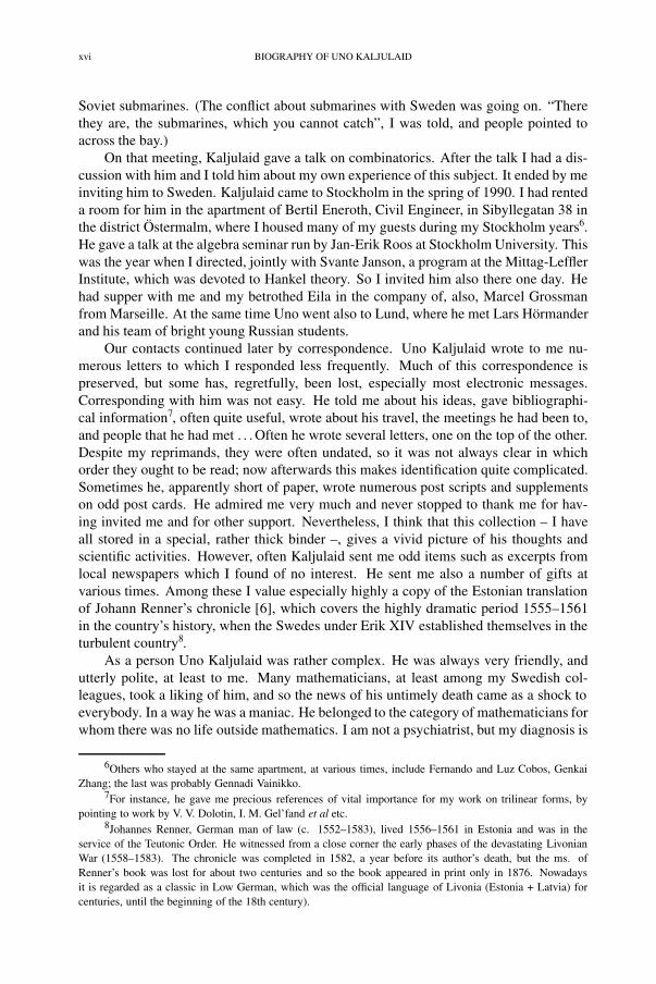
Our contacts continued later by correspondence. Uno Kaljulaid wrote to me nu-merous letters to which I responded less frequently. Much of this correspondence ispreserved, but some has, regretfully, been lost, especially most electronic messages.Corresponding with him was not easy. He told me about his ideas, gave bibliographi-cal information7, often quite useful, wrote about his travel, the meetings he had been to,and people that he had met . . . Often he wrote several letters, one on the top of the other.Despite my reprimands, they were often undated, so it was not always clear in whichorder they ought to be read; now afterwards this makes identification quite complicated.Sometimes he, apparently short of paper, wrote numerous post scripts and supplementson odd post cards. He admired me very much and never stopped to thank me for hav-ing invited me and for other support. Nevertheless, I think that this collection – I haveall stored in a special, rather thick binder –, gives a vivid picture of his thoughts andscientific activities. However, often Kaljulaid sent me odd items such as excerpts fromlocal newspapers which I found of no interest. He sent me also a number of gifts atvarious times. Among these I value especially highly a copy of the Estonian translationof Johann Renner’s chronicle [6], which covers the highly dramatic period 1555–1561in the country’s history, when the Swedes under Erik XIV established themselves in theturbulent country8.
As a person Uno Kaljulaid was rather complex. He was always very friendly, andutterly polite, at least to me. Many mathematicians, at least among my Swedish col-
everybody. In a way he was a maniac. He belonged to the category of mathematicians forwhom there was no life outside mathematics. I am not a psychiatrist, but my diagnosis is
6Others who stayed at the same apartment, at various times, include Fernando and Luz Cobos, GenkaiZhang; the last was probably Gennadi Vainikko.
7For instance, he gave me precious references of vital importance for my work on trilinear forms, bypointing to work by V. V. Dolotin, I. M. Gel’fand et al etc.
8Johannes Renner, German man of law (c. 1552–1583), lived 1556–1561 in Estonia and was in theservice of the Teutonic Order. He witnessed from a close corner the early phases of the devastating LivonianWar (1558–1583). The chronicle was completed in 1582, a year before its author’s death, but the ms. ofRenner’s book was lost for about two centuries and so the book appeared in print only in 1876. Nowadaysit is regarded as a classic in Low German, which was the official language of Livonia (Estonia + Latvia) forcenturies, until the beginning of the 18th century).
leagues, took a liking of him, and so the news of his untimely death came as a shock to
BIOGRAPHY OF UNO KALJULAID xvii
that he suffered from a kind of persecution mania. I once called, in desperation, Vainikko(then at Helsinki) about this, but he showed little understanding; some of the things thatKaljulaid had told him also turned out not be true (that obstructions were made to himwhen he left Tartu etc.). Already in the very beginning of our acquaintance Kaljulaidbegan to worry about that some of his letters could have been intercepted. This was stillin Soviet times, but such allegations continued throughout the period of our relation. Letme relate only one such episode, which is supposed to have taken place during one ofhis stays at Lund (cf. infra). Namely, Kaljulaid claimed that, in our Department’s coffeeroom, some Swedes, speaking in Swedish, had slandered him in his presence. With myknowledge of Swedes and Swedish mentality, I find this highly improbable, especiallyas I have doubts of Kaljulaid’s ability to understand spoken Swedish. Also many peoplehere liked him; among them was Anders Melin – I am not sure if he was supposed to havebeen present on the occasion referred to above; it was also Melin who first suggested tous to make an application to the Crafoord Foundation (see again infra). Kaljulaid toldme also of several other incidents, about various acts of persecution against him, whichI found more or less credible. On these occasions his whole attitude suddenly changed,the voice altered almost to whisper, although there could be nobody nearby who couldoverhear our conversation in Estonian; to me he then looked more like an old womantelling a gossip. Once I wrote to him and advised to go to the Rector of the Universityand complain; afterwards I realized that, although this could have been a logical step inSweden, it could hardly have been a good idea in post-communist Estonia. I doubt thatKaljulaid followed my advice.
After my return to Lund in 1992, I arranged Uno Kaljulaid a second visit to Swedenwith money coming from the Swedish National Council for Scientific Research (NFR);again, he visited both Stockholm and Lund. To Lund he came in September 1994. It wason this occasion that we set up a plan to study majorization from a very general point ofview. However, only a tiny portion of our rather ambitious plan was ever materialized(see Chapter III); it is clear that I wrote the first version of that paper already then. Wemade also plans for future cooperation; to this end we applied, in 1995, for a grant fromthe Crafoord Foundation, and, indeed, we were given a rather handsome sum of money,which allowed Kaljulaid to come to Lund several times.
So, Kaljulaid arrived again in Lund at the end of September 1994. By the irony offate, he came the week before the Estonia catastrophe9, so, had he come only slightlylater, he could well have been one of the victims. I recall that Eila and I heard about itby 6 o’clock in the morning by early, Finnish language broadcast on the Swedish radio.I immediately phoned Uno, who was staying in one of our Department’s guestrooms.We were both, of course, utterly shocked, and I reminded him about all the Estonianrefugees, often in tiny vessels, who had drowned in similar weather conditions in thesame month in September, 1944. Anyhow, soon we went on with mathematics. Kaljulaidgave several colloquium talks on automata theory; they were based on material which hehad prepared on previous occasions. So I volunteered to write them up for him (seeChapter II, Section 2). Having learnt about his inability in practical matters, I saw it
9The passenger vessel Estonia, owned by a joint-venture Swedish Estonian company on the line Tallinn-Stockholm, perished near the Finnish coast, on September 28, 1994, in one of the fierce autumn storms in theBaltic. On this occasion, 869 persons were killed.
xviii BIOGRAPHY OF UNO KALJULAID
as my duty to try to help him publish at least part of his ideas. Probably, I prepared aTeX-version of Lecture 1 already while he was in Lund.
Next time that Uno Kaljulaid came to Sweden was the year after, in October, 1996.We then made plans for another visit. This time we made an application to the SwedishInstitute (SI), which included also a visit for Kaljulaid’s bright student Peeter Laud; I wassupposed to have become his advisor. Unfortunately, the application was turned down.Later Laud showed interest in more applied things and defended his PhD thesis [3] oninformation security matters in 2002. An even shorter, last trip was in May 1997.
After that time (during the last two years of the life of Uno Kaljulaid), my contactswith him were even more sporadic. I wrote Lecture 2. Uno sent me corrections andadditions, and also some material for Lecture 3. Rereading our correspondence from
On my side, I also took almost none initiative, as I was busy with teaching and otheractivities . . .
Marriage. Uno Kaljulaid married in 1973. His future wife Helle was a technicalFrom this marriage two daughters were born,
Annika in 1974 and Kristina in 1979. In the mid 1980’s the parents divorced, but theynever separated.
Illness and death. Uno Kaljulaid became ill already at the end of the 1987 andhad a surgery for a stomach cancer. At the time doctors gave him only at most five yearsto live. However, he was practically rather healthy until the middle of July, 1999. Heworked and went jogging every morning. Until the mid of July he rested in his belovedPärnu but then he began to cough and gradually felt less and less at ease. Nevertheless, atthe end of July he participated in a conference in Poland, and, probably, gave also a talkthere. Upon his return he, finally, went to see a doctor, because his health had seriouslybegan to deteriorate. Mid September he underwent another surgery, but its purpose wasonly to set a diagnosis: a cancer in the stomach with remote metastases in the lungs andin the liver. After the operation Uno told that he would not surrender so easily and thathe hoped to be able to finish at least the ongoing work. A few days before his death,however, asked that all should be finished. Luckily he did not suffer of heavy pain, butstill it was very hard.
Uno Kaljulaid passed away at the age of 57 on September 26, 1999 in the pulmonaryclinic at Tartu. Annika wrote me that it was a sunny autumn day. He died in the armsof his half-sister Laine. He was buried on October 1st at his native village Kõpu in thedistrict of Viljandi. His death was that of a true hero . . .
In the meantime, I was quite unaware of everything. Early in June I received twopostcards from Uno, dated in Tartu on June 4, 1999, and, apparently, sent in the sameenclosure, the text of which I hereby offer a translation:
this period, I find it striking that he showed relatively little interest in the whole project.
assistant at the mathematics department.

BIOGRAPHY OF UNO KALJULAID xix
Dear Mr. Peetre,Thank you for sending me the thesis of Mr. Rosengren10, and
likewise for your lines. This time everything arrived in unhurt shape,although with some delay.
I have now finished my courses, and very soon I shall also fin-ish the exams. But this occupation gives me steadily less and lesssatisfaction. Probably I’ll have a chance to participate in the CS-conference in Uppsala. But I have not yet made up my mind whetherto go there or not, because its scope covers a few of my interests. Butit would be an opportunity to see Stockholm once more.
Spring here was chilly, frost took the flowering of the currantbushes. Probably things were not so bad where you are – for Lundis on the latitude of Latvia or even further south. I presume that youare already by the sea, I wish a pleasant summer.
Uno Kaljulaid
I was notified about Kaljulaid’s death, three days after, in an email message from hisdaughter Annika. She gave me also the above details of his illness and death. Further-more, she told me that at his sickbed her father told that he wanted me to take care of his“Nachlass”, which I also eventually did . . . So all this is just my tribute to him . . .
References(including two articles [2] and [5], in Estonian, commemorating Uno Kaljulaid)
[1] Eesti Entsüklopeedia 1–14 + Supplementary Volume. (Estonian Encyclopedia.), Tallinn, 1985.[2] Mati Kilp. Uno Kaljulaid 21.10.1941–26.09.1999. In: Annual, 1999. Eesti Matemaatka Selts (Estonian
Mathematical Society), Tartu, 2001, 111–114.[3] Peeter Laud, Computationally Secure Information Flow. Ph.D. Thesis. Universität des Saarlandes, Saar-
brücken, April 2002.[4] Ü. Lumiste and J. Peetre. Edgar Krahn , A centenary volume 1894–1961. IOS Press, Providence, Rhode
Island, 1994.[5] Rein Prank. Remebering Uno Kaljulaid. In: Annual, 1999. Eesti Matemaatka Selts (Estonian Mathematical
Society), Tartu, 2001, 119–123.[6] J. Renner. Liivimaa ajalugu 1556–1561 (History of Livonia). Translated by Ivar Leimus and Enn Tarvel.
Olion, Tallinn, 1995.
10Hjalmar Rosengren defended his PhD thesis Multivariable orthogonal polynomials as coupling coeffi-cients for Lie and quantum representations on May 6, 1999.

This page intentionally left blank
BIBLIOGRAPHY OF UNO KALJULAID xxi
Bibliography of Uno Kaljulaid
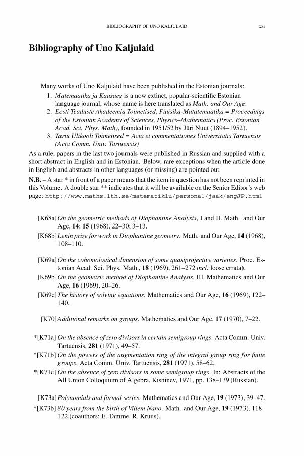
Many works of Uno Kaljulaid have been published in the Estonian journals:
1. Matemaatika ja Kaasaeg is a now extinct, popular-scientific Estonianlanguage journal, whose name is here translated as Math. and Our Age.
2. Eesti Teaduste Akadeemia Toimetised, Füüsika-Matatemaatika = Proceedingsof the Estonian Academy of Sciences, Physics–Mathematics (Proc. EstonianAcad. Sci. Phys. Math), founded in 1951/52 by Jüri Nuut (1894–1952).
3. Tartu Ülikooli Toimetised = Acta et commentationes Universitatis Tartuensis(Acta Comm. Univ. Tartuensis)
As a rule, papers in the last two journals were published in Russian and supplied with ashort abstract in English and in Estonian. Below, rare exceptions when the article donein English and abstracts in other languages (or missing) are pointed out.
N.B. – A star * in front of a paper means that the item in question has not been reprinted inthis Volume. A double star ** indicates that it will be available on the Senior Editor’s webpage: http://www.maths.lth.se/matematiklu/personal/jaak/engJP.html
[K68a]On the geometric methods of Diophantine Analysis, I and II. Math. and OurAge, 14; 15 (1968), 22–30; 3–13.
[K68b]Lenin prize for work in Diophantine geometry. Math. and Our Age, 14 (1968),108–110.
[K69a]On the cohomological dimension of some quasiprojective varieties. Proc. Es-tonian Acad. Sci. Phys. Math., 18 (1969), 261–272 incl. loose errata).
[K69b]On the geometric method of Diophantine Analysis, III. Mathematics and OurAge, 16 (1969), 20–26.
[K69c]The history of solving equations. Mathematics and Our Age, 16 (1969), 122–140.
[K70]Additional remarks on groups. Mathematics and Our Age, 17 (1970), 7–22.
*[K71a] On the absence of zero divisors in certain semigroup rings. Acta Comm. Univ.Tartuensis, 281 (1971), 49–57.
*[K71b] On the powers of the augmentation ring of the integral group ring for finitegroups. Acta Comm. Univ. Tartuensis, 281 (1971), 58–62.
*[K71c] On the absence of zero divisors in some semigroup rings. In: Abstracts of theAll Union Colloquium of Algebra, Kishinev, 1971, pp. 138–139 (Russian).
[K73a]Polynomials and formal series. Mathematics and Our Age, 19 (1973), 39–47.
*[K73b] 80 years from the birth of Villem Nano. Math. and Our Age, 19 (1973), 118–122 (coauthors: E. Tamme, R. Kruus).
xxii BIBLIOGRAPHY OF UNO KALJULAID
*[K73c] On the powers of the augmentation ideal. Proc. Estonian Acad. Sci. Phys.Math., 22 (1973), 3–21.
[K75a]On Galois theory. Mathematics and Our Age, 20 (1975), 17–31.
[K75b]Theory of automata. Mathematics and Our Age, 20 (1975), 32–47. (coauthor:E. Tamme).
*[K76] On wreath type constructions for algebras. In: Abstracts of the Third AllUnion Symposium of Rings, Algebras and Modules, Tartu, 1976, pp. 49–50(Russian).
[K77a]Triangular products of representations of semigroups and associative alge-bras. Uspehi Mat. Nauk 32 (1977), no 4/196, 253-254 (Russian).
*[K77b] Remarks on the varieties of semigroup representations and automata. ActaComm. Univ. Tartuensis, 431 (1977), 47–67.
*[K77c] Remarks on the course on discrete mathematics. Proc. of the III RegionalConference-Seminar of Leading Departments and Leading Lecturers of Ma-thematics, Minsk, 1977, p. 50 (Russian).
*[K78a] A remark the basis of identities of an algebra of upper triangular matrices.In: Materials of Conf. “Methods of Algebra and Functional Analysis”, Tartu,1978, pp. 105–107 (Russian).
*[K78b] Triangular products and group rings. Vestn. Moskov. Univ. Mat., no. 6,1978, p. 81 (Russian).
[K79a]Triangular products and stability of representations. Candidate dissertation.Tartu University, 1979, 150 pp. (Russian, typescript).
[K79b]Triangular products and stability of representations. Author review of Can-didate thesis in Physico-Mathematical Sciences [K79a]. Minsk, 1979, 13 pp.(Russian).
*[K79c] The arithmetics of varieties of representations of semigroups and algebras.Manuscript, deposited at VINITI, no. 344–78; “Matematika” 2AI36 DEP,1979, 42 pp. (Russian).
*[K81] About semigroup actions. Acta Comm. Univ. Tartuensis, 556 (1981), 27–32.
*[K82a] Terminals of groups and stability of representations. Acta Comm. Univ.Tartuensis, 610 (1982), 15–25.
**[K82b] A lower bound for the terminal of certain groups. Acta Comm. Univ. Tartuen-sis, 610 (1982), 26–37.
[K83a]Triangular products representations of linear semigroups actions. ActaComm. Univ. Tartuensis, 640 (1983), 13–28.
*[K83b] A remark on Stirling numbers. In: Sb. “Komb. Analiz”, 6 (1983), p. 98(Russian).

BIBLIOGRAPHY OF UNO KALJULAID xxiii
*[K83c] Elements of discrete mathematics. Tartu University Press, Tartu, 1983, 100 pp.(Estonian).
*[K83d] Lattices and combinatorics – a problem book. Tartu University Press, Tartu,1983, 27 pp., (Estonian).
*[K83e] On the freedom of the semigroup of special ideals. In: Abstracts of the con-ference “Methods of algebra and analysis”, Tartu, 1983, pp. 10–12.
**[K85a] Unique factorization of varieties of semigroup representations. Acta Comm.Univ. Tartuensis, 700 (1985), 17–31.
[K85b]Remarks on subcommutant rings. In: XVIII All Union Algebraic Conference,Abstracts of talks. Kishinev, 1985, p. 227.
[K85c]On two results on strongly regular rings. In: Proc. of the Conference “Theo-retical and applied questions of mathematics”, Abstracts of talks, Tartu, 1985,pp. 67–69.
[K87a]Some remarks on Shevrin’s problem. Acta Comm. Univ. Tartuensis, 764(1987), 30–38 (English).
*[K87b] On the theory of vacuum deposition of layer on the rotating cylindrical sub-strate. Acta Comm. Univ. Tartuensis, 779 (1987), 127–136 (coauthor:J. Lembra).
*[K87d] Theodor Molien and group algebras. In: Development of schools, ideas andtheories in natural sciences at Tartu University, Tartu, 1987, pp. 16–24 (Es-tonian).
[K87e]On the results of Molien about invariants of finite groups and their renaissancein contemporary mathematics. In: Development of schools, ideas and theoriesin Natural Sciences at Tartu University, Tartu, 1987, pp. 111–119 (Russian).
[K88a]On Stirling and Lah numbers. In: Methods of algebra and analysis. Tartu,1988, pp. 11–14 (Russian).
[K88b]Fibonacci numbers of outer planar graphs. In: Methods of algebra and analy-sis, Tartu, 1988, pp. 15–17 (Russian, coauthor: T. Pikkmaa).
*[K88c] On the theory of vacuum deposition of layer on a rotating cylindrical substratefrom an asymmetrically located source. Acta Comm. Univ. Tartuensis, 830(1988), 127–136 (coauthor: J. Lembra).
[K90]Transferable elements in group rings. Acta Comm. Univ. Tartuensis, 878(1990), 39–52.
*[K93a] M. Meriste, J. Penjam, Algebraic theory of tape-controlled attributed au-tomata. Research Report CS59/93, Institute of Cybernetics, Tallinn, 1993,28 pp. (coauthors: M. Meriste, J. Penjam).
*[K93b] Analytical and algebraic methods in combinatorics. Tartu University Press,Tartu, 1993, 159 pp. (Estonian, coauthor: Ü. Kaasik).

xxiv BIBLIOGRAPHY OF UNO KALJULAID
*[K93c] Mordell’s problem. Estonian Mathematical Society. Annual 1988, Tartu Uni-versity Press, Tartu, 1993, pp. 128–151, 178, 182 (Estonian, summary in Eng-lish and Russian).
*[K93d] Languages, tools and methods of conceptual modelling. Research Re-port CS61/93, Institute of Cybernetics, Tallinn, 1993, 49 pp. (coauthors:M. Meriste, J. Penjam et al.)
[K96]On two discrete models in connection with structures of mathematics and lan-guage (the languages of life). Schola Biotheoretica XII, Tartu, 1996, pp. 84–95(Estonian).
[K97a]On two algebraic constructions for automata. Research Report CS92/97, In-stitute of Cybernetics, Tallinn, 1997, 27 pp. (coauthor:J. Penjam).
*[K97b] Categories, automata and splicing systems. In: Proc. of 9th Nordic Workshopon Programming Theory, Tallinn, 1997, p. 47 (coauthor: J. Penjam).
*[K98a] Flatness and localizations of Ω-semigroups. Research Report CS96/98, Insti-tute of Cybernetics, Tallinn, 1998, 49 pp. (coauthor: O. Sokratova.)
*[K98b] Does there exist a (non-abelian simple) linearly right-orderable group all ofwhose proper subgroups are cyclic?. In: Kourovka Notebook, 14th augmentededition, problem 14.45, Novosibirsk, 1999, p. 110.
[K98c]Revisiting wreath poducts, with applications to representations and invari-ants. In: Yu. A. Bahturin, A. I. Kostrikin, A. Yu. Ol’shanskiı (eds.), KuroshAlgebraic Conference, Abstract of talks, Moscow University Press, Moscow,1998, pp. 64–65.
[K98d]Right order groups; their representations, structure and combinatorics. Man-uscript, 37 pp.; 2nd version (1998) (to be submitted).
[K00]Ω-rings and their flat representations. In: Contributions to General Algebra12, Verlag Joh. Heyn, Klagenfurt 2000, 377–390 (coauthor: Olga Sokratova).
CHAPTER I
Representations of semigroups andalgebras

This page intentionally left blank
3
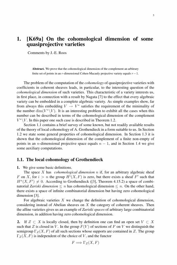
1. [K69a] On the cohomological dimension of somequasiprojective varietiesComments by J.-E. Roos
Abstract. We prove that the cohomological dimension of the complement an arbitrary
finite set of points in an r-dimensional Cohen-Macauly projective variety equals r−1.
The problem of the computation of the cohomology of quasiprojective varieties withcoefficients in coherent sheaves leads, in particular, to the interesting question of thecohomological dimension of such varieties. This characteristic of a variety interests us,in first place, in connection with a result by Nagata [7] to the effect that every algebraicvariety can be embedded in a complete algebraic variety. As simple examples show, farfrom always this embedding V → V ∗ satisfies the requirement of the minimality ofthe number dim(V ∗\V ). It is an interesting problem to exhibit all the cases when thisnumber can be described in terms of the cohomological dimension of the complementV ∗\V . In this paper one such case is described in Theorem 1.2.
Section 1.1 contains a brief survey of some known, but not readily available resultsof the theory of local cohomology of A. Grothendieck in a form suitable to us. In Section1.2 we state some general properties of cohomological dimension. In Section 1.3 it isshown that the cohomological dimension of the complement of a finite non-empty ofpoints in an n-dimensional projective space equals n − 1, and in Section 1.4 we givesome auxiliary computations.
1.1. The local cohomology of Grothendieck
1. We give some basic definitions.The space X has cohomological dimension n if, for an arbitrary algebraic sheaf
F on X , for i > n the group Hi(X,F ) is zero, but there exists a sheaf F ′ such thatHn(X,F ′) �= 0. According to Grothendieck ([3], Theorem 4.15.2) a space of combi-natorial Zariski dimension ≤ n has cohomological dimension ≤ n. On the other hand,there exists a space of infinite combinatorial dimension but having zero cohomologicaldimension [3].
For algebraic varieties X we change the definition of cohomological dimension,considering instead of Abelian sheaves on X the category of coherent sheaves. Thenthe affine varieties gives us an example of Zariski spaces of arbitrary large combinatorialdimension, in addition having zero cohomological dimension.
2. If Z ⊂ X is locally closed, then by definition one can find an open set V ⊂ Xsuch that Z is closed in V . In the group F (V ) of sections of F on V we distinguish thesemigroup ΓZ(X,F ) of all such sections whose supports are contained in Z . The groupΓZ(X,F ) is independent of the choice of V , and the functor
F =⇒ ΓZ(X,F )

4 CHAPTER I. REPRESENTATIONS OF SEMIGROUPS AND ALGEBRAS
maps an exact sequence of sheaves 0 → F → G→ H into an exact sequence of Abeliangroups
0 → ΓZ(F ) → ΓZ(G) → ΓZ(H).
This means that the functor F =⇒ ΓZ(X,F ) is exact from the left from the category ofAbelian sheaves on X into the category of Abelian groups.
If U ⊂ X is open, then the natural homomorphism of restriction
F (V ) → F (V ∩ U)
induces a homomorphism
ΓZ(X,F )→ ΓZ∩U (U,F |U),
which is indeed a sheaf. The functor
F =⇒ ΓZ(F )
is exact from the left in the category of Abelian functions onto itself; we define the rightderivative H i
Z(X,F ) of this functor which is called the sheaf of local cohomology of X .Let X be an r-dimensional Zariski space F , F an Abelian sheaf on it and Z ⊂ X
locally closed. Grothendieck’s theorem ([5], Proposition 1.12) says that for i > r thegroups H i
Z(X,F ) and that the sheaves H iZ(X,F ) are zero.
3. Let X = SpecA be an additive scheme, Y one of its subschemes, given by an idealI ⊂ A; the sheaf of coefficients F associated with the A-module N . Then one has forall i > 0 the isomorphism
HiY (X,F ) ≈ lim
nExtiA(A/In, N) ([5], Theorem 2.8).
For each open Y ⊂ X and a coherent sheaf F on X one has the exact sequence
0 → ΓY (X,F )→ Γ(X,F ) → Γ(X\Y, F )→ HiY (X,F )→ . . .
HiY (X,F )→ Hi(X,F )→ Hi(X\Y, F )→ H i+1
Y (X,F )→ . . . .
As in the case at hand Hi(X,F ) = 0 for all i > 0, we have the isomorphism
H i(X\Y, F ) ≈ H i+1Y (X,F ).
Next, let X be an r-dimensional projective space and S = k[t0, . . . , tr] the algebraof polynomials over the field k. We take for F the sheaf O(n). Then, by Serre [11], for0 < i < r the groups H i(X,O(n)) are zero, while the group Hr(X,O(n)) is a vectorspace over k of dimension
(−n−1r
)and has a basis of skew symmetric cocycles of cover
U = (ti �= 0) of the form
f01...r =1
tα0 . . . tαr,
where αi > 0 and∑
αi = −n. Therefore we have for 0 < r < r − 1 the isomorphism
H i(X\Y,O(n)) ≈ H iY (X,O(n)),
while, by definition the groups Hr(X\Y,O(n)) are given by the exact sequence
HrY (X,O(n)) → Hr(X,O(n)) → Hr(X\Y,O(n))→ 0.

1. On the cohomological dimension ... 5
4. Let M and N be graded S-modules. Then the derived functor Ext of the functorHoms(M,N) = ⊕
nHomn
S(M,N), defined, on the one hand, by Serre in [11] and, on the
other hand, Cartan and Eilenberg in [1] need not coincide. However, it is easy to see theydo coincide in the case needed by us of ExtiA(A/In, A), where A = k[t1, . . . ,r ] and Iis the ideal in A given by Y ⊂ X . Indeed, the ring A/In as a module over itself, is alsoan A-module. As a ring A/In is Noetherian. The submodules of A/In are ideals in it;therefore, it follows from Hilbert’s theorem ([1], p. 32) that this module is Noetherian.But a Noetherian module over a Noetherian ring is of finite type. In this case ([11],p. 434) both definitions coincide.
Let there be given R-modules A,B,A′, B′ and R-homomorphisms α : A′ → Aand β : B → B′. Introduce an R-homomorphism Hom(α, β) : Hom(A,B) →Hom(A′, B′) which to each ϕ ∈ Hom(A,B) is defined by the
Hom(α, β) ◦ ϕ = β ◦ ϕ ◦ α.The objects Hom(A, β) and Hom(α,B) are obtained from Hom(α, β) for A = A′
and B = B′ respectively. The following theorem from homological algebra may beuseful in the calculation of local groups of cohomology.
Let us consider the exact sequences of modules
0 → In α→ A→ A/In → 0
and0 → A→ K
β→ A→ K/A→ 0,where A is a projective and K an injective module. The following isomorphisms holdtrue (cf. [1], p.141):
ExtiA(A/In, A) ≈ Exti−2
A (In,K/A);
Ext2A(A/In, A) ≈ Coker(HomA(α, β));Ext1A(A/In, A) ≈ Ker (Hom(α, β))/[Ker (HomA(α,K/A)) + Ker (HomA(A, β))].
As by the first main theorem of Grothendieck one has the isomorphism
HiY (X,O) ≈ lim
nExtiA(A/In, A),
the three isomorphisms just given suffice for the calculation in a 3-dimensional space.
1.2. Some general properties of cohomological dimension1. Let X and Y be algebraic varities; ϕ : Y → X a morphism and F an algebraic sheafon X . Then there is defined on Y an algebraic sheaf Fϕ, called the inverse image of thesheaf F under the isomorphism1 ϕ.
If F is a coherent sheaf on X , then Fϕ too is coherent on Y . Indeed, in view of thecoherence of F there exists U ⊂ X for which one has an exact sequence
Op → Oq → F → 0.
The homomorphism Ox → Oy induces the identity map on the base field k; thereforewe have the canonical isomorphism
Oy ⊗Ox Ox ≈ Oy.
1Regarding the construction of the sheaf F ϕ, cf. [9].
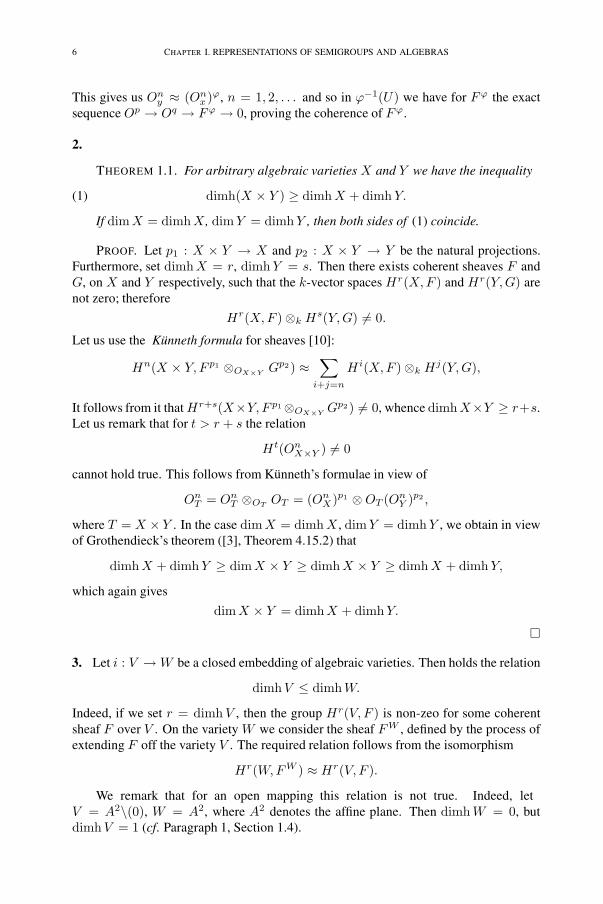
6 CHAPTER I. REPRESENTATIONS OF SEMIGROUPS AND ALGEBRAS
This gives us Ony ≈ (On
x )ϕ, n = 1, 2, . . . and so in ϕ−1(U) we have for Fϕ the exactsequence Op → Oq → Fϕ → 0, proving the coherence of Fϕ.
2.
THEOREM 1.1. For arbitrary algebraic varieties X and Y we have the inequality
(1) dimh(X × Y ) ≥ dimhX + dimh Y.
If dimX = dimhX , dimY = dimhY , then both sides of (1) coincide.
PROOF. Let p1 : X × Y → X and p2 : X × Y → Y be the natural projections.Furthermore, set dimhX = r, dimhY = s. Then there exists coherent sheaves F andG, on X and Y respectively, such that the k-vector spaces Hr(X,F ) and Hr(Y,G) arenot zero; therefore
Hr(X,F )⊗k Hs(Y,G) �= 0.
Let us use the Künneth formula for sheaves [10]:
Hn(X × Y, F p1 ⊗OX×Y Gp2) ≈∑
i+j=n
Hi(X,F )⊗k Hj(Y,G),
It follows from it that Hr+s(X×Y, F p1⊗OX×Y Gp2) �= 0, whence dimhX×Y ≥ r+s.Let us remark that for t > r + s the relation
Ht(OnX×Y ) �= 0
cannot hold true. This follows from Künneth’s formulae in view of
OnT = On
T ⊗OT OT = (OnX)p1 ⊗OT (On
Y )p2 ,
where T = X × Y . In the case dimX = dimhX , dimY = dimh Y , we obtain in viewof Grothendieck’s theorem ([3], Theorem 4.15.2) that
dimhX + dimhY ≥ dimX × Y ≥ dimhX × Y ≥ dimhX + dimhY,
which again gives
dimX × Y = dimhX + dimhY.
�
3. Let i : V →W be a closed embedding of algebraic varieties. Then holds the relation
dimhV ≤ dimhW.
Indeed, if we set r = dimh V , then the group Hr(V, F ) is non-zeo for some coherentsheaf F over V . On the variety W we consider the sheaf FW , defined by the process ofextending F off the variety V . The required relation follows from the isomorphism
Hr(W,FW ) ≈ Hr(V, F ).
We remark that for an open mapping this relation is not true. Indeed, letV = A2\(0), W = A2, where A2 denotes the affine plane. Then dimhW = 0, butdimhV = 1 (cf. Paragraph 1, Section 1.4).

1. On the cohomological dimension ... 7
4. We make the following conjecture: for an arbitrary fiber bundle (E, π,B) whosefiber is the projective space P r, it holds the formula
dimhE = dimhB + r.
If this is true it follows from it in a trivial way that the cohomological dimension for theσ-process for a point only can increase.
Let X∗ be a variety obtained by monoidal transformations from a non-special, ir-reducible algebraic variety X of dimension r. Let the center of this σ-process be anonspecial d-dimensional variety i : V → X . Furthermore, let f : X∗ → X be theprojection. The inverse image of X under this projection of X∗ is a projective fiberingof rank r − d− 1 with basis V . In view of the fact that the embedding i∗ : V ∗ → X∗ isclosed, the hypothesis made and the monotonicity properties we obtain
dimhX∗ ≥ dimhV + r + d− 1.
In particular, for the σ-process for a point we obtain dimhX∗ ≥ r − 1. As dimX∗ =dimhX , we have in view of known theorems (cf. Paragraph 1, Section 1.1) we obtaineither dimhX∗ = r or dimhX∗ = r − 1. Let us now take for X an affine variety ofdimension r, and for V a point. It is clear that dimhX = 0. Clearly, as V ∗ is a projectivespace, then dimhX∗ = r − 1. Thus for r > 1 we have dimhX∗ > dimhX .
1.3. The cohomological dimension of a certain variety
1. Let us consider the projective space P r and an arbitrary subvariety of codimension≥ 2 in it. In Section 1.1 we saw that the group Hr(P r\Y,O(n)) can be found from theexact sequence
HrY (P r, O(n)) → Hr(P r, O(n)) → Hr(P r\Y,O(n))→ 0.
Is the group Hr(P r\Y,O(n)) always different from zero? The answer to this questionis negative and follows at once from the following theorem ([5], Theorem 6.8): For anyquasiprojective variety of dimension r the following three conditions are equivalent:
(1) all irreducible components of X of dimension r are non-proper;(2) Hr(X,F ) = 0 for any quasi-coherent sheaf F on X ;(3) Hr(X,OX(−n)) = 0 for all n ≥ 0, where OX(1) is the “very abundant
sheaf” of Serre, induced by some projective embedding of X .
As X = P r\Y is a quasiprojective variety of dimension r (open in P r), apparentlyirreducible and non-complete, then condition (1) is fulfilled. Therefore condition (2)gives
Hr(P r\Y, F ) = 0
for every coherent sheaf F on X .
2.
THEOREM 1.2. The cohomological dimension of a quasi-projective variety P r\Yobtained by throwing away a non-empty finite set of points Y = {Q1, . . . , Qs} in theprojective space P r equals r − 1.
8 CHAPTER I. REPRESENTATIONS OF SEMIGROUPS AND ALGEBRAS
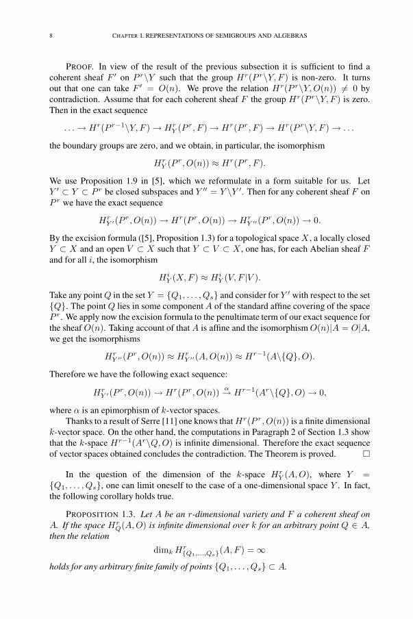
PROOF. In view of the result of the previous subsection it is sufficient to find acoherent sheaf F ′ on P r\Y such that the group Hr(P r\Y, F ) is non-zero. It turnsout that one can take F ′ = O(n). We prove the relation Hr(P r\Y,O(n)) �= 0 bycontradiction. Assume that for each coherent sheaf F the group Hr(P r\Y, F ) is zero.Then in the exact sequence
. . .→ Hr(P r−1\Y, F )→ HrY (P r, F )→ Hr(P r, F )→ Hr(P r\Y, F )→ . . .
the boundary groups are zero, and we obtain, in particular, the isomorphism
HrY (P r, O(n)) ≈ Hr(P r, F ).
We use Proposition 1.9 in [5], which we reformulate in a form suitable for us. LetY ′ ⊂ Y ⊂ P r be closed subspaces and Y ′′ = Y \Y ′. Then for any coherent sheaf F onP r we have the exact sequence
HrY ′(P r, O(n)) → Hr(P r, O(n)) → Hr
Y ′′(P r, O(n)) → 0.
By the excision formula ([5], Proposition 1.3) for a topological space X , a locally closedY ⊂ X and an open V ⊂ X such that Y ⊂ V ⊂ X , one has, for each Abelian sheaf Fand for all i, the isomorphism
H iY (X,F ) ≈ Hi
Y (V, F |V ).
Take any point Q in the set Y = {Q1, . . . , Qs} and consider for Y ′ with respect to the set{Q}. The point Q lies in some component A of the standard affine covering of the spaceP r. We apply now the excision formula to the penultimate term of our exact sequence forthe sheaf O(n). Taking account of that A is affine and the isomorphism O(n)|A = O|A,we get the isomorphisms
HrY ′′(P r, O(n)) ≈ Hr
Y ′′(A,O(n)) ≈ Hr−1(A\{Q}, O).
Therefore we have the following exact sequence:
HrY ′(P r, O(n)) → Hr(P r, O(n)) α→ Hr−1(Ar\{Q}, O)→ 0,
where α is an epimorphism of k-vector spaces.Thanks to a result of Serre [11] one knows that Hr(P r, O(n)) is a finite dimensional
k-vector space. On the other hand, the computations in Paragraph 2 of Section 1.3 showthat the k-space Hr−1(Ar\Q,O) is infinite dimensional. Therefore the exact sequenceof vector spaces obtained concludes the contradiction. The Theorem is proved. �
In the question of the dimension of the k-space HrY (A,O), where Y =
{Q1, . . . , Qs}, one can limit oneself to the case of a one-dimensional space Y . In fact,the following corollary holds true.
PROPOSITION 1.3. Let A be an r-dimensional variety and F a coherent sheaf onA. If the space Hr
Q(A,O) is infinite dimensional over k for an arbitrary point Q ∈ A,then the relation
dimk Hr{Q1,...,Qs}(A,F ) =∞
holds for any arbitrary finite family of points {Q1, . . . , Qs} ⊂ A.

1. On the cohomological dimension ... 9
PROOF. By Grothendieck [3] for Q1 ⊂ {Q1, . . . , Qs} ⊂ A one has the exact se-quence
HrQ1
(A,F ) α→ Hr{Q1,...,Qs}(A,F )
β→ Hr{Q2,...,Qs}(A,F )→ 0,
which we, for the sake of simplicity, rewrite in the form
A(1) α→ B(s)β→ C(s− 1)→ 0.
Our Proposition gives the possibility to carry induction over the number of points s. Letus assume that the statement is proved for s < n. Then in the exact sequence
A(1)→ B(n)→ C(n− 1)→ 0,
the term C(n−1) has infinite dimension, which in view of the fact that B(n) is a k-spacegives a contradiction. As the computation in 1.4.2 shows that
dimk HrQ(kr, O) = dimk H
r−1(kr\Q,O) = ∞,
it follows from what has been proved that for each finite collection of points S in kr thek-space Hr−1(kr\S,O) is infinite dimensional. �
3. The character of the facts, from [5] and [11], used in the proof of Theorem 1.2is such that the statement of the theorem, apparently, can be carried over to the caseof an arbitrary variety V of dimension ≥ 2, if it were possible for each affine varietyX = SpecA, dimA = r, to prove that the k-space Hr
Q(X,OX) is infinite dimensional.Clearly, A may be taken as a local ring; then everything reduced to the proof that Hr
M(A)is infinite dimensional, where M ⊂ A is a maximal ideal.
As S. I. Dolgaev has observed that, when all local rings of a variety V are Cohen-Macauly rings (for example, when V is nonsingular or is locally a complete intersection),this easily follows from the following criterion of Grothendieck for the coherence ofsheaves of local cohomology:
Let X be a locally Noetherian pre-scheme locally embedded in a regular pre-scheme,and Y a closed subvariety of X , F a coherent OX -module, c(x) = dim{x}, n ∈ Z. Thefollowing two conditions are equivalent [4]:
(i) for all x ∈ X\Y such that c(x) = 1, depthFx ≥ n;(ii) for i ≤ n the sheaves Hi
Y (F ) are coherent.
Indeed, take X = SpecOV,Q = SpecA. As by assumption A is a Cohen-Macaulyring and c(x) = dim{x} = 1, then depthAx = dimAx = r − 1. If the space Hr
M(A)were finite dimensional, then it would follow from condition (ii) that n = r, from whichby (i) depthAx ≥ r, which is contradictory.
1.4. Some computations and remarks
1. Let us consider the algebraic variety X , obtained from the affine plane [with co-ordinates (x, y)] by exclusion of the origin; it is not affine but admits an affine coverU = (U1, U2), where U1 = X\(x = 0) and U2 = X\(y = 0). If X ′ is an arbi-trary variety in which the subvariety Y has codimension ≥ 2, we obtain, in view ofthe fact that the singularity of every rational function on X ′ has codimension 1, thatH0(X ′\Y,O) ≈ H0(X ′, O). Therefore, in this case H0(X,O) consists of all polyno-mials P (x, y).

10 CHAPTER I. REPRESENTATIONS OF SEMIGROUPS AND ALGEBRAS
Let us compute the group H1(U, O). It is clear that all cochains f12 ∈ C1(U)
have the formP (x, y)xkyl
, where k, l are integers. In view of C2(U) = 0, all one dimen-
sional cochains are cocycles. The clarification of the question which of the cochains are
coboundaries is equivalent to when allP (x, y)xk′y�′ can be written in the form
xkP1(x, y)− x�P2(x, y)xky�
, k, � ≥ 0
Thus, we have
H1(X,O) ≈{P (x, y)xkyl
}/{xkP1(x, y)− x�P2(x, y)
xky�
},
where P, P1, P2 are arbitrary polynomials, while k′, �′, k, l ≥ 0. It is easy to see that this
factor space is infinite dimensional. To this end we remark that all expressions1
xky�give
different cosets:1
xky�− 1
xmyn=
xk′y�′ − xm′
yn′
xpyq,
where p = max(k,m), q = max(l, n), k′ = p−n, m′ = p−m, �′ = q− �, n′ = q−n.It is sufficient to show that there exist numbers P and Q such that xk′
y�′ − xm′yn′
=xpP − yqQ. To this end we have to consider two cases
1) p = k, q = � and 2) p = k, q = n.
Assuming that such P and Q exist in the first case, we obtain
xpP − yqQ = 1− xp−myq−n,
which is a contradiction, as the left hand side of the equation has unity among its terms.Analogously, in the second case the equation yq−�−xp−m = xpP−yqQ, where p−m <p, q − � < q, leads us to a contradiction. Thus we have proved that
dimk H1(X,Q) = ∞.
2.
THEOREM 1.4. Let X be an r-dimensional affine space with a distinguished point,defined over an algebraically closed field k. Then the cohomology group Hr−1(X,O) isan infinite dimensional vector space over k.
PROOF. Consider the affine covering U = (Ui) of X , where Ui = (xi �= 0), i =1, . . . , r. As dimU = r− 1 all (r− 1)-dimensional cochains are cocycles. The elementsf1,...,r ∈ Cr−1(U) have the form
P (x1, . . . , xr)xi1
1 , . . . , xirr
.
Let ρi be the restriction homomorphisms, i.e.
ρi : Γ( ∩j �=i
Uj, O) → Γ(∩jUj, O).

1. On the cohomological dimension ... 11
As by definition of the differential d
df =r∑
j=1
(−1)j+1ρj
(Pj(x1, . . . , xn)
xi1(j)1 . . . xj . . . x
ir(j)r
),
then for the computation of the group Hr−1(X,O) we must clarify which expressionsP (x1, . . . , xr)xi1
1 , . . . , xirr
are expressible in the form
1xα1
1 . . . xαrr
⎛⎝ r∑j=1
(−1)j+1xα1−i1(j)1 . . . x
αj
j . . . xαr−ir(j)1 · P ′
j(x1, . . . , xr)
⎞⎠ =
=1
xα11 . . . xαr
r
⎛⎝ r∑j=1
(−1)j+1xαj
j Pj(x1, . . . , xr)
⎞⎠ ,
whereαk = max
1≤j≤rik(j), k = 1, . . . , r.
Let us denote this equivalence by E. We show that the factor space{P (x1, . . . , xr)xi1
1 , . . . , xirr
}/E
is infinite dimensional over the field k. To this end it is sufficient to remark that in thecase that there exists an index j such that the expressions
I1 =1
xi11 . . . xir
r
and I2 =1
xk11 . . . xkr
r
, ∀ij > 0, kj > 0,
j = 1, . . . , r, must lie in different cosets. Let us set
αj = max(ij , kj), j = 1, . . . , r.
Then
I1 − I2 =1
xα11 . . . xαr
r(xa1−i1
1 . . . xαr−irr − xa1−k1
1 . . . xαr−krr ).
We must show that the expression within parentheses can be written in the formr∑
j=1
(−1)j+1xαj
j Pj(x1, . . . , xr).
Without loss of generality we can assume that there exists an index s such that α1 =i1, . . . , αs = is, αs+1 = ks+1, . . . , αr = kr. The expression within parentheses takesthe form
(2) xas+1−is+11 . . . xαr−ir
r − xa1−k11 . . . xαs−kr
r .
where αs+1 − is+1 < αs+1 . . . , αr−ir ; α1 − k1 < α1, . . . , αs − ks < αs. But thisequation shows that (2) cannot be expressed in the form

12 CHAPTER I. REPRESENTATIONS OF SEMIGROUPS AND ALGEBRAS
r∑j=1
(−1)j+1xαj
j Pj(x1, . . . , xr).
Our statement is proven. �
3. As has been proved by M. Kneser, in a 3-dimensional space X ′ an irreducible curveE can be expressed by three algebraic surfaces, which we denote by V0, V1, V2. In viewof E = ∩
iVi we have for X = X ′\E the open affine covering U = (Ui = X ′\Vi) and
we can apply the following theorem of Serre [11]. Let X ′ be an algebraic variety, F acoherent sheaf on X and U = (Ui) a finite affine covering of X . Then for each i ≥ 0 thehomomorphism
σ(U) : H i(UU,F )→ H i(X,F )
is an isomorphism. As dimU = 2, we have by this theorem H3(X,F ) = 0 for allcoherent sheafs on X . There arises an interesting question: For an algebraic curve Eand a coherent sheaf F on X , can the group H2(X,F ) be different from zero? Thisis connected with the conjecture on the impossibility to express an arbitrary curve in a3-dimensional space by two surfaces. Indeed, we would have a proof of this negativestatement if for some curve E the answer to the question posed would be positive. Thequestion of the non-triviality of H2(X,F ) arises also in connection with the conjecturethat each vector bundle of rank 2 on a 3-dimensional affine space is trivial. Indeed,Serre proved in [12] that if this problem has a positive solution then each non-specialrational or elliptic curve in a 3-dimensional affine space would be a complete intersection.Therefore this conjecture would be refuted if in a 3-dimensional affine space one couldfind a rational or elliptic curve E such that H2(CE,F ) �= 0 for some coherent sheafF . This shows that the question perhaps could be solved in terms of cohomological ofalgebra.
In [6] Hartshorne introduced the notion of local connectivity of a variety of codimen-sion 1, which refers to the situation when spreading out of a subvariety of codimensiongreater than unity does not disturb the connectivity structure of the variety. He obtains anecessary condition for a manifold to be a complete intersection, which amounts to localconnectivity of this variety of codimension 1. It turns out that the non-triviality of thegroups Hi(X ′\V,O), i ≥ 2, is not a necessary for the representability of that variety asa complete intersection. This is shown by the following example.
Consider in the complex affine space X ′ = C4 with the Zariski topology the varietyV which is the union of two planes: x1 = x2 = 0 and x3 = x4 = 0. It is clear that at theorigin this variety is not connected with codimension 1 and so it cannot be a completeintersection. However, a computation reveals that
H2(CV,O) = H3(CV,O) = 0,
where [as before] CM denotes the complement on C4 of a set M . We have
X = CV = C[(x1 = x2 = 0) ∪ (x3 = x4 = 0)] =
=C(x1 = x2 = 0) ∩ C(x3 = x4 = 0) =3∪
i=0Ui,

1. On the cohomological dimension ... 13
whereU0 = (x1 �= 0)∩(x3 �= 0), U1 = (x1 �= 0)∩(x4 �= 0), U3 = (x2 �= 0)∩(x4 �= 0).Take in X the covering U = (Ui). By Serre’s theorem H i(X,O) ≈ Hi(U, O), i = 2, 3.Let us complete H3(U, O). To this end we remark that all 3-dimensional cochains are ofthe form
P (x, y, z, t)xky�zmtn
.
It is clear that all 3-dimensional cochains are cocycles. For all j = 0, 1, 2, 3 we have∩
i�=jUi = ∩
iUi. Therefore, all restriction homomorphisms
ρi : Γ( ∩j �=i
Uj)→ Γ(∩jUj), i = 0, 1, 2, 3,
are exact. It is now easy to see that all 3-dimensional cochains are exact, henceH3(U, O) =0. An analogous reasoning reveals that also the groups H2(U, O) are trivial.
Note added in proof. R. Hartshorne, Cohomological dimension of algebraic varieties(Ann. Math. 3, 444–450 (1968)), has shown that H2(P 3\E,F ) = 0 for all F .
Comments. The reference [5] has now appeared in Springer Lecture Notes in Mathematics 41 (1967).The reference [4] has been published by North-Holland/Masson 1968 as Volume 2 in the series AdvancedStudies in Pure Mathematics.
The problem of [12], mentioned at the end of Kaljulaid’s paper has now been solved: The conjecture of
Serre that all projective modules over a polynomial ring are free (i.e. that algebraic vector bundles over kn are
trivial) has been proved independently by Quillen [8] and Suslin [13] (Cf. also: [2]).
Jan-Erik Roos
References
[1] H. Cartan and S. Eilenberg. Homological Algebra. Princeton Landmarks in Mathematics. Princeton Uni-versity Press, Princeton, 1999. Reprint of the 1956 original.
[2] D. Ferrand. Les modules projectifs de type fini sur un anneau de oltnômes sur un corps sont libres. In:Séminaire Bourbaki, Vol. 1975/76. Springer-Verlag, Berlin, 1977, 202–221.
[3] R. Godement. Topologie algébrique et théorie des faisceaux. Technical Report 13. Actualit’es Sci. Ind.,no. 1252., Publ. Math. Univ. Strasbourg., Hermann, Paris, 1958. Russian translation: Moscow, 1961.
[4] A. Grothendieck. Cohomologie locale des faisceaux cohérents et théorèmes de Lefschetz locaux etglobaux. Technical Report exposé 8, 8-2-4, I.H.E. Seminaire de Géométrie Algébrique, 1962.
[5] A. Grothendieck. Local Cohomology. Technical Report Lecture notes by R. Hartshorne. Harvard Univer-sity, 1961.
[6] R. Hartshorne. Complete intersections and connectedness. Amer. J. Math. 84, 1962, 497–508.[7] M. Nagata. Imbedding of an abstract variety in a complete variety. J. Math. Kyoto Univ. 2, 1962, 1–10.[8] D. Quillen. Projective modules over polynomial rings. Invent. Math. 36, 1976, 167–171.[9] J. Sampson and G. Washnitzer. A Vietoris mapping theorem for algebraic projective fibre bundles.
Ann. Math. 68, 1958, 348–371.[10] J. Sampson and G. Washnitzer. A Künneth formula for coherent algebraic sheaves. Illinois J. Math. 3,
1959, 389–402.[11] J. P. Serre. Faisceaux algébriques cohérents. Ann. Math. 61, 1955, 191–278.[12] J. P. Serre. Sur les modules projectifs. Technical Report 14-e année, no. 2. Seminaire Dubreil Pisot,
Algèbre et Théorie des nombres, 1960.[13] A. A. Suslin. Projective modules over polynomial rings are free. Dokl. Akad. Nauk. SSSR 229, 1976,
1063–1066.

This page intentionally left blank

15
2. [K77a] Triangular products of representations ofsemigroups and associative algebrasRevised by J. Peetre, comments by R. Lipyanskiı
The triangular product in the theory of varieties of representations of groups playsa role analogous to the role of the wreath product for group varieties. In this note westudy the triangular product of representations of semigroups and associative algebras.We assume that K is a field. This is required in the main results of the paper, althoughthe principal constructions and notions can be introduced for any associative and com-mutative ring K with unit.
For pairs (G,Γ) such that the semigroup (algebra) Γ acts by semigroup (algebra) en-domorphisms on the K-module G, one can introduce, exactly as in the case of groups,a net of notions and constructions. A variety of representations of semigroups and al-gebras is a saturated Birkhoff class of the corresponding pairs. By definition, a classK of pairs is termed saturated if for all right epimorphisms of pairs (G,Γ) → (G′,Γ′)with (G′,Γ′) ∈ K it holds that (G,Γ) ∈ K. The variety generated by the class K willbe denoted VarK. Multiplication of two varieties Θ1 and Θ2 is defined by the rule:a pair (G,Γ) is contained in Θ1 · Θ2 if G has a Γ-invariant submodule H such that(H,Γ) ∈ Θ1 and (G/H,Γ) ∈ Θ2. There arises the semigroup M(K) (the semigroupL(K)) of varieties of representations of semigroups (algebras). The semigroup M(K)is anti-isomorphic to the semigroup of ideals of the semigroup ring F = KΨ of thefree monoid Ψ with a countable set of free generators, invariant with respect to all en-domorphisms F induced by endomorphisms of the monoid Ψ. The semigroup L(K)is anti-isomorphic to the semigroup T (K) of non-zero ideals of the free associative K-algebra F of countable rank (with respect to the usual multiplication of ideals of F ).
1. For pairs (A,Σ1) and (B,Σ2) we set Φ = Hom+K(B,A) ⊂ EndK(A,B). The
natural action of the semigroups Σ1 and Σ2 on the (additive) semigroup Φ allows us tointroduce a multiplication in Φ× Σ1 × Σ2,
(ϕ, σ1, σ2) · (ϕ′, σ′1, σ
′2) = (σ2 · ϕ′, ϕ · σ′
1, σ1σ′1, σ2σ
′2).
There arises the semigroup Γ = Φ � Σ1 ×Σ2; its action on G = A⊕B goes accordingto the formula
(a + b) ◦ (ϕ, σ1, σ2) = a ◦ σ1 + bϕ ◦ σ1 + b ◦ σ2,
extends to the pair (G,Γ), which will be denoted (A,Σ1) � (B,Σ2) and called thetriangular product of the given pairs. The properties of this construction are in manyrespects parallel to the properties of the triangular product of group pairs (B.I. Plotkin,1971, [3]). Let us remark that Γ is a group if and only if Σ1 and Σ2 are groups and Φ istreated as the additive closure to a group of the semigroup Hom+
K(B,A).
THEOREM 2.1. The following formula holds true:
Var(K1 �K2) = VarK1 · VarK2.

16 CHAPTER I. REPRESENTATIONS OF SEMIGROUPS AND ALGEBRAS
From this one deduces that the variety of linear representations (over a field) is asemigroup with a unique decomposition as a product of a finite number of indecompos-able varieties.
2. The questions under study are also connected with automata theory. A linear semi-group automatonA = (A,Γ, B) is a system, where A (the states) and B (the outputs) areK-modules, while Γ (the input signals) is a semigroup and there are given K-linear oper-ations A◦Γ → A and AΓ → B such that (A,Γ) is a liner map with respect to the action◦, and a∗γ1γ2 = (a◦γ1)∗γ2 for all a ∈ A, γ1γ2 ∈ Γ. The automatonA′ = (A′,Γ′, B′)is called an invariant subautomaton of A if A′ and B′ are K-submodules in A and Brespectively and A′ ◦ Γ ⊂ A′, A′ Γ ⊂ B′. By definition an automaton A belongsto the product of two varieties of linear automata Θ1 and Θ2 if there exists an invariantsubautomaton such that A′ ⊂ A, A′ ∈ Θ1 with A/A′ ∈ Θ2.
THEOREM 2.2. A variety of linear automata with the multiplication indicated is asemigroup which is not free but contains a free subsemigroup isomorphic to M(K).
3. Let there be given K-algebras Φ and Σ, where Σ acts from the left and the right onΦ and that this is a bimultiplication in the sense of Hochschild. On Γ = Φ⊕ Σ we retainthe definition of addition and multiplication by scalars, while multiplication is definedanew putting
(ϕ, σ) · (ϕ′, σ′) = (ϕ · σ′ + σ · ϕ′ + ϕϕ′, σσ′).
There arises the K-algebra Φ � Σ, which is the semidirect product of the algebras Φ andΣ.
For given pairs (G1,Σ1) and (G2,Σ2), where Σi are K-algebras, we let (G1, Σ1)and (G2, Σ2) be the corresponding faithful pairs and set G = G1 ⊕ G2. We treat Σ =Σ1⊕Σ2 and Φ = HomK(G2, G1) as subalgebras of EndK G. Multiplication in EndK Gdefines a left and a right action of Σ on Φ. Setting Σ = Σ1 ⊕ Σ2 we obtain a naturalepimorphism f : Σ → Σ, then we can extend the action of Σ on Φ to an action of Σ onΦ. We arrive at the algebra Φ � Σ = Γ whose action on G = G1 ⊕ G2 is given by theformula
(g1 + g2) ◦ (ϕ, σ) = gϕ2 + (g1 + g2) ◦ σ.
This action agrees with the operations on Γ. There arises the pair (G,Γ), which is thetriangular product of the representations (G1,Σ1) and (G2,Σ2), which we denote by(G1,Σ1)� (G2,Σ2).
THEOREM 2.3 (Main theorem). For any two classes K1 and K2 of representationsthere holds the formula Var(K1 �K2) = VarK1 · VarK2.
It follows from this that each non-trivial representation of algebras decomposesuniquely as a finite product of indecomposbale representations. Thus, the semigroupL(K) is free. This opens a new door to the result of Bergman and Lewin [1] on the free-ness of the semigroup T (K). Here we have supplementary possibilities. It is known thatthe set A(K) of proper varieties of (associative) K-algebras is in a bijective correspon-dence with the set T (K). Multiplication in T (K) induces now on A(K) an associativemultiplication , which we denote by ∗. We are led to the following results.
For a K-algebra A let A∗ be the result of an outer adjunction of a unit to it , and letVarA be the variety of K-algebras generated by A. Let us introduce for any K-algebras

2. Triangular products of representations 17
A and B the operation of wreath product by the formula
AwrB = HomK(B∗, A∗) � (A⊕B),
where A∗ and B∗ are regarded as K-modules. The justification of this name is givenby the functional role of this operation, which is disclosed by the formula (VarA∗) ∗(VarB∗) = Var(BwrA).
By definition a T -ideal is finitary if the variety of K-algebras defined by it generatesa finite dimensional K-algebra. It turns out that a finite product of T -ideals is finitarywhen all factors are finitary.
If a variety of K-algebras is given with the aid of identities in n variables then it cannot be decomposed in more than n factors. In particular, the semisimplicity (in the senseof Jacobson)of a K-algebra forces VarA to be indecomposable.
The author is obliged to Professor B.I. Plotkin for supervising this work, and for hisvaluable advice and interesting discussion, and, furthermore, G. Bergman for sendinghim his pre-print. [3], [2]
Comments. It is known that if K1 and K2 are two classes of group representations over a field andK1 � K2 their triangle product, then Var(K1 � K2) = VarK1 · VarK2 [4]. Uno Kaljulad extendsthis result to representations of semigroups, associative algebras and linear automata. In this way he ob-tains another proof of the Bergman-Lewin theorem that the semigroup of T -ideals (verbal ideals of absolutelyfree associative algebra over a field) is free Bergman-Lewin [1]. He introduces a new operation over as-sociative algebras, the wreath product of algebras, and proves some interesting properties of this operation:(Var A∗)∗ (Var B∗) = Var(BwrA), where A∗ (and B∗) is obtained from algebra A (and B) by adjunctionto it a unit. Author investigates also decomposition of finitary T -ideal in indecomposable factors. He brings asufficient condition when factors of this decomposition to be indecomposable: if K-algebra is semisimple (inthe sense of Jacobson), then Var A to be indecomposable. There are also other sufficient conditions for theabove-mentioned properties. I think that this paper of Uno Kaljulad was a pioneer work in the theory of the va-riety of semigroup representations and the variety of linear automata. His results extend also above mentionedBergman-Lewin theorem.
[1] G. Bergman and J. Lewin. The semigroup of ideals of a fir is (usually) free. J. London Math. Soc. 11 (2),1975, 21–31.
[2] G. Birkhoff. The role of algebra in computing. Computers in algebra and number theory, SIAM-AMSProc., Amer. Math. Soc IV, 1971, 1 – 47.
[3] B.I. Plotkin and A.S. Grinberg. On semigroups of varieties, connected with group representations.Siberian Math. Journal 13, 1972, 841–858.
[4] B.I. Plotkin. Multiplicative systems of varieties of pairs – group representations. Latvian MathematicalYearbook 18, 1976, 143–169, 223.
References
Ruvim Lipyanskiı

This page intentionally left blank
19
3. [K79a] Triangular products and stability of represen-tations. Candidate dissertationTranslation by J. Peetre, revised by K. Kaarli
Contents of the dissertationIntroduction . . . . . . . . . . . . . . . . . . . . . . . . . . . . . . . . . . . . . . . . . . . . . . . . 191. The triangular product . . . . . . . . . . . . . . . . . . . . . . . . . . . . . . . . . . . . .231.1. Triangular products of group representations . . . . . . . . . . . . . . . . . . . . . 231.2. Triangular products of semigroup representations . . . . . . . . . . . . . . . . . 251.3. Triangular products of representations of algebras . . . . . . . . . . . . . . . . 351.4. Connections between �-constructions . . . . . . . . . . . . . . . . . . . . . . . . . . . 401.5. Comments . . . . . . . . . . . . . . . . . . . . . . . . . . . . . . . . . . . . . . . . . . . . . . . . . . . . 42
2. The arithmetics of varieties of representations of semigroups andalgebras . . . . . . . . . . . . . . . . . . . . . . . . . . . . . . . . . . . . . . . . . . . . . . . . . . . 432.1. Varieties of linear pairs and automata . . . . . . . . . . . . . . . . . . . . . . . . . . . . 432.2. Technical results . . . . . . . . . . . . . . . . . . . . . . . . . . . . . . . . . . . . . . . . . . . . . . 482.3. The fundamental lemma . . . . . . . . . . . . . . . . . . . . . . . . . . . . . . . . . . . . . . . . 532.4. The theorem on generating representations of semigroups . . . . . . . . . . 552.5. Consequences. Connections with linear automata . . . . . . . . . . . . . . . . . 572.6. The theorem on generating representations of algebras . . . . . . . . . . . . . 622.7. Comments . . . . . . . . . . . . . . . . . . . . . . . . . . . . . . . . . . . . . . . . . . . . . . . . . . . . 68
3. Powers of the fundamental ideal and stability of representations ofgroups and semigroups . . . . . . . . . . . . . . . . . . . . . . . . . . . . . . . . . . . . . . 693.1. Preliminary topics; on the terminal of nilpotent groups . . . . . . . . . . . . . 703.2. Construction of stable representations of groups with the aid of the tri-angular product . . . . . . . . . . . . . . . . . . . . . . . . . . . . . . . . . . . . . . . . . . . . . . . . . . . 783.3. Generalized measure subgroups of finite groups . . . . . . . . . . . . . . . . . . . 853.4. Mal’cev nilpotency and stability of semigroups . . . . . . . . . . . . . . . . . . . 903.5. Comments and remarks . . . . . . . . . . . . . . . . . . . . . . . . . . . . . . . . . . . . . . . . 96
References . . . . . . . . . . . . . . . . . . . . . . . . . . . . . . . . . . . . . . . . . . . . . . . . . 97
Introduction
In various branches of mathematics and its applications there arises a need to use repre-sentations, and so problems of their classification become urgent; cf. [18, 20, 32, 46, 47,50,54,65,66,86]. If one takes into account that a representation is a two-sorted algebraicsystem (a pair) then the systematics of representations is facilitated. The book [35] is

20 CHAPTER I. REPRESENTATIONS OF SEMIGROUPS AND ALGEBRAS
written from this point of view, and, furthermore, there is visible evidence of this in thenote [57] and in the survey [41]. The naturality and usefulness of the study of classesof algebraic systems has often been emphasized by A. I. Mal’cev; for example, in [30].The reduction of classes to “simpler” ones is one of the fundamental problems of thisdirection; as an example, let us mention the result of A. L. Shmel’kin and Neumanns 2
on the freedom of the semigroup of varieties of groups ([34, Theorem 23.4]).The problem of decomposition has always been an essential ingredient of every the-
ory of representations: the classical theory of reduction to irreducible linear represen-tations of a fixed group (§14 in the book [48] by D. A. Suprunenko) or the reductionto indecomposable varieties of representations with a variable group (the paper [43] byB. I. Plotkin and A. S. Grinberg, as an example). Indecomposable classes as “simplestblocks” in a given theory can not be reduced to simpler classes and have to be studied sep-arately. On the other hand, for the reduction to indecomposable classes one needs toolsfor doing the decomposition. In the theory of varieties of groups this role is played by thewreath product of groups, and in the case of representations with a variable group the con-struction of the triangular�-product of group representations. According to B. I. Plotkin[36], the pair (G,Γ) is the triangular product of its subpairs (A,Σ1) and (B,Σ2) if thefollowing conditions are fulfilled:
(1) for the subgroup Σ = {Σ1,Σ2} ≤ Γ, generated by two subgroups Σ1 and Σ2,the subpair (G,Σ) decomposes into the direct product of its subpairs (A,Σ1)and (B,Σ2);
(2) in the group Γ there exists a normal subgroup Φ such that the subrepresentation(G,Φ) is faithful, and the image of Φ in AutG coincides with the centralizerof the series 0 ⊂ A ⊂ G, that is, it acts as identity on each factor of this series;
(3) the group Γ coincides with the semi-direct product Φ � Σ.
The object of this thesis is the study of the triangular product and its applications.It consists of two parts. The goal of the first part (Sections 3.1 and 3.2) is to find the�-construction for representations of semigroups and algebras, to study the properties ofthese tools and their application to the decomposition of the varieties of the correspondingrepresentations. In the second part (Section 3.3) the triangular product is applied to thestudy of the powers of the fundamental ideal of group rings.
Representations by endomorphisms of modules, semigroups and algebras have beenthe subject of many studies by A. V. Mihalev [33] and L. M. Gluskin [10]. On the otherhand, the representations of rings by endomorphisms of Z-modules is a classical researchtopic. The tendency towards a category-theoretic formulation of the classification of rep-resentations makes urgent the problem of the decomposition of classes of representationsof various algebraic objects (groups, semigroups, algebras etc.), as the elaboration of ageneral theory requires the understanding of the possible deviations and its leading toa coherent series of notions, constructions, and results. This is one of the reasons whythe introduction and the study of tools of decomposition of representations of semigroupsand algebras deserve attention. The known difficulties for carrying over results for groupsand their representations to semigroups increases the interest for cases and ways whereit is possible; concerning that see [24, Chapter 7].
2Editors’ note. Three well-known group-theorists: Bernhard and Hanna Neumann and their son Peter M.Neumann
3. Triangular products and stability of representations 21
The essential results of the first part of this thesis concern the search for suitableconstructions for representations of semigroups and algebras, the study of several theirproperties, and further the establishing of connections between these new constructionswith the triangular products of representations of groups. There exists a cryptomorphism(in the sense of G. Birkhoff [58]) of the three constructions mentioned, although eventheir definitions are quite different, and, as a result, sometimes there are considerabledifferences in the proofs of properties. The varieties of representations of the semigroupsadmit an associative multiplication and the corresponding semigroup is factorial. Thisfollows from the main result of Section 3.2, Theorem 3.33 about the generating repre-sentations. Such results are also obtained for algebras (Theorem 3.43 and Theorem 3.44).The role of the �-constructions, introduced in Section 3.1, in the proof of these facts isanalogous to the role of the wreath product in the proof of the above mentioned group-theoretic theorem of Shmel’kin and Neumanns. For the theorem on freedom of the semi-group of varieties of linear representations of semigroups there is also a proof in terms ofthe semigroup ring of the free countably generated monoid; the extract of the reasoningneeded is well-known from [56]. Among the consequences of the theorem on generatingrepresentations of algebras (Theorem 3.43) let us mention the theorem of Bergman andLewin on the freedom of the semigroup of T -ideals, which in [56] is proved by means ofthe theory of FI-rings of Cohn [5]. Here the corresponding fact is interpreted as a state-ment about the freedom of the semigroup of varieties of representations of algebras, andin this form it readily follows from Theorem 3.43. The given approach, however, allowsto penetrate more deeply into the essence of the matter. For example, for given finitedimensional (over a fixed field K) pairs (A,Σ1) and (B,Σ2) the identities for the varietyVar(A,Σ1)·Var(B,Σ2) are readily found, these are exactly the identities for Var(G,Γ),where (G,Γ) = (A,Σ1)� (B,Σ2). This might be rather difficult to obtain such a resultby means of multiplication of T -ideals. There are also other applications of the materialin Section 3.2 concerning representations of algebras in the theory of associative algebrasthemselves. Let us mention a necessary condition for the indecomposability of a varietyof algebras (Theorem 3.49).
The technique developed in the first part of this thesis is tightly connected with au-tomata theory [31]. After the interaction of this discipline with the theory of algebras(V. M. Glushkov [9]) an essential result was established, that is the theory of decomposi-tion of finite automata. Nowadays algebraic methods in automata theory are developingrather intensively; cf. [18], [42], [65], [45] etc., and furthermore in Eilenbergs’ book [66]there is given a detailed analysis of the corresponding methods in a modern presentation.The present author has introduced the semigroup of varieties of linear automata and hasgiven a description of it in the language of pairs of “consistent” ideals in the free count-ably generated associative algebra (over the given field), which gives the possibility toestablish interesting properties of this semigroup (Theorem 3.37).
Since the very beginning of the theory of group representations a major role havebeen played by the group and semigroup algebras. In this connection it was observedthat the application of the ideas and methods of the (general) theory of algebras and theirrepresentations to group algebras was fertile and even the group algebras themselvesturned out to be a subtle tool of calculation in the study of the structure of groups. Thepapers [81,98–100] convince of the great heuristic value of group and semigroup algebras

22 CHAPTER I. REPRESENTATIONS OF SEMIGROUPS AND ALGEBRAS
in Combinatorics. The situation here reminds the one in Number Theory, where for theachievement of many deep facts on integers one applies algebraic and analytic methods.
The main goal of Section 3.3 of this dissertation is the study of an issue of the ofthe powers of the fundamental ideal of an integral groups ring stabilization, which isalready being deeply investigated for more than a decade, cf., for example the surveyA. V. Mihalev and A. E. Zaleskiı [51], the lectures by A. A. Bovdi [3] or the book byD. Passman [96]. Our choice of subject was stimulated by the deep and beautiful workof A. I. Mal’cev [27], K. Gruenberg [69] and B. Hartley [77], where the special role ofnilpotence in this circle of ideas is likewise clearly set forth.
In Sections 3.3.1–3.3.3 the possible values of terminal are found for Artinian groupsand the limit of finite groups is calculated. These results of the papers [13,14] have beenobtained independently and by other methods, and were in part generalized by Gruenbergand Roseblade [71], Sandling [102] and Hartley [80]. In Section 3.3 the methods of[13, 14] are developed, using moreover systematically the language and technique of thegeneral theory of group representations, and, furthermore, a circle of ideas connectedwith the well-known theorem of L. A. Kaluzhnin [84] on nilpotence of a group, actingfaithfully and stably on a finite invariant series of another group, and some applicationsof it. The elements of such an approach were set forth by Hartley [76], but he uses itonly for the interpretation of some results. Due to mentioned approach, a self-developedpresentation, and in several cases a generalization and a considerable simplification ofthe proofs in [14, 71, 80] are achieved.
The paper [26] of A. I. Mal’cev on the possibility of embedding semigroups intoa group gave rise to a well-known cycle of developments, in particular, there appearedresults, that are at the first glance not connected with stability. Given the goal for finding“good” classes of semigroups with cancellation embeddable in a group, A. I. Mal’cev hasfound in [28] a notion of nilpotence for semigroups such that each such semigroup withcancellation is embeddable in a nilpotent group. Up to now the interest for this notionhas not been considerable. The present author has made an attempt to unify the results of[28] with the above mentioned theorem of Kaluzhnin. This leads to the necessity of re-considering the notion of stability for semigroups of endomorphisms. This question, andfurther some properties of semigroup rings of locally nilpotent (in the sense of Mal’cev)semigroups are treated in Section 3.3.4.
The papers [11–17] have been published on the theme of this dissertation. The mainresults have been communicated at the XI All Union Algebraic Colloquium (Kishinev,1971); the All Union Symposium on Ring Theory, Algebras and Modules (Kääriku,1976); at the Algebra Seminar of Tartu State University; at the Riga Algebra Seminar; atthe the Seminars of Higher Algebra and Rings and Modules at Moscow State University;and at the Minsk Algebra Seminar. Twice the material of the two first sections wasused in a special lecture course in automata theory presented by the author himself atTartu State University; the main contents of this course were set forth at the III RegionalConference-Seminar of leading lecturers of mathematics of the Belorussian, Latvian,Lithuanian, Estonian Soviet Republics and the Kaliningrad Oblast of the Soviet Union(Minsk, 1977).
Acknowledgement. The author is thankful to Prof. B. I. Plotkin for supervising thiswork, for his valuable advice, and generous support.

3. Triangular products and stability of representations 23
3.1. The triangular products
This section has a preparatory character. First of all, here we treat representations astwo-sorted entities (pairs) and carry over the corresponding definitions to the case whenthe acting object of a pair is a semigroup or an associative algebra. The main object ofthe section is the introduction of the triangular product of representations of semigroupsand algebras and the study of their properties and connections. Applications of the frameof notions considered are given in the Sections 3.2–3.3.
We underline that although the main constructions and notions of this section canbe introduced for an arbitrary associative and commutative unitary ring K , we prefer torestrict ourselves in the first two sections because of reasons of organization, to the casewhen K is a field.
3.1.1. Triangular products of group representations
1. The object of this first section is preparatory, to acquaint the Reader with the notion oftriangular product for group pairs. This construction turns out to be useful for us also inour study of the fundamental ideal of group rings in Section 3.3, but, in the first place, itserves as a model for analogous constructions of the triangular product of representationsof semigroups and algebras.
2. Let A and B be any two groups. The set AB of all functions B → A forms a groupon which B acts according to the formula
∀x, b ∈ B, f ∈ AB, (f ◦ b)(x) = f(xb−1).
There arises the pair (AB , B). We accompany this pair with the semi-direct productAB � B which will be called the (complete) wreath product of A and B, and denotedAwrB.
Let us fix an associative-commutative ring K , for example K = Z and let Γ be anarbitrary group. If there is given a representation of Γ by automorphisms of a certainK-module G, then one speaks on the (group) pair (G,Γ).
Let (A,Σ1) and (B,Σ2) be any two group pairs, and let Φ = HomK(A,B) be themodule of all K-homomorphisms of B into A. Defining an action of the groups Σ1 andΣ2 on Φ respectively by the formulae
∀x ∈ B, σ1 ∈ Σ1, ϕ ∈ Φ, (ϕ ◦ σ1)(x) = ϕ(x) ◦ σ1
and∀x ∈ B, σ2 ∈ Σ2, ϕ ∈ Φ, (ϕ ◦ σ2)(x) = ϕ(x ◦ σ−1
2 )we arrive at the pairs (Φ,Σ1) and (Φ,Σ2). Moreover, as the actions of Σ1 and Σ2 arepermutable on Φ, we can now define the pair (Φ,Σ1 × Σ2) to which corresponds thegroup Γ = Φ � Σ1 × Σ2, where the initial groups Φ and Σ1 × Σ2 are embedded,
Φ → Φ = {φ = (φ, 1)|ϕ ∈ Φ} ⊂ Γ,
while the group Σ1 × Σ2 can be identified with its image in Γ via the map (σ1, σ2) �→(ε, σ1σ2). To the semi-direct product Φ � Σ1 × Σ2 there corresponds the pair (Φ,Σ1 ×Σ2), the representation of the group Σ1 ×Σ2 by inner automorphisms of the group Φ. Itis easy to convince oneself that (Φ,Σ1 × Σ2) ∼= (Φ,Σ1 × Σ2).
Let G = A ⊕ B and let us define the pair (G,Φ). To this end we consider in G theseries of submodules 0 ⊂ A ⊂ G. In the group AutG we introduce the centralizer Z

24 CHAPTER I. REPRESENTATIONS OF SEMIGROUPS AND ALGEBRAS
of this series, that is, all automorphisms that act as identities of A and G/A. The mapσ′ : Z → Φ, for each b ∈ B, σ ∈ Z given by the formula bσ′
= b◦σ− b, is, as is readilyseen, an isomorphism between the groupsZ and Φ. Hence, we have a right isomorphismof the pairs (G,Φ) and (G,Z).
Next, let us turn to the following question. Let there be given the pairs (G,Φ) and(G,Σ), and set Γ = Φ � Σ. What are the necessary and sufficient conditions for theexistence of the pair (G,Γ)? It turns out that if the condition
∀ g ∈ G, ϕ ∈ Φ, σ ∈ Σ, (g ◦ σ) ◦ ϕ = (g ◦ ϕσ−1) ◦ σ
is fulfilled, then the action of the groups Φ and Σ can be extended to an action of thegroup Γ on G. Applying this to the reviewing situation, we arrive to the pair (A ⊕B, HomK(B,A) � Σ1 × Σ2) = (G,Γ), in which the action is given by the formula
∀ a ∈ A, b ∈ B, ϕ ∈ Φ, σ1 ∈ Σ1, σ2 ∈ Σ2,
(a + b) ◦ ϕσ1σ2 = a ◦ σ1 + bϕ ◦ σ1 + b ◦ σ2 = (a + bϕ) ◦ σ1 + b ◦ σ2.
This pair (G,Γ) is called the triangular product of the pairs (A,Σ1) and (B,Σ2) andwill be denoted by (A,Σ1)� (B,Σ2).
Let us add that the pairs (A,Σ1) and (B,Σ2) need not necessarily be faithful andtherefore the following formula is of interest
Ker [(A,Σ1)� (B,Σ2)] = [Ker (A,Σ1)]× Ker [(B,Σ2)].
The operation of triangular product is a covariant functor in the first argument in thecategory of linear group actions, which preserves exactness from the left and from theright. But if we consider as morphisms only right homomorphisms of pairs, the triangularproduct becomes a covariant functor in both arguments preserving exactness from the leftand from the right. These and many other properties of the �-operation on group pairsare proved in [36], to which we refer the interested Reader.
3. Let A be any Abelian group, and B1 and B2 arbitrary groups. Let us consider thegroup AB1 � B1 corresponding to the pair (AB1 , B1), where the action of B1 in AB1 isdefined by the formula
∀x ∈ B1, f ∈ AB1 , (f ◦ b)(x) = f(xb−1).
For the regular pair (ZB2, B2) and the triangular product (G,Γ) = (AB1 , B1)�(ZB2, B2),B. I. Plotkin established the formula
(3) Γ = HomZ(ZB2, AB1) � B1 ×B2
∼= Awr (B1 ×B2).
One consequence of this fact deserves special attention because of an application inthe last section.
THEOREM 3.1. Let A be an arbitrary (additively written) Abelian group, B anarbitrary group, and E the unit group. The acting group of the pair (A,E)� (ZB,B)is isomorphic to AwrB.
PROOF. The proof amounts to applying the preceding formula to the pairs (A,E)and (ZB,B). Let us also give a sketch of the proof of formula (3), because of the lackof a suitable reference.
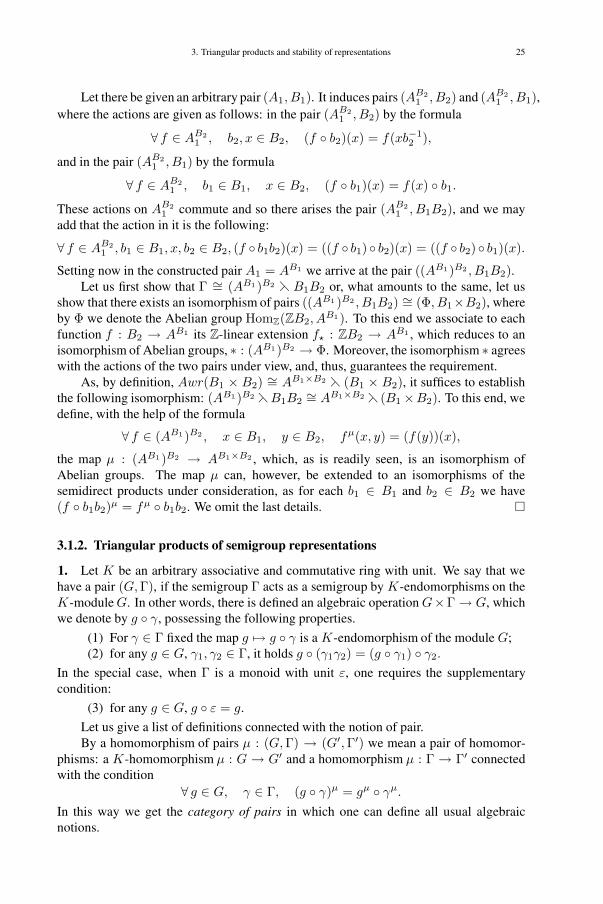
3. Triangular products and stability of representations 25
Let there be given an arbitrary pair (A1, B1). It induces pairs (AB21 , B2) and (AB2
1 , B1),where the actions are given as follows: in the pair (AB2
1 , B2) by the formula
∀ f ∈ AB21 , b2, x ∈ B2, (f ◦ b2)(x) = f(xb−1
2 ),
and in the pair (AB21 , B1) by the formula
∀ f ∈ AB21 , b1 ∈ B1, x ∈ B2, (f ◦ b1)(x) = f(x) ◦ b1.
These actions on AB21 commute and so there arises the pair (AB2
1 , B1B2), and we mayadd that the action in it is the following:
∀ f ∈ AB21 , b1 ∈ B1, x, b2 ∈ B2, (f ◦ b1b2)(x) = ((f ◦ b1) ◦ b2)(x) = ((f ◦ b2) ◦ b1)(x).
Setting now in the constructed pair A1 = AB1 we arrive at the pair ((AB1)B2 , B1B2).Let us first show that Γ ∼= (AB1)B2 � B1B2 or, what amounts to the same, let us
show that there exists an isomorphism of pairs ((AB1 )B2 , B1B2) ∼= (Φ, B1×B2), whereby Φ we denote the Abelian group HomZ(ZB2, A
B1). To this end we associate to eachfunction f : B2 → AB1 its Z-linear extension f� : ZB2 → AB1 , which reduces to anisomorphism of Abelian groups, ∗ : (AB1)B2 → Φ. Moreover, the isomorphism ∗ agreeswith the actions of the two pairs under view, and, thus, guarantees the requirement.
As, by definition, Awr(B1 × B2) ∼= AB1×B2 � (B1 × B2), it suffices to establishthe following isomorphism: (AB1)B2 �B1B2
∼= AB1×B2 � (B1×B2). To this end, wedefine, with the help of the formula
∀ f ∈ (AB1)B2 , x ∈ B1, y ∈ B2, fμ(x, y) = (f(y))(x),
the map μ : (AB1 )B2 → AB1×B2 , which, as is readily seen, is an isomorphism ofAbelian groups. The map μ can, however, be extended to an isomorphisms of thesemidirect products under consideration, as for each b1 ∈ B1 and b2 ∈ B2 we have(f ◦ b1b2)μ = fμ ◦ b1b2. We omit the last details. �
3.1.2. Triangular products of semigroup representations
1. Let K be an arbitrary associative and commutative ring with unit. We say that wehave a pair (G,Γ), if the semigroup Γ acts as a semigroup by K-endomorphisms on theK-module G. In other words, there is defined an algebraic operation G×Γ → G, whichwe denote by g ◦ γ, possessing the following properties.
(1) For γ ∈ Γ fixed the map g �→ g ◦ γ is a K-endomorphism of the module G;(2) for any g ∈ G, γ1, γ2 ∈ Γ, it holds g ◦ (γ1γ2) = (g ◦ γ1) ◦ γ2.
In the special case, when Γ is a monoid with unit ε, one requires the supplementarycondition:
(3) for any g ∈ G, g ◦ ε = g.
Let us give a list of definitions connected with the notion of pair.By a homomorphism of pairs μ : (G,Γ) → (G′,Γ′) we mean a pair of homomor-
phisms: a K-homomorphism μ : G → G′ and a homomorphism μ : Γ → Γ′ connectedwith the condition
∀ g ∈ G, γ ∈ Γ, (g ◦ γ)μ = gμ ◦ γμ.
In this way we get the category of pairs in which one can define all usual algebraicnotions.

26 CHAPTER I. REPRESENTATIONS OF SEMIGROUPS AND ALGEBRAS
The pair (H,Σ) is a subpair of (G,Γ) if H is a submodule of G, Σ a subsemigroupof Γ, the submodule H is invariant with respect to the action of Σ and the representationof Σ with respect to H is induced by the given representation of the semigroup Γ.
The kernel of a pair (G,Γ) is, by definition, the congruence Ker (G,Γ) of the semi-group Γ, whose classes are the classes of Γ which are equi-acting on G. If Ker (G,Γ)is the equality relation on G, then we say that (G,Γ) is a faithful pair. A congruence ofthe pair (G,Γ) is a pair 〈H,σ〉, where H is a Γ-invariant submodule of G, and σ a con-gruence on the semigroup Γ such that σ ≤ Ker (G/H,Γ). In a natural way one defineslikewise the notion of factor pairs, formulates and proves the homomorphism theorem,and, furthermore, Remak’s theorem.3
Besides usual homomorphisms of pairs one distinguishes also their onesided homomor-phisms. A left homomorphism is a homomorphism of the Γ-modules corresponding tothese pairs. In the case of right homomorphisms of pairs the latter have one and the samedomain of action, on which the homomorphism acts identically.
A variety of representations of semigroups is a saturated Birkhoff class of corre-sponding pairs. By definition, the class K is saturated if for any right epimorphism ofpairs (G,Γ) � (G,Γ′) it follows from (G,Γ′) ∈ K that (G,Γ) ∈ K.
To each variety Θ there corresponds a verbal function ∗Θ, which to each pair (G,Γ)associates the intersection ∗Θ(G,Γ) of all Γ-submodules H ⊂ G such that (G/H,Γ) ∈Θ. It is clear that (G/∗Θ(G,Γ),Γ) ∈ Θ. This verbal function has the following property.Let Θ1 and Θ2 be varieties of pairs. The relation (G,Γ) ∈ Θ1 ·Θ2 is fulfilled if and onlyif (∗Θ2(G,Γ),Γ) ∈ Θ1.
On the other hand, to each variety of pairs Θ there corresponds a radical function′Θ which associates to each pair (G,Γ) the sum of all Γ-submodules H in G for which(H,Γ) ∈ Θ. Moreover, let Θ1 and Θ2 are the varieties of pairs. The relation (G,Γ) ∈Θ1 ·Θ2 is fulfilled if and only if (G/′Θ1(G,Γ),Γ) ∈ Θ2.
We limit ourselves to these remarks in order not to overburden the picture with de-tails somewhat modifying the notions and reasonings in the group case [37, 40].
2. Let there be given the semigroups Φ, Σ1 and Σ2; we agree to write additively theoperation on Φ.
We assume that Σ1 acts from the right on Φ and that Σ2 acts from the left on Φ;moreover, we require that these two actions intertwine element-wise 4.
On the set of triples5
Γ = {(ϕ, σ1, σ2)|ϕ ∈ Φ, σ1 ∈ Σ1, σ2 ∈ Σ2)}we define an operation setting
(ϕ, σ1, σ2) · (ϕ′, σ′1, σ
′2) = (σ2 · ϕ′ + ϕ · σ′
1, σ1σ′1, σ2σ
′2).
3Translators’ note. The theorem of Krull-Remak-Schmidt was proved around 1925. This important resultstates that any finite dimensional A-module M , where A is an associative F -algebra over a field F can bewritten in an essentially unique way as a direct sum of submodules, which submodules cannot be written asdirect sums of proper submodules. This reduces the problem of classification of A-modules to the determinationof these so-called indecomposable modules.
4We denote these actions by σ2 ·ϕ and ϕ ·σ1 using the sign ‘·’ distinctly from the sign ‘◦’, which denotesthe action of Γ on G
5The triple (ϕ, σ1, σ2) will in the sequel also be denoted ϕσ1σ2.

3. Triangular products and stability of representations 27
One can check that this operation is associative, so that the set of pairs Γ has a semigroupstructure, which we call the triple product of semigroups 6 and denote by Γ = Φ � Σ1 ×Σ2.
For given pairs (A,Σ1) and (B,Σ2), where Σ1 and Σ2 are semigroups, acting onthe K-modules A and B respectively, we set Φ = Hom+
K(B,A) ⊂ EndK(A ⊕ B). 7
The natural action of the semigroups Σ1 and Σ2 on Φ defines semigroup structure on thesemigroup Γ = Φ � Σ1 × Σ2. The action of Γ on G = A⊕B, defined by the rule
(a + b) ◦ (ϕ, σ1, σ2) = bϕ + a ◦ σ1 + b ◦ σ2,
agrees with the multiplication of the semigroup Γ and we arrive at the pair (G,Γ), whichwe denote by (A,Σ1)� (B,Σ2) and call the triangular product of the two given pairs.
3. The following remark hints to the usefulness of this construction in the study ofvarieties of representations of semigroups.
If the pair (A,Σ1) is contained in the variety Θ1 and (B,Σ2) in the variety Θ2, thenthe triangular product (G,Γ) = (A,Σ1)� (B,Σ2) is contained in the variety Θ1 ·Θ2.
For the proof we remark that A is a Γ-submodule of G and so we have the pairs(A,Γ) and (G/A,Γ). Let us consider the diagram
Σ1
Γ = Φ � Σ1 × Σ2
μ1
������������������������������������Σ1 × Σ2��μ
pr1
���������������
Σ2��
μ2
������������������������������������
pr2
�������������
where the “erasing” homomorphism μ is given by the formula (ϕσ1σ2)μ = σ1σ2, themap pri : Σ1×Σ2 → Σi is the natural projection, and μi = μ · pri, i = 1, 2. It is easy tosee that Kerμ1 and Kerμ2 act trivially on A and G/A ∼= B, respectively. For all a ∈ A,γ ∈ Γ we have a ◦ γ = a ◦ γμ1 , from which follows the existence of a right epimorphism(A,Γ)→ (A,Σ1), which implies that (A,Γ) ∈ Θ1.
6Cf. also [66, p. 142]7Translators’ note. In the notation Hom+ the symbol + refers to a “forgetful” functor: While
HomK(B, A) denotes the Abelian group of homomorphisms from B to A, as K-modules, writingHom+
K(B, A) we regard them as Abelian groups thus “forgetting” the K-module structure.

28 CHAPTER I. REPRESENTATIONS OF SEMIGROUPS AND ALGEBRAS
Furthermore, definingμ2 as the natural projection we obtain an epimorphism of pairsμ2 : (G,Γ) → (B,Σ2). Moreover, the kernel of μ2 is A. Consequently, there arises thecommutative diagram
(G,Γ)μ2 �� ��
����
(B,Σ2)
(G/A,Γ) ≈ �� (B,Γ)
������
the existence of which gives (G/A,Γ) ∈ Θ2. Hence we have (A,Γ) ∈ Θ1 and (G/A,Γ) ∈Θ2. Hence, by definition, it follows that (G,Γ) ∈ Θ1 ·Θ2. �
4. The final part of this section will be devoted to a deduction of the properties of thetriangular product of pairs of representations of semigroups.
PROPOSITION 3.2. If the pairs (A,Σ1) and (B,Σ2) are faithful, then the pair(G,Γ) = (A,Σ1)� (B,Σ2) is faithful too.
PROOF. Let us assume the contrary. Then there exist distinct elements γ = (ϕ, σ1, σ2)and γ′ = (ϕ′, σ′
1, σ′2) in Γ which act identically in G = A⊕B: we have g ◦ γ = g′ ◦ γ′
for all g ∈ G. In view of the faithfulness of (A,Σ1) and (B,Σ2) it follow readily thatγ = γ′, which contradicts our assumption. �
PROPOSITION 3.3. Let (A,Σ1) and (B,Σ2) be two pairs8 and (G,Γ) = (A,Σ1)�(B,Σ2) their triangular product. For each Γ-submodule H in G one has either H ⊂ Aor A ⊂ H .
PROOF. If H ⊂ A everything is proved. So assume that A �⊃ H . Then there existsan element h ∈ H such that h �∈ A. This implies the existence of a1 ∈ A and b ∈ B,b �= 0, such that h = b + a1. Let us pick a basis in B containing the element b and letus consider an arbitrary map ϕ′ of this basis into A with bϕ′
= a. We continue ϕ′ to anelement in Φ = Hom(B,A), which we likewise denote by ϕ′.
Moreover, we require the following remark. The pair (A,Σ1) can be “completed” toa pair (A,Σ∗
1), where the semigroup Σ∗1 is obtained by adjoining to Σ1 a unity element ε,
whose action on A is defined by the formula a ◦ ε = a for all a ∈ A. In an analogousmanner we obtain (B,Σ∗
2), and we end up with the pair (G,Γ∗) = (A,Σ∗1)� (B,Σ∗
2).It is easy to see that from the fact that the submodule H ⊂ G is Γ-invariant it follows His Γ∗-invariant, and vice versa.
8As earlier in this section here Σ1 and Σ2, are semigroups acting on the K-modules A and B respectively.Let us also emphasize that Σ1 and Σ2 need not be monoids. Starting with this moment and everywhere in thispaper, we assume that K is a field.

3. Triangular products and stability of representations 29
Let us now take γ ∈ Γ∗, where γ =(ε ϕ′
0 ε
)∈ EndG and apply it to the ele-
ment h. We have
h ◦ γ = (b, a1)(ε ϕ′
0 ε
)= (b ◦ ε + a1 ◦ 0, b ◦ ϕ′ + a1 ◦ ε) =
= (b, bϕ′+ a1) = (b, a1) + (0, a) = h + a.
We have showed that for any a ∈ A one can find γ ∈ Γ∗ such that h ◦ γ = h+ a. Hence,it follows that a = h◦γ−h ∈ H in view the remark made above concerning the moduleH . Therefore, we deduce that A ⊂ H . �
5. The triangular product of semigroup pairs enjoys good functional properties whichare collected in the following two propositions.
PROPOSITION 3.4. Let there be given a homomorphism ν : (A,Σ1) → (A′,Σ′1)
and let (B,Σ2) be an arbitrary pair. Then there exists a homomorphism of pairs
μ : (A,Σ1)� (B,Σ2) → (A′,Σ′1)� (B,Σ2)
coinciding with ν on (A,Σ1) and with identity on (B,Σ2). Moreover, if ν is a monomor-phism (epimorphism), then μ is likewise a monomorphism (epimorphism).
PROOF. Let us introduce the notation: (G,Γ) = (A,Σ1) � (B,Σ2), (G′,Γ′) =(A′,Σ′
1) � (B,Σ2), Φ = Hom+K(B,A) and Φ′ = Hom+
K(B,A′). We define a mor-phism of semigroups μ : Φ → Φ′ by the formula
∀ϕ ∈ Φ, b ∈ B, bϕμ
= (bϕ)ν ,
and, furthermore, “lift” it to a morphism of semigroups μ : Γ → Γ′ by setting
(ϕ, σ1, σ2)μ = (ϕμ, σν1 , σ2).
Moreover, we define a morphism of K-modules μ : G→ G′ by the formula
∀a ∈ A, b ∈ B, (a + b)μ = aν + b.
For any a + b ∈ A⊕B = G, σ1 ∈ Σ1 and σ2 ∈ Σ2 we then have
((a + b) ◦ (ϕ, σ1, σ2))μ = (a ◦ σ1 + bϕ + b ◦ σ2)μ =
= (a ◦ σ1 + bϕ)ν + b ◦ σ2 =
= (a ◦ σ1)ν + (bϕ)ν + b ◦ σ2 =
= aν ◦ σν1 + bϕμ
+ b ◦ σ2
= (aν + b) ◦ (ϕμ, σν1 , σ2) =
= (a + b)μ ◦ (ϕ, σ1, σ2)μ.
We see that the given morphism ν can be extended to a morphism of pairs μ : (G,Γ) →(G,Γ′). It is clear that μ is an identity on (B,Σ2). One verifies immediately that ifν is a monomorphism (epimorphism), then μ is defined by a pair of monomorphisms(epimorphisms) μ : G → G′ and μ : Γ → Γ′ and so is also a monomorphism (epimor-phism). �

30 CHAPTER I. REPRESENTATIONS OF SEMIGROUPS AND ALGEBRAS
Let us again consider the triangular product (A,Σ1) � (B,Σ2). For a fixed leftpair the product still can be viewed as a functor, but now in the category of change ofsemigroups 9. Before formulating the result, we recall the definition of this category.
The objects in the considered category are still pairs, but the morphism μ : (G,Γ) →(G′,Γ′) in the category of changes is just two morphisms μ : G → G′ and μ : Γ′ → Γconnected with the following “compatibility condition”,
∀g ∈ G, γ′ ∈ Γ′, gμ ◦ γ′ = (g ◦ γ′μ)μ.
In order to distinguish the morphisms in the category of changes of semigroups, wedenote them by μ : (G,Γ) � (G′,Γ′).
PROPOSITION 3.5. An arbitrary object (A,Σ1) and a morphism ν : (B,Σ2) �(B′,Σ′
2) in the category of changes of semigroups induce a morphism
μ : (A,Σ1)� (B,Σ2) � (A,Σ1)� (B′,Σ′2).
in this category.
PROOF. 1) Let (G,Γ), (G′,Γ′), Φ and Φ′ have the same meaning as in the proof ofProposition 3.4. Let us define the map μ : Φ′ → Φ in the following way:
∀b ∈ B, bϕ′μ= (bν)ϕ′
.
Moreover, we extend the homomorphism ν : Σ′2 → Σ2 to a morphism of direct products
μ : Σ1×Σ′2 → Σ1×Σ2, defining ν as identity on Σ1. By the definition of the triangular
product we have the pairs (Φ′,Σ1×Σ′2) and (Φ,Σ1×Σ2). Let us show that μ : Φ′ → Φ
and μ : Σ1 ×Σ′2 → Σ1 ×Σ2 induce a morphism of the pairs indicated. Indeed, for each
b ∈ B we have
b(σ′2·ϕ′·σ1)μ
= (bν)σ′2·ϕ′·σ1 = (bν ◦ σ′
2)ϕ′ ◦ σ1 = [(b ◦ σ′
2
ν
)ν ]ϕ′ ◦ σ1 =
= (b ◦ σ′2ν)ϕ′μ ◦ σ1 = (b ◦ σ′
2μ)ϕ′μ ◦ σ1 = bσ′
2μ·ϕ′μ·σ1 .
In an analogous manner one can show that (σ′2 · ϕ′)μ = σ′
2μ · ϕ′μ and (ϕ′ · σ1)μ =
ϕ′μ · σ1.2) Let us give the map μ : Γ′ → Γ by the formula
(ϕ′, σ1, σ′2)
μ = (ϕ′μ, σ1, σ′2μ).
It turns out that μ is a morphism of triple products, μ : Γ′ → Γ. This follows from thecomputation
[(ϕ′, σ1, σ′2)(ψ
′, τ1, τ′2)]
μ = ((σ′2 · ψ′ + ϕ′ · τ1)μ, σ1τ1, (σ′
2τ′2)
μ) =
= (σ′2μ · ψ′μ + ϕ′μ · τμ
1 , σ1τ1, σ′2μ · τ ′2μ) =
= (ϕ′μ, σ1, σ′2μ) · (ψ′μ, τ1, τ
′2μ) =
= (ϕ′, σ1, σ′2)
μ · (ψ′, τ1, τ′2)
μ.
3) Moreover, from the formula (a + b)μ = a + bν , bν ∈ B we obtain the morphismμ : A⊕B → A⊕B′. Next, let us show that the mapping μ just defined gives a morphism
μ : (A,Σ1)� (B,Σ2) � (A,Σ1)� (B′,Σ′2)
9Translators’ note. This translation of the Russian “kategoriya zamen”, used by the author was kindlysuggested to us by B. I. Plotkin,
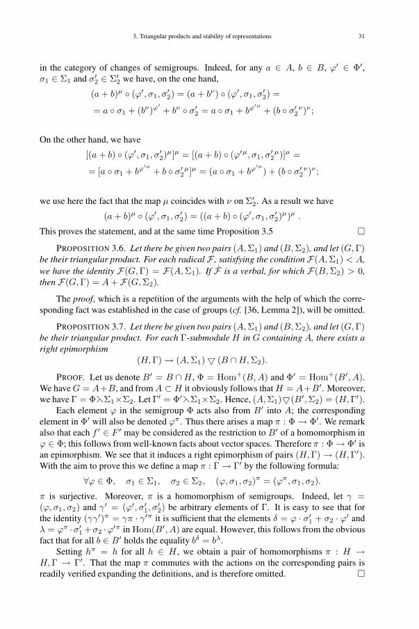
3. Triangular products and stability of representations 31
in the category of changes of semigroups. Indeed, for any a ∈ A, b ∈ B, ϕ′ ∈ Φ′,σ1 ∈ Σ1 and σ′
2 ∈ Σ′2 we have, on the one hand,
(a + b)μ ◦ (ϕ′, σ1, σ′2) = (a + bν) ◦ (ϕ′, σ1, σ
′2) =
= a ◦ σ1 + (bν)ϕ′+ bν ◦ σ′
2 = a ◦ σ1 + bϕ′μ+ (b ◦ σ′
2ν)ν ;
On the other hand, we have
[(a + b) ◦ (ϕ′, σ1, σ′2)
μ]μ = [(a + b) ◦ (ϕ′μ, σ1, σ′2μ)]μ =
= [a ◦ σ1 + bϕ′μ+ b ◦ σ′
2μ]μ = (a ◦ σ1 + bϕ′μ
) + (b ◦ σ′2ν)ν ;
we use here the fact that the map μ coincides with ν on Σ′2. As a result we have
(a + b)μ ◦ (ϕ′, σ1, σ′2) = ((a + b) ◦ (ϕ′, σ1, σ
′2)
μ)μ .
This proves the statement, and at the same time Proposition 3.5 �PROPOSITION 3.6. Let there be given two pairs (A,Σ1) and (B,Σ2), and let (G,Γ)
be their triangular product. For each radicalF , satisfying the conditionF(A,Σ1) < A,we have the identity F(G,Γ) = F(A,Σ1). If F is a verbal, for which F(B,Σ2) > 0,then F(G,Γ) = A + F(G,Σ2).
The proof, which is a repetition of the arguments with the help of which the corre-sponding fact was established in the case of groups (cf. [36, Lemma 2]), will be omitted.
PROPOSITION 3.7. Let there be given two pairs (A,Σ1) and (B,Σ2), and let (G,Γ)be their triangular product. For each Γ-submodule H in G containing A, there exists aright epimorphism
(H,Γ)→ (A,Σ1)� (B ∩H,Σ2).
PROOF. Let us denote B′ = B ∩H , Φ = Hom+(B,A) and Φ′ = Hom+(B′, A).We have G = A+B, and from A ⊂ H it obviously follows that H = A+B′. Moreover,we have Γ = Φ�Σ1×Σ2. Let Γ′ = Φ′�Σ1×Σ2. Hence, (A,Σ1)�(B′,Σ2) = (H,Γ′).
Each element ϕ in the semigroup Φ acts also from B′ into A; the correspondingelement in Φ′ will also be denoted ϕπ. Thus there arises a map π : Φ → Φ′. We remarkalso that each f ′ ∈ F ′ may be considered as the restriction to B′ of a homomorphism inϕ ∈ Φ; this follows from well-known facts about vector spaces. Therefore π : Φ → Φ′ isan epimorphism. We see that it induces a right epimorphism of pairs (H,Γ) → (H,Γ′).With the aim to prove this we define a map π : Γ → Γ′ by the following formula:
∀ϕ ∈ Φ, σ1 ∈ Σ1, σ2 ∈ Σ2, (ϕ, σ1, σ2)π = (ϕπ , σ1, σ2).
π is surjective. Moreover, π is a homomorphism of semigroups. Indeed, let γ =(ϕ, σ1, σ2) and γ′ = (ϕ′, σ′
1, σ′2) be arbitrary elements of Γ. It is easy to see that for
the identity (γγ′)π = γπ · γ′π it is sufficient that the elements δ = ϕ · σ′1 + σ2 · ϕ′ and
λ = ϕπ ·σ′1 +σ2 ·ϕ′π in Hom(B′, A) are equal. However, this follows from the obvious
fact that for all b ∈ B′ holds the equality bδ = bλ.Setting hπ = h for all h ∈ H , we obtain a pair of homomorphisms π : H →
H,Γ → Γ′. That the map π commutes with the actions on the corresponding pairs isreadily verified expanding the definitions, and is therefore omitted. �

32 CHAPTER I. REPRESENTATIONS OF SEMIGROUPS AND ALGEBRAS
6. Further information about a pair is obtained by its input to the triangular products ofpairs that are more or less simpler arranged than the given single pair. The first result ofthis kind, which is obtained by passing to a simpler domain of action, is an analogue ofthe well-known theorem of Kaluzhnin and Krasner in group theory; in semigroup theorythe corresponding fact is not known.
PROPOSITION 3.8. Let there be given an arbitrary faithful pair (G,Γ), and a Γ-submodule A of G, while Σ1 and Σ2 are the semigroups of endomorphisms induced bythe semigroup Γ in A and in G/A. Then the pair (G,Γ) can be embedded as a subpairin the triangular product (A,Σ1)� (G/A,Σ2).
PROOF. Exploiting the faithfulness of (G,Γ) and replacing Γ by the subsemigroupin EndG, we arrive at a pair isomorphic (from the right) to the given pair (G,Γ). There-fore we can in what follows assume that Γ is contained in EndG.
For any element γ ∈ Γ we denote by γμ and γν respectively the endomorphismof the spaces A and G/A induced by γ. Moreover, we set Γμ = Σ′
1 and Γν = Σ′2.
Also, in G we can find a K-subspace B complementary to A. This yields for G a directdecomposition G = A+B, which provokes a natural epimorphism α : G→ G/A and aprojection β : G→ B. The map α can also be viewed as an isomorphism α : B → G/Aand this gives a unique sense for the notation α−1, in particular, for each g ∈ G we have(gα)α−1
= gβ . The pair (G/A,Σ′2) and the map α induce the pair (B,Σ′
2): for b ∈ Band γ ∈ Γ, γν = σ′
2 ∈ Σ′2, we have
b ◦ σ′2 = (bα ◦ σ′
2)α−1
= ((b ◦ γ)α)α−1= (b ◦ γ)β .
We find from the decomposition G = A + B and the elements σ′1 ∈ Σ′
1 and σ′2 ∈ Σ′
2
respectively, the elements
σ1 =(ε 00 σ′
1
)and σ2 =
(σ′
2 00 ε
)in EndG, in this way establishing the embeddings Σ′
i → Σi ⊂ EndG, i = 1, 2. Inaddition, for each element g ∈ G, g = a + b, we have
gσ1 = (b + a)σ1 = b + a ◦ σ′1 and gσ2 = (b + a)σ2 = b ◦ σ′
2 + a.
Moreover, remarking that it follows from bσ2 = b◦σ′2 = (b◦γ)β that b◦γ− b◦σ′
2 ∈ A,we define a map ϕ′ : B → A according to the formula bϕ′
= b ◦ γ − b ◦ σ′2, it is
easy to check that ϕ′ ∈ Hom(B,A). The semigroup Hom(B,A) can also be viewedas a subsemigroup Φ in EndG, by associating to each element ϕ′ ∈ Hom(B,A) the
endomorphism ϕ =(ε ϕ′
0 ε
)of the space G. In addition, we have
gϕ = (a + b)ϕ = a + bϕ′+ b.
Let Γ′ = Φ � Σ1 × Σ2. By our construction, (G,Γ′) = (A,Σ1)� (B,Σ2).The map σ1ϕσ2 �→ (ϕ, σ1, σ2) induces an isomorphism of the subsemigroup Σ1 ·
Φ · Σ2 of EndG onto Φ � Σ1 × Σ2, which isomorphism will be denoted π. Indeed, asin EndG holds the equation
σ1ϕσ2 =(ε 00 σ′
1
)(ε ϕ′
0 ε
)(σ′
2 00 ε
)=
(σ′
2 ϕ′
0 σ′1
),
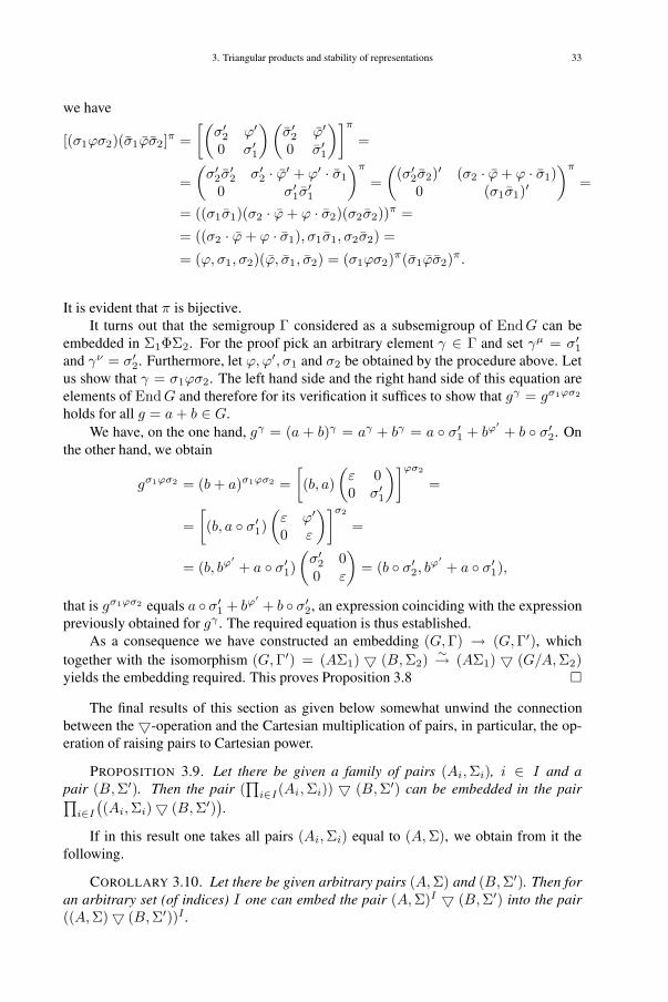
3. Triangular products and stability of representations 33
we have
[(σ1ϕσ2)(σ1ϕσ2]π =[(
σ′2 ϕ′
0 σ′1
)(σ′
2 ϕ′
0 σ′1
)]π
=
=(σ′
2σ′2 σ′
2 · ϕ′ + ϕ′ · σ1
0 σ′1σ
′1
)π
=(
(σ′2σ2)′ (σ2 · ϕ + ϕ · σ1)0 (σ1σ1)′
)π
=
= ((σ1σ1)(σ2 · ϕ + ϕ · σ2)(σ2σ2))π =
= ((σ2 · ϕ + ϕ · σ1), σ1σ1, σ2σ2) =
= (ϕ, σ1, σ2)(ϕ, σ1, σ2) = (σ1ϕσ2)π(σ1ϕσ2)π.
It is evident that π is bijective.It turns out that the semigroup Γ considered as a subsemigroup of EndG can be
embedded in Σ1ΦΣ2. For the proof pick an arbitrary element γ ∈ Γ and set γμ = σ′1
and γν = σ′2. Furthermore, let ϕ, ϕ′, σ1 and σ2 be obtained by the procedure above. Let
us show that γ = σ1ϕσ2. The left hand side and the right hand side of this equation areelements of EndG and therefore for its verification it suffices to show that gγ = gσ1ϕσ2
holds for all g = a + b ∈ G.We have, on the one hand, gγ = (a + b)γ = aγ + bγ = a ◦ σ′
1 + bϕ′+ b ◦ σ′
2. Onthe other hand, we obtain
gσ1ϕσ2 = (b + a)σ1ϕσ2 =[(b, a)
(ε 00 σ′
1
)]ϕσ2
=
=[(b, a ◦ σ′
1)(ε ϕ′
0 ε
)]σ2
=
= (b, bϕ′+ a ◦ σ′
1)(σ′
2 00 ε
)= (b ◦ σ′
2, bϕ′
+ a ◦ σ′1),
that is gσ1ϕσ2 equals a ◦ σ′1 + bϕ′
+ b ◦ σ′2, an expression coinciding with the expression
previously obtained for gγ . The required equation is thus established.As a consequence we have constructed an embedding (G,Γ) → (G,Γ′), which
together with the isomorphism (G,Γ′) = (AΣ1) � (B,Σ2)∼→ (AΣ1) � (G/A,Σ2)
yields the embedding required. This proves Proposition 3.8 �
The final results of this section as given below somewhat unwind the connectionbetween the �-operation and the Cartesian multiplication of pairs, in particular, the op-eration of raising pairs to Cartesian power.
PROPOSITION 3.9. Let there be given a family of pairs (Ai,Σi), i ∈ I and apair (B,Σ′). Then the pair (
∏i∈I(Ai,Σi)) � (B,Σ′) can be embedded in the pair∏
i∈I
((Ai,Σi)� (B,Σ′)
).
If in this result one takes all pairs (Ai,Σi) equal to (A,Σ), we obtain from it thefollowing.
COROLLARY 3.10. Let there be given arbitrary pairs (A,Σ) and (B,Σ′). Then foran arbitrary set (of indices) I one can embed the pair (A,Σ)I � (B,Σ′) into the pair((A,Σ)� (B,Σ′))I .

34 CHAPTER I. REPRESENTATIONS OF SEMIGROUPS AND ALGEBRAS
We limit ourselves here to the following Proposition 3.11; let us just add that Propo-sition 3.9 is proved by similar arguments.
PROPOSITION 3.11. Let there be given arbitrary pairs (A,Σ1) and (B,Σ2). Thenfor an arbitrary set (of indices) I one can embed the pair (A,Σ1)I � (B,Σ2) into thepair ((A,Σ1)� (B,Σ2))I .
PROOF. We introduce the three maps
(1) ω : A + BI → (A + B)I ;(2) τ : Σ1 × ΣI
2 → (Σ1 × Σ2)I ;(3) ν : Hom(BI , A)→ (Hom(B,A))I .
They are defined as follows.First, for all a ∈ A and b ∈ BI we define (a + b)ω = a + b, where a(i) = a for all
i ∈ I . Clearly, a is the constant function sending the entire domain I onto one and thesame value a ∈ A; in addition, a + b is the function I → A + B required.
Second, pick arbitrary σ1 ∈ Σ1 and σ2 ∈ ΣI2. Let us set (σ1σ2)τ = σ1σ2, where
σ1(i) = σ1 for all i ∈ I .
Third, for each ϕ ∈ Hom(BI , A) we define ϕν ∈ (Hom(B,A))I by the followingcondition
∀i ∈ I, b ∈ B, [b(i)]ϕν(i) = bϕ.
It is easy to see that ν is an isomorphism, and that ω and τ are monomorphisms.The pair of maps τ and ν can be joined to a homomorphism of semigroups
μ : Hom(BI , A) � Σ1 × ΣI2 → (Hom(B,A) � Σ1 × Σ2)I ,
if we give the map μ by the formula
(ϕ, σ1, σ2)μ = (ϕν , σ1, σ2).
It suffices to verify that the map μ is compatible with multiplication on the triangularproduct. As σ1σ
′1 = σ1·σ′
1, it is clear that the comparison of the elements [(ϕ, σ1, σ2)(ϕ′, σ′1, σ
′2)]
μ
and (ϕ, σ1, σ2)μ · (ϕ′, σ′1, σ
′2)μ reduces to the verification that the expressions (σ′
2 ·ϕ′ +ϕ ·σ′
1)ν and σ′
2 ·ϕ′ν +ϕν ·σ′1 represent one and the same element in (Hom(B,A))I . To
this end, take any b ∈ BI , i ∈ I and compute
[b(i)](σ2·ϕ′+ϕ·σ′1)ν(i) = b(σ2·ϕ′+ϕ·σ′
1) =
= (b ◦ σ2)ϕ′+ (bϕ) ◦ σ′
1 = [(b ◦ σ2)(i)]ϕ′ν(i) +
+ [b(i)]ϕν(i) ◦ σ′
1 =
= [b(i) ◦ σ2(i)]ϕ′ν(i) + [b(i)]ϕ
ν(i) ◦ σ′1 =
= [b(i)](σ2·ϕ′ν+ϕν ·σ′
1)(i).
Thus we are led to the condition
∀i ∈ I, (σ2 · ϕ′ + ϕ · σ′1)
ν(i) = (σ2 · ϕ′ν + ϕν · σ′1)(i),
which, apparently, is equivalent to the required equation.It remains to check that the morphisms μ and ω define monomorphisms of pairs
μ∗ : (A + BI ,Hom(BI , A) � Σ1 × ΣI2) → ((A + BI), (Hom(B,A) � Σ1 × Σ2)I).

3. Triangular products and stability of representations 35
The only not completely immediate part of the proof is the verification of the compati-bility of the map μ∗, defined with the help of ω and μ, with the action of the pairs.
Indeed, for arbitrary a ∈ A, b ∈ BI , ϕ ∈ Hom(BI , A), σ ∈ Σ1, σ2 ∈ Σ2 we have
(a + b)ω ◦ (ϕ, σ1, σ2)μ = (a + b) ◦ (ϕν , σ1, σ2) =
= bϕν
+ a ◦ σ1 + b ◦ σ2 =
= (bϕν
+ a ◦ σ1) + b ◦ σ2 =
= [(bϕ + a ◦ σ1) + b ◦ σ2]ω = [(a + b) ◦ (ϕ, σ1, σ2)]ω.
It remains only to check that here we used the equality of the elements bϕν
+ a ◦ σ1 and
bϕ + a ◦ σ1, which follows from the relation
∀i ∈ I, (bϕ + a ◦ σ1)(i) = bϕ + a ◦ σ1 =
= [b(i)]ϕν(i) + a ◦ σ1(i) = (bϕν
+ a ◦ σ1)(i).
By this the proof of the proposition is complete. �
3.1.3. Triangular products of representations of algebras
1. The construction indicated in the heading of this section will be achieved in twosteps. First, let there be given two K-algebras Φ and Σ. We may assume that Σ actsfrom the right and the left on Φ and will denote this circumstance by ϕ · σ and σ · ϕ,respectively. We require that these two actions satisfy the following conditions 10:
a) σ · (ϕ + ϕ′) = σ · ϕ + σ · ϕ′; (ϕ + ϕ′) · σ = ϕ · σ + ϕ′ · σ;b) σ · (ϕϕ′) = (σ · ϕ)ϕ′; (ϕϕ′) · σ = ϕ(ϕ′ · σ);c) (σ · ϕ) · σ′ = σ · (ϕ · σ′); (ϕ · σ)ϕ′ = ϕ(σ · ϕ′);d) (σ + σ′) · ϕ = σ · ϕ + σ′ · ϕ; ϕ · (σ + σ′) = ϕ · σ + ϕ · σ′;e) (σσ′) · ϕ = σ(σ′ · ϕ); ϕ · (σσ′) = (ϕ · σ) · σ′;f) σ · (κϕ) = κ(σ · ϕ); (kϕ) · σ = κ(ϕ · σ);g) (κσ) · ϕ = κ(σ · ϕ); ϕ · (κσ) = κ(ϕ · σ)
In the direct sum of algebras Γ = Φ + Σ we define addition and multiplication byscalars component wise, but multiplication will be defined a new setting
(ϕ, σ)(ϕ′, σ′) = (ϕ · σ′ + σ · ϕ′ + ϕϕ′, σσ′).
On the set Γ there raises the structure of a new K-algebra, which we denote by Γ = Φ�Σand call the semidirect product of the algebras Φ and Σ.
Remarks.
1) Let Σ be any K-algebra. Considering the field K as a K-algebra, we form thesemidirect sum Σ∗ = Σ �K . One gets a K-algebra, having the element (0, 1)as unit; moreover, the pairs of the form (σ, 0), σ ∈ Σ, give in Σ∗ a subalgebraisomorhic to Σ. This contains the essential part of a result mentioned in [21,p. 54-55].
10Following MacLane [88] we speak of commuting bimultiplications (of Hochschild) on the algebra Φ.
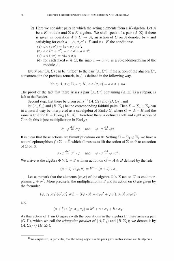
36 CHAPTER I. REPRESENTATIONS OF SEMIGROUPS AND ALGEBRAS
2) Here we consider pairs in which the acting elements form a K-algebra. Let Abe a K-module and Σ a K-algebra. We shall speak of a pair (A,Σ) if thereis given an operation A × Σ → A, an action of Σ on A denoted by ◦ andsatisfying for each a ∈ A, σ, σ′ ∈ Σ and κ ∈ K the conditions:(a) a ◦ (σσ′) = (a ◦ σ) ◦ σ′;(b) a ◦ (σ + σ′) = a ◦ σ + a ◦ σ′;(c) a ◦ (κσ) = κ(a ◦ σ);(d) for each fixed σ ∈ Σ, the map a → a ◦ σ is a K-endomorphism of the
module A.
Every pair (A,Σ) can be “lifted” to the pair (A,Σ∗), if the action of the algebra Σ∗,constructed in the previous remark, in A is defined in the following way,
∀a ∈ A, σ ∈ Σ, κ ∈ K, a ◦ (σ, κ) = a ◦ σ + κa.
The proof of the fact that there arises a pair (A,Σ∗) containing (A,Σ) as a subpair, isleft to the Reader.
Second step. Let there be given pairs 11 (A,Σ1) and (B,Σ2), andlet (A, Σ1) and (B, Σ2) be the corresponding faithful pairs. Then Σ = Σ1⊕ Σ2 can
in a natural way be interpreted as a subalgebra of EndK G, where G = A + B and thesame is true for Φ = HomK(B,A). Therefore there is defined a left and right action ofΣ in Φ; this is just multiplication in EndK :
σ · ϕ def= σϕ and ϕ · σ def= ϕσ.
It is clear that these actions are bimultiplications on Φ. Setting Σ = Σ1 ⊕ Σ2 we have anatural epimorphism f : Σ → Σ which allows us to lift the action of Σ on Φ to an actionof Σ on Φ:
σ · ϕ def= σf · ϕ and ϕ · σ def= ϕ · σf .
We arrive at the algebra Φ � Σ = Γ with an action on G = A⊕B defined by the rule
(a + b) ◦ (ϕ, σ) = bϕ + (a + b) ◦ σ.
Let us remark that the elements (ϕ, σ) of the algebra Φ � Σ act on G as endomor-phisms ϕ + σf . More precisely, the multiplication in Γ and its action on G are given bythe formulae
(ϕ, σ1, σ2)(ϕ′, σ′1, σ
′2) = ((ϕ · σ′
1 + σ2ϕ′ + ϕϕ′), σ1σ
′1, σ2σ
′2)
and
(a + b) ◦ (ϕ, σ1, σ2) = bϕ + a ◦ σ1 + b ◦ σ2.
As this action of Γ on G agrees with the operations in the algebra Γ, there arises a pair(G,Γ), which we call the triangular product of (A,Σ1) and (B,Σ2); we denote it by(A,Σ1)� (B,Σ2).
11We emphasize, in particular, that the acting objects in the pairs given in this section are K-algebras.
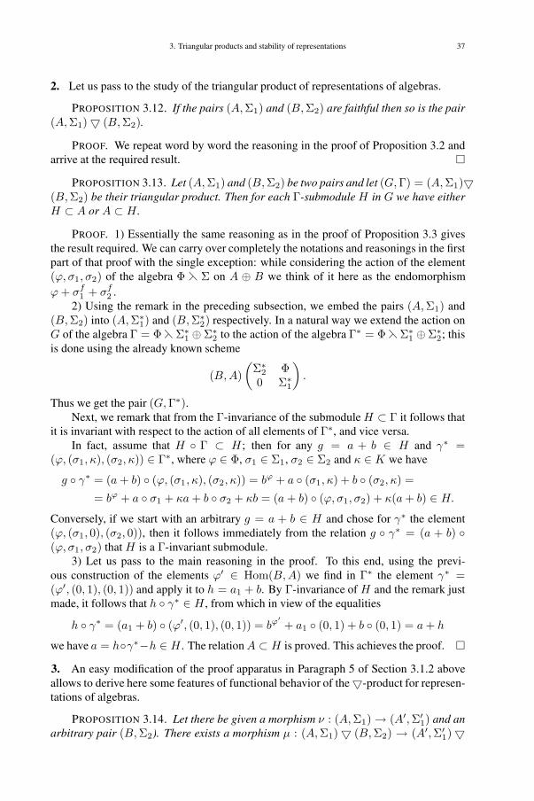
3. Triangular products and stability of representations 37
2. Let us pass to the study of the triangular product of representations of algebras.
PROPOSITION 3.12. If the pairs (A,Σ1) and (B,Σ2) are faithful then so is the pair(A,Σ1)� (B,Σ2).
PROOF. We repeat word by word the reasoning in the proof of Proposition 3.2 andarrive at the required result. �
PROPOSITION 3.13. Let (A,Σ1) and (B,Σ2) be two pairs and let (G,Γ) = (A,Σ1)�(B,Σ2) be their triangular product. Then for each Γ-submodule H in G we have eitherH ⊂ A or A ⊂ H .
PROOF. 1) Essentially the same reasoning as in the proof of Proposition 3.3 givesthe result required. We can carry over completely the notations and reasonings in the firstpart of that proof with the single exception: while considering the action of the element(ϕ, σ1, σ2) of the algebra Φ � Σ on A ⊕ B we think of it here as the endomorphismϕ + σf
1 + σf2 .
2) Using the remark in the preceding subsection, we embed the pairs (A,Σ1) and(B,Σ2) into (A,Σ∗
1) and (B,Σ∗2) respectively. In a natural way we extend the action on
G of the algebra Γ = Φ � Σ∗1 ⊕ Σ∗
2 to the action of the algebra Γ∗ = Φ � Σ∗1 ⊕Σ∗
2; thisis done using the already known scheme
(B,A)(
Σ∗2 Φ
0 Σ∗1
).
Thus we get the pair (G,Γ∗).Next, we remark that from the Γ-invariance of the submodule H ⊂ Γ it follows that
it is invariant with respect to the action of all elements of Γ∗, and vice versa.In fact, assume that H ◦ Γ ⊂ H ; then for any g = a + b ∈ H and γ∗ =
(ϕ, (σ1, κ), (σ2, κ)) ∈ Γ∗, where ϕ ∈ Φ, σ1 ∈ Σ1, σ2 ∈ Σ2 and κ ∈ K we have
g ◦ γ∗ = (a + b) ◦ (ϕ, (σ1, κ), (σ2, κ)) = bϕ + a ◦ (σ1, κ) + b ◦ (σ2, κ) =
= bϕ + a ◦ σ1 + κa + b ◦ σ2 + κb = (a + b) ◦ (ϕ, σ1, σ2) + κ(a + b) ∈ H.
Conversely, if we start with an arbitrary g = a + b ∈ H and chose for γ∗ the element(ϕ, (σ1, 0), (σ2, 0)), then it follows immediately from the relation g ◦ γ∗ = (a + b) ◦(ϕ, σ1, σ2) that H is a Γ-invariant submodule.
3) Let us pass to the main reasoning in the proof. To this end, using the previ-ous construction of the elements ϕ′ ∈ Hom(B,A) we find in Γ∗ the element γ∗ =(ϕ′, (0, 1), (0, 1)) and apply it to h = a1 + b. By Γ-invariance of H and the remark justmade, it follows that h ◦ γ∗ ∈ H , from which in view of the equalities
h ◦ γ∗ = (a1 + b) ◦ (ϕ′, (0, 1), (0, 1)) = bϕ′+ a1 ◦ (0, 1) + b ◦ (0, 1) = a + h
we have a = h◦γ∗−h ∈ H . The relation A ⊂ H is proved. This achieves the proof. �
3. An easy modification of the proof apparatus in Paragraph 5 of Section 3.1.2 aboveallows to derive here some features of functional behavior of the�-product for represen-tations of algebras.
PROPOSITION 3.14. Let there be given a morphism ν : (A,Σ1)→ (A′,Σ′1) and an
arbitrary pair (B,Σ2). There exists a morphism μ : (A,Σ1)� (B,Σ2) → (A′,Σ′1)�
38 CHAPTER I. REPRESENTATIONS OF SEMIGROUPS AND ALGEBRAS
(B,Σ2), which coincides with the map ν on (A,Σ1) and is an identity on (B,Σ2). If νis injective (surjective), then μ is also so.
PROOF. The proof is obtained by repeating almost word by word the proof of Propo-sition 3.4, the notations of which are preserved here with an immediate modification oftheir interpretation.
We stop only at a fragment of the reasoning. Let us assume that
∀ϕ ∈ Φ, σ1 ∈ Σ1, σ2 ∈ Σ2, (ϕ, σ1, σ2)μ = (ϕμ, σν1 , σ2).
We have to verify that μ : Γ → Γ′ is a morphism of algebras, which agrees with theaction of these algebras on G and G′ respectively. We restrict the verification to thefact that μ intertwine with multiplication on the algebras Γ and Γ′; the rest follows evensimpler by checking the definitions. We have
(ϕ, σ1, σ2)μ · (ϕ′, σ′1, σ
′2)
μ = (ϕμ, σν1 , σ2) · (ϕ′μ, σ′
1ν , σ′
2) =
= ((ϕ · σ′1 + σ2 · ϕ′ + ϕϕ′)μ, (σ1σ
′1)
ν , σ2σ′2) =
= [(ϕ, σ1, σ2)(ϕ′, σ′1, σ
′2)]
μ.
In these computations we used the relation
ϕμ · σ′1ν + σ2 · ϕ′μ + ϕμϕ′μ = (ϕ · σ′
1 + σ2 · ϕ′ + ϕϕ′)μ;
it follows from the identities
ϕμ · σ′1ν = (ϕ · σ′
1)μ ; σ2 · ϕ′μ = (σ2 · ϕ′)μ and ϕμϕ′μ = (ϕϕ′)μ,
of which only two first ones require the proof. The first of them follows from the seriesof equations, valid for any b ∈ B,
bϕμ·σ′1
ν
= bϕμ ◦ σ′1ν = (bϕ)ν ◦ σ′
1ν = (bϕ ◦ σ′
1)ν = b(ϕ·σ′
1)μ
.
Moreover, for all b ∈ B we have
bσ2·ϕ′μ= (b ◦ σ2)ϕ′μ
=[(b ◦ σ2)ϕ′]ν
= (bσ2·ϕ′μ)ν = b(σ2·ϕ′)μ
,
from which the second equation in view follows. The statement is proved. We allowourself not to produce the remaining details. �
The category of changes of substitutions of pairs of representations of algebras isdefined completely in analogy with the semigroup case (cf. Subsection 3.2.5).
PROPOSITION 3.15. An arbitrary object (A,Σ1) and a morphism ν : (B,Σ2) �(B′,Σ′
2) in the category of substitutions of pairs of representations of algebras inducesa morphism
μ : (A,Σ1)� (B,Σ2) � (A,Σ1)� (B′,Σ′2)
of the same category.
PROOF. The proof is obtained carrying over verbatim to the present situation thenotations and reasonings of Section 3.1.4, with the difference that here Φ and Φ′ arethought of as subalgebras in EndK(A⊕B) and EndK(A′⊕B) respectively; all the restof the proof mentioned is preserved in the present interpretation. �
3. Triangular products and stability of representations 39
4. The behavior of radicals and verbals with respect to the triangular product of repre-sentations of algebras is the same as in the semigroup case described in Proposition 3.6;we omit its formulation as well as the proof, because in an obvious way it repeats thesemigroup case. The same remarks refer to
PROPOSITION 3.16. Let there be given two pairs (A,Σ1) and (B,Σ2) and a set(G,Γ) = (A,Σ1)� (B,Σ2). For any Γ-submodule H in G contained in A, there existsa right epimorphism
(H,Γ)→ (A,Σ1)� (B ∩H,Σ2).
5. Embedding theorems referred in Paragraph 6 of Section 3.1.2 hold true also forrepresentations of algebras.
PROPOSITION 3.17. Let there be given an arbitrary faithful pair (G,Γ), a Γ-sub-module A of G, while Σ1 and Σ2 are the subalgebras of endomorphisms, induced by theK-algebra Γ in A and in G/A respectively. Then the pair (G,Γ) can be embedded as asubalgebra in the triangular product (A,Σ1)� (G/A,Σ2).
PROOF. We take advantage of the fact that the pair (G,Γ) is faithful and replacethe algebra Γ by the corresponding subalgebra in EndK G; in this way we obtain a pairwhich is right isomorphic to the original pair (G,Γ). Therefore we may assume, in whatfollows, that Γ is already contained in the algebra EndK G.
The action of the elements of the algebra Γ on the module G induces their actions onA and on G/A; the morphisms arising in this way will be denoted μ and ν respectively.We set Imμ = Σ1 and Im ν = Σ2. We select in G a subspace B complementary to A,which gives a direct decomposition G = A+B, with the accompanying natural epimor-phism α : G � G/A and projection β : G → G/A. The map α may be viewed as anisomorphism B → G/A, giving a unique meaning to the notation α−1; in particular, foreach g ∈ G we have (gα)α−1
= gβ .The pair (G/A,Σ2) and the map α induce the pair (B,Σ2); for b ∈ B and γ ∈ Γ,
γν = σ2 ∈ Σ2 we have
b ◦ σ2 = (bα ◦ σ2)α−1=
((b ◦ γ)α
)α−1
= (b ◦ γ)β.
Take an arbitrary element γ ∈ Γ and let γμ = σ1, γν = σ2.Let us associate to the elements σ1 ∈ Σ1 and σ2 ∈ Σ2 respectively the elements(
0 00 σ1
)and
(σ2 00 0
)in EndG, which determine the embeddings Σi → EndG, i = 1, 2. Further, if Φ =Hom(B,A) is embedded, in the manner indicated in Section 3.1.1, in EndG, then thesubalgebra Φ ⊂ EndG may be treated as the annihilator of the series 0 ⊂ A ⊂ G.
Next, we remark that by the construction of the embedding of Σ1 ⊕ Σ2 in EndG,for each g = a + b ∈ G we have g ◦ σ1 = a ◦ σ1 and g ◦ σ2 = b ◦ σ2. Moreover, fromb ◦ σ2 = (b ◦ γ)β it follows the existence of an a ∈ A such that b ◦ γ = a+ b ◦ σ2. Fromthese remarks we obtain the relations
b ◦ (γ − σ2 − σ1) = a and a ◦ (γ − σ2 − σ1) = 0;
they show that γ − σ2 − σ1 ∈ Φ, because Φ is the annihilator of the series 0 ⊂ A ⊂ G.Therefore there exists a ϕ ∈ Φ such that γ = ϕ+σ1 +σ2. There arises an embedding of
40 CHAPTER I. REPRESENTATIONS OF SEMIGROUPS AND ALGEBRAS
algebras Γ → Φ�Σ1⊕Σ2, which we denote by π; for each γ ∈ Γ, γ = ϕ+σ1 +σ2 it isgiven by the formula γπ = (ϕ, σ1, σ2). This morphism π together with the isomorphism(A,Σ1)� (B,Σ2)→ (A,Σ1)� (G/A,Σ2) induces also the useful embedding of pairs(G,Γ)→ (A,Σ1)� (G/A,Σ2). �
The proof of each of the following three propositions is essentially a transfer ofthe corresponding proof in the semigroup case, sometimes with light modifications; alldifficulties are overcome without any pain, so we leave them to the Reader. We limitourselves to the formulations.
PROPOSITION 3.18. Let there be given an arbitrary family of pairs (Ai,Σi), i ∈ I ,and the pair (B,Σ′). Then the pair
(∏i∈I(Ai,Σi)
)� (B,Σ′) can be embedded into the
pair∏
i∈I
((Ai,Σi)� (B,Σ′)
).
COROLLARY 3.19. Let there be given arbitrary pairs (A,Σ1) and (B,Σ2). Thenfor each family of indices I one has the embedding
(A,Σ1)I � (B,Σ2) → ((A,Σ1)�
(B,Σ2))I.
PROPOSITION 3.20. Let there be given arbitrary pairs (A,Σ1) and (B,Σ2). Thenfor each family of indices I the pair (A,Σ1) � (B,Σ2)I can be embedded in the pair((A,Σ1)� (B,Σ2))I .
3.1.4. Connections between�-constructions
1. The constructions of the triangular product of pairs of representations of groups,semigroups and algebras, as considered in the previous sections of this paper, are, as itseems to us, not only isolated technical tools, but partial appearances of a whole, moregeneral concept. Here we shall indicate some correlations between these three construc-tions.
2.
PROPOSITION 3.21. Let there be given pairs representations of semigroups (A,Σ1)and (B,Σ2), while (G,Γ) is their triangular product. The acting semigroup Γ = Φ �Σ1 × Σ2 is a group if and only if Σ1 and Σ2 are groups and the semigroup Φ =Hom+
K(B,A) is treated as a group. If these conditions are fulfilled then (G,Γ) is iso-morphic to the triangular product of (A,Σ1) and (B,Σ2) as group pairs.
PROOF. Let us first make an observation.Let Σ1 and Σ2 be groups and let us treat Φ = HomK(B,A) as an additive Abelian
group. Let us show that then Γ = Φ � Σ1 × Σ2 is also a group. To this end, weremark that the element (ϕ′, σ′
1, σ′2) ∈ Γ is a unity of Γ exactly when for each element
(ϕ, σ1, σ2) ∈ Γ we have
(4)(ϕ, σ1, σ2) = (ϕ · σ′
1 + σ2 · ϕ′, σ1σ′1, σ2σ
′2) and
(ϕ, σ1, σ2) = (ϕ′ · σ1 + σ′2 · ϕ, σ′
1σ1, σ′2σ2).
From these relations it follows that, in particular, σ′i = εi, where εi are the units of Σi,
i = 1, 2. Taking account of this, the equality of the first components in the triples in (4)takes the form
ϕ · ε1 + σ2 · ϕ′ = ϕ′ · σ1 + ε2 · ϕ = ϕ.

3. Triangular products and stability of representations 41
The equation ϕ = ϕ · ε1 and the arbitrariness of the the choice of the element σ2 ∈ Σ2
imply now that ϕ + ε2 · ϕ′ = ϕ, i.e. ϕ′ = 0. Consequently, the unity of Γ must be thetriple (0, ε1, ε2), where 0 is the zero homomorphism in HomK(B,A), which is verifiedby an immediate check.
In an analogous way one solves the question of inverse elements. Indeed, for thetriple (ϕ′, σ′
1, σ′2) to be the inverse of (ϕ, σ1, σ2) it is necessary and sufficient that the
following equations be fulfilled
(5)(ϕ · σ′
1 + σ2 · ϕ′, σ1σ′1, σ2σ
′2) = (0, ε1, ε2) and
(ϕ′ · σ1 + σ′2 · ϕ, σ′
1σ1, σ′2σ2) = (0, ε1, ε2).
It follows from () that σ′1 = σ−1
1 and σ′2 = σ−1
2 . It follows then from the equalitiesfor the first components in (5) that ϕ · σ−1
1 = −σ2 · ϕ′ and ϕ′ · σ1 = −σ−12 · ϕ, which
equalities are equivalent to ϕ′ = −σ−12 ·ϕ·σ−1
1 . We conclude that the inverse to the triple(ϕ, σ1, σ2) is given by (−σ−1
2 ·ϕ ·σ−11 , σ−1
1 , σ−12 ). The first statement of the proposition
is now proved in a standard way in both directions of the implication.Let us pass to the proof of the second statement of the proposition. First, it is clear
that for the subgroup Σ generated in Γ by Σ1 and Σ2 the subrepresentation (G,Σ) splits,(G,Σ) = (A⊕B,Σ1×Σ2). Second, for each (ϕ, ε1, ε2) ∈ Φ and (ϕ1, σ1, σ2) ∈ Γ onehas
(ϕ, σ1, σ2)−1 · (ϕ, ε1, ε2) · (ϕ1, σ1, σ2) = (−σ−12 · ϕ · σ−1
1 , σ−11 , σ−1
2 )×× (ϕ, ε1, ε2) · (ϕ1, σ1, σ2) = (σ−1
2 · ϕ · σ1, ε1, ε2),
which shows the invariance of the subgroup Φ in Γ. Moreover, one checks immediatelythat the pair (G,Φ) is faithful, along with the fact that the image of Φ in AutG coincideswith the centralizer of the series 0 ⊂ A ⊂ G. Third, let us introduce the map f of thepair (G,Γ) into the pair (G,Γ∗), being the triangular product of (A,Σ1) and (B,Σ2) asgroup pairs, defining it as the identity map on G and on Γ by the formula
(ϕ, σ1, σ2)f def= (ϕ · σ−11 , σ1, σ2).
A check shows that the map f is a morphism of the group pairs (G,Γ) and (G,Γ∗), and,furthermore, bijective.
With these reasonings our statement is proved, and at the same time the proof ofProposition 3.21 is finished as well. �
3. In the study of the interrelations between the triangular product of semigroup pairs(A,Σ1) � (B,Σ2) and of pairs (or representations) of algebras (A,S1) � (B,S2) anessential role is played by the following remark. In the semigroup Φ � Σ1 × Σ2 itselements (ϕ, σ1, σ2) and their components ϕ, σ1, σ2 are thought of as endomorphisms inEndG: (
σ2 ϕ0 σ1
)and
(ε2 ϕ0 ε1
),
(ε2 00 σ1
),
(σ2 00 ε1
)respectively. In the algebra Φ�S1⊕S2 one has a different interpretation for its elements(ϕ, σ1, σ2) and their components :(
σ2 ϕ0 σ1
)and
(0 ϕ0 0
),
(0 00 σ1
),
(σ2 00 0
).

42 CHAPTER I. REPRESENTATIONS OF SEMIGROUPS AND ALGEBRAS
Next, let there be given two semigroup pairs (A,Σ1) and (B,Σ2), which we, in awell-known manner, lift to the corresponding monoid pairs (A,Σ∗
1) and (B,Σ∗2). The lin-
ear extension of the actions of Σ∗1 in A and Σ∗
2 in B gives pairs (A,KΣ∗1) and (B,KΣ∗
2),where the acting object are the corresponding semigroup algebras. Let us consider thetriangular products
(A,Σ1)� (B,Σ2) = (A⊕B,Φ � Σ1 × Σ2),
(where the semigroup Φ = HomK(B,A) is treated as the centralizer of the series 0 ⊂A ⊂ G in EndG) and
(A,KΣ∗1)� (B,KΣ∗
2) = (A⊕B,Φ � (KΣ∗1 ⊕KΣ∗
2)),
(where Φ is treated as the annihilator of the series 0 ⊂ A ⊂ G in EndG.)It is easy to verify that one has the following fact.
PROPOSITION 3.22. The map π∗ : (ϕ, σ1, σ2) �→ (ϕ− ε, σ1− ε2, σ2− ε1) gives anembedding of Φ � Σ1 × Σ2 into the multiplicative semigroup of algebra Φ � (KΣ∗
1 ⊕KΣ∗
2), which agrees with the actions in the pairs (A⊕B,Φ�Σ1×Σ2) and (A⊕B,Φ�(KΣ∗
1 ⊕KΣ∗2)).
4. Let there be given any two pairs (A,S1) and (B,S2), whose acting objects S1 andS2 are unitary K-algebras. Using the natural “cutting” functor, we obtain the semigrouppairs (A,Σ1) and (B,Σ2), where Σi is the multiplicative semigroup of the algebra Si,i = 1, 2. We form anew the corresponding triangular products
(A,S1)� (B,S2) = (A⊕B,Φ � (S1 ⊕ S2))
and
(A,Σ1)� (B,Σ2) =(A⊕B,Φ � Σ1 × Σ2
).
Then we obtain
PROPOSITION 3.23. The map π∗ : (ϕ, σ1, σ2) �→ (ϕ + ε, σ1 + ε2, σ2 + ε1) givesan isomorphism of the multiplicative semigroup of the algebra Φ � (S1 ⊕ S2) with thesemigroup Φ � Σ1 × Σ2, which agrees with the action in the pairs
(A⊕B,Φ � (S1 ⊕ S2)) and (A⊕B,Φ � Σ1 × Σ2).
The proof is easily obtained by an immediate checking of the definition, and will beomitted. �
3.1.5. Comments
1. Under the influence of the view at representations of algebraic structures as two-sorted systems (or pairs) there arose the language of pairs which as a working tool in thesystematic study of representations by B. I. Plotkin in his book [35] balances the role ofthe inner structure of groups and their outer properties of actions on the representationmodules.
3. Triangular products and stability of representations 43
2. The extension of the theme of varieties of groups (cf., e.g., [34]) to varieties of linearpairs-representations of groups required the statement of the questions there, which weresuggested by group theory. Their solution, however, leads rather far from the originaland requires new tools. So, in [36] there arose the construction of the triangular productof group representations. This carries in itself the analogue of the properties and therole of the wreath product of groups: cf. [38, 43, 49]. This construction is the naturalmodel for the�-construction for representations of semigroups and algebras consideredin the present Section. The connections found in Section 3.1.4 between the three �-constructions may be interpreted as an argument for the advantage of these constructions.The term, but not the notion of triangular product is borrowed from Eilenberg [66], butits appearance is (according to [66]) connected with Schützenberger (1965). The booksI. B. Menskiı [32] and S. Eilenberg [66] point to further paths for developing this theme,important for the applications.
3.2. The arithmetics of varieties of representations of semigroups andalgebras
The topic of this Section concerns the arithmetic properties of families of varieties oflinear representations (over a field K) of semigroups and algebras, and also the sameproperties of varieties. In the study of varieties the machinery of the triangular products,as developed in the previous Sections, is applied. The main goal is to prove the “theoremof generators” for varieties of representations of semigroups as well as of algebras. Inorder to make its formulation more precise we remark that the set of varieties of pairsadmits an associative multiplication: the pair (G,Γ) is contained in Θ1 ·Θ2 if G admitsa Γ-submodule H such that (H,Γ) ∈ Θ1 and (G/H,Γ) ∈ Θ2. Furthermore, let us agreeto denote by VarK the variety generated by the class of pairs K. The formula we areinterested in is given by the formula Var(K1 � K2) = VarK1 · VarK2, which holdsfor arbitrary classes of pairs K1 and K2. From this one can derive, in particular, thatthe semigroup of non-trivial varieties of linear representations of semigroups is a semi-group with unique decomposition into factors. As an application of this fact we proveTheorem 3.37 on the structure of the semigroup of varieties of linear automata. In thecase of algebras this leads to a new proof of the theorem of Bergman and Lewin on thefreedom of the semigroup of T -ideals in a free associative K-algebra of countable rank.Our approach puts this theorem and its proof into one row with the corresponding resultsfor varieties of representations of groups and semigroups, and gives supplementary in-formation on varieties of algebras, which is hard to obtain in the language of T -ideals(cf. Theorems 3.49, 3.50 and 3.51 below).
Everywhere in this Section, K is a field. We speak here of a pair (G,Γ) if the semi-group (algebra) Γ acts as a semigroup (algebra) of K-endomorphisms on the K-moduleG; also, in Sections 3.2.5 the acting object is a semigroup, while in the Section 3.2.6 itis a K-algebra. Unless the contrary is told, the word “variety” means a“ variety of pairswhich is distinct from the unit variety (the class of all pairs with zero domain of action),and from the “variety of all pairs”.
3.2.1. Varieties of linear pairs and automata
1. Here we introduce a connection (of Galois type) whose closed objects are varietiesof representations of semigroups and special ideals in suitable algebras.
44 CHAPTER I. REPRESENTATIONS OF SEMIGROUPS AND ALGEBRAS
2. Let X = {x1, x2, . . . } be a countable set. Let Ψ and Ψ∗ be the free semigroupand the free monoid, respectively, with the elements of X as free generators. Let u =u(xi1 , . . . , xik
) be an arbitrary element of the semigroup ring KΨ∗. By definition, inthe pair (G,Γ) holds the (special) bi-identity y ◦ u ≡ 0 if for each specialization y �→g ∈ G, xij �→ γij ∈ Γ the equality g ◦ u(γi1 , . . . γiiik
) = 0 holds in (G,KΓ∗). Herewe can consider also bi-identities of a more general type, parallel to what was done in[35, p. 566–572]. However, in the case when K is a field each such system of bi-identitiescan easily be replaced by a system of special bi-identities equivalent to it.
To each class of pairs Θ we associate in KΨ∗ the set UΘ of all u ∈ KΨ∗ such that ineach pair in Θ the bi-identity y ◦ u ≡ 0 is fulfilled; we call UΘ the indicator of the classΘ. The subset UΘ is a two-sided ideal in KΨ∗, invariant with respect to all endomor-phisms of the ring KΨ∗ which are induced by an endomorphism of the monoid Ψ∗; theendomorphisms of the ring KΨ∗ with this property will be called special. Furthermore,we call special likewise those ideals of KΨ∗ which are invariant with respect to allspecial endomorphisms. Thus to each class of pairs Θ there corresponds a special idealΘU in the ring KΨ∗.
On the other hand, let U be an arbitrary subset in KΨ∗. We associate with it a classΘU according to the following rule: the pair (G,Γ) belongs to the class ΘU if and only ifall bi-identities y ◦ u ≡ 0, u ∈ U , are fulfilled in this pair. We remark that if U is a two-sided ideal in KΨ∗, then the class ΘU is closed with respect to subpairs, homomorphicimages and Cartesian products of pairs, an furthermore saturated. The last thing means,by definition that the class is also closed with respect to complete pre-images of this pairunder right homomorphisms. In other words, what was said above means that the classΘU is a variety of pairs.
Next, let Θ be a variety of pairs, and U ⊂ KΨ∗ a two-sided special ideal. We havethe relations
Θ → UΘ → Θ(UΘ) = Θ′ and U → ΘU → U(ΘU) = U ′.
It turns out that one has the equalities U = U ′ and Θ = Θ′. Hence, varieties of pairs-representations of semigroups are in a bijective correspondence with special ideals inKΨ∗.
On the set of linear representations of semigroups one can define a multiplication asfollows. By definition a pair (G,Γ) is contained in the class Θ1 · Θ2 if in G there exista Γ-submodule H such that (H,Γ) ∈ Θ1 and (G/H,Γ) ∈ Θ2. Varieties of pairs forma semigroup with respect to this multiplication, which we denote by M = M(K). Weremark that the indicator of the variety Θ1 ·Θ2 is the ideal U2 · U1, where U1 and U2 arethe indicators of the varieties Θ1 and Θ2, respectively. We have the following result.
PROPOSITION 3.24 ([17]). The semigroupM(K) of varieties of representations ofsemigroups is anti-isomorphic to the semigroup of special ideals of the ring KΨ∗.
In the case of a fixed acting semigroup Γ the requirement of saturation in the defin-ition of variety becomes trivial, and in this case the variety of pairs is the Birkhoff classof the corresponding Γ-modules. Here we have the following.
PROPOSITION 3.25 ([17]). The varieties of Γ-modules are in one-to-one correspon-dence with the two-sided ideals of the semigroup ring KΓ∗.

3. Triangular products and stability of representations 45
3. Let us pass to linear automata, which constitute a partial generalization of the linearsystems in [18].
A linear automaton (semigroup automaton (Mealey)) is a three-sorted algebraic sys-tem A = (A,Γ, B), where A (the states) and B (the outputs) are K-modules, Γ is thesemigroup of input signals, and there are given a K-linear map of transition A ◦ Γ → Aand an operation of output A ∗ Γ → B with the properties
∀a ∈ A; γ1, γ2 ∈ Γ,
{a ◦ (γ1γ2) = (a ◦ γ1) ◦ γ2,
a ∗ (γ1γ2) = (a ◦ γ1) ∗ γ2.
A linear automatonA′ = (A′,Γ′, B′) is a subautomaton of A = (A,Γ, B) if A′ ⊂A, Γ′ ⊂ Γ, B′ ⊂ B are subobjects of the corresponding algebraic structures, and A′ ◦Γ′ ⊂ A′ and A′ ∗ Γ′ ⊂ B′.
Let there be given two linear automata A = (A,Γ, B) and A′ = (A′,Γ′, B′) anda triple of morphisms σ = (σ1, σ2, σ3), σ1 : A → A′, σ2 : Γ → Γ′, σ3 : B → B′.By definition, σ : A → A′ is a morphism of automata if the following conditions arefulfilled
∀a ∈ A, γ ∈ Γ (a ◦ γ)σ1 = aσ1 ◦ γσ2 and (a ∗ γ)σ3 = aσ1 ∗ γσ2 .
It is clear that the submodules Kerσ1 = Aσ ⊂ A, Kerσ3 = Bσ ⊂ B, and the kernelcongruence Kerσ2 = κ on Γ satisfy the requirement
∀a, a′ ∈ A, γ, γ′ ∈ Γ ((a− a′ ∈ Aσ)&(γκγ′)) =⇒=⇒ ((a ◦ γ − a′ ◦ γ′ ∈ Aσ)&(a ∗ γ − a′ ∗ γ′ ∈ Bσ)).
Conversely, if in the components of the linear automaton A = (A,Γ, B) is cho-sen a family of congruences Λ = (Aσ, κ, Bσ) satisfying the requirements mentionedthen Λ is called a congruence of the automaton A. In this case the system A/Λ =(A/Aσ,Γ/κ,B/Bσ), in which all operations on the equivalence classes are induced bythe corresponding ones in A, is a linear automaton. This is, by definition, the factor au-tomaton of A by Λ. It is clear that for linear automata one can formulate and prove thehomomorphism theorems and Remak’s theorem.
The Cartesian product of the family of linear automata Ai = (Ai,Γi, Bi), i ∈ I , iscalled the system
∏i∈I Ai = (A,Γ, B), where A =
∑ci∈I Ai and B =
∑ci∈I Bi are the
complete direct sums of the modules Ai and Bi, i ∈ I , respectively, while Γ =∏
i∈I Γi
is the Cartesian product of the semigroups Γi, i ∈ I , the operations A ◦ Γ → A andB ∗ Γ → B being defined component wise.
By definition, a class Θ of linear automata is called a Birkhoff class if it is closedwith respect to epimorphic images, subautomata and Cartesian products. Furthermore,we say that a class Θ of linear automata is saturated if together with the automatonA = (A,Γ, B) it contains all automata of the form (A,Γ, B′), where B′ ⊃ B and foreach epimorphism (A,Γ, B) → (A,Σ, B) which is identity on A and B, it follows from(A,Σ, B) ∈ Θ that (A,Γ, B) ∈ Θ. Saturated Birkhoff classes of linear automata will becalled varieties of linear automata.
4. Let A = (A,Γ, B) be a linear automaton, accompanied by the maps μ0 : Γ →EndK A and μ∗ : Γ → Hom(A,B), given by the formulae
∀a ∈ A, γμ0(a) = a ◦ γ and γμ∗(a) = a ∗ γ.
46 CHAPTER I. REPRESENTATIONS OF SEMIGROUPS AND ALGEBRAS
We extend them by linearity to maps
μ0 : KΓ→ EndK A and μ∗ : KΓ → HomK(A,B).
Then there arises the automatonAL = (A,KΓ, B). We say that in the automatonA thebi-identity y ◦ u ≡ 0 (the bi-identity z ∗ u ≡ 0) is fulfilled if for the linear extensionσ : KΨ∗ → KΓ of an arbitrary homomorphism σ : Ψ → Γ induced by a specializationσ : X → Γ, the following condition is satisfied: for all a ∈ A we have in the automatonAL the relation a ◦ uσ = 0 (a ∗ uσ = 0).
To a class of automata Θ we associate inF = KΨ∗ the pair of subsets (UΘ,VΘ), theindicator of the class Θ. Here UΘ (the indicator of states of the class Θ) is the subset ofall u ∈ KΨ such that for every automaton in Θ there is fulfilled the bi-identity y ◦u ≡ 0.Similarly, VΘ (the indicator of outputs for Θ) is the subset of all v ∈ KΨ such that forevery automaton in Θ there is fulfilled the bi-identity z ∗ v ≡ 0. One sees readily thatUΘ is a two-sided ideal in F , while VΘ is a left special ideal in F . For the pair (UΘ,VΘ)we have further UΘ · F ⊂ VΘ (compatibility condition). Indeed, for all a ∈ A, u ∈ UΘ,f ∈ F we have:
a ∗ (uf)σ = a ∗ (uσfσ) = (a ◦ uσ) ∗ fσ = 0 ◦ fσ = 0,
proving the required statement. A pair (U ,V), where U is a two-sided special ideal in Fand V is a left special ideal in F , will be called an ideal pair.
On the other hand, let (U ,V) be any compatible pair of subsets of KΨ, the com-patibility means that UF ⊂ V . We associate to such a pair a class of automata Θ bythe following rule: the automatonA = (A,Γ, B) belongs to the class Θ if in A hold allbi-identities y ◦ u ≡ 0, u ∈ U , and likewise all bi-identities z ∗ v ≡ 0, v ∈ V . It is clearthat the class of automata Θ = Θ(U ,V) obtained in this way is a variety. Let (UΘ,VΘ) bethe indicator of Θ, U ′ being the minimal special ideal in F , containing the set U , and V ′
being the minimal special left ideal in F , containing V . Then U ′ = UΘ and V ′ = VΘ.The equation U ′ = UΘ is proved by the following reasoning. As the indicator UΘ
is special it suffices, in view of the inclusion U ⊂ UΘ, to show that UΘ is containedin each special ideal I containing U . To this end, we consider the pair (KΨ∗/I,Ψ),induced by the regular action of Ψ on KΨ∗; from U ⊂ I it follows that this pair iscontained in Θ. Let J be the subset of all u ∈ KΨ∗ such that for the given pair hold thebi-identities y ◦ u ≡ 0, u ∈ J . We have UΘ ⊂ J . It is not hard to convince oneself thatI = J . Indeed, clearly I ⊂ J . Furthermore, for arbitrary g ∈ KΨ∗, v ∈ J we haveI = (g + I) ◦ v = gv + I. Taking g = ε ∈ KΨ∗, we deduce that v ∈ I that impliesJ ⊂ I. The statement is proved.
Next, we show that V ′ = VΘ. We note that the elements of V ′ are sums of the form∑i fivi, fi ∈ F , vi ∈ V . Therefore in each automatonA = (A,Γ, B) ∈ Θ we have
∀a ∈ A, a ∗ (∑
i
fivi)σ = a ∗ (∑
i
fσi v
σi ) =
∑i
(a ◦ fσi ) ∗ vσ
i =∑
i
a′i ∗ vi = 0.
This proves that V ′ ⊂ VΘ. We begin the verification of the converse inclusion withthe following observation. From the condition UF ⊂ V it is easy to see that U ′F ⊂V ′. Therefore, if V ′′ is any special left ideal containing the set V , we have the linearautomatonA′′ = (F/U ′,Ψ,F/V ′′) with the regular action in the role of ◦ and ∗. FromV ⊂ V ′′ it follows that A′′ ∈ Θ. Regarding the automaton A′′ we prove further that its
3. Triangular products and stability of representations 47
indicatorW coincides with V ′′. By definition,
W = {w ∈ KΨ | (g + U ′) ∗ w = 0 for all g ∈ F}.Next, for each v ∈ V ′′ we have
(g + U ′) ∗ v = (g + U ′)v = gv + U ′v ⊂ V ′′,
from which it follows that V ′′ ⊂ W . Conversely, for each w ∈ W we have
V ′′ = (ε + U ′) ∗ w = (ε + U ′)w = w + U ′w,
but U ′w ⊂ U ′ ⊂ V ′ ⊂ V ′′. Hence, we find w ∈ V ′, and thus W ⊂ V ′′. Consequently,we have proved the required equality W = V ′′. Furthermore, we have the followingobvious fact: if the ideal pair (UΘ,VΘ) is the indicator of some class of linear automataΘ, while the ideal pair (U ′,V ′) is the indicator of some concrete automaton in the classΘ, then UΘ ⊂ U ′ and VΘ ⊂ V ′′. From this it follows that VΘ ⊂ ∩V⊂V′′V ′′ = V ′. Theequality V ′ = VΘ is proved. �5. This Subsection is devoted to the proof of the following proposition.
PROPOSITION 3.26. The nontrivial varieties of linear semigroup automata are inbijective correspondence with the ideal pairs of the ring F .
We require an auxiliary result.
LEMMA 3.27. If for a linear automaton A = (A,Γ, B) all its subautomata of theform Aa = (a ◦KΓA,Γ, a ∗KΓ) are contained in the variety Θ, then also A ∈ Θ.
PROOF. We select for each a ∈ A an automaton (A′a,Γ, B′
a) isomorphic to Aa,and form the automaton (A′,Γ, B′) = (
∑ca∈A A′
a,Γ,∑c
a∈A B′a). Each element γ ∈
Γ can be viewed as a constant function: γ(a) = γ for all a ∈ A. In this way thesemigroup Γ is embedded in the Cartesian power ΓA, which induces an embedding ofautomata (A′,Γ, B′) → (A′,ΓA, B′). But (A′,ΓA, B′) =
∏a∈A(A′
a,Γ, B′a) ∈ Θ,
hence also (A′,ΓA, B′) ∈ Θ. The automaton (A′,Γ, B′) contains the subautomatonAA = (
∑da∈A A′
a,Γ,∑d
a∈A B′a), where we denote by
∑da∈A the discrete direct sum of
the corresponding modules. However, the class Θ is closed with respect to subautomata,from which it follows that AA ∈ Θ. The isomorphisms isomorphisms A′
a → a ◦KΓ∗
and B′a → a ∗KΓ * induce epimorphisms
d∑a∈A
A′a �
∑a∈A
a ◦KΓ∗ = A andd∑
a∈A
B′a � B′′ ⊂ B,
so that we obtain an epimorphism of automataAA � (A,Γ, B′′). In view of AA ∈ Θ itfollows now that (A,Γ, B′′) ∈ Θ, hence, also (A,Γ, B) = A ∈ Θ.
Proof of Proposition 3.26. Let there be given an arbitrary variety of linear automataΘ and an ideal pair (U ,V). We have the juxtapositions
(U ,V) → Θ(U ,V) → (UΘ(U,V) ,VΘ(U,V))
andΘ → (UΘ,VΘ) → Θ(UΘ,VΘ).
In the previous subsection, we have, actually, shown that U = UΘ(U,V) and V = VΘ(U,V) .We show now the equality Θ = Θ(UΘ,VΘ); for simplicity of notation, we shall denote theright hand side by the symbol Θ′.

48 CHAPTER I. REPRESENTATIONS OF SEMIGROUPS AND ALGEBRAS
It is clear that it suffices to show that Θ′ ⊂ Θ. To this end it is in turn sufficientto prove that, for each automaton A = (A,Γ, B) ∈ Θ′, all its subautomata of the formAa = (a ◦KΓ∗,Γ, a ∗KΓ), a ∈ A, lie in Θ; this follows from Lemma 3.27. Next, weprove this statement itself. Let a map τ = (τ1, τ2, τ3) of the automaton (KΓ∗,Γ,KΓ) tothe automatonAa be given by the formula
∀u ∈ KΓ∗, γ ∈ Γ, v ∈ KΓ, uτ1 = a ◦ u, γτ2 = γ vτ3 = a ∗ v.It is clear that τ is an epimorphism of automata. Set Ker τ1 = U and Ker τ3 = V .As Aa ∈ Θ′ and one has the isomorphism B = (KΓ∗/U ,Γ,KΓ/V) ∼= Aa, we haveB ∈ Θ′. In the following writing of the remaining deductions we shall use the followingnotation. Let W be an arbitrary special ideal in KΨ∗ and Γ a semigroup. We denote byWΓ the set of images (values) of all elements ofW under the homomorphisms KΨ∗ →KΓ∗, induced by all possible specializations X → Γ. Note that WΓ is a special idealin KΓ∗. By definition of the class Θ′ all bi-identities y ◦ u ≡ 0, u ∈ UΘ, as well as allbi-identities z ∗ v ≡ 0, v ∈ VΘ, are fulfilled in the automaton B. Hence, the ideal (UΘ)Γin the regular action ◦ annihilates the module KΓ∗/U and we have for each u ∈ (UΘ)Γ
U = (ε + U) ∗ u = ε ◦ u′ + U = u′ + U ,which implies u′ ∈ U . Thus we have showed that (UΘ)Γ ⊂ U .
In analogous manner one proves (VΘ)Γ ⊂ V .The relations proved guarantee the existence of an epimorphism of the automaton
(KΓ∗/(UΘ)Γ, (KΓ∗/(VΘ)Γ), contained in Θ, onto the automaton B. Therefore B ∈ Θ,and hence, in view of Aa
∼= B, it follows that Aa ∈ Θ. The proof of the propositionformulated in the proposition beginning of this subsection, is complete. �
3.2.2. Technical results
1. First of all, we mention the following result on the triangular product of pairs, whichis going to be used.
PROPOSITION 3.28. For arbitrary subpairs (A′,Σ′1) and (B′,Σ′
2) of (A,Σ1) and(B,Σ2) respectively, the pair (A′,Σ′
1) � (B′,Σ′2) belongs to the variety
Var((A,Σ1)� (B,Σ2))
PROOF. Let us introduce the notation (G,Γ) = (A,Σ1)� (B,Σ2). The statementwill be established in several steps.
First, we note that the embeddings Σ′i → Σi, i = 1, 2, induce in obvious way the
embedding of pairs (A,Σ′1)� (B,Σ′
2)→ (G,Γ).Let Γ′ be the acting semigroup of the pair (A,Σ′
1) � (B,Σ′2). Set H = A +
B′. Clearly, H ∩ B = B′, while an immediate verification shows that H ◦ Γ′ ⊂ H .Therefore we have the epimorphism of pairs (A ⊕ B′,Γ′) � (A,Σ′
1) � (B′,Σ′2); cf.
Proposition 3.7. The acting semigroup of the pair to the right of the arrow will be denotedΓ′′. We remark further that A′ is a Γ′′-submodule of A⊕B′.
Let us consider the pair (A′,Σ′1)� (B′,Σ′
2) and distinguish in the semigroup Φ =Hom+(B′, A) the subsemigroup Φ′ of all elements ϕ such that Imϕ ⊂ A′. Clearly,we have the natural isomorphism Hom+(B′, A′)→ Φ′, which again induces an isomor-phism of pairs (A′,Σ′
1)� (B′,Σ′2)→ (A′⊕B′,Φ′ � Σ′
1×Σ′2), from which, in view of
the fact that (A′ ⊕B′,Φ′ � Σ′1 ×Σ′
2) is a subpair of (A,Σ′1)� (B′,Σ′
2), it follows that

3. Triangular products and stability of representations 49
there exists an embedding (A′,Σ′1)� (B′,Σ′
2) → (A,Σ′1)� (B′,Σ′
2). In view of theproperties of Var(G,Γ), the constructed morphism of pairs gives the inclusion requiredin the proposition. �
2. Let X = {x1, x2, . . . } be a countable set, while Ψ and Ψ∗ are the free semigroupand the free monoid respectively with the elements of X as free generators. Furthermore,let Θ be a variety of pairs and U the corresponding special ideal in KΨ∗. The pair(KΨ∗/U ,Ψ), apparently, is a cyclic pair, and, as is readily seen, free in the variety Θ. Itis easy to see that Θ = Var(KΨ∗/U ,Ψ).
PROPOSITION 3.29. Let (A,Σ) be an arbitrary pair and (R,Ψ) a free pair in thevariety Θ2. Then
Var((A,Σ)� (R,Ψ)) = Var(A,Σ) ·Θ2.
PROOF. Let us denote Θ1 = Var(A,Σ) and Θ3 = Var((A,Σ) � (R,Ψ)). UsingProposition 3.4 and the Corollary to Proposition 3.9 together with Proposition 3.28 justproved, we deduce that Θ1 ·Θ2 ⊂ Θ3. On the other hand, we have Θ3 = Var((A,Σ)�(R,Ψ)) ⊂ Θ1 ·Θ2. Hence Θ3 = Θ1 ·Θ2. �
3. The results of the preceding subsection widen our understanding of the structureof semigroups of varieties of representations of semigroups. We can at once establisha useful property of this semigroup – it is a semigroup with twosided cancellation. Weformulate this as the following theorem.
THEOREM 3.30. Let Θ, Θ1, Θ2 be arbitrary varieties. The following implicationsare true:
(a) Θ1 ·Θ = Θ2 ·Θ =⇒ Θ1 = Θ2;(b) Θ ·Θ1 = Θ ·Θ2 =⇒ Θ1 = Θ2.
Let the proof be preceded by two remarks on special ideals in the ring KΨ∗.First, an immediate check of the definitions shows that each special ideal U in KΨ∗
is contained in the fundamental ideal Δ of the semigroup ring KΨ∗.Second, for the semigroup ring KΨ∗ as a ring of polynomials in noncommuting
variables from X we have the relation⋂∞
n Δn = 0. This allows us to introduce a notionof weight of an ideal U , v(U), defining it as the first index κ such that U ⊂ Δκ, U �⊂Δκ+1. It is easy to see that if a special ideal U is split into the product of two other properspecial ideals, then the weight of the factors is less than the weight of U itself.
Proof of Theorem 3.30. (a) We must show that Θ1 ⊂ Θ2 and Θ2 ⊂ Θ1. Letassume that, for instance, Θ1 �⊂ Θ2. Choose an arbitrary pair (A,Σ), generating thevariety Θ1 and let (R,Ψ) be a free pair in Θ. Then, in view of Proposition 3.29, the pair(G,Γ) = (A,Σ)� (R,Ψ) generates the variety Θ1 ·Θ = Θ2 ·Θ.
Let ′Θ2 be the radical of the variety Θ2. Let us consider the submodule H =′Θ2(A,Σ) ⊂ A. If we have H = A, then (A,Σ) ∈ Θ2, hence Θ1 = Var(A,Σ) ⊂ Θ2,which contradicts the assumption. Consequently, we must have H < A and we can applyProposition 3.6; as a result we obtain the relation H = ′Θ2(G,Γ), which together with(G,Γ) ∈ Θ2Θ gives (G/H,Γ) ∈ Θ. The natural epimorphism (A,Σ) � (A/H,Σ)
50 CHAPTER I. REPRESENTATIONS OF SEMIGROUPS AND ALGEBRAS
induces an epimorphism (G,Γ) � (A/H,Σ)� (R,Ψ); cf. Proposition 3.4. The sub-module H lies, in view of the construction, in the kernel of this epimorphism. But thenwe have the following commutative diagram of epimorphisms.
(G,Γ) ��
��
��
(A/H,Σ)� (R,Ψ)
(G/H,Γ)
������
Therefore it follows from (G,Γ) ∈ Θ that (A/H,Γ)� (R,Ψ) ∈ Θ, and from this againwe find (in view of Proposition 3.29) that
Θ ⊂ Var(A/H,Σ) ·Θ =
Var(A/H,Σ) · Var(R,Ψ) = Var((A/H,Σ)� (R,Ψ)) ⊂ Θ,
i.e. Θ = Var(A/H,Σ) ·Θ.Next, let us show that the last equality leads to a contradiction. To this note we
notice that in view of H < A the variety Var(A/H,Σ) is not identity, and that it followsfrom Var(A/H,Σ) ⊂ Θ that it cannot be the variety of all pairs. Consequently, to thevariety Var(A/H,Σ) there corresponds in KΨ∗ a proper special ideal U2. The specialideal corresponding to Θ shall be denoted U1. In view of Proposition 3.24 we haveU1 = U1U2. Comparison of the weights in the left hand side and the right hand side ofthis equality gives
v(U1) = v(U1U2) ≥ v(U1) + v(U2) > v(U1).
This is a contradiction. Hence, it is true that Θ1 ⊂ Θ2.As the varieties Θ1 and Θ2, in this argument, enter in a symmetric fashion, we obtain
analogously Θ2 ⊂ Θ1.(b) Let us assume that Θ1 �⊂ Θ2. Take any pair (A,Σ) generating the variety Θ,
and let (R,Ψ) be a free pair in Θ1. According to Proposition 3.29, the pair (G,Γ) def=(A,Σ) � (R,Ψ) then generates the variety ΘΘ1 = ΘΘ2. Let ∗Θ2 be the verbal ofΘ2. Consider the submodule R0 = ∗Θ2(R,Ψ). If R0 = (0), then (R,Ψ) ∈ Θ2.Then Θ1 = Var(R,Ψ) ⊂ Θ2, contradicting the assumption. Hence R0 > (0). Using
Proposition 3.6 we obtain Hdef=
∗Θ2(G,Γ) = A + R0. From (G,Γ) ∈ ΘΘ2 it follows
now that (H,Γ) ∈ Θ. We have, however, the natural right epimorphism (H,Γ) →(A,Σ)� (R0,Ψ); so the pair to the right of the arrow belongs also to the variety Θ.
Furthermore, note that the free cyclic pair (B,Ψ) in the variety Var(R0,Ψ) is con-tained in V SC(R0,Ψ); the proof of this fact is done carrying over Lemma 1.3 in [49]word by word, to the semigroup case.
Next according to Proposition 3.11 the pair (A,Σ) � (R0,Ψ)I can be embeddedinto ((A,Σ) � (R0,Ψ))I . It follows from the above mentioned relation (B,Ψ) ∈V SC(R0,Ψ) the existence of a subpair (B,Σ2) in (R0,Ψ)I such that there exists aright epimorphism
μ : (B,Ψ) � (B,Σ2).The map μ, apparently, induces an epimorphism of pairs
(A,Σ)� (B,Ψ) � (A,Σ)� (B,Σ2)

3. Triangular products and stability of representations 51
while it follows from the relations (B,Σ2) ⊂ (R0,Ψ)I and (A,Σ)� (R0,Ψ)I ∈ Θ that(A,Σ)� (B,Σ2) ∈ Θ; cf. Proposition 3.28. Hence (A,Σ)� (B,Ψ) ∈ Θ. Let us useProposition 3.29; as in (a) we deduce that Θ = Θ · Var(B,Ψ). Assume that U1 and U2
are the special ideals corresponding to the varieties Θ and Var(B,Ψ), respectively. Weobtain the equality U1 = U2 · U1, which, however, is a contradiction, as a comparison ofthe weights to the left and to the right shows. Consequently, Θ1 ⊂ Θ2. The roles of Θ1
and Θ2, being symmetric, we derive in an analogous fashion Θ2 ⊂ Θ1. This completesthe proof of the theorem. �
4. Let us now pass to the presentation of a technical result, which will be necessaryin the proof of the Theorem of generators. Namely, we study in detail the form of thebi-identities satisfied by the triangular products of pairs.
Let there be given two arbitrary pairs (A,Σ1) and (B,Σ2) and let (G,Γ) be their tri-angular product. Furthermore, select arbitrary elements γi ∈ Γ, γi = (ϕi, σ
′i, σ
′′i ), where
ϕi ∈ Φ = Hom(B,A), σ′i ∈ Σ1, σ′′
i ∈ Σ2, i = 1, . . . , n; and let u = u(x1, . . . , xn) besome fixed element in the semigroup algebra KΨ∗. As a first step in this direction let uscompute the element u(γ1, . . . , γn) ∈ KΓ∗.
It is easy to understand that in the basic case when u = f(x1, . . . , xn) ∈ KΨ∗, theelement f(γ1, . . . , γn) has the form
(6)
f(γ1, . . . , γn) =( n∑
i=1
m∑j=1
rij(σ′′1 , . . . , σ
′′n) · ϕi · sij(σ′
1, . . . , σ′n),
f(σ′1, . . . , σ
′n), f(σ′′
1 , . . . , σ′′n)
),
here m1 + · · · + mn is the length of the word f ∈ Ψ∗, while each of the elementsrij(x1, . . . , xn) and sij(x1, . . . , xn) are defined by the word f and the pair of indicesi, j only. The details of the necessary verification here are left to the Reader.
The formula (6) may be written more compactly by taking account of the following.Let us set out with the fact that Φ is an additive Abelian group: therefore, together withelements in Σk on Φ there act also elements in Z0Σk ⊂ ZΣ∗
k, k = 1, 2, where we denoteby Z0 the set of non-negative integers. Setting
ri =mi∑j=1
rij(σ′′1 , . . . , σ
′′n) and si =
mi∑j=1
sij(σ′1, . . . , σ
′n),
we get the following formula,
f(γ1, . . . , γn) =( n∑
i=1
ri · ϕi · si, f(σ′1, . . . , σ
′n), f(σ′′
1 , . . . , σ′′n)
).
An anewed attempt allows us now also to settle the general case. Indeed, let there begiven a fixed element
u = u(x1, . . . , xn) =∑
k
λkfk(x1, . . . , xn), λk ∈ K.
in the semigroup algebra KΨ∗, and elements γi ∈ Γ as before. It is not hard to seethat there exist in Z0Ψ∗ elements rik(x1, . . . , xn) and sik(x1, . . . , xn) such that their

52 CHAPTER I. REPRESENTATIONS OF SEMIGROUPS AND ALGEBRAS
values rik = rik(σ′′1 , . . . , σ
′′n) and sik = sik(σ′
1, . . . , σ′n) allow us to write the element
u(γ1, . . . , γn) ∈ KΓ∗ in the form
u(γ1, . . . , γn) =∑
k
λkfk(γ1, . . . , γn) =
=(∑
k
λk(n∑
i=1
rik · ϕi · sik),∑
k
λkfk(σ′1, . . . , σ
′n),
∑k
λkfk(σ′′1 , . . . , σ
′′n)
).
Below we denote the element∑n
i=1 rik · ϕi · sik by ψk; then the expression then foru(γ1, . . . , γn) can be written more concisely as
(7) u(γ1, . . . , γn) =(∑
k
λkψk, u(σ′1, . . . , σ
′n), u(σ′′
1 , . . . , σ′′n)
).
Let us make explicit how the element u(γ1, . . . , γn) acts on G. To this end we applyit to the element g = a + b, a ∈ A, b ∈ B. The action of elements in the ring KΓ∗ onG is the linear extension of the action of the elements of Γ∗; therefore, using (7) we seethat
g ◦ u(γ1, . . . , γn) = (a + b) ◦ (∑
k
λkψk, u(σ′1, . . . , σ
′n), u(σ′′
1 , . . . , σ′′n)) =
a ◦ u(σ′1, . . . , σ
′n) +
∑k
λkbψk + b ◦ u(σ′′
1 , . . . , σ′′n).
After these preparatory calculations let us pass to the main issue of this subsection– the form of the bi-identities in (G,Γ) = (A,Σ1)� (B,Σ2). More exactly, we seekthe form of the element g ◦ u(γ1, . . . , γn) in the assumption that in both factors of thetriangular product the bi-identity y ◦ u ≡ 0 is satisfied. From this assumption it follows,in particular, that
a ◦ u(σ′1, . . . , σ
′n) = 0 and b ◦ u(σ′′
1 , . . . , σ′′n) = 0.
Thus, we are here led to the formula
g ◦ u(γ1, . . . , γn) =∑
k
λkbψk .
The terms of the right and the left side of this equation can be processed further.Assume that we have
rik(x1, . . . , xn) =∑
p
nikpvikp(x1, . . . , xn)
andsik(x1, . . . , xn) =
∑q
mikqwikq(x1, . . . , xn),
where all nikp,mikq ∈ Z0 and all vikp(x1, . . . , xn) and all wikq(x1, . . . , xn) belong tothe monoid Ψ∗. For simplicity we write
vikp = vikp(σ′′1 , . . . , σ
′′n) and wikq = wikq(σ′
1, . . . , σn);
in this notation we haverik =
∑p
nikpvikρ

3. Triangular products and stability of representations 53
andsik =
∑q
mikqwikq .
In this way we obtain the element in a form of interest to us:
(8)
g ◦ u(γ1, . . . , γn) =∑
k
λkbψk =
∑k
λkb( i rik·ϕi·sik) =
=∑
k,i,p,q
(nikp ·mikq · λk)bvikp·ϕi·wikp .
3.2.3. The fundamental lemma
1. LetK be an arbitrary class of pairs, and DK the class of all direct products of pairs inK, Θ = VarK and (A,Σ) a free pair in Θ. In these assumptions we have the following.
LEMMA 3.31. If there is given in A a finite linearly independent system of elementsa1, . . . , an, then there exists a pair (B,Σ′) ∈ DK and a homomorphism of pairs μ :(A,Σ) → (B,Σ′) such that the elements aμ
1 , . . . , aμn are linearly independent in B.
PROOF. The varieties of semigroup pairs are in bijective correspondence with spe-cial ideals in the ring KΨ∗; cf. Section 3.1.2 Thus, if the variety Θ corresponds to thespecial ideal U , then the pair (KΨ∗/U ,Ψ) is a free cyclic pair in Θ; therefore the givenpair (A,Σ) is a subpair of the Cartesian power of the pair (KΨ∗/U ,Ψ). However, us-ing Remak’s theorem, we readily see that in K there are pairs (Ai,Σi), i ∈ I , suchthat there exists a right homomorphism ν of the pair (A,Σ) into the pair
∏i∈I(Ai,Σi);
this pair will be denoted (A, Σ). As ν is the identity map on A, the elements ai = aνi ,
i = 1, . . . , n, must be linearly independent in A.Furthermore, for any set of indices F ⊂ I , let πF be the natural projection of A into
the Cartesian sum of the subspaces Ai, the index i of which lies in F . Moreover, let A(F )
be the kernel of πF ; apparently, for any subsets F ′, F ′′ ⊂ I , we have the relation
A(F ′)⋂
A(F ′′) = A(F ′∪F ′′).
Finally, let V be the linear hull of the vectors a1, . . . , an. Let us show the existence of afinite subset of I such that the projection corresponding to it induces a monomorphismon V .
Indeed, we observe that one has the equalities⋂F⊂I
A(F ) = A(∪F⊂IF ) = A(I) = (0).
From this it follows that
0 = V⋂( ⋂
F⊂I
A(F ))
=⋂
F⊂I
(V⋂
A(F )).
As V is a finite dimensional space, it follows from this that there exists a finite subsetF ∗ ⊂ I such that V ∩ A(F∗) = 0.
It is not hard to see that the map πF∗ is a monomorphism on V .Similarly to as was done above for the domain of action, we define a projection
πF : Σ → ∏i∈F Σi for the acting semigroups; in this way we get a projection of pairs
πF : (A, Σ) → ∏i∈F (Ai,Σi). Let us set (B,Σ′) =
∏i∈F∗(Ai,Σi). It is clear that
54 CHAPTER I. REPRESENTATIONS OF SEMIGROUPS AND ALGEBRAS
(B,Σ′) ∈ DK and that the homomorphism μ = νπF∗ : (A,Σ) → (B,Σ′) satisfies thedesired requirement. �
2. We are in a position to formulate and prove a fundamental lemma en route to theTheorem on a generating pair.
LEMMA 3.32. Let the variety Θ1 be generated by the single pair (A,Σ1) and as-sume that the variety Θ2 is generated by an arbitrary class of pairs K2, subject to thecondition DK2 = K2. Then
Θ1Θ2 = Var((A,Σ1)�K2)).
PROOF. Clearly, we have the inclusion Var((A,Σ1) � K2) ⊂ Θ1Θ2. However,if (R,Ψ) is a free pair in Θ2, then we have by virtue of Proposition 3.29 Θ1Θ2 =Var(A,Σ1)Var(R,Ψ). Consequently, every bi-identity of the pair (A,Σ1)� (R,Ψ) isalso true in the pairs (A,Σ1)� (B,Σ2), where (B,Σ2) ∈ K2. All this leads thus to theverification of the following statement: if a certain bi-identity y ◦ u ≡ 0 is not fulfilled inthe pair (G, Γ) = (A,Σ1)� (R,Ψ), then there exists a pair (B,Σ2) ∈ K2 such that thisbi-identity is not fulfilled in the pair (A,Σ1)� (B,Σ2) either.
First, we may assume that in both varieties Θ1 and Θ2 the bi-identity y ◦ u ≡ 0 isfulfilled. Indeed, if the bi-identity y ◦ u ≡ 0 is not fulfilled in Θ2, then there exists apair (B,Σ2) ∈ K2, in which the said bi-identity is not fulfilled. But then this bi-identitycannot be fulfilled in (A,Σ1)� (B,Σ2) either, and our assertion is proved. If, however,the bi-identity y ◦ u ≡ 0 is not fulfilled in Θ1, then it cannot hold neither in (A,Σ1) norin (A,Σ1) � (B,Σ2), for any choice of (B,Σ2) ∈ K2, and in this case all is provedanew.
Using this observation we assume that the bi-identity y ◦ u ≡ 0 is not fulfilled in(G, Γ), but holds true in Θ1 and Θ2. This means that there exist g∗ ∈ G and γ∗
1 , . . . , γ∗n ∈
Γ such thatg∗ ◦ u(γ∗
1 , . . . , γ∗n) �= 0.
In view of this condition, if g∗ = a + h, where a ∈ A, h ∈ R and γ∗i = (ϕ∗
i , σ′i, σ
′′i ),
where ϕ∗i ∈ Hom+(R,A), σ′
i ∈ Σ1, σ′′i ∈ Ψ, i = 1, . . . , n, then
a ◦ u(σ′1, . . . , σ
′n) = 0 and h ◦ u(σ′′
1 , . . . , σ′′n) = 0.
With the aid of formula (8) of the previous Subsection we have
g∗ ◦ u(γ∗1 , . . . , γ
∗n) =
∑i,k,p,q
(nikp ·mikpq · λk)hvikp·ϕ′1·wikq .
Let V be the linear hull in R of the finite subset⋃
i,k,phvikp . This is a finite dimensional
subspace in R and so we may apply Lemma3.31. In view of this result there exists a pair(B,Σ2) ∈ K2 and a homomorphism μ : (R,ψ) → (B,Σ2) which is a monomorphismon V .
It turns out that in the pair (G,Γ) = (A,Σ1)� (B,Σ2) the bi-identity y ◦ u ≡ 0 isnot fulfilled.
In order to prove this let us consider a K-morphism ν : B → R which is inverse toμ on V μ and defined in an arbitrary, but fixed manner outside V μ; such a morphism canbe defined in a corresponding way on a basis of B obtained by complementing a basis ofV μ ⊂ B. Moreover, we put

3. Triangular products and stability of representations 55
(1) fidef= νϕ∗
i , i = 1, . . . , n; it is clear that ϕi ∈ Hom+(B,A).We further remark that
[(h ◦ vikp)μ]ϕi = [(h ◦ vikp)μν ]ϕ∗i = (h ◦ vikp)ϕ∗
i ,
(2) bdef= hμ, and g
def= a + b ∈ A⊕B;
(3) τ ′′idef= (σ′′
i )μ ∈ Σ2, i = 1, , . . . , n;(4) γi = (ϕi, σ
′i, τ
′′i ) ∈ Hom+(B,A) � Σ1 × Σ2;
(5) vikp = vikp(τ ′′1 , . . . , τ′′n ) = [vikp(σ′′
1 , . . . , σ′′n)]μ ∈ Σ2.
According to formula (8) we have in this notation
g ◦ u(γ1, . . . , γn) =∑
i,k,p,q
(nikpmikqλk)bvikp·ϕi·wikq .
The sum to the right in this equation admits a not very difficult transformation12 showingthat it equals g∗ ◦ u(γ∗
1 , . . . , γ∗n). However, g∗ ◦ u(γ∗
1 , . . . , γ∗n) �= 0, so we conclude that
g ◦ u(γ1, . . . , γn) �= 0. Hence, y ◦ u ≡ 0 cannot hold in (G,Γ).Thereby, our statement is proved and so also Lemma 3.32. �
3.2.4. The theorem on generating representations of semigroups
This section will be devoted to the proof of one of the fundamental results of this sec-tion, Theorem 3.33 below. It is a key result and admits a series of consequences for thestructure of classes of linear representations of semigroups, and gives also means for thestudy of interesting individual representations.
THEOREM 3.33. Let K1 and K2 be any two classes of linear representations (overa field K) of semigroups. The following formula holds true
VarK1 · VarK2 = Var(K1 �K2).
PROOF. Let us introduce the notations Θ = Var(K1 � K2) and Θi = VarKi,i = 1, 2. As was shown in Paragraph 3 of Section 3.1.2, for arbitrary pairs (A,Σ1) ∈ Θ1
and (B,Σ2) ∈ Θ2 it holds (A,Σ1)� (B,Σ2) ∈ Θ1Θ2. Therefore we have the inclusionK1 �K2 ⊂ Θ1Θ2, which also implies that Θ ⊂ Θ1Θ2.
It remains to prove the converse inclusion Θ1Θ2 ⊂ Θ. The corresponding reasoningwill be given in two steps. In the first of them we assume temporarily that one can removethe restriction DK2 = K2 in Lemma 3.32, and show that this can be used in the proof athand. In the second step we show that this refined version of Lemma 3.32, indeed, holdstrue.
The first step is a reduction. Let (A,Σ1) be a faithful pair generating the variety Θ1,as (A,Σ1) we may take, for instance, the “faithfulling” of a free cyclic pair in Θ1. Onesees readily that in these assumptions there exists a family of pairs (Ai,Σi) ∈ K1, i ∈ I ,and a subpair (A′,Σ′) in the Cartesian product (A,Σ) =
∏i∈I(Ai,Σi) such that there
is an epimorphism of pairs (A′,Σ′) � (A,Σ1). Next, let us fix an arbitrary pair (B,Σ2)in the class K2. According to Proposition 3.9 there exists an embedding
(A,Σ)� (B,Σ2)→∏i∈I
((Ai,Σi)� (B,Σ2)),
12But is hard to write down and so will be omitted,
56 CHAPTER I. REPRESENTATIONS OF SEMIGROUPS AND ALGEBRAS
where the pair to the right of the arrow, clearly, lies in Θ. But then the same is also true forthe pair (A,Σ)� (B,Σ2) and also for the pair (A′,Σ′)� (B,Σ2); cf. Proposition 3.28.Finally, using Proposition 3.4: the epimorphism (A′,Σ′) � (A,Σ1) guarantees therelation (A,Σ1)� (B,Σ2) ∈ Θ.
To sum up, we see that (A,Σ1)� K2 ⊂ Θ, from which, on the basis of our aboveassumption and Lemma 3.32, the relation Θ1Θ2 ⊂ Θ follows at once.
The second step is the refinement of Lemma 3.32. Assume that the classK1 consistsof the single pair (A,Σ), the class K2 being arbitrary. Furthermore, let us denote K2 =DK2, Θ = Var(K1 � K2) and Θi = VarKi, i = 1, 2. It follows immediately fromLemma 3.32 that Var(K1 � K2) = Θ1Θ2. Therefore we have Θ ⊂ Θ1Θ2.
Let us show that we have also the converse embedding Θ1Θ2 ⊂ Θ.Let (Bi,Σi), i = 1, . . . , n, be an arbitrary finite family in the class K2; (B, Σ) =∏n
i=1(Bi,Σi); G = A + B; Γ = Hom(B, A) � Σ × Σ. An easy verification showsthat the subspaces A + Bi ⊂ G, i = 1, . . . , n, are Γ-invariant; thus we have the pairs(A + Bi,Γ). We show that all these pairs lie in the variety Θ.
Indeed, the pairs (A,Σ)� (Bi,Σi) lie, apparently, in Θ. Let us prove the existenceof epimorphisms μi : (A + Bi,Γ) → (A,Σ)� (Bi,Σi), from which it will follow that(A + Bi,Γ) ∈ Θ, i = 1, . . . , n.
On the domains of action we define μi as the identity. The natural projections Σ →Σi give homomorphismsμi : Σ×Σ→ Σ×Σi. The association to each ϕ ∈ Hom(B, A)its restriction to Bi defines an epimorphism μi : Hom(B, A) � Hom(Bi, A); it sufficesto recall that it is sufficient to give a K-morphism on the bases of B obtained by com-pleting the bases of Bi ⊂ B. Let us check that the triple of maps μi thus defined gives amorphism of the triangle products
μi : Γ → Hom+(Bi, A) � (Σ× Σi).
Take any two elements (ϕ, σ1, σ2) and (ϕ′, σ′1, σ
′2) in Γ. We compute
[(ϕ, σ1, σ2)(ϕ′, σ′1, σ
′2)]
μi = ((σ2 · ϕ′ + ϕ · σ′1)
μi , σ1σ′1, (σ2σ
′2)
μi) =
= (σμi
2 · ϕ′μi + ϕμi · σ′1, σ1σ
′1, σ
μi
2 · σ′2μi) =
= (ϕ, σ1, σ2)μi · (ϕ′, σ′1, σ
′2)
μi .
For this it suffices to invoke the relation
(σ2 · ϕ′ + ϕ · σ′1)
μi = σμi
2 · ϕ′μi + ϕμi · σ′1,
which we used in these computations. Indeed, for each b ∈ Bi we have b ·σ2 = b ·σμi
2 ∈Bi, from which it follows that
b(σ2·ϕ′+ϕ·σ′1)
μi = bσ2·ϕ′+ϕ·σ′1 = (b ◦ σ2)ϕ′
+ (bϕ) · σ′1 =
= (b ◦ σμi
2 )ϕ′μi + (bϕμi ) ◦ σ′1 =
= bσμi2 ·ϕ′μi+ϕμi ·σ′
1 .
Our statement is completely proved.It remains to establish that the map μi agrees with the action in the pairs considered.
Take arbitrary elements a + b ∈ A + Bi and (ϕ, σ1, σ2) ∈ Γ, and let us provide the

3. Triangular products and stability of representations 57
necessary verification taking in account that the map is identity on the domains of action.We have
(a + b)μi ◦ (ϕ, σ1, σ2)μi = (a + b) ◦ (ϕμi , σ1, σμi
2 ) =
= bϕμi + a ◦ σ1 + b ◦ σμi
2 = bϕ + a ◦ σ1 + b ◦ σ2 =
= (a + b) ◦ (ϕ, σ1, σ2).
To sum up, we have proved the relation (A + Bi,Γ) ∈ Θ, i = 1, . . . , n. But the Γ-modules A + Bi, i = 1, . . . , n, generate the module G. Hence, repeating the train ofthoughts in the proof of Lemma 3.27 we deduce that (G,Γ) ∈ Θ. Consequently, we haveK1 � K2 ⊂ Θ, which at once implies the desired relation Θ1Θ2 = Var(K1 � K2) ⊂Θ. �
3.2.5. Consequences. Connections with linear automata
1. The rising interest in the arithmetic and the geometry of non-commutative ringsgives the stimulus for the study of the question on the unique factorization of elements insemigroups. Here we shall prove that, in particular, the unique factorization holds in thesemigroup of varieties of linear representations of semigroups. We are going to use thefollowing lemma.
LEMMA 3.34. Assume that the relations Θ1Θ2 = Θ′1Θ
′2 and Θ′
2 �⊂ Θ2 hold for thevarieties Θ1, Θ2, Θ′
1, Θ′2. Then there exists a variety Θ′
3 such that Θ1Θ2 = Θ′1Θ
′3Θ2.
PROOF. Let (Ri,Ψ) be a free pair in Θ′i, i = 1, 2, and set (G,Γ) = (R1,Ψ) �
(R2,Ψ). In view of the relations Θ′2 = Var(R2,Ψ) and Θ′
2 �⊂ Θ2 we have (R2,Ψ) �∈Θ2. We denote by ∗Θ2 the verbal of the variety Θ2, and set ∗B = Θ2(R2,Ψ). One cancheck that B �= 0; otherwise we would have (R2,Ψ) = (R2/B,Ψ) ∈ Θ2, which is acontradiction.
We take Θ′3 = Var(B,Ψ) and prove first that Θ′
1Θ′3Θ2 ⊂ Θ1Θ2. Indeed, from
B > 0 it follows that ∗Θ2(G,Γ) = R1 +B, and there exists a right epimorphism (R1 +B,Γ)→ (R1,Ψ)�(B,Ψ), as follows from Propositions 3.6 and 3.7. However, by virtueof Theorem 3.33 the pair (R1,Ψ)�(B2,Ψ) generates the variety Θ′
1Θ′3 from where, due
to the epimorphism indicated above, it follows Var(R1 +B,Γ) = Θ′1Θ
′3. Note also that
(G,Γ) ∈ Θ′1Θ′
2 = Θ1Θ2, which is equivalent to the inclusion (∗Θ2(G,Γ),Γ) ∈ Θ1. Tosum up, we have shown that Θ′
1Θ′2 ⊂ Θ1, from which the relation required here follows.
On the other hand, by virtue of Theorem 3.33 we have Var(G,Γ) = Θ′1Θ
′2, so the
relation (∗Θ2(G,Γ),Γ) ∈ Θ′1Θ′
3 obtained above is equivalent to (G,Γ) ∈ Θ′1Θ′
3Θ2.We obtain Θ1Θ2 = Θ′
1Θ′2 ⊂ Θ′
1Θ′3Θ2, which together with the inclusion proved above
gives Θ1Θ2 = Θ′1Θ′
3Θ2. �
A variety is called indecomposable, if it cannot be presented as the product of twonon-trivial factors.
The main consequence of the Theorem of Generating Representations is the follow-ing.

58 CHAPTER I. REPRESENTATIONS OF SEMIGROUPS AND ALGEBRAS
THEOREM 3.35. Each variety of linear representations (over a field K) of semi-groups can uniquely be decomposed as a product of finitely many indecomposable varie-ties.
PROOF. Let us first show the possibility to decompose every variety as a product offinitely many indecomposable varieties. The anti-isomorphism between the semigroupof varieties of pairs and the semigroup of proper special ideals of KΨ∗ permits us totranslate this statement to the language of ideals: we have to replace the word “variety”by “proper special ideal”. In this new formulation the statement is readily proved byinduction over the weight of the special ideal considered.
It remains to prove the uniqueness of the decomposition. It is not hard to see that thisfollows from the following fact: if the varieties Θ1 and Θ′
1 are indecomposable, then, forany varieties Θ2 and Θ′
2, the equality Θ1Θ2 = Θ′1Θ
′2 implies Θ1 = Θ′
1 and Θ2 = Θ′2.
In order to prove this statement we replace Θ2 = Θ′2 by the equivalent pair of inclusions
Θ2 ⊂ Θ′2 and Θ′
2 ⊂ Θ2, assuming that Θ′2 �⊂ Θ2. In view of Lemma 3.34 there exists
then a variety Θ′3 such that Θ′
1Θ′3Θ2 = Θ1Θ2. Next, using Theorem 3.30 and cancelling
this identity to the right by Θ2, we obtain Θ1 = Θ′1Θ
′3, which contradicts the condition.
The relation Θ2 ⊂ Θ′2 is proved analogously. Thus, the equation Θ2 = Θ′
2 is established.Applying anew Theorem 3.30, we deduce from Θ1Θ2 = Θ′
1Θ′2 that Θ1 = Θ′
1. �
THEOREM 3.36. The semigroup of varieties of linear representations (over a fieldK) of semigroups is free.
This theorem follows at once from Theorem 2.3.
2. The role of the wreath product of groups in the proof of the theorem of Shmel’kinand Neumanns on the possibility of free generation of nontrivial varieties of groups byindecomposable varieties of groups is well-known; cf. [51, Theorem 23.4]. However,there is a different path of proof using another technique [64]. Guided by this, we give,for the sake of completeness, another proof of Theorem 3.36, which, moreover, worksinside the ring KΨ∗; it is a suitable reinterpretation of the argument in [56]. Moreover, itis convenient to give here a new formulation of Theorem 3.36: The semigroup of properspecial ideals of the ring KΨ∗ is free.
Second proof of Theorem 3.36. It is mentioned in [56] that the semigroup ring F =KΨ∗ (it is a free associative algebra with unit on X over K) is a left and right FI-ring without non-trivial elements invariant from the right. Consequently, one can applyTheorem 5 in the same paper [56]; according to this theorem, the semigroup R of allnonzero two-sided ideals of the ring F is free with the set of all indecomposable properideals F in the role of the system of free generators. Furthermore, we note that theproduct of proper special ideals of F is again a proper special ideal, and in this way onedistinguishes in R a subsemigroup S of such ideals. Clearly, our theorem is proved ifwe show that, for arbitrary ideals A and B in R such that AB ∈ S, it is true that A ∈ Sand B ∈ S. This will be proved below.

3. Triangular products and stability of representations 59
We remark that from the uniqueness of decomposition of an ideal A ∈ S into in-decomposable factors follows the invariance of these factors with respect to each spe-cial13 automorphism of the ring F . Moreover, it is expedient to introduce the follow-ing notion. An endomorphism of the ring F is called particular if it is induced by anendomorphism η of the monoid Ψ∗ such that X ⊂ Xη. Let us show that for each par-ticular endomorphism η holds A ⊂ Aη. Indeed, let u be an arbitrary element of A andS = {x1, · · · , xn} ⊂ X be such that u ∈ K〈x1, . . . , xn〉. In view of the particularity ofη there exist xi′ ∈ X such that xη
i′ = xi, i = 1, . . . , n. Consider a permutation γ on Xpermutation such that xγ
i = xi′ , i = 1, . . . , n, and extend it to an automorphism of F .It is clear that γ is a special automorphism of F and according to the above remark wetherefore have Aγ = A. By our construction uγη = u; hence, u = uγη ∈ Aγη = Aη .Thus we have proved that A ⊂ Aη.
Next, we complete the proof of our main statement. The map η, being particular andAB a special ideal, we deduce that
AB ⊃ (AB)η = AηBη ⊃ AηB ⊃ AB,
henceAB = AηB. The particularity of η further forces thatFη = F . ThereforeAη is anideal in F and, next, from the freedom of the semigroupR it follows, in particular, thatA = Aη. Furthermore, let μ be a special endomorphism of the ring F . For each u ∈ Aone can construct a particular endomorphism η : F → F , which coincides with μ on theelement u. Indeed, for all xi ∈ S we set xη
i = xμi ∈ Ψ∗, and on the complement X\S
we define η as an arbitrary surjective map X\S � X . The map η : X → Ψ∗ obtainedin this way is extended to a special endomorphism η : F → F which is particular by theconstruction. We have uμ = uη ∈ Aη = A which proves that A is a special ideal. In ananalogous way one proves that B is special. This completes the proof. �
3. Let us consider the relation between the above mentioned material and the theory ofautomata.
An automaton A′ = (A′,Γ, B′) is called an invariant subautomaton of the linearautomatonA = (A,Γ, B) if the following conditions are fulfilled:
(1) A′ ⊂ A and B′ ⊂ B are K-submodules;(2) A′ is Γ-invariant with respect to the action ◦;(3) For any a ∈ A′ and γ ∈ Γ we have a ∗ γ ∈ B′.
Every invariant subautomatonA′ ⊂ A is accompanied by a factor automatonA/A′ =(A/A′,Γ, B/B′), where for all a ∈ A/A′ and γ ∈ Γ is put a ◦ γ = a ◦ γ and a ∗ γ =a ∗ γ. It is apparent that this definition is consistent.
Having this notion to our disposal, we can then define a corresponding associativemultiplication of varieties of linear automata. Let there be given any two linear automataΘ1 and Θ2. Then, by definition A = (A,Γ, B) ∈ Θ1 · Θ2 if there exists an invariantsubautomaton A′ ⊂ A, A′ ∈ Θ1, such that A/A′ ∈ Θ2. We denote by Ma(K) thesemigroup of varieties of linear automata over K . Each linear automaton (A,Γ, B) isaccompanied by a linear pair (A,Γ), and the semigroupMa(K) of the varieties of suchpairs is free (Theorem 3.36). It is naturally to try to settle the question of the freedom
13Such a name is given to those automorphisms (endomorphism) of the ring F which are induced byautomorphisms (endomorphisms) of the monoid Ψ∗.

60 CHAPTER I. REPRESENTATIONS OF SEMIGROUPS AND ALGEBRAS
of the semigroup of varieties of linear automata Ma(K). The answer is given in thefollowing theorem.
THEOREM 3.37. The semigroup Ma(K) of varieties of linear automata (over thefield K) is not free, but it contains a maximal free subsemigroup isomorphic to the semi-group of varieties of linear representations of semigroups.
PROOF. Introduce on the set Ia(K) of ideal pairs (cf. Section 3.1.4) the followingmultiplication
(U1,V1) ∗ (U2,V2) = (U1U2,U1V2).It is clear that Ia(K) equipped with this multiplication is a semigroup, the semigroup ofideal pairs. It turns out that this semigroup is anti-isomorphic to the semigroupMa(K).In order to see this we have to show: if the varieties of linear automata Θi are definedby the ideal pair (Ui,Vi), i = 1, 2, then the variety Θ1 · Θ2 is defined by the idealpairs (U1,V1) ∗ (U2,V2). Let us denote by Θ the variety defined by the latter ideal pair.It is easy to check that the automaton A = (F/U2U1,Ψ,F/V2V1) ∈ Θ is a free14
linear automaton in the variety Θ. Let us also take into consideration the following twoautomata:
A1 = (F/U1,Ψ,F/V1) and A2 = (F/U2,Ψ,F/V2);it is clear that the Ai are free in the varieties Θi, i = 1, 2, respectively.
Let us show that A ∈ Θ1 · Θ2. Let us consider in A the invariant subautomatonA3 = (U2/U2U1,Ψ,V2/U2V1); the properties of the ideal pair (U2,V2) guarantee itsexistence. One has A3 ∈ Θ1. Indeed, we have the relations
(U2/U2U1) ◦ U1 = (U2/U2U1) · U1 = U2U1/U2U1 and
(U2/U2V1) ∗ V1 = (U2/U2V1) · V1 = U2V1/U2V1.
This means that in A there is an invariant subautomatonA3, A3 ∈ Θ, such that
A/A3 = (F/U2,Ψ,F/V2) ∈ Θ2.
Hence, it follows by definition that A ∈ Θ1 ·Θ2. So we have proved that Θ ⊂ Θ1 ·Θ2.Let us show the converse inclusion Θ1 · Θ2 ⊂ Θ. Take any automaton A =
(A,Γ, B) ∈ Θ1 · Θ2. By definition, there exists an invariant subautomaton A′ =(A′,Γ, B′) ⊂ A, A′ ∈ Θ1, such that A/A′ = (A/A′,Γ, B/B′) ∈ Θ2. With the help ofthis we show that A ∈ Θ. We have to verify that in A hold all bi-identities y ◦ u ≡ 0,u ∈ U2U1 and all bi-identities z ∗ v ≡ 0, v ∈ V2V1. The interpretation of the relationsA′ ∈ Θ1, A/A′ ∈ Θ2 gives
A′ ◦ Uσ1 = 0, A′ ∗ Vσ
1 = 0 andA ◦ Uσ2 ⊂ A′, A ∗ Vσ
2 ⊂ B′
for each specialization homomorphism σ. This implies that
A ◦ (U2U1)σ = A ◦ (UσUσ1 ) = (A ◦ Uσ
2 ) ◦ Uσ1 ⊂ A′ ◦ Uσ
1 = 0 and
A ◦ (U2V1)σ = A ◦ (UσVσ1 ) = (A Uσ
2 ) Vσ1 ⊂ A′ Vσ
1 = 0.
14The notion of a free (free in a given variety) of a linear automaton is formulated in the known categoryscheme, and is left to the Reader.
3. Triangular products and stability of representations 61
From these computations it follows that A ∈ Θ. The relation Θ1 · Θ2 ⊂ Θ has beenchecked, and thus we have established the statement in the beginning of the proof.
In view of the anti-isomorphism of the semigroupsMa = Ma(K) and the relationIa = Ia(K) it is sufficient to prove the non-freedom for the semigroup Ia. We assumethe converse, and take arbitrary three ideal pairs (U1,V1), (U1,V ′
1) and (U2,V2) withV1 �= V ′
1). Then we have
(U1,V1) ∗ (U2,V2) = (U1U2,U1V2) = (U1,V ′1) ∗ (U2,V2).
But the semigroup Ia, by assumption being free, is a semigroup with cancellation. There-fore, from the equality
(U1,V1) ∗ (U2,V2) = (U1,V ′1) ∗ (U2,V2)
we deduce that (U1,V1) = (U1,V ′1), contradicting the condition V1 �= V ′
1.At the same time, there is an epimorphism of the semigroupMa onto the free semi-
group M, τ : Ma � M, which in the language of ideal pairs is given by the formula(U ,V)τ = U . Moreover, in the semigroupMa we can distinguish the free subsemigroupM0, isomorphic to M; in the same language of ideal pairs M0 is described as a sub-semigroup of all ideal pairs of the form (U ,U). It is easy to see that M0 is a maximalfree subsemigroup ofMa. Indeed, in the opposite case one can embedM0 into a largerfree subsemigroup M1 ⊂ Ma, anti-isomorphic copy Ia
1 of which in Ia contains idealpairs of the form (U1,V1) with V1 �= U1. But then we have, for each pair (U2,V2) ∈ Ia,
(U1,V1) ∗ (U2,V2) = (U1U2,U1V2) = (U1,U1) ∗ (U2,V2).
We obtain a relation which, by virtue of V1 �= U1 cannot hold true in the free semigroupIa
1. Thus Theorem 3.37 is proved. �
4. The fact established in Theorem 3.35 brings up the question of the description ofindecomposable varieties of linear representations of semigroups. There exists a discus-sion of the corresponding question for varieties of group pairs, [30]. It turns out thatthese arguments remain in force also for semigroup pairs.
First, let us remark that in the ring KΨ∗ one can build up a Fox calculus [70]15, anddeduce, in particular, all results which are reviewed in the two first pages of [30]. Weomit the details of this translation of the fundamentals of the free differential calculus tothe semigroup case. In view of this one can prove the following facts.
THEOREM 3.38. Let Θ be a variety of linear representations of semigroups givenby bi-identities of the form y · u ≡ 0, where the expression of the elements u ∈ KΨ∗
involves only n elements (variables) in X . Then the equation Θ = Θ1Θ2 . . .Θm withm > n is not possible for any varieties of pairs Θ1,Θ2, . . . ,Θm.
From this we obtain at once the following
COROLLARY 3.39. If we, in the conditions and notations of the previous theorem,in addition impose n = 1, then the variety Θ is indecomposable.
PROOF. The proof of Theorem 3.38 runs parallel to the corresponding proof in thegroup case. It is necessary to alter a little bit only the proof of Lemma 1 on pp. 1209-1210in [8], where there is derived an expression of a certain special form of the element u.
15Translators’ Remark. For the work of Ralph Fox (1913-1873), see [90].
62 CHAPTER I. REPRESENTATIONS OF SEMIGROUPS AND ALGEBRAS
But this expression of the element u exists also in the ring KΨ∗; it suffices only to takein account the relations
xixj ≡ xjxi (mod Δ2) and xti − 1 = t(xi − 1) (mod Δ2),
which are fulfilled for arbitrary xi, xj ∈ X and any natural number t. The further partic-ularities are omitted. �
3.2.6. The theorem on generating representations of algebras
1. The facts on linear semigroup pairs in the form in which they were presented inthe previous section, have analogues also for representations of algebras. The degreeof the parallelism with the semigroup case is high here, and all statements and theirstatements verifications can in practice be carried over word by word to the algebra case.Therefore we limit ourselves to formulating the results and making remarks. A centralrole is anew taken by the triangular product construction; for representations of algebrasthis construction was introduced in Section 3.1.3.
As before, through out this section,K will be a fixed field and all algebras consideredassociative K-algebras.
2. A variety of representations of associative algebras, is, by definition, a class ofpairs (G,G), where G is an algebra and G a K- and G-module, satisfying a conditionof saturation, this class being closed with respect to Cartesian products, subpairs andhomomorphic images. In the case of algebras we have the following results.
PROPOSITION 3.40. For any subpairs (A′,S′1) and (B′,S′
2) in (A,S1) and (B,S2)respectively, the pair (A′,S′
1)� (B′,S′2) belongs to the variety Var((A,S1)� (B,S2)).
Let Θ be a variety of representations of algebras and U a special ideal correspondingto it in F = KΨ∗, being a free algebra of countable rank. The regular pair (F/U ,F) isa cyclic and free pair in the variety Θ, and Θ = Var(F/U ,F).
PROPOSITION 3.41. Let (A,S) be an arbitrary pair, and (R,F) a free pair in thevariety Θ2. Then Var((A,S)� (R,F)) = Var(A,S) ·Θ2.
In complete analogy to the semigroup case we can define a multiplication of varietiesof representations of algebras and the semigroup A(K). Similarly to Theorem 3.30 weprove Theorem 3.42.
THEOREM 3.42. The semigroup of varieties of representations of algebras is a semi-group with cancellation.
If we take into account that in the subalgebra
Φ = HomK(B,A) ⊂ EndK(A⊕B),
arising in the definition of the pair (A,S1) � (B,S2), the multiplication is zero, thenthe necessary reasonings in the Sections 3.2.3 and 3.2.4 can be easily carried over to thesituation of representations of algebras, so in the same way we prove
THEOREM 3.43 (Theorem of generators of algebras). LetK1 andK2 be two classesof representations of algebras. Then holds the formula
VarK1 · VarK2 = Var(K1 �K2).
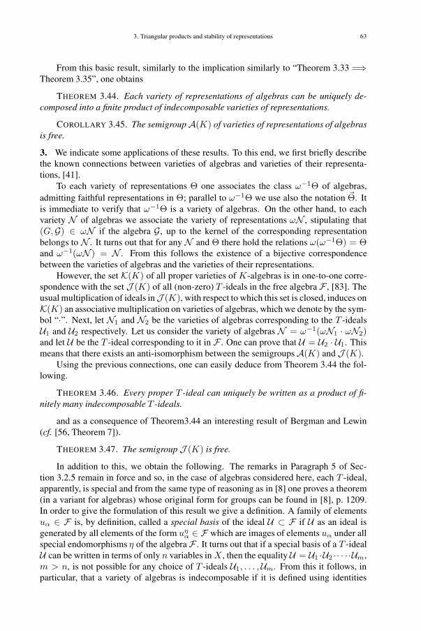
3. Triangular products and stability of representations 63
From this basic result, similarly to the implication similarly to “Theorem 3.33 =⇒Theorem 3.35”, one obtains
THEOREM 3.44. Each variety of representations of algebras can be uniquely de-composed into a finite product of indecomposable varieties of representations.
COROLLARY 3.45. The semigroupA(K) of varieties of representations of algebrasis free.
3. We indicate some applications of these results. To this end, we first briefly describethe known connections between varieties of algebras and varieties of their representa-tions, [41].
To each variety of representations Θ one associates the class ω−1Θ of algebras,admitting faithful representations in Θ; parallel to ω−1Θ we use also the notation �Θ. Itis immediate to verify that ω−1Θ is a variety of algebras. On the other hand, to eachvariety N of algebras we associate the variety of representations ωN , stipulating that(G,G) ∈ ωN if the algebra G, up to the kernel of the corresponding representationbelongs to N . It turns out that for any N and Θ there hold the relations ω(ω−1Θ) = Θand ω−1(ωN ) = N . From this follows the existence of a bijective correspondencebetween the varieties of algebras and the varieties of their representations.
However, the set K(K) of all proper varieties of K-algebras is in one-to-one corre-spondence with the set J (K) of all (non-zero) T -ideals in the free algebra F , [83]. Theusual multiplication of ideals inJ (K), with respect to which this set is closed, induces onK(K) an associative multiplication on varieties of algebras, which we denote by the sym-bol “·”. Next, let N1 and N2 be the varieties of algebras corresponding to the T -idealsU1 and U2 respectively. Let us consider the variety of algebras N = ω−1(ωN1 · ωN2)and let U be the T -ideal corresponding to it in F . One can prove that U = U2 · U1. Thismeans that there exists an anti-isomorphism between the semigroupsA(K) and J (K).
Using the previous connections, one can easily deduce from Theorem 3.44 the fol-lowing.
THEOREM 3.46. Every proper T -ideal can uniquely be written as a product of fi-nitely many indecomposable T -ideals.
and as a consequence of Theorem3.44 an interesting result of Bergman and Lewin(cf. [56, Theorem 7]).
THEOREM 3.47. The semigroup J (K) is free.
In addition to this, we obtain the following. The remarks in Paragraph 5 of Sec-tion 3.2.5 remain in force and so, in the case of algebras considered here, each T -ideal,apparently, is special and from the same type of reasoning as in [8] one proves a theorem(in a variant for algebras) whose original form for groups can be found in [8], p. 1209.In order to give the formulation of this result we give a definition. A family of elementsuα ∈ F is, by definition, called a special basis of the ideal U ⊂ F if U as an ideal isgenerated by all elements of the form uη
α ∈ F which are images of elements uα under allspecial endomorphisms η of the algebra F . It turns out that if a special basis of a T -idealU can be written in terms of only n variables in X , then the equality U = U1 ·U2 · · · ··Um,m > n, is not possible for any choice of T -ideals U1, . . . ,Um. From this it follows, inparticular, that a variety of algebras is indecomposable if it is defined using identities

64 CHAPTER I. REPRESENTATIONS OF SEMIGROUPS AND ALGEBRAS
in only one variable (from X). Using the Nagata-Higman theorem (cf., e.g. [83, Ap-pendix C]), we deduce that there exist indecomposable varieties consisting of radicalalgebras.
4. In order to exhibit still another series of indecomposable varieties of algebras, letus first prove an auxiliary statement. We denote by varK the variety generated by theclass of algebras K, at the same time we denote, as before, by VarK the variety ofrepresentations of algebras generated by their class K. Furthermore, if one adjoins tothe algebra S a unit, we get as the result an algebra S∗ and the regular representation(S∗,S).
LEMMA 3.48. For any algebra S and a faithful representation (L,S) of it we havethe formula
varS =−−−−−−→Var(L,S).
PROOF. Denote Θ1 = ω varS and Θ2 = Var(L,S). It follows from the definitionof Θ1 that (L,S) ∈ Θ1, which is sufficient for Θ2 ⊂ Θ1. Let us prove the converse inclu-sion. Using the existence for any c ∈ L of an isomorphism of pairs (S∗/AnnS(c),S) ∼=∼= (c·S∗,S) and Remak’s theorem, we see that the regular pair (S∗/∩c∈L AnnS(c),S) iscontained in Θ2. But from the fact that (L,S) is faithful it follows that ∩c∈L AnnS(c) =0, giving that the pair (S∗,S) lies in Θ2. Next, let (A, T ) be an arbitrary pair in the va-riety Θ1, while (A, T1) is the corresponding faithful pair. It follows from (A, T1) ∈ Θ1
that T1 ∈ varS and, therefore, T1 ∈ QSCS. Let us show that from the last thing itfollows that (T ∗
1 , T1) ∈ Θ2.In the case T1 = SI (Cartesian power) the statement is easy to prove if we use the
embedding (SI)∗ → (S∗)I and the fact that Θ2 is closed with respect to to subpairsand Cartesian products. If T1 is a subalgebra of SI then the embedding (T ∗
1 , T1) →((SI)∗,SI) shows that (T ∗
1 , T1) ∈ Θ2. Finally, let T1 be the endomorphic image ofthe subalgebra S1 ⊂ SI . We have the endomorphism of pairs (S∗
1 ,S) � (T ∗1 , T1),
so in view of (S∗1 ,S) ∈ Θ2 it follows that (T ∗
1 , T ) ∈ Θ2. Thus we have proved thatT1 ∈ varS implies (T ∗
1 , T1) ∈ Θ2.Now it is not hard to see that (A, T1) ∈ Θ2. Indeed, for each a ∈ A the cyclic
subpair (a ◦ T ∗1 , T1) in (A, T1) is isomorphic to the pair (T ∗
1 /AnnT1(a), T1) ∈ Θ2, andso lies in Θ2. But from the membership in the variety Θ2 of all cyclic subpairs of thepair (A, T1) it follows that (A, T1) ∈ Θ2. For the proof we have to apply a variation ofthe argument in the proof of Lemma 3.27. As a result we get the inclusion Θ1 ⊂ Θ2, butalong with it also the equality ω(varS) = Var(L,S). Applying to the main part of thisequation the operator ω−1 we are lead to the formula of interest to us. �
5.
THEOREM 3.49. If the algebraA is semi-simple (in the sense of Jacobson), then thevariety varA is indecomposable.
PROOF. 1) Assume that the algebra is primitive. In this case there exists an irre-ducible representation (G,A). The variety of representations generated by this pair, willbe denoted by Θ. From the relation A ∈ ω−1Θ we deduce that (A∗,A) ∈ Θ; cf.Lemma 3.48 for this type of proof. On the other hand, there exists an epimorphism of

3. Triangular products and stability of representations 65
pairs (A∗,A) � (G,A), from which it follows that (G,A) ∈ Var(A∗,A), hence alsoΘ = Var(A∗,A). Lemma 3.48 now gives ω−1Θ = varA.
Let us assume that varA = N2 · N1 and that to the variety Ni in F correspondsthe T -ideal Ui, i = 1, 2. Consider the variety N = ω−1(ωN1 · ωN2). In Paragraph 3of this section it was stated that the T -ideal corresponding to this variety of algebras isU2 ·U1. But this T -ideal corresponds to the varietyN2 ·N1 = varA. Hence,N = varA.From this we deduce that Θ = ωN1 · ωN2, that is, the decomposablity of the variety ofrepresentations Var(G,A). But this is a contradiction, as will be proved in the secondhalf of the proof.
2) Let the algebraA be semi-simple. Then it is a subdirect sum of primitive algebras:
A =.∑sd
i∈I
Ai, Ai∼= A/Di,
⋂i∈I
Di = 0.
Furthermore, let (Gi,Ai) be a faithful irreducible representation corresponding to theprimitive summand Ai. Repeating the argument of the first part of the proof, we derivethe equalities Var(Gi,Ai) = Var(A∗
i ,Ai), i ∈ I . However, the pairs (A∗i ,Ai) are
contained in the variety Var(A∗,A); this follows from the existence of an epimorphism(A∗,A) � (A∗
i ,Ai). Moreover, it follows from Remak’s theorem that Var(A∗,A) ⊂Var(
⋃i∈I(A∗
i ,Ai)). In view of the equalities Var(A∗i ,Ai) = Var(Gi,Ai), i ∈ I ,
it follows from this that the variety Var(A∗,A) is generated by the irreducible pairs(Gi,Ai). Using these facts we show that Var(A∗,A) is indecomposable.
Let us assume that Var(A∗,A) = Θ1·Θ2. Introduce the notation Ω =⋃
i∈I(Gi,Ai)and Ωl = Θl ∩ Ω, l = 1, 2. It turns out that one has Ω = Ω1 ∪ Ω2. Apparently, we haveonly to comment on the inclusion Ω ⊂ Ω1 ∪ Ω2. If a pair (Gi,Ai) is not contained inΩ1, then it is not contained in Θ1 either. But at the same time, it follows from (Gi,Ai) ∈Θ1 ·Θ2 that there exists a subpair (Hi,Ai) in (Gi,Ai) such that and (Hi,Ai) ∈ Θ1 and(Gi/Hi,Ai) ∈ Θ2. As (Gi,Ai) is irreducible, it follows, however, that either Hi = 0 orHi = Gi. In the second case (Gi,Ai) ∈ Θ1, which is excluded. Hence Hi = 0 and so(Gi,Ai) ∈ Θ2, hence also (Gi,Ai) ∈ Ω2. The inclusion Ω ⊂ Ω1 ∪Ω2 is established.
From the equality Ω = Ω1∪Ω2 and the relation Var(A∗,A) ⊂ VarΩ it follows thatΘ1 ·Θ2 = Var Ω1 ·VarΩ2. As the semigroup of varieties of representations is free, thisthen shows that Θ� = Var Ω�, � = 1, 2. Furthermore, from the definitions we deducethat Θ1 ·Θ2 ⊂ Var(Θ1 ∪Θ2) ⊂ Θ2 ·Θ1.
In the case of incidence of the varieties Θ1 and Θ2, the preceding relation gives acontradiction. Indeed, if, for example, Θ1 ⊂ Θ2, then Ω ⊂ Θ2 and so Θ1 · Θ2 = Θ2,which is a contradiction. Therefore, in order to complete the proof of the theorem itsuffices to show that Θ1 and Θ2 are incident.
We argue by contradiction and choose arbitrary (Gi′ ,Ai′) ∈ Ω1\Θ2 and(Gi′′ ,Ai′′) ∈ Ω2\Θ1; here i′, i′′ ∈ I . In the triangular product (G,G) = (Gi′ ,Ai′)�(Gi′′ ,Ai′′) we take a verbal with respect to Θ1. As (G,G) ∈ Θ1 · Θ2 ⊂ Θ2 · Θ1, wehave (∗Θ1(G,G),G) ∈ Θ2. The irreducibility of all pairs in Ω implies that the only G-modules in G are 0, Gi′ and G. If now ∗Θ1(G,G) is 0 or Gi′ , then, together with the pair(G,G) or the pair (G/Gi′ ,G) � (Gi′′ ,G) respectively, also its subpair (Gi′′ ,Ai′′ ) liesΘ1, which was excluded by the choice. If ∗θ1(G,G) = G, then, likewise, (Gi,Ai) ∈ Θ2,which also was excluded. The statement is proved.

66 CHAPTER I. REPRESENTATIONS OF SEMIGROUPS AND ALGEBRAS
Let us note that the reasoning given works also in the case |I| = 1, guaranteeing theindecomposability of Var(A∗,A) in the first part of the proof. This proves the theorem.
�
6. For associative K-algebras one can introduce a operation of wreath product. Namely,for the algebrasA and B we consider the K-module HomK(B∗,A∗) as an algebra withzero multiplication and set
AwrB def= HomK(B∗,A∗) � (A⊕ B),
we call this algebraAwrB the wreath product of the algebrasA and B.The operation of the wreath product of algebras permits us to make explicit the
generating algebra of the product of varieties of algebras. Indeed, let A = varA andB =varB. Using Lemma 3.48 and the theorem of generating representations of algebras, weobtain
ω(B · A) = ωA · ωB = Var(A∗,A) ·Var(B∗,B) =
= Var((A∗,A)�Var(B∗,B)) = Var(A∗ ⊕ B∗,AwrB) =
= Var((AwrB)∗,AwrB) = ωvar (AwrB).
Let us add that in this computation we used the equation
Var(A∗ ⊕ B∗,AwrB) = Var((AwrB)∗,AwrB),
the verification of which is immediate on the basis of the properties of the correspondinggenerating pairs.
These computations prove the following
THEOREM 3.50. For any two algebrasA and B holds the formula
(varB) · (varA) = var (AwrB).
Finally, let us indicate yet another application of the wreath product of algebras. AT -ideal is called finitary, if the variety of algebras defined by it is generated by a finitedimensional algebra.
THEOREM 3.51. The product of finitely many T -ideals in F is finitary if and only ifall the factors are finitary.
PROOF. It is clearly sufficient to prove the theorem for two T -ideals U1 and U2.Thus, let the T -ideals Ui be finitary, and let the varietiesNi defined by them be generatedby the finite dimensional algebrasAi, i = 1, 2. The product U1 · U2 is a T -ideal definingthe varietyN1 · N2. According to Theorem 3.50 the variety A1 · N2. is generated by thealgebra
A2wrA1 = Hom(A∗1,A∗
2) � (A2 ⊕A1),
which clearly is finite dimensional. Thus the finitarity of U1 · U2 is established.Conversely, assume that the T -idealU1U2 is finitary. Then the varietyN1·N2 defined
by it is generated by some finite dimensional algebra G, A1 · N2 = varG. Let us thenconsider the regular pair (G∗,G), which in view of Lemma 3.48 generates the varietyωN2 · ωN1. Take in G∗ a right ideal A such that (A,G) ∈ ωN2 and (G∗/A,G) ∈ ωN1.

3. Triangular products and stability of representations 67
According to Propositions 3.17 and 3.40 we have (G∗,G) ∈ Var((A,G)� (G∗/A,G)).However, using the theorem of generating representations, generating we have
Var((A,G)� (G∗/A,G)) ⊂ ωN2 · ωN1,
from which it follows that
ωN2 · ωN1 = Var(G∗,G) ⊂ Var(A,G) · Var(G∗/A,G) ⊂ ωN2 · ωN1.
Thus we have proved the equality
Var(A,G) ·Var(G∗/A,G) = ωA2 · ωN1,
where Var(A,G) ⊂ ωN2 and Var(G∗/A,G) ⊂ ωA1. By the Corollary to Theorem 3.44it follows from this that ωN2 = Var(A,G) and ωA1 = Var(G∗/A,G). Thus, the vari-eties ωN1 and ωN2 are generated by finite dimensional pairs. Let (C1,H1) be a finitedimensional faithful pair generating the variety of representations ωN1. Then the alge-bra H1 is a finite dimensional K-algebra, and it is not hard to see that N1 = varH1.Thus, the ideal U1 is finitary. In an analogous manner one shows that the T -ideal U2 isfinitary. �7. Let T = T (n) be the algebra of upper triangular matrices of ordern over the field K .The natural representation (L, T ) of this algebra is faithful and there is the isomorphismof representations
(L, T ) ∼= (K,K)� · · · � (K,K)︸ ︷︷ ︸n times
.
According to Theorem 3.43 we get from this the equation
Var(L, T ) = (Var(K,K))n.
Moreover, we remark that the variety of algebras varT and the variety of representationsof algebras Var(L, T ) correspond in the free algebra F to one and the same T -ideal Tn:proof by unwrapping the definitions. This remark and the anti-isomorphism of the semi-group of varieties of representations with the semigroup of T -ideals of the algebra Fallows us to rewrite the above equation as Tn = T n
1 , T1 being the ideal of identities ofthe algebra K . Thus we have proved the following.
THEOREM 3.52. The ideal of identities of the algebra of upper triangular matricesof order n over the field K coincides with T n
1 , T1 being the ideal of identities of thealgebra K .
For charK = 0 this theorem coincides with the result of Yu. N. Mal’cev (1971)stating that the ideal Tn is generated by the polynomials
[x1, x2][x3, x4] · · · · · [x2n−1, x2n],
where we have written [x, y] = xy − yx. In the case charK > 0 this constitutes ananswer to Problem 109 in [6].

68 CHAPTER I. REPRESENTATIONS OF SEMIGROUPS AND ALGEBRAS
3.2.7. Comments
1. The notion of automaton as an object for mathematical inquiry arose long ago andsimultaneously in many papers; cf. [31]. The connections of this circle of questions inTheoretical Computer Science with Algebra (as indicated in B. M. Glushkov [9]) ledto the proof of the basic theorems on decomposition of automata; a systematic study ofthese questions and their connection with linear systems was given in [18]. The point ofview of automata as three-sorted systems and their connections with pairs, as in the workof B. I. Plotkin and others in [42], has led to a systematic application in automata theoryof the techniques ready in the theory of representations. In particular, the �-productintroduced in Section 3.1 for semigroups leads to the construction of the �-product ofMoore automata and to a proof of theorems analogous to the theorems of Kaluzhnin-Krasner and Krohn-Rhodes (B. I. Plotkin, unpublished). In problems of classification oflinear automata, as indicated in the present chapter, the bijection between the varieties oflinear automata varieties and ideal pairs in the algebra F proves to be useful. Here thisbijection is used for the study of the multiplicative properties of the set of varieties oflinear automata.
2. The subject of this chapter is related to the theme of unique factorization of ring andsemigroups. The unique factorization in the ring of integers is beautiful and useful, andits properties have been known over a long time, but already in some rings of algebraicintegers it is not easy to establish this property. The study of the rings of linear differen-tial operators (Edmund Landau, 1902) led to the question of the unique decompositionof elements in certain non-commutative rings. Much attention has been devoted to theunique factorization in semigroups, as the unique factorization of a ring is a propertyof its multiplicative semigroup; cf. the paper [62] and the book of P. Cohn [5]. TheTheorems 3.35 and 3.46 proved in this chapter are natural reformulations of the themeindicated parallel to the Theorem 23.4 in [34] and of the main theorem in [43].
3. It is clear that the approach described in Paragraph 7 of Section 3.2.6 allows us toreduce the search of a basis for the identities of the algebra T of upper block-triangularmatrices to the corresponding case of diagonal blocks. A definitive answer can be ob-tained in the case when the sizes of the upper triangular matrices from T do not exceedtwo, while the field K is either finite or has characteristic 0, because thanks to work byYu. N. Mal’cev, E. N. Kuzmin and Yu. P. Razmyslov one knows a basis for the identitiesof square matrices for such fields.
4. In the theory of varieties of algebras one encounters usually another multiplication.Let us denote by T (A) the T-ideal defining a variety of (associative) K-algebrasA. Thenfor any two varieties of algebrasA1 andA2, their productA1∗A2 is the variety of algebrasdefined by the T-ideal TA1 ∗ TA2, generated by the set {f(g1 . . . gn) | f(x1 . . . xn) ∈T (A1), g1 . . . gn ∈ T (A2)} ⊂ F . It is possible that an improvement of the approach inthis Section 3.2 together with an attraction of the notion of the free Menger system16 al-lows to achieve progress in the description of the “*-structure” arising here (cf. Problems18 and 25 in [6]).
16Translators’ note. Cf. Jaak Henno. Free G-commutative Menger systems. In: Mathematics and Theo-retical Mechanics, VIII, Proc. Estonian Acad. Sci., Phys. Math., 373, 1975, 19–26

3. Triangular products and stability of representations 69
5. Our treatment of M(K) and L(K) as locally finite partially ordered sets togetherwith the information on indecomposable elements in these semigroups permits us, really,to use with advantage ideas in [98] and to develop the analytic side of a question in thespirit of the book [86].
3.3. Powers of the fundamental ideal and stability of representationsof groups and semigroups
Let ZΓ be the integral group ring of a group Γ. The fundamental ideal Δ in the ringZΓ is the kernel of the homomorphism ZΓ → Z; in other words Δ is the set of allpossible finite sums
∑i niγi, where ni ∈ Z, γi ∈ Γ, such that
∑i ni = 0. Powers
of Δ are defined inductively, that is, Δν = Δν−1 · Δ for a non-limit ordinal ν andΔν =
⋂μ<ν Δμ for limit ordinals ν. In the ring ZΓ there is a decreasing series of ideals
(9) ZΓ ⊃ Δ ⊃ Δ2 ⊃ · · · ⊃ Δν ⊃ Δν+1 ⊃ . . . .
Let τ = τ(Γ) be the index of stabilization the series (9), that is, τ is an ordinal numberbeginning from which Δτ = Δτ+1 = . . . Partially following [71], we use the followingnotation and terminology: τ = τ(Γ) is the terminal of the group Γ; Δ∞ = Δτ(Γ) isthe terminal of the ring ZΓ; Dν = Γ ∩ (1 + Δν) is the ν-th (generalized) dimensionalsubgroup: in particular, D∞ = D∞(Γ) = Γ ∩ (1 + Δ∞) is the limit dimensionalsubgroup (shorter limit) of Γ.
The goal of this Section is the computation of the terminal and the limit of variousfinite groups, and also of Artinian groups. A main role in these computations is playedby the apparatus of triangular products and the connection of the question with stability,as described in Section 3.1. For this approach it is highly essential that for some classesof nilpotent groups it is possible to carry out the computation of the terminal exactly.This constitutes the main subject of Section 3.3.1. There we give also the definitionsand known facts necessary in the proofs, and, furthermore, the proof of a refinement of atheorem of Gruenberg [69, Theorem B]. The main part of the following two sections con-cerns the terminal and the limit of finite groups. Section 3.3.4 is devoted to an extensionof the theme of stability (and likewise, in a perspective, also the problem of the terminal)for semigroups. Here the technique of quasi-rings (distributively generated near-rings) isuseful, [68].
Everywhere in Sections 3.3.1–3.3.3, while studying pairs (G,Γ) the acting objectΓ will be a group, and the domain of action G an Abelian group. In this way, pairs arerepresentations of groups by automorphisms of Abelian groups. The symbol17 ω denotesthe first infinite ordinal, and, likewise, the operator associating to a subgroup in Γ theright ideal in ZΓ. Finally, we remark that writing A ⊂ B does not exclude the equalityof the sets A and B.
17Such is the tradition, whose meaning is readily understood from the context.

70 CHAPTER I. REPRESENTATIONS OF SEMIGROUPS AND ALGEBRAS
3.3.1. Preliminary topics; on the terminal of nilpotent groups
1. Let there be given a pair (G,Γ). We fix γ ∈ Γ and assume that in G there is a finitedecreasing series of subgroups
(10) G = S0 ⊃ S1 ⊃ · · · ⊃ Sm = 0
such that for all i = 0, 1, . . . ,m − 1 the condition g ◦ γ − g ∈ Si+1 is fulfilled for allg ∈ Si. In such a situation we say that γ acts finitely stably with respect to the series(10). If all γ ∈ Γ satisfy this condition, then we say that the group Γ is finitely stablewith respect to (10); the pair (G,Γ) is then also called, by definition, finitely stable (moreexactly, m-stable), which will be written (G,Γ) ∈ Sm. In the case of a faithful pair(G,Γ) the group G is a subgroup of the stabilizer of the series (10). The latter constitutesthe collection of all automorphisms of G which act stably on (10). By a well-knowntheorem by L. A. Kaluzhnin ([19, p. 144]; [84]) it is a nilpotent group. The fact that afaithful pair (G,Γ) is finitely stable with respect to (10) will be written (G,Γ) ∈ Sm.Moreover, if for a given group Γ it is only important the existence of such a pair, and notthe concrete nature of G, we write Γ ∈ −→Sm. What can be said about the structure of thestabilizer of an infinite decreasing series of subgroups in an Abelian group? What grouptheoretic properties enjoys a group Γ which embeds in the stabilizer of a series of type
(11) G = S0 ⊃ S1 ⊃ Sα ⊃ · · · ⊃ Sσ = 0,
in this case we write (G,Γ) ∈ Sσ and also simply Γ ∈ −→S∞. It appears that this is tightlyconnected with the problem of the calculation of the limit of the group Γ.
For the pair (G,Γ) we introduce the notation [g, γ] = −g+ g ◦ γ, g ∈ G, γ ∈ Γ; theZ-module generated by all [g, γ], g ∈ G, γ ∈ Γ, will be called the mutual commutator ofG and Γ and denoted by [G,Γ]. One can introduce the submodule [G,Γ, ν] for all ordinalnumbers ν. To this end we set [G,Γ, 0] = G, [G,Γ, 1] = [G,Γ], and, furthermore,we define by induction [G,Γ, ν] = [[G,Γ, ν − 1],Γ] for each non-limit ordinal ν and[G,Γ, ν] =
⋂μ<ν [G,Γ, μ] for each limit ν. The series
(12) G ⊃ G1 ⊃ · · · ⊃ Gν ⊃ Gν+1 ⊃ . . . , where Gν = [G,Γ, ν]
is called18 the lower stable series of the pair (G,Γ). For example, in case of the regularpair (ZΓ,Γ) the series (12) coincides with (9). The stability of the action of Γ on (11)means, by definition, that [Sν ,Γ] ⊂ Sν+1 for all ν < σ. A trivial induction shows that[G,Γ, ν] ⊂ Sν for all ν ≤ σ. We remark that together with Γ there acts in G also thegroup ring ZΓ. We can, in particular, write [g, γ] = g◦(γ−1) so that [G,Γ, n] = G◦Δn
for n = 1, 2, 3, . . . . However, in general we only have G ◦ Δω ⊂ Gω =⋂
n G ◦ Δn.Transfinite induction shows that G ◦Δν ⊂ Gν for all ordinals ν.
It turns out that the condition Γ ∈ −→S∞ is equivalent to the triviality of the limit ofΓ, i.e. the condition D∞(Γ) = 1. Indeed, let Γ ∈ −→S∞; then there exists a faithful pair(G,Γ) such that Γ is embedded in a stabilizer of a series of the type (11). In particular,we have G ◦ Δσ ⊂ Sσ = 0. The fact that (G,Γ) is faithful gives now Dσ = 1, as foreach γ ∈ Dσ (in view of γ − 1 ∈ Δσ) we have G ◦ (γ − 1) = 0. Clearly, D∞ ⊂ Dσ
implies D∞ = 1. In order to prove the implication in the converse direction we consider
18One speaks also of the lower Γ-stable series of G.

3. Triangular products and stability of representations 71
the pair (ZΓ/Δ∞,Γ/D∞). This is a faithful pair, and the group Γ/D∞ acts stably onthe series
(13) ZΓ/Δ∞ ⊃ Δ/Δ∞ ⊃ · · · ⊃ Δ∞/Δ∞ = 0.
Thus we have Γ/D∞ ∈ −→S∞ whence it follows for D∞ = 1 that Γ ∈ −→S∞
We note the possibility of more general formulations considered in [39]; the varietyS of pairs with identical action can be replaced with an arbitrary variety of pairs X . Thefundamental ideal Δ is then replaced by an ideal DX ⊂ ZΓ, namely by the indicator ofthe class X in ZΓ, cf. Section 3.1.2.
2. Here we present a list of known facts, which below will be frequently used. Thefollowing three statements are due to V. G. Vilyatser (cf. [35, p. 458–464]).
LEMMA 3.53. If for a pair (G,Γ) the element of finite order σ ∈ Γ is an outernil-element with respect to G, and [G, σ] is torsion free, then σ is a pure element.
LEMMA 3.54. Let the pair (G,Γ) be finitely stable. An element σ ∈ Γ is an almostπ-element if and only if [G, σ] is a π-group.
We are also going to use a corollary of this lemma.
LEMMA 3.55. For a finitely stable pair (G,Γ) the group Γ is a relative π-group ifand only if [G,Γ] is a π-group.
LEMMA 3.56. If a pair (G,Γ) is contained in S∞, then the group Γ is residuallynilpotent.
PROOF. By hypothesis, for the members Gk of the lower Γ-stable series of G onehas
⋂k≥0 Gk = 0. Let Σk be the kernel of (G/Gk,Γ). Then the pair (G/Gk,Γ/Σk) is
faithful and finitely stable and so the group Γ/Σk is nilpotent (according to Kaluzhnin’stheorem). For any k ≥ 0, g ∈ G, σ ∈ Σ =
⋂∞k Σk there exists a gk ∈ Gk such that
g ◦ σ = g + gk. Consequently, g ◦ σ − g ∈ ⋂∞k Gk , that is g ◦ σ − g = 0. Hence,
σ ∈ Ker (G,Γ), so that, (G,Γ) being faithful, we must have σ = 1 and Σ = 1. �
LEMMA 3.57 (Connell, [63]). If Γ is infinite, then the left annihilator of the funda-mental ideal Δ in the ring ZΓ equals zero.
LEMMA 3.58 (Hartley, [77]). Assume that Γ contains an element x of prime orderp. Then for the fundamental ideal Δ ⊂ ZΓ one has
(a) p(1− x) ∈ Δp;(b) (1− x)(1 − ypn
) ∈ Δn+2 for all y ∈ Γ and n ≥ 0.
LEMMA 3.59 (Buckley, [60]). Let γ1 and γ2 be a pair of commuting elements ofrelatively prime orders in Γ. Then the element (γ1 − 1)(γ2 − 1) is contained in the idealΔω+1 ⊂ ZΓ.
LEMMA 3.60 (Plotkin, [39]). Assume that (A,Γ) is a pair, Σ a normal subgroup ofΓ having a central (in Γ) series of length m, (A,Σ) ∈ Sn, and that A∗ is the submoduleof Σ-invariant elements of A. If the pair (A∗,Γ) belongs to the variety X , then (A,Γ) ∈Xnm
.

72 CHAPTER I. REPRESENTATIONS OF SEMIGROUPS AND ALGEBRAS
Below this lemma will be used in the case m = 1, in which case Σ is a centralsubgroup of Γ. The proof of the lemma in this special case runs by induction over thelength n of the upper Σ-stable series of A,
0 ⊂ A∗ ⊂ H2 ⊂ · · · ⊂ Hn = A.
Consider the case n = 2. For any σ ∈ Σ introduce the map f(σ) : A → A by therule
∀a ∈ A, af(σ) = a ◦ (σ − 1) .In view of the centrality of the subgroup Σ every map f(σ), σ ∈ Σ, permutes with theaction of Γ in A and so is an endomorphism of the Γ-module A. Let Aσ = Ker f(σ);it is clear that
⋂σ∈ΣAσ = A∗. In view of the properties of the class X we have
(A/Aσ,Γ) ∈ X and, applying Remak’s theorem , deduce (A/A∗,Γ) ∈ X . This, to-gether with (A∗,Γ) ∈ X , gives the required statement (A,Γ) ∈ X 2. �
The general case. It is clear that
0 ⊂ H2/A∗ ⊂ · · · ⊂ A/A∗
is the upper Σ-stable series of length ≤ n − 1 in A/A∗; in particular, H2/A∗ is the
submodule of Σ-invariant elements in A/A∗. Hence (A/A∗,Σ) ∈ Sn−1. The relation(H2/A
∗,Γ) ∈ X is derived similarly to how (A/A∗,Γ) ∈ X was obtained in the firstpart of the proof. By the induction hypothesis we have here (AA∗/,Γ) ∈ Xn−1. Thisproves the Lemma for m = 1. �
LEMMA 3.61 (Gruenberg, [70]). The terminal of a group, for which the factor groupby the commutator subgroup is complete and torsion, equals two.
Essential applications of the proofs can be found in
THEOREM 3.62 (P. Hall, [72]). The integral group ring of a group, which admits aninvariant polycyclic subgroup of finite index, satisfies the ascending chain condition forright ideals.
3. We give a simple proof, essentially based on the following fact.
PROPOSITION 3.63 ([71] or [39]). The group Γ has a finite terminal if and only ifeither Γ = [Γ,Γ] and then τ(Γ) = 1, or Γ �= [Γ,Γ], and then Γ/[Γ,Γ] is a completetorsion group, so in this case τ(Γ) = 2.
PROOF. In the case Γ = Γ′ = [Γ,Γ] we use the following identity, valid for allγ1, γ2 ∈ Γ:
γ−11 γ−1
2 γ1γ2 − 1 = γ−11 γ−1
2 [(γ1 − 1)(γ2 − 1)− (γ2 − 1)(γ1 − 1)],
and conclude at once that ΔΓ = Δ2Γ.
Next, assume that Γ �= Γ′. First, we remark the following. Let ϕ : Γ → Σ be anarbitrary epimorphism and M = Kerϕ. By the assumption Δn
Γ ⊂ Δn+1Γ it follows that
(ΔnΓ + ωM)/ωM ⊂ (Δn+1
Γ + ωM)/ωM.
Under the isomorphism ZΓ/ωM ∼= Z(Γ/M) the ideal (ΔnΓ +ωM)/ωM is mapped onto
ΔnΣ. We conclude that Δn
Σ ⊂ Δn+1Σ . Thus, every homomorphic image of a group with a
finite terminal also has a finite terminal. In particular, the terminal of the Abelian groupΓ = Γ/Γ′ must be finite. If Γ is not complete then there exists an epimorphism Γ � T
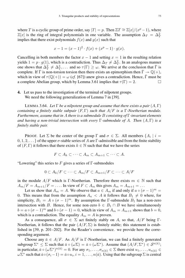
3. Triangular products and stability of representations 73
where T is a cyclic group of prime order, say |T | = p. Then ZT ∼= Z[x]/(xp−1), whereZ[x] is the ring of integral polynomials in one variable. The assumption ΔT = Δ2
T
implies that there exist polynomials f(x) and g(x) such that
x− 1 = (x− 1)2 · f(x) + (xp − 1) · g(x).
Cancelling in both members the factor x − 1 and setting x = 1 in the resulting relationyields 1 = p · g(1), which is a contradiction. Thus ΔT �= Δ2
T . In an analogous mannerone shows that Δ2
T �= Δ3T , . . . and so τ(Γ) ≥ ω. We arrive at the conclusion that Γ is
complete. If Γ is non-torsion torsion then there exists an epimorphism then Γ � Q(+),which in view of τ(Q(+)) = ω (cf. [67]) anew gives a contradiction. Hence, Γ must bea complete Abelian group, which by Lemma 3.61 implies that τ(Γ) = 2. �
4. Let us pass to the investigation of the terminal of nilpotent groups.We need the following generalization of Lemma 7 in [39].
LEMMA 3.64. Let Γ be a nilpotent group and assume that there exists a pair (A,Γ)containing a finitely stable subpair (F,Γ) such that A/F is a Γ-Noetherian module.Furthermore, assume that in A there is a submoduleB consisting of Γ-invariant elementsand having a non-trivial intersection with every Γ-submodule of A. Then (A,Γ) is afinitely stable pair.
PROOF. Let Σ be the center of the group Γ and σ ∈ Σ. All members {Ai | i =0, 1, 2, . . .} of the upper σ-stable series of A are Γ-admissible and from the finite stabilityof (F,Γ) it follows that there exists k ∈ N such that that we have the series
F ⊂ Ak ⊂ · · · ⊂ Am ⊂ Am+1 ⊂ · · · ⊂ A.
“Lowering” this series to F gives a series of Γ-submodules
0 ⊂ Ak/F ⊂ · · · ⊂ Am/F ⊂ Am+1/F ⊂ · · · ⊂ A/F
in the module A/F which is Γ-Noetherian. Therefore there exists m ∈ N such thatAm/F = Am+1/F = . . . . In view of F ⊂ Am this gives Am = Am+1 = . . .
Let us show that Am = A. We observe that a ∈ Am if and only if a ◦ (σ − 1)m =0. This means that from the assumption An < A it follows that B1 �= 0 where, forsimplicity, B1 = A ◦ (σ − 1)m. By assumption the Γ-submodule B1 has a non-zerointersection with B. Hence, for some non-zero b ∈ B1 ∩ B we have simultaneouslyb = a ◦ (σ − 1)m and b ◦ (σ − 1) = 0, which in view of Am = Am+1 shows that b = 0,which is a contradiction. The equality Am = A is proven.
As a consequence, all σ ∈ Σ act finitely stably on A, so that, A/F being Γ-Noetherian, it follows that the pair (A/F,Σ) is finitely stable; this statement is estab-lished in [39, p. 201–202]. For the Reader’s convenience. we provide here the corre-sponding argument.
Choose any a ∈ A/F . As A/F is Γ-Noetherian, we can find a finitely generatedsubgroup Σ∗ ≤ Σ such that a ◦ (ωΣ) = a ◦ (ωΣ∗). Assume that (A/F,Σ∗) ∈ Sn(a);in particular, a ◦ (ωΣ∗)n(a) = 0. For any σ1, . . . , σn(a) ∈ Σ there exist u1, . . . , un(a) ∈ωΣ∗ such that a◦(σi−1) = a◦ui, i = 1, . . . , n(a). Using that the subgroup Σ is central
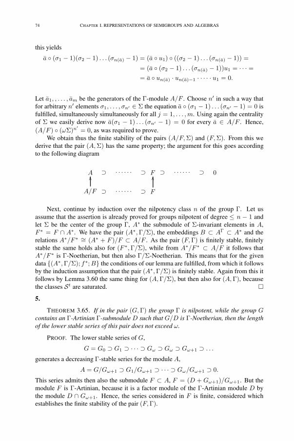
74 CHAPTER I. REPRESENTATIONS OF SEMIGROUPS AND ALGEBRAS
this yields
a ◦ (σ1 − 1)(σ2 − 1) . . . (σn(a) − 1) = (a ◦ u1) ◦ ((σ2 − 1) . . . (σn(a) − 1)) =
= (a ◦ (σ2 − 1) . . . (σn(a) − 1))u1 = · · · == a ◦ un(a) · un(a)−1 · · · · · u1 = 0.
Let a1, , . . . , am be the generators of the Γ-module A/F . Choose n′ in such a way thatfor arbitrary n′ elements σ1, . . . , σn′ ∈ Σ the equation a ◦ (σ1 − 1) . . . (σn′ − 1) = 0 isfulfilled, simultaneously simultaneously for all j = 1, . . . ,m. Using again the centralityof Σ we easily derive now a(σ1 − 1) . . . (σn′ − 1) = 0 for every a ∈ A/F . Hence,(A/F ) ◦ (ωΣ)n′
= 0, as was required to prove.We obtain thus the finite stability of the pairs (A/F,Σ) and (F,Σ). From this we
derive that the pair (A,Σ) has the same property; the argument for this goes accordingto the following diagram
A ⊃ · · · · · · ⊃ F ⊃ · · · · · · ⊃ 0
A/F
��
⊃ · · · · · · ⊃ F
��
Next, continue by induction over the nilpotency class n of the group Γ. Let usassume that the assertion is already proved for groups nilpotent of degree ≤ n − 1 andlet Σ be the center of the group Γ, A∗ the submodule of Σ-invariant elements in A,F ∗ = F ∩ A∗. We have the pair (A∗,Γ/Σ), the embeddings B ⊂ AΓ ⊂ A∗ and therelations A∗/F ∗ ∼= (A∗ + F )/F ⊂ A/F . As the pair (F,Γ) is finitely stable, finitelystable the same holds also for (F ∗,Γ/Σ), while from A∗/F ∗ ⊂ A/F it follows thatA∗/F ∗ is Γ-Noetherian, but then also Γ/Σ-Noetherian. This means that for the givendata {(A∗,Γ/Σ); f∗;B} the conditions of our lemma are fulfilled, from which it followsby the induction assumption that the pair (A∗,Γ/Σ) is finitely stable. Again from this itfollows by Lemma 3.60 the same thing for (A,Γ/Σ), but then also for (A,Γ), becausethe classes St are saturated. �5.
THEOREM 3.65. If in the pair (G,Γ) the group Γ is nilpotent, while the group Gcontains an Γ-Artinian Γ-submodule D such that G/D is Γ-Noetherian, then the lengthof the lower stable series of this pair does not exceed ω.
PROOF. The lower stable series of G,
G = G0 ⊃ G1 ⊃ · · · ⊃ Gω ⊃ Gω ⊃ Gω+1 ⊃ . . .
generates a decreasing Γ-stable series for the module A,
A = G/Gω+1 ⊃ G1/Gω+1 ⊃ · · · ⊃ Gω/Gω+1 ⊃ 0.
This series admits then also the submodule F ⊂ A, F = (D + Gω+1)/Gω+1. But themodule F is Γ-Artinian, because it is a factor module of the Γ-Artinian module D bythe module D ∩ Gω+1. Hence, the series considered in F is finite, considered whichestablishes the finite stability of the pair (F,Γ).

3. Triangular products and stability of representations 75
Set B = Gω/Gω+1 and let H be a maximal Γ-submodule in A, having zero inter-section with B; such an H does exist in view of Zorn’s lemma. Next, let us set
A = A/H, F = (F + H)/H and B = (B + H)/H.
As the pair (F,Γ) is finitely stable, it follows that (F ,Γ) is likewise finitely stable. Itsuffices to remark that there exist epimorphisms of Γ-modules
G/D � A/F � A/F
and that by this A/F is Γ-Noetherian. Thus, to the triple {A, F , B} Lemma 3.64is applicable. We deduce that the pair (A/H,Γ) is finitely stable. This shows thatGn/Gω+1 ⊂ H for some n ∈ N. This again, apparently, gives B ⊂ H . In view ofthe choice of H from this it must follow that B = 0, i.e. Gω = Gω+1. �
6. If in the assumptions of Theorem 3.65 D = 0, we are led to the following.
THEOREM 3.66 (Plotkin, [39]). If in the pair (G,Γ) the group Γ is nilpotent, whilethe module G is Γ-Noetherian, then the lower stable series of this pair has length notexceeding ω.
In turn, an immediate consequence of Theorems 3.62 and 3.66 is the following.
THEOREM 3.67 (Smith, [105]). The terminal of a Noetherian nilpotent group equalsω.
On the other hand, we have.
THEOREM 3.68. The terminal of a complete Artinian Abelian group equals 2. If Γis a non-complete nilpotent group, then τ(Γ) = ω.
PROOF. The first statement of the theorem follows from Lemma 3.61; here it is for-mulated in order to make the picture complete. Next, assume that Γ is not full. Then (cf.[22, p. 370-371]) Γ can be represented in the form Γ = Σ · Φ, where Σ is a central com-plete Artinian subgroup of Γ, and Φ a finite invariant subgroup of Γ; by our assumptionΦ �= 1. The fundamental ideal in ZΓ will be written Δ. By Proposition 3.63, Δn �= Δω
for all natural n. Let us show that Δω �= Δω+1, to this end reducing the proof of thisclaim to a situation in which Theorem 3.65 is applicable.
Let T = {γ1, . . . , γt} be a complete system of representatives of the cosets of Σin Γ, ΔΣ being the fundamental ideal in the group ring ZΣ. Let us demonstrate theexistence of direct decompositions of the form
(14) (ωΣ)r = ΔrΣ · γ1 + · · ·+ Δr
Σ · γt; r = 1, 2, . . . .
Let us denote the sum to the right in (14) by M (r). It is clear that M (r) ⊂ (ωΣ)r, becauseclearly Δr
Σ · γi ⊂ (ωΣ)r. We have to check that (ωΣ)r ⊂ M (r). We note that for anyz1, . . . , zr ∈ ΔΣ and γi1 , . . . , γir ∈ T one has z1 · . . . · zr ∈ Δr
Σ and there exist σ ∈ Σ,γk ∈ T such that γi1 ·. . .·γir = σγk. Therefore the product (z1γi1)·. . .·(zrγir ), which, asΣ is central equals (z1 . . . zr)(γi1 . . . γir ), lies in M (r). This gives (ωΣ)r ⊂ M (r). Therelation (Δr
Σ · γi) ∩ (ΔrΣ · γj) = 0 for i �= j is verified by an argument by contradiction.
In particular, we have the direct decomposition (14) for r = 1 and 2 and we obtain theisomorphism of Z-modules
ωΣ/(ωΣ)2 ∼=(ΔΣ/Δ2
Σ
)· γ1 + · · ·+
(ΔΣ/Δ2
Σ
)· γt.
By a well-known result, ΔΣ/Δ2Σ∼= Σ. Hence, the Z-module ωΣ/(ωΣ)2 is Artinian.

76 CHAPTER I. REPRESENTATIONS OF SEMIGROUPS AND ALGEBRAS
Let us consider the Γ-module G = ZΓ/Δω+1 and in it the submodule D = (ωΣ +Δω+1)/Δω+1. By Lemma 3.61 we have Δ2
Σ = Δω+1Σ . Therefore we obtain
(ωΣ)2 = Δ2Σ · γ1 + · · ·+ Δ2
Σ · γt = Δω+1Σ · γ1 + · · ·+ Δω+1
Σ · γt ⊂ Δω+1Γ .
Thus, the Z-submodule D, being an epimorphic image of the module ωΣ/(ωΣ)2i, isalso Artinian. The module G/D, being an epimorphic image of the Γ-Noetherian mod-ule ZΓ/ωΣ ∼= ZΦ is Γ-Noetherian; that Φ is Φ-Noetherian (and, likewise, ZΦ isΓ-Noetherian) follows from Theorem 3.62. What concerns the data {G,D}, all condi-tions of Theorem 3.65 are fulfilled. Therefore we may conclude that Gω = Gω+1, i.e.Δω = Δω+1. �7. In this subsection we prove Theorem 3.69, constituting a generalization of a resultby K. Gruenberg.
THEOREM 3.69. Let Δ be the fundamental ideal in the integral group ring of thegroup Γ satisfying the descending chain condition for normal subgroups, let k be a non-negative integer and λ = ω(k+ 1). In the ring ZΓ holds the relation Δλ = 0 if and onlyif the group is finite and primary.
Remark. For k = 0 this theorem reduces to a result of Gruenberg ([69, Theo-rem B]), another proof of it is given in [74]. We note that for a non-limit λ the relationΔλ = 0 is not possible in the integral group rings of an infinite group; this follows fromLemma 3.57.
PROOF. a) The condition is sufficient. Let Γ be a finite p-group. Let us denote theadditive group of the ring ZpnΓ by A. The group A � Γ is a finite p-group and, thus,nilpotent. But then the pair (A,Γ) is stable, which is equivalent to the nilpotency of thefundamental ideal Δn ⊂ ZpnΓ.
Thus, there exists a number m = m(n) such that Δmn = 0.
Furthermore, let us remark that for every natural number n the natural homomor-phism of the rings of coefficients Z → Zpn induces a homomorphism of group ringsνn : ZΓ → ZpnΓ. One verifies at once that for every natural number m there holdsthe relation (Δm)νn ⊂ Δm
n . Together with Δmn = 0 this shows that Δm(n) ⊂ Ker νn.
But Ker νn consists of all elements of the ring ZΓ whose coefficients are divisible by pn.Thus one has ∩∞
n=1Ker νn = 0. In view of the embeddings
Δω ⊂ ∞∩n=1
Δm(n) ⊂ ∞∩n=1
Ker νn
this gives the condition of the Theorem.b) The condition is necessary. Let us set Δω0 = ZΓ. For each i = 0, 1, . . . , k
we denote by Σi the semigroup of Γ of all elements which act as identity in the factorΔωi/Δω(i+1); we have Σi �Γ. We apply Lemma 3.56 to the pair (Δωi/Δω(i+1),Γ/Σi).It follows that the groups Γ/Σi must be nilpotent, as these groups satisfy the descendingchain condition for normal subgroups. Set Σ∗ = ∩k
i=0Σi; using Remak’s theorem wesee that the group Γ/Σ∗ is nilpotent. We remark further that the pair (ZΓ,Σ∗) is finitelystable, while the domain of action of this pair is torsion-free. It follows from Lemma 3.53that Σ∗ acts trivially on ZΓ. Consequently, Σ∗ ⊂ Ker (ZΓ,Γ). Again, the faithfulness of(ZΓ,Γ) shows that Σ∗ = 1. Thus, the group Γ is nilpotent.
However, in the class of nilpotent groups the descending chain condition for normalsubgroups implies the same condition for all subgroups. Thus, Γ is an Artinian nilpotent

3. Triangular products and stability of representations 77
group. From the assumption and the fact that the terminal of an Artinian nilpotent groupdoes not exceed ω it follows that Δω = 0. Again, arguing by contradiction and applyingLemma 3.59, it follows that Γ is a Chernikov p-group. Let Σ be a complete subgroup ofprimary index in Γ. Then Γ = Σ · Φ, where Φ is a finite p-group. Let us assume thatindΓ Σ > 1. Then there exists a pair of non-unity elements σ ∈ Σ, ϕ ∈ Φ with ϕp = 1,which in view of Lemma 3.58 implies that (1 − ϕ)(1 − σ) ∈ Δω
Γ . This contradictsthe condition Δω
Γ = 0. We conclude that either Σ = Γ or Σ = 1. In the first caseLemma 3.61 gives Δω
Γ = ΔωΣ = Δ2
Σ �= 0, which is a contradiction. Consequently,Σ = 1 and so Γ = Φ. �8. P. Smith [105] has shown that the nilpotency of a finite group is equivalent to theexistence of x ∈ ΔΓ ⊂ ZΓ such that
(15) ΔωΓ · (1− x) = 0 .
It is clear that (15) implies that τ(Γ) ≤ ω. However, the converse is not true.
PROPOSITION 3.70. Let Γ be a group. In the group ring ZΓ holds the relationτ(Γ) = ω if and only if Γ has an invariant subgroup Σ such that [Σ,Σ] = Σ andτ(Γ/Σ) = ω.
PROOF. Taking Σ = 1, it is clear that the condition is necessary.Let us show that it is sufficient. Denote Γ = Γ/Σ and G = ZΓ. Let us, first of all,
show that ωΣ ⊂ Δω+1Γ . By the assumption, for each σ ∈ Σ there exist elements σ1 and
σ2 in Σ such that σ = σ−11 σ−1
2 σ1σ2. We have
(16) σ − 1 = σ−11 σ−1
2
[(σ1 − 1)(σ2 − 1)− (σ2 − 1)(σ1 − 1)
].
This relation shows that ωΣ ⊂ Δ2Γ. In turn, this inclusion together with (16) gives
ωΣ ⊂ Δ3Γ etc. We see that ωΣ ⊂ ∩nΔn
Γ = ΔωΓ . Using (16) once more we deduce
from ωΣ ⊂ ΔωΓ that ωΣ ⊂ Δω+1
Γ . Hence, we have ΔnΓ + ωΣ = Δn
Γ for each naturalnumber n. Therefore, under the isomorphism G ∼= ZΓ/ωΓ the ideal Δω
Γis identified
with ΔωΓ/ωΣ. In view of τ(Γ) = ω we have Δω
Γ/ωΣ = ΔωΓ/ωΣ · ΔΓ/ωΣ, which
implies that ΔωΓ ⊂ Δω
Γ ·ΔΓ + ωΣ ⊂ Δω+1Γ . Thus τ(Γ) ≤ ω.
On the other hand, let us remark the following: The relation (G, Γ) ∈ Sn+1 \ Sn
together with the right epimorphism of pairs (G,Γ) � (G, Γ) implies that (G,Γ) ∈Sn+1 \ Sn. In these conditions (ZΓ,Γ) �∈ Sn, because we have the epimorphism ofpairs (ZΓ,Γ) � (G,Γ). As a consequence of τ(Γ) = ω we obtain from this τ(Γ) ≥ ω.This establishes the equality τ(Γ) = ω. �
Concretizing, let us consider, in the group of all substitutions of a set of cardinalityν, the subgroup Fν of all those substitutions which permute only a finite number ofelements. Moreover, let Aν be the set of those elements in Fν which can be written asthe product of an even number of transpositions; the group Aν is simple for all ν, exceptfor ν = 4, Aν � Fν and |Fν/Aν | = 2. Using Proposition 3.70 and the Theorem ofGruenberg mentioned in the previous Subsection we deduce that τ(Fν ) = ω. Thus, theseries of groups Fν , ν ≥ 5, provides an example of non-nilpotent groups of arbitrarylarge cardinality whose terminal is ω.

78 CHAPTER I. REPRESENTATIONS OF SEMIGROUPS AND ALGEBRAS
3.3.2. Construction of stable representations of groups with the aid of the triangularproduct
1. In this Section a technique of triangular products and, likewise, connections withstability, described in the last Subsection, are applied to exhibit the possible values of theterminal of finite groups. The result is somewhat unexpected: in the non-trivial case19
they comprise all ordinals τ with ω ≤ τ < ω2.
2. For given pairs (A,P ) and (B,Q) consider their triangular product
(G,Γ) = (A,P )� (B,Q) = (A⊕B,Φ � Σ),
where Φ = HomZ(B,A) and Σ = P ×Q. Let
G = G0 ⊃ G1 ⊃ · · · ⊃ Gω = ∩k Gk ⊃ Gω+1 ⊃ . . . ,
where Gν = [G,Γ; ν], be the lower stable series of this pair (G,Γ). Moreover, let B∗ bethe subgroup of all Q-fixed elements in B, Bk = [B,Q; k] and Ak = [A,P ; k], k ∈ N.Fix prime numbers p and q, p �= q, and let us assume that the following conditions arefulfilled for the pairs (A,P ) and (B,Q):
a) A is an Abelian p-group, the pair (A,P ) being finitely stable; more exactly,An−1 �= 0 = An for some n ∈ N.
b) B and B/B1 are free Abelian groups, B∗ being a direct summand in B, allB1/Bk (for k ≥ 2) being q-groups and ∩∞
k Bk = 0.
In the notation just defined and the conditions fulfilled we have the following.
THEOREM 3.71. There hold the relations Gω = A and Gω+n−1 > Gω+n = 0; if,in addition, if it is required that A is a vector space over a field of characteristic p andthat Q is a finite q-group, then it is also true that G ◦Δω
Γ = A.
PROOF. The proof of the Theorem is given in several steps.(1) We show that A ⊂ G1. We remark that [B,Φ] ⊂ G1 and [b, ϕ] = −b + b ◦ ϕ =
−b + (b + bϕ) = bϕ for all b ∈ B and ϕ ∈ Φ. Take as the element b a basis elementin the free Abelian group B. Then for each a ∈ A the map b �→ a can be extended to ahomomorphism ϕ of B to A. Hence, we have A ⊂ [B,Φ] ⊂ G1.
(2) We show that A ⊂ G2. The group B1, being a subgroup of the free Abeliangroup B, is likewise free and Abelian. The same reasoning as in (1) shows that A ⊂[B1,Hom(B1, A)]. The factor group B/B1 is free by assumption, and so the semigroupB1 is a direct summand of B, B = T ⊕B1. Hence Φ = Hom(T,A)⊕Hom(B1, A), soHom(B,A) ⊂ Φ. It follows that
A ⊂ [B1,Hom(B1, A)] ⊂ [B1,Φ] ⊂ [G1,Γ] = G2.
(3) The inclusion A ⊂ Gk holds for all k ≥ 3. Indeed, let b1 be a generatingelement of the free Abelian group B1. For any a ∈ A there is a ϕ ∈ Hom(B1, A) such
that bϕ1 = a. Moreover, there exists a number m such that b
def= qmb1 ∈ Bk−1, becauseB1/Bk−1 is (by assumption) a q-group. Therefore
bϕ = (qmb1)ϕ = qmbϕ1 = qma.
In view of p �= q, when the element a runs through the whole group A, the elementx = qma will run through the group A. We saw above that for any such element x ∈ A
19The meaning of this expression is revealed on Proposition 3.63
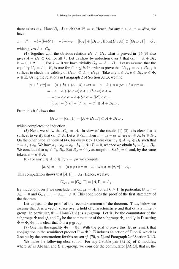
3. Triangular products and stability of representations 79
there exists ϕ ∈ Hom(B1, A) such that bϕ = x. Hence, for any x ∈ A, x = qma, wehave
x = bϕ = −b+(b+bϕ) = −b+b◦ϕ = [b, ϕ] ∈ [Bk−1,Hom(B1, A)] ⊂ [Gk−1,Γ] = Gk,
which gives A ⊂ Gk.(4) Together with the obvious relation Bk ⊂ Gk, what is proved in (1)-(3) also
gives A + Bk ⊂ Gk for all k. Let us show by induction over k that Gk = A + Bk,k = 0, 1, 2, . . . . For k = 0 we have trivially G0 = A + B0. Let us assume that theequality Gs = A + Bs is true for all s ≤ k. In order to prove that Gk+1 = A + Bk+1 itsuffices to check the validity of Gk+1 ⊂ A + Bk+1. Take any a ∈ A, b ∈ Bk, ϕ ∈ Φ,σ ∈ Σ. Using the relations in Paragraph 2 of Section 3.1.3, we find
[a + b, ϕσ] = −(a + b) + (a + b) ◦ ϕσ = −a− b + a ◦ ϕσ + b ◦ ϕσ =
= −a− b + (a ◦ ϕ) ◦ σ + (b ◦ ϕ) ◦ σ =
= −a + a ◦ σ − b + b ◦ σ + (bϕ) ◦ σ =
= [a, σ] + [b, σ] + [bϕ, σ] + bϕ ∈ A + Bk+1.
From this it follows that
Gk+1 = [Gk,Γ] = [A + Bk,Γ] ⊂ A + Bk+1,
which completes the induction.(5) Next, we show that Gω = A. In view of the results (1)-(3) it is clear that it
suffices to verify that Gω ⊂ A. Let x ∈ Gω. Then x = a1 + b1 where a1 ∈ A, b1 ∈ B1.On the other hand, in view of (4), for every k > 1 there exist ak ∈ A, bk ∈ Bk such thatx = ak +bk. We have a1−ak = bk−b1 ∈ A∩B = 0, whence we obtain b1 = bk ∈ Bk.We conclude that b1 ∈ ∩k Bk. But Bω = 0 by assumption. So b1 = 0, and, by the sametoken, x = a ∈ A.
(6) For any a ∈ A, γ ∈ Γ, γ = ϕσ we compute
[a, γ] = −a + (a ◦ ϕ) ◦ σ = −a + a ◦ σ = [a, σ] ∈ A1.
This computation shows that [A,Γ] = A1. Hence, we have
Gω+1 = [Gω,Γ] = [A,Γ] = A1.
By induction over k we conclude that Gω+k = Ak for all k ≥ 1. In particular, Gω+n =An = 0 and Gω+n−1 = An−1 �= 0. This concludes the proof of the first statement ofthe theorem.
Let us pass to the proof of the second statement of the theorem. Thus, below weassume that A is a vector space over a field of characteristic p and that Q is a finite q-group. In particular, Φ = Hom(B,A) is a p-group. Let Φ1 be the commutator of thesubgroups Φ and Q, and Φ2 be the commutator of the subgroups Φ1 and Q in Γ; settingΦ = Φ/Φ2, it is clear that Φ is a p-group.
(7) One has the equality Φ1 = Φ2. With the goal to prove this, let us remark thatconjugation in the semidirect product Γ = Φ � Σ induces an action of Σ on Φ which is2-stable by the construction; for this reason cf. [70, p. 2] and Paragraph 2 of Section 3.1.3.
We make the following observation. For any 2-stable pair (M,Σ) of Z-modules,where M is Abelian and Σ a q-group, we consider the commutator [M,Σ], that is, the
80 CHAPTER I. REPRESENTATIONS OF SEMIGROUPS AND ALGEBRAS
Z-module, generated by the commutators [a, σ] = −a + a ◦ σ, a ∈ M , σ ∈ Σ. As aconsequence of the 2-stability of (M,Σ) we derive from a ◦ σ = a + [a, σ] that
a ◦ σ2 = (a + [a, σ]) ◦ σ = a ◦ σ + [a, σ] = a + 2[a, σ], . . .
and (by induction over k), a ◦ σk = a + k[a, σ]. For some n = n(σ) we have σqn
= ε,because Σ is a q-group. Hence a = a◦ε = a◦σqn
= a+ qn[a, σ], whence qn[a, σ] = 0.Therefore [M,Σ] is a q-group.
When applied to the pair (Φ, Q) this observation shows that Φ1/Φ2 is a q-group.However, at the same time Φ1/Φ2 must be a q-group, as it is a subgroup of Φ. Weconclude that Φ1 ⊂ Φ2. As Φ2 ⊂ Φ1 is evident, the equality Φ1 = Φ2 is proved.
(8) We present some auxiliary computations for the pair (G,Γ), cf. Paragraph 2 ofSection 3.1.3. For any b ∈ B, ϕ ∈ Φ, σ ∈ Q we have b = b ◦ϕϕ−1 = (b+ bϕ) ◦ϕ−1 =b ◦ ϕ−1 + bϕ, whence b ◦ ϕ−1 = b− bϕ. Furthermore
b ◦ [ϕ, σ] = (b− bϕ) ◦ (σ−1ϕσ) = (b ◦ σ−1 − bϕ) ◦ (ϕσ) =
= (b ◦ σ−1 + (b ◦ σ−1)ϕ − bϕ) ◦ σ = b + (b ◦ σ−1)ϕ − bϕ.
Take now arbitrary b ∈ B and ϕ1 ∈ Φ1. There exist ϕ ∈ Φ and σ ∈ Q such thatϕ1 = [ϕ, σ] and, so we find
[b, ϕ1] = −b + b ◦ [ϕ, σ] = (−b + b ◦ σ−1)ϕ = [b, σ−1]ϕ.
These computations show that [B,Φ1] ⊂ [B,Q]Φ. But the group [B,Q] ⊂ B is free,and so [B,Q]Φ = A.
Thus the module A contains [B,Φ1].(9) Let us show that A ⊂ [B,Φ1]. This was shown in step (2) of this proof in the
case Φ1 = Φ. Let Φ1 < Φ. Using the classical theorem of Maschke ([19, p. 182]) forthe pair (Φ, Q), we obtain the existence of a Q-invariant decomposition Φ = Φ0 ⊕ Φ1.Moreover, (Φ0, Q) ∈ S. Indeed, for any ϕ ∈ Φ0 and σ ∈ Q we have −ϕ + ϕ ◦ σ ∈ Φ1,and also −ϕ + ϕ ◦ σ ∈ Φ0, as Φ0 is Q-invariant. From Φ1 ∩ Φ0 = 0 we conclude thatϕ ◦ σ = ϕ.
Consider the pair (B,Q) and let B∗ be the set of all Q-fixed points of B. We checknow that AnnΦ B∗ = Φ1. On one hand, in view of the definition of the action of Φ inB (Subsection 3.1.1.2) we must have b ◦ ϕ1 = b + bϕ1 for any b ∈ B∗ and ϕ1 ∈ Φ1.The elements ϕ1 = [ϕ, σ], where ϕ ∈ Φ and σ ∈ Q generate Φ1, and so in view of thecomputations in step (8) we have
b ◦ ϕ1 = b ◦ [ϕ, σ] = b + (b ◦ σ−1)ϕ − bϕ = b + bϕ − bϕ = b,
because b ◦ σ−1 = b. We come to equalities b+ bϕ1 = b ◦ϕ1 = b, from which it followsthat bϕ1 = 0. Hence ϕ1 ∈ AnnΦ B∗. So we have verified that Φ1 ⊂ AnnΦ B∗.
On the other hand, an immediate verification shows that for any b ∈ B the elementb =
∑σ∈Q b ◦ σ−1 is Q-invariant. Moreover, an arbitrary ϕ ∈ AnnΦ B∗ as well as each
other element of Φ = Φ0⊕Φ1, can be written in the form ϕ = ϕ0 +ϕ1, where ϕi ∈ Φi,i = 0, 1. Taking now into account the relations Φ1 ⊂ AnnΦ B∗ and (Φ0, Q) ∈ Sobtained before, along with the formula
∀b ∈ B,ψ ∈ Φ, σ ∈ Q, bψ◦σ = (b ◦ σ−1)ψ

3. Triangular products and stability of representations 81
in Paragraph 2 of Section 3.1.3, we obtain
0 = bϕ = bϕ0+ϕ1 = bϕ0 + bϕ1 = bϕ0 =
= (∑σ∈Q
b ◦ σ−1)ϕ0 =∑σ∈Q
bϕ0◦σ =∑σ∈Q
bϕ0 = |Q| · bϕ0 .
From this it follows that bϕ0 = 0, because bϕ0 lies in the p-group A, while |Q| = qk forsome k ∈ N, and this is true for all b ∈ B. Hence ϕ0 = 0. This argument shows thatAnnΦ B∗ ⊂ Φ1 and so we have Φ1 = AnnΦ B∗.
(10) The subgroup B∗ is servant in B. Indeed, if for some b ∈ B and n ∈ Z theelement nb is contained in B∗, then for any σ ∈ Q we have nb = n(b ◦ σ), hencen(b − b ◦ σ) = 0. For a free Abelian group B this is possible only if b ◦ σ = b. Henceb ∈ B∗ and we have established that B∗ is servant in B. We add, however, that this factfollows here from condition b), according to which there exists a subgroup B∗ ≤ B suchthat
B = B∗ ⊕ B∗.
From this we conclude that
Hom(B,A) = Hom(B∗, A)⊕Hom(B∗, A).
We remark that for each a ∈ A and a basis element b∗ ∈ B∗ the map b∗ �→ a extends toa Z-homomorphism ϕ∗ : B∗ → A. We obtain from this
A ⊂ [B∗,Hom(B∗, A)].
The equality Φ1 = AnnΦ B∗ proved above along with the obvious relation Hom(B∗, A)⊂ Φ1 shows, however that A ⊂ [B,Φ1].
(11) Using the relation Φ1 = Φ2 we see that Ψ = Φ1Q is a subgroup of the group Γand that Φ1 � Ψ. We shall find the ideal Δω
Ψ in the ring ZΨ.For any subgroup Ψ∗ ≤ Ψ we denote by ωΨ∗ the right ideal in ZΨ, generated by all
ψ− 1 where ψ ∈ Ψ∗. In an analogous way as was done in the proof of Proposition 3.70,one can prove that ωΦ1 ⊂ Δω
Ψ. Let us prove the converse inclusion. First, we remarkthat Ψ/Φ1 is a finite q-group so that Δω
Ψ/Φ1= 0. But
ΔωΨ/Φ1
=∞∩
n=1(Δn
Ψ + ωΦ1)/ωΦ1,
which gives
ωΦ1 ⊃∞∩
n=1(Δn
Ψ + ωΦ1) ⊃∞∩
n=1Δn
Ψ = ΔωΨ.
Thus we have the equality ΔωΨ = ωΦ1.
(12) By what was set out above, it follows that
Gω = A = [B,Φ1] ⊂ B ◦ ωΦ1 = B ◦ΔωΨ ⊂ B ◦Δω
Γ ⊂ G ◦ΔωΓ .
From this we obtain A = Gω = G◦ΔωΓ, because the inclusion converse to Gω ⊂ G◦Δω
Γ
is always true, cf. Subsection 3.3.1.1. �

82 CHAPTER I. REPRESENTATIONS OF SEMIGROUPS AND ALGEBRAS
3. Let us pass to estimating the terminal of the group Γ introduced in the previous Sub-section; to this end we assume that the auxiliary requirements, indicated in the statementof Theorem 3.71 are fulfilled.
We assume that Δω+n−1Γ = Δω+n
Γ , then we have
0 �= Gω+n−1 ⊂ Gω ◦Δn−1Γ = (G ◦Δω
Γ) ◦Δn−1Γ =
= G ◦ (ΔωΓ ·Δn−1
Γ ) = G ◦Δω+n−1Γ = G ◦Δω+n
Γ ⊂ Gω+n = 0.
This contradiction proves that Δω+n−1Γ �= Δω+n
Γ . A quantitative reformulation of theresult of these computations gives the following.
THEOREM 3.72. The terminal of the group Γ, introduced in Subsection 3.3.2.2, isnot less than ω + n.
4. We give an application of this result.Fix n ∈ N and let A be an n-dimensional vector space over Zp, and let P =
UT 1(n,Zp) be the group of (n × n)-matrices with elements in Zp with unit main di-agonal and zeros under it (the unitriangular group). We denote by UT r(n,Zp) the subsetof matrices in P with r − 1 zero diagonals above the main diagonal. In view of (12) in[19, p. 38] we have the relation
[UT r(n,Zp), UT 1(n,Zp)] = UT r+1(n,Zp),
showing that the nilpotency class of P equals n− 1.Let us remark that, in a natural way, there appears the pair (A,P ), which is faithful
and has a stable series of length n. However, A does not have a P -stable series ofthe length less than n, because otherwise by Kaluzhnin’s theorem ([19, p. 144]) thenilpotency class of P would be less than n − 1. The pair (A,P ) satisfies, thus, therequirement a) in Theorem 3.71; cf. the beginning of Subsection 3.3.2.2.
Furthermore, let us for B take the additive group of the integral group ring of afinite q-group Q, leading to the regular pair (B,Q); then B = B0 = ZQ(+) and Bk =Δk
Q, k = 1, 2, . . . , while the Abelian group B/B∗ decomposes into a direct sum ofcyclic subgroups, because together with B also B/B∗ is finitely generated. Hence, theservant subgroup B∗ is a direct summand of B ([22, p. 150]). It is easy to see that forsuch a group B the whole requirement b) in Theorem 3.71 is fulfilled. requirement In[61, p. 277], one finds, writing exp(Q/[Q,Q]) = n, the simple fact that the additivegroup ΔQ/Δk
Q has an exponent dividing nk (and hence is a q-group), but this can alsobe proved by the argument in step (7) of the proof of Theorem 3.71 by applying it to thepairs
(Δk−2Q /Δk
Q, Q/[Q,Q]), k = 2, 3, . . .and making an induction over k. Hence, the results of the two previous Subsections arealso true for the pair (G,Γ) = (A,P )�(B,Q) introduced here. We obtain the followingresult.
THEOREM 3.73. For each natural number n there exists a finite group such that inits integral group ring the (ω+n−1)-th and (ω+n)-th powers of the fundamental idealsare distinct.
An example in [71, p. 223], shows that all values ω + n, n = 0, 1, 2, . . . , indeedappear as terminals of finite groups.

3. Triangular products and stability of representations 83
5. Groups, in which there exists an invariant nilpotent subgroup with a nilpotent factorgroup, are usually called metanilpotent.
We denote in this Subsection by Γn the n-th term of the lower central series of thegroup Γ. Along with Theorem 3.73 one may now formulate the following statementwhich gives further properties of terminals of finite groups.
THEOREM 3.74. Let there be given a representation (G,Γ) of the group Γ with allmetanilpotent factor groups torsion and the factor group Γ/∩nΓn nilpotent, by automor-phisms of the Z-module G whose torsion part B is Γ-Artinian, while the factor moduleG/B is Γ-Noetherian. If G has a Γ-stable descending series of length ≤ ωn (n ∈ N)which reaches the zero, then the lower stable series of the pair (G,Γ) stabilizes to zeroat a term of index < ω2.
PROOF. The statement of the theorem is obvious for n = 1, because the terms ofthe lower stable series of the pair (G,Γ) are contained in the corresponding terms of thegiven Γ-stable series of G. Hence we may assume that n ≥ 2.
By the assumption, there exists in the module G a descending stable series of length≤ ωn,
(17) G ⊃ G1 ⊃ · · · ⊃ Gu ⊃ . . . Gλ ⊃ · · · ⊃ Gμ = 0.
Consider the family of submodules {Gλ + B |λ ≤ μ}. In view of the Γ-stability ofthe series (17) and the Γ-invariance of the module B invariance we have for a non-limitλ
(18) Gλ−1 + B,Γ] ⊂ [Gλ−1,Γ] + [B,Γ] ⊂ Gλ + B .
Let us show that for a limit λ holds the relation
(19) Gλ + B =⋂
α<λ
(Gα + B).
We introduce the factor modules Gdef= G/Gλ, Gα
def= Gα/Gλ for α ≤ λ and Bdef=
(B + Gλ)/Gλ; the module B is Γ-Artinian, in view of the Γ-Artinicity of B. It is clearthat (19) is equivalent to the equality equality B = ∩α<λ(Gα+B), which we shall show.
We remark that in B one has the descending series descending of submodules
B ⊃ G1 ∩ B ⊃ ∩B · · · ⊃ Gα ∩ B ⊃ . . . ,
which, as B is Artinian, must stabilize at some index β, β < λ. From the fact that theseries (17) exists we obtain the relation∩α<λGα = 0. This gives∩α<λ(B∩Gα) = 0. Sothe stabilization hinted at above occurs at the term equal to 0. Hence, we have Gα∩B = 0for all α, on index β ≤ α ≤ λ. As λ is a limit ordinal, there are infinitely many suchordinal numbers α. It is now easy to see that ∩α<λ(Gα + B) ⊂ B. Indeed, take anyelement x in ∩α<λ(Gα + B). Then x ∈ Gα + B, and so x = g + b for some g ∈ Gβ
and b ∈ B. On the other hand, as x belongs to ∩α<λ(Gα + B), it follows that for eachα, β < α < λ, there exist elements gα ∈ Gα and bα ∈ B such that x = gα + bα. Wehave
g − gα = bα − b ∈ Gβ ∩ B = 0,whence g = gα. As a consequence, the element g lies in every Gα, β < α < λ, andtherefore also in the module ∩α<λGα, which equals 0. We obtain x = g + b = b ∈ B.Clearly the equality ∩α<λ(Gα + B) = B is now proved.
84 CHAPTER I. REPRESENTATIONS OF SEMIGROUPS AND ALGEBRAS
Let ωm, m ∈ N, be the last limit ordinal not exceeding μ. Then one can find anon-negative integer e such that μ = ωm+ e. It follows from the relations (18) and (19)that in G one has the Γ-stable series
(20) G ⊃ G1 +B ⊃ · · · ⊃ Gω +B ⊃ · · · ⊃ Gω2 +B ⊃ · · · ⊃ Gωm +B ⊃ · · · ⊃ B,
where the link from Gωm + B to B contains e members.Let Σ0 be the kernel of the pair (G/B,Γ), Σ1 be the kernel of the pair
(G/(Gω +
B),Γ), Σk be the kernel of the pair ((Gω(k−1) + B)/(Gωk + B),Γ), for k = 2, . . . ,m,
and Σm+1 be the kernel of the pair((Gωm + B)/B,Γ
). An application of Lemma 3.56
implies that the groups Γ/Σk, k = 1, . . . ,m, are residually nilpotent. This yields therelations ∩nΓn ⊂ Σk, thanks to which it follows from the nilpotency of Γ/∩nΓ that allgroups Γ/Σk, k = 1, . . . ,m, are nilpotent; again the nilpotency of Γ/Σm+1 follows fromKaluzhnin’s Theorem. Let Σ∗ = ∩m+1
k=1 Σk; it is clear that Σ0 ⊂ Σ∗, while an applicationof Remak’s theorem shows that G/Σ∗ is nilpotent. Likewise, the factor group Σ∗/Σ0 isnilpotent, because the subpair (G/B,Σ∗/Σ0) of (G/B,Γ) is faithful and finitely stable.Thus the group Γ/Σ0 is metanilpotent, but then according to the condition of the Theo-rem it is also a torsion group. Its subgroup Σ∗/Σ0 acts faithfully and finitely stably onthe torsion free module G/B, which according to Lemma 3.53 implies that Σ∗/Σ0.
Thus, we have shown that the group Γ/Σ0 of automorphisms of the Γ-Noetherianmodule G/B is nilpotent. We may apply Theorem 3.66; we find that the lower stableseries of the pair (G/B,Γ/Σ0) must stabilize at a term of index ≤ ω,
(21) G/B ⊃ · · · ⊃ (G/B)ω = (G/B)ω+1 = . . . .
We have, however, the equation (G/B)ω = 0, because the terms of the series (21) arecontained in the corresponding terms of the Γ/Σ0-stable series
G/B ⊃ (G1 + B)/B ⊃ · · · ⊃ (Gω + B)/B ⊃ · · · ⊃ 0 .
Let us consider the series of preimages of the terms of the series (21) under the epimor-phism G � G/B and let us add to it the finite chain from 0 to B a of the original series(17); such a chain exists as B is Γ-Artinian module. We obtain a descending Γ-stabledescending series of length < ω2 for the module G,
(22) G ⊃ · · · ⊃ B ⊃ · · · ⊃ 0.
As, the terms of the lower Γ-stable series of G are contained in the corresponding termsof the series (22), then this series becomes zero for terms of index < ω2. This concludesthe proof of Theorem 3.74. �
6. For representations of an Artinian group Γ by automorphisms of the Z-module G weconsider the corresponding lower stable series,
G ⊃ G1 ⊃ · · · ⊃ Gω ⊃ · · · ⊃ · · · ⊃ Gω2 ⊃ . . . .
Let us assume that the torsion part of the module G/Gω2 is a Γ-Artinian Z-module, andthat its quotient by the torsion part is Γ-Noetherian. Then it follows from Theorem 3.74that the lower stable series of G/Gω2 stabilizes to zero at a term of index < ω2. Hence,in the initial series we have for some n ∈ N
Gω+n = Gω+n+1 = . . . .
3. Triangular products and stability of representations 85
Let Γ be arbitrary finite group. The regular pair (ZΓ,Γ) can be taken as the representation(G,Γ) considered above in this Subsection. The lower stable series of this pair is theseries (9). As Γ is a finite group the Z-module ZΓ/Δω2 is Noetherian and so its torsionpart must be finite. Thus the series (9) stabilizes at a term of index < ω2. In other words,we have proved the following.
THEOREM 3.75. The terminal of a finite group is less than ω2.
3.3.3. Generalized measure subgroups of finite groups
1. In this Section we show that the results set forth above on the terminal and thetriangular product construction of linear pairs allows one to give a completely closeddescription of the limit groups in the class of finite groups, the task referred by B. Hartleyin [80, p. 15].
The nilpotent coradical of a group Γ is the subgroup N(Γ) of Γ which is the in-tersection of all normal subgroups of Γ such that the quotients groups of Γ by them arenilpotent.
PROPOSITION 3.76. If Γ is a finite group, then the kernel of the regular pair (ZΓ/Δω,Γ) is the nilpotent coradical of Γ.
PROOF. Let Σ be the kernel of (ZΓ/Δω ,Γ). The group Γ/Σ acts in ZΓ/Δω faith-fully and ω∗-stably. An application of Lemma 3.56 shows that Γ/Σ is nilpotent. Hence,we have Σ ⊃ N(Γ).
In order to prove the inclusion Σ ⊂ N(Γ), we require an observation: for each finitenilpotent group Γ there exists a natural number n such that (ZΓ/Δn,Γ) is faithful. In-deed, if Γp is the p-component in the primary decomposition of Γ, then Γp acts faithfullyon the basis subgroup Bp of the wreath product ZpwrΓp because the action is regular.This action is also stable, since Bp is a finite p-group. The pair (ΣpBp,Γ) gives an r-stable representation of Γ, where we for n take the maximal length of Γ-stable seriesof the groups Bp. But then, likewise, the free representation corresponding to the pair(ZΓ/Δn,Γ) is faithful.
Next, let Γ be anew an arbitrary finite group. Then the group Γ/N(Γ) is nilpotent.Therefore, by our observation, there exists a numbern such that the pair (ZΓ/Δn,Γ/N(Γ))is faithful. In other words, the coradicalN(Γ) is the kernel of the pair (ZΓ/Δn,Γ). Butthe kernel of the pair (ZΓ/Δω,Γ) apparently must be contained in the kernel of the pair(ZΓ/Δn,Γ), so we must have Σ ⊂ N(Γ). �
One can also look on the reasoning given above as a new proof of a theorem ofBuckley [60], based on the technique of linear pairs. Indeed, let Dk be the kernel of(ZΓ/Δk,Γ), Dω = ∩k Dk, while D∗ is the kernel of (ZΓ/Δω,Γ); it is readily seen thatD∗ = Dω (the proof amounts to unwinding the definitions of D∗ and Dω). Moreover,let Γω be the intersection of the terms of the lower central series of the finite group Γ; itis clear that Γω = N(Γ). From Proposition 3.76 now follows the following.
COROLLARY 3.77 ([60, Theorem 2]). For each finite group Γ one has the equalityDω = Γω.

86 CHAPTER I. REPRESENTATIONS OF SEMIGROUPS AND ALGEBRAS
Remark. It remains to settle the question whether every group Γ admits a represen-tation of class Sω exactly when it is residually nilpotent. It is clear that this is equivalentto the question about the equality Dω = Γω and that a positive answer to it would followfrom a positively solution of the problem of the existence, for each nilpotent group, of afaithful finitely stable representation. The existence of such a representation is evident forfinite nilpotent groups (cf. the observation in the proof of the previous Proposition), andit was proven by A. I. Mal’cev [27] for torsion-free nilpotent groups, and, likewise, fornilpotent groups with finite exponent, while B. I. Plotkin [39] established it for nilpotentgroups of finite special rank.
2. Let Γ be a torsion group, Ω the set of all prime numbers, π ⊂ Ω, π′ = Ω \ π, whileΓπ′ is the subgroup of Γ, generated by all π′-elements in Γ. It is clear that Γπ′ �Γ. Let usintroduce the notation Π2(Γ) for ∩π,|π|=2Γπ′ , and consider the class of torsion groups Γ,satisfying Π2(Γ) = 1. We show that these are precisely the residually biprimary groups.
Indeed, on the one hand, Γ/Γπ′ is a π-group. We denote by Π(n) the set of all primedivisors of n, and by Π(Γ) the set of prime divisors of the orders of all elements of Γ.Let γ ∈ Γ be an element of order n, γ �∈ Γπ′ . Then Π(n) �⊂ π′, whence Π(n) ∩ π �= ∅.Let n = m · n′, where Π(m) ⊂ Π(n) ∩ π and Π(n′) ∩ π = ∅. Then it follows from1 = γn = (γm)n′
that γm ∈ Γπ′ , as Π(n) ⊂ π′. We have (γΓπ′)m = 1, which again,in view of Π(m) ⊂ π implies that Π(γΓπ′) ⊂ π. As a consequence, each element ofΓ/Γπ′ is a π-element.
On the other hand, let Γ be a residually biprimary torsion group: there exist sub-groups Σi � Γ, i ∈ I , such that every Γ/Σi is a πi-group, |πi| = 2 and ∩i∈IΣi = 1. Weshow that Γπ′
i⊂ Σi for all i ∈ I . It suffices to check that each π′
i-element in Γ lies in Σi.Take any γ ∈ Γ, γm = 1, Π(m) ⊂ π′
i. It follows from Π(Γ/Σi) ⊂ πi that there exists aπ′-number n such that γn ∈ Σi. In view of Π(m) ∩ Π(n) = ∅ there exist integers u, vsuch that um + vn = 1. We have
γ = γum+vn = (γm)n(γn)v = (γn)v ∈ Σi.
i.e. γ ∈ Σi. These reasonings prove that Γπ′i⊂ Σi, which immediately implies that
Π2(Γ) = 1. The original statement is completely proved. �Let us now study some auxiliary properties of the classN(2), introduced by B. Hart-
ley [75]. This class of finite groups is defined via the following conditions 20
(23) Γ ∈ N(2) ⇐⇒ Γ ∈ AN& Π2(Γ) = 1.
As a consequence of what was said above and the properties of the variety AN we seethat the N(2)-groups are subdirect products of biprimary AN-groups, and, conversely,every such product is anN(2)-group.
THEOREM 3.78 ([75, Theorem 2.]). Each N(2)-group has a faithful stable repre-sentation of type (ω + n)∗ in a finitely generated Abelian group.
PROOF. The proof consists of a reduction ofN(2)-groups to groups of rather specialform, for which the desired representation is constructed with the aid of the triangularproduct construction. Let us introduce the corresponding class of finite groups R: by
20As usual A denotes the class of Abelian groups, andN the class of nilpotent groups.

3. Triangular products and stability of representations 87
definition T ∈ R if for some prime numbers p and q there exist an Abelian p-group Aand a nilpotent (p, q)-group B such that T = AwrB.
Let us first show 21 that N(2) ≤ R0SR. For any prime numbers p and q set π ={p, q} and Γ = Γ/Γπ′ . As the properties of being AN- and π-groups are preserved underepimorphisms we have Γ ∈ A and Π(Γ) ⊂ π. Therefore there exists a normal subgroupA � Γ such that A ∈ A, and Σ = Γ/A is a nilpotent π-group. Let A = A(p) × A(q)be the primary decomposition of A. It is easy to observe that Γ/A(q) is an extension ofA(p) by Σ, from which, by a well-known theorem ([19, p. 70]), it follows that the wreathproduct A(p)wrΣ contains a subgroup isomorphic to Γ/A(q). Hence, Γ/A(q) ∈ SR,and, as A(p) ∩ A(q) = 1, then Γ ∈ R0SR. It follows now from Π2(Γ) = 1 that alsoΓ ∈ R0SR.
Fix the number n. It is not hard to see that for the class of groups−−−→Sω+n we have
the equality R0S−−−→Sm+n =
−−−→Sω+n. Indeed, the class
−−−→Sω+n is, trivially, closed. Moreover,
assume that for some group Γ there exist two normal subgroups Σ1 and Σ2 such that
Σ1∩Σ2 = 1 and the factor groups Γ/Σ1 and Γ/Σ2 lie in−−−→Sω+n. Then we have the faithful
pairs (Gi,Γ/Σi) ∈ Sω+n, i = 1, 2. We denote G = G1⊕G2 and Γ = Γ/Σ1×Γ/Σ2; wehave the pair (G, Γ), which is faithful and lies in Sω+n. As the group Γ may be viewedas a subgroup of Γ, we obtain the pair (G,Γ), having the same properties. We conclude
that Γ ∈−−−→Sω+n and our equality is proved.
From the equality just proven and the relation N(2) ≤ R0SR it follows that it suf-fices to prove the theorem for R-groups. Let T = AwrB be such a group and let P ×Qbe the primary decomposition for B, where P = B(p) and Q = B(q). Furthermore, letAP be the basis subgroup of AwrB. with (AP , P ) and (ZQ,Q), which are also faithful.The group AP � P is a p-group and so nilpotent, which implies that (AP , P ) ∈ Sn fora suitable n. The fact that the pair (ZQ,Q) is contained in the class Sω follows fromTheorem 3.69. The triangular product of these pairs
(G,Γ) = (AP , P )� (ZQ,Q)
is contained in the class Sn · Sω = Sω+n and is faithful, because the initial pairs are
faithful (cf. Paragraph 2 of Section 3.1.3). Hence Γ ∈−−−→Sω+n and since by (3) the group
Γ is isomorphic to Awr(P × Q), we have T ∈−−−→Sω+n. Taking in account the fact that
the group AP ⊕ ZQ is finitely generated, it is not hard to deduce by the argument of theproof given (from its beginning) the possibility to satisfy these properties for the requiredrepresentation of the givenN(2)-group. �
PROPOSITION 3.79. A group of class N(2) is nilpotent precisely when its terminalequals ω. For a non-nilpotentN(2)-group Γ holds the inequality τ(Γ) ≥ ω+1 and thereexists an ordinal number ν such that the ν-th member of the central series of Γ is notcontained in the corresponding (generalized) dimension subgroup Dν .
PROOF. If the N(2)-group Γ is nilpotent then it follows from Theorem 3.67 thatτ(Γ) = ω. Conversely, let the terminal of someN(2)-group Γ equal ω. By Theorem 3.78there exist a number n ≥ 0 and a faithful representation (G,Γ) such that Gω+n = 0.
21Here S is the operator of taking subgroups, while the operator R0 is defined by the following rule: Aclass K is called R0-closed precisely when it contains each group Γ having invariant subgroups Ψ and Σ suchthat Ψ ∩ Σ = 1 and Γ/Ψ ∈ K and Γ/Σ ∈ K.
88 CHAPTER I. REPRESENTATIONS OF SEMIGROUPS AND ALGEBRAS
We have also G ◦ Δω+nΓ ⊂ Gω+n. In view of τ(Γ) = ω we deduce that G ◦ Δω
Γ = 0.This means that Dω ⊂ Ker (G,Γ), and as Γω ⊂ Dω and Ker (G,Γ) = 1, then Γω = 1.Therefore Γ is nilpotent.
For the nilpotency of an N(2)-group Γ we have, thus, the inequality τ(Γ) ≥ ω + 1.For such a group let the number n and the pair (G,Γ) once more be given by Theo-rem 3.78; it is not hard to see that here n ≥ 1. We show that Γω+n �⊂ Dω+n. Indeed, inthe opposite case we would have Γω = Γω+n ⊂ Dω+n ⊂ Ker (G,Γ) = 1, i.e. Γω = 1,which contradicts the non-nilpotency of Γ. �
Remark. In [63] it was, erroneously, stated (Proposition 17) that Γν ⊂ Dν holds truefor all groups Γ an all ordinals ν.
B. Hartley [77] solved positively Gruenberg’s conjecture to the effect that the inter-section of all powers of the fundamental ideal of the integral group ring of an arbitrarytorsion-free nilpotent group is zero. This led to a conjecture of A. A. Bovdi, formulatedduring the XI Algebraic Symposium in Kishinev: Δω
Φ = 0 for each torsion-free groupΦ. The answer is, however, negative. Let us consider B. I. Plotkin’s example of a weaklystable automorphism group Φ, having no central system, of an Abelian group G, beingthe direct sum of a countable family of groups Q(+); cf. for details [35, pp. 470–471].One can show that the group Φ in this example is torsion-free. There arises a faithful pair(G,Φ) ∈ Sω+1. For Δω
Φ = Δω+1Φ we obtain G ◦Δω
Φ = G ◦Δω+1Φ ⊂ Gω+1 = 0, which
gives Φω ⊂ Dω ⊂ Ker (G,Φ) = 1, i.e. Φω = 1. This contradicts the existence for Φ acentral system. Therefore we have Δω
Φ �= Δω+1Φ and also Δω
Φ �= 0.
3. Let Γ∗ be a finite group, Δ the fundamental ideal of the ring ZΓ∗ and τ the terminalof Γ∗. Let us make explicit the group theoretical structure of the limit subgroup D∞ =(1 + Δτ ) ∩ Γ∗. In view of Proposition 3.63 and the fact that structure of the dimensionsubgroups D1 and D2 is known, one can restrict oneself to those finite groups Γ∗ whoseterminal is ≥ ω.
THEOREM 3.80. The limit of a finite group Γ∗ with infinite terminal τ is the smallestof its normal subgroups such that all its factor groups areN(2)-groups.
PROOF. Let us consider the regular pair (ZΓ∗/Δω,Γ∗). In view of Proposition 3.76its kernel is the nilpotent coradical of Γ∗, which we denote by Σ∗. As Δτ ⊂ Δω we haveD∞ ⊂ Σ∗, which makes it possible to pick in Γ∗/D∞ the subgroup Σ∗/D∞. As wasestablished in Theorem 3.75 there exists a non-negative integer n such that τ = ω + n.The additive group of the ring ZΓ∗/Δω+n will be denoted by G, and the factor groupsΓ∗/D∞ and Σ∗/D∞ by Γ and Σ, respectively. It is not hard to see that Σ is the nilpotentcoradical of Γ.
Therefore we have
(24) Σ =∏p�=q
[Γp,Γq] = ∩p Γp′ and Σp = Γp′,p ,
where we denote by Γp′,p the subgroup generated by the p-elements in Γp′ ; the straight-forward verification of these equations can be found in [80, p. 5]. As a first step in theproof we establish that Σ ∈ A.
The regular pair (G,Γ) is faithful and admits the lower stable series
(25) G ⊃ G1 ⊃ · · · ⊃ Gω ⊃ · · · ⊃ Gω+n = 0.

3. Triangular products and stability of representations 89
where Gν = Δν/Δω+n(+), ν = 1, 2, . . . . The subpair (G,Σ) in (G,Γ) is faithful,because (G,Γ) is faithful. It is finitely stable, because in the factor G/Gω of the series(25) the subgroup Σ acts as the identity. By Kaluzhnin’s theorem it follows that Σ ∈ N.In view of this the subgroup Σp coincides with the Sylow p-subgroup Σ(p). Thus, itsuffices to establish that Σp ∈ A, as Σ is the direct product of the groups Σ(p). The groupΣp, being a p-group, is also a relative p-group ([35, p. 144]), while the pair (G,Σp) isfaithful and finitely stable since it is a subpair of (G,Σ). By Lemma 3.55 it follows fromthis that the commutator [G,Σp] is a p-group, which we denote by H . Next, we showthat [H,Γp′ ] = 0.
Indeed, for all g ∈ G, σ ∈ Σp and γ ∈ Γp we have
[g, σ] ◦ γ = −g ◦ γ + g ◦ σγ = −g ◦ γ + g ◦ γ · γ−1σγ =
= −(g ◦ γ) + (g ◦ γ) ◦ γ−1σγ = [g ◦ γ, γ−1σγ].
This computation shows that the subgroup H ≤ G is Γp′ -invariant: indeed, γ−1σγ∈ Σp, as Σp � Γp′ , while the elements of the form [g, σ], where g ∈ G, σ ∈ Σp,generate H . For each ν = 1, 2, . . . the term Hν of the lower stable series of the pair(H,Γp′) is contained in Gν+1, and as Gτ+1 = 0, then also Hτ = 0. Let K be the kernelof (H,Γp′) The factor group Γp′/K , which we denote by Φ, is a p-group. Indeed, for anyh ∈ H we consider the Φ-invariant subgroup H∗ ≤ H , generated by all h ◦ ϕ, ϕ ∈ Φ.Clearly, H∗ is a finite p-group, as Φ is finite and H is an Abelian p-group. Thereforethe intersection of H∗ with the terms of the lower stable series of the pair (H,Φ) gives afinite Φ-stable series of H∗. Lemma 3.55, applied to (H∗,Φ), shows that Φ acts on H∗
as a p-group. In other words, for each ϕ ∈ Φ there exists a number m with Π(m) = {p}such that ϕm is contained in the kernel of the pair (H∗,Φ); we denote this kernel by Ψ.Assume now that there exists in Φ a non-unit p′-element ϕ �= 1. Then, for some n withΠ(n) ⊂ p′, we have ϕn = 1, and as n and m are relatively prime there exist u, v ∈ Zsuch that nu + mv = 1. This gives ϕ = ϕnv · ϕmv = (ϕm)v ∈ Ψ, i.e. ϕ ∈ Ψ. Thus,the p′-element φ acts trivially on H∗. The choice of the element h ∈ H being arbitraryin our construction, we conclude that ϕ acts trivially on H . This means that ϕ lies in thekernel of the pair (H,Φ) and, as this pair is faithful, we deduce ϕ = 1. Contradiction.Thus we have proved our statement concerning the group Φ.
The equality [H,Γp′ ] = 0 now follows readily. Indeed, let ϕ be an arbitrary p′-element of Γ. For some p′-number n we have ϕn = 1, and, as by what was proved aboveΓp′/K is a p-group, there exists a p-numberm such that ϕm ∈ K . In view of (m,n) = 1it follows (as above) that ϕ ∈ K . The group Γp′ is generated by the p′-elements of Γ,and so it is entirely contained in K . This means that Γp′ acts trivially on H . In particular,we have [H,Σp] = 0. This shows that Σp is Abelian.
Indeed, the subpair (G,Σp) of the faithful pair (G,Γ) must be faithful also. In viewof what was proved above, we have [[G,Σp],Σp] = 0. This implies that the faithful pair(G,Σp) is 2-stable. From Kaluzhnin’s theorem it follows that Σp is Abelian. Therebywe have also proved the relation Γ ∈ AN.
A second step in the proof is the verification of the equality Π2(Γ) = 1. We observethat Σ is a normal subgroup of Γ on which the lower central series of Γ stabilizes. Abovewe have established that Σ ∈ A. Hence, by a theorem of Shenkman [104] there existsa subgroup Θ ≤ Γ such that Γ = Σ � Θ. Let p and q be two arbitrary prime numbers.

90 CHAPTER I. REPRESENTATIONS OF SEMIGROUPS AND ALGEBRAS
The subgroup Σp′ is characteristic in Σ and therefore in Σ and, hence, Σp′ � Γ. One cantherefore consider the subgroup Σp′ ·Θ(p,q)′ . Invoking the relation Σ ∩Θ = 1, a simpleargument (by contradiction) shows that
(26)⋂p�=q
Σp′ ·Θ(p,q)′ = 1.
The isomorphism of Θ with Γ/Σ gives Θ ∈ N. Therefore we have Σ = Σp × Σp′ andΘ = Θ(p,q) ×Θ(p,q)′ , which along with Σp′ � Γ gives the equality 22
Γ = gp{Σp ·Θ(p,q),Σp′ ·Θ(p,q)′}.Hence,
(27) Γ/(Σp′ ·Θ(p,q)′) ∼= Σp ·Θ(p,q)/(Σp ·Θ(p,q) ∩Σp′ ·Θ(p,q)′).
One verifies, however, immediately that
Σp ·Θ(p,q) ∩Σp′ ·Θ(p,q)′ = 1.
Therefore the factor group to the right of (27) is isomorphic to Σp ·Θ(p,q), while the lastgroup is biprimary, in view of the facts that Σ ∈ A, Θ ∈ N and Σp � Γ. The relations(26) and (27) now show that Π2(Γ) = 1.
By what has been said we have Γ ∈ N(2). In other words, there exists a family Ωof normal subgroups X of Γ having trivial intersection, factor groups Γ/X by which arebiprimary and belong to the class AN. Let Ω∗ = {X∗} be the complete pre-image ofX ∈ Ω in Γ∗. It is clear that Γ∗/X∗ is biprimary, contained in the class AN, and that∩X∗∈Ω∗ X∗ = D∞. We denote by Ω∗ the family of all invariant subgroups X∗ in Γ∗
with the properties described. We have ∩X∗∈Ω∗ ⊂ ∩X∗∈Ω∗ , which gives ∩
X∗∈Ω∗ ⊂D∞. Let us prove the converse inclusion. It suffices to verify that D∞ is contained inevery X∗ ∈ Ω∗. We remark that Γ∗/X∗ ∈ N(2) for every Γ∗ ∈ Ω∗. Therefore, forsome non-negative n the group Γ∗/X∗ admits a faithful (ω + n)∗-stable representationin an Abelian group (cf. Theorem 3.78). We obtain the faithful pair (A,Γ∗/X∗), whichcan be naturally lifted by the epimorphism Γ∗ � Γ∗/X∗ to the pair (A,Γ∗) with kernelX∗. By what has been said, Aω+n = [A,Γ∗;ω + n] = 0. However we have alsoA ◦ Δω+n
Γ∗ ⊂ Aω+n, which implies that A ◦ Δ∞Γ∗ = 0, because Δ∞
Γ∗ ⊂ Δω+nΓ∗ . The
result obtained A ◦ (D∞ − 1) = 0 means that D∞ lies in the kernel of (A,Γ∗), that is,D∞ ⊂ X∗. The Theorem is proven. �
3.3.4. Mal’cev nilpotency and stability of semigroups
1. The problems on the terminal and the dimension subgroups can also be carried overto semigroups. In order to formulate them we have to make precise some notions.
For a congruenceA of a semigroup Γ we consider in the ring R = ZΓ the ideal I(A),generated by all differences γ−σ, where γ, σ ∈ Γ and γ ∼ σ (A). It is clear that I(A) isa two-sided ideal of R and it arises in a natural way as the kernel of the homomorphismof semigroup rings ZΓ → Z(Γ/A). We observe some properties of the correspondenceA→ I(A), their proofs being straightforward verifications:
(1) A ≤ B =⇒ I(A) ⊂ I(B);
22Translators’ note. The symbol gp here, apparently, means taking the subgroup spanned by the groupsindicated within the curly brackets.

3. Triangular products and stability of representations 91
(2) I(A ∩B) ⊂ I(A) ∩ I(B);(3) I(A ∪B) ⊃ I(A) ∪ I(B).
In the case when A is the zero congruence on Γ, i.e. it is defined by the set Γ × Γof all pairs, it is natural to call the ideal I(A) the fundamental ideal 23 and denote it byΔ(Γ,Z) or simply Δ. For every natural number n one defines on Γ a binary relation ϑn:
γ ∼ σ(ϑn) on Γ ⇐⇒ γ − σ ∈ Δn in ZΓ.
It is clear that ϑn is a congruence on Γ. We call it the n-th dimension congruence of thesemigroup Γ with respect to Z. If Γ is a monoid, then the class of ϑn containing the unityelement is a submonoid; we denote it Dn(Γ,Z). For a group Γ the submonoid Dn(Γ,Z)is the well-known n-th dimension subgroup, which has been the object of much attention(cf. [33, 91, 92, 96], as well as the literature given there).
Nilpotence of semigroups will be considered in the sense of A. I. Mal’cev. Letx, y, u1, u2, . . . ,un, . . . be arbitrary variables. We set X0 = x, Y0 = y, and define further
Xn+1 = Xnun+1Yn, Yn+1 = Ynun+1Xn,
According to Mal’cev [28], a semigroup Γ whose elements satisfy the identity Xn = Yn
is said to be nilpotent of class n. For a group Γ we obtain then the usual notion ofnilpotence of class n for groups ([28, Theorem 1]). For an arbitrary semigroup Γ onecan consider the congruence Cn+1 = Nn(Γ) with respect to the variety of nilpotentsemigroups of class n: it is the minimal congruenceA on Γ with the property that Γ/A ∈Nn. Moreover we agree that τ1 is the zero relation on Γ. This gives rise to a decreasingseries of congruences
C1 ≥ C2 ≥ · · · ≥ Cn ≥ Cn+1 ≥ . . . ,
which is called the lower central series of the semigroup Γ. We remark that for a groupΓ the Cn-classes (n ≥ 1) containing the unity element coincide with the terms of thelower central series of this group Γ. The comparison of the mutual relations betweenthe congruences Cn and ϑn seems to be an interesting problem. One must, however, addthat already the equation C2 = ϑ2 for a semigroup Γ requires some separativity typeconditions on Γ.
As the series (9), likewise the definition of its terminal τ(Γ) in the case when Γ is asemigroup do not change, there arises a question of terminal behavior in the class of finitesemigroups. In particular, we conjecture that τ(Γ,Z) ≤ ω2 for each finite monoid Γ.Moreover, considering the limit congruence D∞(Γ) on Γ, which is the kernel of the pair(ZΓ/Δτ(Γ),Γ), one can also state the problem of describing (in terms of semigroups)this limit congruence for the class of all finite semigroups.
2. In this Subsection we consider pairs whose domain of action is an (arbitrary) group,while the acting object is a semigroup. In the study of pairs of this kind it will be conve-nient to use the language of quasi-rings, [68].
A set K equipped with two binary operations (addition and multiplication) is, bydefinition, a quasi-ring, if:
23Translators’ note. Also known as the augmentation ideal.
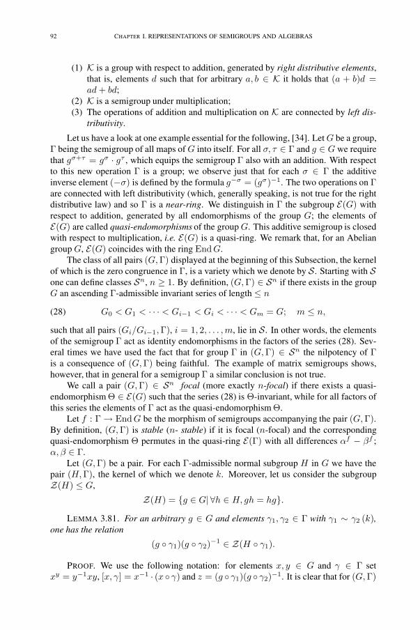
92 CHAPTER I. REPRESENTATIONS OF SEMIGROUPS AND ALGEBRAS
(1) K is a group with respect to addition, generated by right distributive elements,that is, elements d such that for arbitrary a, b ∈ K it holds that (a + b)d =ad + bd;
(2) K is a semigroup under multiplication;(3) The operations of addition and multiplication on K are connected by left dis-
tributivity.
Let us have a look at one example essential for the following, [34]. Let G be a group,Γ being the semigroup of all maps of G into itself. For all σ, τ ∈ Γ and g ∈ G we requirethat gσ+τ = gσ · gτ , which equips the semigroup Γ also with an addition. With respectto this new operation Γ is a group; we observe just that for each σ ∈ Γ the additiveinverse element (−σ) is defined by the formula g−σ = (gσ)−1. The two operations on Γare connected with left distributivity (which, generally speaking, is not true for the rightdistributive law) and so Γ is a near-ring. We distinguish in Γ the subgroup E(G) withrespect to addition, generated by all endomorphisms of the group G; the elements ofE(G) are called quasi-endomorphisms of the group G. This additive semigroup is closedwith respect to multiplication, i.e. E(G) is a quasi-ring. We remark that, for an Abeliangroup G, E(G) coincides with the ring EndG.
The class of all pairs (G,Γ) displayed at the beginning of this Subsection, the kernelof which is the zero congruence in Γ, is a variety which we denote by S. Starting with Sone can define classes Sn, n ≥ 1. By definition, (G,Γ) ∈ Sn if there exists in the groupG an ascending Γ-admissible invariant series of length ≤ n
(28) G0 < G1 < · · · < Gi−1 < Gi < · · · < Gm = G; m ≤ n,
such that all pairs (Gi/Gi−1,Γ), i = 1, 2, . . . ,m, lie in S. In other words, the elementsof the semigroup Γ act as identity endomorphisms in the factors of the series (28). Sev-eral times we have used the fact that for group Γ in (G,Γ) ∈ Sn the nilpotency of Γis a consequence of (G,Γ) being faithful. The example of matrix semigroups shows,however, that in general for a semigroup Γ a similar conclusion is not true.
We call a pair (G,Γ) ∈ Sn focal (more exactly n-focal) if there exists a quasi-endomorphism Θ ∈ E(G) such that the series (28) is Θ-invariant, while for all factors ofthis series the elements of Γ act as the quasi-endomorphism Θ.
Let f : Γ → EndG be the morphism of semigroups accompanying the pair (G,Γ).By definition, (G,Γ) is stable (n- stable) if it is focal (n-focal) and the correspondingquasi-endomorphism Θ permutes in the quasi-ring E(Γ) with all differences αf − βf ;α, β ∈ Γ.
Let (G,Γ) be a pair. For each Γ-admissible normal subgroup H in G we have thepair (H,Γ), the kernel of which we denote k. Moreover, let us consider the subgroupZ(H) ≤ G,
Z(H) = {g ∈ G| ∀h ∈ H, gh = hg}.
LEMMA 3.81. For an arbitrary g ∈ G and elements γ1, γ2 ∈ Γ with γ1 ∼ γ2 (k),one has the relation
(g ◦ γ1)(g ◦ γ2)−1 ∈ Z(H ◦ γ1).
PROOF. We use the following notation: for elements x, y ∈ G and γ ∈ Γ setxy = y−1xy, [x, γ] = x−1 · (x ◦ γ) and z = (g ◦ γ1)(g ◦ γ2)−1. It is clear that for (G,Γ)

3. Triangular products and stability of representations 93
one has the relation
∀x, y ∈ G, γ ∈ Γ, [xy, γ] = [x, γ]y · [y, γ];
we use this twice in the calculations below. For an arbitrary h ∈ H one has
h−1zh = (g−1h)−1 · [g, γ1] · [g, γ2]−1 · (g−1h) =
= [g, γ1]g−1h · ([g, γ2]g
−1h)−1 =
= [h, γ1] · [g−1h, γ1]−1 · [g−1h, γ2] · [h, γ2]−1 =
= [h, γ1] · ([g−1hg, γ1]g−1 · [g−1, γ1])−1 · [g−1hg, γ2]g
−1 · [g−1, γ2][h, γ2]−1 =
= [h, γ1][g−1, γ1]−1 · [g−1, γ2] · [h, γ2]−1 =
= [h, γ1] · z · [h, γ2]−1,
from which the required relation z = (h ◦ γ1)z(h ◦ γ1)−1 follows. �
THEOREM 3.82. If a faithful pair is n-stable, then the acting semigroup is nilpotentof class (≤ (n− 1)) in the sense of Mal’cev.
PROOF. The proof will be given by induction over n.For n = 1 the statement of the Theorem is trivial. Let us consider the case n = 2.
As (G,Γ) is a faithful pair, we may assume that Γ is a subset of E(G). the elements ofΓ being distributive elements of E(G). Take arbitrary α, β and γ in Γ, g in G and letΘ be the quasi-endomorphism in E(G) associated with the 2-stable pair (G,Γ) and setgΘ = h. Then there exists g1 ∈ G1 such that gγβ = g1h. We have further gα−γ ∈ G1.Using Lemma 3.81, we see that we have the following computation:
gαβγ−γβα = g(αβγ−γβγ)+(γβγ−γβα) =
= g(α−γ)βγ · gγβ(γ−α) = g(α−γ)θ · gγβ(γ−α) =
= gθ(α−γ) · gγβ(γ−α) = hα−γ · (g1h)γ−α =
= hα · h−γ · (gγ1h
γh−αg−α1 ) =
= hα · h−γ · (gγ1h
γh−αg−γ1 ) =
= hα · h−γ(hγh−α) = 1,
from which it follows that, (G,Γ) being a faithful pair, one has αβγ = γβα. Hence, theidentity X1 = Y1 holds in the semigroup Γ, and so it must be 1-nilpotent.
Assume that the statement holds true for all m-stable faithful pairs, m < n.Furthermore, let (G,Γ) be an arbitrary faithful n-stable pair. By definition, in the
group G there is a series (28) with respect to which Γ acts stably. We introduce in Γthe congruences k1 = Ker (Gn−1,Γ) and k2 = Ker (G/G1,Γ). In view of the inductionhypothesis, the factor semigroups Γ/k1 and Γ/k2 both lie in the classNn−2, which yieldsΓ/k1 ∩ k2 ∈ Nn−2, because Γ/k1 ∩ k2 is a subsemigroup of Γ/k1 × Γ/k2.
In the identity Xn−2 = Yn−2 defining (n − 2)-nilpotency of semigroups we giveto the variables x, y, u1, u2, . . . , un−2 encountered in the left and the right hand side(arbitrary) fixed values in Γ. Let σ and τ be the corresponding values of Xn−2 and

94 CHAPTER I. REPRESENTATIONS OF SEMIGROUPS AND ALGEBRAS
Yn−2. From Γ/k1 ∩ k2 ∈ Nn−2 it follows that σ ∼ τ (k1 ∩ k2). Hence, we have forany g ∈ G the congruence gσ ≡ gτ (mod G1) and deduce that gσ−τ = g2 ∈ G1. Forg ∈ Gn−1 we have also gσ = gτ . Furthermore, fix an element γ ∈ Γ. The stabilityof the action of Γ with respect to the series (28) allows us to carry out the followingcomputation:
gσγτ = (gσ)γτ = (g2 · gτ )γτ = gΘ2 (gτγ)τ = gΘ
2 (gΘ · g−Θgτγ)τ =
= gΘ2 gΘτ · (g−Θ+τγ)τ = gΘ
2 gΘτ (g−Θ+τγ)σ = gΘ2 gΘ(τ−σ) · gτγσ =
= g(σ−τ)Θ · gΘ(τ−σ) · gτγσ = gΘ(σ−τ)+Θ(τ−σ)+τγσ = gτγσ.
As (G,Γ) is faithful, it follows from this that σγτ = τγσ. Again, from this we deducethat in Γ we have the identity Xn−2 · un−1 · Yn−2 = Yn−2 · un−1 · Xn−2, that isΓ ∈ Nn−1. �
Remark. The quasi-endomorphism Θ introduced in the definition of the stabilityof the pair (G,Γ) may not belong to the semigroup Γ. In the special case when Γ is amonoid, the notion of the stability of the pair (G,Γ) acquires the general meaning (inthe factors of the series (28) the elements of Γ act identically). In view of Theorem 3.82we have Γ ∈ Nn−1. However, one can also make use of the following observation: theseries (28) is admissible for the elements of Γ, which, acting identically on the factorsof this series, are automorphisms, ([35, p. 222]). Hence, Γ is a cancellative nilpotentsemigroup of class n − 1 and so can be viewed as a subsemigroup of a nilpotent group([28, Theorem 2]).
3. Which properties of a semigroup are equivalent to the absence of zero divisors in itssemigroup ring? We recall the necessary definitions.
A semigroup S is called a Kaplansky semigroup if from the absence of zero divisorsin a ring K follows their absence also in the ring KS. Kaplansky semigroups are, appar-ently, cancellative: for arbitrary a, b, x ∈ S any of the equations ax = bx or xa = xbgives a = b. The class of cancellative semigroups will be denoted byB, the class of Ka-plansky semigroups by K. By an immediate reasoning, via contradiction, one may showthat that the class of Kaplansky semigroups is closed with respect to subdirect products.Using the notions of index and period of an element in a semigroup ([4, p. 39]) it is nothard to see that that in a Kaplansky semigroup all cyclic subsemigroups, with at mostone exception, are infinite.
Furthermore, a semigroup S is called an A-semigroup if for arbitrary two finite sub-sets F and H there exists a pair of elements a ∈ F , b ∈ H such that from ab = xy, wherex ∈ F , y ∈ H , it always follows that x = a, y = b. It is easy to see that linearly orderedcancellative groups (their class will be denotedO) are A-subgroups, and the latter in turn,are Kaplansky semigroups.
A semigroup S is called R-semigroup if for each natural number m and elementsa, b ∈ S it follows from the relation am = bm that a = b. In the class of R-semigroupsone can distinguish a class of E-semigroups. By definition a semigroup S belongs to theclass E if any non-empty finite subset F in it contains an element a such that for anynatural number k it always follows from the equations ak = f1f2 . . . fk, where fi ∈ Fthat f1 = f2 = · · · = fk = a.
Generalizing a result of Banachewski [53] we have
3. Triangular products and stability of representations 95
THEOREM 3.83. For locally nilpotent (in the sense of Mal’cev) semigroups S, thefollowing conditions are equivalent: conditions
(1) S is a Kaplansky semigroup;(2) S is an A-semigroup;(3) S is a cancellative R-semigroup;(4) S is a cancellative E-semigroup;(5) S is a cancellative O-semigroup.
The proof of this Theorem is based on two lemmata.
LEMMA 3.84. Each Kaplansky semigroup which is nilpotent of class n, is embed-dable into a torsionfree nilpotent group of class n.
PROOF. Let a Kaplansky semigroup S be nilpotent of class n. Then S ∈ B, and, inview of a theorem of Mal’cev ([28, Theorem 2]) S can be embedded into a group GS of(right) fractions of S which is nilpotent of class n; this group GS is uniquely determinedby S up to isomorphism, contains S as a subsemigroup, and each element of GS can bewritten in the form ab−1; a, b ∈ S.
We show that the center Z of GS is a torsion-free group. To this end we remark that
if ab−1 ∈ Z then the elements a and b commute. Indeed, in view of [z def= ]ab−1 ∈ Zwe have (ab−1)b = b(ab−1), i.e. a = bab−1, whence ab = ba. Next for such a pair ofelements a, b ∈ S one has the relation abm = bma for each natural number m, whichyields zm = (ab−1)m = amb−m. So the relation 1 = zm is equivalent to am = bm. Letus assume that some element equivalent z = ab−1 ∈ Z has finite order m. Then m isthe least positively integer such that am = bm. As the elements a and b are permutable,we obtain the relation
0 = (a− b)(am−1 + am−2b + · · ·+ abm−2 + bm−1)
in the ring KS; here K is any cancellative ring with unity. From this equality it followsthat
0 = am−1 + am−2b + · · ·+ abm−2 + bm−1,
because a − b �= 0 and S ∈ K. But the last equality cannot hold true if in its righthand side equality all terms are distinct. Consequently, for some i and j, i < j < m,one must have am−1bi−1 = am−jbj−1, from which we deduce, in view of S ∈ B thataj−i = bj−1. Here 0 < j− i < m and so there arises a contradiction to the choice of m.Our statement about Z is proven.
As the center of the group GS is torsion-free, one obtains easily that the group offractions GS is also torsion-free. Indeed, in a nilpotent group elements of finite orderform a normal subgroup which must have a non-trivial intersection with the center. �
The following lemma is proved in an analogous way.
LEMMA 3.85. Each nilpotent R-semigroup of class n can be embedded into atorsion-free nilpotent group of class n.
Proof of Theorem 3.83. Our objective shall be to prove for the class L of locallynilpotent semigroups the chain of inclusions
O ∩B ⊂ A ⊂ K ⊂ R ∩B ⊂ O ∩B ⊂ E ∩B ⊂ R ∩B.It is clear that it suffices to show that K ∩ L ⊂ R, B ∩ R ∩ L ⊂ O and O ∩B ⊂ E.

96 CHAPTER I. REPRESENTATIONS OF SEMIGROUPS AND ALGEBRAS
Let S be an arbitrary semigroup of the classK∩L, a and b being distinct elements ofS. Let also m be a natural number such that am = bm. Consider in S the subsemigroupT generated by the elements a and b. Clearly T is a nilpotent Kaplansky semigroupand so, by virtue of Lemma 3.84, it can be embedded into a torsion-free nilpotent groupGT . But torsion-free nilpotent groups are R-groups. Therefore, having the embeddingT → GT , it follows from am = bm that a = b. As a consequence, S ∈ R.
Next, let S be an arbitrary semigroup in B ∩ R ∩ L, and let T be any of its finitelygenerated subgroups. Then T is a cancellative R-semigroup. In view of Lemma 3.85it can be embedded into a torsion-free nilpotent group GT . By a known theorem GT
must be a O-group. By the embedding T → GT , we can order T linearly. However, forO-semigroups the local theorem holds true (cf. [44, Theorem 2.4.3]) and so S ∈ O. Therequired implication is established.
Finally, each linearly ordered cancellative semigroup S is an E-group. The proofis carried out by verifying for S the conditions in the definition of E-semigroups. LetF ⊂ S be an arbitrary non-empty finite subset. For |F | = 1 the conditions are trivial.Therefore we assume that |F | ≥ 2, F = {f0, f1, . . . , fn}, where, moreover, f0 is theleast element in F . The implication fk
0 = f1 . . . fk =⇒ f0 = f1 = · · · = fk shallbe prove by induction over k. We assume that f0 �= f1. Then f0 < f1, which yieldsfk0 = f0 · fk−1
0 < f1f2 . . . fk, which is a contradiction. As a consequence f0 = f1. Butthen it follows from fk
0 = f1f2 . . . fk that fk−10 = f2 . . . fk. So the induction hypothesis
gives f0 = f2 = · · · = fk.Our statement is proved, which together all what has been proved also the whole
Theorem. �
3.3.5. Comments and remarks
5. In a group Γ one can obtain definite information by passing to a factor group Γ/Γ′.However, many may be “glued together” for different Γ in this approach. An attempt toinvoke Γ′/Γ′′, . . . does not always help, because these factors may have a rather involvedconstruction. Ph. Hall suggested, in 1933, to study, instead of Γ′/Γ′′, . . . , the lowercentral series of Γ, which joined with the ideas of W. Magnus (1940) led to a seriesof beautiful developments; [25, Chap. 5]. Thus one has Magnus’ Theorem on residualnilpotence of the free group. In terms of the group Γ and the field K , A. I. Mal’cev[27] completely settled the question concerning ∩n Δn(Γ,K) = 0, which is closelyconnected with what we have said above. In particular, from his results follows Magnus’Theorem with a new proof, cf. [22, p. 230].
2. The question of the powers of the fundamental ideal was taken up anew (now overZ) by Gruenberg [69], who for a noncyclic free group Γ and Σ � Γ studied the structureof the lower central series for factor groups Γ/Σ′ with the object of a deeper under-standing of the connections between the commutator structure of Γ/Σ′ structure and thearithmetical structure of Γ/Σ in view. Essentially relying on “Gruenberg’s Theorem”(cf. Theorem 3.69) he proved that if indΓ Σ < ∞ the intersection of the terms of thelower central series of the groups Γ/Σ′ equals unity if and only if Γ/Σ is primary. Thesystematic study of the terminal of groups (the stabilization of the powers Δ(Γ,Z)) wasbegun by Gruenberg and Roseblade in [71], and, independently, by the present author[13, 14]. The applied technical means for this were different: the computations in [71]were done inside the group algebra itself, while our approach makes use of the language

3. Triangular products and stability of representations 97
and technique of general theory of group representations [35], and the circle of ideasconnected with Kaluzhnin’s Theorem [84]. A program for the study of this connectionwas set up this, was by B. I. Plotkin in [39].
3. The connections of the theme studied with dimension subgroups is well-known, cf.[96, Chapter 3], and also [51, 92]. In the author’s paper [14] there is given a group the-oretic description of the limit group for finite groups. Independently of this, the samedescription was obtained by Sandling [102]. Based on the technique and results of [71],Hartley [80] gives a complete description of the limit of locally finite groups. An essentialrole is here played by the abstract characterization of locally finite groups Γ, admittinga faithful representation in a group, where there exist infinite descending invariant de-scending Γ-stable series (Hartley [75]). In Sections 3.3.1–3.3.3 there was given a closedstudy of these questions.
4. The search of a proof for semigroups of the inclusion R ∩ B ⊂ A is apparentlydifficult, because its success would also mean the solution of the known problem ofzero divisors [85] in the class of R-groups. Some little hope in the access of this moreparticular question is based on the following observation. The insulator of an arbitrarynon-unity element of an R-group is a torsion-free Abelian group of rank one, and servesas the insulator of an arbitrary non-unity element of it, while the insulators of any twoelements of an R-group either coincide or intersect at the unity; [22, p. 413]. At anycase, this together with the fact that the absence of zero divisors in a group ring KS of atorsion-free group S is equivalent to the absence in KS of non-zero elements with zerosquare (cf. [95, p. 176]) allows us to derive, for anyR-group, the absence of zero divisorsin its group ring with coefficients in a field of characteristic 2. Puuduvad viited: [2] [1][23] [29] [7] [55] [52] [59] [73] [78] [79] [82] [87] [89] [93] [94] [97] [101] [103]
References
Publications in Russian.[1] L. A. Bokut. Associative rings, Vol. I, Novosibirsk, 1977.[2] A. A. Bovdi. The intersection of the powers of the fundamental ideal of an integral group ring. Mat. Za-
metki 2, 1967, 129–132.[3] A. A. Bovdi. Group rings. University of Uzhgorod, Uzhgorod, 1974.[4] A. H. Clifford and G. B. Preston. The algebraic theory of semigroups. Vol. I., 1961. Russian translation:
Algebraic theory of semigroups, 1-2, Moscow, 1972.[5] P. M. Cohn. Free rings and their relations. London Mathematical Society Monographs 2. Academic
Press, London, New York, 1971. Russian translation: Mir, Moscow, 1975.[6] The Dnestrovskiı tetrad, Novosibirsk, 1976.[7] L. Fuchs. Infinite abelian groups, Vol. 1, 2. Academic Press, New York, 1970, 1973. Russian translation:
Mir, Moscow, 1974 (Vol. 1), 1977 (Vol. 2).[8] A. S. Ginberg. On multiplication of varieties of pairs. Sib. Mat. Zh. 14 (6), 1973, 1207–1215.[9] V. M. Glushkov. Abstract theory of automata. Usp. Mat. Nauk 16 (5), 1961, 3–62.[10] L. M. Gluskin. Semigroups and rings of endomorphims of linear spaces. Izv. Akad. Nauk SSSR, Ser. Math.
23, 25, 1959, 1961, 841–870, 809–814.[11] U. Kaljulaid. On the absence of zero divisors in certain semigroup rings. Acta Comm. Univ. Tartuensis
281, 1971, 49–57. (see [K71a]).[12] U. Kaljulaid. On the absence of zero divisors in some semigroup rings. In: All Union Colloquium of
Algebra, Kishinev, 1971, 138–139. (see [K71c]).

98 CHAPTER I. REPRESENTATIONS OF SEMIGROUPS AND ALGEBRAS
[13] U. Kaljulaid. On the powers of the augmentation ring of the integral group ring for finite groups. ActaComm. Univ. Tartuensis 281, 1971, 58–62. (see [K71b].
[14] U. Kaljulaid. On the powers of the augmentation ideal. Proc. Estonian Acad. Sci. Phys. Math. 22, 1973,3–21. (see [K73c]).
[15] U. Kaljulaid. On wreath type constructions for algebras. In: Abstracts of the Third All Union Symposiumof Rings, Algebras and Modules, Tartu, 1976, 49–50. (see [K76]).
[16] U. Kaljulaid. Triangular products of representations of semigroups and associative algebras. Uspehi Mat.Nauk 32, no 4/196, 253-254, 1977, 253-254. (see [K77a] and Sec. 2).
[17] U. Kaljulaid. Remarks on the varieties of semigroup representations and automata. Acta Comm. Univ.Tartuensis 431, 1977, 47–67. (see [K77b]).
[18] R. Kalman, P. L. Falb, and M. A. Arbib. Topics in mathematical system theory. McGraw-Hill Book Co.,New York, Toronto, Ont., London, 1969. Russian translation: Mir, Moscow, 1971.
[19] M. I. Kargapolov and Yu.I. Merzlyakov. General group theory, Moscow, 1972. English translation:Fundamentals of the theory of groups, translated from the second Russian edition by Robert G. Burns.Graduate Texts in Mathematics, 62. Springer-Verlag, New York, Berlin, 1979.
[20] A. I. Kostrikin. Introduction to algebra. Nauka, Moscow, 1977. English translation: Springer-Verlag,New York-Berlin, 1982.
[21] A.G. Kurosh. Lectures on general algebra. Fizmatgiz, Moscow, 1962. English translation: ChelseaPub. Co., New York, 1965.
[22] A.G. Kurosh. Theory of groups, 1967. English translation: Vol. 1-2., Chelsea Pub. Co., New York, 1979.[23] J. Lambek. Lectures on rings and modules (with an appendix by Ian G. Connell). Blaisdell Pub. Co.,
Waltham, Toronto, London, 1966. Russian translation: Rings and modules, Mir, Moscow, 1971.[24] E. S. Lyapin. Semigroups. Fizmatgiz, Moscow, 1960. English translation: In Translations of Mathematical
Monographs, Vol. 3, American Math. Soc., 1963.[25] W. Magnus, A. Karras, and D. Soltar. Combinatorial group theory. Presentations of groups in terms of
generators and relations, 1976. Russian translation: Combinatorial theory of groups, Nauka, Moscow,1974.
[26] A. I. Mal’cev. On the embedding of associative system in groups. Mat. Sbornik 6, 8, 1939, 1940, 311–336, 251–264.
[27] A. I. Mal’cev. Generalized nilpotent algebras and their associated groups. Mat. Sb., Nov. Ser. 25, 1949,347–366.
[28] A. I. Mal’cev. Nilpotent semigroups. Uch. Zap. Ivanovskogo Pedinstituta 4, 1953, 107–111.[29] A. I. Mal’cev. On some classes of infinite solvable groups. Mat. Sb., Nov. Ser 28 (3), 1951, 567–588.[30] A. I. Mal’cev. On the multiplication of classes of algebraic systems. Sib. Mat. Zh. 7, 1967, 346–365.[31] Mathematical Encyklopedia, I. Edited by Vinogradov, I. M., Sovetskaya Encyklopedia, Moscow, 1976.[32] M. B. Menskiı. The method of induced representations: space-time and the particle concept, Moscow,
1976.[33] A. V. Mikhalev. Isomorphisms of semigroups by endomorphisms of modules. Algebra i Logika 5, 6 (5, 2),
1966, 1967, 59–67, 35–48.[34] H. Neumann. Varieties of groups. Springer-Verlag, New York, 1967. Russian translation: Mir, Moscow,
1969.[35] B. I. Plotkin. Groups of automorphisms of algebraic systems. Nauka, Moscow, 1966.[36] B. I. Plotkin. The triangular product of pairs. P.Stuckas Latvijas Valsts universitates Zinatniskie raksti
(Acta Universitatis Latviensis) 151, 1971, 140–170.[37] B. I. Plotkin. Radicals and varieties of representations of groups. Latvian mathematics yearbook 10, 1972,
75–131.[38] B. I. Plotkin. Group varieties and varieties of pairs connected with group representations. Sib. Mat. Zh.
13 (5), 1972, 1030–1053.[39] B. I. Plotkin. Remarks on stable representations of nilpotent groups. Transactions of the Moscow Math.
Soc. 29, 1973, 191–205.[40] B. I. Plotkin. Radicals in groups, operations on groups and radical classes. In: Book in memory of
A.I. Mal’cev, Novosibrisk, 1973. English translation: Am. Math. Soc., Ser. 2, 119, 1983, 89-118.[41] B. I. Plotkin. Varieties of group representations. Usp. Mat. Nauk 32 (5), 1977, 3–68. English translation:
Russian Math. Surveys 32 (1977), no. 5, 1–72.[42] B. I. Plotkin, C. E. Dididze, and E. M. Kublanova. Varieties of automata. Dokl. Akad. Nauk SSSR 221
(6), 1975, 1284–1287.
3. Triangular products and stability of representations 99
[43] B. I. Plotkin and A. S. Grinberg. On groups of varieties and varieties of pairs connected with grouprepresentations. Sib. Mat. Zh. 13 (4), 1972, 841–858.
[44] A Robinson. Introduction to model theory and to the metamathematics of algebra. North-Holland Pub-lishing Co., Amsterdam, 1963. Russian translation: Nauka, Moscow, 1967.
[45] V. I. Shestakov. On a universal method of a symbolic representation of cascadic two step chains. Vest-nik Mosk. Univ., Ser. III 18, 1977, 11–19.
[46] L. A. Skornyakov. On the homological classification of monoids. Sib. Mat. Zh. 10 (5), 1969, 1139–1043.[47] B. I. Spasskiı and A. V. Moslovskiı. Quantum physics and the dilemma of near action and action on
distance. Vestnik Mosk. Univ., Ser. III 18, 1977.[48] D. I. Suprunenko. Matrix groups, 1972. English translation: (Monographs 45.) American Mathematical
Society, Providence, R.I., 1976.[49] S. M. Vovsi. Semigroup of prevarieties of linear representations of groups. Mat. Sb. (N.S.) 93 (135), 1974,
405–421.[50] H. Weyl. The classical groups. Their invariants and representations. Princeton University Press, Prince-
ton, N.J., 1939. Russian translation: Gos. Izdat. Inostr. Lit., Moscow, 1947.[51] A. E. Zaleskiı and A. V. Mikhalev. Group rings. In: Contemporary Mathematics, 2. VINITI, Moscow,
1973, 5–118. English translation: J. Sov. Math. 4, 1–78, 1975.
Publications in English.[52] S. Amitsur. The T -ideals of the free ring. J. London Math. Soc. 30, 1955, 470–475.[53] B Banachewski. On proving the absense of zero divisors for semigroup rings. Canad. Math. Bull. 4,
1961, 225-231.[54] A. O. Barut and R. Racska. Theory of group representations and applictions. PWN – Polish Scientific
Publishers, Warsaw, 1977. Second revised editoin: World Scientific, Singapore, 1986.[55] G. Baumslag. Lecture notes on nilpotent groups. In: Regional Conference Series in Mathematics 2.
Am. Math. Soc., Providence, R.I., 1971.[56] G. Bergman and J. Lewin. The semigroup of ideals of a fir is (usually) free. J. London Math. Soc. 11
(2), 1975, 21–31.[57] G. Birkhoff. The role of algebra in computing. In: Computers in algebra and number theory, SIAM-AMS
Proc., Amer. Math. Soc., Vol. IV, 1971, 1 – 47.[58] G. Birkhoff. Current trends algebra. Am. Math. Monthly 88, 1973, 760–762.[59] L. S. Bobrow and M. A. Arbib. Discrete mathematics: applied algebra for computer and information
science. W.B. Saunders, Philadelphia, 1974.[60] J. Buckley. On the D-series of a finite group. Proc. Am. Math. Soc. 18, 1967, 185–186.[61] J. Buckley. Polynomial functions and wreath products. Illinois J. Math. 14, 1970, 274–282.[62] P. M. Cohn. Factorization in general rings and strictly cyclic modules. J. Reine Angew. Math. 239/240,
1970, 185–200.[63] I. G. Connell. On the group ring. Canad. J. Math. 15, 1963, 650–685.[64] M. J. Dunwoody. On product varieties. Math. Zeit. 104, 1968, 91–97.[65] S. Eilenberg. Algebraic problems in the theory of automata. In: Spezialtagung über algebraische Struc-
turen und ihre Anwendungen, Potsdam, 1970.[66] S. Eilenberg. Automata, languages and machines, Vol. A, B. Academic Press, New York, London,
1947, 1976.[67] E. Formanek. A short proof of a theorem of Jennings. Proc. Am. Math. Soc. 26, 1970, 405–407.[68] A. Fröhlich. Distributively generated near-rings. Proc. London Math. Soc. 8, 1958, 76–108.[69] K. W. Gruenberg. The residual nilpotence of certain presentations of finite groups. Arch. Math. 13, 1962,
408–417.[70] K. W. Gruenberg. Cohomological topics in group theory. In: Lecture Notes in Mathematics, Vol. 143.
Springer-Verlag, Berlin, New York, 1970.[71] K. W. Gruenberg and J. Roseblade. The augmemtation terminal of certain locally finite groups.
Can. J. Math. 24, 1972, 221–238.[72] P. Hall. Finiteness conditions for soluble groups. Proc. London Math. Soc. 4, 1954, 419–436.[73] P. Hall. Some sufficient conditions for a group to be nilpotent. Illinois J. Math. 2, 1958, 787–801.[74] P. Hall and B. Hartley. The stability group of a series of semigroups. Proc. London Math. Soc. 16, 1966,
19–39.
100 CHAPTER I. REPRESENTATIONS OF SEMIGROUPS AND ALGEBRAS
[75] B. Hartley. Locally finite groups embedded in stability groups. J. Algebra. 3, 1966, 187–205.[76] B. Hartley. The stability group of a descending invariant series of semigroups. J. Algebra 5 (2), 1967,
133–156.[77] B. Hartley. The residual nilpotence of wreath products. Proc. London Math. Soc. 20, 1970, 365–392.[78] B. Hartley and D. McDougall. Injective modules and soluble groups satisfying the minimal condition
for normal subgroups. Bull. Austral. Math. Soc. 4, 1971, 113–135.[79] B. Hartley. A class of modules over a locally finite group. Bull. Austral. Math. Soc. 14, 1976, 95–110.[80] B. Hartley. Augmentation powers of locally finite groups. Proc. London Math. Soc. 32, 1976, 1–24.[81] M. Henle. Dissection of generating functions. Studies in Appl. Math. 51, 1972, 397–410.[82] N. Jacobson. The structure of rings. Am. Math. Soc., Providence, RI, 1964. Revisited edition.[83] S. A. Jennings. The group ring of a class of infinite nilpotent groups. Canad. J. Math. 7, 1955, 169–187.[84] L. Kalujnin (Kaluznin). Über gewisse Beziehungen zwischen lineare Gruppen und ihren Automorphis-
men. In: Bericht über die Mathematiker-Tagung in Berlin. Deutscher Verlag der Wissenschaften, Berlin,1953, 164–172.
[85] I. Kaplansky. “Problems in the theory of rings” revisited. Am. Math. Monthly 77 (5), 1970, 445–454.[86] A. Kerber. Representations of permutation groups, I, II. Lect. Notes in Math. 240, 495, 1971, 1975.[87] J. Knopfmacher. Abstract analytic number theory, (North-Holland Mathematical Library, 12). North-
Holland Publishing Co., 1975. Second edition: Dover Publications, Inc., New York, 1990.[88] S. Mac Lane. Extensions and obstructions for rings. Illinois J. Math. 2, 1958, 316–345.[89] I. Mohamed. On series of subgroups related to groups of automorphisms. Proc. London Math. Soc. 13,
1963, 711–723.[90] T. S. Motzkin and O. Taussky. On representations of finite groups. Nederl. Akad. Wetensch. Proc. Ser. A
55 (5), 1952, 511–512.[91] I. Passi. Polynomial maps on groups. J. Algebra 9 (2), 1968, 121–151.[92] I. Passi. Dimension subgroups. J. Algebra 9 (2), 1968, 152-182.[93] D. Passman. Infinite group rings (Pure and Applied Mathematics 6). Marcel Dekker, Inc., New York,
1971.[94] D. Passman. Advances in group rings. Israel J. Math. 19 (1–2), 1974, 67–107.[95] D. Passman. What is a group ring?. Am. Math. Monthly 83 (3), 1976, 173–184.[96] D. Passman. The algebraic structure of group rings. Wiley-Interscience, New York, 1977.[97] D. Robinson. Finiteness conditions and generalized soluble groups, Part 2. (Ergebnisse der Mathematik
und ihrer Grenzgebiete, Band 63). Springer-Verlag, Berlin, Heidelberg, New York, 1972.[98] G.-C. Rota. On the foundations of combinatorial theory I. Theory of Möbius functions. Z. Wahrschein-
lichkeitstheorie 2, 1964, 340–368.[99] G.-C. Rota. Baxter algebras and combinatorial identities. Bull. Am, Math. Soc. 75, 1969, 325–334.[100] G.-C. Rota. On the combinatorics of the Euler characteristic. In: Studies in Pure Mathematics. Academic
Press, London, 1971, 221–233.[101] W. Rudin and H. Schneider. Idempotents in group rings. Duke Math. J. 31, 1964, 585–602.[102] R. Sandling. Note on the integral group ring problem. Math. Z. 124, 1972, 255–258.[103] R. Sandling. Dimension subgroups over arbitrary coefficient rings. J. Algebra 21, 1972, 250–265.[104] E. Schenkman. The splitting of certain solvable groups. Proc. Am. Math. Soc. 6, 1955, 286–290.[105] P. F. Smith. On the intersection theorem. Proc. London Math. Soc. 21, 1970, 385–389.

101
4. [K79b] Triangular products and stability of repre-sentations. (Author review of Candidate thesis inPhysico-Mathematical Sciences)Translation revised by B. I. Plotkin
The urgency of the theme.24 The group representation is an important mathematicalnotion with many applications outside algebra. Representations of associative algebrasand Lie algebras, semigroups and other algebraic objects are also studied. In the classi-cal theory much attention was given to the problem of decomposition of representations,and the corresponding results on irreducible linear representations of groups and algebrasplay a great role in algebra. Parallel to the traditional computational apparatus, varietiesand the bi-identities of representations as two-sorted systems were applied for the studyof individual representations and their systematization. One of the ways for reduction ofclasses of systems to simpler ones is the introduction and study of composition of classes(for a general formulation, see A. I. Mal’tsev [7]). As a forerunner of this approach thereis a well-known result of A. L. Shmel’kin and H. Neumann (1962) on multiplication inthe variety of groups (freedom of their semigroups), where a fundamental technical roleis played by the wreath product of groups. In the case of linear representations of groupswreath product are replaced by the triangular product of representations, introduced byB. I. Plotkin (1971), which allows one to reduce arbitrary varieties with a changing thegroup to indecomposable ones, [10]. Questions of decomposition of varieties and defin-ing them by means of identities have led to new applications until now; [15], [21], etc.
The object of this thesis is the decomposition of varieties of semigroups and of al-gebras, and further, the study of the augmentation ideal25 of the integral group ring. Theintroduction of the triangular product of linear representations of semigroups and asso-ciative algebras makes it possible to prove decomposition theorems about their varieties,which, in turn, will be used in the study of linear automata and algebras. The connectionof the results of the dissertation with the theory of varieties of algebras opens up a possi-bility for a new approach to some problems in this active domain, studied by Soviet, aswell as foreign authors. In particular, this makes it possible to find the ideal of identitiesof upper triangular matrices over an arbitrary field; cf. Problem 109 in [2].
From the very beginning on, in the theory of group representations an important rolewas played by the group rings, that constitutes now an intensively evolving branch of
24Editors’ note. According to Soviet tradition all Candidate Dissertations were presented as manuscripts.However, Author Reviews based on the Dissertation (maximal length 16 pages) were published before the de-fence. Besides a description of the paper’s main result such a review was supposed to contain a special chapteron the importance of the paper; on its novelties and the possibility to make applications; further informationabout the place and time of the defence; the name of the opponents; and of the so-called Leading Institution,that was supposed to have been acquainted beforehand with the Dissertation given it its approval. This LeadingInstitution was as a rule a scientific establishment, one of whose principal scientific directions of research wasconnected with the Dissertation’s theme. The Department, where the work had been done, was not allowed tobe the Leading Institution.
25Translators’ note. Throughout the translation the term fundamental ideal, in the Russian original, hasbeen replaced by augmentation ideal, which is customary in Western literature.
102 CHAPTER I. REPRESENTATIONS OF SEMIGROUPS AND ALGEBRAS
algebra (the recent survey [12], the lectures [1] and the book [20] are entirely devotedto this topic). Such a rapid development was to a great extent stimulated by the prob-lem of Kaplansky and Mal’tsev on group rings. The theme of the third chapter of thepaper under review is the application of tools of representation theory to the study of thestabilization of the series of powers of the augmentation ideal in an integer group ring.Such a statement of the problem arises from the conditions implying the triviality of theintersection of the finite powers of the augmentation. The beautiful and deep work ofA. I. Mal’tsev [5] and K. Gruenberg [16] are devoted to this subject. The main results ofthe dissertation are contained in the Theorems 3.33, 3.43, 3.49 and 3.65, 3.71, 3.74.
The goal of this research. The aim of this dissertation is to study of questions related tothe decomposition of the varieties of linear representations and, further, the application ofthe construction of triangular product arising in this connection to the study of varietiesof algebras, and to the terminal and the limit of groups.
Scientific novelty and practical significance. The main results of this paper are new.We introduce triangular products of representations of semigroups and algebras, investi-gating their properties and applications to the problem of decomposition of the varietiesof the corresponding representations, to the problem of the description of indecompos-able varieties of algebras, and further to the determination the ideal of identities of thealgebra of triangular matrices. We study the connection of the results obtained with au-tomata theory. An approach to the triangular product and the technique of stable repre-sentations different from direct computational methods is developed in this dissertation.This approach is based on triangular products and on the technique of stable representa-tions. The paper has a theoretical character. Its results can be use in the theory of varietiesof algebras, to the study of group and semigroup rings, and further in automata theory.
Approval of the thesis. The results of the dissertation were presented at the All UnionAlgebraic Colloquium (Kishinev, 1971), at the XI All Union Symposium on Ring The-ory, Algebras and Modules (Kääriku, 1976); at the Algebraic Seminars of Tartu and Riga(1977); at the Seminars of Higher Algebra and Rings and Modules at Moscow State Uni-versity; at the Minsk Algebra Seminar and the Combined Seminar of the Departmentof Algebra and Number Theory of the Latvian State University and the Laboratory ofAlgebraic Methods of LOMI (1978). The material of the first two chapters was used inlecture courses in automata theory, which the author read twice at Tartu State University;the main aspects of this course were set forth at the Third Regional Conference-Seminarof leading lecturers of mathematics of the Belorussian, Latvian, Lithuanian, EstonianSoviet Republics and the Kaliningrad Oblast of the Soviet Union (Minsk, 1977).
Size of the thesis. The thesis comprises 142 pages, and has three chapters consisting of18 sections. The bibliography carries 105 items.
The Contents of the Thesis. In Section 3.126, which has a preparatory character,we introduce the operation of the triangular product for representations of semigroupsand algebras, and study their properties and the connection with the triangular product
26Editors’ note. Throughout this paper, the references to corresponding section numbers in this volumeare used instead of original ones. For example, Section 3.1 is referred as Chapter 1 of the Dissertation itself.

4. Triangular products and stability 103
for groups. By definition, a representation (G,Γ) is the triangular product of the subrep-resentations (A,Σ1) and (B,Σ2) if:
(1) for the subgroup Σ = {Σ1,Σ2} ≤ Γ, the representation (G,Σ) decomposesinto the direct product of its subrepresentations (A,Σ1) and (B,Σ2);
(2) in the group Γ there exists a normal divisor Φ such that the subrepresentation(G,Φ) is faithful, and the image of Φ in AutG coincides with the centralizerof the series 0 ⊂ A ⊂ G;
(3) the group Γ coincides with the semi-direct product Φ � Σ.
Next, we give a survey of the contents of Section 3.1.Let there be fixed an arbitrary associative and commutative ring K with unity, a K-
module G and a semigroup Γ. By a representation of the semigroup Γ we understand atwo-sorted system (G,Γ), where there is defined a composition G× Γ → G denoted by◦ with the following properties:
(1) for a fixed γ ∈ Γ the map g �→ g ◦ γ is a K-endomorphism of the module G,and
(2) for all g ∈ G and γ1, γ2 ∈ Γ there holds the identity
g ◦ (γ1γ2) = (g ◦ γ1) ◦ γ2.
In order to indicate the variable character of the semigroup Γ and the balance of theroles of G and Γ, we introduce for (G,Γ) the term “pair”. By a morphism of pairsμ : (G,Γ) → (G′,Γ′) we mean a couple of two homomorphisms μ : G → G′ andΓ → Γ′ subject to the condition
∀g ∈ G, γ ∈ Γ, (g ◦ γ)μ = gμ ◦ γμ.
For this category of pairs one introduces, similarly to the case when Γ is a group (cf. [9,Chapter 1]), a series of notions: kernel of a pair, congruence of a pair, subpair, Cartesianproduct of pairs, Birkhoff class of pairs etc. In a similar way, one defines pairs where theacting object Γ is an associative algebra. Representations by module endomorphisms ofsemigroups and algebras is a classical object of study, the interest of which still prevails;[3], [8] etc.
Let us mention the definition of the triangular product for representations of semi-groups and algebras.
For representations of the semigroups (A,Σ1) and (B,Σ2) we interpret the semi-group Φ = Hom+
K(B,A) as the centralizer of the sequence 0 ⊂ A ⊂ A ⊕ B in thesemigroup End(A⊕B). The natural action of the semigroups Σ1 and Σ2 on Φ makes itpossible to define a multiplication on the set Φ× Σ1 × Σ2,
(ϕ1, σ1, σ2) · (ϕ′1, σ
′1, σ
′2) = (σ2 · ϕ′ + ϕ · σ′
1, σ1σ′1, σ2σ
′2).
There arises the semigroup Γ = Φ � (Σ1 × Σ2); it acting on G = A ⊕ B according tothe formula
(a + b) ◦ (ϕ, σ1, σ2) = bϕ + a ◦ σ1 + b ◦ σ2,
leads to a representation (G,Γ), called the triangular product of the given representationsand is denoted (A,Σ1)� (B,Σ2).
Among the properties of this construction proved in Section 3.1 we mention thefollowing propositions.
104 CHAPTER I. REPRESENTATIONS OF SEMIGROUPS AND ALGEBRAS
PROPOSITION 3.8. Let there be given an arbitrary faithful pair (G,Γ), a Γ-submoduleA of G, and Σ1,Σ2 the semigroups of endomorphisms induced by Γ in A and G/A re-spectively. Then the pair (G,Γ) can be embedded as a subpair in the triangular product(A,Σ1)� (G/A,Σ2).
Let there be given K-algebras Φ and Σ∗, where Σ∗ acts from the left and from theright on Φ, these action commuting with each other and making Φ a bimodule algebra inthe sense of Hochschild. On Γ∗ = Φ ⊕ Σ∗ we keep the definition there of addition andmultiplication by scalars, but define multiplication anew, setting
(ϕ, σ) · (ϕ′, σ′) = (ϕ · σ′ + σ · ϕ′ + ϕϕ′, σσ′).
There arises the K-algebra Φ � Σ∗ – the semidirect product of Φ and Σ∗.For given pairs (A,Σ1) and (B,Σ2), where the Σi are K-algebras, let (A,Σ∗
1) and(B,Σ∗
2) be the corresponding faithful pairs and set G = A⊕B. We treat Σ∗ = Σ∗1⊕Σ∗
2
as a subalgebra and Φ = HomK(B,A) as the annihilator of the series 0 ⊂ A ⊂ G inEndK G. Multiplication in EndK defines the left and right action of Σ∗ on Φ, theseactions intertwine and give a bimultiplication on Φ. Setting Σ = Σ1 ⊕ Σ2, we obtain anatural epimorphism f : Σ → Σ∗ which allows us to “understand” the action of Σ∗ onΦ as an action of Σ on Φ. We arrive at the K-algebra Φ � Σ = Γ, the action of which onG = A⊕B is defined by the formula
(a + b) ◦ (ϕ, σ) = bϕ + (a + b) ◦ σ.This action agrees with the operations in Γ. There arises the pair (G,Γ), which is thetriangular product of the pairs of representations of the algebras (A,Σ1) and (A,Σ2).We likewise denote this pair by (A,Σ1)� (B,Σ2).
One can speak of a cryptomorphism (in the parlance of G. Birkhoff) of the “theories”of the three noted constructions in the limits of the list of properties, which are exploitedin the proofs in the following chapter. Apparently, the reason for this phenomenon isthe existence of a general (category-theoretic) construction, whose presentations are thethree ones indicated. As an example of this correlation we mention the following.
PROPOSITION 3.21. Let there be given the pairs of semigroup representations (A,Σ1)and (B,Σ2), and let (G,Γ) be their triangular product. The acting semigroup Γ is agroup if and only if Σ1 and Σ2 are groups and the semigroup Φ = Hom+
K(B,A) canbe treated as a group. If this condition is fulfilled the pair (G,Γ) is isomorphic to thetriangular product of (A,Σ1) and (B,Σ2) viewed as group pairs.
The list of properties just noted, of the construction introduced, is applicable if K isa field. This requirement relates also to the results of Section 3.2.
The following two chapters of our thesis are devoted to applications of the toolsindicated. Such a structure of presentation of the material has been chosen in order tounderline the independent value of the notions introduced, besides what is indicated of itin this paper.
Section 3.2 is devoted to the arithmetic properties of classes of linear representations(over the field K) of semigroups and likewise algebras. The main result of the Section isthe “formula of generating of representations”
Var(K1) · Var(K2) = Var(K1 �K2),
which is valid for arbitrary classes K1 and K2 of representations of semigroups (repre-sentations of algebras). This is the content of Theorems 3.33 and 3.43 in the dissertation;

4. Triangular products and stability 105
an essential part of the corresponding proofs consist of an analysis of of the form of thebi-identities satisfied by triangular products of pairs. As an application we obtain factsabout the structure of the semigroups of the corresponding varieties of representations.We now pass to the definitions required.
A variety of representations of semigroups (algebras) is a saturated Birkhoff class ofcorresponding pairs. By definition, a classK is saturated if for any epimorphism of pairs(G,Γ)→ (G,Γ′) it follows from (G,Γ′) ∈ K that (G,Γ) ∈ K. The variety generated bythe class of pairsK will be denoted Var(K). Multiplication of the varieties Θ1 and Θ2 isdefined by the rule: The pair (G,Γ) is contained in Θ1 ·Θ2, if there is in G an invariantsubmodule H such that (H,Γ) ∈ Θ1 and (G/H,Γ) ∈ Θ2. There arises a semigroupM(K) (a semigroup L(K)) of varieties of semigroups (algebras).
THEOREM 3.35. Each variety of linear representations (over the field K) can beuniquely decomposed into a product of finitely many indecomposable varieties.
Here the indecomposability of a variety means that it cannot be written as the product(in the semigroupM(K)) of two non-trivial factors.
In this Section we introduce and study the semigroup of varieties of linear automata.A linear automaton is a partial extension of linear systems. The exact definition readsas follows. A linear semigroup automaton A = (A,Γ, B) is a 3-sorted algebraic systemwhere A (the states) and B (the outputs) are K-modules, Γ (the inputs) a semigroupoperations, and there are given K-linear operations A◦Γ → A and A∗Γ → B such that(A,Γ) is a pair (linear) with respect to the action ◦ and one has a∗ (γ1γ2) = (a◦γ1)∗γ2
for all a ∈ A and γ1, γ2 ∈ Γ.
THEOREM 3.37. The semigroup of varieties of linear automata (over K) is not freebut contains a maximal free subsemigroup isomorphic toM(K).
In the case of algebras the formula of generators of representations gives informa-tion about the semigroup L(K). We establish a fact analogous to Theorem 3.35 justdescribe likewise for varieties of representations of algebras. From this we derive, usingthe known connection between T -ideals and varieties of algebras, on the one hand, andthe connection of the last objects with varieties of representations of algebras, on theother hand, the following.
THEOREM 3.46 (Bergman-Lewin [14]). The semigroup of T -ideals of a free count-ably infinitely generated K-algebra is free.
This approach does not only include the Bergman-Lewin theorem and its proof ina single line with the results on varieties of representations of groups, but gives alsosupplementary information about varieties of algebras, which are hard to discover in thelanguage of T -ideals.
THEOREM 3.49. If the K-algebra A is semi-simple (in the sense of Jacobson), thenthe algebra of varieties varA generated by A is indecomposable.
Turning to the connection between T -ideals and varieties, we obtain from the for-mula of generators of representations the following.
THEOREM 3.52. The ideal Tn of identities of the algebra of upper triangular ma-trices of order n over the field K coincides with T n
1 , where T1 is the ideal of identitiesof K .
For charK = 0 this statement reduces to the well-known result of Yu. N. Mal’cev(1971), to the effect that the ideal Tn is generated by the polynomials [x1, x2] · [x3, x4] ·

106 CHAPTER I. REPRESENTATIONS OF SEMIGROUPS AND ALGEBRAS
. . .·[x2n−1, x2n], where [x, y] = xy−yx, while for charK > 0 it constitutes the answerto Question 3 in [2].
Section 3.3 contains results obtained by application of the technique of the theory ofrepresentations (in particular, their triangular product) to the study of the stabilization ofthe powers of the augmentation ideal of the integral group ring.
Let ZΓ be an integral group ring of the group Γ. The fundamental ideal Δ in thering ZΓ is the kernel of the homomorphism ZΓ → Δ. Let us set Δν = Δν−1 ·Δ for νnot a limit ordinal, and Δν = ∩μ<νΔμ for ν a limit ordinal. In particular, Δω = ∩nΔn;here the letter ω stands for the first infinite ordinal. There arises the decreasing system ofideals
(29) ZΓ ⊃ Δ ⊃ Δ2 ⊃ · · · ⊃ Δν ⊃ Δν+1 ⊃ . . .
In this Section we investigate the stabilizing index (as a function of ν) of the series (29),that is, the number τ such that from this number on one has Δτ = Δτ+1 = . . . Weshall use the following notation and terminology: τ = τ(Γ) is the terminal of the groupΓ; Dν = Γ ∩ (1 + Δν) is the ν-th (generalized) dimensional subgroup of Γ; D∞ =Γ ∩ (1 + Δτ(Γ)) is the limit dimensional subgroup (shorter, the limit) of Γ.
The acting object Γ of the pair (G,Γ), studied in Sections 3.1–3.3, is a group, whilethe domain of action G is a Z-module. In other words, here we have a pair which isa group representation by automorphisms of an Abelian group. Let G0 = G, and letG1 = [G,Γ] be the Z-module generated in G by all elements [g, γ] = −g+g ◦γ, g ∈ G,γ ∈ Γ, and define by induction Gν = [Gν−1,Γ] for a non-limit ν, and Gν = ∩μ<νGν
for a limit ordinal number ν. The series
(30) G ⊃ G1 ⊃ · · · ⊃ Gν ⊃ Gν+1 ⊃ . . .
is called the lower stable series of the pair (G,Γ). For example, for the regular pair(ZΓ,Γ) the series (30) coincides with (29). Together with Γ, the whole ring ZΓ actson G; in particular, we can write [g, γ] = −g ◦ (γ − 1). For ν = 1, 2, 3, . . . we haveGν = G ◦Δν ; for infinite ν, we have however only G ◦Δν ⊂ Gν . If σ is the stabilizingindex of the series (30), then we say also that σ is the length of the series (30).
THEOREM 3.65. If in the pair (G,Γ), the group Γ is nilpotent, while the module Gcontains a Γ-Artinian Γ-submodule D such that G/D is Γ-Noetherian, then the lengthof the lower stabilizing series of the pair does not exceed ω.
From Theorem 3.65 one derives as consequences the following results.
THEOREM 3.66 (B. I. Plotkin). If in the pair (G,Γ), the group Γ is nilpotent, whilethe module G is Γ-Noetherian, then the length of the lower stabilizing series of the pairhas length not exceeding ω.
THEOREM 3.67 (P. Smith). The terminal of a Noetherian nilpotent group equals ω.
THEOREM 3.68. The terminal of a complete Artinian Abelian group equals two. IfΓ is a non-complete Artinian group, then τ(Γ) = ω.
The first statement of Theorem 3.68 is mentioned for the completeness of the picture.This is known, as well as all facts concerning groups with a finite terminal; see e.g. [17].Below we shall call non-trivial only the case of groups with infinite terminal.
The triangular product and the possibility mentioned above to interpret the series(29) as the lower stable series of the regular pair (ZΓ,Γ) leads to clear up the issue of thepossible values of the terminal in the class of finite groups: in the non-trivial case these
4. Triangular products and stability 107
are all ordinal numbers τ subject to the condition ω ≤ τ < ω2. This unexpected resultagrees with the more general result of Gruenberg and Roseblade [17] on the terminal ofa class of locally finite groups, but was obtained independently in the author’s papers[25, 26].
The facts about the terminals of finite groups follow as consequences from the mainresults of this Section formulated as Theorems 3.71 and 3.74. Let us pass to set themforth.
For given pairs (A,P ) and (B,Q) let us consider their triangular product (G,Γ)= (A,P ) � (B,Q) and let Gν be the terms of the lower stable series for the pair(G,Γ). Furthermore, let B∗ be the semigroup of all Q-invariant points of B, settingBk = [B,Q; k] and Ak = [A,P ; k], k ∈ N. Let us fix two prime numbers p and q,p �= q, and impose the following conditions on the pairs (A,P ) and (B,Q):
(a) A is an Abelian p-group, while the pair (A,P ) is finitely stable; more exactlyAn−1 �= 0 = An for some n ∈ N.
(b) The Abelian groups B and B/B1 are free, B∗ appears as a direct summand in
B, all B1/Bk are q-groups and∞∩kBk = 0.
In these notation and assumptions the following holds true.
THEOREM 3.71. One has the relations Gω = A and Gω+n−1 > Gω+n = 0; if weassume in addition that A is a vector space over a field of characteristic p and Q is afinite q-group, then one has G ◦Δω = A.
This result is supplemented by the following.
THEOREM 3.74. Let there be given a representation (G,Γ) of the group Γ by auto-morphisms of the Z-module G, whose periodic part B is Γ-Artinian, the factor moduleG/B being Γ-Noetherian. Suppose that all metanilpotent factor groups of Γ are peri-odic and that the factor group Γ/
⋂nΓn is nilpotent. Then, if in G, one has a Γ-stable
decreasing series of length ≤ ωn (n ∈ N) descending to zero, then the lower stableseries of (G,Γ) stabilizes to zero for a term of number < ω2.
On the basis of the results indicated on a terminal a group-theoretic description ofthe limit of finite groups is obtained. A major role in this is played by the class of N (2)-groups: these are subdirect products of biprimaryAN -groups (as usual, we denote byAthe class of Abelian groups and by N the class of nilpotent groups). Each N (2)-groupadmits an faithful representation in a finitely generated Abelian group whose lower stableseries has a length not exceedingω+n for some n ∈ N. In this dissertation there is givena simple proof of a result of Hartley [18], which amounts to a reduction ofN 2-groups togroups of a rather special form, for which the required representation is constructed withthe aid of the triangular product. The description of the limit is given by the following.
THEOREM 3.80. The limit of a finite group with an infinite terminal is the least of itsnormal divisors with the property that factor group is anN 2-group.
This result is contained in the author’s paper [26]. In a somewhat different form itwas obtained by R. Sandling [22], and later by Hartley [19], who extended it to locallyfinite groups. Let us, however, add that our knowledge of the terminal of locally finitegroups was still rather fragmentary; cf. [17] and [19].
Questions about the terminal and the limit can be formulated also for semigroups. InSection 3.3.4 there is a theorem showing that the most used facts in this Section – that the

108 CHAPTER I. REPRESENTATIONS OF SEMIGROUPS AND ALGEBRAS
finite stability of a faithful group action implies its nilpotence – extends to semigroups.Let us introduce the classes Sn (n > 4) of pairs-representations (G,Γ), where the semi-group Γ is represented by quasi-endomorphisms of an (arbitrary) group G. By definition,(G,Γ) ∈ Sn if in the group G there exists an increasing Γ-admissible invariant series
(31) 1 = G0 < G1 < · · · < Gi−1 < Gi < · · · < Gm = G, m ≤ n,
such that the kernels of all the pairs (Gi/Gi−1,Γ), i = 1, 2, . . . , are unit congruences onΓ. The representation (G,Γ) is called n-stable if (G,Γ) ∈ Sn, and, if in the distributivelygenerated near-ring E(G) of endo-isomorphisms of the group G, there exists an elementθ which commutes in E(G) with all differences αf − βf , α, β ∈ Γ, the series (31) isθ-invariant, while in the factors of this series the elements of Γ have the same effect as θ.We have the following generalization of Kaluzhnin’s theorem.
THEOREM 3.82. If a faithful representation of a semigroup by endomorphisms ofsome group is n-stable, then this semigroup is (≤ (n− 1))-fold nilpotent in the sense ofMal’cev.
For semigroups locally nilpotent in the sense of Mal’cev we generalize in the samesection a result of B. Banachewski [13] on zero divisors of the semigroup ring of a com-mutative semigroup.
Acknowledgement. The author is obliged to Prof. B. I. Plotkin for supervising thiswork, and for his valuable advice and interesting discussion.
[4],[6],[11], [24],[23],[25],[26], [27],[29],[28],[30],
References
[1] A. A. Bovdi. Group rings. University of Uzhgorod, Uzhgorod, 1974.[2] The Dnestrovskiı tetrad, Novosibirsk, 1976.[3] L. M. Gluskin. Semigroups and rings of endomorphims of linear spaces. Izv. Akad. Nauk SSSR, Ser. Math.
23, 25, 1959, 1961, 841–870, 809–814.[4] A.G. Kurosh. Theory of groups, 1967. English translation: Vol. 1-2., Chelsea Pub. Co., New York, 1979.[5] A. I. Mal’cev. Generalized nilpotent algebras and their associated groups. Mat. Sb., Nov. Ser. 25, 1949,
347–366.[6] A. I. Mal’cev. Nilpotent semigroups. Uch. Zap. Ivanovskogo Pedinstituta 4, 1953, 107–111.[7] A. I. Mal’cev. On the multiplication of classes of algebraic systems. Sib. Mat. Zh. 7, 1967, 346–365.[8] A. V. Mikhalev. Isomorphisms of semigroups by endomorphisms of modules. Algebra i Logika 5, 6 (5, 2),
1966, 1967, 59–67, 35–48.[9] B. I. Plotkin. Varieties of group representations. Usp. Mat. Nauk 32 (5), 1977, 3–68. English translation:
Russian Math. Surveys 32 (1977), no. 5, 1–72.[10] B. I. Plotkin and A. S. Grinberg. On groups of varieties and varieties of pairs connected with group
representations. Sib. Mat. Zh. 13 (4), 1972, 841–858.[11] D. I. Suprunenko. Matrix groups, 1972. English translation: (Monographs 45.) American Mathematical
Society, Providence, R.I., 1976.[12] A. E. Zaleskiı and A. V. Mikhalev. Group rings. In: Contemporary Mathematics, 2. VINITI, Moscow,
1973, 5–118. English translation: J. Sov. Math. 4, 1–78, 1975.[13] B Banachewski. On proving the absense of zero divisors for semigroup rings. Canad. Math. Bull. 4, 1961,
225-231.[14] G. Bergman and J. Lewin. The semigroup of ideals of a fir is (usually) free. J. London Math. Soc. 11 (2),
1975, 21–31.[15] S. Eilenberg. Automata, languages and machines, Vol. A, B. Academic Press, New York, London,
1947, 1976.

4. Triangular products and stability 109
[16] K. W. Gruenberg. The residual nilpotence of certain presentations of finite groups. Arch. Math. 13, 1962,408–417.
[17] K. W. Gruenberg and J. Roseblade. The augmemtation terminal of certain locally finite groups.Can. J. Math. 24, 1972, 221–238.
[18] B. Hartley. Locally finite groups embedded in stability groups. J. Algebra. 3, 1966, 187–205.[19] B. Hartley. Augmentation powers of locally finite groups. Proc. London Math. Soc. 32, 1976, 1–24.[20] D. Passman. The algebraic structure of group rings. Wiley-Interscience, New York, 1977.[21] G.-C. Rota. Baxter algebras and combinatorial identities. Bull. Am, Math. Soc. 75, 1969, 325–334.[22] R. Sandling. Note on the integral group ring problem. Math. Z. 124, 1972, 255–258.
Publications of the author on the theme of the dissertation[23] U. Kaljulaid. On the absence of zero divisors in certain semigroup rings. Acta Comm. Univ. Tartuensis
281, 1971, 49–57. (see [K71a]).[24] U. Kaljulaid. On the absence of zero divisors in some semigroup rings. In: All Union Colloquium of
Algebra, Kishinev, 1971, 138–139. (see [K71c]).[25] U. Kaljulaid. On the powers of the augmentation ring of the integral group ring for finite groups. Acta
Comm. Univ. Tartuensis 281, 1971, 58–62. (see [K71b].[26] U. Kaljulaid. On the powers of the augmentation ideal. Proc. Estonian Acad. Sci. Phys. Math. 22, 1973,
3–21. (see [K73c]).[27] U. Kaljulaid. On wreath type constructions for algebras. In: Abstracts of the Third All Union Symposium
of Rings, Algebras and Modules, Tartu, 1976, 49–50. (see [K76]).[28] U. Kaljulaid. Triangular products of representations of semigroups and associative algebras. Uspehi Mat.
Nauk 32, no 4/196, 253-254, 1977, 253-254. (see [K77a] and Sec. 2).[29] U. Kaljulaid. Remarks on the varieties of semigroup representations and automata. Acta Comm. Univ.
Tartuensis 431, 1977, 47–67. (see [K77b]).[30] U. Kaljulaid. Remarks on the course on discrete mathematics. In: Proc. of the III Regional Conference-
Seminar of Leading Departments and Leading Lecturers of Mathematics, Minsk, 1977, 50. (see [K77c]).

This page intentionally left blank
111
5. [K87a] Some remarks on Shevrin’s problemEdited with the help of K. Kaarli
5.1. Preliminary remarksLet us begin by recalling some notions.
A semigroup S with zero is said to be nilpotent if there exists n ∈ N such that allproducts with n or more factors in S are zero. The least among these numbers n is calledthe class of the nilpotent semigroup S. A semigroup S is said to be nil if for any elementx in S there exists a number n(x) ∈ N such that xn(x) = 0; the least of such numbersn(x) is called the nilpotency index of x.
Clearly all subsemigroups of a nilpotent semigroup are also nilpotent. But the sameis not obvious for subgroups of a nil semigroup. A non-nilpotent semigroup with allits proper subsemigroups nilpotent will be called critical. In [2] it is shown that amongnon-nil semigroups there are only few critical ones. But even now the question about theexistence of critical nil semigroups remains open. This question was posed by L. Shevrin[2]. He answered it negatively for commutative nil semigroups.
It is quite natural to look for noncommutative generalizations of these results ofShevrin. From known facts about nil ideals in [4] we obtain quite easily the following.
THEOREM 5.1. Critical nil semigroups cannot be finitely generated.
To give further results we need some more definitions.A semigroup S is said to be left duo if for all u, v ∈ S there exists v′ ∈ S such
that uv = v′u. If, in addition, there exists u′ ∈ S with uv = vu′ then S is calleda duo semigroup. A semigroup is said to be left subduo (subnilpotent) if all its propersubsemigroups are left duo (nilpotent). Examples of such semigroups can be found in[3].
In her diploma work [5] Riina Miljan answered Shevrin’s question for locally duosemigroups. The announcement [1] shows a permanent interest in the above line ofreasoning. So we present here a negative answer to Shevrin’s question for left duo nilsemigroups. As noticed already, for the nilpotency of a semigroup S it is clearly nec-essary for S to be subnilpotent. Our result is that subnilpotency of left nil subduo nilsemigroup S is also sufficient for S to be nilpotent.
THEOREM 5.2. Every subnilpotent left nil subduo semigroup is nilpotent.
From this theorem the non-existence of commutative critical nil semigroups followsimmediately. However, the proof of our Theorem 5.2 is nothing more than a noncommu-tative version of Shevrin’s original argument in [2]. The interaction of Theorem 5.1 withthe results of [1] and [3] shows, of course, a close interconnection of our results withthose of Miljan and Katzman. Unfortunately, there exist no published versions of theseresults referred, and so we prefer to give an independent presentation of this theme.
112 CHAPTER I. REPRESENTATIONS OF SEMIGROUPS AND ALGEBRAS
5.2. On the number of generators of critical nil semigroupsLet us suppose that there exists a critical nil semigroup S. It appears that to solve
Shevrin’s problem it is convenient to consider separately the following two a priori pos-sible cases;
(a) S not finitely generated,(b) S has a finite system of generators.
Our aim in this section is to show that (b), actually, is not possible, i.e. to proveTheorem 5.1.
PROOF OF THEOREM 5.1. Assume on the contrary that there exists a critical nilsemigroup S generated by a1, . . . , an. Then [4, Lemma VIII 4.1] says that there existbj , j = 1, . . . , n, all having the same common factor am ∈ {a1, . . . , an}, and such thatthe subsemigroup T = 〈b1, . . . , bn〉 is not nilpotent. Since S is critical, it follows thatT = S.
For any subset H ⊆ S let AnnH = {z ∈ S|∀x ∈ H,xz = 0}. It is clear thatAnnS ⊆ Ann T . For S critical it appears that AnnS �= Ann T .
Denote by h the nilpotency index of am and let h > 2. Then ah−1m �= 0 and so
ah−2m �∈ AnnS. Also, every element of T is a finite product of elements bj = b′jam,
j ∈ {1, . . . , r}, and so ah−1m ∈ AnnT . Then it follows that bja
h−2m = b′ja
h−1m = 0 for
all j ∈ 1, . . . , r}. Consequently, ah−2m ∈ AnnT . But this is a contradiction because
T = S and ah−2m ∈ AnnT . In the case h = 2 it follows from bjam = b′ja
2m = b′j0 = 0
that am ∈ Ann T . Supposing that am ∈ AnnS we obtain that all bj = b′jam = 0, i.e.,T = 0, and this contradicts the fact that T is non-nilpotent.
Therefore AnnA �⊆ AnnT , but this is impossible because T = S. �
5.3. Some lemmas about nil semigroupsThe result in the previous section allows us to assume, in what follows, that our critical
nil semigroup S is not finitely generated.For convenience of reference we state the following easy
LEMMA 5.3. Let u be a nonzero element in a nil semigroup S with nilpotency indexh. Then 〈u〉 = {0, u, u2, . . . , uh−1}.
The following two lemma are contained in [2].
LEMMA 5.4. A nonzero element of a nil semigroup cannot be a proper factor ofitself.
LEMMA 5.5. If S is a critical semigroup then S = S2.
LEMMA 5.6. A finitely generated left duo nil semigroup is nilpotent.
PROOF. Let T = 〈t1, . . . , tn〉 be a left duo nil semigroup. Then there exist ni ∈ Nsuch that tni
i = 0. Let us denote n =∑
i ni and show that T n = 0.Indeed, it is clear that every product s = s1s2 · · · · · sn, si ∈ T , contains one of the
generators ti = ti(s), i ∈ {1, . . . ,m}, at least ni times, say k times. As T is left duo,we have
s = (. . . )1ti(. . . )2 . . . ti . . . = (. . . )1(. . . )′2 . . . tki = utki
for some u ∈ T , while from k ≥ ni it follows that tki = 0. So we have s = 0. �

5. Some remarks on Shevrin’s problem 113
LEMMA 5.7. For any elements u and v in left duo semigroup S and for any k ∈ Nthere exists wk ∈ S such that (uv)k = wk · uk.
PROOF. By repeated application of the left duo property of S it follows that thereexist elements w0, w1, . . . in S such that
(uv)k = uvuv . . . uv︸ ︷︷ ︸k times
= w0u2v . . . uv = w0w1u
3v . . . uv =
= · · · = w0w1 . . . wk−1yk = wku
k.
�
For the free semigroup Fm with free generators f0, f1, . . . , fm we denote byF (m,n) the Rees factor semigroup Fm/Fn
m. The semigroup F (m,n) is called thefree m-generated nilpotent semigroup. An easy combinatorial consideration shows that
LEMMA 5.8. The semigroup F (m,n) is finite.
Denote by f(m,n) the number of elements in F (m,n).
5.4. Left duo versions of Shevrin’s lemma
Let S be a critical semigroup. Then Lemma 5.5 tells us that S = S2, and so for anyx ∈ S there exist elements a1, a2, . . . and b1, b2, . . . in S such that
x = a1b1, b1 = a2b2, b2 = a3b3, . . . , bk−1 = akbk, . . .
Consequently,
x = a1b1 = a1a2b2 = · · · = a1a2 . . . akbk = . . . ,
and so to each x ∈ S we have associated an infinite sequence {ak} of its factors; in [2]such a sequence is called an x-sequence. In this section our aim is to prove the followinglemma.
LEMMA 5.9. Let S be a left subduo nil semigroup which is not finitely generatedand such that S = S2. Then for each nonzero element x ∈ S there exists an x-sequence{ak} such that a1 �∈ 〈a2, a3, . . . am〉 for all m = 2, 3, . . . .
PROOF. The proof runs by induction over m.
1. We begin with the case m = 2.Let x = a1b1. We show that there exists a factorization b1 = a2b2 such that a1 �∈
〈a2〉. Suppose that b1 = u1v1 and let h be the nilpotency index of u1. There are twopossibilities. First, if a1 �∈ 〈u1〉, then take a2 = u1. Second, if a1 ∈ 〈u1〉, a1 = uk1
1 , andfor a factorization v1 = u2v2, consider the element u1u2. Again, two possibilities canoccur: u1 �∈ 〈u1 · u2〉 or a1 �∈ 〈u1 · u2〉. In the first case take a2 = u1u2. In the secondcase we have a1 = (u1u2)k2 and for a factorization v2 = u3v3, consider the elementu1u2u3.
Continuing in this way, it can be shown that there exists an r ∈ N such that a1 �∈〈u1u2 · · · · · ur〉. Suppose, on the contrary, that a1 ∈ 〈u1〉, a1 ∈ 〈u1 · u2〉,. . . , i.e. that
a1 = uk11 = (u1u2)k2 = · · · = (u1u2 . . . ur)kr = . . . .

114 CHAPTER I. REPRESENTATIONS OF SEMIGROUPS AND ALGEBRAS
All the subsemigroups 〈u1u2〉, 〈u1u2u3〉, . . . , 〈u1u2 . . . ur〉 are proper, because S is notfinitely generated, and so these subsemigroups are all left duo. It follows from Lemma 5.7that there exist elements w2, . . . , wr ∈ S such that
(u1u2)k2 = w2uk21 , (u1 · u2u3)k3 = w3u
k31 , . . . , (u1 · u2 . . . ur)kr = wru
kr1 .
Note that here all ki < h. Indeed, having ki ≥ h for some i, implies that a1 = (u1 ·u2ui)ki = 0, but this contradicts 0 �= 0x = a1b1.
Lemma 5.3 shows that among the non-zero elements, uk11 , uk2
1 , . . . , ukh1 there are at
least two of them equal to the other. Let uki1 = u
kj
1 . Because 1 ≤ ki, kj ≤ h, this giveski = kj ; without loss of generality we may assume that i < j. Denoting c = u1u2 · ui
and c = di+1 · uj , we obtain
a1 = cki = (c · d)ki .
On other hand, observe now that the previous calculations were done in the subsemi-group P = 〈u1, u2, . . . , ui, . . . , uj〉, which is proper in S, as S is not finitely generated.So it follows that this subsemigroup is left duo. Two cases are possible: either cd = c orthere exists d ∈ P such that cd = dc. In this last case there exists (by Lemma 5.7) an ele-ment w ∈ P such that cki = (cd)ki = wcki . On other hand, according to Lemma 5.4 thenon-zero element c (or cki ) cannot be its own proper factor so we come to a contradictionin both cases.
From the above considerations it follows that for some r < h we have a1 �∈〈u1u2 . . . ur〉. We take a2 = u1u2 . . . ur and b2 = vr. The deduction in Case 1 isnow complete.
2. Suppose now that there are elements a2, . . . , am in S such that x = a1a2 . . . ambm
and a1 �∈ 〈a2, . . . , am〉. Then we prove that there exists a factorization bm = am+1
bm+1 with a1 �∈ 〈a2, . . . , am, am+1〉.Let bn = y1z1. If a1 �∈ 〈y1, a2, . . . , am〉 take am+1 = y1.If a1 ∈ 〈y1, a2, . . . , am〉, then a1 may be written in the form
a1 = yk(1)1
1 ak(1)2
2 . . . ak(1)
mm ,
where clearly k(1)1 > 0 and otherwise k
(1)i ≥ 0. We get such a representation for a1 in
the following way. Starting with a1 ∈ 〈y1, a2, . . . , am〉, i.e. a1 = s0(y1.a2, . . . , am), weutilize, recursively for i = 0, 1, . . . ,m − 3. the left duo property of the subsemigroup〈y1, a2, . . . , am−i〉 of S to extract the whole power ak(1)
m−i from the right,
si(y1, a2, . . . , am−i) = si+1(y1, a2, . . . , am−i−1)ak(1)m−i
m−i .
Observe also that
sm−2(y1, a2) = sm−1(y1)ak(1)2
2 = yk(1)1
1 ak(1)2
2 .
This process of extracting all powers of a fixed generator am−i to the right is finite,because a1 �= 0 in the nil semigroup S. Furthermore, take a factorization z1 = y2z2
and consider the element y1y2. If a1 �∈ 〈y1y2, a2, . . . , am〉, take am+1 = y1y2. Inthe case a1 ∈ 〈y1y2, a2, . . . , am〉 repeat the procedure described above, starting witha1 = s′0(y1, a2, . . . , am) ∈ 〈y1, y2, a2, . . . , am〉 and obtain
a1 = (y1y2)k(2)1 a
k(2)2
2 · · · · · ak(2)m
m

5. Some remarks on Shevrin’s problem 115
with k(2)1 > 0 and otherwise k(2)
i ≥ 0.Continuing in this way, we see that, after a finite number of such procedures, we
obtain an element y1y2 . . . yr such that a1 �∈ 〈y1, . . . yr, a2, . . . , am〉. To prove this as-sertion observe that the subsemigroupF = 〈y1, a2, . . . , am〉 is nilpotent (by Lemma 5.6).So F is an epimorphic image of F (m,n), n being the index of nilpotency of F and itfollows from Lemma 5.8 that |F | ≤ f(m,n). Denote s = f(m,n) and suppose that a1
is contained in all subsemigroups
〈y1, a2, . . . , am〉, 〈y1y2, a2, . . . , am〉, . . . , 〈y1y2 . . . ys, a2, . . . , am〉.Then we have
a1 = yk(1)1
1 ak(1)2
2 . . . ak(1)
mm =
= (y1y2)k(2)1 a
k(2)2
2 . . . ak(2)
mm = · · · =
= (y1y2 . . . ys)k(s)1 a
k(s)2
2 . . . ak(s)
mm ,
with k(j)1 > 0 for all j = 1, 2, . . . s. The subsemigroup Y = 〈y1y2 . . . ys〉 is a left duo.
Therefore, by Lemma 5.7, Y contains elements wk(2)1, . . . , w
k(s)1
such that
a1 = yk(1)1
1 ak(1)2
2 . . . ak(1)
mm = w
k(2)1y
k(2)1
1 ak(2)1
1 . . . ak(2)
mm = · · · =
= wk(s)1
yk(s)1
1 ak(s)2
2 . . . ak(s)
mm .
Since the semigroup F is an epimorphic image of F (m,n), it follows that among the
non-zero elements yk(t)1
1 ak(t)2
1 · · · · · ak(t)m
m , t = 1, 2, . . . , s, in F there are at least two ofthem which are equal as words in the alphabet {y2, a2, . . . , am}. From this it followsagain that �k(i) = �k(j) for some i < j and so we obtain
a1 = · · · = (y1y2 . . . yi)k(i)1 a
k(i)2
2 . . . ak(i)
mm = · · · =(32)
= (y1y2 . . . yi+1 . . . yj)k(i)1 a
k(i)2
2 . . . ak(i)
mm .
According to Lemma 5.4, y1y2 . . . yi = y1y2 . . . yiyj is impossible. Therefore it followsfrom Lemma 5.7 that for some w
k(i)1∈ Y one has
(y1y2 . . . yiyi+1 . . . yj)k(i)1 = w
k(i)1
(y1y2 . . . yi)k(i)1 .
From (32) we now get
(y1y2 . . . yi)k(i)1 a
k(i)2
2 . . . ak(i)
mm = w
k(i)1
(y1y2 . . . yi)k(i)1 a
k(i)2
2 . . . ak(i)
mm .
But this equality again contradicts Lemma 5.4.We deduce that for some r ≤ s = f(m,n) one must have a1 �∈ 〈y1y2 . . . yr,
a2, . . . , am〉. Taking am+1 = y1y2 . . . yr and bn+1 = zr, we get the desired result.The induction argument is completed and so Lemma 5.9 is proved. �

116 CHAPTER I. REPRESENTATIONS OF SEMIGROUPS AND ALGEBRAS
5.5. Proof of Theorem 5.2Suppose on the contrary that there exists a critical left subduo nil semigroup S. Then
by Theorem 5.1 the semigroup S is not finitely generated. From Lemma 5.5 it followsthat S = S2.
We shall prove that S must have a non-nilpotent proper subsemigroup. Take anynonzero element x ∈ S and let {ak} be an x-sequence considered in Lemma 5.9. DenoteSm = 〈a2, . . . , am〉, m = 2, 3, . . . , and let S∗ = ∪m≥2Sm. Then clearly S∗ is leftsubduo subsemigroup on S. Obviously, from x �= 0 it follows that a2 . . . am �= 0 for allm ≥ 2. So S∗ ia a left duo subsemigroup in S. Observe that from x �= 0 it follows thata2 . . . am �= 0 for all m ≥ 2. In view of Lemma 5.9 we have a1 �= Sm for all m ≥ 2.Therefore the subsemigroup S∗ in S is proper. Consequently, we have found a propernon-nilpotent subsemigroup S∗ in S, which contradicts the fact that S is critical.
Theorem 5.2 is proved. �
References
[1] S. I. Katsman. On subgroups whose all proper subgroups are nilpotent. In: XVIII All Union Conferenceof Algebra, abstracts of talks, Vol. Part I, Kishinev, 1985.
[2] L. N. Shevrin. On subgroups whose all proper subgroups are nilpotent. Sib. Mat. Zh. 2 (6), 1961, 936–942.[3] A. Cherubini and A. Varisco. On subgroups whose all proper subgroups are nilpotent. Czechoslo-
vak Math. J. 34, 1984, 630–644.[4] N. Jacobson. The structure of rings. Am. Math. Soc., Providence, RI, 1964. Revisited edition.[5] R. Miljan, Some structure theorems concerning subgroups. Diploma work at Tartu University, Tartu,
1973.

117
6. [K90] Transferable elements in group rings
This paper has two objects.First, we give a detailed presentation of some arguments in [13], with the object to
set forth this as a basic reference in further publications of the author on semigroup rings.Second, we indicate some new applications of the notion of transferable elements of aring. In particular, the description by S. V. Mihovski [14] of strongly regular semigrouprings is here obtained as a consequence of Menal’s theorem [13]. For this it is importantto emphasize that the answer to the question if a given group ring k[G] is a during or not,does not depend only on the group theoretic structure of G and the characteristic of thefield k, but also on other arithmetic and algebraic circumstances. Examples of this kindare not very numerous in the theory of group rings.
6.1. Preliminary results
1. Let R be an associative ring with unity. An element x ∈ R is called right (left)R-transferable if Rx ⊂ xR (xR ⊂ Rx).27 If all elements of R are right (left) transfer-able, then R is called a right (left) transferable duoring (or a right (left) subcommutativering).
This notion was introduced by Feller [6] in 1958, and was subsequently studied byBarbilian, Koch, Kurter and others. Transferable elements of subgroups and rings arealso studied by Cohn [5]. Thereby, a major role in the study of the arithmetic of noncom-mutative rings is played by these transferable elements which are not zero divisors of R.Such elements are called invariant elements of R. They generate a subgroup denoted byI(R).
2. We remark that in a right duoring all right ideals are two-sided. Indeed, let I ≤ Rbe a right ideal in a right duoring R. Then for all i ∈ I , r ∈ R there exists r′ ∈ R suchthat ri = ir′ and so ri ∈ I . This shows that I is a left ideal in R. Analogously, in a leftduoring each left ideal is two-sided. Consequently, in a duoring all ideals are two-sided.Also the converse is true, if in a ring R with unity each right (left) ideal is two-sided,then it is a right (left) duoring. Indeed, if, for example, each right ideal in R is two-sided,then, in particular, each principal right ideal xR is two-sided for each element x ∈ R, i.e.R ·xR ⊆ xR, which implies that Rx ⊆ Rx ·R ⊆ xR. Consequently, we have Rx ⊆ xRfor any x ∈ R. In the same way we can argue in the “left” case.
As a result we arrive at the conclusion that a right (left) ideal duoring may be definedan associative ring with unity in which every right (left) ideal is two-sided. Koch definesthese rings in this way.
27Translator’s note. Here Rx is the left principal ideal generated by x ∈ R, similarly xR stands for theright principal ideal.
118 CHAPTER I. REPRESENTATIONS OF SEMIGROUPS AND ALGEBRAS
3. In the case when R is the group ring of a group G over a field k let us mention twomajor points.
First, if R = k[G] is a right duoring it is a the same time a left duoring and vice versa.
For the proof, we shall use the anti-isomorphism ∗ of R, (∑
g xgg)∗def=
∑g xgg
−1. Forexample, if xR ⊆ Rx we have a relation of the type xy = y′ · x, which gives y∗ · x∗ =x∗ · (y′)∗. Taking into account that y∗ runs through the whole of k[G], we conclude thatRx∗ ⊆ x∗R. Analogously, we establish the implication Rx ⊆ xR =⇒ x∗R ⊆ Rx∗.Thus, for group rings the notions of right and left ideals do not differ from each other. Atthe same time there exist right duorings which are not left ideal duorings, and vice versa;even among finite dimensional k-algebras one has such examples, as found by R. Kurter(1982).
Second, if for all finitely generated subgroupsH , H ≤ G, the ring k[H ] is a duoring,then also k[G] is duo. Indeed, take any two elements x =
∑g∈G xgg and y =
∑h yhh
in k[G]. Consider the subgroup Hdef= 〈suppx∪ supp y〉; it is finitely generated. In view
of our assumption, k[H] is subcommutative. Therefore, for it elements x and y thereexists y′ such that xy = y′x. From this follows the subcommutativity of k[G]. Also theconverse holds true: if k[G] is subcommutative then also all subrings k[H ] for all finitelygenerated subgroups H , H ≤ G, are subcommutative. In order to prove this statement,we fix a complete system of representatives T = {ti | i ∈ I} in the decompositionG = ∪t∈T tH with cosets of G with respect to H ; we assume that t0 = 1. This makesit possible to view k[G] as a right k[H ]-module with basis T ; therefore each element xin k[G] may be represented uniquely in the form
∑i tizi, zi ∈ k[H ]. For arbitrary
x and y from k[H ] there exists (as k[G] is subcommutative) an element y′ =∑
i tiyi,yi ∈ K[H ], such that
xy = y′ · x = (∑
i
tiyi) · x =∑
i
ti(yix).
We remark that xy and all elements yix lie in k[H ], while the elements ti, i ∈ I , give abasis for the k[H ]-module k[G]. Therefore xy =
∑i ti(yix) implies that all coefficients
ti (i �= 0) vanish. Hence, xy = y0x, y0 ∈ k[H ]. This argument shows that k[H ] issubcommutative.
4. Let us consider the group ring R = k[G] of the non-Abelian group G over thefield k, making the assumption that is a duoring. In a duoring all ideas are two-sided.Consequently, this is also true for all (right) ideals in R of the form ωH , H ≤ G,generated by all elements h − 1, h ∈ H . This implies that all subgroups H in G areinvariant:
∀g ∈ G, h ∈ H, 1− g−1hg = g−1(1− h)g ∈ ωH =⇒ g−1hg ∈ H.
Non-Abelian groups, in which all subgroups are invariant, are called Hamiltonian;their structure is well-known: G is the direct product of an 8-th order group V of quater-nions, an Abelian group of exponent 2, and an Abelian group A1, all of which elementshave odd number; [7, p. 190 (213)]28
28Translator’s note. Page references in [3], [4],[7], [16], etc. are to the English original, with those in theRussian translation used by the author within parentheses.
6. Transferable elements in group rings 119
Consequently we can assume that G = A×V , where A is the product of the Abelianfactors and V the group of quaternions,
Vdef= 〈a, b | a4 = 1, a2 = b2, ba = a−1b〉.
5. It turns out that in the case char k �= 2, k[V ] is the direct composition of twosubrings, k[V ] = P (k)⊕ V (k), where P (k) = k ⊕ k ⊕ k ⊕ k is the direct compositionof four fields isomkorphic to k, and V (k) is the algebra of quaternion with respect tothe pair (−1, 1) over the field K; [3, p. (300)]. It follows at once from the definitionsthat P ⊕V (k) is subcommutative precisely when V (k) is subcommutative, because P iscommutative as a direct sum of fields. At the same time one has the following alternative:if char k �= 2, the algebra V (k) is either an sfield (for this it is necessary and sufficientthat the form x2
0+x21+x2
2+x23 does not represent zero in the field k) or V (k) ∼= M2(k)29;
[3, p. (267)]. We remark that in an arbitrary sfield and for arbitrary elements x and y onehas x · y = y−1 · yxy and xy = xyx−1 · x, and that in the algebra M2(k) all matrices
of the form
(a 0b 0
)generate a left ideal, but not a right ideal. This argument shows that
the sfield is subcommutative, but not M2(k).
6. It follows from the previous subsection that the abundance of transferable elementsin a group ring k[G] is influenced not only by the structure of G and char k but alsoby some other arithmetic and algebraic circumstannces for k and G. Relying on thealternative indicated in Subsection 5 we shall supplement yet another example.
It is a well-known fact that V (k) is an sfield for k = Q. However, already k = Q(i)admits the non-trivial presentation of zero, as 0 = 12 + i2 + 02 + 02 in Q(i). HenceV (Q(i)) is not an sfield. But then in view of our alternative V (Q(i)) ∼= M2(k)(Q(i)),i.e. V (Q(i)) is nota duoring.
7. A field k, char k = p > 2, contains the prime subfield Z2. If k[G] is a duoring, thenin view of the relation
k[G] ∼= k ⊗Zp Zp[G]Zp must be duo too. This again implies the subcommutativity of V (Zp), in view of theformula
Zp[G] ∼= P (Zp)⊕ V (Zp).Hence, an obstruction to the subcommutativity of the ring k[G] is the fact that that V (Zp)is not duo. We observed above that for p �= 2 such a condition appears as the repre-sentability of zero in Zp by the form x2
0 + x21 + x2
2 + x23. It follows from a well-known
theorem of Lagrange in Number Theory that each (prime) number p > 2 admits a repre-sentation in integers p = c20 + c21 + c22 + c22; moreover, it is known that not all relationsci ≡ 0 (mod p), i ∈ {0, 1, 2, 3}, are fulfilled. In other words, in Zp the element 0 of theform x2
0 + x21 + x2
2 + x23 is represented in the following way: 0 = c20 + c21 + c22 + c23, and
there is an index i such that ci �= 0.As a result, we see that in the group ring k[G] for char k /∈ {0, 2} cannot be a
duoring.
29Translator’s note. The algebra of 2 × 2 matrices with entries in k.

120 CHAPTER I. REPRESENTATIONS OF SEMIGROUPS AND ALGEBRAS
6.2. Menal’s theorem, the case of 0 characteristic.
8. From Menal’s results [13] it is possible to obtain a description of the subcommutativegroup rings. This can be formulated as follows.
THEOREM 6.1. Let k be a field and G a non-Abelian group. The group ring k[G] isa duoring if and only if one of the following two conditions is fulfilled:
(1) char k = 0, G is a Hamiltonian group, G = E × A1 × V , and for each oddn, which is the order of a suitable x ∈ A1, the quaternion algebra V (k(ξn)) isan sfield; here ξn is a primitive n-th root of unity over k;
(2) char k = 2 and G is a Hamiltonian group of the form G = A1 × V , where A1
is an Abelian group, with all of each elements having odd order, while k andall fields k(ξn) have no primitive cubic roots of unity; here ξn is is a primitiven-th root of unity over k, for n = o(x) for the element x ∈ A1.
PROOF. A sufficiently detailed and as closed as possible proof of this theorem willbe given below for fields of characteristic 0. The case of fields of characteristic 2 will begiven in a subsequent paper by the author30. Theorem 6.1 was first proved in [13].
9. NECESSITY. Let char k = 0. Assume that k[G] is subcommutative. Then G isHamiltonian and for each finitely generated subgroup H ≤ G the ring k[H ] is subcom-mutative. Consider now subgroups of the form H = 〈x〉 × V , x ∈ A1; let us denoten = o(x). In view of [work] by Deskins and others (cf. [17, p. (48)]) 31,
k[〈x〉] ∼= ⊕d|n
k(ξd),
where ξd is primitive d-th root of unity. Therefore, we have
k[〈x〉 × V ] ∼= k[〈x〉]⊗k k[V ] ∼=∼= [⊕
d|nk(ξd)]⊗k [(k ⊕ k ⊕ k ⊕ k)⊕ V (k)] =
= · · · ⊕ (k(ξd)⊗k V (k))⊕ · · · = · · · ⊕ V (k(ξd))⊕ . . .
The subcommutativity of the ring k[〈x〉 ×V implies the subcommutativity of the factorsk(ξd)) in the direct composition for all d, d|o(x), x ∈ A1. In particular, this means thatall the algebras V (k(ξd)), n = o(x), x ∈ A1, are sfields.
10. Before passing to the proof of condition (1), we remind of a fact necessary in whatfollows on groups ring of Abelian groups. Namely, let k be a field of characteristic �= 2,and let C2 = 〈t | t2 = 1〉, a cyclic group of order 2. The following relations hold true:
(1) k[C2] ∼= k ⊕ k;(2) k[C2×C2] ∼= k⊕k⊕k⊕k, and, in general, for an elementary Abelian 2-group
E∗ = C2 × · · · × C2 it holds
k[E∗] ∼= k ⊗ . . .⊗ k︸ ︷︷ ︸2n times
.
Indeed,
30Translator’s note. A promise that, apparently, was not fulfilled.31Translator’s note. Probably, W. E. Deskins, cf. the book [18].

6. Transferable elements in group rings 121
(1) in the group ring k[C2] the elements 12 (1 − t) and 1
2 (1 + t) are orthogonalidempotents. Hence, k[C2] ∼= 1
2 (1 − t) · k[C2] ⊕ 12 (1 + t)k[C2]. It remains
to remark that the maps corresponding to the first and the second fact in thisdirect decomposition over k, given by the formulae 1
2 (1+ t)(α+βt) �→ α+β
and 12 (1− t)(α + βt) �→ α− β, respectively, give isomorphisms (of rings).
(2) We remark that the reasoning (1) also yields
k[C2 × C2] = k[C2][C2] ∼= k[C2]⊕ k[C2] ∼= (k ⊕ k)⊕ (k ⊕ k) ∼= k ⊕ k ⊕ k ⊕ k.
Continuing a similar reasoning, we deduce at the general case.
11. SUFFICIENCY. Let char k = 0. Assume that k and G satisfy the condition (1).This means that G is a Hamiltonian group, that G = E × A1 × V and that all algebrasV (k(ξn)), n = o(x), x ∈ A1, are sfields. Let us show that k[G] is a duoring.
To this end, it suffices to verify that the group rings (over k) of all non-Abelianfinitely generated subgroups in G are duorings. But each such semigroup of G is fi-nite and has the form 〈V, c1, . . . , ck〉 with elements c1, . . . , ck from the centralizer ofthe semigroup V . Such a subgroup can be presented in the same form as G itself,〈V, c1, . . . , ck〉 = E∗ × A∗
1 × V , where E∗ is an elementary Abelian 2-group, whileA∗
1 is a finite Abelian group of odd order; [7, p. (215)]. Let us further remark that for thedirect sum of commutative rings K = K1 ⊕K2 and an arbitrary group G we have
K[G] ∼= K1[G]⊕K2[G],
because the map ∑i
(τ (i)1 , τ
(i)2 )gi �−→ (
∑i
τ(i)1 gi,
∑i
τ(i)2 gi)
yields the desired isomorphism. We have
k[E∗ ×A∗1 × V ] ∼= k[E∗][A∗
1 × V ] ∼=∼= k ⊕ . . .⊕ k︸ ︷︷ ︸
2mtimes
[A∗1 × V ] ∼= k[A∗
1 × V ]⊕ . . .⊕ k[A∗1 × V ]︸ ︷︷ ︸
2mtimes
.
Consequently, the subcommutativity of the ring k[E∗ × A∗1 × V ] follows from the sub-
commutativity of the direct factor k[A∗1 × V ]. We have
k[A∗1 × V ] ∼= k[A∗
1]⊗k k[V ] ∼= k[A1]⊗k (k ⊕ k ⊕ k ⊕ k ⊕ V (k)) ∼=∼= (k[A∗
1]⊗k k)⊕ · · · ⊕ (k[A∗1]⊗k k)⊕ (k[A∗
1]⊗k V (k)) ∼=∼= k[A∗
1]⊕ · · · ⊕ k[A∗1] + ((⊕mdk(ξd))⊗k V (k)) ∼=
∼= k[A∗1]⊕ · · · ⊕ k[A∗
1]⊕(· · · ⊕ V (k(ξd))⊕ . . .
).
In these calculations we have employed the result of Deskins and others (cf. [17, p. (48)]):there is a ring isomorphism k[A∗
1] ∼= ⊕dmdk(ξd); in this formula ξd is a d-th root of
unity, the number md · [k(ξd) : k] counts the number of elements of order d in A∗1,
while mdk(ξd) means the direct composition of md copies of the ring k(ξd). The firstfour factors in the composition of rings obtained in the course of these computations areAbelian, while the last factors V (k(ξd)) are sfields, as the conditions (1) of Theorem 6.1

122 CHAPTER I. REPRESENTATIONS OF SEMIGROUPS AND ALGEBRAS
are fulfilled; at the same time, they are duorings. But then also the whole direct com-position k[E∗ × A∗
1 × V ] is a duoring, from which, in view of the second remark inSubsection 6.1.3, follows the subcommutativity of the entire ring k[G].
These reasonings conclude the proof of Theorem 6.1 for fields k of characteristiczero. �
6.3. Transferable elements in regular rings
12. Let us recall that an associative ring R is called strictly regular if for all a ∈ Rthere exists an element x ∈ R such that a = a2x. Characterizations of such rings havebeen given by Andrunakievich (1964), Luh (1964), Shain (1966), Lajos- Szasz (1970),and others.
It is easy to see that a strictly regular ring does not contain nilpotent elements, andso is regular. That these two last conditions are equivalent to the strict regularity of thering is the content of the theorem of Forsyte-MacKoy: a regular ring without nilpotentelements is strictly regular. Let us add that in view of the Lemma 6.2 given below, it issufficient, for the proof of this theorem, to show that a regular ring R without nilpotentelements is a duoring. The previous statement can be proved as follows. Let a ∈ R; thereexists b ∈ R such that a = aba. Let us denote e = ab; one verifies immediately that foreach r ∈ R one has 0 = (er − ere)2, which yields er = ere. In an analogous way oneshows that re = ere. On the other hand, one can show that aR = eR and Ra = Re.Consequently, aR = Ra for each a ∈ R.
13.
LEMMA 6.2. Strictly regular rings are regular duoring and vice versa.
PROOF. If the ring R is strictly regular, then (in view of [1, Theorems 3.2 and 3.4])R is regular and subcommutative. Conversely, if R is a regular duoring, then for eacha ∈ R there exist y ∈ R such that a = aya, and x ∈ R such that ya = ax. Now we havea = a(ya) = a(ax) = a2x. �
14. In [12] Lajos and Szász proved the theorem: an associative ring is strictly regular ifand only if its multiplicative semigroup is a many-structured group.
It is rather easy to prove (following [12]) that an associative ring R, whose multi-plicative semigroup S is many-structured, is strictly regular. The converse statement isproved in [12] with the help of a sufficiently lengthy chain of checks and calculations.We shall show that this result follows from well-known facts on semigroups.
Let R be strictly regular. It follows from the definitions and the above lemma thatthe multiplicative semigroup S of the ring R is a regular and subcommutative semigroup.In a subcommutative semigroup any two of its idempotents commute. Indeed, given twoidempotents e, f ∈ S there exist in S elements f ′ and f ′′ such that ef = f ′e andef ′′ = fe, which again yields ef = f ′e = efe and efe = ef ′′ = fe. We deduce thatef = efe = fe. Hence, S is a regular semigroup. Such a semigroupS is however inverse([4, p. (50), Theorem 1.17]). Moreover, in a subcommutative semigroup S every ideal istwo-sided. The fact that these two last conditions are simultaneously valid implies that Sis a many-structured group (cf. [4, Vol. 1, p. (173), Excercise 2]).
6. Transferable elements in group rings 123
15. In [14], Mihovski gave the following description of strictly regular group rings: thegroup ring k[G] is strictly regular if and only if condition (1) of Theorem 6.1 is fulfilled.We indicate a new path deriving this result, based on the lemma formulated above andMenal’s theorem.
The case char k = 0. If k[G] is a strictly regular group ring, then it is subcom-mutative. Condition (1) follows from Theorem 6.1. Conversely, let condition (1) ofTheorem 6.1 hold. Then k[G] is a duoring. According to the criterion of regularity (agroup ring k[G] is regular exactly when S is regular, G locally finite and the order of allelements from G invertible in k; cf. [16, p. (141), Theorem 18]) k[G] is also a regularring. Indeed, this criterion is applicable, because G, being Hamiltonian, is locally finiteand the order of all of its elements is invertible in the field k.
The case char k = 2. We argue by contradiction, and show that in the case athand the ring is not strictly regular. Lemma 6.2 gives that this ring is subcommutativeand regular. The first thing implies (in view of condition (2) of Theorem 6.1) that Gis presentable as the direct product of an Abelian group such that all its elements haveodd order, and a quaternion group V . The second conclusion of the lemma says thatk[G] = k[A×V ] ∼= k[A][V ] is regular. By the regularity criterion just quoted k[A] mustbe regular (which in the case at hand indeed is the case), and all elements in V must beinvertible in k[A]. However, the last thing is not true: 2 and 4 are not invertible in k[A]as char k = 2. Contradiction.
In the case char k > 2 we do not have either a regular group ring, because byMelan’s theorem in this case k[G] is not a duoring. This argument proves Mihovski’stheorem.
6.4. On a ring without non-trivial transferable elements
16. So far we have considered rings reach of transferable elements, namely the duorings.Let us know consider the opposite case, rings with non-trivial transferable elements.
Let k be field, andF the free monoid of elements of a countable set X = {x1, x2, . . . }as a system of free generators. The semigroup ring k[F ] does not contain zero divisors,and so all transferable elements in k[F ] are invariant. However, in Bergman-Lewin [2]it is observed that the semigroup ring k[F ] is a left and right FI-ring without non-trivialright invariant elements. For this ring k[F ] holds the following
THEOREM 6.3. The semigroup of proper special ideals of k[F ] is free.
PROOF. According to Theorem 5 in [2], the semigroup R of all non-zero two-sidedideals in the ring R is free with the set of all indecomposable proper ideals in k[F ] as asystem of free generators. Further, we remark that the product of proper special idealsin R is again a proper special ideal in R, and so it distinguishes a subsemigroupS in R.The theorem is proved if for all ideals A and B in R such that AB ∈ S we prove thatA ∈ S and B ∈ S. This will also be proved in what follows.
We remark that by the unique factorability of the ideal A ∈ S in indecomposablefactors it follows the invariance of factors with respect to each special automorphismof R. By the word “special” we refer to those automorphisms (endomorphisms) whichare induced by automorphisms of the monoid F .
Furthermore, it will be expedient to introduce the following notion. An endomor-phism of R is called singular if it induced by an endomorphism η of the monoid F such

124 CHAPTER I. REPRESENTATIONS OF SEMIGROUPS AND ALGEBRAS
that X ⊂ Xη. Let us show that for an arbitrary proper endomorphism η : R → R holdsAη ⊂ A. Indeed, let u be an arbitrary element in A, and S = {x1, . . . , xn} ⊂ X suchthat u ∈ k[x1, . . . , xn]. As η is proper, there exist elements x′
i ∈ X such that x′iη = x′
i,i ∈ n. Let us consider a permutation of X such that x′
iγ = x′
i, i ∈ n, and extendit to an automorphism of R. It is clear that η is a special automorphism of R and thatby the remark just made Aγ = A. By our construction u = uγη; as a consequence,u = uγη ∈ Aγη = Aη. Hence, we have proved that A ⊂ Aη.
Next, let us complete the proof of our main statement. As η is proper and AB aspecial ideal we have
AB ⊃ (AB)η = AηBη ⊃ AηB ⊃ AB,
and by the same token the relation AB = AηB. As η is singular we have also the relationA = Aη. Moreover, let μ be an arbitrary special endomorphism of R. For any u ∈ A wecan construct a proper endomorphism η : R → R, coinciding with μ on the element u.Indeed, for each xi ∈ S we put xη
i = xμi , while on the complement X\S we define η as
an arbitrary surjection X\S � X . The map thus defined η : X → F is then extendedto a special endomorphism η : R→ R, which will be singular by construction. We haveuμ = uη ∈ Aη = A, showing that A is a special ideal.
In an analogous manner, one shows that B is special. Theorem 6.3 is proved. �
We add that Theorem 6.3 admits also another formulation – as a statement about thefreedom of the semigroup of the variety of representations (over k), and in this form itwas established in [11] using the technique of triangular products.
17. The argument set forth above leads to the problem: describe all subcommutativegroup rings 32 k�G. Likewise the simpler problem of describing crossed subcommutativegroup rings 33 is of interest; see the definition in [15]. In this connection the answer twothe following problem might be of interest: What is the criterion for a twisted groupring K � G for a commutative ring K , with G a group? May we take the risk to askif there is something (and namely what?) in the role of the alternative mentioned inSubsection 6.1.5. for k � V ; for kt[V ]?
We raise also the question of the question of subcommutative semigroup rings k[S].The author will turn to this issue in a future publication34.
We remark that subcommutativity is preserved under epimorphisms of rings. Thusfor all non-Abelian groups G the group ring Z[G] is not subcommutative, although thereexist endomorphisms onto the group ring Zp[G], p �= 2. Therefore there arises the naturalproblem of describing the semigroup of transferable elements in Z[G], more generallygroup rings K[G] with G an arbitrary group. Let us add that such a problem has beenposed already for V (Z); cf. [5, p. 155]. Namely, here is of interest the question if thesubcommutativity of K[G] depends on other arithmetical and algebraic circumstances,besides the existence of “bad reductions” K → k, where k is a field with char k �= 0, 2.
32[in English in the original] skew group rings (– the twisting is trivial)33[in English in the original] twisted group rings (– the action is trivial)34Translator’s note. Again this was never materialized.

6. Transferable elements in group rings 125
Puudu: [8],[9],[10]
References
[1] R. Arens and I. Kaplansky. Topological representations of algebras. Tr. Am. Math. Soc. 63, 1948, 457–481.
[2] G. Bergman and J. Lewin. The semigroup of ideals of a fir is (usually) free. J. London Math. Soc. 11 (2),1975, 21–31.
[3] N. Bourbaki. Elements of Mathematics, Algebra I, Chapters 1–3; 4–7. Springer-Verlag, Berlin, 1998.Russian translation: Fizmatgiz, Moscow, 1962.
[4] A. H. Clifford and G. B. Preston. The algebraic theory of semigroups. Vol. I–II. Mathematical Surveys,No. 7. American Mathematical Society, Providence, R.I., 1961: 1967. Russian translation: Algebraictheory of semigroups, 1-2, Mir, Moscow, 1972.
[5] P. Cohn. Free rings and their relations. Academic Press, London, 1971.[6] E. H. Feller. Properties of primary non-commutative rings. Trans. Am. Math. Soc. 89, 1958, 79–91.[7] M. Hall. The theory of groups. MacMillan, New York, 1959. Russian translation: Mir, Moscow, 1962.[8] U. Kaljulaid. On two results on strongly regular rings. In: Proc. of the Conference STheoretical and
applied questions of mathematicsT, Abstracts of talks, Tartu, 1985, 67U-69. (see [K85c]).[9] U. Kaljulaid. On the freedom of the semigroup of special ideals. In: Abstracts of the conference SMethods
of algebra and analysisT, Tartu, 1983, 10U-12. (see [K83e]).[10] U. Kaljulaid. Remarks on subcommutant rings. In: XVIII All Union Algebraic Conference, Abstracts of
talks, Kishinev, 1985, 227. (see [K85b]).[11] U. Kaljulaid. Triangular products of representations of semigroups and associative algebras. Uspehi Mat.
Nauk 32 (4/196), 1977, 253–254. (see [K77a]).[12] S. Lajos and F. Szasz. Characterisations of strongly regular rings, II. Proc. Japan Acad. 46, 1970, 287–
289.[13] P. Menal. Group rings in which every left ideal is a right ideal. Proc. Am. Math. Soc. 76, 1979, 204–208.[14] S. V. Mihovski. Strictly regular group rings. Bull. de l’Inst. Math., Acad. Sci. Bugare 14, 1971, 67–71.[15] D. Passman. Group rings, crossed products and Galois theory. In: CBMS Regional Conf. Ser. in Math.,
64. Am. Math. Soc., Providence, RI, 1986.[16] P. Ribenboim. Rings and modules. Interscience Publ., New York, London, 1969.[17] S. Sehgal. Topics in ring theory. Marcel Dekker, New York, 1978.[18] M. (ed.) Weinstein. Between nilpotent and solvable. Polygonal Publishing House, Passaic, New Jersey,
1962.

This page intentionally left blank
127
7. [K00] Ω-rings and their flat representationsCoauthor O. Sokratova
Abstract. Ω-rings are a natural generalization of rings, semirings,distributive lattices, and semigroups. Here we consider localizationsof Ω-rings, tensor products of representations of Ω-rings (acts overΩ-rings), and a few associated concepts of flatness for acts.
7.1. Introduction
An Ω-ring is a universal algebra equipped with a binary associative multiplication con-nected with operations in Ω with two-sided distributivity. Ω-rings provide a natural com-mon generalization of rings, semirings, distributive lattices, and semigroups. Called dis-tributive Ω-semigroups they appeared in the investigations of B. I. Plotkin [18] of rep-resentations of groups by automorphisms of Ω-algebras. The study of Ω-rings on theirown right began with Jaak Hion [8] and was continued by L. N. Shevrin [20] throughan investigation of dense immersions of ideals of Ω-rings, and by L. A. Skornyakov [21]who studied radicals of Ω-rings.
Many constructions in ring theory can be transferred to monoids or semirings. So itis interesting to consider analogous constructions in the more general context of Ω-ringtheory. Here some new constructions and results on Ω-rings and their acts are presented.For a commutative Ω-ring with its underlying Hamiltonian Ω-algebra it is proved thatthere exists an immersion of such an Ω-ring into an Ω-ring with every element either aunit or a zero divisor.
Tensor products for different autonomous (commutative) varieties of algebras havebeen considered in the general context by many mathematicians at different times. Thetensor product bifunctor in the general context of autonomous varieties of algebras wasexplicitly described by Y. Katsov [13]. Related categorical constructions appeared in[1, 11]. We consider tensor products of acts over Ω-rings, a case that is not includedin the papers cited above. We prove a generalization of the Govorov-Lazard and theStenström theorems: an act over an Ω-rings is strongly flat if and only if it is a directlimit of finitely generated free acts.
Localizations of Ω-rings are also considered. Namely, we introduce the notion of anΩ-ring of fractions of Ore and prove that there exists unique immersion of an Ω-ring, ap-proximated by an inverse system of congruences, into the inverse limit of correspondingfactor-Ω-rings.

128 CHAPTER I. REPRESENTATIONS OF SEMIGROUPS AND ALGEBRAS
Several proofs are omitted, especially those parallel to corresponding proofs in ringtheory. Details can be found in [22].
7.1.1. Notions and examples
Let Ω be a signature35. By an Ω-ring we mean an Ω-algebra R equipped with a multi-plication such that
(R1) (R, ·) is a monoid with identity element 1;(R2) The formulae r(s1 . . . snω) = (rs1) . . . (rsn)ω and (s1 . . . snω)r =
(s1r) . . . (snr)ω hold for all n-ary (n ≥ 0) operation ω ∈ Ω and all elementsr, s1, . . . , sn ∈ R.
The formulae r(s1 . . . snω) = (rs1) . . . (rsn)ω and (s1 . . . snω)r = (s1r) . . . (snr)ωhold for all n-ary (n ≥ 0) operation ω ∈ Ω and all elements r, s1, . . . , sn ∈ R.
Let an Ω-ring R be given. By a left unitary R-act is meant an Ω-algebra A with anaction (r, a) �→ a ∈ A such that the following conditions hold:
(A1) (rs)a = r(sa);(A2) (r1 . . . rnω)a = (r1) . . . (rna)ω and r(a1 . . . anω) = (ra1) . . . (ran)ω;(A3) 1a = a;
for all elements a, a1, . . . an in A, r, s, r1 . . . rn in R and every n-ary (n ≥ 0) operationin Ω.
Right R-acts are defined analogously.Note that all nullary operations in Ω, if they exist, fix in an Ω-ring R (in an R-act A)
one and the same element, which will be denoted by 0 (0A).Recall that an Ω-algebra A is called commutative, if any two operations in Ω are
permutable on it, i.e.
(a11 . . . a1nω)(a21 . . . a2nω) . . . (am1 . . . amnω)τ =
= (a11 . . . am1τ)(a12 . . . am2τ) . . . (a1n . . . amnτ)ω
for arbitrary ω ∈ Ωn, τ ∈ Ωm and a11, . . . , amn ∈ A.Throughout the paper, Ω-rings, such that their Ω-algebras belong to some given
variety A of commutative Ω-algebras, will be considered.36 For such an Ω-ring R, theclass of all left (right) R-acts whose Ω-algebras belong to A is a variety RA (AR) withsignature {Ω, ·R} ({Ω, R·}). So, we can use for acts over an Ω-ring the usual notions ofuniversal algebra. In particular, by injective (free) left R-acts we mean injective (free)algebras in the variety RA.
35Editors’ Note. The word “signature” means here a set of operators. For example, a ring is a universalalgebra with signature {+, ·,−, 0, 1}.
36Editors’ Note. An Ω-algebra is any universal algebra with the set of operators Ω. For a fixed set Ω,and Ω-ring is any algebra whose operations are all the operations in Ω, plus binary multiplication (plus 1necessary). The Ω-algebra of an Ω-ring R is the same set R if we "forget" about multiplication. If an Ω-ringR is an ordinary ring, its Ω-algebra is the same set R but considered only as Abelian group (with respect to the+). If an Ω-ring R is a monoid, its Ω-algebra is just the same set R with no operations.

7. Ω-rings and their flat representations 129
As usual, an Ω-ring R is called commutative if the monoid (R, ·) is commutative. Bya (left) ideal of an Ω-ring R is meant an Ω-subalgebra closed under (left) multiplicationby elements of R. The set of all units of R is denoted by U(R). If U(R) = R\{0}, thenR is called a division Ω-ring. A commutative division Ω-ring is called an Ω-field. Theset of all cancellative elements of (R, ·) is denoted by C(R).
For a nonempty subset S of R, the following congruences generated by S are con-sidered: the congruence Θ(S) of the Ω-ring R, the congruence ΘΩ(S) of the Ω-algebraof R, and the congruence ΘR(S) (RΘ(S)) of the right R-act RR (the left R-act RR).
Special attention is given to Ω-rings whose Ω-algebra is Hamiltonian. Recall that analgebra is called Hamiltonian if any subalgebra is the class of a suitable congruence.
Let us consider the main examples of Ω-rings and acts over them.
EXAMPLE 7.1. IfA is the class of all sets, i.e. Ω is empty, then the notion of Ω-ringcoincides with the notion of monoid.
EXAMPLE 7.2. In case when A is the variety of (additive) Abelian groups we getthe notion of (ordinary) ring and module over it.
EXAMPLE 7.3. In case when A is the variety of commutative semigroups, then anΩ-ring turns out to be a semiring and R-acts are semimodule over it.
EXAMPLE 7.4. If, in addition to the conditions in Example 7.2, the identity x+x =x holds in A and R is a bounded distributive lattice we obtain acts over a distributivelattice.
7.2. The semigroup of Ω-rings
In this section we introduce the construction of a semigroup Ω-ring. Let Γ be a semi-group. Given an element γ ∈ Γ, denote by Rγ an Ω-algebra isomorphic to (R,Ω). Let(RΓ,Ω) be a coproduct of the algebras Rγ in the varietyA,
(33) (RΓ,Ω) =∏γ∈Γ
Rγ.
Then the multiplication on RΓ is defined by extending rxisxj = rsxi+j by thedistributive law. That is, given arbitrary elements
p(r1γ1, . . . , rnγn) and q(s1γ′1, . . . , smγ′
m)
in RΓ, take
(34)p(r1γ1, . . . , rnγn) · q(s1γ
′1, . . . , smγ′
m) =
= p(q(r1s1γ1γ′1, . . . , r1smγ1γ
′m), . . . , q(rns1γnγ
′1, . . . , rnsmγnγ
′m)).
The associativity of the multiplication in RΓ follows from that in R. Thus we getthe following
PROPOSITION 7.1. The Ω-algebra RΓ defined by (33) is an Ω-ring with respect tothe multiplication (34).

130 CHAPTER I. REPRESENTATIONS OF SEMIGROUPS AND ALGEBRAS
Let us call RΓ the semigroup Ω-ring of Γ over R. Setting r �→ r1 (r ∈ R) we get anembedding of R into the semigroup Ω-ring RΓ.
Semigroup R-acts are defined analogously. For a left R-act RA take
(AΓ,Ω) =∏γ∈Γ
Aγ,
where by Aγ (γ ∈ Γ) are denoted Ω-algebras isomorphic to A. The R-action on AΓ isdefined by
rp(a1γ1, . . . , anγn) = p(ra1, . . . , ran, γn),for all r ∈ R and p(a1γ1, . . . , anγn) ∈ AΓ.
In the case when Γ is a free monoid X∗ we obtain the polynomial Ω-ring, whichwill be denoted by R[X ]. Another way to obtain polynomial Ω-rings is to use the generalconstruction of a polynomial algebra. Let R be an algebra in a varietyK, and let F be thefree algebra in K over a set X . Then the coproduct R
∐F in K is called the polynomial
algebra over X with coefficients in R. Polynomial Ω-rings can be obtained as a specialcase of this constructions.
Using the above construction of polynomial Ω-rings we show further (see Teo-rem 7.6 below) that every commutative Ω-ring with its Ω-algebra Hamiltonian can beembedded into a commutative Ω-ring such that that every non-unit is a zero-divisor.
The following lemma can be proved using Mal’cev’s description [16] of principalcongruences.
LEMMA 7.2. If I is a left ideal of an Ω-ring R, then ΘΩ(I) = RΘ(I). If I is anideal of R, then ΘΩ(I) = Θ(I).
PROPOSITION 7.3. Every proper congruence of an Ω-ring R with zero is containedin a maximal proper congruence.
PROPOSITION 7.4. Every commutative congruence-free Ω-ring with its Ω-algebraHamiltonian is an Ω-field.
Let us prove a preliminary result.
LEMMA 7.5. Let R be a commutative Ω-ring with zero such that (R,Ω) is Hamil-tonian and let a be a non-unit in R. Then R can be embedded into a commutative Ω-ringR′ with (R′,Ω) Hamiltonian so that a is a zero-divisor in R′ and U(R′) ⊆ U(R).
PROOF. Since aR �= R and (R,Ω) is Hamiltonian, the congruence ΘΩ(aR) isproper. According to Lemma 7.2, ΘΩ(aR) = Θ(aR). By Proposition 7.3 this congru-ence is contained in a maximal congruence ρ0 of R. For every i ∈ N0, let φi : R[x]→ Rbe the unique homomorphism extending the R-homomorphisms defined by rxj �→ δijr;here δij is the Kronecker symbol.
Define the relation ρ on R[x] setting uρv if and only if φ0(u) = φ0(v) and 〈φi(u),φi(v)〉 ∈ ρ0 for all i ≥ 1. One can show that ρ is a congruence of the rings R[x]. DenoteR[x]/ρ by R′. Note that R is embedded into the Ω-ring R′. We identify R with its imagein R′. Observe that the element a is a zero-divisor in R′.
It remains to show that U(R) ⊆ U(R′). Assume that u/ρ · v/ρ = 1, where u, v ∈R[x]. If u ∈ R, then φ0(uv) = uφ0(v), and u/ρ · v/ρ = 1 implies that uφ0(v) = 1.Hence, u ∈ U(R). Thus, it is sufficient to show that the class u/ρ contains an elementof R.

7. Ω-rings and their flat representations 131
To prove this, suppose that u �∈ R. Then one can assume that 〈φi(u), 0〉 �∈ ρ0 and〈φi(v), 0〉 �∈ ρ0 provided φi(u) �= 0, respectively φi(v) �= 0, hold for all i ≥ 1. Let i(respectively j) be the maximal element for the element u (for v) such that φi(u) �= 0(φj(v) �= 0). Furthermore, consider two cases.
F i r s t, i = 0. Then 〈u, φ0(u)〉 ∈ ρ, and hence one can suppose that u ∈ R.S e c o n d, i ≥ 1. Then i+j ≥ 1 and from 〈uv, 1〉 ∈ ρ it follows that 〈φi+j(u), 0〉 ∈
ρ0. One can check that φi+j(u + v) = φi(u)φj(v). Since ρ0 is maximal, it followsfrom Proposition 7.4 that either 〈φi(u), 0〉 ∈ ρ0 or 〈φj(v), 0〉 ∈ ρ0, contradicting theassumption. Hence, one can suppose that the elements u and v belong to R and so toU(R) as well. �
Using the preceding lemma we can prove the following
THEOREM 7.6. Every commutative Ω-ring R with zero such that (R,Ω) is Hamil-tonian can be embedded into a commutative Ω-ring R with (R,Ω) Hamiltonian and suchthat every non-unit element of R is a zero-divisor.
PROOF. Let the set J(R) = {aα|α ∈ I} of all non-units in R be indexed by a well-ordered set I . Using Lemma 7.5 we can build inductively an increasing chain (Rα, α ∈I) of Ω-rings such that the following conditions are satisfied: aα is a zero-divisor inRα+1 for every α ∈ I , U(Rα) ⊆ U(R), (Rα,Ω) ∈ A, and Rα = ∪β>αRβ for any limitordinal α.
Now, put R(0) = R and define R(1) = ∪α∈IRα. It is clear that (R(1),Ω) ∈ A,U(R(1)) ⊆ U(R) and that all non-units in R are zero-divisors in R(1). Analogously,the Ω-ring R(1) can be embedded into a commutative Ω-ring R(2), and so on. Put R =∪∞
α∈IR(i). �
7.3. Ω-rings of fractionsThe classical construction of fractions can be considered in the context of Ω-rings.
Any submonoid B of C(R) satisfying the following conditions:
(O1) bR ∩ rB �= 0 for all b ∈ B and r ∈ R;(O2) if b and br belong to b, then r ∈ B
can serve as a (right) Ore set of elements for R.
LEMMA 7.7. Given elements b1, . . . , bn in B, there exist elements u1, . . . , un ∈ Bsuch that b1u1 = b2u2 = · · · = bnun.
PROOF by induction over n.
For an Ore set B ⊆ R define the (equivalence) relation∼ on R× B by setting
(r, b) ∼ (r′, b′)⇐⇒ ∃c, c′ ∈ B such that bc = b′c′ and rc = r′c′.
Denote the set (R × B)/ ∼ by RB−1 and the equivalence class of a pair (r, b) byr/b. Define multiplication in RB−1 by
r1/b1 · r2/b2 = r1r/b2b,
where the elements b ∈ B and r ∈ R are chosen so that r2b = b1r, provided by (O1).The operations from Ω in RB−1 are defined by
(r1/b1) . . . (rn/bn)ω = (r1u1) . . . (rnun)ω/b1u1,

132 CHAPTER I. REPRESENTATIONS OF SEMIGROUPS AND ALGEBRAS
where the elements u1, . . . , un are such that b1u1 = b2u2 = · · · = bnun, and areprovided by Lemma 7.7
THEOREM 7.8. The set RB−1 with the operations defined above is an Ω-ring suchthat (RB−1,Ω) ∈ A. Moreover, r �→ r/1 (r ∈ R) gives an embedding R→ RB−1.
The Ω-ring RB−1 is called an Ω-ring of fractions for R.Let R be an Ω-ring with an Ore system B. Given an R-act AR, a construction of an
RB−1-act of fractions AB−1 appears.First on the set A×B we define an (equivalence) relation:
(a, r) ∼ (c, s)⇐⇒ ∃r′, s′ ∈ R, as′ = cr′, rs′ = sr′,
and consider the ∼-classes as the elements a/r of RB−1.Then the operations from Ω on AB−1 are defined as follows:
(a1/r1) . . . (an/rn)ω = (a1u1) . . . (anun)ω/r1u1,
where the elements u1, . . . , un with r1u1 = · · · = r2u2 = rnun are provided byLemma 7.7. The RB−1-act structure on AB−1 is given by
a/r · s/t = as′/tr′,
where the elements s′ and r′ such that rs′ = sr′ exist due to (O1).Next, let us consider extensions of homomorphisms of Ω-rings (acts) to their Ω-rings
(acts) of fractions.
PROPOSITION 7.9. Let S and R be Ω-rings with Ore systems B(S) and B(R), re-spectively. Given a homomorphism f : S → RB−1
(R) such that f(B(S)) ⊆ B(R), there
exists a unique extension f : SB−1(S) → RB−1
(R). If, in addition, f(B(S)) = B(R) and f is
injective, then f is injective, too.
PROOF. Define f by f(s/b) = r/(f(b)c), where s ∈ S, b ∈ B(S) and f(s) = r/cfor some r ∈ R and c ∈ B(R). �
PROPOSITION 7.10. Let R be an Ω-ring with an Ore systems B. Let AR and CR
be R-acts. Every homomorphism f : AR → CR can be uniquely extended to a corre-sponding homomorphism f of acts of fractions. Moreover, if f is injective, then f is alsoinjective.
PROOF. Define f : AB−1 → CB−1 as f(a/r) = f(a)/r for any a/r ∈ AB−1.�
Let {ρλ|λ ∈ I} be a family of congruences of an Ω-ring R such that the followingconditions hold: ρλ ≤ ρμ whenever λ ≥ μ and ∩
λ∈Iρλ = ΔR. Then R is said to be
approximated by the inverse system of congruences {ρλ|λ ∈ I}.
THEOREM 7.11. Let an Ω-ring R be approximated by an inverse system of congru-ences {ρλ|λ ∈ I}. Assume that eachR/ρλ has an Ore system Bλ and thatBλ/(ρμ/ρλ) ⊆Bμ holds whenever λ ≥ μ. Then there exists an embedding of R into the inverse limit ofthe Ω-rings of fractions of R/ρλ.

7. Ω-rings and their flat representations 133
PROOF. According to the assumption each R/ρλ has an Ore system Bλ, and byTheorem 7.8, the Ω-ring R/ρλ can be embedded into the Ω-ring of fractions Kλ :=R/ρλB
−1λ using certain injections hλ. Let fλμ : R/ρλ → R/ρμ (λ ≥ μ) be the natural
surjections. According to the assumption, fλμ(Bλ) ⊆ Bμ and, by Proposition 7.9, thehomomorphism fλμ can be extended to fλμ : Kλ → Kμ. Thus we obtain an inversesystem of Ω-rings of fractions (Kλ, fλμ, I). Let K∞ = lim
←−Kλ be its inverse limit.
Denote by pλ the restriction of the λ-th projection of∏
λ∈I Kλ onto K∞. Then fλμpλ =pμ (λ ≥ μ). Using the natural surjections fλ : R → R/ρλ define gλ = hλfλ. It holdsfλμhλ = hμfλμ. Then gμ = fλμgλ, and by the universal property of inverse limitsthere exists a unique homomorphism g : R → K∞ such that pλgλ = gλ (λ ∈ I). Thehomomorphism g is injective due to the assumption ∩λ∈Iρλ = ΔR. �
7.4. Flatness of acts over Ω-rings
7.4.1. Flat acts
Throughout this section, an Ω-ring R is fixed. Let AR ∈ AR and RB ∈ RA be someacts and let C be an Ω-algebra in A. A map Φ : A×B → C is called bilinear if
Φ(a1 . . . anω, b) = Φ(a1, b) . . .Φ(an, b)ω,
Φ(a, b1 . . . bnω, b) = Φ(a, b1) . . .Φ(a, bn)ω,
Φ(ar, b) = Φ(a, rb)
for arbitrary elements a, a1, . . . , an in A, b, b1, . . . , bn in B, r in R, and every operationω ∈ Ωn (n ≥ 0).
By a tensor product of AR and RB is meant an Ω-algebra G in A together with abilinear map Φ : A× B → G such that that for every algebra C ∈ A and every bilinearmap ψ : A×B → C there exist a unique homomorphism ψ : G→ C such that ψΦ = ψ.
The (unique) tensor productA⊗B of AR and RB is constructed as the factor algebra(A�B)/∼, where −�− : A × A → A is the internal tensor product bifunctor (see[13, Section 2]) and ∼ is the congruence generated by the pairs (ar�b, a�rb), a ∈ A,b ∈ B. Note that the algebra A ⊗ B is generated by the elements Φ(a, b) = a ⊗ b(= a�b/∼).
Tensoring with a (left) R-act RC is a functor−⊗C : AR → A. Given a homomor-phism κ : AR → BR of right R-acts, define the homomorphism κ⊗1CA⊗C → B⊗Cas the extension of the bilinear map (a, c) �→ κ(a)⊗ c, a ∈ A, c ∈ C. Thus,
(35) (κ⊗ 1C)(a⊗ c) = κ(a)⊗ c a ∈ A, c ∈ C.
A left R-act is called flat if the functor− ⊗ C preserves injective homomorphisms;i.e., if for any injective homomorphismκ the induced homomorphism κ⊗1C is injective,too.
Readily repeating the routine arguments in the classical case, we get
LEMMA 7.12. Given a right R-act AR, there exists a natural isomorphism of Ω-algebras A ∼= A ⊗ R. Moreover, in the tensor product A ⊗ R it holds a ⊗ r = b ⊗ s ifand only if ar = bs in A.
COROLLARY 7.13. Every one-generated free R-act is flat.
134 CHAPTER I. REPRESENTATIONS OF SEMIGROUPS AND ALGEBRAS
Given a family {Bi|i ∈ I} of left R-acts, one can form a priori two different co-products. Let
∐R Bi be a coproduct of the given family of R-acts in the varietyAR and
let∐
Bi be a coproduct of the Ω-algebras of the Bi in the varietyA. It turns out that theΩ-algebra
∐Bi is a left R-act with respect to the natural action on it. Furthermore,
LEMMA 7.14. There exists a natural isomorphism of R-acts∐
Bi∼=
∐R Bi.
As usual, one can prove that the functor Hom(C,−) is a right adjoint to the functor−⊗ C.
An Ω-algebra D ∈ A is called a cogenerator if for any distinct homomorphismsα, β : A → B (A,B ∈ A) there exists a homomorphism φ : B → D such thatφα �= φβ.
Injective cogenerators exist and are known in many varieties of algebras. E.g., Q/Zis an injective cogenerator for the variety of all Abelian groups; the smallest injectivecogenerator for the class of all sets is the two-element set [9]; for an injective cogeneratorfor the variety of all semilattices with zero serves the two-element lattice 2 [10]; andQ/Z×2 is an injective cogenerator for the variety of commutative inverse monoids [13].
For all these examples appropriate R-acts of characters have been considered in theliterature. However, the variety of all commutative monoids does not contain any nonzeroinjective objects.
In Theorems 7.15–7.18 below it is assumed that the variety A contains an injectivecogenerator D.
For a left R-act C, the homomorphisms C → D form a right R-act, which is calledthe act of characters of the R-act RC and is denoted by C∗
R.The following theorem is of a folklore character and can be proved repeating, for
example, the arguments in [11, Theorem 2].
THEOREM 7.15. A left R-act RC is flat if and only if its R-act of characters C∗R is
injective.
The preceding results lead to the following examples of R-acts.
THEOREM 7.16. Every free R-act is flat.
PROOF. Note that every free R-act is isomorphic to a coproduct of some copies ofthe R-act R. So, let RF =
∐Ri (all Ri
∼= RR) be a free R-act. Then
F ∗R = Hom(
∐Ri, D) ∼=
∏Hom(Ri, D) =
∏R∗
i .
Hence, F ∗R is injective as a direct product of injective R-act, and RF is flat by Theo-
rem 7.15. �THEOREM 7.17. Every projective R-act is flat.
PROOF. Let RP be a projective R-act generated by {pi|i ∈ I}. Take the appropriatefree R-act RF =
∐Ri. Then there exist homomorphismsφ : RF → RP and ψ : RP →
RF such that φψ = 1P . One can show that P ∗R is injective. Hence RP is flat. �
Immediately from Theorem 7.15 it follows that
THEOREM 7.18. If all right R-acts are injective, then all left R-acts are flat.
Given a right R-act M and a direct system (Ci, hij , I) of left R-acts, the Ω-algebras{M ⊗ Ci|i ∈ I} form the direct system (M ⊗ Ci|i ∈, 1M ⊗ hij , I).

7. Ω-rings and their flat representations 135
LEMMA 7.19. lim−→
(M ⊗ Ci) ∼= M ⊗ lim−→
Ci.
Using Lemma 7.19 we can prove that
PROPOSITION 7.20. Every direct act of flat acts is flat.
PROPOSITION 7.21. Let R be an Ω-ring with an Ore system B. For any R-act AR,there exists a natural isomorphism
A⊗RB−1 ∼= AB−1.
PROOF. The desired isomorphism is the homomorphic extension of a bilinear mapφ : A×RB−1 → AB−1 defined as φ(a, r/s) = ar/s, for a ∈ A and r/s ∈ RB−1. �
THEOREM 7.22. RB−1 is a flat R-act.
The proof follows from Propositions 7.10 and 7.21.
REMARK 7.23. Without requiring an injective cogenerator in A we need a specialassumption in order to make a free R-act flat.
PROPOSITION 7.24. A free R-act over a set {xi|i ∈ I} is flat if and only if forany inclusion AR → BR of R-acts, the induced homomorphism
∐I A →
∐I B is also
injective.
PROOF. The proof follows from Corollary 7.13 and the fact that tensor products andcoproducts commute. �
In particular, the condition of Proposition 7.24 holds if the variety A satisfies thehereditary condition for coproducts (see [17]).
Let B =∐
i∈I Bi be any coproduct of algebras in A. Then, for any family ofsubalgebras Ai ⊂ Bi (i ∈ I), the subalgebra of B generated by all Ai is isomorphic totheir free product.
In this way, Theorems 7.16 and 7.17 remain true for semimodules over semirings aswell. Theorem 7.18 holds for any R-acts without any special assumptions.
It is well known that all left (right) modules over a ring are flat if and only if the ringis regular. In the case of monoids, flatness of all S-acts implies regularity of the monoidS. The converse is not true [9]. Note also that all semimodules over a semiring are flat ifand only if this semiring is a regular ring [24]. These results can be extended to the caseof Ω-rings.
An Ω-ring R is called regular if its semigroup (R, ·) is (von Neumann) regular, i.e.,for every r ∈ R there exists s ∈ R such that r = rsr.
THEOREM 7.25. Let R be an Ω-ring with (R,Ω) Hamiltonian. If all left R-acts areflat, then R is regular.
PROOF. Given an arbitrary element r ∈ R, assume that rR �= R and Rr �= R. Letus consider the congruences θ = ΘΩ(Rr) and θ′ = ΘΩ(rRr) on (R,Ω). Let us denoteR/θ by R/Rr and R/θ′ by R/rRr. By Lemma 7.2, R/Rr is a left R-act.
By Lemma 7.12, r · 1/θ = r · r/θ = r · r/θ implies that r ⊗ 1/θ = r ⊗ r/θ holdsin the tensor product R ⊗ R/Rr. Since R/Rr is a flat act, the last equality holds inR⊗R/Rr, too.
136 CHAPTER I. REPRESENTATIONS OF SEMIGROUPS AND ALGEBRAS
Define a homomorphism φ : rR ⊗ R/rRr → R/rRr as the extension of a bilinearmap φ : rR ×R/Rr→ R/rRr such that φ(u, v/θ) = (ruv)/θ′. Then
r/θ′ = φ(r1, 1/θ) = φ(r ⊗ 1/θ) = φ(r ⊗ r/θ) = φ(r1, r/θ) = r2/θ′.
It follows that r ∈ rRr. �
It is known that if all (left) modules over a commutative ring R are flat, then everyelement of R is either a unit or a zero-divisor. For monoids this statement does not hold,as shows the following example.
EXAMPLE 7.5. Let S = {0, e, 1} be a monoid with zero and with e = e2. Ob-viously, S is regular. Moreover, since S is a commutative monoid with all its idealsprincipal, we can see that all S-acts are flat [9]. However, the element e is neither a unitnor a zero-divisor.
An Ω-ringR with zero is called regular at zero, if every congruence of R is uniquelydefined by its class defined containing zero.
THEOREM 7.26. Let R be a regular at zero, commutative, regular Ω-ring. Thenevery element of R is either a unit or a zero-divisor.
PROOF. Given an arbitrary element r ∈ R, we have r = rxr for some x ∈ R.Denote by e the idempotent xr. Then Θ(e, 1) = σe, where the congruence σe is definedby 〈x, y〉 ∈ σe if and only if ex = ey, x, y ∈ R. One has σe = σr. Now let K bethe zero class of the congruence Θ(e, 1) = σe = σr . If there exists a non-zero elementa ∈ K , then ra = r0 = 0 implies that r is a zero-divisor. If, instead, K = {0}, the thecongruence Θ(e, 1), is trivial and so r is a unit. �
7.4.2. Strongly flat acts
A pair (X,K) is a presentation of an R-act A if A ∼= F/ΘR(K), where F is the freeR-act over the set X . As usual, an R-act is called finitely presented if it has a presentation(X,K) such that the sets X and K are finite.
A surjective homomorphism of R-acts φ : RB → RA is called pure if for anyfinitely presented R-act RC and any arbitrary homomorphism η : RC → RA there existsa homomorphism μ : RC → RB such that φμ = η.
An R-act A is called strongly flat if there exists a pure surjective homomorphismφ : RF →R A for some free R-act F .
Note that in the case of (ordinary) rings, the notions of flat and strongly flat modulescoincide. They are different for acts over monoids.
Examples of strongly flat R-acts are given in the following propositions.
PROPOSITION 7.27. Every free R-act is strongly flat.
PROOF. For a projective R-act P there exist a surjective homomorphism φ of somefree R-act onto P and a homomorphism ψ : P → F such that φψ = 1P . The homomor-phism φ is pure, since for every homomorphism η : C → P we have φ(ψη) = η. �
PROPOSITION 7.28. An R-act A is strongly flat if and only if for every free R-act Fevery surjective homomorphism φ : F → A is pure.
7. Ω-rings and their flat representations 137
Let K be a variety of algebras and let A be an algebra in K. Following R. Shan-non [19], we say that A has the “Killing Interpolation Property” (KIP) if for any n-arypolynomials p and q, and an element a ∈ An the equality p(a) = q(a) implies the exis-tence of m-ary polynomials t1, . . . , tn and of an element c ∈ Am such that ti(c) = (a)i
(i = 1, . . . , n) and p(t1, . . . , tn) = q(t1, . . . , tn) is an identity in K.The following theorem was proved for acts over monoids by B. Stenström [23],
and was stated for arbitrary algebras by S. Bulman-Fleming and K. McDowell in [3].Y. Katsov [14] extended this theorem to functor categories. We give a sketch of a prooffor acts over Ω-rings.
THEOREM 7.29. The following properties of an R-act RA are equivalent:
(1) RA is strongly flat;(2) RA is a direct limit of finitely generated free R-acts;(3) RA has the KIP with respect to the variety RA.
PROOF. (1) =⇒ (2) : Assume that RA is a strongly flat act. Denote by E theCartesian product A× N and let F =
∐E R be the free R-act with the set of generators
indexed by E. Define the homomorphism φ : F → A by
φ(r(x,n)) = rx, r ∈ R, x ∈ A, n ∈ N.
Let the R-act A be presented by (E,K) with K being the subset of F ×F that generatesthe congruence Kerφ. Then RA is isomorphic to the limit of a direct system (Ai, hij , I)of finitely presentedR-acts. Moreover, one can choose I to be the set of all pairs (E′,K ′)such that E′ ⊆ E and K ′ ⊆ Θ(K) ∩ (F ′ × F ′) are finite; here we denote by F ′ the freeR-act
∐E′ R.
It remains to show that all those indices i for that Ai is a free R-act form a cofinalsubset of I .
Given any R-act Ai, with i = (E′,K ′) in the direct system, there exists a homo-morphism μ : Ai → F such that φμ = hi. Since Ai is finitely generated, the imageμ(Ai) is contained in some finitely generated free subact F ⊆ F . Let F be generated bya set E = {(x1, n1), . . . (xk, nk)} of free generators. Choose n′
1, . . . , n′k ∈ N in such a
way that n1 �= n′1, . . . , nk �= n′
k, and the sets E = {(x1, n′1), . . . (xk, n
′k)} and E′ are
disjoint. Note that the R-acts F and F :=∐
E R are isomorphic. Let α : F → F be thecorresponding isomorphism. Denote F ′′ = F ′ ∐ F . Take the surjective homomorphismβ : F ′′ → F , so that the restriction of β to F ′ equals μφ′ (here φ is the natural surjectionfrom F ′ onto Ai) and so that the restriction of β to F is the map inverse to α. Thenthe congruence Kerβ on F ′′ is generated by the finite set K of all pairs 〈u, αβ(u)〉 withu ∈ E′. Thus, F is presented by (E′ ∪ E,K ′′). Moreover, K ′ ⊆ Kerβ = Θ(K ′′) andK ′′ ⊆ Θ(K).
(2) =⇒ (1): Let us assume now that A = lim−→
Fi, where Fi (i ∈ I) are free
finitely-generated R-acts. We have to show that an arbitrary surjective homomorphismφ : F → A is pure. Indeed, any homomorphism η : C → A of a finitely-presented R-actC factorizes through some componentFk; i.e., there exists a homomorphismμ : C → Fk
such that η = hkμ. Then one can find a homomorphism κ : Fk → F such that φk = hk.It holds φ(κμ) = hkμ = η.
(2)⇐⇒ (3) is proved for arbitrary varieties in [19]. �
138 CHAPTER I. REPRESENTATIONS OF SEMIGROUPS AND ALGEBRAS
COROLLARY 7.30. If the variety A has an injective cogenerator or satisfies thehereditary conditions for coproducts, then every strongly flat act is flat.
The proof follows from Theorem 7.16, Propositions 7.24 and 7.20, and Theorem 7.29.�
An act A satisfying condition (2) of Theorem 7.29 is called L-flat [12].For modules over (ordinary) rings the notions of flatness and L-flatness coincide (the
Govorov and Lazard Theorem [6, 7, 15]). The same result holds also for acts over finiteBoolean algebras (Y. Katsov [12]).
In the case of monoids, an act A is strongly flat if and only if the functor − ⊗ Apreserves pullbacks [2]. It seems interesting to investigate conditions on Ω-rings forstrong flatness and pullback-flatness to coincide.
The authors are grateful to Yefim Katsov for the literature he gave them, and for veryuseful discussions on the subject.
Comments. Informally Ω-rings can be viewed as rings with several (not necessarily binary) additions.In this way, Ω-rings are a common generalization of rings and semigroups. Due to their nature, they requireinteresting techniques for investigation – a combination of techniques used for rings, semigroups, universalalgebras, and category theory.
Some Readers can probably see a formal parallel with Ω-groups, which explore the common features ofrings and groups. In spite of the similarity of definition (Ω-groups are defined as rings with several multiplica-tions), these objects are of different nature.
Ω-rings have a long history in Tartu. While they appeared implicitly in the works of Boris Plotkin and
Lev Skornyakov, they were formally introduced by the Tartu mathematician Jaak Hion [8]. At this time Ω-
rings and their acts were studied by Hion and his students, particularly by Vladimir Fleischer. Later Fleischer
suggested flatness of acts over Ω-rings as a topic for my Master thesis. Uno Kaljulaid was very enthusiastic
about this subject. He proposed several new directions in investigations of Ω-rings such as semigroup Ω-rings,
their localization, etc. This became a part of my Ph.D. thesis “Ω-rings, their flat and projective acts with some
applications” (Diss. Math. Univ. Tartuensis 24, Univ. of Tartu, 2000) supervised by Uno Kaljulaid. The present
paper was written for the conference AAA-58 in Vienna, and it is a short version of our joint reprint [22].
Olga Sokratova
[4], [5]
References
[1] B. Banaschewski and E. Nelson. Tensor products and bimorphisms. Canad. Math. Bull. 19, 1976, 385–402.
[2] S. Bulman-Fleming. Pullback flat acts are strongly flat. Canad. Math. Bull. 34, 1991, 456–461.[3] S. Bulman-Fleming and K. McDowell. Flatness in varieties of normal bands. Semigroup Forum 19, 1980,
139–149.[4] P. M. Cohn. On the embedding of rings and skew fields. Proc. London Math. Soc. 3, 1961, 511–530.[5] V. Fleischer. Ω-rings over which all acts are n-free. Acta Comm. Univ. Tartuensis 390, 1975, 56–83.[6] V. Govorov. Rings over which all flat modules are free. Dokl. Akad. Nauk 144, 1962, 965–968.[7] V. Govorov. On flat modules. Sib. Mat. Zh. 6, 1965, 300–304.[8] J. Hion. Ω-ringoids, Ω-rings and their representations. Transactions of the Moscow Math. Soc. 14, 1965,
3–47.[9] M. Kilp. On flat acts. Acta Comm. Univ. Tartuensis 253, 1970, 66–72.

7. Ω-rings and their flat representations 139
[10] V. Kornienko. On flat acts over distributive lattices. Ordered Sets and Lattices 4, 1977, 69–85.[11] Y. Katsov. The tensor product of functors. Sib. Mat. Zh. 19, 1978, 222–229.[12] Y. Katsov. The Govorov-Lazard theorem for modules over finite boolean algebras. Mathematika 4 (2),
1986, 8–14.[13] Y. Katsov. Tensor products and injective envelopes of semimodules over additively regular algebras.
Algebra Colloquium 4 (2), 1997, 121–131.[14] Y. Katsov. Note on flatness: categorical-algebraic approaches. In: Kurosh Algebraic Conference ’98,
Abstracts of talks, Moscow, 1998, 67–68.[15] D. Lazard. Sur les modules plats. Comptes Rendus Acad. Sci. Paris, Series I 258, 1964, 6313–6316.[16] A. I Mal’cev. On the general theory of algebraic systems. Matem. Sb. 35 (77), 1954, 3–20.[17] A. I Mal’cev. Algebraic systems. Springer-Verlag, New York, Heidelberg, 1973.[18] B. I. Plotkin. Ω-semigroups, Ω-rings and representations. Dokl. Akad. Nauk 149, 1963, 1037–1040.[19] R. Shannon. Lazard’s theorem in algebraic categories. Algebra Universalis 4, 1974, 226–228.[20] L. N. Shevrin. On the dense embedded idels of algebras. Matem. Sb. 88 (130) (2), 1972, 218–226.[21] L. A. Skornyakov. Radicals of Ω-rings. In: Selected issues of algebra and logic, Novosibirsk, 1972,
283–299.[22] U. Kaljulaid and O. Sokratova. Flatness and localizations of Ω-semigroups. Technical Report CS96/98.
Institute of Cybernetics, 1998. (see [K98a]).[23] B. Stenström. Flatness and localization over monoids. Math. Nachr. 48, 1971, 315–334.[24] L. Tukavkin. Commutative semirings with flat modules. Vestnik Mosk. Univ. 5, 1978, 60–62.

This page intentionally left blank

CHAPTER II
Automata theory

This page intentionally left blank
143
1. Preambleby the Editors
Besides representations theory, automata was another major field of interest of UnoKaljulaid, particularly during the second half of his life. His favorite study topic wasalgebraic composition theory of automata and its applications in biology, cryptology andimage processing. Uno used extensively category theoretic representation of automata.His main goal was to develop as general as possible composition operation for automata.Uno Kaljulaid believed that this generalized composition can be given as a wreath prod-uct of automata and that all practically meaningful compositions can be obtained byspecializing of this product.
Uno Kajulaid also drafted a lectures course on classical and modern automata the-ory including his own research results in years 1994 – 1997. The grandiosity of thisattempt can be imagined from his plan of contents of the lecture notes below. The mainpart of this subject was given as a series of colloquium presentations at Lund Univer-sity (Automata, Languages and Rationality) in 1994 and at Stockholm University (Onthe Languages of and Rationality of Formal Series Using Order and Topology) in 1996and 1997. Jaak Peetre wrote down part of these lectures using Kaljuliad’s slides andhandwritten notes in Estonian and English, occasionally also Russian. The lecture notespublished in this volume is edited by J. Penjam. In the table of contents of the plannedlectures these parts have supplemented by the corresponding sections numbers of thisChapter in parenthesis. The lectures on generalized automata (Sections 3.1 – 3.4) werereprinted from the technical report no 97 of the Estonian Institute of Cybernetics, 1997.The star * in front of a section means that this part of lectures Kaljulaid did not finishedand never presented.
The planned contents of the lectures on Automata TheoryPart A: Automata, Languages and Rationality
* Introduction
Chapter I. Automata and their decomposition (Sec. 2)1.1. Definition of automata1.2. Preliminary motivation and more notions1.3. Semigroup automata1.4. Cyclic automata1.5. Wreath products of actions1.6. Kaluzhnin-Krasner type theorem1.7. Cascades and wreath products of automata; their interconnections1.8. Linear automata1.9. Triangular products and decomposition of linear automata1.10. Decomposition of linear automata and image compression

144 CHAPTER II. AUTOMATA THEORY
Chapter II. Rationality2.1. Recalling well-known things: formal series2.2. Rational series2.3. Recognizable series2.4. Rational (regular) languages
Chapter III. Generalized automata (Sec. 3)3.1. Preliminary motivation and a very brief introduction to categories3.2. Cascades once more – their intersections with wreath products3.3. Wreath products of general automata – covariant case3.4. Wreath products of presheaves – contravariant case*3.5. Properties of the wreath product construction and the key result*3.6. Groupoids, symmetries and the Van Kampen Theorem*3.7. Wreath products of of species and their many combinatorics
Part B: On the Languages and Rationality of Formal Series Us-ing Order and Topology
Chapter IV. Remarkable functions (zeta!)4.1. General remarks, motivation4.2. Some more definitions, concerning languages and automata4.3. The Berstel-Reutenauer Theorem4.4. Other remarks on rationality4.5. Rationality – on the notion itself*4.6. Wreath products of actions4.7. Gert Almkvist’s results on periodic Boolean sequences revisited4.8 Supplement. Radar codes
Chapter V. Rationality5.1. How the idea of continuity first appears in Language Theory5.2. How to generalize this context5.3. The leading example – Björner topology5.4. The key object of study – the algorithm C5.5. New interpretation of C. Further possibilities*5.6. Grothendieck topologies and formal languages*5.7. Grothendieck topologies and RO-groups and R-groups
The Chapter is terminated by Section 4 with Uno Kaljulaid’s abstract of his presentationat Kurosh Algebraic Conference presenting the plan of further research, and so, it is likescientific testimony in its way.
Together with Enn Tamme, Uno Kaljulaid wrote a popular scientific paper on hisinterests in automata theory that is also published in this volume (Section 1 of Chap-ter VI). There is another paper for the first time published in English here (Section 9 ofChapter VI), that is closely related to automata and where Uno Kaljulaid, in his attrac-tive style, introduces applications of formal language theory in mathematics, computerscience and biology.

145
2. Automata and their decompositionLecture notes by Uno Kaljulaid (compiled with the assistance of Jaak Peetre)
Qu’on ne dise pas que je n’ai rien dit de nouveau: la disposition des matières est nouvelle; quand on
joue à la paume, c’est une même balle dont joue l’un et l’autre, mais l’un la place mieux. – BLAISE
PASCAL.
2.1. Definition of automataBy an automaton we mean a quintupleA = (A,X, Y ;λ, δ) where
– A is the set of states ofA;– X is the input alphabet;– Y is the output alphabet;– λ : A×X → A is the (state) transition function;– δ : A×X → Y is the output function.
This notion was introduced in the 30’s by S. Kleene, A. Markov and A. Turing.Later on, it will be convenient to use the notation
λ(a, x) = a � xand
δ(a, x) = a ∗ x.Correspondingly, we will use also alternative notation for automata: A = (A,X, Y ; �, ∗),where it is appropriate. Furthermore, for brevity of notations, we sometimes even skip� and ∗ and write simply A = (A,X, Y ) rather than A = (A,X, Y ; �, ∗), if there is noambiguity.
Quite often, it is supposed that A, X and Y are finite. Also, a state s ∈ A (calledthe start (or initial) state for the automaton A) and, furthermore, a subset Afin ⊆ A (offinal states for A) are fixed. Such automata are called deterministic finite state machinesor Mealy machines. Initially, λ : A×X → A could have been a partial map. However,λ can always be made a total function using additional (dummy) states. Given A ={a1, . . . , am} and X = {x1, . . . , xn} we can implement λ as a m × n matrix Λ withits elements defined by the rule Λ(i, j) = k if and only if λ(ai, xj) = ak. In this wayone can represent a semi-automaton A = (A,X ;λ) in a computer. Moreover, any such(semi-)automaton can be represented as a labelled digraph.
EXAMPLE 2.1. Let A = {s def= a1, a2, a3, a4}, where a3 is the final state and a4 is
a dummy state, X = {0, 1} and λ defined by the following table:
λ 0 1s = a1 a4 a2
a2 a1 a3
a3 a3 a4
a4 a4 a4
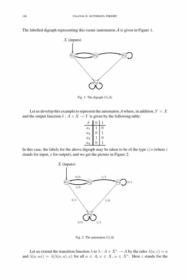
146 CHAPTER II. AUTOMATA THEORY
The labelled digraph representing this (semi-)automaton A is given in Figure 1.
X (inputs)
���������a1 ��
��
�������a2 �� �������a3 ��
��
�������a4�� ��
Fig. 1: The digraph G(A)
Let us develop this example to represent the automatonAwhere, in addition, Y = Xand the output function δ : A×X → Y is given by the following table:
δ 0 1a1 1 0a2 0 1a3 1 0a4 0 1
In this case, the labels for the above digraph may be taken to be of the type i/o (where istands for input, o for output), and we get the picture in Figure 2.
X (inputs)
���������a1
1/0
��
0/1
�����
����
����
����
���������a2
1/1
0/0�� �������a3 0/1��
1/0
���������������������
�������a4
0/0
��
1/1
��
Fig. 2: The automaton G(A)
Let us extend the transition function λ to λ : A×X∗ → A by the rules λ(a, ε) = aand λ(a, ux) = λ(λ(a, u), x) for all a ∈ A, x ∈ X , u ∈ X∗. Here ε stands for the
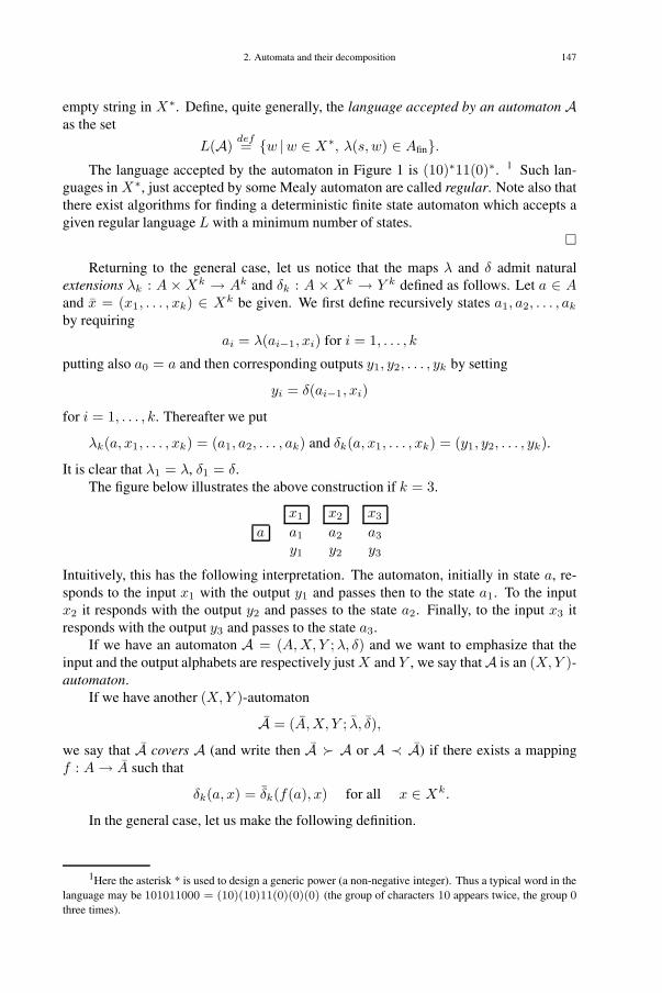
2. Automata and their decomposition 147
empty string in X∗. Define, quite generally, the language accepted by an automaton Aas the set
L(A)def= {w |w ∈ X∗, λ(s, w) ∈ Afin}.
The language accepted by the automaton in Figure 1 is (10)∗11(0)∗. 1 Such lan-guages in X∗, just accepted by some Mealy automaton are called regular. Note also thatthere exist algorithms for finding a deterministic finite state automaton which accepts agiven regular language L with a minimum number of states.
�
Returning to the general case, let us notice that the maps λ and δ admit naturalextensions λk : A ×Xk → Ak and δk : A ×Xk → Y k defined as follows. Let a ∈ Aand x = (x1, . . . , xk) ∈ Xk be given. We first define recursively states a1, a2, . . . , ak
by requiringai = λ(ai−1, xi) for i = 1, . . . , k
putting also a0 = a and then corresponding outputs y1, y2, . . . , yk by setting
yi = δ(ai−1, xi)
for i = 1, . . . , k. Thereafter we put
λk(a, x1, . . . , xk) = (a1, a2, . . . , ak) and δk(a, x1, . . . , xk) = (y1, y2, . . . , yk).
It is clear that λ1 = λ, δ1 = δ.The figure below illustrates the above construction if k = 3.
x1 x2 x3
a a1 a2 a3
y1 y2 y3
Intuitively, this has the following interpretation. The automaton, initially in state a, re-sponds to the input x1 with the output y1 and passes then to the state a1. To the inputx2 it responds with the output y2 and passes to the state a2. Finally, to the input x3 itresponds with the output y3 and passes to the state a3.
If we have an automaton A = (A,X, Y ;λ, δ) and we want to emphasize that theinput and the output alphabets are respectively just X and Y , we say thatA is an (X,Y )-automaton.
If we have another (X,Y )-automaton
A = (A,X, Y ; λ, δ),
we say that A covers A (and write then A A or A ≺ A) if there exists a mappingf : A→ A such that
δk(a, x) = δk(f(a), x) for all x ∈ Xk.
In the general case, let us make the following definition.
1Here the asterisk * is used to design a generic power (a non-negative integer). Thus a typical word in thelanguage may be 101011000 = (10)(10)11(0)(0)(0) (the group of characters 10 appears twice, the group 0
three times).

148 CHAPTER II. AUTOMATA THEORY
DEFINITION 2.1. A homomorphism of automata
σ : A = (A,X, Y ;λ, δ)→ A = (A, X, Y ; λ, δ)
is a triple σ = (σ1, σ2, σ3) of maps, where σ1 : A → A, σ2 : X → X, σ3 : Y → Y ,such that
σ2(λ(a, x)) = λ(σ1(a), σ2(x))
σ3(δ(a, x)) = δ(σ1(a), σ2(x))
for all a ∈ A and x ∈ X .
In particular, an epimorphism of two (X,Y )-automata A = (A,X, Y ;λ, δ) andA = (A,X, Y ; λ, δ) is provided by a triple of mappings of the type (σ, idX , idY ) withσ : A→ A surjective such that
[λ(a, x)]σ = λ(aσ, x) and [δ(a, x)]σ = δ(aσ, x)
for all a ∈ A. (Here we have written σ : a �→ aσ.)
PROPOSITION 2.2. If there exists an epimorphismA → A, then A A.
PROOF. Define f(a) = aσ for a ∈ A. Take any element (x1, . . . , xk) ∈ Xk andlet a ∈ A be given. Define, as before, a1, a2, . . . , ak recursively starting with a0 = aand postulating that ai = λ(ai−1, xi) for 1 ≤ i ≤ k. In a similar way, define a1, . . . , ak
starting with a0 = aσ ∈ A. Note that
a0 = aσ = aσ0 .
Suppose that we have already proved that
ai−1 = aσi−1
for some i ≥ 1. Then we get
aσi = [λ(ai−1, xi)]σ = λ(aσ
i−1, xi) = λ(ai−1, xi) = ai.
Hence, by induction we see that
ai = aσi
holds for all i ≤ k.Now it is easy to prove that
δk(a, x1, . . . , xk) = δk(aσ, x1, . . . , xk).
Indeed, as δ1 = δ and δ1 = δ we find
δ1(aσ, x1) = δ(aσ, x1) = δ(a, x1) = δ1(a, x1).
Suppose that we have already proved, for some i < k, that
δi(a, x1, . . . , xi) = δi(aσ, x1, . . . , xi).
2. Automata and their decomposition 149
Then it follows that
δi+1(a, x1, . . . , xi+1) =(δi(a, x1, . . . , xi), δ(ai, xi+1)
)=
=(δi(aσ, x1, . . . , xi), δ(aσ
i , xi+1))
=
=(δi(aσ, x1, . . . , xi), δ(ai, xi+1)
)=
= δi+1(aσ, x1, . . . , xi+1).
Thus, in view of our definition of f , we have established that for any x ∈ Xk
δk(a, x) = δk(f(a), x).
�DEFINITION 2.3. We say that two automata A and A are equivalent if and only if
A A and A A. It is easy to see that this relation is an equivalence relation on(X,Y )-automata. Let us agree to denote it byA ∼ A.
Consider the semigroup X+ of all (non-empty) words in the alphabet X , that is,w = x1x2 . . . xk where x1, x2, . . . , xk are any elements of X .
We can define recursively the operation � on X+ by stipulating that
a � x1 . . . xk = (a � x1 . . . xk−1) � xk (k > 1).
Note that � is a semigroup action of X+ on A in the sense that (a �w) �w′ = a � (ww′)for all a ∈ A and all w,w′ ∈ X+. Similarly, we can define ∗ on X+ by requiring that
a ∗ x1 . . . xk = (a � x1 . . . xk−1) ∗ xk (k > 1).
REMARK 2.4. We see that a � x1 . . . xk is nothing but the k-th component ofλk(a, x1, . . . , xk) and, similarly, that a ∗ x1 . . . xk is nothing but the k-th componentof δk(a, x1, . . . , xk). �
For any element a ∈ A consider the function
δa : X+ → Y +
given by the rule
δa(x1x2 · · ·xk) = δk(a, x1, . . . , xk) with x1, . . . , xk ∈ X , k ≥ 1.
Such a function will be called the line of behavior2 of A beginning at the state a. Intro-duce the set
Δ(A) = {δa : X+ → Y + | a ∈ A}.If the correspondence a �→ δa is a bijection between the set of states of A and the setΔ(A), then the automatonA is called reduced.
Fix again a ∈ A and consider the map fa : X+ → Y ,
fa(w) = a ∗ w.From the algorithmic point of view it is more convenient to consider the set
Φ(A) = {fa : X+ → Y | a ∈ A}rather than the previous set Δ(A).
We have the following useful result.
2Editors’ Note. Sometimes called also as a trace of A.
150 CHAPTER II. AUTOMATA THEORY
PROPOSITION 2.5. For any automatonA one has
δa = δb ⇐⇒ fa = f b.
PROOF. Suppose that δa = δb for some a, b ∈ A. Take any wordw = x1x2 · · ·xk ∈Xk. Then
fa(w) = a ∗ (x1x2 · · ·xk) =
= (a � x1 · · ·xk−1) ∗ xk =
= prk(δa(w)) = prk(δb(w)) = · · · = f b(w),
where prk stands for projection to the kth component. Therefore, fa = f b.On the other hand, assume that fa = f b for some a, b ∈ A. Then we obtain
δa(w) = (a ∗ x1, a ∗ x1x2, . . . , a ∗ x1x2 · · ·xk) =
= (fa(x1), fa(x1x2), . . . , fa(x1x2 · · ·xk)) =
= (f b(x1), f b(x1x2), . . . , f b(x1x2 · · ·xk)) = · · · = δb(w).
This shows that δa = δb. �
It follows from Proposition 2.5 that for any automaton A = (A,X, Y ;λ, δ) thecorrespondence a �→ δa (a ∈ A) is one-to-one if and only if the same is true for thecorrespondence a �→ fa (a ∈ A). Therefore, for an automaton A to be reduced it isnecessary and sufficient that one has a one-to-one correspondence between A and Φ(A).
PROPOSITION 2.6. Let A and A be any two reduced (X,Y )-automata. Then thefollowing conditions are equivalent:
(i): A and A are isomorphic;(ii): A and A are equivalent;(iii): Δ(A) = Δ(A);(iv): Φ(A) = Φ(A).
PROOF. (i) ⇒ (ii). Suppose that A and A are two isomorphic (X,Y )-automata.Then, one has, in particular, epimorphisms μ : A → A and μ−1 : A → A. Hence, itfollows from Proposition 2.2 that A A and A A. Therefore,A ∼ A.
(ii) ⇒ (iii). Suppose that A ∼ A for some reduced (X,Y )-automata A and A. Bydefinition, we then have A A and A A. Therefore, according to Proposition 2.2there exist epimorphisms μ : A → A, μ = (f, idX , idY ), and ν : A → A, ν =(g, idX , idY ), such that for the first components of these maps (i.e., for the corresponding“epimorphisms of states" f : A→ A and g : A→ A) one has
δ(a, x) = δ(f(a), x) and δ(a, x) = δ(g(a), x),
where a ∈ A, a ∈ A and x ∈ X .

2. Automata and their decomposition 151
It follows that, for any word w = x1 · · ·xk ∈ X+,
δa(w) = δk(a, x1 · · ·xk) =
= (δ(a, x1), δ(a1, x2), . . . , δ(ak−1, xk)) =
=(δ(f(a), x1), δ(f(a1), x2), . . . , δ(f(ak−1), xk)
)=
= (δ(f(a), x1), δ((f(a)
)1, x2), . . . , δ
((f(a)
)k−1
, xk))
=
= δk(f(a), x1 · · ·xk) = δf(a)(w).
Here ai = a � x1 · · ·xi and we have used the relations
f(ai) = f(a � x1 · · ·xi) = f(a) � x1 · · ·xi = f(a)i (i ≥ 2)
which hold true since μ = (f, idX , idY ) is a homomorphism of automata. As a resultwe get δa = δf(a), which implies that Δ(A) ⊆ Δ(A). In the same way, we obtainδa = δg(a) and so also Δ(A) ⊆ Δ(A).
(iii) ⇒ (iv). The equality Δ(A) = Δ(A) implies that for any function δa ∈ Δ(A)there exists a function δa (where a ∈ A) such that δa = δa as functions on X+. Itfollows that
Φ(A) = {δak | a ∈ A, k ∈ N} ⊆ {δa
k | a ∈ A, k ∈ N} = Φ(A),
where the subscript k indicates the k-th component of the function in question. Inter-changing the rôle of A and A gives Φ(A) ⊆ Φ(A) also.
(iv) ⇒ (i). The equality Φ(A) = Φ(A) implies that for any f a there exists somefa ∈ Φ(A) such that fa = f a as functions on X+. At the same time, there is no otherstate a1 ∈ A such that fa1 = f a – otherwise one would have fa = fa1 (with a �= a1)contradicting the fact that A is a reduced automaton. It follows that the correspondenceψ : a �→ a thus obtained is a bijection.
Let us now prove that
μ = (m, idX , idY ) : A → Ais an isomorphism of automata. Even more is true. Namely, for any a ∈ A, v ∈ X+, wehave
(a ∗ v)μ = (a ∗ v)idY = fa(v) = f a(v) = a ∗ v = am ∗ vidX+ = aμ ∗ vμ.
Moreover,(a � v)μ = aμ � vμ.
Indeed, as A is reduced, it is enough to show that
f (a�v)m
= fam�v.
To this end, take any w ∈ X+; then
f (a�v)m
(w) = fa�v(w) = (a � v) ∗ w = a ∗ (vw) = fa(vw) =
= fam
(vw) = am ∗ vw = (am � v) ∗ w = fam�v(w).
�

152 CHAPTER II. AUTOMATA THEORY
2.2. Preliminary motivation and more notions
Finite automata can serve as a bridge also between such topics in theoretical computerscience as classification of formal languages and the investigation of their structure, orcrypto-analysis and systems theory. Automata theory provides several valuable conceptsfor the analysis and modelling of cryptographic devices. For instance, it often happensthat a cipher device is assembled from a set of simpler components (such as shift regis-ters), and so additional attacks may become feasible if the given machine can be decom-posed in a way different from its original construction. However, it appears that cascadesof clock-controlled shift registers can only be decomposed in the way they were con-structed [7].
In order to show that the completion of a semi-automaton with output function δ isnot a mere formality for achieving coherence with the notions in the classics, let us seehow it can be used in coding. Namely, any Mealy automaton that satisfies the condition
(36) ∀a ∈ A δa(u) = δa(v) ⇒ u = v in X∗,
is called a Mealy coding machine. This means that, for such an automaton A, Δ(A)consists of injective functions. In terms of the digraph representation for A condition(36) means that there are no two arcs leaving any given state with the same output label.At the same time, as λ is a function, it is clear that each node of the digraph representingA has no arcs leaving this node with the same input labels. This property makes itpossible to construct a new automaton
A−1 = ((s;A), X, Y ;λ−1, δ−1)
defining, for any a ∈ A
λ−1(a, o)def= b if and only if λ(a, i) = b and
δ−1(a, o)def= i if and only if δ(a, i) = o .(37)
Here i is an input symbol and o the corresponding output symbol, defined by δ(a, i) = o.It follows that
δs(v) = w ⇒ (δ−1)s(w) = v;
this can be shown by induction on the length |v| = |w|. For instance, for the Mealyautomaton given in Figure 2, taking w = 101100 as an input word in X∗ we get δs(w) =δa1(101100) = 000111. Note also that s � w = a1 � 101100 = a3. Given a digraphG(A) representing a Mealy coding machineA, as in the case of Figure 2, it is easy to getG(A−1): just change the labels i/o to o/i. For instance, for the automatonA in Figure 2this means that G(A−1) is as in Figure 3.In this case one finds that
(δ−1(s, 000111) = 101100 and λ−1(s, 000111) = a3.
Let us go one step further. Consider a shift register R#n functioning according to the
scheme in Figure 4.During any fixed time interval the content (B0, B1, . . . , Bn−1) of its binary storage el-ements Bi (i = 0, 1, . . . , n − 1) is represented by a (0, 1)-vector called a state of R#
n .

2. Automata and their decomposition 153
X (inputs)
���������a1
0/1
��
1/0
�����
����
����
����
���������a2
1/1
0/0�� �������a3 1/0��
0/1
���������������������
�������a4
0/0
��
1/1
��
Fig. 3: The reversed automaton G(A−1)
��⊗
��
B = R( B0, B1, · · · , Bn−1) B
L B0��
��
B1��
��
· · · �� Bn−1
����
Fig. 4: A shift register R#n
During this same time interval the value B of the function R(B0, B1, . . . , Bn−1) is cal-culated. Using this value and the input i, the new value B′
0 for B0 is found; often, this isdone using the rule
B′0
def= B · i ∨ B · i (“exclusive or").
Usually, this value B′0 is considered also as the output of R#
n during this time interval.Further, at the same time the transfer of the content of the storage elements is madeaccording to the rule
Bk �→ Bk+1 (k = 0, 1, . . . , n− 2).
Thus, during this time interval the transfer
(B0, B1, B2, . . . , Bn−1) �→ (B′0, B0, B1, . . . , Bn−2)
takes place. A concrete example (for n = 3) of R#3 is given by the following table; we
take X = {0, 1} = Y , Bdef= R(B0, B1, B2) = B0 · B1 ∨B2 and B′
0def= B · i ∨B · i.

154 CHAPTER II. AUTOMATA THEORY
Stateno.
B0 B1 B2 Bdef= B0 · B1 ∨ B2 i B′
0def= B · i ∨ B · i B′
0 B′1 B′
2
Newstateno
Output
0 0 0 0 0 · 0 ∨ 0 = 001
0 · 0 ∨ 0 · 0 = 00 · 1 ∨ 0 · 1 = 1
01
00
00
04
01
1 0 0 1 0 · 0 ∨ 1 = 101
1 · 0 ∨ 1 · 0 = 11 · 1 ∨ 1 · 1 = 0
10
00
00
40
10
2 0 1 0 0 · 1 ∨ 0 = 001
0 · 0 ∨ 0 · 0 = 00 · 1 ∨ 0 · 1 = 1
01
00
11
15
01
3 0 1 1 0 · 1 ∨ 1 = 101
1 · 0 ∨ 1 · 0 = 11 · 1 ∨ 1 · 1 = 0
10
00
11
51
10
4 1 0 0 1 · 0 ∨ 0 = 101
1 · 0 ∨ 1 · 0 = 11 · 1 ∨ 1 · 1 = 0
10
11
00
62
10
5 1 0 1 1 · 0 ∨ 1 = 101
1 · 0 ∨ 1 · 0 = 11 · 1 ∨ 1 · 1 = 0
10
11
00
62
10
6 1 1 0 1 · 1 ∨ 0 = 001
0 · 0 ∨ 0 · 0 = 00 · 1 ∨ 0 · 1 = 1
01
11
11
37
01
7 1 1 1 1 · 1 ∨ 1 = 101
1 · 0 ∨ 1 · 0 = 11 · 1 ∨ 1 · 1 = 0
10
11
11
73
10
Corresponding to this table the Mealy automaton A(R#3 ) can be represented by
the following labelled digraph (see Figure 5). There, aidef= (i)2 are the states for
G(A(R#3 )). Here (i)2 stands for the binary representation of the number i.
�� ����a0000
0/0
��
1/1
�������
������
��
�� ����a1001
1/0
���������������
0/1
���� ����a20100/0
��
1/1
��
�� ����a41001/0
��
0/1
���� ����a3011
1/0
��
0/1 �� �� ����a5101
0/1 ��
1/0
��
�� ����a6110
1/1�����
������
����
0/0
��
�� ����a7111
0/1
��
1/0
��
Fig. 5: The automaton of the shift register G(A(R#3 ))
To get the digraph G(R+) corresponding to the decoder for the Mealy coding ma-chine given by the digraph G(R#
n ) it remains to reverse the i/o-labels to o/i-labels.The Mealy automaton obtained in this fashion corresponds to the shift register whereR(B0, B1, . . . , Bn−1) and Bk �→ Bk+1 (k = 0, 1, . . . , n − 2) are calculated as beforebut B0 is taken to be the input. The output is “exclusive or" of B and B0 (for furtherinformation on cipher systems cf. [1]).
DEFINITION 2.7. By a congruence on an automaton A = (A,X, Y ;λ, δ) is meanta triple of equivalence relations ρ = (ρ1, ρ2, ρ3) such that if a ρ1 b in A and u ρ2 v in X

2. Automata and their decomposition 155
then we have also
(a � u) ρ1 (b � v) in A and (a ∗ u) ρ3 (b ∗ v) in Y .
Every congruence ρ on an automatonA gives rise to a factor-automaton
A/ρ = (A/ρ1, X/ρ2, Y/ρ3; �′, ∗′)where
[a]ρ1 �′ [x]ρ2
def= [a � x]ρ1 and [a]ρ1 ∗′ [x]ρ2
def= [a ∗ x]ρ3 .
It is easy to formulate and to prove the analogues of the well-known first and secondhomomorphism theorems (of E. Noether) in this context. This is left as an exercise to theReader. Here we will only require the following special case.
THEOREM 2.8. Let there be given an epimorphism of automata ψ : A → B. Thenthere exists an isomorphism ϕ : A/ kerψ → B that makes the diagram
A
τ��
ψ �� �� B
A/ kerψ
ϕ
����
��
�
commutative.
PROOF. The proof is standard. �
Here kerψ = (kerψ1, kerψ2, kerψ3) is a congruence, while τ is the natural epi-morphism of A onto the factor-automaton A/ kerψ. (More precisely, for instance theequivalence of a and b under kerψ1 simply means that these elements have the sameψ1-image, that is, ψ1(a) = ψ1(b).)
To every automatonA = (A,X, Y ) there corresponds a reduced automaton
A = (A/ρ,X, Y )
where ρ is a congruence such that a ρ a′ if and only if a ∗ u = a′ ∗ u for all u ∈ X .
2.3. Semigroup automata
Given an automaton A = (A,X, Y ; �, ∗) we have already extended (Sec. 2.1) theoperations � and ∗ to cover the case of the free semigroup X+ generated by X .
In a similar way all other notions can be extended to automata of the type A =(A,X+, Y ; �, ∗). More generally, we can consider, instead of X+, any semigroup Γ.We can then define a semigroup automaton as a quintuple A = (A,Γ, Y ; �, ∗) obeyingthe rules
a � γ1γ2 = (a � γ1) � γ2 and a ∗ γ1γ2 = (a � γ1) ∗ γ2
for all a ∈ A and all γ1, γ2 ∈ Γ.In particular, every semigroup automaton A may be considered as a heterogeneous
algebra (in the sense of G. Birkhoff)3. This point of view helps one to find quicklythe notions decisive for the decomposition of automata. In this connection we give thefollowing definition.
3Editors’ Note. Also called a many-sorted algebra.

156 CHAPTER II. AUTOMATA THEORY
DEFINITION 2.9. A homomorphism of semigroup automata
A = (A,Γ, Y ; �, ∗)→ A′ = (A′,Γ′, Y ′; �′, ∗′)is a triple ψ = (ψ1, ψ2, ψ3) of mappings,
ψ1 : A→ A′, ψ2 : Γ → Γ′ and ψ3 : Y → Y ′,
where, in addition, ψ2 is a semigroup homomorphism and we have
ψ1(a � u) = ψ1(a) �′ ψ2(u) and ψ3(a ∗ u) = ψ1(a) ∗′ ψ2(u)
for all a ∈ A and u ∈ Γ.
The notions of isomorphism, epimorphism, monomorphism etc. are defined in theusual way. Notice that we obtain a category with semigroup automata as its objects andtheir homomorphisms as its morphisms. This point of view is also very helpful in findingpatterns for decomposition of automata.
In the special case when Γ has a unit element ε ∈ Γ it is assumed that a � ε = a forall a ∈ A. This implies that
a ∗ γ = a ∗ γε = (a � γ) ∗ ε.Therefore, introducing a map μ : A→ Y by the rule
μ(a) = a ∗ ε,it follows that a ∗ γ = μ(a � γ) for all a ∈ A and γ ∈ Γ.
Conversely, consider any action (A,Γ; �) of a semigroup Γ on a set A and anymap μ : A → Y . We obtain an automaton A = (A,Γ, Y ; �, ∗) defining ∗ by the rulea ∗ γ = μ(a � γ). Indeed, we have
a ∗ γ1γ2 = μ(a � (γ1γ2)
)= μ
((a � γ1) � γ2
)= (a � γ1) ∗ γ2.
We say then that A is a Moore automaton.Let us now change our notation writing F (X) for the free semigroup over X (pre-
viously written X+) and, similarly, F ∗(X) for the free monoid over X .Given a semigroup automaton
A = (A,F (X), Y ; �, ∗),define on F (X) a binary relation ρ by stipulating that
u ρ v⇐⇒ a � u = a � v for all a ∈ A.
It follows at once from the properties of the action (A,F (X); �) that ρ is an equivalenceon F (X) which is two-sided stable under multiplication by elements of F (X), i.e. ρ is acongruence on F (X).
The factor-semigroup ΓA = F (X)/ρ is called the semigroup of the automatonA.Note that ρ = ker(A,F (X)), that is, ρ is the kernel of the action (A,F (X); �).
Furthermore, the induced action (A,ΓA; �) is faithful. The last thing means that any twoelements in ΓA acting in the same way on A coincide by necessity (i.e. a � σ = a � τ forall a ∈ A implies that σ = τ ).
Notice also that if |A| <∞ then |ΓA| <∞. In words: finiteness of the set of statesof an automaton forces its semigroup to be finite also.
2. Automata and their decomposition 157
Finally, let us take a semigroup automaton A = (A,Γ, Y ; �, ∗) and define a binaryrelation ρ on Γ by the rule
γ1 ∼ γ2 (mod ρ) ⇐⇒ a � γ1 = a � γ2 and a ∗ γ1 = a ∗ γ2 for all a ∈ A.
Then ρ is two-sided stable on Γ, both for � and ∗. So, it is clear that always ρ ⊂ker(A,Γ). For a Moore automaton one has equality, ρ = ker(A,Γ).
2.4. Cyclic automata
Let us call an action (A,Γ; �) cyclic if there exists an element a ∈ A such that A ={a � γ | γ ∈ Γ}.
Consider now the map
ψ : (F ∗(X), X)→ (A,X),
of the regular action (F ∗(X), X) into a cyclic automaton (A,X), by the rule
ψ(u) = a � u, u ∈ F ∗(X).
It is easy to see that(F ∗(X)/ρ,X) ∼= (A,X)
with ρ as in Sec. 2.3.More can be said in this context. Namely, let (A,X, Y ; �, ∗) be any cyclic automa-
ton, i.e. A coincides with the set {a�x |x ∈ X} for some a ∈ A. Consider the automaton(F ∗(X), X, Y ; �′, ∗′) with the basic operations given by
u �′ x = ux and u ∗′ x = a ∗ ux for x ∈ X and u ∈ F ∗(X);
here ux means that we take the product of u and x in F ∗(X). The map ψ : F ∗(X)→ A
given by uψ def= a � u yields an epimorphism of automata
ψ : (F ∗(X), X, Y )→ (A,X, Y )
and so we obtain a natural isomorphism
(F ∗(X)/ρ,X, Y ) ∼= (A,X, Y )
with ρ as above.Now consider the special case when A = (A,X, Y ) is a reduced cyclic Moore
automaton. Let A be generated by the element a ∈ A. Consider the map
f = fa : F ∗(X)→ Y,
given byf(u) = a ∗ u for all u ∈ F ∗(X).
It is readily seen that knowledge of f allows us to restore ρ. Indeed, take on F ∗(X)the binary relation ρ∗ defined as follows
u ∼ u′ (mod ρ∗) def⇐⇒ f(vuw) = f(vu′w) for all v, w ∈ F ∗(X).
It is easy to check that ρ = ρ∗. Indeed, take any two words u and u′ in F ∗(X) suchthat uρu′. Then, for any words v and w in F ∗(X) it is true that
(vu) ρ (vu′) and a � vu = a � vu′.

158 CHAPTER II. AUTOMATA THEORY
Therefore,
a ∗ (vuw) = (a � vu) ∗w = (a � vu′) ∗ w = a � (vu′w),
which impliesf(vuw) = f(vu′w).
This shows that uρ∗u′, which proves ρ ⊆ ρ∗.In the other direction, suppose that uρ∗u′. Then, for any two words v and w in
F ∗(X) we have
a ∗ (vuw) = f(vuw) = f(vu′w) = a ∗ (vu′w).
Taking here v = ε gives
(a � u) ∗ w = a ∗ uw = a ∗ u′w = (a � u′) ∗ w.Therefore, fa�u = fa�u′ and, asA is reduced by hypothesis, it follows that a�u = a�u′
and so also uρu′.
This reasoning leads us to the following construction: given (arbitrary) sets X andY and a map f : F ∗(X) → Y define on F ∗(X) the binary relation ρ∗ as just was doneabove. So we get an action
(F ∗(X)/ρ∗, X).As ρ∗ ⊆ ker f (by definition!) the map f : F ∗(X)→ Y induces a map
μ : F ∗(X)/ρ∗ → Y.
Thus, having the action (F ∗(X)/ρ∗, X) (a semi-automaton) and the map μ, we get aMoore automaton (F ∗(X)/ρ∗, X, Y ), which we denote byA(f). A straightforward ver-ification shows thatA(f) is a reduced cyclic Moore automaton. Therefore, the followingresult is true.
PROPOSITION 2.10. The automaton A(f) is a reduced cyclic Moore automaton.Conversely, every reduced cyclic Moore automaton can be obtained in this way.
2.5. Wreath products of actions
Let there be given two semigroup actions (A,Φ) and (B,Σ). Take the set of all func-tions ϕ : B → Φ (that is, ϕ ∈ ΦB = Fun(B,Φ)) and make it a semigroup by definingmultiplication of such functions pointwise:
(ϕ1 · ϕ2)(b) = ϕ1(b) · ϕ2(b) for b ∈ B.
Furthermore, let us consider the semi-direct product
Γ = ΦB � Σ = {(ϕ, σ)|ϕ ∈ ΦB, σ ∈ Σ}defining multiplication of pairs (ϕ, σ) by the formula
(ϕ1, σ1) · (ϕ2, σ2) = (ϕ1 · σ1ϕ2, σ1σ2),
where σ1ϕ2 is given byσ1ϕ2(b) = ϕ2(b � σ1) for b ∈ B.

2. Automata and their decomposition 159
(To check the associativity, it suffices to note that (ϕ1 ·σ1ϕ2)·σ1σ2ϕ3 = ϕ1 ·σ1(ϕ2 ·σ2ϕ3).)Lastly, let us take the Cartesian product
G = A× B = {(a, b) | a ∈ A, b ∈ B}
giving an action of the semigroup Γ on G by the rule
(a, b) � (ϕ, σ) def= (a � ϕ(b), b � σ) .
In this way we obtain an action (G,Γ),
(G,Γ) = (A,Φ)wr(B,Σ)
called the wreath product of the given pairs (A,Φ) and (B,Σ).
PROPOSITION 2.11. Let ρ = ker(G,Γ), ρ1 = ker(A,Φ) and ρ2 = ker(B,Σ). Then
(ϕ1, σ1) ∼ (ϕ2, σ2) (mod ρ)
if and only if
σ1 ∼ σ2 (mod ρ2)
and
ϕ1(b) ∼ ϕ2(b) (mod ρ1) for all b ∈ B.
PROOF. right hand side, suppose that
(ϕ1, σ1) ∼ (ϕ2, σ2) (mod ρ).
Then for any (a, b) ∈ G holds
(a � ϕ1(b), b � σ1) = (a, b) � (ϕ1, σ1) = (a, b) � (ϕ2, σ2) = (a � ϕ2(b), b � σ2).
Therefore,
b � σ1 = b � σ2 for all b ∈ B
which gives σ1 ∼ σ2 (mod ρ2). Also, as a � ϕ1(b) = a � ϕ2(b) for all a ∈ A, thisimplies that ϕ1(b) ∼ ϕ2(b) (mod ρ1) for all b ∈ B.
On the other hand, if
a � ϕ1(b) = a � ϕ2(b) and b � σ1 = b � σ2
for all a ∈ A and all b ∈ B, we get
(a, b) � (ϕ1, σ1) = (a, b) � (ϕ2, σ2)
for all (a, b) ∈ G and therefore
(ϕ1, σ1) ∼ (ϕ2, σ2).
�
COROLLARY 2.12. If both the actions (A,Φ) and (B,Σ) are faithful, then the sameis true for (G,Γ) also.

160 CHAPTER II. AUTOMATA THEORY
PROOF. Indeed, suppose that
(a, b) � (ϕ1, σ1) = (a, b) � (ϕ2, σ2)
holds for all (a, b) ∈ G. Then, according to Proposition 2.11, it follows that
σ1 ∼ σ2 (mod ρ2)
andϕ1(b) ∼ ϕ2(b) (mod ρ1) for all b ∈ B.
The faithfulness of (B,Σ) implies that
σ1 ∼ σ2 (mod ρ2) =⇒ σ1 = σ2.
Also, the faithfulness of (A,Φ) gives
ϕ1(b) ∼ ϕ2(b) (mod ρ1) =⇒ ϕ1(b) = ϕ2(b) for all b ∈ B.
The last thing means that ϕ1 = ϕ2 and so we get (ϕ1, σ1) = (ϕ2, σ2). �
PROPOSITION 2.13. Let there be given two homomorphisms of pairs
α : (A,Φ) → (A, Φ) and β : (B,Σ)→ (B, Σ),
where the first component of β is the identity map on B. Then there exists a homomor-phism
(A,Φ)wr(B,Σ) → (A, Φ)wr(B, Σ)extending the given mappings. In particular, if (A,Φ) � (A, Φ) and (B,Σ) � (B, Σ)are the natural epimorphisms onto the corresponding faithful pairs, then there exists anepimorphism
(A,Φ)wr(B,Σ) � (A, Φ)wr(B, Σ)with the right hand side faithful also.
PROOF. Define μ : G→ G, where G = A×B, by
(a, b)μ = (aα, b) for any (a, b) ∈ G.
Also, let ν : ΦB → ΦB be given by the rule
ϕν(b) = [ϕ(b)]α.
Thereafter, extend these two maps to
μ : ΦB � Σ → ΦB � Σdef= Γ
defined by(ϕ, σ)μ = (ϕν , σβ).
Let us prove that the homomorphism μ : Γ → Γ appears in this way.Indeed, on the one hand we have
[(ϕ1, σ1) · (ϕ2, σ2)]μ = (ϕ1 · σ1 ϕ2, σ1σ2)μ =((ϕ1 · σ1 ϕ2)ν , (σ1σ2)β
)and on the other hand
(ϕ1, σ1)μ · (ϕ2, σ2)μ = (ϕν1 , σ
β1 ) · (ϕν
2 , σβ2 ) =
(ϕν
1 · σβ1 ϕν
2), σβ1 · σβ
2
)As β is a homomorphism of actions, we certainly have
(σ1σ2)β = σβ1 · σβ
2 .

2. Automata and their decomposition 161
So, it remains to prove that
(38) (ϕ1 · σ1 ϕ2)ν = ϕν1 · σβ
1 ϕν2 .
Take any b ∈ B. As β a homomorphism of actions, it follows that
b � σ1 = (b � σ1)β = bβ � σβ1 = b � σβ
1 .
Hence,
(ϕ1 · σ1 ϕ2)ν(b) =[(ϕ1 · σ2 ϕ)(b)
]α=
[ϕ1(b) · ϕ2(b � σ1)
]α= ϕ1(b)α · ϕ2(b � σ1)α =
= ϕν1(b) · ϕν
2(b � σβ1 ) =
(ϕν
1 · σβ1 (ϕν
2))(b).
This holds for all b ∈ B and so implies (38).It remains to prove that μ is a homomorphism of actions, i.e. that
(39) ((a, b) � (ϕ, σ))μ = (a, b)μ � (ϕ, σ)μ.
Indeed, (39) follows from the properties of the homomorphisms α and β along withthe following series of equalities:
((a, b) � (ϕ, σ))μ = (a � ϕ(b), b � σ))μ = ((a � ϕ(b))α, b � σ) =(aα � ϕ(b)α, b � σβ)
)=
= (aα, b) � (ϕν , σβ) = (a, b)μ � (ϕ, σ)μ.
Now suppose that α and β are natural epimorphisms and let us prove that the homo-morphism
μ : (A,Φ)wr(B,Σ) → (A, Φ)wr(B, Σ),defined above by
(ϕ, σ)μ = (ϕν , σβ)and
∀b ∈ B ϕν(b) = [ϕ(b)]α,is an epimorphism. In view of what has been done above it remains to show that μ issurjective.
Take any element (ψ, σ) ∈ ΦB � Σ. We must verify that there exists an element(ϕ, σ) in ΦB � Σ such that
(ϕ, σ)μ = (ψ, σ).Here, as β is surjective, it follows immediately that there exists σ ∈ Σ such that σβ = σ.Therefore, it remains to prove that there exists a function ϕ : B → Φ such that ϕν = ψ.
As α is likewise surjective, it follows that for every element in Φ of the form ψ(b)with b ∈ B there exists an element ϕb ∈ Φ such that (ϕb)α = ψ(b). Take the functionϕ, ϕ : B → Φ, given by the rule
∀b ∈ B ϕ(b) = ϕb.
It is easy to check that ϕν = ψ: for every b ∈ B one has
ϕν(b) = ϕ(b)α = [ϕb]α = ψ(b).
Consequently, ϕν = ψ and, hence, the map ν : ΦB → ΦB is surjective. It follows thatthe same is true for
μ : ΦB � Σ → ΦB � Σ.
As μ is the identity map on A×B, we can take μ as the epimorphism requested. �

162 CHAPTER II. AUTOMATA THEORY
Note that there exists a natural analogue of Theorem 2.8 for semi-automata. Thisshows that
kerμ = (0A×B, π),
where 0A×B is the least equivalence on A× B (with one-element subsets as its classes)and π is the kernel for the pair (G,Γ).
2.6. Kaluzhnin-Krasner type theorem
Let there be given a group action (A,Γ), that is, a semigroup action such that Γ isa group. Assume that ρ is a congruence of the action (A,Γ) with the property that(A/ρ,Γ) is transitive, i.e. for any two classes [a] and [b] in A/ρ there exists γ ∈ Γ suchthat [a] � γ = [b]. Fix (arbitrarily) an element a ∈ A and consider the stabilizer of [a] inΓ, i.e. the semigroup
Σ = StΓ([a])def= {γ ∈ Γ
∣∣ [a] � γ = [a]}.Notice that the choice of [a] does not matter very much – if we take another element than[a] we obtain a semigroup conjugate to Σ, this due to the transitivity of (A/ρ,Γ). Letus interpret [a] as a subset of A denoting it in this role by B. We obtain thus a subpair(B,Σ) of (A,Γ). Denote by (A/ρ, Γ) the faithful action corresponding to (A/ρ,Γ).
THEOREM 2.14. There exists a monomorphism of semi-automata
(A,Γ) ↪→ (B,Σ)wr(A/ρ, Γ).
PROOF. Let us begin with the observation that any transitive action (D,Γ) is iso-morphic to some factor-action (Γ/Σ,Γ) of the (right-)regular action (Γ,Γ). Indeed, fixany element e ∈ D. Then for any x ∈ D there exists γ ∈ Γ such that e � γ = x. If
e � γ = e � γ1 for some elements γ and γ1 in Γ, then γγ−11 ∈ StΓ(e)
def= Σ. It follows
that the map μ : x �→ γ gives an isomorphism of the actions (D,Γ) and (Γ/Σ,Γ).Let us apply this observation to the action (A/ρ,Γ). Then we find that (A/ρ,Γ) is
isomorphic to (Γ/Σ,Γ) where Σ = StΓ([a]ρ). Let T be a full set of representatives forΣ-cosets Σγ (γ ∈ Γ) in Γ/Σ. By the above we have a bijection ν : A/ρ→ T . Moreover,we have
A/ρ = {[a] � τ | τ ∈ T },and this representation of elements of A/ρ is unique. Thus,
aμ�−→ [a] � τ ν�−→ τ,
i.e. aμν = τ .To prove the theorem we consider a pair of maps
(40) A→ B ×A/ρ
and
(41) Γ → ΣA/ρ � Γ,
given as follows.To get (40), let us set
(42) aα def= (a � (aμν)−1, aμ).
2. Automata and their decomposition 163
To get (41), define first a collection of maps fγ (γ ∈ Γ) where each individual mapfγ : A/ρ→ Σ is given by
(43) fγ(y) = yν · γ ·(
(y � γμ)ν
)−1
.
Then the required map (41) is obtained by the rule
(44) γα = (fγ , γμ).
It remains to verify that the pair of maps whose construction has been indicated doesthe job!
The map α : A → B × A/ρ given by (42) is injective. Indeed, let a1 and a2 beelements in A such that(
a1 � (aμν1 )−1, aμ
1
)=
(a2 � (aμν
2 )−1, aμ2
).
It follows that aμ1 = aμ
2 which, in turn, implies that
a1 � (aμν1 )−1 = a2 � (aμν
2 )−1 = a2 �((aμ
2 )ν)−1 = a2 �
((aμ
1 )ν)−1 = a2 � (aμν
1 )−1.
This gives a1 = a2 showing that α is indeed an injection.Next, observe that the right hand side of (43) belongs to Σ. Indeed, take y = [a] � τ ,
τ ∈ T with yν = τ . Then
[a] � fγ(y) = [a] � yν · y ·((y � yμ)ν
)−1 = ([a] � τy) �((
([a] � τ) � yμ)ν
)−1
=
= [a] �((τγ) � (τγμ)−1
)= [a].
It follows that fγ(y) ∈ StΓ([a]) = Σ.Let us prove that the map
α : Γ → ΣA/ρ � Γ
given by (44) is a homomorphism of groups. Let us take any two elements γ1 and γ2 inΓ and prove that (γ1γ2)α = γα
1 · γα2 . The left hand side is given by
(γ1γ2)α =(fγ1γ2 , (γ1γ2)μ
)= (fγ1γ2 , γ
μ1 γ
μ2 )
and the right hand side by
γα1 · γα
2 = (fγ1 , γμ1 )(fγ2 , γ
μ2 ) = (fγ1 · γμ
1fγ2 , γμ1 · γμ
2 ).
So, it suffices to prove that
(45) fγ1γ2 = fγ1 · γμ1fγ2 .
164 CHAPTER II. AUTOMATA THEORY
Indeed, for any y ∈ A/ρ we have
fγ1γ2(y) = yν · γ1γ2 ·((
y � (γ1γ2)μ)ν
)−1
=
= yν · γ1γ2 ·((y � γμ
1 γμ2 )ν
)−1 =
= yν · γ1
((y � γμ
1 )ν)−1 · (y � γμ
1 )ν · γ2 ·((
(y � γμ1 ) � γμ
2
)ν)−1
=
= fγ1(y) · fγ2(y � γμ1 ) =
= (fγ1 · γμ1 fγ2)(y).
This proves (45).It turns out that the homomorphism α is really a monomorphism. Suppose that
γα = (fγ , γμ) is the identity element in ΣAρ � Γ. This implies that γμ is the identity
element in Γ and, therefore, acts trivially on A/ρ. Also, it follows that fγ is the identityof ΣA/ρ and, consequently, for every y ∈ A/ρ it holds fγ(y) = ε ∈ Σ. We obtain
ε = fγ(y) = yν · γ ·(y � γμ)ν
)−1 = yν · γ · (yν)−1,
i.e. γ = ε showing that the map α : Γ → ΣA/ρ � Γ is injective.Next, notice that the action of Γ on A can be extended to a corresponding action on
B ×A/ρ. Indeed, for any two elements a ∈ A and γ ∈ Γ,
(a � γ)α =(
(a � γ) �((a � γ)μν
)−1, (a � γ)μ
)=
=(a �
((aμν)−1 · aμν · γ ·
((a � γ)μν
)−1), (a � γ)μ
)=
=((
a � (aμν)−1)�(aμν · γ ·
((a � γ)μν
)−1), aμ � γμ
)=
=(a � (aμν)−1, aμ
)� (fγ , γ
μ) == aα � γα.
Resuming, the above shows that we have a monomorphism of actions
(A,Γ) a−→ (B ×A/ρ,ΣA/ρ � Γ).
�
As a special case, let us take (A,Γ) to be the regular action (Γ,Γ) and let Σ ≤ Γbe any semigroup. Moreover, take ρ to be a partition of Γ into right Σ-cosets. One ofthese cosets, the one containing ε, is Σ and its centralizer in Γ is Σ also. According toTheorem 2.14 there exists a monomorphism
α : (Γ,Γ)→ (Σ,Σ)wr(Γ/Σ, Γ)
and, thus, there exists a monomorphism
Γ → ΣΓ/Σ � Γ

2. Automata and their decomposition 165
also.Further specializing, let Σ be an invariant semigroup in Γ. Then Γ = Γ/Σ and so
there exists an immersion
(Γ,Γ) ↪→ (Σ,Σ)wr(Γ/Σ,Γ/Σ).
The acting group of the wreath product of actions here coincides with the wreath productof groups Σwr(Γ/Σ).
Let us now describe how this result can be used to obtain the Krohn-Rhodes Theo-rem. Suppose that Γ is a finite group. Then by the Jordan-Hölder Theorem there existsan invariant (composition) series:
Γ = Γ0 � Γ1 � · · · � Γm = (1),
with all its factor cyclic groups of prime order. Applying here Theorem 2.14 gives amonomorphism,
(Γ,Γ) ↪→ (Γ1,Γ1)wr(Γ∗1 ,Γ
∗1),
where we have put Γ∗1 = Γ/Γ1.
Analogously, we find
(Γ1,Γ1) ↪→ (Γ2,Γ2)wr(Γ∗2 ,Γ
∗2)
where we have set Γ∗2 = Γ1/Γ2. Continuing this way gives a sequence of the form
(Γ,Γ) ↪→ (Γ1,Γ1)wr(Γ∗1 ,Γ
∗1) ↪→
((Γ2,Γ2)wr(Γ∗
2 ,Γ∗2))wr(Γ∗
1 ,Γ∗1) ↪→ · · ·
Finally, using the associativity of the operation wr for semi-automata, we find that
(Γ,Γ) ↪→ (Γ∗m−1,Γ
∗m−1)wr(Γ
∗m−2,Γ
∗m−2)wr · · ·wr(Γ∗
1 ,Γ∗1).
Here all Γ∗i (i = 1, 2, . . . ,m − 1) are finite simple groups and at the same time they
are epimorphic images of groups contained in the (semi)group Γ, i.e. its “factors" in thesense of Krohn-Rhodes theory.
To this end, let us add that the Krohn-Rhodes Theorem asserts that every finite(semi-)automaton can be modelled by a cascade of finite simple (semi-)automata thatare “factors" and “triggers". The latter are defined as (semi-)automata (A,X) with A ={a1, a2} and X = {ε, x1, x2} along with the rules a � ε = a, a � xi = ai (i = 1, 2) forany a ∈ A.
It remains to explain what a cascade of automata is; this will be done in the nextsection.
2.7. Cascades and wreath products of automata; their interconnec-tions
Let there be given two automata
A1 = (A1, X1, Y1) and A2 = (A2, X2, Y2)
and, in addition, a set X together with the following two maps:
α : X ×A2 → X1 and β : X → X2.
We obtain a new automatonA = (A,X, Y ) if we define the basic sets A and Y as
Adef= A1 ×A2; Y
def= Y1 × Y2

166 CHAPTER II. AUTOMATA THEORY
and give the basic operations � and ∗ by the rules
(a1, a2) � x def= (a1 � α(x, a2), a2 � β(x))
and
(a1, a2) ∗ x def= (a1 ∗ α(x, a2), a2 ∗ β(x))
This new automaton A is called the cascade of the two given automata determined bythe joining maps α and β, and is denoted αA1 � βA2.
Figure 6 below illustrates this construction.
X
��
•��β A2 α A1 Y ��
Fig. 6: The cascade of automata A = αA1 � βA2
Two special cases of this construction deserve special mentioning. First, the parallelcomposition of two automataA1 and A2 appears if we take
X = X1 ×X2;
α : (X1 ×X2)×A2pr−→ X1;
β : (X1 ×X2)pr−→ X2.
Second, the sequential composition of two automataA1 and A2 appears if we take
X = X2;
α(x, a2) = (a2 ∗ x)ψ with ψ : Y2 → X1 given;β = idX2 .
Given any two “pure" automata
A1 = (A1, X1, Y1) and A2 = (A2, X2, Y2)
let us extend them to the corresponding semigroup automata
A•1 = (A1, F (X1), Y1) and A•
2 = (A2, F (X2), Y2)
Let us further, for brevity, write Fi = F (Xi), i = 1, 2. Then we have the two actions
(A1, F1) and (A2, F2)
and so also the action
(A1, F1)wr(A2 , F2) = (A1 ×A2, Fun(A2, F1) � F2),
which action we denote by (A,Φ).
2. Automata and their decomposition 167
Define now a map f : X → Φ. To this end, we first define f1 : X → Fun(A2, F1)by
xf1 (a2)def= α(x, a2) ∈ X1 ↪→ F1.
Next, we define f2 : X → F2 by the rule
xf2 def= β(x) ∈ X2 ↪→ F2.
With the aid of these two maps f1 and f2 we obtain f by the rule
x �→ xf def= (xf1 , xf2 ).
A verification shows that
(a) (a1, a2) � xf =(a1 �α(x, a2), a2 � β(x)
)= (a1, a2) � x in αA1 � βA2 and,
(b) extending f to f∗ : Fdef= F (X)→ Φ, we have a morphism of actions
f∗ : (A,F ) → (A1, F1)wr(A2 , F2) = (A,Φ).
Passing to the corresponding faithful actions using the natural epimorphisms of the semi-groups involved,
F1 � Σ1def= F1/ρ1, F2 � Σ2
def= F2/ρ1 and F � Φ
def= F/ρ,
gives the diagram
(A,F )
f∗
��
f∗·Ψ
����������������
(A1, F1)wr(A2 , F2)Ψ �� �� (A1,Γ1)wr(A2,Γ2)
One sees that ker(A,F ) = ker(f∗ · ψ). Therefore, there exists a monomorphism
(A,F/ ker f∗ψ)→ (A,Φ).
Moreover, we have F/ ker(f∗ϕ) ∼= Φ. As f∗ϕ is the identity map on A, we obtain
(A,Φ) ∼= (A,F )/ ker(f∗ϕ) ↪→ (A1,Σ1)wr(A2 ,Σ2).
To sum up, we have the following:Given any two “pure" automata A1 andA2,
A1 = (A1, X1, Y1) and A2 = (A2, X2, Y2),
together with joining maps α and β, we can form their cascade A = αA1 � βA2. Ex-tending these three automataA, A1 andA2 to the corresponding semigroup automata
(A,F (X), Y ), (A1, F (X1), Y1) and (A2, F (X2), Y2)
and thereafter taking for these extended automata the corresponding faithful actions –denote them (A,Γ), (A1,Σ1) and (A2,Σ2) respectively –, we get a natural immersion ofthe faithful cascade semi-automaton into the wreath product of the faithful semi-automatacorresponding to the given automata.
This leads to the following construction.

168 CHAPTER II. AUTOMATA THEORY
For any two automataA1 and A2, et us define a new automaton
A = A1wrA2 = (A,Γ, Y )
by taking
(A,Γ)def= (A1,Σ1)wr(A2 ,Σ2), Y
def= Y1 × Y2
and setting
(a1, a2) ∗ (ϕ, σ)def= (a1 ∗ ϕ(a2), a2 ∗ σ).
Here(ϕ, σ) ∈ Fun(A2,Σ1) � Σ, Σ = Σ1 × Σ2
and the operation (a1, a2) � (ϕ, σ) is already given by the action (A,Γ). A verificationshows that we in this way obtain a new semigroup automaton which is called the wreathproduct of the given semigroup automataA1 andA2.
Note also that in the case when both A1 and A2 are Moore automata then theirwreath productA1wrA2 is a Moore automaton too. From the above reasoning one seesalso the role of this construction for cascade joins of automata.
The interested Reader will find additional comments in Section 3.
2.8. Linear automata
Let Λ be any commutative ring. Consider the triple A = (A,X,B), where A and Bare Λ-modules (of states and of output signals, respectively) and X is the set of inputsignals. We assume also that there are given two maps
ν1 : X → EndΛ A and ν2 : X → HomΛ(A,B).
In this situation we say that A is a linear (Mealy) automaton over Λ. Let us write � forν1 and ∗ for ν2, as we did above, that is, ν1(x)a = a � x and ν2(x)a = a ∗ x. Using thisnotation, we say that A is a linear Moore automaton provided, if there exists a Λ-linearmap ε : A→ B such that
a ∗ x = (a � x)ε or, equivalently, ν2(x) = ε(ν1(x)).
The map ν1 gives an action of X on A which can be extended to an action of F (X):For any word u ∈ F (X) we set uν1 = (u1x)ν1 = uν1
1 · xν1 if u = u1x (x ∈ X).Similarly, for ν2 we define uν2 = uν1
1 · xν2 . As a result, we get a linear semigroupautomatonA+ = (A,F (X), B). If the original linear automaton is a Moore automaton,then we take, instead of F (X), the monoid F ∗(X) = F (X) ∪ {1} and require that1ν2 = ε. This yields
xν2 = (x1)ν2 = xν1 · 1ν2 = xν1 · ε, (u · v)ν2 = uν1 · vν2
andvν2 = (v1x)ν2 = vν1
1 · 1ν2 = vν11 · ε.
Therefore, we are led to the linear Moore automaton (A,F ∗(X), B).More generally, consider triples of the type A = (A,Γ, B), where A and B are Λ-
modules and Γ is any semigroup (of input signals), together with appropriate operations� and ∗, Λ-linear in their first argument, satisfying the conditions
a � (γ1γ2) = (a � γ1) � γ2 and a ∗ (γ1γ2) = (a � γ1) ∗ γ2

2. Automata and their decomposition 169
valid for all a ∈ A, γi ∈ Γ. Note that giving the maps � and ∗ is equivalent to givinglinear representations
ν1 : Γ → EndΛ A and ν2 : Γ → Hom+Λ(A,B),
respectively. IfA′ = (A′,Γ′, B′, �′, ∗′) is another linear automaton, then giving a homo-morphism μ : A → A′ is the same as giving a triple of maps μ, μ = (μ1, μ2, μ3), withμ1 : A → A′ and μ3 : B → B′ both Λ-linear and μ2 : Γ → Γ′ a homomorphism ofsemigroups subject to the conditions
(a � γ)μ1 = aμ1 �′ γμ2 and (a ∗ γ)μ3 = aμ1 ∗′ γμ2
valid for all a ∈ A and γ ∈ Γ.For a linear Moore automaton A = (A,Γ, B; �, ∗) there are given a representation
ν1 : Γ → EndΛ A and a Λ-linear map ε : A → B. It is easy to verify that these datacompletely define A. Here the map ε can be chosen arbitrarily, i.e. independently of ν1.
This is also the appropriate place to note that not every linear semigroup automatonallows adjoining an external unity to Γ to make it a monoid. This is however possibleif there exists an element ψ ∈ HomΛ(A,B) such that one has a ∗ γ = (a � γ)ψ for alla ∈ A and γ ∈ Γ.
Let Λ[Γ] be the semigroup algorithm for a semigroup Γ over the ring Λ. It isoften useful to extend a linear semigroup automaton (A,Γ, B; �, ∗) to the automaton(A,Λ[Γ], B; �, ∗) by defining for all a ∈ A and u = u1γ1 + · · ·+ unγn in Λ[Γ]
a � u = a � (u1γ1 + · · ·+ unγn) = u1(a � γ1) + · · ·+ un(a � γn)
and
a ∗ u = a ∗ (u1γ1 + · · ·+ unγn) = u1(a ∗ γ1) + · · ·+ un(a ∗ γn).
It is easy to see that the relations a ∗ (u + v) = a ∗ u + a ∗ v and a ∗ (uv) = (a � u) ∗ vhold for all u, v ∈ Λ[Γ].
An important example of a linear automaton is provided by the linear regular au-tomatonA with A = B = Λ[Γ] and the maps νi given by the rule u � v = u ∗ v = u · v;here u · v means multiplication of u and v in Λ[Γ].
Using semigroup algorithm extension for a linear semigroup automaton it is easyto introduce the notion of a linear cyclic automaton. Namely, call a linear automa-ton (A,Γ, B; �, ∗) cyclic if there exists a ∈ A such that A = a � Λ[Γ] and B =a ∗ Λ[Γ]. An example of a cyclic automaton is supplied by the linear regular automa-ton (Λ[Γ]/U ,Γ,Λ[Γ]/V), where U � Λ[Γ] is a right ideal and V is any Λ-submodule inΛ[Γ] such that U ⊆ V . A straightforward verification shows that any cyclic automaton isof this type, i.e. it can be obtained as an epimorphic image of a linear regular automaton.Further, call a linear automaton (A,Γ, B) reduced if the zero element in A is the onlyelement a ∈ A such that a ∗ γ = 0 for all γ ∈ Γ. Indeed, denoting generally speaking
D(A) = {a ∈ A | a ∗ γ = 0 for all γ ∈ Γ},it is easy to verify that D(A) is Γ-invariant and coincides for a linear Moore automaton(A,Γ, B) with the set {a ∈ A | (a � γ) ∗ ε = 0 for all γ ∈ Γ}. Note that (A/D(A),Γ, B)is a reduced automaton.
Concluding this section, let us consider other linearities for automata and their inter-connections.

170 CHAPTER II. AUTOMATA THEORY
The case when Λ is a field has been by far the most interesting for applications. Notealso that stochastic automata [10] and stationary linear dynamical systems, as understoodin [9], are just linear automata.
Affine automata, which are just linear systems in the sense of Kalman, are also linearautomata, however given invariantly. Take a commutative ring Λ with identity and a setX (the input alphabet), and let A and B be Λ-modules of states and outputs, respectively.Further, suppose that a Λ-module C together with an encoding map τ : X → C is given,along with four linear maps:
α1 ∈ EndΛ A; α2 ∈ HomΛ(C,A); β1 ∈ HomΛ(A,B); β2 ∈ HomΛ(C,B).
These maps give rise to the following two operations:
a � x = aα1 + (xτ )α2
and
a ∗ x = aβ1 + (xτ )β2
for a ∈ A, x ∈ X . Note that this time the operations � and ∗ are not linear in the usualsense. Yet, we have here an automaton called an affine automaton; this is the main objectof study in Kalman’s theory of linear systems in [9].
Any study of linear systems aims to tie the linear structure to the dynamics. Give’onand Zalcstein [6] use a new compatibility relation between the linear operations of thesystem and concatenation in the monoid of transformations induced on the state space bythe dynamical action of inputs. Let us indicate some details of their approach.
Writing X∗ = ∪n≥0Xn, as usual, note that on X∗ there is a natural multiplication
Xk ×X l → Xk+l : (u, v) �→ uv (k, l ≥ 0)
for u ∈ Xk and v ∈ X l. As a generalization, one has the notion of Λ-monoid whichdefined as follows (compare the notion of a graded algorithm!).
DEFINITION 2.15. A Λ-monoid is a sequence M = (Mn |n ≥ 0) of Λ-modulestogether with a double sequence of maps (τk,l | k, l ≥ 0),
τk,l : Mk ×Ml →Mk+l, τk,l(u, v) = uv,
such that:
(i) all maps τk,l are surjective and Λ-linear;(ii) M0 = (0), where 0 is the zero element with 0v = v = v0 for all v ∈Ml;
(iii) (uv)w = u(vw) for all u ∈Mk, v ∈Ml and w ∈Mm (k, l,m ≥ 0).
Writing (ii) and (iii) in terms of the maps τk,l, one finds
τ0,l(0, v) = v = τl,0(v, 0) for all v ∈Ml and l ≥ 0
and
τk+l,m(τk,l(u, v), w) = τk,l+m(u, τl,m(v, w)) for all u ∈Mk, v ∈Ml and w ∈Mm.
2. Automata and their decomposition 171
We have a homomorphism ψ : M →M ′ of Λ-monoids if there is given a sequenceψ = (ψn |n ≥ 0) of Λ-linear maps ψn : Mn →M ′
n such that the diagram of Λ-modules
Mk ×Ml
(ψk,ψl)
��
τk,l �� Mk+l
ψk+l
��M ′
k ×M ′l
τ ′k,l �� M ′
k+l
is commutative for all k, l ≥ 0.Thus we obtain the categoryM(Λ) of Λ-monoids.In the present context the appropriate replacement for the classical Λ-linear action
(A,X∗; �) is the following notion. Consider the triple (A,W ;λ) where A is a Λ-moduleof states, W a Λ-monoid (of inputs) and λ = (λn |n ≥ 0) a sequence of Λ-linear maps
λn : A×Wn → A : (a,w) �→ a � w,these data satisfying the following conditions:
(i) a � 0 = a for all a ∈ A and W0 = (0);(ii) a � (w1w2) = (a � w1) � w2 for all a ∈ A and w1, w2 ∈W .
We say that (A,W ;λ) is a Λ-linear transition system. Here W plays the role of themonoid of input words for usual automata.
Consider quintuples of the typeL = (A,W,B;λ; δ) where A, W and λ are as above,while B is a Λ-module (of outputs) and δ : A → B a Λ-linear output map. Such triplesare called discrete time, time-invariant Λ-linear dynamical systems in [9].
Let us change this set-up as follows. We keep all objects as above but for δ we takea sequence of Λ-linear maps δ = (δn |n ≥ 0),
δn : A×Wn → B : (a,w) �→ a ∗ w,satisfying the condition
a ∗ (w1w2) = (a � w1) ∗ w2
for all a ∈ A, w1, w2 ∈ W . We call the quintuple L thus obtained a general linearsystem. An input-output map for such system is a map f : W → B such that f
∣∣Wn
:Wn → B is Λ-linear for all n ≥ 0 and f(0w) = f(w) for all w ∈W where W0 = (0).
However, we will not follow the traditional path for linear systems (Nerode andMyhill equivalences, canonical realizations for f , etc.) here. Instead, we note that, e.g.,in the case of a field Λ = K and finite dimensional K-vector spaces A and B, linearsystems defined above are nothing else than finite automata. Yet, representing themas linear system allows one to reduce considerably their size in comparison with finiteautomata in general. In algorithmic situations it is a not unimportant feature. In Section 3it will be shown that the above notions together with several other important concepts incomputer science can be extended to a more general setting. This implies – and this is,probably, the most interesting thing here – a more powerful mathematical framework forthe questions dealt with in this chapter.

172 CHAPTER II. AUTOMATA THEORY
2.9. Triangular products and decomposition of linear automata
In this section attention is paid to the triangular product construction. This constructionseems to be indispensable in the decomposition of linear automata. It is shown here howcascades of linear automata, which are widely used when decomposing them, can bereduced to triangular products of the corresponding components (Theorem 2.17).
Take any two linear semigroup automata
A′ = (A′,Σ′, B′; �′, ∗′) and A′′ = (A′′,Σ′′, B′′; �′′, ∗′′)assuming that, at least, the first automaton is a Moore automaton. In particular, we havetwo representations (A′,Σ′; �′) and (A′′,Σ′′; �′′) of the corresponding semigroups Σ′
and Σ′′. So we can form their triangular product (see [8])
(A, Γ)def= (A′,Σ′)� (A′′,Σ′′).
We recall that this means that A = A′ ⊕ A′′ and Γdef= Φ × Σ′ × Σ′′, where Φ is the
additive (semi)group of the Λ-module Hom+Λ (A′′, A′); Γ is thus a set of triples,
Γ = {(φ, σ′, σ′′) |ϕ ∈ Φ, σ(i) ∈ Σ(i), i = ′ or ′′}.Furthermore, one has natural actions
Σ′′ × Φ →Φ and Φ× Σ′ →Φ
given by the rules
(a′′)σ′′·ϕ def= (a′′ �′′ σ′′)ϕ and (a′′)ϕ·σ′ def
= (a′′)ϕ �′ σ′,
respectively, where the elements a′′ ∈ A′′, ϕ ∈ Φ and σ(i) ∈ Σ(i) (i = ′ or ′′) arearbitrary. The multiplication on Γ is given by the formula
(ϕ, σ′, σ′′) · (ψ, τ ′, τ ′′) = (σ′′ · ψ + ϕ · τ ′, σ′τ ′, σ′′τ ′′).
The associativity is easily verified by remarking that this multiplication rule can be inter-preted as matrix multiplication:(
σ′′ ϕ0 σ′
)·(τ ′′ ψ0 τ ′
)=
(σ′′τ ′′ σ′′ · ψ + ϕ · τ ′
0 σ′τ ′
).
So, Γ is indeed a semigroup also denoted about Φ � Σ.Furthermore, there exists an action A× Γ �→ A given by the rule
(a′, a′′) � (ϕ, σ′, σ′′)def=
((a′′)ϕ + a′ �′ σ′, a′′ �′′ σ′′).
Therefore, we obtain the semi-automaton (A, Γ; �).Finally, let B = B′ ⊕ B′′. Then we can define the output function A × Γ ∗→ A
as follows. For any two elements a = (a′, a′′), with a(i) ∈ A(i) (i = ′ or ′′), andγ = (ϕ, σ′, σ′′), in A and in Γ respectively, put
a ∗ γ =(a′ ∗′ σ′ + (a′′)ϕ ∗′ ε, a′′ ∗′′ σ′′).
In what follows, we drop the marks ′ and ′′ in �′, �′′ and ∗′, ∗′′, as the correct meaning ofthe corresponding operations can be understood unambiguously from the context.

2. Automata and their decomposition 173
PROPOSITION 2.16. For any a = (a′, a′′) in A and all elements γi = (ϕi, σ′i, σ
′′i )
(i = 1, 2) in Γ one hasa ∗ (γ1γ2) = (a � γ1) ∗ γ2
PROOF. Indeed, from
γ1γ2 = (ϕ1, σ′1, σ
′′1 ) · (ϕ2, σ
′2, σ
′′2 ) = (σ′′
1 · ϕ2 + ϕ1 · σ′2, σ′
1 · σ′2, σ′′
1 · σ′′2 ),
we obtain, on the one hand,
a ∗ (γ1γ2) =(a′ ∗ (σ′
1σ′′2 ) +
((a′′)σ′′
1 ·ϕ2+ϕ1·σ′2)∗ ε, a′′ ∗ (σ′′
1 · σ′′2 )
)and, on the other hand,
(a � γ1) ∗ γ2 =((a′′ϕ1 + a′ � σ′
1), a′′ � σ′′1
)∗ γ2 =
=((a′′ϕ1 + a′ � σ′
1) ∗ σ′2 + (a′′ � σ′′
1 )ϕ2 ∗ ε, (a′′ � σ′′1 ) ∗ σ′′
2
)=
=((a′′)ϕ1 ∗ (σ′
2ε) + (a′ � σ′1) ∗ σ′
2 + (a′′ � σ′′1 )ϕ2 ∗ ε, a′′ ∗ (σ′′
1 · σ′′2 )
)=
=(a′ ∗ (σ′
1σ′2) +
((a′′)ϕ1 � σ′
2
)+ (a′′ � σ′′
1 )ϕ2) ∗ ε, a′′ ∗ (σ′′1 · σ′′
2 ))
=
=(a′ ∗ (σ′
1σ′2) +
((a′′)σ′′
1 ·ϕ2+ϕ1·σ′2))∗ ε, a′′ ∗ (σ′′
1 · σ′′2 )
).
�
As a result, there appears a new linear (semigroup) automaton A = (A, Γ, B; �, ∗)called the triangular product of the given automataA′ and A′′ and denotedA′ �A′′
In what follows we shall prove the main decomposition theorem for linear automata.An application to Image Compression will be given in Sec. 2.10.
Take Λ = K (a field). Let there be given a linear semigroup Moore automatonA =(A,Γ, B; �, ∗) where it is assumed that the action A = (A,Γ, B) is faithful. Supposethat we have a Γ-invariant subspace A′ ≤ A and let B′ = A′ ∗ ε where ε is the unitelement in Γ. In order to obtain a decomposition forA let us argue as follows.
F i r s t. Let us prove that there exist subspaces A′′ ≤ A and B′′ ≤ B complemen-tary to A′ in A and to B′ in B, respectively, such that A′′ ∗ ε ≤ B′′.
Set B1def= A ∗ ε. Then
B′ = A′ ∗ ε ⊆ A ∗ ε = B1.
DenoteE = {a | a ∈ A, a ∗ ε = 0}
and introduce the subspace A1def= A′ + E in A. Then we have
A1 ∗ ε = (A′ + E) ∗ ε = A′ ∗ ε = B′.
Therefore, the correspondence
ψ : a + A1 �→ a ∗ ε + B′
is a map: if u− v ∈ A1 for some u, v ∈ A then
u ∗ ε− v ∗ ε = (u− v) ∗ ε ∈ A1 ∗ ε = B′,
i.e., we have u ∗ ε + B′ = v ∗ ε + B′.

174 CHAPTER II. AUTOMATA THEORY
It is clear that this map ψ is a K-homomorphism:
ψ(k(u + A1) + l(v + A1)
)= ψ
((ku + lv) + A1
)=
= (ku + lv) ∗ ε + B′ =
= k(u ∗ ε + B′) + l(v ∗ ε + B′) =
= kψ(u + A1) + lψ(v + A1)
for k, l ∈ K and u, v ∈ A.Suppose that for some u, v ∈ A it holds
u ∗ ε + B′ = v ∗ ε + B′.
Then(u− v) ∗ ε = a′ ∗ ε
for some a′ ∈ A and, hence, u − v − a′ ∈ E. It follows that u − v ∈ A1, i.e. thatu + A1 = v + A1, showing that ψ is an injection. The map ψ is surjective also, and sothe rule a + A1 �→ a + ε + B′ gives an isomorphism of K-spaces ψ : A/A1
∼→ B1/B′.
Next, take any K-subspace B2 in B1 which is complementary to B′ and choose anarbitrary basis {bα |α ∈ I} in B2. As B2 ≤ B1 = A ∗ ε, we can choose elements
aα ∈ A such that aα ∗ ε = bα. Take the K-subspace A2def= 〈aα |α ∈ I〉k (K-hull) and
define the following two maps: B2τ→ A2, by the rule bτ
α = aα (α ∈ I), and A2ε→ B2,
by ε(aα) = bα (α ∈ I). We get
bτ εα = (bτ
α)ε = aεα = bα
showing that τ ε is identical on the basis chosen in B2 and, consequently, on the entirespace B2, i.e., τ ε = idB2 . It follows that the map ε is a K-isomorphism. Note also that
(A1 + A2) ∗ ε = A1 ∗ ε + A2 ∗ ε = B′ + B2 = B1 = A ∗ εand that
(A1 ∩A2) ∗ ε ⊆ (A1 ∗ ε) ∩ (A2 ∗ ε) = B′ ∩B2 = B1 = {0}.If there would exist a nonzero element y in A1 ∩A2, then we could find nonzero scalarskα ∈ K such that
y =∑α∈I′
kaaα
for some finite subset I ′ ⊆ I . However, then it follows that y ∗ ε ∈ A1 ∗ ε = A′ ∗ ε = B′
along with
y ∗ ε =∑α∈I′
kαε(aα) =∑α∈I′
kαbα ∈ B2.
But we know that B′ ∩ B2 = {0}. Therefore∑
α∈I′ kαbα = 0 and so kα = 0 for allα, contradicting the choice of y. Thus y = 0 and so also A1 ∩ A2 = {0}. Of course,A1 + A2 ⊆ A and we have also (A1 + A2) ∗ ε = A ∗ ε. Consequently, for any a ∈ Athere exist elements ai ∈ Ai (i = 1, 2) such that a ∗ ε = a1 ∗ ε + a2 ∗ ε. Therefore,a− a1 − a2 = e ∈ E and we get
a = (a1 + e) + a2 ∈ A1 + A2
showing that A ⊆ A1 + A2. As a result it follows that A = A1 ⊕A2.

2. Automata and their decomposition 175
From A1 = A′ + E it follows that there exists a subspace A3 ≤ E so that A1 =A′ ⊕A3 and, hence, also
A = A1 ⊕A2 = A′ ⊕ (A3 ⊕A2).
Denote by A′′ the subspace A3 ⊕A2 ⊆ A. As A3 ≤ E we get
A′′ ∗ ε = (A2 + A3) ∗ ε = A2 ∗ ε = B2.
Again, as B′ ⊕ B2 = B1 ≤ B we can extend the basis {bα |α ∈ I} for B2 to get a asubspace B′′ complementary to B′ in B, i.e. B = B′⊕B′′ together with A′′ ∗ε = B2 ⊆B′′.
S e c o n d. Consider again the linear Moore semigroup automatonA = (A,Γ, B; �, ∗)but suppose now that the action (A,Γ; �) is faithful. (Note that we have not used this as-sumption during the first part of our reasoning!) Then Γ can be treated as a subsemigroupof EndK A. For any γ ∈ Γ denote by γμ and γν the endomorphisms of A and A/A′,respectively, induced by γ. Let us take Γμ = Σ′ and Γν = Σ′′. As A = A′ ⊕ A′′ wehave the natural epimorphism α : A � A/A′ and the projection πA′′ : A � A′′. Themap α induces an isomorphism A′′ → A/A′ for the inverse of which we introduce thenotation α−1; in particular, for any a ∈ A we have the formula
(aα)α−1= aπA′′ .
The representation (A/A′,Σν ; ©� ) and the map α produce the representation
(A′′,Σ′′) = (A′′,Σ′′; �′′).Namely, for a′′ ∈ A′′ and γ ∈ Γ, γν = σ′′ ∈ Σ′′ define
a′′ �′′ σ′′ def= (a � γ)πA′′ .
It is easy to see that �′′ is, indeed, an action on A′′. Note that
(a � γ)π′′A =
((a � γ)α
)α−1
= (aαγν)α−1= (aα©� σ′′)α−1
.
It follows also that
aα©� γν = (a′′ �′′ σ′′)α.
Let us prove that the rule for �′′ gives an action. Indeed:
a′′ �′′ (σ′′1σ
′′2 ) = (a � γ1γ2)πA′′ = ((a � γ1) � γ2)πA′′ =
=((
(a � γ1) � γ2
)α)α−1
=((a � γ1)α � γν
2
)α−1
=
=((aα©� γν
1 )©� γν2
)α−1
=((a′′ �′′ σ′′
1 )α©� γν2
)α−1
=
=((
(a′′ �′′ σ′′1 ) �′′ σ′′
2
)α)α−1
=((a′′ �′′ σ′′
1 ) �′′ σ′′2
)πA′′ =
= (a′′ �′′ σ′′1 ) �′′ σ′′
2 .
176 CHAPTER II. AUTOMATA THEORY
T h i r d. Let us show that the action (A, Γ; �) can be represented as the triangularproduct of the representations (A′,Σ′; �′) and (A′′,Σ′′; �′′). This will be done using thematrix form of this construction.
Using again A = A′ ⊕A′′, consider the immersions
Σ(i) ↪→ Σ(i) ≤ EndK A, i = ′ or ′′,
given by the rules:
σ′ �→ σ′ =(ε 00 σ′
)for σ′ ∈ Σ′
and
σ′′ �→ σ′′ =(σ′′ 00 ε
)for σ′′ ∈ Σ′′
Then for any a ∈ A, a = a′ + a′′ with a′ ∈ A′, a′′ ∈ A′′, we have
aσ′= (a′ + a′′)σ′
= a′ �′ σ′ + a′′
andaσ′′
= (a′ + a′′)σ′′= a′ + a′′ �′′ σ′′.
Notice that it follows from
(a′′)σ′′= a′′ �′′ σ′′ = (a′′ � γ)πA′′
that a′′ � γ − a′′ �′′ σ′′ ∈ A′. Therefore, we may consider the map ϕ given by the rule
(a′′)ϕ def= a′′ � γ − a′′ � σ.
It is easy to verify that ϕ ∈ Homk(A′′.A′). The semigroup Homk(A′′, A′) can beconsidered also as a subsemigroup Φ in EndK A. To achieve this let us interpret anyϕ ∈ HomK(A′′, A′) as the endomorphism ϕ ∈ EndK A,
ϕ =(ε ϕ0 ε
).
Thenaϕ = (a′ + a′′)ϕ = (a′ + (a′′)ϕ) + a′′.
Take now the subsemigroup Γdef= Σ′ · Φ′ · Σ′′ in EndK A. The map
ω : σ′ϕ′σ′′ �→ (ϕ, σ′, σ′′)
induces an isomorphism of Γ to the semigroup Γ of triples,
Γ = Φ � Σ = {(ϕ, σ′, σ′′) |ϕ ∈ Φ, σ(i) ∈ Σ(i), i = ′ or ′′}.Indeed, using the relation
σ′ϕ′σ′′ =(ε 00 σ′
)·(ε ϕ0 ε
)·(σ′′ 00 ε
)=
(σ′′ ϕ0 σ′
)

2. Automata and their decomposition 177
we get
[(σ′ϕ′σ′′) · (τ ′ψ′τ ′′)]ω =[(
σ′′ ϕ0 σ′
)·(τ ′′ ψ0 τ ′
)]ω
=
=(σ′′τ ′′ σ′′ · ψ + ϕ · τ ′
0 σ′τ ′
)ω
=
= (σ′′ · ψ + ϕ · τ, σ′τ ′, σ′′τ ′′) =
= (ϕ, σ′, σ′′) · (ψ, τ ′, τ ′′) =
= (σ′ϕ′σ′′)ω · (τ ′ψ′τ ′′)ω.
This calculation shows that ω is a homomorphism of semigroups. It is easy to verify alsothat ω is a bijection. This result together with the constructions above inside EndK Ashow that
(A, Γ) = (A′,Σ′)� (A′′,Σ′′).
F o u r t h. More is true! The automaton A′ = (A′,Σ′, B′; �′, ∗′) appears throughthe natural homomorphism μ : Γ � Σ′. Note that the output operation ∗′ is inducedhere by the map ε : A → B, ε(a) = a ∗ ε, with ε the unit element in Γ. Analogously,the natural epimorphisms α : A ↪→ A/A′, ν : Γ ↪→ Σ′′ and β : B ↪→ B/B′ define theautomaton
A′′ = (A/A′,Σ′′, B/B′; ©� ,�).
Again, the output operation � is induced by the map ε : A→ B, according to the rule:
aα � εdef= (a ∗ ε)β
for any a ∈ A. Using the isomorphism of the representation (A/A′,Σν ; �) to (A′′,Σ′′; �′′),established in the second step of our argument we obtain the automaton
A′′ = (A′′,Σ′′, B′′; �′′, ∗′′).Indeed, let us define
a′′ ∗′′ σ′′ def= (a ∗ γ)π′′
B .
This give what is needed:
a′′ ∗′′ (σ′′1 , σ
′′2 ) = (a ∗ (γ1γ2))πB′′ =
= ((a � γ1) ∗ γ2))πB′′ =(((a � γ1) ∗ γ2))β
)β−1
=
= ((a � γ1)α � γν2 )β−1
= ((aα©� γν1 ) � γν
2 )β−1=
= ((a′′ �′′ σ′′1 )α � γν
2 )β−1= (a′′ �′′ σ′′
1 ) ∗′′ σ′′2 .
Here we used the notation γν1 = σ′′
1 and γν2 = σ′′
2 .
Next, let us prove that the triple of maps (α, idΣ′′ , β) gives rise to an automorphismof automata
χ : (A′′,Σ′′, B′′)→(A/A′,Σ′′, B/B′).
178 CHAPTER II. AUTOMATA THEORY
We have already shown that all three components of χ are bijections. Therefore, itremains to prove that
(a′′ �′′ σ′′)α = a′′α©� σ′′
and that
(a′′ ∗′′ σ′′)β = a′′α � σ′′
To prove the first of these equalities, recall that
(a � γ)πA′′ = (aα©� σ′′)α−1.
It follows that
(a′′ �′′ σ′′)α = ((a � γ)πA′′ )α = ((a � σ′′)α−1)α =
= (a � σ′′)idA/A′ = aα � σ′′.
To prove the second equality note that
a′′ �′′ σ′′ = (a ∗ γ)πB′′ =((aγ)β)
)β−1
=
=((
(a � γ) ∗ ε)β
)β−1
=((a � γ)α � εν
)β−1
=
=((aα©� γν) � εν
)β−1
= (aα � γν)β−1.
Hence
(a′′ �′′ σ′′)β =((a � γ)πB′′ )β = ((aα©� γν)β−1
)β =
= (aα©� γν)idB/B′ = a′′α � σ′′.
Let us prove that there exits an immersion of semigroups Γ ↪→ Γ with Γ = Γμ·Φ·Γν .To this end, using faithfulness of the action (A,Γ; �) associated to the automaton A,consider Γ as a subsemigroup in EndA. For any element γ ∈ Γ denote by γ the imageof this element in EndA and consider the map
δ = ωΓ : γ = γμϕγν .
Using what was said above about the map ω and the faithfulness of (A,Γ) it follows thatδ is a monomorphism. Consequently, we get the monomorphism of automata
δ : (A,Γ, B)→(A, Γ, B),
where δdef= (idA, δ, idB). Further, note that exactly in the same way the isomorphism
ω : Γ → Γ considered above induces the isomorphism of automata
ω : (A,Γ, B)→(A, Γ, B);
we take here ωdef= (idA, ω, idB). �
To sum up, we have now established the following theorem.
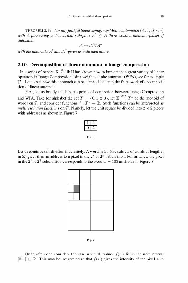
2. Automata and their decomposition 179
THEOREM 2.17. For any faithful linear semigroup Moore automaton (A,Γ, B; �, ∗)with A possessing a Γ-invariant subspace A′ ≤ A there exists a monomorphism ofautomata
A ↪→ A′�A′′
with the automataA′ andA′′ given as indicated above.
2.10. Decomposition of linear automata in image compressionIn a series of papers, K. Culik II has shown how to implement a great variety of linear
operators in Image Compression using weighted finite automata (WFA), see for example[2]. Let us see how this approach can be “embedded" into the framework of decomposi-tion of linear automata.
First, let us briefly touch some points of connection between Image Compression
and WFA. Take for alphabet the set T = {0, 1, 2, 3}, let Σdef= T ∗ be the monoid of
words on T , and consider functions f : T ∗ → R. Such functions can be interpreted asmultiresolution functions on T . Namely, let the unit square be divided into 2 × 2 pieceswith addresses as shown in Figure 7.
1 30 2
Fig. 7
Let us continue this division indefinitely. A word in Σn (the subsets of words of length nin Σ) gives then an address to a pixel in the 2n × 2n-subdivision. For instance, the pixelin the 23 × 23-subdivision corresponds to the word w = 103 as shown in Figure 8.
Fig. 8
Quite often one considers the case when all values f(w) lie in the unit interval[0, 1] ⊆ R. This may be interpreted so that f(w) gives the intensity of the pixel with

180 CHAPTER II. AUTOMATA THEORY
address w, w ∈ Σ. Also, let us consider the extreme cases f(w) = 0 and f(w) = 1 asthe pixel with address w being white or black, respectively. Then a multiresolution func-tion f : T ∗ → [0, 1] defines a sequence of grey-tone images with increasing resolution.The restriction of f to Σn defines an image in the 2n × 2n-resolution.
Note that there exist no principal difficulties in considering the colored case: one hasto take, instead of the previous function f , three such functions r, g and b : T ∗ → [0, 1]to represent the intensities (red, green and blue). Alternatively, we could as well haveused an alphabet T with |T | = 2m to produce functions [0, 1]m → [0, 1].
Let us say that a multiresolution function f : T ∗ → R is average-preserving if thecondition ∑
a∈T
f(wa) = 4f(w)
holds for all w ∈ T ∗. Observe that this condition makes images at various resolutionscompatible. Note also that every function f : T ∗ → R defines a collection of functionsfv : T ∗ → R given by the formula
fv(w)def= f(vw) for all w ∈ T ∗.
This may be interpreted so that these functions fv give the image in the subsquare withthe address v. The following theorem holds true.
THEOREM 2.18 ((K. Culik [2]). An average-preserving multiresolution function f :T ∗ → R can be given by a weighted finite automaton – in a sense made explicit below –if and only if the R-vector space generated by the set {fv | v ∈ T ∗} is finite-dimensional.This dimension equals the minimal number of states of the WFA realizing f .
Following [2], let us state the definition of WFA. A weighted finite automaton is aquintuple
A = (S, T, {Wa | a ∈ T }; I, F )
with
• S – the set of states; we put |S| = n;• T – a finite alphabet;• Wa : S × S → R – weights of transition; a triple (p, a, q) ∈ S × T × S is
called a transition if Wa(p, q) �= 0;• I : S → R – the initial distribution (a row vector in R1×n);• F : S → R – the final distribution (a column vector in Rn×1).
Every weighted finite automaton A = (S, T, {Wa | a ∈ T }; IA, FA) gives a mul-tiresolution image by the rule
fA(a1a2 . . . ak)def= IAWa1Wa2 . . .Wak
FA (ai ∈ T ).
In this formula we used matrix multiplication. A WFA is called average-preserving ifwe have ∑
a∈T
WaFA = 4FA.
It turns out that if a weighted finite automaton A is average-preserving, then the corre-sponding multiresolution function fA is also average-preserving ([2], Lemma 2). Also,there exist good algorithms that enable to encode a given image (picture) by some weighted
2. Automata and their decomposition 181
finite automaton A, and thereafter to compute from such an automaton the function fArepresenting finite resolution approximations of the given image; [3–5].
Let us see now how WFA and the corresponding multiresolution functions can betreated using linear automata. To this end, note that we can extend the correspondence
a �→Wa ∈ Mn(R) (a ∈ T )
to the whole monoid T ∗ defining the map Δ : T ∗ → Mn(R) recursively by the rule
Δ(wa) = Δ(a) ·Wa for w ∈ Σ, a ∈ T .
So we get for a word w = a1 . . . ak that
Δ(w) = Wa1 · · · · ·Wak.
We have the relation Δ(vw) = Δ(v)Δ(w) and, hence, we get a matrix representation,
Δ : T ∗ → Mn(R).
Next, fix (some) total order on the set S and, thinking of S as an ordered basis(s1, s2, . . . , sn), consider the R-space A of all finite (formal) sums
A = A(R, S)def=
{n∑
i=1
|αi ∈ R, si ∈ S
},
denoting by i and f the vectors that correspond to the initial and the finite distribution,respectively.
Define the action of Σ on A as follows. For any word w = a1 . . . ak (ai ∈ T ) andany element z in A,
z = α1s1 + · · ·+ αnsn (αi ∈ R),
define
z � w = zΔ(w) = z(Wa1 · · ·Wak).
Here we write z = (α1, . . . , αn) considering it as a vector in R1×n. For any two wordsv and w in Σ, we find
z � (vw) = zΔ(vw) = z(Δ(v)Δ(w)
)=
(zΔ(v)
)Δ(w) = (z � v) � w,
which show that we have a (linear) action of Σ on A. Taking z = i we obtain the vectors
i � w = iΔ(w) = IA(Wa1 · · ·Wak),
which are called multiresolution vectors for A. Furthermore, define
z ∗ w def= zWa1 · · ·Wak
f .
It follows that
z ∗ w = zWa1 · · ·Wakf = (z � w) ∗ 1.
In particular, for z = i we get
i ∗ w = IAWa1 · · ·Wakf = fA(w).
i.e. i ∗w is the value of the multiresolution function at w, w ∈ Σ∗. Furthermore, one has
z ∗ (w1w2) = (z � (w1w2)) ∗ 1 = [(z �w1) � w2] ∗ 1 = (z � w1) ∗ w2

182 CHAPTER II. AUTOMATA THEORY
for all w1, w2 ∈ Σ∗. Thus, to sum up, we see that WFA and multiresolution functionsmay be considered in the language of linear automata.
References
[1] H. Beker and F. Piper. Cipher systems: the protection of communication. Northwood, London, 1982.[2] K Culik II and J. Karhumäki. Finite automata computing real functions. SIAM J. Comput 23(4), 1994,
789–814.[3] K Culik II and J. Kari. Computational fractal geometry with WFA. Acts Informatica 34 (2), 1994, 151–
166.[4] K Culik II and J. Kari. Finite state transformation of images. Computers and Graphics 20, 1996, 125–135.[5] K Culik II and J. Kari. Finite state methods for image manipulation. In: Proc. of ICALP’95,
Lect. Notes in Comp. Sci., Vol. 944, 1995, 51-U62.[6] Y. Give’on and Y. Zalcstein. Algebraic structures in linear system theory. J. Comput. Syst. Sci. 4 (6),
1970, 539-556.[7] D. Gollman, Kaskadenschaltungen taktgesteuerter Schiebenregister als Pseudozufallsgeneratoren. Dis-
sertation an der Universität Linz, Nr. 59. Verband der Wissenschaftlicher Gesellschaften Österreichs,1986.
[8] U. Kaljulaid, Triangular products and stability of representations. Candidate dissertation, 1979. Russian,typescript; see [K79a], reprinted in this book as Sect. 4.
[9] R. E. Kalman, P. L. Falb, and M. A. Arbib. Topics in mathematical system theory. McGraw-Hill, NewYork, 1969.
[10] M. O. Rabin and A. Paz. Probabilistic automata. Information and Control 6, 1963, 230–245.

183
3. [K97] On two algebraic constructions for automataCoauthor J. Penjam
ABSTRACT. Categories naturally appear when we attempt to find means useful bothfor describing attributed rewriting systems and for expressing features of process alge-bra models. Following an idea in Mumford’s old paper [19] on Picard moduli, one canconsider semiautomata as sheaves and automata with monotonous (as well as with all)homomorphisms as Grothendieck topologies. This idea naturally leads us to systems ofthe type (A −→ Set; �). Wreath products of these systems are introduced and investi-gated in this paper. Some earlier results – both on algebraic and attributed automata, onrewriting and transition systems – are reconsidered from this viewpoint.
Keywords: automata, category theory, Grothendieck topologies, fiber products andwreath products of automata
3.1. Introduction and Preliminary Motivation
Using of categories in theoretical computer science is an old enterprize. So, G. Hotz[10] applied categories for clarifying the syntax of a language generated by a given setof productions. D. Knuth [15] viewed productions as functions (i.e. morphisms betweenobjects) in his investigations of semantics of CF-languages. Recent applications of cat-egories to areas of programming languages and to models of parallel computation aresurveyed in [1] and [25]. This line of reasoning reflects many important logical con-cepts in a way independent of their syntactic presentation. Categories naturally appearalso when we attempt to develop executable specifications of programming languages(e.g. automata), distributed systems (e.g. process algebras), or imperative functionalprogramming [9].
As a model for automata we use a quintuple A = (A,Σ, Y ; ◦, ∗), where the set ofstates A, the semigroup Σ and the output set Y are given so that (A,Σ; ◦) is a semigroupaction (i.e., it holds a ◦ (uv) = (a ◦ u) ◦ v) together with the action A × Σ ∗−→ Ysatisfying a ∗ (uv) = (a ◦ u) ∗ v for all a ∈ A and u, v in Σ. In this case A is calleda semigroup automaton. Also, we consider automata A with A and Y ordered, togetherwith (A,Σ; ◦) being an ordered action and with ∗ being an increasing map; call themo-automata. As a general model for automata a system A = (A, A; �) is used. Here, Ais a small category,A is a functor from A to Set (or to Set∗) and � is a (partial) feedbackoperation
(46) � : (∐
a∈Obj(A)
aA ×Mor(A)) −→ Mor(A),
satisfying the condition
(47) x�(f · g) = fA(x)�g
184 CHAPTER II. AUTOMATA THEORY
for all f ∈ HomA(a, a′), g ∈ HomA(a′, a′′) and x ∈ aA with a, a′ and a′′ in Obj(A).The sets and categories considered in Sect. 3.3 of this paper are supposed to be small.Considering for each open set U in a analytic space X the set F (U) of all analyticfunctions defined on U we get a contravariant functor from the category of open setsto Set; with some consistency conditions satisfied, a sheaf of analytic functions on Xappears. In the 1950-ies it was shown that sheaves on X (“toposes”) are the main objectsto be studied in geometry [7, 23]. A category A of finite sets and bijections together
with a covariant functor A A−→ A is called a species and they are intensively used incombinatorics [20].
In Sec. 3.3, for given automata A = (A, A; �) andB = (B, B; ) a new automatonAwrB = (AwrB, AwrB; ) is defined and called the wreath product of the giventwo. Any transition system can be considered as a labelled category (A, A) and so theirwreath products can be investigated. It is shown that these wreath products include asspecial cases products and sums of transition systems important in [25]. It also appearsthat semi-Thue systems can be represented by wreath products of the above type.
Using of colored categories, i.e. categories A with Mor(A) colored, one can con-sider questions concerning the languages L(A) accepted by such a general automaton A.It seems to be important to investigate interrelations between the languages L(A), L(B)and L(AwrB).
3.2. Fiber Products of Automata and Grothendieck Pretopologies
In this section, let us discuss the idea that automata can be viewed as devices for givingnearness on the set X∗ of all words written in some alphabet X . An origin of this idea isthe following context in mathematics.
Giving a topology on a space T means that some collection T of open subsets of T isfixed. A.Grothendieck [7] proposed to supply T with some additional structure allowingnot to refer to T . Recall that a Grothendieck pretopology is defined as a category G withdistinguished family of covers for its objects. A cover of an object U is meant as a setof morphisms {Ui −→ U}. Objects of G are called open sets of the topology G. Thefollowing conditions must hold:
(1) For any objects U, V and S in Obj(G), there exists the fiber product U×SV ∈Obj(G). The fiber product U ×S V , also called pullback or universal cone ofU and V over S, is defined by the rule: for any diagram
U
f���
��V
g ���
S
there must exist an object W together with morphisms Wu−→U and W
v→V
such that for any other objectW ′ together with some morphismsW ′ u′−→U and
W ′ v′−→V there exists the unique morphism W ′ w′
−→W making the diagram
W
u !!��� v
""�������
���� W ′
v′##���u′
����������
���w′
��� � � � � � � �
U
f���
��V
g ���
Scommutative.
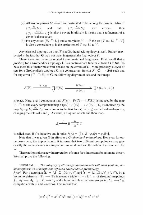
3. On two algebraic constructions for automata 185
(2) All isomorphisms U ′ p−→U are postulated to be among the covers. Also, if
{Uifi−→U} and all {Ui,j
fi,j−→Ui} are covers, then
{Ui,jfi,j ·fi−−−−→ U} is also a cover; intuitively it means that a refinement of a
cover is also a cover.(3) For any cover {Ui
fi−→U} and a morphism V → U the set {V ×U Uipi−→V }
is also a cover; here pi is the projection of V ×U Ui to V .
Any classical topology on a set T is a Grothendieck topology as well. Rather unex-pected is the fact that G may not have, in general, the final object T .
These ideas are naturally related to automata and languages. First, recall that apresheaf for a Grothendieck topology G is a contravariant functor F from G to Set. Tobe a sheaf this functor must well-behave on the covers of G. More precisely, a sheaf ofsets for a Grothendieck topology G is a contravariant functor F : G −→ Set such thatfor any cover {Ui
pi−→U} of G the following diagram of sets and their maps
F (U)(F (pi)) �� ∏
i
F (Ui)(F (pri)) ��(F (prj))
��∏i,j
F (Ui ×U Uj)
is exact. Here, every component map F (pi) : F (U) −→ F (Ui) is induced by the mapUi
pi−→U and every component map F (pri) : F (Ui) −→ F (Ui×U Uj) is induced by the
map Ui ×U Ujpri−→Ui (projection onto the first factor). F (prj) are defined analogously,
changing the roles of i and j. As usual, a diagram of sets and their maps
Af �� B
g1 ��g2
�� C
is called exact if f is injective and it holds f(A) = {b ∈ B | g1(b) = g2(b)}.Note that it was given G in effect as a Grothendieck pretopology. However, for our
purposes here, the imprecision in it in sense that two different pretopologies may giveexactly the same sheaves is unimportant; so we do not use the notion of a sieve, etc. forG.
These notions give a new interpretation of some facts important for automata theory.We shall prove the following.
THEOREM 3.1. The category of all semigroup o-automata with their (isotone) ho-momorphisms as its morphisms defines a Grothendieck pretopology.Proof. For o-automata A1 = (A1,Σ1, Y1; ◦′, ∗′) and A2 = (A2,Σ2, Y2; ◦′′, ∗′′), by ahomomorphism m : A1 −→ A2 is meant a triple m = (f, h, g) of (isotone) mappingsf : A1 −→ A2, g : Y1 −→ Y2 and a homomorphism of semigroups h : Σ1 −→ Σ2,compatible with ◦- and ∗-actions. This means that
(a ◦′ u)f = af ◦′′ uh and (a ∗′ u)g = af ∗′′ uh

186 CHAPTER II. AUTOMATA THEORY
for all a ∈ A1 and u ∈ Σ1. The identity endomorphism idA = (idA, idΣ, idY ) and thecomposition of isotone homomorphisms are isotone. Therefore a category A(o) appearswith o-automata as its objects and isotone homomorphisms as its morphisms.
To prove that fiber products exist in A(o), let us suppose that o-automata A1 andA2 are given together with their homomorphisms mi = (fi, hi, gi), i = 1, 2, into someo-automaton A = (A,Σ, Y : ◦, ∗). Define the subsets
A = A1 ×A A2 = {(a1, a2) | ai ∈ Ai, af11 = af2
2 ; i = 1, 2},Σ = Σ1 ×Σ Σ2 = {(σ1, σ2) | σi ∈ Σi, σ
h11 = σh2
2 ; i = 1, 2},Y = Y1 ×Y Y2 = {(y1, y2) | yi ∈ Yi, y
g11 = yg2
2 ; i = 1, 2},with A and Y ordered componentwise4. Here Σ is a semigroup. If both Σ1 and Σ2 aregroups then it is true for Σ also. Now, defining
(a1, a2) • (σ1, σ2) = (a1 ◦′ σ1, a2 ◦′′ σ2)
and(a1, a2) (σ1, σ2) = (a1 ∗′ σ1, a2 ∗′′ σ2)
for any ai ∈ Ai and σi ∈ Σi, i = 1, 2, we obtain for (σ1, σ2) ∈ Σ and (a1, a2) ∈ A that
(a1 ◦′ σ1)f1 = af11 ◦ σh1
1 = af22 ◦ σh2
2 = (a2 ◦′′ σ2)f2
and(a1 ∗′ σ1)g1 = af1
1 ∗ σh11 = af2
2 ∗ σh22 = (a2 ∗′′ σ2)g2 .
Therefore
(a1 ◦′ σ1, a2 ◦′′ σ2) ∈ A1 ×A A2 and (a1 ∗′ σ1, a2 ∗′′ σ2) ∈ Y1 ×Y Y2.
Also, one can observe that
(a1, a2) • ((σ1, σ2) · (τ1, τ2)) == (a1, a2) • (σ1τ1, σ2τ2) == (a1 ◦′ σ1τ1, a2 ◦′′ σ2τ2) == ((a1 ◦′ σ1) ◦′ τ1, (a2 ◦′′ σ2) ◦′′ τ2) == (a1 ◦′ σ1, a2 ◦′′ σ2) • (τ1, τ2) == ((a1, a2) • (σ1, σ2)) • (τ1, τ2),
and
(a1, a2) ((σ1, σ2) · (τ1, τ2)) == (a1, a2) (σ1τ1, σ2τ2) == (a1 ∗′ σ1τ1, a2 ∗′′ σ2τ2) == ((a1 ◦′ σ1) ∗′ τ1, (a2 ◦′′ σ2) ∗′′ τ2) == (a1 ◦′ σ1, a2 ◦′′ σ2) (τ1, τ2) == ((a1, a2) • (σ1, σ2)) (τ1, τ2).
Having (a1, a2) ≤ (b1, b2) in A means ai ≤ bi in Ai (i = 1, 2). Therefore,
a1 ◦′ σ1 ≤ b1 ◦′ σ1 and a2 ◦′′ σ2 ≤ b2 ◦′′ σ2
4In the middle of these equations and in the case of free monoids, where Σ1 = Σ2 = S∗ and Σ = T ∗
the diagonal ΔE(h1,h2) in E2(h1, h2) for the equality set E(h1, h2) ⊆ S+ is contained in Σ. Equality sets
are useful both for classical languages and for those obtained by splicing systems, see [13, 16].

3. On two algebraic constructions for automata 187
hold and so also
(a1, a2) • (σ1, σ2) = a1 ◦′ σ1, a2 ◦′′ σ2) ≤ (b1 ◦′ σ1, b2 ◦′′ σ2) = (b1, b2) • (σ1, σ2).
It follows that (A, Σ; •) is an o-action. Analogously, it is verified that is isotone. Asa result, a new o-automaton A = (A, Σ, Y ; •, ) appears, which has the universal coneproperty. I.e., given any automatonB = (B,Δ, Z;$,�) and any morphisms li : B −→Ai (i = 1, 2) such that the diagram
Bl1����� l2
$$���
A1
m1 $$����
A2
m2������
A
is commutative, there exists uniquely a homomorphism m : B −→ A, m = (f , h, g),that makes the diagram
A
pr1 ������ pr2
""�������
������ B
l2������l1
����������
�����
m ( ˜m)��� � � � � � � � �
A1
m1 $$����
A2
m2��
Acommutative.
Existence of m. Given any morphisms
li : B −→ Ai (i = 1, 2) with l1 = (f ′, h′, g′) and l2 = (f ′′, h′′, g′′)
one can define m : B −→ A, where m = (f , h, g), by the rules
b �−→ (bf′, bf
′′) , δ �−→ (δh
′, δh
′′) , z �−→ (zg
′, zg
′′).
Observe that the components f and g of m are isotone. The map h : Δ −→ Σ, given by
the rule δ �−→ (δh′, δh
′′) is a homomorphism of semigroups. From the commutativity of
the last diagram it follows that
(bf′)f1 = (bf
′′)f2 , (δh
′)h1 = (δh
′′)h2 , (zg
′)g1 = (zg
′′)g2 .
Thus, m is a map from B into the automaton A. Furthermore,
(b$ δ)f = bf • δh, and (b � δ)g = bf δh
together with what was said above imply that m is a homomorphism of o-automata.
Uniqueness of ˜m. Suppose there exists an another morphism ˜m : B −→ A thatmakes the last diagram commutative. This means, in particular, that
b˜m = (a
′′1 , a
′′2 ) ∈ A1 ×A A2,
δ˜m = (σ
′′1 , σ
′′2 ) ∈ Σ1 ×Σ Σ2,
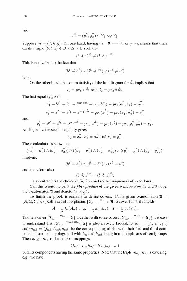
188 CHAPTER II. AUTOMATA THEORY
andz
˜m = (y′′1 , y
′′2 ) ∈ Y1 ×Y Y2.
Suppose ˜m = ( ˜f,
˜h, ˜g). On one hand, having ˜m : B −→ A, ˜m �= m, means that there
exists a triple (b, δ, z) ∈ B ×Δ× Z such that
(b, δ, z)m �= (b, δ, z) ˜m.
This is equivalent to the fact that
(bf �= b˜f ) ∨ (δh �= δ
˜h) ∨ (zg �= z
˜g)
holds.On the other hand, the commutativity of the last diagram for ˜m implies that
l1 = pr1 ◦ ˜m and l2 = pr2 ◦ ˜m.
The first equality gives
a′1 = bf ′
= bl1 = bpr1◦ ˜m = pr1(b˜m) = pr1(a
′′1 , a
′′2 ) = a
′′1 ,
σ′1 = σh′
= σl1 = σpr1◦ ˜m = pr1(σ˜h) = pr1(σ
′′1 , σ
′′2 ) = σ
′′1
andy
′1 = zg′
= zl1 = zpr1◦ ˜m = pr1(z˜m) = pr1(z
˜g) = pr1(y′′1 , y
′′2 ) = y
′′1 .
Analogously, the second equality gives
a′2 = a
′′2 , σ
′2 = σ
′′2 and y
′2 = y
′′2 .
These calculations show that
((a′1 = a
′′1 ) ∧ (a
′2 = a
′′2 )) ∧ ((σ
′1 = σ
′′1 ) ∧ (σ
′2 = σ
′′2 )) ∧ ((y
′1 = y
′′1 ) ∧ (y
′2 = y
′′2 )),
implying
(bf = b˜f ) ∧ (δh = δ
˜h) ∧ (zg = z˜g)
and, therefore, also(b, δ, z)m = (b, δ, z) ˜m.
This contradicts the choice of (b, δ, z) and so the uniqueness of m follows.Call this o-automaton A the fiber product of the given o-automaton A1 and A2 over
the o-automaton A and denote A1 ×AA2.To finish the proof, it remains to define covers. For a given o-automaton A =
(A,Σ, Y ; ◦, ∗) call a set of morphisms {Aαmα−−−−→ A} a cover for A if it holds
A = ∪αfα(Aα) , Σ = ∪
αhα(Σα), Y = ∪
αgα(Yα).
Taking a cover {Aαmα−−−−→ A} together with some covers {Aαβ
mαβ−−−−→ Aα} it is easy
to understand that {Aαβmαβ ·mα−−−−−→ A} is also a cover. Indeed, let mα = (fα, hα, gα)
and mαβ = (fαβ , hαβ, gαβ) be the corresponding triples with their first and third com-ponents isotone mappings and with hα and hαβ being homomorphisms of semigroups.Then mαβ ·mα is the triple of mappings
(fαβ · fα, hαβ · hα, gαβ · gα)
with its components having the same properties. Note that the triplemαβ ·mα is covering:e.g., we have

3. On two algebraic constructions for automata 189
A = ∪αfα(Aα) = ∪
αfα(∪
βfαβ(Aα,β)) =
∪α∪βfα(fαβ(Aαβ)) = ∪
α,β(fαβ · fα)(Aαβ).
To see that the condition (48) in the definition of the Grothendieck topology holds it re-mains to realize that for the projections qα : B×α Aα −→ B,
∪αqα(B×A Aα) = ∪
αqα(B ×A Aα,Γ×Σ Σα, Z ×Y Yα) =
∪α{(b, γ, z) | f ′(b) ∈ fα(Aα), h′(γ) ∈ hα(Σα), g′(z) ∈ gα(Yα)} =
{(b, γ, z) | f ′(b) ∈ A, h′(γ) ∈ Σ, g′(z) ∈ Y } ={(b, γ, z) | b ∈ B, γ ∈ Γ, z ∈ Z} = B.
�This proof can be modified to give
THEOREM 3.2. The category of all semigroup ordered actions of the type (A,Σ; ◦)with their isotone homomorphisms as its morphisms defines a Grothendieck pretopology.
Further specialization is possible: when fixing the semigroup Σ the category of or-dered Σ-sets with (isotone) homomorphisms as its morphisms gives again a Grothendieckpretopology. The case (of trivial order) – with all homomorphisms of Σ-sets as the mor-phisms – is considered in [21].
To strengthen the mathematical backbone and to prepare the ground for the nextsection, let us see how contravariant functors A : A −→ Set appear of the present con-text. Additional motivation comes from concurrency models in [25] and from associativememory investigations, see [3].
For a group Γ denote it Γ∗ when considered as a regular Γ-set. Take all Γ-sets tobe the open sets and all homomorphisms of Γ-sets to be the morphisms of the coveringtopology T = T(Γ) on {ε}. Here, ε is the identity element of Γ. Each element σ ∈ Γdefines an automorphism σ : Γ∗ −→ Γ∗ by the rule γ �−→ γσ. These automorphisms acton the set S = F (Γ∗) for any sheaf F on T(Γ). It appears that S is a Γ-set that uniquelydefines F . Indeed, let F be any sheaf on T. As S is a transitive Γ-set then there existsan epimorphism f : Γ∗ −→ S giving a cover for S. The sequence
F (S)(F (f)) �� F (Γ∗)
(F (pr1)) ��(F (pr2))
�� F (Γ∗ ×S Γ∗)
is exact. It means that (F (S);F (f)) is the kernel for the pair (F (pr1), F (pr2)) andF (f) is a monomorphism of F (S) into F (Γ∗). Denote by S1
the image F (f)(F (S)) in S. To describe the subset S1 in S means to find thecokernel for the diagram
Γ∗ ×S Γ∗pr1 ��pr2
�� Γ∗ f �� S
This cokernel is given by Γ∗/π, where π is the least Γ-equivalence on Γ∗ × Γ∗ thatcontains the set of all pairs {(γ1, γ2) | γf
1 = γf2 }. It follows
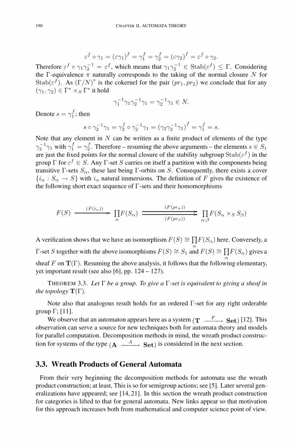
190 CHAPTER II. AUTOMATA THEORY
εf ◦ γ1 = (εγ1)f = γf
1 = γf2 = (εγ2)
f = εf ◦ γ2.
Therefore εf ◦ γ1γ−12 = εf , which means that γ1γ
−12 ∈ Stab(εf ) ≤ Γ. Considering
the Γ-equivalence π naturally corresponds to the taking of the normal closure N forStab(εf ). As (Γ/N)∗ is the cokernel for the pair (pr1, pr2) we conclude that for any(γ1, γ2) ∈ Γ∗ ×S Γ∗ it hold
γ−11 γ1γ
−12 γ1 = γ−1
2 γ1 ∈ N.
Denote s = γf1 ; then
s ◦ γ−12 γ1 = γf
2 ◦ γ−12 γ1 = (γ2γ
−12 γ1)
f= γf
1 = s.
Note that any element in N can be written as a finite product of elements of the typeγ−12 γ1 with γf
1 = γf2 . Therefore – resuming the above arguments – the elements s ∈ S1
are just the fixed points for the normal closure of the stability subgroup Stab(εf ) in thegroup Γ for εf ∈ S. Any Γ-set S carries on itself a partition with the components beingtransitive Γ-sets Sα, these last being Γ-orbits on S. Consequently, there exists a cover{iα : Sα → S} with iα natural immersions. The definition of F gives the existence ofthe following short exact sequence of Γ-sets and their homomorphisms
F (S)(F (iα)) �� ∏
αF (Sα)
(F (prα)) ��(F (prβ))
��∏α,β
F (Sα ×S Sβ)
A verification shows that we have an isomorphism F (S) ∼=∏αF (Sα) here. Conversely, a
Γ-set S together with the above isomorphisms F (S) ∼= S1 and F (S) ∼=∏αF (Sα) gives a
sheaf F on T(Γ). Resuming the above analysis, it follows that the following elementary,yet important result (see also [6], pp. 124 – 127).
THEOREM 3.3. Let Γ be a group. To give a Γ-set is equivalent to giving a sheaf inthe topology T(Γ).
Note also that analogous result holds for an ordered Γ-set for any right orderablegroup Γ; [11].
We observe that an automaton appears here as a system (T F−−−−→ Set) [12]. Thisobservation can serve a source for new techniques both for automata theory and modelsfor parallel computation. Decomposition methods in mind, the wreath product construc-tion for systems of the type (A A−−−−→ Set) is considered in the next section.
3.3. Wreath Products of General Automata
From their very beginning the decomposition methods for automata use the wreathproduct construction; at least, This is so for semigroup actions; see [5]. Later several gen-eralizations have appeared; see [14, 21]. In this section the wreath product constructionfor categories is lifted to that for general automata. New links appear so that motivationfor this approach increases both from mathematical and computer science point of view.
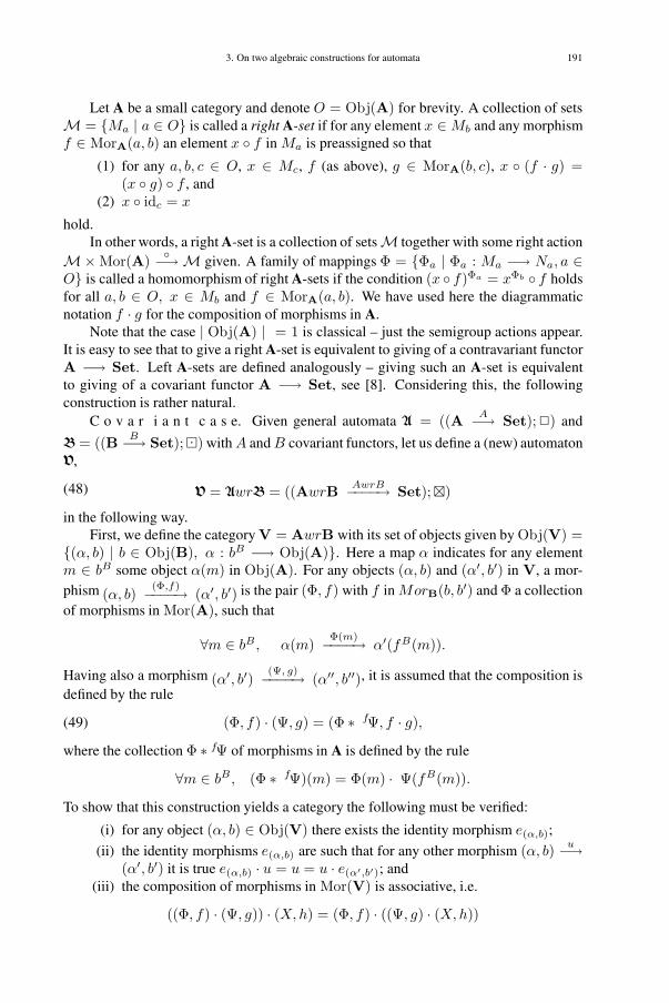
3. On two algebraic constructions for automata 191
Let A be a small category and denote O = Obj(A) for brevity. A collection of setsM = {Ma | a ∈ O} is called a right A-set if for any element x ∈Mb and any morphismf ∈ MorA(a, b) an element x ◦ f in Ma is preassigned so that
(1) for any a, b, c ∈ O, x ∈ Mc, f (as above), g ∈ MorA(b, c), x ◦ (f · g) =(x ◦ g) ◦ f , and
(2) x ◦ idc = x
hold.In other words, a right A-set is a collection of setsM together with some right action
M×Mor(A) ◦−→M given. A family of mappings Φ = {Φa | Φa : Ma −→ Na, a ∈O} is called a homomorphism of right A-sets if the condition (x ◦ f)Φa = xΦb ◦ f holdsfor all a, b ∈ O, x ∈ Mb and f ∈ MorA(a, b). We have used here the diagrammaticnotation f · g for the composition of morphisms in A.
Note that the case | Obj(A) | = 1 is classical – just the semigroup actions appear.It is easy to see that to give a right A-set is equivalent to giving of a contravariant functorA −→ Set. Left A-sets are defined analogously – giving such an A-set is equivalentto giving of a covariant functor A −→ Set, see [8]. Considering this, the followingconstruction is rather natural.
C o v a r i a n t c a s e. Given general automata A = ((A A−→ Set); �) and
B = ((B B−→ Set); ) with A and B covariant functors, let us define a (new) automatonV,
(48) V = AwrB = ((AwrB AwrB−−−−→ Set); )
in the following way.First, we define the category V = AwrB with its set of objects given by Obj(V) =
{(α, b) | b ∈ Obj(B), α : bB −→ Obj(A)}. Here a map α indicates for any elementm ∈ bB some object α(m) in Obj(A). For any objects (α, b) and (α′, b′) in V, a mor-phism (α, b)
(Φ,f)−−−−→ (α′, b′) is the pair (Φ, f) with f in MorB(b, b′) and Φ a collectionof morphisms in Mor(A), such that
∀m ∈ bB, α(m)Φ(m)−−−−→ α′(fB(m)).
Having also a morphism (α′, b′)(Ψ, g)−−−−→ (α′′, b′′), it is assumed that the composition is
defined by the rule
(49) (Φ, f) · (Ψ, g) = (Φ ∗ fΨ, f · g),
where the collection Φ ∗ fΨ of morphisms in A is defined by the rule
∀m ∈ bB, (Φ ∗ fΨ)(m) = Φ(m) · Ψ(fB(m)).
To show that this construction yields a category the following must be verified:
(i) for any object (α, b) ∈ Obj(V) there exists the identity morphism e(α,b);
(ii) the identity morphisms e(α,b) are such that for any other morphism (α, b) u−→(α′, b′) it is true e(α,b) · u = u = u · e(α′,b′); and
(iii) the composition of morphisms in Mor(V) is associative, i.e.
((Φ, f) · (Ψ, g)) · (X,h) = (Φ, f) · ((Ψ, g) · (X,h))

192 CHAPTER II. AUTOMATA THEORY
holds for any three morphisms where it makes sense.
The condition (i) is satisfied by taking e(α,b) = (I, idb). Indeed, as functors preserveidentity morphisms, it follows that the functor B takes the identity idb ∈ Mor(b, b) intothe identity map bB → bB , i.e. it is true that (idb)B = idbB ; here idbB is the identity inMorSet(bB, bB). Therefore,
(idb)B(m) = idbB (m) = m
for every element m in the set bB . It follows that I gives the needed collection of mor-phisms
I(m) = idα(m) : α(m) −→ α(m) = α((idb)B(m)).
To prove (ii) take any morphism in V,
(α, b)(Φ,f)−−−−→ (α′, b′).
Then it holds
(I, idb) ∗ (Φ, f) = (I ∗ idbΦ), idb · f).
The identity idb · f = f is obvious, as it holds in the category B. So, to prove (ii) itremains to verify that I ∗ idbΦ = Φ is true. Indeed, for any m ∈ bB it holds
(I ∗ idbΦ)(m) = I(m) ·Φ((idb)B(m)) = I(m) ·Φ(idbB (m))= idα(m) · Φ(m) = Φ(m),
so giving the desired equality for the first components of (I, idb) ∗ (Φ, f) and (Φ, f).Analogously it is verified that
(Φ, f) ∗ (I ′, idb′) = (Φ, f).
As a result, it is proved that (ii) holds forW.
Let us prove (iii) now.On the one hand we have
[(Φ, f) ∗ (Ψ, g)] ∗ (X,h) = [Φ ∗ fΨ, f · g] ∗ (X,h) =
= ((Φ ∗ fΨ) ∗ f ·gX, (f · g) · h).
On the other hand,
(Φ, f) ∗ [(Ψ, g) ∗ (X,h)] = (Φ, f) ∗ (Ψ ∗ gX, g · h) =
= (Φ ∗ f(Ψ ∗ gX), f · (g · h)).
It follows from the definition of the category B, that
(f · g) · h = f · (g · h).
To see that the following formula is true
(50) (Φ ∗ fΨ) ∗ f ·gX = Φ ∗ f(Ψ ∗ gX),

3. On two algebraic constructions for automata 193
take any element m ∈ bB and consider the corresponding morphisms in A on the left andon the right side. We get
[(Φ ∗ fΨ) ∗ f ·gX ](m) = [(Φ ∗ fΨ)(m)] · f ·gX(m) =
= [Φ(m) ·Ψ(fB(m))] ·X((f · g)B(m)) =
= Φ(m) · [Ψ(fB(m)) ·X(gB(fB(m)))] =
= Φ(m) · [Ψ ∗ gX ](fB(m)) =
= Φ(m) · f[Ψ ∗ gX ](m) =
= (Φ ∗ f[Ψ ∗ gX ](m)
for any m ∈ bB . It implies that (50) holds and,consequently, (iii) also. Thus we haveproved that V is a category.
Let us now define the functorAwrB : AwrB −→ Set now, using for it the functorsA and B. The rule
(51) (α, b)AwrB = {(l,m) | m ∈ bB, l ∈ [α(m)]A}gives AwrB as a mapping Obj(V) −→ Obj(Set). For any morphism
(Φ, f) ∈MorV((α, b), (α′, b′))
define (Φ, f)AwrB as the map (ΦA, fB) in
MorSet((α, b)AwrB , (α′, b′)AwrB) .
Let us prove that AwrB preserves the identity morphisms in V. Note that
(I, idb)AwrB = (IA, (idb)B) = (IA, idbB ),
where for any m ∈ bB we have IA(m) = I(m)A by definition. Therefore,
[α(m)]AI(m)A
−−−−→ [α((idb)B(m))]A = [α(idbB (m))]A = [α(m)]A,
i.e. I(m)A ∈ MorSet([α(m)]A, [α(m)]A). As I(m) = idα(m) in Mor(A) and thefunctor A preserves identity morphisms in A then I(m)A = id[α(m)]A . It remains toprove that AwrB is compatible with the composition in V, i.e. that
(52) [(Φ, f) · (Ψ, g)]AwrB = (Φ, f)AwrB · (Ψ, g)AwrB
holds.Here, on the right side of (52) the symbol · stands for the composition of morphisms
(i.e. mappings) in Set. The left side of (52) can be written as
[(Φ, f) · (Ψ, g)]AwrB = (Φ ∗ fΨ, f · g)AwrB =
= ((Φ ∗ fΨ)A, (f · g)B) =
= (ΦA ∗ (fΨ)A, fB · gB) =
= (ΦA, fB) · (ΨA, gB) =
= (Φ, f)AwrB · (Ψ, g)AwrB
Here, the composition of the pairs (ΦA, fB) and (ΨA, gB) with the collections ΦA and(fΨ)A as their first components goes shifted as indicated above. It follows that AwrB is

194 CHAPTER II. AUTOMATA THEORY
a covariant functor and so V(AwrB)−−−−−→ Set is a labelled category. Note also that having
A A−→ Set, B B−→ Set and C C−→ Set, it follows that
(AwrB)wrC(AwrB)wrC−−−−−−−−→ Set
and
Awr(BwrC)Awr(BwrC)−−−−−−−−→ Set
are isomorphic, see [24].Having any morphism (Φ, f) ∈ MorV((α, b), (α′, b′)) and any element (l,m) ∈
[(α, b)]AwrB , let us define
(53) (l,m) (Φ, f) = (l�Φ(m),m f).
To prove that
V = (V AwrB−−−−→ Set; )is a general automaton, it remains to verify that
(54) (l,m) ((Φ, f) · (Ψ, g)) = (((Φ, f)AwrB)(l,m)) (Ψ, g)
for all elements (l,m) in [(α, b)]AwrB .On the left side of (54),
(l,m) ((Φ, f) · (Ψ, g)) = (l,m) ((Φ ∗ fΨ), f · g) =
= (l�(Φ ∗ fΨ)(m), m (f · g)) =
= (l�(Φ(m) ·Ψ(fB(m))), m (f · g)) =
= (Φ(m)A(l)�Ψ(fB(m)), fB(m) g).
On the right side of (54),
((Φ, f)AwrB)(l,m) (Ψ, g) = ((ΦA, fB)(l,m)) (Ψ, g) =
= (Φ(m)A(l), fB(m)) (Ψ, g) =
= (Φ(m)A(l)�Ψ(fB(m), fB(m)) g).
The results on both sides are the same and so (54) follows.As a result, it is proved now that a new automaton V appears. Let us call V the
wreath product of A andB.C o n t r a v a r i a n t c a s e. Given two general automata A and B with A and
B being contravariant functors this time, it is possible to modify the above ’covariantconstruction’ to be applicable here. This can achieved by considering A : Aop −→ Set(with Af = Afop) and B : Bop −→ Set and taking
(AopwrBop)op AwrB−−−−→ Set
thereafter. However, to avoid isomorphisms of the type (Aop)op ∼= A together withA ∼= A it is useful to give a direct construction for AwrB in contravariant case as well.
The sets of objects for V = AwrB with the functors A and B contravariant are thesame as for covariant case. Yet, a morphism (α, b)
(Φ,f)−−−−→ (α′, b′) is defined now as apair (Φ, f) with f ∈ MorB(b, b′) and Φ being some (fixed) collection of morphisms (inA)
∀m ∈ b′B, α′(m)Φ(m)−−−−→ α(fB(m)).
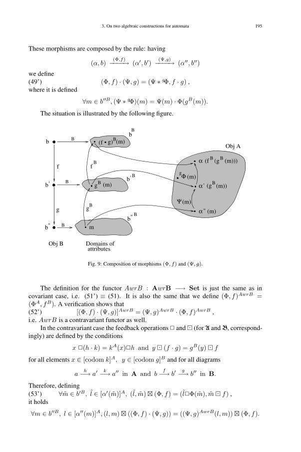
3. On two algebraic constructions for automata 195
These morphisms are composed by the rule: having
(α, b)(Φ,f)−−−−→ (α′, b′)
(Ψ,g)−−−−→ (α′′, b′′)
we define(Φ, f) · (Ψ, g) = (Ψ ∗ gΦ, f · g) ,(49’)
where it is defined
∀m ∈ b′′B, (Ψ ∗ gΦ)(m) = Ψ(m) ·Φ(gB(m)).
The situation is illustrated by the following figure.
(m)Bg)
g (m)b’
’’
b
b
b
’
Ψ (m)
Φ (m)
’’
g
(m)))B B(g(fα
attributes
b
f
g
B
B
Bb
B
Obj B
B
f
g
B
B
m
α ’’ (m)
α (gB (m))’
B
B
Obj A
Domains of
(f
Fig. 9: Composition of morphisms (Φ, f) and (Ψ, g).
The definition for the functor AwrB : AwrB −→ Set is just the same as incovariant case, i.e. (51’) ≡ (51). It is also the same that we define (Φ, f)AwrB =(ΦA, fB). A verification shows that
[(Φ, f) · (Ψ, g)]AwrB = (Ψ, g)AwrB · (Φ, f)AwrB ,(52’)i.e. AwrB is a contravariant functor as well.
In the contravariant case the feedback operations � and (forA andB, correspond-ingly) are defined by the conditions
x �(h · k) = kA(x)�h and y (f · g) = gB(y) f
for all elements x ∈ [codom k]A, y ∈ [codom g]B and for all diagrams
ah−→ a′
k−→ a′′ in A and bf−→ b′
g−→ b′′ in B.
Therefore, defining∀m ∈ b′B, l ∈ [α′(m)]A, (l, m) (Φ, f) = (l�Φ(m), m f) ,(53’)
it holds
∀m ∈ b′′B, l ∈ [α′′(m)]A, (l,m) ((Φ, f) · (Ψ, g)) = ((Ψ, g)AwrB(l,m)) (Φ, f).

196 CHAPTER II. AUTOMATA THEORY
Resuming the above modifications (49’) – (53’) we get the wreath product construc-tion for the contravariant case. Note that in the contravariant case there exists an anotherpossibility to introduce wreath product construction, which will be treated elsewhere.
3.4. Examples and Further MotivationEXAMPLE 3.1. Consider the special case of an A-set M and a B-set N with Obj(A) =
{a} and Obj(B) = {b}; i.e., |Obj(A)| = 1 = |Obj(B)|. It follows that there existsthe single object (α, b) for AwrB as well, with α : N −→ {a} being the constantfunction. The set Mor(AwrB) consists of the pairs (Φ, σ) with σ ∈ Σ2 = End (b) andΦ(y) ∈ Σ1 = End (a) for every y ∈ N ; their composition is given by the rule (49),therefore
(55) (Φ1, σ1) · (Φ2, σ2) = (Φ1 · σ1Φ2, σ1σ2).
Further, having the functorsA and B given by aA = M and bB = N , together with somemappings M −→ M and N −→ N replacing the endomorphisms for a and b corre-spondingly, it follows from (51) that (α, b)AwrB = M ×N . The formula (Φ, σ)AwrB =(ΦA, σB) gives the action of Mor(AwrB) on M ×N by the rule
(56) (x, y) ◦ (Φ, σ) = (Φ(y)A(x), σB(y))
for all x ∈ M and y ∈ N . As a result we get the wreath product of the two monoidactions (M,Σ1) and (N,Σ2) as given by the following
DEFINITION 3.4. Let (M,Σ1) and (N,Σ2) be any two monoid actions. Take the setΣN
1 of all functions from N to Σ1 together with their pointwise multiplication. Thereafter,take the set Γ = ΣN
1 × Σ2 with the multiplication on it given by (55). So the monoid Γappears together with its action on M ×N given by (56). This resulting action is calledthe wreath product of the given two actions and is denoted by (M,Σ1)wr(N,Σ2).
Going one step further, let us think of the feedback operations � and given by
(46) and (47) for the systems A1 = (A A−→ Set; �), and A2 = (B B−→ Set; ) as“output operations” ∗(i), changing for it the codomain in (46) to some “output set” Yi for∗(i) (i =′ or ′′). Then (53) and (54) imply that the wreath product A1wrA2 in the senseof Section 3.3 for one-object categories A and B (with the functors A and B as above)gives us precisely the wreath product of the monoid automata A1 = (M,Σ1, Y1; ◦′, ∗′)and A2 = (N,Σ2, Y2; ◦′′, ∗′′) as defined by the following.
Definition. Let A1 = (M,Σ1, Y1; ◦′, ∗′) and A2 = (N,Σ2, Y2; ◦′′, ∗′′) be any twosemigroup automata. Take the wreath product (M ×N,Γ; •) of the actions (M,Σ1; ◦′)and (N,Σ2; ◦′′), with Γ being the semigroup ΣN
1 λΣ2. Define the “output action” of Γon M ×N by the rule
(x, y) ∗ (Φ, σ) = (x ∗′ Φ(y), y ∗′′ σ).The condition
(x, y) ∗ ((Φ1, σ1) · (Φ2, σ2)) = ((x, y) • (Φ1, σ1)) ∗ (Φ2σ2)is satisfied. So, the semigroup automaton A = (M ×N,Γ, Y1 × Y2; •, ∗) appears whichis called the wreath product of the semigroup automata A1 and A2.
It is easy to understand that for any monoid automata A1 and A2 their wreath prod-ucts as given by the latter definition, can be realized as wreath products of suitable sys-
tems A = (A A−→ Set; �), where it is |Obj(A)| = 1. �

3. On two algebraic constructions for automata 197
EXAMPLE 3.2. According to [22], a rewriting system (called also a semi-Thue sys-tem) is a pairR = (X ;P), where X is an alphabet and P is a finite set of ordered pairs ofwords in X+. The elements (q, p) ∈ P are referred to as rewriting rules (productions),their components together with an axiom s ∈ X+ we call primitives. If some words uand v in X+ are such that u = w1qw2 and v = w1pw2 then it is said that u yields vdirectly. A derivation in R is a finite sequence of words u0 = u, u1, . . . , un = v suchthat ui yields ui+1 directly, 0 ≤ i ≤ n − 1; in such a case the derivation is denotedby u −→ v and it is said that u yields v in R. A rewriting system R generates severalcategories.
First, the category P of primitives for R: its objects are all primitives, Mor (P)consists of all primitive derivations, i.e. derivations of the type p −→ p′ with p and p′
primitives. When an axiom s ∈ X+ is fixed then s is considered a primitive also. Inthis case, taking for every primitive p the set D∗(p) of all primitive derivations from s top, we can define a functor D∗ : P −→ Set as well. In this way the labelled category
(P D∗−−−−→ Set) appears.Second, the linguistic category L for R. The objects for L are all words in X∗, its
morphisms are all the derivations in R.Third, we get the syntactic category B for R by taking Obj(B) = Obj(L) and
assuming that MorB(u, v) �= ∅ if there exists in L a derivation s −→ u. To have acovariant functor D : B −→ Set one can define for every u ∈ Obj(L) the set uD as the
set of all derivations s −→ u. Also, for every derivation uf−→ v, it is possible to define
the map fD : uD −→ vD by the rule: h �−→ h · f , for any h ∈ uD. So, the labelled
category (B D−→ Set) appears.Fourth, the semantic pair (B, B) forR appears; see in [2]. For any letter x ∈ X take
a nonempty set xB so that these sets are pairwise disjoint and it holds (wx)B = wB×xB
for every letter x ∈ X and every word w in X+. Taking some maps fB : pB −→ qB inall cases where q yields p directly, with p and q primitives, let us extend this action of B
to all productionsw1qw2f−→ w1pw2 by taking fB : wB
1 ×pB×wB2 −→ wB
1 ×qB×wB2 ,
where fB is considered to be the identity map on the corresponding contexts. Functionsfrom uB to sB for any derivation s −→ u are called interpretations, their images in sB
are called values of u. As a result, a contravariant “interpreting functor” B : B −→ Setappears.
Consider the full subcategory (PwrB D∗wrD−−−−−→ Set) generated by the objects (α, u)in PwrB, where α : uD −→ Obj(P) is any constant function such that α(uD) = p withp primitive and p a subword of u. Any such function α can be taken as choosing someprimitive subword α(u) in u. This means that there exists a context (w1, w2) ∈ X∗×X∗
such that u = w1α(u)w2. Therefore, to take such an object (α, u) for PwrB means thatwe take a word u ∈ X∗ together with choosing some primitive α(u) in it. Consequently,having a morphism (α, u)
(Φ,f)−−−−→ (α′, v) in this subcategory for PwrB means that
there exists a derivation uf−→ v in R which begins with u0 = u = w1α(u)w2 and ends
up with un = v = w1α′(v)w2; here α(u) and α′(v) are primitives and wi, wi are some
words in X∗. Saying it in another way, for any derivation uf−→ v there is chosen a

198 CHAPTER II. AUTOMATA THEORY
companion primitive derivation α(u)Φ(u)−−−−→ α′(v) also. This argument shows that any
semi-Thue system R together with its derivations can be naturally considered as a fullsubcategory in PwrB. Treating of semi-Thue systems in this way allows to simplify, atleast to some extent, quite a complicated notion of the transition adopted in [2]. Thoughthe idea to use categories as a proper framework for derivations is not original with us, itseems to have gone unnoticed the feature of a rewriting system to allow to be treated asa wreath product of suitable categories. �
EXAMPLE 3.3. The conception of the transition system is a fundamental modelof computation in Computer Science [25]. Such a system J is a structure of the type(S, i, L;T), where S is a set of states together with the initial state i fixed, L is a setof labels and T ⊆ S × L × S is the transition relation. Let us denote the transition(s, l, s′) ∈ T by s
l−→ s′. Note that no two distinct transitions with the same pre- andpost-states have the same labels.
Every transition system J generates a category T = (S, i, L∗;T∗), quite analo-gously to the way how a finite automaton generates the corresponding free semigroupautomaton. Namely, define (s, v, s′) ∈ T∗ if v = l1 . . . ln−1 ∈ L∗ is such that thereexists a path s = s1, s2, . . . , sn = s′ so that (si, li, si+1) ∈ T for all i = 1, . . . , n − 1;call s
v−→ s′ an extended transition from s to s′. A category T appears: there is given anatural (associative) composition of extended transitions together with existing the label1 ∈ L∗ (usually denoted ∗) so that there exist “idle” transitions ids : s ∗−→ s.
The transition system where exist paths from the initial state to all other states iscalled a reachable transition system. For a reachable transition system J the followingcovariant functor T : T −→ Set can be defined. Namely, the rule
T (s) = {w | w ∈ L∗, ∃(i w−→ s) ∈ T∗}gives the functor on the objects of T. Further, let us define the functor T on Mor (T) asfollows. For any given extended transition s
w−→ s′, the mapping T (s w−→ s′) transformsany transition (i v−→ s) ∈ T (s) into the transition (i vw−−−−→ s′) ∈ T (s′). A verification
shows that in this way we get a covariant functor T : T −→ Set. We call (T T−→ Set) atransition category. LetJj = (Sj , ij, L
∗j ;Tj) (j = 1, 2), be any two reachable transition
systems and let (TjTj−−−−→ Set) be the corresponding transition categories. Taking
their wreath product (T1wrT2T1wrT2−−−−−→ Set) and thereafter the full subcategory F in
it generated by the objects (α, b) such that α : bT2 −→ Obj(T1) = S1 is a constantfunction, we get just the productJ1 × J2 of the transition systems as defined in [25]. Itis instructive to reconsider from the point of view of wreath products the example of theproduct of the transition systems
(•S1
i1•a
��; L1 = {a} ) and (
•S2
i2•b
��; L2 = {b} )
as given in [25]; we drop the details. Note also that in the special case, where thereare given J1 = (S, i, L′;T′) and J2 = (S, i, L;T) together with some inclusion mapλ : L ↪→ L′, the full subcategory F supplies a natural interpretation for the restrictionmorphism (λ∗, 1S) : J1 |L ↪→ J2. �

3. On two algebraic constructions for automata 199
3.5. Discussion
This is not surprising that the categories developed for automata appear also suitablefor modelling of transition systems. Transition systems generalize automata model ofcomputations by enabling usage of values of state variables in previous states passed.Such a feedback information together with input/output primitives attached to transitionsmakes it useful operational model of distributed and reactive systems. Conventional tran-sition systems use common memory to store state variables. However, real memories aremore complicated and often seem to be matched together from some “pieces”. More-over, according to an observation by N.de Bruijn [3] there exists a kind of buffer keepingtrack of the most recent information, including information very recently retrieved fromthe memory. This buffer can be compared to what is called the active window in a textediting system. According to De Bruijn’s idea, there is no fixed window through whichinformation flows, but rather a moving window that floats over information. Distributedmemory is used by an another generalization of state transition systems called attributedautomata [17]
Namely, an attributed automaton, as defined in [17], is a transition network A =(S,L), where S is a set of states together with its subsets Si (initial states) and Sf (finalstates) indicated; for every state s ∈ S a variable (an attribute as with its domain Ts
of values) is attached; L ⊆ S × S is the set of transitions for A together with a mapfl : Ts −→ Ts′ for every transition (s, l, s′) ∈ S × L × S and “allowing” predicatesP
(sl−→s′)
: Ts −→ bool are given. To illustrate it, we can represent an attributed au-
tomaton as a transition graph with nodes corresponding to states and arcs to transitions.The states are labelled by associated attributes, arcs by enabling predicates and transfor-mation functions as it is done in Fig. 10.
x
zt
yy=f(x)
t=s(z)
x=o(t)
z=h(y)z=g(x)
x=m(z)
[P1(x)]
[P(x)]
2
[P(
)]4
z
[P ( )]6 z
[P(
)]5
t
[P(
)]3
y
Fig. 10: Transition graph forA
In the framework of the attributed automata model we can consider a traditionalfinite automaton as a special case. This kind of automata have the same attribute domain(the finite input and output alphabets) for all states with appropriate specific operations[17]. Moreover, a finite automaton can be presented as an attributed automaton with one

200 CHAPTER II. AUTOMATA THEORY
state [18]. On the other hand, an attributed automaton with finite domains of attributescan be considered as a finite automaton [12].
The notion of a transition category when modified appropriately (bool instead ofSet) and with �-operation added seems to cover some main features of attributed au-tomata. Systems of this type are close also to the context in [4] concerning questionsof modelling of distributed systems. The idea of “moving window” seems to havesome link with choosing the functions for α : bB −→ Obj(A) for abstract scheme
(AwrB AwrB−−−−→ Set; �). Information technology requires models of software andhardware systems allowing to specify behavior of the systems, to synthesize, analyzeand verify complex systems. Compositional techniques is expected to be the most nat-ural to use here, including that for attributed automata. Systems of type (A −→ Set; �)and their wreath products seem to provide a good theoretical framework for further studyof compositions of attributed models of computations.
References
[1] A. Asperti and G. Longo. Categories, Types and Structures: An introduction to Category Theory for theworking computer scientist. M.I.T. Press, Cambridge, MA, 1991.
[2] D. Benson. Syntax and semantics: a categorical view. Information and Control 17, 1970, 145–160.[3] N. G. de Bruijn. A model for information processing in human memory and consciousness. In: Nieuw
archief voor wiskunde, ser. 4, Vol. 12, 1994, 35 – 48.[4] K. M. Chandy and L. Lamport. Distributed snapshots: determining global states of distributed systems.
ACM Transactions on Computer Systems 3 (1), 1985, 63–75.[5] S. Eilenberg. Automata, Languages and Machines, vol B. Academic Press, N.-Y., 1976.[6] S. I. Gelfand and Yu. I. Manin. Methods of Homological Algebra, vol. I. Nauka, Moscow, 1988.[7] A. Grothendieck. The cohomology theory of abstract algebraic varieties. In: Proc. Internat. Congress
Math. Oxford University Press, Edinburgh, 1958, 103–118.[8] M. Hasse and L. Michler. Theorie der Kategorien. VEB Deutsher Verlag der Wissenschaften, Berlin,
1960.[9] J. Hill and K. Clarke. An introduction to category theory, category theory monads, and their relationship
to functional programming. Technical Report QMW-DCS-681. Department of Computer Science, QueenMary & Westfield College, 1994.
[10] G. Hotz. Eindeutigkeit und Mehrdeutigkeit Formaler Sprachen. Elektronische Informationsverarbeitungund Kybernetik 2 (4), 1966, 235–247.
[11] U. Kaljulaid. Right ordered groups and their representations, 1996, 1–42, manuscript.[12] U. Kaljulaid, M. Meriste, and J. Penjam. Algebraic theory of tape-controlled attributed automata. Tech-
nical Report CS59/93. Institute of Cybernetics, 1993. (see [K93a]).[13] L. Kari. DNA computers, Tomorrow’s reality. In: Bulletin EATCS, Vol. 59, 1996, 256–266.[14] G. M. Kelly. On clubs and doctrines. In: Lecture Notes in Mathematics, Vol. 420. Springer-Verlag, 1974,
181U-256.[15] D. Knuth. Semantics of context-free languages. Math. Systems Theory 2, 1968, 127–146.[16] M. Lipponen and A. Salomaa. Simple words in equality sets. In: Bulletin EATCS, Vol. 60, 1996, 123–143.[17] M. Meriste and J. Penjam. Attributed Models of Computing. Proc. Estonian Acad. Sci. Engin. 2 (1),
1995, 139–157.[18] M. Meriste and V. Vene. Attributed Automata and Language Recognizers. In: Proc. of the Fourth Sym-
posium on Programming Languages and Software Tools, Vol. 420, 1995, 114 – 121.[19] D. Mumford. Picard groups and moduli problems. In: Arithmetical Algebraic Geometry (Proc. Conf.
Purdue Univ., 1963). Harper & Row, N. Y., 1965, 33–81.[20] O. Nava and G.-C. Rota. Plethysm, categories, and combinatorics. Advances in Math. 58, 1985, 61–88.[21] B. I. Plotkin. Universal algebra, algebraic logic and data bases. Nauka, Moscow, 1991.[22] G. Rozenberg and A. Salomaa. Cornerstones of Undecidability. Prentice-Hall, New York, London, 1994.[23] J.-P. Serre. Faisceaux algébriques cohérents. Ann. of Math 61, 1955, 197–278.
3. On two algebraic constructions for automata 201
[24] C. Wells. A Krohn-Rhodes theorem for categories. J. of Algebra 64, 1980, 37–45.[25] G. Winskel and M. Nielsen. Models for concurrency. In: Handbook of logic in computer science (vol. 4):
semantic modelling. Oxford University Press, 1995, 1–148.

This page intentionally left blank

203
4. [K98c] Revisiting wreath products, with applicationsto representations and invariantsComments by the Editors
Wreath product constructions (wrpc) for systems of the type (A A−→ U ; �) or
(A A−→ U) are considered. Here, basically, A is a (small) category, U = Set, A a(covariant) functor from A to U and � is a partial feedback operation defined on themorphisms and some local elements of A. The grupoid and monoid cases are alsotreated; for the last case U = Map(X) – the (strict) monoidal category of mappingsXm → Xn (n,m ∈ N0). Wreath products of Grothendick (pre)topologiesA and wrpcfor presheaves and sheaves on them are considered as well. Some general theorems areproved, preliminary motivated by the case of Aleksandrov and Björner topologies. Asan application a new look on Petri nets appear. In this way a unified picture appears fornumerous results of classical wrcp, including those for acts, o-acts, actions on o-sets, for(linear) representations of (semi)groups, algebras, also for distributive Ω-semigroups andfor (attributed) algebraic automata.
Some results close to this approach and concerning invariants of varieties of k-algebras (char k = 0) are presented. Using results of the author on the arithmetic ofvarieties of (associative) algebras and some properties of Grothendick rings, both newproofs and extensions of some earlier results by E. Formanek and R. Stanley on noncom-mutative invariants and Hilbert functions of graded algebras are obtained. As the “arith-metical component” here is characteristic-free, there are generated some future hopes fora q-extension of this approach when using the Lusztig Conjecture instead of Grothendickrings. [1], [2], [4], [5], [6]
Comments. This short note is about the last publication appearing in Uno Kaljulaid’s life time; it was
written for the Kurosh Algebraic Conference in 1998. We do not know if he then knew that the was soon to
die, but in a way it constitutes a kind of mathematical will, expressing his ideas in the realm of generalized
automata. Some of it refers to the contents of [3], printed here for the first time. But the author also indicates
applications to Petri nets. Some material about this can be found in his Heritage (see Preface and the chapter
Bibliography of this Volume). Perhaps we will publish this separately on a future occasion.
The Editors
References
[1] E. Formanek. Invariants and the ring of generic matrices. J. Algebra 89, 1984, 178–222.
204 CHAPTER II. AUTOMATA THEORY
[2] S. I. Gel’fand and Yu. I. Manin. Methods of homological algebra. Vol. 1, Introduction to the theory ofcohomology, and derived categories. Nauka, Moscow, 1988. English Translation: Springer Monographs inMathematics, Second edition, Springer-Verlag, Berlin, 2003.
[3] U Kaljulaid and J. Penjam. On two algebraic constructions for automata. Technical Report CS92/97.Institute of Cybernetics, 1997. (see [K97a]).
[4] V. Lychagin. Braided differential operators and quantization in ABC-categories. In: Competes RendusAcad. Sci., Ser. 1, Vol. 318, Paris, 1994, 857–862.
[5] Nava O. and G. C. Rota. Plethysm, categories, and combinatorics. Adv. Math. 58, 1985, 61–88.[6] I. R. Shafarevich. Basic notions of algebra. VINITI, Moscow, 1986. English translaton: Springer, Berlin
et al, 1997.

CHAPTER III
Majorization

This page intentionally left blank
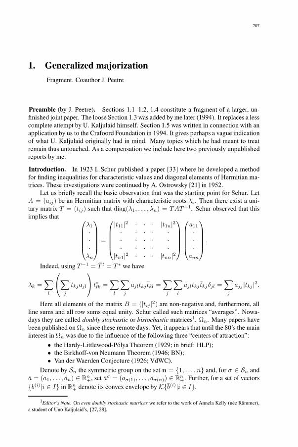
207
1. Generalized majorizationFragment. Coauthor J. Peetre
Preamble (by J. Peetre). Sections 1.1–1.2, 1.4 constitute a fragment of a larger, un-finished joint paper. The loose Section 1.3 was added by me later (1994). It replaces a lesscomplete attempt by U. Kaljulaid himself. Section 1.5 was written in connection with anapplication by us to the Crafoord Foundation in 1994. It gives perhaps a vague indicationof what U. Kaljulaid originally had in mind. Many topics which he had meant to treatremain thus untouched. As a compensation we include here two previously unpublishedreports by me.
Introduction. In 1923 I. Schur published a paper [33] where he developed a methodfor finding inequalities for characteristic values and diagonal elements of Hermitian ma-trices. These investigations were continued by A. Ostrowsky [21] in 1952.
Let us briefly recall the basic observation that was the starting point for Schur. LetA = (aij) be an Hermitian matrix with characteristic roots λi. Then there exist a uni-tary matrix T = (tij) such that diag(λ1, . . . , λn) = TAT−1. Schur observed that thisimplies that ⎛⎜⎜⎜⎜⎝
λ1
···λn
⎞⎟⎟⎟⎟⎠ =
⎛⎜⎜⎜⎜⎝|t11|2 · · · |t1n|2· · · · ·· · · · ·· · · · ·
|tn1|2 · · · |tnn|2
⎞⎟⎟⎟⎟⎠⎛⎜⎜⎜⎜⎝a11
···
ann
⎞⎟⎟⎟⎟⎠ .
Indeed, using T−1 = T t = T ∗ we have
λk =∑
l
⎛⎝∑j
tkjajl
⎞⎠ t∗lk =∑
l
∑j
ajltkj tkl =∑
j
∑l
ajltkj tkjδjl =∑
j
ajj |tkj |2.
Here all elements of the matrix B = (|tij |2) are non-negative and, furthermore, allline sums and all row sums equal unity. Schur called such matrices “averages”. Nowa-days they are called doubly stochastic or bistochastic matrices1. Ωn. Many papers havebeen published on Ωn since these remote days. Yet, it appears that until the 80’s the maininterest in Ωn was due to the influence of the following three “centers of attraction”:
• the Hardy-Littlewood-Pólya Theorem (1929; in brief: HLP);• the Birkhoff-von Neumann Theorem (1946; BN);• Van der Waerden Conjecture (1926; VdWC).
Denote by Sn the symmetric group on the set n = {1, . . . , n} and, for σ ∈ Sn anda = (a1, . . . , an) ∈ Rn
+, set aσ = (aσ(1), . . . , aσ(n)) ∈ Rn+. Further, for a set of vectors
{b(i)|i ∈ I} in Rn+ denote its convex envelope by K{b(i)|i ∈ I}.
1Editor’s Note. On even doubly stochastic matrices we refer to the work of Annela Kelly (née Rämmer),a student of Uno Kaljulaid’s, [27, 28].

208 CHAPTER III. MAJORIZATION
HLP can now be formulated as follows. Given any two vectors a, b ∈ Rn+, the
following conditions are equivalent:
(1) There exist a matrix B ∈ Ωn such that a = bB;(2) a ∈ K(bσ|σ ∈ Sn);(3) a ≺ b
where in (3) the sign ≺ means that we have the inequalities
k∑i=1
a[i] ≤k∑
i=1
b[i]
for all k ∈ {1, 2, . . . , n− 1}, whereas for k = n the corresponding equality holds:n∑
i=1
a[i] =n∑
i=1
b[i];
a[1] ≥ a[2] ≥ · · · ≥ a[n] and b[1] ≥ b[2] ≥ · · · ≥ b[n] being the decreasing rearrangementsof the vectors a and b respectively.
BN states that every doubly stochastic matrix in Ωn is a convex combination ofpermutation matrices. This result may be interpreted in terms of a probabilistic modelfor fuzzy bijections X → Y : we let each element bij of B give the transition probabilityfor xi �→ yj ; the fact that the i-th row sum is 1 means then that the element xi is bynecessity mapped into some element in Y and that the j-th row sum is 1 that the elementyj can be obtained as the image of some element in X . In this language, BN means thatevery fuzzy bijection X → Y is a convex combination of ordinary bijections from X toY . The importance of BN for Discrete Mathematics appears to be due to the fact that BNis the matrix analogue of Ph. Hall’s famous Matching Theorem (proved in the late 30’s;see [10]). BN has been rediscovered, commented on, or given new proofs by severalauthors; see, e.g., [24] for an infinite generalization of BN.
Let us briefly recall one of the proofs of BN that goes by induction on the number ofpositive elements of X ∈ Ωn and uses as an important ingredient the Frobenius-Koenigcriterion for the existence of a positive diagonal in a non-negative matrix2. Accordingto this criterion, every diagonal matrix (aσ(1), . . . , aσ(n)), σ ∈ Sn, of a non-negativematrix A = (aij) contains a zero if and only if A contains an s × t submatrix of zeroswith s + t ≥ n + 1. The proof of BN goes now as follows.
Let X = (xij) ∈ Ωn be given. The proof is carried by induction on the cardinalityof the support [X ] of X . If #[X ] = n, then X is a permutation matrix and BN istrivially true for X . If #[X ] < n, then we use the Frobenius-Koenig criterion to producea positive diagonal in X . Let this positive diagonal be denoted P = (pij) and set ε =min(i,j)∈supp P xij . Consider the matrix Y = X− εP . Then it is clear that the line sumsof Y equal 1 − ε and, further, that # suppY < # suppX . Hence Y ′ = 1
1−εY ∈ Ωn.Therefore the induction hypothesis implies that we can write Y ′ =
∑σ∈Sn
λσPσ with
2Editor’s Note, with the assistance of Laszo Filep. For this theorem, see Encyclopedia Applied Math-ematics, Vol. 6. Frobenius established it for determinants in 1910. Denes König (Koenig) gave a simplifiedproof in 1915 and generalized it to matrices in 1931. “This seems to have lead to some hostility between thetwo men. After Nazi occupation of Hungary, König worked to help persecuted mathematicians. This lead tohis death [by suicide?] a few days after the Hungarian National Socialist Party [the Arrow Cross] took over thecountry.” (Ian Anderson, in MacTutor.)
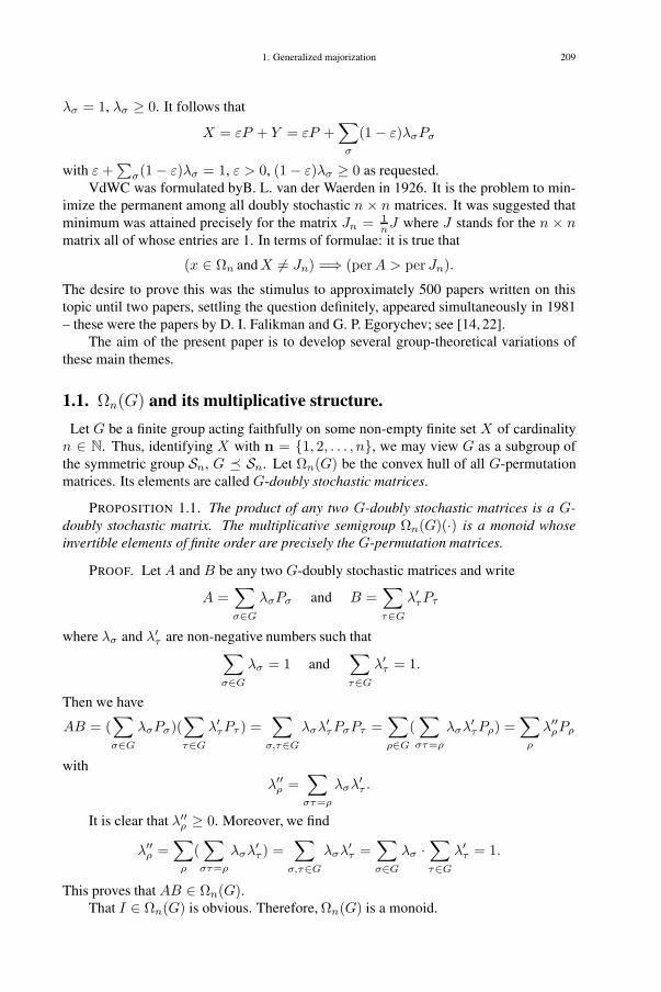
1. Generalized majorization 209
λσ = 1, λσ ≥ 0. It follows that
X = εP + Y = εP +∑
σ
(1− ε)λσPσ
with ε +∑
σ(1− ε)λσ = 1, ε > 0, (1− ε)λσ ≥ 0 as requested.VdWC was formulated byB. L. van der Waerden in 1926. It is the problem to min-
imize the permanent among all doubly stochastic n × n matrices. It was suggested thatminimum was attained precisely for the matrix Jn = 1
nJ where J stands for the n × nmatrix all of whose entries are 1. In terms of formulae: it is true that
(x ∈ Ωn andX �= Jn) =⇒ (perA > per Jn).
The desire to prove this was the stimulus to approximately 500 papers written on thistopic until two papers, settling the question definitely, appeared simultaneously in 1981– these were the papers by D. I. Falikman and G. P. Egorychev; see [14, 22].
The aim of the present paper is to develop several group-theoretical variations ofthese main themes.
1.1. Ωn(G) and its multiplicative structure.
Let G be a finite group acting faithfully on some non-empty finite set X of cardinalityn ∈ N. Thus, identifying X with n = {1, 2, . . . , n}, we may view G as a subgroup ofthe symmetric group Sn, G & Sn. Let Ωn(G) be the convex hull of all G-permutationmatrices. Its elements are called G-doubly stochastic matrices.
PROPOSITION 1.1. The product of any two G-doubly stochastic matrices is a G-doubly stochastic matrix. The multiplicative semigroup Ωn(G)(·) is a monoid whoseinvertible elements of finite order are precisely the G-permutation matrices.
PROOF. Let A and B be any two G-doubly stochastic matrices and write
A =∑σ∈G
λσPσ and B =∑τ∈G
λ′τPτ
where λσ and λ′τ are non-negative numbers such that∑
σ∈G
λσ = 1 and∑τ∈G
λ′τ = 1.
Then we have
AB = (∑σ∈G
λσPσ)(∑τ∈G
λ′τPτ ) =
∑σ,τ∈G
λσλ′τPσPτ =
∑ρ∈G
(∑
στ=ρ
λσλ′τPρ) =
∑ρ
λ′′ρPρ
withλ′′
ρ =∑
στ=ρ
λσλ′τ .
It is clear that λ′′ρ ≥ 0. Moreover, we find
λ′′ρ =
∑ρ
(∑
στ=ρ
λσλ′τ ) =
∑σ,τ∈G
λσλ′τ =
∑σ∈G
λσ ·∑τ∈G
λ′τ = 1.
This proves that AB ∈ Ωn(G).That I ∈ Ωn(G) is obvious. Therefore, Ωn(G) is a monoid.

210 CHAPTER III. MAJORIZATION
Now, let A be an invertible G-doubly stochastic matrix. Then we may assume thatAm = I for some integer m ≥ 2. Arguing by contradiction, suppose that A is not apermutation matrix. Then for some matrix element akl in A holds 0 < akl < 1. Setmaxi∈n{ail} = apl. Then it is clear that 0 < apl < 1, as apl together with akl and,possibly, other elements in the lthe column sums to unity. Notice that, in view of whathas already been proved, the matrix Am−1 is doubly stochastic. Therefore, consideringthe elements
∑s∈n a∗isasl in the l-th column of the doubly stochastic matrices Am−1 and
A, it follows that for any one of them holds∑s∈n
a∗isasl ≤ apl
∑s∈n
a∗is = apl < 1.
This contradicts the assumption that Am = I .Finally, let us prove that A is a G-permutation matrix. Take a reduced representation
for A, i.e. A =∑
σ∈H λσPσ with H ⊂ G and all λσ > 0. By the above argument, weknow that
∑σ∈H λσPσ = P for some permutation matrix P . Thus we have P (i, j) =∑
σ∈H λσPσ(i, j).If P (i, j) = 0 then 0 =
∑σ∈H λσPσ(i, j) together with the fact that all λσ > 0
while Pσ(i, j) ∈ {0, 1} implies that Pσ(i, j) = 0 for all σ ∈ H .If, however, P (i, j) = 1 then Pσ(i, j) = 1 for all σ ∈ H . Indeed, if Pτ (i, j) = 0 for
some τ ∈ H , it would follow from 1 =∑
σ∈H λσPσ(i, j) that∑
σ∈H λσ =∑
σ∈H′ λσ
with H ′ = H\τ . But as all λσ > 0 this is impossible.Thus we have shown that for all σ ∈ H holds
Pσ(i, j) =
{0, if P (i, j) = 0,
1, if P (i, j) = 1.
As Pσ and P are permutation matrices, this gives Pσ = P for all σ ∈ H . It follows thatA = P is a G-permutation matrix. '(
Fix a convex subset S ⊆ Mn(R). Linear transformations g : Mn(R) → Mn(R)such that g(S) = S are called symmetries for S. The set of all symmetries for S isa group. Its subgroups are called symmetric groups for S. Denote the action of g onmatrices Q ∈ S by Q ◦ g.
Take now S = Ωn(G) and consider a finite group L of symmetries for it. If Q is amatrix such that Q ◦ � = Q for all � ∈ L, then Q is called an L-fixed point.
PROPOSITION 1.2. Let L be a finite group of linear transformations of the spaceof matrices Mn(R) such that Ωn(G) is L-invariant. Then the subset of L-fixed pointscoincides with the convex hull of the set of all matrices of the form
Qσ =1|L|
∑�∈L
Pσ ◦ �.
PROOF. Denote bt L∗ the set of all L-fixed points in Ωn(G). Given A,B ∈ L∗
consider the matrix C = λ + (1 − λ)B, λ ∈ [0, 1]; it is clear that C ∈ L∗, as, for any� ∈ L,
C ◦ � = λ(A ◦ �) + (1− λ)(B ◦ �) = λA + (1− λ)B = C.

1. Generalized majorization 211
For any matrix
Qσ =1|L|
∑�∈L
Pσ ◦ � with σ ∈ G fixed
and �′ ∈ L we find
Qσ ◦ �′ =1|L|
∑�∈L
Pσ ◦ � =1|L|
∑�′′∈L
Pσ ◦ �′′ = Qσ;
here we used the fact that if � runs through all of L the same is true for �′′ = ��′ also.This shows that Qσ ∈ L∗.
Now, any element D ∈ L∗ ⊆ Ωn(G) can be written as
D =∑π∈G
δπPπ with δπ ≥ 0,∑
π
δπ = 1.
Hence,
D =1|L|
∑�∈L
D =1|L|
∑�∈L
(∑π∈G
δπ(Pπ ◦ �))
=
=∑π∈G
δπ
(1|L|
∑�∈L
(Pπ ◦ �))
=∑π∈G
δπQπ.
This together with what was proved above finishes the proof. '(
REMARK 1.3. Using the obvious relations (A + B)t = At + Bt and P tσ = Pσ−1
we see that for the transpose of any matrix X ∈ Ωn(G) it holds
Xt =
(∑σ∈G
λσPσ
)t
=∑σ∈G
λσPtσ
∑σ∈G
λσPσ−1 ,
which, as σ−1 ∈ G if σ ∈ G, implies that Xt ∈ Ωn(G). Therefore, Ωn(G) is invariantunder transposition of matrices. Taking L to be the 2-element group 〈t|t2 = idΩn(G)〉,it follows that the set of all symmetric doubly stochastic G-matrices coincides with theconvex hull of the set of matrices { 1
2 (Pσ +Pσ−1)}. Furthermore, specializing G to be thegroup Sn (the symmetric group of n) we obtain the result: the set of all symmetric n×ndoubly stochastic matrices is identical with the convex hull of the set of all matrices ofthe form 1
2 (P +P t), where P is an n×n permutation matrix. This is a result by M. Katz[12]; see also [5]
Following [8], a semigroup S with involution a �→ a∗ is called a special involutionsemigroup if and only if every finite nonempty subset T ⊆ S has the property that
there exists an element a ∈ T such that if for some b, c ∈ T we haveaa∗ = bc∗ then b = c.
PROPOSITION 1.4. The multiplicative subgroup of all doubly stochastic G-matrices(for any given finite group G, G ≥ Sn) is a special involution semigroup.
PROOF. Take any X ∈ Ωn(G) and write it in the form X =∑
π∈G λπPπ. Then weget Xt =
∑π∈G λπPπ−1 . It follows that X �→ Xt is an involution on the multiplicative
subgroup Ωn(G)(·).
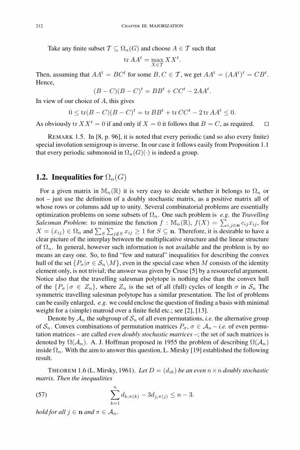
212 CHAPTER III. MAJORIZATION
Take any finite subset T ⊆ Ωn(G) and choose A ∈ T such that
trAAt = maxX∈T
XXt.
Then, assuming that AAt = BCt for some B,C ∈ T , we get AAt = (AAt)t = CBt.Hence,
(B − C)(B − C)t = BBt + CCt − 2AAt.
In view of our choice of A, this gives
0 ≤ tr(B − C)(B − C)t = trBBt + trCCt − 2 trAAt ≤ 0.
As obviously trXXt = 0 if and only if X = 0 it follows that B = C, as required. '(
REMARK 1.5. In [8, p. 96], it is noted that every periodic (and so also every finite)special involution semigroup is inverse. In our case it follows easily from Proposition 1.1that every periodic submonoid in Ωn(G)(·) is indeed a group.
1.2. Inequalities for Ωn(G)
For a given matrix in Mn(R) it is very easy to decide whether it belongs to Ωn ornot – just use the definition of a doubly stochastic matrix, as a positive matrix all ofwhose rows or columns add up to unity. Several combinatorial problems are essentiallyoptimization problems on some subsets of Ωn. One such problem is e.g. the TravellingSalesman Problem: to minimize the function f : Mn(R), f(X) =
∑i,j∈n cijxij , for
X = (xij) ∈ Ωn and∑
S
∑j /∈S xij ≥ 1 for S ⊆ n. Therefore, it is desirable to have a
clear picture of the interplay between the multiplicative structure and the linear structureof Ωn. In general, however such information is not available and the problem is by nomeans an easy one. So, to find “few and natural” inequalities for describing the convexhull of the set {Pσ|σ ∈ Sn\M}, even in the special case when M consists of the identityelement only, is not trivial; the answer was given by Cruse [5] by a resourceful argument.Notice also that the travelling salesman polytope is nothing else than the convex hullof the {Pσ |σ ∈ Zn}, where Zn is the set of all (full) cycles of length σ in Sn Thesymmetric travelling salesman polytope has a similar presentation. The list of problemscan be easily enlarged, e.g. we could enclose the question of finding a basis with minimalweight for a (simple) matroid over a finite field etc.; see [2], [13].
Denote byAn the subgroup of Sn of all even permutations, i.e. the alternative groupof Sn. Convex combinations of permutation matrices Pσ , σ ∈ An – i.e. of even permu-tation matrices – are called even doubly stochastic matrices –; the set of such matrices isdenoted by Ω(An). A. J. Hoffman proposed in 1955 the problem of describing Ω(An)inside Ωn. With the aim to answer this question, L. Mirsky [19] established the followingresult.
THEOREM 1.6 (L. Mirsky, 1961). Let D = (dik) be an even n×n doubly stochasticmatrix. Then the inequalities
(57)n∑
k=1
dk,π(k) − 3dj,π(j) ≤ n− 3.
hold for all j ∈ n and π ∈ An.
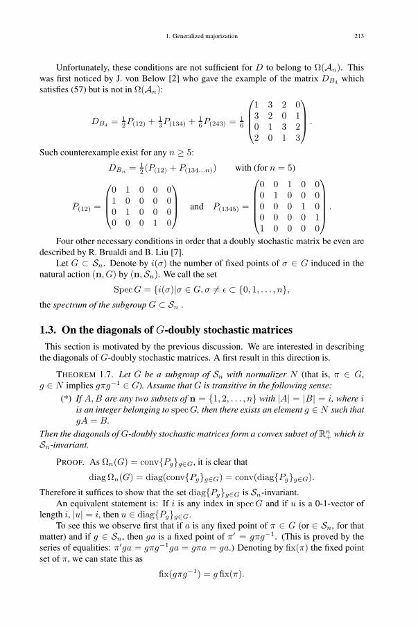
1. Generalized majorization 213
Unfortunately, these conditions are not sufficient for D to belong to Ω(An). Thiswas first noticed by J. von Below [2] who gave the example of the matrix DB4 whichsatisfies (57) but is not in Ω(An):
DB4 = 12P(12) + 1
3P(134) + 16P(243) = 1
6
⎛⎜⎜⎝1 3 2 03 2 0 10 1 3 22 0 1 3
⎞⎟⎟⎠ .
Such counterexample exist for any n ≥ 5:
DBn = 12 (P(12) + P(134...n)) with (for n = 5)
P(12) =
⎛⎜⎜⎝0 1 0 0 01 0 0 0 00 1 0 0 00 0 0 1 0
⎞⎟⎟⎠ and P(1345) =
⎛⎜⎜⎜⎜⎝0 0 1 0 00 1 0 0 00 0 0 1 00 0 0 0 11 0 0 0 0
⎞⎟⎟⎟⎟⎠ .
Four other necessary conditions in order that a doubly stochastic matrix be even aredescribed by R. Brualdi and B. Liu [7].
Let G ⊂ Sn. Denote by i(σ) the number of fixed points of σ ∈ G induced in thenatural action (n, G) by (n,Sn). We call the set
SpecG = {i(σ)|σ ∈ G, σ �= ε ⊂ {0, 1, . . . , n},the spectrum of the subgroup G ⊂ Sn .
1.3. On the diagonals of G-doubly stochastic matrices
This section is motivated by the previous discussion. We are interested in describingthe diagonals of G-doubly stochastic matrices. A first result in this direction is.
THEOREM 1.7. Let G be a subgroup of Sn with normalizer N (that is, π ∈ G,g ∈ N implies gπg−1 ∈ G). Assume that G is transitive in the following sense:
(*) If A,B are any two subsets of n = {1, 2, . . . , n} with |A| = |B| = i, where iis an integer belonging to specG, then there exists an element g ∈ N such thatgA = B.
Then the diagonals of G-doubly stochastic matrices form a convex subset of Rn+ which is
Sn-invariant.
PROOF. As Ωn(G) = conv{Pg}g∈G, it is clear that
diag Ωn(G) = diag(conv{Pg}g∈G) = conv(diag{Pg}g∈G).
Therefore it suffices to show that the set diag{Pg}g∈G is Sn-invariant.An equivalent statement is: If i is any index in specG and if u is a 0-1-vector of
length i, |u| = i, then u ∈ diag{Pg}g∈G.To see this we observe first that if a is any fixed point of π ∈ G (or ∈ Sn, for that
matter) and if g ∈ Sn, then ga is a fixed point of π′ = gπg−1. (This is proved by theseries of equalities: π′ga = gπg−1ga = gπa = ga.) Denoting by fix(π) the fixed pointset of π, we can state this as
fix(gπg−1) = g fix(π).

214 CHAPTER III. MAJORIZATION
Equivalently:
Pg diagPπ = diag(PπPgP−1π ) = diagPgπg−1 .
(Note that fix(g) = supp diagPg .)Let now u be an arbitrary 0-1-vector with |u| = i, i ∈ specG. As i ∈ specG, there
exists then also a vector w with w = diagPπ for some π ∈ G and |w| = i. But (∗),together with the observations in the preceding paragraph, shows that u = Pgw for someg ∈ N . It follows now that
u = Pgw = Pg diagPπ = diagPgπg−1 = diagPg′
with g′ = gπg−1 ∈ G. Therefore u ∈ diag{Pg}g∈G. '(
So our problem is reduced to a purely geometric question: describing the structureof the convex hull of an Sn-invariant set M of 0-1-vectors. We will answer this questiononly in a very special situation.
LEMMA 1.8. Let n be a positive integer and let f be an integer satisfying 0 ≤ f ≤ n.Let Mf be the set of all vectors in Rn all of whose components are either 0 or 1, suchthat this set includes the vector (1, 1, 1, 1, ...., 1) and also all vectors which have at mostn− f components equal to 1. (Thus Mf also contains the vector (0, 0, ..., 0).) Then theconvex hull of Mf consists of all vectors (x1, x2, ...., xn) which satisfy the conditions
(58) 0 ≤ xj ≤ 1 and n− f + fxj ≥n∑
k=1
xk for j = 1, 2, ..., n.
PROOF. (After Michael Cwikel3) Let F be the set of all vectors in Rn which satisfyall the conditions (58). It is clear that F is a convex set containing every vector in Mf . Sowe have conv v(Mf ) ⊂ F , where conv v(E) denotes the convex hull of any set E ⊂ Rn.
It remains to show that F ⊂ conv v(Mf ). In fact it suffices to show instead merelythat F∗ ⊂ conv v(Mf ), where F∗ is the subset of F consisting of those vectors x =(x1, x2, ..., xn) which satisfy 1 ≥ x1 ≥ x2 ≥ ... ≥ xn ≥ 0. This reduction of theproblem follows immediately from the fact that the set F and also the set conv v(Mf )are both invariant under permutations of the components of vectors.
It will be convenient to use the notation D for the larger set of all vectors x =(x1, x2, ..., xn) ∈ Rn which satisfy x1 ≥ x2 ≥ ... ≥ xn ≥ 0.
REMARK 1.9. Let x be any vector of the form x =∑k
j=1 αjwj where wj ∈ Mf
or merely wj ∈ conv v(Mf ), and αj ≥ 0 for j = 1, 2, ..., k and∑k
j=1 αk ≤ 1. Then itis clear that x ∈ conv v (conv v(Mf )) = conv v(Mf ), since we can write x in the formx =
∑kj=0 αjwj where w0 is the zero vector and α0 = 1−∑k
j=1 αj . '(
Let us define the vectors v0, v1, ..., vn in Rn by letting v0 be the zero vector and, forj = 1, 2, ..., n, letting vj be the vector whose first j components equal 1 and all of whoseremaining components (if there are any) equal 0.
3Note by J. Peetre. This result is due to Uno Kaljulaid, but his proof was not quite complete. So in 1997I gave another proof. Unfortunately, I have been unable to reconstruct it. Therefore we offer here yet a thirdproof, constructed on my request by friend Michael Cwikel. I am immensely grateful to him for this.

1. Generalized majorization 215
Suppose that x = (x1, x2, ..., xn) is an arbitrary element of F∗. Then we can writex in the form
(59) x =n∑
j=1
θjvj ,
where each θj ∈ [0, 1] and∑n
j=1 θj ≤ 1 and vj are the special vectors just defined. Infact θj = xj − xj+1 for j = 1, 2, ..., n, where we define xn+1 = 0. By summing allcomponents of all vectors in the sum for x in (59) we see that
(60)n∑
j=1
xj =n∑
j=1
θjj.
For x ∈ F∗ the n conditions n − f + fxj ≥∑n
k=1 xk for j = 1, 2, ..., n, whichappear in (58), are equivalent to the single condition
(61) n− f + fxn ≥n∑
k=1
xk.
We will sometimes use the notation ‖x‖ =∑n
k=1 xk .Suppose first that f = 0. Then vj ∈ Mf for every j = 0, 1, 2, ..., n. Taking the first
component of the vector equation (59) shows that 1 ≥ x1 ≥∑n
j=1 θj . This inequality,combined with Remark 1.9 and (59), immediately gives us that x ∈ conv v(Mf ).
Let us next consider the case where f = 1. By definition M1 = M0, so we still havevj ∈ Mf for every j = 0, 1, 2..., n. Exactly the same reasoning as for f = 0 shows thatx ∈ conv v(Mf ). (Note that so far the only part of condition (58) that we have had touse is
(62) 0 ≤ xj ≤ 1 for j = 1, 2, ..., n.
In fact, although we do not need it for this proof, it can be immediately checked directlythat condition (58) for f = 0 is equivalent to condition (58) for f = 1 .
Now suppose that f = n. Then condition (58) implies that the average value ofthe n components x1, x2, ..., xn is less than or equal to their minimum value. So all thecomponents xj must be equal. Thus x = θnvn where θn = xn ∈ [0, 1] is the commonvalue of all the components. So, again by Remark 1.9, we have x ∈ conv v(Mf ).
It remains to consider the case where 1 < f < n. In this case we have vj ∈Mf forj = 0, 1, 2, ..., n − f and also for j = n. For each j in the range n − f < j < n weclaim that
(63)n− f
jvj ∈ conv v(Mf ).
This is fairly obvious intuitively, but let us check it anyway. Consider the subspace Vof Rn consisting of all vectors y of the form (y1, y2, ..., yj , 0, 0, ...0) i.e. all componentsafter the j-th component are 0. Now consider the cyclic permutation map T acting on Vdefined by T (y1, y2, ..., yj , 0, 0, ...0) = (yj , y1, y2, ..., yj−1, 0, 0, ...0). Since vn−f andall its permutations are in Mf , the vector
w =1j
(vn−f + Tvn−f + T 2vn−f + T 3vn−f + ... + T j−1vn−f
)

216 CHAPTER III. MAJORIZATION
must be in conv v(Mf ) and must be of the form (a, a, a, ..., a, 0, ..., 0), i.e., the first jelements all equal the average value a = n−f
j of the first j elements of vn−f , and theremaining elements are 0. This proves (63).
It is convenient to divide the case where 1 < f < n into several subcases.Subcase (i): Suppose that the arbitrary element x ∈ F∗ chosen above satisfies xj = 0
for all j > n− f . Then we also have θj = 0 for all j > n− f in the representation (59).Since vj ∈ Mf whenever θj �= 0, we obtain that x ∈ conv v(Mf ) by exactly the samereasoning as was used in the case f = 0.
Subcase (ii): Suppose that x is such that in its representation (59) we have θj = 0for all integers j in the range 1 ≤ j ≤ n − f and also θn = 0. This last condition isequivalent to xn = 0. So, by (58) and (60), we have
(64)n−1∑
j=n−f+1
θjj =n∑
j=1
θjj ≤ n− f.
Note that n−fj vj = wj ∈ Mf for each j in the range n− f + 1 ≤ j ≤ n − 1. We
now see that
x =n−1∑
j=n−f+1
θjvj =n−1∑
j=n−f+1
αjwj
where αj = jn−f θj . By (64) we have
∑n−1j=n−f+1 αj ≤ 1. So, once again, Remark 1.9
applies to show that x =∑n−1
j=n−f+1 αjwj is an element of conv v(Mf ).Subcase (iii): Suppose that x ∈ F∗ is of the form x =
∑n−fj=1 θjvj + θkvk for some
particular k in the range n−f +1 ≤ k ≤ n−1. Now let y =∑n−f
j=1 θjvj and let z = vk.
So y and z are both in D. Let y′ = n−f‖y‖ y and z′ = n−f
‖z‖ z = n−fk vk. These are both
elements of F∗ and furthermore, by subcases (i) and (ii) they are also in conv v(Mf ).We can now write x = αy′ + βz′ where, necessarily αn−f
‖y‖ = 1 and β n−fk = θk. Then
α + β = ‖y‖n−f + θkk
n−f = ‖x‖n−f ≤ 1. So Remark 4.1 shows that x ∈ conv v(Mf ).
Subcase (iv): Suppose that x ∈ F∗ satisfies xn = 0, or equivalently θn = 0. So, asin (59) we have
x =n−1∑j=1
θjvj =n−f∑j=1
θjvj +n−1∑
k=n−f+1
θkvk =
=n−1∑
k=n−f+1
⎡⎣ θk∑n−1q=n−f+1 θq
n−f∑j=1
θjvj + θkvk
⎤⎦ =
=n−1∑
k=n−f+1
yk
where yk = θkn−1q=n−f+1 θq
∑n−fj=1 θjvj + θkvk. For each k in the range n − f + 1 ≤
k ≤ n − 1 we can see that the vector y′k := n−f‖yk‖yk is exactly an element of F∗ of the
form treated in subcase (iii) and so it is in conv v(Mf ). Furthermore we clearly have

1. Generalized majorization 217
∑n−1k=n−f+1 ‖yk‖ = ‖x‖ ≤ n − f . So x =
∑n−1k=n−f+1 αky
′k where αk = ‖yk‖
n−f and so∑n−1k=n−f+1 αk ≤ 1. This shows that x ∈ conv v(Mf ).
Subcase (v): Finally we have to treat the last remaining subcase, where xn > 0. Weshall write x in the form x = y+z where z = xnvn and so y = x−xnvn = (x1−xn, x2−xn, . . . , xn−1 − xn, 0). Let w = (w1, w2, . . . , wn−1, 0) be the vector w = 1
1−xny. We
claim that w ∈ F∗. To check this first note that 0 ≤ wj = xj−xn
1−xn≤ x1−xn
1−xn≤ 1 for each
j. Then we have the following sequence of inequalities, where we shall use the fact thatx ∈ F∗ in the second line.
n∑j=1
wj =n−1∑j=1
wj =1
1− xn
n−1∑j=1
(xj − xn) =1
1− xn
⎛⎝n−1∑j=1
xj − (n− 1)xn
⎞⎠=
11− xn
⎛⎝ n∑j=1
xj − nxn
⎞⎠ ≤ 11− xn
(fxn + n− f − nxn)
=(n− f)(1− xn)
1− xn= n− f.
Since wn = 0 this is exactly what we need to show that w ∈ F∗. Also, again usingthe fact that wn = 0, we see, from the previous case, that w ∈ conv v(Mf ). Finally weexpress x as a convex combination x = (1 − xn)w + xnvn. Since both w and vn are inconv v(Mf ), so is x. '(
Combining Theorem 1.7 with Lemma 1.8 we obtain at once the following result.
THEOREM 1.10. Assume that G ⊂ Sn satisfies condition (∗) in Theorem 1.7 and,moreover, that specG = {0, 1, . . . , n− f, n}. Then a vector x = (x1, . . . , xn) belongsto the convex hull of all diagonals of G-doubly stochastic matrices if and only if condition(1) in Lemma 1.8 is fulfilled.
1.4. G-variations on HPLFix n ∈ N and consider any subgroup G & Sn. Take some vectors �a = (a1, . . . , an)
and�b = (b1, . . . , bn) with real non-negative components.
DEFINITION 1.11. The vector�a is said to be a G-average of�b, if there exists a matrixX ∈ Ωn(G) such that �a = �bX .
DEFINITION 1.12. The polynomial
[�a]G :=1|G|
∑σ∈G
Xaσ(1)1 . . .X
aσ(n)n
is called the symmetric G-mean of �a.
The following two examples are well-known
[(1, 0, . . . , 0)]Sn =1n
(x1 + . . . xn)
and
[(1n, . . . ,
1n
)]Sn = n√x1x2 . . . xn.
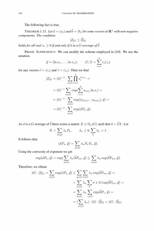
218 CHAPTER III. MAJORIZATION
The following fact is true.
THEOREM 1.13. Let�a = (ai) and�b = (bi) be some vectors in Rn with non-negativecomponents. The condition
[�a]G ≤ [�b]Gholds for all real xi ≥ 0 if and only if �a ia a G-average of�b
PROOF. SUFFICIENCY. We can modify the scheme employed in [10]. We use thenotation
�y = (lnx1, . . . , lnxn); (�c, �z) =n∑
i=1
ci(zi)
for any vectors �c = (ci) and �z = (zi). Then we find
[�a]G = |G|−1 ·∑σ∈G
n∏i=1
xaσ(i)i =
= |G|−1∑σ∈G
exp(n∑
i=1
aσ(i) lnxi) =
= |G|−1 ·∑σ∈G
exp((aσ(1), ·, aσ(n)), �y) =
= |G|−1 ·∑σ∈G
exp(�aPσ, �y).
As �a is a G-average of�b there exists a matrix X ∈ Ωn(G) such that �a = �bX . Let
X =∑π∈G
λπPπ , λπ ≥ 0,∑
π
λπ = 1.
It follows that(�aPσ, �y) =
∑π∈G
λπPπPσ, �y).
Using the convexity of exponent we get
exp(�aPσ, �y) = exp(∑π∈G
λπ(�bPπσ, �y) ≤∑π∈G
λπ exp(�bPπσ, �y).
Therefore, we obtain
|G| · [�a]G =∑σ∈G
exp(�aPσ, �y) ≤∑g∈G
∑π∈G
λπ exp(�bPπσ, �y) =
=∑π∈G
λπ
∑π
σ ∈ G exp(�bPπσ, �y) =
=∑π∈G
λπ
∑γ∈G
exp(�bPγ , �y) =
= (∑π∈G
λπ) · |G| · [�b]G = |G| · [�b]G.

1. Generalized majorization 219
The needed inequality [�a]G ≤ [�b]G follows. '(To prove the necessity part of the theorem use the following result by R. Rado [26]
THEOREM 1.14 (Rado, 1952). For given vectors �a = (ai) and �b = (bi) in Rn withall their components non-negative and for any subgroup G & Sn it holds [�a]G ≥ [�b]G ifand only if �a belongs to the convex hull of the set {�bσ |σ ∈ G}.
Here the following notation is used: for�b = (b1, . . . , bn) one writes
�bσ = (bσ(1), . . . , bσ(n)) ∈ Rn.
Denote further by KG(�b) the convex hull of the set {�bπ |π ∈ G}.It remains to prove that
�a ∈ KG(�b)
is the same as saying that �a is a G-average �b. Indeed, if �a = �bX for some matrixX ∈ Ωn(G), then, representing X as
X =∑π∈G
tπPπ . tπ ≥ 0,∑
π
tπ,
we get�a = �b(
∑π∈G
tπPπ) =∑π∈G
tπ(�bPπ =∑π∈G
tπ�bπ ∈ KG(�b).
In the other direction, if �a ∈ KG(�b), then for some λσ ≥ 0,∑
σ ≥ 0,∑
σ lamσ = 1, wehave
�a =∑σ∈G
λσ�bσ
and therefore
�a =∑σ∈G
λσ�bσ =
∑σ∈G
λσ(�bPσ) = �b(∑σ∈G
λσPσ) = �bX, X =∑
σ
Pσ,
with X belonging to Ωn(G). This means that �a is a G-average�b.
PROOF OF THEOREM 1.14 ([26]). Let there hold [�a]G ≤ [�b]G] and, arguing bycontradiction, suppose that �a /∈ CG(�b). Then it follows (see [26] that
∃uiR (i ∈ n), δ > 0,∑
i
ui(ai − bτ(i)) ≥ δ.
Take any number M > 1 and set x�u = Mu�u . Then we have
|G| · [�b]G =∑τ∈G
n∏i
xbτ(i)i =
∑τ∈G
Mubτ(i)i ≤
≤∑τ∈G
Muiai−δ ≤
≤ |G| ·M−δ · [n∏i
(Mui)ai +∑τ �=ε
n∏i
(Mui)ai ] =
= |G| ·M−δ · |G|[�a]G.

220 CHAPTER III. MAJORIZATION
Taking here
lnM >ln |G|δ
we get|G| ·M−δ · |G|[�a]G < |G|[�a]G.
Hence, it follows[�b]G < [�a]G,
which contradicts [�a]G ≤ [�b]G.Suppose now that a ∈ CG(�b). Then there exist real numbers tπ ≥ 0,
∑π tπ = 1
such that �a =∑
π tπ�bπ. This implies that
aj =∑π∈G
tπ�bπ(j).
Then
[�a]G =1|G|
∑π∈G
n∏i=1
xa{σ(i)
i =
=1|G|
∑σ∈G
n∏i=1
x π tπbσ(i)i =
=1|G|
∑σ∈G
n∏i=1
x π tπbσ(i)i =
=1|G|
∑σ∈G
n∏π∈G
(n∏
i=1
xbπσ(i)i
)tπ
≤
≤ 1|G|
∑σ∈G
∑π∈G
tπ
(n∏
i=1
xbπσ(i)i
)=
=∑π∈G
tπ · [�b]G = [�b]G.
The first inequality in this calculation follows from the generalized version of the arithmetic-geometric inequality [9]: for αi ≥ 0,
∑i αi = 1 and xj non-negative it holds
xα11 xα2
2 · xαnn ≤ α1x1 + α2x2 + · · ·+ α1xn.
As a result we obtain[�a]G ≤ [�b]G,
as needed. '(

1. Generalized majorization 221
1.5. Appendix. Research plan of the project “Groups and inequalitieswith applications to combinatorics and optimization”
Introduction. History, motivation, examples.
A. History: I. Schur (1923); Hardy-Littlewood-Pólya (1929); G. Birkhoff–J. vonNeumann (1946); A. Ostrowsky and R. Rado (50’s); L. Mirsky (60’s); G Ego-rychev et al (1980); R. Brualdi (1970-1990).
B. Motivation:(a) Majorization: Marshall-Olkin book – examples using the relation ≺ in
combinatorics; T. Ando’s lectures on majorization – preprint (1990, ‘old’version) of the lectures notes & the new version (T. Ando, Lin. Alg. Appl.1994).
(b) Generalized majorization. Peetre’s pre-print (1985).(c) Discrete optimization on Sn and its subsets. Marshall-Olkin’s examples
of combinatorial and discrete optimization through majorization theorymethods. The results of H. Ryser et al revisited. Minsk seminar (70’s and80’s). Vershik - Barvinok (1990).
(d) Polytope algebra. Lattice-theoretic generalizations. Permutohedron andsuperconductivity. McMullen’s polytope algebra I,II. Valuations – Geis-singer, Rota, Lovász, etc. K. Fan and S. Sternberg’s results on Bruhatorder and superconductivity.
(e) H. Ryser’s problem and M. Hall’s problem on (0, 1)-matrices. Infiniteextensions. Problems. H. Ryser’s survey; L. Skornyakov on ∞ versions;lattice theoretic versions; L. Lovász et al.
Part I. Ωn(G) group theoretic variations on ‘bistochastic’ themes.
A. Multiplicative structure of Ωn(G)(a) Elements of finite order in the monoid Ωn(G)(·)(b) Subgroups of Ωn(G)(·) via D. Farkas’ paper(c) Unit in the group rings ZS3, ZD4, . . . via Hughes-Pearson; . . .(d) On the algebra structure of the monoid Ωn(G). Eastwood & Munn (B =
Sn)B. Giving Ωn(G) by a few inequalities
(a) The spectrum of a group G, G & Sn. A theorem on the inequalitiesfor X ∈ Ωn(G). Corollaries: Results of L. Mirsky and A. Cruse. Newcounterexamples to Mirsky’s conjecture.
(b) A criterion for the diagonalsC. On a problem on finite simple groups: the (second) main theorem (THEOREM 2)
on the classification of groups (using FGC).D. Infinite extensions of results on the diagonals of bistochastic G-matrices, G &S∞ (substitutions displacing finitely may symbols only).
E. G-majorizations(a) G-version of the HLP-theorem. TG-transformations(b) a & b for any G & Sn; the Dirichlet polytope(c) . . .(d) . . .

222 CHAPTER III. MAJORIZATION
Part II. G-permanents.
A. A new solution of the van der Waerden inequality via L. Gårding’s inequalityfor hyperbolic polynomials. – Peetre’s preprint [22].
B. . . .(a) THEOREM 3. G-extension of P. Hall’s marriage theorem.(b) THEOREM 4. G-extension of the Frobenius-König theorem.(c) Egorychev-like proof of the (extended) G-version of the van der Waerden
problem – via Peetre’s preprint(d) THEOREM 5. Algebraic structure of the McMullen polytope algebra for
Ωn(G). A (new?) Molien series for Ωn(G).
Part III. Applications.
A. Kaplansky-Riordan theory revisited: G-extension via Moebius inversion asso-ciated to the restriction matrix.
B. Bruhat order on G & Sn and (possible permutahedron results for Ωn(G).Applications to superconductivity (K. Fan and S. Sternberg). On a problem ofH. Ryser on (0, 1)-matrices.
C. The M. Hall theorem on permanents of (0, 1)-matrices. G-extension.
[1],[4],[3], [6],[11],[15],[16],[17], [20],[23],[25],[29],[30], [31],[32],[18],[34]
References
[1] A. I. Barvinok and A. M. Vershik. Methods of representation theory in combinatorial optimization prob-lems. Izv. Akad. Nauk SSSR, ser. Tekhn. Kibernet. 6, 1988, 64–71. English translation: Soviet J. Com-put. Systems Sci. 27 (5), 1989, 1–7.
[2] J. von Below. On a theorem of L. Mirsky on even doubly stochastic matrices. Discrete Math. 55 (3),1985, 311–312.
[3] N. Biggs. Finite groups of automorphisms. London Mathematical Society Lecture Notes Series, 6. Cam-bridge Univ. Press, 1971.
[4] T. Bonnesen and W. Fenchel. Theorie der konvexen Körper. In: Erg. Math. u. ihrer Grenzgebiete, 3,No. 1. Springer, Berlin, 1934.
[5] A. Cruse. A note on symmetric doubly stochastic matrices. Discrete Math. 13, 1976, 109–119.[6] A. Cruse. On removing a vertex from the assignment polytope. Linear Algebra Appl. 26, 1979, 45–57.[7] R. Brualdi and B. Liu. The polytope of even doubly stochastic matrices. J. Combin. Theory Ser. A 57 (2),
1991, 243–253.[8] D. Eastwood and W.D. Munn. On semigroups with involution. Bull. Aust. Math. Soc. 48, 1993, 93–100.[9] G. H. Hardy, G. Littlewood, and G. Pólya. Inequalities. Cambridge Univ. Press, Cambridge, 1934.[10] L. Harper and G.-C. Rota. Matching theory, an introduction. Advances in Probability Theory 1, 1971,
169–215.[11] A. Horn. Doubly stochastic matrices and the diagonal of a rotation matrix. Amer. J. Math. 76, 1954,
620–630.[12] M. Katz. On the extreme points of a certain convex polytope. J. Comb. Theory 8, 1970, 417–423.[13] A. W. J. Kolen and J. K. Lenstra. Combinatorics in operator research. In: Handbook of combinatorics,
Chap. 35. Elsevier, Amsterdam, 1995.[14] J. H. van Lint. The Van der Waerden Conjecture: two proofs in a year. Math. Intell. 4, 1982, 72–77.[15] M. Marcus and H. Minc. A survey of matrix theory and matrix inequalities. Allyn and Bacon, Inc.,
Boston, 1964.[16] A. W. Marshall and I. Olkin. Inequalities, theory of majorization and its applications. Aacdemic Press,
New York, 1979.
1. Generalized majorization 223
[17] P. McMullen and G. C. Shephard. Convex polytopes and the upper bound conjecture. London Mathemat-ical Society Lecture Notes Series, 3. Cambridge Univ. Press, 1971.
[18] H. Minc. Non negative matrices. London Mathematical Society Lecture Notes Series, 3. John Wiley,New York, 1988.
[19] L. Mirsky. Even doubly stochastic matrices. Math. Ann. 144, 1961, 418–421.[20] L. Mirsky. Results and problems in the theory of doubly stochastic matrices. Z. Wahrscheinlichkeits-
theorie 1, 1963, 319–334.[21] A. Ostrowski. Sur quelques applications des fonctions convexes et concaves au sens de I. Schur.
J. Math. Pures Appl., IX. Ser. 31, 1952, 253–292.[22] J. Peetre. Van der Waerden’s conjecture and hyperbolicity. Technical Report LTH 1981:9. Lunds Univer-
sitet, Lund, 1981. Reprinted in this Volume.[23] J. Peetre. On generalized majorization. Technical Report LTH 1985:2. Lunds Universitet, Lund, 1985.
Reprinted in this Volume.[24] L. I. Polotskiı, M. V. Saphir, and L. A. Skornyakov. Convex combinations of infinite permutation matri-
ces. Acta Sci. Math. 51, 1987, 185–189.[25] D. G. Poole. The stochastic group. Amer. Math. Monthly 102, 1995, 798–801.[26] R. Rado. An inequality. J. London Math. Soc. 27, 1952, 1–6.[27] A. Rämmer. On minimizing matrices. In: Proc. of the First Est. Conf. on Graphs and Appl. (Tartu–
Kääriku). Tartu Univ. Press, Tartu, 1991, 121–134.[28] A. Rämmer. On even doubly stochastic matrices with minimal even permanent. Acta
Comm. Univ. Tartuensis 878, 1990, 103–114.[29] J. V. Ryff. On the representation of doubly stochastic operators. Pac. J. Math. 13, 1963, 1379–1386.[30] J. V. Ryff. Orbits of L1-functions under doubly stochastic transformations. Tr. Am. Math. Soc. 117, 1965,
92–100.[31] J. V. Ryff. Majorized functions and measures. Nederl. Akad. Wetensch. Proc. Ser., A. 71 = Indag. Math.
30, 1968, 431–437.[32] J. V. Ryff. Extreme points of some convex subsets of L1(0, 1). Proc. Am. Math. Soc. 18, 1967, 1026–
1034.[33] I. Schur. Über eine Klasse von Mittelbildungen mit Anwendungen auf die Determinantentheorie.
Sitzungsber. Berl. Math. Gesell. 22, 1923, 9–20.[34] G. Ziegler. Lectures on polytopes, Graduate Texts in Mathematics, 152. Springer-Verlag, New York,
1995.

This page intentionally left blank
225
2. Van der Waerden’s conjecture and hyperbolicityby J. Peetre 4
Introduction. The Van der Waerden’s conjecture says that, if A = (aik) is an n × n
doubly stochastic matrix, then perA ≥ n!nn
with equality if and only if A = Jdef= ( 1
n )(see definitions infra). It has been settled independently by two Soviet mathematiciansEgorychev [4] and Falikman [5], that is, the latter proves only the inequality withoutdiscussing the case of equality. An analysis of Egorychev’s proof by van der Lint [13]has also appeared5. It is interesting that both Egorychev and Falikman at least implicitlyinvoke hyperbolic quadratic forms (Lorentz forms). In this note we wish to further clar-ify the role of hyperbolicity in this context, the main point being the simple observationthat the permanent as a function of the rows (or columns) of the matrix is the completepolarization of a certain hyperbolic (in the sense of Gårding) polynomial, viz. the poly-nomial P (x) = n!x1 · · ·xn. Since Falikman’s proof at least has not yet appeared intranslation we reproduce its main features below (Section 2.2). We also indicate a fewminor simplifications of Egorychev’s proof based on Falikman’s lower bound (Section2.3). Therefore we have, in fact, here a proof which is “almost self-contained”, thatis, modulo the only remaining purely combinatorial element, the celebrated Frobenius-König theorem (see [12, Chapter 3]) and the circumstance that we have not bothered toreproduce some reasoning which we otherwise would have taken over verbatim from [5]or [13].
Notation. If A = (aik) is an n× n matrix then its permanent is defined as
perA =∑
σ
a1σ(1) · · · anσ(n)
(summation over all permutations σ of {1, . . . , n}). If we consider it as a function of therows x1, . . . , xn of A we write per(x1, . . . , xn). Notice that
per(eσ(1), . . . , eσ(n)) ={ 1 if σ is a permutation
0 if not,
which relation essentially characterizes the permanent function 6.A matrix A = (aik) is called doubly stochastic if
∑k aik = 1 =
∑i aik , aik ≥ 0.
The set of all doubly stochastic matrices will be denoted Ω (it is a convex subset of Rn2,
dimΩ = (n− 1)2). The “interior of Ω will be denoted by Ω∗ and its “boundary” by ∂Ω(= Ω\Ω∗). Every permutation matrix is in ∂Ω. Also J = ( 1
n ) is in Ω∗.Attention: Sometimes xi means the i-th component of the vector x = (x1, . . . , xn)
but sometimes it is the i-th member of the family of vectors {x1, . . . , xm}.
4Report LTH 1981:9, Lund, 1981. Reprint.5Egorychev’s paper [4] has not been available to us; we know of its contents only through van der Lint
[13].6The standard reference for permanent theory is Minc’s book [12].
226 CHAPTER III. MAJORIZATION
2.1. HyperbolicityHyperbolic polynomials were introduced by Gårding [7] in 1950 in the context of
Cauchy’s problem for linear partial differential equations. Their main algebraic char-acteristics in purely algebraic terms are summarized in his beautiful paper [6] (see alsoHörmander’s book [8, Chapter 5] and Beckenbach-Bellman [2, §§ 36–39]).
Let P (x1, . . . , xm) be a real symmetricm-linear form in Rn. If all the arguments areequal we write P (x) = P (x, . . . , x). Thus P is a homogeneous polynomial of degree mwhich uniquely determines P (x1, . . . , xm). One says that P (x1, . . . xm) is the completepolarization of P (x).
Let a be any non-zero vector in Rn.
DEFINITION 2.1. P is hyperbolic with respect to a (or a is hyperbolic with respect toP ) if P (a) > 0 and if, further, for any x in Rn, the polynomial P (sa+x) in one variables hasm distinct roots. That is, one has the factorizationP (sa+x) = c
∏j(a+λj(x, P )),
where c > 0 and λ1(x, P ) < λ2(x, P ) < · · · < λm(x, P ).7
If P is hyperbolic with respect to a, let us introduce the set
C(a, P ) def= {x|∀ j λj(x, P ) > 0}.The main properties of hyperbolic polynomials can be summarized in the following
theorem.
THEOREM 2.2. C(a, P ) is an open convex cone in Rn, in fact, as a set equal to theconnected component of {P �= 0} that contains the vector a. The vector b is hyperbolicwith respect to P for any b ∈ C(a, P ); then, in particular, C(b, P ) = C(a, P ).
For the proof we refer to Gårding’s paper [6]. Here we shall only need the following.
COROLLARY 2.3. If b1, . . . , bk are any k vectors in C(a, P ) (0 < k < n) then the“partial” polarization
Q(x) def= P (x, x, . . . , x︸ ︷︷ ︸n−k times
, b1, . . . , bk)
is hyperbolic with respect to any vector in C(a, P ).
PROOF. By induction it suffices to consider the case k = 1, b1 = a. That is, weshall prove that
Q(x) def= P (x, x, . . . , x︸ ︷︷ ︸n−1 times
, a)
is hyperbolic throughout C(a, P ). We have the formula
d
dsP (sa + x) = mP (sa + x, . . . , a) = mQ(sa + x).
It follows from Rolle’s theorem that for any x all the roots of Q(sa + x) are real and, infact, separated by the roots of P (sa + x):
(65) λ1(x, P ) < λ1(x,Q) < λ2(x, P ) < λ2(x,Q) < . . .
7Editors’ Note. It is advantageous to interpret the relation t = sa + x geometrically as a straight line inthe t, x plane with direction vector a. Then we are dealing with the intersection of this line with the variety{P (t) = 0}. For hyperbolicity of non-homogeneous polynomials, see [7, 8].
2. Van der Waerden’s conjecture and hyperbolicity 227
Thus Q is hyperbolic with respect to a. Also (65) shows that C(a,Q) = C(a, P ), so that,moreover, by Theorem 2.2 Q is hyperbolic with respect to any element of C(a, P ). '(
Let us consider some examples of hyperbolic polynomials.
EXAMPLE 2.1. m = 2, P = x21 − x2
2 − · · · − x2n (Lorentz form). This is the
canonical example, because every other hyperbolic quadratic form can be written in thisway after a linear change of variables. As is well-known this example is of fundamentalimportance for special relativity. Hyperbolic vectors are now called time-like, those onthe conical surface x2
1−x22−· · ·−x2
n = 0 light-like, all other vectors (�= 0) being termedspace-like. '(
EXAMPLE 2.2. m = n, P = n!x1x2 . . . xn. Every positive vector is hyperbolic. Asalready mentioned in the Introduction, the complete polarization is now the permanentfunction perA = per(x,x2, . . . , xn) = P (x,x2, . . . , xn) if A is a matrix with rowsx1, x2, . . . , xn. '(
REMARK 2.4. In relation to the permanent used in Example 2.2 let us forward thefollowing interesting observation. Curiously enough the interpretation of the permanentas a multilinear form does not seem to be explicitly mentioned in [12]. On p. 103 thereis reproduced Muir’s formula
perAι1 . . . ιn =n∏
i=1
n∑k=1
aikιk,
where the ιk are generators of a commutative associative algebra such that ι2k = 0.Of course, a similar thing can be done with any polynomial (hyperbolic or not). IfP (x1, . . . , xm) =
∑aα1...αmx1α1 . . . xmαm then
P (x1, . . . , xm)ι1 . . . ιm =n∏
i=1
n∑α=1
xiαια
with ια1 . . . ιαm = aα1...αm . Cf. Dirac’s introduction of the Dirac matrices etc. '(
EXAMPLE 2.3. Take n =ν(ν + 1)
2and identify Rn with the set of all symmetric
ν × ν matrices. Define P (x) = det(xik). Then P is hyperbolic with respect to anypositive definite matrix. '(
EXAMPLE 2.3BIS . Analogous example with Hermitian matrices. '(An elementary fact about hyperbolic quadratic forms is the “reverse Cauchy inequal-
ity”:
(66) P (x, y) ≥√
P (x)√
P (y),
valid for time-like vectors with equality if and only if x = y.In [6] Gårding generalized (65) by proving hyperbolic polynomials P an inequality
of the type
(67) P (x1, x2, . . . , xm) ≥ (P (x1))1m · · · (P (xm))
1m (Gårding’s inequality)
The special case of (67) corresponding to Example 2.3 is due to Aleksandov [1](apparently rediscovered by Chern [3]). It is just the Aleksandov’s inequality that pre-sumably is used in Egorychev’s paper [4] and which van Lint [13] manages to replace
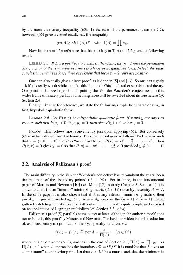
228 CHAPTER III. MAJORIZATION
by the more elementary inequality (65). In the case of the permanent (example 2.2),however, (66) gives a trivial result, viz. the inequality
perA ≥ n!(Π(A))1n with Π(A) =
∏aik.
Now let us record for reference that the corollary to Theorem 2.2 gives the followingresult.
LEMMA 2.5. If A is a positive n×nmatrix, then fixing any n−2 rows the permanentas a function of the remaining two rows is a hyperbolic quadratic form. In fact, the sameconclusion remains in force if we only know that these n− 2 rows are positive.
One can also easily give a direct proof, as is done in [5] and [13]. So one can rightlyask if it is really worth while to make this detour via Gårding’s rather sophisticated theory.Our point is that we hope that, in putting the Van der Waerden’s conjecture into thiswider frame ultimately perhaps something more will be revealed about its true nature (cf.Section 2.4).
Finally, likewise for reference, we state the following simple fact characterizing, infact, hyperbolic quadratic forms.
LEMMA 2.6. Let P (x, y) be a hyperbolic quadratic form. If x and y are any twovectors such that P (x) > 0, P (x, y) = 0, then also P (y) < 0 unless y = 0.
PROOF. This follows most conveniently just upon applying (65). But conversely(65) can be obtained from the lemma. The direct proof goes as follows: Pick a basis suchthat x = (1, 0, . . . , 0) and P is “in normal form”, P (x) = x2
1 − x22 − · · · − x2
n. ThenP (x, y) = 0 gives y1 = 0 so that P (y) = −y2
2 − · · · − y2n < 0 provided y �= 0. '(
2.2. Analysis of Falikman’s proof
The main difficulty in the Van der Waerden’s conjecture has, throughout the years, beenthe treatment of the “boundary points” (A ∈ ∂Ω). For instance, in the fundamentalpaper of Marcus and Newman [10] (see Minc [12], notably Chapter 5, Section 1) it isshown that if A is an “interior” minimizing matrix (A ∈ Ω∗) then by necessity A = J .In the same paper it is also shown that if A is any interior” minimizing matrix, thenperAik = perA provided aik > 0, where Aik denotes the (n − 1) × (n − 1) matrixgotten by deleting the i-th row and k-th column. The proof is quite simple and is basedon an application of Lagrange multipliers (cf. Section 2.3, infra).
Falikman’s proof [5] parallels at the outset at least, although the author himself doesnot refer to it, this proof by Marcus and Newman. The basic new idea is the introductionof, as is customary in optimization theory, a penalty function, viz.
f(A) = fε(A) def= perA +ε
Π(A), (A ∈ Ω∗)
where ε is a parameter (> 0), and, as in the end of Section 2.1, Π(A) =∏
aik . AsΠ(A) → 0 when A approaches the boundary ∂Ω = Ω\Ω∗ it is manifest that f takes ona “minimum” at an interior point. Let thus A ∈ Ω∗ be a matrix such that the minimum is

2. Van der Waerden’s conjecture and hyperbolicity 229
assumed. Then using Lagrange multipliers, or by a direct computation, which everybodyfamiliar with the rudiment of calculus can do for himself,8 one finds
(68) pik −c
aik= λi + μk,
where λi and μk are the Lagrange multiplier, and where we have put pik = perAik,
c =ε
Π(A).
CLAIM 2.7. All the λi and all the μk are equal.
PROOF. If we multiply both members of (68) by aik and sum over k we get
(69) λi = b−∑
k
aikμk
with b = p− nc, p = perA =∑
k aikpik. Similarly, we find
(70) μk = b−∑
i
aikλi.
If we substitute the expression for μk as given by (70) into formula (69) we get a relationof the form λi =
∑j bijλj , where bij ≥ 0,
∑j bij = 1 =
∑i bij . It is easy to see that
λ1 = · · · = λn = λ. Similarly, we find μ1 = · · · = μn = μ. '(
REMARK 2.8. The argument (omitted!) leading to the above conclusion is but aspecial case of the Perron(-Frobenius) theorem on positive matrices. What is really goingon becomes somewhat more transparent if we use matrix notation. Then (69) and (70)can be written as λ = b1−Aμ and μ = b1−A∗λ respectively (remember that A1 = 1,since A is doubly stochastic), that is, λ = Bλ with B = AA∗ positive. This gives againλ = const · 1 (Perron’s theorem).
Note that from (69) and (70) now follows b = λ+μ. We have thus proved (see (68))that if A ∈ Ω∗ is a critical point for fε, ε arbitrary then
(71) pik = b +c
aik.
The final step in the proof can now be condensed in the following lemma.
LEMMA 2.9. Assume that A = (aik) ∈ Ω∗ with
(72) pikdef= perAik = φ(aik)
where the function φ is strictly decreasing or constant. Then by necessity A = J = ( 1n ).
This lemma is thus, in particular, applicable if (68) holds with c ≥ 0 (correspondingto ε ≥ 0).
8The “tangent space” of Ω (the “infinitesimal doubly stochastic matrices”) is generated by all matrices
containing a submatrix of the type1 −1
−1 1, all other entries being zero. This gives fik − fi� − fjk +
fj� = 0 (with fik = ∂f∂aik
), whence readily fik = λi + μk .

230 CHAPTER III. MAJORIZATION
PROOF. It suffices to prove that any two rows, say, x = x1 and y = x2 are equal:x = y. We consider the quadratic form P (x, y) = per(x, y, x3, . . . xn), which we knowis hyperbolic (Lemma 2.5). Then by (72)
xi def= P (x, ei) = φ(yi);
yi def= P (y, ei) = φ(xi),
where e1, . . . , en is the standard basis in Rn. Using a fancy language, the xi (yi) are the
contravariant coordinates of x (y) and P (x, y) =∑
xiyi =∑
xiyi. Set z
def= x − y.Then similarly
zi def= P (z, ei) = φ(yi)− φ(xi).Assuming first that φ is strictly decreasing, we draw from this the important conclusionthat
zi ≥ 0 =⇒ zi > 0.Thus, in particular, P (z) ≥ 0. Furthermore, since x and y are rows of a doubly stochasticmatrix we have
∑xi =
∑yi = 1, whence
∑zi = 0. It follows that we cannot have
zi ≥ 0 for all i. Therefore we can find a positive vector c such that∑
cizi = 0 or
P (c, z) = 0. Also P (c, c) = 0. But this plainly contradicts the hyperbolicity (seeLemma 2.6). The case π constant is even simpler. Now zi = 0 for all i, which contradictsalready the fact that P is a non-degenerate quadratic form. '(
REMARK 2.10. To make the above argument work it obviously just suffices to knowthat the remaining rows (i.e. x2, . . . xn) are positive but not by necessity x1 and x2.
So now we know that if A ∈ Ω∗ is any minimizing element for fε (ε ≥ 0) thenA = J . In particular, thus
perA +ε
Π(A)≥ per J +
ε
Π(A).
Passing to the limit (ε→ 0) we get perA ≥ perJ for A ∈ Ω∗ and by continuity also forA ∈ Ω.
We have established
THEOREM 2.11. perA ≥ per J for any A ∈ Ω.
2.3. Comments on Egorychev’s proofUsing Falikman’s proof and result (Theorem 2.11) we can somewhat simplify Ego-
rychev’s proof to the effect that A = J is the only minimizing element in Ω. In particular,we can eliminate all the partial result on which it depends (London’s theorem [9] etc.; cf.[13]). We are thus out for the proof of
THEOREM 2.12. If A ∈ Ω and perA = per J then A = J .
PROOF. We do this in several steps.The idea is to prove directly that for a minimiz-ing matrix A ∈ Ω we must have pik = p (according to (71), with ε = 0). First we verifythat this is indeed sufficient.
Step 1. If we have a minimizing matrix A ∈ Ω with pik = p it is easy to reproduceanother one, A′, say, with the same property, having one row, x = x1, say in common

2. Van der Waerden’s conjecture and hyperbolicity 231
withA and all other rows positive. (This is achieved by successively forming mean valuesof rows; for details see [13].) We see that x = ( 1
n ). Since this row was an arbitrary rowwe infer that A = J = ( 1
n ).Step 2. It suffices to prove that pik ≥ p. For assume that A ∈ Ω is a minimizing
matrix with this property. Then if x and y are any two rows of A inequality (66) gives
p2 = P (x, y)2 ≥ P (x)P (y) =∑
xixi∑
yiyi ≥
∑xip ·
∑yip = p2.
(Here we use the notation of the Lemma 2.9.) Thus we are in the case of equality for thatinequality (but since we do not know yet that P is (strictly) hyperbolic we cannot, at thisstage, conclude that x = y), and it is plain that indeed pik = p must hold.
Step 3. Next we conclude that a minimizing matrix, at any rate, must be fully in-decomposable (cf. [12]). Indeed, assume that, contrariwise, A is decomposable, which,A being doubly stochastic, just means that the matrix after suitable permutations of therows and columns can be put in the form A′ ⊕ A′′, where A′ is an r × r matrix, and A′′
an (n− r) × (n− r) matrix, with 0 < r < n. Then Theorem 2.11 gives
n!nn
= perA = perA′ · perA′′ ≥ r!rr· (n− r)!(n− r)n−r
or (n
r
)(nr
)r(1− n
r
)n−r ≥ 1.
But this contradicts the elementary inequality(n
r
)xr(1− x)n−r < 1 if 0 < r < n, 0 < x < 1.
Step 4. Now we are (in principle) in a position to carry out the details of the proofof the theorem of Marcus and Newman [10] already referred to at the beginning of Sec-tion 2.2: pik = p if aik > 0. We add additional constraints of the form aik = 0, one foreach zero matrix element, and proceed exactly as in Section 2.2. Since we know that Ais fully indecomposable the conclusion of Perron’s theorem is still applicable.
Step 5. There remains only one more step – London’s theorem [9] (see [12], Chap-ter 5, p. 85-86) to the effect that without the restriction pik ≥ p for a minimizing matrixon has A ∈ Ω. The proof is based on the inequality
(73)n∑
s=1
piσ(s) ≥ p,
valid for any permutation σ. (Proof by a straightforward variational argument. Considerthe “deformation” (1 − θ)A + θP , 0 < θ < 1, of A, where P is the permutation matrixcorresponding to σ. Remember that Ω is a convex set!) Having (73) at our disposalit suffices to remark that, A being fully indecomposable (see Step 3), for any i and kwe can find a permutation σ such that σ(i) = k and aσ(s) > 0 if s �= i, provingaik > 0. This again is essentially the Frobenius-König theorem ([12, Chapter 3, seenotably Theorem 2.2, p. 31 and Theorem 35, p. 38.]) '(

232 CHAPTER III. MAJORIZATION
2.4. Open questions4a. Having uncovered the role of hyperbolicicity in the Van der Waerden’s conjecturethere arises the question whether the conjecture perhaps is a special case of somethingmore general. Here is, tentatively, a “non-commutative” version of the Van der Waerden’s“conjecture”: to minimize the complete polarization PerA (“hyperpermanent”) of thehyperbolic polynomial P (x1, . . . , xn) = n! detx1 . . . detxn, where each entry xi is asymmetric, say, ν × ν matrix (see Example 2.3), under the side conditions
∑k aik =
1 =∑
i aik, aik being the “matrix elements” of A, each of them thus in turn a positivedefinite (aik ≥ 0) matrix. Analogous problem with Hermitian matrices (Section 2.1,Example 2.3BIS).
4b. In view of all the trouble one has had with the (non-existent!) minimizing boundarymatrices one is tempted to ask if there is perhaps a more quantitative result than just themere statement that the are no minimizing points on the boundary. In other words, whatcan be said about inf
A∈∂ΩperA?
4c. The more general conjecture of Marcus and Minc [11] (cf. [12], p. 91) to the effectthat
perA ≥ pernJ −A
n− 1, A ∈ ∂Ω,
is still unsettled [in 1981]. The latter is also meaningful in the context of Subsection 4b,ultra (that is, for “hyperpermanents”).
References
[1] A. D. Aleksandrov. Zur Theorie der gemischten Volumina von konvexen Körpern IV: Die gemischtenDiskriminanten und die gemischten Volumina. Mat. Sbornik 3 (2), 1938, 227–249. Russian with Germansummary.
[2] E. F. Beckenbach and R. Bellman. Inequalities. Ergebnisse der Mathematik und ihrer Grenzgebiete, 30.Springer-Verlag, Berlin, Göttingen, Heidelberg, 1961.
[3] S.-S. Chern. Integral formulas for hypersurfaces in Euclidean space and their appplication to uniquenesstheorems. Indiana Univ. Math. J. 8, 1959, 947–966.
[4] G. P. Egorychev. The solution of van der Waerden’s problem for permanents. Advances in Math. 42,1981, 299–305.
[5] D. I. Falikman. Proof of van der Waerden’s hypothesis on the permanent of doubly stochastic matrices.Mat. Zametki 19, 1981, 931–938, 957.
[6] L. Gårding. An inequality for hyperbolic polynomials. J. Math. Mech. 8 (6), 1959, 957–966.[7] L. Gårding. Linear hyperbolic partial differential equations with constant coefficients. Acta Math. 85,
1951, 1–62.[8] L. Hörmander. Linear partial differential operators. (Grundlehren 116.) Springer-Verlag, Berlin, Göttin-
gen, Heidelberg, 1963.[9] D. London. Some notes on the van der Waerden conjecture. Linear Algebra and Appl. 4, 1971, 155-160.[10] M. Marcus and M. Newman. On the minimum of the permanent of a doubly stochastic matrix. Duke
Math. J. 26, 1959, 61–72.[11] M. Marcus and H. Minc. On a conjecture of B.L. van der Waerden. Proc. Cambridge Philos. Soc. 63,
1967, 305–309.[12] H. Minc. Permanents. In: Encyclopedia of Mathematicss and its applications, 6. Addison-Wesley, London
etc., 1978.[13] J. H. van Lint. Notes on Egorychev’s proof of the van der Waerden’s conjecture. Linear Algebra and
Appl. 39, 1981, 1–8.
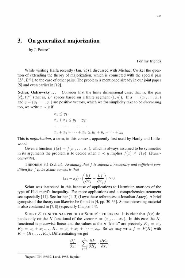
233
3. On generalized majorizationby J. Peetre 9
For my friends
While visiting Haifa recently (Jan. 85) I discussed with Michael Cwikel the ques-tion of extending the theory of majorization, which is connected with the special pair(L1, L∞), to the case of other pairs. The problem is mentioned already in our joint paper[5] and even earlier in [12].
Schur, Ostrowsky . . . Consider first the finite dimensional case, that is, the pair(�1n, �
∞n ) (that is, Lp spaces based on a finite segment (1, n)). If x = (x1, . . . , xn)
and y = (y1, . . . , yn) are positive vectors, which we for simplicity take to be decreasingtoo, we write x ≺ y if
x1 ≤ y1;x1 + x2 ≤ y1 + y2;. . . . . . . . . . . . . . . . . . .
x1 + x2 + · · ·+ xn ≤ y1 + y2 + · · ·+ yn.
This is majorization, a term, in this context, apparently first used by Hardy and Little-wood.
Given a function f(x) = f(x1, . . . , xn), which is always assumed to be symmetricin its arguments the problem is to decide when x ≺ y implies f(x) ≤ f(y) (Schur-convexity).
THEOREM 3.1 (Schur). Assuming that f is smooth a necessary and sufficient con-dition for f to be Schur convex is that
(xi − xj) ·(
∂f
∂xi− ∂f
∂xj
)≥ 0.
Schur was interested in this because of applications to Hermitian matrices of thetype of Hadamard’s inequality. For more applications and a comprehensive treatmentsee especially [11]. See further [1–3] (I owe these references to Jonathan Arazy). A briefsynopsis of the theory can likewise be found in [4, pp. 30-33]. Some interesting materialis also contained in [7, 8] (especially Chapter 14),
SHORT K -FUNCTIONAL PROOF OF SCHUR’S THEOREM. It is clear that f(x) de-pends only on the K-functional of the vector x = (x1, . . . , xn). In this case the K-functional is piecewise linear and the values at the n “knots” are precisely K1 = x1,K2 = x1 + x2,. . . , Kn = x1 + x2 + · · · + xn. So we may write f = F (K) withK = (K1, . . . ,Kn). Differentiating we get
∂f
∂xi=
n∑j=1
∂F
∂Kj· ∂Kj
∂xi.
9Report LTH 1985:2, Lund, 1985. Reprint.

234 CHAPTER III. MAJORIZATION
But∂Kj
∂xi=
{1 if i ≥ j;0 otherwise.
Therefore we find∂f
∂xi− ∂f
∂xi+1=
∂F
∂Kj.
This clearly is the embryo of Schur’s condition. '(We won’t elaborate more on the details. Instead we shall look on some more general
cases, the point being that the argument just produced is quite general (Schur’s theorem isnot too deep!). Every time we have sufficiently exact information about the K-functionalthe same proof can be carried over.
The case (L2, L2(λ)). In this case it is convenient to use K2 in place of K . (In view of[10] this causes no essential change.)
(74) K22 (t, a) =
∞∫0
1
1 +1
(λt)2
|a(λ)|2 dλ.
Let f = F (K22 ). Then formally (variational or Volterra derivatives)
δf
δa(λ)=
∞∫0
δF
δK22 (t, a)
· δK22 (t, a)
δa(λ)dt.
But by (74) [for a positive]
δK22 (t, a)
δa(λ)=
2a(λ)
1 +1
(λt)2
.
Thus substituting
δf
δa(λ)=
∞∫0
δF
δK22 (t, a)
· 2a(λ)
1 +1
(λt)2
dt.
Now if F is monotone in K2 thenδF
δK22
≥ 0. Thus the integral is of the form∫dμ(λ)
1 +1
(λt)2
.
with a positive measure μ, thus represents a Loewner (or Pick) function.
THEOREM 3.2. f is K-monotone if and only if
1a(λ)
· δf
δa(λ)is a Loewner function in λ.
EXAMPLE 3.1. Let f be quadratic, f =∫(a(λ))2(w(λ))2 dλ, w a (positive) weight.
Our condition for K-monotonicity then becomes the classical one of (w(λ))2 being aLoewner function.
3. On generalized majorization 235
REMARK 3.3. The above points also to that there might be a sort of “generalizedLoewner theory”. As is well-known (for Loewner theory, see e.g. [6], cf. [13]) Loewnerwas concerned with the issue of “monotone operator functions”. For which (scalar) func-tions ϕ, is it true that A ≥ B in operator sense (A and B being s.a. operators in a Hibertspace H) implies ϕ(A) ≥ ϕ(B)? Given a function Φ = Φ(x,A) of two variables(x ∈ H , A a s.a. operator in H) we may instead consider the more general inequalityΦ(x,A) ≥ Φ(x,B). Thus Φ(x,A) = (ϕ(A)x, x) will correspond to the classical case.
The case (Lp, Lp(λ), 1 ≤ p ≤ ∞. Nothing essential happens if we pass to the case ofgeneral p. The condition formally becomes that
(a(λ))p−1 ·Φ(x,A)
should admit an analogous integral representation with the (convolution) kernel1
1 + t2
replaced by1
(1 + t−q)1q
, where1p
+1q
= 1. (Compare again [13].)
The limiting case p = 1 is noteworthy. Then we have the kernel min(1, t) and by
Sparr’s lemma [14] (see once more [13]) this is the same as to say thatδf
δa(λ)has to be
a concave function of λ (observation by M. Cwikel).
The case (Lp, Lq), p �= q. The case of different exponents is slightly more rewarding10.We further find it convenient to use the L-functional now. Recall that
L(t, a;Lp, Lq) =
∞∫0
L(t, a(λ); R,R) dλ.
If f = F (L) we have
δf
δa(λ)=
∞∫0
δF
δL(t, a)· δL(t, a)
δa(λ)dt.
Therefore we will end up with a condition involving the kernel
δL(t, a(λ); R,R)δa(λ)
.
REMARK 3.4. The “scalar” L-functional L(t, a) = L(t, a(λ; R,R) has been inves-
tigated in [9] but not much seems to be known about the derivativeδL(t, a)
δa.
Conclusion. The drawback of all this is that we have no applications at all, whereasin the primitive Schur case concrete applications (see especially [11]). Challenge to theReader: find some!
References
[1] P. Alberti and A. Uhlmann. Dissipative motion in state spaces. Teubner-Texte zur Mathematik, 33. Teub-ner, Leipzig, 1981.
10Because of the Stein-Weiss trick [15] the weight can always be removed.

236 CHAPTER III. MAJORIZATION
[2] P. Alberti and A. Uhlmann. Stochasticity and partial order: doubly stochastic maps and unitary mixing.Mathematical monographs, 18. Deutscher Verlag der Wissenschaften, Berlin, 1981.
[3] T. Ando, Computationally secure information flow. Hokkaido University, Sapporo, 1982.[4] E. F. Beckenbach and R. Bellman. Inequalities. Ergebnisse der Mathematik, 30. Springer Verlag,
Berlin, Göttingen, Heidelberg, 1961.[5] M. Cwikel and J. Peetre. Abstract K and J spaces. Abstract K and J spaces 60, 1981, 1–50.[6] W. Donoghue. Monotone matrix functions and analytic continuation. Die Grundlehren der mathematis-
chen Wissenschaften, 207. Springer Verlag, New York, Heidelberg, 1974.[7] R. Farell. Multivariate calculation. Springer Series in statistics. Springer Verlag, New York, Heidel-
berg, Tokyo, 1985.[8] I. Gohberg and M. Krein. Introduction to the theory of linear non-selfadjoint operators. Nauka, Moscow,
1965. English translation: Am. Math. Soc., Providence, 1988.[9] M. Gustavsson and J. Peetre. Properties of the L function. Audia Math. 74, 1982, 106–121.[10] T. Holmstedt and J. Peetre. On certain functionals arising in the theory of interpolation. Func. Anal. 4,
1969, 88–94.[11] A. Marshall and I. Olkin. Inequalities: Theory of Majorization and Its Applications. Academic Press,
New York, 1979.[12] J. Peetre. On the connection between the theory of interpolation spaces and approximation theory. In:
Proc. Conf. on Constructive Theory of Functions. Akadémiai Kiado, Budapest, 1969, 351–363.[13] J. Peetre. On Apslund’s averaging method – the interpolation (function) way. In: Proc. Int. Conf. on Con-
structive Theory of Functions. Bulgarian Acad. Sci., Sofia, 1984, 664–671.[14] G. Sparr. Interpolation of weighted Lp spaces. Studia Math. 62, 1978, 229–271.[15] E. Stein and G. Weiss. Interpolation of operators with change of measure. Trans. Am. Math. Soc. 87,
1958, 159–172.

CHAPTER IV
Combinatorics

This page intentionally left blank

239
1. [K88a] On Stirling and Lah numbers
Given a finite set S, |S| = n, let us consider the set of all possible functions f : S →X , |X | = x. Each such function f gives a certain equivalence relation Ker f , the kernelof f . Conversely, each equivalence relation π serves as the kernel of a function f : S →X , and the number of functions with a given kernel π equals to decreasing subfactorial(x)n(π), where n(π) is the number of blocks of the partition on S corresponding to theequivalency π.1 Let Π(n) be the lattice of all equivalencies on S. We have the equation
(75)∑
n∈Π(n)
(x)n(π) = x(n).
As (75) is true for infinitely many natural numbers x, it is the equality of two polynomialsin Q[x]. Based on (75) and using methods of linear algebra, G.-C. Rota derived ([7], in
1964) a series of properties of the numbers Bndef= |Π(n)|, which, in particular, showed
that Bn is the n-th Bell number [2]; for details about this see [4].In the Proceedings of the All Union Seminar on Combinatorial Analysis (Moscow
University, Jan. 1980), the author suggested a similar approach also to Stirling and Lahnumbers; cf. further [1]. In part, this was realized (for the derivation of the basic prop-erties of the Stirling numbers of the second kind) in [2], and, more completely, in [4],where one considers from this point of view (but, this time, involving a suitable orderrelation on the blocks of a partition of S) also Stirling numbers of the first kind. So farthe author knows the papers [6] and [3], showing that the line of thought indicated de-serves much attention. Here we give a new combinatorial foundation for some identitiesfor Stirling and Lah numbers 2 illustrating the synthesis of the ideas of Pólya and Rotajust mentioned.
The polynomials pu(x) def= (x)u, u = 0, 1, 2, . . . form a basis of the vector spaceof polynomials Q[x], and so the formula Lk(pu(x)) = δu,k, k = 0, 1, 2, . . . definesuniquely a sequence of linear functionals Lk : Q[x] → Q, k = 0, 1, 2, . . . . Next, weobtain from (75) for the numbers
(76) S(n, k) def= |{p ∈ Π(n)|n(π) = k}|
the “strange”definition
(77) S(n, k) =∑
p∈Π(n)|n(π)=k}1 = Lk(xn).
On the basis of (77) all fundamental relations for the Stirling numbers of the second kindS(n, k) were derived in [4]. There it was also shown that the same approach works for a
1Translator’s Note. Quite generally, (x)n = x(x − 1) . . . (x − (n − 1)) for any integer n.2Translator’s Note. These numbers were, apparently, introduced by Lah in [5], noted in [2].
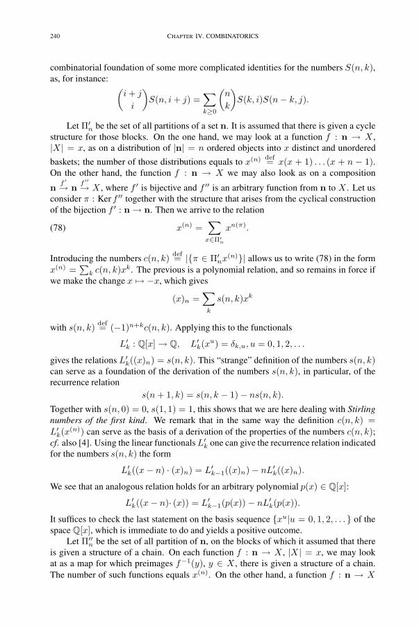
240 CHAPTER IV. COMBINATORICS
combinatorial foundation of some more complicated identities for the numbers S(n, k),as, for instance: (
i + j
i
)S(n, i + j) =
∑k≥0
(n
k
)S(k, i)S(n− k, j).
Let Π′n be the set of all partitions of a set n. It is assumed that there is given a cycle
structure for those blocks. On the one hand, we may look at a function f : n → X ,|X | = x, as on a distribution of |n| = n ordered objects into x distinct and unordered
baskets; the number of those distributions equals to x(n) def= x(x + 1) . . . (x + n − 1).On the other hand, the function f : n → X we may also look as on a composition
nf ′→ n
f ′′→ X , where f ′ is bijective and f ′′ is an arbitrary function from n to X . Let us
consider π : Ker f ′′ together with the structure that arises from the cyclical constructionof the bijection f ′ : n→ n. Then we arrive to the relation
(78) x(n) =∑
x∈Π′n
xn(π).
Introducing the numbers c(n, k) def= |{π ∈ Π′nx
(n)}| allows us to write (78) in the formx(n) =
∑k c(n, k)xk. The previous is a polynomial relation, and so remains in force if
we make the change x �→ −x, which gives
(x)n =∑
k
s(n, k)xk
with s(n, k) def= (−1)n+kc(n, k). Applying this to the functionals
L′k : Q[x]→ Q, L′
k(xu) = δk,u, u = 0, 1, 2, . . .
gives the relations L′k((x)n) = s(n, k). This “strange” definition of the numbers s(n, k)
can serve as a foundation of the derivation of the numbers s(n, k), in particular, of therecurrence relation
s(n + 1, k) = s(n, k − 1)− ns(n, k).
Together with s(n, 0) = 0, s(1, 1) = 1, this shows that we are here dealing with Stirlingnumbers of the first kind. We remark that in the same way the definition c(n, k) =L′
k(x(n)) can serve as the basis of a derivation of the properties of the numbers c(n, k);cf. also [4]. Using the linear functionalsL′
k one can give the recurrence relation indicatedfor the numbers s(n, k) the form
L′k((x − n) · (x)n) = L′
k−1((x)n)− nL′k((x)n).
We see that an analogous relation holds for an arbitrary polynomial p(x) ∈ Q[x]:
L′k((x− n)· (x)) = L′
k−1(p(x)) − nL′k(p(x)).
It suffices to check the last statement on the basis sequence {xu|u = 0, 1, 2, . . .} of thespace Q[x], which is immediate to do and yields a positive outcome.
Let Π′′n be the set of all partition of n, on the blocks of which it assumed that there
is given a structure of a chain. On each function f : n → X , |X | = x, we may lookat as a map for which preimages f−1(y), y ∈ X , there is given a structure of a chain.The number of such functions equals x(n). On the other hand, a function f : n → X
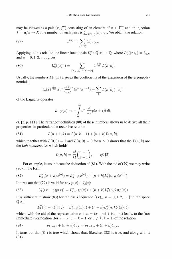
1. On Stirling and Lah numbers 241
may be viewed as a pair (π, f ′′) consisting of an element of π ∈ Π′′n and an injection
f ′′ : n/π → X ; the number of such pairs is∑
π∈Π′′n(x)n(π). We obtain the relation
(79) x(n) =∑
π∈Π′′n
(x)n(π).
Applying to this relation the linear functionals L′′k : Q[x] → Q, where L′′
k((x)u) = δu,k
and u = 0, 1, 2, . . . , gives
(80) L′′k((x)n) =
∑{π∈Π′′
n|n(π)=x}1 def= L(n, k).
Usually, the numbers L(n, k) arise as the coefficients of the expansion of the eigenpoly-nomials
�n(x) def= xex(dxdx
)n(e−xxn−1) =n∑k
L(n, k)(−x)n
of the Laguerre operator
L : p(x) �→ −∞∫0
e−t d
dxp(x + t)t dt;
cf. [2, p. 111]. The “strange” definition (80) of these numbers allows us to derive all theirproperties, in particular, the recursive relation
(81) L(n + 1, k) = L(n, k − 1) + (n + k)L(n, k),
which together with L(0, 0) = 1 and L(n, 0) = 0 for n > 0 shows that the L(n, k) arethe Lah numbers, for which holds
L(n, k) =n!k!
(n− 1k − 1
), cf. [2].
For example, let us indicate the deduction of (81). With the aid of (79) we may write(80) in the form
(82) L′′k((x + n)x(n)) = L′′
k−1(x(n)) + (n + k)L′′
k(n, k)(x(n))
It turns out that (79) is valid for any p(x) ∈ Q[x]:
(83) L′′k((x + n)p(x)) = L′′
k−1(p(x)) + (n + k)L′′k(n, k)(p(x))
It is sufficient to show (83) for the basis sequence {(x)u, u = 0, 1, 2, . . .} in the spaceQ[x]:
L′′k((x + n)(x)u) = L′′
k−1((x)u) + (n + k)L′′k(n, k)((x)u))
which, with the aid of the representation x + n = (x − u) + (n + u) leads, to the (notimmediate) verification (for u = k; u = k − 1; or u �= k, k − 1) of the relation
(84) δk,u+1 + (n + u)δu,k = δk−1,u + (n + k)δk,u.
It turns out that (84) is true which shows that, likewise, (82) is true, and along with it(81).

242 CHAPTER IV. COMBINATORICS
Perhaps it might be of some interest to carry over this approach to the case when oneconsiders on n partitions on which blocks one assume that there is given a completelyarbitrary structure.
References
[1] U. Kaljulaid. A remark on Stirling numbers. Sb. “Komb. Analiz” 6, 1983, 98. (see [K83b]).[2] M. Aigner. Combinatorial theory. Grudlagen der Mathematik, 234. Springer Verlag, Berlin, Heidel-
berg, New York, 1979.[3] S.-N. A. Joni, G.-C. Rota, and B. Sagan. From sets to functions: three elementary examples. Discrete
Math. 37, 1981, 193–202.[4] U. Kaljulaid. Elements of discrete mathematics. Tartu University Press, Tartu, 1983. (see [K83c]).[5] I. Lah. Ein neue Art von Zahlen, ihre Eigenschaften und Anwendungen in der Mathemstischen Statistik.
Mitteilungsblatt Math. Stat. 7, 1955, 203–212.[6] G. Pólya. Partitions of a finite set into structures subsets. Math. Proc. Camb. Phil. Soc. 77, 1975, 453–458.[7] G.-C. Rota. The number of partitions of a set. Am. Math. Monthly 71, 1964, 498–504.
Remark. The references [5, 7] were added by translator.

243
2. Letter (or draft of letter) c. 1991 from Uno Kaljulaidto Torbjörn Tambour
Preamble (Note by Uno Kaljulaid to J. Peetre). This material and such a letter was sentto Professor Tambour in order to initiate anew our cooperation, which was interrupted in1991 by reasons known to you (and he in the beginning of his trip returned to Sweden).3
Dear Professor Tambour,
You asked me some details. Though chaotic, here they are!I would like to add to the remarks on p. 299 that, of course when
finding Ω(P,Fm) it seems to be important also [to invoke] the widthw(P ) of P and the fact that order preserving maps P → Fm mapchains “convexly” into chains of Fm.
So there does not seem to remain so many possibilities whenalso taking into account a Dilworth partition on P (into chains witha minimal number of such blocks).
Sincerely, Uno Kaljulaid
3Note by J. Peetre Gert Almkvist and Torbjörn Tambour were supposed to visit Tartu in the summer of1991. However, in Moscow Tambour was attacked by a robber, so he decided to cancel his trip, and returnedhome.

This page intentionally left blank
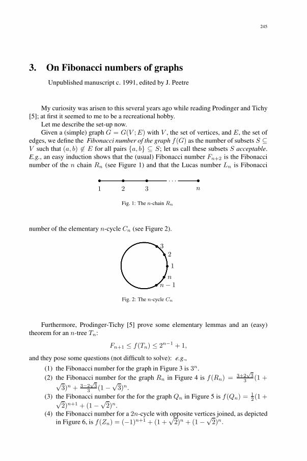
245
3. On Fibonacci numbers of graphsUnpublished manuscript c. 1991, edited by J. Peetre
My curiosity was arisen to this several years ago while reading Prodinger and Tichy[5]; at first it seemed to me to be a recreational hobby.
Let me describe the set-up now.Given a (simple) graph G = G(V ;E) with V , the set of vertices, and E, the set of
edges, we define the Fibonacci number of the graph f(G) as the number of subsets S ⊆V such that (a, b) �∈ E for all pairs {a, b} ⊆ S; let us call these subsets S acceptable.E.g., an easy induction shows that the (usual) Fibonacci number Fn+2 is the Fibonaccinumber of the n chain Rn (see Figure 1) and that the Lucas number Ln is Fibonacci
• • • . . . •1 2 3 n
Fig. 1: The n-chain Rn
number of the elementary n-cycle Cn (see Figure 2).
• 1
• 2• 3
• n− 1• n
Fig. 2: The n-cycle Cn
Furthermore, Prodinger-Tichy [5] prove some elementary lemmas and an (easy)theorem for an n-tree Tn:
Fn+1 ≤ f(Tn) ≤ 2n−1 + 1,
and they pose some questions (not difficult to solve): e.g.,
(1) the Fibonacci number for the graph in Figure 3 is 3n.(2) the Fibonacci number for the graph Rn in Figure 4 is f(Rn) = 3+2
√3
3 (1 +√3)n + 3−2
√3
3 (1 −√
3)n.(3) the Fibonacci number for the for the graph Qn in Figure 5 is f(Qn) = 1
2 (1 +√2)n+1 + (1−
√2)n.
(4) the Fibonacci number for a 2n-cycle with opposite vertices joined, as depictedin Figure 6, is f(Zn) = (−1)n+1 + (1 +
√2)n + (1−
√2)n.

246 CHAPTER IV. COMBINATORICS
n + 1 n + 2 n + 3 n + 4 2n• • • • . . . • •
• • • • . . . • •1 2 3 4 n
Fig. 3: The forest of “dipoles”
n + 1 n + 2 n + 3 n + 4 2n• • • • . . . • •
• • • • . . . • •1 2 3 4 n
Fig. 4: The The graph Rn
n + 1 n + 2 n + 3 n + 4 2n• • • • . . . • •
• • • • . . . • •1 2 3 4 n
Fig. 5: The The graph Qn
��������������
����
����
����
��
0
12
2n− 1
Fig. 6: The The graph Zn
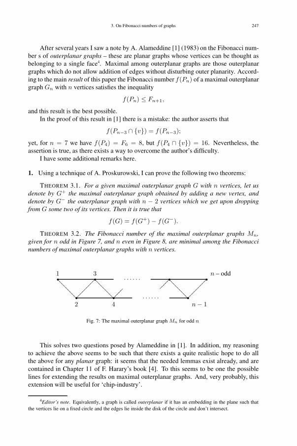
3. On Fibonacci numbers of graphs 247
After several years I saw a note by A. Alameddine [1] (1983) on the Fibonacci num-ber s of outerplanar graphs – these are planar graphs whose vertices can be thought asbelonging to a single face4. Maximal among outerplanar graphs are those outerplanargraphs which do not allow addition of edges without disturbing outer planarity. Accord-ing to the main result of this paper the Fibonacci number f(Pn) of a maximal outerplanargraph Gn with n vertices satisfies the inequality
f(Pn) ≤ Fn+1,
and this result is the best possible.In the proof of this result in [1] there is a mistake: the author asserts that
f(Pn−3 ∩ {v}) = f(Pn−3);
yet, for n = 7 we have f(P4) = F6 = 8, but f(P4 ∩ {v}) = 16. Nevertheless, theassertion is true, as there exists a way to overcome the author’s difficulty.
I have some additional remarks here.
1. Using a technique of A. Proskurowski, I can prove the following two theorems:
THEOREM 3.1. For a given maximal outerplanar graph G with n vertices, let usdenote by G+ the maximal outerplanar graph obtained by adding a new vertex, anddenote by G− the outerplanar graph with n − 2 vertices which we get upon droppingfrom G some two of its vertices. Then it is true that
f(G) = f(G+)− f(G−).
THEOREM 3.2. The Fibonacci number of the maximal outerplanar graphs Mn,given for n odd in Figure 7, and n even in Figure 8, are minimal among the Fibonaccinumbers of maximal outerplanar graphs with n vertices.
• •
• •
• •
•�����
�����
����
����
�
���������
����
����
�
����
����
�
���������· · · · · ·
· · · · · ·
1
2
3
4
n – odd
n− 1
Fig. 7: The maximal outerplanar graph Mn for odd n
This solves two questions posed by Alameddine in [1]. In addition, my reasoningto achieve the above seems to be such that there exists a quite realistic hope to do allthe above for any planar graph: it seems that the needed lemmas exist already, and arecontained in Chapter 11 of F. Harary’s book [4]. To this seems to be one the possiblelines for extending the results on maximal outerplanar graphs. And, very probably, thisextension will be useful for ‘chip-industry’.
4Editor’s note. Equivalently, a graph is called outerplanar if it has an embedding in the plane such thatthe vertices lie on a fixed circle and the edges lie inside the disk of the circle and don’t intersect.

248 CHAPTER IV. COMBINATORICS
• •
• •
• •
•�����
�����
����
����
�
���������
����
����
�
����
����
�
���������· · · · · ·
· · · · · ·
1
2
3
4 n – even
n− 1
Fig. 8: The maximal outerplanar graph Mn for even n
2. The equationf(Mn) = f(Mn−1) + f(Mn−3)
has the characteristic equation x3−x2−1 = 0. Setting x = y+ 13 we get y3− 1
3y− 2927 = 0
with the roots ⎧⎪⎪⎪⎨⎪⎪⎪⎩y1 = u + v;
y2 = −u + v
2+ i
u− v
2
√3;
y3 = −u + v
2− i
u− v
2
√3,
where
u =3
√2954
+
√31108
and v =3
√2954−
√31108
.
So we obtain the general solution
f(Mn) = axn1 + bxn
2 + cxn3 ,
where the approximate values of xi (i = 1, 2, 3) are⎧⎪⎨⎪⎩x1 = 1.465572;x2 = −0.232786 + i · 0.792551;x3 = −0.232786− i · 0.792551;
As|f(Mn)| ≤ |a||x1|n + |b||x2|n + |c||x3|n
and we have |x2| = |x3| < 1, then for n → ∞ we have |x2| = |x3| → 0, and so forlarge values of n we obtain
f(Mn−1)f(Mn)
≤ |x1| = 1.465572.
Experimenting a little with various n shows that the ratio f(Mn−1)f(Mn) tends to this value
1.465572 well enough even for small n:
n f(Mn) f(Mn+1)f(Mn)
3 44 6 1.56 13 1.4447 19 1.44615388 28 1.44756849 41 1.4464287

3. On Fibonacci numbers of graphs 249
EDITOR’S REMARK. As
Rn =f(Mn+1)f(Mn)
=axn+1
1 + bxn+12 + cxn+1
3
axn1 + bxn
2 + cxn3
= x1
a + b(x2x1
)n+1 + c(x3x1
)n+1
a + b(x2x1
)n + c(x32x1
)n,
we see that the sought ratio Rn, indeed, tend to x1 as n→∞. Likewise, it is easy to seethat we have
|Rn − x1| ≤ K(|x2|x1
)n+1
for suitable constant K and all n. '(Note also that here the technique used by Pólya for solving recurrences appearing in
connection with the enumeration of trees can be applied (when suitably extended) – andthis seems to be an interesting reasoning here.
3. To sum up, all the above, probably, deserves to be written down, and to be criticallyanalyzed once more together – [this should be] interesting at least for people concerningwith graphs and chips-technology.
I finish with some chaotic thoughts on these matters.First note that for mathematics the most interesting things seems to begin to appear,
yet, when we pose questions analogous to the graph-theoretic ones above for a finite posetP . For such a P it is natural to define the Fibonacci number P as the number of all anti-chains in P . Let ζP be the zeta-function for the order relation in P ; that is, ζP (x, y) = 1if and only if x ≥ y in P . So f(P ) equals the number of all k × k zero-submatrices inthe matrix ‖ζP (x, y)‖; here x, y ∈ P (listing P ) and k takes all values in {1, 2, . . . , |P |}.The role of antichains when investigating the structure of poset is, of course, well-known;e.g., the maximal size of antichains in P as the width of P , Dilwoorth’s theorem, . . . . I
have several observations here. To be more concrete I shall describe two of them here.
4. When considering order preserving maps ϕ : P → P it seems natural to considerthe kernel of ϕ, π = Kerϕ. And then to define x ≤ y on P / = P Kerϕ if and only ifthere exist x′, x′ π∼ x, and y′, y′
π∼ y such that x′ ≤ y′ holds in P . This is a consistentdefinition as in the case if x < y then for any pair (x′′, y′′) with different componentsx′′, x′′ π∼x, and y′′, y′′
π∼y such that x′ ≤ y′ if these components are comparable thenwe must have x′′ < y′′. Note also that for a (finite) poset P , taking π ∈ Π(P ) such thatthat all π-classes are connected (as subsets of P ), we can define x ≤ y in P/π by therule: x ≤ y if and only if there exist x′ ∼ x and y′ ∼ y such that x′ ≤ y′ in P . Call suchan π an acceptable equivalence. It follows from R. Stanley’s results that all acceptableequivalences form an Eulerian sublattice in Π(P ). Returning to the main point, observethat for any order preserving map ϕ : P → P there exists a natural ◦-epimorphismψ : P → P , π(x) = x, x ∈ P , and so the usual “◦-diagram” appears:
P
ϕ %%�����
����
Ψ – epi �� �� P/Kerϕ = P
ε – iso&&� � � � �
Imϕ ≤ P
Now, the finding of the number Ω(P, P ) of all order preserving maps P → Preduces to the enumeration of acceptable equivalences on P and of ◦-automorphismsof P/π for acceptable π. This seems to have some point of contact with the Sands

250 CHAPTER IV. COMBINATORICS
conjecture, that I shall describe below. More generally, for any order preserving mapϕ : P → Q it holds
ζP (x, y) = 1 =⇒ ζP (ϕ(x), ϕ(y)) = 1for x ≥ y in P .
5. As above, denote by Ω(P,m) the number of order preserving maps Ω → m. Stanleyhas observed that Ω(P,m) = Z(Z(P ),m), with Z(Q,n) denoting the number of mul-tichains y1 ≤ y2 ≤ · · · ≤ yn in Q, and this n-expression is called the zeta-polynomialof the poset Q. Ω(P,m) is called the order-polynomial of P and can be thought of as anm-polynomial of degree |P |. Stanley [6, Theorem 4.5.14], gives the following intriguingformula ∑
m≥0
Ω(P,m) = (∑
π∈L(P )
λ1+d(π))(1 − λ)−p+1,
where L(P ) denotes the Jordan-Hölder set for P . My question is now: What will happento this theory of Stanley if we take Fm (a fence (zigzag): {1, 2, . . . .m} with the only in-equations 1 > 2, 2 < 3, 3 > 4, . . . ,m− 1 < m) instead of the cochain m? Other posetsP , instead of m, may be of interest also. Yet, Fm is interesting in relation to the paperCurrie-Visentin [2]. In this respect, at least the Ω(P,Fm) should deserve an attention.In [2] the generating function of Ω(Fm,Fm) is introduced. According a conjecture ofB. Sands the number Ω(P, P ) is minimal for P = Fm. Let us further mention the paperDuffus-Rödl-Sands-Woodrow [3], although we have not seen it so far.
Here we can make the conjecture that
Ω(P, P ) ≥ Ω(P,Fm) ≥ Ω(Fm,Fm),
for any poset P , |P | = m. It seems that the outerplanar graphs Mn here somehowcorrespond to the “bichromatic” Jordan-Hölder sets for Fm, and so the role of f(Mn)was, presumably, not just an accident? This expectation is supported by the observationthat for any poset P its order polynomial depends only on its graph of comparabilityG(P ), with (x, y) ∈ E(G) if and only if x < y or y < x. Also, Ω(m,Fm), Ω(Fm,m),Ω(Fm,Fm) and |Aut(Fm)| are interesting, and so are the Eulerian (sec,tan)-numbers. . .
References
[1] A. F. Alameddine. Centers of maximal planar graphs with two vertices of degree three. J. Combin. Inform.System Sci. 8, 1983, 90–96.
[2] J. D. Currie and T. I. Visentin. The number of order-preserving maps of fences and crowns. Order 8, 1991,133–142.
[3] D. Duffus, V. Rödl, B. Sands, and R. Woodrow. Enumeration of order preserving maps. Order 9, 1992,15–29.
[4] F. Harary. Graph theory. Addison-Wesley, Reading, MA, 1969. Russian translation: Mir, 1973.[5] H. Prodinger and R. Tichy. Fibonacci numbers of graphs. Fibonacci Quarterly, 9, 1982, 16–21.[6] R. Stanley. Enumerative combinatorics I. The Wadsworth & Brooks/Cole Mathematics Series. Wadsworth
& Brooks/Cole Advanced Books & Software, Monterey, CA, 1986.

CHAPTER V
History of Mathematics

This page intentionally left blank
253
1. Th. Molien, an innovator of algebraUnpublished manuscript, c. 1985, translation from Estonian by J. Peetre
The life of Fedor Eduardovich Molin (1861-1941) was somewhat unusual.He was born in Riga and in 1883 received the scientific degree of a candidatein astronomy from the University of Dorpat/Tartu. In 1883-1885 he workedin Leipzig in the seminar of Felix Klein, on whose advice Molin began toresearch linear transformations of elliptic functions. When he returned tohis alma mater, Molin was appointed a docent and during the following sixyears made contributions that earned him his place in the history of algebra.In 1892 he published his paper “On systems of higher complex numbers”.In modern language, in that paper by analogy with the notion of a sim-ple group Molin defined simple algebras over the field of complex numbers,showed that they are algebras of matrices, and finally, discovered that thestudy of an arbitrary algebra over the field of complex numbers reduces tothe case when the quotient by the radical is a direct sum of matrix algebras.In the short articles that followed that memoir, Molin applied these resultsto representation theory of finite groups. His research had much in com-mon with works by Frobenius, Killing and Lie Lie, and immediately broughthim international acclaim and a gold medal from the Paris Academy of Sci-ences. Georg Frobenius in one of his letters to Molin said, in particular,that Molin “with one stroke completely solved the most important questionsin this field”. Unfortunately, neither Moscow nor St-Petersburg universitieshad any influential people capable of giving Molin’s papers their due, andafter receiving for them his doctorate degree, he had to take a full professorposition (called “ordinary professor”) in mathematics in the newly openedTomsk Technological Institute. There, the daily needs of organizing teaching,a library, and other tasks vital for an institution of higher education that wasnew and distant from the capital remove him for a long time from the streamof international mathematical life. In 1917 Molin was appointed a professorof mathematics in the department of physics and mathematics in the newlyopened Tomsk University. He became completely absorbed into organizingthis department, and published form time to time articles of a general math-ematical nature. For a long time, Tomsk had been the cultural capital ofSiberia, and the current flourishing of Siberian mathematics is partially dueto F.E. Molin.
Excerpt from A.I. Ma’lcev, To history of algebra in the USSR for the first 25 years, Algebrai Logika 10, 1971, 102–118 (Russian). English Translation: Algebra Logic , pp. 68–81.

254 CHAPTER V. HISTORY OF MATHEMATICS
According to [1] the picture of the early history of the theory of group representa-tions is perverted: the approach of Frobenius and Burnside is usually considered as fun-damental, although in reality the innovative work was done by the little known T. Molien.However, the wider mathematical and historical context of Molien’s results and their con-nection with problems of contemporary mathematics has been little studied [2].
125 years have elapsed since the birth (September 10, 1861) of Theodor Molien.He was born in a family of Swedish origin, which from northern Estonia had settled inRiga. His father [Eduard Molien] had graduated from Tartu University, was a teacher ata private gymnasium in Riga. T. Molien had received his basic education at the Gov-ernment Gymnasium at Riga. There were laid the foundations for his ability for studiesand his character, his intellectual interests and habits. At Tartu University Molien beganto prepare himself for a career as an astronomer. His aptness and diligence was noted,his scientific tastes and ability developed. He graduated at the university (1883) and wassent to Leipzig (1883–1885), which gave him modern and deep knowledge. There, inthe seminar of F. Klein, his scientific interests definitely turned to interior problems ofmathematics.
The future Docent at Tartu University (1885–1900) did not give up his connectionswith Leipzig (from 1886 on, the seminar was directed by Sophus Lie). Therefore, inthe study of systems of hypercomplex numbers, he got stimulation and help from theactivities which arose in Lie’s seminar from the results of Weierstrass and Dedekind onthis theme, and in particular from Poincaré’s remark that the expression of the multipli-cation of hypercomplex numbers gives a Lie group. As a result [3] the results of Molienobtained in 1887–92 began the structure theory of algebras [5].
The facts known to Molien that group algebras, in special cases already known to A.Cayley, constitute a bridge between representation theory and the theory of algebras, ledhim to fundamental notions and facts in the theory of group representations [4]. In thisway the “hypercomplex aspect” of the theory was born.
Let G be a finite subgroup in the group of all regular linear maps of the subspaceof the linear forms in the algebra of polynomials R = C[x1, . . . , xm]. The descrip-
tion of the homogeneous components RGn , the so-called subalgebra of invariants RG ={f ∈ R | ∀G ∈ G, fG = f} constitutes the central problem of the theory of invari-ants. This problem is equivalent to the determination of the formal series MG(t) =∑
n≥0(dimRGn )tn, the Molien series of G. The answer, an the explicit form of therational function MG(t), is provided by Molien’s formula:
MG(t) =1|G|
∑G∈G
1det(I − tG)
.
The so-called Polyá theory in combinatorics studies the numbers d(τ) ofG-schemes of agiven type, that is, the series LG(t) =
∑τ d(τ)tτ . The formula for LG(t), which is the
central part of Polyá theory, can be found in a similar way [6]. This example [6] does notlimit the connections of Molien’s results with problems of contemporary mathematics. Inparticular, a somewhat more general variant of Molien’s formula just considered admits

1. Th. Molien, an innovator of algebra 255
applications to the noncommutative theory of invariants. Apparently, this new interest inthe innovative papers [3, 4] of Molien is yet another confirmation of their lasting value.
References
[1] W. Gustafson. Review on S. Sehgal’s topics in group rings. Bull. Amer. Math. Soc. 1, 1979, 654–657.[2] N. F. Kanunov. Fedor Eduardovich Molien. Nauka, Moscow, 1983.[3] T. Molien. Über Systeme höherer komplexen Zahlen. Math. Ann. 41, 1893, 83–156.[4] T. Molien. Über die Invarianten der linearen Substitutionsgruppen. Sitzungsber. der Königl. Preuss. Akad.
d. Wiss. 52, 1897, 1152–1156.[5] R. S. Pierce. Associative algebras. Graduate Texts in Mathematics, 88. Springer-Verlag, New York, Berlin,
1982. Russian translation: Mir, Moscow, 1986.[6] R. Stanley. Invariants of finite groups and their applications to combinatorics. Bull. Amer. Math. Soc. 1,
1979, 475–511.

This page intentionally left blank

257
2. [K87e] On the results of Molien about invariants offinite groups and their renaissance in contemporarymathematicsTranslation by J. Peetre
1. Molien’s papers [11] and [12] occupy an honorable place in the history of mathe-matics (cf. [1]). Nevertheless, it is written comparatively little on the wider historical-mathematical context of his classical results and their connection with the problems ofcontemporary mathematics [8, 15]. One of the reasons for this situation is a long-lastingcomplicated treatment of the interaction of different the results and the notions of thetheory of representations of finite groups and their group algebras, which arose after thepublication of the books [2] and [22]. These outstanding books indicated a landmarkin the algebraic literature and become the basic text-books for several generations ofmathematicians, still nowadays their impact is great. However, questions of the forma-tion history of these concepts and results are not illuminated sufficiently clearly cf. e.g.[13]). Apparently, this distortion of history was caused by the underestimation the con-tribution of S. Lie and other mathematicians taking part in the Leipzig seminars (in thesecond half of the 1880’s) and thinking the same way, as well as by neglecting the worksMolien and É. Cartan that were written in the old-fashioned language of the Pierce idem-potents (1871). The latter happened after the brilliant presentation and generalization ofthe Molien-Cartan theory by Wedderburn (1907) and especially after the appearance of[14]. This is clearly seen in the history of group algebras, to which the second part ofour paper is devoted. Only E. Noether was considered the founder of the theory of groupalgebras. Nowadays, more and more people refer to the role of A. Cayley in the genesisof the notion of group algebra, and as regarding to the theory of group algebras – of T.Molien, cf. [5, 8, 16].
In particular W. Gustafson writes in [5]: “Most people familiar with the early historyof the theory of representations of finite groups in C, think immediately of Frobeniusand Burnside, who used approaches that seem unsuitable and even bizarre in the lightof modern treatments. Admittedly Frobenius’ group determinant and Burnside’s Lie-theoretic approach both yielded the basic properties of complex characters. However,they said much less about the representations themselves. For this reason they havelittle application to the important problems of finding properties of representations overother rings[: representations over fields of finite characteristic and over rings of algebraicintegers have very important applications in group theory, algebraic number theory andtopology. Hence, a more flexible approach was needed.] In fact, the groundwork hasbeen done by the little known Estonian mathematician Theodor Molien.” Let us add tothis the words of H. Weyl: “The matter is closely connected with hypercomplex numbersystems or algebras. After Hamilton’s foundation of quaternion calculus (1843), and along period of more or less formal research in which R. Pierce is played the major role,Molien (1892) was really the first who reached several general and profound results in
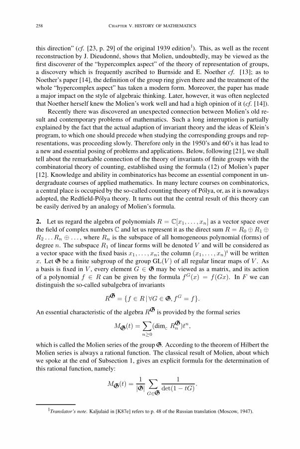
258 CHAPTER V. HISTORY OF MATHEMATICS
this direction” (cf. [23, p. 29] of the original 1939 edition1). This, as well as the recentreconstruction by J. Dieudonné, shows that Molien, undoubtedly, may be viewed as thefirst discoverer of the “hypercomplex aspect” of the theory of representation of groups,a discovery which is frequently ascribed to Burnside and E. Noether cf. [13]; as toNoether’s paper [14], the definition of the group ring given there and the treatment of thewhole “hypercomplex aspect” has taken a modern form. Moreover, the paper has madea major impact on the style of algebraic thinking. Later, however, it was often neglectedthat Noether herself knew the Molien’s work well and had a high opinion of it (cf. [14]).
Recently there was discovered an unexpected connection between Molien’s old re-sult and contemporary problems of mathematics. Such a long interruption is partiallyexplained by the fact that the actual adaption of invariant theory and the ideas of Klein’sprogram, to which one should precede when studying the corresponding groups and rep-resentations, was proceeding slowly. Therefore only in the 1950’s and 60’s it has lead toa new and essential posing of problems and applications. Below, following [21], we shalltell about the remarkable connection of the theory of invariants of finite groups with thecombinatorial theory of counting, established using the formula (12) of Molien’s paper[12]. Knowledge and ability in combinatorics has become an essential component in un-dergraduate courses of applied mathematics. In many lecture courses on combinatorics,a central place is occupied by the so-called counting theory of Pólya, or, as it is nowadaysadopted, the Redfield-Pólya theory. It turns out that the central result of this theory canbe easily derived by an analogy of Molien’s formula.
2. Let us regard the algebra of polynomials R = C[x1, . . . , xn] as a vector space overthe field of complex numbers C and let us represent it as the direct sum R = R0 ⊕R1 ⊕R2 . . . Rn ⊕ . . . , where Rn is the subspace of all homogeneous polynomial (forms) ofdegree n. The subspace R1 of linear forms will be denoted V and will be considered asa vector space with the fixed basis x1, . . . , xn; the column (x1, . . . , xn)t will be writtenx. Let G be a finite subgroup of the group GL(V ) of all regular linear maps of V . Asa basis is fixed in V , every element G ∈ G may be viewed as a matrix, and its actionof a polynomial f ∈ R can be given by the formula fG(x) = f(Gx). In F we candistinguish the so-called subalgebra of invariants
RG = {f ∈ R | ∀G ∈ G, fG = f}.
An essential characteristic of the algebra RG is provided by the formal series
MG(t) =∑n≥0
(dimCRGn )tn,
which is called the Molien series of the groupG. According to the theorem of Hilbert theMolien series is always a rational function. The classical result of Molien, about whichwe spoke at the end of Subsection 1, gives an explicit formula for the determination ofthis rational function, namely:
MG(t) =1|G|
∑G∈G
1det(1 − tG)
.
1Translator’s note. Kaljulaid in [K87e] refers to p. 48 of the Russian translation (Moscow, 1947).
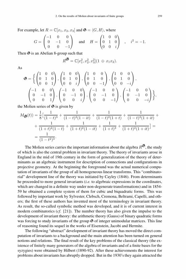
259
For example, let R = C[x1, x2, x3] and G = 〈G,H〉, where
G =
⎛⎝−1 0 00 −1 00 0 −1
⎞⎠ and H =
⎛⎝1 0 00 1 00 0 i
⎞⎠ , i2 = −1.
Then G is an Abelian 8-group such that
RG = C[x21, x
22, x
23](1 ⊕ x1x2).
As
G ={⎛⎝1 0 0
0 1 00 0 1
⎞⎠ ,
⎛⎝1 0 00 1 00 0 i
⎞⎠ ,
⎛⎝1 0 00 1 00 0 −1
⎞⎠ ,
⎛⎝1 0 00 1 00 0 −i
⎞⎠ ,
⎛⎝−1 0 00 −1 00 0 1
⎞⎠ ,
⎛⎝−1 0 00 −1 00 0 i
⎞⎠ ,
⎛⎝−1 0 00 −1 00 0 −1
⎞⎠ ,
⎛⎝−1 0 00 −1 00 0 −i
⎞⎠},
the Molien series of G is given by
MG(t)) =18[ 1(1 − t)3
+1
(1 − t)2(1− it)+
1(1− t)2(1 + t)
+1
(1 − t)2(1 + it)+
+1
(1 + t)2(1− t)+
1(1 + t)2(1− it)
+1
(1 + t)3+
1(1 + t)2(1 + it)
]=
=1
(1 − t2)3.
The Molien series carries the important information about the algebra RG, the studyof which is also the central problem in invariant theory. The theory of invariants arose inEngland in the mid of 19th century in the form of generalization of the theory of deter-minants as an algebraic instrument for description of connections and configurations inprojective geometry. At the beginning the foreground was the actual numerical compu-tation of invariants of the group of all homogeneous linear transforms. This “combinato-rial” development line of the theory was initiated by Cayley (1846). From determinantshe proceeded to more general invariants (i.e. to algebraic expressions in the coordinates,which are changed in a definite way under non-degenerate transformations) and in 1854-59 he obtained a complete system of them for cubic and biquadratic forms. This wasfollowed by important work by Sylvester, Clebsch, Cremona, Beltrami, Capelli, and oth-ers; the first of these authors has invented most of the terminology in invariant theory.As result, the so-called symbolic method was developed, and it is of current interest inmodern combinatorics (cf. [21]). The number theory has also given the impulse to thedevelopment of invariant theory: the arithmetic theory (Gauss) of binary quadratic formswas forcing to study invariants of the group G of integer unimodular matrices. This lineof reasoning found its sequel in the works of Eisenstein, Jacobi and Hermite.
The following “abstract” development of invariant theory has moved the direct com-putation of invariants to a background and the main attention has been turned on generalnotions and relations. The final result of the key problems of the classical theory (the ex-istence of finitely many generators of the algebra of invariants and of a finite bases for thesyzygies) were obtained by Hilbert (1890-92). After these achievements the interest forproblems about invariants has abruptly dropped. But in the 1930’s they again attracted the
2. On the results of Molien about invariants of finite groups

260 CHAPTER V. HISTORY OF MATHEMATICS
interest due to developments in physics. At the same time the general formulation of theproblem of invariants has been originated in the way as it was set forth at the beginningof this section and which provides the basis for reduction of the problem of invariants toa special case of the general problems of representations theory. Above we mentionedthe underestimate role of S. Lie’s approach in the development of representation theoryof groups. We may add to this that the theory of invariants has been productively unifiedwith Lie’s infinitesimal methods by E. Study. Today his results have become the sourceof ideas that support the development of concrete differential equations for the invariants.This fact as long as the increased interest to this relation from the side of contemporaryDiscrete Mathematics shows that this approach did not exhaust all the possibilities.
3. The most interesting applications of the ideas and results in Molien’s paper [12] tookplace in the past decade [the 1970’s]. Let us now familiarize ourselves with a generaliza-tion of Molien’s formula, that lead to surprisingly wide range of applications in contem-porary combinatorics. To this end let us consider the decompositionV = V1⊕+ · · ·⊕Vn,where Vi is the homogeneous subspace in V spanned by the basis element xi. LetG ≤ GL(V ) be a finite subgroup such that for each element G ∈ G there exists a permu-tation πG ∈ Sm with the property that G(Vi) = VπG , i = 1, . . . ,m. In this situation wesay thatG is a monomial group and it consists of monomial matrices having on each of itsrows precisely one element different from zero. If, for some G ∈ G, C = {i1, . . . it} is acycle in the permutation πG, then {i1, . . . it} ⊆m and π(ik) = ik+1 for 1 ≤ k ≤ t− 1,while π(it) = i1. In view of the monomiality of G there exist numbers α1, . . . , αt ∈ Csuch that G(xik
) = αkxik+1 for 1 ≤ k ≤ t− 1 for 1 ≤ k ≤ t− 1 and G(xit) = αtxi1 ;denote by γG(C) the product α1α2 . . . αt.
The type of a monomialxn11 . . . xnm
m is the sequence τ = (τ1, τ2, . . . ), where τi is thenumber of indices nj equal to i, i.e. τi = |{nj |nj = 1}|. Let Rτ be the subspace of theC-algebra R spanned by all monomials of type τ . As the type does not change under theaction of a monomial matrix G ∈ G, we have G(Rτ ) = Rτ . If we set RGτ = RG ∩Rτ ,
then the representation RG =∐
RGτ grades RG as a C-space; let us, however, note thatRGτ · RGσ is not always contained in some RGμ . Molien’s formula suggests a path forfinding the generating function of (infinitely many) variables t = (t1, t2, . . . )
LG(t) =∑
τ
(dimCRGτ )tτ =
1|G|
∑G∈G
∏C
(1 + γG(c)t|C|1 + γG(c)2t|C|
2 + . . . ),
where tτ = tτ1tτ2 . . . and C runs through all cycles of the permutations πG. For example,
for the monomial group
G ={⎛⎝1 0 0
0 1 00 0 1
⎞⎠ ,
⎛⎝−1 0 00 −1 00 0 −1
⎞⎠ ,
⎛⎝0 0 10 1 01 0 0
⎞⎠ ,
⎛⎝ 0 0 −10 −1 0−1 0 0
⎞⎠}

261
we obtain
LG(t) =14[(1 + t1 + t2 + t3 + . . . )3 + (1− t1 + t2 − t3 + . . . )3 +
(1 + t1 + t2 + t3 + . . . )(1 + t21 + t22 + t23 + . . . ) +
(1 − t1 + t2 − t3 + . . . )(1 + t21 + t22 + t23 + . . . )] =
= 1 +∞∑
k=1
t2k +∞∑
k=1
t2k +∞∑
k,�=1
t2kt2� .
4. The results on invariants of finite groups, to which the interest again arose in the1950’s, admit various important applications in contemporary mathematics. It is espe-cially noteworthy that the general theorem of Pólya that plays such an eminent role incombinatorics, is a special case of the generalization of Molien’s formula described inSubsection 3. Apparently, firstly this was noticed by Stanley [21]. Let us now describebriefly the ideas that led to the so-called Pólya theory. It has its origin in Cayley’s paper(1875) on counting of carbo-hydrides. However, the method proposed turned out to beimpractical and so chemists did not pay much attention to it. Nevertheless, in the follow-ing 30 years many have showed interest to that technique, but on the mathematical levelthere was still no progress; for a survey of these attempts see [7]. The remarkable pa-per [18] was written by Redfield (1927). This paper remained unknown for a long time,although it contained many ideas and results that were later (1934–37) rediscovered byG. Pólya. Partially the neglecting of [18] was caused by its discouraging terminology anda hard penetrable presentation. Pólya’s work was likewise preceded by the paper [10],where the author promotes the idea of the usefulness of the terminology and techniqueof group representations for the counting of isomers. Let us note an interesting fact thatone of cornerstones of the theory is called everywhere the “theorem or lemma of Burn-side”, although according to [13] it was known to Cauchy and Frobenius long before theappearance of the book [2].
The work of Pólya and in particular his final paper [17] became a landmark in count-ing theory because of its influence on the subsequent development. The Redfield-Pólyatheory results and its generalizations compose nowadays an important chapter of mod-ern combinatorics. The above mentioned connection between this theory and Molien’sformula can be briefly described as follows.
Let us consider the case wfere the monomial group G consists of permutation ma-trices. Then each element G ∈ G induces a substitution on the set F of all functionsf : m → N satisfying the condition (Gf)(i) = f(πG(i)). If we now identify the
function f using the monomial xf = xf(1)1 x
f(2)2 . . . x
f(m)m , then the action of G on the
C-algebra R satisfies the relation
G(xf ) = XG−1f , where G−1f(i) = f(πG−1(i)).
The action G on F gives a partitioning of the set F , its classes (so-called G-schemes)are the orbits of this action, i.e. we write f ∼ g, if for some G ∈ G holds g = Gf . Iff ∼ g then the multisets {f(1), . . . , f(m)} and {g(1), . . . , g(m)} and therefore xf andxg have the same type. One can speak of the type of G-schemes. The main problem ofthe counting theory of Pólya is to determine the number of G-schemes of a given typeτ . Consequently, denoting the sought number by d(τ), the counting theory problem can
2. On the results of Molien about invariants of finite groups

262 CHAPTER V. HISTORY OF MATHEMATICS
be thought of as a problem of finding the generating series LG(t) =∑
τ d(τ)tτ . Theanswer is given by theory of Pólya, which is obtained by specialization of the formulafor LG(t) given above by considering the special case
LG(t) =∑
τ
d(τ)tτ =
1|G|
∑G∈G
∏C
(1 + t|C|1 + t
|C|2 + t
|C|3 + . . . ),
where C runs through all cycles of the permutations πG.This example does not exhaust the connections of Molien’s formula with mod-
ern mathematics. In algebra, during the recent years there has been a great interestfor the non-commutative analogue of the situation considered in Subsection2. Thisamounts to studying the subalgebra of invariants RG of a finite group G in the algebraR = C[x1, . . . , xn] of polynomials of non-commutative variables xi. The correspondinggeneralization of Molien’s formula and its various applications are discussed in [4]. Theauthors of this paper developed the analogue of Molien’s formula for a non-commutativecompact topological group2 G and used it for solving subtle (discrete) algebraic prob-lems. Besides of the above-mentioned generalization of Molien’s formula finds the usein the theory of multi-partitions, in coding theory and other divisions, yielding a clearingup of the problems considered, and together with a single approach and simplification ofthe corresponding proofs and possibilities of generalizations. However, a more detailedanalysis of these problems requires, the attraction of new notions and results and so thissurpasses the bounds of the present publication. The interested Reader may acquainthim- or herself with the papers [4, 19, 20] that exhibit the importance of the paper [12]and an unprecedented value of Molien’s results. Our account is sufficient to see the un-foundedness of the pretty narrow appreciation of the scientific activity of T. Molien inthe country at the turn of the century, which forced him to leave Tartu, the town wherehe wrote his classical papers [11] and [12] in the theory of algebras and groups.
[9],[3],[4],[6]
References
[1] Nicolas Bourbaki. Éléments d’histoire des mathématiques. Masson, Paris, 1984. Russian translation:Gos. Izdat. Inostr. Lit., Moscow, 1963.
[2] W. Burnside. Theory of groups of finite order. University Press, Camnbridge, 1897.[3] A. Cayley. On the analytical forms called trees, with application to the theory of chemical combinations.
Rep. Brit. Assoc. Adv. Sci. 45, 1875, 257–305.[4] W. Dicks and E. Formanek. Poincaré series and a problem of S. Montgomery. Linear and Multilinear
Alg. 12, 1982, 21–30.[5] W. Gustafson. Review on S. Sehgal’s topics in group rings. Bull. Amer. Math. Soc. 1, 1979, 654–657.[6] T. Hawkins. Cayley’s counting problem and the representation of Lie algebras. In: Proc. of the Int.
Congress of Math., August 3–11, 1986. Amer. Math. Soc., Providence, RI, 1987, 1642–1656.[7] H. Henze and C. Blair. The number of isomeric hydrocarbons of the methan series. J. Amer. Chem. Soc.
53, 1931, 3077–3085.[8] N. F. Kanunov. Fedor Eduardovich Molien. Nauka, Moscow, 1983.
2In such groups, the formula is called the Molien-Weyl formula.
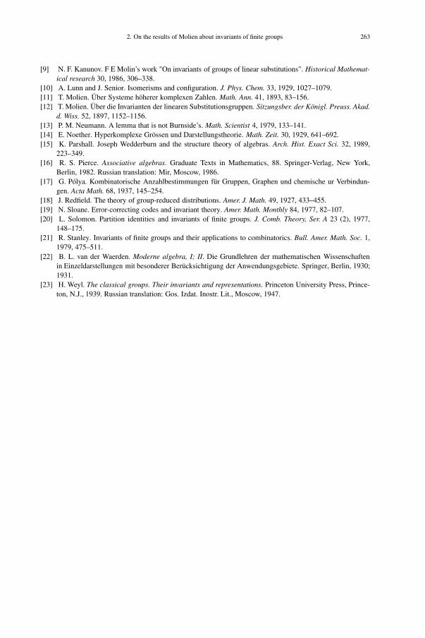
263
[9] N. F. Kanunov. F E Molin’s work "On invariants of groups of linear substitutions". Historical Mathemat-ical research 30, 1986, 306–338.
[10] A. Lunn and J. Senior. Isomerisms and configuration. J. Phys. Chem. 33, 1929, 1027–1079.[11] T. Molien. Über Systeme höherer komplexen Zahlen. Math. Ann. 41, 1893, 83–156.[12] T. Molien. Über die Invarianten der linearen Substitutionsgruppen. Sitzungsber. der Königl. Preuss. Akad.
d. Wiss. 52, 1897, 1152–1156.[13] P. M. Neumann. A lemma that is not Burnside’s. Math. Scientist 4, 1979, 133–141.[14] E. Noether. Hyperkomplexe Grössen und Darstellungstheorie. Math. Zeit. 30, 1929, 641–692.[15] K. Parshall. Joseph Wedderburn and the structure theory of algebras. Arch. Hist. Exact Sci. 32, 1989,
223–349.[16] R. S. Pierce. Associative algebras. Graduate Texts in Mathematics, 88. Springer-Verlag, New York,
Berlin, 1982. Russian translation: Mir, Moscow, 1986.[17] G. Pólya. Kombinatorische Anzahlbestimmungen für Gruppen, Graphen und chemische ur Verbindun-
gen. Acta Math. 68, 1937, 145–254.[18] J. Redfield. The theory of group-reduced distributions. Amer. J. Math. 49, 1927, 433–455.[19] N. Sloane. Error-correcting codes and invariant theory. Amer. Math. Monthly 84, 1977, 82–107.[20] L. Solomon. Partition identities and invariants of finite groups. J. Comb. Theory, Ser. A 23 (2), 1977,
148–175.[21] R. Stanley. Invariants of finite groups and their applications to combinatorics. Bull. Amer. Math. Soc. 1,
1979, 475–511.[22] B. L. van der Waerden. Moderne algebra, I; II. Die Grundlehren der mathematischen Wissenschaften
in Einzeldarstellungen mit besonderer Berücksichtigung der Anwendungsgebiete. Springer, Berlin, 1930;1931.
[23] H. Weyl. The classical groups. Their invariants and representations. Princeton University Press, Prince-ton, N.J., 1939. Russian translation: Gos. Izdat. Inostr. Lit., Moscow, 1947.
2. On the results of Molien about invariants of finite groups

This page intentionally left blank

265
3. Theodor Molien, about his life and mathematicalwork as seen a century later. (A biographical sketchand a glimpse of his work)Xerox3 copy of handwritten original [c. 1991], edited by J. Peetre, correctionsby A. Zubkov
Contents of the chapter1. A biographical sketch and a glimpse of his thesis . . . . . . . . . . . 2652. Molien’s 1897 papers on group rings and invariants . . . . . . . . .2693. Molien type formulae in Combinatorics . . . . . . . . . . . . . . . . . . . 2754. Noncommutative versions of Molien type formulae . . . . . . . . . 277References . . . . . . . . . . . . . . . . . . . . . . . . . . . . . . . . . . . . . . . . . . . . . . . .288
Science and art are the two sides of our life. Usually science is considering all that isdetermined by some laws, and so its development can be predicted. But what is history?
If we know the laws of processes we can predict them. But often there appears apoint in developing some idea where we have two or infinitely many choices – chaosappears. If we look behind – there were laws and predicability. But looking forwardwe see chaos. The historian cannot write the history of what has not happened. Thehistory of things that have not happened but might have happened – that is art. To goback to some point and try again in a new direction and with new connections in mind.Considered in such a way, the history of mathematical ideas, can, I believe, be a usefulthing for a mathematician. Something like this has happened with some of the ideas ofMolien.
3.1. A biographical sketch and a glimpse of his thesisTheodor Molien was born [in Riga] on September 10, 1861. His great-grandfather was
a Swede, who had settled near Reval/Tallinn in the 18th century, and was a teacher at thelocal school there.4 Molien’s grandfather (Andrei [Andrew]) was a watchmaker who hadsettled in Riga. His father, Eduard Molien, had got his education at Riga Gymnasium andafterwards at Dorpat/Tartu University, where he got a diploma as a teacher of classicallanguages in 1843. Then he worked as a private teacher in Riga.
Theodor Molien himself5 was a student at Riga Gymnasium in 1872–79; after his fa-ther’s death he wanted very much to support and please his mother, so he was very care-ful in his studies. All his family (himself, two sisters and their mother) moved to Tartuin 1880. There he became a student of mathematics, with the aim to prepare himselfas an astronomer – he was primarily influenced by the famous observatory and intense
3Editors’ Note. The symbol [GAP!] is used where a portion of the text has, regretfully, been lost in theprocess of Xeroxing.
4Editor’s Note. According to Kanunov [12, p.7], the great-grandfather, Johan Molien, moved to Livo-nia from Göteborg in Sweden in 1751. He came to live a small town near Reval/Tallinn. Kanunov says“mestechko”.
5Editor’s Note. His full name reads Theodor Georg Andreas.

266 CHAPTER V. HISTORY OF MATHEMATICS
scientific work in it from the days of W. Struve . He was a listener of P. Helmling (math-ematics), F. Minding (mechanics), A. Oettinger (physics) and P. Schwarz (astronomy).He was very much engaged by lectures and seminars by a young Swedish astronomerand mathematician Lindstedt. Anders Lindstedt was born in 1853, and after having gota doctor’s degree in astronomy from Lund, he served as an astronomer at the Tartu Ob-servatory since 1879. After the retirement of Minding, Lindstedt served as a Professorof applied mathematics at Tartu University (1883-86). He published works on celestialmechanics and integral calculus in the Memoirs of Petersburg Academy. His lectureswere new, original, and influential for students, and (what is important in our context,among them were algebra and algebraic geometry courses). What was absolutely newfor Tartu was his seminar for students with the object to support their scientific work.It was in this seminar where Molien got much encouragement and advice. As a resultMolien wrote and published two papers in astronomy and got his diploma [8,24]. AndersLindstedt was the first person to recognize Molien’s talent, and he insisted on Molien’sremaining at the University to prepare himself for the doctor’s degree. He also insistedthat Molien be given a stipend for continuation of his (then beginning) studies in puremathematics in Germany, namely for participation in the famous seminar of Felix Kleinin Leipzig. Under the influence of this seminar (from 1886 on it was directed by S. Lie)Molien’s astronomical interests were finally changed into pure mathematics. Molien re-mained in Leipzig for two years for writing there (under Klein) his master’s thesis onelliptic functions, which he presented in October 1885 in Tartu [26].6
For the next 15 years Molien was a docent in Dorpat (soon afterwards renamed Yur-jev’7) University, teaching on a huge variety of fields. Among them were new courses forTartu, e.g. on quaternions and other hypercomplex numbers, lectures on Gauss’s theoryof division of the circle etc. All this time Molien was keeping contact with the Leipzigseminar. And so it happened that he was among the very few who knew of W. Killing’swork on simple Lie algebras8 and, with E. Study and F. Engel, he considered Killing’stheory as a paradigm for his own investigations of hypercomplex numbers. His thesis ad-visor was Friedrich Schur, who had worked in Leipzig with S. Lie during the time whenKilling was working on the structure of semisimple Lie algebras. Using this paradigm,Molien succeeded in solving some problems (the corresponding paper in MathematischeAnnalen appeared in 1892 [28]). In September of same year he presented these results asa doctoral dissertation at Tartu. Molien’s results on hypercomplex numbers were quicklyesteemed by the experts: they were included in S. Lie’s monograph, and two years laterMolien got also the Ch. Hermite Gold Medal from the Paris Academy of Sciences.
Let us stop our story for a moment, and give a glimpse at some mathematical details.
6Editor’s Note. After his return to Sweden, Anders Lindstedt was a Professor of Mathematics and Theo-retical Mechanic at the Royal Institute of Technology (KTH), Stockholm, in 1886-1909 and also the Rector ofthis school 1902–1909. He had also several other assignments as a civil servant. He died in 1939.
7Translator’s Note. After the Christian name of the Kiev king Yaroslav the Wise who in 1030 during ashort campaign founded here a small town Yurjev, as indicated in a Russian chronicle. It was recaptured by theEstonians about 1060.
8Quite recently (Mathematical Intelligencer 11, no. 3, 1989) Killing’s papers in the “Mathematische An-nalen” were characterized by John Coleman as the greatest mathematical papers of all times – only the Elementaof Euclid, and Newton’s Principia he considers [to] have been more influential. Really, Wilhelm Killing haddiscovered the entire theory of simple Lie groups, i.e. what is now called Coxeter groups, Weyl groups, Dynkindiagrams . . . Slowly then, beginning [GAP!].

3. Th. Molien’s life and mathematical work 267
The successful experience in Number Theory of Gauss had, at least, two conse-quences. First, the theory of algebraic numbers was created (E. Kummer, L. Kronecker,R. Dedekind – to name only very few!). Second, there followed quaternions and bi-quaternions by W. Hamilton in 1837, and matrices by A. Cayley in 1855. Then (1884) J.Sylvester noticed the possibility
‖aij‖ =∑i,j
aijEij with Eij · Ek� = δijEi�.
There remains a little step to “n-ary numbers” and Dedekind’s extraction of the “hyper-complex aspect” of all these new tools. So there was opened a way to a general theoryof finite-dimensional associative algebras. Among the first general results: Karl Weier-strass proved the 3-dimensional numbers do not exist, i.e. that the non-existence of 3-dimensional R-algebras without zero divisors, and Frobenius’ theorem was proved. Forpeople connected with Lie’s seminar in Leipzig a turning point in the story was providedby the following remark by H. Poincaré (1884): multiplication of n-ary numbers,
(∑
xiei)(∑
yiei) =∑
ziei,
is given by equations
zi = ϕi(x1, . . . , xn; y1, . . . , yn)
that determine a Lie group. This observation was made by Scheffers, Study, etc., andtheir understanding related to W. Killing’s penetrating results and notions were taken byMolien as a paradigm for his investigation of associative C-algebras.
A finite dimensional algebra is said to be simple if it has no non-trivial two-sidedideals, and semisimple if its only nilpotent ideal (the radical) is zero; nilpotency of anideal means the existence of m ∈ N such that any product with ≥ m factors is 0. Ac-cording to Molien: every semisimple C-algebra is isomorphic to the direct sum of simpleC-algebras. Moreover, for every such simple componentSi there exists ni ∈ N such thatSi � Mni(C). Specializing these results to that case where the basis {e1, . . . , en} is agroup led Molien to many results on group representations. As pointed out by Hawkinsand Gustafson, Molien was the first to discover the “hypercomplex aspect” of this theory.Some details in this story deserve special attention – they are to be provided later.
Five years later one of several graduates of the prestigious École Normale Supér-ieure, encouraged by Picard, Darboux, Poincaré . . . , and having already made rigoroussense out of W. Killing’s (1888-1890) papers on semisimple Lie algebras (dissertation1894), entered into the story. Élie Cartan was the man who clarified the notions of rad-ical and of simple and semisimple algebras and further proved the uniqueness of thedecomposition; his corresponding report appeared in 1897. He considered also the R-case. To finish our story: in 1907, Joseph Wedderburn generalized the theory to any fieldk (instead C or R). In this general situation, the simple algebras are, as before, full matrixalgebras. Although, now not over k itself, but over a suitable division k-algebra. In thecase k = R there are three division k-algebras only: R, C and H – this fact is knownas Frobenius’ theorem. As Wedderburn returned to the Peirce approach via idempotentsand this approach culminated in E. Noether’s paper, the style of which became standardin algebra for a long time, Molien’s name fell into oblivion for at least 50 years. Thishas happened despite the fact that E. Noether herself highly respected both Molien’s andCartan’s contributions. Perhaps, one of the reasons was also that [GAP!].
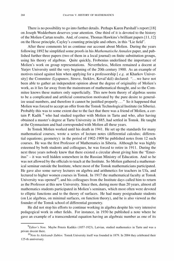
268 CHAPTER V. HISTORY OF MATHEMATICS
There is no possibility to go into further details. Perhaps Karen Parshall’s report [18]on Joseph Wedderburn deserves your attention. One third of it is devoted to the historyof the Molien-Cartan results. And, of course, Thomas Hawkins’s brilliant papers [11,12]on the Hesse principle, Cayley’s counting principle and others, in this “Lie field”.
After these comments let us continue our account about Molien. During the yearsfollowing 1892 he simplified some proofs in his Mathematische Annalen paper, and pub-lished further three papers (two of them in a local journal) on finite substitution groups,using his theory of algebras. Quite quickly, Frobenius underlined the importance ofMolien’s work on group representations. Nevertheless, Molien remained a docent atYurjev University until the very beginning of the 20th century 1900. As an example ofmotives raised against him when applying for a professorship [ e.g. at Kharkov Univer-sity] the Commitee (Lyapunov, Struve, Steklov, Koval’skiı) declared: “. . . we have notbeen able to gather an independent opinion about the degree of originality of Molien’swork, as it lies far away from the mainstream of mathematical thought, and so the Com-mitee knows these matters only superficially. This new-born theory of algebras seemsto be a complicated and artificial construction motivated by the pure desire to general-ize usual numbers, and therefore it cannot be justified properly . . . ” So it happened thatMolien was forced to accept an offer from the Tomsk Technological Institute (in Siberia).Probably this was to some extent due to the fact that there was a friend of Molien, a cer-tain P. Kadik 9 who had studied together with Molien in Tartu and who, after havingobtained a master’s degree at Tartu University in 1885, had settled in Tomsk. He taughtat the Gymnasium and had corresponded with Molien all these years.
In Tomsk Molien worked until his death in 1941. He set up the standards for manymathematical courses, wrote a series of lecture notes (differential calculus; differen-tial equations; geometry): in the period of 1902-1909 he published notes from 12 suchcourses. He was the first Professor of Mathematics in Siberia. Although he was highlyesteemed by both students and colleagues, he was forced to retire in 1911. During thenext three years nobody knew that there existed a circular about giving him the “Emer-itus” – it was well hidden somewhere in the Russian Ministry of Education. And so hewas not allowed by the officials to teach at the Institute. So Molien gathered a mathemat-ical seminar outside the Institute, where most of the Tomsk mathematicians participated.He gave also some survey lectures on algebra and arithmetics for teachers in Ufa, andlectured to higher women courses in Tomsk. In 1917 the mathematical faculty at TomskUniversity was opened10, and his colleagues from the Institute days called him to returnas the Professor at this new University. Since then, during more than 20 years, almost allmathematics students participated in Molien’s seminars, which most often were devotedto elliptic functions and to the theory of surfaces. He had many postgraduate students(on Lie algebras, on minimal surfaces, on function theory), and he is also viewed as thefounder of the Tomsk school of differential geometry.
He did not stop his efforts to continue working in algebra despite his very intensivepedagogical work in other fields. For instance, in 1930 he published a note where hegave an example of a transcendental equation having an algebraic number as one of its
9Editor’s Note. Maybe Peteris Kadikis (1857-1923), Latvian, studied mathematics in Tartu and was aprivate docent there.
10Note by Aleksandr Zubkov. Tomsk University itself was founded in 1879. In 2004 they celebrated their125-th anniversary.

3. Th. Molien’s life and mathematical work 269
roots but not all conjugates of this “algebraic” root are roots of the equation. In 1935he attempted to do some systematic work in the theory of algebras. In his last yearshe was very interested in hypergeometric series – he has an almost finished manuscriptgiving a systematic survey of the theory. There are also almost finished papers aboutGalois groups: there he wants to finds linear groups with [GAP!] a given Galois groupis contained [GAP!]. Furthermore, there are almost finished methodological notes onLobachevsky’s views in Geometry, Cremona transformations . . . There are lecture notes,e.g. notes on the theory of elliptic functions (from the time of the Klein-Lie seminars),
notes on the history of mathematics. There are reprints of Hurwitz, Dehn, Klein, Kneser,Kronecker, Minkowsky, Study, Frobenius, Schur, Engel and others. Letters from Hur-witz, Klein, A. Kneser, Frobenius, I. Schur, Struve. All these and other things of theMolien Archive were left by his daughter Eliza to her blind student V. D. Fatneva, aLatinist. What will be the further fate of this heritage?
In Siberia Molien has not been forgotten. In 1986, his bas-relief was put on thehouse in Nikitin Street where he had lived. Also his portraits hang at Tomsk University.The well-known Russian algebraist A. Mal’cev has designated Molien as the first profes-sor and the patriarch of Siberian mathematics in the pre-war period. Recently, ProfessorLeonid Bokut, the leader of a well-known ring theory-school in Siberia (Efim I. Zel-manov and A.R. Kemer were [among] his postgraduate students) visited Tartu, and hedeclared, in his talk, that Th. Molien should be considered as the first real classic in thefield of Algebra in the Russian Empire of that time.
Sources for further details: a booklet in Russian with comments on Molien’s disser-tation by Kanunov (a graduate from Tomsk University) [14] and, similarly a booklet withRussian translations of his main (1892 and 1897) papers [16].
3.2. Molien’s 1897 papers on group rings and invariantsTo get a 3-dimensional R-space with basis G = {x, y, z} we take all formal R-
combinationsαxx+αyy+αzz. Similarly if |G| > 3 and, instead of R, there is any fieldK , we get the space V (G,K) = {α | α =
∑g∈G αgg}. If G is a group, then its mul-
tiplication can be extended (distributively) to V (G,K). In this way we obtain the groupring KG. The elements of KG, i.e. the formal series sums
∑g∈G αgg can be interpreted
as mappings α : G → K with finite support, α(g) def= αg; their multiplication in KG iscalled convolution.
Quite often E. Noether is considered to be the only creator of group algebras. Nev-ertheless, A. Cayley (in 1854) dealt with the ring C[S3]. A look at Molien’s paper (1897)on invariants of substitution groups shows that some first fundamental results in this fieldare due to him. The genesis of the the notion of “group algebra” can be illustrated by thediagram in Figure 111. More is true: in 1895–97 Molien discovered (independently of G.Frobenius) the basic facts in group representation theory. He was formally motivated by
11Editor’s note. Part of this chart is missing in the Xerox version. We are, however, convinced that itmust be Euler that points to Hamilton; in 1770 he gave a parametrization of rotations in R3, which can beinterpreted in terms of quaternions. This has made some authors to view Euler as a forerunner of Hamilton:if a is a quaternion of unit length, one associates to it an orthogonal transformation given by x → a−1xa
(see e.g. [3, p. 3-4]). Another predecessor of Hamilton was C. F. Gauss. In posthumous work (cf. [10,especially p. 358]), he parameterized rotations with the aid of 4-tuplesx = (x0, x1, x2, x3) ∈ R4. If there aretwo rotations corresponding to x and y respectively, and z corresponds to their composition, he wrote down

270 CHAPTER V. HISTORY OF MATHEMATICS
Group algebras(Cayley, Molien, Noether)
Hypercomplex numbers(Dedekind, Peirce, Noether)
&&
������������������
Group RepresentationTheory
(Frobenius, Molien,I.Schur, Noether)
''
�������������
Vector spaces(Hamilton, Grassmann)
Lie Theory(Poincaré, Killing)
������������������
Algebraic numbers(Kummer, Kronecker, Dedekind)
((���������������������������
Matrix algebras
(Cayley, Sylvester)
))!!!!!!!!!!!!!!!!!!!!!!!!!
" " " " " " "Substitution groups
(Cauchy, Galois, Jordan)
��
��#############
Z[i](Gauss)
��
H(Hamilton)
��
Algebraic equations,Galois Theory
(Lagrange, Gauss, Abel, Galois)
��
Parametrization of rotations(Euler, Gauss)
��####################
$$$$$$$$$$$$$$$$$
Fig. 1: Genesis of the the notion “group algebra”
the problem of determining the representation of minimal degree for a group. This prob-lem had been suggested by F. Klein’s attempt to generalize Galois theory. The main stepin Molien’s approach can be well illustrated by having a look at the problem of studyinggroup determinants – the formal motivation for G. Frobenius.
Let G be a finite group, |G| = n, and let {xg|g ∈ G} be n independent variables(over C). Frobenius’ theory of representations of finite groups in its historical context
was concerned with factorization of the group determinant Dgdef= det ‖xh−1g‖, with
h, u ∈ G, viewed as a polynomial in C[xg|g ∈ G]. Take the field K = C(xg|g ∈ G) ofrational functions over C. The group algebra KG can be viewed as a K-space V with allelements of G as its basis. Right multiplication by an element XG =
∑g∈G xg on KG
gives an endomorphism of V with matrix ‖xh−1g‖:
h ∈ G �−→ h ·Xg = h ·∑g∈G
xgg =∑g∈G
xg(hg) =∑u∈G
xh−1uu,
where udef= hg �→ g = h−1u. We see that h �−→ h·Xg =
∑u∈G gxh−1uu, again is a K-
linear combination of all basis elements u ∈ G, so the matrix of this K-endomorphismis ‖xh−1u‖. As a result, the group determinant DG is interpreted as the determinant ofthe endomorphism of V , given by right multiplication by XG on KG. As charK = 0(N.B. K = C(xg|g ∈ G)), the group ring KG is known to be semisimple. Thereforeit is isomorphic as a K-algebra to the direct product of a full matrix algebra (over K =
the components of z in terms of the ones of x and y, which again corresponds to the multiplication of thecorresponding quaternions.

3. Th. Molien’s life and mathematical work 271
C(xg)):
(85) ψ = (ψ1, . . . , vs) : KGψ−→ Mn1(K)× · · · ×Mns(K)
Every element Y ∈ Mn(C) corresponds to an endomorphism of row spaces Cn → Cn,(z1, . . . , zn) �→ (z1, . . . , zn)Y . It follows that the endomorphism Mn(C) �→ Mn(C),given by right multiplication by Y on Mn(C), has the determinant (det Y )n. Indeed, asa right Mn(C)-module, Mn(C) is isomorphic to Cn ⊕ · · · ⊕ Cn︸ ︷︷ ︸
n
, and so right multipli-
cation by Y on Mn(C) can be viewed as an endomorphism Y of Cn⊕ · · ·⊕Cn with thematrix ⎛⎜⎜⎜⎜⎝
Y 0 · · · 00 Y · · · 0...
.... . .
...0 0 · · · Y
⎞⎟⎟⎟⎟⎠with the determinant (det Y )n. Using this result together with formula (85) we get thefollowing formula:
DG =(detψ1(XG))n1 · · · · · detψm(XG)
)ns.
It appears that this is the complete factorization of DG in C(xg) and so we have obtaineda solution to Frobenius’ question [9].
All that has been said above is true for any k instead of C. K. Johnson (1988) raisedthe question (in a combinatorial context) whether the group determinant determines thegroup G. It was proved recently by E. Formanek and D. Sibley [8] that is indeed true inthe nonmodular case, i.e. if chark � |G|. More precisely, they established the following.
THEOREM 3.1. If G and H are finite groups, char k � |G|, and ϕ : G → H is abijection (of them as sets!) such that ϕ(DH) = DH for f(xg) = xϕ(g), then G ∼= H asgroups.
Next, we are going to give some details about Molien’s formula, another remarkableresult in his 1897 paper [32].
Take the polynomial ring R = C[x1, . . . , xn] and, viewing it as an R-space, present
it in the form R =∞⊕
i=0Ri, where Ri is the subspace of all homogeneous polynomials
(forms) of degree i, i = 1, 2, . . . . The subspace V = R1 of linear forms has x1, . . . , xn
as its basis, thus is n-dimensional. Fix any finite subgroup G ≤ GL(V ) in the groupGL(V ) of all C-linear automorphisms of V . An action of G on R is induced by theformula
fA(x) def= f(xA), x = (x1, . . . , xn), A = ‖aij‖.This yields the subalgebra of G-invariants in R,
RG(x) def= {f ∈ R | ∀A ∈ G, fA = f},with the homogeneous components RGi = RG ∩ Ri. Substantial information about the
subalgebra RG is given by the formal series
MGdef=
∑i≥0
(dimC RGi )ti,

272 CHAPTER V. HISTORY OF MATHEMATICS
called its Hilbert-Poincaré series of RG, sometimes also its Molien series. Indeed, thisseries is a rational function in t, and Molien proved (1897) the following theorem.
THEOREM 3.2. Let R = C[x1, . . . , xn] and G ≤ Mn(C) as above, and let G ={A1, . . . , Ag} be all its elements. Then the generating function for the numbers dimC RGiof linearly C-independent i-forms is given by
(86) MG(t) =1g
g∑α=1
1det(I − tAα)
.
EXAMPLE 3.1. For
G = C2 ={(
1 00 1
),
(−1 00 −1
)}we have RG = C[x1, x2]G = C[x2
1, x22]⊕ x1x2C[x2
1, x22] and
MG(t) =12[ 1(1− t)2
+1
(1 + t)2]
=1 + t2
(1− t2)2.
EXAMPLE 3.2. R = C[x1, x2, x3] and G = 〈G,H〉 with G =
⎛⎝−1 0 00 −1 00 0 −1
⎞⎠and H =
⎛⎝1 1 00 1 00 1 i
⎞⎠, i2 = −1, we have that |G| = 8 and that G is Abelian,
G =
⎧⎨⎩⎛⎝1 0 0
0 1 00 0 1
⎞⎠ ,
⎛⎝1 1 00 1 00 0 i
⎞⎠ ,
⎛⎝1 0 00 1 00 0 −1
⎞⎠ ,
⎛⎝1 0 10 1 00 0 −i
⎞⎠ ,
⎛⎝−1 0 00 −1 00 0 1
⎞⎠ ,
⎛⎝−1 0 00 −1 00 0 i
⎞⎠ ,
⎛⎝−1 0 00 −1 00 0 −1
⎞⎠ ,
⎛⎝−1 0 00 −1 00 0 −i
⎞⎠⎫⎬⎭ .
and RG = C[x21, x
22, x
43](1⊕ x1x2). According to (86) we get (R. Stanley [??])
MG(t) =18
[1
(1− t)3+
1(1− t)2(1− it)
+
+1
(1− t)2(1 + t)+
1(1 − t)2(1 + it)
+
+1
(1− t)2(1− t)+
1(1 + t)2(1− it)
+
+1
(1 + t)3+
1(1 + t)3(1 + it)
]=
=1
(1− t2)3.
REMARK 3.3. Two nonisomorphic groups can have the same Molien series: e.g.the dihedral groupD4 and the Abelian group C2 × C4 have both the series
MD4(t) =1
(1− t)2(1 − t4)= MC2×C4(t).
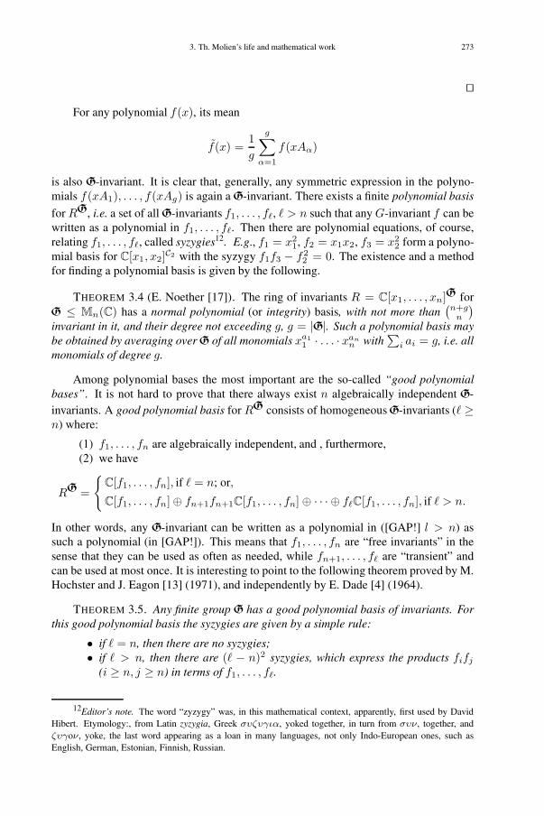
3. Th. Molien’s life and mathematical work 273
'(
For any polynomial f(x), its mean
f(x) =1g
g∑α=1
f(xAα)
is also G-invariant. It is clear that, generally, any symmetric expression in the polyno-mials f(xA1), . . . , f(xAg) is again a G-invariant. There exists a finite polynomial basis
for RG, i.e. a set of allG-invariants f1, . . . , f�, � > n such that any G-invariant f can bewritten as a polynomial in f1, . . . , f�. Then there are polynomial equations, of course,relating f1, . . . , f�, called syzygies12. E.g., f1 = x2
1, f2 = x1x2, f3 = x22 form a polyno-
mial basis for C[x1, x2]C2 with the syzygy f1f3 − f22 = 0. The existence and a method
for finding a polynomial basis is given by the following.
THEOREM 3.4 (E. Noether [17]). The ring of invariants R = C[x1, . . . , xn]G forG ≤ Mn(C) has a normal polynomial (or integrity) basis, with not more than
(n+g
n
)invariant in it, and their degree not exceeding g, g = |G|. Such a polynomial basis maybe obtained by averaging overG of all monomials xa1
1 · . . . · xann with
∑i ai = g, i.e. all
monomials of degree g.
Among polynomial bases the most important are the so-called “good polynomialbases”. It is not hard to prove that there always exist n algebraically independent G-invariants. A good polynomial basis for RG consists of homogeneousG-invariants (� ≥n) where:
(1) f1, . . . , fn are algebraically independent, and , furthermore,(2) we have
RG =
{C[f1, . . . , fn], if � = n; or,
C[f1, . . . , fn]⊕ fn+1fn+1C[f1, . . . , fn]⊕ · · · ⊕ f�C[f1, . . . , fn], if � > n.
In other words, any G-invariant can be written as a polynomial in ([GAP!] l > n) assuch a polynomial (in [GAP!]). This means that f1, . . . , fn are “free invariants” in thesense that they can be used as often as needed, while fn+1, . . . , f� are “transient” andcan be used at most once. It is interesting to point to the following theorem proved by M.Hochster and J. Eagon [13] (1971), and independently by E. Dade [4] (1964).
THEOREM 3.5. Any finite group G has a good polynomial basis of invariants. Forthis good polynomial basis the syzygies are given by a simple rule:
• if � = n, then there are no syzygies;• if � > n, then there are (� − n)2 syzygies, which express the products fifj
(i ≥ n, j ≥ n) in terms of f1, . . . , f�.
12Editor’s note. The word “zyzygy” was, in this mathematical context, apparently, first used by DavidHibert. Etymology:, from Latin zyzygia, Greek συζυγια, yoked together, in turn from συν, together, andζυγoν, yoke, the last word appearing as a loan in many languages, not only Indo-European ones, such asEnglish, German, Estonian, Finnish, Russian.
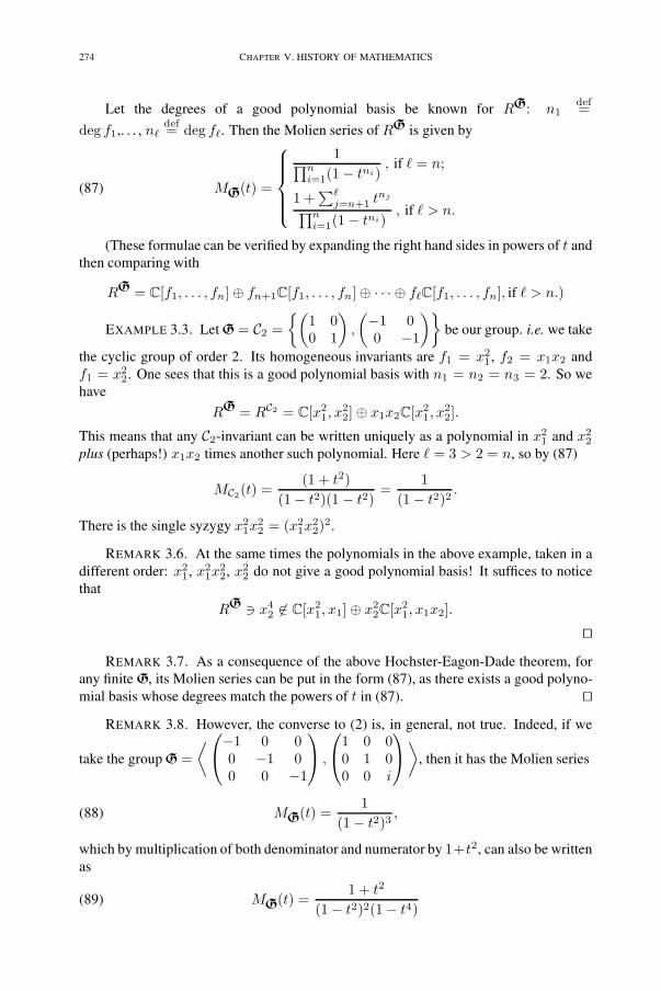
274 CHAPTER V. HISTORY OF MATHEMATICS
Let the degrees of a good polynomial basis be known for RG: n1def=
deg f1,. . . , n�def= deg f�. Then the Molien series of RG is given by
(87) MG(t) =
⎧⎪⎪⎪⎨⎪⎪⎪⎩1∏n
i=1(1 − tni), if � = n;
1 +∑�
j=n+1 tnj∏n
i=1(1− tni), if � > n.
(These formulae can be verified by expanding the right hand sides in powers of t andthen comparing with
RG = C[f1, . . . , fn]⊕ fn+1C[f1, . . . , fn]⊕ · · · ⊕ f�C[f1, . . . , fn], if � > n.)
EXAMPLE 3.3. LetG = C2 ={(
1 00 1
),
(−1 00 −1
)}be our group. i.e. we take
the cyclic group of order 2. Its homogeneous invariants are f1 = x21, f2 = x1x2 and
f1 = x22. One sees that this is a good polynomial basis with n1 = n2 = n3 = 2. So we
have
RG = RC2 = C[x21, x
22]⊕ x1x2C[x2
1, x22].
This means that any C2-invariant can be written uniquely as a polynomial in x21 and x2
2
plus (perhaps!) x1x2 times another such polynomial. Here � = 3 > 2 = n, so by (87)
MC2(t) =(1 + t2)
(1− t2)(1 − t2)=
1(1− t2)2
.
There is the single syzygy x21x
22 = (x2
1x22)
2.
REMARK 3.6. At the same times the polynomials in the above example, taken in adifferent order: x2
1, x21x
22, x2
2 do not give a good polynomial basis! It suffices to noticethat
RG + x42 �∈ C[x2
1, x1]⊕ x22C[x2
1, x1x2].
'(
REMARK 3.7. As a consequence of the above Hochster-Eagon-Dade theorem, forany finite G, its Molien series can be put in the form (87), as there exists a good polyno-mial basis whose degrees match the powers of t in (87). '(
REMARK 3.8. However, the converse to (2) is, in general, not true. Indeed, if we
take the group G =⟨⎛⎝−1 0 0
0 −1 00 0 −1
⎞⎠ ,
⎛⎝1 0 00 1 00 0 i
⎞⎠⟩, then it has the Molien series
(88) MG(t) =1
(1− t2)3,
which by multiplication of both denominator and numerator by 1+t2, can also be writtenas
(89) MG(t) =1 + t2
(1− t2)2(1− t4)

3. Th. Molien’s life and mathematical work 275
As seen above, there exits a good basis corresponding to MG(t) in form (88), whichgives us
C[x1, x2, x3]G = C[x21, x
22, x
43]⊕ x1x2C[x2
1, x22, x
43].
But not corresponding to the form (89). It is a question of N. J. Sloane (1977): to whichforms of MG(t) does there correspond good polynomial bases, and to which not? Thereare old results by Shephard-Todd (1954), but, in general, it seems to be open. '(
3.3. Molien type formulae in Combinatorics. 13
During the past decades this old theme has been combined with new ones, so in orderto gain greater coherence in understanding combinatorial and algebraic problems, I shallgive briefly three such results.
3.3.1. Let V = V1 ⊕ · · · ⊕ Vn, with all dim Vi = 1 and xi as basis vectors of Vi. LetG ≤ GL(V ) be such a finite subgroup that for every G ∈ G there exists a πG ∈ Sn withViG = VπG(i), i = 1, 2, . . . , n. In this case G is called a monomial group; it consistsof monomial matrices, i.e. of matrices such that every line contains exactly one non-zeroelement of C. For any cycle {C = (i1, . . . , it)} of πG we have {i1, . . . , it} ∈ n, π(ik) =ik+1 (if 1 ≥ k ≥ t− 1) and π(it) = i1. Monomiality of Gmeans that ∃α1, . . . , αt ∈ C,xG
ik= αkxik+1 (if 1 ≥ k ≥ t − 1) and xG
it= αtxi1 . Put γG(C) = α1 · . . . · αt. For
any monomial xa11 · . . . · xan
n let τ be its type, the sequence such that τ = (τ1, τ2, . . . )
with τidef= #{ak | ak = i}. Next, take the subspace Rτ of all monomials of type τ .
Then for any G ∈ G it is clear that RGτ = Rτ . Therefore setting RGτ ∩ Rτ , we see that
RG = ⊕τRGτ is a graduation of this C-space RG, and that the following Molien-type
formula is true:
PG(t) =∑
τ
(dimRGτ )tτ =1|G|
∑G∈G
∏C
(1 + γG(C)t|C|1 + γ2
G(C)t|C|2 + . . . ),
with C here covering all cycles of the substitution πG, and t = (t1, t2, . . . ) being indeterminants; |C| denotes the length of the cycle C, and [GAP!]. See Stanley [???].
3.3.2. In the special case of the monomial matrices being permutation matrices, everyelement G ∈ G induces a substitution on the set F of functions f : n → N by fG(i) =f(πG(i)). To every such function there corresponds the monomial xf = x
f(1)1 x
f(2)2 ·
. . . · xf(n)n , and so G acts on the C-algebra R = C[x1, . . . , xn] by the formula ∀ i ∈
n, (xf )G = xfG
, where fG(i) = f(πG(i)). The orbits under this action are calledG-schemes; they are given by the following equivalency on F :
f ∼ g ⇐⇒ ∃G, g = fG.
This means that the multisets {f(1), . . . , f(n)} and {g(1), . . . , g(n)} coincide; in par-ticular, the monoidals xf and xg have the same type. The main problem of the Redfield-Pólya theory can be described as the question to find the number d(τ) of G of a given
13See Tambour [23] for other finite lattices and their automorphism groups (homogeneous – [GAP!]degrees).

276 CHAPTER V. HISTORY OF MATHEMATICS
type τ . The answer is given by the following formula:
PG(t) =∑
τ
d(τ)tτ =1|G|
∑G∈G
∏C
(1 + t
|C|1 + t
|C|2 + . . .
),
where C runs over all cycles of πG.
3.3.3. Torbjörn Tambour also recently published a paper on this topic [23] (1989). Hisproblem is the following.
Let G be a finite group acting on a finite set S. It induces an action on Pk(S), theset of k-subsets of S:
{s1, . . . , sk}G = {πG(s1), . . . , πG(sk)}.
Denote by pk the number of G-orbits of this action. Tambour aims at finding∑
pktk.
[GAP!] generalize [GAP!] to other lattices.
PROBLEM. Finite vector spaces or equivalences of some others.A function-theoretic interpretation of this question is possible. First, we interpret
any k-subset n as the image Im f of a suitable injection f : k → n. The action of G onn induces an action of G on Pk(n) : f �→ fG with the rule, ∀ i ∈ k, fG(i) = πg(f(i)).It follows that if Im f = (Im f)πG , from which it again follows that Im f is a (disjoint)union of cycles of πG. The converse “if Im f is a union of cycles of πG” is obvious. Soit follows that
(90) 1 +∑k≥1
iGk tk =
∏C<πG
(1 + t|C|);
here iGG denotes the number of G-fixed points of (Pk(n),G); all possibilities of puttingtogether the various cycles of the substitutions must be taken account of. Forming thesum 1
|G|∑
G∈G in both sides of (90) and using the Cauchy-Frobenius lemma in the left
hand side, we get
1|G|
∑G∈G
(1 +∑k≥1
iGk tk) =
=1|G|
∑k≥1
∏C<πG
(1 + t|C|) =
=1|G|
∑G∈G
1 +∑k≥1
1|G|
⎛⎝ ∑G∈G
iGk
⎞⎠ tk =
= 1 +∑
pktk.
'(
(In the last step we used the Cauchy-Frobenius Lemma.)To see the similarity of this result with Molien’s formula Tambour interprets this
formula in the following way. Take V to be the C-space with basis S = n, and let VC be

3. Th. Molien’s life and mathematical work 277
its subspace with the cyclic basis C < πG. With this choice, πG/VChas the matrix
[G]C =
⎛⎜⎜⎜⎜⎝0 1 0 . . . 00 0 1 . . . 0· · · . . .0 0 0 . . . 11 0 0 . . . 0
⎞⎟⎟⎟⎟⎠ ,
and so we get per(I|C|)+t|C|) = 1+t|C|). Now, by the permanent analogue of Laplace’sformula, ∏
C<πG
(1 + t|C|) =∏
C<πG
per(I|C| + t[G]C) = per(In + t[G]n),
[GAP]14
3.4. Noncommutative versions of Molien type formulae
3.4.1. Representations of Sn
Let k be a field of characteristic 0. Then we have
k[Sn] = Mn1(k)× · · · ×Mnκ(k),
a direct product of full matrix rings.Here κ is the number of distinct irreducible representations of Sn, and n1, . . . , nκ
are the dimensions of the corresponding simple modules. The number of simple factorsequals the number of partitions of n:
λ = (λ1, . . . , λκ), λ1 ≥ · · · ≥ λκ > 0, λ1 + · · ·+ λκ = n.
Here n = |λ| is the weight (or size) of λ, and κ is the length of λ. To each partition λthere corresponds a Young diagram D(λ) with κ rows as λi boxes in the ith row:
= (3, 2, 2, 1)λ
There exists an algorithm which associates representations with partitions of n. Let usalso add that k[Sn], n ≥ 2, has exactly two 1-dimensional representations:
• the trivial representation:
λ n= ( ) ( ) =λD
14Editor’s note. Section 3 stops abruptly on p. 19 of the manuscript, the formula per(In + t[G]n)
being barely visible. The text continues then only on p. 33 with Section 4. Thus as much as some 10 pages,regretfully, may be missing in the present book.

278 CHAPTER V. HISTORY OF MATHEMATICS
• sign representation:= (1, ..., 1)λ ( ) =λD
The set of diagrams is partially ordered by D1 ≥ D2 if D2 can be obtained from D1
by adding boxes, see e.g. Figure 2.
. . .
. . .
. . .
Fig. 2: The lattice of Young diagrams
For any diagram diagram D(λ) let M(D) be the corresponding simple Sn-module.Then we have the following two fundamental facts:
(1) Any two-sided ideal in k[Sn] is a direct product of some matrix algebras in thedirect decomposition of k[Sn], and each such matrix algebra corresponds to adiagram
(2) Let u < n; if M is an Su-module, then its restriction M |Sn is an Su-module.Let u > n; if M is an Su-module, then its induction is given by MSu ∼=k[Su]⊗k[Sn
]M .
The following is true:
THEOREM 3.9 (Branching Theorem). Suppose that M(D) is an irreducible Sn-module. Let A1, . . . , As be all diagrams of weight n − 1, which precede D. And letB1, . . . , Bt be all diagrams of size n + 1, which follow D. Then
M(D)|Sn−1∼= M(A1)⊕ · · · ⊕M(As),
andM(D)Sn−1 ∼= M(B1)⊕ · · · ⊕M(Bt).

3. Th. Molien’s life and mathematical work 279
3.4.2. Representations of GL(n,K)
Let V be a vector space over κ of dimension n; it is a standard GL(n, k)-module. Thegroup GL(n, κ) acts diagonally also on V ⊗κ:
(v1 ⊗ · · · ⊗ vκ)G = vG1 ⊗ · · · ⊗ vG
κ .
The symmetry group Sκ acts on V ⊗κ by permuting positions:
(v1 ⊗ · · · ⊗ vκ)πG = vπ−1(G)(1) ⊗ · · · ⊗ vπ−1(G)(κ).
It is possible to describe the structure of V ⊗κ as a GL(n, k)-module.Let M(D1), . . . ,M(Dt) be the full set of irreducible Sκ-modules corresponding to
Young diagrams with κ boxes, and set midef= M(Di), ni
def= the multiplicity of M(Di)in V ⊗κ. Then
V ⊗κ = U1 ⊕ · · · ⊕ Ut∼= n1M(D1)⊕ · · · ⊕ ntM(Dt),
where Ui is the sum of all irreducible Sκ-modules of V ⊗κ isomorphic to M(Di). It is amanifest that each Ui is GL(n, k)-invariant and that
V ⊗κ = U1 ⊕ · · · ⊕ Ut∼= m1N(D1)⊕ · · · ⊕mtN(Dt),
with N(D1), . . . , N(Dt) being non isomorphic irreducible Sκ-modules (or zero!), whileeach Ui is the sum of all irreducible submodules in V ⊗κ isomorphic to N(Di), andni = dimk N(Di).
Let us add that the numbersni and mi here can be computed directly from the Youngdiagrams by some ingenious algorithms. It appears that mi �= 0 if and only if the Youngdiagram Di has ≤ n = dimV rows.
One has the following fundamental theorem.
THEOREM 3.10. The irreducible GL(n, k)-submodules of V ⊗κ are in 1-1 corre-spond with the Young diagrams with κ boxes and n = dimk V rows. As a GL(n, k)-module, one has
V ⊗κ ∼= m1N(D1)⊕ · · · ⊕msN(Ds),where D1, . . .Ds are all the Young diagrams with κ boxes and ≤ n rows; the N(D1),. . . , N(Ds) are non-isomorphic irreducible GL(n, k)-modules, and the multiplicities mi
= dimension of the irreducible Sk-module M(Di).
For distinct κ, the irreducible GL(n, k)-modules which occur are non-isomorphic;this follows from the fact that V ⊗k is a vector space of dimension κn, so that the actionof GL(n, k) on V ⊗κ gives rise to a homomorphism GL(n, k)→ GL(κn, k),
(aij) �→ (fpq(aij)),
the fpq being homogeneous polynomials of degreeκn, and all finite dimensional GL(n, k)-modules arise from this construction.
To describe briefly the representation theory of GL(n, k), we need one more notion –the Grothendieck ring S = S(GL(n, k)) of GL(n, k)-modules: let by [M ] be the elementof the ring of equivalency classes GL(n, k)-modules represented by the module M , andtake addition and multiplication of these elements to be
[M ] + [N ] = [M ⊕N ]; [M ] · [N ] = [M ⊗k N ],
with GL(n, k) acting here diagonally on M ⊗k N .
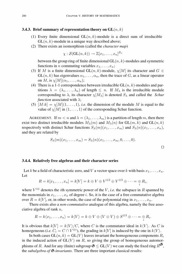
280 CHAPTER V. HISTORY OF MATHEMATICS
3.4.3. Brief summary of representation theory on GL(n, k)
(1) Every finite dimensional GL(n, k)-module is a direct sum of irreducibleGL(n, k)-module in a unique way described above;
(2) There exists an isomorphism (called the character map)
χ : S(GL(n, k))→ Z[x1, . . . , xn]Sn
between the group ring of finite dimensional GL(n, k)-modules and symmetricfunctions in n commuting variables x1, . . . , xn;
(3) If M is a finite dimensional GL(n, k)-module, χ[M ] its character and G ∈GL(n, k) has eigenvalues α1, . . . , αn, then the trace of G, as a linear operatoron M , is χ[M ](α1, . . . , αn);
(4) There is a 1-1 correspondence between irreducible GL(n, k)-modules and par-titions λ = (λ1, . . . , λn) of length ≤ n. If Mλ is the irreducible modulecorresponding to λ, its character χ[Mλ] is denoted Sλ and called the Schurfunction associated with λ;
(5) [M :k] = χ[M ](1, . . . , 1), i.e. the dimension of the module M is equal to thevalue of χ[M ] in (1, . . . , 1) of the corresponding Schur function.
AGREEMENT. If m < n and λ = (λ1, . . . , λm) is a partition of length m, then thereexist two distinct irreducible modules Mλ(m) and Mλ(n) for GL(m, k) and GL(n, k)respectively with distinct Schur functions Sλ(m)(x1, . . . , xm) and Sλ(n)(x1, . . . , xn),and they are related by
Sλ(m)(x1, . . . , xm) = Sλ(n)(x1, . . . , xm, 0, . . . , 0).
'(
3.4.4. Relatively free algebras and their character series
Let k be a field of characteristic zero, and V a vector space over k with basis x1, . . . , xn.Let
R = k[x1, . . . , xn] = k[V ] = k ⊕ V ⊕ V ⊗2 ⊕ V ⊗3 ⊕ · · · = ⊕iRi,
where V i⊗ denotes the ith symmetric power of the V , i.e. the subspace in R spanned bythe monomials in x1, . . . , xn of degree i. So, it is the case of a free commutative algebraover R = k[V ], or, in other words, the case of the polynomial ring in x1, . . . , xn.
There exists also a non-commutative analogue of this algebra, namely the free asso-ciative algebra of rank n,
R = k〈x1, . . . , xn〉 = k〈V 〉 = k ⊕ V ⊕ (V ⊗ V )⊕ S⊗3 ⊕ · · · = ⊕iRi.
It is obvious that k[V ] = k〈V 〉/C, where C is the commutator ideal in k〈V 〉. As C ishomogeneous (i.e. Ci = C ∩ V ⊗i), the grading in k[V ] is induced by the one in k〈V 〉.
In both cases GL(n, k) = GL(V ) leaves invariant the homogeneous components Ri
in the induced action of GL(V ) on R, so giving the group of homogeneous automor-
phisms of R. And for any (finite) subgroupG ≤ GL(V ) we can study the fixed ring RG,the subalgebra of G-invariants. There are three important classical results:

3. Th. Molien’s life and mathematical work 281
(1) Molien (1897): for char k �= 0 one had the Poincaré series
H(k[V ]G) =1|G|
∑G∈G
1det(I −Gt)
;
(2) E. Noether (1916): k[V ]G is finitely generated as a k-algebra;(3) Shephard-Todd (1954), Chevalley (1955): For chark = 0 the fixed algebra
k[V ]G is a free commutative algebra i.e. (it is itself a polynomial algebra) ifand only if G is generated by pseudo-reflections. Here an element G ∈ G iscalled a pseudo-reflection if it has an eigenvalue 1 with multiplicity n − 1 =dimV − 1.
Next, we want to describe some (quite recent) noncommutative extensions of these(classical) theorems. For this we need some more notions.
For any graded k-algebra
R = k ⊕R1 ⊕R2 ⊕ . . .
with all its homogeneous components finite dimensional over k, the Hilbert (or Poincaré)series of R is the formal series
H(R) = 1 +∑i≥1
(dimk Ri)ti.
Let R = k〈X〉 = k〈x1, . . . , xn, . . . 〉 be a free associative algebra of countablyinfinite rank, while k〈V 〉 remains a free associative algebra of finite rank. We call anideal T in k〈X〉 (or in k〈V 〉) a T -ideal if T is closed under k-endomorphisms. Andk〈X〉/T is called a relatively free algebra, and k〈V 〉/T a relatively free algebra of rankn. In this last case we have
R = k〈V 〉/T = k〈x1, . . . , xn〉/T =⊕∑
i≥0
Ri with Ri = V ⊗i/(T ∩ V ⊗i).
The character series of R is defined by
χ(R) = 1 +∑i≥1
χ[Ri]ti,
where χ is the character map in the “Main Representation Theorem”.So, χ(R) is a formal series in t with coefficients in Z[x1, . . . , xn]Sn , i.e.
χ(R) ∈ Z[x1, . . . , xn]Sn [[t]];
and it can be written also in terms of Schur functions:
χ(R) =∑
λ
a(λ)Sλt|λ|,
where a(λ) ∈ Z≥0 and Sλ is a homogeneous polynomial in x1, . . . , xn of degree |λ|.Now, a brief summary is on the main properties of T -ideals.

282 CHAPTER V. HISTORY OF MATHEMATICS
3.4.5. Additional observations on T -ideals
REMARK 3.11. If R is commutative, it satisfies [x1, x2] = x1x2 − x2x1; hereT = C, the commutator ideal of k〈X〉, and C is generated as a T -ideal by [x1, x2].
REMARK 3.12. If R is a finite dimensional k-algebra of dimension n, then R satis-fies the standard identity of degree n + 1,
Sn+1(x1, . . . , xn+1) =∑
σ∈Sn+1
sign(n)xσ(1) . . . xσ(n+1).
REMARK 3.13. The ring of n×n matrices over k, Mn(k) satisfies S2n(x1, . . . , x2n),Amitsur-Levitzki Theorem.
REMARK 3.14. The ring of upper triangular matrices over k satisfies (x1x2−x2x1)n
and its T -ideal of identities is Cn, where C is the commutator ideal of k〈X〉.
REMARK 3.15. The exterior (or Grassmann) algebra E = k〈v1, v2, . . . 〉/J overan infinite dimensional vector space with basis v1, v2, . . . , where J is the ideal generatedby v2
i and vivj + vjvi. Then E satisfies
[x1, x2, x3] = (x1x2 − x2x1)x3 − x3(x1x2 − x2x1).
and this polynomial generates E as a T -ideal.
REMARK 3.16. E ⊗ E satisfies
[[x1, x2]2, x3] and [x1, x2, [x3, x4], x5],
and these two polynomials generate E ⊗ E as a T -ideal (Popov).
REMARK 3.17. Let T � k〈X〉 be a T-ideal, T (n) = k〈x1, . . . , xn〉 ∩ T . Then, ifm < N , we have
χ(k〈x1, . . . , xn〉)/T (n) =∑
λ
a(λ)Sλ(x1, . . . , xn) = ϕ(x1, . . . , xn; t)
and
χ(k〈x1, . . . , xn〉)/T (m) =∑
λ
a(λ)Sλ(x1, . . . , xm) = ϕ(x1, . . . , xm, 0, . . . , 0; t).
Note that the coefficient a(λ) is the same in both equations. Here it is also importantthat this coefficient a(λ) is independent of the number of variables involved. Thus,χ(k〈X〉)/T may be regarded as well-defined and equal to
∑λ aΛSλt
|λ|. This step canbe formalized if we introduce the “ring of symmetric functions of infinitely many vari-ables” and then we write the character series as
∑λ aΛt
|λ|., a formal series with Sλ assymmetric functions in variables x1, . . . , xn, . . . , the number of which we may ignore.
Let us also notice that if k〈V 〉/T has the character series ϕ(x1, . . . , xn; t), then from(Remark 3.15) in the “Main Representation Theorem” it follows that it Poincaré series isϕ(1, . . . , 1; t).
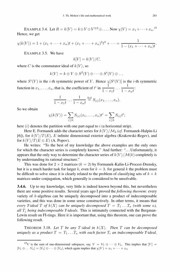
3. Th. Molien’s life and mathematical work 283
EXAMPLE 3.4. Let R = k〈V 〉 = k⊕V ⊕V ⊗2⊕ . . . . Now χ(V ) = x1 + · · ·+xn.15
Hence, we get
χ(k〈V 〉) = 1 + (x1 + · · ·+ xn)t + (x1 + · · ·+ xn)2t2 + · · · = 11− (x1 + · · ·+ xn)t
.
EXAMPLE 3.5. We have
k[V ] = k〈V 〉/C,where C is the commutator ideal of k〈V 〉, so
k〈V 〉 = k ⊕ V ⊕ S2(V )⊕ · · · ⊕ Si(V )⊕ . . .
where Si(V ) is the i-th symmetric power of V . Hence χ[Si(V )] is the i-th symmetric
function in x1, . . . , xn, that is, the coefficient of ti in1
1− x1t. . .
11− xnt
:
11− x1t
. . .1
1− xnt
fed= S(i)(x1, . . . , xn).
So we obtain
χ(k〈V 〉) =∑i≥0
S(i)(x1, . . . , xn)ti =∑i≥0
S(i)ti;
here (i) denotes the partition with one part equal to i (a horizontal strip).Here E. Formanek adds the character series for k〈V 〉/M2 (cf. Formanek-Halpin-Li
[6]), for k〈V 〉/T (E), E infinite dimensional exterior algebra (Krakowski-Regev), andfor k〈V 〉/T (E ⊗ E) (A. Popov).
He writes: “To the best of my knowledge the above examples are the only onesfor which the character series is completely known.” And further: “. . . Unfortunately, itappears that the only way to determine the character series of k〈V 〉/M(k) completely isby understanding its rational structure.”
This was done for 2 × 2 matrices (k = 2) by Formanek-Kalin-Li-Procesi-Drensky,but it is a much harder task for larger k, even for k = 3. for general k the problem mustbe difficult to solve since it is clearly related to the problem of classifying sets of k × kmatrices under conjugation, which generally is considered to be unsolvable.
3.4.6. Up to my knowledge, very little is indeed known beyond this, but neverthelessthere are some positive results. Several years ago I proved the following theorem: everyvariety of k-algebras can be uniquely decomposed into a product of indecomposablevarieties, and this was done in some sense constructively. In other terms, it means thatevery T-ideal T of k〈X〉 can be uniquely decomposed T = T1 . . . Tκ (with some κ),all Tj being indecomposable T-ideals. This is intimately connected with the Bergman-Lewin result on FI-rings. Here it is important that, using this theorem, one can prove thefollowing result.
THEOREM 3.18. Let T be any T -ideal in k〈X〉. Then T can be decomposeduniquely as a product T = T1 . . . Tκ with each factor Ti an indecomposable T-ideal,
15V is the sum of one-dimensional subspaces, say, V = V1 ⊕ · · · ⊕ Vn. This implies that [V ] =
[V1 ⊕ . . . Vn] = [V1] ⊕ · · · ⊕ [Vn], which again implies that χ(V ) = x1 + · · · + xn

284 CHAPTER V. HISTORY OF MATHEMATICS
and the following formula holds true:
χ(k〈X〉/T ) = σ1
(χ(k〈X〉/T1)
), . . . , χ(k〈X〉/Tκ) +
+ (S(1)t− 1) · σ2
(χ(k〈X〉/T1)
), . . . , χ(k〈X〉/Tκ) +
+ (S(1)t− 1)2 · σ3(χ(k〈X〉/T1)) + · · ·+ (S(1)t− 1)κ−1 · σκ(. . . ),
where σi(. . . ) denotes the i-th elementary symmetric expression in the formal series
χ(k〈X〉/T1), . . . , χ(k〈X〉/Tκ).
The proof will be given below (p. 284-286).This theorem is interesting because it reduces the general problem (for any T -ideal)
to the case of irreducible T -ideals. [These factors can be quite effectively found by theD-construction technique; in this way I solved an old problem by Yu. Mal’cev regardingthe triangular matrix algebra, and achieved much the same as had been done, indepen-dently, by Plamen Siderov [20] using (complicated) direct calculations in k〈X〉.] And so,knowing the character series for all irreducible varieties, it is possible to find the characterseries of any relatively free algebra. Let us add here (we shall explain it in details later)that, taking in these character series all xi = 1, we can find, in principle, the Poincaréseries of any relatively free algebra!
From these results it is possible to find χ(k〈X〉/M(r)) for r ≥ 3 in some caseswhen there exists a suitable block-structure for the matrices present there; for somematrix algebras it is possible to bring all elements simultaneously into block-triangularshape.
When can all operators in an algebra (over C) be brought simultaneously into block-triangular shape? Cf. the Suprunenko-Tyshkevich theorem16.
PROOF OF THE THEOREM 3.18. We are going to use the following
LEMMA 3.19 (E. Formanek [7, p. 10]). Let T and U be T-ideals in k〈V 〉. Then TUis a T-ideal, and
χ(k〈V 〉/TU) = χ(k〈V 〉/TU) +
+ χ(k〈V 〉/U) + (S(1)t− 1)χ(k〈V 〉/T ) · χ(k〈V 〉/U).
Now our Theorem follows from my main theorem for k-algebras (Dissertation ofmine [K79a], see Section 4 in Chapter I or [K76]). Indeed, from this follows that forany T-ideal T there is a (unique) decomposition T = T1 . . . Tκ (with some κ), intoindecomposable T-ideals T1, T2, . . . , Tκ. The last assertion of the Theorem now followswith induction on κ.
We illustrate the induction step by the special case T = T1T2T3 = TUW ; thereduction κ �→ κ − 1 is of the same sort as the reduction 3 −→ 2 below. As TUW =
16Editor’s note Probably it is in the paper [22]

3. Th. Molien’s life and mathematical work 285
(TU)W , we have
χ(k〈V 〉/TUW ) = [E. Formanek lemma]χ(k〈V 〉/TU) + χ(k〈V 〉/W ) +
+ (S(1)t− 1)χ(k〈V 〉/TU) · χ(k〈V 〉/W ) =
= (χ(k〈V 〉/T ) + χ(k〈V 〉/U)) +
+ (S(1)t− 1)χ(k〈V 〉/T )χ(k〈V 〉/TU) +
+ χ(k〈V 〉/W ) + (S(1)t− 1) · (exactly the same thing) ·· χ(k〈V 〉/W ) =
= (χ(k〈V 〉/T ) + χ(k〈V 〉/U) + (χ(k〈V 〉/W ) +
+ (S(1)t− 1) · (χ(k〈V 〉/T ) · χ(k〈V 〉/U)) +
+ χ(k〈V 〉/T ) · χ(k〈V 〉/W ) + χ(k〈V 〉/U) · χ(k〈V 〉/W )) +
+ (S(1)t− 1)2 · χ(k〈V 〉/T )χ(k〈V 〉/U)χ(k〈V 〉/W ) =
= σ1(χ(k〈V 〉/T ), χ(k〈V 〉/U), χ(k〈V 〉/W )) +
+ (S(1)t− 1)σ2(∗, ∗, ∗) + (S(1)t− 1)2 · σ3(∗, ∗, ∗).
[In the last term the arguments of σ2 and σ3, indicated by the three stars ∗, are the sameas the argument of σ1.]
General case: the induction κ− 1 �−→ κ. We write
T = T1 . . . Tκ = (T1 . . . Tκ−)Tκ = U ·W.
Using the Formanek lemma as the main tool, we find:
χ(k〈V 〉/T ) = χ(k〈V 〉/U) + χ(k〈V 〉/W ) + (S(1)t− 1)χ(k〈V 〉/U) · χ(k〈V 〉/W ) =
= χ(k〈V 〉/T1 . . . Tκ−1) + χ(k〈V 〉/Tκ) +
+ (S(1)t− 1)χ(k〈V 〉/T1 . . . Tκ−1) · χ(k〈V 〉/Tκ) == [by the induction hypothesis]
κ−1∑i=1
σ(κ−1)i (χ(k〈V 〉/T1), . . . , χ(k〈V 〉/Tκ−1)·
· (S(1)t− 1)i−1 + χ(k〈V 〉/Tκ) =
= σ(κ−1)i (χ(k〈V 〉/T1 . . . Tκ−1)) + χ(k〈V 〉/Tκ)︸ ︷︷ ︸
σκ1 (χ(k〈V 〉/T1),...,χ(k〈V 〉/Tκ))
+
+(κ−1)∑i=2
σ(κ−1)i (S1t− 1)i−1 +
κ−1∑i=1
χ(k〈V 〉/Tκ)(S(1)t− 1)i−1 =

286 CHAPTER V. HISTORY OF MATHEMATICS
χ(k〈V 〉/T ) = σ(κ)1 +
[σ
(κ−1)1 χ(k〈V 〉/Tκ)
]u +
[σκ
3 + σκ2χ(k〈V 〉/Tκ)
]u2 +
+ · · ·+ [σκ−1κ−1 + σκ−1
κ−2χ(k〈V 〉/Tκ)︸ ︷︷ ︸σκ
κ−1
]uκ−2 + σ(κ−1)κ−1 χ(k〈V 〉/Tκ)︸ ︷︷ ︸
σκκ
uk−1 =
= σ(κ)1 + σ
(κ)2 u + · · ·+ σ
(κ)κ−1u
κ−2 + σ(κ)κ uκ−1 =
=κ∑
i=1
σ(κ)i ui−1.
From this calculation the induction step follows. '(
So one needs to know the character series for the irreducible T-ideals only. In thisway we can overcome (using my thesis [K79a]) the difficulties described by Formanekin the case k〈V 〉/M(r), r ≥ 3.
It ought also be stressed that this Theorem is true for any field k (of any characteristic,not only for k with chark = 0, as in Formanek’s paper!) if and only if Theorem 2in Formanek’s paper is true for any field – as our results about the triangular productconstructions are proved for any field. This is important, because in this way one canhope to be able to reprove some of the results of Dicks-Formanek [5] and Almkvist-Fossum [2] on the calculation of the Poincaré series for relatively free algebras in thepositive characteristic case (chark = p > 0).
3.4.7. For any finite group G, let Rep(k,G) be the set isomorphism classes of finitelygenerated kG-modules; let [M ] be the isomorphism class of such a module M . It is an(additive) monoid under [M ] ⊕ [M ′] = [M ⊕M ′]. As G is finite, the Krull-SchmidtTheorem implies that it is a free monoid freely generated by the classes of indecom-posable finitely generated kG-modules. Take [M ] · [M ′] = [M ⊗k M ′] with diagonalaction of G on M ⊗M ′. Let us consider the k-space of additive maps Rep → k, e.g.
ψ : Rep → k, ψ(M) def= [MG : k]. The ones among them which preserve multipli-cation in the monoid Rep also are called k-characters of Rep. Each G ∈ G defines acharacteristic χG : Rep→ k by M �→ trace(G : M →M.).
If we now take G ≤ GL(V ) and M any GL(V )-module, [V :k] = n, and G ∈GL(V ) has the eigenvalues α1, . . . , αn as a linear operator on V , we know by our
Main Representation Theorem that traceG = χ[M ](α1, . . . , αn). Let MGdef= {m ∈
M |mG = m for allG ∈ G}, i.e. the fixed points of M .It follows from the inner product formula for characters that
(91) [MkG:k] =1|G|
∑G∈G
χG[M ].
Here χG[M ] is the trace of G as a linear operator on M . Now we shall see that all thismaterial about the character series has intimate connections with Molien’s formula andits analogues.
Taking k〈V 〉/T = k ⊕R1 ⊕R2 ⊕ . . . , we have
(k〈V 〉/T )G = k ⊕RG1 ⊕RG2 ⊕ . . . ,
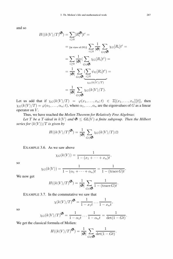
3. Th. Molien’s life and mathematical work 287
and so
H((k〈V 〉/T )G) =∑i≥0
[RGi ]ti =
= [in view of (91)]
∑i≤0
1|G|
∑G∈G
χG[Ri]ti =
=∑i≥0
1|G| (
∑G∈G
χG[Ri]ti) =
=1|G|
∑G∈G
(∑i≥0
ψG[Ri]ti)︸ ︷︷ ︸χG(k〈V 〉/T )
=
=1|G|
∑G∈G
χG(k〈V 〉/T ).
Let us add that if χG(k〈V 〉/T ) = ϕ(x1, . . . , xn; t) ∈ Z[(x1, . . . , xn][[t]], thenχG(k〈V 〉/T ) = ϕ(α1, . . . , αn; t), where α1, . . . , αn are the eigenvalues of G as a linearoperator on V .
Thus, we have reached the Molien Theorem for Relatively Free Algebras:Let T be a T -ideal in k〈V 〉 and G ≤ GL(V ) a finite subgroup. Then the Hilbert
series for (k〈V 〉)/T is given by
H((k〈V 〉/T )G) =1|G|
∑G∈G
χG(k〈V 〉/T ).'(
EXAMPLE 3.6. As we saw above
χG(k〈V 〉) =1
1− (x1 + · · ·+ xn)t,
so
χG(k〈V 〉) =1
1− (α1 + · · ·+ αn)t=
11− (traceG)t
.
We now get
H((k〈V 〉/T )G) =1|G|
∑G∈G
11− (traceG)t
.
EXAMPLE 3.7. In the commutative we saw that
χ(k〈V 〉/T )G =1
1− x1t. . .
11− xnt
,
so
χG(k〈V 〉/T )G =1
1− α1t. . .
11− αnt
=1
det(1−Gt).
We get the classical formula of Molien:
H((k〈V 〉/T )G) =1|G|
∑G∈G
1det(1−Gt)
.
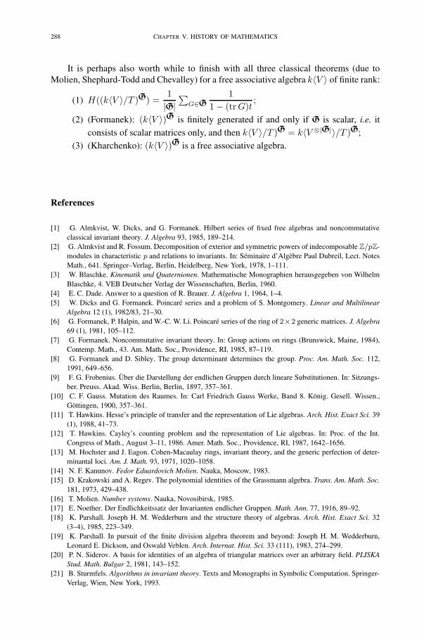
288 CHAPTER V. HISTORY OF MATHEMATICS
It is perhaps also worth while to finish with all three classical theorems (due toMolien, Shephard-Todd and Chevalley) for a free associative algebra k〈V 〉 of finite rank:
(1) H((k〈V 〉/T )G) =1|G|
∑G∈G
11− (trG)t
;
(2) (Formanek): (k〈V 〉)G is finitely generated if and only if G is scalar, i.e. it
consists of scalar matrices only, and then k〈V 〉/T )G = k〈V ⊗|G|〉/T )G;
(3) (Kharchenko): (k〈V 〉)G is a free associative algebra.
[1],[2],[4],[5], [6],[7],[8],[9], [11],[12],[13],[14], [15],[16],[17], [18],[19],[20],[21][24],[25],[26], [27],[28],[29],[30], [31],[32],[33], [34],[35],[36]
References
[1] G. Almkvist, W. Dicks, and G. Formanek. Hilbert series of fixed free algebras and noncommutativeclassical invariant theory. J. Algebra 93, 1985, 189–214.
[2] G. Almkvist and R. Fossum. Decomposition of exterior and symmetric powers of indecomposable Z/pZ-modules in characteristic p and relations to invariants. In: Séminaire d’Algèbre Paul Dubreil, Lect. NotesMath., 641. Springer–Verlag, Berlin, Heidelberg, New York, 1978, 1–111.
[3] W. Blaschke. Kinematik und Quaternionen. Mathematische Monographien herausgegeben von WilhelmBlaschke, 4. VEB Deutscher Verlag der Wissenschaften, Berlin, 1960.
[4] E. C. Dade. Answer to a question of R. Brauer. J. Algebra 1, 1964, 1–4.[5] W. Dicks and G. Formanek. Poincaré series and a problem of S. Montgomery. Linear and Multilinear
Algebra 12 (1), 1982/83, 21–30.[6] G. Formanek, P. Halpin, and W.-C. W. Li. Poincaré series of the ring of 2×2 generic matrices. J. Algebra
69 (1), 1981, 105–112.[7] G. Formanek. Noncommutative invariant theory. In: Group actions on rings (Brunswick, Maine, 1984),
Contemp. Math., 43. Am. Math. Soc., Providence, RI, 1985, 87–119.[8] G. Formanek and D. Sibley. The group determinant determines the group. Proc. Am. Math. Soc. 112,
1991, 649–656.[9] F. G. Frobenius. Über die Darstellung der endlichen Gruppen durch lineare Substitutionen. In: Sitzungs-
ber. Preuss. Akad. Wiss. Berlin, Berlin, 1897, 357–361.[10] C. F. Gauss. Mutation des Raumes. In: Carl Friedrich Gauss Werke, Band 8. König. Gesell. Wissen.,
Göttingen, 1900, 357–361.[11] T. Hawkins. Hesse’s principle of transfer and the representation of Lie algebras. Arch. Hist. Exact Sci. 39
(1), 1988, 41–73.[12] T. Hawkins. Cayley’s counting problem and the representation of Lie algebras. In: Proc. of the Int.
Congress of Math., August 3–11, 1986. Amer. Math. Soc., Providence, RI, 1987, 1642–1656.[13] M. Hochster and J. Eagon. Cohen-Macaulay rings, invariant theory, and the generic perfection of deter-
minantal loci. Am. J. Math. 93, 1971, 1020–1058.[14] N. F. Kanunov. Fedor Eduardovich Molien. Nauka, Moscow, 1983.[15] D. Krakowski and A. Regev. The polynomial identities of the Grassmann algebra. Trans. Am. Math. Soc.
181, 1973, 429–438.[16] T. Molien. Number systems. Nauka, Novosibirsk, 1985.[17] E. Noether. Der Endlichkeitssatz der Invarianten endlicher Gruppen. Math. Ann. 77, 1916, 89–92.[18] K. Parshall. Joseph H. M. Wedderburn and the structure theory of algebras. Arch. Hist. Exact Sci. 32
(3–4), 1985, 223–349.[19] K. Parshall. In pursuit of the finite division algebra theorem and beyond: Joseph H. M. Wedderburn,
Leonard E. Dickson, and Oswald Veblen. Arch. Internat. Hist. Sci. 33 (111), 1983, 274–299.[20] P. N. Siderov. A basis for identities of an algebra of triangular matrices over an arbitrary field. PLISKA
Stud. Math. Bulgar 2, 1981, 143–152.[21] B. Sturmfels. Algorithms in invariant theory. Texts and Monographs in Symbolic Computation. Springer-
Verlag, Wien, New York, 1993.

3. Th. Molien’s life and mathematical work 289
[22] P. N. Siderov. The similarity and substitutive equivalence of (0,1)-matrices. Dokl. Nats. Akad. NaukBelarusi 22, 1978, 485–487, 571.
[23] T. Tambour. A theorem of Molien type in combinatorics. European J. Combin. 10, 1989, 197–199.
Supplement. List of scientific papers of Th. Molien. 17
[24] T. Molien. Bahn des Kometen 1880, III. Astronomische Nachrichten 2519, 1883, 353–362.[25] T. Molien. Zusats zur Bahnbestimmung des Kometen 1880 III. Astronomische Nachrichten 2519, 1883,
353–362.[26] T. Molien. Über gewisse, in der Theorie der elliptischen Functionen auftretenden Einheitswurzeln.
Berichte der k. Sächsischen Gesellschaft der Wissenschaften, 1885.[27] T. Molien. Über lineare Transformation der elliptischen Functionen. Master’s thesis, Dorpat, 1885.[28] T. Molien. Über Systeme höherer komplexen Zahlen. Math. Ann. 41, 1893, 83–156.[29] T. Molien. Berichtigung zum Aufsatze “Ueber Systeme höherer complexen Zahlen”. Math. Ann. 42,
1893, 308–312.[30] T. Molien. Eine Bemerkung zur Theorie der homogenen Substitutionensgruppen. Sitzungsberichte der
Naturforschenden Gesellschaft der Universität Jurjew 18, 1897, 259–274.[31] T. Molien. Über die Anzahl der Variablen einer irreduzibeln Substitutionensgruppen. Sitzungsberichte
der Naturforschenden Gesellschaft der Universität Jurjew 18, 1897, 277–288.[32] T. Molien. Über die Invarianten der linearen Substitutionsgruppen. Sitzungsber. der Königl. Preuss. Akad.
d. Wiss. 52, 1897, 1152–1156.[33] T. Molien. Über gewisse transzendente Gleichungen. Math. Ann. 103, 1930, 35–37.[34] T. Molien. Lösung der Aufgabe 148. Jahresber. Dtsch. Math.-Ver. 44, 1934, 35–37.[35] T. Molien. Zahlensysteme mit einer Haupteinheit (Systems of higher complex numbers with a principal
unit). Uch. Zap. Tomsk Ped. Inst. Mat. Mekh. Kubyshev-Univ., Tomsk 1 (1), 1935, published 1937, 217–224.
[36] T. Molien. On a certain transformation of the hypergeometric series. Uch. Zap. Tomsk Ped. Inst. Mat.Mekh. Kubyshev-Univ., Tomsk 1, 1935, published 1937, 119–121.
17Editor’s Note. Several text-books by Molien are also mentioned in Kanunov’s book [14], ultra.

This page intentionally left blank

291
4. Notes on five 19th century Tartu mathematicians(Backlund, Kneser, Lindstedt, Molien, Weihrauch)Edited and translated by J. Peetre with the assistance of V. Ufanrovsky
Preamble (by J. Peetre). This notes represent material found by Uno Kaljulaid inarchives in Tartu. Kaljulaid sent me the manuscript probably a few years before his death,without any explanation. On the top of one of the pages about Molien there was, however,a note to me in Estonian, of which I can decern the following words: “Jaak . . . Vaadataja tõlkida.” (To look and to translate.) The language in the original has been Russian(occasionally German, or other languages), by Kaljulaid translated into Estonian. Hereall is rendered in English. Sometimes the Russian/German has been preserved becauseof emphasis. I express the hope that this compilation will be of interest for historians ofmathematics. Recall that the language of administration at Dorpat/Tartu University wasRussian, whereas, until 1893, all teaching took place in German.
The text is divided into five sections corresponding to each of the five men treated.All of them had a connection to mathematics, although Backlund was primarily an as-tronomer. Two of them are native Swedes, another, Molien, having at least Swedishancestry. At the end each of these sections there is a separate list of references, com-piled by me. The footnotes are, likewise, by me. The text is usually rendered verbatim.The Reader will probably have no difficulty in discerning what is taken directly from thearchives from occasional interpretations by Kaljulaid. The pages of the various “folders”in the archives has been numbered 1, 2, . . . , empty (or skipped?) pages being sometimesdenoted, by Kaljulaid, by a question mark (?). Some headings inside the chapters areprinted in bold letters. Passages which I have been unable to decipher are indicated as[?????].

292 CHAPTER V. HISTORY OF MATHEMATICS
Johan Oskar Backlund (1846-1916)
The astronomer Backlund was a native Swede, he studied in Uppsalaand became a docent there in 1875. He was an assistant astronomer atthe Observatory of the Royal Swedish Academy of Sciences (KVA18)in Stockholm in 1875-1876, and an astronomer at Dorpat University1876-1879. From there he moved to Russia and was an adjoint as-tronomer at the Pulkovo Observatory19 in 1879-1887.
Backlund became a member of the Russian Academy of Sci-ences in 1887. In 1895 he was appointed director of the Observatory.
Backlund’s scientific work was mainly devoted to the study ofEncke’s comet20
One of Backlund’s two sons Helge Backlund (1878-58) becamea geologist and was first a professor in Åbo (1918-1924), and then inUppsala (1924-1943).21
18Kungliga Vetenskaps Akademien19Near St. Petersburg, founded in 1839 by the German-born astronomer Wilhelm Struve (1793-1864),
studied in Dorpat, and taught there 1813-1839. Struve was the first to determine, in 1837, the parallax offixed stars. The Russian name of the Observatory is a corruption of Finnish Purkola, an estate given by CzarPeter to his wife Catharine, a Lithuanian peasant woman. Two more Swedes to work in St. Petersburg werethe mathematician Anders Johan Lexell, an assistant of Leonard Euler, and Georg Lindhagen, who marriedStruve’s daughter.
20This is the comet with the smallest period of rotation about the Sun. It was identified by Johann FranzEncke (1791-1865) in 1819. Encke also found the first signs of a non-gravitational force acting on it [2].
21Interesting information about the Backlund family can be found in the book [1]. Backlund had also adaughter Elsa, who became a painter. A well-known picture “På skidor (On skies)" has Helge as model. Afterthe Revolution she returned to Sweden together with her mother the Secret Counciloress Ulrika.
4. Notes on five 19th century Tartu mathematicians 293
Folder 1207: March 25, 1876 – March 7, 1879.
Page 4. Extract from the proposal of the Physico-Mathematical Faculty on March 25,1976.
The Faculty proposes to the Council to nominate Johan Oskar Back-lund for the vacant position of astronomy observer at the Universityof Dorpat as the single candidate.
J. O. Backlund was born on April 8, 1846, entered Uppsala Uni-versity as a student in 1866, became a Candidate of Philosophy in1872, and defended on December 5, 1874 [a thesis] pro grado philo-sophico “Beräkning af relativa störningar för Planeten (112) Iphige-nia”, and was, since January 1875, appointed docent at Uppsala Uni-versity, and obtained (in March?) the degree of doctor. Besides thathe has written a yet non-published article on the influence of Encke’scomet to shortening of the orbit of Earth, however, KVA has beengiven him for that the Ferner prize.
. . . By the way, these works show that Dr. Backlund is an out-standing theoretical astronomer, and, on other hand, he was recom-mended by the director of the Astronomical Observatory of Stock-holm, Professor Dr. Hugo Gyldén22, who for two years already hasbeen Backlund’s adviser.
Page 6. Excerpt from the Journal des Conseils der Kaiserlichen Universität Dorpat,March 26, 1876, No. 162.
Having listened to the presentation of Dr. J. O. Backlund, the sin-gle candidate to the position of astronomy observer, the election wasperformed, thereby 34 voted for him and their were no votes against.The Council decides to turn to Mr. Curator to affirm Dr. Backlundto this position, and to refund him his travel expenses for the trip toTartu.
Page 9. On April 13, 1876 there is the confirmation (which had arrived in Dorpat onApril 27, 1876) signed (in Riga?) by the Curator Saburov together with the decision toreimburse the travel expenses of Backlund to the amount 437 rubles 75 kopeks; Backlundexpressed the wish to obtain this money in Dorpat. [The Curator had earlier asked whereBacklund wanted this money, in Stockholm or in Dorpat. So the rules were.]
Page 21. Extract from the minutes of the Council of the University on April 13, 1877.
[Item on the agenda:] Does the Physico-Mathematical Faculty sup-port Dr. Backlund’s application for a summer vacation so that hecould participate in the Congress of Astronomers in Stockholm inAugust?
22Hugo Gyldén (1841-1896), Finnish-Swedish astronomer, employed at Pulkovo, St. Petersburg 1863-1871, was then as an Astronomer at KVA, worked mainly on the perturbation theory of planets, had a greatinfluence to the development of this subject in Sweden [2]. See also [3, Chapter 9.]

294 CHAPTER V. HISTORY OF MATHEMATICS
He was given a summer vacation + 28 days.Signed by the Minister of National Education, Count Dmitriı Tolstoı
Page 34. On Dec. 2, 1877 Curator Saburov’s decided to pay to Dr. Backlund the sum of150 ruble for lectured delivered on “Algebraische Analysis” (3 hours weekly).
Page 40. On May 24, 1878 [there is] a new order by “Curator Saburov (?)” aboutpayment of 150 rubles for the running semester (that is the spring semester of 1878)for lectures (3 hours a week) “Ausgewählte Theile der Elementar-Matematik” (from thefunds of the vacant docentship).
Page 42. The Department of National Education has informed Curator Saburov onJan. 10, 1879 that the Director of the Nikolaı Observatory of Pulokvo submitted to theMinistery of Education a proposal for appointing Dr. Backlund to the vacant position ofAdjunct Observer. It is asked whether Dorpat has any objections to this?
Page 47. Extract from the Journal of the Council of Dorpat University.
On Feb. 12 1879 it is replied that there are no objections, and it isdecided to forward to the Curatorship, that there are no hindrances inthe transfer of Dr. Backlund.
Page 48. The Council of the Imperial Dorpat University confirms that Dr. Oskar A.Backlund23, foreigner, not a Russian citizen, 32 years of age, after finishing the sciencecourse at Uppsala University with the degree of Candidate, further in 1875 with the de-gree of Doctor of Philosophy, was a docent at Uppsala University 1875-76, and earlieremployed as an astronomer at Stockholm, was, on April 13, 1876, appointed by a deci-sion of the Curator of the Dorpat District of Education, in accordance with the results ofvoting in the Council, to astronomer at Dorpat University, from which position (being inClass VII) he has been transferred to an adjoint-astronomer at the Nikolaı Main Astro-nomical Observatory from Feb. 24, 1879 on. The salary in Dorpat was 10000 rubles ayear. He fulfilled his obligations with satisfaction.
Backlund is married to Ulrika (née Widebeck) and has the sons: Hjalmar (born onApr. 5, 1877) and Helge (born on Aug. 24, 1878). Wife and sons are of Evangelic-Lutheran confession.
Folder 1208: July 29, 1876 - February 28, 1880.
On August 20, 1876, a letter from the Custom Office (City of Saint Petersburg, Customof the Port) that 40 rubles, 80 kopeks has to be payed back to Backlund, which he hadpayed for a pianoforte, brought into the country by him from abroad.
Generally speaking, the information about Backlund in Tartu, what substance goes,is rather scant. Two sons were born to him here . . . 24 One needs supplementary explana-tion what he did here, and why he left.
23Editor’s note. The name of Dr Backlund appears on Russian documents as Oskar Andreevich Baklund24One of the sons was the aforementioned future geologist Helge Backlund, born in 1878.

4. Notes on five 19th century Tartu mathematicians 295
References
[1] B. Jangfeldt. Svenska vägar till S:t Peterburg: kapitel ur historien om svenskarna vid Nevans strän-der (Swedish routes to St. Peterburg. Chapters from the story of the Swedes on the shores of the Neva.)Wahlström & Wifstrand, Stockholm, 2000.
[2] Nationalencyklopedin (Swedish National Encyclopedia).[3] L. Gårding. Matematik och Matematiker. Matematiken i Sverige före 1950. Lund University Press, Lund,
1994. English translation: Mathematics and mathematicians. Mathematics in Sweden before 1950. In: His-tory of Mathematics, 13. American Mathematical Society, Providence, RI; London Mathematical Society,London, 1998.

This page intentionally left blank

4. Notes on five 19th century Tartu mathematicians 297
Adolf Kneser (186225-1930)
Kneser was born in Grüssow, Mecklenburg, Germany. He studiedmathematics in Berlin under Kronecker and Weierstrass. In 1884he became a private docent in Marburg, but in 1886 he moved toBreslau (Wrosław), as a professor and successor of O. Staude, whohad left for Dorpat. He was thus made a professor at the early ageof 27. However, when Staude accepted an invitation to Rostock in1889, Kneser became his successor for the second time. In 1893the previously German-language university became a Russian uni-versity, named Yurjev University, and the language of teaching be-came Russian. At least one of the professors, Oettingen26, quit. Inthis context Kneser drafted a letter of protest on the behalf of theGerman professors. Finally, Kneser himself returned to Germany, in1900. It should however emphasized that he had a good relation toseveral Russian mathematicians, among them Steklov, in particularwas very close to him. Eventually got an invitation back to Breslau,where he then stayed for the rest of his life.
Adolf Kneser gave rise to a mathematical dynasty; both his sonHelmuth27 and his grandson Martin became famous mathematicians.
25Note that Kneser born in the same year as David Hilbert.26Arthur Joachim von Oettingen (1836-1920), Baltic-Geman physicist and meteorologist, taught at Tartu
1863-1893, in Leipzig 1984; upon the “Russification” of the University he refused to teach in Russian and sohad to emigrate and taught one year, 1894, in Leipzig. In 1899 he went to Transval, and return from there via“Eastern Africa” (see [5, Part 5]); by this is probably meant German Eastern Africa (Deutsch Ostafrika), thatis, present day, Tanzania. Oettingen started regular meteorological observation in 1865, and founded the firstmeteorological station in Estonian territory in 1876.
27A second son Lorents Friedrich died as a soldier in World War.
298 CHAPTER V. HISTORY OF MATHEMATICS
Folder 402/3/805: November 22, 1888 – April 11, 1900.
Certificate and place of birth:Great Duchy of Mecklenburg-Schwerin, born on March 19, 1862 in Grüssow, Meck-
lenburg, father Adolph Hermann Kneser, worked as a Lutheran pastor, mother FriederikeWilhelmine Filippe Augusta (née Kolman), the full name of their son was Julius ChristianCarl Adolph.
• On November 22, 1888, the Council of the Physico-Mathematical Faculty proclaimedthat the Private Docent Adolph Kneser from Breslau is the only candidate to the vacantextra-ordinary professorship in applied mathematics. His basic training is obtained fromthe Gymnasium of Rostock, from which he graduated in 1879 with a certificate of matu-rity. Then he studied at the Universities of Rostock, Heidelberg, and Berlin; in the latterhe obtained the degree of Doctor of Philosophy on March 8, 1884. In the same year hebegan to read mathematics at Marburg University as a private docent. In 1886 he movedto Breslau, where he began to work upon the leave of Professor Staude, and he is still(i.e., in 1888) a private docent there. Until now he has mainly given lectures on: ana-lytical mechanics; function theory; the theory of algebraic equations; on the numericalsolution of equations; number theory; determinants; Fourier series; algebraic analysis;calculus of variation and integral calculus.
He has a number of papers (on mathematical physics; algebraic equations; Kro-necker’s principle that number theory only then gets its true arithmetical nature wheneverything is founded in a purely arithmetical way; etc.).
From these abstract questions Kneser has lately passed on to geometrical problemsof the distribution of real twisting of plane curved lines in space not investigated suffi-ciently before28. With this paper he has shown himself as a skilled applied mathemati-cian. Furthermore, he has a paper that fulfils a very essential gap in Halphen’s text-bookof elliptic functions29; here he has also proved himself as a powerful analyst. He has alsoread analytical mechanics, that for Tartu was a novelty. The Faculty has obtained fromoutstanding scientists rather good characterizations of Kneser.
Weierstrass recommends to consider Kneser as the first candidate, Kronecker char-acterizes him as a good and many-sided laborer, who finds independently his themes anddelivers lectures, which lack formalism, and are dictated by an independent thinking. Headds that already in the gymnasium Kneser displayed an unusual ability in presentingmathematics, and that later, being already a lecturer in Marburg or in Breslau, he contin-ued exhibiting this ability. Professor [H.] Weber 30 (in Marburg) says that Kneser is freefrom the one-sidedness of only one school, he possesses a broad knowledge of in manydomains of mathematics, and he has enjoyable clarity of his presentation. The studentshere appreciated him and listened to his lectures; also in Breslau, where he was active ina much broader spectrum, he made the same success. Professor Hurwitz (Königsberg)says that hiring him would be a great victory for the Faculty.
28It may be [1].29This paper was probably not published; the only paper by Kneser dealing with elliptic functions seems
to be [2], but Halphen is not mentioned there at all.30Heinrich Weber (1815-1897), well-known German mathematical, mainly distinguished for his work in
Algebra and Number Theory. He was a professor in Marburg 1885-1892. In the last year he obtained a call toGöttingen and, finally, in 1895, one to Strassburg (Strasbourg) [4].

4. Notes on five 19th century Tartu mathematicians 299
Professor Schröter31 (Breslau) adds that as a comrade is agreeable, because he is freefrom waywardness and superiority; Professor Mayer adds that his over all impression ofhim is very high. He is diffident, and in the beginning he does not show his feelings buthe is always reliable and obliging, he has a trustworthy and efficient character.
• On Feb. 1, 1889, Kneser gave his oath of office (“Sittliches Gelübde”) to Tartu Univer-sity.
• On Mar. 1, 1890, he asks for permission to go abroad; in 1891 he signs such applica-tions as Professor of Mathematics.
•On Dec. 18, 1892, it is told in the minutes of the Council that 400 rubles has been payedto Kneser for the first half of this year one for his lectures in newer Algebra and Geometry(from money available for the vacant position in the Chair of Pure Mathematics).
• On Feb. 11, 1893, there is an application from Kneser to participate, in September,in an already ongoing international exhibition of mathematical models in München, andlikewise in another meeting taking place at the same time. The use of models in bothpure and applied mathematics gains an even greater importance; it will also be necessaryto renew the collection in the Mathematical Cabinet. (This gets the support of the Dean!)
• On Nov. 11, 1893, there is an interesting note: The Board of the Imperial Universityof Yurjev pronounces to the question if there might be any objections to the marriage ofthe Ordinary Professor and Councillor of State Adolph Kneser with the daughter of thedeceased landowner Lorentz Booth (Laura Booth), that no such objections existed.
• On Nov. 7, 1893, there is an entry by the Council that Kneser has obtained a vacationbecause of domestic reasons during the winter break.
• On Nov. 28, 1895, there is a letter from the Rector giving permission for Kneser to goabroad during the winter break.
• On March 18, 1896, Kneser asks for permission to go to Germany because of personalreasons. (He was then a professor of applied mathematics.)
• On Feb. 28, 1897, there is in the Council of the Imperial Yurjev University an interest-ing communication by Kneser: He has accepted the editorship of the Part “Calculus ofVariations” in the Enzyklopedädie, which is composed by united scientists abroad, andacademies. For this it is necessary to visit for a long time libraries abroad, because thecorresponding biographic information is not available here. He intends also to participatein the Meeting of Natural Scientists (Gesellschaft Deutscher Naturforscher und Ärtzte)in Braunschweig in September.
• April 22, 1898, The application has been approved by the Councillor of the YurjevUniversity, from the Riga District of Education, but at the end there is an interestingnote: “Independently of this, taking into account that a professor’s being away from theuniversity at his lecturing time may lead to insufficient acquisition of the study course
31Heinrich Eduard Schroeter (Schröter) (1829-1892), German mathematician, devoted himself mainly toelliptic functions and synthetic geometry.
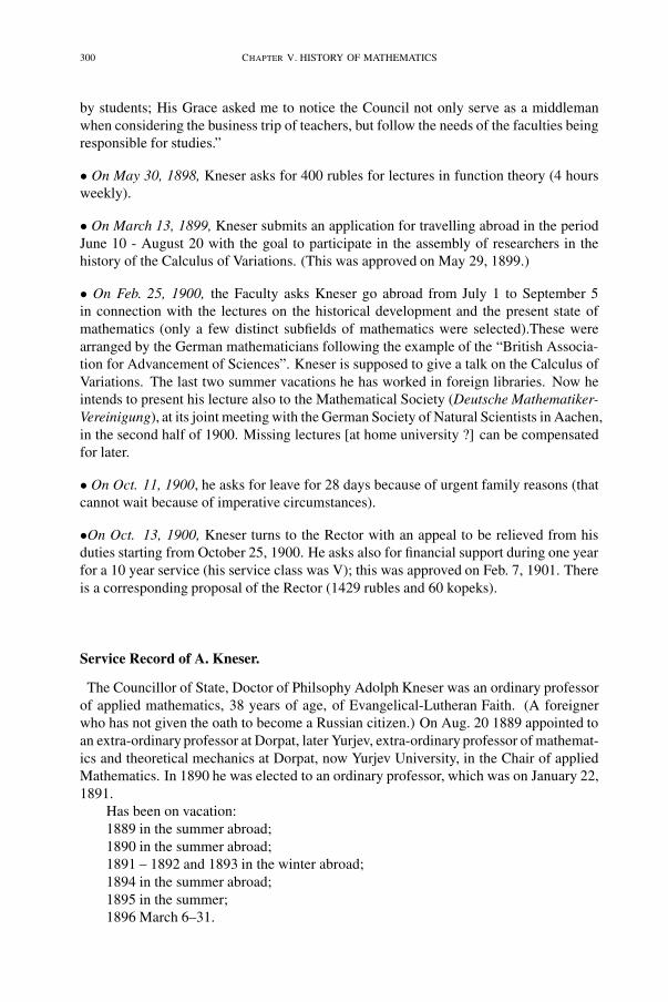
300 CHAPTER V. HISTORY OF MATHEMATICS
by students; His Grace asked me to notice the Council not only serve as a middlemanwhen considering the business trip of teachers, but follow the needs of the faculties beingresponsible for studies.”
• On May 30, 1898, Kneser asks for 400 rubles for lectures in function theory (4 hoursweekly).
• On March 13, 1899, Kneser submits an application for travelling abroad in the periodJune 10 - August 20 with the goal to participate in the assembly of researchers in thehistory of the Calculus of Variations. (This was approved on May 29, 1899.)
• On Feb. 25, 1900, the Faculty asks Kneser go abroad from July 1 to September 5in connection with the lectures on the historical development and the present state ofmathematics (only a few distinct subfields of mathematics were selected).These werearranged by the German mathematicians following the example of the “British Associa-tion for Advancement of Sciences”. Kneser is supposed to give a talk on the Calculus ofVariations. The last two summer vacations he has worked in foreign libraries. Now heintends to present his lecture also to the Mathematical Society (Deutsche Mathematiker-Vereinigung), at its joint meeting with the German Society of Natural Scientists in Aachen,in the second half of 1900. Missing lectures [at home university ?] can be compensatedfor later.
• On Oct. 11, 1900, he asks for leave for 28 days because of urgent family reasons (thatcannot wait because of imperative circumstances).
•On Oct. 13, 1900, Kneser turns to the Rector with an appeal to be relieved from hisduties starting from October 25, 1900. He asks also for financial support during one yearfor a 10 year service (his service class was V); this was approved on Feb. 7, 1901. Thereis a corresponding proposal of the Rector (1429 rubles and 60 kopeks).
Service Record of A. Kneser.
The Councillor of State, Doctor of Philsophy Adolph Kneser was an ordinary professorof applied mathematics, 38 years of age, of Evangelical-Lutheran Faith. (A foreignerwho has not given the oath to become a Russian citizen.) On Aug. 20 1889 appointed toan extra-ordinary professor at Dorpat, later Yurjev, extra-ordinary professor of mathemat-ics and theoretical mechanics at Dorpat, now Yurjev University, in the Chair of appliedMathematics. In 1890 he was elected to an ordinary professor, which was on January 22,1891.
Has been on vacation:1889 in the summer abroad;1890 in the summer abroad;1891 – 1892 and 1893 in the winter abroad;1894 in the summer abroad;1895 in the summer;1896 March 6–31.

4. Notes on five 19th century Tartu mathematicians 301
Wife: Laura [née Booth]; sons Lorents Friedrich September 17/29 1896, Helmuth32
4/16 1898 living with the parents. Both wife and children are of Evangelical-LutheranFaith.
A. Kneser was in the service at Tartu University as a professor of applied mathemat-ics in the period January 23, 1889 – October 25, 1900.
(This testimony was given on the request of A. Kneser himself on August 17, 1929;he writes that he needs this information for “settling his problem of widow’s pension”,see also the paper by P. Müürsepp33 [3].)
ReferencesTwo selected mathematical papers by A. Kneser
[1] A. Kneser. Bemerkung über die Frenet-Serret’schen Formeln und die analytische Unterscheidung rechtund links gewundener Raumkurven. J. Reine Angew. Math. 113, 1894, 89–101.
[2] A. Kneser. Elementarer Beweis für die Darstellung der elliptischen Functionen als Quotienten beständigconvergenter Potenzreihen. J. Reine Angew. Math. 82, 1888, 309–330.
Biographies[3] P. Müürsepp. Professor of mathematics Adolf Kneser (1862-1930) and the Tartu University. In: Items from
History of Science in the Estonian SSR Acadademy of Science of the Estonian SSR, Tartu, 1971, 56–71.[4] S. Gottwald, H.-J. Ilgauds, and K.-H. Schlote (eds.) Lexikon bedeutender Mathematiker (Dictionary of
eminent mathematicians). Bibliographisches Institut, Leipzig, 1990.
Auxiliary reference[5] J. C. Poggendorff’s biographisch-litterarisches Handwörterbuch, Vierter Band Band (Die Jahre 1888 . . . ).
Barth, Leipzig, 1904.
32Later, like his father, a famous mathematician.33Peeter Müürsepp (1918-1999), Estonian mechanist and historian of science, has written books about the
self-taught Estonian astro-optician Bernhard Schmidt (1879-1935), inventor of the famous Schmidt telescope,and about the mathematician Carl Friedrich Gauss.

This page intentionally left blank

4. Notes on five 19th century Tartu mathematicians 303
Anders Lindstedt (1854-1939)
Anders Lindstedt was born in Sunborn, Sweden, in 1854. He studiedand worked at Lund University 1872-1879, except for one year 1874-1875, when he served as an astronomer at Hamburg Observatory. In1879-1886 he was at Dorpat University, first as an astronomer andthen, 1883-1886, as professor of applied mathematics. In this periodhe devoted himself, scientifically, mostly to the problem of the sec-ular perturbations of Mercury, an enigma settled by Albert Einsteinon the basis of the latter’s theory of general relativity in 1916. Afterhis return to Sweden in 1886, Lindstedt was a professor of mathe-matics and general theoretical mechanics at the the Royal Instituteof Technology and Stockholm (KTH) in the years 1886-1909, beingits rector 1902-1909. The last years he quit his professorship, afterthat period he worked only in government service. He was an as-sistant under secretary (departementsråd) 1909-1916 and Presidentof the Insurance Council (Försäkringsrådet) 1917-1924. He was thedriving force behind the law of a general pension (allmän folkpen-sion) 1913, and has been given the epithet “Father of the SwedishSocial Insurance” (Svenska socialförsäkringens fader). [13]

304 CHAPTER V. HISTORY OF MATHEMATICS
“A small folder”: April 4, 1879 – February 19, 1886.
Page 4. On May 3, 1879, there was sent a letter to the Customs Office in Libau (Liepaja,Latvia), asking that goods belonging to Lindstedt, be delivered to the merchant EgbertDassel (the cost of transportation was payed by Dorpat University).
Page 7. Below a message that to the Customs Office in Reval two boxes have arrivedin the name of “Observator Dr. And. Lindstedt”, containing [household] equipment,underwear, dresses. To be given to the merchant Geppener.
Page 15. [Direction of District of Education]: According the application of the Univer-sity management from December 13, I permit to give to Astronomer Lindstedt 150 rublesfor the course taught this semester (3 hours weekly) on the theory of elliptic and Abelianfunctions.
Page 35. To the Collegium for National Education, Department for international ex-change of scientific literature.
The University management sends back the parcel from January 9, as Mr. Lindstedtdid not returned Dorpat in this semester and has been dismissed from the position ofProfessor of this University. (Secretary Tamberg.)
“A big folder”: 1879 – 1886.
Page 19.There are he following notes:
• 1878, Lund, dissertation “Beobachtungen des Mars während seiner Opposition1877” [9].
• Feb. 24, 1879. The Council of the University recommends him to the positionof astronomer.
• March 24, 1879. [The Curator of Dorpat University] appoints Lindstedt toastronomer.
Page 26. On March 27, 1879, the Council of the University receives a letter on thisappointment from Curator Saburov about his decision from February 27, 1879.
Page 31. The order that a transfer of money (85 half-imperials34) should be made to A.Lindstedt for travel expenses so that he could arrive.
Page 36. Inauguration to the service on May 19, 1879 (signature of A. Lindstedt).
Page 47. On November 10, 1879 a sum of 159 rubles is given to Lindstedt from thefunds left over by the vacant docentship for “Lectures on analytic functions” (during thecurrent semester, 3 hours per week). [Thus, in the fall semester of 1879 he already reada whole series of courses 3 hours weekly.]
34In tsarist Russia, a half-imperial was a coin of gold worth 5 rubles and 50 kopeks.
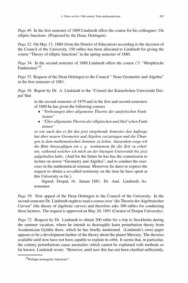
4. Notes on five 19th century Tartu mathematicians 305
Page 49. In the first semester of 1889 Lindstedt offers the course for his colleagues: Onelliptic functions. (Proposed by the Dean, Oettingen).
Page 52. On May 13, 1880 (from the District of Education) according to the decision ofthe Council of the University, 150 rubles has been allocated to Lindstedt for giving thecourse “Theory of elliptic functions” in the spring semester of 1880.
Page 54. In the second semester of 1880 Lindstedt offers the course (?) “MorphischeFunktionen”35.
Page 55. Request of the Dean Oettingen to the Council “ Neue Geometrie und Algebra”in the first semester of 1881.
Page 56. Report by Dr. A. Lindstedt to the “Conseil der Kaiserlichen Universität Dor-pat”that
in the second semester of 1879 and in the first and second semestersof 1880 he has given the following courses• “Vorlesungen über allgemeine Theorie der analytischen Funk-
tionen”• “Über allgemeine Theorie der elliptischen und Abel’schen Funk-
tionen”so wie auch das er für das jetzt eingehende Semester den Auftragehat über neuere Geometrie und Algebra vorzutragen und die Übun-gen in dem mathematischen Seminar zu leiten. Ausserdem wage ichdie Bitte hinzuzufügen ein s. g. testimonem für die Zeit zu erhal-ten, während welcher ich mich an der hiesigen Universität bis jetztaufgehalten habe. (And for the future he has has the commission tolecture on newer “Geometry and Algebra”, and to conduct the exer-cises in the mathematical seminar. Moreover, he dares to express therequest to obtain a so-called testimony on the time he have spent atthis University so far ).
Signed: Dorpat, 16. Januar 1881. Dr. And. Lindstedt, As-tronomer.
Page 59. New appeal of the Dean Oettingen to the Council of the University. In thesecond semester Dr. Lindstedt ought to read a course over “die Theorie der AlgebraischerCurven” (the theory of algebraic curves) and therefore asks 300 rubles for conductingthese lactures. The request is approved on May 20, 1891 (Curator of Dorpat University).
Page 72. Request by Dr. Lindstedt to obtain 200 ruble for a trip to Stockholm duringthe summer vacation, where he intends to thoroughly learn perturbation theory fromAcademician Gyldén there, which he has briefly mentioned. (Lindstedt’s own) paperappears to be a development further of the theory about the planet Mercury. The theoriesavailable until now have not been capable to explain its orbit. It seems that, in particular,the century perturbations cause anomalies which cannot be explained with methods sofar known. Lindstedt wrote: “However, until now this has not been clarified sufficiently,
35Perhaps monogenic functions?

306 CHAPTER V. HISTORY OF MATHEMATICS
and so I have begun to compute anew the perturbations of Mercury using the theory ofHansen36, and almost completed the computations of the perturbations of Venus and theEarth. Among the other planets only Jupiter may have a more significant influence and,regarding it, I have the hope to finish completely before the beginning of the summer,so that it will be possible to see how sufficient is the method that I applied. Otherwisethe method suggested by Academician Gyldén should be viewed as the only one whichcan lead to a complete success. By these reasons and on the request of the the Physico-Mathematical Faculty to give lectures describing the main features of this method as anexample of application of elliptic functions, I would like to ask the Council to supportmy appeal.“
On April 14, he obtains this permit.
Page 79. On May 23, 1882, the decision is made by the Curator Saburov for the Councilof the Imperial Dorpat University to pay to astronomer Lindstedt 300 rubles for his lec-tures course “Theory of analytic functions”, and for conducting the mathematical seminar(from special sources of the University).
[On May 20, one can see the name of Weihrauch in the Council of the University andon this day there was there a voting in favor of Lindstedt’s trip in the summer vacation.]
Page 90. On Dec. 10, 1882 once more 300 rubles is allocated for lectures and the con-ducting the seminar.
Page 92. On May 5, 1883 there is again a demand of Dean Oettingen to pay 300 ruble(200 + 100) to Anders Lindstedt for lectures on “Newer Geometry and Algebra” and fordirecting the seminar.
Page 98. Below there is the proposal for acquiring for Dr. A. Lindstedt the degree ofprofessor, May 13, 1883.
From the Dean’s proposal to present A. Lindstedt as the single candidate to theposition of professor of applied mathematics, opening up on August 12, as an ordinaryprofessor:
Lindstedt was born in Sundborn on July 27, 1854 near Falun in Swe-den, and got his first education . . . . On Sept. 16, 1872 he enteredLund University. He became a Candidate of Philosophy on May 231874 and was, from July on until June 1875, an astronomer at Ham-burg Observatory. The stay in Hamburg was followed by the summersemester in Leipzig. Upon his return to Lund he became a Licentiateof Philosophy on May 28 1877, and a Doctor of Philosophy on June6, 1877, among the promovendi had the position of first auster. OnAug. 1, 1877, he became private docent in Lund, and from there hegot an invitation for a position of Astronomer in Dorpat on May 27,1879.
36Peter Andreas Hansen (1795-1874), Danish born self-taught astronomer, worked at the Gotha Observa-tory. Developed a perturbation theory together with Palowsky. Karl Rudolph Palowsky (1817-1881), Germanastronomer, was the assistant of Hansen in 1850-56, moved later to Washington, died there.
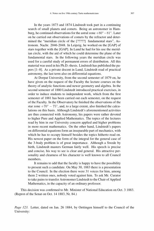
4. Notes on five 19th century Tartu mathematicians 307
In the years 1873 and 1874 Lindstedt took part in a continuingsearch of small planets and comets. Being an astronomer in Ham-burg, he continued observations for the astral zone +80◦−81◦. Lateron he carried out observations of comets by the refractor and deter-mined the “meridian circle of the [?????] fundamental stars”, As-tronom. Nachr. 2046-2048. In Leipzig, he worked on the [GAP] ofstars together with the [GAP]. In Lund he had for his use the merid-ian circle, with the aid of which he could determine the plane of thefundamental stars. In the following years the meridian circle wasused for a careful study of permanent errors of distribution. All thismaterial was used in his Ph.D.-thesis. Lindstedt has published the pa-pers [1–8]. As a private docent in Lund, Lindstedt read of practicalastronomy, the last term also on differential equations.
At Dorpat University, from the second semester of 1879 on, hehave given on the request of the Faculty the lecture courses on thetheory of analytic functions and newer geometry and algebra. In thesecond semester of 1880 Lindstedt introduced practical exercises, inorder to induce students to independent work, which from the firstsemester of 1881 has been carried out each semester, on the requestof the Faculty. In the Observatory he finished the observations of thestar zone +70◦ − 75◦, and, to a large extent, also finished the calcu-lations on this basis. Although Lindstedt’s aforementioned activitiesare thus connected with Astronomy, his papers were rather devotedto higher Pure and Applied Mathematics. The topics of the lecturesread by him in our University concern applied and higher problemsin more recent mathematics. On the other hand, Lindstedt’s paperson differential equations form an inseparable part of mechanics, withwhich he has to occupy himself besides the topics hitherto read on.His newest paper on the form of the integral for the general case ofthe 3-body problem is of great importance. Although a Swede bybirth, Lindstedt masters German fairly well. His speech is preciseand concise, his way to see is clear and general. His attractive per-sonality and clearness of his character is well known to all Councilmembers.
It remains to add that the faculty is happy to have the possibilityto present such a candidate. On May 30, 1883 there is a presentationto the Council. In the election there were 31 voices for him, amongthem 2 written ones, nobody voted against him. To ask Mr. Curatorto take pains to transfer Astronomer Lindstedt to the Chair of AppliedMathematics, in the capacity of an ordinary professor.
This decision was confirmed to Mr. Minister of National Education on Oct. 3 1883.(Reprot of the Senat on Oct. 14 1883, Nr. 84.)
Page 123. Letter, dated on Jan. 26 1884, by Oettingen himself to the Council of theUniversity:
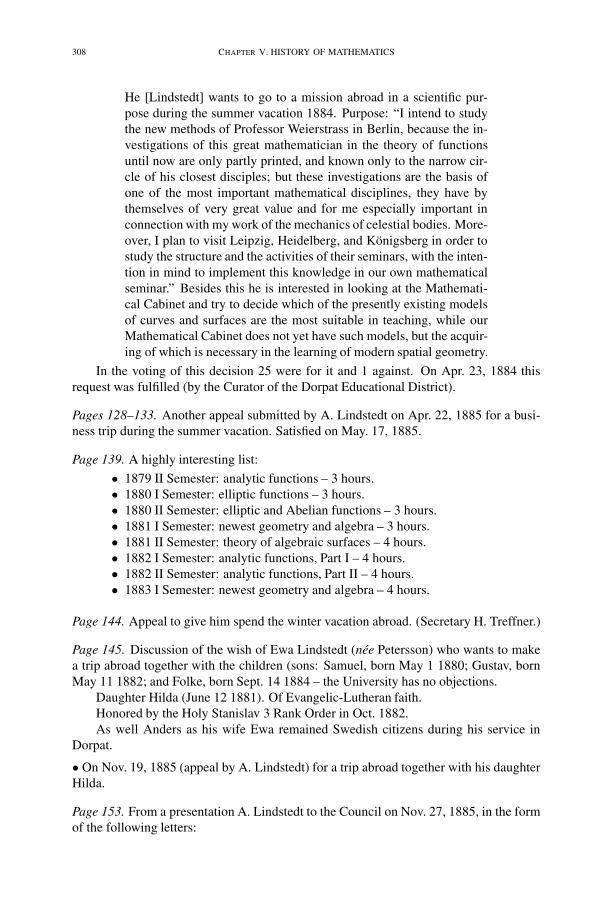
308 CHAPTER V. HISTORY OF MATHEMATICS
He [Lindstedt] wants to go to a mission abroad in a scientific pur-pose during the summer vacation 1884. Purpose: “I intend to studythe new methods of Professor Weierstrass in Berlin, because the in-vestigations of this great mathematician in the theory of functionsuntil now are only partly printed, and known only to the narrow cir-cle of his closest disciples; but these investigations are the basis ofone of the most important mathematical disciplines, they have bythemselves of very great value and for me especially important inconnection with my work of the mechanics of celestial bodies. More-over, I plan to visit Leipzig, Heidelberg, and Königsberg in order tostudy the structure and the activities of their seminars, with the inten-tion in mind to implement this knowledge in our own mathematicalseminar.” Besides this he is interested in looking at the Mathemati-cal Cabinet and try to decide which of the presently existing modelsof curves and surfaces are the most suitable in teaching, while ourMathematical Cabinet does not yet have such models, but the acquir-ing of which is necessary in the learning of modern spatial geometry.
In the voting of this decision 25 were for it and 1 against. On Apr. 23, 1884 thisrequest was fulfilled (by the Curator of the Dorpat Educational District).
Pages 128–133. Another appeal submitted by A. Lindstedt on Apr. 22, 1885 for a busi-ness trip during the summer vacation. Satisfied on May. 17, 1885.
Page 139. A highly interesting list:
• 1879 II Semester: analytic functions – 3 hours.• 1880 I Semester: elliptic functions – 3 hours.• 1880 II Semester: elliptic and Abelian functions – 3 hours.• 1881 I Semester: newest geometry and algebra – 3 hours.• 1881 II Semester: theory of algebraic surfaces – 4 hours.• 1882 I Semester: analytic functions, Part I – 4 hours.• 1882 II Semester: analytic functions, Part II – 4 hours.• 1883 I Semester: newest geometry and algebra – 4 hours.
Page 144. Appeal to give him spend the winter vacation abroad. (Secretary H. Treffner.)
Page 145. Discussion of the wish of Ewa Lindstedt (née Petersson) who wants to makea trip abroad together with the children (sons: Samuel, born May 1 1880; Gustav, bornMay 11 1882; and Folke, born Sept. 14 1884 – the University has no objections.
Daughter Hilda (June 12 1881). Of Evangelic-Lutheran faith.Honored by the Holy Stanislav 3 Rank Order in Oct. 1882.As well Anders as his wife Ewa remained Swedish citizens during his service in
Dorpat.
• On Nov. 19, 1885 (appeal by A. Lindstedt) for a trip abroad together with his daughterHilda.
Page 153. From a presentation A. Lindstedt to the Council on Nov. 27, 1885, in the formof the following letters:
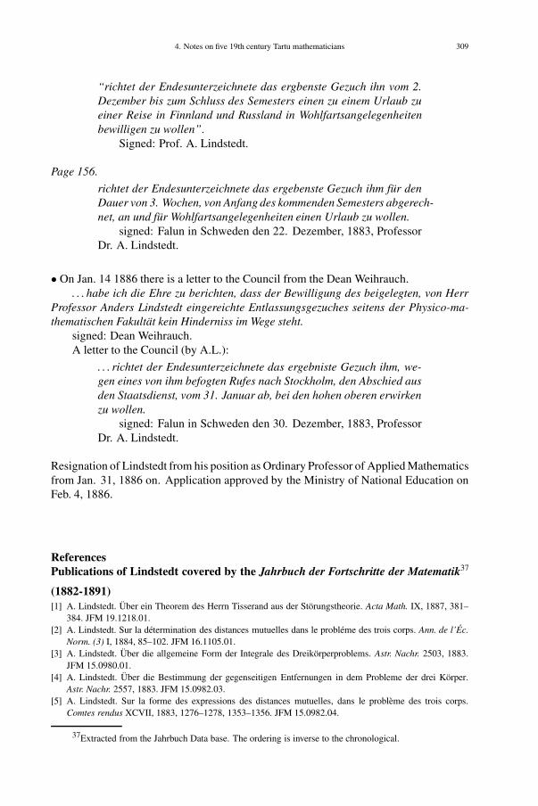
4. Notes on five 19th century Tartu mathematicians 309
“richtet der Endesunterzeichnete das ergbenste Gezuch ihn vom 2.Dezember bis zum Schluss des Semesters einen zu einem Urlaub zueiner Reise in Finnland und Russland in Wohlfartsangelegenheitenbewilligen zu wollen”.
Signed: Prof. A. Lindstedt.
Page 156.
richtet der Endesunterzeichnete das ergebenste Gezuch ihm für denDauer von 3. Wochen, von Anfang des kommenden Semesters abgerech-net, an und für Wohlfartsangelegenheiten einen Urlaub zu wollen.
signed: Falun in Schweden den 22. Dezember, 1883, ProfessorDr. A. Lindstedt.
• On Jan. 14 1886 there is a letter to the Council from the Dean Weihrauch.. . . habe ich die Ehre zu berichten, dass der Bewilligung des beigelegten, von Herr
Professor Anders Lindstedt eingereichte Entlassungsgezuches seitens der Physico-ma-thematischen Fakultät kein Hinderniss im Wege steht.
signed: Dean Weihrauch.A letter to the Council (by A.L.):
. . . richtet der Endesunterzeichnete das ergebniste Gezuch ihm, we-gen eines von ihm befogten Rufes nach Stockholm, den Abschied ausden Staatsdienst, vom 31. Januar ab, bei den hohen oberen erwirkenzu wollen.
signed: Falun in Schweden den 30. Dezember, 1883, ProfessorDr. A. Lindstedt.
Resignation of Lindstedt from his position as Ordinary Professor of Applied Mathematicsfrom Jan. 31, 1886 on. Application approved by the Ministry of National Education onFeb. 4, 1886.
[10],[11],[12],[14]
ReferencesPublications of Lindstedt covered by the Jahrbuch der Fortschritte der Matematik37
(1882-1891)[1] A. Lindstedt. Über ein Theorem des Herrn Tisserand aus der Störungstheorie. Acta Math. IX, 1887, 381–
384. JFM 19.1218.01.[2] A. Lindstedt. Sur la détermination des distances mutuelles dans le probléme des trois corps. Ann. de l’Éc.
Norm. (3) I, 1884, 85–102. JFM 16.1105.01.[3] A. Lindstedt. Über die allgemeine Form der Integrale des Dreikörperproblems. Astr. Nachr. 2503, 1883.
JFM 15.0980.01.[4] A. Lindstedt. Über die Bestimmung der gegenseitigen Entfernungen in dem Probleme der drei Körper.
Astr. Nachr. 2557, 1883. JFM 15.0982.03.[5] A. Lindstedt. Sur la forme des expressions des distances mutuelles, dans le problème des trois corps.
Comtes rendus XCVII, 1883, 1276–1278, 1353–1356. JFM 15.0982.04.
37Extracted from the Jahrbuch Data base. The ordering is inverse to the chronological.

310 CHAPTER V. HISTORY OF MATHEMATICS
[6] A. Lindstedt. Über die Integration einer gewissen Differentialgleichung. Astr. Nachr. 2482, 1883. JFM15.0983.01.
[7] A. Lindstedt. Beitrag zur Integration der Differentialgleichungen der Störungstheorie. Petersburg undLeipzig Voss’s Sortiment, 1883. JFM 15.0983.02.
[8] A. Lindstedt. Zur Theorie der Fresnel’schen Integrale. Wiedemann Ann. (2) XVII, 1882, 720–725. JFM14.0836.01.
Other publications of Lindstedt[9] A. Lindstedt. Undersökning av meridiancirkeln påLunds observatorium jemte bestemning af densammas
polhöjd. (Investigation of the meridian circle at Lund Observatory, together with a determination of itspolar height.) In: Thesis, Lund, 1877. Also: Lunds Universitets Årskrift, 13 (1876-77).
[10] A. Lindstedt. Beobachtungen des Mars während seiner Opposition 1877 angestellt auf der sternwarte zuLund. In: Lunds Universitets Årskrift, 14, Lund, 1876.
Auxiliary references[11] Svenskt biografiskt Lexikon XIII, 1898, 612–617.[12] Svensk Uppslagsbok (Swedish Encyclopedia).[13] Nationalencyklopedin (Swedish National Encyclopedia).[14] B. Lindblad. Anders Lindstedt, obituary. Populär Astronomisk Tidskrift 20 (3–4), 1939, 134–135.

4. Notes on five 19th century Tartu mathematicians 311
Theodor Molien (1861-1941)38
Molien was born in Riga in a family of Swedish decent. He stud-ied in Dorpat, and in Leipzig, taking part in Lie’s famous seminar.He became a docent in Dorpat in 1885. Unable to get a professor-ship elsewhere he moved to Tomsk (in Siberia) in 1900, and livedthere for the rest of the life, and died there. Although generally littleknown, Molien has to be viewed as a pioneer in contemporary alge-bra. For more details about this, see the previous paper Uno Kalju-laid, “Theodor Molien, about his life and mathematical work as seena century later. (A biographical sketch and a glimpse of his work.)”in Section 3 of this Chapter, as well as the book by Kanunov quotedthere. For a short but excellent biography of Molien, also summariz-ing well his scientific achievements, we refer to Bashmakova [1].
“A Big folder” no 2333: January 18, 1880 – January 17, 1901.
Theodor Georg Andreas Molien, born on August 29, 1861 (Riga).
Service record:
Councillor of State, Doctor of Pure Mathematics Fedor EduardovichMolien, Docent of Mathematics, 39 years and by birth of Evangelic-Lutheran faith, Knight of the Order of the Holy Stanislav III class.Has the Government Medal of Alexander III.
• Has a salary 1200 rubles a year.
38Editor’s Note. After this paper was completed (May 2004), we became aware of the thesis ofL. B. Stiller [3]. There there is an interesting historical note about Theodor Molien (and Friedrich Amel-ing) [3, Sec. 6.1.3, p. 76–82]. In particular, Molien’s achievements as a theoretician of chess of note arediscussed there, something which Kanunov [2] and other of his biographers seem to have overlooked.

312 CHAPTER V. HISTORY OF MATHEMATICS
•Having finished the complete course at the University of Dorpat/Yurjev,he was nominated for the degree of Candidate of Astronomy (August5, 1883) and for the degree of Master of Pure Mathematics by theCouncil of the University (October 24, 1885; he defended his Mas-ter’s thesis which was also certified by the Council on October 29,1885).
• On November 29, 1885 he was appointed (on the basis of a deci-sion of the Council) to a Docent of Mathematics at the Universitymentioned. On December 20, 1888 he was appointed to the rank ofCourt Councillor (November 19, 1885) and to the rank of CollegiateCouncillor (November 19, 1888).
• He has not participated in war, has not been punished.
• Travel abroad.- In 1886 Molien was abroad during the summer break;- In 1887 Molien was abroad during the summer break and like-
wise during the winter break;- In 1889 Molien was abroad during the summer;- In 1898 Molien was abroad during the summer;- In 1899 Molien was abroad during the summer.
•Married to: Elise, née Baranius
• Children:- son Benedikt October 20, 1895;- daughter Elise March 28, 189439.
• In 1892 he was sent to Moscow University during the first semesterwith the object to improve his Russian.
• September 30, 1892. The Council of the University conferred himthe degree of doctor of pure mathematics.
• November 19, 1893. From the last year nominated for State Coun-cillor.
• January 1, 1899. For diligent service and special work he wasgiven the Order of St. Stanislav of of the 3-d degree.
• August 11, 1899. He is sent abroad on a scientific mission with theRobert grant during the second semester.
•December 16, 1900. He is appointed to ordinary professor of math-ematics at Tomsk University of Technology (from September 1, 1900on).
39Petr Krylov and Aleksandr Nikolskiı in Tomsk have kindly communicated to me the following infor-mation: F. E. Molin had a son and a daughter. The son, Benedikt, was killed in a battle of the Civil War in1919. Elise was an assistant professor of the Department of Classical Philology in Tomsk State University. Shedied in 1988 and had no children. The family archive was acquired by the Scientific Library of Tomsk StateUniversity in 1994. Unfortunately, the documents of the archive are not sorted yet. For this reason, the archiveis unavailable for investigators.
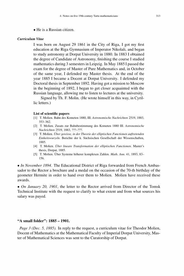
4. Notes on five 19th century Tartu mathematicians 313
• He is a Russian citizen.
Curriculum Vitae
I was born on August 29 1861 in the City of Riga, I got my firsteducation at the Riga Gymnasium of Imperator Nikolaıi, and beganto study astronomy at Dorpat University in 1880. In 1883 I obtainedthe degree of Candidate of Astronomy, finishing the course I studiedmathematics during 3 semesters in Leipzig. In May 1885 I passed theexam for the degree of Master of Pure Mathematics and, in Octoberof the same year, I defended my Master thesis. At the end of theyear 1885 I became a Docent at Dorpat University. I defended myDoctoral thesis in September 1892. Having got a mission to Moscowin the beginning of 1892, I began to get closer acquainted with theRussian language, allowing me to listen to lectures at the university.
Signed by Th. F. Molin. (He wrote himself in this way, in Cyril-lic letters.)
[1], [2],[3],[4],[5]List of scientific papers[1] T. Molien. Bahn des Kometen 1880, III. Astronomische Nachrichten 2519, 1883,
353–362.[2] T. Molien. Zusats zur Bahnbestimmung des Kometen 1880 III. Astronomische
Nachrichten 2519, 1883, ???–???.[3] T. Molien. Über gewisse, in der Theorie der elliptischen Functionen auftretenden
Einheitswurzeln. Berichte der k. Sächsischen Gesellschaft der Wissenschaften,1885.
[4] T. Molien. Über lineare Transformation der elliptischen Functionen. Master’sthesis, Dorpat, 1885.
[5] T. Molien. Über Systeme höherer komplexen Zahlen. Math. Ann. 41, 1893, 83–156.
• In November 1894. The Educational District of Riga forwarded from French Ambas-sador to the Rector a brochure and a medal on the occasion of the 70-th birthday of thegeometer Hermite in order to hand over them to Molien. Molien have received theseawards.
• On January 20, 1901, the letter to the Rector arrived from Director of the TomskTechnical Institute with the request to clarify to what extent and from what sources hissalary was payed.
“A small folder”: 1885 – 1901.
Page 3 (Dec. 5, 1885). In reply to the request, a curriculum vitae for Theodor Molien,Docent of Mathematics at the Mathematical Faculty of Imperial Dorpat University, Mas-ter of Mathematical Sciences was sent to the Curatorship of Dorpat.

314 CHAPTER V. HISTORY OF MATHEMATICS
Page 8.
Service record constituted in 1887 (1888?).
A docent, 26 years of age, of Evangelic-Lutheran faith, has no dis-tinguishing signs, has a salary of 900 rubles.
. . . “Having finished the science curriculum at Dorpat Universitywith the degree of Candidate of Astronomy in 1883, he obtained in1885 at the same university the degree of Master of Sciences in math-ematical sciences. From November 29, 1885 on (Nr. 5999) promotedto docent at the Mathematical Faculty of Dorpat University.
He was on vacation abroad: 1886 during the summer break,1887 at the time of the whole winter vacation and remained duringthe term.
Unmarried.”
Page 10. On May 5, 1890 there is an order “To the Board of the Imperial Public Library”:
American Journal of Mathematics, Vol. IV, 1881. 40
He asks for the possibility to keep it for 2 weeks, the journalnamed is needed for scientific work.
Signature: Docent Master Th. Molien. The answer arrives onMay 5, 1890 (in the library there is no such delivery). This is fol-lowed by a letter.
Page 12. The request from Th. Molien to the Highly Honored Board (der KaiserlichenUniversität Dorpat) to obtain from Imperial Academy of Sciences for not very long timethe following books, which are needed in his research as a docent41:
(1) Proceedings of the American Acad. of Arts and Sciences II ser., vol. II, 1867-73.
(2) Proceedings of the American Acad. of Arts and Sciences, vol. X, XI, 1875.(3) American Journal of Mathematics, Vol. IV, 1881.
• On January 18, 1901, letter of the Chancellor the Dorpat Educational District (fromJan. 15, Nr. 294, Riga) to the Council of the University confirming that in accordance ofthe Order no 83 dated December 16, 1900, F.Molin has been appointed to the position ofordinary professor at Tomsk university of Technology.
Page 15. The Rector’s letter to the Director of the Tomsk Technical Institute from January22, 1901, where he makes a complaints and asks to reimburse 49 rubles paid to Molienas salary for December 16, 1900 – Jan. 1, 1901, and send this sum as fast as possible toYurjev University. The letter refers to § 5 of Chapter 1 of the Order issued by the Ministryof National Education (to pay a docent’s salary of 1200 rubles a year). Thereafter
Page 16. The Rector’e letter to the Department of National Education (from January 15,1901, Nr. 294, Riga) that begins with the same story, and then at the end comes a note:
40This Volume to contains a posthumous paper by Benjamin Peirce (1809-1880). It has the title “LinearAssociative Algebra. With Notes and Addenda by C.S. Peirce, son of the Author” (pp. 97-229).
41The last one is a paper by B. Peirce entitled “Linear associative algebras”. It may be conceived that theformer two also contain also reports by the same author.

4. Notes on five 19th century Tartu mathematicians 315
“According to this, I inform the Department of National Education that if this sumwould come in time to the University, it will be transferred to the Department, accordingto the official regulation No. 28984 from November 30, 1898.”
Page 17. However, the 392 rubles was received. About this there is also given a receipt.
Page 18. Now follows a letter from Tartu University (by the Rector?) to the Departmentof National Education that there is a letter from Molien, saying that he has obtained asalary of 392 rubles on the position of docent from September 1, 1900 to January 1,1901.
ReferencesPublications of Molien)
See the bibliography of the paper “Theodor Molien, about his life and mathematicalwork . . . ”, this Volume, Section 3.
Other references[1] I. G. Bashmakova. Fedor Eduardovich Molin. In: Dictionary of scientific biography, Vol. IX. Charles
Scribner’s Sons, New York, 1974, 457–458.[2] N. F. Kanunov. Fedor Eduardovich Molien. Nauka, Moscow, 1983.[3] L. B. Stiller. Exploiting symmetry on parallel architectures, Ph. D. thesis. John Hopkins University, Balti-
more, Maryland, 1995.

This page intentionally left blank

4. Notes on five 19th century Tartu mathematicians 317
Karl Weihrauch (1841-1891)42
Karl Weihrauch (also Carl Wayrauch) was born in Mainz, Germanyin 1841. He studied first at Heidelberg and the at Giessen, wherehe got his Ph.D. in in 1860, and went to Livonia43 in 1862, wherehe worked as Senior Teacher (Oberlehrer) of mathematics at vari-ous secondary schools: from 1862 on at the Private Gymnasium inBirkenruh near Wenden (Latvian: Cesis) and then from 1862 on atthe Crown Gymnasium (Kronsgymnasium) in Ahrensburg 44 In 1869Weihrauch defended a master’s thesis at Dorpat/Tartu, on a problemdealing with partitions. The question concerns the number fn(A) ofsolution to the Diophantine equation
a1x1 + · · ·+ anxn = A.
Subsequently he published several papers on this or related problemsof algebra in Schlömilch’s Zeitschrift für Mathematik Later he servedas a Professor of Physical Geography and Meteorology in Dorpat, allthe time continuing to publish mathematical papers also.
42Editor’s Note. In German, the name means “myrrh”.43Historical province comprising most of present day Estonia and Latvia. The Livonian were a Fenno-
Ugrian people who around 1200 AD lived on both side of the Gulf of Riga; the City of Riga was founded bythe Germans on their territory in 1201; today this people, and their language (close to Estonian) is practicallyextinct.
44Town nowadays called Kuressaare (Kingissepp in Soviet times, named after the Estonian revolutionaryViktor Kingissepp (1888–1922), executed after the abortive communist coup in 1922) on the island Saaremaa(Ösel).

318 CHAPTER V. HISTORY OF MATHEMATICS
“A big folder” no 3183, Stock 402 no. 3/277.
Page 9. Dr. Carl Weyhrauch (Weihrauch Johann-Karl-Friedrich Filippovich) was bornin Mainz on November 23, 1841. Has received a certificate from Pastor Bauder of theEvangelic Congregation in Mainz on November 20, 1862 (that he has begun as a servantof this religious belief and been confirmed, being admitted to The Holy Secret [?????] in1850.)
Page 11. In 1875 a German passport had been issued to him.
Page 23. Dr. Weihrauch was until 1871 (on February 12, 1871 there is a letter to theCouncil of the University about this) senior teacher of mathematics at the AhrensburgGymnasium. He was then promoted to Docent of Physics of the Earth at the University(from July 1, 1871 on).
Page 36. On September 25, 1871 asks the Council of the University for an allowanceof 100 rubles, to cover his expenses in connection with his moving from Ahrensburg toDorpat.
Page 48. There is a record with some previously approved applications by DocentWeihrauch to send him to a vacation abroad so that he could acquaint himself with someobservatories.
He obtains permission in order to improve his health, and to recover his strength (onthe basis of a new application) for 29 days (he had pneumonia and was recovering froma throat infection), but he needs medical treatment and he ought to abstain from lecturingthis term and seek a better climate. That this should be for a longer period in the Southis demanded by his doctor. He went to Trieste in the summer of 1874, and he asks nowfor a prolongation of his sojourn there.
He read on the following subjects: meteorology; physical geography; terrestrialmagnetism; algebraic analysis; determinants; continued fractions; Diophantine [unde-termined] equations; and practical work. During these three years he has done manymeteorological observations, each day 6 times, and corresponding calculations, whichhave been presented in print, and in numerous reports.
Concerning mathematics he has sent for printing to Zeitschrift für Mathematik anexpansion of material contained in Chapter 1 of his master’s thesis, as well as 2 papersto the journal Determinantenlehre [24]. From this it can be drawn the conclusion thatgreat powers are hidden in him. However, as Doc. Weihrauch has not published anymonograph in meteorology or in the field of mathematics, the Faculty is not going topropose him for a position of ordinary professor but proposes him for a position of extraordinary professor of meteorology and physical geography (this position was opened onJanuary 1, 1875). On December 26, 1874 there was an election, and in the ballot 32 ofthe votes were in favor of him and nobody was against (this was ratified by the Ministerof Education Count Tolstoı on March 29, 1875).
Page 88. On November 6, 1875 Weihrauch asks for a possibility to spend the winterholidays abroad. This was satisfied on December 4, 1875.

4. Notes on five 19th century Tartu mathematicians 319
Presentation of the Physico-Mathematical Faculty on March 3, 1877 in the Council of the Uni-versity
From his election to extra-ordinary professor of meteorology and physical geogra-phy at the end of 1874 on, Weihrauch did not only keep all instruments in good shape,but also repaired them and increased their number. On the top of the 6 usual daily ob-servation he added 2 more hours. He has published in the Dorpater MeteorologischeBeobachtungen in 1874 and 1875. In connection with these observations one can relyon the absolute exactness and in all data, provided by professor Weihrauch. This isconnected with his methodical control of the computations. Also there are the 10 yearaverages, a comprehensive paper, which was sent to the printer this year. Of great interestis also the influence of the moon’s position on weather. This occupies him already fortwo years and involves a lot of calculating.
During the past two years Weihrauch has published, in the area of pure mathematicsthe following:
(1) Über unimodulare Determinanten.(2) Ueber die allgemeine unbestimte Gleichung mit vier Unbekanten.(3) Theorie der Restproductsumme
1. (These 3 papers are printed in Schlömilchs Zeitschrift für Mathematik und Physik.45.)The Faculty expressed its opinion over the unprecedented educational gifts of Pro-
fessor Weihrauch. In this connection they propose him for a promotion to an ordinaryprofessor. The election took place on March 8, 1877 (32 for him, 2 of them in letter form,no voices against).
Page 113. On November 9, 1878 he asks for permission to be sent abroad for 6 monthswith a scientific purpose, beginning January 1, 1879 to acquaint himself with some cen-tral observatories with meteorological surveys. This was granted on December 13, 1878in the Ministry of Education (The Curator Saburov46). On January 31, 1879 there arrivesa letter from Weihrauch, already in Trieste. [He had the intention also to participate inthe Congress of Meteorology. This took place in Rome in April 1879, and the Facultyallocated to him 400 rubles for this purpose. In the voting there were 30 for him, and3 against.] In the summer of 1881 he asks for permission to spend his vacation abroadbecause of personal reasons. In the summer of 1884 the same procedure is repeated.
Page 162. Professor Weihrauch and Professor von Kennel 47 ask during the summervacation 400 rubles for investigating Lake Peipus48 from the point of view of zoologyand physical geography (32 for him, 1 against). For many years naturalists in Germany,Switzerland and France have been engaged in the study small or big inland bodies of wa-ter. Therefore we have the following goal: an exact determination of the fauna; openingup, hitherto unknown lower supplies; the spread of horizontal as well as lower animals;their resettling. Connection with fish. Great praise and explanation why Lake Peipus sospecial. This was approved on April 17, 1889.
45This seems to be preliminary titles of the papers in view; see the References below.46Andreı Saburov was appointed Curator of the University in 1875. In 1880 he became Minister of
National Education. [39, p. 121.]47Julius Thomas von Kennel, was appointed professor of zoology at Dorpat University in 1886; he had
previously been private docent at Würzburg University. [39, pp. 194, 270, 347, 357].48Big lake forming the frontier between Estonia and Russia.
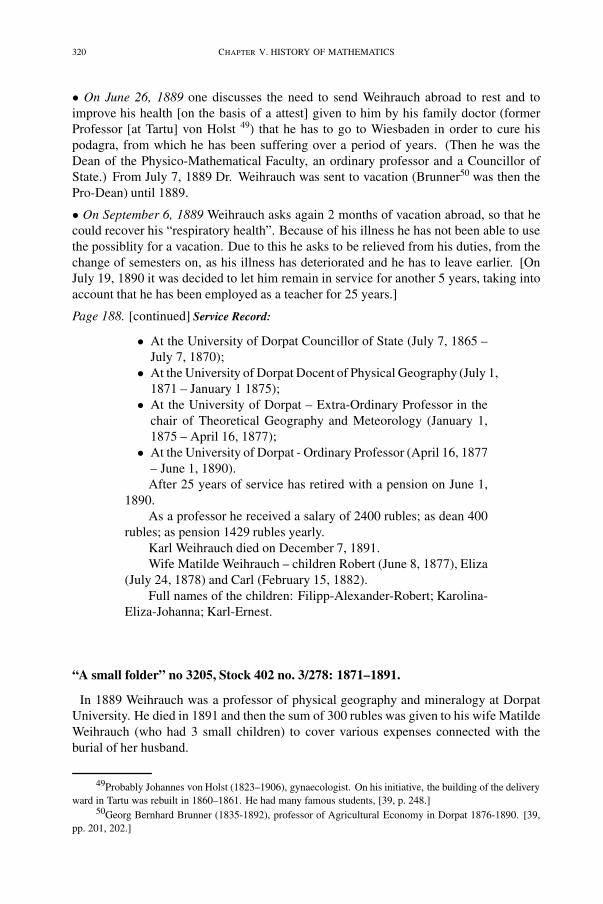
320 CHAPTER V. HISTORY OF MATHEMATICS
• On June 26, 1889 one discusses the need to send Weihrauch abroad to rest and toimprove his health [on the basis of a attest] given to him by his family doctor (formerProfessor [at Tartu] von Holst 49) that he has to go to Wiesbaden in order to cure hispodagra, from which he has been suffering over a period of years. (Then he was theDean of the Physico-Mathematical Faculty, an ordinary professor and a Councillor ofState.) From July 7, 1889 Dr. Weihrauch was sent to vacation (Brunner50 was then thePro-Dean) until 1889.
• On September 6, 1889 Weihrauch asks again 2 months of vacation abroad, so that hecould recover his “respiratory health”. Because of his illness he has not been able to usethe possiblity for a vacation. Due to this he asks to be relieved from his duties, from thechange of semesters on, as his illness has deteriorated and he has to leave earlier. [OnJuly 19, 1890 it was decided to let him remain in service for another 5 years, taking intoaccount that he has been employed as a teacher for 25 years.]
Page 188. [continued] Service Record:
• At the University of Dorpat Councillor of State (July 7, 1865 –July 7, 1870);
• At the University of Dorpat Docent of Physical Geography (July 1,1871 – January 1 1875);
• At the University of Dorpat – Extra-Ordinary Professor in thechair of Theoretical Geography and Meteorology (January 1,1875 – April 16, 1877);
• At the University of Dorpat - Ordinary Professor (April 16, 1877– June 1, 1890).After 25 years of service has retired with a pension on June 1,
1890.As a professor he received a salary of 2400 rubles; as dean 400
rubles; as pension 1429 rubles yearly.Karl Weihrauch died on December 7, 1891.Wife Matilde Weihrauch – children Robert (June 8, 1877), Eliza
(July 24, 1878) and Carl (February 15, 1882).Full names of the children: Filipp-Alexander-Robert; Karolina-
Eliza-Johanna; Karl-Ernest.
“A small folder” no 3205, Stock 402 no. 3/278: 1871–1891.
In 1889 Weihrauch was a professor of physical geography and mineralogy at DorpatUniversity. He died in 1891 and then the sum of 300 rubles was given to his wife MatildeWeihrauch (who had 3 small children) to cover various expenses connected with theburial of her husband.
49Probably Johannes von Holst (1823–1906), gynaecologist. On his initiative, the building of the deliveryward in Tartu was rebuilt in 1860–1861. He had many famous students, [39, p. 248.]
50Georg Bernhard Brunner (1835-1892), professor of Agricultural Economy in Dorpat 1876-1890. [39,pp. 201, 202.]
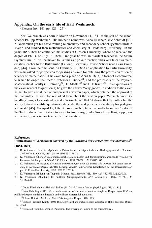
4. Notes on five 19th century Tartu mathematicians 321
Appendix. On the early life of Karl Weihrauch.(Excerpt from [41, pp. 123–125])
Karl Weihrauch was born in Mainz on November 11, 1841 as the son of the schoolteacher Philipp Weihrauch. His mother’s name was Anna Elisabeth, née Schmidt [43].K. Weihrauch got his basic training (elementary and secondary school (gymnasium)) inMainz, and studied then mathematics and chemistry at Heidelberg University. In theyears 1858-1860 he continued his studies at Giessen University, where he received thedegree of Ph. D. on July 13, 1860. One year he was an assistant teacher in the MainzGymnasium. In 1861 he moved to Estonia as a private teacher, and a year later as a math-ematics teacher to the Birkenruhe (Latvian: Berzaine) Private School near Cesis (Wen-den) [44]. From here he sent, on February 17, 1863 an application to Tartu University,where he asked for permission for passing an exam for obtaining the profession of seniorteacher of mathematics. This exam took place on April 8, 1863, in front of a committee,to which belonged the Rector Professor F. Bidder51, and the professors of the Physico-Mathematical Faculty (P. Helmling52), H. Mädler53 and L. F. Kämtz54. To all questions ofthe exam (except to question 1) he gave the answer “very good”. In addition to the examhe had to give a trial lecture and present a written paper, which obtained the approval ofthe committee. It was also remarked there about the written paper “Versuch einer Be-handling einiger Gegenstände aus der Wärmelehre” that “it shows that the author has theability to treat scientific questions independently, and possesses a maturity for pedagog-ical work” [45]. On April 15, 1863 K. Weihrauch obtained an order from the Curator ofthe Tartu Educational District to move to Arensburg (under Soviet rule Kingisepp [nowKuressaare]) as a senior teacher of mathematics. [1],[2],[3],[4],[5], [6],[7],[8],[9],[10],[11],[12],[13],[14],[15], [16],[17],[18],[19],[20], [21],[22],[23],[24],[25], [27],[28],[29],[30],[31],[32],[33],[34],[35],[36], [37],[38],[39],[40],[41], [42],
ReferencesPublications of Weihrauch covered by the Jahrbuch der Fortschritte der Matematik55
(1881-1891)[1] K. Weihrauch. Über eine algebraische Determinante mit eigentümlichem Bildungsgesetz der Elemente.
Schlömilch Z. XXXVI, 1891, 34–40. JFM 23.0148.03.[2] K. Weihrauch. Über gewisse goniometrische Determinanten und damit zusammenhängende Systeme von
linearen Gleichungen. Schlömilch Z. XXXVI, 1891, 71–77. JFM 23.0151.03.[3] K. Weihrauch. Fortsetzung der neuen Untersuchungen über die Bessel’sche Formel und deren Verwen-
dung in der Meteorologie. Schriften herausg. von der Naturforscher-Gesellschaft bei der Universität Dor-pat. K. F. Koehler., Leipzig, 1890. JFM 22.1235.01.
[4] K. Weihrauch. Bildung von Taupunkt-Mitteln. Met. Zeitschr. VII, 1890, 429–432. JFM 22.1250.01.[5] K. Weihrauch. Ableitung des mittleren Sättigungsdeficits. Met. Zeitschr. VI, 1889, 73–74. JFM
21.1246.01.
51Georg Friedrich Karl Heinrich Bidder (1810-1894) was a famous physiologist. [39, p. 236.]52Peter Helmling (1817-1901), mathematician of German extraction, taught at Dorpat from 1852 on,
published papers on definite integrals and ordinary differential equations.53Johann Heinrich Mädler (1794-1874), taught at Dorpat 1840-1865.54Ludwig Friedrich Kämtz (1801-1867), physicist and meteorologist, educated in Halle, taught at Dorpat
1841-186555Extracted from the Jahrbuch Data base. The ordering is inverse to the chronological.

322 CHAPTER V. HISTORY OF MATHEMATICS
[6] K. Weihrauch. Über gewisse Determinanten. Schlömilch Z. XXXIII, 1888, 126–128. JFM 20.0148.03.[7] K. Weihrauch. Die elementaren Ableitungen des Satzes von der “ablenkenden Kraft der Erdrotation”.
Met. Zeitschr. (2) V, 1888, 81–82. JFM 20.0942.01.[8] K. Weihrauch. Neue Untersuchungen über die Bessel’sche Formel und deren Verwendung in der Meteo-
rologie. Th. Hoppe und E. J. Karow; K. F. Koehler., Dorpat, Leipzig, 1888. JFM 20.1270.01.[9] K. Weihrauch. Theorie der Restreihen zweiter Ordnung. Schlömilch Z. XXXII, 1887, 1–21. JFM
19.0179.02.[10] K. Weihrauch. Über Pendelbewegung bei ablenkenden Kräften, nebst Anwendung auf das Foucault’sche
Pendel. Exner Rep. XXII, 1886, 480–491. JFM 18.0865.01.[11] K. Weihrauch. Einfluss des Widerstandes auf die Pendelbewegung bei ablenkenden Kräften, mit Anwen-
dung auf das Foucault’sche Pendel. Exner Rep. XXII, 1886, 643–675. JFM 18.0865.02.[12] K. Weihrauch. Über die dynamischen Centra des Rotationsellipsoids mit Anwendung auf die Erde. In:
Bull. de l. Soc. Imp. d. Nat. de Moscou, Moscow, 1886, 643–675. JFM 18.0928.02.[13] K. Weihrauch. Über die Zunahme der Schwere beim Eindringen in das Erdinnere. Exner Rep. XXII, 1886,
396–401. JFM 18.1086.01.[14] K. Weihrauch. Über die Berechnung meteorologischer Jahresmittel. Mattiesen, Dorpat, 1886. JFM
18.1119.01.[15] K. Weihrauch. Über die Abweichung eines freifallenden Körpers von der Verticalen. Met. Zeitschr. II,
1885, 27–29. JFM 17.0880.02.[16] K. Weihrauch. Ein neuer Satz aus der Anemometrie. Met. Zeitschr. I, 1885, 291–293. JFM 17.1150.01.[17] K. Weihrauch. Über das Sättigungsdeficit. Met. Zeitschr. I, 1885, 260–264. JFM 17.1151.03.[18] K. Weihrauch. Über doppelt-orthosymmetrische Determinanten. Schlömilch Z. XXVI, 1881, 64–70. JFM
13.0127.01.[19] K. Weihrauch. Wert einer doppelt-orthosymmetrischen Determinanten. Schlömilch Z. XXVI, 1881, 132–
133. JFM 13.0127.02.[20] K. Weihrauch. Eine Polynomenentwickelung. Schlömilch Z. XXVI, 1881, 127–132. JFM 13.0189.01.
Other mathematical publications of Weihrauch[21] K. Weihrauch. Beiträge zur Lehre von den unbestimmten Gleichungen ersten Grades. Programm des
Gymnasium zu Ahrensburg, 1866.[22] K. Weihrauch. Untersuchungen über eine Gleichung des ersten Grades mit mehreren Unbekannten, Dor-
pat, 1869.[23] K. Weihrauch. Über die Formen, in denen die Lösungen einer diophantischen Gleichung vom ersten
Grades enthalten sind. Schlömilch Z. XIX, 1874, 53–67.[24] K. Weihrauch. Zur Determinantenlehre. Determinantenlehre, 1874.[25] K. Weihrauch. Die Anzahl der Lösungen diophantischer Gleichungen ersten mit teilerfremden Koeffizien-
ten. Schlömilch Z. XXII, 1877, 97–111.[26] K. Weihrauch. Über die Ausdrücke Σfx(m) und die Umgestalltungen der Formel für die Lösungsan-
zahlen; Anwendung der Formeln der Kombinationslehre. Schlömilch Z. XX, 1875, 112–117.[27] K. Weihrauch. Anzahl der Auflösungen einer unbestimmten Gleichung für einen Spezialfall von nicht
teilerfremden Koeffizienten. Schlömilch Z. XX, 1875, 314–316.[28] K. Weihrauch. Zur Konstruktion einer unimodularen Determinante. Schlömilch Z. XXI, 1876, ??–??.[29] K. Weihrauch. Ein Satz von ebenen Viereck. Schlömilch Z. XXVI, 1881, 1–21.[30] K. Weihrauch. Über eine algebraischen Determinante mit eigentümlichen Bildungsgesetz der Elemente.
Schlömilch Z. XXVI, 1881, 34–40.[31] K. Weihrauch. Über gewise goniometrische Determinanten und damit zusammenhängenden Bildungsgetz
Systeme von linearen Gleichungen. Schlömilch Z. XXVI, 1881, 71–77.[32] K. Weihrauch. Zusammenhang der Seiten des regelmässigen 5- und 10-Ecks mit dem Radius. Grünerts
Archiv der Mathematik und Physik 45, 1866, 355–356.[33] K. Weihrauch. Zur geometrischen Construction der vierten und der mittleren Proportionale. Grünerts
Archiv der Mathematik und Physik 46, 1866, 336–337.[34] K. Weihrauch and A. J. Oettingen. Meteorologische Beobachtungen in Dorpat 1866-70 und Kritik der
Beobachtungsmethoden, I–II, Dorpat, 1866.[35] K. Weihrauch. Anemometrischen Scalen für Dorpat. Ein Beitrag zur Klimatologie Dorpats. In: Archiv für
Naturkunde Liv-, Ehst- und Kurlands. Dorpater Natuforscher Gesellschaft, Vol. 9, Dorpat, 1885.
4. Notes on five 19th century Tartu mathematicians 323
[36] K. Weihrauch. Neue Untersuchungen über die Bessel’sche Formel und deren Verwendung in der Meteo-rologie, Dorpat, 1890.
Auxiliary references[37] J. C. Poggendorff’s biographisch-litterarisches Handwörterbuch, Dritter Band (1858 bis 1883). Barth,
Leipzig, 1898.[38] J. C. Poggendorff’s biographisch-litterarisches Handwörterbuch, Vierter Band Band (Die Jahre 1888
. . . ). Barth, Leipzig, 1904.[39] K. Siilivask (ed.) Tartu Ülikooli Ajalugu, II (1798-1918). Eesti Raamat, Tallinn, 1982. English translation
of the entire series: Karl Siilivask (ed.), History of Tartu University 1632-1982. Perioodika, Tallinn, 1985.[40] G. G. Levitskiı(ed.) Biographical Dictionary of Professors and Teachers of the Imperial Yurjev, formerly
Dorpat, University one hundred years from its foundation (1802-1902), Vol. I. K. Mattisen, Yurjev, 1902.[41] L. Kongo. Johann Karl Friedrich Weihrauch – Tartu Ülikooli esimene füüsilise geograafia ja meteo-
roloogia professor (Johann Karl Friedrich Weihrauch, the first professor of physical geography and mete-orology at Tartu University). Tartu Ülikooli ajaloo küsimusi (Questions of the History of Tartu University.)5, 1977, 123–137.
[42] E. Tammiksaar. Das Fach der Geographie an der Universität DorpatTartu in den Jahren 1802-1891. In:Jahrbuch der Akademischen gesellschaft für Deutschbaltische Kultur in Tartu (Dorpat) Band 1., Tartu,1996, 78–102. see the Section “Johann Karl Friedrich Weihrauch: Geograph oder Geophysiker?” writtenby E. Tammiksaar, pp. 20.-23.
References for the Appendix[43] Deutsch-Baltisches Biografisches Lexikon 1710-1060. Böhlau Verlag, Köln, Wien, 1970.[44] Birkenruher Album 1825-1892, St. Petersburg, 1910.[45] Archive of the Estonian Soviet State Archives,f. 402, nim. 3, s.-ü. 277, l. 15.

This page intentionally left blank

CHAPTER VI
Popularization of Mathematics

This page intentionally left blank
327
1. [K68a] and [K69b] On the geometric methods of Dio-phantine Analysis
“What’s the good of that?” said Rabbit.“Well,” said Pooh, “we keep looking for Home and not finding it, so I thoughtthat if we looked for this Pit, we’d be sure not to find it, which would be a GoodThing, because then we might find something that we weren’t looking for, whichmight be just what we were looking for, really.”
A. A. Milne, The house at Pooh corner
The domain in Number Theory which is concerned with problems and results aboutthe search of integer solutions of algebraic equations is [nowadays] referred to as Dio-phantine Analysis. Its elementary problems [early] caught the attention of many math-ematicians.1 But solutions of seemingly different problems were usually obtained eachtime by a separate artifice, so in the opinion of mathematicians “chaos” ruled there fora long time. In the course of the 20th century greater clarity about these matters wasbrought by the flourishing of algebraic geometry, the main object of study of which dis-cipline are so-called algebraic varieties. Namely, it became clear that with each algebraicequation, or system of equations, one can associate a certain algebraic variety, then thesolution, or the solutions, can be interpreted as points of this variety. The Diophantineproblem consists now of finding all points with integer or rational coordinates on it.
One may ask in which way such a geometric point of view is more advantageousthan the earlier methods used in Diophantine Analysis? The answer is the following:in the case of an algebraic variety one has to deal with a whole series of algebraic andtopological structures – it is a topological space in several different topologies, an analyticspace, a Lie group etc. The theory of structure referred to here is today very rich infundamental results and ideas, which, along with arithmetical considerations, can beused to a great advantage in the theory of equations. Algebraic Geometry provides alangauge for the clarification of these simple2 notions, as the number of unknowns in theequations, the degree of the equations, change of variables etc. The geometric methodsbrought order into the “chaos” of Diophantine Analysis, classifying them according tothe invariants of the corresponding varieties. An example of such an invariant is thedimension of the variety. In our paper we will mainly deal with one dimensional varieties,which usually are called algebraic curves. We shall here encounter more closely with the
1Translators’ note. For the history of the Diophantine analysis, see the book [1] written by I. G. Bash-makova. The traditional view has been that Diophantus wrote just a collection of problems, whereas this authoradvocates the opinion that the Greek, indeed, possessed deep insights in algebraic geometry.
2. . . and thus possessing from the point of view of Diophantine question a completely mystical meaning. . .

328 CHAPTER VI. POPULARIZATION OF MATHEMATICS
notion of algebraic curve and their classification 3. A major part of the actual materialwas obtained by L. J. Mordell, A. Weil and C. L. Siegel in the years 1920–30. TheReader will here have a chance to penetrate rather deeply into the results and problemsof the theory of elliptic curves.
I. Algebraic introduction– John, what topic did you treat in mathematics at school?.– Addition.– How much does it make, if you add three to two apples?– I do not know. We did it with oranges.
English anecdote
1.1. Number fields 4
Let us compare two rather well-known domains of numbers: the set of integers andthe set of rational numbers. They will be denoted by Z and Q, respectively. Adding,subtracting and multiplying integers, we get as a result again integers. In this senseone says that the domain of integers is closed for the three operations mentioned. Moreexactly, one says that the domain of integers Z is a ring. But division is not alwayspossible in the domain of integers. Now the question “is the integer b divisible by theinteger a?” is equivalent to the question “does the equation ax = b have a solution interms of integers?”. Therefore the ring of integers Z is an example of a commutativering such that the equation ax = b (a �= 0) does not have a solution which is also anelement of the same ring. The situation is different for the domain of rational numbersQ, which is closed with respect to division. In this domain Q each equation ax = b
(a �= 0, a, b ∈ Q) has a solution x =b
a∈ Q. Finally, we have reached a simple example
of a so-called field.A field is a commutative ring in which all equations ax = b (a �= 0) have a unique
solution; or, in other words, it is a commutative ring with a unit element such that eachelement other than zero has an inverse element. 5
As an example of a field we have the domain of rational numbers Q and the domainof real numbers R, and likewise the domain of complex numbers C = {a + bi| a, b ∈R, i =
√−1}. Complex numbers are usually identified with points in the real plane (cf.
Figure 1).
3See also [7], Section 2.4A more prepared Reader can begin with Section 1.3. Translator’s note. For an introduction to basic
notions of algebra such as group, semigroup, ring, field etc., we refer to the classical texts by B.L. van derWaerden [19], S. Lang [11], and P. M. Cohn [4]. We mention further two excellent books by A. G. Kurosh[9, 10].
5See E. Gabovitsh, Algebra põhimõisted I-V. (In Estonian: The fundamental notions of algebra). In:Mathematics and Our Age 6-10. (Translator’s note. Reprinted in the latter’s book Stories about contemporarymathematics. (Estonian) Valgus, Tartu, 1967.) See also footnote 4.

1. On the geometric methods of Diophantine Analysis 329
�
�
�
z = x + iy
x
y
0
Fig. 1
Let us give here also another less known way of presenting some other properties ofthe last field. Complex numbers can be viewed as second order square matrices. Indeed,consider the ring of real second order square matrices
R2 ={(
a bc d
), where a, b, c, d ∈ R
}.
We introduce now a one-to-one correspondence
a + bi←→(
a b−b a
).
In particular, to a real number a there corresponds a so-called scalar matrix:
a←→(a 00 a
),
and to the imaginary unit i the matrix:
i←→(
0 1−1 0
).
Making use of the recipes for adding and multiplying matrices and complex numbers, wemake sure that this correspondence establishes an isomorphism between the domain ofcomplex numbers C (each field is a ring) and a certain subring A of the ring of matricesR2. As this subring is isomorphic to the field C, it is likewise a field.
At the same time, the ring of matrices R2 is far from being a field. Indeed, it containsdivisors of zero: (
a 00 0
)(0 00 b
)=
(0 00 0
)←→ 0,
But in a field there cannot be divisors of zero. By the way, the last assertion is easy toverify: if we should have ab = 0, (a �= 0, b �= 0), the one gets b = a−1ab = a−10 = 0,that is b = 0.
In the fields Q, R and C given in the examples, there are infinitely many elements.The simplest finite field consists of two elements – the zero element and the unit elemente, with
0 · 0, 0 · e = e · 0, e · e = e,
0 + 0 = 0, 0 + e = e + 0 = e, e + e = 0.
330 CHAPTER VI. POPULARIZATION OF MATHEMATICS
We obtain a series of examples of finite fields by taking the fields of remainder classesZ/(p), where p is an arbitrary fixed prime number. They are defined as follows.
In the domain of integers Z we introduce a distribution into classes, taking into oneclass all integers, which give the same remainder upon division by p. In this way one getsthe various remainder classes 0, 1, 2, . . . p− 1; here we denote by k the class consistingof the integers p · n + k. Addition and multiplication of the classes thus gotten is deniedby the formulae
m + n ={
m + n, if m + n < p,m + n− p, if m + n ≥ p;
m · n = r, if mn = p · q + r, 0 ≤ r < p.
For example, Z/(3) consists of the classes 0, 1, 2, where
0 + 0 = 0, 0 + 1 = 1, 0 + 2 = 2; 1 + 1 = 2; 1 + 2 = 0, 2 + 2 = 1;
0 · 0 = 0, 0 · 1 = 0, 0 · 2 = 0; 1 · 1 = 1, 1 · 2 = 2; 2 · 2 = 1.
We leave it to the Reader to check that [passing to the case of general p] the set ofclasses 0, 1, 2, . . . p− 1 equipped with these operations of addition and multiplication isa field, which we denote by Z/(p).
Next, we consider an arbitrary field K . Its unit element (the solution of the equa-tion ax = a (a �= 0)) shall be denoted e. The field K being closed for addition andmultiplication, the integer multiples of the unit element±0,±e,±2e,±3e, . . . ,±ne are,similarly, elements of K .
Let us first have a look at the case when all elements ne, for different multipliersn, are all distinct. Such a field K is said to be of characteristic 0. One can make thecorrespondence e �→ 1 and verify that the ring ±0,±e,±2e,±3e, . . . is isomorphic tothe ring Z. Thus one can say that a field K of characteristic 0 contains the domain ofintegers, that is, Z ⊂ K . But K is also closed with respect to division and so contains all
fractionsm
n, m,n ∈ Z. In other words, if K is a field of characteristic 0, then Q ⊂ K .
This result tells us that all fields of characteristic 0 must be infinite. Among examples offields of characteristic 0 are the known to us domains Q, R and C.
Another logically possible case is when there exits m �= n, m,n ∈ Z such thatme = ne. Assume, for instance that m > n. As (m − n)e = 0, we deduce that thereexists a natural number u such that ue = 0. Let p be the smallest natural number suchthat pe = 0. As a field does not have zero divisors, it is easy to see that p must be prime.In this case one says that K is of characteristic p. In a similar way as above one can nowprove that each field of characteristic p contains the field of remainder classes Z/(p). Atthe same time, Z/(p) is the simplest example of a field of characteristic p.
Let there be given a field K . Each field E which contains the given field K (K ⊂ E)is called an extension of K and is written E/K . An extension E/K is called finite, ifthere exist elements α1, . . . , αm ∈ E such that each α ∈ E can be written in a uniqueway as
α = p1α1 + · · ·+ pmαm,
where pi ∈ K . Then the extension E/K may be viewed as a finite dimensional vectorspace over the base field K .

1. On the geometric methods of Diophantine Analysis 331
Next, we look at an example. The set of real numbers {p + q√
2,where p, q ∈ Q}turns out to be a field, that is, it is closed for addition, subtraction, multiplication anddivision (please, check!). Taking here q = 0 we see that Q ⊂ Q(
√2). The extension
Q(√
2)/Q is finite, because it can be seen as a 2-dimensional vector space over Q. Oneof its bases is {1,
√2).
Let us now have another look at finite fields. In a finite field E all multiples necannot be distinct. Therefore such a field must be of characteristic p > 0. It follows thatE must contain the field of remainders Z/(p) and so E must be an extension of Z/(p),and, of course, a finite one. Therefore any finite field E can be viewed as a vector spaceof finite dimension over finite field Z/(p). Let n be the dimension of E: dimE = n.Now it is easy to see that the corresponding n-dimensional vector space must consists ofpn elements (for the field Z/(p) has p elements). From this it is seen that in a finite fieldthe number of elements must be a power of the characteristic. The converse is also true.Indeed, for any number q = pn, where p is a prime number, there exits a field Fq with qelements; all such fields with q element are isomorphic among themselves.
1.2. Algebraic number fields
Consider the equation p(x) = 0, where p is a polynomial with rational coefficients.Letting n be the degree of this equation, it follows from the fundamental theorem ofalgebra that the equation has n solutions in C. However, these solutions need not at allbe rational numbers. Complex numbers which are solution of such an equation are calledalgebraic numbers.
All rational numbers are algebraic numbers, because each q ∈ Q is the solution ofthe equation x − q = 0. The numbers n
√q (q ∈ Q), likewise, are algebraic numbers,
being solutions of the equation xn − q = 0.It is easy to see that the sum, difference, product and quotient of algebraic numbers
are again algebraic numbers. Therefore all algebraic numbers form a field containingQ. It will be denoted Ω. It can be proved that if a complex number is the solutionof an equation P (z) = 0, where P (z) is a polynomial whose coefficients are algebraicnumbers, then z is an algebraic number. This result shows that Ω is a algebraically closedfield, that is, all solutions of an equation where P (z) is any polynomial over Ω belong tothis field. Another example of an algebraically closed field is C.
Let us consider the extension Ω/Q. This extension is not anymore finite, but itcontains subfields A which are finite extensions of Q. For example, the field Q(
√2). In
a narrower sense, one intends by an algebraic number field a finite extension of Q all ofwhich elements are algebraic numbers. Thus we have for each algebraic number field A
Q ⊂ A ⊂ Ω ⊂ C.
The following remarkable description of algebraic number fields is due to LeopoldKronecker. He proved that each algebraic number field is isomorphism to a field of re-mainder classes of polynomials Q[x]/(f(x)). In order to understand this notion let ussay the following. Here Q[x] denotes the set of polynomials with rational coefficients;one checks readily that this is a ring. In this ring, as in the ring of integers Z, not everyelement (a polynomial) is divisible with another element (likewise a polynomial), so it ispossible to speak of the remainder under division. In the ring Q[x], a role analogous tothe one of prime numbers [in the ring Z] is played by the irreducible polynomials, that
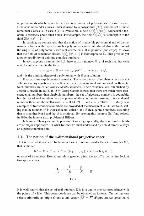
332 CHAPTER VI. POPULARIZATION OF MATHEMATICS
is, polynomials which cannot be written as a product of polynomials of lower degree.Here arise remainder classes under division by a polynomial f(x), and the set of theseremainder classes is, in case f(x) is irreducible, a field Q[x]/(f(x)). Kronecker’s the-orem is precisely about such fields. For example, the field Q(
√2) is isomorphic to the
field Q[x]/(x2 − 2).In passing, we remark also that the notion of irreducible polynomial and of the re-
mainder classes with respect to such a polynomial can be introduced also in the case ofthe ring R[x] of polynomials with real coefficients. It is possible [and easy!] to showthat the field of remainder classes R[x]/(x2 + 1) is isomorphic to C. This gives us yetanother possibility of defining complex numbers.
In each algebraic number field A there exists a number Θ ∈ A such that that eachα ∈ A can be written in the form
α = a0 + a1Θ + · · ·+ an−1Θn−1, where ai ∈ Q,
and n is the minimal degree of a polynomial with Θ as a solution.Finally, some supplementary remarks. There are plenty of numbers which are not
solutions to any equation p(x) = 0, where p(x) is polynomial with rational coefficients.Such numbers are called transcendental numbers. Their existence was established byJoseph Liouville in 1844. In 1874 Georg Cantor showed that there are much more tran-scendental numbers than algebraic numbers: the set of algebraic numbers is countable,but the set of real numbers has the power of the continuum. Among transcendentalnumbers there are the well-known π = 3.14159 . . . and e = 2.718281 . . . Many newexamples of transcendental numbers are provided of the theorem of A. O. Gel’fond, stat-ing that the number αβ is transcendental d that α and β are algebraic numbers, assumingthat α is neither 0 or 1 and that β is irrational. By proving this theorem Gel’fond solved,in 1936, the famous sixth problem of Hilbert.
In Number Theory and in Diophantine Geometry, especially, algebraic number fieldsare of major importance. In what follows we shall understand by a field almost alwaysan algebraic number field.
1.3. The notion of the n-dimensional projective spaceLet K be an arbitrary field. In the sequel we will often consider the set of n-tuples Kn,
that is, the set
Kn = K ×K · · · ×K = {(k1, . . . , kn),where each ki ∈ K}or some of its subsets. How to introduce geometry into the set Kn? Let us first look attwo special cases.
�0
RE
x
XO
1
Fig. 2
It is well-known that the set of real numbers R is in a one-to-one correspondence withthe points of a line. This correspondence can be obtained as follows. On the line oneselects arbitrarily an origin O and a unit vector
−−→OE = −→e1 (Figure 2); we agree that 0
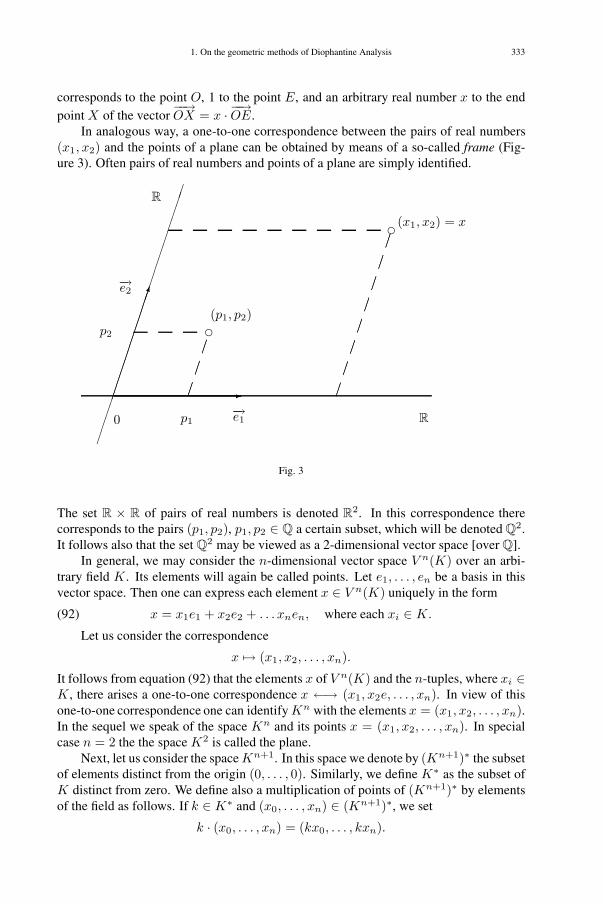
1. On the geometric methods of Diophantine Analysis 333
corresponds to the point O, 1 to the point E, and an arbitrary real number x to the endpoint X of the vector
−−→OX = x · −−→OE.
In analogous way, a one-to-one correspondence between the pairs of real numbers(x1, x2) and the points of a plane can be obtained by means of a so-called frame (Fig-ure 3). Often pairs of real numbers and points of a plane are simply identified.
�
�
��
��
��
��
��
��
��
��
��������������������
��
��
��
�����������
0 R
R
(x1, x2) = x
(p1, p2)
−→e2
p2
p1−→e1
Fig. 3
The set R × R of pairs of real numbers is denoted R2. In this correspondence therecorresponds to the pairs (p1, p2), p1, p2 ∈ Q a certain subset, which will be denoted Q2.It follows also that the set Q2 may be viewed as a 2-dimensional vector space [over Q].
In general, we may consider the n-dimensional vector space V n(K) over an arbi-trary field K . Its elements will again be called points. Let e1, . . . , en be a basis in thisvector space. Then one can express each element x ∈ V n(K) uniquely in the form
(92) x = x1e1 + x2e2 + . . . xnen, where each xi ∈ K.
Let us consider the correspondence
x �→ (x1, x2, . . . , xn).
It follows from equation (92) that the elements x of V n(K) and the n-tuples, where xi ∈K , there arises a one-to-one correspondence x ←→ (x1, x2e, . . . , xn). In view of thisone-to-one correspondence one can identify Kn with the elements x = (x1, x2, . . . , xn).In the sequel we speak of the space Kn and its points x = (x1, x2, . . . , xn). In specialcase n = 2 the the space K2 is called the plane.
Next, let us consider the space Kn+1. In this space we denote by (Kn+1)∗ the subsetof elements distinct from the origin (0, . . . , 0). Similarly, we define K∗ as the subset ofK distinct from zero. We define also a multiplication of points of (Kn+1)∗ by elementsof the field as follows. If k ∈ K∗ and (x0, . . . , xn) ∈ (Kn+1)∗, we set
k · (x0, . . . , xn) = (kx0, . . . , kxn).

334 CHAPTER VI. POPULARIZATION OF MATHEMATICS
Clearly, the multiplication of points in (Kn+1)∗ by elements of K∗ gives again elementsof (Kn+1)∗. Thus we have defined a composition (k, x) �→ kx, in other words a mapping
K∗ × (Kn+1)∗ → (Kn+1)∗.
This composition makes it possible to introduce in the point set (Kn+1)∗ a distributioninto classes. The points (x0, . . . , xn) and y = (y0, . . . , yn) are considered equivalent ifthere exists a k ∈ K∗ such that x = ky, that is x0 = ky0, . . . , xn = kyn. We denotethis equivalence by the letter E. We have on the point set (Kn+1)∗ a decomposition intoclasses, whose sets of classes (Kn+1)∗/E is called the n-dimensional projective spacePn(K). The equivalence classes of E (that is, the points of the space Pn(K)) can, beidentified to lines in Kn+1 through the origin [rays]. In the special case K = R and n =2 this construction gives the ordinary projective plane 6, so that we have a generalizationof the notion of projective plane to the case of an arbitrary field and general dimension.The problems of Diophantine Geometry require that we consider the projective spacePn(K).
II. Algebraic curvesMathematicians are like Frenchmen: whatever you tell them, they at once in-terpret it in their own language and it has become something quite different. . .
J. W. Goethe
1.4. Curves and their arithmetic
Now we shall investigate how the solution of a curve can be interpreted as a geometricproblem. In the plane one can consider point sets of a rather varied kind. What is acurve?
Let there be given the equation p(x, y) = 0 where the left hand side is a polynomialwith real coefficients, that is, the equation
Am(x)ym + Am−1(x)ym−1 + · · ·+ A1(x)y + A0(x) = 0,
where Ai(x) = a(i)kixki + · · · + a
(i)1 x + a
(i)0 is a polynomial with real coefficients. We
distinguish in the plane all the points (x, y) whose coordinates satisfy this equation. Thesubset thus obtained is a curve. For example, the solutions of the equation x2 + y2 = 1can be interpreted as the points in the plane R2 with P = (cosα, sinα) (cf. Figure 4).Such a definition of the notion of a curve looks perfectly reasonable, but it is not com-plete. Indeed, considering the equation x2 + y2 + 1 = 0, one sees that there are “curves”without a single point. Trying to evade this unpleasant circumstance we agree it as a
6Cf. [13, page 16].Translator’s note. For an introduction to projective geometry, see [17], also available in paperback. We
mention also, quite generally, the book [3]. See further this Chapter, Section 8
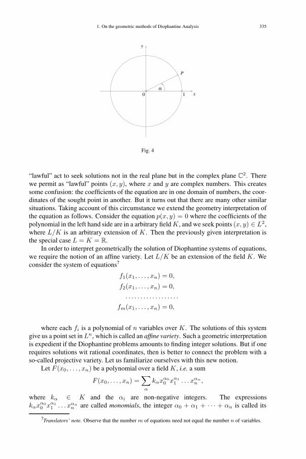
1. On the geometric methods of Diophantine Analysis 335
0
P
1α
y
x
Fig. 4
“lawful” act to seek solutions not in the real plane but in the complex plane C2. Therewe permit as “lawful” points (x, y), where x and y are complex numbers. This createssome confusion: the coefficients of the equation are in one domain of numbers, the coor-dinates of the sought point in another. But it turns out that there are many other similarsituations. Taking account of this circumstance we extend the geometry interpretation ofthe equation as follows. Consider the equation p(x, y) = 0 where the coefficients of thepolynomial in the left hand side are in a arbitrary field K , and we seek points (x, y) ∈ L2,where L/K is an arbitrary extension of K . Then the previously given interpretation isthe special case L = K = R.
In order to interpret geometrically the solution of Diophantine systems of equations,we require the notion of an affine variety. Let L/K be an extension of the field K . Weconsider the system of equations7
f1(x1, . . . , xn) = 0,
f2(x1, . . . , xn) = 0,. . . . . . . . . . . . . . . . . .
fm(x1, . . . , xn) = 0,
where each fi is a polynomial of n variables over K . The solutions of this systemgive us a point set in Ln, which is called an affine variety. Such a geometric interpretationis expedient if the Diophantine problems amounts to finding integer solutions. But if onerequires solutions wit rational coordinates, then is better to connect the problem with aso-called projective variety. Let us familiarize ourselves with this new notion.
Let F (x0, . . . , xn) be a polynomial over a field K , i.e. a sum
F (x0, . . . , xn) =∑
α
kαxα00 xα1
1 . . . xαnn ,
where kα ∈ K and the αi are non-negative integers. The expressionskαx
α00 xα1
1 . . . xαnn are called monomials, the integer α0 + α1 + · · · + αn is called its
7Translators’ note. Observe that the number m of equations need not equal the number n of variables.

336 CHAPTER VI. POPULARIZATION OF MATHEMATICS
order. The order of the polynomial F is the biggest order of its monomials. We write Fin the form
F = H0 + H1 + . . . Hm,
where we denote by Hi = Hi(x0, . . . , xn), i = 0, 1, . . . ,m the sum of all monomials oforder i in F . Each of these polynomials will be called a form of order i or homogeneousform of order i. More precisely, a form of order i is a sum of a collection of monomialof order i. For example, the polynomial
2x20x
51x2 +
35x0x
61x2 + 12x4
0x31x2
is a form of order 8 over the field Q.A form H is said to be irreducible if there do not exist any forms P and Q over the
field K such that H = P ·Q.A projective algebraic variety in Pn(K) is a set of points determined by a certain
system of homogeneous equations
H1(x0, . . . , xn) = 0,
H2(x0, . . . , xn) = 0,. . . . . . . . . . . . . . . . . . . . .
Hm(x0, . . . , xn) = 0,
Thus all polynomials Hi here are forms over K . But every point set in Pn(K) isa set of rays through the origin in Kn+1. Therefore we can view a projective algebraicvariety as a certain cone in Kn+1. Next we look at an important example of such variety(Figure 5).
(0,0,0)
P
a
Fig. 5
We pick in the projective plane P2(K) a suitable coordinate system (x0, x1, x2) andwrite a certain form of order m over K ,
F (x) = F (x0, x1, x2).
We assume that this form is irreducible. Let P ∈ P2(K). We know that to the point Pthere corresponds a certain equivalence class in the space K3, i.e., a ray through the point
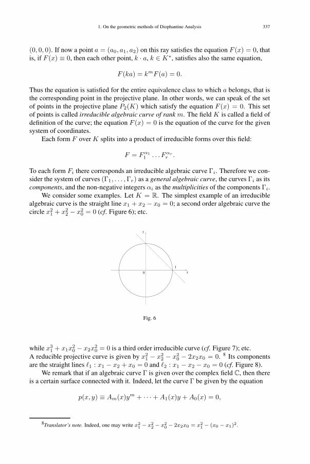
1. On the geometric methods of Diophantine Analysis 337
(0, 0, 0). If now a point a = (a0, a1, a2) on this ray satisfies the equation F (x) = 0, thatis, if F (x) ≡ 0, then each other point, k · a, k ∈ K∗, satisfies also the same equation,
F (ka) = kmF (a) = 0.
Thus the equation is satisfied for the entire equivalence class to which a belongs, that isthe corresponding point in the projective plane. In other words, we can speak of the setof points in the projective plane P2(K) which satisfy the equation F (x) = 0. This setof points is called irreducible algebraic curve of rank m. The field K is called a field ofdefinition of the curve; the equation F (x) = 0 is the equation of the curve for the givensystem of coordinates.
Each form F over K splits into a product of irreducible forms over this field:
F = Fα11 . . . Fαr
r .
To each form Fi there corresponds an irreducible algebraic curve Γi. Therefore we con-sider the system of curves (Γ1, . . . ,Γr) as a general algebraic curve, the curves Γi as itscomponents, and the non-negative integers αi as the multiplicities of the components Γi.
We consider some examples. Let K = R. The simplest example of an irreduciblealgebraic curve is the straight line x1 + x2 − x0 = 0; a second order algebraic curve thecircle x2
1 + x22 − x2
0 = 0 (cf. Figure 6); etc.
0
1
y
x
Fig. 6
while x31 + x1x
20 − x2x
20 = 0 is a third order irreducible curve (cf. Figure 7); etc.
A reducible projective curve is given by x21 − x2
2 − x20 − 2x2x0 = 0. 8 Its components
are the straight lines �1 : x1 − x2 + x0 = 0 and �2 : x1 − x2 − x0 = 0 (cf. Figure 8).We remark that if an algebraic curve Γ is given over the complex field C, then there
is a certain surface connected with it. Indeed, let the curve Γ be given by the equation
p(x, y) ≡ Am(x)ym + · · ·+ A1(x)y + A0(x) = 0,
8Translator’s note. Indeed, one may write x21 − x2
2 − x20 − 2x2x0 = x2
1 − (x0 − x1)2.
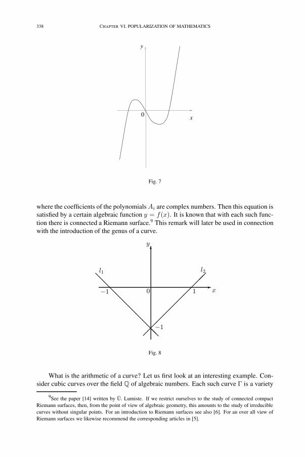
338 CHAPTER VI. POPULARIZATION OF MATHEMATICS
0
y
x
Fig. 7
where the coefficients of the polynomials Ai are complex numbers. Then this equation issatisfied by a certain algebraic function y = f(x). It is known that with each such func-tion there is connected a Riemann surface.9 This remark will later be used in connectionwith the introduction of the genus of a curve.
�
�
��
��
��
��
����
��
��
��
��
0 x1
−1
−1
l1 l2
y
Fig. 8
What is the arithmetic of a curve? Let us first look at an interesting example. Con-sider cubic curves over the field Q of algebraic numbers. Each such curve Γ is a variety
9See the paper [14] written by Ü. Lumiste. If we restrict ourselves to the study of connected compactRiemann surfaces, then, from the point of view of algebraic geometry, this amounts to the study of irreduciblecurves without singular points. For an introduction to Riemann surfaces see also [6]. For an over all view ofRiemann surfaces we likewise recommend the corresponding articles in [5].
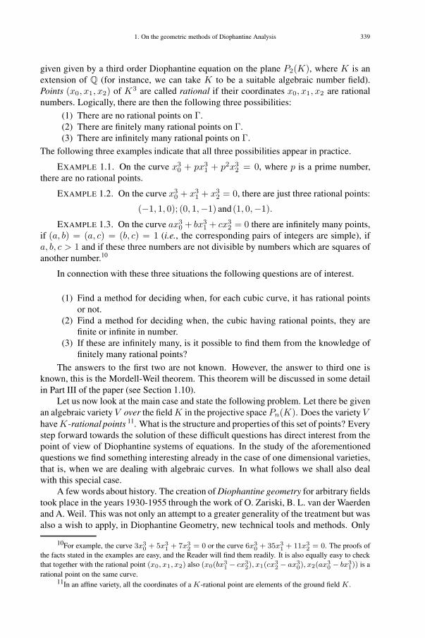
1. On the geometric methods of Diophantine Analysis 339
given given by a third order Diophantine equation on the plane P2(K), where K is anextension of Q (for instance, we can take K to be a suitable algebraic number field).Points (x0, x1, x2) of K3 are called rational if their coordinates x0, x1, x2 are rationalnumbers. Logically, there are then the following three possibilities:
(1) There are no rational points on Γ.(2) There are finitely many rational points on Γ.(3) There are infinitely many rational points on Γ.
The following three examples indicate that all three possibilities appear in practice.
EXAMPLE 1.1. On the curve x30 + px3
1 + p2x32 = 0, where p is a prime number,
there are no rational points.
EXAMPLE 1.2. On the curve x30 + x3
1 + x32 = 0, there are just three rational points:
(−1, 1, 0); (0, 1,−1) and (1, 0,−1).
EXAMPLE 1.3. On the curve ax30 + bx3
1 + cx32 = 0 there are infinitely many points,
if (a, b) = (a, c) = (b, c) = 1 (i.e., the corresponding pairs of integers are simple), ifa, b, c > 1 and if these three numbers are not divisible by numbers which are squares ofanother number.10
In connection with these three situations the following questions are of interest.
(1) Find a method for deciding when, for each cubic curve, it has rational pointsor not.
(2) Find a method for deciding when, the cubic having rational points, they arefinite or infinite in number.
(3) If these are infinitely many, is it possible to find them from the knowledge offinitely many rational points?
The answers to the first two are not known. However, the answer to third one isknown, this is the Mordell-Weil theorem. This theorem will be discussed in some detailin Part III of the paper (see Section 1.10).
Let us now look at the main case and state the following problem. Let there be givenan algebraic variety V over the field K in the projective space Pn(K). Does the variety VhaveK-rational points 11. What is the structure and properties of this set of points? Everystep forward towards the solution of these difficult questions has direct interest from thepoint of view of Diophantine systems of equations. In the study of the aforementionedquestions we find something interesting already in the case of one dimensional varieties,that is, when we are dealing with algebraic curves. In what follows we shall also dealwith this special case.
A few words about history. The creation of Diophantine geometry for arbitrary fieldstook place in the years 1930-1955 through the work of O. Zariski, B. L. van der Waerdenand A. Weil. This was not only an attempt to a greater generality of the treatment but wasalso a wish to apply, in Diophantine Geometry, new technical tools and methods. Only
10For example, the curve 3x30 + 5x3
1 + 7x32 = 0 or the curve 6x3
0 + 35x31 + 11x3
2 = 0. The proofs ofthe facts stated in the examples are easy, and the Reader will find them readily. It is also equally easy to checkthat together with the rational point (x0, x1, x2) also (x0(bx3
1 − cx32), x1(cx3
2 − ax30), x2(ax3
0 − bx31)) is a
rational point on the same curve.11In an affine variety, all the coordinates of a K-rational point are elements of the ground field K .

340 CHAPTER VI. POPULARIZATION OF MATHEMATICS
from them one had a hope for the solution of the so fascinating but enormously difficultDiophantine problems.
1.5. Birational equivalence of algebraic curves
A few words about the notion brought out in the heading of this Section. On the setof all algebraic curves it is possible to introduce a decomposition into classes whichis called the birational equivalence of curves. This equivalence is related birationalgeometry, one of the classical divisions of mathematics, mainly cultivated, around theturn of the past century by Italian mathematicians. Of great interest are those objectswhich are the same, from the point of view of birational geometry, for all curves in aclass, the so-called birational invariants. The most important birational invariant is theirgenus, introduced in geometry by Bernhard Riemann. The genus gives a possibility for aclassification of curves, of the importance of which in Diophantine Geometry we spokein the Introduction. The third Part of this paper (see 1.8) is devoted to this classification.
Let there be given a curve Γ with the equation f(x, y) = 0. We consider rational
functions ϕ(x, y) =α(x, y)β(x, y)
, where α and β are polynomials over K and β is not divis-
ible by f . The function ϕ is considered as trivial and we write ϕ = O(Γ), if f |α (i.e., αis divisible by the polynomial f ).
We are interested in points of the curve whose coordinates are in K . Such pointswill be called K-rational. It will be expedient also to consider K-algebraic points withcoordinates belonging to some extension of the field K . Next, let (x0, y0) ∈ Γ be a pointon the curve (regardless if it is rational or algebraic). Then ϕ(x0, y0) is determined ifβ(x0, y0) �= 0. There are only finitely many points such that β(x0, y0) = 0. Indeed, asβ does not divide f and f is irreducible (Γ is an irreducible curve), then by eliminationtheory 12 the number of solutions of the system{
β(x, y) = 0f(x, y) = 0
is ≤ (deg β) · (deg f), where deg f indicates the degree of the polynomial f . Thusϕ(x, y) is determined on Γ except for finitely many points.
It turns out that the triviality of a rational function on Γ is equivalent to its trivialityat all algebraic points 13. Indeed, if ϕ = O(Γ), then ϕ(x0, y0) = 0 holds true thanksto the fact that f |α, because ϕ(x0, y0) = 0 for all points (x0, y0) ∈ Γ. Conversely, ifϕ(x0, y0) = 0 for all algebraic points of Γ, but ϕ �= O(Γ), then α is not divisible by fand the system {
f(x, y) = 0ϕ(x, y) = 0
would have only finitely many solutions. But this is a contradiction, because there areinfinitely many algebraic points on the curve.
12See [8, p. 280-285]. Translator’s note. See also the references in footnote 4. We remark that Kangro’sbook [8] in many respects reminds of Kurosh [10] mentioned there. For elimination theory, see in particular[19, Chapter I], or [16].
13The triviality of a function ϕ at a point (x0, y0) of Γ means that ϕ(x0, y0) ∈ Γ is determined andϕ(x0, y0) = 0. For rational points the analogous statement is not true.

1. On the geometric methods of Diophantine Analysis 341
Next, we introduce a decomposition into classes for rational functions ϕ(x, y) =α(x, y)β(x, y)
. To this end, we declare two rational functionsϕ(x, y) and ψ(x, y) as equivalent
on the curve if the function ϕ− ψ is trivial on the curve. Putting all functions equivalentamong themselves on the curve, we get a decomposition of rational functions into classes.Each such equivalence class will be called a rational function on the curve Γ. Let ϕ andψ two arbitrary classes and ω ∈ ϕ and τ ∈ ψ arbitrary rational functions in these classes.We define addition and multiplication of classes by the formulae:
ϕ + ψ = ω + τ,
ϕ · ψ = ω · τ .
In other words, with the help of arbitrary representatives of classes one introducesoperations on classes. It is easy to check that the set of classes forms a field, denoted byK(x, y). The field K(x, y) shall be called the field of rational functions on the curve Γ.For example, on the straight line y = 1 one has the field of rational functions K(x, y) =K(x). Each element ϕ of K(x, y) can uniquely be represented in the form
ϕ = α0(x) + α1(x)y + · · ·+ αm−1(x)ym−1,
where the αi(x) are rational functions and m = degy f(x, y)14. At first sight one mightbelieve that the two functions x and y play a “privileged role” in K(x, y). But thisis so only apparently, since for each non-constant function y′ ∈ K(x, y) we can findx′ ∈ K(x, y) such that
x = ϕ(x′, y′), y = ψ(x′, y′),and there exists a polynomial g over K with g(x′, y′) = 0, that is, K(x, y) ≡ K(x′, y′).
If two algebraic curves have the same field of rational functions, then we say thatthey are birationally equivalent. Examples of birationally equivalence of curves will befound in Section 1.7.
Let there be given the curve Γ : f(x, y) = 0 and the curve Γ′ : g(x′, y′) = 0. It turnsout that a necessary and sufficient condition for the curves Γ and Γ′ to be birationallyequivalent is that there exist rational functions ϕ, ψ, ϕ′, ψ′ such that x′ = ϕ′(x, y),y′ = ψ′(x, y), x = ϕ(x′, y′), y = ψ(x′, y′).
If the point (x0, y0) ∈ Γ is K-rational, then, apparently, the point f ′(x0, y0),ψ′(x0, y0) ∈ Γ′ is K-rational, and vice versa. Here we assume, of course, that thefunctions ϕ, ψ, ϕ′, ψ′ are determined in the points considered. But these functions arenot determined only at finitely many points of Γ. Now we have arrived at an essentialfact:
THEOREM 1.1. There is a one-to-one correspondence between the points of twobirationally equivalent curves, provided one excludes a finite set of points (where thefunctions ϕ, ψ, ϕ′, ψ′ are not determined).
14Here degy denotes the degree of the polynomial f(x, y) with respect to y.

342 CHAPTER VI. POPULARIZATION OF MATHEMATICS
1.6. Singular points of a curveWe consider a curve Γ given by the equation f(x, y) = 0. The polynomial f(x, y), as a
function of two variables has the derivatives fx, fy, fxy, . . . . A point P on Γ is called anr-fold point, if at this point its derivatives up to order r−1 vanish, but there is a derivativeof order r which is different from zero; if r > 1 we call an r-fold point a singular point.The number and multiplicity of such singular points is bounded: considering an algebraiccurve of genus n without multiple components with points Pi with multiplicities ri,i ∈ I , then one has ∑
i∈I
ri(ri − 1) ≤ n(n− 1).
For an irreducible curve there is an even stronger inequality:∑i∈I
ri(ri − 1) ≤ (n− 1)(n− 2).
As an example, we consider the issue of singular point on a cubic curve. Let thecurve Γ be give by the equation f(x, y) = 0. We use a system of coordinates with theorigin on Γ. Then the polynomial f does not have a constant term and we write it as
f(x, y) = ax + by + g(x, y),
where the polynomial g contains only monomials of degree two and three. This givesreadily fx(0, 0) and fy(0, 0):
∂f
∂x|(0,0) = a,
∂f
∂y|(0,0) = b.
If a = b = 0, then (0, 0) is a singular point, because then fx(0, 0) = 0 and fy(0, 0) = 0.Consider the points of intersections of Γ with the straight line y = kx:
(93) 0 = f(x, kx) = x(a + bk) + g(x, kx) = x(a + bk) + x2�(x),
where �(x) is a linear polynomial, that is, �(x) = cx+ d. From this equation we can findx. The value x = 0 satisfies the equation given. If a + bk �= 0, then x = 0 is a simplesolution of (93) and, in this case, we call straight line y = kx a secant of Γ. If, however,a + bk = 0, then x = 0 is a double solution of (93) and we call y = kx a tangent of Γ,x = 0 being a double solution of (93).
This allows us to conclude that on a cubic curve there are not more than two singularpoints. Assume that P1 = (x1, y1) and P2 = (x2, y2) are two distinct singular pointson Γ. We choose the system of coordinates such that (0, 0) ∈ Γ and the direction of theunit vectors such that x1 = x2. We draw through the points P1 and P2 a straight line �and form the equation for finding the point of intersection between the line � and Γ. AsP1 and P2 are both singular points, then, in view of the above, x = x1 and x = x1 bothmust be double solutions. But then we have produced at least 4 solutions. But this is acontradiction since the degree of the equation is≤ 3 (the cubic and the straight line haveat most three points of intersection). This proves the assertion.15 '(
15Further examples in [12, p. 35]. Translator’s note. Similar examples can be found in the excellent book[20, e.g. p. 57].
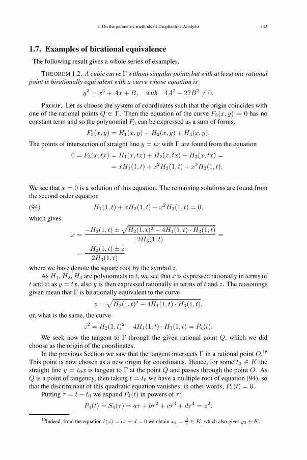
1. On the geometric methods of Diophantine Analysis 343
1.7. Examples of birational equivalence
The following result gives a whole series of examples.
THEOREM 1.2. A cubic curve Γ without singular points but with at least one rationalpoint is birationally equivalent with a curve whose equation is
y2 = x3 + Ax + B, with 4A3 + 27B2 �= 0.
PROOF. Let us choose the system of coordinates such that the origin coincides withone of the rational points Q ∈ Γ. Then the equation of the curve F3(x, y) = 0 has noconstant term and so the polynomial F3 can be expressed as a sum of forms,
F3(x, y) = H1(x, y) + H2(x, y) + H3(x, y).
The points of intersection of straight line y = tx with Γ are found from the equation
0 = F3(x, tx) = H1(x, tx) + H2(x, tx) + H3(x, tx) =
= xH1(1, t) + x2H2(1, t) + x3H3(1, t).
We see that x = 0 is a solution of this equation. The remaining solutions are found fromthe second order equation
(94) H1(1, t) + xH2(1, t) + x2H3(1, t) = 0,
which gives
x =−H2(1, t)±
√H2(1, t)2 − 4H1(1, t) ·H3(1, t)
2H3(1, t)=
=−H2(1, t)± z
2H3(1, t)where we have denote the square root by the symbol z.
As H1, H2, H3 are polynomials in t, we see that x is expressed rationally in terms oft and z; as y = tx, also y is then expressed rationally in terms of t and z. The reasoningsgiven mean that Γ is birationally equivalent to the curve
z =√H2(1, t)2 − 4H1(1, t) ·H3(1, t),
or, what is the same, the curve
z2 = H2(1, t)2 − 4H1(1, t) ·H3(1, t) = P4(t).
We seek now the tangent to Γ through the given rational point Q, which we didchoose as the origin of the coordinates.
In the previous Section we saw that the tangent intersects Γ in a rational point O.16
This point is now chosen as a new origin for coordinates. Hence, for some t0 ∈ K thestraight line y = t0x is tangent to Γ at the point Q and passes through the point O. AsQ is a point of tangency, then taking t = t0 we have a multiple root of equation (94), sothat the discriminant of this quadratic equation vanishes; in other words, P4(t) = 0.
Putting τ = t− t0 we expand P4(t) in powers of τ :
P4(t) = S4(τ) = aτ + bτ2 + cτ3 + dτ4 = z2.
16Indeed, from the equation �(x) = cx + d = 0 we obtain x3 = dc∈ K , which also gives y3 ∈ K .

344 CHAPTER VI. POPULARIZATION OF MATHEMATICS
this gives
(z
τ2)2 = d + c
1τ
+ b1τ2
+ a1τ3
.
Denoting here 1τ = v and z
τ2 = u and taking au = α, av = β, we obtain
a2u2 = a3v3 + a2bv2 + a2cv + a2d
andα2 = β3 + bβ2 + acβ + a2d.
Finally, making the substitution γ = β+ b3 allows us to bring this equation in the desired
form. As all changes of variable made have been rational, the assertion of the theorem isproved. '(
III. The classification of algebraic curves.Schüler: “Kann Euch nicht eben ganz verstehen.”Mephistoteles: “Das wird nähstens schon besser gehen, wenn Ihr lernt allesreduzieren und gehörig klassifizieren.”
(The student: “I do not quite understand you now.”Mephistoteles: “It will soon be much easier for you. when you have learnt toreduce and to classify appropriately.”)
J. W. Goethe “Faust”
1.8. The genus of an algebraic curveLet there be given an irreducible algebraic curve Γ. To each point Pi of Γ we associate
a natural number ri ≥ 1 (see Section 1.6), the order of the point. If the degree of Γ is n,we have seen that one has the equation∑
Pi∈Γ
(ri − 1)ri ≤ (n− 1)(n− 2).
With each algebraic curve one can associate a non-negative integer g, its genus,which in the simplest cases can be found from the formula17
g =(n− 1)(n− 2)
2−
∑Pi∈Γ(ri − 1)ri
2.
We saw above that in the case K = C there is associated to any algebraic curve acompact Riemann surface. Each such surface is, however, topologically equivalent to a“sphere with handles”, and so the single topological invariant of the topological structureof this surface, the number of the “handles”, determines the genus of the surface. In the
17Each projective each algebraic curve can be settled into one-to-one correspondence with a plane curvewith only ordinary 2-fold singularities (without multiple tangents at these points), so, the genus g being abirational invariant, then the given evaluation formula is universal (for, using it, we can find in each birationalequivalency class a curve of genus g).

1. On the geometric methods of Diophantine Analysis 345
special case K = C (that is, when the field of definition of the curve is the complexdomain C) is nothing but the genus of the Riemann surface [14] corresponding to it. 18
When we look at algebraic curves over number fields, then the genus of a curve isdetermined not only by the structure of all algebraic points on the curve, but to a largeextent also the structure of its Q- and Z-points (cf. below the Mordell-Weyl theorem).From the point of view of Diophantine problems it is therefore a significant fact that thegenus g is a birational invariant, being equal for all curves belonging to the same classof birationality. This gives a possibility for a classification of curves, and thereby also aclassification of the corresponding Diophantine problems.
1.9. About classification
Curves of genus 0 are called rational. As the genus g of a curve of order n withoutsingular points is given by the formula
g =12(n− 1)(n− 2),
we see that curves of degree one i.e. straight lines and second order curves are rational.On the other hand, David Hilbert and Adolf Hurwitz showed in 1890 that every rationalcurve is isomorphic to a plane second order curve a0x
20 + a1x
21 + a2x
22 = 0. The cor-
responding isomorphism is obtained by a substitution of variables where the coefficientsdetermining the substitution belong to the field of definition of the curve.
Curves of genus g = 1 are called elliptic; they are isomorphic to cubic curves with-out singular points. From this we see19, that if an elliptic curve has a rational point thenit is birationally equivalent to a curve with equation y2 = x3 + Ax + B. Elliptic curveshave received their name from the fact that if K = C then they admit a parametrizationin terms of elliptic functions ([14, p. 261]20).
In the case when the ground field K = C an elliptic curve corresponds to a Riemannsurface of genus g = 1, that is, a torus. A torus is topologically the direct product of twocircles. Therefore it is possible to define on it the structure of a compact Lie group. Ifan elliptic curve has a rational point, then one can take this point on the correspondingRiemann surface to be the zero element, and the composition can be expressed in termsof algebraic functions in the coordinates. A complex compact Lie group, which in thesame time is also an algebraic variety, is called an Abelian variety. Basing himself on aseries of fundamental results, A. Weil arrived at the opinion that any development in thearea of elliptic curves will also mean a major progress in the theory of general Abelianvarieties. Therefore it is understandable why the class of these curves has been givenparamount interest in Algebraic Geometry.
18Translator’s note. For Riemann surfaces, see also the reference indicated in the footnote 9.19Cf. Theorem 1.220Editors’ note. Page number is given according to Russian translation.

346 CHAPTER VI. POPULARIZATION OF MATHEMATICS
Curves of genus g > 1 are called non-elliptic. 21 In the beginning of the 20th centurythere was raised the following conjecture in Diophantine Geometry: non-elliptic curvesover number fields have only a finite number of rational points. Despite the efforts ofmany mathematicians a corresponding theorem has not been established. Yu. I. Maninshowed that the proof of this conjecture reduces to the generalized Mordell conjecture.22 It is not possible to give here a closer account of these curves, as so far this subject israther difficult to study and a satisfactory theory is missing here.
1.10. Rational curvesCurves with genus g = 0 are called rational. The genus of a curve Γ of degree n is
given by
g =n(n− 1)
2−
∑Pi∈Γ(ri − 1)ri
2,
so that the criterion for a curve of order n to be rational is∑P∈Γ
(ri − 1)ri =n(n− 1)
2.
The simplest curve is the straight line y = 1 for that the field of rational functions isK(x, 1) = K(x). In the preceding Section we saw that straight lines are rational curves.This gives at once the following necessary condition for rationality.
For a curve over the field of rational functions K(x, y) to be rational it is necessary,that there exists a function ϕ ∈ K(x, y) allowing to express x and y rationally over thefield K . 23
In order to illustrate the application of this condition we prove that the curve
(95) x230 + x
231 + x
232 = 0
is rational.To this send we observe that the values x0 = i, x0 = sin3 α, x0 = cos2 α satisfy
equation (95). Taking
t = tanα
2=
1− cosαsinα
,
we find
1 + t2 =2
sinα· 1− cosα
sinα=
2sinα
· t,which yields
sinα =1 + t2
2t, cosα =
i(1− t2)2t
.
Thus we find that
(96) cx0 = −8t3; cx1 = i(1 + t2)23 ; cx2 = (1− t2)3,
21As an example, one has the curves p(x)y2 + q(x) = 0, where deg p(x) = g, deg q(x) = g + 2, andthe equation p(x) · q(x) = 0 has now multiple zeros. Such a curve is of degree g + 2, and its only singularpoint has multiplicity g. Therefore, by the formula given in Section 1.8, its genus is given by
(g + 2 − 1)(g + 2 − 2)
2− g(g − 1)
2=
g(g + 1)
2− g(g − 1)
2= g.
22Cf. Section 2.23Indeed, this condition is also a sufficient one.

1. On the geometric methods of Diophantine Analysis 347
where 0 �= 0 ∈ C.
In other words, as−icx1 + cx2 = 2+6t4 and 6t4 =3t4
(8t3) =3t4
(cx0), we obtain
(97) t = −4i3
(x1
x0) +
43(x2
x0)− 8i
3c∈ C(
x1
x0,x2
x0), c ∈ C.
The relations (96) and (97) allow us to use the previous rationality conditions, fromwhich we conclude that the curve (95) is rational.
We now answer the question raised in Section 1.4 about the rationality of quadraticcurves.
THEOREM 1.3. If a second order curve has a rational point, then there are (in thecase of an infinite field K) infinitely many such points.
PROOF. Let there be given a second order curve which has a rational point Γ, andlet it have the rational point Q = (x0, y0) ∈ Γ. Consider the straight lines through thispoint:
x− x0 = t(x0 − y0).We seek the point of intersection of Γ which such a line. To this end we have to solve thefollowing quadratic equation in t:
f(x0 + t(x0 − y0), y) = 0.
We know one such solution y = y0. The second solution can be expressed, in viewof Viète’s rule, in terms of y0 and the coefficients of the quadratic polynomial f , thatis, it is expressed rationally in terms of x0, t, y0 and elements of K . In other words, asx0, y0 ∈ K , then y is expressed rationally in terms of t. But then x = x0 + t(x0 − y0)is, likewise, expressed rationally in terms of t. The reasoning given shows that the pointsof intersection with Γ of the “rational” straight lines through the point Q (t ∈ K) arerational points. '(
If K = Q, the the presence of rational points on a second order curve can be con-trolled by an effective process of calculation (given by the Minkowski-Hasse Theorem).
1.11. Elliptic curvesLet us begin by the birational classification of elliptic curves.
If the base field K is algebraically closed, then each elliptic curve over K is bira-tionally equivalent to a curve in the so-called “Weierstrass normal form”:
y2 = x3 + ax + b, a, b ∈ K.
Two curves with such an equation are birational to each other if and only if their absoluteinvariant coincide, the absolute invariant of an elliptic curve j being given by the formula
j =4a3
4a3 + 27b2, j ∈ K.
If the base field K is not algebraically closed, the classification requires the use ofa cumbersome technical apparatus. If on the elliptic curve Γ there is a K-rational pointO 24, we can put the set of its K-rational points, which we denote by G(Γ,K) = G, in
24If K is a finite field, then such a point exists always (Theorem of F. K. Schmidt). In the general casethe existence of such a point may be a truly serious question.

348 CHAPTER VI. POPULARIZATION OF MATHEMATICS
0
−P
P
Fig. 9
correspondence with the structure an Abelian group with zero element at the pointO. Wedo this in the following way (see Figure 9). As zero in the group G we take the point O.The inverse to a given point P is the point−P obtained as the third point of intersectionwith Γ of the straight line through O and P . Next, let there be given two rational pointsP1 and P2 on Γ (see Figure 10).
P2
P1
P −P =−Q1 2
0
Q
Fig. 10
We draw a secant through these two points and take inverse −Q of the third point ofintersection Q obtained in this way. We define −Q = P1 + P2. If P1 ≡ P2 we takeinstead of a secant the tangent at the point P1 ≡ P2. It is possible to show that theaddition of points defined in this way makes the set G = G(Γ,K) into an Abelian group.25 This group turns out to be a birational invariant, that is, the groups of elliptic curvesbelonging to one and the same birationality class are isomorphic. This circumstancepermits us to give a much better idea of the group G. Indeed, the group G(Γ,K) being abirational invariant, the result given in the beginning of this Section permits us to replace
25It is possible to define on the set G a binary algebraic operation denoted ◦ by the formula P1◦P2 = Q.R. H. Bruck and V. D. Belousov call this system as TS-quasigroup. (Translator’s remark. TS stands for totallysymmetric. See [2] This algebraic object allowed Yu. I. Manin, recently, to realize an interesting geometric ideaand find an essential generalization of results corresponding to the results of classical Diophantine Geometry.See [15].

1. On the geometric methods of Diophantine Analysis 349
the elliptic curve Γ with a curve Γ′ in normal form:
Γ′ : y2 = x3 + ax + b.
Passing to homogeneous coordinates, writingξ1ξ0
= x,ξ1ξ0
= y,∞ = (0, 0, 1) we get for
the equation of Γ′
ξ0ξ22 = ξ3
1 + a · ξ20ξ1 + b3ξ0.
Clearly ∞ ∈ Γ′. We set ∞ ≡ 0, that is, we take ∞ as the zero element of the groupG(Γ′,K)
As G(Γ′,K) ∼= G(Γ,K) (the groups being isomorphic), we obtain for the groupG(Γ,K) the following structure formulae 26
If P = (x, y), then −P = (x,−y);If P1 = (x1, y1) and P2 = (x1, y2), then P1 + P2 = P3 =
(x3, y3) =(−(x1 + x2) + (
y1 − y2
x1 − x2)2), y1 +
y1 − y2
x1 − x2(x3 − x1)
).
Let us look at elliptic curves over the rational field, that is, the special case K =Q. In 1901, H. Poincaré made the conjecture that this group has a finite number ofgenerators. This assertion founds its affirmation; in 1922 L. J. Mordell obtained its proof.Six years later A. Weil managed to extend the theorem to arbitrary number fields. Thistheorem, which is called the Mordell-Weil theorem has several important applications inDiophantine Geometry. Several proofs of this theorems have been given, but they are allnon-effective, that is, they give only an upper bound for the number of generators, butnot a method fore finding these generators. So in most cases the structure of the groupG(Γ,K) remains unknown to us. However, in 1935, Tryggve Nagell gave the followingmethod for finding the elements of finite rank in G(Γ,Q).
The elliptic curve Γ has to be presented in the normal form
y2 = x3 −Ax−B, A,B ∈ Z.
Then all rational points of finite rank on Γ (that, is Q-points of finite rank) must haveinteger coordinates x and y; then either y2 = 0 or y2 is an integer divisor of [the discrim-inant] 4A3 − 27B2.
Nagell’s result show that all Q-points of finite rank can be found from the set oftheir all possible values, by checking all points of this set. The English mathematiciansB. J. Birch and H. P. F. Swinnerton-Dyer recently made a number of conjectures of highcredibility about the structure of the Q-points of finite rank on an elliptic curve (see [18])These conjectures are based on empirical material, which were obtained using computers,because for the check of the assertions a large number of bulky computations had to bemade.
Despite the apparent fragmental form of the material set out here, we still venture tohope that the Reader has got some confirmation to Lagrange’s words:
As long as algebra and geometry developed each side by side, theirprogress was slow and the applications limited. By making friends
26Translator’s note. In the theory of elliptic functions, these formulae are equivalent to the Weierstrassaddition theorem. See e.g. the book of Hurwitz mentioned in the footnote 9.
350 CHAPTER VI. POPULARIZATION OF MATHEMATICS
each got new vigor from each other, and now they move with a muchgreater speed in the direction of completion.
References
[1] I. G. Bashmakova. Diophantus and Diophantine Equations. Dolciani Mathematical Expositions (20).Math. Assoc. Amer., Washington, DC, 1997. Translated from Russian: Nauka, Moscow, 1972.
[2] V. D. Belousov. Some remarks on TS-quasigroups. Kišinev. Gos. Univ. Ucen. Zap. 91, 1967, 3–8.[3] M. Berger. Geometry, I–II. Universitext. Springer-Verlag, New York, 1987.[4] P. M. Cohn. Algebra, Vol. 1-3. Second Edition. John Wiley & Sons, Chichester, et. al., 1981; 1989; 1991.
Russian translation: Mir, Moscow, 1968.[5] M. Hazewinkel (ed.). Encyclopaedia of Mathematics. Kluwer Academic Publishers, Dordrecht, Boston,
London, 1988. A translated and expanded version of a Soviet mathematics encyclopedia, in ten volumes.[6] A. Hurwitz. Vorlesungen über Allgemeine Funktionentheorie und Elliptische Funktionen; herausgegeben
und ergänzt durch einen Abschnitt über geometrische Funktionentheorie von R. Courant. Die Grundlehrender mathematischen Wissenschaften, Bd. 3. Springer Verlag, Berlin, New York, 1964.
[7] U. Kaljulaid. Lenin prize for work in Diophantine geometry. Math. and Our Age 14, 1968, 108–110. (see[K68b]).
[8] G. Kangro. Kõrgem algebra (Higher algebra). Eesti Riiklik Kirjastus, Tallinn, 1962. (Estonian.)[9] A. G. Kurosh. Lectures in general algebra. Fizmatgiz, Moscow, 1962. English translation: Pergamon
Press, Oxford, London, Edinburgh, New York, 1965.[10] A. G. Kurosh. A course of higher algebra. Nauka, Moscow, 1975.[11] S. Lang. Algebra. Reading, Massachusetts, 1965. Russian translation: Mir, Moscow, 1968.[12] Ü. Lumiste. Diferentsiaalgeomeetria (Differential geometry). Eesti Riiklik Kirjastus, Tallinn, 1963. (Es-
tonian.)[13] Ü. Lumiste. The notion of space in geometry. Geometry and transformation groups. Math. and Our Age
14, 1968, 3–21.[14] Ü. Lumiste. Riemann as the founder of topology and the general curved space. Math. and Our Age 11,
1966, 65–76. (Estonian).[15] Yu. I. Manin. Cubic hypersurfaces, I. Izv. Math. Nauk 32 (6), 1968.[16] A. Seidenberg. Elements of the theory of algebraic curves. Addison-Wesley Pub. Co., Reading, Mass.,
London, Don Mills, Ont., 1968.[17] J. G. Semple and T. T. Kneebone. Algebraic projective geometry. Oxford Science Publications. Oxford
University Press, New York, etc., 1998.[18] H. P. F. Swinnerton and B. J. Birch. Elliptic curves and modular functions. Lecture Notes in Math. 476,
1975, 2–32.[19] B. L. van der Waerden. Moderne algebra, I; II. Die Grundlehren der mathematischen Wissenschaften
in Einzeldarstellungen mit besonderer Berücksichtigung der Anwendungsgebiete. Springer, Berlin, 1930;1931. Many subsequent editions, from the 4 ed.,1950, on, with the changed title Algebra, dropping theword “Moderne” (Modern). Russian translation: Nauka, Moscow, 1979.
[20] R. J. Walker. Algebraic curves. Princeton Mathematical Series, vol. 13. Princeton University Press,Princeton, N. J., 1950.

351
2. [K68b] Lenin prize for work in Diophantine geome-tryComments by M. Tsfasman
In the year 1967 the young Moscow mathematician Yu. I. Manin was honored withthe Lenin prize.
Yuri Ivanovich Manin was born in Simferopol 27 onFebruary 16, 1937. In 1958 he got his diploma fromMoscow State University, and begun his research stud-ies under the direction of Prof. I. R. Shafarevich. In 1960Manin defended his Candidate thesis “On the theory ofAbelian varieties”. There the author considers the theoryof algebraic curves over a field of finite characteristic anddiscovers a number of original analogies with the classi-cal case, where the base field are the complex numbers.Since 1960 Manin works at the Steklov Institute of TheSoviet [now Russian] Academy of Sciences.28 In 1963 hedefended his Doctoral thesis “The theory of formal seriesin the case of a finite field”. Since 1965 he is also a pro-
fessor at Moscow University, where he directs, together with Shafarevich, an extensiveactivity in the founding of a school of Algebraic Geometry.
Manin’s domain of research is Diophantine Geometry, which subject has its roots inantiquity; in the third century B.C. Diophantos raised the problem of finding solutionsin terms of rational numbers of an equation with rational coefficients. Considering theproblems of this kind begun already in early medieval times in China and in India. Moreserious progress was, however, obtained in the work of such classics as Euler, Lagrange,and Gauss.
A new stage in the study of these problems was opened up in the 20th century, whenvarious possibilities for classifying and studying Diophantine problems with the aid ofmethods of algebraic geometry were found . A new branch of mathematics, DiophantineGeometry, arose, where the main object of study is the structure of some given “arith-metic” variety over some field and its dependence on the “arithmetic” of this field. Todaythese questions are seen as a touchstone for the methods of algebraic geometry.
Already the arithmetic of one-dimensional varieties or algebraic curves is of interest.The connection with Diophantine problems here is the following. To each algebraic equa-tion in two variables, whose coefficients are elements of some field, there corresponds analgebraic curve over this field. To each algebraic curve there corresponds a non-negativeinteger, the genus of the curve. The curves of genus 0 are the rational curves, the ones ofgenus 1 the elliptic ones. One has found that the arithmetic of an algebraic curve, that isthe nature of the Diophantine problem, depends on the genus of the curve.
27Translator’s note. On the Crimea, now belonging to the Ukraine (population 352000 in 1995).28Edtors’ note. He is now the director of the Max-Planck-Institute of Mathematics in Bonn, Germany.
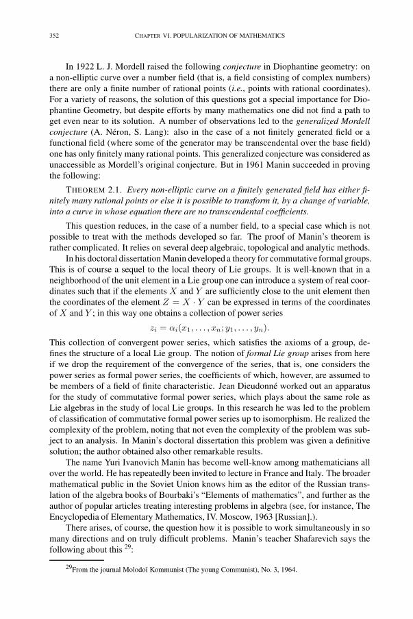
352 CHAPTER VI. POPULARIZATION OF MATHEMATICS
In 1922 L. J. Mordell raised the following conjecture in Diophantine geometry: ona non-elliptic curve over a number field (that is, a field consisting of complex numbers)there are only a finite number of rational points (i.e., points with rational coordinates).For a variety of reasons, the solution of this questions got a special importance for Dio-phantine Geometry, but despite efforts by many mathematics one did not find a path toget even near to its solution. A number of observations led to the generalized Mordellconjecture (A. Néron, S. Lang): also in the case of a not finitely generated field or afunctional field (where some of the generator may be transcendental over the base field)one has only finitely many rational points. This generalized conjecture was considered asunaccessible as Mordell’s original conjecture. But in 1961 Manin succeeded in provingthe following:
THEOREM 2.1. Every non-elliptic curve on a finitely generated field has either fi-nitely many rational points or else it is possible to transform it, by a change of variable,into a curve in whose equation there are no transcendental coefficients.
This question reduces, in the case of a number field, to a special case which is notpossible to treat with the methods developed so far. The proof of Manin’s theorem israther complicated. It relies on several deep algebraic, topological and analytic methods.
In his doctoral dissertation Manin developed a theory for commutative formal groups.This is of course a sequel to the local theory of Lie groups. It is well-known that in aneighborhood of the unit element in a Lie group one can introduce a system of real coor-dinates such that if the elements X and Y are sufficiently close to the unit element thenthe coordinates of the element Z = X · Y can be expressed in terms of the coordinatesof X and Y ; in this way one obtains a collection of power series
zi = αi(x1, . . . , xn; y1, . . . , yn).
This collection of convergent power series, which satisfies the axioms of a group, de-fines the structure of a local Lie group. The notion of formal Lie group arises from hereif we drop the requirement of the convergence of the series, that is, one considers thepower series as formal power series, the coefficients of which, however, are assumed tobe members of a field of finite characteristic. Jean Dieudonné worked out an apparatusfor the study of commutative formal power series, which plays about the same role asLie algebras in the study of local Lie groups. In this research he was led to the problemof classification of commutative formal power series up to isomorphism. He realized thecomplexity of the problem, noting that not even the complexity of the problem was sub-ject to an analysis. In Manin’s doctoral dissertation this problem was given a definitivesolution; the author obtained also other remarkable results.
The name Yuri Ivanovich Manin has become well-know among mathematicians allover the world. He has repeatedly been invited to lecture in France and Italy. The broadermathematical public in the Soviet Union knows him as the editor of the Russian trans-lation of the algebra books of Bourbaki’s “Elements of mathematics”, and further as theauthor of popular articles treating interesting problems in algebra (see, for instance, TheEncyclopedia of Elementary Mathematics, IV. Moscow, 1963 [Russian].).
There arises, of course, the question how it is possible to work simultaneously in somany directions and on truly difficult problems. Manin’s teacher Shafarevich says thefollowing about this 29:
29From the journal Molodoı Kommunist (The young Communist), No. 3, 1964.
2. Lenin prize for work in Diophantine geometry 353
All who know Manin are amazed at his bright mathematical talentand his ability to work much and aspiringly. It has happened thathe has finished a paper, where he had to overcome great obstaclesand the presentation of which required many tens of pages, and onemight have expected that now there would be a break . . . But alreadythe following day he had completely dug himself into the solution ofanother problem. Probably this can be explained by an extraordinaryability to work that he can simultaneously treat so many things. Andthese things not only seem to obstruct his principal activity but seemeven to assist him in it.
Manin, addressing himself to young Readers, writes as follows 30:
Basing myself on my own modest personal experience, I would liketo say to those who are 16-17 years of age: don’t be afraid of thescientific literature! Anyone of you will be able to understand whatis written there and follow what is known, and what is not, whatproblems are posed and the solution of which is under it way. Butone should not believe that this is easy. It is hard. But not harder thanoccupying oneself besides the usual school curriculum, with music,or with matters concerning radio31.
Comments. The above article was written when Manin was 31, a young very promising mathematician. He himselfsays that the prize he got was somewhat embarrassing for him, and he considered it as an advance for work yet to be done. Nowhe is 66 and one of the most famous mathematicians of his generation. Even the formal list of his distinctions is impressing.He is an invited speaker at five ICM congresses; recipient of Moscow Mathematical Society Award, Lenin Prize for work inAlgebraic Geometry, Brouwer Gold Medal for work in Number Theory, Frederic Esser Nemmers Prize in Mathematics, RolfSchock Prize in Mathematics, Georg Cantor Medal, King Faisal International Prize for Mathematics; elected member of atleast 8 academies; and so on.
The diversity of his mathematical interests is striking. His research being extremely broad and characterized by specialattention to interrelations of different branches of science, it has however two principal centers: the meeting point of numbertheory and algebraic geometry, and that of algebra and physics. To name briefly some fields he developed, at least the followingcome to mind:
The function field analogue of the Mordell conjecture; the Gauss-Manin connection; formal groups and Dieudonnémodules; cubic forms and arithmetic of rational varieties; a counter-example to the Lüroth problem for threefold; modularforms, p-adic theory of automorphic functions, and Manin-Drinfel’d symbols; distribution of rational points on algebraicvarieties; approaches to the theory of real multiplication; matrix solitons; instantons; homogeneous super spaces and superstrings; the Polyakov measure and the Selberg zeta function; mirror symmetry; quantized theta functions, quantum cohomologyand Frobenius manifolds; quantum computing.
Manin’s impact by far exceeds research results of his own. His books on algebraic geometry, K-theory, cubic forms,linear algebra, homological algebra, mathematical logic, number theory, gauge fields, elementary particles, quantum cohomol-ogy are widely read. The number and quality of his students, the influence of his knowledge and ideas, his enticing lecturingstyle, the broadness of his intellect, his agreeable personality, all this forms a unique image of scientist and scholar we ad-mire. The list of mathematicians considering him as a teacher can hardly be cited. The Ph.D. theses of A. Beilinson, A.Belskiı, V. Berkovich, I. Cherednik, V. Danilov, E. Demidov, V. Drinfel’d, M. Frumkin, A. Geronimus, El Hushi, V. Iskovskih,G. H. Höhn D. Kanevskiı, M. Kapranov, R. Kaufmann, Kha Huy Khoai, K. Kii, V. Kolmykov, V. Kolyvagin, P. Kurchanov, D.Lebedev, D. Leites, A. Levin, B. Martynov, Hoang Le Minh, G. Mustafin, A. Panchishkin, I. Penkov, A. Roitman, G. Shabat, A.Shermenev, V. Shokurov, A. Skorobogatov, Yu. Tschinkel, M. Tsfasman, B. Tsygan, Yu. Vainberg, A. Vaintrob, A. Verevkin,M. Vishik, S. Vladuts, A. Voronov, M. Wodzicki, Yu. Zarhin bear Manin’s name as thesis advisor. The list of his students ismuch vaster, including M. Kontsevich, S. Merkulov, V. Serganova, I. Zaharevich, and many others.
His non-mathematical interests are not less widespread than mathematical ones. He published research and expositorypapers on literature, linguistics, glotto-genesis, mythology, semiotics, physics, history of culture, and philosophy of science.The example he set for those around him was not that of a monomaniac mathematician, but of a deep scholar “par excellence”for whom the penetration into the mystery of knowledge is much more important than professional success.
Michael Tsfasman
30From the journal Molodoı Kommunist (The young Communist), No. 3, 1964.31Translator’s note. The contemporary Reader could perhaps substitute the word radio for IT.

354 CHAPTER VI. POPULARIZATION OF MATHEMATICS
[1], [2]
References
[1] Yuri I. Manin, Selected papers. World Scientific Series in 20th Century Mathematics, 3. World ScientificPublishing Co., Inc., River Edge, NJ, 1996.
[2] Dedicated to Yuri I. Manin on the occasion of his 65-th birthday. Moscow Math. J. 2 (3), 2002, 108–110.
355
3. [K69c] The history of solving equations
In this paper we shall be concerned with the algebraic equation of one variable
a0 + a1x + a2x2 + · · ·+ anx
n = 0 (n ≥ 1),
where the coefficients ai are complex numbers32. For equations of degree three and foursuch recipes were found only in the 16th century (in Italy): in the case n = 5, however,all attempts to find solution formulae turned out to be fruitless.
The problem of finding solution formulae for equations of higher degree appeared ina new light at the end of the 18th century, when J. L. Lagrange discovered the notion oftransformation group and, upon applying it to equations, found basic principles for theirstudy.
In the general case the problem was solved, some 60 years later, by É. Galois, whichturned out to be fertile not only in algebra but also in geometry (the work of S. Lie,F. Klein, É. Cartan etc.), in the theory of differential equations, and elsewhere. The reasonwas here probably that Galois studies in his work important mathematical structure andtheir interrelations in “pure form”. He was the first to state that the future mathematicsis l’analyse de l’analyse (the analysis of analysis), the object of which is the study ofmathematical structures 33
The Reader will observe that Galois was a forerunner of the famous Nicolas Bour-baki. The latter’s widely spread (but not generally accepted) point of view that mathemat-ics is a hierarchy of structures and that its central problem (and even of natural science)are the structures and the study of the interrelations is a confirmation of this. The authorhopes to acquaint below the Reader (in its broad outlines) with the proof of the followingfact:
THEOREM 3.1. In an arbitrary n-th order algebraic equation
(98) a0 + a1x + a2x2 + · · ·+ anx
n = 0
whose coefficients ai are independent in the complex domain cannot be solved in termsof radicals.
This means that there cannot exist a formula which produces the solution of an ar-bitrary n-th order algebraic equation by applying to its coefficients ai a finite number ofarithmetical operations and extractions of roots. Of course, one should here bear in mindthat the equation (98) of course has solutions but these cannot be expressed in terms thecoefficients ai as a “nice” formula. In many concrete special cases there may be solutionformulae in terms of radicals. But often these formulae are so complicated that in order
32As the complex numbers got “priority” only in the beginning of the 19th century, we consider, for awhile (Sections 3.1–3.4), only equations with real coefficients and seek only their real solutions. Neverthelessit is possible to obtain from the formulae found also complex solutions of these equations.
33The contemporary, deeply founded notion of mathematical structure is due to [2, Chapitre I: Descriptionde la mathématique formelle; Chapitre II: Théorie des ensembles.]
356 CHAPTER VI. POPULARIZATION OF MATHEMATICS
to find the solutions of (98) and in order to learn the properties needed in its applicationone uses indirect methods. 34
3.1. Equations solvable in terms of radicals
The White Rabbit put on his spectacles. “Where shall I begin, please yourMajesty?” he asked. “Begin at the beginning,” the King said gravely, “and goon till you come to the end: then stop”.
Lewis Carrol, Alice in Wonderland
1. The first information about the solution of algebraic equations comes from AncientEgypt. (Cf. [14, p. 110].)
The attempts to solve non-linear algebraic equations showed that the solution can notany longer be expressed in terms of the equation’s coefficients by application to them afinite number of arithmetical operations (addition, subtraction, multiplication, division);in other words, it appeared that the solution cannot always be expressed in rational termsby the given quantities. For instance, already from the solution formula for the quadraticequation x2 + px + q = 0,
x = −p
2∓
√p2
4− q,
it is seen that in addition to the arithmetical operations there comes a square root extrac-tion. This formula was known already in Ancient Babylon.
2. The ancient Greeks rediscovered the solution formula of the quadratic equation,expressing it in geometric terms. It is also well-known that the ancients liked to reducethe solution of algebraic equations to the search of the intersection of two auxiliary curvesor else the repeated application (“iteration”) of this procedure. For example, the equationy3 = ab2 was solved by intersection of two conic sections, the parabola y2 = bx andthe hyperbola xy = ab. The duplication of the cube is a special case of this problem,for a = 2b. The problem to intersect a sphere by a plane in such a way that the areasof two segments arising are in a given ratio to each other, led to a cubic equation, to thesolution of which again geometrical methods were employed. (We leave it to the Readerto derive, as a problem, this cubic equation and to find the corresponding conic sections.)
The main attention was directed to the case when the auxiliary curves were circlesor straight lines. Each such construction (by ruler and compass) reduces to the findingthe intersection of two straight lines; a straight line and a circle; or two circles and, ifnecessary, iteration of this method. When in the 17th century the method of coordinateswas taken into use, it became manifest that in the case at hand the application of thegeometrical method is equivalent to the sequential solution of a chain of linear and cubicequations. In other words, the possibility of carrying out these constructions was relatedto the problem of the solvability of the cubic equation in radicals. 35
34For a short introduction, see [7, 11]. Editors’ note: See also article [12]35In greater detail about this in [9].

3. The history of solving equations 357
3. In the middle ages, many trials were made to solve the cubic equation; let us recall, forinstance, the attempt of the famous Italian mathematician Leonardo Fibonacci36, around1225. Finally, Scipione del Ferro, professor at the university of Bologna, succeeded, in1506–1515, to find a solution formula for the equation a+ bx + x3 = 0. But he kept hisdiscovery in secret, revealing it only to his student Antonio Maria Fiore. The latter hada dispute with his gifted compatriot Niccolo Tartaglia, which later also was followed bya public disputation. The problem sent to Tartaglia required to give a method of solutionfor the equation x3 +ax2 = b. Tartaglia had prepared himself well for the contest: he didfind not only the solution of x3+ax2 = b but also of x3+ax = b (in 1535)! He publishedthe results first as a pentagram (1539) and then with a full description. But they becamewidely known only through the well-known treatise written by the Italian mathematicianGeronimo Cardano Ars magna, sive de regulis algebraicis (The great art or on the rulesof algebra, 1545). Therefore the solution formula for the equation x3 + bx + a = 0 isalso known as Cardano’s formula,
x = 3
√−a
2+√
Δ + 3
√−a
2−√
Δ where Δ =a2
4+
b3
27.
But the general cubic equation a0 + a1x+ a2x2 + a3x
3 = 0 can be reduced to the above
special case by the rational change of variable 37 x = y − a2
3. Therefore Cardano’s
formula can also be used to solve the general cubic equation. This substitution waspresumably known to Cardano, because he transformed all his cubic equations to a formwhere the quadratic term was absent. However, it was François Viète who was to presentthe change of variable just mentioned. The Dutchman Jan Hudde simplified considerablyViète’s treatment in 1658, in which way the solution of the cubic equation took more orless the present day form. In doing this he used the symbolic formalism invented by R.Descartes.
4. Several facts about equation of the fourth degree [or quartic equations] were knownalready to Apollonius (around 200 B.C.). Also Arabian mathematicians, in the middleages, knew how to solve some such equations. For example, in order to solve the equationx4+px3 = q they sought the intersection between the parabola y = x2 and the hyperbolay2 + pxy − q = 0.
After having being successful in the case n = 3, the 16th century mathematiciansbegan intensively to look for a solution formula for the equation of the fourth degree.Thus Cardano worked for a long time on this, but his efforts gave no harvest and he gaveup. Instead he directed his student Luigi Ferrari to continue. In 1645, Ferrari found thesought method.
The equation a0 + a1z+ a2z2 + a3z
3 + z4 = 0 can be brought in the form r+ qx+px2 + x4 = 0 changing the variable z = x− a3
4. Introducing a new parameter, we can
36Translator’s note. Also known as Leonardo of Pisa or Pisanus; Leonardo’s father’s name was Bonacci,so the son wrote himself as Leonardo filius Bonacci; the name Fibonacci was used, only in the first half of the19th century, by the Italian mathematician and mathematical historian Guglielmo Libri Carucci della Sommaja(1803-1865), at the same time a great scoundrel (a thief of old books). Leonardo’s algebra book starts with thesentence in Latin: Incipit liber Abbaci compositus a Leonardo filio Bonnaci Pisano, in anno 1202. (Quotedfrom [10, p. 133]).
37Translator’s note. Known as a Tschirnhaus transformation.

358 CHAPTER VI. POPULARIZATION OF MATHEMATICS
present the last equation as
(x2 + p + y)2 = (p + 2y)x2 − qx + (p2 − r + 2py + y2).
We determine y in such a way that the right hand side of the last equation is a full square:it transpires that this is so if and only if
4(p + 2y)(p2 − r + 2py + y2) = q2.
But this is a cubic equation for finding y. After y has been found (it turns out that itsuffices to know only one cubic root) we obtain for the determination of x two quadraticequations:
x2 + p + y = Px + Q and x2 + p + y = −(Px + Q).
We see that the solution of the quartic equation is reduced to the successive solution ofequations of lower degree. Also this method became known to the algebraists by themediation of Cardano’s treatise Ars Magna.
We remark that the solution of the quartic equation can readily be given a geometricinterpretation. Indeed, taking y = x2 the general equation can be written as
y2 + a3xy + a2y + a1x + a0 = 0.
The original algebraic problem is now reduced to finding the equations in the xy-planefor the intersections of two-dimensional second order curves.38
A strong push forward for further development of the theory of equations was givenby the plan of Descartes, according to which algebra should rise to primacy in mathe-matics, to be an adequate mean in the posing and in the study of geometric problems.However, after the creation of calculus, the attention of the mathematicians moved in aquite different direction, but not for very long.
The successful solution for n = 2, 3, 4 had put on the agenda the finding of a solutionformula for the fifth order (or quintic) equation. Nobody had (on the base of induction)any doubts about that such a formula would be found sooner or later. Among othersmathematician such as R. Descartes, G.-W. Leibniz, E. Bézout and L. Euler workedon this. The later found an approach differing from Ferrari’s method for reducing thequartic equation to cubic equations, and he had also the idea to apply this in the quinticcase. Likewise J.-L. Lagrange made an attempt to find a solution formula for the quinticequation. But not even the efforts of all these famous mathematicians did the desiredresult. This arose doubt about the correctness of the position of the problem, and onebegan to find a proof of the solvability of the quintic equation a priori, that is, withoutfinding directly the solution formula.
38Making the substitution y = x2 in the equation r + qx + px2 + x4 = 0, we can give it the shape
x2 + y2 + qx + (p − 1)y + r = 0.
This is the equation of a circumference with center (− q2,− p−1
2) and radius
R =q2
4+ (
p − 1
2)2 − r.
Thus it is possible to find the real solutions of the general quartic equation with the aid of a circumference fromthe graph of the parabola y = x2.

3. The history of solving equations 359
3.2. The plan of Lagrange
So Alice was considering in her own mind (as well as she could, for the hotday made her feel very sleepy and stupid), whether the pleasure of making adaisy-chain would be worth the trouble of getting up and picking the daisies
Lewis Carrol, Alice in Wonderland
5. An extraordinary importance in the development of the theory of equations was theappearance, in 1770-1771, of Lagrange’s memoir “Refléxions sur la théorie algébique deséquations”. It consists of four parts. In the first three of them the author gives an analysisof all the then known methods of solution for the third and the fourth order equationsand likewise some higher order equations; the fourth is devoted to consequences of thisanalysis.
Lagrange succeeded to give a general principle for the solution methods. It turns outthat in the case of all the existing methods one has to solve some auxiliary equations, thecoefficients of which are expressed rationally in the coefficients of the initial equation.The solutions of these auxiliary equations are the values of a certain rational functions,when the arguments are the solution of the initial equation. Here the degree of the aux-iliary equation is determined not by the shape of this function but the fact how manyvalues it takes under all possible rearrangements (or substitutions) of its arguments, thatis the solution of the initial equation.
Lagrange reached the conclusion that the finding of a solution formula for an alge-braic equation reduces to the problem of finding such rational functions of the solutionsof an equation which take the fewest number of possible values. If in this case the degreeof the auxiliary equation arising is lower than the degree of the initial equation, then thesolution of the equation is reduced to solving of an equation of lower degree. In thisway one can, in certain conditions, by iterating the procedure arrive at a solution of thegiven equation. This is Lagrange’s plan in its broad outline. Let us get acquainted withits details.39
Let there be given the general equation a0 + a1x+ a2x2 + · · ·+ anx
n = 0; its coef-ficients are variables which may assume arbitrary complex values and are algebraicallyindependent over the field of complex numbers C (that is, they do not satisfy any alge-braic equation with complex coefficient). Its solution will be denoted x1, . . . , xn. Thelatter may also be viewed as independent variables over C, as in view of Vietè’s formulaethere correspond to each set of values for xi fixed ai values and vice versa.
Let us consider a rational expression ϕ(x1, . . . , xn) in the solutions xi of the equa-tion f(x) = 0 with coefficients in an transcendental extension40 C(a1, . . . , an)/C. Let
39In explaining Lagrange’s plan we used several notions about groups and fields, so this subsection maycause some of the Readers certain difficulties. In such a situation we advice them to acquaint themselves withthem the book [5]. Translator’s note. Cf, 1, footnote 12.
40The elements of the field C(a1, . . . , an)/C are all such divisions f(a1,...,an)g(a1,...,an)
, where g �≡ 0; here f
and g are polynomials with complex coefficients over a1, . . . , an. These variables are treated as independentquantities in the field C.

360 CHAPTER VI. POPULARIZATION OF MATHEMATICS
us permute the solution xi among themselves in the expression ϕ(x1, . . . , xn) (i.e. xi �→xσ(i), σ ∈ Sn) and turn our attention to the case when ϕ does note change, that is
ϕ(x1, . . . , xn) = ϕ(xσ(1), . . . , xσ(n)).
For example, ϕ = x1x2 + x3x4 does not change if we apply to it the substitution 41
σ =(
1 2 3 43 4 2 1
)It is easy to see that all the substitutions which do not alter a given rational expression
ϕ(x1, . . . , xn) form a group Φ. For example, in the case of ϕ = x1x2 + x3x4 this groupis the following one of order 8:
Φ ={(
1 2 3 41 2 3 4
),
(1 2 3 42 1 3 4
),
(1 2 3 41 2 4 3
),
(1 2 3 42 1 4 3
),(
1 2 3 43 4 1 2
),
(1 2 3 44 3 2 1
),
(1 2 3 43 4 2 1
),
(1 2 3 44 3 1 2
)}.
By a direct check, the Reader can verify that each fourth order substitution which liesoutside Φ ⊂ S4 changes the expression ϕ(x1, . . . , x4).
DEFINITION 3.2. If a rational expression ϕ(x1, . . . , xn) does not change a givensubstitution group Φ (Φ ⊂ Sn) by application of any element but changes if we applyan n-th order substitution not belonging to the subgroup Φ, then we say that ϕ belongsto the group Φ.
For example, the linear expression ω = α1x1 + α2x2 + · · · + αnxn, where the αi
all are distinct, belongs to the unity group Φ = (e).Let the rational expression ϕ belong to the subgroup Φ ⊂ Sn. Taking an arbitrary
subgroup G in Sn with G ⊃ Φ and applying to ϕ all substitution xi �→ xσ(i) we obtaina complex of distinct expressions
ϕ, ϕ1, . . . , ϕs−1,
which we call the G-co-expressions of ϕ. Taking for example G = Sn we obtain forϕ = x1x2 + x3x4 the following G-co-expressions:
ϕ = x1x2 + x3x4, ϕ1 = x1x3 + x2x4, ϕ2 = x1x4 + x2x3.
Equations whose solutions are formed from the solutions of the given general equa-tion rational co-expressions will be called auxiliary equations. It turns out that the G-co-expressions of a rational expression ϕ belonging to Φ are solutions of an auxiliaryequation of degree (G : Φ) 42; moreover, the coefficients of the auxiliary equation are“G-conservative”, that is, they do not change under the action of any element of G.
The plan is based on the following theorem.
41To apply the substitution
σ =1 2 3 4
3 4 1 2
must be interpreted in the “natural way”: in the expression ϕ(x1, . . . , xn) all the variables i have to be replacedby σ(i).
42Let the number of elements in the finite groups G and Φ be |G| and |Φ| respectively. Then the index
of Φ in G is the number (G : Φ) =|G||Φ| .
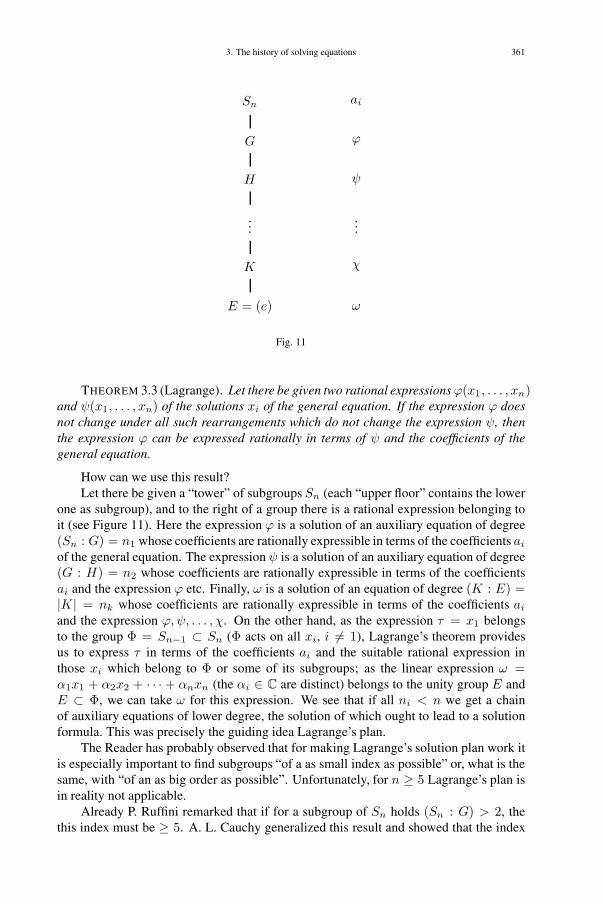
3. The history of solving equations 361
Sn ai
G ϕ
H ψ
......
K χ
E = (e) ω
Fig. 11
THEOREM 3.3 (Lagrange). Let there be given two rational expressionsϕ(x1, . . . , xn)and ψ(x1, . . . , xn) of the solutions xi of the general equation. If the expression ϕ doesnot change under all such rearrangements which do not change the expression ψ, thenthe expression ϕ can be expressed rationally in terms of ψ and the coefficients of thegeneral equation.
How can we use this result?Let there be given a “tower” of subgroups Sn (each “upper floor” contains the lower
one as subgroup), and to the right of a group there is a rational expression belonging toit (see Figure 11). Here the expression ϕ is a solution of an auxiliary equation of degree(Sn : G) = n1 whose coefficients are rationally expressible in terms of the coefficients ai
of the general equation. The expression ψ is a solution of an auxiliary equation of degree(G : H) = n2 whose coefficients are rationally expressible in terms of the coefficientsai and the expression ϕ etc. Finally, ω is a solution of an equation of degree (K : E) =|K| = nk whose coefficients are rationally expressible in terms of the coefficients ai
and the expression ϕ, ψ, . . . , χ. On the other hand, as the expression τ = x1 belongsto the group Φ = Sn−1 ⊂ Sn (Φ acts on all xi, i �= 1), Lagrange’s theorem providesus to express τ in terms of the coefficients ai and the suitable rational expression inthose xi which belong to Φ or some of its subgroups; as the linear expression ω =α1x1 + α2x2 + · · · + αnxn (the αi ∈ C are distinct) belongs to the unity group E andE ⊂ Φ, we can take ω for this expression. We see that if all ni < n we get a chainof auxiliary equations of lower degree, the solution of which ought to lead to a solutionformula. This was precisely the guiding idea Lagrange’s plan.
The Reader has probably observed that for making Lagrange’s solution plan work itis especially important to find subgroups “of a as small index as possible” or, what is thesame, with “of an as big order as possible”. Unfortunately, for n ≥ 5 Lagrange’s plan isin reality not applicable.
Already P. Ruffini remarked that if for a subgroup of Sn holds (Sn : G) > 2, thethis index must be ≥ 5. A. L. Cauchy generalized this result and showed that the index
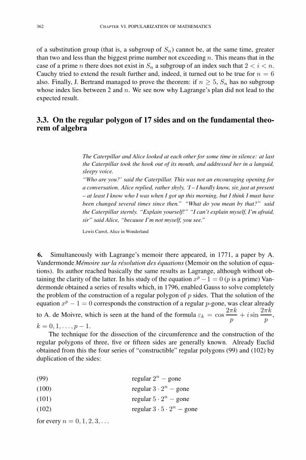
362 CHAPTER VI. POPULARIZATION OF MATHEMATICS
of a substitution group (that is, a subgroup of Sn) cannot be, at the same time, greaterthan two and less than the biggest prime number not exceeding n. This means that in thecase of a prime n there does not exist in Sn a subgroup of an index such that 2 < i < n.Cauchy tried to extend the result further and, indeed, it turned out to be true for n = 6also. Finally, J. Bertrand managed to prove the theorem: if n ≥ 5, Sn has no subgroupwhose index lies between 2 and n. We see now why Lagrange’s plan did not lead to theexpected result.
3.3. On the regular polygon of 17 sides and on the fundamental theo-rem of algebra
The Caterpillar and Alice looked at each other for some time in silence: at lastthe Caterpillar took the hook out of its mouth, and addressed her in a languid,sleepy voice.“Who are you?’ said the Caterpillar. This was not an encouraging opening fora conversation. Alice replied, rather shyly, ‘I – I hardly know, sir, just at present– at least I know who I was when I got up this morning, but I think I must havebeen changed several times since then.” “What do you mean by that?” saidthe Caterpillar sternly. “Explain yourself!” “I can’t explain myself, I’m afraid,sir” said Alice, “because I’m not myself, you see.”
Lewis Carrol, Alice in Wonderland
6. Simultaneously with Lagrange’s memoir there appeared, in 1771, a paper by A.Vandermonde Mémoire sur la résolution des équations (Memoir on the solution of equa-tions). Its author reached basically the same results as Lagrange, although without ob-taining the clarity of the latter. In his study of the equation xp−1 = 0 (p is a prime) Van-dermonde obtained a series of results which, in 1796, enabled Gauss to solve completelythe problem of the construction of a regular polygon of p sides. That the solution of theequation xp − 1 = 0 corresponds the construction of a regular p-gone, was clear already
to A. de Moivre, which is seen at the hand of the formula εk = cos2πkp
+ i sin2πkp
,
k = 0, 1, . . . , p− 1.The technique for the dissection of the circumference and the construction of the
regular polygons of three, five or fifteen sides are generally known. Already Euclidobtained from this the four series of “constructible” regular polygons (99) and (102) byduplication of the sides:
= regular 2n − gone(99)
= regular 3 · 2n − gone(100)
= regular 5 · 2n − gone(101)
= regular 3 · 5 · 2n − gone(102)
for every n = 0, 1, 2, 3, . . .
3. The history of solving equations 363
One might have thought that these were the only series of constructible regular poly-gons. However, Gauss proved that also the regular polygon of 17 sides was constructible.More exactly, he established the following theorem:
THEOREM 3.4. The regular p-gone is constructible with the aid of the ruler andcompass if and only if one of the following conditions is fulfilled:
(α) p is a prime of the form p = 2n + 1;(β) p = 2k;(γ) the number p is the product of a finitely many pairwise relatively prime num-
bers of the previous two types.
For Reader, who hears about this theorem for the first time, the meaning of thesenumbers will probably be somewhat mysterious. The author has the intention to writein the pages of our journal about Galois’ criterion for the solvability of algebraic equa-tions.43 Having learnt this criterion and bearing in mind that the geometric question isequivalent to the solution of the equation xp−1 + xp−2 + · · · + x + 1 = 0 in terms ofsquare roots, the mystery of these numbers disappear. In connection with Gauss’s theo-rem we should note that the number p = 2n + 1 cannot be a prime, unless n in turn isnot a number of the form 2k for k an integer. Indeed, assuming that n = 2k ·m with modd and setting 22k = α, we obtain using that m is odd the identity
p = 2n + 1 = 22k·m + 1 = αm + 1 =
= (α + 1)(αm−1 − αm−2 + · · · − α + 1).
This shows that for all m �= 1 it is true that p is not a prime. Then number p = 22k
+ 1,k = 0, 1, 2, 3, 4 are primes so according to our theorem the regular polygons with 3, 5,17, 257 and 65537 sides are constructible (see the paper [13]p. 86). Already for n = 5one has a composite number (L. Euler found the factor 641). There arises the questionif the series 22k
+ 1 contains a finite or an infinite number of primes. G. Eisensteinasserted that they are only finitely many (. . . and perhaps he had indeed reasons for suchan assertion).
7. Let us next have a look at the number of solutions of an algebraic equation; thisquestion is intimately tied to the creation of the notion of complex number.
Already Apollonius knew that two conic sections cannot have more than four pointsof intersection, i.e. the coordinate 4-th degree equation has at most 4 solutions. Cardanobegan to operate, in the solution of the equation x4 + 40 = 10x2, with the numbers5 +
√−15 and 5−
√−15, calling “sophistic numbers”, and, upon multiplying them, he
verified that they were correct solutions. He was the earliest man who regarded thesenumbers as “lawful”, and so he arrived at the conclusion that the cubic equation has threebut the 4th order 4 solutions. The first ever to state explicitly that the n-th order equationhas n solutions was P. Roth[e] (1608); he was one of the Nuremberg “reckoners”44
These ideas were the foundations of a conjecture with the same formulation by theeminent algebraist A. Girard (1629); in 1746 J. d’Alembert made an effort to prove
43Translator’s note. See [4], also Section 6 of this book.44Translators note. Peter Rothe, d. 1617.

364 CHAPTER VI. POPULARIZATION OF MATHEMATICS
this conjecture and, although his attempt failed, he had found a valuable idea. In 1749L. Euler tried to verify Girard’s conjecture, and after him likewise J. L. Lagrange.
The “sophistic quantities” had to go through still a long evolution, where we cannote names such as J. Wallis (1673), C. Wessel (1798) and J. Argand (1813), before onereached a clear picture of the complex numbers and their geometric presentation.
The first to make a serious use of complex numbers was C. F. Gauss, in this wayconsiderably enriching the apparatus of Mathematical Analysis. In algebra Gauss man-aged to prove the general case of Girard’s conjecture. This was done in his dissertation(the years 1797-1799).
Basing himself on d’Alembert’s result, Gauss proved the following result.
THEOREM 3.5. For each n and arbitrary complex numbers a0, a1, . . . , an the equa-tion p(x) = a0 + a1x + a2x
2 + · · ·+ anxn = 0 there exits a complex number such that
p(α) = 0.
Girard’s conjecture follows at once from this so-called fundamental theorem of al-gebra and a simple fact (already known to Cardano): the number α is a solution of theequation p(x) = 0 if and only if the polynomial p(x) is divisible by the linear polynomialx− α.
For young Readers it will probably be sufficiently interesting and useful to learn theproof of this theorem. We present Gauss’ proof in a variant due to F. Klein and H. Weber.
PROOF. (1) Reduction. It turns out that it suffices to prove the theorem for polyno-mials with real coefficients. Indeed, let us consider the polynomial
f(z) = a0 + a1z + a2z2 + · · ·+ anz
n, z ∈ C
also the polynomialf(z) = a0 + a1z + a2z
2 + · · ·+ zn,
where the symbol ai denotes the complex conjugate of the number ai. Let us form thepolynomial F (z) = f(z) · f(z); then all coefficients are real. Indeed, the polynomial Fhas the coefficients Ak =
∑i+j=k aj aj , and, as
Ak =∑
i+j=k
aiaj =∑
i+j=k
aj ai = Ak,
then Ak ∈ R (this is our notation for the domain of real numbers). For α ∈ C letF (α) = 0. Then at least one of the relations f(α) = 0 or f(α) = 0 must be fulfilled.Thus if f(α) �= 0 then one would have f(α) = 0. So the reduction is carried out, and inwhat follows we may assume that all ai ∈ R.
(2) Introduction of geometric elements. Let z = x + iy. Using Newton’s binomialtheorem we obtain
f(z) = f(x + iy) = u(x, y) + iv(x, y).
Each point of intersection in the xy-plane of the curves U : u(x, y) = 0 and V :v(x, y) = 0 gives a solution of our equation f(z) = 0. Therefore we have to showthat, indeed, they intersect at least once. To this end, we shall have a closer look at thebehavior of these curves in the xy-plane.
Viewing the polynomials u = u(x, y) and v = v(x, y) as functions of two variables,we note their continuity. Therefore we have:
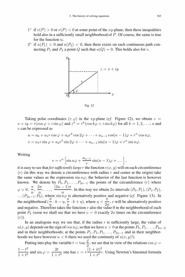
3. The history of solving equations 365
1◦ if v(P ) > 0 or v(P ) < 0 at some point of the xy-plane, then these inequalitieshold also in a sufficiently small neighborhood of P . Of course, the same is truefor the function u;
2◦ if u(P1) > 0 and u(P2) < 0, then there exists on each continuous path con-necting P1 and P2 a point Q such that u(Q) = 0. This holds also for v.
�
�
�
�
�
��
��
��
�z = x + iy
x
y
0
r
ϕ
Fig. 12
Taking polar coordinates (r, ϕ) in the xy-plane (cf. Figure 12), we obtain z =x + iy = r(cosϕ + i sinϕ) and zk = rk(cos kϕ + i sinkϕ) for all k = 1, 2, . . . ; u andv can be expressed as
u = a0 + a1r cosϕ + a2r2 cos 2ϕ + · · ·+ an−1 cos(n− 1)ϕ + rn cosnϕ,
v = a1r sinϕ + a2r2 sin 2ϕ + · · ·+ an−1 sin(n− 1)ϕ + rn sinnϕ.
Writing
v = rn[sinnϕ +
an−1
rsin(n− 1)ϕ + . . .
],
it is easy to see that for sufficiently large r the function v(x, y) will on each circumference(r) (in this way we denote a circumference with radius r and center at the origin) takethe same values as the expression sinnϕ; the behavior of the last function is howeverknown. We denote by P0, P1, . . . , P2n−1 the points of the circumference (r) where
ϕ = 0,π
n,
2πn, . . . ,
(2n− 1)πn
. In this way we obtain 2n intervals (P0;P1), (P1;P2),
. . . (P2n−1;P0), where sinnϕ is alternatively positive and negative (cf. Figure 13). In
the neighborhood (π
n· k − η,
π
n· k + η), where η <
π
2n, v will be alternatively positive
and negative. Therefore takes the function v also the value 0 in the neighborhood of eachpoint Pk (soon we shall see that we have v = 0 exactly 2n times on the circumference(r)).
In an analogous way we see that, if the radius r is sufficiently large, the value ofu(x, y) depends on the sign of cosnϕ, so that we haveu > 0 at the pointsP0, P1, . . . , P2n−2
and in their neighborhoods; at the points P1, P3, P5, . . . , P2n−1 and in their neighbor-hoods we have however u < 0 (here we used the continuity of u(x, y)!).
Putting into play the variable t = tanϕ
2, we see that in view of the relations cosϕ =
1− t2
1 + t2and sinϕ =
2t1 + t2
one has z = r(1 + it)2
1 + t2. Using Newton’s binomial formula

366 CHAPTER VI. POPULARIZATION OF MATHEMATICS
P0
P8P7
P6
P5
P4
P3 P2
P1
P9
x0
y
_
_
_
_ _+
++
+ +
Fig. 13
we obtain
u =Φ(r, t)
(1 + t2)nand v =
Ψ(r, t)(1 + t2)n
,
where degt Φ ≤ 2n, degt Ψ ≤ 2n− 1, degr Φ ≤ n, degr Ψ ≤ n. Here degt Φ denotesthe degree of the polynomial Φ with respect to t, and degr Φ its degree with respect to r.
(3) Topological considerations. There are only finitely many circumferences (r)such that Φt ≡ 0 or Ψt ≡ 0 (here the sign ≡ stands for equivalence in the variable t).Indeed, in view of the inequalities degr Φ ≤ n and degr Ψ ≤ n we have in either case analgebraic equation of degree at most n; and each such equation cannot have more than nsolutions (do not confuse this with the question of their existence, which we will proveonly later!). The proof of this fact (by contradiction) is trivial.
It is likewise easy to see that on the circumferences (r) on which holds Φ �≡ 0 andΨ �≡ 0 (on the basis of what was said above, on can affirm that there exists an r0 suchthat for r = r0 are these conditions fulfilled) the functions u and v become zero not morethan 2n times – this in view of the inequalities degt Φ ≤ 2n and degt Ψ ≤ 2n. Usingnow the result of both considerations, we see that neither u nor v can be zero in a domainof points with finite area. In other words, we can say that the plane falls into two type ofdomains (in one of them one has v > 0 and the others v < 0), which are separates by thecurved line V : v = 0.
The following considerations are illustrated by Figure 14. 45
As the curve v = 0 behaves asymptotically as rn sinnϕ (i.e. for sufficiently largevalues of r the curves are close to each other), we know that the domains v > 0 lie in a
45Translator’s note. This is not the figure given by Kaljulaid, which is defective, but is taken from theclassical book Felix Klein [6, pp. 111–112]. It concerns the cubic polynomial f(z) = z3 − 1, so thatU = r3 cos 3ϕ, V = r3 sin 3ϕ. Note that, quite generally, if f is a polynomial with real coefficients, asassumed by Kaljulaid in this paper, the zeros are symmetrically situated about the real axis. The level linesdepicted in Figure 14 below, and in Klein’s book, display this symmetry, but, unfortunately, not those in thefigure originally given by Kaljulaid.

3. The history of solving equations 367
0v =
0u =
0u =
0v =
0u
=
0v
=
Fig. 14
sector (2kπn , (2k+1)π
n
),
extending (in view of the continuity of v) to the interior of the of the circumference (r).Let us now have a look at the parts of the domains v > 0 inside the circumference (r),moving along the contour V : v = 0 in such a way that these domains all the time aresituated to the left. The contour curve of the domains v > 0 then can behave inside (r)in a rather varied way: it can return to the same sector (see the sector (P2;P3)) it canmove into a sector of the type (2�π
n , (2�+1)πn ) and can then bifurcate and then each branch
moves into a sector of the aforementioned type (see Figure 14). It is however easy to seethat the contour V : v = 0 “departs” into the circumference (r) in the neighborhood ofpoints of bifurcation Pk of an odd index (where, however, u < 0) and “arrives” on thecircumference (r) in the neighborhood of points of division Pk′ of an even index (where,however, u > 0).46 Because of the continuity of the function u = u(x, y) there mustnow exist a point Q between the points Pk and Pk′ such that u(Q) = 0. Quod eratdemonstrandum. '(
In his dissertation Gauss raised the conjecture that higher order equations (n ≥ 5)do not have solutions in terms of radicals. He turned attention to this also in his famousmonograph Disquisitiones arithmeticae (Studies of Arithmetic), which appeared in theyears 1797-1801. In fact, it is possible to find, for each natural number n ≥ 5, annth order algebraic equation (even with integer coefficients) whose solutions are notexpressible in terms of radicals. At the same time, by the theorem just established, eachsuch equation has n complex solutions. From here it is also clear that the set of allalgebraic numbers is much larger than the one which can be “write down” by radicals.
46All the time we move in such a way that the domain v > 0 stays to the left.

368 CHAPTER VI. POPULARIZATION OF MATHEMATICS
In algebraic geometry one often encounters equations whose coefficients are rationalfunctions; the solutions of such equations are algebraic functions.47 Because of this oneconsiders also algebraic equations over fields differing from the field of complex numbers(of course, this has also many other reasons). The fundamental theorem of algebra is notapplicable to such field, and is replaced by the following statement:
Let P be a field and f(z) = a0 + a1z + a2z2 + · · · + anz
n = 0 an algebraicequation over P , i.e. all ai ∈ P . There cannot be more than n solution of the equationf(x) = 0 neither in P nor in any of its extension fields. On the other hand, there existsan extension F ⊇ P such that the equation f(x) = 0 has in it precisely n solutions(counting repetitions).
3.4. On the theorem of Ruffini-Abel
The only goal of history is not at all to satisfy only fruitless curiosity; learningthe past must clarify the future.
P. Tannery
9. The Italian mathematician Paolo Ruffini tried in 1799 to prove that the higher ordergeneral equation cannot be solved “in the finite extended arithmetic” (see Section 3.1).Although his proof turned out to be lacunary and despite repeated attempts (in the years1801, 1802, 1806, 1813) Ruffini did not succeeded to complete it, these papers containedmany new ideas and facts, that really constituted a preparatory step in the establishmentof group theory. Regretfully, Ruffini’s text-book Teoria generale delle equazioni, in cui sidimostra impossibili la soluzione algebraica delleequazioni generali di grado superioreal quarta (A general theory of equations, in which one demonstrates the impossibilityof the algebraic solution of equations of degree higher than four) became little knownoutside Italy.
However A.-L. Cauchy became acquainted with this book. He became the first(around 1815, that is, some time later) to develop the terminology and notation for thetheory of substitution groups. Having obtained some basic facts, he wrote a memoirSur le nombre des valeurs qu’une fonction peut acquérir lorsqu’on y permute toutesles manières possibles les quantités qu’elle renferme (On the number of values which afunction can acquire when one permutes in all possible manners the quantities which itcontains), where he set out the basis of an entire theory. We see that until the beginningof the 19th century a whole range of developments had taken place in Lagrange’s originalideas – one had laid the foundations of the theory of substitution groups. However, thebasic principles of field theory were still missing.
10. Niels Henrik Abel48 busied himself with the solution of the 5th degree equationalready in his youth. Once (in 181249) he thought that he had solved the problem, but laterhe had doubts about the validity of his proof. Intense research led Abel to a correct proof
47See [8], as well as the additional references in Section 1, footnote 9.48One can read about Abel’s life in the magnificent book Ø. Ore, The remarkable life of N. H. Abel.
Several editions in Western languages (German, Norwegian, English). Russian translation: Moscow, 1961.49Translator’s note. Born in 1802 he was about ten then; Abel died prematurely at the age of twenty six
in 1829.

3. The history of solving equations 369
(1824), and in 1826 there appeared in the Journal für Reine und Angewandte Mathematik(Journal of pure and applied mathematics) his paper Démonstration de l’impossibilité dela résolution algébrique des équations générales qui passent le quatrième degré. (Proofof the impossibility of the algebraic solvability of general equations the degree of whichexceeds four.)
Abel formulated the problem as follows. A function v of finitely many variablesx1, . . . , xn is called algebraic if v can be expressed in terms of x1, . . . , xn in the “finitelyextended arithmetic” (here Abel considered only roots to a prime number exponent).Treating the solutions of the equations as algebraic functions of the coefficients of theequation, with the aid of which one can replace the unknown in the equation, the latterwill be satisfied, Abel understands the solvability of the equation as finding the generalform of such algebraic functions.
Although the Abel(-Ruffini) theorem told that the general higher order equation isnot solvable in radicals, but its proof did not say anything about the solvability of concretealgebraic equations (with numerical coefficients) in terms of radicals. Examples showthat there exist series of equations solvable by radicals: xn + a = 0, (xn + a)m+ b = 0,x2n + pxn + q = 0. A more complicated and more interesting example of an n-th orderequation, which is solved in terms of radicals, is given by
[ n−12 ]∑
k=0
(−1)k
(n
2k
)xn−2k(1− x2)k = a, a ∈ R, |a| < 1, n ∈ N;
[x] denoting the integer part of x.Using the formula cosnα + i sinnα = (cosα + i sinα)n along with Newton’s
binomial theorem, we get
cosnα = cosn α−(n
2
)cosn−2 sin2 α + · · · =
= cosn α−(n
2
)cosn−2(1− cos2 α) + . . .
Next, writing cosnα = a and cosα = x, we see that the equation in question provides arelation for finding the cosine of an angle, when the cosine of the n-fold angle is known.The fact that this equation is solvable in radicals becomes manifest by the followingcomputation:
(cosα + i sinα)n = cosnα + i sinnα = a + i√
1− a2,
which gives
cosα + i sinα =n
√a + i
√1− a2.
In an analogous way one finds that
cosα− i sinα =n
√a− i
√1− a2.
Thus we obtain
x = cosα =12
(n
√a + i
√1− a2 +
n
√a− i
√1− a2
).

370 CHAPTER VI. POPULARIZATION OF MATHEMATICS
So we see that there remains the possibility that each concrete equation perhaps issolvable by radicals, only that in each concrete case perhaps the solution formulae differ,i.e. there exists no general formula in radicals applicable to all n-th order equations.
In the years 1826-1829 Abel worked very intensively on these questions, settingfor himself the problem to find the conditions on an equation to be solvable in termsof radicals. The honor of solving completely this problem goes, however, to anotherextraordinary mathematician Évariste Galois. However, Abel managed to find half ofGalois’ criterion: If just one of the solutions of an algebraic equation expresses it selfin radicals, then the Galois group of this equation is solvable (of course, he expressedhimself in a quite different way). The results of this fruitful work were published in hisCollected Works (1839) as the paper “Sur la résolution algébrique des équations” (Onthe solution of algebraic equations).
Of major interest is likewise his paper “Mémoire sur une classe particulière d’équa-tions résolubles algébriquement” (Memoir on a particular class of algebraically solvableequations). Here the following two theorems are established.
(1) If each solution of an equation can be expressed rationally in terms of onesolution, that is, if, for example, xj = Θj(x1), where the Θj are rationalfunctions of x1 and if these functions satisfy the “commutativity relations”
Θi(Θk(x1)) = Θk(Θi(x1)),
then the equation can be solved in terms of radicals.(2) If of two solutions of an irreducible equation of prime degree one can be ex-
pressed rationally, and vice versa, then this equation is solvable in radicals.
That Abel, in 1829, was already quite close to the results of Galois, is shown clearlyby his result (in a letter to Crelle dated October 18, 1828): if for an irreducible equationof prime degree any three of its solutions are connected with each other in such a waythat any one of them is expressible in terms of the two remaining ones, then this equationis solvable in radicals.
11. The crown of this century long line of development in algebra were the resultsof Évariste Galois (1831-32) [3]. Using a series of new mathematical notions (todayfundamental in mathematics) Galois achieved in the treatment of the questions and ideasan extraordinary precision and generality. The fact that he himself considers his maintheorem as a generalization of Gauss’ theorem (see Theorem 3.4) shows that one ofthe causes of his success was that he understood with extraordinary depth the results ofVandermonde and Gauss in the search of the solvability of the equation xp − 1 = 0 interms of square roots. Galois must be seen as the founder of group theory, because manydeep results and notions, which today constitute the basis of this theory, are due to him.
Because of these and other reasons 50 his contemporaries did not acknowledge atonce the results of Galois. Even in 1843 J. Liouville writes to the Paris Academy ofSciences: “I hope that the Academy will find it of interest to learn that, among the man-uscripts of Évariste Galois, I found a deep and exact solution to the following beautifulquestion: given an irreducible algebraic equation of prime degree, one asks if it is solv-able in radicals.” In the course of the following decade there was a revival of the ideas
50To this contributed probably also the “structural style” of his presentation (the style of the future),its remarkable richness of content, and level of abstraction, which made the appreciation of Galois’ results aserious obstacle to most mathematicians of the period.
3. The history of solving equations 371
of Galois. In 1848 J. A. Serret taught, in Paris, the first course on Galois theory. Thefirst coherent presentation in print appeared in 1852 in the form of Betti’s book “Sullarisoluzione del’equazioni algebriche” (On the solution of algebraic equation). In 1870,there appeared C. Jordan’s “Traité des substitutions et des équations algébriques” (Trea-tise of substitutions and algebraic equations), which constituted a magnificent commen-tary of Galois theory. To pursue further systematically the subsequent development ofthe ideas would be very hard within the frameworks of the present paper. 51
References
[1] N. Bourbaki. “Éléments d’histoire des mathématiques”. Actualités Sci. Ind., no. 1212. Masson, Paris,1984. English translation: “Elements of the history of mathematics”. Springer-Verlag, Berlin, 1994.Russian translation: Moscow, 1963.
[2] N. Bourbaki. Théorie des ensembles XVII. Premiére partie: Les structures fondamentales de l’analyse.Actualités Sci. Ind., no. 1212. Hermann & Cie, Paris, 1954.
[3] L. Infeld. Whom the Gods Love: The Story of Évariste Galois. National Council of Teachers of Math.,Reston, VA, 1948.
[4] U. Kaljulaid. On Galois theory. Math. and Our Age 20, 1975, 17–31. (see [K75a]).[5] G. Kangro. Kõrgem algebra (Higher algebra) II. Eesti Riiklik Kirjastus, Tallinn, 1950. (Estonian.)[6] F. Klein. Elementarmathematik vom höheren Standpunkt I. Dritte Auflage. Verlag von Julius Springer,
Berlin, 1928. Russian translation: “Nauka", Moscow, 1987.[7] M. Levin and S. Ulm. Handbook of computation methods. Valgus, Tallinn, 1966, 1977.[8] Ü. Lumiste. Riemann as the founder of topology and the general curved space. Math. and Our Age 11,
1966, 65–76. (Estonian).[9] Yu. I. Manin. On the solvability of the problem of construction with ruler and compass. Encyklopedia of
Elementary Mathematics 4, 1963, 205–227.[10] M. Marie. Histoire des sciences mathématiques et physiques. Tome I, De Thales à Diophante. Gauthiers-
Villars, Paris, 1883.[11] I. R. Shafarevich. On the solutions of equations of higher degree (the method of Sturm), Moscow, 1954.[12] I. R. Shafarevich. Selected chapters from algebra. The teachng of mathematics IV (1), 2001, 1–34.[13] E. Tamme. Pierre Fermat and mathematics of the 17th century. Math. and Our Age 5, 1964, 74–87.[14] M. Vanem and E. Tamme. How people learned to solve equations. Math. and Our Age 16, 1969, 110–121.
51The Reader will find interesting material about this in N. Bourbaki’s book [1].

This page intentionally left blank

373
4. [K70] Additional remarks on groupsComments by G. Traustason
– Que faut il faire? dit le petit ptince.– Il faut être très patient, répondit le renard.– Tu t’assoira d’abord un peu loin de moi, comme ça, dans l’herbe. Je te re-garderai du coin de lœil et tu diras rien. Le language est source de malentendus.Mais chaque jour, tu pourras t’assoir un peu plus près . . .
(Translation:– What does one have to do for this, asked the little prince.– One has to be very patient, answered the fox.– First sit down at some distance from me on the grass. . . So. . . I’ll look at youfrom a corner of my eye and you must not say anything to me. Language is anincomprehensible source. But each day you may sit down a little bit closer tome . . . )
A. de Saint-Exupéry, Le petit prince (The little prince)
The paper at hand may be viewed as a sequel to the group theory part of the surveyPrinciples of Algebra by Evgenii Gabovitsh52 [5]. Besides new notions (homomorphism,normal divisor etc.) the Reader will here become acquainted with the “description” ofcyclic groups; the notion of solvability of groups, criteria for the “discovery” of thisproperty; and examples of solvable groups. He or she will also find the Feit-ThompsonTheorem, and the formulation of some of its consequences. An extended knowledge ofgroups will be a good background for understanding Galois theory; for learning contem-porary geometry; and elsewhere. The value of group theory in applications does todaynot require special comments. There are well-known applications in physics and chem-istry (See e.g. [9] or [2]), not to speak of mathematics itself [11] or the foundations ofdifferential and Riemann geometry (see also e.g. [6, Chapter I].)
1. We consider an arbitrary group and one of its subgroups, denoting them usually byG and H . We can introduce in G a division into classes taking as classes the orbits, thatis, the sets Hg = {hg| g ∈ G fixed;h ∈ H being arbitrary}. For example, if the groupG is the complex plane C with respect to addition of complex numbers, H being theimaginary axes, then the orbits are vertical lines (cf. Figure 15).
Orbits are sometimes called cosets, and the element g is a representative of the class.The Reader will easily verify that as representative one may take an arbitrary “point”of the orbit; that distinct orbits do not intersect; that the orbit corresponding to the unitelement coincides with the subgroup H ; and, finally, that all the orbits fill up the en-tire group. Therefore, one has indeed a decomposition into classes, which is written as
52Translator’s note. See also the references provided in Section 1, footnote 12

374 CHAPTER VI. POPULARIZATION OF MATHEMATICS
�
�
�
�
��
���
����
���
H H + g
0
C(+)
Fig. 15
G = H + Hg2 + Hg3 + . . . or, compactly, G =∑
k∈K
Hg, where K = {e, g2, g3, . . . }is a complete system of representatives, that is a set to which belongs precisely one rep-resentative in each class.
Let us have a look at the case when G is a finite group. The number of elements iscalled the order of the group and is denoted |G|. The number of distinct orbits is calledthe index of the subgroup H in the group G and is written indG H or, also, (G : H).
THEOREM 4.1 (Lagrange). The order of a finite group is divisible by the order ofthe each subgroup, the quotient being then the index of the subgroup.
PROOF. We check first that the map ϕ : H �→ Hg, given by f(H) = hg, is one-to-one. This shows that all orbits have the same number of points. As the orbits fillout the entire group and do not intersect, we see, in view of the definition of index, that|G| = |H | · indG H , which proves the assertion of the theorem. '(
Thus Lagrange’s theorem says that in a finite group the orders of its subgroups aredivisors of its order. One can also ask if the converse is true: if a number m dividesthe order of a finite group, is it then the order of some subgroup of order m? Simpleexamples indicate that such a “converse conjecture” is not true in general. However, itis true when m is a prime. Even more, if |G| = pn · r, if p is a prime number and thenumber p and r are relatively prime to each other, then G contains subgroups of orderp, p2, p3, . . . , pn. This statement (together with a small addendum) is known as the FirstTheorem of Sylow.
Isn’t it possible, in all the previous reasonings, to consider, instead of the [previous]so-called right cosets, left cosets gH , that is, sets
gH = {gh|g ∈ Gfixed; h ∈ H being arbitrary}?
The Reader will easily realize this case (by a completely analogous argument) and as aresult we obtain a “left hand picture” of the previous “right hand picture”. In the specialcase when the group operation is commutative, that is the equation ab = ba holds truefor arbitrary a, b ∈ G, the two pictures coincide. In the general case, we have, of course,Hg �= gH .
4. Additional remarks on groups 375
Let there be given an arbitrary G and a subgroup H . We know that the group can becovered both by right cosets Hg and by left cosets gH , that is,
G =∑g∈K
Hg =∑
g∈K′gH.
Here K and K ′ denote a complete system of representatives in the first and in the secondcase, respectively. In general, we have, of course, K �= K ′. We ask if it is possible tochoose the representatives of the cosets so that K = K ′, that is, that the system of therepresentative of the right cosets is at the same time a system of the representative of theleft cosets? In the general case, the answer is negative. However, G. Miller showed, in1910, that such a choice is always possible if H is a finite subgroup. The situation underview takes place also in some other cases. One of these will be described in the nextsubsection; we will not dwell on the remaining ones.53
2. Let G be a group and fix an arbitrary element a ∈ G. We define a selfmap σa of Gby the formula σa(g) = a−1ga. Then e �→ e, as a−1ea = a−1a = e;
g1 �= g2 ⇐⇒ σa(g1) �= σa(g2),
as a−1g1a = a−1g2a is equivalent to g1 = g2;
σa(g1 · g2) = σa(g1)σ2(g2),
as a−1(g1g2)a = a−1g1aa−1g2a = (a−1g1a) · (a−1g2a). We see that the unit element e
of G is a fixed point of σa, and further also that σa gives a one-to-one correspondence onG and maps products of elements into products of the corresponding images. Apparently,one can carry out the construction a �→ σa for all a ∈ G, so σa gives us a so-called innerautomorphism of G.
An important role in group theory is played by so-called invariant subgroups ornormal divisors. These are subgroups N ⊆ G with the property that σa(N) ⊆ N holdsfor all inner automorphisms σa of G. In other words, a subgroup N ⊆ G is a normaldivisor if and only if for all n ∈ N we have that a ∈ G =⇒ a−1na ∈ N .
It is easy to see that the above definition is equivalent to the statement that aN = Nafor all a ∈ G, that is, left and right cosets with respect to N coincide. The fact that asubgroup N is a normal divisor in the group G, will be written as N � G.
The unity subgroup and the group itself are normal divisors in any group; they arethe so-called trivial normal divisors. If there are no other normal divisors, then we speakof a simple group.
EXAMPLE 4.1. Bijective selfmaps of a finite set are called substitutions; the orderof a substitution is the number n of the set under consideration. Since the “individuality”of the set is of no interest, we may view the elements of the set as the first n naturalnumbers. Therefore, every substitution S of order n can be codified in the form [of amatrix]
S =(i1 . . . inj1 . . . jn
),
53The Reader will find interesting material about this in [12].

376 CHAPTER VI. POPULARIZATION OF MATHEMATICS
where [the rows] (i1, . . . , in) and (j1, . . . , jn) are permutations of the numbers 1, 2, . . . , n.In this notation one should bear in mind that arbitrary rearrangements of the [vertical]columns does not change the substitution, so that we agree that(
1 2 3 42 1 4 3
)≡
(2 1 4 31 2 3 4
)≡
(2 1 3 41 2 4 3
)≡ etc.
It is possible to “multiply” substitutions with each other: the product of
S =(i1 . . . inj1 . . . jn
)and T =
(j1 . . . jnk1 . . . kn
)is the substitution
S · T =(i1 . . . ink1 . . . kn
).
Taking account of the previous remark (about notation) the Reader will see that one canmultiply [or compose] any two n-th order substitutions. Thus the setSn of all n-th ordersubstitutions comes equipped with an algebraic operation (multiplication [or composi-tion]), which, as one checks readily, is associative but (if n > 2) not commutative. Thismultiplication has as unit element
E =(
1 2 . . . n1 2 . . . n
)≡
(i1 . . . ini1 . . . in
)≡ . . . ,
and each substitution has an inverse S−1,
S−1 =(j1 . . . jni1 . . . in
),
since S ·S−1 = S−1S = E. ThusSn is a group, usually called the (complete) symmetricgroup. Its subgroups are called substitution groups.
The remark about the notation above allows us to present each substitution in theso-called “normal form”
S =(
1 2 . . . ns1 s2 . . . sn
),
from which we see that the permutation s = (s1, s2, . . . , sn) determines the substitutionuniquely. Even more, this “new notation” makes it possible to divide all substitutions intotwo classes, the even and the odd ones using the notion of inversion. One says that thenumbers si and sj , i < j, form an inversion in the the permutation s = (s1, s2, . . . , sn)if si > sj . The substitution S is called even or odd depending on if the permutation
s contains an even or odd number of inversions. For example,
(1 2 33 1 2
)is an even,
while
(1 2 33 2 1
)is an odd substitution.
It is not hard do see that the number of even substitutions isn!2
and that these form
a group An ⊂ Sn, [usually called the alternating group]. It turns out that the groups An
(with n ≥ 5) are simple. 54
All the groups An have an even number of elements. It was observed that all knownfinite non-commutative simple groups are of even order. Thus arose, in the early 20th
54The Reader will find the proof of this fact, in what concerns the tools, elementary in [10, p. 77–78].
4. Additional remarks on groups 377
century, the difficult Burnside’s problem: prove that all of finite non-commutative simplegroups are of even order. This problem is now solved. 55 '(
In an arbitrary group G, which is not simple, there exists a non-trivial normal divisorN , and we can consider the decomposition of G with respect to N . It is remarkable thatin the case of a normal divisor “multiplication” in the system of orbits according to theformula Ng1 ·Ng2 = Ng1g2 is “lawful”, that is, it does not depend on the choice on therepresentatives g1 and g2 in these orbits. Moreover, with respect to this multiplicationthe orbit acts as “unity” and each orbit Ng has an “inverse orbit”, namely Ng−1. As aconsequence, the set of orbits, denoted G/N , is a group with respect to this multiplica-tion; it is called the factor group with respect to the normal divisor N . It follows fromthe definition if the index that |G/N | = indG N .
Let us familiarize ourselves with some examples.
EXAMPLE 4.2. In our previous discussion we have encountered the subgroupAn ofthe groupSn. Let us check that this is a normal divisor.
Let us take the odd substitution
T =(
1 2 3 4 . . . n2 1 3 4 . . . n
),
and let us form the orbit AnT ; its “points” are all odd substitutions, because the productof an even of an odd substitution is always odd. Next, take an arbitrary element S ∈ Sn.If S is an even substitution, then S ∈ An. But if S is odd, then S · T is even, and asS = (S · T ) · T then S ∈ An · T . We see that
Sn = An + An · T.
Hence indSnAn = 2. But a subgroup of index 2 is always a normal divisor. Indeed,
let N be a normal divisor of index 2 in a group G. Then for each a ∈ N we haveG = N + aN = N +Na, which implies that aN = Na. But this is the same as N �G.
'(
EXAMPLE 4.3. If G is commutative or an Abelian group, then each subgroup in itis normal. This follows at once from the definition of a normal divisor. '(
EXAMPLE 4.4. In each group G we have the subgroup
Z(G) = {z|z ∈ G, zg = gz for each g ∈ G},
which is called the center of the group G. This is a normal divisor. Indeed, for arbitraryz ∈ Z(G) and a ∈ G we have
gzg−1a = gg−1za = eza = az = azgg−1 = a · gzg−1 =⇒ gzg−1 ∈ Z(G).
'(
55After the Reader has become familiar with the description of cyclic groups (Subsection 4), he or shewill notice that the only commutative simple groups are those of prime order. Burnside’s problem will bediscussed in Subsection 8. Commentator’s note. Nowadays the name Burnside’s problem is used in connectionwith another outstanding problem in group theory: whether a finitely generated group of bounded exponentmust be finite.
378 CHAPTER VI. POPULARIZATION OF MATHEMATICS
EXAMPLE 4.5. In an arbitrary group G we consider its subgroup G′ generated byall elements g−1h−1gh, g ∈ G, h ∈ G, that is the subgroup consisting of all elementsof the form g−1h−1gh and all possible products of such elements. This subgroup G′ iscalled the commutator subgroup of G.
The subgroup G′ is a normal divisor of G. Indeed, it is easy to see that for allinner automorphisms σa of G one has σa(G′) ≤ G. That G′ � G follows now from thedefinition. '(
Immediate computations show that (S3)′ = A3 and (S4)′ = A4. We shall soonsee that, likewise, (Sn)′ = An for all n ≥ 5. For the proof of this fact we requirealso two auxiliary facts, which, both taken by themselves, help to clarify the role of thecommutator subgroup.
LEMMA 4.2. The factor group with respect to the commutator subgroup is Abelian.
PROOF. Let a, b ∈ G be arbitrary. Then
aG′ · bG′ = abG′ = ba(a−1b−1ab)G′,
that in view of a−1b−1ab ∈ G′ equals baG′ = bG′ ·aG′. The relation at hand aG′ ·bG′ =bG′ · aG′ shows that G/G′ is Abelian. '(
LEMMA 4.3. The commutator is contained in each normal divisor of the group suchthat the factor group with respect to it is Abelian.
PROOF. Let N �G be such that G/N is Abelian, that is, for all a, b ∈ G one has theidentity aN · bN = a · N . This gives abN = baN , that again yields a−1b−1 · abN =a−1b−1 · baN = N . Thus a−1b−1ab ∈ N . As a, b ∈ G are arbitrary, this relation showsthat G′ ⊆ N . '(
Let us now prove that if n ≥ 5 then (Sn)′ = An. To this end we observe that(Sn : An) = 2, so thatSn/An is a group of order 2. It is easy to see that groups of ordertwo have the same structure as the group {a, e | e·e = e; e·a = a·e = a; a·a = e}. Butthis is an Abelian group, so that that in view of Lemma 4.3 (Sn)′ ⊆ An. Furthermore,the Reader will notice that only in an Abelian group G we have the relation G′ = {e}.But as the groupsSn (n ≥ 5) are non-commutative, then (Sn)′ �= {e}. From the relation(Sn)′ �Sn, apparently follows the weaker relation (Sn)′ � An. But An is simple, so inview of (Sn)′ �= {e} we obtain the sought relation (Sn)′ = An. '(
3.
DEFINITION 4.4. Let there be given a single-valued function ϕ whose domain ofdefinition is the set of all elements of a group (G1, ·), its values being the elements of thegroup (G2, ◦). The function ϕ is called a homomorphism of G1 into G2 (or a represen-tation of G1 in G2), if for arbitrary x, x′ ∈ G1 holds the relation
ϕ(x · x′) = ϕ(x) ◦ ϕ(x′)
A trivial example of a homomorphism of a group G1 is the constant function whosevalue is the unit element in the group G2. The set of elements in G1 for which the valueof ϕ is unit element e2 of G2 is called the kernel of the homomorphism; notation:
Kerϕ = {n|n ∈ G1, ϕ(n) = e2}.

4. Additional remarks on groups 379
This is normal divisor in G1, since
ϕ(gng−1) = ϕ(g) ◦ ϕ(n) ◦ ϕ(g−1) = ϕ(g)e2 ◦ ϕ(g)−1 =
= e2 =⇒ gng−1 ∈ Kerϕ.
But if N � G, then the function ϕ : G → G/N , ϕ(g) = Ng, is a homomorphism withkernel N . Therefore we see that normal divisors of a group, and only normal divisors arekernels of homomorphisms of this group.
If the function ϕ : G1 → G2 gives a one-to-one correspondence between G1 and thedomain of values Imϕ = ϕ(G2), we call it a monomorphism; in this case Kerϕ = (e1).If Imϕ = G2, that is if the domain of values is the whole of the group G2, we callthe function an epimorphism. If a homomorphism is at the same time a monomorphismand an epimorphism it carries the name isomorphism. The isomorphism of two groupsG1 and G2 will be written G1
∼= G2. As a simplest example we have the “identityhomomorphism” of the group G1 onto itself, that is, the function ϕ : G1 → G1, givenby the formula ϕ(g) = g for all g ∈ G1.
If G1 = G2, an isomorphism of G1 is called an automorphism, that is, an auto-morphism of a group is an isomorphism of the group with itself. We note that the setof automorphisms of a given group G is a group denoted Aut(G); the composition ofautomorphisms is concatenation:
Gσ1 ���� ��
σ1·σ2
��Gσ2 ��G
In the case of the groupsSn (n ≥ 3, n �= 6) one has Aut(Sn) ∼= Sn; this theoremwas proved by O. Hölder in 1895.
The Reader can check that for each a ∈ G the homomorphism σa : G → G givenby σa(g) = a−1ga, is an automorphism. Automorphisms of this type are called innerautomorphisms. Apparently, the set of all inner automorphisms of G forms subgroup ofAut(G).
In order to get used to the new notion we familiarize ourselves with some examples.
EXAMPLE 4.6. Let us take as G1 the additive group of all real numbers R(+) and asG2 the multiplicative group of complex numbers on the unit circle C◦. We consider thefunction ϕ given by the formula
ϕ(a) = e2πia = cos 2π a + i sin 2πa.
As ϕ(a + b) = e2πi(a+b) = e2πia · e2πib = ϕ(a) · ϕ(b), we have a homomorphism. Letus find its kernel. By definition Kerϕ = {a| a ∈ R, e2πia = 1}; thus Kerϕ = Z. As,apparently Imϕ = C◦, we have an epimorphism. '(
EXAMPLE 4.7. Let again G1 = R(+) and take as G2 the multiplicative group ofpositive real numbers R∗. The function ϕ(α) = eα determines an isomorphism betweenthese groups (see Figure 16).
'(EXAMPLE 4.8. Also the inverse function ϕ = ln : R∗ → R(+) gives an isomor-
phism of groups (see Figure 17). '(
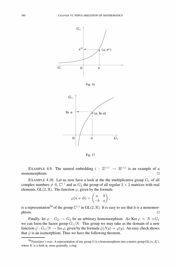
380 CHAPTER VI. POPULARIZATION OF MATHEMATICS
G 2
G 1
ea ( e )a, a
a0
Fig. 16
ln a ( ln )a, a
G 1
G 2
a0
Fig. 17
EXAMPLE 4.9. The natural embedding i : Z(+) → R(+) is an example of amonomorphism. '(
EXAMPLE 4.10. Let us now have a look at the the multiplicative group G1 of allcomplex numbers �= 0, C(·) and as G2 the group of all regular 2 × 2 matrices with realelements, GL(2,R). The function ϕ, given by the formula
ϕ(a + ib) =(
a b−b a
),
is a representation56 of the group C(·) in GL(2,R). It is easy to see that it is a monomor-phism. '(
Finally, let ϕ : G2 → G2 be an arbitrary homomorphism. As Kerϕ = N � G1
we can form the factor group G1/N . This group we may take as the domain of a newfunction ϕ : G1/N → Imϕ, given by the formula ϕ(Ng) = ϕ(g). An easy check showsthat ϕ is an isomorphism. Thus we have the following theorem.
56Translator’s note. A representation of any group G is a homomorphism into a matrix group GL(n, K),where K is a field or, more generally, a ring.

4. Additional remarks on groups 381
THEOREM 4.5 (Theorem of homomorphisms). The function ϕ is an isomorphismbetween the groups G1/Ker f and Imϕ.
4. Let us introduce some classes of groups. We have already spoken of Abelian groups:these were the groups where the algebraic operation is commutative. As examples wemay take the multiplicative groups Q(·), R(·), C(·), that is, the corresponding sets ofnumbers, deprived of zero, where composition is usual multiplication of numbers, and,further, the additive groups Q(+), R(+), C(+), that is, the corresponding sets of numbers,where the operation is the usual addition of numbers.
An important subclass of these [Abelian ] groups are the cyclic groups. In a cyclicgroup all elements can be taken as the various powers of its distinguished element so-called generator (if the composition is called “multiplication”) or multiplier (if the com-position is called “addition”).
EXAMPLE 4.11. Consider the solutions of the equation xn − 1 = 0, that is then-th roots of unity ε0, ε1, . . . , εn−1. Clearly, the product of two roots of unity is againa root of unity; likewise, the inverse of a root of unity is a root of unity. So we have agroup whose elements are the n-th roots of unity, the algebraic operation being ordinarymultiplication of complex numbers. As the solutions of the equation xn − 1 = 0 form
a regular n-gone inscribed in the unit circle, we have εk = cos2πkn
+ i sin2πkn
. By de
Moivre’s formula εk1 = εk, k = 0, 1, . . . , n− 1, which shows that we are dealing with a
finite cyclic group: all elements εk are powers of the generator ε1 '(EXAMPLE 4.12. The additive group of integers Z(+) is cyclic. Indeed, it has the
generator 1, because each n ∈ Z can be written n = n · 1.All subgroups or factor groups of a cyclic group are again cyclic. For the proof of
the first assertion we remark that as a generator of a subgroup we can take the power ofa generator of the entire group with the lowest positive exponent. For the proof of thesecond assertion it suffices to take, as generator, an orbit of of the factor group passingthrough a generator of the group. '(
Let us now apply these observations to the additive group of integers Z. Takingan arbitrary n ∈ Z, n �= 0, and considering the set N ⊂ Z of all integers divisibleby it, we obtain a subgroup. It is easy to see that all subgroups are of this form. AsZ is Abelian , then all its subgroups are normal divisors. Therefore we can form thesubgroups Z/N = Zn, which being the factor group of a cyclic group must be cyclic.In this way we have found all subgroups, all normal divisors, and all factor groups ofZ. Even more, we have determined all homomorphisms of Z, because the Theorem 4.5allows us to restore these from their kernels, and we know also the latter, as they coincidewith set of normal divisors of Z.
Next, we consider an arbitrary cyclic groupG2 with generator a and define a functionwhose domain of definition is Z and whose domain of values is G2, defined with the helpof the formula ϕ(1) = a. This implies that ϕ(n) = an. It is easy to see that Imϕ = G2,so that we have an epimorphism. The Theorem 4.5 yields now
G2∼= Z/Kerϕ.
But all factor groups of Z are known to us; they are the groups Zn. Thus, we haveG2
∼= Zn for some n; in case Kerϕ = (0) we obtain G2 = Z, and we have an infinitecyclic group.
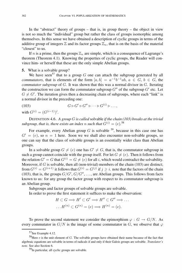
382 CHAPTER VI. POPULARIZATION OF MATHEMATICS
In the “abstract” theory of groups – that is, in group theory – the object in viewis not so much the “individual” group but rather the class of groups isomorphic amongthemselves. In this sense we have obtained a description of cyclic groups in terms of theadditive group of integers Z and its factor groups Zn, that is on the basis of the material“closest” to us.
If n is a prime, then the groups Zn are simple, which is a consequence of Lagrange’stheorem (Theorem 4.1). Knowing the properties of cyclic groups, the Reader will con-vince him- or herself that these are the only simple Abelian groups.
5. What is a solvable group?We have seen57 that to a group G one can attach the subgroup generated by all
commutators, that is elements of the form [a, b] = a−1b−1ab, a ∈ G, b ∈ G, thecommutator subgroup of G. It was shown that this was a normal divisor in G. Iteratingthe construction we can form the commutator subgroup G′′ of the subgroup G′ etc. LetG �= G′. The iteration gives then a decreasing chain of subgroups, where each “link” isa normal divisor in the preceding one:
(103) G G′ G′′ · · · G(i) . . . ,
with G(i) = (G(i−1))′.
DEFINITION 4.6. A group G is called solvable if the chain (103) breaks at the trivialsubgroup, that is, there exists an index n such that G(i) = (e).58
For example, every Abelian group G is solvable 59, because in this case one hasG′ = (e), so n = 1 here. Soon we we shall also encounter non-solvable groups, soone can say that the class of solvable groups is an essentially wider class than Abeliangroups.
In a solvable group G �= (e) one has G′ �= G, that is, the commutator subgroup insuch a group cannot coincide with the group itself. For let G �= (e). Then it follows fromthe relation G′ = G that G(i) = G �= (e) for all i, which would contradict the solvability.Moreover, if G is solvable, then all (non-trivial) members of the chain (103) are distinct;from G(i) = G(i+1) it follows that G(i) = G(j) if j ≥ i. note that the factors of the chain(103), that is, the groups G/G′, G/G′′, . . . , are Abelian groups. This follows from factsknown to us: for any group the factor group with respect to its commutator subgroup isan Abelian group.
Subgroups and factor groups of solvable groups are solvable.In order to prove the first statement it suffices to make the observation:
H ⊂ G =⇒ H ′ ⊂ G′ =⇒ H ′′ ⊂ G′′ =⇒ . . .
. . .H(n) ⊂ G(n) = (e) =⇒ H(n) = (e).
To prove the second statement we consider the epimorphism ϕ : G → G/N . Asevery commutator in G/N is the image of some commutator in G, we observe that ϕ
57See Example 4.12.58Here e is the unit element of G. The solvable groups have obtained their name because of the fact that
algebraic equations are solvable in terms of radicals if and only if their Galois groups are solvable. Translator’snote. See also Section 6.
59In particular, all cyclic groups are solvable.

4. Additional remarks on groups 383
induces a new epimorphism ϕ′ : G′ → (G/N)′. Iterating this observation we get theepimorphisms ϕ′′ : G′′ → (G/N)′′, ϕ′′′ : G′′′ → (G/N)′′′ etc. As G(n) = (e) and ϕ(n)
is an epimorphism, then (G/N)(n) = (N). '(
6. In the case of finite groups one usually gives a different definition of solvability. Thisis done with the aid of the notion of composition series of a group.
Let us first look at a concrete situation in order to be able to use it as an example inthe following general reasoning.
We consider the 6-th order group G = {e, a, a2, a3, a4, a5 | a6 = e}. Thesets N1 = {e, a3}, N2 = {e, a2, a4} are subgroups, with N1 �⊂ N2. There are noother proper subgroups. 60 In view of Theorem 4.1 the order of a subgroup must dividethe order of the group itself. But the number 6 has only the divisors 2 and 3. As G iscommutative, it follows that N1 and N2 are normal divisors. This gives us two chains
G N1 (e) and G N2 (e).
It is easy to check that G/N1∼= N2/(e) ∼= N2 and N1
∼= N1/(e) ∼= G/N2.
DEFINITION 4.7. Let G be a finite group. A decreasing chain of subgroups
(104) G = N0 ⊃ N1 ⊃ N2 ⊃ · · · ⊃ Nk = (e)
is called a composition series if the following two conditions are fulfilled:
(1) for all i = 0, . . . , k − 1, Ni+1 is a normal divisor of Ni, and(2) for no i = 0, . . . , k−1 there exists in Ni a normal divisor M such that Ni+1 ⊂
M ⊂ Ni, M �= Ni+1, M �= Ni.
The Reader sees at once that the chains G ⊃ N1 ⊃ (e) and G ⊃ N2 ⊃ (e) in theabove example are composition series.
Each finite group has a composition series. According to the Jordan-Hölder Theo-rem (see [7, p. 286] or suitable references in Section 1, footnote 12.) any two compositionseries have the same length, and one can find a one-to-one correspondence between themsuch that that the corresponding factor groups are isomorphic; one may say that the com-position series of a finite group are isomorphic. This theorem allows to consider in afinite group any composition series as the “copy” of some “original” composition series.Thus, in essence a finite group has a unique composition series, namely this “original”,all others being just “copies” of the “original”, that is chains isomorphic to the latter. Asthe “original” one can, of course, take an arbitrary composition series.
It turns out that a finite group is solvable if and only if all factor groups of its compo-sition series are cyclic groups of prime order. This is the second definition of solvabilityin the case of a finite solvable group. In using it, the Reader will notice that for a finitesolvable group to be simple it is necessary and sufficient that it be cyclic of prime order;that such a group is solvable is already known to us.61
Likewise, the Reader sees that the order |G| of a solvable group is the product of theorder of its factors. Indeed, a repeated application of Lagrange’s Theorem (Theorem 4.1
60That is, subgroups distinct from (e) and G itself.61. . . but it is also an immediate consequence of the second definition just given.

384 CHAPTER VI. POPULARIZATION OF MATHEMATICS
to the chain 104 gives
|G| = |G/N1| · |N1| = |G/N1| · |N1/N2| · |N2| = · · · == |G/N1| · |N1/N2| · |N2/N3| . . . |Nk|.
'(Here the orders of the factors may be equal. Even they can be all equal, i.e., the order
|G| must then be of the form pα, p a prime number. According to Lagrange’s Theorem,the order of the group must divisible by the order of any of its subgroups. The interestingquestion arises whether the “converse conjecture” holds true for solvable groups. 62
It turns out that in a solvable group G of order |G| = m · n, where the numbers mand n are relatively prime, there exist subgroups of order m and n.
For the proof of this fact we would have to plunge into the “technical wilderness”,which would not be suitable for the present compilation. However, it is of some interestto note that this fact is characteristic for the “nature” of solvable groups, that is, it can beused as a criterion for solvability.
We mention further two criteria due to J. G. Thompson, as they can often be easilyapplied to the solvability or non-solvability of groups (see [13, 383-437]):
I. A finite group is solvable if and only if each subgroup generated by any pair ofelements in it is solvable.
II. A finite group is solvable if and only if it does not contain any three elementsdistinct from unity whose orders are pairwise relatively prime and whose prod-uct equals unity.
7. The following theorem gives a series of examples of non-solvable groups. It playsalso a decisive role in the proof of the Abel-Ruffini Theorem.
THEOREM 4.8. The complete symmetric groups Sn (n ≥ 5) are not solvable. ThegroupsS2,S3,S4 (n ≥ 5) are solvable.
PROOF. As a subgroup of a solvable group is solvable, it suffices, for the proof ofthe first statement to find in the groups Sn (n ≥ 5) subgroups which are not solvable.This is easy: the subgroups An ⊂ Sn (n ≥ 5) suffice! The groups An are simple, buttheir order |An| = n!
2 is not a prime number; hence they are not solvable. Indeed, wesaw in the previous Section that among solvable groups only those are simple which arecyclic of prime order. This proves the first assertion.
Let us consider the group S2. As |S2| = 2! = 2 it is cyclic of prime order and sosolvable.
For the proof of the solvability of S3, we note that A3 is solvable because in viewof |A3| = 1
23! = 3 we have a cyclic group. Moreover, (S3 : A3) = 2 is a prime so that(e) ⊂ A3 ⊂ S3 is a composition series. The factors of the latter are visibly cyclic ofprime order. That the groupS3 is solvable follows now from the definition.
62See also the first subsection of this paper.
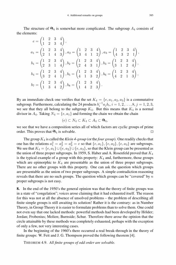
4. Additional remarks on groups 385
The structure of S4 is somewhat more complicated. The subgroup A4 consists ofthe elements:
e =(
1 2 3 41 2 3 4
),
a1 =(
1 2 3 42 1 4 3
), a2 =
(1 2 3 43 4 1 2
), a3 =
(1 2 3 44 3 2 1
),
b1 =(
1 2 3 42 3 1 4
), b2 =
(1 2 3 42 4 3 1
), b3 =
(1 2 3 43 1 2 4
),
b4 =(
1 2 3 43 2 4 1
), b5 =
(1 2 3 44 1 3 2
), b6 =
(1 2 3 44 2 1 3
),
b7 =(
1 2 3 41 3 4 2
), b8 =
(1 2 3 41 4 2 3
).
By an immediate check one verifies that the set K4 = {e, a1, a2, a3} is a commutativesubgroup. Furthermore, calculating the 24 products b−1
i ajbi, i = 1, 2, . . . , 8, j = 1, 2, 3,we see that they all belong to the subgroup K4. But this means that K4 is a normaldivisor in A4. Taking N4 = {e, a1} and forming the chain we obtain the chain
(e) ⊂ N4 ⊂ K4 ⊂ A4 ⊂ S4,
we see that we have a composition series all of which factors are cyclic groups of primeorder. This proves that S4 is solvable. '(
The groupK4 is called the Klein 4-group (or the four group). One readily checks thatone has the relations a2
1 = a22 = a2
3 = e so that {e, a1}, {e, a2}, {e, a3} are subgroups.We see that K4 = {e, a1}∪{e, a2}∪{e, a3}, so that the Klein group can be presented asthe union of three proper subgroups. In 1959, S. Haber and A. Rosenfeld proved that K4
is the typical example of a group with this property: K4 and, furthermore, those groupswhich are epimorphic to K4 are presentable as the union of three proper subgroups.There are no other groups with this property. One can ask the question which groupsare presentable as the union of two proper subgroups. A simple contradiction reasoningreveals that there are no such groups. The question which groups can be “covered” by nproper subgroups is not easy.
8. In the end of the 1950’s the general opinion was that the theory of finite groups wasin a state of “congelation”; voices arose claiming that it had exhausted itself. The reasonfor this was not at all the absence of unsolved problems – the problem of describing allfinite simple groups is still awaiting its solution! Rather it is the contrary: as in NumberTheory, in Group Theory it is easier to formulate problems than to solve them. One couldnot even say that one lacked methods: powerful methods had been developed by Hölder;Jordan; Frobenius; Molien; Burnside; Schur. Therefore there arose the opinion that thecircle attainable by these methods was completely exhausted, perhaps with the exceptionof only a few, not very interesting cases.
In the beginning of the 1960’s there occurred a real break-through in the theory offinite groups: W. Feit and J. G. Thompson proved the following theorem [4].
THEOREM 4.9. All finite groups of odd order are solvable.

386 CHAPTER VI. POPULARIZATION OF MATHEMATICS
The proof of this theorem is based on ideas, results and theories due to P. Hall; G.Higman; H. Wieland; R. Brauer; M. Suzuki; and others. This theorem with its monu-mental proof, undoubtedly, has a deep influence on the development of Group Theory63.
Below we study two examples of the numerous consequences of this theorem.We start with the following question: if a group G is not cyclic of prime order,
what can be said about the existence of subgroups H of “sufficiently high” order in G?More exactly, we would like to prove the following conjecture: there exists always aproper subgroup H ⊆ G such that |H | > 3
√|G|. In the case of groups G of even order,
R. Brauer and K. Fowler managed to prove this conjecture in 1955. There remained thecase |G| odd; one was not able to “conquer” this.
The knowledge of the Feit-Thompson Theorem makes this problem fairly simpleand so also acceptable in the framework of this paper. Indeed, by this theorem all oddgroups are solvable. But in every finite solvable group G whose order is not a prime andgreater than unity, there exists a subgroup of order ≥
√|G|.
PROOF. Let us present the number |G| = g as a product of prime numbers g =pα11 . . . pαs
s . We consider two cases.First, let s = 1. Then g = pα. As g must be a prime greater than unity, we deduce
that α ≥ 2. The first theorem of Sylow tells us that G has a subgroup of order pα−1. Butas α ≥ 2 implies the inequality pα−1 ≥ √g, we have found the desired subgroup H .
Second, let s > 1. Then we can divide the set P = {p1, p2, . . . , ps} into two non-empty and non-intersecting (all the pi are distinct!) subset P ′ and P ′′, that is, we havethe relations
P = P ′ ∪ P ′′ and P ′ ∩ P ′′ = ∅.Let m =
∏pi∈P ′ p
αi
i and n =∏
pj∈P ′′ pαj
j . It follows from P ′ ∩ P ′′ = ∅ that thenumbers m and n are relatively prime. There are two possible special cases:
(i) m > n, and(ii) n > m.
Let us now apply the “natural property” of a solvable group (cf. Subsection 6).In case (i) it guarantees that there is a subgroup H in G of order m. As m > n, then
g = mn < m2, hence |H | = m >√g, and we have found the desired subgroup.
The reasonings in case (ii) are analogous. It suffices only to make in them the re-placements m→ n and n→ m. Our assertion is proved. '(
As for |H | >√|G| one has also |H | > 3
√|G|, the conjecture under view is estab-
lished for all finite groups.We give yet another application of the Thompson-Feit Theorem.In Subsection 2 we mentioned the following problem of W. Burnside: Does there
exist non-commutative simple groups of even order? The answer to this question is animmediate consequence of the Thompson-Feit Theorem: assuming that such a groupexists, we see from this theorem that the group must be solvable. On the other hand, theclass of simple solvable groups consists of only cyclic groups of prime order, thus onlyof commutative groups. This contradiction shows that the answer is negative.
63See the book [3], where the Reader will have a magnificent opportunity to familiarize him- or herselfwith contemporary Group Theory.

4. Additional remarks on groups 387
Up to this day64 two interesting (and difficult) questions remain unsolved.
(1) It is well-known that groups of order pα · qβ , where p, q are prime numbers,are solvable. This is Burnside’s Theorem. But so far one does not know thestructure of groups whose order is divisible by precisely three distinct primenumbers. Nor does one know which simple groups have this property, andeven not if there are only finitely many such groups. That we here have to dealwith a very well-founded problem should be clear from the following theoremof Thompson: if the order of a simple group has the form pα · qβ · rγ withdistinct primes p, q, r (say p < q < r), then p = 2, q = 3, r = 5, 7 or 17.
(2) To prove that a finite group, which admits an automorphism whose only fixedpoint is its identity, must be solvable. A support for this conjecture is thefollowing fact: If the automorphism under view (considered as an element ofAut(G)) is of order = 2n, n an integer, then G is of odd order; that G issolvable follows now from the Feit-Thompson Theorem. It is essential that Gbe finite. Indeed, there exist infinite non-solvable “linearly ordered” groups G.Each such group admits the automorphism σ : g → G, σ(g) = g−1, with unityof G as the single fixed point.
Comments.
1) In the proof on the pages 386 to 386 it is written “First, let s > 1 . . . ”, but the case s = 1 is neverdealt with. However, this is easy, as any group of order pn contains a subgroup of of order pn−1.
2) The problem of classifying non-Abelian finite simple groups, essentially going back to Galois, isnow generally believed to be settled. This classification was finished in the early 1980’s. Accordingto this there are, apart from the alternating groups, 16 infinite families of groups of Lie type (thefinite analogies to the classical families of simple Lie groups that include:
- the projective special linear groups PSL(n, K), the projective symplectic groups;- the simple orthogonal and unitary groups)
and 26 sporadic simple groups (5 of which are the Mathieu groups discovered by E. Mathieualready in 1861 and 1873).For further discussion see e.g. the book [1].
The following two items refer to the two questions referred at the end of the paper.
3) Question 1 on p. 387. From the classification of finite simple groups, one can read exactly whichsimple groups occur that have orders divisible by exactly three distinct prime numbers.
4) Question 2 on p. 387. It has now been shown, using the classification of finite simple groups,that all finite groups, that admit an automorphism, whose only fixed point is the identity, must besolvable. For more information, see the book [8].
Gunnar Traustason
References
[1] R. Carter. Simple groups of Lie type. John Wiley & Sons, London, New York, Sidney, 1989.[2] F. A. Cotton. Chemical applications of group theory, New York, London, 1964.[3] W. Feit. Characters of finite groups. W. A. Benjamin, Inc., New York, Amsterdam, 1967.[4] W. Feit and J. G. Thompson. Solvability of groups of odd order. Pac. J. Math. 13, 1963.[5] E. Gabovitš. Principles of Algebra, I – V. Math. and Our Age 6–10, 1965.
64. . . according to the information available to the author.
388 CHAPTER VI. POPULARIZATION OF MATHEMATICS
[6] S. Helgason. Differential geometry and symmetric spaces. Academic Press, New York, London, 1962.[7] G. Kangro. Kõrgem algebra (Higher algebra) II. Eesti Riiklik Kirjastus, Tallinn, 1950. (Estonian.)[8] E. I. Khukhro. p-Automorphisms of finite p-groups. London Mathematical Society Lecture Note Series,
246. Cambridge University Press, Cambridge, 1997.[9] N. Kristoffel and K. Rebane. Group theory and its applications in the physics of molecules and chrystals.
Tartu Univ. Press, Tartu, 1961.[10] A. G. Kurosh. Lectures in general algebra. Fizmatgiz, Moscow, 1962. English translation: Pergamon
Press, Oxford, London, Edinburgh, New York, 1965.[11] Ü. Lumiste. The notion of space in geometry. Geometry and transformation groups. Math. and Our Age
14, 1968, 3–21.[12] Ø. Ore. On coset representatives in groups. Proc. Am. Math. Soc. 9, 1958, 665–670.[13] J. G. Thompson. Non-solvable finite groups all of whose local subgroups are solvable. Bull. Am. Math.
Soc. 74, 1968.

389
5. [K73a] Polynomials and formal series
This paper arose from a desire to give the Reader a handy compilation for the for-mulation and proof of the Ruffini-Abel Theorem. Here we treat the symmetry of thepolynomial and the notion of irreducibility and, moreover, the concept of formal series.
Symmetric polynomials have applications in several domains of mathematics. TheReader will find on the pages of this paper an interesting possibility to use them in thesolution of algebraic equations of higher order, see [2]65.
Irreducible polynomials play in the arithmetic of the ring of polynomials about thesame role as prime numbers in ordinary number theory. In recent times they have foundapplications in the theory of coding an decoding (see the book [1]66).
The Reader will probably find the concept of formal series specially interesting.An elegant use of this theory is, among other things, one of the tools by which HenriCartan has refreshed the presentation, in university courses, of such an important branchof classical mathematics as the theory of functions of a complex variable.
However, our goal has not been to give a complete catalogue of the properties of anyof the mathematical objects mentioned. The Reader will only learn of those properties ofan object which will be later required to understand the proof of Abel’s theorem. In theopinion of the author the best way of learning something about mathematical objects isto see how they are used in achieving significant goals. In the composition of the remarkswe have in an essential way used M. M. Postnikov’s book on Galois Theory [6].
5.1. Irreducibility of polynomials
Let P be a field. We consider the ring P [x], that is, the set consisting of all polynomialswith coefficients in P ,
f(x) = an + an−1x + · · ·+ a0xn, ai ∈ P.
Addition and multiplication are defined, as in the case of polynomials with numericalcoefficients, by the formulae
(f + g)(x) = f(x) + g(x),
(f · g) = f(x) · g(x).
There are no divisors of zero in the ring P [x] and one can develop a theory of divisionsimilar to the one in the domain of ordinary integers; in the role of prime numbers thereappear then the “irreducible polynomials”; let us familiarize us with these strange “primenumbers”.
65Translator’s note. For symmetric functions see e.g. Chap. 11 of Kurosh’s book [10] quoted in Section 1,footnote 12
66Editors’ note. We suggest also an introduction to coding theory [5]

390 CHAPTER VI. POPULARIZATION OF MATHEMATICS
DEFINITION 5.1. A polynomial f(x) ∈ P [x] is called reducible over the field P ifthere exist non-constant lower order polynomials f1(x) and f2(x) in the ring P [x] suchthat f(x) = f1(x) · f1(x). In the opposite case one says that f(x) is irreducible over P .
Next, we present an assertion which illustrates the similarity between irreduciblepolynomials and prime numbers.
THEOREM 5.2. If the polynomial f(x) with coefficients in P has a common solutionwith the polynomial p(x), which is irreducible over P , then f(x) is divisible by p(x).
PROOF. Let g(x) = GCD(f(x), p(x)). As the equation f(x) = 0 and p(x) = 0have a common solution then67 deg g(x) ≥ 1. The coefficients of the polynomial g(x),obtained by Euclid’s algorithm, belong to P . If we had deg f(x) < deg p(x), thenp(x) = g(x) · p1(x), where deg p1(x) < deg p(x) and where the coefficients of p1(x)belong to P . But this contradicts the irreducibility of p(x). Thus deg g(x) = deg p(x).
'(
As an example we consider the irreducibility of polynomials over number fields. Weuse the standard notation: Z for the set of integers, Q for the set of rational numbers, Cfor the set of complex numbers. Let P = Q. It turns out that it suffices to know if apolynomial f(x) with integer coefficients is irreducible in the ring68 Z or not. Indeed, letf(x) be a polynomial with rational coefficients. We determine the least common divisora of the coefficients ai and consider the polynomial af(x); this is a polynomial withinteger coefficients and its reducibility is, apparently, necessary and sufficient for thereducibility of f(x) over Q. Thus the question of the reducibility over Q is solvable ifwe can clarify the reducibility of polynomials over Z. For this several criteria are knownin algebra. We list a few of them.
EISENSTEIN’S CRITERION. Let there be given a polynomial
f(x) = an + an−1x + . . . a1xn−1 + a0x
n, ai ∈ Z.
If there exist a prime number p such that the following conditions69 are fulfilled:
p � a0; p|ai for i �= 0; p2 � an,
then f(x) is irreducible over Q.The proof is easy; assuming the contrary the Reader will easily arrive at a contradic-
tion. '(
It follows from this criterion that there exist irreducible polynomials (over Q) ofarbitrary high degree. Indeed, the polynomials xn + p, n = 1, 2, 3, . . . are irreducible.
COHN’S CRITERION. If the coefficients ai ∈ Z of the polynomial f(x) =∑ni=0 an−ix
i satisfy the condition 0 ≤ an−i ≤ 9, and f(10) is a prime number, thenf(x) is irreducible over Q. '(
67Here deg f(x) denotes the degree of the polynomial f(x).68The polynomial f(x) is reducible in the ring Z[x] if there exist polynomials f1(x) and f2(x) with
non-constant integer coefficients such that f(x) = f1(x) · f2(x) and deg fi(x) < deg f(x), i = 1, 2.69Here p|ai means that the number ai is divisible by p, and p � ai its contrary.

5. Polynomials and formal series 391
According to Cohn’s criterion the polynomials f1(x) = x3 + 8x2 + 2x + 3,f2(x) = 2x3 + 6x + 3, f3(x) = 2x3 + x2 + 2x + 9 are irreducible over Q.
Among less know criteria of irreducibility, we note the following.In order for a polynomial f(x) = xn + a1x
n−1 + · · ·+ an, ai ∈ Z to be irreducible(over Q) it is sufficient that one of the following conditions is fulfilled:
(1) |a1| > |1 + a2|+ |a3|+ · · ·+ |an|,(2) a2 > 0,
√a2 >
3√2(|a1|+ |a3|+ . . . |an|),
(3) a1 = 0, a2 > 0, an �= 0,√a2 >
√3(|a3|+ · · ·+ |an|),
(4) n > 4, a4 > 0,√a4 > 4
√2(1 + |a1|+ |a2|+ · · ·+ |an|), an �= 0.
Over the complex numbers, only linear polynomials are irreducible. Indeed, by thefundamental theorem of algebra it follows that an equation f(x) = 0 with complexcoefficients has at least one solution α ∈ C, from which it again follows by Bézout’sLemma that f(x) is divisible with the factor x − α. If necessary applying the sameargument to the quotient, we find that f(x) decomposes into a product of linear factors.
Over the field of real numbers there are already quadratic polynomials which areirreducible – a well-known example is provided by the polynomial x2 + 1. It turns outthat higher order polynomials with real coefficients are already reducible. The fact thathere appear besides linear polynomials some quadratic polynomials, follows again fromthe reasoning that if f(α) = 0, α ∈ C, α �∈ R, then also f(α) = 0 and that the factor(x− α)(x − α) is irreducible over R.
We note the absence of effective criteria for deciding the irreducibility of polyno-mials over an arbitrary field. The answer to the following interesting question70 is notknown.
PROBLEM OF PAUL TURAN. Does there exist a non-negative integer c such thatfor each polynomial f(x) =
∑ni=0 aix
n−i, ai ∈ Z, a0 �= 0 there exist a polynomialg(x) =
∑ni=0 bix
n−i, bi ∈ Z, which is irreducible over Z, such that∑n
i=0 |ai − bi| ≥ c.'(
5.2. Symmetric polynomials
We consider the polynomial f(x) = xn + a1xn−1 + an−1x + an with coefficients
in the field P . There exists always an extension L of P in which f(x) decomposesinto linear factors, that is, there exist elements α1, . . . , αn ∈ L/P such that f(x) =(x − α1) . . . (x − αn). For example, if P ⊆ C we may take for L the field of complexnumbers C. But if two polynomials are equal, then there coefficients in front of thecorresponding powers of the variable x must be equal also. This gives the well-known
70In this relation, see [7]
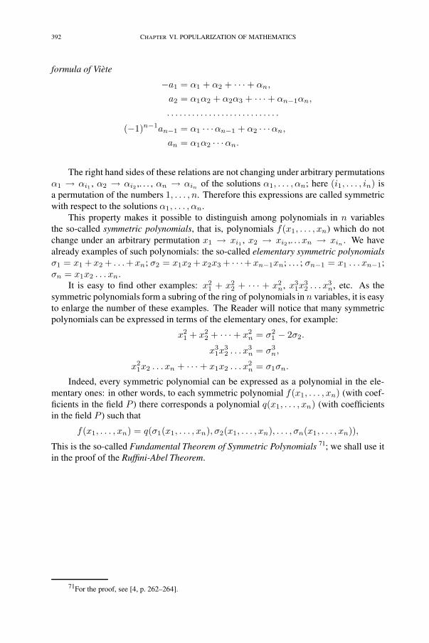
392 CHAPTER VI. POPULARIZATION OF MATHEMATICS
formula of Viète
−a1 = α1 + α2 + · · ·+ αn,
a2 = α1α2 + α2α3 + · · ·+ αn−1αn,
. . . . . . . . . . . . . . . . . . . . . . . . . . .
(−1)n−1an−1 = α1 · · ·αn−1 + α2 · · ·αn,
an = α1α2 · · ·αn.
The right hand sides of these relations are not changing under arbitrary permutationsα1 → αi1 , α2 → αi2 ,. . . , αn → αin of the solutions α1, . . . , αn; here (i1, . . . , in) isa permutation of the numbers 1, . . . , n. Therefore this expressions are called symmetricwith respect to the solutions α1, . . . , αn.
This property makes it possible to distinguish among polynomials in n variablesthe so-called symmetric polynomials, that is, polynomials f(x1, . . . , xn) which do notchange under an arbitrary permutation x1 → xi1 , x2 → xi2 ,. . .xn → xin . We havealready examples of such polynomials: the so-called elementary symmetric polynomialsσ1 = x1 +x2 + . . .+xn; σ2 = x1x2 +x2x3 + · · ·+xn−1xn; . . . ; σn−1 = x1 . . . xn−1;σn = x1x2 . . . xn.
It is easy to find other examples: x21 + x2
2 + · · · + x2n, x3
1x32 . . . x
3n, etc. As the
symmetric polynomials form a subring of the ring of polynomials in n variables, it is easyto enlarge the number of these examples. The Reader will notice that many symmetricpolynomials can be expressed in terms of the elementary ones, for example:
x21 + x2
2 + · · ·+ x2n = σ2
1 − 2σ2.
x31x
32 . . . x
3n = σ3
n,
x21x2 . . . xn + · · ·+ x1x2 . . . x
2n = σ1σn.
Indeed, every symmetric polynomial can be expressed as a polynomial in the ele-mentary ones: in other words, to each symmetric polynomial f(x1, . . . , xn) (with coef-ficients in the field P ) there corresponds a polynomial q(x1, . . . , xn) (with coefficientsin the field P ) such that
f(x1, . . . , xn) = q(σ1(x1, . . . , xn), σ2(x1, . . . , xn), . . . , σn(x1, . . . , xn)),
This is the so-called Fundamental Theorem of Symmetric Polynomials 71; we shall use itin the proof of the Ruffini-Abel Theorem.
71For the proof, see [4, p. 262–264].

5. Polynomials and formal series 393
5.3. Embedding of the field of rational functions in an algebraicallyclosed field
Let P be a field of characteristic 0, that is, Q ⊆ P . We consider the field of rationalfunctions R = P (x1, . . . , xn) over P . Its elements are quotients
f(x1, . . . , xn)g(x1, . . . , xn)
of two polynomials f, g ∈ P [x]. Such a field needs not be algebraically closed, that is,there may exist non-linear irreducible polynomials over it.
EXAMPLE 5.1. Let P = Q. We show that the equation x2 + 1 = 0 does not haveany solutions in the field R = Q(x1, . . . , xn). Indeed, if
f(x1, . . . , xn)g(x1, . . . , xn)
∈ R
were a solution of the equation x2 + 1 = 0, we would have(f(x1, . . . , xn)g(x1, . . . , xn)
)2
≡ −1,
which implies that (f(c1, . . . , cn)g(c1, . . . , cn)
)2
= −1,
for any (c1, . . . , cn) ∈ Qn. But as(f(c1, . . . , cn)g(c1, . . . , cn)
)∈ Q,
we have obtained a contradiction, because there exists no rational number r ∈ Q suchthat r2 = −1. '(
Nevertheless, it is possible to embed the field R into an algebraically closed field,provided the base field P is algebraically closed. First we embed R in the field of formalseries.
What is a formal series?We denote the variable by x. A formal series is an infinite formal sum of the form
a−mx−m + a−m+1x−m+1 + · · ·+ a−1x
−1 + a0 + a1x + a2x2 + . . . ,
where ai ∈ P and m ∈ Z; in short,∑
i≥−m aixi. Among the formal series we have all
polynomials, as a0 + a1x + · · ·+ akxk =
∑i≥0 aix
i, where ak+1 = ak+2 = · · · = 0.The sum and product of any two formal series f =
∑i≥−m aix
i and g =∑
i≥−n bixi
is defined by the formulae:
(1) if, for example n ≥ m, and f + g =∑
i≥−n(ai + bi)xi, where am−1 = · · · =a−n = 0 and
(2)
f · g =∑
i≥−m−n
cixi,

394 CHAPTER VI. POPULARIZATION OF MATHEMATICS
where ⎧⎪⎨⎪⎩c−m−n = a−m · b−n
c−m−n+1 = a−mb−n+1 + a−m+1b−n.
. . . . . . . . .
An easy check shows that one has a ring with respect to these operations – the ring offormal series P 〈x〉. The Reader will notice that here we have to deal with an “extension”of addition and multiplication of polynomials. Thus the ring of polynomials P [x] is asubring of P 〈x〉. However, the latter is a field, as each formal series f other than zerohas an “inverse series”, that is, a series f−1 ∈ P 〈x〉 such that f · f−1 = 1. Indeed, eachformal series different from zero has the form
f = xn(a0 + a1x + a2x2 + . . . ), n ∈ Z, a0 �= 0.
Determining the coefficients bi of the series f−1 = x−n(b0 + b1x + b2x2 + . . . ) by the
identities
a0 · b0 = 1,a0 · b1 + a1 · b0 = 0,
a0 · b2 + a1 · b1 + a2b0 = 0,. . . . . . . . . . . .
we see that f · f−1 = 1. From the relation P [x] ⊆ P 〈x〉 it follows that the quotient ofany two polynomials is contained in the field of formal series, that is, P (x) ⊆ P 〈x〉.
By induction one defines the notion of the field of formal series of several variables:
P 〈x1, x2〉 = P 〈x1〉〈x2〉.P 〈x1, x2, x3〉 = P 〈x1, x2〉〈x3〉.P 〈x1, . . . , xn〉 = P 〈x1, . . . , xn−1〉〈xn〉.
We see that P (x1, . . . , xn) ⊂ P 〈x1, . . . , xn〉.Next we extend the field of formal series to an algebraically complete field. To this
end we consider general formal series, that is, formal sums
f =∑i≥0
aixnin , where , n ∈ Z, n > 0; n, n0, n1, · · · ∈ Z,
n0 < n1 < n2 . . . , among the integers only finitely many being negative. If n = 1 wehave ordinary formal series. Introducing the variable y = x
1n , we can view the general
formal series as an ordinary formal series in the variable y:
f(x) =∑i≥0
aixnin =
∑i≥0
aiyni .
This simple remark shows that that general formal series may be added and multiplied inthe same way as ordinary formal series. This gives again a ring, which we denote P{x}.Even more, P{x} is a field. Indeed, given a general formal series f(x) �= 0 we considerthe corresponding formal series f(y) ∈ P 〈y〉. As P 〈y〉 is a field, we can find a series
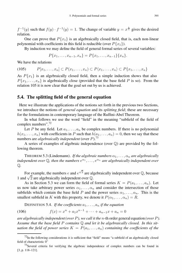
5. Polynomials and formal series 395
f−1(y) such that f(y) · f−1(y) = 1. The change of variable y = x1n gives the desired
relation.One can prove that P{x1} is an algebraically closed field, that is, each non-linear
polynomial with coefficients in this field is reducible (over P{x1}).By induction we may define the field of general formal series of several variables:
P{x1, . . . , xn−1, xn} = P{x1, . . . , xn−1}{xn}.We have the relations
(105) P [x1, . . . , xn] ⊂ P (x1, . . . , xn) ⊂ P 〈x1, . . . , xn〉 ⊂ P{x1, . . . , xn}As P{x1} is an algebraically closed field, then a simple induction shows that alsoP{x1, . . . , xn} is algebraically close (provided that the base field P is so). From therelation 105 it is now clear that the goal set out by us is achieved.
5.4. The splitting field of the general equation
Here we illustrate the applications of the notions set forth in the previous two Sections,we introduce the notions of general equation and its splitting field; these are necessaryfor the formulations in contemporary language of the Ruffini-Abel Theorem.
In what follows we use the word “field” in the meaning “subfield of the field ofcomplex numbers”.72
Let P be any field. Let a1, . . . , an be complex numbers. If there is no polynomialh(x1, . . . , xn) with coefficients in P such that h(a1, . . . , an) = 0, then we say that thesenumbers are algebraically independent (over P ).73
A series of examples of algebraic independence (over Q) are provided by the fol-lowing theorem.
THEOREM 5.3 (Lindemann). If the algebraic numbers α1, . . . , αn are algebraicallyindependent over Q, then the numbers eα1 , . . . , eαn are algebraically independent overQ.
For example, the numbers e and e√
2 are algebraically independent over Q, because1 and
√2 are algebraically independent over Q.
As in Section 5.3 we can form the field of formal series K = P (a1, . . . , an). Letus now take arbitrary power series α1, . . . , αn and consider the intersection of thosesubfields which contain the base field P and the power series α1, . . . , αn. This is thesmallest subfield in K with this property, we denote it P (α1, . . . , αn) = R.
DEFINITION 5.4. If the coefficients a1, . . . , an if the equation
(106) f(x) = xn + a1xn−1 + · · ·+ an−1x + an = 0
are algebraically independent (overP ), we call it the n-th order general equation (overP ).Assume that the base field P contains Q and let it be algebraically closed. In this sit-uation the field of power series K = P (a1, . . . , an) containing the coefficients of the
72In the following considerations it is sufficient that “field” means “a subfield of an algebraically closedfield of characteristic 0”
73Several criteria for verifying the algebraic independence of complex numbers can be found in[3, p. 118–121].
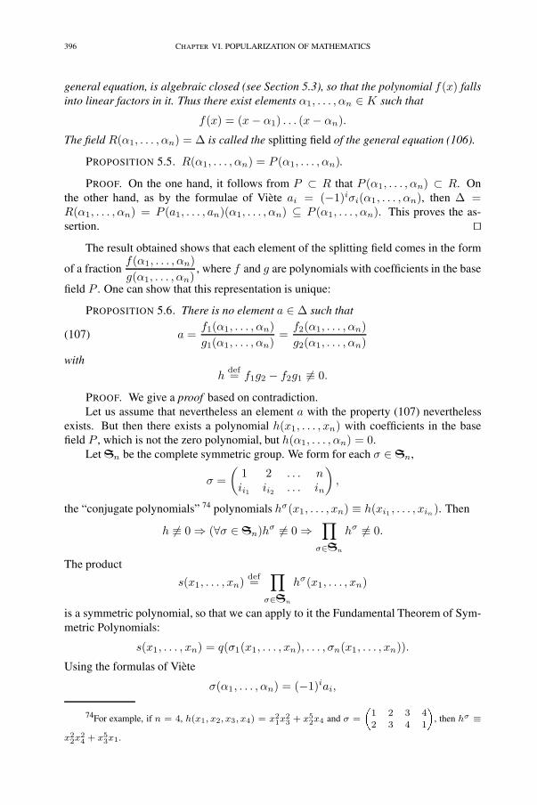
396 CHAPTER VI. POPULARIZATION OF MATHEMATICS
general equation, is algebraic closed (see Section 5.3), so that the polynomial f(x) fallsinto linear factors in it. Thus there exist elements α1, . . . , αn ∈ K such that
f(x) = (x− α1) . . . (x− αn).
The field R(α1, . . . , αn) = Δ is called the splitting field of the general equation (106).
PROPOSITION 5.5. R(α1, . . . , αn) = P (α1, . . . , αn).
PROOF. On the one hand, it follows from P ⊂ R that P (α1, . . . , αn) ⊂ R. Onthe other hand, as by the formulae of Viète ai = (−1)iσi(α1, . . . , αn), then Δ =R(α1, . . . , αn) = P (a1, . . . , an)(α1, . . . , αn) ⊆ P (α1, . . . , αn). This proves the as-sertion. '(
The result obtained shows that each element of the splitting field comes in the form
of a fractionf(α1, . . . , αn)g(α1, . . . , αn)
, where f and g are polynomials with coefficients in the base
field P . One can show that this representation is unique:
PROPOSITION 5.6. There is no element a ∈ Δ such that
(107) a =f1(α1, . . . , αn)g1(α1, . . . , αn)
=f2(α1, . . . , αn)g2(α1, . . . , αn)
withh
def= f1g2 − f2g1 �≡ 0.
PROOF. We give a proof based on contradiction.Let us assume that nevertheless an element a with the property (107) nevertheless
exists. But then there exists a polynomial h(x1, . . . , xn) with coefficients in the basefield P , which is not the zero polynomial, but h(α1, . . . , αn) = 0.
Let Sn be the complete symmetric group. We form for each σ ∈ Sn,
σ =(
1 2 . . . nii1 ii2 . . . in
),
the “conjugate polynomials” 74 polynomials hσ(x1, . . . , xn) ≡ h(xi1 , . . . , xin). Then
h �≡ 0 ⇒ (∀σ ∈ Sn)hσ �≡ 0 ⇒∏
σ∈Sn
hσ �≡ 0.
The product
s(x1, . . . , xn) def=∏
σ∈Sn
hσ(x1, . . . , xn)
is a symmetric polynomial, so that we can apply to it the Fundamental Theorem of Sym-metric Polynomials:
s(x1, . . . , xn) = q(σ1(x1, . . . , xn), . . . , σn(x1, . . . , xn)).
Using the formulas of Viète
σ(α1, . . . , αn) = (−1)iai,
74For example, if n = 4, h(x1, x2, x3, x4) = x21x2
3 + x52x4 and σ =
1 2 3 4
2 3 4 1, then hσ ≡
x22x2
4 + x53x1.
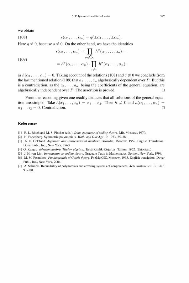
5. Polynomials and formal series 397
we obtain
(108) s(α1, . . . , αn) = q(±α1, . . . ,±αn).
Here q �≡ 0, because s �≡ 0. On the other hand, we have the identities
(109)
s(α1, . . . , αn) =∏
σ∈Sn
hσ(α1, . . . , αn) =
= hσ(α1, . . . , αn) ·∏σ �=ε
·hσ(α1, . . . , αn),
as h(α1, . . . , αn) = 0. Taking account of the relations (108) and q �≡ 0 we conclude fromthe last mentioned relation (109) that a1, . . . , an algebraically dependent over P . But thisis a contradiction, as the a1, . . . , an, being the coefficients of the general equation, arealgebraically independent over P . The assertion is proved. '(
From the reasoning given one readily deduces that all solutions of the general equa-tion are simple. Take h(x1, . . . , xn) = x1 − x2. Then h �≡ 0 and h(α1, . . . , αn) =α1 − α2 = 0. Contradiction. '(
References
[1] E. L. Bloch and M. S. Pinsker (eds.). Some questions of coding theory. Mir, Moscow, 1970.[2] H. Espenberg. Symmetric polynomials. Math. and Our Age 19, 1973, 25–38.[3] A. O. Gel’fond. Algebraic and transcendental numbers. Gosizdat, Moscow, 1952. English Translation:
Dover Publ., Inc., New York, 1960.[4] G. Kangro. Kõrgem algebra (Higher algebra). Eesti Riiklik Kirjastus, Tallinn, 1962. (Estonian.)[5] J. H. van Lint. Introduction to coding theory. Graduate Texts in Mathematics. Spriner, New York, 1999.[6] M. M. Postnikov. Fundamentals of Galois theory. FyzMatGIZ, Moscow, 1963. English translation: Dover
Publ., Inc., New York, 2004.[7] A. Schinzel. Reducibility of polynomials and covering systems of congruences. Acta Arithmetica 13, 1967,
91–101.

This page intentionally left blank

399
6. [K75a] On Galois theoryComments by U. Persson
It is not feasible in practise to proceed like Swift’s scholar, whom Gulliver vis-its in Balnibarbi, namely to develop in systematic order, say according to therequired number of inferential steps, all consequences and discard the “unin-teresting” ones; just as the great works of world literature have not come intobeing by taking the twenty-six letters of the alphabet, forming all ‘combinationswith repetition’ up to the length of 1010, and selecting and preserving the mostmeaningful and beautiful among them.
H. Weyl, Philosophy of Mathematics and Natural Science, Princeton, 1949
The path for Galois theory was prepared by the work of Lagrange, Gauss and Abel.The recognition of the main principles of the theory and their application is due to Galois.Galois associates to each algebraic equation a corresponding group and, having founda series of deep connections between the properties of these two objects, he gives anexhaustive answer to the difficult question about the algebraic solvability of algebraicequations by radicals, which occupied mathematicians for several centuries75. Galois’point of view in the study of an equation via trying to understand the properties of itsgroup is of revolutionary importance. His work gave the impetus to a tendency wherethe center of gravity in research in the area of algebra began to incline towards structuredtheories. The clear-cut unfolding of this tendency occurred in the 1920’s and a specialcredit here goes to D. Hilbert and E. Noether. Today such a point of view is well-knownthanks to the influence of N. Bourbaki’s treatise Éléments de mathématique (Elements ofmathematics).
This paper consists of two parts. In the first of them the Reader will be acquaintedwith some notions, connections and results in Galois theory. We give also a proof of theAbel-Ruffini theorem and treat one line in Galois theory, the inverse problem of Galois.However, the level of generality considered has no limits: In a Bourbaki seminar in 1959A. Grothendieck presented his results on the so-called Galois theory of schemes, of whichwhat will be set out below is just a very narrow special case. This opened up for Galoistheory a broad path in geometry. Of course, even this is not a limit, because the employ-ment of the Galois correspondence is nowadays so frequent that it has almost developedinto a philosophical principle.76 In the second half of the paper, which carries the title“The duality principle in mathematics”, we consider in which way this development ofthe ideas of Galois has taken place, and we treat some general questions connected withthe application of Galois’ ideas in new disciplines.
75See also the author’s paper in Section 3.76In the article [K75b] (see Section 7 on automata theory the Reader can acquaint himself with the
realization of the main idea of Galois in Computer Science.

400 CHAPTER VI. POPULARIZATION OF MATHEMATICS
One can also view the lines below as the final chord of the ideas of a series ofpapers77, where I have tried to prepare the Reader for the understanding of the presentmaterial. It will be assumed that the Reader has access to the papers in question, towhich he or she can refer in case of need. Special references will not be given, but eachtime the Reader encounters a little known term or fact, he or she can turn for help tothe papers mentioned. Finally, let us also remark that the paper’s second half can beread independently of the first one, so that a Reader who is only interested in the generaldevelopment of the ideas derived from Galois theory may at once turn to the reading ofthe second half.
6.1. On the Galois correspondence1. Let us consider the equation x4 + x3 + x2 + x + 1 = 0. Its solutions are 5th roots
of unity: α1 = e, α2 = e2, α3 = e3, α4 = e4, where e = cos2π5
+ i sin2π5
. These
solutions satisfy the relations
(110) α1α4 = 1, α2α3 = 1, α21α3 = 1, α3
1α2 = 1.
Of course, these solutions also satisfy the relations given by the formulae of Viète. Thelatter remain in force also after applying to the solutions in them an arbitrary substitutionof degree 4. In the case of the relations we cannot maintain this. For example, the
substitution
(α1 α2 α3 α4
α2 α1 α3 α4
)carries the relation α1α4 = 1 into α2α4 = 1. If
we try all 24 substitutions on the roots α1, α2, α3, α4 we see that the relations are notdisturbed by the following four among them:(
α1 α2 α3 α4
α2 α1 α3 α4
),
(α1 α2 α3 α4
α2 α4 α1 α3
),(
α1 α2 α3 α4
α4 α3 α3 α4
),
(α1 α2 α3 α4
α3 α1 α4 α2
).
An immediate check shows that these four substitutions form a subgroup of the group ofpermutationsS4.
Let us consider the general case. We consider the n-th order algebraic equation
(111) a0 + a1x + · · ·+ an−1xn−1 + xn = 0.
We denote the left hand side of the equation by f(x) and assume that its coefficientsbelong to some fixed field P . With the aid of the derivative of f(x) we can separate fromf(x) the product of all factors which have only simple solutions. This can be done insuch a way that the coefficients of these factors likewise belong to P . Therefore we mayhenceforth assume that all solutions α1, . . . , αn of f(x) = 0 are simple.
Let
(112) Ψi(α1, . . . , αn) = 0, i ∈ I
be the system of all possible polynomial relations between the solutions of f(x) = 0(the relations given by the Vietè formulae are always present; in general, this system ofrelations may also be infinite). In the complete symmetric group Sn we distinguish the
77Cf. [K69c, K70, K73a] or Sections 3, 4 and 5.

6. On Galois theory 401
subgroup G(f) of those substitutions which either do not change any of the relations ofthe system (112) or else map each relation in (112) again to a relation in the system, inother words we have the assertion
∀ i ∈ I ∃ j ∈ I,Ψσi (α1, . . . , αn) = Ψj(α1, . . . , αn).
The set G(f) ⊂ Sn gives a subgroup. Indeed, if σ, τ ∈ G(f), then one readily sees thatσ · τ ∈ G(f), and, likewise, that the identity substitution belongs to the set G(f). On theother hand, for each substitution σ of order n there exists an m > 0 such that σm = ε,so that σ−1 = σm−1, from which it is clear that σ−1 ∈ G(f).
DEFINITION 6.1. The substitution group G(f), none of which elements change therelations between the solutions of the equation f(x) = 0, is called the Galois group ofthe equation.
We will see some examples in the next section.
2. We give now another definition of the notion of Galois group, in which the equationitself is replaced by a new field, the splitting field of the equation. This makes the theorymore transparent and increases its generality; at the same time it widens its range ofapplication.
Let Δ be a field. We look at those bijections σ : Δ → Δ which preserve in the fielda given sum or product, i.e. for any a, b ∈ Δ one has the relations
(a + b)σ = aσ + bσ; (a · b)σ = aσ · bσ.
Such maps σ : Δ → Δ are called automorphisms of Δ. As automorphisms are one-to-one, it follows that for each b ∈ Δ one can find an a ∈ Δ such that aσ = b; here theelement b is uniquely determined, as a �= b =⇒ aσ �= bσ. From this it follows that themap defined by the formula bσ−1
= a is an automorphism. If we define multiplication ofautomorphisms as composition, then the set of all automorphisms of the field Δ equippedwith this operation (multiplication) is a group which we denote by G(Δ). The unitelement of G(Δ) is the automorphism ε for which all elements of Δ are fixed points. Wecall G(Δ) the group of all automorphisms of Δ; it is often denoted AutΔ.
Next, let Δ be the splitting field of equation (111), i.e. the smallest field containingall solutions α1, . . . , αn of the equation f(x) = 0. Thus Δ = P (α1, . . . , αn). Weconsider the group of those automorphisms σ in G(P ) which leave invariant all elementsof P , i.e. from a ∈ P it follows that aσ = a. These automorphisms σ form a subgroup inG(P ) which is called the Galois group of the extension Δ/P and denote it by G(Δ, P ).
REMARK 6.2. The definition given indicates a path to far reaching generalizations.Indeed, we can speak of the Galois group, not only of the splitting field of an equation,but of the Galois group G(L,K) of an arbitrary extension L/K , where
G(L,K) = {σ ∈ AutL|aσ = a for all a ∈ K}.In other words, the elements of G(L,K) are all the automorphisms for which all theelements of the subfield K are fixed points.
LEMMA 6.3. Let f(x) = 0 be an algebraic equation whose coefficients are in thefield P and the splitting field is Δ. The Galois group of the extension Δ/P coincideswith the Galois group of the equation f(x) = 0.
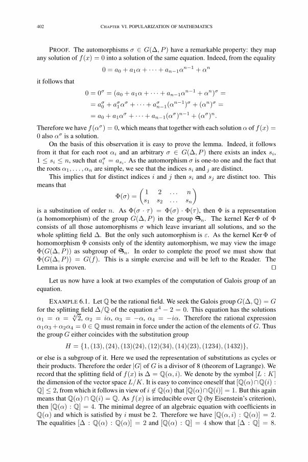
402 CHAPTER VI. POPULARIZATION OF MATHEMATICS
PROOF. The automorphisms σ ∈ G(Δ, P ) have a remarkable property: they mapany solution of f(x) = 0 into a solution of the same equation. Indeed, from the equality
0 = a0 + a1α + · · ·+ an−1αn−1 + αn
it follows that
0 = 0σ = (a0 + a1α + · · ·+ an−1αn−1 + αn)σ =
= aσ0 + aσ
1ασ + · · ·+ aσ
n−1(αn−1)σ + (αn)σ =
= a0 + a1ασ + · · ·+ an−1(ασ)n−1 + (ασ)n.
Therefore we have f(ασ) = 0, which means that together with each solution α of f(x) =0 also ασ is a solution.
On the basis of this observation it is easy to prove the lemma. Indeed, it followsfrom it that for each root αi and an arbitrary σ ∈ G(Δ, P ) there exists an index si,1 ≤ si ≤ n, such that aσ
i = asi . As the automorphism σ is one-to one and the fact thatthe roots α1, . . . , αn are simple, we see that the indices si and j are distinct.
This implies that for distinct indices i and j then si and sj are distinct too. Thismeans that
Φ(σ) =(
1 2 . . . ns1 s2 . . . sn
)is a substitution of order n. As Φ(σ · τ) = Φ(σ) · Φ(τ), then Φ is a representation(a homomorphism) of the group G(Δ, P ) in the group Sn. The kernel Ker Φ of Φconsists of all those automorphisms σ which leave invariant all solutions, and so thewhole splitting field Δ. But the only such automorphism is ε. As the kernel Ker Φ ofhomomorphism Φ consists only of the identity automorphism, we may view the imageΦ(G(Δ, P )) as subgroup of Sn. In order to complete the proof we must show thatΦ(G(Δ, P )) = G(f). This is a simple exercise and will be left to the Reader. TheLemma is proven. '(
Let us now have a look at two examples of the computation of Galois group of anequation.
EXAMPLE 6.1. Let Q be the rational field. We seek the Galois group G(Δ,Q) = Gfor the splitting field Δ/Q of the equation x4 − 2 = 0. This equation has the solutionsα1 = α = 4
√2, α2 = iα, α3 = −α, α4 = −iα. Therefore the rational expression
α1α3 +α2α4 = 0 ∈ Q must remain in force under the action of the elements of G. Thusthe group G either coincides with the substitution group
H = {1, (13), (24), (13)(24), (12)(34), (14)(23), (1234), (1432)},or else is a subgroup of it. Here we used the representation of substitutions as cycles ortheir products. Therefore the order |G| of G is a divisor of 8 (theorem of Lagrange). Werecord that the splitting field of f(x) is Δ = Q(α, i). We denote by the symbol [L : K]the dimension of the vector space L/K . It is easy to convince oneself that [Q(α)∩Q(i) :Q] ≤ 2, from which it follows in view of i �∈ Q(α) that [Q(α)∩Q(i)] = 1. But this againmeans that Q(α) ∩ Q(i) = Q. As f(x) is irreducible over Q (by Eisenstein’s criterion),then [Q(α) : Q] = 4. The minimal degree of an algebraic equation with coefficients inQ(α) and which is satisfied by i must be 2. Therefore we have [Q(α, i) : Q(α)] = 2.The equalities [Δ : Q(α) : Q(α)] = 2 and [Q(α) : Q] = 4 show that [Δ : Q] = 8.

6. On Galois theory 403
In view of the Galois correspondence (cf. Subsection 4 [below]) we obtain the equality|G| = [Δ : Q] = 8. Therefore the group sought must coincide with the substitutiongroup H .
EXAMPLE 6.2. To find the Galois group G(Δ,Q(i)) = G for the [same equation]x4 − 2 = 0 but in the splitting group Δ/Q(i). Here we have the equalities
α1
α4=
α4
α3=
α3
α2=
α2
α1= i ∈ Q(i),
so these three rational expressionsαk
αimust be invariants of the group G. Hence,
G = {1, (1234), (13)(24), (1432)}.3. Let us now determine the Galois group of the general algebraic equation
a0 + a1x + · · ·+ an−1xn−1 + xn = 0.
To this end we consider the extension Δ/R, where R stands for the field of rationalfunctions P (a1, . . . , an) and Δ is the root field of the general equation. In view ofLemma 6.3, established in the previous section the problem is equivalent to finding theGalois field of Δ/R.
LEMMA 6.4. The Galois group G(Δ, R) of the extension Δ/R is isomorphic to thecomplete symmetric group Sn.
PROOF. As the solutionsα1, . . . , αn of the equation are all simple eachσ ∈ G(Δ, R)determines via the formulae aσ
k = aik, k = 1, 2, . . . , n, a substitution
Sσ =(α1 α2 . . . αn
αi1 αi2 . . . αin
).
This can also be read as
Sσ =(
1 2 . . . ni1 i2 . . . in.
).
In the proof of Lemma 6.3 we showed that the map μ : G(Δ, R) → Sn, given bythe formula μ(σ) is a monomorphism. In order to prove the lemma at hand it thereforesuffices to prove that μ is an epimorphism. For the proof of the last statement we associateto each substitution
Sσ =(
1 2 . . . ni1 i2 . . . in.
)a transformation σ in the splitting field Δ given by the formula
(113)
(f(α1, α2, . . . , αn)g(α1, α2, . . . , αn)
)σ
=f(αi1 , αi2 , . . . , αin)g(αi1 , αi2 , . . . , αin)
.
In order to show that μ is an epimorphism we must convince ourselves that for eachtransformation σ there holds the relation σ ∈ G(Δ, R). Let us first verify that σ isbijective. That σ is injective follows at once from (113) if we take account of the fact
that each element in Δ can be represented in a unique way in the formf
g. Moreover,
σ is bijective since the transformation σ−1 : Δ → Δ given by (113) in the case of thesubstitution S−1, has the property that σ · σ−1 is identity.

404 CHAPTER VI. POPULARIZATION OF MATHEMATICS
We show that the transformations σ under consideration are automorphisms of Δ.Indeed, using the notation f(αi1 , αi2 , . . . , αin) = fS(α1, α2, . . . , αn) = fS , we seethat we have the equations(
f1
g1+
f2
g2
)σ
=(f1g2 + f2g1
g1g2
)σ
=(f1g2 + f2g1)S
(g1g2)S=
fS1 g
S2 + fS
2 gS1
gS1 · gS
2
=fS1
gS1
+fS2
gS2
=(f1
g1
)σ
+(f2
g2
)σ
and (f1
g1· f2
g2
)σ
=(f1f2
g1g2
)σ
=(fS
1 · fS2 )
(gS1 · gS
2 )==
fS1 · fS
2
gS1 · gS
2
=
=fS1
gS1
· fS2
gS2
= (f1
g1)σ ·
(f2
g2
)σ
.
These equations and the fact that the transformation σ is a bijective show the relationσ ∈ AutΔ.
It remains to convince oneself that for each a ∈ R it holds aσ = a. In other words,we have to show that the subfield R ⊂ Δ is invariant under all the transformations givenby (113). More exactly, for any element
a =f(α1, α2, . . . , αn)g(α1, α2, . . . , αn)
= A(α1, α2, . . . , αn) ∈ R
and each substitution σ ∈ Sn we have to verify the relation AS(α1, α2, . . . , αn) ≡A(α1, α2, . . . , αn). Thus we have to check that the rational functionA(α1, α2, . . . , αn) is symmetric. We show that this is in fact so. Let
a = A(α1, α2, . . . , αn) =f(α1, α2, . . . , αn)g(α1, α2, . . . , αn)
be an element of Δ belonging to the subfield R. Then it can be presented in the form
a =f(α1, α2, . . . , αn)g(α1, α2, . . . , αn)
,
where f and g are polynomials with coefficients in P . Using Viète’s formulae ai =(−1)iσi(α1, α2, . . . , αn), we find that the function A(α1, α2, . . . , αn) is symmetric. Sowe have proved that σ ∈ G(Δ, R), which completes the proof. '(
4. Let K be a field and G a finite group of automorphisms of this field. Thus G ⊂AutK . We consider all those elements of G which are “conservative” with respect tothe group G, i.e. we consider the following subset of the field K:
KG = {a ∈ K such that for all σ ∈ G holds aσ = a.}
A check shows that KG is a field.The fundamental theorem of Galois theory can now be formulated in the follow-
ing manner.
THEOREM 6.5. It is possible to establish a 1:1 correspondence τ : Li ←→ Hτ(i)
between, on the one hand, the extensions L contained in K and containing the subfieldKG, and, on the other hand, the subgroupsH of G, such that it follows from Li ⊇ Lj that

6. On Galois theory 405
Hτ(i) ⊆ Hτ(j). Thereby, the order [K : Li] of the extension K/Li equals the number ofelements in the subgroup Hτ(i). The correspondence under view is τ : H ↔ KH , where
KH = {a ∈ K such that for each σ ∈ H holds aσ = a}.In order illustrate the above we give the following scheme:
(1)��τ
��
⊂ H��τ
��
⊂ H��τ
��K ⊃ L = KH ⊃ KG
At the same time it is often not very easy to survey the structure of the extension K/KG
by “direct” means.Let us give two applications of this correspondence.First, we consider an algebraic equation f(x) = 0 with multiple solutions and coef-
ficients in a field P . The splitting field of this equation will be written Δ. By Lemma 6.3the Galois field of f(x) = 0 is isomorphic to the Galois field of the extension Δ/P . Tak-ing K = Δ and G = G(Δ, P ) we obtain the relation KG = P . We see that in order tostudy the properties of the extension Δ/P (and thereby also the equation f(x) = 0) onecan use the Galois correspondence discussed above. The result of these considerations is
THEOREM 6.6 (Galois’ criterion). For an equation f(x) = 0 to be solvable byradicals it is necessary and sufficient that its Galois group is solvable.
An immediate consequence of Galois’ criterion and Lemma 6.4 is the followingfundamental result.
THEOREM 6.7 (Abel-Ruffini). The general n-th order algebraic equation is notsolvable by radicals for n ≥ 5.
Indeed, by Lemma 6.4 the general n-th order algebraic equation has as Galois fieldthe complete symmetric group Sn. But the groups Sn, n ≥ 5, are not solvable, so theassertion of the theorem follows from Galois’ criterion.
Second, let K be a field of algebraic numbers, i.e. a finite extension of the field ofrational numbers Q and let [K : Q] = n. According to Kronecker’s theorem there existsa complex number θ ∈ K and each k ∈ K can uniquely be expressed in the form
k = k0 + k1θ + · · ·+ kn−1θn−1, ki ∈ Q.
Thus K = Q(θ). As 1, θ, θ2, . . . , θn are linearly dependent over Q (because dimK =[K : Q = n]), there exists a polynomial p(x) with rational coefficients such thatp(θ) = 0. On can check that there is no other polynomial with the same property.Thus, dividing p(x) by the coefficient of xn (normalizing) p(x)), we obtain for θ theso-called minimal polynomial p(x), which is uniquely determined by p(x). Accordingto the “fundamental theorem of algebra” an algebraic equation of the n-th order has nsolutions; let the solutions of p(x) = 0 besides θ0 = θ further be θ1, . . . , θn−1. Themaps κi : K → K given by the equations
kκi = k0 + k1θi + · · ·+ kn−1θn−1i i = 0, 1, . . . , n− 1
turn out to be automorphisms. The set {κ0 = ε, κ1, . . . , κn−1} is a group which we canview as the group G. As KG = Q, one can obtain from the structure of G valuableinformation about the structure of the field of algebraic numbers K/Q.

406 CHAPTER VI. POPULARIZATION OF MATHEMATICS
5. Today the central problem in field theory is the classification and description of all(algebraic) extensions. The so-called Galois inversion problem belongs here. Given aground field it is the question to find all extensions which have a given group as Galoisgroup. For example, in the case of finite fields it has been known since the times of Galoisthat their algebraic extensions are cyclic, i.e. they possess a cyclic Galois field and thereexists precisely one extension of a given degree. In the general case the Galois inversionproblem is still far from completely solved.
The Galois inversion problem in its classical form was already known to Niels Hen-rik Abel. This question can be stated in several distinct forms.
A. Given a group find an algebraic equation having the given group as Galoisgroup.
B. Find a method for determining all equations with a given Galois group.C. Given a group find the general form of the coefficients of those algebraic equa-
tions having the given group as Galois group.
Basic among these question is C, because from its solution one can derive also thesolutions of A and B. Is problem C always solvable? Emmy Noether showed that theanswer is affirmative if the following (Lüroth’s) conjecture is true.
Let us consider the field of rational functions P (x1, . . . , xn) over a ground field P .It is easy to find an “elementary series” of subfields in this field. To this end takem (≤ n) algebraically independent78 elements y1, . . . , ym in the field P (x1, . . . , xn)and consider the subfield P (y1, . . . , ym) ⊂ P (x1, . . . , xn). Here P (y1, . . . , ym) de-notes the smallest extension of P containing y1, . . . , ym. One can show that the fieldP (y1, . . . , ym) is isomorphic to P (x1, . . . , xm). Lüroth’s question [9] is if the seriesof subfields {P (x1, . . . , xm),m ≤ n} obtained in this way exhausts all subfields ofP (x1, . . . , xn) (up to isomorphisms)? Using notions and facts about algebraic curvesLüroth proved this assertion if n = 1. A simplified, purely algebraic proof was given byE. Netto already in 1895. G. Castelnuovo proved Lüroth’s conjecture for n = 2 in 1894,using deep results about algebraic surfaces. In 1908 G. Fano thought that he had found acounter-example to Lüroth’s conjecture for n = 3, but later essential gaps and shortcom-ings were found in his argument. In the following decades many attempts were madeto prove Lüroth’s conjecture in general, but it turned out that the problem was exceed-ingly difficult. Adding a series of original ideas and new technical devices Yu. Maninand V. Iskovskih succeeded, comparatively recently (in 1971) to save Fano’s main ideas[6]. This allowed them to conclude that the answer to Lüroth’s question was in generalnegative. Using analytic method, also Ph. Griffiths and Ch. Clemens, reached about thesame result almost simultaneously [1].
Let us also stop at a special case of the Galois inversion problem. Let us have a lookat the Abelian extensions of the field Q, that is, extensions of Q the Galois group ofwhich is Abelian. More exactly, an extension L/Q is called Abelian if the group G(L,Qis Abelian. The Kroencker-Weber theorem states that each Abelian extension of Q iscontained in a suitable field of the type Q( n
√1), such fields are also called a cyclotomic
fields. This assertion contains useful information about the structure of Abelian exten-sions of Q. The attempts to generalize the Kronecker-Weber theorem have led to seriesof different proofs. Hilbert raised the question to study Abelian extensions of the fields
78That is, there exists no polynomial f �= 0 in m variables and with coefficients in P such thaty1, . . . , ym are solutions of the corresponding equation.
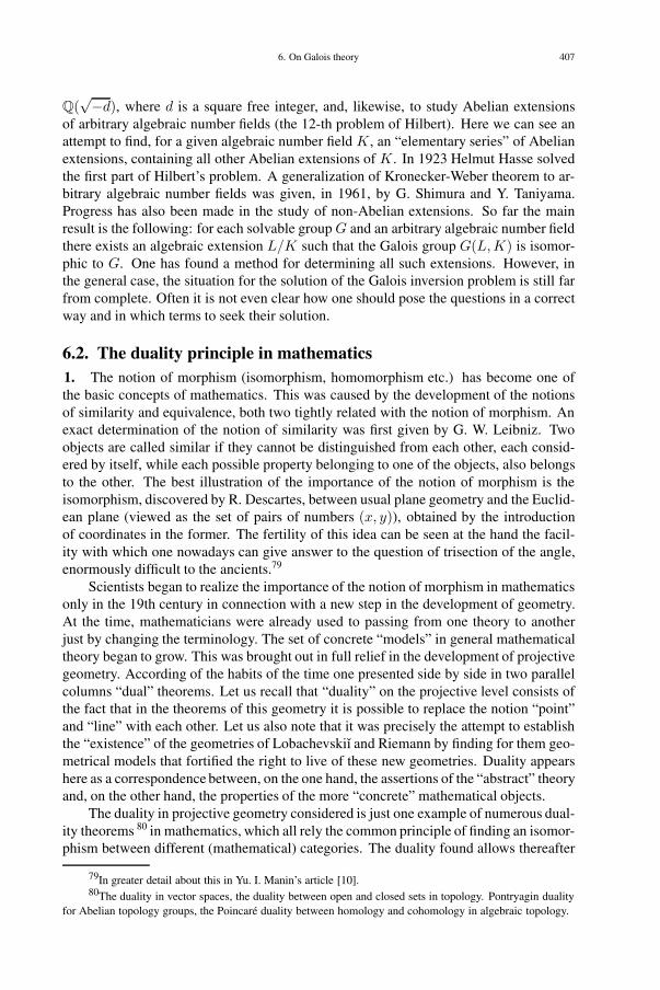
6. On Galois theory 407
Q(√−d), where d is a square free integer, and, likewise, to study Abelian extensions
of arbitrary algebraic number fields (the 12-th problem of Hilbert). Here we can see anattempt to find, for a given algebraic number field K , an “elementary series” of Abelianextensions, containing all other Abelian extensions of K . In 1923 Helmut Hasse solvedthe first part of Hilbert’s problem. A generalization of Kronecker-Weber theorem to ar-bitrary algebraic number fields was given, in 1961, by G. Shimura and Y. Taniyama.Progress has also been made in the study of non-Abelian extensions. So far the mainresult is the following: for each solvable group G and an arbitrary algebraic number fieldthere exists an algebraic extension L/K such that the Galois group G(L,K) is isomor-phic to G. One has found a method for determining all such extensions. However, inthe general case, the situation for the solution of the Galois inversion problem is still farfrom complete. Often it is not even clear how one should pose the questions in a correctway and in which terms to seek their solution.
6.2. The duality principle in mathematics1. The notion of morphism (isomorphism, homomorphism etc.) has become one ofthe basic concepts of mathematics. This was caused by the development of the notionsof similarity and equivalence, both two tightly related with the notion of morphism. Anexact determination of the notion of similarity was first given by G. W. Leibniz. Twoobjects are called similar if they cannot be distinguished from each other, each consid-ered by itself, while each possible property belonging to one of the objects, also belongsto the other. The best illustration of the importance of the notion of morphism is theisomorphism, discovered by R. Descartes, between usual plane geometry and the Euclid-ean plane (viewed as the set of pairs of numbers (x, y)), obtained by the introductionof coordinates in the former. The fertility of this idea can be seen at the hand the facil-ity with which one nowadays can give answer to the question of trisection of the angle,enormously difficult to the ancients.79
Scientists began to realize the importance of the notion of morphism in mathematicsonly in the 19th century in connection with a new step in the development of geometry.At the time, mathematicians were already used to passing from one theory to anotherjust by changing the terminology. The set of concrete “models” in general mathematicaltheory began to grow. This was brought out in full relief in the development of projectivegeometry. According of the habits of the time one presented side by side in two parallelcolumns “dual” theorems. Let us recall that “duality” on the projective level consists ofthe fact that in the theorems of this geometry it is possible to replace the notion “point”and “line” with each other. Let us also note that it was precisely the attempt to establishthe “existence” of the geometries of Lobachevskiı and Riemann by finding for them geo-metrical models that fortified the right to live of these new geometries. Duality appearshere as a correspondence between, on the one hand, the assertions of the “abstract” theoryand, on the other hand, the properties of the more “concrete” mathematical objects.
The duality in projective geometry considered is just one example of numerous dual-ity theorems 80 in mathematics, which all rely the common principle of finding an isomor-phism between different (mathematical) categories. The duality found allows thereafter
79In greater detail about this in Yu. I. Manin’s article [10].80The duality in vector spaces, the duality between open and closed sets in topology. Pontryagin duality
for Abelian topology groups, the Poincaré duality between homology and cohomology in algebraic topology.
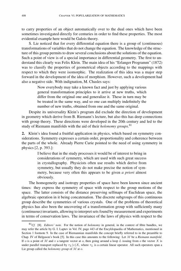
408 CHAPTER VI. POPULARIZATION OF MATHEMATICS
to carry properties of an object automatically over to the dual ones which have beensometimes investigated directly for centuries in order to find these properties. The mostevidential example here would be Galois theory.
S. Lie noticed that for every differential equation there is a group of (continuous)transformations of variables that do not change the equation. The knowledge of the struc-ture of this group permits to draw several conclusions about the solutions of the equation.Such a point of view is of a special importance in differential geometry. The first to un-derstand this clearly was Felix Klein. The main idea of his “Erlanger Programm” (1872)was to classify the properties of geometrical objects according to the mappings withrespect to which they were isomorphic. The realization of this idea was a major stepforward in the development of the idea of morphism. However, such a development hadalso a negative side. With indignation, M. Chasles says:
Now everybody may take a known fact and just by applying variousgeneral transformation principles to it arrive at new truths, whichdiffer from the original one and generalize it. These in turn may bebe treated in the same way, and so one can multiply indefinitely thenumber of new truths, obtained from one and the same original.
Despite its universality Klein’s program did exclude the direction of developmentin geometry which derive from B. Riemann’s lecture, but also this has deep connectionswith group theory. These directions were developed in the 20th century and led to thestudy of Riemann manifolds with the aid of their holonomy groups.81
2. Klein’s idea found a fruitful application in physics, which based on symmetry con-siderations. Symmetry expresses a certain order, proportionality and coherence betweenthe parts of the whole. Already Pierre Curie pointed to the need of using symmetry inphysics [2, p. 393.]:
I believe that in the study processes it would be of interest to bring inconsiderations of symmetry, which are used with such great successin crystallography. Physicists often use results which derive fromsymmetry, but usually they do not make precise the notion of sym-metry, because very often this appears to be given a priori almostobviously.
The homogeneity and isotropy properties of space have been known since ancienttimes: they express the symmetry of space with respect to the group motions of thespace. The latter consists of the distance preserving selfmaps of Euclidean space, thealgebraic operation in it being concatenation. The discrete subgroups of this continuousgroup describe the symmetries of various crystals. One of the problems of theoreticalphysics has also been the uncovering of a transformation group with sufficiently many(continuous) invariants, allowing to interpret sets found by measurement and experimentsin terms of conservation laws. The invariance of the laws of physics with respect to the
81Cf. [8]. Editors’ note. For the notion of holonomy in general, in the context of fibre bundles, wemay refer the article by G. I. Laptev in Vol. IV, page 443 of the Encyklopaedia of Mathematics, mentioned inSection 1 footnote 9. In the case of Riemannian manifolds the concept briefly referred to in the preamble toChap. IV of Helgason’s book [5]. In this case this amounts to the following: Let M be a Riemann manifold.If o is a point of M and v a tangent vector at o, then going around a loop L issuing from o the vector X isunder parallel transport replaced by τL(v)X, where τL is a certain linear operator. All such operators span aLie group called the holonomy group of M at o.

6. On Galois theory 409
group of Lorentz transformations is reflected by the principle of relativity, first formulatedby H. Poincaré 82.
Especially rich of symmetries is the micro-cosmos.83
The mathematical apparatus created by Sophus Lie has had a special importance inthe discovery of new properties of elementary particles in physics. This is explained bythe following circumstance. If some physical theory expresses its experimental resultswith the help of differential equations, then it may be that the physical content harboredin these equations is much wider and covers a larger range of experiments than that fromwhich the equations were derived. In connection with the discovery of electromagneticalradiation in Maxwell’s equations, Heinrich Hertz says strikingly:
One cannot avoid the feeling that the mathematical equations have anexistence independent of us, their own consciousness, that they aremore clever than we, because we can obtain from them more than weinitially invested in them.
A good illustration of what was said is also the discovery of anti matter. It wasobserved that if a particle is described by the Dirac equation then it can be in two differ-ent states of charge. That the electron was described by the Dirac equation was known.Therefore the existence of the positron was predicted, which later also found an experi-mental verification. From here it was inferred that every particle has an anti particle. Inelementary particle theory two kinds of symmetry are presented. Some of them are con-nected with a subgroup of the group of space-time transformations (that is, the Lorentzgroup). Others, so-called inner symmetries appear in the study of special unitary groupsand reflect the “inner” properties of particles. 84
But nature is not throughout only symmetry! The irreversibility of thermodynamicalprocesses, the violation of the laws of parity, time reversal, and charge conjugation forparticles in the case of weak interaction – all this speaks of asymmetry. Also the organicworlds abounds of them. Here we may speak of an interchange of strata of symmetryand asymmetry, of their levels. Symmetry manifests itself now in the organization ofasymmetrical elements and in doing this reflects their striving for development.
3. The world surrounding us is characterized by its structure, the granularity of thisstructure and the relative independence of the structures. This gives one the possibilityto distinguish single structures with the purpose in mind to learn to know them more dis-tinctly. The similarity of differing structures is in mathematics reflected by the notion ofmorphism – similarity on the level of a certain theory. Such an approach makes axiomaticmethods expedient. The use of this method in mathematics was initiated in the work ofM. Pasch, D. Hilbert and E. Steinitz. The acceptance more widely of this method did notgo without pain. For example, Felix Klein was from the onset rather sceptical towardsthis “axiomatic mathematics”, as he saw here an assault on intuition and imagination,that is, the truly productive elements in the process of creation. The undoubtedly mostoutstanding achievement of this direction is the appearance of the theory of algebraic
82See the articles “The principle of relativity” and “Professor H. A. Lorentz as a researcher” in the book[4]
83An exhaustive presentation of the questions to be treated below can be found in [12]. Translator’s note.See also e.g. [3].
84Translator’s note. One example is SU(2)-symmetry, which explains the similarity in the behavior ofthe proton and the neutron; recall that SU(2) is the group of unitary 2 × 2 matrices.

410 CHAPTER VI. POPULARIZATION OF MATHEMATICS
structures in the 1920’s (on the basis of the set theory of Cantor). A further step on thisroad was the enfolding of the mathematical structure and the closely related with this theallied appearance of the complete notion of morphism, which gradually became a toolfor a reshaping all of mathematics.
It is without doubt true that mathematics starts with number. In all ages number hasbeen the soul of mathematics, because their level of development is tightly connectedwith the possibility of applying mathematics in other sciences. But the development andspread of “quantitative” methods has always called for a completion and development ofthe “qualitative” methods, because the latter enrich the art of calculation with new formsand promote the organizing part in the development of metrical (numerical) mathemat-ics.85
4. The interaction of these two trends in mathematics, the applied and the theoreticalones, has been a constant source of stimulation in the work of many mathematicians. Forinstance, Feix Klein estimates the work of C. F. Gauss in applied mathematics as follows:
Gauss obtained the stimulation for this work outside mathematics.But then, in the posing of the problems and in their solution, thereappears a special creational power and experience, which he coulddevelop in himself only by solving problems of “pure” mathemat-ics. It manifests itself also in the principle not to count as done suchproblems where there still remains something to be done.
The interaction of these tendencies were brought in even greater relief in the workof J.-L. Lagrange. Lagrange’ mathematical style is characterized by an unusual conse-quence, a desire to solve this or that problem to the very end. However, his most famousbook is his Mécanique analytique (Analytical Mechanics), which appeared in 1788. Hereis treated from a general point of view various principles for the solution of mechanicalproblems found up to that time, the relations between these principles, the dependenceof each other are shown, as well as the limits of their applicability. In this treatise Me-chanics has become part of Mathematical Analysis, as one does not stop at the narrowspecial cases of the problems of mechanics, but one has brought to the foreground thesteps that are necessary in the solution of the problems under view, which in the course ofthe following centuries has been the point of departure, the foundation and the source ofmany theories in the various branches of applied mechanics. These methods have beenapplicable in the design of screws of ships, as well as in the study of the oscillation ofships, in creation of gyrocompasses, in the computation of the trajectories of shells, inprojecting railway bridges, or also in the investigation of the motion of celestial bodies.86
One has compared Mathematics with a big city, in the outskirts of which a livelyactivity of construction takes place, where new districts and new blocks rise, where theair is cleaner and where the youth crowds, bringing new force and stimulus to the city.The birth of these new quarters is an inevitable necessity in the development of a bigcity, the exigency of its life. At the same time there is going on a not less intensive
85Everybody knows the role played today by functional analysis in the development of numerical methods(and thereby also in widening of the possibilities for using the computer).
86One can read more details about this in the paper [7]. A more contemporary illustration of what wehave said is the works of J. von Neumann. The Reader can acquaint him- or herself about his views aboutthe development of mathematics, the balance of empirical and aesthetic deliberations in it, in the paper “TheMathematician” contained in the book [11, p. 1–9].

6. On Galois theory 411
and extensive building activity downtown. Streets are reconstructed and widened, newup-to-date houses rise, in order to adapt the life of the big city to the new needs andrequirements of life. We have a truly expedient and beautiful city only when these twotendencies in its development are in good harmony.
Comments. The basic tenet of Galois theory, namely the correspondence between field extensions andgroups can be succinctly stated and easily proved, and is being offered as fare to undergraduates all aroundthe world. In its basics it is a finished theory and nothing can be added to or subtracted from it. It involved aconceptual leap from the notion of a root of a polynomial to the notions of groups and fields, nowadays formingcornerstones of modern mathematics, which would be inconceivable without them.
But Galois theory is not a dead subject as Kaljulaid points out. Once you start to apply it to specificsituations, its subtlety becomes apparent. One fundamental example is the classification of Abelian extensions(Abelian Galois groups) of the rational numbers as subfields of cyclotomic extensions (adding roots to xn = 1).A surprisingly intractable problem is the inverse Galois problem over the rationales, namely to characterizethe finite groups that can occur as Galois groups of number fields (i.e. finite extensions over the rationales).This may seem to be a somewhat artificial problem, although Kaljulaid is obviously fascinated with it andits ramifications; but natural applications of Galois theory abound whenever fields pop up, and thus it is aninevitable tool of the algebraic geometer or number theorist.
Fields and groups are very different things, although in standard introductory courses both tend to betreated on equal footing as examples of algebraic structures. Groups are more fundamental, and they haveworked on human imagination long before being recognized and identified as independent entities. The crucialconcept is symmetry, the instinctive feeling that two different things are really the same, and that there is noway of intrinsically distinguishing between them. One example - the embryo of Galois theory, is to ask whichone is ’i’ (the square root of -1) ’i’ or ’−i’? Is the question meaningful? The outcome of the question iscomplex conjugation constantly used even by people innocent of Galois theory.
Kaljulaid speaks somewhat confusingly about duality and isomorphisms. The two things are really dif-ferent. The classical example of duality is the correspondence between lines and points in the projective plane(a phenomenon so attractive that it literally forced the invention of the projective plane itself). Here there issome kind of symmetry. Isomorphism is something different and more general. In duality there is no naturalisomorphism, to achieve one you need to specify and make a choice, and thus destroy the simplicity of thesituation. The concept of isomorphism is far more further reaching, and the concept of auto-isomorphism (au-tomorphism) makes exact the vaguer notion of symmetry and allows hence the introduction of compositionand of groups. As Kaljulaid rightly points out, it is Felix Klein’s vision, of groups of symmetries being at thebasis of geometrical classification – the oft referred to Erlangen program –, that elevated the notion. It is ofcourse a great unifying principle, seductive in its elegance, but of course not telling the whole story. Funda-mental physics should really be thought of as enhanced geometry, as Einstein’s general relativity so eloquentlybears witness to, and it is in theoretical physics the Klein’s Erlangen program really has struck its deepestroots. Nowadays groups of symmetries play fundamental roles in describing different physical phenomena,and from a philosophical point of view, it is tempting to see in groups the deeper reality that Plato postulated,and whose various manifestations make up the material world. (One amusing example may be the aptly calledPlatonic solids as mere aspects of their underlying symmetry groups). This mathematical view of the world isreally nothing but the modern sophisticated version of ancient number mysticism. Groups and mathematicalformulas seem to rule the physical world, and some physicists, notably Dirac, set greater store in an elegantmathematical formula, than an ugly one empirically born out, only to be eventually vindicated! Why is there aworld? Mathematical formulas of the vacuum predict its spontaneous emergence. Thus in a sense, mathematicsis God, existing even before nothing. In the most ambitious effort so far to fundamentally understand physics,optimistically referred to TOE (Theory of Everything), empirical testing is no longer feasible, and the onlysource of corroboration and inspiration is mathematical beauty.
Indeed Kaljulaid takes the ideas of Galois theory to the most exalted end.
Ulf Persson

412 CHAPTER VI. POPULARIZATION OF MATHEMATICS
References
[1] Ch. Clemens and Ph. Griffiths. The intermediate Jacobian of the cubic threefold. Ann. of Math. 95 (2),1872, 281–356.
[2] P. Curie. Sur la symmétrie dans les phenomènes physiques. J. Phys. 3 (3), 1894.[3] J. P. Elliott and P. G. Dawber. Symmetry in Physics I–II. Vol. 1. MacMillan Press Ltd., Vol. 2. Clarendon
Press, Oxfod Univ. Press, London, New York, 1979. Russian Translation: “Mir”, Moscow, 1983.[4] P. Erenfest. Relativity. Quanta. Statistics. Nauka, Moscow, 1972.[5] S. Helgason. Differential geometry and symmetric spaces. Academic Press, New York, London, 1962.[6] V. A. Iskovskih and Yu. I. Manin. Three-dimensional quartics and counterexamples to the Lüroth prob-
lem. Mat. Sbornik (N. S.) 86 (128), 1871, 140U-166.[7] A. N. Krylov. Joseph Louis Lagrange. Uspehi Mat. Nauk 2, 1936, 3–16.[8] Ü. Lumiste. The notion of space in geometry. Geometry and transformation groups. Math. and Our Age
14, 1968, 3–21.[9] P. Lüroth. Beweis eines Satzes über rationale Curven. Math. Ann. 9, 1876, 163–165.[10] Yu. I. Manin. On the solvability of the problem of construction with ruler and compass. In: Encyklopedia
of Elementary Mathematics, Vol. 4. FizMatGIZ, Moscow, 1963, 205–227.[11] J. von Neumann. Collected works. Vol 1. Pergamon Press, New York, 1961.[12] H. Õiglane. Chapters from Theoretical Physics, I–II. Tartu University Press, Tartu, 1965, 1967.
413
7. [K75b] Theory of automataCoauthor E. Tamme
To the memory of Rein Tammeste87
I was asked to speak on “possible future developments, give conjectures, andspeculate about futures advances”. To do so is always hazardous, if not fool-hardy; it may be possible that right in this very moment a graduate student isbusily at work on a theorem that might change present trends drastically.
I. M. Singer, Future extensions of index theory and elliptic operators, Ann. of Math. Studies, 70(1971), 171-185
7.1. Some points of view in analytic Cybernetics
1. Already since remote times man has tried to put the forces of Nature under his will.The study of the secrets of Nature has led to the discovery of the laws of Nature. Everysuch step forward has been followed with a shift in the development of Engineering:new machines are designed which using the conquered forces of Nature have enlargedthe physical powers of man. At the same time man has sought paths and means formaking the action of the human brain more powerful. In the 1940’s this question becameespecially actual due to necessity to carry out extraordinarily complicated and bulkycomputations. Electronic computers were discovered88. The use of computers becomesnecessary in ever more numerous new domains of practical and intellectual activity, andit is not always that existing computers can satisfy these needs, both in quantity and inquality.89 A comeback from computer to abacus is as unthinkable as from electricity tocandle light. While the technology improves the interference of man in the controllingof the work of the machines (automatized factories; automatic control and test devices;autopilots; an improved military technology etc.) is often abandoned. A need to create
87Rein Tammeste was a gifted young Estonian mathematician. Born on the island of Hiiumaa (Dagö) onJanuary 19, 1939 he graduated from Tartu University in 1960. He was the first one in Estonia to investigatenotions connected with random variables in complex Hilbert space. These results were set forth in the book“Probabilities in Hilbert spaces” (in Estonian), and in a thesis, written in Russian, defended in Tartu in 1971.He published also research on the axiomatic generalization of information and entropy. Rein Tammeste diedat the age of 34, on August 13, 1973, while descending Mount Elbrus. An obituary of him was published inMath. and Our Age 20 (1975), 132-135, and it is written about his thesis in Math. and Our Age 19 (1973), 122(both in Estonian). E. Tamme
88This work began in 1943, when, under the direction of John W. Mauchly, the first computer projectENIAC was started in practice. The computer was completed in 1946.Editors’ Note. In 1940ties, several computer projects were carried on simultaneously in different countries.for example, the computer Colosseum (UK) was working already in 1944 and Z3 (Germany, Konrad Zuse) in1943.
89Interesting material about the balance between reality and illusion can be found in the book [2]

414 CHAPTER VI. POPULARIZATION OF MATHEMATICS
more perfect and more powerful computers and automation devices enter the agenda. Tosucceed in this it is, undoubtedly, essential to know if it is possible to reach the goal setby improving or enlarging the size of the existing automata. Otherwise, one must hopethat it will be possible to understand more deeply the principles of the functioning of thebrain and to develop formal models of it that could be technically implemented (see [1]).The mathematician is here mainly interested in the following question: will it be possibleto give, on the basis of existing mathematics, an adequate description of the law whichgovern the world of complicated automata?
2. In dealing with distinct (control) systems their structural similarity often becomesapparent, that is, the analogue between many elements and their mutual relations, but alsoa functional similarity, that is, a similar behavior of the systems in analogous situations.
This makes it possible to create a general (axiomatic) theory for classes of controlsystems, in which the concrete systems are viewed as representatives of a class. In theaxiomatization of the behavior of elements one has to assume that the elements can beregarded as “black boxes”, the inner structure of which need not to be known, but whoreact in a certain determined way to exactly determined exterior excitation. However,the axiomatics of such a theory requires, from time to time, improvements, especiallyafter changes in our knowledge of the physico-chemical nature of the elements and theirproperties. The principal task is then to find suitable notions and methods for the researchof the structure of systems and functional properties of a given class.
A step on this path is the work of W. Mc Culloch and W. Pitts regarding formal neuralnetworks [6]. A central role in this theory is the notion of a formal neuron. This is an(abstract) element, a “black box” with m inputs x1, . . . , xm (where m ≥ 1), and a singleoutput d. A neuron has m + 1 numerical characteristics: the level θ, and the weights ωi
of the inputs xi. Here ωi > 0 means that the input xi is stimulating, while ωi < 0 thatxi is inhibitory. Such a formal neuron works on a discrete scale of time t = 0, 1, 2, . . . ,and gives at time t = n + 1 an impulse to the output d precisely when, at t = n, thesum of the weights of stimulating inputs exceeds the level of the neuron. A formal neuralnetwork is a union of elements obtained in the following way. The output of the neuronis divided into a suitable number of branches which are connected to the inputs of someother neurons. Here the outputs of a neuron can be connected with an arbitrary numberof inputs in itself or to other neurons, but each input may only be connected with a singleoutput. Some inputs of neurons may remain free and these are either connected to eachother (to be considered as identical) or else they are grouped into input lines of the net(each free input is connected to an exactly one input line; the number of the latter may,however, be smaller than the number of free inputs). The output lines are identified asoutputs, which are not joined to inputs of any other neuron. All neurons are working atthe same time, and their level and weights do not change in the course of time. The studythe functioning of such a formal network amounts to clarifying with which signals on theoutput lines the net will react to various signals on its input lines.
Although the formal neural network is a rather primitive analogue of the brain, theirstudy was still a first real step to use of mathematical devices in neuro-physiology. Thestudy of such networks stimulated to a large extent the genesis of automata theory. In-deed, in 1946, John von Neumann set forth new ideas of the construction of electroniccomputers (the EDVAC project). Von Neumann had as basis of his construction themodule, a notion, in the creation of which an essential role was played by the functional
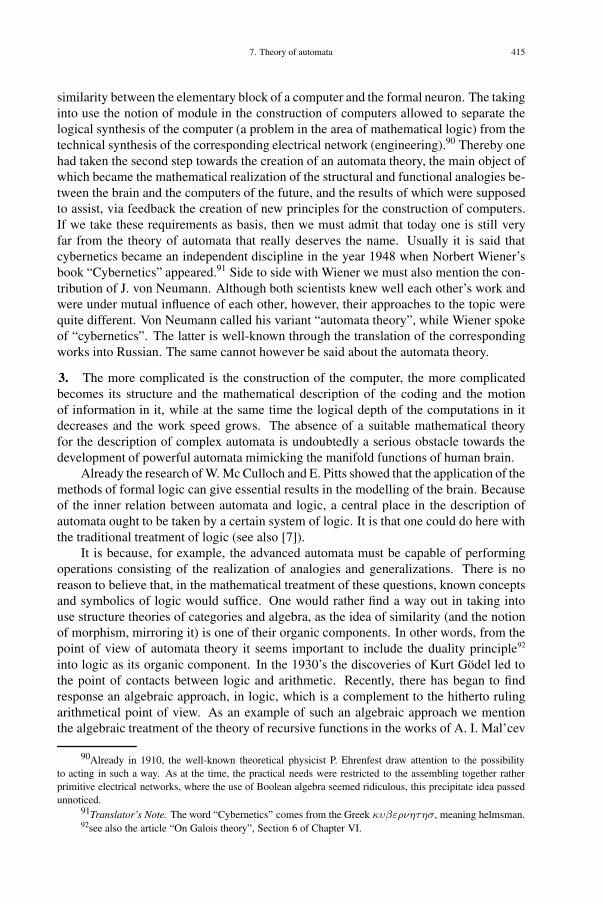
7. Theory of automata 415
similarity between the elementary block of a computer and the formal neuron. The takinginto use the notion of module in the construction of computers allowed to separate thelogical synthesis of the computer (a problem in the area of mathematical logic) from thetechnical synthesis of the corresponding electrical network (engineering).90 Thereby onehad taken the second step towards the creation of an automata theory, the main object ofwhich became the mathematical realization of the structural and functional analogies be-tween the brain and the computers of the future, and the results of which were supposedto assist, via feedback the creation of new principles for the construction of computers.If we take these requirements as basis, then we must admit that today one is still veryfar from the theory of automata that really deserves the name. Usually it is said thatcybernetics became an independent discipline in the year 1948 when Norbert Wiener’sbook “Cybernetics” appeared.91 Side to side with Wiener we must also mention the con-tribution of J. von Neumann. Although both scientists knew well each other’s work andwere under mutual influence of each other, however, their approaches to the topic werequite different. Von Neumann called his variant “automata theory”, while Wiener spokeof “cybernetics”. The latter is well-known through the translation of the correspondingworks into Russian. The same cannot however be said about the automata theory.
3. The more complicated is the construction of the computer, the more complicatedbecomes its structure and the mathematical description of the coding and the motionof information in it, while at the same time the logical depth of the computations in itdecreases and the work speed grows. The absence of a suitable mathematical theoryfor the description of complex automata is undoubtedly a serious obstacle towards thedevelopment of powerful automata mimicking the manifold functions of human brain.
Already the research of W. Mc Culloch and E. Pitts showed that the application of themethods of formal logic can give essential results in the modelling of the brain. Becauseof the inner relation between automata and logic, a central place in the description ofautomata ought to be taken by a certain system of logic. It is that one could do here withthe traditional treatment of logic (see also [7]).
It is because, for example, the advanced automata must be capable of performingoperations consisting of the realization of analogies and generalizations. There is noreason to believe that, in the mathematical treatment of these questions, known conceptsand symbolics of logic would suffice. One would rather find a way out in taking intouse structure theories of categories and algebra, as the idea of similarity (and the notionof morphism, mirroring it) is one of their organic components. In other words, from thepoint of view of automata theory it seems important to include the duality principle92
into logic as its organic component. In the 1930’s the discoveries of Kurt Gödel led tothe point of contacts between logic and arithmetic. Recently, there has began to findresponse an algebraic approach, in logic, which is a complement to the hitherto rulingarithmetical point of view. As an example of such an algebraic approach we mentionthe algebraic treatment of the theory of recursive functions in the works of A. I. Mal’cev
90Already in 1910, the well-known theoretical physicist P. Ehrenfest draw attention to the possibilityto acting in such a way. As at the time, the practical needs were restricted to the assembling together ratherprimitive electrical networks, where the use of Boolean algebra seemed ridiculous, this precipitate idea passedunnoticed.
91Translator’s Note. The word “Cybernetics” comes from the Greek κυβερνητησ, meaning helmsman.92see also the article “On Galois theory”, Section 6 of Chapter VI.
416 CHAPTER VI. POPULARIZATION OF MATHEMATICS
and S. Eilenberg. It may be that in the course of time there will be a synthesis of thesetwo points of view on a new level on the basis of an “arithmetized algebra”, being ageneralization of the arithmetical point of view.
It is also of importance to note that formal logic, because of its approach (the princi-ple of “all or nothing at all”), has so far been cut off from the possibility of using the mostadvanced part of mathematics – mathematical analysis – using instead combinatorics, anarea, were there appear great mathematical difficulties. At the same time, one has, in An-alytic Number Theory and in Diophantine Geometry, since a long time ago, found waysfor fruitful application of the idea of continuity in the solution of problems which by theirnature were discrete. One can claim even more, that the deepest results in the disciplinesmentioned have been obtained precisely in this way (often by the intermediary of algebraand probability theory).
In the mathematics of the antiquity an essential achievement was the polarity “finite-infinite”, which now (based on the set theory of Georg Cantor) with the appearance ofMathematical Analysis has become a powerful instrument of cognition. But a deeperand more complete use of the polarity “continuous-discrete” still lies ahead. That thishas not yet been done to its full extent is perhaps one of the reasons why physicists intheir perspective research still find to little satisfaction in mathematics they can use. Thisidea due to Hermann Weyl seems to be forth to develop with respect of many parts ofapplied mathematics. The needs of the applications and the difficulties of the theorieshave created a situation where one appreciates ever more the value of the ideas whichhave arisen in the path to the goal, in which C. G. J. Jacobi believed in a passionate way:
There will come a time when from each theorem in MathematicalAnalysis there will follow a theorem in Number Theory, and viceversa each regularity in the domain of natural numbers will give atheorem in analysis.
A powerful basis for the arising and development of such ideas was founded in the workof Leonard Euler. A series of original considerations were given by Yu. Manin in his talk“The physical and mathematical continuum” at the summer school in the history of math-ematics in Tartu in 1973. These observations agree with the view of J. von Neumann,according to which the mathematical apparatus for the study of complicated automataought to start with mathematical logic and proceed in the direction of algebraic, proba-bilistic and analytic structures and further optics and thermodynamics (in the form givenby L. Boltzmann the latter is in many things close to the theory of information processingand measurement). The same point of view was also echoed in a talk by V. Glushkov ata meeting devoted to automata theory in Tashkent in May, 1968. Namely, according toGlushkov the main attention of mathematicians until the end of the 20th century will bedirected towards the creation of the algebra and topology of a (formal) language, that isnecessary for the mathematical description of complicated automata (see also [3]).
7.2. On algebraic methods in automata theory
Several points of contact between automata theory and structural theories of algebrahave been know for a long time. Namely, it turns out that each automaton can be inter-preted as a certain algebraic object that allows to study the construction of the automatonby means of the structure theory. Proceeding in this way it becomes possible to get an
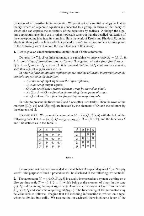
7. Theory of automata 417
overview of all possible finite automata. We point out an essential analogy to Galoistheory, where an algebraic equation is connected to a group, in terms of the theory ofwhich one can express the solvability of the equations by radicals. Although the alge-braic apparatus taken into use is rather modest, it turns out that the detailed realization ofthe corresponding idea is quite complex. Here the work of Krohn and Rhodes [5], on thealgebraic theory of machines which appeared in 1965, turned out to be a turning point.In the following we will set out the main features of this theory.
1. Let us give an exact mathematical definition of a finite automaton.
DEFINITION 7.1. By a finite automaton or a machine we mean system M = (A,Q,B,λ, δ) consisting of three finite sets A, Q and B, together with the fixed functions λ :Q × A → Q and δ : Q × A → B. It is assumed that the set Q contains an element psuch that λ(p, x) = p for each x ∈ A.
In order to have an intuitive explanation, we give the following interpretation of thesymbols appearing in the definition:
- A is the set of input signals or the input alphabet,- B is the set of output signals,- Q is the set of states, whose element p may be viewed as a halt,- λ : Q×A→ Q – a function determining the mapping of states,- δ : Q×A→ B – a function for getting the output signals.
In order to present the functions λ and δ one often uses tables. Then the rows of thematrices ‖λ(q, x)‖ and ‖δ(q, x)‖ are indexed by the elements of Q, and the columns bythe elements of A.
EXAMPLE 7.1. We present the automaton M = (A,Q,B, λ, δ) with the help of thefollowing data. Let A = {a, b}, Q = {q0, q1, q2, p}, B = {0, 1, 2}, and the functions λand δ be defined as in the Table 1.
λ a b Λq0 q1 p pq1 q1 q2 pq2 p q2 q0p p p p
δ a b Λq0 1 0 0q1 0 1 0q2 0 0 1p 2 2 2
Table 1
Let us point out that we have added to the alphabet A a special symbol Λ, an “emptyword”. The purpose of such a procedure will be disclosed in the following two sections.
2. The automaton M = (A,Q,B, λ, δ) is usually interpreted as a system working on adiscrete time scale T = {0, 1, 2, . . .}, which being at the moment of time t in the stateq ∈ Q and receiving the input signal x ∈ A moves at the moment t + 1 into the stateλ(q, x) ∈ Q and sends the output signal δ(q, x). The functioning of the automaton maybe visualized as follows. Imagine that the incoming information is written on a tape,which is divided into cells. We assume that in each cell there is either a letter of the
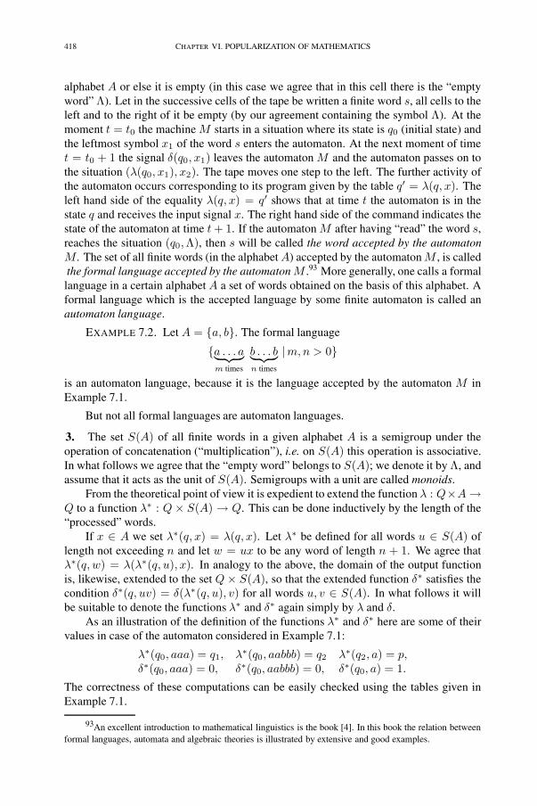
418 CHAPTER VI. POPULARIZATION OF MATHEMATICS
alphabet A or else it is empty (in this case we agree that in this cell there is the “emptyword” Λ). Let in the successive cells of the tape be written a finite word s, all cells to theleft and to the right of it be empty (by our agreement containing the symbol Λ). At themoment t = t0 the machine M starts in a situation where its state is q0 (initial state) andthe leftmost symbol x1 of the word s enters the automaton. At the next moment of timet = t0 + 1 the signal δ(q0, x1) leaves the automaton M and the automaton passes on tothe situation (λ(q0, x1), x2). The tape moves one step to the left. The further activity ofthe automaton occurs corresponding to its program given by the table q′ = λ(q, x). Theleft hand side of the equality λ(q, x) = q′ shows that at time t the automaton is in thestate q and receives the input signal x. The right hand side of the command indicates thestate of the automaton at time t + 1. If the automaton M after having “read” the word s,reaches the situation (q0,Λ), then s will be called the word accepted by the automatonM . The set of all finite words (in the alphabet A) accepted by the automaton M , is calledthe formal language accepted by the automaton M .93 More generally, one calls a formallanguage in a certain alphabet A a set of words obtained on the basis of this alphabet. Aformal language which is the accepted language by some finite automaton is called anautomaton language.
EXAMPLE 7.2. Let A = {a, b}. The formal language
{a . . . a︸ ︷︷ ︸m times
b . . . b︸ ︷︷ ︸n times
|m,n > 0}
is an automaton language, because it is the language accepted by the automaton M inExample 7.1.
But not all formal languages are automaton languages.
3. The set S(A) of all finite words in a given alphabet A is a semigroup under theoperation of concatenation (“multiplication”), i.e. on S(A) this operation is associative.In what follows we agree that the “empty word” belongs to S(A); we denote it by Λ, andassume that it acts as the unit of S(A). Semigroups with a unit are called monoids.
From the theoretical point of view it is expedient to extend the function λ : Q×A→Q to a function λ∗ : Q× S(A) → Q. This can be done inductively by the length of the“processed” words.
If x ∈ A we set λ∗(q, x) = λ(q, x). Let λ∗ be defined for all words u ∈ S(A) oflength not exceeding n and let w = ux to be any word of length n + 1. We agree thatλ∗(q, w) = λ(λ∗(q, u), x). In analogy to the above, the domain of the output functionis, likewise, extended to the set Q× S(A), so that the extended function δ∗ satisfies thecondition δ∗(q, uv) = δ(λ∗(q, u), v) for all words u, v ∈ S(A). In what follows it willbe suitable to denote the functions λ∗ and δ∗ again simply by λ and δ.
As an illustration of the definition of the functions λ∗ and δ∗ here are some of theirvalues in case of the automaton considered in Example 7.1:
λ∗(q0, aaa) = q1, λ∗(q0, aabbb) = q2 λ∗(q2, a) = p,δ∗(q0, aaa) = 0, δ∗(q0, aabbb) = 0, δ∗(q0, a) = 1.
The correctness of these computations can be easily checked using the tables given inExample 7.1.
93An excellent introduction to mathematical linguistics is the book [4]. In this book the relation betweenformal languages, automata and algebraic theories is illustrated by extensive and good examples.

7. Theory of automata 419
4. Let there be given an automaton M = (A,Q,B, λ, δ), which at a fixed momentof time t ∈ T is in state q. The future behavior of the automaton M is characterizedby the function f : S(A) → B, which for each u ∈ S(A) is given by the formulaf(u) = δ(q, u). Of course, there may exist such distinct states q and r in M suchthat δ(q, ∗) ≡ δ(r, ∗). But if such a situation does not occur we say that M is a reducedautomaton. It turns out that to each automaton M there corresponds a reduced automatonM ′ = {A,Q′, B, λ′, δ′} which is equivalent to M in the following sense: for each stateq ∈ Q there exists a state r ∈ Q′ such that δ(q, ∗) = δ′(r, ∗) as functions on S(A).
To each word u ∈ S(A) we associate the left shift lu : S(A)→ S(A), a function thatfor each v ∈ S(A) is defined by the formula lu(v) = uv. For arbitrary u, v, w ∈ S(A)one has lulv(w) = luv(w).
On the basis of the automaton M = (A,Q,B, λ, δ) we construct the automatonM(f) = (A,Qf , B, λf , δf ) whose set of states is
Qf = {g : S(A)→ B | g = flu for some u ∈ S(A)}.The functions λf and δf are defined by the formulae
λf (g, v) = glv, δf (g, v) = g(v).
Here flu and glu denote functions S(A) → B whose values at the word w ∈ S(A) arecomputed according to the formulae flu(w) = f(uw) and glu(w) = g(uw).
In order to better understand the nature of the automaton M(f) we make the follow-ing observations.
First, for each u ∈ S(A) the identity flu(∗) = δ(λ(q, u), ∗) holds. Indeed, for anarbitrary v ∈ S(A) we have the equalities
flu(v) = δ(q, lu(v)) = δ(q, uv) = δ(λ(q, u), v),
from which the desired equality follows.Second, it holds δf (g, v) = δ(q, uv), because δf (g, v) = g(v) = flu(v) = f(uv) =
δ(q, uv). We observe further that λf (g, v) = glv = flulv = fluv = δ(q, luv(∗)).Third, we show that M(f) is a reduced automaton. To this end, it is sufficient to
show that δf (g′, ∗) = δf(g, ∗) implies that g′(∗) = g(∗). Let g = flu, g′ = flw,u,w ∈ S(A), and take an arbitrary word v ∈ S(A). Assume that δf (g′, ∗) = δf (g, ∗).We have the following chain of equalities
g′(v) = flw(v) = δ(q, wv) = δf (g′, v) = δf (g, v) = δ(q, uv) = flu(v) = g(v).
It follows from them that g′ = g. The assertion is proved.The reasonings given show that the set of states Qf of the automaton M(f) can
be regarded as the trajectory emanating from the state f(∗) ∈ Qf , where each state is“accessible” from the state f(∗). The connection of the automaton M(f) with M isreflected by the fact that if we take the state q ∈ Q for the state f(∗) ∈ Qf , we can viewQf as the subset of Q consisting of those states which are “accessible” from the state qand where the states of the automaton M with the same behavior are considered to beidentical.
5. On the monoid S(A) of input words of the automaton M(f) there is given thefollowing (Myhill) equivalence≡f :
v ≡f v′ ⇐⇒ ∀u,w ∈ S(A), f(uvw) = f(uv′w).
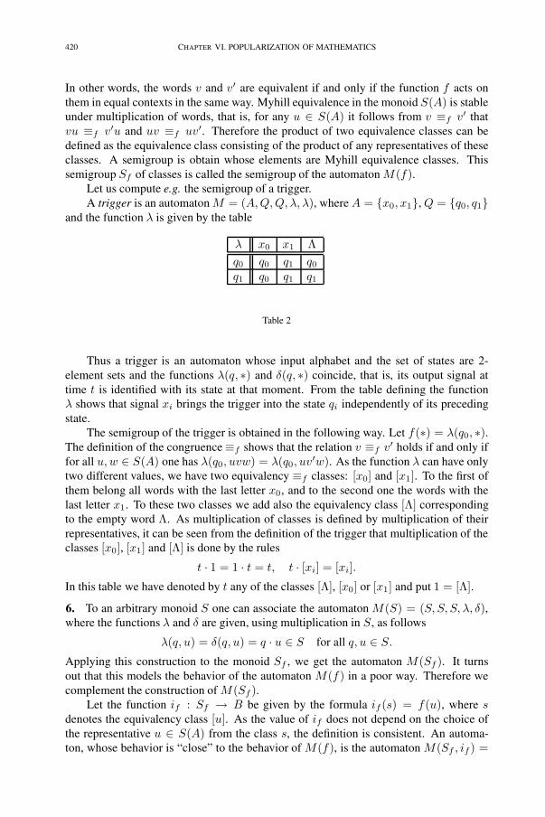
420 CHAPTER VI. POPULARIZATION OF MATHEMATICS
In other words, the words v and v′ are equivalent if and only if the function f acts onthem in equal contexts in the same way. Myhill equivalence in the monoid S(A) is stableunder multiplication of words, that is, for any u ∈ S(A) it follows from v ≡f v′ thatvu ≡f v′u and uv ≡f uv′. Therefore the product of two equivalence classes can bedefined as the equivalence class consisting of the product of any representatives of theseclasses. A semigroup is obtain whose elements are Myhill equivalence classes. Thissemigroup Sf of classes is called the semigroup of the automaton M(f).
Let us compute e.g. the semigroup of a trigger.A trigger is an automaton M = (A,Q,Q, λ, λ), where A = {x0, x1}, Q = {q0, q1}
and the function λ is given by the table
λ x0 x1 Λq0 q0 q1 q0q1 q0 q1 q1
Table 2
Thus a trigger is an automaton whose input alphabet and the set of states are 2-element sets and the functions λ(q, ∗) and δ(q, ∗) coincide, that is, its output signal attime t is identified with its state at that moment. From the table defining the functionλ shows that signal xi brings the trigger into the state qi independently of its precedingstate.
The semigroup of the trigger is obtained in the following way. Let f(∗) = λ(q0, ∗).The definition of the congruence≡f shows that the relation v ≡f v′ holds if and only iffor all u,w ∈ S(A) one has λ(q0, uvw) = λ(q0, uv′w). As the function λ can have onlytwo different values, we have two equivalency ≡f classes: [x0] and [x1]. To the first ofthem belong all words with the last letter x0, and to the second one the words with thelast letter x1. To these two classes we add also the equivalency class [Λ] correspondingto the empty word Λ. As multiplication of classes is defined by multiplication of theirrepresentatives, it can be seen from the definition of the trigger that multiplication of theclasses [x0], [x1] and [Λ] is done by the rules
t · 1 = 1 · t = t, t · [xi] = [xi].
In this table we have denoted by t any of the classes [Λ], [x0] or [x1] and put 1 = [Λ].
6. To an arbitrary monoid S one can associate the automaton M(S) = (S, S, S, λ, δ),where the functions λ and δ are given, using multiplication in S, as follows
λ(q, u) = δ(q, u) = q · u ∈ S for all q, u ∈ S.
Applying this construction to the monoid Sf , we get the automaton M(Sf ). It turnsout that this models the behavior of the automaton M(f) in a poor way. Therefore wecomplement the construction of M(Sf ).
Let the function if : Sf → B be given by the formula if (s) = f(u), where sdenotes the equivalency class [u]. As the value of if does not depend on the choice ofthe representative u ∈ S(A) from the class s, the definition is consistent. An automa-ton, whose behavior is “close” to the behavior of M(f), is the automaton M(Sf , if) =

7. Theory of automata 421
(Sf , Sf , B, λ, δ), where λ(s, s′) = s · s′ and δ(s, s′) = if (s · s′). The automatonM(Sf , if) is close to the automaton M(f) in the following sense: to the automatonM(Sf , if) it is possible (if necessary) to add a coder of its input signals, and a decoderof its output signals in such a way that for each state of M(f) there exists a state ofM(Sf , if) such that when the automaton M(Sf , if ) starts at this state, it maps the inputsignals in the same way as M(f) does. In this case one says that M(Sf , if) is a modelof the automaton M(f). As the automata M(Sf , if) and M(f) can be interchanged inthe case at hand, these automata are quasi-equivalent.
7. What kind of information about the automaton M(f) does the pair (Sf , if) contain,and how can this information be used to study the automaton M(f)?
The more extensive the functions fulfilled by the automatical devices become, themore grow the dimensions of its blocks and the complexity of its hierarchical structure.This tendency forces to construct the devices in several steps: first one determines thestructure of the blocks of the automaton and afterwards the optimal block structure. Thisway the assembling of more complicated automatical devices has to be dealt with, whichleads to the necessity of theoretical treatment of these problems – the theory of decom-position and synthesis of automata do the job.
The decomposing of an automaton into “bricks” can be done in different “scales”.In case of the computer we can consider as such bricks both semiconductors as well asthe complete circuits, while studying the brain, whole parts of it or just specific neurons.It is clear that a presupposition for a successful theory of decomposition and synthesis isthe choice of an optimal “scale”. The classification of the bricks and the determinationof their properties requires always a specific knowledge about the domain to which theseobjects belong. The experimental studies are here always accompanied by mathematicalmethods, where logic and algebraic methods have a sufficiently prominent position.
In the first part of the paper we spoke of the work ofMcCulloch and Pitts on neuralnetworks. It follows directly from the corresponding definitions that each formal neuralnetwork can be considered as a finite automaton. However, the possibility to realizethe behavior of every finite automaton in some formal neural network is somewhat ofa surprise. This result of McCulloch and Pitts solves the problem of decomposition ofautomata, if in joining of its primitive building blocks (the neurons), cycles are allowed(in joining neurons into the network, rather complicated cycles may occur). However,in practice one imposes several kinds of restrictions to the presentation of the automata(or their blocks) to exclude such cycles. Often serial or parallel connection of automata,or some combination of these, etc. is used. The properties of several connections ofsuch type are reflected in the notion of cascade of automata. Let us now introduce thisimportant concept.
We consider an automaton M = (A,Q,B, λ, δ) such that its state at each momentof time determines the output at that moment, i.e., there is a function β : Q → B suchthat δ(q, x) = β(λ(q, x)). Such an automaton is called a state-output automaton or aMoore automaton. An example of a Moore automaton – a trigger is already known to us.Another important example (the PR-automaton) will be introduced to the Reader in thefollowing Section.
Let there be given two Moore automataM = (A,Q,B, λ, β) andM ′ = (A′, Q′, B′,λ′, β′), an alphabet Z , and two arbitrary functions σ : Z×B → A′ and κ : Z → A. Thecoder κ maps each signal from Z to a signal acceptable by the automaton M . The coder

422 CHAPTER VI. POPULARIZATION OF MATHEMATICS
σ maps pairs of signals, of which the first component is a signal in Z , and the second onean output signal of M , into signals acceptable by the automaton M ′.
A cascade of the automata M and M ′ is the automaton
M ′ ◦M = (Z,Q′ ×Q,B′ ×B, λ∗, β∗),
whose state and output functions are given by the formulae
λ∗((q′, q), z) = (λ′(q′, σ(z, β(q))), λ(q, κ(z))),
β∗(q′, q) = (β′(q′), β(q)).
The functioning of the automaton M ′ ◦M is illustrated by the scheme in Figure 18.
Z
��•��κ �� M ��•
B ��
σ ��M ′ B ��
Fig. 18
In the special case where there exists a function τ : B → A′ such that σ(z, y) = τ(y)for all z ∈ Z and y ∈ B, we are dealing with the serial connection of the automata Mand M ′. We have a parallel connection if their exists a function τ : Z → A′ such thatfor all z ∈ Z and y ∈ B there holds σ(z, y) = τ(z). The notion of cascade of automatais illustrated also by the proof of the theorem in the next Section.
8. The main result in the theory of decomposition of automata is the following
THEOREM 7.2 (Krohn-Rhodes). It is possible to model each finite automaton withusing triggers and a cascade of the automata M(G) corresponding to a suitable finitesimple groups G.
In this case one says that the given automaton cascades to a set of these automata.The most interesting route to this result belongs to H. Zeiger [8]. In the central role
here is the notion of PR-automaton that is a Moore automaton where each input signalinduces either a substitution on the state space or else brings the automaton into a statefixed by this input signal (that is, does not depend on the state of the automaton beforereceiving the input signal). It follows from the definition that to each PR-automaton akind of substitution group on the set of its states is related. It turns out that a set of suchautomata is sufficient to build an arbitrary finite automaton. More exactly, we have thefollowing result.
THEOREM 7.3 (Zeiger). Each finite automaton can be presented by a cascade ofPR-automata.
The proof of this theorem is rather complicated. It is essential to note that the methodof covers (or mosaic pictures) used at this can probably be adapted for mathematical
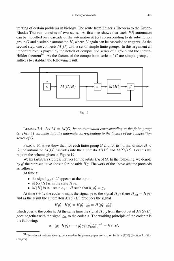
7. Theory of automata 423
treating of certain problems in biology. The route from Zeiger’s Theorem to the Krohn-Rhodes Theorem consists of two steps. At first one shows that each PR-automatoncan be modelled on a cascade of the automaton M(G) corresponding to its substitutiongroup G and a suitable automaton K , where K again can be cascaded to triggers. At thesecond step, one connects M(G) with a set of simple finite groups. In this argument animportant role is played by the notion of composition series of a group and the Jordan-Hölder theorem94. As the factors of the composition series of G are simple groups, itsuffices to establish the following result.
��
•
��κ �� M(G/H) ��•
��σ �� M(H) �� β ��
Fig. 19
LEMMA 7.4. Let M = M(G) be an automaton corresponding to the finite groupG. Then M cascades into the automata corresponding to the factors of the compositionseries of G.
PROOF. First we show that, for each finite group G and for its normal divisor H <G, the automaton M(G) cascades into the automata M(H) and M(G/H). For this werequire the scheme given in Figure 19.
We fix (arbitrary) representatives for the orbits Hg of G. In the following, we denoteby g′ the representative chosen for the orbit Hg. The work of the above scheme proceedsas follows:
At time t:
• the signal g2 ∈ G appears at the input,• M(G/H) is in the state Hg1,• M(H) is in a state h1 ∈ H such that h1g
′1 = g1.
At time t + 1: the coder κ maps the signal g2 to the signal Hg2 (here Hg′2 = Hg2)and as the result the automaton M(G/H) produces the signal
Hg′1 ·Hg′2 = Hg′1 · g′2 = H(g′1 · g′2)′,which goes to the coder β. At the same time the signal Hg′1, from the output of M(G/H)goes, together with the signal g2, to the coder σ. The working principle of the coder σ isthe following:
σ : (g2, Hg′1) −→ g′1g2[(g′1g′2)
′]−1 = h ∈ H.
94The relevant notions about groups used in the present paper are also set forth in [K70] (Section 4 of thisChapter).
424 CHAPTER VI. POPULARIZATION OF MATHEMATICS
The signal received h ∈ H goes now onto M(H), which is in the state h1. The behaviorthe automaton M(H) can be described by the following equation
h1 · h = h1g′1g2[(g′1g
′2)
′]−1 = g1g2[(g′1g′2)
′]−1.
The coder β maps pair of signals according to the rule:
β : (H(g′1g′2)
′, h1h) −→ h1h(g′1g′2)
′ =
= g1g2[(g′1g′2)
′]−1 · (g′1g′2)′ = g1g2.
These computations show that the statement made at the beginning of the proof isvalid.
We prove now the lemma by induction over the length of the composition series of G(in view of the Jordan-Hölder theorem the length of the composition series is an invariantof the group). If G is a simple group, then the validity of the theorem is evident. In theopposite case G has a non-trivial composition series
G = G0 > G1 > · · · > Gk−1 > Gk = (1).
Assume that the assertion has been proved for all groups with a composition seriesof length ≤ k − 1. The reasoning given at the beginning of the proof shows thatM(G) cascades into the automata M(G/G1) and M(G1). From the induction hy-pothesis we see that M(G1) cascades into the automata that correspond to the factorsG1/G2, G2/G3, . . . , Gk−1/Gk = Gk−1 of the composition series. Thus we see that theseeking for cascade for the automaton M(G) is found. '(
9. Triggers can be viewed as sufficiently simple building blocks for automata. Butwhat can be said about the automata corresponding to simple groups? If we had a listof all simple groups G and their necessary properties, then the Krohn-Rhodes Theoremwould give a solution to the problem of decomposition of automata. But so far there isno such list.95 Therefore there arises the idea to look for even simpler building blocksthan the automata M(G) corresponding to simple groups. For this one should continuecascading these automata. A closer investigation of the relations between the cascade ofthe automata and its semigroup shows that such a desire cannot be out into practice.
We call an automaton M noncascadable if each time that it is modelled by thecascade of two automata M1 and M2 (with the corresponding semigroups S1 and S2) itfollows that either M(S1) models M , or else M(S2) models M .
An algebraic treatment of the problem of noncascadability of automata is made pos-sible by the following two notions.
DEFINITION 7.5. Let S1 and S2 be two semigroups, and let σ : S1 → End(S2) be ahomomorphism of the monoid S1 to the semigroup of endomorphisms of the monoid S2.
95The classification of simple groups has been worked on for about 70 years. First whole series ofsuch groups were found, but later also individual groups of very high order. For example, at a meeting onIreland (Galways) in 1973 about the application of computers in algebra, M. Hall treated a group of order460 815 505 920, which simplicity was to be decided by a computer. It is so that there an algorithm canbe given for decision of simplicity of the group by its Cayley’s table. A deficiency of such an approach isapparently that we lack a criterion to determine if the list already composed contains all simple groups ornot. The question of the existence of such a criterion is difficult. Translator’s Note. The problem of theclassification of simple groups is now settled. See Gunnar Traustason’s comments to Section 4 in this Chapter,and the references indicated there.

7. Theory of automata 425
Then the semi-direct product S2Δσ is the set of all pairs in S2×S1 with the composition(multiplication of pairs) given by the rule
(s2, s1) · (s′2, s′1) = (s2 · σs1 (s′2), s1 · s′1).
DEFINITION 7.6. A semigroup S is atomary if for all possible homomorphisms σ :S1 → End(S2) it follows from the relation S|S2ΔσS1 that S|S1 or S|S2. (Here thenotation P |Q means that the semigroup P divides the semigroup Q in the followingsense: there exist a semigroup Q1 ⊂ Q which can be mapped epimorphically onto P .)
It turns out that an automaton is noncascadable if and only if its semigroup is atom-ary. This result is important because it transfers the difficulties related to the problemof deciding the noncascadability of an automaton to the algebraic domain. A somewhatexpected fact is the atomarity of the semigroup of a trigger. The atomarity of simplegroups is studied using an algebraic reasoning of considerable logical depth. Therefore arefinement of the building blocks obtained in the Krohn-Rhodes Theorem is not possible,so that getting an overview of all possible finite automata is, within the framework of thistheory, tightly connected with the classification of simple finite groups.
10. At an international meeting devoted to universal algebras and their applications,held in Potsdam in 1970, Samuel Eilenberg indicated a new road to the Krohn-Rhodesresult. His approach has in automata theory about the same effect as the passing fromequations to the study of extensions of fields in Galois theory; in both cases it leads to awidening and a clarification of the theory.
The ideas of automata theory have found widespread application in the creation offormalized methods in the schemes for designing computers. And likewise in the solu-tion of theoretical problems in programming. Let us especially mention that it were theconcepts arising from the algebraic decomposition theory of Krohn-Rhodes that madeit possible for R. Kalman, in the years 1962-67, to carry out an “algebraic reform” inthe theory of linear dynamic systems. This branch of optimal control theory turned inthis way especially in relief and makes possible a fast improvement and widening of thetheory in future.
Undoubtedly, it is true that major progress in algebra has always been related topossibilities for an inner development of its theories. Moreover, it is necessary to useopportunities to apply the obtained results outside the traditional borders. Analyticalcybernetics gives here an excellent opportunity. One cannot hope that all branches ofalgebra have yet been created which could turn out to be necessary in the course of suchresearch. Also, it does not seem today probable that the necessary apparatus ought tobe purely algebraic, although it is true that algebra takes always a fundamental role inall kinds of structural theories. One should rather treat the existing algebraic theoriesand facts as the basic matter in the creation of a language that will be adequate for amathematical description of complex automata.
References
[1] N. Basov and O. Krohin. Laser-71. Izvestiya, Feb. 12, 1974.[2] H. Dreyfus. What computers can’t do: the limits of artificial intelligence. Harper & Row, New York, 1972.[3] V. Gluškov. Abstract theory of automata. Usp. Mat. Nauk 5, 1961, 3–62.

426 CHAPTER VI. POPULARIZATION OF MATHEMATICS
[4] M. Gross and A. Lantin. Notions sur les grammaires formelles (The theory of formal grammars). Gauthier-Villars, Paris, 1967. Russian Translation: “Mir”, Moscow, 1971.
[5] K. Krohn and J. Rhodes. Algebraic theory of machines. I. Prime decomposition theorem for finite semi-groups and machines. Trans. Am. Math. Soc. 116, 1965, 450–464.
[6] W. Mc Culloch and W. Pitts. A logical calculus of the ideas immanent in nervous activity. Bull. Math.Biophys. 5, 1943, 115–133.
[7] P. Rashevskii. On the dogma of the natural number system. Usp. Mat. Nauk 28 (4), 1973, 243–246.[8] H. P. Zeiger. Cascade decomposition of automata using covers. In: M. A. Arbib (ed.), Algebraic Theory
of Machines, Languages, and Semigroups. Academic Press, Netherlands, 1968, 55 – 80.

427
8. [K93c] Mordell’s problemComments by G. Almkvist
In this paper we describe two results which have been widely known in the past 15years, crowning the efforts of numerous mathematicians since the times of Pierre Fermat(1601-1665). At the same time we try to present the notions which allowed to arrive atthis milestone. Regretfully, however, major events in the area of mathematics resemblehigh peaks of mountains – even if we have already climbed up to them, a majority ofthem remain unaccessible to but the very few, possessing the necessary special equip-ment and training for reaching these heights. Therefore it is natural that although peopleoften speak romantically about the peaks of the “mathematical mountain range”, theyavoid to mention the techniques and paths leading to the goals. About the latter it isalso exceedingly difficult to speak, and which is even worse – the narrative becomesfragmentary and, as it is so hard to understand, it creates only displeasure. The authorwas however encouraged by many people (among them not only mathematicians) whonevertheless want to know more about the results of Pierre Deligne and Gerd Faltings.
This paper is based on material presented in the first half of my talk “On old andnew problems in Discrete Mathematics” at a meeting on Estonian mathematicians inSaaremaa96. In streamlining it I was very much helped by pertinent remarks done byDocent R. Prank, and, in particular, by Professor Ülo Kaasik. But it is hardly necessaryto add that it is impossible to eliminate all its shortcomings – but, of course, the authordoes not accuse anyone besides himself.
8.1. The algebra of Fermat’s equation.
1. Since times immemorial the main object of study in mathematics has been numbersand equations. The simplest are the algebraic equations, and much more complicatedthe Diophantine equations. During the past centuries new objects of study have enrichedmathematics - functions have been added, and differential and functional equations.
The properties of integer numbers and Diophantine problems have attracted mathe-matics since the time of Hammurabi. For instance, in these days, one knew the equationx2+y2 = z2, which has the solution (3, 4, 5), and also all triples of the form (3n, 4n, 5n),where n ∈ N97. Triples of integers (a, b, c), having only number one as a common divisorand satisfy the relation a2 + b2 = c2, are called simple Pythagorean triples.
Let m ≤ n be natural numbers without a common divisor and of different parity.Putting the relation a2 + b2 = c2 in the form (a/c)2 + (b/c)2 = 1, we observe that toeach triple (a, b, c) there corresponds a solution of the equation x2 + y2 = 1 in terms ofrational numbers (a Q-solution Q-solution), and, apparently, also more or less conversely.
96Translator’s note. Saaremaa (Swedish or German: Ösel, Latin: Osilia) big island in the Baltic Sea,belonging to Estonia.
97Here and in the sequel we use the following notation: N = the set of (all) natural numbers, Z = the setof integers, Q = the set of real numbers, C = the set of complex numbers.
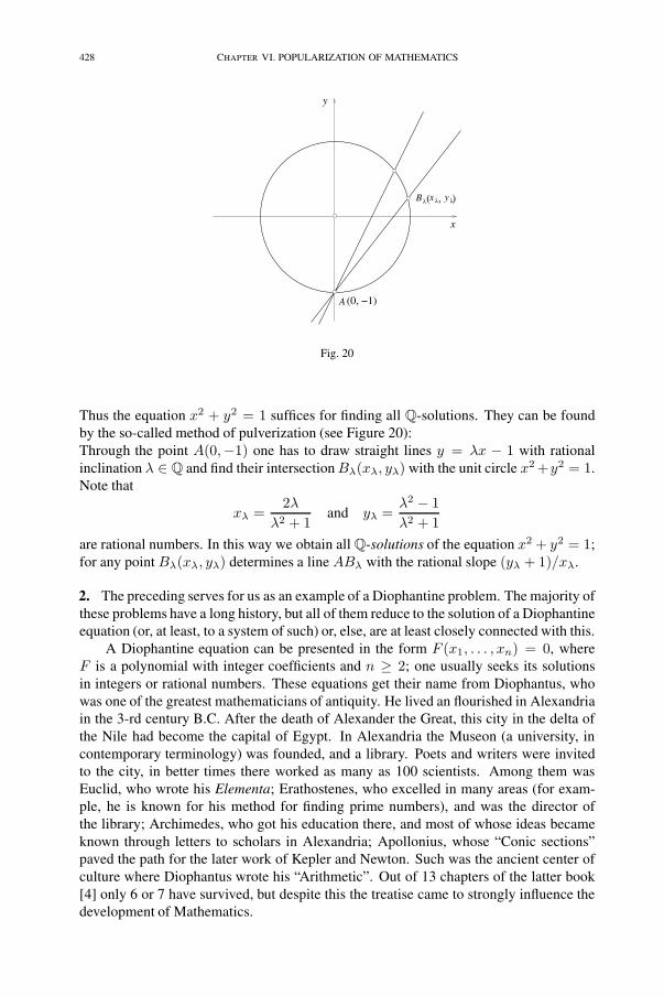
428 CHAPTER VI. POPULARIZATION OF MATHEMATICS
x λ y λBλ( , )
A (0, −1)
x
y
Fig. 20
Thus the equation x2 + y2 = 1 suffices for finding all Q-solutions. They can be foundby the so-called method of pulverization (see Figure 20):Through the point A(0,−1) one has to draw straight lines y = λx − 1 with rationalinclination λ ∈ Q and find their intersection Bλ(xλ, yλ) with the unit circle x2 +y2 = 1.Note that
xλ =2λ
λ2 + 1and yλ =
λ2 − 1λ2 + 1
are rational numbers. In this way we obtain all Q-solutions of the equation x2 + y2 = 1;for any point Bλ(xλ, yλ) determines a line ABλ with the rational slope (yλ + 1)/xλ.
2. The preceding serves for us as an example of a Diophantine problem. The majority ofthese problems have a long history, but all of them reduce to the solution of a Diophantineequation (or, at least, to a system of such) or, else, are at least closely connected with this.
A Diophantine equation can be presented in the form F (x1, . . . , xn) = 0, whereF is a polynomial with integer coefficients and n ≥ 2; one usually seeks its solutionsin integers or rational numbers. These equations get their name from Diophantus, whowas one of the greatest mathematicians of antiquity. He lived an flourished in Alexandriain the 3-rd century B.C. After the death of Alexander the Great, this city in the delta ofthe Nile had become the capital of Egypt. In Alexandria the Museon (a university, incontemporary terminology) was founded, and a library. Poets and writers were invitedto the city, in better times there worked as many as 100 scientists. Among them wasEuclid, who wrote his Elementa; Erathostenes, who excelled in many areas (for exam-ple, he is known for his method for finding prime numbers), and was the director ofthe library; Archimedes, who got his education there, and most of whose ideas becameknown through letters to scholars in Alexandria; Apollonius, whose “Conic sections”paved the path for the later work of Kepler and Newton. Such was the ancient center ofculture where Diophantus wrote his “Arithmetic”. Out of 13 chapters of the latter book[4] only 6 or 7 have survived, but despite this the treatise came to strongly influence thedevelopment of Mathematics.

8. Mordell’s problem 429
Its true richness in ideas and content was appreciated only at the end of the 16thcentury (F. Viète, R. Bombelli), but especially in the 17th century. Diophantus’s text wastranslated into Latin by Claude Bachet (1621), whose own interest in numbers had beenarisen by the solution of (mathematical) problems of recreation. This translation, thenumber-theoretic comments of which are especially emphasized, fell into the hands ofPierre Fermat and, in the years 1636-1640, turned the latter’s mathematical interest evermore towards Diophantine problems. In his research Fermat came to a conjecture whichafterwards was called “Fermat’s Last Theorem” (FLT): “No cube decomposes into thesum of two cubes, no fourth power decomposes into the sum of two fourth powers.” Inother words, the Diophantine equation xn + yn = zn admits, for n ≥ 3, no solutionsin terms of natural numbers. Fermat had proved [this in] the special case n = 4 (usingthe so-called method of decent), and he may have had the case n = 3 in its broad outline(as was carried out by Euler in 1753). Fermat frequently wrote to his colleagues aboutthese special cases, but he never mentions the general case again. (Around 1640 Fermatwrote a note in the margin of his copy of Diophantus’s book that he was in possession ofa proof of FLT, but that it was far to long to be written down there; according to A. Weil’sversion, Fermat might have thought so only in his youth). With his intensive work, up tothe year 1660, Fermat laid a solid basis on which Euler, Lagrange, and Gauss later couldbuild the edifice of Number Theory.
3. In the following centuries, FLT was one of the most well-known problems in math-ematics. The attempts to solve this problem using new technique have enriched mathe-matics with quite fruitful notions and methods. In the case n = 3 Euler used in his proofof FLT numbers of the form a + b
√−3, where a, b ∈ Z, and developed in an essential
way the arithmetic of the domain Z[√−3]. This line of thought was continued by Gauss
(1831), who invented the domain G = (a + b√−1; a, b ∈ Z) = Z[
√−1] = Z[i], or
the arithmetic of so-called Gaussian numbers. In 1825 Legendre and Dirichlet estab-lished FLT for n = 5, while Lamé and Lebesque did it for n = 7 in 1840. Really, itsuffices to prove the theorem for n = 4 and for n a prime number. Indeed, each nat-ural number n ≥ 3 is either divisible by 4 or else by an odd prime number. In the firstcase one can rewrite xn + yn = zn as (xm)4 + (ym)4 = (zm)4, in the second case as(xm)p + (ym)p = (zm)p, where p is an odd prime. Now it is clear that from the truth ofFLT for n = 4 and for all primes n > 2 follows also its truth in the case of all n ≥ 3.
4. An essential step forward toward the solution of FLT was taken by the Germanmathematician Ernst Eduard Kummer (1850’s). He managed to find a condition fromwhich the correctness of FLT follows for almost all primes n less than 100. Only inthree cases (37, 59 and 67) the issue remained open, because then Kummer’s conditiondoes not work; the case n = 37 was solved later (1892). In this and the following fourSubsections we shall learn about Kummer’s scheme of reasoning.
In his proof of FLT for n = 3 Euler used the quadratic field Q(√−3), and in partic-
ular its subring Z[√−3], that is, properties of the Eulerian ring of integers. Euler noticed
that if, for a, b relative prime a2 + 3b2, is a perfect cube, then it follows from the identitya2 + 3b2 = (a + b
√−3)(a − b
√−3) that also both factors of the right hand side are
perfect cubes in the ring Z(√−3). In particular, there ought to exist c, d ∈ Z such than
a + b√−3 = (c + d
√−3)3. This would be sufficient, if the fundamental theorem of
arithmetic (uniqueness of the decomposition into prime factors) is true in Z[√−3] and
430 CHAPTER VI. POPULARIZATION OF MATHEMATICS
the factors a + b√−3 and a − b
√−3 were without a common factor – this is what our
experience in ordinary arithmetic tells us.But the fundamental theorem of arithmetic fails in the ring Z(
√−3). Indeed, we
have4 = 2 · 2 = (1 +
√−3) · (1−
√−3),
where a simple argument (by contradiction) shows that the factors 2, 1+√−3, 1−
√−3
are indecomposable; for example, the number 2 does not have a representation in theform 2 = (e + f
√−3)(e− h
√−3).
5. But there is a way out if this dilemma. Let ζ3 = 1, ζ �= 1; thus, ζ is a C-solution ofthe equation x2 + x + 1 = 0, or to be concrete: ζ = (−1 +
√−3)/2. We consider the
domain of numbers Q[ζ] = {r + sζ | r, s ∈ Q}. As it is possible to carry out the fourarithmetical operations with this set without violation of the usual rules of calculation,then in the guise of Q[ζ] we are dealing with a so-called number field Q(ζ). The subsetE = Z + Z · ζ = {a + bζ | r, s ∈ Z} should, of course, be viewed as the “integers” ofthe field Q(ζ). In view of the identity a + bζ = ((2a − b) + b
√−3)/2 these integers
can be represented as (p + q√−3)/2, where p and q are ordinary integers, both of the
same parity. It is somewhat more natural to consider the “integers” (p + q√−3)/2 ∈ E,
and not restrict oneself to the use of Euler’s integers. The reason is that the fundamentaltheorem of arithmetic holds true in E, but not in the ring of Eulerian integers. As anexplanation we add that the identity
2 = (1 +√−3) · (1 −
√−3)/2,
does not contradict the fundamental theorem of arithmetic, as (1 −√−3)/2 is a unit in
this ring (its inverse is, also an “integer”), and so the identity shown expresses just thefact that the number 2 and 1 +
√−3 are associated (one number is obtained from the
other by multiplication with a unit).It follows from the correctness of the fundamental theorem of arithmetic in the do-
main E and the immediate verification of the fact that the Eulerian integers a + b√−3
and a − b√−3 have no common factor in the ring E (that is, these numbers have no
common factor there distinct from a unit) that there exists a number c+d√−3 ∈ E such
than a + b√−3 = (c + d
√−3)3. It may then happen that c + d
√−3 is a number of the
form) (p+q√−3)/2, where p and q are both odd; then c and d are not integers. From the
last identity we get p = 2u− v and q = v. Thus, if v is even, then p and q are also even,and, as a consequence, u + vζ is an Eulerian integer. We observe further that among thethree numbers u + vζ, (u + vζ) · ζ and (u + vζ) · ζ2 (associated to each other) thereis in front of the multiplier ζ an even number. It follows from these reasonings that, ifnecessary multiplying both members of a + b
√−3 = (c + d
√−3)3 with ζ or ζ2, that c
and d are integers.
6. Next, let us consider the relation xp + yp = zp, where p ≥ 3 is a prime. Accordinglylet ζ be a p-th order root of unity other than unity: ζp = 1, ζ �= 1. Then 1 + ζ + · · · +ζp−1 = 0, so that we have the relation
xp + yp = (x + y)(x + ζy)(x + ζ2y) . . . (x + ζp−1y).
This gives the idea to use the ring of so-called algebraic integers
Ep = {a + bζ + cζ2 + . . . dζp−1 | a, b, . . . d ∈ Z}

8. Mordell’s problem 431
contained in the number field Q(ζ); similarly, this ring is denoted Z[ζ].The arithmetic of [ordinary] integers is based on the notion of integers and the funda-
mental theorem of arithmetic. It follows effectively from the latter that if AB . . . F = Lp
and the factors A,B, . . . , F do not have a common factor, then they must likewise be p-th powers. Are such statements true in number rings other than the ordinary integers?Sometimes it is so – for instance, in the case of Gaussian integers. It is also so in therings Z[ζ], where
ζ = cos(2πp
) + i sin(2πp
); p ∈ {3, 5, 7, 11, 13, 17, 19},
in which case one has a unique decomposition into prime factors. On the other hand, inthe number rings Z[
√−3] and Z[
√−5] the unique factorization fails, as:
4 = 2 · 2 = (1 +√−3)(1−
√−3) and
9 = 3 · 3 = (2 +√−5)(2−
√−5).
Although, for example, in the last product the factors 2 ±√−5 are unity divisors, they
cannot be represented as squares of numbers a + b√−5.
7. Hilbert found a simple model explaining the difficulties in what was just said, indi-cating also a way to overcome them. Let us consider the domain of numbers
H = { 4n + 1 |n = 0, 1, 2, . . .} = {1, 5, 9, 13, 17, 21, 25, . . .}.
A number p ∈ H is called a “prime number”, if it cannot be represented in theform p = a · b, where a, b ∈ H and a �= 1, b �= 1. For example, 21 turns out to beprime in “H-arithmetic”: although 21 = 3 · 7, one has 3 �∈ H and 7 �∈ H . We note that693 = 9 ·77 = 21 ·33 are two distinct decomposition of 693 ∈ H , but from the equalities212 = 9 · 49 and GCD(9, 49) = 1 it does not follow that the numbers 9 and 49 can bepresented as squares of H-numbers.
A way out is the following. We extend the set H to the “domain of numbers” H ={4n + 1, 4n + 3 |n = 0, 1, 2, . . .} = {1, 3, 5, 7, . . .}, in which all the rules of ordinaryZ-arithmetic hold true (one has to take into account that all even numbers have beenomitted). For example, one has now 9 = 32, 77 = 7 · 11, 21 = 3 · 7 = 3 · 11, so thatthe two distinct decompositions of the number 693, to wit 9 · 77 and 21 · 33 reduce to asingle one 32 · 7 · 11; also other difficulties disappear.
8. Is it possible to extend the domain Z[√−5], by adding to it new so-called “ideal
numbers” in such a way that the the fundamental theorem of arithmetic remains valid inthe new domain? Kummer showed that this can really be done; indeed, not only in thecase of Z[
√−5], but even in many other cases. In this way mathematicians arrived at the
notion of ideal numbers in the middle of the 19th century. Later Richard Dedekind, froma set theoretic point of view, changed them into the often used “ideals” (for instance, inring theory). In the work of Kummer, Dedekind, Kronecker, and others there arose anew, general theory of division in domains of numbers – the theory of algebraic numbers(for more details see [13]).
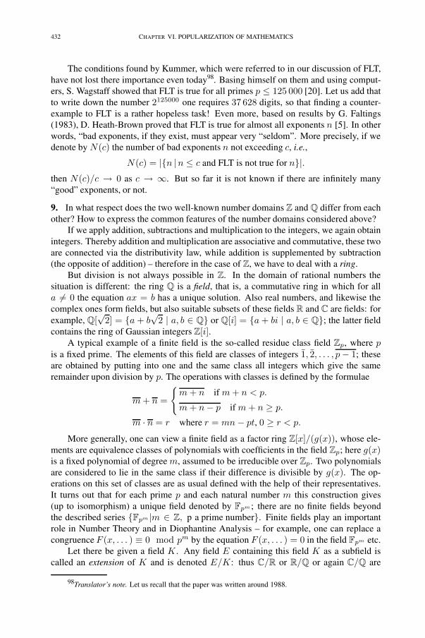
432 CHAPTER VI. POPULARIZATION OF MATHEMATICS
The conditions found by Kummer, which were referred to in our discussion of FLT,have not lost there importance even today98. Basing himself on them and using comput-ers, S. Wagstaff showed that FLT is true for all primes p ≤ 125 000 [20]. Let us add thatto write down the number 2125000 one requires 37 628 digits, so that finding a counter-example to FLT is a rather hopeless task! Even more, based on results by G. Faltings(1983), D. Heath-Brown proved that FLT is true for almost all exponents n [5]. In otherwords, “bad exponents, if they exist, must appear very “seldom”. More precisely, if wedenote by N(c) the number of bad exponents n not exceeding c, i.e.,
N(c) = |{n |n ≤ c and FLT is not true for n}|.then N(c)/c → 0 as c → ∞. But so far it is not known if there are infinitely many“good” exponents, or not.
9. In what respect does the two well-known number domains Z and Q differ from eachother? How to express the common features of the number domains considered above?
If we apply addition, subtractions and multiplication to the integers, we again obtainintegers. Thereby addition and multiplication are associative and commutative, these twoare connected via the distributivity law, while addition is supplemented by subtraction(the opposite of addition) – therefore in the case of Z, we have to deal with a ring.
But division is not always possible in Z. In the domain of rational numbers thesituation is different: the ring Q is a field, that is, a commutative ring in which for alla �= 0 the equation ax = b has a unique solution. Also real numbers, and likewise thecomplex ones form fields, but also suitable subsets of these fields R and C are fields: forexample, Q[
√2] = {a + b
√2 | a, b ∈ Q} or Q[i] = {a + bi | a, b ∈ Q}; the latter field
contains the ring of Gaussian integers Z[i].A typical example of a finite field is the so-called residue class field Zp, where p
is a fixed prime. The elements of this field are classes of integers 1, 2, . . . , p− 1; theseare obtained by putting into one and the same class all integers which give the sameremainder upon division by p. The operations with classes is defined by the formulae
m + n =
{m + n if m + n < p.
m + n− p if m + n ≥ p.
m · n = r where r = mn− pt, 0 ≥ r < p.
More generally, one can view a finite field as a factor ring Z[x]/(g(x)), whose ele-ments are equivalence classes of polynomials with coefficients in the field Zp; here g(x)is a fixed polynomial of degree m, assumed to be irreducible over Zp. Two polynomialsare considered to lie in the same class if their difference is divisible by g(x). The op-erations on this set of classes are as usual defined with the help of their representatives.It turns out that for each prime p and each natural number m this construction gives(up to isomorphism) a unique field denoted by Fpm ; there are no finite fields beyondthe described series {Fpm |m ∈ Z, p a prime number}. Finite fields play an importantrole in Number Theory and in Diophantine Analysis – for example, one can replace acongruence F (x, . . . ) ≡ 0 mod pm by the equation F (x, . . . ) = 0 in the field Fpm etc.
Let there be given a field K . Any field E containing this field K as a subfield iscalled an extension of K and is denoted E/K: thus C/R or R/Q or again C/Q are
98Translator’s note. Let us recall that the paper was written around 1988.
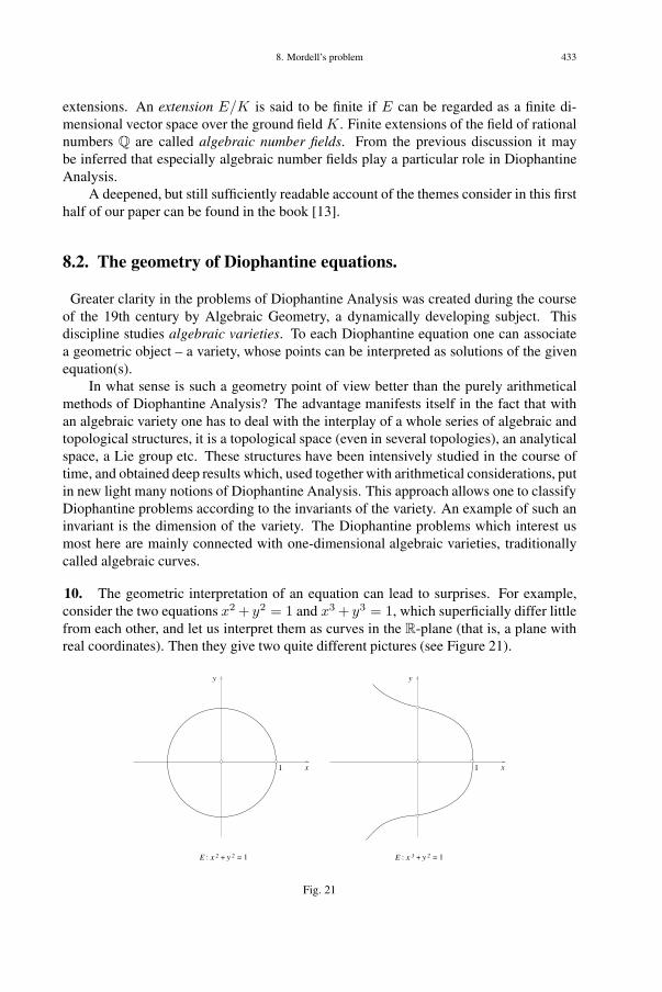
8. Mordell’s problem 433
extensions. An extension E/K is said to be finite if E can be regarded as a finite di-mensional vector space over the ground field K . Finite extensions of the field of rationalnumbers Q are called algebraic number fields. From the previous discussion it maybe inferred that especially algebraic number fields play a particular role in DiophantineAnalysis.
A deepened, but still sufficiently readable account of the themes consider in this firsthalf of our paper can be found in the book [13].
8.2. The geometry of Diophantine equations.
Greater clarity in the problems of Diophantine Analysis was created during the courseof the 19th century by Algebraic Geometry, a dynamically developing subject. Thisdiscipline studies algebraic varieties. To each Diophantine equation one can associatea geometric object – a variety, whose points can be interpreted as solutions of the givenequation(s).
In what sense is such a geometry point of view better than the purely arithmeticalmethods of Diophantine Analysis? The advantage manifests itself in the fact that withan algebraic variety one has to deal with the interplay of a whole series of algebraic andtopological structures, it is a topological space (even in several topologies), an analyticalspace, a Lie group etc. These structures have been intensively studied in the course oftime, and obtained deep results which, used together with arithmetical considerations, putin new light many notions of Diophantine Analysis. This approach allows one to classifyDiophantine problems according to the invariants of the variety. An example of such aninvariant is the dimension of the variety. The Diophantine problems which interest usmost here are mainly connected with one-dimensional algebraic varieties, traditionallycalled algebraic curves.
10. The geometric interpretation of an equation can lead to surprises. For example,consider the two equations x2 + y2 = 1 and x3 + y3 = 1, which superficially differ littlefrom each other, and let us interpret them as curves in the R-plane (that is, a plane withreal coordinates). Then they give two quite different pictures (see Figure 21).
x
y
1
x 2 y 2E : + = 1 x 3 y 2E : + = 1
x
y
1
Fig. 21
434 CHAPTER VI. POPULARIZATION OF MATHEMATICS
The equation x2+y2+1 = 0 surprises even more – there exist “curves” without R-points!In order to get rid of this inconvenience one allows oneself too took look for points of thecorresponding curve in the C2-plane (that is, with coordinates in the extension C/R). Forexample, if we in the case of the curve under view set x = x1 + ix2 and y = y1 + iy2, weget relations connecting the R-quantities x1, x2, y1, y2, which in the case of the equationx2 + y2 = 1 is a sphere in R4, but for x3 + y3 = 1 a torus in the same space (seeFigure 22, where these surfaces are depicted in the usual space)
Sphere Torus
Fig. 22
In Diophantine geometry one often encounters situations when the coefficients of theequation determining the curve are from one domain (the field K) but the coordinates ofthe sought points have to be taken from another domain (an extension L/K of K).
11. In the geometric interpretation of the solution of a Diophantine equation one re-quires the notion of projective space. Let us fix a fieldK . The points of the n-dimensionalaffine space An(K) can then be identified with sequences (x1, . . . , xn) in the set Kn,The projective space Pn(K) is now obtained as follows. We denote by (Kn+1)∗ theset of all sequences (x0, x1, . . . , xn), omitting the origin (0, 0, . . . , 0). We partitionthis set in such a way that we regard the points (x0, x1, . . . , xn) and (y0, y1, . . . , yn) in(An+1(K))∗ to lie in the same class if there exists a ∈ K (a �= 0) such than x0 = ay0,x1 = ay1, . . .xn = ayn. The set of classes thus obtained is called the n-dimensional pro-jective space Pn(K). These equivalence classes may be viewed as straight lines throughthe origin in the affine space An+1(K). In the special case when K = R and n = 2, weobtain then the (ordinary) real projective plane.
Let there be fixed a set I of natural numbers and let there be given for each i ∈ Ia polynomial Fi(x1, . . . , xn) with coefficients in K . The point set in An(K), definedby the system Fi(x1, . . . , xn) = 0, where i ∈ I and L/K is a suitable extension of theground field K , is called an affine variety. A system of equations Fi(x1, . . . , xn) = 0,where all polynomials Fi are forms (that is, homogeneous polynomials over K), deter-mines a subset M in the projective space Pn(K), called a projective algebraic variety.As points in the projective space Pn(L) are rays through the origin in An+1(L), we mayview M as a cone in An+1(L). The field K is the field of definition of M . The points(x0, x1, . . . , xn) in M ⊂ Pn(L) such than all quotients xi/xj ∈ K are called its ra-tional points; their set will be denoted by M(K). The answer to the question about thestructure and the properties of the point set M(K) is of paramount interest in the study
8. Mordell’s problem 435
of the corresponding Diophantine system. In the case of algebraic curves these questionswere studied very carefully yielding also decisive progress towards the solution of FLT.
12. Consider an equation F (x, y) = 0 such than the left hand side is a polynomial ofthe form
am(x)ym + am−1(x)ym−1 + · · ·+ a1(x)y + a0(x),where all ai(x) are x-polynomials with real coefficients. Selecting in the plane A2(R)all points (x, y) whose coordinates satisfy the equation F (x, y) = 0 we obtain a certaincurve. Thus the equation y2 + x2 − 1 = 0 defines a circle with center (0, 0).
Next, consider a curve E with equation∑i,j
aijxiyj = 0,
where all aij are integers. We denote the set of Z-points of this curve by E(Z), andits Q-points of this curve by E(Q). Let further o(E) denotes the order of the curve,that is, the maximum of i + j for the monomials aijx
iyj appearing in the equation. In1912, Carl Ludwig Siegel proved an important theorem to the effect that, on any curveof degree higher than two, there are at most finitely many Z-points. However, it is noteasy to decide if E(Z) = ∅ or not; there is no algorithm for this. The question about theexistence of an algorithm for deciding whether E(Q) = ∅ or not is entirely open. Beforethe work of J. L. Mordell(in the 1920’s) the following was know about E(Q).
First, if o(E) = 1, then |E(Q)| = 1. Second, if o(E) = 2, then either E(Q) = ∅or |E(Q)| = ∞. Third, in the case o(E) = 3 already Diophantus knew that a linethrough two Q-points of E must intersect E in a third Q-point. In the case of these linesPoincaré’s conjecture became known (1903), according to which one can find all Q-points from a certain finite set, using the following geometric procedure: one has to drawall possible chords among the points of a given finite set and the tangents in these points,which by intersecting the curve generate new Q-points (starting with this extended set ofQ-points one draws anew all chords and tangents etc.) This conjecture by Poincaré wasproved (1922) by the British mathematician Joel Louis Mordell.
According to Mordell’s theorem one can present the Abelian group of the rationalpoints on the elliptic curve E as E(Q) = Za ⊕ VE , where VE is a finite group. Thenumber a is called the rank of the curve. So far it is not known if there exist elliptic curvesof arbitrary large rank, but computer experiments have shown how the rank depends onthe coefficients of the cubic equation defining E. The group VE – the torsion of E ismade up by its points of finite order. It turns out that either VE is a finite cyclic groupor else it has the form Z2 + T with T finite. B. Mazur showed, in 1976, that either |VE |is one of the numbers 1, 2, . . . , 10 or 12 or else VE = Z2 + T , where |T | equals 2, 4, 6or 8. Thus there are 15 possibilities for VE . The deeper reasons for the mystery of thesenumbers is so far unknown! However, one has obtained hopes for proving the analogueof Mazur’s theorem for an arbitrary number field K/Q, because recently it was foundthat the the torsion of the group E(K) of K-rational points is finite.
A higher dimensional generalization of the Poincaré-Mordell conjecture was prov-ed, in 1927, by the French-American mathematician André Weil.
It is amazing that the arithmetic of Diophantine equations is too a large extent gov-erned by the geometry of the point set E(C) for the corresponding curve E. Indeed,E(C) is a certain compact 2-dimensional surface in R4, called the Riemann surface of
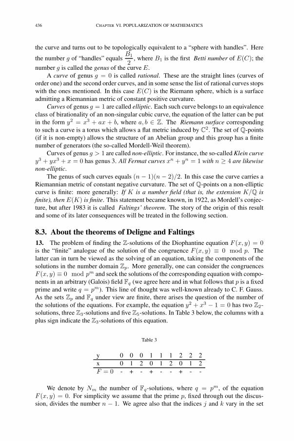
436 CHAPTER VI. POPULARIZATION OF MATHEMATICS
the curve and turns out to be topologically equivalent to a “sphere with handles”. Here
the number g of “handles” equalsB1
2, where B1 is the first Betti number of E(C); the
number g is called the genus of the curve E.A curve of genus g = 0 is called rational. These are the straight lines (curves of
order one) and the second order curves, and in some sense the list of rational curves stopswith the ones mentioned. In this case E(C) is the Riemann sphere, which is a surfaceadmitting a Riemannian metric of constant positive curvature.
Curves of genus g = 1 are called elliptic. Each such curve belongs to an equivalenceclass of birationality of an non-singular cubic curve, the equation of the latter can be putin the form y2 = x3 + ax + b, where a, b ∈ Z. The Riemann surface correspondingto such a curve is a torus which allows a flat metric induced by C2. The set of Q-points(if it is non-empty) allows the structure of an Abelian group and this group has a finitenumber of generators (the so-called Mordell-Weil theorem).
Curves of genus g > 1 are called non-elliptic. For instance, the so-called Klein curvey3 + yx3 + x = 0 has genus 3. All Fermat curves xn + yn = 1 with n ≥ 4 are likewisenon-elliptic.
The genus of such curves equals (n − 1)(n − 2)/2. In this case the curve carries aRiemannian metric of constant negative curvature. The set of Q-points on a non-ellipticcurve is finite: more generally: If K is a number field (that is, the extension K/Q isfinite), then E(K) is finite. This statement became known, in 1922, as Mordell’s conjec-ture, but after 1983 it is called Faltings’ theorem. The story of the origin of this resultand some of its later consequences will be treated in the following section.
8.3. About the theorems of Deligne and Faltings13. The problem of finding the Z-solutions of the Diophantine equation F (x, y) = 0is the “finite” analogue of the solution of the congruence F (x, y) ≡ 0 mod p. Thelatter can in turn be viewed as the solving of an equation, taking the components of thesolutions in the number domain Zp. More generally, one can consider the congruencesF (x, y) ≡ 0 mod pm and seek the solutions of the corresponding equation with compo-nents in an arbitrary (Galois) field Fq (we agree here and in what follows that p is a fixedprime and write q = pm). This line of thought was well-known already to C. F. Gauss.As the sets Zp and Fq under view are finite, there arises the question of the number ofthe solutions of the equations. For example, the equation y2 + x3 − 1 = 0 has two Z2-solutions, three Z3-solutions and five Z5-solutions. In Table 3 below, the columns with aplus sign indicate the Z3-solutions of this equation.
Table 3
y 0 0 0 1 1 1 2 2 2x 0 1 2 0 1 2 0 1 2F = 0 - + - + - - + - -
We denote by Nm the number of Fq-solutions, where q = pm, of the equationF (x, y) = 0. For simplicity we assume that the prime p, fixed through out the discus-sion, divides the number n − 1. We agree also that the indices j and k vary in the set

8. Mordell’s problem 437
{1, 2, . . . , n−1}, however in such a way that their sum is not n: the number of such pairsof indices (j, k) equals (n− 1)(n− 2). In the case of the Fermat equation xn + yn = 1one has the identity
(114) Nm = pm + 1−∑j,k
J(j/n, k/n)m,
where the J(j/n, k/n) are the so-called Jacobi sums. In order to clarify their signifi-cance, we choose a generator ε of the group Z∗
p of p-th roots of unity (that, is a primitivep-th roots of unity) and consider the maps
χj/n : Z∗p → C, with χj/n(εr) = e2πir j
n .
With the help of these so-called multiplicative characters we can now define
J(j/n, k/n) = −∑x∈Zp
χj/n(x) · χk/n(1− x);
here one has to put χ(0) = 0, for each character, thus also for a trivial one. For example,if p = 7 we have
J(1/6, 2/6) = −2− i√
3.
14. In 1924, Emil Artin introduced for the numbers Nm a generating function of theform
(115) Zp(t) = exp(∑ Nm
mtm
);
Zp(t) contains information about the number Nm, m = 1, 2, . . . of solutions of theequation F (x, y) = 0. The series (115) has two good properties. First, if Nm happens tocome in the form αm (for example the number of Fq-solutions of the equation y = f(x)is precisely q, so one can take α = p), then
(116) Zp(t) = exp(∑ Nm
mtm
)= e− ln(1−αt) =
11− αt
.
Second, if Nm = N ′m + N ′′
m (for example, if f = G ·H and G(x, y) = H(x, y) = 0 isnot possible for any pair of elements (x, y) ∈ Fq × Fq). then
(117) Zp(t) = exp(∑ Nm
mtm
)= exp
(∑ N ′m
mtm
)· exp
(∑ N ′′m
mtm
).
If Nm = αm1 + · · ·+ αm
r − βm1 − · · · − βm
s , where αj and βj are allowed to depend onthe equation, but not on the index m, it follows from these properties that
(118) Zp(t) =(1− β1t) . . . (1− βst))(1− α1t) . . . (1 − αrt))
,
that is Zp(t) is in this case a rational function. For example, in the case of the Fermatequation xn + yn = 1 one has α1 = 1, α2 = 1 and in the role of the β:s one has theJacobi sums J(j/n, k/n). Therefore
(119) Zp(t) =
∏j,k
(1− J(j/n, k/n)t
(1− t)(1− pt),
where in the numerator one has a polynomial of degree (n− 1)(n− 2).
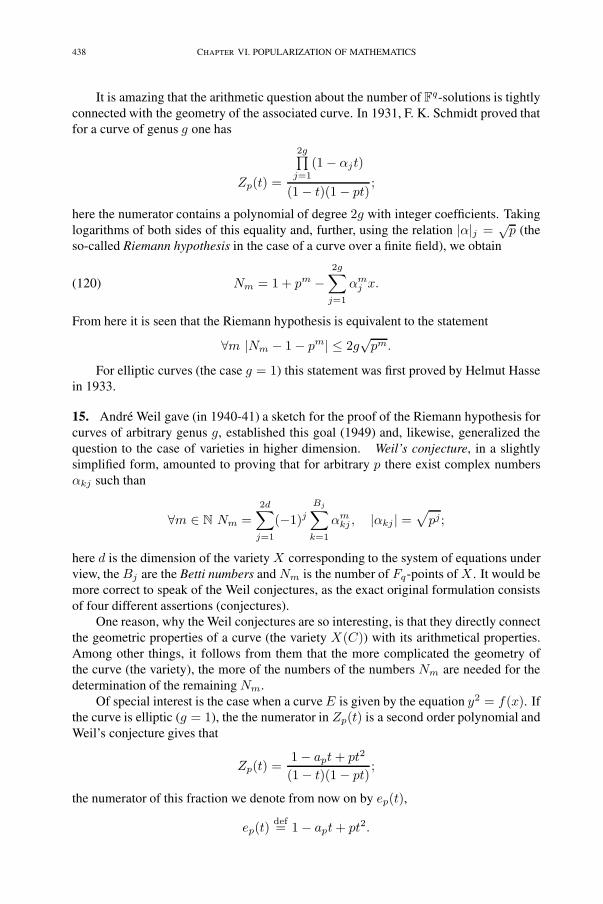
438 CHAPTER VI. POPULARIZATION OF MATHEMATICS
It is amazing that the arithmetic question about the number of Fq-solutions is tightlyconnected with the geometry of the associated curve. In 1931, F. K. Schmidt proved thatfor a curve of genus g one has
Zp(t) =
2g∏j=1
(1− αjt)
(1− t)(1− pt);
here the numerator contains a polynomial of degree 2g with integer coefficients. Takinglogarithms of both sides of this equality and, further, using the relation |α|j =
√p (the
so-called Riemann hypothesis in the case of a curve over a finite field), we obtain
(120) Nm = 1 + pm −2g∑
j=1
αmj x.
From here it is seen that the Riemann hypothesis is equivalent to the statement
∀m |Nm − 1− pm| ≤ 2g√pm.
For elliptic curves (the case g = 1) this statement was first proved by Helmut Hassein 1933.
15. André Weil gave (in 1940-41) a sketch for the proof of the Riemann hypothesis forcurves of arbitrary genus g, established this goal (1949) and, likewise, generalized thequestion to the case of varieties in higher dimension. Weil’s conjecture, in a slightlysimplified form, amounted to proving that for arbitrary p there exist complex numbersαkj such than
∀m ∈ N Nm =2d∑
j=1
(−1)j
Bj∑k=1
αmkj , |αkj | =
√pj ;
here d is the dimension of the variety X corresponding to the system of equations underview, the Bj are the Betti numbers and Nm is the number of Fq-points of X . It would bemore correct to speak of the Weil conjectures, as the exact original formulation consistsof four different assertions (conjectures).
One reason, why the Weil conjectures are so interesting, is that they directly connectthe geometric properties of a curve (the variety X(C)) with its arithmetical properties.Among other things, it follows from them that the more complicated the geometry ofthe curve (the variety), the more of the numbers of the numbers Nm are needed for thedetermination of the remaining Nm.
Of special interest is the case when a curve E is given by the equation y2 = f(x). Ifthe curve is elliptic (g = 1), the the numerator in Zp(t) is a second order polynomial andWeil’s conjecture gives that
Zp(t) =1− apt + pt2
(1− t)(1− pt);
the numerator of this fraction we denote from now on by ep(t),
ep(t)def= 1− apt + pt2.

8. Mordell’s problem 439
It follows from (120) that ap = 1+p−N1, where ap = α1 +α2. This result shows that,for the function under view, the function Zp(t), and thereby all numbers Nm, m > 1, aredetermined by N1.
16. If we know the functionZp(t) for all p, then we know all the numbersNm,p. All thisinformation yields also the following function of one complex variable s (the Hasse-Weilfunction of the curve E)
Z(E, s) =∏
p prime
1ep(p−s)
=∏
p prime
11− app−s + p1−2s
;
the product is convergent in the half-space Re s > 32 . One believes that (Taniyama-
Weil conjecture) for each elliptic curve E one can continue Z(E, s) to a meromorphicfunction in the entire complex s-plane and that the function obtained in this way satisfiessome supplementary conditions (the so-called Weil conditions; see [7, pp. 142-143]). Inthe case that this conjecture is true, one can speak of the “critical” values Z(E, s). Itturns out that the behavior of Z(E, s) at the point s = 1 depends on many arithmeticalproperties of the given elliptic curve over Q. Thus one believes (part of the conjecturesof B. Birch and H. Swinnerton-Dyer) that Z(E, 1) = 0 precisely when E has infinitelymany Q-points.
Finally, we remark that for the curve X : y2 = x3 + x2 (which is not elliptic!) wehave ep(t) = 1− t, so that
Z(E, s) =∏
p prime
11− p−s
this is the ordinary Riemann zeta-function in Eulerian form.Let us further add that it was the question of the truth of the conjecture of Birch and
Swinnerton-Dyer on which J. Tunnel, in 1983, based his proof of his criterion for findingcongruent numbers. Congruent numbers are such numbers which give the area of righttriangles with integer sides, is likewise a Diophantine problem, known since the 10-thcentury. For example, the number 6 = 3 · 4/2 is a congruent number. It is of interest tonote that proving that the number 1 is non-congruent is equivalent to proving FLT in thecase n = 4; see [7].
17. In proving his theorem Weil had to use various results in geometry of the Italianmathematicians, but in the general case one could not assert that these results had beenproved in a convincing way. The attempts to give an adequate, strictly supported foun-dation to Weil’s plans led, in the 1950-1960’s to the creation of new theories in algebraicgeometry.
The man who paved the path to this was Alexandre Grothendieck, whose thirst foraction, in the 1960’s, was almost inexhaustible. His style was to conquer a gorge byfilling it. He tried to treat each notion in a as general way as possible, only those restric-tions were taken into account, whose necessity was forced by the mathematical situation.His work may be viewed as a far reaching generalization of the analytic geometry ofDescartes, where the real numbers are replaced by the elements of an arbitrary commuta-tive ring. With the aid of the so-called covering cohomology devised by Grothendieck itbecame possible to interpret the numbers αkj in a way, on which Deligne later based his

440 CHAPTER VI. POPULARIZATION OF MATHEMATICS
proof. Grothendieck’s achievements were recognized by the mathematical communitywhen he was given the Fields medal a the Moscow-ICM in 1966.
In the 1960’s one began to have an inkling that there existed a connection betweenthe Weil conjectures and a problem of Ramanujan. Let τ(n) be the coefficient in frontof xn in the power series expansion of the function x
∏∞m=1(1 − xm)24, |x| < 1; τ(n)
is always an integer distinct from zero. So far this is not proved, but one has checked itfor n ≤ 1015. Ramanujan had considered it as very plausible that |τ(n)| ≤ n
112 · d(n),
where d(n) is the number of divisors of the natural number n. It follows from thisthat τ(p) ≤ 2p
112 . From 1916 on, this statement is known as the Ramanujan conjec-
ture. Deligne had reason’s to believe in the truth of this relation, because he provedin 1968 that Ramanujan’s conjecture follows from Weil’s. In 1970, R. Langlands drawattention to a possibility which opens up, for the solution of Ramanujan’s conjecture,from little known work of R. Rankin (1939), where the estimation τ(n) = O(n
295 ) was
given. While trying to understand Rankin’s discussion, Deligne managed (supported byJ.-P. Serre) to “geometrize” Rankin’s method. He connected this method with the topo-logical technique of Solomon Lefschetz for finding fixed points of a mapping, and unifiedthis in an unexpected way with the proof of Weil’s conjecture.
Let us add some information about Pierre Deligne. He was born in Bruxelles in1944. At the age of fourteen he began to read the Elements of Bourbaki which containthe essence of contemporary mathematics. Already this enterprize is astounding, as inthese books the treatment goes from the general to the the particular, and in them there isno other motivation besides the logical development of the theme. After having studiedsome time at the University of Bruxelles, he went to Paris at the suggestion of the grouptheorist Jacques Tits. There he took part in the activities of the Grothendieck seminar, inparticular attending with great interest the lectures of Jean-Pierre Serre, having a numbertheoretic outlook. Already in 1966 Grothendieck considered him on a par to himself.The style of Deligne has been described as follows: he likes to surpass the gorge, but notby filling it, but by building a bridge. His papers are readable, the ideas are explainedin an understandable way, what is told there is necessary and it is told at the right time.Pierre Deligne was given the Fields Medal for his proof of the Weil conjectures at theICM in Helsinki in 1976.
18. However, the line of thought described above did not lead immediately furtheron the path of finding the Q-solutions. Thus despite the fact that formula (114) givesthe number of Fq-solutions of Fermat’s equation but it does not tell us anything directlyabout FLT. Even for the question about the existence of Z-solutions there is no answer inthe general case and – as was proved by Yu. Matiyasevich in 1970 – there does not existan answer in terms of a general algorithm. Even more valuable is any general regularitydiscovered about the Q-solutions of Diophantine equations, one example of this is theabove mentioned Mordellconjecture.
Let us now pause at this question, giving it a new, simpler formulation. WhichDiophantine equations F (x, y) = 0 do have infinitely many Q-solutions? As followsfrom our above discussion, the answer is positive, for example, in the case of x2+y2 = 1.Here we have to deal with a first possibility – all solutions are expressible in terms of aparameter (the genus of the corresponding curve is 0). A second possibility is when thesolution of the equation F (x, y) = 0 can be obtained by relations x = Φ(u, v), y =Ψ(u, v), where Φ and Ψ are both quotients of two polynomials with rational coefficients.
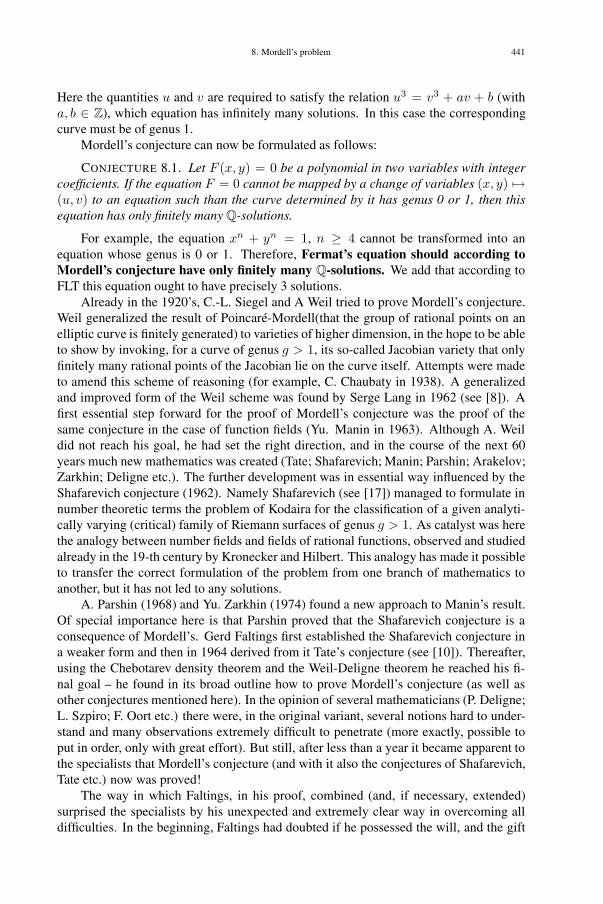
8. Mordell’s problem 441
Here the quantities u and v are required to satisfy the relation u3 = v3 + av + b (witha, b ∈ Z), which equation has infinitely many solutions. In this case the correspondingcurve must be of genus 1.
Mordell’s conjecture can now be formulated as follows:
CONJECTURE 8.1. Let F (x, y) = 0 be a polynomial in two variables with integercoefficients. If the equation F = 0 cannot be mapped by a change of variables (x, y) �→(u, v) to an equation such than the curve determined by it has genus 0 or 1, then thisequation has only finitely many Q-solutions.
For example, the equation xn + yn = 1, n ≥ 4 cannot be transformed into anequation whose genus is 0 or 1. Therefore, Fermat’s equation should according toMordell’s conjecture have only finitely many Q-solutions. We add that according toFLT this equation ought to have precisely 3 solutions.
Already in the 1920’s, C.-L. Siegel and A Weil tried to prove Mordell’s conjecture.Weil generalized the result of Poincaré-Mordell(that the group of rational points on anelliptic curve is finitely generated) to varieties of higher dimension, in the hope to be ableto show by invoking, for a curve of genus g > 1, its so-called Jacobian variety that onlyfinitely many rational points of the Jacobian lie on the curve itself. Attempts were madeto amend this scheme of reasoning (for example, C. Chaubaty in 1938). A generalizedand improved form of the Weil scheme was found by Serge Lang in 1962 (see [8]). Afirst essential step forward for the proof of Mordell’s conjecture was the proof of thesame conjecture in the case of function fields (Yu. Manin in 1963). Although A. Weildid not reach his goal, he had set the right direction, and in the course of the next 60years much new mathematics was created (Tate; Shafarevich; Manin; Parshin; Arakelov;Zarkhin; Deligne etc.). The further development was in essential way influenced by theShafarevich conjecture (1962). Namely Shafarevich (see [17]) managed to formulate innumber theoretic terms the problem of Kodaira for the classification of a given analyti-cally varying (critical) family of Riemann surfaces of genus g > 1. As catalyst was herethe analogy between number fields and fields of rational functions, observed and studiedalready in the 19-th century by Kronecker and Hilbert. This analogy has made it possibleto transfer the correct formulation of the problem from one branch of mathematics toanother, but it has not led to any solutions.
A. Parshin (1968) and Yu. Zarkhin (1974) found a new approach to Manin’s result.Of special importance here is that Parshin proved that the Shafarevich conjecture is aconsequence of Mordell’s. Gerd Faltings first established the Shafarevich conjecture ina weaker form and then in 1964 derived from it Tate’s conjecture (see [10]). Thereafter,using the Chebotarev density theorem and the Weil-Deligne theorem he reached his fi-nal goal – he found in its broad outline how to prove Mordell’s conjecture (as well asother conjectures mentioned here). In the opinion of several mathematicians (P. Deligne;L. Szpiro; F. Oort etc.) there were, in the original variant, several notions hard to under-stand and many observations extremely difficult to penetrate (more exactly, possible toput in order, only with great effort). But still, after less than a year it became apparent tothe specialists that Mordell’s conjecture (and with it also the conjectures of Shafarevich,Tate etc.) now was proved!
The way in which Faltings, in his proof, combined (and, if necessary, extended)surprised the specialists by his unexpected and extremely clear way in overcoming alldifficulties. In the beginning, Faltings had doubted if he possessed the will, and the gift

442 CHAPTER VI. POPULARIZATION OF MATHEMATICS
to deal with such an abstract and complicated thing as Tate’s conjecture. But a great thirstfor truth, and an interest for the many mathematical disciplines cohesive with this thememade it possible for him to understand and learn more, so that he did not stop and fail totest any of the key observations (as had done previously many mathematicians interestedin this). From these small victories there grew finally a big one – the proof of Mordell’sconjecture.
Much was written about this sensational result, one even expressed the opinion thatthis was the “theorem of the century” (Math. Intelligencer 5, No. 4 (1983)). If this istrue, will of course be decided by the mathematicians of the following generations. Inany case, we have here to deal with a triumph of mathematics (see the interview of Jean-Pierre Serre, Math. Intelligencer 8 (1983)). At the time of the solution of the problemGerd Faltings was 28 years of age and was, for the second year, teaching mathematicsat the University of Wuppertal ([West-]Germany). He had obtained his Ph. D. fromProfessor Nastold in Münster, under whom Faltings had studied, and who impressed himas a person. For the results described Faltings received the Fields Medal at the ICM inBerkeley in 1986.
19. The words of Academician V. Platonov (Minsk) “with our intellect we are dealingwith Mordell’s conjecure, but at hearts we are attached to FLT” seem to express the sen-timents of the majority of mathematicians when acquainted with the result of Faltings.Problems and their solution have been the soul of Mathematics – the solution of veritableproblems has always led to a new, deeper understanding of many notions, often givingbirth to new theories, and in this connection to the formulation of many new problems.We have already spoken above of new things which arose immediately from the theoremof Faltings in the case of FLT. In the years following the proof of Faltings (1983) onemade many efforts to find methods for an effective estimation of the number of solutionsof Diophantine equations with a finite set of solutions. However, it became clear ratherquickly that, moving along the path of Faltings’s proof, it seems to be practically impos-sible to determine the equations of the geometric objects appearing in the proof (whichare Abelian varieties). Still one hopes to obtain such effective estimates (Parshin, 1984;Raynaud and others).
In 1984, a new approach to Fermat’s equation was found by the young Germanmathematician G. Frey. To each (assumed) non-simple solution one associates a certainelliptic curve – a so-called Frey curve, obtained as follows. Let p ≥ 5 be a prime and(A,B,C) a triple of integers such than Ap +Bp = Cp and GCD(A,B,C) = 1. Settinga = Ap, b = Bp, c = (−C)p, we observe that a + b + c = 0 and that GCD(a, b, c) = 1.For the simple Fermat triple (A,B,C) the corresponding Frey curve (over Q) is theelliptic curve Ea,b,c given by the equation y2 = x(x − a)(x + b). It turns out that Freycurves have special properties. Assuming the validity of the Taniyama-Weil conjectureand using these special properties together with the results of Serre and Ribet (1986)about the homomorphisms Gal(Q/Q) → GL(2, Fp), where Q and Fp are the algebraicclosures of Q and Fp respectively and Gal(. . . ) is the Galois group of the correspondingextension – so-called modular representations of weight 2 –, Serre and Frey reached atthe conclusion that Frey curves do not exist! Taking into account how Frey curves wereobtained, it appears from this (under the validity of the Taniyama-Weil conjecture) thatFermat’s equation does not have simple solutions.
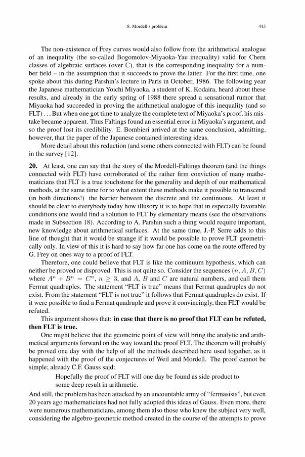
8. Mordell’s problem 443
The non-existence of Frey curves would also follow from the arithmetical analogueof an inequality (the so-called Bogomolov-Miyaoka-Yau inequality) valid for Chernclasses of algebraic surfaces (over C), that is the corresponding inequality for a num-ber field – in the assumption that it succeeds to prove the latter. For the first time, onespoke about this during Parshin’s lecture in Paris in October, 1986. The following yearthe Japanese mathematician Yoichi Miyaoka, a student of K. Kodaira, heard about theseresults, and already in the early spring of 1988 there spread a sensational rumor thatMiyaoka had succeeded in proving the arithmetical analogue of this inequality (and soFLT) . . . But when one got time to analyze the complete text of Miyaoka’s proof, his mis-take became apparent. Thus Faltings found an essential error in Miyaoka’s argument, andso the proof lost its credibility. E. Bombieri arrived at the same conclusion, admitting,however, that the paper of the Japanese contained interesting ideas.
More detail about this reduction (and some others connected with FLT) can be foundin the survey [12].
20. At least, one can say that the story of the Mordell-Faltings theorem (and the thingsconnected with FLT) have corroborated of the rather firm conviction of many mathe-maticians that FLT is a true touchstone for the generality and depth of our mathematicalmethods, at the same time for to what extent these methods make it possible to transcend(in both directions!) the barrier between the discrete and the continuous. At least itshould be clear to everybody today how illusory it is to hope that in especially favorableconditions one would find a solution to FLT by elementary means (see the observationsmade in Subsection 18). According to A. Parshin such a thing would require important,new knowledge about arithmetical surfaces. At the same time, J.-P. Serre adds to thisline of thought that it would be strange if it would be possible to prove FLT geometri-cally only. In view of this it is hard to say how far one has come on the route offered byG. Frey on ones way to a proof of FLT.
Therefore, one could believe that FLT is like the continuum hypothesis, which canneither be proved or disproved. This is not quite so. Consider the sequences (n,A,B,C)where An + Bn = Cn, n ≥ 3, and A, B and C are natural numbers, and call themFermat quadruples. The statement “FLT is true” means that Fermat quadruples do notexist. From the statement “FLT is not true” it follows that Fermat quadruples do exist. Ifit were possible to find a Fermat quadruple and prove it convincingly, then FLT would berefuted.
This argument shows that: in case that there is no proof that FLT can be refuted,then FLT is true.
One might believe that the geometric point of view will bring the analytic and arith-metical arguments forward on the way toward the proof FLT. The theorem will probablybe proved one day with the help of all the methods described here used together, as ithappened with the proof of the conjectures of Weil and Mordell. The proof cannot besimple; already C.F. Gauss said:
Hopefully the proof of FLT will one day be found as side product tosome deep result in arithmetic.
And still, the problem has been attacked by an uncountable army of “fermasists”, but even20 years ago mathematicians had not fully adopted this ideas of Gauss. Even more, therewere numerous mathematicians, among them also those who knew the subject very well,considering the algebro-geometric method created in the course of the attempts to prove

444 CHAPTER VI. POPULARIZATION OF MATHEMATICS
FLT as water sprouts of Diophantine Analysis, generalizations and analogies detachedfrom the real needs of Number Theory. Maybe this is illustrated most significantly byMordell’s own reaction on the occasion of the appearance of the book [8]. He told thathe felt like Rip van Winkel99, adding that if in case one can understand, even the simplestspecial cases, the proofs of the generalizations with great difficulty, it would be better toleave these generalizations, where they are. To these Serge Lang counters strikingly:
A mathematician working in Algebraic Geometry who fell asleepin 1961 and awoke in 1981 will probably feel himself like Rip vanWinkel, this is the natural effect of the rapid and fundamental changesthat have occurred in mathematics.
Because of this, in the case of A. Weil, Grothendieck, Serre, Shafarevich and other,who all contributed the solution of Mordell’s problem, one has to estimate their contri-bution, but even more admire their personal fortitude and insight in the application of themethods of that time.
21. In our pragmatic age one can of course consider all what we have described as afruitless enterprize only by the reason that it concerns only so-called pure mathematics.Here one could quote a letter (July 2, 1830) of Carl Gustav Jacobi to Adrien MarieLegendre;
. . . I have read with great pleasure the opinion of Mr. Poisson aboutmy work, and I could have been quite pleased, but Poisson shouldperhaps have omitted the rather tactless phrase of Mr. Fourier, wherethe latter reproaches Abel and me that we do not prefer to work moreon the question of heat conductivity. One knows of course the opin-ion of Mr. Fourier that the main objects of mathematics are the appli-cations to the clarification of natural phenomena and the yield fromthis. But such a deep thinker ought also have known that the ultimategoal is to glorify the human spirit. And seen from this point of viewNatural Numbers are of no lesser importance than the Structure ofthe Universe.
In a time, when are ever less doubts in the usefulness of computers, it will perhapsnot make sense to complete this argument to the support of the aesthetic origin of Math-ematics. But in a changing world one ought to add that, in Jacobi’s words, there is ex-pressed fully the opposition, peculiar to each generation, about the distinctions in Math-ematics. These distinctions express themselves in the choice whether to prefer problemswhich have arisen from the closest needs of practise, or to think on problems dictatedby the inner logic of things and which will yield a benefit only in a remote future. Thisdilemma may appear also, in one form or the other, in the activities of one and the samemathematician. It is significant here, for instance, that such a well-known mathematicianas John von Neumann has expressed entirely conflicting opinions in the question underview. But it is also precisely here that the dilemma find its solution: Gauss, Riemann,Hilbert, Hermann Weyl and other major front figures of Mathematics have often foundin their theoretical work major inspiration in an applied background. In the course of
99Translator’s note. Character in a book by the classic American writer and humorist Washington Irwing(1783-1859). He is the man who slept for 20 years and when he wakes up find himself in a world that hastransformed, the American Colonies have become independent.

8. Mordell’s problem 445
a longer period of time (30-100 years, sometimes even longer) this distinction may dis-appear or express itself in a different form. Selected results in the solutions of appliedproblems are generalized, in this time, to a theory, and the so-called pure mathematicsfind its way into the applications. Even the new theories treated in the present paper havefound there way into the applications, namely into contemporary physics. We point outhere only the discussion of D. Ruelle [15], in particular his observation that a theoremfound and proved by two physicists Lee and Yang (Phys. Rev 87 (1952), 410-419) andits applications (for example, in the theory of phase transition) probably is connected tothe Weil conjecture.
Finally, we add that, in both of these types of motivation, and their interplay, alwaysit is the concrete problems which bring mathematics forward, and also direct its develop-ment in an essential way. In this sense the words of the Polish born U.S. mathematiciansMarc Kac are remarkable:
Even axiomatic systems change in the waves of time, but their appli-cations live for ever.
Epilogue. This survey was probably written in 1988. Since then Fermat’s Last Theorem has been proved
by Andrew Wiles (assisted by Richard Taylor) [19]. The proof depends on a special case of the Taniyama-
Shimura Conjecture [2], saying that every elliptic curve is modular. This conjecture in general was later proved
by C. Brenil; B. Conrad; F. Diamond; and R. Taylor [1]. A very readable (non-technical) description of Wiles’
work is the book [18].
Gert Almkvist
Other references:[16],[3],[6],[9],[11], [14],[21],[22]
References
[1] C. Brenil, B. Conrad, F. Diamond, and R. Taylor. On the modularity of elliptic curves over Q: wild 3-adicexercises. J. Am. Math. Soc. 14, 2001, 843–939.
[2] H. Darmon. A proof of the full Shimura-Taniyama conjecture. Notices Am. Math. Soc. 46, 1998, 1397–1401.
[3] P. Deligne. Preuve des conjectures de Tate et Shafarevich (d’après G. Faltings). Séminaire Bourbaki,Exposé 616, Novembre 1983. Asterisque 1983/84 (121–122), 1985, 25–41.
[4] Diophant of Alexandria. The Arithmetics and the book on polygonial numbers. Nauka, Moscow, 1974.[5] D. R. Heath-Brown. Fermat’s last theorem for "almost all" exponents. Bull. London Math. Soc. 17 (1),
1985, 15–16.[6] N. Katz. An overview of Deligne’s proof of the Riemann hypothesis for varieties over finite fields. In:
Proc. Pure Appl Math 38, Part 1: Mathematical developments arising from Hilbert problems. Amer. Math.Soc., Providence, R.I., 1976, 275–306.
[7] A. O. Koblitz. Introduction to elliptic curves and modular forms. Graduate Text of Math., 97. Springer-Verlag, New York, 1984.
[8] S. Lang. Diophantine geometry. Interscience Tracts in Pure and Applied Mathematics, 11. IntersciencePubl., New York, London, 1962. Russian translation: Mir, Moscow, 1986.
[9] S. Lang. Higher dimensional Diophantine problems. Bull. Am. Math. Soc. 80, 1974, 779–787.[10] B. Mazur. Higher dimensional Diophantine problems. Bull. Am. Math. Soc. 14, 1986, 207–259.[11] B. Mazur. On some of the mathematical contributions of Gerd Faltings. In: Proceedings of the Int. Con-
gress of Mathematicians, August 3-11, 1986. Amer. Math. Soc., 1987, 7–11.

446 CHAPTER VI. POPULARIZATION OF MATHEMATICS
[12] J. Oesterlé. Preuve des conjectures de Tate et Shafarevich (d’après G. Faltings). Séminaire Bourbaki,Exposé 694. Asterisque 1987/88 (161–162), 1989, 165–186.
[13] M. M. Postnikov. Introduction to algebraic number theory. Nauka, Moscow, 1982.[14] S. Raghavan. Impact of Ramanujan’s work on modern mathematics. J. Indian Inst. Sci. Srinivasa Ra-
manujan centenary 1987, Special Issue, 1987, 45–53.[15] D. Ruelle. Is our mathematics natural? The case of the equilibrium of statistical mechanics. Bull. Am.
Math. Soc. 19 (1), 1988, 259–268.[16] F. Schinzel. Construction of telephone networks by group representations. Notices Am. Math. Soc. 26 (1),
1989, 5–22.[17] I. R. Shavarevich. Algebraic number fields. In: Proceedings of the Int. Congress of Mathematicians,
August 15-22, 1962. Institute Mittag-Leffler. Almqvist & Wiksells, Uppsala, 1963, 163–176.[18] S. Singh. Fermat’s enigma. Walker and Co., New York, 1997.[19] R. Taylor and A. Wiles. Ring theoretic properties of certain Hecke algebras. Ann. of Math. 141, 1995,
553–572.[20] S. S. Jr. Wagstaff. The irregular primes to 125 000. Math. Comp. 32 (142), 1978, 583–591.[21] A. Weil. Number of solutions of equations in finite fields. Bull. Am. Math. Soc. 55, 1949, 497–508.[22] Yu. Zarikhin and A. Parshin. Problems of finiteness in Diophantine Geometry. Supplement to the Russian
edition of [14], 1986, 369–438.

447
9. [K96] On two discrete models in connection withstructures of mathematics and languageTranslation by J. Peetre
In a mathematical theory there is no a priori need to bring its conceptions and lan-guage in agreement with newest needs of natural sciences. Nevertheless this has hap-pened often and the good harvest of the cooperation has given a profit to both parties.During the last decades there has been a steadily growing interest in discrete models ofan ever increasing complexity. As it has not been possible to present adequately such amodel with the aid of standard functional rules, this interest has increased in proportionto the possibilities of computers for theoretical experiments with them. In the followingwe shall describe the possibilities of two such simplest models.
9.1. Binary trees and Strahler numbers
One example is the study of branching phenomena in neurophysiology, botany, geol-ogy – in the last discipline in particular in connection with hydrogeological research byR. E. Horton [2] and A. Strahler concerning the structure of river systems [13]. A com-mon denominator for these phenomena is provided by the notion of tree, which expressedin mathematical language means a cycle-free connected simple graph. In computer sci-ence one employs the notion of a binary tree, which can be determined recursively:
• if such a tree has only one vertex, then this tree is identified with its vertex;• in all other cases a binary tree is defined as a triple B = (v;BL, BR), where v
is a distinguished vertex of B (designated the root) and BL (as well as BR) arebinary trees, called the left (respectively, the right) subtree of the tree B.
•2
•2
%%%%%%%%% •1
���������
•1
&&&&&&& •1
''''''' •0
&&&&&&& •0
((((((
•0)))))) •
0
****** •0)))))) •
0
******
Fig. 23: The orders of the binary tree
The vertices of a binary tree are clas-sified as inner vertices (such an vertexhas two “successors”, its left and its rightsuccessor) and as exterior vertices (theseare the vertices without successors). Theedges of a tree are pairs of vertices (v, w),where w is the successor of v. If we as-sume that in a river system no islandshave been formed and that at each junc-ture not more than two rivers are united,then the branching picture which arisesis a binary tree. To the edges of a tree
one can assign an order using the Horton-Strahler rule:
• the order of a river proceeding from a source is 0;• two order-k rivers join to a river of order k + 1, but two rivers of order i and k
(i < k) give when joined an order-k river (Fig. 23).

448 CHAPTER VI. POPULARIZATION OF MATHEMATICS
The maximal order of the edges of a tree under consideration is called its Strahlernumber and will be denoted st(B). This parameter of a tree can be defined inductivelyas follows:
• we agree upon that st(∅) = 0;• if st(BL) = st(BR), then we agree that st(v;BL, BR) = 1 + st(BL);• if, however, st(BL) �= st(BR) we agree that st(B) = max(st(BL), st(BR)).
•0 ****** •
0
))))))
•0 ****** •
0
))))))
•0 ****** •
0
))))))
•0 ****** •
0
++++++
•1 ''''
''' •
1&&&&&&& •
1 ''''
''' •
1&&&&&&&
•2 ��
����
��� •
2%%%%%%%%%
•3
Fig. 24: A binary tree B: bk/bk+1 = 2 for any k,and st(B) = 3
A maximal path among the paths of atree consisting of edges of order k is calleda k-th order segment of the river system;such a segment starts in a source (in casek = 0) or else arises by joining two edgesof order k − 1 (in case k ≥ 1), but ends bythe joining with a segment of order k′ (k′ >k). Denoting the total number of segmentsof order k by bk, we define the bifurctationratio of the treeB as the quotients bk/bk+1;here k ≤ st(B). For example, for a bi-nary tree with all exterior vertices (leaves)at the same distance k from its root the bi-furctation ratio is 2 and the Strahler num-ber of such a tree is k (Fig. 24). In accor-
dance with hydro-geological observation the bifurctation ratio does not change withinthe frames of a given river system, and stays between 3 and 5, giving a good qualitativepicture of the shape of the river system. Branching trees are of interest also in botany.A result of these investigations for computer science is the discovery of the so-calledLindenmayer grammars and their use in computer graphics, where using these comple-mentary methods one tries to assemble a synthetic picture of the tree [16]. The inputs ofsuch a program are the number k and a stochastic matrix with (at least) k rows, the socalled ramification matrix , and it yields a binary tree with Strahler number k having thegiven matrix as ramification matrix.
��������+
,,,,,,,,
----
----
�� ����×
��������
....
....
�� ����g
��������+
////////
000000
��������+
111111
222222
�� ����/
333333
000000
�� ����/
333333
444444
�� ����e �� ����f
�� ����a �� ����b �� ����c �� ����d
Fig. 25: The syntax tree of the expression(a
b+ c
d)(e + f) + g
Strahler numbers appear in a natural way like-wise in other questions of computer science. Oneof these is the question of the least number of reg-isters needed for the evaluation of a given arith-metic expression. Let us identify the arithmetic ex-pression (consisting binary operations) with a treewhose vertices are labelled by symbols for theseoperations and the variables used in the expres-sion. For example, in Fig. 25 we have drawn alabelled binary tree corresponding to the expres-sion (a/b + c/d) (e + f) + g. In the generalcase it turns out (theorem of A. Ershov!) that theminimal number of registers required in the eval-uation of an arithmetic expression exceed by onethe Strahler number of the corresponding binary tree. The number of registers required

9. Structures of mathematics and language 449
for the evaluation of a long arithmetic expressions is described by a formula for findinglim st(n), where st(n) stands for the average
1cn·∑(Bn)
st(Bn)
over all binary trees Bn with n vertices. Such a formula was found by X. Viennot (1986)(see [16]). As a detail, let us record that the total number of the latter is cn =
(2nn
)/(n+1)
and that the generating function c(t) =∑
n≥0 cntn of these Catalan numbers cn satisfies
the relation 1 + tc(t)− c(t)2 = 0.
9.2. Molecular biology and formal languagesThe results of molecular biology has sometimes been formulated in terms of formal
languages and information theory.On the one hand, the formal languages. Fixing an alphabet X , let us consider
subsets L of the set of all words X∗; such subsets are called formal languages. A lan-guage L can be presented as function L : X → {0, 1}. Therefore, L can also be in-terpreted as a formal series
∑w∈L w. Here we are interested in context free language
(CF-languages)100; such a language can be given by a context free grammar, that is aquadruple G = (X,N ;σ,P), where N (the terminals) and X (the non-terminals) arefinite alphabets, σ ∈ N the so-called initial symbol and the finite set P contains the rulesof deduction (productions) α→ β, that is, pairs (α, β), where α ∈ N and β ∈ (N ∪X)∗
(for details see [11]). As an example, we have the Dyck language D, D ⊆ X , whereX = {x, x} and the rules of deduction are σ → xσxσ and σ → 1; here the symbol 1 de-notes the empty set in X . In a word of the language D there are always the same numberof letters x and x. Moreover, there are in each left term (prefix) not fewer letters x thanletters x. Another example is the Fibonacci language F , F ⊆ X , for which X = {x, a}and N = {σ, τ}, while the productions are σ → aτ , σ → xxσ, τ → aσ, τ → xxτ ,σ → 1. The formal series F representing this language is the solution of the system ofequations
F =1 + aG + xxF
G =aF + xxG
in the algebra Z〈〈X〉〉 of formal series with integer coefficients.One owes to M. P. Schützenberger the idea to seek in the enumeration of combi-
natorial objects in their graduated set K = ∪Kn such a formal algebra language Lwhose n-words are in one-to-one corresponding with the objects of order n, that is,elements of the set Kn. In this situation the desired result will give the generatingfunction l(t) =
∑n>0 lnt
n of the numbers ln = |L(G) ∩ Xn)|. In order to find thenumber of words of a given length in the language L(G) let us consider the morphismΨ : X∗ → {t}∗, which maps all characters of the alphabet X into one and the same(new) variable t. In this situation is the formal series corresponding to L(G) representedby the generating function of the numbers ln: Ψ(L) = l(t). In the case of the Dycklanguage we obtain in this way a series d(t), satisfying the equation
1− d(t) + t2 · d(t)2 = 0.
100The author uses the term algebraic language instead.

450 CHAPTER VI. POPULARIZATION OF MATHEMATICS
This equation is solved by the function d(t) = (1−√
1− 4t2)/2t2 such that in its powerseries the coefficient of t2n is the Catalan number cn =
(2nn
)/(n + 1). In our second
example, we obtain the power series Ψ(F ) = f(t) and Ψ(G) = g(t) satisfying thesystem of equations
f(t) = 1 + t · g(t) + t2 · f(t)
g(t) = t · f(t) + t2 · g(t)
As the solution to this system we obtain the function f(t) = (1− t2)/(1− 3t2 + t4). Inis Taylor series the coefficient of t2n is the Fibonacci number F2n; here F0 = F1 = 1and Fn = Fn−1 + Fn−2 (n ≥ 2). An auxiliary fact: The Fibonacci language is rational,which (according to Kleene’s theorem!) means that that this language is recognizable bya finite automaton; such an automaton is depicted in Fig. 26.
�� ����1
a
��
x
**
�� ����3a
��
x
**�� ����2
x
++
a
��555
5555
55�� ����4
x
++
a
666666666
�� ����5x
,,a
--
Fig. 26: A finite automaton for the Fi-bonacci language
On the other hand, the genetic code. Inter-esting macromolecules are nucleic acid (NA) andproteins. One of the forms of NA - deoxyribonu-cleic acid (DNA) contains chromosomes and car-ries hereditary information. It appears as a doublehelix twisted up in space and consisting of a dualpair of threads joined with each other through hy-drogen bonds. If one separates two DNA strandsand then adds to each of them another DNA chaincomplementary to it one gets as a result two iden-tical copies of the original DNA molecule. Thekinky form of a double helix optimizes the spatialdistribution of the molecule, because in untwistedform the DNA thread the shape of DNA wouldhave been 50 centimeters long. The proteins arethe workhorses of the cell, assuring the stability of its structure, its defence, energy con-tent and life activity. The protein molecule consists of amino acids, of which there are 20species. The latter may be viewed as the semantic primitives of the genetic language, ofwhich finite words (long!) formed by concatenation are called polypeptide chains.
The primary structure of nucleic acids may be viewed as a chain of nucleoides(bases) – a thread. The alphabet G, with the aid of which the DNA thread is trans-ferred as words consists of four bases: A (adenine), G (guanine), C (cytosine) and T(thymine). In the case of the ribonucleic molecule (RNA) one uses in the alphabet Rof the ones mentioned the three first, while T (thymine) is here replaced by the base U(uridine). These bases possess several properties which make it possible to count themas phonemes of the genetic language. But they have also peculiarities:
• the number of phonemes of a natural languages is variable (> 10), the numberof nucleoides is 4 in all organisms;
• the phoneme of a natural language is given by a complex of (binary) predicateswhose order in the words is not important, while at the same time as for exam-ple T (thymine) and C (cytosine), although they consist of the same elements,appear as different graphs. In the alphabet of nucleotides there arises 43 = 64strings – the codons, that in turn form the so-called nucleotide chains – (very
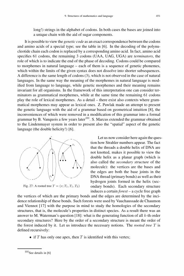
9. Structures of mathematics and language 451
long!) strings in the alphabet of codons. In both cases the bases are joined intoa unique chain with the aid of sugar components.
It is possible to view the genetic code as an exact correspondence between the codonsand amino acids of a special type; see the table in [6]. In the decoding of the polynu-cleotide chain each codon is replaced by a corresponding amino acid. In fact, amino acidspecifies 61 codons, the remaining 3 codons (UAA, UAG, UGA) are terminators, therole of which is to indicate the end of the phase of decoding. Codons could be comparedto morphemes in natural language – each of them is a sequence of genetic phonemes,which within the limits of the given syntax does not dissolve into shorter subsequences.A difference is the same length of codons (3), which is not observed in the case of naturallanguages. In the same way the meaning of the morphemes in natural language is mod-ified from language to language, while genetic morphemes and their meaning remainsinvariant for all organisms. In the framework of this interpretation one can consider ter-minators as grammatical morphemes, while at the same time the remaining 61 codonsplay the role of lexical morphemes. As a detail – there exist also contexts where gram-matical morphemes may appear as lexical ones. Z. Pawlak made an attempt to presentthe genetic language with the aid of a grammar based on geometrical intuition [8], theinconveniences of which were removed in a modification of this grammar into a formalgrammar by B. Vanquois a few years later101. S. Marcus extended the grammar obtainedto the Lindenmayer system in order to present also the “spatial” aspect of the geneticlanguage (the double helicity!) [6].
•
• T3
""""""""""""""""
•
,,,,,,,,,,,,,, •
v77777777777 •
��������
•
)))))) • •
****** •
***********
•T1
&&&&&&&&&&&&& •
77777777777 •
)))))) •
888888 •
'''''''
•T2
Fig. 27: A rooted tree T = (v; T1, T1, T3)
Let us now consider here again the ques-tion how Strahler numbers appear. The factthat the threads a double helix of DNA arenot knotted, makes it possible to view thedouble helix as a planar graph (which isalso called the secondary structure of themolecule): the vertices are the bases andthe edges are both the base joints in theDNA thread (primary bonds) as well as theirhydrogen joints formed in the helix (sec-ondary bonds). Each secondary structureinduces a certain forest – a cycle free graph
the vertices of which are the primary bonds and the edges are determined by the inci-dence relationship of these bonds. Such forests were used by Vauchaussade de Chaumonand Viennot [17] with the purpose in mind to study the homologies of the secondarystructures, that is, the molecule’s properties in distinct species. As a result there was ananswer to M. Waterman’s question [18]: what is the generating function of all k-th ordersecondary structures? Here by the order of a secondary structure is meant the order ofthe forest induced by it. Let us introduce the necessary notions. The rooted tree T isdefined recursively:
• if T has only one apex, then T is identified with this vertex;
101See details in [6]

452 CHAPTER VI. POPULARIZATION OF MATHEMATICS
• in the opposite situation one gives the tree as a sequence T = (v;T1, . . . , Tp),where v is a vertex of T (the root) and Ti is a subtree of T rooted at v, seeFig. 27.
A forest is a list of all connected components of the graph consisting of rooted trees.A maximal sequence of vertices (v1, . . . , vs) such that each vi (i = 1, 2, . . . , s− 1) hasthe unique successor vi+1 and vs is a leaf (that is, an apex without a successor) is called afilament of the forest. The operator δ of removing filaments is defined on the forest M bythe rule that δ(M) is the forest which is obtained from M by omitting all vertices of thefilaments and all the edges incident to them; the filament containing the root is removedin the last instance. The smallest such number i that the vertex x is extinguished byapplication of the operator δi is called the degree of this vertex. The maximal degree ofthe vertices of a forest is called the degree of the forest. In the example given in Fig. 28we have the degree 3. It is clear that the degree of a forest is the least integer k such thatδi(M) = ∅.
•
•
•
9999999 •
::::::::::
•
&&&&&&& •
****** •
(((((((((((( •
'''''''
• •
&&&&&&& •
****** •
888888
• •
•
Fig. 28: A forest of the degree 3
An answer to the Waterman’s questionabove is obtained in the following way. Thesecondary structures of degree k are codedwith the words of a suitable algebraic lan-guage and then one finds a system of equa-tions which is satisfied by the generatingformal series of the words of this language.Subsequently, the desired answer is foundusing the procedure described above (in con-nection with the map Ψ). Indeed, if thenumber of unlabelled k-the degree secondarystructure with n vertices is denoted sn,k,then the generating function under discus-sion is given by the formula∑
n≥0
sn,ktn =
tp(k)
(1 − t)P1P2 . . . Pk,
where p(k) = 5 · 2k−1 − 2 and the polynomials Pi are defined recursively by the rulesP1 = 1 − 2t− t3 and Pi = P 2
i−1 − 2tp(k) (in case i ≥ 2). The problem connected withthis question regarding the enumeration of rooted forests of degree k and n vertices issimpler and, surprisingly, its answer is the same generating function which enumeratedthe binary trees with Strahler number k [15].
9.3. On coding theory
Contemporary technology has lifted on a new level questions about the mechanisms ofinformation processing and their effectiveness. The solutions have required a mathemat-ical formulation of which many essential concepts originates in coding theory. As manysimilar questions are of interest also in the study of the genetic code and language, weshall in what follows likewise give a brief survey of these concepts.
There are many possibilities for sending information. In some cases (for instance,in satellite communication) information is transferred through medial channels, in other

9. Structures of mathematics and language 453
cases the sender writes it, for instance, on a floppy disk, from which the computer laterreads it. The exact mechanism of the transfer is not far from always known – it sufficesto think of the questions of transfer of information in the human brain. However, manycommunication channels have a common characteristic – the transfer of information isthere accompanied by background noise, with the effect that some of the transferred sym-bols get modified in the process of communication and arrive to the receiver in distortedform. In order to improve qualitatively of the reception one applies error detecting anderror correcting codes.
In mathematical formulation, a channel is given by a triple (S, V ;P ), consisting ofan input language S, an output language V and a matrix P = p(y|x). The elementsof the latter are conditional probabilities: p(y|x) shows the probability for receiving thesymbol y in the condition that x was sent and this probability is regarded as independentof the fate of the previous and later signals in the channel under view. Here informationis interpreted as a sequence of (long!) finite sequences (called words, also strings), forthe writing of which the symbols of the given alphabet are used. In the theory the mostsuitable alphabet is some finite field Fq (here q = p� is a prime power). The Readermay picture the field Fq as a domain of numbers where the arithmetical operations arecarried out according the most common rules, to which new ones have been added thatintroduce basically periodicity phenomena, emanating from the finiteness of the domainFq. The coding may be viewed as a procedure (as an algorithm or a mapping), whichmap a natural message or a part of it written in words in the channel’s input language S,adding so-called code symbols (‘redundancy blocks’).
Expressed more exactly, for the coding of a message, broken up into k letter blocks,
may be presented as an injective map Fkq
Ψ−→ Fnq ; words in the image set C = Ψ(Fk
q) ⊆Fn
q are called code words. If Ψ is a linear map, then the set of code words forms a k-dimensional subspace of the sequence space Fn
q ; therefore the code is termed a linear(n, k)-code. All code words of a linear code can be presented in the form xG, wherex ∈ Fn
q and G is a fixed k× n matrix, the rows of which form a basis of the subspace C;it is called the generating matrix of C. There is also another important matrix connectedwith the code, it is the parity check matrix which is a (n − k) × k-matrix H such thatx ∈ C if and only if xH t = 0; here t is standing for taking the transpose of the matrix. Ifwe introduce a form
〈x, y〉 =n∑
i=1
xiyi
in Fnq , then we can ‘compute’ the orthogonality of vectors, that is, interpret this geomet-
rical notion in the analytic language: x⊥y ⇔ 〈x, y〉 = 0. Therefore it makes sense tospeak of the code C⊥ dual to C,
C⊥ = {x| x ∈ Fnq such that x⊥c for all c ∈ C.}
The reception of the coded information is followed by decoding – a procedure whichmaps the sequence received in the channel’s output language V into a natural message.Often this is achieved in such a way that one finds the code word closest to the receivedwords (maximum likelihood decoding). Maximizing the correct choice of the code wordis facilitated by the Hamming distance of two words (vectors) x = x1x2 . . . xn andy = y1y2 . . . yn: dH(x, y) = #{i|xi �= yi}. For example dH((0111), (1001)) = 3 anddH((01100), (11000)) = 2.
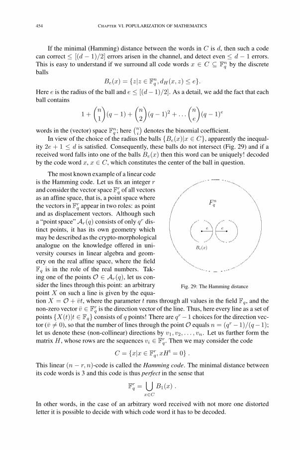
454 CHAPTER VI. POPULARIZATION OF MATHEMATICS
If the minimal (Hamming) distance between the words in C is d, then such a codecan correct ≤ [(d − 1)/2] errors arisen in the channel, and detect even ≤ d − 1 errors.This is easy to understand if we surround all code words x ∈ C ⊆ Fn
q by the discreteballs
Be(x) = {z|z ∈ Fnq , dH(x, z) ≤ e}.
Here e is the radius of the ball and e ≤ [(d− 1)/2]. As a detail, we add the fact that eachball contains
1 +(n
1
)(q − 1) +
(n
2
)(q − 1)2 + . . .
(n
e
)(q − 1)e
words in the (vector) space Fnq ; here
(ni
)denotes the binomial coefficient.
In view of the choice of the radius the balls {Be(x)|x ∈ C}, apparently the inequal-ity 2e + 1 ≤ d is satisfied. Consequently, these balls do not intersect (Fig. 29) and if areceived word falls into one of the balls Be(x) then this word can be uniquely! decodedby the code word x, x ∈ C, which constitutes the center of the ball in question.
• •e e
Be(x)
F nq
Fig. 29: The Hamming distance
The most known example of a linear codeis the Hamming code. Let us fix an integer rand consider the vector space Fr
q of all vectorsas an affine space, that is, a point space wherethe vectors in Fr
q appear in two roles: as pointand as displacement vectors. Although sucha “point space”Ar(q) consists of only qr dis-tinct points, it has its own geometry whichmay be described as the crypto-morphologicalanalogue on the knowledge offered in uni-versity courses in linear algebra and geom-etry on the real affine space, where the fieldFq is in the role of the real numbers. Tak-ing one of the points O ∈ Ar(q), let us con-sider the lines through this point: an arbitrarypoint X on such a line is given by the equa-tion X = O + vt, where the parameter t runs through all values in the field Fq, and thenon-zero vector v ∈ Fr
q is the direction vector of the line. Thus, here every line as a set ofpoints {X(t)|t ∈ Fq} consists of q points! There are qr−1 choices for the direction vec-tor (v �= 0), so that the number of lines through the pointO equals n = (qr−1)/(q−1);let us denote these (non-collinear) directions by v1, v2, . . . , vn. Let us further form thematrix H , whose rows are the sequences vi ∈ Fr
q . Then we may consider the code
C = {x|x ∈ Frq, xH
t = 0} .This linear (n − r, n)-code is called the Hamming code. The minimal distance betweenits code words is 3 and this code is thus perfect in the sense that
Frq =
⋃x∈C
B1(x) .
In other words, in the case of an arbitrary word received with not more one distortedletter it is possible to decide with which code word it has to be decoded.
9. Structures of mathematics and language 455
As another example, let us consider the radar codes. One of the best known me-dieval mathematician was Leonardo (from Pisa, with the nickname Fibonacci 102). Hismost important work concerned the completion and systematization of arithmetic, whichhe had learnt from the Arabs. Through his treatise “Liber Abacci” (1201) his resultsbecame known in Europe. Fibonacci numbers are widely known; this is the sequence1, 1, 3, 5, 8, 13, 21 . . . , which members (Fn|n = 0, 1, . . . ) may be found from the rela-tion Fn = Fn−1 + Fn−2 (n ≥ 2), assuming that F0 = F1 = 1. More generally, let usconsider sequences y = (yn|n = 0, 1, . . . ) satisfy a homogeneous recurrent equation,that is, a relation of type
a0 + a1yi−1 + · · ·+ akyi−k = 0, i = k + 1, . . . ,
where we agree that a0 �= 0 and further that, in the interest of the context that the coef-ficients ai and the members on the sequence are taken in the Galois field Fq . Fixing theinitial values y0 = c0, . . . , yk−1 = ck−1, this equation gives us as solution a sequence(cn|n = 0, 1, 2, . . . ), the components of which can be found from the formula
ci = a−10 ·
k∑j=1
ajci−j , i = k, k + 1 . . .
A useful detail: if we interpret the solution y as a (formal) series y = c0 + c1x +c2x
2 + . . . , then this series comes as the quotient of two polynomials c(x)/a(x), wherethe degree of c(x) is less than k and a(x) = a0 + a1x + · · ·+ akx
k is the (left) charac-teristic polynomial of the equation under consideration.
A radar code codes a k-sequence (c0, c1, . . . , ck−1) written in the input alphabetFq as an infinite recurrent sequence c = (cn|n = 0, 1, . . . ), which is determined as thesolution of the above recurrent equation under the initial condition (c0, c1, . . . , ck−1). If,in addition, ak �= 0 in this equation, then the radar code determined by it generates onlyperiodic sequences (cn), that is, there exist integers p and t such that ci = ci+p for alli ≥ t. For instance, taking q = 2, k = 4 and the equation yi + yi−3 + yi−4 = 0 weobtain sequences with period p = 24 − 1 = 15. The error correcting properties of thisradar code depend on the fact that 24 = 16 distinct initial sequences (these are wordsof length 4 in the alphabet Z2) generate 16 distinct code words of length 15 and thattheir set is closed for addition as well as (obviously) also multiplication by the scalars 0and 1. Hence, C turns out to be a 4-dimensional subspace in the 15-dimensional spaceZ15
2 , in which the minimal distance of any two codes is 24−1 = 8. Therefore the radarcode described can recognize 24−2 = 4 errors, and correct 24−2 − 1 = 3 errors. Theset C may be realized as a simplex, so this code is also known as a simplex code. Thedual to it code C⊥ is the widely known binary (3, 7)-Hamming code. An example of theeffectiveness of radar codes is the fourth test of A. Einstein’s theory of gravitation. A longtime one has known three experimental facts validating this theory (1915): the precessionof the perihelion of the orbit of Mercury; the bending of right rays near the Sun; and thegravitational red shift. The fourth effect (the slowing down of electromagnetic radiationin the gravitational field) was checked only half a century later. To this end one measuredthe arrival of echoing from a radar signal from Mercury both when Mercury was obscured
102Translator’s note. The common used name-form Fibonacci came into use only in the course of the 19thcentury, presumably through the influence of the Italian mathematician and mathematical historian GuglielmoLibri Carucci della Sommaja (1803-1869). Leonardo himself wrote (in Latin) Leonardo filio Bonnaci.

456 CHAPTER VI. POPULARIZATION OF MATHEMATICS
by the Sun (in this case the energy of the echo is 10−27 of the emitted energy!), as wellas when is was not obscured. With the aid of a suitable radar code one succeeded to fixthe time difference in the arrival of the echo.
Interest in mathematical coding theory spread in particular after Shannon’s result[12] regarding the possibilities of good transfer of information in “noise” adding symmet-ric binary channels (BSC). For such a channel (S,B;P ) one has S = V = Z2 = {0, 1},while the elements of the matrix P , the conditional probabilities p(i|j), are given by therules: p(1|0) = p(0|1) = p (probability of error), and p(0|0) = p(1|1) = 1− p for somep ∈ [0, 1]. The rate of transmission for this channel is determined as the ratio betweenthe number of bites appearing in the original message and the total number of bites inputin the channel, where the last number also includes the bites added in the decoding ofthe message. According to Shannon’s theorem transformation of information with noiseis possible in a symmetric channel with given positive rate of transmission, which atthe same time guarantees the correct reception of an initial message with close to oneprobability. Supplementary information about codes can be found in [14].
9.4. Conclusion
One may remark that, despite the ancient origin of the problem of information transfer,some of the questions connected with are still of interest and that often they are onlybeginning to become accessible to research. This problem has provided the motivationfor and is the real testing stone in the development of biology as well as of several com-binatorial theories within mathematics.
In connection with of the genetic language one could note two questions which,presumably, offer a continued interest. First, in which way can the genetic code beviewed as an error detecting and error correcting code? Second, how to explain thecontinuity properties of the genetic language, that is, in which cases (always?) and whydoes closeness between some codons generate corresponding polypeptide chains whichare similarly close to each other? The determinations of nearness of codons (modified;weighted; etc.) have so far not given any result with the aid of the Hamming distance.It is the author’s conjecture that this can be realized via Grothendieck topology. Alsorelated problems are connected with the model of the Dutch mathematician De Bruijn[1] regarding transfer of information in the (human) brain, as well as, the related to this,Grothendieck continuity within the realm of automata.
References
The references [2], [8],[17], and [18] are supplied by the Editors. The works [3], [4],[5], [7], [9], [10] below are actually not cited in the paper. They are kept here because ofthe appearance in the original publication.
[1] N. G. de Bruijn, A model for information processing in human memory and consciousness. Preprint(2.11.1993). Dept. of Math. and Comp. Sci. of Techn. Univ. Eindhoven, 1993.
[2] R. E. Horton. Erosioned development of streams and their drainage basins, hydrophysical approach toquantitative morphology. In: Bull. Geol. Soc. of America, Vol. 56, 1945, 275–370.
[3] A. Jaffe and F. Quinn. Theoretical mathematics: towards a cultural synthesis of Mathematics and Theo-retical Physics. Bull. Am. Math. Soc. 29(I), 1993, 1–12.

9. Structures of mathematics and language 457
[4] U. Kaljulaid. An invited review of the book “Discrete Mathematics and Algebra Structures ”, by S. Ger-stein. In: Acta Appl. Math., Vol. 22. Freman & Co., N. Y., 1987, 325–329.
[5] J. Kiho. Algoritmid ja nende struktuurid, Tartu, 1994. (In Estonian).[6] S. Marcus. Linguistic structures and generative devices in molecular genetics. Cahiers linguistique
théorique et appliqueé 11(2), 1974, 77–104.[7] D. Mumford. Picard groups and moduli problems. In: Arithmetical Algebra Geometry, N. Y., 1965,
33–81.[8] Z. Pawlak. Gramatyka i matematyka. Panstwowe Zaklady Wydawnictw Szkolnych, Warszawa, 1965. (In
Polish).[9] H.-O. Peitgen, H. Jürgens, and D. Satpe. Chaos and Fractals. Springer-Verlag, 1992.[10] P. Prusinkiewicz, A. Lindenmayer, and J. Hannan. Developmental models of herbaceous plants for com-
puter imagery purposes. In: ACM SIGGRAPH Computer Graphics, Vol. 22, 1988, 141–150.[11] A. Salomaa. Formal Languages and Power Series. In: “Formal Models and Semantics”, Handbook of
Theor. Comp. Sci., Vol. B. Elsevier Science Publ. B.V., 1990, 103–132.[12] C. E. Shannon. A Mathematical theory of communication. The Bell System Technical Journal 27, 1948,
379–423, 623–656.[13] A. N. Strahler. Hypsometric (area-altitude) analysis of erosonal topology. In: Bull. Geol. Soc. of America,
Vol. 63, 1952, 1117–1142.[14] H. C. A. van Tilborg. Error-correcting codes - a first course. Chartwell Bratt, Studentlitteratur, Lund,
1993.[15] M. Vauchaussade de Chaumont, Nombre de Strahler des arbres, languages algébriques et dénombrement
des structure sécondaires en biologie moléculaire. Thèse. Univ. de Bordeaux 1, 1985.[16] X. Viennot, G. Eyrolles, N. Janey, and D. Arqués. Combinatorial analysis of ramified patterns and com-
puter imagery of trees. In: ACM SIGGRAPH Computer Graphics, Vol. 23, 1989, 31–40.[17] M. Vauchaussade de Chaumont and X. G. Viennot. Enumeration of RNA’s secondary structures by com-
plexity, in Mathematics in Medecine and Biology. In: Lecture Notes in Biomath., Vol. 57. Springer, Berlin-New York, Berlin, N. Y., 1985, 360–365.
[18] M. S. Waterman. Secondary structure of single stranded nucleic acids. Adv. Math. Suppl. Stud. I, 1978,167–212.

This page intentionally left blank

Index of Names
Abel, Niels Henrik, 3, 4, 8, 24, 25, 27, 40, 51, 69,70, 72, 73, 75, 78, 79, 81, 82, 86–90, 92, 97,106, 107, 118–121, 123, 124, 128, 129, 134,259, 272, 345, 348, 351, 368–370, 377, 378,381, 382, 384, 387, 389, 392, 395, 399,405–407, 411, 435, 436, 442, 444
Alameddine, Ahmad Fawzi, 247Aleksandrov, Pavel Sergeevich, 203Aleksandrov (Alexandroff), Aleksandr Danilovic,
227Alexander the Great, 428Alexander I, ixAlmkvist, Gert, ix, 243, 286, 427, 445Ameling, Friedrich, 311Amitsur, Shimshon Avraham, 282Anderson, Ian, 208Ando, Tsuyoshi, 221Andrunakievich, Vladimir Aleksandrovich, 122Apollonius of Perga, 428Arakelov, Suren Yu, 441Arazy, Jonathan, 233Archimedes of Syracuse, 428Argand, Jean Robert, 364Artin, Emil, 74–77, 83, 84, 106, 107, 437
Bézout E., 358, 391Bachet, Claude, 429Backlund, Helge Gotrik, 292, 294Backlund, Hjalmar, 294Backlund, Johan Oskar, 291–294Backlund, Ulrika Catharina, 292, 294Backlund-Celsing, Elsa Carolina, 292Bahturin, Yuri A., xxivBanachewski, Bernhard, 94, 108Barbilian, Dan (Barbu, Ion), 117Bashmakova, Isabella Grigoyevna, 311, 327Beckenbach, Erwin F., 226Beilinson, Alexander, 353Bell, Eric Temple, 239Bellman, Richard, 226Belousov, V. D., 348Belskiı, A., 353Beltrami, Eugenio, 259
Bergman, George, 16, 17, 21, 43, 63, 105, 123,283
Berkovich, Vladimir, 353Bertrand, Joseph Louis François, 362Betti, Enrico, 371, 436, 438Bidder, Georg Friedrich Karl Heinrich, 321Birch, Bryan John, 349, 439Birkhoff, Garrett, 15, 21, 26, 44, 45, 103–105,
155, 207, 221Björner, Anders, 203Blauert, Marianne, ixBogomolov, Fedor Alekseevich, 443Bokut, Leonid Arkadievich, ix, 269Boltzmann, Ludwig, 416Bombelli, Rafael, 429Bombieri, Enrico, 443Booth, Laura, 299Booth, Lorentz, 299Borevich, Zenon Ivanovich, xiiBourbaki, Nicolas, 352, 355, 371, 399, 440Bovdi, Adalbert, 22, 88Brandt, Kerstin, ixBrauer, Richard Dagobert, 386Brenil, C., 445Brouwer, Luitzen Egbertus Jan, 353Brualdi, Richard A., 213, 221Bruck, Richard Hubert, 348Bruhat, François Georgwe René, 221Brunner, Georg Bernhard, 320Buckley, Joseph T., 71, 85Bulman-Fleming, Sydney, 137Burnside, William, 254, 257, 258, 261, 377, 385,
386
Cantor, Georg Ferdinand Ludwig Philipp, 332,353, 410, 416
Capelli, Alfred, 259Cardano, Geronimo, 357, 358, 363, 364Carrol, Lewis , 356, 359, 362Cartan, Élie Joseph, 257, 267, 268Cartan, Henri, 5, 355, 389Castelnuovo, Guido, 406Catalan, Eugène Charles , 449Catharine I (Martha Skovronska), 292
459

460 INDEX OF NAMES
Cauchy, Augustin Louis, 226, 227, 261, 276,361, 362, 368
Cayley, Arthur, 254, 257, 259, 261, 267–269, 424Chabauty, Claude, 441Chasles, Michel, 408Chebotarev, Nikolai Grigorievich , 441Cherednik, Ivan, 353Chern, Shiing-Shen, 227, 443Chernikov, Sergei Nikolaevich, 77Chevalley, Claude, 288Clebsch, Rudolf Friedrich Alfred, 259Clemens, Charles Herbert, 406Cobos, Fernando, xviCobos, Luz, xviCohen, I. S., 3, 9Cohn, Paul Moritz, 21, 68, 328, 390, 391Connell, Ian, 71Conrad, B., 445Coxeter, Harold Scott MacDonald, 266Crelle, August Leopold, 370Cremona, Antonio Luigi Gaudenzio Giuseppe,
259, 269Cruse, Allan B., 212, 221Culik II, Karel, 179, 180Curie, Pierre, 408Currie, James D., 250Cwikel, Michael, ix, 214, 233
d’Alembert, Jean Le Rond, 364Dade, Everett C., 273, 274Danilov, Volodymyr Yakovych, 353Darboux, Jean Gaston, 267Dassel, Egbert, 304de Bruijn, Nicolaas Govert, 456de Saint-Exupéry, Antonie Marie Roger, 373de Moivre, Abraham de, 362, 381Dedekind, Julius Wihelm Richard, 254, 267, 431Dehn, Max Wilhelm, 269Deligne, Pierre, 427, 436, 439–441Demidov, E. E., 353Descartes, René, 357, 358, 407, 439Deskins, Wilbur Eugene, 120, 121Diamond, F., 445Dicks, Warren, 286Dieudonné, Jean Alexandre Eugéne, 258, 352Dilworth, Robert Palmer, 243, 249Dimberg, Sven, ixDiophantus of Alexandria, 427–429, 432–436,
439, 440, 442, 444, 467Dirac, Paul Adrien Maurice, 409, 411Dirichlet, Johann Peter Gustav Lejeune, 221, 429Dolgaev, Sergey Ivanovich, 9Dolotin, Valeri V., xviDrensky, Vesselin Stoyanov, 283Drinfel’d, Vladimir Gershonovich, 353Duffus, Dwight, 250
Dynkin, Eugene Borisovich, 266
Eagon, John, 273, 274Eastwood, David, 221Egorychev, Georgiy Petrovich, 209, 221, 222,
225, 227, 230Ehrenfest, Paul, 415Eicheldinger, Martina, ixEilenberg, Samuel, 5, 21, 43, 416, 425Einstein, Albert, 411, 455Eisenstein, Ferdinand Gotthold Max, 259, 363,
390, 402El Hushi, 353Encke, Johann Franz, 292, 293Eneroth, Bertil, xviEngel, Friedrich, 266, 269Engliš, Miroslav, ixEratosthenes of Cyrene, 428Erik XIV, xviErshov Andrei Petrovich, 448Euclid of Alexandria, 266, 362, 390, 407, 408,
428Euler, Leonhard, 249, 250, 269, 292, 351, 358,
363, 416, 429, 430, 439
Faisal Ibn Abdul Aziz Al Saud, 353Falikman, Dmitry I., 209, 225, 228, 230Faltings, Gerd, 427, 432, 436, 441–443Fan, Kenneth, 221Fano, Gino, 406Farkas, David K., 221Feit, Walter, 373, 385–387Feller, Edmund H., 117Fermat, Pierre, 427, 429, 436, 437, 440–443, 445Ferro, Scipione, 357Fibonacci, Leonardo, xxiii, 245, 247, 249, 357,
450, 455Filep, László, ix, 208Fiore, Antonio Maria, 357Formanek, Edward, 203, 271, 283–286, 288Forsyte, 122Fossum, Robert M., 286Fourier, Jean Baptiste Joseph, 444Fowler, Kenneth Arthur, 386Fox, Ralph, 61Frey, Gerhard, 442, 443Frobenius, Georg Ferdinand, 208, 222, 225, 229,
231, 253, 254, 257, 261, 267–271, 276, 353,385
Frumkin, M. A., 353
Gödel, Kurt, 415Gårding, Lars Jakob, 225–228Gabovitsh, Evgeniı, 328, 373

INDEX OF NAMES 461
Galois, Évariste, vii, xxii, 269, 270, 355, 363,370, 371, 373, 387, 389, 399–408, 411, 415,417, 425, 436, 455
Gauss, Johann Carl Friedrich, 259, 266, 267, 269,351, 353, 362–364, 367, 370, 399, 410, 429,431, 432, 436, 443, 444
Geissinger, Ladnor, 221Gel’fand, Israil Moiseevich, xviGel’fond, Aleksandr Osipovich, 332Geronimus, A. Yu., 353Girard, Albert, 363, 364Give’on, Yehoshafat, 170Glushkov, Victor Mihaylovich, 21, 68, 416Gluskin, Lazar Matveevich, xiv, 20Goethe, Johann Wolfgang, 334, 344Govorov, Valentin Evgenevich, 127, 138Grassmann, Hermann Günter, 282Griffiths, Phillip Augustus, 406Grinberg, A. S., 20Grossman, Marcel, xviGrothendieck, Alexander, xii, 3, 5, 6, 9, 144, 183,
203, 399, 439, 440, 444, 456Gruenberg, Karl W., 22, 72, 76, 77, 88, 96, 102,
107Gustafson, William H., 257, 267Gustavsson, Jan, ixGustavus, Adolphus, viiiGyldén, Hugo, 293, 305, 306
Hölder, Otto , 165, 250, 379, 383, 385, 423, 424Hörmander, Lars Valter, xvi, 226Haber, Semyour, 385Hadamard, Jacques Salomon, 233Hall, Philip, 72, 96, 208, 221, 386, 424Halpin, Patrick, 283Hamilton, William Rowan, 123, 127, 130, 257,
267, 269Hamming, Richard Wesley, 453, 454Hankel, Hermann, xviHansen, Peter Andreas, 306Harary, Frank, 247Hardy, Godfrey Harold, 207, 221, 233Hartley, Brian, 22, 71, 85, 86, 88, 97, 107Hartshorne, Robin, 12, 13Hasse, Helmut, 347, 407, 438, 439Hawkins, Thomas W., 267, 268Heath-Brown, D. Roger, 432Helmling, Peter, 266, 321Henno, Jaak, 68Hermite, Charles, 207, 227, 232, 233, 259, 266Hertz, Heinrich, 409Hesse, Ludwig Otto, 268Higman, Graham, 64, 386Hilbert, David, vii, 5, 203, 235, 258, 259, 272,
297, 332, 345, 399, 406, 407, 409, 413, 431,441, 444
Hion, Jaak, xiii–xvHochschild, Gerhard Paul, 16, 35, 104Hochster, Melvin, 273, 274Hoffman, Allan J., 212Horton, Robert Elmer, 447Hotz, Günter, 183Hudde, Jan, 357Hughes, Ian, 221Hurwitz, Adolf, 269, 298, 345, 349Höhn, Gerald Helmut, 353
Irwing, Washington, 444Iskovskih, Vasili Alexeevich, 353, 406
Jaakson, Hermann, xiJacobi, Carl Gustav Jacob, 259, 416, 437, 441,
444Jacobson, Nathan, 17, 64Janson, Svante, xviJansson-Peetre, Eila Ritva, ix, xvi, xviiJohnson, Kenneth W., 271Johnsson, Margreth, ixJordan, Camille , 165, 250, 371, 383, 385, 423,
424
Kämtz, Ludwig Friedrich, 321König, Denes, 208, 222, 225, 231Kaarli, Kalle, ix, 19, 111Kaasik,Ülo, xxiii, 427Kac, Mark, 445Kadikis, Peteris, 268Kalin, 283Kaljulaid, Elmar, xiKaljulaid, Uno, vii, xi–xix, xxi, 13, 17, 143, 145,
207, 214, 243, 284, 291, 311, 366, 411Kalman, Rudolf Emil, 170, 425Kaluzhnin (Kalujnin), Lev Arkad’evich, 22, 32,
68, 70, 71, 82, 84, 89, 97, 108, 162Kanevskiı, D., 353Kangro, Gunnar, xi, 340Kanunov, Nikolai Feodorovich, 265, 269, 289,
311Kaplansky, Irving, 94–96, 102Kapranov, Mihail M., 353Katsov, Yefim, 127, 137, 138Katz, Matthew J., 211Katzman, Simha Idelevich, 111Kaufmann, Ralph M., 353Kelly, Annela, xv, 207Kemer, Aleksandr Robertovich, 269Kennel, Julius Thomas, 319Kepler, Johannes, 428Kharchenko, Vladislav Kirillovich, 288Khoai, Kha Huy, 353Kii, K., 353Killing, Wilhelm Karl Joseph, 253, 266, 267

462 INDEX OF NAMES
Kilp, Mati, xiiiKingissepp, Viktor, 317Kiselman, Christer, ixKiselman, Dan, ixKivinukk, Andi, ixKleene, Stephen Cole, 145, 450Klein, Felix Christian, 253, 254, 258, 266, 269,
270, 355, 364, 366, 385, 408–411Kneser, Adolph Hermann, 298Kneser, Friederike Wilhelmine Filippe Augusta,
298Kneser, Helmuth, 297Kneser, Julius Carl Christian Adolf, 291,
297–301Kneser, Lorents Friedrich, 297Kneser, Martin, 12, 297Knuth, Donald Ervin, 183Koch, 117Koch, Richard, ixKodaira, Kunihiko, 441, 443Kolmykov, Vladislav Alekseevich, 353Kolyvagin, Victor A., 353Kostrikin, Aleksei Ivanovich, xxivKoval’skiı Nikolai Pavlovich, 268Krakowski, Don, 283Krasner, Marc, 32, 68, 162Krohn Kenneth, 68, 165, 417, 422–425Kronecker, Leopold, 130, 267, 269, 297, 298,
331, 332, 405–407, 431, 441Krull, Wolfgang, 26, 286Kruus, R., xxiKrylov, Petr Andreevich, ix, 312Kummer, Ernst Eduard, 267, 429, 431, 432Kurchanov, Pavel Fedorovich, 353Kurosh, Aleksandr Gennadievich, xiii, xxiv, 203,
328, 340Kurter, 117, 118Kuzmin, Evgenii N., 68Künneth, Hermann, 6
Lüroth, Jacob, 353, 406Lagrange, Joseph-Louis, 349, 351, 355, 358, 359,
361, 362, 364, 368, 374, 382–384, 399, 402,410, 429
Laguerre, Edmond Nicolas, 241Lah, Ivo, xxiii, 239, 241Lajos, Sándor, 122Lamé, Gabriel, 429Landau, Edmund, 68Lang, Serge, 328, 352, 441, 444Langlands, Robert Phelan, 440Laptev, German Fedorovich, 408Laud, Peeter, xv, xviiiLazard, Daniel, 127, 138Lebedev, D. R., 353Lebesque, Henri Léon, 429
Lee, Tsung-Dao, 445Lefschetz, Solomon, 440Legendre, Adrien-Marie, 429, 444Leibniz, Gottfried Wilhelm, 358, 407Leites, Dimitry Alexander, 353Lembra, Jaak, xxiiiLenin (Ulyanov), Vladimir Ilych, xxi, 351Levin, Andrey, 353Levitzki, Jacob, 282Lewin, Jacques, 16, 17, 21, 43, 63, 105, 123, 283Lexell, Anders Johan, 292Li, Winnie, 283Libri, Guglielmo, 357, 455Lie, Marius Sophus, 101, 254, 257, 260,
266–269, 327, 345, 352, 355, 387, 408, 409Lindemann, Carl Louis Ferdinand, 395Lindenmayer, Aristid, 448, 451Lindhagen, Georg, 292Lindstedt, Anders, 266, 291, 303–310Lindstedt, Ewa, 308Lindstedt, Folke, 308Lindstedt, Hilda, 308Lindstedt, Samuel, 308Liouville, Joseph, 332, 370Lipyanskiı, Ruvim, ix, 15, 17Littlewood, John Edensor, 207, 221, 233Liu, Bo Lian, 213Lobachevsky, Nikolai Ivanovich, 269, 407Loewner, Charles, 234London, David, 230Lorentz, Hendrik Antoon, 225, 409Lovász, László, 221Lucas, François Edouard Anatole, 245Luh, Jiang, 122Luigi Ferrari, 357, 358Lumiste, Ülo, ix, xiii, 338Lusztig, George, 203Lyapin, Evgeniı Sergejevich, xivLyapunov, Aleksandr Mihailovich, 268
Mädler, Johann Heinrich, 321Müürsepp, Peeter, 301Mac Lane, Saunders, 35Macauly, F. S., 3, 9MacKoy, 122Magnus, Wilhelm, 96Mal’cev, Anatoly Ivanovich, 20, 22, 86, 91, 96,
101, 102, 108, 130, 253, 269, 415Mal’cev, Yurii N., 67, 68, 105Manin, Yuri Ivanovich, vii, xii, xiv, 348,
351–353, 406, 407, 416, 441Marcus, Marvin, 228, 231, 232Marcus, Solomon, 451Markov, Andrei Andreyevich, 145Marshall, Albert W., 221Martinson, Indrek, ix

INDEX OF NAMES 463
Martynov, B., 353Maschke, Heinrich, 80Mathieu, Emile Léonard, 387Matiyasevich, Yuri Vladimirovich, 440Mauchly, John William, 413Maxwell, James Clerk, 409Mayer, Christian Gustav Adolph, 299Mazur, Barry Charles, 435Mc Culloch, Warren Sturgis, 414, 415, 421McDowell, Kenneth, 137McMullen, P., 221, 222Mealy, George, 45, 145, 147, 152, 154, 168Melin, Anders, xviiMenal, Pere, 117, 120, 123Menger, Karl, 68Menskiı, Michail Borisovich, 43Meriste, Merik, xxiii, xxivMerkulov, Segei A., 353Mihalev , Alexander Vasilyevich, 20, 22Mihovski, Stoyl Vassilev, 117, 123Miljan, Riina, xv, 111Miller, George Abram, 375Milne, Alan Alexander, 327Minc, Henryk, 225, 228, 232Minding, Ernst Ferdinand Adolf, 266Minh, Hoang Le, 353Minkowski, Hermann, 269, 347Mirsky, Leon, 212, 221Miyaoka, Yoichi, 443Molien, Andrei [Andrew], 265Molien, Benedikt, 312Molien, Eduard, 265Molien, Elise, 312Molien, Johan, 265Molien, Theodor (Molin, Fedor Eduardovich),
vii, xv, xxiii, 222, 253–255, 257–262,265–272, 274–277, 281, 286, 287, 291,311–315, 385
Molotov, Vyacheslav Mihailovich, viiiMoore, Edward F., 68, 156–158, 168, 169, 172,
173, 175, 179, 421Mordell, Louis Joel, xxiv, 328, 339, 345, 346,
349, 352, 353, 427, 435, 436, 440–444Muir, Thomas, 227Mumford, David, 183Munn, Walter Douglas, 221Mustafin, G. A., 353Myhill, John, 171, 419, 420Myrberg, Caroline, ix
Néron, André, 352Nagata, Masayoshi, 3, 64Nagell, Trygve, 349Nano, Villem, xxiNemmers, Frederic Esser, 353Nerode, Anil, 171
Netto, Eugen Otto Erwin, 406Neumann, Bernhard Hermann, 20, 21, 58Neumann, Hanna, 20, 21, 58, 101Neumann, Peter M., 20, 21, 58Newman, Morris, 228, 231Newton, Isaac, 266, 364, 365, 369, 428Nikolskii, Aleksandr Vadimovich, ix, 312Noether, Emmy, xv, 5, 9, 73–76, 83–85, 106, 107,
155, 257, 258, 267, 269, 273, 281, 399, 406Nuut, Jüri, xxi
Oettingen, Arthur Joachim, 297, 305, 307Oettinger, Arthur Joachim, 266Ol’shanskiı Alexander Yu., xxivOlkin, Ingram, 221Oort, Frans, 441Ore, Oystein, 127, 131, 132Ostrowsky, Alexander Markowich, 207, 221, 233
Pólya, George, 207, 239, 249, 254, 258, 261,262, 275
Palowsky, Karl Rudolph, 306Panchishkin, Alexei, 353Parshin, Aleksey Nikolaevich, 441–443Pasch, Moritz, 409Passman, Donald, 22Pawlak, Zdzisław, 451Pearson, Kenneth Robert, 221Peetre, Inga-Britt, ixPeetre, Jaak, vii, xvi, xvii, xix, 15, 19, 101, 143,
145, 203, 207, 221, 222, 225, 233, 243, 245,253, 257, 265, 291, 447
Peetre, Jakob-Sebastian, ixPeirce, Benjamin, 314Peirce, Charles Sanders, 314Penjam, Jaan, xv, xxiii, xxiv, 143, 183, 203Penkov, Ivan, 353Perkmann, Monika, ixPerron, Oskar, 229, 231Persson, Ann-Christin, ixPersson, Ulf, ix, 399, 411Peter the Great (Romanov, Pjotr Alexeiovich),
292Petri, Carl Adam, vii, 203Picard, Emile, 183, 267Pick, Georg, 234Pierce, Richard S, 257Pikkmaa, Tiit, xv, xxiiiPiltz, Anders, ixPitts, Walter H., 414, 415, 421Plato, 411Platonov, Vladimir Petrovich, 442Plotkin, Boris Isakovich, vii, ix, xii–xiv, 15, 17,
20, 22, 24, 30, 42, 68, 71, 75, 86, 88, 97,101, 106, 108, 127

464 INDEX OF NAMES
Poincaré, Jules Henri, 254, 267, 272, 349, 407,409, 435, 441
Poisson, Siméon Denis, 444Pontryagin, Lev Semenovich, 407Popov, Vladimir Leonidovich, 282, 283Postnikov, Mihail Mihailovich, 389Prank, Rein, 427Procesi, Claudio, 283Prodinger, Helmut, 245Proskurowski, Andrzej, 247Pythagores, 427
Quillen, Daniel Grey, 13
Rägo, Gerhard, xiRödl, Vojtech, 250Rado, Richard, 219, 221Ramanujan, Srinivasa Aiyangar, 440Rankin, Robert Alexander, 440Raynaud, Michel, 442Razmyslov, Yurii P., 68Redfield, J. Howard, 261, 275Rees, Mina, Spiegel, 113Regev, Amitai, 283Remak, Robert, 26, 64, 72, 76, 84Renner, Johann, xviRhodes, John, 68, 165, 417, 422–425Ribbentrop, Joachim, viiiRiemann, Bernhard, 338, 340, 344, 345, 373,
407, 408, 435, 436, 438, 439, 441, 444Roitman, A. M., 353Rolle, Michel, 226Roos, Jan-Erik, xii, xvi, 3, 13Roseblade, James Edward, 22, 96, 107Rosenfeld, A, 385Rosengren, Hjalmar, xixRota, Gian-Carlo, 221, 239Rothe, Peter, 363Ruelle, David, 445Ruffini, Paolo, 361, 368, 369, 384, 389, 392, 395,
399, 405Ryser, Herbert John, 221
Saburov, Andrei, 293, 294, 304, 319Sandling, Robert, 22, 97, 107Sands, Bill, 250Sarv, Jaan, xiSchützenberger, Marcel-Paul, 43, 449Scheffers, Georg, 267Schlömilch, Oscar Xavier, 317Schmidt, Erhard, 26, 286Schmidt, Friedrich Karl, 347, 438Schock, Rolf, 353Schroeter (Schröter), Heinrich Eduard, 299Schur, Friedrich Heinrich, 266, 269, 385Schur, Issai, 207, 221, 233–235, 269, 280, 281
Schwarz, Peter Carl Ludwig, 266Selberg, Atle, 353Serganova, Vera V., 353Serre, Jean-Pierre, xii, 5, 7, 8, 12, 13, 440,
442–444Serret, Joseph Alfred, 371Shabat, George, 353Shafarevich, Igor Rostislavovich, 351, 352, 356,
441, 444Shain, Aleksandr, 122Shannon, Claude Elwood, 456Shannon, R. T., 137Shenkman, 89Shephard, G. C., 275, 288Shermenev, Alexander Mihailovich, 353Shevrin, Lev Naumovich, xiv, xxiii, 111–113,
127Shimura, Goro, 407, 445Shmel’kin, Alfred Lvovich, 20, 21, 58, 101Shokurov, Vyacheslav V., 353Sibley, David, 271Siderov, Plamen N., 284Siegel, Carl Ludwig, 328, 435, 441Singer, Isadore M., 413Skornyakov, Lev Anatolyevich, 127, 221Skorobogatov, Alexei Nikolayevich, 353Sloane, Neil James Alexander, 275Smith, Patrick F., 75, 77, 106Sokratova, Olga, ix, xiv, xxiv, 127, 138Spanne, Sven, ixSparr, Gunnar, ixSpivak, Michael David, ixStanley, Richard, 203, 249, 250, 261, 272, 275Staude, Ernst Otto, 297, 298Stein, Elias M., 235Steinitz, Ernst, 409Steklov, Vladimir Andreevich, 268, 297, 351Stenström, Bo, 127, 137Sternberg, Shlomo, 221Stirling, James, xxii, xxiii, 239Strahler, Arthur Newell, 447, 448, 451, 452Struve, Friedrich Georg Wilhelm, 266, 268, 269,
292Study, Eduard, 260, 266, 267, 269Suprunenko, Dmitrii Alekseevich, 20, 284Suslin, Andrei Aleksandrovich, 13Suzuki, Michio, 386Swinnerton-Dyer, H. Peter F., 349, 439Sylow, Peter Ludwig Mejdell, 89, 374, 386Sylvester,James Joseph, 259, 267Szász, Ferenc A., 122Szpiro, Lucien, 441
Tacitus, Publius Cornelius, viiiTallinn, Annika, ix, xviii, xixTambour, Torbjörn, 243, 275, 276
INDEX OF NAMES 465
Tamm, Hellis, ixTamm, Marje, ixTamme, Enn, ix, xxi, xxii, 144, 413Tammeste, Rein, 413Tammiksaar, Erki, ixTaniyama, Yutaka, 407, 439, 442, 445Tannery, Paul, 368Tartaglia, Niccolo, 357Tate, John Torrence, 441, 442Taylor, Brook, 450Taylor, Richard, 445Thompson, John Griggs, 373, 385–387Tichy, Robert F., 245Tits, Jacques, 440Todd, J. A., 275, 288Tolstoı, Dmitriı, 294Traustason, Gunnar, ix, 373, 387, 424Tschinkel, Yuri, 353Tschirnhaus, Ehrenfried Walter, 357Tsfasman, Michael A., ix, 351, 353Tsygan, Boris L., 353Tunnel, Jerrold Bates, 439Turan, Paul, 391Turing, Alan Mathison, 145Tyshkevich, Regina Iosifovna, 284
Ufanrovsky, Victor, ix, 291
Vainberg, Yu., 353Vainikko, Gennadi, xvi, xviiVaintrob, Arkady Yu., 353van der Waerden, Bartel Leendert, 207, 209, 222,
225, 328, 339van Lint, Jacobus Hendricus, 225, 227Van Tilborg, Henk, 456Vandermonde, Alexandre-Théophile, 362, 370Vanquois, Bernard, 451Vauchaussade de Chaumont, Mireille, 451Vene, Varmo, xvVerevkin, A. B., 353Vershik, Anatoly Moyseevich, 221Viéte, François, 347, 357, 359, 391, 396, 400,
404, 429Viennot, Xavier, 449, 451Vilyatser, V. G., 71Visentin, Terry I., 250Vishik, Mihail M., 353Vladuts, Serge, 353Volterra, Vito, 234von Below, Joachim, 213von Dyck, Walther , 449von Neumann, John, 135, 207, 221, 410,
414–416, 444Voronov, Alexander A., 353
Wagstaff, Samuel S., 432Wallis, John, 364Waterman, Michael, 451Weber, Heinrich, 298, 364, 406Wedderburn, Joseph Henry Maclagen, 257Weierstrass, Karl Theodor Wilhelm, 254, 267,
297, 298, 308, 347, 349Weihrauch, Anna Elisabeth, 321Weihrauch, Filipp Alexander Robert, 320Weihrauch, Karl, 291, 306, 309, 317–322Weihrauch, Karl Ernest, 320Weihrauch, Karolina Eliza Johanna, 320Weihrauch, Matilde, 320Weihrauch, Philipp, 321Weil, André, 328, 339, 345, 349, 429, 435,
438–441, 443–445Weiss, Guido, 235Wessel, Caspar, 364Weyl, Hermann Klaus Hugo, 257, 262, 266, 399,
416, 444Wieland, Helmut, 386Wiener, Norbert, 415Wiles, Andrew, 445Wodzicki, Mariuz, 353Woodrow, Robert, 250
Yang, Chen Ning, 445Yaroslav the Wise, 266Yau, Shing-Tung, 443Young, Alfred, 277, 279
Zaharevich, Ilya, 353Zalcstein, Yechezkel, 170Zaleskiı, Alexander E., xii, 22Zarhin, Yuri G., 353Zariski, Oscar, 3, 12, 339Zarkhin, Yuri Gennadievich, 441Zeiger, H. Paul, 422, 423Zelmanov, Efim Isaakovich, 269Zhang, Genkai, xviZingel, Tiina, xvZorn, Max August, 75Zubkov, Aleksandr Nikolaevich, ix, 265, 268Zuse, Konrad, 413
Vagner, V. V., xiv

This page intentionally left blank

Subject Index
(X, Y )- automaton, 147G-average, 217G-co-expressions, 360G-doubly stochastic matrix, 209K-algebraic point, 340K-rational point, 339, 340RB−1-act of fractions AB−1, 132T -ideal, 281Λ-linear transition system, 171Λ-monoid, 170, 171Λ-monoid of inputs, 171Ω-field, 129Ω-ring, 128Ω-ring of fractions, 132L-fixed point, 210N (2)-groups, 107R-semigroup, 94G-scheme, 275k-characters, 286m-linear form, 226n-dimensional projective space, 334n-focal, 92n-stable representation, 108n-th order general equation, 395q-extension, 203r-fold point, 342x-sequence, 113Diophantine equation, 427
Abelian extension, 406Abelian group, 377, 381Abelian sheaf, 3, 4Abelian variety, 345acceptable equivalence, 249acceptable subset, 245act of characters, 134action, 156adenine, 450affine automaton, 170affine space, 434affine variety, 335, 434Aleksandrov topology, 203algebraic curve, 327algebraic integer, 430
algebraic number, 331algebraic number field, 331, 433algebraic variety, 433algebraically closed field, 331algebraically independent numbers, 395alternating group, 376amino acid, 450Amitsur-Levitzki theorem, 282approximated Ω-ring, 132atomary semigroup, 425attributed automaton, 199augmentation ideal, 101, 106automaton, 145automaton language, 418automorphism, 379, 401average-preserving function, 180average-preserving WFA, 180
Bézout’s Lemma, 391Bell number, 239Betti number, 436, 438bifurctation ratio, 448bilinear map, 133binary (3, 7)-Hamming code, 455binary tree, 447birational equivalence of curves, 340birational geometry, 340birational invariant, 340birationally equivalence, 341Birkhoff class, 15bistochastic matrix, 207Björner topology, 203branching theorem, 278Burnside’s Theorem, 387
cancellative semigroup, 94cascade, 165cascade of automata, 166, 421, 422cascading, 422Catalan numbers, 449category of changes, 38category of pairs, 25category of primitives, 197Cauchy-Frobenius lemma, 276
467
468 SUBJECT INDEX
center of group, 377centralizer, 23CF-language, 449channel, 453character map, 280character series, 281class of nilpotent semigroup, 111code words, 453coding, 453cogenerator, 134Cohen-Macauly ring, 9cohomological dimension, 3, 5cohomology, 3colored category, 184commutative Om-algebra, 128commutative Om-ring, 129commutator subgroup, 382commutators, 382compatible pair of subsets, 46complete polarization, 226complete system of representatives, 374complex character, 257component of curve, 337composition series, 383congruence of automata, 45congruence on an automaton, 154congruent numbers, 439conjecture of Birch and Swinnerton-Dyer, 439context free grammar, 449context free language, 449contravariant coordinate, 230convolution, 269coset, 373cover, 184cover of automata, 147critical semigroup, 111cryptomorphism, 104cyclic action, 157cyclic automaton, 157cyclic group, 381cyclotomic field, 406cytosine, 450
decoding, 453decomposition, 21degree of the forest, 452deoxyribonucleic acid, 450deterministic finite state machine, 145dimension congruence, 91Diophantine geometry, 339discrete time system, 171division Ω-ring, 129DNA, 450doubly stochastic matrix, 207, 225duo semigroup, 111Dyck language, 449
edge, 447elementary symmetric polynomial, 392elliptic curve, 328, 345, 436epimorphism, 379epimorphism of (X, Y )-automata, 148equivalent automata, 149Eulerian ring of integers, 429even doubly stochastic matrix, 207even substitution, 376exact diagram, 185extension, 330extension of ring, 432exterior algebra, 282exterior vertices, 447
factor automaton, 45factor group, 377factor-automaton, 155faithful action, 156, 159faithful pair, 26Faltings’ theorem, 436Fermat equation, 437Fermat’s Last Theorem, 429fiber product, 184, 188Fibonacci number of a graph, 245Fibonacci numbers, 450, 455field, 328field of characteristic 0, 330field of characteristic p, 330field of definition, 345field of rational functions on the curve, 341fields of remainder classes, 330filament, 452final state, 145finitary T ideal, 66finite automaton, 21, 417finite extension, 330finite group, 165finitely presented R-act, 136finitely stable action, 70First Theorem of Sylow, 374flat R-act, 133focal, 92forest, 451, 452form of order i, 336formal language, 418, 449formal Lie group, 352formal neuron, 414formal series, 393formula of Viète, 391Fox calculus, 61frame, 333free m-generated nilpotent semigroup, 113Frey curve, 442Frobenius’ theorem, 267Frobenius-König theorem, 225
SUBJECT INDEX 469
fundamental ideal, 91, 101
Galois group of the equation, 401Galois group of the extension Δ/P , 401Galois inversion problem, 406Galois theory of schemes, 399Gaussian numbers, 429general algebraic curve, 337general equation, 395general formal series, 394general linear system, 171generalized dimensional subgroup, 106generalized Mordell conjecture, 346, 352generating matrix, 453generator, 381genetic code, 450genetic language, 450genus of birational invariant, 340genus of curve, 344, 351, 436genus of the Riemann surface, 345good polynomial bases, 273Grassmann algebra, 282Grothendick (pre)topology, 203Grothendieck ring, 279Grothendieck pretopology, 184, 185Grothendieck topology, 456group algebra, 269group determinant, 270group of all automorphisms of Δ, 401group pair, 23guanine, 450
Hamiltonian algebra, 129Hamiltonian group, 118Hamming code, 454Hamming distance, 453hereditary condition, 135Hermitian matrix, 227heterogeneous algebra, 155Hilbert series, 281Hilbert-Poincaré series, 272holonomy, 408holonomy group, 408homogeneous form of order i, 336homogeneous recurrent equation, 455homomorphism, 378homomorphism of automata, 148Horton-Strahler rule, 447hyperbolic polynomial, 226hyperbolic quadratic form, 227
ideal pair, 46indecomposable module, 26indecomposable variety, 57indecomposbale representations, 16index of stabilization, 69
index of subgroup, 374indicator, 44infinite cyclic group, 381infinite ordinal, 69initial state, 145initial symbol, 449inner automorphism, 375, 379inner vertices, 447input alphabet, 145input signal, 417input-output map, 171integrity basis, 273interpretation, 197invariant element, 117invariant subautomaton, 59invariant subgroup, 375inversion, 376irreducible T -ideal, 284irreducible algebraic curve of rank m, 337irreducible form, 336irreducible polynomial, 331, 390isomorphism, 379
Jacobi sum, 437joining map, 166Jordan-Hölder Theorem, 165, 383
Künneth formula, 6Kaplansky semigroup, 94kernel of a pair, 26kernel of homomorphism, 378Klein 4-group, 385Klein curve, 436Krohn-Rhodes Theorem, 165
L-flat condition, 138Lah numbers, 241language accepted by an automaton, 147language accepted by the automaton, 418left R-transferable duoring, 117left R-transferable element, 117left coset, 374left distributivity, 92left duo semigroup, 111left homomorphism, 26left ideal, 129left subcommutative ring, 117left subduo semigroup, 111left unitary R-act, 128length of partition, 277length of series, 106light-like vector, 227limit, 69, 106limit dimensional subgroup, 69, 106line of behavior, 149linear (n, k)-code, 453
470 SUBJECT INDEX
linear automaton, 45, 105, 168linear cyclic automaton, 169linguistic category, 197local cohomology, 3, 4Loewner unction, 234Lorentz form, 227lower central series, 91lower stable series of a pair, 70lower stable series of pair, 106Lusztig Conjecture, 203
machine, 417majorization, 233many-sorted algebra, 155maximum likelihood decoding, 453Mealy coding machine, 152Mealy machine, 145metanilpotent group, 83model of the automaton, 421Molien series, 272Molien’s formula, 271monoid, 418monomial, 335monomial group, 275monomorphism, 379Moore automaton, 156, 158, 421Mordell-Weil theorem, 349morphism of automata, 45Muir’s formula, 227multiplication of varieties, 15multiplicity of component, 337multiresolution function, 179multiresolution vector, 181mutual commutator, 70
NA, 450near-ring, 92nil, 111nilpotency index, 111nilpotent coradical, 85nilpotent ideal, 267nilpotent of class, 91nilpotent semigroup, 111Noetherian module, 5Noetherian pre-scheme, 9Noetherian ring, 5non-commutative analogue of algebra, 280non-elliptic curve, 346, 436non-homogeneous polynomial, 226non-terminal, 449noncascadable automaton, 424normal divisor, 375nucleic acid, 450nucleoide, 450nucleotide chain, 450number field Q(ζ), 430
o-automaton, 183odd substitution, 376orbit, 275, 373order, 447order of a substitution, 375order of group, 374order of monomial, 336order-polynomial, 250Ore set, 131outerplanar graph, 247output alphabet, 145output signal, 417
parallel composition, 166parity check matrix, 453partial feedback operation, 203particular ring, 59partition, 277permanent, 225Petri net, 203Pick unction, 234Poincaré series, 281Poincaré’s conjecture, 435Poincaré-Mordell conjecture, 435polynomial Ω-ring, 130polynomial algebra, 130polynomial basis, 273polypeptide chain, 450presentation of an R-act, 136presheaf, 185primitive, 197primitive derivation, 197production, 449projective algebraic variety, 336, 434projective space, 7, 434proper subgroups, 383pseudo-reflection, 281pullback, 184pure homomorphism, 136
quasi-endomorphism, 92quasi-equivalent automata, 421quasi-ring, 91quaternion, 269quivalent automata, 419
radar code, 455radical, 267ramification matrix, 448rank of curve, 435rational curve, 345, 346, 436rational function on the curve Γ, 341rational point, 339, 434Redfield-Pólya theory, 275reduced automaton, 149, 419reduced linear automaton, 169
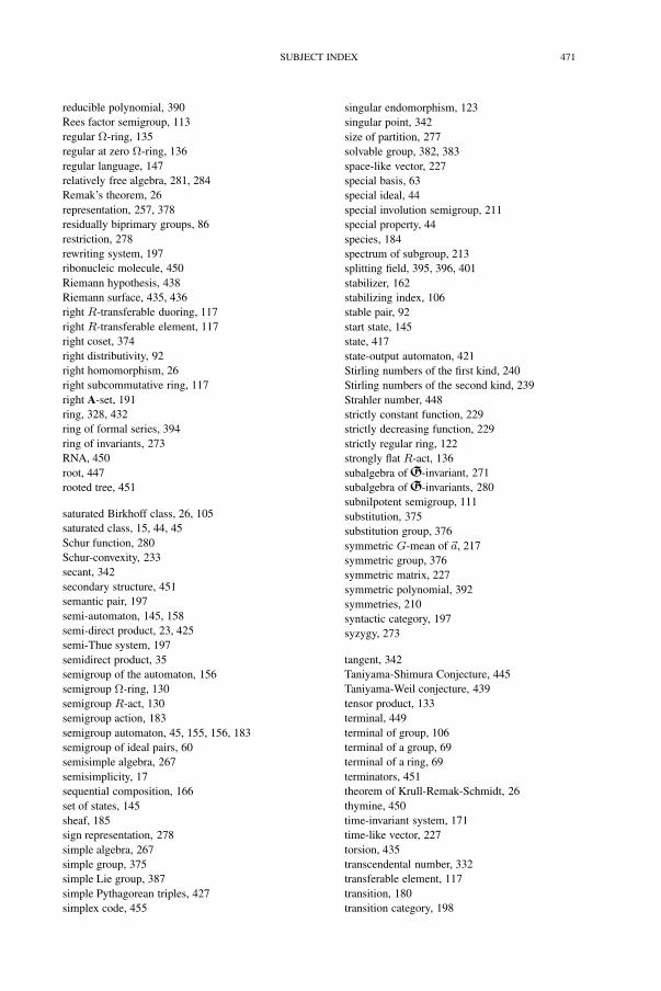
SUBJECT INDEX 471
reducible polynomial, 390Rees factor semigroup, 113regular Ω-ring, 135regular at zero Ω-ring, 136regular language, 147relatively free algebra, 281, 284Remak’s theorem, 26representation, 257, 378residually biprimary groups, 86restriction, 278rewriting system, 197ribonucleic molecule, 450Riemann hypothesis, 438Riemann surface, 435, 436right R-transferable duoring, 117right R-transferable element, 117right coset, 374right distributivity, 92right homomorphism, 26right subcommutative ring, 117right A-set, 191ring, 328, 432ring of formal series, 394ring of invariants, 273RNA, 450root, 447rooted tree, 451
saturated Birkhoff class, 26, 105saturated class, 15, 44, 45Schur function, 280Schur-convexity, 233secant, 342secondary structure, 451semantic pair, 197semi-automaton, 145, 158semi-direct product, 23, 425semi-Thue system, 197semidirect product, 35semigroup of the automaton, 156semigroup Ω-ring, 130semigroup R-act, 130semigroup action, 183semigroup automaton, 45, 155, 156, 183semigroup of ideal pairs, 60semisimple algebra, 267semisimplicity, 17sequential composition, 166set of states, 145sheaf, 185sign representation, 278simple algebra, 267simple group, 375simple Lie group, 387simple Pythagorean triples, 427simplex code, 455
singular endomorphism, 123singular point, 342size of partition, 277solvable group, 382, 383space-like vector, 227special basis, 63special ideal, 44special involution semigroup, 211special property, 44species, 184spectrum of subgroup, 213splitting field, 395, 396, 401stabilizer, 162stabilizing index, 106stable pair, 92start state, 145state, 417state-output automaton, 421Stirling numbers of the first kind, 240Stirling numbers of the second kind, 239Strahler number, 448strictly constant function, 229strictly decreasing function, 229strictly regular ring, 122strongly flat R-act, 136subalgebra ofG-invariant, 271subalgebra ofG-invariants, 280subnilpotent semigroup, 111substitution, 375substitution group, 376symmetric G-mean of �a, 217symmetric group, 376symmetric matrix, 227symmetric polynomial, 392symmetries, 210syntactic category, 197syzygy, 273
tangent, 342Taniyama-Shimura Conjecture, 445Taniyama-Weil conjecture, 439tensor product, 133terminal, 449terminal of group, 106terminal of a group, 69terminal of a ring, 69terminators, 451theorem of Krull-Remak-Schmidt, 26thymine, 450time-invariant system, 171time-like vector, 227torsion, 435transcendental number, 332transferable element, 117transition, 180transition category, 198
472 SUBJECT INDEX
transition system, 198Travelling Salesman Problem, 212tree, 447triangular product, 15, 16, 24, 36, 103triangular product of automata, 172, 173trigger, 420triple product of semigroups, 27, 30trivial normal divisor, 375trivial representation, 277type, 275
universal cone, 184uridine, 450
value, 197variety, 26verbal function, 26verbatim, 38
Weierstrass addition theorem, 349weight of partition, 277weighted finite automaton, 180Weil’s conjecture, 438word accepted by the automaton, 418wreath product, 15, 23, 184wreath product construction, 203wreath product of actions, 159, 196wreath product of automata, 194wreath product of semigroup automata, 168, 196wreath product of the algebras, 66
Young diagram, 277
Zariski dimension, 3Zariski space, 3, 4Zariski topology, 12zeta-polynomial, 250zyzygy, 273
Related Documents