EASURING THE OUTPUT RESPONSES TO FISCAL OLICYygorodni/AG_fiscal_multiplier.pdf · MEASURING THE OUTPUT RESPONSES TO FISCAL POLICY Alan Auerbach Yuriy Gorodnichenko University of California,

MEASURING THE OUTPUT RESPONSES TO FISCAL POLICY

Alan Auerbach Yuriy Gorodnichenko

University of California, Berkeley

University of California, Berkeley

August 2010

Abstract A key issue in current research and policy is the size of fiscal multipliers when the economy is in recession. Using a variety of methods and data sources, we provide three insights. First, using regime-switching models, we estimate effects of tax and spending policies that can vary over the business cycle; we find large differences in the size of fiscal multipliers in recessions and expansions with fiscal policy being considerably more effective in recessions than in expansions. Second, we estimate multipliers for more disaggregate spending variables which behave differently in relation to aggregate fiscal policy shocks, with military spending having the largest multiplier. Third, we show that controlling for predictable components of fiscal shocks tends to increase the size of the multipliers.

This paper was presented at the NBER TAPES conference on Fiscal Policy, Varenna, June 14-16, 2010. We are grateful to Olivier Coibion, Lorenz Kueng, Alex Michaelides, Roberto Perotti, and participants in the UC Berkeley Departmental Seminar and the NBER/IGIER TAPES conference for comments and suggestions.

1. Introduction

The impact of fiscal policy on output and its components has long been a central part of fiscal

policy analysis. But, as has been made clear by the recent debate over the likely effects and

desired composition of fiscal stimulus in the United States and abroad, there remains an

enormous range of views over the strength of fiscal policy’s macroeconomic effects, the

channels through which these effects are transmitted, and the variations in these effects and

channels with respect to economic conditions. In particular, the central issue is the size of fiscal

multipliers when the economy is in recession.

Recent theoretical work by Christiano et al. (2009), Woodford (2010) and others

emphasizes that government spending may have a large multiplier when the nominal interest rate

is at the zero bound, which occurs only in recessions. These novel theoretical findings for

models where markets clear echo earlier Keynesian arguments that government spending is

likely to have larger expansionary effects in recessions than in expansions. Intuitively, when the

economy has slack, expansionary government spending shocks are less likely to crowd out

private consumption or investment. To the extent discretionary fiscal policy is heavily used in

recessions to stimulate aggregate demand, the key empirical question is how the effects of fiscal

shocks vary over the business cycle. The answer to this question is not only interesting to

policymakers in designing stabilization strategies but it can also help the economics profession

to reconcile conflicting predictions about the effects of fiscal shocks across different types of

macroeconomic models.

Despite these important theoretical insights and strong demand by the policy process for

estimates of fiscal multipliers, there is little, if any, empirical research trying to assess how the

size of fiscal multiplies varies over the business cycle. In part, this dearth of evidence reflects

2

the fact that much of empirical research in this area is based on linear structural vector

autoregressions (SVARs) or linearized dynamic stochastic general equilibrium (DSGE) models

which by construction rule out state-dependent multipliers.1 The limitations of these two

approaches became evident during the recent policy debate in the United States, when

government economists relied on neither of these approaches, but rather on more traditional

large-scale macroeconometric models, to estimate the size and timing of U.S. fiscal policy

interventions being undertaken then (e.g., Romer and Bernstein 2009, Congressional Budget

Office 2009). This reliance on a more traditional approach, in turn, led to criticisms based on

conflicting predictions which used SVAR and DSGE approaches (e.g., Barro and Redlick, 2009,

Cogan et al., 2009, Leeper et al., 2009). Thus, a main objective of this paper is to explore this

gray area and to provide estimates of state-dependent fiscal multipliers.

Our starting point is the classic paper by Blanchard and Perotti (2002), which estimated

multipliers for government purchases and taxes on quarterly US data with the identifying

assumptions that (1) discretionary policy does not respond to output within a quarter; (2) non-

discretionary policy responses to output are consistent with auxiliary estimates of fiscal output

elasticities; (3) innovations in fiscal variables not predicted within the VAR constitute

unexpected fiscal policy innovations; and (4) fiscal multipliers do not vary over the business

cycle. These multipliers are still commonly cited, although subsequent research has questioned

whether the innovations in these SVARs really represent unanticipated changes in fiscal policy,

1 Alternative identification approaches, notably the narrative approach of Ramey and Shapiro (1998) and Romer and Romer (2010), rely instead on published information about the nature of fiscal changes. But while the narrative approach offers a potentially more convincing method of identification, it imposes a severe constraint on its own, that the effects of only a very specific class of shocks can be evaluated (respectively, military spending build-ups and tax changes unrelated to short-term considerations such as recession or the need to balance spending changes). Furthermore, the narrative approach tends to provide qualitative assessments of the effects of fiscal policy shocks while policymakers are most interested in quantitative estimates of the effects. Romer and Romer (2010) and Ramey (2009) are exceptions that provide quantitative estimates of fiscal multipliers.

3

the challenge relating both to expectations and to whether the changes in fiscal variables

represent actual changes in policy, rather than other changes in the relationship between fiscal

variables and the included SVAR variables.

Building on Blanchard and Perotti (2002) and the subsequent studies, our paper extends

the existing literature in three ways. First, using regime-switching SVAR models, we estimate

effects of tax and spending policies that can vary over the business cycle.2 We find large

differences in the size of fiscal multipliers in recessions and expansions with fiscal policy being

considerably more effective in recessions than in expansions. Second, to measure the effects for

a broader range of policies, we estimate multipliers for more disaggregate spending variables,

which often behave quite differently in relation to aggregate fiscal policy shocks. Third, we

provide a more precise measure of unanticipated shocks to fiscal policy. Specifically, we have

collected and converted into electronic form the quarterly forecasts of fiscal and aggregate

variables from the University of Michigan’s RSQE macroeconometric model. We also use

information from the Survey of Professional Forecasters (SPF) and the forecasts prepared by the

staff of the Federal Reserve Board (FRB) for the meetings of the Federal Open Market

Committee (FOMC). We include these forecasts in the SVAR to purge fiscal variables of

“innovations” that were predicted by professional forecasters. We find that the forecasts help

explain a considerable share of the fiscal innovations, and that controlling for this increases the

size of estimated multipliers in recession.

The next section of the paper lays out the basic specification of our regime-switching

model. Section 3 presents basic results for this model for aggregate spending and taxes. Section

2 We prefer introducing regime switches in a SVAR rather than in a DSGE model since it is difficult to model slack in the economy and potentially non-clearing markets in a DSGE framework without imposing strong assumptions regarding the behavior of households and firms. In contrast, SVAR models require fewer identifying assumptions and thus are tied more easily to empirical reality.

4

4 provides results for individual components of spending and Section 5 develops and presents

results for our method of controlling for expectations. Section 6 concludes.

2. Econometric specification

To allow for responses differentiated across recessions and expansions, we employ a regime

switching vector autoregression where transitions across states (i.e., recession and expansion) are

smooth. Our estimation approach, which we will call STVAR, is similar to smooth transition

autoregressive (STAR) models developed in Granger and Teravistra (1993). One important

difference between STAR and our STVAR, however, is that we allow not only differential

dynamic responses but also differential contemporaneous responses to structural shocks.

The key advantage of STVAR relative to estimating SVARs for each regime separately is

that with the latter we may have relatively few observations in a particular regime – especially

for recessions – which makes estimates unstable and imprecise. In contrast, STVAR effectively

utilizes more information by exploiting variation in the degree (which sometimes can be

interpreted as the probability) of being in a particular regime so that estimation and inference for

each regime is based on a larger set of observations. Note that, to the extent we estimate

properties of a given regime using in part dynamics of the system in another regime, we bias our

estimates towards not finding differential fiscal multipliers across regimes.

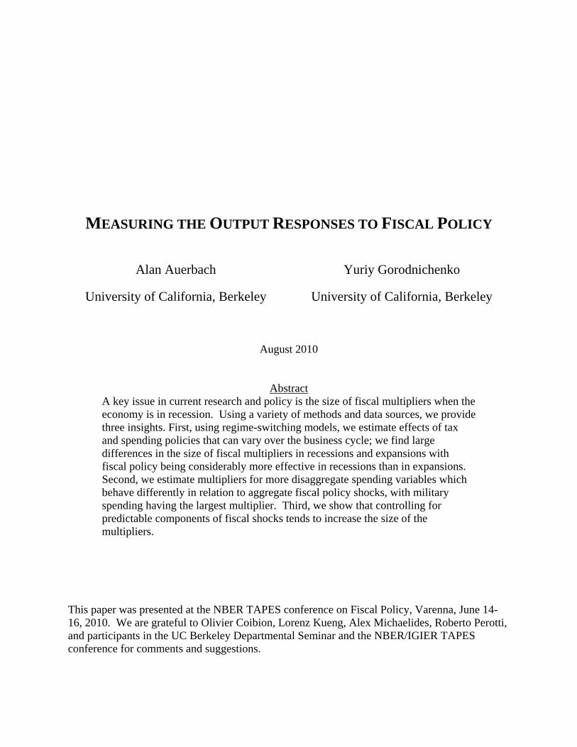
Our basic specification is:

1 (1)

~ 0, Ω (2)

Ω Ω 1 Ω (3)

, 0 (4)

1, 0 (5)

5

As in Blanchard and Perotti (2002), we estimate the equation using quarterly data and set

in the basic specification where G is log real government (federal, state, and

local) purchases (consumption and investment)3, T is log real government receipts of direct and

indirect taxes net of transfers to businesses and individuals, and Y is log real gross domestic

product (GDP) in chained 2000 dollars.4,5 This ordering of variables in Xt means that shocks in

tax revenues and output have no contemporaneous effect on government spending. As argued in

Blanchard and Perotti (2002), this identifying minimum-delay assumption may be a sensible

description of how government spending operates because in the short run government may be

unable to adjust its spending in response to changes in fiscal and macroeconomic conditions.

The model allows two ways for differences in the propagation of structural shocks: a)

contemporaneous via differences in covariance matrices for disturbances Ω and Ω ; b) dynamic

via differences in lag polynomials and .6 Variable z is an index (normalized to have

unit variance so that is scale invariant) of the business cycle, with positive z indicating an

expansion. Adopting the convention that 0, we interpret Ω and as describing the

behavior of the system in a (sufficiently) deep recession (i.e., 1) and Ω and as

describing the behavior of the system in a (sufficiently) strong expansion (i.e., 1 1).

3 We use the traditional approach of defining G to include direct consumption and investment purchases, which excludes the imputed rent on government capital stocks. While the current U.S. method of constructing the national accounts now includes imputed rent, this was not the case for most of our sample period. Although the historical national accounts have been revised to conform to the new approach, we cannot do this for our series of professional forecasts. Therefore, we utilize the traditional method of measuring G in order to have series that are consistent over time. 4 To compute G and T, we apply the GDP deflator to nominal counterparts of G and T. We estimate the equations in log levels in order to preserve the cointegrating relationships among the variables. An alternative but more complex approach would be to estimate the equations in differences and include error correction terms. 5 We find similar results when we augment this VAR with variables capturing the stance of monetary policy. 6 The number of lags is chosen by Akaike Information Criterion.

6

We date the index z by t-1 to avoid contemporaneous feedbacks from policy actions into whether

the economy is in a recession or an expansion.

The choice of index z is not trivial because there is no clear-cut theoretical prescription

for what this variable should be. We set z equal to a seven-quarter moving average of the output

growth rate. The key advantages of using this measure of z are: i) we can use our full sample for

estimation, which makes our estimates as precise and robust as possible; ii) we can easily

consider dynamic feedbacks from policy changes to the state of the regime (i.e., we can

incorporate the fact that policy shocks can alter the regime).7

Although it is possible, in principle, to estimate , , Ω , Ω and

simultaneously, identification of relies on nonlinear moments and hence estimates may be

sensitive to a handful of observations in short samples. Granger and Teravistra (1993) suggest

imposing fixed values of and then using a grid search over to ensure that estimates for

, , Ω , Ω are not sensitive to changes in . We calibrate 1.5 so that the

economy spends about 20 percent of time in a recessionary regime (that is, Pr 0.8

0.2) where we define an economy to be in a recession if 0.8.8 This calibration is

consistent with the duration of recessions in the U.S. according to NBER business cycle dates

(21 percent of the time since 1946). Figure 1 compares the dynamics of with recessions

identified by the NBER.

7 We also considered, as an alternative, the Stock and Watson (1989) coincident index of the business cycle (now maintained by the Federal Reserve Bank of Chicago and called Chicago Fed National Activity Index). This series dates only to the mid-1960s and cannot be used for endogenous-regime multiplier calculations, but a potential benefit is that it incorporates more information than the growth rate of real GDP. However, our alternative estimates using this index (not shown) suggest that the choice between the two definitions of z does not have a qualitatively important impact on our empirical results. 8 When we estimate , , Ω , Ω and simultaneously, we find point estimates for to be above 5 to 10 depending on the definitions of variables and estimation sample. These large parameter estimates suggest that the model is best described as a model switching regimes sharply at certain thresholds. However, we prefer smooth transitions between regimes (which amounts to considering moderate values of ) because in some samples we have only a handful of recessions and then parameter estimates for , , Ω , Ω become very imprecise.

7

Given the highly non-linear nature of the system described by equations (1)-(5), we use

Monte Carlo Markov Chain methods developed in Chernozhukov and Hong (2003) for

estimation and inference (see the Appendix for more details). Under standard conditions, this

approach finds a global optimum in terms of fit. Furthermore, the parameter estimates as well as

their standard errors can be computed directly from the generated chains.

When we construct impulse responses to government spending shocks in a given regime,

we initially ignore any feedback from changes in z into the dynamics of macroeconomic

variables.9 In other words, we assume that the system can stay for a long time in a regime. The

advantage of this approach is that, once a regime is fixed, the model is linear and hence impulse

responses are not functions of history (see Koop et al. (1996) for more details). However, we do

consider later the effect of incorporating changes in z as part of the impulse response functions,

recomputing z consistently with the predicted changes in output.

Most of the impulse response functions and multipliers we present below are for changes

in government purchases, G, and its components. We will also present some results for changes

in taxes, but we have several reasons for focusing on G. First, much of the debate in the SVAR

and DSGE literatures has been about the effects of government purchases. Second, we are less

confident of the SVAR framework as a tool for measuring the effects of tax policy, because (as

discussed above) many of the unexpected changes in T may not arise as a result of a policy

change, and because we would expect the effects of tax policy to work through the structure of

taxation (e.g. marginal tax rates) rather than simply through the level of tax revenues. Finally,

our identification of tax shocks depends on our ability to purge innovations in revenues of

automatic responses to output. In attempting to do so, we follow Blanchard and Perotti (2002) in

9 Alternatively, one can interpret this approach as ordering z last in the VAR and setting all z to a fixed value.

8

using auxiliary information on the elasticity of revenue with respect to output, but it is possible

that this elasticity varies over the cycle, thereby introducing a bias of unknown magnitude and

direction in our regime-specific estimates.

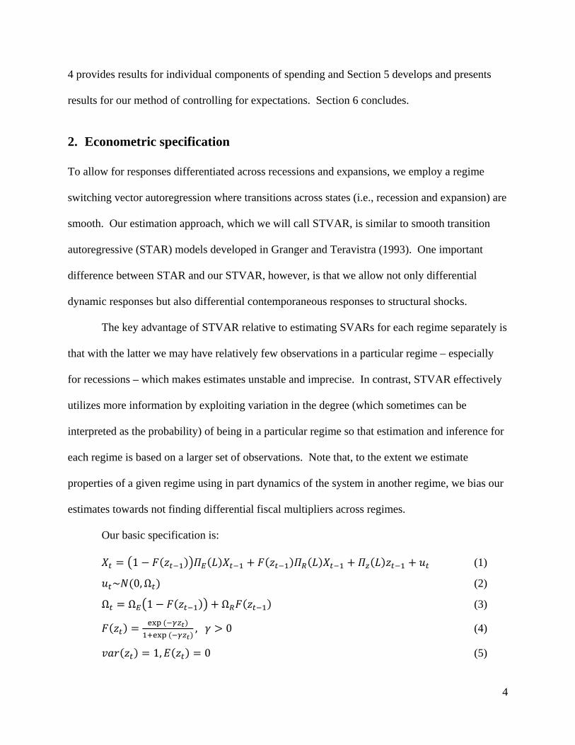
3. Basic Aggregate Results

We begin by considering the effects of aggregate government purchases in the linear model with

no regime shifts or control for expectations, following the basic specification of Blanchard and

Perotti (2002), including the same ordering for the Cholesky decomposition and the

control for the automatic tax response to contemporaneous output shocks (an elasticity of 2.08).

Our sample period is 1947:1—2009:2. Figure 2 displays, in three panels, the resulting impulse

response functions (IRFs) for a government purchase shock. These multipliers demonstrate by

how many dollars output, taxes, and government purchases increase over time when government

purchases are increased by $1.10 In this and all subsequent figures, the shaded bands around the

impulse response functions are 90 percent confidence intervals.11 Consistent with results

reported in previous studies (see, for example, the survey by Hall, 2009), the maximum size of

the government spending multiplier in the linear VAR model is about 1 and this maximum effect

of a government spending shock on output is achieved after a short delay. The response of future

government purchases also peaks after a short delay, indicating that the typical government

spending shock during the sample period is of relatively short duration. Taxes fall slightly in

response to the increase in government purchases. This fall in taxes may contribute to the

positive impact on output that persists even as the increase in government purchases dies off over

time. 10 Because government purchases and output enter the estimated equations in logs, we scale the estimated IRFs by the sample average values of Y/G to convert percent changes into dollar changes. 11 The Appendix discusses our method of estimating these confidence intervals.

9

The next two figures plot the corresponding IRFs in expansions (Figure 3) and recessions

(Figure 4). Because of the smaller effective number of observations for each regime, particularly

for recessions, the confidence bounds are greater for these IRFs than for those for the linear

model in Figure 2. Even with these wide bands, however, the responses in recession and

expansion are quite different. In both regimes, the impact output multiplier is about 0.5, slightly

below that estimated for the linear model. Over time, though, the IRFs diverge, with the

response in expansions never rising higher and soon falling below zero, while the response in

recessions rises steadily, reaching a value of over 2.5 after 20 quarters. The strength of this

output response in recession is not attributable simply to differences in the permanence of the

spending shock or the tax response. Taxes actually rise in recession, while falling in expansion.

This difference, which is consistent with the automatic responses of tax collections to changes in

output, should weaken the differences in the observed output responses in recession and

expansion; and while the government spending shock is more persistent in recession, it is

stronger in the short run in expansion.12

To put the magnitudes of these multipliers in perspective, consider multipliers in

Keynesian models as well as the more recent DSGE literature. Traditional Keynesian (IS-LM-

AS) models usually have large multipliers since the size of the multiplier is given by 1/ 1

where is the marginal propensity to consume which is typically quite large (about

0.5-0.9).13 To the extent that the AS curve in the IS-LM-AS model is upward sloping, the

multiplier can vary from relatively large (the AS curve is flat and there is a great deal of slack in

12 Note that the contemporaneous responses of output to a shock in government spending are similar in recessions and expansions. This result suggests that the differences in the magnitudes of the multipliers across regimes are driven by the differences in the dynamics (i.e., , ) rather than in the covariance of error terms (i.e., Ω , Ω ).

13 For example, Shapiro and Slemrod (2003) and Johnson et al..(2006) report that the marginal propensity to consume out of (small) tax rebates in 2001 EGTRRA was somewhere between in 0.5 and 0.7.

10

the economy; i.e., in a recession) to relatively small (the AS curve is steeply upward sloping and

the economy operates at full capacity; i.e., in an expansion). In contrast, an increase in

government spending in modern business cycle models usually leads to a large crowding out of

private consumption in recessions and expansions and correspondingly the typical magnitude for

the multiplier is less than 0.5 (in many cases much smaller). Recent findings from DSGE models

with some Keynesian features (e.g., Christiano et al. 2009, Eggertsson 2008, and Woodford

2010), however, suggest that the government spending multiplier in periods with a binding zero

lower bound on nominal interest rates (which are recessionary times) could be somewhere

between 3 and 5. Intuitively, with the binding zero lower bound, increases in government

spending have no effect on interest rates and thus there is no crowding out of investment or

consumption, which leads to large multipliers.

In short, our estimates of the government spending multiplier in recessions and

expansions are largely consistent with the theoretical arguments in both (old) Keynesian and

(new) modern business cycle models. Table 1 summarizes these output multipliers for the cases

just considered, as well as those that follow. The table presents multipliers measured in two

ways. The first column gives the maximum impact on output (with standard errors in the second

column) and the third column (with standard errors in the fourth column) shows the ratio of the

sum of the Y response (to a shock in G) to the sum of G response (to a shock in G). The first

measure of the fiscal multiplier has been widely used since Blanchard and Perotti (2002). The

second measure has been advocated by Woodford (2010) and others since the size of the

multiplier depends on the persistence of fiscal shocks. Regardless of which way we compute the

multiplier, it is much larger in recessions than in expansions.

11

One might guess that the differences between our regime-based multipliers are

exaggerated by our assumptions that the regimes themselves don’t change. That is, if the

multiplier is smaller in expansion than in recession and the economy has a positive probability of

shifting from recession to expansion in future periods, then the actual multipliers starting in

recession (or expansion) should be a blend of those estimated for the separate regimes.

Calculating full dynamic impulse response functions that include internally consistent regime

shifts is complicated, because we must compute the index z and evaluate the function F(z) at

each date along the trajectory. Also, because the IRFs are now nonlinear, they will depend on

the initial value of the index z and the size of the government policy shock. For example, the

more deep the initial recession, and the less positive the spending shock, the less important future

regime shifts out of recession will be. Therefore, we must specify the initial conditions and the

size of the policy experiment in order to estimate the dynamic IRFs.

Figure 5 presents estimates for the historical effects of shocks to government purchases

on output, incorporating regime shifts in response to government spending shocks. For each

period, we consider a policy shock equal to one percent increase in G and report a dollar increase

in output per dollar increase in government spending over 20 quarters (i.e., ∑ /∑ ).

The size of the multiplier varies considerably over the business cycle. For example in 1985, an

increase in government spending would have barely increased output. In contrast, a dollar

increase in government spending in 2009 could raise output by about $1.75. Typically, the

multiplier is between 0 and 0.5 in expansions and between 1 and 1.5 in recessions. Note the size

of the multiplier tends to change relatively quickly as the economy starts to grow after reaching a

trough. Thus, the timing of changes in discretionary government spending is critical for

effectiveness of countercyclical fiscal policies.

12

Bearing in mind caveats we have discussed above, we turn now to the effects of taxes on

output. Figures 6-8 are comparable to Figures 2-4 for government purchases, with Figures 6-8

showing the IRFs for output, spending and taxes in response to a tax increase for each of the

three regimes, with confidence bands. As with government purchases, the results for taxes in the

linear model are consistent with the past results in the SVAR literature. From an initial impact of

-0.2, the effect on output grows in strength over time, reaching -1.0 by the end of five years,

which is similar to results reported in Blanchard and Perotti (2002).14 In contrast to the case of

spending shocks, however, the IRFs for the expansion and recession regimes do not bracket

those for the linear case. In both regimes, the output effects are less negative. They are, in fact,

generally positive in the recession regime. However, this response is sensitive to using

alternative measures of the elasticity of tax revenue with respect to output and one can obtain

negative responses of Y to a shock in T if the elasticity in recessions is larger than the elasticity

estimated in Blanchard and Perotti (2002).

The results for the expansion regime may be understood by observing that the responses

of government purchases to a tax increase are much more positive in expansions than in the

linear model. This increase in G is what can cause a less negative impact on output in

expansions. In recessions, the output response is more puzzling; subsequent tax increases are

stronger and government spending increases weaker, at least initially, than in expansions, and yet

the output effects of an initial tax increase are positive. Presumably, the stronger subsequent tax

increases reflect, at least in part, the automatic responses of tax collections to higher output. But

14 Romer and Romer (2010) report larger multipliers (-3) for changes in tax revenue. After a series of methodological refinements (e.g., use changes in tax receipts rather than tax liabilities, formal statistical criteria to choose the length of lag polynomials, more precise timing of the shocks) and using the same approach, Perotti (2010) finds multipliers to be approximately -1.5.

13

the overall pattern still suggests that the underlying effect on output of the initial tax increase is

quite positive, a result for which we can offer no obvious explanation.

4. Results for Components of Spending

Just as output multipliers for government purchases differ according to the regime in which they

occur, they also differ for different components of government purchases. As discussed earlier,

studies using the narrative approach tend to focus on military build-ups, but how useful are these

shocks to defense spending in analyzing the effects of other changes in spending policies, such as

those adopted during the recent recession?

Figure 9 shows that IRFs for output in response to defense and non-defense spending

shocks, based on a four-variable VAR including defense and non-defense purchases, as well as

output and taxes. We order the Cholesky decomposition with defense spending first and non-

defense spending second, although this does not have an important effect on the results.15

Clearly, the IRFs have different shapes for the linear model. For a unit shock to defense

spending, output rises immediately by just over 1, which is consistent with Ramey (2009), and

then gradually falls, becoming negative after several quarters. For non-defense spending, the

output effect starts smaller but eventually exceeds 1 and remains above 0.6 for the entire period

shown. Once the results are broken down by regime, however, we can see a much stronger

dependence on the regime of the defense spending IRFs, which are similar to the linear-model

results for the case of expansion but much more positive in recession, peaking at nearly 4 in the

fifth quarter after the shock. For non-defense spending, on the other hand, the differences

15 Further details regarding confidence intervals and the effects on taxes and spending components are provided in the Appendix in Figures A1-A6.

14

between regimes are primarily with respect to timing rather than size, with the most positive

responses occurring rapidly in expansions but with several quarters’ delay in recessions.

Figure 10 shows the results of an experiment that breaks government purchases down in a

different way, into consumption and investment spending, with consumption ordered first.16

Once again, the results differ considerably by regime and by spending component. In this

decomposition, both components of spending have positive effects on output in the linear model,

although the effects of investment spending are much stronger, particularly during the first few

quarters when the impact on output exceeds 2 for investment but is around 0.5 for consumption.

Estimating the IRFs separately for recession and expansion leads in general to the expected result

of more positive multipliers in recession than in expansion. The IRFs are also noisier for the

separate regimes, indicating an imprecision of these point estimates that is consistent with the

larger confidence intervals (see Appendix figures).

5. Controlling for Expectations

As emphasized by Ramey (2009) and others, the timing of fiscal shocks plays a critical role in

identifying the effect of fiscal shocks. In spirit of Ramey (2009), we control for expectations not

already absorbed by the VAR using real-time professional forecasts from three sources. First,

we draw forecasts for output and government spending variables from the Survey of Professional

Forecasters (SPF), an average of forecasts (with the number of individual forecasters ranging

from 9 to 50) available since 1968 for GDP and since 1982 for government spending and its

components. Second, for government revenues, we use the University of Michigan RSQE

16 Appendix Figures A7-A12 provide further details of this experiment.

15

econometric model, for which forecasts are available for the period beginning in 1982.17 Third,

we use government spending (Greenbook) forecasts prepared by the FRB staff for FOMC

meetings. The Greenbook forecasts for government spending are available from 1966 to 2004.

Since the FOMC meets 8 or 12 times a year in our sample, we take Greenbook forecasts

prepared for the meeting which is the closest to the middle of the quarter to make it comparable

to SPF forecasts. Since the properties of the Greenbook and SPF forecasts are similar, we splice

the Greenbook and SPF government spending forecasts and construct a continuous forecast

series running from 1966 to present. For each variable, we use the forecast made in period t-1

for the period-t value. Because there have been numerous data revisions in the National Income

and Product Accounts since the dates of these forecasts, we use forecast growth rates rather than

levels.

The importance of controlling for expectations is illustrated in Figure 11, which plots the

residuals from projecting forecasted and actual growth rates of government spending on lags of

the variables in our baseline VAR.18 If the VAR innovations were truly unexpected, then these

two residuals would be unrelated, but the correlation between forecasted and actual growth rates

of government spending (net of the information contained in the VAR lags) is about 0.3-0.4

which points to conclusion that a sizable fraction of VAR innovations is predictable. Therefore,

one should be interested in using refined measures of unanticipated shocks to government

spending.

The simplest way to account for these forecastable components of VAR residuals is to

expand the vector X to include professional forecasts. That is, if we let the

17 The University of Michigan data are coded from hard copies. Hard copies of forecasts prior to 1982 were lost that year in the fire that destroyed that university’s Economics Department building. 18 The figure presents two versions of this plot, with similar results, one relating forecast residuals to VAR residuals based on real-time data, the other to VAR residuals based on final-vintage data.

16

SPF/Greenbook/RSQE forecasts made at time t-1 for the growth rate of real government

purchases for time t be denoted ∆ | (where ∆ | is the growth rate of government spending

G at time s forecasted at time t) and define the professional forecasts for output and taxes the

same way, we would use the expanded vector in equation (1) ∆ | ∆ | ∆ | ,

stacking the forecasts first because by the timing there is no contemporaneous feedback from

unanticipated shocks at time t to forecasts made at time t-1.19 This direct approach is attractive

because it accounts automatically for any effects that expectations might have on the aggregate

variables and for the determinants of the expectations themselves. In practice, however, we have

found this approach to be too demanding given our data limitations, for it doubles the number of

variables in the VAR while eliminating more than half of the observations in our sample (i.e.,

those before 1982); the resulting confidence intervals are very large, particularly for the

recession regime for which we have effectively fewer observations.20,21

We consider two alternative approaches. The first alternative is a two-step process. The

first step of this process is to create “true” innovations by subtracting forecasts of the vector Xt

from Xt itself. We then fit Ω Ω 1 Ω (i.e., equation (3)) using these

forecast errors (rather than the residuals from the VAR itself). From this step, we use estimated

Ω and Ω to construct contemporaneous responses to shocks in expansions and recessions. The

second step involves using the previously-estimated baseline VAR with regime switches. In this

step, we use the estimated coefficients Π and Π to map the propagation of

19 See Leduc et al. (2007) for a more detailed discussion on the ordering. 20 We do consider a more restricted version of this approach shortly, in which we add a series on defense spending innovations available for our full sample directly to the VAR. 21 Mertens and Ravn (2010) distinguish anticipated and unanticipated shocks in a VAR by using long-run restrictions combined with calibration. We do not use this strategy in part because with regime switches we cannot distinguish long-run responses in expansions and recessions.

17

contemporaneous responses created in the first step. This two-step approach has the advantage

of allowing us to base the VAR on our full sample and the original number of variables. Its main

disadvantage is that the IRF dynamics will not necessarily be correct, given that the VAR is

estimated under the assumption that the innovations to X are fully unanticipated.

The second alternative approach is to augment the baseline VAR directly, but with only

one variable, pertaining to the forecast of government spending. For example, the vector of

variables in the VAR could be ∆ | or where is

the forecast error for the growth rate of government spending or some other measure of news

about government spending. In the former specification, an innovation in orthogonal to

∆ | is interpreted as an unanticipated shock. In the latter specification, an innovation in the

forecast error or news about government spending is interpreted as an unanticipated shock. The

key advantage of this approach is that, with sufficiently long series, we can have a VAR of a

manageable size and yet we can remove directly a predictable component from government

spending innovations.

With these alternative approaches and specifications, unanticipated shocks to government

spending of a given initial size will lead to differing government spending responses over time.

To make IRFs comparable, we normalize the size of the unanticipated government spending

shock so that the integral of a government spending response over 20 quarters is equal to one.

Therefore the interpretation of the fiscal multipliers is similar to the second column in Table 1.

Figure 12 shows the IRFs for different approaches and specifications and contrasts these results

with the results for the baseline specification (1)-(5) that does not control for the predictable

component in government spending innovations. Table 1 reports the maximum and average

multipliers along with associated standard errors.

18

Panel A (Figure 12) presents IRFs for the first approach. The results suggest that

controlling for expectations increases the absolute magnitudes of the government spending

multipliers, making them more positive in recessions and more negative in expansions. Panel B

(Figure 12) shows results for the second approach with ∆ | where ∆ |

is the spliced Greenbook/SPF forecast series for the growth rate of government spending. In this

specification, which is estimated on the 1966-2009 sample, the multiplier in the recession regime

is a notch larger than in the baseline model while the multiplier in the expansion regime stays

positive but small which contrasts with the baseline model where the multiplier turns negative at

long horizons. Panel C (Figure 12) shows results for the second approach with

where is the forecast error computed as the difference between spliced

Greenbook/SPF forecast series and actual, first-release series of the government spending growth

rate.22 In this specification, an unanticipated shock to government spending in an expansion has

an effect on output similar to the effect we find in the baseline model. In a recession, however,

the multiplier could be larger than in the baseline model, especially at short horizons. By and

large, these results suggest that the government spending multiplier in recessions increases and

the multiplier in expansions does stay close to zero when we purify government spending shocks

from predictable movements.

Finally, we use spending news constructed in Ramey (2009) to control for the timing of

fiscal shocks (Panel D, Figure 12). Specifically, we augment the baseline VAR with Ramey’s

spending news series, which is ordered first in this new VAR. The key advantage of using

Ramey’s series is that, in contrast to forecast series, it covers the whole post-WWII sample and

thus our estimates are more precise. A limitation of Ramey’s unanticipated shocks is that these

22 An advantage of using real-time data to compute forecast errors is that it makes forecasts and actual series refer to the same concept of government spending.

19

shocks refer only to military spending. However, since changes in military spending account for

a large share of variation in total government spending, Ramey’s shocks are informative for our

analysis. Panel D shows that although controlling for spending news does not materially affect

output responses during expansions, there are some important differences during recessions. In

particular, the multiplier on impact is about 2 in response to an unanticipated shock and the

average multiplier over 20 quarters is 3.7. In contrast, the baseline VAR specification reports the

impact multiplier of 0.8 and the average multiplier of 2.2. We view these findings as

corroborating our other evidence on the importance of constructing unanticipated fiscal shocks,

which tend to have larger effects on output in recessions.

6. Concluding remarks

Our findings suggest that all of the extensions we developed in this paper – controlling for

expectations, allowing responses to vary in recession and expansion, and allowing for different

multipliers for different components of government purchases – all have important effects on the

resulting estimates. In particular, policies that increase government purchases have a much

larger impact in recession than is implied by the standard linear model, even more so when one

controls for expectations, which is clearly called for given the extent to which independent

forecasts help predict VAR policy “shocks.”

While we have extended the SVAR approach, our analysis still shares some of the

limitations of the previous literature. We have allowed for different economic environments, but

there may be still other important differences among historical episodes that we lump together,

for example recessions, such as the recent one, associated with financial market disruptions and

very low nominal government interest rates, and other recessions induced by monetary

contractions (such as the one in the early 1980s). Our predictions are also tied to historical

20

experience concerning the persistence of policy shocks, and therefore may not apply to policies

either less or more permanent. The effects of taxes, even if purged of expected changes, are still

probably too simple as they fail to take account of the complex ways in which structural tax

policy changes can influence the economy. And, finally, as we enter a period of unprecedented

long-run budget stress, the U.S. postwar experience, or even the experience of other countries

that have dealt with more acute budget stress23, may not provide very accurate forecasts of future

responses.

These limitations of our analysis should motivate future theoretical work to develop

realistic DSGE models with potentially nonlinear features to understand more deeply the forces

driving differences in the size of fiscal multipliers over the business cycle, the role of

(un)anticipated shocks for fiscal multipliers in these environments, and implications of levels of

government debt for the potency of discretionary fiscal policy to stabilize the economy.

23 See, for example, Perotti (1999) and Ardagna (2004).

21

References

Ardagna, Silvia. 2004. “Fiscal Stabilizations: When Do They Work and Why?” European Economic Review 48(5), 1047-1074.

Barro, Robert J. and Charles J. Redlick. 2009. “Macroeconomic Effects from Government Purchases and Taxes,” NBER Working Paper 15369.

Blanchard, Olivier, and Roberto Perotti. 2002. “An Empirical Characterization of the Dynamic Effects of Changes in Government Spending and Taxes on Output,” Quarterly Journal of Economics 117(4), 1329-1368.

Chernozhukov, Victor, and Han Hong. 2003. “An MCMC Approach to Classical Estimation,” Journal of Econometrics 115(2), 293-346.

Christiano, Lawrence, Martin Eichenbaum, and Sergio Rebelo. 2009. “When is the government spending multiplier large?” NBER Working Paper 15394.

Cogan, John F., Tobias Cwik, John B. Taylor, and Volker Wieland. 2009. “New Keynesian versus Old Keynesian Government Spending Multipliers,” NBER Working Paper 14782.

Congressional Budget Office. 2009. “Estimated Macroeconomic Impacts of the American Recovery and Reinvestment Act of 2009,” March 2.

Eggertsson, Gauti B. 2008. “Can Tax Cuts Deepen Recessions?” Federal Reserve Bank of New York, December.

Gelman, Andrew, John B. Carlin, Hal S. Stern, and Donald B. Rubin. 2004. Bayesian Data Analysis, Chapman and Hall/CRC.

Granger, Clive W., and Timo Terasvirta. 1993. Modelling Nonlinear Economic Relationships. Oxford University Press.

Hall, Robert E. 2009. “By How Much Does GDP Rise If the Government Buys More Output?” Brookings Papers on Economic Activity, Fall, 183-231.

Hamilton, James D. 1994. Time Series Analysis. Princeton University Press.

Johnson, David S., Jonathan A. Parker and Nicholas S. Souleles. 2006. “Household Expenditure and the Income Tax Rebates of 2001,” American Economic Review 96(5), 1589–1610.

Koop, Gary, M. Hashem Pesaran, and Simon M., Potter. 1996. “Impulse Response Analysis in Nonlinear Multivariate Models,” Journal of Econometrics 74(1), 119-147.

Leduc, Sylvain, Keith Sill, and Tom Stark. 2007. “Self-fulfilling expectations and the inflation of the 1970s: Evidence from the Livingston Survey,” Journal of Monetary Economics 54(2), 433-459.

22

Leeper, Eric M., Todd B. Walker, and Shu-Chun Susan Yang. 2009. “Government Investment and Fiscal Stimulus in the Short and Long Runs,” NBER Working Paper 15153.

Mertens, Karel, and Morten O. Ravn. 2009. “Understanding the Aggregate Effects of Anticipated and Unanticipated Tax Policy Shocks,” manuscript.

Mertens, Karel, and Morten O. Ravn. 2010. “Measuring the Impact of Fiscal Policy in the Face of Anticipation: A Structural VAR Approach,” Economic Journal 120 (May), 393–413

Perotti, Roberto. 1999. “Fiscal Policy in Good Times and Bad,” Quarterly Journal of Economics 114(4), 1399-1436.

Perotti, Roberto. 2010. “The Effects of Tax Shocks: Negative and Large,” manuscript.

Ramey, Valerie A. 2009. “Identifying Government Spending Shocks: It’s All in the Timing,” NBER Working Paper 15464.

Ramey, Valerie A. and Matthew Shapiro. 1997. “Costly Capital Reallocation and the Effects of Government Spending,” Carnegie-Rochester Conference on Public Policy 48, June, 145-194.

Romer, Christina, and Jared Bernstein. 2009. “The Job Impact of the American Recovery and Reinvestment Plan,” Council of Economic Advisors, January 9.

Romer, Christina D., and David H. Romer. 2010. “The Macroeconomic Effects of Tax Changes: Estimates Based on a New Measure of Fiscal Shocks,” American Economic Review 100, 763–801.

Shapiro, Matthew D. and Joel Slemrod. 2003. “Consumer Response to Tax Rebates,” American Economic Review 93(1), 381-396.

Stock, James, and Mark Watson. 1989. “New indexes of coincident and leading economic indicators,” NBER Macroeconomics Annual 4, 351-409.

Woodford, Michael. 2010. “Simple Analytics of the Government Expenditure Multiplier,” NBER Working Paper 15714.

23

Appendix: Estimation procedure

The model is estimated using maximum likelihood methods. The log-likelihood for model (1)-

(5) is given by:

∑ | | ∑ (A1)

where 1 – .24 Since the model is highly

nonlinear and has many parameters Ψ , Ω , Ω , Π , Π , using standard optimization

routines is problematic and, thus, we employ the following procedure.

Note that conditional on , Ω , Ω the model is linear in lag polynomials

Π , Π . Thus, for a given guess of , Ω , Ω , we can estimate Π , Π with

weighted least squares where weights are given by and estimates of Π , Π must

minimize ∑ . Let

1 – … 1 –

be the extended vector of regressors and Π Π Π so that – and the objective

function is

∑ – – . (A2)

Note that we can rewrite (A2) as

∑ – – ∑ – –

∑ – – .

The first order condition with respect to is ∑ – 0.

Now using the vec operator, we get

∑ ∑ ∑

∑ ∑

which gives

∑ ∑ . (A3)

The procedure iterates on , Ω , Ω (which yields and the likelihood) until an optimum is

reached. Note that with a homoscedastic error term (i.e. Ω ), we recover standard VAR

estimates. 24 To simplify notation, we omit other controls in equation (1).

24

Since the model is highly non-linear in parameters, it is possible to have several local

optima and one must try different starting values for , Ω , Ω . To ensure that Ω and Ω are

positive definite, we use Ψ , Ω , Ω , Π , Π , where chol is the operator

for Cholesky decomposition. Furthermore, given the non-linearity of the problem, it may be

difficult to construct confidence intervals for parameter estimates as well as impulse responses.

To address these issues, we use a Markov Chain Monte Carlo (MCMC) method developed in

Chernozhukov and Hong (2003; henceforth CH). This method delivers not only a global

optimum but also distributions of parameter estimates.

We employ the Hastings-Metropolis algorithm to implement CH’s estimation method.

Specifically our procedure to construct chains of length N can be summarized as follows:

Step 1: Draw (n), a candidate vector of parameter values for the chain’s n+1 state, as

(n) = (n) + (n) where (n) is the current n state of the vector of parameter values in the

chain, (n) is a vector of i.i.d. shocks taken from N(0,), and is a diagonal matrix.

Step 2: Take the n+1 state of the chain as

ΨΘ with probability min 1, exp Θ Ψ

Ψ otherwise

where L((n)) is the value of the objective function at the current state of the chain and

L((n)) is the value of the objective function using the candidate vector of parameter

values.

The starting value (0) is computed as follows. We approximate the model in (1)-(5) so that the

model can be written as regressing on lags of , , . We take the residual from this

regression and fit equation (3) using MLE to estimate Ω and Ω . These estimates are used as

staring values. Given Ω and Ω and the fact that the model is linear conditional on Ω and Ω ,

we construct starting values for lag polynomials Π , Π using equation (A3).

The initial is calibrated to about one percent of the parameter value and then adjusted

on the fly for the first 20,000 draws to generate 0.3 acceptance rates of candidate draws, as

proposed in Gelman et al (2004). We use 100,000 draws for our baseline and robustness

estimates, and drop the first 20,000 draws (“burn-in” period). We run a series of diagnostics to

check the properties of the resulting distributions from the generated chains. We find that the

simulated chains converge to stationary distributions and that simulated parameter values are

consistent with good identification of parameters.

25

CH show that Ψ ∑ Ψ is a consistent estimate of under standard regularity

assumptions of maximum likelihood estimators. CH also prove that the covariance matrix of the

estimate of is given by ∑ Ψ Ψ var Ψ , that is the variance of the

estimates in the generated chain.

Furthermore, we can use the generated chain of parameter values Ψ to construct

confidence intervals for the impulse responses. Specifically, we make 1,000 draws (with

replacement) from Ψ and for each draw we calculate an impulse response. Since

columns of Ω and Ω in Ψ are identified up to sign, the generated chains

for Ω and Ω can change signs. Although this change of signs is not a problem

for estimation, it can sometimes pose a problem for the analysis of impulse responses. In

particular, when there is a change of signs for the entries of Ω and Ω that

correspond to the variance of government spending shocks, these entries can be very close to

zero. Given that we compute responses to a unit shock in government spending and thus have to

divide entries of chol(R) and chol(E) that correspond to the government spending shock by

the standard deviation of the government spending shock, confidence bands may be too wide.

To address this numerical issue, when constructing impulse responses, we draw Π , Π

directly from Ψ while the covariance matrix of residuals in regime s is drawn from

vec Ω , Σ where Σ 2 var vec Ω var vec Ω ,

Dn is the duplication matrix, and var vec Ω is computed from Ψ (see Hamilton

(1994) for more details). The 90 percent confidence bands are computed as the 5th and 95th

percentiles of the generated impulse responses.

Table 1: Multipliers max ,…, ∑ /∑ Point

estimateStandard

error Point

estimate Standard

errorTotal spending

Linear 1.00 0.32 0.57 0.25Expansion 0.57 0.12 -0.33 0.20Recession 2.48 0.28 2.24 0.24

Total taxes* Linear -0.99 0.10 -6.71 0.11Expansion -0.50 0.10 -2.03 0.11Recession -0.08 0.12 0.30 0.10

Defense spending Linear 1.16 0.52 -0.21 0.27Expansion 0.80 0.22 -0.43 0.24Recession 3.56 0.74 1.67 0.72

Non-defense spending Linear 1.17 0.19 1.58 0.18Expansion 1.26 0.14 1.03 0.15Recession 1.12 0.27 1.09 0.31

Consumption spending Linear 1.21 0.27 1.20 0.31Expansion 0.17 0.13 -0.25 0.10Recession 2.11 0.54 1.47 0.31

Investment spending Linear 2.12 0.68 2.39 0.67Expansion 3.02 0.25 2.27 0.15Recession 2.85 0.36 3.42 0.38

Total spending; multipliers for alternative measures of normalized unanticipated shocks to government spending

Baseline model, normalized shocks to government Expansion 0.63 0.13 -0.33 0.20Recession 3.06 0.35 2.24 0.24

SPF/RSQE forecast errors as contemporaneous shocks (Panel A in Figure 12) Expansion 1.13 0.20 -1.23 0.65Recession 3.85 0.29 2.99 0.27

Control for SPF/Greenbook forecast of government spending (Panel B in Figure 12) Expansion 0.82 0.12 0.40 0.15Recession 3.27 0.73 2.58 0.59

Real-time SPF/Greenbook forecast error for G as an unanticipated shock (Panel C in Figure 12)Expansion 0.46 0.27 -0.25 0.23Recession 7.14 1.45 2.09 1.35

Ramey (2009) news shocks (Panel D in Figure 12) Expansion 0.66 0.12 -0.49 0.24Recession 4.88 0.67 3.76 0.52

* Note: the first column for total taxes is the minimal response to a positive shock in taxes.

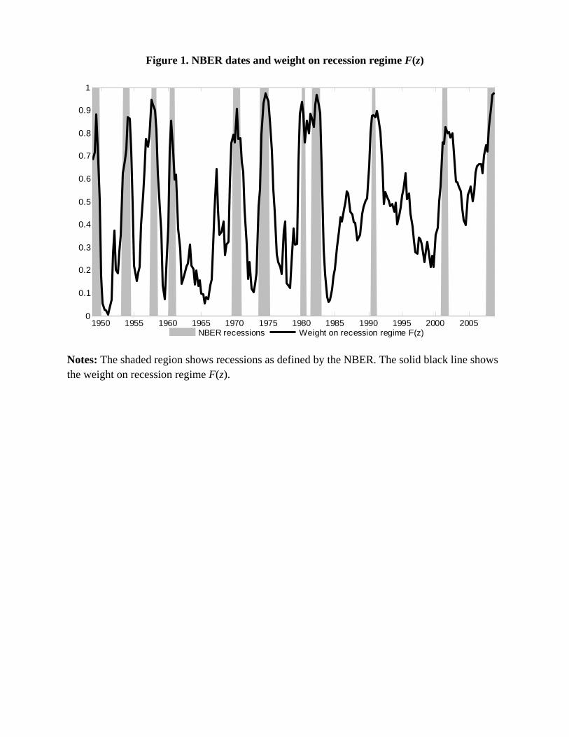
Figure 1. NBER dates and weight on recession regime F(z)

Notes: The shaded region shows recessions as defined by the NBER. The solid black line shows the weight on recession regime F(z).

1950 1955 1960 1965 1970 1975 1980 1985 1990 1995 2000 20050

0.1

0.2

0.3

0.4

0.5

0.6

0.7

0.8

0.9

1

NBER recessions Weight on recession regime F(z)

Figure 2. Impulse responses in the linear model

Notes: The figures show impulse responses to a $1 increase in government spending. Shaded region is the 90% confidence interval. Dashed lines show the responses in expansionary (red, long dash) and recessionary (blue, short dash) regimes. Solid line with circles shows the response in the linear model.

2 4 6 8 10 12 14 16 18 20-0.5

0

0.5

1

1.5

2

2.5G shock => G response

90% CIlinearexpansionrecession

2 4 6 8 10 12 14 16 18 20-1.5

-1

-0.5

0

0.5

1

1.5G shock => T response

2 4 6 8 10 12 14 16 18 20-1.5

-1

-0.5

0

0.5

1

1.5

2

2.5

3G shock => Y response

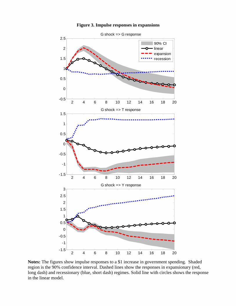
Figure 3. Impulse responses in expansions


2 4 6 8 10 12 14 16 18 20-0.5

0

0.5

1

1.5

2



2 4 6 8 10 12 14 16 18 20-1.5

-1

-0.5

0

0.5

1


2 4 6 8 10 12 14 16 18 20-1.5

-1

-0.5

0

0.5

1

1.5

2

2.5


Figure 4. Impulse responses in recessions


2 4 6 8 10 12 14 16 18 20-0.5

0

0.5

1

1.5

2



2 4 6 8 10 12 14 16 18 20-1.5

-1

-0.5

0

0.5

1


2 4 6 8 10 12 14 16 18 20-1.5

-1

-0.5

0

0.5

1

1.5

2

2.5


Figure 5. Historical multiplier for total government spending

Notes: shaded regions are recessions defined by the NBER. The solid black line is the cumulative multiplier computed as ∑ /∑ , where time index h is in quarters. Blue dashed lines are 90% confidence interval. The multiplier incorporates the feedback from G shock to the business cycle indicator z. In each instance, the shock is one percent increase in government spending.

1950 1955 1960 1965 1970 1975 1980 1985 1990 1995 2000 2005-1

-0.5

0

0.5

1

1.5

2

2.5

3

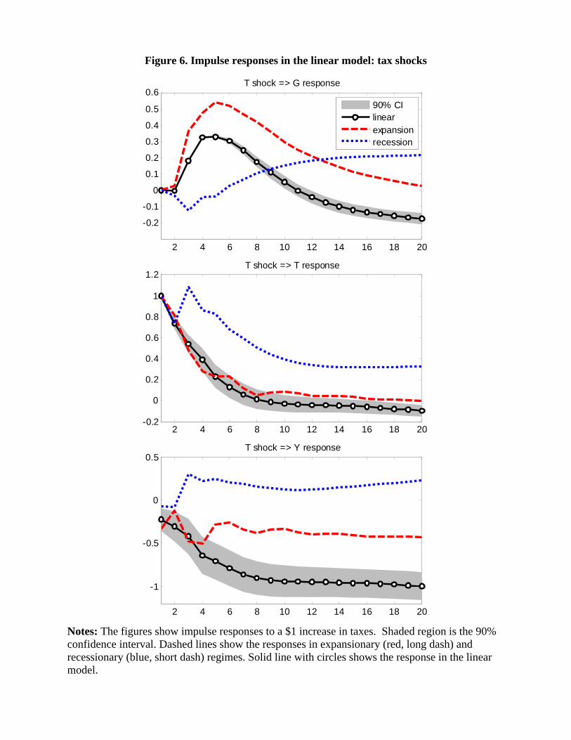
Figure 6. Impulse responses in the linear model: tax shocks

Notes: The figures show impulse responses to a $1 increase in taxes. Shaded region is the 90% confidence interval. Dashed lines show the responses in expansionary (red, long dash) and recessionary (blue, short dash) regimes. Solid line with circles shows the response in the linear model.

2 4 6 8 10 12 14 16 18 20

-0.2

-0.1

0

0.1

0.2

0.3

0.4

0.5

0.6T shock => G response


2 4 6 8 10 12 14 16 18 20-0.2

0

0.2

0.4

0.6

0.8

1

1.2T shock => T response

2 4 6 8 10 12 14 16 18 20

-1

-0.5

0

0.5T shock => Y response

Figure 7. Impulse responses in expansions: tax shocks


2 4 6 8 10 12 14 16 18 20

-0.2

-0.1

0

0.1

0.2

0.3

0.4

0.5



2 4 6 8 10 12 14 16 18 20-0.2

0

0.2

0.4

0.6

0.8

1


2 4 6 8 10 12 14 16 18 20

-1

-0.5

0


Figure 8. Impulse responses in recessions: tax shocks


2 4 6 8 10 12 14 16 18 20

-0.2

-0.1

0

0.1

0.2

0.3

0.4

0.5



2 4 6 8 10 12 14 16 18 20-0.2

0

0.2

0.4

0.6

0.8

1


2 4 6 8 10 12 14 16 18 20

-1

-0.5

0


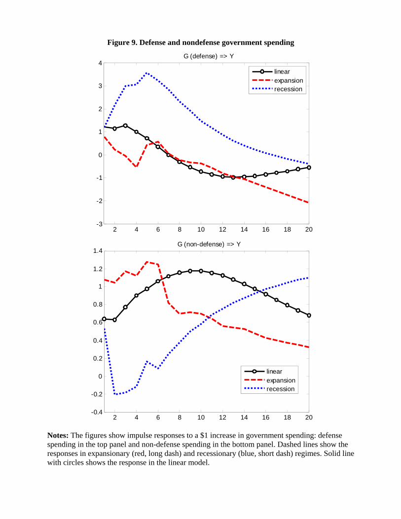
Figure 9. Defense and nondefense government spending

Notes: The figures show impulse responses to a $1 increase in government spending: defense spending in the top panel and non-defense spending in the bottom panel. Dashed lines show the responses in expansionary (red, long dash) and recessionary (blue, short dash) regimes. Solid line with circles shows the response in the linear model.

2 4 6 8 10 12 14 16 18 20-3

-2

-1

0

1

2

3

4 G (defense) => Y

linearexpansionrecession

2 4 6 8 10 12 14 16 18 20-0.4

-0.2

0

0.2

0.4

0.6

0.8

1

1.2

1.4 G (non-defense) => Y


Figure 10. Consumption and investment government spending

Notes: The figures show impulse responses to a $1 increase in government spending: consumption spending in the top panel and investment spending in the bottom panel. Dashed lines show the responses in expansionary (red, long dash) and recessionary (blue, short dash) regimes. Solid line with circles shows the response in the linear model.

2 4 6 8 10 12 14 16 18 20-0.5

0

0.5

1

1.5

2

2.5 G (consumption) => Y


2 4 6 8 10 12 14 16 18 20-1.5

-1

-0.5

0

0.5

1

1.5

2

2.5

3

3.5 G (investment) => Y


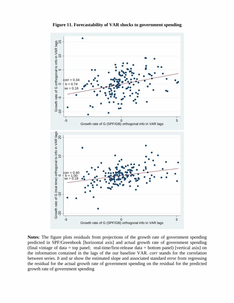
Figure 11. Forecastability of VAR shocks to government spending

Notes: The figure plots residuals from projections of the growth rate of government spending predicted in SPF/Greenbook [horizontal axis] and actual growth rate of government spending (final vintage of data = top panel; real-time/first-release data = bottom panel) [vertical axis] on the information contained in the lags of the our baseline VAR. corr stands for the correlation between series. b and se show the estimated slope and associated standard error from regressing the residual for the actual growth rate of government spending on the residual for the predicted growth rate of government spending

corr = 0.34b = 0.74se = 0.16

-10

-50

510

15G

row

th r

ate

of G

ort

hog

onal

to in

fo in

VA

R la

gs

-5 0 5Growth rate of G (SPF/GB) orthogonal info in VAR lags

corr = 0.40b = 1.00se = 0.18

-20

-10

010

20G

row

th r

ate

of G

(re

al t

ime

) o

rtho

gon

al to

info

in V

AR

lag

s

-5 0 5Growth rate of G (SPF/GB) orthogonal info in VAR lags

Figure 12. Government spending multipliers for purified unanticipated shocks.

Panel A: Contemporaneous responses based on forecast errors from SPF/RSQE

Panel B: Purify innovations in government spending using SPF/Greenbook forecasts

Panel C: Interpret forecast errors (real time data) of SPF/Greenbook forecasts for the growth rate of government spending as unanticipated shocks to government spending

(continued on next page)

2 4 6 8 10 12 14 16 18 20-3

-2

-1

0

1

2

3

4

5Expansion

90% CIContemp. responses using SPF/RSQE forec errorsBaseline

2 4 6 8 10 12 14 16 18 20-3

-2

-1

0

1

2

3

4

5Recession

2 4 6 8 10 12 14 16 18 20-1

0

1

2

3

4

5Expansion

90% CIControl for GB/SPF forecastsBaseline

2 4 6 8 10 12 14 16 18 20-1

0

1

2

3

4

5Recession

2 4 6 8 10 12 14 16 18 20-4

-2

0

2

4

6

8

10Expansion

90% CISPF/GB forecast errors as G shocksBaseline

2 4 6 8 10 12 14 16 18 20-4

-2

0

2

4

6

8

10Recession

Panel D: Government spending innovations are Ramey (2009) news shocks to military spending.

Notes: Note: The figure plots impulse response of output to an unanticipated government spending shock which is normalized to have the sum of government spending over 20 quarters equal to one. The red lines with circles correspond to the responses in the baseline VAR specification. The shaded region is the 90% confidence interval.

2 4 6 8 10 12 14 16 18 20-3

-2

-1

0

1

2

3

4

5

6Expansion

90% CIRamey (2009) news shocksBaseline

2 4 6 8 10 12 14 16 18 20-3

-2

-1

0

1

2

3

4

5

6Recession

Figure A1. Defense spending: linear model

2 4 6 8 10 12 14 16 18 200

0.5

1

1.5

2G (defense) => G (defense)

2 4 6 8 10 12 14 16 18 20-1.5

-1

-0.5

0

0.5

1G (defense) => G (non-defense)

2 4 6 8 10 12 14 16 18 20-4

-2

0

2

4

6G (defense) => T


2 4 6 8 10 12 14 16 18 20-4

-2

0

2

4G (defense) => Y

Figure A2. Non-defense spending: linear model

2 4 6 8 10 12 14 16 18 20-0.6

-0.4

-0.2

0

0.2G (non-defense) => G (defense)

2 4 6 8 10 12 14 16 18 200.2

0.4

0.6

0.8

1G (non-defense) => G (non-defense)


2 4 6 8 10 12 14 16 18 20-1.5

-1

-0.5

0

0.5

1G (non-defense) => T

2 4 6 8 10 12 14 16 18 20-0.5

0

0.5

1

1.5

2G (non-defense) => Y

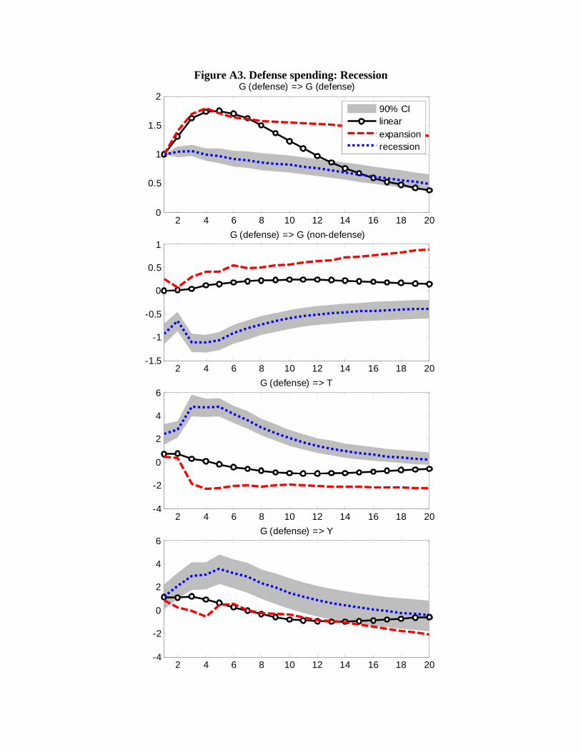
Figure A3. Defense spending: Recession

2 4 6 8 10 12 14 16 18 200

0.5

1

1.5

2G (defense) => G (defense)


2 4 6 8 10 12 14 16 18 20-1.5

-1

-0.5

0

0.5

1G (defense) => G (non-defense)

2 4 6 8 10 12 14 16 18 20-4

-2

0

2

4

6G (defense) => T

2 4 6 8 10 12 14 16 18 20-4

-2

0

2

4

6G (defense) => Y

Figure A4. Non-defense spending: recessions

2 4 6 8 10 12 14 16 18 20-0.6

-0.4

-0.2

0


2 4 6 8 10 12 14 16 18 200.2

0.4

0.6

0.8



2 4 6 8 10 12 14 16 18 20-1.5

-1

-0.5

0

0.5


2 4 6 8 10 12 14 16 18 20-1

-0.5

0

0.5

1

1.5

2G (non-defense) => Y

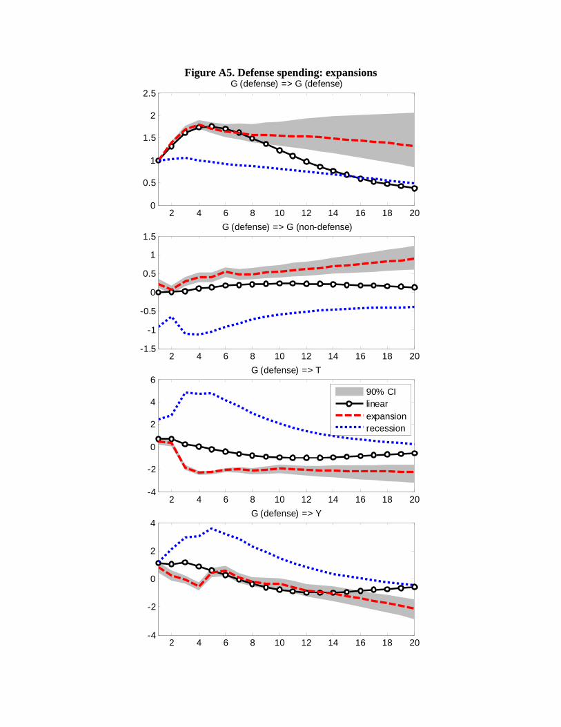
Figure A5. Defense spending: expansions

2 4 6 8 10 12 14 16 18 200

0.5

1

1.5

2

2.5G (defense) => G (defense)

2 4 6 8 10 12 14 16 18 20-1.5

-1

-0.5

0

0.5

1

1.5G (defense) => G (non-defense)

2 4 6 8 10 12 14 16 18 20-4

-2

0

2

4

6G (defense) => T


2 4 6 8 10 12 14 16 18 20-4

-2

0

2

4G (defense) => Y

Figure A6. Non-defense spending: expansion

2 4 6 8 10 12 14 16 18 20-0.6

-0.4

-0.2

0


2 4 6 8 10 12 14 16 18 200.2

0.4

0.6

0.8



2 4 6 8 10 12 14 16 18 20-1.5

-1

-0.5

0

0.5


2 4 6 8 10 12 14 16 18 20-0.5

0

0.5

1

1.5G (non-defense) => Y

Figure A7. Consumption spending: linear model

2 4 6 8 10 12 14 16 18 200

0.5

1

1.5G (consumption) shock => G (consumption) response


2 4 6 8 10 12 14 16 18 20-1

-0.5

0

0.5G (consumption) shock => G (investment) response

2 4 6 8 10 12 14 16 18 20-2

-1

0

1

2

3G (consumption) shock => T response

2 4 6 8 10 12 14 16 18 20-0.5

0

0.5

1

1.5

2

2.5G (consumption) shock => Y response

Figure A8. Investment spending: linear model

2 4 6 8 10 12 14 16 18 20-0.5

0

0.5

1

1.5G (investment) shock => G (consumption) response

2 4 6 8 10 12 14 16 18 200.2

0.4

0.6

0.8

1G (investment) shock => G (investment) response


2 4 6 8 10 12 14 16 18 20-3

-2

-1

0

1

2

3G (investment) shock => T response

2 4 6 8 10 12 14 16 18 20-2

-1

0

1

2

3

4G (investment) shock => Y response

Figure A9. Consumption spending: recessions

2 4 6 8 10 12 14 16 18 200

0.5

1

1.5

2G (consumption) shock => G (consumption) response

2 4 6 8 10 12 14 16 18 20-1

-0.5

0


2 4 6 8 10 12 14 16 18 20-2

-1

0

1

2

3


2 4 6 8 10 12 14 16 18 20-1

0

1

2

3

4G (consumption) shock => Y response


Figure A10. Investment spending: recessions

2 4 6 8 10 12 14 16 18 20-0.5

0

0.5

1


2 4 6 8 10 12 14 16 18 20-0.5

0

0.5

1

1.5G (investment) shock => G (investment) response


2 4 6 8 10 12 14 16 18 20-4

-2

0

2

4


2 4 6 8 10 12 14 16 18 20-4

-2

0

2

4


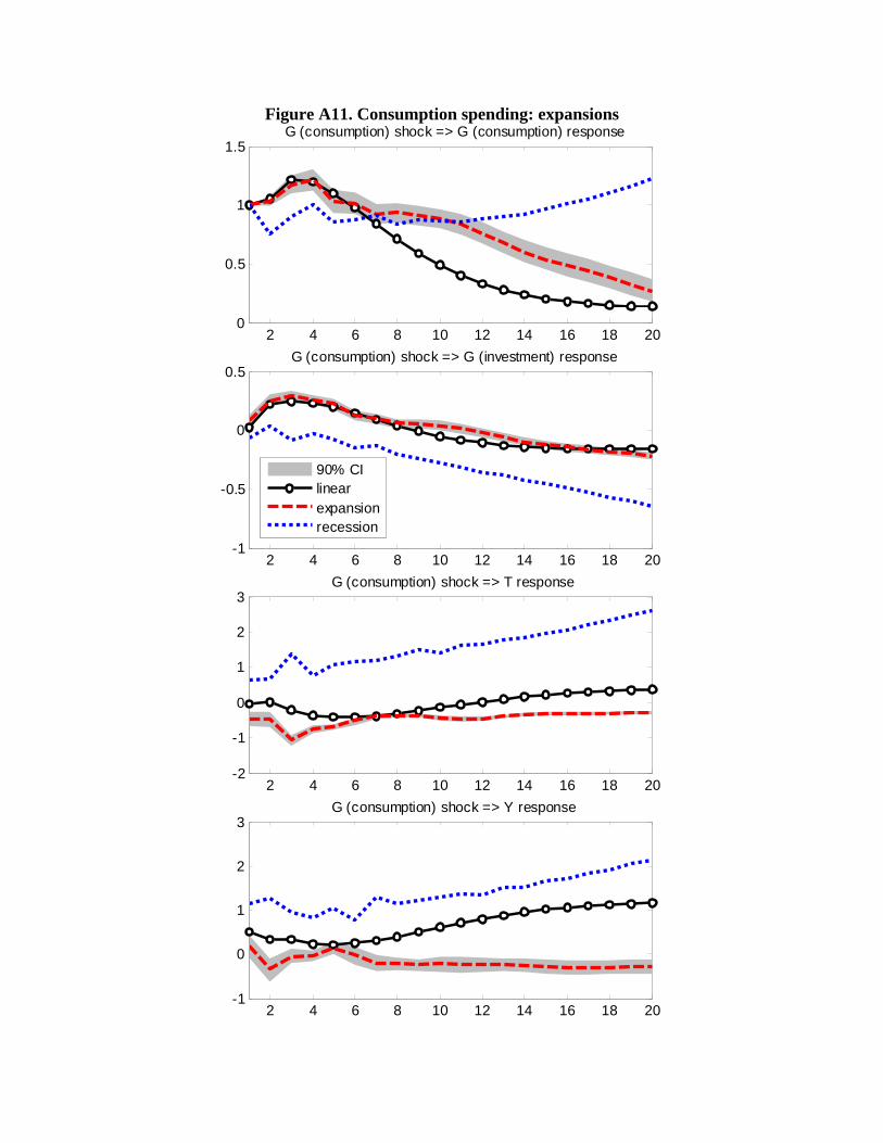
Figure A11. Consumption spending: expansions

2 4 6 8 10 12 14 16 18 200

0.5

1

1.5G (consumption) shock => G (consumption) response

2 4 6 8 10 12 14 16 18 20-1

-0.5

0



2 4 6 8 10 12 14 16 18 20-2

-1

0

1

2


2 4 6 8 10 12 14 16 18 20-1

0

1

2

3G (consumption) shock => Y response

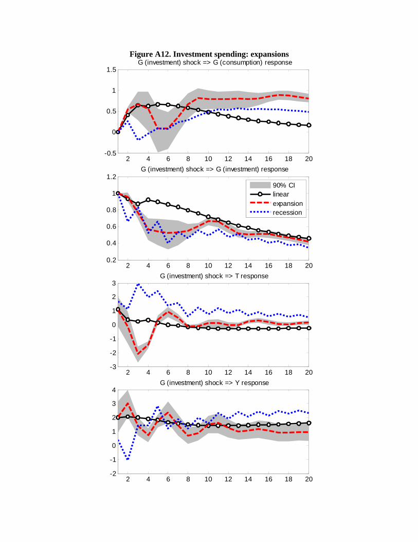
Figure A12. Investment spending: expansions

2 4 6 8 10 12 14 16 18 20-0.5

0

0.5

1


2 4 6 8 10 12 14 16 18 200.2

0.4

0.6

0.8

1

1.2G (investment) shock => G (investment) response


2 4 6 8 10 12 14 16 18 20-3

-2

-1

0

1

2


2 4 6 8 10 12 14 16 18 20-2

-1

0

1

2

3


EASURING THE OUTPUT RESPONSES TO FISCAL OLICYygorodni/AG_fiscal_multiplier.pdf · MEASURING THE OUTPUT RESPONSES TO FISCAL POLICY Alan Auerbach Yuriy Gorodnichenko University of California,

Documents