Earthquake Resistant Design of Structures Earthquake Resistant Design of Structures Pankaj Agarwal Manish Shrikhande

Welcome message from author
This document is posted to help you gain knowledge. Please leave a comment to let me know what you think about it! Share it to your friends and learn new things together.
Transcript
EarthquakeResistant Designof Structures
EarthquakeResistant Designof Structures
Pankaj AgarwalManish Shrikhande

I
PHI • I
PANI<AJ AGARWAL Assistant Professor
Department of Earthquake Engineering Indian Institute of Technology Roorkee
and
MANISH SHRIKHANDE Assistant Professor
Department of Earthquake Engineering Indian Institute of iechnology Roorkee
New Delhi-11 0001 2011

Copy R 68
EARTHQUAKE RESISTANT DESIGN OF STRUCTURESPankaj Agarwal and Manish Shrikhande
© 2006 by PHI Learning Private Limited, Delhi. All rights reserved. No part of this book may be reproduced in any form, by mimeograph or any other means, without permission in writing from the publisher.
ISBN-978-81-203-2892-1
The export rights of this book are vested solely with the publisher.
Thirteenth Printing … … July, 2014
Published by Asoke K. Ghosh, PHI Learning Private Limited, Rimjhim House, 111, Patparganj Industrial Estate, Delhi-110092 and Printed by Rajkamal Electric Press, Plot No. 2, Phase IV, HSIDC, Kundli-131028, Sonepat, Haryana.

To Our Parents

Contents
Preface ............................................................................................................................... xxi
Contributors ..................................................................................................................... xxv
Part IEARTHQUAKE GROUND MOTION
1. Engineering Seismology .................................................................... 3–44
1.1 Introduction ....................................................................................................................... 31.2 Reid’s Elastic Rebound Theory ....................................................................................... 31.3 Theory of Plate Tectonics ................................................................................................. 4
1.3.1 Lithospheric Plates ................................................................................................ 61.3.2 Plate Margins and Earthquake Occurrences ........................................................ 71.3.3 The Movement of Indian Plate ............................................................................ 9
1.4 Seismic Waves ................................................................................................................. 10
1.4.1 Body Waves ......................................................................................................... 101.4.2 Surface Waves ...................................................................................................... 11
1.5 Earthquake Size ............................................................................................................... 13
1.5.1 Intensity ............................................................................................................... 131.5.2 Isoseismal Map .................................................................................................... 181.5.3 Earthquake Magnitude ....................................................................................... 181.5.4 Energy Released in an Earthquake .................................................................... 231.5.5 Earthquake Frequency ........................................................................................ 23
1.6 Local Site Effects ............................................................................................................ 24
1.6.1 Basin/Soil Effects ................................................................................................ 241.6.2 Lateral Discontinuity Effects .............................................................................. 271.6.3 Effect of the Surface Topography ...................................................................... 28
vii
Contentsviii
1.7 Internal Structure of the Earth ........................................................................................ 30
1.7.1 Crust ..................................................................................................................... 301.7.2 Upper Mantle ....................................................................................................... 311.7.3 Lower Mantle ...................................................................................................... 311.7.4 Core ...................................................................................................................... 32
1.8 Seismotectonics of India ................................................................................................. 321.9 Seismicity of India .......................................................................................................... 341.10 Classification of Earthquakes ......................................................................................... 351.11 Tsunami ........................................................................................................................... 36
1.11.1 Tsunami Velocity ............................................................................................... 371.11.2 Run-up and Inundation ..................................................................................... 37
Summary .............................................................................................................................. 38Glossary of Earthquake/Seismology ....................................................................................... 38References .............................................................................................................................. 41
2. Seismic Zoning Map of India ......................................................... 45–58
2.1 Introduction ..................................................................................................................... 452.2 Seismic Hazard Map ....................................................................................................... 452.3 Seismic Zone Map of 1962 ............................................................................................ 482.4 Seismic Zone Map of 1966 ............................................................................................ 50
2.4.1 Grade Enhancement ............................................................................................ 512.4.2 Review of Tectonic ............................................................................................. 51
2.5 Seismic Zone Map of 1970 ............................................................................................ 522.6 Seismic Zone Map of 2002 ............................................................................................ 562.7 Epilogue ........................................................................................................................... 56
Summary .............................................................................................................................. 58References .............................................................................................................................. 58
3. Strong Motion Studies in India .................................................... 59–69
3.1 Introduction ..................................................................................................................... 593.2 Understanding the Nature of Ground Motions ............................................................. 60
3.2.1 Source Effect ........................................................................................................ 603.2.2 Path Effect ............................................................................................................ 623.2.3 Site Effect ............................................................................................................ 63
3.3 Estimation of Ground Motion Parameters ..................................................................... 643.4 The Indian Perspective ................................................................................................... 653.5 Utilization of Strong Motion Data ................................................................................. 65
Summary .............................................................................................................................. 66References .............................................................................................................................. 66
4. Strong Motion Characteristics ...................................................... 70–87
4.1 Introduction ..................................................................................................................... 70
ixChapter Contents
4.2 Terminology of Strong Motion Seismology ................................................................. 73
4.2.1 Amplitude Parameters ......................................................................................... 734.2.2 Duration of Strong Motion ................................................................................. 744.2.3 Fourier Spectrum ................................................................................................. 744.2.4 Power Spectrum ................................................................................................... 754.2.5 Response Spectrum ............................................................................................. 764.2.6 Seismic Demand Diagrams ................................................................................. 794.2.7 Spatial Variation of Earthquake Ground Motion ............................................. 804.2.8 Damage Potential of Earthquakes ...................................................................... 81
Summary .............................................................................................................................. 86References .............................................................................................................................. 86
5. Evaluation of Seismic Design Parameters .............................. 88–107
5.1 Introduction ..................................................................................................................... 885.2 Types of Earthquakes ...................................................................................................... 88
5.2.1 Intensity ............................................................................................................... 895.2.2 Magnitude ............................................................................................................ 89
5.3 Fault Rupture Parameters ................................................................................................ 905.4 Earthquake Ground Motion Characteristics .................................................................. 91
5.4.1 Amplitude Properties .......................................................................................... 915.4.2 Duration ............................................................................................................... 935.4.3 Effect of Distance ................................................................................................ 935.4.4 Ground Motion Level ......................................................................................... 965.4.5 Geographical, Geophysics and Geotechnical Data ........................................... 96
5.5 Deterministic Approach .................................................................................................. 975.6 Probabilistic Approach ................................................................................................... 98
5.6.1 Example ............................................................................................................. 100
5.7 Response Spectra ........................................................................................................... 1015.8 Design Spectrum ............................................................................................................ 101
Summary ............................................................................................................................ 105References ............................................................................................................................ 106
Part IISTRUCTURAL DYNAMICS
6. Initiation into Structural Dynamics ........................................ 111–114
6.1 Introduction ................................................................................................................... 1116.2 Mathematical Modelling .............................................................................................. 112
Summary ............................................................................................................................ 114References ............................................................................................................................ 114
Contentsx
7. Dynamics of Single Degree of Freedom Systems................ 115–128
7.1 Introduction ................................................................................................................... 1157.2 Free Vibration of Viscous-Damped SDOF Systems .................................................... 116
7.2.1 Underdamped Case (z < 1) ............................................................................... 1187.2.2 Critically-damped Case (z = 1) ......................................................................... 1187.2.3 Overdamped Case (z > 1) .................................................................................. 118
7.3 Forced Vibrations of SDOF Systems ............................................................................ 120
7.3.1 Response of SDOF Systems to Harmonic Excitations .................................... 1207.3.2 Excitation by Base Motion .............................................................................. 1227.3.3 Response of SDOF Systems to a Finite Duration Excitation ......................... 1227.3.4 Response of SDOF Systems to a Short Duration Impulse .............................. 1247.3.5 Response of SDOF Systems to General Dynamic Excitation ......................... 125
7.4 Vibration Isolation ........................................................................................................ 126
Summary ............................................................................................................................ 128References ............................................................................................................................ 128
8. Theory of Seismic Pickups ......................................................... 129–136
8.1 Introduction ................................................................................................................... 1298.2 The Physics of Operation .............................................................................................. 1298.3 Which Parameter to Measure? ...................................................................................... 1318.4 Seismometers ................................................................................................................. 132
8.4.1 Displacement Pickups ....................................................................................... 1328.4.2 Velocity Pickups ............................................................................................... 132
8.5 Accelerometers ............................................................................................................... 133
8.5.1 Servo-accelerometers ......................................................................................... 1358.5.2 Calibration of Accelerometers .......................................................................... 136
Summary ............................................................................................................................ 136References ............................................................................................................................ 136
9. Numerical Evaluation of Dynamic Response ........................137–143
9.1 Numerical Solution Based on Interpolation of Excitation ........................................ 1379.2 Numerical Solution Based on Approximation of Derivatives ................................... 1399.3 Stability and Accuracy Considerations ....................................................................... 141
Summary ............................................................................................................................ 143References ............................................................................................................................ 143
10. Response Spectra........................................................................... 144–156
10.1 Introduction ................................................................................................................... 14410.2 Fourier Spectra ............................................................................................................... 144
xiChapter Contents
10.3 Response Spectra ........................................................................................................... 146
10.3.1 Formulation ...................................................................................................... 14710.3.2 Solution: Initially at Rest ................................................................................ 14810.3.3 Solution: General Conditions ......................................................................... 15110.3.4 Smooth Spectrum ............................................................................................. 15410.3.5 Seismic Demand Diagrams .............................................................................. 154
Summary ............................................................................................................................ 155References ............................................................................................................................ 155
11. Dynamics of Multi-Degree-of-Freedom Systems .................. 157–188
11.1 Introduction .................................................................................................................. 15711.2 System Property Matrices ............................................................................................ 15811.3 Dynamics of Two Degree of Freedom Systems .......................................................... 15911.4 Free Vibration Analysis of MDOF Systems ............................................................... 162
11.4.1 Orthogonality Conditions .............................................................................. 163
11.5 Determination of Fundamental Frequency ................................................................. 165
11.5.1 Rayleigh Quotient .......................................................................................... 16511.5.2 Stodola Method .............................................................................................. 16511.5.3 Converging to Higher Modes ........................................................................ 166
11.6 Forced Vibration Analysis ........................................................................................... 169
11.6.1 Mode-superposition Method .......................................................................... 17011.6.2 Excitation by Support Motion ...................................................................... 17111.6.3 Mode Truncation ............................................................................................ 17511.6.4 Static Correction for Higher Mode Response ............................................... 176
11.7 Model Order Reduction in Structural Dynamics ....................................................... 17711.8 Analysis for Multi-Support Excitation ....................................................................... 17811.9 Soil–Structure Interaction Effects ............................................................................... 181
11.9.1 Dynamic Analysis including SSI Effects ...................................................... 182Summary ......................................................................................................................... 187References ......................................................................................................................... 187
Part IIICONCEPTS OF EARTHQUAKE RESISTANT DESIGN OF
REINFORCED CONCRETE BUILDING
12. Earthquake and Vibration Effect on Structures:Basic Elements of Earthquake Resistant Design ................ 191–206
12.1 Introduction .................................................................................................................. 19112.2 Static and Dynamic Equilibrium ................................................................................ 19212.3 Structural Modelling.................................................................................................... 194
12.3.1 Structural Models for Frame Building .......................................................... 194
Contentsxii
12.4 Seismic Methods of Analysis ...................................................................................... 196
12.4.1 Code-based Procedure for Seismic Analysis ................................................. 197
12.5 Seismic Design Methods ............................................................................................. 198
12.5.1 Code-based Methods for Seismic Design ...................................................... 198
12.6 Response Control Concepts ........................................................................................ 199
12.6.1 Earthquake Protective Systems ...................................................................... 200
12.7 Seismic Evaluation and Retrofitting .......................................................................... 201
12.7.1 Methods for Seismic Evaluation ................................................................... 20212.7.2 Methods for Seismic Retrofitting .................................................................. 203
12.8 Seismic Test Methods .................................................................................................. 204
12.8.1 Methods for Seismic Testing ......................................................................... 204
Summary ......................................................................................................................... 205References ......................................................................................................................... 205
13. Identification of Seismic Damages in RC Buildingsduring Bhuj Earthquake..............................................................207–225
13.1 Introduction .................................................................................................................. 20713.2 Reinforced Concrete Building Construction Practices ............................................. 20813.3 Identification of Damage in RC Buildings ................................................................ 210
13.3.1 Soft Storey Failure .......................................................................................... 21113.3.2 Floating Columns ........................................................................................... 21213.3.3 Plan and Mass Irregularity ............................................................................. 21313.3.4 Poor Quality of Construction Material and Corrosion of Reinforcement .. 21413.3.5 Pounding of Buildings ................................................................................... 21513.3.6 Inconsistent Seismic Performance of Buildings ........................................... 216
13.4 Damage to Structural Elements ................................................................................... 21713.5 Damage to Non-Structural Panel Elements ................................................................ 219
13.5.1 Damage to Infill Walls ................................................................................... 21913.5.2 Damage to Exterior Walls .............................................................................. 220
13.6 Damage to Water Tank and Parapets .......................................................................... 22013.7 Damage to Vertical Circulation Systems ................................................................... 221
13.7.1 Damage to Staircase ........................................................................................ 22113.7.2 Damage to Elevator ........................................................................................ 222
13.8 Effect of Earthquake on Code Designed Structures .................................................. 22213.9 Lessons Learnt from Damages of RC Buildings ........................................................ 223
Summary ......................................................................................................................... 224References ......................................................................................................................... 224
14. Effect of Structural Irregularities on the Performanceof RC Buildings during Earthquakes ..................................... 226–238
14.1 Introduction .................................................................................................................. 226
xiiiChapter Contents
14.2 Vertical Irregularities ................................................................................................... 227
14.2.1 Vertical Discontinuities in Load Path ........................................................... 22714.2.2 Irregularity in Strength and Stiffness ............................................................ 23014.2.3 Mass Irregularities ........................................................................................... 23214.2.4 Vertical Geometric Irregularity ...................................................................... 23314.2.5 Proximity of Adjacent Buildings ................................................................... 233
14.3 Plan Configuration Problems ...................................................................................... 234
14.3.1 Torsion Irregularities ...................................................................................... 23414.3.2 Re-entrant Corners .......................................................................................... 23614.3.3 Non-parallel Systems ...................................................................................... 23614.3.4 Diaphragm Discontinuity ............................................................................... 237
14.4 Recommendations ........................................................................................................ 237
Summary ......................................................................................................................... 238References ......................................................................................................................... 238
15. Seismoresistant Building Architecture .................................. 239–248
15.1 Introduction .................................................................................................................. 23915.2 Lateral Load Resisting Systems .................................................................................. 239
15.2.1 Moment Resisting Frame ............................................................................... 24015.2.2 Building with Shear Wall or Bearing Wall System ..................................... 24015.2.3 Building with Dual System ............................................................................ 240
15.3 Building Configuration ............................................................................................... 241
15.3.1 Problems and Solutions .................................................................................. 241
15.4 Building Characteristics .............................................................................................. 243
15.4.1 Mode Shapes and Fundamental Period ......................................................... 24315.4.2 Building Frequency and Ground Period ....................................................... 24415.4.3 Damping .......................................................................................................... 24415.4.4 Ductility .......................................................................................................... 24415.4.5 Seismic Weight ............................................................................................... 24515.4.6 Hyperstaticity/Redundancy ............................................................................ 24515.4.7 Non-structural Elements ................................................................................. 24515.4.8 Foundation Soil/Liquefaction ........................................................................ 24615.4.9 Foundations ..................................................................................................... 246
15.5 Quality of Construction and Materials ....................................................................... 246
15.5.1 Quality of Concrete ........................................................................................ 24715.5.2 Construction Joints ......................................................................................... 24715.5.3 General Detailing Requirements .................................................................... 247
Summary ......................................................................................................................... 248References ......................................................................................................................... 248
Contentsxiv
Part IVSEISMIC ANALYSIS AND MODELLING OF
REINFORCED CONCRETE BUILDING
16. Code Based Procedure for Determination of DesignLateral Loads ..................................................................................251–281
16.1 Introduction .................................................................................................................. 25116.2 Seismic Design Philosophy ......................................................................................... 25116.3 Determination of Design Lateral Forces ..................................................................... 252
16.3.1 Equivalent Lateral Force Procedure .............................................................. 25316.3.2 Dynamic Analysis Procedure ......................................................................... 259
Summary ......................................................................................................................... 280References ......................................................................................................................... 280
17. Consideration of Infill Wall in Seismic Analysis ofRC Buildings ...................................................................................282–291
17.1 Introduction .................................................................................................................. 28217.2 Structural and Constructional Aspects of Infills ........................................................ 28217.3 Failure Mechanism of Infilled Frame ......................................................................... 28317.4 Analysis of Infilled Frames .......................................................................................... 284
17.4.1 Equivalent Diagonal Strut .............................................................................. 285
Summary ......................................................................................................................... 290References ......................................................................................................................... 290
18. Step-by-Step Procedure for Seismic Analysis of a Four-storeyed RC Building as per IS 1893 (Part 1): 2002 ......... 292–326
18.1 Introduction .................................................................................................................. 29218.2 Equivalent Static Lateral Force Method .................................................................... 293
18.2.1 Step 1: Calculation of Lumped Masses to Various Floor Levels ............... 29318.2.2 Step 2: Determination of Fundamental Natural Period ................................ 29418.2.3 Step 3: Determination of Design Base Shear ................................................ 29418.2.4 Step 4: Vertical Distribution of Base Shear .................................................. 295
18.3 Response Spectrum Method ........................................................................................ 296
A: Frame without Considering the Stiffness of Infills .............................................. 296
18.3.1 Step 1: Determination of Eigenvalues and Eigenvectors ............................ 29618.3.2 Step 2: Determination of Modal Participation Factors ................................ 29918.3.3 Step 3: Determination of Modal Mass .......................................................... 29918.3.4 Step 4: Determination of Lateral Force at Each Floor in Each Mode ........ 30018.3.5 Step 5: Determination of Storey Shear Forces in Each Mode ..................... 30118.3.6 Step 6: Determination of Storey Shear Force due to All Modes ................ 30218.3.7 Step 7: Determination of Lateral Forces at Each Storey .............................. 304
B: Frame Considering the Stiffness of Infills ............................................................. 305
xvChapter Contents
18.4 Time History Method .................................................................................................. 311
18.4.1 Step 1: Calculation of Modal Matrix ............................................................ 31218.4.2 Step 2: Calculation of Effective Force Vector .............................................. 31418.4.3 Step 3: Calculation of Displacement Response in Normal Coordinate ...... 31418.4.4 Step 4: Displacement Response in Physical Coordinates ............................ 31618.4.5 Step 5: Calculation of Effective Earthquake Response Forces at
Each Storey ..................................................................................................... 31918.4.6 Step 6: Calculation of Storey Shear .............................................................. 32118.4.7 Step 7: Calculation of Maximum Response ................................................. 324
Summary ......................................................................................................................... 324References ......................................................................................................................... 325
Appendix 1: Linear Interpolation of Excitation ................................................................ 325
19. Mathematical Modelling of Multi-storeyedRC Buildings ...................................................................................327–337
19.1 Introduction .................................................................................................................. 32719.2 Planar Models ............................................................................................................... 327
19.2.1 Shear Beam Model .......................................................................................... 32819.2.2 Flexure Beam Model ...................................................................................... 32819.2.3 Idealized Plane Frame Model ......................................................................... 32919.2.4 Equivalent Shear Wall Frame Model ............................................................ 33019.2.5 Plane Frame Model of Coupled Shear Walls ................................................ 330
19.3 3D Space Frame Model ............................................................................................... 33119.4 Reduced 3D Model ...................................................................................................... 33119.5 Some Important Issues in Modelling .......................................................................... 331
19.5.1 Modelling of Floor Diaphragms .................................................................... 33119.5.2 Modelling of Soil-Foundation ....................................................................... 33419.5.3 Foundation Models ........................................................................................ 33419.5.4 Soil Models ..................................................................................................... 33519.5.5 Modelling of Staircases .................................................................................. 33619.5.6 Modelling of Infills ........................................................................................ 336
Summary ......................................................................................................................... 336References ......................................................................................................................... 337
Part VEARTHQUAKE RESISTANT DESIGN (ERD)OF REINFORCED CONCRETE BUILDINGS
20. Ductility Considerations in Earthquake ResistantDesign of RC Buildings ...............................................................341–370
20.1 Introduction .................................................................................................................. 34120.2 Impact of Ductility ....................................................................................................... 34220.3 Requirements for Ductility .......................................................................................... 342

Contentsxvi
20.4 Assessment of Ductility ............................................................................................... 342
20.4.1 Member/Element Ductility ............................................................................. 34320.4.2 Structural Ductility ......................................................................................... 345
20.5 Factors Affecting Ductility .......................................................................................... 34620.6 Ductility Factors .......................................................................................................... 34720.7 Ductile Detailing Considerations as per IS 13920: 1993 ......................................... 348
Summary ......................................................................................................................... 370References ......................................................................................................................... 370
21. Earthquake Resistant Design of a Four-storeyRC Building Based on IS 13920: 1993 .................................... 371–391
21.1 Introduction .................................................................................................................. 37121.2 Preliminary Data for Example Frame .......................................................................... 37121.3 Loading Data ................................................................................................................ 37321.4 Analysis of Sub-frame 4-4 ........................................................................................... 373
21.4.1 Dead Load Analysis ........................................................................................ 37321.4.2 Live (Imposed) Load Analysis ....................................................................... 37521.4.3 Earthquake Load Analysis ............................................................................. 376
21.5 Load Combinations ..................................................................................................... 37721.6 Design of Sub-Frame 4-4 ............................................................................................. 382
21.6.1 Design of a Flexure Member .......................................................................... 38221.6.2 Design of Exterior Columns ........................................................................... 38521.6.3 Design of Interior Columns ............................................................................ 38721.6.4 Detailing of Reinforcements .......................................................................... 389
Summary ......................................................................................................................... 390References ......................................................................................................................... 391
22. Earthquake Resistant Design of Shear Wall as perIS 13920: 1993 ................................................................................. 392–403
22.1 Introduction .................................................................................................................. 39222.2 Description of Building ............................................................................................... 39222.3 Determination of Design Lateral Forces ..................................................................... 39322.4 Design of Shear Wall ................................................................................................... 39722.5 Detailing of Reinforcements ........................................................................................ 402
Summary ......................................................................................................................... 403References ......................................................................................................................... 403
23. Capacity Based Design—An Approach for EarthquakeResistant Design of Soft Storey RC Buildings..................... 404–424
23.1 Introduction .................................................................................................................. 40423.2 Preliminary Data for (G+3) Plane Frame .................................................................... 405
23.2.1 Determination of Loads .................................................................................. 406
xviiChapter Contents
23.3 Step-by-Step Procedure for Capacity Based Design .................................................. 409
23.3.1 Step 1: Seismic Analysis of Frame (G+3) ..................................................... 40923.3.2 Step 2: Determination of Flexural Capacity of Beams ................................ 41223.3.3 Step 3: Establishing a Strong Column–Weak Beam Mechanism ............... 41423.3.4 Step 4: Determination of Moment Magnification Factors for Columns ..... 41523.3.5 Step 5: Capacity Design for Shear in Beams ................................................ 41723.3.6 Step 6: Capacity Design for Shear in Columns ............................................ 41823.3.7 Step 7: Detailing of Reinforcements ............................................................. 419
Summary ......................................................................................................................... 421References ......................................................................................................................... 421
Appendix 1: Beam Flexural Capacity Calculation as per Design Aid IS456: 1978 ...... 422Appendix 2: Determination of Moment Magnification Factor at Every Joint ............... 423
Part VIEARTHQUAKE RESISTANT DESIGN (ERD)
OF MASONRY BUILDINGS
24. Identification of Damages and Non-Damages inMasonry Buildings from Past Indian Earthquakes ............ 427–448
24.1 Introduction .................................................................................................................. 42724.2 Past Indian Earthquakes .............................................................................................. 42724.3 Features of Damages and Non-damages ..................................................................... 429
24.3.1 Bhuj Earthquake, January 26, 2001 .............................................................. 42924.3.2 Chamoli Earthquake, March 29, 1999 .......................................................... 43124.3.3 Jabalpur Earthquake, May 22, 1997 ............................................................. 43324.3.4 Killari Earthquake, September 30, 1993 ....................................................... 43624.3.5 Uttarkashi Earthquake, October 20, 1991 ..................................................... 43824.3.6 Bihar-Nepal Earthquake, August 21, 1988 ................................................... 441
24.4 Lessons Learnt .............................................................................................................. 44424.5 Recommendations ........................................................................................................ 445
Summary ......................................................................................................................... 445References ......................................................................................................................... 446
Appendix 1: Muzaffarabad Earthquake of October 8, 2005 ............................................ 446
25. Elastic Properties of Structural Masonry.............................. 449–462
25.1 Introduction .................................................................................................................. 44925.2 Materials for Masonry Construction ........................................................................... 449
25.2.1 Unit .................................................................................................................. 44925.2.2 Mortar .............................................................................................................. 45025.2.3 Grout ................................................................................................................ 45125.2.4 Reinforcement ................................................................................................. 451
Contentsxviii
25.3 Elastic Properties of Masonry Assemblage ................................................................ 452
25.3.1 Compressive Strength ..................................................................................... 45225.3.2 Flexural Tensile Strength ............................................................................... 45525.3.3 Shear Strength ................................................................................................. 456
Summary ......................................................................................................................... 460References ......................................................................................................................... 460
26. Lateral Load Analysis of Masonry Buildings ....................... 463–485
26.1 Introduction .................................................................................................................. 46326.2 Procedure for Lateral Load Analysis of Masonry Buildings .................................... 464
26.2.1 Step 1: Determination of Lateral Loads ........................................................ 46526.2.2 Step 2: Distribution of Lateral Forces ........................................................... 46826.2.3 Step 3: Determination of Rigidity of Shear Wall ........................................ 47026.2.4 Step 4: Determination of Direct Shear Forces and Torsional
Shear Forces .................................................................................................... 47426.2.5 Step 5: Determination of Increase in Axial Load Due to Overturning ....... 47926.2.6 Step 6: Walls Subjected to Out-of-plane Bending ....................................... 483
Summary ......................................................................................................................... 484References ......................................................................................................................... 485
27. Seismic Analysis and Design of Two-storeyedMasonry Buildings ........................................................................486–502
27.1 Introduction .................................................................................................................. 48627.2 Building Data ............................................................................................................... 48627.3 Step 1: Determination of Design Lateral Load .......................................................... 48827.4 Step 2: Determination of Wall Rigidities .................................................................. 48927.5 Step 3: Determination of Torsional Forces ................................................................ 49227.6 Step 4: Determination Increase in Axial Load due to Overturning ......................... 49527.7 Step 5: Determination of Pier Loads, Moments and Shear ....................................... 49827.8 Step 6: Design of Shear Walls for Axial Load and Moments .................................. 50027.9 Step 7: Design of Shear Walls for Shear .................................................................... 50027.10 Step 8: Structural Details ............................................................................................. 501
Summary ......................................................................................................................... 501References ......................................................................................................................... 502
Part VIISEISMIC EVALUATION AND RETROFITTING OF
REINFORCED CONCRETE AND MASONRY BUILDINGS
28. Seismic Evaluation of Reinforced Concrete Buildings:A Practical Approach .................................................................... 505–523
28.1 Introduction .................................................................................................................. 505
xixChapter Contents
28.2 Components of Seismic Evaluation Methodology.................................................... 506
28.2.1 Condition Assessment for Evaluation ........................................................... 50628.2.2 Field Evaluation/Visual Inspection Method ................................................. 50928.2.3 Concrete Distress and Deterioration Other than Earthquake ....................... 51928.2.4 Non-destructive Testing (NDT) ...................................................................... 519
Summary ......................................................................................................................... 522References ......................................................................................................................... 522
29. Seismic Retrofitting Strategies of ReinforcedConcrete Buildings ........................................................................524–555
29.1 Introduction .................................................................................................................. 52429.2 Consideration in Retrofitting of Structures................................................................ 52829.3 Source of Weakness in RC Frame Building .............................................................. 528
29.3.1 Structural Damage due to Discontinuous Load Path ................................... 52929.3.2 Structural Damage due to Lack of Deformation ........................................... 52929.3.3 Quality of Workmanship and Materials ........................................................ 533
29.4 Classification of Retrofitting Techniques .................................................................. 53329.5 Retrofitting Strategies for RC Buildings ................................................................... 535
29.5.1 Structural Level (or Global) Retrofit Methods ............................................. 53529.5.2 Member Level (or Local) Retrofit Methods ................................................. 541
29.6 Comparative Analysis of Methods of Retrofitting .................................................... 550
Summary ......................................................................................................................... 553References ......................................................................................................................... 553
30. Seismic Retrofitting of Reinforced ConcreteBuildings—Case Studies ..............................................................556–575
30.1 Introduction ................................................................................................................. 55630.2 Methodology for Seismic Retrofitting of RC Buildings ......................................... 55730.3 Case Study 1: Seismic Retrofitting of RC Building with Jacketing and
Shear Walls .................................................................................................................. 55830.4 Case Study 2: Seismic Retrofitting of RC Building with Bracing and
Shear Wall ................................................................................................................... 56030.5 Case Study 3: Seismic Retrofitting of RC Building with Steel Bracing ................ 56230.6 Case Study 4: Seismic Retrofitting of RC Building by Jacketing of Frames ........ 56430.7 Case Study 5: Seismic Retrofitting of RC Building with Shear Walls and
Jacketing ...................................................................................................................... 56530.8 Case Study 6: Seismic Retrofitting of RC Building by Adding Frames ................ 56730.9 Case Study 7: Seismic Retrofitting of RC Building by Steel Bracing and
Infill Walls ................................................................................................................... 56830.10 Case Study 8: Seismic Retrofitting of RC Building with Shear Walls .................. 57030.11 Case Study 9: Seismic Retrofitting of RC Building by Seismic Base Isolation ... 57130.12 Case Study 10: Seismic Retrofitting of RC Building by Viscous Damper ............ 573
Summary ......................................................................................................................... 574References ......................................................................................................................... 575
Contentsxx
31. Seismic Provisions for Improving the Performance ofNon-engineered Masonry Construction withExperimental Verifications ......................................................... 576–590
31.1 Introduction .................................................................................................................. 57631.2 Criteria for Earthquake Resistant Provisions ............................................................. 57731.3 Salient Features of Earthquake Resistant Provisions ................................................ 57731.4 Seismic Strengthening Features .................................................................................. 57731.5 Experimental Verification of Codal Provisions ......................................................... 582
31.5.1 Features of Model ........................................................................................... 58331.5.2 Seismic Strengthening Arrangements ............................................................ 584
31.6 Shock Table Test on Structural Models ..................................................................... 585
31.6.1 Behaviour of Models in Shock Tests ............................................................ 58631.6.2 Recommendations ........................................................................................... 589
Summary ......................................................................................................................... 590References ......................................................................................................................... 590
32. Retrofitting of Masonry Buildings ........................................... 591–624
32.1 Introduction .................................................................................................................. 59132.2 Failure Mode of Masonry Buildings .......................................................................... 592
32.2.1 Out-of-plane Failure ........................................................................................ 59232.2.2 In-plane Failure ............................................................................................... 59332.2.3 Diaphragm Failure .......................................................................................... 59332.2.4 Failure of Connection ..................................................................................... 59332.2.5 Non-structural Components ............................................................................ 59432.2.6 Pounding ......................................................................................................... 595
32.3 Methods for Retrofitting of Masonry Buildings ....................................................... 595
32.3.1 Repair ............................................................................................................... 59632.3.2 Local/Member Retrofitting ............................................................................ 59632.3.3 Structural/Global Retrofitting ........................................................................ 596
32.4 Repairing Techniques of Masonry ............................................................................. 596
32.4.1 Masonry Cracking ........................................................................................... 59632.4.2 Masonry Deterioration .................................................................................... 601
32.5 Member Retrofitting .................................................................................................... 602
32.5.1 Retrofitting Techniques .................................................................................. 602
32.6 Structural Level Retrofitting Methods ....................................................................... 605
32.6.1 Retrofitting Techniques .................................................................................. 606
32.7 Seismic Evaluation of Retrofitting Measures in Stone Masonry Models ................ 618
32.7.1 Behaviour of Retrofitted Models ................................................................... 62032.7.2 Findings ........................................................................................................... 621
Summary ......................................................................................................................... 621References ......................................................................................................................... 622
Index ........................................................................................................................................ 625–634
reface
The vast devastation of engineered systems and facilities during the past few earthquakes has exposed serious deficiencies in the prevalent design and construction practices. These disasters have created a new awareness about the disaster preparedness and mitigation. With increased awareness came the demand of learning resource material which directly address the requirements of professionals without any circumlocution. While the recommended codes of practice for earthquake resistant design do exist but those only specify a set of criteria for compliance. These design codes throw little light on the basic issue of how to design. The proble!Jl becomes more acute as students graduate with degrees in civil/structural engineering without any exposure to earthquake engineering in most of the universities/institutes. The short-term refresher courses routinely offered by various institutes and universities for professionals achieve little more than mere familiarization with the subject matter. Any short-term approach td the learning process, which requires the relevant ideas and concepts to be assimilated, is doomed to fail. Realizing the practical difficulties of professionals ·in attending any long-term direct contact academic programme on earthquake engineering, a six-month· modular course in distance education mode was offered by liT Roorkee in 2004. The course was well-received and culminated in a two-day workshop at Roorkee which was attended by a large number of participants, providing valuable feedback. This book derives its origin from the set of lecture notes prepared for the participants with later additions to incorporate some of the suggestions made in the feedback workshop.
The guiding principle in developing the content of this book has been to provide enough material-at one place-to develop the basic understanding of the issues as required for correctly interpreting and using the standard codes of practices for earthquake resistant design. The objective is to present the essentials in a clear and concise manner with adequate illustrations, while intentionally steering clear of some of the advanced topics which require more rigorous mathematical treatment.
This book is divided into seven parts, each dealing with a specific aspect of earthquake engineering. We start with the discussion of the physics of the earthquake generation, the evolution of the seismic zoning map of India, characteristics of the earthquake strong ground motions, and determination of seismic design parameters in the first part on Earthquake Ground Motions. The second part on Structural Dynamics is concerned with the study of
analytical treatment of vibration problems. Starting with an introductory chapter on Mathematical Modelling for Structural Dynamics Problems, the theory of structural dynamics is developed gradually to the level of dynamics of complex structural systems including multi-support excitation and dynamic soil-structure interaction analysis. The treatment is intentionally focused on deterministic problems in time domain as most of the professional engineers do not feel comfortable with the probabilistic framework and frequency domain methods. The basic philosophy of the earthquake resistant design is discussed along with the deficiencies in the prevalent design and constru~tion practices with the help of several case studies in the third part on Concepts of Earthquake Resistant Design of Reinforced Concrete Buildings. Simple architectural considerations that go a long way in improving the seismic performance of reinforced concrete (RC) buildings are also discussed. The modelling issues, including the modelling of infill panels, and seismic analysis of RC framed buildings are elaborated through several worked-out examples in the fourth part on Seismic Analysis and Modelling of Reinforced Concrete Buildings. The actual design calculations as per relevant IS codes are presented for the seismic design of four-storey RC framed buildings and RC shear walls are described in the fifth part on Earthquake Resistant Design of Reinforced Concrete Buildings. A detailed example on the capacity design method to handle the soft-storey problem in RC framed buildings has also been presented. The modelling, analysis and design of masonry buildings to resist earthquake load forms the thrust of part six entitled Earthquake Resistant Design of Masonry Buildings. Finally, the seventh part on Seismic Evaluation and Retrofitting of Reinforced Concrete and Masonry Buildings elaborates upon the very challenging problem of seismic evaluation and retrofitting/strengthening of existing buildings. A state-of-the-art compilation of methods and materials has been presented along with experimental verification in some case studies. Thus a gamut of earthquake engineering starting from seismology and seismic hazard analysis to analytical study of dynamic behaviour to design and retrofit of RC and masonry buildings has been presented in a single volume.
This book is the result of team work. We have received tremendous support and cooperation from our colleagues and students in bringing it to this form and are greatly indebted to them, in particular, to Prof. Susanta Basu and Prof. S.K. Thakkar who read early drafts and offered useful suggestions for improvement in addition to contributing some chapters for the book. Dr. J.P. Narayan pitched in with his expertise in the engineering seismology to contribute a chapter introducing the basic seismological concepts. Mr. V.V.S. Dadi helped with the calculations and Mr. J.P. Singh and Mr. Hemant Venayak helped with the figures. We greatly appreciate the kind support extended to us by the staff of Prentice-Hall of India, New Delhi. We particularly admire the seemingly infinite patience of Ms. Seema Zahir, who readily accepted numerous revisions/corrections till the last moment. Finally, we are grateful to our wives, Mahima and Ashwini, for their support during the period when time was at a premium.
Although this book is primarily designed to serve as a textbook fqr undergraduate and postgraduate students of civil engineering, it can also be used as a reference book for regular academic courses on design of reinforced concrete and masonry buildings. The book will also serve the needs of structural designers as a ready reckoner for most of the commonly

Preface
encountered problems in earthquake resistant design and construction. Only the problems related to earthquake resistant design of buildings have been addressed in this book to restrict it to a reasonable size. It is planned to address the problems concerning earthquake resistant design of other structural types in another volume. It is but natural that some errors might have crept into the text of such volume. We will appreciate if such errors are brought to our notice. Suggestions for improvement of the book are also welcome.
PANKAJ AGARWAL MANISH SHRIKHANDE


���� �
Earthquake Ground Motion


3
Engineering Seismology��������
1.1 INTRODUCTION
Seismology is the study of the generation, propagation and recording of elastic waves in theearth, and the sources that produce them (Table 1.1). An earthquake is a sudden tremor ormovement of the earth’s crust, which originates naturally at or below the surface. The wordnatural is important here, since it excludes shock waves caused by nuclear tests, man-madeexplosions, etc. About 90% of all earthquakes result from tectonic events, primarily movementson the faults. The remaining is related to volcanism, collapse of subterranean cavities or man-made effects. Tectonic earthquakes are triggered when the accumulated strain exceeds theshearing strength of rocks. Elastic rebound theory gives the physics behind earthquake genesis.This chapter includes elastic rebound theory, plate tectonics, earthquake size, earthquakefrequency and energy, seismic waves, local site effects on the ground motion characteristics,interior of the earth and seismicity of India.
TABLE 1.1 A list of natural and man-made earthquake sources
Seismic Sources
Natural Source Man-made Source
• Tectonic Earthquakes • Controlled Sources (Explosives)
• Volcanic Earthquakes • Reservoir Induces Earthquakes
• Rock Falls/Collapse of Cavity • Mining Induces Earthquakes
• Microseism • Cultural Noise (Industry, Traffic, etc.)
1.2 REID’S ELASTIC REBOUND THEORREID’S ELASTIC REBOUND THEORREID’S ELASTIC REBOUND THEORREID’S ELASTIC REBOUND THEORREID’S ELASTIC REBOUND THEORYYYYY
After the devastating 1906 San Francisco, California earthquake, a fault trace was discoveredthat could be followed along the ground in a more or less straight line for 270 miles. It wasfound that the earth on one side of the fault had slipped compared to the earth on the other sideof the fault up to 21 feet. This fault trace drew the curiosity of a number of scientists, but
����������� ������� �������������4
nobody had yet been able to explain what was happening within the earth to cause earthquakes.From an examination of the displacement of the ground surface which accompanied the 1906earthquake, H.F. Reid, Professor of Geology at Johns Hopkins University, concluded that theearthquakes must have involved an “elastic rebound” of previously stored elastic stress (Reid,1911). The gradual accumulation and release of stress and strain is now referred to as the “elasticrebound theory” of earthquakes.
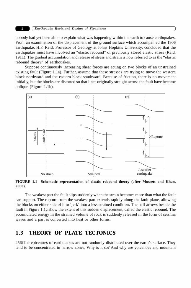
Suppose continuously increasing shear forces are acting on two blocks of an unstrainedexisting fault (Figure 1.1a). Further, assume that these stresses are trying to move the westernblock northward and the eastern block southward. Because of friction, there is no movementinitially, but the blocks are distorted so that lines originally straight across the fault have becomeoblique (Figure 1.1b).
Str
ess
Fau
ltpla
ne
No strain Strained
Just afterearthquake
Rupture
(a) (b) (c)
FIGURE 1.1 Schematic representation of elastic rebound theory (after Mussett and Khan,2000).
The weakest part the fault slips suddenly when the strain becomes more than what the faultcan support. The rupture from the weakest part extends rapidly along the fault plane, allowingthe blocks on either side of it to ‘jerk’ into a less strained condition. The half arrows beside thefault in Figure 1.1c show the extent of this sudden displacement, called the elastic rebound. Theaccumulated energy in the strained volume of rock is suddenly released in the form of seismicwaves and a part is converted into heat or other forms.
1.3 THEORY OF PLATE TECTONICS
456iThe epicentres of earthquakes are not randomly distributed over the earth’s surface. Theytend to be concentrated in narrow zones. Why is it so? And why are volcanoes and mountain

5�������� ��� �� ��� �������
ranges also found in these zones, too? An explanation to these questions can be found in platetectonics, a concept which has revolutionized thinking in the Earth Sciences in the last fewdecades. The epicentres of 99% earthquakes are distributed along narrow zones of interplateseismic activity. The remainder of the earth is considered to be aseismic. However, no regionof the earth can be regarded as completely earthquake-free. About 1% of the global seismicityis due to intraplate earthquakes, which occur away from the major seismic zones. The seismicitymap is one of the important evidences in support of the plate tectonic theory, and delineates thepresently active plate margins (Figure 1.2).
200 40 60 80 100 120 140 160 180 160 140 120 100 80 60 40 20 0
N
60
40
20
0
20
40
60
°S
°N
60
40
20
0
20
40
60
°S
200 40 60 80 100 120 140 160 180 160 140 120 100 80 60 40 20 0
FIGURE 1.2 Geographical distribution of epicentres of 30,000 earthquakes occurred during1961-1967 illustrates the tectonically active regions of the earth (after Barazangi and Dorman,1969).
The pioneering work was done by Alfred Wegener, a German meteorologist andgeophysicist, towards the development of the theory of plate tectonics. He presented hiscontinental drift theory in his 1915 book ‘On the Origin of Continents and Oceans’. Heproposed that at one time all the continents were joined into one huge super continent, whichhe named Pangaea and that at a later date the continents split apart, moving slowly to theirpresent positions on the globe. Wegener’s theory was not accepted since he could notsatisfactorily answer the most fundamental question raised by his critics, i.e. what kind of forcescould be strong enough to move such large masses of solid rock over such great distances?Further, Harold Jeffreys, a noted English geophysicist, argued correctly that it was physicallyimpossible for a large mass of solid rock to plough through the ocean floor without breakingup, as proposed by Wegener. But, Wegener persisted in his study of the idea, finding more andmore supporting evidences like fossils and rocks of vastly different climates in the past thatcould only be explained by a relocation of the particular continent to different latitudes.
����������� ������� �������������6
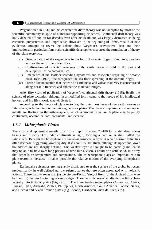
Wegener died in 1930 and his continental drift theory was not accepted by most of thescientific community in spite of numerous supporting evidences. Continental drift theory washotly debated off and on for decades even after his death and was largely dismissed as beingeccentric, preposterous, and improbable. However, in the beginning of 1950s, wealth of newevidences emerged to revive the debate about Wegener’s provocative ideas and theirimplications. In particular, four major scientific developments spurred the formulation of theoryof the plate tectonics.
(i) Demonstration of the ruggedness in the form of oceanic ridges, island arcs, trenchesand youthness of the ocean floor.
(ii) Confirmation of repeated reversals of the earth magnetic field in the past anddevelopment of paleomagnetism.
(iii) Emergence of the seafloor-spreading hypothesis and associated recycling of oceaniccrust. Hess (1962) first recognized the sea floor spreading at the oceanic ridges.
(iv) Precise documentation that the world’s earthquake and volcanic activity is concentratedalong oceanic trenches and submarine mountain ranges.
After fifty years of publication of Wegener’s continental drift theory (1915), finally thescience of plate tectonics, although in a modified form, came to the rescue of his intellectualhonour and his life’s work was vindicated.
According to the theory of plate tectonics, the outermost layer of the earth, known aslithosphere, is broken into numerous segments or plates. The plates comprising crust and uppermantle are floating on the asthenosphere, which is viscous in nature. A plate may be purelycontinental, oceanic or both continental and oceanic.
1.3.1 Lithospheric Plates
The crust and uppermost mantle down to a depth of about 70-100 km under deep oceanbasins and 100-150 km under continents is rigid, forming a hard outer shell called thelithosphere. Beneath the lithosphere lies the asthenosphere, a layer in which seismic velocitiesoften decrease, suggesting lower rigidity. It is about 150 km thick, although its upper and lowerboundaries are not sharply defined. This weaker layer is thought to be partially molten; itmay be able to flow over long periods of time like a viscous liquid or plastic solid, in a waythat depends on temperature and composition. The asthenosphere plays an important role inplate tectonics, because it makes possible the relative motion of the overlying lithosphericplates.
Earthquake epicentres are not evenly distributed over the surface of the globe, but occurpredominantly in well-defined narrow seismic zones that are often associated with volcanicactivity. These narrow zones are: (a) the circum-Pacific ‘ring of fire’; (b) the Alpine-Himalayanbelt and (c) the world-circling oceanic ridges. These seismic zones subdivide the lithospherelaterally into tectonic plates (Figure 1.3). There are twelve major plates (Antarctica, Africa,Eurasia, India, Australia, Arabia, Philippines, North America, South America, Pacific, Nazca,and Cocos) and several minor plates (e.g., Scotia, Caribbean, Juan de Fuca, etc.).
7�������� ��� �� ��� �������
180° 90°W 0° 90°E 180°Spreadingboundary
Convergentboundary
Transformboundary
Uncertainboundary
Relative motion(mm/yr)
23
68
74 2076
73
14
14
14
Antarctica
30
35
SC
84
59103
117
125
63
81158
146
106CO
Pacific
NazcaSouth
America
59 7834
30Africa
12
24
CA
6548
7369
5950
JF NorthAmerica 24
22
20
10
12
30
4063 Australia
67
80
India
3348
60
PH
32
98
Pacific
8477
Eurasia
S. A
rabia
PH = Philippine
JF = Juan de FucaSC = Scotia
Smaller plates:
CO = CocosCA = Caribbean
60°S
40°S
20°S
0°
20°N
40°N
60°N
60°S
40°S
20°S
0°
20°N
40°N
60°N
180° 90°W 0° 90°E 180°
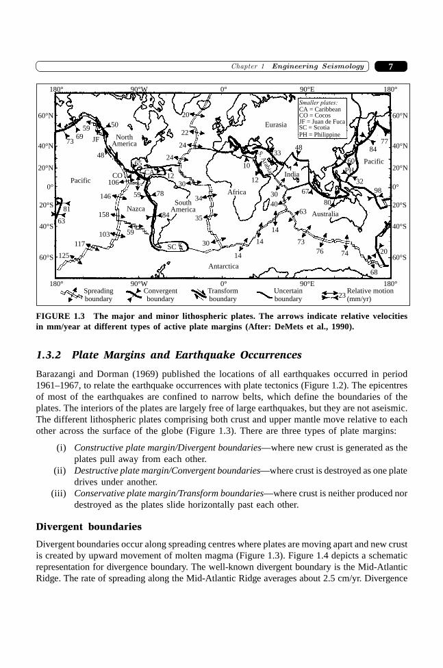
FIGURE 1.3 The major and minor lithospheric plates. The arrows indicate relative velocitiesin mm/year at different types of active plate margins (After: DeMets et al., 1990).
1.3.2 Plate Margins and Earthquake Occurrences
Barazangi and Dorman (1969) published the locations of all earthquakes occurred in period1961–1967, to relate the earthquake occurrences with plate tectonics (Figure 1.2). The epicentresof most of the earthquakes are confined to narrow belts, which define the boundaries of theplates. The interiors of the plates are largely free of large earthquakes, but they are not aseismic.The different lithospheric plates comprising both crust and upper mantle move relative to eachother across the surface of the globe (Figure 1.3). There are three types of plate margins:
(i) Constructive plate margin/Divergent boundaries—where new crust is generated as theplates pull away from each other.
(ii) Destructive plate margin/Convergent boundaries—where crust is destroyed as one platedrives under another.
(iii) Conservative plate margin/Transform boundaries—where crust is neither produced nordestroyed as the plates slide horizontally past each other.
Divergent boundaries
Divergent boundaries occur along spreading centres where plates are moving apart and new crustis created by upward movement of molten magma (Figure 1.3). Figure 1.4 depicts a schematicrepresentation for divergence boundary. The well-known divergent boundary is the Mid-AtlanticRidge. The rate of spreading along the Mid-Atlantic Ridge averages about 2.5 cm/yr. Divergence
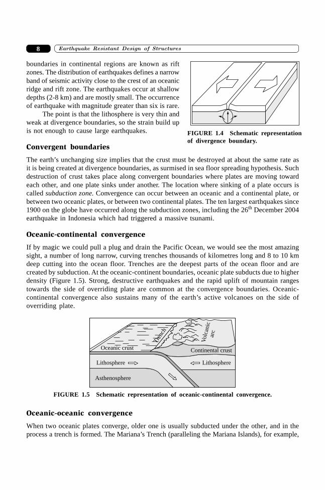
����������� ������� �������������8
boundaries in continental regions are known as riftzones. The distribution of earthquakes defines a narrowband of seismic activity close to the crest of an oceanicridge and rift zone. The earthquakes occur at shallowdepths (2-8 km) and are mostly small. The occurrenceof earthquake with magnitude greater than six is rare.
The point is that the lithosphere is very thin andweak at divergence boundaries, so the strain build upis not enough to cause large earthquakes.
Convergent boundaries
The earth’s unchanging size implies that the crust must be destroyed at about the same rate asit is being created at divergence boundaries, as surmised in sea floor spreading hypothesis. Suchdestruction of crust takes place along convergent boundaries where plates are moving towardeach other, and one plate sinks under another. The location where sinking of a plate occurs iscalled subduction zone. Convergence can occur between an oceanic and a continental plate, orbetween two oceanic plates, or between two continental plates. The ten largest earthquakes since1900 on the globe have occurred along the subduction zones, including the 26th December 2004earthquake in Indonesia which had triggered a massive tsunami.
Oceanic-continental convergence
If by magic we could pull a plug and drain the Pacific Ocean, we would see the most amazingsight, a number of long narrow, curving trenches thousands of kilometres long and 8 to 10 kmdeep cutting into the ocean floor. Trenches are the deepest parts of the ocean floor and arecreated by subduction. At the oceanic-continent boundaries, oceanic plate subducts due to higherdensity (Figure 1.5). Strong, destructive earthquakes and the rapid uplift of mountain rangestowards the side of overriding plate are common at the convergence boundaries. Oceanic-continental convergence also sustains many of the earth’s active volcanoes on the side ofoverriding plate.
Oceanic crust
Tre
nch
Volc
anic
arc
Continental crust
LithosphereLithosphere
Asthenosphere
FIGURE 1.5 Schematic representation of oceanic-continental convergence.
Oceanic-oceanic convergence
When two oceanic plates converge, older one is usually subducted under the other, and in theprocess a trench is formed. The Mariana’s Trench (paralleling the Mariana Islands), for example,
FIGURE 1.4 Schematic representationof divergence boundary.
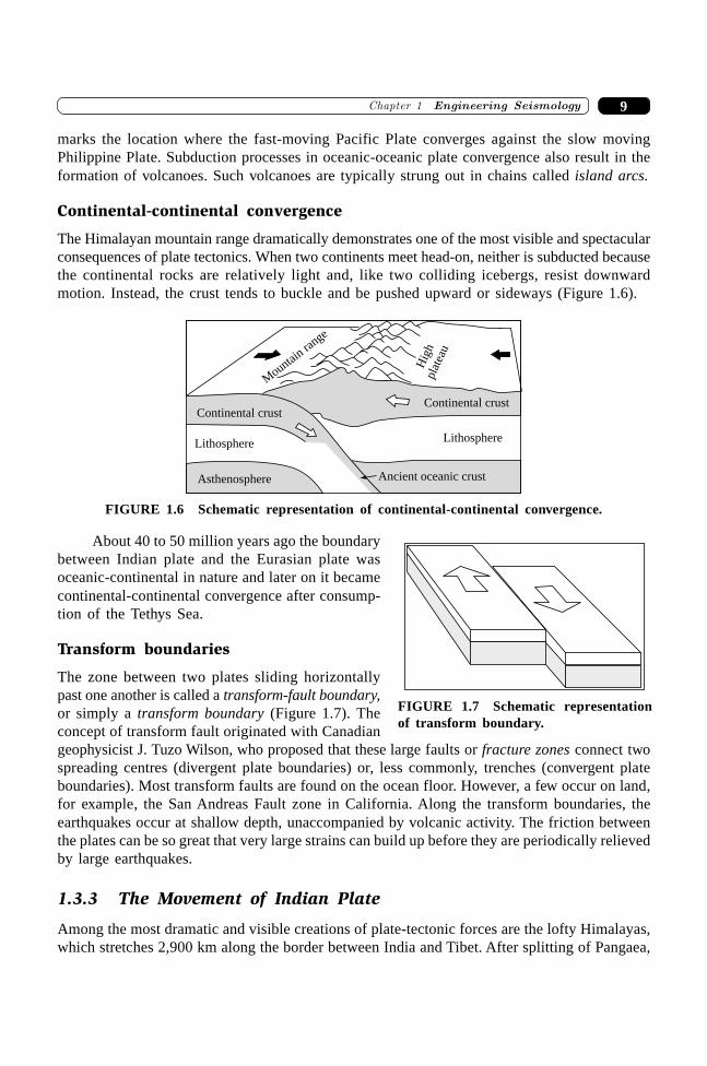
9�������� ��� �� ��� �������
marks the location where the fast-moving Pacific Plate converges against the slow movingPhilippine Plate. Subduction processes in oceanic-oceanic plate convergence also result in theformation of volcanoes. Such volcanoes are typically strung out in chains called island arcs.
Continental-continental convergence
The Himalayan mountain range dramatically demonstrates one of the most visible and spectacularconsequences of plate tectonics. When two continents meet head-on, neither is subducted becausethe continental rocks are relatively light and, like two colliding icebergs, resist downwardmotion. Instead, the crust tends to buckle and be pushed upward or sideways (Figure 1.6).
Mountai
nra
nge
Hig
hpl
atea
uLithosphere
Lithosphere
Continental crust
Ancient oceanic crust
Continental crust
Asthenosphere
FIGURE 1.6 Schematic representation of continental-continental convergence.
About 40 to 50 million years ago the boundarybetween Indian plate and the Eurasian plate wasoceanic-continental in nature and later on it becamecontinental-continental convergence after consump-tion of the Tethys Sea.
Transform boundaries
The zone between two plates sliding horizontallypast one another is called a transform-fault boundary,or simply a transform boundary (Figure 1.7). Theconcept of transform fault originated with Canadiangeophysicist J. Tuzo Wilson, who proposed that these large faults or fracture zones connect twospreading centres (divergent plate boundaries) or, less commonly, trenches (convergent plateboundaries). Most transform faults are found on the ocean floor. However, a few occur on land,for example, the San Andreas Fault zone in California. Along the transform boundaries, theearthquakes occur at shallow depth, unaccompanied by volcanic activity. The friction betweenthe plates can be so great that very large strains can build up before they are periodically relievedby large earthquakes.
1.3.3 The Movement of Indian Plate
Among the most dramatic and visible creations of plate-tectonic forces are the lofty Himalayas,which stretches 2,900 km along the border between India and Tibet. After splitting of Pangaea,
FIGURE 1.7 Schematic representationof transform boundary.
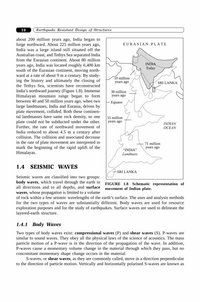
����������� ������� �������������10
about 200 million years ago, India began toforge northward. About 225 million years ago,India was a large island still situated off theAustralian coast, and Tethys Sea separated Indiafrom the Eurasian continent. About 80 millionyears ago, India was located roughly 6,400 kmsouth of the Eurasian continent, moving north-ward at a rate of about 9 m a century. By study-ing the history and ultimately the closing ofthe Tethys Sea, scientists have reconstructedIndia’s northward journey (Figure 1.8). ImmenseHimalayan mountain range began to formbetween 40 and 50 million years ago, when twolarge landmasses, India and Eurasia, driven byplate movement, collided. Both these continen-tal landmasses have same rock density, so oneplate could not be subducted under the other.Further, the rate of northward movement ofIndia reduced to about 4.5 m a century aftercollision. The collision and associated decreasein the rate of plate movement are interpreted tomark the beginning of the rapid uplift of theHimalayas.
1.4 SEISMIC WAVES
Seismic waves are classified into two groups:body waves, which travel through the earth inall directions and to all depths, and surfacewaves, whose propagation is limited to a volumeof rock within a few seismic wavelengths of the earth’s surface. The uses and analysis methodsfor the two types of waves are substantially different. Body waves are used for resourceexploration purposes and for the study of earthquakes. Surface waves are used to delineate thelayered-earth structure.
1.4.1 Body Waves
Two types of body waves exist: compressional waves (P) and shear waves (S). P-waves aresimilar to sound waves. They obey all the physical laws of the science of acoustics. The massparticle motion of a P-wave is in the direction of the propagation of the wave. In addition,P-waves cause a momentary volume change in the material through which they pass, but noconcomitant momentary shape change occurs in the material.
S-waves, or shear waves, as they are commonly called, move in a direction perpendicularto the direction of particle motion. Vertically and horizontally polarised S-waves are known as
10 millionyears ago
SRI LANKA
“INDIA”Landmass
71 millionyears ago
INDIANOCEAN
55 millionyears ago
38 millionyears ago
Equator
INDIAToday
E U R A S I A N P L A T E
SRI LANKA
FIGURE 1.8 Schematic representation ofmovement of Indian plate.
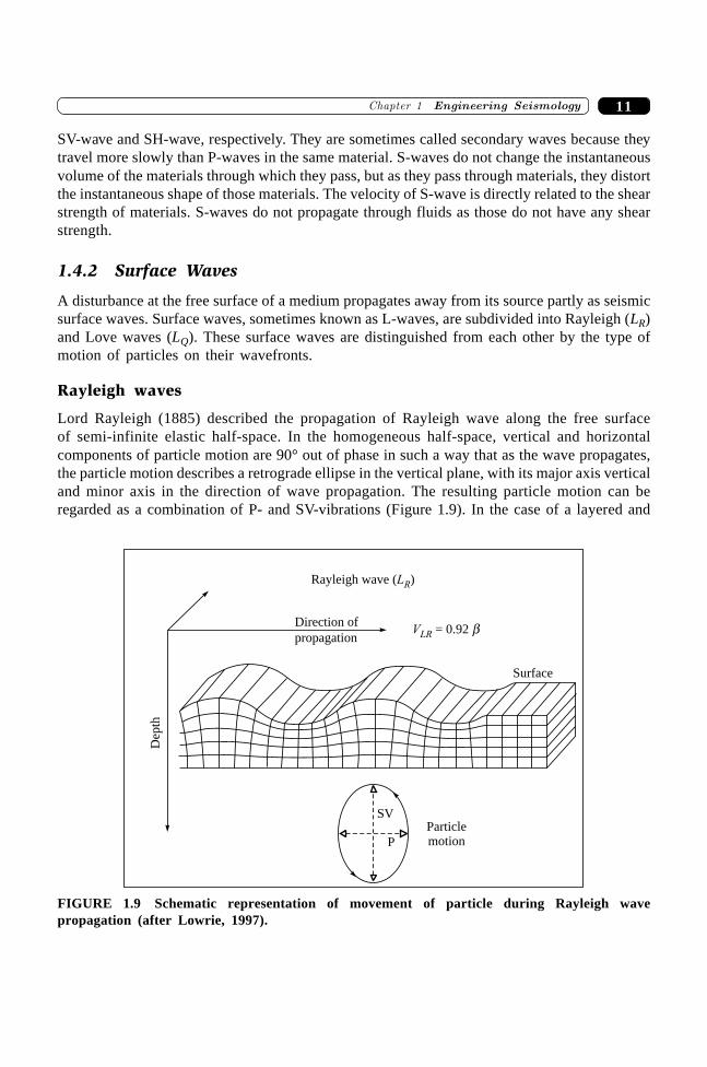
11�������� ��� �� ��� �������
SV-wave and SH-wave, respectively. They are sometimes called secondary waves because theytravel more slowly than P-waves in the same material. S-waves do not change the instantaneousvolume of the materials through which they pass, but as they pass through materials, they distortthe instantaneous shape of those materials. The velocity of S-wave is directly related to the shearstrength of materials. S-waves do not propagate through fluids as those do not have any shearstrength.
1.4.2 Surface Waves
A disturbance at the free surface of a medium propagates away from its source partly as seismicsurface waves. Surface waves, sometimes known as L-waves, are subdivided into Rayleigh (LR)and Love waves (LQ). These surface waves are distinguished from each other by the type ofmotion of particles on their wavefronts.
Rayleigh waves
Lord Rayleigh (1885) described the propagation of Rayleigh wave along the free surfaceof semi-infinite elastic half-space. In the homogeneous half-space, vertical and horizontalcomponents of particle motion are 90° out of phase in such a way that as the wave propagates,the particle motion describes a retrograde ellipse in the vertical plane, with its major axis verticaland minor axis in the direction of wave propagation. The resulting particle motion can beregarded as a combination of P- and SV-vibrations (Figure 1.9). In the case of a layered and
Rayleigh wave ( )LR
Direction of
SV
P
Particlemotion
Dep
th
propagationVLR = 0.92 b
Surface
FIGURE 1.9 Schematic representation of movement of particle during Rayleigh wavepropagation (after Lowrie, 1997).
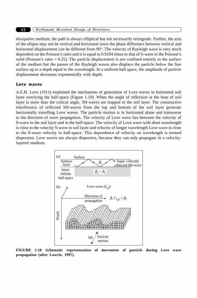
����������� ������� �������������12
dissipative medium, the path is always elliptical but not necessarily retrograde. Further, the axisof the ellipse may not be vertical and horizontal since the phase difference between vertical andhorizontal displacement can be different from 90°. The velocity of Rayleigh wave is very muchdependent on the Poisson’s ratio and it is equal to 0.9194 times to that of S-wave in the Poisson’ssolid (Poisson’s ratio = 0.25). The particle displacement is not confined entirely to the surfaceof the medium but the passes of the Rayleigh waves also displace the particle below the freesurface up to a depth equal to the wavelength. In a uniform half space, the amplitude of particledisplacement decreases exponentially with depth.
Love waves
A.E.H. Love (1911) explained the mechanism of generation of Love waves in horizontal soillayer overlying the half-space (Figure 1.10). When the angle of reflection at the base of soillayer is more than the critical angle, SH-waves are trapped in the soil layer. The constructiveinterference of reflected SH-waves from the top and bottom of the soil layer generatehorizontally travelling Love waves. The particle motion is in horizontal plane and transverseto the direction of wave propagation. The velocity of Love wave lies between the velocity ofS-wave in the soil layer and in the half-space. The velocity of Love wave with short wavelengthis close to the velocity S-wave in soil layer and velocity of longer wavelength Love wave is closeto the S-wave velocity in half-space. This dependence of velocity on wavelength is termeddispersion. Love waves are always dispersive, because they can only propagate in a velocity-layered medium.
Direction of
propagation
SH Particlemotion
Dep
th
(b) Love wave ( )LQ
b, <VLQ b2
b >2 1b
(a)
Surfacelayer
Semi-infinite
half-space
Surface
b1Super critically
reflected SH-wave
FIGURE 1.10 Schematic representation of movement of particle during Love wavepropagation (after Lowrie, 1997).
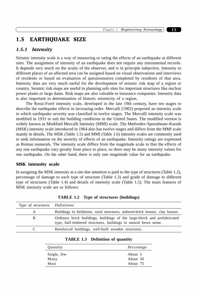
13�������� ��� �� ��� �������
1.5 EARTHQUAKE SIZE
1.5.1 Intensity
Seismic intensity scale is a way of measuring or rating the effects of an earthquake at differentsites. The assignment of intensity of an earthquake does not require any instrumental records.It depends very much on the acuity of the observer, and is in principle subjective. Intensity todifferent places of an affected area can be assigned based on visual observations and interviewsof residents or based on evaluation of questionnaires completed by residents of that area.Intensity data are very much useful for the development of seismic risk map of a region orcountry. Seismic risk maps are useful in planning safe sites for important structures like nuclearpower plants or large dams. Risk maps are also valuable to insurance companies. Intensity datais also important in determination of historic seismicity of a region.
The Rossi-Forel intensity scale, developed in the late 19th century, have ten stages todescribe the earthquake effects in increasing order. Mercalli (1902) proposed an intensity scalein which earthquake severity was classified in twelve stages. The Mercalli intensity scale wasmodified in 1931 to suit the building conditions in the United States. The modified version iswidely known as Modified Mercalli Intensity (MMI) scale. The Medvedev-Spoonheuer-Karnik(MSK) intensity scale introduced in 1964 also has twelve stages and differs from the MMI scalemainly in details. The MSK (Table 1.5) and MMI (Table 1.6) intensity scales are commonly usedto seek information on the severity of effects of an earthquake. Intensity ratings are expressedas Roman numerals. The intensity scale differs from the magnitude scale in that the effects ofany one earthquake vary greatly from place to place, so there may be many intensity values forone earthquake. On the other hand, there is only one magnitude value for an earthquake.
MSK intensity scale
In assigning the MSK intensity at a site due attention is paid to the type of structures (Table 1.2),percentage of damage to each type of structure (Table 1.3) and grade of damage to differenttype of structures (Table 1.4) and details of intensity scale (Table 1.5). The main features ofMSK intensity scale are as follows:
TABLE 1.2 Type of structures (buildings)
Type of structures Definitions
A Buildings in fieldstone, rural structures, unburnt-brick houses, clay houses.
B Ordinary brick buildings, buildings of the large-block and prefabricatedtype, half-timbered structures, buildings in natural hewn stone.
C Reinforced buildings, well-built wooden structures.
TABLE 1.3 Definition of quantity
Quantity Percentage
Single, few About 5Many About 50Most About 75
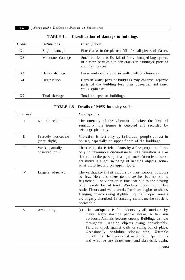
����������� ������� �������������14
TABLE 1.4 Classification of damage to buildings
Grade Definitions Descriptions
G1 Slight damage Fine cracks in the plaster; fall of small pieces of plaster.
G2 Moderate damage Small cracks in walls; fall of fairly damaged large piecesof plaster, pantiles slip off; cracks in chimneys; parts ofchimney brakes.
G3 Heavy damage Large and deep cracks in walls; fall of chimneys.
G4 Destruction Gaps in walls; parts of buildings may collapse; separateparts of the building lose their cohesion; and innerwalls collapse.
G5 Total damage Total collapse of buildings.
TABLE 1.5 Details of MSK intensity scale
Intensity Descriptions
I Not noticeable The intensity of the vibration is below the limit ofsensibility; the tremor is detected and recorded byseismographs only.
II Scarcely noticeable Vibration is felt only by individual people at rest in(very slight) houses, especially on upper floors of the buildings.
III Weak, partially The earthquake is felt indoors by a few people, outdoorsobserved only only in favourable circumstances. The vibration is like
that due to the passing of a light truck. Attentive observ-ers notice a slight swinging of hanging objects, some-what more heavily on upper floors.
IV Largely observed The earthquake is felt indoors by many people, outdoorsby few. Here and there people awake, but no one isfrightened. The vibration is like that due to the passingof a heavily loaded truck. Windows, doors and dishesrattle. Floors and walls crack. Furniture begins to shake.Hanging objects swing slightly. Liquids in open vesselsare slightly disturbed. In standing motorcars the shock isnoticeable.
V Awakening (a) The earthquake is felt indoors by all, outdoors bymany. Many sleeping people awake. A few runoutdoors. Animals become uneasy. Buildings tremblethroughout. Hanging objects swing considerably.Pictures knock against walls or swing out of place.Occasionally pendulum clocks stop, Unstableobjects may be overturned or shifted. Open doorsand windows are thrust open and slam-back again.
Contd.
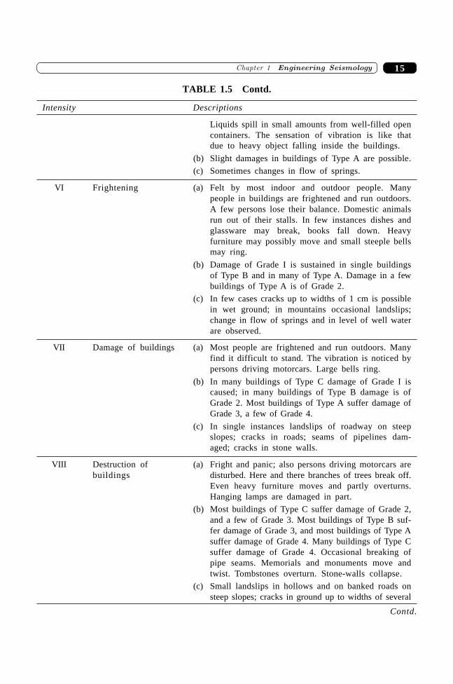
15�������� ��� �� ��� �������
Liquids spill in small amounts from well-filled opencontainers. The sensation of vibration is like thatdue to heavy object falling inside the buildings.
(b) Slight damages in buildings of Type A are possible.
(c) Sometimes changes in flow of springs.
VI Frightening (a) Felt by most indoor and outdoor people. Manypeople in buildings are frightened and run outdoors.A few persons lose their balance. Domestic animalsrun out of their stalls. In few instances dishes andglassware may break, books fall down. Heavyfurniture may possibly move and small steeple bellsmay ring.
(b) Damage of Grade I is sustained in single buildingsof Type B and in many of Type A. Damage in a fewbuildings of Type A is of Grade 2.
(c) In few cases cracks up to widths of 1 cm is possiblein wet ground; in mountains occasional landslips;change in flow of springs and in level of well waterare observed.
VII Damage of buildings (a) Most people are frightened and run outdoors. Manyfind it difficult to stand. The vibration is noticed bypersons driving motorcars. Large bells ring.
(b) In many buildings of Type C damage of Grade I iscaused; in many buildings of Type B damage is ofGrade 2. Most buildings of Type A suffer damage ofGrade 3, a few of Grade 4.
(c) In single instances landslips of roadway on steepslopes; cracks in roads; seams of pipelines dam-aged; cracks in stone walls.
VIII Destruction of (a) Fright and panic; also persons driving motorcars arebuildings disturbed. Here and there branches of trees break off.
Even heavy furniture moves and partly overturns.Hanging lamps are damaged in part.
(b) Most buildings of Type C suffer damage of Grade 2,and a few of Grade 3. Most buildings of Type B suf-fer damage of Grade 3, and most buildings of Type Asuffer damage of Grade 4. Many buildings of Type Csuffer damage of Grade 4. Occasional breaking ofpipe seams. Memorials and monuments move andtwist. Tombstones overturn. Stone-walls collapse.
(c) Small landslips in hollows and on banked roads onsteep slopes; cracks in ground up to widths of several
TABLE 1.5 Contd.
Intensity Descriptions
Contd.
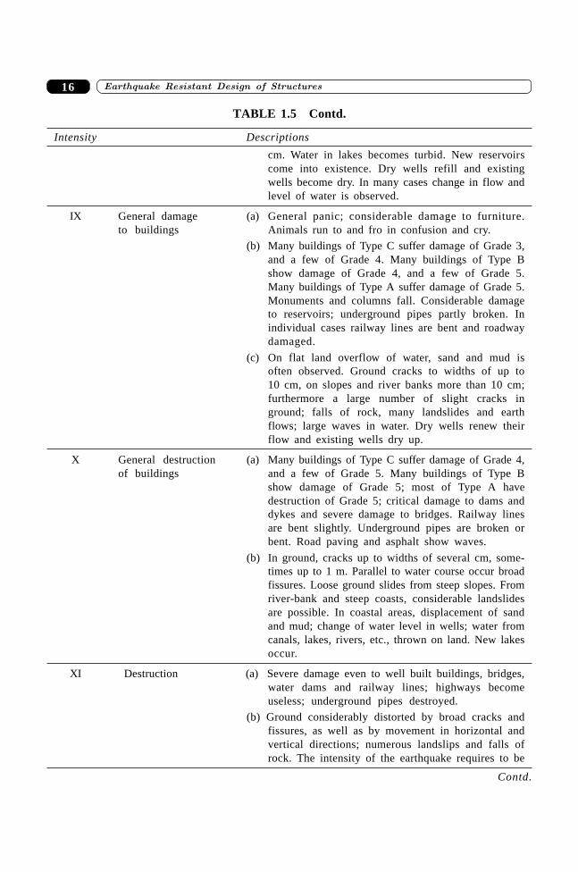
����������� ������� �������������16
cm. Water in lakes becomes turbid. New reservoirscome into existence. Dry wells refill and existingwells become dry. In many cases change in flow andlevel of water is observed.
IX General damage (a) General panic; considerable damage to furniture.to buildings Animals run to and fro in confusion and cry.
(b) Many buildings of Type C suffer damage of Grade 3,and a few of Grade 4. Many buildings of Type Bshow damage of Grade 4, and a few of Grade 5.Many buildings of Type A suffer damage of Grade 5.Monuments and columns fall. Considerable damageto reservoirs; underground pipes partly broken. Inindividual cases railway lines are bent and roadwaydamaged.
(c) On flat land overflow of water, sand and mud isoften observed. Ground cracks to widths of up to10 cm, on slopes and river banks more than 10 cm;furthermore a large number of slight cracks inground; falls of rock, many landslides and earthflows; large waves in water. Dry wells renew theirflow and existing wells dry up.
X General destruction (a) Many buildings of Type C suffer damage of Grade 4,of buildings and a few of Grade 5. Many buildings of Type B
show damage of Grade 5; most of Type A havedestruction of Grade 5; critical damage to dams anddykes and severe damage to bridges. Railway linesare bent slightly. Underground pipes are broken orbent. Road paving and asphalt show waves.
(b) In ground, cracks up to widths of several cm, some-times up to 1 m. Parallel to water course occur broadfissures. Loose ground slides from steep slopes. Fromriver-bank and steep coasts, considerable landslidesare possible. In coastal areas, displacement of sandand mud; change of water level in wells; water fromcanals, lakes, rivers, etc., thrown on land. New lakesoccur.
XI Destruction (a) Severe damage even to well built buildings, bridges,water dams and railway lines; highways becomeuseless; underground pipes destroyed.
(b) Ground considerably distorted by broad cracks andfissures, as well as by movement in horizontal andvertical directions; numerous landslips and falls ofrock. The intensity of the earthquake requires to be
TABLE 1.5 Contd.
Intensity Descriptions
Contd.
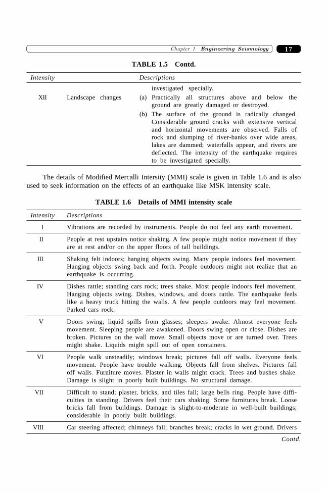
17�������� ��� �� ��� �������
investigated specially.
XII Landscape changes (a) Practically all structures above and below theground are greatly damaged or destroyed.
(b) The surface of the ground is radically changed.Considerable ground cracks with extensive verticaland horizontal movements are observed. Falls ofrock and slumping of river-banks over wide areas,lakes are dammed; waterfalls appear, and rivers aredeflected. The intensity of the earthquake requiresto be investigated specially.
The details of Modified Mercalli Intersity (MMI) scale is given in Table 1.6 and is alsoused to seek information on the effects of an earthquake like MSK intensity scale.
TABLE 1.6 Details of MMI intensity scale
Intensity Descriptions
I Vibrations are recorded by instruments. People do not feel any earth movement.
II People at rest upstairs notice shaking. A few people might notice movement if theyare at rest and/or on the upper floors of tall buildings.
III Shaking felt indoors; hanging objects swing. Many people indoors feel movement.Hanging objects swing back and forth. People outdoors might not realize that anearthquake is occurring.
IV Dishes rattle; standing cars rock; trees shake. Most people indoors feel movement.Hanging objects swing. Dishes, windows, and doors rattle. The earthquake feelslike a heavy truck hitting the walls. A few people outdoors may feel movement.Parked cars rock.
V Doors swing; liquid spills from glasses; sleepers awake. Almost everyone feelsmovement. Sleeping people are awakened. Doors swing open or close. Dishes arebroken. Pictures on the wall move. Small objects move or are turned over. Treesmight shake. Liquids might spill out of open containers.
VI People walk unsteadily; windows break; pictures fall off walls. Everyone feelsmovement. People have trouble walking. Objects fall from shelves. Pictures falloff walls. Furniture moves. Plaster in walls might crack. Trees and bushes shake.Damage is slight in poorly built buildings. No structural damage.
VII Difficult to stand; plaster, bricks, and tiles fall; large bells ring. People have diffi-culties in standing. Drivers feel their cars shaking. Some furnitures break. Loosebricks fall from buildings. Damage is slight-to-moderate in well-built buildings;considerable in poorly built buildings.
VIII Car steering affected; chimneys fall; branches break; cracks in wet ground. Drivers
TABLE 1.5 Contd.
Intensity Descriptions
Contd.
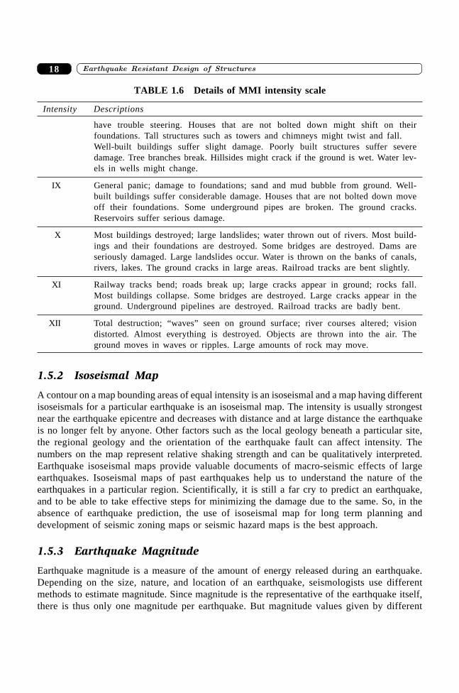
����������� ������� �������������18
have trouble steering. Houses that are not bolted down might shift on theirfoundations. Tall structures such as towers and chimneys might twist and fall.Well-built buildings suffer slight damage. Poorly built structures suffer severedamage. Tree branches break. Hillsides might crack if the ground is wet. Water lev-els in wells might change.
IX General panic; damage to foundations; sand and mud bubble from ground. Well-built buildings suffer considerable damage. Houses that are not bolted down moveoff their foundations. Some underground pipes are broken. The ground cracks.Reservoirs suffer serious damage.
X Most buildings destroyed; large landslides; water thrown out of rivers. Most build-ings and their foundations are destroyed. Some bridges are destroyed. Dams areseriously damaged. Large landslides occur. Water is thrown on the banks of canals,rivers, lakes. The ground cracks in large areas. Railroad tracks are bent slightly.
XI Railway tracks bend; roads break up; large cracks appear in ground; rocks fall.Most buildings collapse. Some bridges are destroyed. Large cracks appear in theground. Underground pipelines are destroyed. Railroad tracks are badly bent.
XII Total destruction; “waves” seen on ground surface; river courses altered; visiondistorted. Almost everything is destroyed. Objects are thrown into the air. Theground moves in waves or ripples. Large amounts of rock may move.
1.5.2 Isoseismal Map
A contour on a map bounding areas of equal intensity is an isoseismal and a map having differentisoseismals for a particular earthquake is an isoseismal map. The intensity is usually strongestnear the earthquake epicentre and decreases with distance and at large distance the earthquakeis no longer felt by anyone. Other factors such as the local geology beneath a particular site,the regional geology and the orientation of the earthquake fault can affect intensity. Thenumbers on the map represent relative shaking strength and can be qualitatively interpreted.Earthquake isoseismal maps provide valuable documents of macro-seismic effects of largeearthquakes. Isoseismal maps of past earthquakes help us to understand the nature of theearthquakes in a particular region. Scientifically, it is still a far cry to predict an earthquake,and to be able to take effective steps for minimizing the damage due to the same. So, in theabsence of earthquake prediction, the use of isoseismal map for long term planning anddevelopment of seismic zoning maps or seismic hazard maps is the best approach.
1.5.3 Earthquake Magnitude
Earthquake magnitude is a measure of the amount of energy released during an earthquake.Depending on the size, nature, and location of an earthquake, seismologists use differentmethods to estimate magnitude. Since magnitude is the representative of the earthquake itself,there is thus only one magnitude per earthquake. But magnitude values given by different
TABLE 1.6 Details of MMI intensity scale
Intensity Descriptions
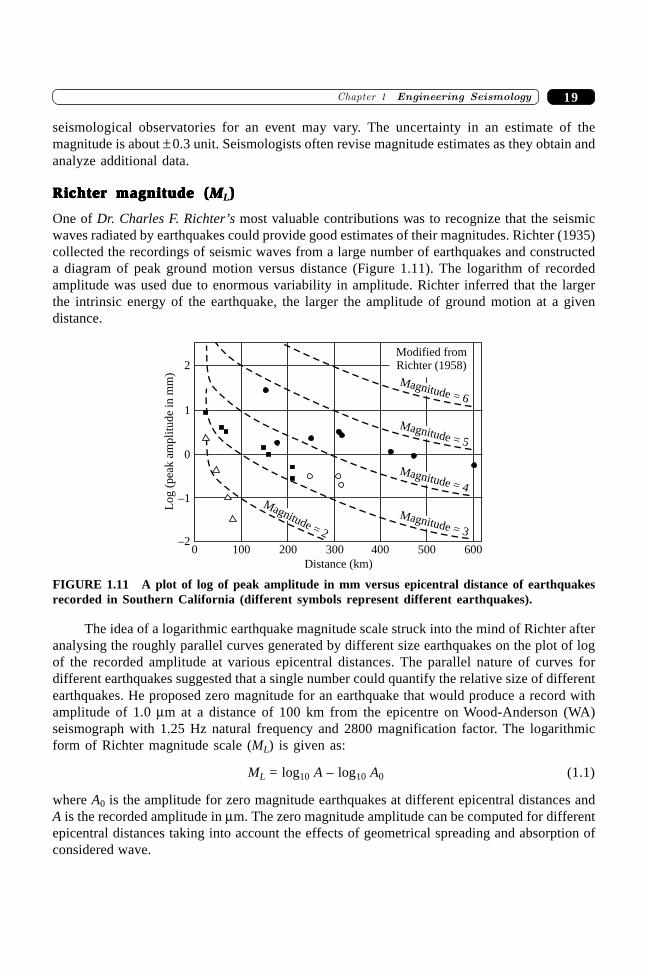
19�������� ��� �� ��� �������
seismological observatories for an event may vary. The uncertainty in an estimate of themagnitude is about ± 0.3 unit. Seismologists often revise magnitude estimates as they obtain andanalyze additional data.
Richter magnitudeRichter magnitudeRichter magnitudeRichter magnitudeRichter magnitude (((((MMMMML)))))
One of Dr. Charles F. Richter’s most valuable contributions was to recognize that the seismicwaves radiated by earthquakes could provide good estimates of their magnitudes. Richter (1935)collected the recordings of seismic waves from a large number of earthquakes and constructeda diagram of peak ground motion versus distance (Figure 1.11). The logarithm of recordedamplitude was used due to enormous variability in amplitude. Richter inferred that the largerthe intrinsic energy of the earthquake, the larger the amplitude of ground motion at a givendistance.
Modified fromRichter (1958)
1000 200 300 400 500 600–2
–1
0
1
2
Log
(pea
kam
pli
tude
inm
m)
Distance (km)
Magnitude = 2
Magnitude = 3
Magnitude = 4
Magnitude = 5
Magnitude = 6
FIGURE 1.11 A plot of log of peak amplitude in mm versus epicentral distance of earthquakesrecorded in Southern California (different symbols represent different earthquakes).
The idea of a logarithmic earthquake magnitude scale struck into the mind of Richter afteranalysing the roughly parallel curves generated by different size earthquakes on the plot of logof the recorded amplitude at various epicentral distances. The parallel nature of curves fordifferent earthquakes suggested that a single number could quantify the relative size of differentearthquakes. He proposed zero magnitude for an earthquake that would produce a record withamplitude of 1.0 mm at a distance of 100 km from the epicentre on Wood-Anderson (WA)seismograph with 1.25 Hz natural frequency and 2800 magnification factor. The logarithmicform of Richter magnitude scale (ML) is given as:
ML = log10 A – log10 A0 (1.1)
where A0 is the amplitude for zero magnitude earthquakes at different epicentral distances andA is the recorded amplitude in mm. The zero magnitude amplitude can be computed for differentepicentral distances taking into account the effects of geometrical spreading and absorption ofconsidered wave.
����������� ������� �������������20
The Richter scale used in Southern California for different epicentral distances and 18 kmfixed focal depth is as follows.
ML = log10 A (mm) + Distance correction factor ‘s’ (1.2)
Distance correction factor ‘s’ is log of inverse of zero magnitude amplitude measured in mmat an epicentral distance ‘D’ in km. The distance correction factors for different epicentraldistances are given in Table 1.7. The distance correction factors given in Table 1.7 cannot beused in other regions of the world since considered focal depth was constant. So, to computeML in any other region like Himalayas, first zero magnitude amplitude at different epicentraldistances should be determined according to the original definition of ML at 100 km anddifferent focal depths taking into account the geometrical spreading and appropriate measure ofabsorption. Since, sufficient time resolution of high frequency records is no longer a problem,therefore, frequency dependent distance correction factors, matched with Richter scale at 100km distance, have been developed based on epicentral as well as hypo-central distances (Huttonand Boore, 1987; Kim, 1998; Langston et al., 1998).
TABLE 1.7 Distance correction factors (sssss) for ML (Elementary Seismology, Richter,1958)
D (km) s(D) D (km) s(D) D (km) s(D) D (km) s(D)
0 1.4 90 3.0 260 3.8 440 4.6
10 1.5 100 3.0 280 3.9 460 4.6
20 1.7 120 3.1 300 4.0 480 4.7
30 2.1 140 3.2 320 4.1 500 4.7
40 2.4 160 3.3 340 4.2 520 4.8
50 2.6 180 3.4 360 4.3 540 4.8
60 2.8 200 3.5 380 4.4 560 4.9
70 2.8 220 3.65 400 4.5 580 4.9
80 2.9 240 3.7 420 4.5 600 4.9
Although, Richter magnitude was originally developed using earthquake records ofWA-seismometer in Southern California but the records of any short period seismometers canbe used. Now, procedures are available to synthesise precisely the response characteristics ofWA-seismograph from digital broadband recordings (Plesinger et al., 1996).
Magnitude is a measure of seismic energy released which, in turn, is proportional to (A/T)2,where A is the ground motion trace amplitude, and T as the period of the considered wave. So,the general form of Richter magnitude scale based on measurements of ground displacementamplitudes A of considered wave with periods T is,
M = log10 (A/T)max + s(D, h) + Cr + Cs (1.3)
where s(D, h), distance correction factor at an epicentral distance ‘D’ and focal depth ‘h’. Cr
is the regional source correction term to account for azimuth dependent source directivity andCs is the station correction factor dependent on local site effects. (A/T) for different periods arecomputed and maximum of them is used in the magnitude computation.
21�������� ��� �� ��� �������
Surface wave magnitude
As more seismograph stations were installed around the world, it became apparent that themethod developed by Richter was strictly valid only for certain frequency and distance ranges.Further, at large epicentral distances, body waves are usually attenuated and scattered so that theresulting motion is dominated by surface waves. On the other hand, the amplitude of surfacewaves, in case of deep focus earthquakes is too small. So, in order to take advantage of thegrowing number of globally distributed seismograph stations, new magnitude scales that are anextension of Richter’s original idea were developed. These include body-wave magnitude (mB)and surface-wave magnitude (MS). Each is valid for a particular period range and type of seismicwave.
A commonly used equation for computing MS of a shallow focus (< 50 km) earthquakefrom seismograph records between epicentral distances 20°< D < 160° is the following oneproposed by Bath (1966).
MS = log10 (As/T)max + 1.66log10 D + 3.3 (1.4)
Where AS is the amplitude of the horizontal ground motion in ‘mm’ deduced from the surfacewave with period T (around 20 ± 2 seconds) and epicentral distance D is in degree.
Body wave magnitude (mB)
Gutenberg (1945) developed body wave magnitude mB for teleseismic body-waves such as P,PP and S in the period range 0.5 s to 12 s. It is based on theoretical amplitude calculationscorrected for geometric spreading and attenuation and then adjusted to empirical observationsfrom shallow and deep-focus earthquakes.
mB = log10(A/T)max + s(D, h) (1.5)
Gutenberg and Richter (1956) published a table with distance correction factors s(D, h)for body waves, which enable magnitude determinations. These distance correction factors areused when ground motion trace amplitudes are measured in ‘mm’.
Duration magnitude (MD)
Analogue paper and tape recordings have a very limited dynamic range of only about 40 dB and60 dB, respectively. ML cannot be determined since these records are often clipped in case ofstrong and near earthquakes. Therefore, alternative duration magnitude scale MD has beendeveloped. Duration from the P-wave onset to the end of the coda (back-scattered waves fromnumerous heterogeneities) is used in computations. Aki and Chouet (1975) reported that for agiven local earthquake at epicentral distances lesser than 100 km the total duration of a signalis almost independent of distance, azimuth and property of materials along the path. This allowsdevelopment of duration magnitude scales without a distance term.
MD = a0 + a1 log D (1.6)
a0 and a1 are constant and D is the duration in seconds. The values of these constants vary regionto region according to crustal structure, scattering and attenuation conditions. They have to bedetermined locally for a region with the help of available ML.
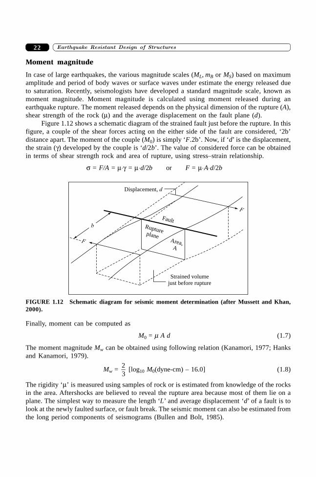
����������� ������� �������������22
Moment magnitude
In case of large earthquakes, the various magnitude scales (ML, mB or MS) based on maximumamplitude and period of body waves or surface waves under estimate the energy released dueto saturation. Recently, seismologists have developed a standard magnitude scale, known asmoment magnitude. Moment magnitude is calculated using moment released during anearthquake rupture. The moment released depends on the physical dimension of the rupture (A),shear strength of the rock (m) and the average displacement on the fault plane (d).
Figure 1.12 shows a schematic diagram of the strained fault just before the rupture. In thisfigure, a couple of the shear forces acting on the either side of the fault are considered, ‘2b’distance apart. The moment of the couple (M0) is simply ‘F.2b’. Now, if ‘d’ is the displacement,the strain (g) developed by the couple is ‘d/2b’. The value of considered force can be obtainedin terms of shear strength rock and area of rupture, using stress–strain relationship.
s = F/A = m◊g = m◊d/2b or F = m◊A◊d/2b
Ruptureplane
Area,A
Fault
F
Strained volumejust before rupture
Displacement, d
F
b
FIGURE 1.12 Schematic diagram for seismic moment determination (after Mussett and Khan,2000).
Finally, moment can be computed as
M0 = m A d (1.7)
The moment magnitude Mw can be obtained using following relation (Kanamori, 1977; Hanksand Kanamori, 1979).
Mw = 23
[log10 M0(dyne-cm) – 16.0] (1.8)
The rigidity ‘m’ is measured using samples of rock or is estimated from knowledge of the rocksin the area. Aftershocks are believed to reveal the rupture area because most of them lie on aplane. The simplest way to measure the length ‘L’ and average displacement ‘d’ of a fault is tolook at the newly faulted surface, or fault break. The seismic moment can also be estimated fromthe long period components of seismograms (Bullen and Bolt, 1985).
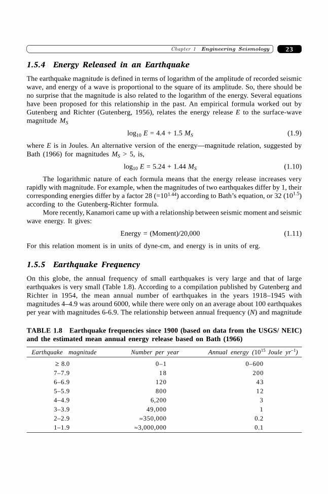
23�������� ��� �� ��� �������
1.5.4 Energy Released in an Earthquake
The earthquake magnitude is defined in terms of logarithm of the amplitude of recorded seismicwave, and energy of a wave is proportional to the square of its amplitude. So, there should beno surprise that the magnitude is also related to the logarithm of the energy. Several equationshave been proposed for this relationship in the past. An empirical formula worked out byGutenberg and Richter (Gutenberg, 1956), relates the energy release E to the surface-wavemagnitude MS
log10 E = 4.4 + 1.5 MS (1.9)
where E is in Joules. An alternative version of the energy—magnitude relation, suggested byBath (1966) for magnitudes MS > 5, is,
log10 E = 5.24 + 1.44 MS (1.10)
The logarithmic nature of each formula means that the energy release increases veryrapidly with magnitude. For example, when the magnitudes of two earthquakes differ by 1, theircorresponding energies differ by a factor 28 (=101.44) according to Bath’s equation, or 32 (101.5)according to the Gutenberg-Richter formula.
More recently, Kanamori came up with a relationship between seismic moment and seismicwave energy. It gives:
Energy = (Moment)/20,000 (1.11)
For this relation moment is in units of dyne-cm, and energy is in units of erg.
1.5.5 Earthquake Frequency
On this globe, the annual frequency of small earthquakes is very large and that of largeearthquakes is very small (Table 1.8). According to a compilation published by Gutenberg andRichter in 1954, the mean annual number of earthquakes in the years 1918–1945 withmagnitudes 4–4.9 was around 6000, while there were only on an average about 100 earthquakesper year with magnitudes 6-6.9. The relationship between annual frequency (N) and magnitude
TABLE 1.8 Earthquake frequencies since 1900 (based on data from the USGS/ NEIC)and the estimated mean annual energy release based on Bath (1966)
Earthquake magnitude Number per year Annual energy (1015 Joule yr–1)
≥ 8.0 0–1 0–600
7–7.9 18 200
6–6.9 120 43
5–5.9 800 12
4–4.9 6,200 3
3–3.9 49,000 1
2–2.9 ª350,000 0.2
1–1.9 ª3,000,000 0.1
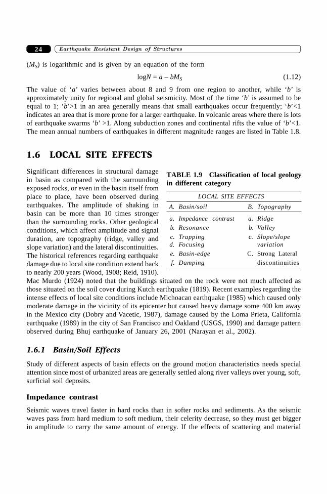
����������� ������� �������������24
(MS) is logarithmic and is given by an equation of the form
logN = a – bMS (1.12)
The value of ‘a’ varies between about 8 and 9 from one region to another, while ‘b’ isapproximately unity for regional and global seismicity. Most of the time ‘b’ is assumed to beequal to 1; ‘b’>1 in an area generally means that small earthquakes occur frequently; ‘b’<1indicates an area that is more prone for a larger earthquake. In volcanic areas where there is lotsof earthquake swarms ‘b’ >1. Along subduction zones and continental rifts the value of ‘b’<1.The mean annual numbers of earthquakes in different magnitude ranges are listed in Table 1.8.
1.6 LOCAL SITE EFFECTS
Significant differences in structural damagein basin as compared with the surroundingexposed rocks, or even in the basin itself fromplace to place, have been observed duringearthquakes. The amplitude of shaking inbasin can be more than 10 times strongerthan the surrounding rocks. Other geologicalconditions, which affect amplitude and signalduration, are topography (ridge, valley andslope variation) and the lateral discontinuities.The historical references regarding earthquakedamage due to local site condition extend backto nearly 200 years (Wood, 1908; Reid, 1910).Mac Murdo (1924) noted that the buildings situated on the rock were not much affected asthose situated on the soil cover during Kutch earthquake (1819). Recent examples regarding theintense effects of local site conditions include Michoacan earthquake (1985) which caused onlymoderate damage in the vicinity of its epicenter but caused heavy damage some 400 km awayin the Mexico city (Dobry and Vacetic, 1987), damage caused by the Loma Prieta, Californiaearthquake (1989) in the city of San Francisco and Oakland (USGS, 1990) and damage patternobserved during Bhuj earthquake of January 26, 2001 (Narayan et al., 2002).
1.6.1 Basin/Soil Effects
Study of different aspects of basin effects on the ground motion characteristics needs specialattention since most of urbanized areas are generally settled along river valleys over young, soft,surficial soil deposits.
Impedance contrast
Seismic waves travel faster in hard rocks than in softer rocks and sediments. As the seismicwaves pass from hard medium to soft medium, their celerity decrease, so they must get biggerin amplitude to carry the same amount of energy. If the effects of scattering and material
TABLE 1.9 Classification of local geologyin different category
LOCAL SITE EFFECTS
A. Basin/soil B. Topography
a. Impedance contrast a. Ridge
b. Resonance b. Valley
c. Trapping c. Slope/sloped. Focusing variation
e. Basin-edge C. Strong Lateral
f. Damping discontinuities
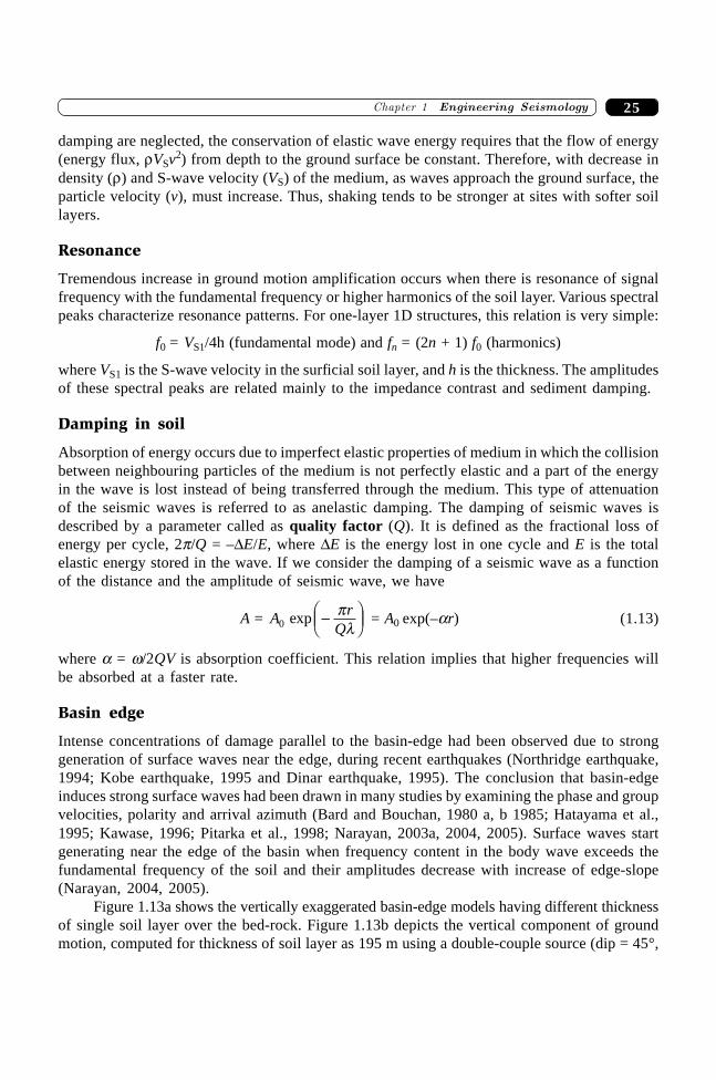
25�������� ��� �� ��� �������
damping are neglected, the conservation of elastic wave energy requires that the flow of energy(energy flux, rVSv2) from depth to the ground surface be constant. Therefore, with decrease indensity (r) and S-wave velocity (VS) of the medium, as waves approach the ground surface, theparticle velocity (v), must increase. Thus, shaking tends to be stronger at sites with softer soillayers.
Resonance
Tremendous increase in ground motion amplification occurs when there is resonance of signalfrequency with the fundamental frequency or higher harmonics of the soil layer. Various spectralpeaks characterize resonance patterns. For one-layer 1D structures, this relation is very simple:
f0 = VS1/4h (fundamental mode) and fn = (2n + 1) f0 (harmonics)
where VS1 is the S-wave velocity in the surficial soil layer, and h is the thickness. The amplitudesof these spectral peaks are related mainly to the impedance contrast and sediment damping.
Damping in soil
Absorption of energy occurs due to imperfect elastic properties of medium in which the collisionbetween neighbouring particles of the medium is not perfectly elastic and a part of the energyin the wave is lost instead of being transferred through the medium. This type of attenuationof the seismic waves is referred to as anelastic damping. The damping of seismic waves isdescribed by a parameter called as quality factor (Q). It is defined as the fractional loss ofenergy per cycle, 2p/Q = –DE/E, where DE is the energy lost in one cycle and E is the totalelastic energy stored in the wave. If we consider the damping of a seismic wave as a functionof the distance and the amplitude of seismic wave, we have
A = A rQ0 exp -FHG
IKJ
pl
= A0 exp(–ar) (1.13)
where a = w/2QV is absorption coefficient. This relation implies that higher frequencies willbe absorbed at a faster rate.
Basin edge
Intense concentrations of damage parallel to the basin-edge had been observed due to stronggeneration of surface waves near the edge, during recent earthquakes (Northridge earthquake,1994; Kobe earthquake, 1995 and Dinar earthquake, 1995). The conclusion that basin-edgeinduces strong surface waves had been drawn in many studies by examining the phase and groupvelocities, polarity and arrival azimuth (Bard and Bouchan, 1980 a, b 1985; Hatayama et al.,1995; Kawase, 1996; Pitarka et al., 1998; Narayan, 2003a, 2004, 2005). Surface waves startgenerating near the edge of the basin when frequency content in the body wave exceeds thefundamental frequency of the soil and their amplitudes decrease with increase of edge-slope(Narayan, 2004, 2005).
Figure 1.13a shows the vertically exaggerated basin-edge models having different thicknessof single soil layer over the bed-rock. Figure 1.13b depicts the vertical component of groundmotion, computed for thickness of soil layer as 195 m using a double-couple source (dip = 45°,
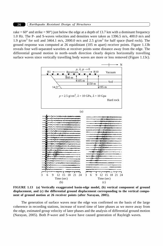
����������� ������� �������������26
rake = 60° and strike = 90°) just below the edge at a depth of 13.7 km with a dominant frequency1.0 Hz. The P- and S-waves velocities and densities were taken as 1396.5 m/s, 400.0 m/s and1.9 g/cm3 for soil and 3464.1 m/s, 2000.0 m/s and 2.5 g/cm3 for half space (hard rock). Theground response was computed at 26 equidistant (105 m apart) receiver points. Figure 1.13breveals four well-separated wavelets at receiver points some distance away from the edge. Thedifferential ground motion in north–south direction clearly depicts horizontally travellingsurface waves since vertically travelling body waves are more or less removed (Figure 1.13c).
14.5°
VacuumR10
N
Soil
195 m150 m
105 m60 m
R1 Receiversp, , 0l m �
p = 2.5 g/cm , = 10 GPa, = 10 Gpa3 l lHard rock
(a)
3 6 9 12 15 18 21 24
Time (sec)
(b)
3 6 9 12 15 18 21 24
Time (sec)
(c)
FIGURE 1.13 (a) Vertically exaggerated basin-edge model, (b) vertical component of grounddisplacement, and (c) the differential ground displacement corresponding to the vertical compo-nent of ground motion at 26 receiver points (after Narayan, 2005).
The generation of surface waves near the edge was confirmed on the basis of the largecoherence in recording stations, increase of travel time of later phases as we move away fromthe edge, estimated group velocity of later phases and the analysis of differential ground motion(Narayan, 2005). Both P-wave and S-wave have caused generation of Rayleigh waves.
27�������� ��� �� ��� �������
The major conclusions drawn in papers of Bard and Bouchan (1980 a, b), Hatayamaet al. (1995), Kawase (1996) Pitarka, et al. (1998) and Narayan (2003a, 2004, 2005) are listedbelow.
∑ Basin-edge induces strong surface waves near the edge.∑ Edge-induced surface waves propagate normal to edge and towards the basin.∑ Surface waves start generating near the edge of the basin when frequency content in
the body wave exceeds the fundamental frequency of the soil deposit.∑ Surface wave amplitude decreases with increase of edge-slope.∑ Damage caused by edge-induced surface waves is confined in a narrow zone (width
2.5–3.5 km) parallel to the edge, and at some distance (0.5–1.0 km).∑ Surface wave amplitude increases with the decrease of propagation velocity in soil.
Further, their characteristics are highly variable with change in propagation velocityand thickness of soil deposit.
∑ The characteristics of edge-induced surface waves are also very much dependent on theangle of incidence of body waves.
∑ Edge-induced surface waves develop significant differential ground, the main causeof damage during earthquakes, in addition to amplification and prolongation of thesignal.
Basement topography
The focusing and defocusing effects caused by basement topography are strongly dependenton the azimuth and angle of incidence of waves. Seismic waves traveling upward from depthmay be redirected by subtle irregularities at geological interfaces, particularly the basementtopography. The effects of focusing and defocusing are maximum for normal incidence ofwaves and it decreases with increase of angle of incidence. Similarly, azimuth also affects thefocusing and defocusing effects. This effect reveals the importance of considering not only thesurficial soil layer but also the basement topography for seismic microzonation.
Trapping of waves
The fundamental phenomenon responsible for the increase of duration of motion over softsediments is the trapping and multiple reflections of seismic waves due to the large impedancecontrast between soft sediments and underlying bedrock. Sometimes, when a wave enters a basinthrough its edge, it can become trapped within the basin if post-critical incidence angles develop,causing total internal reflection at the base of the layer. Waves that become trapped in deepsedimentary basins can therefore be potentially very damaging.
1.6.2 Lateral Discontinuity Effects
There are numerous consistent macroseismic observations showing a significant increase inintensity of damage in narrow zones located along lateral discontinuities, i.e. areas where asofter material lies besides a more rigid one. An amplitude amplification and local surface wavegeneration in the softer medium and large differential motion caused by shorter wavelengthof the surface wave can explain the observed damage. In past, a number of field observations
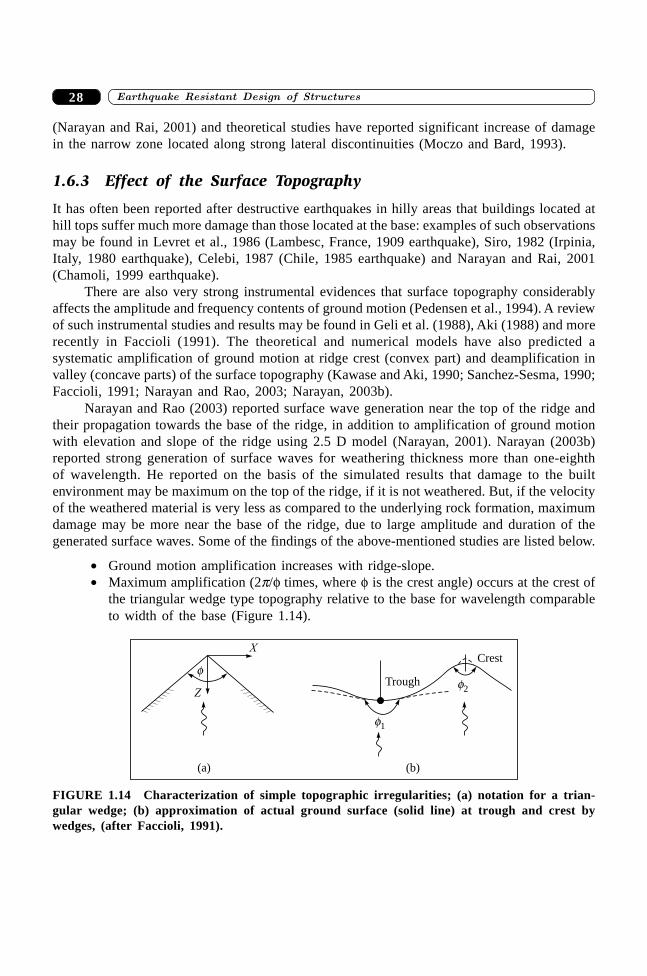
����������� ������� �������������28
(Narayan and Rai, 2001) and theoretical studies have reported significant increase of damagein the narrow zone located along strong lateral discontinuities (Moczo and Bard, 1993).
1.6.3 Effect of the Surface Topography
It has often been reported after destructive earthquakes in hilly areas that buildings located athill tops suffer much more damage than those located at the base: examples of such observationsmay be found in Levret et al., 1986 (Lambesc, France, 1909 earthquake), Siro, 1982 (Irpinia,Italy, 1980 earthquake), Celebi, 1987 (Chile, 1985 earthquake) and Narayan and Rai, 2001(Chamoli, 1999 earthquake).
There are also very strong instrumental evidences that surface topography considerablyaffects the amplitude and frequency contents of ground motion (Pedensen et al., 1994). A reviewof such instrumental studies and results may be found in Geli et al. (1988), Aki (1988) and morerecently in Faccioli (1991). The theoretical and numerical models have also predicted asystematic amplification of ground motion at ridge crest (convex part) and deamplification invalley (concave parts) of the surface topography (Kawase and Aki, 1990; Sanchez-Sesma, 1990;Faccioli, 1991; Narayan and Rao, 2003; Narayan, 2003b).
Narayan and Rao (2003) reported surface wave generation near the top of the ridge andtheir propagation towards the base of the ridge, in addition to amplification of ground motionwith elevation and slope of the ridge using 2.5 D model (Narayan, 2001). Narayan (2003b)reported strong generation of surface waves for weathering thickness more than one-eighthof wavelength. He reported on the basis of the simulated results that damage to the builtenvironment may be maximum on the top of the ridge, if it is not weathered. But, if the velocityof the weathered material is very less as compared to the underlying rock formation, maximumdamage may be more near the base of the ridge, due to large amplitude and duration of thegenerated surface waves. Some of the findings of the above-mentioned studies are listed below.
∑ Ground motion amplification increases with ridge-slope.∑ Maximum amplification (2p/f times, where f is the crest angle) occurs at the crest of
the triangular wedge type topography relative to the base for wavelength comparableto width of the base (Figure 1.14).
Trough
(a)
Z
X
fCrest
f1
f2
(b)
FIGURE 1.14 Characterization of simple topographic irregularities; (a) notation for a trian-gular wedge; (b) approximation of actual ground surface (solid line) at trough and crest bywedges, (after Faccioli, 1991).
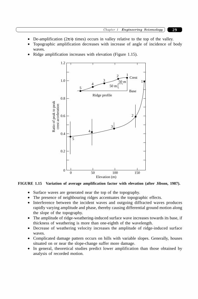
29�������� ��� �� ��� �������
∑ De-amplification (2p/f times) occurs in valley relative to the top of the valley.∑ Topographic amplification decreases with increase of angle of incidence of body
waves.∑ Ridge amplification increases with elevation (Figure 1.15).
54
3
2 1
50 m
50 m
Base
Crest
Ridge profile
0 50 100 150
Elevation (m)
0
0.2
0.4
0.6
0.8
1.0
1.2
5
4
3
2
1
Rat
ioo
fp
eak
top
eak
cres
tac
cele
rati
on
FIGURE 1.15 Variation of average amplification factor with elevation (after Jibson, 1987).
∑ Surface waves are generated near the top of the topography.∑ The presence of neighbouring ridges accentuates the topographic effects.∑ Interference between the incident waves and outgoing diffracted waves produces
rapidly varying amplitude and phase, thereby causing differential ground motion alongthe slope of the topography.
∑ The amplitude of ridge-weathering-induced surface wave increases towards its base, ifthickness of weathering is more than one-eighth of the wavelength.
∑ Decrease of weathering velocity increases the amplitude of ridge-induced surfacewaves.
∑ Complicated damage pattern occurs on hills with variable slopes. Generally, housessituated on or near the slope-change suffer more damage.
∑ In general, theoretical studies predict lower amplification than those obtained byanalysis of recorded motion.
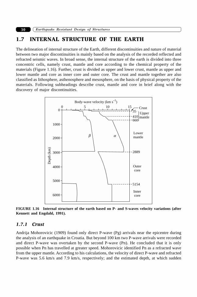
����������� ������� �������������30
1.7 INTERNAL STRUCTURE OF THE EARTH
The delineation of internal structure of the Earth, different discontinuities and nature of materialbetween two major discontinuities is mainly based on the analysis of the recorded reflected andrefracted seismic waves. In broad sense, the internal structure of the earth is divided into threeconcentric cells, namely crust, mantle and core according to the chemical property of thematerials (Figure 1.16). Further, crust is divided as upper and lower crust, mantle as upper andlower mantle and core as inner core and outer core. The crust and mantle together are alsoclassified as lithosphere, asthenosphere and mesosphere, on the basis of physical property of thematerials. Following subheadings describe crust, mantle and core in brief along with thediscovery of major discontinuities.
Lowermantle
Uppermantle
0 5 10 150
1000
2000
3000
4000
5000
6000
5154
Innercore
Outercore
2889
660410
35Crust
Body-wave velocity (km s )–1
ab
Dep
th(k
m)
FIGURE 1.16 Internal structure of the earth based on P- and S-waves velocity variations (afterKennett and Engdahl, 1991).
1.7.1 Crust
Andrija Mohorovicic (1909) found only direct P-wave (Pg) arrivals near the epicentre duringthe analysis of an earthquake in Croatia. But beyond 100 km two P-wave arrivals were recordedand direct P-wave was overtaken by the second P-wave (Pn). He concluded that it is onlypossible when Pn has travelled at greater speed. Mohorovicic identified Pn as a refracted wavefrom the upper mantle. According to his calculations, the velocity of direct P-wave and refractedP-wave was 5.6 km/s and 7.9 km/s, respectively; and the estimated depth, at which sudden
31�������� ��� �� ��� �������
increase of velocity occurred was 54 km. Now, this seismic discontinuity between crust andmantle, where there is sudden increase of seismic wave velocity, is called as Mohorovicicdiscontinuity, or simply Moho.
V. Conrad (1925) found faster P-wave (P*) and S-wave (S*) as compared to Pg and Sgwaves during the analysis of Tauern earthquake of 1923 (Eastern Alps) in upper crustal layer.The estimated velocities of P* and S* waves (6.29 km/s and 3.57 km/s, respectively) were lesserthan the velocities of Pn and Sn waves refracted from the Moho. Conrad inferred the existenceof a lower crustal layer with higher velocity as compared to the upper crustal layer. The interfaceseparating the crustal mass into upper and lower crust is called as Conrad discontinuity, inhonour of V. Conrad.
Worldwide analysis of recorded reflected and refracted seismic waves reveals that thestructures of the crust and upper mantle are very complex. The thickness of crust is highlylaterally variable. It is 5–10 km in oceanic region, below the mean water-depth of about4.5 km. The vertical structure of continental crust is more complicated than that of oceanic crust.The thickness of continental crust varies from 35 to 40 km under stable continental areas and50 to 60 km under young mountain ranges.
1.7.2 Upper Mantle
The Mohorovicic discontinuity defines the top of the mantle. The average depth of Moho is 35km, although it is highly variable laterally. Several discontinuities of seismic wave velocity andvelocity gradients exist in the upper mantle. The uppermost mantle, 80–120 km thick, is rigidin nature in which velocity of seismic wave increases with depth. This rigid part of uppermostmantle together with crust forms the lithosphere. The lithosphere play an important role in platetectonics.
There is an abrupt increase of seismic wave velocity (3 – 4%) at depth of around 220 ±30 km. This interface is called as the Lehmann discontinuity. Between the base of lithosphere andthe Lehmann discontinuity, there is low velocity layer (LVL) with negative velocity gradients.The average thickness of LVL is around 150 km. This LVL is known as asthenosphere, whichalso plays an important role in plate tectonics. Asthenosphere behaves as viscous fluid in longterm and thus decouples the lithosphere from the deeper mantle.
The travel-time versus epicentral-distance curves of body wave show a distinct change inslope at epicentral distance of about 20°. This is attributed to a discontinuity in mantle velocitiesat a depth of around 400 km. This is interpreted as due to a petrological change from an olivine-type lattice to a more closely packed spinel-type lattice. A further seismic discontinuity occursat a depth of 650–670 km. This is a major feature of mantle structure that has been observedworld-wide. In the transition zone between the 400 km and 670 km discontinuities there is afurther change in structure from b-spinel to g-spinel, but this is not accompanied by appreciablechanges in physical properties.
1.7.3 Lower Mantle
The lower mantle lies just below the important seismic discontinuity at 670 km. Its compositionis rather poorly known, but it is thought to be consisting of oxides of iron and magnesium as
����������� ������� �������������32
well as iron-magnesium silicates with a perovskite structure. The uppermost part of the lowermantle between 670 and 770 km depth has a high positive velocity gradient. Beneath it, thereis great thickness of normal mantle, characterized by smooth velocity gradients and the absenceof seismic discontinuities. Just above the core-mantle boundary an anomalous layer, approxi-mately 150–200 km thick, has been identified in which body-wave velocity gradients are verysmall and may even be negative.
1.7.4 Core
R.D. Oldham first detected the fluid nature of the outer core seismologically in 1906. Heobserved that, if the travel-times of P-waves observed at epicentral distances of less than 100°were extrapolated to greater distances, the expected travel-times were less than those observed.This meant that the P-waves recorded at large epicentral distances were delayed in their path.Oldham inferred from this the existence of a central core in which the P-wave velocity wasreduced. Gutenberg (1914) verified the existence of a shadow zone for P-waves in the epicentralrange between 105° and 143°. Gutenberg also located the depth of top of outer core at about2900 km. A modern estimate for this depth is 2889 km. It is characterized by very large seismicvelocity change and is the most sharply defined seismic discontinuity. In honour of Gutenberg,the core-mantle boundary is known as the Gutenberg seismic discontinuity.
Inga Lehmann (1936), a Danish seismologist, reported weak P-wave arrivals within theshadow zone. She interpreted this in terms of a rigid inner core with higher seismic velocityat depth of around 5154 km. Thus core has a radius of 3480 km and consists of a solid innercore surrounded by a liquid outer core.
1.8 SEISMOTECTONICS OF INDIA
Himalaya is one of the tectonically most active belts of the world and one of the rare sites ofactive continent-continent collision. A major portion of the strain due to collision is taken upin the thrusting phenomenon along the Himalayas while the remaining strain is distributednorth of it in a wide area from Tibetan Plateau to Pamirs. The push from the Asian side hasgiven rise to compression from north producing gigantic thrusts progressing from north tosouth.
The northward movement of the Indian plate and the continued convergence process alongthe Himalayas has transmitted large northerly compression in the Indian Peninsula, causingNE oriented faults (Figure 1.17). The other tectonic features like ENE trending Narmada Songraben and NW trending Godavari and Mahanadi grabens are older. Sometimes the NW faultshave been displaced by the younger NE faults. Present-day tectonics as indicated by seismicitystudy shows strike-slip fault either along NE or NW trending faults by reactivation. Normalfaults along Narmada, Godavari and Koyna rifts are also reactivated occasionally. However, thefaults in Peninsular India are small and so only moderate earthquakes have occurred except inKutch region. The source of stress responsible for tectonic activity in the Kutch region is notwell defined.
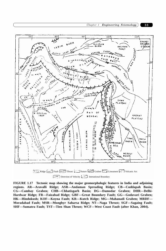
33�������� ��� �� ��� �������
Ridge Fault Thrust Suture Graben Lineament Volcanic Arc
Intenational BoundaryDirection of Velocity
70° 80° 90° 100°
10°
20°
30°
10°
20°
30°
110°100°90°80°70°
FIGURE 1.17 Tectonic map showing the major geomorphologic features in India and adjoiningregions. AR—Aravalli Ridge; ASR—Andaman Spreading Ridge; CB—Cuddapah Basin;CG—Cambay Graben; CHB—Chhatisgarh Basin; DG—Damodar Graben; DHR—Delhi-Hardwar Ridge; FR—Faizabad Ridge; GBF—Great Boundary Fault; GG—Godavari Graben;HK—Hindukush; KOF—Koyna Fault; KR—Kutch Ridge; MG—Mahanadi Graben; MRDF—Moradabad Fault; MSR—Monghyr Saharsa Ridge; NT—Naga Thrust; SGF—Sagaing Fault;SHF—Sumatra Fault; TST—Tien Shan Thrust; WCF—West Coast Fault (after Khan, 2004).

����������� ������� �������������34
1.9 SEISMICITY OF INDIA
Earthquakes have been occurring in the Indian subcontinent from the times immemorial butreliable historical records are available for the last 200 years (Oldham, 1883). From thebeginning of 20th century, more than 700 earthquakes of magnitude 5 or more have beenrecorded and felt in India, as given in the catalogues prepared by US National Oceanographicand Atmospheric Administration, India Meteorological Department, National GeophysicalResearch Institute (Figure 1.18). The seismicity of India can be divided in four groups, namely,Himalayas region, Andaman Nicobar, Kutch region and Peninsular India. Some of the damagingearthquakes which have occurred in these four regions are listed in Table 1.10.
72° 76° 80° 84° 88° 92°
8°
12°
16°
20°
24°
28°
32°
36°
96°92°88°84°80°76°72°68°
36°
32°
28°
24°
20°
16°
12°
8°
© Government of India Copyright Year 2001
Number of shocks (n)From the same origin
Deep focus shocks
More than 8.0
7.5 to < 8.0
7.0 to < 7.5
6.5 to < 7.0
6.0 to < 6.5
5.0 to < 6.0
Magnitude
Legend
Thiruvanantha-Puram
Lakshadweep(India)
Kavaratti
Mysore
Bangalore
Pondicherry(Puduchmeri)
Chennai
Hyderabad
Vishakhapatnam
Bhubaneshwar
Raipur
Ranchi
Kolkata
New Moore(India)
Bhopal
Tropic of Cancer
N D
Lucknow
Patna
I AI
Jaipur
Delhi
DehradunChandigarh
Shimla
Srinagar
14
Gandhinagar
Ahmadabad
Rajkot
Bhuj
Silvassa
Mumbai
Panaji
Aizawl
Imphal
KohimaShillong
GuwahatiDarjeelingGangtok Itanagar
Kilometres
120 0 120 240 360 480
MAP OF INDIAand Surrounding
Showing Epicentres
IndiraPoint
(India)A
ndam
an&
nico
bar
islands
FIGURE 1.18 Seismicity map of India (after, IS:1893 (Pt. 1): 2002).

35�������� ��� �� ��� �������
TABLE 1.10 List of damaging earthquakes in India
Himalayan Region
S. No. Name Location Year Magnitude/ DeathIntensity
1. Kashmir Earthquake Srinagar, J. & K. 1885 — 3,0002. Shillong Earthquake Shillong, Plateau 1897 8.7 1,6003. Kangra Earthquake Kangra, H.P. 1905 8.5 20,0004. Bihar-Nepal Earthquake Bihar-Nepal border region 1934 8.3 10,0005. Assam Earthquake Assam 1950 8.5 1,5266. Bihar-Nepal Earthquake Bihar-Nepal border region 1988 6.5 1,0007. Indo-Burma Earthquake India-Burma Border 1988 7.3 —8. Uttarkashi Earthquake Uttarkashi, Uttaranchal 1991 7.0 7689. Chamoli Earthquake Chamoli, Uttaranchal 1999 6.8 103
Andaman Nicobar
1. Andaman-Nicobar Andaman-Nicobar Trench 1941 8.1 —Earthquake
Kutch Region
1. Samaji Earthquake Samaji, Delta of Indus 1668 X —2. Kutch Earthquake Kutch, Gujarat 1819 8.0 2,0003. Anjar Earthquake Anjar, Gujarat 1956 6.1 1154. Bhuj Earthquake Bachau, Gujarat 2001 6.9 20,000
Peninsular India
1. Bombay-Surat Earthquake Bombay-Surat 1856 VII —2. Son Valley Earthquake Son Valley 1927 6.5 —3. Satpura Earthquake Satpura 1938 6.3 —4. Balaghat Earthquake Balaghat, M.P. 1957 5.5 —5. Koyna Earthquake Koyna 1967 6.0 1776. Ongole Earthquake Ongole, Bhadrachalam 1967 5.4 —7. Broach Earthquake Broach 1970 5.4 268. Latur Earthquake Latur, Maharashtra 1993 6.2 10,0009. Jabalpur Earthquake Jabalpur, M.P. 1997 6.0 54
1.10 CLASSIFICATION OF EARTHQUAKES
1. Based on location 2. Based on epicentral distances(a) Interplate (a) Local earthquake < 1°(b) Intraplate (b) Regional earthquake 1 – 10°
(c) Teleseismic earthquake > 10°3. Based on focal depth 4. Based on magnitude
(a) Shallow depth 0–71 km (a) Mircoearthquake < 3.0(b) Intermediate depth 71–300 km (b) Intermediate earthquake 3–4
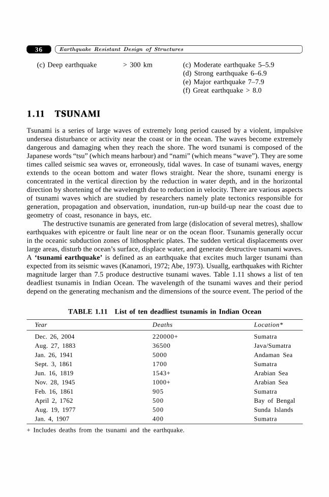
����������� ������� �������������36
(c) Deep earthquake > 300 km (c) Moderate earthquake 5–5.9(d) Strong earthquake 6–6.9(e) Major earthquake 7–7.9(f) Great earthquake > 8.0
1.11 TSUNAMI
Tsunami is a series of large waves of extremely long period caused by a violent, impulsiveundersea disturbance or activity near the coast or in the ocean. The waves become extremelydangerous and damaging when they reach the shore. The word tsunami is composed of theJapanese words “tsu” (which means harbour) and “nami” (which means “wave”). They are sometimes called seismic sea waves or, erroneously, tidal waves. In case of tsunami waves, energyextends to the ocean bottom and water flows straight. Near the shore, tsunami energy isconcentrated in the vertical direction by the reduction in water depth, and in the horizontaldirection by shortening of the wavelength due to reduction in velocity. There are various aspectsof tsunami waves which are studied by researchers namely plate tectonics responsible forgeneration, propagation and observation, inundation, run-up build-up near the coast due togeometry of coast, resonance in bays, etc.
The destructive tsunamis are generated from large (dislocation of several metres), shallowearthquakes with epicentre or fault line near or on the ocean floor. Tsunamis generally occurin the oceanic subduction zones of lithospheric plates. The sudden vertical displacements overlarge areas, disturb the ocean’s surface, displace water, and generate destructive tsunami waves.A ‘tsunami earthquake’ is defined as an earthquake that excites much larger tsunami thanexpected from its seismic waves (Kanamori, 1972; Abe, 1973). Usuallg, earthquakes with Richtermagnitude larger than 7.5 produce destructive tsunami waves. Table 1.11 shows a list of tendeadliest tsunamis in Indian Ocean. The wavelength of the tsunami waves and their perioddepend on the generating mechanism and the dimensions of the source event. The period of the
TABLE 1.11 List of ten deadliest tsunamis in Indian Ocean
Year Deaths Location*
Dec. 26, 2004 220000+ Sumatra
Aug. 27, 1883 36500 Java/Sumatra
Jan. 26, 1941 5000 Andaman Sea
Sept. 3, 1861 1700 Sumatra
Jun. 16, 1819 1543+ Arabian Sea
Nov. 28, 1945 1000+ Arabian Sea
Feb. 16, 1861 905 Sumatra
April 2, 1762 500 Bay of Bengal
Aug. 19, 1977 500 Sunda Islands
Jan. 4, 1907 400 Sumatra
+ Includes deaths from the tsunami and the earthquake.
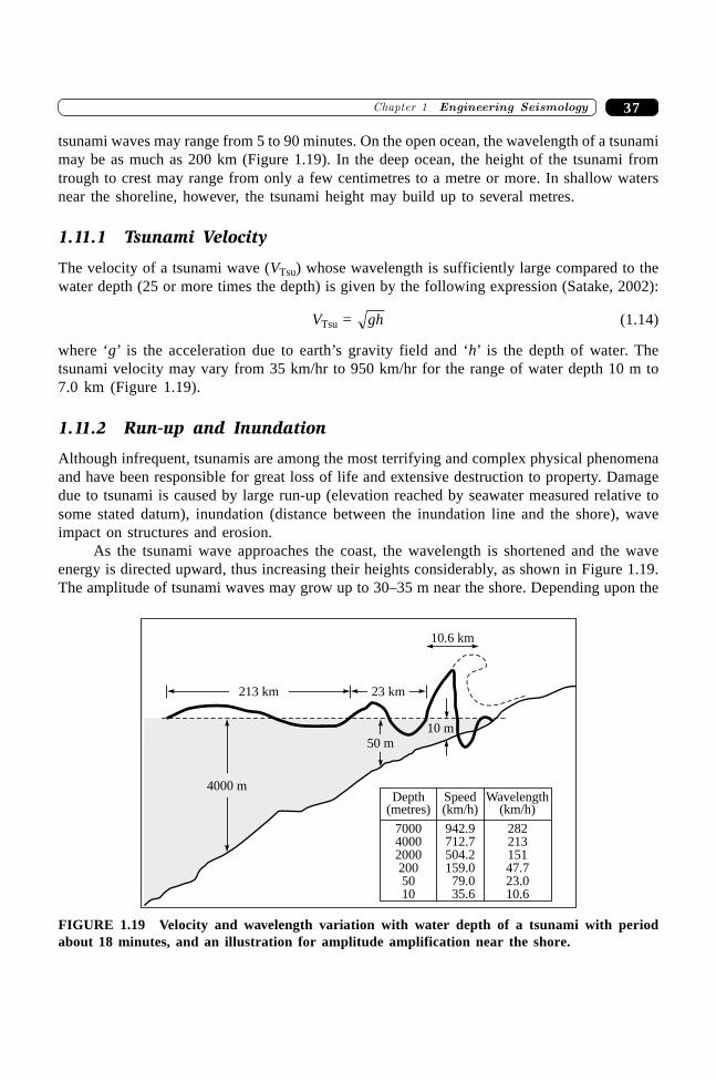
37�������� ��� �� ��� �������
tsunami waves may range from 5 to 90 minutes. On the open ocean, the wavelength of a tsunamimay be as much as 200 km (Figure 1.19). In the deep ocean, the height of the tsunami fromtrough to crest may range from only a few centimetres to a metre or more. In shallow watersnear the shoreline, however, the tsunami height may build up to several metres.
1.11.1 Tsunami Velocity
The velocity of a tsunami wave (VTsu) whose wavelength is sufficiently large compared to thewater depth (25 or more times the depth) is given by the following expression (Satake, 2002):
VTsu = gh (1.14)
where ‘g’ is the acceleration due to earth’s gravity field and ‘h’ is the depth of water. Thetsunami velocity may vary from 35 km/hr to 950 km/hr for the range of water depth 10 m to7.0 km (Figure 1.19).
1.11.2 Run-up and Inundation
Although infrequent, tsunamis are among the most terrifying and complex physical phenomenaand have been responsible for great loss of life and extensive destruction to property. Damagedue to tsunami is caused by large run-up (elevation reached by seawater measured relative tosome stated datum), inundation (distance between the inundation line and the shore), waveimpact on structures and erosion.
As the tsunami wave approaches the coast, the wavelength is shortened and the waveenergy is directed upward, thus increasing their heights considerably, as shown in Figure 1.19.The amplitude of tsunami waves may grow up to 30–35 m near the shore. Depending upon the
7000
213 km 23 km
10.6 km
4000 m
50 m10 m
Depth(metres)
942.9
Speed(km/h)
282
Wavelength(km/h)
4000 712.7 2132000 504.2 151200 159.0 47.750 79.0 23.010 35.6 10.6
FIGURE 1.19 Velocity and wavelength variation with water depth of a tsunami with periodabout 18 minutes, and an illustration for amplitude amplification near the shore.

����������� ������� �������������38
water depth and the coastal configuration, the waves may undergo extensive refraction, anotherprocess that may converge their energy to particular areas on the shore and thus increase theheights and inundation even more. Field surveys are carried out after every large tsunami forassessment of run-ups and inundation limits and to collect associated data from eyewitnessessuch as the number of waves, arrival time of waves and the largest wave.
SUMMARY
Seismology is the study of generation, propagation and recording of elastic waves in the earthand of sources that produce them. An earthquake is a sudden tremor or movement of earth’scrust, which originates naturally at or below the surface. About 90% of all earthquakes resultfrom tectonic events, primarily movements of the faults. The remaining proportion is relatedto volcanism, collapse of sub-terranean cavities, or man-made effects. The epicenters ofearthquakes are not randomly distributed over the earth’s surface. They tend to be concentratedin narrow zones. This chapter describes in detail the elastic rebound theory, seismic waves, localsite effects on ground motion characteristics, interior of the earth and movement of Indian platealong with its seismotectonic features.
GLOSSARY OF EARTHQUAKE/SEISMOLOGY
∑ Active fault. A fault that is likely to have another earthquake some time in the future.Faults are commonly considered to be active if they have moved one or more timesin the past.
∑ Aftershocks. Earthquakes that follow the largest shock of an earthquake sequence.They are smaller than the mainshock and continue over a period of weeks, months,or years. In general, the larger the mainshock, the larger and more numerous theaftershocks, and the longer they will continue.
∑ Alluvium. Loose gravel, sand, silt, or clay deposited by streams.∑ Aseismic. This term describes a fault on which no earthquakes have been observed.∑ Attenuation. When you throw a pebble in a pond, it makes waves on the surface that
move out from the place where the pebble entered the water. The waves are largestwhere they are formed and gradually get smaller as they move away. This decrease insize, or amplitude, of the waves is called attenuation.
∑ Basement. Harder and usually older igneous and metamorphic rocks that underlie themain sedimentary rock sequences (softer and usually younger) of a region and extenddownward to the base of the crust.
∑ Bedrock. Relatively hard, solid rock that commonly underlies softer rock, sediment,or soil; a subset of the basement.
∑ Benioff zone. A dipping planar (flat) zone of earthquakes that is produced by theinteraction of a downgoing oceanic crustal plate with a continental plate. Theseearthquakes can be produced by slip along the subduction thrust fault or by slip onfaults within the downgoing plate as a result of bending and extension as the plate ispulled into the mantle. Also known as the Wadati-Benioff zone.
39�������� ��� �� ��� �������
∑ Body wave. A seismic wave that moves through the interior of the earth, as opposedto the surface waves that travel near the earth’s surface. P- and S-waves are body waves.
∑ Crust. The outermost major layer of the earth, ranging from about 10 to 65 km inthickness worldwide. The uppermost 15 to 35 km of crust is brittle enough to produceearthquakes.
∑ Core. The innermost part of the earth. The outer core extends from 2500 to 3500 milesbelow the earth’s surface and is liquid metal. The inner core is the central 500 milesand is solid metal.
∑ Earthquake. This term is used to describe both sudden slip on a fault, and the resultingground shaking and radiated seismic energy caused by the slip, or by volcanic ormagmatic activity, or other sudden stress changes in the earth.
∑ Earthquake hazard. Anything associated with an earthquake that may affect thenormal activities of people. This includes surface faulting, ground shaking, landslides,liquefaction, tectonic deformation, tsunamis, and seiches.
∑ Earthquake risk. The probable building damage, and number of people that areexpected to be hurt or killed if a likely earthquake on a particular fault occurs.Earthquake risk and earthquake hazard are occasionally used interchangeably.
∑ Epicentre. The point on the earth’s surface vertically above the point in the crust whereseismic rupture begins
∑ Fault. A fracture along which the blocks of crust on either side have moved relativeto one another parallel to the fracture. Strike-slip faults are vertical (or nearlyvertical) fractures where the blocks have mostly moved horizontally. If the blockopposite to an observer looking across the fault moves to the right, the slip styleis termed right lateral; if the block moves to the left, the motion is termed left lateral.Dip-slip faults are inclined fractures where the blocks have mostly shifted vertically.If the rock mass above an inclined fault moves down, the fault is termed normal,whereas if the rock above the fault moves up, the fault is termed reverse (or thrust).Oblique-slip faults have significant components of both slip styles.
∑ Foreshocks. Foreshocks are relatively smaller earthquakes that precede the largestearthquake in a series, which is termed the mainshock. Not all mainshocks haveforeshocks.
∑ Hypocentre. The point within the earth where an earthquake rupture starts. Alsocommonly termed the focus.
∑ Intensity. A number (written as a Roman numeral) describing the severity of anearthquake in terms of its effects on the earth’s surface and on humans and theirstructures. There are many intensity values for an earthquake, depending on where youare, unlike the magnitude, which is one number for each earthquake.
∑ Intraplate and interplate. Intraplate pertains to process within the earth’s crustalplates. Interplate pertains to process between the plates.
∑ Isoseismal. A contour or line on a map bounding points of equal intensity for a particularearthquake.
∑ Left-lateral. If you were to stand on the fault and look along its length, this is a typeof strike-slip fault where the left block moves toward you and the right block movesaway.
����������� ������� �������������40
∑ Lithosphere. The outer solid part of the earth, including the crust and uppermostmantle. The lithosphere is about 100 km thick, although its thickness is age dependent(older lithosphere is thicker). The lithosphere below the crust is brittle enough at somelocations to produce earthquakes by faulting, such as within a subducted oceanic plate.
∑ Love wave. A type of seismic surface wave having a horizontal motion that istransverse (or perpendicular) to the direction the wave is travelling.
∑ Magnitude. A number that characterizes the relative size of an earthquake. Magnitudeis based on measurement of the maximum motion recorded by a seismograph. Severalscales have been defined, but the most commonly used are (1) local magnitude (ML),commonly referred to as “Richter magnitude,” (2) surface-wave magnitude (MS), (3)body-wave magnitude (mB), and (4) moment magnitude (MW).
∑ Mainshock. The largest earthquake in a sequence, sometimes preceded by one or moreforeshocks, and almost always followed by many aftershocks.
∑ Mantle. The part of the earth’s interior between the metallic outer core and the crust.∑ Moho. The boundary between the crust and the mantle in the earth. The boundary is
between 25 and 60 km deep beneath the continents and between 5 and 10 km deepbeneath the ocean floor.
∑ Oceanic spreading ridge. A fracture zone along the ocean bottom where moltenmantle material comes to the surface, thus creating new crust. This fracture can be seenbeneath the ocean as a line of ridges that form as molten rock reaches the ocean bottomand solidifies.
∑ Oceanic trench. A linear depression of the sea floor caused by the subduction of oneplate under another.
∑ P-wave. A seismic body wave that shakes the ground back and forth in the samedirection and the opposite direction as the wave is moving.
∑ Plate tectonics. A theory supported by a wide range of evidence that considers theearth’s crust and upper mantle to be composed of several large, thin, relatively rigidplates that move relative to one another. Slip on faults that define the plate boundariescommonly results in earthquakes. Several styles of faults bound the plates, includingthrust faults along which plate material is subducted or consumed in the mantle, oceanicspreading ridges along which new crustal material is produced, and transform faultsthat accommodate horizontal slip (strike slip) between adjoining plates.
∑ Rayleigh wave. A seismic surface wave causing the ground to shake in an ellipticalmotion, with no transverse, or perpendicular, motion.
∑ Recurrence interval. The average time span between large earthquakes at a particularsite. Also termed return period.
∑ Reflection. The energy or wave from an earthquake that has been returned (reflected)from a boundary between two different materials within the earth, just as a mirrorreflects light.
∑ Refraction. The deflection, or bending, of the ray path of a seismic wave caused byits passage from one material to another having different elastic properties. Bendingof a tsunami wave front owing to variations in the water depth along a coastline.
∑ Right-lateral. If you were to stand on the fault and look along its length, this is a typeof strike-slip fault where the right block moves toward you and the left block movesaway.
41�������� ��� �� ��� �������
∑ Ring of Fire. The zone of earthquakes surrounding the Pacific Ocean which is calledthe Circum-Pacific belt about 90% of the world’s earthquakes occur there. The next mostseismic region (5–6% of earthquakes) is the Alpide belt (extends from Mediterraneanregion, eastward through Turkey, Iran, and northern India).
∑ S-wave. A seismic body wave that shakes the ground back and forth perpendicular tothe direction the wave is moving, also called a shear wave.
∑ Sand boil. Sand and water that come out onto the ground surface during an earthquakeas a result of liquefaction at shallow depth.
∑ Seismic gap. A section of a fault that has produced earthquakes in the past but is nowquiet. For some seismic gaps, no earthquakes have been observed historically, but it isbelieved that the fault segment is capable of producing earthquakes on some other basis,such as plate-motion information or strain measurements.
∑ Seismicity. The geographic and historical distribution of earthquakes.∑ Seismic moment. A measure of the size of an earthquake based on the area of fault
rupture, the average amount of slip, and the force that was required to overcome thefriction sticking the rocks together that were offset by faulting. Seismic moment canalso be calculated from the amplitude spectra of seismic waves.
∑ Seismic zone. An area of seismicity probably sharing a common cause. Example: “TheHimalayan Zone.”
∑ Seismogenic. Capable of generating earthquakes.∑ Seismogram. A record written by a seismograph in response to ground motions
produced by an earthquake, explosion, or other ground-motion sources.∑ Seismology. The study of earthquakes and the structure of the earth, by both naturally
and artificially generated seismic waves.
REFERENCES
[1] Abe, K., “Tsunami and Mechanism of Great Earthquakes”, Physics of the Earth PlanetInteriors, 7: 143–153, 1973.
[2] Aki, K. and Chouet, B., “Origin of Coda Waves: Source, Attenuation and ScatteringEffects”, Journal of Geophysical Research, 80: 3322, 1975.
[3] Aki, K., “Local Site Effects on Strong Ground Motion”, In Earthquake Engineeringand Soil Dynamics II—Recent Advances in Ground Motion Evaluation, J.L. Von Thun(Ed.), Geotechnical Special Publication No. 20, 103–155, American Society of CivilEngineering, New York, 1988.
[4] Barazangi, M. and Dorman, J., “World Seismicity Map Compiled from ESSA, Coatand Geodetic Survey, Epicenter Data, 1961–1967”, Bulletin of the SeismologicalSociety of America, 59: 369–380, 1969.
[5] Bath, M., “Earthquake Energy and Magnitude”, Physics and Chemistry of the Earth,Ahren, L.H. Press, 115–165, 1966.
[6] Bard, P.Y. and Bouchon, M., “The Seismic Response of Sediment-filled Valleys—Part 1: The Case of Incident SH Waves”, Bulletin of the Seismological Society ofAmerica, 70: 1263–1286, 1980a.

����������� ������� �������������42
[7] Bard, P.Y. and Bouchon, M., “The Seismic Response of Sediment-filled Valleys—Part 2: The Case of Incident P and SV Waves”, Bulletin of the Seismological Societyof America, 70: 1921–1941, 1980b.
[8] Bard, P.Y. and Bouchon, M., “The Two-dimensional Resonance of Sediment-filledValleys”, Bulletin of the Seismological Society, of America, 75: 519–541, 1985.
[9] Bullen, K.E. and Bolt, B.A., An Introduction to the Theory of Seismology, CambridgeUniversity Press, Cambridge, 1985.
[10] Celebi, M., “Topographical and Geological Amplifications Determined from Strong-motion and Aftershock Records of the 3 March 1985 Chile Earthquake”, Bulletin ofthe Seismological Society of America, 77: 1147–1167, 1987.
[11] Conrad, V., “Laufzeitkurven Des Tauernbebens”, vom 28: 59: 1–23, Mitt.Erdb.-Komm. Wien, 1925.
[12] DeMets, et al., Current Plate Motions, 101: 425–478, 1990.[13] Faccioli, E., “Seismic Amplification in the Presence of Geological and Topographic
Irregularities”, Proceedings of 2nd International Conference on Recent Advancesin Geotechnical Earthquake Engineering and Soil Dynamics, St. Louis, Missouri, 2:1779–1797, 1991.
[14] Geli, L., Bard, P.Y. and Jullien, B., “The Effect of Topography on Earthquake GroundMotion: A Review and New Results”, Bulletin of the Seismological Society of America,78: 42–63, 1988.
[15] Gutenberg, B., The Energy of Earthquakes, 112: 1–14, 1945.[16] Gutenberg, B. and Richter, C.F., Seismicity of Earth and Related Phenomenon,
Princeton University Press, Princeton, New Jersey, 1945.[17] Gutenberg, B., “Magnitude Determination for Deep Focus Earthquakes”, Bulletin of
the Seismological Society of America, 35: 117–130, 1956.[18] Hatayama, K., Matsunami, K., Iwata, T. and Irikura, K., “Basin-induced Love Wave
in the Eastern Part of the Osaka Basin”, Journal of Physics of the Earth, 43: 131–155,1995.
[19] Hutton, L.K. and Boore, D.M., “The ML Scale in Southern California”, Bulletin of theSeismological Society of America, 77: 6: 2074–2094, 1987.
[20] Jibson, R., “Summary on Research on the Effects of Topographic Amplification ofEarthquake Shaking on Slope Stability”, Open-File-Report-87-268, USGS, California,1987.
[21] Kanamori, H., “Mechanism of Tsunami Earthquake”, Physics of the Earth Planet,Interiors, 6: 246–259, 1972.
[22] Kanamori, H., “The Energy Release in Great Earthquakes”, Tectonophysics, 93: 185–199, 1977.
[23] Hank, T.C. and Kanamori, H., “A Moment Magnitude Scale”, JGR, 84: 2348–2350,1979.
[24] IS: 1893, Indian Standard Criteria for Earthquake Resistant Design of Structures, Part1, BIS, New Delhi, 2002.
[25] Kawase, H., “The Cause of Damage Belt in Kobe: ‘The Basin-edge Effect’,Constructive Interference of the Direct S-Waves with the Basin Induced Diffracted/Rayleigh Waves”, Seismological Research Letters, 67: 25–34, 1996.

43�������� ��� �� ��� �������
[26] Kawase, H. and Aki, K., “Topography Effect at the Critical SV Wave Incidence:Possible Explanation of Damage Pattern by the Whitter Narrow”, Earthquake of 1October 1987, Bulletin of the Seismological Society of America, 80: 1–22, California,1990.
[27] Kennett, B.L.N. and Engdahl, E.R., “Travel Times for Global Earthquake Locationand Phase Identification”, International Journal of Geophysics, 105: 429–465, 1991.
[28] Khan, P.K., “Recent Seismicity Trend in India and Adjoining Regions”, ISET, NewLett., October 2003-July 2004, 10–14, 2004.
[29] Kim, W.Y., “The ML Scale in Eastern North America”, Bulletin of the SeismologicalSociety of America, 88(4): 935–951, 1998.
[30] Langston, C.A., Brazier, R., Nyblade, A.A., and Owens, T.J., “Local Magnitude Scaleand Seismicity Rate for Tanzania, East Africa,” Bulletin of the Seismological Societyof America, 88(3): 712–721, 1998.
[31] Levret, A., Loup, C., and Goula, X., “The Provence Earthquake of June 11, 1909(France): New Assessment of Near Field Effects”, Proceedings of the 8th EuropeanConference of Earthquake Engineering, Lisbon, 2, p. 4.2.79, 1986.
[32] Love, A.E.H., Some Problems of Geodynamics, Cambridge University Press, 1911.[33] Lowrie, W. Fundamentals of Geophysics, Cambridge University Press, 1997.[34] MacMurdo, J., “Papers Relating to the Earthquake which Occurred in India in 1819”,
Philosophical Magazine, 63: 105–177, 1824.[35] Moczo, P. and Bard, P.Y., “Wave Diffraction, Amplification and Differential Motion
Near Strong Lateral Discontinuities”, Bulletin of the Seismological Society of America,83: 85–106, 1993.
[36] Mohorovicic, A., “Das Beben Vom 8 ¥ 1909”, Jb. Met. Obs. Zagreb, 9, 1–63, 1909.[37] Mussett, A.E. and Khan, M.A., Looking into the Earth: An Introduction to Geological
Geophysics, Cambridge University Press, 2000.[38] Narayan, J.P., “Site Specific Strong Ground Motion Prediction Using 2.5-D Modelling”,
Geophysical Journal International, 146: 269–281, 2001.[39] Narayan, J.P. and Rai, D.C., “An Observational Study of Local Site Effects in the
Chamoli Earthquake”, Proceedings of Workshop on Recent Earthquakes of Chamoliand Bhuj’, 273–279, 2001.
[40] Narayan, J.P., Sharma, M.L. and Ashwani Kumar, ‘A Seismological Report on theJanuary 26, 2001 Bhuj, India Earthquake’, Seismological Research Letters, 73:343–355, 2002.
[41] Narayan, J.P. and Prasad Rao, P.V., “Two and Half Dimensional Simulation of RidgeEffects on the Ground Motion Characteristics”, Pure and Applied Geophysics, 160:1557–1571, 2003.
[42] Narayan, J.P., “2.5D Simulation of Basin-edge Effects on the Ground MotionCharacteristics”, Proceedings of Indian Academy of Sciences (Science of the EarthPlanet), 112: 463–469, 2003a.
[43] Narayan, J.P., “Simulation of Ridge Weathering Effects on the Ground MotionCharacteristics”, Journal of Earthquake Engineering, 7: 447–461, 2003b.
[44] Narayan, J.P., “3D Simulation of Basin-edge Effects on the Ground MotionCharacteristics”, 13WCEE, August 1–6, Paper No. 3333, Vancouver, Canada, 2004.
����������� ������� �������������44
[45] Narayan, J.P., “Study of Basin-edge Effects on the Ground Motion CharacteristicsUsing 2.5-D Modelling”, Pure and Applied. Geophysics, 162: 273–289, 2005.
[46] Oldham, R.D., “A Catalog of Indian Earthquakes from the Earliest Times to the Endof A.D., 1869”, Memoir X, Geological Survey of India, 1883.
[47] Oldham, R.D., “The Constitution of the Interior of the Earth, as Revealed byEarthquakes”, Quarterly Journal of Geological Society of London, 62: 456–75, 1906.
[48] Pedersen, H., Hatzfeld, D., Campillo, M., and Bard, P.Y., “Ground Motion AmplitudeAcross Ridges”, Bulletin of the Seismological Soceity of America, 84: 1786–1800,1994.
[49] Pitarka, A., Irikura, K., Iwata, T., and Sekiguchi, H., “Three-dimensional Simulationof the Near Fault Ground Motion for 1995”, Hyogo-ken Nanbu (Kobe), Japanearthquake, Bulletin of the Seismological Soceity of America, 88: 428–440, 1998.
[50] Plesinger A., Zmeskal, M., and Zednik, J., Automated Pre-processing of DigitalSeismograms: Principles and Software. Version 2.2, E. Bergman (Ed.), Prague andGolden, 1996.
[51] Rayleigh, Lord, “On-wave Propagated Along the Plane Surface of an Elastic Solid”,Proceedings of the London Mathematical Society, 17: 4-11, 1885.
[52] Reid, H.F., The California Earthquake of April 18, 1906, Publication 87, 21, CarnegieInstitute of Washington, Washington, D.C., 1910.
[53] Reid, H.F., “The Elastic Rebound Theory of Earthquakes”, Bulletin of Department ofGeology, 6: 413–444, University of Berkeley, 1911.
[54] Richter, C.F., “An Instrumental Earthquake Magnitude Scale”, Bulletin of theSeismological Soceity of America, 25: 1–32, 1935.
[55] Richter, C.F., Elementary Seismology, W.H. Freeman, San Francisco, 1958.[56] Sánchez-Sesma, F.J., “Elementary Solutions for the Response of a Wedge-shaped
Medium to Incident SH and SV Waves”, Bulletin of the Seismological Soceity ofAmerica, 80: 737–742, 1990.
[57] Satake, K., Tsunamis, International Handbook of Earthquake and EngineeringSeismology—Part B, Lee et al. (Eds.), 437–451, 2002.
[58] Siro, L. “Southern Italy November 23, 1980 Earthquake”, Proceedings of 7thEuropean Conference on Earthquake Engineering, Athens, Greece, 1982.
[59] Wood, H.O., “Distribution of Apparent Intensity in San-Francisco, in the CaliforniaEarthquake of April 18, 1906”, Report of the State Earthquake Investigation Commission,1: 220–245, Carnegie Institute of Washington, Washington, D.C., 1908.
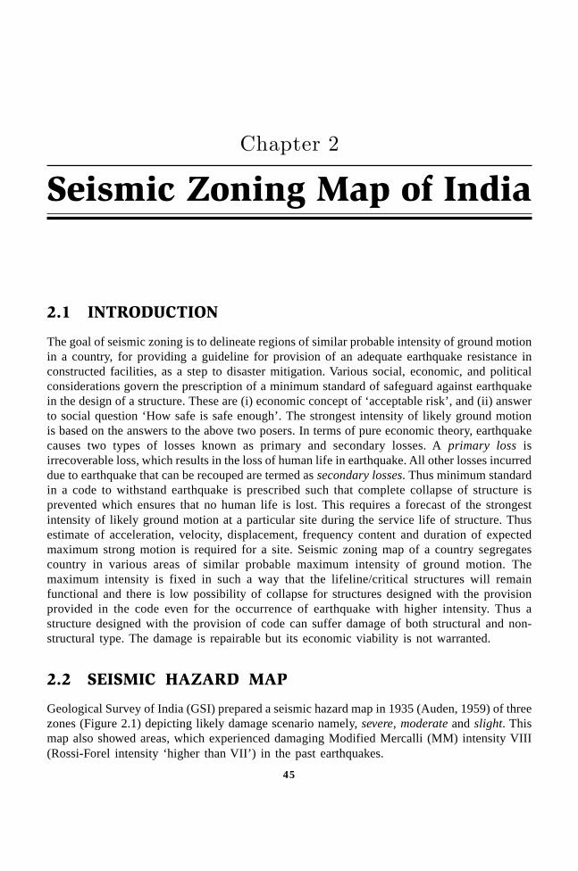
45
Seismic Zoning Map of India��������
2.1 INTRODUCTION
The goal of seismic zoning is to delineate regions of similar probable intensity of ground motionin a country, for providing a guideline for provision of an adequate earthquake resistance inconstructed facilities, as a step to disaster mitigation. Various social, economic, and politicalconsiderations govern the prescription of a minimum standard of safeguard against earthquakein the design of a structure. These are (i) economic concept of ‘acceptable risk’, and (ii) answerto social question ‘How safe is safe enough’. The strongest intensity of likely ground motionis based on the answers to the above two posers. In terms of pure economic theory, earthquakecauses two types of losses known as primary and secondary losses. A primary loss isirrecoverable loss, which results in the loss of human life in earthquake. All other losses incurreddue to earthquake that can be recouped are termed as secondary losses. Thus minimum standardin a code to withstand earthquake is prescribed such that complete collapse of structure isprevented which ensures that no human life is lost. This requires a forecast of the strongestintensity of likely ground motion at a particular site during the service life of structure. Thusestimate of acceleration, velocity, displacement, frequency content and duration of expectedmaximum strong motion is required for a site. Seismic zoning map of a country segregatescountry in various areas of similar probable maximum intensity of ground motion. Themaximum intensity is fixed in such a way that the lifeline/critical structures will remainfunctional and there is low possibility of collapse for structures designed with the provisionprovided in the code even for the occurrence of earthquake with higher intensity. Thus astructure designed with the provision of code can suffer damage of both structural and non-structural type. The damage is repairable but its economic viability is not warranted.
2.2 SEISMIC HAZARD MAP
Geological Survey of India (GSI) prepared a seismic hazard map in 1935 (Auden, 1959) of threezones (Figure 2.1) depicting likely damage scenario namely, severe, moderate and slight. Thismap also showed areas, which experienced damaging Modified Mercalli (MM) intensity VIII(Rossi-Forel intensity ‘higher than VII’) in the past earthquakes.
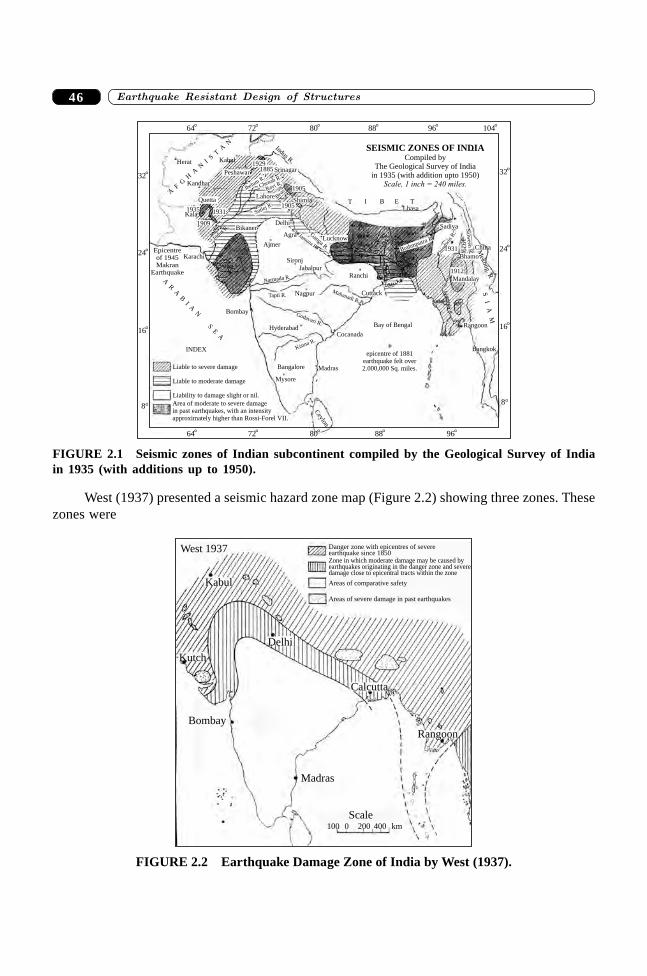
����������� ������� �������������46
Liable to severe damage
Liable to moderate damage
Liability to damage slight or nil.
Area of moderate to severe damagein past earthquakes, with an intensityapproximately higher than Rossi-Forel VII.
Mysore
Bangalore
INDEX
Ceylon
Madras
epicentre of 1881earthquake felt over2.000,000 Sq. miles.
Bay of Bengal
CocanadaHyderabad
Nagpur
Jabalpur
Sironj
Bombay
Ajmer
Agra
DelhiBikaner
Lahore
1905Shimla
1905
1929
Peshawar
Kabul
Kandhar
Quetta
Herat
19311935Kala
1909
Cuttack
Ranchi
Lhasa
Sadiya
China
Bhamo
Mandalay
1912
Rangoon
Bangkok
Karachi
Indus R.
Sutlej R.
BeasRavi R.
Chenab R.
JhelumR.
Epicentreof 1945Makran
Earthquake
Jamuna R.
Ganga
R. Brahmputra R.
Chi
ndw
inR
.
1931
Salw
eenR
.
Mahanadi R.
Godavari R.
Tapti R.
Narmada R.
Kistna R.
SEISMIC ZONES OF INDIA
Compiled byThe Geological Survey of India
in 1935 (with addition upto 1950)Scale, 1 inch = 240 miles.
AR
AB
IA
N
SE
A
T I B E T
AF
GH
AN
IS
TA
N
72°64° 88° 104°80° 96°
32°
24°
16°
8°
32°
24°
16°
8°
72°64° 88°80° 96°
1929 M
ekong.R
SI
AM
Srinagar
Indus R.
1885
Lucknow
FIGURE 2.1 Seismic zones of Indian subcontinent compiled by the Geological Survey of Indiain 1935 (with additions up to 1950).
West (1937) presented a seismic hazard zone map (Figure 2.2) showing three zones. Thesezones were
West 1937
Kabul
Bombay
Madras
Scale100 0 200 400 km
Rangoon
Areas of severe damage in past earthquakes
Areas of comparative safety
Zone in which moderate damage may be caused byearthquakes originating in the danger zone and severedamage close to epicentral tracts within the zone
Danger zone with epicentres of severeearthquake since 1850
Calcutta
Kutch
Delhi
FIGURE 2.2 Earthquake Damage Zone of India by West (1937).
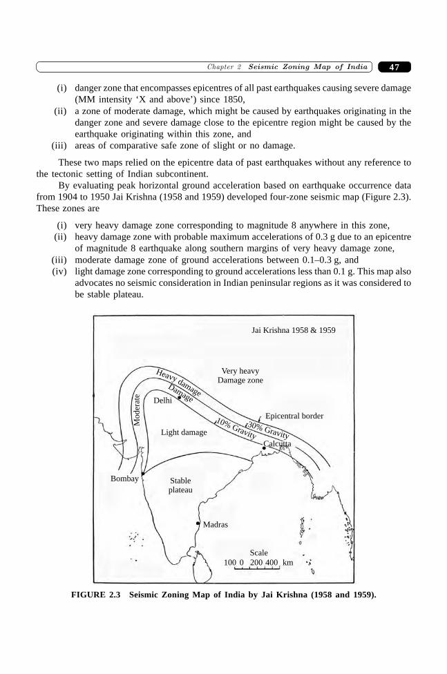
47�������� � �� ���� ������� ��� �
(i) danger zone that encompasses epicentres of all past earthquakes causing severe damage(MM intensity ‘X and above’) since 1850,
(ii) a zone of moderate damage, which might be caused by earthquakes originating in thedanger zone and severe damage close to the epicentre region might be caused by theearthquake originating within this zone, and
(iii) areas of comparative safe zone of slight or no damage.
These two maps relied on the epicentre data of past earthquakes without any reference tothe tectonic setting of Indian subcontinent.
By evaluating peak horizontal ground acceleration based on earthquake occurrence datafrom 1904 to 1950 Jai Krishna (1958 and 1959) developed four-zone seismic map (Figure 2.3).These zones are
(i) very heavy damage zone corresponding to magnitude 8 anywhere in this zone,(ii) heavy damage zone with probable maximum accelerations of 0.3 g due to an epicentre
of magnitude 8 earthquake along southern margins of very heavy damage zone,(iii) moderate damage zone of ground accelerations between 0.1–0.3 g, and(iv) light damage zone corresponding to ground accelerations less than 0.1 g. This map also
advocates no seismic consideration in Indian peninsular regions as it was considered tobe stable plateau.
Stableplateau
Bombay
Madras
Scale
100 200 400 km0
Calcutta
Epicentral border
Light damage
Delhi
Very heavyDamage zone
Jai Krishna 1958 & 1959
Damage
Heavy damage
10% Gravity
30% Gravity
Mo
der
ate
FIGURE 2.3 Seismic Zoning Map of India by Jai Krishna (1958 and 1959).
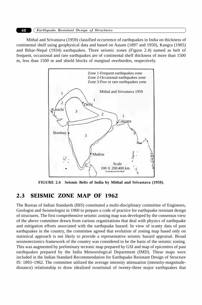
����������� ������� �������������48
Mithal and Srivastava (1959) classified occurrence of earthquakes in India on thickness ofcontinental shelf using geophysical data and based on Assam (1897 and 1950), Kangra (1905)and Bihar-Nepal (1934) earthquakes. Three seismic zones (Figure 2.4) named as belt offrequent, occasional and rare earthquakes are of continental shelf thickness of more than 1500m, less than 1500 m and shield blocks of marginal overburden, respectively.
1
2
3
1
2
3Bombay
Karachi
Delhi
Calcutta
1
Madras
Scale100 0 200 400 km
Mithal and Srivastava 1959
Zone 1-Frequent earthquakes zoneZone 2-Occasional earthquakes zoneZone 3-Few or rare earthquakes zone
2
FIGURE 2.4 Seismic Belts of India by Mithal and Srivastava (1959).
2.3 SEISMIC ZONE MAP OF 1962
The Bureau of Indian Standards (BIS) constituted a multi-disciplinary committee of Engineers,Geologist and Seismologist in 1960 to prepare a code of practice for earthquake resistant designof structures. The first comprehensive seismic zoning map was developed by the consensus viewof the above committee drawn from various organizations that deal with physics of earthquakeand mitigation efforts associated with the earthquake hazard. In view of scanty data of pastearthquakes in the country, the committee agreed that evolution of zoning map based only onstatistical approach is not likely to provide a representative seismic hazard appraisal. Broadseismotectonics framework of the country was considered to be the basis of the seismic zoning.This was augmented by preliminary tectonic map prepared by GSI and map of epicentres of pastearthquakes prepared by the India Meteorological Department (IMD). These maps wereincluded in the Indian Standard Recommendation for Earthquake Resistant Design of StructureIS: 1893–1962. The committee utilized the average intensity attenuation (intensity-magnitude-distance) relationship to draw idealized isoseismal of twenty-three major earthquakes that
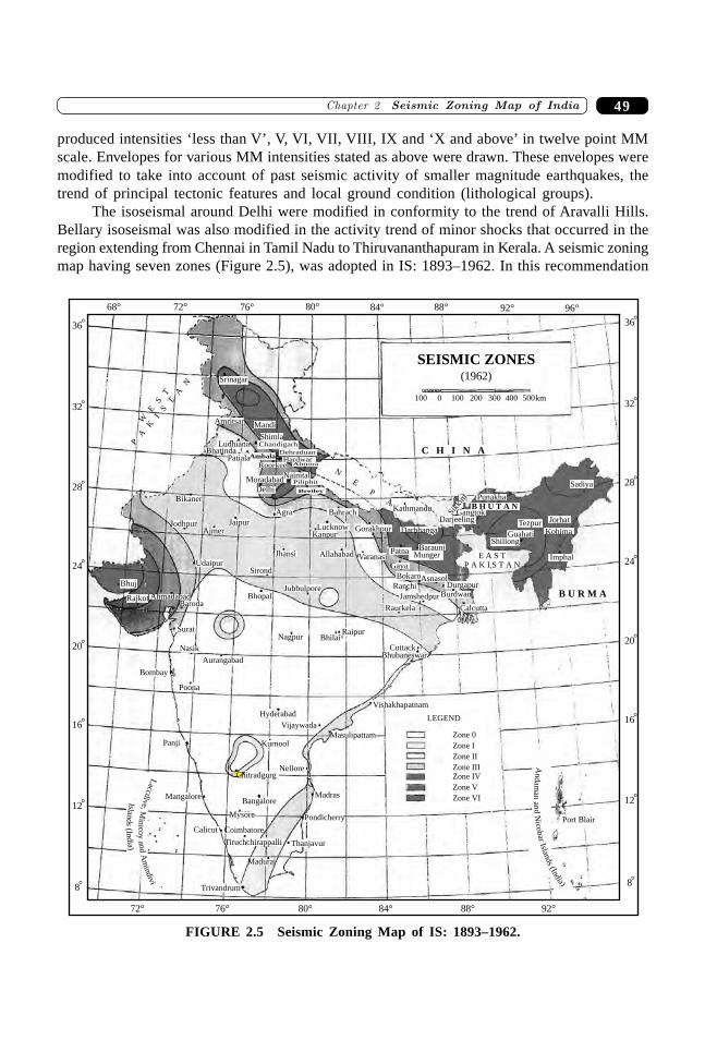
49�������� � �� ���� ������� ��� �
produced intensities ‘less than V’, V, VI, VII, VIII, IX and ‘X and above’ in twelve point MMscale. Envelopes for various MM intensities stated as above were drawn. These envelopes weremodified to take into account of past seismic activity of smaller magnitude earthquakes, thetrend of principal tectonic features and local ground condition (lithological groups).
The isoseismal around Delhi were modified in conformity to the trend of Aravalli Hills.Bellary isoseismal was also modified in the activity trend of minor shocks that occurred in theregion extending from Chennai in Tamil Nadu to Thiruvananthapuram in Kerala. A seismic zoningmap having seven zones (Figure 2.5), was adopted in IS: 1893–1962. In this recommendation
Vijaywada
Hyderabad
Kurnool
Nellore
Bangalore
Mysore
Mangalore
Calicut Coimbatore
Tiruchchirappalli
Madurai
Thanjavur
Trivandrum
Pondicherry
Madras
Masulipattam
Vishakhapatnam
LEGEND
Zone 0
Zone I
Zone II
Zone IIIZone IV
Zone V
Zone VI
Poona
Bombay
Aurangabad
Nasik
Surat
BarodaAhmadabadRajkot
Bhuj
Udaipur
Bhopal
Sirond
Jubbulpore
Jhansi Allahabad VaranasiGaya
BokaroAsnasolRanchi
Jamshedpur
DurgapurBurdwan
Calcutta
E A S TP A K I S T A N
PatnaMunger
Barauni
DarbhangaGorakhpur
Bahrach
LucknowKanpur
Agra
JaipurAjmer
Jodhpur
Bikaner
Delhi
MoradabadNainital
Piliphit
RoorkeeHardwar
Dehraduan
ChandigarhShimla
Mandi
AmbalaPatialaBhatinda
Ludhiana
Amritsar
Srinagar
Nagpur BhilaiRaipur
Raurkela
CuttackBhubaneswar
Kathmandu
DarjeelingGangtokSi
kkim
Punakha
GuahatiShillong
Tezpur Jorhat
Kohima
Imphal
Sadiya
B U R M A
B H U T A N
C H I N A
100 0 100 200 300 400 500km
Islands
(India)
Laccd
ive,
Min
icoy
and
Am
indiv
i
Andam
anan
dN
icobar
Islands
(India)
Port Blair
36°
32°
28°
24°
20°
16°
12°
8°
36°
32°
28°
24°
20°
16°
12°
8°
72° 76° 80° 84° 88° 92°
72° 76° 80° 84° 88° 92°68° 96°
Panji
SEISMIC ZONES
(1962)
WE
ST
PA
KI
ST
AN
Chitradgurg
Breiley
Almora
N
E
P
A
FIGURE 2.5 Seismic Zoning Map of IS: 1893–1962.

����������� ������� �������������50
the zone corresponding to MM intensity of less than five is termed as zone 0 (zero), to suggestthat lateral loading on the structure was envisaged to be small so that the design of structure tocarry vertical loads with proper factor of safety was considered to be adequate.
Guha (1962) prepared a seismic regionlisation map (Figure 2.6) with the premise that pastearthquake data (epicentres) contains all the information pertaining to seismo-tectonic setup ofthe country. Isoseismals were drawn and five seismic regions corresponding to MM intensitybelow V, VI, VII–VIII, IX-X and XI were termed as no damage, moderate damage, heavydamage and very heavy damage. The presumption of availability of historic seismicity data isimplicit in the assumption made to prepare the seismic regionalization map.
64° 68° 72° 76° 80° 84° 88° 92° 96° 100° 104°
4°
8°
12°
16°
20°
24°
28°
32°
36°
64° 68° 76° 80° 84° 88° 92° 96° 100° 104°60° 72° 108°
4°
8°
12°
16°
20°
24°
28°
32°
36°
Nagpur
Zone 0Hyderabad
CuttackBombay
BangaloreMadras Zone 3
Calcutta
Zone 4Zone 3Patna
Zone 2 KathmanduShillong
Ajmer
Zone 1
Delhi
Ahmadabad
Zone 2
Zone 3Zone 4
Zone 3
Srinagar
GUHA
Zone of minor shocksEpicentres of isolatedshocks in the peninsularshield
Zone 4 very heavy damageZone 3 heavy damageZone 2 moderate damageZone 1 minor damageZone 0 no damage Below VI
VIVII and VIIIIX and X
XI
Equivalent earthquakeintensity in modified
mercalli scale
Descriptions ofthe zones
Seismic regionalisation MAP.
Available earthquake records between 1803–1961are included in preparation of this map
Scale:-100 100200 400 5000
Kilometres
T. By: G. Vijay & R. Thakore
FIGURE 2.6 Seismic Regionalisation Map by Guha (1962).
2.4 SEISMIC ZONE MAP OF 1966
The presence of narrow zones of MM intensity V–VII (Seismic zones I–III) around theGujarat region contained in seismic zoning map in IS: 1893–1962 was noted as deficiency. The
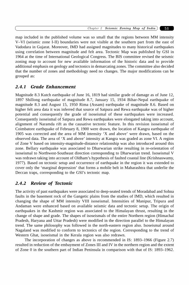
51�������� � �� ���� ������� ��� �
map included in the published volume was so small that the regions between MM intensityV–VI (seismic zone I-II) boundaries were not visible at the southern part from the east ofVadodara in Gujarat. Moreover, IMD had assigned magnitudes to many historical earthquakesusing correlation between magnitude and felt area. Tectonic Map was published by GSI in1964 at the time of International Geological Congress. The BIS committee revised the seismiczoning map to account for new available information of the historic data and to provideadditional emphasis on geology and tectonics in demarcating zones. The committee also decidedthat the number of zones and methodology need no changes. The major modifications can begrouped as:
2.4.1 Grade Enhancement
Magnitude 8.3 Kutch earthquake of June 16, 1819 had similar grade of damage as of June 12,1897 Shillong earthquake of magnitude 8.7, January 15, 1934 Bihar-Nepal earthquake ofmagnitude 8.3 and August 15, 1950 Rima (Assam) earthquake of magnitude 8.6. Based onhigher felt area data it was inferred that source of Satpura and Rewa earthquake was of higherpotential and consequently the grade of isoseismal of these earthquakes were increased.Consequently isoseismal of Satpura and Rewa earthquakes were elongated taking into account,alignment of Naramda rift as the causative tectonic feature. In this revision isoseismal ofCoimbatore earthquake of February 8, 1900 were drawn, the location of Kangra earthquake of1905 was corrected and the area of MM intensity ‘X and above’ were drawn, based on theobserved data. The area of ‘X and above’ intensity at Kangra was graded as zone VI. A regionof Zone V based on intensity-magnitude-distance relationship was also introduced around thiszone. Bellary earthquake was associated to Dharwarian strike resulting in re-orientation ofisoseismal to Northwest-Southeast direction corresponding to Dharwarian trend. Isoseismal Vwas redrawn taking into account of Oldham’s hypothesis of faulted coastal line (Krishnaswamy,1977). Based on tectonic setup and occurrence of earthquake in the region it was extended tocover only the ‘marginal depression’ that forms a mobile belt in Maharashtra that underlie theDeccan traps, corresponding to the GSI’s tectonic map.
2.4.2 Review of Tectonic
The activity of past earthquakes were associated to deep-seated trends of Moradabad and Sohnafaults in the basement rock of the Gangetic plains from the studies of IMD, which resulted inchanging the shape of MM intensity VIII isoseismal. Intensities of Manipur, Tripura andAndaman were enhanced based on available seismic data and tectonic setup. The origin ofearthquakes in the Kashmir region was associated to the Himalayan thrust, resulting in thechange of shape and grade. The shapes of isoseismals of the entire Northern region (HimachalPradesh, Haryana and Uttar Pradesh) were modified in the direction parallel to the Himalayantrend. The same philosophy was followed in the north-eastern region also. Isoseismal aroundNagaland was modified to conform to tectonics of the region. Corresponding to the trend ofWestern Ghat, isoseismal in the Kerala region was also redrawn.
The incorporation of changes as above is recommended in IS: 1893–1966 (Figure 2.7)resulted in reduction of the embayment of Zones III and IV in the northern region and the extentof Zone 0 in the southern part of Indian Peninsula in comparison with that of IS: 1893–1962.
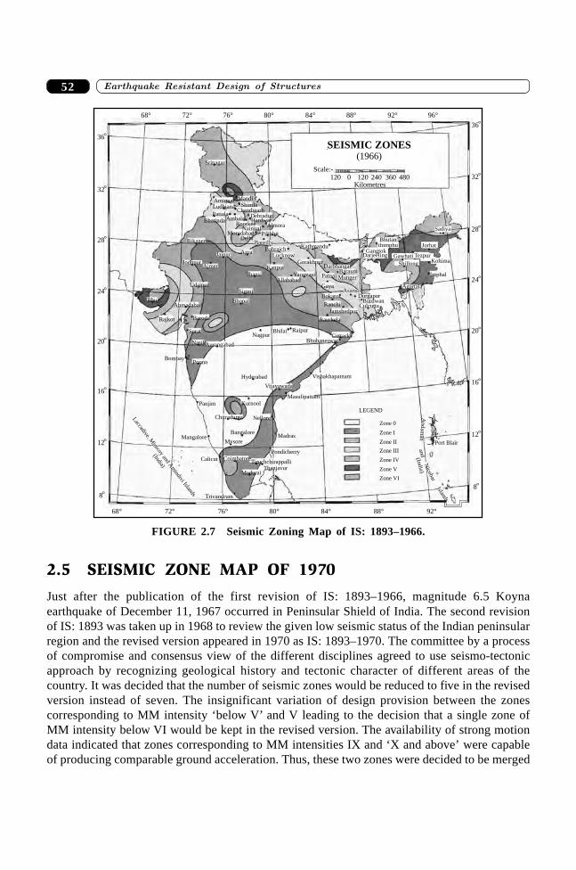
����������� ������� �������������52
68° 72° 76° 80° 84° 88° 92° 96°
36°
32°
28°
24°
20°
16°
12°
8°
36°
32°
28°
24°
20°
16°
12°
8°
68° 72° 76° 80° 84° 88° 92°
Srinagar
Amirtsar Mandi
Ludhiana
PatialaAmbala
ShimlaChandigarh
DehradunHardwar
RoorkeeNainital
Almora
PilibhitMoradabadDelhi
Bhatinda
BareillyBahraich
Lucknow
Kanpur
AgraKathmandu
GorakhpurDarbhanga
BarauniPatna Munger
Gaya
VaramasiAllahabad
BokaroAsansol
DurgapurBurdwan
CulcuttaRanchi
Jamshedpur
Raurkela
CuttackBhubaneswar
RaipurBhilaiNagpur
Bhopal
Sironj
Jhansi
Jaipur
AjmerJodhpur
Bikaner
Udaipur
AhmadabadBhuj
Rajkot Baroda
Surat
NasikAurangabad
BombayPoona
Hyderabad
Vijayawada
Masulipattam
Vishakhapatnam
KurnoolPanjim
Chitradurga Nellore
Bangalore
MysoreMangalore
Calicut CoimbatoreTiruchchirappalli
ThanjavurMadurai
Pondicherry
Madras
Trivandrum
Zone VI
Zone V
Zone IV
Zone III
Zone II
Zone I
Zone 0
LEGEND
Port Blair
Imphal
Agartala
Laccadive, M
inicoyand
Am
indivi Islands
(India)
Andam
anan
dN
icobarIslands
(India)
0120 120 240 360 480Kilometres
Darjeeling
Bhutanthimphu
Gawhati TezpurKohima
Jorhat
Sadiya
Shillong
SEISMIC ZONES
(1966)
Scale:-
Sik
kim
Gangtok
FIGURE 2.7 Seismic Zoning Map of IS: 1893–1966.
2.5 SEISMIC ZONE MAP OF 1970
Just after the publication of the first revision of IS: 1893–1966, magnitude 6.5 Koynaearthquake of December 11, 1967 occurred in Peninsular Shield of India. The second revisionof IS: 1893 was taken up in 1968 to review the given low seismic status of the Indian peninsularregion and the revised version appeared in 1970 as IS: 1893–1970. The committee by a processof compromise and consensus view of the different disciplines agreed to use seismo-tectonicapproach by recognizing geological history and tectonic character of different areas of thecountry. It was decided that the number of seismic zones would be reduced to five in the revisedversion instead of seven. The insignificant variation of design provision between the zonescorresponding to MM intensity ‘below V’ and V leading to the decision that a single zone ofMM intensity below VI would be kept in the revised version. The availability of strong motiondata indicated that zones corresponding to MM intensities IX and ‘X and above’ were capableof producing comparable ground acceleration. Thus, these two zones were decided to be merged

53�������� � �� ���� ������� ��� �
to one and termed as MM intensity ‘IX and above’ zone. Epicentre location, steep geothermalgradient, movement of crust, geomorphic evidence of offset of small landforms, stratigraphicevidence, gravity anomalies were utilised in demarcating seismo-tectonic setup of India.Krishnaswamy (in Srivastava, 1969) proposed five principal seismo-tectonic units (Figure 2.8and Table 2.1) based on these. The proposed seismo-tectonic units are as follows:
LEGEND
Orogenic unit
Foredeep and marginalDepression unitWest coast and NarmadaTapti unit
Gondwana rift unit
Shield unit
Faults
Tapti F
Narmada F
Patn
aF.
Luc
know
F.
Vin
d
s
hyan
rock
Del
hiro
cks
Arav
alli
rock
s
Gre
atubo nda
ry
FM
oradab
adF
Dauki fault
Scale
240 120 120 240km
0
Counter thrust
Main
cent ral thrustMain boundary fault
FIGURE 2.8 Generalised tectonic unit of Indian subcontinent (Krishnaswamy (in Srivastava,1969)).
1. Shield unit of peninsular India with ancient faults and localized seismic activityencompassed by MM intensity ‘less than VI’ and VI.
2. Gondwana rift unit of peninsular India with Mesozoic fault movements and the lateradjustments that includes the Gondwana graben and adjacent platform cover of pen-insular shield with Mesozoic Tertiary sediments were in general of MM intensity VII.
3. West Coast and Narmada-Tapti unit of peninsular shield that is segmented by Tertiary–Quaternary fault movements including the West Coast, Narmada-Son and Tapti riftzone and their extension corresponding to MM intensity VII with islands of MMintensity VIII.
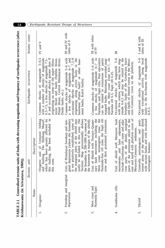
����������� ������� �������������54
TA
BL
E 2
.1G
ener
alis
ed t
ecto
nic
unit
s of
Ind
ia w
ith
decr
easi
ng m
agni
tude
and
freq
uenc
y of
ear
thqu
ake
occu
rren
ce (
afte
rK
rish
nasw
amy
(in
Sriv
asta
va,
1969
)).
Tect
onic
un
itE
arth
quak
e oc
curr
ence
Seis
mic
zon
es
Nam
eD
escr
ipti
on
1.O
roge
nic
IV a
nd V
2.F
ored
eep
and
mar
gina
lII
I an
d IV
wit
hde
pres
sion
isle
ts o
f V
3.W
est
coas
t an
dII
I w
ith
isle
tsN
arm
ada-
Tap
tiof
IV
4.G
ondw
ana
rift
sII
I
5.S
hiel
dI
and
II w
ith
isle
ts o
f II
I
a
Oro
geni
c un
it
of
Cen
ozoi
c fo
ldin
gan
d fa
ulti
ng.
The
S
hill
ong
Mas
sif,
whi
ch
has
been
gr
eatl
y af
fect
ed
byth
is
faul
ting
, ha
s be
en
incl
uded
in
this
zon
e.
Uni
t of
Him
alay
an f
ored
eep
and
mar
-gi
nal
depr
essi
on (
whe
re t
he b
ound
ary
is n
ot p
osit
ivel
y es
tabl
ishe
d, s
ome
ofth
e m
argi
nal
part
s of
the
shi
eld
may
real
ly b
e in
clud
ed i
n th
is z
one.
The
Tect
onic
M
ap
prov
isio
nall
y de
fine
sth
e bo
unda
ry a
t 20
0-10
00 m
con
tour
of
the
base
men
t at
mar
gin
of t
he s
hiel
d).
Uni
t of
Shi
eld
wit
h Te
rtia
ry–Q
uate
r-na
ry
faul
t m
ovem
ent
incl
udin
g th
eW
est
coas
t se
ism
ogen
ic
zone
, th
eN
arm
ada-
Son
rif
t zo
ne,
the
Tapt
i ri
ftzo
ne a
nd t
heir
pos
tula
ted
exte
nsio
ns.
Uni
t of
sh
ield
w
ith
Mes
ozoi
c fa
ult
mov
emen
ts
and
late
r ad
just
men
ts,
incl
ude
Gon
dwan
a ri
ft z
one
and
adja
-ce
nt
part
s of
th
e sh
ield
, m
argi
nal
part
s of
the
pen
insu
lar
shie
ld t
o th
eea
st a
nd n
orth
wit
h pl
atfo
rm c
over
of
Mes
ozoi
c–C
enoz
oic
sedi
men
ts.
Gen
eral
ly
asei
smog
enic
an
d pa
rti-
tion
ed a
reas
of
the
peni
nsul
ar s
hiel
dw
ith
anci
ent
faul
ts a
nd w
ith
loca
lize
dse
ism
ogen
ic
feat
ures
.
Com
mon
sh
ocks
of
m
agni
tude
5–
6.5
wit
h a
num
ber
of s
hock
s of
mag
nitu
de6.
5–7.
5, a
few
sho
cks
of m
agni
tude
7.5
–8
and
occa
sion
al s
hock
s gr
eate
r th
an 8
orig
inat
ing
on s
ome
of t
he m
ajor
Him
a-la
yan
thru
st
and
faul
ts
(Sat
litt
a th
rust
,P
inja
l th
rust
, C
entr
al
Him
alay
an
thru
st,
Dau
ki f
ault
s, e
tc.)
Com
mon
sho
cks
of m
agni
tude
5–6
wit
ha
few
sh
ocks
of
m
agni
tude
6–
7 an
doc
casi
onal
sh
ocks
of
m
agni
tude
7.
5–8
orig
inat
ing
alon
g ac
tive
fa
ults
in
th
eba
sem
ent
(Pat
na
faul
t?
or
othe
r ba
se-
men
t fa
ults
, K
utch
fau
lts)
.
Com
mon
sho
cks
of m
agni
tude
5–6
wit
ha
few
sh
ocks
of
m
agni
tude
6–
7 in
Nar
mad
a an
d Ta
pti
rift
s. P
ast
epic
entr
esca
n be
re
late
d to
ex
tens
ions
of
pa
rtly
map
ped
faul
ts.
Max
imum
rec
orde
d m
ag-
nitu
de
on
Wes
t co
ast
Zon
e 6.
6–7,
on
Nar
mda
rif
t 6.
5, T
apti
rif
t 6.
25.
Occ
asio
nal
shoc
ks
of
mag
nitu
de
5–6
wit
h fe
w c
entr
es,
whi
ch m
ay h
ave
mag
-ni
tude
6-6
.5 a
nd m
ay b
e re
late
d to
the
boun
dary
fau
lts
of t
he G
ondw
ana
basi
nan
d fa
ults
of
lim
ited
ext
ent
in t
he M
eso-
zoic
–Cen
ozoi
c co
ver
on t
he p
latf
orm
.
Occ
asio
nal
shoc
ks
of
mag
nitu
de
5–6
wit
h ex
cept
iona
l ac
tivi
ty
alon
g lo
cal
faul
ts i
n th
e A
rcha
eans
wit
h m
agni
tude
6-6.
5.

55�������� � �� ���� ������� ��� �
4. Himalayan foreland basins (foredeep) and marginal depression units generally containsareas of MM intensities VII and VIII with islets of MM intensity ‘IX and above’.
5. Mountain belts (Orogenic area) that formed by folding and faulting of earth’s crust inthe era beginning from Tertiary period to the present time (Cenozoic) encompassingzones of MM intensity ‘VIII and above’ in general.
The seismic zones I-V in this IS: 1893–1970 (Figure 2.9) broadly follows the trends ofabove stated five seismo-tectonic units in general. The demarcated seismo-tectonic provinceshad earthquakes of different focal depths. Earthquake magnitude and frequency show an overallincrease in general as the zone increase from zone I to zone V with some exception. Thefollowing modifications were also made besides the defined seismic zones on the basis of thefive seismo-tectonic provinces as above.
Four new separate islets were demarcated as zone V (MM intensity ‘IX and above’) to takeinto account the postulated higher seismic status in view of tectonic/past earthquake. These wereislets:
MangaloreBangalore
Mysore
Chitradurg
CalicutCombatore
Tiruchchirappalli
Madurai
Nagappattinam
Pondicherry(Puduchcheri)
CochinKavaratti
Trivandrum
Madras
Nellore
Kurnool
Hyderabad
Masulipattam
Vijaywada
Vishakapatnam
JabalpurGopalpur
Bhubaneswar
Sagar islandsRourkela
RanchiJamshedpur
Bokaro AsansolA
Durgapur
CalcuttaBurdwan
Gaya
VaranasiAllahabadJhansi
Bhopal
DNIUdapur
AjmerJodhpur
JaipurAgra
DelhiBreiley
Lucknow
Kanpur
Bahraich
Nainital
Roorkee
Patiala
Mandi
ShimlaChandigarh
Ambala Dehradun
LudhianaAmritsar
Srinagar
Bikaner
Nagpur
Aurangabad
Surat
Nasik
Silvassa
Bombay Pune
Vernoli
RajkotDwarka
Bhuj
Ahmadabad
Vadodara
Gandhinagar
Ratnagiri
BalgaumPanaji
Marmagao
PatnaBrauni
Munger
Gorakhpur
Darbhanja
Gangtok
DarjeelingDibrugarh
Itanagar
Dispur JorhatKohima
ShillongGawhati
Imphal
Agartala
Aizawl
LEGEND
Zone I
Zone II
Zone III
Zone IV
Zone V
Port Blair
Andam
anan
dN
icobarIslands
(IND
IA)
Lak
shad
weep
(IND
IA)
36°
36°
96°92°88°84°80°76°72°68°
92°88°84°80°76°72°68°
32°
32°
28°
28°
24°
24°
20°
20°
16°
16°
12°
12°
8°
8°
I
SEISMIC ZONES
(1970)
FIGURE 2.9 Seismic Zoning Map of IS: 1893–1970.
����������� ������� �������������56
(i) around Srinagar relating to down-dip extension of Pinjal thrust,(ii) epicentral tract of 1905 Kangra earthquake was related to the extension of Sattilata
thrust and an island around Dharmshala in Himachal Pradesh was introduced,(iii) around western Nepal and Pithoragarh of Uttaranchal was associated with extension of
Himalayan thrust and(iv) epicentral tract of 1934 Bihar-Nepal earthquake in seismic zone IV.
An islet of zone IV encompassing epicentral region of 1967 Koyna earthquake was alsointroduced in the new Western coast seismic zone III. Seismic status of entire Assam, Mizo hills,Tripura and northeast part of Kashmir were enhanced by one based on tectonics and seismicity.In recognition of total tectonic framework entire Andaman island was demarcated as zone V.Two new seismic zones of level III were introduced along Western coast and along marginaldepression in Rajasthan. Seismic status of parts of Indo-Gangetic trough was raised due tore-demarcation in accordance to tectonic features. Narmada-Son-Tapti zone was merged withDamodar graben in the east. The isoseismals for Bellary and Coimbatore earthquakes wereredrawn due to revised estimates of magnitudes. The islet around Coimbatore was nonexistentdue to introduction of costal belt of seismic zone III in the Western coast. The entireLakshadweep group of islands was in seismic zone III in conformity to Western coast belt. Theseismic zone I was limited on the basis of extent of platform cover and past earthquake dataresulting in curtailment of extent of zone I.
Srivastava (1974) indicated that the correlation of likely maximum Richter magnitude withthe seismic zones I-V was ‘less than 5’, 5-6, 6-6.5, 6.5-7 and ‘greater than 7’. The maximummagnitude as indicated might be ‘maximum considered magnitude’.
2.6 SEISMIC ZONE MAP OF 2002
BIS constituted a committee to review seismic status of Indian peninsular shield due tomagnitude 6.2 Killari (Latur) earthquake of September 30, 1993. The committee decided toenhance seismic zone I to seismic zone II. It was also decided that an interim revision to reviewseismic status of peninsular India be made as a revised map based on probabilistic hazardanalysis would be made in future. The committee decided to do a pattern analysis of earthquakehazard using a combination of seismo-tectonics and probabilistic method for Peninsular Indiabelow latitude N 22°. The recently available instrumental seismic data were used in this study.The result of the study had enhanced extent of seismic zone III to include area beyond Chennaiin the south and removal of islets of zone III surrounding epicentral tract of Bellary earthquake.Thus a four-zone seismic zoning map was adopted in IS: 1893–2002 (Figure 2.10). It is to benoted that probabilistic assessment portrays the total hazard from all sources around a sitewhereas the deterministic assessment is in general based on a single source.
2.7 EPILOGUE
The proposed hazard maps prior to IS: 1893–1962 presumed that earthquake processes in therecent past in all likelihood would be the same as those in the near future. These maps wereprimarily based on the effects of four Himalayan earthquakes and Kutch earthquake. Mithal and

57�������� � �� ���� ������� ��� �
Srivastava (1959) did not consider 1819 Kutch earthquake for establishing the seismic belt.More importance was given to geologic and tectonic setup in demarcating the seismic zoningmap from the revision of 1966 onwards. The seismic zone V in the BIS code in the Bhuj regionin Gujarat can only be justified by the deterministic zoning method. The occurrence ofearthquake in this region is very infrequent that result in long return period. The hazarddetermined in this region using probabilistic theory will be lower than that determined usingdeterministic theory. Similarly islets of seismic zone V in the seismic zone IV in the northernregion is due to the observed estimated intensities of past earthquakes. These islets in the zoningmap are due to the use of deterministic theory.
The decision of the BIS is to have a new revised zoning map using probabilisticframework. This needs to have an answer to ‘acceptable risk’ and answer to the ‘safety level’.The present committee of BIS must be extended to include member of planning commission andfinance/commerce ministry to establish the minimum requirement of safety and acceptable risk.Moreover, prior to embarking on probabilistic zoning basis map for the country, boundaries of
Nellore
ChennaiZone II
Andem
an&
Nico
bar
Islands
(India)
Zone III
Zone IV
Zone V
LEGEND
Pondicherry(Puduchcheri)
Combatore
III
Thiruvananthapuram
Calicut
III
Lakshadweep(INDIA)
Mangalore
Panaji
IV
PuneMumbai
Nasik
II
IIIII
IIKolkata
III
Vijaywada
Machilipatnam
Vishakhapatanam
Bhubaneswar
CuttackNew Moore (India)
IV
Asansol
Burdwan
DurgapurBokaro
Gaya
Allahabad
IIIKanpur
Lucknow
BahraichAgra
Breiley
DelhiIV
PilibhitMoradabad
IIIBhatindaPatiala
Ludhiana
Amritsar
V
SrinagarV
IV
ShimlaChandigarh
VDehradun
AmbalaHardwar
RoorkeeNainital Almor
Bikaner
III
II
IVV
Rajkot
Ahmadabad
Vadodara
III
IV
Gorakhpur
PatnaV
MonghyrBrauni
Gangtok
Darjeeling
V
KohimaShillong
Guwahati
Dispur Jorhat
Imphal
Agartala
Cancer
Tropic of
V
IndiraPoint
Scale
120 0 120 240 360 480 km
96°92°88°84°80°76°72°68°
92°88°84°80°76°72°
8°
12°
16°
20°
24°
28°
32°
36°
8°
12°
16°
20°
24°
28°
32°
36°
Jaipur
Bhopal
Jodhpur
Ajmer Jhansi
Bhuj
Mysore
Bangalore
Chitradurg
Kurnool
Hyderabad
Aurangabad
Nagpur
Sadiya
SEISMIC ZONES
(2002)
FIGURE 2.10 Seismic Zoning Map of IS: 1893–2002.
����������� ������� �������������58
different seismo-tectonic block of the entire country should be made.
SUMMARY
The description of perceived threat from earthquakes in different parts of the country in the formof a map began in 1935. The most recent revision of this map was taken up in 2002. This evolutionof seismic zoning map of Indian subcontinent is described in this chapter. The basis and dataused in the preparation of these zoning maps are discussed. The future trends in the preparationof seismic zoning map on the basis of the probabilistic hazard analysis is also discussed.
REFERENCES
[1] Auden, J.B., “Earthquake in Relation to Damodor Valley Project”, Earthquake Engi-neering Seminar, H.L. Sally (Ed.), University of Roorkee, India, pp. 212–216, 1959.
[2] West, W.D., “Earthquake in India (Presidential Address)”, 24 Indian Science Congress,pp. 189–227, 1937.
[3] Krishna, J., “Earthquake Engineering Problems in India”, Journal of Institution ofEngineers, India, 1958.
[4] Krishna, J., “Seismic Zoning of India”, Earthquake Engineering Seminar, H.L. Sally,(Ed.), University of Roorkee, India, pp. 24–31, 1959.
[5] Mithal, R.S. and Srivastava, L.S., “Geotectonic Position and Earthquakes of Ganga-Brahmaputra Region”, in H.L. Sally, (Ed.), Earthquake Engineering Seminar,University of Roorkee, India, pp. 217–233, 1959.
[6] IS: 1893–1962, Indian Standard Recommendations for Earthquake Resistance ofStructures, Indian Standards Institute, New Delhi, 1962.
[7] Guha, S.K. “Seismic Regionalisation of India”, Second Symposium on EarthquakeEngineering, University of Roorkee, India, 1962.
[8] IS: 1893–1966, Indian Standard Recommendations for Earthquake Resistance ofStructures (First Revision), Indian Standards Institute, New Delhi 1967.
[9] Krishnaswamy V.K., “The Evolution of Seismic Zoning Map of India”, SouvenirVolume, H.M. Choudhury, (Ed.), Sixth World Conference of Earthquake Engineering,Prabhat Press, Uttar Pradesh, pp. 77-89, 1977.
[10] IS: 1893–1970, Indian Standard Criteria for Earthquake Resistance of Structures(Second Revision), Indian Standards Institute, New Delhi, 1971.
[11] Srivastava L.S., “A Note on the Seismic Zoning Map of India”, Bulletin of the IndianSociety of Earthquake Technology, 6(4): pp. 185–194, 1969.
[12] Srivastava, L.S., “Seismic Zoning Map of India”, Earthquake Engineering–JaiKrishna Sixtieth Birth Anniversary Commemoration Volume, Sarita Prakashan, Meerut,India, pp. 49–65, 1974.
[13] IS: 1893, Indian Standard Criteria for Earthquake Resistance of Structures—Part 1:General Provisions and Buildings (Fifth Revision), Bureau of Indian Stantands,New Delhi, 2002.
59�������� ����������������� � ������
59
Strong Motion Studiesin India
��������
3.1 INTRODUCTION
The UNESCO had declared the nineties as the International Decade for Natural DisasterReduction (IDNDR). Ironically, this decade also witnessed four earthquakes of magnitude 6.0and above occurring in the Himalayas, central India, and the peninsular region resulting intoapproximately 10000 casualties and many more injuries. These figures would have been muchhigher, if these earthquakes had occurred in the neighbourhood of large urban centres, as wasseen in the case of the Bhuj earthquake of January 2001. This earthquake alone accounted formore than 15000 lives in addition to having a crippling effect on the economy of the region.These disastrous consequences could have been avoided had the systems been designed towithstand earthquake ground motions. Quoting from the declaration of the United NationsInternational Decade for Natural Disaster Reduction (UNIDNDR) Yokohama Convention 1994:
The impact of natural disasters in terms of human and economic losses has risen in recentyears, and society in general has become more vulnerable to natural disasters. Thoseusually most affected by natural and other disasters are the poor and socially disadvantagedgroups in developing countries as they are least equipped to cope with them.Disaster prevention, mitigation, preparedness and relief are four elements which contributeto and gain from the implementation of sustainable development policies. These elements,along with environmental protection and sustainable development, are closely interrelated.Therefore, nations should incorporate them in their development plans and ensure efficientfollow-up measures at the community, sub-regional, regional, national and internationallevels.Disaster response alone is not sufficient, as it yields only temporary results at a veryhigh cost. We have followed this limited approach for too long. This has been furtherdemonstrated by the recent focus on response to complex emergencies which, althoughcompelling should not divert from pursuing a comprehensive approach.
The facts are clear—we cannot prevent big, destructive earthquakes from occurring.These pose a continuing threat to lives and property in more than 55% of the area of this country.However, it is possible to avoid the disastrous consequences of an earthquake and that precisely
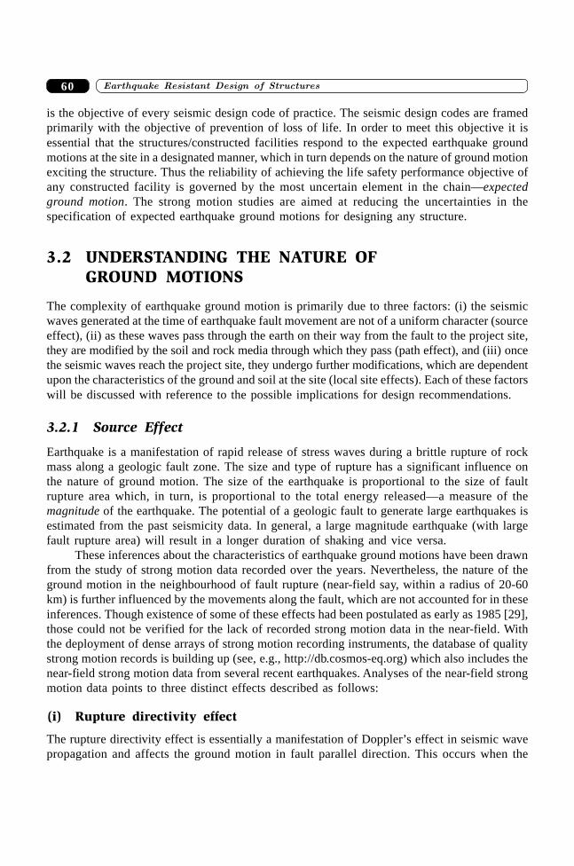
������������ ������� ������������� 60
is the objective of every seismic design code of practice. The seismic design codes are framedprimarily with the objective of prevention of loss of life. In order to meet this objective it isessential that the structures/constructed facilities respond to the expected earthquake groundmotions at the site in a designated manner, which in turn depends on the nature of ground motionexciting the structure. Thus the reliability of achieving the life safety performance objective ofany constructed facility is governed by the most uncertain element in the chain—expectedground motion. The strong motion studies are aimed at reducing the uncertainties in thespecification of expected earthquake ground motions for designing any structure.
3.2 UNDERSTANDING THE NATURE OFGROUND MOTIONS
The complexity of earthquake ground motion is primarily due to three factors: (i) the seismicwaves generated at the time of earthquake fault movement are not of a uniform character (sourceeffect), (ii) as these waves pass through the earth on their way from the fault to the project site,they are modified by the soil and rock media through which they pass (path effect), and (iii) oncethe seismic waves reach the project site, they undergo further modifications, which are dependentupon the characteristics of the ground and soil at the site (local site effects). Each of these factorswill be discussed with reference to the possible implications for design recommendations.
3.2.1 Source Effect
Earthquake is a manifestation of rapid release of stress waves during a brittle rupture of rockmass along a geologic fault zone. The size and type of rupture has a significant influence onthe nature of ground motion. The size of the earthquake is proportional to the size of faultrupture area which, in turn, is proportional to the total energy released—a measure of themagnitude of the earthquake. The potential of a geologic fault to generate large earthquakes isestimated from the past seismicity data. In general, a large magnitude earthquake (with largefault rupture area) will result in a longer duration of shaking and vice versa.
These inferences about the characteristics of earthquake ground motions have been drawnfrom the study of strong motion data recorded over the years. Nevertheless, the nature of theground motion in the neighbourhood of fault rupture (near-field say, within a radius of 20-60km) is further influenced by the movements along the fault, which are not accounted for in theseinferences. Though existence of some of these effects had been postulated as early as 1985 [29],those could not be verified for the lack of recorded strong motion data in the near-field. Withthe deployment of dense arrays of strong motion recording instruments, the database of qualitystrong motion records is building up (see, e.g., http://db.cosmos-eq.org) which also includes thenear-field strong motion data from several recent earthquakes. Analyses of the near-field strongmotion data points to three distinct effects described as follows:
(i) Rupture directivity effect
The rupture directivity effect is essentially a manifestation of Doppler’s effect in seismic wavepropagation and affects the ground motion in fault parallel direction. This occurs when the
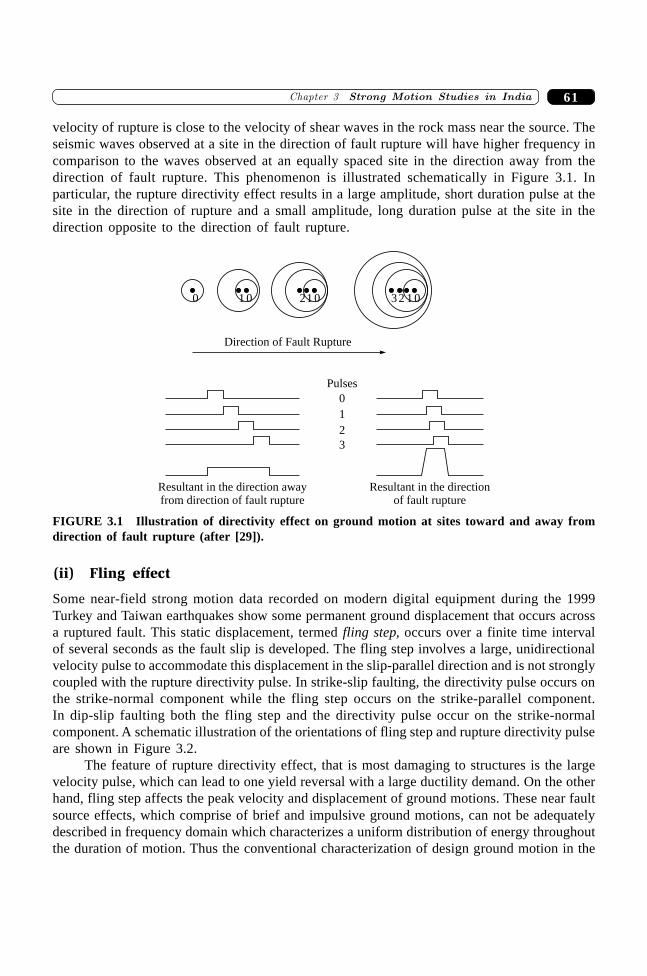
61�������� ����������������� � ������
velocity of rupture is close to the velocity of shear waves in the rock mass near the source. Theseismic waves observed at a site in the direction of fault rupture will have higher frequency incomparison to the waves observed at an equally spaced site in the direction away from thedirection of fault rupture. This phenomenon is illustrated schematically in Figure 3.1. Inparticular, the rupture directivity effect results in a large amplitude, short duration pulse at thesite in the direction of rupture and a small amplitude, long duration pulse at the site in thedirection opposite to the direction of fault rupture.
20 01 01 2 013
Direction of Fault Rupture
Pulses
0
1
2
3
Resultant in the direction awayfrom direction of fault rupture
Resultant in the directionof fault rupture
FIGURE 3.1 Illustration of directivity effect on ground motion at sites toward and away fromdirection of fault rupture (after [29]).
(ii) Fling effect
Some near-field strong motion data recorded on modern digital equipment during the 1999Turkey and Taiwan earthquakes show some permanent ground displacement that occurs acrossa ruptured fault. This static displacement, termed fling step, occurs over a finite time intervalof several seconds as the fault slip is developed. The fling step involves a large, unidirectionalvelocity pulse to accommodate this displacement in the slip-parallel direction and is not stronglycoupled with the rupture directivity pulse. In strike-slip faulting, the directivity pulse occurs onthe strike-normal component while the fling step occurs on the strike-parallel component.In dip-slip faulting both the fling step and the directivity pulse occur on the strike-normalcomponent. A schematic illustration of the orientations of fling step and rupture directivity pulseare shown in Figure 3.2.
The feature of rupture directivity effect, that is most damaging to structures is the largevelocity pulse, which can lead to one yield reversal with a large ductility demand. On the otherhand, fling step affects the peak velocity and displacement of ground motions. These near faultsource effects, which comprise of brief and impulsive ground motions, can not be adequatelydescribed in frequency domain which characterizes a uniform distribution of energy throughoutthe duration of motion. Thus the conventional characterization of design ground motion in the
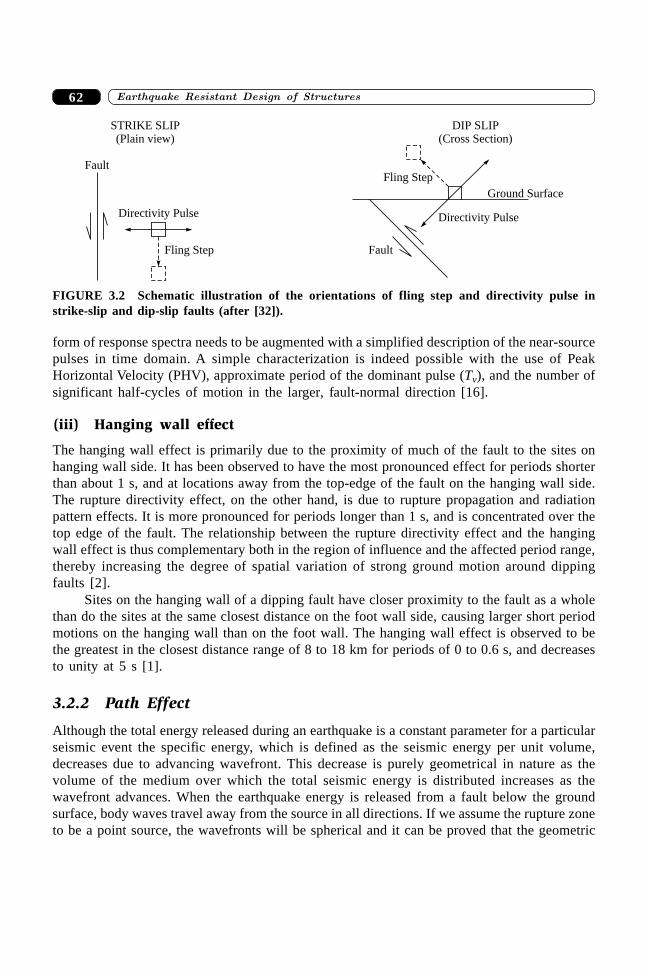
������������ ������� ������������� 62
form of response spectra needs to be augmented with a simplified description of the near-sourcepulses in time domain. A simple characterization is indeed possible with the use of PeakHorizontal Velocity (PHV), approximate period of the dominant pulse (Tv), and the number ofsignificant half-cycles of motion in the larger, fault-normal direction [16].
(iii) Hanging wall effect
The hanging wall effect is primarily due to the proximity of much of the fault to the sites onhanging wall side. It has been observed to have the most pronounced effect for periods shorterthan about 1 s, and at locations away from the top-edge of the fault on the hanging wall side.The rupture directivity effect, on the other hand, is due to rupture propagation and radiationpattern effects. It is more pronounced for periods longer than 1 s, and is concentrated over thetop edge of the fault. The relationship between the rupture directivity effect and the hangingwall effect is thus complementary both in the region of influence and the affected period range,thereby increasing the degree of spatial variation of strong ground motion around dippingfaults [2].
Sites on the hanging wall of a dipping fault have closer proximity to the fault as a wholethan do the sites at the same closest distance on the foot wall side, causing larger short periodmotions on the hanging wall than on the foot wall. The hanging wall effect is observed to bethe greatest in the closest distance range of 8 to 18 km for periods of 0 to 0.6 s, and decreasesto unity at 5 s [1].
3.2.2 Path Effect
Although the total energy released during an earthquake is a constant parameter for a particularseismic event the specific energy, which is defined as the seismic energy per unit volume,decreases due to advancing wavefront. This decrease is purely geometrical in nature as thevolume of the medium over which the total seismic energy is distributed increases as thewavefront advances. When the earthquake energy is released from a fault below the groundsurface, body waves travel away from the source in all directions. If we assume the rupture zoneto be a point source, the wavefronts will be spherical and it can be proved that the geometric
DIP SLIP(Cross Section)
Fling Step
Ground Surface
Directivity Pulse
FaultFling Step
Directivity Pulse
Fault
STRIKE SLIP(Plain view)
FIGURE 3.2 Schematic illustration of the orientations of fling step and directivity pulse instrike-slip and dip-slip faults (after [32]).
63�������� ����������������� � ������
attenuation will cause the amplitude of the body waves to decrease at a rate of 1/r, where rrepresents the radius of the wavefront. It has also been shown that the geometric attenuation of
surface waves occurs at a rate of 1/ r [7]. Thus the surface waves attenuate much more slowlythan the body waves, which also explains the fact that the ground motion at large epicentraldistances predominantly comprises surface wave. In addition to these geometric attenuationeffects, the seismic waves also experience an attenuation of amplitudes on account of thedissipation of seismic energy due to material damping in the soil. A combination of both theseeffects represents the influence of path effects on the nature of ground motion at a site.
3.2.3 Site Effect
Incorporation of the site effects in ground motion estimation procedures is aimed at reducingthe uncertainty in the ground motion estimates as measured by the standard error of theregression analysis and also to remove the potential bias in median estimates. The site effectsrepresent the local influences on the nature of ground motion and include the local groundresponse, basin effects, and the surface topography. The local ground response refers to theresponse of shallow geological deposits to the vertically propagating body waves. The modellingshould ideally involve the full soil profile up to the bed rock level at the site but for deep alluvialdeposits, reasonable estimates can usually be obtained by considering the soil profile onlyup to a depth of 100–120 m. The basin effects correspond to the influence of two or three-dimensional extent of the sedimentary basin structures on ground motions, including criticalbody wave reflections and surface wave generation at basin edges. The dividing line betweenthe local ground response effects and the basin effects is rather arbitrary and usually the localground response effects refer to the one-dimensional response of soil column and basin effectsare considered account for the observed ground motion characteristics that deviate from thepredictions of one-dimensional analysis. The presence of ridges and valleys at the site can alsohave some influence on the nature of ground motion. An approximate estimate of these effectsfor certain cases of ridge-valley terrain is possible by using analytical solutions for someidealized geometries [24].
The effect of soil layer on the nature of surface ground motion can be divided into twoprincipal components: (i) the predominant period of surface ground motion, and (ii) spectralamplification with respect to the bed rock motion. These effects may be studied by analyzingthe recorded strong motion data after eliminating the source and path effects from the strongmotion recordings. Two different approaches have been adopted to achieve this end: (i) bycomparing the strong motion recorded on soil site with motions from a reference site (usuallyrock) [5, 31], and (ii) without using any reference site recordings [11, 19].
(i) Reference Site Approach
If a reference site can be found in the close vicinity of the soil site then the motions at both sitesare expected to have similar source and path effects. Thus a comparison of the two motionsprovides an estimate of the local site effect. In practice ratios of either response spectra, or(smoothed) Fourier spectra of the motions recorded at soil site and the reference site is takento be a representative of the transfer function of the soil column at the site. The predominant period
������������ ������� ������������� 64
and amplification factor can be estimated from the location and amplitude of peaks of derivedtransfer functions.
(ii) Non-reference Site Approach
Since the availability of a rocky outcrop in the close vicinity of the site can not always beguaranteed, a few approaches have been proposed for estimation of site effects, which do notrequire availability of reference site data. A very popular approach is to take the ratio of thespectrum of horizontal component of motion with respect to the spectrum of the verticalcomponent of the motion (termed as H/V ratio) at the same site. This spectral ratio is consideredas the transfer function of the site. The ease of applicability of this approach has lured manyto adopt this approach in site characterization studies. However, it has been shown that theestimates (predominant period and amplification factors) predicted by H/V ratios are not stablefor the same site using different records [25]. Yet another non-reference site approach involvesnormalization of the spectra of recorded motions by a reference spectrum for rocky site obtainedfrom some attenuation relationships [30].
Since the data from large, strong earthquakes in near-field region of intense motions isquite sparse, the use of microtremor data and/or records from small, frequent earthquakes hasbeen proposed to study the site effects [14, 17]. Unfortunately, the behaviour of soil columnduring strong motions generated by large, strong earthquakes differs substantially from thatduring small earthquakes (weak motions). In particular, the large strain levels associated withthe strong motions during large earthquakes force the soil to respond non-linearly as against anessentially linear response during small strain weak motions. It has been shown in several studiesin different regions of the world that site effects estimated by using weak motion records, orthe microtremor data do not correlate well with the observed behaviour of the soil during strongearthquakes [3, 6, 18, 25, 38, 40, 41, 42, 44].
3.3 ESTIMATION OF GROUND MOTION PARAMETERS
In such a scenario, the estimates of site effects using the transfer function theory of linearsystems do not seems to be of much use in estimating the expected motions due to strong,damaging earthquakes. It is, therefore, more rational to relate the ground motion parameter ofinterest directly in terms of earthquake size, type of fault rupture, source to site distance, surfacegeology at the site, depth to bedrock level at the site, etc. to represent the mechanics of groundmotion process as closely as possible. The co-efficients of these predictive relationships areobtained by regression analyses of recorded strong motion data. With the inclusion of more datawith time, the uncertainties in the estimated design ground motions should decrease. A genericexpression for this purpose generally takes the form [15]:
ln Y = c1 + c2M + c3Mc4 + c5 ln [R + c6 exp(c7M)] + c8R + f1(source) + f2(site)
where Y represents the desired ground motion parameter (assumed to be distributed log-normally), M is a measure of the size of the earthquake, R is a measure of source-to-site distance,f1 and f2 are some suitable functions of source parameters (e.g., type of faulting, etc.) and localsite conditions (soil/rock), respectively. Usually, such relations provide the median estimate of
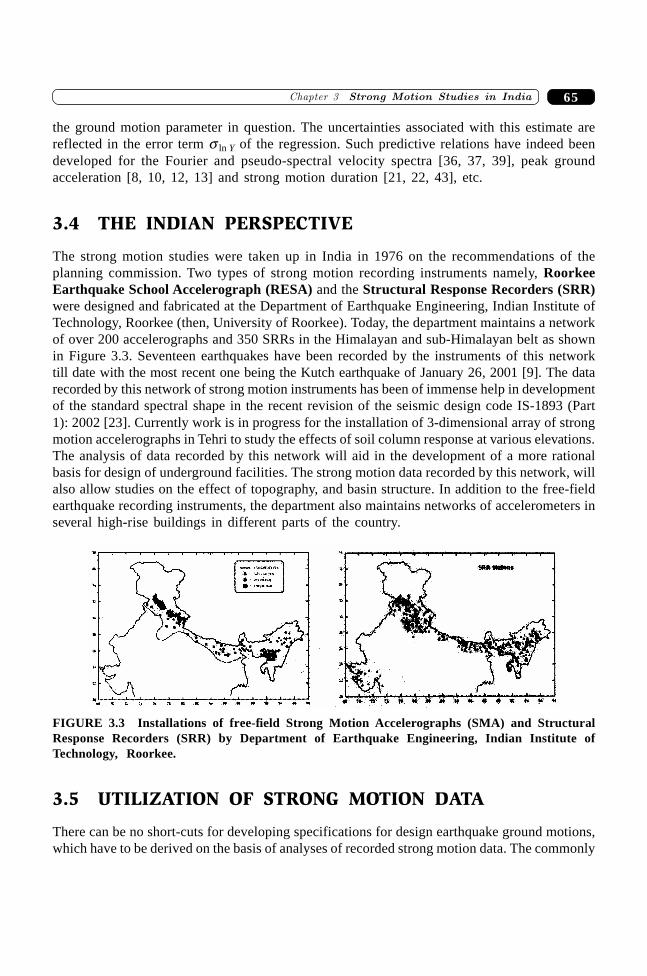
65�������� ����������������� � ������
the ground motion parameter in question. The uncertainties associated with this estimate arereflected in the error term s ln Y of the regression. Such predictive relations have indeed beendeveloped for the Fourier and pseudo-spectral velocity spectra [36, 37, 39], peak groundacceleration [8, 10, 12, 13] and strong motion duration [21, 22, 43], etc.
3.4 THE INDIAN PERSPECTIVE
The strong motion studies were taken up in India in 1976 on the recommendations of theplanning commission. Two types of strong motion recording instruments namely, RoorkeeEarthquake School Accelerograph (RESA) and the Structural Response Recorders (SRR)were designed and fabricated at the Department of Earthquake Engineering, Indian Institute ofTechnology, Roorkee (then, University of Roorkee). Today, the department maintains a networkof over 200 accelerographs and 350 SRRs in the Himalayan and sub-Himalayan belt as shownin Figure 3.3. Seventeen earthquakes have been recorded by the instruments of this networktill date with the most recent one being the Kutch earthquake of January 26, 2001 [9]. The datarecorded by this network of strong motion instruments has been of immense help in developmentof the standard spectral shape in the recent revision of the seismic design code IS-1893 (Part1): 2002 [23]. Currently work is in progress for the installation of 3-dimensional array of strongmotion accelerographs in Tehri to study the effects of soil column response at various elevations.The analysis of data recorded by this network will aid in the development of a more rationalbasis for design of underground facilities. The strong motion data recorded by this network, willalso allow studies on the effect of topography, and basin structure. In addition to the free-fieldearthquake recording instruments, the department also maintains networks of accelerometers inseveral high-rise buildings in different parts of the country.
FIGURE 3.3 Installations of free-field Strong Motion Accelerographs (SMA) and StructuralResponse Recorders (SRR) by Department of Earthquake Engineering, Indian Institute ofTechnology, Roorkee.
3.5 UTILIZATION OF STRONG MOTION DATA
There can be no short-cuts for developing specifications for design earthquake ground motions,which have to be derived on the basis of analyses of recorded strong motion data. The commonly
������������ ������� ������������� 66
recommended approach of using easily available weak motion data instead of data from lessfrequent strong earthquakes may lead to gross errors in land-use planning in addition to leadingto unsafe designs [25]. Strong motion data helps in developing a better understanding of (i)ground response near fault ruptures of large earthquakes, (ii) effects of severe shaking ondifferent sub-surface structures and geologic materials, and (iii) ground response in areas thatare prone to liquefaction. Analysis of strong motion records also leads to the development ofimproved methods for generating artificial earthquake motions for regions where the data fromreal earthquakes are not available [27, 28]. The data recorded by the network of instrumentsin high-rise buildings can be used for deriving information for remote monitoring of the healthof the building, the locations and extent of repair works required, and to verify adequacy of theanalytical modeling and design guidelines.
The strong motion data as recorded by the strong motion instruments, however, are notdirectly useful for strong motion studies. The raw data has to be first processed and correctedfor various possible sources of errors which might have crept in during the process of recording.A detailed discussion of the various issues of strong motion data processing may be found inother publications [4, 20, 26, 33, 34, 35].
SUMMARY
This chapter contains discussion of the various issues involved in strong motion studies—primarily a discussion of what, why, and how. The emphasis is on developing an understandingof the problem of characterizing design earthquake ground motions. This will help readers tointerpret correctly the relevant clauses in design codes and also in making a judicious decisionin special cases requiring special attention beyond the scope of the standard codes of practice.
REFERENCES
[1] Abrahamson, N.A. and Silva, W.J., “Empirical Response Spectral AttenuationRelations for Shallow Crustal Earthquakes”. Seismological Research Letters, 68: 94–127, 1997.
[2] Abrahamson, N.A. and Somerville, P.G., “Effects of the Hanging Wall and Foot Wallon Ground Motions Recorded during the Northridge Earthquake”, Bulletin of theSeismological Society of America, 86: S93–S99, 1996.
[3] Aki, K., Chin, B.-H., and Kato, K., “Seismological and Geotechnical Studies of LocalSite Effects on Strong and Weak Motions”, In Proceedings of the InternationalSymposium on the Effects of Surface Geology on Seismic Motion, ESG1992, Odawara,Japan, Pages I: 97–110, IASPEI/IAEE Joint Working Group on ESG, Association forEarthquake Disaster Prevention, Tokyo, Japan, 1992.
[4] Boore, D.M., Stephens, C.D., and Joyner, W.B., “Comments on Baseline Correctionof Digital Strong Motion Data: Examples from the 1999 Hector Mine, CaliforniaEarthquake”, Bulletin of the Seismological Society of America, 92(4): 1543–1560,2002.
67�������� ����������������� � ������
[5] Borcherdt, R.D., “Effects of Local Geology on Ground Motion Near San FranciscoBay”. Bulletin of the Seismological Society of America, 60: 29–61, 1970.
[6] Bresnev, I.A. and Wen, K.-L., “Nonlinear Soil Response—A Reality?”, Bulletin of theSeismological Society of America, 86: 1964–1978, 1996.
[7] Bullen, K.E., An Introduction to the Theory of Seismology, Cambridge University Press,London, 1953.
[8] Campbell, K.W., “Near Source Attenuation of Peak Horizontal Acceleration”, Bulletinof the Seismological Society of America, 71: 2039–2070, 1981.
[9] Chandra, B., Thakkar S.K., Basu S., Kumar A., Shrikhande M., Das J., Agarwal P.,and Bansal M.K., “Strong Motion Records”, Earthquake Spectra, Supplement A toVolume 18: 53–66, 2002.
[10] Crouse, C.B., “Ground-motion Attenuation Equations for Earthquakes on the CascadiaSubduction Zone”. Earthquake Spectra, 7(2): 201–236, 1991.
[11] Field, E.H. and Jacob, K.H., “A Comparison and Test of Various Site ResponseEstimation Techniques, Including Three that are Non Reference-site Dependent”.Bulletin of the Seismological Society of America, 85: 1127–1143, 1995.
[12] Joyner, W.B. and Boore, D.M., “Method for Regression Analysis of Strong MotionData”, Bulletin of the Seismological Society of America, 83: 469–487, 1993 (Errata in1994).
[13] Joyner, W.B. and Boore, D.M., “Errata: Method for Regression Analysis of StrongMotion Data”. Bulletin of the Seismological Society of America, 84: 955–956, 1994.
[14] Konno, K. and Ohmachi, T., “Ground-motion Characteristics Estimated from SpectralRatio between Horizontal and Vertical Components of Microtremor”. Bulletin of theSeismological Society of America, 88(1): 228–241, 1998.
[15] Kramer, S.L., Geotechnical Earthquake Engineering, Pearson Education, Singapore,1996 (Indian reprint 2003).
[16] Krawinkler, H. and Alavi, B., “Development of Improved Design Procedures for NearFault Ground Motions”, In SMIP98, Seminar on Utilization of Strong Motion Data,Oakland, California, 1998.
[17] Lermo, J. and Chavez-Garcia, F.J., “Are Micro-tremors Useful in Site ResponseEvaluation?”, Bulletin of the Seismological Society of America, 84: 1350–1364, 1994.
[18] Mohammadioun, B., “Nonlinear Response of Soils to Horizontal and Vertical BedrockEarthquake Motion”, Journal of Earthquake Engineering, 1(1): 93–119, 1997.
[19] Nakamura, Y., “Clear Identification of Fundamental Idea of Nakamura’s Technique andits Applications”. In Proceedings of the 12th World Conference on EarthquakeEngineering, Vol. 5, Paper # 2656, Auckland, New Zealand, 2000.
[20] Novikova, E.I. and Trifunac, M.D., “Digital Instrument Response Correction for theForce Balance Accelerometer”. Earthquake Spectra, 8(3): 429–442, 1992.
[21] Novikova, E.I. and Trifunac, M.D., “Modified Mercalli Instensity Scaling of theFrequency Dependent Duration of Strong Ground Motion”, Soil Dynamics andEarthquake Engineering, 12: 309–322, 1993.
[22] Novikova, E.I. and Trifunac, M.D., “Duration of Strong Ground Motion in Termsof Earthquake Magnitude, Epicentral Distance, Site Conditions, and Site Geometry”,Earthquake Engineering and Structural Dynamics, 23: 1023–1043, (1994).
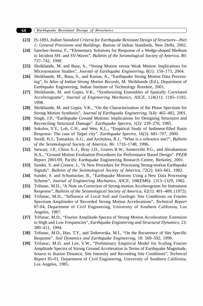
������������ ������� ������������� 68
[23] IS-1893, Indian Standard Criteria for Earthquake Resistant Design of Structures—Part1: General Provisions and Buildings. Bureau of Indian Standards, New Delhi, 2002.
[24] Sanchez-Sesma, F., “Elementary Solutions for Response of a Wedge-shaped Mediumto Incident SH- and SV-Waves”, Bulletin of the Seismological Society of America, 80:737–742, 1990.
[25] Shrikhande, M. and Basu, S., “Strong Motion versus Weak Motion: Implications forMicrozonation Studies”, Journal of Earthquake Engineering, 8(1): 159–173, 2004.
[26] Shrikhande, M., Basu, S., and Kumar, A., “Earthquake Strong Motion Data Process-ing”, In Atlas of Indian Strong Motion Records, M. Shrikhande (Ed.), Department ofEarthquake Engineering, Indian Institute of Technology Roorkee, 2001.
[27] Shrikhande, M. and Gupta, V.K., “Synthesizing Ensembles of Spatially CorrelatedAccelerograms”, Journal of Engineering Mechanics, ASCE, 124(11): 1185–1192,1998.
[28] Shrikhande, M. and Gupta, V.K., “On the Characterization of the Phase Spectrum forStrong Motion Synthesis”, Journal of Earthquake Engineering, 5(4): 465–482, 2001.
[29] Singh, J.P., “Earthquake Ground Motions: Implications for Designing Structures andReconciling Structural Damage”. Earthquake Spectra, 1(2): 239–270, 1985.
[30] Sokolov, V.Y., Loh, C.H., and Wen, K.L., “Empirical Study of Sediment-filled BasinResponse: The case of Taipei city”. Earthquake Spectra, 16(3): 681–707, 2000.
[31] Steidl, H.J., Tumarkin, A.G., and Archuleta, R.J., “What is a reference site?”, Bulletinof the Seismological Society of America, 86: 1733–1748, 1996.
[32] Stewart, J.P., Chiou S.-J., Bray J.D., Graves R.W., Somerville P.G., and AbrahamsonN.A., “Ground Motion Evaluation Procedures for Performance Based Design”. PEERReport 2001/09, Pacific Earthquake Engineering Research Centre, Berkeley, 2001.
[33] Sunder, S. and Connor, J., “A New Procedure for Processing Strong-motion EarthquakeSignals”. Bulletin of the Seismological Society of America, 72(2): 643–661, 1982.
[34] Sunder, S. and Schumacker, B., “Earthquake Motions Using a New Data ProcessingScheme”, Journal of Engineering Mechanics, ASCE, 108(EM6): 1313–1329, 1982.
[35] Trifunac, M.D., “A Note on Correction of Strong-motion Accelerograms for InstrumentResponse”, Bulletin of the Seismological Society of America, 62(1): 401–409, (1972).
[36] Trifunac, M.D., “Influence of Local Soil and Geologic Site Conditions on FourierSpectrum Amplitudes of Recorded Strong Motion Accelerations”, Technical Report87-04, Department of Civil Engineering, University of Southern California, LosAngeles, 1987.
[37] Trifunac, M.D., “Fourier Amplitude Spectra of Strong Motion Acceleration: Extensionto High and Low Frequencies”, Earthquake Engineering and Structural Dynamics, 23:389–411, 1994.
[38] Trifunac, M.D., Hao, T.Y., and Todorovska, M.I., “On the Recurrence of Site SpecificResponse”. Soil Dynamics and Earthquake Engineering, 18: 569–592, 1999.
[39] Trifunac, M.D. and Lee, V.W., “Preliminary Empirical Model for Scaling FourierAmplitude Spectra of Strong Ground Acceleration in Terms of Earthquake Magnitude,Source to Station Distance, Site Intensity and Recording Site Conditions”, TechnicalReport 85-03, Department of Civil Engineering, University of Southern California,Los Angeles, 1985.

69�������� ����������������� � ������
[40] Trifunac, M.D. and Todorovska, M.I., “Nonlinear Soil Response as a Natural PassiveIsolation Mechanism—the 1994 Northridge, California, Earthquake”, Soil Dynamics andEarthquake Engineering, 17: 41–51, 1998.
[41] Trifunac, M.D. and Todorovska, M.I., “Can Aftershock Studies Predict Site Amplifi-cation Factors: Northridge, CA, Earthquake of 17 January 1994”, Soil Dynamics andEarthquake Engineering, 19: 233–251, 2000.
[42] Trifunac, M.D. and Todorovska, M.I., “Long Period Microtremors, Microseisms andEarthquake Damage: Northridge, CA, Earthquake of 17 January 1994”, Soil Dynamicsand Earthquake Engineering, 19: 253–267, 2000.
[43] Trifunac, M.D. and Westermo, B.D., “A Note on the Correlation of Frequency-Dependent Duration of Strong Earthquake Ground Motion with the MMI and GeologicCondition at the Recording Stations”, Bulletin of the Seismological Society of America,67(3): 917–927, 1977.
[44] Udwadia, F.E. and Trifunac, M.D., “Comparison of Earthquake and Micro-tremorGround Motions in El Centro, California”, Bulletin of the Seismological Society ofAmerica, 63: 1227–1253, 1973.
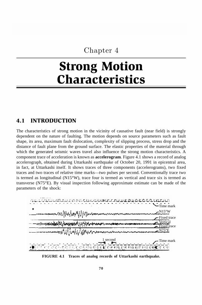
����������� ������� �������������70
70
Strong MotionCharacteristics
��������
4.1 INTRODUCTION
The characteristics of strong motion in the vicinity of causative fault (near field) is stronglydependent on the nature of faulting. The motion depends on source parameters such as faultshape, its area, maximum fault dislocation, complexity of slipping process, stress drop and thedistance of fault plane from the ground surface. The elastic properties of the material throughwhich the generated seismic waves travel also influence the strong motion characteristics. Acomponent trace of acceleration is known as accelerogram. Figure 4.1 shows a record of analogaccelerograph, obtained during Uttarkashi earthquake of October 20, 1991 in epicentral area,in fact, at Uttarkashi itself. It shows traces of three components (accelerograms), two fixedtraces and two traces of relative time marks—two pulses per second. Conventionally trace twois termed as longitudinal (N15°W), trace four is termed as vertical and trace six is termed astransverse (N75°E). By visual inspection following approximate estimate can be made of theparameters of the shock:
Time mark
N15°W
Fixed trace
VerticalFixed traceN75°E
Time mark1 second
FIGURE 4.1 Traces of analog records of Uttarkashi earthquake.
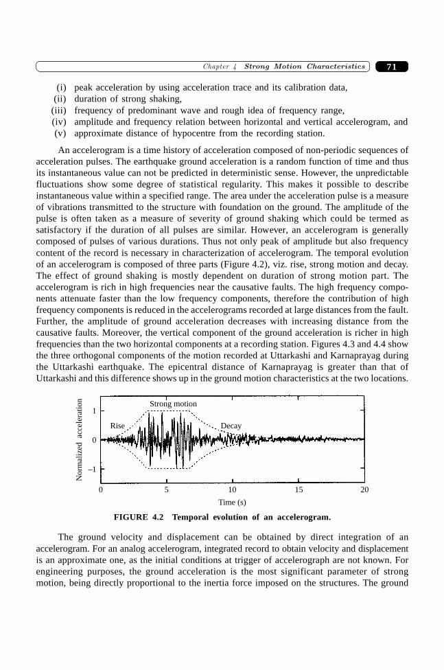
71�������� ��������� ���������� �� ��
(i) peak acceleration by using acceleration trace and its calibration data,(ii) duration of strong shaking,
(iii) frequency of predominant wave and rough idea of frequency range,(iv) amplitude and frequency relation between horizontal and vertical accelerogram, and(v) approximate distance of hypocentre from the recording station.
An accelerogram is a time history of acceleration composed of non-periodic sequences ofacceleration pulses. The earthquake ground acceleration is a random function of time and thusits instantaneous value can not be predicted in deterministic sense. However, the unpredictablefluctuations show some degree of statistical regularity. This makes it possible to describeinstantaneous value within a specified range. The area under the acceleration pulse is a measureof vibrations transmitted to the structure with foundation on the ground. The amplitude of thepulse is often taken as a measure of severity of ground shaking which could be termed assatisfactory if the duration of all pulses are similar. However, an accelerogram is generallycomposed of pulses of various durations. Thus not only peak of amplitude but also frequencycontent of the record is necessary in characterization of accelerogram. The temporal evolutionof an accelerogram is composed of three parts (Figure 4.2), viz. rise, strong motion and decay.The effect of ground shaking is mostly dependent on duration of strong motion part. Theaccelerogram is rich in high frequencies near the causative faults. The high frequency compo-nents attenuate faster than the low frequency components, therefore the contribution of highfrequency components is reduced in the accelerograms recorded at large distances from the fault.Further, the amplitude of ground acceleration decreases with increasing distance from thecausative faults. Moreover, the vertical component of the ground acceleration is richer in highfrequencies than the two horizontal components at a recording station. Figures 4.3 and 4.4 showthe three orthogonal components of the motion recorded at Uttarkashi and Karnaprayag duringthe Uttarkashi earthquake. The epicentral distance of Karnaprayag is greater than that ofUttarkashi and this difference shows up in the ground motion characteristics at the two locations.
0 5 10 15 20
Time (s)
0
1
–1
No
rmal
ized
acce
lera
tio
n
Rise
Strong motion
Decay
FIGURE 4.2 Temporal evolution of an accelerogram.
The ground velocity and displacement can be obtained by direct integration of anaccelerogram. For an analog accelerogram, integrated record to obtain velocity and displacementis an approximate one, as the initial conditions at trigger of accelerograph are not known. Forengineering purposes, the ground acceleration is the most significant parameter of strongmotion, being directly proportional to the inertia force imposed on the structures. The ground
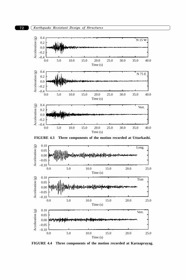
����������� ������� �������������72
–0.4
–0.2
0.0
0.2
0.4A
ccel
erat
ion
(g)
0.0 5.0 10.0 15.0 20.0 25.0 30.0 35.0 40.0
N 15 W
Time (s)
–0.4
–0.2
0.0
0.2
0.4
Acc
eler
atio
n(g
)
0.0 5.0 10.0 15.0 20.0 25.0 30.0 35.0 40.0
N 75 E
Time (s)
–0.4
–0.2
0.0
0.2
0.4
Acc
eler
atio
n(g
)
0.0 5.0 10.0 15.0 20.0 25.0 30.0 35.0 40.0
Vert.
Time (s)
FIGURE 4.3 Three components of the motion recorded at Uttarkashi.
–0.10
–0.05
0.00
0.05
0.10
0.0 5.0 10.0 15.0 20.0 25.0
Long.
Acc
eler
atio
n(g
)
Time (s)
–0.10
–0.05
0.00
0.05
0.10
0.0 5.0 10.0 15.0 20.0 25.0
Tran
Acc
eler
atio
n(g
)
Time (s)
–0.10
–0.05
0.00
0.05
0.10
0.0 5.0 10.0 15.0 20.0 25.0
Vert.
Acc
eler
atio
n(g
)
Time (s)
FIGURE 4.4 Three components of the motion recorded at Karnaprayag.
73�������� ��������� ���������� �� ��
velocity is better correlated with the intensity of damage and it is also directly related with theenergy transmitted to the structures. The ground displacement, however, is important for designof underground pipelines and is also an indicator of the amount of strain the foundation of alarge structure will be subjected to.
4.2 TERMINOLOGY OF STRONG MOTIONSEISMOLOGY
Due to the random nature of ground motion during a strong earthquake, it is not possible tocharacterize it for design purposes by means of the time histories of a recorded ground motion.Some of the physical quantities and derived parameters which are used to describe variousaspects of the ground motion are described as follows:
4.2.1 Amplitude Parameters
The amplitude parameters of the ground motion were the earliest of the strong motionparameters to be proposed. Typically, the peak values of the ground acceleration, velocity anddisplacement give an idea of the severity of shaking at a site, predominant period of vibration,etc.
Peak Acceleration
The Peak Horizontal Acceleration (PHA) is the most commonly used measure of the intensityof shaking at a site and is taken to be the largest absolute value of the horizontal accelerationrecorded at a site. It is also possible to extract the maximum of the vector sum of two orthogonalcomponents of the horizontal ground acceleration recorded at a site. Ground motions with highpeak accelerations are usually, but not always, more damaging than those with lower peakacceleration. However, a short duration stray pulse with large amplitude may not cause anysignificant damage as there is very little time available for the system to respond to suchexcitation. Therefore, the duration of the excitation is also an important consideration inestimating the damage potential of a ground motion.
v/a ratio
As the peak accelerations (a) and peak velocities (v) are usually associated with the motion ofdifferent frequencies, the ratio v/a can be related to the frequency content of the motion. Forearthquake motions that include several frequencies, the parameter 2pv/a can be interpreted asthe period of vibration of an equivalent harmonic wave, thereby providing an indication of thepredominant period of the ground motion. It has been observed that v/a ratio for rocky sites aresubstantially lower than those for alluvium.
ad/v2 ratio
The ratio of the peak acceleration-displacement product to the square of the peak velocity canbe related to the sharpness or flatness of the response spectrum. For harmonic motions, this ratio
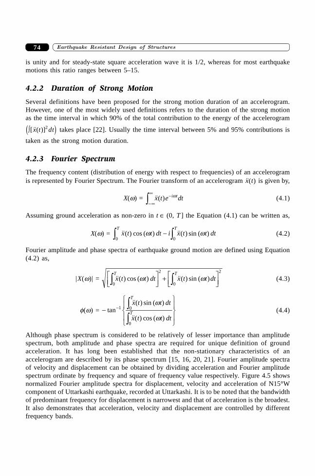
����������� ������� �������������74
is unity and for steady-state square acceleration wave it is 1/2, whereas for most earthquakemotions this ratio ranges between 5–15.
4.2.2 Duration of Strong Motion
Several definitions have been proposed for the strong motion duration of an accelerogram.However, one of the most widely used definitions refers to the duration of the strong motionas the time interval in which 90% of the total contribution to the energy of the accelerogram
z[��( )]x t dt2d i takes place [22]. Usually the time interval between 5% and 95% contributions is
taken as the strong motion duration.
4.2.3 Fourier Spectrum
The frequency content (distribution of energy with respect to frequencies) of an accelerogramis represented by Fourier Spectrum. The Fourier transform of an accelerogram ��( )x t is given by,
X(w) = ��( )x t e dti t-
-•
•z w (4.1)
Assuming ground acceleration as non-zero in t Π(0, T ] the Equation (4.1) can be written as,
X(w) = ��( ) cos ( ) ��( ) sin ( )x t t dt i x t t dtTT
w w- zz 00(4.2)
Fourier amplitude and phase spectra of earthquake ground motion are defined using Equation(4.2) as,
|X(w)| = ��( ) cos ( ) ��( ) sin ( )x t t dt x t t dtT T
w w0
2
0
2z zLNM
OQP + L
NMOQP (4.3)
f(w) = -
RS|
T|
UV|
W|- zz
tan��( ) sin ( )
��( ) cos ( )
1 0
0
x t t dt
x t t dt
T
T
w
w(4.4)
Although phase spectrum is considered to be relatively of lesser importance than amplitudespectrum, both amplitude and phase spectra are required for unique definition of groundacceleration. It has long been established that the non-stationary characteristics of anaccelerogram are described by its phase spectrum [15, 16, 20, 21]. Fourier amplitude spectraof velocity and displacement can be obtained by dividing acceleration and Fourier amplitudespectrum ordinate by frequency and square of frequency value respectively. Figure 4.5 showsnormalized Fourier amplitude spectra for displacement, velocity and acceleration of N15°Wcomponent of Uttarkashi earthquake, recorded at Uttarkashi. It is to be noted that the bandwidthof predominant frequency for displacement is narrowest and that of acceleration is the broadest.It also demonstrates that acceleration, velocity and displacement are controlled by differentfrequency bands.
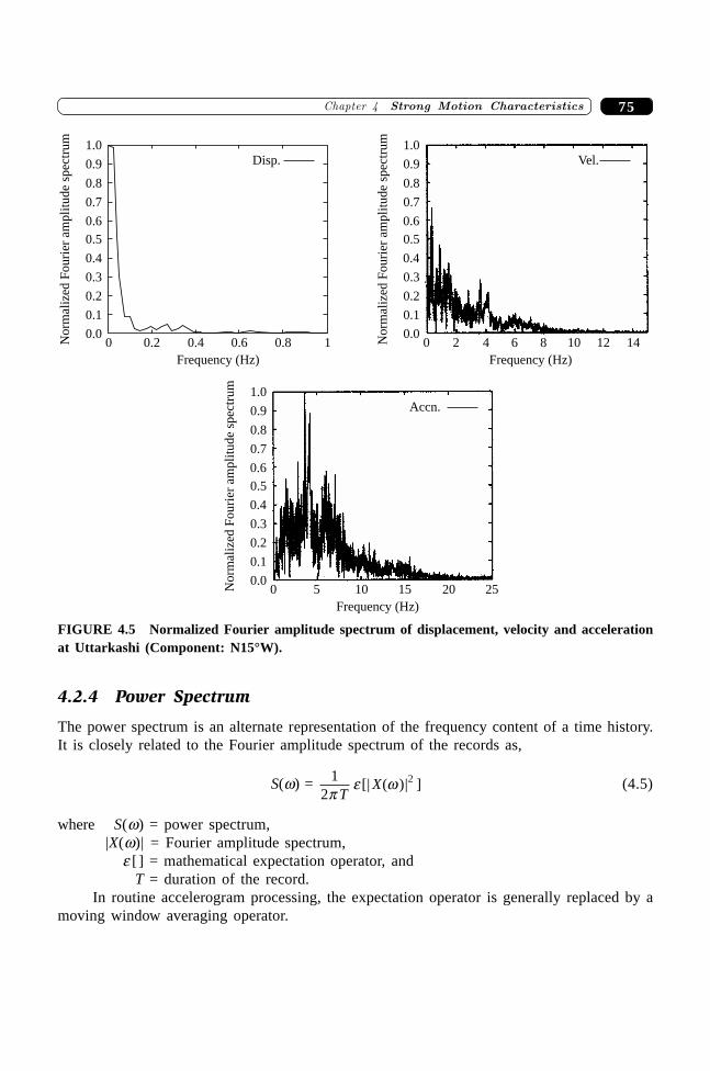
75�������� ��������� ���������� �� ��
4.2.4 Power Spectrum
The power spectrum is an alternate representation of the frequency content of a time history.It is closely related to the Fourier amplitude spectrum of the records as,
S(w) = 12
2
pe w
TX[| ( )| ] (4.5)
where S(w) = power spectrum,|X(w)| = Fourier amplitude spectrum,
e [ ] = mathematical expectation operator, andT = duration of the record.
In routine accelerogram processing, the expectation operator is generally replaced by amoving window averaging operator.
0.00 0.2 0.4 0.6 0.8 1
0.1
0.2
0.3
0.4
0.5
0.6
0.7
0.8
0.9
1.0Disp.
Frequency (Hz)
Norm
aliz
edF
ouri
eram
pli
tude
spec
trum
0.00
0.1
0.2
0.3
0.5
0.7
0.8
0.9
1.0
Norm
aliz
edF
ouri
eram
pli
tude
spec
trum
2 4 6 8 10 12 14
0.4
0.6
Vel.
Frequency (Hz)
0.00
0.1
0.2
0.3
0.5
0.7
0.8
0.9
1.0
Norm
aliz
edF
ouri
eram
pli
tude
spec
trum
5 10 15 20 25
0.4
0.6
Accn.
Frequency (Hz)
FIGURE 4.5 Normalized Fourier amplitude spectrum of displacement, velocity and accelerationat Uttarkashi (Component: N15°W).
����������� ������� �������������76
4.2.5 Response Spectrum
Ever since Housner [6] presented the use of response spectrum in seismic analysis, it has beenadopted as a standard way of representation of effect of ground acceleration on structures. Itreflects frequency content, amplitude of ground motion and effect of subsequent filtering by thestructure. The response of an oscillator, initially at rest, is given by,
x(t) = – 10w
t w t tzw t
dg
td
tx e t dn�� ( ) sin ( )( )- - -z (4.6)
where wd = w zn 1 2- is the damped natural frequency. The plot of maximum relative responsex(t) of linear elastic SDOF system, initially at rest with prescribed damping ratio z subjectedto a ground acceleration versus natural period, or frequency of vibration is defined as relativedisplacement response spectrum and is denoted as,
Sd (z, wn) ∫ Sd(z, Tn) = |x(t)|max
= 10w
t w t tzw t
dg
td
tx e t dn�� ( ) sin ( )( )
max
- - -RSTUVW
LNM
OQPz (4.7)
where natural period of vibration Tn = 2p/wn. For a specified ground motion the Equation (4.6)is numerically integrated and the resulting maximum relative displacement value gives one valueof Sd for a given set of wn and z. Typically this integration is carried out at uniform frequencyinterval in a prescribed range of frequency for different ratios of z. The quantity within thecurly brackets of Equation (4.7) has the unit of velocity. The absolute maximum of this quantityis termed as pseudo relative velocity response spectrum (psv) Spv(z, wn) and is given as,
Spv(z, wn) ∫ Spv(z, Tn) = �� ( ) sin ( )( )
max
x e t dgt
d
tnt w t tzw t- - -L
NMOQPz0 (4.8)
Thus for lightly damped system (i.e., wd ª wn)
Sd(z, wn) ∫ 1 1w
z ww
z wd
pv nn
pv nS S( , ) ( , )ª (4.9)
The relative displacement response spectra asymptotically approaches maximum grounddisplacement for highly flexible structure. Formally the limiting value of Sd (z, wn) is,
limw nÆ0
Sd (z, wn) = |xg(t)|max (4.10)
This implies that the mass remains stationary for all practical purposes and only the groundmoves, as the linear elastic SDOF system is composed of spring with negligible stiffness.
Differentiation of Equation (4.6) with respect to time t gives,
�( )x t = – �� ( ) cos ( )( )x e t dgt
d
tnt w t tzw t- - -z0
+-
-- -zzz
t w t tzw t
1 2 0�� ( ) sin ( )( )x e t dg
td
tn (4.11)
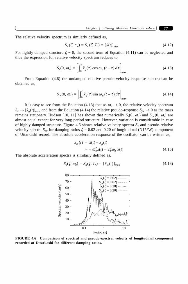
77�������� ��������� ���������� �� ��
The relative velocity spectrum is similarly defined as,
Sv (z, wn) ∫ Sv (z, Tn) = [ �( )]maxx t (4.12)
For lightly damped structure z ª 0, the second term of Equation (4.11) can be neglected andthus the expression for relative velocity spectrum reduces to
Sv(0, wn) = �� ( ) cos ( )max
x t dg n
tt w t t-L
NMOQPz0 (4.13)
From Equation (4.8) the undamped relative pseudo-velocity response spectra can beobtained as,
Spv(0, wn) = �� ( ) sin ( )max
x t dg n
tt w t t-z0 (4.14)
It is easy to see from the Equation (4.13) that as wn Æ 0, the relative velocity spectrumSv Æ | � ( )|maxx tg and from the Equation (4.14) the relative pseudo-response Spv Æ 0 as the massremains stationary. Hudson [10, 11] has shown that numerically Sv(0, wn) and Spv(0, wn) arealmost equal except for very long period structure. However, variation is considerable in caseof highly damped structure. Figure 4.6 shows relative velocity spectra Sv and pseudo-relativevelocity spectra Spv for damping ratios z = 0.02 and 0.20 of longitudinal (N15°W) componentof Uttarkashi record. The absolute acceleration response of the oscillator can be written as,
�� ( )x tm = ��( ) �� ( )x t x tg+
= – w 2nx(t) – 2zwn �( )x t (4.15)
The absolute acceleration spectra is similarly defined as,
Sa(z, wn) = Sa(z, Tn) = [ �� ( )x tm ]max (4.16)
10
1010.1
20
30
40
50
60
70
80
Period (s)
Spec
tral
vel
oci
ty(c
m/s
)
Sv( = 0.02)zSpv( = 0.02)zSv( = 0.20)z
Spv( = 0.20)z
FIGURE 4.6 Comparison of spectral and pseudo-spectral velocity of longitudinal componentrecorded at Uttarkashi for different damping ratios.
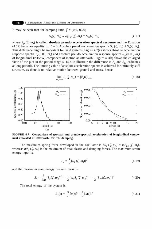
����������� ������� �������������78
It may be seen that for damping ratio z Π(0.0, 0.20)
Sa(z, wn) ª wnSpv(z, wn) = Spa(z, wn) (4.17)
where Spa(z, wn) is called absolute pseudo-acceleration spectral response and the Equation(4.17) becomes equality for z = 0. Absolute pseudo-acceleration spectra Spa(z, wn) £ Sa(z, wn).This difference might be important for rigid systems. Figure 4.7(a) shows absolute accelerationresponse spectra Sa(0.05, wn) and absolute pseudo acceleration response spectra Spa(0.05, wn)of longitudinal (N15°W) component of motion at Uttarkashi. Figure 4.7(b) shows the enlargedview of the plot in the period range 5–15 s to illustrate the difference in Sa and Spa ordinatesat long periods. The limiting value of absolute acceleration spectra is achieved for infinitely stiffstructure, as there is no relative motion between ground and mass, hence
lim ( , )w
z wn
Sa nƕ = | �� ( )|maxx tg (4.18)
0.01 0.1 1 10 1000.00
0.20
0.40
0.60
0.80
1.00
1.20
Spec
tral
acce
lera
tion
(g)
Period (s)
(a)
SaSpa
50.00
0.002
Spec
tral
acce
lera
tion
(g)
Period (s)
(b)
SaSpa
6 7 8 9 10 15 20
0.003
0.004
0.005
FIGURE 4.7 Comparison of spectral and pseudo-spectral acceleration of longitudinal compo-nent recorded at Uttarkashi for 5% damping.
The maximum spring force developed in the oscillator is kSd (z, wn) = mSpa (z, wn),whereas mSa (z, wn) is the maximum of total elastic and damping forces. The maximum strainenergy input is,
EI = k2
[Sd (z, wn)]2 (4.19)
and the maximum stain energy per unit mass is,
Es = km
Sd n22[ ( , )]z w = 1
22[ ( , )]w z wn d nS = 1
22[ ( , )]Spv nz w (4.20)
The total energy of the system is,
ET(t) = m x t k x t2 2
2 2[ �( )] [ ( )]+ (4.21)
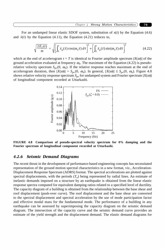
79�������� ��������� ���������� �� ��
For an undamped linear elastic SDOF system, substitution of x(t) by the Equation (4.6)and �( )x t by the Equation (4.11), the Equation (4.21) reduces to,
2E tmT ( )
= �� ( ) cos( ) �� ( ) sin ( )x d x dg n
t
g n
tt w t t t w t t
0
2
0
2z zLNM
OQP + L
NMOQP (4.22)
which at the end of accelerogram t = T is identical to Fourier amplitude spectrum |X(w) | of theground acceleration evaluated at frequency wn. The maximum of the Equation (4.22) is pseudo-relative velocity spectrum Spv(0, wn). If the relative response reaches maximum at the end ofaccelerogram duration, then |X(w) | = Spv(0, wn). In general, |X(w) | £ Spv(0, wn). Figure 4.8shows relative velocity response spectrum Spv for undamped system and Fourier spectrum |X(w)|of longitudinal component recorded at Uttarkashi.
0.0050 10 15 20 25
0.02
0.04
0.06
0.08
0.10
0.12
0.14
Fouri
eram
pli
tude
(gs)◊
Frequency (Hz)
FS
Spv( = 0.0)z
FIGURE 4.8 Comparison of pseudo-spectral velocity spectrum for 0% damping and theFourier spectrum of longitudinal component recorded at Uttarkashi.
4.2.6 Seismic Demand Diagrams
The recent thrust in the development of performance-based engineering concepts has necessitatedrepresentation of the ground motion spectral characteristics in a new format, viz., Acceleration-Displacement Response Spectrum (ADRS) format. The spectral accelerations are plotted againstspectral displacements, with the periods (Tn) being represented by radial lines. An estimate ofinelastic demands imposed on a structure by an earthquake is obtained from the linear elasticresponse spectra computed for equivalent damping ratios related to a specified level of ductility.The capacity diagram of a building is obtained from the relationship between the base shear androof displacement (push-over curve). The roof displacement and the base shear are convertedto the spectral displacement and spectral acceleration by the use of mode participation factorand effective modal mass for the fundamental mode. The performance of a building in anyearthquake can be assessed by superimposing the capacity diagram on the seismic demanddiagram. The intersection of the capacity curve and the seismic demand curve provides anestimate of the yield strength and the displacement demand. The elastic demand diagrams for
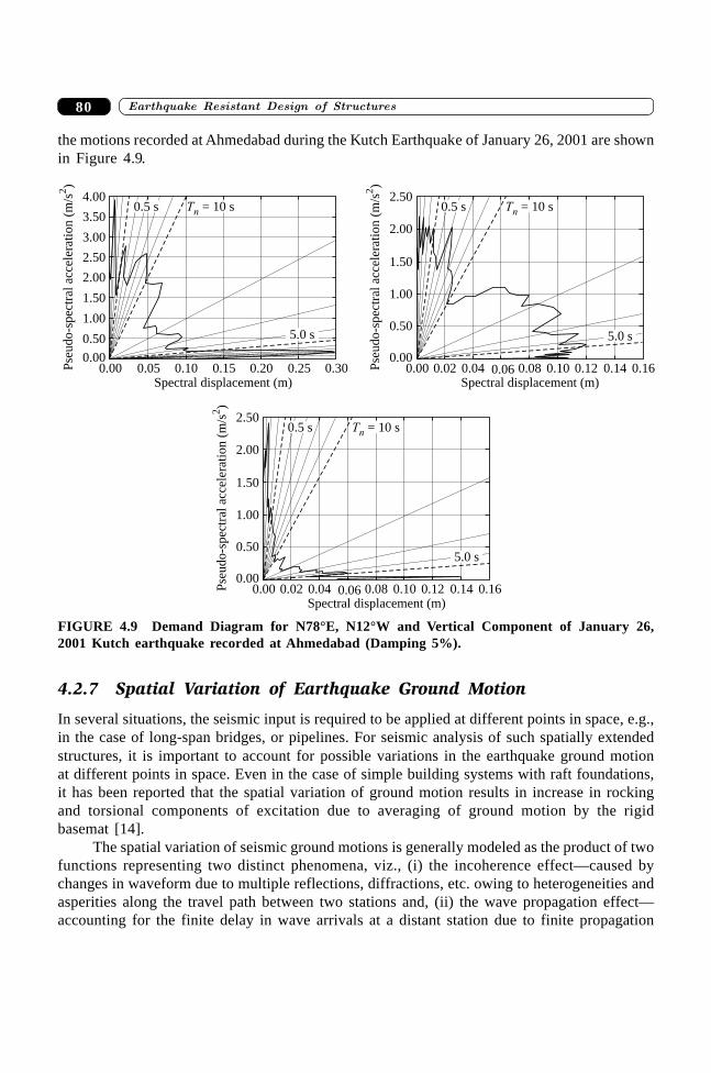
����������� ������� �������������80
the motions recorded at Ahmedabad during the Kutch Earthquake of January 26, 2001 are shownin Figure 4.9.
0.00 0.05 0.10 0.15 0.20 0.25 0.300.00
0.50
1.00
1.50
2.00
2.50
3.00
3.50
4.00Tn = 10 s0.5 s
5.0 s
Spectral displacement (m)
Pse
ud
o-s
pec
tral
acce
lera
tio
n(m
/s)
2
0.00 0.020.00
0.50
1.00
1.50
2.00
2.500.5 s
Spectral displacement (m)P
seu
do
-sp
ectr
alac
cele
rati
on
(m/s
)2
0.04 0.06 0.08 0.10 0.12 0.14 0.16
Tn = 10 s
5.0 s
0.00 0.020.00
0.50
1.00
1.50
2.00
2.500.5 s
Spectral displacement (m)
Pse
ud
o-s
pec
tral
acce
lera
tio
n(m
/s)
2
0.04 0.06 0.08 0.10 0.12 0.14 0.16
5.0 s
Tn = 10 s
FIGURE 4.9 Demand Diagram for N78°E, N12°W and Vertical Component of January 26,2001 Kutch earthquake recorded at Ahmedabad (Damping 5%).
4.2.7 Spatial Variation of Earthquake Ground Motion
In several situations, the seismic input is required to be applied at different points in space, e.g.,in the case of long-span bridges, or pipelines. For seismic analysis of such spatially extendedstructures, it is important to account for possible variations in the earthquake ground motionat different points in space. Even in the case of simple building systems with raft foundations,it has been reported that the spatial variation of ground motion results in increase in rockingand torsional components of excitation due to averaging of ground motion by the rigidbasemat [14].
The spatial variation of seismic ground motions is generally modeled as the product of twofunctions representing two distinct phenomena, viz., (i) the incoherence effect—caused bychanges in waveform due to multiple reflections, diffractions, etc. owing to heterogeneities andasperities along the travel path between two stations and, (ii) the wave propagation effect—accounting for the finite delay in wave arrivals at a distant station due to finite propagation
81�������� ��������� ���������� �� ��
velocities, and is given as
gjk(iw) = S i
S Si i
r
vjk
jj kkjk
jk( )
( ) ( )| ( )| exp
ww w
g w wªFHG
IKJapp
(4.23)
where gjk(iw) is known as the coherency function and is a measure of correlation between thegiven pair of time-histories, Sjk(iw) is the cross-power spectral density function for the pairof motions recorded at stations j and k, Sjj(w) and Skk(w) are the respective auto-power spectraldensity functions of the motions at stations j and k, rij represents the projected horizontalseparation between stations j and k, and vapp denotes the surface apparent velocity ofpropagation of the wave at frequency w.
Although seismic waves of different frequencies, in general, travel with different speedsit is common to prescribe a constant value for vapp for all frequencies because of inherentdifficulties in the estimation of this parameter. The first factor, on the right hand of Equation(4.23), represents the effect of incoherence and can be either derived from entirely theoreticalconsiderations [12, 25], or is empirically obtained from the analysis of strong motion array data[4, 5], and the second factor represents the effect of propagation delay due to finite velocities.
4.2.8 Damage Potential of Earthquakes
The potential of an earthquake to inflict damage on engineered facilities has always been amatter of great concern to all engineers. Very often a situation is encountered wherein one isforced to choose between several alternative ground motion time histories to verify the adequacyof a particular design to resist the design level earthquake motion. Since the design earthquakeloads are usually specified in the form of design spectra, artificial/synthetic accelerograms aregenerated so as to be compatible with the design specifications. However, the solution to theproblem of synthesizing a spectrum compatible accelerogram is not unique and it is possible tohave several different synthetic accelerograms which are compatible with the specified designspectrum. Thus it is desirable to use that time history which has the maximum potential fordamage. It is therefore necessary to derive a set of parameters derived from earthquake recordsthat may be considered as measures of the severity of ground shaking at the site. Further, thecorrelation between three orthogonal components of the ground acceleration vector at a locationis assumed to be negligible in seismic analysis. However, the recorded components are generallycorrelated which may introduce some bias in the analysis results. To eliminate these correlationeffects, the resolution of the ground motion components along the principal direction has beensuggested in the past [13, 17]. The principal directions and resolution of the ground motioncomponents along these principal directions have been discussed below. Further, several strongmotion parameters which are used to measure the severity of the ground motions have beenexplained.
Earthquake motions along principal axes
The seismic design loads on structures are usually specified in terms of a set of normalizeddesign (response) spectra for horizontal and vertical motions expected at a site. These spectralshapes are generally derived from the statistical analysis of the spectral ordinates of previously
����������� ������� �������������82
recorded earthquake motions in the region. In deriving the spectral shape for horizontal motions,it is common to consider the stronger of the two horizontal components of ground motion inthese analyses. Since the directivity of a future earthquake is random, the same spectral shapeis used for the two orthogonal horizontal directions for a conservative estimate of the expectedseismic loading. Further, the two orthogonal horizontal components of design earthquake aregenerally assumed to be uncorrelated. However, if these spectral shapes were derived from therecorded components of the ground motions, the estimates of the expected spectral ordinates arelikely to be biased and also unconservative. The bias in these estimates results from the finitecorrelation between the recorded components of the motions. In order to eliminate this bias, itis desirable to consider the uncorrelated components of the ground motion in statistical analysis.
Let the three translational components of ground acceleration recorded along the threeorthogonal transducer axes of the accelerograph denoted by ai(t); (i = x, y, z) be defined as,
ax(t) = e(t)bx(t)
ay(t) = e(t)by(t) (4.24)
az(t) = e(t)bz(t)
where bi(t); (i = x, y, z) are stationary random processes and e(t) is a deterministic modulatingfunction. Assuming the ground acceleration process to be Gaussian with zero mean, the threedimensional ground acceleration process can be completely characterized in a probabilistic sensethrough the covariance matrix
[m(t, t)] =
m m mm m mm m m
xx xy xz
yx yy yz
zx zy zz
L
N
MMM
O
Q
PPP
(4.25)
where, mij(= mij(t, t) = E[ai(t)aj(t + t)]) represents the covariance between two orthogonalcomponents ai(t) and aj(t) and E[◊] represents the mathematical expectation (ensemble average)operator. As a first approximation, real earthquake accelerograms can be represented by shot orwhite noise processes [7]. In such a situation, the random variables ai(t) and aj(t + t) would bestatistically uncorrelated for non-zero values of time difference t. Hence, the elements of thecovariance matrix of the ground acceleration process may approximated by m ij = E[ai(t)aj(t)].Substituting from Equation (4.24) into Equation (4.25), the covariance matrix can be writtenas,
[m(t)] = e2(t)[b] (4.26)
where, m ij(t) = E[ai(t)aj(t)] and bij(= E[bi(t)bj(t)]) is the time invariant covariance of stationaryprocesses bi(t) and bj(t), for i; j = x, y, z. Further, the components of motion along an arbitraryset of orthogonal axes x ¢, y ¢, z ¢ can be transformed to components along orthogonal axes x, y,z by a simple transformation as,
a t
a t
a t
x
y
z
( )
( )
( )
F
HGG
I
KJJ = [A]
a t
a t
a t
x
y
z
¢
¢
¢
F
HGG
I
KJJ
( )
( )
( )
(4.27)
83�������� ��������� ���������� �� ��
where [A] is the orthogonal transformation matrix satisfying the relation [A]T[A] = [I]. Thusthe covariance matrix for the axis x ¢, y ¢, z ¢ is obtained as
[m ¢(t)] = [A]–1[m(t)]([A]–1)T
= [A]T [m(t)][A] (4.28)
= e2(t)[A]T [b][A]
This transformation of three-dimensional ground motion is identical to the transformationof three-dimensional state of stress. Therefore it can be proved that there exists a set of principalaxes along which the components of motion have maximum, minimum and intermediate valuesof variance and zero covariance. The directions of the principal axis are given by the eigenvectorsof the covariance matrix of the recorded motions whereas the corresponding eigenvalues are theprincipal variances [13, 17]. Since the off-diagonal terms in a covariance matrix indicatequantitatively the correlation between the corresponding components, the components along theprincipal axes are fully uncorrelated with respect to each other. Moreover, the three componentsof motion along the principal axes are statistically independent of each other, provided that theground motions are assumed to be adequately represented by Gaussian random processes. Fora small class of stationary random processes, viz., ergodic processes, the ensemble statistics aresame as the temporal statistics and thus time averages taken over a single sample of the randomprocess provide complete statistical information about the process. For all other types of randomprocesses such a duality between ensemble and temporal statistics does not exist. In a practicalapplication, however, the desired statistical properties of random processes are often estimatedby examining individual members from the ensembles of processes [3]. Thus the covariancesin Equation (4.26) can be obtained by considering the temporal averaging over any singlemember of the process, i.e.,
bij = ·bri(t)b
rj(t)Ò
where, the superscript r denotes the rth sample from the ensemble of the process and angularbrackets represent time averaging over the duration of motion.
It has been reported [17] that there exists a strong correlation between the direction ofone of the principal axis (most often the major principal axis) and the general direction to thefault-slip zone. However, analysis of data from San Fernando earthquake of February 9, 1971indicates that this correlation is not very strong. Further, it was observed that one of the principaldirections is usually aligned with the vertical direction [13]. For the Indian earthquakes also,no correlation could be established between the directions of principal components of therecorded motions and the direction of the rupture of fault plane [18, 19].
Measures of severity
Various parameters have been defined to characterize severity of strong shaking. The PeakGround Acceleration (PGA) is the most widely used parameter to measure severity of earthquake.However, the PGA is a rather poor parameter for measuring severity of strong motion due tovarious reasons such as, its possible association with a pulse of very high frequency, amplificationdue to irregular local topography, interaction of large structure at the site of recording, etc. Thepopularity of PGA as a measure of severity of ground motion is partly because of it being the
����������� ������� �������������84
only parameter that can be directly measured by an instrument—all other strong motionparameters are derived from the processing of strong motion data. Further, the PGA measureis intuitively appealing to the engineers as it is proportional to the maximum inertia forceimposed on a structure during an earthquake. Several parameters that have been proposed asreplacements for PGA as a measure of severity of ground shaking are discussed below.
Arias defined earthquake intensity as sum of the total energy per unit weight, stored inundamped oscillators uniformly distributed with respect to their frequencies at the end of theearthquake [2]:
IA = p2
2
0gx t dt
TD
[��( )]z (4.29)
where, ��( )x t refers to the ground acceleration, g is acceleration due to gravity and TD representsthe earthquake duration. Thus duration and amplitude is implicitly considered in the definitionof IA. Since ��( )x t = 0 for t > TD, the Equation (4.29) can also be written as,
IA = p2
2
0gx t dt[��( )]
•z = 12
2
0gX d| |
•z ( )w w (4.30)
where, |X(w)| is the Fourier amplitude spectrum of ��( )x t . Thus IA will be large for strong motionwith significant amount of high frequency components, high amplitude and long duration.
Housner used the mean square acceleration during the rise time of strong motion to defineearthquake average power [9]. Let
I = [��( )]x t dtTD 2
0z (4.31)
be the total energy in a strong motion. The earthquake average power is defined as,
Pa = 1 2
0 05
0 95
Tx t dt
S t
t[��( )]
.
.z (4.32)
where, t0.05 and t0.95 are the time t at which I has 5% and 95% value respectively and the risetime is defined as (TS = t0.95 – t0.05) the duration of strong motion part of an accelerogram [22].The root mean square of Pa is the measure of average rate of input energy to an elastic system
and is denoted as rmsa = Pa . The larger value of Pa is obtained for an accelerogram whichis of short duration and impulsive in nature. The value of earthquake power and Arias intensityis comparable. Both IA and Pa are fairly good indicator of damage potential for brittle structure.
The elastic response spectra indicate directly how a linear elastic single degree of freedom(SDOF) system responds to strong ground motion. It also indicates maximum elastic deformationproduced in structures having periods in the range of computation. However, it cannot be a goodpredictor of damage potential as the damage is primarily an inelastic phenomenon. For ductilestructure the damage depends on duration of strong motion, number of stress reversals andamplitude of vibration excursions. Number of stress reversal and inelastic deformation arelargely dependent on strong motion duration. To measure intensity of ground shaking from theelastic response of structure Housner [8] proposed an average response in a range of periods.
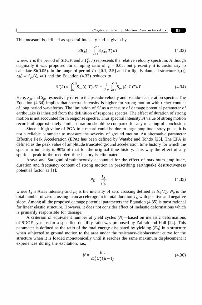
85�������� ��������� ���������� �� ��
This measure is defined as spectral intensity and is given by
SI(z) = S T dTv ( , ).
.z
0 1
2 5z (4.33)
where, T is the period of SDOF, and Sv(z, T) represents the relative velocity spectrum. Althoughoriginally it was proposed for damping ratio of z = 0.02, but presently it is customary tocalculate SI(0.05). In the range of period T Œ [0.1, 2.5] and for lightly damped structure Sv(z,w0) ª Spv(z, w0) and the Equation (4.33) reduces to
SI(z) ª S T dTpv ( , ).
.z
0 1
2 5z = 12 0 1
2 5
pzS T T dTpa ( , )
.
.z (4.34)
Here, Spv and Spa respectively refer to the pseudo-velocity and pseudo-acceleration spectra. TheEquation (4.34) implies that spectral intensity is higher for strong motion with richer contentof long period waveforms. The limitation of SI as a measure of damage potential parameter ofearthquake is inherited from the definition of response spectra. The effect of duration of strongmotion is not accounted for in response spectra. Thus spectral intensity SI value of strong motionrecords of approximately similar duration should be compared for any meaningful conclusion.
Since a high value of PGA in a record could be due to large amplitude stray pulse, it isnot a reliable parameter to measure the severity of ground motion. An alternative parameterEffective Peak Acceleration (EPA) has been defined by Watabe and Tohdo [23]. The EPA isdefined as the peak value of amplitude truncated ground acceleration time history for which thespectrum intensity is 90% of that for the original time history. This way the effect of anyspurious peak in the recorded time history is eliminated.
Araya and Saragoni simultaneously accounted for the effect of maximum amplitude,duration and frequency content of strong motion in prescribing earthquake destructivenesspotential factor as [1]:
PD = IA
m02 (4.35)
where IA is Arias intensity and m0 is the intensity of zero crossing defined as N0 /TD. N0 is thetotal number of zero crossing in an accelerogram in total duration TD with positive and negativeslope. Among all the proposed damage potential parameters the Equation (4.35) is most rationalfor linear elastic structure. However, it does not consider effect of inelastic deformations whichis primarily responsible for damage.
A criterion of equivalent number of yield cycles (N)—based on inelastic deformationsof SDOF systems for a specified ductility ratio was proposed by Zahrah and Hall [24]. Thisparameter is defined as the ratio of the total energy dissipated by yielding (EH) in a structurewhen subjected to ground motion to the area under the resistance-displacement curve for thestructure when it is loaded monotonically until it reaches the same maximum displacement itexperiences during the excitation, i.e.,
N = E
UH
Yw m02 2 1( )-
(4.36)
����������� ������� �������������86
where, wn denotes the natural frequency of the SDOF structure, UY represents the yielddeformation, and m is the specified ductility. The smallest value N can have is 1; in this case,the structure yields only in one direction and reaches its maximum displacement.
SUMMARY
A discussion of various issues involved in the engineering interpretation of strong motiondata is presented. Starting with the explanation of basic terminology used in strong motionseismology the reader is guided through the different forms of characterization of groundmotions. The chapter concludes with a discussion of the various parameters used to quantify thedamage potential of the earthquake ground motion recorded at a site. This will help indeveloping an understanding about the ground motion characterization and the parameters usedto indicate the severity of the motion at a site.
REFERENCES
[1] Araya, R. and Saragoni, G.R., “Earthquake Accelerogram Destructiveness PotentialFactor”, In Proceedings of the Eighth World Conference on Earthquake Engineering,San Francisco, California, U.S.A., pp. II: 835–842, Prentice Hall Inc., New Jersey,1984.
[2] Arias, A., “A Measure of Earthquake Intensity”. In Seismic Design for Nuclear PowerPlants, R.J. Hansen, (Ed.), pp. 438–469. MIT Press, Cambridge, Massachusetts,1970.
[3] Bendat J.S. and Piersol A.G., Random Data, 2nd ed., John Wiley and Sons, 1986.[4] Hao, H., Oliviera, C.S., and Penzien, J., “Multiple-Station Ground Motion Processing
and Simulation Based on SMART-1 Array Data”, Nuclear Engineering and Design,111: 293–310, 1989.
[5] Harichandran, R.S. and Vanmarcke, E.H., “Stochastic Variation of Earthquake GroundMotion in Space and Time”, Journal of Engineering Mechanics, ASCE, 112: 154–174,1986.
[6] Housner, G.W., “Calculating the Response of an Oscillator to Arbitrary GroundMotion”, Bulletin of the Seismological Society of America, 31: 143–149, 1941.
[7] Housner, G.W., “Characteristics of Strong Motion Earthquakes”, Bulletin of theSeismological Society of America, 37(1): 19–31, 1947.
[8] Housner, G.W., “Spectrum Intensities of Strong Motion Earthquakes”, In Proceedingsof the Symposium of Earthquake and Blast Effects on Structures, EarthquakeEngineering Research Institute, Los Angeles, California, pp. 21–36, 1952.
[9] Housner, G.W., “Measures of Severity of Earthquake Ground Shaking”. In Procedingsof the US National Conference on Earthquake Engineering, Earthquake EngineeringResearch Institute, Ann Arbor, Michigan, pp. 25–33, 1975.
[10] Hudson, D.E., “Response Spectrum Techniques in Engineering Seismology”, InProceedings of the First World Conference on Earthquake Engineering, EarthquakeEngineering Research Institute, Los Angeles, California, Vol. 4, pp. 1–12, 1956.
87�������� ��������� ���������� �� ��
[11] Hudson, D.E., “Some Problems in the Application of Spectrum Technique to StrongMotion Earthquake Analysis”, Bulletin of the Seismological Society of America, 52(2):417–430, (1962).
[12] Kiureghian, A. Der, “A Coherency Model for Spatially Varrying Ground Motions”.Earthquake Engineering and Structural Dynamics, 25: 99–111, 1996.
[13] Kubo, T. and Penzien, J., “Analysis of Three-dimensional Strong Ground MotionsAlong Principal Axes, San Fernando Earthquake”, Earthquake Engineering andStructural Dynamics, 7: 265–278, 1979.
[14] Luco, J.E. and Wong, H.L., “Response of a Rigid Foundation to a Spatially RandomGround Motion”, Earthquake Engineering and Structural Dynamics, 14(6): 891–908,1986.
[15] Nigam, N.C., “Phase Properties of a Class of Random Processes”, EarthquakeEngineering and Structural Dynamics, 10: 711–717, 1982.
[16] Ohsaki, Y., “On the Significance of Phase Content in Earthquake Ground Motions”,Earthquake Engineering and Structural Dynamics, 7: 427–439, 1979.
[17] Penzien, J. and Watabe, M., “Characteristics of 3-dimensional Earthquake GroundMotions”, Earthquake Engineering and Structural Dynamics, 3: 365–373, 1975.
[18] Shrikhande, M., Das, J.D., Bansal, M.K., Kumar, A., Basu, S., and Chandra, B.,“Analysis of Strong Motion Records from Dharmsala Earthquake of April 26, 1986”,In Proceedings of the Eleventh Symposium on Earthquake Engineering, Department ofEarthquake Engineering, University of Roorkee, India, Dec. 17–19, pp. 281–285,1998.
[19] Shrikhande, M., Das, J.D., Bansal, M.K., Kumar, A., Basu, S., and Chandra, B.,“Strong Motion Charactertistics of Uttarkashi Earthquake of October 20, 1991 and itsEngineering Significance”, In Research Highlights in Earth System Science; Volume 2:Seismicity, O.P. Varma, (Ed.), Indian Geological Congress, Roorkee, India, pp. 337–342, 2001.
[20] Shrikhande, M. and Gupta, V.K., “Synthesizing Ensembles of Spatially CorrelatedAccelerograms”, Journal of Engineering Mechanics, ASCE, 124(11): 1185–1192,1998.
[21] Shrikhande, M. and Gupta, V.K., “On the Characterization of the Phase Spectrum forStrong Motion Synthesis, Journal of Earthquake Engineering, 5(4): 465–482, 2001.
[22] Trifunac, M.D. and Brady, A.G., “A Study on the Duration of Strong EarthquakeGround Motion”, Bulletin of the Seismological Society of America, 65: 581–626, 1975.
[23] Watabe, M. and Tohdo, M., “Analyses on Various Parameters for the Simulation ofThree-dimensional Earthquake Ground Motions”, In Transaction of the 5th InternationalConference on Structural Mechanics in Reactor Technology, 13–17 August 1979,Number K1/1 in K(a), pp. 1–11, Berlin, Germany, 1979.
[24] Zahrah, T.F. and Hall, W.J., “Earthquake Energy Absorption in SDOF Structures”,Journal of Structural Engineering, ASCE, 110(8): 1757–1772, 1984.
[25] Zerva, A. and Shinozuka, M., “Stochastic Differential Ground Motion”, StructuralSafety, 10: 129–143, 1991.
����������� ������� �������������88
88
Evaluation of SeismicDesign Parameters
��������
5.1 INTRODUCTION
Most of the earthquake occurrences are concentrated in narrow belts along plate boundaries.These earthquakes are known as interplate earthquakes. The earthquakes occurring within aplate are known as intraplate earthquakes. The origins of intraplate earthquakes are stillpoorly understood. Tectonic earthquakes are generated by the process of faulting. Suddendeformation of rock causes earthquake. Earthquake originates at depth (focus) and thus theoryof earthquake occurrence has inherent uncertainties because of its development from theinference on the rocks at the surface. A fault is a fracture or a zone of fractures along whichrocks on opposite side have been displaced relative to each other. The manifestation of fault isthe differential movement parallel to the surface of fracture. The plate boundaries are the mainfaults (sources). There also exist some intraplate faults in Indian region. These faults are in astate of stress due to natural forces acting on them. The very rapid release of this state of stressgenerates earthquake motion. This release produces seismic waves that cause shaking of theground. The structures supported on the ground are subjected to this shaking and as a result,experience deformations (stresses), that must be accounted for in earthquake resistant design.Thus understanding of earthquake process and its effect on ground motion is needed forevaluation of seismic design parameters.
5.2 TYPES OF EARTHQUAKES
The earthquakes can be classified into three categories according to its depth of focus. These are:
(i) Shallow focus earthquakes are earthquakes with depth of focus < 70 km. Nearly 80%of total earthquakes are shallow focus earthquakes. These types of earthquakes are ofgreater concern for earthquake resistant design.
(ii) Intermediate focus earthquakes are earthquakes with depth Π[70, 30] km.(iii) Deep focus earthquakes are earthquakes having focal depth > 300 km.
89�������� ������� ����� �� ��� ����������
5.2.1 Intensity
Intensity is a qualitative measure of the strength of an earthquake. It gives a gradation ofstrength of earthquake using observed damage to structures and/or ground and reaction ofhumans to the earthquake shaking. An earthquake has many intensities, the highest near themaximum fault displacement and progressively to lower grade at further away. Since themeasure is not instrumental, intensity can be assigned to historical earthquakes also. The popularintensity scale is the Modified Mercalli (MMI) scale with twelve gradation denoted by Romannumerals from I to XII. Another intensity scale developed for central and eastern Europeanstates is known as Medvedev-Sponheuer-Karnik (MSK) intensity scale. The twelve gradationMSK scale differs with MMI in details only. Like many other countries, IS 1893 (Part 1), theIndian Standard: 2002, also refers to the MSK scale [14]. An isoseismal map shows intensitiesof a past earthquake in a contoured form of line of equal intensities. Note that the defined scaleis subjective in nature and depend on social and prevailing construction practices. Revision ofintensity scale from time to time is made so that gradations of intensity as per currentconstruction practices are made.
5.2.2 Magnitude
The magnitude is a quantitative or absolute measure of the size of an earthquake. It can becorrelated to the amount of wave energy released at the source of an earthquake. The elasticwave energy is that portion of total strain energy stored in lithospheric rock that is not consumedas mechanical work (e.g. through faulting) during an earthquake. There are various magnitudescales in use. These scales differ from each other because those are derived from measuringdifferent wave components of an earthquake. Richter [25] defined magnitude of local earthquakein southern California for shallow earthquake having epicentral distance D < 600 km. Local(Richter) magnitude (ML) is logarithm to the base 10 of the maximum seismic wave (velocity)amplitude in microns (10–3 mm) recorded on Wood-Anderson seismograph (having period 0.8s, nearly critical damping and magnification 2800) at a distance (D) 100 km from the epicentreof earthquake. Richter magnitude can be scaled for any seismograph of about 1 s period usinginstrumental amplification corrected amplitude of ground motion. Later other scales weredefined for larger and/or distant earthquakes (D > 600 km). Surface wave (S-wave) magnitude(MS) is defined on the basis of the amplitude of surface (Rayleigh) wave of period about 20 sand 80 km wavelength. MS is valid for an aperture D > 15° (approximately 1,650 km distance).The amplitude of compressional and dilatational wave (P-wave) through the earth is notdependent on focal depth. The body wave magnitude (mb) is defined as the maximum amplitudeof P-wavegroup on vertical component seismograph of period about 1 s and less than 10 kmwavelength. This scale is routinely used to describe size of an earthquake at present. Both MS
and mb are determined using maximum trace amplitude and epicentral distances. The size ofsmaller earthquake (micro-earthquake) and near earthquake (distance D < 200 km) is oftenreported as duration magnitude (MD). This scale is based on signal duration (length ofseismograph trace). However, the definition of signal duration is not unique and subjective innature. Maruyama [16] and Burridge and Knopoff [6] among others established the point forceequivalence of fault slip (dislocation) as a double couple. The total moment of this slip isa function of time and is given by M0 = GAs, where G is the modulus of rigidity (taken as
����������� ������� �������������90
3 ¥ 104 MPa for crust and 7 ¥ 104 MPa for mantle in most of the seismic moment calculation),A is the surface area in m2 of ruptured fault and s is the average slip in m across fault. The valueof this moment as time t Æ • is known as the seismic moment. However, only geodetic datacan provide M0 as t Æ •. Further, estimate of M0 is also made from low frequency end of theseismic spectrum (period much larger than 20 s). This far-field seismic parameter is a directmeasure of the extent of faulting and is used for comparison with near-field geodetic andgeological measurements. It may also be noted that surface wave, magnitude MS is an energymeasure and is determined by seismic wave amplitude at a period approximately in the rangeof 18 s to 22 s. The moment magnitude MW as defined by Hanks and Kanamori [11] is givenby,
MW = 2/3 log M0 – 6.7 (5.1)
MW is intrinsically related to seismic moment M0 (Nm). For values at about 6.5 the mb and MSscales coincide. The small earthquakes (< 6.5) are better represented by mb scale and MS scaleunderestimates the same. The magnitude scales (ML, mb and MS) saturate at some upper bound.ML and mb saturate at about 6.5 and 7 respectively. Upper bound of MS is about 8.5. Since, ML,mb and MS are determined from seismic wave of particular period and wavelength that is muchshorter than the earthquake source size of great earthquakes (magnitude eight or larger). TheMW scale adequately measures the size of the source since the scale is independent of particularwave type.
5.3 FAULT RUPTURE PARAMETERS
Tocher [29], Slemmons [28] and Wells and Coppersmith [32] among others studied the corre-lations of fault rupture parameters (e.g. length and displacement) to assess the future earthquakepotential in a region. Based on 216 worldwide past earthquake Wells and Coppersmith gaverelationship between moment magnitude MW and fault rupture parameters. For all styles offaulting, some of the relations are
MW = 1.16 log(L) + 5.08 ± 0.28; log(L) = 0.69 MW – 3.22 ± 0.22
MW = 2.25 log(W) + 4.06 ± 0.41; log(W) = 0.32 MW – 1.01 ± 0.15 (5.2)
MW = 0.98 log(A) + 4.07 ± 0.24; log(A) = 0.91 MW – 3.49 ± 0.24
where, L, W and A are surface rupture length (km), down-dip rupture width (km) and rupturearea (km2) respectively. Similar relationships between moment magnitude MW and displacementare also reported. These are,
MW = 0.74 log(Dm) + 6.69 ± 0.40; log(Dm) = 0.82 MW – 5.46 ± 0.42
MW = 0.82 log(Da) + 6.93 ± 0.39; log(Da) = 0.69 MW – 4.80 ± 0.36 (5.3)
where, Dm is maximum surface displacement (m) and Da is average surface displacement (m).The maximum surface displacement provides the largest slip at a point along a rupture andaverage surface displacement gives the mean displacement along the length of rupture. They alsopresented relations for different styles of faulting but concluded that difference is insignificant.
91�������� ������� ����� �� ��� ����������
Further conclusions are,
(i) L is equal to 75% of the subsurface rupture length,(ii) the average surface displacement per event is about 50% of the maximum surface
displacement per event, and(iii) the average subsurface displacement on the fault plane is bounded by the average
surface displacement and the maximum surface displacement.
5.4 EARTHQUAKE GROUND MOTIONCHARACTERISTICS
The earthquake ground motion of sufficient strength that affect human and their environment(strong ground motion) are of interest for earthquake resistant design. The strong motions aremeasured by accelerographs and its record is time history of acceleration (accelerogram). Thetemporal evolution of an accelerogram is composed of three parts viz. rise, strong motion anddecay. It is composed of non-periodic sequences of acceleration pulses of various durations.Thus not only peak of amplitude but also frequency content of record is necessary to characterizeaccelerogram. The characteristic of strong motion in the vicinity of causative fault (near field)is strongly dependent on the nature of faulting. The motion depends on source parameters suchas fault shape, its area, maximum fault dislocation, and complexity of slipping process, stressdrop, and the distance of fault plane from ground surface. The elastic properties of the materialthrough which the generated seismic waves travel also influence the strong motion. The effectof ground shaking is mostly dependent on duration of strong motion part. The earthquakeground acceleration is generally broadband in frequency composition. It is rich in highfrequencies in the near fields. The high frequency components attenuate faster than the lowfrequency components, therefore the contribution of high frequency components is reduced inthe accelerograms recorded at large distances from the fault. Further, the amplitude of groundacceleration decreases with increasing distance from the causative faults in general. Moreover,in general the vertical component of the ground acceleration is richer in high frequencies thanthe two horizontal components.
5.4.1 Amplitude Properties
Horizontal component of acceleration is primarily used to report ground motion as structuresare designed for vertical loads and margin of safety in the vertical direction are usually adequatefor earthquake induced vertical load. The common amplitude measure of a ground motion isthe largest horizontal acceleration and known as horizontal peak ground acceleration (PGA).The largest dynamic forces induced in very stiff structures are closely related PGA. Historicearthquakes can have only intensity information. Various authors have attempted to proposerelation between MMI and PGA. Ambraseys [2] proposed such a relation using southernEuropean earthquakes as log a = 0.36 IMM – 0.16. Later, using 187 records of 57 western USAearthquake with MMI between III and X, Trifunac and Brady [30] gave a relation as log a =0.30 IMM + 0.014. Murphy and O’Brien [20], using worldwide data of 1465 records having more
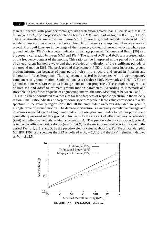
����������� ������� �������������92
than 900 records with peak horizontal ground acceleration greater than 10 cm/s2 and MMI inthe range I to X, also proposed correlation between MMI and PGA as log a = 0.25 IMM + 0.25.These relationships are shown in Figure 5.1. Horizontal ground velocity is derived fromaccelerogram and have less contribution from high frequency component than accelerationrecord. Most buildings are in the range of the frequency content of ground velocity. Thus peakground velocity (PGV) v is a better indicator of damage potential. Trifunac and Brady [30] alsoproposed a correlation between MMI and PGV. The ratio of PGV and PGA is a representationof the frequency content of the motion. This ratio can be interpreted as the period of vibrationof an equivalent harmonic wave and thus provides an indication of the significant periods ofthe ground motion [26]. The peak ground displacement PGD d is the most inaccurate groundmotion information because of long period noise in the record and errors in filtering andintegration of accelerograms. The displacement record is associated with lower frequencycomponent of ground motion. Statistical analysis (Mohraz [19], Newmark and Hall [23]) onground motion was carried to estimate ground motion properties. These studies suggest useof both v/a and ad/v2 to estimate ground motion parameters. According to Newmark andRosenbleuth [24] for earthquake of engineering interest the ratio ad/v2 ranges between 5 and 15.This ratio can be considered as a measure for the sharpness of response spectrum in the velocityregion. Small ratio indicates a sharp response spectrum while a large value corresponds to a flatspectrum in the velocity region. Note that all the amplitude parameters discussed are peak ina single cycle of ground motion. The damage in structure is essentially cumulative damage andit requires repeated cycle of high amplitudes. The use peak amplitudes for design purpose aregenerally questioned on this ground. This leads to the concept of effective peak acceleration(EPA) and effective velocity related acceleration Av. The pseudo velocity corresponding to Av
is termed as effective peak velocity (EPV). Let Sa be the mean pseudo-acceleration value in theperiod T Π[0.1, 0.5] s and Sv be the pseudo-velocity value at about 1 s. For 5% critical dampingNEHRP, 1997 [21] specifies the EPA is defined as Aa = Sa/2.5 and the EPV is similarly definedas Vv = Sv /2.5.
0.01VIV VI VII VIII IX X
Modified Mercalli Intensity (MMI)
0.1
1
10Ambraseys (1974)
Trifunac and Brady (1975)
Murphy and O’Brien (1977)
Acc
eler
atio
n(g
)
FIGURE 5.1 PGA–MMI relations.
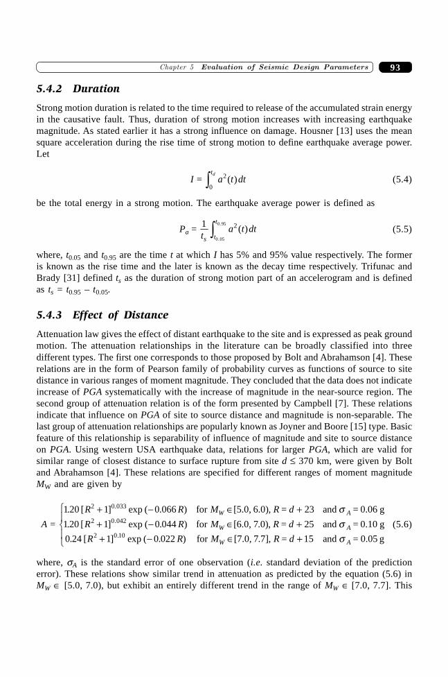
93�������� ������� ����� �� ��� ����������
5.4.2 Duration
Strong motion duration is related to the time required to release of the accumulated strain energyin the causative fault. Thus, duration of strong motion increases with increasing earthquakemagnitude. As stated earlier it has a strong influence on damage. Housner [13] uses the meansquare acceleration during the rise time of strong motion to define earthquake average power.Let
I = a t dttd 2
0( )z (5.4)
be the total energy in a strong motion. The earthquake average power is defined as
Pa = 1 2
0 05
0 95
ta t dt
s t
t( )
.
.z (5.5)
where, t0.05 and t0.95 are the time t at which I has 5% and 95% value respectively. The formeris known as the rise time and the later is known as the decay time respectively. Trifunac andBrady [31] defined ts as the duration of strong motion part of an accelerogram and is definedas ts = t0.95 – t0.05.
5.4.3 Effect of Distance
Attenuation law gives the effect of distant earthquake to the site and is expressed as peak groundmotion. The attenuation relationships in the literature can be broadly classified into threedifferent types. The first one corresponds to those proposed by Bolt and Abrahamson [4]. Theserelations are in the form of Pearson family of probability curves as functions of source to sitedistance in various ranges of moment magnitude. They concluded that the data does not indicateincrease of PGA systematically with the increase of magnitude in the near-source region. Thesecond group of attenuation relation is of the form presented by Campbell [7]. These relationsindicate that influence on PGA of site to source distance and magnitude is non-separable. Thelast group of attenuation relationships are popularly known as Joyner and Boore [15] type. Basicfeature of this relationship is separability of influence of magnitude and site to source distanceon PGA. Using western USA earthquake data, relations for larger PGA, which are valid forsimilar range of closest distance to surface rupture from site d £ 370 km, were given by Boltand Abrahamson [4]. These relations are specified for different ranges of moment magnitudeMW and are given by
A =
1 20 1 0 066 23
1 20 1 0 044 7 25
0 24 1 0 022 7 15
2 0 033
2 0 042
2 0 10
. [ ] exp ( . )
. [ ] exp ( . )
. [ ] exp ( . )
.
.
.
R R M R d
R R M R d
R R M R d
W A
W A
W A
+ - Π++ - Π++ - Π+
RS|
T|
for [5.0, 6.0), = and = 0.06 g
for [6.0, .0), = and = 0.10 g
for [7.0, .7], = and = 0.05 g
sss
(5.6)
where, sA is the standard error of one observation (i.e. standard deviation of the predictionerror). These relations show similar trend in attenuation as predicted by the equation (5.6) inMW Π[5.0, 7.0), but exhibit an entirely different trend in the range of MW Π[7.0, 7.7]. This
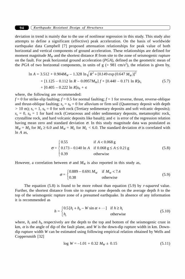
����������� ������� �������������94
deviation in trend is mainly due to the use of nonlinear regression in this study. This study alsoattempts to define a significant (effective) peak acceleration. On the basis of worldwideearthquake data Campbell [7] proposed attenuation relationships for peak value of bothhorizontal and vertical components of ground acceleration. These relationships are defined formoment magnitude MW and the shortest distance R from site to the zone of seismogenic ruptureon the fault. For peak horizontal ground acceleration (PGA), defined as the geometric mean ofthe PGA of two horizontal components, in units of g (= 981 cm/s2), the relation is given by,
ln A = 3.512 + 0.904MW – 1.328 ln R MW2 20 149 0 647+ [ . exp ( . )]
+ [1.125 – 0.112 ln R – 0.0957MW] f + [0.440 – 0.171 ln R]ss (5.7)
+ [0.405 – 0.222 ln R]sh + Œ
where, the following are recommended:f = 0 for strike-slip faulting; f = 0.5 for normal faulting; f = 1 for reverse, thrust, reverse-obliqueand thrust-oblique faulting; ss = sh = 0 for alluvium or firm soil (Quaternary deposit with depth> 10 m); ss = 1, sh = 0 for soft rock (Tertiary sedimentary deposits and soft volcanic deposits);ss = 0, sh = 1 for hard rock (Cretaceous and older sedimentary deposits, metamorphic rock,crystalline rock, and hard volcanic deposits like basalt); and Œ is error of the regression relationhaving mean zero and standard deviation s. In this study magnitude data was postulated asMW = MS for MS ≥ 6.0 and MW = ML for ML < 6.0. The standard deviation s is correlated withln A as,
s =
0 55 0 068
0 173 0 140 0 21
0 39
. .
. . ln .
.
if g
if 0.068 g g
otherwise
A
A A
<- £ £
RS|
T|(5.8)
However, a correlation between s and MW is also reported in this study as,
s = 0 889 0 691 7 4
0 38
. . .
.
- <RSTM MW Wif
otherwise(5.9)
The equation (5.8) is found to be more robust than equation (5.9) by r-squared value.Further, the shortest distance from site to rupture zone depends on the average depth h to thetop of the seismogenic rupture zone of a presumed earthquake. In absence of any informationit is recommended as
h = 0 5. [ sin ]h h W h h
ht b t
t
+ - + ≥RSTa � if
otherwise(5.10)
where, ht and hb respectively are the depth to the top and bottom of the seismogenic crust inkm, a is the angle of dip of the fault plane, and W is the down-dip rupture width in km. Down-dip rupture width W can be estimated using following empirical relation obtained by Wells andCoppersmith [32]
log W = –1.01 + 0.32 MW ± 0.15 (5.11)
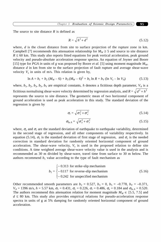
95�������� ������� ����� �� ��� ����������
The source to site distance R is defined as
R = h d2 2+ (5.12)
where, d is the closet distance from site to surface projection of the rupture zone in km.Campbell [7] recommends this attenuation relationship for MW ≥ 5 and source to site distanceR £ 60 km. This study also reports fitted equations for peak vertical acceleration, peak groundvelocity and pseudo-absolute acceleration response spectra. An equation of Joyner and Boore[15] type for PGA in units of g was proposed by Boore et al. [5] using moment magnitude MW,distance d in km from site to the surface projection of fault rupture and average shear-wavevelocity Vs in units of m/s. This relation is given by,
ln A = b1 + b2 (MW – 6) + b3 (MW – 6)2 + b5 ln R + bV (ln Vs – ln VA) (5.13)
where, b1, b2, b3, b5, bV are empirical constants, h denotes a fictitious depth parameter, VA is a
fictitious normalising shear-wave velocity determined by regression analysis, and R = d h2 2+represents the source to site distance. The geometric mean of two horizontal component ofground acceleration is used as peak acceleration in this study. The standard deviation of theregression is given by
sr = s s12 2+ c (5.14)
sln A = s se r2 2+ (5.15)
where, se and sr are the standard deviation of earthquake to earthquake variability, determinedin the second stage of regression, and all other components of variability respectively. Inequation (5.14), s1 is the standard deviation of first stage of regression, and sc is the neededcorrection in standard deviation for randomly oriented horizontal component of groundacceleration. The shear-wave velocity, Vs is used in the proposed relation to define siteconditions. A time weighted average shear-wave velocity value is used in the analysis and isrecommended as 30 m divided by shear-wave, travel time from surface to 30 m below. Theauthors recommend b1 value according to the type of fault mechanism as
b1 =
---
RS|
T|
0 313
0 117
0 242
.
.
.
for strike-slip mechanism
for reverse-slip mechanism
for unspecified mechanism
(5.16)
Other recommended smooth parameters are b2 = 0.527, b3 = 0, b5 = –0.778, bV = –0.371,VA = 1396 m/s, h = 5.57 km, s1 = 0.431, sc = 0.226, sr = 0.486, se = 0.184 and sln A = 0.520.The authors recommend this attenuation relation for moment magnitude MW Œ [5.5, 7.5] andd £ 80 km. This study also provides empirical relations for pseudo-acceleration responsespectra in units of g at 5% damping for randomly oriented horizontal component of groundacceleration.
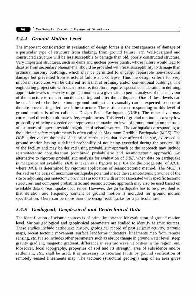
����������� ������� �������������96
5.4.4 Ground Motion Level
The important consideration in evaluation of design forces is the consequences of damage ofa particular type of structure from shaking, from ground failure, etc. Well-designed andconstructed structure will be less susceptible to damage than old, poorly constructed structure.Very important structures, such as dams and nuclear power plants, whose failure would lead todisaster from secondary phenomena, should be provided with least susceptibility to damage thanordinary masonry buildings, which may be permitted to undergo repairable non-structuraldamage but prevented from structural failure and collapse. Thus the design criteria for veryimportant structures will be different from that of ordinary and/or conventional buildings. Theengineering project site with such structure, therefore, requires special consideration in definingappropriate levels of severity of ground motion at a given site to permit analysis of the behaviourof the structure to remain functional during and after the earthquake. One of these levels canbe considered to be the maximum ground motion that reasonably can be expected to occur atthe site once during lifetime of the structure. The earthquake corresponding to this level ofground motion is often called as Design Basis Earthquake (DBE). The other level maycorrespond directly to ultimate safety requirements. This level of ground motion has a very lowprobability of being exceeded and represents the maximum level of ground motion on the basisof estimates of upper threshold magnitude of seismic sources. The earthquake corresponding tothe ultimate safety requirements is often called as Maximum Credible Earthquake (MCE). TheDBE is derived on the basis of historical earthquakes that have affected the site, expressed asground motion having a defined probability of not being exceeded during the service lifeof the facility and may be derived using probabilistic approach or the approach may includeseismotectonic consideration (combined probabilistic and seismotectonic approach). Analternative to rigorous probabilistic analysis for evaluation of DBE, when data on earthquakeis meagre or not available, DBE is taken as a fraction (e.g. 0.4 for the bridge site) of MCE,where MCE is determined by rigorous application of seismotectonic method. The MCE isderived on the basis of maximum earthquake potential inside the seismotectonic province of thesite or adjoining seismotectonic provinces associated with or not associated with specific tectonicstructures, and combined probabilistic and seismotectonic approach may also be used based onavailable data on earthquake occurrence. However, design earthquake has to be prescribed sothat duration and frequency content of ground motion is included for ground motionspecification. There can be more than one design earthquake for a particular site.
5.4.5 Geological, Geophysical and Geotechnical Data
The identification of seismic sources is of prime importance for evaluation of ground motionlevel. Various geological and geophysical parameters are studied to identify seismic sources.These studies include earthquake history, geological record of past seismic activity, tectonicmaps, recent tectonic movement, surface landforms indicators, lineaments map from remotesensing, etc. It also includes other parameters such as abrupt change in ground water level, steepgravity gradient, magnetic gradient, difference in seismic wave velocities in the region, etc.Moreover, local topography, properties of soil and its strength, area of subsidence and/orsettlement, etc., shall be used. It is necessary to ascertain faults by ground verification ofremotely sensed lineaments map. The tectonic (structural geology) map of an area gives
97�������� ������� ����� �� ��� ����������
information about the type of rocks to be found and indicates faults in a geographic region. Itis necessary to determine evidence of any motion in recent times. Locations of epicentres of allavailable seismic data (instrumental and historical) in the region are to be plotted to determinepossible trend to indicate active faulting. A fault that does not extend to earth surface andnormally terminates upward at the axial region of convex upward fold (Anticline) is known asblind fault. This fault cannot be examined and is thus associated with very high uncertainties.But this type of fault has a very great effect on level of ground motion estimation and is oftenvery difficult to incorporate in the evaluation. Different faults have different degree of activity.Specific definition of fault activity is given for regulatory purpose. For quantitative assessmentof activity, some time a capable fault is defined as a fault that had surface displacement withinpast 10,000 years (Holocene active). Generally faults originate as small fracture, successiveearthquakes propagate (lengthen) it. If a site does not belong to a very active complex tectoniczone, chances of new fault breaking are almost none for the service life of a structure.
5.5 DETERMINISTIC APPROACH
When the causative fault cannot be identified, it is very difficult to avoid arbitrariness inspecifying MCE. The standard practice is to determine the intensity of the site (from theavailable isoseismal map of the region) from the strongest earthquake that has ever occurredaround the site. Lacking strong motion accelerogram record, it is customary to increase the scalefactor by one for the specification of MCE. Many earthquake intensity-acceleration relationshipsare available in the literature. These data suggest that the median value of the maximum groundvelocity is approximately 20 cm/s for MMI intensity VIII and changes by a factor of 2 for eachunit of change of intensity. The peak acceleration of 0.167 g thus correspond to MMI intensityVIII, since a velocity of 122 cm/s corresponds to a peak acceleration of g. The correlationbetween MMI and peak ground velocity is almost independent of the property of local soil. Therelationship between peak velocity and peak ground acceleration is dependent slightly on localsoil condition. But the MMI is strongly correlated with damage and the damage is dependenton local soil condition. Hence, local soil condition is implicitly taken into account in arrivingat peak ground velocity. When faults exist around the site, the earthquake of maximumconsidered magnitude associated with each fault is determined from past seismic data. However,care should be taken to ascertain the type of magnitude (e.g. body wave magnitude, surface wavemagnitude, local or Richter magnitude, moment magnitude, etc.) in the reported data. From theknown length of faults from tectonic map, it is ascertained that the identified faults, associatedwith highest magnitude, are capable to release that amount of energy. It is customary to increasethese magnitudes by 1/2 for MCE. The epicentres of these earthquakes are assumed to be theclosest point on the faults from the site. The depth of focus of an earthquake gives the depthat which the strains build up in the earth’s crust and/or Upper Mantle resulting in fracturegenerating seismic waves. The rocks in the immediate vicinity of a site are often not strongenough to store the energy for earthquake of magnitude of engineering significance (magnitudegreater or equal to five) in a few km of the upper depth due to weathering and other naturalprocesses. This depth plus half of the idealized down-dip rupture width, W, is taken for the depthof focus of each earthquake in a causative fault if no specific information of fault dip is
����������� ������� �������������98
available. The effect of these distant earthquakes on the faults to the site, expressed as peakground motion (e.g. acceleration, velocity and displacement), is obtained via attenuation law.Various attenuation laws are available in the literature (e.g. [2], [9] etc.). One of them is dueto Esteva and Villaverde [10] and is given by
a = 5600 exp(0.8ML)/(R + 40)2 (5.17)
v = 32 exp(ML)/(R + 25)2 (5.18)
d = (1 + 200R–0.6) v2/a (5.19)
where, a is PGA in gal, v is PGV (cm/s), d is PGD (cm) and R is focal (hypocentral) distance(km). ML is the Richter magnitude and 40 km and 25 km are empirical constants to account forthe volume of lithospheric rock that participates in releasing the stored energy. The above lawsindicate more rapid reduction in value of high frequency component of ground motion.
5.6 PROBABILISTIC APPROACH
Various workers (Cornell [8], Esteva [9], Algermissen and Perkins [1], McGuire [17] and Basu[3], etc.) developed methodology and techniques for the probabilistic estimations of groundmotion. The combined statistical and seismotectonic approach for the evaluation of groundmotion parameter (acceleration, velocity and displacement) at a site involves identification ofseismotectonic province of the site and seismic sources in which future significant earthquakecan originate, determine the rate at which earthquake can occur in different sources, obtain thefrequency distribution of depth of focus and magnitude in various sources, and establish aground motion attenuation to account for the effect of focal distance of earthquake on the site.The analysis is carried out with the assumption that the available data is not exhaustive andcontain error in locations (say 0.1 degree), depth estimates, magnitude etc. The statistical toolavailable for analysis is Bayesian analysis, and can be carried out on the lines of Basu [3] forevaluation of ground acceleration in following steps:
(i) The data are sorted out for different seismic sources.(ii) A modular source of arc length 150 km at the surface of the earthquake with the project
site as its center and of 150 km depth is taken and seismically active faults lying withinmodular source are considered as area sources.
Locations of floating earthquakes (not associated with faults) in the modular source areconsidered temporarily stationary and spatially homogeneous; and occurrence of earthquake isequally likely in the latitude and longitude direction. The focal depth data with assigned valueof 33 km (average depth of Moho) are assumed to be distributed uniformly within 16 to 51 kmfor estimation of focal depth distribution. A mixed truncated lognormal distribution is fitted inthe modular source and area sources. The probability density function of focal depth for h Œ(0, h0] is,
fH(h) = P
h hhi
i ii
i2
22 22
p s n sn s
F[(ln )/ ]exp [ (ln ) /( )]
0=1 -- -Â (5.20)
99�������� ������� ����� �� ��� ����������
where, 0 < P1 < 1, P2 = 1 – P1 and F(◊) is the probability distribution function of N(0, 1). Theestimation of parameters (P1, s1, s2, n) are formulated as minimum Chi-square problem. Themagnitude, ML, of earthquake is independent of rate of occurrences of earthquake. Themagnitude distribution is estimated in two ways in accordance with available data. Theprobability density function corresponding to the bilinear frequency magnitude relation with anupper and lower threshold is given by
fML(m) = K1b exp[(m0 Рm) b + (m1 Рm)lU(m Рm1)], m Π(m0, m2] (5.21)
where, 1/K1 = [l + b – l exp {(m0 – m) b} – b exp {(m0 – m2) b + (m1 – m2) l}]/(l + b), andm0 < m1 < m2. The U(◊) is Heaviside function. It is assumed that m0 = 5 is the lower thresholdmagnitude. The estimation of parameters (l, b, m1, m2) are obtained using minimum Chi-squareestimation method. Physical interpretation of equation (5.21) is that there exist two differentprocesses, one leading to release of energy below magnitude m1, and other above that. A linearrelation can also be used with upper threshold magnitude m2 that takes care of the ultimatestrength against rupture of underlain strata. The parameter, m2 is inferred from historical and/or geological data. Normalisation of linear frequency-magnitude relation with upper and lowerthreshold leads to the probability density function as
fML(m) = K2 b exp [(m0 Рm) b], m Π(m0, m2] (5.22)
where, 1/K2 = 1 – exp [(m0 – m2) b]. The attenuation law correlating peak ground accelerationwith earthquake parameters for a source including the effect of scatter in the past data is assumedto be
y = a exp[bm – c ln (r + d) + q] (5.23)
where, m is the magnitude, r is the focal distance (km), y is the peak ground acceleration (gal)and q is a normal random variable. Esteva and Villaverde [10] have suggested values of a, b,c and d as 5600, 0.8, 2.0 and 40 km, respectively and normal random variable q is of mean 0.04and variance 0.4096. The occurrence of an earthquake is assumed to be in accordance withPoisson process with intensity, mi, for magnitude greater than five. The posterior intensity ofearthquake arrival is estimated through Bayesian statistics and by using past regional (Newmarkand Rosenblueth [24]) seismic data. Under the assumption of mutual statistical independence ofvarious sources at project site, it can be shown that, the probability distribution function ofmaximum acceleration, Ymax, can formally be
Frmax(y) = exp [ ]t P Y yi i
i
n
m >RS|T|
UV|W|
+
Â=1
1
(5.24)
in which mi is the intensity of earthquake arrival in its source, n is the number of faults in themodular source at site, and P[Yi > y] is the probability of exceeding peak acceleration, y, at thesite due to the ith source. From equation (5.24) t-year return period of PGA, y, is obtained as,
t = 11
P Y yii
n
[ ]>RS|T|
UV|W|
+
Â=1
(5.25)
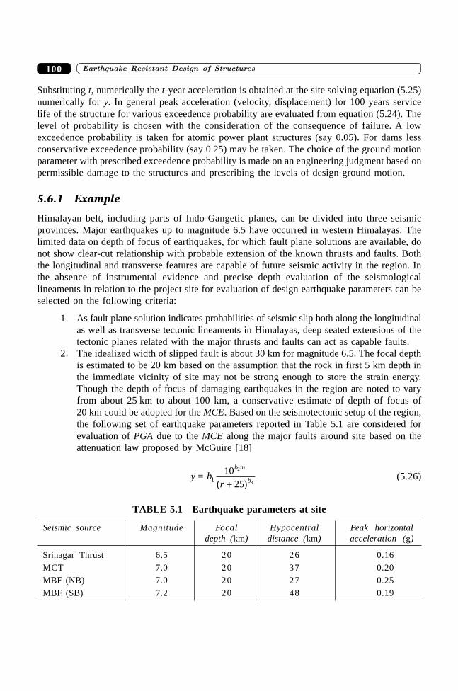
����������� ������� �������������100
Substituting t, numerically the t-year acceleration is obtained at the site solving equation (5.25)numerically for y. In general peak acceleration (velocity, displacement) for 100 years servicelife of the structure for various exceedence probability are evaluated from equation (5.24). Thelevel of probability is chosen with the consideration of the consequence of failure. A lowexceedence probability is taken for atomic power plant structures (say 0.05). For dams lessconservative exceedence probability (say 0.25) may be taken. The choice of the ground motionparameter with prescribed exceedence probability is made on an engineering judgment based onpermissible damage to the structures and prescribing the levels of design ground motion.
5.6.1 Example
Himalayan belt, including parts of Indo-Gangetic planes, can be divided into three seismicprovinces. Major earthquakes up to magnitude 6.5 have occurred in western Himalayas. Thelimited data on depth of focus of earthquakes, for which fault plane solutions are available, donot show clear-cut relationship with probable extension of the known thrusts and faults. Boththe longitudinal and transverse features are capable of future seismic activity in the region. Inthe absence of instrumental evidence and precise depth evaluation of the seismologicallineaments in relation to the project site for evaluation of design earthquake parameters can beselected on the following criteria:
1. As fault plane solution indicates probabilities of seismic slip both along the longitudinalas well as transverse tectonic lineaments in Himalayas, deep seated extensions of thetectonic planes related with the major thrusts and faults can act as capable faults.
2. The idealized width of slipped fault is about 30 km for magnitude 6.5. The focal depthis estimated to be 20 km based on the assumption that the rock in first 5 km depth inthe immediate vicinity of site may not be strong enough to store the strain energy.Though the depth of focus of damaging earthquakes in the region are noted to varyfrom about 25 km to about 100 km, a conservative estimate of depth of focus of20 km could be adopted for the MCE. Based on the seismotectonic setup of the region,the following set of earthquake parameters reported in Table 5.1 are considered forevaluation of PGA due to the MCE along the major faults around site based on theattenuation law proposed by McGuire [18]
y = br
b m
b110
25
2
3( )+(5.26)
TABLE 5.1 Earthquake parameters at site
Seismic source Magnitude Focal Hypocentral Peak horizontaldepth (km) distance (km) acceleration (g)
Srinagar Thrust 6.5 20 26 0.16
MCT 7.0 20 37 0.20
MBF (NB) 7.0 20 27 0.25
MBF (SB) 7.2 20 48 0.19
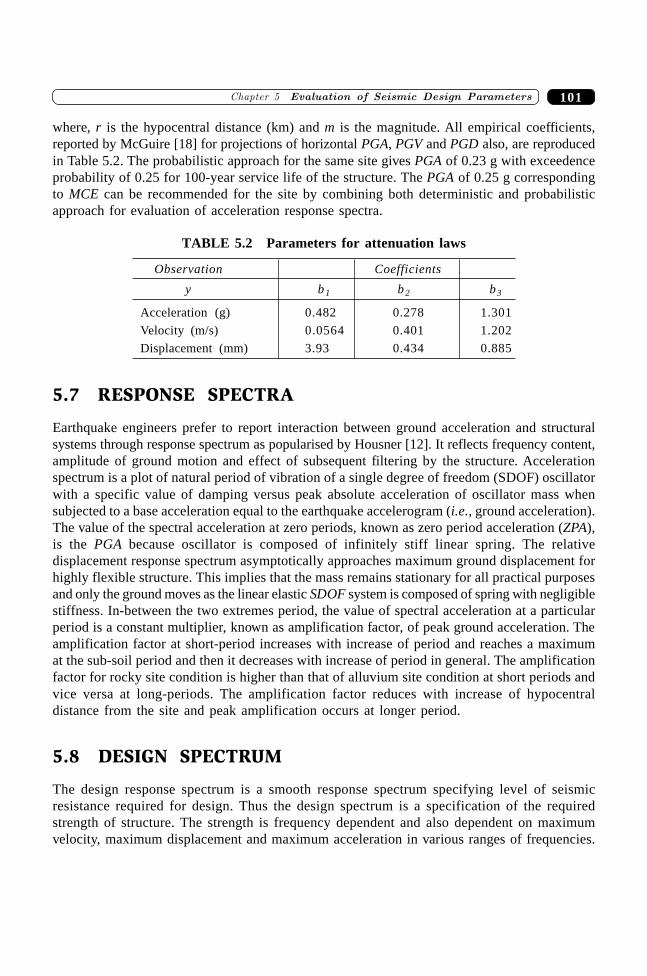
101�������� ������� ����� �� ��� ����������
where, r is the hypocentral distance (km) and m is the magnitude. All empirical coefficients,reported by McGuire [18] for projections of horizontal PGA, PGV and PGD also, are reproducedin Table 5.2. The probabilistic approach for the same site gives PGA of 0.23 g with exceedenceprobability of 0.25 for 100-year service life of the structure. The PGA of 0.25 g correspondingto MCE can be recommended for the site by combining both deterministic and probabilisticapproach for evaluation of acceleration response spectra.
TABLE 5.2 Parameters for attenuation laws
Observation Coefficients
y b1 b2 b3
Acceleration (g) 0.482 0.278 1.301
Velocity (m/s) 0.0564 0.401 1.202
Displacement (mm) 3.93 0.434 0.885
5.7 RESPONSE SPECTRA
Earthquake engineers prefer to report interaction between ground acceleration and structuralsystems through response spectrum as popularised by Housner [12]. It reflects frequency content,amplitude of ground motion and effect of subsequent filtering by the structure. Accelerationspectrum is a plot of natural period of vibration of a single degree of freedom (SDOF) oscillatorwith a specific value of damping versus peak absolute acceleration of oscillator mass whensubjected to a base acceleration equal to the earthquake accelerogram (i.e., ground acceleration).The value of the spectral acceleration at zero periods, known as zero period acceleration (ZPA),is the PGA because oscillator is composed of infinitely stiff linear spring. The relativedisplacement response spectrum asymptotically approaches maximum ground displacement forhighly flexible structure. This implies that the mass remains stationary for all practical purposesand only the ground moves as the linear elastic SDOF system is composed of spring with negligiblestiffness. In-between the two extremes period, the value of spectral acceleration at a particularperiod is a constant multiplier, known as amplification factor, of peak ground acceleration. Theamplification factor at short-period increases with increase of period and reaches a maximumat the sub-soil period and then it decreases with increase of period in general. The amplificationfactor for rocky site condition is higher than that of alluvium site condition at short periods andvice versa at long-periods. The amplification factor reduces with increase of hypocentraldistance from the site and peak amplification occurs at longer period.
5.8 DESIGN SPECTRUM
The design response spectrum is a smooth response spectrum specifying level of seismicresistance required for design. Thus the design spectrum is a specification of the requiredstrength of structure. The strength is frequency dependent and also dependent on maximumvelocity, maximum displacement and maximum acceleration in various ranges of frequencies.
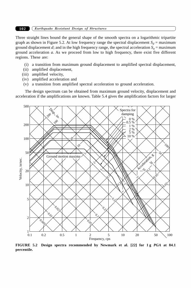
����������� ������� �������������102
Three straight lines bound the general shape of the smooth spectra on a logarithmic tripartitegraph as shown in Figure 5.2. At low frequency range the spectral displacement Sd = maximumground displacement d; and in the high frequency range, the spectral acceleration Sa = maximumground acceleration a. As we proceed from low to high frequency, there exist five differentregions. These are:
(i) a transition from maximum ground displacement to amplified spectral displacement,(ii) amplified displacement,
(iii) amplified velocity,(iv) amplified acceleration and(v) a transition from amplified spectral acceleration to ground acceleration.
The design spectrum can be obtained from maximum ground velocity, displacement andacceleration if the amplifications are known. Table 5.4 gives the amplification factors for larger
500
2
1
5
10
20
50
100
200
0.1 0.2 0.5 1 2 5 10 20 50 100Frequency, cps
Vel
oci
ty,
in/s
ec.
0 %0.5 %
1 %2 %5 %
10 %
Spectra fordamping
Ground motion maxima
Acc
eler
atio
n,g
Disp., in-20
0
20
100
5
10
2
1
0.5
0.2
0.05
0.02
0.1
0.005
0.01
0.02
0.05
0.1
0.2
0.5
1
2
5
10
20
50
100
FIGURE 5.2 Design spectra recommended by Newmark et al. [22] for 1 g PGA at 84.1percentile.
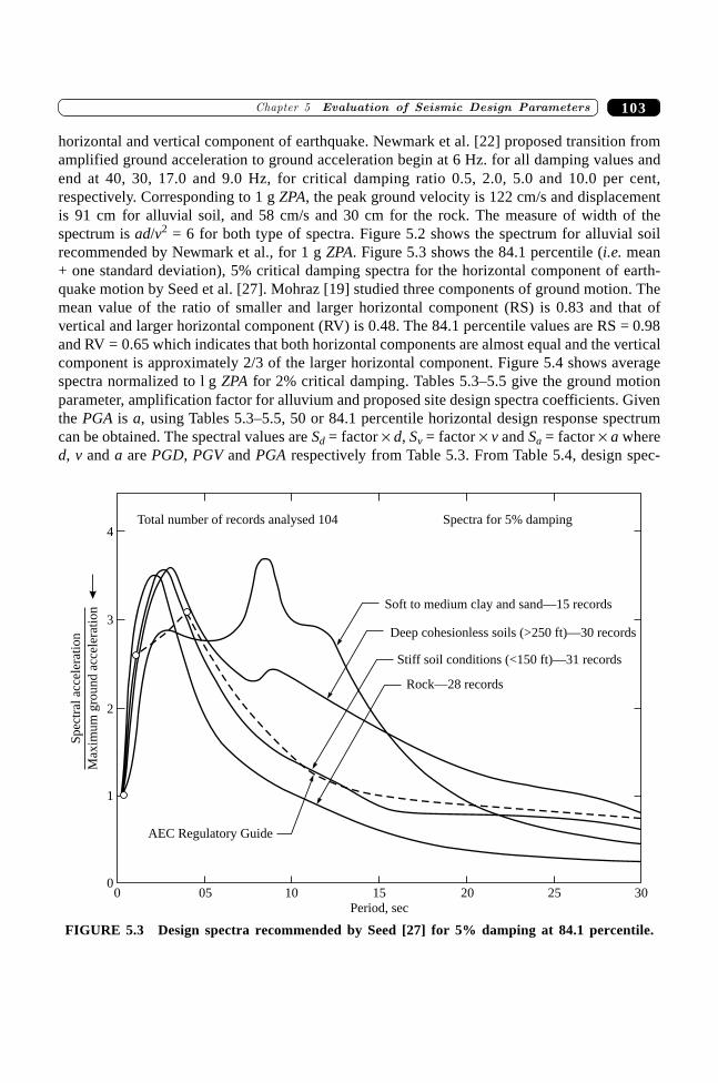
103�������� ������� ����� �� ��� ����������
horizontal and vertical component of earthquake. Newmark et al. [22] proposed transition fromamplified ground acceleration to ground acceleration begin at 6 Hz. for all damping values andend at 40, 30, 17.0 and 9.0 Hz, for critical damping ratio 0.5, 2.0, 5.0 and 10.0 per cent,respectively. Corresponding to 1 g ZPA, the peak ground velocity is 122 cm/s and displacementis 91 cm for alluvial soil, and 58 cm/s and 30 cm for the rock. The measure of width of thespectrum is ad/v2 = 6 for both type of spectra. Figure 5.2 shows the spectrum for alluvial soilrecommended by Newmark et al., for 1 g ZPA. Figure 5.3 shows the 84.1 percentile (i.e. mean+ one standard deviation), 5% critical damping spectra for the horizontal component of earth-quake motion by Seed et al. [27]. Mohraz [19] studied three components of ground motion. Themean value of the ratio of smaller and larger horizontal component (RS) is 0.83 and that ofvertical and larger horizontal component (RV) is 0.48. The 84.1 percentile values are RS = 0.98and RV = 0.65 which indicates that both horizontal components are almost equal and the verticalcomponent is approximately 2/3 of the larger horizontal component. Figure 5.4 shows averagespectra normalized to l g ZPA for 2% critical damping. Tables 5.3–5.5 give the ground motionparameter, amplification factor for alluvium and proposed site design spectra coefficients. Giventhe PGA is a, using Tables 5.3–5.5, 50 or 84.1 percentile horizontal design response spectrumcan be obtained. The spectral values are Sd = factor ¥ d, Sv = factor ¥ v and Sa = factor ¥ a whered, v and a are PGD, PGV and PGA respectively from Table 5.3. From Table 5.4, design spec-
Deep cohesionless soils (>250 ft)—30 records
00
05 10 15 20 25 30
Period, sec
1
2
3
4
Spec
tral
acce
lera
tion
Max
imum
gro
und
acce
lera
tion
Total number of records analysed 104 Spectra for 5% damping
AEC Regulatory Guide
Soft to medium clay and sand—15 records
Stiff soil conditions (<150 ft)—31 records
Rock—28 records
FIGURE 5.3 Design spectra recommended by Seed [27] for 5% damping at 84.1 percentile.
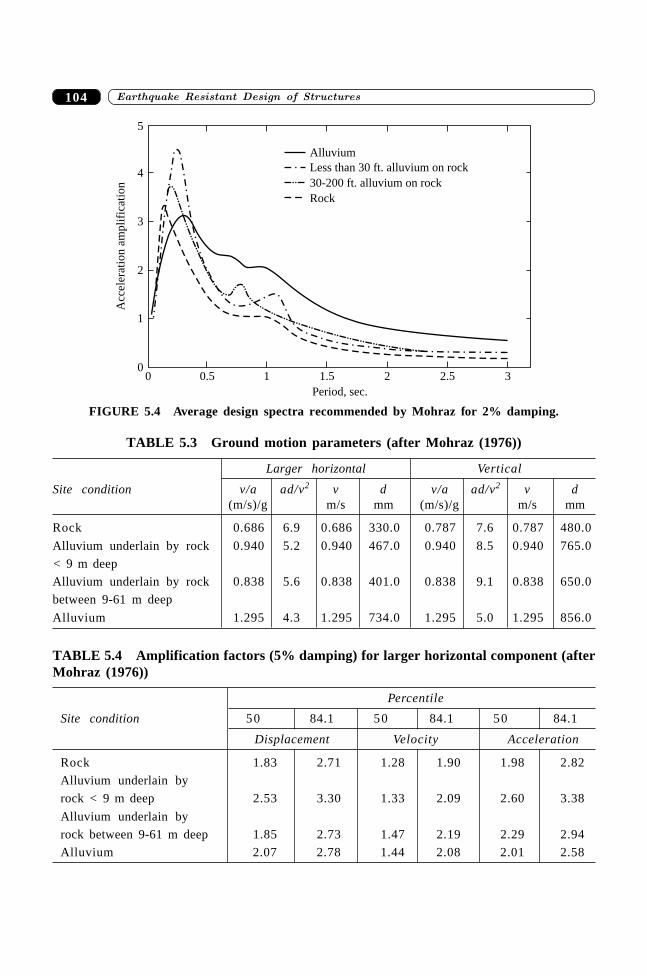
����������� ������� �������������104
Alluvium
00
0.5 1 1.5 2 2.5 3
1
2
3
4
5
Period, sec.
Acc
eler
atio
nam
pli
fica
tion
Less than 30 ft. alluvium on rock
30-200 ft. alluvium on rock
Rock
FIGURE 5.4 Average design spectra recommended by Mohraz for 2% damping.
TABLE 5.3 Ground motion parameters (after Mohraz (1976))
Larger horizontal Vertical
Site condition v/a ad/v2 v d v/a ad/v2 v d(m/s)/g m/s mm (m/s)/g m/s mm
Rock 0.686 6.9 0.686 330.0 0.787 7.6 0.787 480.0
Alluvium underlain by rock 0.940 5.2 0.940 467.0 0.940 8.5 0.940 765.0
< 9 m deep
Alluvium underlain by rock 0.838 5.6 0.838 401.0 0.838 9.1 0.838 650.0
between 9-61 m deep
Alluvium 1.295 4.3 1.295 734.0 1.295 5.0 1.295 856.0
TABLE 5.4 Amplification factors (5% damping) for larger horizontal component (afterMohraz (1976))
Percentile
Site condition 50 84.1 50 84.1 50 84.1
Displacement Velocity Acceleration
Rock 1.83 2.71 1.28 1.90 1.98 2.82
Alluvium underlain by
rock < 9 m deep 2.53 3.30 1.33 2.09 2.60 3.38
Alluvium underlain by
rock between 9-61 m deep 1.85 2.73 1.47 2.19 2.29 2.94
Alluvium 2.07 2.78 1.44 2.08 2.01 2.58
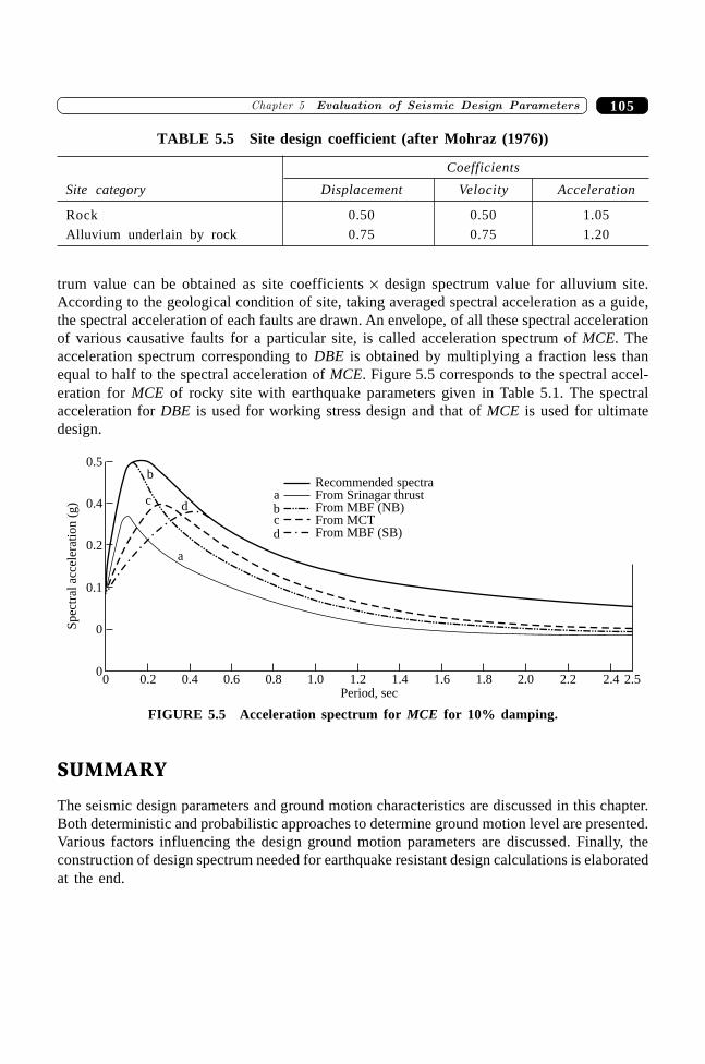
105�������� ������� ����� �� ��� ����������
trum value can be obtained as site coefficients ¥ design spectrum value for alluvium site.According to the geological condition of site, taking averaged spectral acceleration as a guide,the spectral acceleration of each faults are drawn. An envelope, of all these spectral accelerationof various causative faults for a particular site, is called acceleration spectrum of MCE. Theacceleration spectrum corresponding to DBE is obtained by multiplying a fraction less thanequal to half to the spectral acceleration of MCE. Figure 5.5 corresponds to the spectral accel-eration for MCE of rocky site with earthquake parameters given in Table 5.1. The spectralacceleration for DBE is used for working stress design and that of MCE is used for ultimatedesign.
00
0.2 0.4 0.6 0.8 1.0 1.2 1.4 1.6 1.8 2.0 2.2 2.4 2.5Period, sec
0
0.1
0.2
0.4
0.5
Sp
ectr
alac
cele
rati
on
(g)
Recommended spectraFrom Srinagar thrustFrom MBF (NB)From MCTFrom MBF (SB)
abcd
a
d
b
c
FIGURE 5.5 Acceleration spectrum for MCE for 10% damping.
SUMMARY
The seismic design parameters and ground motion characteristics are discussed in this chapter.Both deterministic and probabilistic approaches to determine ground motion level are presented.Various factors influencing the design ground motion parameters are discussed. Finally, theconstruction of design spectrum needed for earthquake resistant design calculations is elaboratedat the end.
TABLE 5.5 Site design coefficient (after Mohraz (1976))
Coefficients
Site category Displacement Velocity Acceleration
Rock 0.50 0.50 1.05
Alluvium underlain by rock 0.75 0.75 1.20

����������� ������� �������������106
REFERENCES
[1] Algermisen, S.T. and Perkins D.M., “A Technique for Seismic Zoning—GeneralConsideration and Parameter”, In Proceedings of the International Conference ofMicrozonation for Safer-Construction, Research and Application, Vol. II, pp. 865–878,Seattle, Washington, 1972.
[2] Ambraseys, N.N., “The Correlation of Intensity with Ground Motions”, In Advancesin Engineering Seismology in Europe, Trieste, 1974.
[3] Basu, S., “Statistical Analysis of Seismic Data and Seismic Risk Analysis of IndianPeninsula”, Ph.D thesis, Department of Civil Engineering, IIT Kanpur, India, 1977.
[4] Bolt, B.A. and Abrahamson, N.A., “New Attenuation Relations for Peak and ExpectedAccelerations of Ground Motion”, Bulletin of the Seismological Society of America,72(6): 2307–2321, 1982.
[5] Boore, D.M., Joyner, W.B., and Fumal, T.E., “Equations for Estimating HorizontalResponse Spectra and Peak Acceleration for Western North American Earthquakes: ASummary of Recent Work”, Seismological Research Letters, 68(1): 128–140, 1997.
[6] Burridge, R. and Knopoff, L., “Body Force Equivalents for Seismic Dislocation”,Bulletin of the Seismological Society of America, 54: 1875–1888, 1964.
[7] Campbell, K.W., “Empirical Near-source Attenuation Relationships for Horizontal andVertical Components of Peak Ground Acceleration, Peak Ground Velocity, and Pseudo-absolute Acceleration Response Spectra”, Seismological Research Letters, 68(1): 154–179, 1997.
[8] Cornell, C.A., “Engineering Seismic Risk Analysis”, Bulletin of the SeismologicalSociety of America, 58(5): 1583–1606, 1968.
[9] Esteva, L., “Bases Para la Formulacion de Decisiones de Diseno Sismico”, TechnicalReport, Institute de Ingenieria, UNAM, Mexico, 1968.
[10] Esteva, L. and Villaverde, R., “Seismic Risk Design Spectra and StructuralReliability”, In Proceedings of Fifth World Conference on Earthquake Engineering,Rome, pp. 2586–2596, 1974.
[11] Hanks, T.C. and Kanamori, H., “A Moment Magnitude Scale”, Journal of GeophysicalResearch, 84(B5): 2348–2350, 1979.
[12] Housner, G.W., “Calculating the Response of an Oscillator to Arbitrary GroundMotion”, Bulletin of the Seismological Society of America, 31:143–149, 1941.
[13] Housner, G.W., “Measures of Severity of Earthquake Ground Shaking”, In Proceedingsof the US National Conference on Earthquake Engineering, Earthquake EngineeringResearch Institute, Ann Arbor, Michigan, pp. 25–33, 1975.
[14] IS-1893, Indian Standard Criteria for Earthquake Resistant Design of Structures—Part 1: General Provisions and Buildings, Bureau of Indian Standards, 2002.
[15] Joyner, W.B. and Boore, D.M., “Peak Horizontal Acceleration and Velocity fromStrong-motion Records Including Records from the 1979 Imperial Valley, CaliforniaEarthquake”, Bulletin of the Seismological Society of America, 71: 2011–2038, 1981.
[16] Maruyama, T., “On the Force Equivalents of Dynamic Elastic Dislocations withReference to the Earthquake Mechanism”, Bulletin of Earthquake Research Institute,Tokyo University, 41: 467–486, 1963.

107�������� ������� ����� �� ��� ����������
[17] McGuire, R.K., “Seismic Structural Response Risk Analysis, Incorporating PeakResponse Regressions on Earthquake Magnitude and Distance”, Technical Report75–51, Department of Civil Engineering, MIT Press, Cambridge, Massachusetts, 1975.
[18] McGuire, R.K., “Seismic Design Spectra and Mapping Procedures Using HazardAnalysis Based Directly on Oscillator Response”, Earthquake Engineering andStructural Dynamics, 5: 211–234, 1977.
[19] Mohraz, B., “A Study of Earthquake Response Spectra for Different GeologicCondition”, Bulletin of the Seismological Society of America, 66: 915–932, 1976.
[20] Murphy, J.R. and O’Brien, L.J., “The Correlation of Peak Ground AccelerationAmplitude with Seismic Intensity and Other Physical Parameters”, Bulletin of theSeismological Society of America, 67(3): 877–915, 1977.
[21] NEHRP, “Recommended Provisions for Seismic Regulation for New Buildings andOther Structures”, Technical Report, Building Safety Council for Federal EmergencyManagement, Washington D.C., 1997.
[22] Newmark, N.M., Blume, J.A., and Kapur, K.K., “Seismic Design Spectra for NuclearPower Plants”, Journal of Power Division, ASCE, 99(02): 873–889, 1973.
[23] Newmark, N.M. and Hall, W.J., “Earthquake Spectra and Design”, Technical Report,Earthquake Engineering Research Institute, Berkeley, California, 1982.
[24] Newmark, N.M. and Rosenblueth, E., “Fundamentals of Earthquake Engineering”,Prentice Hall, Inc., New Jersey, 1971.
[25] Richter, C.F., Elementary Seismology, W.H. Freeman and Co., San Francisco,California, 1958.
[26] Seed, H.B. and Idriss, I.M., “Ground Motions and Soil Liquefaction duringEarthquakes”, Technical Report, Earthquake Engineering Research Institute, Berkeley,California, 1982.
[27] Seed, H.B., Ugas, C., and Lysmer, J., “Site Dependent Spectra for Earthquake-resistantDesign”, Bulletin of the Seismological Society of America, 66: 221–243, 1976.
[28] Slemmons, D.B., “Determination of Design Earthquake Magnitudes for Microzo-nation”, in Proceedings of 3rd International Earthquake Microzonation Conference,pp. 119–130, 1982.
[29] Tocher, D., “Earthquake Energy and Ground Breakage”, Bulletin of the SeismologicalSociety of America, 48(2): 147–153, 1958.
[30] Trifunac, M.D. and Brady, A.G., “On the Correlation of Seismic Intensity with Peaksof Recorded Strong Motion”, Bulletin of the Seismological Society of America, 65:139–162, 1975.
[31] Trifunac, M.D. and Brady, A.G., “A Study on the Duration of Strong EarthquakeGround Motion”, Bulletin of the Seismological Society of America, 65: 581–626, 1975.
[32] Wells, D.L. and Coppersmith, K.J., “New Empirical Relationships among Magnitude,Rupture Length, Rupture Width, Rupture Area and Surface Displacement”, Bulletin ofthe Seismological Society of America, 84(4): 974–1002, 1994.

���� ��
Structural Dynamics

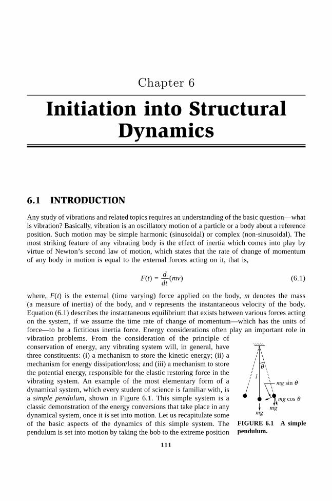
111
Initiation into StructuralDynamics
��������
6.1 INTRODUCTION
Any study of vibrations and related topics requires an understanding of the basic question—whatis vibration? Basically, vibration is an oscillatory motion of a particle or a body about a referenceposition. Such motion may be simple harmonic (sinusoidal) or complex (non-sinusoidal). Themost striking feature of any vibrating body is the effect of inertia which comes into play byvirtue of Newton’s second law of motion, which states that the rate of change of momentumof any body in motion is equal to the external forces acting on it, that is,
F(t) = ddt
mv( ) (6.1)
where, F(t) is the external (time varying) force applied on the body, m denotes the mass(a measure of inertia) of the body, and v represents the instantaneous velocity of the body.Equation (6.1) describes the instantaneous equilibrium that exists between various forces actingon the system, if we assume the time rate of change of momentum—which has the units offorce—to be a fictitious inertia force. Energy considerations often play an important role invibration problems. From the consideration of the principle ofconservation of energy, any vibrating system will, in general, havethree constituents: (i) a mechanism to store the kinetic energy; (ii) amechanism for energy dissipation/loss; and (iii) a mechanism to storethe potential energy, responsible for the elastic restoring force in thevibrating system. An example of the most elementary form of adynamical system, which every student of science is familiar with, isa simple pendulum, shown in Figure 6.1. This simple system is aclassic demonstration of the energy conversions that take place in anydynamical system, once it is set into motion. Let us recapitulate someof the basic aspects of the dynamics of this simple system. Thependulum is set into motion by taking the bob to the extreme position
mg
q
lmg sin q
mg cos qmg
FIGURE 6.1 A simplependulum.
����������� ������� �������������112
and then releasing it. When the bob is at the extreme position the potential energy of the systemis at its maximum while the kinetic energy is minimum. As the bob approaches the mean positionduring its downward swing, the potential energy is gradually converted into the kinetic energyof the bob so much so that at the mean position the kinetic energy is at its maximum withpotential energy being zero. This energy conversion goes on in every half cycle as long as theseoscillations persist. The oscillations eventually subside due to frictional losses caused by theresistance offered by the air to the motion of bob.
Having observed the physical phenomenon, it is then natural to enquire—is it possible todevelop a mathematical model for describing it? The answer is a resounding yes. In fact,mathematical modelling is an integral part of the study of structural dynamics. The solution ofthe differential equation governing the mathematical model correspond to the observed physicalphenomenon. The governing differential equation, also known as the equation of motion, is asecond order differential equation in time. The most important (and many a time quite difficultone) aspect of structural dynamics is the formulation of equation of motion. In general, thegoverning equation of a vibrating system can be developed by adopting any of the followingfive approaches:
1. Newton’s second law of motion,2. Application of d’Alembert’s principle,3. Principle of virtual work,4. Hamilton’s principle, and5. Lagrange’s equation
Of these, the first two approaches are based on the principles of vector mechanics, whereasthe latter two approaches are based on variational principles. The approaches based on vectormechanics are physically intuitive but invariably become intractable in case of complexconfigurations. On the other hand, the variational approaches depend on scalar work-likequantities and can accommodate very complex systems without any difficulty. However, thevariational approaches are more abstract and lack the physical intuitive appeal afforded by thevector mechanics approaches. The principle of virtual work is an extension of the equilibriummethods in the sense that it is a statement of no work being done by a system of forces, inequilibrium, in moving through a set of virtual displacements consistent with the geometricconstraints. For the purpose of introductory exposition to structural dynamics the methods basedon vector mechanics will suffice for establishing the equation(s) of motion.
6.2 MATHEMATICAL MODELLING
The study of structural dynamics involves developing an insight into the dynamic behaviour ofthe structural systems by investigating the behaviour of their models under the influence ofdynamic loads, such as blast, winds, earthquakes, heavy rotating machinery, etc. The modelsused in these investigations can be either small-scale laboratory models for experimental studies,or can be mathematical models for analytical studies. The development of an appropriatemathematical model for a specific study requires an understanding of the basic phenomenon anda clear idea of the basic mechanics.
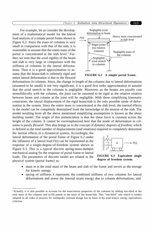
113�������� �� � �� �� ������������������ ��
For example, let us consider the develop-ment of a mathematical model for the lateralload analysis of a simple portal frame shown inFigure 6.2. Since the mass of columns is verysmall in comparison with that of the slab, it isreasonable to assume that the entire mass of theportal is concentrated at the slab level.1 Fur-ther, we note that the axial rigidity of the beamand slab is very large in comparison with thestiffness of columns in the lateral deforma-tions. Thus it is a good approximation to as-sume that the beam/slab is infinitely rigid andentire lateral deformation is due to the flexuraldeformations in columns. Since, the change in length of the columns due to lateral deformations(assumed to be small) is not very significant, it is a good first order approximation to assumethat the axial stretch in the columns is negligible. Moreover, as the beams are usually castmonolithically with the columns, the joint can be assumed to be rigid as the relative rotationbetween beam and column at the joint will be negligible. With these simplifying kinematicconstraints, the lateral displacement of the rigid beam/slab is the only possible mode of defor-mation in the system. Since the entire mass is concentrated at the slab level, the inertial effectsin the model can be completely determined from the knowledge of the motion of the slab. Themodel resulting from all the above mentioned simplifying assumptions is known as the shearbuilding model. The origin of this nomenclature is that the shear force is constant across theheight of the column. It cannot be overemphasized here that the mode of deformation in col-umns is purely flexural. This also brings us to the concept of dynamic degrees of freedom, whichis defined as the total number of displacements (and rotations) required to completely determinethe inertial effects in a dynamical system. Accordingly, thelateral deformation of the portal frame of Figure 6.2 underthe influence of a lateral load F(t) can be represented as theresponse of a single-degree-of-freedom system shown inFigure 6.3. This is a typical discrete spring-mass-dashpotmechanical analog for the response of portal frame to lateralloads. The parameters of discrete model are related to thephysical system (portal frame) as:
∑ mass m is the total mass of the beam and slab of the frame and serves as the storagefor kinetic energy,
∑ spring of stiffness k represents the combined stiffness of two columns for lateraldeformations and stores the internal strain energy due to column deformations, and
Negligible mass ofthe columns
Negligibleaxial stretchin columns
Rigid joints(no relative
rotation)
F t( )
Negligible axialdeformation in beam
Heavy mass concentratedat slab level
FIGURE 6.2 A simple portal frame.
1Actually, it is also possible to account for the mass/inertia properties of the columns by adding one-third of thetotal mass of the columns and in-fill panels to the mass of the beam/slab. This “one-third” rule which is widelyadopted in all codes of practice for earthquake resistant design has its basis in the total kinetic energy equivalencecriterion.
m
c
k
F t( )
FIGURE 6.3 Equivalent singledegree of freedom system.
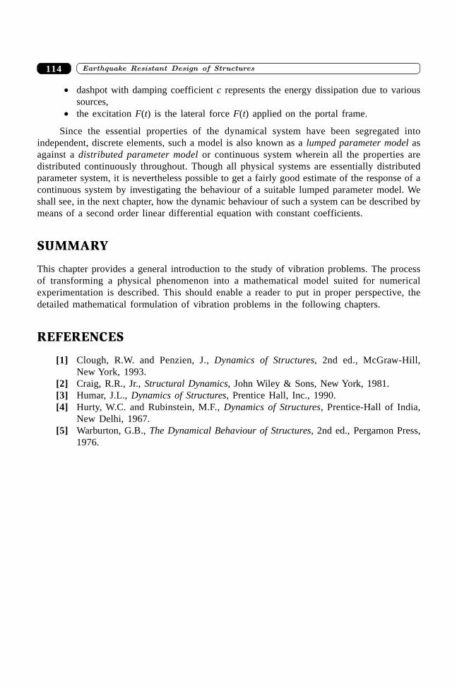
����������� ������� �������������114
∑ dashpot with damping coefficient c represents the energy dissipation due to varioussources,
∑ the excitation F(t) is the lateral force F(t) applied on the portal frame.
Since the essential properties of the dynamical system have been segregated intoindependent, discrete elements, such a model is also known as a lumped parameter model asagainst a distributed parameter model or continuous system wherein all the properties aredistributed continuously throughout. Though all physical systems are essentially distributedparameter system, it is nevertheless possible to get a fairly good estimate of the response of acontinuous system by investigating the behaviour of a suitable lumped parameter model. Weshall see, in the next chapter, how the dynamic behaviour of such a system can be described bymeans of a second order linear differential equation with constant coefficients.
SUMMARY
This chapter provides a general introduction to the study of vibration problems. The processof transforming a physical phenomenon into a mathematical model suited for numericalexperimentation is described. This should enable a reader to put in proper perspective, thedetailed mathematical formulation of vibration problems in the following chapters.
REFERENCES
[1] Clough, R.W. and Penzien, J., Dynamics of Structures, 2nd ed., McGraw-Hill,New York, 1993.
[2] Craig, R.R., Jr., Structural Dynamics, John Wiley & Sons, New York, 1981.[3] Humar, J.L., Dynamics of Structures, Prentice Hall, Inc., 1990.[4] Hurty, W.C. and Rubinstein, M.F., Dynamics of Structures, Prentice-Hall of India,
New Delhi, 1967.[5] Warburton, G.B., The Dynamical Behaviour of Structures, 2nd ed., Pergamon Press,
1976.
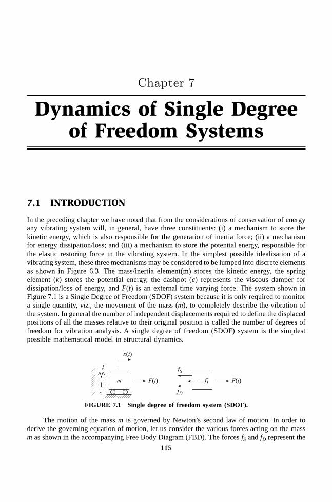
115
Dynamics of Single Degreeof Freedom Systems
��������
7.1 INTRODUCTION
In the preceding chapter we have noted that from the considerations of conservation of energyany vibrating system will, in general, have three constituents: (i) a mechanism to store thekinetic energy, which is also responsible for the generation of inertia force; (ii) a mechanismfor energy dissipation/loss; and (iii) a mechanism to store the potential energy, responsible forthe elastic restoring force in the vibrating system. In the simplest possible idealisation of avibrating system, these three mechanisms may be considered to be lumped into discrete elementsas shown in Figure 6.3. The mass/inertia element(m) stores the kinetic energy, the springelement (k) stores the potential energy, the dashpot (c) represents the viscous damper fordissipation/loss of energy, and F(t) is an external time varying force. The system shown inFigure 7.1 is a Single Degree of Freedom (SDOF) system because it is only required to monitora single quantity, viz., the movement of the mass (m), to completely describe the vibration ofthe system. In general the number of independent displacements required to define the displacedpositions of all the masses relative to their original position is called the number of degrees offreedom for vibration analysis. A single degree of freedom (SDOF) system is the simplestpossible mathematical model in structural dynamics.
m
k
c
F t( )
x t( )
F t( )fI
fS
fD
FIGURE 7.1 Single degree of freedom system (SDOF).
The motion of the mass m is governed by Newton’s second law of motion. In order toderive the governing equation of motion, let us consider the various forces acting on the massm as shown in the accompanying Free Body Diagram (FBD). The forces fS and fD represent the
����������� ������� �������������116
elastic restoring force and the force developed in the damper, respectively. These forces, alongwith the external force F(t) act on the mass (m), which then cause the change in momentum ofthe mass in accordance with Newton’s second law as,
ddt
mx( �) = F(t) – fS – fD (7.1)
where, x(t) denotes the displacement of mass m from its original position of rest. For the specialcase of civil engineering structures, the mass of the system does not change with time, and there-fore, the rate of change of momentum can be considered to have the same effect as that ofapplying a fictitious inertia force fI directed opposite to the direction of motion for consideringthe instantaneous equilibrium of forces acting on the mass. This simplified interpretation ofNewton’s second law of motion (valid only when the mass of the system is time invariant) ispopularly known as the d’Alembert’s principle.
fI = F(t) – fS – fD (7.2)
Thus the inertia force fI = m ��x (mass ¥ acceleration), spring force fS = kx (spring constant¥ spring deformation) and damping force fD = c �x (coefficient of viscous damping ¥ relativevelocity between the two ends of the dashpot).1 By substituting these relations in Equation (7.2),we get,
m ��x + c �x + kx = F(t) (7.3)
Equation (7.3) is a linear second order differential equation with constant parameters. Thegeneral solution for this equation is given by,
x(t) = xh(t) + xp(t) (7.4)
where, xh(t) is the solution of the corresponding homogeneous equation obtained by making theright hand side zero; and xp(t) is the particular solution which depends on the specific form ofapplied force F(t). The homogeneous solution of this second order differential equation containstwo arbitrary constants which can be evaluated by using the initial conditions x(0) and �x (0),i.e., the displacement and velocity of the mass at the onset of vibration.
7.2 FREE VIBRATION OF VISCOUS-DAMPEDSDOF SYSTEMS
For a particular case when there is no external force acting on the system, it is still possibleto make the mass vibrate by giving some arbitrary initial conditions. The ensuing motion of
1This is only a convenient mathematical model for the energy dissipation mechanism in a vibrating system and isactually an expression of the viscous drag in a laminar flow. In real structural systems, energy dissipation actuallytakes place in different ways and the most important of them is the energy loss due to inter-granular frictionbetween the particles of a vibrating system. However, incorporating a dry friction damping behaviour wouldresult in a nonlinear equation of motion. Since the magnitude of damping force is generally very small incomparison to the other forces acting on the system, a viscous damping model (leading to a linear equation!)serves well to get a rational estimate of system response for engineering design.
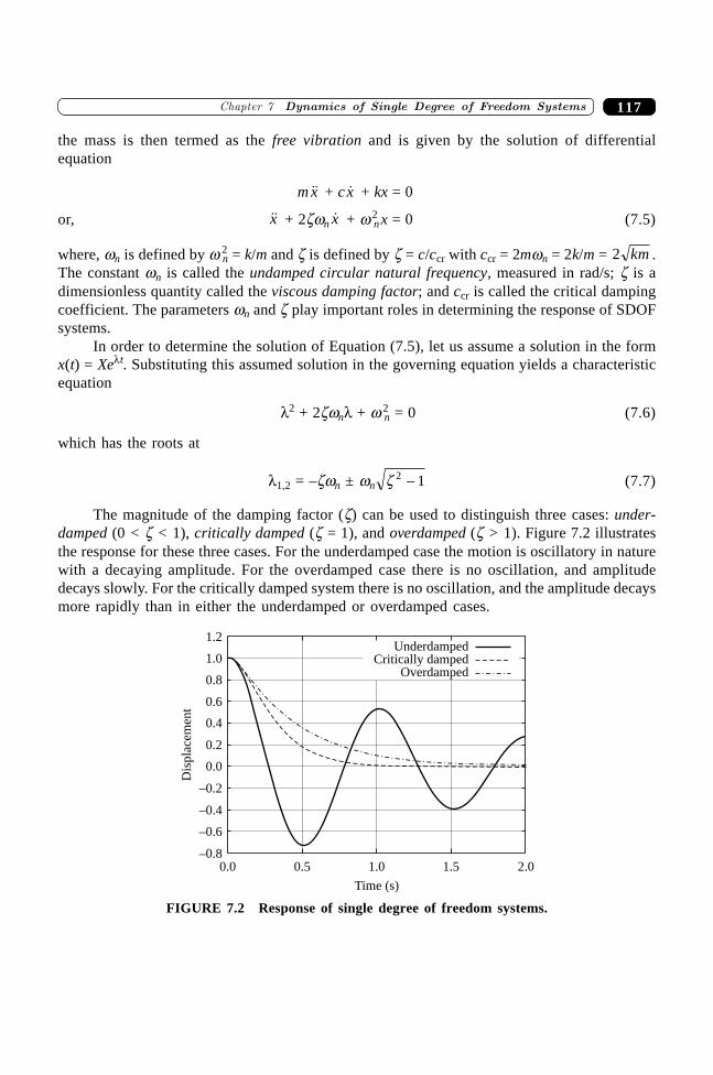
117�������� ����� ����� �������������������
the mass is then termed as the free vibration and is given by the solution of differentialequation
m ��x + c �x + kx = 0
or, ��x + 2zwn �x + w 2nx = 0 (7.5)
where, wn is defined by w 2n = k/m and z is defined by z = c/ccr with ccr = 2mwn = 2k/m = 2 km .
The constant wn is called the undamped circular natural frequency, measured in rad/s; z is adimensionless quantity called the viscous damping factor; and ccr is called the critical dampingcoefficient. The parameters wn and z play important roles in determining the response of SDOFsystems.
In order to determine the solution of Equation (7.5), let us assume a solution in the formx(t) = Xelt. Substituting this assumed solution in the governing equation yields a characteristicequation
l2 + 2zwnl + w 2n = 0 (7.6)
which has the roots at
l1,2 = –zwn ± wn z 2 1- (7.7)
The magnitude of the damping factor (z) can be used to distinguish three cases: under-damped (0 < z < 1), critically damped (z = 1), and overdamped (z > 1). Figure 7.2 illustratesthe response for these three cases. For the underdamped case the motion is oscillatory in naturewith a decaying amplitude. For the overdamped case there is no oscillation, and amplitudedecays slowly. For the critically damped system there is no oscillation, and the amplitude decaysmore rapidly than in either the underdamped or overdamped cases.
Underdamped
–0.8
–0.6
–0.4
–0.2
0.0
0.2
0.4
0.6
0.8
1.0
1.2
0.0 0.5 1.0 1.5 2.0
Time (s)
Dis
pla
cem
ent
Critically dampedOverdamped
FIGURE 7.2 Response of single degree of freedom systems.
����������� ������� �������������118
7.2.1 Underdamped Case (z < 1)
For z < 1, it is convenient to write Equation (7.7) in the form
l1,2 = –zwn ± iwn 12 - z
= –zwn ± iwd (7.8)
where wd is known as the damped circular natural frequency. Using Euler’s formula, the generalsolution, x(t), can be written in the form,
x(t) = e–zw t (A1 cos wdt + A2 sin wdt) (7.9)
The coefficients A1 and A2 are determined from the initial conditions x(t = 0) = x0 and �x (t = 0)= �x0 and the solution is then given by
x(t) = e–zwnt x tx x
tdn
dd0
0 0cos�
sinwz ww
w++F
HGIKJ
LNM
OQP
(7.10)
Although the value of z has an effect on the frequency wd, the most pronounced effect ofdamping is on the rate at which the motion dies out, that is, on the e–zwnt term.
7.2.2 Critically-damped Case (z = 1)
When z = 1, the Equation (7.7) gives only one solution as l = –wn. The response for the caseof repeated roots is then given by
x(t) = e–wnt(A1 + A2t) (7.11)
where, A1 and A2 are determined from the initial conditions x0 and �x0 . The solution in termsof the initial conditions can be derived as,
x(t) = e–wnt [x0(1 + wnt) + �x t0 ] (7.12)
The free-vibration response of a critically damped system does not involve oscillations aboutthe zero-displacement position, instead the system returns to zero-displacement positionasymptotically by virtue of the decayed exponential term of Equation (7.12). However, therewill be precisely one crossing of the zero-displacement position if the initial displacement andinitial velocity were of opposite signs.
7.2.3 Overdamped Case (z > 1)
For z > 1, the Equation (7.7) gives two distinct, negative real roots. The solution is then givenby,
x(t) = e–zwnt (A1 cosh w*t + A2 sinh w*t)
= e–zwnt x tx x
tn0
0 0cosh�
sinh**
*wz ww
w++F
HGIKJ (7.13)
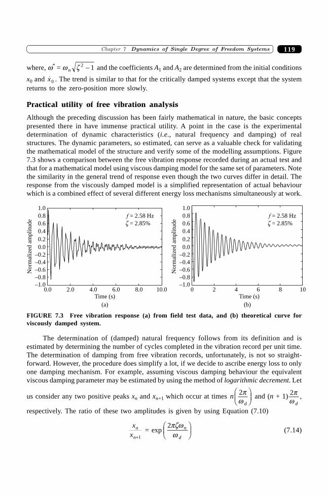
119�������� ����� ����� �������������������
where, w* = w zn2 1- and the coefficients A1 and A2 are determined from the initial conditions
x0 and �x0 . The trend is similar to that for the critically damped systems except that the systemreturns to the zero-position more slowly.
Practical utility of free vibration analysis
Although the preceding discussion has been fairly mathematical in nature, the basic conceptspresented there in have immense practical utility. A point in the case is the experimentaldetermination of dynamic characteristics (i.e., natural frequency and damping) of realstructures. The dynamic parameters, so estimated, can serve as a valuable check for validatingthe mathematical model of the structure and verify some of the modelling assumptions. Figure7.3 shows a comparison between the free vibration response recorded during an actual test andthat for a mathematical model using viscous damping model for the same set of parameters. Notethe similarity in the general trend of response even though the two curves differ in detail. Theresponse from the viscously damped model is a simplified representation of actual behaviourwhich is a combined effect of several different energy loss mechanisms simultaneously at work.
–0.8
0.0 2.0 4.0 6.0 8.0 10.0
Time (s)
(a)
–1.0
–0.6
–0.4
–0.2
0.0
0.2
0.4
0.6
0.8
1.0
No
rmal
ized
amp
litu
de
–0.8
0 2 4 6 8 10
Time (s)
(b)
–1.0
–0.6
–0.4
–0.2
0.0
0.2
0.4
0.6
0.8
1.0
No
rmal
ized
amp
litu
de
f = 2.58 Hz
z = 2.85%
f = 2.58 Hz
z = 2.85%
FIGURE 7.3 Free vibration response (a) from field test data, and (b) theoretical curve forviscously damped system.
The determination of (damped) natural frequency follows from its definition and isestimated by determining the number of cycles completed in the vibration record per unit time.The determination of damping from free vibration records, unfortunately, is not so straight-forward. However, the procedure does simplify a lot, if we decide to ascribe energy loss to onlyone damping mechanism. For example, assuming viscous damping behaviour the equivalentviscous damping parameter may be estimated by using the method of logarithmic decrement. Let
us consider any two positive peaks xn and xn+1 which occur at times nd
2pw
FHG
IKJ and (n + 1) 2p
w d,
respectively. The ratio of these two amplitudes is given by using Equation (7.10)
xx
n
n+1 = exp
2pzww
n
d
FHG
IKJ (7.14)
����������� ������� �������������120
By taking the natural logarithm of both sides and substituting for wd, we get,
d = lnx
xn
n+1 =
2
1 2
pz
z-(7.15)
where, d is known as the logarithmic decrement. In practice it is more convenient to measurethe peak-to-trough amplitudes instead of peaks or troughs due to the absence of zero baselinein the experimental records. It can be shown that the same result for logarithmic decrement(as in Equation (7.15)) also holds for peak-to-trough amplitudes. Further, in the case of lightlydamped systems, it might be more convenient to measure amplitudes which spaced a fewcycles (say, m) apart. It can be shown that in this case the equation for logarithmic decrementchanges to
d = x
xn
n m+ =
2
1 2
mpz
z-
which is commonly used in practice.
7.3 FORCED VIBRATIONS OF SDOF SYSTEMS
The dynamical systems may be set into motion by several types of excitations. These forcingfunctions may either be harmonic or non-harmonic, periodic or aperiodic, etc. Further, theresponse may also differ on account of the duration of exposure to the applied excitation. Thenature of the response of a SDOF system to harmonic excitation is significantly different fromthat for a finite duration excitation. We shall begin with the response of SDOF systems excitedby harmonic excitations, which has great practical significance since any periodic function canbe decomposed into a sum of harmonic functions by using Fourier series2. The results of thissection have an important bearing on the design of vibration recording instruments, industrialvibration isolators, and shock absorbers.
7.3.1 Response of SDOF Systems to Harmonic Excitations
The governing differential equation for a SDOF system as shown in Figure 2.1 with F(t) =F0 sin w t is given by,
m ��x + c �x + kx = F0 sin w t (7.16)
Let us assume the initial conditions given as x0 and �x0 . Moreover, the particular solution of this
2Under a fairly general set of conditions, any periodic function f(t) can be expressed as:
f (t) = a a j tT
b j tTj j
j0
1
2 2+ +FH
IK
=
•Â cos sinp p
where T is the period of f (t). For more details consult any text on Applied Mathematics, such as, E. Kreyszig,Advanced Engineering Mathematics, Wiley Interscience.
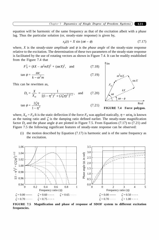
121�������� ����� ����� �������������������
equation will be harmonic of the same frequency as that of the excitation albeit with a phaselag. Thus the particular solution (or, steady-state response) is given by,
xp(t) = X sin (wt – f) (7.17)
where, X is the steady-state amplitude and f is the phase angle of the steady-state responserelative to the excitation. The determination of these two parameters of the steady-state responseis facilitated by the use of rotating vectors as shown in Figure 7.4. It can be readily establishedfrom the Figure 7.4 that
F20 = (kX – w2mX)2 + (wcX)2, and (7.18)
tan f = wwc
k m- 2 (7.19)
This can be rewritten as,
Ds = XXst
= 11 22 2 2 1 2[( ) ( ) ] /- +h zh
, and (7.20)
tan f = 2
1 2
zhh-
(7.21)
where, Xst = F0/k is the static deflection if the force F0 was applied statically, h = w/wn is knownas the tuning ratio and z is the damping ratio defined earlier. The steady-state magnificationfactor Ds and the phase angle f are plotted in Figure 7.5. From Equations (7.17) to (7.21) andFigure 7.5 the following significant features of steady-state response can be observed:
(i) the motion described by Equation (7.17) is harmonic and is of the same frequency asthe excitation.
Im
Real
wt – fwt
kX
wcX
w2mX
F0
FIGURE 7.4 Force polygon.
0 0.2 0.4 0.6 0.8 10.94
0.96
0.98
1.00
1.02
1.04
1.06
[(1
–)
+(2
)]
2 hzh
22
–1/2
z = 0.00
Frequency ratio ( )hz = 0.60 z = 0.65
z = 0.70 z = 0.75
0 0 2 3 4 50.0
0.5
1.5
2.0
2.5
3.0
3.5
Frequency ratio ( )h
1.0
z = 0.00 z = 0.50
z = 0.70 z = 1.00
Phas
ean
gle
(,in
rad)
f
FIGURE 7.5 Magnification and phase of response of SDOF system to different excitationfrequencies.
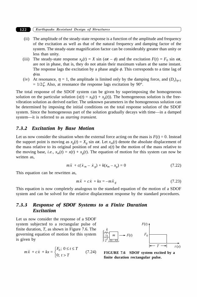
����������� ������� �������������122
(ii) The amplitude of the steady-state response is a function of the amplitude and frequencyof the excitation as well as that of the natural frequency and damping factor of thesystem. The steady-state magnification factor can be considerably greater than unity orless than unity.
(iii) The steady-state response xp(t) = X sin (wt – f) and the excitation F(t) = F0 sin wt,are not in phase, that is, they do not attain their maximum values at the same instant.The response lags the excitation by a phase angle f. This corresponds to a time lag off/w.
(iv) At resonance, h = 1, the amplitude is limited only by the damping force, and (Ds)h=1= 1/2z. Also, at resonance the response lags excitation by 90°.
The total response of the SDOF system can be given by superimposing the homogeneoussolution on the particular solution (x(t) = xh(t) + xp(t)). The homogeneous solution is the free-vibration solution as derived earlier. The unknown parameters in the homogeneous solution canbe determined by imposing the initial conditions on the total response solution of the SDOFsystem. Since the homogeneous part of the solution gradually decays with time—in a dampedsystem—it is referred to as starting transient.
7.3.2 Excitation by Base Motion
Let us now consider the situation when the external force acting on the mass is F(t) = 0. Insteadthe support point is moving as xg(t) = Xg sin wt. Let xm(t) denote the absolute displacement ofthe mass relative to its original position of rest and x(t) be the motion of the mass relative tothe moving base, i.e., xm(t) = x(t) + xg(t). The equation of motion for this system can now bewritten as,
m ��x + c( �x m – �x g) + k(xm – xg) = 0 (7.22)
This equation can be rewritten as,
m ��x + c �x + kx = –m ��x g (7.23)
This equation is now completely analogous to the standard equation of the motion of a SDOFsystem and can be solved for the relative displacement response by the standard procedures.
7.3.3 Response of SDOF Systems to a Finite DurationExcitation
Let us now consider the response of a SDOFsystem subjected to a rectangular pulse offinite duration, T, as shown in Figure 7.6. Thegoverning equation of motion for this systemis given by
m ��x + c �x + kx = F t T
t T0 0
0
;
;
£ £
>RST
(7.24)
m
c
k
F t( ) F0
T t s( )
F t( )
FIGURE 7.6 SDOF system excited by afinite duration rectangular pulse.
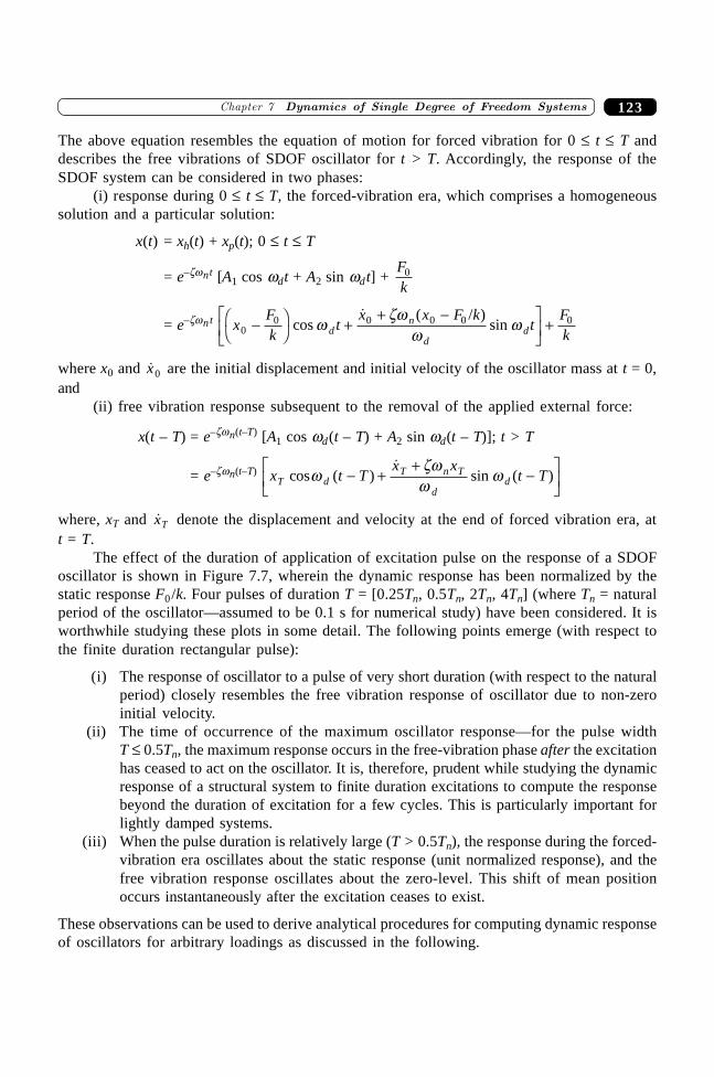
123�������� ����� ����� �������������������
The above equation resembles the equation of motion for forced vibration for 0 £ t £ T anddescribes the free vibrations of SDOF oscillator for t > T. Accordingly, the response of theSDOF system can be considered in two phases:
(i) response during 0 £ t £ T, the forced-vibration era, which comprises a homogeneoussolution and a particular solution:
x(t) = xh(t) + xp(t); 0 £ t £ T
= e–zwnt [A1 cos wdt + A2 sin wdt] + Fk0
= e–zwnt xFk
tx x F k
tFkd
n
dd0
0 0 0 0 0-FH
IK +
+ -LNM
OQP
+cos� ( / )
sinwzw
ww
where x0 and �x0 are the initial displacement and initial velocity of the oscillator mass at t = 0,and
(ii) free vibration response subsequent to the removal of the applied external force:
x(t – T) = e–zwn(t–T) [A1 cos wd(t – T) + A2 sin wd(t – T)]; t > T
= e–zwn(t–T) x t Tx x
t TT dT n T
ddcos ( )
�sin ( )w
zww
w- ++
-LNM
OQP
where, xT and �xT denote the displacement and velocity at the end of forced vibration era, att = T.
The effect of the duration of application of excitation pulse on the response of a SDOFoscillator is shown in Figure 7.7, wherein the dynamic response has been normalized by thestatic response F0/k. Four pulses of duration T = [0.25Tn, 0.5Tn, 2Tn, 4Tn] (where Tn = naturalperiod of the oscillator—assumed to be 0.1 s for numerical study) have been considered. It isworthwhile studying these plots in some detail. The following points emerge (with respect tothe finite duration rectangular pulse):
(i) The response of oscillator to a pulse of very short duration (with respect to the naturalperiod) closely resembles the free vibration response of oscillator due to non-zeroinitial velocity.
(ii) The time of occurrence of the maximum oscillator response—for the pulse widthT £ 0.5Tn, the maximum response occurs in the free-vibration phase after the excitationhas ceased to act on the oscillator. It is, therefore, prudent while studying the dynamicresponse of a structural system to finite duration excitations to compute the responsebeyond the duration of excitation for a few cycles. This is particularly important forlightly damped systems.
(iii) When the pulse duration is relatively large (T > 0.5Tn), the response during the forced-vibration era oscillates about the static response (unit normalized response), and thefree vibration response oscillates about the zero-level. This shift of mean positionoccurs instantaneously after the excitation ceases to exist.
These observations can be used to derive analytical procedures for computing dynamic responseof oscillators for arbitrary loadings as discussed in the following.
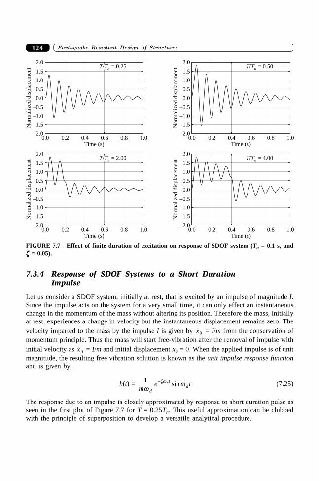
����������� ������� �������������124
0.0–2.0
–1.5
0.2 0.4 0.6 0.8 1.0
–1.0
–0.5
0.0
0.5
1.0
1.5
2.0T/ = 0.25Tn
Norm
aliz
eddis
pla
cem
ent
Time (s)0.0
–2.0
–1.5
0.2 0.4 0.6 0.8 1.0
–1.0
–0.5
0.0
0.5
1.0
1.5
2.0T/ = 0.50Tn
Norm
aliz
eddis
pla
cem
ent
Time (s)
0.0–2.0
–1.5
0.2 0.4 0.6 0.8 1.0
–1.0
–0.5
0.0
0.5
1.0
1.5
2.0T/ = 2.00Tn
Norm
aliz
eddis
pla
cem
ent
Time (s)0.0
–2.0
–1.5
0.2 0.4 0.6 0.8 1.0
–1.0
–0.5
0.0
0.5
1.0
1.5
2.0T/ = 4.00Tn
Norm
aliz
eddis
pla
cem
ent
Time (s)
FIGURE 7.7 Effect of finite duration of excitation on response of SDOF system (Tn = 0.1 s, andzzzzz = 0.05).
7.3.4 Response of SDOF Systems to a Short DurationImpulse
Let us consider a SDOF system, initially at rest, that is excited by an impulse of magnitude I.Since the impulse acts on the system for a very small time, it can only effect an instantaneouschange in the momentum of the mass without altering its position. Therefore the mass, initiallyat rest, experiences a change in velocity but the instantaneous displacement remains zero. Thevelocity imparted to the mass by the impulse I is given by �x0 = I/m from the conservation ofmomentum principle. Thus the mass will start free-vibration after the removal of impulse withinitial velocity as �x0 = I/m and initial displacement x0 = 0. When the applied impulse is of unitmagnitude, the resulting free vibration solution is known as the unit impulse response functionand is given by,
h(t) = 1m
e td
td
n
wwzw- sin (7.25)
The response due to an impulse is closely approximated by response to short duration pulse asseen in the first plot of Figure 7.7 for T = 0.25Tn. This useful approximation can be clubbedwith the principle of superposition to develop a versatile analytical procedure.
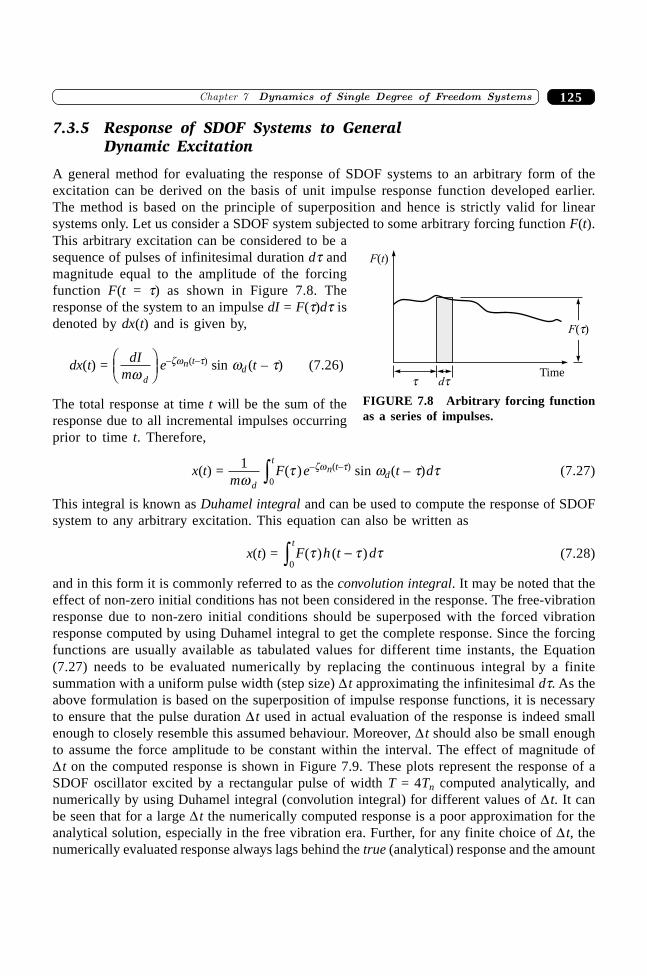
125�������� ����� ����� �������������������
7.3.5 Response of SDOF Systems to GeneralDynamic Excitation
A general method for evaluating the response of SDOF systems to an arbitrary form of theexcitation can be derived on the basis of unit impulse response function developed earlier.The method is based on the principle of superposition and hence is strictly valid for linearsystems only. Let us consider a SDOF system subjected to some arbitrary forcing function F(t).This arbitrary excitation can be considered to be asequence of pulses of infinitesimal duration dt andmagnitude equal to the amplitude of the forcingfunction F(t = t) as shown in Figure 7.8. Theresponse of the system to an impulse dI = F(t)dt isdenoted by dx(t) and is given by,
dx(t) = dIm dw
FHG
IKJ e–zwn(t–t) sin wd (t – t) (7.26)
The total response at time t will be the sum of theresponse due to all incremental impulses occurringprior to time t. Therefore,
x(t) = 10mF
d
t
wt( )z e–zwn(t–t) sin wd(t – t)dt (7.27)
This integral is known as Duhamel integral and can be used to compute the response of SDOFsystem to any arbitrary excitation. This equation can also be written as
x(t) = F h t dt
( ) ( )t t t0z - (7.28)
and in this form it is commonly referred to as the convolution integral. It may be noted that theeffect of non-zero initial conditions has not been considered in the response. The free-vibrationresponse due to non-zero initial conditions should be superposed with the forced vibrationresponse computed by using Duhamel integral to get the complete response. Since the forcingfunctions are usually available as tabulated values for different time instants, the Equation(7.27) needs to be evaluated numerically by replacing the continuous integral by a finitesummation with a uniform pulse width (step size) D t approximating the infinitesimal dt. As theabove formulation is based on the superposition of impulse response functions, it is necessaryto ensure that the pulse duration D t used in actual evaluation of the response is indeed smallenough to closely resemble this assumed behaviour. Moreover, D t should also be small enoughto assume the force amplitude to be constant within the interval. The effect of magnitude ofD t on the computed response is shown in Figure 7.9. These plots represent the response of aSDOF oscillator excited by a rectangular pulse of width T = 4Tn computed analytically, andnumerically by using Duhamel integral (convolution integral) for different values of D t. It canbe seen that for a large D t the numerically computed response is a poor approximation for theanalytical solution, especially in the free vibration era. Further, for any finite choice of D t, thenumerically evaluated response always lags behind the true (analytical) response and the amount
Time
F( )t
dtt
F t( )
FIGURE 7.8 Arbitrary forcing functionas a series of impulses.
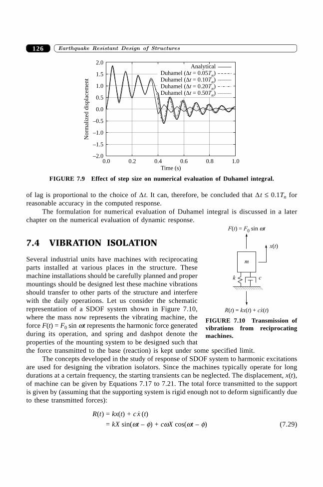
����������� ������� �������������126
of lag is proportional to the choice of D t. It can, therefore, be concluded that D t £ 0.1Tn forreasonable accuracy in the computed response.
The formulation for numerical evaluation of Duhamel integral is discussed in a laterchapter on the numerical evaluation of dynamic response.
7.4 VIBRATION ISOLATION
Several industrial units have machines with reciprocatingparts installed at various places in the structure. Thesemachine installations should be carefully planned and propermountings should be designed lest these machine vibrationsshould transfer to other parts of the structure and interferewith the daily operations. Let us consider the schematicrepresentation of a SDOF system shown in Figure 7.10,where the mass now represents the vibrating machine, theforce F(t) = F0 sin wt represents the harmonic force generatedduring its operation, and spring and dashpot denote theproperties of the mounting system to be designed such thatthe force transmitted to the base (reaction) is kept under some specified limit.
The concepts developed in the study of response of SDOF system to harmonic excitationsare used for designing the vibration isolators. Since the machines typically operate for longdurations at a certain frequency, the starting transients can be neglected. The displacement, x(t),of machine can be given by Equations 7.17 to 7.21. The total force transmitted to the supportis given by (assuming that the supporting system is rigid enough not to deform significantly dueto these transmitted forces):
R(t) = kx(t) + c �x (t)
= kX sin(wt – f) + cwX cos(wt – f) (7.29)
0.0 0.2 0.4 0.6 0.8 1.0
Time (s)
–2.0
–1.5
–1.0
–0.5
0.0
0.5
1.0
1.5
2.0
Norm
aliz
eddis
pla
cem
ent
AnalyticalDuhamel ( = 0.05 )�t TnDuhamel ( = 0.10 )�t TnDuhamel ( = 0.20 )�t TnDuhamel ( = 0.50 )�t Tn
FIGURE 7.9 Effect of step size on numerical evaluation of Duhamel integral.
m
k c
x t( )
F F t0 w( ) = sint
R kx( ) = ( ) + ( )t t cx t.
FIGURE 7.10 Transmission ofvibrations from reciprocatingmachines.
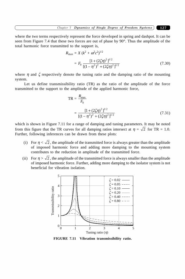
127�������� ����� ����� �������������������
where the two terms respectively represent the force developed in spring and dashpot. It can beseen from Figure 7.4 that these two forces are out of phase by 90°. Thus the amplitude of thetotal harmonic force transmitted to the support is,
Rmax = X (k2 + w2c2)1/2
= F0
2 1 2
2 2 2 1 2
1 2
1 2
[ ( ) ]
[( ) ( ) ]
/
/
+- +
zhh zh
(7.30)
where h and z respectively denote the tuning ratio and the damping ratio of the mountingsystem.
Let us define transmissibility ratio (TR) as the ratio of the amplitude of the forcetransmitted to the support to the amplitude of the applied harmonic force,
TR = RFmax
0
= [ ( ) ]
[( ) ( ) ]
/
/
1 2
1 2
2 1 2
2 2 2 1 2
+- +
zhh zh
(7.31)
which is shown in Figure 7.11 for a range of damping and tuning parameters. It may be notedfrom this figure that the TR curves for all damping ratios intersect at h = 2 for TR = 1.0.Further, following inferences can be drawn from these plots:
(i) For h < 2 , the amplitude of the transmitted force is always greater than the amplitudeof imposed harmonic force and adding more damping to the mounting systemcontributes to the reduction in amplitude of the transmitted force.
(ii) For h > 2 , the amplitude of the transmitted force is always smaller than the amplitudeof imposed harmonic force. Further, adding more damping to the isolator system is notbeneficial for vibration isolation.
00
1 2 3 4 5
1
2
3
4
5
Tuning ratio ( )h
Tra
nsm
issi
bil
ity
rati
o
z = 0.05
z = 0.10
z = 0.20
z = 0.40
z = 0.80
z = 0.02
FIGURE 7.11 Vibration transmissibility ratio.
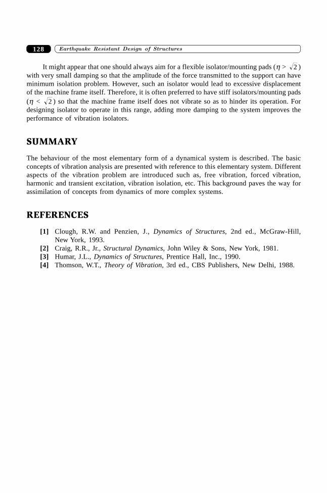
����������� ������� �������������128
It might appear that one should always aim for a flexible isolator/mounting pads (h > 2 )with very small damping so that the amplitude of the force transmitted to the support can haveminimum isolation problem. However, such an isolator would lead to excessive displacementof the machine frame itself. Therefore, it is often preferred to have stiff isolators/mounting pads(h < 2 ) so that the machine frame itself does not vibrate so as to hinder its operation. Fordesigning isolator to operate in this range, adding more damping to the system improves theperformance of vibration isolators.
SUMMARY
The behaviour of the most elementary form of a dynamical system is described. The basicconcepts of vibration analysis are presented with reference to this elementary system. Differentaspects of the vibration problem are introduced such as, free vibration, forced vibration,harmonic and transient excitation, vibration isolation, etc. This background paves the way forassimilation of concepts from dynamics of more complex systems.
REFERENCES
[1] Clough, R.W. and Penzien, J., Dynamics of Structures, 2nd ed., McGraw-Hill,New York, 1993.
[2] Craig, R.R., Jr., Structural Dynamics, John Wiley & Sons, New York, 1981.[3] Humar, J.L., Dynamics of Structures, Prentice Hall, Inc., 1990.[4] Thomson, W.T., Theory of Vibration, 3rd ed., CBS Publishers, New Delhi, 1988.
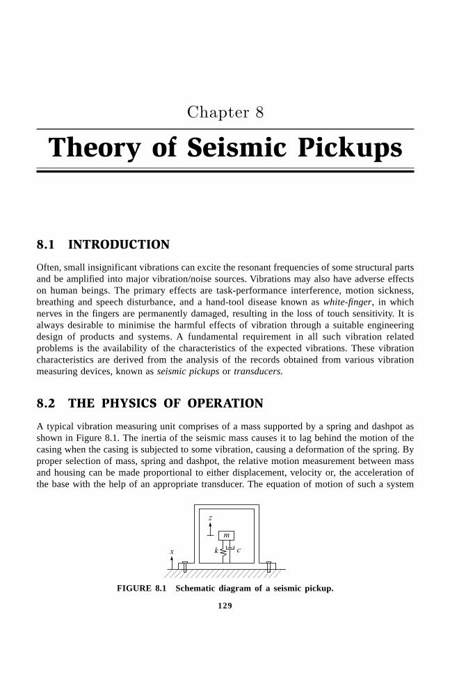
129
Theory of Seismic Pickups��������
8.1 INTRODUCTION
Often, small insignificant vibrations can excite the resonant frequencies of some structural partsand be amplified into major vibration/noise sources. Vibrations may also have adverse effectson human beings. The primary effects are task-performance interference, motion sickness,breathing and speech disturbance, and a hand-tool disease known as white-finger, in whichnerves in the fingers are permanently damaged, resulting in the loss of touch sensitivity. It isalways desirable to minimise the harmful effects of vibration through a suitable engineeringdesign of products and systems. A fundamental requirement in all such vibration relatedproblems is the availability of the characteristics of the expected vibrations. These vibrationcharacteristics are derived from the analysis of the records obtained from various vibrationmeasuring devices, known as seismic pickups or transducers.
8.2 THE PHYSICS OF OPERATION
A typical vibration measuring unit comprises of a mass supported by a spring and dashpot asshown in Figure 8.1. The inertia of the seismic mass causes it to lag behind the motion of thecasing when the casing is subjected to some vibration, causing a deformation of the spring. Byproper selection of mass, spring and dashpot, the relative motion measurement between massand housing can be made proportional to either displacement, velocity or, the acceleration ofthe base with the help of an appropriate transducer. The equation of motion of such a system
x
z
m
k c
FIGURE 8.1 Schematic diagram of a seismic pickup.
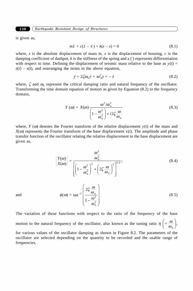
����������� ������� �������������130
is given as,
m��z + c( �z – �x ) + k(z – x) = 0 (8.1)
where, z is the absolute displacement of mass m, x is the displacement of housing, c is thedamping coefficient of dashpot, k is the stiffness of the spring and a (.) represents differentiationwith respect to time. Defining the displacement of seismic mass relative to the base as y(t) =z(t) – x(t), and rearranging the terms in the above equation,
ÿ + 2zwn �y + w 2ny = - ��x (8.2)
where, z and wn represent the critical damping ratio and natural frequency of the oscillator.Transforming the time domain equation of motion as given by Equation (8.2) to the frequencydomain,
Y (w) = X
i
n
n n
( )/w
w w
ww
z ww
2 2
2
21 2-FHG
IKJ +
(8.3)
where, Y (w) denotes the Fourier transform of the relative displacement y(t) of the mass andX(w) represents the Fourier transform of the base displacement x(t). The amplitude and phasetransfer function of the oscillator relating the relative displacement to the base displacement aregiven as,
YX
( )( )ww
=
ww
ww
z ww
2
2
2
2
2 21 2
1 2
n
n n-
FHG
IKJ + F
HGIKJ
L
NMM
O
QPP
/ ; (8.4)
and f(w) = tan-
-
F
H
GGGG
I
K
JJJJ
12
2
2
1
z wwww
n
n
(8.5)
The variation of these functions with respect to the ratio of the frequency of the base
motion to the natural frequency of the oscillator, also known as the tuning ratio h = ww n
FHG
IKJ ,
for various values of the oscillator damping as shown in Figure 8.2. The parameters of theoscillator are selected depending on the quantity to be recorded and the usable range offrequencies.
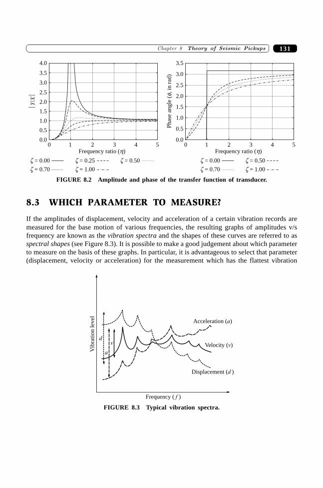
131�������� ����� �� � �� �� �����
z = 0.00 z = 0.25 z = 0.50
z = 0.70 z = 1.00
0 1 2 3 4 50.0
0.5
1.5
2.0
2.5
3.0
3.5
Frequency ratio ( )h
1.0
z = 0.00 z = 0.50
z = 0.70 z = 1.00P
has
ean
gle
(,in
rad)
f
0 1 2 3 4 50.0
0.5
1.5
2.0
2.5
3.0
4.0
Frequency ratio ( )h
1.0
�Y
X/�
3.5
FIGURE 8.2 Amplitude and phase of the transfer function of transducer.
8.3 WHICH PARAMETER TO MEASURE?
If the amplitudes of displacement, velocity and acceleration of a certain vibration records aremeasured for the base motion of various frequencies, the resulting graphs of amplitudes v/sfrequency are known as the vibration spectra and the shapes of these curves are referred to asspectral shapes (see Figure 8.3). It is possible to make a good judgement about which parameterto measure on the basis of these graphs. In particular, it is advantageous to select that parameter(displacement, velocity or acceleration) for the measurement which has the flattest vibration
Frequency ( )f
Velocity ( )v
Displacement ( )d
Acceleration ( )a
d
a
v
Vib
rati
on
level
FIGURE 8.3 Typical vibration spectra.
����������� ������� �������������132
spectrum, in the frequency-range of interest, in order to best utilise the dynamic range(the difference between the smallest and the largest values that can be measured) by theinstrumentation.
Depending on the operating range of frequencies, the seismic-mass transducers may beclassified as (i) seismometers and (ii) accelerometers. The difference in operation of these twobasic types of seismic pickups is described in detail.
8.4 SEISMOMETERS
Seismometers are the instruments with very low natural frequency in comparison to thefrequency of the vibrations to be measured so that the ratio w/wn becomes very large. It maybe noted from Figure 7.5, that as the frequency of the oscillator decreases, the relativedisplacement Y (w) of the oscillator mass approaches the base displacement X(w) irrespectiveof the value of damping. Thus the oscillator mass remains stationary while the casing of theinstrument moves with the vibrating body. Due to the requirement of very low naturalfrequency, the seismometers are often of a very large size. Moreover, the dimensions of aseismometer unit are also governed by the peak to peak maximum displacement of the vibratingbody which will be same as the maximum displacement of the vibrating base. Seismometerswith an arrangement to store the vibrations measured by the seismometer on some kind of astorage device are known as seismographs. The seismometers can be designed to work as eitherdisplacement pickups, or velocity pickups.
8.4.1 Displacement Pickups
These are used to pickup the vibration of a body when there is no fixed reference point available,e.g. in determining the movement of the chassis of a vehicle. It is, therefore, required that theseismic mass should behave (as far as possible) as though it was fixed in space. This can beachieved by having a very heavy seismic mass attached to an extremely flexible spring whichresults in a system with a very low natural frequency wn. For frequencies of vibration well abovethe natural frequency of the pickup the displacement of the seismic mass relative to the casingis practically same as the the displacement of the casing but with the phase difference of 180°as shown in Figure 7.5. This means that as the casing moves in one direction, the seismic massmoves in the opposite direction. The relative motion of the seismic-mass may either beamplified optically to record the displacement trace on a photographic film/smoke paper, or beconverted to a proportional voltage signal by using a potentiometer.
8.4.2 Velocity Pickups
A velocity pickup is designed like a displacement pickup, to have a low value of wn and tooperate at angular frequencies well above wn so that the motion of the seismic mass is virtuallythe same as that of the casing but opposite in phase. The transducer is generally a coil of wirecarried by the seismic mass which is suspended in a radial magnetic field so that a voltageproportional to velocity is generated in the coil when it is vibrated along the sensor axis. Since
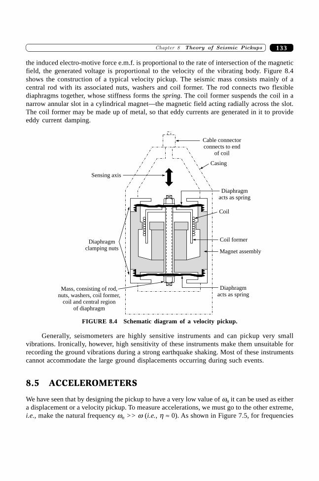
133�������� ����� �� � �� �� �����
the induced electro-motive force e.m.f. is proportional to the rate of intersection of the magneticfield, the generated voltage is proportional to the velocity of the vibrating body. Figure 8.4shows the construction of a typical velocity pickup. The seismic mass consists mainly of acentral rod with its associated nuts, washers and coil former. The rod connects two flexiblediaphragms together, whose stiffness forms the spring. The coil former suspends the coil in anarrow annular slot in a cylindrical magnet—the magnetic field acting radially across the slot.The coil former may be made up of metal, so that eddy currents are generated in it to provideeddy current damping.
Diaphragmclamping nuts
Mass, consisting of rod,nuts, washers, coil former,
coil and central regionof diaphragm
Diaphragmacts as spring
Magnet assembly
Coil former
Coil
Diaphragmacts as spring
Casing
Cable connectorconnects to end
of coil
Sensing axis
FIGURE 8.4 Schematic diagram of a velocity pickup.
Generally, seismometers are highly sensitive instruments and can pickup very smallvibrations. Ironically, however, high sensitivity of these instruments make them unsuitable forrecording the ground vibrations during a strong earthquake shaking. Most of these instrumentscannot accommodate the large ground displacements occurring during such events.
8.5 ACCELEROMETERS
We have seen that by designing the pickup to have a very low value of wn it can be used as eithera displacement or a velocity pickup. To measure accelerations, we must go to the other extreme,i.e., make the natural frequency wn >> w (i.e., h ª 0). As shown in Figure 7.5, for frequencies
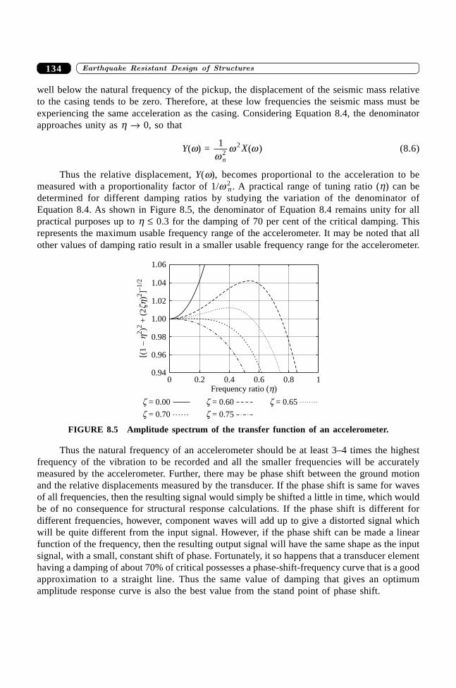
����������� ������� �������������134
well below the natural frequency of the pickup, the displacement of the seismic mass relativeto the casing tends to be zero. Therefore, at these low frequencies the seismic mass must beexperiencing the same acceleration as the casing. Considering Equation 8.4, the denominatorapproaches unity as h Æ 0, so that
Y(w) = 12
2
ww w
n
X( ) (8.6)
Thus the relative displacement, Y(w), becomes proportional to the acceleration to bemeasured with a proportionality factor of 1/w 2
n . A practical range of tuning ratio (h) can bedetermined for different damping ratios by studying the variation of the denominator ofEquation 8.4. As shown in Figure 8.5, the denominator of Equation 8.4 remains unity for allpractical purposes up to h £ 0.3 for the damping of 70 per cent of the critical damping. Thisrepresents the maximum usable frequency range of the accelerometer. It may be noted that allother values of damping ratio result in a smaller usable frequency range for the accelerometer.
0 0.2 0.4 0.6 0.8 10.94
0.96
0.98
1.00
1.02
1.04
1.06
[(1
–)
+(2
)]
2 hzh
22
–1/2
z = 0.00
Frequency ratio ( )hz = 0.60 z = 0.65
z = 0.70 z = 0.75
FIGURE 8.5 Amplitude spectrum of the transfer function of an accelerometer.
Thus the natural frequency of an accelerometer should be at least 3–4 times the highestfrequency of the vibration to be recorded and all the smaller frequencies will be accuratelymeasured by the accelerometer. Further, there may be phase shift between the ground motionand the relative displacements measured by the transducer. If the phase shift is same for wavesof all frequencies, then the resulting signal would simply be shifted a little in time, which wouldbe of no consequence for structural response calculations. If the phase shift is different fordifferent frequencies, however, component waves will add up to give a distorted signal whichwill be quite different from the input signal. However, if the phase shift can be made a linearfunction of the frequency, then the resulting output signal will have the same shape as the inputsignal, with a small, constant shift of phase. Fortunately, it so happens that a transducer elementhaving a damping of about 70% of critical possesses a phase-shift-frequency curve that is a goodapproximation to a straight line. Thus the same value of damping that gives an optimumamplitude response curve is also the best value from the stand point of phase shift.
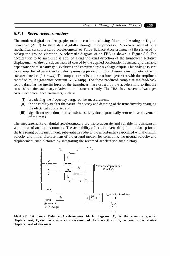
135�������� ����� �� � �� �� �����
8.5.1 Servo-accelerometers
The modern digital accelerographs make use of anti-aliasing filters and Analog to DigitalConverter (ADC) to store data digitally through microprocessor. Moreover, instead of amechanical sensor, a servo-accelerometer or Force Balance Accelerometer (FBA) is used topickup the ground vibration. A schematic diagram of an FBA is shown in Figure 8.6. Theacceleration to be measured is applied along the axial direction of the transducer. Relativedisplacement of the transducer mass M caused by the applied acceleration is sensed by a variablecapacitance with sensitivity D (volts/m) and converted into a voltage output. This voltage is sentto an amplifier of gain k and a velocity-sensing pick-up, or to a phase-advancing network withtransfer function (1 + qd/dt). The output current is fed into a force generator with the amplitudemodified by the generator constant G (N/Amp). The force produced completes the feed-backloop balancing the inertia force of the transducer mass caused by the acceleration, so that themass M remains stationary relative to the instrument body. The FBAs have several advantagesover mechanical accelerometers, such as:
(i) broadening the frequency range of the measurement,(ii) the possibility to alter the natural frequency and damping of the transducer by changing
the electrical constants, and(iii) significant reduction of cross-axis sensitivity due to practically zero relative movement
of the mass.
The measurements of digital accelerometers are more accurate and reliable in comparisonwith those of analog instruments. The availability of the pre-event data, i.e. the data prior tothe triggering of the instrument, substantially reduces the uncertainties associated with the initialvelocity and initial displacement of the ground motion for computing the ground velocity anddisplacement time histories by integrating the recorded acceleration time history.
–G
Xr
XrXa
N
N
SM
K
c
Xg
Forcegenerator
(N/Amp)G
Variable capacitancevolts/mD
R0
Eo = output voltage
k —– + 1qd
dt
FIGURE 8.6 Force Balance Accelerometer block diagram. Xg is the absolute grounddisplacement, Xa denotes absolute displacement of the mass M and Xr represents the relativedisplacement of the mass.
����������� ������� �������������136
8.5.2 Calibration of Accelerometers
The accelerometers capable of recording a constant acceleration (0 Hz/DC) signal can becalibrated using the earth’s gravitational field. The accelerometer is mounted on a tilting tablefrom which the angle q between the sensing axis and the vertical can be measured. At q = 0,the force of gravity on the seismic mass is same as the force of inertia due to an accelerationof 9.81 m/s2. At any other angle q the corresponding acceleration is 9.81 cos q m/s2. A simple90° turn produces a traceable 1 g change in acceleration and a 180° rotation produces a 2 gchange. By recording the output of the accelerometer for these acceleration levels a simple scalefactor to convert the accelerometer output to acceleration units can be established. This is asimple and easy technique for testing the accelerometer before sending it out in the field.
SUMMARY
The aims and objectives of vibration recording and monitoring are discussed. This is followedby a detailed description of the principle of operation of vibration pickups. The importantcriteria for choosing an appropriate type of vibration pickup depending on the application arediscussed.
REFERENCES
[1] Crede, C.M. and Piersol, A.G., Harris’ Shock and Vibration Handbook, 5th ed.,McGraw-Hill Professional, 2001.
[2] De Silva, C.W., Vibration: Fundamentals and Practice, CRC Press, 1999.[3] Rao, S.S., Mechanical Vibrations, 4th ed., Prentice Hall, Inc., 2003.[4] Thomson, W.T., Theory of Vibration with Applications, 3rd ed., CBS Publishers,
New Delhi, 1988.
137
Numerical Evaluation ofDynamic Response
��������
Two distinct approaches exist to evaluate the dynamic response of SDOF systems—(i) byinterpolation of the excitation, or (ii) by approximation of the derivatives in the differentialequations of motion. The first approach is based on Duhamel integral and involves interpolationof the integrand of the Duhamel integral, and therefore, is strictly applicable only for linearsystems. The second approach is applicable for both linear and nonlinear systems.
9.1 NUMERICAL SOLUTION BASED ONINTERPOLATION OF EXCITATION
If the excitation function f(t) is specified as a set of discrete values fi = f(ti) for i = 0 to N spacedat uniform interval of D t. Assuming a linear variation of the excitation function within aninterval, the variation of f(t) within an interval may be given as,
f (t) = f tftii( ) +
DD
t ; 0 £ t £ Dt
where, D fi = f (ti+1) – f (ti). The general solution for the dynamic response of an underdampedSDOF system within the time interval ti and ti+1 is given by,
vi+1 = e v tv v
tnti d
i n i
dd
- ++L
NMOQP
zw wzw
wwcos
�sin
+ --+z1 1
mf e t d
d
td
t
tn
i
i
wt w t tzw t( ) sin ( )( )
and �vi+1 = dv
dti+1
Substituting for f (t) and evaluating the integral, the recurrence relations for displacement and
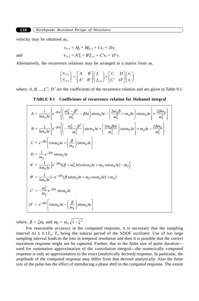
����������� ������� �������������138
velocity may be obtained as,
vi+1 = Afi + Bfi+1 + Cvi + Dvi�
and �vi+1 = A¢fi + B¢fi+1 + C¢vi + ¢D vi�
Alternatively, the recurrence relations may be arranged in a matrix form as,
v
vi
i
+
+
FHG
IKJ
1
1� =
A B
A B
f
f
C D
C D
v
vi
i
i
i¢ ¢LNM
OQPFHG
IKJ +
¢ ¢LNM
OQPFHG
IKJ+1 �
where, A, B, …,C ¢, D ¢ are the coefficients of the recurrence relation and are given in Table 9.1.
TABLE 9.1 Coefficients of recurrence relation for Duhamel integral
Ak t
e t t t t
Bk t
e tt
t t
C e
d
t d
nd
d
nd d
d
n
d
t d
nd
d
nd d
d
n
t
=
=
=
1 2 2
1 2 2
2 2
2 2 2
2 2
2 2 2
ww b
wb w w b
ww w bw
w
ww b
ww w b
ww w bw
w
b
b
b
DD D D D
DD
DD D
D
D
D
-
-
-
--
FHG
IKJ - +
FHG
IKJ
LNMM
OQPP
+RS|T|
UV|W|
--F
HGIKJ +
FHG
IKJ
LNMM
OQPP
+ -RS|T|
UV|W|
sin cos
sin cos
cosw bw
w
ww
wb w w w w w
wb w w w w
ww w
w bw
w
b
b
b
b
b
dd
d
d
td
d
tn d d d d
d
td d d d
n
d
td
td
dd
t t
D e t
Ak t
e t t t
Bk t
e t t
C e t
D e t t
D D
D
DD D D
DD D
D
D D
D
D
D
D
D
+FHG
IKJ
LNM
OQP
¢ + + -
¢ - + +
¢ -
¢ -FHG
IKJ
LNM
OQP
-
-
-
-
-
sin
sin
[( ) sin cos ]
[ ( sin cos ) ]
sin
cos sin
=
=
=
=
=
1
1
1
2
2
{ }
where, b = zwn and wd = w zn 1 2- .
For reasonable accuracy in the computed response, it is necessary that the samplinginterval D t £ 0.1Tn, Tn being the natural period of the SDOF oscillator. Use of too largesampling interval leads to the loss in temporal resolution and then it is possible that the correctmaximum response might not be captured. Further, due to the finite size of pulse duration—used for summation approximation of the convolution integral—the numerically computedresponse is only an approximation to the exact (analytically derived) response. In particular, theamplitude of the computed response may differ from that derived analytically. Also the finitesize of the pulse has the effect of introducing a phase shift in the computed response. The extent
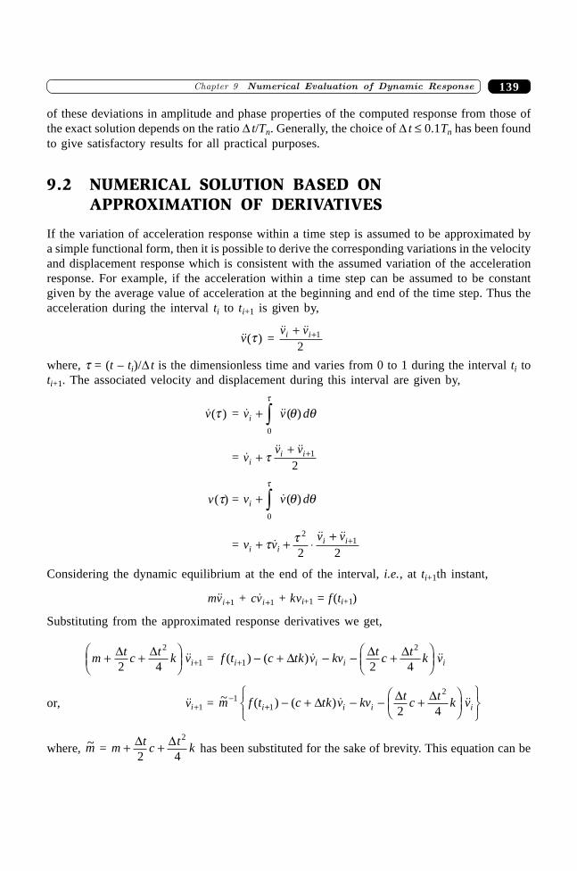
139�������� ���� ���������� ��������� �������
of these deviations in amplitude and phase properties of the computed response from those ofthe exact solution depends on the ratio D t/Tn. Generally, the choice of D t £ 0.1Tn has been foundto give satisfactory results for all practical purposes.
9.2 NUMERICAL SOLUTION BASED ONAPPROXIMATION OF DERIVATIVES
If the variation of acceleration response within a time step is assumed to be approximated bya simple functional form, then it is possible to derive the corresponding variations in the velocityand displacement response which is consistent with the assumed variation of the accelerationresponse. For example, if the acceleration within a time step can be assumed to be constantgiven by the average value of acceleration at the beginning and end of the time step. Thus theacceleration during the interval ti to ti+1 is given by,
��( )v t = �� ��v vi i+ +1
2
where, t = (t – ti)/D t is the dimensionless time and varies from 0 to 1 during the interval ti toti+1. The associated velocity and displacement during this interval are given by,
�( )v t = � ��( )v v di + z q qt
0
= ��� ��
vv v
ii i+
+ +t 1
2
v(t) = v v di + z �( )q qt
0
= v vv v
i ii i+ + ◊
+ +t t��� ��2
1
2 2
Considering the dynamic equilibrium at the end of the interval, i.e., at ti+1th instant,
mvi�� +1 + cvi� +1 + kvi+1 = f (ti+1)
Substituting from the approximated response derivatives we get,
m t c t k vi+ +FHG
IKJ +
D D2 4
2
1�� = f t c tk v kv t c t k vi i i i( ) ( ) � ��+ - + - - +FHG
IKJ1
2
2 4D D D
or, ��vi+1 = ~ ( ) ( ) � ��m f t c tk v kv t c t k vi i i i-
+ - + - - +FHG
IKJ
RSTUVW
11
2
2 4D D D
where, ~m = m t c t k+ +D D2 4
2
has been substituted for the sake of brevity. This equation can be
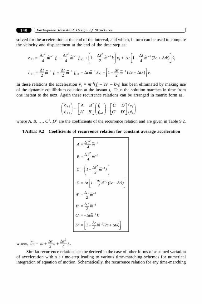
����������� ������� �������������140
solved for the acceleration at the end of the interval, and which, in turn can be used to computethe velocity and displacement at the end of the time step as:
vi+1 = D D Dt m f t m f t m k vi i i
21
21
1
21
4 41
2~ ~ ~- -
+-+ + -F
HGIKJ + D D Dt
tm c tk vi1
421- +L
NMOQP
-~ ( ) �
�vi+1 = D D D D Dtm f
tm f t m kv
tm c tk vi i i i2 2
12
21 11
1 1~ ~ ~ ~ ( ) �- -+
- -+ - + - +LNM
OQP
In these relations the acceleration ��vi = m–1( fi – cvi� – kvi) has been eliminated by making useof the dynamic equilibrium equation at the instant ti. Thus the solution marches in time fromone instant to the next. Again these recurrence relations can be arranged in matrix form as,
v
vi
i
+
+
FHG
IKJ
1
1� =
A B
A B
f
f
C D
C D
v
vi
i
i
i¢ ¢LNM
OQPFHG
IKJ +
¢ ¢LNM
OQPFHG
IKJ+1 �
where A, B, …, C ¢, D ¢ are the coefficients of the recurrence relation and are given in Table 9.2.
TABLE 9.2 Coefficients of recurrence relation for constant average acceleration
A = t4
m
B = t4
m
C = 1 t2
m k
D = t 1 t4
m (2c tk)
A = t2
m
B = t2
m
C = tm k
D = 1 t2
m (2c tk)
21
21
21
1
1
1
1
1
D
D
D
D D D
D
D
D
D D
~
~
~
~
~
~
~
~
-
-
-
-
-
-
-
-
-FHG
IKJ
- +LNM
OQP
¢
¢
¢ -
¢ - +LNM
OQP
where, ~m = m t c t k+ +D D2 4
2
.
Similar recurrence relations can be derived in the case of other forms of assumed variationof acceleration within a time-step leading to various time-marching schemes for numericalintegration of equation of motion. Schematically, the recurrence relation for any time-marching
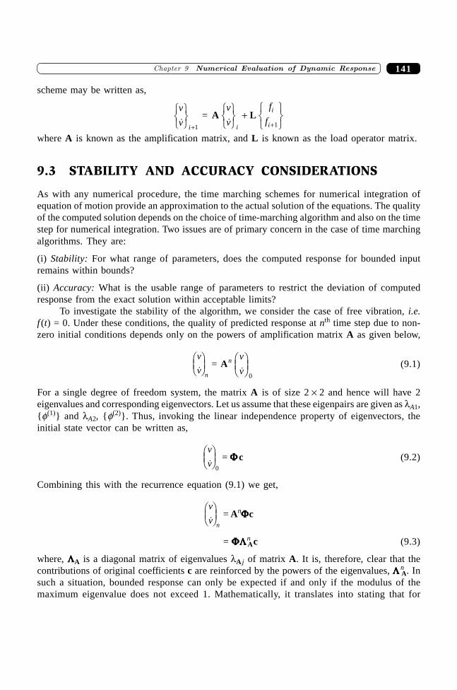
141�������� ���� ���������� ��������� �������
scheme may be written as,
v
vi�
RSTUVW +1
= A Lv
v
f
fi
i
i�RSTUVW
+RST
UVW+1
where A is known as the amplification matrix, and L is known as the load operator matrix.
9.3 STABILITY AND ACCURACY CONSIDERATIONS
As with any numerical procedure, the time marching schemes for numerical integration ofequation of motion provide an approximation to the actual solution of the equations. The qualityof the computed solution depends on the choice of time-marching algorithm and also on the timestep for numerical integration. Two issues are of primary concern in the case of time marchingalgorithms. They are:
(i) Stability: For what range of parameters, does the computed response for bounded inputremains within bounds?
(ii) Accuracy: What is the usable range of parameters to restrict the deviation of computedresponse from the exact solution within acceptable limits?
To investigate the stability of the algorithm, we consider the case of free vibration, i.e.f (t) = 0. Under these conditions, the quality of predicted response at nth time step due to non-zero initial conditions depends only on the powers of amplification matrix A as given below,
v
vn�
FHGIKJ = An v
v�FHGIKJ 0
(9.1)
For a single degree of freedom system, the matrix A is of size 2 ¥ 2 and hence will have 2eigenvalues and corresponding eigenvectors. Let us assume that these eigenpairs are given as lA1,{f(1)} and lA2, {f(2)}. Thus, invoking the linear independence property of eigenvectors, theinitial state vector can be written as,
v
v�FHGIKJ0
= FFFFF c (9.2)
Combining this with the recurrence equation (9.1) we get,
v
vn�FHGIKJ = AnFFFFFc
= FFFFFLLLLLnAc (9.3)
where, LLLLLA is a diagonal matrix of eigenvalues lA j of matrix A. It is, therefore, clear that thecontributions of original coefficients c are reinforced by the powers of the eigenvalues, LLLLL n
A. Insuch a situation, bounded response can only be expected if and only if the modulus of themaximum eigenvalue does not exceed 1. Mathematically, it translates into stating that for
����������� ������� �������������142
stability the spectral radius (rA) of A should not exceed 1:
rA = max| |j
jl A £ 1 (9.4)
In general, A can have real or complex eigenvalues and mere fulfilment of condition inEquation (9.4) does not ensure a satisfactory performance of the time marching scheme. It is,then, worthwhile to investigate the effects of eigenvalues of A on the performance of timemarching scheme. Let us consider an arbitrary complex eigenvalue lAj of A:
lAj = aj + ibj
= a b eb
aj ji
jj
j
2 2 1+ -q q; tan= (9.5)
= rj eiqj
Raising of this eigenvalue to nth power yields
l nAj = r n
j einqj
= r nj (cos nqj + i sin nqj) (9.6)
The following inferences may be drawn:
∑ positive real eigenvalues do not lead to a change in sign,∑ negative real eigenvalues lead to a change in sign at each step,∑ complex eigenvalues may lead to changes in sign, this depending on each individual
step,∑ if the modulus of the eigenvalue is smaller than 1, the involution converges toward
zero.
An algorithm for solving structural dynamics problem should be capable of reproducinga free, undamped oscillation. The reversal of direction of this oscillatory motion should not bedependent on the step-size of the integration and thus, a few complex eigenvalues must exist.If the modulus of all eigenvalues is indeed smaller than 1, stability is ensured, but the algorithmwould simulate a damped motion, a phenomenon often referred to as algorithmic damping.Thus, to achieve a satisfactory performance, we must demand the presence of complexeigenvalues with a modulus of 1.
The above-mentioned issues have to be considered in the design of an algorithm fornumerical integration of equation of motion. More often, an engineer is just interested incomputing dynamic response by using whichever method is available (in the form of a codedprogramme). To ascertain the reliability and accuracy of the computer implementation of anumerical integration algorithm, it is essential to test the performance of the code for a fewsimple bench-mark problems. A simple test which can be quickly performed is to determine thefree-vibration response of an undamped single degree of freedom system (with naturalfrequency wn rad/s) for these initial conditions:
(i) A unit initial displacement with zero initial velocity, i.e., v0 = 1.0, �v0 = 0.0
(ii) Zero initial displacement with unit initial velocity, i.e., v0 = 0.0, �v0 = 1.0.
143�������� ���� ���������� ��������� �������
The exact response for the first case is v(t) = cos wnt, whereas for the second case thesolution is v(t) = sin wnt. The numerically evaluated response is then compared with the knownsolution to evaluate the performance of the algorithm. In addition, it may also be worthwhileto compare the numerically evaluated response to harmonic excitation with the closed-formsolution of the problem discussed in the earlier chapter. In general, an error in numericallyevaluated response shows up in either or both of the following forms:
Period elongation: It is the apparent change in the natural period of vibration caused due tofinite approximation of the integration operator. A direct consequence of this error is thedistortion in the computed response waveforms in comparison with the exact response due toincremental change in phase at each time step.
Artificial damping: Also known as algorithmic damping—this is caused by the deviation fromunity of the modulus of the complex eigenvalues of the integration operator as discussed above.This leads to either artificial decay, or build-up of response amplitudes depending on whetherthe eigenvalue modulus is less than unity, or greater than unity, respectively.
The constant average acceleration algorithm is free from the artificial damping error butdoes lead to period elongation in the computed response. Due to good stability characteristics,the constant average acceleration algorithm is widely used in the numerical evaluation ofresponse of linear/nonlinear systems.
SUMMARY
The analysis of vibration problems is too tedious and cumbersome for manual calculations. Onehas to resort to numerical methods for solution of vibration problems on a digital computer. Theassumptions, formulation and limitations of the numerical algorithms used for the solution ofvibration problems are discussed and some safeguards for the correct use of these numericalmethods are described.
REFERENCES
[1] Argyris, J.H. and Mlejnek, H.P., Dynamics of Structures, North-Holland, 1991.[2] Bathe, K.J., Finite Element Procedures, Prentice Hall, Inc., 1995.[3] Nickell, R.E., “On the Stability of Approximation Operators in Problems of Structural
Dynamics”, International Journal of Solids and Structures, 7: 301–319, 1971.[4] Pegon, P., “Alternative Characterization of Time Integration Schemes”, Computer
Methods in Applied Mechanics and Engineering, 190: 2702–2727, 2001.
����������� ������� �������������144
144
Response Spectra��������
10.1 INTRODUCTION
Earthquake causes ground to vibrate and structures supported on ground are subjected to thismotion. Thus the dynamic loading on the structure during an earthquake is not external loadingbut due to motion of supports. In general, the ground motions have three translational and threerotational components. Not much information is available regarding the properties of rotationalcomponents of ground motion due to difficulties in recording those. On the other hand, thecharacteristics of translational components are relatively better known as they are routinelyrecorded and processed during strong earthquakes by an instrument known as accelerograph.Moreover, it can be deduced from the analysis of vibration records obtained from differentelevations in a structure during an earthquake that the rotational components are quite small inmagnitude in comparison with translational components. Therefore, the effects of rotationalcomponents of ground motion are usually neglected in seismic analysis of structures. Further,the response of a structure is often obtained by subjecting structure to one component of groundtranslation (acceleration). The total response of structural system is obtained by combiningresponse due to individual component, as method of superposition is valid for linear elasticsystems. Since the natural frequencies of the structure are not known a priori, complicationsarise in the design of structure necessitating several iterations. In such a situation, a designengineer requires a prescription of seismic loading that reflects frequency content, amplitude ofground motion and effect of subsequent filtering by the structure. This information is providedby Response Spectra.
In this chapter frequency content of ground motion is discussed first by means of FourierSpectrum and later the concept of response spectrum is introduced as a tool for quick dynamicanalysis.
10.2 FOURIER SPECTRA
Frequency content of an accelerogram can be conveniently depicted by Fourier Spectra. Fouriertransform of an accelerogram ��( )x t is given by
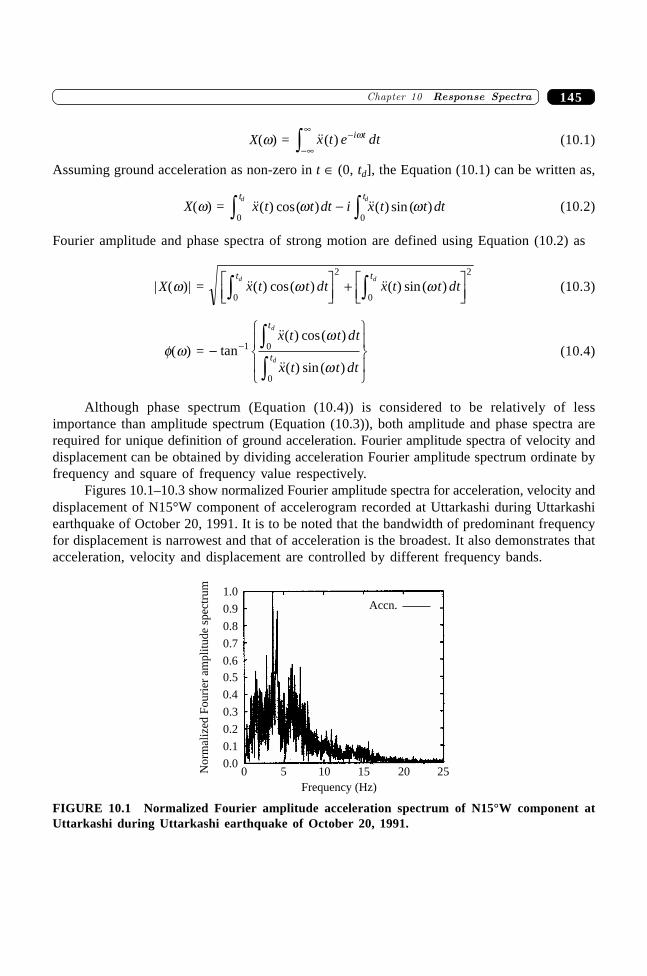
145�������� ������ ������
X(w) = ��( )x t e dti t-
-•
•z w (10.1)
Assuming ground acceleration as non-zero in t Π(0, td], the Equation (10.1) can be written as,
X(w) = ��( ) cos( ) ��( ) sin ( )x t t dt i x t t dttt dd
w w- zz 00(10.2)
Fourier amplitude and phase spectra of strong motion are defined using Equation (10.2) as
| X(w)| = 0
2
0
2t td d
x t t dt x t t dtz zLNM
OQP + L
NMOQP��( ) cos( ) ��( ) sin ( )w w (10.3)
f(w) = -
RS|
T|
UV|
W|- zz
tan��( ) cos( )
��( ) sin ( )
1 0
0
x t t dt
x t t dt
t
t
d
d
w
w(10.4)
Although phase spectrum (Equation (10.4)) is considered to be relatively of lessimportance than amplitude spectrum (Equation (10.3)), both amplitude and phase spectra arerequired for unique definition of ground acceleration. Fourier amplitude spectra of velocity anddisplacement can be obtained by dividing acceleration Fourier amplitude spectrum ordinate byfrequency and square of frequency value respectively.
Figures 10.1–10.3 show normalized Fourier amplitude spectra for acceleration, velocity anddisplacement of N15°W component of accelerogram recorded at Uttarkashi during Uttarkashiearthquake of October 20, 1991. It is to be noted that the bandwidth of predominant frequencyfor displacement is narrowest and that of acceleration is the broadest. It also demonstrates thatacceleration, velocity and displacement are controlled by different frequency bands.
0.00
0.1
0.2
0.3
0.5
0.7
0.8
0.9
1.0
No
rmal
ized
Fo
uri
eram
pli
tud
esp
ectr
um
5 10 15 20 25
0.4
0.6
Accn.
Frequency (Hz)
FIGURE 10.1 Normalized Fourier amplitude acceleration spectrum of N15°W component atUttarkashi during Uttarkashi earthquake of October 20, 1991.
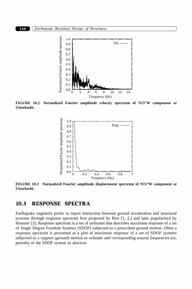
����������� ������� �������������146
0.00
0.1
0.2
0.3
0.5
0.7
0.8
0.9
1.0
No
rmal
ized
Fo
uri
eram
pli
tud
esp
ectr
um
2 4 6 8 10 12 14
0.4
0.6
Vel.
Frequency (Hz)
FIGURE 10.2 Normalized Fourier amplitude velocity spectrum of N15°W component atUttarkashi.
0.00 0.2 0.4 0.6 0.8 1
0.1
0.2
0.3
0.4
0.5
0.6
0.7
0.8
0.9
1.0Disp.
Frequency (Hz)
No
rmal
ized
Fo
uri
eram
pli
tud
esp
ectr
um
FIGURE 10.3 Normalized Fourier amplitude displacement spectrum of N15°W component atUttarkashi.
10.3 RESPONSE SPECTRA
Earthquake engineers prefer to report interaction between ground acceleration and structuralsystems through response spectrum first proposed by Biot [1, 2,] and later popularised byHousner [3]. Response spectrum is a set of ordinates that describes maximum response of a setof Single Degree Freedom Systems (SDOF) subjected to a prescribed ground motion. Often aresponse spectrum is presented as a plot of maximum response of a set of SDOF systemssubjected to a support (ground) motion as ordinate and corresponding natural frequencies (or,periods) of the SDOF system as abscissa.
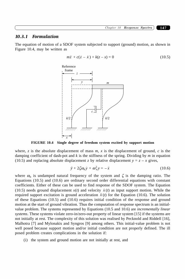
147�������� ������ ������
10.3.1 Formulation
The equation of motion of a SDOF system subjected to support (ground) motion, as shown inFigure 10.4, may be written as
m��z + c( �z – �x ) + k(z – x) = 0 (10.5)
Referenceframe
m
z
y
c
k/2k/2
x
FIGURE 10.4 Single degree of freedom system excited by support motion
where, z is the absolute displacement of mass m, x is the displacement of ground, c is thedamping coefficient of dash-pot and k is the stiffness of the spring. Dividing by m in equation(10.5) and replacing absolute displacement z by relative displacement y = z – x gives,
ÿ + 2zwn �y + w 2n y = - ��x (10.6)
where wn is undamped natural frequency of the system and z is the damping ratio. TheEquations (10.5) and (10.6) are ordinary second order differential equations with constantcoefficients. Either of these can be used to find response of the SDOF system. The Equation(10.5) needs ground displacement x(t) and velocity �x (t) as input support motion. While therequired support excitation is ground acceleration ��x (t) for the Equation (10.6). The solutionof these Equations (10.5) and (10.6) requires initial condition of the response and groundmotion at the start of ground vibration. Thus the computation of response spectrum is an initial-value problem. The systems represented by Equations (10.5 and 10.6) are incrementally linearsystems. These systems violate zero-in/zero-out property of linear system [15] if the systems arenot initially at rest. The complexity of this solution was realised by Pecknold and Riddell [16],Malhotra [7] and Mylonakis and Syngros [9] among others. This initial-value problem is notwell posed because support motion and/or initial condition are not properly defined. The illposed problem creates complications in the solution if:
(i) the system and ground motion are not initially at rest, and
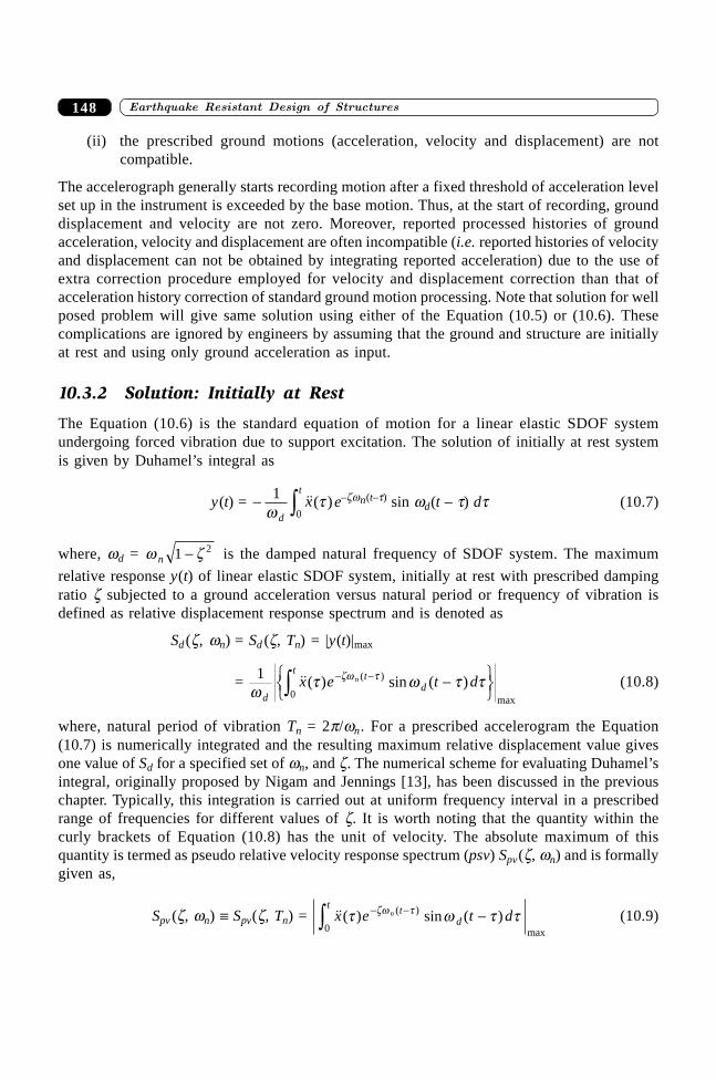
����������� ������� �������������148
(ii) the prescribed ground motions (acceleration, velocity and displacement) are notcompatible.
The accelerograph generally starts recording motion after a fixed threshold of acceleration levelset up in the instrument is exceeded by the base motion. Thus, at the start of recording, grounddisplacement and velocity are not zero. Moreover, reported processed histories of groundacceleration, velocity and displacement are often incompatible (i.e. reported histories of velocityand displacement can not be obtained by integrating reported acceleration) due to the use ofextra correction procedure employed for velocity and displacement correction than that ofacceleration history correction of standard ground motion processing. Note that solution for wellposed problem will give same solution using either of the Equation (10.5) or (10.6). Thesecomplications are ignored by engineers by assuming that the ground and structure are initiallyat rest and using only ground acceleration as input.
10.3.2 Solution: Initially at Rest
The Equation (10.6) is the standard equation of motion for a linear elastic SDOF systemundergoing forced vibration due to support excitation. The solution of initially at rest systemis given by Duhamel’s integral as
y(t) = - z10w
td
tx��( )e–zwn(t–t) sin wd(t – t) dt (10.7)
where, wd = w zn 1 2- is the damped natural frequency of SDOF system. The maximum
relative response y(t) of linear elastic SDOF system, initially at rest with prescribed dampingratio z subjected to a ground acceleration versus natural period or frequency of vibration isdefined as relative displacement response spectrum and is denoted as
Sd (z, wn) = Sd (z, Tn) = |y(t)|max
= 10w
t w t tzw t
d
tt
dx e t dnz - - -RSTUVW��( ) sin ( )( )
max
(10.8)
where, natural period of vibration Tn = 2p/wn. For a prescribed accelerogram the Equation(10.7) is numerically integrated and the resulting maximum relative displacement value givesone value of Sd for a specified set of wn, and z. The numerical scheme for evaluating Duhamel’sintegral, originally proposed by Nigam and Jennings [13], has been discussed in the previouschapter. Typically, this integration is carried out at uniform frequency interval in a prescribedrange of frequencies for different values of z. It is worth noting that the quantity within thecurly brackets of Equation (10.8) has the unit of velocity. The absolute maximum of thisquantity is termed as pseudo relative velocity response spectrum (psv) Spv(z, wn) and is formallygiven as,
Spv (z, wn) ∫ Spv(z, Tn) = 0
t tdx e t dnz - - -��( ) sin ( )( )
max
t w t tzw t (10.9)
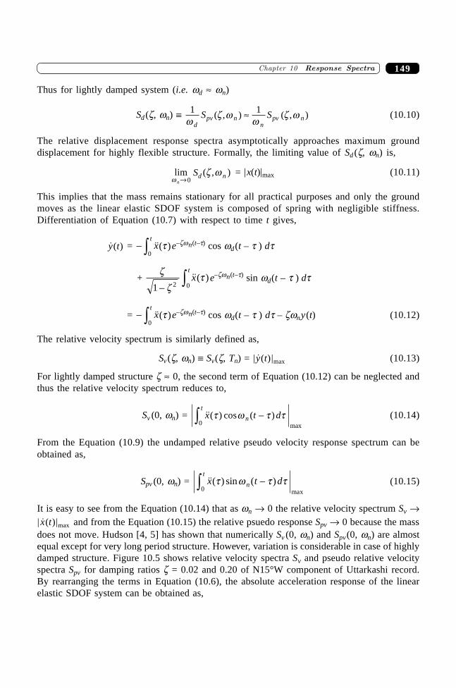
149�������� ������ ������
Thus for lightly damped system (i.e. wd ª wn)
Sd (z, wn) ∫ 1 1w
z ww
z wd
pv nn
pv nS S( , ) ( , )ª (10.10)
The relative displacement response spectra asymptotically approaches maximum grounddisplacement for highly flexible structure. Formally, the limiting value of Sd (z, wn) is,
lim ( , )w
z wn
Sd nÆ0 = |x(t)|max (10.11)
This implies that the mass remains stationary for all practical purposes and only the groundmoves as the linear elastic SDOF system is composed of spring with negligible stiffness.Differentiation of Equation (10.7) with respect to time t gives,
�( )y t = - z0t x��( )t e–zwn(t–t) cos wd(t – t ) dt
+ z
zt
1 2 0- z ��( )xt
e–zwn(t–t) sin wd(t – t ) dt
= - z0t x��( )t e–zwn(t–t) cos wd(t – t ) dt – zwny(t) (10.12)
The relative velocity spectrum is similarly defined as,
Sv(z, wn) ∫ Sv(z, Tn) = | �( )|maxy t (10.13)
For lightly damped structure z ª 0, the second term of Equation (10.12) can be neglected andthus the relative velocity spectrum reduces to,
Sv (0, wn) = 0
t
nx t dz -��( ) cos ( )max
t w t t (10.14)
From the Equation (10.9) the undamped relative pseudo velocity response spectrum can beobtained as,
Spv (0, wn) = 0
t
nx t dz -��( ) sin ( )max
t w t t (10.15)
It is easy to see from the Equation (10.14) that as wn Æ 0 the relative velocity spectrum Sv Æ| �( )|maxx t and from the Equation (10.15) the relative psuedo response Spv Æ 0 because the massdoes not move. Hudson [4, 5] has shown that numerically Sv (0, wn) and Spv(0, wn) are almostequal except for very long period structure. However, variation is considerable in case of highlydamped structure. Figure 10.5 shows relative velocity spectra Sv and pseudo relative velocityspectra Spv for damping ratios z = 0.02 and 0.20 of N15°W component of Uttarkashi record.By rearranging the terms in Equation (10.6), the absolute acceleration response of the linearelastic SDOF system can be obtained as,
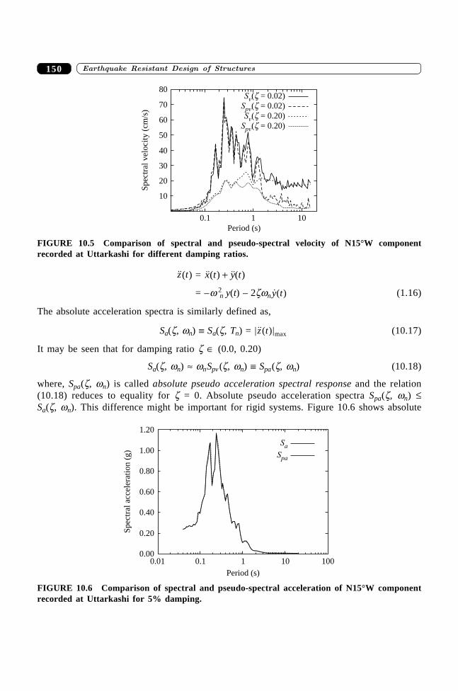
����������� ������� �������������150
��( )z t = ��( ) ��( )x t y t+
= –w 2n y(t) – 2zwn �( )y t (1.16)
The absolute acceleration spectra is similarly defined as,
Sa(z, wn) ∫ Sa(z, Tn) = |��( )|maxz t (10.17)
It may be seen that for damping ratio z Π(0.0, 0.20)
Sa(z, wn) ª wnSpv(z, wn) ∫ Spa(z, wn) (10.18)
where, Spa(z, wn) is called absolute pseudo acceleration spectral response and the relation(10.18) reduces to equality for z = 0. Absolute pseudo acceleration spectra Spa(z, wn) £Sa(z, wn). This difference might be important for rigid systems. Figure 10.6 shows absolute
0.000.01 0.1 1 10 100
Sa
Spa
0.20
0.40
0.60
0.80
1.00
1.20
Sp
ectr
alac
cele
rati
on
(g)
Period (s)
FIGURE 10.6 Comparison of spectral and pseudo-spectral acceleration of N15°W componentrecorded at Uttarkashi for 5% damping.
10
1010.1
20
30
40
50
60
70
80
Period (s)
Spec
tral
vel
oci
ty(c
m/s
)
Sv( = 0.02)zSpv( = 0.02)zSv( = 0.20)z
Spv( = 0.20)z
FIGURE 10.5 Comparison of spectral and pseudo-spectral velocity of N15°W componentrecorded at Uttarkashi for different damping ratios.
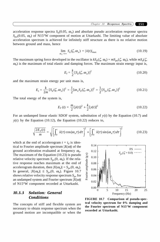
151�������� ������ ������
acceleration response spectra Sa(0.05, wn) and absolute pseudo acceleration response spectraSpa(0.05, wn) of N15°W component of motion at Uttarkashi. The limiting value of absoluteacceleration spectrum is achieved for infinitely stiff structure as there is no relative motionbetween ground and mass, hence
lim ( , )w
z wn
Sa nƕ = | ��( )|maxx t (10.19)
The maximum spring force developed in the oscillator is kSd (z, wn) = mSpa(z, wn), while mSa(z,wn) is the maximum of total elastic and damping forces. The maximum strain energy input is,
EI = k Sd n22[ ( , )]z w (10.20)
and the maximum strain energy per unit mass is,
Es = km
Sd n22[ ( , )]z w =
12
2[ ( , )]w z wn d nS = 12
2[ ( , )]Spv nz w (10.21)
The total energy of the system is,
ET (t) = m y t k y t2 2
2 2[ �( )] [ ( )]+ (10.22)
For an undamped linear elastic SDOF system, substitution of y(t) by the Equation (10.7) and�( )y t by the Equation (10.12), the Equation (10.22) reduces to,
2E tmT ( )
= ��( ) cos( ) ��( ) sin ( )x d x dn
t
n
tt w t t t w t t
0
2
0
2z zLNM
OQP + L
NMOQP (10.23)
which at the end of accelerogram t = td is iden-tical to Fourier amplitude spectrum |X(w)| of theground acceleration evaluated at frequency wn.The maximum of the Equation (10.23) is pseudorelative velocity spectrum Spv(0, wn). If the rela-tive response reaches maximum at the end ofaccelerogram duration, then |X(wn)| = Spv(0, wn).In general, |X(wn)| £ Spv(0, wn). Figure 10.7shows relative velocity response spectrum Spv foran undamped system and Fourier spectrum |X(w)|of N15°W component recorded at Uttarkashi.
10.3.3 Solution: GeneralConditions
The concepts of stiff and flexible system arenecessary to obtain response spectrum when theground motion are incompatible or when the
0.0050 10 15 20 25
0.02
0.04
0.06
0.08
0.10
0.12
0.14
Fouri
eram
pli
tude
(gs)◊
Frequency (Hz)
FS
Spv( = 0.0)z
FIGURE 10.7 Comparison of pseudo-spec-tral velocity spectrum for 0% damping andthe Fourier spectrum of N15°W componentrecorded at Uttarkashi.
����������� ������� �������������152
system/ground is not initially at rest. A SDOF system excited by support excitation is consideredto be stiff (flexible) if the natural frequency is larger (smaller) than the support excitationfrequency. Response spectrum by definition encompasses response of both stiff and flexibleSDOF systems as it prescribes maximum response for a set of SDOF systems. Moreover,absolute displacement response for a very flexible structure is zero and relative displacementresponse of a very stiff structure is zero. Thus, for a specified non-zero initial support motionboth absolute and relative displacement cannot be simultaneously zero. This requires areformulation of the problem. Let wc be a predominant (representative central) frequency of theexcitation and f (wn, wc) be a function such that f(wn, wc) approaches unity as wn Æ 0 andvanishes as wn Æ •. One such generalised function is,
f (wn, wc) = 1 0
1 0
.
. + FHG
IKJ
ww
an
c
(10.24)
where, a > 0 and the function satisfies the specified limit conditions for both flexible and stiffSDOF systems. Define a displacement u by mixing absolute and relative displacement as,
u = y + zww
ac
n
FHG
IKJ (10.25)
Addition of Equation (10.6) and Equation (10.5) multiplied by (wc /wn)a/m results in,
�� �u u un n+ +2 2zw w = - + FHG
IKJ +�� [ � ]x x xc
nn n
ww
zw wa
2 2 (10.26)
The Equation (10.26) is solved with the generalised initial condition u(0) = �u (0) = 0. Note thatthe solution requires acceleration, velocity and displacement of ground motion as excitation.Replacing absolute displacement z by y + x from Equation (10.25) the relative displacement isobtained as,
y = u xn c
n c
w ww w
a a
a a-+
(10.27)
The Equation (10.27) satisfies initial physical condition for both stiff and flexible SDOFsystems. Using Equation (10.27) the relative displacement y is obtained from the values of themixed displacement u. The required spectral displacement is the maximum of y at any time. Inmost of the cases, a simpler approximate method of solution than that of the general methodpresented above can be used satisfying limiting behaviour of SDOF system. In this method afrequency dependent initial condition is obtained from Equation (10.27) by using generalisedinitial condition u(0) = �u(0) = 0 as,
y(0) = -
+ FHG
IKJ
x
n
c
( )
.
0
10ww
a ,
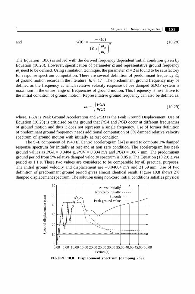
153�������� ������ ������
and �( )y 0 = -
+ FHG
IKJ
�( )
.
x a
n
c10
ww
a (10.28)
The Equation (10.6) is solved with the derived frequency dependent initial condition given byEquation (10.28). However, specification of parameter a and representative ground frequencywc need to be defined. Using simulation technique, the parameter a = 2 is found to be satisfactoryfor response spectrum computation. There are several definition of predominant frequency wc
of ground motion records in the literature [6, 8, 17]. The predominant ground frequency may bedefined as the frequency at which relative velocity response of 5% damped SDOF system ismaximum in the entire range of frequencies of ground motion. This frequency is insensitive tothe initial condition of ground motion. Representative ground frequency can also be defined as,
wc = PGAPGD
(10.29)
where, PGA is Peak Ground Acceleration and PGD is the Peak Ground Displacement. Use ofEquation (10.29) is criticised on the ground that PGA and PGD occur at different frequenciesof ground motion and thus it does not represent a single frequency. Use of former definitionof predominant ground frequency needs additional computation of 5% damped relative velocityspectrum of ground motion with initially at rest condition.
The S–E component of 1940 El Centro accelerogram [14] is used to compute 2% dampedresponse spectrum for initially at rest and at non zero condition. The accelerogram has peakground values as PGA = 0.3484 g, PGV = 0.334 m/s and PGD = 108.7 mm. The predominantground period from 5% relative damped velocity spectrum is 0.85 s. The Equation (10.29) givesperiod as 1.1 s. These two values are considered to be comparable for all practical purposes.The initial ground velocity and displacement are – 0.04664 m/s and 21.59 mm. Use of twodefinition of predominant ground period gives almost identical result. Figure 10.8 shows 2%damped displacement spectrum. The solution using non-zero initial conditions satisfies physical
00.00 5.00 10.00 15.00 20.00 25.00 30.00 35.00 40.00 45.00 50.00
Period (s)
10
20
30
40
50
60
Spec
tral
dis
pla
cem
ent
(cm
)
At rest initially
Non-zero initially
Smooth
Peak ground value
FIGURE 10.8 Displacement spectrum (damping 2%).
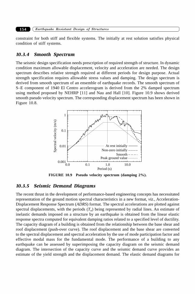
����������� ������� �������������154
constraint for both stiff and flexible systems. The initially at rest solution satisfies physicalcondition of stiff systems.
10.3.4 Smooth Spectrum
The seismic design specification needs prescription of required strength of structure. In dynamiccondition maximum allowable displacement, velocity and acceleration are needed. The designspectrum describes relative strength required at different periods for design purpose. Actualstrength specification requires allowable stress values and damping. The design spectrum isderived from smooth spectrum of an ensemble of earthquake records. The smooth spectrum ofS–E component of 1940 El Centro accelerogram is derived from the 2% damped spectrumusing method proposed by NEHRP [11] and Nau and Hall [10]. Figure 10.9 shows derivedsmooth pseudo velocity spectrum. The corresponding displacement spectrum has been shown inFigure 10.8.
0.0 0.1 1.0 10.0
Period (s)
0.001
0.01
0.1
1
Spec
tral
vel
oci
ty(m
/s)
At rest initially
Non-zero initially
SmoothPeak ground value
FIGURE 10.9 Pseudo velocity spectrum (damping 2%).
10.3.5 Seismic Demand Diagrams
The recent thrust in the development of performance-based engineering concepts has necessitatedrepresentation of the ground motion spectral characteristics in a new format, viz., Acceleration-Displacement Response Spectrum (ADRS) format. The spectral accelerations are plotted againstspectral displacements, with the periods (Tn) being represented by radial lines. An estimate ofinelastic demands imposed on a structure by an earthquake is obtained from the linear elasticresponse spectra computed for equivalent damping ratios related to a specified level of ductility.The capacity diagram of a building is obtained from the relationship between the base shear androof displacement (push-over curve). The roof displacement and the base shear are convertedto the spectral displacement and spectral acceleration by the use of mode participation factor andeffective modal mass for the fundamental mode. The performance of a building to anyearthquake can be assessed by superimposing the capacity diagram on the seismic demanddiagram. The intersection of the capacity curve and the seismic demand curve provides anestimate of the yield strength and the displacement demand. The elastic demand diagrams for
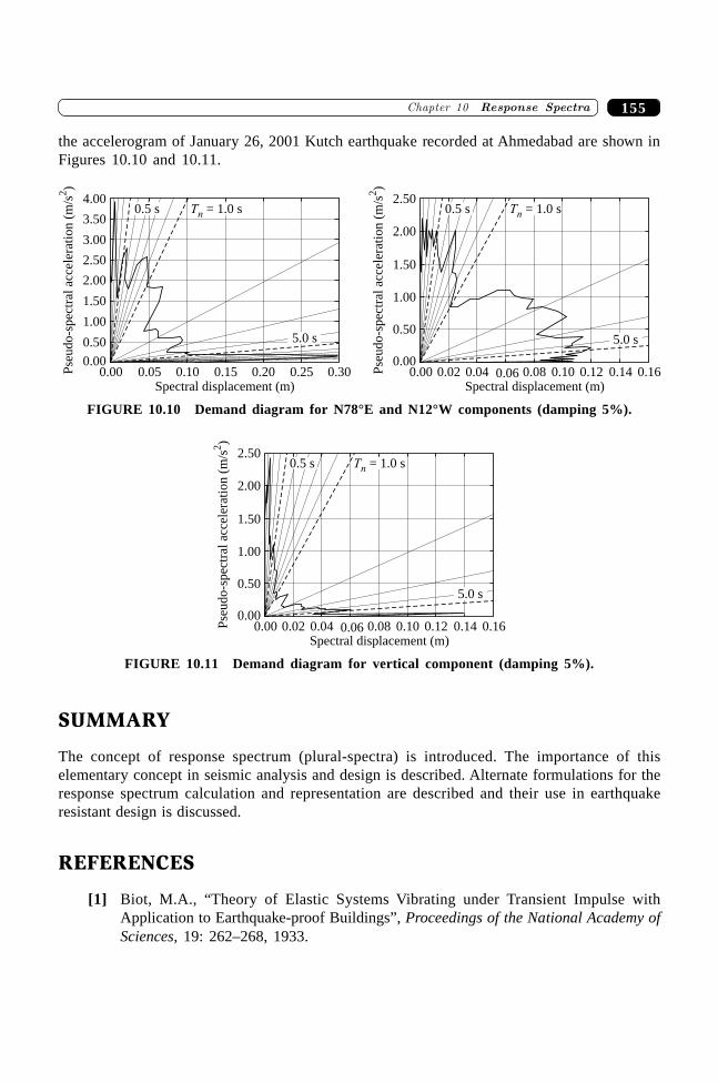
155�������� ������ ������
the accelerogram of January 26, 2001 Kutch earthquake recorded at Ahmedabad are shown inFigures 10.10 and 10.11.
0.00 0.05 0.10 0.15 0.20 0.25 0.300.00
0.50
1.00
1.50
2.00
2.50
3.00
3.50
4.00Tn = 1.0 s0.5 s
5.0 s
Spectral displacement (m)
Pse
ud
o-s
pec
tral
acce
lera
tio
n(m
/s)
2
0.00 0.020.00
0.50
1.00
1.50
2.00
2.500.5 s
Spectral displacement (m)P
seu
do
-sp
ectr
alac
cele
rati
on
(m/s
)2
0.04 0.06 0.08 0.10 0.12 0.14 0.16
Tn = 1.0 s
5.0 s
FIGURE 10.10 Demand diagram for N78°E and N12°W components (damping 5%).
0.00 0.020.00
0.50
1.00
1.50
2.00
2.500.5 s
Spectral displacement (m)
Pse
ud
o-s
pec
tral
acce
lera
tio
n(m
/s)
2
0.04 0.06 0.08 0.10 0.12 0.14 0.16
5.0 s
Tn = 1.0 s
FIGURE 10.11 Demand diagram for vertical component (damping 5%).
SUMMARY
The concept of response spectrum (plural-spectra) is introduced. The importance of thiselementary concept in seismic analysis and design is described. Alternate formulations for theresponse spectrum calculation and representation are described and their use in earthquakeresistant design is discussed.
REFERENCES
[1] Biot, M.A., “Theory of Elastic Systems Vibrating under Transient Impulse withApplication to Earthquake-proof Buildings”, Proceedings of the National Academy ofSciences, 19: 262–268, 1933.

����������� ������� �������������156
[2] Biot, M.A., “A Mechanical Analyser for the Prediction of Earthquake Stresses”,Bulletin of the Seismological Society of America, 31: 151–171, 1941.
[3] Housner, G.W., “Calculating the Response of an Oscillator to Arbitrary Ground Motion”.Bulletin of the Seismological Society of America, 31: 143–149, 1941.
[4] Hudson, D.E., “Response Spectrum Techniques in Engineering Seismology”, InProceedings of the First World Conference on Earthquake Engineering, 4: 1–12.Earthquake Engineering Research Institute, Los Angeles, California, 1956.
[5] Hudson, D.E., “Some Problems in the Application of Spectrum Technique to StrongMotion Earthquake Analysis”, Bulletin of the Seismological Society of America, 52(2):417–430, 1962.
[6] Kramar, S.L., Geotechnical Earthquake Engineering, Prentice Hall, Inc., New Jersey,1996.
[7] Malhotra, P.K., “Response Spectrum of Incompatible Acceleration, Velocity andDisplacement Histories”, Earthquake Engineering and Structural Dynamics, 30: 279–286, 2001.
[8] Miranda, E. and Bertero, V.V., “Evaluation of Strength Reduction Factors for Earth-quake-resistant Design”, Earthquake Spectra, 10(2): 357–379, 1994.
[9] Mylonakis, G. and Syngros, C., “Discussion of Response Spectrum of IncompatibleAcceleration, Velocity and Displacement Histories”, Earthquake Engineering andStructural Dynamics, 31: 1025–1031, 2002.
[10] Nau, J.M. and Hall, W.J., “Scaling Methods for Earthquake Response Spectra”,Journal of Structural Engineering Division, ASCE, 110(7): 1533–1548, 1984.
[11] NEHRP, “Recommended Provisions for Seismic Regulation for New Buildings andOther Structures”, Technical Report, Building Safety Council for Federal EmergencyManagement Agency, Washington D.C., 1997.
[12] Newmark, N.M., “A Method of Computation for Structural Dynamics”, Journal ofEngineering Mechanics Division, ASCE, 85: 67–94, 1959.
[13] Nigam, N.C. and Jennings, P.C., “Calculation of Response Spectra From StrongMotion Earthquake Records”, Bulletin of the Seismological Society of America, 59(2):909–922, 1969.
[14] NOAA, Earthquake Strong Motion: CDROM, National Geophysical Data Center,Boulder Colorado, March 1996.
[15] Oppenheim, A.V., Willisky, A.S., and Young, I.T., Signals and Systems, Prentice Hall,Inc., New Jersey, 1983.
[16] Pecknold, D.A. and Riddell, R., “Effect of Initial Base Motion on Response Spectra”.Journal of Engineering Mechanics Division, ASCE, 104(2): 485–491, 1978.
[17] Rathje, E., Abrahamson, N., and Bray, J., “Simplified Frequency Content Estimatesof Earthquake Ground Motions”, Journal of Geotechnical and GeoenvironmentalEngineering, ASCE, 124(2): 150–159, 1998.
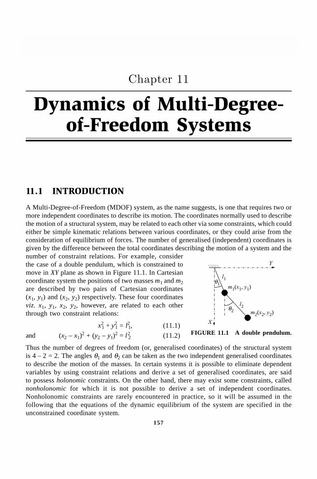
157�������� ���������� ��������������������������
157
Dynamics of Multi-Degree-of-Freedom Systems
��������
11.1 INTRODUCTION
A Multi-Degree-of-Freedom (MDOF) system, as the name suggests, is one that requires two ormore independent coordinates to describe its motion. The coordinates normally used to describethe motion of a structural system, may be related to each other via some constraints, which couldeither be simple kinematic relations between various coordinates, or they could arise from theconsideration of equilibrium of forces. The number of generalised (independent) coordinates isgiven by the difference between the total coordinates describing the motion of a system and thenumber of constraint relations. For example, considerthe case of a double pendulum, which is constrained tomove in XY plane as shown in Figure 11.1. In Cartesiancoordinate system the positions of two masses m1 and m2are described by two pairs of Cartesian coordinates(x1, y1) and (x2, y2) respectively. These four coordinatesviz. x1, y1, x2, y2, however, are related to each otherthrough two constraint relations:
x21 + y2
1 = l21, (11.1)
and (x2 – x1)2 + (y2 – y1)2 = l2
2 (11.2)
Thus the number of degrees of freedom (or, generalised coordinates) of the structural systemis 4 – 2 = 2. The angles q1 and q2 can be taken as the two independent generalised coordinatesto describe the motion of the masses. In certain systems it is possible to eliminate dependentvariables by using constraint relations and derive a set of generalised coordinates, are saidto possess holonomic constraints. On the other hand, there may exist some constraints, callednonholonomic for which it is not possible to derive a set of independent coordinates.Nonholonomic constraints are rarely encountered in practice, so it will be assumed in thefollowing that the equations of the dynamic equilibrium of the system are specified in theunconstrained coordinate system.
Y
X
l2
l1
q2
q1m x y1 1 1( , )
m x y2 2 2( , )
FIGURE 11.1 A double pendulum.
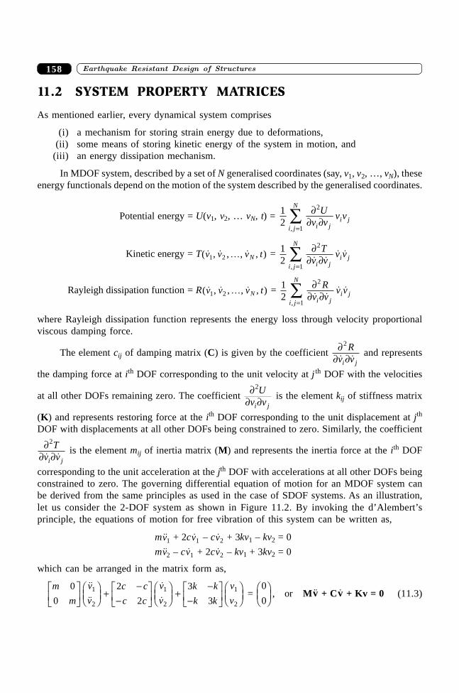
������ ���������������������� �� ���158
11.2 SYSTEM PROPERTY MATRICES
As mentioned earlier, every dynamical system comprises
(i) a mechanism for storing strain energy due to deformations,(ii) some means of storing kinetic energy of the system in motion, and
(iii) an energy dissipation mechanism.
In MDOF system, described by a set of N generalised coordinates (say, v1, v2, …, vN), theseenergy functionals depend on the motion of the system described by the generalised coordinates.
Potential energy = U(v1, v2, … vN, t) = 12
2
1
∂∂ ∂
=Â U
v vv v
i ji j
i j
N
,
Kinetic energy = T( � , � , , � , )v v v tN1 2 º = 12
2
1
∂∂ ∂
=Â T
v vv v
i ji j
i j
N
� �� �
,
Rayleigh dissipation function = R( � , � , , � , )v v v tN1 2 º = 12
2
1
∂∂ ∂
=Â R
v vv v
i ji j
i j
N
� �� �
,
where Rayleigh dissipation function represents the energy loss through velocity proportionalviscous damping force.
The element cij of damping matrix (C) is given by the coefficient ∂∂ ∂
2 Rv vi j� � and represents
the damping force at ith DOF corresponding to the unit velocity at j th DOF with the velocities
at all other DOFs remaining zero. The coefficient ∂∂ ∂
2Uv vi j
is the element kij of stiffness matrix
(K) and represents restoring force at the ith DOF corresponding to the unit displacement at jth
DOF with displacements at all other DOFs being constrained to zero. Similarly, the coefficient
∂∂ ∂
2Tv vi j� � is the element mij of inertia matrix (M) and represents the inertia force at the ith DOF
corresponding to the unit acceleration at the jth DOF with accelerations at all other DOFs beingconstrained to zero. The governing differential equation of motion for an MDOF system canbe derived from the same principles as used in the case of SDOF systems. As an illustration,let us consider the 2-DOF system as shown in Figure 11.2. By invoking the d’Alembert’sprinciple, the equations of motion for free vibration of this system can be written as,
m��v1 + 2c �v1 – c �v2 + 3kv1 – kv2 = 0
m��v2 – c �v1 + 2c �v2 – kv1 + 3kv2 = 0
which can be arranged in the matrix form as,
m
m
v
v
c c
c c
v
v
k k
k k
v
v
0
0
2
2
3
31
2
1
2
1
2
LNM
OQPFHG
IKJ +
--LNM
OQPFHG
IKJ +
--LNM
OQPFHG
IKJ
����
��
= 0
0FHGIKJ , or M��v + C �v + Kv = 0 (11.3)
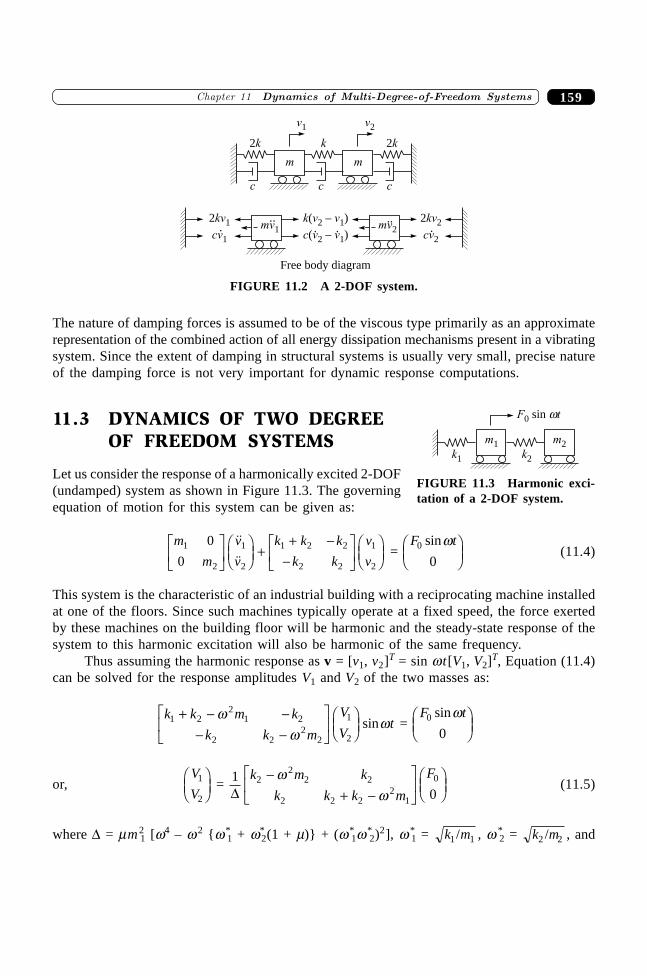
159�������� ���������� ��������������������������
The nature of damping forces is assumed to be of the viscous type primarily as an approximaterepresentation of the combined action of all energy dissipation mechanisms present in a vibratingsystem. Since the extent of damping in structural systems is usually very small, precise natureof the damping force is not very important for dynamic response computations.
11.3 DYNAMICS OF TWO DEGREEOF FREEDOM SYSTEMS
Let us consider the response of a harmonically excited 2-DOF(undamped) system as shown in Figure 11.3. The governingequation of motion for this system can be given as:
m
m
v
v
k k k
k k
v
v1
2
1
2
1 2 2
2 2
1
2
0
0LNM
OQPFHG
IKJ +
+ --
LNM
OQPFHG
IKJ
����
= F t0
0
sinwFHG
IKJ (11.4)
This system is the characteristic of an industrial building with a reciprocating machine installedat one of the floors. Since such machines typically operate at a fixed speed, the force exertedby these machines on the building floor will be harmonic and the steady-state response of thesystem to this harmonic excitation will also be harmonic of the same frequency.
Thus assuming the harmonic response as v = [v1, v2]T = sin w t[V1, V2]T, Equation (11.4)can be solved for the response amplitudes V1 and V2 of the two masses as:
k k m k
k k m
V
Vt1 2
21 2
2 22
2
1
2
+ - -- -
LNM
OQPFHG
IKJ
ww
wsin = F t0
0
sinwFHG
IKJ
or,V
V1
2
FHG
IKJ = 1
02
22 2
2 2 22
1
0
Dk m k
k k k m
F-+ -
LNM
OQPFHG
IKJ
ww
(11.5)
where D = mm21 [w4 – w 2 {w*
1 + w*2(1 + m)} + (w*
1w*2)2], w *
1 = k m1 1/ , w *2 = k m2 2/ , and
k v v2 1( – )
m
c
2k
v1
m
c
k
v2
c
2k
mv1c v v2 1( – )
2kv1
cv1
mv22kv2
cv2
Free body diagram
...
. ...
.
FIGURE 11.2 A 2-DOF system.
m1
k1 k2
m2
F0 sin wt
FIGURE 11.3 Harmonic exci-tation of a 2-DOF system.
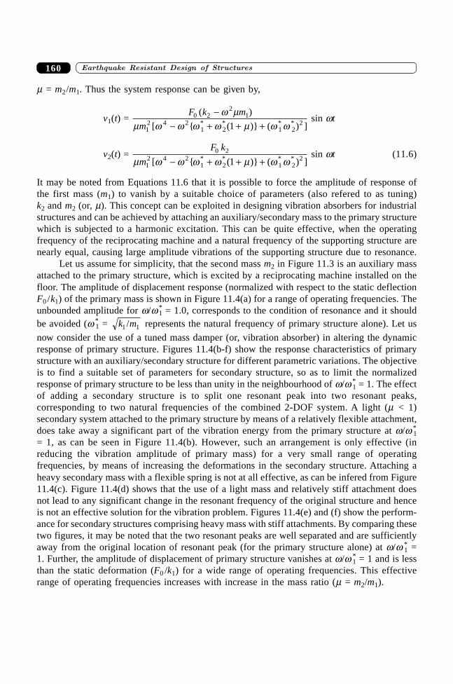
������ ���������������������� �� ���160
m = m2/m1. Thus the system response can be given by,
v1(t) = F k m
m0 2
21
12 4 2
1 2 1 221
( )
[ { ( )} ( ) ]* * * *
-- + + +
w mm w w w w m w w
sin wt
v2(t) = F k
m0 2
12 4 2
1 2 1 221m w w w w m w w[ { ( )} ( ) ]* * * *- + + +
sin wt (11.6)
It may be noted from Equations 11.6 that it is possible to force the amplitude of response ofthe first mass (m1) to vanish by a suitable choice of parameters (also refered to as tuning)k2 and m2 (or, m). This concept can be exploited in designing vibration absorbers for industrialstructures and can be achieved by attaching an auxiliary/secondary mass to the primary structurewhich is subjected to a harmonic excitation. This can be quite effective, when the operatingfrequency of the reciprocating machine and a natural frequency of the supporting structure arenearly equal, causing large amplitude vibrations of the supporting structure due to resonance.
Let us assume for simplicity, that the second mass m2 in Figure 11.3 is an auxiliary massattached to the primary structure, which is excited by a reciprocating machine installed on thefloor. The amplitude of displacement response (normalized with respect to the static deflectionF0 /k1) of the primary mass is shown in Figure 11.4(a) for a range of operating frequencies. Theunbounded amplitude for w/w *
1 = 1.0, corresponds to the condition of resonance and it shouldbe avoided (w *
1 = k m1 1/ represents the natural frequency of primary structure alone). Let us
now consider the use of a tuned mass damper (or, vibration absorber) in altering the dynamicresponse of primary structure. Figures 11.4(b-f) show the response characteristics of primarystructure with an auxiliary/secondary structure for different parametric variations. The objectiveis to find a suitable set of parameters for secondary structure, so as to limit the normalizedresponse of primary structure to be less than unity in the neighbourhood of w/w *
1 = 1. The effectof adding a secondary structure is to split one resonant peak into two resonant peaks,corresponding to two natural frequencies of the combined 2-DOF system. A light (m < 1)secondary system attached to the primary structure by means of a relatively flexible attachment,does take away a significant part of the vibration energy from the primary structure at w/w *
1= 1, as can be seen in Figure 11.4(b). However, such an arrangement is only effective (inreducing the vibration amplitude of primary mass) for a very small range of operatingfrequencies, by means of increasing the deformations in the secondary structure. Attaching aheavy secondary mass with a flexible spring is not at all effective, as can be infered from Figure11.4(c). Figure 11.4(d) shows that the use of a light mass and relatively stiff attachment doesnot lead to any significant change in the resonant frequency of the original structure and henceis not an effective solution for the vibration problem. Figures 11.4(e) and (f) show the perform-ance for secondary structures comprising heavy mass with stiff attachments. By comparing thesetwo figures, it may be noted that the two resonant peaks are well separated and are sufficientlyaway from the original location of resonant peak (for the primary structure alone) at w/w *
1 =1. Further, the amplitude of displacement of primary structure vanishes at w/w *
1 = 1 and is lessthan the static deformation (F0 /k1) for a wide range of operating frequencies. This effectiverange of operating frequencies increases with increase in the mass ratio (m = m2/m1).
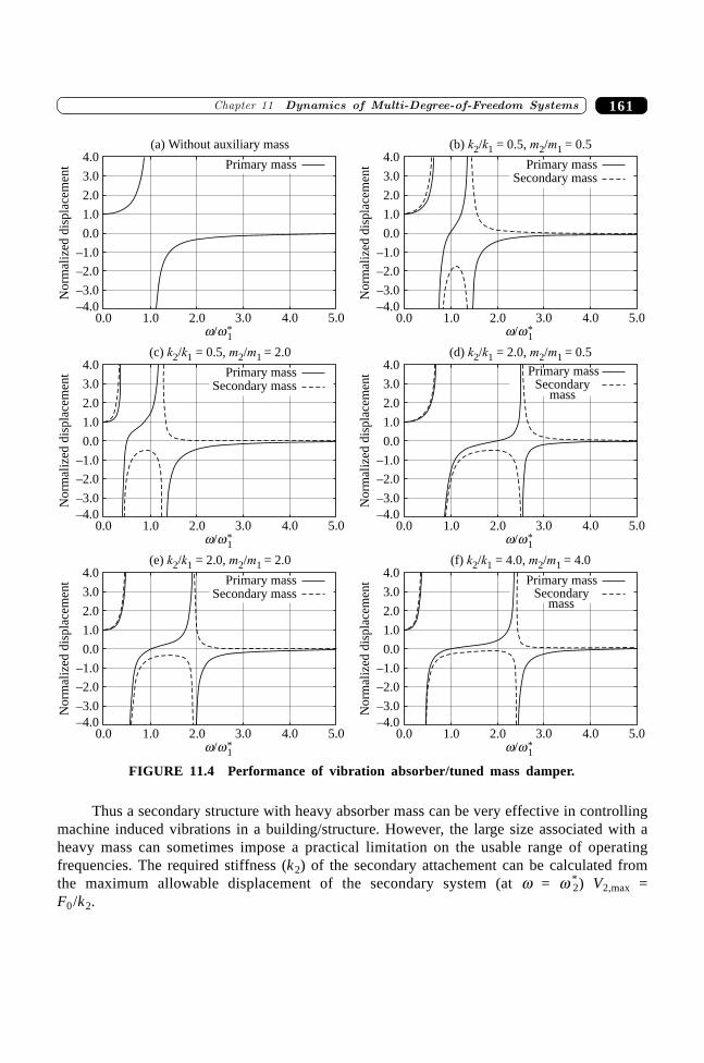
161�������� ���������� ��������������������������
Primary mass
0.0 1.0 2.0 3.0 4.0 5.0–4.0
–3.0
–2.0
–1.0
0.0
1.0
2.0
3.0
4.0
Norm
aliz
eddis
pla
cem
ent
w/w1*
(a) Without auxiliary mass
Primary mass
0.0 1.0 2.0 3.0 4.0 5.0–4.0
–3.0
–2.0
–1.0
0.0
1.0
2.0
3.0
4.0
Norm
aliz
eddis
pla
cem
ent
w/w*1
(b) / = 0.5, / = 0.5k k m m2 1 2 1
Secondary mass
Primary mass
0.0 1.0 2.0 3.0 4.0 5.0–4.0
–3.0
–2.0
–1.0
0.0
1.0
2.0
3.0
4.0
Norm
aliz
eddis
pla
cem
ent
w/w*1
Secondary massPrimary mass
0.0 1.0 2.0 3.0 4.0 5.0–4.0
–3.0
–2.0
–1.0
0.0
1.0
2.0
3.0
4.0N
orm
aliz
eddis
pla
cem
ent
w/w*1
(d) / = 2.0, / = 0.5k k m m2 1 2 1
Secondarymass
(c) / = 0.5, / = 2.0k k m m2 1 2 1
Primary mass
0.0 1.0 2.0 3.0 4.0 5.0–4.0
–3.0
–2.0
–1.0
0.0
1.0
2.0
3.0
4.0
Norm
aliz
eddis
pla
cem
ent
w/w*1
Secondary massPrimary mass
0.0 1.0 2.0 3.0 4.0 5.0–4.0
–3.0
–2.0
–1.0
0.0
1.0
2.0
3.0
4.0
Norm
aliz
eddis
pla
cem
ent
w/w*1
(f) / = 4.0, / = 4.0k k m m2 1 2 1
Secondarymass
(e) / = 2.0, / = 2.0k k m m2 1 2 1
FIGURE 11.4 Performance of vibration absorber/tuned mass damper.
Thus a secondary structure with heavy absorber mass can be very effective in controllingmachine induced vibrations in a building/structure. However, the large size associated with aheavy mass can sometimes impose a practical limitation on the usable range of operatingfrequencies. The required stiffness (k2) of the secondary attachement can be calculated fromthe maximum allowable displacement of the secondary system (at w = w *
2) V2,max =F0/k2.
������ ���������������������� �� ���162
11.4 FREE VIBRATION ANALYSIS OF MDOFSYSTEMS
By considering the fact that the damping levels are usually very small in structural systems, letus consider the response of an undamped MDOF system. The effect of damping will be dealtwith at a later stage. The equation of free vibration then reduces to,
M��v + Kv = 0 (11.7)
We look for a solution in the form vi = q(t)fi, i = 1, 2, …, N, where the dependence on timeand that on space variables can be separated. This implies that the ratio of amplitudes of anytwo coordinates is independent of time. Physically, it implies that all degrees of freedomperform synchronous motion and the system configuration does not change its shape duringmotion but only its amplitude changes.
Substituting for v, the equation of motion may be written as,
M{f} ��q(t) + K{f}q(t) = 0 (11.8)
which is a set of N simultaneous equations of the type
m q t k q tij jj
N
ij jj
N
f f��( ) ( )= =
 Â+1 1
= 0; i = 1, 2, …, N (11.9)
where the separation of variables leads to
-��( )( )
q tq t
= k
m
ij jj
N
ij jj
N
f
f=
=
ÂÂ
1
1
; i = 1, 2, …, N (11.10)
Since the terms on either side of the equality sign are independent of each other, this equalitycan hold only when each of these terms are equal to a positive constant (say, w2).1 Thus we have,
��q(t) + w2q(t) = 0 (11.11)
( )k mij ij jj
N
-=
 w f2
1
= 0; i = 1, 2, …, N. (11.12)
The solution of Equation (11.11) is q(t) = sin(wt – a), a harmonic of frequency w. Thus wemay conclude that the motion of all coordinates is harmonic with same frequency w and samephase difference a. However, it still needs to be established if such a synchronous, harmonicmotion is possible for all frequencies. To investigate this issue let us consider the Equation
1The choice of the sign is dictated by physical considerations. For a conservative system the displacements mustremain finite at all instances. If we had chosen a negative constant then the solution would involve exponentialfunctions which would grow without bounds with time t. The choice of positive constant, on the other hand,provides a harmonic solution which has finite energy at all times.
163�������� ���������� ��������������������������
(11.12), which is a set of N simultaneous linear homogeneous equations in unknowns fj. Theproblem of determining constant (w2) for which the Equation (11.12) has a non-trivial solutionis known as the characteristic value or eigenvalue problem. The eigenvalue problem may berewritten, in matrix notation as,
(K – w2M){f} = 0 (11.13)
A non-trivial solution for Equation (11.13) is feasible only when the determinant of thecoefficient matrix vanishes, i.e.,
|K – w 2M | = 0 (11.14)
The expansion of the determinant in Equation (11.14) yields an algebraic equation of Nth orderin w2, which is known as the characteristic equation. The roots of characteristic equation areknown as the eigenvalues and the positive square root of these eigenvalues are known as thenatural frequencies (wi) of the MDOF system. It is only at these N frequencies that the systemadmits synchronous motion at all coordinates. For stable structural systems with symmetric andpositive definite stiffness and mass matrices the eigenvalues will always be real and positive. Foreach eigenvalue the resulting synchronous motion has a distinct shape and is known as natural/normal mode shape or eigenvector. The normal modes are as much a characteristic of the systemas the eigenvalues are. They depend on the inertia and stiffness, as reflected by the coefficientsmij and kij. These shapes correspond to those structural configurations, in which the inertia forcesimposed on the structure due to synchronous harmonic vibrations are exactly balanced by theelastic restoring forces within the structural system. These eigenvectors are determined as thenon-trivial solution of Equation (11.13). Since the determinant of the coefficient matrixevaluated at one of the natural frequencies is singular, a unique solution for eigenvectors cannot be found. It is, however, possible to compute the amplitudes of the synchronous motion atN – 1 coordinates relative to the amplitude of motion at the remaining coordinate, which maybe selected arbitrarily. Thus an additional constraint—known as normalisation condition—mustbe supplied in addition to Equation (11.13) to completely determine an eigenvector. Two of themost commonly used normalisation procedures are:
(i) assume the amplitude of synchronous motion at the first degree of freedom as unity,(ii) constrain a length measure of the eigenvector to be unity. For example, for any eigen-
vector {f (i)} it is possible to determine elements of {f (i)} such that {f i}TM{f (i)} = 1.Such a normalisation, using mass/inertia matrix (M) is known as mass renormalisationand the resulting mode shape is known as mass orthonormal mode shape.
It can be shown that the N eigenvectors of an N-DOF system completely span the N-dimensionalvector space, and therefore, can be used as basis vectors for representing any Nth order vector.Since the condition of orthogonality is a necessary condition for any set of base vectors, it willnow be shown that the eigenvectors also satisfy this condition.
11.4.1 Orthogonality Conditions
An important property of the mode shapes or eigenvectors is that they are mutually orthogonalwith respect to the mass and stiffness matrices. More precisely, the product involving
������ ���������������������� �� ���164
multiplication of mode shapes corresponding to two different modes vanishes.
{f ( j)}T [M]{f (i)} = Midij and {f(j)}T [K]{f (i)} = Kidij (11.15)
where Mi and Ki are called the generalised mass and stiffness respectively for the i th mode anddij is the Kronecker delta. For the case when mode shapes have been orthonormalized withrespect to the mass, Mi = 1 and Ki = w 2
i .In order to prove this proposition, let us assume that w 2
i and {f (i)} denote the eigenvalueand corresponding eigenvector for i th mode and w 2
j and {f ( j)} correspond to the j(π i)th mode.It follows that both of these eigenpairs satisfy Equation (11.13). Thus,
K{f(i)} = w 2iM{f(i)} (11.16)
K{f( j)} = w 2j M{f(j)} (11.17)
Pre-multiplying Equation (11.16) by {f(j)}T and Equation (11.17) by {f(i)}T, we get,
{f(j)}TK{f(i)} = w2i {f(j)}TM{f(i)} (11.18)
{f(i)}TK{f(j)} = w 2j {f(i)}TM{f(j)} (11.19)
Subtracting Equation (11.19) from Equation (11.18) and noting {f(j)}TK{f(i)} = ({f(i)}TKT{f(j)})T
and the fact that K and M are symmetric matrices we have,
(w 2i – w 2
j){f(j)}TM{f(i)} = 0 (11.20)
For all modes i π j with distinct eigenvalues (w i π wj), Equation (11.20) can be specified onlyif the matrix inner product {f(j)}TM{f(i)} vanishes. This proves the first half of the propositionstated in Equation (11.15). The other half follows by substituting this result in either ofEquation (11.18) or (11.19).
Since the computed mode shapes of a N-DOF system form a set of orthogonal vectors, theyspan the N-dimensional space completely. In other words, these mode shapes can be used as aset of basis vectors in the N-dimensional space and any vector in this space can be representedas a linear combination of these mode-shapes.
The orthogonality property of mode shapes leads to a very powerful theorem, modalexpansion theorem, which states that any vector x in N-dimensional vector space can berepresented as a linear combination of mode-shape vectors,
x = qii
i
N
{ }( )f=Â
1
(11.21)
where {f(i)} represents the ith mode shape and qi denotes the corresponding modal coordinate.For a given vector x, the modal coordinates qi may be computed by using the property oforthogonality of mode-shapes as,
qi = { }
{ } { }
( )
( ) ( )
ff f
i T
i T i
MxM
. (11.22)
165�������� ���������� ��������������������������
11.5 DETERMINATION OF FUNDAMENTALFREQUENCY
The determination of the eigenspectrum of a system is an important part of the dynamic analysisof the system. Since the response of MDOF system is usually contained in the lower modes ofvibration, determination of the characteristics of the fundamental mode is of primary interest.
11.5.1 Rayleigh Quotient
For any arbitrary vector, {u}, representing a displacement configuration of a N-DOF system,the Rayleigh quotient is defined as the ratio
r = u Kuu Mu
T
T (11.23)
For a particular case when the vector u represents the amplitudes of the harmonic oscillationsof the N-DOF system or the Rayleigh quotient, r, corresponds to square of the frequency ofharmonic oscillations. This result follows from the principle of conservation of energy byequating the maximum potential energy stored in the system to the maximum kinetic energy.Further, the Rayleigh quotient has the property of being stationary in the neighbourhood of thenatural modes of the system. It is a global minimum for the fundamental mode and globalmaximum for the highest mode of vibration—also known as the minimax property of Rayleighquotient.
11.5.2 Stodola Method
By transforming the generalised eigenvalue problem to the standard eigenvalue problem,
D{f} = l{f} (11.24)
where D = K–1M is known as the dynamical matrix of the system and l = 12w
. Stodola method
starts with the choice of a trial vector, say, {� }( )f 0 . Pre-multiplying {� }( )f 0 by the dynamical
matrix, D yields another vector { }( )f 1 , which is an improved estimate of the eigenvector. An
estimate of the eigenvalue is obtained by taking the ratio of any element of new vector { }( )f 1
to the corresponding element of the trial vector, i.e.,
l( )1 = f
fj
j
( )
( )�
1
0(11.25)
If {� }( )f 1 were a true eigenvector, this ratio would be constant for any choice of the element ofthese vectors. In general, however, this ratio will be different for different choice of elementsof these vectors. In the special case of symmetric coefficient matrices, the minimum and themaximum values of this ratio provide the upper and lower bounds on the eigenvalue. The
������ ���������������������� �� ���166
iteration resumes with the new trial vector of {� }( )f 1 = 11
1
lf
( )( ){ }. Thus the equation for ith
iteration is given as,
D{� }( )f i = l f( ) ( ){� }i i+ +1 1 (11.26)
The Stodola method can be viewed as an iterative solution of a system of simultaneous equationsto arrive at that configuration of generalised displacements for which the inertia forces areexactly balanced by the elastic forces in the structural members.
Why should iterative procedure converge to the first mode always?
To answer this natural query, let us take recourse to the modal expansion theorem and expand
an arbitrary trial vector {�}f as,
{�}f = q1{f (1)} + q2{f(2)} + ◊ ◊ ◊ + qN{f(N)} (11.27)
where {f(1)}, {f(2)}, …, {f(N)} denote the eigenvectors of the dynamical system. The firstiteration results in,
D{�}f = q q qN
N
N1
12
1 2
22
22w
fw
fw
f{ } { } { }( ) ( ) ( )+ + +� (11.28)
Thus each iteration results in amplification of the ith term in the modal expansion by a factor1/w 2
i . So that after p successive iterations,
Dp{�}f = q q q
p pN
Np
N1
12
1 2
22
22w
fw
fw
f{ } { } { }( ) ( ) ( )+ + +� (11.29)
Assuming that the natural frequencies (wi) are all distinct and are numbered in the ascend-ing order i.e. w1 < w2 < ◊ ◊ ◊ < wN, it follows that after sufficient number of cycles
1 1 1
12
22 2w w wp p
Np>> >> >>� . Therefore the first term in the modal expansion becomes progres-
sively more dominant with each iteration and eventually converges to the first mode {f (1)}.
11.5.3 Converging to Higher Modes
The iteration method described earlier will always converge to the lowest mode, unless thechosen trial vector exactly resembles a higher natural mode. Therefore to determine the highermodes using iteration procedure, it is necessary to sweep out all the lower modes. For example,let us assume that the first mode shape has already been determined and has been massorthonormalized (such that {f(1)}TM{f(1)} = 1.0). Considering any arbitrary trial vector {�}f andpre-multiplying it by {f(1)}TM and invoking the orthogonality of mode shapes,
{f(1)}TM{�}f = {f(1)}TM{f(1)}q1 + {f(1)}TM{f(2)}q2 + ◊◊◊ + {f(1)}TM{f(N)}qN
= q1{f(1)}TM{f(1)} (11.30)
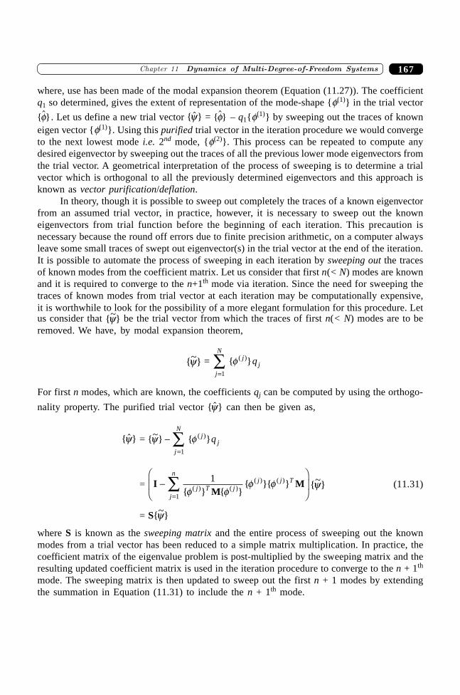
167�������� ���������� ��������������������������
where, use has been made of the modal expansion theorem (Equation (11.27)). The coefficientq1 so determined, gives the extent of representation of the mode-shape {f(1)} in the trial vector
{�}f . Let us define a new trial vector { �}y = {�}f – q1{f(1)} by sweeping out the traces of knowneigen vector {f(1)}. Using this purified trial vector in the iteration procedure we would convergeto the next lowest mode i.e. 2nd mode, {f(2)}. This process can be repeated to compute anydesired eigenvector by sweeping out the traces of all the previous lower mode eigenvectors fromthe trial vector. A geometrical interpretation of the process of sweeping is to determine a trialvector which is orthogonal to all the previously determined eigenvectors and this approach isknown as vector purification/deflation.
In theory, though it is possible to sweep out completely the traces of a known eigenvectorfrom an assumed trial vector, in practice, however, it is necessary to sweep out the knowneigenvectors from trial function before the beginning of each iteration. This precaution isnecessary because the round off errors due to finite precision arithmetic, on a computer alwaysleave some small traces of swept out eigenvector(s) in the trial vector at the end of the iteration.It is possible to automate the process of sweeping in each iteration by sweeping out the tracesof known modes from the coefficient matrix. Let us consider that first n(< N) modes are knownand it is required to converge to the n+1th mode via iteration. Since the need for sweeping thetraces of known modes from trial vector at each iteration may be computationally expensive,it is worthwhile to look for the possibility of a more elegant formulation for this procedure. Letus consider that {~}y be the trial vector from which the traces of first n(< N) modes are to beremoved. We have, by modal expansion theorem,
{~}y = { }( )f jj
j
N
q=
Â1
For first n modes, which are known, the coefficients qj can be computed by using the orthogo-
nality property. The purified trial vector { �}y can then be given as,
{ �}y = {~} { }( )y f-=
 jj
j
N
q1
= IM
M-FHG
IKJ
=Â 1
1 { } { }{ }{ }( ) ( )
( ) ( )
f ff fj T j
j j T
j
n
{~}y (11.31)
= S{~}y
where S is known as the sweeping matrix and the entire process of sweeping out the knownmodes from a trial vector has been reduced to a simple matrix multiplication. In practice, thecoefficient matrix of the eigenvalue problem is post-multiplied by the sweeping matrix and theresulting updated coefficient matrix is used in the iteration procedure to converge to the n + 1th
mode. The sweeping matrix is then updated to sweep out the first n + 1 modes by extendingthe summation in Equation (11.31) to include the n + 1th mode.
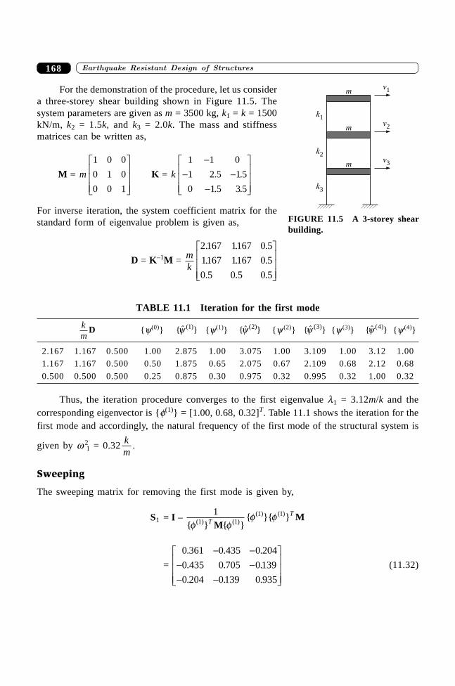
������ ���������������������� �� ���168
For the demonstration of the procedure, let us considera three-storey shear building shown in Figure 11.5. Thesystem parameters are given as m = 3500 kg, k1 = k = 1500kN/m, k2 = 1.5k, and k3 = 2.0k. The mass and stiffnessmatrices can be written as,
M = m
1 0 0
0 1 0
0 0 1
L
NMMM
O
QPPP
K = k
1 1 0
1 2 5 1 5
0 1 5 3 5
-- -
-
L
NMMM
O
QPPP
. .
. .
For inverse iteration, the system coefficient matrix for thestandard form of eigenvalue problem is given as,
D = K–1M = mk
2 167 1167 0 5
1167 1167 0 5
0 5 0 5 0 5
. . .
. . .
. . .
L
NMMM
O
QPPP
TABLE 11.1 Iteration for the first mode
km
D {y(0)} { � }( )y 1 {y(1)} { � }( )y 2 {y (2)} { � }( )y 3 {y (3)} { � }( )y 4 {y (4)}
2.167 1.167 0.500 1.00 2.875 1.00 3.075 1.00 3.109 1.00 3.12 1.00
1.167 1.167 0.500 0.50 1.875 0.65 2.075 0.67 2.109 0.68 2.12 0.68
0.500 0.500 0.500 0.25 0.875 0.30 0.975 0.32 0.995 0.32 1.00 0.32
Thus, the iteration procedure converges to the first eigenvalue l1 = 3.12m/k and thecorresponding eigenvector is {f(1)} = [1.00, 0.68, 0.32]T. Table 11.1 shows the iteration for thefirst mode and accordingly, the natural frequency of the first mode of the structural system is
given by w 21 = 0.32 k
m.
Sweeping
The sweeping matrix for removing the first mode is given by,
S1 = I – 1
1 11 1
{ } { }{ }{ }( ) ( )
( ) ( )
f ff fT
T
MM
=
0 361 0 435 0 204
0 435 0 705 0 139
0 204 0139 0 935
. . .
. . .
. . .
- -- -- -
L
NMMM
O
QPPP
(11.32)
mv1
k1
mv2
mv3
k2
k3
FIGURE 11.5 A 3-storey shearbuilding.
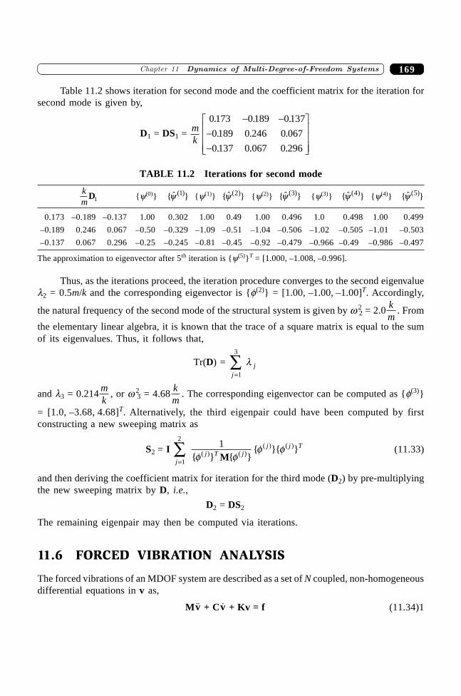
169�������� ���������� ��������������������������
Table 11.2 shows iteration for second mode and the coefficient matrix for the iteration forsecond mode is given by,
D1 = DS1 = mk
0 173 0 189 0137
0189 0 246 0 067
0 137 0 067 0 296
. . .
. . .
. . .
- ---
L
NMMM
O
QPPP
TABLE 11.2 Iterations for second mode
km
D1 {y(0)} { � }( )y 1 {y(1)} { � }( )y 2 {y(2)} { � }( )y 3 {y(3)} { � }( )y 4 {y(4)} { � }( )y 5
0.173 –0.189 –0.137 1.00 0.302 1.00 0.49 1.00 0.496 1.0 0.498 1.00 0.499
–0.189 0.246 0.067 –0.50 –0.329 –1.09 –0.51 –1.04 –0.506 –1.02 –0.505 –1.01 –0.503
–0.137 0.067 0.296 –0.25 –0.245 –0.81 –0.45 –0.92 –0.479 –0.966 –0.49 –0.986 –0.497
The approximation to eigenvector after 5th iteration is {y(5)}T = [1.000, –1.008, –0.996].
Thus, as the iterations proceed, the iteration procedure converges to the second eigenvaluel2 = 0.5m/k and the corresponding eigenvector is {f(2)} = [1.00, –1.00, –1.00]T. Accordingly,
the natural frequency of the second mode of the structural system is given by w 22 = 2.0
km
. From
the elementary linear algebra, it is known that the trace of a square matrix is equal to the sumof its eigenvalues. Thus, it follows that,
Tr(D) = j
j=
Â1
3
l
and l3 = 0.214mk
, or w 23 = 4.68
km
. The corresponding eigenvector can be computed as {f(3)}
= [1.0, –3.68, 4.68]T. Alternatively, the third eigenpair could have been computed by firstconstructing a new sweeping matrix as
S2 = I j
j T jj j T
=Â
1
21
{ } { }{ }{ }( ) ( )
( ) ( )
f ff f
M(11.33)
and then deriving the coefficient matrix for iteration for the third mode (D2) by pre-multiplyingthe new sweeping matrix by D, i.e.,
D2 = DS2
The remaining eigenpair may then be computed via iterations.
11.6 FORCED VIBRATION ANALYSIS
The forced vibrations of an MDOF system are described as a set of N coupled, non-homogeneousdifferential equations in v as,
M��v + C �v + Kv = f (11.34)1
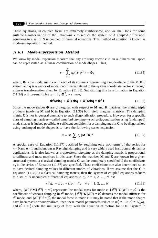
������ ���������������������� �� ���170
These equations, in coupled form, are extremely cumbersome, and we shall look for somesuitable transformation of the unknowns v to reduce the system of N coupled differentialequations to a set of N uncoupled differential equations. This method of solution is known asmode-superposition method.
11.6.1 Mode-superposition Method
We know by modal expansion theorem that any arbitrary vector v in an N-dimensional spacecan be represented as a linear combination of mode-shapes. Thus,
v = r
N
rq t=
Â1
( ){f (r)} = FFFFFq (11.35)
where, FFFFF is the modal matrix with each of its columns representing a mode-shape of the MDOFsystem and q is a vector of modal coordinates related to the system coordinate vector v througha linear transformation given by Equation (11.35). Substituting this transformation in Equation(11.34) and pre-multiplying it by FFFFFT, we have,
FFFFFTMFFFFF ��q + FFFFFTCFFFFF �q + FFFFFTKFFFFFq = FFFFFT f (11.36)
Since the mode shapes FFFFF are orthogonal with respect to M and K matrices, the matrix tripleproducts involving M and K in Equation (11.36) both yield diagonal matrices. The dampingmatrix C is not in general amenable to such diagonalization procedure. However, for a specificclass of damping matrices—called classical damping—such a diagonalization using (undamped)mode shapes is indeed possible. A sufficient condition for a damping matrix C to be diagonalizedusing undamped mode shapes is to have the following series expansion:
C = Mn
na [M–1K]n (11.37)
A special case of Equation (11.37) obtained by retaining only two terms of the series forn = 0 and n = 1 and is known as Rayleigh damping and is very widely used in structural dynamicsapplications. It is also known as proportional damping as the damping matrix is proportionalto stiffness and mass matrices in this case. Since the matrices M and K are known for a givenstructural system, a classical damping matrix C can be completely specified if the coefficientsan in the series of Equation (11.37) are specified. These coefficients can also determined so asto have desired damping values in different modes of vibrations. If we assume that the C inEquation (11.36) is a classical damping matrix, then the system of coupled equations reducesto a set of N uncoupled differential equations in qr, r = 1, 2, …, N, as:
mr* ��qr + cr
* �qr + kr*qr = fr
*, " r = 1, 2, …, N (11.38)
where, {f(r)}TM{f(r)} = m*r represents the modal mass for mode r, {f(r)}TC{f(r)} = cr
* is thecoefficient of viscous damping in rth mode, {f(r)}TK{f(r)} = kr
* denotes the modal stiffness forrth mode, and {f(r)}T f = fr
*, the modal force in mode r. It may be noted that if the mode shapeshave been mass-orthonormalized, then these modal parameters reduce to m*
r = 1.0, cr* = 2z rwr,
and kr* = w 2
r (note the similarity of form with the equation of motion for SDOF system in
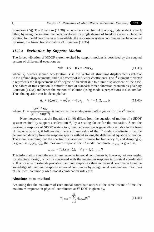
171�������� ���������� ��������������������������
Equation (7.5)). The Equations (11.38) can now be solved for unknowns qr, independent of eachother, by using the solution methods developed for single degree of freedom systems. Once thesolution for modal coordinates qr is available, the response in system coordinates can be obtainedby using the linear transformation of Equation (11.35).
11.6.2 Excitation by Support Motion
The forced vibration of MDOF system excited by support motions is described by the coupledsystem of differential equations as
M��v + C �v + Kv = –Mr��vg (11.39)
where ��vg denotes ground acceleration, v is the vector of structural displacements relativeto the ground displacements, and r is a vector of influence coefficients. The ith element of vectorr represents the displacement of ith degree of freedom due to a unit displacement of the base.The nature of this equation is similar to that of standard forced vibration problem as given byEquation (11.34) and hence the method of solution (using mode-superposition) is also similar.Thus the equation can be decoupled as
��qr + 2z rwr �qr + w 2r qr = –Gr��vg , " r = 1, 2, …, N (11.40)
where, Gr = { }
{ } { }
( )
( ) ( )
ff f
r T
r T r
MrM
is known as the mode-participation factor for the rth mode.
Note, however, that the Equation (11.40) differs from the equation of motion of a SDOFsystem excited by support acceleration ��vg by a scaling factor for the excitation. Since themaximum response of SDOF system to ground acceleration is generally available in the formof response spectra, it follows that the maximum value of the rth modal coordinate qr can bedetermined directly from the response spectra without solving the differential equation of motion.Therefore, assuming that the spectral displacement ordinate for frequency wr and damping zr
is given as Sd(wr, zr), the maximum response for rth modal coordinate qr,max is given as,
qr, max = GrSd(wr, zr); " r = 1, 2, …, N
This information about the maximum response in modal coordinates is, however, not very usefulfor structural design, which is concerned with the maximum response in physical coordinatesv. It is possible to estimate probable maximum response values in physical coordinates from theknowledge of maximum response in modal coordinates by using modal combination rules. Twoof the most commonly used modal combination rules are:
Absolute sum method
Assuming that the maximum of each modal coordinate occurs at the same instant of time, themaximum response in physical coordinates at ith DOF is given by,
vi, max ª r
N
r irq
=Â
1,max
( )f (11.41)
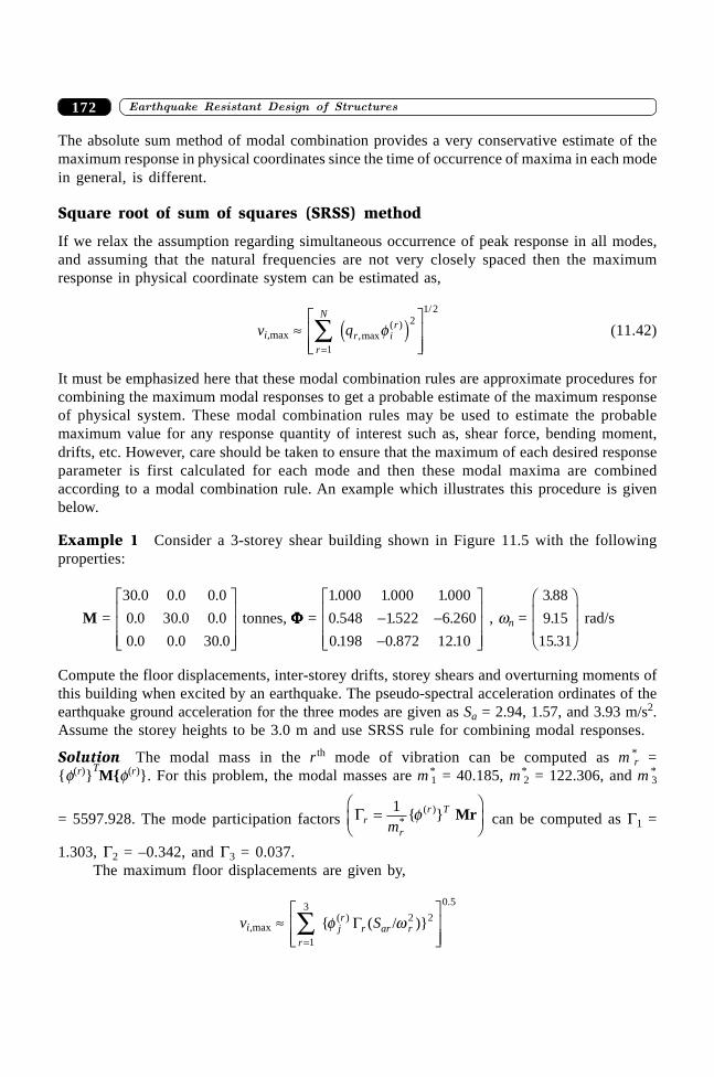
������ ���������������������� �� ���172
The absolute sum method of modal combination provides a very conservative estimate of themaximum response in physical coordinates since the time of occurrence of maxima in each modein general, is different.
Square root of sum of squares (SRSS) method
If we relax the assumption regarding simultaneous occurrence of peak response in all modes,and assuming that the natural frequencies are not very closely spaced then the maximumresponse in physical coordinate system can be estimated as,
vi,max ª r
N
r irq
=ÂLNMM
OQPP1
21 2
,max( )
/
fd i (11.42)
It must be emphasized here that these modal combination rules are approximate procedures forcombining the maximum modal responses to get a probable estimate of the maximum responseof physical system. These modal combination rules may be used to estimate the probablemaximum value for any response quantity of interest such as, shear force, bending moment,drifts, etc. However, care should be taken to ensure that the maximum of each desired responseparameter is first calculated for each mode and then these modal maxima are combinedaccording to a modal combination rule. An example which illustrates this procedure is givenbelow.
Example 1 Consider a 3-storey shear building shown in Figure 11.5 with the followingproperties:
M =
30 0 0 0 0 0
0 0 30 0 0 0
0 0 0 0 30 0
. . .
. . .
. . .
L
NMMM
O
QPPP tonnes, FFFFF =
1 000 1 000 1 000
0 548 1 522 6 260
0 198 0 872 12 10
. . .
. . .
. . .
- --
L
NMMM
O
QPPP
, wn =
3 88
9 15
15 31
.
.
.
F
HGG
I
KJJ rad/s
Compute the floor displacements, inter-storey drifts, storey shears and overturning moments ofthis building when excited by an earthquake. The pseudo-spectral acceleration ordinates of theearthquake ground acceleration for the three modes are given as Sa = 2.94, 1.57, and 3.93 m/s2.Assume the storey heights to be 3.0 m and use SRSS rule for combining modal responses.
Solution The modal mass in the r th mode of vibration can be computed as m *r =
{f(r)}TM{f(r)}. For this problem, the modal masses are m*
1 = 40.185, m*2 = 122.306, and m *
3
= 5597.928. The mode participation factors Grr
r T
m=
FHG
IKJ
1*
( ){ }f Mr can be computed as G1 =
1.303, G2 = –0.342, and G3 = 0.037.The maximum floor displacements are given by,
vi,max ª r
jr
r ar rS=
ÂLNMM
OQPP1
32 2
0 5
{ ( / )}( )
.
f wG
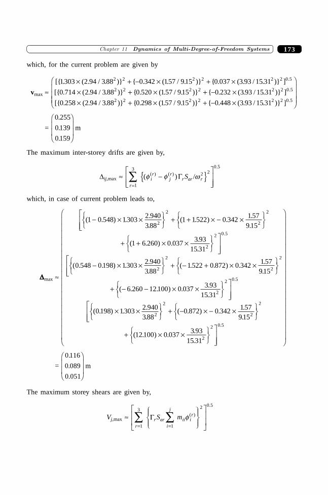
173�������� ���������� ��������������������������
which, for the current problem are given by
vmax ª
[{ . ( . / . )} { . ( . / . )} { . ( . / . )} ]
[{ . ( . / . )} { . ( . / . )} { . ( . / . )} ]
[{ . ( . / . )} { . ( . / . )} { . ( . / . )} ]
.
.
.
1303 2 94 3 88 0 342 157 915 0 037 3 93 15 31
0 714 2 94 3 88 0 520 1 57 915 0 232 3 93 15 31
0 258 2 94 3 88 0 298 157 915 0 448 3 93 15 31
2 2 2 2 2 2 0 5
2 2 2 2 2 2 0 5
2 2 2 2 2 2 0 5
¥ + - ¥ + ¥¥ + ¥ + - ¥¥ + ¥ + - ¥
F
HGGG
I
KJJJ
=
0 255
0 139
0 159
.
.
.
F
HGG
I
KJJ m
The maximum inter-storey drifts are given by,
Dij,max ª r
ir
jr
r ar rS=
 -LNMM
OQPP1
32 2
0 5
( ) /( ) ( )
.
f f wGn s
which, in case of current problem leads to,
DDDDDmax ª
( . ) . ..
( . ) . ..
( . ) . ..
( . . ) . ..
( . . ) . ..
( . . ) . ..
.
1 0 548 1303 2 9403 88
1 1522 0 342 1 579 15
1 6 260 0 037 3 9315 31
0 548 0 198 1303 2 9403 88
1 522 0 872 0 342 1 57915
6 260 12 100 0 037 3 9315 31
2
2
2
2
2
2 0 5
2
2
2
2
2
- ¥ ¥RSTUVW + + ¥ - ¥RST
UVWLNMM
+ + ¥ ¥RSTUVW
OQPP
- ¥ ¥RSTUVW + - + ¥ ¥RST
UVWLNMM
+ - - ¥ ¥RSTUVW
OQPP
¥ ¥RSTUVW + - ¥ - ¥RST
UVWLNMM
+ ¥ ¥RSTUVW
OQPP
F
H
GGGGGGGGGGGGGGGGGG
I
K
JJJJJJJJJJJJJJJJJJ
2 0 5
2
2
2
2
2
2 0 5
0 198 1303 2 9403 88
0 872 0 342 1 57915
12 100 0 037 3 9315 31
.
.
( . ) . ..
( . ) . ..
( . ) . ..
=
0 116
0 089
0 051
.
.
.
F
HGG
I
KJJ m
The maximum storey shears are given by,
Vj,max ª r
r ari
j
ii irS m
= =Â Â
RS|T|
UV|W|
L
NMM
O
QPP
1
3
1
2 0 5
G f ( )
.
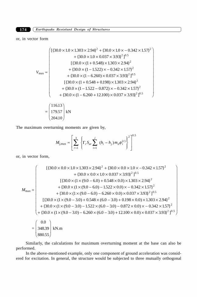
������ ���������������������� �� ���174
or, in vector form
Vmax ª
[{ . . . . } { . . . . }
{ . . . . } ]
[{ . ( . ) . . }
{ . ( . ) . . }
{ . ( . ) . . } ]
[{ . ( . . ) . . }
{ . ( . . )
.
.
30 0 1 0 1303 2 94 30 0 1 0 0 342 1 57
30 0 1 0 0 037 3 93
30 0 1 0 548 1303 2 94
30 0 1 1 522 0 342 1 57
30 0 1 6 260 0 037 3 93
30 0 1 0 548 0198 1303 2 94
30 0 1 1 522 0 872
2 2
2 0 5
2
2
2 0 5
2
¥ ¥ ¥ + ¥ ¥ - ¥+ ¥ ¥ ¥
¥ + ¥ ¥+ ¥ - ¥ - ¥
+ ¥ - ¥ ¥¥ + + ¥ ¥
+ ¥ - - ¥ - ¥+ ¥ - + ¥ ¥
F
H
GGGGGGGGGG
I
K
JJJJJJJJJJ0 342 1 57
30 0 1 6 260 12 100 0 037 3 93
2
2 0 5
. . }
{ . ( . . ) . . } ] .
=
116 13
179 57
204 10
.
.
.
F
HGG
I
KJJ kN
The maximum overturning moments are given by,
Mj,max ª r
r ari
j
i j ii irS h h m
= =Â Â -
RS|T|
UV|W|
L
NMM
O
QPP
1
3
1
2 0 5
G ( ) ( )
.
f
or, in vector form,
Mmax ª
[{ . . . . . } { . . . . . }
{ . . . . . } ]
[{ . ( ( . . ) . . ) . . }
{ . ( ( . . ) . . ) . . }
{ . ( ( . . ) . . ) .
.
30 0 0 0 1 0 1303 2 94 30 0 0 0 1 0 0 342 1 57
30 0 0 0 1 0 0 037 3 93
30 0 1 9 0 6 0 0 548 0 0 1303 2 94
30 0 1 9 0 6 0 1522 0 0 0 342 1 57
30 0 1 9 0 6 0 6 260 0 0 0 037
2 2
2 0 5
2
2
¥ ¥ ¥ ¥ + ¥ ¥ ¥ - ¥+ ¥ ¥ ¥ ¥
¥ ¥ - + ¥ ¥ ¥+ ¥ ¥ - - ¥ ¥ - ¥
+ ¥ ¥ - - ¥ ¥ ¥ 3 93
30 0 1 9 0 3 0 0 548 6 0 3 0 0 198 0 0 1303 2 94
30 0 1 9 0 3 0 1 522 6 0 3 0 0 872 0 0 0 342 157
30 0 1 9 0 3 0 6 260 6 0 3 0 12 100 0 0 0 037 3 93
2 0 5
2
2
2 0 5
. } ]
[{ . ( ( . . ) . ( . . ) . . ) . . }
{ . ( ( . . ) . ( . . ) . . ) . . }
{ . ( ( . . ) . ( . . ) . . ) . . } ]
.
.
¥ ¥ - + ¥ - + ¥ ¥ ¥+ ¥ ¥ - - ¥ - - ¥ ¥ - ¥
+ ¥ ¥ - - ¥ - + ¥ ¥ ¥
F
H
GGGGGGGGGG
I
K
JJJJJJJJJJ
=
0 0
348 39
880 55
.
.
.
F
HGG
I
KJJ kN.m
Similarly, the calculations for maximum overturning moment at the base can also beperformed.
In the above-mentioned example, only one component of ground acceleration was consid-ered for excitation. In general, the structure would be subjected to three mutually orthogonal
175�������� ���������� ��������������������������
translational components of ground motions simultaneously at a support point. Computationsfor any response quantity of interest for simultaneous excitation by multiple components would,in general, yield different estimates than for any single ground motion component acting alone.It is not adequate, for design purpose, to consider the maximum response out of the threeestimates obtained for different ground motion components independently. To find the responseparameters for use in design, the response estimates for excitation by individual componentsmay be combined together by SRSS rule. For any generic response quantity of interest, say, R,the value to be adopted for design calculations Rdes can be obtained as,
Rdes = R R Rx y z2 2 2+ +
where, Rx, Ry, and Rz represent the estimate of response R due to excitation by ground motionin x, y, and z directions, respectively.
11.6.3 Mode Truncation
Generally, the mathematical models for real civil engineering structural systems may involvemillions of degrees of freedoms, implying that the total number of equations to be solved formodal coordinates (Equations (11.38)) could be of the same order—a formidable task even forthe powerful desktop computers available today. Fortunately, it is not necessary to includeresponse in all the modes to get a rational estimate of the total response. Since most of the energyof the dynamic loads of civil engineering structures (such as earthquake ground motions, windforces, ocean waves, etc.) is concentrated in low frequencies (typically < 35 Hz for earthquakes)the higher modes (with larger natural frequencies) are not excited by these low-frequencyforces.2 Thus it is possible to truncate the modal summation in Equation (11.35) to the sum ofonly a few of the lower modes. The total number of terms in such truncated modal summationseldom exceeds a few hundreds, even in very complex structural systems. Thus the responsevector v can be approximately determined as,
v = r
N
rq t=
Â1
�
( ){f(r)} (11.43)
where, �N << N. The decision about the number of modes to be included in the responsecomputations may be based on the following two criteria:
(i) All modes having natural frequencies less than or equal to the highest frequency in theexcitation should be included in the modal summation.
(ii) At least 90% of the total mass of the structural system should be included in the dynamicresponse computation. This criterion in assessed by considering the cumulative effectivemodal mass (= Sr m
*r G 2
r ) for all modes included in the summation, which should bemore than 90% of the total mass of the system.
2This inference can be drawn by considering the nature of response of SDOF systems to harmonic excitations. Thedynamic amplification factor for the oscillator response approaches unity as the ratio of frequency of excitation tonatural frequency (w/wn) decreases and the response approaches that for a static case (see Figure 7.5).
������ ���������������������� �� ���176
The truncation of the modal summation after a few modes undoubtedly introduces someerrors due to neglecting the contribution of higher modes to total response. However, if theabove-mentioned two criteria are adhered to, the error resulting from neglecting the highermode contribution is not likely to be significant to affect the design, except for very raresituations encountered in special structures such as pipings, etc. In such special cases, it ispossible to improve on the accuracy of the solution by including the contribution of highermodes as a static correction to the computed dynamic response.
11.6.4 Static Correction for Higher Mode Response
Let us consider the modal contribution to total response as the sum of two parts:
v = r
Nr
r
s N
Ns
sq t q t= = +
 Â+1 1
�( )
�
( ){ } ( ) { } ( )f f (11.44)
where, the second term of the modal summation represents the error term due to truncation ofmodal summation (assuming that only �N lower modes are being considered for dynamicresponse computation. Let us now consider the equation for the response of sth modal coordinate
ms ��qs(t) + cs �qs(t) + ksqs(t) = fs
which can be rearranged as,
qs(t) = fk
q t q ts
s
s
s
s s
s
- -�� ( ) � ( )
wz
w2
2
where, the first term represents the response in s mode if the load were applied statically; theother two terms represent the dynamic correction to the static response in sth mode. The inertiaterm is inversely proportional to the square of the natural frequency, while the damping term(which is generally very small in magnitude in comparison to elastic and inertia terms) isinversely proportional to the natural frequency. Therefore for higher modes, the contributionfrom dynamic response terms becomes insignificant in comparison with the static responseterm and the response in higher modes can be reasonably approximated by considering only thestatic response. The total response can now be given (after substituting for the modal forcefs = {f(s)}T f ) as,
v = r
Nr
r
s N
N
s
s s Tq tk
= = +Â Â+
1 1
1�
( )
�
( ) ( ){ } ( ) { }{ }f f f f
= r
Nr
r
s N
N
sq t= = +
 Â+1 1
�( )
�{ } ( )f F f (11.45)
where, 1ks
{f (s)}{f (s)}T = Fs represents the contribution of sth mode toward the flexibility matrix
of the structural system.
177�������� ���������� ��������������������������
It should be noted that although the response of higher modes can be approximated byconsidering the static response only, the formulation presented above requires that all modeshapes for the system have to be computed in order to compute the contribution of higher modesto the structural flexibility. It is worthwhile to investigate if it is possible to estimate thecontribution to structural flexibility from higher modes in terms of lower modes which are beingconsidered for dynamic response. It turns out that it is indeed possible to reformulate theexpression of structural flexibility as,
s N
N
sk= +� 1
1 {f(s)}{f(s)}T = K–1 – r
N
rk=
Â1
1�
{f(r)}{f(r)}T
= K–1 – r
N
r=
Â1
�
F (11.46)
where, higher mode contribution to structural flexibility has been computed by subtracting thecontribution of lower modes to structural flexibility from the total structural flexibility (K–1).Thus the total response v can be computed as
v = r
Nr
rr
N
rq t=
-
=Â Â+ -
FHG
IKJ
1
1
1
�( )
�
{ } ( )f K F f (11.47)
where, the second term on the right hand side represents the static correction term to accountfor higher mode response. This correction for higher mode response is also known as the missingmass correction.
11.7 MODEL ORDER REDUCTION IN STRUCTURALDYNAMICS
Since only a few lower modes contribute to the dynamic response of any structural system, itis not necessary to compute all eigenvalues and eigenvectors for a given system. Further, a majorportion of the total time for the solution of a structural dynamics problem goes into the solutionof eigenvalue problem. Hence, it is beneficial to explore the ways to minimise the time spentin the eigensolution phase which directly results in reduced solution times. A convenient way ofachieving this end is by reducing the problem size itself by the use of the concept of generalisedcoordinates. Let us consider a (N-dimensional) vector v, which can be represented as
v ª r
p
rz=
Â1
{y(r)}
= YYYYYz (11.48)
where, {y(r)} represents a set of orthogonal vectors, called as the Ritz base vectors, zr, denotethe rth generalised coordinate associated with the rth Ritz vector, and p << N. Substituting
������ ���������������������� �� ���178
for v from Equation (11.48) in the Equation (11.7) for free vibration, we get,
MYYYYY��z + KYYYYYz = 0 (11.49)
Pre-multiplying by YYYYYT on both sides of the equation, we get,
~ �� ~Mz Kz+ = 0 (11.50)
where, ~M = YYYYY TMYYYYY and
~K = YYYYY TKYYYYY are the reduced (p ¥ p) generalised mass and stiffness
matrices respectively. Equation (11.50) represents an eigenvalue problem which is much smallerin size in comparison with the original eigenvalue problem given by Equation (11.7). Theeigenvectors of this reduced eigenvalue may be substituted back in Equation (11.48) to get theeigenvectors (mode shapes) for the actual structure for further use in the mode superpositionanalysis. For example, let us assume that FFFFFz denotes the modal matrix containing all peigenvectors of the reduced eigenvalue problem of Equation (11.50). The required mode shapes(for lower modes) of the actual structure can then be obtained as,
FFFFF = YFYFYFYFYFz
The frequencies obtained by solving the reduced eigenvalue problem are approximations to thefrequencies of the actual structural system. The agreement between the two set of frequenciesis generally excellent for the lower modes but is relatively poor for higher modes. The qualityof approximation and number of Ritz base vectors required for accurate estimation of desirednumber of mode shapes of actual structure depends on the choice of Ritz base vectors. Generally,it is necessary that p = 2 �N in order to estimate accurately the frequencies and mode shapesfor �N lower modes. Further, a good choice for the first Ritz vector ({y (1)}) is the staticdisplacement response vector (in accordance with Rayleigh’s method). Other additional Ritzvectors can be estimated by making an arbitrary vector orthogonal to the previously determinedRitz vectors by using a procedure similar to the sweeping of lower modes as discussed earlier.The Rayleigh–Ritz method, as this procedure of model reduction is called, can be a verypowerful tool to quickly estimate the frequencies and mode shapes of lower modes and isinvariably used in all commercial structural analysis softwares.
11.8 ANALYSIS FOR MULTI-SUPPORTEXCITATION
The issue of spatial variation of ground motions was discussed earlier in the first part onEarthquake Ground Motions. Although the implications of this important physical phenomenonare not quite obvious when the plan dimensions of the structure under consideration are verysmall in comparison with the wavelengths of the seismic waves propagating through the soil.However, if the plan dimensions of the structural system are very large, or are comparable toseismic wavelengths, the spatial variation of ground motions can be a very important modellingconsideration. Figure 11.6 shows two different structural systems: (i) an elevated reservoir, and(ii) a continuous girder bridge structure, or a pipeline subjected to earthquake excitation. In the
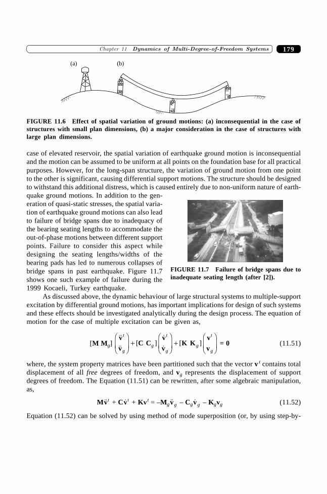
179�������� ���������� ��������������������������
case of elevated reservoir, the spatial variation of earthquake ground motion is inconsequentialand the motion can be assumed to be uniform at all points on the foundation base for all practicalpurposes. However, for the long-span structure, the variation of ground motion from one pointto the other is significant, causing differential support motions. The structure should be designedto withstand this additional distress, which is caused entirely due to non-uniform nature of earth-quake ground motions. In addition to the gen-eration of quasi-static stresses, the spatial varia-tion of earthquake ground motions can also leadto failure of bridge spans due to inadequacy ofthe bearing seating lengths to accommodate theout-of-phase motions between different supportpoints. Failure to consider this aspect whiledesigning the seating lengths/widths of thebearing pads has led to numerous collapses ofbridge spans in past earthquake. Figure 11.7shows one such example of failure during the1999 Kocaeli, Turkey earthquake.
As discussed above, the dynamic behaviour of large structural systems to multiple-supportexcitation by differential ground motions, has important implications for design of such systemsand these effects should be investigated analytically during the design process. The equation ofmotion for the case of multiple excitation can be given as,
[M Mg] ����
[ ]��
[ ]v
vC C
v
vK K
v
v
t
gg
t
gg
t
g
FHG
IKJ
+FHG
IKJ
+FHG
IKJ
= 0 (11.51)
where, the system property matrices have been partitioned such that the vector v t contains totaldisplacement of all free degrees of freedom, and vg represents the displacement of supportdegrees of freedom. The Equation (11.51) can be rewritten, after some algebraic manipulation,as,
M��v t + C �v t + Kv t = –Mg��vg – Cg �vg – Kgvg (11.52)
Equation (11.52) can be solved by using method of mode superposition (or, by using step-by-
(a) (b)
FIGURE 11.6 Effect of spatial variation of ground motions: (a) inconsequential in the case ofstructures with small plan dimensions, (b) a major consideration in the case of structures withlarge plan dimensions.
FIGURE 11.7 Failure of bridge spans due toinadequate seating length (after [2]).
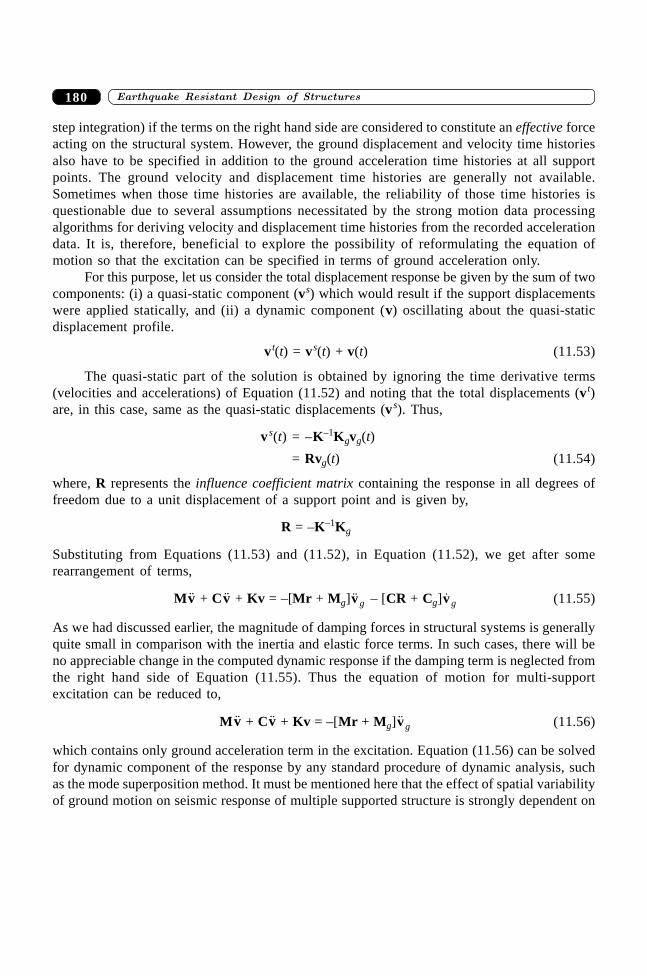
������ ���������������������� �� ���180
step integration) if the terms on the right hand side are considered to constitute an effective forceacting on the structural system. However, the ground displacement and velocity time historiesalso have to be specified in addition to the ground acceleration time histories at all supportpoints. The ground velocity and displacement time histories are generally not available.Sometimes when those time histories are available, the reliability of those time histories isquestionable due to several assumptions necessitated by the strong motion data processingalgorithms for deriving velocity and displacement time histories from the recorded accelerationdata. It is, therefore, beneficial to explore the possibility of reformulating the equation ofmotion so that the excitation can be specified in terms of ground acceleration only.
For this purpose, let us consider the total displacement response be given by the sum of twocomponents: (i) a quasi-static component (vs) which would result if the support displacementswere applied statically, and (ii) a dynamic component (v) oscillating about the quasi-staticdisplacement profile.
v t(t) = vs(t) + v(t) (11.53)
The quasi-static part of the solution is obtained by ignoring the time derivative terms(velocities and accelerations) of Equation (11.52) and noting that the total displacements (v t)are, in this case, same as the quasi-static displacements (v s). Thus,
v s(t) = –K–1Kgvg(t)
= Rvg(t) (11.54)
where, R represents the influence coefficient matrix containing the response in all degrees offreedom due to a unit displacement of a support point and is given by,
R = –K–1Kg
Substituting from Equations (11.53) and (11.52), in Equation (11.52), we get after somerearrangement of terms,
M��v + C��v + Kv = –[Mr + Mg]��vg – [CR + Cg] �vg (11.55)
As we had discussed earlier, the magnitude of damping forces in structural systems is generallyquite small in comparison with the inertia and elastic force terms. In such cases, there will beno appreciable change in the computed dynamic response if the damping term is neglected fromthe right hand side of Equation (11.55). Thus the equation of motion for multi-supportexcitation can be reduced to,
M��v + C��v + Kv = –[Mr + Mg]��vg (11.56)
which contains only ground acceleration term in the excitation. Equation (11.56) can be solvedfor dynamic component of the response by any standard procedure of dynamic analysis, suchas the mode superposition method. It must be mentioned here that the effect of spatial variabilityof ground motion on seismic response of multiple supported structure is strongly dependent on
181�������� ���������� ��������������������������
the type of model used to describe the ground motion variation. It is desirable to analyse theeffects of spatial variation of ground motion by using several suites of ground motions atsupports which have been generated artificially to conform to different alternate modelspostulated to be applicable for the project site [7].
11.9 SOIL–STRUCTURE INTERACTIONEFFECTS
All discussion till this point has been based on a tacit assumption that the foundations ofstructures transfer the loads by direct bearing on firm rocky strata and hence the supportconditions could be assumed to correspond to the fixed-base condition. This is, no doubt, asimplifying assumption and is generally valid if the super-structure is much more flexible/compliant than the underlying soil strata upon which the foundations rest. However, when thereverse is true i.e., the super-structure is much more stiff in comparison with the soil strata, thestructural response can be significantly influenced by the flexibility of soil.
There are two primary issues involved in the phenomenon of soil–structure interaction.First, as the seismic waves propagate through soil during an earthquake, a discontinuity in themedium of wave propagation is encountered at the interface of soil and structural foundations.The change in the material properties leads to scattering, diffraction, reflection, and refractionof the seismic waves at this soil-foundation interface thereby changing the nature of groundmotion at that point from what would have otherwise been observed in the absence of structureand foundation. Further, the seismic wave propagation takes place by deformations in themedium. Since the foundation can be considered to be very rigid in comparison to the soildeposits, the deformations of the soil at the soil–foundation interface are constrained asthe foundation cannot deform by the same amount as the soil. This further leads to slippageacross the soil-foundation interface—a nonlinear phenomenon—which is very difficult toaccount for in the mathematical models for practical vibration analysis. Moreover, the rigidfoundation acts like a low-pass filter by averaging out the high frequency components in seismicmotions due to the kinematic constraint imposed by the rigid foundation. It should be noted thatthe above-mentioned effects are only due to the wave propagation in elastic medium. Thedynamic behaviour of the structure has no role to play in this aspect. Therefore, these effectsarising out of the wave propagation considerations are known as kinematic interaction effects.The actual seismic input motion to the structural foundation is the result of kinematic interactionanalysis considering only the geometry and stiffness properties of the structural foundationand soil. The second aspect of the soil–structure interaction analysis involves the deformationsand stresses in supporting soil, induced due to the base shears and moments generated in thevibrating structure. The soil deformations further lead to a modification of the dynamic responseof structural system and thereby creating a dynamically interacting system. This second aspectof soil–structure interaction problem which results from the dynamic response of structuralsystem is known as the inertial interaction. Figure 11.8 shows a schematic representation ofthese two issues involved in any soil–structure interaction (SSI) analysis [5].
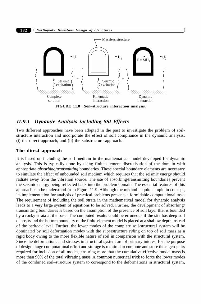
������ ���������������������� �� ���182
Seismicexcitation
U
:=
Completesolution
Seismicexcitation
U1
:
+
Kinematicinteraction
Dynamicinteraction
U2
:
F = MU1
:
Massless structure
FIGURE 11.8 Soil–structure interaction analysis.
11.9.1 Dynamic Analysis including SSI Effects
Two different approaches have been adopted in the past to investigate the problem of soil-structure interaction and incorporate the effect of soil compliance in the dynamic analysis:(i) the direct approach, and (ii) the substructure approach.
The direct approach
It is based on including the soil medium in the mathematical model developed for dynamicanalysis. This is typically done by using finite element discretisation of the domain withappropriate absorbing/transmitting boundaries. These special boundary elements are necessaryto simulate the effect of unbounded soil medium which requires that the seismic energy shouldradiate away from the vibration source. The use of absorbing/transmitting boundaries preventthe seismic energy being reflected back into the problem domain. The essential features of thisapproach can be understood from Figure 11.9. Although the method is quite simple in concept,its implementation for analysis of practical problems presents a formidable computational task.The requirement of including the soil strata in the mathematical model for dynamic analysisleads to a very large system of equations to be solved. Further, the development of absorbing/transmitting boundaries is based on the assumption of the presence of soil layer that is boundedby a rocky strata at the base. The computed results could be erroneous if the site has deep soildeposits and the bottom boundary of the finite element model is placed at a shallow depth insteadof the bedrock level. Further, the lower modes of the complete soil-structural system will bedominated by soil deformation modes with the superstructure riding on top of soil mass as arigid body owing to the more flexible nature of soil in comparison with the structural system.Since the deformations and stresses in structural system are of primary interest for the purposeof design, huge computational effort and storage is required to compute and store the eigen-pairsrequired for inclusion of all modes, ensuring more that the cumulative effective modal mass ismore than 90% of the total vibrating mass. A common numerical trick to force the lower modesof the combined soil–structure system to correspond to the deformations in structural system,
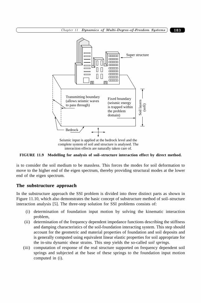
183�������� ���������� ��������������������������
is to consider the soil medium to be massless. This forces the modes for soil deformation tomove to the higher end of the eigen spectrum, thereby providing structural modes at the lowerend of the eigen spectrum.
The substructure approach
In the substructure approach the SSI problem is divided into three distinct parts as shown inFigure 11.10, which also demonstrates the basic concept of substructure method of soil–structureinteraction analysis [5]. The three-step solution for SSI problems consists of:
(i) determination of foundation input motion by solving the kinematic interactionproblem,
(ii) determination of the frequency dependent impedance functions describing the stiffnessand damping characteristics of the soil-foundation interacting system. This step shouldaccount for the geometric and material properties of foundation and soil deposits andis generally computed using equivalent linear elastic properties for soil appropriate forthe in-situ dynamic shear strains. This step yields the so-called soil springs.
(iii) computation of response of the real structure supported on frequency dependent soilsprings and subjected at the base of these springs to the foundation input motioncomputed in (i).
Transmitting boundary(allows seismic wavesto pass through)
Bedrock
Seismic input is applied at the bedrock level and thecomplete system of soil and structure is analysed. The
interaction effects are naturally taken care of.
Fixed boundary(seismic energyis trapped withinthe problemdomain)
Super structure
So
illa
yer
s(s
oft
)
FIGURE 11.9 Modelling for analysis of soil–structure interaction effect by direct method.
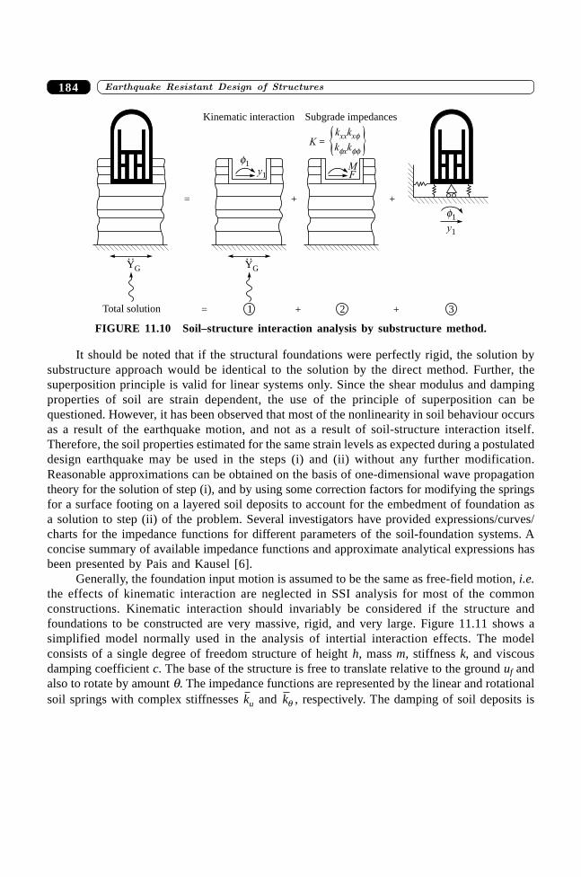
������ ���������������������� �� ���184
It should be noted that if the structural foundations were perfectly rigid, the solution bysubstructure approach would be identical to the solution by the direct method. Further, thesuperposition principle is valid for linear systems only. Since the shear modulus and dampingproperties of soil are strain dependent, the use of the principle of superposition can bequestioned. However, it has been observed that most of the nonlinearity in soil behaviour occursas a result of the earthquake motion, and not as a result of soil-structure interaction itself.Therefore, the soil properties estimated for the same strain levels as expected during a postulateddesign earthquake may be used in the steps (i) and (ii) without any further modification.Reasonable approximations can be obtained on the basis of one-dimensional wave propagationtheory for the solution of step (i), and by using some correction factors for modifying the springsfor a surface footing on a layered soil deposits to account for the embedment of foundation asa solution to step (ii) of the problem. Several investigators have provided expressions/curves/charts for the impedance functions for different parameters of the soil-foundation systems. Aconcise summary of available impedance functions and approximate analytical expressions hasbeen presented by Pais and Kausel [6].
Generally, the foundation input motion is assumed to be the same as free-field motion, i.e.the effects of kinematic interaction are neglected in SSI analysis for most of the commonconstructions. Kinematic interaction should invariably be considered if the structure andfoundations to be constructed are very massive, rigid, and very large. Figure 11.11 shows asimplified model normally used in the analysis of intertial interaction effects. The modelconsists of a single degree of freedom structure of height h, mass m, stiffness k, and viscousdamping coefficient c. The base of the structure is free to translate relative to the ground uf andalso to rotate by amount q. The impedance functions are represented by the linear and rotationalsoil springs with complex stiffnesses ku and kq , respectively. The damping of soil deposits is
F
Total solution
YG
:
=
= 1
YG
:
+
+
f1y1
2
M
3+
+
f1
y1
Kinematic interaction Subgrade impedances
kxxk
k kx
x
f
f ffK =
FIGURE 11.10 Soil–structure interaction analysis by substructure method.
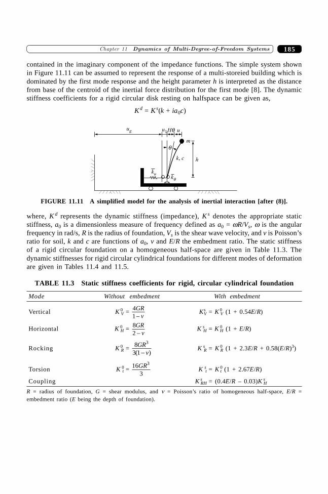
185�������� ���������� ��������������������������
contained in the imaginary component of the impedance functions. The simple system shownin Figure 11.11 can be assumed to represent the response of a multi-storeied building which isdominated by the first mode response and the height parameter h is interpreted as the distancefrom base of the centroid of the inertial force distribution for the first mode [8]. The dynamicstiffness coefficients for a rigid circular disk resting on halfspace can be given as,
K d = K s(k + ia0c)
m
ug u1 uHq
q
hk c,
kukq
FIGURE 11.11 A simplified model for the analysis of inertial interaction [after (8)].
where, K d represents the dynamic stiffness (impedance), K s denotes the appropriate staticstiffness, a0 is a dimensionless measure of frequency defined as a0 = wR/Vs, w is the angularfrequency in rad/s, R is the radius of foundation, Vs is the shear wave velocity, and v is Poisson’sratio for soil, k and c are functions of a0, v and E/R the embedment ratio. The static stiffnessof a rigid circular foundation on a homogeneous half-space are given in Table 11.3. Thedynamic stiffnesses for rigid circular cylindrical foundations for different modes of deformationare given in Tables 11.4 and 11.5.
TABLE 11.3 Static stiffness coefficients for rigid, circular cylindrical foundation
Mode Without embedment With embedment
Vertical K 0V = 4
1GR
v-Ks
V = K 0V (1 + 0.54E/R)
Horizontal K 0H = 8
2GR
v-K s
H = K 0H (1 + E/R)
Rocking K 0R = 8
3 1
3GRv( )-
K sR = K 0
R (1 + 2.3E/R + 0.58(E/R)3)
Torsion K 0t = 16
3
3GRK s
t = K 0t (1 + 2.67E/R)
Coupling K sRH = (0.4E/R – 0.03)K s
H
R = radius of foundation, G = shear modulus, and n = Poisson’s ratio of homogeneous half-space, E/R =embedment ratio (E being the depth of foundation).
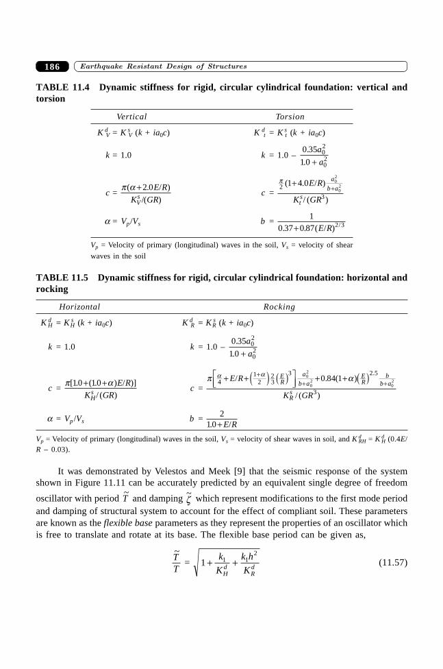
������ ���������������������� �� ���186
It was demonstrated by Velestos and Meek [9] that the seismic response of the systemshown in Figure 11.11 can be accurately predicted by an equivalent single degree of freedom
oscillator with period ~T and damping ~z which represent modifications to the first mode period
and damping of structural system to account for the effect of compliant soil. These parametersare known as the flexible base parameters as they represent the properties of an oscillator whichis free to translate and rotate at its base. The flexible base period can be given as,
~TT
= 1 1 12
+ +k
K
k h
KHd
Rd
(11.57)
TABLE 11.4 Dynamic stiffness for rigid, circular cylindrical foundation: vertical andtorsion
Vertical Torsion
K dV = K s
V (k + ia0c) K dt = K s
t (k + ia0c)
k = 1.0 k = 1.0 – 0 35
1 002
02
.
.
a
a+
c = p a( . / )
/( )
+ 2 0E R
K GRVs c =
p2
3
1 4 0 02
02( . / )
/ ( )
++
E R
K GR
a
b a
ts
a = Vp/Vs b = 1
0 37 0 87 2 3. . ( / ) /+ E R
Vp = Velocity of primary (longitudinal) waves in the soil, Vs = velocity of shear
waves in the soil
TABLE 11.5 Dynamic stiffness for rigid, circular cylindrical foundation: horizontal androcking
Horizontal Rocking
K dH = K s
H (k + ia0c) K dR = K s
R (k + ia0c)
k = 1.0 k = 1.0 – 0 35
1 002
02
.
.
a
a+
c = p a[ . ( . ) / )]
/ ( )
10 10+ + E R
K GRHs c =
p aa a4
12
23
3 2 5
3
02
02
020 84 1+ +L
NMOQP + ++
+ +E R
K GR
ER
a
b aER
bb a
Rs
/ . ( )
/ ( )
.e j c h c h
a = Vp /Vs b = 21 0. /+ E R
Vp = Velocity of primary (longitudinal) waves in the soil, Vs = velocity of shear waves in soil, and K dRH = K d
H (0.4E/R – 0.03).
187�������� ���������� ��������������������������
where T is the period of the (fixed-base) structure in its first mode, and k1 represents the modalstiffness for the first mode of (fixed-base) structure. The equivalent viscous damping ratio canbe defined in terms of the viscous damping of the structure and the radiation and hystereticdamping of the soil–foundation system. The flexible base damping can be given as [10],
~z =
~
(~
/ )z z
0 3+
T T(11.58)
where ~z 0 represents the damping contributions (radiation and hysteretic) from the soil–
foundation system. A closed form expression for ~z 0 can be found in the article by Velestos and
Nair [10]. It can be inferred from Equations (11.57) and (11.58) that the primary effect ofinertial interaction is the lengthening of natural period and increase in the damping ratio of thedynamical system.
SUMMARY
Different issues in the study of dynamics of a complex system are described in this chapter.Starting from the basic formulation and terminology of the problem, through the discussion offree vibration, forced vibration, the concept of tuned-mass dampers, response spectrum methodof seismic analysis, multi-support excitation, to the discussion and analytical modeling ofthe dynamic soil-structure interaction effects, a wide range of topics are covered. This willhelp demystify the seismic design codes and promote a better understanding and correctimplementation of their commendations of seismic design codes of practice.
REFERENCES
[1] Clough, R.W. and Penzien J., Dynamics of Structures, 2nd ed., McGraw-Hill,New York, 1993.
[2] Learning from Earthquakes Series Volume IV. “The 1999 Turkey Earthquakes: BridgePerformance and Remedial Actions”, Earthquake Engineering Research Institute, USA2003.
[3] Meirovitch, L., Analytical Methods in Vibrations, The Macmillan Company,New York, 1967.
[4] Meirovitch, L., Computation Methods in Structural Dynamics, Sijthoff and Noordhoff,Alphen aan den Rijn, The Netherlands, 1980.
[5] Kausel, E., Whitman, R.V., Morray, J.P., and Elsabee F., “The Spring Method forEmbedded Foundations”, Nuclear Engineering and Design, 48: 377–392, 1978.
[6] Pais, A. and Kausel, E., “Approximate Formulas for Dynamic Stiffnesses of RigidFoundations”, Soil Dynamics and Earthquake Engineering, 7: 213–226, 1998.
[7] Shrikhande, M. and Gupta, V.K., “Synthesizing Ensembles of Spatially CorrelatedAccelerograms”, Journal of Engineering Mechanics, ASCE, 124: 1185–1192, 1998.

������ ���������������������� �� ���188
[8] Stewart, J.P., Seed, R.B. and Fenves, G.L., “Empirical Evaluation of Inertial SoilStructure, Interaction and Effects”, Technical Report No. PEER 1998/07, PacificEarthquake Engineering Research Centre, University of California, Berkeley.
[9] Velestos, A.S. and Meek, J.W., “Dynamic Behaviour of Building Foundation Systems”,Earthquake Engineering and Structural Dynamics, 3: 121–138, 1974.
[10] Velestos, A.S. and Nair, V.V., “Seismic Interaction of Structures on HystereticFoundations”, Journal of Structural Engineering, ASCE, 101: 109–129, 1975.
���� ���
Concepts of EarthquakeResistant Design of
Reinforced Concete Building

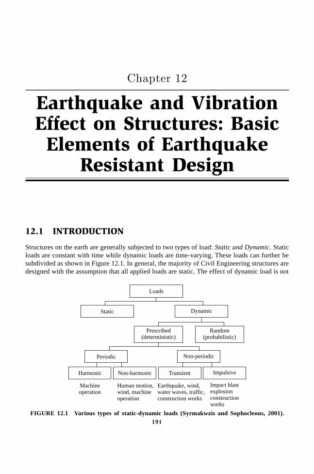
191
Earthquake and VibrationEffect on Structures: BasicElements of Earthquake
Resistant Design
��������
12.1 INTRODUCTION
Structures on the earth are generally subjected to two types of load: Static and Dynamic. Staticloads are constant with time while dynamic loads are time-varying. These loads can further besubdivided as shown in Figure 12.1. In general, the majority of Civil Engineering structures aredesigned with the assumption that all applied loads are static. The effect of dynamic load is not
Loads
Static Dynamic
Periodic Non-periodic
Prescribed(deterministic)
Random(probabilistic)
Harmonic Non-harmonic Transient Impulsive
Machineoperation
Human motion,wind, machineoperation
Earthquake, wind,water waves,construction works
traffic,
Impact blastexplosionconstructionworks
FIGURE 12.1 Various types of static-dynamic loads (Syrmakwzis and Sophocleous, 2001).
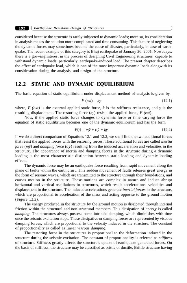
����������� ������� �������������192
considered because the structure is rarely subjected to dynamic loads; more so, its considerationin analysis makes the solution more complicated and time consuming. This feature of neglectingthe dynamic forces may sometimes become the cause of disaster, particularly, in case of earth-quake. The recent example of this category is Bhuj earthquake of January 26, 2001. Nowadays,there is a growing interest in the process of designing Civil Engineering structures capable towithstand dynamic loads, particularly, earthquake-induced load. The present chapter describesthe effect of earthquake load, which is one of the most important dynamic loads alongwith itsconsideration during the analysis, and design of the structure.
12.2 STATIC AND DYNAMIC EQUILIBRIUM
The basic equation of static equilibrium under displacement method of analysis is given by,
F (ext) = ky (12.1)
where, F (ext) is the external applied static force, k is the stiffness resistance, and y is theresulting displacement. The restoring force (ky) resists the applied force, F (ext).
Now, if the applied static force changes to dynamic force or time varying force theequation of static equilibrium becomes one of the dynamic equilibrium and has the form
F(t) = mÿ + c �y + ky (12.2)
If we do a direct comparison of Equations 12.1 and 12.2, we shall find the two additional forcesthat resist the applied forces with the restoring forces. These additional forces are called inertiaforce (mÿ) and damping force (c �y) resulting from the induced acceleration and velocities in thestructure. The appearance of inertia and damping forces in the structure during a dynamicloading is the most characteristic distinction between static loading and dynamic loadingeffects.
The dynamic force may be an earthquake force resulting from rapid movement along theplane of faults within the earth crust. This sudden movement of faults releases great energy inthe form of seismic waves, which are transmitted to the structure through their foundations, andcauses motion in the structure. These motions are complex in nature and induce abrupthorizontal and vertical oscillations in structures, which result accelerations, velocities anddisplacement in the structure. The induced accelerations generate inertial forces in the structure,which are proportional to acceleration of the mass and acting opposite to the ground motion(Figure 12.2).
The energy produced in the structure by the ground motion is dissipated through internalfriction within the structural and non-structural members. This dissipation of energy is calleddamping. The structures always possess some intrinsic damping, which diminishes with timeonce the seismic excitation stops. These dissipative or damping forces are represented by viscousdamping forces, which are proportional to the velocity induced in the structure. The constantof proportionality is called as linear viscous damping.
The restoring force in the structures is proportional to the deformation induced in thestructure during the seismic excitation. The constant of proportionality is referred as stiffnessof structure. Stiffness greatly affects the structure’s uptake of earthquake-generated forces. Onthe basis of stiffness, the structure may be classified as brittle or ductile. Brittle structure having
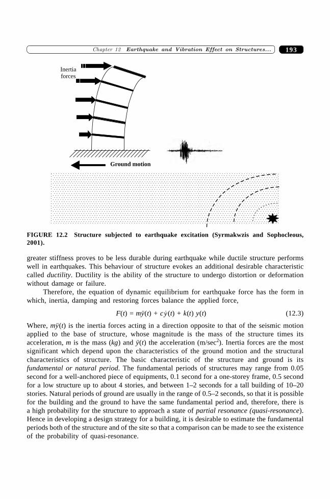
193�������� ������������� ���� ���������������������
greater stiffness proves to be less durable during earthquake while ductile structure performswell in earthquakes. This behaviour of structure evokes an additional desirable characteristiccalled ductility. Ductility is the ability of the structure to undergo distortion or deformationwithout damage or failure.
Therefore, the equation of dynamic equilibrium for earthquake force has the form inwhich, inertia, damping and restoring forces balance the applied force,
F(t) = mÿ(t) + c �y(t) + k(t) y(t) (12.3)
Where, mÿ(t) is the inertia forces acting in a direction opposite to that of the seismic motionapplied to the base of structure, whose magnitude is the mass of the structure times itsacceleration, m is the mass (kg) and ÿ(t) the acceleration (m/sec2). Inertia forces are the mostsignificant which depend upon the characteristics of the ground motion and the structuralcharacteristics of structure. The basic characteristic of the structure and ground is itsfundamental or natural period. The fundamental periods of structures may range from 0.05second for a well-anchored piece of equipments, 0.1 second for a one-storey frame, 0.5 secondfor a low structure up to about 4 stories, and between 1–2 seconds for a tall building of 10–20stories. Natural periods of ground are usually in the range of 0.5–2 seconds, so that it is possiblefor the building and the ground to have the same fundamental period and, therefore, there isa high probability for the structure to approach a state of partial resonance (quasi-resonance).Hence in developing a design strategy for a building, it is desirable to estimate the fundamentalperiods both of the structure and of the site so that a comparison can be made to see the existenceof the probability of quasi-resonance.
Inertiaforces
Ground motion
FIGURE 12.2 Structure subjected to earthquake excitation (Syrmakwzis and Sophocleous,2001).
����������� ������� �������������194
c �y(t) is the damping force acting in a direction opposite to that of the seismic motion, c is thedamping coefficient (N-sec/m) and y(t) the velocity (m/sec). The value of damping in a structuredepends on its components, component connections, materials etc. The amount of damping instructural system cannot be analytically ascertained, it must be determined experimentally. Inpractice this damping effect is expressed as a percentage of the critical damping which is thegreatest damping value that allows vibratory movement to develop. Experience has made itpossible to estimate the degree of damping in various types of structures, and some of commontypes of structures are reinforced concrete 5–10%, metal frame 1–5%, masonry 8–15%, Woodstructures 15–20%.
k (t)y(t) is the restoring force k (t) is the stiffness (N/m) or resistance is a function of the yieldcondition in the structure, which in turn is a function of time. The stiffness parameter k is apotential source of discrepancy, and is affected by quality of material, age, cracking, supportcondition etc. y(t) is the displacement (m).
F(t) is the externally applied force (N). The forcing function is often difficult to estimateaccurately, particularly in the case of earthquake.
The Equation (12.3) is a second order differential equation that needs to be solved for thedisplacement y(t). The number of displacement components required for specifying the positionof mass points is called the number of degrees-of-freedom required to obtain an adequatesolution. This depends upon the complexity of the structural system. For some structures asingle degree-of-freedom may be sufficient, whereas, for others several hundred degrees offreedom may be required (Anderson, 2001). Depending upon the degree of freedom, a numberof structural models can be proposed for analyzing the structure. A structure can be analyzedby different models depending upon the objective of the particular analysis.
12.3 STRUCTURAL MODELLING
Earthquake response analysis is an art to simulate the behaviour of a structure subjected to anearthquake ground motion based on dynamics and a mathematical model of the structure. Thecorrect analysis will depend upon the proper modelling of the behaviour of materials, elements,connection and structure. Models may be classified mainly by essential difference in the degree-of-freedom. The model, or the number of degree of freedom, should be selected carefullyconsidering the objective of the analysis. Sometimes sophistication or complicated models arenot only useless but also create misunderstanding to interpret the results in practical problems.Therefore, it is important to select an appropriate and simple model to match the purpose ofthe analysis. Analytical models should also be based on physical observations and its behaviourunder dynamic load. Different types of structural model are described as below to simulate thebehaviour of a frame building (Kadeyasawa, 2001; Gioncu and Mazzolani, 2002).
12.3.1 Structural Models for Frame Building
A three-dimensional model has independent displacements at each node and can simulateany type of behaviour. Because of the difficulties in modelling, verification and numericalcalculation, the three-dimensional model has not yet been used even in the most sophisticated
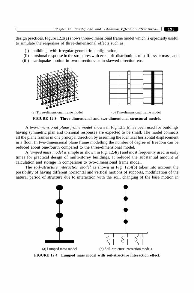
195�������� ������������� ���� ���������������������
design practices. Figure 12.3(a) shows three-dimensional frame model which is especially usefulto simulate the responses of three-dimensional effects such as
(i) buildings with irregular geometric configuration,(ii) torsional response in the structures with eccentric distributions of stiffness or mass, and
(iii) earthquake motion in two directions or in skewed direction etc.
(a) Three-dimensional frame model (b) Two-dimensional frame model
FIGURE 12.3 Three-dimensional and two-dimensional structural models.
A two-dimensional plane frame model shown in Fig 12.3(b)has been used for buildingshaving symmetric plan and torsional responses are expected to be small. The model connectsall the plane frames in one principal direction by assuming the identical horizontal displacementin a floor. In two-dimensional plane frame modelling the number of degree of freedom can bereduced about one-fourth compared to the three-dimensional model.
A lumped mass model is simple as shown in Fig. 12.4(a) and most frequently used in earlytimes for practical design of multi-storey buildings. It reduced the substantial amount ofcalculation and storage in comparison to two-dimensional frame model.
The soil–structure interaction model as shown in Fig. 12.4(b) takes into account thepossibility of having different horizontal and vertical motions of supports, modification of thenatural period of structure due to interaction with the soil, changing of the base motion in
(b) Soil–structure interaction models(a) Lumped mass model
FIGURE 12.4 Lumped mass model with soil-structure interaction effect.
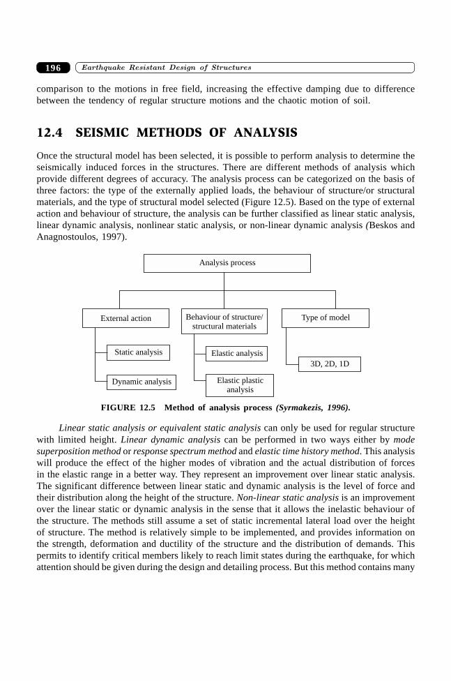
����������� ������� �������������196
comparison to the motions in free field, increasing the effective damping due to differencebetween the tendency of regular structure motions and the chaotic motion of soil.
12.4 SEISMIC METHODS OF ANALYSIS
Once the structural model has been selected, it is possible to perform analysis to determine theseismically induced forces in the structures. There are different methods of analysis whichprovide different degrees of accuracy. The analysis process can be categorized on the basis ofthree factors: the type of the externally applied loads, the behaviour of structure/or structuralmaterials, and the type of structural model selected (Figure 12.5). Based on the type of externalaction and behaviour of structure, the analysis can be further classified as linear static analysis,linear dynamic analysis, nonlinear static analysis, or non-linear dynamic analysis (Beskos andAnagnostoulos, 1997).
Analysis process
External action Behaviour of structure/structural materials
Type of model
3D, 2D, 1D
Elastic analysis
Elastic plasticanalysis
Static analysis
Dynamic analysis
FIGURE 12.5 Method of analysis process (Syrmakezis, 1996).
Linear static analysis or equivalent static analysis can only be used for regular structurewith limited height. Linear dynamic analysis can be performed in two ways either by modesuperposition method or response spectrum method and elastic time history method. This analysiswill produce the effect of the higher modes of vibration and the actual distribution of forcesin the elastic range in a better way. They represent an improvement over linear static analysis.The significant difference between linear static and dynamic analysis is the level of force andtheir distribution along the height of the structure. Non-linear static analysis is an improvementover the linear static or dynamic analysis in the sense that it allows the inelastic behaviour ofthe structure. The methods still assume a set of static incremental lateral load over the heightof structure. The method is relatively simple to be implemented, and provides information onthe strength, deformation and ductility of the structure and the distribution of demands. Thispermits to identify critical members likely to reach limit states during the earthquake, for whichattention should be given during the design and detailing process. But this method contains many
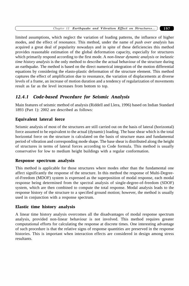
197�������� ������������� ���� ���������������������
limited assumptions, which neglect the variation of loading patterns, the influence of highermodes, and the effect of resonance. This method, under the name of push over analysis hasacquired a great deal of popularity nowadays and in spite of these deficiencies this methodprovides reasonable estimation of the global deformation capacity, especially for structureswhich primarily respond according to the first mode. A non-linear dynamic analysis or inelastictime history analysis is the only method to describe the actual behaviour of the structure duringan earthquake. The method is based on the direct numerical integration of the motion differentialequations by considering the elasto-plastic deformation of the structure element. This methodcaptures the effect of amplification due to resonance, the variation of displacements at diverselevels of a frame, an increase of motion duration and a tendency of regularization of movementsresult as far as the level increases from bottom to top.
12.4.1 Code-based Procedure for Seismic Analysis
Main features of seismic method of analysis (Riddell and Llera, 1996) based on Indian Standard1893 (Part 1): 2002 are described as follows:
Equivalent lateral force
Seismic analysis of most of the structures are still carried out on the basis of lateral (horizontal)force assumed to be equivalent to the actual (dynamic) loading. The base shear which is the totalhorizontal force on the structure is calculated on the basis of structure mass and fundamentalperiod of vibration and corresponding mode shape. The base shear is distributed along the heightof structures in terms of lateral forces according to Code formula. This method is usuallyconservative for low to medium height buildings with a regular conformation.
Response spectrum analysis
This method is applicable for those structures where modes other than the fundamental oneaffect significantly the response of the structure. In this method the response of Multi-Degree-of-Freedom (MDOF) system is expressed as the superposition of modal response, each modalresponse being determined from the spectral analysis of single-degree-of-freedom (SDOF)system, which are then combined to compute the total response. Modal analysis leads to theresponse history of the structure to a specified ground motion; however, the method is usuallyused in conjunction with a response spectrum.
Elastic time history analysis
A linear time history analysis overcomes all the disadvantages of modal response spectrumanalysis, provided non-linear behaviour is not involved. This method requires greatercomputational efforts for calculating the response at discrete times. One interesting advantageof such procedure is that the relative signs of response quantities are preserved in the responsehistories. This is important when interaction effects are considered in design among stressresultants.
����������� ������� �������������198
12.5 SEISMIC DESIGN METHODS
Conventional Civil engineering structures are designed on the basis of two main criteria that arestrength and rigidity. The strength is related to damageability or ultimate limit state, assuringthat the force level developed in structures remains in the elastic range, or some limited plasticdeformation. The rigidity is related to serviceability limit state, for which the structuraldisplacements must remain in some limits. This assures that no damage occurs in non-structuralelements. In case of earthquake resistant design, a new demand must be added to the above-mentioned ones, that is the ductility demand. Ductility is an essential attribute of a structure thatmust respond to strong ground motions. Ductility serves as the shock absorber in a building,for it reduces the transmitted force to one that is sustainable. The resultant sustainable forcehas traditionally been used to design a hypothetically elastic representation of the building.Therefore, the survivability of a structure under strong seismic actions relies on the capacity todeform beyond the elastic range, and to dissipate seismic energy through plastic deformations.So, the ductility check is related to the control of whether the structure is able to dissipate thegiven quantity of seismic energy considered in structural analysis or not. Based on three criteriarigidity (serviceability), strength (damagebility) and ductility (survivability), the methods ofseismic design are described in Figure 12.6 as follows.
Structural demand
Serviceability
Rigidity
Elastic analysis Elasto-plastic analysis Kinematic analysis
DuctilityStrength
Damageability Survivability
FIGURE 12.6 Design criteria for three performance levels (Gioncu and Mazzolani, 2002).
12.5.1 Code-based Methods for Seismic Design
Lateral strength-based design
This is the most common seismic design approach used today and the IS: 13920: 1993 code isbased on this approach. It is based on providing the structure with the minimum lateral strengthto resist seismic loads, assuming that the structure will behave adequately in the non-linearrange. For this reason only some simple constructional detail rules are to be satisfied—asmaterial ductility, member slenderness, cross-sectional clauses, etc.
Displacement or ductility-based design
It is very well recognized now that because of economic reasons the structure is not designedto have sufficient strength to remain elastic in severe earthquakes. The structure is designed topossess adequate ductility so that it can dissipate energy by yielding and survive the shock. This
199�������� ������������� ���� ���������������������
method operates directly with deformation quantities and therefore gives better insight onexpected performance of structures, rather than simply providing strength in the above-mentioned lateral strength design approach. The ductility-based design has been adopted by theseismic codes of many countries.
Capacity-based design
It is a design approach in which the structures are designed in such a way that hinges can onlyform in predetermined positions and sequences. It is a procedure of the design process in whichstrengths and ductilities are allocated and the analysis are interdependent. The capacity designprocedure stipulates the margin of strength that is necessary for elements to ensure that theirbehaviour remains elastic. The reason to name the capacity design is that, in the yielding condition,the strength developed in weaker member is related to the capacity of the stronger member.
Energy-based design
One of the promising approaches for earthquake resistant design in future is energy approach.In this approach, it is recognized that the total energy input, EI can be resisted by the sum of thekinetic energy EK, the elastic strain energy EES, energy dissipated through plastic deformations(hysteretic damping) EH, and the equivalent viscous damping Ez.
The energy equation for a single mass vibrating system is the energy balance between totalinput energy and the energies dissipated by viscous damping and inelastic deformations and canbe written as,
EI = EK + EES + EH + Ez
12.6 RESPONSE CONTROL CONCEPTS
Structural response control for seismic loads is a rapidly expanding field of control systems, alsoknown as earthquake protection system. The aim of this system is the modification of thedynamic interaction between structure and earthquake ground motion, in order to minimize thestructure damage and to control the structural response. The family of earthquake protectivesystems has grown to include passive, active and hybrid (semi-active) systems as shown inFigure 12.7. The control is based on two different approaches, either the modification of thedynamic characteristics or the modification of the energy absorption capacity of the structure.In the first case, the structural period is shifted away from the predominant periods of theseismic input, thus avoiding the risk of resonance occurrence. It is clear here that the isolationis effective only for a limited range of frequencies of structures (Figure 12.8). The accelerationresponses in the structure for some earthquakes can be reduced at the same time; for the othertype of earthquake the responses have proved to be much worse. Thus the effectiveness ofisolation depends upon the effectiveness of knowing in advance the kind of frequency contentthat the earthquake will have. In the second case, the capacity of the structure to absorb energyis enhanced through appropriate devices, which reduces damage to the structure. Both theapproaches are used in the earthquake protection system. Brief discussions of earthquakeprotection system are as follows:
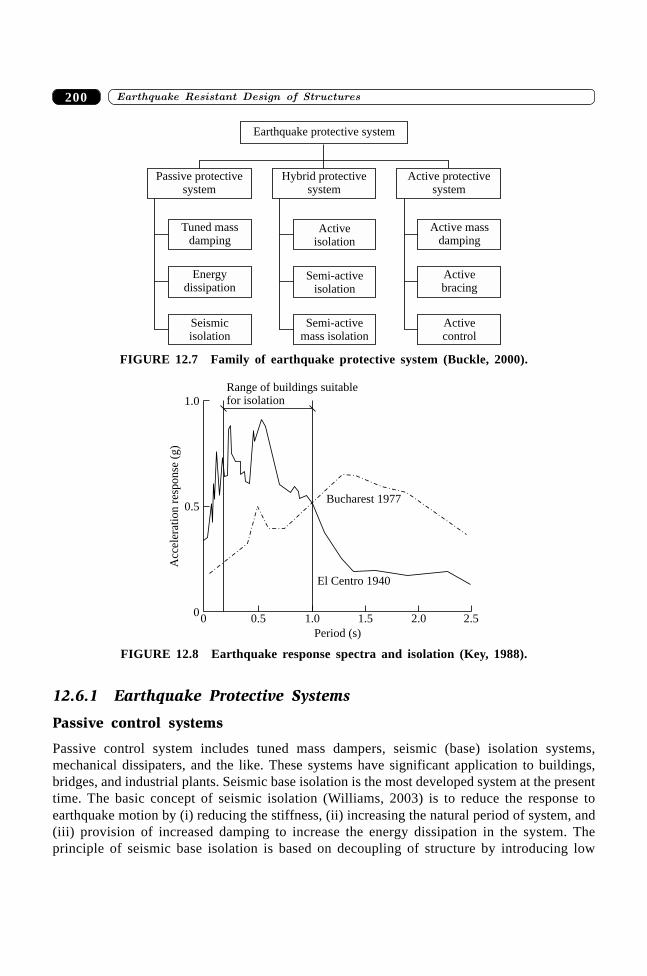
����������� ������� �������������200
Semi-activemass isolation
Seismicisolation
Energydissipation
Semi-activeisolation
Activecontrol
Activebracing
Active massdamping
Activeisolation
Tuned massdamping
Passive protectivesystem
Hybrid protectivesystem
Active protectivesystem
Earthquake protective system
FIGURE 12.7 Family of earthquake protective system (Buckle, 2000).
Range of buildings suitablefor isolation
00
0.5 1.0 1.5 2.0 2.5
0.5
1.0
Acc
eler
atio
nre
spo
nse
(g)
Bucharest 1977
El Centro 1940
Period (s)
FIGURE 12.8 Earthquake response spectra and isolation (Key, 1988).
12.6.1 Earthquake Protective Systems
Passive control systems
Passive control system includes tuned mass dampers, seismic (base) isolation systems,mechanical dissipaters, and the like. These systems have significant application to buildings,bridges, and industrial plants. Seismic base isolation is the most developed system at the presenttime. The basic concept of seismic isolation (Williams, 2003) is to reduce the response toearthquake motion by (i) reducing the stiffness, (ii) increasing the natural period of system, and(iii) provision of increased damping to increase the energy dissipation in the system. Theprinciple of seismic base isolation is based on decoupling of structure by introducing low
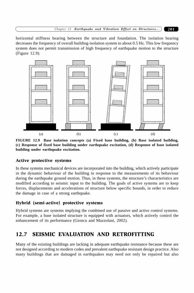
201�������� ������������� ���� ���������������������
horizontal stiffness bearing between the structure and foundation. The isolation bearingdecreases the frequency of overall building-isolation system to about 0.5 Hz. This low frequencysystem does not permit transmission of high frequency of earthquake motion to the structure(Figure 12.9).
(a) (b) (c) (d)
FIGURE 12.9 Base isolation concepts (a) Fixed base building, (b) Base isolated building,(c) Response of fixed base building under earthquake excitation, (d) Response of base isolatedbuilding under earthquake excitation.
Active protective systems
In these systems mechanical devices are incorporated into the building, which actively participatein the dynamic behaviour of the building in response to the measurements of its behaviourduring the earthquake ground motion. Thus, in these systems, the structure’s characteristics aremodified according to seismic input to the building. The goals of active systems are to keepforces, displacements and accelerations of structure below specific bounds, in order to reducethe damage in case of a strong earthquake.
Hybrid (semi-active) protective systems
Hybrid systems are systems implying the combined use of passive and active control systems.For example, a base isolated structure is equipped with actuators, which actively control theenhancement of its performance (Gioncu and Mazzolani, 2002).
12.7 SEISMIC EVALUATION AND RETROFITTING
Many of the existing buildings are lacking in adequate earthquake resistance because these arenot designed according to modern codes and prevalent earthquake resistant design practice. Alsomany buildings that are damaged in earthquakes may need not only be repaired but also
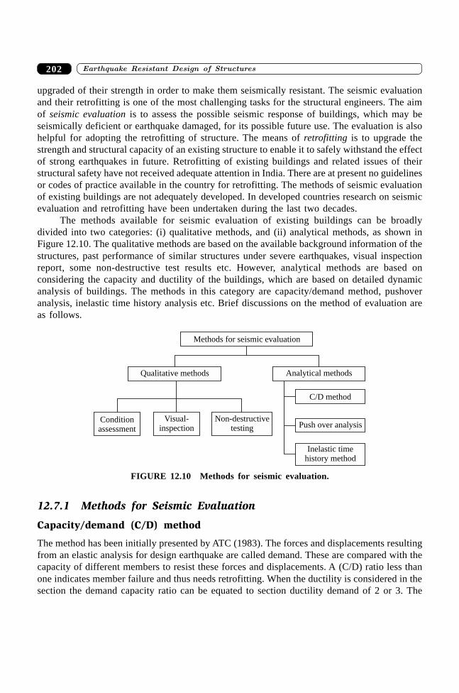
����������� ������� �������������202
upgraded of their strength in order to make them seismically resistant. The seismic evaluationand their retrofitting is one of the most challenging tasks for the structural engineers. The aimof seismic evaluation is to assess the possible seismic response of buildings, which may beseismically deficient or earthquake damaged, for its possible future use. The evaluation is alsohelpful for adopting the retrofitting of structure. The means of retrofitting is to upgrade thestrength and structural capacity of an existing structure to enable it to safely withstand the effectof strong earthquakes in future. Retrofitting of existing buildings and related issues of theirstructural safety have not received adequate attention in India. There are at present no guidelinesor codes of practice available in the country for retrofitting. The methods of seismic evaluationof existing buildings are not adequately developed. In developed countries research on seismicevaluation and retrofitting have been undertaken during the last two decades.
The methods available for seismic evaluation of existing buildings can be broadlydivided into two categories: (i) qualitative methods, and (ii) analytical methods, as shown inFigure 12.10. The qualitative methods are based on the available background information of thestructures, past performance of similar structures under severe earthquakes, visual inspectionreport, some non-destructive test results etc. However, analytical methods are based onconsidering the capacity and ductility of the buildings, which are based on detailed dynamicanalysis of buildings. The methods in this category are capacity/demand method, pushoveranalysis, inelastic time history analysis etc. Brief discussions on the method of evaluation areas follows.
Non-destructivetesting
Visual-inspection
Conditionassessment
Qualitative methods Analytical methods
Methods for seismic evaluation
Push over analysis
C/D method
Inelastic timehistory method
FIGURE 12.10 Methods for seismic evaluation.
12.7.1 Methods for Seismic Evaluation
Capacity/demand (C/D) method
The method has been initially presented by ATC (1983). The forces and displacements resultingfrom an elastic analysis for design earthquake are called demand. These are compared with thecapacity of different members to resist these forces and displacements. A (C/D) ratio less thanone indicates member failure and thus needs retrofitting. When the ductility is considered in thesection the demand capacity ratio can be equated to section ductility demand of 2 or 3. The
203�������� ������������� ���� ���������������������
C/D procedures have been subjected to more detailed examination in the light of recent advancesin earthquake response studies. The main difficulty encountered in using this method is thatthere is no relationship between member and structure ductility factor because of non-linearbehaviour.
Push Over analysis
The push over analysis of a structure is a static non-linear analysis under permanent verticalloads and gradually increasing lateral loads. The equivalent static lateral loads approximatelyrepresent earthquake-induced forces. A plot of total base shear verses top displacement in astructure is obtained by this analysis that would indicate any premature failure or weakness. Theanalysis is carried out upto failure, thus it enables determination of collapse load and ductilitycapacity. On a building frame, load/displacement is applied incrementally, the formation ofplastic hinges, stiffness degradation, and plastic rotation is monitored, and lateral inelastic forceversus displacement response for the complete structure is analytically computed. This type ofanalysis enables weakness in the structure to be identified. The decision to retrofit can be takenon the basis of such studies.
Inelastic time-history analysis
A seismically deficient building will be subjected to inelastic action during design earthquakemotion. The inelastic time history analysis of the building under strong ground motion bringsout the regions of weakness and ductility demand in the structure. This is the most rationalmethod available for assessing building performance. There are computer programs availableto perform this type of analysis. However there are complexities with regard to biaxial inelasticresponse of columns, modelling of joints behaviour, interaction of flexural and shear strengthand modeling of degrading characteristics of member. The methodology is used to ascertaindeficiency and post-elastic response under strong ground shaking.
12.7.2 Methods for Seismic Retrofitting
Retrofit technique employed for a structure can be categorized as (i) structural/global, and(ii) member/local. The techniques employed for seismic retrofitting are illustrated inFigure 12.11.
Structural or global retrofitting
Generally structural level retrofitting are applied when the entire structural lateral load resistingsystem is deemed to be deficient. Common approaches in this regard are employed to increasestiffness and strength with limited ductility.
Member or local retrofitting
Member or local retrofitting deals with an increase of the ductility of the components withadequate capacities to satisfy their specific limit states.
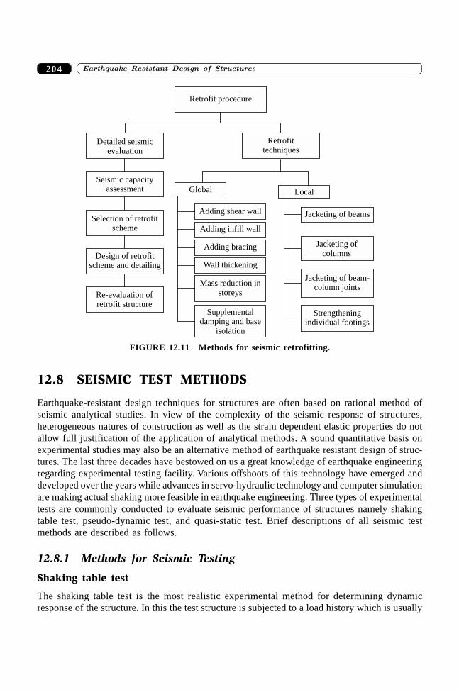
����������� ������� �������������204
Retrofit procedure
Detailed seismicevaluation
Seismic capacityassessment
Selection of retrofitscheme
Design of retrofitscheme and detailing
Re-evaluation ofretrofit structure
Retrofittechniques
LocalGlobal
Jacketing of beamsAdding shear wall
Adding infill wall
Adding bracing
Wall thickening
Jacketing ofcolumns
Strengtheningindividual footings
Jacketing of beam-column joints
Mass reduction instoreys
Supplementaldamping and base
isolation
FIGURE 12.11 Methods for seismic retrofitting.
12.8 SEISMIC TEST METHODS
Earthquake-resistant design techniques for structures are often based on rational method ofseismic analytical studies. In view of the complexity of the seismic response of structures,heterogeneous natures of construction as well as the strain dependent elastic properties do notallow full justification of the application of analytical methods. A sound quantitative basis onexperimental studies may also be an alternative method of earthquake resistant design of struc-tures. The last three decades have bestowed on us a great knowledge of earthquake engineeringregarding experimental testing facility. Various offshoots of this technology have emerged anddeveloped over the years while advances in servo-hydraulic technology and computer simulationare making actual shaking more feasible in earthquake engineering. Three types of experimentaltests are commonly conducted to evaluate seismic performance of structures namely shakingtable test, pseudo-dynamic test, and quasi-static test. Brief descriptions of all seismic testmethods are described as follows.
12.8.1 Methods for Seismic Testing
Shaking table test
The shaking table test is the most realistic experimental method for determining dynamicresponse of the structure. In this the test structure is subjected to a load history which is usually
205�������� ������������� ���� ���������������������
a ground motion recorded during an earthquake is simulated. A recent trend in shaking tablesystems is total six-degree of freedom motion ability. The capital equipment cost of shake tableis a power function of specific weight and dimension, so only models of the real structures maybe tested (Clark, 1990).
Pseudo-dynamic test
In the pseudo-dynamic test dynamic conditions are simulated. This testing is done with on-linecomputer simulation techniques. The load or deformation is applied quasi-statically at variouspositions of the test structure, depending on the restoring force directly measured during the test.The test structure is idealised into a discrete parameter system for which the equations of motionare written and integrated and the restoring forces for the system are applied at various floorlevels.
Quasi-static test
The quasi-static test is not a dynamic test, in which the rate of application of the load is verylow so that the material strain-rate effects do not influence the structural behaviour and inertiaforces are not developed. The loading pattern and history must be carefully chosen to be generalenough to provide the full range of deformations that the structure will experience under theearthquake excitation. This method adequately captures the important dynamic characteristicsof the structure: hysteresis behaviour, energy dissipation capacity, stiffness degradation,ductility, hysteretic damping, the most distressed zones, and lateral strength and deformationcapacity. This data is also utilized to make the hysteretic model of component for the dynamicanalysis of structure
SUMMARY
The chapter deals with an introduction to the main attributes of earthquake resistant designof structures with a special emphasis on related additional features in comparison to civilengineering design. It introduces briefly the available methods of seismic analysis, seismicdesign, seismic response control, alongwith current techniques of seismic evaluation andretrofitting. The relevant experimental studies to earthquake engineering practice have also beenunderlined.
REFERENCES
[1] Anderson, J.C., “Dynamic Response of Structures”, The Seismic Design Handbook,2nd ed., Farzad Naeim (Ed.), Kluwer Academic Publisher, The Netherlands, 2001.
[2] Buckle, I.G., “Passive Control of Structures for Seismic Loads”, Twelfth WorldConference on Earthquake Engineering, New Zealand, 2000.
[3] Beskos, D.E. and Anagnostoulos, S.A., Advances in Earthquake Engineering—Computer Analysis and Design of Earthquake Resistant Structures: A Handbook,Computational Mechanics Publications, Southampton, UK, 1997.
����������� ������� �������������206
[4] Clark, A. “Earthquake Testing Methods for Structures—Examples of Current Practiceand Future Directions”, Earthquake Resistant Construction and Design, Savidis (Ed.),Balkema, Rotterdam, 1990.
[5] Gioncu, V. and Mazzolani, F.M., Ductility of Seismic Resistant Steel Structures, SponPress, New York, 2002.
[6] IS 1893, “Criteria for Earthquake Resistant Design of Buildings—Part 1”, Bureau ofIndian Standards, New Delhi, (2002).
[7] Kabeyasawa Toshimi, “Earthquake Response Analysis”, Series on Innovation inStructures and Construction: Vol. 3, Design of Modern High-rise Reinforced ConcreteStructures, Hiroyuki Aoyama (Ed.), Imperial College Press, London, 2001.
[8] Key David., Earthquake Design Practice for Buildings, Thomas Telford, London,1988.
[9] Riddell, R. and Llera, J.C.D.L., “Seismic Analysis and Design: Current Practice andFuture Trends”, Eleventh World Conference on Earthquake Engineering, Mexico,1996.
[10] Syrmakezis, C.A. and Sophocleous, A.A., “Earthquake and Vibration Effect”, Compu-tational Modeling of Masonry, Brickwork and Brickwork Structures, John W. Bull(Ed.), Saxe-Coburg Publication, Stirling, UK, pp. 1–21, 2001.
[11] Syrmakezis, C.A., “Tentative Guidelines for Protection and Rehabilitations”, CISMCourse on Protection of the Architectural Heritage against Earthquakes, V. Petrini andM. Save (Eds.), Springer Wien, NewYork, 1996.
[12] Williams, A., Seismic Design of Buildings and Bridges, Oxford University PressOxford, New York, 2003.
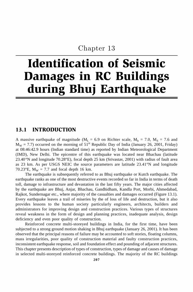
207
Identification of SeismicDamages in RC Buildingsduring Bhuj Earthquake
��������
13.1 INTRODUCTION
A massive earthquake of magnitude (ML = 6.9 on Richter scale, Mb = 7.0, MS = 7.6 andMW = 7.7) occurred on the morning of 51st Republic Day of India (January 26, 2001, Friday)at 08:46:42.9 hours (Indian standard time) as reported by Indian Meteorological Department(IMD), New Delhi. The epicentre of this earthquake was located near Bhachau (latitude23.40°N and longitude 70.28°E), focal depth 25 km (Srivastav, 2001) with radius of fault areaas 23 km. As per USGS NEIC the source parameters are latitude 23.41°N and longitude70.23°E, MW = 7.7 and focal depth 16 km.
The earthquake is subsequently referred to as Bhuj earthquake or Kutch earthquake. Theearthquake ranks as one of the most destructive events recorded so far in India in terms of deathtoll, damage to infrastructure and devastation in the last fifty years. The major cities affectedby the earthquake are Bhuj, Anjar, Bhachau, Gandhidham, Kandla Port, Morbi, Ahmedabad,Rajkot, Sundernagar etc., where majority of the casualties and damages occurred (Figure 13.1).Every earthquake leaves a trail of miseries by the of loss of life and destruction, but it alsoprovides lessons to the human society particularly engineers, architects, builders andadministrators for improving design and construction practices. Various types of structuresreveal weakness in the form of design and planning practices, inadequate analysis, designdeficiency and even poor quality of construction.
Reinforced concrete multi-storeyed buildings in India, for the first time, have beensubjected to a strong ground motion shaking in Bhuj earthquake (January 26, 2001). It has beenobserved that the principal reasons of failure may be accounted to soft stories, floating columns,mass irregularities, poor quality of construction material and faulty construction practices,inconsistent earthquake response, soil and foundation effect and pounding of adjacent structures.This chapter presents description of types of construction, types of damage and causes of damagein selected multi-storeyed reinforced concrete buildings. The majority of the RC buildings
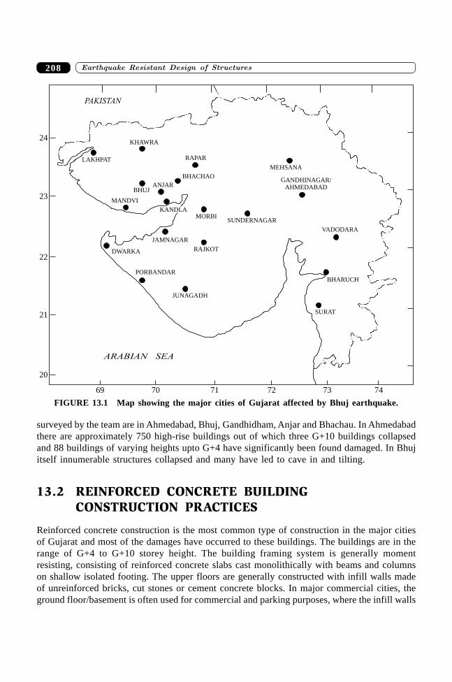
����������� ������� �������������208
surveyed by the team are in Ahmedabad, Bhuj, Gandhidham, Anjar and Bhachau. In Ahmedabadthere are approximately 750 high-rise buildings out of which three G+10 buildings collapsedand 88 buildings of varying heights upto G+4 have significantly been found damaged. In Bhujitself innumerable structures collapsed and many have led to cave in and tilting.
13.2 REINFORCED CONCRETE BUILDINGCONSTRUCTION PRACTICES
Reinforced concrete construction is the most common type of construction in the major citiesof Gujarat and most of the damages have occurred to these buildings. The buildings are in therange of G+4 to G+10 storey height. The building framing system is generally momentresisting, consisting of reinforced concrete slabs cast monolithically with beams and columnson shallow isolated footing. The upper floors are generally constructed with infill walls madeof unreinforced bricks, cut stones or cement concrete blocks. In major commercial cities, theground floor/basement is often used for commercial and parking purposes, where the infill walls
LAKHPAT
KHAWRA
RAPAR
BHACHAO
ANJARBHUJ
MANDVI
KANDLAMORBI
SUNDERNAGAR
MEHSANA
GANDHINAGAR/AHMEDABAD
VADODARA
RAJKOT
JAMNAGAR
DWARKA
PORBANDAR
JUNAGADH
SURAT
BHARUCH
PAKISTAN
ARABIAN SEA
69 70 71 72 73 74
20
21
22
23
24
FIGURE 13.1 Map showing the major cities of Gujarat affected by Bhuj earthquake.
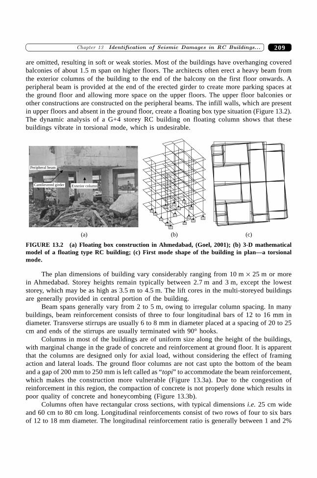
209�������� ���� � ��� ����� �� ������� ����� �� ������
are omitted, resulting in soft or weak stories. Most of the buildings have overhanging coveredbalconies of about 1.5 m span on higher floors. The architects often erect a heavy beam fromthe exterior columns of the building to the end of the balcony on the first floor onwards. Aperipheral beam is provided at the end of the erected girder to create more parking spaces atthe ground floor and allowing more space on the upper floors. The upper floor balconies orother constructions are constructed on the peripheral beams. The infill walls, which are presentin upper floors and absent in the ground floor, create a floating box type situation (Figure 13.2).The dynamic analysis of a G+4 storey RC building on floating column shows that thesebuildings vibrate in torsional mode, which is undesirable.
(a) (b) (c)
Peripheral beam
Cantilevered girder Exterior column
FIGURE 13.2 (a) Floating box construction in Ahmedabad, (Goel, 2001); (b) 3-D mathematicalmodel of a floating type RC building; (c) First mode shape of the building in plan—a torsionalmode.
The plan dimensions of building vary considerably ranging from 10 m ¥ 25 m or morein Ahmedabad. Storey heights remain typically between 2.7 m and 3 m, except the loweststorey, which may be as high as 3.5 m to 4.5 m. The lift cores in the multi-storeyed buildingsare generally provided in central portion of the building.
Beam spans generally vary from 2 to 5 m, owing to irregular column spacing. In manybuildings, beam reinforcement consists of three to four longitudinal bars of 12 to 16 mm indiameter. Transverse stirrups are usually 6 to 8 mm in diameter placed at a spacing of 20 to 25cm and ends of the stirrups are usually terminated with 90° hooks.
Columns in most of the buildings are of uniform size along the height of the buildings,with marginal change in the grade of concrete and reinforcement at ground floor. It is apparentthat the columns are designed only for axial load, without considering the effect of framingaction and lateral loads. The ground floor columns are not cast upto the bottom of the beamand a gap of 200 mm to 250 mm is left called as “topi” to accommodate the beam reinforcement,which makes the construction more vulnerable (Figure 13.3a). Due to the congestion ofreinforcement in this region, the compaction of concrete is not properly done which results inpoor quality of concrete and honeycombing (Figure 13.3b).
Columns often have rectangular cross sections, with typical dimensions i.e. 25 cm wideand 60 cm to 80 cm long. Longitudinal reinforcements consist of two rows of four to six barsof 12 to 18 mm diameter. The longitudinal reinforcement ratio is generally between 1 and 2%
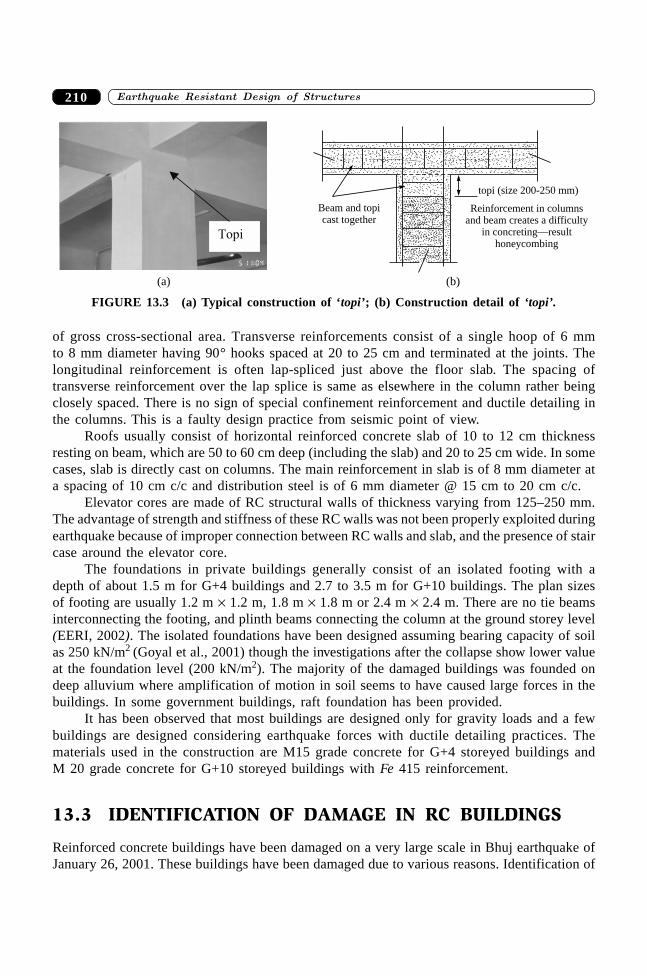
����������� ������� �������������210
of gross cross-sectional area. Transverse reinforcements consist of a single hoop of 6 mmto 8 mm diameter having 90° hooks spaced at 20 to 25 cm and terminated at the joints. Thelongitudinal reinforcement is often lap-spliced just above the floor slab. The spacing oftransverse reinforcement over the lap splice is same as elsewhere in the column rather beingclosely spaced. There is no sign of special confinement reinforcement and ductile detailing inthe columns. This is a faulty design practice from seismic point of view.
Roofs usually consist of horizontal reinforced concrete slab of 10 to 12 cm thicknessresting on beam, which are 50 to 60 cm deep (including the slab) and 20 to 25 cm wide. In somecases, slab is directly cast on columns. The main reinforcement in slab is of 8 mm diameter ata spacing of 10 cm c/c and distribution steel is of 6 mm diameter @ 15 cm to 20 cm c/c.
Elevator cores are made of RC structural walls of thickness varying from 125–250 mm.The advantage of strength and stiffness of these RC walls was not been properly exploited duringearthquake because of improper connection between RC walls and slab, and the presence of staircase around the elevator core.
The foundations in private buildings generally consist of an isolated footing with adepth of about 1.5 m for G+4 buildings and 2.7 to 3.5 m for G+10 buildings. The plan sizesof footing are usually 1.2 m ¥ 1.2 m, 1.8 m ¥ 1.8 m or 2.4 m ¥ 2.4 m. There are no tie beamsinterconnecting the footing, and plinth beams connecting the column at the ground storey level(EERI, 2002). The isolated foundations have been designed assuming bearing capacity of soilas 250 kN/m2 (Goyal et al., 2001) though the investigations after the collapse show lower valueat the foundation level (200 kN/m2). The majority of the damaged buildings was founded ondeep alluvium where amplification of motion in soil seems to have caused large forces in thebuildings. In some government buildings, raft foundation has been provided.
It has been observed that most buildings are designed only for gravity loads and a fewbuildings are designed considering earthquake forces with ductile detailing practices. Thematerials used in the construction are M15 grade concrete for G+4 storeyed buildings andM 20 grade concrete for G+10 storeyed buildings with Fe 415 reinforcement.
13.3 IDENTIFICATION OF DAMAGE IN RC BUILDINGS
Reinforced concrete buildings have been damaged on a very large scale in Bhuj earthquake ofJanuary 26, 2001. These buildings have been damaged due to various reasons. Identification of
(a)
Reinforcement in columnsand beam creates a difficulty
in concreting—resulthoneycombing
topi (size 200-250 mm)
Beam and topicast together
(b)
FIGURE 13.3 (a) Typical construction of ‘topi’; (b) Construction detail of ‘topi’.
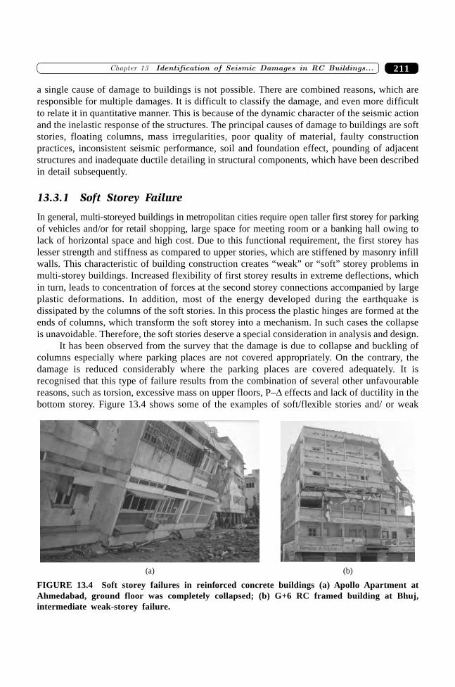
211�������� ���� � ��� ����� �� ������� ����� �� ������
a single cause of damage to buildings is not possible. There are combined reasons, which areresponsible for multiple damages. It is difficult to classify the damage, and even more difficultto relate it in quantitative manner. This is because of the dynamic character of the seismic actionand the inelastic response of the structures. The principal causes of damage to buildings are softstories, floating columns, mass irregularities, poor quality of material, faulty constructionpractices, inconsistent seismic performance, soil and foundation effect, pounding of adjacentstructures and inadequate ductile detailing in structural components, which have been describedin detail subsequently.
13.3.1 Soft Storey Failure
In general, multi-storeyed buildings in metropolitan cities require open taller first storey for parkingof vehicles and/or for retail shopping, large space for meeting room or a banking hall owing tolack of horizontal space and high cost. Due to this functional requirement, the first storey haslesser strength and stiffness as compared to upper stories, which are stiffened by masonry infillwalls. This characteristic of building construction creates “weak” or “soft” storey problems inmulti-storey buildings. Increased flexibility of first storey results in extreme deflections, whichin turn, leads to concentration of forces at the second storey connections accompanied by largeplastic deformations. In addition, most of the energy developed during the earthquake isdissipated by the columns of the soft stories. In this process the plastic hinges are formed at theends of columns, which transform the soft storey into a mechanism. In such cases the collapseis unavoidable. Therefore, the soft stories deserve a special consideration in analysis and design.
It has been observed from the survey that the damage is due to collapse and buckling ofcolumns especially where parking places are not covered appropriately. On the contrary, thedamage is reduced considerably where the parking places are covered adequately. It isrecognised that this type of failure results from the combination of several other unfavourablereasons, such as torsion, excessive mass on upper floors, P–D effects and lack of ductility in thebottom storey. Figure 13.4 shows some of the examples of soft/flexible stories and/ or weak
(a) (b)
FIGURE 13.4 Soft storey failures in reinforced concrete buildings (a) Apollo Apartment atAhmedabad, ground floor was completely collapsed; (b) G+6 RC framed building at Bhuj,intermediate weak-storey failure.
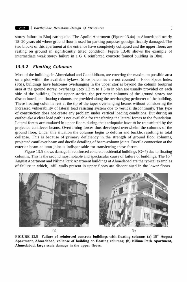
����������� ������� �������������212
storey failure in Bhuj earthquake. The Apollo Apartment (Figure 13.4a) in Ahmedabad nearly15–20 years old where ground floor is used for parking purposes got significantly damaged. Thetwo blocks of this apartment at the entrance have completely collapsed and the upper floors areresting on ground in significantly tilted condition. Figure 13.4b shows the example ofintermediate weak storey failure in a G+6 reinforced concrete framed building in Bhuj.
13.3.2 Floating Columns
Most of the buildings in Ahmedabad and Gandhidham, are covering the maximum possible areaon a plot within the available bylaws. Since balconies are not counted in Floor Space Index(FSI), buildings have balconies overhanging in the upper stories beyond the column footprintarea at the ground storey, overhangs upto 1.2 m to 1.5 m in plan are usually provided on eachside of the building. In the upper stories, the perimeter columns of the ground storey arediscontinued, and floating columns are provided along the overhanging perimeter of the building.These floating columns rest at the tip of the taper overhanging beams without considering theincreased vulnerability of lateral load resisting system due to vertical discontinuity. This typeof construction does not create any problem under vertical loading conditions. But during anearthquake a clear load path is not available for transferring the lateral forces to the foundation.Lateral forces accumulated in upper floors during the earthquake have to be transmitted by theprojected cantilever beams. Overturning forces thus developed overwhelm the columns of theground floor. Under this situation the columns begin to deform and buckle, resulting in totalcollapse. This is because of primary deficiency in the strength of ground floor columns,projected cantilever beam and ductile detailing of beam-column joints. Ductile connection at theexterior beam-column joint is indispensable for transferring these forces.
Figure 13.5 shows damage in reinforced concrete residential buildings (G+4) due to floatingcolumns. This is the second most notable and spectacular cause of failure of buildings. The 15th
August Apartment and Nilima Park Apartment buildings at Ahmedabad are the typical examplesof failure in which, infill walls present in upper floors are discontinued in the lower floors.
(a) (b)
FIGURE 13.5 Failure of reinforced concrete buildings with floating columns (a) 15th AugustApartment, Ahmedabad, collapse of building on floating columns; (b) Nilima Park Apartment,Ahmedabad, large scale damage in the upper floors.
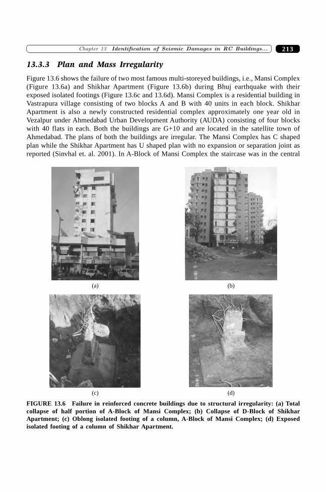
213�������� ���� � ��� ����� �� ������� ����� �� ������
13.3.3 Plan and Mass Irregularity
Figure 13.6 shows the failure of two most famous multi-storeyed buildings, i.e., Mansi Complex(Figure 13.6a) and Shikhar Apartment (Figure 13.6b) during Bhuj earthquake with theirexposed isolated footings (Figure 13.6c and 13.6d). Mansi Complex is a residential building inVastrapura village consisting of two blocks A and B with 40 units in each block. ShikharApartment is also a newly constructed residential complex approximately one year old inVezalpur under Ahmedabad Urban Development Authority (AUDA) consisting of four blockswith 40 flats in each. Both the buildings are G+10 and are located in the satellite town ofAhmedabad. The plans of both the buildings are irregular. The Mansi Complex has C shapedplan while the Shikhar Apartment has U shaped plan with no expansion or separation joint asreported (Sinvhal et. al. 2001). In A-Block of Mansi Complex the staircase was in the central
(a) (b)
(c) (d)
FIGURE 13.6 Failure in reinforced concrete buildings due to structural irregularity: (a) Totalcollapse of half portion of A-Block of Mansi Complex; (b) Collapse of D-Block of ShikharApartment; (c) Oblong isolated footing of a column, A-Block of Mansi Complex; (d) Exposedisolated footing of a column of Shikhar Apartment.
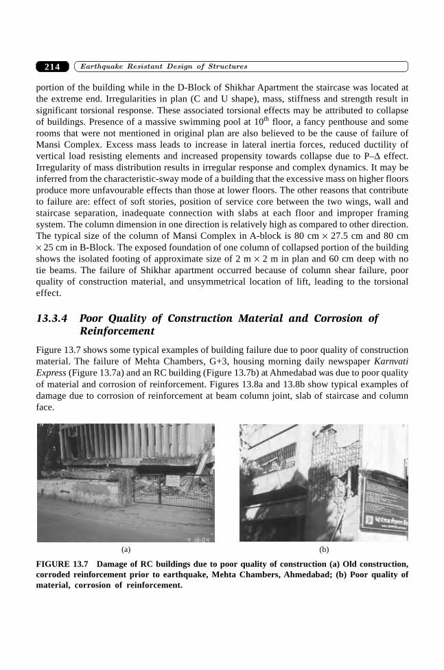
����������� ������� �������������214
portion of the building while in the D-Block of Shikhar Apartment the staircase was located atthe extreme end. Irregularities in plan (C and U shape), mass, stiffness and strength result insignificant torsional response. These associated torsional effects may be attributed to collapseof buildings. Presence of a massive swimming pool at 10th floor, a fancy penthouse and somerooms that were not mentioned in original plan are also believed to be the cause of failure ofMansi Complex. Excess mass leads to increase in lateral inertia forces, reduced ductility ofvertical load resisting elements and increased propensity towards collapse due to P–D effect.Irregularity of mass distribution results in irregular response and complex dynamics. It may beinferred from the characteristic-sway mode of a building that the excessive mass on higher floorsproduce more unfavourable effects than those at lower floors. The other reasons that contributeto failure are: effect of soft stories, position of service core between the two wings, wall andstaircase separation, inadequate connection with slabs at each floor and improper framingsystem. The column dimension in one direction is relatively high as compared to other direction.The typical size of the column of Mansi Complex in A-block is 80 cm ¥ 27.5 cm and 80 cm¥ 25 cm in B-Block. The exposed foundation of one column of collapsed portion of the buildingshows the isolated footing of approximate size of 2 m ¥ 2 m in plan and 60 cm deep with notie beams. The failure of Shikhar apartment occurred because of column shear failure, poorquality of construction material, and unsymmetrical location of lift, leading to the torsionaleffect.
13.3.4 Poor Quality of Construction Material and Corrosion ofReinforcement
Figure 13.7 shows some typical examples of building failure due to poor quality of constructionmaterial. The failure of Mehta Chambers, G+3, housing morning daily newspaper KarnvatiExpress (Figure 13.7a) and an RC building (Figure 13.7b) at Ahmedabad was due to poor qualityof material and corrosion of reinforcement. Figures 13.8a and 13.8b show typical examples ofdamage due to corrosion of reinforcement at beam column joint, slab of staircase and columnface.
(a) (b)
FIGURE 13.7 Damage of RC buildings due to poor quality of construction (a) Old construction,corroded reinforcement prior to earthquake, Mehta Chambers, Ahmedabad; (b) Poor quality ofmaterial, corrosion of reinforcement.
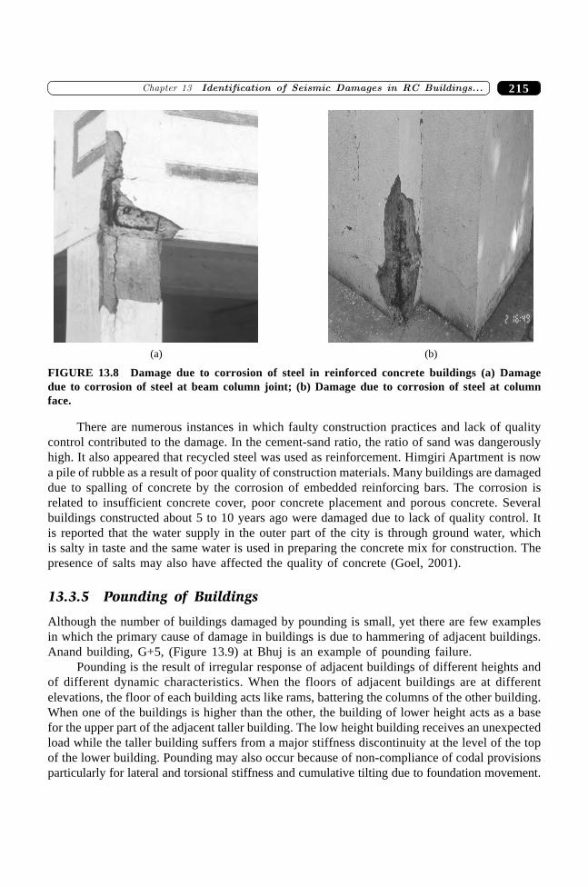
215�������� ���� � ��� ����� �� ������� ����� �� ������
(a) (b)
FIGURE 13.8 Damage due to corrosion of steel in reinforced concrete buildings (a) Damagedue to corrosion of steel at beam column joint; (b) Damage due to corrosion of steel at columnface.
There are numerous instances in which faulty construction practices and lack of qualitycontrol contributed to the damage. In the cement-sand ratio, the ratio of sand was dangerouslyhigh. It also appeared that recycled steel was used as reinforcement. Himgiri Apartment is nowa pile of rubble as a result of poor quality of construction materials. Many buildings are damageddue to spalling of concrete by the corrosion of embedded reinforcing bars. The corrosion isrelated to insufficient concrete cover, poor concrete placement and porous concrete. Severalbuildings constructed about 5 to 10 years ago were damaged due to lack of quality control. Itis reported that the water supply in the outer part of the city is through ground water, whichis salty in taste and the same water is used in preparing the concrete mix for construction. Thepresence of salts may also have affected the quality of concrete (Goel, 2001).
13.3.5 Pounding of Buildings
Although the number of buildings damaged by pounding is small, yet there are few examplesin which the primary cause of damage in buildings is due to hammering of adjacent buildings.Anand building, G+5, (Figure 13.9) at Bhuj is an example of pounding failure.
Pounding is the result of irregular response of adjacent buildings of different heights andof different dynamic characteristics. When the floors of adjacent buildings are at differentelevations, the floor of each building acts like rams, battering the columns of the other building.When one of the buildings is higher than the other, the building of lower height acts as a basefor the upper part of the adjacent taller building. The low height building receives an unexpectedload while the taller building suffers from a major stiffness discontinuity at the level of the topof the lower building. Pounding may also occur because of non-compliance of codal provisionsparticularly for lateral and torsional stiffness and cumulative tilting due to foundation movement.
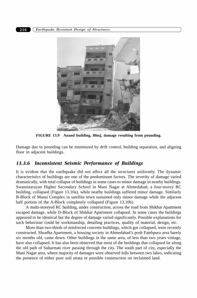
����������� ������� �������������216
Damage due to pounding can be minimized by drift control, building separation, and aligningfloor in adjacent buildings.
13.3.6 Inconsistent Seismic Performance of Buildings
It is evident that the earthquake did not affect all the structures uniformly. The dynamiccharacteristics of buildings are one of the predominant factors. The severity of damage varieddramatically, with total collapse of buildings in some cases to minor damage in nearby buildings.Swaminarayan Higher Secondary School in Mani Nagar at Ahmedabad, a four-storey RCbuilding, collapsed (Figure 13.10a), while nearby buildings suffered minor damage. SimilarlyB-Block of Mansi Complex in satellite town sustained only minor damage while the adjacenthalf portion of the A-Block completely collapsed (Figure 13.10b).
A multi-storeyed RC building, under construction, across the road from Shikhar Apartmentescaped damage, while D-Block of Shikhar Apartment collapsed. In some cases the buildingsappeared to be identical but the degree of damage varied significantly. Possible explanations forsuch behaviour could be workmanship, detailing practices, quality of material, design, etc.
More than two-thirds of reinforced concrete buildings, which got collapsed, were recentlyconstructed. Shradha Apartment, a housing society in Ahmedabad’s posh Fatehpura area barelysix months old, came down. Other buildings in the same area, of less than two years vintage,have also collapsed. It has also been observed that most of the buildings that collapsed lie alongthe old path of Sabarmati river passing through the city. The south part of city, especially theMani Nagar area, where majority of damages were observed falls between two lakes, indicatingthe presence of either poor soil strata or possible construction on reclaimed land.
FIGURE 13.9 Anand building, Bhuj, damage resulting from pounding.
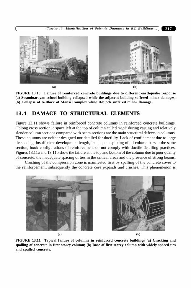
217�������� ���� � ��� ����� �� ������� ����� �� ������
13.4 DAMAGE TO STRUCTURAL ELEMENTS
Figure 13.11 shows failure in reinforced concrete columns in reinforced concrete buildings.Oblong cross section, a space left at the top of column called ‘topi’ during casting and relativelyslender column sections compared with beam sections are the main structural defects in columns.These columns are neither designed nor detailed for ductility. Lack of confinement due to largetie spacing, insufficient development length, inadequate splicing of all column bars at the samesection, hook configurations of reinforcement do not comply with ductile detailing practices.Figures 13.11a and 13.11b show the failure at the top and bottom of the column due to poor qualityof concrete, the inadequate spacing of ties in the critical areas and the presence of strong beams.
Crushing of the compression zone is manifested first by spalling of the concrete cover tothe reinforcement; subsequently the concrete core expands and crushes. This phenomenon is
(a) (b)
FIGURE 13.10 Failure of reinforced concrete buildings due to different earthquake response(a) Swaminarayan school building collapsed while the adjacent building suffered minor damages;(b) Collapse of A-Block of Mansi Complex while B-block suffered minor damage.
(a) (b)
FIGURE 13.11 Typical failure of columns in reinforced concrete buildings (a) Cracking andspalling of concrete in first storey column; (b) Base of first storey column with widely spaced tiesand spalled concrete.
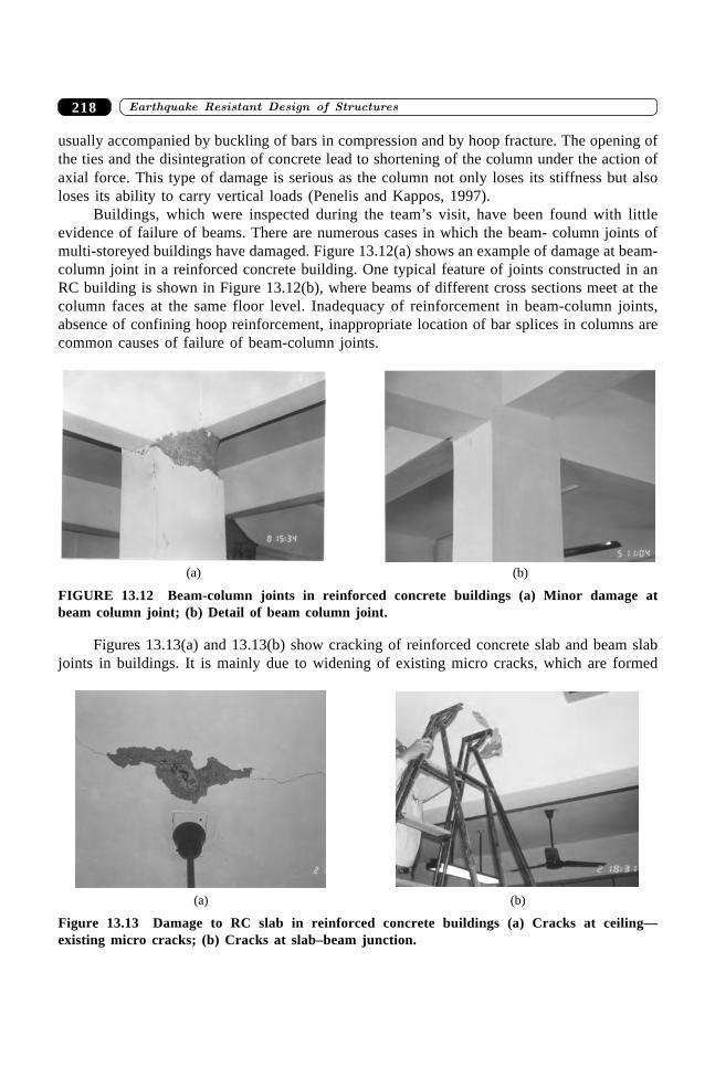
����������� ������� �������������218
usually accompanied by buckling of bars in compression and by hoop fracture. The opening ofthe ties and the disintegration of concrete lead to shortening of the column under the action ofaxial force. This type of damage is serious as the column not only loses its stiffness but alsoloses its ability to carry vertical loads (Penelis and Kappos, 1997).
Buildings, which were inspected during the team’s visit, have been found with littleevidence of failure of beams. There are numerous cases in which the beam- column joints ofmulti-storeyed buildings have damaged. Figure 13.12(a) shows an example of damage at beam-column joint in a reinforced concrete building. One typical feature of joints constructed in anRC building is shown in Figure 13.12(b), where beams of different cross sections meet at thecolumn faces at the same floor level. Inadequacy of reinforcement in beam-column joints,absence of confining hoop reinforcement, inappropriate location of bar splices in columns arecommon causes of failure of beam-column joints.
(a) (b)
FIGURE 13.12 Beam-column joints in reinforced concrete buildings (a) Minor damage atbeam column joint; (b) Detail of beam column joint.
Figures 13.13(a) and 13.13(b) show cracking of reinforced concrete slab and beam slabjoints in buildings. It is mainly due to widening of existing micro cracks, which are formed
(a) (b)
Figure 13.13 Damage to RC slab in reinforced concrete buildings (a) Cracks at ceiling—existing micro cracks; (b) Cracks at slab–beam junction.
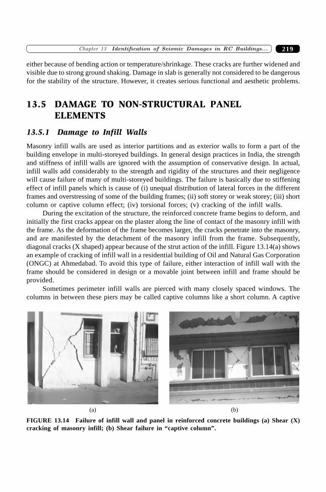
219�������� ���� � ��� ����� �� ������� ����� �� ������
either because of bending action or temperature/shrinkage. These cracks are further widened andvisible due to strong ground shaking. Damage in slab is generally not considered to be dangerousfor the stability of the structure. However, it creates serious functional and aesthetic problems.
13.5 DAMAGE TO NON-STRUCTURAL PANELELEMENTS
13.5.1 Damage to Infill Walls
Masonry infill walls are used as interior partitions and as exterior walls to form a part of thebuilding envelope in multi-storeyed buildings. In general design practices in India, the strengthand stiffness of infill walls are ignored with the assumption of conservative design. In actual,infill walls add considerably to the strength and rigidity of the structures and their negligencewill cause failure of many of multi-storeyed buildings. The failure is basically due to stiffeningeffect of infill panels which is cause of (i) unequal distribution of lateral forces in the differentframes and overstressing of some of the building frames; (ii) soft storey or weak storey; (iii) shortcolumn or captive column effect; (iv) torsional forces; (v) cracking of the infill walls.
During the excitation of the structure, the reinforced concrete frame begins to deform, andinitially the first cracks appear on the plaster along the line of contact of the masonry infill withthe frame. As the deformation of the frame becomes larger, the cracks penetrate into the masonry,and are manifested by the detachment of the masonry infill from the frame. Subsequently,diagonal cracks (X shaped) appear because of the strut action of the infill. Figure 13.14(a) showsan example of cracking of infill wall in a residential building of Oil and Natural Gas Corporation(ONGC) at Ahmedabad. To avoid this type of failure, either interaction of infill wall with theframe should be considered in design or a movable joint between infill and frame should beprovided.
Sometimes perimeter infill walls are pierced with many closely spaced windows. Thecolumns in between these piers may be called captive columns like a short column. A captive
(a) (b)
FIGURE 13.14 Failure of infill wall and panel in reinforced concrete buildings (a) Shear (X)cracking of masonry infill; (b) Shear failure in “captive column”.
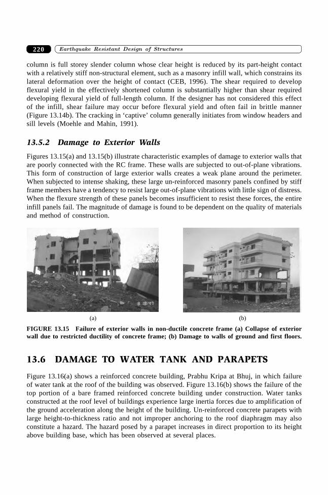
����������� ������� �������������220
column is full storey slender column whose clear height is reduced by its part-height contactwith a relatively stiff non-structural element, such as a masonry infill wall, which constrains itslateral deformation over the height of contact (CEB, 1996). The shear required to developflexural yield in the effectively shortened column is substantially higher than shear requireddeveloping flexural yield of full-length column. If the designer has not considered this effectof the infill, shear failure may occur before flexural yield and often fail in brittle manner(Figure 13.14b). The cracking in ‘captive’ column generally initiates from window headers andsill levels (Moehle and Mahin, 1991).
13.5.2 Damage to Exterior Walls
Figures 13.15(a) and 13.15(b) illustrate characteristic examples of damage to exterior walls thatare poorly connected with the RC frame. These walls are subjected to out-of-plane vibrations.This form of construction of large exterior walls creates a weak plane around the perimeter.When subjected to intense shaking, these large un-reinforced masonry panels confined by stiffframe members have a tendency to resist large out-of-plane vibrations with little sign of distress.When the flexure strength of these panels becomes insufficient to resist these forces, the entireinfill panels fail. The magnitude of damage is found to be dependent on the quality of materialsand method of construction.
(a) (b)
FIGURE 13.15 Failure of exterior walls in non-ductile concrete frame (a) Collapse of exteriorwall due to restricted ductility of concrete frame; (b) Damage to walls of ground and first floors.
13.6 DAMAGE TO WATER TANK AND PARAPETS
Figure 13.16(a) shows a reinforced concrete building, Prabhu Kripa at Bhuj, in which failureof water tank at the roof of the building was observed. Figure 13.16(b) shows the failure of thetop portion of a bare framed reinforced concrete building under construction. Water tanksconstructed at the roof level of buildings experience large inertia forces due to amplification ofthe ground acceleration along the height of the building. Un-reinforced concrete parapets withlarge height-to-thickness ratio and not improper anchoring to the roof diaphragm may alsoconstitute a hazard. The hazard posed by a parapet increases in direct proportion to its heightabove building base, which has been observed at several places.
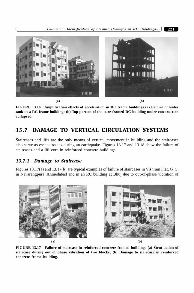
221�������� ���� � ��� ����� �� ������� ����� �� ������
13.7 DAMAGE TO VERTICAL CIRCULATION SYSTEMS
Staircases and lifts are the only means of vertical movement in building and the staircasesalso serve as escape routes during an earthquake. Figures 13.17 and 13.18 show the failure ofstaircases and a lift core in reinforced concrete buildings.
13.7.1 Damage to Staircase
Figures 13.17(a) and 13.17(b) are typical examples of failure of staircases in Vishram Flat, G+5,in Navarangpura, Ahmedabad and in an RC building at Bhuj due to out-of-phase vibration of
(a) (b)
FIGURE 13.16 Amplification effects of acceleration in RC frame buildings (a) Failure of watertank in a RC frame building; (b) Top portion of the bare framed RC building under constructioncollapsed.
(a) (b)
FIGURE 13.17 Failure of staircase in reinforced concrete framed buildings (a) Strut action ofstaircase during out of phase vibration of two blocks; (b) Damage to staircase in reinforcedconcrete frame building.
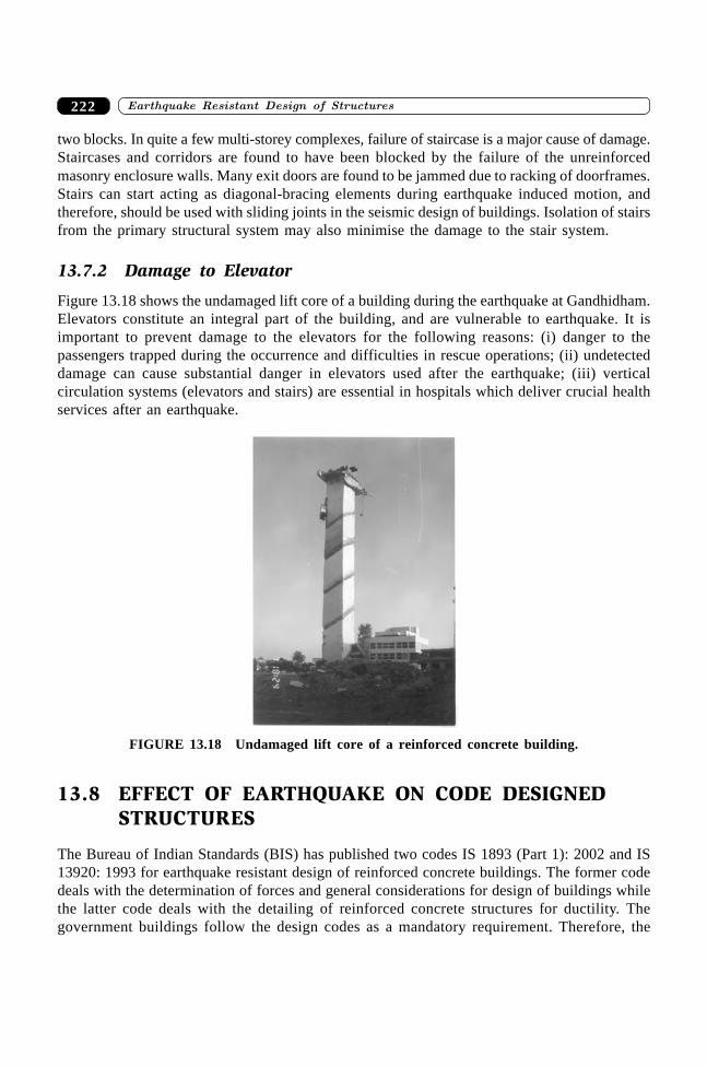
����������� ������� �������������222
two blocks. In quite a few multi-storey complexes, failure of staircase is a major cause of damage.Staircases and corridors are found to have been blocked by the failure of the unreinforcedmasonry enclosure walls. Many exit doors are found to be jammed due to racking of doorframes.Stairs can start acting as diagonal-bracing elements during earthquake induced motion, andtherefore, should be used with sliding joints in the seismic design of buildings. Isolation of stairsfrom the primary structural system may also minimise the damage to the stair system.
13.7.2 Damage to Elevator
Figure 13.18 shows the undamaged lift core of a building during the earthquake at Gandhidham.Elevators constitute an integral part of the building, and are vulnerable to earthquake. It isimportant to prevent damage to the elevators for the following reasons: (i) danger to thepassengers trapped during the occurrence and difficulties in rescue operations; (ii) undetecteddamage can cause substantial danger in elevators used after the earthquake; (iii) verticalcirculation systems (elevators and stairs) are essential in hospitals which deliver crucial healthservices after an earthquake.
FIGURE 13.18 Undamaged lift core of a reinforced concrete building.
13.8 EFFECT OF EARTHQUAKE ON CODE DESIGNEDSTRUCTURES
The Bureau of Indian Standards (BIS) has published two codes IS 1893 (Part 1): 2002 and IS13920: 1993 for earthquake resistant design of reinforced concrete buildings. The former codedeals with the determination of forces and general considerations for design of buildings whilethe latter code deals with the detailing of reinforced concrete structures for ductility. Thegovernment buildings follow the design codes as a mandatory requirement. Therefore, the
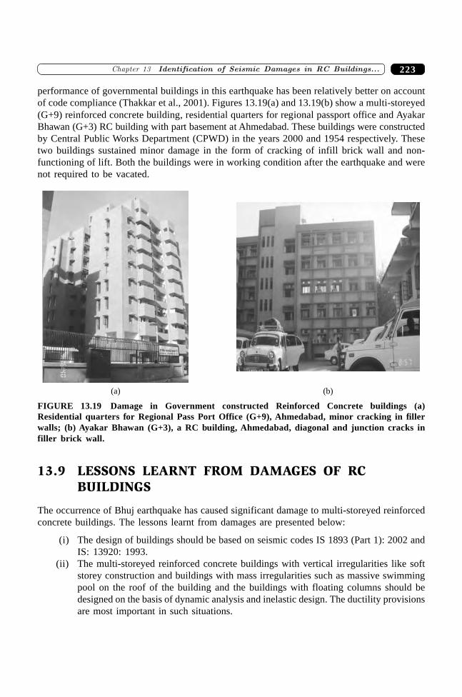
223�������� ���� � ��� ����� �� ������� ����� �� ������
performance of governmental buildings in this earthquake has been relatively better on accountof code compliance (Thakkar et al., 2001). Figures 13.19(a) and 13.19(b) show a multi-storeyed(G+9) reinforced concrete building, residential quarters for regional passport office and AyakarBhawan (G+3) RC building with part basement at Ahmedabad. These buildings were constructedby Central Public Works Department (CPWD) in the years 2000 and 1954 respectively. Thesetwo buildings sustained minor damage in the form of cracking of infill brick wall and non-functioning of lift. Both the buildings were in working condition after the earthquake and werenot required to be vacated.
(a) (b)
FIGURE 13.19 Damage in Government constructed Reinforced Concrete buildings (a)Residential quarters for Regional Pass Port Office (G+9), Ahmedabad, minor cracking in fillerwalls; (b) Ayakar Bhawan (G+3), a RC building, Ahmedabad, diagonal and junction cracks infiller brick wall.
13.9 LESSONS LEARNT FROM DAMAGES OF RCBUILDINGS
The occurrence of Bhuj earthquake has caused significant damage to multi-storeyed reinforcedconcrete buildings. The lessons learnt from damages are presented below:
(i) The design of buildings should be based on seismic codes IS 1893 (Part 1): 2002 andIS: 13920: 1993.
(ii) The multi-storeyed reinforced concrete buildings with vertical irregularities like softstorey construction and buildings with mass irregularities such as massive swimmingpool on the roof of the building and the buildings with floating columns should bedesigned on the basis of dynamic analysis and inelastic design. The ductility provisionsare most important in such situations.
����������� ������� �������������224
(iii) More care is necessary at the time of planning. The torsional effects in a building canbe minimised by proper location of vertical resisting elements and mass distribution.Building design with strong-column weak beam can be achieved at the planning stage.The soft storey stiffness can also be controlled by appropriate design procedure.
(iv) The infill construction in RC buildings should be duly accounted for structuralanalysis. The staircase connection with buildings should be made using sliding joints.
(v) Shear walls should be employed for increasing stiffness and are uniformly distributedin both principal directions.
(vi) There should be a greater emphasis on the quality of construction.
SUMMARY
Reinforced concrete multi-storeyed buildings in India, for the first time, have been subjectedto a strong ground motion shaking during Bhuj earthquake of January 26, 2001 resulting in aconsiderable damage. It has been observed that the principal reasons of failure are due to softstoreys, floating columns, mass irregularities, poor quality of construction material and faultyconstruction practices, inconsistent earthquake response, soil and foundation effect andpounding of adjacent structures. This chapter presents description of types of construction, typesof damage and causes of damage in selected multi-storeyed reinforced concrete buildings andlessons learnt from the failure. Modifications needed in the design practices to minimizeearthquake damages have also been proposed.
REFERENCES
[1] CEB., RC Frame under Earthquake Loading–State of the Art Report, Thomas Telford,1996.
[2] Goel, R.K., “Performance of Buildings during the January 26, 2001 Bhuj Earthquake”,Earthquake Engineering Research Institute, California.
[3] Goyal, A., Sinha, R., Chaudhari, M. and Jaiswal, K., “Performance of ReinforcedConcrete Buildings in Ahmedabad during Bhuj Earthquake January 26, 2001”,Workshop on Recent Earthquakes of Chamoli and Bhuj: Volume I, Roorkee, India,May 24–26, 2001.
[4] IS 13920, “Ductile Detailing of Reinforced Concrete Structures Subjected to SeismicForces—Code of Practice”, Bureau of Indian Standards, 1993.
[5] IS 1893, “Criteria for Earthquake Resistant Design of Structures (Part 1) GeneralProvisions and Buildings (Fifth Revision)”, Bureau of Indian Standards, 2002.
[6] Moehle, J.P. and Mahin, S.A., “Observation of the Behaviour of Reinforced ConcreteBuildings during Earthquake”, SP-127, Earthquake Resistant Concrete Structures—Inelastic Response and Design, American Concrete Institute Publication, S.K. Ghosh,(Ed.), 1991.
[7] Penelis, G.G. and Kappos, A.J., “Earthquake-Resistant Concrete Structures”, E & FNSPON, an imprint of Chapman & Hall, 1997.

225�������� ���� � ��� ����� �� ������� ����� �� ������
[8] Sinvhal, A., Bose, P.R., Bose, A., and Prakash, V. “Destruction of Multi-storeyedBuildings in Kutch Earthquake of January 26, 2001”, Workshop on Recent Earthquakesof Chamoli and Bhuj: Volume II, Roorkee, India, May 24–26, 2001.
[9] Srivastav, S.K., “Bhuj Earthquake of January 26, 2001—Some Pertinent Questions”,International Conference on Seismic Hazard with Particular Reference to BhujEarthquake of January 26, 2001, New Delhi, October 3–5, 2001.
[10] Thakkar, S.K., Dubey, R.N., and Agarwal, P., “Behaviour of Buildings, Bridges andDams in Bhuj Earthquake of January 26, 2001”, Proceedings of 17th US-Japan BridgeEngineering Workshop, Tsukuba City, Japan, Nov. 12–14, 2001.
����������� ������� �������������226
226
Effect of StructuralIrregularities on the
Performance of RC Buildingsduring Earthquakes
��������
14.1 INTRODUCTION
Earthquake resistant design of reinforced concrete buildings is a continuing area of researchsince the earthquake engineering has started not only in India but in other developed countriesalso. The buildings still damage due to some one or the other reason during earthquakes. In spiteof all the weaknesses in the structure, either code imperfections or error in analysis and design,the structural configuration system has played a vital role in catastrophe. The IS: 1893 (Part 1):2002 has recommended building configuration system in Section 7 for the better performanceof RC buildings during earthquakes. The building configuration has been described as regularor irregular in terms of size and shape of the building, arrangement of structural elements andmass. Regular building configurations are almost symmetrical (in plan and elevation) about theaxis and have uniform distribution of the lateral force-resisting structure such that, it providesa continuous load path for both gravity and lateral loads. A building that lacks symmetry andhas discontinuity in geometry, mass, or load resisting elements is called irregular. Theseirregularities may cause interruption of force flow and stress concentrations. Asymmetricalarrangements of mass and stiffness of elements may cause a large torsional force (where thecentre of mass does not coincide with the centre of rigidity).
The section 7 of IS 1893 (Part 1): 2002 enlists the irregularity in building configurationsystem. These irregularities are categorised in two types (i) vertical irregularities referring tosudden change of strength, stiffness, geometry and mass results in irregular distribution of forcesand/or deformation over the height of building and (ii) horizontal irregularities which refer to
227�������� ������������������������� � �����������������
asymmetrical plan shapes (e.g. L-, T-, U-, F-) or discontinuities in the horizontal resistingelements (diaphragms) such as cut-outs, large openings, re-entrant corners and other abruptchanges resulting in torsion, diaphragm deformations and stress concentration.
There are numerous examples enlisted in the damage report of past earthquakes inwhich the cause of failure of multi-storeyed reinforced concrete buildings is irregularities inconfigurations. This chapter describes the irregularities, performance of irregular buildings inthe past earthquakes and possible causes of damage with some recommendations.
14.2 VERTICAL IRREGULARITIES
14.2.1 Vertical Discontinuities in Load Path
One of the major contributors to structural damage in structures during strong earthquake is thediscontinuities/irregularities in the load path or load transfer. The structure should contain acontinuous load path for transfer of the seismic force, which develops due to accelerations ofindividual elements, to the ground. Failure to provide adequate strength and toughness ofindividual elements in the system, or failure to tie individual elements together can result indistress or complete collapse of the system. Therefore, all the structural and non-structuralelements must be adequately tied to the structural system. The load path must be complete andsufficiently strong.
The general load path is as follows: earthquake forces, which originate in all the elementsof the building are delivered through structural connections to horizontal diaphragms. Thediaphragms distribute these forces to vertical resisting components such as columns, shear walls,frames and other vertical elements in the structural system which transfer the forces into thefoundation (Figure 14.1). The diaphragms must have adequate stiffness to transmitting theseforces.
The examples of load path irregularities are, discontinuous columns, shear walls, bracing,frames, that arise a floating box type situation (Figures 14.2(a) and 14.2(b)). In the case ofcolumns or shear walls that do not continue upto the ground but end at an upper level, shearis induced to overturning forces to another resisting element of a lower level. This impositionof overturning forces overwhelms the columns of lower level through connecting elements.Therefore, the most critical region of damage is the connecting element (link betweendiscontinuous column to lower level column) and lower level columns. Therefore, the primaryconcern in load path irregularities is regarding the strength of lower level columns and strengthof the connecting beams that support the load of discontinuous frame.
The failure due to discontinuity of vertical elements of the lateral load resisting systemhas been among the most notable and spectacular. One common example of this type ofdiscontinuity occurs in Bhuj earthquake in which, infill walls that are present in upper floorsare discontinued in the lower floor (floating columns concept). Another example ofdiscontinuous shear wall is the Olive View Hospital, which nearly collapsed due to excessivedeformation in the first two stories during the 1972 San Fernando earthquake and wassubsequently demolished (Figure 14.3).
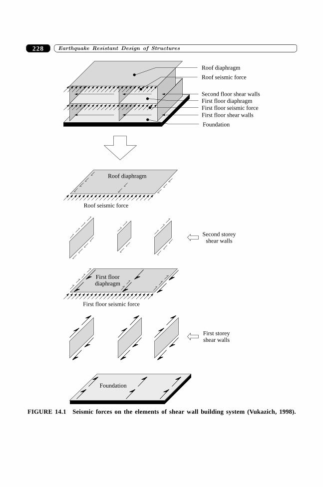
����������� ������� �������������228
Roof diaphragm
Roof seismic force
Second floor shear walls
First floor diaphragm
First floor seismic force
First floor shear walls
Foundation
Roof diaphragm
Roof seismic force
Second storeyshear walls
First floor seismic force
First storeyshear walls
First floordiaphragm
Foundation
FIGURE 14.1 Seismic forces on the elements of shear wall building system (Vukazich, 1998).
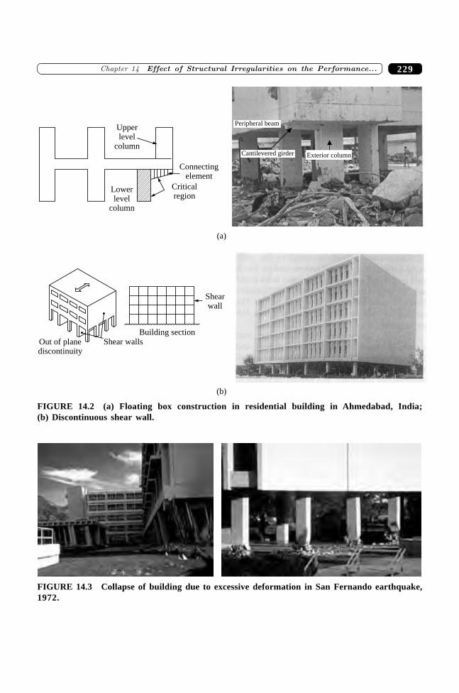
229�������� ������������������������� � �����������������
Connectingelement
Criticalregion
Lowerlevel
column
Upperlevel
column
Out of planediscontinuity
Shear walls
Shearwall
Building section
(a)
(b)
Peripheral beam
Cantilevered girder Exterior column
FIGURE 14.2 (a) Floating box construction in residential building in Ahmedabad, India;(b) Discontinuous shear wall.
FIGURE 14.3 Collapse of building due to excessive deformation in San Fernando earthquake,1972.
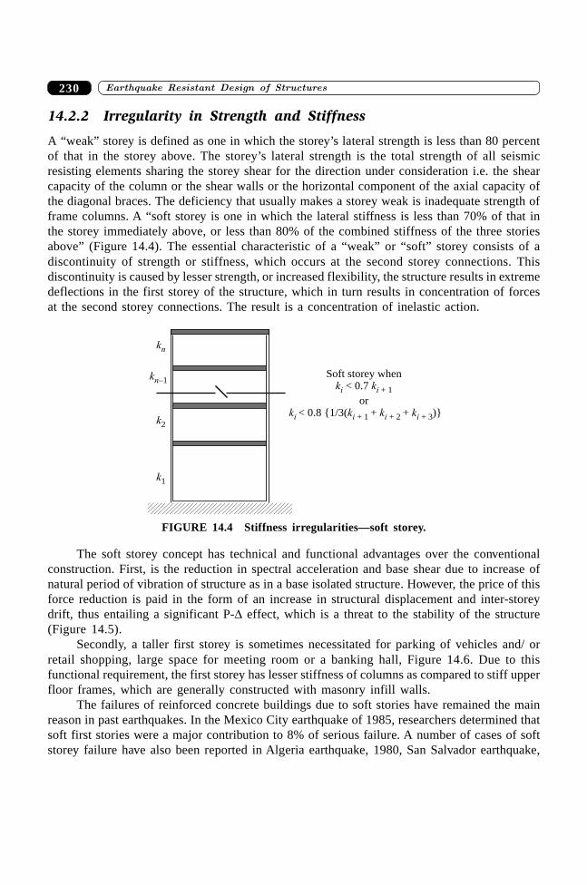
����������� ������� �������������230
14.2.2 Irregularity in Strength and Stiffness
A “weak” storey is defined as one in which the storey’s lateral strength is less than 80 percentof that in the storey above. The storey’s lateral strength is the total strength of all seismicresisting elements sharing the storey shear for the direction under consideration i.e. the shearcapacity of the column or the shear walls or the horizontal component of the axial capacity ofthe diagonal braces. The deficiency that usually makes a storey weak is inadequate strength offrame columns. A “soft storey is one in which the lateral stiffness is less than 70% of that inthe storey immediately above, or less than 80% of the combined stiffness of the three storiesabove” (Figure 14.4). The essential characteristic of a “weak” or “soft” storey consists of adiscontinuity of strength or stiffness, which occurs at the second storey connections. Thisdiscontinuity is caused by lesser strength, or increased flexibility, the structure results in extremedeflections in the first storey of the structure, which in turn results in concentration of forcesat the second storey connections. The result is a concentration of inelastic action.
k1
k2
kn–1
kn
Soft storey when< 0.7
or< 0.8 {1/3( + + )}
k k
k k k k
i i
i i i i
+ 1
+ 1 + 2 + 3
FIGURE 14.4 Stiffness irregularities—soft storey.
The soft storey concept has technical and functional advantages over the conventionalconstruction. First, is the reduction in spectral acceleration and base shear due to increase ofnatural period of vibration of structure as in a base isolated structure. However, the price of thisforce reduction is paid in the form of an increase in structural displacement and inter-storeydrift, thus entailing a significant P-D effect, which is a threat to the stability of the structure(Figure 14.5).
Secondly, a taller first storey is sometimes necessitated for parking of vehicles and/ orretail shopping, large space for meeting room or a banking hall, Figure 14.6. Due to thisfunctional requirement, the first storey has lesser stiffness of columns as compared to stiff upperfloor frames, which are generally constructed with masonry infill walls.
The failures of reinforced concrete buildings due to soft stories have remained the mainreason in past earthquakes. In the Mexico City earthquake of 1985, researchers determined thatsoft first stories were a major contribution to 8% of serious failure. A number of cases of softstorey failure have also been reported in Algeria earthquake, 1980, San Salvador earthquake,
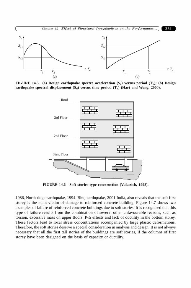
231�������� ������������������������� � �����������������
1986, North ridge earthquake, 1994. Bhuj earthquake, 2001 India, also reveals that the soft firststorey is the main victim of damage to reinforced concrete building. Figure 14.7 shows twoexamples of failure of reinforced concrete buildings due to soft stories. It is recognised that thistype of failure results from the combination of several other unfavourable reasons, such astorsion, excessive mass on upper floors, P-D effects and lack of ductility in the bottom storey.These factors lead to local stress concentrations accompanied by large plastic deformations.Therefore, the soft stories deserve a special consideration in analysis and design. It is not alwaysnecessary that all the first tall stories of the buildings are soft stories, if the columns of firststorey have been designed on the basis of capacity or ductility.
Sa2
T1 T2
Sa1
Sa
Tn
(a)
Sd1
T1 T2
Sd2
Sd
Tn
(b)
FIGURE 14.5 (a) Design earthquake spectra acceleration (Sa) versus period (Tn); (b) Designearthquake spectral displacement (Sd) versus time period (Tn) (Hart and Wong, 2000).
Roof
3rd Floor
First Floor
2nd Floor
FIGURE 14.6 Soft stories type construction (Vukazich, 1998).
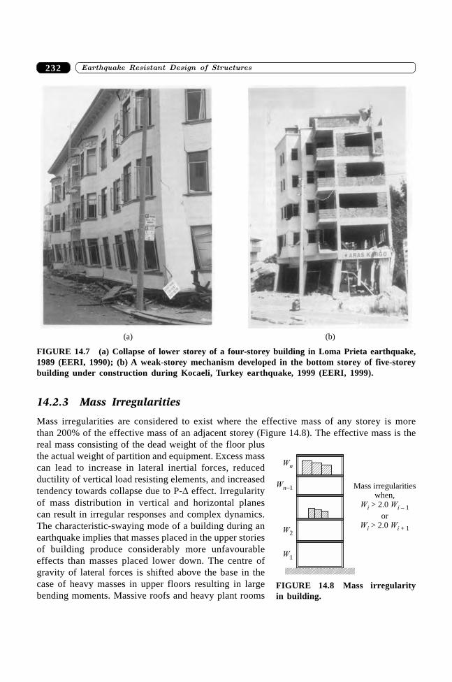
����������� ������� �������������232
(a) (b)
FIGURE 14.7 (a) Collapse of lower storey of a four-storey building in Loma Prieta earthquake,1989 (EERI, 1990); (b) A weak-storey mechanism developed in the bottom storey of five-storeybuilding under construction during Kocaeli, Turkey earthquake, 1999 (EERI, 1999).
14.2.3 Mass Irregularities
Mass irregularities are considered to exist where the effective mass of any storey is morethan 200% of the effective mass of an adjacent storey (Figure 14.8). The effective mass is thereal mass consisting of the dead weight of the floor plusthe actual weight of partition and equipment. Excess masscan lead to increase in lateral inertial forces, reducedductility of vertical load resisting elements, and increasedtendency towards collapse due to P-D effect. Irregularityof mass distribution in vertical and horizontal planescan result in irregular responses and complex dynamics.The characteristic-swaying mode of a building during anearthquake implies that masses placed in the upper storiesof building produce considerably more unfavourableeffects than masses placed lower down. The centre ofgravity of lateral forces is shifted above the base in thecase of heavy masses in upper floors resulting in largebending moments. Massive roofs and heavy plant rooms
W1
W2
Wn
Wn–1 Mass irregularitieswhen,
> 2.0
or> 2.0
W W
W W
i i
i i
– 1
+ 1
FIGURE 14.8 Mass irregularityin building.
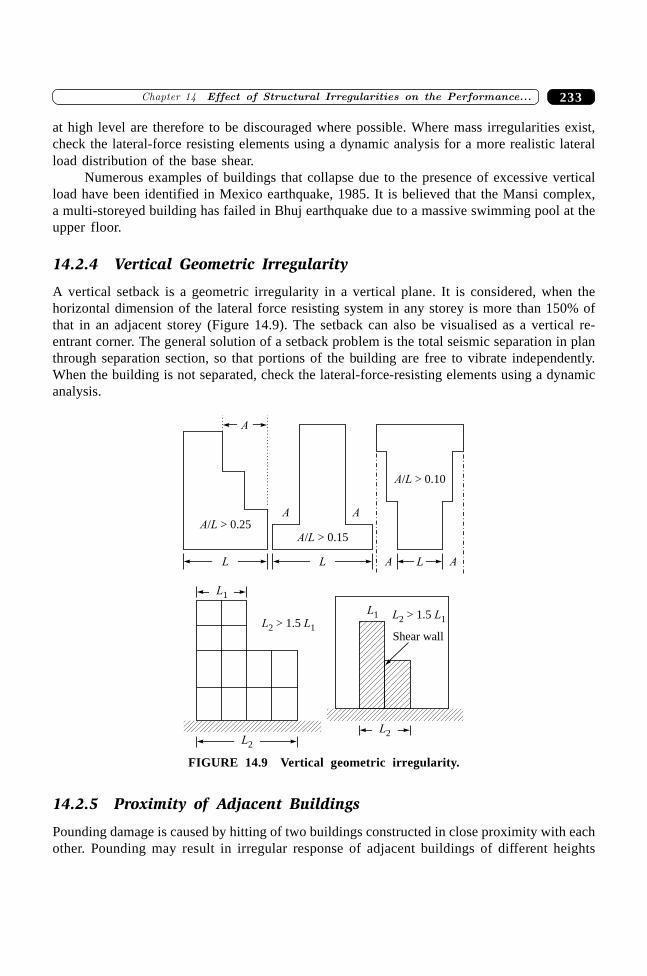
233�������� ������������������������� � �����������������
at high level are therefore to be discouraged where possible. Where mass irregularities exist,check the lateral-force resisting elements using a dynamic analysis for a more realistic lateralload distribution of the base shear.
Numerous examples of buildings that collapse due to the presence of excessive verticalload have been identified in Mexico earthquake, 1985. It is believed that the Mansi complex,a multi-storeyed building has failed in Bhuj earthquake due to a massive swimming pool at theupper floor.
14.2.4 Vertical Geometric Irregularity
A vertical setback is a geometric irregularity in a vertical plane. It is considered, when thehorizontal dimension of the lateral force resisting system in any storey is more than 150% ofthat in an adjacent storey (Figure 14.9). The setback can also be visualised as a vertical re-entrant corner. The general solution of a setback problem is the total seismic separation in planthrough separation section, so that portions of the building are free to vibrate independently.When the building is not separated, check the lateral-force-resisting elements using a dynamicanalysis.
A L/ > 0.25A L/ > 0.15
A A
A
A L/ > 0.10
A ALL
L1
L2
L L2 1> 1.5L1 L L2 1> 1.5
Shear wall
L2
L
FIGURE 14.9 Vertical geometric irregularity.
14.2.5 Proximity of Adjacent Buildings
Pounding damage is caused by hitting of two buildings constructed in close proximity with eachother. Pounding may result in irregular response of adjacent buildings of different heights
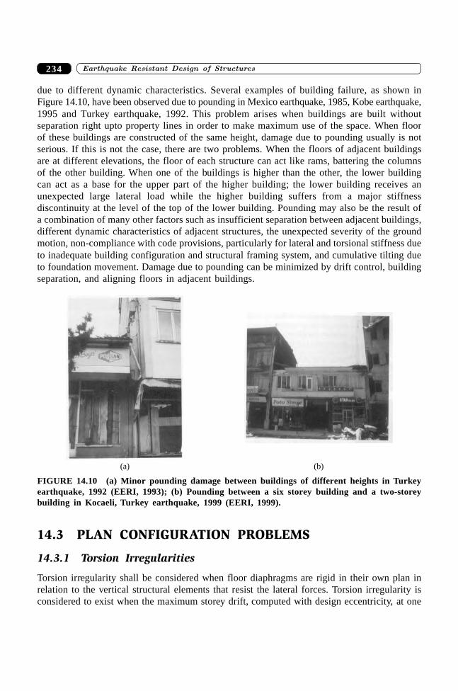
����������� ������� �������������234
due to different dynamic characteristics. Several examples of building failure, as shown inFigure 14.10, have been observed due to pounding in Mexico earthquake, 1985, Kobe earthquake,1995 and Turkey earthquake, 1992. This problem arises when buildings are built withoutseparation right upto property lines in order to make maximum use of the space. When floorof these buildings are constructed of the same height, damage due to pounding usually is notserious. If this is not the case, there are two problems. When the floors of adjacent buildingsare at different elevations, the floor of each structure can act like rams, battering the columnsof the other building. When one of the buildings is higher than the other, the lower buildingcan act as a base for the upper part of the higher building; the lower building receives anunexpected large lateral load while the higher building suffers from a major stiffnessdiscontinuity at the level of the top of the lower building. Pounding may also be the result ofa combination of many other factors such as insufficient separation between adjacent buildings,different dynamic characteristics of adjacent structures, the unexpected severity of the groundmotion, non-compliance with code provisions, particularly for lateral and torsional stiffness dueto inadequate building configuration and structural framing system, and cumulative tilting dueto foundation movement. Damage due to pounding can be minimized by drift control, buildingseparation, and aligning floors in adjacent buildings.
(a) (b)
FIGURE 14.10 (a) Minor pounding damage between buildings of different heights in Turkeyearthquake, 1992 (EERI, 1993); (b) Pounding between a six storey building and a two-storeybuilding in Kocaeli, Turkey earthquake, 1999 (EERI, 1999).
14.3 PLAN CONFIGURATION PROBLEMS
14.3.1 Torsion Irregularities
Torsion irregularity shall be considered when floor diaphragms are rigid in their own plan inrelation to the vertical structural elements that resist the lateral forces. Torsion irregularity isconsidered to exist when the maximum storey drift, computed with design eccentricity, at one
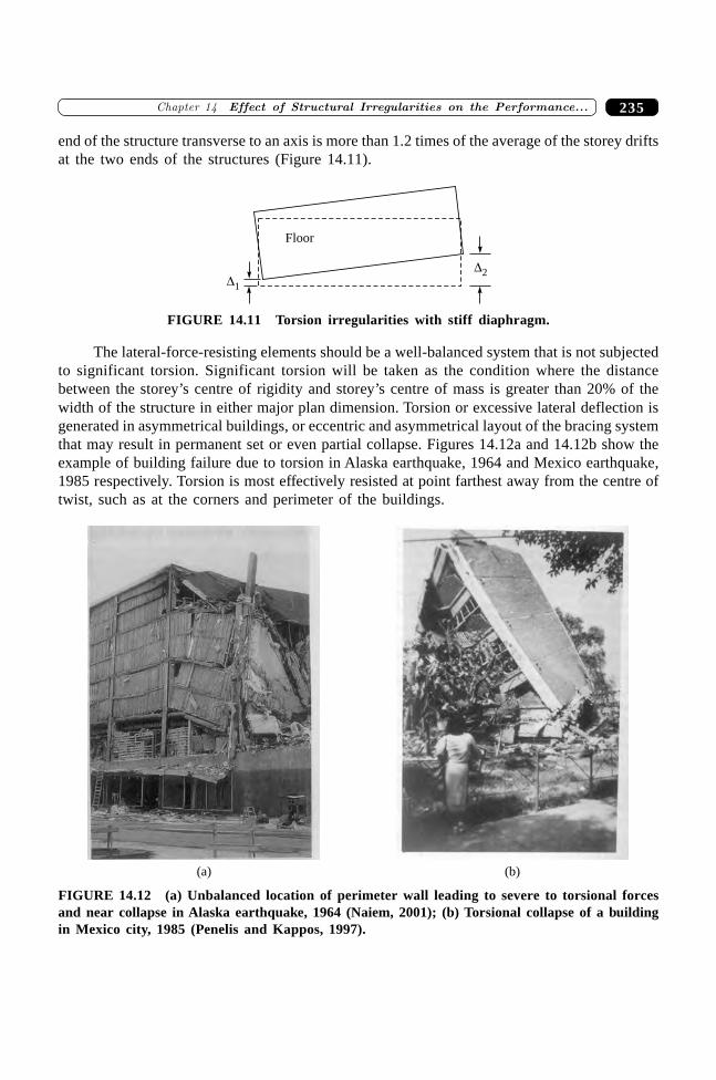
235�������� ������������������������� � �����������������
end of the structure transverse to an axis is more than 1.2 times of the average of the storey driftsat the two ends of the structures (Figure 14.11).
Floor
�1
�2
FIGURE 14.11 Torsion irregularities with stiff diaphragm.
The lateral-force-resisting elements should be a well-balanced system that is not subjectedto significant torsion. Significant torsion will be taken as the condition where the distancebetween the storey’s centre of rigidity and storey’s centre of mass is greater than 20% of thewidth of the structure in either major plan dimension. Torsion or excessive lateral deflection isgenerated in asymmetrical buildings, or eccentric and asymmetrical layout of the bracing systemthat may result in permanent set or even partial collapse. Figures 14.12a and 14.12b show theexample of building failure due to torsion in Alaska earthquake, 1964 and Mexico earthquake,1985 respectively. Torsion is most effectively resisted at point farthest away from the centre oftwist, such as at the corners and perimeter of the buildings.
(a) (b)
FIGURE 14.12 (a) Unbalanced location of perimeter wall leading to severe to torsional forcesand near collapse in Alaska earthquake, 1964 (Naiem, 2001); (b) Torsional collapse of a buildingin Mexico city, 1985 (Penelis and Kappos, 1997).
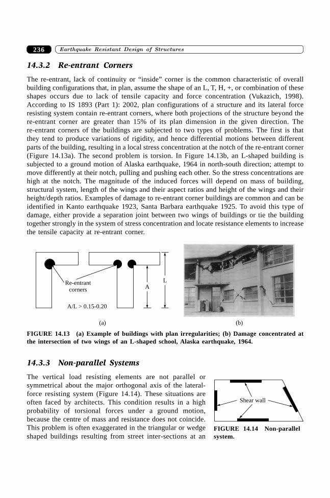
����������� ������� �������������236
14.3.2 Re-entrant Corners
The re-entrant, lack of continuity or “inside” corner is the common characteristic of overallbuilding configurations that, in plan, assume the shape of an L, T, H, +, or combination of theseshapes occurs due to lack of tensile capacity and force concentration (Vukazich, 1998).According to IS 1893 (Part 1): 2002, plan configurations of a structure and its lateral forceresisting system contain re-entrant corners, where both projections of the structure beyond there-entrant corner are greater than 15% of its plan dimension in the given direction. There-entrant corners of the buildings are subjected to two types of problems. The first is thatthey tend to produce variations of rigidity, and hence differential motions between differentparts of the building, resulting in a local stress concentration at the notch of the re-entrant corner(Figure 14.13a). The second problem is torsion. In Figure 14.13b, an L-shaped building issubjected to a ground motion of Alaska earthquake, 1964 in north-south direction; attempt tomove differently at their notch, pulling and pushing each other. So the stress concentrations arehigh at the notch. The magnitude of the induced forces will depend on mass of building,structural system, length of the wings and their aspect ratios and height of the wings and theirheight/depth ratios. Examples of damage to re-entrant corner buildings are common and can beidentified in Kanto earthquake 1923, Santa Barbara earthquake 1925. To avoid this type ofdamage, either provide a separation joint between two wings of buildings or tie the buildingtogether strongly in the system of stress concentration and locate resistance elements to increasethe tensile capacity at re-entrant corner.
Re-entrantcorners
A/L > 0.15-0.20
AL
(b)(a)
FIGURE 14.13 (a) Example of buildings with plan irregularities; (b) Damage concentrated atthe intersection of two wings of an L-shaped school, Alaska earthquake, 1964.
14.3.3 Non-parallel Systems
The vertical load resisting elements are not parallel orsymmetrical about the major orthogonal axis of the lateral-force resisting system (Figure 14.14). These situations areoften faced by architects. This condition results in a highprobability of torsional forces under a ground motion,because the centre of mass and resistance does not coincide.This problem is often exaggerated in the triangular or wedgeshaped buildings resulting from street inter-sections at an
Shear wall
FIGURE 14.14 Non-parallelsystem.
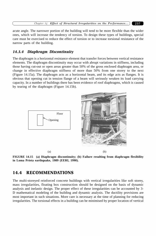
237�������� ������������������������� � �����������������
acute angle. The narrower portion of the building will tend to be more flexible than the widerones, which will increase the tendency of torsion. To design these types of buildings, specialcare must be exercised to reduce the effect of torsion or to increase torsional resistance of thenarrow parts of the building.
14.3.4 Diaphragm Discontinuity
The diaphragm is a horizontal resistance element that transfer forces between vertical resistanceelements. The diaphragm discontinuity may occur with abrupt variations in stiffness, includingthose having cut-out or open areas greater than 50% of the gross enclosed diaphragm area, orchange in effective diaphragm stiffness of more than 50% from one storey to the next(Figure 14.15a). The diaphragm acts as a horizontal beam, and its edge acts as flanges. It isobvious that opening cut in tension flange of a beam will seriously weaken its load carryingcapacity. In a number of buildings there has been evidence of roof diaphragms, which is causedby tearing of the diaphragm (Figure 14.15b).
Opening
Floor
(a) (b)
FIGURE 14.15 (a) Diaphragm discontinuity; (b) Failure resulting from diaphragm flexibilityin Loma Prieta earthquake, 1989 (EERI, 1990).
14.4 RECOMMENDATIONS
The multi-storeyed reinforced concrete buildings with vertical irregularities like soft storey,mass irregularities, floating box construction should be designed on the basis of dynamicanalysis and inelastic design. The proper effect of these irregularities can be accounted by 3-D mathematical modeling of the building and dynamic analysis. The ductility provisions aremost important in such situations. More care is necessary at the time of planning for reducingirregularities. The torsional effects in a building can be minimised by proper location of vertical
����������� ������� �������������238
resisting elements and mass distribution. Shear walls should be employed for increasing stiffnesswhere necessary and be uniformly distributed in both principal directions.
SUMMARY
There are numerous examples cited in the damage reports of past earthquakes in which the causeof failure of reinforced concrete building has been ascribed to irregularities in configurations.IS 1893 (Part 1): 2002 has identified some of the irregularities in elements of load resistingsystem, which are mainly categorized as horizontal irregularity and vertical irregularity. Verticalirregularities, referring to sudden change of strength, stiffness, geometry and mass, result inirregular distribution of forces and/or deformation over the height of building while horizontalirregularities refer to asymmetrical plan shapes (e.g. L-, T-, U-, F-) or discontinuities in thehorizontal resisting elements (diaphragms) such as cut-outs, large openings, re-entrant cornersand other abrupt changes resulting in torsion, diaphragm deformations, stress concentration. Thechapter presents the influence of irregularity on performance of building during earthquakes.Some recommendations are presented to account for the effects of these irregularities in analysisand design.
REFERENCES
[1] “Kocaeli, Turkey, Earthquake Reconnaissance Report”, Earthquake Spectra, Vol. 16,Earthquake Engineering Research Institute, California, December 1999.
[2] “Erzincan, Turkey, Earthquake Reconnaissance Report”, Earthquake Spectra, Supple-ment to Vol. 9, Earthquake Engineering Research Institute, California, July, 1993.
[3] “Loma Prieta Earthquake Reconnaissance Report”, Earthquake Spectra, Supplement toVol. 6, Earthquake Engineering Research Institute, California, July, 1990.
[4] Hart, G.C. and Wong, K., Structural Dynamics for Structural Engineers, John Wiley& Sons, New York, 2001.
[5] Moehle, J.P. and Mahin, S.A, “Observation of the Behaviour of Reinforced ConcreteBuildings during Earthquake”, Earthquake Resistant Concrete Structures—InelasticResponse and Design, S.K. Ghosh, (Ed.), American Concrete Institute PublicationSP-127, 1991.
[6] Naeim, F., Seismic Design Handbook, 2nd ed., Kluwer Academic Publishers, 2001.[7] Penelis, G.G. and Kappos, A.J. Earthquake-Resistant Concrete Structures, E & FN
SPON, an Imprint of Chapman & Hall, 1997.[8] The Mexico Earthquakes—1985, Michael A. Cassaro and Martinez Romero (Eds.),
American Society of Civil Engineers, New York, 1985.[9] Vukazich, S.E., The Apartment Owner’s Guide to Earthquake Safety, San Jose State
University, 1998.
239�������� ��������������� ��������������� ��
239
SeismoresistantBuilding Architecture
��������
15.1 INTRODUCTION
Rational studies along with a knowledge regarding the performance of buildings in earthquakesshow that the building architectural design would create maladjustments in building space-forming elements that would not only decrease the seismoresistant capacity of the buildingbut also become the cause of collapse of the building. It is believed that a structural analysisin itself is not sufficient to ensure the seismoresistant stability of the buildings. An integralseismoresistant system must be necessary, in which all components of the buildings canpositively interact during the seismic action. A real compatibility between the architectural andthe structural design avoids a stepping of the seismoresistant capacity of the building and alsoprovides a positive, efficient and integral seismic resistant system. Several studies andrecommendations have been carried out to avoid situations affecting negatively the building’searthquake resistant behaviour. These studies enable architects to develop a systematic study anda methodology to be applied to the architectural design of buildings to optimize earthquakeresistant capacity. This study is called seismoresistant building architecture. The main objectiveof seismoresistant building architecture is to prevent stepping of seismoresistant capacity ofbuilding and to optimize seismoresistance. The major aspects involved in seismoresistantbuilding construction are: (i) selection of load resisting system; (ii) its configuration system;(iii) its basic dynamic characteristics and (iv) its construction quality. The present chapter willdiscuss all these aspects in detail.
15.2 LATERAL LOAD RESISTING SYSTEMS
The first step in architectural planning of a building is to select the lateral load resisting system.The load resisting system must be of closed loops, so that it is able to transfer all the forcesacting either vertically or horizontally to the ground. Bureau of Indian Standards (BIS) hasapproved three major types of lateral force resisting system in the code IS 1893 (Part 1): 2002.
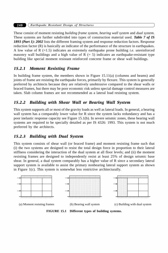
����� ����������������������� �� ���240
These consist of moment resisting building frame system, bearing wall system and dual system.These systems are further subdivided into types of construction material used. Table 7 of IS1893 (Part 1): 2002 lists the different framing system and response reduction factors. Responsereduction factor (R) is basically an indicator of the performance of the structure in earthquakes.A low value of R (=1.5) indicates an extremely earthquake prone building i.e. unreinforcedmasonry wall buildings and a high value of R (= 5) indicates an earthquake-resistant typebuilding like special moment resistant reinforced concrete frame or shear wall buildings.
15.2.1 Moment Resisting Frame
In building frame system, the members shown in Figure 15.11(a) (columns and beams) andjoints of frame are resisting the earthquake forces, primarily by flexure. This system is generallypreferred by architects because they are relatively unobtrusive compared to the shear walls orbraced frames, but there may be poor economic risk unless special damage control measures aretaken. Slab column frames are not recommended as a lateral load resisting system.
15.2.2 Building with Shear Wall or Bearing Wall System
This system supports all or most of the gravity loads as well as lateral loads. In general, a bearingwall system has a comparably lower value for R since the system lacks redundancy and has apoor inelastic response capacity see Figure 15.1(b). In severe seismic zones, these bearing wallsystems are required to be specially detailed as per IS 4326: 1993. This system is not muchpreferred by the architects.
15.2.3 Building with Dual System
This system consists of shear wall (or braced frame) and moment resisting frame such that(i) the two systems are designed to resist the total design force in proportion to their lateralstiffness considering the interaction of the dual system at all floor levels; and (ii) the momentresisting frames are designed to independently resist at least 25% of design seismic baseshear. In general, a dual system comparably has a higher value of R since a secondary lateralsupport system is available to assist the primary nonbearing lateral support system as shownin Figure 1(c). This system is somewhat less restrictive architecturally.
(a) Moment resisting frames (b) Bearing wall system (c) Building with dual system
FIGURE 15.1 Different types of building systems.
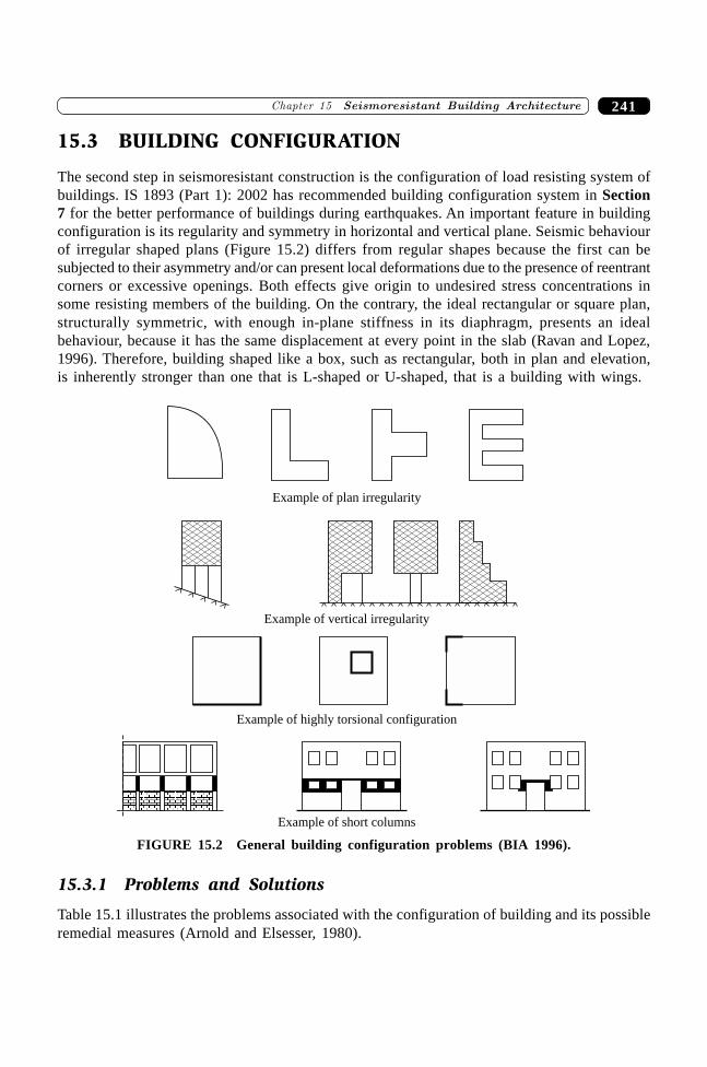
241�������� ��������������� ��������������� ��
15.3 BUILDING CONFIGURATION
The second step in seismoresistant construction is the configuration of load resisting system ofbuildings. IS 1893 (Part 1): 2002 has recommended building configuration system in Section7 for the better performance of buildings during earthquakes. An important feature in buildingconfiguration is its regularity and symmetry in horizontal and vertical plane. Seismic behaviourof irregular shaped plans (Figure 15.2) differs from regular shapes because the first can besubjected to their asymmetry and/or can present local deformations due to the presence of reentrantcorners or excessive openings. Both effects give origin to undesired stress concentrations insome resisting members of the building. On the contrary, the ideal rectangular or square plan,structurally symmetric, with enough in-plane stiffness in its diaphragm, presents an idealbehaviour, because it has the same displacement at every point in the slab (Ravan and Lopez,1996). Therefore, building shaped like a box, such as rectangular, both in plan and elevation,is inherently stronger than one that is L-shaped or U-shaped, that is a building with wings.
Example of plan irregularity
Example of vertical irregularity
Example of highly torsional configuration
Example of short columns
FIGURE 15.2 General building configuration problems (BIA 1996).
15.3.1 Problems and Solutions
Table 15.1 illustrates the problems associated with the configuration of building and its possibleremedial measures (Arnold and Elsesser, 1980).
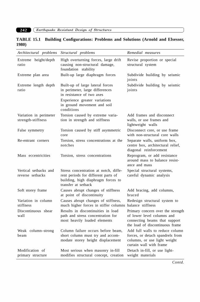
����� ����������������������� �� ���242
TABLE 15.1 Building Configurations: Problems and Solutions (Arnold and Elsesser,1980)
Architectural problems Structural problems Remedial measures
Extreme height/depth High overturning forces, large drift Revise proportion or specialratio causing non-structural damage, structural system
foundation stability
Extreme plan area Built-up large diaphragm forces Subdivide building by seismicjoints
Extreme length depth Built-up of large lateral forces Subdivide building by seismicratio in perimeter, large differences joints
in resistance of two axes
Experience greater variationsin ground movement and soilconditions
Variation in perimeter Torsion caused by extreme varia- Add frames and disconnectstrength-stiffness tion in strength and stiffness walls, or use frames and
lightweight walls
False symmetry Torsion caused by stiff asymmetric Disconnect core, or use framecore with non-structural core walls
Re-entrant corners Torsion, stress concentrations at the Separate walls, uniform box,notches centre box, architectural relief,
diagonal reinforcement
Mass eccentricities Torsion, stress concentrations Reprogram, or add resistancearound mass to balance resist-ance and mass
Vertical setbacks and Stress concentration at notch, diffe- Special structural systems,reverse setbacks rent periods for different parts of careful dynamic analysis
building, high diaphragm forces totransfer at setback
Soft storey frame Causes abrupt changes of stiffness Add bracing, add columns,at point of discontinuity braced
Variation in column Causes abrupt changes of stiffness, Redesign structural system tostiffness much higher forces in stiffer columns balance stiffness
Discontinuous shear Results in discontinuities in load Primary concern over the strengthwall path and stress concentration for of lower level columns and
most heavily loaded elements connecting beams that supportthe load of discontinuous frame
Weak column–strong Column failure occurs before beam, Add full walls to reduce columnbeam short column must try and accom- forces, or detach spandrels from
modate storey height displacement columns, or use light weightcurtain wall with frame
Modification of Most serious when masonry in-fill Detach in-fill, or use light-primary structure modifies structural concept, creation weight materials
Contd.
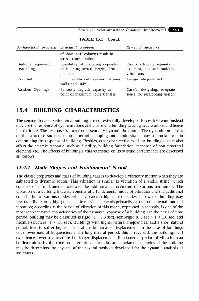
243�������� ��������������� ��������������� ��
of short, stiff columns result instress concentration
Building separation Possibility of pounding dependent Ensure adequate separation,(Pounding) on building period, height, drift, assuming opposite building
distance vibrations
Coupled Incompatible deformation between Design adequate linkwalls and links
Random Openings Seriously degrade capacity at Careful designing, adequatepoint of maximum force transfer space for reinforcing design
15.4 BUILDING CHARACTERISTICS
The seismic forces exerted on a building are not externally developed forces like wind insteadthey are the response of cyclic motions at the base of a building causing accelerations and henceinertia force. The response is therefore essentially dynamic in nature. The dynamic propertiesof the structure such as natural period, damping and mode shape play a crucial role indetermining the response of building. Besides, other characteristics of the building system alsoaffect the seismic response such as ductility, building foundation, response of non-structuralelements etc. The effects of building’s characteristics on its seismic performance are describedas follows.
15.4.1 Mode Shapes and Fundamental Period
The elastic properties and mass of building causes to develop a vibratory motion when they aresubjected to dynamic action. This vibration is similar to vibration of a violin string, whichconsists of a fundamental tone and the additional contribution of various harmonics. Thevibration of a building likewise consists of a fundamental mode of vibration and the additionalcontribution of various modes, which vibrates at higher frequencies. In low-rise building (sayless than five-storey high) the seismic response depends primarily on the fundamental mode ofvibration; accordingly, the period of vibration of this mode, expressed in seconds, is one of themost representative characteristics of the dynamic response of a building. On the basis of timeperiod, building may be classified as rigid (T < 0.3 sec), semi-rigid (0.3 sec < T < 1.0 sec) andflexible structure (T > 1.0 sec). Buildings with higher natural frequencies, and a short naturalperiod, tend to suffer higher accelerations but smaller displacement. In the case of buildingswith lower natural frequencies, and a long natural period, this is reversed: the buildings willexperience lower accelerations but larger displacements. Fundamental period of vibration canbe determined by the code based empirical formulas and fundamental modes of the buildingmay be determined by any one of the several methods developed for the dynamic analysis ofstructures.
TABLE 15.1 Contd.
Architectural problems Structural problems Remedial measures
����� ����������������������� �� ���244
15.4.2 Building Frequency and Ground Period
Inertial forces generated in the building depend upon the frequencies of the ground on whichthe building is standing and the building’s natural frequency. When these are near or equal toone another, the building’s response reaches a peak level. In some circumstances, this dynamicamplification effect can increase the building acceleration to a value, which may be double ormore than that of the ground acceleration at the base of the building. Past studies show that thepredominant period at a firm ground site is typically in the range 0.2–0.4 sec while the periodcan reach 2 sec or more on soft ground. Since building structures have fundamental periods ofapproximately 0.1 N (where N is the number of storeys), it can be concluded that if thefoundation soil is firm, rigid structure will have more unfavourable seismic response thanflexible structures, whereas the seismic response of flexible structures on soft foundation siteswill be less favourable than that of rigid structure. A spectacular example was in Mexico cityduring 1985 earthquake, which saw enormous damage in medium height buildings of 10–20storeys, which have periods matching the 2 sec period of the earthquake motions in the citycentre, while adjacent low re-rise buildings, with much shorter periods, were proportionatelyfar less damaged. Similar site effects are observed in most damaging earthquakes (Booth, 1994).
15.4.3 Damping
The degree of structural amplification of the ground motion at the base of the building is limitedby structural damping. Therefore, damping is the ability of the structural system to dissipate theenergy of the earthquake ground shaking. Since the building response is inversely proportionalto damping. The more damping a building possesses, the sooner it will stop vibrating—whichof course is highly desirable from the standpoint of earthquake performance. There is nonumerical method available for determining the damping. It is only obtained by experiments.In a structure, damping is due to internal friction and the absorption of energy by the building’sstructural and non-structural elements. Today, some of the more advanced techniques ofearthquake resistant design and construction employ added damping devices like shock absorbersto increase artificially the intrinsic damping of a building and so improve its earthquakeperformance.
15.4.4 Ductility
Ductility is defined as the capacity of the building materials, systems, or structures to absorbenergy by deforming in the inelastic range. The safety of the building from collapse is on thebasis of energy, which must be imparted to the structure in order to make it fail. In such instance,consideration must be given to structure’s capacity to absorb energy rather than to its resistance.Therefore ductility of a structure in fact is one of the most important factors affecting itsearthquake performance. The primary task of an engineer designing a building to be earthquakeresistant is to ensure that the building will possess enough ductility. Although there are as yetno clearly defined methods for determining the ductility of a structure, it is useful to clarify theconcept, so that at least a relative appreciation of its importance can be attained. The greaterenergy is required causing a structure to fail, the greater is its ductility. The ductility of astructure depends on the type of material used and also the structural characteristics of the
245�������� ��������������� ��������������� ��
assembly. It is possible to build ductile structures with reinforced concrete if care is taken duringdesigning to provide the joints with sufficient abutments that can adequately confine theconcrete, thus permitting it to deform plastically without breaking. It is also important for thispurpose to ensure that the tension edges of the structure are adequately reinforced and that thereare sufficient stirrups to ensure that concrete is properly confined along the compression edge.For example, in columns, due to combined effect of flexure and axial produces a flexuralcompression failure mode in which failure takes place near the column ends and buckling oflongitudinal reinforcement. This can be eliminated by providing the lateral reinforcement in theregion of plastic deformation as per IS 13920: 1993.
15.4.5 Seismic Weight
Seismic forces are proportional to the building weight and increases along the height of thebuilding. Weight reduction can be obtained by using lighter materials or by relocation of heavyweight such as file racks, libraries, swimming pools etc., at lower levels. For example, if a loadP placed at fifth level, the overturning moment becomes 25 times greater than P placed at thefirst level. Besides, the seismic shear affects from level 1 to 5, whereas, in the second case, onlythe first level is affected but to a lesser extent (5 times less).
15.4.6 Hyperstaticity/Redundancy
In general, hyperstatic (statically indeterminate) structures have advantage because if primarysystem yields or fails, the lateral force can be redistributed to secondary elements or system toprevent progressive failure (alternate load path). Moreover, hyperstaticity of the structure causesthe formation of plastic hinges that can absorb considerable energy without depriving thestructure of its stability. Therefore, the redundancy of hyperstatic structure is highly desirablecharacteristic for earthquake resistant design.
15.4.7 Non-structural Elements
The non-structural damage problem is particularly difficult to deal with because the non-structural components that are subjected to seismic forces are not normally within the designscope of the structural engineer, whose responsibility is to provide the seismic safety of thebuilding. In addition, non-structural components—such as partition walls—are often added afterthe initial building design, and the original architect, or an architect at all, is often not involved.Finally, non-structural components remain uninvolved in the building design and become thesource of damage. In general, non-structural damage is caused in two ways. The component maybe directly affected by ground motion transmitted by the main structure of the building and besubjected to accelerations and consequent inertial forces in similar way to the building structure.Alternatively, the non-structural components may be affected by the movement or distortion inthe structural elements that support or abet the element. These two causes can be summarizedas acceleration or drift related damage.
Methods of mitigating the damage to nonstructural components must recognize theprobable mode of failure, whether through inertial forces or movement of failure in backing
����� ����������������������� �� ���246
or abetting structures. For the former, non-structural components must be designed and detailedin a similar way to the building structure, using an analysis of forces to determine bracingsupport requirements. For the latter, separation from backup or abetting structures is necessary.Mechanical, electrical, and plumbing distribution system must be secured to the buildingstructure, with allowances for differential movement where applicable.
15.4.8 Foundation Soil/Liquefaction
Knowledge of the foundation soil is essential to correct earthquake-resistant design. In somecases a soil behaving well under static loads will pose serious problems under seismic loads.Problems related to foundation soil can be classified mainly in two groups: (i) influence ofsubsoil on the characteristics of seismic movement, landslides and loss of soil resistance(liquefaction), these problems are not significantly affected by the structures and theirfoundations and (ii) problems caused by the loads transmitted to the soil by foundations and thesettling of the foundations under static and seismic loads. This problem generally arises in looseunsaturated granular soils, which may be compacted as a result of earthquake.
The liquefaction of the soil is most common feature in an earthquake. This phenomenonof loss of resistance is generally occurred in saturated granular soil. At Niigata, Japan, in 1964subsoil of the loose saturated sand underwent a considerable loss of resistance during anearthquake, as a result, many buildings were damaged, severely undermined and in extremecases, completely toppled.
15.4.9 Foundations
Foundation of the building is subjected to earthquake stresses; the following major recommen-dation on structural design must be borne in mind
(i) Foundation should preferably be designed as continuous (mat or raft) in order to avoidrelative horizontal displacement
(ii) In case of isolated footing, they should be joined to each other by means of foundationbeams or ties. These ties should be designed such that it will bear tension andcompression forces.
(iii) It is recommended that parts of building foundations, which rest on soils of differenttypes or are sunk to different depths, should be designed as separate units. In such casesthere should also be structural independence in the superstructure.
(iv) It is recommended that if different parts of the building are to be structurallyindependent because of the shape of their ground plan; their foundations should alsobe independent.
15.5 QUALITY OF CONSTRUCTION AND MATERIALS
One of the main factors responsible for stepping of seismoresistant capacity of building is itsquality of materials and workmanship of construction. The industrially produced materials used

247�������� ��������������� ��������������� ��
in construction such as cement, reinforcement, brick etc. should satisfy minimum standards ofquality and resistance, which can only be guaranteed by the manufacturers. Besides that, qualityof concrete, faulty execution of construction joint, and detailing reinforcement are also affectingthe performance of structure. The factors affecting the seismoresistant capacity of building aredescribed as follows. By proper inspection programme their effect could be minimized.
15.5.1 Quality of Concrete
Grade of concrete specified in design documents may not be developed during constructionmainly due to
∑ incorrect proportioning∑ insufficient mixing which causes segregation∑ aggregates with excessive impurities or improper grading∑ excessive high water/cement ratio
15.5.2 Construction Joints
A defective concrete joint, which contributed significantly to causing of failure of manybuildings in past earthquakes is due to
∑ poor execution of the construction joint/discontinuity∑ not located at the points specified by the designer∑ accumulation of sawdust, dust and loose materials at the surface of joint
15.5.3 General Detailing Requirements
Stepping of seismoresistant capacity of the building is due to
∑ amount of reinforcement is not placed as specified in design∑ insufficient concrete cover to reinforcement results resting in reinforcing bar and
cracks in surface concrete∑ proper placing of reinforcement during casting∑ improper confinement and large tie spacing especially in plastic hinge region∑ insufficient confinement and anchorage length at joints∑ insufficient splicing length of longitudinal reinforcement in columns or splicing of all
bars at the same cross section∑ accumulation of splices just above a concrete joint or in plastic hinge zone∑ splicing of tension reinforcement in beams and columns in region of tension or
reversing stress∑ the end of lateral reinforcement should be bent at 135 degree∑ use of high resistance steel in relatively low-resistance concrete∑ curves in reinforcement cause thrust in concrete when the bar is subjected to tension
and compression
����� ����������������������� �� ���248
SUMMARY
Seismic safety of a building is an interdisciplinary endeavour involving a close cooperation andco-efforts of architects and structural engineers adopting mutually suitable architectural andstructural schemes. The seismic analysis and design alone do not ensure good performance ofthe structure during earthquakes. The building framing system should also conform to theprinciples of earthquake resistant configuration. The chapter presents structural requirements forbuilding system regarding its selection of load resisting system, configuration system, dynamiccharacteristics and finally construction quality that are essential for enhancing the seismoresistantcapacity of the structure. This will help in eliminating most of the vulnerabilities in thestructural system at the conceptual design stage itself.
REFERENCES
[1] Arnold, Christopher and Elsesser, Eric, “Building Configuration: Problems andSolutions”, Seventh World Conference on Earthquake Engineering, 1980.
[2] Arnold, Christopher, “Building Configuration: Characteristics for Seismic Design”,Seventh World Conference on Earthquake Engineering, 1980.
[3] Arnold, Christopher, “Architectural Aspects of Seismic Resistant Design”, EleventhWorld Conference on Earthquake Engineering, 1996.
[4] Arnold, Christopher, “The Seismic Response of Nonstructural Elements in Building”,Bulletin of the New Zeland National Society for Earthquake Engineering, Vol. 24,No. 4, December, 1991.
[5] Booth, E., “Concrete Structures in Earthquake Regions”, Longman Scientific andTechnical, Longman Group UK Limited, 1994.
[6] BIA., “The Assessment and Improvement of the Structural Performance of EarthquakeRisk Buildings”, New Zealand National Society for Earthquake Engineering, June,1996.
[7] Giuiliani, H., Rodriguez, V.I., Yacante, M.I., Campora, A.M. and Giuliani, H.L.,“Seismic Resisting Architecture on Building Scale”, Eleventh World Conference onEarthquake Engineering, 1996.
[8] Giuiliani, H., “Seismic Resisting Architecture: A Theory for the Architectural Designof Buildings in Seismic Zones”, Twelfth World Conference on Earthquake Engineering,2000.
[9] Raven, E. and Lopez, O.A., “Regular and Irregular Plan Shape Buildings in SeismicRegions: Approaching to an Integral Evaluation”, Eleventh World Conference onEarthquake Engineering, 1996.
���� ��
Seismic Analysis and Modellingof Reinforced Concrete Building

251
Code Based Procedure forDetermination of Design
Lateral Loads
��������
16.1 INTRODUCTION
Earthquake and its occurrence and measurements, its vibration effect and structural responsehave been continuously studied for many years in earthquake history and thoroughlydocumented in literature. Since then the structural engineers have tried hard to examine theprocedure, with an aim to counter the complex dynamic effect of seismically induced forces instructures, for designing of earthquake resistant structures in a refined and easy manner. Thisre-examination and continuous effort has resulted in several revisions of Indian Standard: 1893:(1962, 1966, 1970, 1975, 1984, 2002) code of practice on the “Criteria for EarthquakeResistant Design of Structures” by the Bureau of Indian Standards (BIS), New Delhi. In orderto properly interpret the codes and their revisions, it has become necessary; that the structuralengineers must understand the basic design criteria and procedures for determining the lateralforces. Various approaches to seismic analysis have been developed to determine the lateralforces, ranging from purely linear elastic to non-linear inelastic analysis. Many of the analysistechniques are being used in design and incorporated in codes of practices of many countries.However, this chapter is restricted to the method of analysis described or employed in IS 1893(Part 1): 2002 of “Criteria for Earthquake Resistant Design of Structures” essentially tobuildings although in some cases that may be applied to other types of structures as well.
16.2 SEISMIC DESIGN PHILOSOPHY
The philosophy of seismic design can be summarized as:
(a) The design philosophy adopted in the code is to ensure that structures possess at leasta minimum strength to(i) resist minor earthquake (< DBE), which may occur frequently, without damage;
����������� ������� �������������252
(ii) resist moderate earthquake (DBE) without significant structural damage throughsome non-structural damage;
(iii) resist major earthquake (MCE) without collapse.
“Design Basis Earthquake (DBE) is defined as the maximum earthquake that reasonablycan be expected to experience at the site once during lifetime of the structure. Theearthquake corresponding to the ultimate safety requirements is often called as MaximumConsidered Earthquake (MCE). Generally, the DBE is half of MCE”.
(b) Actual forces that appear on structures during earthquakes are much higher than thedesign forces specified in the code. It is recognized that the complete protection againstearthquakes of all sizes is not economically feasible and design based alone on strengthcriteria is not justified. The basic criteria of earthquake resistant design should be basedon lateral strength as well as deformability and ductility capacity of structure withlimited damage, but no collapse. Ductility in the structures will arise from inelasticmaterial, behaviour and detailing of reinforcement in such a manner that brittle failureis avoided and ductile behaviour is induced by allowing steel to yield in controlledmanner. Therefore, the gap between the actual and design lateral forces is narroweddown by providing ductility in the structure and additional reserve strength instructures over and above the design strength.
(c) The design lateral forces specified in the code shall be considered in each of the twoorthogonal directions of the structure. For structures, which have lateral force resistingelements in the two orthogonal directions only, the design lateral force shall beconsidered along one direction at a time, and not in both directions simultaneously.Structures, having lateral force resisting elements in direction other than the twoorthogonal directions, shall be analysed considering the load combination as specifiedin clause 6.3 of IS 1893 (Part 1): 2002.
(d) Earthquake generated vertical inertia forces are to be considered in design unless it isnot significant. Vertical acceleration should be considered in structures with largespans, those in which stability is a criterion for design, or for overall stability analysisof structures. Reduction in gravity force due to vertical component of ground motionscan be particularly detrimental in case of pre-stressed horizontal members and ofcantilevered members. Hence, special attention should be paid to the effect of verticalcomponent of the ground motion on pre-stressed or cantilevered beams, girders andslab. Where both horizontal and vertical seismic forces are taken into account, loadcombination specified in the code shall be considered.
(e) The response of a structure to ground vibrations is a function of the nature offoundation soil; materials, form, size and mode of construction of structures; and theduration and characteristics of ground motion. This code specifies design forces forstructures standing on rock or firm soils, which do not liquefy or slide due to loss ofstrength during ground vibrations.
16.3 DETERMINATION OF DESIGN LATERAL FORCES
The procedures recommended for the determination of lateral force in the code are based onthe approximation effects, yielding can be accounted for linear analysis of the building using
253�������� ��������������������� ��� ������ �������������
the design spectrum. This analysis is carried out by either modal analysis procedure or dynamicanalysis procedure (Clause 7.8 of IS 1893 (Part 1): 2002). A simplified method may also beadopted that will be referred as lateral force procedure (Clause 7.5 of IS 1893 (Part 1): 2002)also recognised as equivalent lateral force procedure or equivalent static procedure in theliterature. The main difference between the equivalent lateral force procedure and dynamicanalysis procedure lies in the magnitude and distribution of lateral forces over the height of thebuildings. In the dynamic analysis procedure the lateral forces are based on the properties ofthe natural vibration modes of the building, which are determined by the distribution of massand stiffness over height. In the equivalent lateral force procedures the magnitude of forces isbased on an estimation of the fundamental period and on the distribution of forces, as given bysimple formulas appropriate for regular buildings. Otherwise the two procedures have similarcapabilities and are subject to the same limitation.
16.3.1 Equivalent Lateral Force Procedure
As discussed in the previous section that the equivalent lateral force procedure is the simplestmethod of analysis and requires less computational effort because, the forces depend on the codebased fundamental period of structures with some empirical modifier. The design base shearshall first be computed as a whole, than be distributed along the height of the buildings basedon simple formulas appropriate for buildings with regular distribution of mass and stiffness. Thedesign lateral force obtained at each floor level shall then be distributed to individual lateralload resisting elements depending upon floor diaphragm action. In case of rigid diaphragm(reinforced concrete monolithic slab-beam floors or those consisting of prefabricated/precastelements with topping reinforced screed can be taken as rigid diaphragm) action, the total shearin any horizontal plane shall be distributed to the various elements of lateral force resistingsystem on the basis of relative rigidity (Clause 7.7.2 of IS 1893(Part 1): 2002). The followingare the major steps for determining the forces by equivalent static procedures.
Determination of base shear
The total design lateral force or design base shear along any principal direction shall bedetermined by the following expression, Clause 7.5 of IS 1893 (Part 1): 2002.
VB = AhW
where,Ah = Design horizontal seismic coefficient for a structureW = Seismic weight of buildingAh shall be determined by the following expression:Ah = (Z/2)(I/R)(Sa/g)
Note: The value of Ah will not be taken less than Z/2 whatever the value of (I/R).
In factor (Z/2), Z is the Zone factor given in Table 2 of IS 1893 (Part 1): 2002, for theMaximum Considered Earthquake (MCE) and service life of structure in a Zone. The factor 2in the denominator of Z is used so as to reduce the Maximum Considered Earthquake (MCE)zone factor to the factor for Design Basis Earthquake (DBE). Z can also be determined fromthe seismic zone map of India, shown in Figure 1 of IS 1893 (Part 1): 2002, which segregates
����������� ������� �������������254
the country in various areas of similar probable maximum intensity ground motion. Themaximum intensity is fixed in such a way that the lifeline/critical structures will remainfunctional and there is low probability of collapse for structures designed with the provisionsprovided in the code even for an event of occurrence of earthquake with higher intensity.The values of Z ranges from 0.10 to 0.36 corresponding to Zone II to Zone V. This map hasdivided the whole country into four zones starting from Zone II to V. The Intensity as perComprehensive Intensity Scale (MSK 64) broadly associated with the various zones is VI (orless), VII, VIII and IX (and above) for Zones II, III, IV and V respectively. In Zone II, lowseismic intensity zone where minor damage could occur has a Z value of 0.10. Zone III (Z =0.16), moderate intensity zone where moderate damage could occur. Zone IV (Z = 0.24), severeintensity zone where major property damage could occur and Zone V (Z = 0.36), very severeintensity zone that lies in close proximity to certain prescribed major fault systems.
In factor (I/R), I is the importance factor, depending upon the functional use of thestructures, characterised by hazardous consequences of its failure, post earthquake functionalneeds, historic value, or economic importance. The minimum values of importance factor aregiven in Table 6 of IS 1893 (Part 1): 2002. According to Table 6, buildings are classified intwo categories: (i) important service and community buildings and (ii) all other buildings.Important service buildings have an I factor 1.5, and all other buildings are assigned a value of1.0. The value of I may be more than the assigned value as proposed in Table 6, depending uponeconomy, strategy considerations like multi-storey buildings, hazardous consequences etc.Essential facilities refer to those buildings of structures that must be safe and usable foremergency purpose after a major earthquake has occurred in order to preserve the peace, health,and safety of general public.
R is the response reduction factor, depending on the perceived seismic damageperformance of the structure, characterised by ductile or brittle deformations. This characteristicrepresents the structure’s ductility, damping as well as the past seismic performance of structurewith various structural framing systems. In actual, the need for incorporation of factor R in baseshear formula is an attempt to consider the structure’s inelastic characteristics in linear analysismethod since it is undesirable as well as uneconomical that a structure will be designed on thebasis that it will remain in elastic range for all major earthquakes. A limited inelastic yieldingmust be allowed to the structure by considering that its vertical load carrying capacity andendangering life safety should not be impairing. The inelastic characteristics include (i) inelasticdeformation and its changing pattern as yielding progresses, (ii) the damping characteristics ofthe yielding elements, and (iii) the variation in stiffness and period of the structure as yieldingprogresses. In this way, the base shear equation produces force levels that are probably morenearly representative of those occurring in an actual structure. It is achieved by applying thosebase shears for linear design that are reduced by a factor 1/R from those that would be obtainedfrom fully elastic response. Experiments and performance of structure during earthquake haveshown that the structure designed for those reduced force level perform adequately, if properlydetailed. The value of R increases with the increase of structural ductility and its energydissipation capacity and degree of redundancy. The factor R is assigned to different types ofbuilding structures generally on the basis of empirical or semi-empirical judgement, experiencewith building performance in past earthquakes, on analytical and experimental studies and oncalibration with force levels in codes. The values of R are prescribed in Table 7 of IS 1893 (Part
255�������� ��������������������� ��� ������ �������������
1): 2002 for different types of building systems. Table 7 shows a low value of R approaching1.5 assigned to an extremely brittle building i.e. unreinforced masonry wall buildings and a highvalue of R (= 5) is assigned to a more ductile structure like special moment resistant framereinforced concrete or shear wall buildings. The response reduction factor R is also be knownby the name response modification factor (ATC –3, UBC, NEHRP) or behaviour factor(q-factors) in EC8.
Sa/g is the Average response acceleration coefficient for rock or soil sites as given byFigure 2 of IS 1893 (Part 1): 2002 and by the equations describe in clause 6.0 for different soilcondition based on appropriate natural periods of the structure. These values are given for 5%of damping of the structure; for other value of damping it is modified according to Table 3 ofIS 1893 (Part 1): 2002. These curves represent free field ground motion.
The fundamental natural period for buildings are given in Clause 7.6 of IS 1893 (Part 1):2002 and it is summarized as:
Ta = 0.075h0.75 moment resisting RC frame building without brick infill walls
Ta = 0.075h0.75 moment resisting steel frame building without brick infill walls
Ta = 0.075h/ d all other buildings including moment resisting RC frame buildingwith brick infill walls
h is the height of building in m and d is the base dimension of building at plinth level in m,along the considered direction of lateral force.
W is the Seismic weight of building which is the sum of the seismic weight of floors. Theseismic weight at any floor level would be equal to dead weight of the floor system plus weightof column and walls in inverse proportion to its distance from the floors plus appropriate amountof imposed load as specified in Clause 7.3 of IS 1893 (Part 1): 2002. Imposed load on rooflevel need not be considered. The basic reasons for considering the percentage of live load asspecified in Table 8 of IS 1893 (Part 1): 2002 are (i) only a part of the maximum live loadwill probably be existing at the time of earthquake, (ii) non-rigid mounting of the live loadabsorbs part of the earthquake energy and (iii) specified live load include as part of it, impacteffect of the loads which need not be considered since earthquake loads act on the mass only.
Lateral distribution of base shear
The computed base shear is now distributed along the height of the building. The shear force,at any level, depends on the mass at that level and deforms shape of the structure. Earthquakeforces deflect a structure into number of shapes, known as the natural mode shapes. Numberof natural mode shapes depends upon the degree-of-freedom of the system. Generally, astructure has a continuous system with infinite degree-of-freedom. From structural idealisationwe convert an infinite degree-of-freedom to finite degree of freedom system. For example, amulti-storeyed building has been idealised into lumped mass model by assuming the mass of thebuilding lumped at each floor level (called node); with one degree of freedom in the directionof lateral displacement in which the structure is being analysed per floor, resulting in as manydegree of freedom as the number of floors. Therefore, a multi-storeyed building has a multiple-degree of freedom system with many possible patterns of deformations. The magnitude of thelateral force at a particular floor (node) depends on the mass of that node, the distribution of
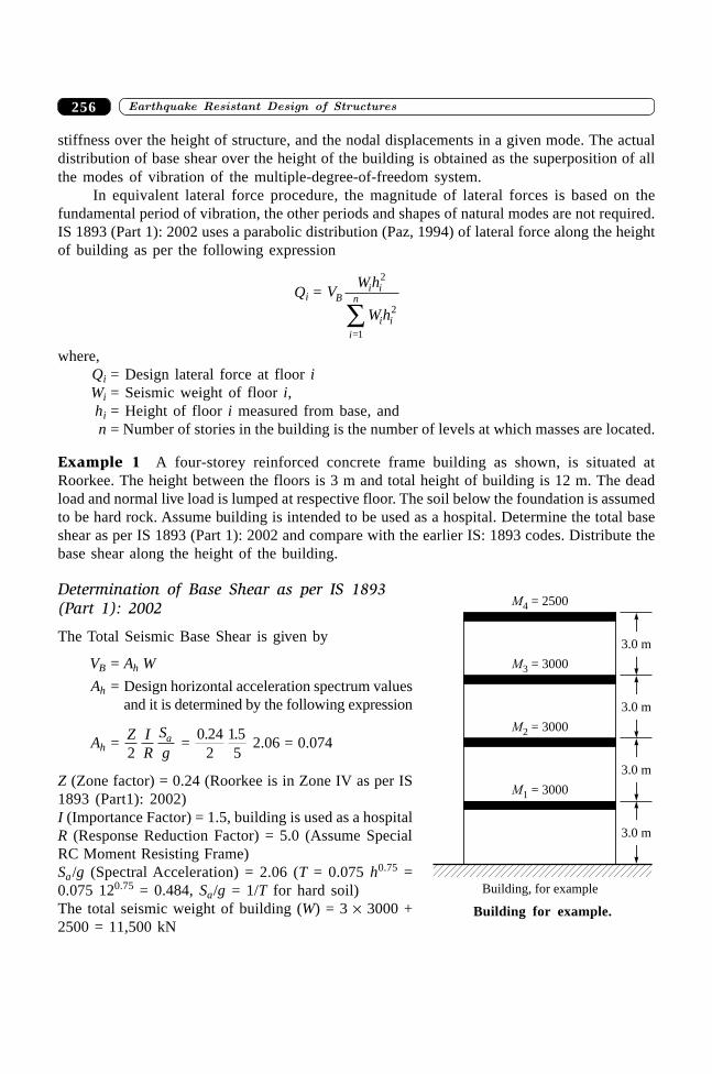
����������� ������� �������������256
stiffness over the height of structure, and the nodal displacements in a given mode. The actualdistribution of base shear over the height of the building is obtained as the superposition of allthe modes of vibration of the multiple-degree-of-freedom system.
In equivalent lateral force procedure, the magnitude of lateral forces is based on thefundamental period of vibration, the other periods and shapes of natural modes are not required.IS 1893 (Part 1): 2002 uses a parabolic distribution (Paz, 1994) of lateral force along the heightof building as per the following expression
Qi = VWh
WhB
i i
i ii
n
2
2
1=Â
where,Qi = Design lateral force at floor iWi = Seismic weight of floor i,hi = Height of floor i measured from base, andn = Number of stories in the building is the number of levels at which masses are located.
Example 1 A four-storey reinforced concrete frame building as shown, is situated atRoorkee. The height between the floors is 3 m and total height of building is 12 m. The deadload and normal live load is lumped at respective floor. The soil below the foundation is assumedto be hard rock. Assume building is intended to be used as a hospital. Determine the total baseshear as per IS 1893 (Part 1): 2002 and compare with the earlier IS: 1893 codes. Distribute thebase shear along the height of the building.
Determination of Base Shear as per IS 1893(Part 1): 2002
The Total Seismic Base Shear is given by
VB = Ah W
Ah = Design horizontal acceleration spectrum valuesand it is determined by the following expression
Ah = Z IR
Sga
2 =
0 242
1 55
. . 2.06 = 0.074
Z (Zone factor) = 0.24 (Roorkee is in Zone IV as per IS1893 (Part1): 2002)I (Importance Factor) = 1.5, building is used as a hospitalR (Response Reduction Factor) = 5.0 (Assume SpecialRC Moment Resisting Frame)Sa/g (Spectral Acceleration) = 2.06 (T = 0.075 h0.75 =0.075 120.75 = 0.484, Sa/g = 1/T for hard soil)The total seismic weight of building (W) = 3 ¥ 3000 +2500 = 11,500 kN
M4 = 2500
M3 = 3000
M2 = 3000
M1 = 3000
Building, for example
3.0 m
3.0 m
3.0 m
3.0 m
Building for example.
257�������� ��������������������� ��� ������ �������������
Total base shear (VB) = 0.074 ¥ 11500 = 851 kN
Determination of Base Shear as per earlier IS: 1893
Total design base shear for the same building is worked out from the earlier version of IS: 1893as shown below:
IS: 1893–1962 VB = ah W
ah = Horizontal seismic coefficient = ah = 0.04 ¥ 0.535 = 0.02
K factor to allow for the increased flexibility K = 0.35 S/(N + 0.9(S–8) = 0.535
S = total number of stories ( ≥13 = 13, N = number of stories = 4
(Roorkee is in zone III as per IS: 1893–1962 and soil is hard)
W = Seismic weight of building = 11,500 kN
VB = 0.02 ¥ 11500 = 230 kN
Total base shear as per IS: 1893–1962 = 230 kN
IS: 1893–1966 VB = C ah W
C = a coefficient defining the flexibility of structure = 1
C = 9/(n+5) not greater than 1, n = number of stories = 4
C = 9/(4+5) = 1
ah = Horizontal seismic coefficient = 0.05
Roorkee is in zone IV as per IS 1893: 1966 and soil type I i.e hardsoil
W = Weight of building = 11500 kN
VB = 1 ¥ 0.05 ¥ 11500 = 575 kN
Total base shear as per IS: 1893–1966 = 575 kN
IS: 1893–1970 VB = C ah bW
C = a coefficient defining the flexibility of structure = 0.5/T1/3
T = (0.1 n) = 0.4 sec, n = number of stories = 4
C = 0.676
b = a coefficient depending upon soil foundation system = 1.0
for rock and hard soil and for all types of foundation
ah = Horizontal seismic coefficient = 0.05
(Roorkee is in zone IV as per IS: 1893: 1970)
W = Weight of building (total dead load + appropriate amount of liveload) = 11500 kN
VB = 0.676 ¥ 0.05 ¥ 11500 = 388.7 kN
Total base shear as per IS: 1893–1970 = 388.7 kN
����������� ������� �������������258
IS: 1893–1975 VB = C ah W
C = a coefficient defining the flexibility of structure
C = 0.9 for fundamental period (T) = 0.1 ¥ n = 0.4 sec
ah = Horizontal seismic coefficient = 0.075
ah = b I a0 (In Seismic Coefficient Method) = 1 ¥ 1.5 ¥ 0.05 = 0.075
a0 = 0.05 since Roorkee is in zone IV as per IS: 1893: 1975
I = 1.5 (building is used as a hospital)
ah = b I F0 Sa/g (In Response Spectrum Method) = 1 ¥ 1.5 ¥ 0.25 ¥0.1875 = 0.0703
F0 = Seismic zone factor for average acceleration spectra = 0.25 for zoneIV
b = 1.0 for rock and hard soil and for all type of foundation
Sa/g = 0.1875 correspond to T = 0.4 sec and damping 5%
W = Weight of building (total dead load + appropriate amount of liveload) = 11500 kN
VB = 0.9 ¥ 0.075 ¥ 11500 = 776.25 kN
Total base shear as per IS: 1893 – 1975 = 776.25 kN
IS: 1893–1984 VB = K C ah W
K = performance factor depending on the structural framing system andbrittleness or ductility of construction = 1.0
C = a coefficient defining the flexibility of structure with increase innumber of stories depending upon fundamental time period = 0.9for T = 0.4 sec
K (performance factor) = 1.0
ah = Horizontal seismic coefficient = 0.075
ah = b I a0 (In Seismic Coefficient Method)
= 1 ¥ 1.5 ¥ 0.05 = 0.075
ah = b I F0 Sa/g (In Response Spectrum Method)
= 1 ¥ 1.5 ¥ 0.25 ¥ 0.18 = 0.07
b = 1.0 for rock and hard soil and for all types of foundation
I = a coefficient depending upon the importance of structures = 1.5(building is used as a hospital)
a0 = 0.05 since Roorkee is in zone IV as per IS: 1893: 1984
W = Weight of building = 11500 kN
VB = 0.9 ¥ 0.075 ¥ 11500 = 776.25 kN
F0 = 0.25 for zone IV
Sa/g = 0.18 correspond to T = 0.4 sec and damping 5%
Total base shear as per IS: 1893 – 1984 = 776.25 kN
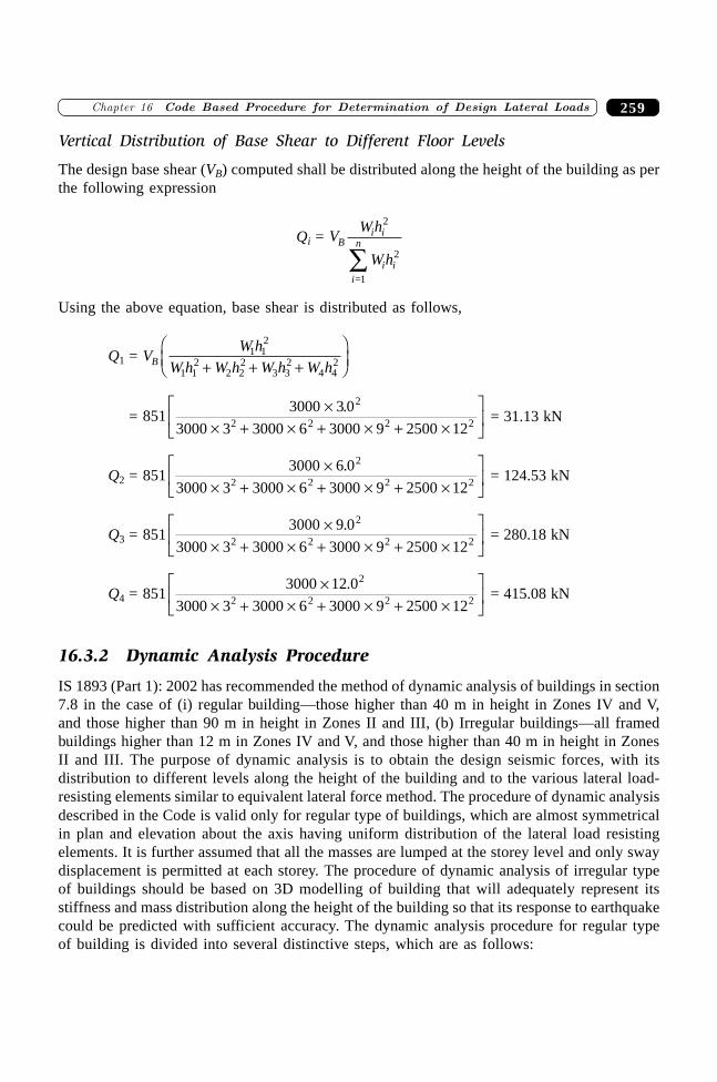
259�������� ��������������������� ��� ������ �������������
Vertical Distribution of Base Shear to Different Floor Levels
The design base shear (VB) computed shall be distributed along the height of the building as perthe following expression
Qi = VWh
WhB
i i
i ii
n
2
2
1=Â
Using the above equation, base shear is distributed as follows,
Q1 = VW h
W h W h W h W hB1 1
2
1 12
2 22
3 32
4 42+ + +
FHG
IKJ
= 8513000 3 0
3000 3 3000 6 3000 9 2500 12
2
2 2 2 2
¥¥ + ¥ + ¥ + ¥
LNM
OQP
. = 31.13 kN
Q2 = 8513000 6 0
3000 3 3000 6 3000 9 2500 12
2
2 2 2 2
¥¥ + ¥ + ¥ + ¥
LNM
OQP
. = 124.53 kN
Q3 = 8513000 9 0
3000 3 3000 6 3000 9 2500 12
2
2 2 2 2
¥¥ + ¥ + ¥ + ¥
LNM
OQP
. = 280.18 kN
Q4 = 8513000 12 0
3000 3 3000 6 3000 9 2500 12
2
2 2 2 2
¥¥ + ¥ + ¥ + ¥
LNM
OQP
. = 415.08 kN
16.3.2 Dynamic Analysis Procedure
IS 1893 (Part 1): 2002 has recommended the method of dynamic analysis of buildings in section7.8 in the case of (i) regular building—those higher than 40 m in height in Zones IV and V,and those higher than 90 m in height in Zones II and III, (b) Irregular buildings—all framedbuildings higher than 12 m in Zones IV and V, and those higher than 40 m in height in ZonesII and III. The purpose of dynamic analysis is to obtain the design seismic forces, with itsdistribution to different levels along the height of the building and to the various lateral load-resisting elements similar to equivalent lateral force method. The procedure of dynamic analysisdescribed in the Code is valid only for regular type of buildings, which are almost symmetricalin plan and elevation about the axis having uniform distribution of the lateral load resistingelements. It is further assumed that all the masses are lumped at the storey level and only swaydisplacement is permitted at each storey. The procedure of dynamic analysis of irregular typeof buildings should be based on 3D modelling of building that will adequately represent itsstiffness and mass distribution along the height of the building so that its response to earthquakecould be predicted with sufficient accuracy. The dynamic analysis procedure for regular typeof building is divided into several distinctive steps, which are as follows:
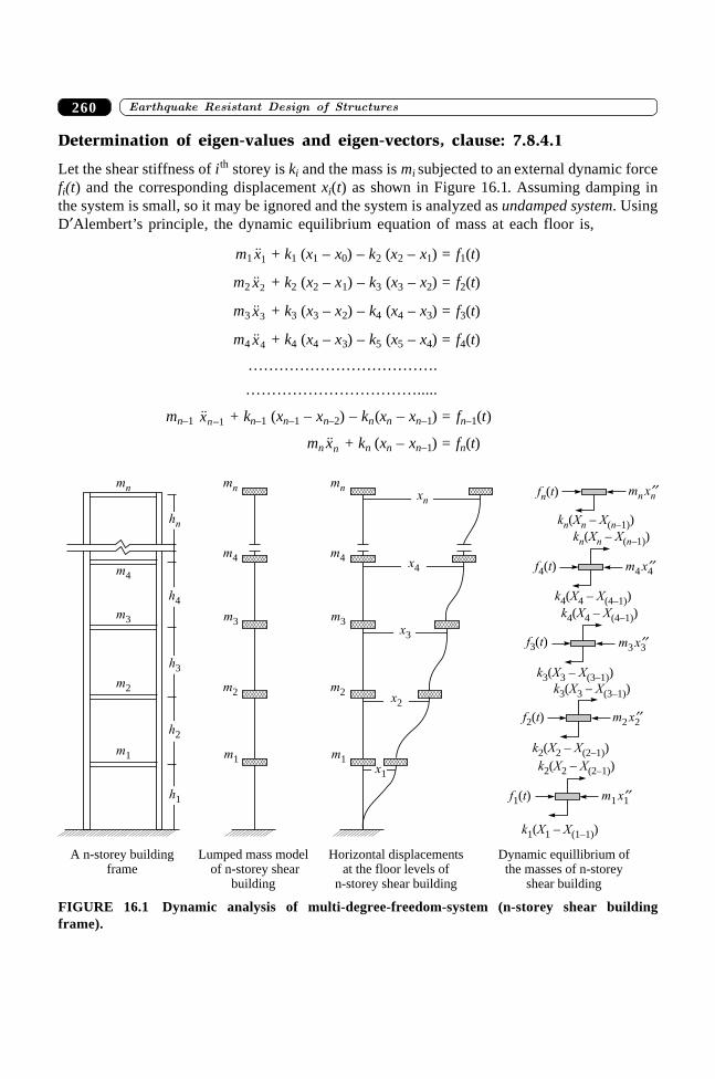
����������� ������� �������������260
Determination of eigen-values and eigen-vectors, clause: 7.8.4.1
Let the shear stiffness of ith storey is ki and the mass is mi subjected to an external dynamic forcefi(t) and the corresponding displacement xi(t) as shown in Figure 16.1. Assuming damping inthe system is small, so it may be ignored and the system is analyzed as undamped system. UsingD¢Alembert’s principle, the dynamic equilibrium equation of mass at each floor is,
m1 ��x1 + k1 (x1 – x0) – k2 (x2 – x1) = f1(t)
m2 ��x2 + k2 (x2 – x1) – k3 (x3 – x2) = f2(t)
m3 ��x3 + k3 (x3 – x2) – k4 (x4 – x3) = f3(t)
m4 ��x4 + k4 (x4 – x3) – k5 (x5 – x4) = f4(t)
……………………………….
…………………………….....
mn–1 ��xn-1 + kn–1 (xn–1 – xn–2) – kn(xn – xn–1) = fn–1(t)
mn ��xn + kn (xn – xn–1) = fn(t)
Lumped mass modelof n-storey shear
building
mn
m4
m3
m2
m1
h1
h2
h3
h4
hn
Horizontal displacementsat the floor levels of
n-storey shear building
xn
x4
x3
x2
x1
f tn( ) m xn n¢¢
k X Xn n n( – )( –1)
f t4( ) m4 4x¢¢
k X X4 4 (4–1)( – )
k X Xn n n( – )( –1)
f t3( ) m3 x3¢¢
k X X3 3 (3–1)( – )
k X X4 4 (4–1)( – )
f t2( ) m2 x2¢¢
k X X2 2 (2–1)( – )
k X X3 3 (3–1)( – )
f t1( ) m1 x1¢¢
k X X1 1 (1–1)( – )
k X X2 2 (2–1)( – )
Dynamic equillibrium ofthe masses of n-storey
shear building
A n-storey buildingframe
mn
m4
m3
m2
m1
mn
m4
m3
m2
m1
FIGURE 16.1 Dynamic analysis of multi-degree-freedom-system (n-storey shear buildingframe).
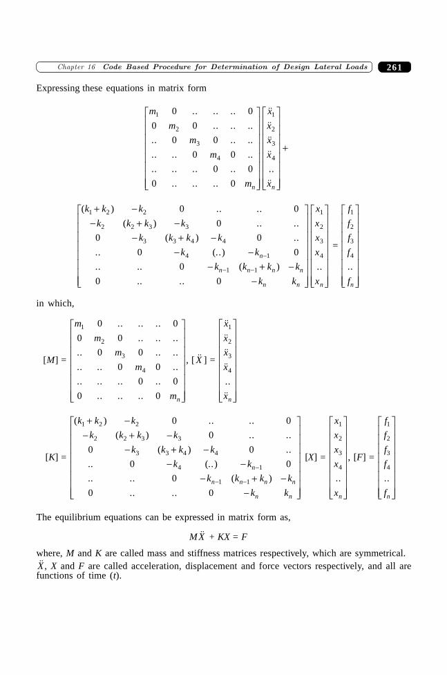
261�������� ��������������������� ��� ������ �������������
Expressing these equations in matrix form
m
m
m
m
m
x
x
x
x
xn n
1
2
3
4
1
2
3
4
0 0
0 0
0 0
0 0
0 0
0 0
.. .. ..
.. .. ..
.. .. ..
.. .. ..
.. .. .. ..
.. .. ..
��������..
��
L
N
MMMMMMMM
O
Q
PPPPPPPP
L
N
MMMMMMMM
O
Q
PPPPPPPP
+
( ) .. ..
( ) .. ..
( ) ..
.. (..)
.. .. ( )
.. ..
..
k k k
k k k k
k k k k
k k
k k k k
k k
x
x
x
x
x
n
n n n n
n n n
1 2 2
2 2 3 3
3 3 4 4
4 1
1 1
1
2
3
4
0 0
0
0 0
0 0
0
0 0
+ -- + -
- + -- -
- + --
L
N
MMMMMMMM
O
Q
PPPPPPPP
L
N
MMMMMMMM
O
Q
PPPPPPPP
-
- -
=
f
f
f
f
fn
1
2
3
4
..
L
N
MMMMMMMM
O
Q
PPPPPPPP
in which,
[M] =
m
m
m
m
mn
1
2
3
4
0 0
0 0
0 0
0 0
0 0
0 0
.. .. ..
.. .. ..
.. .. ..
.. .. ..
.. .. .. ..
.. .. ..
L
N
MMMMMMMM
O
Q
PPPPPPPP
, [ ��X ] =
��������
..
��
x
x
x
x
xn
1
2
3
4
L
N
MMMMMMMM
O
Q
PPPPPPPP
[K] =
( ) .. ..
( ) .. ..
( ) ..
.. (.. )
.. .. ( )
.. ..
k k k
k k k k
k k k k
k k
k k k k
k k
n
n n n n
n n
1 2 2
2 2 3 3
3 3 4 4
4 1
1 1
0 0
0
0 0
0 0
0
0 0
+ -- + -
- + -- -
- + --
L
N
MMMMMMMM
O
Q
PPPPPPPP
-
- -
[X] =
x
x
x
x
xn
1
2
3
4
..
L
N
MMMMMMMM
O
Q
PPPPPPPP
, [F] =
f
f
f
f
fn
1
2
3
4
..
L
N
MMMMMMMM
O
Q
PPPPPPPP
The equilibrium equations can be expressed in matrix form as,
M ��X + KX = F
where, M and K are called mass and stiffness matrices respectively, which are symmetrical.��X , X and F are called acceleration, displacement and force vectors respectively, and all are
functions of time (t).
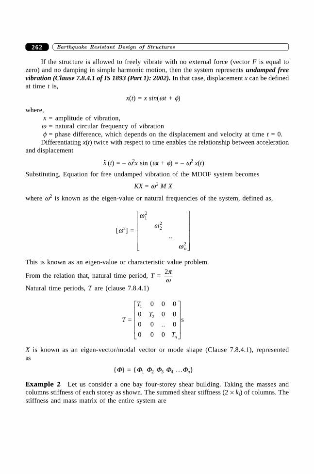
����������� ������� �������������262
If the structure is allowed to freely vibrate with no external force (vector F is equal tozero) and no damping in simple harmonic motion, then the system represents undamped freevibration (Clause 7.8.4.1 of IS 1893 (Part 1): 2002). In that case, displacement x can be definedat time t is,
x(t) = x sin(wt + f)
where,x = amplitude of vibration,
w = natural circular frequency of vibrationf = phase difference, which depends on the displacement and velocity at time t = 0.
Differentiating x(t) twice with respect to time enables the relationship between accelerationand displacement
��x (t) = – w2x sin (wt + f) = – w2 x(t)
Substituting, Equation for free undamped vibration of the MDOF system becomes
KX = w2 M X
where w2 is known as the eigen-value or natural frequencies of the system, defined as,
[w2] =
ww
w
12
22
2
..
n
L
N
MMMMM
O
Q
PPPPP
This is known as an eigen-value or characteristic value problem.
From the relation that, natural time period, T = 2pw
Natural time periods, T are (clause 7.8.4.1)
T =
T
T
Tn
1
2
0 0 0
0 0 0
0 0 0
0 0 0
..
L
N
MMMM
O
Q
PPPPs
X is known as an eigen-vector/modal vector or mode shape (Clause 7.8.4.1), representedas
{F} = {F1 F2 F3 F4 …Fn}
Example 2 Let us consider a one bay four-storey shear building. Taking the masses andcolumns stiffness of each storey as shown. The summed shear stiffness (2 ¥ ki) of columns. Thestiffness and mass matrix of the entire system are
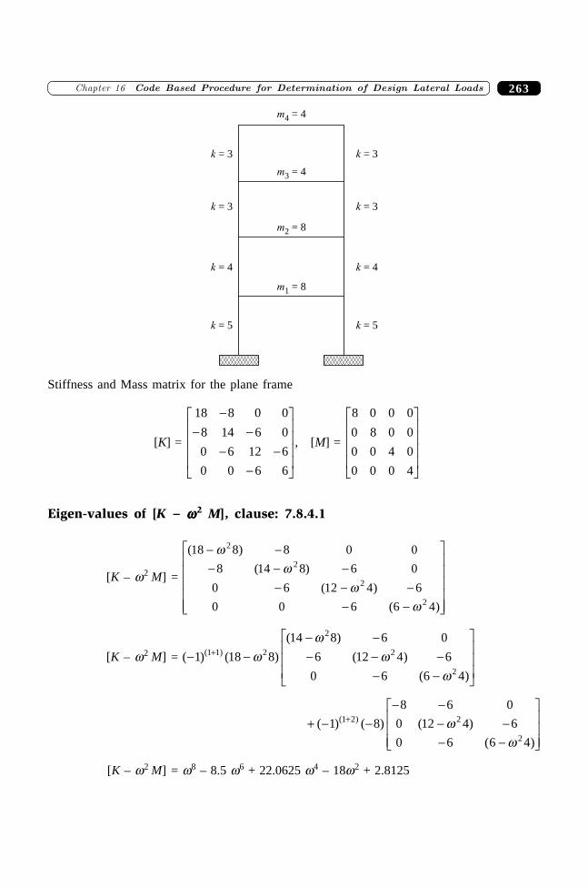
263�������� ��������������������� ��� ������ �������������
k = 3
m1 = 8
m2 = 8
m3 = 4
m4 = 4
k = 3
k = 4
k = 5
k = 3
k = 3
k = 4
k = 5
Stiffness and Mass matrix for the plane frame
[K] =
18 8 0 0
8 14 6 0
0 6 12 6
0 0 6 6
-- -
- --
L
N
MMMM
O
Q
PPPP
, [M] =
8 0 0 0
0 8 0 0
0 0 4 0
0 0 0 4
L
N
MMMM
O
Q
PPPP
Eigen-values of [K – wwwww2 M], clause: 7.8.4.1
[K – w2 M] =
( )
( )
( )
( )
18 8 8 0 0
8 14 8 6 0
0 6 12 4 6
0 0 6 6 4
2
2
2
2
- -- - -
- - -- -
L
N
MMMMM
O
Q
PPPPP
ww
ww
[K – w2 M] = ( ) ( )
( )
( )
( )
( )- -- -- - -
- -
L
N
MMM
O
Q
PPP
+1 18 8
14 8 6 0
6 12 4 6
0 6 6 4
1 1 2
2
2
2
ww
ww
+ - -- -
- -- -
L
NMMM
O
QPPP
+( ) ( ) ( )
( )
( )1 8
8 6 0
0 12 4 6
0 6 6 4
1 2 2
2
ww
[K – w2 M] = w8 – 8.5 w6 + 22.0625 w4 – 18w2 + 2.8125
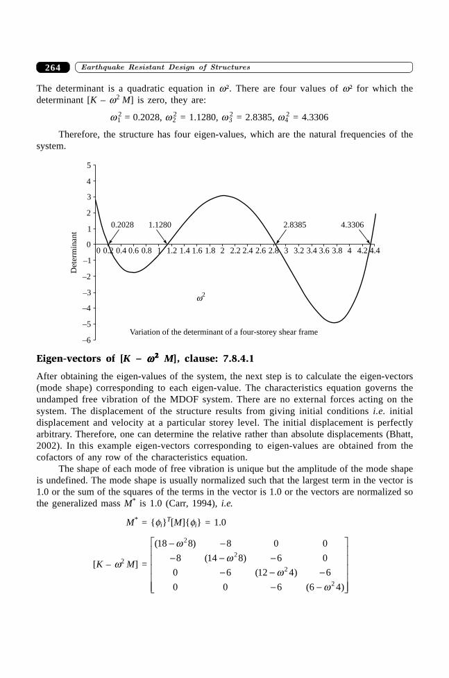
����������� ������� �������������264
The determinant is a quadratic equation in w². There are four values of w² for which thedeterminant [K – w2 M] is zero, they are:
w12 = 0.2028, w2
2 = 1.1280, w32 = 2.8385, w4
2 = 4.3306
Therefore, the structure has four eigen-values, which are the natural frequencies of thesystem.
Variation of the determinant of a four-storey shear frame–6
–5
–4
–3
–2
–1
0
1
2
3
4
5
0 0.2 0.4 0.6 0.8 1 1.2 1.4 1.6 1.8 2 2.2 2.4 2.6 2.8 3 3.2 3.4 3.6 3.8 4 4.2 4.4
w2
4.33062.83851.12800.2028
Det
erm
inan
t
Eigen-vectors of [K – wwwww22222 M], clause: 7.8.4.1
After obtaining the eigen-values of the system, the next step is to calculate the eigen-vectors(mode shape) corresponding to each eigen-value. The characteristics equation governs theundamped free vibration of the MDOF system. There are no external forces acting on thesystem. The displacement of the structure results from giving initial conditions i.e. initialdisplacement and velocity at a particular storey level. The initial displacement is perfectlyarbitrary. Therefore, one can determine the relative rather than absolute displacements (Bhatt,2002). In this example eigen-vectors corresponding to eigen-values are obtained from thecofactors of any row of the characteristics equation.
The shape of each mode of free vibration is unique but the amplitude of the mode shapeis undefined. The mode shape is usually normalized such that the largest term in the vector is1.0 or the sum of the squares of the terms in the vector is 1.0 or the vectors are normalized sothe generalized mass M* is 1.0 (Carr, 1994), i.e.
M* = {fi}T[M]{fi} = 1.0
[K – w2 M] =
( )
( )
( )
( )
18 8 8 0 0
8 14 8 6 0
0 6 12 4 6
0 0 6 6 4
2
2
2
2
- -- - -
- - -- -
L
N
MMMMM
O
Q
PPPPP
ww
ww
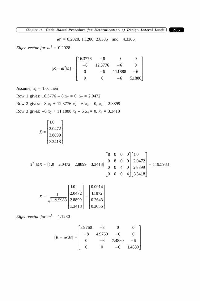
265�������� ��������������������� ��� ������ �������������
w2 = 0.2028, 1.1280, 2.8385 and 4.3306
Eigen-vector for w 2 = 0.2028
[K – w 2M] =
16 3776 8 0 0
8 12 3776 6 0
0 6 111888 6
0 0 6 51888
.
.
.
.
-- -
- --
L
N
MMMM
O
Q
PPPP
Assume, x1 = 1.0, then
Row 1 gives: 16.3776 – 8 x2 = 0, x2 = 2.0472
Row 2 gives: –8 x1 + 12.3776 x2 – 6 x3 = 0, x3 = 2.8899
Row 3 gives: –6 x2 + 11.1888 x3 – 6 x4 = 0, x4 = 3.3418
X =
1 0
2 0472
2 8899
3 3418
.
.
.
.
L
N
MMMM
O
Q
PPPP
XT MX = [1.0 2.0472 2.8899 3.3418]
8 0 0 0
0 8 0 0
0 0 4 0
0 0 0 4
1 0
2 0472
2 8899
3 3418
L
N
MMMM
O
Q
PPPP
L
N
MMMM
O
Q
PPPP
.
.
.
.
= 119.5983
X = 1119 5983
1 0
2 0472
2 8899
3 3418
.
.
.
.
.
L
N
MMMM
O
Q
PPPP
=
0 0914
11872
0 2643
0 3056
.
.
.
.
L
N
MMMM
O
Q
PPPP
Eigen-vector for w2 = 1.1280
[K – w2M] =
8 9760 8 0 0
8 4 9760 6 0
0 6 7 4880 6
0 0 6 1 4880
.
.
.
.
-- -
- --
L
N
MMMM
O
Q
PPPP
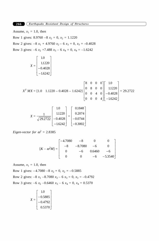
����������� ������� �������������266
Assume, x1 = 1.0, then
Row 1 gives: 8.9760 –8 x2 = 0, x2 = 1.1220
Row 2 gives: –8 x1 + 4.9760 x2 – 6 x3 = 0, x3 = –0.4028
Row 3 gives: –6 x2 +7.488 x3 – 6 x4 = 0, x4 = –1.6242
X =
1 0
11220
0 4028
16242
.
.
.
.
--
L
N
MMMM
O
Q
PPPP
XT MX = [1.0 1.1220 – 0.4028 – 1.6242]
8 0 0 0
0 8 0 0
0 0 4 0
0 0 0 4
1 0
11220
0 4028
16242
L
N
MMMM
O
Q
PPPP
--
L
N
MMMM
O
Q
PPPP
.
.
.
.
= 29.2722
X = 129 2722
1 0
11220
0 4028
16242
.
.
.
.
.
--
L
N
MMMM
O
Q
PPPP
=
01848
0 2074
0 0744
0 3002
.
.
.
.
--
L
N
MMMM
O
Q
PPPP
Eigen-vector for w2 = 2.8385
[K – w2M] =
- -- - -
- -- -
L
N
MMMM
O
Q
PPPP
4 7080 8 0 0
8 8 7080 6 0
0 6 0 6460 6
0 0 6 5 3540
.
.
.
.
Assume, x1 = 1.0, then
Row 1 gives: – 4.7080 –8 x2 = 0, x2 = –0.5885
Row 2 gives: –8 x1 –8.7080 x2 – 6 x3 = 0, x3 = –0.4792
Row 3 gives: –6 x2 –0.6460 x3 – 6 x4 = 0, x4 = 0.5370
X =
1 0
0 5885
0 4792
0 5370
.
.
.
.
--
L
N
MMMM
O
Q
PPPP
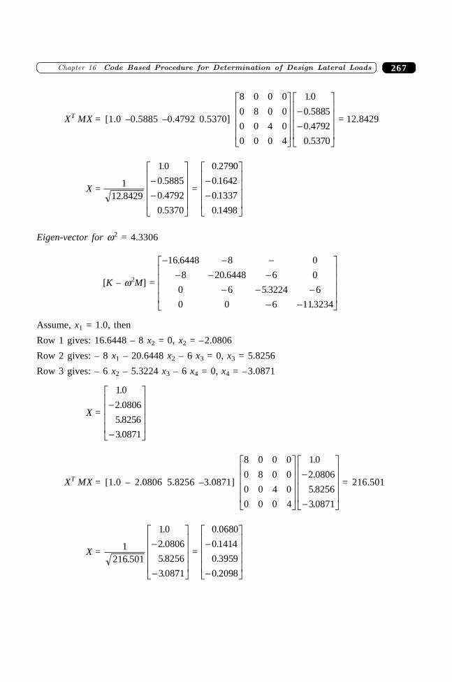
267�������� ��������������������� ��� ������ �������������
XT MX = [1.0 –0.5885 –0.4792 0.5370]
8 0 0 0
0 8 0 0
0 0 4 0
0 0 0 4
1 0
0 5885
0 4792
0 5370
L
N
MMMM
O
Q
PPPP
--
L
N
MMMM
O
Q
PPPP
.
.
.
.
= 12.8429
X = 112 8429
1 0
0 5885
0 4792
0 5370
.
.
.
.
.
--
L
N
MMMM
O
Q
PPPP =
0 2790
0 1642
0 1337
0 1498
.
.
.
.
--
L
N
MMMM
O
Q
PPPP
Eigen-vector for w2 = 4.3306
[K – w2M] =
- - -- - -
- - -- -
L
N
MMMM
O
Q
PPPP
16 6448 8 0
8 20 6448 6 0
0 6 5 3224 6
0 0 6 113234
.
.
.
.
Assume, x1 = 1.0, then
Row 1 gives: 16.6448 – 8 x2 = 0, x2 = –2.0806
Row 2 gives: – 8 x1 – 20.6448 x2 – 6 x3 = 0, x3 = 5.8256
Row 3 gives: – 6 x2 – 5.3224 x3 – 6 x4 = 0, x4 = –3.0871
X =
1 0
2 0806
5 8256
3 0871
.
.
.
.
-
-
L
N
MMMM
O
Q
PPPP
XT MX = [1.0 – 2.0806 5.8256 –3.0871]
8 0 0 0
0 8 0 0
0 0 4 0
0 0 0 4
1 0
2 0806
5 8256
3 0871
L
N
MMMM
O
Q
PPPP
-
-
L
N
MMMM
O
Q
PPPP
.
.
.
.
= 216.501
X = 1216 501
1 0
2 0806
5 8256
3 0871
.
.
.
.
.
-
-
L
N
MMMM
O
Q
PPPP
=
0 0680
0 1414
0 3959
0 2098
.
.
.
.
-
-
L
N
MMMM
O
Q
PPPP
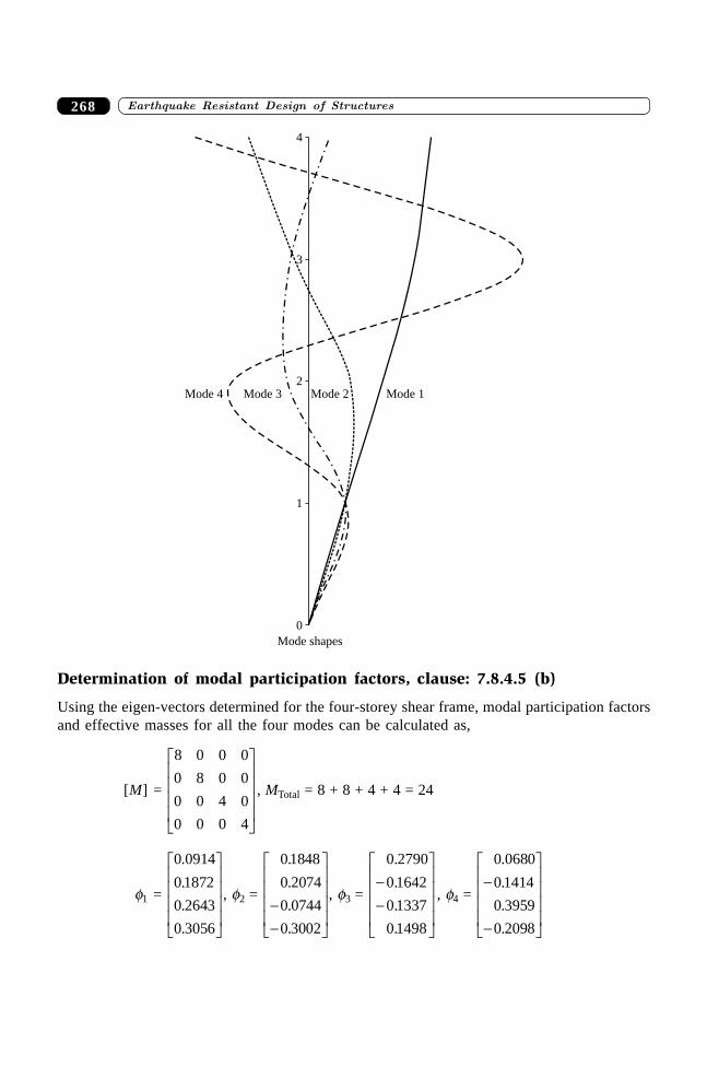
����������� ������� �������������268
Mode 3 Mode 2 Mode 1Mode 4
Mode shapes
4
3
2
1
0
Determination of modal participation factors, clause: 7.8.4.5 (b)
Using the eigen-vectors determined for the four-storey shear frame, modal participation factorsand effective masses for all the four modes can be calculated as,
[M] =
8 0 0 0
0 8 0 0
0 0 4 0
0 0 0 4
L
N
MMMM
O
Q
PPPP
, MTotal = 8 + 8 + 4 + 4 = 24
f1 =
0 0914
0 1872
0 2643
0 3056
.
.
.
.
L
N
MMMM
O
Q
PPPP, f2 =
01848
0 2074
0 0744
0 3002
.
.
.
.
--
L
N
MMMM
O
Q
PPPP, f3 =
0 2790
0 1642
0 1337
0 1498
.
.
.
.
--
L
N
MMMM
O
Q
PPPP
, f4 =
0 0680
0 1414
0 3959
0 2098
.
.
.
.
-
-
L
N
MMMM
O
Q
PPPP
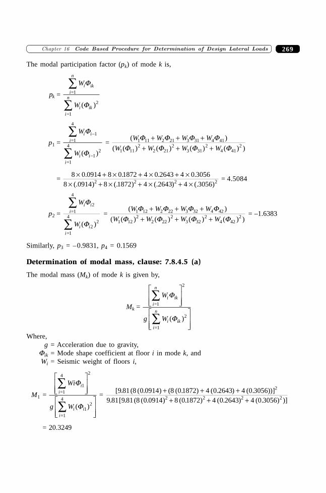
269�������� ��������������������� ��� ������ �������������
The modal participation factor (pk) of mode k is,
pk =
W
W
i iki
n
i iki
n
F
F
=1
=1
Â
 ( )2
p1 =
W
W
i ii
i ii
F
F
-
-
Â
Â
1
4
12
4=1
=1
( )
= ( )
( ( ) ( ) ( ) ( ) )
W W W W
W W W W1 11 2 21 3 31 4 41
1 112
2 212
3 312
4 412
F F F FF F F F
+ + ++ + +
=8 0 0914 8 0 1872 4 0 2643 4 0 3056
8 0914 8 1872 4 2643 4 30562 2 2 2¥ + ¥ + ¥ + ¥
¥ + ¥ + ¥ + ¥. . . .
(. ) (. ) (. ) (. )= 4.5084
p2 =
W
W
i ii
i ii
F
F
2
4
22
4=1
=1
Â
 ( )
= ( )
( ( ) ( ) ( ) ( ) )
W W W W
W W W W1 12 2 22 3 32 4 42
1 122
2 222
3 322
4 422
F F F FF F F F
+ + ++ + +
= –1.6383
Similarly, p3 = –0.9831, p4 = 0.1569
Determination of modal mass, clause: 7.8.4.5 (a)
The modal mass (Mk) of mode k is given by,
Mk =
W
g W
i iki
n
i iki
n
F
F
=1
=1
Â
Â
LNMM
OQPP
LNMM
OQPP
2
2( )
Where,g = Acceleration due to gravity,
Fik = Mode shape coefficient at floor i in mode k, andWi = Seismic weight of floors i,
M1 =
Wi
g W
ii
i ii
F
F
1
4 2
12
4
=1
=1
Â
Â
LNMM
OQPP
LNMM
OQPP
( )
= [ . (8 ( . ) (8 ( . ) ( . ) ( . ))]
. [ . (8 ( . ) ( . ) ( . ) ( . ) )]9 81 0 0914 0 1872 4 0 2643 4 0 3056
9 81 9 81 0 0914 8 0 1872 4 0 2643 4 0 3056
2
2 2 2 2+ + +
+ + +
= 20.3249
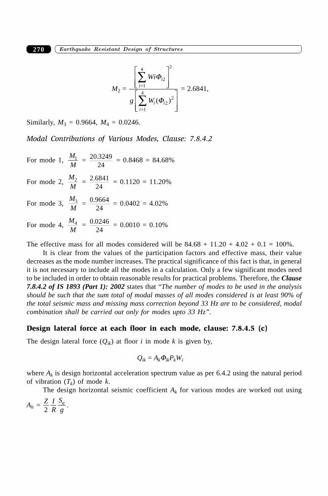
����������� ������� �������������270
M2 =
Wi
g W
ii
i ii
F
F
2
4 2
22
4
=1
=1
Â
Â
LNMM
OQPP
LNMM
OQPP
( )
= 2.6841,
Similarly, M3 = 0.9664, M4 = 0.0246.
Modal Contributions of Various Modes, Clause: 7.8.4.2
For mode 1,MM
1 = 20 324924. = 0.8468 = 84.68%
For mode 2,MM
2 = 2 684124
. = 0.1120 = 11.20%
For mode 3,MM
3 = 0 966424
. = 0.0402 = 4.02%
For mode 4,MM
4 = 0 024624
. = 0.0010 = 0.10%
The effective mass for all modes considered will be 84.68 + 11.20 + 4.02 + 0.1 = 100%.It is clear from the values of the participation factors and effective mass, their value
decreases as the mode number increases. The practical significance of this fact is that, in generalit is not necessary to include all the modes in a calculation. Only a few significant modes needto be included in order to obtain reasonable results for practical problems. Therefore, the Clause7.8.4.2 of IS 1893 (Part 1): 2002 states that “The number of modes to be used in the analysisshould be such that the sum total of modal masses of all modes considered is at least 90% ofthe total seismic mass and missing mass correction beyond 33 Hz are to be considered, modalcombination shall be carried out only for modes upto 33 Hz”.
Design lateral force at each floor in each mode, clause: 7.8.4.5 (c)
The design lateral force (Qik) at floor i in mode k is given by,
Qik = AkFikPkWi
where Ak is design horizontal acceleration spectrum value as per 6.4.2 using the natural periodof vibration (Tk) of mode k.
The design horizontal seismic coefficient Ak for various modes are worked out using
Ah = Z IR
Sga
2.
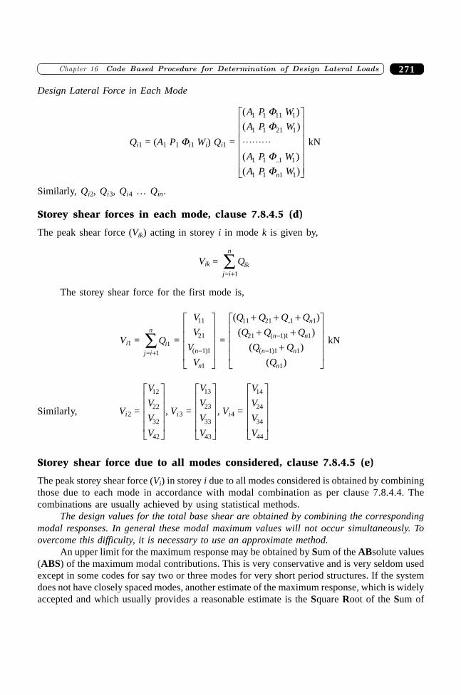
271�������� ��������������������� ��� ������ �������������
Design Lateral Force in Each Mode
Qi1 = (A1 P1 Fi1 Wi) Qi1 =
( )
( )
( )
( )..
A P W
A P W
A P W
A P Wn
1 1 11 1
1 1 21 1
1 1 1 1
1 1 1 1
FF
FF
���
L
N
MMMMMM
O
Q
PPPPPP
kN
Similarly, Qi2, Qi3, Qi4 … Qin.
Storey shear forces in each mode, clause 7.8.4.5 (d)
The peak shear force (Vik) acting in storey i in mode k is given by,
Vik = Qikj i
n
= +Â
1
The storey shear force for the first mode is,
Vi1 = Qij i
n
11= +
 =
V
V
V
Vn
n
11
21
1 1
1
( )-
L
N
MMMM
O
Q
PPPP
=
( )
( )
( )
( )
..
( )
( )
Q Q Q Q
Q Q Q
Q Q
Q
n
n n
n n
n
11 21 1 1
21 1 1 1
1 1 1
1
+ + ++ +
+
L
N
MMMM
O
Q
PPPP
-
- kN
Similarly, Vi2 =
V
V
V
V
12
22
32
42
L
N
MMMM
O
Q
PPPP, Vi3 =
V
V
V
V
13
23
33
43
L
N
MMMM
O
Q
PPPP
, Vi4 =
V
V
V
V
14
24
34
44
L
N
MMMM
O
Q
PPPP
Storey shear force due to all modes considered, clause 7.8.4.5 (e)
The peak storey shear force (Vi) in storey i due to all modes considered is obtained by combiningthose due to each mode in accordance with modal combination as per clause 7.8.4.4. Thecombinations are usually achieved by using statistical methods.
The design values for the total base shear are obtained by combining the correspondingmodal responses. In general these modal maximum values will not occur simultaneously. Toovercome this difficulty, it is necessary to use an approximate method.
An upper limit for the maximum response may be obtained by Sum of the ABsolute values(ABS) of the maximum modal contributions. This is very conservative and is very seldom usedexcept in some codes for say two or three modes for very short period structures. If the systemdoes not have closely spaced modes, another estimate of the maximum response, which is widelyaccepted and which usually provides a reasonable estimate is the Square Root of the Sum of
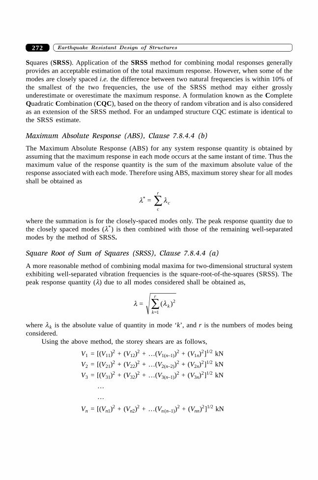
����������� ������� �������������272
Squares (SRSS). Application of the SRSS method for combining modal responses generallyprovides an acceptable estimation of the total maximum response. However, when some of themodes are closely spaced i.e. the difference between two natural frequencies is within 10% ofthe smallest of the two frequencies, the use of the SRSS method may either grosslyunderestimate or overestimate the maximum response. A formulation known as the CompleteQuadratic Combination (CQC), based on the theory of random vibration and is also consideredas an extension of the SRSS method. For an undamped structure CQC estimate is identical tothe SRSS estimate.
Maximum Absolute Response (ABS), Clause 7.8.4.4 (b)
The Maximum Absolute Response (ABS) for any system response quantity is obtained byassuming that the maximum response in each mode occurs at the same instant of time. Thus themaximum value of the response quantity is the sum of the maximum absolute value of theresponse associated with each mode. Therefore using ABS, maximum storey shear for all modesshall be obtained as
l* = lcc
r
Â
where the summation is for the closely-spaced modes only. The peak response quantity due tothe closely spaced modes (l*) is then combined with those of the remaining well-separatedmodes by the method of SRSS.
Square Root of Sum of Squares (SRSS), Clause 7.8.4.4 (a)
A more reasonable method of combining modal maxima for two-dimensional structural systemexhibiting well-separated vibration frequencies is the square-root-of-the-squares (SRSS). Thepeak response quantity (l) due to all modes considered shall be obtained as,
l = ( )l kk
r2
=1Â
where lk is the absolute value of quantity in mode ‘k’, and r is the numbers of modes beingconsidered.
Using the above method, the storey shears are as follows,
V1 = [(V11)2 + (V12)
2 + …(V1(n–1))2 + (V1n)
2]1/2 kN
V2 = [(V21)2 + (V22)
2 + …(V2(n–2))2 + (V2n)
2]1/2 kN
V3 = [(V31)2 + (V32)
2 + …(V3(n–1))2 + (V3n)
2]1/2 kN
…
…
Vn = [(Vn1)2 + (Vn2)2 + …(Vn (n–1))2 + (Vnn)2]1/2 kN
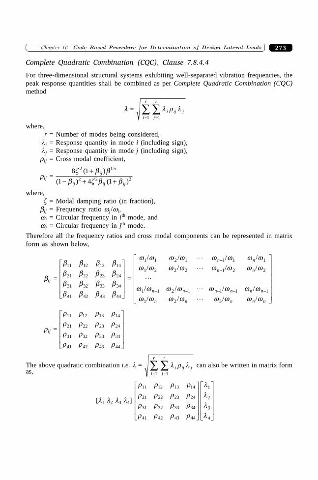
273�������� ��������������������� ��� ������ �������������
Complete Quadratic Combination (CQC), Clause 7.8.4.4
For three-dimensional structural systems exhibiting well-separated vibration frequencies, thepeak response quantities shall be combined as per Complete Quadratic Combination (CQC)method
l = l r li ij jj
r
i
r
=1=1ÂÂ
where,r = Number of modes being considered,
li = Response quantity in mode i (including sign),lj = Response quantity in mode j (including sign),rij = Cross modal coefficient,
rij =8 1
1 4 1
2 1 5
2 2 2
z b bb z b b
( )
( ) ( )
.+- + +
ij
ij ij ij
where,z = Modal damping ratio (in fraction),
bij = Frequency ratio wj/wi,wi = Circular frequency in ith mode, andwj = Circular frequency in jth mode.
Therefore all the frequency ratios and cross modal components can be represented in matrixform as shown below,
bij =
b b b bb b b bb b b bb b b b
11 12 13 14
21 22 23 24
31 32 33 34
41 42 43 44
L
N
MMMM
O
Q
PPPP =
w w w w w w w ww w w w w w w w
w w w w w w w ww w w w w w w w
1 1 2 1 1 1 1
1 2 2 2 1 2 2
1 1 2 1 1 1 1
1 2 3
/ / / /
/ / / /
/ / / /
/ / / /
��
���
n n
n n
n n n n n n
n n n n n
-
-
- - - - -
L
N
MMMMMM
O
Q
PPPPPP
rij =
r r r rr r r rr r r rr r r r
11 12 13 14
21 22 23 24
31 32 33 34
41 42 43 44
L
N
MMMM
O
Q
PPPP
The above quadratic combination i.e. l = l r li ij jj
r
i
r
=1=1ÂÂ can also be written in matrix form
as,
[l1 l2 l3 l4]
r r r rr r r rr r r rr r r r
llll
11 12 13 14
21 22 23 24
31 32 33 34
41 42 43 44
1
2
3
4
L
N
MMMM
O
Q
PPPP
L
N
MMMM
O
Q
PPPP
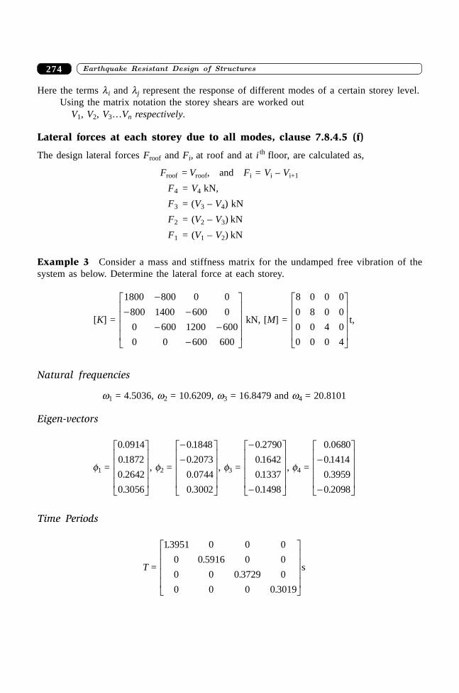
����������� ������� �������������274
Here the terms li and lj represent the response of different modes of a certain storey level.Using the matrix notation the storey shears are worked out
V1, V2, V3…Vn respectively.
Lateral forces at each storey due to all modes, clause 7.8.4.5 (f)
The design lateral forces Froof and Fi, at roof and at i th floor, are calculated as,
Froof = Vroof, and Fi = Vi – Vi+1
F4 = V4 kN,
F3 = (V3 – V4) kN
F2 = (V2 – V3) kN
F1 = (V1 – V2) kN
Example 3 Consider a mass and stiffness matrix for the undamped free vibration of thesystem as below. Determine the lateral force at each storey.
[K] =
1800 800 0 0
800 1400 600 0
0 600 1200 600
0 0 600 600
-- -
- --
L
N
MMMM
O
Q
PPPP
kN, [M] =
8 0 0 0
0 8 0 0
0 0 4 0
0 0 0 4
L
N
MMMM
O
Q
PPPP
t,
Natural frequencies
w1 = 4.5036, w2 = 10.6209, w3 = 16.8479 and w4 = 20.8101
Eigen-vectors
f1 =
0 0914
0 1872
0 2642
0 3056
.
.
.
.
L
N
MMMM
O
Q
PPPP, f2 =
--L
N
MMMM
O
Q
PPPP
0 1848
0 2073
0 0744
0 3002
.
.
.
.
, f3 =
-
-
L
N
MMMM
O
Q
PPPP
0 2790
0 1642
0 1337
0 1498
.
.
.
.
, f4 =
0 0680
0 1414
0 3959
0 2098
.
.
.
.
-
-
L
N
MMMM
O
Q
PPPP
Time Periods
T =
13951 0 0 0
0 0 5916 0 0
0 0 0 3729 0
0 0 0 0 3019
.
.
.
.
L
N
MMMM
O
Q
PPPPs
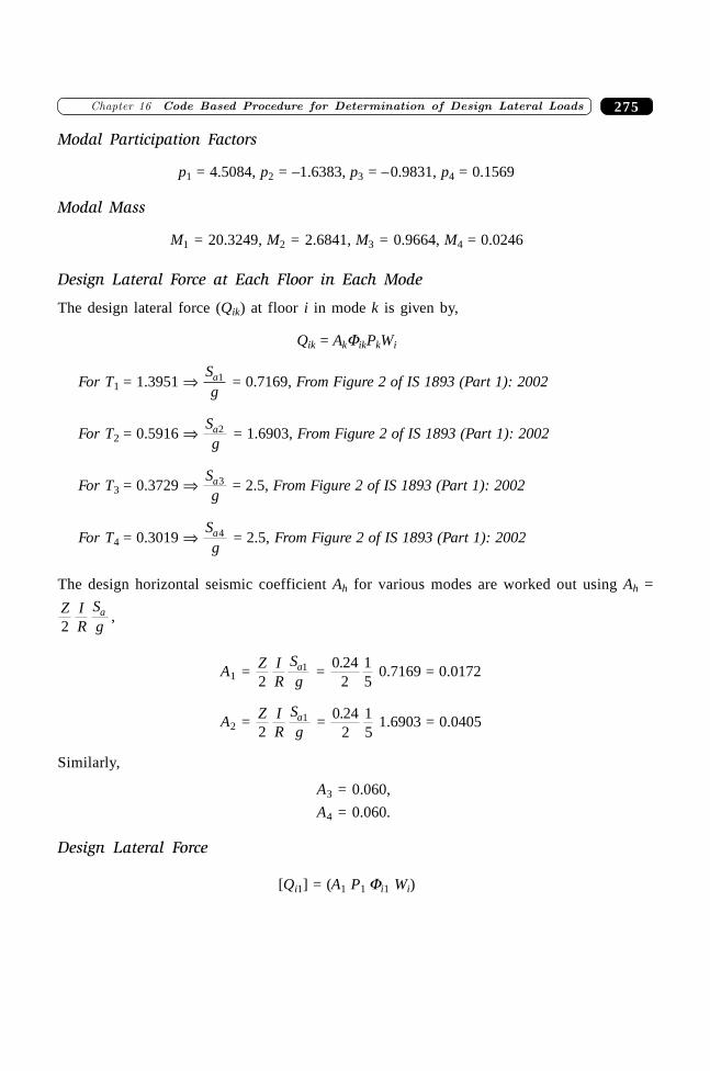
275�������� ��������������������� ��� ������ �������������
Modal Participation Factors
p1 = 4.5084, p2 = –1.6383, p3 = –0.9831, p4 = 0.1569
Modal Mass
M1 = 20.3249, M2 = 2.6841, M3 = 0.9664, M4 = 0.0246
Design Lateral Force at Each Floor in Each Mode
The design lateral force (Qik) at floor i in mode k is given by,
Qik = AkFikPkWi
For T1 = 1.3951 fi Sga1 = 0.7169, From Figure 2 of IS 1893 (Part 1): 2002
For T2 = 0.5916 fi Sga2 = 1.6903, From Figure 2 of IS 1893 (Part 1): 2002
For T3 = 0.3729 fi Sga3 = 2.5, From Figure 2 of IS 1893 (Part 1): 2002
For T4 = 0.3019 fi Sga4 = 2.5, From Figure 2 of IS 1893 (Part 1): 2002
The design horizontal seismic coefficient Ah for various modes are worked out using Ah =
Z IR
Sga
2,
A1 = Z IR
Sga
21 =
0 242
15
. 0.7169 = 0.0172
A2 = Z IR
Sga
21 = 0 24
215
. 1.6903 = 0.0405
Similarly,
A3 = 0.060,
A4 = 0.060.
Design Lateral Force
[Qi1] = (A1 P1 Fi1 Wi)
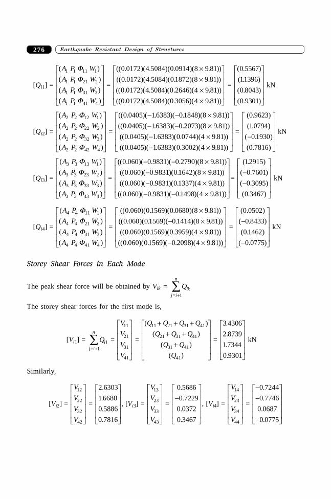
����������� ������� �������������276
[Qi1] =
( )
( )
( )
( )
A P W
A P W
A P W
A P W
1 1 11 1
1 1 21 2
1 1 31 3
1 1 41 4
FFFF
L
N
MMMM
O
Q
PPPP =
(( . )( . )( . )(8 . ))
(( . )( . )( . )(8 . ))
(( . )( . )( . )( . ))
(( . )( . )( . )( . ))
0 0172 4 5084 0 0914 9 81
0 0172 4 5084 0 1872 9 81
0 0172 4 5084 0 2646 4 9 81
0 0172 4 5084 0 3056 4 9 81
¥¥¥¥
L
N
MMMM
O
Q
PPPP
=
( . )
( . )
( . )
( . )
0 5567
11396
0 8043
0 9301
L
N
MMMM
O
Q
PPPP
kN
[Qi2] =
( )
( )
( )
( )
A P W
A P W
A P W
A P W
2 2 12 1
2 2 22 2
2 2 32 3
2 2 42 4
FFFF
L
N
MMMM
O
Q
PPPP =
(( . )( . )( . )(8 . ))
(( . )( . )( . )(8 . ))
(( . )( . )( . )( . ))
(( . )( . )( . )( . ))
0 0405 1 6383 0 1848 9 81
0 0405 16383 0 2073 9 81
0 0405 1 6383 0 0744 4 9 81
0 0405 16383 0 3002 4 9 81
- - ¥- - ¥- ¥- ¥
L
N
MMMM
O
Q
PPPP =
( . )
( . )
( . )
( . )
0 9623
1 0794
0 1930
0 7816
-
L
N
MMMM
O
Q
PPPP
kN
[Qi3] =
( )
( )
( )
( )
A P W
A P W
A P W
A P W
3 3 13 1
3 3 23 2
3 3 33 3
3 3 43 4
FFFF
L
N
MMMM
O
Q
PPPP =
(( . )( . )( . )(8 . ))
(( . )( . )( . )(8 . ))
(( . )( . )( . )( . ))
(( . )( . )( . )( . ))
0 060 0 9831 0 2790 9 81
0 060 0 9831 0 1642 9 81
0 060 0 9831 0 1337 4 9 81
0 060 0 9831 0 1498 4 9 81
- - ¥- ¥- ¥
- - ¥
L
N
MMMM
O
Q
PPPP
=
( . )
( . )
( . )
( . )
12915
0 7601
0 3095
0 3467
--
L
N
MMMM
O
Q
PPPP
kN
[Qi4] =
( )
( )
( )
( )
A P W
A P W
A P W
A P W
4 4 11 1
4 4 21 2
4 4 31 3
4 4 41 4
FFFF
L
N
MMMM
O
Q
PPPP
=
(( . )( . )( . )(8 . ))
(( . )( . )( . )(8 . ))
(( . )( . )( . )( . ))
(( . )( . )( . )( . ))
0 060 0 1569 0 0680 9 81
0 060 0 1569 0 1414 9 81
0 060 01569 0 3959 4 9 81
0 060 01569 0 2098 4 9 81
¥- ¥
¥- ¥
L
N
MMMM
O
Q
PPPP
=
( . )
( . )
( . )
( . )
0 0502
0 8433
0 1462
0 0775
-
-
L
N
MMMM
O
Q
PPPP
kN
Storey Shear Forces in Each Mode
The peak shear force will be obtained by Vik = Qikj i
n
= +Â
1
The storey shear forces for the first mode is,
[Vi1] = Qij i
n
11= +
 =
V
V
V
V
11
21
31
41
L
N
MMMM
O
Q
PPPP
=
( )
( )
( )
( )
Q Q Q Q
Q Q Q
Q Q
Q
11 21 31 41
21 31 41
31 41
41
+ + ++ +
+
L
N
MMMM
O
Q
PPPP =
3 4306
2 8739
1 7344
0 9301
.
.
.
.
L
N
MMMM
O
Q
PPPP
kN
Similarly,
[Vi2] =
V
V
V
V
12
22
32
42
L
N
MMMM
O
Q
PPPP =
2 6303
1 6680
0 5886
0 7816
.
.
.
.
L
N
MMMM
O
Q
PPPP, [Vi3] =
V
V
V
V
13
23
33
43
L
N
MMMM
O
Q
PPPP
=
0 5686
0 7229
0 0372
0 3467
.
.
.
.
-L
N
MMMM
O
Q
PPPP, [Vi4] =
V
V
V
V
14
24
34
44
L
N
MMMM
O
Q
PPPP =
--
-
L
N
MMMM
O
Q
PPPP
0 7244
0 7746
0 0687
0 0775
.
.
.
.
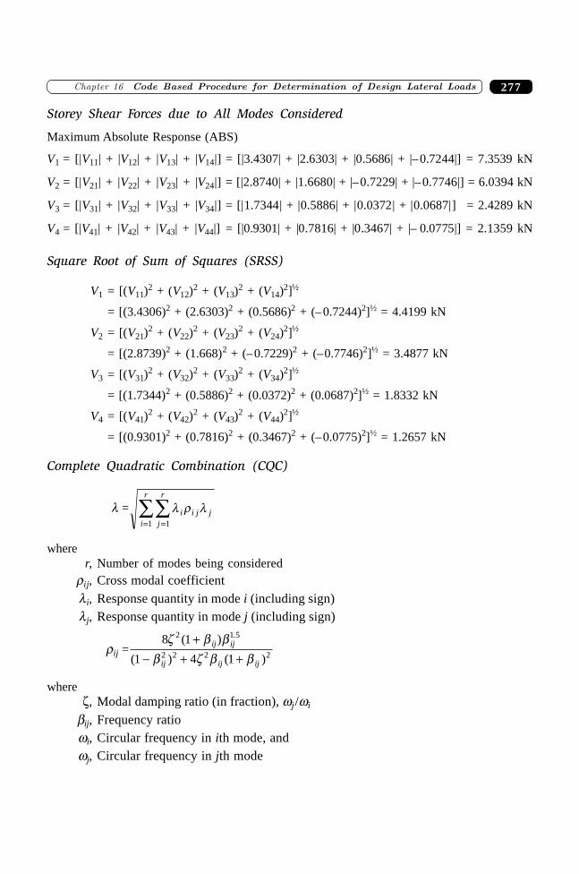
277�������� ��������������������� ��� ������ �������������
Storey Shear Forces due to All Modes Considered
Maximum Absolute Response (ABS)
V1 = [|V11| + |V12| + |V13| + |V14|] = [|3.4307| + |2.6303| + |0.5686| + |–0.7244|] = 7.3539 kN
V2 = [|V21| + |V22| + |V23| + |V24|] = [|2.8740| + |1.6680| + |–0.7229| + |–0.7746|] = 6.0394 kN
V3 = [|V31| + |V32| + |V33| + |V34|] = [|1.7344| + |0.5886| + |0.0372| + |0.0687|] = 2.4289 kN
V4 = [|V41| + |V42| + |V43| + |V44|] = [|0.9301| + |0.7816| + |0.3467| + |– 0.0775|] = 2.1359 kN
Square Root of Sum of Squares (SRSS)
V1 = [(V11)2 + (V12)
2 + (V13)2 + (V14)
2]½
= [(3.4306)2 + (2.6303)2 + (0.5686)2 + (–0.7244)2]½ = 4.4199 kN
V2 = [(V21)2 + (V22)
2 + (V23)2 + (V24)
2]½
= [(2.8739)2 + (1.668)2 + (–0.7229)2 + (–0.7746)2]½ = 3.4877 kN
V3 = [(V31)2 + (V32)
2 + (V33)2 + (V34)
2]½
= [(1.7344)2 + (0.5886)2 + (0.0372)2 + (0.0687)2]½ = 1.8332 kN
V4 = [(V41)2 + (V42)
2 + (V43)2 + (V44)
2]½
= [(0.9301)2 + (0.7816)2 + (0.3467)2 + (–0.0775)2]½ = 1.2657 kN
Complete Quadratic Combination (CQC)
l = l r li i j jj
r
i
r
==ÂÂ
11
wherer, Number of modes being considered
rij, Cross modal coefficient
li, Response quantity in mode i (including sign)lj, Response quantity in mode j (including sign)
rij =8 1
1 4 1
2 1 5
2 2 2 2
z b bb z b b
( )
( ) ( )
.+
- + +ij ij
ij ij ij
wherez, Modal damping ratio (in fraction), wj/wi
bij, Frequency ratiowi, Circular frequency in ith mode, andwj, Circular frequency in jth mode
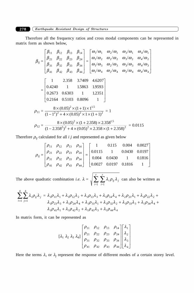
����������� ������� �������������278
Therefore all the frequency ratios and cross modal components can be represented inmatrix form as shown below,
bij =
b b b bb b b bb b b bb b b b
11 12 13 14
21 22 23 24
31 32 33 34
41 42 43 44
L
N
MMMM
O
Q
PPPP =
w w w w w w w ww w w w w w w ww w w w w w w ww w w w w w w w
1 1 2 1 3 1 4 1
1 2 2 2 3 2 4 2
1 3 2 3 3 3 4 3
1 4 2 4 3 4 4 4
/ / / /
/ / / /
/ / / /
/ / / /
L
N
MMMM
O
Q
PPPP
=
1 2 358 3 7409 4 6207
0 4240 1 15863 19593
0 2673 0 6303 1 12351
0 2164 0 5103 0 8096 1
. . .
. . .
. . .
. . .
L
N
MMMM
O
Q
PPPP
r11 = 8 0 05 1 1 1
1 1 4 0 05 1 1 1
2 1 5
2 2 2 2
¥ ¥ + ¥- + ¥ ¥ ¥ +
( . ) ( )
( ) ( . ) ( )
.
= 1
r12 = 8 0 05 1 2 358 2 358
1 2 358 4 0 05 2 358 1 2 358
2 1 5
2 2 2 2
¥ ¥ + ¥- + ¥ ¥ ¥ +
( . ) ( . ) .
( . ) ( . ) . ( . )
.
= 0.0115
Therefore rij calculated for all i j and represented as given below
rij =
r r r rr r r rr r r rr r r r
11 12 13 14
21 22 23 24
31 32 33 34
41 42 43 44
L
N
MMMM
O
Q
PPPP =
1 0115 0 004 0 0027
0 0115 1 0 0430 0 0197
0 004 0 0430 1 0 1816
0 0027 0 0197 0 1816 1
. . .
. . .
. . .
. . .
L
N
MMMM
O
Q
PPPP
The above quadratic combination i.e. l = i
r
i ij ji
r
=1 =1Â Â l r l can also be written as
l r li ij jji ==ÂÂ
1
4
1
4
= l r l l r l l r l l r l l r l l r ll r l l r l l r l l r l l r l l r ll r l l r l l r l l r l
1 11 1 1 12 2 1 13 3 1 14 4 2 21 1 1 22 2
1 23 3 1 24 4 1 31 1 1 32 2 1 33 3 1 34 4
1 41 1 1 42 2 1 43 3 1 44 4
+ + + + + +
+ + + + + +
+ + +
In matrix form, it can be represented as
[l1 l2 l3 l4]
r r r rr r r rr r r rr r r r
llll
11 12 13 14
21 22 23 24
31 32 33 34
41 42 43 44
1
2
3
4
L
N
MMMM
O
Q
PPPP
L
N
MMMM
O
Q
PPPP
Here the terms l i or lj represent the response of different modes of a certain storey level.
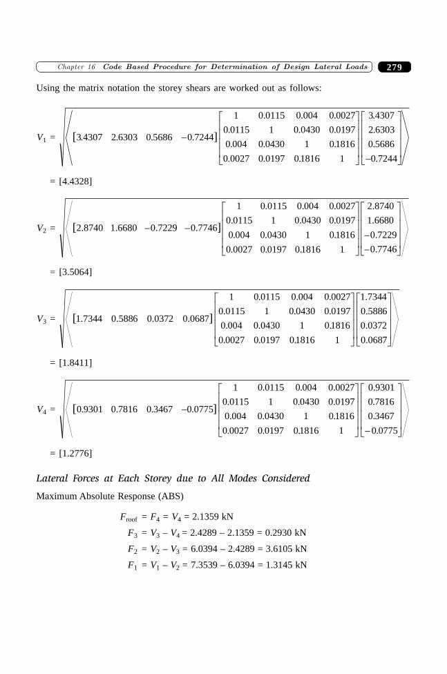
279�������� ��������������������� ��� ������ �������������
Using the matrix notation the storey shears are worked out as follows:
V1 = [ ]
. . .
. . .
. . .
. . .
3 4307 2 6303 0 5686 0 7244
1 0 0115 0 004 0 0027
0 0115 1 0 0430 0 0197
0 004 0 0430 1 0 1816
0 0027 0 0197 0 1816 1
3 4307
2 6303
0 5686
0 7244
. . . .
.
.
.
.
-
L
N
MMMM
O
Q
PPPP -
L
N
MMMM
O
Q
PPPP
= [4.4328]
V2 = [ ]
. . .
. . .
. . .
. . .
2.8740 1.6680 0.7229 0.7746
2.8740
1.6680
0.7229
0.7746
- -
L
N
MMMM
O
Q
PPPP
--
L
N
MMMM
O
Q
PPPP
1 0 0115 0 004 0 0027
0 0115 1 0 0430 0 0197
0 004 0 0430 1 0 1816
0 0027 0 0197 0 1816 1
= [3.5064]
V3 = [ ]
. . .
. . .
. . .
. . .
1.7344 0.5886 0.0372 0.0687
1.7344
0.5886
0.0372
0.0687
1 0 0115 0 004 0 0027
0 0115 1 0 0430 0 0197
0 004 0 0430 1 0 1816
0 0027 0 0197 01816 1
L
N
MMMM
O
Q
PPPP
L
N
MMMM
O
Q
PPPP
= [1.8411]
V4 = [ ]
. . .
. . .
. . .
. . .
0 9301 0 7816 0 3467 0 0775
1 0 0115 0 004 0 0027
0 0115 1 0 0430 0 0197
0 004 0 0430 1 0 1816
0 0027 0 0197 01816 1
0 9301
0 7816
0 3467
0 0775
. . . .
.
.
.
.
-
L
N
MMMM
O
Q
PPPP -
L
N
MMMM
O
Q
PPPP
= [1.2776]
Lateral Forces at Each Storey due to All Modes Considered
Maximum Absolute Response (ABS)
Froof = F4 = V4 = 2.1359 kN
F3 = V3 – V4 = 2.4289 – 2.1359 = 0.2930 kN
F2 = V2 – V3 = 6.0394 – 2.4289 = 3.6105 kN
F1 = V1 – V2 = 7.3539 – 6.0394 = 1.3145 kN
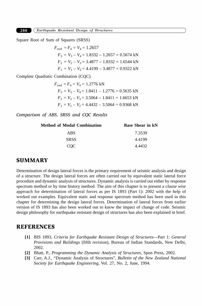
����������� ������� �������������280
Square Root of Sum of Squares (SRSS)
Froof = F4 = V4 = 1.2657
F3 = V3 – V4 = 1.8332 – 1.2657 = 0.5674 kN
F2 = V2 – V3 = 3.4877 – 1.8332 = 1.6544 kN
F1 = V1 – V2 = 4.4199 – 3.4877 = 0.9322 kN
Complete Quadratic Combination (CQC)
Froof = F4 = V4 = 1.2776 kN
F3 = V3 – V4 = 1.8411 – 1.2776 = 0.5635 kN
F2 = V2 – V3 = 3.5064 – 1.8411 = 1.6653 kN
F1 = V1 – V2 = 4.4432 – 3.5064 = 0.9368 kN
Comparison of ABS, SRSS and CQC Results
Method of Modal Combination Base Shear in kN
ABS 7.3539
SRSS 4.4199
CQC 4.4432
SUMMARY
Determination of design lateral forces is the primary requirement of seismic analysis and designof a structure. The design lateral forces are often carried out by equivalent static lateral forceprocedure and dynamic analysis of structures. Dynamic analysis is carried out either by responsespectrum method or by time history method. The aim of this chapter is to present a clause wiseapproach for determination of lateral forces as per IS 1893 (Part 1): 2002 with the help ofworked out examples. Equivalent static and response spectrum method has been used in thischapter for determining the design lateral forces. Determination of lateral forces from earlierversion of IS 1893 has also been worked out to know the impact of change of code. Seismicdesign philosophy for earthquake resistant design of structures has also been explained in brief.
REFERENCES
[1] BIS 1893, Criteria for Earthquake Resistant Design of Structures—Part 1: GeneralProvisions and Buildings (fifth revision), Bureau of Indian Standards, New Delhi,2002.
[2] Bhatt, P., Programming the Dynamic Analysis of Structures, Spon Press, 2002.[3] Carr, A.J., “Dynamic Analysis of Structures”, Bulletin of the New Zealand National
Society for Earthquake Engineering, Vol. 27, No. 2, June, 1994.

281�������� ��������������������� ��� ������ �������������
[4] IS 1893, Indian Standard Recommendations for Earthquake Resistance of Structure,Indian Standard Institute, New Delhi, 1962.
[5] IS 1893, Indian Standard Recommendations for Earthquake Resistance of Structure(First Revision), Indian Standard Institute, New Delhi, 1966.
[6] IS 1893, Indian Standard Criteria for Earthquake Resistance of Structure (secondrevision), Indian Standard Institute, New Delhi, 1970.
[7] IS 1893, Indian Standard Criteria for Earthquake Resistance of Structure (thirdrevision),’ Indian Standard Institute, New Delhi, 1975.
[8] IS 1893, Indian Standard Criteria for Earthquake Resistance of Structure (fourthrevision), Indian Standard Institute, New Delhi, 1984.
[9] Newmark, N.M. and Hall, W.J., “Earthquake Spectra and Design”, EngineeringMonographs on Earthquake Criteria, Structural Design, and Strong Motion Records,Earthquake Engineering Research Institute, 1982.
[10] Paz, M., International Handbook of Earthquake Engineering—Codes, Programmesand Examples, Chapman & Hall, 1994.
����������� ������� �������������282
282
Consideration of InfillWall in Seismic Analysis of
RC Buildings
��������
17.1 INTRODUCTION
A large number of reinforced concrete and steel buildings are constructed with masonry infills.Masonry infills are often used to fill the void between the vertical and horizontal resistingelements of the building frames with the assumption that these infills will not take part inresisting any kind of load either axial or lateral; hence its significance in the analysis of frameis generally neglected. Moreover, non-availability of realistic and simple analytical models ofinfill becomes another hurdle for its consideration in analysis. In fact, an infill wall enhancesconsiderably the strength and rigidity of the structure. It has been recognised that frames withinfills have more strength and rigidity in comparison to the bared frames and their ignorancehas become the cause of failure of many of the multi-storeyed buildings. The recent examplein this category is the Bhuj earthquake on 26 January, 2001. The main reason of failure is thestiffening effect of infilled frame that changes the basic behaviour of buildings duringearthquake and creates new failure mechanism. This chapter will discuss the structural actionof infill panel and failure modes and modelling of infill walls with and without openings.
17.2 STRUCTURAL AND CONSTRUCTIONALASPECTS OF INFILLS
The presence of masonry infills is the cause of (i) unequal distribution of lateral forces in thedifferent frames of a building—overstressing of some frames; (ii) vertical irregularities instrength and stiffness—soft storey or weak storey as a result higher interstorey drifts and higherductility demands of RC elements of the soft storey in comparison to remaining stories;(iii) horizontal irregularities—significant amount of unexpected torsional forces since the centreof rigidity is moved towards the stiffer infilled frames of increased stiffness and as a result
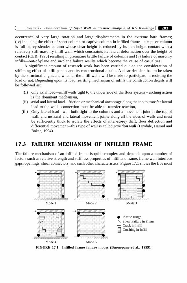
283�������� ���� ���� ������� ������ �� �� ������� ������� �� ���
occurrence of very large rotation and large displacements in the extreme bare frames;(iv) inducing the effect of short column or captive column in infilled frame—a captive columnis full storey slender column whose clear height is reduced by its part-height contact with arelatively stiff masonry infill wall, which constraints its lateral deformation over the height ofcontact (CEB, 1996) resulting in premature brittle failure of columns and (v) failure of masonryinfills—out-of-plane and in-plane failure results which become the cause of casualties.
A significant amount of research work has been carried out on the consideration ofstiffening effect of infill panels and its constructional details. A clear decision has to be takenby the structural engineers, whether the infill walls will be made to participate in resisting theload or not. Depending upon its load resisting mechanism of infills the construction details willbe followed as:
(i) only axial load—infill walls tight to the under side of the floor system – arching actionis the dominant mechanism,
(ii) axial and lateral load—friction or mechanical anchorage along the top to transfer lateralload to the wall—connection must be able to transfer reaction,
(iii) Only lateral load—wall built tight to the columns and a movement joint at the top ofwall, and no axial and lateral movement joints along all the sides of walls and mustbe sufficiently thick to isolate the effects of inter-storey drift, floor deflection anddifferential movement—this type of wall is called partition wall (Drydale, Hamid andBaker, 1994).
17.3 FAILURE MECHANISM OF INFILLED FRAME
The failure mechanism of an infilled frame is quite complex and depends upon a number offactors such as relative strength and stiffness properties of infill and frame, frame wall interfacegaps, openings, shear connectors, and such other characteristics. Figure 17.1 shows the five most
Mode 1 Mode 2 Mode 3
Mode 4 Mode 5
Plastic Hinge
Shear Failure in Frame
Crack in Infill
Crushing in Infill
FIGURE 17.1 Infilled frame failure modes (Buonopane et al., 1999).
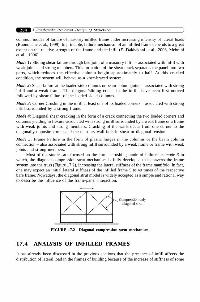
����������� ������� �������������284
common modes of failure of masonry infilled frame under increasing intensity of lateral loads(Buonopane et al., 1999). In principle, failure mechanism of an infilled frame depends to a greatextent on the relative strength of the frame and the infill (El-Dakhakhni et al., 2003, Mehrabiet al., 1996).
Mode 1: Sliding shear failure through bed joint of a masonry infill – associated with infill withweak joints and strong members. This formation of the shear crack separates the panel into twoparts, which reduces the effective column height approximately to half. At this crackedcondition, the system will behave as a knee-braced system.
Mode 2: Shear failure at the loaded side columns or beam-column joints – associated with stronginfill and a weak frame. The diagonal/sliding cracks in the infills have been first noticedfollowed by shear failure of the loaded sided columns.
Mode 3: Corner Crushing in the infill at least one of its loaded corners – associated with stronginfill surrounded by a strong frame.
Mode 4: Diagonal shear cracking in the form of a crack connecting the two loaded corners andcolumns yielding in flexure-associated with strong infill surrounded by a weak frame or a framewith weak joints and strong members. Cracking of the walls occur from one corner to thediagonally opposite corner and the masonry wall fails in shear or diagonal tension.
Mode 5: Frame Failure in the form of plastic hinges in the columns or the beam columnconnection – also associated with strong infill surrounded by a weak frame or frame with weakjoints and strong members.
Most of the studies are focused on the corner crushing mode of failure i.e. mode 3 inwhich, the diagonal compression strut mechanism is fully developed that converts the framesystem into the truss (Figure 17.2), increasing the lateral stiffness of the frame manifold. In fact,one may expect an initial lateral stiffness of the infilled frame 5 to 40 times of the respectivebare frame. Nowadays, the diagonal strut model is widely accepted as a simple and rational wayto describe the influence of the frame-panel interaction.
Compression onlydiagonal strut
FIGURE 17.2 Diagonal compression strut mechanism.
17.4 ANALYSIS OF INFILLED FRAMES
It has already been discussed in the previous sections that the presence of infill affects thedistribution of lateral load in the frames of building because of the increase of stiffness of some
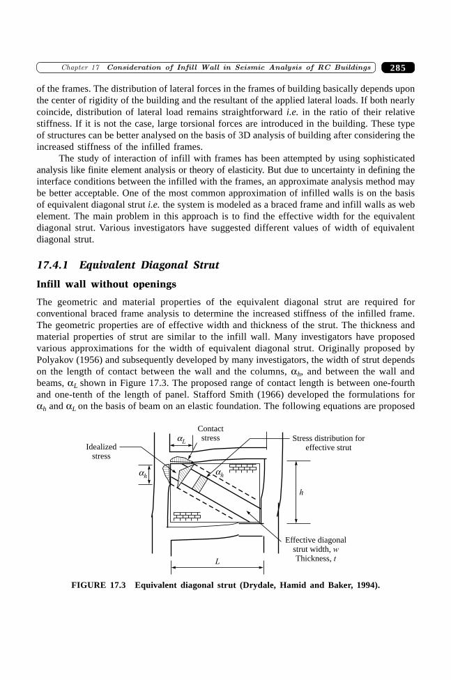
285�������� ���� ���� ������� ������ �� �� ������� ������� �� ���
of the frames. The distribution of lateral forces in the frames of building basically depends uponthe center of rigidity of the building and the resultant of the applied lateral loads. If both nearlycoincide, distribution of lateral load remains straightforward i.e. in the ratio of their relativestiffness. If it is not the case, large torsional forces are introduced in the building. These typeof structures can be better analysed on the basis of 3D analysis of building after considering theincreased stiffness of the infilled frames.
The study of interaction of infill with frames has been attempted by using sophisticatedanalysis like finite element analysis or theory of elasticity. But due to uncertainty in defining theinterface conditions between the infilled with the frames, an approximate analysis method maybe better acceptable. One of the most common approximation of infilled walls is on the basisof equivalent diagonal strut i.e. the system is modeled as a braced frame and infill walls as webelement. The main problem in this approach is to find the effective width for the equivalentdiagonal strut. Various investigators have suggested different values of width of equivalentdiagonal strut.
17.4.1 Equivalent Diagonal Strut
Infill wall without openings
The geometric and material properties of the equivalent diagonal strut are required forconventional braced frame analysis to determine the increased stiffness of the infilled frame.The geometric properties are of effective width and thickness of the strut. The thickness andmaterial properties of strut are similar to the infill wall. Many investigators have proposedvarious approximations for the width of equivalent diagonal strut. Originally proposed byPolyakov (1956) and subsequently developed by many investigators, the width of strut dependson the length of contact between the wall and the columns, ah, and between the wall andbeams, aL shown in Figure 17.3. The proposed range of contact length is between one-fourthand one-tenth of the length of panel. Stafford Smith (1966) developed the formulations forah and aL on the basis of beam on an elastic foundation. The following equations are proposed
Contactstress
Idealizedstress
ah
aL
ah
Stress distribution foreffective strut
Effective diagonalstrut width,Thickness,
wtL
h
FIGURE 17.3 Equivalent diagonal strut (Drydale, Hamid and Baker, 1994).
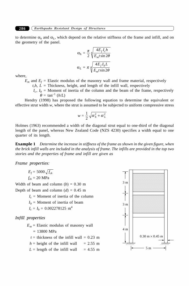
����������� ������� �������������286
to determine ah and aL, which depend on the relative stiffness of the frame and infill, and onthe geometry of the panel.
ah = pq2
4
24
E I h
E tf c
m sin
aL = pq
4
24
E I L
E tf b
m sin
where,Em and Ef = Elastic modulus of the masonry wall and frame material, respectively
t,h, L = Thickness, height, and length of the infill wall, respectivelyIc , Ib = Moment of inertia of the column and the beam of the frame, respectively
q = tan–1 (h/L)Hendry (1998) has proposed the following equation to determine the equivalent or
effective strut width w, where the strut is assumed to be subjected to uniform compressive stress
w = 12
2 2a ah L+
Holmes (1963) recommended a width of the diagonal strut equal to one-third of the diagonallength of the panel, whereas New Zealand Code (NZS 4230) specifies a width equal to onequarter of its length.
Example 1 Determine the increase in stiffness of the frame as shown in the given figure, whenthe brick infill walls are included in the analysis of frame. The infills are provided in the top twostories and the properties of frame and infill are given as
Frame properties:
Ef = 5000 fck
fck = 20 MPa
Width of beam and column (b) = 0.30 m
Depth of beam and column (d) = 0.45 m
Ic = Moment of inertia of the column
Ib = Moment of inertia of beam
Ic = Ib = 0.002278125 m4
Infill properties
Em = Elastic modulus of masonry wall
= 13800 MPa
t = thickness of the infill wall = 0.23 m
h = height of the infill wall = 2.55 m
L = length of the infill wall = 4.55 m
0.30 m 0.45 m�
3 m
3 m
4 m
5 m
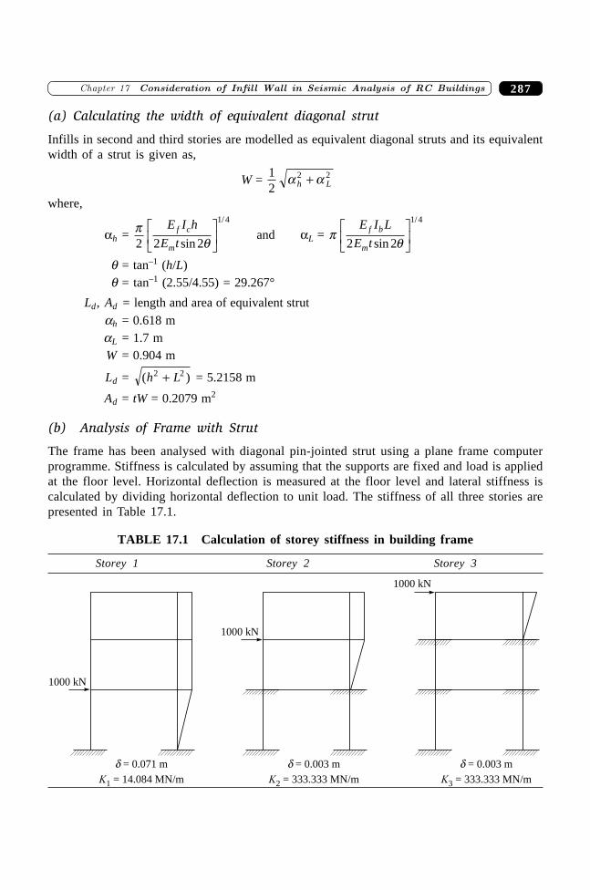
287�������� ���� ���� ������� ������ �� �� ������� ������� �� ���
(a) Calculating the width of equivalent diagonal strut
Infills in second and third stories are modelled as equivalent diagonal struts and its equivalentwidth of a strut is given as,
W = 12
2 2a ah L+
where,
ah = pq2 2 2
1 4E I h
E tf c
m sin
/LNM
OQP
and aL = pq
E I L
E tf b
m2 2
1 4
sin
/LNM
OQP
q = tan–1 (h/L)q = tan–1 (2.55/4.55) = 29.267°
Ld, Ad = length and area of equivalent strutah = 0.618 maL = 1.7 mW = 0.904 m
Ld = ( )h L2 2+ = 5.2158 m
Ad = tW = 0.2079 m2
(b) Analysis of Frame with Strut
The frame has been analysed with diagonal pin-jointed strut using a plane frame computerprogramme. Stiffness is calculated by assuming that the supports are fixed and load is appliedat the floor level. Horizontal deflection is measured at the floor level and lateral stiffness iscalculated by dividing horizontal deflection to unit load. The stiffness of all three stories arepresented in Table 17.1.
TABLE 17.1 Calculation of storey stiffness in building frame
Storey 1 Storey 2 Storey 3
d = 0.071 m
K1 = 14.084 MN/m
1000 kN
d = 0.003 m
K2 = 333.333 MN/m
1000 kN
d = 0.003 m
K3 = 333.333 MN/m
1000 kN
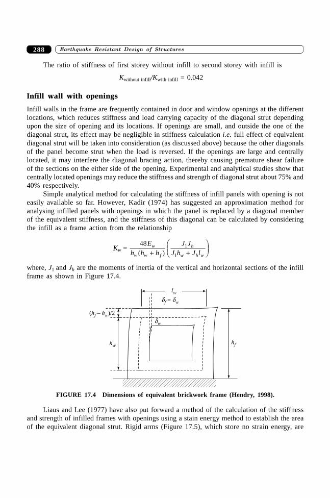
����������� ������� �������������288
The ratio of stiffness of first storey without infill to second storey with infill is
Kwithout infill/Kwith infill = 0.042
Infill wall with openings
Infill walls in the frame are frequently contained in door and window openings at the differentlocations, which reduces stiffness and load carrying capacity of the diagonal strut dependingupon the size of opening and its locations. If openings are small, and outside the one of thediagonal strut, its effect may be negligible in stiffness calculation i.e. full effect of equivalentdiagonal strut will be taken into consideration (as discussed above) because the other diagonalsof the panel become strut when the load is reversed. If the openings are large and centrallylocated, it may interfere the diagonal bracing action, thereby causing premature shear failureof the sections on the either side of the opening. Experimental and analytical studies show thatcentrally located openings may reduce the stiffness and strength of diagonal strut about 75% and40% respectively.
Simple analytical method for calculating the stiffness of infill panels with opening is noteasily available so far. However, Kadir (1974) has suggested an approximation method foranalysing infilled panels with openings in which the panel is replaced by a diagonal memberof the equivalent stiffness, and the stiffness of this diagonal can be calculated by consideringthe infill as a frame action from the relationship
Kw = 48 1
1
Eh h h
J JJ h J l
w
w w f
h
w h w( )+ +FHG
IKJ
where, J1 and Jh are the moments of inertia of the vertical and horizontal sections of the infillframe as shown in Figure 17.4.
df = dw
dw
( – )/2hhf w
hwhf
lw
FIGURE 17.4 Dimensions of equivalent brickwork frame (Hendry, 1998).
Liaus and Lee (1977) have also put forward a method of the calculation of the stiffnessand strength of infilled frames with openings using a stain energy method to establish the areaof the equivalent diagonal strut. Rigid arms (Figure 17.5), which store no strain energy, are
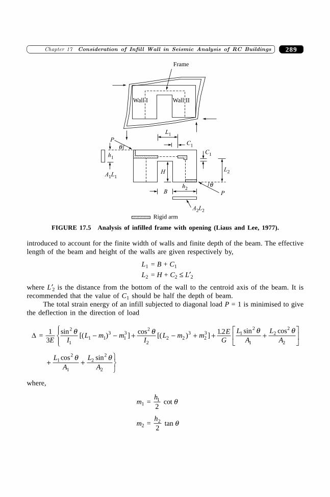
289�������� ���� ���� ������� ������ �� �� ������� ������� �� ���
introduced to account for the finite width of walls and finite depth of the beam. The effectivelength of the beam and height of the walls are given respectively by,
L1 = B + C1
L2 = H + C2 £ L¢2
where L¢2 is the distance from the bottom of the wall to the centroid axis of the beam. It isrecommended that the value of C1 should be half the depth of beam.
The total strain energy of an infill subjected to diagonal load P = 1 is minimised to givethe deflection in the direction of load
D = 13
1 22
11 1
313
2
22 2
323 1
2
1
22
2E IL m m
IL m m E
GL
AL
Asin [( ) ] cos [( ) ] . sin cosq q q q
- - + - + + +LNM
OQP
RS|T|
+ +UVW
LA
LA
12
1
22
2
cos sinq q
where,
m1 = h1
2 cot q
m2 = h2
2 tan q
Frame
Wall IIWall I
P
qh1
A L1 1H
Bh2
A L2 2
Rigid arm
qP
L1
C1
C1
L2
FIGURE 17.5 Analysis of infilled frame with opening (Liaus and Lee, 1977).
����������� ������� �������������290
The diagonal stiffness k of the infill is equal to the reciprocal of the deflection when P = 1.If an equivalent diagonal strut of length Ld replaces the infill, the stiffness of the strut isgiven by,
k = EAe /Ld
Hence the cross-sectional area of the equivalent diagonal strut is,
Ae = Ld /ED
The infilled frame can then be converted into the frame with the equivalent diagonal struts, andanalysed by usual method of frame analysis.
SUMMARY
Multi-storeyed buildings are often analysed without considering the effect of infill wall panelson the assumption that these infill panel will not resist any kind of load. However, these infillpanels increase the strength and stiffness of frame considerably and are responsible for unequaldistribution of forces in buildings. The aim of the chapter is to focus on structural andconstructional aspect of infill along with its failure mechanism. It also presents how to consideran infill wall in seismic analysis of frame. A solved example has also been presented formodeling the infill as an equivalent diagonal strut. An approximate solution of infill wall withopening has also been discussed.
REFERENCES
[1] IS 1893, Criteria for Earthquake Resistant Design of Structures—Part 1, GeneralProvisions and Buildings (fifth revision), Bureau of Indian Standards, New Delhi,2002.
[2] CEB, RC Frames under Earthquake Loading—State of the Art Report, ThomasTelford, 1996.
[3] Drydale, R.G., Hamid, A.A., and Baker, L.R., Masonry Structures—Behaviour andDesign, Prentice Hall, Englewood Cliffs, New Jersey, 1994.
[4] Hendry, A.W. Structural Masonry, 2nd ed., Macmillan Press, 1998.[5] Holmes, M., “Combined Loading on Infilled Frames”, Proceedings of the Institute of
Civil Engineers, 25: 31–38, 1963.[6] Kadir, M.R.A., “The Structural Behaviour of Masonry Infill Panels in Framed
Structures”, Ph.D. Thesis, University of Edinburgh, 1974.[7] Liauw, T.C. and Lee, S.W., “On the Behaviour and the Analysis of Multi-storey Infilled
Frames Subject to Lateral Loading”, Proceedings of Institute of Civil Engineers, 1977.[8] Liauw, T.C., “An Approximate Method of Analysis for Infilled Frame with or without
Openings”, Building Science, 7: 223–238, Pergamon Press, 1972.[9] NZS 4230, “Code of Practice for the Design of Masonry Structures (Part 1)”, Standard
Association of New Zealand, Willington, 1990.

291�������� ���� ���� ������� ������ �� �� ������� ������� �� ���
[10] Polyakov, S.V., “Masonry in Framed Buildings, Gosudalst—Vennoe’ stvo Literature poStraitel’ stuv i Arkitecture, Moskva, Trans. G.L. Cairns”, Building Research Station,Watford, Herts, 1956.
[11] Parducci, A. and Mezzi, M., “Repeated Horizontal Displacements of Infilled Frameshaving Different Stiffness and Connection Systems—Experimental Analysis”,Proceedings of 7th World Conference on Earthquake Engineering, 7: 193–196, Istanbul,1980.
[12] Stafford-Smith, B., “Behaviour of Square Infilled Frames”, Journal of the StructuralDivision, Proceedings of ASCE, Vol. 91, No. ST1, pp. 381–403, 1966.
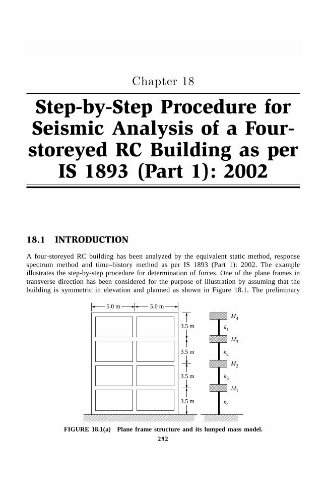
����������� ������� �������������292
292
Step-by-Step Procedure forSeismic Analysis of a Four-storeyed RC Building as per
IS 1893 (Part 1): 2002
��������
18.1 INTRODUCTION
A four-storeyed RC building has been analyzed by the equivalent static method, responsespectrum method and time–history method as per IS 1893 (Part 1): 2002. The exampleillustrates the step-by-step procedure for determination of forces. One of the plane frames intransverse direction has been considered for the purpose of illustration by assuming that thebuilding is symmetric in elevation and planned as shown in Figure 18.1. The preliminary
M4
M3
k1
k2
M2
k3
M1
k4
3.5 m
3.5 m
3.5 m
3.5 m
5.0 m 5.0 m
FIGURE 18.1(a) Plane frame structure and its lumped mass model.
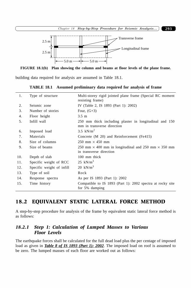
293�������� ����������������� ���� �� ������� ����
building data required for analysis are assumed in Table 18.1.
TABLE 18.1 Assumed preliminary data required for analysis of frame
1. Type of structure Multi-storey rigid jointed plane frame (Special RC momentresisting frame)
2. Seismic zone IV (Table 2, IS 1893 (Part 1): 2002)
3. Number of stories Four, (G+3)
4. Floor height 3.5 m
5. Infill wall 250 mm thick including plaster in longitudinal and 150mm in transverse direction
6. Imposed load 3.5 kN/m2
7. Materials Concrete (M 20) and Reinforcement (Fe415)
8. Size of columns 250 mm ¥ 450 mm
9. Size of beams 250 mm ¥ 400 mm in longitudinal and 250 mm ¥ 350 mmin transverse direction
10. Depth of slab 100 mm thick
11. Specific weight of RCC 25 kN/m3
12. Specific weight of infill 20 kN/m3
13. Type of soil Rock
14. Response spectra As per IS 1893 (Part 1): 2002
15. Time history Compatible to IS 1893 (Part 1): 2002 spectra at rocky sitefor 5% damping
18.2 EQUIVALENT STATIC LATERAL FORCE METHOD
A step-by-step procedure for analysis of the frame by equivalent static lateral force method isas follows:
18.2.1 Step 1: Calculation of Lumped Masses to VariousFloor Levels
The earthquake forces shall be calculated for the full dead load plus the per centage of imposedload as given in Table 8 of IS 1893 (Part 1): 2002. The imposed load on roof is assumed tobe zero. The lumped masses of each floor are worked out as follows:
Transverse frame
5.0 m 5.0 m
2.5 m
2.5 mLongitudinal frame
FIGURE 18.1(b) Plan showing the column and beams at floor levels of the plane frame.
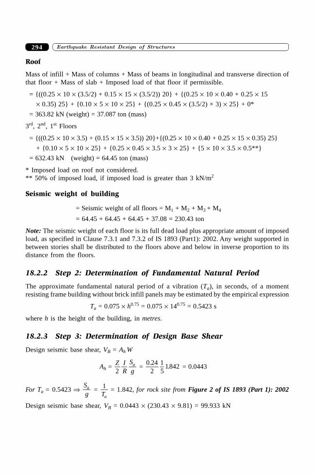
����������� ������� �������������294
Roof
Mass of infill + Mass of columns + Mass of beams in longitudinal and transverse direction ofthat floor + Mass of slab + Imposed load of that floor if permissible.
= {((0.25 ¥ 10 ¥ (3.5/2) + 0.15 ¥ 15 ¥ (3.5/2)) 20} + {(0.25 ¥ 10 ¥ 0.40 + 0.25 ¥ 15
¥ 0.35) 25} + {0.10 ¥ 5 ¥ 10 ¥ 25} + {(0.25 ¥ 0.45 ¥ (3.5/2) × 3) ¥ 25} + 0*
= 363.82 kN (weight) = 37.087 ton (mass)
3rd, 2nd, 1st Floors
= {((0.25 ¥ 10 ¥ 3.5) + (0.15 ¥ 15 ¥ 3.5)) 20}+{(0.25 ¥ 10 ¥ 0.40 + 0.25 ¥ 15 ¥ 0.35) 25}
+ {0.10 ¥ 5 ¥ 10 ¥ 25} + {0.25 ¥ 0.45 ¥ 3.5 ¥ 3 ¥ 25} + {5 ¥ 10 ¥ 3.5 ¥ 0.5**}
= 632.43 kN (weight) = 64.45 ton (mass)
* Imposed load on roof not considered.** 50% of imposed load, if imposed load is greater than 3 kN/m2
Seismic weight of building
= Seismic weight of all floors = M1 + M2 + M3 + M4
= 64.45 + 64.45 + 64.45 + 37.08 = 230.43 ton
Note: The seismic weight of each floor is its full dead load plus appropriate amount of imposedload, as specified in Clause 7.3.1 and 7.3.2 of IS 1893 (Part1): 2002. Any weight supported inbetween stories shall be distributed to the floors above and below in inverse proportion to itsdistance from the floors.
18.2.2 Step 2: Determination of Fundamental Natural Period
The approximate fundamental natural period of a vibration (Ta), in seconds, of a momentresisting frame building without brick infill panels may be estimated by the empirical expression
Ta = 0.075 ¥ h0.75 = 0.075 ¥ 140.75 = 0.5423 s
where h is the height of the building, in metres.
18.2.3 Step 3: Determination of Design Base Shear
Design seismic base shear, VB = Ah W
Ah = Z IR
Sga
2 =
0 242
15
1842. . = 0.0443
For Ta = 0.5423 fi Sga = 1
Ta = 1.842, for rock site from Figure 2 of IS 1893 (Part 1): 2002
Design seismic base shear, VB = 0.0443 ¥ (230.43 ¥ 9.81) = 99.933 kN
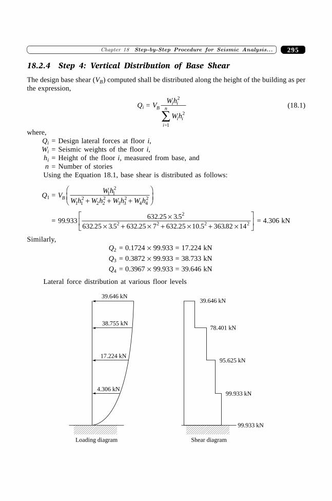
295�������� ����������������� ���� �� ������� ����
18.2.4 Step 4: Vertical Distribution of Base Shear
The design base shear (VB) computed shall be distributed along the height of the building as perthe expression,
Qi = VWh
WhB
i i
i ii
n
2
2
=1Â
(18.1)
where,Qi = Design lateral forces at floor i,Wi = Seismic weights of the floor i,hi = Height of the floor i, measured from base, andn = Number of stories
Using the Equation 18.1, base shear is distributed as follows:
Q1 = VW h
W h W h W h W hB1 1
2
1 12
2 22
3 32
4 42+ + +
FHG
IKJ
= 99 933632 25 3 5
632 25 3 5 632 25 7 632 25 10 5 363 82 14
2
2 2 2 2.. .
. . . . . .¥
¥ + ¥ + ¥ + ¥LNM
OQP
= 4.306 kN
Similarly,Q2 = 0.1724 ¥ 99.933 = 17.224 kN
Q3 = 0.3872 ¥ 99.933 = 38.733 kN
Q4 = 0.3967 ¥ 99.933 = 39.646 kN
Lateral force distribution at various floor levels
4.306 kN99.933 kN
17.224 kN95.625 kN
38.755 kN78.401 kN
39.646 kN39.646 kN
99.933 kN
Loading diagram Shear diagram
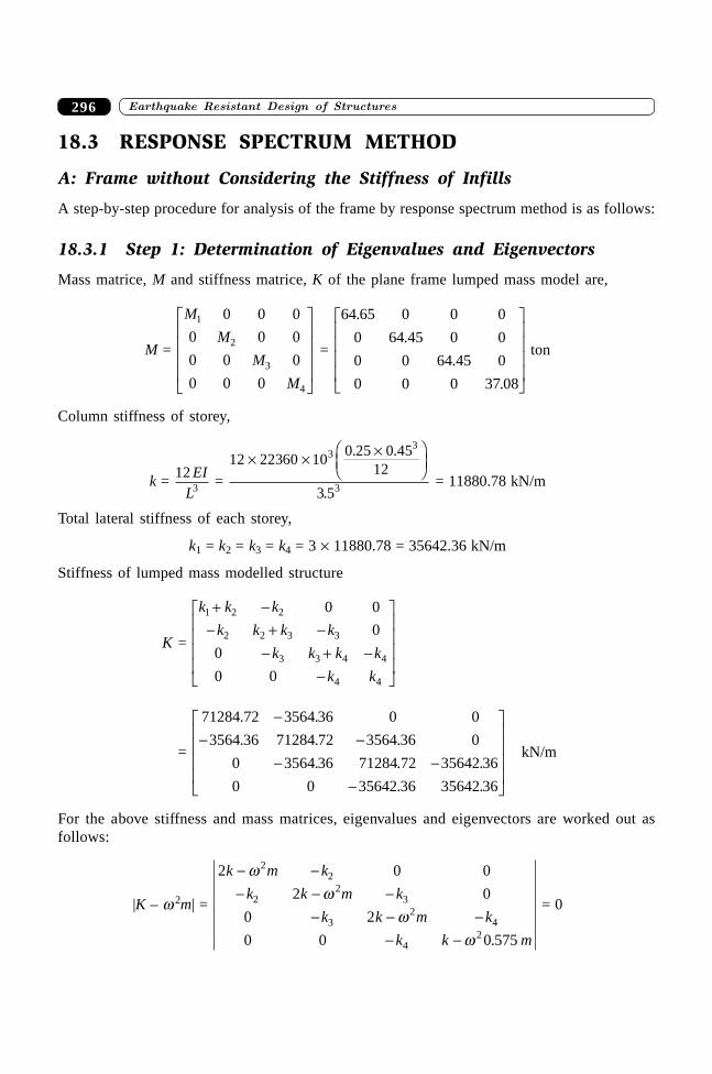
����������� ������� �������������296
18.3 RESPONSE SPECTRUM METHOD
A: Frame without Considering the Stiffness of Infills
A step-by-step procedure for analysis of the frame by response spectrum method is as follows:
18.3.1 Step 1: Determination of Eigenvalues and Eigenvectors
Mass matrice, M and stiffness matrice, K of the plane frame lumped mass model are,
M =
M
M
M
M
1
2
3
4
0 0 0
0 0 0
0 0 0
0 0 0
L
N
MMMM
O
Q
PPPP
=
64 65 0 0 0
0 64 45 0 0
0 0 64 45 0
0 0 0 37 08
.
.
.
.
L
N
MMMM
O
Q
PPPP
ton
Column stiffness of storey,
k = 12
3EI
L =
12 22360 100 25 0 45
12
3 5
33
3
¥ ¥ ¥FHG
IKJ
. .
. = 11880.78 kN/m
Total lateral stiffness of each storey,
k1 = k2 = k3 = k4 = 3 ¥ 11880.78 = 35642.36 kN/m
Stiffness of lumped mass modelled structure
K =
k k k
k k k k
k k k k
k k
1 2 2
2 2 3 3
3 3 4 4
4 4
0 0
0
0
0 0
+ -- + -
- + --
L
N
MMMM
O
Q
PPPP
=
71284 72 3564 36 0 0
3564 36 71284 72 3564 36 0
0 3564 36 71284 72 35642 36
0 0 35642 36 35642 36
. .
. . .
. . .
. .
-- -
- --
L
N
MMMM
O
Q
PPPP
kN/m
For the above stiffness and mass matrices, eigenvalues and eigenvectors are worked out asfollows:
|K – w 2m| =
2 0 0
2 0
0 2
0 0 0 575
22
22
3
32
4
42
k m k
k k m k
k k m k
k k m
- -- - -
- - -- -
ww
ww .
= 0
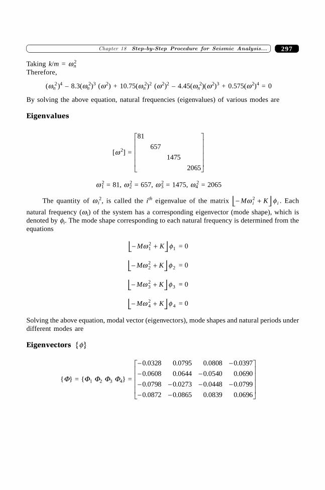
297�������� ����������������� ���� �� ������� ����
Taking k/m = wn2
Therefore,
(wn2)4 – 8.3(wn
2)3 (w2) + 10.75(wn2)2 (w2)2 – 4.45(wn
2)(w2)3 + 0.575(w2)4 = 0
By solving the above equation, natural frequencies (eigenvalues) of various modes are
Eigenvalues
[w 2] =
81
657
1475
2065
L
N
MMMM
O
Q
PPPP
w 12 = 81, w 2
2 = 657, w 32 = 1475, w4
2 = 2065
The quantity of w i2, is called the ith eigenvalue of the matrix - +M Ki iw f2 . Each
natural frequency (wi) of the system has a corresponding eigenvector (mode shape), which isdenoted by fi. The mode shape corresponding to each natural frequency is determined from theequations
- +M Kw f12
1 = 0
- +M Kw f22
2 = 0
- +M Kw f32
3 = 0
- +M Kw f42
4 = 0
Solving the above equation, modal vector (eigenvectors), mode shapes and natural periods underdifferent modes are
Eigenvectors {f}
{F} = {F1 F2 F3 F4} =
- -- -- - - -- -
L
N
MMMM
O
Q
PPPP
0 0328 0 0795 0 0808 0 0397
0 0608 0 0644 0 0540 0 0690
0 0798 0 0273 0 0448 0 0799
0 0872 0 0865 0 0839 0 0696
. . . .
. . . .
. . . .
. . . .
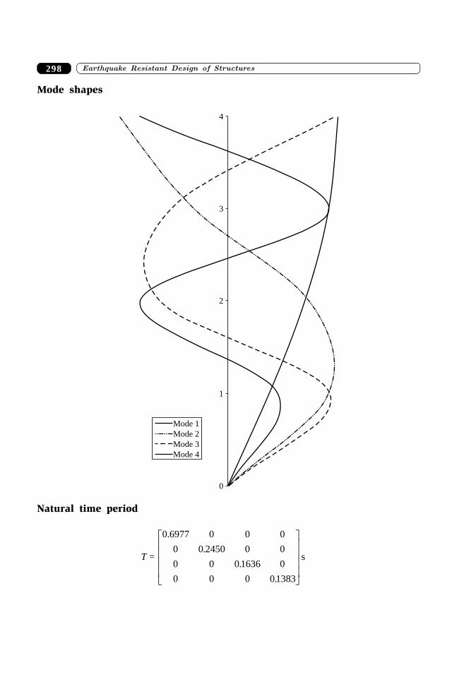
����������� ������� �������������298
Mode shapes
Mode 4
Mode 3
Mode 2
Mode 1
4
3
2
1
0
Natural time period
T =
0 6977 0 0 0
0 0 2450 0 0
0 0 0 1636 0
0 0 0 01383
.
.
.
.
L
N
MMMM
O
Q
PPPP
s
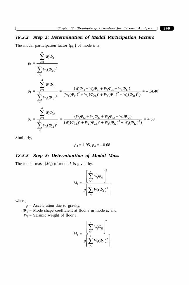
299�������� ����������������� ���� �� ������� ����
18.3.2 Step 2: Determination of Modal Participation Factors
The modal participation factor (pk ) of mode k is,
pk =
W
W
i iki
n
i iki
n
F
F
=1
=1
Â
 ( )2
p1 =
W
W
i ii
i ii
F
F
1
4
12
4=1
=1
Â
 ( )
= ( )
( ( ) ( ) ( ) ( ) )
W W W W
W W W W1 11 2 21 3 31 4 41
1 112
2 212
3 312
4 412
F F F FF F F F
+ + ++ + +
= – 14.40
p2 =
W
W
i ii
i ii
F
F
2
4
22
4=1
=1
Â
 ( )
= ( )
( ( ) ( ) ( ) ( ) )
W W W W
W W W W1 12 2 22 3 32 4 42
1 122
2 222
3 322
4 422
F F F FF F F F
+ + ++ + +
= 4.30
Similarly,
p3 = 1.95, p4 = –0.68
18.3.3 Step 3: Determination of Modal Mass
The modal mass (Mk) of mode k is given by,
Mk =
W
g W
i iki
n
i iki
n
F
F
=1
=1
Â
Â
LNMM
OQPP
LNMM
OQPP
2
2( )
where,g = Acceleration due to gravity,
Fik = Mode shape coefficient at floor i in mode k, andWi = Seismic weight of floor i,
M1 =
W
g W
i ii
i ii
F
F
1
4 2
12
4
=1
=1
Â
Â
LNMM
OQPP
LNMM
OQPP
( )
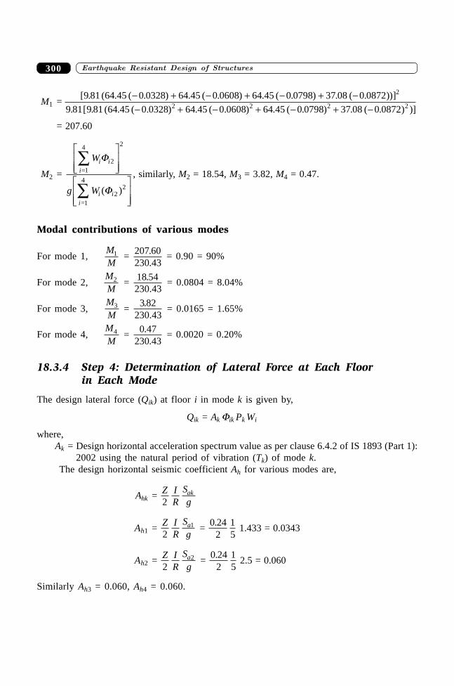
����������� ������� �������������300
M1 = [ . ( . ( . ) . ( . ) . ( . ) . ( . ))]
. [ . ( . ( . ) . ( . ) . ( . ) . ( . ) )]
9 81 64 45 0 0328 64 45 0 0608 64 45 0 0798 37 08 0 0872
9 81 9 81 64 45 0 0328 64 45 0 0608 64 45 0 0798 37 08 0 0872
2
2 2 2 2
- + - + - + -- + - + - + -
= 207.60
M2 =
W
g W
i ii
i ii
F
F
2
4 2
22
4
=1
=1
Â
Â
LNMM
OQPP
LNMM
OQPP
( )
, similarly, M2 = 18.54, M3 = 3.82, M4 = 0.47.
Modal contributions of various modes
For mode 1,MM
1 = 207 60230 43
.
. = 0.90 = 90%
For mode 2,MM
2 = 18 54230 43
..
= 0.0804 = 8.04%
For mode 3,MM
3 = 3 82
230 43.
. = 0.0165 = 1.65%
For mode 4,MM
4 = 0 47230 43
..
= 0.0020 = 0.20%
18.3.4 Step 4: Determination of Lateral Force at Each Floorin Each Mode
The design lateral force (Qik) at floor i in mode k is given by,
Qik = Ak Fik Pk Wi
where,Ak = Design horizontal acceleration spectrum value as per clause 6.4.2 of IS 1893 (Part 1):
2002 using the natural period of vibration (Tk) of mode k.The design horizontal seismic coefficient Ah for various modes are,
Ahk = Z IR
Sgak
2
Ah1 = Z I
RSga
21 =
0 242
15
.1.433 = 0.0343
Ah2 = Z IR
Sga
22 =
0 242
15
.2.5 = 0.060
Similarly Ah3 = 0.060, Ah4 = 0.060.
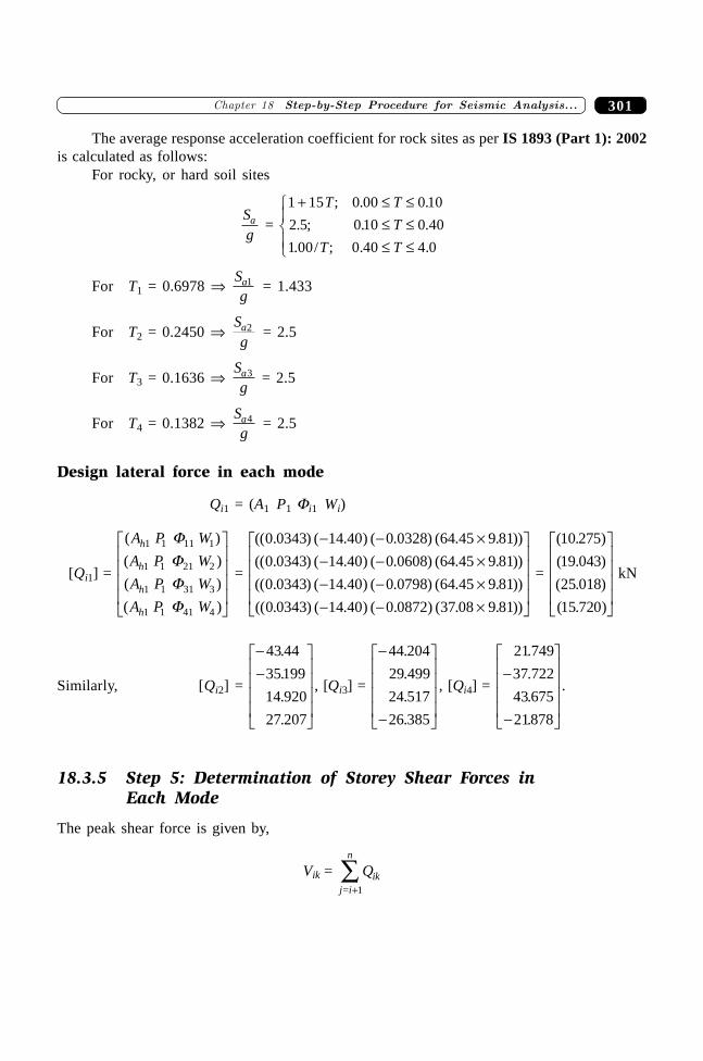
301�������� ����������������� ���� �� ������� ����
The average response acceleration coefficient for rock sites as per IS 1893 (Part 1): 2002is calculated as follows:
For rocky, or hard soil sites
Sga =
1 15 0 00 0 10
2 5 0 10 0 40
1 00 0 40 4 0
+ £ ££ ££ £
RS|
T|
T T
T
T T
; . .
. ; . .
. / ; . .
For T1 = 0.6978 fi Sga1 = 1.433
For T2 = 0.2450 fi Sga2 = 2.5
For T3 = 0.1636 fi Sga3 = 2.5
For T4 = 0.1382 fi Sga4 = 2.5
Design lateral force in each mode
Qi1 = (A1 P1 Fi1 Wi)
[Qi1] =
( )
( )
( )
( )
A P W
A P W
A P W
A P W
h
h
h
h
1 1 11 1
1 1 21 2
1 1 31 3
1 1 41 4
FFFF
L
N
MMMM
O
Q
PPPP
=
(( . ) ( . ) ( . ) ( . . ))
(( . ) ( . ) ( . ) ( . . ))
(( . ) ( . ) ( . ) ( . . ))
(( . ) ( . ) ( . ) ( . . ))
0 0343 14 40 0 0328 64 45 9 81
0 0343 14 40 0 0608 64 45 9 81
0 0343 14 40 0 0798 64 45 9 81
0 0343 14 40 0 0872 37 08 9 81
- - ¥- - ¥- - ¥- - ¥
L
N
MMMM
O
Q
PPPP
=
( . )
( . )
( . )
( . )
10 275
19 043
25 018
15 720
L
N
MMMM
O
Q
PPPP
kN
Similarly, [Qi2] =
--L
N
MMMM
O
Q
PPPP
43 44
35199
14 920
27 207
.
.
.
.
, [Qi3] =
-
-
L
N
MMMM
O
Q
PPPP
44 204
29 499
24 517
26 385
.
.
.
.
, [Qi4] =
21 749
37 722
43 675
21878
.
.
.
.
-
-
L
N
MMMM
O
Q
PPPP
.
18.3.5 Step 5: Determination of Storey Shear Forces inEach Mode
The peak shear force is given by,
Vik = Qikj i
n
= +Â
1
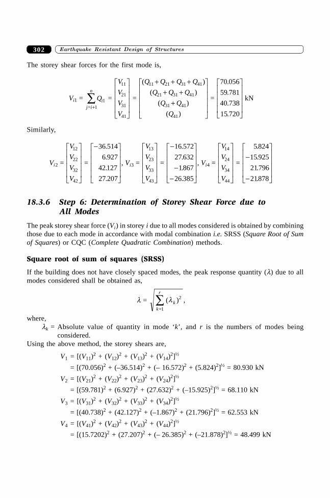
����������� ������� �������������302
The storey shear forces for the first mode is,
Vi1 = Qij i
n
11= +
 =
V
V
V
V
11
21
31
41
L
N
MMMM
O
Q
PPPP
=
( )
( )
( )
( )
Q Q Q Q
Q Q Q
Q Q
Q
11 21 31 41
21 31 41
31 41
41
+ + ++ +
+
L
N
MMMM
O
Q
PPPP =
70 056
59 781
40 738
15 720
.
.
.
.
L
N
MMMM
O
Q
PPPP
kN
Similarly,
Vi2 =
V
V
V
V
12
22
32
42
L
N
MMMM
O
Q
PPPP =
-L
N
MMMM
O
Q
PPPP
36 514
6 927
42 127
27 207
.
.
.
.
, Vi3 =
V
V
V
V
13
23
33
43
L
N
MMMM
O
Q
PPPP
=
-
--
L
N
MMMM
O
Q
PPPP
16 572
27 632
1867
26 385
.
.
.
.
, Vi4 =
V
V
V
V
14
24
34
44
L
N
MMMM
O
Q
PPPP =
5 824
15 925
21 796
21878
.
.
.
.
-
-
L
N
MMMM
O
Q
PPPP
18.3.6 Step 6: Determination of Storey Shear Force due toAll Modes
The peak storey shear force (Vi) in storey i due to all modes considered is obtained by combiningthose due to each mode in accordance with modal combination i.e. SRSS (Square Root of Sumof Squares) or CQC (Complete Quadratic Combination) methods.
Square root of sum of squares (SRSS)
If the building does not have closely spaced modes, the peak response quantity (l) due to allmodes considered shall be obtained as,
l = ( )l kk
r2
=1Â ,
where,lk = Absolute value of quantity in mode ‘k’, and r is the numbers of modes being
considered.Using the above method, the storey shears are,
V1 = [(V11)2 + (V12)
2 + (V13)2 + (V14)
2]½
= [(70.056)2 + (–36.514)2 + (– 16.572)2 + (5.824)2]½ = 80.930 kN
V2 = [(V21)2 + (V22)
2 + (V23)2 + (V24)
2]½
= [(59.781)2 + (6.927)2 + (27.632)2 + (–15.925)2]½ = 68.110 kN
V3 = [(V31)2 + (V32)
2 + (V33)2 + (V34)
2]½
= [(40.738)2 + (42.127)2 + (–1.867)2 + (21.796)2]½ = 62.553 kN
V4 = [(V41)2 + (V42)
2 + (V43)2 + (V44)
2]½
= [(15.7202)2 + (27.207)2 + (– 26.385)2 + (–21.878)2]½ = 48.499 kN
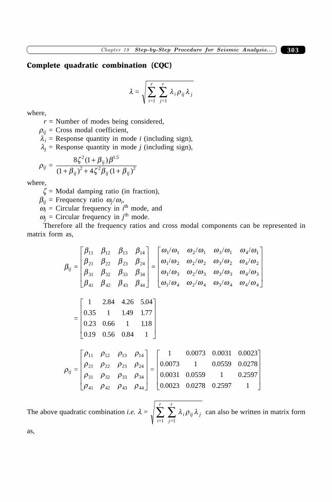
303�������� ����������������� ���� �� ������� ����
Complete quadratic combination (CQC)
l = i
r
i ij jj
r
=1 =1Â Â l r l
where,r = Number of modes being considered,
rij = Cross modal coefficient,l i = Response quantity in mode i (including sign),lj = Response quantity in mode j (including sign),
rij =8 1
1 4 1
2 1 5
2 2 2
z b bb z b b
( )
( ) ( )
.++ + +
ij
ij ij ij
where,z = Modal damping ratio (in fraction),
bij = Frequency ratio wj /w i,wi = Circular frequency in ith mode, andwj = Circular frequency in jth mode.
Therefore all the frequency ratios and cross modal components can be represented inmatrix form as,
bij =
b b b bb b b bb b b bb b b b
11 12 13 14
21 22 23 24
31 32 33 34
41 42 43 44
L
N
MMMM
O
Q
PPPP =
w w w w w w w ww w w w w w w ww w w w w w w ww w w w w w w w
1 1 2 1 3 1 4 1
1 2 2 2 3 2 4 2
1 3 2 3 3 3 4 3
1 4 2 4 3 4 4 4
/ / / /
/ / / /
/ / / /
/ / / /
L
N
MMMM
O
Q
PPPP
=
1 2 84 4 26 5 04
0 35 1 1 49 1 77
0 23 0 66 1 118
0 19 0 56 0 84 1
. . .
. . .
. . .
. . .
L
N
MMMM
O
Q
PPPP
rij =
r r r rr r r rr r r rr r r r
11 12 13 14
21 22 23 24
31 32 33 34
41 42 43 44
L
N
MMMM
O
Q
PPPP =
1 0 0073 0 0031 0 0023
0 0073 1 0 0559 0 0278
0 0031 0 0559 1 0 2597
0 0023 0 0278 0 2597 1
. . .
. . .
. . .
. . .
L
N
MMMM
O
Q
PPPP
The above quadratic combination i.e. l = i
r
i ij jj
r
=1 =1Â Â l r l can also be written in matrix form
as,
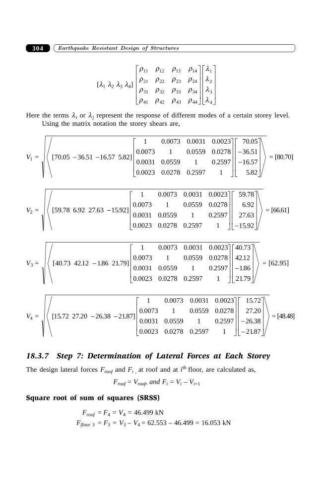
����������� ������� �������������304
[l1 l2 l3 l4]
r r r rr r r rr r r rr r r r
llll
11 12 13 14
21 22 23 24
31 32 33 34
41 42 43 44
1
2
3
4
L
N
MMMM
O
Q
PPPP
L
N
MMMM
O
Q
PPPP
Here the terms l i or l j represent the response of different modes of a certain storey level.Using the matrix notation the storey shears are,
V1 = [ . . . . ]
. . .
. . .
. . .
. . .
.
.
.
.
70 05 36 51 16 57 5 82
1 0 0073 0 0031 0 0023
0 0073 1 0 0559 0 0278
0 0031 0 0559 1 0 2597
0 0023 0 0278 0 2597 1
70 05
36 51
16 57
5 82
- -
L
N
MMMM
O
Q
PPPP
--
L
N
MMMM
O
Q
PPPP
= [80.70]
V2 = [ . . . . ]
. . .
. . .
. . .
. . .
.
.
.
.
59 78 6 92 27 63 15 92
1 0 0073 0 0031 0 0023
0 0073 1 0 0559 0 0278
0 0031 0 0559 1 0 2597
0 0023 0 0278 0 2597 1
59 78
6 92
27 63
15 92
-
L
N
MMMM
O
Q
PPPP -
L
N
MMMM
O
Q
PPPP
= [66.61]
V3 = [ . . . . ]
. . .
. . .
. . .
. . .
.
.
.
.
40 73 4212 186 21 79
1 0 0073 0 0031 0 0023
0 0073 1 0 0559 0 0278
0 0031 0 0559 1 0 2597
0 0023 0 0278 0 2597 1
40 73
4212
186
21 79
-
L
N
MMMM
O
Q
PPPP
-
L
N
MMMM
O
Q
PPPP
= [62.95]
V4 = [ . . . . ]
. . .
. . .
. . .
. . .
.
.
.
.
15 72 27 20 26 38 2187
1 0 0073 0 0031 0 0023
0 0073 1 0 0559 0 0278
0 0031 0 0559 1 0 2597
0 0023 0 0278 0 2597 1
15 72
27 20
26 38
2187
- -
L
N
MMMM
O
Q
PPPP
--
L
N
MMMM
O
Q
PPPP
= [48.48]
18.3.7 Step 7: Determination of Lateral Forces at Each Storey
The design lateral forces Froof and Fi , at roof and at ith floor, are calculated as,
Froof = Vroof, and Fi = Vi – Vi+1
Square root of sum of squares (SRSS)
Froof = F4 = V4 = 46.499 kN
Ffloor 3 = F3 = V3 – V4 = 62.553 – 46.499 = 16.053 kN
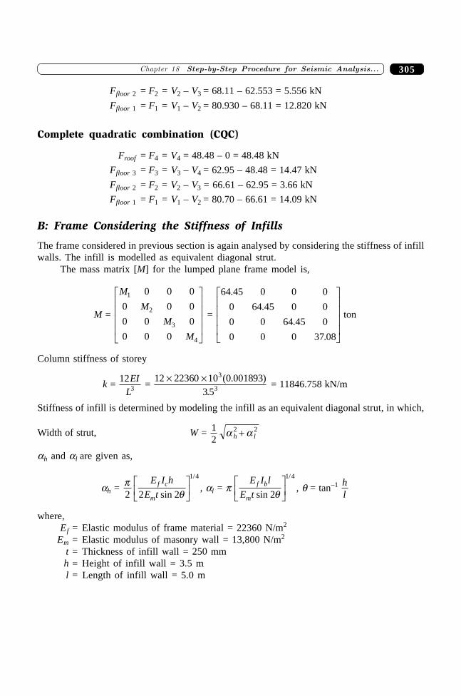
305�������� ����������������� ���� �� ������� ����
Ffloor 2 = F2 = V2 – V3 = 68.11 – 62.553 = 5.556 kN
Ffloor 1 = F1 = V1 – V2 = 80.930 – 68.11 = 12.820 kN
Complete quadratic combination (CQC)
Froof = F4 = V4 = 48.48 – 0 = 48.48 kN
Ffloor 3 = F3 = V3 – V4 = 62.95 – 48.48 = 14.47 kN
Ffloor 2 = F2 = V2 – V3 = 66.61 – 62.95 = 3.66 kN
Ffloor 1 = F1 = V1 – V2 = 80.70 – 66.61 = 14.09 kN
B: Frame Considering the Stiffness of Infills
The frame considered in previous section is again analysed by considering the stiffness of infillwalls. The infill is modelled as equivalent diagonal strut.
The mass matrix [M] for the lumped plane frame model is,
M =
M
M
M
M
1
2
3
4
0 0 0
0 0 0
0 0 0
0 0 0
L
N
MMMM
O
Q
PPPP
=
64 45 0 0 0
0 64 45 0 0
0 0 64 45 0
0 0 0 37 08
.
.
.
.
L
N
MMMM
O
Q
PPPP
ton
Column stiffness of storey
k = 12
3EI
L =
12 22360 10 0 0018933 5
3
3¥ ¥ ( . )
. = 11846.758 kN/m
Stiffness of infill is determined by modeling the infill as an equivalent diagonal strut, in which,
Width of strut, W = 12
2 2a ah l+
ah and al are given as,
ah = pq2 2 2
1 4E I h
E tf c
m sin
/LNM
OQP
, al = pE I l
E tf b
m sin
/
2
1 4
qLNM
OQP
, q = tan–1 hl
where,Ef = Elastic modulus of frame material = 22360 N/m2
Em = Elastic modulus of masonry wall = 13,800 N/m2
t = Thickness of infill wall = 250 mmh = Height of infill wall = 3.5 ml = Length of infill wall = 5.0 m
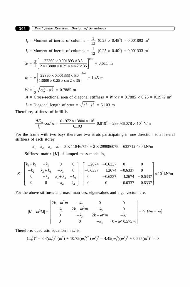
����������� ������� �������������306
Ic = Moment of inertia of columns = 112
(0.25 ¥ 0.453) = 0.001893 m4
Ic = Moment of inertia of columns = 112
(0.25 ¥ 0.403) = 0.001333 m4
ah = p2
22360 0 001893 3 52 13800 0 25 2 35
1 4¥ ¥¥ ¥ ¥ ¥
LNM
OQP
. .. sin
/
= 0.611 m
al = p 22360 0 001333 5 013800 0 25 2 35
1 4¥ ¥
¥ ¥ ¥LNM
OQP
. .. sin
/
= 1.45 m
W = 12
2 2a ah l+ = 0.7885 m
A = Cross-sectional area of diagonal stiffness = W ¥ t = 0.7885 ¥ 0.25 = 0.1972 m2
ld = Diagonal length of strut = h l2 2+ = 6.103 m
Therefore, stiffness of infill is
AEl
m
dcos2 q =
0 1972 13800 106 103
6..
¥ ¥0.8192 = 299086.078 ¥ 103 N/m
For the frame with two bays there are two struts participating in one direction, total lateralstiffness of each storey
k1 = k2 = k3 = k4 = 3 ¥ 11846.758 + 2 ¥ 299086078 = 633712.430 kN/m
Stiffness matrix [K] of lumped mass model is,
K =
k k k
k k k k
k k k k
k k
1 2 2
2 2 3 3
3 3 4 4
4 4
0 0
0
0
0 0
+ -- + -
- + --
L
N
MMMM
O
Q
PPPP =
12674 0 6337 0 0
0 6337 12674 0 6337 0
0 0 6337 12674 0 6337
0 0 0 6337 0 6337
. .
. . .
. . .
. .
-- -
- --
L
N
MMMM
O
Q
PPPP ¥ 106 kN/m
For the above stiffness and mass matrices, eigenvalues and eigenvectors are,
|K – w 2M| =
2 0 0
2 0
0 2
0 0 0 575
22
22
3
32
4
42
k m k
k k m k
k k m k
k k m
- -- - -
- - -- -
L
N
MMMMM
O
Q
PPPPP
ww
ww .
= 0, k/m = wn2
Therefore, quadratic equation in w is,
(wn2)4 – 8.3(wn
2)3 (w2) + 10.75(wn2)2 (w2)2 – 4.45(wn
2)(w2)3 + 0.575(w2)4 = 0
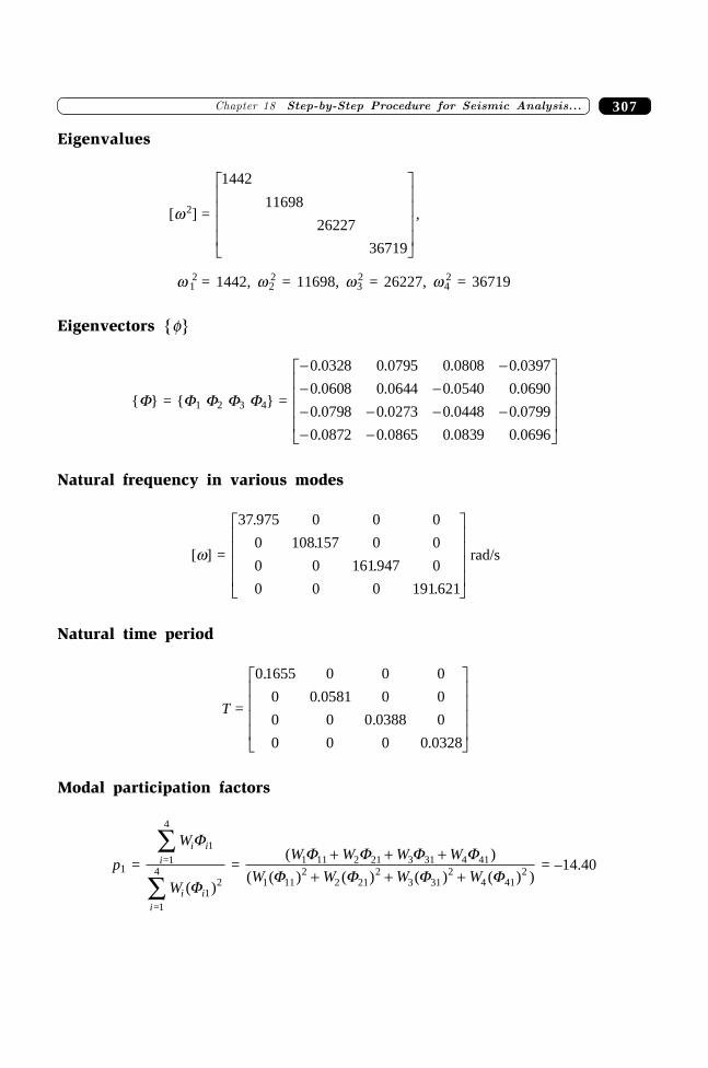
307�������� ����������������� ���� �� ������� ����
Eigenvalues
[w 2] =
1442
11698
26227
36719
L
N
MMMM
O
Q
PPPP
,
w 12 = 1442, w2
2 = 11698, w32 = 26227, w4
2 = 36719
Eigenvectors {f}
{F} = {F1 F2 F3 F4} =
- -- -- - - -- -
L
N
MMMM
O
Q
PPPP
0 0328 0 0795 0 0808 0 0397
0 0608 0 0644 0 0540 0 0690
0 0798 0 0273 0 0448 0 0799
0 0872 0 0865 0 0839 0 0696
. . . .
. . . .
. . . .
. . . .
Natural frequency in various modes
[w] =
37 975 0 0 0
0 108157 0 0
0 0 161947 0
0 0 0 191 621
.
.
.
.
L
N
MMMM
O
Q
PPPP
rad/s
Natural time period
T =
0 1655 0 0 0
0 0 0581 0 0
0 0 0 0388 0
0 0 0 0 0328
.
.
.
.
L
N
MMMM
O
Q
PPPP
Modal participation factors
p1 =
W
W
i ii
i ii
F
F
1
4
12
4=1
=1
Â
 ( )
= ( )
( ( ) ( ) ( ) ( ) )
W W W W
W W W W1 11 2 21 3 31 4 41
1 112
2 212
3 312
4 412
F F F FF F F F
+ + ++ + +
= –14.40
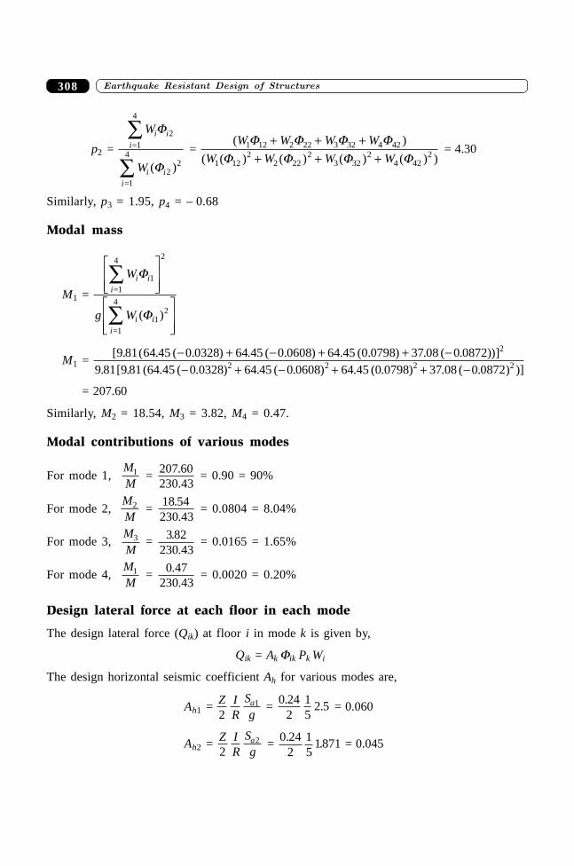
����������� ������� �������������308
p2 =
W
W
i ii
i ii
F
F
2
4
22
4=1
=1
Â
 ( )
= ( )
( ( ) ( ) ( ) ( ) )
W W W W
W W W W1 12 2 22 3 32 4 42
1 122
2 222
3 322
4 422
F F F FF F F F
+ + ++ + +
= 4.30
Similarly, p3 = 1.95, p4 = – 0.68
Modal mass
M1 =
W
g W
i ii
i ii
F
F
1
4 2
12
4
=1
=1
Â
Â
LNMM
OQPP
LNMM
OQPP
( )
M1 = [ . ( . ( . ) . ( . ) . ( . ) . ( . ))]
. [ . ( . ( . ) . ( . ) . ( . ) . ( . ) )]9 81 64 45 0 0328 64 45 0 0608 64 45 0 0798 37 08 0 0872
9 81 9 81 64 45 0 0328 64 45 0 0608 64 45 0 0798 37 08 0 0872
2
2 2 2 2- + - + + -- + - + + -
= 207.60
Similarly, M2 = 18.54, M3 = 3.82, M4 = 0.47.
Modal contributions of various modes
For mode 1,MM
1 = 207 60230 43
.
. = 0.90 = 90%
For mode 2,MM
2 = 18 54230 43
..
= 0.0804 = 8.04%
For mode 3,MM
3 = 3 82230 43
..
= 0.0165 = 1.65%
For mode 4,MM
1 = 0 47230 43
..
= 0.0020 = 0.20%
Design lateral force at each floor in each mode
The design lateral force (Qik) at floor i in mode k is given by,
Qik = Ak Fik Pk Wi
The design horizontal seismic coefficient Ah for various modes are,
Ah1 = Z IR
Sga
21 =
0 242
15
2 5. . = 0.060
Ah2 = Z IR
Sga
22 = 0 24
215
1871. . = 0.045
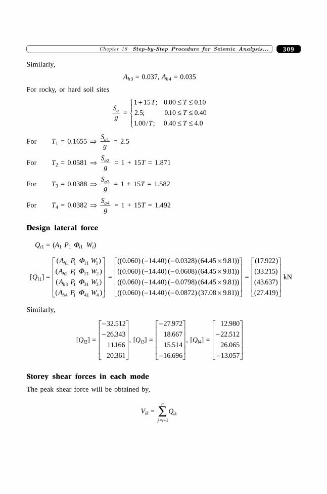
309�������� ����������������� ���� �� ������� ����
Similarly,
Ah3 = 0.037, Ah4 = 0.035
For rocky, or hard soil sites
Sga =
1 15 0 00 0 10
2 5 0 10 0 40
1 00 0 40 4 0
+ £ ££ ££ £
RS|
T|
T T
T
T T
; . .
. ; . .
. / ; . .
For T1 = 0.1655 fi Sga1 = 2.5
For T2 = 0.0581 fi Sga2 = 1 + 15T = 1.871
For T3 = 0.0388 fi Sga3 = 1 + 15T = 1.582
For T4 = 0.0382 fi Sga4 = 1 + 15T = 1.492
Design lateral force
Qi1 = (A1 P1 Fi1 Wi)
[Qi1] =
( )
( )
( )
( )
A P W
A P W
A P W
A P W
h
h
h
h
1 1 11 1
2 1 21 2
3 1 31 3
4 1 41 4
FFFF
L
N
MMMM
O
Q
PPPP
=
(( . ) ( . ) ( . ) ( . . ))
(( . ) ( . ) ( . ) ( . . ))
(( . ) ( . ) ( . ) ( . . ))
(( . ) ( . ) ( . ) ( . . ))
0 060 14 40 0 0328 64 45 9 81
0 060 14 40 0 0608 64 45 9 81
0 060 14 40 0 0798 64 45 9 81
0 060 14 40 0 0872 37 08 9 81
- - ¥- - ¥- - ¥- - ¥
L
N
MMMM
O
Q
PPPP
=
( . )
( . )
( . )
( . )
17 922
33 215
43 637
27 419
L
N
MMMM
O
Q
PPPP
kN
Similarly,
[Qi2] =
--L
N
MMMM
O
Q
PPPP
32 512
26 343
11166
20 361
.
.
.
.
, [Qi3] =
-
-
L
N
MMMM
O
Q
PPPP
27 972
18 667
15 514
16 696
.
.
.
.
, [Qi4] =
12 980
22 512
26 065
13 057
.
.
.
.
-
-
L
N
MMMM
O
Q
PPPP
Storey shear forces in each mode
The peak shear force will be obtained by,
Vik = Qikj i
n
= +Â
1
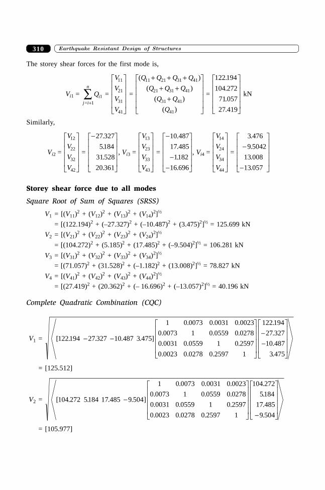
����������� ������� �������������310
The storey shear forces for the first mode is,
Vi1 = Qij i
n
11= +
 =
V
V
V
V
11
21
31
41
L
N
MMMM
O
Q
PPPP
=
( )
( )
( )
( )
Q Q Q Q
Q Q Q
Q Q
Q
11 21 31 41
21 31 41
31 41
41
+ + ++ +
+
L
N
MMMM
O
Q
PPPP =
122 194
104 272
71 057
27 419
.
.
.
.
L
N
MMMM
O
Q
PPPP
kN
Similarly,
Vi2 =
V
V
V
V
12
22
32
42
L
N
MMMM
O
Q
PPPP =
-L
N
MMMM
O
Q
PPPP
27 327
5184
31 528
20 361
.
.
.
.
, Vi3 =
V
V
V
V
13
23
33
43
L
N
MMMM
O
Q
PPPP
=
-
--
L
N
MMMM
O
Q
PPPP
10 487
17 485
1182
16 696
.
.
.
.
, Vi4 =
V
V
V
V
14
24
34
44
L
N
MMMM
O
Q
PPPP =
3 476
9 5042
13 008
13 057
.
.
.
.
-
-
L
N
MMMM
O
Q
PPPP
Storey shear force due to all modes
Square Root of Sum of Squares (SRSS)
V1 = [(V11)2 + (V12)
2 + (V13)2 + (V14)
2]½
= [(122.194)2 + (–27.327)2 + (–10.487)2 + (3.475)2]½ = 125.699 kN
V2 = [(V21)2 + (V22)
2 + (V23)2 + (V24)
2]½
= [(104.272)2 + (5.185)2 + (17.485)2 + (–9.504)2]½ = 106.281 kN
V3 = [(V31)2 + (V32)
2 + (V33)2 + (V34)
2]½
= [(71.057)2 + (31.528)2 + (–1.182)2 + (13.008)2]½ = 78.827 kN
V4 = [(V41)2 + (V42)
2 + (V43)2 + (V44)
2]½
= [(27.419)2 + (20.362)2 + (– 16.696)2 + (–13.057)2]½ = 40.196 kN
Complete Quadratic Combination (CQC)
V1 = [ . . . . ]
. . .
. . .
. . .
. . .
.
.
.
.
122194 27 327 10 487 3 475
1 0 0073 0 0031 0 0023
0 0073 1 0 0559 0 0278
0 0031 0 0559 1 0 2597
0 0023 0 0278 0 2597 1
122 194
27 327
10 487
3 475
- -
L
N
MMMM
O
Q
PPPP
--
L
N
MMMM
O
Q
PPPP
= [125.512]
V2 = [ . . . . ]
. . .
. . .
. . .
. . .
.
.
.
.
104 272 5184 17 485 9 504
1 0 0073 0 0031 0 0023
0 0073 1 0 0559 0 0278
0 0031 0 0559 1 0 2597
0 0023 0 0278 0 2597 1
104 272
5184
17 485
9 504
-
L
N
MMMM
O
Q
PPPP -
L
N
MMMM
O
Q
PPPP
= [105.977]
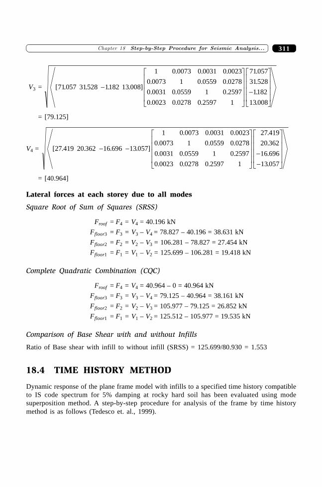
311�������� ����������������� ���� �� ������� ����
V3 = [ . . . . ]
. . .
. . .
. . .
. . .
.
.
.
.
71 057 31528 1182 13 008
1 0 0073 0 0031 0 0023
0 0073 1 0 0559 0 0278
0 0031 0 0559 1 0 2597
0 0023 0 0278 0 2597 1
71 057
31 528
1182
13 008
-
L
N
MMMM
O
Q
PPPP
-
L
N
MMMM
O
Q
PPPP
= [79.125]
V4 = [ . . . . ]
. . .
. . .
. . .
. . .
.
.
.
.
27 419 20 362 16 696 13 057
1 0 0073 0 0031 0 0023
0 0073 1 0 0559 0 0278
0 0031 0 0559 1 0 2597
0 0023 0 0278 0 2597 1
27 419
20 362
16 696
13 057
- -
L
N
MMMM
O
Q
PPPP
--
L
N
MMMM
O
Q
PPPP
= [40.964]
Lateral forces at each storey due to all modes
Square Root of Sum of Squares (SRSS)
Froof = F4 = V4 = 40.196 kN
Ffloor3 = F3 = V3 – V4 = 78.827 – 40.196 = 38.631 kN
Ffloor2 = F2 = V2 – V3 = 106.281 – 78.827 = 27.454 kN
Ffloor1 = F1 = V1 – V2 = 125.699 – 106.281 = 19.418 kN
Complete Quadratic Combination (CQC)
Froof = F4 = V4 = 40.964 – 0 = 40.964 kN
Ffloor3 = F3 = V3 – V4 = 79.125 – 40.964 = 38.161 kN
Ffloor2 = F2 = V2 – V3 = 105.977 – 79.125 = 26.852 kN
Ffloor1 = F1 = V1 – V2 = 125.512 – 105.977 = 19.535 kN
Comparison of Base Shear with and without Infills
Ratio of Base shear with infill to without infill (SRSS) = 125.699/80.930 = 1.553
18.4 TIME HISTORY METHOD
Dynamic response of the plane frame model with infills to a specified time history compatibleto IS code spectrum for 5% damping at rocky hard soil has been evaluated using modesuperposition method. A step-by-step procedure for analysis of the frame by time historymethod is as follows (Tedesco et. al., 1999).
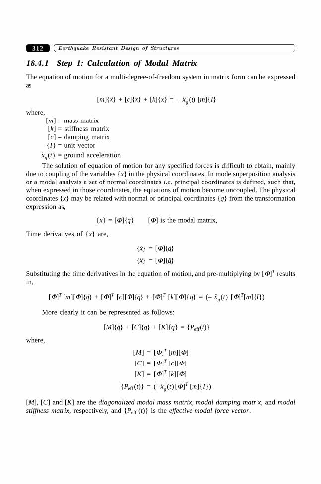
����������� ������� �������������312
18.4.1 Step 1: Calculation of Modal Matrix
The equation of motion for a multi-degree-of-freedom system in matrix form can be expressedas
[m]{��}x + [c]{�}x + [k]{x} = – ��xg (t) [m]{I}
where,[m] = mass matrix[k] = stiffness matrix[c] = damping matrix{I} = unit vector�� ( )x tg = ground acceleration
The solution of equation of motion for any specified forces is difficult to obtain, mainlydue to coupling of the variables {x} in the physical coordinates. In mode superposition analysisor a modal analysis a set of normal coordinates i.e. principal coordinates is defined, such that,when expressed in those coordinates, the equations of motion become uncoupled. The physicalcoordinates {x} may be related with normal or principal coordinates {q} from the transformationexpression as,
{x} = [F]{q} [F] is the modal matrix,
Time derivatives of {x} are,
{�}x = [F]{ �}q
{��}x = [F]{��}q
Substituting the time derivatives in the equation of motion, and pre-multiplying by [F]T resultsin,
[F]T [m][F]{��}q + [F]T [c][F]{ �}q + [F]T [k][F]{q} = (– �� ( )x tg [F]T[m]{I})
More clearly it can be represented as follows:
[M]{��}q + [C]{�}q + [K]{q} = {Peff(t)}
where,
[M] = [F]T [m][F]
[C] = [F]T [c][F]
[K] = [F]T [k][F]
{Peff (t)} = (– �� ( )x tg [F]T [m]{I})
[M], [C] and [K] are the diagonalized modal mass matrix, modal damping matrix, and modalstiffness matrix, respectively, and {Peff (t)} is the effective modal force vector.
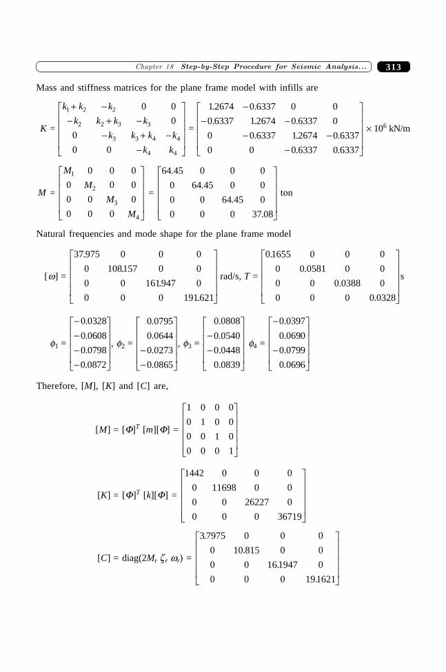
313�������� ����������������� ���� �� ������� ����
Mass and stiffness matrices for the plane frame model with infills are
K =
k k k
k k k k
k k k k
k k
1 2 2
2 2 3 3
3 3 4 4
4 4
0 0
0
0
0 0
+ -- + -
- + --
L
N
MMMM
O
Q
PPPP =
1 2674 0 6337 0 0
0 6337 1 2674 0 6337 0
0 0 6337 1 2674 0 6337
0 0 0 6337 0 6337
. .
. . .
. . .
. .
-- -
- --
L
N
MMMM
O
Q
PPPP ¥ 106 kN/m
M =
M
M
M
M
1
2
3
4
0 0 0
0 0 0
0 0 0
0 0 0
L
N
MMMM
O
Q
PPPP
=
64 45 0 0 0
0 64 45 0 0
0 0 64 45 0
0 0 0 37 08
.
.
.
.
L
N
MMMM
O
Q
PPPP
ton
Natural frequencies and mode shape for the plane frame model
[w] =
37 975 0 0 0
0 108157 0 0
0 0 161947 0
0 0 0 191 621
.
.
.
.
L
N
MMMM
O
Q
PPPP
rad/s, T =
0 1655 0 0 0
0 0 0581 0 0
0 0 0 0388 0
0 0 0 0 0328
.
.
.
.
L
N
MMMM
O
Q
PPPP
s
f1 =
----
L
N
MMMM
O
Q
PPPP
0 0328
0 0608
0 0798
0 0872
.
.
.
.
, f2 =
0 0795
0 0644
0 0273
0 0865
.
.
.
.
--
L
N
MMMM
O
Q
PPPP, f3 =
0 0808
0 0540
0 0448
0 0839
.
.
.
.
--
L
N
MMMM
O
Q
PPPP
f4 =
-
-
L
N
MMMM
O
Q
PPPP
0 0397
0 0690
0 0799
0 0696
.
.
.
.
Therefore, [M], [K] and [C] are,
[M] = [F]T [m][F] =
1 0 0 0
0 1 0 0
0 0 1 0
0 0 0 1
L
N
MMMM
O
Q
PPPP
[K] = [F]T [k][F] =
1442 0 0 0
0 11698 0 0
0 0 26227 0
0 0 0 36719
L
N
MMMM
O
Q
PPPP
[C] = diag(2Mr zr wr) =
3 7975 0 0 0
0 10 815 0 0
0 0 16 1947 0
0 0 0 191621
.
.
.
.
L
N
MMMM
O
Q
PPPP
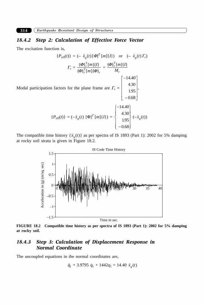
����������� ������� �������������314
18.4.2 Step 2: Calculation of Effective Force Vector
The excitation function is,
{Peff(t)} = (– �� ( )x tg [F]T [m]{I}) or (– �� ( )x tg Gr)
Gr = { } [ ]{ }
{ } [ ]{ }
FF F
rT
rT
r
m I
m =
{ } [ ]{ }F rT
r
m IM
Modal participation factors for the plane frame are Gr =
-
-
L
N
MMMM
O
Q
PPPP
14 40
4 30
1 95
0 68
.
.
.
.
,
{Peff(t)} = (– �� ( )x tg [F]T [m]{I}) =
-
-
RS||
T||
UV||
W||
14 40
4 30
195
0 68
.
.
.
.
(– �� ( )x tg )
The compatible time history {�� ( )x tg } as per spectra of IS 1893 (Part 1): 2002 for 5% dampingat rocky soil strata is given in Figure 18.2.
IS Code Time History
–1.5
–1
–0.5
0
0.5
1
1.5
0 5 10 15 20 25 30 35 40
Time in sec.
Acc
eler
atio
nin
(g)
(m/s
q.
sec)
FIGURE 18.2 Compatible time history as per spectra of IS 1893 (Part 1): 2002 for 5% dampingat rocky soil.
18.4.3 Step 3: Calculation of Displacement Response inNormal Coordinate
The uncoupled equations in the normal coordinates are,
��q1 + 3.9795 �q1 + 1442q1 = 14.40 �� ( )x tg
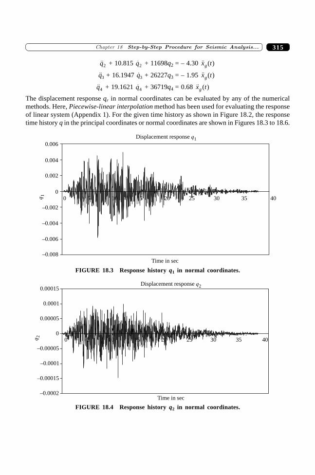
315�������� ����������������� ���� �� ������� ����
��q2 + 10.815 �q2 + 11698q2 = – 4.30 �� ( )x tg
��q3 + 16.1947 �q3 + 26227q3 = – 1.95 �� ( )x tg
��q4 + 19.1621 �q4 + 36719q4 = 0.68 �� ( )x tg
The displacement response qr in normal coordinates can be evaluated by any of the numericalmethods. Here, Piecewise-linear interpolation method has been used for evaluating the responseof linear system (Appendix 1). For the given time history as shown in Figure 18.2, the responsetime history q in the principal coordinates or normal coordinates are shown in Figures 18.3 to 18.6.
Displacement response q1
–0.008
–0.006
–0.004
–0.002
0
0.002
0.004
0.006
0 5 10 15 20 25 30 35 40
Time in sec
q1
FIGURE 18.3 Response history q1 in normal coordinates.
Displacement response q2
–0.0002
–0.00015
–0.0001
–0.00005
0
0.00005
0.0001
0.00015
Time in sec
q2
0 5 10 15 20 25 30 35 40
FIGURE 18.4 Response history q2 in normal coordinates.
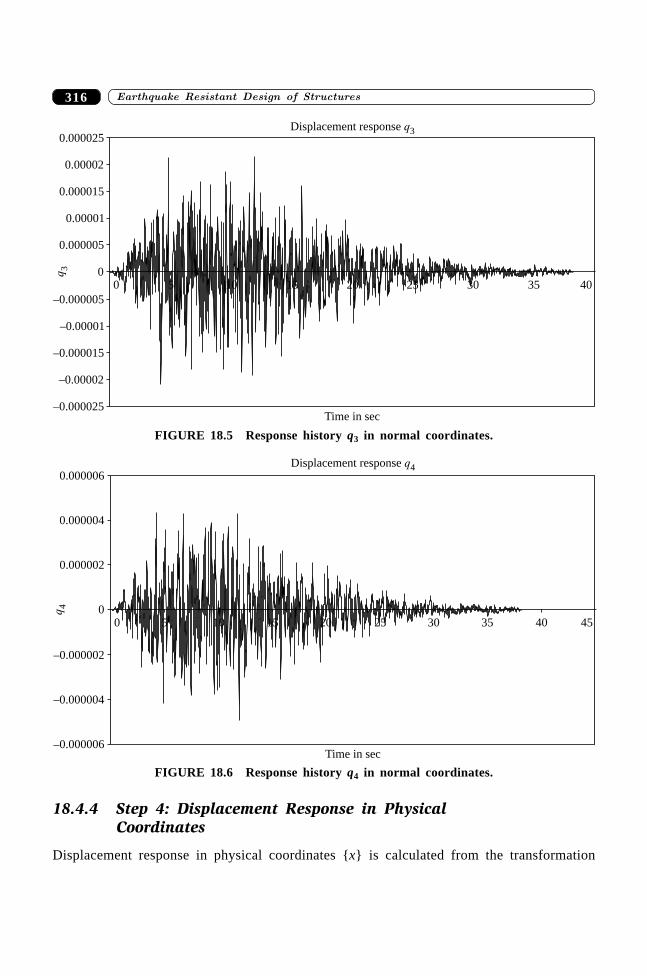
����������� ������� �������������316
Displacement response q3
–0.000025
–0.00002
–0.000015
–0.00001
–0.000005
0
0.000005
0.00001
0.000015
0.00002
0.000025
0 5 10 15 20 25 30 35 40
Time in sec
q3
FIGURE 18.5 Response history q3 in normal coordinates.
Displacement response q4
–0.000006
–0.000004
–0.000002
0
0.000002
0.000004
0.000006
0 5 10 15 20 25 30 35 40 45
Time in sec
q4
FIGURE 18.6 Response history q4 in normal coordinates.
18.4.4 Step 4: Displacement Response in PhysicalCoordinates
Displacement response in physical coordinates {x} is calculated from the transformation
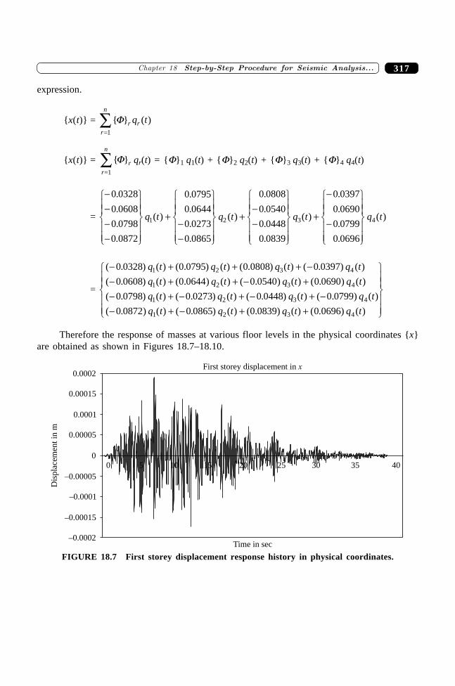
317�������� ����������������� ���� �� ������� ����
expression.
{x(t)} = { }=1
F r rr
n
q t( )Â
{x(t)} = { }F rr
n
=1Â qr(t) = {F}1 q1(t) + {F}2 q2(t) + {F}3 q3(t) + {F}4 q4(t)
=
----
RS||
T||
UV||
W||
+--
RS||
T||
UV||
W||
+--
RS||
T||
UV||
W||
+
-
-
RS||
T||
UV||
W||
0 0328
0 0608
0 0798
0 0872
0 0795
0 0644
0 0273
0 0865
0 0808
0 0540
0 0448
0 0839
0 0397
0 0690
0 0799
0 0696
1 2 3 4
.
.
.
.
( )
.
.
.
.
( )
.
.
.
.
( )
.
.
.
.
( )q t q t q t q t
=
( . ) ( ) ( . ) ( ) ( . ) ( ) ( . ) ( )
( . ) ( ) ( . ) ( ) ( . ) ( ) ( . ) ( )
( . ) ( ) ( . ) ( ) ( . ) ( ) ( . ) ( )
( . ) ( ) ( . ) ( ) ( . ) ( ) ( . )
- + + + -- + + - +- + - + - + -- + - + +
0 0328 0 0795 0 0808 0 0397
0 0608 0 0644 0 0540 0 0690
0 0798 0 0273 0 0448 0 0799
0 0872 0 0865 0 0839 0 0696
1 2 3 4
1 2 3 4
1 2 3 4
1 2 3
q t q t q t q t
q t q t q t q t
q t q t q t q t
q t q t q t q t4( )
RS||
T||
UV||
W||
Therefore the response of masses at various floor levels in the physical coordinates {x}are obtained as shown in Figures 18.7–18.10.
First storey displacement in x
–0.0002
–0.00015
–0.0001
–0.00005
0
0.00005
0.0001
0.00015
0.0002
0 5 10 15 20 25 30 35 40
Time in sec
Dis
pla
cem
ent
inm
FIGURE 18.7 First storey displacement response history in physical coordinates.
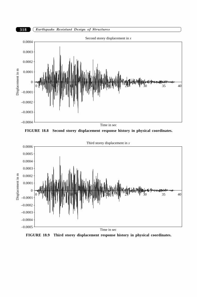
����������� ������� �������������318
Second storey displacement in x
–0.0004
–0.0003
–0.0002
–0.0001
0
0.0001
0.0002
0.0003
0.0004
0 5 10 15 20 25 30 35 40
Time in sec
Dis
pla
cem
ent
inm
FIGURE 18.8 Second storey displacement response history in physical coordinates.
Third storey displacement in x
–0.0005
–0.0004
–0.0003
–0.0002
–0.0001
0
0.0001
0.0002
0.0003
0.0004
0.0005
0.0006
0 5 10 15 20 25 30 35 40
Time in sec
Dis
pla
cem
ent
inm
FIGURE 18.9 Third storey displacement response history in physical coordinates.
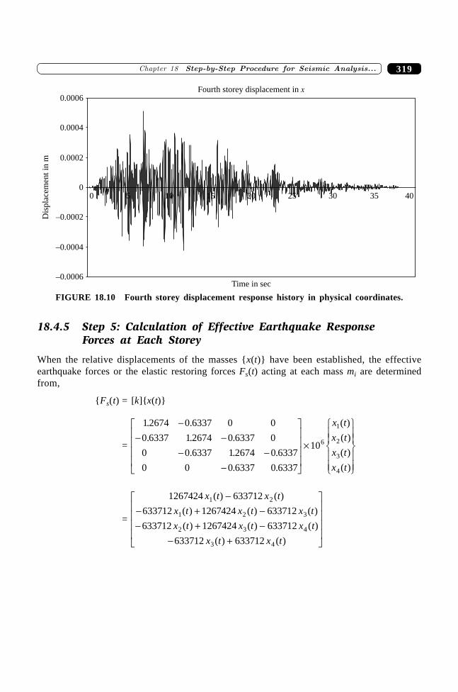
319�������� ����������������� ���� �� ������� ����
Fourth storey displacement in x
–0.0006
–0.0004
–0.0002
0
0.0002
0.0004
0.0006
0 5 10 15 20 25 30 35 40
Time in sec
Dis
pla
cem
ent
inm
FIGURE 18.10 Fourth storey displacement response history in physical coordinates.
18.4.5 Step 5: Calculation of Effective Earthquake ResponseForces at Each Storey
When the relative displacements of the masses {x(t)} have been established, the effectiveearthquake forces or the elastic restoring forces Fs(t) acting at each mass mi are determinedfrom,
{Fs(t) = [k]{x(t)}
=
1 2674 0 6337 0 0
0 6337 1 2674 0 6337 0
0 0 6337 1 2674 0 6337
0 0 0 6337 0 6337
106
1
2
3
4
. .
. . .
. . .
. .
( )
( )
( )
( )
-- -
- --
L
N
MMMM
O
Q
PPPP
¥
RS||
T||
UV||
W||
x t
x t
x t
x t
=
1267424 633712
633712 1267424 633712
633712 1267424 633712
633712 633712
1 2
1 2 3
2 3 4
3 4
x t x t
x t x t x t
x t x t x t
x t x t
( ) ( )
( ) ( ) ( )
( ) ( ) ( )
( ) ( )
-- + -- + -
- +
L
N
MMMM
O
Q
PPPP
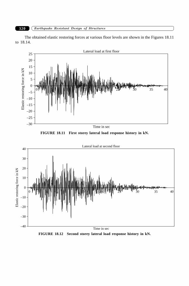
����������� ������� �������������320
The obtained elastic restoring forces at various floor levels are shown in the Figures 18.11to 18.14.
Lateral load at first floor
–30
–25
–20
–15
–10
–5
0
5
10
15
20
25
0 5 10 15 20 25 30 35 40
Time in sec
Ela
stic
rest
ori
ng
forc
ein
kN
FIGURE 18.11 First storey lateral load response history in kN.
Lateral load at second floor
–40
–30
–20
–10
0
10
20
30
40
0 5 10 15 20 25 30 35 40
Time in sec
Ela
stic
rest
ori
ng
forc
ein
kN
FIGURE 18.12 Second storey lateral load response history in kN.
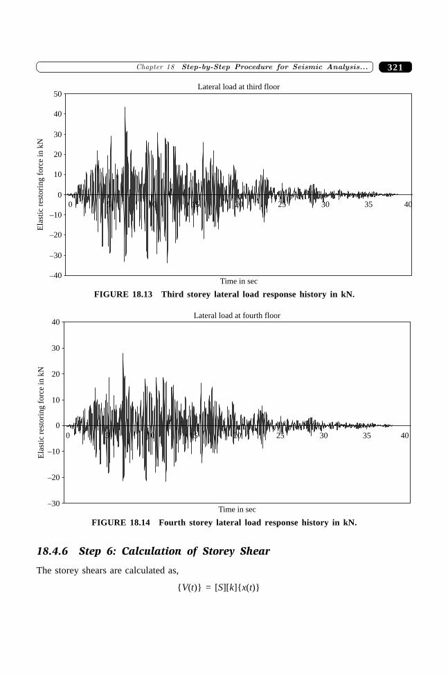
321�������� ����������������� ���� �� ������� ����
Lateral load at third floor
–40
–30
–20
–10
0
10
20
30
40
50
0 5 10 15 20 25 30 35 40
Time in sec
Ela
stic
rest
ori
ng
forc
ein
kN
FIGURE 18.13 Third storey lateral load response history in kN.
Lateral load at fourth floor
–30
–20
–10
0
10
20
30
40
0 5 10 15 20 25 30 35 40
Time in sec
Ela
stic
rest
ori
ng
forc
ein
kN
FIGURE 18.14 Fourth storey lateral load response history in kN.
18.4.6 Step 6: Calculation of Storey Shear
The storey shears are calculated as,
{V(t)} = [S][k]{x(t)}
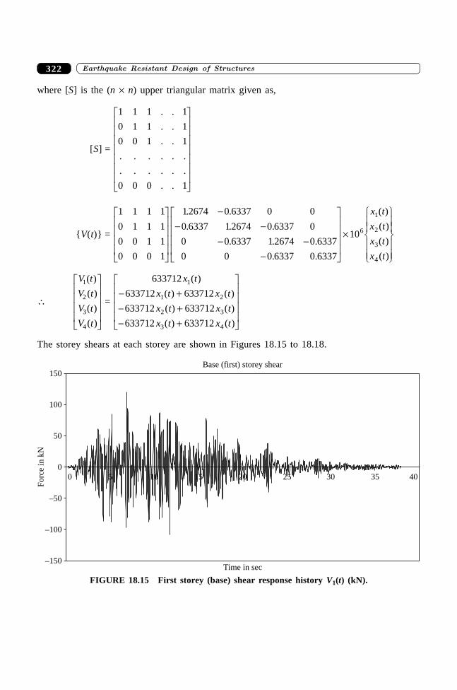
����������� ������� �������������322
where [S] is the (n ¥ n) upper triangular matrix given as,
[S] =
1 1 1 1
0 1 1 1
0 0 1 1
0 0 0 1
. .
. .
. .
. . . . . .
. . . . . .
. .
L
N
MMMMMMM
O
Q
PPPPPPP
{V(t)} =
1 1 1 1
0 1 1 1
0 0 1 1
0 0 0 1
12674 0 6337 0 0
0 6337 12674 0 6337 0
0 0 6337 1 2674 0 6337
0 0 0 6337 0 6337
106
1
2
3
4
L
N
MMMM
O
Q
PPPP
-- -
- --
L
N
MMMM
O
Q
PPPP
¥
R
S||
T||
U
V||
W||
. .
. . .
. . .
. .
( )
( )
( )
( )
x t
x t
x t
x t
\
V t
V t
V t
V t
1
2
3
4
( )
( )
( )
( )
L
N
MMMM
O
Q
PPPP
=
633712
633712 633712
633712 633712
633712 633712
1
1 2
2 3
3 4
x t
x t x t
x t x t
x t x t
( )
( ) ( )
( ) ( )
( ) ( )
- +- +- +
L
N
MMMM
O
Q
PPPP
The storey shears at each storey are shown in Figures 18.15 to 18.18.
Base (first) storey shear
–150
–100
–50
0
50
100
150
0 5 10 15 20 25 30 35 40
Time in sec
Fo
rce
ink
N
FIGURE 18.15 First storey (base) shear response history V1(t) (kN).
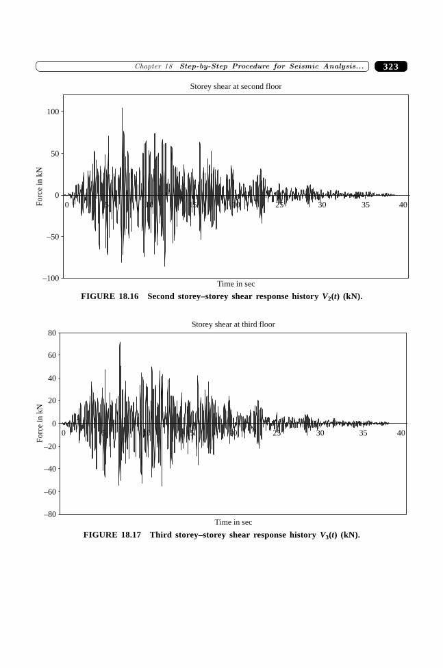
323�������� ����������������� ���� �� ������� ����
Storey shear at second floor
–100
–50
0
50
100
0 5 10 15 20 25 30 35 40
Time in sec
Fo
rce
ink
N
FIGURE 18.16 Second storey–storey shear response history V2(t) (kN).
Storey shear at third floor
–80
–60
–40
–20
0
20
40
60
80
0 5 10 15 20 25 30 35 40
Time in sec
Fo
rce
ink
N
FIGURE 18.17 Third storey–storey shear response history V3(t) (kN).
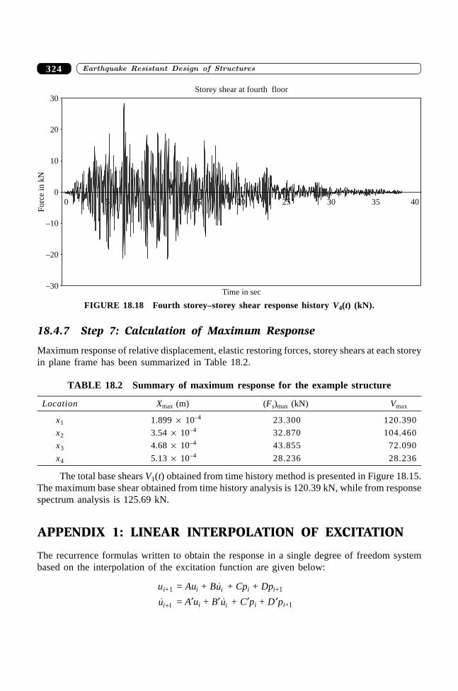
����������� ������� �������������324
Storey shear at fourth floor
–30
–20
–10
0
10
20
30
0 5 10 15 20 25 30 35 40
Time in sec
Fo
rce
ink
N
FIGURE 18.18 Fourth storey–storey shear response history V4(t) (kN).
18.4.7 Step 7: Calculation of Maximum Response
Maximum response of relative displacement, elastic restoring forces, storey shears at each storeyin plane frame has been summarized in Table 18.2.
TABLE 18.2 Summary of maximum response for the example structure
Location Xmax (m) (Fs)max (kN) Vmax
x1 1.899 ¥ 10–4 23.300 120.390
x2 3.54 ¥ 10–4 32.870 104.460
x3 4.68 ¥ 10–4 43.855 72.090
x4 5.13 ¥ 10–4 28.236 28.236
The total base shears V1(t) obtained from time history method is presented in Figure 18.15.The maximum base shear obtained from time history analysis is 120.39 kN, while from responsespectrum analysis is 125.69 kN.
APPENDIX 1: LINEAR INTERPOLATION OF EXCITATION
The recurrence formulas written to obtain the response in a single degree of freedom systembased on the interpolation of the excitation function are given below:
ui+1 = Aui + B �ui + Cpi + Dpi+1
�ui+1 = A¢ui + B¢ �ui + C¢pi + D ¢pi+1
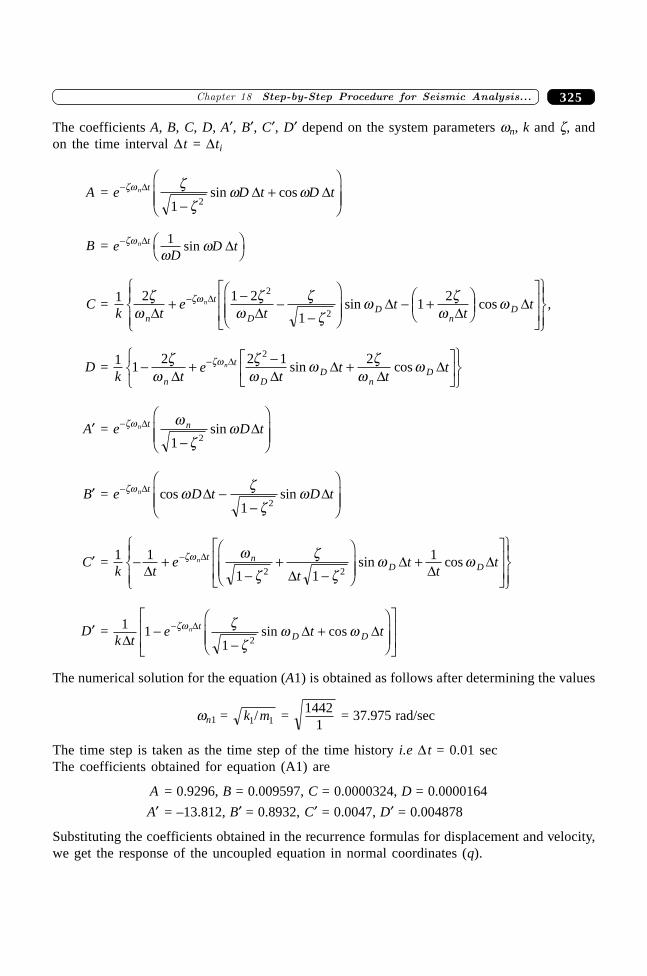
325�������� ����������������� ���� �� ������� ����
The coefficients A, B, C, D, A¢, B¢, C¢, D¢ depend on the system parameters wn, k and z, andon the time interval Dt = Dti
A = e D t D tn t-
-+
FHGG
IKJJ
zw zz
w wD D D1 2
sin cos
B = eD
D tn t- FH IKzw
wwD D1 sin
C = 1 2 1 2
11
22
2k te
tt
tt
n
t
DD
nD
nz
wz
wz
zw z
wwzw
D DD
DDD+ - -
-
FHGG
IKJJ - +F
HGIKJ
L
NMM
O
QPP
RS|T|
UV|W|
- sin cos ,
D = 1 12 2 1 22
k te
tt
tt
n
t
DD
nD
n- + - +LNM
OQP
RST
UVW
-zw
zw
w zw
wzw
D DD
DDD sin cos
A¢ = e D tn t n-
-
FHGG
IKJJ
zw w
zwD D
1 2sin
B¢ = e D t D tn t- --
FHGG
IKJJ
zw w zz
wD D Dcos sin1 2
C¢ = 1 1
1 1
12 2k t
et
tt
tn t nD D- +
-+
-
FHGG
IKJJ +
L
NMM
O
QPP
RS|T|
UV|W|
-
D DD
DDDzw w
zz
zw wsin cos
D¢ = 1 11 2k t
e t tn tD DD
D DD--
+FHGG
IKJJ
L
NMM
O
QPP
-zw zz
w wsin cos
The numerical solution for the equation (A1) is obtained as follows after determining the values
wn1 = k m1 1/ = 14421
= 37.975 rad/sec
The time step is taken as the time step of the time history i.e D t = 0.01 secThe coefficients obtained for equation (A1) are
A = 0.9296, B = 0.009597, C = 0.0000324, D = 0.0000164
A¢ = –13.812, B¢ = 0.8932, C¢ = 0.0047, D¢ = 0.004878
Substituting the coefficients obtained in the recurrence formulas for displacement and velocity,we get the response of the uncoupled equation in normal coordinates (q).
����������� ������� �������������326
SUMMARY
The chapter illustrates the procedure of seismic analysis of a real frame as per IS 1893 (Part 1):2002 with and without considering the effect of infill. Equivalent static, response spectrum andtime history methods have been used to analyse the frame and a comparison for all the methodshas also been made. A step-by -step approach has been employed to illustrate the procedures.In the equivalent static force procedure, the inertia forces are determined based on empiricalformulas as specified in IS 1893 (Part 1): 2002 and are distributed along the height of thebuilding by assuming parabolic distribution (applicable only for regular structures with limitedheight). The forces determined by the response spectrum method and time history methodaccount for the effect of higher modes of vibration and actual distribution of forces in the elasticrange.
REFERENCES
[1] BIS 1893, Criteria for Earthquake Resistant Design of Structures—Part 1: GeneralProvisions and Buildings (fifth revision), Bureau of Indian Standards, New Delhi,2002.
[2] Tedesco, J.W., McDougal, W.G., and Ross, C.A. Structural Dynamics—Theory andApplication, Addison-Wesley Longman, 1999.
327�������� ���������������� ����������������������� ��
327
Mathematical Modelling ofMulti-storeyed RC Buildings
��������
19.1 INTRODUCTION
Mathematical model of a structure is its idealization by a suitable form amenable to structuralanalysis by a standard procedure. The most important step in the design process of a buildingis to create an appropriate mathematical model that will adequately represent its stiffness, massdistribution and energy dissipation so that its response to earthquake could be predicted withsufficient accuracy. The model and its degree of sophistication are dependent upon the analysisand design requirements specified in the code. Some of the common types of models employedfor buildings are 2D plane frame model, 3D space frame model, and reduced 3D model with threedegree of freedom per storey. A practice commonly followed is to employ 3D space frame modelsfor static solution and reduced 3D model for dynamic solution. If the main purpose of analysisis to calculate seismic actions for proportioning and designing of RC members, a member-by-member type of model is most suitable. In such a model, beams, columns and walls betweensuccessive floors are represented as 3D beam element. The degrees of freedom considered are3 translations and 3 rotations at each joint of these elements. Masses can be lumped at nodalpoints with all 6 DOFs there. The principal issues in mathematical modelling of a buildingsystem are: (i) assumptions in modelling (ii) modelling of beams and columns, floor diaphragms,shear walls, infill walls, staircases and soil and foundation. The idealisation of an RC structurefor seismic response analysis should capture all-important features of structural behaviour underdesign earthquake forces. The detailed finite element analysis of a building is usually notrequired, as accurate predictions of displacements and point-by-point determination of elasticstresses are not necessary to be determined for seismic design.
19.2 PLANAR MODELS
Majority of typical buildings are structured on the basis of frames, shear walls and box type ofelements like staircases and elevator shafts to transmit vertical and horizontal loads. Theseelements are tied together by beams and slabs, which are supposed to act as rigid or flexible
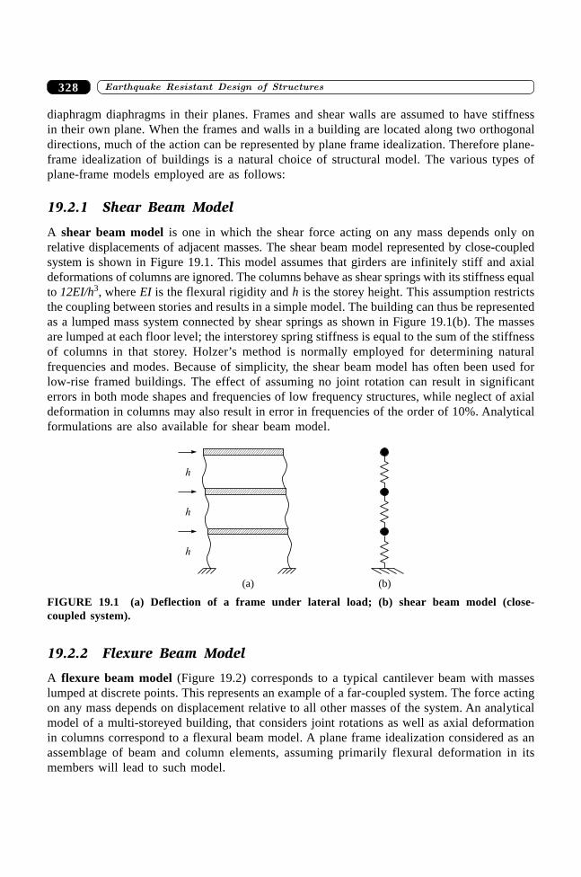
����������������� ������ ������������328
diaphragm diaphragms in their planes. Frames and shear walls are assumed to have stiffnessin their own plane. When the frames and walls in a building are located along two orthogonaldirections, much of the action can be represented by plane frame idealization. Therefore plane-frame idealization of buildings is a natural choice of structural model. The various types ofplane-frame models employed are as follows:
19.2.1 Shear Beam Model
A shear beam model is one in which the shear force acting on any mass depends only onrelative displacements of adjacent masses. The shear beam model represented by close-coupledsystem is shown in Figure 19.1. This model assumes that girders are infinitely stiff and axialdeformations of columns are ignored. The columns behave as shear springs with its stiffness equalto 12EI/h3, where EI is the flexural rigidity and h is the storey height. This assumption restrictsthe coupling between stories and results in a simple model. The building can thus be representedas a lumped mass system connected by shear springs as shown in Figure 19.1(b). The massesare lumped at each floor level; the interstorey spring stiffness is equal to the sum of the stiffnessof columns in that storey. Holzer’s method is normally employed for determining naturalfrequencies and modes. Because of simplicity, the shear beam model has often been used forlow-rise framed buildings. The effect of assuming no joint rotation can result in significanterrors in both mode shapes and frequencies of low frequency structures, while neglect of axialdeformation in columns may also result in error in frequencies of the order of 10%. Analyticalformulations are also available for shear beam model.
h
h
h
(a) (b)
FIGURE 19.1 (a) Deflection of a frame under lateral load; (b) shear beam model (close-coupled system).
19.2.2 Flexure Beam Model
A flexure beam model (Figure 19.2) corresponds to a typical cantilever beam with masseslumped at discrete points. This represents an example of a far-coupled system. The force actingon any mass depends on displacement relative to all other masses of the system. An analyticalmodel of a multi-storeyed building, that considers joint rotations as well as axial deformationin columns correspond to a flexural beam model. A plane frame idealization considered as anassemblage of beam and column elements, assuming primarily flexural deformation in itsmembers will lead to such model.
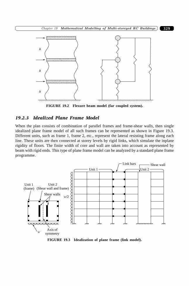
329�������� ���������������� ����������������������� ��
h
h
h
FIGURE 19.2 Flexure beam model (far coupled system).
19.2.3 Idealized Plane Frame Model
When the plan consists of combination of parallel frames and frame-shear walls, then singleidealized plane frame model of all such frames can be represented as shown in Figure 19.3.Different units, such as frame 1, frame 2, etc., represent the lateral resisting frame along eachline. These units are then connected at storey levels by rigid links, which simulate the inplanerigidity of floors. The finite width of core and wall are taken into account as represented bybeam with rigid ends. This type of plane frame model can be analyzed by a standard plane frameprogramme.
Link bars Shear wall
Unit 1 Unit 2
Unit 1(frame)
Unit 2(Shear wall and frame)
Shear wallsw/2
wAxis of
symmetry
FIGURE 19.3 Idealization of plane frame (link model).
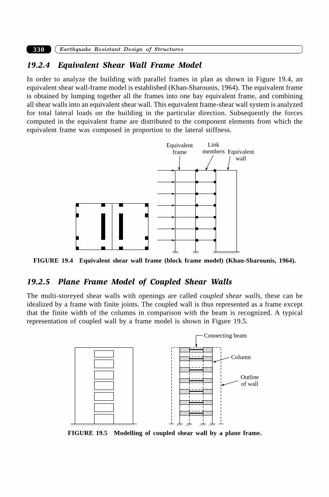
����������������� ������ ������������330
19.2.4 Equivalent Shear Wall Frame Model
In order to analyze the building with parallel frames in plan as shown in Figure 19.4, anequivalent shear wall-frame model is established (Khan-Sbarounis, 1964). The equivalent frameis obtained by lumping together all the frames into one bay equivalent frame, and combiningall shear walls into an equivalent shear wall. This equivalent frame-shear wall system is analyzedfor total lateral loads on the building in the particular direction. Subsequently the forcescomputed in the equivalent frame are distributed to the component elements from which theequivalent frame was composed in proportion to the lateral stiffness.
Equivalentframe
Linkmembers Equivalent
wall
FIGURE 19.4 Equivalent shear wall frame (block frame model) (Khan-Sbarounis, 1964).
19.2.5 Plane Frame Model of Coupled Shear Walls
The multi-storeyed shear walls with openings are called coupled shear walls, these can beidealized by a frame with finite joints. The coupled wall is thus represented as a frame exceptthat the finite width of the columns in comparison with the beam is recognized. A typicalrepresentation of coupled wall by a frame model is shown in Figure 19.5.
Connecting beam
Column
Outlineof wall
FIGURE 19.5 Modelling of coupled shear wall by a plane frame.
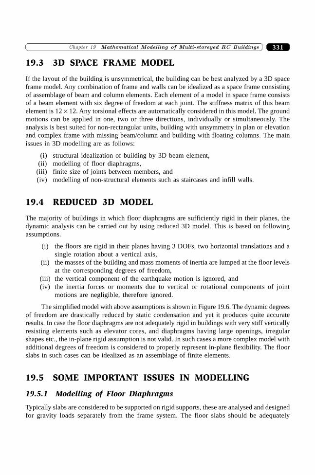
331�������� ���������������� ����������������������� ��
19.3 3D SPACE FRAME MODEL
If the layout of the building is unsymmetrical, the building can be best analyzed by a 3D spaceframe model. Any combination of frame and walls can be idealized as a space frame consistingof assemblage of beam and column elements. Each element of a model in space frame consistsof a beam element with six degree of freedom at each joint. The stiffness matrix of this beamelement is 12 ¥ 12. Any torsional effects are automatically considered in this model. The groundmotions can be applied in one, two or three directions, individually or simultaneously. Theanalysis is best suited for non-rectangular units, building with unsymmetry in plan or elevationand complex frame with missing beam/column and building with floating columns. The mainissues in 3D modelling are as follows:
(i) structural idealization of building by 3D beam element,(ii) modelling of floor diaphragms,
(iii) finite size of joints between members, and(iv) modelling of non-structural elements such as staircases and infill walls.
19.4 REDUCED 3D MODEL
The majority of buildings in which floor diaphragms are sufficiently rigid in their planes, thedynamic analysis can be carried out by using reduced 3D model. This is based on followingassumptions.
(i) the floors are rigid in their planes having 3 DOFs, two horizontal translations and asingle rotation about a vertical axis,
(ii) the masses of the building and mass moments of inertia are lumped at the floor levelsat the corresponding degrees of freedom,
(iii) the vertical component of the earthquake motion is ignored, and(iv) the inertia forces or moments due to vertical or rotational components of joint
motions are negligible, therefore ignored.
The simplified model with above assumptions is shown in Figure 19.6. The dynamic degreesof freedom are drastically reduced by static condensation and yet it produces quite accurateresults. In case the floor diaphragms are not adequately rigid in buildings with very stiff verticallyresisting elements such as elevator cores, and diaphragms having large openings, irregularshapes etc., the in-plane rigid assumption is not valid. In such cases a more complex model withadditional degrees of freedom is considered to properly represent in-plane flexibility. The floorslabs in such cases can be idealized as an assemblage of finite elements.
19.5 SOME IMPORTANT ISSUES IN MODELLING
19.5.1 Modelling of Floor Diaphragms
Typically slabs are considered to be supported on rigid supports, these are analysed and designedfor gravity loads separately from the frame system. The floor slabs should be adequately
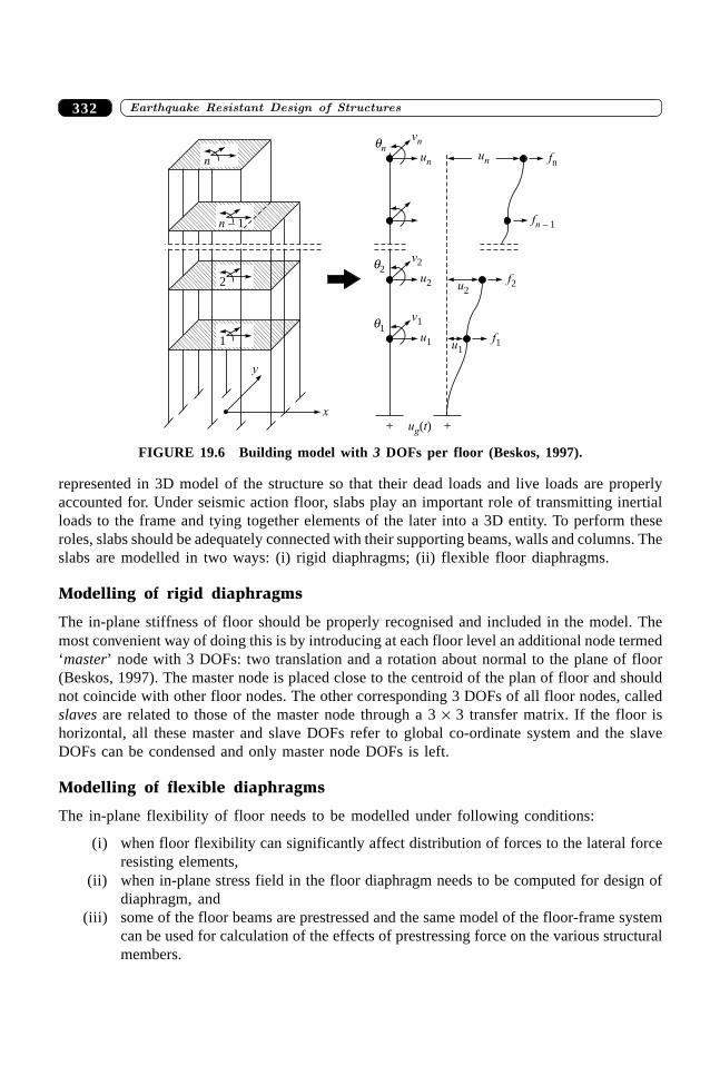
����������������� ������ ������������332
represented in 3D model of the structure so that their dead loads and live loads are properlyaccounted for. Under seismic action floor, slabs play an important role of transmitting inertialloads to the frame and tying together elements of the later into a 3D entity. To perform theseroles, slabs should be adequately connected with their supporting beams, walls and columns. Theslabs are modelled in two ways: (i) rigid diaphragms; (ii) flexible floor diaphragms.
Modelling of rigid diaphragms
The in-plane stiffness of floor should be properly recognised and included in the model. Themost convenient way of doing this is by introducing at each floor level an additional node termed‘master’ node with 3 DOFs: two translation and a rotation about normal to the plane of floor(Beskos, 1997). The master node is placed close to the centroid of the plan of floor and shouldnot coincide with other floor nodes. The other corresponding 3 DOFs of all floor nodes, calledslaves are related to those of the master node through a 3 ¥ 3 transfer matrix. If the floor ishorizontal, all these master and slave DOFs refer to global co-ordinate system and the slaveDOFs can be condensed and only master node DOFs is left.
Modelling of flexible diaphragms
The in-plane flexibility of floor needs to be modelled under following conditions:
(i) when floor flexibility can significantly affect distribution of forces to the lateral forceresisting elements,
(ii) when in-plane stress field in the floor diaphragm needs to be computed for design ofdiaphragm, and
(iii) some of the floor beams are prestressed and the same model of the floor-frame systemcan be used for calculation of the effects of prestressing force on the various structuralmembers.
1 u1
v1q1
u1f1
2 u2
v2q2
u2f2
fn – 1
n un
vnqnfn
n – 1
x
y
+ +u tg( )
un
FIGURE 19.6 Building model with 3 DOFs per floor (Beskos, 1997).
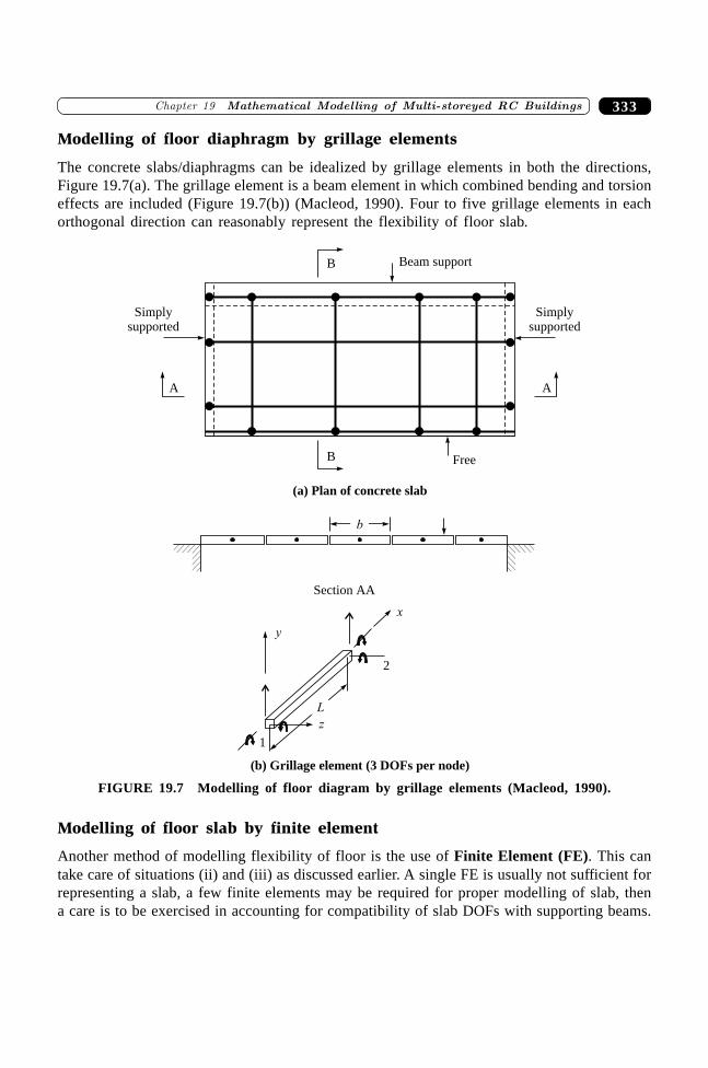
333�������� ���������������� ����������������������� ��
Modelling of floor diaphragm by grillage elements
The concrete slabs/diaphragms can be idealized by grillage elements in both the directions,Figure 19.7(a). The grillage element is a beam element in which combined bending and torsioneffects are included (Figure 19.7(b)) (Macleod, 1990). Four to five grillage elements in eachorthogonal direction can reasonably represent the flexibility of floor slab.
Simplysupported
Section AA
FreeB
B Beam support
A
Simplysupported
A
(a) Plan of concrete slab
b
y
x
z
2
1
L
(b) Grillage element (3 DOFs per node)
FIGURE 19.7 Modelling of floor diagram by grillage elements (Macleod, 1990).
Modelling of floor slab by finite element
Another method of modelling flexibility of floor is the use of Finite Element (FE). This cantake care of situations (ii) and (iii) as discussed earlier. A single FE is usually not sufficient forrepresenting a slab, a few finite elements may be required for proper modelling of slab, thena care is to be exercised in accounting for compatibility of slab DOFs with supporting beams.
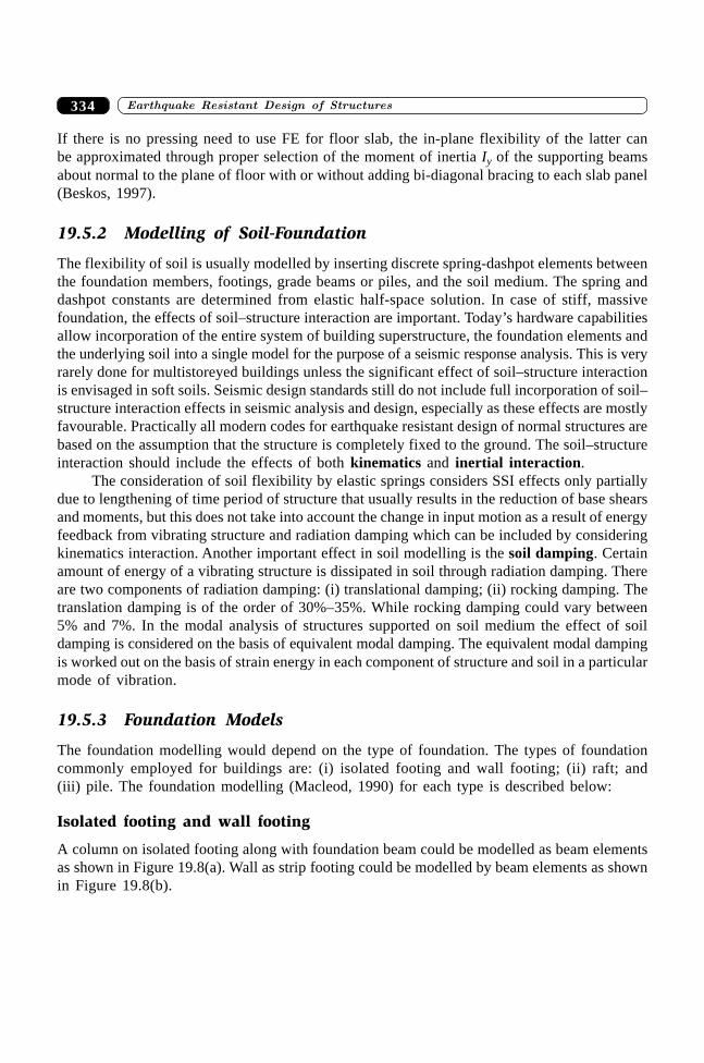
����������������� ������ ������������334
If there is no pressing need to use FE for floor slab, the in-plane flexibility of the latter canbe approximated through proper selection of the moment of inertia Iy of the supporting beamsabout normal to the plane of floor with or without adding bi-diagonal bracing to each slab panel(Beskos, 1997).
19.5.2 Modelling of Soil-Foundation
The flexibility of soil is usually modelled by inserting discrete spring-dashpot elements betweenthe foundation members, footings, grade beams or piles, and the soil medium. The spring anddashpot constants are determined from elastic half-space solution. In case of stiff, massivefoundation, the effects of soil–structure interaction are important. Today’s hardware capabilitiesallow incorporation of the entire system of building superstructure, the foundation elements andthe underlying soil into a single model for the purpose of a seismic response analysis. This is veryrarely done for multistoreyed buildings unless the significant effect of soil–structure interactionis envisaged in soft soils. Seismic design standards still do not include full incorporation of soil–structure interaction effects in seismic analysis and design, especially as these effects are mostlyfavourable. Practically all modern codes for earthquake resistant design of normal structures arebased on the assumption that the structure is completely fixed to the ground. The soil–structureinteraction should include the effects of both kinematics and inertial interaction.
The consideration of soil flexibility by elastic springs considers SSI effects only partiallydue to lengthening of time period of structure that usually results in the reduction of base shearsand moments, but this does not take into account the change in input motion as a result of energyfeedback from vibrating structure and radiation damping which can be included by consideringkinematics interaction. Another important effect in soil modelling is the soil damping. Certainamount of energy of a vibrating structure is dissipated in soil through radiation damping. Thereare two components of radiation damping: (i) translational damping; (ii) rocking damping. Thetranslation damping is of the order of 30%–35%. While rocking damping could vary between5% and 7%. In the modal analysis of structures supported on soil medium the effect of soildamping is considered on the basis of equivalent modal damping. The equivalent modal dampingis worked out on the basis of strain energy in each component of structure and soil in a particularmode of vibration.
19.5.3 Foundation Models
The foundation modelling would depend on the type of foundation. The types of foundationcommonly employed for buildings are: (i) isolated footing and wall footing; (ii) raft; and(iii) pile. The foundation modelling (Macleod, 1990) for each type is described below:
Isolated footing and wall footing
A column on isolated footing along with foundation beam could be modelled as beam elementsas shown in Figure 19.8(a). Wall as strip footing could be modelled by beam elements as shownin Figure 19.8(b).
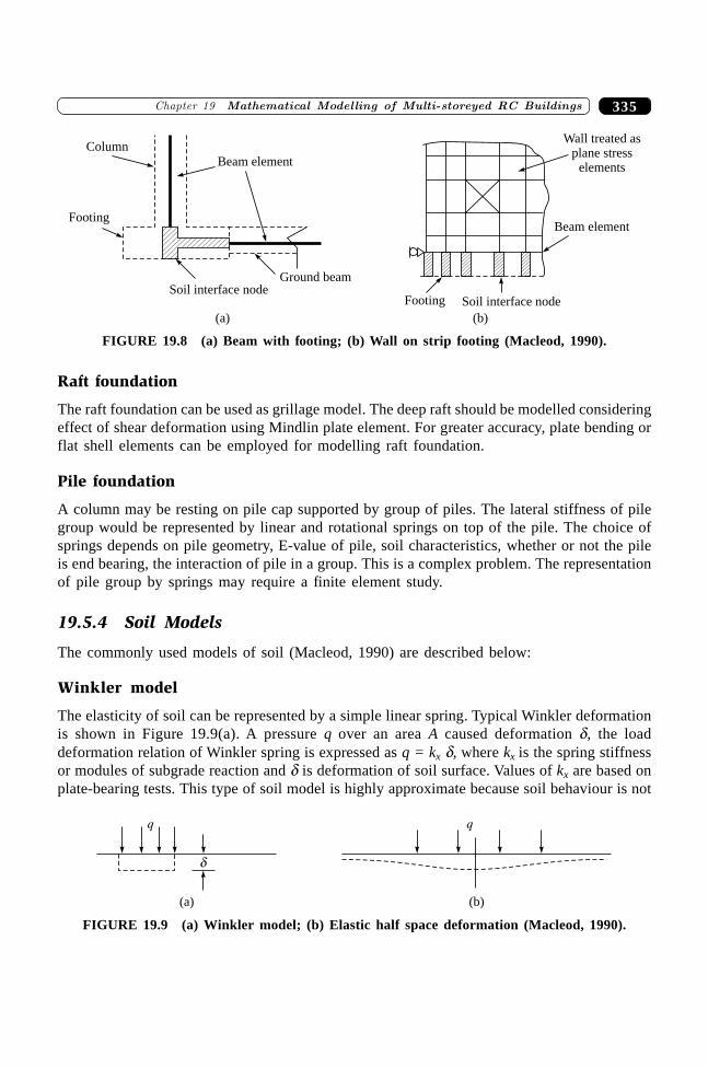
335�������� ���������������� ����������������������� ��
Column
Footing
Beam element
Soil interface nodeGround beam
Wall treated asplane stress
elements
Beam element
Footing Soil interface node
(b)(a)
FIGURE 19.8 (a) Beam with footing; (b) Wall on strip footing (Macleod, 1990).
Raft foundation
The raft foundation can be used as grillage model. The deep raft should be modelled consideringeffect of shear deformation using Mindlin plate element. For greater accuracy, plate bending orflat shell elements can be employed for modelling raft foundation.
Pile foundation
A column may be resting on pile cap supported by group of piles. The lateral stiffness of pilegroup would be represented by linear and rotational springs on top of the pile. The choice ofsprings depends on pile geometry, E-value of pile, soil characteristics, whether or not the pileis end bearing, the interaction of pile in a group. This is a complex problem. The representationof pile group by springs may require a finite element study.
19.5.4 Soil Models
The commonly used models of soil (Macleod, 1990) are described below:
Winkler model
The elasticity of soil can be represented by a simple linear spring. Typical Winkler deformationis shown in Figure 19.9(a). A pressure q over an area A caused deformation d, the loaddeformation relation of Winkler spring is expressed as q = kx d, where kx is the spring stiffnessor modules of subgrade reaction and d is deformation of soil surface. Values of kx are based onplate-bearing tests. This type of soil model is highly approximate because soil behaviour is not
q
d
q
(a) (b)
FIGURE 19.9 (a) Winkler model; (b) Elastic half space deformation (Macleod, 1990).
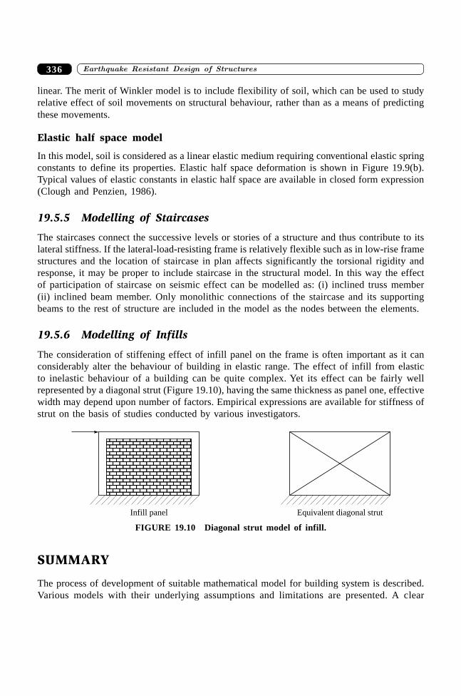
����������������� ������ ������������336
linear. The merit of Winkler model is to include flexibility of soil, which can be used to studyrelative effect of soil movements on structural behaviour, rather than as a means of predictingthese movements.
Elastic half space model
In this model, soil is considered as a linear elastic medium requiring conventional elastic springconstants to define its properties. Elastic half space deformation is shown in Figure 19.9(b).Typical values of elastic constants in elastic half space are available in closed form expression(Clough and Penzien, 1986).
19.5.5 Modelling of Staircases
The staircases connect the successive levels or stories of a structure and thus contribute to itslateral stiffness. If the lateral-load-resisting frame is relatively flexible such as in low-rise framestructures and the location of staircase in plan affects significantly the torsional rigidity andresponse, it may be proper to include staircase in the structural model. In this way the effectof participation of staircase on seismic effect can be modelled as: (i) inclined truss member(ii) inclined beam member. Only monolithic connections of the staircase and its supportingbeams to the rest of structure are included in the model as the nodes between the elements.
19.5.6 Modelling of Infills
The consideration of stiffening effect of infill panel on the frame is often important as it canconsiderably alter the behaviour of building in elastic range. The effect of infill from elasticto inelastic behaviour of a building can be quite complex. Yet its effect can be fairly wellrepresented by a diagonal strut (Figure 19.10), having the same thickness as panel one, effectivewidth may depend upon number of factors. Empirical expressions are available for stiffness ofstrut on the basis of studies conducted by various investigators.
Infill panel Equivalent diagonal strut
FIGURE 19.10 Diagonal strut model of infill.
SUMMARY
The process of development of suitable mathematical model for building system is described.Various models with their underlying assumptions and limitations are presented. A clear
337�������� ���������������� ����������������������� ��
understanding of these modelling issues will greatly facilitate an automated design of structuralsystems by the use of an appropriate computer software.
REFERENCES
[1] Beskos, D.E. and Anagnostopoulos, S.A., Computer Analysis and Design of EarthquakeResistant Structures—A Handbook, Principles of Earthquake Resistant Design byJ.M. Roesset, (ch. 7, p. 333), Buildings by S.A. Anagnostopoulos, (ch. 8, 369),Reinforced Concrete Structures by M.N. Fardis, (ch. 9, p. 441), ComputationalMechanics Publications, 1997.
[2] Clough and Penzien, Dynamics of Structures, McGraw-Hill, International Editions,1986.
[3] Fintel, Mark, Handbook of Concrete Engineering, Multi-storey Structures (ch. 10) byMark Fintel Earthquake Resistant Structures (ch. 12), by Aranaldo T. Derecho andMark Fintel, Van Nostrand Reinhold Company.
[4] Farzad Naim, The Seismic Design Handbook, 2nd ed., Van Nostrand ReinholdCompany, New York, 2001.
[5] Macleod, I.A., Analytical Modelling of Structural Systems, Ellis Horwood, England,1990.
[6] Khan, F.R. and Sbarounis, J.A., “Interaction of Shear Wall and Frames”, Proceedingsof ASCE, 90 (St 3). 285–335, June, 1964.

���� �
Earthquake Resistant Design(ERD) of Reinforced
Concrete Buildings

341
Ductility Considerations inEarthquake Resistant
Design of RC Buildings
��������
20.1 INTRODUCTION
As per IS 1893 (Part 1): 2002, Clause 6.1.3, “Actual forces that appear on structures duringearthquakes are much higher than the design forces specified in the code.” It is recognized thatneither the complete protection against earthquakes of all sizes is economically feasible nordesign alone based on strength criteria is justified. The basic approach of earthquake resistantdesign should be based on lateral strength as well as deformability and ductility capacity ofstructure with limited damage but no collapse. The code IS 13920: 1993 entitled “DuctileDetailing of Reinforced Concrete Structures Subjected to Seismic Forces—Code of Practice” isbased on this approach. This standard covers the requirements of lateral strength designing anddetailing of monolithic reinforced concrete buildings so as to give them adequate toughness andductility to resist severe earthquake shock without collapse. Thus, the ductility of a structure isin fact one of the most important factors affecting its seismic performance and it has been clearlyobserved that the well-designed and detailed reinforced structures behave well duringearthquakes and “the gap between the actual and design lateral forces is narrowed down byproviding ductility in the structure.”
Ductility in the structures will arise from inelastic material behaviour and detailing ofreinforcement in such a manner that brittle failure is avoided and ductile behaviour is inducedby allowing steel to yield in controlled manner. Therefore, one of the primary tasks of anengineer designing an earthquake resistant building is to ensure that the building will possessenough ductility to withstand the size and types of earthquakes, which it is likely to experienceduring its lifetime.
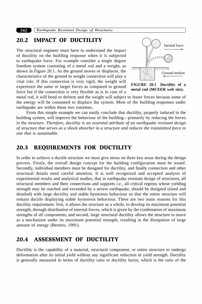
����������� ������� �������������342
20.2 IMPACT OF DUCTILITY
The structural engineer must have to understand the impactof ductility on the building response when it is subjectedto earthquake force. For example consider a single degreefreedom system consisting of a metal rod and a weight, asshown in Figure 20.1. As the ground moves or displaces, thecharacteristics of the ground to weight connection will play avital role. If this connection is very rigid, the weight willexperience the same or larger forces as compared to groundforce but if the connection is very flexible as is in case of ametal rod, it will bend or deform and the weight will subject to lesser forces because some ofthe energy will be consumed to displace the system. Most of the building responses underearthquake are within these two extremes.
From this simple example we can easily conclude that ductility, properly induced in thebuilding system, will improve the behaviour of the building—primarily by reducing the forcesin the structure. Therefore, ductility is an essential attribute of an earthquake resistant designof structure that serves as a shock absorber in a structure and reduces the transmitted force toone that is sustainable.
20.3 REQUIREMENTS FOR DUCTILITY
In order to achieve a ductile structure we must give stress on three key areas during the designprocess. Firstly, the overall design concept for the building configuration must be sound.Secondly, individual members must be designed for ductility, and finally connection and otherstructural details need careful attention. It is well recognized and accepted analysis ofexperimental results and analytical studies, that in earthquake resistant design of structures, allstructural members and their connections and supports i.e., all critical regions whose yieldingstrength may be reached and exceeded by a severe earthquake, should be designed (sized anddetailed) with large ductility and stable hysteresis behaviour so that the entire structure willremain ductile displaying stable hysteresis behaviour. There are two main reasons for thisductility requirement: first, it allows the structure as a whole, to develop its maximum potentialstrength, through distribution of internal forces, which is given by the combination of maximumstrengths of all components; and second, large structural ductility allows the structure to moveas a mechanism under its maximum potential strength, resulting in the dissipation of largeamount of energy (Bertero, 1991).
20.4 ASSESSMENT OF DUCTILITY
Ductility is the capability of a material, structural component, or entire structure to undergodeformation after its initial yield without any significant reduction in yield strength. Ductilityis generally measured in terms of ductility ratio or ductility factor, which is the ratio of the
Inertial force
Ground motion
FIGURE 20.1 Ductility of ametal rod (MCEER web site).
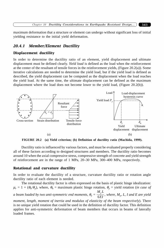
343�������� ���� � ������ ���� ��� ������������ ������� �����
maximum deformation that a structure or element can undergo without significant loss of initialyielding resistance to the initial yield deformation.
20.4.1 Member/Element Ductility
Displacement ductility
In order to determine the ductility ratio of an element, yield displacement and ultimatedisplacement must be defined clearly. Yield load is defined as the load when the reinforcementat the center of the resultant of tensile forces in the reinforcement yields, (Figure 20.2(a)). Someiterative calculations are needed to determine the yield load, but if the yield load is defined asdescribed, the yield displacement can be computed as the displacement when the load reachesthe yield load. At the same time, the ultimate displacement can be defined as the maximumdisplacement where the load does not become lower to the yield load, (Figure 20.2(b)).
Cross-section Strain distribution Tensile forcedistribution
Resultantforce
Load
Yield load Py
Load-displacementhysteresis curve
dy
Yielddisplacement
du
Ultimatedisplacement
(a) (b)
es = ey
FIGURE 20.2 (a) Yield criterion; (b) Definition of ductility ratio (Machida, 1999).
Ductility ratio is influenced by various factors, and must be evaluated properly consideringall of these factors according to designed structures and members. The ductility ratio becomesaround 10 when the axial compressive stress, compressive strength of concrete and yield strengthof reinforcement are in the range of 1 MPa, 20–30 MPa, 300–400 MPa, respectively.
Rotational and curvature ductility
In order to evaluate the ductility of a structure, curvature ductility ratio or rotation angleductility ratio of each element is needed.
The rotational ductility factor is often expressed on the basis of plastic hinge idealization:mr = 1 + (qh/qy), where, qh = maximum plastic hinge rotation, qy = yield rotation (in case of
a beam loaded by two anti-symmetric end moments, qy = M L
EIy
6, where, My, L, I and E are yield
moment, length, moment of inertia and modulus of elasticity of the beam respectively). Thereis no unique yield rotation that could be used in the definition of ductility factor. This definitionapplies for anti-symmetric deformation of beam members that occurs in beams of laterallyloaded frames.
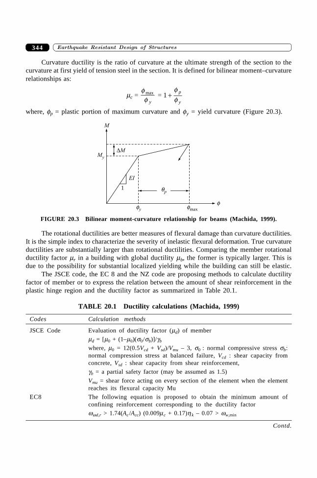
����������� ������� �������������344
Curvature ductility is the ratio of curvature at the ultimate strength of the section to thecurvature at first yield of tension steel in the section. It is defined for bilinear moment–curvaturerelationships as:
mc = ffmax
y = 1 +
ff
p
y
where, fp = plastic portion of maximum curvature and fy = yield curvature (Figure 20.3).
EI
1
M
My
�M
qp
fy fmax
f
FIGURE 20.3 Bilinear moment-curvature relationship for beams (Machida, 1999).
The rotational ductilities are better measures of flexural damage than curvature ductilities.It is the simple index to characterize the severity of inelastic flexural deformation. True curvatureductilities are substantially larger than rotational ductilities. Comparing the member rotationalductility factor mr in a building with global ductility mb, the former is typically larger. This isdue to the possibility for substantial localized yielding while the building can still be elastic.
The JSCE code, the EC 8 and the NZ code are proposing methods to calculate ductilityfactor of member or to express the relation between the amount of shear reinforcement in theplastic hinge region and the ductility factor as summarized in Table 20.1.
TABLE 20.1 Ductility calculations (Machida, 1999)
Codes Calculation methods
JSCE Code Evaluation of ductility factor (md) of member
md = [m0 + (1–m0)(s0/sb)]/gb
where, m0 = 12(0.5Vcd + Vsd)/Vmu – 3, s0 : normal compressive stress sb:normal compression stress at balanced failure, Vcd : shear capacity fromconcrete, Vsd : shear capacity from shear reinforcement,
gb = a partial safety factor (may be assumed as 1.5)
Vmu = shear force acting on every section of the element when the elementreaches its flexural capacity Mu
EC8 The following equation is proposed to obtain the minimum amount ofconfining reinforcement corresponding to the ductility factor
wwd,r > 1.74(Ac /Acc) (0.009mc + 0.17)h k – 0.07 > ww,min
Contd.
345�������� ���� � ������ ���� ��� ������������ ������� �����
where, wwd,r: minimum amount of reinforcement, Ac: gross concrete area ofsection, Acc: confined concrete area of section, ww,min: 0.12 for ductile and0.08 for limited ductile structures,
mc = required curvature ductility,
hk = normalized axial force
NZ Code The following equation is derived for rectangular column
As h
sh
h ◊ ¢¢ =
A
A
p m ff
Nf A
g
c
u y t c
vt c g
( / ).
*f ff
- ◊ + ¢ ◊¢◊
RS|T|
UV|W|
-33 22
1110 006
where, Ash: total effective area of transverse bars in the direction underconsideration within centre to center spacing of hoops sets sh, h≤: dimen-sion of core of rectangular or square column at right angles to the directionof transverse bars under consideration measured to the center line of theperimeter hoop, Ag: gross area of column, Ac: core area of column, fu /fy:curvature ductility factor, pt = Ast /Ag, Ast: total area of longitudinal steel,m = fvt/0.85f ¢c, fvt: lower characteristics strength yield strength of transversesteel, f ¢c : concrete compressive cylinder strength, N*: axial compressiveload on column, f: strength reduction factor
Ash may be controlled by other requirement on transverse reinforcement.
20.4.2 Structural Ductility
Structure ductility in a global sense depends on the displacement ductility of its membersbecause response displacement of each member can be evaluated even with static analysis. Itsquantification requires a relationship between lateral loads and displacement of whole building.This may be obtained by a pushover analysis by plotting total base shear versus the top storeydisplacement or preferably, versus the displacement at the level where the resultant force Qb =S Fi is applied (Figure 20.4). The ub is determined from the work of lateral forces Fi as follows:
ub =
F u
Q
i ii
n
b
=Â
1
where Fi is the lateral force at floor i and ui its lateral displacement. The code defined that lateralforce distribution can be used for analysis. The ductility of a building may be quantified by thefactor
mb = uuy
max
For a single storey frame the relationship between the beam ductility (mm) and system ductility(mb) is,
mb = k kk kb c m
b c
//
++m1
TABLE 20.1 Contd.
Codes Calculation methods
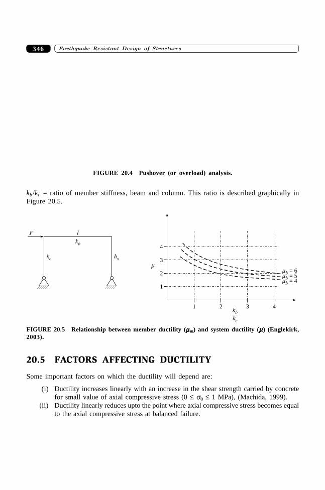
����������� ������� �������������346
kb/kc = ratio of member stiffness, beam and column. This ratio is described graphically inFigure 20.5.
F
kc
kb
hx
l
4
3
2
1
m
1 2 3 4k
kb
c
mb = 6mb = 5mb = 4
FIGURE 20.5 Relationship between member ductility (mmmmmm) and system ductility (mmmmm) (Englekirk,2003).
20.5 FACTORS AFFECTING DUCTILITY
Some important factors on which the ductility will depend are:
(i) Ductility increases linearly with an increase in the shear strength carried by concretefor small value of axial compressive stress (0 £ s0 £ 1 MPa), (Machida, 1999).
(ii) Ductility linearly reduces upto the point where axial compressive stress becomes equalto the axial compressive stress at balanced failure.
FIGURE 20.4 Pushover (or overload) analysis.
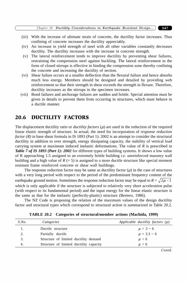
347�������� ���� � ������ ���� ��� ������������ ������� �����
(iii) With the increase of ultimate strain of concrete, the ductility factor increases. Thusconfining of concrete increases the ductility appreciably.
(iv) An increase in yield strength of steel with all other variables constantly decreasesductility. The ductility increases with the increase in concrete strength.
(v) The lateral reinforcement tends to improve ductility by preventing shear failures,restraining the compression steel against buckling. The lateral reinforcement in theform of closed stirrups is effective in binding the compression zone thereby confiningthe concrete and increasing the ductility of section.
(vi) Shear failure occurs at a smaller deflection than the flexural failure and hence absorbsmuch less energy. Members should be designed and detailed by providing webreinforcement so that their strength in shear exceeds the strength in flexure. Therefore,ductility increases as the stirrups in the specimen increases.
(vii) Bond failures and anchorage failures are sudden and brittle. Special attention must begiven in details to prevent them from occurring in structures, which must behave ina ductile manner.
20.6 DUCTILITY FACTORS
The displacement ductility ratio or ductility factors (m) are used in the reduction of the requiredlinear elastic strength of structure. In actual, the need for incorporation of response reductionfactor (R) in base shear formula in IS 1893 (Part 1): 2002 is an attempt to consider the structuralductility in addition to over strength, energy dissipating capacity, the stability of vertical loadcarrying system at maximum induced inelastic deformations. The value of R is prescribed inTable 7 of IS 1893 (Part 1): 2002 for different types of building systems. It shows a low valueof R approaching 1.5 assigned to an extremely brittle building i.e. unreinforced masonry wallbuilding and a high value of R (= 5) is assigned to a more ductile structure like special momentresistant frame reinforced concrete or shear wall buildings.
The response reduction factor may be same as ductility factor (m) in the case of structureswith a very long period with respect to the period of the predominant frequency content of theearthquake ground motion. Sometimes the response reduction factor may be equal to R = 2 1m -which is only applicable if the structure is subjected to relatively very short acceleration pulse(with respect to its fundamental period) and the input energy for the linear elastic structure isthe same as that for the inelastic (perfectly-plastic) structure (Bertero, 1986).
The NZ Code is proposing the relation of the maximum values of the design ductilityfactor and structural types which correspond to structural action is summarized in Table 20.2.
TABLE 20.2 Categories of structural/member actions (Machida, 1999)
S.No. Categories Applicable ductility factors (m)
1. Ductile structure m = 3 ~ 6
2. Partially ductile m = 3.3 ~ 6
3. Structure of limited ductility demand m < 6
4. Structure of limited ductility capacity m < 6
Contd.
����������� ������� �������������348
5. Elastic structure m = 1
6. Structure incorporating mechanicalenergy dissipating devices
7. Structure locked into the ground m = 1
20.7 DUCTILE DETAILING CONSIDERATIONSAS PER IS 13920: 1993
Provision for ductile detailing in the members of reinforced concrete buildings are given in IS13920: 1993. These provisions are for the anchorage and splices of longitudinal reinforcement,spacing, anchorage and splices of lateral reinforcement, and joint of member. It is oftenobserved in past earthquakes that the problems in structural detailing may also be a significantcause of damage. The discussions herein focus on the provision of ductile detailing provisionfor RC buildings and its possible reasons for providing structure, which will be helpful tounderstand the importance of the ductile detailing for earthquake resistant design of structure.
5.0 General Specifications
5.1 The design and construction of reinforced concrete buildings shall be governed by theprovision of IS 456: 1978 (now IS: 456: 2000), except as modified by the provisionsof this code.
5.2 For all buildings which are more than 3 stories in height, the minimum grade ofconcrete shall be M 20 (fck = 20 MPa)
Possible Explanations:
∑ The concrete strength below M 20 may not have the requisite strength in bond orshear to take full advantage of the design provisions
∑ Bending strength of a reinforced concrete member is relatively insensitive to concretecompressive, tensile and shear strength and durability, which are adversely affectedby weak concrete
5.3 Steel reinforcements of grade Fe 415 or less shall be used
Possible Explanations:
∑ For reinforcement, the provisions, firstly, of adequate ductility and secondly, of anupper limit on the yield stress or characteristic strength, are essential. It is a generalpractice to limit the yield stress of reinforcement to 415 MPa
∑ Strong steel is not preferable to low strength steel in earthquake prone region becausetypical stress strain curve of low steel shows the following advantages: (a) a long yieldplateau; (b) a greater breaking strain; and (c) less strength gain after first yield
TABLE 20.2 Contd.
S.No. Categories Applicable ductility factors (m)
349�������� ���� � ������ ���� ��� ������������ ������� �����
∑ Mild steel is more ductile and its reduced post yield strength gain is advantageous.Provided that the yield strength is confined to specified limits, design can determinesection maximum flexure strengths in order to design other areas of the structure toprevent premature brittle shear failure (capacity design approach)
∑ Mild steel should be used, as primarily reinforcement in areas where earthquakedamage is expected, such as beam in moment resisting frames Higher strength steel(with a yield strength > 300 MPa) is appropriate for other structural elements whereflexural yielding can’t occur under earthquake load
6.0 Flexural Members
6.1 General
These requirements apply to frame members resisting earthquake-induced forces anddesigned to resist flexure. These members shall satisfy the following requirements.
6.1.1 The factored axial stress on the member under earthquake loading shall not exceed 0.1fck.
Possible Explanation:
∑ Generally, axial force in the flexural member is relatively very less but if factoredaxial compressive stress in the frame member exceeds to 0.1fck, axial force will alsobe considered besides bending and member will be designed as per clause 7.0
6.1.2 The member shall preferably have a width to depth ratio of more than 0.3.
Possible Explanations:
∑ To provide more uniform design approach∑ To minimize the risk of lateral instability∑ Experience gained from past
6.1.3 The width of the member shall not be less than 200 mm.
Possible Explanations:
∑ To decrease the sensitivity to geometric error∑ Experience gained from practice with RC frames resisting earthquake induced forces
6.1.4 The depth D of the member shall preferably be not more than one-fourth of the clear span.
Possible Explanations:
∑ To take into account the non-linearity of strain distribution and lateral buckling∑ Experimental evidence indicates that under load reversals or displacement into
nonlinear range, the behaviour of continuous members having length to depth ratiosof less than four is significantly different from the behaviour of relatively slendermembers
6.2 Longitudinal Reinforcement
6.2.1 (a) The top as well as bottom reinforcement shall consist of at least two bars throughoutthe member length.
����������� ������� �������������350
Possible Explanations:
∑ To ensure integrity of the member under reversed loading∑ It is a construction requirement rather than behavioral requirement
6.2.1 (b) The tension steel ratio on any face, at any section, shall not be less than rmin =0.24÷fck /fy , where fck and fy are in MPa.
Possible Explanation:
∑ To provide necessary ductility or to avoid brittle failure upon cracking
6.2.2 The maximum steel ratio on any face at any section shall not exceed pmax = 0.025.
Possible Explanations:
∑ To avoid steel congestion and limit shear stresses in beams of typical proportions∑ Practically, low steel ratio should be used whenever possible
6.2.3 The positive steel at a joint face must be at least equal to half of the negative steel atthat face.
Possible Explanations:
∑ To ensure adequate ductility at potential plastic hinge regions, and to ensure thatminimum tension reinforcement is present for moment reversal
∑ To allow the possibility of the positive moment at the end of a beam due to earthquakeinduced lateral displacements exceeding the negative moments due to gravity loads
∑ To produce balanced conditions and limit the incorrect assumption such as linearstrain distribution, well defined yield point for the steel, limiting compressive strainin concrete of 0.003 and compressive stress in the shell concrete
6.2.4 The steel provided at each of the top and bottom face of the member at any section alongits length shall be at least equal to one-fourth of the maximum negative moment steelprovided at the face of either joint. It may be clarified that redistribution of momentspermitted in IS 456:1978 (clause 36.1) will be used only for vertical load moments andnot for lateral load moments
Possible Explanations:
∑ This is to ensure some positive and negative moment capacity throughout the beamin order to allow unexpected deformations and moment distribution from severeearthquake action
∑ To allow the possibility of the positive moment at the end of a beam due to earthquakeinduced lateral displacements exceeding the negative moments due to gravity loads
∑ To produce balanced conditions and limit the incorrect assumption such as linearstrain distribution, well defined yield point for the steel, limiting compressive strainin concrete of 0.003 and compressive stress in the shell concrete
6.2.5 In an external joint, both the top and the bottom bars of the beam shall be provided withanchorage length, beyond the inner face of the column, equal to the development length intension plus 10 times the bar diameter minus the allowance for 90 degrees bend(s). In aninternal joint, both face bars of the beam shall be taken continuously through the column.
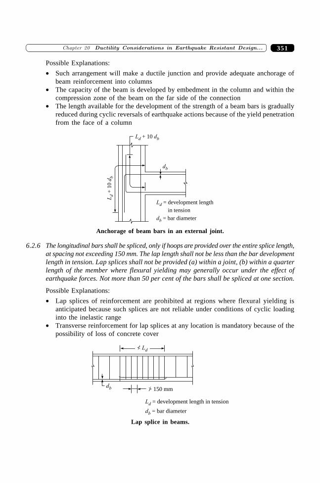
351�������� ���� � ������ ���� ��� ������������ ������� �����
Possible Explanations:
∑ Such arrangement will make a ductile junction and provide adequate anchorage ofbeam reinforcement into columns
∑ The capacity of the beam is developed by embedment in the column and within thecompression zone of the beam on the far side of the connection
∑ The length available for the development of the strength of a beam bars is graduallyreduced during cyclic reversals of earthquake actions because of the yield penetrationfrom the face of a column
L dd b+ 10
Ld
db
+10
db
db = bar diameter
Ld = development length
in tension
Anchorage of beam bars in an external joint.
6.2.6 The longitudinal bars shall be spliced, only if hoops are provided over the entire splice length,at spacing not exceeding 150 mm. The lap length shall not be less than the bar developmentlength in tension. Lap splices shall not be provided (a) within a joint, (b) within a quarterlength of the member where flexural yielding may generally occur under the effect ofearthquake forces. Not more than 50 per cent of the bars shall be spliced at one section.
Possible Explanations:
∑ Lap splices of reinforcement are prohibited at regions where flexural yielding isanticipated because such splices are not reliable under conditions of cyclic loadinginto the inelastic range
∑ Transverse reinforcement for lap splices at any location is mandatory because of thepossibility of loss of concrete cover
db > 150 mm
Ld = development length in tension
db = bar diameter
< Ld
Lap splice in beams.
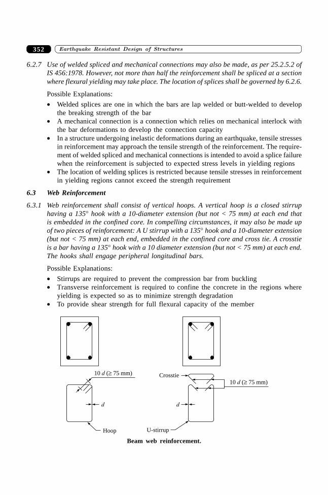
����������� ������� �������������352
6.2.7 Use of welded spliced and mechanical connections may also be made, as per 25.2.5.2 ofIS 456:1978. However, not more than half the reinforcement shall be spliced at a sectionwhere flexural yielding may take place. The location of splices shall be governed by 6.2.6.
Possible Explanations:
∑ Welded splices are one in which the bars are lap welded or butt-welded to developthe breaking strength of the bar
∑ A mechanical connection is a connection which relies on mechanical interlock withthe bar deformations to develop the connection capacity
∑ In a structure undergoing inelastic deformations during an earthquake, tensile stressesin reinforcement may approach the tensile strength of the reinforcement. The require-ment of welded spliced and mechanical connections is intended to avoid a splice failurewhen the reinforcement is subjected to expected stress levels in yielding regions
∑ The location of welding splices is restricted because tensile stresses in reinforcementin yielding regions cannot exceed the strength requirement
6.3 Web Reinforcement
6.3.1 Web reinforcement shall consist of vertical hoops. A vertical hoop is a closed stirruphaving a 135∞ hook with a 10-diameter extension (but not < 75 mm) at each end thatis embedded in the confined core. In compelling circumstances, it may also be made upof two pieces of reinforcement: A U stirrup with a 135∞ hook and a 10-diameter extension(but not < 75 mm) at each end, embedded in the confined core and cross tie. A crosstieis a bar having a 135∞ hook with a 10 diameter extension (but not < 75 mm) at each end.The hooks shall engage peripheral longitudinal bars.
Possible Explanations:
∑ Stirrups are required to prevent the compression bar from buckling∑ Transverse reinforcement is required to confine the concrete in the regions where
yielding is expected so as to minimize strength degradation∑ To provide shear strength for full flexural capacity of the member
d d
Hoop U-stirrup
10 ( 75 mm)d �
10 ( 75 mm)d �
Crosstie
Beam web reinforcement.
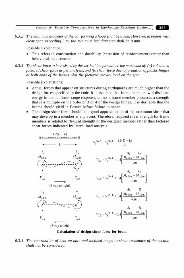
353�������� ���� � ������ ���� ��� ������������ ������� �����
6.3.2 The minimum diameter of the bar forming a hoop shall be 6 mm. However, in beams withclear span exceeding 5 m, the minimum bar diameter shall be 8 mm.
Possible Explanation:
∑ This refers to construction and durability (corrosion of reinforcement) rather thanbehavioral requirements
6.3.3 The shear force to be resisted by the vertical hoops shall be the maximum of: (a) calculatedfactored shear force as per analysis, and (b) shear force due to formation of plastic hingesat both ends of the beams plus the factored gravity load on the span.
Possible Explanations:
∑ Actual forces that appear on structures during earthquakes are much higher than thedesign forces specified in the code, it is assumed that frame members will dissipateenergy in the nonlinear range response, unless a frame member possesses a strengththat is a multiple on the order of 3 or 4 of the design forces. It is desirable that thebeams should yield in flexure before failure in shear
∑ The design shear force should be a good approximation of the maximum shear thatmay develop in a member at any event. Therefore, required shear strength for framemembers is related to flexural strength of the designed member rather than factoredshear forces indicated by lateral load analysis
L
A B1.2( + )D L
A
Ms
u,lim
Vu a,
B
Mh
u,lim
Vu b,
(Sway to right)
A
Mh
u,lim
Vu a,
B
Ms
u,lim
Vu b,
(Sway to left)
V VD L
A B
V VM M
L
A B
V VM M
L
A B
V VM M
L
A B
V VM M
L
aD L
bD L
s h
u a aD L u u
AB
s h
u b bD L u u
AB
h s
u a aD L u u
AB
h s
u b bD L u u
AB
+ +
+
+
+
+
+
-+L
NMOQP
+LNM
OQP
+LNM
OQP
-+L
NMOQP
= =
=
= +
= +
=
1 22
1
1
1
1
. ( )
.4
.4
.4
.4
,,lim ,lim
,,lim ,lim
,,lim ,lim
,,lim ,lim
Calculation of design shear force for beam.
6.3.4 The contribution of bent up bars and inclined hoops to shear resistance of the sectionshall not be considered.
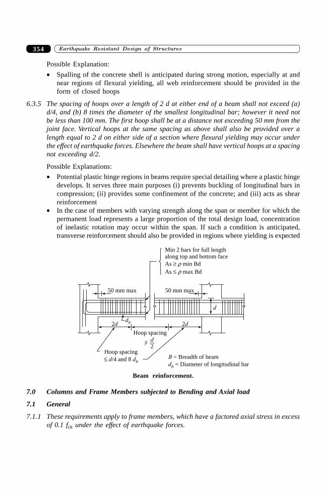
����������� ������� �������������354
Possible Explanation:
∑ Spalling of the concrete shell is anticipated during strong motion, especially at andnear regions of flexural yielding, all web reinforcement should be provided in theform of closed hoops
6.3.5 The spacing of hoops over a length of 2 d at either end of a beam shall not exceed (a)d/4, and (b) 8 times the diameter of the smallest longitudinal bar; however it need notbe less than 100 mm. The first hoop shall be at a distance not exceeding 50 mm from thejoint face. Vertical hoops at the same spacing as above shall also be provided over alength equal to 2 d on either side of a section where flexural yielding may occur underthe effect of earthquake forces. Elsewhere the beam shall have vertical hoops at a spacingnot exceeding d/2.
Possible Explanations:
∑ Potential plastic hinge regions in beams require special detailing where a plastic hingedevelops. It serves three main purposes (i) prevents buckling of longitudinal bars incompression; (ii) provides some confinement of the concrete; and (iii) acts as shearreinforcement
∑ In the case of members with varying strength along the span or member for which thepermanent load represents a large proportion of the total design load, concentrationof inelastic rotation may occur within the span. If such a condition is anticipated,transverse reinforcement should also be provided in regions where yielding is expected
Hoop spacing
50 mm max 50 mm max
Min 2 bars for full lengthalong top and bottom face
As min Bd� rAs max Bd� r
d2
>
Hoop spacing
/4 and 8d db�B = Breadth of beam
db = Diameter of longitudinal bar
db2d 2d
d
Beam reinforcement.
7.0 Columns and Frame Members subjected to Bending and Axial load
7.1 General
7.1.1 These requirements apply to frame members, which have a factored axial stress in excessof 0.1 fck under the effect of earthquake forces.
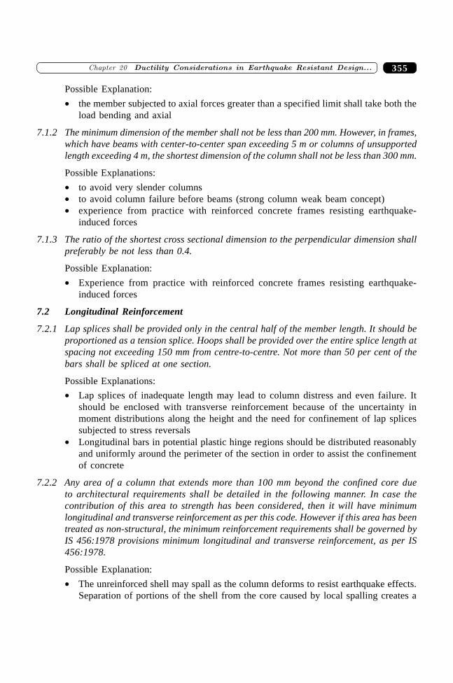
355�������� ���� � ������ ���� ��� ������������ ������� �����
Possible Explanation:
∑ the member subjected to axial forces greater than a specified limit shall take both theload bending and axial
7.1.2 The minimum dimension of the member shall not be less than 200 mm. However, in frames,which have beams with center-to-center span exceeding 5 m or columns of unsupportedlength exceeding 4 m, the shortest dimension of the column shall not be less than 300 mm.
Possible Explanations:
∑ to avoid very slender columns∑ to avoid column failure before beams (strong column weak beam concept)∑ experience from practice with reinforced concrete frames resisting earthquake-
induced forces
7.1.3 The ratio of the shortest cross sectional dimension to the perpendicular dimension shallpreferably be not less than 0.4.
Possible Explanation:
∑ Experience from practice with reinforced concrete frames resisting earthquake-induced forces
7.2 Longitudinal Reinforcement
7.2.1 Lap splices shall be provided only in the central half of the member length. It should beproportioned as a tension splice. Hoops shall be provided over the entire splice length atspacing not exceeding 150 mm from centre-to-centre. Not more than 50 per cent of thebars shall be spliced at one section.
Possible Explanations:
∑ Lap splices of inadequate length may lead to column distress and even failure. Itshould be enclosed with transverse reinforcement because of the uncertainty inmoment distributions along the height and the need for confinement of lap splicessubjected to stress reversals
∑ Longitudinal bars in potential plastic hinge regions should be distributed reasonablyand uniformly around the perimeter of the section in order to assist the confinementof concrete
7.2.2 Any area of a column that extends more than 100 mm beyond the confined core dueto architectural requirements shall be detailed in the following manner. In case thecontribution of this area to strength has been considered, then it will have minimumlongitudinal and transverse reinforcement as per this code. However if this area has beentreated as non-structural, the minimum reinforcement requirements shall be governed byIS 456:1978 provisions minimum longitudinal and transverse reinforcement, as per IS456:1978.
Possible Explanation:
∑ The unreinforced shell may spall as the column deforms to resist earthquake effects.Separation of portions of the shell from the core caused by local spalling creates a
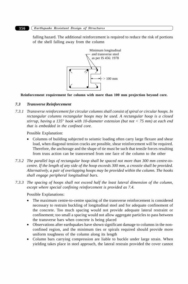
����������� ������� �������������356
falling hazard. The additional reinforcement is required to reduce the risk of portionsof the shell falling away from the column
> 100 mm
Minimum longitudinaland transverse steelas per IS 456: 1978
Reinforcement requirement for column with more than 100 mm projection beyond core.
7.3 Transverse Reinforcement
7.3.1 Transverse reinforcement for circular columns shall consist of spiral or circular hoops. Inrectangular columns rectangular hoops may be used. A rectangular hoop is a closedstirrup, having a 135∞ hook with 10-diameter extension (but not < 75 mm) at each endthat is embedded in the confined core.
Possible Explanation:
∑ Columns of building subjected to seismic loading often carry large flexure and shearload, when diagonal tension cracks are possible, shear reinforcement will be required.Therefore, the anchorage and the shape of tie must be such that tensile forces resultingfrom truss action can be transversed from one face of the column to the other
7.3.2 The parallel legs of rectangular hoop shall be spaced not more than 300 mm centre-to-centre. If the length of any side of the hoop exceeds 300 mm, a crosstie shall be provided.Alternatively, a pair of overlapping hoops may be provided within the column. The hooksshall engage peripheral longitudinal bars.
7.3.3 The spacing of hoops shall not exceed half the least lateral dimension of the column,except where special confining reinforcement is provided as 7.4.
Possible Explanations:
∑ The maximum centre-to-centre spacing of the transverse reinforcement is considerednecessary to restrain buckling of longitudinal steel and for adequate confinement ofthe concrete. Too much spacing would not provide adequate lateral restraint orconfinement; too small a spacing would not allow aggregate particles to pass betweenthe transverse bars when concrete is being placed
∑ Observations after earthquakes have shown significant damage to columns in the non-confined region, and the minimum ties or spirals required should provide moreuniform toughness of the column along its length
∑ Column bars carrying compression are liable to buckle under large strain. Whenyielding takes place in steel approach, the lateral restrain provided the cover cannot
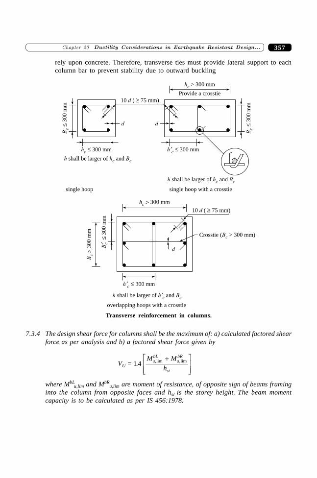
357�������� ���� � ������ ���� ��� ������������ ������� �����
rely upon concrete. Therefore, transverse ties must provide lateral support to eachcolumn bar to prevent stability due to outward buckling
Bc
300
mm
�
h¢c 300 mm�
10 (d 75 mm)�
Bc
300
mm
�d d
hc 300 mm�
hc > 300 mm
Provide a crosstie
h shall be larger of andh Bc c
h shall be larger of andh Bc c
single hoop with a crosstiesingle hoop
hc 300 mm�
10 (d 75 mm)�
Crosstie (Bc > 300 mm)
d
B¢ c
300
mm
�
Bc
300
mm
�
h¢c 300 mm�
h shall be larger of andh B¢c c
overlapping hoops with a crosstie
Transverse reinforcement in columns.
7.3.4 The design shear force for columns shall be the maximum of: a) calculated factored shearforce as per analysis and b) a factored shear force given by
VU = 1 4. ,lim ,limM M
hubL
ubR
st
+LNMM
OQPP
where MbLu,lim and MbR
u,lim are moment of resistance, of opposite sign of beams framinginto the column from opposite faces and hst is the storey height. The beam momentcapacity is to be calculated as per IS 456:1978.
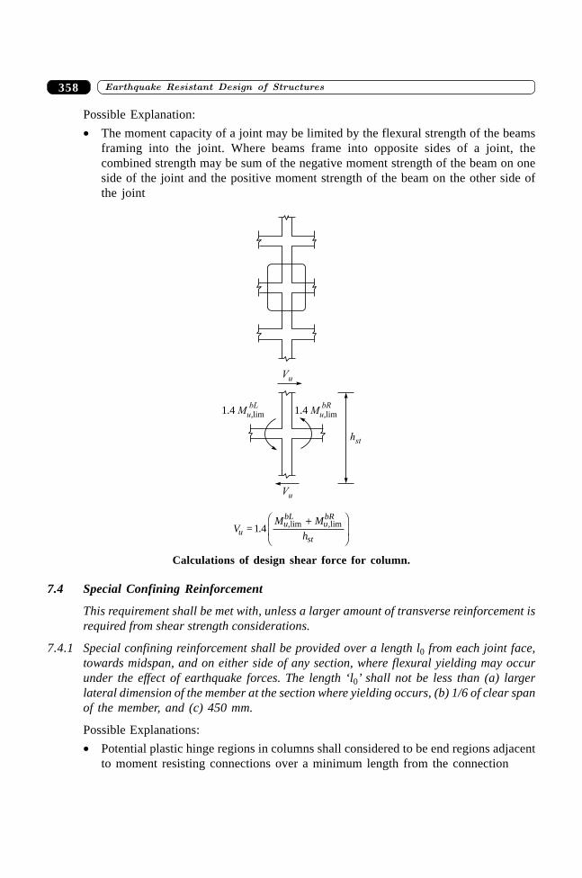
����������� ������� �������������358
Possible Explanation:
∑ The moment capacity of a joint may be limited by the flexural strength of the beamsframing into the joint. Where beams frame into opposite sides of a joint, thecombined strength may be sum of the negative moment strength of the beam on oneside of the joint and the positive moment strength of the beam on the other side ofthe joint
Vu
hst
1.4 Mu,limbL
1.4 Mu,limbR
Vu
VM M
huubL
ubR
st= 1.4 ,lim ,lim+F
HGIKJ
Calculations of design shear force for column.
7.4 Special Confining Reinforcement
This requirement shall be met with, unless a larger amount of transverse reinforcement isrequired from shear strength considerations.
7.4.1 Special confining reinforcement shall be provided over a length l0 from each joint face,towards midspan, and on either side of any section, where flexural yielding may occurunder the effect of earthquake forces. The length ‘l0’ shall not be less than (a) largerlateral dimension of the member at the section where yielding occurs, (b) 1/6 of clear spanof the member, and (c) 450 mm.
Possible Explanations:
∑ Potential plastic hinge regions in columns shall considered to be end regions adjacentto moment resisting connections over a minimum length from the connection
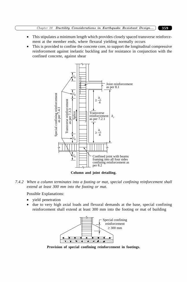
359�������� ���� � ������ ���� ��� ������������ ������� �����
∑ This stipulates a minimum length which provides closely spaced transverse reinforce-ment at the member ends, where flexural yielding normally occurs
∑ This is provided to confine the concrete core, to support the longitudinal compressivereinforcement against inelastic buckling and for resistance in conjunction with theconfined concrete, against shear
Transversereinforcementas per 7.2.1
Joint reinforcementas per 8.1
l0
l0
l0
l0
hc
4�
hc
4
hc
�
Sp
lice
Tra
nsv
erse
rein
forc
emen
tas
per
7.3
.3
Sp
ecia
lco
nfi
nin
gre
info
rcem
ent
asp
er7
.4.1
Confined joint with beamsframing into all four sidesconfining reinforcement asper 8.2
Column and joint detailing.
7.4.2 When a column terminates into a footing or mat, special confining reinforcement shallextend at least 300 mm into the footing or mat.
Possible Explanations:
∑ yield penetration∑ due to very high axial loads and flexural demands at the base, special confining
reinforcement shall extend at least 300 mm into the footing or mat of building
Special confiningreinforcement
300 mm�
Provision of special confining reinforcement in footings.
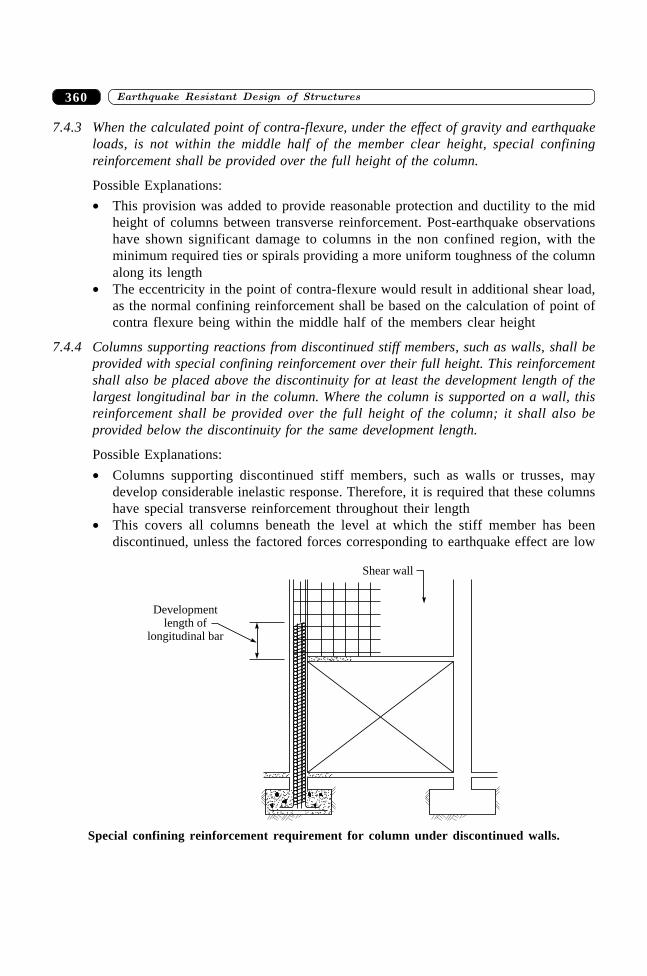
����������� ������� �������������360
7.4.3 When the calculated point of contra-flexure, under the effect of gravity and earthquakeloads, is not within the middle half of the member clear height, special confiningreinforcement shall be provided over the full height of the column.
Possible Explanations:
∑ This provision was added to provide reasonable protection and ductility to the midheight of columns between transverse reinforcement. Post-earthquake observationshave shown significant damage to columns in the non confined region, with theminimum required ties or spirals providing a more uniform toughness of the columnalong its length
∑ The eccentricity in the point of contra-flexure would result in additional shear load,as the normal confining reinforcement shall be based on the calculation of point ofcontra flexure being within the middle half of the members clear height
7.4.4 Columns supporting reactions from discontinued stiff members, such as walls, shall beprovided with special confining reinforcement over their full height. This reinforcementshall also be placed above the discontinuity for at least the development length of thelargest longitudinal bar in the column. Where the column is supported on a wall, thisreinforcement shall be provided over the full height of the column; it shall also beprovided below the discontinuity for the same development length.
Possible Explanations:
∑ Columns supporting discontinued stiff members, such as walls or trusses, maydevelop considerable inelastic response. Therefore, it is required that these columnshave special transverse reinforcement throughout their length
∑ This covers all columns beneath the level at which the stiff member has beendiscontinued, unless the factored forces corresponding to earthquake effect are low
Shear wall
Developmentlength of
longitudinal bar
Special confining reinforcement requirement for column under discontinued walls.
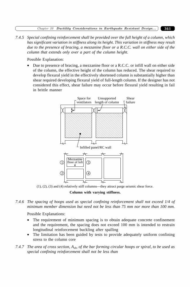
361�������� ���� � ������ ���� ��� ������������ ������� �����
7.4.5 Special confining reinforcement shall be provided over the full height of a column, whichhas significant variation in stiffness along its height. This variation in stiffness may resultdue to the presence of bracing, a mezzanine floor or a R.C.C. wall on either side of thecolumn that extends only over a part of the column height.
Possible Explanation:
∑ Due to presence of bracing, a mezzanine floor or a R.C.C. or infill wall on either sideof the column, the effective height of the column has reduced. The shear required todevelop flexural yield in the effectively shortened column is substantially higher thanshear required developing flexural yield of full-length column. If the designer has notconsidered this effect, shear failure may occur before flexural yield resulting in failin brittle manner
Space forventilators
Mezzaninefloor of loft 31
42
Infilled panel/RC wall
(1), (2), (3) and (4) relatively stiff columns—they attract parge seismic shear force.
Unsupportedlength of column
Shearfailure
Column with varying stiffness.
7.4.6 The spacing of hoops used as special confining reinforcement shall not exceed 1/4 ofminimum member dimension but need not be less than 75 mm nor more than 100 mm.
Possible Explanations:
∑ The requirement of minimum spacing is to obtain adequate concrete confinementand the requirement, the spacing does not exceed 100 mm is intended to restrainlongitudinal reinforcement buckling after spalling
∑ The limitation has been guided by tests to provide adequately uniform confiningstress to the column core
7.4.7 The area of cross section, Ash, of the bar forming circular hoops or spiral, to be used asspecial confining reinforcement shall not be less than
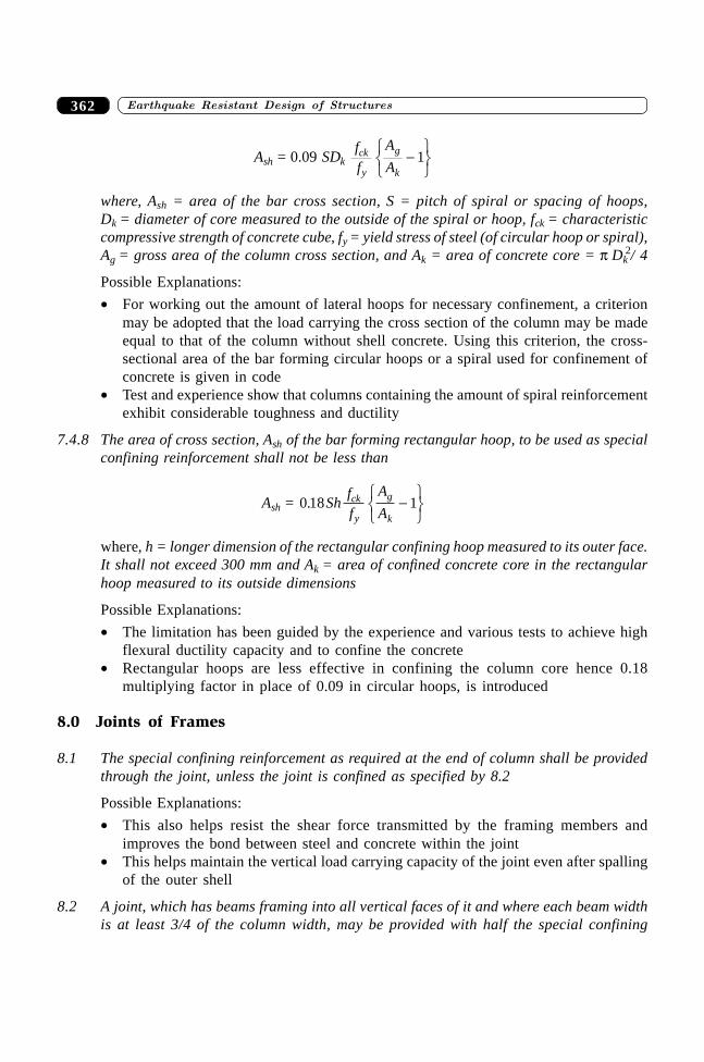
����������� ������� �������������362
Ash = 0.09 SDk ff
A
Ack
y
g
k
-RST
UVW1
where, Ash = area of the bar cross section, S = pitch of spiral or spacing of hoops,Dk = diameter of core measured to the outside of the spiral or hoop, fck = characteristiccompressive strength of concrete cube, fy = yield stress of steel (of circular hoop or spiral),Ag = gross area of the column cross section, and Ak = area of concrete core = p Dk
2/ 4
Possible Explanations:
∑ For working out the amount of lateral hoops for necessary confinement, a criterionmay be adopted that the load carrying the cross section of the column may be madeequal to that of the column without shell concrete. Using this criterion, the cross-sectional area of the bar forming circular hoops or a spiral used for confinement ofconcrete is given in code
∑ Test and experience show that columns containing the amount of spiral reinforcementexhibit considerable toughness and ductility
7.4.8 The area of cross section, Ash of the bar forming rectangular hoop, to be used as specialconfining reinforcement shall not be less than
Ash = 0 18 1. Shff
A
Ack
y
g
k
-RST
UVWwhere, h = longer dimension of the rectangular confining hoop measured to its outer face.It shall not exceed 300 mm and Ak = area of confined concrete core in the rectangularhoop measured to its outside dimensions
Possible Explanations:
∑ The limitation has been guided by the experience and various tests to achieve highflexural ductility capacity and to confine the concrete
∑ Rectangular hoops are less effective in confining the column core hence 0.18multiplying factor in place of 0.09 in circular hoops, is introduced
8.0 Joints of Frames
8.1 The special confining reinforcement as required at the end of column shall be providedthrough the joint, unless the joint is confined as specified by 8.2
Possible Explanations:
∑ This also helps resist the shear force transmitted by the framing members andimproves the bond between steel and concrete within the joint
∑ This helps maintain the vertical load carrying capacity of the joint even after spallingof the outer shell
8.2 A joint, which has beams framing into all vertical faces of it and where each beam widthis at least 3/4 of the column width, may be provided with half the special confining
363�������� ���� � ������ ���� ��� ������������ ������� �����
reinforcement required at the end of the column. The spacing of hoops shall not exceed150 mm.
Possible Explanation:
∑ The minimum transverse reinforcement required in the joint is the same as theconfinement reinforcement specified for the column ends immediately above orbelow the joint, except that where the joint is confined by elastic beams on all 4 sides,these requirements may be relaxed. This is because the rest half of the confinementis provided by the rigid beams framing into the vertical faces of the joint
9.0 Shear Walls
9.1 General Requirements
9.1.1 The requirements of this section apply to the shear walls, which are part of the lateralforce resisting system of the structure.
Possible Explanation:
∑ Wall being relative stiff elements, will in general resist all earthquake forces
9.1.2 The thickness of any part of the wall shall preferably be not less than 150 mm.
Possible Explanations:
∑ To avoid very thin section, because these sections are susceptible to lateral instabilityin zones where inelastic cyclic loading may have to be sustained
∑ To safeguard against premature out-of-plane buckling in the potential plastic hingeregion of walls
9.1.3 The effective flange width to be used in the design of flanged wall sections, shall be assumedto extend beyond the face of the web for a distance which shall be the smaller of (a) halfthe distance to an adjacent shear wall web, and (b) 1/10th of the total wall height.
Possible Explanation:
∑ Tests show that effective flange width increases with increasing drift level and theeffectiveness of a flange in compression differs from that of a flange in tension. Thevalue used for the effective compression flange width has little impact on the strengthand deformation capacity of the wall therefore to simplify design a single value ofeffective flange width based on an estimate of the effective tension flange width isused in both tension and compression
9.1.4 Shear walls shall be provided with reinforcement in the longitudinal and transversedirections in the plane of the wall. The minimum reinforcement ratio shall be 0.0025 ofthe gross area in each direction. This reinforcement shall be distributed uniformly acrossthe cross section of the wall.
Possible Explanations:
∑ The uniform distribution requirement of the shear reinforcement is related to theintent to control the width of inclined cracks
����������� ������� �������������364
9.1.5 If the factored shear stress in the wall exceeds 0.25÷fck or if the wall thickness exceeds200 mm, reinforcement shall be provided in two curtains, each having bars running in thelongitudinal and transverse directions in the plane of the wall.
Possible Explanations:
∑ The use of two curtains of reinforcement will reduce fragmentation and prematuredeterioration of the concrete under cyclic loading into the inelastic range
∑ The requirement of two layers of reinforcement in walls carrying substantial designshears is based on the observation that under ordinary construction conditions, theprobability of maintaining a single layer of reinforcement near middle of the wallsection is quite low. Furthermore, presence of reinforcement close to the surface tendsto inhibit fragmentation of the concrete in the event of severe cracking during anearthquake
9.1.6 The diameter of the bars to be used in any part of the wall shall not exceed 1/10th of thethickness of that part.
Possible Explanations:
∑ This is to prevent the use of very large diameter bars in thin wall sections∑ The maximum diameter of bars is restricted to avoid the use of large bars in thin walls
9.1.7 The maximum spacing of reinforcement in either direction shall not exceed the smaller oflw /5, 3tw, and 450 mm, where lw is the horizontal length of the wall, and tw is the thicknessof the wall web
Possible Explanation:
∑ This limitation has been guided by the experience and various tests to confine theconcrete
9.2 Shear Strength
9.2.1 The nominal shear stress tv, shall be calculated as: tv = V
t du
w w
where, Vu = factored shear force, tw = thickness of the web, and dw = effective depth ofwall section. This may be taken as 0.8 lw for rectangular sections.
Possible Explanation:
∑ The nominal shear strength of the section is computed with the nominal shear strengthprovided by concrete and shear reinforcement
9.2.2 The design shear strength of concrete tc shall be calculated as per Table 13 of IS 456:1978.
Possible Explanation:
∑ The shear carried by the concrete is affected primarily by the concrete tensile strengthand the ratio of the longitudinal steel
365�������� ���� � ������ ���� ��� ������������ ������� �����
9.2.3 The nominal shear stress in the wall tv shall not exceed tc, max ¢ as per Table 14 of IS 456:1978.
9.2.4 When tv is less than tc shear reinforcement shall be provided in accordance with 9.1.4,9.1.5 and 9.1.7.
9.2.5 When tv is greater than tc, the area of horizontal shear reinforcement, Ah, to be providedwithin a vertical spacing, Sv , is given by
Vus = 0 87. f A d
Sy h w
v
where, Vus = (Vu – tctwdw), is the shear force to be resisted by the horizontal reinforcement.However, the amount of horizontal reinforcement provided shall not be less than theminimum as per 9.1.4.
Possible Explanation:
∑ Research has shown that shear behaviour of wide beams with substantial flexuralreinforcement is improved if the transverse spacing of stirrup legs across the sectionis reduced
9.2.6 The vertical reinforcement that is uniformly distributed in the wall shall not be less thanthe horizontal reinforcement calculated as per 9.2.5.
Possible Explanation:
∑ Uniform distribution of the reinforcement across the height and width of the wallhelps control the width of inclined cracks
9.3 Flexural strength
9.3.1 The moment of resistance, Muv ¢ of the wall section may be calculated as for columnssubjected to combined bending and axial load as per IS 456 1978. The moment ofresistance of slender rectangular shear wall section with uniformly distributed verticalreinforcement is given in Annex A.
Possible Explanations:
∑ These equations were derived assuming a rectangular wall section of depth lw andthickness tw that is subjected to combine uniaxial bending and axial compression
∑ Two equations are given for calculating the flexure strength of the section. Their usedepends on whether the section fails in flexure tension or in flexure compression(Medhekar and Jain, 1993)
9.3.2 The cracked flexural strength of the wall section should be greater than its uncrackedflexural strength.
Possible Explanations:
∑ Applicable to those wall sections which, for architectural or other reasons, are muchlarger in cross section than required from strength consideration alone
∑ To prevent a brittle failure involving sudden fracture of the tension reinforcement
����������� ������� �������������366
9.3.3 In walls that do not have boundary elements, vertical reinforcement shall be concentratedat the end of the wall. Each concentration shall consist of a minimum of 4 bars of 12mm diameter arranged in at least 2 layers.
Possible Explanation:
∑ Concentrated vertical reinforcement near the edges of the wall is more effective inresisting bending moment
9.4 Boundary Element
Boundary elements are portions along the wall edges that are strengthened by longitu-dinal and transverse reinforcement. Though they may have the same thickness as that ofthe wall web, it is advantageous to provide them with greater thickness.
Possible Explanations:
∑ To consider the factor of safety as these boundary element carry all the vertical forcesat the critical wall section, when the maximum horizontal earthquake force act on thewall
∑ Wall sections having stiff and well confined boundary elements which developsubstantial flexural strength, are less susceptible to lateral buckling, and have bettershear strength and ductility in comparison to plane rectangular walls not having stiffand well confined boundary elements
9.4.1 Where the extreme fibre compressive stress in the wall due to factored gravity loads plusfactored earthquake force exceeds 0.2fck, boundary elements shall be provided along thevertical boundary of walls. The boundary elements may be discontinued where thecalculated compressive stress becomes less than 0.15fck . The compressive stress shall becalculated using a linearly elastic model and gross section properties.
Possible Explanation:∑ During severe earthquake, the flanges of a wall are subjected to high compressive and
tensile stress reversals. Hence, the concrete needs to be well confined so as to sustainthe load reversals without a large degradation in strength
9.4.2 A boundary element shall have adequate axial load carrying capacity, assuming shortcolumn action, so as to enable it to carry an axial compression equal to the sum of factoredgravity load on it and the additional compressive load induced by the seismic force. The
latter may be calculated as: ( )M M
Cu uv
w
-
where, Mu = factored design moment on the entire wall section. Muv = moment ofresistance provided by distributed vertical reinforcement across the wall section. Cw =center to center distance between the boundary elements along the two vertical edges ofthe wall.
Possible Explanation:
∑ The boundary element is assumed to be effective in resisting the design moment dueto earthquake induced forces along with the web of the wall. The axial compression
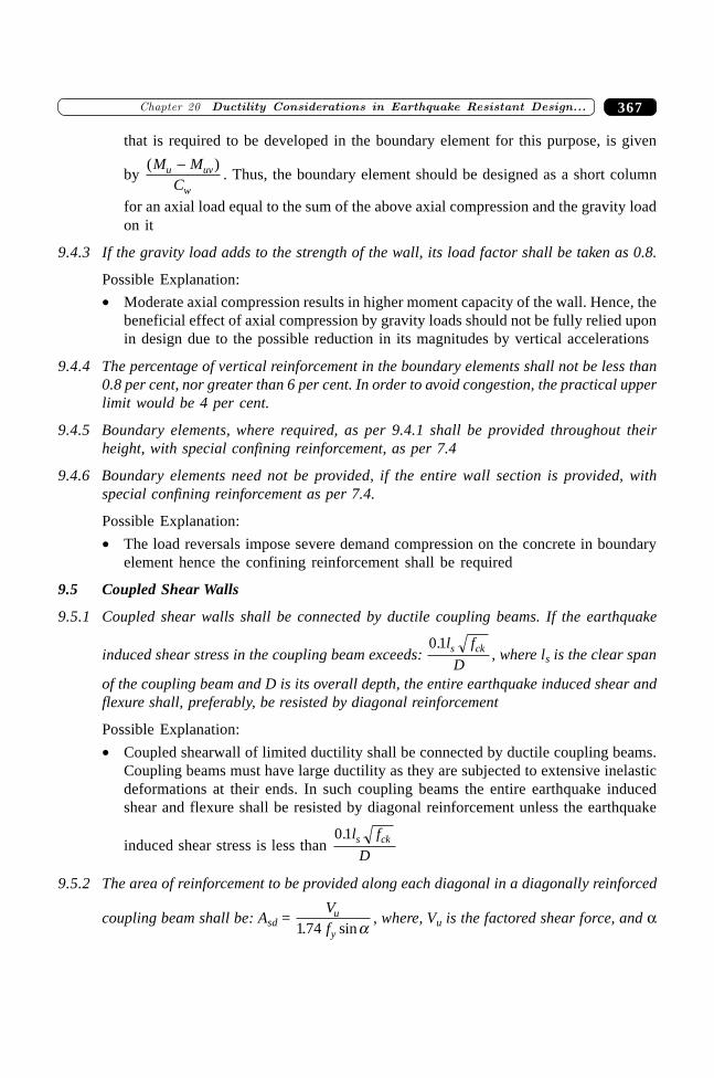
367�������� ���� � ������ ���� ��� ������������ ������� �����
that is required to be developed in the boundary element for this purpose, is given
by ( )M M
Cu uv
w
-. Thus, the boundary element should be designed as a short column
for an axial load equal to the sum of the above axial compression and the gravity loadon it
9.4.3 If the gravity load adds to the strength of the wall, its load factor shall be taken as 0.8.
Possible Explanation:
∑ Moderate axial compression results in higher moment capacity of the wall. Hence, thebeneficial effect of axial compression by gravity loads should not be fully relied uponin design due to the possible reduction in its magnitudes by vertical accelerations
9.4.4 The percentage of vertical reinforcement in the boundary elements shall not be less than0.8 per cent, nor greater than 6 per cent. In order to avoid congestion, the practical upperlimit would be 4 per cent.
9.4.5 Boundary elements, where required, as per 9.4.1 shall be provided throughout theirheight, with special confining reinforcement, as per 7.4
9.4.6 Boundary elements need not be provided, if the entire wall section is provided, withspecial confining reinforcement as per 7.4.
Possible Explanation:
∑ The load reversals impose severe demand compression on the concrete in boundaryelement hence the confining reinforcement shall be required
9.5 Coupled Shear Walls
9.5.1 Coupled shear walls shall be connected by ductile coupling beams. If the earthquake
induced shear stress in the coupling beam exceeds: 0 1. l f
Ds ck , where ls is the clear span
of the coupling beam and D is its overall depth, the entire earthquake induced shear andflexure shall, preferably, be resisted by diagonal reinforcement
Possible Explanation:
∑ Coupled shearwall of limited ductility shall be connected by ductile coupling beams.Coupling beams must have large ductility as they are subjected to extensive inelasticdeformations at their ends. In such coupling beams the entire earthquake inducedshear and flexure shall be resisted by diagonal reinforcement unless the earthquake
induced shear stress is less than 0 1. l f
Ds ck
9.5.2 The area of reinforcement to be provided along each diagonal in a diagonally reinforced
coupling beam shall be: Asd = Vf
u
y1 74. sina, where, Vu is the factored shear force, and a
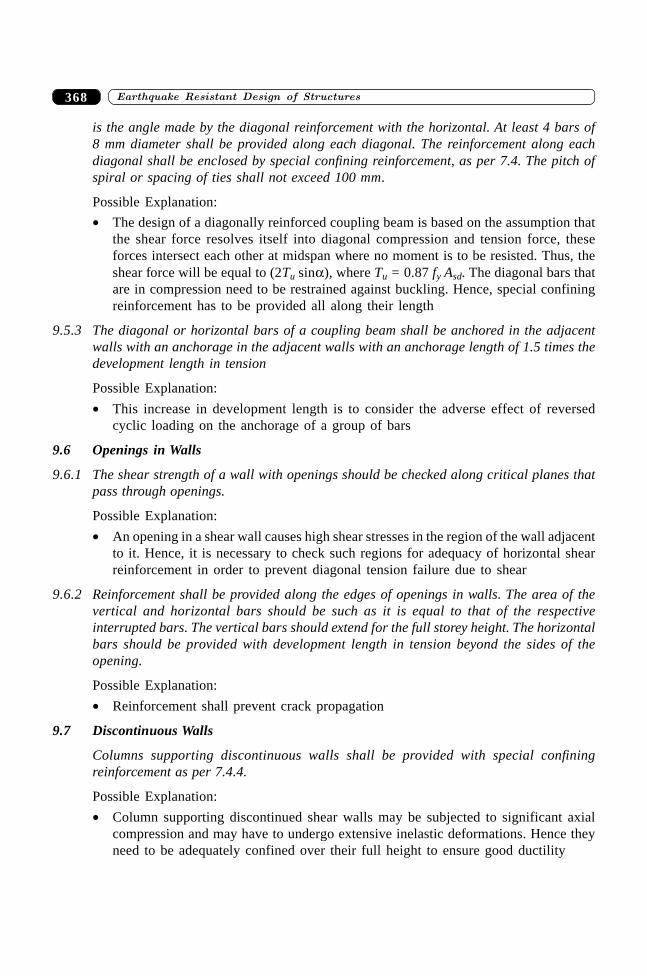
����������� ������� �������������368
is the angle made by the diagonal reinforcement with the horizontal. At least 4 bars of8 mm diameter shall be provided along each diagonal. The reinforcement along eachdiagonal shall be enclosed by special confining reinforcement, as per 7.4. The pitch ofspiral or spacing of ties shall not exceed 100 mm.
Possible Explanation:
∑ The design of a diagonally reinforced coupling beam is based on the assumption thatthe shear force resolves itself into diagonal compression and tension force, theseforces intersect each other at midspan where no moment is to be resisted. Thus, theshear force will be equal to (2Tu sina), where Tu = 0.87 fy Asd. The diagonal bars thatare in compression need to be restrained against buckling. Hence, special confiningreinforcement has to be provided all along their length
9.5.3 The diagonal or horizontal bars of a coupling beam shall be anchored in the adjacentwalls with an anchorage in the adjacent walls with an anchorage length of 1.5 times thedevelopment length in tension
Possible Explanation:
∑ This increase in development length is to consider the adverse effect of reversedcyclic loading on the anchorage of a group of bars
9.6 Openings in Walls
9.6.1 The shear strength of a wall with openings should be checked along critical planes thatpass through openings.
Possible Explanation:
∑ An opening in a shear wall causes high shear stresses in the region of the wall adjacentto it. Hence, it is necessary to check such regions for adequacy of horizontal shearreinforcement in order to prevent diagonal tension failure due to shear
9.6.2 Reinforcement shall be provided along the edges of openings in walls. The area of thevertical and horizontal bars should be such as it is equal to that of the respectiveinterrupted bars. The vertical bars should extend for the full storey height. The horizontalbars should be provided with development length in tension beyond the sides of theopening.
Possible Explanation:
∑ Reinforcement shall prevent crack propagation
9.7 Discontinuous Walls
Columns supporting discontinuous walls shall be provided with special confiningreinforcement as per 7.4.4.
Possible Explanation:
∑ Column supporting discontinued shear walls may be subjected to significant axialcompression and may have to undergo extensive inelastic deformations. Hence theyneed to be adequately confined over their full height to ensure good ductility
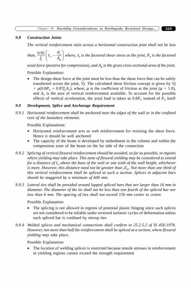
369�������� ���� � ������ ���� ��� ������������ ������� �����
9.8 Construction Joints
The vertical reinforcement ratio across a horizontal construction joint shall not be less
than, 0 92.f
PAy
vu
gt -FHG
IKJ where, tv is the factored shear stress at the joint, Pu is the factored
axial force (positive for compression), and Ag is the gross cross sectional area of the joint.
Possible Explanation:
∑ The design shear force at the joint must be less than the shear force that can be safelytransferred across the joint, Vj. The calculated shear friction concept is given by Vj= m(0.8Pu + 0.87fyAv), where, m is the coefficient of friction at the joint (m = 1.0),and Av is the area of vertical reinforcement available. To account for the possibleeffects of vertical acceleration, the axial load is taken as 0.8Pu instead of Pu itself
9.9 Development, Splice and Anchorage Requirement
9.9.1 Horizontal reinforcement shall be anchored near the edges of the wall or in the confinedcore of the boundary elements.
Possible Explanations:
∑ Horizontal reinforcement acts as web reinforcement for resisting the shear force.Hence it should be well anchored
∑ The capacity of the beam is developed by embedment in the column and within thecompression zone of the beam on the far side of the connection
9.9.2 Splicing of vertical flexural reinforcement should be avoided, as far as possible, in regionswhere yielding may take place. This zone of flexural yielding may be considered to extendfor a distance of lw above the base of the wall or one sixth of the wall height, whicheveris more. However, this distance need not be greater than 2lw. Not more than one third ofthis vertical reinforcement shall be spliced at such a section. Splices in adjacent barsshould be staggered by a minimum of 600 mm.
9.9.3 Lateral ties shall be provided around lapped spliced bars that are larger than 16 mm indiameter. The diameter of the tie shall not be less than one fourth of the spliced bar norless than 6 mm. The spacing of ties shall not exceed 150 mm center to centre.
Possible Explanation:
∑ The splicing is not allowed in regions of potential plastic hinging since such splicesare not considered to be reliable under reversed inelastic cycles of deformation unlesseach spliced bar is confined by stirrup ties
9.9.4 Welded splices and mechanical connections shall confirm to 25.2.5.2 of IS 456:1978.However, not more than half the reinforcement shall be spliced at a section, where flexuralyielding may take place.
Possible Explanation:
∑ The location of welding splices is restricted because tensile stresses in reinforcementin yielding regions cannot exceed the strength requirement
����������� ������� �������������370
SUMMARY
Ductility is one of the main attributes for earthquake resistant design of structures. To makereinforced concrete structures sufficiently ductile, various provisions are stipulated in the codeIS 13920: 1993 entitled “Ductile Detailing of Reinforced Concrete Structures Subjected toSeismic Forces”. These provisions are related to the anchorage and splices of longitudinalreinforcement, spacing, anchorage, and splicing of lateral reinforcement, special confiningreinforcement at the potential plastic hinge region, minimum size requirements for flexural,axial member etc. The ductile detailing requirement in shear wall is also discussed. The chapterdeals with the importance of ductility and a clause - by - clause explanation of IS 13920: 1993so that one can understand and appreciate its importance.
REFERENCES
[1] ACI 318M–99/318RM–99, “Building Code Requirements for Structural Concrete(318M-99) and Commentary (318RM-99)”, American Concrete Institute, FarmingtonHills, Michigan.
[2] Bertero, V.V., Anderson, J.C., Krawinkler, H., Miranda, E., et al., “Design Guidelinesfor Ductility and Drift Limits”, Report No. UCB/EERC–91/15, Earthquake EngineeringResearch Center, University of California, 1991.
[3] Bertero, V.V., “Implication of Recent Earthquakes and Research on EarthquakeResistant Design and Construction of Buildings”, Report No. UCB/EERC–86/03,Earthquake Engineering Research Center, University of California, 1986.
[4] Eurocode 8, “Design of Structures for Earthquake Resistance—Part 1: General Rules,Seismic Actions and Rules for Buildings”, CEN, (2002).
[5] Englekirk, R.E., Seismic Design of Reinforced and Precast Concrete Buildings, JohnWiley & Sons, 2003.
[6] IS 13920, “Ductile Detailing of Reinforced Concrete Structures Subjected to SeismicForces”, Edition 1.2, Bureau of Indian Standards, New Delhi, 2002-03.
[7] Machida, A., Moehle, J., Pinto, P. and Matsumoto, N., “Ductility Consideration forSingle Element and for Frame Structures”, Proceedings of Comparative Performance ofSeismic Design Codes for Concrete Structures, Vol. 1, T. Tanabe (Ed.), ElsevierScience, 1999.
[8] Machida, A., Moehle, J., Pinto, P., Park, R. and Niwa, J., “Detailing Consideration”,Proceedings of Comparative Performance of Seismic Design Codes for ConcreteStructures, Vol. 1, T. Tanabe (Ed.), Elsevier Science, 1999.
[9] Medhekar, M.S. and Jain, S.K., “Seismic Behaviour Design and Detailing of RC ShearWalls, Part 1: Behaviour and Strength”, Indian Concrete Journal, Vol. 67, No. 7,pp. 311–318, 1993.
[10] Medhekar, M.S. and Jain, S.K., “Seismic Behaviour Design and Detailing of RCShear Walls, Part II: Design and Detailing”, Indian Concrete Journal, Vol. 67, No. 9,pp. 451–457, 1993.

371�������� ���� � ������ ���� ��� ������������ ������� �����
[11] Naeim, Farzad, The Seismic Design Handbook, 2nd ed. Kluwer Academic Publisher,The Netherlands, 2001.
[12] NZS 3101, Concrete Structures Standard Part 1—The Design of Concrete Structures,Standards New Zealand, Paerewa Aotearoa, 1995.
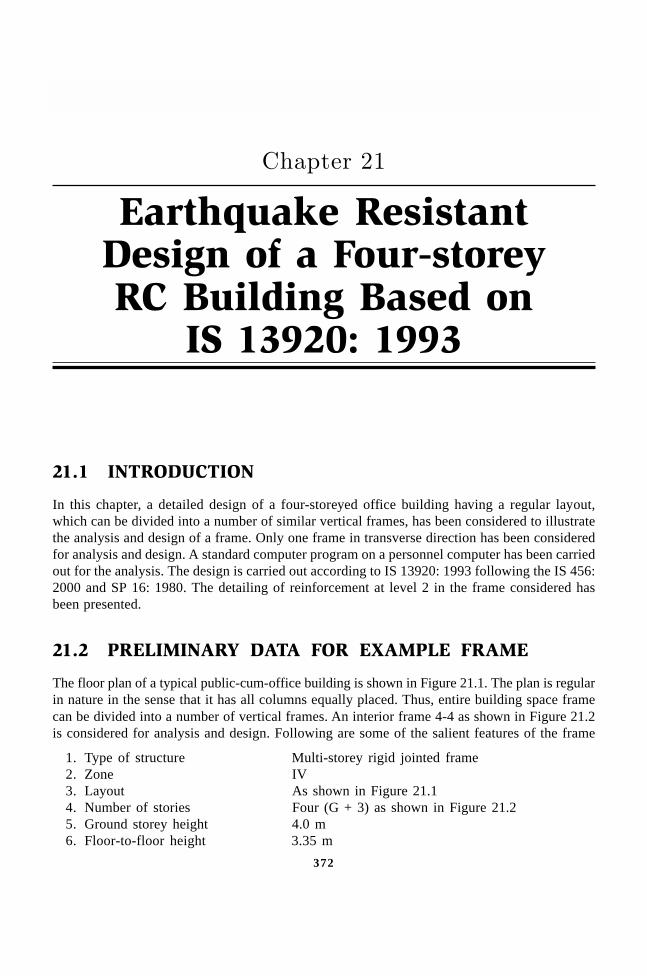
����������� ������� �������������372
372
Earthquake ResistantDesign of a Four-storeyRC Building Based on
IS 13920: 1993
��������
21.1 INTRODUCTION
In this chapter, a detailed design of a four-storeyed office building having a regular layout,which can be divided into a number of similar vertical frames, has been considered to illustratethe analysis and design of a frame. Only one frame in transverse direction has been consideredfor analysis and design. A standard computer program on a personnel computer has been carriedout for the analysis. The design is carried out according to IS 13920: 1993 following the IS 456:2000 and SP 16: 1980. The detailing of reinforcement at level 2 in the frame considered hasbeen presented.
21.2 PRELIMINARY DATA FOR EXAMPLE FRAME
The floor plan of a typical public-cum-office building is shown in Figure 21.1. The plan is regularin nature in the sense that it has all columns equally placed. Thus, entire building space framecan be divided into a number of vertical frames. An interior frame 4-4 as shown in Figure 21.2is considered for analysis and design. Following are some of the salient features of the frame
1. Type of structure Multi-storey rigid jointed frame2. Zone IV3. Layout As shown in Figure 21.14. Number of stories Four (G + 3) as shown in Figure 21.25. Ground storey height 4.0 m6. Floor-to-floor height 3.35 m
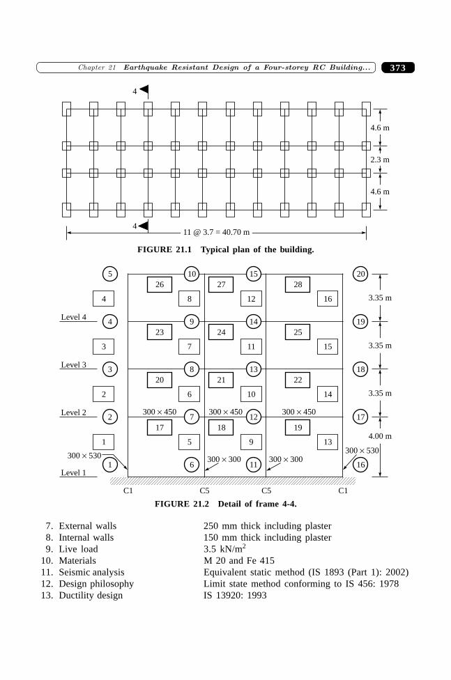
373�������� ����������� ������� ������������������� �� �����
7. External walls 250 mm thick including plaster8. Internal walls 150 mm thick including plaster9. Live load 3.5 kN/m2
10. Materials M 20 and Fe 41511. Seismic analysis Equivalent static method (IS 1893 (Part 1): 2002)12. Design philosophy Limit state method conforming to IS 456: 197813. Ductility design IS 13920: 1993
11 @ 3.7 = 40.70 m4
4
4.6 m
2.3 m
4.6 m
FIGURE 21.1 Typical plan of the building.
5 10
26
84
4 9
23
73
Level 4
3 8
20
62
Level 3
2 7
17
51
Level 2
1 6Level 1
300 300�
15
27
12
14
24
11
13
21
10
12
18
9
11300 300�
28
16
25
15
22
14
19
13300 530�
20
19
18
17
16300 530�
3.35 m
3.35 m
3.35 m
4.00 m
C1 C5 C5 C1
300 450� 300 450� 300 450�
FIGURE 21.2 Detail of frame 4-4.
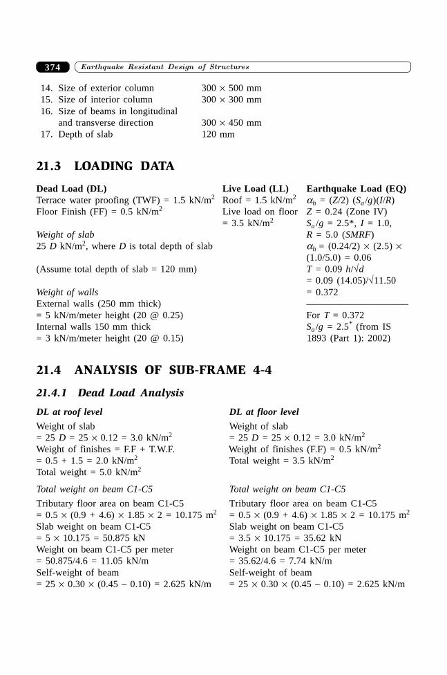
����������� ������� �������������374
14. Size of exterior column 300 ¥ 500 mm15. Size of interior column 300 ¥ 300 mm16. Size of beams in longitudinal
and transverse direction 300 ¥ 450 mm17. Depth of slab 120 mm
21.3 LOADING DATA
Dead Load (DL) Live Load (LL) Earthquake Load (EQ)Terrace water proofing (TWF) = 1.5 kN/m2 Roof = 1.5 kN/m2 ah = (Z/2) (Sa /g)(I/R)Floor Finish (FF) = 0.5 kN/m2 Live load on floor Z = 0.24 (Zone IV)
= 3.5 kN/m2 Sa /g = 2.5*, I = 1.0,Weight of slab R = 5.0 (SMRF)25 D kN/m2, where D is total depth of slab ah = (0.24/2) ¥ (2.5) ¥
(1.0/5.0) = 0.06(Assume total depth of slab = 120 mm) T = 0.09 h/÷d
= 0.09 (14.05)/÷11.50Weight of walls = 0.372External walls (250 mm thick) ——————————–= 5 kN/m/meter height (20 @ 0.25) For T = 0.372Internal walls 150 mm thick Sa /g = 2.5* (from IS= 3 kN/m/meter height (20 @ 0.15) 1893 (Part 1): 2002)
21.4 ANALYSIS OF SUB-FRAME 4-4
21.4.1 Dead Load Analysis
DL at roof level DL at floor level
Weight of slab Weight of slab= 25 D = 25 ¥ 0.12 = 3.0 kN/m2 = 25 D = 25 ¥ 0.12 = 3.0 kN/m2
Weight of finishes = F.F + T.W.F. Weight of finishes (F.F) = 0.5 kN/m2
= 0.5 + 1.5 = 2.0 kN/m2 Total weight = 3.5 kN/m2
Total weight = 5.0 kN/m2
Total weight on beam C1-C5 Total weight on beam C1-C5
Tributary floor area on beam C1-C5 Tributary floor area on beam C1-C5= 0.5 ¥ (0.9 + 4.6) ¥ 1.85 ¥ 2 = 10.175 m2 = 0.5 ¥ (0.9 + 4.6) ¥ 1.85 ¥ 2 = 10.175 m2
Slab weight on beam C1-C5 Slab weight on beam C1-C5= 5 ¥ 10.175 = 50.875 kN = 3.5 ¥ 10.175 = 35.62 kNWeight on beam C1-C5 per meter Weight on beam C1-C5 per meter= 50.875/4.6 = 11.05 kN/m = 35.62/4.6 = 7.74 kN/mSelf-weight of beam Self-weight of beam= 25 ¥ 0.30 ¥ (0.45 – 0.10) = 2.625 kN/m = 25 ¥ 0.30 ¥ (0.45 – 0.10) = 2.625 kN/m
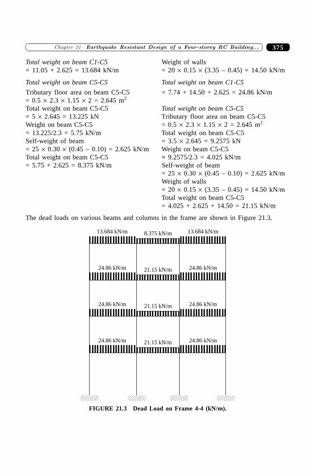
375�������� ����������� ������� ������������������� �� �����
Total weight on beam C1-C5 Weight of walls= 11.05 + 2.625 = 13.684 kN/m = 20 ¥ 0.15 ¥ (3.35 – 0.45) = 14.50 kN/m
Total weight on beam C5-C5 Total weight on beam C1-C5
Tributary floor area on beam C5-C5 = 7.74 + 14.50 + 2.625 = 24.86 kN/m= 0.5 ¥ 2.3 ¥ 1.15 ¥ 2 = 2.645 m2
Total weight on beam C5-C5 Total weight on beam C5-C5= 5 ¥ 2.645 = 13.225 kN Tributary floor area on beam C5-C5Weight on beam C5-C5 = 0.5 ¥ 2.3 ¥ 1.15 ¥ 2 = 2.645 m2
= 13.225/2.3 = 5.75 kN/m Total weight on beam C5-C5Self-weight of beam = 3.5 ¥ 2.645 = 9.2575 kN= 25 ¥ 0.30 ¥ (0.45 – 0.10) = 2.625 kN/m Weight on beam C5-C5Total weight on beam C5-C5 = 9.2575/2.3 = 4.025 kN/m= 5.75 + 2.625 = 8.375 kN/m Self-weight of beam
= 25 ¥ 0.30 ¥ (0.45 – 0.10) = 2.625 kN/mWeight of walls= 20 ¥ 0.15 ¥ (3.35 – 0.45) = 14.50 kN/mTotal weight on beam C5-C5= 4.025 + 2.625 + 14.50 = 21.15 kN/m
The dead loads on various beams and columns in the frame are shown in Figure 21.3.
13.684 kN/m 8.375 kN/m
24.86 kN/m 24.86 kN/m21.15 kN/m
21.15 kN/m24.86 kN/m 24.86 kN/m
21.15 kN/m24.86 kN/m 24.86 kN/m
13.684 kN/m
FIGURE 21.3 Dead Load on Frame 4-4 (kN/m).
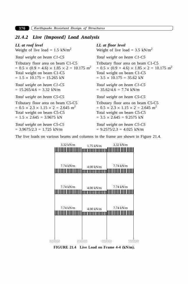
����������� ������� �������������376
21.4.2 Live (Imposed) Load Analysis
LL at roof level LL at floor levelWeight of live load = 1.5 kN/m2 Weight of live load = 3.5 kN/m2
Total weight on beam C1-C5 Total weight on beam C1-C5
Tributary floor area on beam C1-C5 Tributary floor area on beam C1-C5= 0.5 ¥ (0.9 + 4.6) ¥ 1.85 ¥ 2 = 10.175 m2 = 0.5 ¥ (0.9 + 4.6) ¥ 1.85 ¥ 2 = 10.175 m2
Total weight on beam C1-C5 Total weight on beam C1-C5= 1.5 ¥ 10.175 = 15.265 kN = 3.5 ¥ 10.175 = 35.62 kN
Total weight on beam C1-C5 Total weight on beam C1-C5= 15.265/4.6 = 3.32 kN/m = 35.62/4.6 = 7.74 kN/m
Total weight on beam C5-C5 Total weight on beam C5-C5
Tributary floor area on beam C5-C5 Tributary floor area on beam C5-C5= 0.5 ¥ 2.3 ¥ 1.15 ¥ 2 = 2.645 m2 = 0.5 ¥ 2.3 ¥ 1.15 ¥ 2 = 2.645 m2
Total weight on beam C5-C5 Total weight on beam C5-C5= 1.5 ¥ 2.645 = 3.9675 kN = 3.5 ¥ 2.645 = 9.2575 kN
Total weight on beam C5-C5 Total weight on beam C5-C5= 3.9675/2.3 = 1.725 kN/m = 9.2575/2.3 = 4.025 kN/m
The live loads on various beams and columns in the frame are shown in Figure 21.4.
3.32 kN/m 1.75 kN/m
7.74 kN/m 4.00 kN/m
3.32 kN/m
7.74 kN/m
4.00 kN/m7.74 kN/m 7.74 kN/m
4.00 kN/m7.74 kN/m 7.74 kN/m
FIGURE 21.4 Live Load on Frame 4-4 (kN/m).
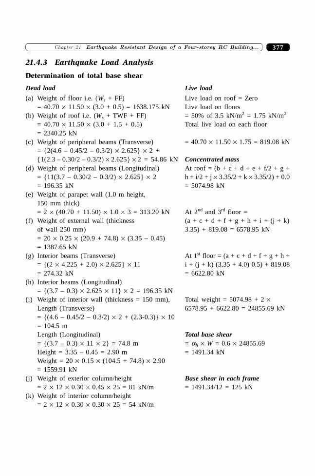
377�������� ����������� ������� ������������������� �� �����
21.4.3 Earthquake Load Analysis
Determination of total base shear
Dead load Live load
(a) Weight of floor i.e. (Ws + FF) Live load on roof = Zero= 40.70 ¥ 11.50 ¥ (3.0 + 0.5) = 1638.175 kN Live load on floors
(b) Weight of roof i.e. (Ws + TWF + FF) = 50% of 3.5 kN/m2 = 1.75 kN/m2
= 40.70 ¥ 11.50 ¥ (3.0 + 1.5 + 0.5) Total live load on each floor= 2340.25 kN
(c) Weight of peripheral beams (Transverse) = 40.70 ¥ 11.50 ¥ 1.75 = 819.08 kN= {2(4.6 – 0.45/2 – 0.3/2) ¥ 2.625} ¥ 2 +{1(2.3 – 0.30/2 – 0.3/2) ¥ 2.625} ¥ 2 = 54.86 kN Concentrated mass
(d) Weight of peripheral beams (Longitudinal) At roof = (b + c + d + e + f/2 + g += {11(3.7 – 0.30/2 – 0.3/2) ¥ 2.625} ¥ 2 h + i/2 + j ¥ 3.35/2 + k ¥ 3.35/2) + 0.0= 196.35 kN = 5074.98 kN
(e) Weight of parapet wall (1.0 m height,150 mm thick)= 2 ¥ (40.70 + 11.50) ¥ 1.0 ¥ 3 = 313.20 kN At 2nd and 3rd floor =
(f) Weight of external wall (thickness (a + c + d + f + g + h + i + (j + k)of wall 250 mm) 3.35) + 819.08 = 6578.95 kN= 20 ¥ 0.25 ¥ (20.9 + 74.8) ¥ (3.35 – 0.45)= 1387.65 kN
(g) Interior beams (Transverse) At 1st floor = (a + c + d + f + g + h += {(2 ¥ 4.225 + 2.0) ¥ 2.625} ¥ 11 i + (j + k) (3.35 + 4.0) 0.5) + 819.08= 274.32 kN = 6622.80 kN
(h) Interior beams (Longitudinal)= {(3.7 – 0.3) ¥ 2.625 ¥ 11} ¥ 2 = 196.35 kN
(i) Weight of interior wall (thickness = 150 mm), Total weight = 5074.98 + 2 ¥Length (Transverse) 6578.95 + 6622.80 = 24855.69 kN= {(4.6 – 0.45/2 – 0.3/2) ¥ 2 + (2.3-0.3)} ¥ 10= 104.5 mLength (Longitudinal) Total base shear= {(3.7 – 0.3) ¥ 11 ¥ 2} = 74.8 m = ah ¥ W = 0.6 ¥ 24855.69Height = 3.35 – 0.45 = 2.90 m = 1491.34 kNWeight = 20 ¥ 0.15 ¥ (104.5 + 74.8) ¥ 2.90= 1559.91 kN
(j) Weight of exterior column/height Base shear in each frame= 2 ¥ 12 ¥ 0.30 ¥ 0.45 ¥ 25 = 81 kN/m = 1491.34/12 = 125 kN
(k) Weight of interior column/height= 2 ¥ 12 ¥ 0.30 ¥ 0.30 ¥ 25 = 54 kN/m
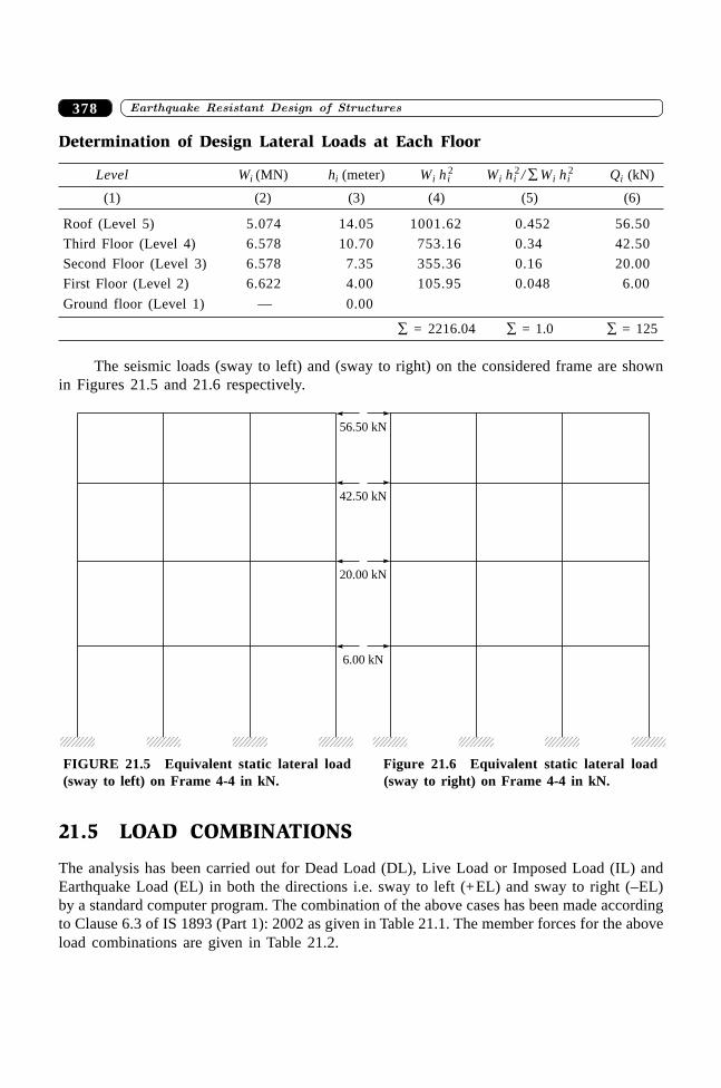
����������� ������� �������������378
Determination of Design Lateral Loads at Each Floor
Level Wi (MN) hi (meter) Wi hi2 Wi hi
2 / Â Wi hi2 Qi (kN)
(1) (2) (3) (4) (5) (6)
Roof (Level 5) 5.074 14.05 1001.62 0.452 56.50
Third Floor (Level 4) 6.578 10.70 753.16 0.34 42.50
Second Floor (Level 3) 6.578 7.35 355.36 0.16 20.00
First Floor (Level 2) 6.622 4.00 105.95 0.048 6.00
Ground floor (Level 1) .— 0.00
 = 2216.04  = 1.0  = 125
The seismic loads (sway to left) and (sway to right) on the considered frame are shownin Figures 21.5 and 21.6 respectively.
56.50 kN
42.50 kN
20.00 kN
6.00 kN
FIGURE 21.5 Equivalent static lateral load Figure 21.6 Equivalent static lateral load(sway to left) on Frame 4-4 in kN. (sway to right) on Frame 4-4 in kN.
21.5 LOAD COMBINATIONS
The analysis has been carried out for Dead Load (DL), Live Load or Imposed Load (IL) andEarthquake Load (EL) in both the directions i.e. sway to left (+EL) and sway to right (–EL)by a standard computer program. The combination of the above cases has been made accordingto Clause 6.3 of IS 1893 (Part 1): 2002 as given in Table 21.1. The member forces for the aboveload combinations are given in Table 21.2.
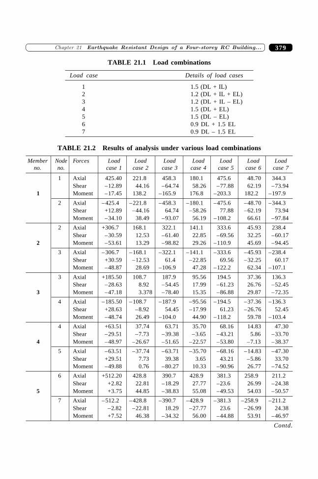
379�������� ����������� ������� ������������������� �� �����
TABLE 21.1 Load combinations
Load case Details of load cases
1 1.5 (DL + IL)2 1.2 (DL + IL + EL)3 1.2 (DL + IL – EL)4 1.5 (DL + EL)5 1.5 (DL – EL)6 0.9 DL + 1.5 EL7 0.9 DL – 1.5 EL
TABLE 21.2 Results of analysis under various load combinations
Member Node Forces Load Load Load Load Load Load Loadno. no. case 1 case 2 case 3 case 4 case 5 case 6 case 7
1 Axial 425.40 221.8 458.3 180.1 475.6 48.70 344.3Shear –12.89 44.16 –64.74 58.26 –77.88 62.19 –73.94
1 Moment –17.45 138.2 –165.9 176.8 –203.3 182.2 –197.9
2 Axial –425.4 –221.8 –458.3 –180.1 –475.6 –48.70 –344.3Shear +12.89 –44.16 64.74 –58.26 77.88 –62.19 73.94Moment –34.10 38.49 –93.07 56.19 –108.2 66.61 –97.84
2 Axial +306.7 168.1 322.1 141.1 333.6 45.93 238.4Shear –30.59 12.53 –61.40 22.85 –69.56 32.25 –60.17
2 Moment –53.61 13.29 –98.82 29.26 –110.9 45.69 –94.45
3 Axial –306.7 –168.1 –322.1 –141.1 –333.6 –45.93 –238.4Shear +30.59 –12.53 61.4 –22.85 69.56 –32.25 60.17Moment –48.87 28.69 –106.9 47.28 –122.2 62.34 –107.1
3 Axial +185.50 108.7 187.9 95.56 194.5 37.36 136.3Shear –28.63 8.92 –54.45 17.99 –61.23 26.76 –52.45
3 Moment –47.18 3.378 –78.40 15.35 –86.88 29.87 –72.35
4 Axial –185.50 –108.7 –187.9 –95.56 –194.5 –37.36 –136.3Shear +28.63 –8.92 54.45 –17.99 61.23 –26.76 52.45Moment –48.74 26.49 –104.0 44.90 –118.2 59.78 –103.4
4 Axial +63.51 37.74 63.71 35.70 68.16 14.83 47.30Shear –29.51 –7.73 –39.38 –3.65 –43.21 5.86 –33.70
4 Moment –48.97 –26.67 –51.65 –22.57 –53.80 –7.13 –38.37
5 Axial –63.51 –37.74 –63.71 –35.70 –68.16 –14.83 –47.30Shear +29.51 7.73 39.38 3.65 43.21 –5.86 33.70Moment –49.88 0.76 –80.27 10.33 –90.96 26.77 –74.52
6 Axial +512.20 428.8 390.7 428.9 381.3 258.9 211.2Shear +2.82 22.81 –18.29 27.77 –23.6 26.99 –24.38
5 Moment +3.75 44.85 –38.83 55.08 –49.53 54.03 –50.57
7 Axial –512.2 –428.8 –390.7 –428.9 –381.3 –258.9 –211.2Shear –2.82 –22.81 18.29 –27.77 23.6 –26.99 24.38Moment +7.52 46.38 –34.32 56.00 –44.88 53.91 –46.97
Contd.
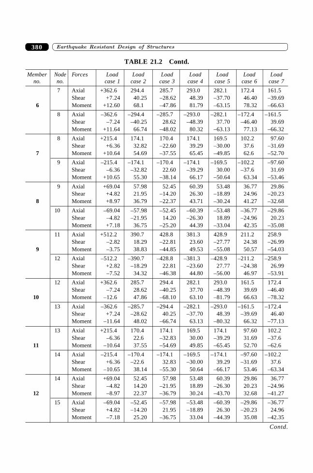
����������� ������� �������������380
7 Axial +362.6 294.4 285.7 293.0 282.1 172.4 161.5Shear +7.24 40.25 –28.62 48.39 –37.70 46.40 –39.69
6 Moment +12.60 68.1 –47.86 81.79 –63.15 78.32 –66.63
8 Axial –362.6 –294.4 –285.7 –293.0 –282.1 –172.4 –161.5Shear –7.24 –40.25 28.62 –48.39 37.70 –46.40 39.69Moment +11.64 66.74 –48.02 80.32 –63.13 77.13 –66.32
8 Axial +215.4 174.1 170.4 174.1 169.5 102.2 97.60Shear +6.36 32.82 –22.60 39.29 –30.00 37.6 –31.69
7 Moment +10.64 54.69 –37.55 65.45 –49.85 62.6 –52.70
9 Axial –215.4 –174.1 –170.4 –174.1 –169.5 –102.2 –97.60Shear –6.36 –32.82 22.60 –39.29 30.00 –37.6 31.69Moment +10.65 55.30 –38.14 66.17 –50.64 63.34 –53.46
9 Axial +69.04 57.98 52.45 60.39 53.48 36.77 29.86Shear +4.82 21.95 –14.20 26.30 –18.89 24.96 –20.23
8 Moment +8.97 36.79 –22.37 43.71 –30.24 41.27 –32.68
10 Axial –69.04 –57.98 –52.45 –60.39 –53.48 –36.77 –29.86Shear –4.82 –21.95 14.20 –26.30 18.89 –24.96 20.23Moment +7.18 36.75 –25.20 44.39 –33.04 42.35 –35.08
11 Axial +512.2 390.7 428.8 381.3 428.9 211.2 258.9Shear –2.82 18.29 –22.81 23.60 –27.77 24.38 –26.99
9 Moment –3.75 38.83 –44.85 49.53 –55.08 50.57 –54.03
12 Axial –512.2 –390.7 –428.8 –381.3 –428.9 –211.2 –258.9Shear +2.82 –18.29 22.81 –23.60 27.77 –24.38 26.99Moment –7.52 34.32 –46.38 44.80 –56.00 46.97 –53.91
12 Axial +362.6 285.7 294.4 282.1 293.0 161.5 172.4Shear –7.24 28.62 –40.25 37.70 –48.39 39.69 –46.40
10 Moment –12.6 47.86 –68.10 63.10 –81.79 66.63 –78.32
13 Axial –362.6 –285.7 –294.4 –282.1 –293.0 –161.5 –172.4Shear +7.24 –28.62 40.25 –37.70 48.39 –39.69 46.40Moment –11.64 48.02 –66.74 63.13 –80.32 66.32 –77.13
13 Axial +215.4 170.4 174.1 169.5 174.1 97.60 102.2Shear –6.36 22.6 –32.83 30.00 –39.29 31.69 –37.6
11 Moment –10.64 37.55 –54.69 49.85 –65.45 52.70 –62.6
14 Axial –215.4 –170.4 –174.1 –169.5 –174.1 –97.60 –102.2Shear +6.36 –22.6 32.83 –30.00 39.29 –31.69 37.6Moment –10.65 38.14 –55.30 50.64 –66.17 53.46 –63.34
14 Axial +69.04 52.45 57.98 53.48 60.39 29.86 36.77Shear –4.82 14.20 –21.95 18.89 –26.30 20.23 –24.96
12 Moment –8.97 22.37 –36.79 30.24 –43.70 32.68 –41.27
15 Axial –69.04 –52.45 –57.98 –53.48 –60.39 –29.86 –36.77Shear +4.82 –14.20 21.95 –18.89 26.30 –20.23 24.96Moment –7.18 25.20 –36.75 33.04 –44.39 35.08 –42.35
TABLE 21.2 Contd.
Member Node Forces Load Load Load Load Load Load Loadno. no. case 1 case 2 case 3 case 4 case 5 case 6 case 7
Contd.
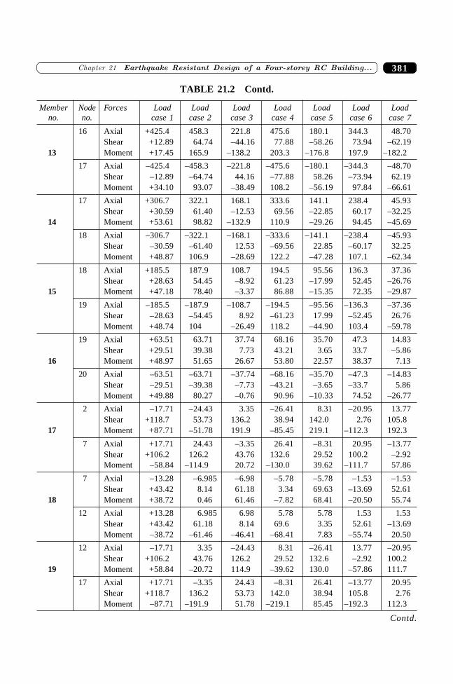
381�������� ����������� ������� ������������������� �� �����
16 Axial +425.4 458.3 221.8 475.6 180.1 344.3 48.70Shear +12.89 64.74 –44.16 77.88 –58.26 73.94 –62.19
13 Moment +17.45 165.9 –138.2 203.3 –176.8 197.9 –182.2
17 Axial –425.4 –458.3 –221.8 –475.6 –180.1 –344.3 –48.70Shear –12.89 –64.74 44.16 –77.88 58.26 –73.94 62.19Moment +34.10 93.07 –38.49 108.2 –56.19 97.84 –66.61
17 Axial +306.7 322.1 168.1 333.6 141.1 238.4 45.93Shear +30.59 61.40 –12.53 69.56 –22.85 60.17 –32.25
14 Moment +53.61 98.82 –132.9 110.9 –29.26 94.45 –45.69
18 Axial –306.7 –322.1 –168.1 –333.6 –141.1 –238.4 –45.93Shear –30.59 –61.40 12.53 –69.56 22.85 –60.17 32.25Moment +48.87 106.9 –28.69 122.2 –47.28 107.1 –62.34
18 Axial +185.5 187.9 108.7 194.5 95.56 136.3 37.36Shear +28.63 54.45 –8.92 61.23 –17.99 52.45 –26.76
15 Moment +47.18 78.40 –3.37 86.88 –15.35 72.35 –29.87
19 Axial –185.5 –187.9 –108.7 –194.5 –95.56 –136.3 –37.36Shear –28.63 –54.45 8.92 –61.23 17.99 –52.45 26.76Moment +48.74 104 –26.49 118.2 –44.90 103.4 –59.78
19 Axial +63.51 63.71 37.74 68.16 35.70 47.3 14.83Shear +29.51 39.38 7.73 43.21 3.65 33.7 –5.86
16 Moment +48.97 51.65 26.67 53.80 22.57 38.37 7.13
20 Axial –63.51 –63.71 –37.74 –68.16 –35.70 –47.3 –14.83Shear –29.51 –39.38 –7.73 –43.21 –3.65 –33.7 5.86Moment +49.88 80.27 –0.76 90.96 –10.33 74.52 –26.77
2 Axial –17.71 –24.43 3.35 –26.41 8.31 –20.95 13.77Shear +118.7 53.73 136.2 38.94 142.0 2.76 105.8
17 Moment +87.71 –51.78 191.9 –85.45 219.1 –112.3 192.3
7 Axial +17.71 24.43 –3.35 26.41 –8.31 20.95 –13.77Shear +106.2 126.2 43.76 132.6 29.52 100.2 –2.92Moment –58.84 –114.9 20.72 –130.0 39.62 –111.7 57.86
7 Axial –13.28 –6.985 –6.98 –5.78 –5.78 –1.53 –1.53Shear +43.42 8.14 61.18 3.34 69.63 –13.69 52.61
18 Moment +38.72 0.46 61.46 –7.82 68.41 –20.50 55.74
12 Axial +13.28 6.985 6.98 5.78 5.78 1.53 1.53Shear +43.42 61.18 8.14 69.6 3.35 52.61 –13.69Moment –38.72 –61.46 –46.41 –68.41 7.83 –55.74 20.50
12 Axial –17.71 3.35 –24.43 8.31 –26.41 13.77 –20.95Shear +106.2 43.76 126.2 29.52 132.6 –2.92 100.2
19 Moment +58.84 –20.72 114.9 –39.62 130.0 –57.86 111.7
17 Axial +17.71 –3.35 24.43 –8.31 26.41 –13.77 20.95Shear +118.7 136.2 53.73 142.0 38.94 105.8 2.76Moment –87.71 –191.9 51.78 –219.1 85.45 –192.3 112.3
TABLE 21.2 Contd.
Member Node Forces Load Load Load Load Load Load Loadno. no. case 1 case 2 case 3 case 4 case 5 case 6 case 7
Contd.
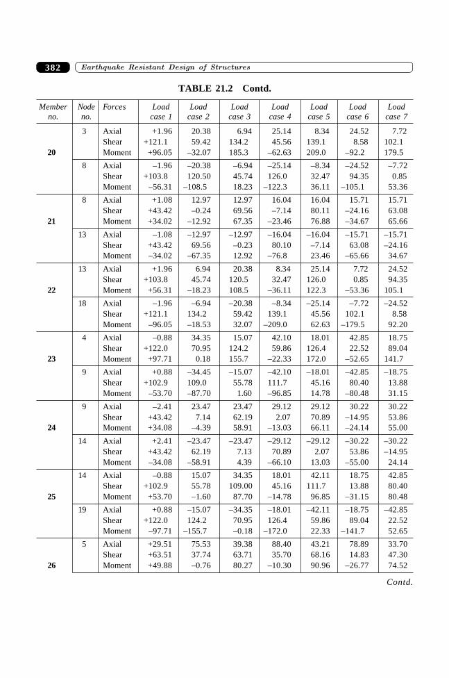
����������� ������� �������������382
3 Axial +1.96 20.38 6.94 25.14 8.34 24.52 7.72Shear +121.1 59.42 134.2 45.56 139.1 8.58 102.1
20 Moment +96.05 –32.07 185.3 –62.63 209.0 –92.2 179.5
8 Axial –1.96 –20.38 –6.94 –25.14 –8.34 –24.52 –7.72Shear +103.8 120.50 45.74 126.0 32.47 94.35 0.85Moment –56.31 –108.5 18.23 –122.3 36.11 –105.1 53.36
8 Axial +1.08 12.97 12.97 16.04 16.04 15.71 15.71Shear +43.42 –0.24 69.56 –7.14 80.11 –24.16 63.08
21 Moment +34.02 –12.92 67.35 –23.46 76.88 –34.67 65.66
13 Axial –1.08 –12.97 –12.97 –16.04 –16.04 –15.71 –15.71Shear +43.42 69.56 –0.23 80.10 –7.14 63.08 –24.16Moment –34.02 –67.35 12.92 –76.8 23.46 –65.66 34.67
13 Axial +1.96 6.94 20.38 8.34 25.14 7.72 24.52Shear +103.8 45.74 120.5 32.47 126.0 0.85 94.35
22 Moment +56.31 –18.23 108.5 –36.11 122.3 –53.36 105.1
18 Axial –1.96 –6.94 –20.38 –8.34 –25.14 –7.72 –24.52Shear +121.1 134.2 59.42 139.1 45.56 102.1 8.58Moment –96.05 –18.53 32.07 –209.0 62.63 –179.5 92.20
4 Axial –0.88 34.35 15.07 42.10 18.01 42.85 18.75Shear +122.0 70.95 124.2 59.86 126.4 22.52 89.04
23 Moment +97.71 0.18 155.7 –22.33 172.0 –52.65 141.7
9 Axial +0.88 –34.45 –15.07 –42.10 –18.01 –42.85 –18.75Shear +102.9 109.0 55.78 111.7 45.16 80.40 13.88Moment –53.70 –87.70 1.60 –96.85 14.78 –80.48 31.15
9 Axial –2.41 23.47 23.47 29.12 29.12 30.22 30.22Shear +43.42 7.14 62.19 2.07 70.89 –14.95 53.86
24 Moment +34.08 –4.39 58.91 –13.03 66.11 –24.14 55.00
14 Axial +2.41 –23.47 –23.47 –29.12 –29.12 –30.22 –30.22Shear +43.42 62.19 7.13 70.89 2.07 53.86 –14.95Moment –34.08 –58.91 4.39 –66.10 13.03 –55.00 24.14
14 Axial –0.88 15.07 34.35 18.01 42.11 18.75 42.85Shear +102.9 55.78 109.00 45.16 111.7 13.88 80.40
25 Moment +53.70 –1.60 87.70 –14.78 96.85 –31.15 80.48
19 Axial +0.88 –15.07 –34.35 –18.01 –42.11 –18.75 –42.85Shear +122.0 124.2 70.95 126.4 59.86 89.04 22.52Moment –97.71 –155.7 –0.18 –172.0 22.33 –141.7 52.65
5 Axial +29.51 75.53 39.38 88.40 43.21 78.89 33.70Shear +63.51 37.74 63.71 35.70 68.16 14.83 47.30
26 Moment +49.88 –0.76 80.27 –10.30 90.96 –26.77 74.52
TABLE 21.2 Contd.
Member Node Forces Load Load Load Load Load Load Loadno. no. case 1 case 2 case 3 case 4 case 5 case 6 case 7
Contd.
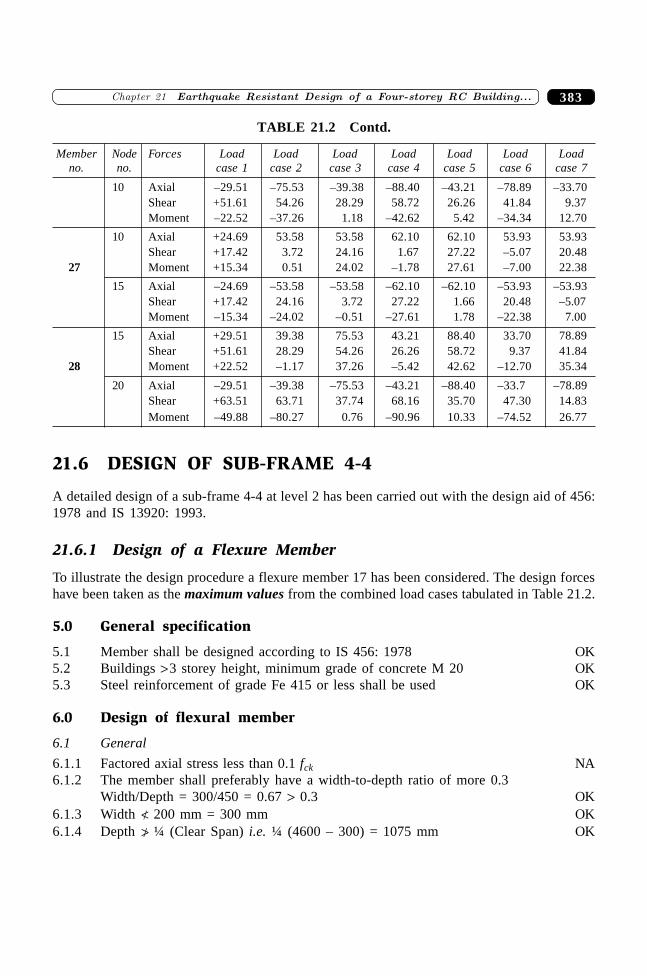
383�������� ����������� ������� ������������������� �� �����
10 Axial –29.51 –75.53 –39.38 –88.40 –43.21 –78.89 –33.70Shear +51.61 54.26 28.29 58.72 26.26 41.84 9.37Moment –22.52 –37.26 1.18 –42.62 5.42 –34.34 12.70
10 Axial +24.69 53.58 53.58 62.10 62.10 53.93 53.93Shear +17.42 3.72 24.16 1.67 27.22 –5.07 20.48
27 Moment +15.34 0.51 24.02 –1.78 27.61 –7.00 22.38
15 Axial –24.69 –53.58 –53.58 –62.10 –62.10 –53.93 –53.93Shear +17.42 24.16 3.72 27.22 1.66 20.48 –5.07Moment –15.34 –24.02 –0.51 –27.61 1.78 –22.38 7.00
15 Axial +29.51 39.38 75.53 43.21 88.40 33.70 78.89Shear +51.61 28.29 54.26 26.26 58.72 9.37 41.84
28 Moment +22.52 –1.17 37.26 –5.42 42.62 –12.70 35.34
20 Axial –29.51 –39.38 –75.53 –43.21 –88.40 –33.7 –78.89Shear +63.51 63.71 37.74 68.16 35.70 47.30 14.83Moment –49.88 –80.27 0.76 –90.96 10.33 –74.52 26.77
21.6 DESIGN OF SUB-FRAME 4-4
A detailed design of a sub-frame 4-4 at level 2 has been carried out with the design aid of 456:1978 and IS 13920: 1993.
21.6.1 Design of a Flexure Member
To illustrate the design procedure a flexure member 17 has been considered. The design forceshave been taken as the maximum values from the combined load cases tabulated in Table 21.2.
5.0 General specification
5.1 Member shall be designed according to IS 456: 1978 OK5.2 Buildings >3 storey height, minimum grade of concrete M 20 OK5.3 Steel reinforcement of grade Fe 415 or less shall be used OK
6.0 Design of flexural member
6.1 General
6.1.1 Factored axial stress less than 0.1 fck NA6.1.2 The member shall preferably have a width-to-depth ratio of more 0.3
Width/Depth = 300/450 = 0.67 > 0.3 OK6.1.3 Width /< 200 mm = 300 mm OK6.1.4 Depth /> ¼ (Clear Span) i.e. ¼ (4600 – 300) = 1075 mm OK
TABLE 21.2 Contd.
Member Node Forces Load Load Load Load Load Load Loadno. no. case 1 case 2 case 3 case 4 case 5 case 6 case 7
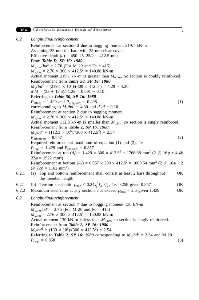
����������� ������� �������������384
6.2 Longitudinal reinforcement
Reinforcement at section 2 due to hogging moment 219.1 kN-mAssuming 25 mm dia bars with 25 mm clear coverEffective depth (d) = 450–25–25/2 = 412.5 mmFrom Table D, SP 16: 1980Mu,lim/bd2 = 2.76 (For M 20 and Fe = 415)Mu,lim = 2.76 ¥ 300 ¥ 412.52 = 140.88 kN-mActual moment 219.1 kN-m is greater than Mu,lim, So section is doubly reinforced.Reinforcement from Table 50, SP 16: 1980Mu/bd2 = (219.1 ¥ 106)/(300 ¥ 412.52) = 4.29 ª 4.30d ¢/d = (25 + 12.5)/41.25 = 0.091 ª 0.10Referring to Table 50, SP 16: 1980P1(top) = 1.429 and P1(bottom) = 0.498 (1)corresponding to Mu/bd2 = 4.30 and d ¢/d = 0.10Reinforcement at section 2 due to sagging momentMu,lim = 2.76 ¥ 300 ¥ 412.52 = 140.88 kN-mActual moment 112.3 kN-m is smaller than Mu,lim, so section is singly reinforced.Reinforcement from Table 2, SP 16: 1980Mu/bd2 = (112.3 ¥ 106)/(300 ¥ 412.52) = 2.54P2(bottom) = 0.857 (2)Required reinforcement maximum of equation (1) and (2), i.e.P(top) = 1.429 and P(bottom) = 0.857Reinforcement at top (At) = 1.429 ¥ 300 ¥ 412.52 = 1768.38 mm2 (2 @ 16f + 4 @22f = 1922 mm2)Reinforcement at bottom (Ab) = 0.857 ¥ 300 ¥ 412.52 = 1060.54 mm2 (2 @ 16f + 2@ 22f = 1162 mm2)
6.2.1 (a) Top and bottom reinforcement shall consist at least 2 bars throughout OKthe member length
6.2.1 (b) Tension steel ratio rmin £ 0.24 fck / fy , i.e. 0.258 given 0.857 OK6.2.2 Maximum steel ratio at any section, not exceed rmax = 2.5 given 1.429 OK
6.2 Longitudinal reinforcement
Reinforcement at section 7 due to hogging moment 130 kN-mMu,lim/bd2 = 2.76 (For M 20 and Fe = 415)Mu,lim = 2.76 ¥ 300 ¥ 412.52 = 140.88 kN-mActual moment 130 kN-m is less than Mu,lim, so section is singly reinforced.Reinforcement from Table 2, SP 16: 1980Mu/bd2 = (130 ¥ 106)/(300 ¥ 412.52) = 2.54Referring to Table 2, SP 16: 1980 corresponding to Mu/bd2 = 2.54 and M 20P(top) = 0.858 (3)
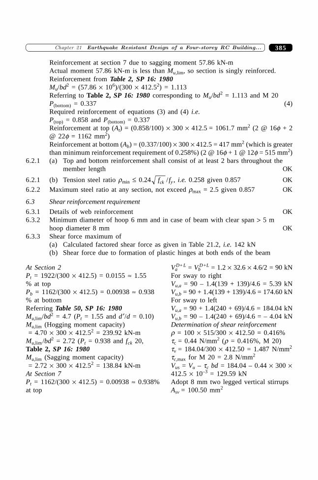
385�������� ����������� ������� ������������������� �� �����
Reinforcement at section 7 due to sagging moment 57.86 kN-mActual moment 57.86 kN-m is less than Mu,lim, so section is singly reinforced.Reinforcement from Table 2, SP 16: 1980Mu/bd2 = (57.86 ¥ 106)/(300 ¥ 412.52) = 1.113Referring to Table 2, SP 16: 1980 corresponding to Mu/bd2 = 1.113 and M 20P(bottom) = 0.337 (4)Required reinforcement of equations (3) and (4) i.e.P(top) = 0.858 and P(bottom) = 0.337Reinforcement at top (At) = (0.858/100) ¥ 300 ¥ 412.5 = 1061.7 mm2 (2 @ 16f + 2@ 22f = 1162 mm2)Reinforcement at bottom (Ab) = (0.337/100) ¥ 300 ¥ 412.5 = 417 mm2 (which is greaterthan minimum reinforcement requirement of 0.258%) (2 @ 16f + 1 @ 12f = 515 mm2)
6.2.1 (a) Top and bottom reinforcement shall consist of at least 2 bars throughout themember length OK
6.2.1 (b) Tension steel ratio rmin £ 0.24 fck / fy , i.e. 0.258 given 0.857 OK
6.2.2 Maximum steel ratio at any section, not exceed rmax = 2.5 given 0.857 OK
6.3 Shear reinforcement requirement
6.3.1 Details of web reinforcement OK6.3.2 Minimum diameter of hoop 6 mm and in case of beam with clear span > 5 m
hoop diameter 8 mm OK6.3.3 Shear force maximum of
(a) Calculated factored shear force as given in Table 21.2, i.e. 142 kN(b) Shear force due to formation of plastic hinges at both ends of the beam
At Section 2 VaD+L = Vb
D+L = 1.2 ¥ 32.6 ¥ 4.6/2 = 90 kNPt = 1922/(300 ¥ 412.5) = 0.0155 ª 1.55 For sway to right% at top Vu,a = 90 – 1.4(139 + 139)/4.6 = 5.39 kNPb = 1162/(300 ¥ 412.5) = 0.00938 ª 0.938 Vu,b = 90 + 1.4(139 + 139)/4.6 = 174.60 kN% at bottom For sway to leftReferring Table 50, SP 16: 1980 Vu,a = 90 + 1.4(240 + 69)/4.6 = 184.04 kNMu,lim/bd2 = 4.7 (Pt = 1.55 and d ¢/d = 0.10) Vu,b = 90 – 1.4(240 + 69)/4.6 = – 4.04 kNMu,lim (Hogging moment capacity) Determination of shear reinforcement = 4.70 ¥ 300 ¥ 412.52 = 239.92 kN-m r = 100 ¥ 515/300 ¥ 412.50 = 0.416%Mu,lim/bd2 = 2.72 (Pt = 0.938 and fck 20, tc = 0.44 N/mm2 (r = 0.416%, M 20)Table 2, SP 16: 1980 tv = 184.04/300 ¥ 412.50 = 1.487 N/mm2
Mu,lim (Sagging moment capacity) tc,max for M 20 = 2.8 N/mm2
= 2.72 ¥ 300 ¥ 412.52 = 138.84 kN-m Vus = Vu – tc bd = 184.04 – 0.44 ¥ 300 ¥At Section 7 412.5 ¥ 10–3 = 129.59 kNPt = 1162/(300 ¥ 412.5) = 0.00938 ª 0.938% Adopt 8 mm two legged vertical stirrupsat top Asv = 100.50 mm2
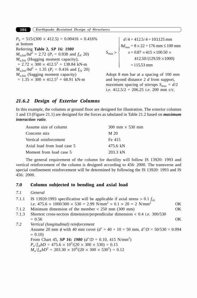
����������� ������� �������������386
Pb = 515/(300 ¥ 412.5) = 0.00416 ª 0.416%at bottomReferring Table 2, SP 16: 1980Mu,lim/bd2 = 2.72 (Pt = 0.938 and fck 20)Mu,lim (Hogging moment capacity), = 2.72 ¥ 300 ¥ 412.52 = 138.84 kN-mMu,lim/bd2 = 1.35 (Pt = 0.416 and fck 20)Mu,lim (Sagging moment capacity) Adopt 8 mm bar at a spacing of 100 mm = 1.35 ¥ 300 ¥ 412.52 = 68.91 kN-m and beyond distance 2 d from support,
maximum spacing of stirrups Smax = d/2i.e. 412.5/2 = 206.25 i.e. 200 mm c/c.
21.6.2 Design of Exterior Columns
In this example, the columns at ground floor are designed for illustration. The exterior columns1 and 13 (Figure 21.1) are designed for the forces as tabulated in Table 21.2 based on maximuminteraction ratio.
Assume size of column 300 mm ¥ 530 mm
Concrete mix M 20
Vertical reinforcement Fe 415
Axial load from load case 5 475.6 kN
Moment from load case 5 203.3 kN
The general requirement of the column for ductility will follow IS 13920: 1993 andvertical reinforcement of the column is designed according to 456: 2000. The transverse andspecial confinement reinforcement will be determined by following the IS 13920: 1993 and IS456: 2000.
7.0 Column subjected to bending and axial load
7.1 General
7.1.1 IS 13920:1993 specification will be applicable if axial stress > 0.1 fcki.e. 475.6 ¥ 1000/300 ¥ 530 = 2.99 N/mm2 > 0.1 ¥ 20 = 2 N/mm2 OK
7.1.2 Minimum dimension of the member < 250 mm (300 mm) OK7.1.3 Shortest cross-section dimension/perpendicular dimension < 0.4 i.e. 300/530
= 0.56 OK7.2 Vertical (longitudinal) reinforcement
Assume 20 mm f with 40 mm cover (d ¢ = 40 + 10 = 50 mm, d ¢/D = 50/530 = 0.094ª 0.10)From Chart 45, SP 16: 1980 (d ¢/D = 0.10, 415 N/mm2)Pu/ fckbD = 475.6 ¥ 103/(20 ¥ 300 ¥ 530) = 0.15Mu/ fckbD2 = 203.30 ¥ 106/(20 ¥ 300 ¥ 5302) = 0.12
Smax >
d
d
s
/ . /
. .
. /( . )
.
min
4 412 5 4 103125
8 8 22 176 100
0 87 415 100 50
412 50 129 59 1000
115 53
= = . mm
= = mm mm
=
= mm
¥ £¥ ¥ ¥
¥
R
S|||
T|||
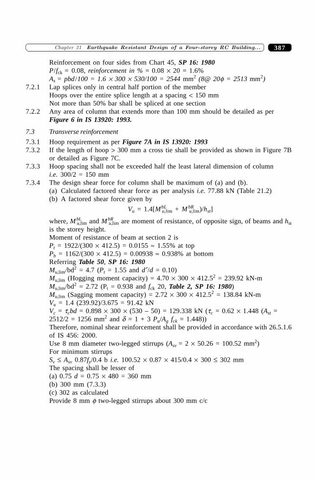
387�������� ����������� ������� ������������������� �� �����
Reinforcement on four sides from Chart 45, SP 16: 1980P/fck = 0.08, reinforcement in % = 0.08 ¥ 20 = 1.6%As = pbd /100 = 1.6 ¥ 300 ¥ 530/100 = 2544 mm2 (8@ 20f = 2513 mm2)
7.2.1 Lap splices only in central half portion of the memberHoops over the entire splice length at a spacing < 150 mmNot more than 50% bar shall be spliced at one section
7.2.2 Any area of column that extends more than 100 mm should be detailed as perFigure 6 in IS 13920: 1993.
7.3 Transverse reinforcement
7.3.1 Hoop requirement as per Figure 7A in IS 13920: 19937.3.2 If the length of hoop > 300 mm a cross tie shall be provided as shown in Figure 7B
or detailed as Figure 7C.7.3.3 Hoop spacing shall not be exceeded half the least lateral dimension of column
i.e. 300/2 = 150 mm7.3.4 The design shear force for column shall be maximum of (a) and (b).
(a) Calculated factored shear force as per analysis i.e. 77.88 kN (Table 21.2)(b) A factored shear force given by
Vu = 1.4[MbLu,lim + M bR
u,lim)/hst]
where, MbLu,lim and MbR
u,lim are moment of resistance, of opposite sign, of beams and hstis the storey height.Moment of resistance of beam at section 2 isPt = 1922/(300 ¥ 412.5) = 0.0155 ª 1.55% at topPb = 1162/(300 ¥ 412.5) = 0.00938 ª 0.938% at bottomReferring Table 50, SP 16: 1980Mu,lim/bd2 = 4.7 (Pt = 1.55 and d ¢/d = 0.10)Mu,lim (Hogging moment capacity) = 4.70 ¥ 300 ¥ 412.52 = 239.92 kN-mMu,lim/bd2 = 2.72 (Pt = 0.938 and fck 20, Table 2, SP 16: 1980)Mu,lim (Sagging moment capacity) = 2.72 ¥ 300 ¥ 412.52 = 138.84 kN-mVu = 1.4 (239.92)/3.675 = 91.42 kNVc = tcbd = 0.898 ¥ 300 ¥ (530 – 50) = 129.338 kN (tc = 0.62 ¥ 1.448 (Ast =2512/2 = 1256 mm2 and d = 1 + 3 Pu/Ag fck = 1.448))Therefore, nominal shear reinforcement shall be provided in accordance with 26.5.1.6of IS 456: 2000.Use 8 mm diameter two-legged stirrups (Asv = 2 ¥ 50.26 = 100.52 mm2)For minimum stirrupsSv £ Asv 0.87fy/0.4 b i.e. 100.52 ¥ 0.87 ¥ 415/0.4 ¥ 300 £ 302 mmThe spacing shall be lesser of(a) 0.75 d = 0.75 ¥ 480 = 360 mm(b) 300 mm (7.3.3)(c) 302 as calculatedProvide 8 mm f two-legged stirrups about 300 mm c/c
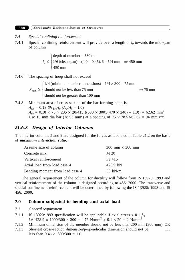
����������� ������� �������������388
7.4 Special confining reinforcement
7.4.1 Special confining reinforcement will provide over a length of l0 towards the mid-spanof column
l0 £
depth of member = 530 mm
1/6 (clear span) = (4.0 0.45)/6 = 591 mm 450 mm
450 mm
- fiRS|
T|
7.4.6 The spacing of hoop shall not exceed
Smax ≥ 1 4 1 4 300/ ( ) /minimun member dimensions = = 75 mm
should not be less than 75 mm 75 mm
should not be greater than 100 mm
¥fi
RS|
T|7.4.8 Minimum area of cross section of the bar forming hoop is,
Ash = 0.18 Sh fck/fy (Ag /Ak – 1.0)Ash = 0.18 ¥ 75 ¥ 235 ¥ 20/415 ((530 ¥ 300)/(470 ¥ 240) – 1.0)) = 62.62 mm2
Use 10 mm dia bar (78.53 mm2) at a spacing of 75 ¥ 78.53/62.62 = 94 mm c/c.
21.6.3 Design of Interior Columns
The interior columns 5 and 9 are designed for the forces as tabulated in Table 21.2 on the basisof maximum interaction ratio.
Assume size of column 300 mm ¥ 300 mm
Concrete mix M 20
Vertical reinforcement Fe 415
Axial load from load case 4 428.9 kN
Bending moment from load case 4 56 kN-m
The general requirement of the column for ductility will follow from IS 13920: 1993 andvertical reinforcement of the column is designed according to 456: 2000. The transverse andspecial confinement reinforcement will be determined by following the IS 13920: 1993 and IS456: 2000.
7.0 Column subjected to bending and axial load
7.1 General requirement
7.1.1 IS 13920:1993 specification will be applicable if axial stress > 0.1 fcki.e. 428.9 ¥ 1000/300 ¥ 300 = 4.76 N/mm2 > 0.1 ¥ 20 = 2 N/mm2
7.1.2 Minimum dimension of the member should not be less than 200 mm (300 mm) OK7.1.3 Shortest cross-section dimension/perpendicular dimension should not be OK
less than 0.4 i.e. 300/300 = 1.0
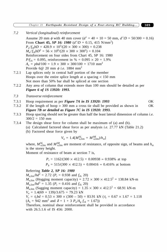
389�������� ����������� ������� ������������������� �� �����
7.2 Vertical (longitudinal) reinforcement
Assume 20 mm f with 40 mm cover (d ¢ = 40 + 10 = 50 mm, d ¢/D = 50/300 = 0.16)From Chart 45, SP 16: 1980 (d ¢/D = 0.15, 415 N/mm2)Pu/ fckbD = 428.9 ¥ 103/(20 ¥ 300 ¥ 300) = 0.238Mu/ fckbD2 = 56 ¥ 106/(20 ¥ 300 ¥ 3002) = 0.104Reinforcement on four sides from Chart 45, SP 16: 1980P/fck = 0.095, reinforcement in % = 0.095 ¥ 20 = 1.9%As = pbd/100 = 1.9 ¥ 300 ¥ 300/100 = 1710 mm2
Provide 6@ 20 mm f i.e. 1884 mm2
7.2.1 Lap splices only in central half portion of the memberHoops over the entire splice length at a spacing < 150 mmNot more than 50% bar shall be spliced at one section
7.2.2 Any area of column that extends more than 100 mm should be detailed as perFigure 6 of 1S 13920: 1993.
7.3 Transverse reinforcement
7.3.1 Hoop requirement as per Figure 7A in IS 13920: 1993 OK7.3.2 If the length of hoop > 300 mm a cross tie shall be provided as shown in OK
Figure 7B or detailed as Figure 7C in IS 13920: 1993.7.3.3 Hoop spacing should not be greater than half the least lateral dimension of column i.e.
300/2 = 150 mm7.3.4 The design shear force for column shall be maximum of (a) and (b).
(a) Calculated factored shear force as per analysis i.e. 27.77 kN (Table 21.2)(b) Factored shear force given by
Vu = 1.4[MbLu,lim + M bR
u,lim)/hst]
where, MbLu,lim and MbR
u,lim are moment of resistance, of opposite sign, of beams and hstis the storey height.Moment of resistance of beam at section 7 is,
Pt = 1162/(300 ¥ 412.5) = 0.00938 ª 0.938% at top
Pb = 515/(300 ¥ 412.5) = 0.00416 ª 0.416% at bottom
Referring Table 2, SP 16: 1980Mu,lim/bd2 = 2.72 (Pt = 0.938 and fck 20)Mu,lim (Hogging moment capacity) = 2.72 ¥ 300 ¥ 412.52 = 138.84 kN-mMu,lim/bd2 = 1.35 (Pt = 0.416 and fck 20)Mu,lim (Sagging moment capacity) = 1.35 ¥ 300 ¥ 412.52 = 68.91 kN-mVu = 1.4(69 + 139)/3.675 = 79.23 kNVc = tcbd = 0.53 ¥ 300 ¥ (300 – 50) = 83.91 kN (tc = 0.67 ¥ 1.67 = 1.118(As = 942 mm2 and d = 1 + 3 Pu/Ag fck = 1.67))Therefore, nominal shear reinforcement shall be provided in accordancewith 26.5.1.6 of IS 456: 2000.
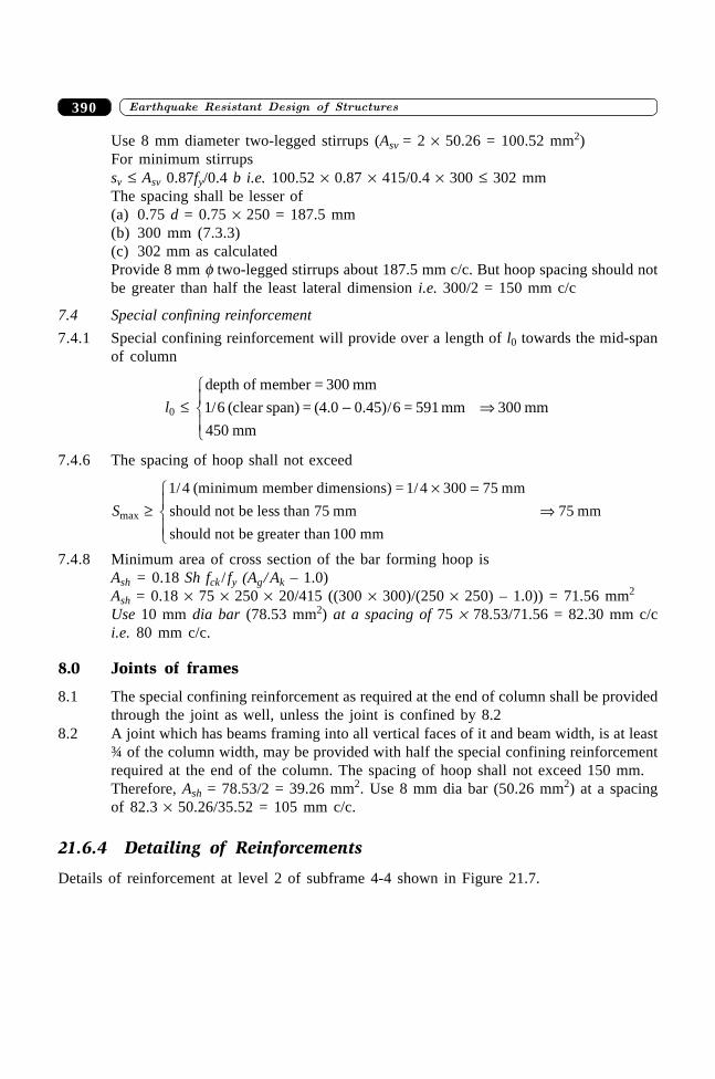
����������� ������� �������������390
Use 8 mm diameter two-legged stirrups (Asv = 2 ¥ 50.26 = 100.52 mm2)For minimum stirrupssv £ Asv 0.87fy/0.4 b i.e. 100.52 ¥ 0.87 ¥ 415/0.4 ¥ 300 £ 302 mmThe spacing shall be lesser of(a) 0.75 d = 0.75 ¥ 250 = 187.5 mm(b) 300 mm (7.3.3)(c) 302 mm as calculatedProvide 8 mm f two-legged stirrups about 187.5 mm c/c. But hoop spacing should notbe greater than half the least lateral dimension i.e. 300/2 = 150 mm c/c
7.4 Special confining reinforcement
7.4.1 Special confining reinforcement will provide over a length of l0 towards the mid-spanof column
l0 £
depth of member = 300 mm
1/6 (clear span) = (4.0 0.45)/6 = 591 mm 300 mm
450 mm
- fiRS|
T|7.4.6 The spacing of hoop shall not exceed
Smax ≥ 1/4 (minimum member dimensions) = 1/4 300 75 mm
should not be less than 75 mm 75 mm
should not be greater than 100 mm
¥ =fi
RS|
T|7.4.8 Minimum area of cross section of the bar forming hoop is
Ash = 0.18 Sh fck / fy (Ag/ Ak – 1.0)Ash = 0.18 ¥ 75 ¥ 250 ¥ 20/415 ((300 ¥ 300)/(250 ¥ 250) – 1.0)) = 71.56 mm2
Use 10 mm dia bar (78.53 mm2) at a spacing of 75 ¥ 78.53/71.56 = 82.30 mm c/ci.e. 80 mm c/c.
8.0 Joints of frames
8.1 The special confining reinforcement as required at the end of column shall be providedthrough the joint as well, unless the joint is confined by 8.2
8.2 A joint which has beams framing into all vertical faces of it and beam width, is at least¾ of the column width, may be provided with half the special confining reinforcementrequired at the end of the column. The spacing of hoop shall not exceed 150 mm.Therefore, Ash = 78.53/2 = 39.26 mm2. Use 8 mm dia bar (50.26 mm2) at a spacingof 82.3 ¥ 50.26/35.52 = 105 mm c/c.
21.6.4 Detailing of Reinforcements
Details of reinforcement at level 2 of subframe 4-4 shown in Figure 21.7.
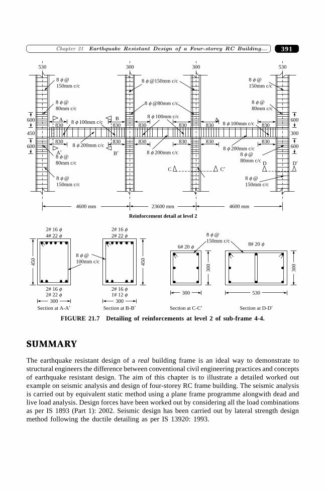
391�������� ����������� ������� ������������������� �� �����
8 @
80mm c/c
f
8 @
150mm c/c
f
530
830A
830
A�
8 @
80mm c/c
f
8 @
150mm c/c
f
8 @
80mm c/c
f
8 @
150mm c/c
f
530
830
830
8 @
80mm c/c
f
8 @
150mm c/c
f
8 @80mm c/cf
830
830
830
830
8 100mm c/cf830A
830
D�
830
830
8 200mm c/cf
DC�C
8 200mm c/cf
8 100mm c/cf
8 @150mm c/cf
B�
B8 100mm c/cf
8 200mm c/cf
Reinforcement detail at level 2
2# 16 f2# 22 f
2# 16 f4# 22 f
Section at A-A�
2# 16 f1# 12 f
2# 16 f2# 22 f
Section at B-B�
8 @
100mm c/c
f
8# 20 f
Section at D-D�
6# 20 f
Section at C-C�
8 @
150mm c/c
f
300 300
600
450
600
600
300
600
4600 mm 4600 mm23600 mm
450
300
300
300
300300
530
450
FIGURE 21.7 Detailing of reinforcements at level 2 of sub-frame 4-4.
SUMMARY
The earthquake resistant design of a real building frame is an ideal way to demonstrate tostructural engineers the difference between conventional civil engineering practices and conceptsof earthquake resistant design. The aim of this chapter is to illustrate a detailed worked outexample on seismic analysis and design of four-storey RC frame building. The seismic analysisis carried out by equivalent static method using a plane frame programme alongwith dead andlive load analysis. Design forces have been worked out by considering all the load combinationsas per IS 1893 (Part 1): 2002. Seismic design has been carried out by lateral strength designmethod following the ductile detailing as per IS 13920: 1993.

����������� ������� �������������392
REFERENCES
[1] IS 1893, Criteria for Earthquake Resistant Design of Structures—Part 1, GeneralProvisions and Buildings (Fifth Revision), Bureau of Indian Standards, New Delhi,2002.
[2] IS 13920, Ductile Detailing of Reinforced Concrete Structures Subjected to SeismicForce, Bureau of Indian Standards, New Delhi, 1993.
[3] IS 456, Plain and Reinforced Concrete—Code of Practice, Bureau of Indian Standards,New Delhi, 2000.
[4] Paulay T. and Priestley, M.J.N., Seismic Design of Reinforced Concrete and MasonryBuildings, John Wiley & Sons, New York, 1992.
[5] SP 16, Design Aids for Reinforced Concrete to IS: 456–1978, Bureau of IndianStandards, New Delhi, 1980.
393�������� ����������� ������� ���������������
393
Earthquake ResistantDesign of Shear Wallas per IS 13920: 1993
��������
22.1 INTRODUCTION
A 14-storeyed reinforced concrete building with shear wall in zone IV has been considered forthe illustration of design of shear wall. The lateral forces have been resisted by a dual systemconsisting of Special Moment Resisting Frames (SMRF) and reinforced concrete shear walls.The main emphasis in this chapter is on (i) distribution of design lateral force in SMRF withshear wall and SMRF without shear wall and (ii) design of shear wall and reinforcementrequirement, through practical example.
22.2 DESCRIPTION OF BUILDING
The building considered for this study is assumed to be a hospital building (I = 1.5) situatedin zone IV (Z = 0.24) consisting of five blocks out of which the central block with shear wallhas been considered for the study. The building has a dual system; the response reduction factor(R = 5) has been opted for two reasons (a) the shear wall and the SMRF systems are designedto resist the total design lateral forces in proportion to their relative rigidities considering theinteraction of the dual system at all floor levels; and (b) the SMRF are designed to independentlyresist not less than 25% of the design seismic base shear. The typical plan and elevation of thecentral block and its elevation is shown in Figure 22.1.
The X-direction of the block consists of 4 bay of SMRF @ 6.5 m each and in Z-direction3 bay of frames @ 6 m each. The building is 14 storeyed and floor-to-floor heights are 3.1 m.The columns and structural walls have same cross-sections throughout the height of the building.The floor beams and slabs also have the universal dimensions at all floor levels. A shear wallof 250 mm thickness is centrally located at the exterior frames in X-direction of the block. It
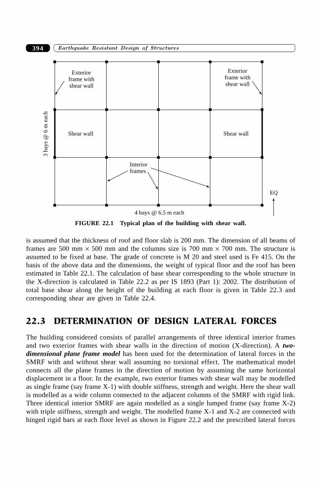
����������� ������� �������������394
is assumed that the thickness of roof and floor slab is 200 mm. The dimension of all beams offrames are 500 mm ¥ 500 mm and the columns size is 700 mm ¥ 700 mm. The structure isassumed to be fixed at base. The grade of concrete is M 20 and steel used is Fe 415. On thebasis of the above data and the dimensions, the weight of typical floor and the roof has beenestimated in Table 22.1. The calculation of base shear corresponding to the whole structure inthe X-direction is calculated in Table 22.2 as per IS 1893 (Part 1): 2002. The distribution oftotal base shear along the height of the building at each floor is given in Table 22.3 andcorresponding shear are given in Table 22.4.
22.3 DETERMINATION OF DESIGN LATERAL FORCES
The building considered consists of parallel arrangements of three identical interior framesand two exterior frames with shear walls in the direction of motion (X-direction). A two-dimensional plane frame model has been used for the determination of lateral forces in theSMRF with and without shear wall assuming no torsional effect. The mathematical modelconnects all the plane frames in the direction of motion by assuming the same horizontaldisplacement in a floor. In the example, two exterior frames with shear wall may be modelledas single frame (say frame X-1) with double stiffness, strength and weight. Here the shear wallis modelled as a wide column connected to the adjacent columns of the SMRF with rigid link.Three identical interior SMRF are again modelled as a single lumped frame (say frame X-2)with triple stiffness, strength and weight. The modelled frame X-1 and X-2 are connected withhinged rigid bars at each floor level as shown in Figure 22.2 and the prescribed lateral forces
Exteriorframe withshear wall
Exteriorframe withshear wall
Shear wallShear wall
Interiorframes
4 bays @ 6.5 m each
EQ
3b
ays
@6
mea
ch
FIGURE 22.1 Typical plan of the building with shear wall.
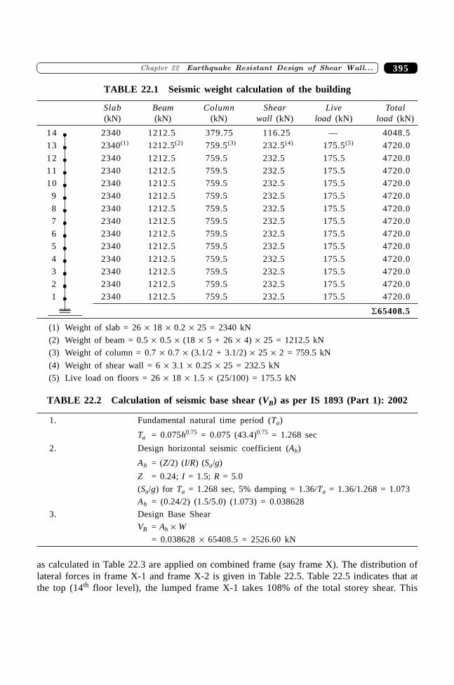
395�������� ����������� ������� ���������������
as calculated in Table 22.3 are applied on combined frame (say frame X). The distribution oflateral forces in frame X-1 and frame X-2 is given in Table 22.5. Table 22.5 indicates that atthe top (14th floor level), the lumped frame X-1 takes 108% of the total storey shear. This
TABLE 22.1 Seismic weight calculation of the building
Slab Beam Column Shear Live Total(kN) (kN) (kN) wall (kN) load (kN) load (kN)
14 2340 1212.5 379.75 116.25 — 4048.5
13 2340(1) 1212.5(2) 759.5(3) 232.5(4) 175.5(5) 4720.0
12 2340 1212.5 759.5 232.5 175.5 4720.0
11 2340 1212.5 759.5 232.5 175.5 4720.0
10 2340 1212.5 759.5 232.5 175.5 4720.0
9 2340 1212.5 759.5 232.5 175.5 4720.0
8 2340 1212.5 759.5 232.5 175.5 4720.0
7 2340 1212.5 759.5 232.5 175.5 4720.0
6 2340 1212.5 759.5 232.5 175.5 4720.0
5 2340 1212.5 759.5 232.5 175.5 4720.0
4 2340 1212.5 759.5 232.5 175.5 4720.0
3 2340 1212.5 759.5 232.5 175.5 4720.0
2 2340 1212.5 759.5 232.5 175.5 4720.0
1 2340 1212.5 759.5 232.5 175.5 4720.0
S65408.5
(1) Weight of slab = 26 ¥ 18 ¥ 0.2 ¥ 25 = 2340 kN
(2) Weight of beam = 0.5 ¥ 0.5 ¥ (18 ¥ 5 + 26 ¥ 4) ¥ 25 = 1212.5 kN
(3) Weight of column = 0.7 ¥ 0.7 ¥ (3.1/2 + 3.1/2) ¥ 25 ¥ 2 = 759.5 kN
(4) Weight of shear wall = 6 ¥ 3.1 ¥ 0.25 ¥ 25 = 232.5 kN
(5) Live load on floors = 26 ¥ 18 ¥ 1.5 ¥ (25/100) = 175.5 kN
TABLE 22.2 Calculation of seismic base shear (VB) as per IS 1893 (Part 1): 2002
1. Fundamental natural time period (Ta)
Ta = 0.075h0.75 = 0.075 (43.4)0.75 = 1.268 sec
2. Design horizontal seismic coefficient (Ah)
Ah = (Z/2) (I/R) (Sa/g)
Z = 0.24; I = 1.5; R = 5.0
(Sa/g) for Ta = 1.268 sec, 5% damping = 1.36/Ta = 1.36/1.268 = 1.073
Ah = (0.24/2) (1.5/5.0) (1.073) = 0.038628
3. Design Base Shear
VB = Ah ¥ W
= 0.038628 ¥ 65408.5 = 2526.60 kN
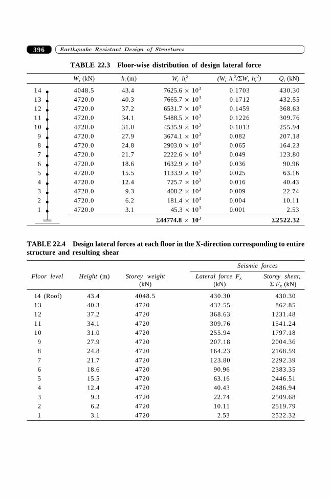
����������� ������� �������������396
TABLE 22.3 Floor-wise distribution of design lateral force
Wi (kN) hi (m) Wi hi2 (Wi hi
2/SWi hi2) Qi (kN)
14 4048.5 43.4 7625.6 ¥ 103 0.1703 430.30
13 4720.0 40.3 7665.7 ¥ 103 0.1712 432.55
12 4720.0 37.2 6531.7 ¥ 103 0.1459 368.63
11 4720.0 34.1 5488.5 ¥ 103 0.1226 309.76
10 4720.0 31.0 4535.9 ¥ 103 0.1013 255.94
9 4720.0 27.9 3674.1 ¥ 103 0.082 207.18
8 4720.0 24.8 2903.0 ¥ 103 0.065 164.23
7 4720.0 21.7 2222.6 ¥ 103 0.049 123.80
6 4720.0 18.6 1632.9 ¥ 103 0.036 90.96
5 4720.0 15.5 1133.9 ¥ 103 0.025 63.16
4 4720.0 12.4 725.7 ¥ 103 0.016 40.43
3 4720.0 9.3 408.2 ¥ 103 0.009 22.74
2 4720.0 6.2 181.4 ¥ 103 0.004 10.11
1 4720.0 3.1 45.3 ¥ 103 0.001 2.53
S44774.8 ¥ 103 S2522.32
TABLE 22.4 Design lateral forces at each floor in the X-direction corresponding to entirestructure and resulting shear
Seismic forces
Floor level Height (m) Storey weight Lateral force Fx Storey shear,(kN) (kN) S Fx (kN)
14 (Roof) 43.4 4048.5 430.30 430.30
13 40.3 4720 432.55 862.85
12 37.2 4720 368.63 1231.48
11 34.1 4720 309.76 1541.24
10 31.0 4720 255.94 1797.18
9 27.9 4720 207.18 2004.36
8 24.8 4720 164.23 2168.59
7 21.7 4720 123.80 2292.39
6 18.6 4720 90.96 2383.35
5 15.5 4720 63.16 2446.51
4 12.4 4720 40.43 2486.94
3 9.3 4720 22.74 2509.68
2 6.2 4720 10.11 2519.79
1 3.1 4720 2.53 2522.32
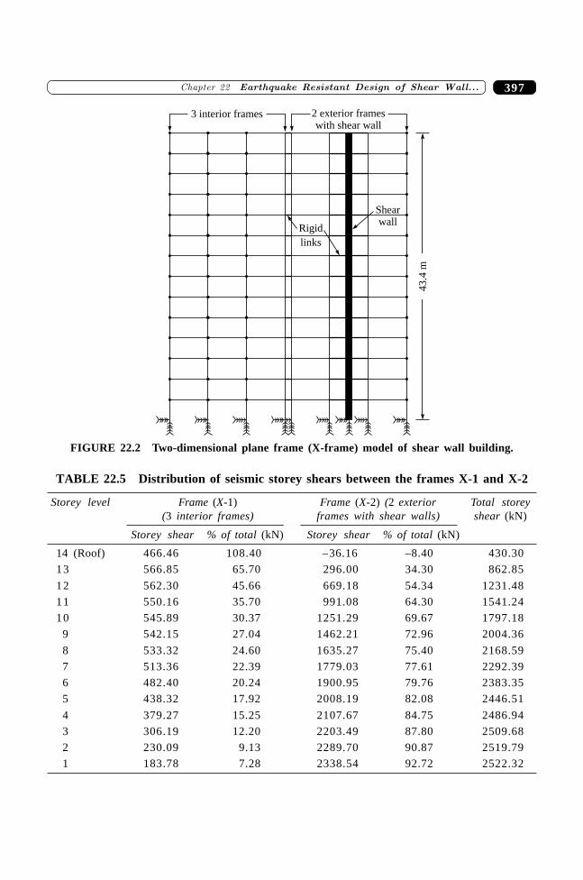
397�������� ����������� ������� ���������������
Shearwall
3 interior frames 2 exterior frameswith shear wall
Rigid
links
43.4
m
FIGURE 22.2 Two-dimensional plane frame (X-frame) model of shear wall building.
TABLE 22.5 Distribution of seismic storey shears between the frames X-1 and X-2
Storey level Frame (X-1) Frame (X-2) (2 exterior Total storey (3 interior frames) frames with shear walls) shear (kN)
Storey shear % of total (kN) Storey shear % of total (kN)
14 (Roof) 466.46 108.40 –36.16 –8.40 430.30
13 566.85 65.70 296.00 34.30 862.85
12 562.30 45.66 669.18 54.34 1231.48
11 550.16 35.70 991.08 64.30 1541.24
10 545.89 30.37 1251.29 69.67 1797.18
9 542.15 27.04 1462.21 72.96 2004.36
8 533.32 24.60 1635.27 75.40 2168.59
7 513.36 22.39 1779.03 77.61 2292.39
6 482.40 20.24 1900.95 79.76 2383.35
5 438.32 17.92 2008.19 82.08 2446.51
4 379.27 15.25 2107.67 84.75 2486.94
3 306.19 12.20 2203.49 87.80 2509.68
2 230.09 9.13 2289.70 90.87 2519.79
1 183.78 7.28 2338.54 92.72 2522.32
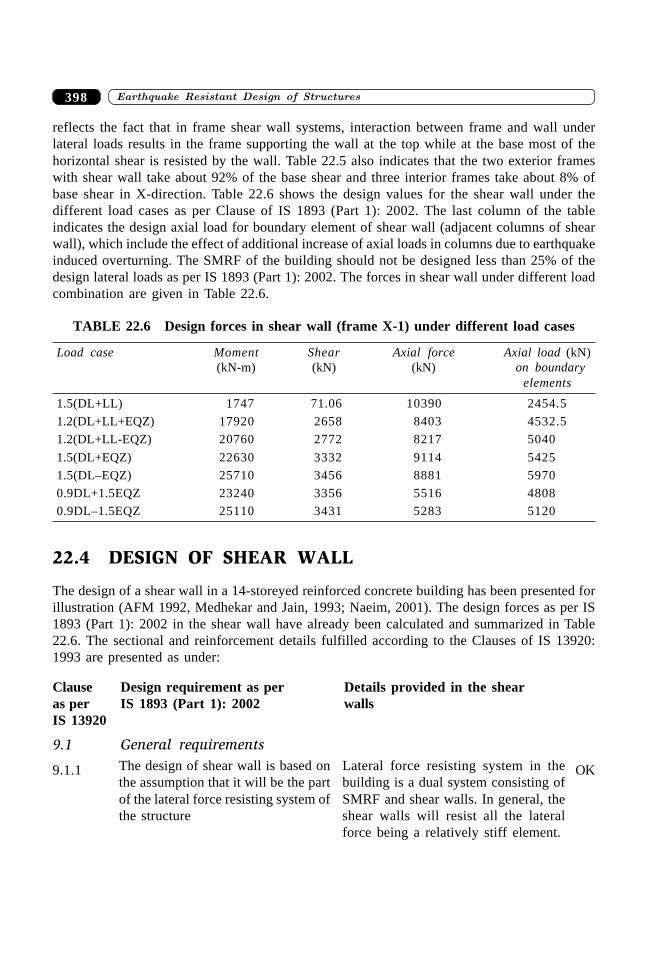
����������� ������� �������������398
reflects the fact that in frame shear wall systems, interaction between frame and wall underlateral loads results in the frame supporting the wall at the top while at the base most of thehorizontal shear is resisted by the wall. Table 22.5 also indicates that the two exterior frameswith shear wall take about 92% of the base shear and three interior frames take about 8% ofbase shear in X-direction. Table 22.6 shows the design values for the shear wall under thedifferent load cases as per Clause of IS 1893 (Part 1): 2002. The last column of the tableindicates the design axial load for boundary element of shear wall (adjacent columns of shearwall), which include the effect of additional increase of axial loads in columns due to earthquakeinduced overturning. The SMRF of the building should not be designed less than 25% of thedesign lateral loads as per IS 1893 (Part 1): 2002. The forces in shear wall under different loadcombination are given in Table 22.6.
TABLE 22.6 Design forces in shear wall (frame X-1) under different load cases
Load case Moment Shear Axial force Axial load (kN)(kN-m) (kN) (kN) on boundary
elements
1.5(DL+LL) 1747 71.06 10390 2454.5
1.2(DL+LL+EQZ) 17920 2658 8403 4532.5
1.2(DL+LL-EQZ) 20760 2772 8217 5040
1.5(DL+EQZ) 22630 3332 9114 5425
1.5(DL–EQZ) 25710 3456 8881 5970
0.9DL+1.5EQZ 23240 3356 5516 4808
0.9DL–1.5EQZ 25110 3431 5283 5120
22.4 DESIGN OF SHEAR WALL
The design of a shear wall in a 14-storeyed reinforced concrete building has been presented forillustration (AFM 1992, Medhekar and Jain, 1993; Naeim, 2001). The design forces as per IS1893 (Part 1): 2002 in the shear wall have already been calculated and summarized in Table22.6. The sectional and reinforcement details fulfilled according to the Clauses of IS 13920:1993 are presented as under:
Clause Design requirement as per Details provided in the shearas per IS 1893 (Part 1): 2002 wallsIS 13920
9.1 General requirements
9.1.1 OKThe design of shear wall is based onthe assumption that it will be the partof the lateral force resisting system ofthe structure
Lateral force resisting system in thebuilding is a dual system consisting ofSMRF and shear walls. In general, theshear walls will resist all the lateralforce being a relatively stiff element.
399�������� ����������� ������� ���������������
9.1.2 OK
9.1.3 OK
9.1.4 OK
9.1.5 OK
9.1.6 OK
Assumed thickness of shear wall250 mm
The shear wall is provided in betweenthe middle two columns of the exteriorframes. These columns will act as aflange element or boundary elementsfor the shear wall. Therefore, there isno need for further thickening of shearwall at the end or boundary regions.
Calculated reinforcement in horizontaland vertical direction is greater than theminimum prescribed reinforcement.Provided reinforcement is uniformlydistributed in both the directions
Since the thickness of shear wall is 250mm and also the factored shear stress
(tv) is greater than 0.25 fck the rein-forcement is provided in two curtains.(see Clause 9.2.1)
Diameter of bar used in horizontal andvertical reinforcement is 8 mm, whichis smaller than 1/10 (250) = 25 mm.
In order to safeguard against prematureout-of-plane buckling in the potentialplastic hinge region of walls, mini-mum thickness of shear wall shouldnot be less than 150 mm
Shear wall is subjected to combinedflexure and axial load therefore; theends of the wall will be subjected tohigh axial load. Therefore, it is nec-essary to thicken the wall in bound-ary regions. This is readily achievedby providing flange elements withsufficient dimensions so as to provideadequate flexural rigidity at the endof the wall section. This effectiveflange width to be used in the designof flanged wall sections, shall be as-sumed to extend beyond the face ofthe web for a distance which shall besmaller of (a) half the distance to anadjacent shear wall web (b) 1/10 th ofthe total wall height.
To control the width of inclinedcracks in the wall, the code recom-mends the reinforcement in both thedirection of walls i.e. horizontal andvertical. The minimum reinforce-ment ratio should be 0.0025 of thegross area in each direction of thewall and should be uniform across thecross section of the wall.
To reduce fragmentation and prema-ture deterioration of the concreteunder load reversal loading ininelastic range, it is preferred that thelongitudinal and transverse rein-forcement should be provided intwo curtains if (a) factored shear
stress in the wall exceeds 0.25 fck
or (b) wall thickness > 200 mmTo prevent the use of very largediameter of reinforcement, the coderestricts the diameter of bar upto1/10th of the thickness of part.
����������� ������� �������������400
9.1.7 OK
9.2 Shear strength requirements
9.2.1 OK
9.2.2 OK
9.2.3 OK
9.2.4 NA
9.2.5 OK
The maximum spacing of reinforce-ment in either direction shall not ex-ceed the smallest of lw / 5, 3 tw, and450 mm; where lw is the horizontallength of wall, and tw is the thicknessof the wall web. This limitation hasbeen guided by the experience andvarious tests to confine the concrete.
The nominal shear stress, tv, shall becalculated as
tv = Vu/twlw
where,Vu = Factored shear forcetw = thickness of webdw = effective depth of wall section.
This may be taken as 0.8 lw forrectangular sections.
lw = horizontal length of wall
The design strength of concrete (tc)shall be calculated as per Table 13 ofIS: 456: 2000
The nominal shear stress in the wall,tv, shall not exceed tc, max as per Table14 of IS: 456: 2000
When tv is less than tc, shear rein-forcement shall be provided in accor-dance with 9.1.3, 9.1.4, and 9.1.6 ofthe code
When tv is greater than tc, the area ofhorizontal shear reinforcement, Ah,to be provided within a vertical spac-ing Sv, is given by
Vus = 0.87fy Ahdw /Sv
where, Vus = (Vu – tctwdw) is the shearforce to be resisted by the horizontalreinforcement. However, the amountof horizontal reinforcement provided
Spacing provided in horizontal andvertical direction of reinforcementis 130 mm which is smaller of (a) lw/5= 1160 mm, (b) 3 tw = 750 mm and450 mm.
The nominal shear stress,
tv = 1728250 4800¥
= 1.44 N/mm2
Vu = 3456/2 = 1728 kN
tw = 250 mm
dw = 0.8 ¥ 6000 = 4800 mm
lw = 6000 mm
Assume horizontal and vertical rein-forcement (As) is 0.25% and concretegrade M 20, permissible shear stress inconcrete is tc = 0.36 N/mm2
tc, max = 2.8 N/mm2
Therefore, tv (1.44 N/mm2) <
tc, max (2.8 N/mm2)
tv (1.44 N/mm2) > tc (0.36 N/mm2)
Shear force required for horizontalshear reinforcement is
Vus = (tv – tc) twdw
= (1.44 – 0.36) ¥ 250 ¥ 4800= 1296 kN
Spacing required for two legged 8 Ftor bar is,
Sv = 0 87 415 100 4800
1296 103. ¥ ¥ ¥
¥= 133.7 mm
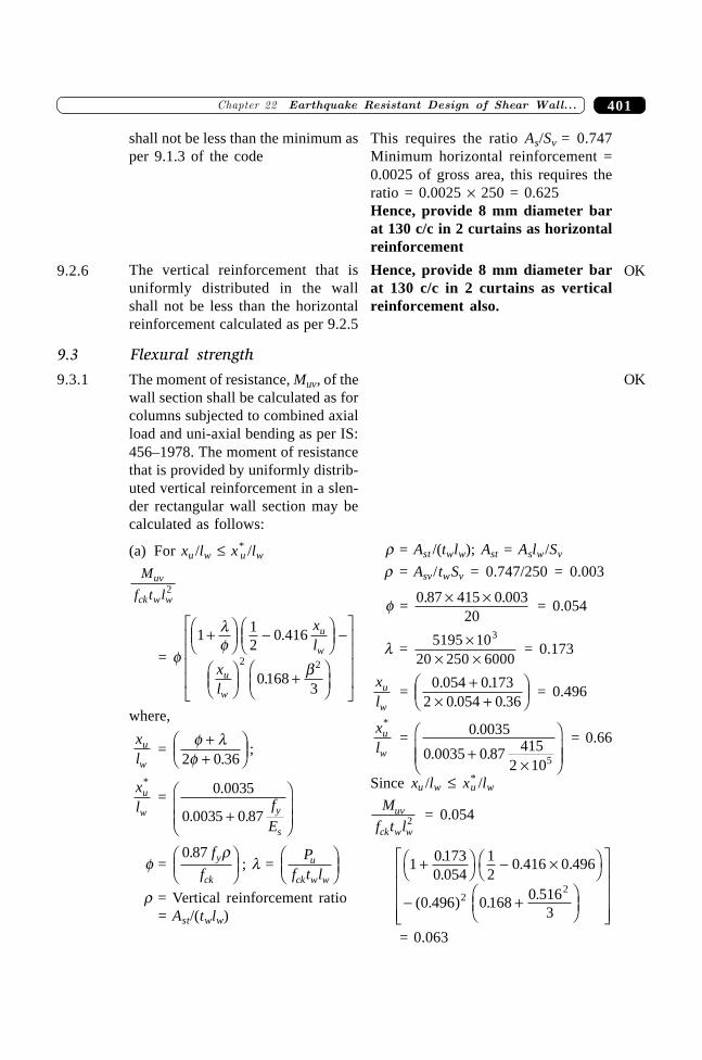
401�������� ����������� ������� ���������������
9.2.6 OK
9.3 Flexural strength
9.3.1 OK
shall not be less than the minimum asper 9.1.3 of the code
The vertical reinforcement that isuniformly distributed in the wallshall not be less than the horizontalreinforcement calculated as per 9.2.5
The moment of resistance, Muv, of thewall section shall be calculated as forcolumns subjected to combined axialload and uni-axial bending as per IS:456–1978. The moment of resistancethat is provided by uniformly distrib-uted vertical reinforcement in a slen-der rectangular wall section may becalculated as follows:
(a) For xu /lw £ x*u /lw
M
f t luv
ck w w2
= f
lf
b
1 12
0 416
01683
2 2
+FHG
IKJ -FHG
IKJ -
FHG
IKJ +
FHG
IKJ
L
N
MMMM
O
Q
PPPP
.
.
xl
xl
u
w
u
w
where,
xl
u
w =
f lf
++
FHG
IKJ2 0 36.
;
xl
u
w
*
=0 0035
0 0035 0 87
.
. .+
F
HGG
I
KJJf
Ey
s
f =0 87. f
fy
ck
rFHG
IKJ ; l =
Pf t l
u
ck w w
FHG
IKJ
r = Vertical reinforcement ratio= Ast/(twlw)
This requires the ratio As/Sv = 0.747Minimum horizontal reinforcement =0.0025 of gross area, this requires theratio = 0.0025 ¥ 250 = 0.625Hence, provide 8 mm diameter barat 130 c/c in 2 curtains as horizontalreinforcement
Hence, provide 8 mm diameter barat 130 c/c in 2 curtains as verticalreinforcement also.
r = Ast /(twlw); Ast = Aslw/Sv
r = Asv/twSv = 0.747/250 = 0.003
f =0 87 415 0 003
20. .¥ ¥
= 0.054
l =5195 10
20 250 6000
3¥¥ ¥
= 0.173
xl
u
w =
0 054 0 1732 0 054 0 36
. .. .
+¥ +
FHG
IKJ = 0.496
xl
u
w
*
= 0 0035
0 0035 0 87 4152 105
.
. .+¥
FHGG
IKJJ
= 0.66
Since xu /lw £ x*u /lw
M
f t luv
ck w w2 = 0.054
1 01730 054
12
0 416 0 496
0 496 0 168 0 5163
22
+FH IK - ¥FH IK- +
FHG
IKJ
L
N
MMMM
O
Q
PPPP
..
. .
( . ) . .
= 0.063
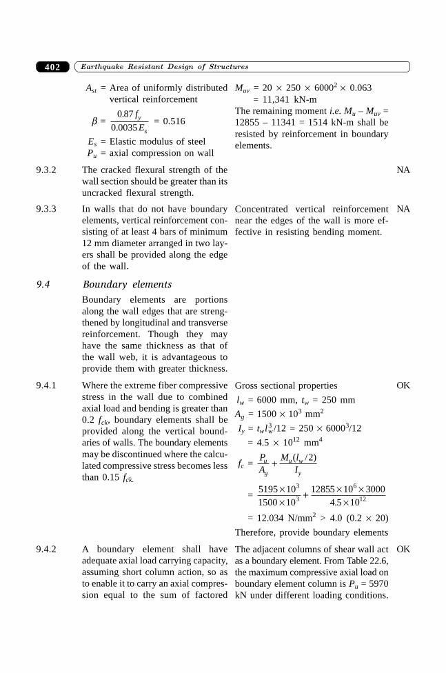
����������� ������� �������������402
9.3.2 NA
9.3.3 NA
9.4 Boundary elements
9.4.1 OK
9.4.2 OK
Muv = 20 ¥ 250 ¥ 60002 ¥ 0.063= 11,341 kN-m
The remaining moment i.e. Mu – Muv =12855 – 11341 = 1514 kN-m shall beresisted by reinforcement in boundaryelements.
Concentrated vertical reinforcementnear the edges of the wall is more ef-fective in resisting bending moment.
Gross sectional properties
lw = 6000 mm, tw = 250 mm
Ag = 1500 ¥ 103 mm2
Iy = twl3w /12 = 250 ¥ 60003/12
= 4.5 ¥ 1012 mm4
fc =PA
M lI
u
g
u w
y+ ( / )2
=5195 101500 10
12855 10 30004 5 10
3
3
6
12¥¥
+ ¥ ¥¥.
= 12.034 N/mm2 > 4.0 (0.2 ¥ 20)
Therefore, provide boundary elements
The adjacent columns of shear wall actas a boundary element. From Table 22.6,the maximum compressive axial load onboundary element column is Pu = 5970kN under different loading conditions.
Ast = Area of uniformly distributedvertical reinforcement
b =0 87
0 0035
.
.
f
Ey
s = 0.516
Es = Elastic modulus of steelPu = axial compression on wall
The cracked flexural strength of thewall section should be greater than itsuncracked flexural strength.
In walls that do not have boundaryelements, vertical reinforcement con-sisting of at least 4 bars of minimum12 mm diameter arranged in two lay-ers shall be provided along the edgeof the wall.
Boundary elements are portionsalong the wall edges that are streng-thened by longitudinal and transversereinforcement. Though they mayhave the same thickness as that ofthe wall web, it is advantageous toprovide them with greater thickness.
Where the extreme fiber compressivestress in the wall due to combinedaxial load and bending is greater than0.2 fck, boundary elements shall beprovided along the vertical bound-aries of walls. The boundary elementsmay be discontinued where the calcu-lated compressive stress becomes lessthan 0.15 fck.
A boundary element shall haveadequate axial load carrying capacity,assuming short column action, so asto enable it to carry an axial compres-sion equal to the sum of factored
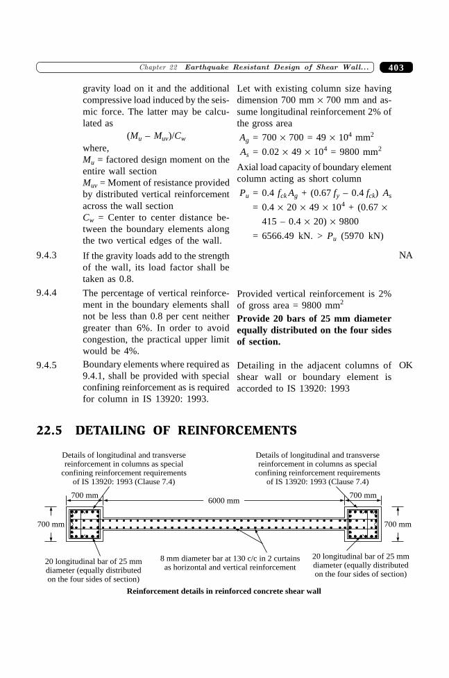
403�������� ����������� ������� ���������������
9.4.3 NA
9.4.4
9.4.5 OK
22.5 DETAILING OF REINFORCEMENTS
Details of longitudinal and transversereinforcement in columns as special
confining reinforcement requirementsof IS 13920: 1993 (Clause 7.4)
700 mm
700 mm
700 mm
700 mm
6000 mm
Details of longitudinal and transversereinforcement in columns as special
confining reinforcement requirementsof IS 13920: 1993 (Clause 7.4)
20 longitudinal bar of 25 mmdiameter (equally distributedon the four sides of section)
20 longitudinal bar of 25 mmdiameter (equally distributedon the four sides of section)
8 mm diameter bar at 130 c/c in 2 curtainsas horizontal and vertical reinforcement
Reinforcement details in reinforced concrete shear wall
gravity load on it and the additionalcompressive load induced by the seis-mic force. The latter may be calcu-lated as
(Mu – Muv)/Cw
where,Mu = factored design moment on theentire wall sectionMuv = Moment of resistance providedby distributed vertical reinforcementacross the wall sectionCw = Center to center distance be-tween the boundary elements alongthe two vertical edges of the wall.
If the gravity loads add to the strengthof the wall, its load factor shall betaken as 0.8.
The percentage of vertical reinforce-ment in the boundary elements shallnot be less than 0.8 per cent neithergreater than 6%. In order to avoidcongestion, the practical upper limitwould be 4%.Boundary elements where required as9.4.1, shall be provided with specialconfining reinforcement as is requiredfor column in IS 13920: 1993.
Let with existing column size havingdimension 700 mm ¥ 700 mm and as-sume longitudinal reinforcement 2% ofthe gross area
Ag = 700 ¥ 700 = 49 ¥ 104 mm2
As = 0.02 ¥ 49 ¥ 104 = 9800 mm2
Axial load capacity of boundary elementcolumn acting as short column
Pu = 0.4 fck Ag + (0.67 fy – 0.4 fck) As
= 0.4 ¥ 20 ¥ 49 ¥ 104 + (0.67 ¥415 – 0.4 ¥ 20) ¥ 9800
= 6566.49 kN. > Pu (5970 kN)
Provided vertical reinforcement is 2%of gross area = 9800 mm2
Provide 20 bars of 25 mm diameterequally distributed on the four sidesof section.
Detailing in the adjacent columns ofshear wall or boundary element isaccorded to IS 13920: 1993
����������� ������� �������������404
SUMMARY
Multi-storeyed reinforced concrete building frame with shear walls (dual system) are now fastbecoming as popular as an alternate structural form for resisting the earthquake forces. However,the design of a dual system always requires special consideration for distribution of lateral forcesbetween frames and shear walls. The aim of this chapter is to illustrate a simple procedure forthe distribution of lateral forces in shear wall and frame. A two-dimensional rigid link modelhas been discussed in which shear wall is modelled as a wide column connected with frame byrigid link. Seismic design procedure of a shear wall has also been presented by considering eachclause as mentioned in IS 13920: 1993 with the help of a worked out example for a 14-storeyedreinforced concrete building.
REFERENCES
[1] AFM 88-3. “Seismic Design for Buildings”, Technical Manual of Army TM 5-809-10,Navy Navfac P-355 and Air Force, Department of the Army, the Navy, and the AirForce, Washington, 1992.
[2] IS 1893, Criteria for Earthquake Resistant Design of Structures—Part 1: GeneralProvisions and Buildings (Fifth Revision), Bureau of Indian Standards, New Delhi,2002.
[3] IS 13920, Ductile Detailing of Reinforced Concrete Structures Subjected to SeismicForce, Bureau of Indian Standards, New Delhi, 1993.
[4] IS 456, Plain and Reinforced Concrete—Code of Practice, Bureau of Indian Standards,New Delhi, 2000.
[5] Medhekar, M.S. and Jain, S.K., “Seismic Behaviour Design and Detailing of RC ShearWalls, Part 1: Behaviour and Strength”, Indian Concrete Journal, Vol. 67, No. 7,pp. 311–318, 1993.
[6] Medhekar, M.S. and Jain, S.K., “Seismic Behaviour Design and Detailing of RC ShearWalls—Part II: Design and Detailing”, Indian Concrete Journal, Vol. 67, No. 9,pp. 451–457, 1993.
[7] Naeim Farzad, The Seismic Design Handbook, 2nd ed., Kluwer Academic Publisher,The Netherlands, 2001.
[8] SP 16, Design Aids for Reinforced Concrete to IS: 456–1978, Bureau of IndianStandards, New Delhi, 1980.
[9] SP 34, Handbook on Concrete Reinforcement and Detailing, Bureau of IndianStandards, New Delhi, 1987.
405�������� ��������� ���� �������� ��������� ���� �������������
405
Capacity BasedDesign—An Approach
for Earthquake ResistantDesign of Soft Storey
RC Buildings
��������
23.1 INTRODUCTION
The basic concept of capacity design of structures is the spreading of inelastic deformationdemands throughout the structures in such a way that the formation of plastic hinges takes placeat predetermined positions and sequences. In other words, the capacity design is based ondeterministic allocation of strength and ductility in the structural elements for successfulresponse and collapse prevention during a catastrophic earthquake by rationally choosing thesuccessive regions of energy dissipation so that predecided energy dissipation mechanism wouldhold throughout the seismic action. The reason to name the capacity design is that, in theyielding condition, the strength developed in weaker member is related to the capacity of thestronger member.
In multi-storey reinforced concrete buildings this can be achieved by formation of plastichinges at the end regions of nearly all the beams in all stories of the building while verticalmembers (columns and walls) remain essentially elastic in all stories, with the exception of thebase of the bottom storey (Figure 23.1). This will provide a strong column–weak beam structureby eliminating the possibility of column sway mechanism (soft storey) of building and avoidingshear failures in columns and beams (CEB, 1998). This chapter will illustrate the capacity designprocedure for a multi-storey building frame with the help of an example.
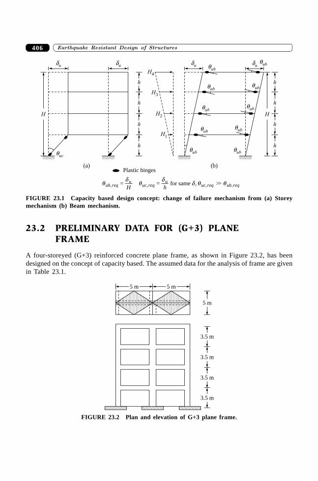
������������������� �����������������406
du du
h
h
h
h
quc
du du
h
h
h
h
qub
qubqub
qub
qubqub
qubqub
qub
qub
H1
H2
H3
H4
(a) (b)Plastic hinges
HH
q d q d d q qub requ
uc requ
uc req ub reqH h, , , ,,= = for same >>
FIGURE 23.1 Capacity based design concept: change of failure mechanism from (a) Storeymechanism (b) Beam mechanism.
23.2 PRELIMINARY DATA FOR (G+3) PLANEFRAME
A four-storeyed (G+3) reinforced concrete plane frame, as shown in Figure 23.2, has beendesigned on the concept of capacity based. The assumed data for the analysis of frame are givenin Table 23.1.
5 m
3.5 m
3.5 m
3.5 m
3.5 m
5 m 5 m
FIGURE 23.2 Plan and elevation of G+3 plane frame.
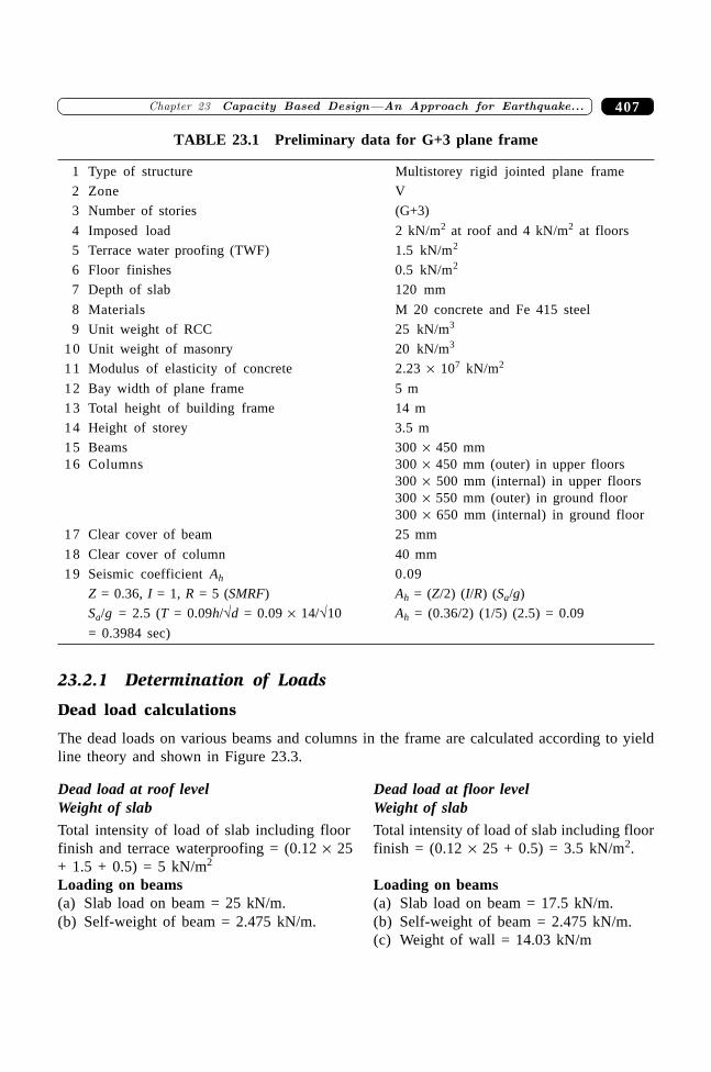
407�������� ��������� ���� �������� ��������� ���� �������������
TABLE 23.1 Preliminary data for G+3 plane frame
1 Type of structure Multistorey rigid jointed plane frame
2 Zone V
3 Number of stories (G+3)
4 Imposed load 2 kN/m2 at roof and 4 kN/m2 at floors
5 Terrace water proofing (TWF) 1.5 kN/m2
6 Floor finishes 0.5 kN/m2
7 Depth of slab 120 mm
8 Materials M 20 concrete and Fe 415 steel
9 Unit weight of RCC 25 kN/m3
10 Unit weight of masonry 20 kN/m3
11 Modulus of elasticity of concrete 2.23 ¥ 107 kN/m2
12 Bay width of plane frame 5 m
13 Total height of building frame 14 m
14 Height of storey 3.5 m
15 Beams 300 ¥ 450 mm16 Columns 300 ¥ 450 mm (outer) in upper floors
300 ¥ 500 mm (internal) in upper floors300 ¥ 550 mm (outer) in ground floor300 ¥ 650 mm (internal) in ground floor
17 Clear cover of beam 25 mm
18 Clear cover of column 40 mm
19 Seismic coefficient Ah 0.09
Z = 0.36, I = 1, R = 5 (SMRF) Ah = (Z/2) (I/R) (Sa/g)
Sa/g = 2.5 (T = 0.09h/÷d = 0.09 ¥ 14/÷10 Ah = (0.36/2) (1/5) (2.5) = 0.09
= 0.3984 sec)
23.2.1 Determination of Loads
Dead load calculations
The dead loads on various beams and columns in the frame are calculated according to yieldline theory and shown in Figure 23.3.
Dead load at roof level Dead load at floor levelWeight of slab Weight of slab
Total intensity of load of slab including floor Total intensity of load of slab including floorfinish and terrace waterproofing = (0.12 ¥ 25 finish = (0.12 ¥ 25 + 0.5) = 3.5 kN/m2.+ 1.5 + 0.5) = 5 kN/m2
Loading on beams Loading on beams(a) Slab load on beam = 25 kN/m. (a) Slab load on beam = 17.5 kN/m.(b) Self-weight of beam = 2.475 kN/m. (b) Self-weight of beam = 2.475 kN/m.
(c) Weight of wall = 14.03 kN/m
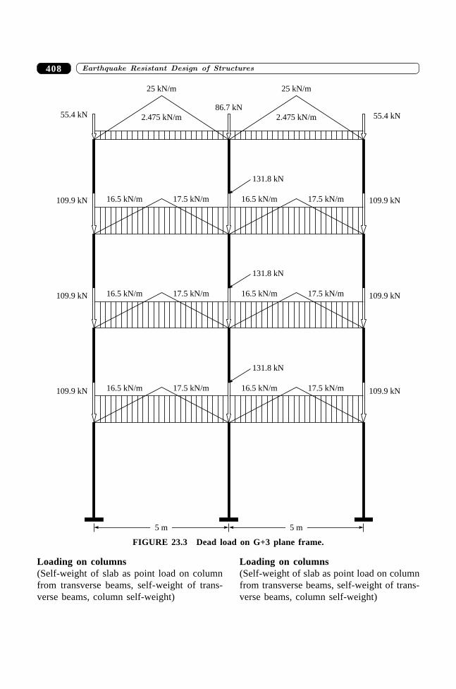
������������������� �����������������408
Loading on columns Loading on columns(Self-weight of slab as point load on column (Self-weight of slab as point load on columnfrom transverse beams, self-weight of trans- from transverse beams, self-weight of trans-verse beams, column self-weight) verse beams, column self-weight)
2.475 kN/m
16.5 kN/m 17.5 kN/m 16.5 kN/m 17.5 kN/m
25 kN/m 25 kN/m
86.7 kN55.4 kN 55.4 kN
109.9 kN
109.9 kN
109.9 kN
109.9 kN
109.9 kN
109.9 kN
2.475 kN/m
5 m 5 m
131.8 kN
16.5 kN/m 17.5 kN/m 16.5 kN/m 17.5 kN/m
131.8 kN
16.5 kN/m 17.5 kN/m 16.5 kN/m 17.5 kN/m
131.8 kN
FIGURE 23.3 Dead load on G+3 plane frame.
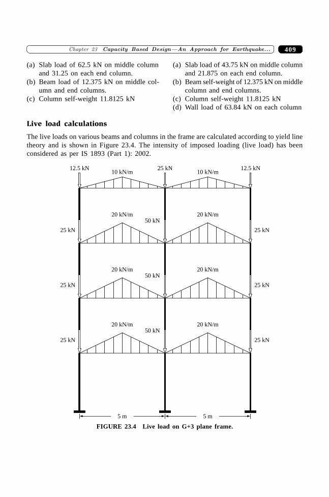
409�������� ��������� ���� �������� ��������� ���� �������������
(a) Slab load of 62.5 kN on middle column (a) Slab load of 43.75 kN on middle columnand 31.25 on each end column. and 21.875 on each end column.
(b) Beam load of 12.375 kN on middle col- (b) Beam self-weight of 12.375 kN on middleumn and end columns. column and end columns.
(c) Column self-weight 11.8125 kN (c) Column self-weight 11.8125 kN(d) Wall load of 63.84 kN on each column
Live load calculations
The live loads on various beams and columns in the frame are calculated according to yield linetheory and is shown in Figure 23.4. The intensity of imposed loading (live load) has beenconsidered as per IS 1893 (Part 1): 2002.
10 kN/m
20 kN/m50 kN
25 kN
10 kN/m
20 kN/m
25 kN
25 kN 12.5 kN12.5 kN
20 kN/m50 kN
25 kN
20 kN/m
25 kN
20 kN/m50 kN
25 kN
20 kN/m
25 kN
5 m 5 m
FIGURE 23.4 Live load on G+3 plane frame.
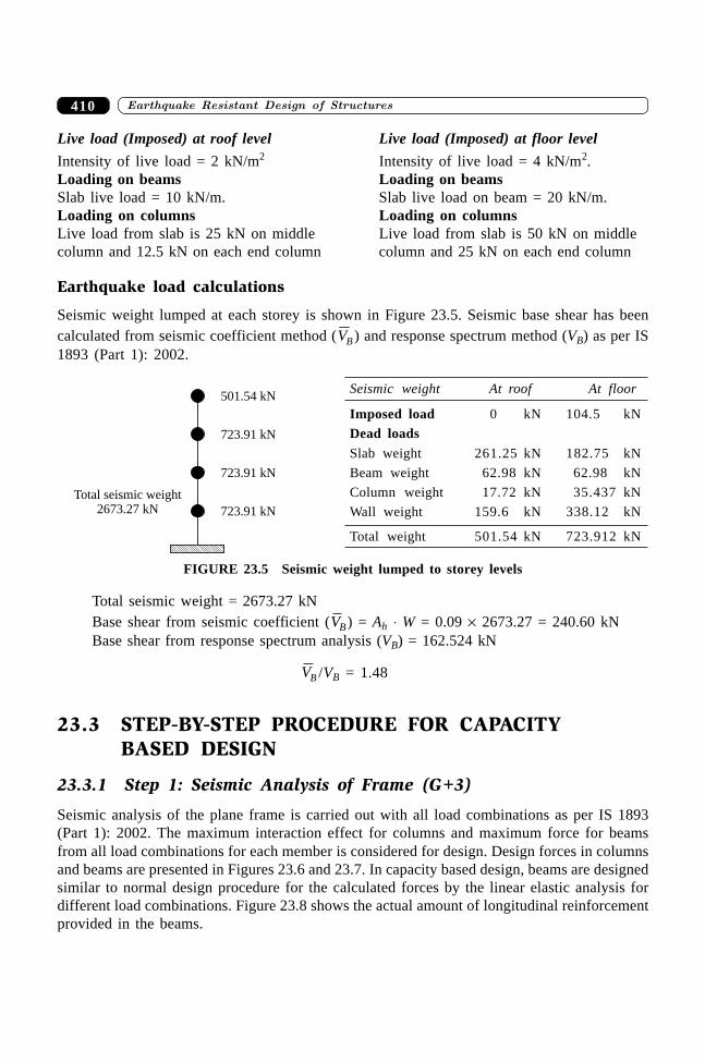
������������������� �����������������410
Live load (Imposed) at roof level Live load (Imposed) at floor level
Intensity of live load = 2 kN/m2 Intensity of live load = 4 kN/m2.Loading on beams Loading on beamsSlab live load = 10 kN/m. Slab live load on beam = 20 kN/m.Loading on columns Loading on columnsLive load from slab is 25 kN on middle Live load from slab is 50 kN on middlecolumn and 12.5 kN on each end column column and 25 kN on each end column
Earthquake load calculations
Seismic weight lumped at each storey is shown in Figure 23.5. Seismic base shear has beencalculated from seismic coefficient method (VB ) and response spectrum method (VB) as per IS1893 (Part 1): 2002.
501.54 kN
723.91 kN
723.91 kN
723.91 kN
Total seismic2673.27 kN
weight
FIGURE 23.5 Seismic weight lumped to storey levels
Total seismic weight = 2673.27 kNBase shear from seismic coefficient (VB) = Ah ◊ W = 0.09 ¥ 2673.27 = 240.60 kNBase shear from response spectrum analysis (VB) = 162.524 kN
VB /VB = 1.48
23.3 STEP-BY-STEP PROCEDURE FOR CAPACITYBASED DESIGN
23.3.1 Step 1: Seismic Analysis of Frame (G+3)
Seismic analysis of the plane frame is carried out with all load combinations as per IS 1893(Part 1): 2002. The maximum interaction effect for columns and maximum force for beamsfrom all load combinations for each member is considered for design. Design forces in columnsand beams are presented in Figures 23.6 and 23.7. In capacity based design, beams are designedsimilar to normal design procedure for the calculated forces by the linear elastic analysis fordifferent load combinations. Figure 23.8 shows the actual amount of longitudinal reinforcementprovided in the beams.
Seismic weight At roof At floor
Imposed load 0 kN 104.5 kN
Dead loadsSlab weight 261.25 kN 182.75 kN
Beam weight 62.98 kN 62.98 kN
Column weight 17.72 kN 35.437 kN
Wall weight 159.6 kN 338.12 kN
Total weight 501.54 kN 723.912 kN
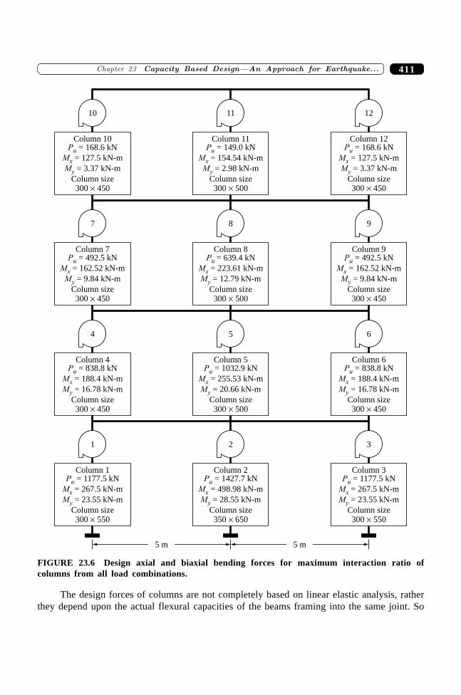
411�������� ��������� ���� �������� ��������� ���� �������������
Column 10= 168.6 kN
= 127.5 kN-m
= 3.37 kN-m
Column size300 450
P
M
M
u
�
x
y
10
Column 11= 149.0 kN
= 154.54 kN-m
= 2.98 kN-m
Column size300 500
P
M
M
�
u
x
y
11
Column 12= 168.6 kN
= 127.5 kN-m
= 3.37 kN-m
Column size300 450
P
M
M
�
u
x
y
12
Column 7= 492.5 kN
= 162.52 kN-m
= 9.84 kN-m
Column size300 450
P
M
M
�
u
x
y
7
Column 8= 639.4 kN
= 223.61 kN-m
= 12.79 kN-m
Column size300 500
P
M
M
�
u
x
y
8 9
Column 4= 838.8 kN
= 188.4 kN-m
= 16.78 kN-m
Column size300 450
P
M
M
�
u
x
y
4
Column 5= 1032.9 kN
= 255.53 kN-m
= 20.66 kN-m
Column size300 500
P
M
M
�
u
x
y
5 6
Column 1= 1177.5 kN
= 267.5 kN-m
= 23.55 kN-m
Column size300 550
P
M
M
�
u
x
y
1
Column 2= 1427.7 kN
= 498.98 kN-m
= 28.55 kN-m
Column size350 650
P
M
M
�
u
x
y
2 3
5 m 5 m
Column 9= 492.5 kN
= 162.52 kN-m
= 9.84 kN-m
Column size300 450
P
M
M
�
u
x
y
Column 6= 838.8 kN
= 188.4 kN-m
= 16.78 kN-m
Column size300 450
P
M
M
�
u
x
y
Column 3= 1177.5 kN
= 267.5 kN-m
= 23.55 kN-m
Column size300 550
P
M
M
�
u
x
y
FIGURE 23.6 Design axial and biaxial bending forces for maximum interaction ratio ofcolumns from all load combinations.
The design forces of columns are not completely based on linear elastic analysis, ratherthey depend upon the actual flexural capacities of the beams framing into the same joint. So
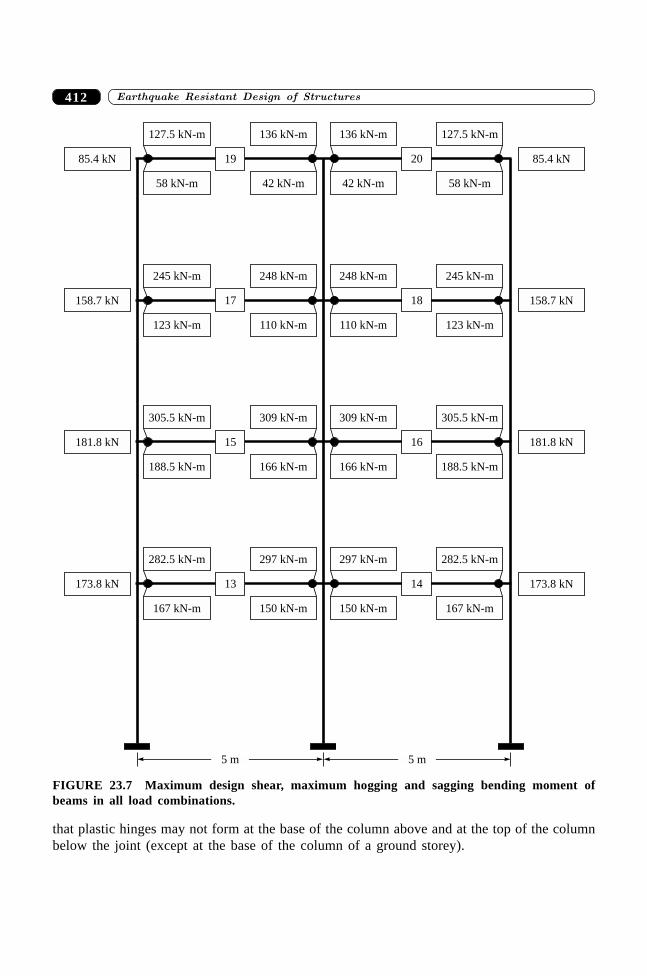
������������������� �����������������412
that plastic hinges may not form at the base of the column above and at the top of the columnbelow the joint (except at the base of the column of a ground storey).
127.5 kN-m
58 kN-m
19
127.5 kN-m
58 kN-m
2085.4 kN
245 kN-m
123 kN-m
17 18158.7 kN
305.5 kN-m
188.5 kN-m
15 16181.8 kN
282.5 kN-m
167 kN-m
13 14173.8 kN
5 m 5 m
85.4 kN
136 kN-m 136 kN-m
42 kN-m 42 kN-m
110 kN-m
248 kN-m
110 kN-m
248 kN-m
123 kN-m
245 kN-m
158.7 kN
305.5 kN-m
188.5 kN-m
309 kN-m 309 kN-m
166 kN-m166 kN-m
181.8 kN
173.8 kN
282.5 kN-m
167 kN-m
297 kN-m 297 kN-m
150 kN-m 150 kN-m
FIGURE 23.7 Maximum design shear, maximum hogging and sagging bending moment ofbeams in all load combinations.
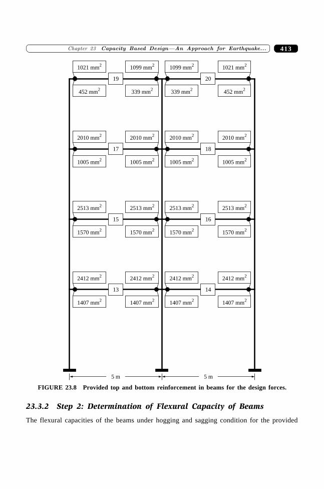
413�������� ��������� ���� �������� ��������� ���� �������������
23.3.2 Step 2: Determination of Flexural Capacity of Beams
The flexural capacities of the beams under hogging and sagging condition for the provided
1021 mm2
19 20
17 18
15 16
13 14
5 m 5 m
1099 mm2
1021 mm2
1099 mm2
339 mm2
339 mm2
452 mm2
452 mm2
2010 mm2
2010 mm2
1005 mm2
1005 mm2
2513 mm2
2513 mm2
1570 mm2
1570 mm2
2513 mm2
2513 mm2
1570 mm2
1570 mm2
2412 mm2
2412 mm2
2412 mm2
2412 mm2
1407 mm2
1407 mm2
1407 mm2
1407 mm2
2010 mm2
1005 mm2
2010 mm2
1005 mm2
FIGURE 23.8 Provided top and bottom reinforcement in beams for the design forces.
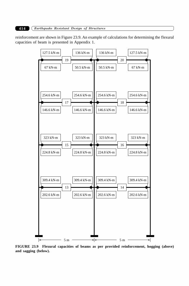
������������������� �����������������414
reinforcement are shown in Figure 23.9. An example of calculations for determining the flexuralcapacities of beam is presented in Appendix 1.
127.5 kN-m
67 kN-m
19
127.5 kN-m
20
254.6 kN-m
146.6 kN-m
17 18
323 kN-m
224.8 kN-m
15 16
309.4 kN-m 309.4 kN-m 309.4 kN-m 309.4 kN-m
202.6 kN-m
13 14
5 m 5 m
136 kN-m 136 kN-m
50.5 kN-m 50.5 kN-m 67 kN-m
146.6 kN-m
254.6 kN-m 254.6 kN-m 254.6 kN-m
146.6 kN-m 146.6 kN-m
224.8 kN-m 224.8 kN-m 224.8 kN-m
323 kN-m 323 kN-m 323 kN-m
202.6 kN-m 202.6 kN-m 202.6 kN-m
FIGURE 23.9 Flexural capacities of beams as per provided reinforcement, hogging (above)and sagging (below).
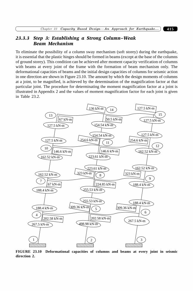
415�������� ��������� ���� �������� ��������� ���� �������������
23.3.3 Step 3: Establishing a Strong Column–WeakBeam Mechanism
To eliminate the possibility of a column sway mechanism (soft storey) during the earthquake,it is essential that the plastic hinges should be formed in beams (except at the base of the columnsof ground storey). This condition can be achieved after moment capacity verification of columnswith beams at every joint of the frame with the formation of beam mechanism only. Thedeformational capacities of beams and the initial design capacities of columns for seismic actionin one direction are shown in Figure 23.10. The amount by which the design moments of columnsat a joint, to be magnified, is achieved by the determination of the magnification factor at thatparticular joint. The procedure for determinating the moment magnification factor at a joint isillustrated in Appendix 2 and the values of moment magnification factor for each joint is givenin Table 23.2.
1367 kN-m
127.5 kN-m
127.5 kN-m
127.5 kN-m
10146.6 kN-m
162.52 kN-m
162.52 kN-m
767 kN-m
188.4 kN-m
188.4 kN-m
4202.58 kN-m
267.5 kN-m
1
14136 kN-m
15
127.5 kN-m
127.5 kN-m
50.5 kN-m
154.54 kN-m
154.54 kN-m
11254.6 kN-m254.6 kN-m
12
146.6 kN-m
223.61 kN-m
223.61 kN-m
89
323 kN-m 323 kN-m
162.52 kN-m
162.52 kN-m
224.85 kN-m
255.53 kN-m
255.53 kN-m
188.4 kN-m
188.4 kN-m
309.36 kN-m309.36 kN-m5
6
267.5 kN-m202.58 kN-m
498.98 kN-m
2 3
FIGURE 23.10 Deformational capacities of columns and beams at every joint in seismicdirection 2.
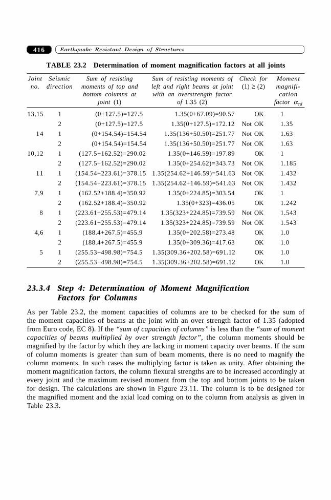
������������������� �����������������416
TABLE 23.2 Determination of moment magnification factors at all joints
Joint Seismic Sum of resisting Sum of resisting moments of Check for Momentno. direction moments of top and left and right beams at joint (1) ≥ (2) magnifi-
bottom columns at with an overstrength factor cationjoint (1) of 1.35 (2) factor acd
13,15 1 (0+127.5)=127.5 1.35(0+67.09)=90.57 OK 1
2 (0+127.5)=127.5 1.35(0+127.5)=172.12 Not OK 1.35
14 1 (0+154.54)=154.54 1.35(136+50.50)=251.77 Not OK 1.63
2 (0+154.54)=154.54 1.35(136+50.50)=251.77 Not OK 1.63
10,12 1 (127.5+162.52)=290.02 1.35(0+146.59)=197.89 OK 1
2 (127.5+162.52)=290.02 1.35(0+254.62)=343.73 Not OK 1.185
11 1 (154.54+223.61)=378.15 1.35(254.62+146.59)=541.63 Not OK 1.432
2 (154.54+223.61)=378.15 1.35(254.62+146.59)=541.63 Not OK 1.432
7,9 1 (162.52+188.4)=350.92 1.35(0+224.85)=303.54 OK 1
2 (162.52+188.4)=350.92 1.35(0+323)=436.05 OK 1.242
8 1 (223.61+255.53)=479.14 1.35(323+224.85)=739.59 Not OK 1.543
2 (223.61+255.53)=479.14 1.35(323+224.85)=739.59 Not OK 1.543
4,6 1 (188.4+267.5)=455.9 1.35(0+202.58)=273.48 OK 1.0
2 (188.4+267.5)=455.9 1.35(0+309.36)=417.63 OK 1.0
5 1 (255.53+498.98)=754.5 1.35(309.36+202.58)=691.12 OK 1.0
2 (255.53+498.98)=754.5 1.35(309.36+202.58)=691.12 OK 1.0
23.3.4 Step 4: Determination of Moment MagnificationFactors for Columns
As per Table 23.2, the moment capacities of columns are to be checked for the sum ofthe moment capacities of beams at the joint with an over strength factor of 1.35 (adoptedfrom Euro code, EC 8). If the “sum of capacities of columns” is less than the “sum of momentcapacities of beams multiplied by over strength factor”, the column moments should bemagnified by the factor by which they are lacking in moment capacity over beams. If the sumof column moments is greater than sum of beam moments, there is no need to magnify thecolumn moments. In such cases the multiplying factor is taken as unity. After obtaining themoment magnification factors, the column flexural strengths are to be increased accordingly atevery joint and the maximum revised moment from the top and bottom joints to be takenfor design. The calculations are shown in Figure 23.11. The column is to be designed forthe magnified moment and the axial load coming on to the column from analysis as given inTable 23.3.
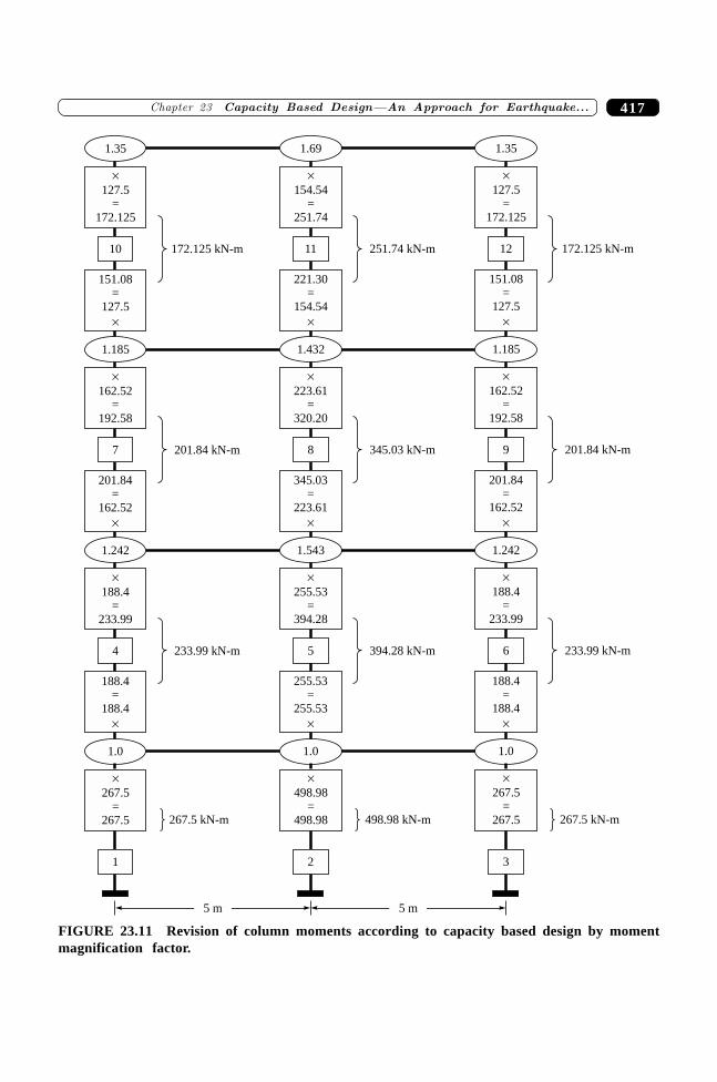
417�������� ��������� ���� �������� ��������� ���� �������������
�
127.5=
172.125
10 172.125 kN-m
7 201.84 kN-m
4 233.99 kN-m
�
188.4=
233.99
1
267.5 kN-m
1.35
151.08=
127.5
�
1.185
�
162.52=
192.58
201.84=
162.52
�
1.242
188.4=
188.4
�
1.0
�
267.5=
267.5
�
154.54=
251.74
11 251.74 kN-m
8 345.03 kN-m
5 394.28 kN-m
�
255.53=
394.28
2
498.98 kN-m
1.69
221.30=
154.54
�
1.432
�
223.61=
320.20
345.03=
223.61
�
1.543
255.53=
255.53
�
1.0
�
498.98=
498.98
�
127.5=
172.125
12 172.125 kN-m
9 201.84 kN-m
6 233.99 kN-m
�
188.4=
233.99
3
267.5 kN-m
1.35
151.08=
127.5
�
1.185
�
162.52=
192.58
201.84=
162.52
�
1.242
188.4=
188.4
�
1.0
�
267.5=
267.5
5 m 5 m
FIGURE 23.11 Revision of column moments according to capacity based design by momentmagnification factor.
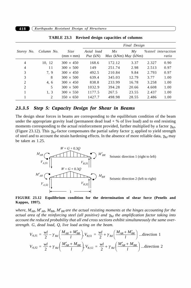
������������������� �����������������418
TABLE 23.3 Revised design capacities of columns
Final Design
Storey No. Column No. Size Axial load Mx My %steel interaction(mm ¥ mm) Puz (kN) Mux (kNm) Muy (kNm) ratio
4 10, 12 300 ¥ 450 168.6 172.12 3.37 2.327 0.904 11 300 ¥ 500 149 251.74 2.98 2.513 0.973 7, 9 300 ¥ 450 492.5 210.84 9.84 2.793 0.973 8 300 ¥ 500 639.4 345.03 12.79 3.77 1.002 4, 6 300 ¥ 450 838.8 233.99 16.78 3.258 1.002 5 300 ¥ 500 1032.9 394.28 20.66 4.608 1.001 1, 3 300 ¥ 550 1177.5 267.5 23.55 2.437 1.001 2 350 ¥ 650 1427.7 498.98 28.55 2.486 1.00
23.3.5 Step 5: Capacity Design for Shear in Beams
The design shear forces in beams are corresponding to the equilibrium condition of the beamunder the appropriate gravity load (permanent dead load + % of live load) and to end resistingmoments corresponding to the actual reinforcement provided, further multiplied by a factor gRd,(Figure 23.12). This gRd-factor compensates the partial safety factor gs applied to yield strengthof steel and to account the strain hardening effects. In the absence of more reliable data, gRd maybe taken as 1.25.
VB, 1SVA S, 1
MAR M¢BR
W G Q= + 0.3
VB, 2SVA, 2S
M¢AR MBR
W G Q= + 0.3
Seismic direction 1 (right to left)
Seismic direction 2 (left to right)
1
FIGURE 23.12 Equilibrium condition for the determination of shear force (Penelis andKappos, 1997).
where, MAR, M¢AR, MBR, M¢BR are the actual resisting moments at the hinges accounting for theactual area of the reinforcing steel (all positive) and gRd the amplification factor taking intoaccount the reduced probability that all end cross sections exhibit simultaneously the same over-strength. G, dead load, Q, live load acting on the beam.
VA,S1 = wl M Ml
VRdAR BR
B S2 1- + ¢FH
IKg , , = wl M M
lRdAR BR
2+ + ¢F
HIKg ...direction 1
VA,S2 = wl M Ml
VRdAR BR
B S2 2+¢ +F
HGIKJg , , = wl M M
lRdAR BR
2+
¢ +FHG
IKJg ...direction 2
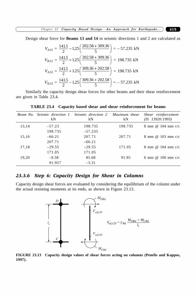
419�������� ��������� ���� �������� ��������� ���� �������������
Design shear force for Beams 13 and 14 in seismic directions 1 and 2 are calculated as
VA,S1 = 14152
1 25202 58 309 36
5. .
. .- +FH
IK = – 57.235 kN
VB,S1 = 14152
125202 58 309 36
5. .
. .+ +FH
IK = 198.735 kN
VA,S2 = 14152
125309 36 202 58
5. .
. .+ +FH
IK = 198.735 kN
VB,S2 = 14152
1 25309 36 202 58
5. .
. .- +FH
IK = – 57.235 kN
Similarly the capacity design shear forces for other beams and their shear reinforcementare given in Table 23.4.
TABLE 23.4 Capacity based shear and shear reinforcement for beams
Beam No. Seismic direction 1 Seismic direction 2 Maximum shear Shear reinforcementkN kN kN (IS 13920:1993)
13,14 –57.23 198.735 198.735 8 mm @ 104 mm c/c198.735 –57.235
15,16 –66.21 207.71 207.71 8 mm @ 103 mm c/c207.71 –66.21
17,18 –29.55 –29.55 171.05 8 mm @ 104 mm c/c171.05 171.05
19,20 –9.58 85.68 91.95 6 mm @ 100 mm c/c91.957 –3.31
23.3.6 Step 6: Capacity Design for Shear in Columns
Capacity design shear forces are evaluated by considering the equilibrium of the column underthe actual resisting moments at its ends, as shown in Figure 23.13.
MDRd
Vsd CD,
D
MCRd
Vsd CD,
C
lc VM M
lsd CD RdDRd CRd
c, =
+g
FIGURE 23.13 Capacity design values of shear forces acting on columns (Penelis and Kappos,1997).
������������������� �����������������420
where, MDRd and MCRd are the flexural capacities of the end sections as detailed (the earth-quake action has to be considered with both signs), lc is the clear height of the column andgRd = 1.35
Calculated capacity based design shear forces in the columns of the plane frame are givenin Table 23.5.
TABLE 23.5 Capacity based design shear in columns and design of lateral ties
Columns Capacity based shear (kN) Specially confiningreinforcement
1,3 1.35 ((267.50+267.5)/3.5) = 206.35 kN 10 F @ 50 mm c/c upto lo
10 F @ 150 mm c/c after lo
2 1.35 ((498.98+498.98)/3.5) = 384.92 kN 10 F @ 100 mm c/c upto lo
10 F @ 175 mm c/c after lo
4,6 1.35 ((233.99+233.99)/3.5) = 180.50 kN 10 F @ 45 mm c/c upto lo
10 F @ 150 mm c/c after lo
5 1.35 ((394.28+394.28)/3.5) = 304.15 kN 10 F @ 45 mm c/c upto lo
10 F @ 150 mm c/c after lo
7,9 1.35 ((201.84+201.84)/3.5) = 155.70 kN 10 F @ 45 mm c/c upto lo
10 F @ 150 mm c/c after lo
8 1.35 ((345.03+345.03)/3.5) = 266.16 kN 10 F @ 48 mm c/c upto lo
10 F @ 150 mm c/c after lo
10,12 1.35 ((172.12+172.12)/3.5) = 132.78 kN 10 F @ 45 mm c/c upto lo
10 F @ 150 mm c/c after lo
11 1.35 ((251.74+251.74)/3.5) = 194.20 kN 10 F @ 48 mm c/c upto lo
10 F @ 150 mm c/c after lo
23.3.7 Step 7: Detailing of Reinforcements
The detailing of shear reinforcement for the whole frame is shown in Figure 23.14, specialconfining reinforcement requirements as per IS 13920:1993. The details of main reinforcementare not shown.
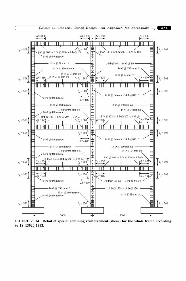
421�������� ��������� ���� �������� ��������� ���� �������������
2 = 830d 2 = 830d
lo = 508
lo = 508
14 @ 89 mm c/c�
14 @ 89 mm c/c�
14 @ 89 mm c/c�2 = 830d
lo = 508
lo = 508
14 @ 150 mm c/c�
14 @ 89 mm c/c�
14 @ 89 mm c/c�
2 = 830d
lo = 508
lo = 508
14 @ 150 mm c/c�
14 @ 89 mm c/c�
14 @ 89 mm c/c�
2 = 830d
lo = 550
lo = 550
14 @ 150 mm c/c�
14 @ 99 mm c/c�
14 @ 99 mm c/c�
6 @ 100 -:- 6 @ 209 -:- 6 @ 100�� �
14 @ 150 mm c/c�
14 @ 94 mm c/c�
14 @ 94 mm c/c�
8 @ 103 -:- 8 @ 207 -:- 8 @� � �
2 = 830d
2 = 830d
2 = 830d
14 @ 94 mm c/c�
8 @ 104 -:- 8 @ 208 -:- 8 @� � �
2 = 830d
10 @ 100 mm c/c�
2 = 830d 2 = 830d
lo = 508
lo = 508 2 = 830d
lo = 508
lo = 508
14 @ 150 mm c/c�
2 = 830d
lo = 508
lo = 508
14 @ 150 mm c/c�
2 = 830d
lo = 650
lo = 650
10 @ 100 c/c -:- 14 @ 99 c/c� �
14 @ 99 mm c/c�
6 @ 100 -:- 6 @ 209 -:- 6 @ 100� � �
14 @ 150 mm c/c�
14 @ 94 mm c/c�
14 @ 94 mm c/c�
8 @ 103 -:- 6 @ 207 -:- 8 @� � �
2 = 830d
2 = 830d
2 = 830d
14 @ 94 mm c/c�
8 @ 104 -:- 8 @ 208 -:- 8 @� � �
2 = 830d
lo = 508
lo = 508
lo = 508
lo = 508
lo = 508
lo = 508
lo = 508
lo = 508
5000 5000
10 @ 175 -:- 14 @ 150� �
14 @ 94 c/c -:- 14 @ 89 c/c� �
14 @ 94 c/c -:- 14 @ 89 c/c� �
14 @ 94 -:- 14 @ 89� �
2 = 830d
FIGURE 23.14 Detail of special confining reinforcement (shear) for the whole frame accordingto IS 13920:1993.
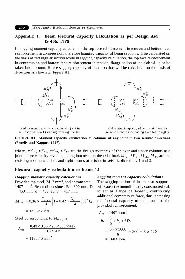
������������������� �����������������422
Appendix 1: Beam Flexural Capacity Calculation as per Design AidIS 456: 1978
In hogging moment capacity calculation, the top face reinforcement in tension and bottom facereinforcement in compression, therefore hogging capacity of beam section will be calculated onthe basis of rectangular section while in sagging capacity calculation, the top face reinforcementin compression and bottom face reinforcement in tension, flange action of the slab will also betaken into account. Hence sagging capacity of beam section will be calculated on the basis ofT-section as shown in Figure A1.
MRl1
MRO1
MRr1
MRU1
MRl2
MRO2
MRr2
MRU2
End moment capacity of beams at a joint inseismic direction 1 (loading from right to left)
End moment capacity of beams at a joint inseismic direction 2 (loading from left to right)
FIGURE A1 Moment capacity verification of columns at any joint in two seismic directions(Penelis and Kappos, 1997).
where, MOR1, MU
R1, MOR2, MU
R2 are the design moments of the over and under columns at ajoint before capacity revision, taking into account the axial load. Ml
R1, MrR1, Ml
R2, MrR2 are the
resisting moments of left and right beams at a joint in seismic directions 1 and 2.
Flexural capacity calculation of beam 13
Sagging moment capacity calculationsThe sagging action of beam near supportswill cause the monolithically constructed slabto act as flange of T-beam, contributingadditional compressive force, thus increasingthe flexural capacity of the beam for theprovided reinforcement.
Ast = 1407 mm2,
bf = l
b Dw f0
66+ +
= 0 7 5000
6. ¥
+ 300 + 6 ¥ 120
= 1603 mm
Hogging moment capacity calculationsProvided top steel, 2412 mm2, and bottom steel,1407 mm2. Beam dimensions: B = 300 mm, D= 450 mm, d = 450–25–8 = 417 mm
Mulim = 0.36 ¥ X
du max 1 0 42- ¥L
NMOQP. maxX
du bd2 fck
= 143.942 kN
Steel corresponding to Mulim, is
Ast1 = 0 48 0 36 20 300 417
0 87 415. .
.¥ ¥ ¥ ¥
¥
= 1197.46 mm2
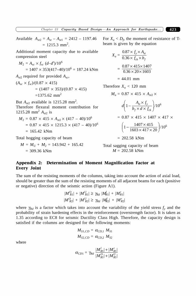
423�������� ��������� ���� �������� ��������� ���� �������������
For Xu < Df, the moment of resistance of T-beam is given by the equation
Xu = 0 87
0 36
.
.
¥ ¥¥ ¥
f A
f by st
ck f
= 0 87 415 14070 36 20 1603..
¥ ¥¥ ¥
= 44.01 mm
Therefore Xu < 120 mm
Mu = 0.87 ¥ 415 ¥ Ast2 ¥
d 1 -¥
¥ ¥FHG
IKJ
A f
b d fst y
f ck/106
= 0.87 ¥ 415 ¥ 1407 ¥ 417 ¥
11407 415
1603 417 20- ¥
¥ ¥FHG
IKJ /106
= 202.58 kNm
Total sagging capacity of beamM = 202.58 kNm
Appendix 2: Determination of Moment Magnification Factor atEvery Joint
The sum of the resisting moments of the columns, taking into account the action of axial load,should be greater than the sum of the resisting moments of all adjacent beams for each (positiveor negative) direction of the seismic action (Figure A1).
|MOR1| + |MU
R1| ≥ gRd |MlR1| + |Mr
R1|
|MOR2| + |MU
R2| ≥ gRd |MlR2| + |Mr
R2|
where gRd is a factor which takes into account the variability of the yield stress fy and theprobability of strain hardening effects in the reinforcement (overstrength factor). It is taken as1.35 according to EC8 for seismic Ductility Class High. Therefore, the capacity design issatisfied if the columns are designed for the following moments:
MS1,CD = aCD,1 MS1
MS2,CD = aCD,2 MS2
where
aCD1 = gRd | | | |
| | | |
M M
M MRl
Rr
RO
RU
1 1
1 1
++
Available Ast2 = Ast – Ast1 = 2412 – 1197.46
= 1215.3 mm2.
Additional moment capacity due to availablecompression steel
M2 = Asc ¥ fsc (d–d¢)/106
= 1407 ¥ 353(417–40)/106 = 187.24 kNm
Ast2 required for provided Asc,
(Asc ¥ fsc)/(0.87 ¥ 415)
= (1407 ¥ 353)/(0.87 ¥ 415)
=1375.62 mm2
But Ast2 available is 1215.28 mm2.Therefore flexural moment contribution for1215.28 mm2 Ast2 is
M2 = 0.87 ¥ 415 ¥ Ast2 ¥ (417 – 40)/106
= 0.87 ¥ 415 ¥ 1215.3 ¥ (417 – 40)/106
= 165.42 kNm
Total hogging capacity of beam
M = MU + M2 = 143.942 + 165.42
= 309.36 kNm
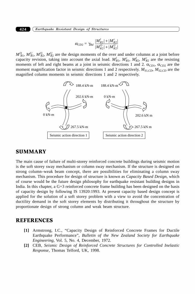
������������������� �����������������424
aCD2 = gRd | | | |
| | | |
M M
M MRl
Rr
RO
RU
2 2
2 2
++
MOR1, MU
R1, MOR2, MU
R2 are the design moments of the over and under columns at a joint beforecapacity revision, taking into account the axial load. Ml
R1, MrR1, Ml
R2, MrR2 are the resisting
moments of left and right beams at a joint in seismic directions 1 and 2. aCD1, aCD2 are themoment magnification factor in seismic directions 1 and 2 respectively. MS1,CD, MS2,CD are themagnified column moments in seismic directions 1 and 2 respectively.
Seismic action direction 1 Seismic action direction 2
188.4 kN-m 188.4 kN-m
202.6 kN-m 0 kN-m
0 kN-m 202.6 kN m
267.5 kN-m 267.5 kN m
SUMMARY
The main cause of failure of multi-storey reinforced concrete buildings during seismic motionis the soft storey sway mechanism or column sway mechanism. If the structure is designed onstrong column–weak beam concept, there are possibilities for eliminating a column swaymechanism. This procedure for design of structure is known as Capacity Based Design, whichof course would be the future design philosophy for earthquake resistant building designs inIndia. In this chapter, a G+3 reinforced concrete frame building has been designed on the basisof capacity design by following IS 13920:1993. At present capacity based design concept isapplied for the solution of a soft storey problem with a view to avoid the concentration ofductility demand in the soft storey elements by distributing it throughout the structure byproportionate design of strong column and weak beam structure.
REFERENCES
[1] Armstrong, I.C., “Capacity Design of Reinforced Concrete Frames for DuctileEarthquake Performance”, Bulletin of the New Zealand Society for EarthquakeEngineering, Vol. 5, No. 4, December, 1972.
[2] CEB, Seismic Design of Reinforced Concrete Structures for Controlled InelasticResponse, Thomas Telford, UK, 1998.

425�������� ��������� ���� �������� ��������� ���� �������������
[3] Chapman, H.E., North, P.J. and Park, R., “Capacity Design Principles and Practices”,Bulletin of the New Zealand National Society for Earthquake Engineering, Vol. 13,No. 3, September, 1980.
[4] Dadi, V.V.S., Surya Kumar, “Seismic Evaluation of Reinforced Concrete Buildingwith Soft Storey”, M. Tech. Dissertation, Department of Earthquake Engineering, IITRoorkee, June 2004.
[5] Eurocode 8, “Design of Structures for Earthquake Resistance—Part 1: General rules,Seismic actions and rules for Buildings”, CEN, 2002.
[6] IS 13920, Ductile Detailing of Reinforced Concrete Structures Subjected to SeismicForces—Code of Practice”, Bureau of Indian Standards, New Delhi, 1993.
[7] IS 1893, Criteria for Earthquake Resistant Design of Structures—Part 1: GeneralProvisions and Buildings (Fifth Revision), Bureau of Indian Standards, New Delhi,2002.
[8] NZS 3101, Concrete Structures Standard, Part 1—The Design of Concrete Structures,Standards New Zealand, Paerewa Aotearoa, 1995.
[9] Paulay, T. and Goodsir, W.J., “The Capacity Design of Reinforced Concrete HybridStructures for Multistorey Buildings”, Bulletin of the New Zealand National Societyfor Earthquake Engineering, Vol. 19, No. 1, March, 1986.
[10] Penelis, G.G. and Kappos, A.J., “Earthquake-Resistant Concrete Structures”, E & FNSPON, an Imprint of Chapman & Hall, 1997.

���� ��
Earthquake Resistant Design(ERD) of Masonay Buildings

429
Identification of Damagesand Non-damages in
Masonry Buildings fromPast Indian Earthquakes
��������
24.1 INTRODUCTION
The masonry buildings have proved to be the most vulnerable to earthquake forces and havesuffered maximum damage in past earthquakes. A survey of the affected areas in past earthquakes(Bhuj, 2001, Chamoli, 1999, Jabalpur, 1997, Killari, 1993, Uttarkashi, 1991 and Bihar-Nepal,1988) has clearly demonstrated that the major loss of lives was due to collapse of low strengthmasonry buildings. The loss of lives could have been minimized upto optimum by making thebuildings earthquake resistant. This requires diagnostic analysis of the structural behaviour ofthe ‘As Built’ condition of these constructions. Diagnostic studies are best achieved by dynamictesting of stereotyped, prototype buildings, which manifest their structural distress pattern, andverification upto its optimum limit. Each earthquake puts buildings in the affected area to anearthquake withstand test and provides an opportunity to learn lessons for future preparednessto meet the challenge of disaster. Thus, the efforts of post-earthquake damage survey should bedirected to arrive at engineering lessons for improving earthquake resistant design and construc-tion practice. This chapter is motivated towards the identification of typical features of damagesand non-damages of masonry buildings during recent earthquakes in India. The experience andobservations of damages and performance of structures in earthquakes with the results of earth-quake engineering research must be utilized in improving earthquake resistant design and con-struction techniques of masonry buildings for preventing damages in future earthquakes.
24.2 PAST INDIAN EARTHQUAKES
The characteristic of past earthquakes where masonry construction is significantly damaged isdescribed in Table 24.1. The table illustrates some parameters of earthquake and losses in terms
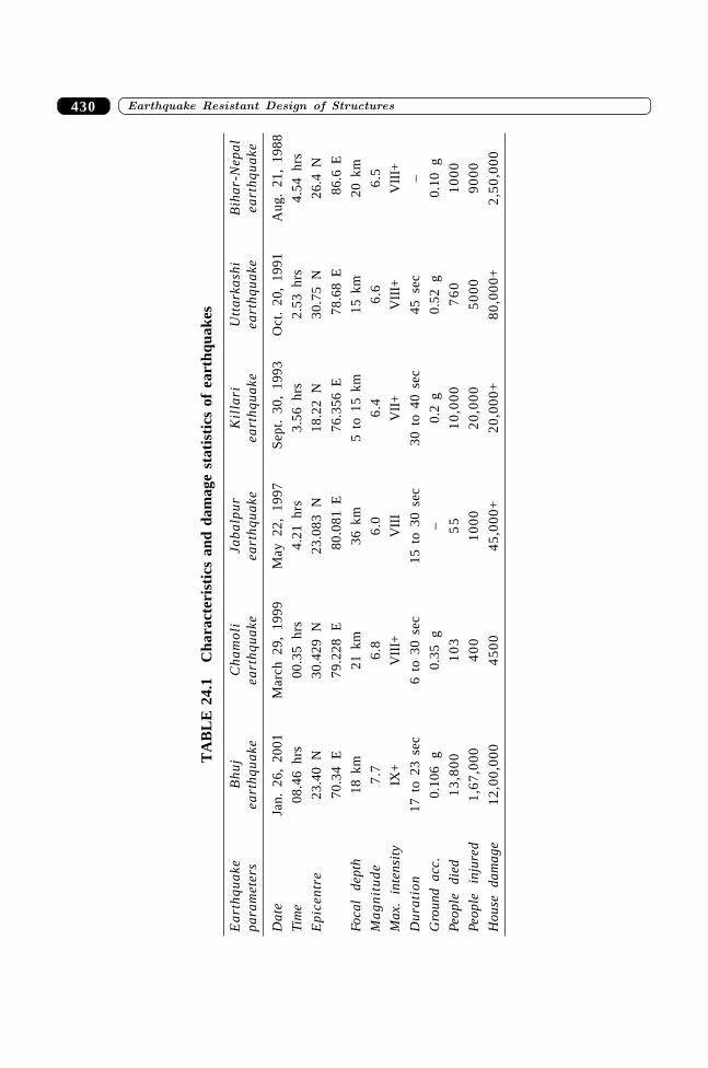
����������� ������� �������������430
TA
BL
E 2
4.1
Cha
ract
eris
tics
and
dam
age
stat
isti
cs o
f ea
rthq
uake
s
Ea
rth
qu
ake
Bh
uj
Ch
am
oli
Jab
alp
ur
Kil
lari
Utt
arka
shi
Bih
ar-N
epal
para
met
ers
eart
hq
ua
keea
rth
qu
ake
eart
hq
ua
keea
rth
qu
ake
eart
hq
ua
keea
rth
qu
ake
Dat
eJa
n. 2
6, 2
001
Mar
ch 2
9, 1
999
May
22,
199
7 S
ept.
30,
199
3O
ct.
20,
1991
Aug
. 21
, 19
88
Tim
e08
.46
hrs
00.3
5 hr
s4.
21 h
rs3.
56 h
rs2.
53 h
rs4.
54 h
rs
Epi
cent
re23
.40
N30
.429
N23
.083
N18
.22
N30
.75
N26
.4 N
70.3
4 E
79.2
28 E
80.
081
E 7
6.35
6 E
78.
68 E
86.
6 E
Foca
l de
pth
18 k
m21
km
36 k
m5
to 1
5 km
15 k
m20
km
Ma
gn
itu
de
7.7
6.8
6.0
6.4
6.6
6.5
Max
. in
tens
ity
IX+
VII
I+V
III
VII
+V
III+
VII
I+
Dur
atio
n17
to
23 s
ec6
to 3
0 se
c15
to
30 s
ec30
to
40 s
ec45
sec
–
Gro
und
acc.
0.10
6 g
0.35
g–
0.2
g0.
52 g
0.10
g
Peop
le
died
13
,80
01
03
55
10
,00
07
60
10
00
Peop
le
inju
red
1,67
,000
40
01
00
02
0,0
00
50
00
90
00
Hou
se
dam
age
12,0
0,00
04
50
045
,000
+20
,000
+80
,000
+2,
50,0
00
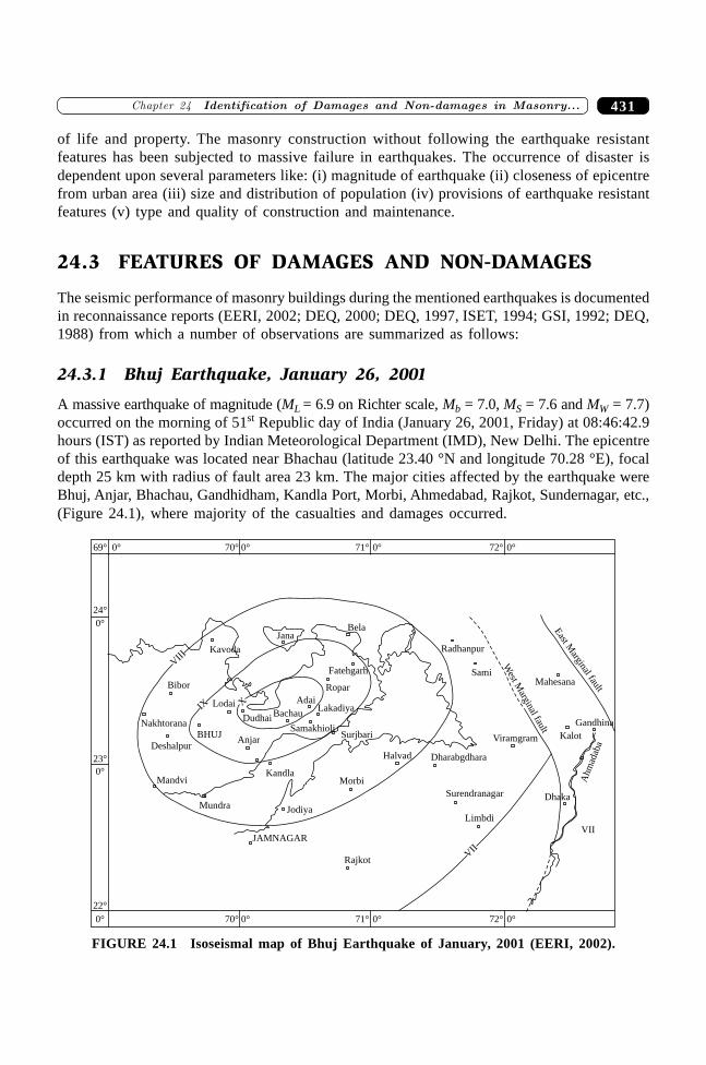
431�������� ���� � ��� ����������������������� �����������
of life and property. The masonry construction without following the earthquake resistantfeatures has been subjected to massive failure in earthquakes. The occurrence of disaster isdependent upon several parameters like: (i) magnitude of earthquake (ii) closeness of epicentrefrom urban area (iii) size and distribution of population (iv) provisions of earthquake resistantfeatures (v) type and quality of construction and maintenance.
24.3 FEATURES OF DAMAGES AND NON-DAMAGES
The seismic performance of masonry buildings during the mentioned earthquakes is documentedin reconnaissance reports (EERI, 2002; DEQ, 2000; DEQ, 1997, ISET, 1994; GSI, 1992; DEQ,1988) from which a number of observations are summarized as follows:
24.3.1 Bhuj Earthquake, January 26, 2001
A massive earthquake of magnitude (ML = 6.9 on Richter scale, Mb = 7.0, MS = 7.6 and MW = 7.7)occurred on the morning of 51st Republic day of India (January 26, 2001, Friday) at 08:46:42.9hours (IST) as reported by Indian Meteorological Department (IMD), New Delhi. The epicentreof this earthquake was located near Bhachau (latitude 23.40 °N and longitude 70.28 °E), focaldepth 25 km with radius of fault area 23 km. The major cities affected by the earthquake wereBhuj, Anjar, Bhachau, Gandhidham, Kandla Port, Morbi, Ahmedabad, Rajkot, Sundernagar, etc.,(Figure 24.1), where majority of the casualties and damages occurred.
70°
70°
0°
0°
71°
71°
0°
0°
72°
72°
0°
0°69° 0°
24°
0°
23°
0°
22°
0°
Bibor
Nakhtorana
BHUJ
DeshalpurAnjar
Kandla
Mundra
Mandvi
Jodiya
JAMNAGAR
Rajkot
Morbi
Halvad Dharabgdhara
Surendranagar
Limbdi
Dhaka
Ahm
adab
a
Kalot
Gandhina
Mahesana
East M
arginal fault
West M
arginal fault
Viramgram
Sami
Radhanpur
Bela
Fatehgarh
Ropar
LakadiyaAdai
BachauDudhai
SamakhioliSurjbari
Lodai
Kavoda
Jana
XIX
VIII
VII
VII
FIGURE 24.1 Isoseismal map of Bhuj Earthquake of January, 2001 (EERI, 2002).
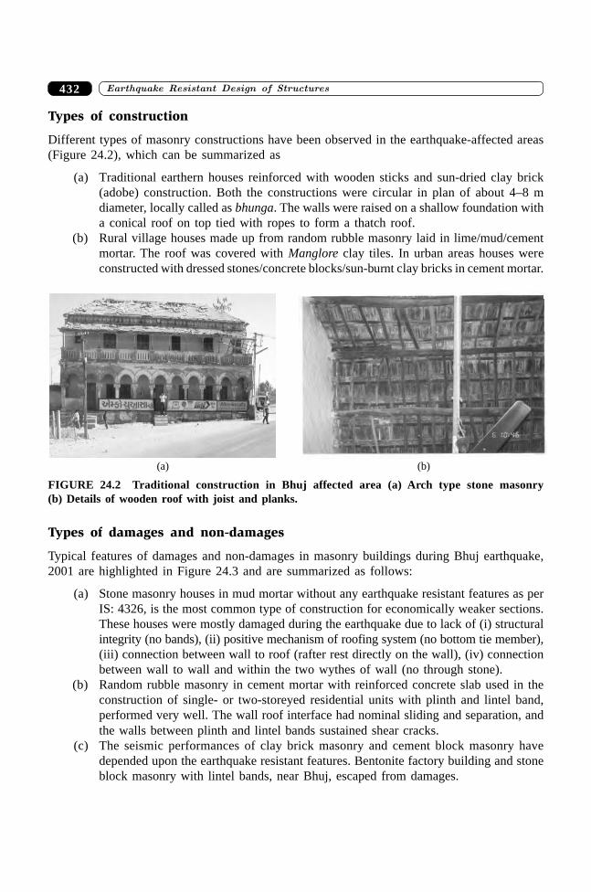
����������� ������� �������������432
Types of construction
Different types of masonry constructions have been observed in the earthquake-affected areas(Figure 24.2), which can be summarized as
(a) Traditional earthern houses reinforced with wooden sticks and sun-dried clay brick(adobe) construction. Both the constructions were circular in plan of about 4–8 mdiameter, locally called as bhunga. The walls were raised on a shallow foundation witha conical roof on top tied with ropes to form a thatch roof.
(b) Rural village houses made up from random rubble masonry laid in lime/mud/cementmortar. The roof was covered with Manglore clay tiles. In urban areas houses wereconstructed with dressed stones/concrete blocks/sun-burnt clay bricks in cement mortar.
(a) (b)
FIGURE 24.2 Traditional construction in Bhuj affected area (a) Arch type stone masonry(b) Details of wooden roof with joist and planks.
Types of damages and non-damages
Typical features of damages and non-damages in masonry buildings during Bhuj earthquake,2001 are highlighted in Figure 24.3 and are summarized as follows:
(a) Stone masonry houses in mud mortar without any earthquake resistant features as perIS: 4326, is the most common type of construction for economically weaker sections.These houses were mostly damaged during the earthquake due to lack of (i) structuralintegrity (no bands), (ii) positive mechanism of roofing system (no bottom tie member),(iii) connection between wall to roof (rafter rest directly on the wall), (iv) connectionbetween wall to wall and within the two wythes of wall (no through stone).
(b) Random rubble masonry in cement mortar with reinforced concrete slab used in theconstruction of single- or two-storeyed residential units with plinth and lintel band,performed very well. The wall roof interface had nominal sliding and separation, andthe walls between plinth and lintel bands sustained shear cracks.
(c) The seismic performances of clay brick masonry and cement block masonry havedepended upon the earthquake resistant features. Bentonite factory building and stoneblock masonry with lintel bands, near Bhuj, escaped from damages.
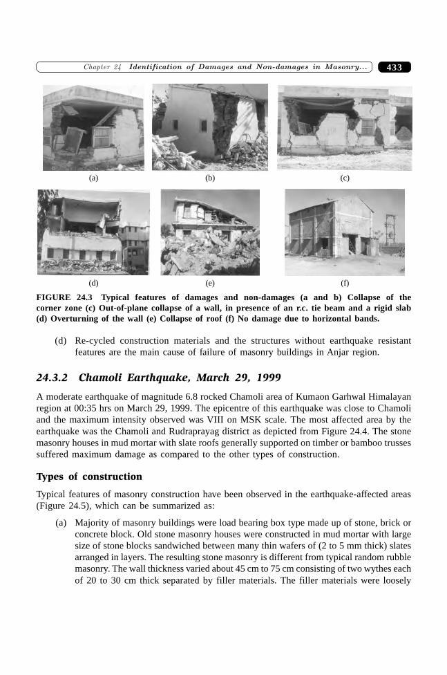
433�������� ���� � ��� ����������������������� �����������
(d) Re-cycled construction materials and the structures without earthquake resistantfeatures are the main cause of failure of masonry buildings in Anjar region.
24.3.2 Chamoli Earthquake, March 29, 1999
A moderate earthquake of magnitude 6.8 rocked Chamoli area of Kumaon Garhwal Himalayanregion at 00:35 hrs on March 29, 1999. The epicentre of this earthquake was close to Chamoliand the maximum intensity observed was VIII on MSK scale. The most affected area by theearthquake was the Chamoli and Rudraprayag district as depicted from Figure 24.4. The stonemasonry houses in mud mortar with slate roofs generally supported on timber or bamboo trussessuffered maximum damage as compared to the other types of construction.
Types of construction
Typical features of masonry construction have been observed in the earthquake-affected areas(Figure 24.5), which can be summarized as:
(a) Majority of masonry buildings were load bearing box type made up of stone, brick orconcrete block. Old stone masonry houses were constructed in mud mortar with largesize of stone blocks sandwiched between many thin wafers of (2 to 5 mm thick) slatesarranged in layers. The resulting stone masonry is different from typical random rubblemasonry. The wall thickness varied about 45 cm to 75 cm consisting of two wythes eachof 20 to 30 cm thick separated by filler materials. The filler materials were loosely
(a) (b) (c)
(d) (e) (f)
FIGURE 24.3 Typical features of damages and non-damages (a and b) Collapse of thecorner zone (c) Out-of-plane collapse of a wall, in presence of an r.c. tie beam and a rigid slab(d) Overturning of the wall (e) Collapse of roof (f) No damage due to horizontal bands.
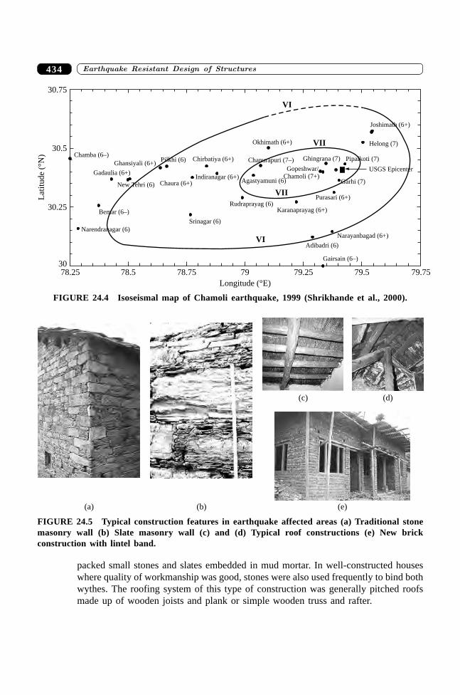
����������� ������� �������������434
packed small stones and slates embedded in mud mortar. In well-constructed houseswhere quality of workmanship was good, stones were also used frequently to bind bothwythes. The roofing system of this type of construction was generally pitched roofsmade up of wooden joists and plank or simple wooden truss and rafter.
Chamba (6–)
78.25 78.5 78.75 79 79.25 79.5 79.7530
30.25
30.5
30.75
Lat
itu
de
(°N
)
VI
VII
VII
VI
Gadaulia (6+)
Ghansiyali (6+)Pilkhi (6)
New Tehri (6) Chaura (6+)
Chirbatiya (6+)
Indiranagar (6+)
Okhimath (6+)
Chanurapuri (7–)
Chamoli (7+)
Ghingrana (7)
Agastyamuni (6)
Gopeshwar/
Garhi (7)
Pipalkoti (7)
Helong (7)
USGS Epicenter
Joshimath (6+)
Rudraprayag (6)Karanaprayag (6+)
Purasari (6+)
Narayanbagad (6+)
Adibadri (6)
Gairsain (6–)
Srinagar (6)
Narendranagar (6)
Bemar (6–)
Longitude (°E)
FIGURE 24.4 Isoseismal map of Chamoli earthquake, 1999 (Shrikhande et al., 2000).
(a) (b)
(c) (d)
(e)
FIGURE 24.5 Typical construction features in earthquake affected areas (a) Traditional stonemasonry wall (b) Slate masonry wall (c) and (d) Typical roof constructions (e) New brickconstruction with lintel band.
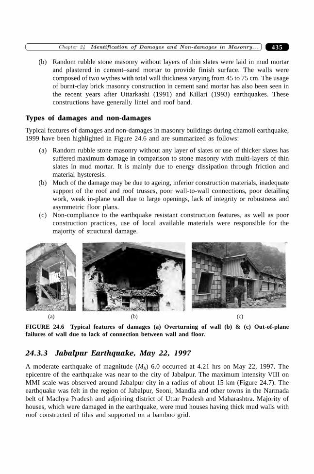
435�������� ���� � ��� ����������������������� �����������
(b) Random rubble stone masonry without layers of thin slates were laid in mud mortarand plastered in cement–sand mortar to provide finish surface. The walls werecomposed of two wythes with total wall thickness varying from 45 to 75 cm. The usageof burnt-clay brick masonry construction in cement sand mortar has also been seen inthe recent years after Uttarkashi (1991) and Killari (1993) earthquakes. Theseconstructions have generally lintel and roof band.
Types of damages and non-damages
Typical features of damages and non-damages in masonry buildings during chamoli earthquake,1999 have been highlighted in Figure 24.6 and are summarized as follows:
(a) Random rubble stone masonry without any layer of slates or use of thicker slates hassuffered maximum damage in comparison to stone masonry with multi-layers of thinslates in mud mortar. It is mainly due to energy dissipation through friction andmaterial hysteresis.
(b) Much of the damage may be due to ageing, inferior construction materials, inadequatesupport of the roof and roof trusses, poor wall-to-wall connections, poor detailingwork, weak in-plane wall due to large openings, lack of integrity or robustness andasymmetric floor plans.
(c) Non-compliance to the earthquake resistant construction features, as well as poorconstruction practices, use of local available materials were responsible for themajority of structural damage.
(a) (b) (c)
FIGURE 24.6 Typical features of damages (a) Overturning of wall (b) & (c) Out-of-planefailures of wall due to lack of connection between wall and floor.
24.3.3 Jabalpur Earthquake, May 22, 1997
A moderate earthquake of magnitude (Mb) 6.0 occurred at 4.21 hrs on May 22, 1997. Theepicentre of the earthquake was near to the city of Jabalpur. The maximum intensity VIII onMMI scale was observed around Jabalpur city in a radius of about 15 km (Figure 24.7). Theearthquake was felt in the region of Jabalpur, Seoni, Mandla and other towns in the Narmadabelt of Madhya Pradesh and adjoining district of Uttar Pradesh and Maharashtra. Majority ofhouses, which were damaged in the earthquake, were mud houses having thick mud walls withroof constructed of tiles and supported on a bamboo grid.
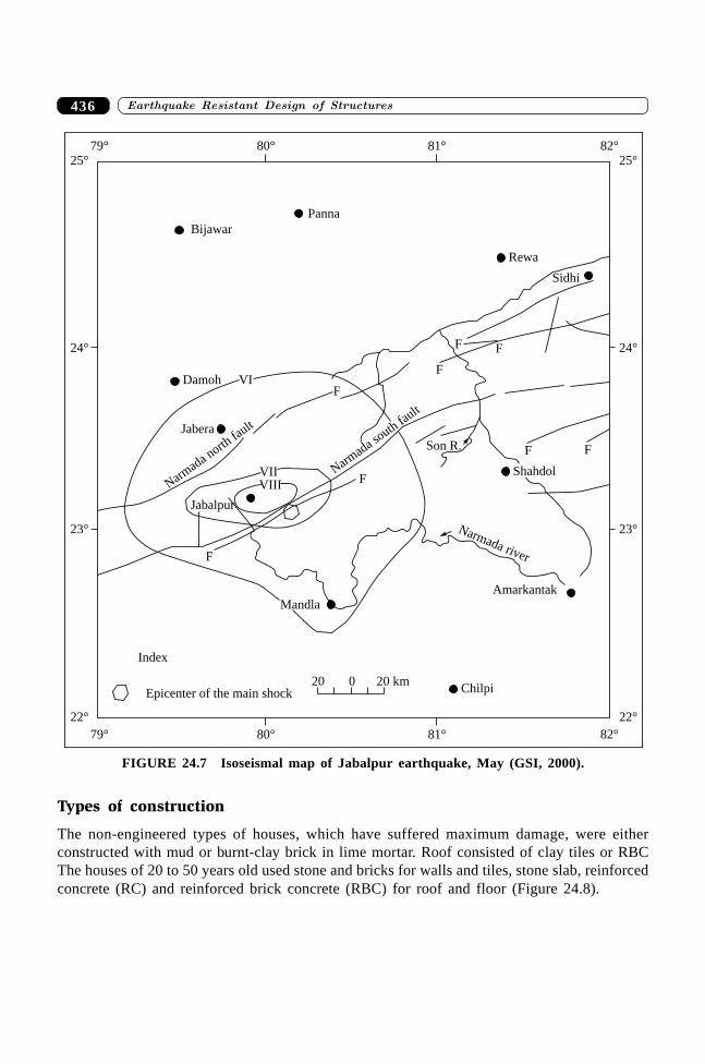
����������� ������� �������������436
79° 80° 81° 82°
79° 80° 81° 82°25°
24°
23°
22°
25°
24°
23°
22°
20 0 20 km
F
F
FVIIVIII
VI
Son R.
F
Jabalpur
Narmad
a northfau
ltJabera
Damoh
Narmad
a south
fault
F F
F F
Shahdol
Narmada river
Amarkantak
Mandla
Index
Chilpi
Sidhi
Rewa
Bijawar
Panna
Epicenter of the main shock
FIGURE 24.7 Isoseismal map of Jabalpur earthquake, May (GSI, 2000).
Types of construction
The non-engineered types of houses, which have suffered maximum damage, were eitherconstructed with mud or burnt-clay brick in lime mortar. Roof consisted of clay tiles or RBCThe houses of 20 to 50 years old used stone and bricks for walls and tiles, stone slab, reinforcedconcrete (RC) and reinforced brick concrete (RBC) for roof and floor (Figure 24.8).
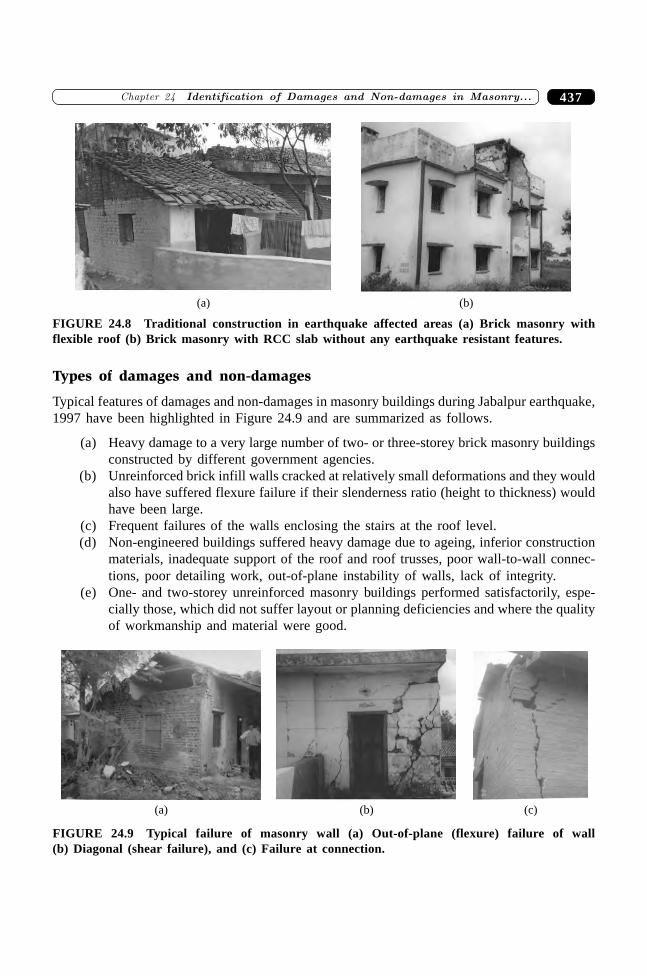
437�������� ���� � ��� ����������������������� �����������
(a) (b)
FIGURE 24.8 Traditional construction in earthquake affected areas (a) Brick masonry withflexible roof (b) Brick masonry with RCC slab without any earthquake resistant features.
Types of damages and non-damages
Typical features of damages and non-damages in masonry buildings during Jabalpur earthquake,1997 have been highlighted in Figure 24.9 and are summarized as follows.
(a) Heavy damage to a very large number of two- or three-storey brick masonry buildingsconstructed by different government agencies.
(b) Unreinforced brick infill walls cracked at relatively small deformations and they wouldalso have suffered flexure failure if their slenderness ratio (height to thickness) wouldhave been large.
(c) Frequent failures of the walls enclosing the stairs at the roof level.(d) Non-engineered buildings suffered heavy damage due to ageing, inferior construction
materials, inadequate support of the roof and roof trusses, poor wall-to-wall connec-tions, poor detailing work, out-of-plane instability of walls, lack of integrity.
(e) One- and two-storey unreinforced masonry buildings performed satisfactorily, espe-cially those, which did not suffer layout or planning deficiencies and where the qualityof workmanship and material were good.
(a) (b) (c)
FIGURE 24.9 Typical failure of masonry wall (a) Out-of-plane (flexure) failure of wall(b) Diagonal (shear failure), and (c) Failure at connection.
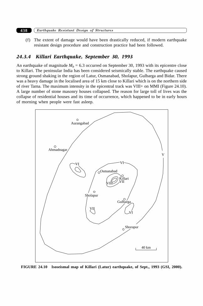
����������� ������� �������������438
(f) The extent of damage would have been drastically reduced, if modern earthquakeresistant design procedure and construction practice had been followed.
24.3.4 Killari Earthquake, September 30, 1993
An earthquake of magnitude Mb = 6.3 occurred on September 30, 1993 with its epicentre closeto Killari. The peninsular India has been considered seismically stable. The earthquake causedstrong ground shaking in the region of Latur, Osmanabad, Sholapur, Gulbarga and Bidar. Therewas a heavy damage in the localised area of 15 km close to Killari which is on the northern sideof river Tarna. The maximum intensity in the epicentral track was VIII+ on MMI (Figure 24.10).A large number of stone masonry houses collapsed. The reason for large toll of lives was thecollapse of residential houses and its time of occurrence, which happened to be in early hoursof morning when people were fast asleep.
40 km
VII
Sholapur
Gulbarga
VI
Shorapur
VI
VIII
KillariVII
Osmanabad
VI
Ahmadnagar
Aurangabad
V
FIGURE 24.10 Isoseismal map of Killari (Latur) earthquake, of Sept., 1993 (GSI, 2000).
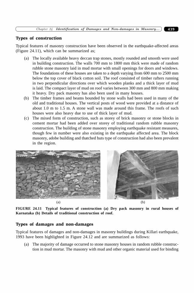
439�������� ���� � ��� ����������������������� �����������
Types of construction
Typical features of masonry construction have been observed in the earthquake-affected areas(Figure 24.11), which can be summarized as;
(a) The locally available heavy deccan trap stones, mostly rounded and smooth were usedin building construction. The walls 700 mm to 1800 mm thick were made of randomrubble stone masonry laid in mud mortar with small openings for doors and windows.The foundations of these houses are taken to a depth varying from 600 mm to 2500 mmbelow the top cover of black cotton soil. The roof consisted of timber rafters runningin two perpendicular directions over which wooden planks and a thick layer of mudis laid. The compact layer of mud on roof varies between 300 mm and 800 mm makingit heavy. Dry pack masonry has also been used in many houses.
(b) The timber frames and beams bounded by stone walls had been used in many of theold and traditional houses. The vertical posts of wood were provided at a distance ofabout 1.0 m to 1.5 m. A stone wall was made around this frame. The roofs of suchhouses were also heavy due to use of thick layer of mud.
(c) The mixed form of construction, such as storey of brick masonry or stone blocks incement mortar had been added over storey of traditional random rubble masonryconstruction. The building of stone masonry employing earthquake resistant measures,though few in number were also existing in the earthquake affected area. The blockmasonry, adobe building and thatched huts type of construction had also been prevalentin the region.
(a) (b)
FIGURE 24.11 Typical features of construction (a) Dry pack masonry in rural houses ofKarnataka (b) Details of traditional construction of roof.
Types of damages and non-damages
Typical features of damages and non-damages in masonry buildings during Killari earthquake,1993 have been highlighted in Figure 24.12 and are summarized as follows:
(a) The majority of damage occurred to stone masonry houses in random rubble construc-tion in mud mortar. The masonry with mud and other organic material used for binding
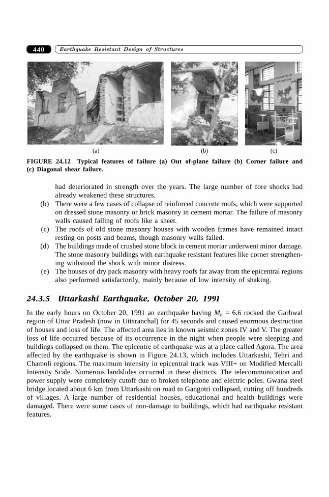
����������� ������� �������������440
had deteriorated in strength over the years. The large number of fore shocks hadalready weakened these structures.
(b) There were a few cases of collapse of reinforced concrete roofs, which were supportedon dressed stone masonry or brick masonry in cement mortar. The failure of masonrywalls caused falling of roofs like a sheet.
(c) The roofs of old stone masonry houses with wooden frames have remained intactresting on posts and beams, though masonry walls failed.
(d) The buildings made of crushed stone block in cement mortar underwent minor damage.The stone masonry buildings with earthquake resistant features like corner strengthen-ing withstood the shock with minor distress.
(e) The houses of dry pack masonry with heavy roofs far away from the epicentral regionsalso performed satisfactorily, mainly because of low intensity of shaking.
24.3.5 Uttarkashi Earthquake, October 20, 1991
In the early hours on October 20, 1991 an earthquake having Mb = 6.6 rocked the Garhwalregion of Uttar Pradesh (now in Uttaranchal) for 45 seconds and caused enormous destructionof houses and loss of life. The affected area lies in known seismic zones IV and V. The greaterloss of life occurred because of its occurrence in the night when people were sleeping andbuildings collapsed on them. The epicentre of earthquake was at a place called Agora. The areaaffected by the earthquake is shown in Figure 24.13, which includes Uttarkashi, Tehri andChamoli regions. The maximum intensity in epicentral track was VIII+ on Modified MercalliIntensity Scale. Numerous landslides occurred in these districts. The telecommunication andpower supply were completely cutoff due to broken telephone and electric poles. Gwana steelbridge located about 6 km from Uttarkashi on road to Gangotri collapsed, cutting off hundredsof villages. A large number of residential houses, educational and health buildings weredamaged. There were some cases of non-damage to buildings, which had earthquake resistantfeatures.
(a) (b) (c)
FIGURE 24.12 Typical features of failure (a) Out of-plane failure (b) Corner failure and(c) Diagonal shear failure.
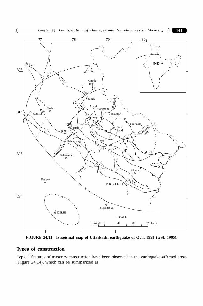
441�������� ���� � ��� ����������������������� �����������
29°
30°
31°
32°
77 78 79 80
INDIAM B F
Kullu
MC
T
Tato
Kaurikfault
F
F
FF
F
F
Sangla
AungiF
FF
F
F
F
F
F
F
Badrinath
F
F
F
F
FF
F
F
F
F
F
F
Simla
Kunihar
M B F
Timb
VI Uttarkashi
VII
VIII
Terri
Gaurikund
Gangotri
Gangnani Bhag
irat
h
Alaknan
da
fault
M C T
Alnora
MB F
M B F-ILL
VI
VI
Dogadda
Gan
ga R.
Saharanpur
Yam
una
R. VI
Dehradun
Panipat
Moradabad
DELHI
V
V
SCALE
Kms.20 0 40 80 120 Kms.
FIGURE 24.13 Isoseismal map of Uttarkashi earthquake of Oct., 1991 (GSI, 1995).
Types of construction
Typical features of masonry construction have been observed in the earthquake-affected areas(Figure 24.14), which can be summarized as:
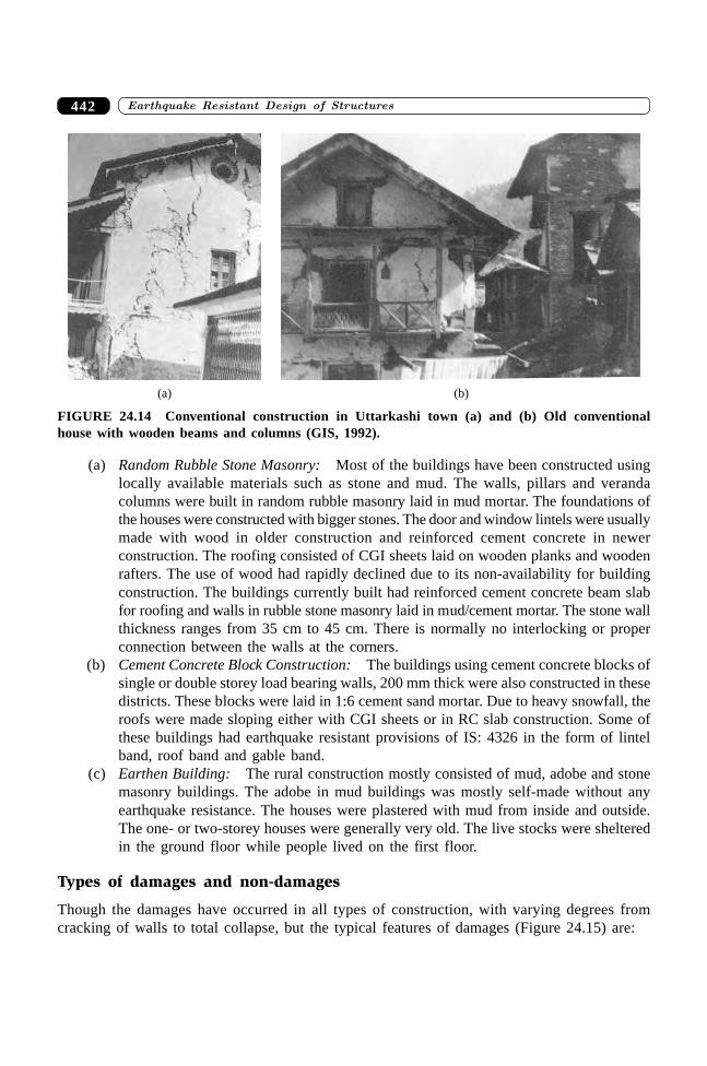
����������� ������� �������������442
(a) (b)
FIGURE 24.14 Conventional construction in Uttarkashi town (a) and (b) Old conventionalhouse with wooden beams and columns (GIS, 1992).
(a) Random Rubble Stone Masonry: Most of the buildings have been constructed usinglocally available materials such as stone and mud. The walls, pillars and verandacolumns were built in random rubble masonry laid in mud mortar. The foundations ofthe houses were constructed with bigger stones. The door and window lintels were usuallymade with wood in older construction and reinforced cement concrete in newerconstruction. The roofing consisted of CGI sheets laid on wooden planks and woodenrafters. The use of wood had rapidly declined due to its non-availability for buildingconstruction. The buildings currently built had reinforced cement concrete beam slabfor roofing and walls in rubble stone masonry laid in mud/cement mortar. The stone wallthickness ranges from 35 cm to 45 cm. There is normally no interlocking or properconnection between the walls at the corners.
(b) Cement Concrete Block Construction: The buildings using cement concrete blocks ofsingle or double storey load bearing walls, 200 mm thick were also constructed in thesedistricts. These blocks were laid in 1:6 cement sand mortar. Due to heavy snowfall, theroofs were made sloping either with CGI sheets or in RC slab construction. Some ofthese buildings had earthquake resistant provisions of IS: 4326 in the form of lintelband, roof band and gable band.
(c) Earthen Building: The rural construction mostly consisted of mud, adobe and stonemasonry buildings. The adobe in mud buildings was mostly self-made without anyearthquake resistance. The houses were plastered with mud from inside and outside.The one- or two-storey houses were generally very old. The live stocks were shelteredin the ground floor while people lived on the first floor.
Types of damages and non-damages
Though the damages have occurred in all types of construction, with varying degrees fromcracking of walls to total collapse, but the typical features of damages (Figure 24.15) are:
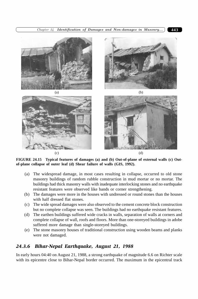
443�������� ���� � ��� ����������������������� �����������
(a) (b)
(c) (d)
FIGURE 24.15 Typical features of damages (a) and (b) Out-of-plane of external walls (c) Out-of-plane collapse of outer leaf (d) Shear failure of walls (GIS, 1992).
(a) The widespread damage, in most cases resulting in collapse, occurred to old stonemasonry buildings of random rubble construction in mud mortar or no mortar. Thebuildings had thick masonry walls with inadequate interlocking stones and no earthquakeresistant features were observed like bands or corner strengthening.
(b) The damages were more in the houses with undressed or round stones than the houseswith half dressed flat stones.
(c) The wide spread damages were also observed to the cement concrete block constructionbut no complete collapse was seen. The buildings had no earthquake resistant features.
(d) The earthen buildings suffered wide cracks in walls, separation of walls at corners andcomplete collapse of wall, roofs and floors. More than one-storeyed buildings in adobesuffered more damage than single-storeyed buildings.
(e) The stone masonry houses of traditional construction using wooden beams and plankswere not damaged.
24.3.6 Bihar-Nepal Earthquake, August 21, 1988
In early hours 04:40 on August 21, 1988, a strong earthquake of magnitude 6.6 on Richter scalewith its epicentre close to Bihar-Nepal border occurred. The maximum in the epicentral track
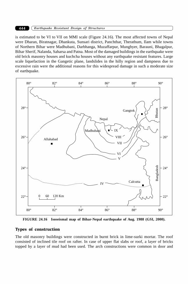
����������� ������� �������������444
is estimated to be VI to VII on MMI scale (Figure 24.16). The most affected towns of Nepalwere Dharan, Biratnagar, Dhankuta, Sunsari district, Panchthar, Therathum, Ilam while townsof Northern Bihar were Madhubani, Darbhanga, Muzaffarpur, Munghyer, Barauni, Bhagalpur,Bihar Sherif, Nalanda, Saharsa and Patna. Most of the damaged buildings in the earthquake wereold brick masonry houses and kuchcha houses without any earthquake resistant features. Largescale liquefaction in the Gangetic plane, landslides in the hilly region and dampness due toexcessive rain were the additional reasons for this widespread damage in such a moderate sizeof earthquake.
82°80° 84° 86° 88° 90°
82°80° 84° 86° 88° 90°
22°
24°
26°
28°
0 60 120 Km 22°
24°
26°
28°
Allahabad
Nepal
Madhubani IX
VIII
VII
Gangtok
Bh
uta
nVI
V
CalcuttaIV
Ban
gla
des
h
FIGURE 24.16 Isoseismal map of Bihar-Nepal earthquake of Aug. 1988 (GSI, 2000).
Types of construction
The old masonry buildings were constructed in burnt brick in lime-surki mortar. The roofconsisted of inclined tile roof on rafter. In case of upper flat slabs or roof, a layer of brickstopped by a layer of mud had been used. The arch constructions were common in door and
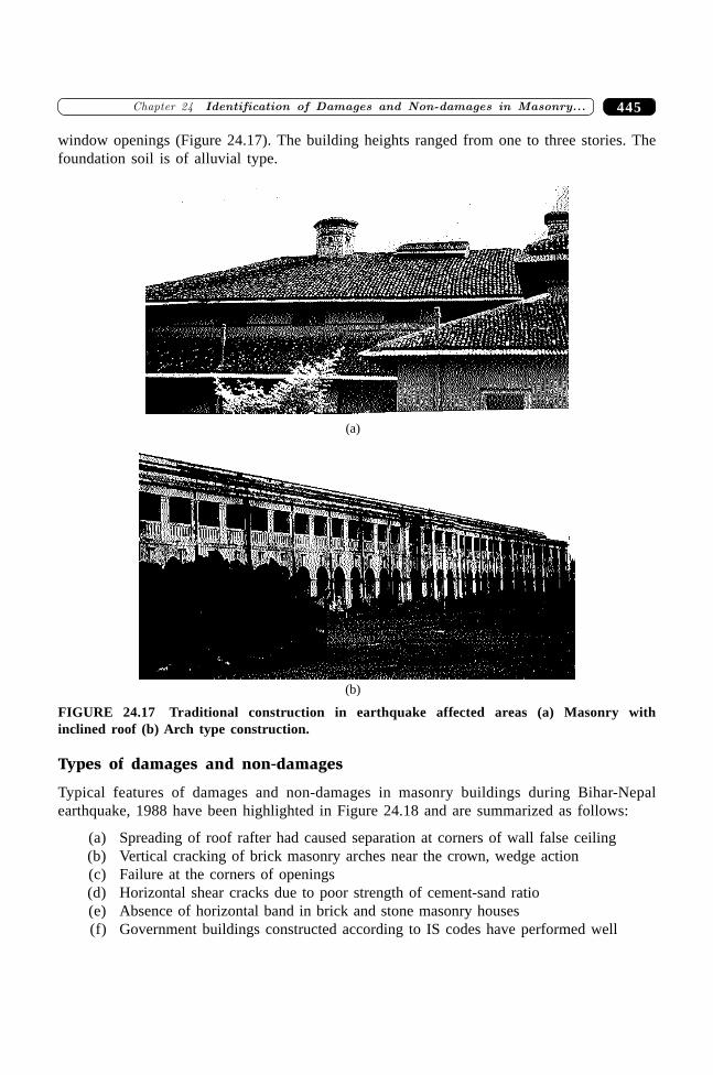
445�������� ���� � ��� ����������������������� �����������
window openings (Figure 24.17). The building heights ranged from one to three stories. Thefoundation soil is of alluvial type.
(a)
(b)
FIGURE 24.17 Traditional construction in earthquake affected areas (a) Masonry withinclined roof (b) Arch type construction.
Types of damages and non-damages
Typical features of damages and non-damages in masonry buildings during Bihar-Nepalearthquake, 1988 have been highlighted in Figure 24.18 and are summarized as follows:
(a) Spreading of roof rafter had caused separation at corners of wall false ceiling(b) Vertical cracking of brick masonry arches near the crown, wedge action(c) Failure at the corners of openings(d) Horizontal shear cracks due to poor strength of cement-sand ratio(e) Absence of horizontal band in brick and stone masonry houses(f) Government buildings constructed according to IS codes have performed well
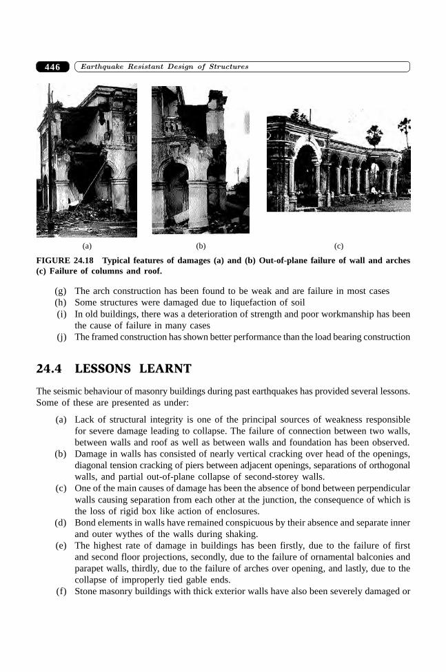
����������� ������� �������������446
(g) The arch construction has been found to be weak and are failure in most cases(h) Some structures were damaged due to liquefaction of soil(i) In old buildings, there was a deterioration of strength and poor workmanship has been
the cause of failure in many cases(j) The framed construction has shown better performance than the load bearing construction
24.4 LESSONS LEARNT
The seismic behaviour of masonry buildings during past earthquakes has provided several lessons.Some of these are presented as under:
(a) Lack of structural integrity is one of the principal sources of weakness responsiblefor severe damage leading to collapse. The failure of connection between two walls,between walls and roof as well as between walls and foundation has been observed.
(b) Damage in walls has consisted of nearly vertical cracking over head of the openings,diagonal tension cracking of piers between adjacent openings, separations of orthogonalwalls, and partial out-of-plane collapse of second-storey walls.
(c) One of the main causes of damage has been the absence of bond between perpendicularwalls causing separation from each other at the junction, the consequence of which isthe loss of rigid box like action of enclosures.
(d) Bond elements in walls have remained conspicuous by their absence and separate innerand outer wythes of the walls during shaking.
(e) The highest rate of damage in buildings has been firstly, due to the failure of firstand second floor projections, secondly, due to the failure of ornamental balconies andparapet walls, thirdly, due to the failure of arches over opening, and lastly, due to thecollapse of improperly tied gable ends.
(f) Stone masonry buildings with thick exterior walls have also been severely damaged or
(a) (b) (c)
FIGURE 24.18 Typical features of damages (a) and (b) Out-of-plane failure of wall and arches(c) Failure of columns and roof.
447�������� ���� � ��� ����������������������� �����������
collapsed because of poor construction but survived, and remain intact during majorearthquakes when they exhibit excellent workmanship.
(g) Walls that are inadequately anchored to the floor diaphragm can exhibit large diagonalcracks in the piers due to inplane loads. If the mortar joints are weak, as in lime mortar,the cracks follow the joint.
(h) Diaphragms that are insufficiently anchored can separate from the masonry wall,causing wall collapse. Unanchored gable ends of masonry walls are susceptible to thisproblem.
(i) The provision of vertical steel or elements in the corner of the buildings as well asexistence of horizontal tie beams increase resistance to earthquakes.
(j) Non-structural elements must be given proper design considerations for lateral forcesand should be braced or restrained. The collapse of many of these walls clearly illustratesthis point.
(k) The potential out-of-plane failure of non-structural elements (parapet, veneers, gables,and unanchored walls) during earthquakes constitutes the most serious life-safetyhazard for this type of construction.
(l) Inplane failure less common than out-of-plane failures was noted in many strengthenedbuildings. The typical shear failures occurred in many buildings.
(m) In general, buildings with irregular plans experienced more damage than rectangularbuildings. The damage was often concentrated at corners due to lack of a detailedanalysis that included the effects of odd shaped plans.
24.5 RECOMMENDATIONS
In compliance with the past earthquake resistive structures, a number of principles have beenformulated which may be summed up as: (i) The weight and rigidity of a structure must beuniformly and symmetrically distributed to the plane of symmetry passing through the centreof gravity; (ii) The proportionality requirements must be met by the building dimensions i.e.the length and height of the building should not be too great; (iii) The structure must be light,as practicable and have its centre of gravity as low as possible; (iv) Desirable tough, light andelastic material be used which have uniform properties; (v) In the vertical and horizontal planesthe load carrying elements must be coupled to form closed contours; (vi) The foundations ofearthquake resistant buildings must be firm and have enough depth.
SUMMARY
Masonry is widely used for housing construction in India and many countries of the world dueto innumerable advantages over both reinforced concrete and steel. However, there are somedisadvantages as well, particularly, when it is to be built in seismic environment. The seismicresistance capacity of masonry construction is relatively low in comparison to steel or reinforcedconcrete constructions. Past earthquakes have revealed that masonry construction is susceptibleto damages during earthquakes because of lack of integral action, lack of strong and ductileconnections between walls, roof elements and foundation, inadequate strength for out-of-plane
����������� ������� �������������448
forces, low tensile and shear strength of mortar, high in plane stiffness of wall, low ductilityand deformability capacity and heavy mass. This chapter focuses on the behaviour of masonrybuilding during past earthquakes in India, which help to identify the causes of damage and non-damage in masonry buildings.
REFERENCES
[1] Agarwal, Pankaj., “Experimental Study of Seismic Strengthening and RetrofittingMeasures in Masonry Buildings”, Ph.D. Thesis, Department of Earthquake Engineering,University of Roorkee, Roorkee, June 1999.
[2] DEQ, Jabalpur Earthquake of May 22, 1997: Reconnaissance Report, Department ofEarthquake Engineering, University of Roorkee, Roorkee, September, 2000.
[3] DEQ, Damage Survey Report on Bihar-Nepal Earthquake of August 21, 1988,Department of Earthquake Engineering, University of Roorkee, Roorkee, 1988.
[4] DEQ, A Report on Chamoli Earthquake of March 29, 1999, Department of EarthquakeEngineering, University of Roorkee, Roorkee, September, 2000.
[5] Dubey, R.N., Thakkar, S.K., and Agarwal, Pankaj, “Performance of Masonry Buildingduring Bhuj Earthquake”, 12th Symposium on Earthquake Engineering, IIT Roorkee,December, 2002.
[6] EERI. “Bhuj, India Earthquake of January 26, 2001: Reconnaissance Report”,Earthquake Spectra, Supplement to Vol. 18, July, 2002.
[7] GSI, Uttarkashi Earthquake, October 20, 1991, Geological Survey of India, SpecialPublication No. 30, 1992.
[8] ISET, “Damage Report of the Latur—Osmanabad Earthquake of September 30, 1993”,Bulletin of Indian Society of Earthquake Technology, Vol. 31, No. 1, 1994.
[9] Narayan, J.P., Sharma, M.L., and Kumar Ashwani. “A Seismological Report on the26 January 2001 Bhuj, India Earthquake”, Seismological Research Letters, Vol. 73,No. 3, May/June, 2002.
[10] Shrikhande, M., et al., “The March 29, 1999 Earthquake at Chamoli, India”, 12thWCEE, Auckland, New Zealand, February, 2000.
[11] Thakkar, S.K., Dubey, R.N., and Agarwal, Pankaj, “Damages and Lessons Learnt fromRecent Indian Earthquakes”, Symposium on Earthquake Effects on Structures, Plantand Machinery, New Delhi, November 13–15, 1996.
[12] GSI, Seismotectonic Atlas of India and its Environe, Geological Survey of India, 2000.[13] GSI, Uttarkashi Earthquake, Geological Survey of India, 1995.
449�������� ���������� �� ��������������������
449
Elastic Properties ofStructural Masonry
��������
25.1 INTRODUCTION
Structural masonry is a combination of a few or all the constituent masonry materials: masonryunit, mortar, grout and reinforcement. The physical and engineering properties of constituentmaterials have already been widely discussed in standard undergraduate textbooks and theirrespective BIS codes. The strength and stiffness properties of integral masonry or masonryassemblage are not very common particularly in India, hence very limited information is avail-able even in the codes. This chapter will deal with the engineering properties of constituentmaterials in brief and with a detailed discussion on the strength and stiffness properties ofmasonry assemblage. Information and data given here are valid for respective masonry tests inlaboratory. However, a good interpretation can be made for the similar type of masonry in caseof absence of sufficient data.
25.2 MATERIALS FOR MASONRY CONSTRUCTION
25.2.1 Unit
A masonry unit may be brick, block made from concrete or clay, stone, adobe etc. Dependingupon the unit used in the masonry, the construction may be classified as brick masonry, blockmasonry, stone masonry, adobe masonry, etc. IS 4326: 1993 in Clause 8.1.1 has specified theminimum requirement of masonry unit. The code specifies that well-burnt bricks and solidconcrete blocks possessing a compressive/crushing strength not less than 35 MPa shall be used.Moreover for squared stone masonry, stone block masonry or hollow concrete blocks thespecification according to IS 1597 (Part 2): 1992 having adequate strength may be used. Thecompressive strength of unit may be defined as the maximum stress to which the unit can besubjected by a gradually increasing load applied in perpendicular either to the bedding plane ornormal position. The modulus of elasticity of the individual unit is not generally determinedand is therefore not specified in most of the codes. If it is required, the modulus of elasticity
�������� �� ��������� �������������� �450
for the units may be obtained by secant modulus of stress–strain curve of unit under compression,which is the slope of a line from zero stress to approximately 33% of the unit compressivestrength. The modulus of elasticity of the unit remains somewhat greater than the respectivemasonry.
The tensile strength of the unit is measured by the modulus of rupture or splitting tension,which increases with the unit’s compressive strength, but is generally a smaller fraction of thecompressive strength. The ratio of modulus of rupture to compressive strength varies from about0.10 up to 0.32 (Drydale, Hamid and Baker, 1994).
Another stiffness index may be expressed in terms of Poisson’s ratio i.e. the ratio of lateralexpansion to longitudinal deformation. Experiments reveal values 0.23 for ungrouted claymasonry to 0.40 for grouted clay masonry (Schneider and Dickey, 1994).
25.2.2 Mortar
Mortar is a plastic mixture of materials used to bind masonry unit into a structural mass. IS4326: 1993 in Clause 8.1.2 has recommended mortar mixture used in masonry construction inseismic areas for various categories of building. The categories of construction are defined inClause 7.1 depending upon the design seismic coefficient (ah) (Category: A (0.04 < ah < 0.05),B (0.05 < ah < 0.06), C (0.06 < ah < 0.08), D (0.08 < ah < 0.12) and E (0.12 £ ah).Recommended mortar mixture for A categories of construction type building are M2 (Cement-sand 1:6) or M3 (Lime-cinder 1:3) or even richer. For the construction of B and C category typebuildings the recommended mortar are M2 (Cement-lime-sand 1:2:9 or Cement-sand 1:6) orricher and for D and E type of construction, the recommended mortar are H2 (Cement-sand 1:4)or M1 (Cement-lime-sand 1:1:6) or richer. Masonry may further be subdivided on the basis oftype of mortar used for example brick masonry in cement mortar. The important properties ofthe hardened mortar that affect masonry construction are bond strength, flexural tensile strengthand compressive strength. Bond strength of mortar is usually lesser than the flexural tensilestrength of mortar therefore the flexural tensile strength of masonry is governed by the bondstrength of mortar to brick. These properties may be determined as (Grimn, 1975),
Bond strength of mortar to brick can be estimated as:
fb = 0.005[1.8 + (F – 105)0.5](40 – A)(124 – tm)
in which,
fb = bond strength of mortar to brick in psi (1 psi = 6.894 N/m2)F = initial flow of mortar, as a % {F = 195[1.72 + log(Cv/L] [(W/Cw) – 0.05] – 72}; and
W/Cw = water-cement ratio by weight where 0.4 < (W/Cw) < 1.0A = air content in mortar by volume, where A < 30, as a %tm = mortar exposure time (spreading mortar of laying brick), where t < 120, in seconds
Flexural tensile strength of mortar can be approximated as:
ftm = 1.47 ¥ 10–5 fc (11,700 – fc)
451�������� ���������� �� ��������������������
in which,
ftm = flexural tensile strength of mortar in psi (1 psi = 6.894 N/m2)
fc = compressive strength of mortar in psi (1 psi = 6.894 N/m2)
Compressive strength of mortar can be approximated as:
fc = 3.25sabT(554d + g (130 – F))
fc = compressive strength of mortar in psi (1 psi = 6.894 N/m2)s = 1 for 2 in (50 mm) cubes, 0.9 for 2-in ¥ 4-in (50 mm ¥ 100 mm) or 3-in ¥ 6-in
(76 mm ¥ 150 mm) cylindersa = mortar curing factor values varies 0.7 at 7 days, 0.85 at 14 days, 0.93 at 21 days, and
1.0 at 28 days. For air-dried specimen at 7 days and 28 days, a = 0.8.b = air content factor [b = 0.021 (57.3 – A)], A = Air content in mortar by volume, where
A < 30, as a %T = plastic mortar age factor [T = 0.029 (35 – Tp
2)]; and Tp = age of plastic mortar i.e.,time in mixing to time in use), in hours (Tp < 4)
d = mortar type factor [d = 1 + 1.46 log (Cv/L)]g = (Cv/L + 3.7)
25.2.3 Grout
Grout is a mixture of Portland cement, sand, gravel and water. It is generally used for increasingthe compressive strength of masonry. It is placed in the cores of hollow masonry units orbetween the wythe of solid units to bind the reinforcing steel and masonry into a structuralsystem. IS 4326: 1993 has recommended minimum cement concrete of grade M 15 so as toachieve good bond and corrosion resistance. Here masonry is further subdivided on the basisof grouting. Grouted masonry excels in compressive strength.
25.2.4 Reinforcement
Reinforcing steel in masonry has been extensively used in the western countries for revitalisingthe masonry construction in earthquake prone areas. Reinforcing steel extends the characteristicsof ductility, toughness and energy absorption that is very necessary in structures subjected tothe dynamic forces of earthquakes. Reinforcing steel also resist the shear and tensile forcesgenerated by the dynamic load. Masonry with reinforcement is further classified as reinforcedmasonry. Reinforced masonry performs well in earthquake because it has sufficient ductility tosustain the load reversals beyond the capability of plain, unreinforced masonry. In India,reinforcement is provided in the form of various horizontal bands, and vertical reinforcementat the corners and junctions of walls and around the openings. Horizontal bands with verticalreinforcement at corners and junctions of walls are provided to integrate the structure and steelprovided around the opening to prevent the diagonal cracks that tend to radiate from the cornersof opening. IS 4326: 1993 specifies the requirements and the size of reinforcement in themasonry depending upon the building category.
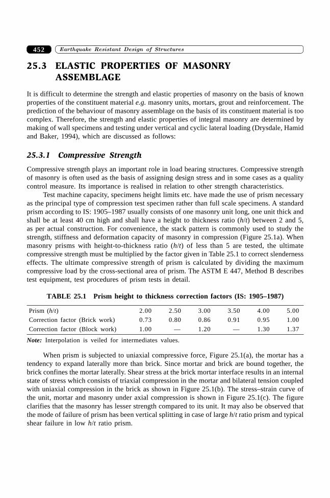
�������� �� ��������� �������������� �452
25.3 ELASTIC PROPERTIES OF MASONRYASSEMBLAGE
It is difficult to determine the strength and elastic properties of masonry on the basis of knownproperties of the constituent material e.g. masonry units, mortars, grout and reinforcement. Theprediction of the behaviour of masonry assemblage on the basis of its constituent material is toocomplex. Therefore, the strength and elastic properties of integral masonry are determined bymaking of wall specimens and testing under vertical and cyclic lateral loading (Drysdale, Hamidand Baker, 1994), which are discussed as follows:
25.3.1 Compressive Strength
Compressive strength plays an important role in load bearing structures. Compressive strengthof masonry is often used as the basis of assigning design stress and in some cases as a qualitycontrol measure. Its importance is realised in relation to other strength characteristics.
Test machine capacity, specimens height limits etc. have made the use of prism necessaryas the principal type of compression test specimen rather than full scale specimens. A standardprism according to IS: 1905–1987 usually consists of one masonry unit long, one unit thick andshall be at least 40 cm high and shall have a height to thickness ratio (h/t) between 2 and 5,as per actual construction. For convenience, the stack pattern is commonly used to study thestrength, stiffness and deformation capacity of masonry in compression (Figure 25.1a). Whenmasonry prisms with height-to-thickness ratio (h/t) of less than 5 are tested, the ultimatecompressive strength must be multiplied by the factor given in Table 25.1 to correct slendernesseffects. The ultimate compressive strength of prism is calculated by dividing the maximumcompressive load by the cross-sectional area of prism. The ASTM E 447, Method B describestest equipment, test procedures of prism tests in detail.
TABLE 25.1 Prism height to thickness correction factors (IS: 1905–1987)
Prism (h/t) 2.00 2.50 3.00 3.50 4.00 5.00
Correction factor (Brick work) 0.73 0.80 0.86 0.91 0.95 1.00
Correction factor (Block work) 1.00 .— 1.20 .— 1.30 1.37
Note: Interpolation is veiled for intermediates values.
When prism is subjected to uniaxial compressive force, Figure 25.1(a), the mortar has atendency to expand laterally more than brick. Since mortar and brick are bound together, thebrick confines the mortar laterally. Shear stress at the brick mortar interface results in an internalstate of stress which consists of triaxial compression in the mortar and bilateral tension coupledwith uniaxial compression in the brick as shown in Figure 25.1(b). The stress–strain curve ofthe unit, mortar and masonry under axial compression is shown in Figure 25.1(c). The figureclarifies that the masonry has lesser strength compared to its unit. It may also be observed thatthe mode of failure of prism has been vertical splitting in case of large h/t ratio prism and typicalshear failure in low h/t ratio prism.
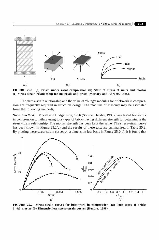
453�������� ���������� �� ��������������������
Mortar
Prism
Unit
Stress
Strain
(c)
Unit Mortar
(b)(a)
FIGURE 25.1 (a) Prism under axial compression (b) State of stress of units and mortar(c) Stress–strain relationship for materials and prism (McNary and Abrams, 1985).
The stress–strain relationship and the value of Young’s modulus for brickwork in compres-sion are frequently required in structural design. The modulus of masonry may be estimatedfrom the following methods;
Secant method: Powell and Hodgkinson, 1976 (Source: Hendry, 1998) have tested brickworkin compression to failure using four types of bricks having different strength for determining thestress–strain relationship. The mortar strength has been kept the same. The stress–strain curvehas been shown in Figure 25.2(a) and the results of these tests are summarized in Table 25.2.By plotting these stress-strain curves on a dimension less basis in Figure 25.2(b), it is found that
Str
ess
(N/m
m)
2
0.002 0.004 0.006Strain
(a)
0.2 0.4 0.6 0.8 1.0 1.2 1.4 1.6
ss m
ax
(b)
0
0.2
0.4
0.6
0.8
1.0
Pow
ell a
ndH
odgk
inso
n
Turn
sek
and
Cac
ovic
0
10
20
A
B
C
D
e e/ max
FIGURE 25.2 Stress–strain curves for brickwork in compression: (a) Four types of bricks1:¼:3 mortar (b) Dimensionless stress–strain curves (Hendry, 1998).
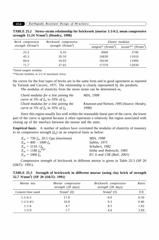
�������� �� ��������� �������������� �454
the curves for the four types of bricks are in the same form and in good agreement as reportedby Turnsek and Cacovic, 1971. The relationship is closely represented by the parabola.
The modulus of elasticity from the stress strain can be determined as,
Chord modulus for a line joining the MIA, 1998curve at 5% of fm to 33% of fmChord modulus for a line joining the Knutsson and Nielsen, 1995 (Source: Hendry,curve at 5% of fm to 35% of fm 1998)
Since this region usually lies well within the reasonable linear part of the curve, the lowerpart of the curve is ignored because it often represents a relatively flat region associated withclosing up of the interface between the mortar and the units.
Empirical basis: A number of authors have correlated the modulus of elasticity of masonryto its compressive strength (fm) on an empirical basis as below:
Em = 750 fm, 20.5 Gpa (maximum) MIA, 1998Em = 400 – 1000 fm Sahlin, 1971Em = 2116 ÷ fm Schubert, 1982Em = 1180 fm
0.83 Sinha and Pedreschi, 1983Em = 1000 fm EC 6 and CIB (Bull, 2001)
Compressive strength of brickwork in different mortar is given in Table 25.3 (SP 20(S&T): 1991).
TABLE 25.3 Strength of brickwork in different mortar (using clay brick of strength32.7 N/mm2) (SP 20 (S&T): 1991)
Mortar mix Mortar compressive Brickwork compressive Ratiostrength (28 days) strength (28 days)
Cement:lime:sand N/mm2 (X) N/mm2 (Y) Y/X
1:1/4:3 17.8 8.9 0.501:1/2:4½ 10.8 9.3 0.86
1:1:6 4.7 8.5 1.821:2:9 1.7 4.6 2.69
TABLE 25.2 Stress–strain relationship for brickwork (mortar 1:1/4:3, mean compressivestrength 15.24 N/mm2) (Hendry, 1998)
Brick compressive Brickwork compressive Elastic modulusstrength (N/mm2) strength (N/mm2) tangent* (N/mm2) secant** (N/mm2)
25.5 9.33 4960 374045.3 20.10 16830 1161069.6 19.93 18230 1190071.7 27.65 17370 12930
*Initial tangent modulus**Secant modulus at 2/3 of maximum stress
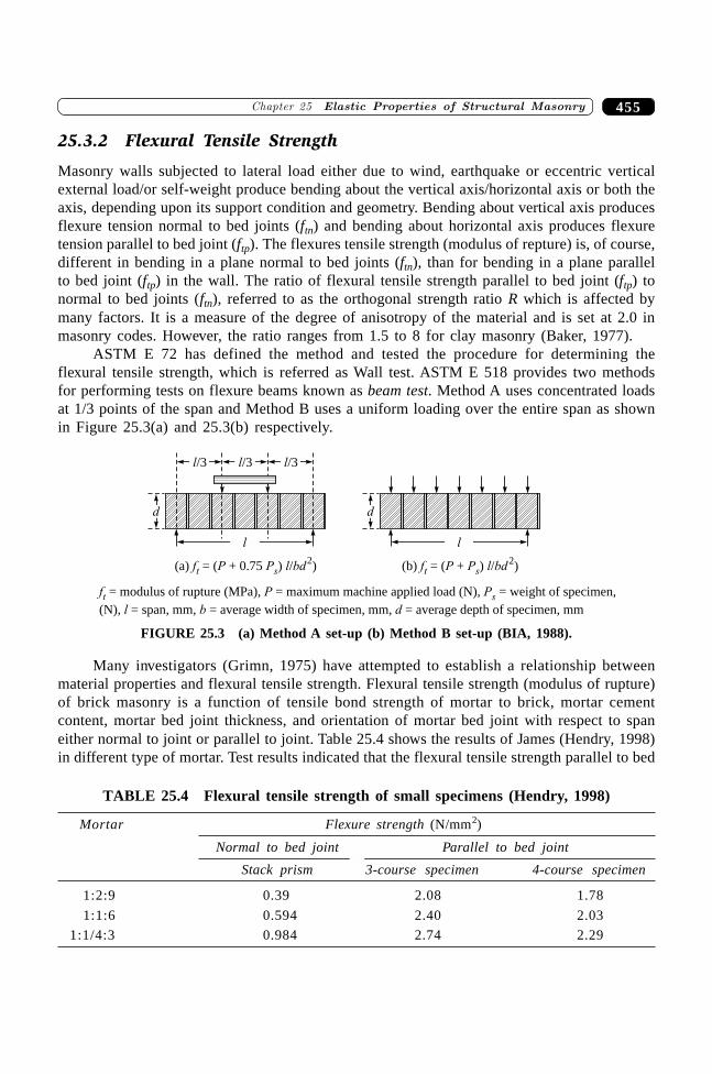
455�������� ���������� �� ��������������������
25.3.2 Flexural Tensile Strength
Masonry walls subjected to lateral load either due to wind, earthquake or eccentric verticalexternal load/or self-weight produce bending about the vertical axis/horizontal axis or both theaxis, depending upon its support condition and geometry. Bending about vertical axis producesflexure tension normal to bed joints (ftn) and bending about horizontal axis produces flexuretension parallel to bed joint (ftp). The flexures tensile strength (modulus of repture) is, of course,different in bending in a plane normal to bed joints (ftn), than for bending in a plane parallelto bed joint (ftp) in the wall. The ratio of flexural tensile strength parallel to bed joint (ftp) tonormal to bed joints (ftn), referred to as the orthogonal strength ratio R which is affected bymany factors. It is a measure of the degree of anisotropy of the material and is set at 2.0 inmasonry codes. However, the ratio ranges from 1.5 to 8 for clay masonry (Baker, 1977).
ASTM E 72 has defined the method and tested the procedure for determining theflexural tensile strength, which is referred as Wall test. ASTM E 518 provides two methodsfor performing tests on flexure beams known as beam test. Method A uses concentrated loadsat 1/3 points of the span and Method B uses a uniform loading over the entire span as shownin Figure 25.3(a) and 25.3(b) respectively.
d
l
d
l
l/3 l/3 l/3
(a) = ( + 0.75 ) / )f P P l bd2
t s (b) = ( + ) / )f P P l bd2
t s
f P P
l b d
= modulus of rupture (MPa), = maximum machine applied load (N), = weight of specimen,
(N), = span, mm, = average width of specimen, mm, = depth of specimen, mmt s
average
FIGURE 25.3 (a) Method A set-up (b) Method B set-up (BIA, 1988).
Many investigators (Grimn, 1975) have attempted to establish a relationship betweenmaterial properties and flexural tensile strength. Flexural tensile strength (modulus of rupture)of brick masonry is a function of tensile bond strength of mortar to brick, mortar cementcontent, mortar bed joint thickness, and orientation of mortar bed joint with respect to spaneither normal to joint or parallel to joint. Table 25.4 shows the results of James (Hendry, 1998)in different type of mortar. Test results indicated that the flexural tensile strength parallel to bed
TABLE 25.4 Flexural tensile strength of small specimens (Hendry, 1998)
Mortar Flexure strength (N/mm2)
Normal to bed joint Parallel to bed joint
Stack prism 3-course specimen 4-course specimen
1:2:9 0.39 2.08 1.78
1:1:6 0.594 2.40 2.03
1:1/4:3 0.984 2.74 2.29
�������� �� ��������� �������������� �456
joint has not been much affected by the type of mortar however a difference was noticeable inthe orthogonal direction.
Grimn, 1975 has established a formula for estimating the flexural tensile strength of brickmasonry as,
ft = 0.67q kfb (1.1 – tj) 3 8 10 5
..
+ -FH
IK
LNM
OQP
CLv
in which,
ft = flexural tensile strength of brick masonry normal to bed joint in psi (1 psi =6.894 N/m2)
q = workmanship constant for masonry in flexure (1 for all mortar joint filled and 0.8joints partly filled)
k = stress orientation factor (1 for normal to bed joint and 2 for parallel to bed joint)fb = bond strength of mortar to brick in psi (1 psi = 6.894 N/m2)tj = mortar joint thickness, in inch
Cv /L = cement-lime ratio by volume in mortar
Typical values for the flexural tensile strength normal to bed joint of conventional brickmasonry range from 50 psi to 500 psi (340 kN/m2 to 3,400 kN/m2)
25.3.3 Shear Strength
Load bearing masonry walls are often subjected to axial compression (vertical dead and liveloads), flexure (eccentric vertical loading, wind or earthquake loading) and also shear (in-planelateral loads and the effects of axial load and bending). This combined loading creates a stateof complex stress in the wall and becomes one of the causes to its failure. Depending upon theform of construction and the relative value of compressive and shear forces the possible shearfailure modes in masonry assemblages are: (i) shear slip failure along bed joint—if shear forceis greater than the normal compression force; (ii) diagonal tension cracking—if both shear forceand normal compressive force are comparative; and (iii) shear compression failure or splittingfailure—if shear force is a small fraction of normal compressive force. First two modes offailure are more commonly observed in the case of failure of masonry walls during earthquakes.Therefore, the shear strength against bed joint failure as well as diagonal tensile (shear) strengthagainst diagonal tension are of considerable concern to structural designer, especially whereseismic design is required.
Shear strength along bed joint
The shear strength along the bed joint is the function of bond strength between mortar and unitsand normal compressive stress. It is best represented by the Mohr–Coulomb type of equation i.e.
t = t0 +mfn
t = ultimate shear strength of the brickwork in N/mm2
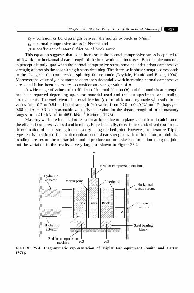
457�������� ���������� �� ��������������������
t0 = cohesion or bond strength between the mortar to brick in N/mm2
fn = normal compressive stress in N/mm2 andm = coefficient of internal friction of brick work
This equation suggests that as an increase in the normal compressive stress is applied tobrickwork, the horizontal shear strength of the brickwork also increases. But this phenomenonis perceptible only upto when the normal compressive stress remains under prism compressivestrength; afterwards the shear strength starts declining. The decrease in shear strength correspondsto the change in the compression splitting failure mode (Drydale, Hamid and Baker, 1994).Moreover the value of m also starts to decrease substantially with increasing normal compressivestress and it has been necessary to consider an average value of m.
A wide range of values of coefficient of internal friction (m) and the bond shear strengthhas been reported depending upon the material used and the test specimens and loadingarrangements. The coefficient of internal friction (m) for brick masonry made with solid brickvaries from 0.2 to 0.84 and bond strength (t0) varies from 0.20 to 0.40 N/mm2. Perhaps m =0.68 and t0 = 0.3 is a reasonable value. Typical value for the shear strength of brick masonryranges from 410 kN/m2 to 4690 kN/m2 (Grimm, 1975).
Masonry walls are intended to resist shear force due to in plane lateral load in addition tothe effect of compressive load and bending. Experimentally, there is no standardised test for thedetermination of shear strength of masonry along the bed joint. However, in literature Triplettype test is mentioned for the determination of shear strength, with an intention to minimizebending stresses on the mortar joint and to produce uniform shear deformation along the jointbut the variation in the results is very large, as shown in Figure 25.4.
Hydraulicactuator
P
Mortar joint
Head of compression machine
FiberboardHorizontal
reaction frame
Stiffened Isection
Steel bearingblock
P/2P/2Bed for compression
machine
Hydraulicactuator
Brick BrickBrick
FIGURE 25.4 Diagrammatic representation of Triplet test equipment (Smith and Carter,1971).
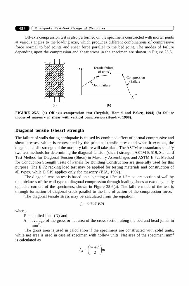
�������� �� ��������� �������������� �458
Off-axis compression test is also performed on the specimens constructed with mortar jointsat various angles to the loading axis, which produces different combinations of compressiveforce normal to bed joints and shear force parallel to the bed joint. The modes of failuredepending upon the compression and shear stress in the specimen are shown in Figure 25.5.
Joint failure
Tensile failureof units
Compressionfailure
fn
t
(a) (b)
FIGURE 25.5 (a) Off-axis compression test (Drydale, Hamid and Baker, 1994) (b) failuremodes of masonry in shear with vertical compression (Hendry, 1998).
Diagonal tensile (shear) strength
The failure of walls during earthquake is caused by combined effect of normal compressive andshear stresses, which is represented by the principal tensile stress and when it exceeds, thediagonal tensile strength of the masonry failure will take place. The ASTM test standards specifytwo test methods for determining the diagonal tension (shear) strength. ASTM E 519, StandardTest Method for Diagonal Tension (Shear) in Masonry Assemblages and ASTM E 72, Methodfor Conduction Strength Tests of Panels for Building Construction are generally used for thispurpose. The E 72 racking load test may be applied for testing materials and construction ofall types, while E 519 applies only for masonry (BIA, 1992).
The diagonal tension test is based on subjecting a 1.2m ¥ 1.2m square section of wall bythe thickness of the wall type to diagonal compression through loading shoes at two diagonallyopposite corners of the specimens, shown in Figure 25.6(a). The failure mode of the test isthrough formation of diagonal crack parallel to the line of action of the compression force.
The diagonal tensile stress may be calculated from the equation;
ft = 0.707 P/A
where,P = applied load (N) andA = average of the gross or net area of the cross section along the bed and head joints in
mm2.The gross area is used in calculation if the specimens are constructed with solid units,
while net area is used in case of specimen with hollow units. Net area of the specimen, mm2
is calculated as
An = w h
tn+F
HIK2
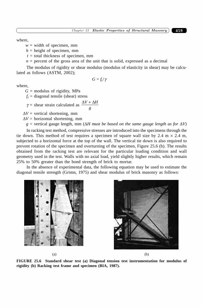
459�������� ���������� �� ��������������������
where,w = width of specimen, mmh = height of specimen, mmt = total thickness of specimen, mmn = percent of the gross area of the unit that is solid, expressed as a decimal
The modulus of rigidity or shear modulus (modulus of elasticity in shear) may be calcu-lated as follows (ASTM, 2002);
G = ft /gwhere,
G = modulus of rigidity, MPaft = diagonal tensile (shear) stress
g = shear strain calculated as D DV H
g+
DV = vertical shortening, mmDV = horizontal shortening, mm
g = vertical gauge length, mm (DH must be based on the same gauge length as for DV)
In racking test method, compressive stresses are introduced into the specimens through thetie down. This method of test requires a specimen of square wall size by 2.4 m ¥ 2.4 m,subjected to a horizontal force at the top of the wall. The vertical tie down is also required toprevent rotation of the specimen and overturning of the specimen, Figure 25.6 (b). The resultsobtained from the racking test are relevant for the particular loading condition and wallgeometry used in the test. Walls with no axial load, yield slightly higher results, which remain25% to 50% greater than the bond strength of brick to mortar.
In the absence of experimental data, the following equation may be used to estimate thediagonal tensile strength (Grimn, 1975) and shear modulus of brick masonry as follows:
(a) (b)
FIGURE 25.6 Standard shear test (a) Diagonal tension test instrumentation for modulus ofrigidity (b) Racking test frame and specimen (BIA, 1987).
�������� �� ��������� �������������� �460
Diagonal tensile (shear) strength
fdt = k( f¢m )0.5
fdt = diagonal tensile strength of brick masonry in diagonal tension, in psi (1 psi = 6.894N/m2)
k = constant factor, the values of k ranged between 2.5 and 4.5. An average value of 3.5may be used.
f¢m = Compressive strength of brick masonry prism, in psi (1 psi = 6.894 N/m2)
Shear modulus
The shear modulus of brick masonry G is inversely proportional to the shearing stress and isproportional to the pre compressive stress. For approximate calculation, G might be taken as
G = E/2(1 + n)
where,E = modulus of elasticity in compressionn = Poisson’s ratio (for brick masonry value varies from 0.11 to 0.20)
MIA, 1998 has assumed the value of G = 0.4 E. Typical value for shear modulus ofbrickwork ranges from 1500–2000 N/mm2.
SUMMARY
The properties of masonry are not very well related to its constituent’s materials such as unit,mortar, grout and reinforcement. However, for seismic design of masonry structure there is aneed to consider strength and elastic characteristics of masonry. The strength characteristics suchas compressive strength, tensile and shear strength are often required in checking design ofmasonry structures. The modulus of elasticity, Poisson’s ratio and damping properties arerequired for carrying out seismic studies. There is a scarcity of data available on strengthcharacteristics and elastic properties of masonry. This chapter deals with the engineeringproperties of constituent materials in brief with a detailed discussion on the strength and stiffnessproperties of masonry assemblage. The tests for determining the structural properties have alsobeen discussed.
REFERENCES
[1] American Society of Testing and Materials, “Compressive Strength of MasonryAssemblages”, ASTM E 447–84, Philadelphia, PA, 1984.
[2] American Society of Testing and Materials, “Measurements of Masonry Flexural BondStrength”, ASTM C 1072–82, Philadelphia, PA, 1986.
[3] American Society of Testing and Materials, ‘Test Method for Flexural Bond Strengthof Masonry”, ASTM E 518–80, Philadelphia, PA, 1987.

461�������� ���������� �� ��������������������
[4] American Society of Testing and Materials, “Standard Methods for ConductingStrength Tests on Panels for Building Construction”, ASTM E 72, Philadelphia, PA,1989.
[5] Amrhein, J.E., Reinforced Masonry Engineering Handbook—Clay and ConcreteMasonry, 5th ed., Masonry Institute of America, 1992.
[6] ASTM, ASTM Standards in Building Codes, ASTM International, West Conshohocken,PA, 2002.
[7] Baker, L.R., “The Lateral Strength of Brickwork—An Overview”, Proceedings of theSixth International Symposium on Load Bearing Brickwork, London, 1997.
[8] BIA., “Testing for Engineered Brick Masonry—Quality Control”, Technical Notes 39Bon Brick Construction, Brick Industry Association, Reston, Virginia, 1988.
[9] BIA, “Testing of Engineered Brick Masonry—Determination of Allowable DesignStresses”, Technical Notes 39A on Brick Construction, Brick Industry Association,Reston, Virginia, 1987.
[10] Bull, J.W., Computation Modelling of Masonry, Brickwork and Blockwork Structures,Saxe-Coburg Publications, UK, 2001.
[11] CIB, “International Recommendations for Design and Erection of Masonry Buildings”,1958.
[12] Dhanasekar, M., Page, A.W., and Kleeman, P.W., “The Failure of Brick MasonryUnder Bi-axial Stresses”, Proceedings of Institution of Civil Engineers, Part 2, 79,295–313, June 1985.
[13] Drydale, R.G., Hamid, A.A., and Baker, L.R., Masonry Structures—Behaviour andDesign, Prentice Hall, Englewood Cliffs, New Jersey, 1994.
[14] Eurocode No. 6, 1988. “Common Unified Rules for Masonry Structures”, Commissionof the European Communities, Report EUR 9888 EN, 1988.
[15] Grimn, C.T., “Strength and Related Properties of Brick Masonry”, Journal ofStructural Engineering, ASCE, Vol. 101, No. ST 1, 217–232, January, 1975.
[16] Hamid, A.A. and Drydale, R.C. “The Shear Behaviour of Brickwork Bed Joints”,Proceedings of British Ceramic Society, No. 30, September 1982.
[17] Hendry, A.W, Structural Masonry, 2nd ed., Macmillan Press, 1998.[18] Hendry, A.W. and Sinha, B.P. “Shear Test on Full Scale Single Storey Brickwork
Structures Subjected to Pre-compression”, Civil Engineering Publications Wks Rev.,1339-44, 1971.
[19] IS 1905:1987 (1985). Code of Practice for Structural Use of Unreinforced Masonry,Bureau of Indian Standards, New Delhi, 1985.
[20] IS 4326:1993, Earthquake Resistant Design and Construction of Buildings—Code ofPractice, Bureau of Indian Standards, New Delhi. 1993.
[21] Knutsson, H.H. and Nielson, J. “On the Modulus of Elasticity for Masonry”, MasonryInternational, 9(2), 57–61, 1995.
[22] McNary, W.S. and Abrams, D.P. “Mechanics of Masonry in Compression”, Journal ofStructural Engineering, ASCE, Vol. 111, No. 4, 857–870, April, 1985.
[23] MIA, Masonry Codes and Specification, A Co-publication of the Masonry Institute ofAmerica and CRC Press, New York, 1998.

�������� �� ��������� �������������� �462
[24] Page, A.W., “Concentrated Loads on Solid Masonry Walls—A Parameteric Study andDesign Recommendations”, Proceedings of Institution of Civil Engineers, Part 2, 85:271–289, June, 1982.
[25] Pieper, K. and Trautsch, W., “Shear Tests on Walls”, Proceedings of 2nd InternationalBrick Masonry Conference (Stoke-on-Trent), H.W.H. West and K.H. Speed (Eds.)British Ceramic Research Association, Stoke-on-Trent, 1971.
[26] Powell, B. and Hodgkinson, H.R., “The Determination of Stress/Strain Relationship ofBrickwork”, Proceedings of Fourth International Brick Masonry Conference, Brugge,Paper 2.a.5, 1976.
[27] Sahlin, S., Structural Masonry, Prentice Hall, Englewood Cliffs, New Jersey, 1971.[28] Schneider, H., “Tests on Shear Resistance of Masonry”, Proceedings of the Fourth
International Brick Masonry Conference, Brugge, 1976.[29] Schneider, H. and Schnell, W., “Tests on the Shear Strength of Brickwork”, Betonwerk
& Fertigteil-Technik, 44, 1978.[30] Schneider, R.R. and Dickey, W.L., Reinforced Masonry Design, 3rd ed., Prentice Hall,
New Jersey, 1994.[31] Schubert, P., “Modulus of Elasticity of Masonry”, Proceedings of the Fifth Inter-
national Brick Masonry Conference, Washington, 1982.[32] Sinha, B.P. and Pedreschi, R., “Compressive Strength and Some Elastic Properties of
Brickwork”, International Journal of Masonry Construction, 1983.[33] Sinha, B.P. and Hendry, A.W., “Racking Test on Storey Height Shear Wall Structures
with Openings Subjected to Pre-compression”, Designing, Engineering and Constructingwith Masonry Products, F.B. Johnson (Ed.), Gulf, Houston, Texas, 1969.
[34] Smith, B.S. and Carter, C., “Hypothesis for Shear Failure of Brickwork”, Journal ofthe Structural Division, Proceedings of the American Society of Civil Engineers, April,1971.
[35] SP 20 (S&T), Handbook on Masonry Design and Construction, Bureau of IndianStandards, New Delhi, 1991.
[36] Turnsek, V. and Cacovic, F., “Some Experimental Results on the Strength of BrickMasonry Walls”, Proceedings of 2nd International Brick Masonry Conference, Stoke-on-Trent, pp. 149–156, 1970.
463�������� ���������������� � ������ ������������
463
Lateral LoadAnalysis of Masonry
Buildings
��������
26.1 INTRODUCTION
Masonry buildings are widely used for housing construction not only in India but in many othercountries of the world. There are innumerable advantages of masonry construction over bothtypes of construction i.e. reinforced concrete and steel such as, thermal comfort, sound control,possibility of addition and alteration after construction, less formwork, easy and inexpensiverepair, use of locally available materials, need of less skilled labour, less engineeringintervention etc. However, there are some disadvantages as well, particularly, when it is builtin seismic environment. The seismic resistance capacity of masonry construction is relativelylow in comparison to engineered constructions. Table 26.1 compares the properties of masonryto the comparable properties of structural steel and reinforced concrete (STP 992, 1988).Therefore, many developed nations have imposed certain restrictions on the use of unreinforcedmasonry constructions. However, in developing nations unreinforced masonry construction isstill being used frequently. In India, masonry constructions are generally made by using locallyavailable materials like stone, brick, timber, adobe, mud etc. and are constructed in a traditionalmanner with or without the earthquake resistant features mentioned in IS: 4326 and 13927.Therefore, this type of construction is treated as non-engineered construction and most of thecasualties are due to collapse of these constructions in earthquakes. Moreover the plight is thateven after gaining knowledge of earthquake engineering since the last three decades, neither aproper method has been developed for the seismic analysis and design of masonry buildings northe topic is fairly covered in the current Indian curriculum in spite of the fact that about 90%population of India lives in masonry buildings. The present and subsequent chapters are a steptowards with regard to develop a procedure for seismic analysis and design of masonrybuildings. The procedure is divided into several distinctive steps in order to create a solid feelingand confidence that masonry buildings may also be designed as engineered construction.
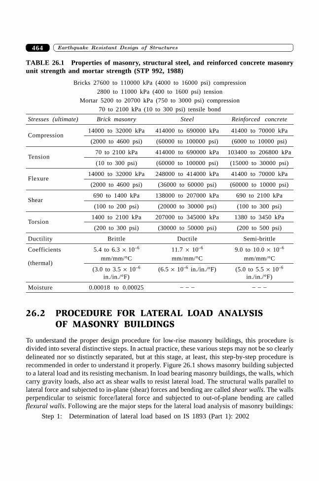
������������� � ������� ���������������� 464
TABLE 26.1 Properties of masonry, structural steel, and reinforced concrete masonryunit strength and mortar strength (STP 992, 1988)
Bricks 27600 to 110000 kPa (4000 to 16000 psi) compression
2800 to 11000 kPa (400 to 1600 psi) tension
Mortar 5200 to 20700 kPa (750 to 3000 psi) compression
70 to 2100 kPa (10 to 300 psi) tensile bond
Stresses (ultimate) Brick masonry Steel Reinforced concrete
Compression14000 to 32000 kPa 414000 to 690000 kPa 41400 to 70000 kPa
(2000 to 4600 psi) (60000 to 100000 psi) (6000 to 10000 psi)
Tension70 to 2100 kPa 414000 to 690000 kPa 103400 to 206800 kPa
(10 to 300 psi) (60000 to 100000 psi) (15000 to 30000 psi)
Flexure14000 to 32000 kPa 248000 to 414000 kPa 41400 to 70000 kPa
(2000 to 4600 psi) (36000 to 60000 psi) (60000 to 10000 psi)
Shear690 to 1400 kPa 138000 to 207000 kPa 690 to 2100 kPa
(100 to 200 psi) (20000 to 30000 psi) (100 to 300 psi)
Torsion1400 to 2100 kPa 207000 to 345000 kPa 1380 to 3450 kPa
(200 to 300 psi) (30000 to 50000 psi) (200 to 500 psi)
Ductility Brittle Ductile Semi-brittle
Coefficients 5.4 to 6.3 ¥ 10–6 11.7 ¥ 10–6 9.0 to 10.0 ¥ 10–6
(thermal)mm/mm/°C mm/mm/°C mm/mm/°C
(3.0 to 3.5 ¥ 10–6 (6.5 ¥ 10–6 in./in./°F) (5.0 to 5.5 ¥ 10–6
in./in./°F) in./in./°F)
Moisture 0.00018 to 0.00025 – – – – – –
26.2 PROCEDURE FOR LATERAL LOAD ANALYSISOF MASONRY BUILDINGS
To understand the proper design procedure for low-rise masonry buildings, this procedure isdivided into several distinctive steps. In actual practice, these various steps may not be so clearlydelineated nor so distinctly separated, but at this stage, at least, this step-by-step procedure isrecommended in order to understand it properly. Figure 26.1 shows masonry building subjectedto a lateral load and its resisting mechanism. In load bearing masonry buildings, the walls, whichcarry gravity loads, also act as shear walls to resist lateral load. The structural walls parallel tolateral force and subjected to in-plane (shear) forces and bending are called shear walls. The wallsperpendicular to seismic force/lateral force and subjected to out-of-plane bending are calledflexural walls. Following are the major steps for the lateral load analysis of masonry buildings:
Step 1: Determination of lateral load based on IS 1893 (Part 1): 2002
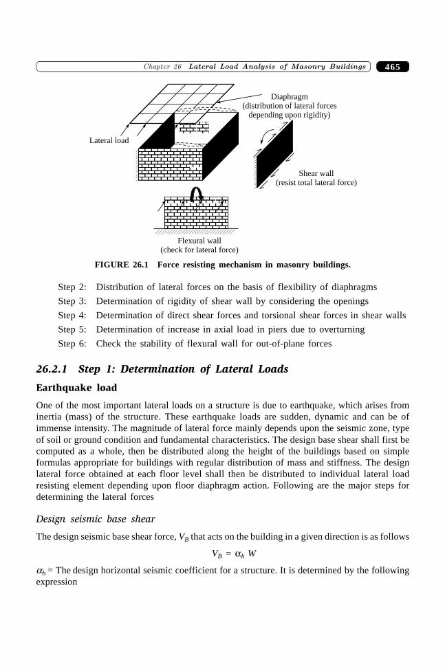
465�������� ���������������� � ������ ������������
Step 2: Distribution of lateral forces on the basis of flexibility of diaphragms
Step 3: Determination of rigidity of shear wall by considering the openings
Step 4: Determination of direct shear forces and torsional shear forces in shear walls
Step 5: Determination of increase in axial load in piers due to overturning
Step 6: Check the stability of flexural wall for out-of-plane forces
26.2.1 Step 1: Determination of Lateral Loads
Earthquake load
One of the most important lateral loads on a structure is due to earthquake, which arises frominertia (mass) of the structure. These earthquake loads are sudden, dynamic and can be ofimmense intensity. The magnitude of lateral force mainly depends upon the seismic zone, typeof soil or ground condition and fundamental characteristics. The design base shear shall first becomputed as a whole, then be distributed along the height of the buildings based on simpleformulas appropriate for buildings with regular distribution of mass and stiffness. The designlateral force obtained at each floor level shall then be distributed to individual lateral loadresisting element depending upon floor diaphragm action. Following are the major steps fordetermining the lateral forces
Design seismic base shear
The design seismic base shear force, VB that acts on the building in a given direction is as follows
VB = ah W
ah = The design horizontal seismic coefficient for a structure. It is determined by the followingexpression
Diaphragm(distribution of lateral forces
depending upon rigidity)
Lateral load
Shear wall(resist total lateral force)
Flexural wall(check for lateral force)
FIGURE 26.1 Force resisting mechanism in masonry buildings.
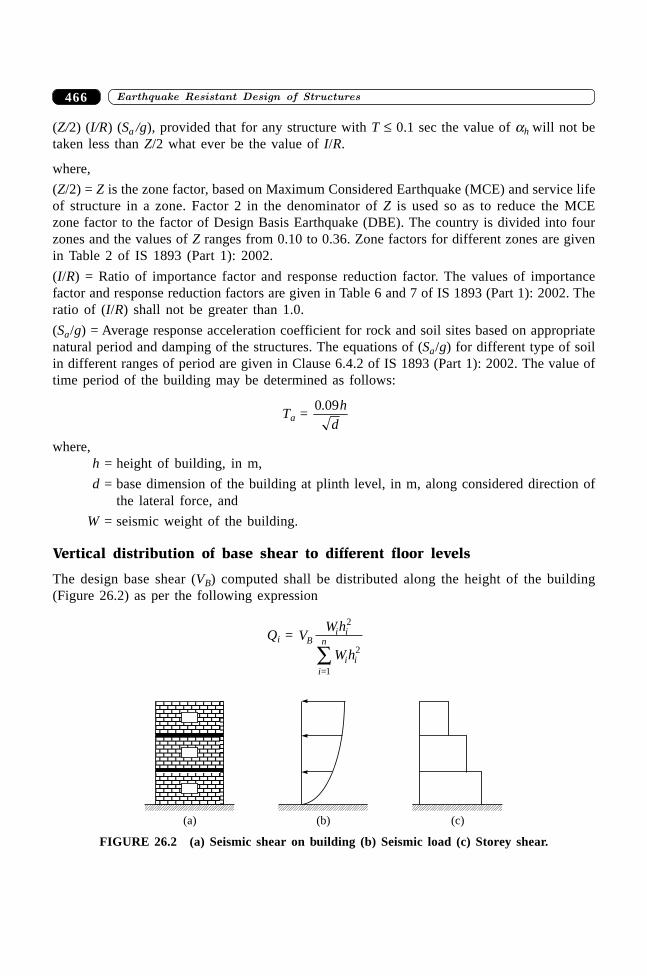
������������� � ������� ���������������� 466
(Z/2) (I/R) (Sa /g), provided that for any structure with T £ 0.1 sec the value of ah will not betaken less than Z/2 what ever be the value of I/R.
where,
(Z/2) = Z is the zone factor, based on Maximum Considered Earthquake (MCE) and service lifeof structure in a zone. Factor 2 in the denominator of Z is used so as to reduce the MCEzone factor to the factor of Design Basis Earthquake (DBE). The country is divided into fourzones and the values of Z ranges from 0.10 to 0.36. Zone factors for different zones are givenin Table 2 of IS 1893 (Part 1): 2002.
(I/R) = Ratio of importance factor and response reduction factor. The values of importancefactor and response reduction factors are given in Table 6 and 7 of IS 1893 (Part 1): 2002. Theratio of (I/R) shall not be greater than 1.0.
(Sa/g) = Average response acceleration coefficient for rock and soil sites based on appropriatenatural period and damping of the structures. The equations of (Sa/g) for different type of soilin different ranges of period are given in Clause 6.4.2 of IS 1893 (Part 1): 2002. The value oftime period of the building may be determined as follows:
Ta = 0 09. h
d
where,h = height of building, in m,
d = base dimension of the building at plinth level, in m, along considered direction ofthe lateral force, and
W = seismic weight of the building.
Vertical distribution of base shear to different floor levels
The design base shear (VB) computed shall be distributed along the height of the building(Figure 26.2) as per the following expression
Qi = VWh
W hB
i i
i ii
n
2
2
=1Â
(a) (b) (c)
FIGURE 26.2 (a) Seismic shear on building (b) Seismic load (c) Storey shear.
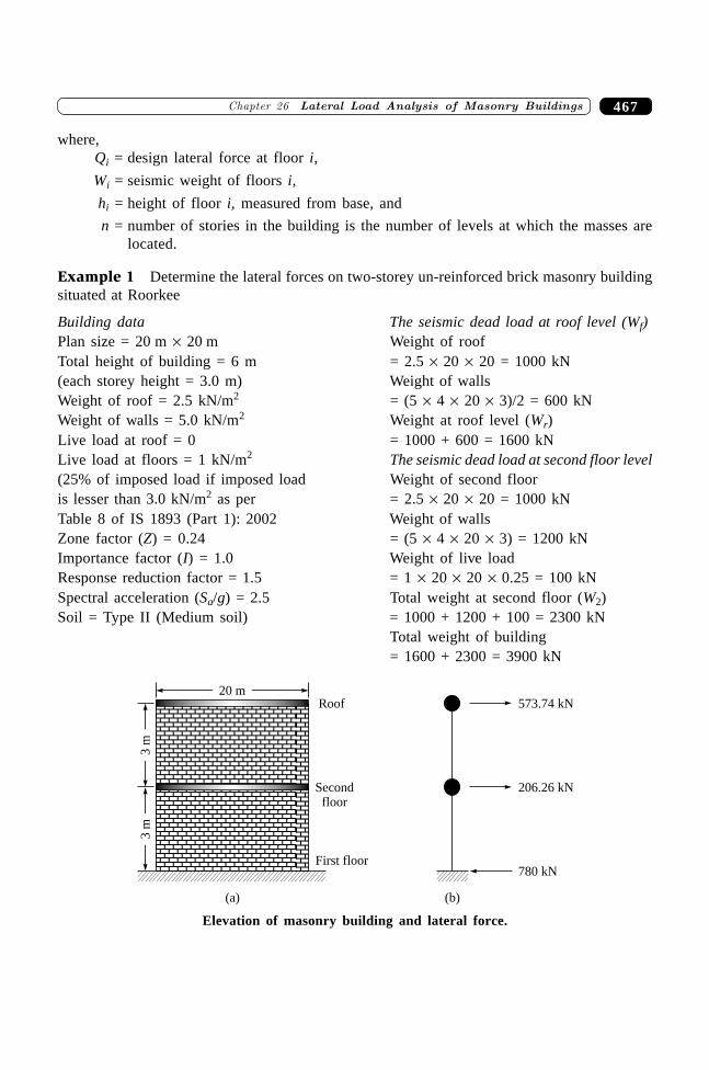
467�������� ���������������� � ������ ������������
where,Qi = design lateral force at floor i,
Wi = seismic weight of floors i,
hi = height of floor i, measured from base, and
n = number of stories in the building is the number of levels at which the masses arelocated.
Example 1 Determine the lateral forces on two-storey un-reinforced brick masonry buildingsituated at Roorkee
Building data The seismic dead load at roof level (Wf)Plan size = 20 m ¥ 20 m Weight of roofTotal height of building = 6 m = 2.5 ¥ 20 ¥ 20 = 1000 kN(each storey height = 3.0 m) Weight of wallsWeight of roof = 2.5 kN/m2 = (5 ¥ 4 ¥ 20 ¥ 3)/2 = 600 kNWeight of walls = 5.0 kN/m2 Weight at roof level (Wr)Live load at roof = 0 = 1000 + 600 = 1600 kNLive load at floors = 1 kN/m2 The seismic dead load at second floor level(25% of imposed load if imposed load Weight of second flooris lesser than 3.0 kN/m2 as per = 2.5 ¥ 20 ¥ 20 = 1000 kNTable 8 of IS 1893 (Part 1): 2002 Weight of wallsZone factor (Z) = 0.24 = (5 ¥ 4 ¥ 20 ¥ 3) = 1200 kNImportance factor (I) = 1.0 Weight of live loadResponse reduction factor = 1.5 = 1 ¥ 20 ¥ 20 ¥ 0.25 = 100 kNSpectral acceleration (Sa/g) = 2.5 Total weight at second floor (W2)Soil = Type II (Medium soil) = 1000 + 1200 + 100 = 2300 kN
Total weight of building= 1600 + 2300 = 3900 kN
20 mRoof
Secondfloor
First floor
3m
3m
573.74 kN
206.26 kN
780 kN
(a) (b)
Elevation of masonry building and lateral force.
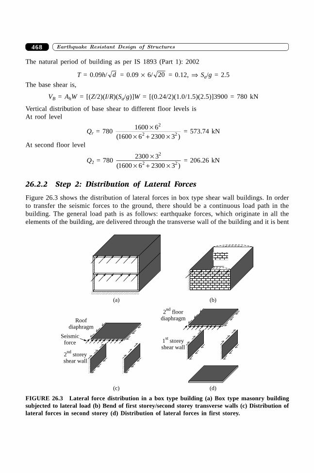
������������� � ������� ���������������� 468
The natural period of building as per IS 1893 (Part 1): 2002
T = 0.09h/ d = 0.09 ¥ 6/ 20 = 0.12, fi Sa/g = 2.5
The base shear is,
VB = AhW = [(Z/2)(I/R)(Sa/g)]W = [(0.24/2)(1.0/1.5)(2.5)]3900 = 780 kN
Vertical distribution of base shear to different floor levels isAt roof level
Qr = 780 1600 6
1600 6 2300 3
2
2 2¥
¥ + ¥( ) = 573.74 kN
At second floor level
Q2 = 780 2300 3
1600 6 2300 3
2
2 2¥
¥ + ¥( ) = 206.26 kN
26.2.2 Step 2: Distribution of Lateral Forces
Figure 26.3 shows the distribution of lateral forces in box type shear wall buildings. In orderto transfer the seismic forces to the ground, there should be a continuous load path in thebuilding. The general load path is as follows: earthquake forces, which originate in all theelements of the building, are delivered through the transverse wall of the building and it is bent
Roofdiaphragm
Seismicforce
2 storeyshear wall
nd
1 storeyshear wall
st
2 floordiaphragm
nd
(a) (b)
(c) (d)
FIGURE 26.3 Lateral force distribution in a box type building (a) Box type masonry buildingsubjected to lateral load (b) Bend of first storey/second storey transverse walls (c) Distribution oflateral forces in second storey (d) Distribution of lateral forces in first storey.
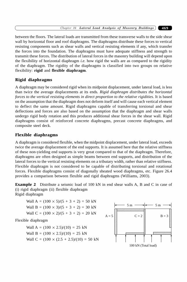
469�������� ���������������� � ������ ������������
between the floors. The lateral loads are transmitted from these transverse walls to the side shearwall by horizontal floor and roof diaphragms. The diaphragms distribute these forces to verticalresisting components such as shear walls and vertical resisting elements if any, which transferthe forces into the foundation. The diaphragms must have adequate stiffness and strength totransmit these forces. The distribution of lateral forces in the masonry building will depend uponthe flexibility of horizontal diaphragm i.e. how rigid the walls are as compared to the rigidityof the diaphragm. The rigidity of the diaphragms is classified into two groups on relativeflexibility: rigid and flexible diaphragm.
Rigid diaphragms
A diaphragm may be considered rigid when its midpoint displacement, under lateral load, is lessthan twice the average displacements at its ends. Rigid diaphragm distributes the horizontalforces to the vertical resisting elements in direct proportion to the relative rigidities. It is basedon the assumption that the diaphragm does not deform itself and will cause each vertical elementto deflect the same amount. Rigid diaphragms capable of transferring torsional and sheardeflections and forces are also based on the assumption that the diaphragm and shear wallsundergo rigid body rotation and this produces additional shear forces in the shear wall. Rigiddiaphragms consist of reinforced concrete diaphragms, precast concrete diaphragms, andcomposite steel deck.
Flexible diaphragms
A diaphragm is considered flexible, when the midpoint displacement, under lateral load, exceedstwice the average displacement of the end supports. It is assumed here that the relative stiffnessof these non-yielding end supports is very great compared to that of the diaphragm. Therefore,diaphragms are often designed as simple beams between end supports, and distribution of thelateral forces to the vertical resisting elements on a tributary width, rather than relative stiffness.Flexible diaphragm is not considered to be capable of distributing torsional and rotationalforces. Flexible diaphragms consist of diagonally sheated wood diaphragms, etc. Figure 26.4provides a comparison between flexible and rigid diaphragms (Williams, 2003).
Example 2 Distribute a seismic load of 100 kN in end shear walls A, B and C in case of(i) rigid diaphragm (ii) flexible diaphragmRigid diaphragm
Wall A = (100 ¥ 5)/(5 + 3 + 2) = 50 kN
Wall B = (100 ¥ 3)/(5 + 3 + 2) = 30 kN
Wall C = (100 ¥ 2)/(5 + 3 + 2) = 20 kN
Flexible diaphragm
Wall A = (100 ¥ 2.5)/(10) = 25 kN
Wall B = (100 ¥ 2.5)/(10) = 25 kN
Wall C = (100 ¥ (2.5 + 2.5)/(10) = 50 kN
5 m 5 m
100 kN (Total load)
A = 5 C = 2 B = 3
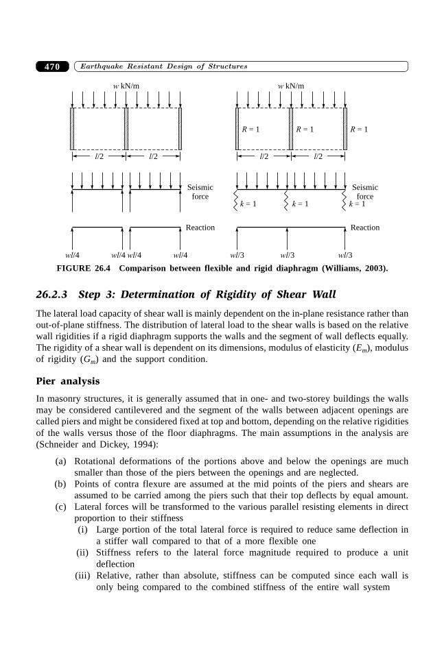
������������� � ������� ���������������� 470
26.2.3 Step 3: Determination of Rigidity of Shear Wall
The lateral load capacity of shear wall is mainly dependent on the in-plane resistance rather thanout-of-plane stiffness. The distribution of lateral load to the shear walls is based on the relativewall rigidities if a rigid diaphragm supports the walls and the segment of wall deflects equally.The rigidity of a shear wall is dependent on its dimensions, modulus of elasticity (Em), modulusof rigidity (Gm) and the support condition.
Pier analysis
In masonry structures, it is generally assumed that in one- and two-storey buildings the wallsmay be considered cantilevered and the segment of the walls between adjacent openings arecalled piers and might be considered fixed at top and bottom, depending on the relative rigiditiesof the walls versus those of the floor diaphragms. The main assumptions in the analysis are(Schneider and Dickey, 1994):
(a) Rotational deformations of the portions above and below the openings are muchsmaller than those of the piers between the openings and are neglected.
(b) Points of contra flexure are assumed at the mid points of the piers and shears areassumed to be carried among the piers such that their top deflects by equal amount.
(c) Lateral forces will be transformed to the various parallel resisting elements in directproportion to their stiffness(i) Large portion of the total lateral force is required to reduce same deflection in
a stiffer wall compared to that of a more flexible one(ii) Stiffness refers to the lateral force magnitude required to produce a unit
deflection(iii) Relative, rather than absolute, stiffness can be computed since each wall is
only being compared to the combined stiffness of the entire wall system
Seismicforce
l/2 l/2
w kN/m
Reaction
wl/4 wl/4 wl/4 wl/4
Seismicforce
l/2 l/2
w kN/m
Reaction
wl/3 wl/3 wl/3
R = 1 R = 1 R = 1
k = 1 k = 1 k = 1
FIGURE 26.4 Comparison between flexible and rigid diaphragm (Williams, 2003).
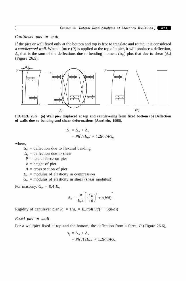
471�������� ���������������� � ������ ������������
Cantilever pier or wall
If the pier or wall fixed only at the bottom and top is free to translate and rotate, it is considereda cantilevered wall. When a force (P) is applied at the top of a pier, it will produce a deflection,Dc that is the sum of the deflections due to bending moment (Dm) plus that due to shear (Dv)(Figure 26.5).
�cP
h
P
(a) (b)
FIGURE 26.5 (a) Wall pier displaced at top and cantilevering from fixed bottom (b) Deflectionof walls due to bending and shear deformations (Amrhein, 1998).
Dc = Dm + Dv
= Ph3/3EmI + 1.2Ph/AGm
where,Dm = deflection due to flexural bendingDv = deflection due to shearP = lateral force on pierh = height of pierA = cross section of pier
Em = modulus of elasticity in compressionGm = modulus of elasticity in shear (shear modulus)
For masonry, Gm = 0.4 Em
Dc = PE tm
4 33h
dh dFH IK +
LNM
OQP
( / )
Rigidity of cantilever pier Rc = 1/Dc = Emt/(4(h/d)3 + 3(h/d))
Fixed pier or wall
For a wall/pier fixed at top and the bottom, the deflection from a force, P (Figure 26.6),
Df = Dm + Dv
= Ph3/12EmI + 1.2Ph/AGm
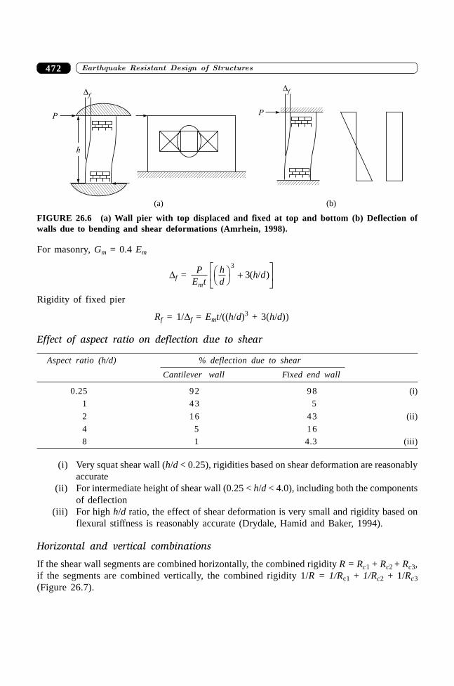
������������� � ������� ���������������� 472
P
h
�f
P
�f
(a) (b)
FIGURE 26.6 (a) Wall pier with top displaced and fixed at top and bottom (b) Deflection ofwalls due to bending and shear deformations (Amrhein, 1998).
For masonry, Gm = 0.4 Em
Df = PE tm
hd
h dFH IK +LNM
OQP
3
3( / )
Rigidity of fixed pier
Rf = 1/Df = Emt/((h/d)3 + 3(h/d))
Effect of aspect ratio on deflection due to shear
Aspect ratio (h/d) % deflection due to shear
Cantilever wall Fixed end wall
0.25 92 98 (i)
1 43 5
2 16 43 (ii)
4 5 16
8 1 4.3 (iii)
(i) Very squat shear wall (h/d < 0.25), rigidities based on shear deformation are reasonablyaccurate
(ii) For intermediate height of shear wall (0.25 < h/d < 4.0), including both the componentsof deflection
(iii) For high h/d ratio, the effect of shear deformation is very small and rigidity based onflexural stiffness is reasonably accurate (Drydale, Hamid and Baker, 1994).
Horizontal and vertical combinations
If the shear wall segments are combined horizontally, the combined rigidity R = Rc1 + Rc2 + Rc3,if the segments are combined vertically, the combined rigidity 1/R = 1/Rc1 + 1/Rc2 + 1/Rc3(Figure 26.7).
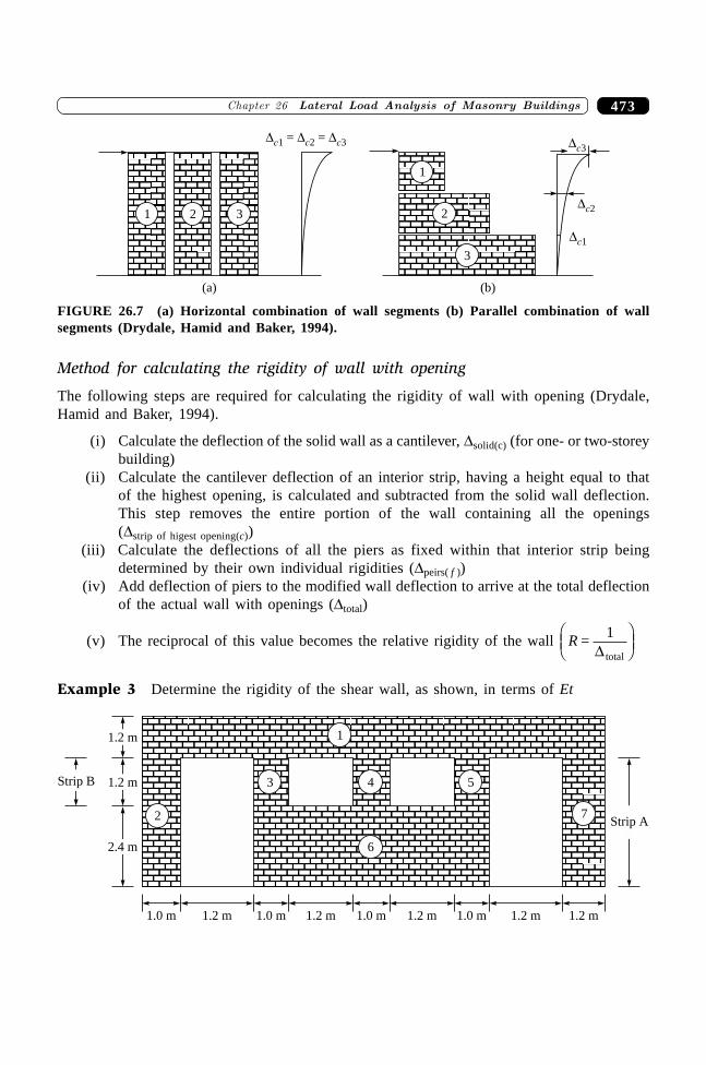
473�������� ���������������� � ������ ������������
� �c c1 2= = �c3 �c3
1
2
3
�c2
�c1
(a) (b)
321
FIGURE 26.7 (a) Horizontal combination of wall segments (b) Parallel combination of wallsegments (Drydale, Hamid and Baker, 1994).
Method for calculating the rigidity of wall with opening
The following steps are required for calculating the rigidity of wall with opening (Drydale,Hamid and Baker, 1994).
(i) Calculate the deflection of the solid wall as a cantilever, Dsolid(c) (for one- or two-storeybuilding)
(ii) Calculate the cantilever deflection of an interior strip, having a height equal to thatof the highest opening, is calculated and subtracted from the solid wall deflection.This step removes the entire portion of the wall containing all the openings(Dstrip of higest opening(c))
(iii) Calculate the deflections of all the piers as fixed within that interior strip beingdetermined by their own individual rigidities (Dpeirs( f ))
(iv) Add deflection of piers to the modified wall deflection to arrive at the total deflectionof the actual wall with openings (Dtotal)
(v) The reciprocal of this value becomes the relative rigidity of the wall R =total
1D
FHG
IKJ
Example 3 Determine the rigidity of the shear wall, as shown, in terms of Et
1.2 m 1.2 m
3
1.0 m1.0 m
2
1.2 m1.2 m
5
1.0 m 1.2 m
7
4
6
1
1.0 m
1.2 m
1.2 m
2.4 m
Strip B
Strip A
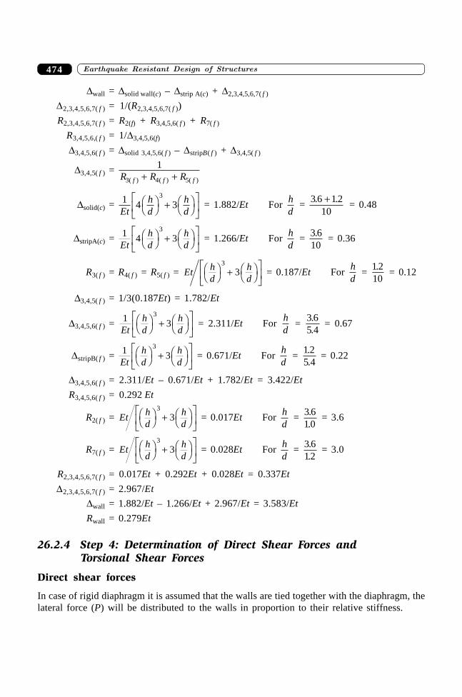
������������� � ������� ���������������� 474
Dwall = Dsolid wall(c) – Dstrip A(c) + D2,3,4,5,6,7( f )
D2,3,4,5,6,7( f ) = 1/(R2,3,4,5,6,7( f ))
R2,3,4,5,6,7( f ) = R2(f) + R3,4,5,6( f ) + R7( f )
R3,4,5,6,( f ) = 1/D3,4,5,6(f)
D3,4,5,6( f ) = Dsolid 3,4,5,6( f ) – DstripB( f ) + D3,4,5( f )
D3,4,5( f ) = 1
3 4 5(R R Rf f f( ) ( ) )+ +
Dsolid(c) = 1 4 33
Ethd
hd
FH IK + FH IKLNM
OQP
= 1.882/Et For hd
= 3 6 1 2
10. .+
= 0.48
DstripA(c) = 1 4 33
Ethd
hd
FH IK + FH IKLNM
OQP
= 1.266/Et For hd
= 3 610. = 0.36
R3( f ) = R4( f ) = R5( f ) = Et hd
hd
FH IK + FH IKLNM
OQP
3
3 = 0.187/Et For hd
= 1 210.
= 0.12
D3,4,5( f ) = 1/3(0.187Et) = 1.782/Et
D3,4,5,6( f ) = 1 33
Ethd
hd
FH IK + FH IKLNM
OQP = 2.311/Et For
hd
= 3 65 4..
= 0.67
DstripB( f ) = 1 33
Ethd
hd
FH IK + FH IKLNM
OQP = 0.671/Et For
hd
= 1 25 4..
= 0.22
D3,4,5,6( f ) = 2.311/Et – 0.671/Et + 1.782/Et = 3.422/Et
R3,4,5,6( f ) = 0.292 Et
R2( f ) = Et hd
hd
FH IK + FH IKLNM
OQP
3
3 = 0.017Et For hd
= 3 61 0..
= 3.6
R7( f ) = Et hd
hd
FH IK + FH IKLNM
OQP
3
3 = 0.028Et For hd
= 3 612..
= 3.0
R2,3,4,5,6,7( f ) = 0.017Et + 0.292Et + 0.028Et = 0.337Et
D2,3,4,5,6,7( f ) = 2.967/Et
Dwall = 1.882/Et – 1.266/Et + 2.967/Et = 3.583/Et
Rwall = 0.279Et
26.2.4 Step 4: Determination of Direct Shear Forces andTorsional Shear Forces
Direct shear forces
In case of rigid diaphragm it is assumed that the walls are tied together with the diaphragm, thelateral force (P) will be distributed to the walls in proportion to their relative stiffness.
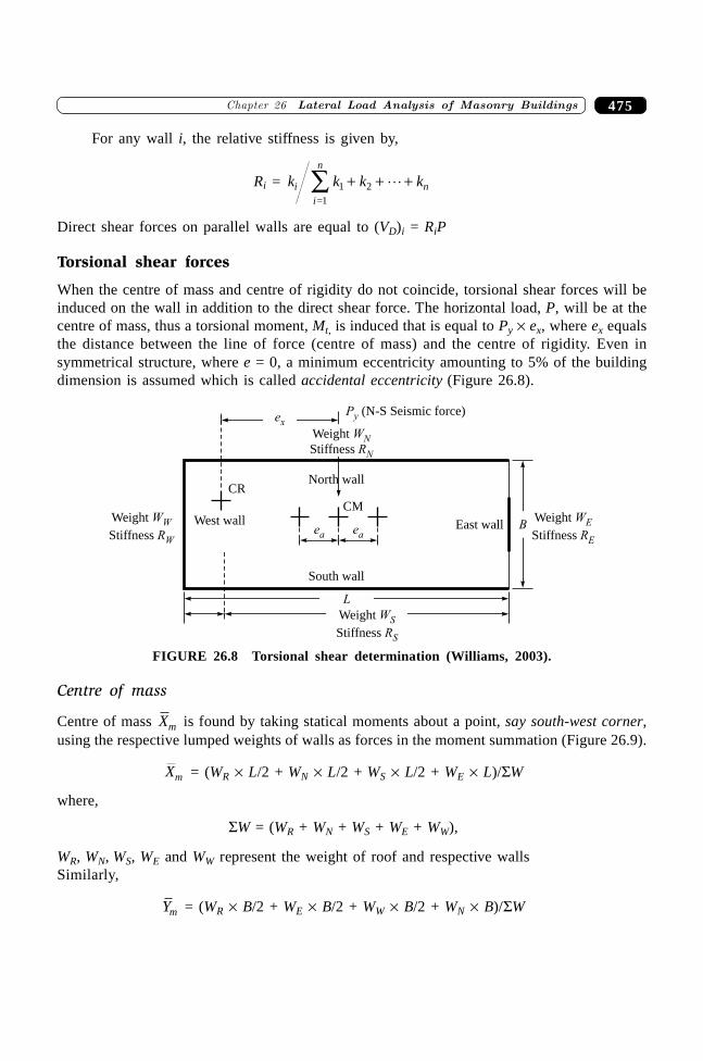
475�������� ���������������� � ������ ������������
For any wall i, the relative stiffness is given by,
Ri = k k k ki ni
n
1 2+ + +Â �=1
Direct shear forces on parallel walls are equal to (VD)i = RiP
Torsional shear forces
When the centre of mass and centre of rigidity do not coincide, torsional shear forces will beinduced on the wall in addition to the direct shear force. The horizontal load, P, will be at thecentre of mass, thus a torsional moment, Mt, is induced that is equal to Py ¥ ex, where ex equalsthe distance between the line of force (centre of mass) and the centre of rigidity. Even insymmetrical structure, where e = 0, a minimum eccentricity amounting to 5% of the buildingdimension is assumed which is called accidental eccentricity (Figure 26.8).
North wall
ea ea
CR
CM
East wallWest wall
South wall
BWeight
Stiffness
W
RE
E
Weight
Stiffness
W
RS
S
Weight
Stiffness
W
RW
W
exPy (N-S Seismic force)
L
Weight
Stiffness
W
RN
N
FIGURE 26.8 Torsional shear determination (Williams, 2003).
Centre of mass
Centre of mass Xm is found by taking statical moments about a point, say south-west corner,using the respective lumped weights of walls as forces in the moment summation (Figure 26.9).
Xm = (WR ¥ L/2 + WN ¥ L/2 + WS ¥ L/2 + WE ¥ L)/SW
where,
SW = (WR + WN + WS + WE + WW),
WR, WN, WS, WE and WW represent the weight of roof and respective wallsSimilarly,
Ym = (WR ¥ B/2 + WE ¥ B/2 + WW ¥ B/2 + WN ¥ B)/SW
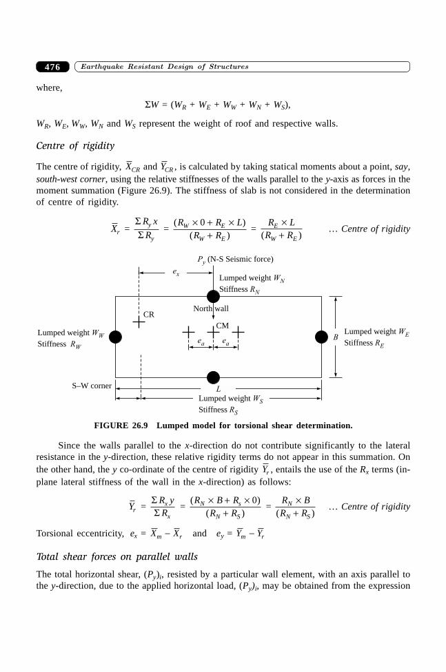
������������� � ������� ���������������� 476
where,
SW = (WR + WE + WW + WN + WS),
WR, WE, WW, WN and WS represent the weight of roof and respective walls.
Centre of rigidity
The centre of rigidity, XCR and YCR , is calculated by taking statical moments about a point, say,south-west corner, using the relative stiffnesses of the walls parallel to the y-axis as forces in themoment summation (Figure 26.9). The stiffness of slab is not considered in the determinationof centre of rigidity.
Xr = SSR x
Ry
y =
( )( )
R R LR R
W E
W E
¥ + ¥+
0 =
R LR R
E
W E
¥+( )
… Centre of rigidity
North wall
ea ea
CR
CM
BLumped weight W
RW
WStiffness
ex
Py (N-S Seismic force)
L
Lumped weight WN
Stiffness RN
Lumped weight WE
Stiffness RE
Lumped weight WS
Stiffness RS
S–W corner
FIGURE 26.9 Lumped model for torsional shear determination.
Since the walls parallel to the x-direction do not contribute significantly to the lateralresistance in the y-direction, these relative rigidity terms do not appear in this summation. Onthe other hand, the y co-ordinate of the centre of rigidity Yr , entails the use of the Rx terms (in-plane lateral stiffness of the wall in the x-direction) as follows:
Yr = SS
R yRx
x =
( )( )
R B RR R
N s
N S
¥ + ¥+
0 =
R BR R
N
N S
¥+( )
… Centre of rigidity
Torsional eccentricity, ex = X Xm r- and ey = Y Ym r-
Total shear forces on parallel walls
The total horizontal shear, (Py)i, resisted by a particular wall element, with an axis parallel tothe y-direction, due to the applied horizontal load, (Py)i, may be obtained from the expression
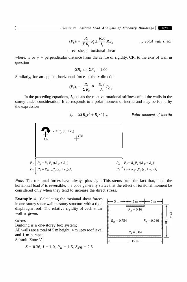
477�������� ���������������� � ������ ������������
(Py)i = R
RP
R x
JP ey
yy
y
ry xS
± … Total wall shear
direct shear torsional shear
where, x or y = perpendicular distance from the centre of rigidity, CR, to the axis of wall inquestion
SRy or SRx = 1.00
Similarly, for an applied horizontal force in the x-direction
(Px)i = RR
PR yJ
P ex
x
x
rx yS
+
In the preceding equations, Jr, equals the relative rotational stiffness of all the walls in thestorey under consideration. It corresponds to a polar moment of inertia and may be found bythe expression
Jr = S ( )R y R xx y2 2+ … Polar moment of inertia
T e= ( + )P ey x a
P R P Rd W y W E= /( + )RPd
P R x P e e JT W w y x a r= ( + )/PT
P R P Rd E y W E= /( + )RPd
P R x P e e JT E e y x a r= ( + )/PT
CRCM
Note: The torsional forces have always plus sign. This stems from the fact that, since thehorizontal load P is reversible, the code generally states that the effect of torsional moment beconsidered only when they tend to increase the direct stress.
Example 4 Calculating the torsional shear forcesin one-storey shear wall masonry structure with a rigiddiaphragm roof. The relative rigidity of each shearwall is given.
Given:Building is a one-storey box system;All walls are a total of 5 m height; 4 m upto roof leveland 1 m parapet.Seismic Zone V,
Z = 0.36, I = 1.0, RW = 1.5, Sa/g = 2.5
RW = 0.754
RN = 0.16
RS = 0.84
RE = 0.246
5 m
10
m
5 m 5 m
15 m
N
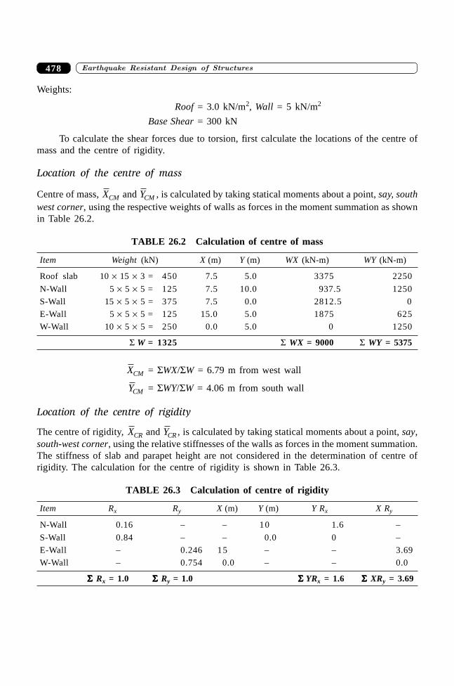
������������� � ������� ���������������� 478
Weights:
Roof = 3.0 kN/m2, Wall = 5 kN/m2
Base Shear = 300 kN
To calculate the shear forces due to torsion, first calculate the locations of the centre ofmass and the centre of rigidity.
Location of the centre of mass
Centre of mass, XCM and YCM , is calculated by taking statical moments about a point, say, southwest corner, using the respective weights of walls as forces in the moment summation as shownin Table 26.2.
TABLE 26.2 Calculation of centre of mass
Item Weight (kN) X (m) Y (m) WX (kN-m) WY (kN-m)
Roof slab 10 ¥ 15 ¥ 3 = 450 7.5 5.0 3375 2250
N-Wall 5 ¥ 5 ¥ 5 = 125 7.5 10.0 937.5 1250
S-Wall 15 ¥ 5 ¥ 5 = 375 7.5 0.0 2812.5 0
E-Wall 5 ¥ 5 ¥ 5 = 125 15.0 5.0 1875 625
W-Wall 10 ¥ 5 ¥ 5 = 250 0.0 5.0 0 1250
S W = 1325 S WX = 9000 S WY = 5375
XCM = SWX/SW = 6.79 m from west wall
YCM = SWY/SW = 4.06 m from south wall
Location of the centre of rigidity
The centre of rigidity, XCR and YCR , is calculated by taking statical moments about a point, say,south-west corner, using the relative stiffnesses of the walls as forces in the moment summation.The stiffness of slab and parapet height are not considered in the determination of centre ofrigidity. The calculation for the centre of rigidity is shown in Table 26.3.
TABLE 26.3 Calculation of centre of rigidity
Item Rx Ry X (m) Y (m) Y Rx X Ry
N-Wall 0.16 – – 10 1.6 –
S-Wall 0.84 – – 0.0 0 –
E-Wall – 0.246 15 – – 3.69
W-Wall – 0.754 0.0 – – 0.0
SSSSS Rx = 1.0 SSSSS Ry = 1.0 SSSSS YRx = 1.6 SSSSS XRy = 3.69
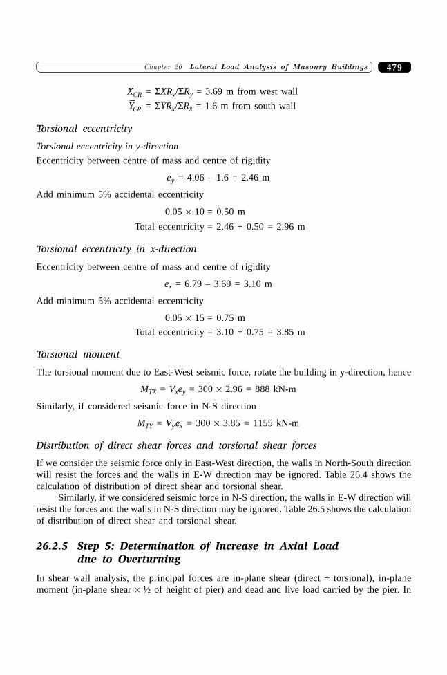
479�������� ���������������� � ������ ������������
XCR = SXRy/SRy = 3.69 m from west wall
YCR = SYRx/SRx = 1.6 m from south wall
Torsional eccentricity
Torsional eccentricity in y-direction
Eccentricity between centre of mass and centre of rigidity
ey = 4.06 – 1.6 = 2.46 m
Add minimum 5% accidental eccentricity
0.05 ¥ 10 = 0.50 m
Total eccentricity = 2.46 + 0.50 = 2.96 m
Torsional eccentricity in x-direction
Eccentricity between centre of mass and centre of rigidity
ex = 6.79 – 3.69 = 3.10 m
Add minimum 5% accidental eccentricity
0.05 ¥ 15 = 0.75 m
Total eccentricity = 3.10 + 0.75 = 3.85 m
Torsional moment
The torsional moment due to East-West seismic force, rotate the building in y-direction, hence
MTX = Vxey = 300 ¥ 2.96 = 888 kN-m
Similarly, if considered seismic force in N-S direction
MTY = Vyex = 300 ¥ 3.85 = 1155 kN-m
Distribution of direct shear forces and torsional shear forces
If we consider the seismic force only in East-West direction, the walls in North-South directionwill resist the forces and the walls in E-W direction may be ignored. Table 26.4 shows thecalculation of distribution of direct shear and torsional shear.
Similarly, if we considered seismic force in N-S direction, the walls in E-W direction willresist the forces and the walls in N-S direction may be ignored. Table 26.5 shows the calculationof distribution of direct shear and torsional shear.
26.2.5 Step 5: Determination of Increase in Axial Loaddue to Overturning
In shear wall analysis, the principal forces are in-plane shear (direct + torsional), in-planemoment (in-plane shear ¥ ½ of height of pier) and dead and live load carried by the pier. In
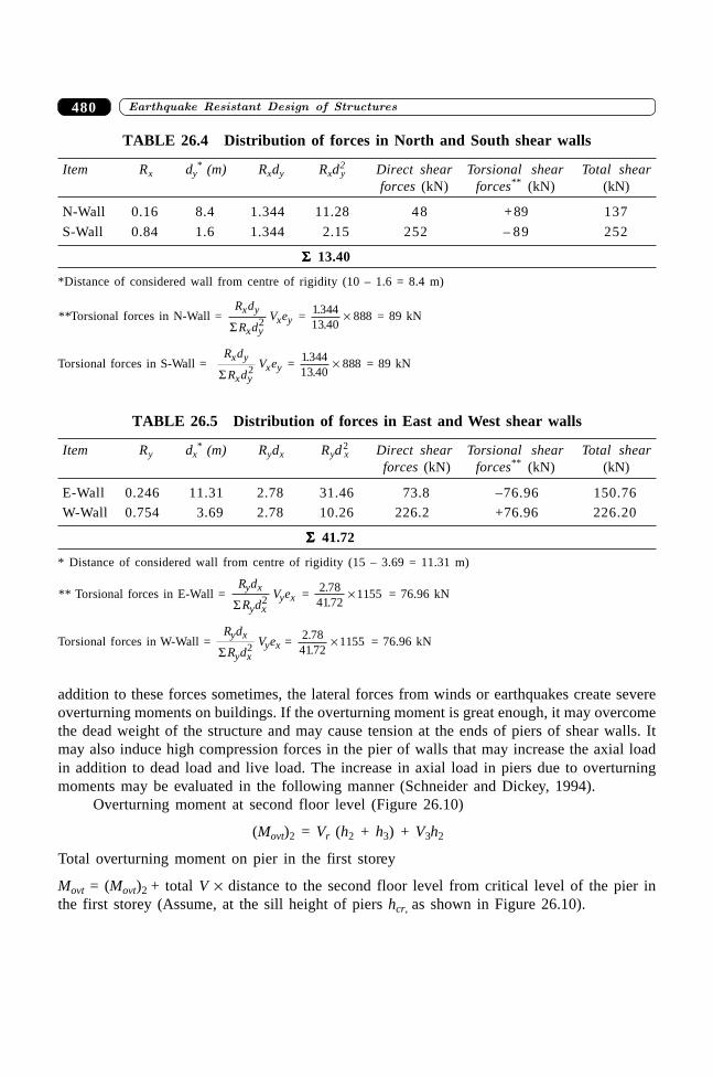
������������� � ������� ���������������� 480
addition to these forces sometimes, the lateral forces from winds or earthquakes create severeoverturning moments on buildings. If the overturning moment is great enough, it may overcomethe dead weight of the structure and may cause tension at the ends of piers of shear walls. Itmay also induce high compression forces in the pier of walls that may increase the axial loadin addition to dead load and live load. The increase in axial load in piers due to overturningmoments may be evaluated in the following manner (Schneider and Dickey, 1994).
Overturning moment at second floor level (Figure 26.10)
(Movt)2 = Vr (h2 + h3) + V3h2
Total overturning moment on pier in the first storey
Movt = (Movt)2 + total V ¥ distance to the second floor level from critical level of the pier inthe first storey (Assume, at the sill height of piers hcr, as shown in Figure 26.10).
TABLE 26.4 Distribution of forces in North and South shear walls
Item Rx dy* (m) Rxdy Rxd
2y Direct shear Torsional shear Total shear
forces (kN) forces** (kN) (kN)
N-Wall 0.16 8.4 1.344 11.28 48 +89 137
S-Wall 0.84 1.6 1.344 2.15 252 – 89 252
SSSSS 13.40
*Distance of considered wall from centre of rigidity (10 – 1.6 = 8.4 m)
**Torsional forces in N-Wall = R d
R dV e
x y
x yx y
S 2 = 1 34413 40
888..
¥ = 89 kN
Torsional forces in S-Wall = R d
R dV e
x y
x yx y
S 2 = 1 34413 40
888..
¥ = 89 kN
TABLE 26.5 Distribution of forces in East and West shear walls
Item Ry dx* (m) Rydx Ryd
2x Direct shear Torsional shear Total shear
forces (kN) forces** (kN) (kN)
E-Wall 0.246 11.31 2.78 31.46 73.8 –76.96 150.76
W-Wall 0.754 3.69 2.78 10.26 226.2 +76.96 226.20
SSSSS 41.72
* Distance of considered wall from centre of rigidity (15 – 3.69 = 11.31 m)
** Torsional forces in E-Wall = R d
R dV e
y x
y xy x
S 2 = 2 7841 72
1155..
¥ = 76.96 kN
Torsional forces in W-Wall = R d
R dV e
y x
y xy x
S 2 = 2 7841 72
1155..
¥ = 76.96 kN
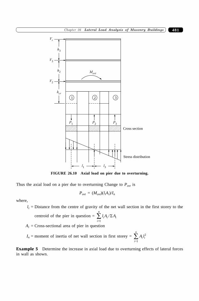
481�������� ���������������� � ������ ������������
Thus the axial load on a pier due to overturning Change to Povt is
Povt = (Movt)(liAi)/In
where,
li = Distance from the centre of gravity of the net wall section in the first storey to the
centroid of the pier in question = l A Ai i ii
n
/S=1Â
Ai = Cross-sectional area of pier in question
In = moment of inertia of net wall section in first storey = A li ii
n2
=1Â
Example 5 Determine the increase in axial load due to overturning effects of lateral forcesin wall as shown.
2 31
P1 P2 P3
l1 l3
Stress distribution
Cross section
Movt
V2
V3
Vr
h3
h2
hcr
FIGURE 26.10 Axial load on pier due to overturning.
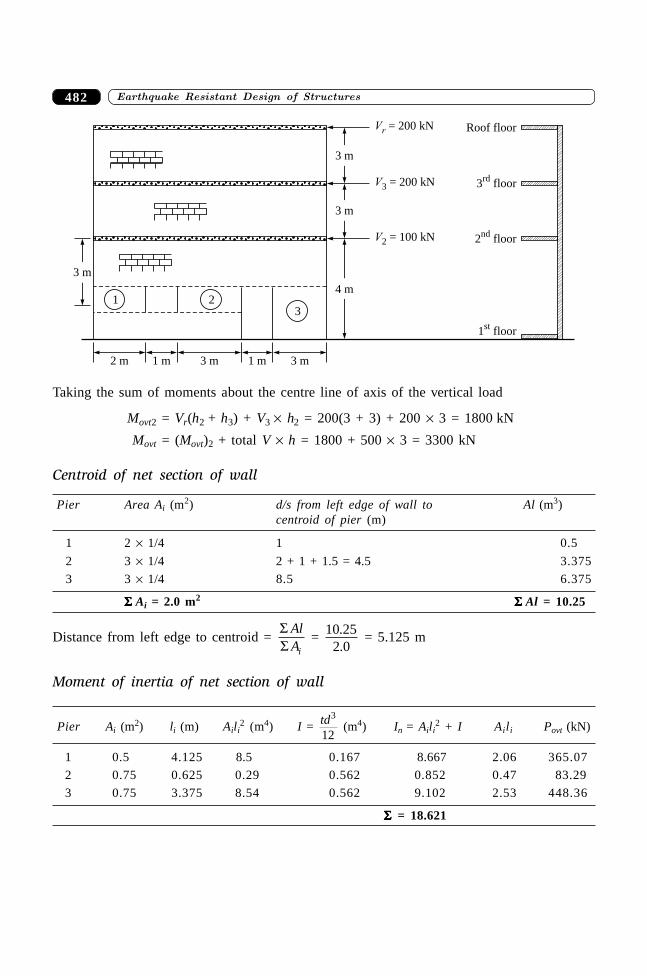
������������� � ������� ���������������� 482
Vr = 200 kN Roof floor
V3 = 200 kN
3 m
V2 = 100 kN 2 floornd
3 m
3 floorrd
1 floorst
1 2
3 m
4 m
3
2 m 1 m 3 m 3 m1 m
Taking the sum of moments about the centre line of axis of the vertical load
Movt2 = Vr(h2 + h3) + V3 ¥ h2 = 200(3 + 3) + 200 ¥ 3 = 1800 kN
Movt = (Movt)2 + total V ¥ h = 1800 + 500 ¥ 3 = 3300 kN
Centroid of net section of wall
Pier Area Ai (m2) d/s from left edge of wall to Al (m3)centroid of pier (m)
1 2 ¥ 1/4 1 0.5
2 3 ¥ 1/4 2 + 1 + 1.5 = 4.5 3.375
3 3 ¥ 1/4 8.5 6.375
SSSSS Ai = 2.0 m2 SSSSS Al = 10.25
Distance from left edge to centroid = SS
AlAi
= 10 252 0..
= 5.125 m
Moment of inertia of net section of wall
Pier Ai (m2) li (m) Aili2 (m4) I = td3
12 (m4) In = Aili
2 + I Aili Povt (kN)
1 0.5 4.125 8.5 0.167 8.667 2.06 365.07
2 0.75 0.625 0.29 0.562 0.852 0.47 83.29
3 0.75 3.375 8.54 0.562 9.102 2.53 448.36
S S S S S = 18.621
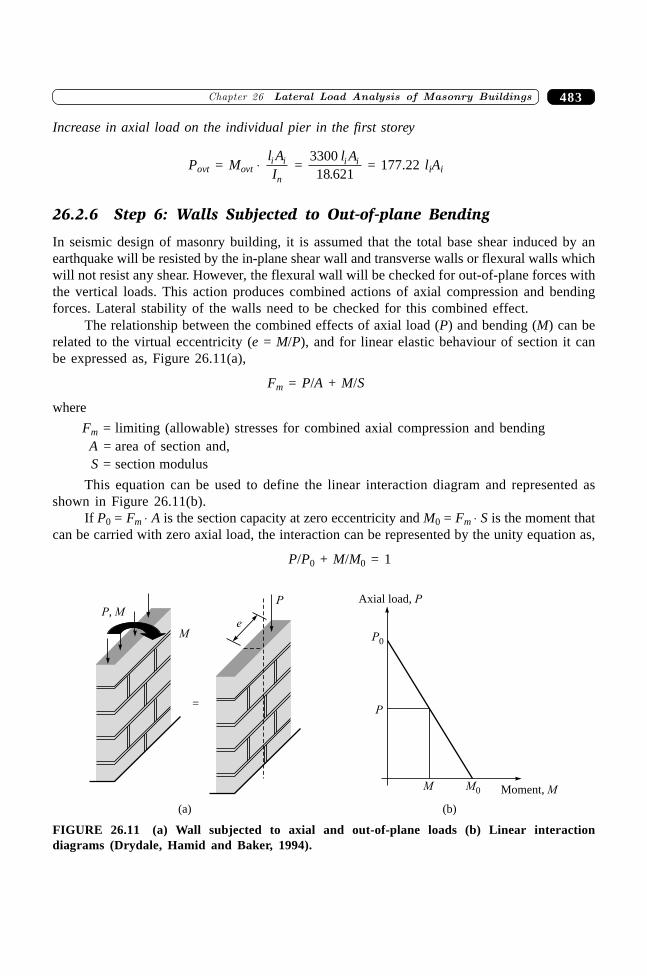
483�������� ���������������� � ������ ������������
Increase in axial load on the individual pier in the first storey
Povt = Movt ◊ l AIi i
n =
330018 621
l Ai i
. = 177.22 liAi
26.2.6 Step 6: Walls Subjected to Out-of-plane Bending
In seismic design of masonry building, it is assumed that the total base shear induced by anearthquake will be resisted by the in-plane shear wall and transverse walls or flexural walls whichwill not resist any shear. However, the flexural wall will be checked for out-of-plane forces withthe vertical loads. This action produces combined actions of axial compression and bendingforces. Lateral stability of the walls need to be checked for this combined effect.
The relationship between the combined effects of axial load (P) and bending (M) can berelated to the virtual eccentricity (e = M/P), and for linear elastic behaviour of section it canbe expressed as, Figure 26.11(a),
Fm = P/A + M/S
where
Fm = limiting (allowable) stresses for combined axial compression and bendingA = area of section and,S = section modulus
This equation can be used to define the linear interaction diagram and represented asshown in Figure 26.11(b).
If P0 = Fm ◊ A is the section capacity at zero eccentricity and M0 = Fm ◊ S is the moment thatcan be carried with zero axial load, the interaction can be represented by the unity equation as,
P/P0 + M/M0 = 1
P
eM
=
P M,
M0M Moment, M
P0
P
Axial load, P
(a) (b)
FIGURE 26.11 (a) Wall subjected to axial and out-of-plane loads (b) Linear interactiondiagrams (Drydale, Hamid and Baker, 1994).
������������� � ������� ���������������� 484
The unity equation in some of masonry codes also be present in the form of
fa/Fa + fb/Fb = 1
where,
fa, fb = compressive stresses due to applied axial load and bending, respectivelyFa, Fb = allowable axial and bending compressive stresses, respectively
Both these equations are used for describing linear behaviour of section. For masonry, theeffects of tensile cracking, non-linear stress–strain behaviour of masonry, the equation isconservative. However, the unity equation can be useful for working stress design of crackedsections, where the limiting compressive stresses under axial compression and bending are notequal. For unreinforced masonry, the allowable compressive stresses, Fa and Fb are given asfollows:
Fb = 1/3f¢m
and
Fa = 0.25 f¢m(70r/h)2 for h/r > 99
= 0.25 f¢m[1 – (h/140r)2] for h/r £ 99where,
h/r = slenderness ratio of the wall andfm = design compressive strength of masonry
Nominal allowable load carrying capacity Pn of the wall in out-of-plane is,
Pn = f ¢mbt(1/1 + 6e/t)) for 0 < e < t/6
Pn = btf ¢m34
1 2-FH IKFH
IK
et
for e > t/6
SUMMARY
Masonry buildings in India are generally designed on the basis of IS 1905. The procedure forseismic analysis and design of masonry buildings has still not received adequate attention inIndia in spite of the fact that the single-most important factor of contributing maximum damageand casualties in past earthquake is the collapse of masonry buildings. This chapter deals withstep-by-step procedure for lateral load analysis of masonry buildings. The analysis includes thedetermination of lateral loads, distribution of lateral loads in case of rigid and flexiblediaphragms, pier analysis of shear walls with torsional effects and increase of axial load in piersof shear wall due to overturning. A number of worked-out examples have been presented toillustrate the procedure properly.

485�������� ���������������� � ������ ������������
REFERENCES
[1] Amrhein, J.E., Reinforced Masonry Engineering Handbook, Masonry Institute ofAmerica, CRC Press, 1998.
[2] Drydale, R.G., Hamid, A.H., and Baker, L.R., Masonry Structure: Behaviour andDesign, Prentice Hall, Englewood Cliffs, New Jersey, 1994.
[3] Schneider, R.R. and Dickey, W.L., Reinforced Masonry Design, 3rd ed., Prentice Hall,Englewood Cliffs, New Jersey, 1994.
[4] Williams, Alan, Seismic Design of Buildings and Bridges, Oxford University Press,2003.
[5] STP 992, Masonry: Materials, Design, Construction and Maintenance, Harry A.Harris (Ed.), ASTM, Philadelphia, PA, 1988.
����������� ������� �������������486
486
Seismic Analysis andDesign of Two-storeyed
Masonry Buildings
��������
27.1 INTRODUCTION
Masonry buildings in India are generally designed for vertical loads based on IS 1905. It is notconfirmed whether the lateral load effects from wind or earthquakes have been considered inanalysis or not, particularly when the buildings are constructed in seismic prone areas. In thischapter, an example has been presented to illustrate the design procedure for low rise masonrybuildings.
27.2 BUILDING DATA
The plan and elevation of building are shown in Figure 27.1. Assume data for the building asfollows:
Material strength
Permissible compressive strength of masonry ( fm) = 2.5 N/mm2
(Assuming unit strength = 35 MPa and mortar H1 type)Permissible stresses in steel in tension = 0.55 fy(Use high strength deformed bar (Fe 415) i.e. fy = 230 N/mm2)
Live load data
Live load on roof = 1.0 kN/m2 (for seismic calculation = 0)Live load on floor = 1.0 kN/m2
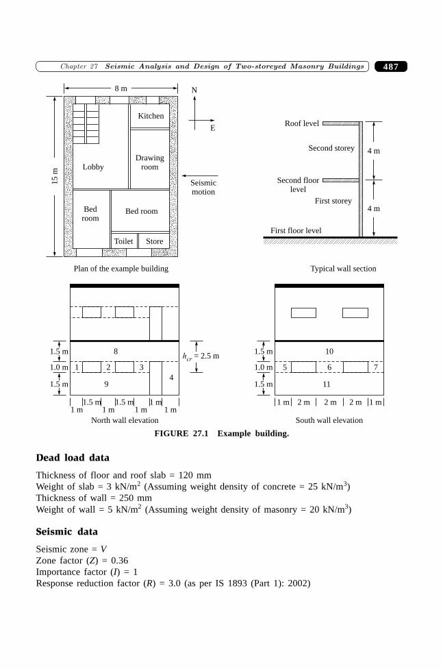
487�������� � �� ������� ������ ����������������������� �� ���
Dead load data
Thickness of floor and roof slab = 120 mmWeight of slab = 3 kN/m2 (Assuming weight density of concrete = 25 kN/m3)Thickness of wall = 250 mmWeight of wall = 5 kN/m2 (Assuming weight density of masonry = 20 kN/m3)
Seismic data
Seismic zone = VZone factor (Z) = 0.36Importance factor (I) = 1Response reduction factor (R) = 3.0 (as per IS 1893 (Part 1): 2002)
LobbyDrawing
room
Bed roomBedroom
Toilet Store
Kitchen
N
E
Seismicmotion
8 m
15
m
First floor level
Roof level
Second floorlevel
Second storey
First storey
4 m
4 m
Plan of the example building Typical wall section
1.5 m
1.5 m
1.0 m 1 2 3
49
8hcr = 2.5 m
1.5 m 1.5 m1 m
1 m1 m1 m1 m
North wall elevation
1.5 m
1.5 m
1.0 m 5 7
11
10
1 m2 m1 m
South wall elevation
2 m 2 m
6
FIGURE 27.1 Example building.
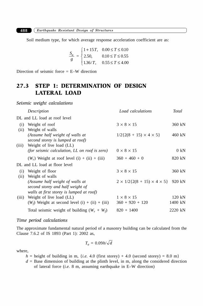
����������� ������� �������������488
Soil medium type, for which average response acceleration coefficient are as:
Sga =
1 15 0 00 010
2 50 0 10 0 55
136 0 55 4 00
+ £ ££ ££ £
RS|
T|
T T
T
T T
, . .
. , . .
. / , . .
Direction of seismic force = E–W direction
27.3 STEP 1: DETERMINATION OF DESIGNLATERAL LOAD
Seismic weight calculations
Description Load calculations Total
DL and LL load at roof level
(i) Weight of roof 3 ¥ 8 ¥ 15 360 kN(ii) Weight of walls
(Assume half weight of walls at 1/2{2(8 + 15) ¥ 4 ¥ 5} 460 kNsecond storey is lumped at roof)
(iii) Weight of live load (LL)(for seismic calculation, LL on roof is zero) 0 ¥ 8 ¥ 15 0 kN
(Wr) Weight at roof level (i) + (ii) + (iii) 360 + 460 + 0 820 kN
DL and LL load at floor level
(i) Weight of floor 3 ¥ 8 ¥ 15 360 kN(ii) Weight of walls
(Assume half weight of walls at 2 ¥ 1/2{2(8 + 15) ¥ 4 ¥ 5} 920 kNsecond storey and half weight ofwalls at first storey is lumped at roof)
(iii) Weight of live load (LL) 1 ¥ 8 ¥ 15 120 kN(Wf) Weight at second level (i) + (ii) + (iii) 360 + 920 + 120 1400 kN
Total seismic weight of building (Wr + Wf) 820 + 1400 2220 kN
Time period calculations
The approximate fundamental natural period of a masonry building can be calculated from theClause 7.6.2 of IS 1893 (Part 1): 2002 as,
Ta = 0.09h/ d
where,h = height of building in m, {i.e. 4.0 (first storey) + 4.0 (second storey) = 8.0 m}d = Base dimension of building at the plinth level, in m, along the considered direction
of lateral force (i.e. 8 m, assuming earthquake in E–W direction)
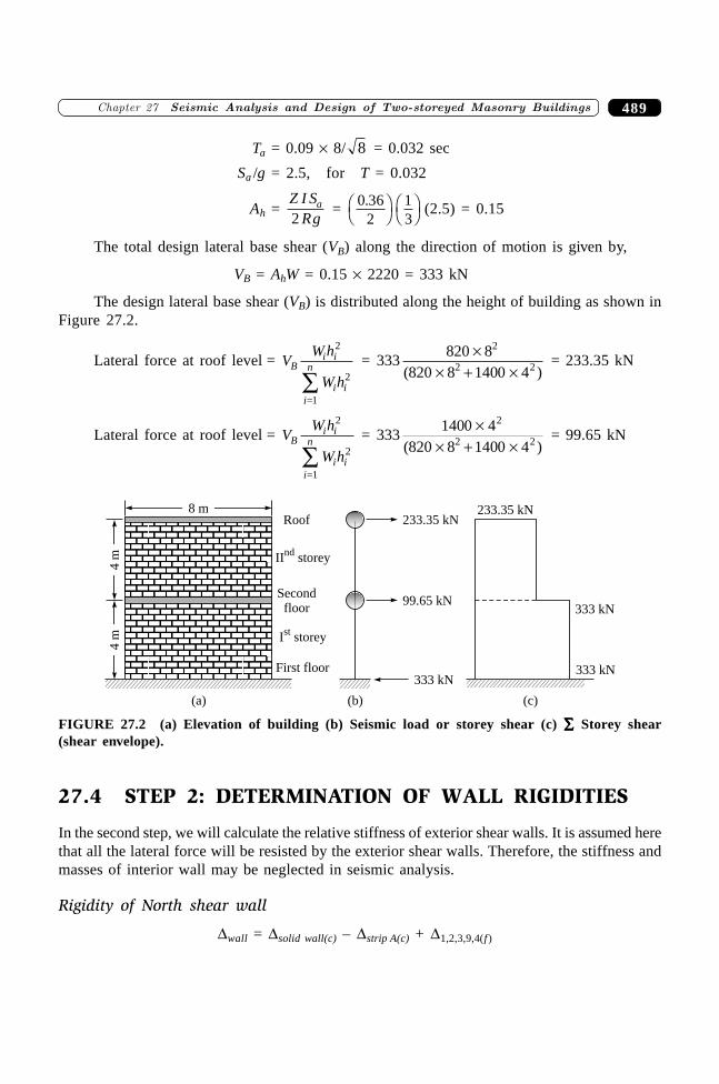
489�������� � �� ������� ������ ����������������������� �� ���
Ta = 0.09 ¥ 8/ 8 = 0.032 sec
Sa /g = 2.5, for T = 0.032
Ah = Z I S
Rga
2 = 0 36
213
.FH IK FH IK (2.5) = 0.15
The total design lateral base shear (VB) along the direction of motion is given by,
VB = AhW = 0.15 ¥ 2220 = 333 kN
The design lateral base shear (VB) is distributed along the height of building as shown inFigure 27.2.
Lateral force at roof level = VW h
W hB
i i
i ii
n
2
2
=1Â
= 333820 88 1400 4
2
2 2¥
¥ + ¥(820 ) = 233.35 kN
Lateral force at roof level = VW h
W hB
i i
i ii
n
2
2
=1Â
= 3331400 48 1400 4
2
2 2¥
¥ + ¥(820 ) = 99.65 kN
Roof8 m
Secondfloor
II storeynd
I storeyst
First floor
4m
4m
333 kN
99.65 kN
233.35 kN
333 kN
333 kN
233.35 kN
(a) (b) (c)
FIGURE 27.2 (a) Elevation of building (b) Seismic load or storey shear (c) ÂÂÂÂÂ Storey shear(shear envelope).
27.4 STEP 2: DETERMINATION OF WALL RIGIDITIES
In the second step, we will calculate the relative stiffness of exterior shear walls. It is assumed herethat all the lateral force will be resisted by the exterior shear walls. Therefore, the stiffness andmasses of interior wall may be neglected in seismic analysis.
Rigidity of North shear wall
Dwall = Dsolid wall(c) – Dstrip A(c) + D1,2,3,9,4(f )
����������� ������� �������������490
D1,2,3,9,4( f ) = 1
1 2 3 9 4R f, , , , ( )
R1,2,3,9,4( f ) = R1,2,3,9( f ) + R4( f)
R1,2,3,9( f ) = 1
1 2 3 9D , , , ( )f
D1,2,3,9( f ) = Dsolid1,2,3,9(c) – DstripB( f ) + D1,2,3( f )
D1,2,3( f ) = 1
1 2 3R R Rf f f( ) ( ) ( )+ +
Rigidity of cantilever pier is given by RC = Ethd
hd
4 33FH IK + FH IK
Rigidity of fixed pier is given by Rf = Ethd
hd
FH IK + FH IK3
3
Rsolid(c) = Et
4 48
3 48
3FH IK + FH IK = 0.5Et, Dsolid (c) = 2.0/Et
RstripA(c) = Et
4 2 58
3 2 58
3. .FH IK + FH IK = 0.944 Et
DstripA (c) = 1.06/Et
Rsolid 1,2,3,9 ( f ) = Et
4 2 56
3 2 56
3. .FH IK + FH IK = 0.756 Et
Dsolid 1,2,3,9( f ) = 1.322/Et
RstripB( f ) = Et16
3 16
3FH IK + FH IK = 1.98Et
DstripB( f ) = 0.546/Et
R1( f ) = R2( f ) = R3( f ) = Et11
3 11
3FH IK + FH IK = 0.25Et
D1,2,3( f ) = 1.33/Et
D1,2,3,9( f ) = 1.322/Et – 0.5046/Et + 1.33/Et = 2.15/Et
R1,2,3,9( f ) = Et/2.15 = 0.465Et
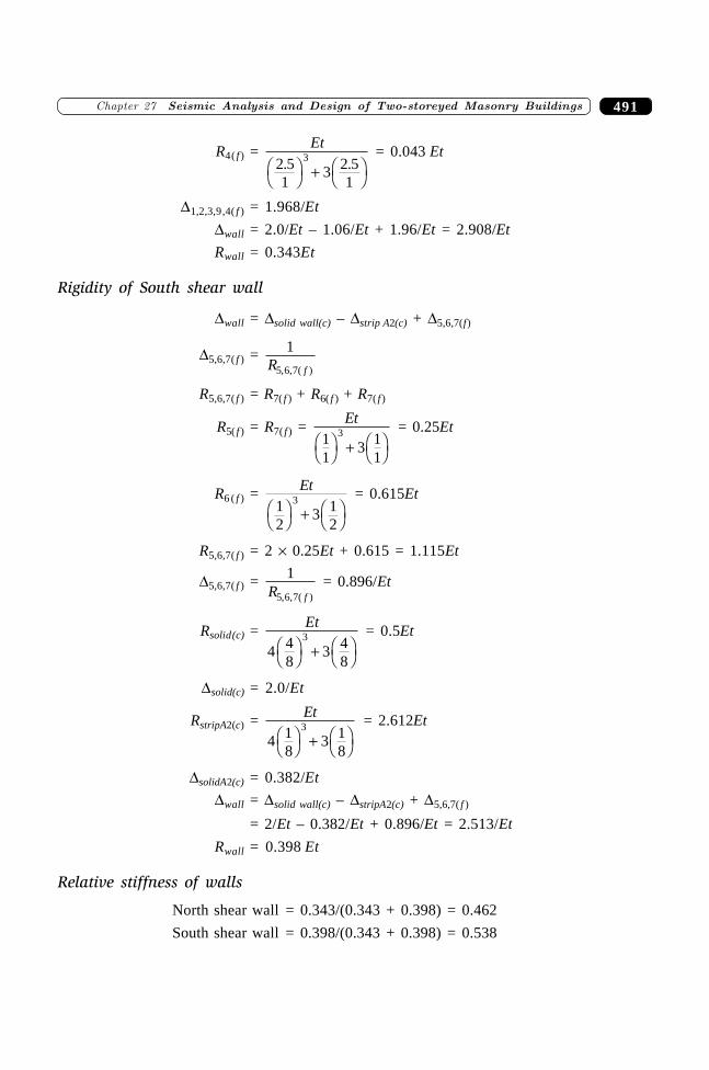
491�������� � �� ������� ������ ����������������������� �� ���
R4( f ) = Et
2 51
3 2 51
3. .FH IK + FH IK = 0.043 Et
D1,2,3,9,4( f ) = 1.968/Et
Dwall = 2.0/Et – 1.06/Et + 1.96/Et = 2.908/Et
Rwall = 0.343Et
Rigidity of South shear wall
Dwall = Dsolid wall(c) – Dstrip A2(c) + D5,6,7(f)
D5,6,7( f ) = 1
5 6 7R f, , ( )
R5,6,7( f ) = R7( f ) + R6( f ) + R7( f )
R5( f ) = R7( f ) = Et
11
3 11
3FH IK + FH IK = 0.25Et
R6 ( f ) = Et12
3 12
3FH IK + FH IK = 0.615Et
R5,6,7( f ) = 2 ¥ 0.25Et + 0.615 = 1.115Et
D5,6,7( f ) = 1
5 6 7R f, , ( ) = 0.896/Et
Rsolid(c) = Et
4 48
3 48
3FH IK + FH IK = 0.5Et
Dsolid(c) = 2.0/Et
RstripA2(c) = Et
4 18
3 18
3FH IK + FH IK = 2.612Et
DsolidA2(c) = 0.382/Et
Dwall = Dsolid wall(c) – DstripA2(c) + D5,6,7( f )
= 2/Et – 0.382/Et + 0.896/Et = 2.513/Et
Rwall = 0.398 Et
Relative stiffness of walls
North shear wall = 0.343/(0.343 + 0.398) = 0.462
South shear wall = 0.398/(0.343 + 0.398) = 0.538
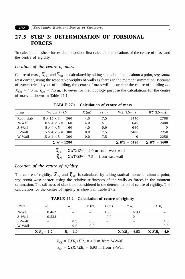
����������� ������� �������������492
27.5 STEP 3: DETERMINATION OF TORSIONALFORCES
To calculate the shear forces due to torsion, first calculate the locations of the centre of mass andthe centre of rigidity.
Location of the centre of mass
Centre of mass, XCM and YCM , is calculated by taking statical moments about a point, say, southwest corner, using the respective weights of walls as forces in the moment summation. Becauseof symmetrical layout of building, the centre of mass will occur near the centre of building i.e.XCM = 4.0 m, YCM = 7.5 m. However for methodology purpose the calculations for the centreof mass is shown in Table 27.1.
TABLE 27.1 Calculation of centre of mass
Item Weight i (kN) X (m) Y (m) WX (kN-m) WY (kN-m)
Roof slab 8 ¥ 15 ¥ 3 = 360 4.0 7.5 1440 2700N-Wall 8 ¥ 4 ¥ 5 = 160 4.0 15 640 2400S-Wall 8 ¥ 4 ¥ 5 = 160 4.0 0.0 640 0E-Wall 15 ¥ 4 ¥ 5 = 300 8.0 7.5 2400 2250W-Wall 15 ¥ 4 ¥ 5 = 300 0.0 7.5 0 2250
ÂÂÂÂÂ W = 1280 ÂÂÂÂÂ WX = 5120 ÂÂÂÂÂ WY = 9600
XCM = SWX/SW = 4.0 m from west wall
YCM = SWY/SW = 7.5 m from east wall
Location of the centre of rigidity
The centre of rigidity, XCR and YCR , is calculated by taking statical moments about a point,say, south-west corner, using the relative stiffnesses of the walls as forces in the momentsummation. The stiffness of slab is not considered in the determination of centre of rigidity. Thecalculation for the centre of rigidity is shown in Table 27.2.
TABLE 27.2 Calculation of centre of rigidity
Item Rx Ry X (m) Y (m) Y Rx X Ry
N-Wall 0.462 – – 15 6.93 –S-Wall 0.538 – – 0.0 0 –E-Wall – 0.5 8.0 – – 4.0W-Wall – 0.5 0.0 – – 0.0
ÂÂÂÂÂ Rx = 1.0 Ry = 1.0 ÂÂÂÂÂ Y.Rx = 6.93 ÂÂÂÂÂ X.Ry = 4.0
XCR = SXRy / SRy = 4.0 m from W-Wall
YCR = SYRx / SRx = 6.93 m from S-Wall
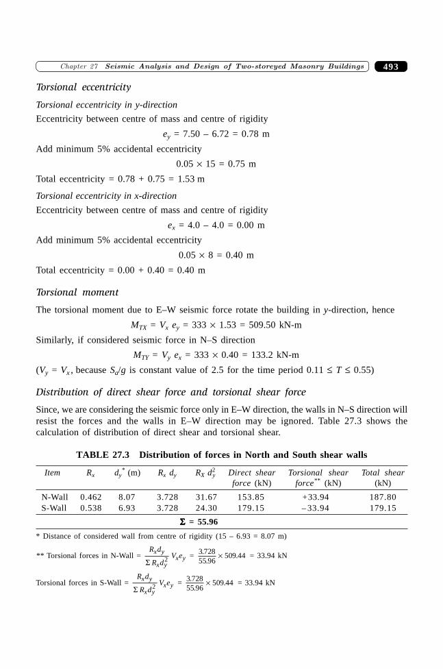
493�������� � �� ������� ������ ����������������������� �� ���
Torsional eccentricity
Torsional eccentricity in y-direction
Eccentricity between centre of mass and centre of rigidity
ey = 7.50 – 6.72 = 0.78 m
Add minimum 5% accidental eccentricity
0.05 ¥ 15 = 0.75 m
Total eccentricity = 0.78 + 0.75 = 1.53 m
Torsional eccentricity in x-direction
Eccentricity between centre of mass and centre of rigidity
ex = 4.0 – 4.0 = 0.00 m
Add minimum 5% accidental eccentricity
0.05 ¥ 8 = 0.40 m
Total eccentricity = 0.00 + 0.40 = 0.40 m
Torsional moment
The torsional moment due to E–W seismic force rotate the building in y-direction, hence
MTX = Vx ey = 333 ¥ 1.53 = 509.50 kN-m
Similarly, if considered seismic force in N–S direction
MTY = Vy ex = 333 ¥ 0.40 = 133.2 kN-m
(Vy = Vx , because Sa/g is constant value of 2.5 for the time period 0.11 £ T £ 0.55)
Distribution of direct shear force and torsional shear force
Since, we are considering the seismic force only in E–W direction, the walls in N–S direction willresist the forces and the walls in E–W direction may be ignored. Table 27.3 shows thecalculation of distribution of direct shear and torsional shear.
TABLE 27.3 Distribution of forces in North and South shear walls
Item Rx dy* (m) Rx dy RX d2
y Direct shear Torsional shear Total shearforce (kN) force** (kN) (kN)
N-Wall 0.462 8.07 3.728 31.67 153.85 +33.94 187.80S-Wall 0.538 6.93 3.728 24.30 179.15 – 33.94 179.15
SSSSS = 55.96
* Distance of considered wall from centre of rigidity (15 – 6.93 = 8.07 m)
** Torsional forces in N-Wall = R d
R dV e
x y
x yx y
S 2 = 3 72855 96
509 44..
.¥ = 33.94 kN
Torsional forces in S-Wall = R d
R dV e
x y
x yx y
S 2 = 3 72855 96
509 44..
.¥ = 33.94 kN
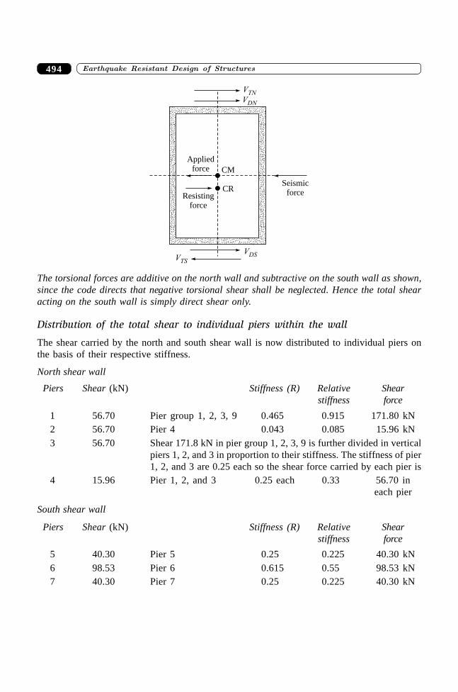
����������� ������� �������������494
VTN
VDN
VTS
VDS
CM
CR
Appliedforce
Resistingforce
Seismicforce
The torsional forces are additive on the north wall and subtractive on the south wall as shown,since the code directs that negative torsional shear shall be neglected. Hence the total shearacting on the south wall is simply direct shear only.
Distribution of the total shear to individual piers within the wall
The shear carried by the north and south shear wall is now distributed to individual piers onthe basis of their respective stiffness.
North shear wall
Piers Shear (kN) Stiffness (R) Relative Shearstiffness force
1 56.70 Pier group 1, 2, 3, 9 0.465 0.915 171.80 kN2 56.70 Pier 4 0.043 0.085 15.96 kN3 56.70 Shear 171.8 kN in pier group 1, 2, 3, 9 is further divided in vertical
piers 1, 2, and 3 in proportion to their stiffness. The stiffness of pier1, 2, and 3 are 0.25 each so the shear force carried by each pier is
4 15.96 Pier 1, 2, and 3 0.25 each 0.33 56.70 ineach pier
South shear wall
Piers Shear (kN) Stiffness (R) Relative Shearstiffness force
5 40.30 Pier 5 0.25 0.225 40.30 kN6 98.53 Pier 6 0.615 0.55 98.53 kN7 40.30 Pier 7 0.25 0.225 40.30 kN
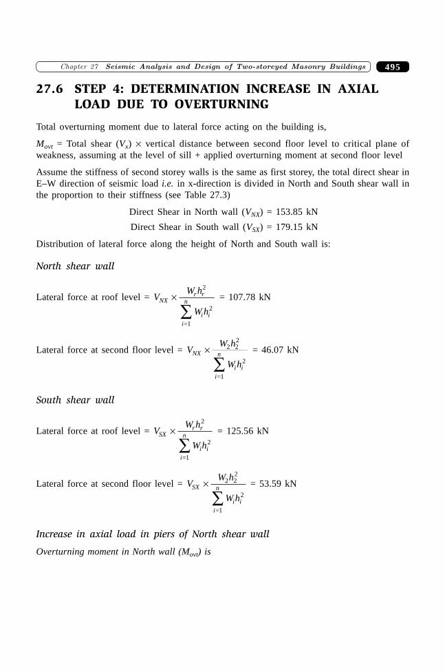
495�������� � �� ������� ������ ����������������������� �� ���
27.6 STEP 4: DETERMINATION INCREASE IN AXIALLOAD DUE TO OVERTURNING
Total overturning moment due to lateral force acting on the building is,
Movt = Total shear (Vx) ¥ vertical distance between second floor level to critical plane ofweakness, assuming at the level of sill + applied overturning moment at second floor level
Assume the stiffness of second storey walls is the same as first storey, the total direct shear inE–W direction of seismic load i.e. in x-direction is divided in North and South shear wall inthe proportion to their stiffness (see Table 27.3)
Direct Shear in North wall (VNX) = 153.85 kN
Direct Shear in South wall (VSX) = 179.15 kN
Distribution of lateral force along the height of North and South wall is:
North shear wall
Lateral force at roof level = VW h
W hNX
r r
i ii
n¥
Â
2
2
=1
= 107.78 kN
Lateral force at second floor level = VW h
W hNX
i ii
n¥
Â2 2
2
2
=1
= 46.07 kN
South shear wall
Lateral force at roof level = VW h
W hSX
r r
i ii
n¥
Â
2
2
=1
= 125.56 kN
Lateral force at second floor level = VW h
W hSX
i ii
n¥
Â2 2
2
2
=1
= 53.59 kN
Increase in axial load in piers of North shear wall
Overturning moment in North wall (Movt) is
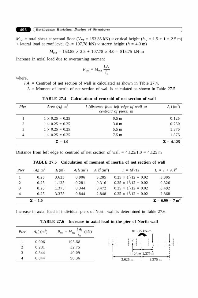
����������� ������� �������������496
Movt = total shear at second floor (VNX = 153.85 kN) ¥ critical height (hcr = 1.5 + 1 = 2.5 m)+ lateral load at roof level Qr = 107.78 kN) ¥ storey height (h = 4.0 m)
Movt = 153.85 ¥ 2.5 + 107.78 ¥ 4.0 = 815.75 kN-m
Increase in axial load due to overturning moment
Povt = Movt l AIi i
n
where,liAi = Centroid of net section of wall is calculated as shown in Table 27.4.
In = Moment of inertia of net section of wall is calculated as shown in Table 27.5.
TABLE 27.4 Calculation of centroid of net section of wall
Pier Area (Ai) m2 l (distance from left edge of wall to Ai l (m3)
centroid of piers) m
1 1 ¥ 0.25 = 0.25 0.5 m 0.125
2 1 ¥ 0.25 = 0.25 3.0 m 0.750
3 1 ¥ 0.25 = 0.25 5.5 m 1.375
4 1 ¥ 0.25 = 0.25 7.5 m 1.875
SSSSS = 1.0 SSSSS = 4.125
Distance from left edge to centroid of net section of wall = 4.125/1.0 = 4.125 m
TABLE 27.5 Calculation of moment of inertia of net section of wall
Pier (Ai) m2 Ii (m) Ai li (m3) Ai l2
i (m4) I = td3/12 In = I + Ai l2i
1 0.25 3.625 0.906 3.285 0.25 ¥ 13/12 = 0.02 3.305
2 0.25 1.125 0.281 0.316 0.25 ¥ 13/12 = 0.02 0.326
3 0.25 1.375 0.344 0.472 0.25 ¥ 13/12 = 0.02 0.492
4 0.25 3.375 0.844 2.848 0.25 ¥ 13/12 = 0.02 2.868
SSSSS = 1.0 SSSSS = 6.99 = 7 m4
Increase in axial load in individual piers of North wall is determined in Table 27.6.
TABLE 27.6 Increase in axial load in the pier of North wall
Pier Ai li (m3) Povt = Movt
l AIi i
n (kN)
1 0.906 105.58
2 0.281 32.75
3 0.344 40.09
4 0.844 98.36
1 2
3 4
3.375 m3.625 m
1.375 m1.125 m
815.75 kN-m
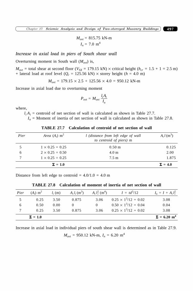
497�������� � �� ������� ������ ����������������������� �� ���
Movt = 815.75 kN-m
In = 7.0 m4
Increase in axial load in piers of South shear wall
Overturning moment in South wall (Movt) is,
Movt = total shear at second floor (VSX = 179.15 kN) ¥ critical height (hcr = 1.5 + 1 = 2.5 m)+ lateral load at roof level (Qr = 125.56 kN) ¥ storey height (h = 4.0 m)
Movt = 179.15 ¥ 2.5 + 125.56 ¥ 4.0 = 950.12 kN-m
Increase in axial load due to overturning moment
Povt = Movt l AIi i
n
where,li Ai = centroid of net section of wall is calculated as shown in Table 27.7.
In = Moment of inertia of net section of wall is calculated as shown in Table 27.8.
TABLE 27.7 Calculation of centroid of net section of wall
Pier Area (Ai) m2 l (distance from left edge of wall Ai l (m3)
to centroid of piers) m
5 1 ¥ 0.25 = 0.25 0.50 m 0.125
6 2 ¥ 0.25 = 0.50 4.0 m 2.00
7 1 ¥ 0.25 = 0.25 7.5 m 1.875
SSSSS = 1.0 SSSSS = 4.0
Distance from left edge to centroid = 4.0/1.0 = 4.0 m
TABLE 27.8 Calculation of moment of inertia of net section of wall
Pier (Ai) m2 li (m) Ai li (m3) Ai l2
i (m4) I = td3/12 In = I + Ai l2i
5 0.25 3.50 0.875 3.06 0.25 ¥ 13/12 = 0.02 3.08
6 0.50 0.00 0 0 0.50 ¥ 13/12 = 0.04 0.04
7 0.25 3.50 0.875 3.06 0.25 ¥ 13/12 = 0.02 3.08
SSSSS = 1.0 SSSSS = 6.20 m4
Increase in axial load in individual piers of south shear wall is determined as in Table 27.9.
Movt = 950.12 kN-m, In = 6.20 m4
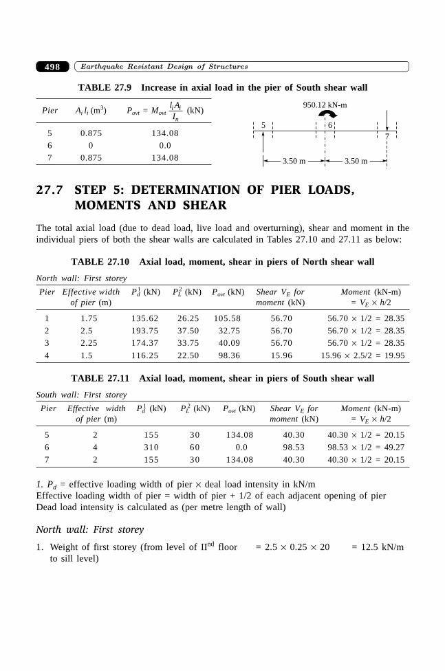
����������� ������� �������������498
TABLE 27.9 Increase in axial load in the pier of South shear wall
Pier Ai li (m3) Povt = Movt
l AIi i
n (kN)
5 0.875 134.08
6 0 0.0
7 0.875 134.08
27.7 STEP 5: DETERMINATION OF PIER LOADS,MOMENTS AND SHEAR
The total axial load (due to dead load, live load and overturning), shear and moment in theindividual piers of both the shear walls are calculated in Tables 27.10 and 27.11 as below:
TABLE 27.10 Axial load, moment, shear in piers of North shear wall
North wall: First storey
Pier Effective width Pd 1 (kN) PL 2 (kN) Povt (kN) Shear VE for Moment (kN-m)
of pier (m) moment (kN) = VE ¥ h/2
1 1.75 135.62 26.25 105.58 56.70 56.70 ¥ 1/2 = 28.35
2 2.5 193.75 37.50 32.75 56.70 56.70 ¥ 1/2 = 28.35
3 2.25 174.37 33.75 40.09 56.70 56.70 ¥ 1/2 = 28.35
4 1.5 116.25 22.50 98.36 15.96 15.96 ¥ 2.5/2 = 19.95
TABLE 27.11 Axial load, moment, shear in piers of South shear wall
South wall: First storey
Pier Effective width Pd 1 (kN) PL 2 (kN) Povt (kN) Shear VE for Moment (kN-m)
of pier (m) moment (kN) = VE ¥ h/2
5 2 155 30 134.08 40.30 40.30 ¥ 1/2 = 20.15
6 4 310 60 0.0 98.53 98.53 ¥ 1/2 = 49.27
7 2 155 30 134.08 40.30 40.30 ¥ 1/2 = 20.15
1. Pd = effective loading width of pier ¥ deal load intensity in kN/mEffective loading width of pier = width of pier + 1/2 of each adjacent opening of pierDead load intensity is calculated as (per metre length of wall)
North wall: First storey
1. Weight of first storey (from level of IInd floor = 2.5 ¥ 0.25 ¥ 20 = 12.5 kN/mto sill level)
5 6
7
950.12 kN-m
3.50 m3.50 m
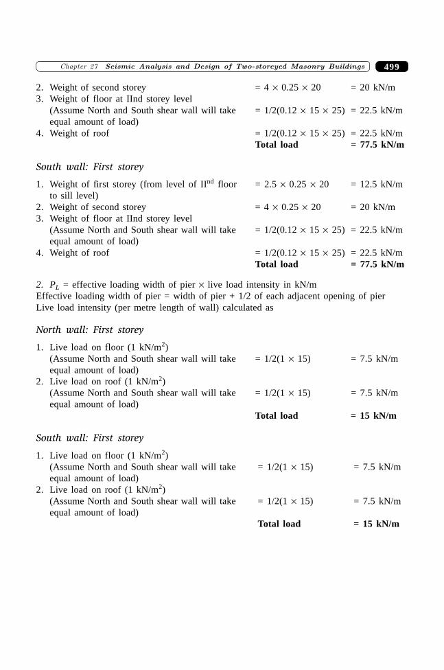
499�������� � �� ������� ������ ����������������������� �� ���
2. Weight of second storey = 4 ¥ 0.25 ¥ 20 = 20 kN/m3. Weight of floor at IInd storey level
(Assume North and South shear wall will take = 1/2(0.12 ¥ 15 ¥ 25) = 22.5 kN/mequal amount of load)
4. Weight of roof = 1/2(0.12 ¥ 15 ¥ 25) = 22.5 kN/mTotal load = 77.5 kN/m
South wall: First storey
1. Weight of first storey (from level of IInd floor = 2.5 ¥ 0.25 ¥ 20 = 12.5 kN/mto sill level)
2. Weight of second storey = 4 ¥ 0.25 ¥ 20 = 20 kN/m3. Weight of floor at IInd storey level
(Assume North and South shear wall will take = 1/2(0.12 ¥ 15 ¥ 25) = 22.5 kN/mequal amount of load)
4. Weight of roof = 1/2(0.12 ¥ 15 ¥ 25) = 22.5 kN/mTotal load = 77.5 kN/m
2. PL = effective loading width of pier ¥ live load intensity in kN/mEffective loading width of pier = width of pier + 1/2 of each adjacent opening of pierLive load intensity (per metre length of wall) calculated as
North wall: First storey
1. Live load on floor (1 kN/m2)(Assume North and South shear wall will take = 1/2(1 ¥ 15) = 7.5 kN/mequal amount of load)
2. Live load on roof (1 kN/m2)(Assume North and South shear wall will take = 1/2(1 ¥ 15) = 7.5 kN/mequal amount of load)
Total load = 15 kN/m
South wall: First storey
1. Live load on floor (1 kN/m2)(Assume North and South shear wall will take = 1/2(1 ¥ 15) = 7.5 kN/mequal amount of load)
2. Live load on roof (1 kN/m2)(Assume North and South shear wall will take = 1/2(1 ¥ 15) = 7.5 kN/mequal amount of load)
Total load = 15 kN/m
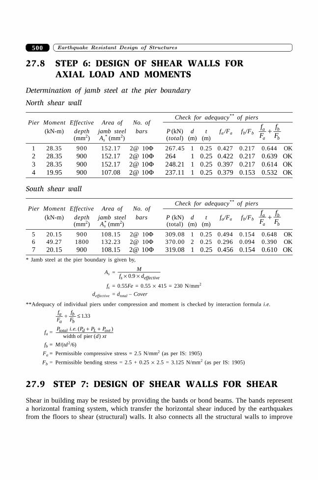
����������� ������� �������������500
27.8 STEP 6: DESIGN OF SHEAR WALLS FORAXIAL LOAD AND MOMENTS
Determination of jamb steel at the pier boundary
North shear wall
Pier Moment Effective Area of No. ofCheck for adequacy** of piers
(kN-m) depth jamb steel bars P (kN) d t fa /Fa fb/FbfF
fF
a
a
b
b+
(mm2) As*
(mm2) (total) (m) (m)
1 28.35 900 152.17 2@ 10F 267.45 1 0.25 0.427 0.217 0.644 OK2 28.35 900 152.17 2@ 10F 264 1 0.25 0.422 0.217 0.639 OK3 28.35 900 152.17 2@ 10F 248.21 1 0.25 0.397 0.217 0.614 OK4 19.95 900 107.08 2@ 10F 237.11 1 0.25 0.379 0.153 0.532 OK
South shear wall
Pier Moment Effective Area of No. ofCheck for adequacy** of piers
(kN-m) depth jamb steel bars P (kN) d t fa/Fa fb/FbfF
fF
a
a
b
b+
(mm2) As*
(mm2) (total) (m) (m)
5 20.15 900 108.15 2@ 10F 309.08 1 0.25 0.494 0.154 0.648 OK6 49.27 1800 132.23 2@ 10F 370.00 2 0.25 0.296 0.094 0.390 OK7 20.15 900 108.15 2@ 10F 319.08 1 0.25 0.456 0.154 0.610 OK
* Jamb steel at the pier boundary is given by,
As = M
f ds effective¥ ¥0 9.
fs = 0.55Fe = 0.55 ¥ 415 = 230 N/mm2
deffective = dtotal – Cover
**Adequacy of individual piers under compression and moment is checked by interaction formula i.e.
fF
fF
a
a
b
b+ £ 1 33.
fa =P i e P P P
d xttotal d L ovt. . ( )
( )+ +
width of pier
fb = M/(td2/6)
Fa = Permissible compressive stress = 2.5 N/mm2 (as per IS: 1905)
Fb = Permissible bending stress = 2.5 + 0.25 ¥ 2.5 = 3.125 N/mm2 (as per IS: 1905)
27.9 STEP 7: DESIGN OF SHEAR WALLS FOR SHEAR
Shear in building may be resisted by providing the bands or bond beams. The bands representa horizontal framing system, which transfer the horizontal shear induced by the earthquakesfrom the floors to shear (structural) walls. It also connects all the structural walls to improve
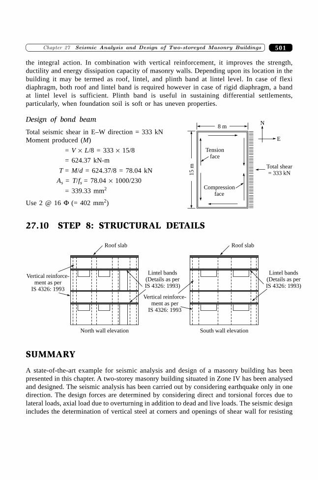
501�������� � �� ������� ������ ����������������������� �� ���
the integral action. In combination with vertical reinforcement, it improves the strength,ductility and energy dissipation capacity of masonry walls. Depending upon its location in thebuilding it may be termed as roof, lintel, and plinth band at lintel level. In case of flexidiaphragm, both roof and lintel band is required however in case of rigid diaphragm, a bandat lintel level is sufficient. Plinth band is useful in sustaining differential settlements,particularly, when foundation soil is soft or has uneven properties.
Design of bond beam
Total seismic shear in E–W direction = 333 kNMoment produced (M)
= V ¥ L/8 = 333 ¥ 15/8
= 624.37 kN-m
T = M/d = 624.37/8 = 78.04 kN
As = T/fs = 78.04 ¥ 1000/230
= 339.33 mm2
Use 2 @ 16 F (= 402 mm2)
27.10 STEP 8: STRUCTURAL DETAILS
Vertical reinforce-ment as per
IS 4326: 1993
Roof slab Roof slab
Vertical reinforce-ment as per
IS 4326: 1993
Lintel bands(Details as perIS 4326: 1993)
Lintel bands(Details as perIS 4326: 1993)
North wall elevation South wall elevation
SUMMARY
A state-of-the-art example for seismic analysis and design of a masonry building has beenpresented in this chapter. A two-storey masonry building situated in Zone IV has been analysedand designed. The seismic analysis has been carried out by considering earthquake only in onedirection. The design forces are determined by considering direct and torsional forces due tolateral loads, axial load due to overturning in addition to dead and live loads. The seismic designincludes the determination of vertical steel at corners and openings of shear wall for resisting
Compressionface
Tensionface
8 m
15
m
N
E
Total shear= 333 kN

����������� ������� �������������502
the compression and flexure forces and design of lintel band for resisting the shear forces inpiers of shear walls.
REFERENCES
[1] Amrhein, J.E., Reinforced Masonry Engineering Handbook, Masonry Institute ofAmerica, CRC Press, 1998.
[2] Drysdale, R.G., Hamid, A.H., and Baker, L.R., Masonry Structure: Behaviour andDesign, Prentice Hall, Englewood Cliffs, New Jersey, 1994.
[3] Schneider, R.R. and Dickey, W.L., Reinforced Masonry Design, 3rd ed., Prentice Hall,New Jersey, 1994.
[4] Tally, N., Design of Reinforced Masonry Structures, McGraw-Hill, 2001.[5] Tomazevic, M., Earthquake-Resistant Design of Masonry Buildings, Imperial Colleges
Press, London, 2000.[6] Williams, Alan, Seismic Design of Buildings and Bridges, Oxford University Press,
2003.
���� ���
Seismic Evaluation andRetrofitting of Reinforced
Concrete and Masonry Buildings

505
Seismic Evaluation ofReinforced Concrete
Buildings: A PracticalApproach
��������
28.1 INTRODUCTION
Most of the existing buildings, which do not fulfil the current seismic requirements, may sufferextensive damage or even collapse if shaken by a severe ground motion. The aim of evaluationis to assess the seismic capacity of earthquake vulnerable buildings or earthquake damagedbuildings for the future use. The evaluation may also prove helpful for degree of interventionrequired in seismically deficient structures. The methodologies available so far for theevaluation of existing buildings can be broadly divided into two categories: (i) qualitativemethods (ii) analytical methods. The qualitative methods are based on the backgroundinformation available of the building and its construction site, which require some or fewdocuments like architectural and structural drawings, past performance of similar buildingsunder severe earthquakes, visual inspection report, some non-destructive test results. Themethods under this category are Field Evaluation Method, Rapid Visual Screening Method,ATC-14 methodology etc. The analytical methods are based on the consideration of the capacityand ductility of buildings on the basis of available drawings. The methods in this category areCapacity/Demand (C/D) method, Screening method, Pushover analysis, Nonlinear inelasticanalysis etc. It is often seen that the drawings of buildings are generally not available due toone or more reasons. Moreover, the evaluation of the capacity and ductility of a building is alsoa cumbersome task, which is difficult for a field engineer and may not be practical in the presentIndian scenario. It is important to underline that the methods of evaluation procedure shouldbe very simple and immediate based on synthetic information that can prove suitable for riskevaluation on large populations. Therefore, qualitative evaluation of the buildings is generallybeing carried out.
����������� ������� �������������506
The aim of these methods is to direct the evaluating engineer to identify the weak linksin the structure that could precipitate the structural or component failure. Traditionally, aqualitative evaluation of a structure is conducted by a visual examination of the structurealongwith some testing of materials. Over the last decade or more, other valuable and practicalnon-destructive evaluation methods have been developed for relatively rapid inspection ofdamage and deterioration of structures. The objective of this chapter is to present a generalmethodology for evaluation of buildings based on the condition assessment, visual inspectionand some non-destructive test. This methodology should be treated as a guide to that decisionmaking process and not as the absolute method of evaluation.
28.2 COMPONENTS OF SEISMIC EVALUATIONMETHODOLOGY
The evaluation of any building is a difficult task, which requires a wide knowledge about thestructures, cause and nature of damage in structures and its components, material strength etc.The proposed methodology is divided into three components:
1. Condition Assessment based on (i) data collection or information gathering of structuresfrom architectural and structural drawings (ii) performance characteristics of similar typeof buildings in past earthquakes, (iii) rapid evaluation of strength, drift, materials, structuralcomponents and structural details. This component of methodology is primarily based onATC-14 project and is used basically for undamaged existing structures.
2. Visual Inspection/Field Evaluation based on observed distress and damage in structures.Visual inspection is more useful for damaged structures however it may also be conductedfor undamaged structures.
3. Non-Destructive Evaluation (NDE) is generally carried out for quick estimation of materialsstrength, determination of the extent of deterioration and to establish causes remain out ofreach from visual inspection and determination of reinforcement and its location. NDT mayalso be used for preparation of drawing in case of non-availability.
28.2.1 Condition Assessment for Evaluation
The aim of condition assessment of the structure is the collection of information about thestructure and its past performance characteristics to similar type of structure during pastearthquakes and the qualitative evaluation of structure for decision-making purpose. Moreinformation can be included, if necessary as per requirement.
Data collection/information gathering
Collection of the data is an important portion for the seismic evaluation of any existing building.The information required for the evaluated building can be divided as follows:
Building data
∑ architectural, structural and construction drawings

507�������� � �� �������� ����� �������������� �� ������
∑ vulnerability parameters: number of stories, year of construction, and total floor area∑ specifications, soil reports, and design calculations∑ seismicity of the site
Construction data
∑ identifications of gravity load resisting system∑ identifications of lateral load resisting system∑ maintenance, addition, alteration, or modifications in structures∑ field surveys of the structure’s existing condition
Structural data
∑ materials∑ structural concept: vertical and horizontal irregularities, torsional eccentricity, pounding,
short column and others∑ detailing concept: ductile detailing, special confinement reinforcement∑ foundations∑ non-structural elements
Past performance data
Past performance of similar type of structure during the earthquake provides considerableamount of information for the building, which is under evaluation process. Following are theareas of concerns, which are responsible for poor performance of buildings during earthquake
Materials concerns
∑ low grade on concrete∑ deterioration in concrete and reinforcement∑ high cement–sand ratio∑ corrosion in reinforcement∑ use of recycled steel as reinforcement∑ spalling of concrete by the corrosion of embedded reinforcing bars∑ corrosion related to insufficient concrete cover∑ poor concrete placement and porous concrete
Structural concerns
∑ the relatively low stiffness of the frames—excessive inter-storey drifts, damage to non-structural items
∑ pounding—column distress, possibly local collapse∑ unsymmetrical buildings (U, T, L, V) in plan—torsional effects and concentration of damage
at the junctures (i.e., re-entrant corners)∑ unsymmetrical buildings in elevation—abrupt change in lateral resistance∑ vertical strength discontinuities—concentrate damage in the “soft” stories∑ short column
����������� ������� �������������508
Detailing concerns
∑ large tie spacing in columns lack of confinement of concrete core—shear failures.∑ insufficient column lengths—concrete to spall.∑ locations of inadequate splices—brittle shear failure.∑ insufficient column strength for full moment hinge capacity—brittle shear failure.∑ lack of continuous beam reinforcement—hinge formation during load reversals.∑ inadequate reinforcing of beam column joints or location of beam bar splices at columns—
joint failures.∑ improper bent-up of longitudinal reinforcing in beams as shear reinforcement—shear failure
during load reversal∑ foundation dowels that are insufficient to develop the capacity of the column steel above—
local column distress.
Seismic evaluation data
Seismic evaluation of data will provide a general idea about the building performance duringan earthquake. The criteria of evaluation of building will depend on materials, strength andductility of structural components and detailing of reinforcement.
Materials evaluation
∑ buildings height > 3 stories, minimum grade concrete M 20, desirable M 30 to M 40particularly in columns of lower stories
∑ maximum grade of steel should be Fe 415 due to adequate ductility∑ no significant deterioration in reinforcement∑ no evidence of corrosion or spalling of concrete
Structural components
∑ evaluation of columns shear strength and drift—check for permissible limits∑ evaluation of plan irregularities—check for torsional forces and concentration of forces∑ evaluation of vertical irregularities—check for soft storey, mass or geometric discontinuities∑ evaluation of discontinuous load path—check for ground floor columns, projected cantilever
beam and ductile detailing at beam–column joints∑ evaluation of beam–column joints—check for strong column–weak beams∑ evaluation of pounding—check for drift control or building separation∑ evaluation of interaction between frame and infill—check for force distribution in frames
and overstressing of frames
Structural detailing
Flexural members
∑ limitation of sectional dimensions∑ limitation on minimum and maximum flexural reinforcement—at least two continuous
reinforced bars at top and bottom of the members
509�������� � �� �������� ����� �������������� �� ������
∑ restriction of lap splices∑ development length requirements—for longitudinal bars∑ shear reinforcement requirements—stirrup and tie hooks, tie spacing, bar splices
Columns
∑ limitation of sectional dimensions∑ longitudinal reinforcement requirement∑ transverse reinforcement requirements—stirrup and tie hooks, column tie spacing, column
bar splices∑ special confining requirements
Foundation
∑ column steel doweled into the foundation
Non-structural components
∑ cornices, parapet, and appendages are anchored∑ exterior cladding and veneer are well anchored
Note: Structural detailing in the structural member should comply with IS 13920: 1993
28.2.2 Field Evaluation/Visual Inspection Method
Visual inspection is an integral part of evaluation, and in fact, is the most widely used formof Non-Destructive Evaluation (NDE). Visual inspection can provide a wealth of informationthat may lead to positive identification of the cause of observed distress. Before performing adetailed visual inspection, the investigator must be familiar with the type of damage and its causeand be able to distinguish between recent damage and pre-existing damage, ensuring that theobserved damage may or may not prove to be dangerous for the structures. It is not always truethat the observed damage is due to earthquake; it may be due to some other reasons as well.
Procedure for visual inspection method
The procedure for visual inspection method and its limitations are described in the followingsections (FEMA 306, 1999).
Description
∑ perform a walk through visual inspection to become familiar with the structure∑ gather background documents and information on the design, construction, maintenance, and
operation of the structure∑ plan the complete investigation∑ perform a detailed visual inspection and observe type of damage—cracks spalls and
delaminations, permanent lateral displacement, and buckling or fracture of reinforcement,estimating of drift
∑ observe damage documented on sketches—interpreted to assess the behaviour duringearthquake
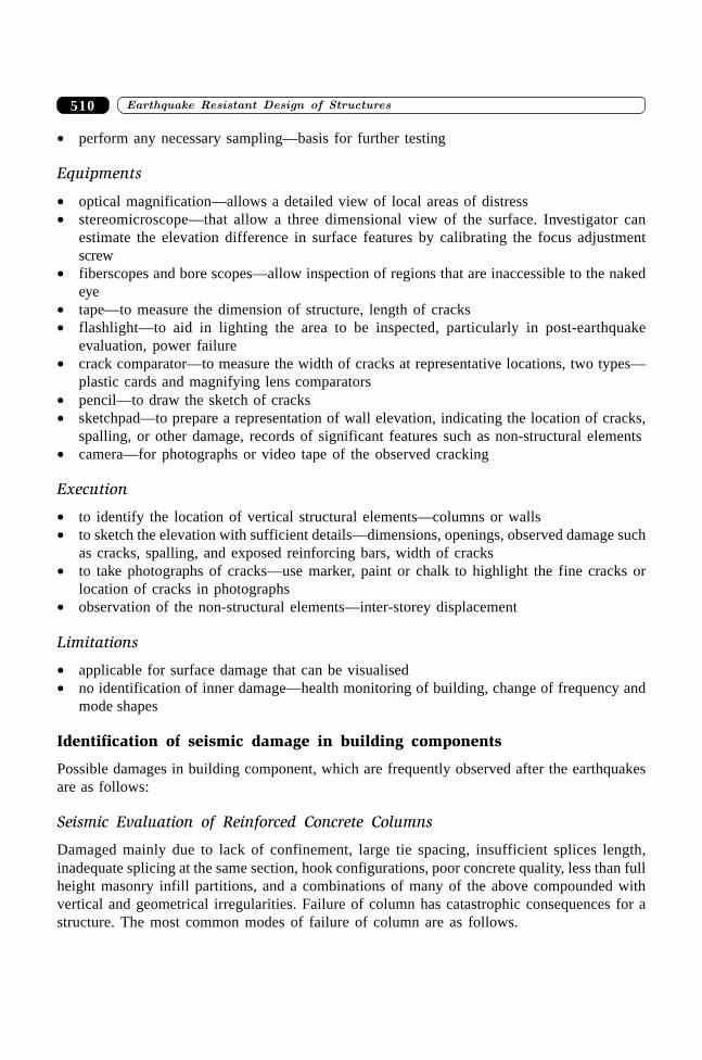
����������� ������� �������������510
∑ perform any necessary sampling—basis for further testing
Equipments
∑ optical magnification—allows a detailed view of local areas of distress∑ stereomicroscope—that allow a three dimensional view of the surface. Investigator can
estimate the elevation difference in surface features by calibrating the focus adjustmentscrew
∑ fiberscopes and bore scopes—allow inspection of regions that are inaccessible to the nakedeye
∑ tape—to measure the dimension of structure, length of cracks∑ flashlight—to aid in lighting the area to be inspected, particularly in post-earthquake
evaluation, power failure∑ crack comparator—to measure the width of cracks at representative locations, two types—
plastic cards and magnifying lens comparators∑ pencil—to draw the sketch of cracks∑ sketchpad—to prepare a representation of wall elevation, indicating the location of cracks,
spalling, or other damage, records of significant features such as non-structural elements∑ camera—for photographs or video tape of the observed cracking
Execution
∑ to identify the location of vertical structural elements—columns or walls∑ to sketch the elevation with sufficient details—dimensions, openings, observed damage such
as cracks, spalling, and exposed reinforcing bars, width of cracks∑ to take photographs of cracks—use marker, paint or chalk to highlight the fine cracks or
location of cracks in photographs∑ observation of the non-structural elements—inter-storey displacement
Limitations
∑ applicable for surface damage that can be visualised∑ no identification of inner damage—health monitoring of building, change of frequency and
mode shapes
Identification of seismic damage in building components
Possible damages in building component, which are frequently observed after the earthquakesare as follows:
Seismic Evaluation of Reinforced Concrete Columns
Damaged mainly due to lack of confinement, large tie spacing, insufficient splices length,inadequate splicing at the same section, hook configurations, poor concrete quality, less than fullheight masonry infill partitions, and a combinations of many of the above compounded withvertical and geometrical irregularities. Failure of column has catastrophic consequences for astructure. The most common modes of failure of column are as follows.

511�������� � �� �������� ����� �������������� �� ������
Mode 1: Formation of plastic hinge at the base of ground level columns
Mechanism: The column, when subjected to seismic motion, its concrete begins to disintegrateand the load carried by the concrete shifts to longitudinal reinforcement of the column. Thisadditional load causes buckling of longitudinal reinforcement. As a result the column shortensand looses its ability to carry even the gravity load (Kono and Watanabe, 2000).
Reasons: Insufficient confinement length and improper confinement in plastic hinge region dueto smaller numbers of ties.
Design Consideration: This type of damage is sensitive to the cyclic moments generated duringthe earthquake and axial load intensity. Consideration is to be paid on plastic hinge length orlength of confinement.
Mode 2: Diagonal shear cracking in mid span of columns
Mechanism: In older reinforced concrete building frames, column failures were more frequentsince the strength of beams in such constructions was kept higher than that of the columns. Thisshear failure brings forth loss of axial load carrying capacity of the column. As the axial capacitydiminishes, the gravity loads carried by the column are transferred to neighbouring elements
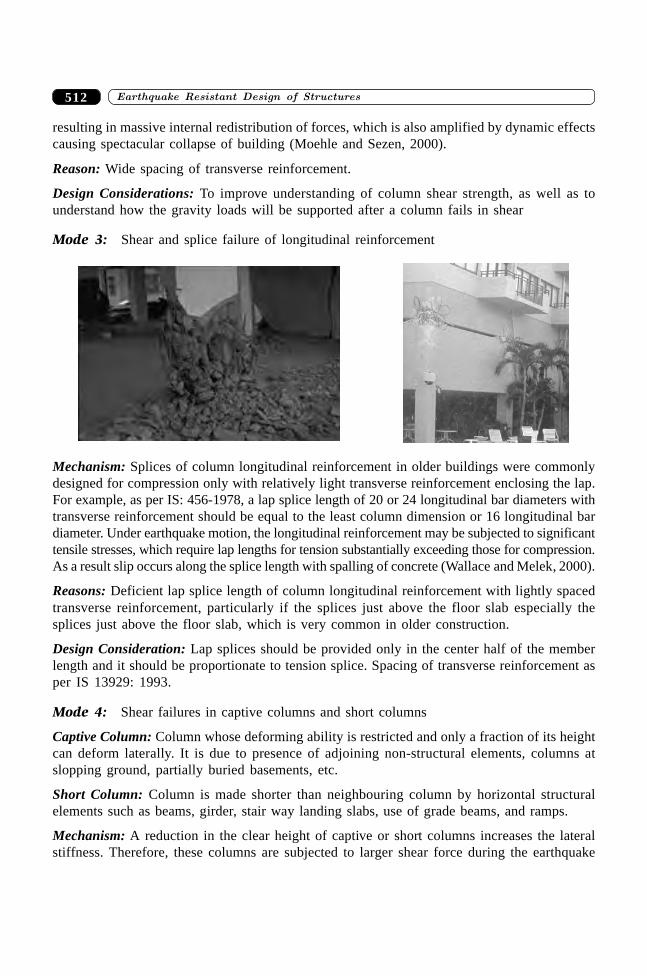
����������� ������� �������������512
resulting in massive internal redistribution of forces, which is also amplified by dynamic effectscausing spectacular collapse of building (Moehle and Sezen, 2000).
Reason: Wide spacing of transverse reinforcement.
Design Considerations: To improve understanding of column shear strength, as well as tounderstand how the gravity loads will be supported after a column fails in shear
Mode 3: Shear and splice failure of longitudinal reinforcement
Mechanism: Splices of column longitudinal reinforcement in older buildings were commonlydesigned for compression only with relatively light transverse reinforcement enclosing the lap.For example, as per IS: 456-1978, a lap splice length of 20 or 24 longitudinal bar diameters withtransverse reinforcement should be equal to the least column dimension or 16 longitudinal bardiameter. Under earthquake motion, the longitudinal reinforcement may be subjected to significanttensile stresses, which require lap lengths for tension substantially exceeding those for compression.As a result slip occurs along the splice length with spalling of concrete (Wallace and Melek, 2000).
Reasons: Deficient lap splice length of column longitudinal reinforcement with lightly spacedtransverse reinforcement, particularly if the splices just above the floor slab especially thesplices just above the floor slab, which is very common in older construction.
Design Consideration: Lap splices should be provided only in the center half of the memberlength and it should be proportionate to tension splice. Spacing of transverse reinforcement asper IS 13929: 1993.
Mode 4: Shear failures in captive columns and short columns
Captive Column: Column whose deforming ability is restricted and only a fraction of its heightcan deform laterally. It is due to presence of adjoining non-structural elements, columns atslopping ground, partially buried basements, etc.
Short Column: Column is made shorter than neighbouring column by horizontal structuralelements such as beams, girder, stair way landing slabs, use of grade beams, and ramps.
Mechanism: A reduction in the clear height of captive or short columns increases the lateralstiffness. Therefore, these columns are subjected to larger shear force during the earthquake
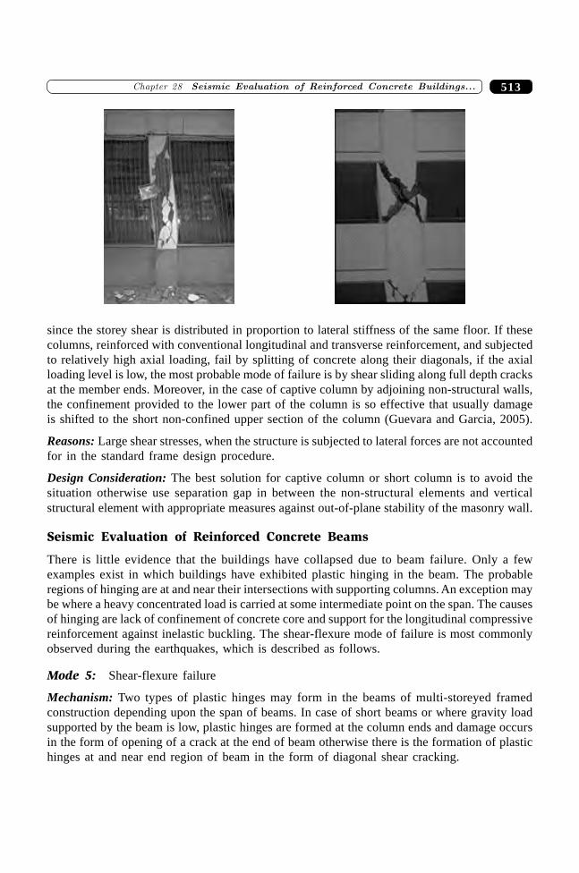
513�������� � �� �������� ����� �������������� �� ������
since the storey shear is distributed in proportion to lateral stiffness of the same floor. If thesecolumns, reinforced with conventional longitudinal and transverse reinforcement, and subjectedto relatively high axial loading, fail by splitting of concrete along their diagonals, if the axialloading level is low, the most probable mode of failure is by shear sliding along full depth cracksat the member ends. Moreover, in the case of captive column by adjoining non-structural walls,the confinement provided to the lower part of the column is so effective that usually damageis shifted to the short non-confined upper section of the column (Guevara and Garcia, 2005).
Reasons: Large shear stresses, when the structure is subjected to lateral forces are not accountedfor in the standard frame design procedure.
Design Consideration: The best solution for captive column or short column is to avoid thesituation otherwise use separation gap in between the non-structural elements and verticalstructural element with appropriate measures against out-of-plane stability of the masonry wall.
Seismic Evaluation of Reinforced Concrete Beams
There is little evidence that the buildings have collapsed due to beam failure. Only a fewexamples exist in which buildings have exhibited plastic hinging in the beam. The probableregions of hinging are at and near their intersections with supporting columns. An exception maybe where a heavy concentrated load is carried at some intermediate point on the span. The causesof hinging are lack of confinement of concrete core and support for the longitudinal compressivereinforcement against inelastic buckling. The shear-flexure mode of failure is most commonlyobserved during the earthquakes, which is described as follows.
Mode 5: Shear-flexure failure
Mechanism: Two types of plastic hinges may form in the beams of multi-storeyed framedconstruction depending upon the span of beams. In case of short beams or where gravity loadsupported by the beam is low, plastic hinges are formed at the column ends and damage occursin the form of opening of a crack at the end of beam otherwise there is the formation of plastichinges at and near end region of beam in the form of diagonal shear cracking.
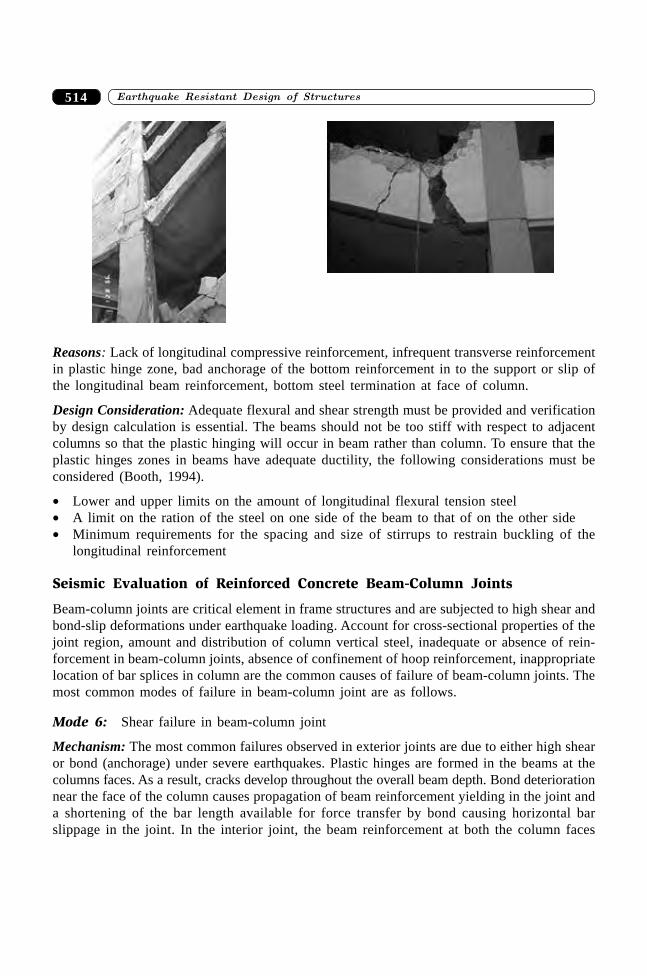
����������� ������� �������������514
Reasons: Lack of longitudinal compressive reinforcement, infrequent transverse reinforcementin plastic hinge zone, bad anchorage of the bottom reinforcement in to the support or slip ofthe longitudinal beam reinforcement, bottom steel termination at face of column.
Design Consideration: Adequate flexural and shear strength must be provided and verificationby design calculation is essential. The beams should not be too stiff with respect to adjacentcolumns so that the plastic hinging will occur in beam rather than column. To ensure that theplastic hinges zones in beams have adequate ductility, the following considerations must beconsidered (Booth, 1994).
∑ Lower and upper limits on the amount of longitudinal flexural tension steel∑ A limit on the ration of the steel on one side of the beam to that of on the other side∑ Minimum requirements for the spacing and size of stirrups to restrain buckling of the
longitudinal reinforcement
Seismic Evaluation of Reinforced Concrete Beam-Column Joints
Beam-column joints are critical element in frame structures and are subjected to high shear andbond-slip deformations under earthquake loading. Account for cross-sectional properties of thejoint region, amount and distribution of column vertical steel, inadequate or absence of rein-forcement in beam-column joints, absence of confinement of hoop reinforcement, inappropriatelocation of bar splices in column are the common causes of failure of beam-column joints. Themost common modes of failure in beam-column joint are as follows.
Mode 6: Shear failure in beam-column joint
Mechanism: The most common failures observed in exterior joints are due to either high shearor bond (anchorage) under severe earthquakes. Plastic hinges are formed in the beams at thecolumns faces. As a result, cracks develop throughout the overall beam depth. Bond deteriorationnear the face of the column causes propagation of beam reinforcement yielding in the joint anda shortening of the bar length available for force transfer by bond causing horizontal barslippage in the joint. In the interior joint, the beam reinforcement at both the column faces

515�������� � �� �������� ����� �������������� �� ������
undergoes different stress conditions (compression and tension) because of opposite sights ofseismic bending moments results in failure of joint core (UNDP, 1983).
Reasons: Inadequate anchorage of flexural steel in beams, lack of transverse reinforcement.
Design considerations
Exterior Joint: The provision on anchorage stub for the beam reinforcement improves theperformance of external joints by preventing spalling of concrete cover on the outside faceresulting in loss of flexural strength of the column. This increases diagonal strut action as wellas reduces steel congestion as the beam bars can be anchored clear of the column bars.
Interior Joint: Reliable anchorage of the beam reinforcement in the joints.
Seismic Evaluation of Reinforced Concrete Slabs
Generally slab on beams performed well during earthquakes and are not dangerous but cracks inslab creates serious aesthetic and functional problems. It reduces the available strength, stiffnessand energy dissipation capacity of building for future earthquake. In flat slab construction,punching shear is the primary cause of failure. The common modes of failure are:
Mode 7: Shear cracking in slabs
Mechanism: Damage to slab oftenly occurs due to irregularities such as large openings atconcentration of earthquake forces, close to widely spaced shear walls, at the staircase flightlandings.
Reasons: Existing micro cracks which widen due to shaking, differential settlement.
Design consideration
∑ Use secondary reinforcement in the bottom of the slab∑ Avoid the use of flat slab in high seismic zones, provided this is done in conjunction with
a stiff lateral load resisting system
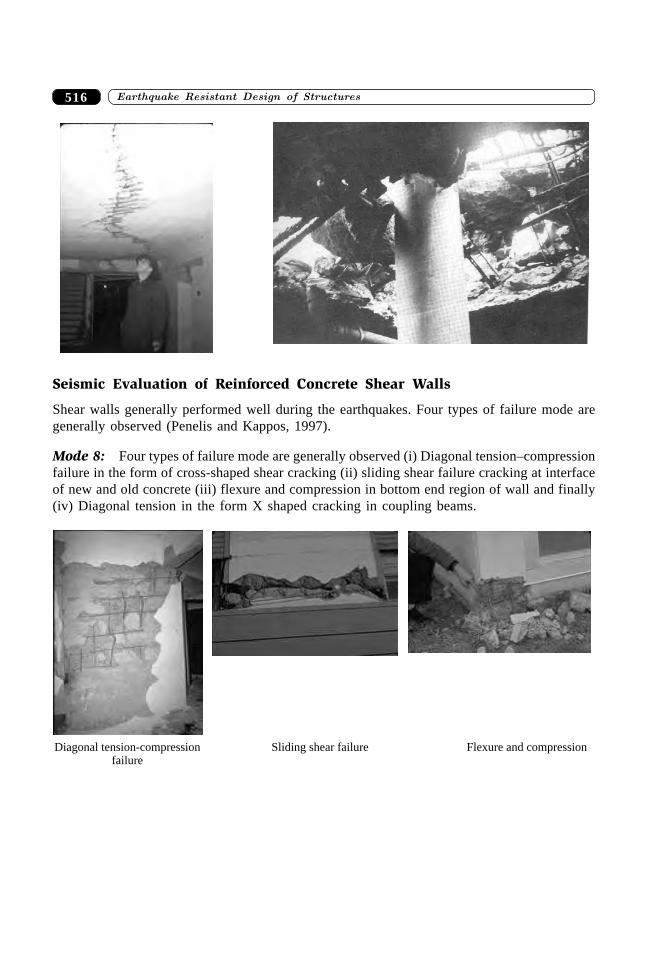
����������� ������� �������������516
Seismic Evaluation of Reinforced Concrete Shear Walls
Shear walls generally performed well during the earthquakes. Four types of failure mode aregenerally observed (Penelis and Kappos, 1997).
Mode 8: Four types of failure mode are generally observed (i) Diagonal tension–compressionfailure in the form of cross-shaped shear cracking (ii) sliding shear failure cracking at interfaceof new and old concrete (iii) flexure and compression in bottom end region of wall and finally(iv) Diagonal tension in the form X shaped cracking in coupling beams.
Diagonal tension-compressionfailure
Sliding shear failure Flexure and compression
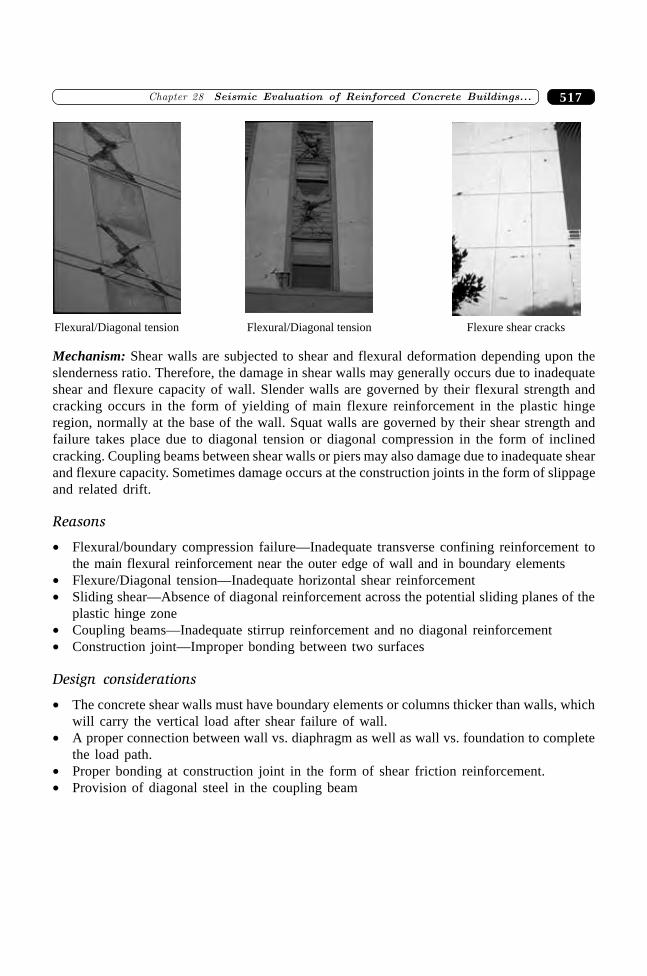
517�������� � �� �������� ����� �������������� �� ������
Mechanism: Shear walls are subjected to shear and flexural deformation depending upon theslenderness ratio. Therefore, the damage in shear walls may generally occurs due to inadequateshear and flexure capacity of wall. Slender walls are governed by their flexural strength andcracking occurs in the form of yielding of main flexure reinforcement in the plastic hingeregion, normally at the base of the wall. Squat walls are governed by their shear strength andfailure takes place due to diagonal tension or diagonal compression in the form of inclinedcracking. Coupling beams between shear walls or piers may also damage due to inadequate shearand flexure capacity. Sometimes damage occurs at the construction joints in the form of slippageand related drift.
Reasons
∑ Flexural/boundary compression failure—Inadequate transverse confining reinforcement tothe main flexural reinforcement near the outer edge of wall and in boundary elements
∑ Flexure/Diagonal tension—Inadequate horizontal shear reinforcement∑ Sliding shear—Absence of diagonal reinforcement across the potential sliding planes of the
plastic hinge zone∑ Coupling beams—Inadequate stirrup reinforcement and no diagonal reinforcement∑ Construction joint—Improper bonding between two surfaces
Design considerations
∑ The concrete shear walls must have boundary elements or columns thicker than walls, whichwill carry the vertical load after shear failure of wall.
∑ A proper connection between wall vs. diaphragm as well as wall vs. foundation to completethe load path.
∑ Proper bonding at construction joint in the form of shear friction reinforcement.∑ Provision of diagonal steel in the coupling beam
Flexural/Diagonal tension Flexural/Diagonal tension Flexure shear cracks
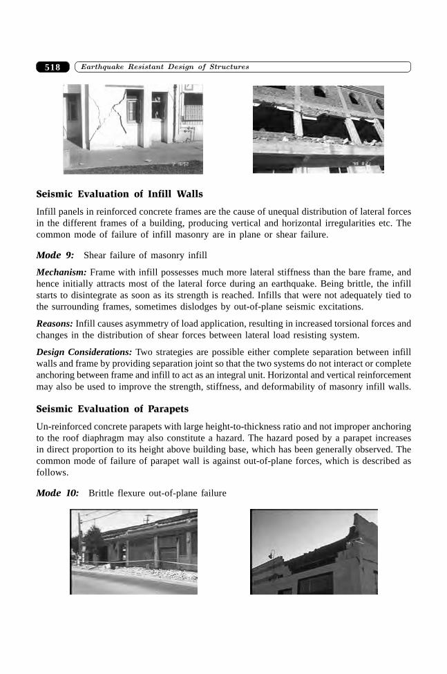
����������� ������� �������������518
Seismic Evaluation of Infill Walls
Infill panels in reinforced concrete frames are the cause of unequal distribution of lateral forcesin the different frames of a building, producing vertical and horizontal irregularities etc. Thecommon mode of failure of infill masonry are in plane or shear failure.
Mode 9: Shear failure of masonry infill
Mechanism: Frame with infill possesses much more lateral stiffness than the bare frame, andhence initially attracts most of the lateral force during an earthquake. Being brittle, the infillstarts to disintegrate as soon as its strength is reached. Infills that were not adequately tied tothe surrounding frames, sometimes dislodges by out-of-plane seismic excitations.
Reasons: Infill causes asymmetry of load application, resulting in increased torsional forces andchanges in the distribution of shear forces between lateral load resisting system.
Design Considerations: Two strategies are possible either complete separation between infillwalls and frame by providing separation joint so that the two systems do not interact or completeanchoring between frame and infill to act as an integral unit. Horizontal and vertical reinforcementmay also be used to improve the strength, stiffness, and deformability of masonry infill walls.
Seismic Evaluation of Parapets
Un-reinforced concrete parapets with large height-to-thickness ratio and not improper anchoringto the roof diaphragm may also constitute a hazard. The hazard posed by a parapet increasesin direct proportion to its height above building base, which has been generally observed. Thecommon mode of failure of parapet wall is against out-of-plane forces, which is described asfollows.
Mode 10: Brittle flexure out-of-plane failure
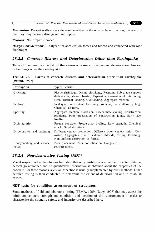
519�������� � �� �������� ����� �������������� �� ������
Mechanism: Parapet walls are acceleration sensitive in the out-of-plane direction; the result isthat they may become disengaged and topple.
Reasons: Not properly braced.
Design Considerations: Analyzed for acceleration forces and braced and connected with roofdiaphragm.
28.2.3 Concrete Distress and Deterioration Other than Earthquake
Table 28.1 summarizes the list of other causes or reasons of distress and deterioration observedin buildings other than earthquake.
TABLE 28.1 Forms of concrete distress and deterioration other than earthquake(Poston, 1997)
Description Typical causes
Cracking Plastic shrinkage, Drying shrinkage, Restraint, Sub-grade supportdeficiencies, Vapour barrier, Expansion, Corrosion of reinforcingsteel, Thermal loading, Overloading, Aggregate reaction.
Scaling Inadequate air content, Finishing problems, Freeze-thaw cycling,Chemical de-icers.
Spalling Aggregate reaction, Corrosion, Freeze-thaw cycling, Constructionproblems, Poor preparation of construction joints, Early ageloading.
Disintegration Frozen concrete, Freeze-thaw cycling, Low strength, Chemicalattack, Sulphate attack.
Discoloration and straining Different cement production, Different water–cement ratios, Cor-rosion, Aggregates, Use of calcium chloride, Curing, Finishing,Non-uniform absorption of forms.
Honeycombing and surface Poor placement, Poor consolidation, Congestedvoids reinforcement.
28.2.4 Non-destructive Testing (NDT)
Visual inspection has the obvious limitation that only visible surface can be inspected. Internaldefects go unnoticed and no quantitative information is obtained about the properties of theconcrete. For these reasons, a visual inspection is usually supplemented by NDT methods. Otherdetailed testing is then conducted to determine the extent of deterioration and to establishcauses.
NDT tests for condition assessment of structures
Some methods of field and laboratory testing (FEMA, 1999; Nawy, 1997) that may assess theminimum concrete strength and condition and location of the reinforcement in order tocharacterize the strength, safety, and integrity are described here.
����������� ������� �������������520
Rebound hammer/Swiss hammer
The rebound hammer is the most widely used non-destructive device for quick surveys to assessthe quality of concrete. In 1948, Ernest Schmidt, a Swiss engineer, developed a device for testingconcrete based upon the rebound principal strength of in-place concrete; comparison of concretestrength in different locations and provides relative difference in strength only.
Limitations
∑ not give a precise value of compressive strength, provide estimate strength for comparison∑ sensitive to the quality of concrete; carbonation increases the rebound number∑ more reproducible results from formed surface rather than finished surface; smooth hard-
towelled surface giving higher values than a rough-textured surface.∑ surface moisture and roughness also affect the reading; a dry surface results in a higher
rebound number∑ not take more than one reading at the same spot
Penetration Resistance Method—Windsor Probe Test
Penetration resistance methods are used to determine the quality and compressive strength ofin-situ concrete. It is based on the determination of the depth of penetration of probes (steel rodsor pins) into concrete by means of powder-actuated driver. This provides a measure of thehardness or penetration resistance of the material that can be related to its strength.
Limitations
∑ both probe penetration and rebound hammer test provide means of estimating the relativequality of concrete not absolute value of strength of concrete
∑ probe penetration results are more meaningful than the results of rebound hammer∑ because of greater penetration in concrete, the probe test results are influenced to a lesser
degree by surface moisture, texture, and carbonation effect∑ probe test may be the cause of minor cracking in concrete
Rebar locator/convert meter
It is used to determine quantity, location, size and condition of reinforcing steel in concrete. Itis also used for verifying the drawing and preparing as-built data, if no previous informationis available. These devices are based on interaction between the reinforcing bars and lowfrequency electromagnetic fields. Commercial covermeter can be divided into two classes: thosebased on the principal of magnetic reluctance and those based on eddy currents.
Limitations
∑ difficult to interpret at heavy congestion of reinforcement or when depth of reinforcementis too great
∑ embedded metals sometimes affect the reading∑ used to detect the reinforcing bars closest to the face
521�������� � �� �������� ����� �������������� �� ������
Ultrasonic pulse velocity
It is used for determining the elastic constants (modulus of elasticity and Poisson’s ratio) andthe density. By conducting tests at various points on a structure, lower quality concrete can beidentified by its lower pulse velocity. Pulse–velocity measurements can detect the presence ofvoids or discontinuities within a wall; however, these measurements cannot determine the depthof the voids.
Limitations
∑ Moisture content—an increase in moisture content increases the pulse velocity∑ Presence of reinforcement oriented parallel to the pulse propagation direction—the pulse
may propagate through the bars and result is an apparent pulse velocity that is higher thanthat propagating through concrete
∑ Presence of cracks and voids—increases the length of the travel path and result in a longertravel time
Impact echo
Impact echo is a method for detecting discontinuities within the thickness of a wall. An impact-echo test system is composed of three components: an impact source, a receiving transducer, anda waveform analyzer or a portable computer with a data acquisition.
Limitations
∑ accuracy of results highly dependent on the skill of the engineer and interpreting the results∑ The size, type, sensitivity, and natural frequency of the transducer, ability of FFT analyzer
also affect the results∑ Mainly used for concrete structures
Spectral Analysis of Surface Waves (SASW)
To assess the thickness and elastic stiffness of material, size and location of discontinuities withinthe wall such as voids, large cracks, and delimitations.
Limitations
∑ interpretation of results is very complex∑ mainly used on slab and other horizontal surface, to determine the stiffness profiles of soil
sites and of flexible and rigid pavement systems, measuring the changes in elastic propertiesof concrete slab
Penetrating radar
It is used to detect the location of reinforcing bars, cracks, voids or other material discontinuities,verify thickness of concrete.
Limitations
∑ mainly used for detecting subsurface condition of slab-on-grade∑ not useful for detecting the small differences in materials
����������� ������� �������������522
∑ not useful for detecting the size of bars, closely spaced bars make difficult to detect featuresbelow the layer of reinforcing steel
SUMMARY
There are many buildings that have primary structural system, which do not meet the currentseismic requirements and suffer extensive damage during the earthquake. The methods forseismic evaluation of existing seismically deficient or earthquake-damaged buildings are not yetfully developed. The present chapter deals with the practical methodology for seismic evaluationof existing buildings or earthquake damaged buildings on the basis of three-tier system whichare condition assessment, field inspection report and non-destructive testing. Each system isindependent in itself and evaluation process can be stopped at any stage depending upon theobjective of evaluation process.
REFERENCES
[1] ATC, “Evaluating the Seismic Resistance of Existing Buildings”, ATC-14 Project,Applied Technology Council, California, 1987.
[2] Booth, E., Concrete Structures in Earthquake Regions, Longman Scientific andTechnical, Longman Group UK Limited, 1994.
[3] Carino, N.J., “Non-destructive Test Method”, Concrete Construction EngineeringHandbook, Edward G. Nawy, CRC Press, New York, 1997.
[4] FEMA-306, “Evaluation of Earthquake Damaged Concrete and Masonry WallBuildings”, ATC-43 Project, Applied Technology Council, California, 1999.
[5] Guevara, L.T. and Garcia, L.E., “The Captive and Short Column Effect”, EarthquakeSpectra, 21(1), 141-160, 2005
[6] IS: 13935, Ductile Detailing of Reinforced Concrete Structures Subjected to SeismicForces, Bureau of Indian Standards, New Delhi, 1993.
[7] Kono, S. and Watanabe, F., “Damage Evaluation of Reinforced Concrete Columnsunder Multi-axial Cyclic Loadings”, The Second US–Japan Workshop on PerformanceBased Earthquake Engineering Methodology for Reinforced Concrete BuildingStructures, PEER 2000/10, 2000.
[8] Malhotra, V.M. and Carino, N.J., Handbook on Non-destructive Testing of Concrete, CRCPress, 1991.
[9] Moehle, J.P., Wood, K.J. and Sezen, “Shear Failure and Axial Load Collapse of ExistingReinforced Concrete Columns”, The Second US–Japan Workshop on PerformanceBased Earthquake Engineering Methodology for Reinforced Concrete BuildingStructures, PEER 2000/10, 2000.
[10] Nawy, Edward G., Concrete Construction Engineering Handbook, CRC Press,New York, 1997.
[11] Poston, W.R., “Structural Concrete Repair: General Principles and a Case Study(ch. 19)”, Concrete Construction Engineering Handbook, Edward G. Nawy (Ed.-in-Chief), Chapter 19, CRC Press, New York, 1997.

523�������� � �� �������� ����� �������������� �� ������
[12] Smith, B.S. and Carter, C., “Hypothesis for shear Failure of Brickwork”, Journalof the Structural Divsion, Proceedings of the American Society of Civil Engineers,April, 1971.
[13] UNDP/UNIDO Project RER/79/015, “Repair and Strengthening of Reinforced Concrete,Stone and Brick Masonry Buildings”, Building Construction Under Seismic Conditionsin the Balkan Regions, Vol. 5., United Nations Industrial Development Programme,Austria, 1983.
[14] UNDP/UNIDO Project RER/79/015, “Repair and Strengthening of ReinforcedConcrete, Stone and Brick Masonry Buildings”, Building Construction Under SeismicConditions in the Balkan Regions, Vol. 5, United Nations Industrial DevelopmentProgramme, Austria, 1983.
[15] Wallace, J.W. and Melek, M., “Column Splies: Observed Earthquake Damage,Modeling Approaches, and the PEER/UCLA Research Program”, The Second US–Japan Workshop on Performance Based Earthquake Engineering Methodology forReinforced Concrete Building Structures, PEER 2000/10, 2000.
����������� ������� �������������524
524
Seismic RetrofittingStrategies of Reinforced
Concrete Buildings
��������
29.1 INTRODUCTION
The aftermath of an earthquake manifests great devastation due to unpredicted seismic motionstriking extensive damage to innumerable buildings of varying degree i.e. either full or partialor slight. This damage to structures in its turn causes irreparable loss of life with a large numberof casualties. As a result frightened occupants may refuse to enter the building unless assuredof the safety of the building from future earthquakes. It has been observed that majority of suchearthquake damaged buildings may be safely reused, if they are converted into seismicallyresistant structures by employing a few retrofitting measures. This proves to be a better optioncatering to the economic considerations and immediate shelter problems rather than replacementof buildings. Moreover it has often been seen that retrofitting of buildings is generally moreeconomical as compared to demolition and reconstruction even in the case of severe structuraldamage. Therefore, seismic retrofitting of building structures is one of the most importantaspects for mitigating seismic hazards especially in earthquake-prone countries. Various termsare associated to retrofitting with a marginal difference like repair, strengthening, retrofitting,remoulding, rehabilitation, reconstruction etc. but there is no consensus on them. The mostcommon definition of these terms may be summarized in Table 29.1.
The need of seismic retrofitting of buildings arises under two circumstances: (i) earthquake-damaged buildings and (ii) earthquake-vulnerable buildings that have not yet experienced severeearthquakes. The problems faced by a structural engineer in retrofitting earthquake damagedbuildings are: (a) lack of standards for methods of retrofitting; (b) effectiveness of retrofittingtechniques since there is a considerable dearth of experience and data on retrofitted structures;(c) absence of consensus on appropriate methods for the wide range of parameters like type ofstructures, condition of materials, type of damage, amount of damage, location of damage,significance of damage, condition under which a damaged element can be retrofitted etc.Therefore, a catalogue of available options regarding feasible and practical retrofitting method
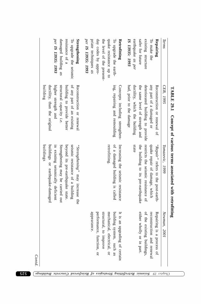
525 ��������� �� ������ �� �������� ���� �������������� �� ���T
AB
LE
29.1C
oncept of various terms associated w
ith retrofitting
Terms
CE
B, 1995
Tomazevic,
1999N
ewm
an, 2001
Rep
airing
Reconstruction or renew
al of“R
epair” refers to the post-earth-
Repairing is a process of
To make the
any part of a damaged or
quake repair of damage, w
hichreconstruction
and renew
al
existing structure
deteriorated building
to provide
restricts the seismic resistance of
of the existing buildings,
safer for futurethe sam
e level of strength andthe building to its pre-earthquake
either wholly or in part.
earthquake as perductility,
which
the building
state
IS 13935: 1993
had, prior to the damage
Retrofitting
Concepts
including strengthen-
Increasing the seismic resistance
It is an upgrading of certain
To upgrade the earth-ing, repairing and rem
ouldingof a dam
aged building is calledbuilding system
, such as
quake resistance up toretrofitting.
mechanical, electrical, or
the level of the present-structural, to im
prove
day codes by appro-perform
ance, function, or
priate techniques asappearance.
per IS 13935: 1993
Stren
gthen
ing
Reconstruction
or renew
al“
Strengthening”
may
increase the
To upgrade the seismic
of any part of an existingseism
ic resistance of a building
resistance of abuilding to provide better
beyond its pre-earthquake state.
damaged
building as
structural capacity i.e.S
trengthening may be carried out
per IS 13935: 1993
higher strength andin existing seism
ically deficient
ductility, than the originalbuildings
or earthquake-dam
aged
bu
ildin
gb
uild
ing
s
Co
ntd
.
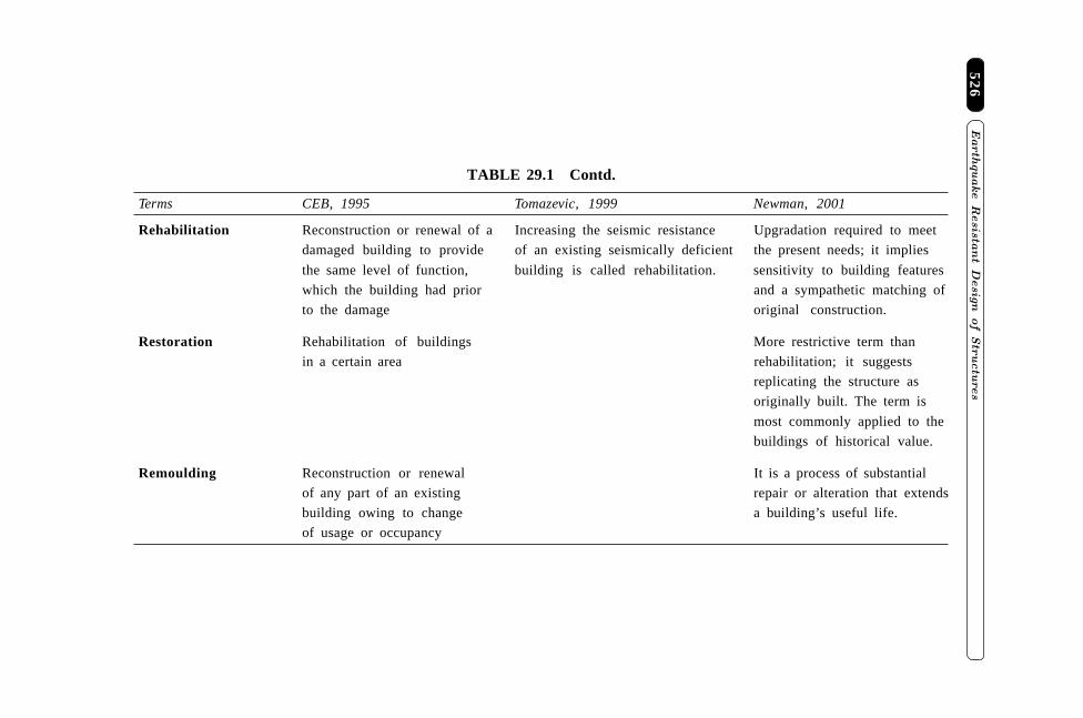
�����
������ �
����
�� �
���
���
����
��
526
Rehabilitation Reconstruction or renewal of a Increasing the seismic resistance Upgradation required to meet
damaged building to provide of an existing seismically deficient the present needs; it implies
the same level of function, building is called rehabilitation. sensitivity to building features
which the building had prior and a sympathetic matching of
to the damage original construction.
Restoration Rehabilitation of buildings More restrictive term than
in a certain area rehabilitation; it suggests
replicating the structure as
originally built. The term is
most commonly applied to the
buildings of historical value.
Remoulding Reconstruction or renewal It is a process of substantial
of any part of an existing repair or alteration that extends
building owing to change a building’s useful life.
of usage or occupancy
TABLE 29.1 Contd.
Terms CEB, 1995 Tomazevic, 1999 Newman, 2001
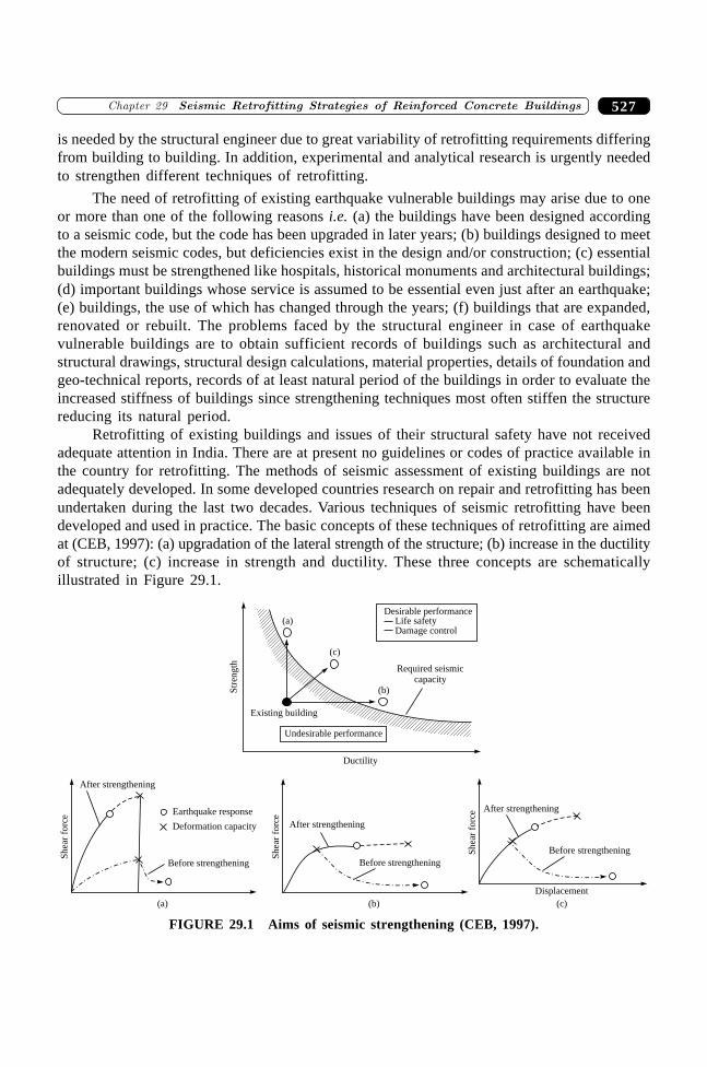
527�������� � �� ������ �� �������� ���� �������������� �� ���
is needed by the structural engineer due to great variability of retrofitting requirements differingfrom building to building. In addition, experimental and analytical research is urgently neededto strengthen different techniques of retrofitting.
The need of retrofitting of existing earthquake vulnerable buildings may arise due to oneor more than one of the following reasons i.e. (a) the buildings have been designed accordingto a seismic code, but the code has been upgraded in later years; (b) buildings designed to meetthe modern seismic codes, but deficiencies exist in the design and/or construction; (c) essentialbuildings must be strengthened like hospitals, historical monuments and architectural buildings;(d) important buildings whose service is assumed to be essential even just after an earthquake;(e) buildings, the use of which has changed through the years; (f) buildings that are expanded,renovated or rebuilt. The problems faced by the structural engineer in case of earthquakevulnerable buildings are to obtain sufficient records of buildings such as architectural andstructural drawings, structural design calculations, material properties, details of foundation andgeo-technical reports, records of at least natural period of the buildings in order to evaluate theincreased stiffness of buildings since strengthening techniques most often stiffen the structurereducing its natural period.
Retrofitting of existing buildings and issues of their structural safety have not receivedadequate attention in India. There are at present no guidelines or codes of practice available inthe country for retrofitting. The methods of seismic assessment of existing buildings are notadequately developed. In some developed countries research on repair and retrofitting has beenundertaken during the last two decades. Various techniques of seismic retrofitting have beendeveloped and used in practice. The basic concepts of these techniques of retrofitting are aimedat (CEB, 1997): (a) upgradation of the lateral strength of the structure; (b) increase in the ductilityof structure; (c) increase in strength and ductility. These three concepts are schematicallyillustrated in Figure 29.1.
Desirable performanceLife safetyDamage control
(a)
(c)
(b)Str
ength
Existing building
Undesirable performance
Required seismiccapacity
Ductility
After strengthening
Sh
ear
forc
e
Earthquake response
Deformation capacity
Before strengthening
(a)
Sh
ear
forc
e
(b)
Before strengthening
After strengthening
Sh
ear
forc
e
(c)
Before strengthening
After strengthening
Displacement
FIGURE 29.1 Aims of seismic strengthening (CEB, 1997).
����������� ������� �������������528
The decision to repair and strengthen a structure depends not only on technical consider-ations as mentioned above but also on a cost/benefit analysis of the different possible alterna-tives. It is suggested that the cost of retrofitting of a structure should remain below 25% of thereplacement as major justification of retrofitting (Nateghi and Shahbazian, 1992). The presentchapter will discuss different aspects of retrofitting scheme and their limitations, side effectsas well as cost considerations. The information in this chapter is gathered from the availableliterature and is based on the experiences of individual authors and their studies.
29.2 CONSIDERATION IN RETROFITTING OFSTRUCTURES
The method of retrofitting principally depends on the horizontal and vertical load resistingsystem of the structure and the type of materials used for parent construction. It also relies onthe technology that is feasible and economical. The understanding of mode of failure, structuralbehaviour and weak and strong design aspects as derived from the earthquake damage surveysexercise considerable influence on selection of retrofitting methods of buildings. Usually theretrofitting method is aimed at increasing the lateral resistance of the structure. The lateralresistance includes the lateral strength or stiffness and lateral displacement or ductility of thestructures. The lateral resistance is often provided through modification or addition ofretrofitting elements of an existing structure in certain areas only. The remaining elements inthe structure are usually not strengthened and are assumed to carry vertical load only, but in anearthquake, all components at each floor, retrofitted or not, will undergo essentially the samelateral displacements. While modified or added elements can be designed to sustain these lateraldeformations, the remaining non-strengthened elements could still suffer substantial damageunless lateral drifts are controlled. Therefore, caution must be taken to avoid an irregularstiffness distribution in the strengthened structure. Thus the ability to predict initial and finalstiffness of the retrofitted structure need clarification and quantification. Consequently, it issuggested that the design of retrofitted schemes should be based on drift control rather than onstrength consideration alone. The use of three-dimensional analysis is recommended to identifyand locate the potential weakness of the retrofitted building.
29.3 SOURCE OF WEAKNESS IN RC FRAME BUILDING
Earthquake engineering is not a pure science; rather it has been developed through theobservation of failure of structure during earthquake (Otani, 2004). Damage survey reports ofpast earthquakes reveal the following main sources of weakness in reinforced concrete momentresisting frame buildings.
(i) discontinuous load path/interrupted load path/irregular load path(ii) lack of deformation compatibility of structural members
(iii) quality of workmanship and poor quality of materials
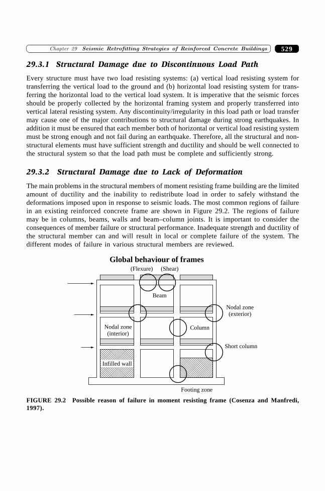
529�������� � �� ������ �� �������� ���� �������������� �� ���
29.3.1 Structural Damage due to Discontinuous Load Path
Every structure must have two load resisting systems: (a) vertical load resisting system fortransferring the vertical load to the ground and (b) horizontal load resisting system for trans-ferring the horizontal load to the vertical load system. It is imperative that the seismic forcesshould be properly collected by the horizontal framing system and properly transferred intovertical lateral resisting system. Any discontinuity/irregularity in this load path or load transfermay cause one of the major contributions to structural damage during strong earthquakes. Inaddition it must be ensured that each member both of horizontal or vertical load resisting systemmust be strong enough and not fail during an earthquake. Therefore, all the structural and non-structural elements must have sufficient strength and ductility and should be well connected tothe structural system so that the load path must be complete and sufficiently strong.
29.3.2 Structural Damage due to Lack of Deformation
The main problems in the structural members of moment resisting frame building are the limitedamount of ductility and the inability to redistribute load in order to safely withstand thedeformations imposed upon in response to seismic loads. The most common regions of failurein an existing reinforced concrete frame are shown in Figure 29.2. The regions of failuremay be in columns, beams, walls and beam–column joints. It is important to consider theconsequences of member failure or structural performance. Inadequate strength and ductility ofthe structural member can and will result in local or complete failure of the system. Thedifferent modes of failure in various structural members are reviewed.
Footing zone
Short column
Nodal zone(exterior)
(Flexure) (Shear)
Global behaviour of frames
Column
Beam
Nodal zone(interior)
Infilled wall
FIGURE 29.2 Possible reason of failure in moment resisting frame (Cosenza and Manfredi,1997).
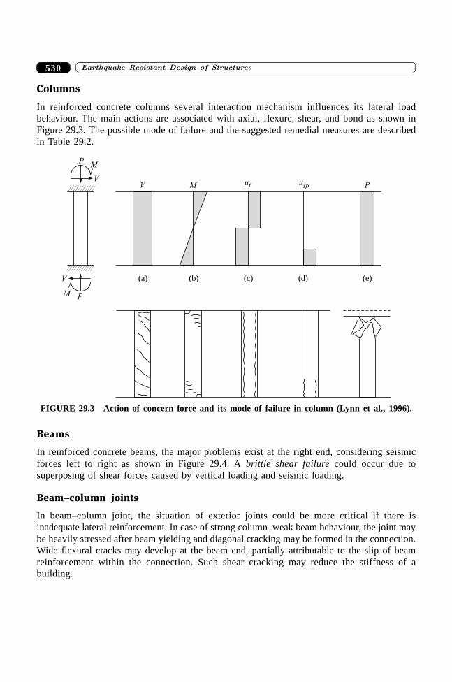
����������� ������� �������������530
Columns
In reinforced concrete columns several interaction mechanism influences its lateral loadbehaviour. The main actions are associated with axial, flexure, shear, and bond as shown inFigure 29.3. The possible mode of failure and the suggested remedial measures are describedin Table 29.2.
V
M P
V
MP
V M uf usp P
(a) (b) (c) (d) (e)
FIGURE 29.3 Action of concern force and its mode of failure in column (Lynn et al., 1996).
Beams
In reinforced concrete beams, the major problems exist at the right end, considering seismicforces left to right as shown in Figure 29.4. A brittle shear failure could occur due tosuperposing of shear forces caused by vertical loading and seismic loading.
Beam–column joints
In beam–column joint, the situation of exterior joints could be more critical if there isinadequate lateral reinforcement. In case of strong column–weak beam behaviour, the joint maybe heavily stressed after beam yielding and diagonal cracking may be formed in the connection.Wide flexural cracks may develop at the beam end, partially attributable to the slip of beamreinforcement within the connection. Such shear cracking may reduce the stiffness of abuilding.
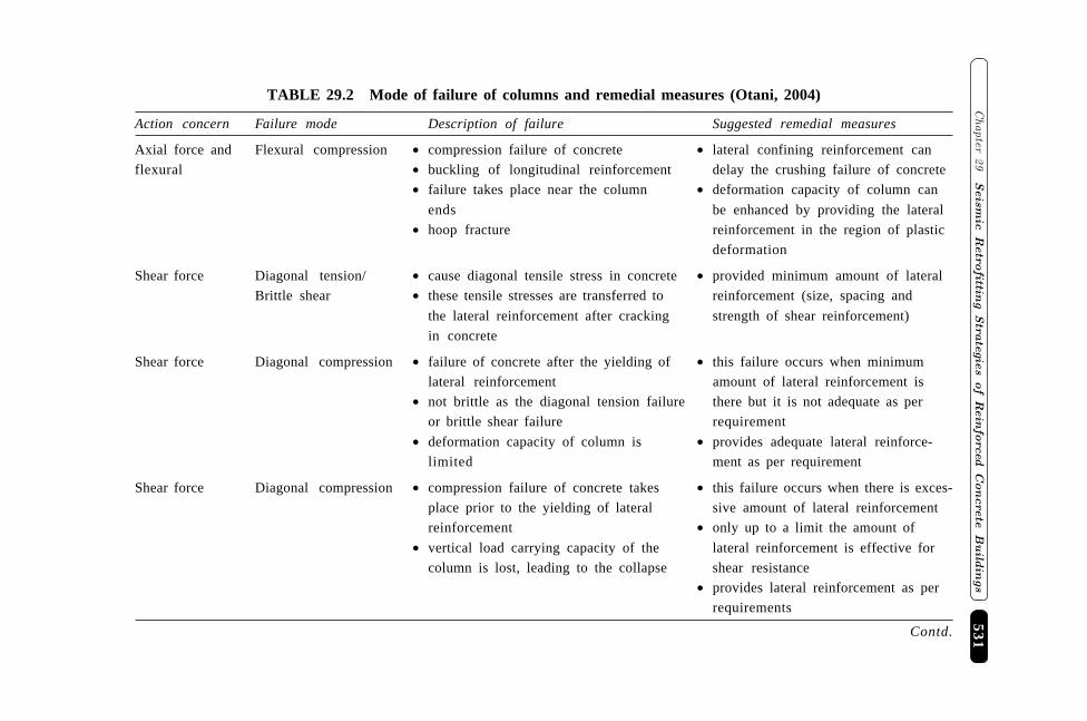
531�
�����
��
� �
� �
�
��
�� �� �
����
��
�
���
� �
������
�����
�
� ��
���
TABLE 29.2 Mode of failure of columns and remedial measures (Otani, 2004)
Action concern Failure mode Description of failure Suggested remedial measures
Axial force and Flexural compression ∑ compression failure of concrete ∑ lateral confining reinforcement can
flexural ∑ buckling of longitudinal reinforcement delay the crushing failure of concrete
∑ failure takes place near the column ∑ deformation capacity of column can
ends be enhanced by providing the lateral
∑ hoop fracture reinforcement in the region of plastic
deformation
Shear force Diagonal tension/ ∑ cause diagonal tensile stress in concrete ∑ provided minimum amount of lateral
Brittle shear ∑ these tensile stresses are transferred to reinforcement (size, spacing and
the lateral reinforcement after cracking strength of shear reinforcement)
in concrete
Shear force Diagonal compression ∑ failure of concrete after the yielding of ∑ this failure occurs when minimum
lateral reinforcement amount of lateral reinforcement is
∑ not brittle as the diagonal tension failure there but it is not adequate as per
or brittle shear failure requirement
∑ deformation capacity of column is ∑ provides adequate lateral reinforce-
limited ment as per requirement
Shear force Diagonal compression ∑ compression failure of concrete takes ∑ this failure occurs when there is exces-
place prior to the yielding of lateral sive amount of lateral reinforcement
reinforcement ∑ only up to a limit the amount of
∑ vertical load carrying capacity of the lateral reinforcement is effective for
column is lost, leading to the collapse shear resistance
∑ provides lateral reinforcement as per
requirements
Contd.
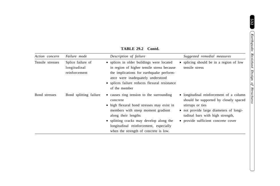
�����
������ �
����
�� �
���
���
����
��
532
Tensile stresses Splice failure of ∑ splices in older buildings were located ∑ splicing should be in a region of low
longitudinal in region of higher tensile stress because tensile stress
reinforcement the implications for earthquake perform-
ance were inadequately understood
∑ splices failure reduces flexural resistance
of the member
Bond stresses Bond splitting failure ∑ causes ring tension to the surrounding ∑ longitudinal reinforcement of a column
concrete should be supported by closely spaced
∑ high flexural bond stresses may exist in stirrups or ties
members with steep moment gradient ∑ not provide large diameters of longi-
along their lengths tudinal bars with high strength,
∑ splitting cracks may develop along the ∑ provide sufficient concrete cover
longitudinal reinforcement, especially
when the strength of concrete is low.
TABLE 29.2 Contd.
Action concern Failure mode Description of failure Suggested remedial measures
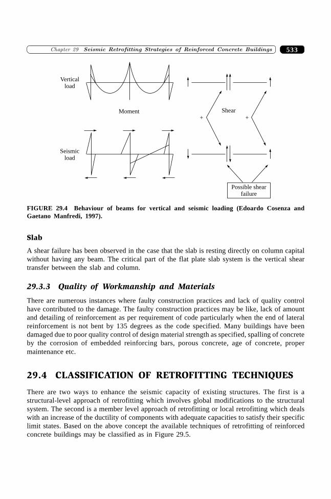
533�������� � �� ������ �� �������� ���� �������������� �� ���
Slab
A shear failure has been observed in the case that the slab is resting directly on column capitalwithout having any beam. The critical part of the flat plate slab system is the vertical sheartransfer between the slab and column.
29.3.3 Quality of Workmanship and Materials
There are numerous instances where faulty construction practices and lack of quality controlhave contributed to the damage. The faulty construction practices may be like, lack of amountand detailing of reinforcement as per requirement of code particularly when the end of lateralreinforcement is not bent by 135 degrees as the code specified. Many buildings have beendamaged due to poor quality control of design material strength as specified, spalling of concreteby the corrosion of embedded reinforcing bars, porous concrete, age of concrete, propermaintenance etc.
29.4 CLASSIFICATION OF RETROFITTING TECHNIQUES
There are two ways to enhance the seismic capacity of existing structures. The first is astructural-level approach of retrofitting which involves global modifications to the structuralsystem. The second is a member level approach of retrofitting or local retrofitting which dealswith an increase of the ductility of components with adequate capacities to satisfy their specificlimit states. Based on the above concept the available techniques of retrofitting of reinforcedconcrete buildings may be classified as in Figure 29.5.
Verticalload
+ +
Shear
Seismicload
Possible shearfailure
Moment
FIGURE 29.4 Behaviour of beams for vertical and seismic loading (Edoardo Cosenza andGaetano Manfredi, 1997).
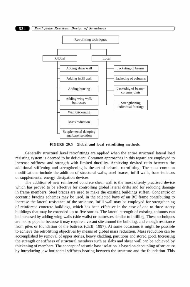
����������� ������� �������������534
Jacketing of columns
Jacketing of beams
Jacketing of beam–column joints
Strengtheningindividual footings
Retrofitting techniques
Global Local
Adding shear wall
Adding infill wall
Adding bracing
Adding wing wall/buttresses
Wall thickening
Mass reduction
Supplemental dampingand base isolation
FIGURE 29.5 Global and local retrofitting methods.
Generally structural level retrofittings are applied when the entire structural lateral loadresisting system is deemed to be deficient. Common approaches in this regard are employed toincrease stiffness and strength with limited ductility. Achieving desired ratio between theadditional stiffening and strengthening is the art of seismic retrofitting. The most commonmodifications include the addition of structural walls, steel braces, infill walls, base isolatorsor supplemental energy dissipation devices.
The addition of new reinforced concrete shear wall is the most oftenly practised devicewhich has proved to be effective for controlling global lateral drifts and for reducing damagein frame members. Steel braces are used to make the existing buildings stiffen. Concentric oreccentric bracing schemes may be used, in the selected bays of an RC frame contributing toincrease the lateral resistance of the structure. Infill wall may be employed for strengtheningof reinforced concrete buildings, which has been effective in the case of one to three storeybuildings that may be extended up to five stories. The lateral strength of existing columns canbe increased by adding wing walls (side walls) or buttresses similar to infilling. These techniquesare not so popular because it may require a vacant site around the building, and enough resistancefrom piles or foundation of the buttress (CEB, 1997). At some occasions it might be possibleto achieve the retrofitting objectives by means of global mass reduction. Mass reduction can beaccomplished by removal of upper stories, heavy cladding, partitions and stored good. Increasingthe strength or stiffness of structural members such as slabs and shear wall can be achieved bythickening of members. The concept of seismic base isolation is based on decoupling of structureby introducing low horizontal stiffness bearing between the structure and the foundation. This
535�������� � �� ������ �� �������� ���� �������������� �� ���
is found to be efficient for seismic protection of historical buildings where superstructure hasa limited seismic resistance and intervention is required only at foundation level. The supplementaldamping devices such as addition of viscous damper, visco-elastic damper, frictional damper indiagonals of bays of frame substantially reduces the earthquake response by dissipation of energy.
Local retrofittings are typically used either when the retrofit objectives are limited ordirect treatment of the vulnerable components is needed. The most popular and frequently usedmethod in local retrofitting is jacketing or confinement by the jackets of reinforced concrete,steel, fibre reinforced polymer (FRP), carbon fibre etc. Jacketing around the existing membersincreases lateral load capacity of the structure in a uniformly distributed way with a minimalincrease in loading on any single foundation and with no alternative in the basic geometry ofthe building.
29.5 RETROFITTING STRATEGIES FOR RC BUILDINGS
The need for retrofitting or strengthening of earthquake-damaged or earthquake-vulnerablebuildings in India have been tremendously increased during recent years after the devastatingBhuj earthquake with an alarming awakening for sufficient preparedness in anticipation to facefuture earthquakes. Many professional engineers are accustomed to the designing of newbuildings but they may find themselves not fully equipped to face the challenges posed at thetime of strengthening the existing buildings with a view to improve their seismic performance.This section presents the most common devices for retrofitting of reinforced concrete buildingswith technical details, constructional details and limitations.
29.5.1 Structural Level (or Global) Retrofit Methods
Two approaches are used for structure-level retrofitting: (i) conventional methods based onincreasing the seismic resistance of existing structure, and (ii) non-conventional methods basedon reduction of seismic demands.
Conventional methods
Conventional methods of retrofitting are used to enhance the seismic resistance of existingstructures by eliminating or reducing the adverse effects of design or construction. The methodsinclude adding of shear wall, infill walls and steel braces.
Adding new shear walls
One of the most common methods to increase the lateral strength of the reinforced concretebuildings is to make a provision for additional shear walls (Figure 29.6). The technique ofinfilling/adding new shear walls is often taken as the best and simple solution for improvingseismic performance. Therefore, it is frequently used for retrofitting of non-ductile reinforcedconcrete frame buildings. The added elements can be either cast-in-place or pre-cast concreteelements. New elements preferably be placed at the exterior of the building, however it maycause alteration in the appearance and window layouts. Placing of shear walls in the interior ofthe structure is not preferred in order to avoid interior mouldings.
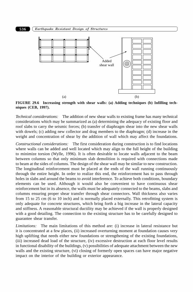
����������� ������� �������������536
Technical considerations: The addition of new shear walls to existing frame has many technicalconsiderations which may be summarized as (a) determining the adequacy of existing floor androof slabs to carry the seismic forces; (b) transfer of diaphragm shear into the new shear wallswith dowels; (c) adding new collector and drag members to the diaphragm; (d) increase in theweight and concentration of shear by the addition of wall which may affect the foundations.
Constructional considerations: The first consideration during construction is to find locationswhere walls can be added and well located which may align to the full height of the buildingto minimize torsion (Wylle, 1996). It is often desirable to locate walls adjacent to the beambetween columns so that only minimum slab demolition is required with connections madeto beam at the sides of columns. The design of the shear wall may be similar to new construction.The longitudinal reinforcement must be placed at the ends of the wall running continuouslythrough the entire height. In order to realize this end, the reinforcement has to pass throughholes in slabs and around the beams to avoid interference. To achieve both conditions, boundaryelements can be used. Although it would also be convenient to have continuous shearreinforcement but in its absence, the walls must be adequately connected to the beams, slabs andcolumns ensuring proper shear transfer through shear connectors. Wall thickness also variesfrom 15 to 25 cm (6 to 10 inch) and is normally placed externally. This retrofitting system isonly adequate for concrete structures, which bring forth a big increase in the lateral capacityand stiffness. A reasonable structural ductility may be achieved if the wall is properly designedwith a good detailing. The connection to the existing structure has to be carefully designed toguarantee shear transfer.
Limitations: The main limitations of this method are: (i) increase in lateral resistance butit is concentrated at a few places, (ii) increased overturning moment at foundation causes veryhigh uplifting that needs either new foundations or strengthening of the existing foundations,(iii) increased dead load of the structure, (iv) excessive destruction at each floor level resultsin functional disability of the buildings, (v) possibilities of adequate attachment between the newwalls and the existing structure, (vi) closing of formerly open spaces can have major negativeimpact on the interior of the building or exterior appearance.
Addedshear wall
(b)(a)
FIGURE 29.6 Increasing strength with shear walls: (a) Adding techniques (b) Infilling tech-niques (CEB, 1997).
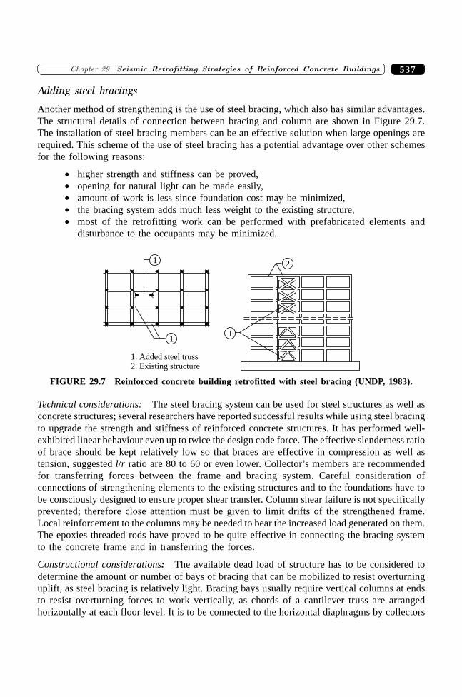
537�������� � �� ������ �� �������� ���� �������������� �� ���
Adding steel bracings
Another method of strengthening is the use of steel bracing, which also has similar advantages.The structural details of connection between bracing and column are shown in Figure 29.7.The installation of steel bracing members can be an effective solution when large openings arerequired. This scheme of the use of steel bracing has a potential advantage over other schemesfor the following reasons:
∑ higher strength and stiffness can be proved,∑ opening for natural light can be made easily,∑ amount of work is less since foundation cost may be minimized,∑ the bracing system adds much less weight to the existing structure,∑ most of the retrofitting work can be performed with prefabricated elements and
disturbance to the occupants may be minimized.
2
11
1
1. Added steel truss2. Existing structure
FIGURE 29.7 Reinforced concrete building retrofitted with steel bracing (UNDP, 1983).
Technical considerations: The steel bracing system can be used for steel structures as well asconcrete structures; several researchers have reported successful results while using steel bracingto upgrade the strength and stiffness of reinforced concrete structures. It has performed well-exhibited linear behaviour even up to twice the design code force. The effective slenderness ratioof brace should be kept relatively low so that braces are effective in compression as well astension, suggested l/r ratio are 80 to 60 or even lower. Collector’s members are recommendedfor transferring forces between the frame and bracing system. Careful consideration ofconnections of strengthening elements to the existing structures and to the foundations have tobe consciously designed to ensure proper shear transfer. Column shear failure is not specificallyprevented; therefore close attention must be given to limit drifts of the strengthened frame.Local reinforcement to the columns may be needed to bear the increased load generated on them.The epoxies threaded rods have proved to be quite effective in connecting the bracing systemto the concrete frame and in transferring the forces.
Constructional considerations: The available dead load of structure has to be considered todetermine the amount or number of bays of bracing that can be mobilized to resist overturninguplift, as steel bracing is relatively light. Bracing bays usually require vertical columns at endsto resist overturning forces to work vertically, as chords of a cantilever truss are arrangedhorizontally at each floor level. It is to be connected to the horizontal diaphragms by collectors
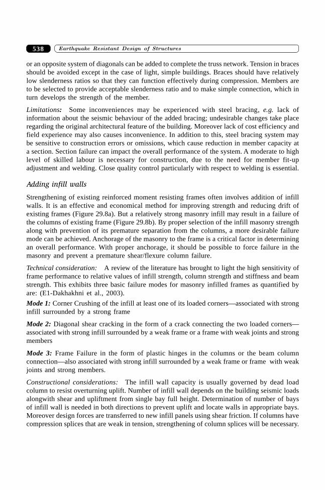
����������� ������� �������������538
or an opposite system of diagonals can be added to complete the truss network. Tension in bracesshould be avoided except in the case of light, simple buildings. Braces should have relativelylow slenderness ratios so that they can function effectively during compression. Members areto be selected to provide acceptable slenderness ratio and to make simple connection, which inturn develops the strength of the member.
Limitations: Some inconveniences may be experienced with steel bracing, e.g. lack ofinformation about the seismic behaviour of the added bracing; undesirable changes take placeregarding the original architectural feature of the building. Moreover lack of cost efficiency andfield experience may also causes inconvenience. In addition to this, steel bracing system maybe sensitive to construction errors or omissions, which cause reduction in member capacity ata section. Section failure can impact the overall performance of the system. A moderate to highlevel of skilled labour is necessary for construction, due to the need for member fit-upadjustment and welding. Close quality control particularly with respect to welding is essential.
Adding infill walls
Strengthening of existing reinforced moment resisting frames often involves addition of infillwalls. It is an effective and economical method for improving strength and reducing drift ofexisting frames (Figure 29.8a). But a relatively strong masonry infill may result in a failure ofthe columns of existing frame (Figure 29.8b). By proper selection of the infill masonry strengthalong with prevention of its premature separation from the columns, a more desirable failuremode can be achieved. Anchorage of the masonry to the frame is a critical factor in determiningan overall performance. With proper anchorage, it should be possible to force failure in themasonry and prevent a premature shear/flexure column failure.
Technical consideration: A review of the literature has brought to light the high sensitivity offrame performance to relative values of infill strength, column strength and stiffness and beamstrength. This exhibits three basic failure modes for masonry infilled frames as quantified byare: (E1-Dakhakhni et al., 2003).
Mode 1: Corner Crushing of the infill at least one of its loaded corners—associated with stronginfill surrounded by a strong frame
Mode 2: Diagonal shear cracking in the form of a crack connecting the two loaded corners—associated with strong infill surrounded by a weak frame or a frame with weak joints and strongmembers
Mode 3: Frame Failure in the form of plastic hinges in the columns or the beam columnconnection—also associated with strong infill surrounded by a weak frame or frame with weakjoints and strong members.
Constructional considerations: The infill wall capacity is usually governed by dead loadcolumn to resist overturning uplift. Number of infill wall depends on the building seismic loadsalongwith shear and upliftment from single bay full height. Determination of number of baysof infill wall is needed in both directions to prevent uplift and locate walls in appropriate bays.Moreover design forces are transferred to new infill panels using shear friction. If columns havecompression splices that are weak in tension, strengthening of column splices will be necessary.
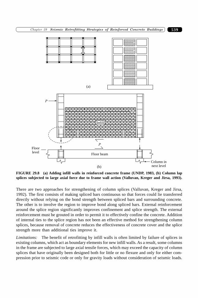
539�������� � �� ������ �� �������� ���� �������������� �� ���
There are two approaches for strengthening of column splices (Valluvan, Kreger and Jirsa,1992). The first consists of making spliced bars continuous so that forces could lie transferreddirectly without relying on the bond strength between spliced bars and surrounding concrete.The other is to involve the region to improve bond along spliced bars. External reinforcementaround the splice region significantly improves confinement and splice strength. The externalreinforcement must be grouted in order to permit it to effectively confine the concrete. Additionof internal ties to the splice region has not been an effective method for strengthening columnsplices, because removal of concrete reduces the effectiveness of concrete cover and the splicestrength more than additional ties improve it.
Limitations: The benefit of retrofitting by infill walls is often limited by failure of splices inexisting columns, which act as boundary elements for new infill walls. As a result, some columnsin the frame are subjected to large axial tensile forces, which may exceed the capacity of columnsplices that have originally been designed both for little or no flexure and only for either com-pression prior to seismic code or only for gravity loads without consideration of seismic loads.
(a)
Infill
Floor beam
Floorlevel
Column innext level
P
P
(b)
FIGURE 29.8 (a) Adding infill walls in reinforced concrete frame (UNDP, 1983, (b) Column lapsplices subjected to large axial force due to frame wall action (Valluvan, Kreger and Jirsa, 1993).
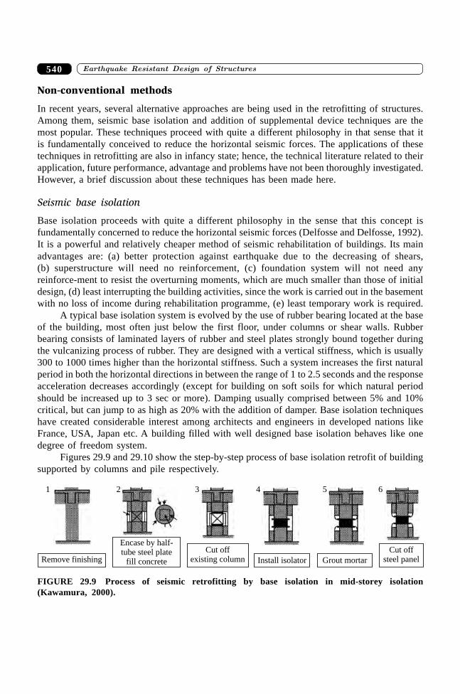
����������� ������� �������������540
Non-conventional methods
In recent years, several alternative approaches are being used in the retrofitting of structures.Among them, seismic base isolation and addition of supplemental device techniques are themost popular. These techniques proceed with quite a different philosophy in that sense that itis fundamentally conceived to reduce the horizontal seismic forces. The applications of thesetechniques in retrofitting are also in infancy state; hence, the technical literature related to theirapplication, future performance, advantage and problems have not been thoroughly investigated.However, a brief discussion about these techniques has been made here.
Seismic base isolation
Base isolation proceeds with quite a different philosophy in the sense that this concept isfundamentally concerned to reduce the horizontal seismic forces (Delfosse and Delfosse, 1992).It is a powerful and relatively cheaper method of seismic rehabilitation of buildings. Its mainadvantages are: (a) better protection against earthquake due to the decreasing of shears,(b) superstructure will need no reinforcement, (c) foundation system will not need anyreinforce-ment to resist the overturning moments, which are much smaller than those of initialdesign, (d) least interrupting the building activities, since the work is carried out in the basementwith no loss of income during rehabilitation programme, (e) least temporary work is required.
A typical base isolation system is evolved by the use of rubber bearing located at the baseof the building, most often just below the first floor, under columns or shear walls. Rubberbearing consists of laminated layers of rubber and steel plates strongly bound together duringthe vulcanizing process of rubber. They are designed with a vertical stiffness, which is usually300 to 1000 times higher than the horizontal stiffness. Such a system increases the first naturalperiod in both the horizontal directions in between the range of 1 to 2.5 seconds and the responseacceleration decreases accordingly (except for building on soft soils for which natural periodshould be increased up to 3 sec or more). Damping usually comprised between 5% and 10%critical, but can jump to as high as 20% with the addition of damper. Base isolation techniqueshave created considerable interest among architects and engineers in developed nations likeFrance, USA, Japan etc. A building filled with well designed base isolation behaves like onedegree of freedom system.
Figures 29.9 and 29.10 show the step-by-step process of base isolation retrofit of buildingsupported by columns and pile respectively.
1 2 3 4 5 6
Remove finishing
Encase by half-tube steel plate
fill concrete
Cut offexisting column Install isolator Grout mortar
Cut offsteel panel
FIGURE 29.9 Process of seismic retrofitting by base isolation in mid-storey isolation(Kawamura, 2000).
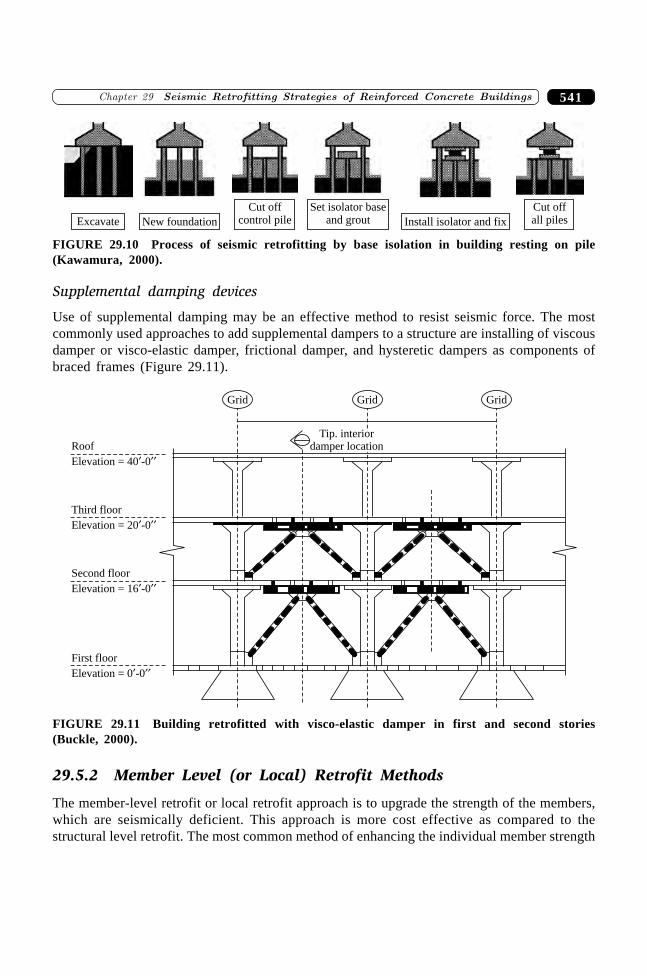
541�������� � �� ������ �� �������� ���� �������������� �� ���
Excavate New foundation
Cut offcontrol pile
Set isolator baseand grout Install isolator and fix
Cut offall piles
FIGURE 29.10 Process of seismic retrofitting by base isolation in building resting on pile(Kawamura, 2000).
Supplemental damping devices
Use of supplemental damping may be an effective method to resist seismic force. The mostcommonly used approaches to add supplemental dampers to a structure are installing of viscousdamper or visco-elastic damper, frictional damper, and hysteretic dampers as components ofbraced frames (Figure 29.11).
Second floor
Grid Grid Grid
Roof
Elevation = 40 -0���
Third floor
Elevation = 20 -0���
Elevation = 16 -0���
First floor
Elevation = 0 -0���
Tip. interiordamper location
FIGURE 29.11 Building retrofitted with visco-elastic damper in first and second stories(Buckle, 2000).
29.5.2 Member Level (or Local) Retrofit Methods
The member-level retrofit or local retrofit approach is to upgrade the strength of the members,which are seismically deficient. This approach is more cost effective as compared to thestructural level retrofit. The most common method of enhancing the individual member strength
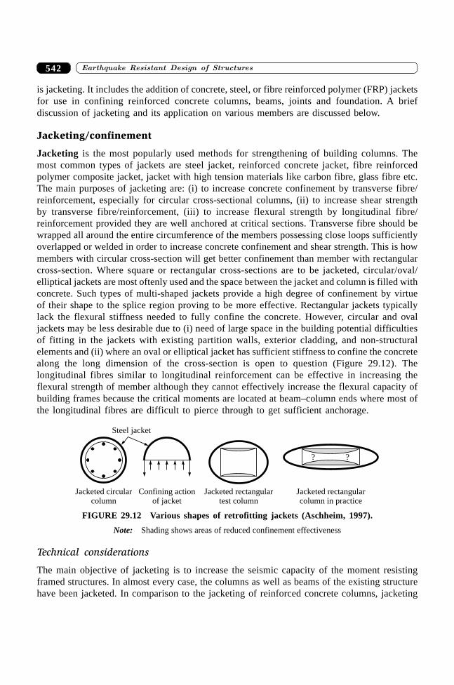
����������� ������� �������������542
is jacketing. It includes the addition of concrete, steel, or fibre reinforced polymer (FRP) jacketsfor use in confining reinforced concrete columns, beams, joints and foundation. A briefdiscussion of jacketing and its application on various members are discussed below.
Jacketing/confinement
Jacketing is the most popularly used methods for strengthening of building columns. Themost common types of jackets are steel jacket, reinforced concrete jacket, fibre reinforcedpolymer composite jacket, jacket with high tension materials like carbon fibre, glass fibre etc.The main purposes of jacketing are: (i) to increase concrete confinement by transverse fibre/reinforcement, especially for circular cross-sectional columns, (ii) to increase shear strengthby transverse fibre/reinforcement, (iii) to increase flexural strength by longitudinal fibre/reinforcement provided they are well anchored at critical sections. Transverse fibre should bewrapped all around the entire circumference of the members possessing close loops sufficientlyoverlapped or welded in order to increase concrete confinement and shear strength. This is howmembers with circular cross-section will get better confinement than member with rectangularcross-section. Where square or rectangular cross-sections are to be jacketed, circular/oval/elliptical jackets are most oftenly used and the space between the jacket and column is filled withconcrete. Such types of multi-shaped jackets provide a high degree of confinement by virtueof their shape to the splice region proving to be more effective. Rectangular jackets typicallylack the flexural stiffness needed to fully confine the concrete. However, circular and ovaljackets may be less desirable due to (i) need of large space in the building potential difficultiesof fitting in the jackets with existing partition walls, exterior cladding, and non-structuralelements and (ii) where an oval or elliptical jacket has sufficient stiffness to confine the concretealong the long dimension of the cross-section is open to question (Figure 29.12). Thelongitudinal fibres similar to longitudinal reinforcement can be effective in increasing theflexural strength of member although they cannot effectively increase the flexural capacity ofbuilding frames because the critical moments are located at beam–column ends where most ofthe longitudinal fibres are difficult to pierce through to get sufficient anchorage.
? ?
Steel jacket
Jacketed circularcolumn
Confining actionof jacket
Jacketed rectangulartest column
Jacketed rectangularcolumn in practice
FIGURE 29.12 Various shapes of retrofitting jackets (Aschheim, 1997).
Note: Shading shows areas of reduced confinement effectiveness
Technical considerations
The main objective of jacketing is to increase the seismic capacity of the moment resistingframed structures. In almost every case, the columns as well as beams of the existing structurehave been jacketed. In comparison to the jacketing of reinforced concrete columns, jacketing
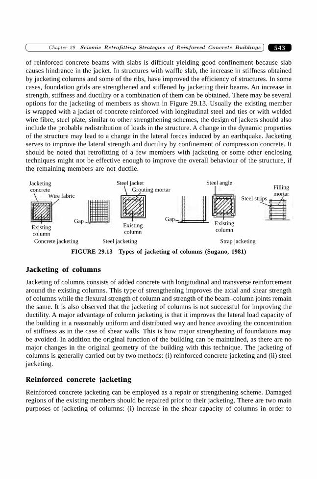
543�������� � �� ������ �� �������� ���� �������������� �� ���
of reinforced concrete beams with slabs is difficult yielding good confinement because slabcauses hindrance in the jacket. In structures with waffle slab, the increase in stiffness obtainedby jacketing columns and some of the ribs, have improved the efficiency of structures. In somecases, foundation grids are strengthened and stiffened by jacketing their beams. An increase instrength, stiffness and ductility or a combination of them can be obtained. There may be severaloptions for the jacketing of members as shown in Figure 29.13. Usually the existing memberis wrapped with a jacket of concrete reinforced with longitudinal steel and ties or with weldedwire fibre, steel plate, similar to other strengthening schemes, the design of jackets should alsoinclude the probable redistribution of loads in the structure. A change in the dynamic propertiesof the structure may lead to a change in the lateral forces induced by an earthquake. Jacketingserves to improve the lateral strength and ductility by confinement of compression concrete. Itshould be noted that retrofitting of a few members with jacketing or some other enclosingtechniques might not be effective enough to improve the overall behaviour of the structure, ifthe remaining members are not ductile.
Jacketingconcrete
Wire fabric
Existingcolumn
GapExistingcolumn
Steel jacketGrouting mortar
Gap
Steel angle
Existingcolumn
Steel strips
Fillingmortar
Concrete jacketing Steel jacketing Strap jacketing
FIGURE 29.13 Types of jacketing of columns (Sugano, 1981)
Jacketing of columns
Jacketing of columns consists of added concrete with longitudinal and transverse reinforcementaround the existing columns. This type of strengthening improves the axial and shear strengthof columns while the flexural strength of column and strength of the beam–column joints remainthe same. It is also observed that the jacketing of columns is not successful for improving theductility. A major advantage of column jacketing is that it improves the lateral load capacity ofthe building in a reasonably uniform and distributed way and hence avoiding the concentrationof stiffness as in the case of shear walls. This is how major strengthening of foundations maybe avoided. In addition the original function of the building can be maintained, as there are nomajor changes in the original geometry of the building with this technique. The jacketing ofcolumns is generally carried out by two methods: (i) reinforced concrete jacketing and (ii) steeljacketing.
Reinforced concrete jacketing
Reinforced concrete jacketing can be employed as a repair or strengthening scheme. Damagedregions of the existing members should be repaired prior to their jacketing. There are two mainpurposes of jacketing of columns: (i) increase in the shear capacity of columns in order to
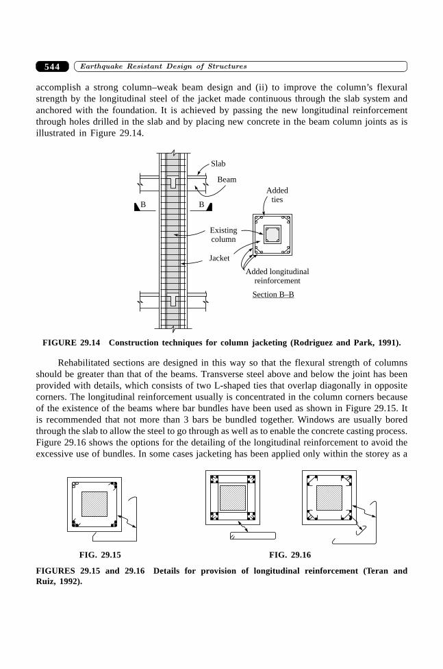
����������� ������� �������������544
accomplish a strong column–weak beam design and (ii) to improve the column’s flexuralstrength by the longitudinal steel of the jacket made continuous through the slab system andanchored with the foundation. It is achieved by passing the new longitudinal reinforcementthrough holes drilled in the slab and by placing new concrete in the beam column joints as isillustrated in Figure 29.14.
B B
Slab
Beam
Addedties
Existingcolumn
Jacket
Added longitudinalreinforcement
Section B–B
FIGURE 29.14 Construction techniques for column jacketing (Rodriguez and Park, 1991).
Rehabilitated sections are designed in this way so that the flexural strength of columnsshould be greater than that of the beams. Transverse steel above and below the joint has beenprovided with details, which consists of two L-shaped ties that overlap diagonally in oppositecorners. The longitudinal reinforcement usually is concentrated in the column corners becauseof the existence of the beams where bar bundles have been used as shown in Figure 29.15. Itis recommended that not more than 3 bars be bundled together. Windows are usually boredthrough the slab to allow the steel to go through as well as to enable the concrete casting process.Figure 29.16 shows the options for the detailing of the longitudinal reinforcement to avoid theexcessive use of bundles. In some cases jacketing has been applied only within the storey as a
FIG. 29.15 FIG. 29.16
FIGURES 29.15 and 29.16 Details for provision of longitudinal reinforcement (Teran andRuiz, 1992).
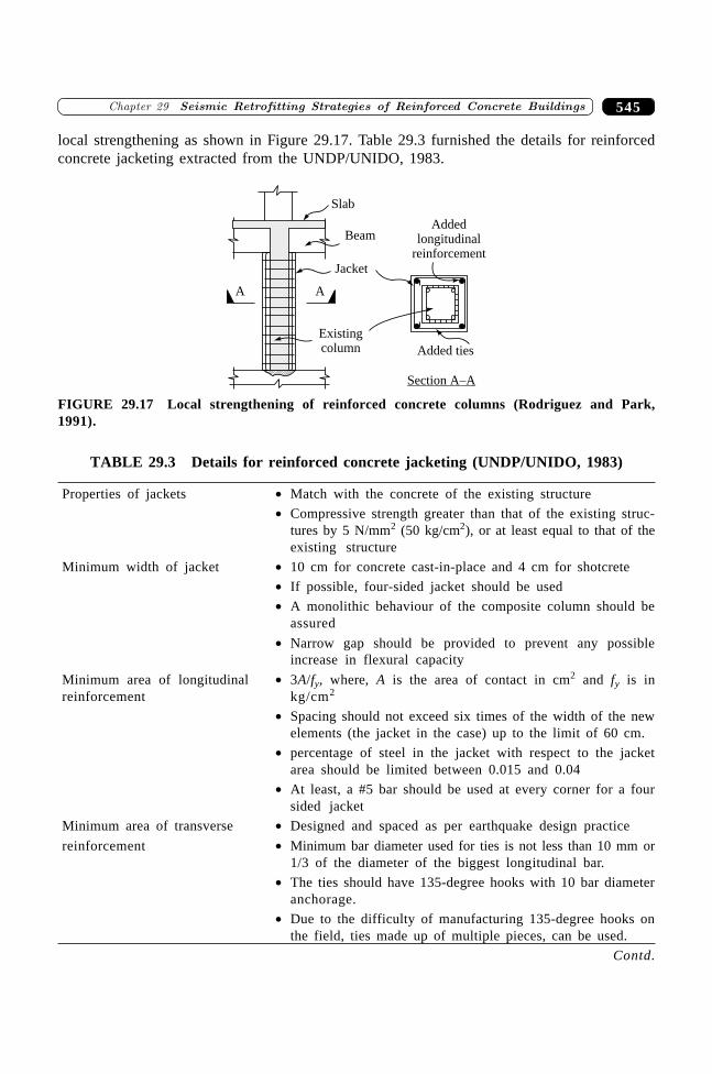
545�������� � �� ������ �� �������� ���� �������������� �� ���
local strengthening as shown in Figure 29.17. Table 29.3 furnished the details for reinforcedconcrete jacketing extracted from the UNDP/UNIDO, 1983.
Beam
A A
Slab
Jacket
Added ties
Addedlongitudinal
reinforcement
Existingcolumn
Section A–A
FIGURE 29.17 Local strengthening of reinforced concrete columns (Rodriguez and Park,1991).
TABLE 29.3 Details for reinforced concrete jacketing (UNDP/UNIDO, 1983)
Properties of jackets ∑ Match with the concrete of the existing structure
∑ Compressive strength greater than that of the existing struc-tures by 5 N/mm2 (50 kg/cm2), or at least equal to that of theexisting structure
Minimum width of jacket ∑ 10 cm for concrete cast-in-place and 4 cm for shotcrete
∑ If possible, four-sided jacket should be used
∑ A monolithic behaviour of the composite column should beassured
∑ Narrow gap should be provided to prevent any possibleincrease in flexural capacity
Minimum area of longitudinal ∑ 3A/fy, where, A is the area of contact in cm2 and fy is inreinforcement kg/cm2
∑ Spacing should not exceed six times of the width of the newelements (the jacket in the case) up to the limit of 60 cm.
∑ percentage of steel in the jacket with respect to the jacketarea should be limited between 0.015 and 0.04
∑ At least, a #5 bar should be used at every corner for a foursided jacket
Minimum area of transverse ∑ Designed and spaced as per earthquake design practice
reinforcement ∑ Minimum bar diameter used for ties is not less than 10 mm or1/3 of the diameter of the biggest longitudinal bar.
∑ The ties should have 135-degree hooks with 10 bar diameteranchorage.
∑ Due to the difficulty of manufacturing 135-degree hooks onthe field, ties made up of multiple pieces, can be used.
Contd.
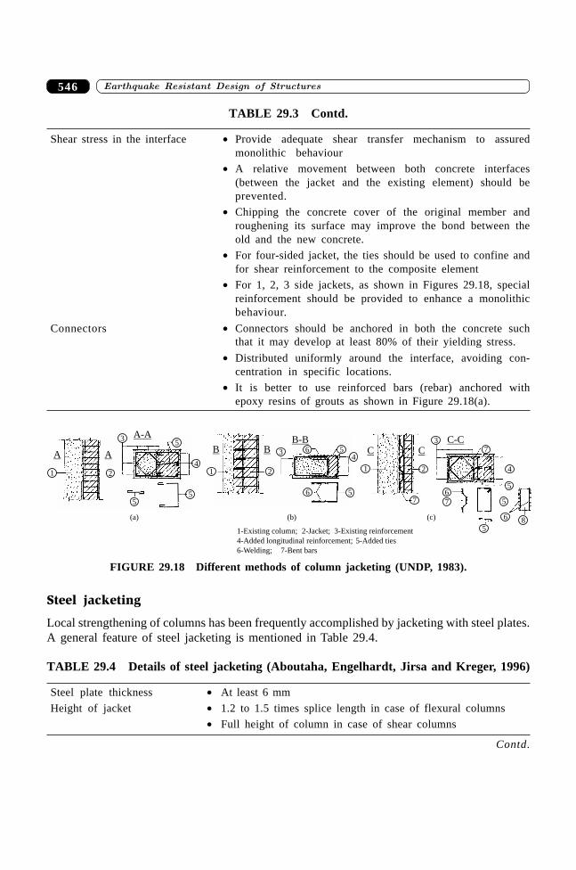
����������� ������� �������������546
Shear stress in the interface ∑ Provide adequate shear transfer mechanism to assuredmonolithic behaviour
∑ A relative movement between both concrete interfaces(between the jacket and the existing element) should beprevented.
∑ Chipping the concrete cover of the original member androughening its surface may improve the bond between theold and the new concrete.
∑ For four-sided jacket, the ties should be used to confine andfor shear reinforcement to the composite element
∑ For 1, 2, 3 side jackets, as shown in Figures 29.18, specialreinforcement should be provided to enhance a monolithicbehaviour.
Connectors ∑ Connectors should be anchored in both the concrete suchthat it may develop at least 80% of their yielding stress.
∑ Distributed uniformly around the interface, avoiding con-centration in specific locations.
∑ It is better to use reinforced bars (rebar) anchored withepoxy resins of grouts as shown in Figure 29.18(a).
1
4563
21
56
1 2
35
55
42
6
77
7
5
5
5
6 8
4
3
A A
A-A
B BB-B C-C
CC
(a) (b) (c)
1-Existing column; 2-Jacket; 3-Existing reinforcement
4-Added longitudinal reinforcement; 5-Added ties
6-Welding; 7-Bent bars
FIGURE 29.18 Different methods of column jacketing (UNDP, 1983).
Steel jacketing
Local strengthening of columns has been frequently accomplished by jacketing with steel plates.A general feature of steel jacketing is mentioned in Table 29.4.
TABLE 29.4 Details of steel jacketing (Aboutaha, Engelhardt, Jirsa and Kreger, 1996)
Steel plate thickness ∑ At least 6 mm
Height of jacket ∑ 1.2 to 1.5 times splice length in case of flexural columns
∑ Full height of column in case of shear columns
TABLE 29.3 Contd.
Contd.
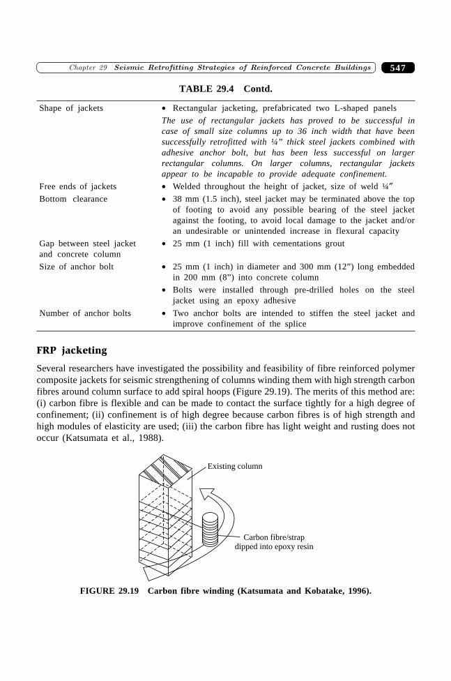
547�������� � �� ������ �� �������� ���� �������������� �� ���
Shape of jackets ∑ Rectangular jacketing, prefabricated two L-shaped panels
The use of rectangular jackets has proved to be successful incase of small size columns up to 36 inch width that have beensuccessfully retrofitted with ¼” thick steel jackets combined withadhesive anchor bolt, but has been less successful on largerrectangular columns. On larger columns, rectangular jacketsappear to be incapable to provide adequate confinement.
Free ends of jackets ∑ Welded throughout the height of jacket, size of weld ¼≤Bottom clearance ∑ 38 mm (1.5 inch), steel jacket may be terminated above the top
of footing to avoid any possible bearing of the steel jacketagainst the footing, to avoid local damage to the jacket and/oran undesirable or unintended increase in flexural capacity
Gap between steel jacket ∑ 25 mm (1 inch) fill with cementations groutand concrete column
Size of anchor bolt ∑ 25 mm (1 inch) in diameter and 300 mm (12”) long embeddedin 200 mm (8”) into concrete column
∑ Bolts were installed through pre-drilled holes on the steeljacket using an epoxy adhesive
Number of anchor bolts ∑ Two anchor bolts are intended to stiffen the steel jacket andimprove confinement of the splice
FRP jacketing
Several researchers have investigated the possibility and feasibility of fibre reinforced polymercomposite jackets for seismic strengthening of columns winding them with high strength carbonfibres around column surface to add spiral hoops (Figure 29.19). The merits of this method are:(i) carbon fibre is flexible and can be made to contact the surface tightly for a high degree ofconfinement; (ii) confinement is of high degree because carbon fibres is of high strength andhigh modules of elasticity are used; (iii) the carbon fibre has light weight and rusting does notoccur (Katsumata et al., 1988).
Existing column
Carbon fibre/strapdipped into epoxy resin
FIGURE 29.19 Carbon fibre winding (Katsumata and Kobatake, 1996).
TABLE 29.4 Contd.
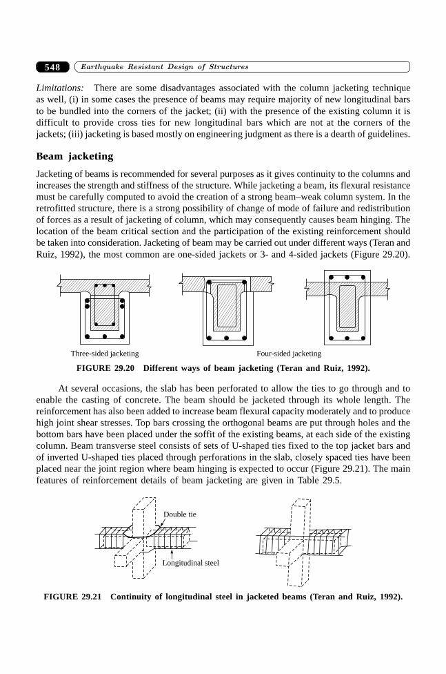
����������� ������� �������������548
Limitations: There are some disadvantages associated with the column jacketing techniqueas well, (i) in some cases the presence of beams may require majority of new longitudinal barsto be bundled into the corners of the jacket; (ii) with the presence of the existing column it isdifficult to provide cross ties for new longitudinal bars which are not at the corners of thejackets; (iii) jacketing is based mostly on engineering judgment as there is a dearth of guidelines.
Beam jacketing
Jacketing of beams is recommended for several purposes as it gives continuity to the columns andincreases the strength and stiffness of the structure. While jacketing a beam, its flexural resistancemust be carefully computed to avoid the creation of a strong beam–weak column system. In theretrofitted structure, there is a strong possibility of change of mode of failure and redistributionof forces as a result of jacketing of column, which may consequently causes beam hinging. Thelocation of the beam critical section and the participation of the existing reinforcement shouldbe taken into consideration. Jacketing of beam may be carried out under different ways (Teran andRuiz, 1992), the most common are one-sided jackets or 3- and 4-sided jackets (Figure 29.20).
Three-sided jacketing Four-sided jacketing
FIGURE 29.20 Different ways of beam jacketing (Teran and Ruiz, 1992).
At several occasions, the slab has been perforated to allow the ties to go through and toenable the casting of concrete. The beam should be jacketed through its whole length. Thereinforcement has also been added to increase beam flexural capacity moderately and to producehigh joint shear stresses. Top bars crossing the orthogonal beams are put through holes and thebottom bars have been placed under the soffit of the existing beams, at each side of the existingcolumn. Beam transverse steel consists of sets of U-shaped ties fixed to the top jacket bars andof inverted U-shaped ties placed through perforations in the slab, closely spaced ties have beenplaced near the joint region where beam hinging is expected to occur (Figure 29.21). The mainfeatures of reinforcement details of beam jacketing are given in Table 29.5.
Double tie
Longitudinal steel
FIGURE 29.21 Continuity of longitudinal steel in jacketed beams (Teran and Ruiz, 1992).
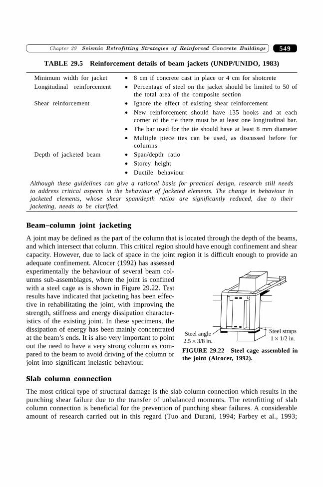
549�������� � �� ������ �� �������� ���� �������������� �� ���
TABLE 29.5 Reinforcement details of beam jackets (UNDP/UNIDO, 1983)
Minimum width for jacket ∑ 8 cm if concrete cast in place or 4 cm for shotcrete
Longitudinal reinforcement ∑ Percentage of steel on the jacket should be limited to 50 ofthe total area of the composite section
Shear reinforcement ∑ Ignore the effect of existing shear reinforcement
∑ New reinforcement should have 135 hooks and at eachcorner of the tie there must be at least one longitudinal bar.
∑ The bar used for the tie should have at least 8 mm diameter
∑ Multiple piece ties can be used, as discussed before forcolumns
Depth of jacketed beam ∑ Span/depth ratio
∑ Storey height
∑ Ductile behaviour
Although these guidelines can give a rational basis for practical design, research still needsto address critical aspects in the behaviour of jacketed elements. The change in behaviour injacketed elements, whose shear span/depth ratios are significantly reduced, due to theirjacketing, needs to be clarified.
Beam–column joint jacketing
A joint may be defined as the part of the column that is located through the depth of the beams,and which intersect that column. This critical region should have enough confinement and shearcapacity. However, due to lack of space in the joint region it is difficult enough to provide anadequate confinement. Alcocer (1992) has assessedexperimentally the behaviour of several beam col-umns sub-assemblages, where the joint is confinedwith a steel cage as is shown in Figure 29.22. Testresults have indicated that jacketing has been effec-tive in rehabilitating the joint, with improving thestrength, stiffness and energy dissipation character-istics of the existing joint. In these specimens, thedissipation of energy has been mainly concentratedat the beam’s ends. It is also very important to pointout the need to have a very strong column as com-pared to the beam to avoid driving of the column orjoint into significant inelastic behaviour.
Slab column connection
The most critical type of structural damage is the slab column connection which results in thepunching shear failure due to the transfer of unbalanced moments. The retrofitting of slabcolumn connection is beneficial for the prevention of punching shear failures. A considerableamount of research carried out in this regard (Tuo and Durani, 1994; Farbey et al., 1993;
Steel angle
2.5 3/8 in.�
Steel straps
1 1/2 in.�
FIGURE 29.22 Steel cage assembled inthe joint (Alcocer, 1992).
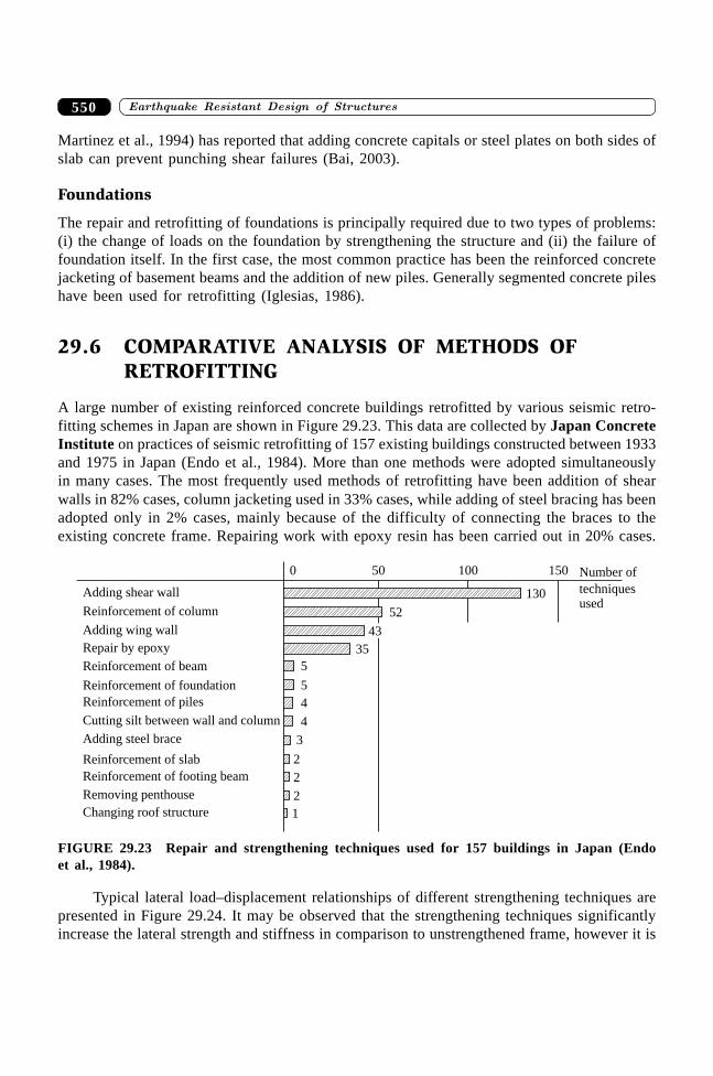
����������� ������� �������������550
Martinez et al., 1994) has reported that adding concrete capitals or steel plates on both sides ofslab can prevent punching shear failures (Bai, 2003).
Foundations
The repair and retrofitting of foundations is principally required due to two types of problems:(i) the change of loads on the foundation by strengthening the structure and (ii) the failure offoundation itself. In the first case, the most common practice has been the reinforced concretejacketing of basement beams and the addition of new piles. Generally segmented concrete pileshave been used for retrofitting (Iglesias, 1986).
29.6 COMPARATIVE ANALYSIS OF METHODS OFRETROFITTING
A large number of existing reinforced concrete buildings retrofitted by various seismic retro-fitting schemes in Japan are shown in Figure 29.23. This data are collected by Japan ConcreteInstitute on practices of seismic retrofitting of 157 existing buildings constructed between 1933and 1975 in Japan (Endo et al., 1984). More than one methods were adopted simultaneouslyin many cases. The most frequently used methods of retrofitting have been addition of shearwalls in 82% cases, column jacketing used in 33% cases, while adding of steel bracing has beenadopted only in 2% cases, mainly because of the difficulty of connecting the braces to theexisting concrete frame. Repairing work with epoxy resin has been carried out in 20% cases.
52
50 100 150
130
0
43
35
5
5
4
4
3
2
2
2
1
Number of
techniquesused
Adding shear wall
Reinforcement of column
Adding wing wall
Repair by epoxy
Reinforcement of beam
Reinforcement of foundation
Reinforcement of piles
Cutting silt between wall and column
Adding steel brace
Reinforcement of slab
Reinforcement of footing beam
Removing penthouse
Changing roof structure
FIGURE 29.23 Repair and strengthening techniques used for 157 buildings in Japan (Endoet al., 1984).
Typical lateral load–displacement relationships of different strengthening techniques arepresented in Figure 29.24. It may be observed that the strengthening techniques significantlyincrease the lateral strength and stiffness in comparison to unstrengthened frame, however it is
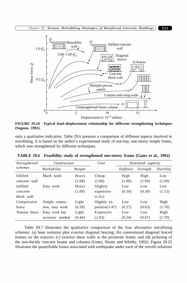
551�������� � �� ������ �� �������� ���� �������������� �� ���
only a qualitative indication. Table 29.6 presents a comparison of different aspects involved inretrofitting. It is based on the author’s experimental study of one-bay, one-storey simple frame,which was strengthened by different techniques.
TABLE 29.6 Feasibility study of strengthened one-storey frame (Gates et al., 1992)
Strengthened Construction Cost Structural capacityschemes Workability Weight Stiffness Strength Ductility
Infilled Much work Heavy Cheap High High Low
concrete wall (1.00) (1.00) (1.00) (1.00) (1.00)
Infilled Easy work Heavy Slightly Low Low Low
concrete (1.00) expensive (0.30) (0.30) (1.13)
block wall (1.61)
Compression Simple connec- Light Slightly ex- Low Low High
brace tion, easy work (0.39) pensive(1.47) (0.27) (0.63) (1.70)
Tension brace Easy work but Light Expensive Low Low High
accuracy needed (0.44) (2.93) (0.24) (0.67) (1.70)
Table 29.7 illustrates the qualitative comparison of the four alternative retrofittingschemes: (a) base isolation plus exterior diagonal bracing; (b) conventional diagonal bracedframes on the exterior; (c) exterior shear walls in the perimeter frame; and (d) jacketing ofthe non-ductile concrete beams and columns (Gates, Nester and Whitby, 1992). Figure 29.25illustrates the quantifiable losses associated with earthquake under each of the retrofit solutions
Concreteblock wall
1510500
0.5 Qw
1.0 Qw
QMonolithic
wall
QInfilled concrete
wall
0.60–1.00 Qw Diagonalbraces
K-braces
Multiple precastpanels
Column with wing walls
Displacement ( 10 radian)�–3
Sh
ear
forc
e,Q
Unstrengthened frame column
FIGURE 29.24 Typical load–displacement relationship for different strengthening techniques(Sugano, 1981).
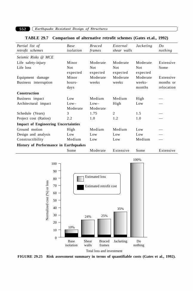
����������� ������� �������������552
TABLE 29.7 Comparison of alternative retrofit schemes (Gates et.al., 1992)
Partial list of Base Braced External Jacketing Doretrofit schemes isolation frames shear walls nothing
Seismic Risks @ MCE
Life safety-injury Minor Moderate Moderate Moderate ExtensiveLife loss Not Not Not Not Some
expected expected expected expectedEquipment damage Minor Moderate Moderate Moderate ExtensiveBusiness interruption hours- weeks weeks weeks- months or
days months relocation
ConstructionBusiness impact Low Medium Medium High —Architectural impact Low– Low– High Low —
Moderate ModerateSchedule (Years) 3 1.75 2 1.5 —Project cost (Ratios) 2.2 1.0 1.2 1.0 —
Impact of Engineering UncertaintiesGround motion High Medium Medium Low —Design and analysis Low Low Low Low —Constructibility Medium Low Low Medium —
History of Performance in EarthquakesSome Moderate Extensive Some Extensive
20
Baseisolation
Shearwalls
10%
24%
Bracedframes
25%
Jacketing
35%
Donothing
100%
0
10
30
40
50
60
70
80
90
100
No
rmal
ized
cost
(%)
or
loss
Estimated loss
Estimated retrofit cost
Total loss and investment
FIGURE 29.25 Risk assessment summary in terms of quantifiable costs (Gates et al., 1992).
553�������� � �� ������ �� �������� ���� �������������� �� ���
as well as the do-nothing alternative. Superimposed on this figure is the estimated retrofittingcost for each scheme.
SUMMARY
Retrofitting of seismically-deficient buildings or earthquake-damaged building is one of themost challenging tasks, which structural engineers face in the aftermath of an earthquake. Thereare at present no guidelines or code of practice available in the country for seismic retrofitting.The chapter presents a state-of-the-art documentation on the methods available for seismicretrofitting and their pros and cons. The methods of retrofitting are divided into two categories,namely, structural retrofitting and member retrofitting. The methods for structural retrofittingare adding shear walls, adding steel bracing, adding infill walls, seismic base isolation andsupplemental damping devices. The most common method of enhancing the individual memberstrength is jacketing. It includes the addition of concrete, steel, or fibre reinforced polymer(FRP) jackets for use in confining reinforced concrete columns, beams, joints and foundation.A comparative analysis has also been made for different methods of retrofitting depending oneffectiveness and cost.
REFERENCES
[1] Aboutaha, R.S., Engelhardt, M.D., Jirsa, J.O. and Kreger, M.E, “Retrofit of ConcreteColumn with Inadequate Lap Splices by the Use of Rectangular Steel Jackets”,Earthquake Spectra, Volume 12, No. 4, November, 1996.
[2] Alcocer, S.M., “Rehabilitation of RC Frame Connections Using Jacketing”, TenthWorld Conference on Earthquake Engineering, Madrid, Spain, 19–24 July, 1992.
[3] Aschheim, M. “Seismic Vulnerability, Evaluation, Retrofit, and New Design ofCalifornia Bridges—An Overview”, D.P. Abrams and G.M. Calvi (Eds.), US–ItalianWorkshop on Seismic Evaluation and Retrofit, NCEER–97-0003, 1997.
[4] Bai, J.W., “Seismic Retrofit for Reinforced Concrete Building Structures”, Conse-quences-Based Engineering (CBE) Institute Final Report, Texas A&M University,Mid-America Earthquake Center (from Internet), 2003.
[5] Buckle, I.G., “Passive Control of Structures for Seismic Loads”, Twelfth WorldConference on Earthquake Engineering, Paper No. 2825, 2000.
[6] CEB, Fastenings for Seismic Retrofitting—State-of-the Art-Report, Thomas Telford,1997.
[7] Delfosse, G.C. and Delfosse, P.G., “Seismic Rehabilitation of a Shear Wall Buildingby means of Base Isolation”, Tenth World Conference on Earthquake Engineering,Madrid, Spain, 19–24 July, 1992.
[8] Edoardo, Cosenza and Gaetano, Manfredi, “Some Remarks on the Evaluation andStrengthening of Under-designed R.C. Frame Buildings”, U.S.–Italian Workshop onSeismic Evaluation and Retrofit, D.P. Abrams and G.M. Calvi (Eds.), NCEER–97-0003, 1997.
����������� ������� �������������554
[9] El-Dakhakhni, W.W. Elgaaly, M., and Hamid, A.A., “Three-Strut Model for ConcreteMasonry-Infilled Steel Frames”, Journal of Structural Engineering, Vol. 129, No. 2,2003.
[10] Endo, T. et, al., “Practices of Seismic Retrofit of Existing Concrete Structures inJapan”, Eighth World Conference on Earthquake Engineering, San Francisco, 1984.
[11] Gates, W.E., Nester, M.R., and Whitby, T.R., “Managing Seismic Risk: A Case Historyof Seismic Retrofit for a Non-ductile Reinforced Concrete Frame High Rise OfficeBuilding”, Tenth World Conference on Earthquake Engineering, Madrid, Spain, 19–24July, 1992.
[12] Iglesias, J., “Repairing and Strengthening of Reinforced Concrete Buildings Damagedin the 1985 Mexico City Earthquake”, The Mexico Earthquakes—1985—FactorsInvolved and Lessons Learned, Michael A. Cassaro and Enrique Martinez Romero(Eds.), Proceedings of the International Conference, Mexico City, Mexico, ASCEPublication, September 19–21, 1986.
[13] IS 13935, Repair and Seismic Strengthening of Buildings—Guidelines, Bureau ofIndian Standards, New Delhi, 1993.
[14] Jara, M., Hernandez, C., Garcia, R., and Robles, F., “The Mexico Earthquake ofSeptember 19, 1985—Typical cases of Repair and Strengthening of ConcreteBuildings”, Earthquake Spectra, Vol. 5, No. 1, 1989.
[15] “Guideline for Seismic Evaluation of Existing Reinforced Concrete Buildings”, (inJapanese), Japan Building Disaster Prevention Association (JBDPA), Akasaka, Tokyo,1990.
[16] Katsumata, H. and Kobatake, Y., “Seismic Retrofit with Carbon Fibres for ReinforcedConcrete Columns”, Eleventh World Conference on Earthquake Engineering, PaperNo. 293, 1996.
[17] Katsumata, H., Kobatake, Y. and Tanaka, T., “A Study on Strengthening with CarbonFibre for Earthquake Resistant Capacity of Existing Reinforced Concrete Columns”,Ninth World Conference on Earthquake Engineering, Vol. 7, pp. 517–522, 1988.
[18] Kawamura, S., Sugisaki, R., Ogura, K., Maezawa, S., Tanaka, S., and Yajima, A.,“Seismic Isolation Retrofit in Japan”, Twelfth World Conference on EarthquakeEngineering, Paper No. 2523, 2000.
[19] Lynn, A.C., Moehle, J.P., Mahin, S.A., and Holmes, W.T., “Seismic Evaluation ofExisting Reinforced Concrete Building Columns”, Earthquake Spectra, Vol. 12,No. 4, 1996.
[20] Nateghi, F. and Shahbazian, B., “Seismic Evaluation, Upgrading and Retrofitting ofStructures: Recent Experiences in Iran”, Tenth World Conference on EarthquakeEngineering, Madrid, Spain, 19–24 July, 1992.
[21] Newman, Alexander, Structural Renovation of Buildings—Methods, Details, andDesign Example, McGraw-Hill, USA, 2001.
[22] Otani, S. “Earthquake Resistant Design of Reinforced Concrete Buildings—Past andFuture”, Journal of Advanced Concrete Technology, Vol. 2, No. 1, 3–24, JapanConcrete Institute, 2004.
[23] Rodriguez, M. and Park R., “Repair and Strengthening of Reinforced Concrete Buildingsfor Seismic Resistance”, Earthquake Spectra, Vol. 7, No. 3, 1991.
555�������� � �� ������ �� �������� ���� �������������� �� ���
[24] Sugano, S., “Seismic Strengthening of Existing Reinforced Concrete Buildings inJapan”, Bulletin of the New Zealand National Society for Earthquake Engineering,Vol. 14, No. 4, December, 1981.
[25] Teran, A. and Ruiz, J., “Reinforced Concrete Jacketing of Existing Structures”, TenthWorld Conference on Earthquake Engineering, Madrid, Spain, 1992.
[26] UNDP/UNIDO Project RER/79/015. “Repair and Strengthening of Reinforced Concrete,Stone and Brick Masonry Buildings”, Building Construction Under Seismic Conditionsin the Balkan Regions, Vol. 5, United Nations Industrial Development Programme,Austria, 1983.
[27] UN Economic and Social Council, Committee on Housing, Building and Planning,“Redesign, Repair and Strengthening of Buildings in Seismic Regions”, ECE/HBP/43,1982.
[28] Valluvan, R., Kreger, M.E., and Jirsa, J.O., “Strengthening of Column Splices forSeismic Retrofit of Non-ductile Reinforced Concrete Frames”, ACI Structural Journal,Vol. 90, No. 4, July–Aug., 1993.
[29] Valluvan, R., Kreger, M.E., and Jirsa, J.O., “Strengthening of Column Splices inInfilled Shear Wall”, Tenth World Conference on Earthquake Engineering, Madrid,Spain, 19–24 July, 1992.
[30] Wyllie, L.A. “Strengthening Strategies for Improved Seismic Performance”, EleventhWorld Conference on Earthquake Engineering, Paper No. 1424, 1996.
����������� ������� �������������556
556
Seismic Retrofitting ofReinforced Concrete
Buildings—Case Studies
��������
30.1 INTRODUCTION
This chapter deals with a few case studies in which the applications of the most commonretrofitting schemes are employed to improve the efficiency and proficiency of either theseismically deficient vulnerable buildings or earthquake damaged buildings. In view of themixed and complex seismic responses of retrofitted structures, heterogeneous nature of differentconstructions alongwith the strain dependent elastic properties of various materials hamper tobring a complete justification of the application of analytical studies. A sound qualitative basisof experimental studies or the experience of retrofitted structures during future earthquake willexactly judge and reveal the success of retrofitted structures. Since we have a considerable dearthof experience and experimental data on the behaviour and response of retrofitted structures, thecase studies presented here are based on the experience obtained by the others. Incidentally, twomajor earthquakes of March 14 and September 19, 1979 hit a large number of reinforcedconcrete buildings in Mexico. Some of them were retrofitted whose efficacy came to be actuallyjudged by the reoccurrence of an earthquake in the same region in 1985. Similar experience hasbeen initially obtained from Turkey earthquake, 1988 in which a large number of buildings weredamaged and retrofitted. This proved to be a good learning opportunity about the behaviour ofthe retrofitted structures. A few available case studies presented in this chapter serve as goodinstances for a better understanding of conventional retrofitted schemes. Some of the studiesreferred here are based on advance technological devices like base isolation and supplementaldampers. The information regarding suitability, effectiveness, test results of the analytical orexperimental recommendations are based on the studies and experience obtained by individualauthors as expressed in the published work.
557�������� � �� ������ �� ����� �������������� �� ����������� �
30.2 METHODOLOGY FOR SEISMIC RETROFITTINGOF RC BUILDINGS
A brief outline procedure followed for seismic assessment and retrofit works for a reinforcedconcrete building has been described here. This procedure has been adopted by the inspectionteam for retrofitting of reinforced concrete buildings in Turkey after the Adana–Ceyhanearthquake in Southern Turkey on June 27, 1998 (Sucuoglu, Gur and Gulkan, 2000). The surveyteam recommended 120 moderately damaged reinforced concrete residential apartmentbuildings in Ceyhan. The procedure of the method employed for 3–9-storey building stock maybe followed as:
∑ Visit to the actual site with all documentation of buildings should be made and all structuraldimensions and details should be verified. If necessary, reinforcement has to be checked onselected elements by rebar locator with some non-destructive testing (NDT) and by strippingconcrete cover. Foundations should be inspected by excavating trenches at one or twoexterior footings.
∑ An intense investigation has to be made regarding the existing concrete quality by taking1–3 core specimens from each building and taking rebound hammer readings on a largenumber of structural elements calibrated with the core test results.
∑ Inspection of each structural and architectural element for damage should be done and theobserved damage grade (none, light, moderate or heavy) on the structural and architecturalplans should be accordingly marked.
∑ Three-dimensional linear elastic model of the existing building should be prepared andsubjected to code specified vertical and lateral loads. The modulus of elasticity on concreteis to be reduced in accordance with material test results.
∑ The method for temporary shoring of damaged elements in buildings should be recom-mended. The damaged structures should be shored for vertical loads and braced for 25% ofthe estimated lateral loads and taking into account the live loads that will exist during con-struction. The most commonly used elements have been timber elements, steel elements, andtubular scaffolding (Iglesias, 1989).
∑ The buckling of longitudinal reinforcement, rupture of ties and crushing of concrete is oftenobserved in columns of damaged building. In that case, the original geometry of columnsis recovered by the use of hydraulic jacks.
∑ The seismic retrofit strategy for the building after considering all aspects should berecommended.
∑ The upgraded building is analyzed under code specified loading and its compliance with thecode is verified.
∑ For selected buildings, capacity spectrum method is employed to assess the seismicperformance of the retrofitted building.
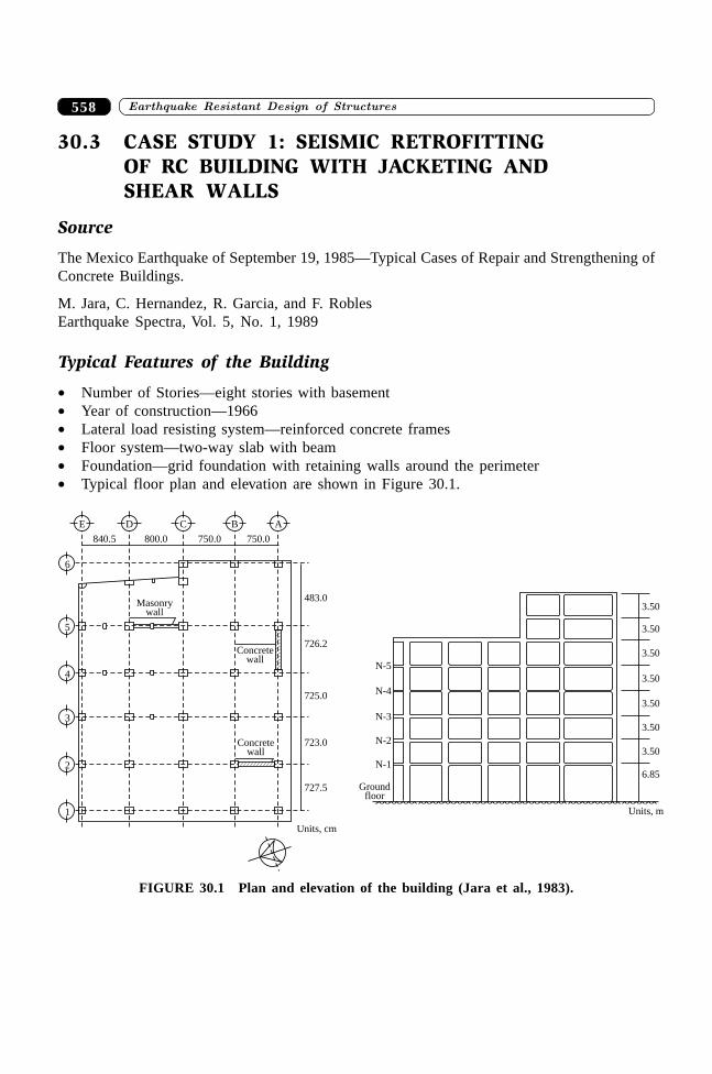
����������� ������� �������������558
30.3 CASE STUDY 1: SEISMIC RETROFITTINGOF RC BUILDING WITH JACKETING ANDSHEAR WALLS
Source
The Mexico Earthquake of September 19, 1985—Typical Cases of Repair and Strengthening ofConcrete Buildings.
M. Jara, C. Hernandez, R. Garcia, and F. RoblesEarthquake Spectra, Vol. 5, No. 1, 1989
Typical Features of the Building
∑ Number of Stories—eight stories with basement∑ Year of construction—1966∑ Lateral load resisting system—reinforced concrete frames∑ Floor system—two-way slab with beam∑ Foundation—grid foundation with retaining walls around the perimeter∑ Typical floor plan and elevation are shown in Figure 30.1.
E
1
2
3
4
5
6
D C B A
Units, cm
Concretewall
Concretewall
Masonrywall
840.5 800.0 750.0 750.0
483.0
726.2
725.0
723.0
727.5
3.50
3.50
3.50
3.50
3.50
3.50
3.50
6.85
Units, m
Groundfloor
N-1
N-2
N-3
N-4
N-5
FIGURE 30.1 Plan and elevation of the building (Jara et al., 1983).
559�������� � �� ������ �� ����� �������������� �� ����������� �
Features of Damages in Mexico Earthquake, 1979
∑ Minor cracks in beams and columns
Retrofitting Techniques Employed after Mexico Earthquake, 1979
∑ Addition of concrete shear wall in axis 2 and A∑ Addition of masonry wall in axis 5
Behaviour of Retrofitted Building in Mexico Earthquake, 1985
∑ Severe damage such as spalling of the concrete cover and buckled bar at the interface of thewalls and beam–column joints
∑ Main reinforcement in the columns located at the ground floor buckled and crushing of theconcrete core occurred
∑ Most damaged columns were the columns adjacent to the added walls∑ Damage attributed to the inadequate connection between the added walls and original frame
connection and the poor quality of the concrete
Retrofitting Techniques Employed after Mexico Earthquake, 1985
∑ Minor cracks—Repaired by injecting epoxy resins∑ Buckled longitudinal reinforcement, broken ties, and crushed concrete—Replacement
of new reinforcement welded with the existing bars and new additionally closed ties wereplaced, concrete with low shrinkage properties were placed
∑ Severely damaged columns adjacent to added walls—Retrofitted with encasing inconcrete with appropriate longitudinal and transverse reinforcement, existing surface shouldbe chipped and cleaned of all loose materials. The surface was moistened before the newconcrete was placed
∑ Other columns—Retrofitted with wire mesh and a cover of 50 mm of shotcrete∑ Damaged concrete wall added after 1979 earthquake—Demolished and replaced with
new concrete walls with 200 mm in thickness∑ Wall with slight damage—repaired by injecting epoxy resins and by increasing their
thickness to 200 mm∑ Added new walls along the axis 2, 5, 6, E and A∑ Foundation—The foundation grid was encased to permit the anchorage to the new
longitudinal reinforcement. Additionally, the grid was connected to the retaining wallslocated around the perimeter to ensure monolithic behaviour.
Expected Performance
∑ Static and dynamic analysis was performed on the original undamaged building, match tothe distribution of the damage observed accordingly
����������� ������� �������������560
∑ Retrofitted building has been analyzed with the assumption of monolithic behaviourbetween old and new material
∑ Results indicate no additional piles to the foundation
30.4 CASE STUDY 2: SEISMIC RETROFITTINGOF RC BUILDING WITH BRACING ANDSHEAR WALL
Source
Seismic Retrofit of an RC Building: A Case Study
Enrique DEL VALLE CALDERON, Douglas A. FOUTCH, Keith D. HJELMSTAD, EduardoFIGUEROA-GUTIERREZ and Arturo TENA-COLUNGA
Proceedings of Ninth World Conference on Earthquake Engineering, Tokyo-Kyoto, Japan(Vol. VII), 1988
Typical Features of the Building
∑ Number of stories—twelve, acting as Hotel building∑ Year of construction—1927∑ Lateral load resisting systems—non-ductile reinforced concrete frames∑ Floor system—cast-in-place concrete joist beam construction with 2.5-inch concrete
slab∑ Foundation system—mat foundation (2.4 m thick) on concrete friction piles∑ Typical floor plan and elevation shown in Figure 30.2
Features of Damages in Mexico Earthquake, 1979
∑ Extensive damage to first four stories in transverse direction∑ The spandrel beams and columns in Frame 1 and 5 experienced diagonal cracking over much
of their length in the first floor. In addition, the beam–column joints of these frames sufferedsevere cracking and spalling
∑ The medium column in the fourth storey of Frame 3 suffered cracking and crushing∑ The foundation performed well
Retrofitting Techniques Employed
∑ Cracked beams and columns—Repaired with epoxy injection∑ The columns of Frames 1 and 5—Encased in steel through the fourth storey level∑ Frame 1 and 5—Braced steel frames were attached on the outside of the building in
E–W direction
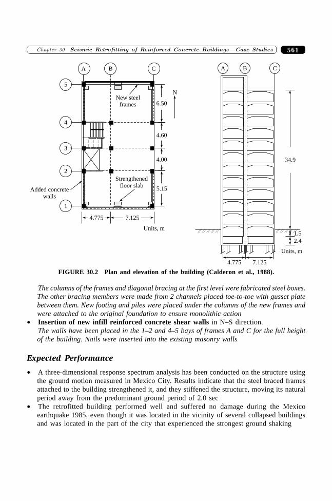
561�������� � �� ������ �� ����� �������������� �� ����������� �
The columns of the frames and diagonal bracing at the first level were fabricated steel boxes.The other bracing members were made from 2 channels placed toe-to-toe with gusset platebetween them. New footing and piles were placed under the columns of the new frames andwere attached to the original foundation to ensure monolithic action
∑ Insertion of new infill reinforced concrete shear walls in N–S direction.The walls have been placed in the 1–2 and 4–5 bays of frames A and C for the full heightof the building. Nails were inserted into the existing masonry walls
Expected Performance
∑ A three-dimensional response spectrum analysis has been conducted on the structure usingthe ground motion measured in Mexico City. Results indicate that the steel braced framesattached to the building strengthened it, and they stiffened the structure, moving its naturalperiod away from the predominant ground period of 2.0 sec
∑ The retrofitted building performed well and suffered no damage during the Mexicoearthquake 1985, even though it was located in the vicinity of several collapsed buildingsand was located in the part of the city that experienced the strongest ground shaking
4
5
3
2
1
4.775 7.125
BA C
New steelframes
Strengthenedfloor slab
Added concretewalls
6.50
4.60
4.00
5.15
N
4.775 7.125
2.4
1.5
A B C
34.9
Units, m
Units, m
FIGURE 30.2 Plan and elevation of the building (Calderon et al., 1988).
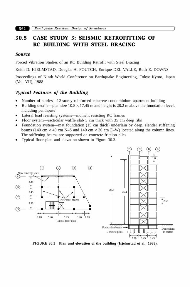
����������� ������� �������������562
30.5 CASE STUDY 3: SEISMIC RETROFITTING OFRC BUILDING WITH STEEL BRACING
Source
Forced Vibration Studies of an RC Building Retrofit with Steel Bracing
Keith D. HJELMSTAD, Douglas A. FOUTCH, Enrique DEL VALLE, Ruth E. DOWNS
Proceedings of Ninth World Conference on Earthquake Engineering, Tokyo-Kyoto, Japan(Vol. VII), 1988
Typical Features of the Building
∑ Number of stories—12-storey reinforced concrete condominium apartment building∑ Building details—plan size 10.8 ¥ 17.45 m and height is 28.2 m above the foundation level,
including penthouse∑ Lateral load resisting systems—moment resisting RC frames∑ Floor system—racticular waffle slab 5 cm thick with 35 cm deep ribs∑ Foundation system—mat foundation (15 cm thick) underlain by deep, slender stiffening
beams (140 cm ¥ 40 cm N–S and 140 cm ¥ 30 cm E–W) located along the column lines.The stiffening beams are supported on concrete friction piles
∑ Typical floor plan and elevation shown in Figure 30.3.
New concrete walls
1 2 3 4
A
B
C
D
3.45
3.45
3.90
Typical floor plan
1.65 5.40 5.25 3.20 1.95
New steel braces
3.90 3.45 3.45
Dimensionsin metresConcrete piles
Foundation beams
2.65
1.0
D C B A
26.428.2
FIGURE 30.3 Plan and elevation of the building (Hjelmstad et al., 1988).
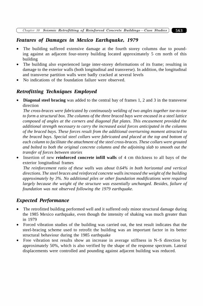
563�������� � �� ������ �� ����� �������������� �� ����������� �
Features of Damages in Mexico Earthquake, 1979
∑ The building suffered extensive damage at the fourth storey columns due to pound-ing against an adjacent four-storey building located approximately 5 cm north of thisbuilding
∑ The building also experienced large inter-storey deformations of its frame; resulting indamage to the exterior walls (both longitudinal and transverse). In addition, the longitudinaland transverse partition walls were badly cracked at several levels
∑ No indications of the foundation failure were observed.
Retrofitting Techniques Employed
∑ Diagonal steel bracing was added to the central bay of frames 1, 2 and 3 in the transversedirectionThe cross-braces were fabricated by continuously welding of two angles together toe-to-toeto form a structural box. The columns of the three braced bays were encased in a steel latticecomposed of angles at the corners and diagonal flat plates. This encasement provided theadditional strength necessary to carry the increased axial forces anticipated in the columnsof the braced bays. These forces result from the additional overturning moment attracted tothe braced bays. Special steel collars were fabricated and placed at the top and bottom ofeach column to facilitate the attachment of the steel cross-braces. These collars were groutedand bolted to both the original concrete columns and the adjoining slab to smooth out thetransfer of forces between stories
∑ Insertion of new reinforced concrete infill walls of 4 cm thickness to all bays of theexterior longitudinal framesThe reinforcement ratio of these walls was about 0.64% in both horizontal and verticaldirections. The steel braces and reinforced concrete walls increased the weight of the buildingapproximately by 3%. No additional piles or other foundation modifications were requiredlargely because the weight of the structure was essentially unchanged. Besides, failure offoundation was not observed following the 1979 earthquake.
Expected Performance
∑ The retrofitted building performed well and it suffered only minor structural damage duringthe 1985 Mexico earthquake, even though the intensity of shaking was much greater thanin 1979
∑ Forced vibration studies of the building was carried out, the test result indicates that thesteel-bracing scheme used to retrofit the building was an important factor in its betterstructural behaviour during the 1985 earthquake
∑ Free vibration test results show an increase in average stiffness in N–S direction byapproximately 50%, which is also verified by the shape of the response spectrum. Lateraldisplacements were controlled and pounding against adjacent building was reduced.
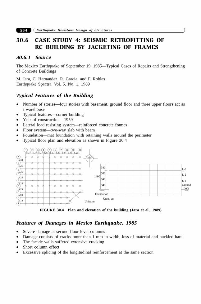
����������� ������� �������������564
30.6 CASE STUDY 4: SEISMIC RETROFITTING OFRC BUILDING BY JACKETING OF FRAMES
30.6.1 Source
The Mexico Earthquake of September 19, 1985—Typical Cases of Repairs and Strengtheningof Concrete Buildings
M. Jara, C. Hernandez, R. Garcia, and F. RoblesEarthquake Spectra, Vol. 5, No. 1, 1989
Typical Features of the Building
∑ Number of stories—four stories with basement, ground floor and three upper floors act asa warehouse
∑ Typical features—corner building∑ Year of construction—1959∑ Lateral load resisting system—reinforced concrete frames∑ Floor system—two-way slab with beam∑ Foundation—mat foundation with retaining walls around the perimeter∑ Typical floor plan and elevation as shown in Figure 30.4
5.37
A
5.38
15.37
25.37
35.37
45.37
55.37
65.37
75.30
86.20
9 10
B
5.25
C
5.25D
5.25
E
5.25F
5.25
G5.04
H
5.18
I
L-3
L-2
L-1
Groundfloor
340
380
340
340
1400
Foundation
Units, mUnits, cm
FIGURE 30.4 Plan and elevation of the building (Jara et al., 1989)
Features of Damages in Mexico Earthquake, 1985
∑ Severe damage at second floor level columns∑ Damage consists of cracks more than 1 mm in width, loss of material and buckled bars∑ The facade walls suffered extensive cracking∑ Short column effect∑ Excessive splicing of the longitudinal reinforcement at the same section
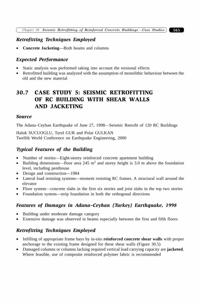
565�������� � �� ������ �� ����� �������������� �� ����������� �
Retrofitting Techniques Employed
∑ Concrete Jacketing—Both beams and columns
Expected Performance
∑ Static analysis was performed taking into account the torsional effects∑ Retrofitted building was analyzed with the assumption of monolithic behaviour between the
old and the new material
30.7 CASE STUDY 5: SEISMIC RETROFITTINGOF RC BUILDING WITH SHEAR WALLSAND JACKETING
Source
The Adana–Ceyhan Earthquake of June 27, 1998—Seismic Retrofit of 120 RC Buildings
Haluk SUCUOGLU, Turel GUR and Polat GULKANTwelfth World Conference on Earthquake Engineering, 2000
Typical Features of the Building
∑ Number of stories—Eight-storey reinforced concrete apartment building∑ Building dimensions—floor area 245 m2 and storey height is 3.0 m above the foundation
level, including penthouse∑ Design and construction—1984∑ Lateral load resisting systems—moment resisting RC frames. A structural wall around the
elevator∑ Floor system—concrete slabs in the first six stories and joist slabs in the top two stories∑ Foundation system—strip foundation in both the orthogonal directions
Features of Damages in Adana–Ceyhan (Turkey) Earthquake, 1998
∑ Building under moderate damage category∑ Extensive damage was observed in beams especially between the first and fifth floors
Retrofitting Techniques Employed
∑ Infilling of appropriate frame bays by in-situ reinforced concrete shear walls with properanchorage to the existing frame designed for these shear walls (Figure 30.5)
∑ Damaged columns or columns lacking required vertical load carrying capacity are jacketed.Where feasible, use of composite reinforced polymer fabric is recommended
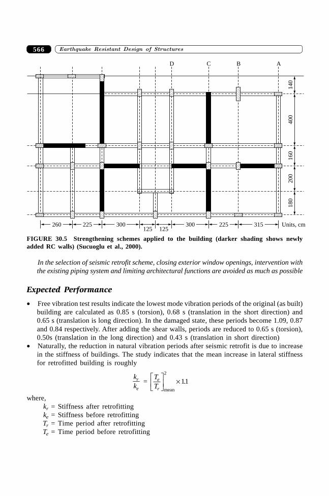
����������� ������� �������������566
In the selection of seismic retrofit scheme, closing exterior window openings, intervention withthe existing piping system and limiting architectural functions are avoided as much as possible
Expected Performance
∑ Free vibration test results indicate the lowest mode vibration periods of the original (as built)building are calculated as 0.85 s (torsion), 0.68 s (translation in the short direction) and0.65 s (translation is long direction). In the damaged state, these periods become 1.09, 0.87and 0.84 respectively. After adding the shear walls, periods are reduced to 0.65 s (torsion),0.50s (translation in the long direction) and 0.43 s (translation in short direction)
∑ Naturally, the reduction in natural vibration periods after seismic retrofit is due to increasein the stiffness of buildings. The study indicates that the mean increase in lateral stiffnessfor retrofitted building is roughly
kk
r
e =
TT
e
r
LNM
OQP
¥mean
2
11.
where,kr = Stiffness after retrofittingke = Stiffness before retrofittingTr = Time period after retrofittingTe = Time period before retrofitting
D C B A
260 225 300125 125
300 225 315
140
400
160
200
180
Units, cm
FIGURE 30.5 Strengthening schemes applied to the building (darker shading shows newlyadded RC walls) (Sucuoglu et al., 2000).
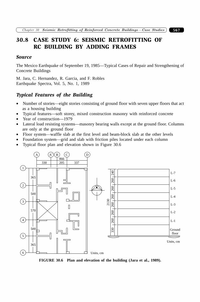
567�������� � �� ������ �� ����� �������������� �� ����������� �
30.8 CASE STUDY 6: SEISMIC RETROFITTING OFRC BUILDING BY ADDING FRAMES
Source
The Mexico Earthquake of September 19, 1985—Typical Cases of Repair and Strengthening ofConcrete Buildings
M. Jara, C. Hernandez, R. Garcia, and F. RoblesEarthquake Spectra, Vol. 5, No. 1, 1989
Typical Features of the Building
∑ Number of stories—eight stories consisting of ground floor with seven upper floors that actas a housing building
∑ Typical features—soft storey, mixed construction masonry with reinforced concrete∑ Year of construction—1979∑ Lateral load resisting systems—masonry bearing walls except at the ground floor. Columns
are only at the ground floor∑ Floor system—waffle slab at the first level and beam-block slab at the other levels∑ Foundation system—grid and slab with friction piles located under each column∑ Typical floor plan and elevation shown in Figure 30.6
4
3
1
2
5
6
A A� B C D
205 337
866
330
365
500
570
500
365
L-724
02
60
26
02
60
26
02
60
26
03
30
21
30
Groundfloor
L-6
L-5
L-4
L-3
L-2
L-1
Units, cm
Units, cm
FIGURE 30.6 Plan and elevation of the building (Jara et al., 1989).
����������� ������� �������������568
Features of Damages in Mexico Earthquake, 1985
∑ Severe damage occurred in masonry walls∑ Foundation of the columns at the first level suffered no damage∑ Principal failure direction was east–west due to irregularities in plan and insufficient area
of walls in east–west direction
Retrofitting Techniques Employed
∑ Adding of reinforced concrete frames over the existing column in the ground floor alongaxis 1, 3, 4 and 6
∑ Adding two concrete shear walls from first level to the upper storey were placed in axis3 and 4
∑ The existing masonry walls were retrofitted using wire mesh and 30 mm of mortar∑ The cover of the existing columns was removed to permit the continuity of the new
longitudinal reinforcement. The dimensions of the existing columns were increased∑ The monolithic behaviour between the new frames and the floor system was provided by
eliminating part of the floor system so that the new reinforcement of the frame was casttogether with slab
∑ Foundation—The foundation grid was encased to permit the anchorage to the new longitudinalreinforcement
Expected Performance
∑ Four new concrete frames with concrete walls were analyzed by taking into account thetorsional effects
∑ Retrofitted building was analyzed with the assumption of monolithic behaviour between oldand new material
∑ The results indicate that the bearing capacity of the existing foundation was consideredsufficient to resist the forces induced by the new structure
30.9 CASE STUDY 7: SEISMIC RETROFITTING OFRC BUILDING BY STEEL BRACING ANDINFILL WALLS
Source
The Mexico Earthquake of September 19, 1985—Typical Cases of Repairs and Strengtheningof Concrete Buildings
M. Jara, C. Hernandez, R. Garcia, and F. RoblesEarthquake Spectra, Vol. 5, No. 1, 1989
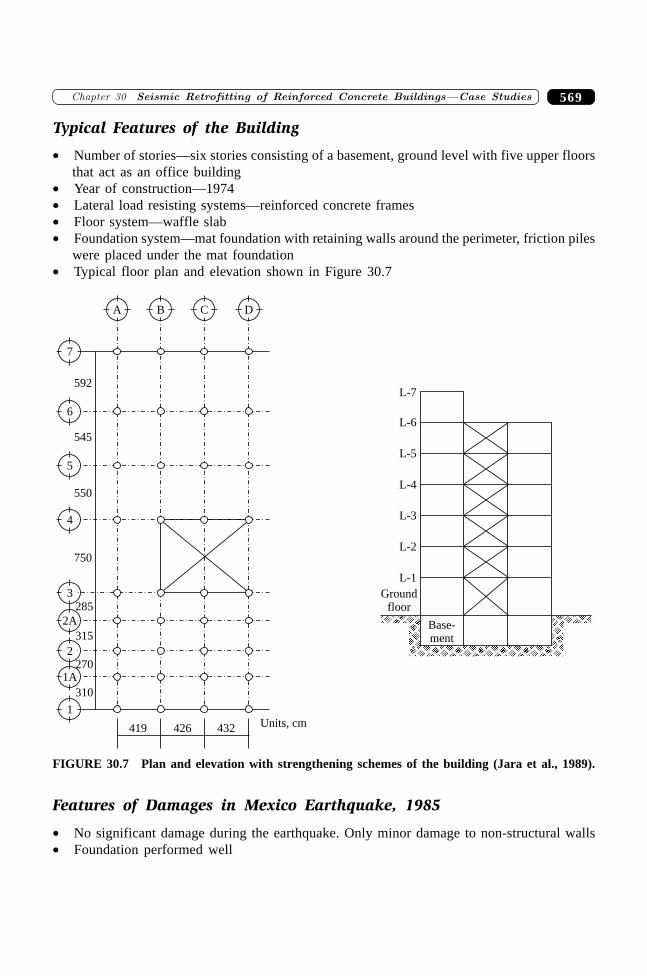
569�������� � �� ������ �� ����� �������������� �� ����������� �
Typical Features of the Building
∑ Number of stories—six stories consisting of a basement, ground level with five upper floorsthat act as an office building
∑ Year of construction—1974∑ Lateral load resisting systems—reinforced concrete frames∑ Floor system—waffle slab∑ Foundation system—mat foundation with retaining walls around the perimeter, friction piles
were placed under the mat foundation∑ Typical floor plan and elevation shown in Figure 30.7
6
A B C D
7
5
4
3
2A
2
1A
1
419 426 432
310
270
315
285
750
550
545
592L-7
L-6
L-5
L-4
L-3
L-2
L-1
Groundfloor
Base-ment
Units, cm
FIGURE 30.7 Plan and elevation with strengthening schemes of the building (Jara et al., 1989).
Features of Damages in Mexico Earthquake, 1985
∑ No significant damage during the earthquake. Only minor damage to non-structural walls∑ Foundation performed well
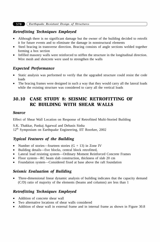
����������� ������� �������������570
Retrofitting Techniques Employed
∑ Although there is no significant damage but the owner of the building decided to retrofitit for future events and to eliminate the damage in nonstructural elements
∑ Steel bracing in transverse direction. Bracing consists of angle sections welded togetherforming a box section
∑ Infilled masonry walls were reinforced to stiffen the structure in the longitudinal direction.Wire mesh and shotcrete were used to strengthen the walls
Expected Performance
∑ Static analysis was performed to verify that the upgraded structure could resist the codeloads
∑ The bracing frames were designed in such a way that they would carry all the lateral loadswhile the existing structure was considered to carry all the vertical loads
30.10 CASE STUDY 8: SEISMIC RETROFITTING OFRC BUILDING WITH SHEAR WALLS
Source
Effect of Shear Wall Location on Response of Retrofitted Multi-Storied Building
S.K. Thakkar, Pankaj Agarwal and Debasis Sinha12th Symposium on Earthquake Engineering, IIT Roorkee, 2002
Typical Features of the Building
∑ Number of stories—fourteen stories (G + 13) in Zone IV∑ Building details—five blocks, central block retrofitted,∑ Lateral load resisting system—Ordinary Moment Reinforced Concrete Frames∑ Floor system—RC beam slab construction, thickness of slab 20 cm∑ Foundation system—Considered fixed at base above the raft foundation
Seismic Evaluation of Building
∑ Three-dimensional linear dynamic analysis of building indicates that the capacity demand(C/D) ratio of majority of the elements (beams and columns) are less than 1
Retrofitting Techniques Employed
∑ Addition of concrete shear wall∑ Two alternative locations of shear walls considered∑ Addition of shear wall in external frame and in internal frame as shown in Figure 30.8
571�������� � �� ������ �� ����� �������������� �� ����������� �
Expected Performance
∑ Provision of shear walls in external frames are more effective than the shear wall providedin internal frame however it is more effective for reducing base shear
∑ Storey drifts can be significantly decreased by addition of shear wall
30.11 CASE STUDY 9: SEISMIC RETROFITTING OFRC BUILDING BY SEISMIC BASE ISOLATION
Source
∑ Passive Control of Structures for Seismic LoadsIan G. Buckle12th World Conference on Earthquake Engineering, 2000
∑ Latest Advances in Seismic IsolationWilliam H. RobinsonEleventh World Conference on Earthquake Engineering, 1996
∑ Retrofitting of Historical Building by Seismic Base IsolationsSarvesh Kr. Jain and S.K. ThakkarWorkshop on Earthquake Disaster Preparedness, Roorkee, 1997
Typical Features of the Buildings
∑ Name of buildings—New Zealand Parliament House and Library, both are historicalbuildings
∑ Year of construction—1899 and 1922 respectively∑ Lateral load resisting systems—seismically vulnerable un-reinforced masonry
Retrofitting Techniques Employed
∑ Seismic isolation chosen over conventional strengthening techniques to maintain the historicfabric of the building
x
x 4 bays @ 6.5 m each
3bay
s@
6m
each
x
x 4 bays @ 6.5 m each
3bay
s@
6m
each
FIGURE 30.8 Two different retrofitting schemes by shear wall (Thakkar et al., 2002).
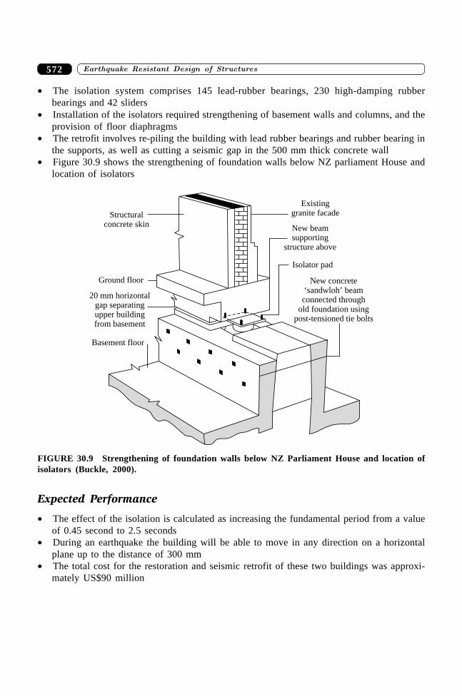
����������� ������� �������������572
∑ The isolation system comprises 145 lead-rubber bearings, 230 high-damping rubberbearings and 42 sliders
∑ Installation of the isolators required strengthening of basement walls and columns, and theprovision of floor diaphragms
∑ The retrofit involves re-piling the building with lead rubber bearings and rubber bearing inthe supports, as well as cutting a seismic gap in the 500 mm thick concrete wall
∑ Figure 30.9 shows the strengthening of foundation walls below NZ parliament House andlocation of isolators
Structuralconcrete skin
Ground floor
20 mm horizontalgap separatingupper buildingfrom basement
Basement floor
Existinggranite facade
New beamsupporting
structure above
Isolator pad
New concrete‘sandwloh’ beamconnected through
old foundation usingpost-tensioned tie bolts
FIGURE 30.9 Strengthening of foundation walls below NZ Parliament House and location ofisolators (Buckle, 2000).
Expected Performance
∑ The effect of the isolation is calculated as increasing the fundamental period from a valueof 0.45 second to 2.5 seconds
∑ During an earthquake the building will be able to move in any direction on a horizontalplane up to the distance of 300 mm
∑ The total cost for the restoration and seismic retrofit of these two buildings was approxi-mately US$90 million
573�������� � �� ������ �� ����� �������������� �� ����������� �
30.12 CASE STUDY 10: SEISMIC RETROFITTING OFRC BUILDING BY VISCOUS DAMPER
Source
Seismic Rehabilitation of a Non-Ductile Soft-Storey Concrete Structure Using Viscous Damper
H. Kit Miyamoto and Roger E. SchollEleventh World Conference on Earthquake Engineering, 1996
Typical Features of the Building
∑ Number of stories—four-storey building consisting of ground floor with three upper floors∑ Typical features—historical building, soft/weak storey structure in E–W direction, ground
floor is used as commercial/retail space, and the 2nd floor and above is single occupancyapartments
∑ Year of construction—1927∑ Lateral load resisting systems—no lateral resisting elements in North and South elevation
of the building at the ground floor, except for 16” square light RC frame, Non-ductile soft/weak storey structure in the East–West direction, Non-ductile reinforced concrete frames atthe first level, and conventional shear walls or braces at levels 2, 3, and 4
∑ Floor system—cast-in-place concrete joist beam construction with 2.5-inch concrete slab.
Features of Possible Damages
∑ Three-dimensional time history analysis of the original building was performed and theresult indicates that the concrete columns at the ground floor level were overstressed inbending and shears due to excessive deflection and the lack of ductility detailing andstrength. This type of adverse behaviour could cause total collapse of the superstructure
∑ At present, there is no significant damage in the structure.
Retrofitting Techniques Employed
Since the building is a National Registered building, only limited options for retrofitting wereconsidered so that they should not affect the appearance of the landmark hotel, maximizing theretail/commercial area at the ground floor, avoiding disturbance to tenants living in apartmenton the upper floors and of course should be cost effective. The finally selected retrofittingschemes are:
∑ Steel moment frames with fluid viscous dampers (VDs) at the ground floor. The steelmoment frames were designed to provide stiffness, strength, and redundancy to the existinglightly reinforced concrete columns. VDs were provided to control drift at the first floor andto keep steel moment frames in the elastic range. VDs were attached to the top of the steelChevron Braces and were strategically located to meet the above requirements
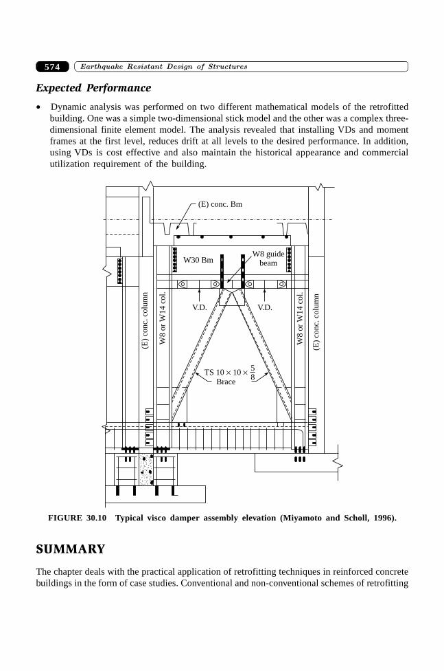
����������� ������� �������������574
Expected Performance
∑ Dynamic analysis was performed on two different mathematical models of the retrofittedbuilding. One was a simple two-dimensional stick model and the other was a complex three-dimensional finite element model. The analysis revealed that installing VDs and momentframes at the first level, reduces drift at all levels to the desired performance. In addition,using VDs is cost effective and also maintain the historical appearance and commercialutilization requirement of the building.
(E)
con
c.co
lum
n
W8 guidebeam
V.D. V.D.
(E) conc. Bm
W30 Bm
W8
or
W1
4co
l.
(E)
con
c.co
lum
n
W8
or
W1
4co
l.
TS 10 10� �58
Brace
FIGURE 30.10 Typical visco damper assembly elevation (Miyamoto and Scholl, 1996).
SUMMARY
The chapter deals with the practical application of retrofitting techniques in reinforced concretebuildings in the form of case studies. Conventional and non-conventional schemes of retrofitting
575�������� � �� ������ �� ����� �������������� �� ����������� �
are presented with their application, suitability and effectiveness. A few available case studiespresented in this chapter serve as good instances for a better understanding of conventionalretrofitted schemes such as addition of shear wall, bracing, infill wall, jacketing and a combi-nation of them. Some of the studies referred here are based on advanced technological deviceslike base isolation and supplemental dampers. As there is a scarcity of data on the retrofittingof building in India, the case studies presented in this chapter are extracted from the availableliterature.
REFERENCES
[1] Buckle, I.G., “Passive Control of Structures for Seismic Loads”, Twelfth WorldConference on Earthquake Engineering, Auckland, New Zealand, 2000.
[2] Calderon, Valle, E.D. et al., “Seismic Retrofit of an RC Building: A Case Study”,Proceedings of Ninth World Conference on Earthquake Engineering, Tokyo-Kyoto,Vol. VII, Japan, 1988.
[3] Iglesias, J., “Repairing and Strengthening of Reinforced Concrete Buildings Damaged inthe 1985 Mexico City Earthquake”, The Mexico Earthquakes 1985—Factors Involvedand Lessons Learned, Cassaro and Romero (Eds.). Proceedings of the InternationalConference, Mexico City, Mexico, September 19–21, ASCE Publication, 1986.
[4] Jain, Sarvesh K. and Thakkar, S.K., “Retrofitting of Historical Building by SeismicBase Isolations”, Workshop on Earthquake Disaster Preparedness, Roorkee, 1997.
[5] Jara, M., et al., “The Mexico Earthquake of September 19, 1985—Typical Cases ofRepair and Strengthening of Concrete Buildings”, Earthquake Spectra, Vol. 5, No. 1,1989.
[6] Keith Hjelmstad D., et al., “Forced Vibration Studies of an RC Building Retrofit withSteel Bracing”, Proceedings of Ninth World Conference on Earthquake Engineering,(Vol. VII), Tokyo-Kyoto, Japan 1988.
[7] Miyamoto, H.K. and Scholl, R.E., “Seismic Rehabilitation of a Non-ductile Soft-storey Concrete Structure Using Viscous Damper”, Eleventh World Conference onEarthquake Engineering, Acapulco, Mexico, 1996.
[8] Robinson, W.H., “Latest Advances in Seismic Isolation”, Eleventh World Conferenceon Earthquake Engineering, Acapulco, Mexico, 1996.
[9] Sucuoglu, H., Gur, T. and Gulkan, P., “The ADANA–CEYHAN Earthquake of June27, 1998: Seismic Retrofit of 120 RC Buildings”, Twelfth World Conference onEarthquake Engineering, Auckland, New Zealand, 2000.
[10] Thakkar, S.K., Agarwal, P., and Sinha, Debasis, “Effect of Shear Wall Location onResponse of Retrofitted Multi-storied Building”, Twelfth Symposium on EarthquakeEngineering, IIT Roorkee, 2002.
����������� ������� �������������576
576
Seismic Provisions forImproving the Performanceof Non-engineered Masonry
Construction withExperimental Verifications
��������
31.1 INTRODUCTION
Masonry is one of the most traditional, oldest materials and widely accepted medium for housingconstruction in India. This construction system is usually made spontaneously and informallywith the help of local masons without any or only a little intervention by professional experts,therefore it is termed as non-engineered construction. Non-engineered construction in Indiais generally made with fieldstone, fired brick, concrete blocks, adobe or rammed earth, woodor a combination of locally available traditional materials. The long history of earthquakes andage-old tradition of construction should have lead to the reasoning, logic and assumption thatsufficient precautionary measures are to be incorporated in these constructions to withstand theearthquake forces. But, on the contrary, this is not the case. Past experience has shown thatcollapse of non-engineered construction is the single largest factor contributing to the hugelosses and casualties during earthquakes till now. Unfortunately, however, the subject ofearthquake resistant construction of such buildings has not received the attention it deserves andthe construction practices continue to ignore the warning issued by nature time and again. Theremay be two possibilities for this situation, either people are unaware and do not know about theearthquake resistant measure of masonry construction or they doubt the efficiency, proficiencyand efficacy of these measures. The present chapter will deal with the earthquake resistantprovisions in non-engineered construction in general and brick and stone masonry buildings inparticular alongwith experimental verification to build confidence among the people.
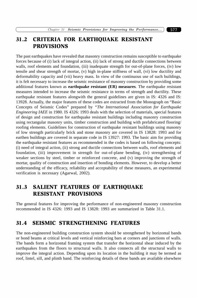
577�������� � �� ����� � ��� ��� ������ �� ��������������
31.2 CRITERIA FOR EARTHQUAKE RESISTANTPROVISIONS
The past earthquakes have revealed that masonry construction remains susceptible to earthquakeforces because of (i) lack of integral action, (ii) lack of strong and ductile connections betweenwalls, roof elements and foundation, (iii) inadequate strength for out-of-plane forces, (iv) lowtensile and shear strength of mortar, (v) high in-plane stiffness of wall, (vi) low ductility anddeformability capacity and (vii) heavy mass. In view of the continuous use of such buildings,it is felt necessary to increase the seismic resistance of masonry construction by providing someadditional features known as earthquake resistant (ER) measures. The earthquake resistantmeasures intended to increase the seismic resistance in terms of strength and ductility. Theseearthquake resistant features alongwith the general guidelines are given in IS: 4326 and IS:13928. Actually, the major features of these codes are extracted from the Monograph on “BasicConcepts of Seismic Codes” prepared by “The International Association for EarthquakeEngineering IAEE in 1980. IS 4326: 1993 deals with the selection of materials, special featuresof design and construction for earthquake resistant buildings including masonry constructionusing rectangular masonry units, timber construction and building with prefabricated flooring/roofing elements. Guidelines for construction of earthquake resistant buildings using masonryof low strength particularly brick and stone masonry are covered in IS 13828: 1993 and forearthen buildings are covered in separate code in IS 13927: 1993. The basic aim for providingthe earthquake resistant features as recommended in the codes is based on following concepts:(i) need of integral action, (ii) strong and ductile connections between walls, roof elements andfoundation, (iii) improvement in strength for out-of-plane bending, (iv) strengthening ofweaker sections by steel, timber or reinforced concrete, and (v) improving the strength ofmortar, quality of construction and insertion of bonding elements. However, to develop a betterunderstanding of the efficacy, reliability and acceptability of these measures, an experimentalverification is necessary (Agarwal, 2002).
31.3 SALIENT FEATURES OF EARTHQUAKERESISTANT PROVISIONS
The general features for improving the performance of non-engineered masonry constructionrecommended in IS 4326: 1993 and IS 13828: 1993 are summarized in Table 31.1.
31.4 SEISMIC STRENGTHENING FEATURES
The non-engineered building construction system should be strengthened by horizontal bandsor bond beams at critical levels and vertical reinforcing bars at corners and junctions of walls.The bands form a horizontal framing system that transfer the horizontal shear induced by theearthquakes from the floors to structural walls. It also connects all the structural walls toimprove the integral action. Depending upon its location in the building it may be termed asroof, lintel, sill, and plinth band. The reinforcing details of these bands are available elsewhere
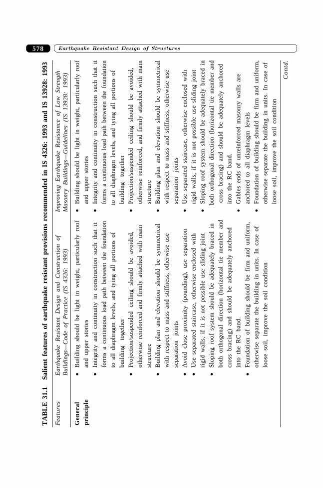
����������� ������� �������������578T
AB
LE
31.
1Sa
lient
fea
ture
s of
ear
thqu
ake
resi
stan
t pr
ovis
ions
rec
omm
ende
d in
IS
4326
: 19
93 a
nd I
S 13
928:
199
3
Fea
ture
sE
arth
quak
e R
esis
tant
Des
ign
and
Con
stru
ctio
n of
Impr
ovin
g E
arth
quak
e R
esis
tanc
e of
Low
Str
engt
hB
uild
ings
—C
ode
of P
ract
ice
(IS
4326
: 19
93)
Mas
onry
B
uild
ings
—G
uide
line
s (I
S 13
928:
19
93)
Gen
eral
∑B
uild
ing
shou
ld b
e li
ght
in w
eigh
t, p
arti
cula
rly
roof
∑B
uild
ing
shou
ld b
e li
ght
in w
eigh
t, p
arti
cula
rly
roof
pri
nci
ple
and
uppe
r st
orie
san
d up
per
stor
ies
∑In
tegr
ity
and
cont
inui
ty i
n co
nstr
ucti
on s
uch
that
it
∑In
tegr
ity
and
cont
inui
ty i
n co
nstr
ucti
on s
uch
that
it
form
s a
cont
inuo
us l
oad
path
bet
wee
n th
e fo
unda
tion
form
s a
cont
inuo
us l
oad
path
bet
wee
n th
e fo
unda
tion
to a
ll d
iaph
ragm
lev
els,
and
tyi
ng a
ll p
orti
ons
ofto
all
dia
phra
gm l
evel
s, a
nd t
ying
all
por
tion
s of
buil
ding
to
geth
erbu
ildi
ng
toge
ther
∑P
roje
ctio
n/su
spen
ded
ceil
ing
shou
ld
be
avoi
ded,
∑P
roje
ctio
n/su
spen
ded
ceil
ing
shou
ld
be
avoi
ded,
othe
rwis
e re
info
rced
and
fir
mly
att
ache
d w
ith
mai
not
herw
ise
rein
forc
ed,
and
firm
ly a
ttac
hed
wit
h m
ain
stru
ctur
est
ruct
ure
∑B
uild
ing
plan
and
ele
vati
on s
houl
d be
sym
met
rica
l∑
Bui
ldin
g pl
an a
nd e
leva
tion
sho
uld
be s
ymm
etri
cal
wit
h re
spec
t to
mas
s an
d st
iffn
ess,
oth
erw
ise
use
wit
h re
spec
t to
mas
s an
d st
iffn
ess,
oth
erw
ise
use
sepa
rati
on
join
tsse
para
tion
jo
ints
∑A
void
clo
se p
roxi
mit
y (p
ound
ing)
, us
e se
para
tion
∑U
se s
epar
ated
sta
irca
se,
othe
rwis
e en
clos
ed w
ith
∑U
se s
epar
ated
sta
irca
se,
othe
rwis
e en
clos
ed w
ith
rigi
d w
alls
, if
it
is n
ot p
ossi
ble
use
slid
ing
join
t
rigi
d w
alls
, if
it
is n
ot p
ossi
ble
use
slid
ing
join
t∑
Slo
ping
roo
f sy
stem
sho
uld
be a
dequ
atel
y br
aced
in
∑S
lopi
ng r
oof
syst
em s
houl
d be
ade
quat
ely
brac
ed i
nbo
th o
rtho
gona
l di
rect
ion
(hor
izon
tal
tie
mem
ber
and
both
ort
hogo
nal
dire
ctio
n (h
oriz
onta
l ti
e m
embe
r an
dcr
oss
brac
ing)
and
sho
uld
be a
dequ
atel
y an
chor
ed
cros
s br
acin
g) a
nd s
houl
d be
ade
quat
ely
anch
ored
into
the
RC
ban
d.
into
the
RC
ban
d.∑
Gab
les
ends
of
unre
info
rced
mas
onry
wal
ls a
re
∑F
ound
atio
n of
bui
ldin
g sh
ould
be
firm
and
uni
form
,an
chor
ed t
o al
l di
aphr
agm
lev
els
othe
rwis
e se
para
te t
he b
uild
ing
in u
nits
. In
cas
e of
∑F
ound
atio
n of
bui
ldin
g sh
ould
be
firm
and
uni
form
,
loos
e so
il,
impr
ove
the
soil
con
diti
onot
herw
ise
sepa
rate
the
bui
ldin
g in
uni
ts.
In c
ase
of
loos
e so
il,
impr
ove
the
soil
con
diti
on
Co
ntd
.
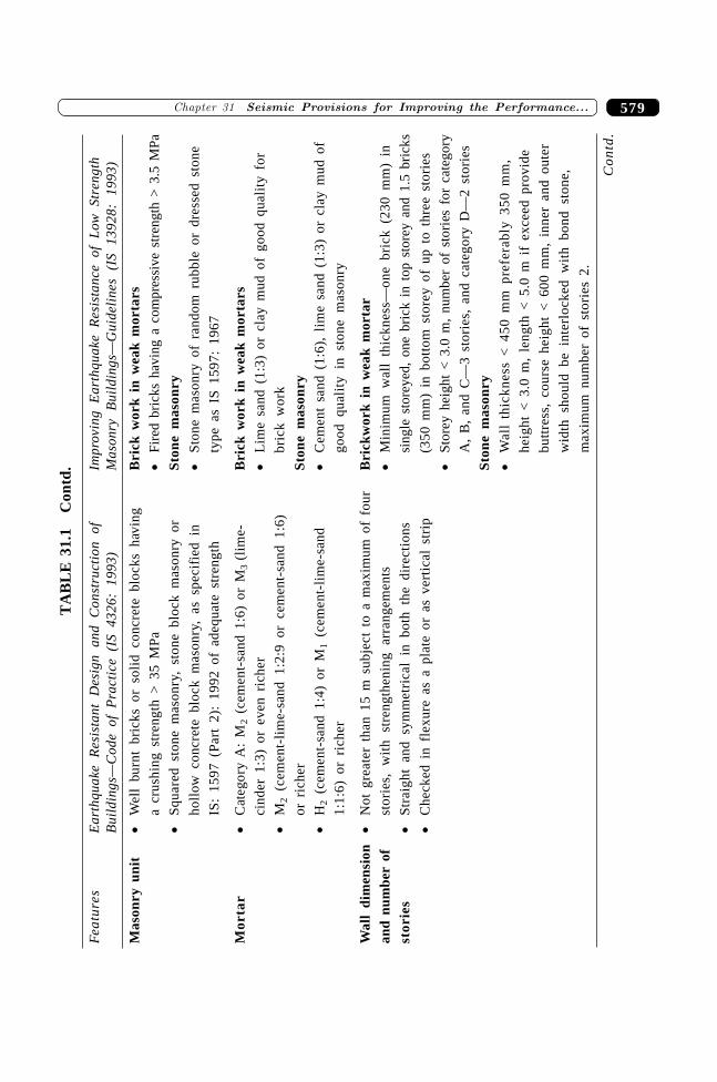
579�������� � �� ����� � ��� ��� ������ �� ��������������
Mas
onry
uni
t∑
Wel
l bu
rnt
bric
ks o
r so
lid
conc
rete
blo
cks
havi
ngB
rick
wor
k in
wea
k m
orta
rsa
crus
hing
str
engt
h >
35
MP
a∑
Fire
d br
icks
hav
ing
a co
mpr
essi
ve s
tren
gth
> 3
.5 M
Pa
∑S
quar
ed s
tone
mas
onry
, st
one
bloc
k m
ason
ry o
rSt
one
mas
onry
holl
ow c
oncr
ete
bloc
k m
ason
ry,
as s
peci
fied
in
∑S
tone
mas
onry
of
rand
om r
ubbl
e or
dre
ssed
sto
ne
IS:
1597
(P
art
2):
1992
of
adeq
uate
str
engt
hty
pe a
s IS
159
7: 1
967
Mor
tar
∑C
ateg
ory
A:
M2
(cem
ent-
sand
1:6
) or
M3
(lim
e-B
rick
wor
k in
wea
k m
orta
rsci
nder
1:3
) or
eve
n ri
cher
∑L
ime
sand
(1:
3) o
r cl
ay m
ud o
f go
od q
uali
ty f
or
∑M
2 (c
emen
t-li
me-
sand
1:2
:9 o
r ce
men
t-sa
nd 1
:6)
bric
k w
ork
or r
iche
rSt
one
mas
onry
∑H
2 (c
emen
t-sa
nd 1
:4)
or M
1 (c
emen
t-li
me-
sand
∑C
emen
t sa
nd (
1:6)
, li
me
sand
(1:
3) o
r cl
ay m
ud o
f
1:1:
6) o
r ri
cher
good
qua
lity
in
ston
e m
ason
ry
Wal
l di
men
sion
∑N
ot g
reat
er t
han
15 m
sub
ject
to
a m
axim
um o
f fo
urB
rick
wor
k in
wea
k m
orta
ran
d nu
mbe
r of
stor
ies,
wit
h st
reng
then
ing
arra
ngem
ents
∑M
inim
um w
all
thic
knes
s—on
e br
ick
(230
mm
) in
stor
ies
∑S
trai
ght
and
sym
met
rica
l in
bot
h th
e di
rect
ions
sing
le s
tore
yed,
one
bri
ck i
n to
p st
orey
and
1.5
bri
cks
∑C
heck
ed i
n fl
exur
e as
a p
late
or
as v
erti
cal
stri
p(3
50 m
m)
in b
otto
m s
tore
y of
up
to t
hree
sto
ries
∑S
tore
y he
ight
< 3
.0 m
, nu
mbe
r of
sto
ries
for
cat
egor
y
A,
B,
and
C—
3 st
orie
s, a
nd c
ateg
ory
D—
2 st
orie
s
Ston
e m
ason
ry∑
Wal
l th
ickn
ess
< 4
50 m
m p
refe
rabl
y 35
0 m
m,
heig
ht <
3.0
m,
leng
th <
5.0
m i
f ex
ceed
pro
vide
butt
ress
, co
urse
hei
ght
< 6
00 m
m,
inne
r an
d ou
ter
wid
th s
houl
d be
int
erlo
cked
wit
h bo
nd s
tone
,
max
imum
num
ber
of s
tori
es 2
.
TA
BL
E 3
1.1
Con
td.
Fea
ture
sE
arth
quak
e R
esis
tant
Des
ign
and
Con
stru
ctio
n of
Impr
ovin
g E
arth
quak
e R
esis
tanc
e of
Low
Str
engt
hB
uild
ings
—C
ode
of P
ract
ice
(IS
4326
: 19
93)
Mas
onry
B
uild
ings
—G
uide
line
s (I
S 13
928:
19
93)
Co
ntd
.
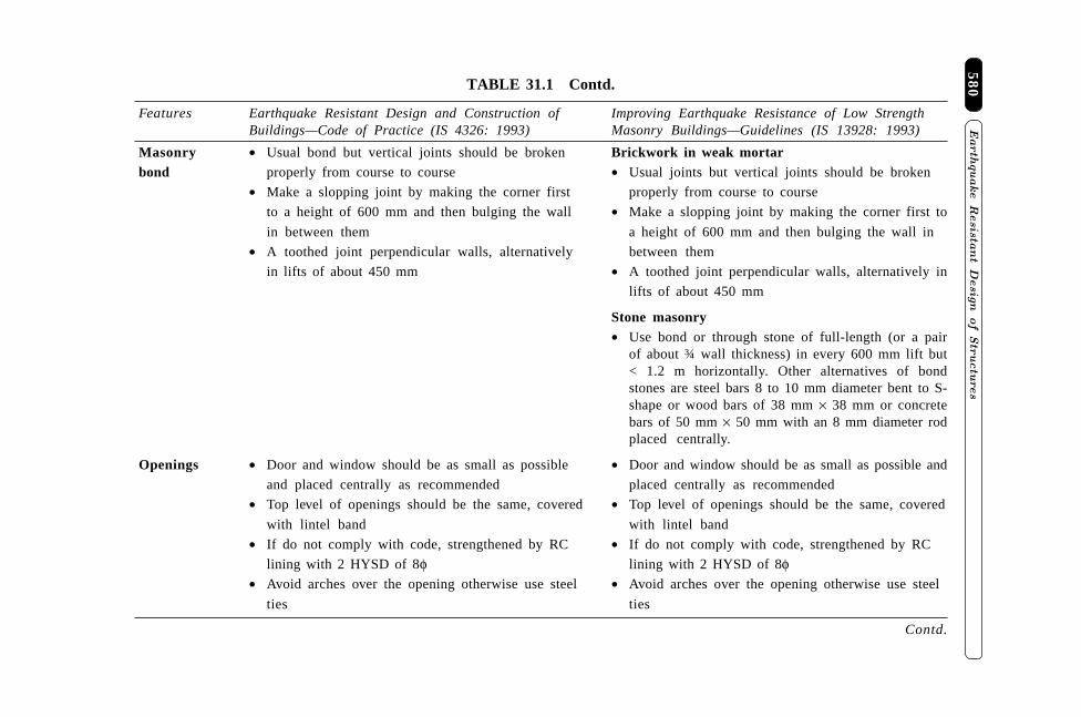
�����
������ �
����
�� �
���
���
����
��
580
Contd.
Masonry ∑ Usual bond but vertical joints should be broken Brickwork in weak mortarbond properly from course to course ∑ Usual joints but vertical joints should be broken
∑ Make a slopping joint by making the corner first properly from course to course
to a height of 600 mm and then bulging the wall ∑ Make a slopping joint by making the corner first to
in between them a height of 600 mm and then bulging the wall in
∑ A toothed joint perpendicular walls, alternatively between them
in lifts of about 450 mm ∑ A toothed joint perpendicular walls, alternatively in
lifts of about 450 mm
Stone masonry∑ Use bond or through stone of full-length (or a pair
of about ¾ wall thickness) in every 600 mm lift but< 1.2 m horizontally. Other alternatives of bondstones are steel bars 8 to 10 mm diameter bent to S-shape or wood bars of 38 mm ¥ 38 mm or concretebars of 50 mm ¥ 50 mm with an 8 mm diameter rodplaced centrally.
Openings ∑ Door and window should be as small as possible ∑ Door and window should be as small as possible and
and placed centrally as recommended placed centrally as recommended
∑ Top level of openings should be the same, covered ∑ Top level of openings should be the same, covered
with lintel band with lintel band
∑ If do not comply with code, strengthened by RC ∑ If do not comply with code, strengthened by RC
lining with 2 HYSD of 8f lining with 2 HYSD of 8f∑ Avoid arches over the opening otherwise use steel ∑ Avoid arches over the opening otherwise use steel
ties ties
TABLE 31.1 Contd.
Features Earthquake Resistant Design and Construction of Improving Earthquake Resistance of Low StrengthBuildings—Code of Practice (IS 4326: 1993) Masonry Buildings—Guidelines (IS 13928: 1993)
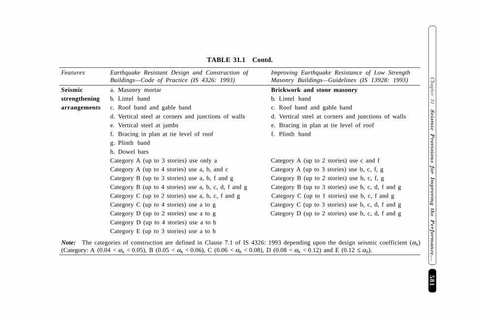
581�
�����
��
� �
� �
���� �
�����
���
���� �
���
����
��
������
Seismic a. Masonry mortar Brickwork and stone masonrystrengthening b. Lintel band b. Lintel band
arrangements c. Roof band and gable band c. Roof band and gable band
d. Vertical steel at corners and junctions of walls d. Vertical steel at corners and junctions of walls
e. Vertical steel at jambs e. Bracing in plan at tie level of roof
f. Bracing in plan at tie level of roof f. Plinth band
g. Plinth band
h. Dowel bars
Category A (up to 3 stories) use only a Category A (up to 2 stories) use c and f
Category A (up to 4 stories) use a, b, and c Category A (up to 3 stories) use b, c, f, g
Category B (up to 3 stories) use a, b, f and g Category B (up to 2 stories) use b, c, f, g
Category B (up to 4 stories) use a, b, c, d, f and g Category B (up to 3 stories) use b, c, d, f and g
Category C (up to 2 stories) use a, b, c, f and g Category C (up to 1 stories) use b, c, f and g
Category C (up to 4 stories) use a to g Category C (up to 3 stories) use b, c, d, f and g
Category D (up to 2 stories) use a to g Category D (up to 2 stories) use b, c, d, f and g
Category D (up to 4 stories) use a to h
Category E (up to 3 stories) use a to h
Note: The categories of construction are defined in Clause 7.1 of IS 4326: 1993 depending upon the design seismic coefficient (ah)(Category: A (0.04 < ah < 0.05), B (0.05 < ah < 0.06), C (0.06 < ah < 0.08), D (0.08 < ah < 0.12) and E (0.12 £ ah).
TABLE 31.1 Contd.
Features Earthquake Resistant Design and Construction of Improving Earthquake Resistance of Low StrengthBuildings—Code of Practice (IS 4326: 1993) Masonry Buildings—Guidelines (IS 13928: 1993)
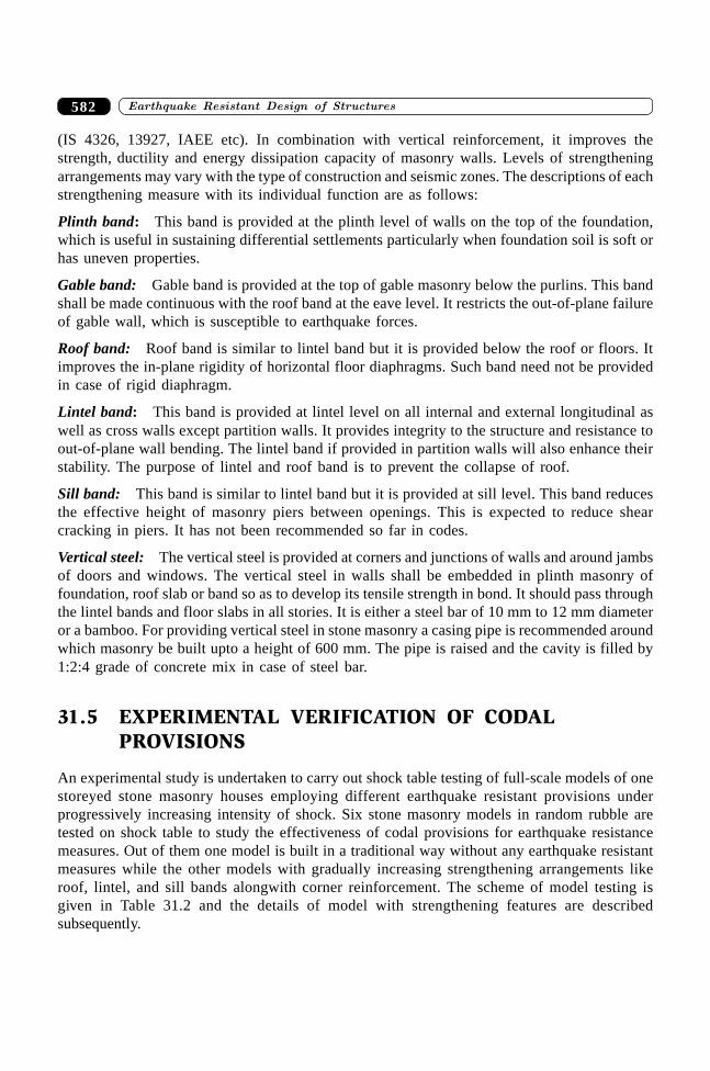
����������� ������� �������������582
(IS 4326, 13927, IAEE etc). In combination with vertical reinforcement, it improves thestrength, ductility and energy dissipation capacity of masonry walls. Levels of strengtheningarrangements may vary with the type of construction and seismic zones. The descriptions of eachstrengthening measure with its individual function are as follows:
Plinth band: This band is provided at the plinth level of walls on the top of the foundation,which is useful in sustaining differential settlements particularly when foundation soil is soft orhas uneven properties.
Gable band: Gable band is provided at the top of gable masonry below the purlins. This bandshall be made continuous with the roof band at the eave level. It restricts the out-of-plane failureof gable wall, which is susceptible to earthquake forces.
Roof band: Roof band is similar to lintel band but it is provided below the roof or floors. Itimproves the in-plane rigidity of horizontal floor diaphragms. Such band need not be providedin case of rigid diaphragm.
Lintel band: This band is provided at lintel level on all internal and external longitudinal aswell as cross walls except partition walls. It provides integrity to the structure and resistance toout-of-plane wall bending. The lintel band if provided in partition walls will also enhance theirstability. The purpose of lintel and roof band is to prevent the collapse of roof.
Sill band: This band is similar to lintel band but it is provided at sill level. This band reducesthe effective height of masonry piers between openings. This is expected to reduce shearcracking in piers. It has not been recommended so far in codes.
Vertical steel: The vertical steel is provided at corners and junctions of walls and around jambsof doors and windows. The vertical steel in walls shall be embedded in plinth masonry offoundation, roof slab or band so as to develop its tensile strength in bond. It should pass throughthe lintel bands and floor slabs in all stories. It is either a steel bar of 10 mm to 12 mm diameteror a bamboo. For providing vertical steel in stone masonry a casing pipe is recommended aroundwhich masonry be built upto a height of 600 mm. The pipe is raised and the cavity is filled by1:2:4 grade of concrete mix in case of steel bar.
31.5 EXPERIMENTAL VERIFICATION OF CODALPROVISIONS
An experimental study is undertaken to carry out shock table testing of full-scale models of onestoreyed stone masonry houses employing different earthquake resistant provisions underprogressively increasing intensity of shock. Six stone masonry models in random rubble aretested on shock table to study the effectiveness of codal provisions for earthquake resistancemeasures. Out of them one model is built in a traditional way without any earthquake resistantmeasures while the other models with gradually increasing strengthening arrangements likeroof, lintel, and sill bands alongwith corner reinforcement. The scheme of model testing isgiven in Table 31.2 and the details of model with strengthening features are describedsubsequently.
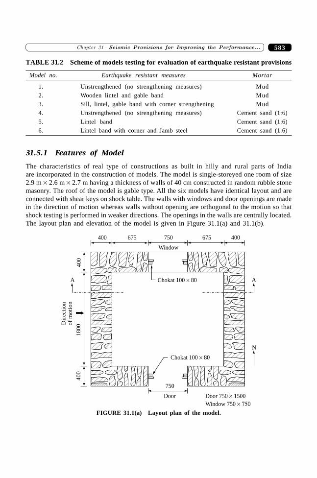
583�������� � �� ����� � ��� ��� ������ �� ��������������
TABLE 31.2 Scheme of models testing for evaluation of earthquake resistant provisions
Model no. Earthquake resistant measures Mortar
1. Unstrengthened (no strengthening measures) Mud
2. Wooden lintel and gable band Mud
3. Sill, lintel, gable band with corner strengthening Mud
4. Unstrengthened (no strengthening measures) Cement sand (1:6)
5. Lintel band Cement sand (1:6)
6. Lintel band with corner and Jamb steel Cement sand (1:6)
31.5.1 Features of Model
The characteristics of real type of constructions as built in hilly and rural parts of Indiaare incorporated in the construction of models. The model is single-storeyed one room of size2.9 m ¥ 2.6 m ¥ 2.7 m having a thickness of walls of 40 cm constructed in random rubble stonemasonry. The roof of the model is gable type. All the six models have identical layout and areconnected with shear keys on shock table. The walls with windows and door openings are madein the direction of motion whereas walls without opening are orthogonal to the motion so thatshock testing is performed in weaker directions. The openings in the walls are centrally located.The layout plan and elevation of the model is given in Figure 31.1(a) and 31.1(b).
750
Door
750
Window
675400 675 400
A
N
Chokat 100 80�
Door 750 1500�
Window 750 �����
Chokat 100 80�
40
04
00
18
00D
irecti
on
of
mo
tio
n
A
FIGURE 31.1(a) Layout plan of the model.
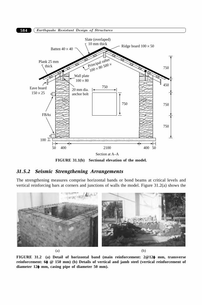
����������� ������� �������������584
Wall plate
100 80�
20 mm dia.anchor bolt
100
50 400 2100 400
750
750
750
450
750
750
Batten 40 40�
Slate (overlaped)10 mm thick
Ridge board 100 50�
Principal rafter
100 80 500�
�
Plank 25 mmthick
Eave board
150 25�
FBAs
Section at A–A
50
FIGURE 31.1(b) Sectional elevation of the model.
31.5.2 Seismic Strengthening Arrangements
The strengthening measures comprise horizontal bands or bond beams at critical levels andvertical reinforcing bars at corners and junctions of walls the model. Figure 31.2(a) shows the
(a) (b)
FIGURE 31.2 (a) Detail of horizontal band (main reinforcement: 2@12fffff mm, transversereinforcement: 6fffff @ 150 mm) (b) Details of vertical and jamb steel (vertical reinforcement ofdiameter 12fffff mm, casing pipe of diameter 50 mm).
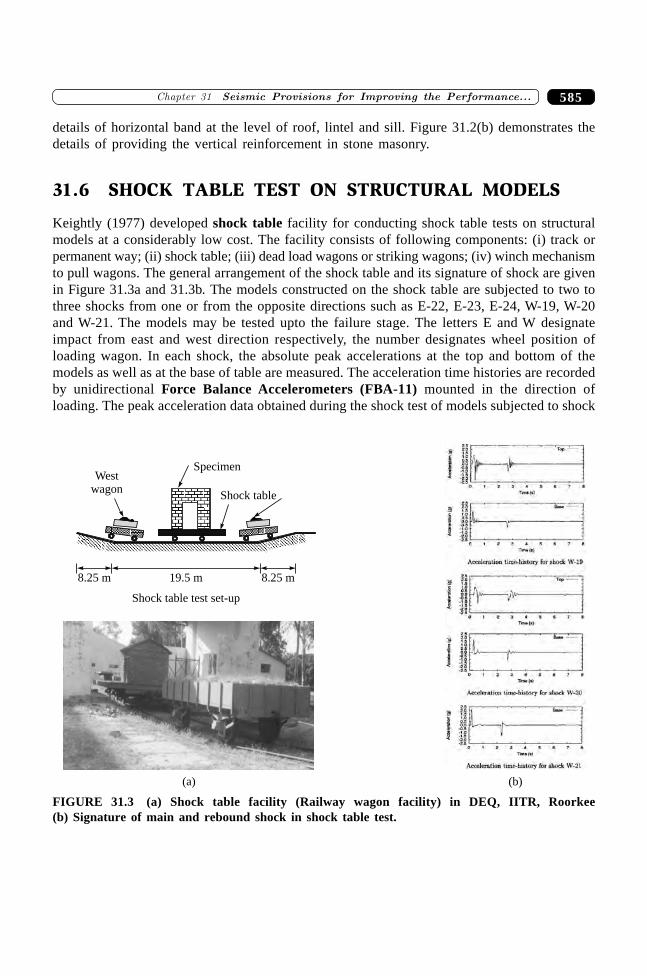
585�������� � �� ����� � ��� ��� ������ �� ��������������
details of horizontal band at the level of roof, lintel and sill. Figure 31.2(b) demonstrates thedetails of providing the vertical reinforcement in stone masonry.
31.6 SHOCK TABLE TEST ON STRUCTURAL MODELS
Keightly (1977) developed shock table facility for conducting shock table tests on structuralmodels at a considerably low cost. The facility consists of following components: (i) track orpermanent way; (ii) shock table; (iii) dead load wagons or striking wagons; (iv) winch mechanismto pull wagons. The general arrangement of the shock table and its signature of shock are givenin Figure 31.3a and 31.3b. The models constructed on the shock table are subjected to two tothree shocks from one or from the opposite directions such as E-22, E-23, E-24, W-19, W-20and W-21. The models may be tested upto the failure stage. The letters E and W designateimpact from east and west direction respectively, the number designates wheel position ofloading wagon. In each shock, the absolute peak accelerations at the top and bottom of themodels as well as at the base of table are measured. The acceleration time histories are recordedby unidirectional Force Balance Accelerometers (FBA-11) mounted in the direction ofloading. The peak acceleration data obtained during the shock test of models subjected to shock
Westwagon
Specimen
Shock table
8.25 m 8.25 m19.5 m
Shock table test set-up
(a) (b)
FIGURE 31.3 (a) Shock table facility (Railway wagon facility) in DEQ, IITR, Roorkee(b) Signature of main and rebound shock in shock table test.
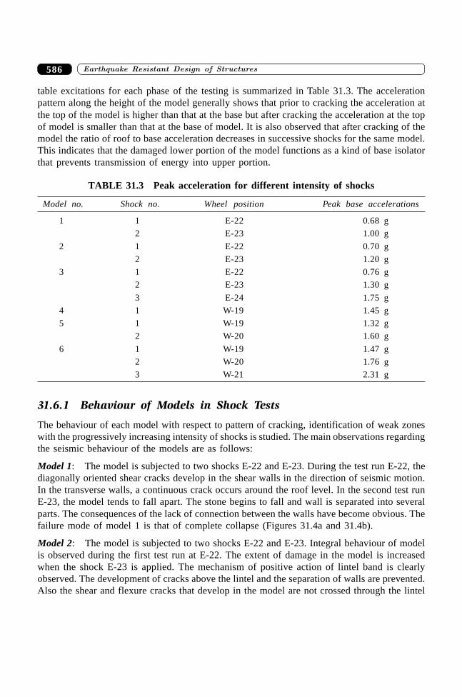
����������� ������� �������������586
table excitations for each phase of the testing is summarized in Table 31.3. The accelerationpattern along the height of the model generally shows that prior to cracking the acceleration atthe top of the model is higher than that at the base but after cracking the acceleration at the topof model is smaller than that at the base of model. It is also observed that after cracking of themodel the ratio of roof to base acceleration decreases in successive shocks for the same model.This indicates that the damaged lower portion of the model functions as a kind of base isolatorthat prevents transmission of energy into upper portion.
TABLE 31.3 Peak acceleration for different intensity of shocks
Model no. Shock no. Wheel position Peak base accelerations
1 1 E-22 0.68 g
2 E-23 1.00 g
2 1 E-22 0.70 g
2 E-23 1.20 g
3 1 E-22 0.76 g
2 E-23 1.30 g
3 E-24 1.75 g
4 1 W-19 1.45 g
5 1 W-19 1.32 g
2 W-20 1.60 g
6 1 W-19 1.47 g
2 W-20 1.76 g
3 W-21 2.31 g
31.6.1 Behaviour of Models in Shock Tests
The behaviour of each model with respect to pattern of cracking, identification of weak zoneswith the progressively increasing intensity of shocks is studied. The main observations regardingthe seismic behaviour of the models are as follows:
Model 1: The model is subjected to two shocks E-22 and E-23. During the test run E-22, thediagonally oriented shear cracks develop in the shear walls in the direction of seismic motion.In the transverse walls, a continuous crack occurs around the roof level. In the second test runE-23, the model tends to fall apart. The stone begins to fall and wall is separated into severalparts. The consequences of the lack of connection between the walls have become obvious. Thefailure mode of model 1 is that of complete collapse (Figures 31.4a and 31.4b).
Model 2: The model is subjected to two shocks E-22 and E-23. Integral behaviour of modelis observed during the first test run at E-22. The extent of damage in the model is increasedwhen the shock E-23 is applied. The mechanism of positive action of lintel band is clearlyobserved. The development of cracks above the lintel and the separation of walls are prevented.Also the shear and flexure cracks that develop in the model are not crossed through the lintel
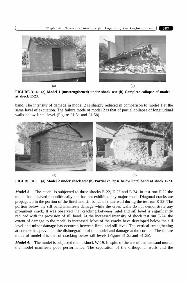
587�������� � �� ����� � ��� ��� ������ �� ��������������
band. The intensity of damage in model 2 is sharply reduced in comparison to model 1 at thesame level of excitation. The failure mode of model 2 is that of partial collapse of longitudinalwalls below lintel level (Figure 31.5a and 31.5b).
(a) (b)
FIGURE 31.5 (a) Model 2 under shock test (b) Partial collapse below lintel band at shock E-23.
Model 3: The model is subjected to three shocks E-22, E-23 and E-24. In test run E-22 themodel has behaved monolithically and has not exhibited any major crack. Diagonal cracks arepropagated in the portion of the lintel and sill bands of shear wall during the test run E-23. Theportion below the sill band manifests damage while the cross walls do not demonstrate anyprominent crack. It was observed that cracking between lintel and sill level is significantlyreduced with the provision of sill band. At the increased intensity of shock test run E-24, theextent of damage to the model is increased. Most of the cracks have developed below the silllevel and minor damage has occurred between lintel and sill level. The vertical strengtheningat corners has prevented the disintegration of the model and damage at the corners. The failuremode of model 3 is that of cracking below sill levels (Figure 31.6a and 31.6b).
Model 4: The model is subjected to one shock W-19. In spite of the use of cement sand mortarthe model manifests poor performance. The separation of the orthogonal walls and the
(a) (b)
FIGURE 31.4 (a) Model 1 (unstrengthened) under shock test (b) Complete collapse of model 1at shock E-23.
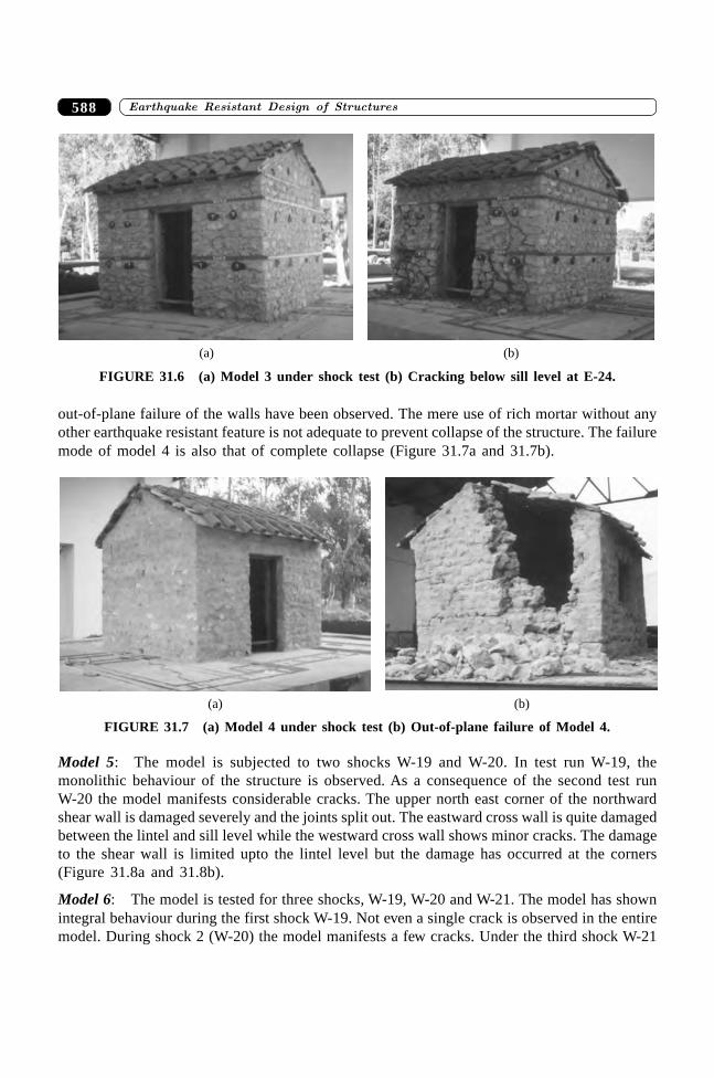
����������� ������� �������������588
out-of-plane failure of the walls have been observed. The mere use of rich mortar without anyother earthquake resistant feature is not adequate to prevent collapse of the structure. The failuremode of model 4 is also that of complete collapse (Figure 31.7a and 31.7b).
(a) (b)
FIGURE 31.7 (a) Model 4 under shock test (b) Out-of-plane failure of Model 4.
Model 5: The model is subjected to two shocks W-19 and W-20. In test run W-19, themonolithic behaviour of the structure is observed. As a consequence of the second test runW-20 the model manifests considerable cracks. The upper north east corner of the northwardshear wall is damaged severely and the joints split out. The eastward cross wall is quite damagedbetween the lintel and sill level while the westward cross wall shows minor cracks. The damageto the shear wall is limited upto the lintel level but the damage has occurred at the corners(Figure 31.8a and 31.8b).
Model 6: The model is tested for three shocks, W-19, W-20 and W-21. The model has shownintegral behaviour during the first shock W-19. Not even a single crack is observed in the entiremodel. During shock 2 (W-20) the model manifests a few cracks. Under the third shock W-21
(a) (b)
FIGURE 31.6 (a) Model 3 under shock test (b) Cracking below sill level at E-24.

589�������� � �� ����� � ��� ��� ������ �� ��������������
though the model has remained intact yet it is cracked considerably. The cracking is mainlyconcentrated between lintel and sill level (Figure 31.9a and 31.9b).
(a) (b)
FIGURE 31.9 (a) Model 6 under shock test (b) Crack pattern of Model 6.
31.6.2 Recommendations
Some important recommendations have been arrived at from the study of shock response ofstone masonry models which are highlighted below:
1. The provision of seismic band at lintel level is the minimum requirement to preventcollapse of house made in mud or cement sand mortar. The mere use of rich mortarwithout any other earthquake resistance measure is not adequate to prevent collapse ofstructures.
2. The codal provisions are effective in reducing the damage mainly above the lintel level.The brittle shear failure in wall piers still occurs. The cracking in piers can be reduced
(a) (b)
FIGURE 31.8 (a) Model 5 under shock test, strengthened with lintel band (b) Crack pattern ofModel 5 at shock W-20, cracking below lintel level.

����������� ������� �������������590
by providing the additional horizontal band, preferably at sill level. The verticalreinforcement at the corner of model, in combination with horizontal bands increasesthe strength of model as well as reduces the cracking at corners.
SUMMARY
Masonry is widely used for housing construction in India and many countries of the world. Thepast earthquakes that have occurred in Indian subcontinent reveal that the root cause ofdevastation is the collapse of non-engineered masonry construction. Hence, it is necessary toincrease the seismic resistance of non-engineered masonry construction by providing someadditional features. The present chapter presents the summary of earthquake resistant featuresfor improving the seismic performance of non-engineered masonry buildings. In order todevelop a better understanding of the efficacy, reliability and acceptability of these measures,an experimental verification is also present. The experimental study is undertaken to carry outshock table testing of full-scale models of one storeyed stone masonry houses employingdifferent strengthening measures under progressively increasing intensity of shock.
REFERENCES
[1] Agarwal, P. and Thakkar, S.K., “Seismic Evaluation of Strengthening and RetrofittingMeasures in Stone Masonry Houses under Shock Loading”, Workshop on Retrofittingof Structures, IIT Roorkee, Oct. 2003.
[2] Agarwal, P. and Thakkar, S.K., “An Experimental Study of Effectiveness of SeismicStrengthening and Retrofitting Measures in Stone Masonry Buildings”, Journal ofEuropean Earthquake Engineering, pp. 48–64, 2002.
[3] Agarwal, P. and Thakkar, S.K., “Study of Adequacy of Earthquake Resistance andRetrofitting Measures of Stone Masonry Buildings”, Research Highlights in EarthSystems Science, DST Special, Vol. 2, on ‘Seismicity’ pp. 327–335, O.P. Verma (Ed.),Indian Geological Congress, August 2001.
[4] Agarwal, P. and Thakkar, S.K., “Seismic Evaluation of Strengthening Measures inStone Masonry Houses”, Eleventh Symposium on Earthquake Engineering, Universityof Roorkee, Roorkee, December 17–19, 1998.
[5] IS 13828, Improving Earthquake Resistance of Low Strength Masonry Buildings—Guidelines, Bureau of Indian Standards, New Delhi, 1993.
[6] IS 4326, Earthquake Resistant Design and Construction of Buildings—Code ofPractice, Bureau of Indian Standards, New Delhi, 1993.
[7] IAEE, “Basic Concepts of Seismic Codes—Vol. I”, The International Association forEarthquake Engineering, Tokyo, Japan, 1980.
[8] Keightley, W.O., Report on Indo-US Subcommission on Education and Culture,Department of Earthquake Engineering, University of Roorkee, Roorkee, 1977.
[9] Thakkar, S.K. and Agarwal, P., “Seismic Evaluation of Earthquake Resistant andRetrofitting Measures of Stone Masonry Houses”, Paper No. 110, 12th WCEE,February 2000, Auckland, New Zealand, 1999.
591�������� ��������������� �����������
591
Retrofitting ofMasonry Buildings
��������
32.1 INTRODUCTION
Masonry buildings are the most common type of construction used for housing purpose allaround the world. In India masonry construction is employed in the rural, urban and hillyregions upto its optimum, since it is flexible enough to accommodate itself according to theprevailing environmental conditions. That is why more than 90% population of the countryprefers to live in such houses. Although this type of construction is most oftenly preferred andmost frequently employed yet it is not completely perfect with regard to seismic efficiency. Ithas likewise some flaws. The recent earthquakes in India reveal that its low seismic resistancehas proved to be one of the principal causes of extensive damage, as compared to other modesof construction like reinforced concrete and steel. In addition improper seismic design ofmasonry building emerges as a sister cause of such devastation. It is evidently clear that aproper adherence to recommended earthquake resistant measures as per IS code may avoid sucha heavy loss of life and property. But the already constructed, in use buildings facing the threatof further damage in future seismic activity turn out to be a challenge to earthquake engineeringcommunity which is making ceaseless perennial efforts in finding out ways to minimize thedamage. In this regard retrofitting of existing buildings may emerge as a probable possibilitywhich implies incorporation of earthquake resistant measure in either seismically deficientor earthquake damaged parent constructions. This is a difficult but essential task becausefirstly there is a majority of seismically deficient buildings and secondly due to economicconsiderations and immediate shelter requirements earthquake damaged buildings cannot bereplaced or rebuilt in the event of an earthquake. Hence it is the need of the hour to retrofit wellin time the seismically deficient or seismically damaged buildings as per current codes so thatthey may be safely reused in future.
The past experience of retrofitted buildings has not been very convincing and promising.But the recent studies show that proper retrofitting may very well upgrade the seismic resistancebringing it at par with the newly constructed earthquake resistant design construction. Innumerableconventional and non-conventional techniques have been applied and employed for retrofitting
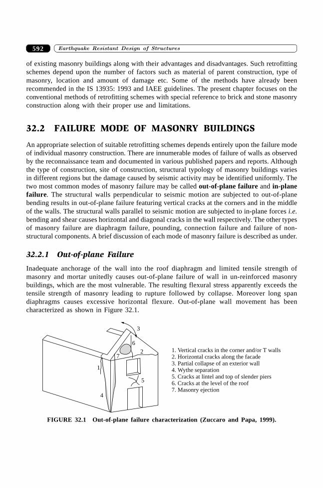
������������ � ������ ������������� 592
of existing masonry buildings along with their advantages and disadvantages. Such retrofittingschemes depend upon the number of factors such as material of parent construction, type ofmasonry, location and amount of damage etc. Some of the methods have already beenrecommended in the IS 13935: 1993 and IAEE guidelines. The present chapter focuses on theconventional methods of retrofitting schemes with special reference to brick and stone masonryconstruction along with their proper use and limitations.
32.2 FAILURE MODE OF MASONRY BUILDINGS
An appropriate selection of suitable retrofitting schemes depends entirely upon the failure modeof individual masonry construction. There are innumerable modes of failure of walls as observedby the reconnaissance team and documented in various published papers and reports. Althoughthe type of construction, site of construction, structural typology of masonry buildings variesin different regions but the damage caused by seismic activity may be identified uniformly. Thetwo most common modes of masonry failure may be called out-of-plane failure and in-planefailure. The structural walls perpendicular to seismic motion are subjected to out-of-planebending results in out-of-plane failure featuring vertical cracks at the corners and in the middleof the walls. The structural walls parallel to seismic motion are subjected to in-plane forces i.e.bending and shear causes horizontal and diagonal cracks in the wall respectively. The other typesof masonry failure are diaphragm failure, pounding, connection failure and failure of non-structural components. A brief discussion of each mode of masonry failure is described as under.
32.2.1 Out-of-plane Failure
Inadequate anchorage of the wall into the roof diaphragm and limited tensile strength ofmasonry and mortar unitedly causes out-of-plane failure of wall in un-reinforced masonrybuildings, which are the most vulnerable. The resulting flexural stress apparently exceeds thetensile strength of masonry leading to rupture followed by collapse. Moreover long spandiaphragms causes excessive horizontal flexure. Out-of-plane wall movement has beencharacterized as shown in Figure 32.1.
1. Vertical cracks in the corner and/or T walls2. Horizontal cracks along the facade3. Partial collapse of an exterior wall4. Wythe separation5. Cracks at lintel and top of slender piers6. Cracks at the level of the roof7. Masonry ejection
6
2
3
7
1
5
4
FIGURE 32.1 Out-of-plane failure characterization (Zuccaro and Papa, 1999).
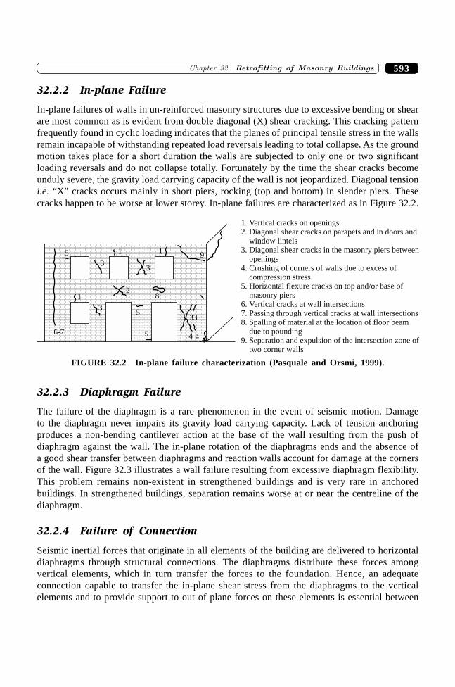
593�������� ��������������� �����������
32.2.2 In-plane Failure
In-plane failures of walls in un-reinforced masonry structures due to excessive bending or shearare most common as is evident from double diagonal (X) shear cracking. This cracking patternfrequently found in cyclic loading indicates that the planes of principal tensile stress in the wallsremain incapable of withstanding repeated load reversals leading to total collapse. As the groundmotion takes place for a short duration the walls are subjected to only one or two significantloading reversals and do not collapse totally. Fortunately by the time the shear cracks becomeunduly severe, the gravity load carrying capacity of the wall is not jeopardized. Diagonal tensioni.e. “X” cracks occurs mainly in short piers, rocking (top and bottom) in slender piers. Thesecracks happen to be worse at lower storey. In-plane failures are characterized as in Figure 32.2.
5
33
1 19
8
3
1
5
5
2
4 4
33
6-7
1. Vertical cracks on openings2. Diagonal shear cracks on parapets and in doors and
window lintels3. Diagonal shear cracks in the masonry piers between
openings4. Crushing of corners of walls due to excess of
compression stress5. Horizontal flexure cracks on top and/or base of
masonry piers6. Vertical cracks at wall intersections7. Passing through vertical cracks at wall intersections8. Spalling of material at the location of floor beam
due to pounding9. Separation and expulsion of the intersection zone of
two corner walls
FIGURE 32.2 In-plane failure characterization (Pasquale and Orsmi, 1999).
32.2.3 Diaphragm Failure
The failure of the diaphragm is a rare phenomenon in the event of seismic motion. Damageto the diaphragm never impairs its gravity load carrying capacity. Lack of tension anchoringproduces a non-bending cantilever action at the base of the wall resulting from the push ofdiaphragm against the wall. The in-plane rotation of the diaphragms ends and the absence ofa good shear transfer between diaphragms and reaction walls account for damage at the cornersof the wall. Figure 32.3 illustrates a wall failure resulting from excessive diaphragm flexibility.This problem remains non-existent in strengthened buildings and is very rare in anchoredbuildings. In strengthened buildings, separation remains worse at or near the centreline of thediaphragm.
32.2.4 Failure of Connection
Seismic inertial forces that originate in all elements of the building are delivered to horizontaldiaphragms through structural connections. The diaphragms distribute these forces amongvertical elements, which in turn transfer the forces to the foundation. Hence, an adequateconnection capable to transfer the in-plane shear stress from the diaphragms to the verticalelements and to provide support to out-of-plane forces on these elements is essential between
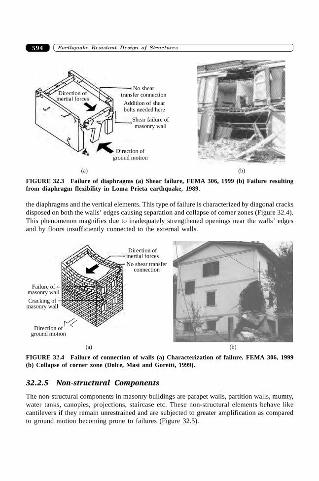
������������ � ������ ������������� 594
the diaphragms and the vertical elements. This type of failure is characterized by diagonal cracksdisposed on both the walls’ edges causing separation and collapse of corner zones (Figure 32.4).This phenomenon magnifies due to inadequately strengthened openings near the walls’ edgesand by floors insufficiently connected to the external walls.
Direction ofinertial forces
No shear transferconnection
Cracking ofmasonry wall
Failure ofmasonry wall
(b)(a)
Direction ofground motion
FIGURE 32.4 Failure of connection of walls (a) Characterization of failure, FEMA 306, 1999(b) Collapse of corner zone (Dolce, Masi and Goretti, 1999).
32.2.5 Non-structural Components
The non-structural components in masonry buildings are parapet walls, partition walls, mumty,water tanks, canopies, projections, staircase etc. These non-structural elements behave likecantilevers if they remain unrestrained and are subjected to greater amplification as comparedto ground motion becoming prone to failures (Figure 32.5).
No sheartransfer connection
Addition of shearbolts needed here
Shear failure ofmasonry wall
Direction ofground motion
Direction ofinertial forces
(a) (b)
FIGURE 32.3 Failure of diaphragms (a) Shear failure, FEMA 306, 1999 (b) Failure resultingfrom diaphragm flexibility in Loma Prieta earthquake, 1989.
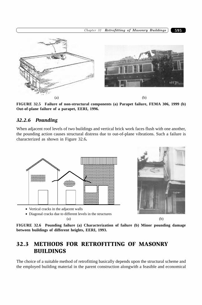
595�������� ��������������� �����������
(a) (b)
FIGURE 32.5 Failure of non-structural components (a) Parapet failure, FEMA 306, 1999 (b)Out-of-plane failure of a parapet, EERI, 1996.
32.2.6 Pounding
When adjacent roof levels of two buildings and vertical brick work faces flush with one another,the pounding action causes structural distress due to out-of-plane vibrations. Such a failure ischaracterized as shown in Figure 32.6.
� Vertical cracks in the adjacent walls
� Diagonal cracks due to different levels in the structures
(b)(a)
FIGURE 32.6 Pounding failure (a) Characterization of failure (b) Minor pounding damagebetween buildings of different heights, EERI, 1993.
32.3 METHODS FOR RETROFITTING OF MASONRYBUILDINGS
The choice of a suitable method of retrofitting basically depends upon the structural scheme andthe employed building material in the parent construction alongwith a feasible and economical

������������ � ������ ������������� 596
technology. Moreover an understanding of failure mode, structural behaviour with the weak andstrong aspects of design as derived from the earthquake damage surveys also influence theselection of retrofitting schemes. Numerous techniques, used to retrofit seismically deficient ordamaged masonry buildings, may be broadly classified into three categories on the basis of theireffect on structural performance namely, (i) improving the existing masonry strength anddeformability, not related to any specific objective which is similar to the repairing processof masonry structures; (ii) improving the in-plane strength of the wall or any weak zone of thesection akin to local/member retrofitting and (iii) improving the structural integrity of thewhole structure in terms of in-plane and out-of-plane strength or only against out-of-planeforces very much like the global/structural retrofitting. Various techniques under each schemeare described as:
32.3.1 Repair
It is a process to preserve the mechanical efficiency of a masonry structure and to increase shearresistance of walls having large internal voids. The commonly employed repairing techniquesof masonry are (i) cement or epoxy injection (ii) reinforced injection (iii) grouting with cementor epoxy (iv) insertion of stones (v) re-pointing of mortar.
32.3.2 Local/Member Retrofitting
It enhances the shear resistance of un-reinforced masonry components especially against in-plane forces. Feasible retrofitting techniques are: (i) surface coatings (ii) shotcrete overlays oradhered fabric with wire mesh or FRP materials (iii) use of RC and steel frames in openings.
32.3.3 Structural/Global Retrofitting
Improving the response of existing un-reinforced masonry buildings to both gravity and seismicloads it provides them “box type” behaviour and increases the flexural strength of un-reinforcedwalls and piers. The most common techniques are (i) addition of reinforcement (ii) externalbinding or jacketing (iii) prestressing, (iv) confinements with RC element and steel sections (v)strengthening of wall intersections and (vi) strengthening of connection between walls and floor.
32.4 REPAIRING TECHNIQUES OF MASONRY
Repairing of cracks or replacement of damaged wall sections is an essential feature of repairprocess. It is a general assumption that repairing only helps to retain the original shape of thestructure without increasing its strength. The main two problems solved during the repairingprocess are: (i) masonry cracking and (ii) masonry deterioration.
32.4.1 Masonry Cracking
According to Grimm, 1988, a crack may be defined as a “break, split, fracture, fissure, separation,cleavage, or elongated narrow opening visible to the normal human eye and extending from the
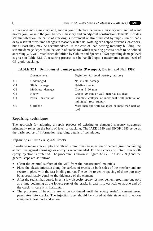
597�������� ��������������� �����������
surface and into a masonry unit, mortar joint, interface between a masonry unit and adjacentmortar joint, or into the joint between masonry and an adjacent construction element”. Besidesseismic vibration, the cause of cracking is movement or strain induced by imposition of loadsor by restraint of volume changes in masonry materials. Nothing can help to prevent such cracks,but at least they may be accommodated. In the case of load bearing masonry building, theseismic damage depends on the width of cracks for which repairing process needs to be definedaccordingly. A well-established definition by Coburn and Spence (1992) regarding damage levelis given in Table 32.1. A repairing process can be handled upto a maximum damage level ofG3 grade cracking.
TABLE 32.1 Definitions of damage grades (Davenport, Burton and Nail 1999)
Damage level Definition for load bearing masonry
G0 Undamaged No visible damage
G1 Slight damage Hairline cracks
G2 Moderate damage Cracks 5–20 mm
G3 Heavy Cracks 20 mm or wall material dislodge
G4 Partial destruction Complete collapse of individual wall material orindividual roof support
G5 Collapse More than one wall collapsed or more than half ofroof
Repairing techniques
The approach for adopting a repair process of existing or damaged masonry structuresprincipally relies on the basis of level of cracking. The IAEE 1980 and UNDP 1983 serve asthe basic source of information regarding details of techniques.
Repair of G0 and G1 grade cracks
In order to repair cracks upto a width of 5 mm, pressure injection of cement grout containingadmixtures against shrinkage or epoxy is recommended. For fine cracks of upto 1 mm widthepoxy injection is preferred. The procedure is shown in Figure 32.7 (IS 13935: 1993) and thegeneral steps are as follows:
∑ Clean the external surface of the wall from the nonstructural materials∑ Place the plastic injection along the surface of cracks on both sides of the member and are
secure in place with the fast binding mortar. The centre-to-centre spacing of these port maybe approximately equal to the thickness of the element
∑ After the sealant has cured, inject a low viscosity epoxy resin/or cement grout into one portat a time beginning at the lowest part of the crack, in case it is vertical, or at one end ofthe crack, in case it is horizontal.
∑ The processes of injection are to be continued until the epoxy resin/or cement groutpenetrates into cracks. The injection port should be closed at this stage and injectionequipment next port and so on.
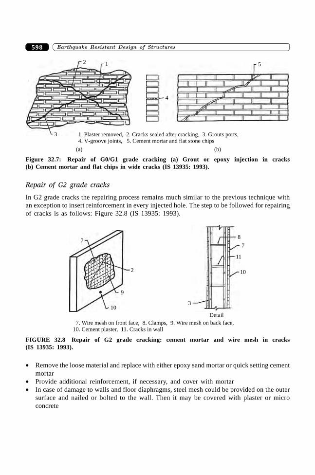
������������ � ������ ������������� 598
2 1
4
5
3 1. Plaster removed, 2. Cracks sealed after cracking, 3. Grouts ports,4. V-groove joints, 5. Cement mortar and flat stone chips
(a) (b)
Figure 32.7: Repair of G0/G1 grade cracking (a) Grout or epoxy injection in cracks(b) Cement mortar and flat chips in wide cracks (IS 13935: 1993).
Repair of G2 grade cracks
In G2 grade cracks the repairing process remains much similar to the previous technique withan exception to insert reinforcement in every injected hole. The step to be followed for repairingof cracks is as follows: Figure 32.8 (IS 13935: 1993).
7
2
9
10
7
10
8
11
3
7. Wire mesh on front face, 8. Clamps, 9. Wire mesh on back face,10. Cement plaster, 11. Cracks in wall
Detail
FIGURE 32.8 Repair of G2 grade cracking: cement mortar and wire mesh in cracks(IS 13935: 1993).
∑ Remove the loose material and replace with either epoxy sand mortar or quick setting cementmortar
∑ Provide additional reinforcement, if necessary, and cover with mortar∑ In case of damage to walls and floor diaphragms, steel mesh could be provided on the outer
surface and nailed or bolted to the wall. Then it may be covered with plaster or microconcrete
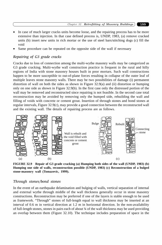
599�������� ��������������� �����������
∑ In case of much larger cracks units become loose, and the repairing process has to be moreextensive than injection. In that case defined process is, UNDP, 1983, (a) remove crackedunits (b) insert new units in rich mortar or the use of steel bars/stitching dogs (c) fill thevoid
∑ Same procedure can be repeated on the opposite side of the wall if necessary
Repairing of G3 grade cracks
Cracks due to loss of connection among the multi-wythe masonry walls may be categorized asG3 grade cracking. Multi-wythe wall construction practice is frequent in the rural and hillyregions of India with stone masonry houses built in poor mortars. Such wall constructionshappen to be more susceptible to out-of-plane forces resulting in collapse of the outer leaf ofmultiple leaves stone masonry walls. There may be two possibilities of damage (i) permanentdistortion of wall on both the sides as shown in Figure 32.9(a) and (ii) distortion or humpingonly on one side as shown in Figure 32.9(b). In the first case only the distressed portion of thewall may be removed and reconstructed since repairing is not feasible. In the second case totalreconstruction may be avoided by removing only the humped side, rebuilding the wall andfilling of voids with concrete or cement grout. Insertion of through stones and bond stones atregular intervals, Figure 32.9(c), may provide a good connection between the reconstructed walland the existing wall. The details of repairing process are as follows.
Wall is rebuilt andthe void filled withconcrete or cement
grout
Bulge Rebuilt
Connectingstone
(a) (b) (c)
FIGURE 32.9 Repair of G3 grade cracking (a) Humping both sides of the wall (UNDP, 1983) (b)Humping one side of walls, reconstruction possible (UNDP, 1983) (c) Reconstruction of a bulgedstone-masonry wall (Tomazevic, 1999).
Through stones/bond stones
In the event of an earthquake delamination and bulging of walls, vertical separation of internaland external wythe through middle of the wall thickness generally occur in stone masonryconstructions. Reconstruction may be preferred if one of the layers is stable enough to be usedas framework. “Through” stones of full-length equal to wall thickness may be inserted at aninterval of 0.6 m in vertical direction at 1.2 m in horizontal direction. In the non-availabilityof full-length stones, stones in pairs each of about ¾ of the wall thickness may be used providingan overlap between them (Figure 32.10). The technique includes preparation of space in the
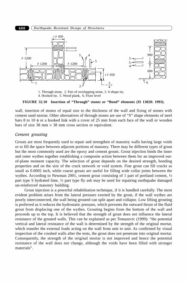
������������ � ������ ������������� 600
wall, insertion of stones of equal size to the thickness of the wall and fixing of stones withcement sand mortar. Other alternatives of through stones are use of “S” shape elements of steelbars 8 to 10 f or a hooked link with a cover of 25 mm from each face of the wall or woodenbars of size 38 mm ¥ 38 mm cross section or equivalent.
Cement grouting
Grouts are most frequently used to repair and strengthen of masonry walls having large voidsor to fill the space between adjacent portions of masonry. There may be different types of groutbut the most commonly used are the epoxy and cement grouts. Grout injection binds the innerand outer wythes together establishing a composite action between them for an improved out-of-plane moment capacity. The selection of grout depends on the desired strength, bondingproperties and on the size of the crack network or void system. Fine grout can fill cracks assmall as 0.0005 inch, while coarse grouts are useful for filling wide collar joints between thewythes. According to Newman 2001, cement grout consisting of 1 part of portland cement, ½part type S hydrated lime, ½ part type fly ash may be used for repairing earthquake damagedun-reinforced masonry building.
Grout injection is a powerful rehabilitation technique, if it is handled carefully. The mostevident problem arises from the lateral pressure exerted by the grout, if the wall wythes arepoorly interconnected, the wall being grouted can split apart and collapse. Low lifting groutingis preferred as it reduces the hydrostatic pressure, which prevents the outward thrust of the fluidgrout from displacing one of the wythes. Grouting begins from the bottom of the wall andproceeds up to the top. It is believed that the strength of grout does not influence the lateralresistance of the grouted walls. This can be explained as per Tomazevic (1999): “the potentialvertical and lateral resistance of the wall is determined by the strength of the original mortar,which transfer the external loads acting on the wall from unit to unit. As confirmed by visualinspection of the crushed walls after the tests, the grout does not penetrate into original mortar.Consequently, the strength of the original mortar is not improved and hence the potentialresistance of the wall does not change, although the voids have been filled with strongermaterials”.
t > 450
34
t<
t > 450
3 4
5> 1200
> 1200 > 1200
12
6
3
54
900
600
1. Through stone, 2. Pair of overlapping stone, 3. S-shape tie,4. Hooked tie, 5. Wood plank, 6. Floor level
FIGURE 32.10 Insertion of “Through” stones or “Bond” elements (IS 13828: 1993).
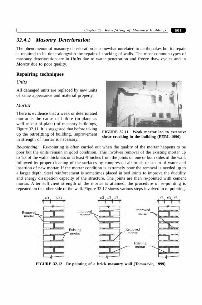
601�������� ��������������� �����������
32.4.2 Masonry Deterioration
The phenomenon of masonry deterioration is somewhat unrelated to earthquakes but its repairis required to be done alongwith the repair of cracking of walls. The most common types ofmasonry deterioration are in Units due to water penetration and freeze thaw cycles and inMortar due to poor quality.
Repairing techniques
Units
All damaged units are replaced by new unitsof same appearance and material property.
Mortar
There is evidence that a weak or deterioratedmortar is the cause of failure (in-plane aswell as out-of-plane) of masonry buildings,Figure 32.11. It is suggested that before takingup the retrofitting of building, improvementin strength of mortar is necessary.
Re-pointing: Re-pointing is often carried out when the quality of the mortar happens to bepoor but the units remain in good condition. This involves removal of the existing mortar upto 1/3 of the walls thickness or at least ¾ inches from the joints on one or both sides of the wall,followed by proper cleaning of the surfaces by compressed air brush or steam of water andinsertion of new mortar. If the mortar condition is extremely poor the removal is needed up toa larger depth. Steel reinforcement is sometimes placed in bed joints to improve the ductilityand energy dissipation capacity of the structure. The joints are then re-pointed with cementmortar. After sufficient strength of the mortar is attained, the procedure of re-pointing isrepeated on the other side of the wall. Figure 32.12 shows various steps involved in re-pointing.
t/3 2/3 t t/3 t/3 t/3 t/3 t/3 t/3
Improvedmortar
Existingmortar
Removedmortar
Improvedmortar
Removedmortar
Existingmortar
FIGURE 32.12 Re-pointing of a brick masonry wall (Tomazevic, 1999).
FIGURE 32.11 Weak mortar led to extensiveshear cracking in the building (EERI, 1996).
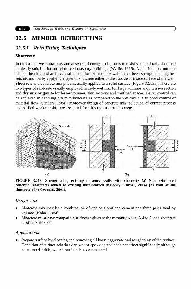
������������ � ������ ������������� 602
32.5 MEMBER RETROFITTING
32.5.1 Retrofitting Techniques
Shotcrete
In the case of weak masonry and absence of enough solid piers to resist seismic loads, shotcreteis ideally suitable for un-reinforced masonry buildings (Wyllie, 1996). A considerable numberof load bearing and architectural un-reinforced masonry walls have been strengthened againstseismic motion by applying a layer of shotcrete either to the outside or inside surface of the wall.Shotcrete is a concrete mix pneumatically applied to a solid surface (Figure 32.13a). There aretwo types of shotcrete usually employed namely wet mix for large volumes and massive sectionand dry mix or gunite for lesser volumes, thin sections and confined spaces. Better control canbe achieved in handling dry mix shotcrete as compared to the wet mix due to good control ofmaterial flow (Sanders, 1984). Moreover design of concrete mix, selection of correct processand skilled workmanship are essential for effective use of shotcrete.
New anchor
Min
imu
m
1.5
d
d
Shotcreterib
Shotcreterib
d
Min
imu
m
1.5
d(a) (b)
FIGURE 32.13 Strengthening existing masonry walls with shotcrete (a) New reinforcedconcrete (shotcrete) added to existing unreinforced masonry (Turner, 2004) (b) Plan of theshotcrete rib (Newman, 2001).
Design mix
∑ Shotcrete mix may be a combination of one part portland cement and three parts sand byvolume (Kahn, 1984)
∑ Shotcrete must have compatible stiffness values to the masonry walls. A 4 to 5 inch shotcreteis often sufficient.
Applications
∑ Prepare surface by cleaning and removing all loose aggregate and roughening of the surface.Condition of surface whether dry, wet or epoxy coated does not affect significantly althougha saturated brick, wetted surface is recommended.
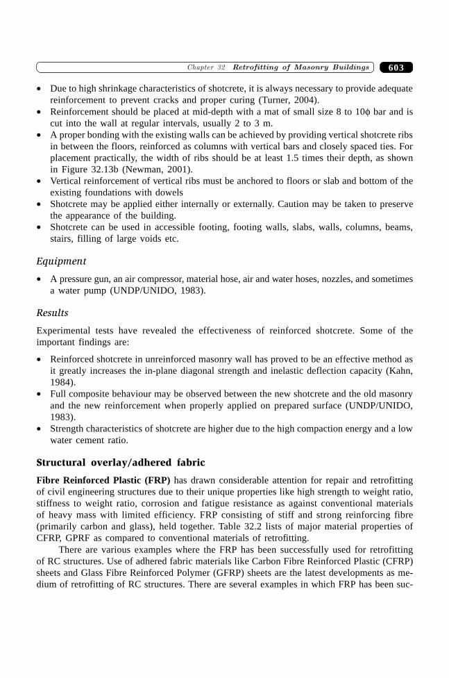
603�������� ��������������� �����������
∑ Due to high shrinkage characteristics of shotcrete, it is always necessary to provide adequatereinforcement to prevent cracks and proper curing (Turner, 2004).
∑ Reinforcement should be placed at mid-depth with a mat of small size 8 to 10f bar and iscut into the wall at regular intervals, usually 2 to 3 m.
∑ A proper bonding with the existing walls can be achieved by providing vertical shotcrete ribsin between the floors, reinforced as columns with vertical bars and closely spaced ties. Forplacement practically, the width of ribs should be at least 1.5 times their depth, as shownin Figure 32.13b (Newman, 2001).
∑ Vertical reinforcement of vertical ribs must be anchored to floors or slab and bottom of theexisting foundations with dowels
∑ Shotcrete may be applied either internally or externally. Caution may be taken to preservethe appearance of the building.
∑ Shotcrete can be used in accessible footing, footing walls, slabs, walls, columns, beams,stairs, filling of large voids etc.
Equipment
∑ A pressure gun, an air compressor, material hose, air and water hoses, nozzles, and sometimesa water pump (UNDP/UNIDO, 1983).
Results
Experimental tests have revealed the effectiveness of reinforced shotcrete. Some of theimportant findings are:
∑ Reinforced shotcrete in unreinforced masonry wall has proved to be an effective method asit greatly increases the in-plane diagonal strength and inelastic deflection capacity (Kahn,1984).
∑ Full composite behaviour may be observed between the new shotcrete and the old masonryand the new reinforcement when properly applied on prepared surface (UNDP/UNIDO,1983).
∑ Strength characteristics of shotcrete are higher due to the high compaction energy and a lowwater cement ratio.
Structural overlay/adhered fabric
Fibre Reinforced Plastic (FRP) has drawn considerable attention for repair and retrofittingof civil engineering structures due to their unique properties like high strength to weight ratio,stiffness to weight ratio, corrosion and fatigue resistance as against conventional materialsof heavy mass with limited efficiency. FRP consisting of stiff and strong reinforcing fibre(primarily carbon and glass), held together. Table 32.2 lists of major material properties ofCFRP, GPRF as compared to conventional materials of retrofitting.
There are various examples where the FRP has been successfully used for retrofittingof RC structures. Use of adhered fabric materials like Carbon Fibre Reinforced Plastic (CFRP)sheets and Glass Fibre Reinforced Polymer (GFRP) sheets are the latest developments as me-dium of retrofitting of RC structures. There are several examples in which FRP has been suc-
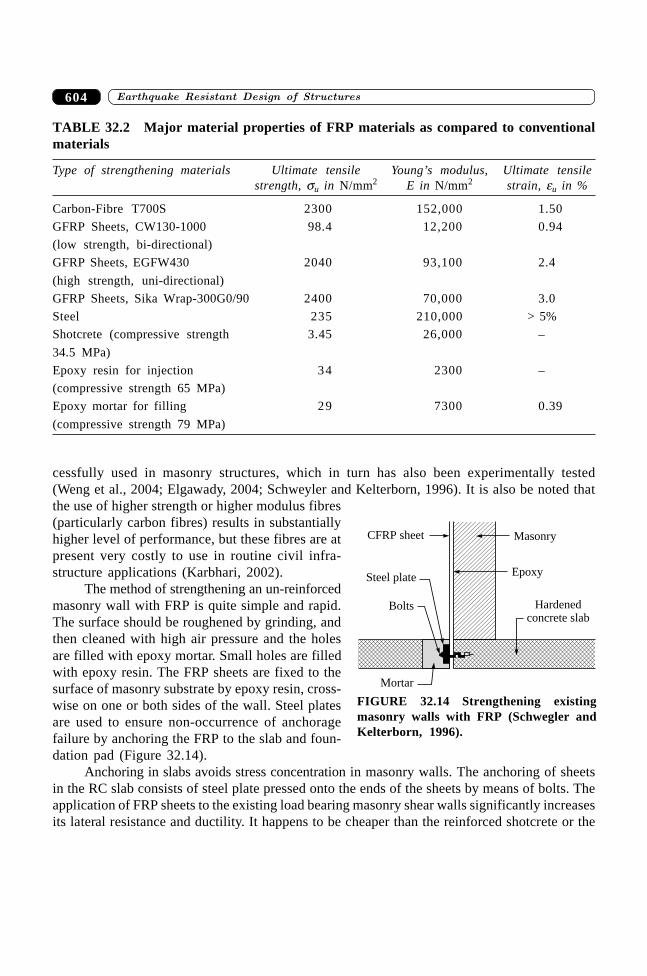
������������ � ������ ������������� 604
cessfully used in masonry structures, which in turn has also been experimentally tested(Weng et al., 2004; Elgawady, 2004; Schweyler and Kelterborn, 1996). It is also be noted thatthe use of higher strength or higher modulus fibres(particularly carbon fibres) results in substantiallyhigher level of performance, but these fibres are atpresent very costly to use in routine civil infra-structure applications (Karbhari, 2002).
The method of strengthening an un-reinforcedmasonry wall with FRP is quite simple and rapid.The surface should be roughened by grinding, andthen cleaned with high air pressure and the holesare filled with epoxy mortar. Small holes are filledwith epoxy resin. The FRP sheets are fixed to thesurface of masonry substrate by epoxy resin, cross-wise on one or both sides of the wall. Steel platesare used to ensure non-occurrence of anchoragefailure by anchoring the FRP to the slab and foun-dation pad (Figure 32.14).
Anchoring in slabs avoids stress concentration in masonry walls. The anchoring of sheetsin the RC slab consists of steel plate pressed onto the ends of the sheets by means of bolts. Theapplication of FRP sheets to the existing load bearing masonry shear walls significantly increasesits lateral resistance and ductility. It happens to be cheaper than the reinforced shotcrete or the
TABLE 32.2 Major material properties of FRP materials as compared to conventionalmaterials
Type of strengthening materials Ultimate tensile Young’s modulus, Ultimate tensilestrength, su in N/mm2 E in N/mm2 strain, eu in %
Carbon-Fibre T700S 2300 152,000 1.50
GFRP Sheets, CW130-1000 98.4 12,200 0.94
(low strength, bi-directional)
GFRP Sheets, EGFW430 2040 93,100 2.4
(high strength, uni-directional)
GFRP Sheets, Sika Wrap-300G0/90 2400 70,000 3.0
Steel 235 210,000 > 5%
Shotcrete (compressive strength 3.45 26,000 –
34.5 MPa)
Epoxy resin for injection 34 2300 –
(compressive strength 65 MPa)
Epoxy mortar for filling 29 7300 0.39
(compressive strength 79 MPa)
Masonry
Epoxy
CFRP sheet
Steel plate
Bolts Hardenedconcrete slab
Mortar
FIGURE 32.14 Strengthening existingmasonry walls with FRP (Schwegler andKelterborn, 1996).
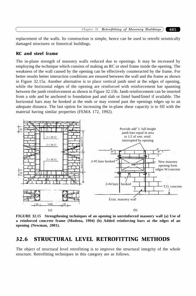
605�������� ��������������� �����������
replacement of the walls. Its construction is simple, hence can be used to retrofit seismicallydamaged structures or historical buildings.
RC and steel frame
The in-plane strength of masonry walls reduced due to openings. It may be increased byemploying the technique which consists of making an RC or steel frame inside the opening. Theweakness of the wall caused by the opening can be effectively counteracted by the frame. Forbetter results better interaction conditions are ensured between the wall and the frame as shownin Figure 32.15a. Another alternative is to place vertical jamb steel at the edges of opening,while the horizontal edges of the opening are reinforced with reinforcement bar spanningbetween the jamb reinforcement as shown in Figure 32.15b. Jamb reinforcement can be insertedfrom a side and be anchored to foundation pad and slab or lintel band/lintel if available. Thehorizontal bars may be hooked at the ends or may extend past the openings edges up to anadequate distance. The last option for increasing the in-plane shear capacity is to fill with thematerial having similar properties (FEMA 172, 1992).
2 3 12� f
2 3 12� f
2 3 12� f
20
20
20 20VAB
max
.0.7
5m
ax.0
.75
Provide add’ L full-heightjamb bars equal in area
to 1/2 of vert. reinf.interrupted by opening
New masonryopening form
edges W/concrete
T.O. concrete
2-#5 bars hooked
2-#4 bars hooked
Exist. masonry wall
(b)(a)
FIGURE 32.15 Strengthening techniques of an opening in unreinforced masonry wall (a) Use ofa reinforced concrete frame (Modena, 1994) (b) Added reinforcing bars at the edges of anopening (Newman, 2001).
32.6 STRUCTURAL LEVEL RETROFITTING METHODS
The object of structural level retrofitting is to improve the structural integrity of the wholestructure. Retrofitting techniques in this category are as follows.
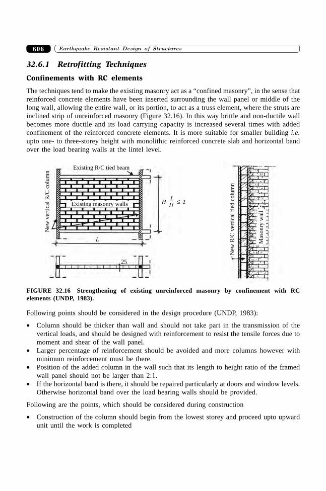
������������ � ������ ������������� 606
32.6.1 Retrofitting Techniques
Confinements with RC elements
The techniques tend to make the existing masonry act as a “confined masonry”, in the sense thatreinforced concrete elements have been inserted surrounding the wall panel or middle of thelong wall, allowing the entire wall, or its portion, to act as a truss element, where the struts areinclined strip of unreinforced masonry (Figure 32.16). In this way brittle and non-ductile wallbecomes more ductile and its load carrying capacity is increased several times with addedconfinement of the reinforced concrete elements. It is more suitable for smaller building i.e.upto one- to three-storey height with monolithic reinforced concrete slab and horizontal bandover the load bearing walls at the lintel level.
Existing R/C tied beam
Existing masonry walls
New
ver
tica
lR
/Cco
lum
n
L
25M
aso
nry
wal
l
New
R/C
ver
tica
lti
edco
lum
n
LH
H 2£
FIGURE 32.16 Strengthening of existing unreinforced masonry by confinement with RCelements (UNDP, 1983).
Following points should be considered in the design procedure (UNDP, 1983):
∑ Column should be thicker than wall and should not take part in the transmission of thevertical loads, and should be designed with reinforcement to resist the tensile forces due tomoment and shear of the wall panel.
∑ Larger percentage of reinforcement should be avoided and more columns however withminimum reinforcement must be there.
∑ Position of the added column in the wall such that its length to height ratio of the framedwall panel should not be larger than 2:1.
∑ If the horizontal band is there, it should be repaired particularly at doors and window levels.Otherwise horizontal band over the load bearing walls should be provided.
Following are the points, which should be considered during construction
∑ Construction of the column should begin from the lowest storey and proceed upto upwardunit until the work is completed
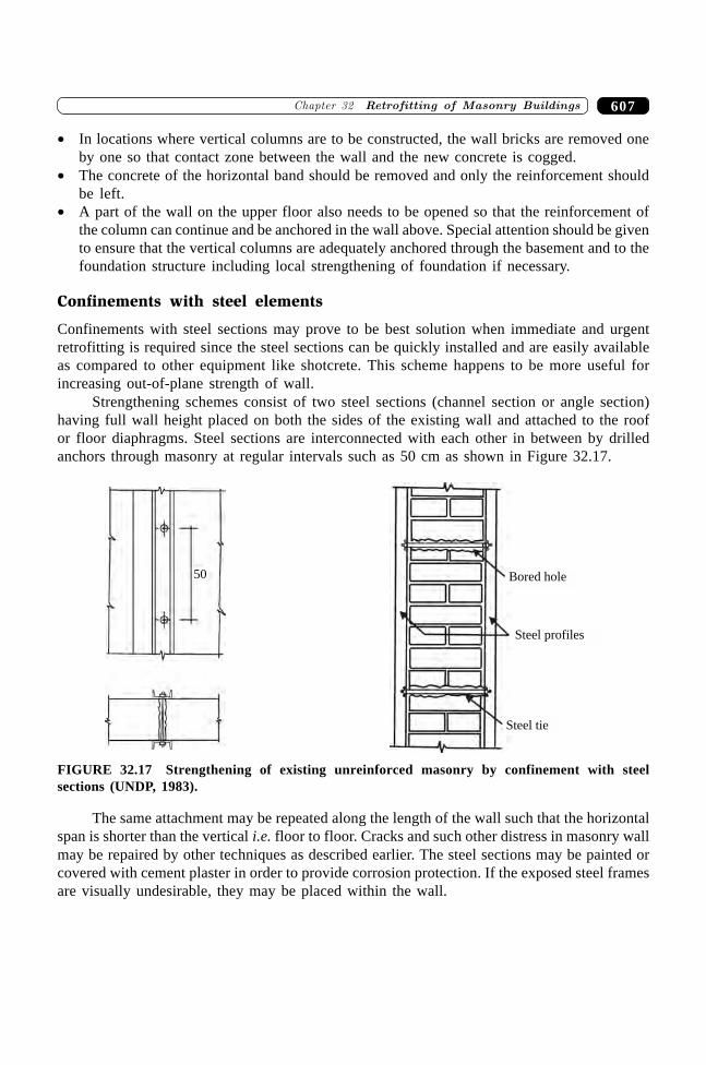
607�������� ��������������� �����������
∑ In locations where vertical columns are to be constructed, the wall bricks are removed oneby one so that contact zone between the wall and the new concrete is cogged.
∑ The concrete of the horizontal band should be removed and only the reinforcement shouldbe left.
∑ A part of the wall on the upper floor also needs to be opened so that the reinforcement ofthe column can continue and be anchored in the wall above. Special attention should be givento ensure that the vertical columns are adequately anchored through the basement and to thefoundation structure including local strengthening of foundation if necessary.
Confinements with steel elements
Confinements with steel sections may prove to be best solution when immediate and urgentretrofitting is required since the steel sections can be quickly installed and are easily availableas compared to other equipment like shotcrete. This scheme happens to be more useful forincreasing out-of-plane strength of wall.
Strengthening schemes consist of two steel sections (channel section or angle section)having full wall height placed on both the sides of the existing wall and attached to the roofor floor diaphragms. Steel sections are interconnected with each other in between by drilledanchors through masonry at regular intervals such as 50 cm as shown in Figure 32.17.
50 Bored hole
Steel profiles
Steel tie
FIGURE 32.17 Strengthening of existing unreinforced masonry by confinement with steelsections (UNDP, 1983).
The same attachment may be repeated along the length of the wall such that the horizontalspan is shorter than the vertical i.e. floor to floor. Cracks and such other distress in masonry wallmay be repaired by other techniques as described earlier. The steel sections may be painted orcovered with cement plaster in order to provide corrosion protection. If the exposed steel framesare visually undesirable, they may be placed within the wall.
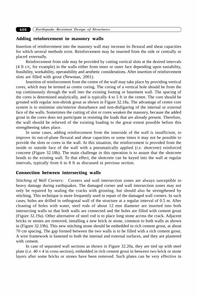
������������ � ������ ������������� 608
Adding reinforcement to masonry walls
Insertion of reinforcement into the masonry wall may increase its flexural and shear capacitiesfor which several methods exist. Reinforcement may be inserted from the side or centrally orplaced externally.
Reinforcement from side may be provided by cutting vertical slots at the desired intervals(4 ft c/c, for example) in the walls either from inner or outer face depending upon easiability,feasibility, workability, operatability and aesthetic considerations. After insertion of reinforcementslots are filled with grout (Newman, 2001).
Insertion of reinforcement from the centre of the wall may take place by providing verticalcores, which may be termed as centre coring. The coring of a vertical hole should be from thetop continuously through the wall into the existing footing or basement wall. The spacing ofthe cores is determined analytically, and is typically 4 to 5 ft in the centre. The core should begrouted with regular non-shrink grout as shown in Figure 32.18a. The advantage of centre coresystem is to minimise site/interior disturbance and non-disfiguring of the internal or externalface of the walls. Sometimes the cutting of slot or cores weaken the masonry, because the addedgrout in the cores does not participate in resisting the loads that are already present. Therefore,the wall should be relieved of the existing loading to the great extent possible before thisstrengthening takes place.
In some cases, adding reinforcement from the innerside of the wall is insufficient, toimprove its out-of-plane flexural and shear capacities or some times it may not be possible toprovide the slots or cores in the wall. At this situation, the reinforcement is provided from theinside or outside face of the wall with a pneumatically applied (i.e. shotcrete) reinforcedconcrete (Figure 32.18b). The main challenge in this operation is to assure that the shotcretebonds to the existing wall. To that effect, the shotcrete can be keyed into the wall at regularintervals, typically from 6 to 8 ft as discussed in previous section.
Connection between intersecting walls
Stitching of Wall Corners: Corners and wall intersection zones are always susceptible toheavy damage during earthquakes. The damaged corner and wall intersection zones may notonly be repaired by sealing the cracks with grouting, but should also be strengthened bystitching. This technique is more frequently used in repair of the damaged wall corners. In suchcases, holes are drilled in orthogonal wall of the structure at a regular interval of 0.5 m. Aftercleaning of holes with water, steel rods of about 12 mm diameter are inserted into bothintersecting walls so that both walls are connected and the holes are filled with cement grout(Figure 32.19a). Other alternative of steel rod is to place long stone across the crack. Adjacentbricks or stones are removed, installing a new brick or stone, common to both walls as shownin (Figure 32.19b). This new stitching stone should be embedded in rich cement grout, at about70 cm spacing. The gap formed between the two walls is to be filled with a rich cement grout.A wire framework is fastened to both the internal and external surfaces, and they are plasteredwith cement.
In case of separated wall sections as shown in Figure 32.20a, they are tied up with steelplate (i.e. 40 ¥ 4 in cross section), embedded in rich cement grout in between two brick or stonelayers after some bricks or stones have been removed. Such plates can be very effective in
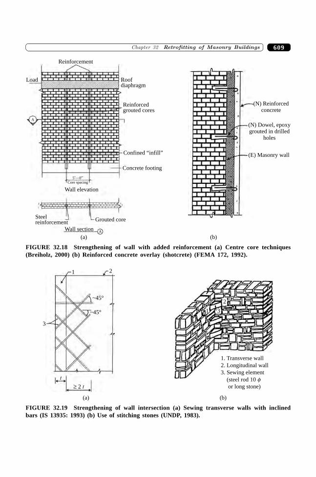
609�������� ��������������� �����������
Reinforcement
Steelreinforcement
Grouted core
Wall sectionA
Wall elevation
5 —0�� �
Core spacing
Concrete footing
Confined “infill”
Reinforcedgrouted cores
Roofdiaphragm
A
Load
(N) Reinforcedconcrete
(N) Dowel, epoxygrouted in drilled
holes
(E) Masonry wall
(a) (b)
FIGURE 32.18 Strengthening of wall with added reinforcement (a) Centre core techniques(Breiholz, 2000) (b) Reinforced concrete overlay (shotcrete) (FEMA 172, 1992).
~45°
~45°
3
� 2 t
t
1 2
2
31
(a) (b)
1. Transverse wall
2. Longitudinal wall
3. Sewing element
(steel rod 10
or long stone)
f
FIGURE 32.19 Strengthening of wall intersection (a) Sewing transverse walls with inclinedbars (IS 13935: 1993) (b) Use of stitching stones (UNDP, 1983).

������������ � ������ ������������� 610
reinforcing the corner but they cannot bring the walls back to vertical position. The gap is thensealed and the surface be covered with wire trellies and plaster as mentioned above.
Another alternative of steel plate is to drill horizontal holes in the masonry through verticalcrack and grouting or epoxing steel rods in the holes. In both these procedures, the remainingcracks should be filled with cement mortar. To reduce the separation prior to repair, tie rods,installed on both sides of the walls, can be used, Figure 32.20b.
Metallic plate for bondingup the wall
Metallic plate forbonding up the wall
CrackCrack
(a) (b)
FIGURE 32.20 Strengthening of separated wall intersection (a) Use of steel plates (b) Use of tierod (UNDP, 1983).
In case of total collapse of corner region, which is generally uncommon, strengthening isrequired by rebuilding of the corners with proper bond of the rebuilt part and the wall onto thecontact surface (Figure 32.21a). A horizontal belt like a seismic band of thickness 15 to 20 cm,reinforcement 4 @ 16 f and stirrups 6 mm at 20 cm, should be added. A reinforced concretecorner column properly tied into the intersecting walls could be added to strengthen the wallintersection. Such column should have minimum reinforcement of 4 @ 16 mm and stirrups6F mm at 20 cm, (Figure 32.21b).
4 16f u 6/20f
(a) (b)
FIGURE 32.21 Strengthening of collapse wall intersection (a) Rebuilding (b) Use of RC column(UNDP, 1983).
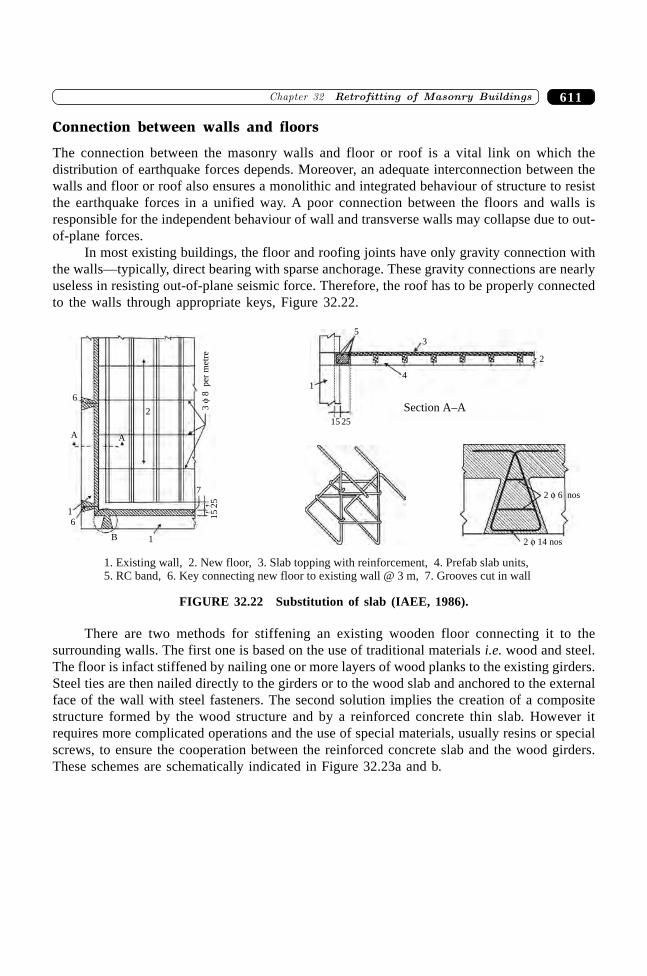
611�������� ��������������� �����������
Connection between walls and floors
The connection between the masonry walls and floor or roof is a vital link on which thedistribution of earthquake forces depends. Moreover, an adequate interconnection between thewalls and floor or roof also ensures a monolithic and integrated behaviour of structure to resistthe earthquake forces in a unified way. A poor connection between the floors and walls isresponsible for the independent behaviour of wall and transverse walls may collapse due to out-of-plane forces.
In most existing buildings, the floor and roofing joints have only gravity connection withthe walls—typically, direct bearing with sparse anchorage. These gravity connections are nearlyuseless in resisting out-of-plane seismic force. Therefore, the roof has to be properly connectedto the walls through appropriate keys, Figure 32.22.
1. Existing wall, 2. New floor, 3. Slab topping with reinforcement, 4. Prefab slab units,5. RC band, 6. Key connecting new floor to existing wall @ 3 m, 7. Grooves cut in wall
Section A–A
2 14 nos�
2 6 nos�
2
3
4
5
1
15 25
38
per
met
re�
2
6
A A
16
B 1
7
15
25
FIGURE 32.22 Substitution of slab (IAEE, 1986).
There are two methods for stiffening an existing wooden floor connecting it to thesurrounding walls. The first one is based on the use of traditional materials i.e. wood and steel.The floor is infact stiffened by nailing one or more layers of wood planks to the existing girders.Steel ties are then nailed directly to the girders or to the wood slab and anchored to the externalface of the wall with steel fasteners. The second solution implies the creation of a compositestructure formed by the wood structure and by a reinforced concrete thin slab. However itrequires more complicated operations and the use of special materials, usually resins or specialscrews, to ensure the cooperation between the reinforced concrete slab and the wood girders.These schemes are schematically indicated in Figure 32.23a and b.
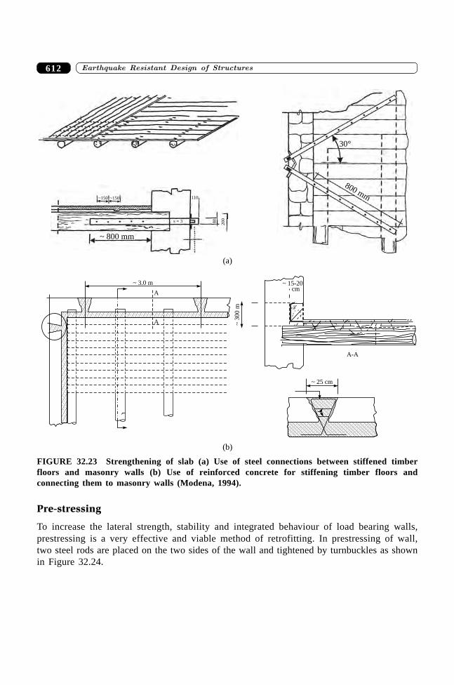
������������ � ������ ������������� 612
~ 800 mm
~150 ~150 110
20
0
80s = 3
30°
800 mm
(a)
A
A
~ 3.0 m
~300
m
~ 15-20cm
A-A
~ 25 cm
(b)
FIGURE 32.23 Strengthening of slab (a) Use of steel connections between stiffened timberfloors and masonry walls (b) Use of reinforced concrete for stiffening timber floors andconnecting them to masonry walls (Modena, 1994).
Pre-stressing
To increase the lateral strength, stability and integrated behaviour of load bearing walls,prestressing is a very effective and viable method of retrofitting. In prestressing of wall,two steel rods are placed on the two sides of the wall and tightened by turnbuckles as shownin Figure 32.24.
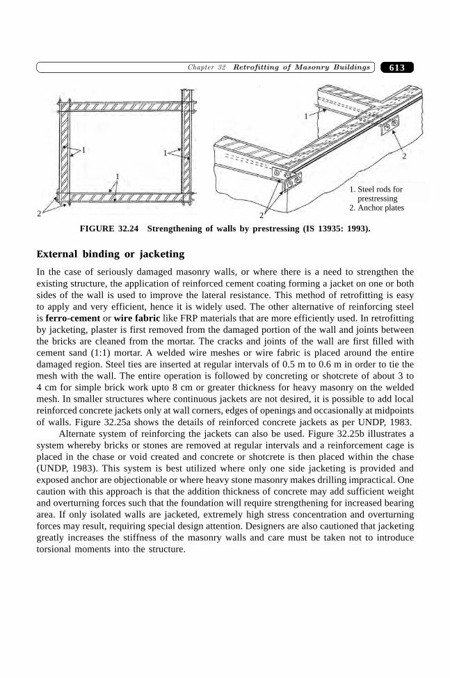
613�������� ��������������� �����������
2
1
1 1
2
2
1. Steel rods forprestressing
2. Anchor plates
1
FIGURE 32.24 Strengthening of walls by prestressing (IS 13935: 1993).
External binding or jacketing
In the case of seriously damaged masonry walls, or where there is a need to strengthen theexisting structure, the application of reinforced cement coating forming a jacket on one or bothsides of the wall is used to improve the lateral resistance. This method of retrofitting is easyto apply and very efficient, hence it is widely used. The other alternative of reinforcing steelis ferro-cement or wire fabric like FRP materials that are more efficiently used. In retrofittingby jacketing, plaster is first removed from the damaged portion of the wall and joints betweenthe bricks are cleaned from the mortar. The cracks and joints of the wall are first filled withcement sand (1:1) mortar. A welded wire meshes or wire fabric is placed around the entiredamaged region. Steel ties are inserted at regular intervals of 0.5 m to 0.6 m in order to tie themesh with the wall. The entire operation is followed by concreting or shotcrete of about 3 to4 cm for simple brick work upto 8 cm or greater thickness for heavy masonry on the weldedmesh. In smaller structures where continuous jackets are not desired, it is possible to add localreinforced concrete jackets only at wall corners, edges of openings and occasionally at midpointsof walls. Figure 32.25a shows the details of reinforced concrete jackets as per UNDP, 1983.
Alternate system of reinforcing the jackets can also be used. Figure 32.25b illustrates asystem whereby bricks or stones are removed at regular intervals and a reinforcement cage isplaced in the chase or void created and concrete or shotcrete is then placed within the chase(UNDP, 1983). This system is best utilized where only one side jacketing is provided andexposed anchor are objectionable or where heavy stone masonry makes drilling impractical. Onecaution with this approach is that the addition thickness of concrete may add sufficient weightand overturning forces such that the foundation will require strengthening for increased bearingarea. If only isolated walls are jacketed, extremely high stress concentration and overturningforces may result, requiring special design attention. Designers are also cautioned that jacketinggreatly increases the stiffness of the masonry walls and care must be taken not to introducetorsional moments into the structure.
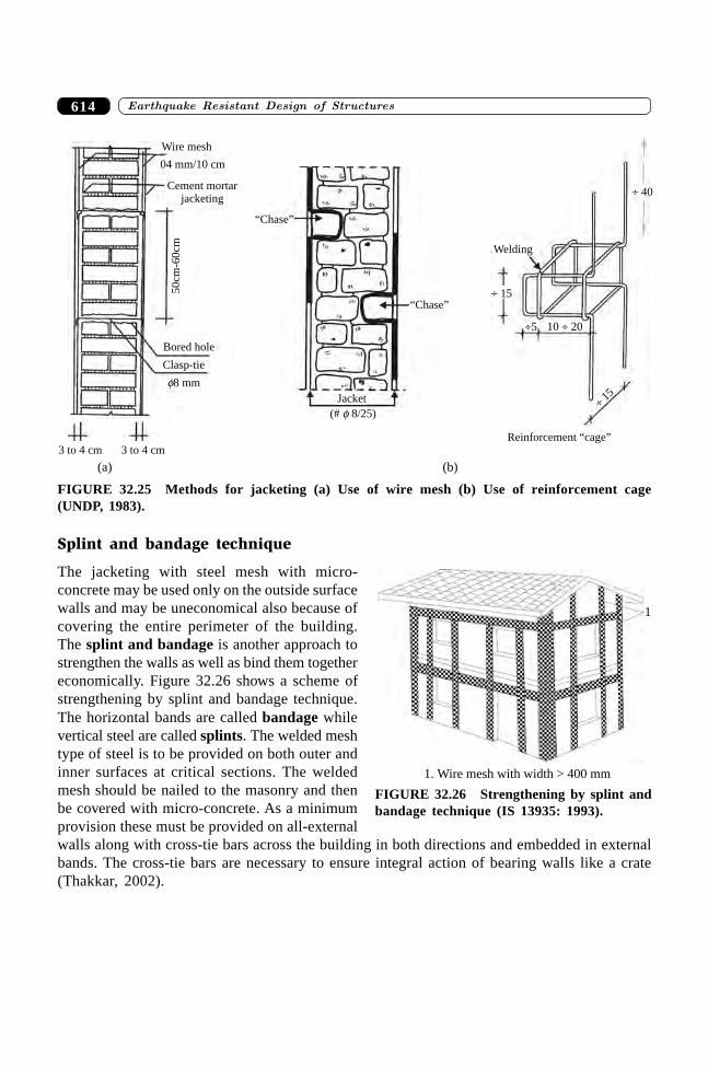
������������ � ������ ������������� 614
Splint and bandage technique
The jacketing with steel mesh with micro-concrete may be used only on the outside surfacewalls and may be uneconomical also because ofcovering the entire perimeter of the building.The splint and bandage is another approach tostrengthen the walls as well as bind them togethereconomically. Figure 32.26 shows a scheme ofstrengthening by splint and bandage technique.The horizontal bands are called bandage whilevertical steel are called splints. The welded meshtype of steel is to be provided on both outer andinner surfaces at critical sections. The weldedmesh should be nailed to the masonry and thenbe covered with micro-concrete. As a minimumprovision these must be provided on all-externalwalls along with cross-tie bars across the building in both directions and embedded in externalbands. The cross-tie bars are necessary to ensure integral action of bearing walls like a crate(Thakkar, 2002).
Wire mesh
04 mm/10 cm
Cement mortarjacketing
50
cm-6
0cm
Bored hole
Clasp-tie
f8 mm
Jacket
(# 8/25)f
“Chase”
“Chase”
Welding
� 15
�5 10 � 20
�15
Reinforcement “cage”
� 40
(a) (b)
3 to 4 cm 3 to 4 cm
FIGURE 32.25 Methods for jacketing (a) Use of wire mesh (b) Use of reinforcement cage(UNDP, 1983).
1. Wire mesh with width > 400 mm
1
FIGURE 32.26 Strengthening by splint andbandage technique (IS 13935: 1993).
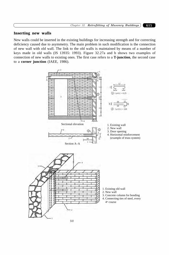
615�������� ��������������� �����������
Inserting new walls
New walls could be inserted in the existing buildings for increasing strength and for correctingdeficiency caused due to asymmetry. The main problem in such modification is the connectionof new wall with old wall. The link to the old walls is maintained by means of a number ofkeys made in old walls (IS 13935: 1993). Figure 32.27a and b shows two examples ofconnection of new walls to existing ones. The first case refers to a T-junction, the second caseto a corner junction (IAEE, 1986).
2
A
3
1
1
A
15
1
15
4
Sectional elevation
4
2 50
1
12
15
Section A–A
12
25 5
1 1 6 = 0.25f L
50
50
22
22
20
10
2 1 12 = 220f L
1. Existing wall2. New wall3. Door opening4. Horizontal reinforcement
(example of truss system)
1. Existing old wall2. New wall3. Concrete column for bonding4. Connecting ties of steel, every
4 courseth
1
2
4
3
(a)

������������ � ������ ������������� 616
f 16
= 1, 150L
1
~1.0
0
~1.0
0
150 150
A
3
2 5 f 166—f 8/200
5
21
0
210
A
1 4
1
tt
4
4
500
500
3
(b)
250
FIGURE 32.27 Inserting new walls (a) Connection of new and old brick wall and connection ofnew brick wall with existing stone wall at T-junction (b) Connection of new and old walls atcorner junctions (IAEE, 1986).
Exterior supplemental elements
Provision of additional shear walls at the perimeter of the building or external buttresses are theexamples of exterior supplemental devises to increase in-plane strength of the existing masonrywalls. Figure 32.28 shows the application of external buttresses to an existing masonry building.
(N) Piles or caissonsif required
(N) Concrete, masonryor steel buttress wall
(N) Tension tie tobuilding each side
of buttress
(E) Reinforced concrete orunreinforced masonry wall
(N) Collector
FIGURE 32.28 Strengthening of walls with external buttresses (FEMA 172, 1992).
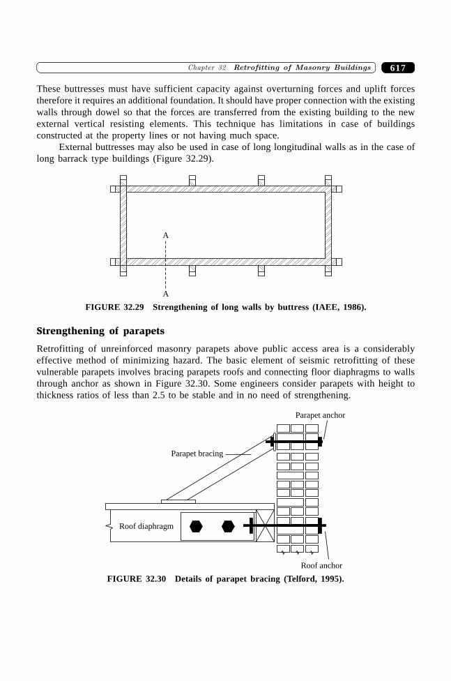
617�������� ��������������� �����������
These buttresses must have sufficient capacity against overturning forces and uplift forcestherefore it requires an additional foundation. It should have proper connection with the existingwalls through dowel so that the forces are transferred from the existing building to the newexternal vertical resisting elements. This technique has limitations in case of buildingsconstructed at the property lines or not having much space.
External buttresses may also be used in case of long longitudinal walls as in the case oflong barrack type buildings (Figure 32.29).
A
A
FIGURE 32.29 Strengthening of long walls by buttress (IAEE, 1986).
Strengthening of parapets
Retrofitting of unreinforced masonry parapets above public access area is a considerablyeffective method of minimizing hazard. The basic element of seismic retrofitting of thesevulnerable parapets involves bracing parapets roofs and connecting floor diaphragms to wallsthrough anchor as shown in Figure 32.30. Some engineers consider parapets with height tothickness ratios of less than 2.5 to be stable and in no need of strengthening.
Roof diaphragm
Roof anchor
Parapet bracing
Parapet anchor
FIGURE 32.30 Details of parapet bracing (Telford, 1995).

������������ � ������ ������������� 618
32.7 SEISMIC EVALUATION OF RETROFITTINGMEASURES IN STONE MASONRY MODELS
In the previous chapter, models 5 and 6 have been tested for earthquake resistant measures onshock table. After damage under shock loading, models were retrofitted by two differentschemes and tested for evaluating the effectiveness of retrofitting techniques. Model 5 has beenretrofitted with cement grouting, strengthening with wire mesh, and stitching of walls whilemodel 6 has been retrofitted with through stones, external binding and prestressing at sill level,designated as Model R1 and Model R2 respectively. The Indian Standard Code IS 13935: 1993,“Repair and Seismic Strengthening of Buildings—Guidelines” furnishes the detailed specificationsof techniques used for retrofitting. However, brief details of retrofitting techniques used inmodels have been described as (Agarwal and Thakkar, 2002):
Grouting: A grout mix consisting of Portland cement and water in the ratio of 1:1 is injectedinto the walls through nozzles, if the cracks are fine; or with cement sand mortar (1:1), if thecracks are wide. A number of holes, preferably 2 to 4 holes in each square metre area of wall,are drilled between the stones to a depth of atleast half the thickness of walls, and injectionnozzles are put into the holes.
Stitching of wall corners: In this technique, holes are drilled in orthogonal wall of the structureat a regular interval of 0.5 m. After the cleaning of holes with water, steel rods of about 12 mmdiameter are inserted into both intersecting walls so that both walls are connected and the holesare filled with cement grout (Figure 32.31).
FIGURE 32.31 Stitching of damaged corner.
Strengthening of wall with wire mesh: This consists of reinforced welded wire mesh of size50 mm ¥ 50 mm of 3 mm diameter forming a vertical plate bounded to the wall. The mesh isanchored with the wall by steel ties at spacing of about 30 cm to 40 cm and plastered by cementsand mortar of 20 mm to 40 mm thickness on the outer surface (Figure 32.32).
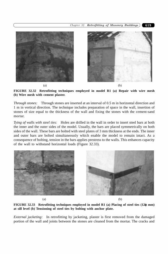
619�������� ��������������� �����������
(a) (b)
FIGURE 32.32 Retrofitting techniques employed in model R1 (a) Repair with wire mesh(b) Wire mesh with cement plaster.
Through stones: Through stones are inserted at an interval of 0.5 m in horizontal direction and1 m in vertical direction. The technique includes preparation of space in the wall, insertion ofstones of size equal to the thickness of the wall and fixing the stones with the cement-sandmortar.
Tying of walls with steel ties: Holes are drilled in the wall in order to insert steel bars at boththe inner and the outer sides of the model. Usually, the bars are placed symmetrically on bothsides of the wall. These bars are bolted with steel plates of 3 mm thickness at the ends. The innerand outer bars are bolted simultaneously which enable the model to remain intact. As aconsequence of bolting, tension in the bars applies prestress to the walls. This enhances capacityof the wall to withstand horizontal loads (Figure 32.33).
(a) (b)
FIGURE 32.33 Retrofitting techniques employed in model R1 (a) Placing of steel ties (12fffff mm)at sill level (b) Tensioning of steel ties by bolting with anchor plate.
External jacketing: In retrofitting by jacketing, plaster is first removed from the damagedportion of the wall and joints between the stones are cleaned from the mortar. The cracks and
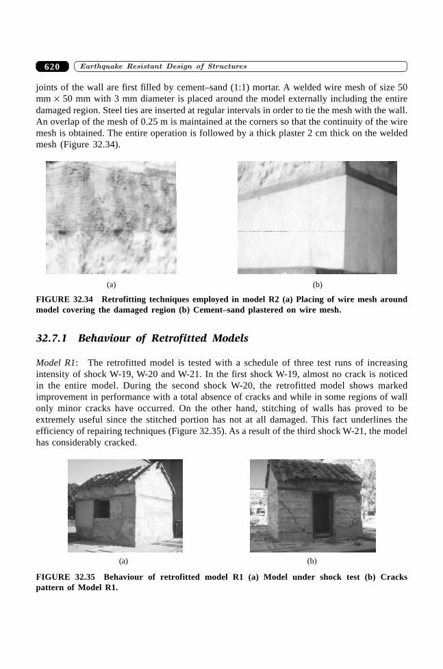
������������ � ������ ������������� 620
joints of the wall are first filled by cement–sand (1:1) mortar. A welded wire mesh of size 50mm ¥ 50 mm with 3 mm diameter is placed around the model externally including the entiredamaged region. Steel ties are inserted at regular intervals in order to tie the mesh with the wall.An overlap of the mesh of 0.25 m is maintained at the corners so that the continuity of the wiremesh is obtained. The entire operation is followed by a thick plaster 2 cm thick on the weldedmesh (Figure 32.34).
(a) (b)
FIGURE 32.34 Retrofitting techniques employed in model R2 (a) Placing of wire mesh aroundmodel covering the damaged region (b) Cement–sand plastered on wire mesh.
32.7.1 Behaviour of Retrofitted Models
Model R1: The retrofitted model is tested with a schedule of three test runs of increasingintensity of shock W-19, W-20 and W-21. In the first shock W-19, almost no crack is noticedin the entire model. During the second shock W-20, the retrofitted model shows markedimprovement in performance with a total absence of cracks and while in some regions of wallonly minor cracks have occurred. On the other hand, stitching of walls has proved to beextremely useful since the stitched portion has not at all damaged. This fact underlines theefficiency of repairing techniques (Figure 32.35). As a result of the third shock W-21, the modelhas considerably cracked.
(a) (b)
FIGURE 32.35 Behaviour of retrofitted model R1 (a) Model under shock test (b) Crackspattern of Model R1.
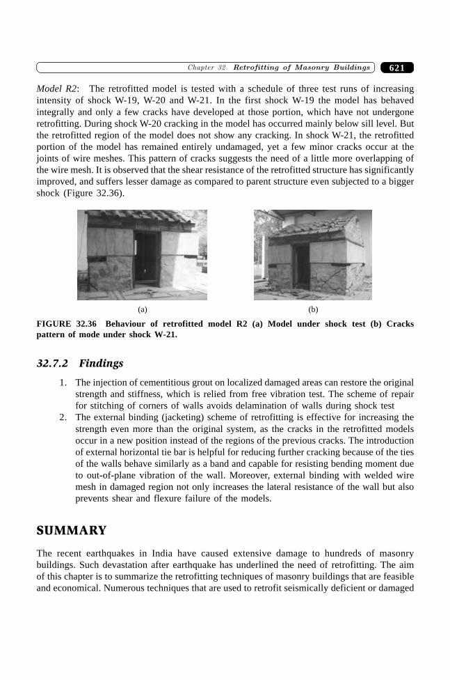
621�������� ��������������� �����������
Model R2: The retrofitted model is tested with a schedule of three test runs of increasingintensity of shock W-19, W-20 and W-21. In the first shock W-19 the model has behavedintegrally and only a few cracks have developed at those portion, which have not undergoneretrofitting. During shock W-20 cracking in the model has occurred mainly below sill level. Butthe retrofitted region of the model does not show any cracking. In shock W-21, the retrofittedportion of the model has remained entirely undamaged, yet a few minor cracks occur at thejoints of wire meshes. This pattern of cracks suggests the need of a little more overlapping ofthe wire mesh. It is observed that the shear resistance of the retrofitted structure has significantlyimproved, and suffers lesser damage as compared to parent structure even subjected to a biggershock (Figure 32.36).
(a) (b)
FIGURE 32.36 Behaviour of retrofitted model R2 (a) Model under shock test (b) Crackspattern of mode under shock W-21.
32.7.2 Findings
1. The injection of cementitious grout on localized damaged areas can restore the originalstrength and stiffness, which is relied from free vibration test. The scheme of repairfor stitching of corners of walls avoids delamination of walls during shock test
2. The external binding (jacketing) scheme of retrofitting is effective for increasing thestrength even more than the original system, as the cracks in the retrofitted modelsoccur in a new position instead of the regions of the previous cracks. The introductionof external horizontal tie bar is helpful for reducing further cracking because of the tiesof the walls behave similarly as a band and capable for resisting bending moment dueto out-of-plane vibration of the wall. Moreover, external binding with welded wiremesh in damaged region not only increases the lateral resistance of the wall but alsoprevents shear and flexure failure of the models.
SUMMARY
The recent earthquakes in India have caused extensive damage to hundreds of masonrybuildings. Such devastation after earthquake has underlined the need of retrofitting. The aimof this chapter is to summarize the retrofitting techniques of masonry buildings that are feasibleand economical. Numerous techniques that are used to retrofit seismically deficient or damaged
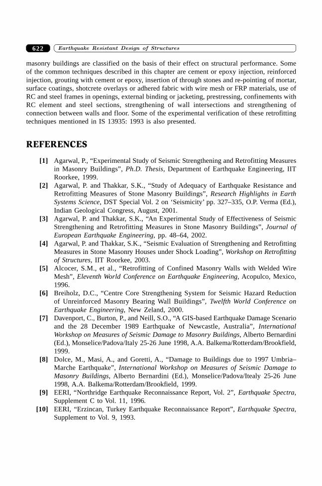
������������ � ������ ������������� 622
masonry buildings are classified on the basis of their effect on structural performance. Someof the common techniques described in this chapter are cement or epoxy injection, reinforcedinjection, grouting with cement or epoxy, insertion of through stones and re-pointing of mortar,surface coatings, shotcrete overlays or adhered fabric with wire mesh or FRP materials, use ofRC and steel frames in openings, external binding or jacketing, prestressing, confinements withRC element and steel sections, strengthening of wall intersections and strengthening ofconnection between walls and floor. Some of the experimental verification of these retrofittingtechniques mentioned in IS 13935: 1993 is also presented.
REFERENCES
[1] Agarwal, P., “Experimental Study of Seismic Strengthening and Retrofitting Measuresin Masonry Buildings”, Ph.D. Thesis, Department of Earthquake Engineering, IITRoorkee, 1999.
[2] Agarwal, P. and Thakkar, S.K., “Study of Adequacy of Earthquake Resistance andRetrofitting Measures of Stone Masonry Buildings”, Research Highlights in EarthSystems Science, DST Special Vol. 2 on ‘Seismicity’ pp. 327–335, O.P. Verma (Ed.),Indian Geological Congress, August, 2001.
[3] Agarwal, P. and Thakkar, S.K., “An Experimental Study of Effectiveness of SeismicStrengthening and Retrofitting Measures in Stone Masonry Buildings”, Journal ofEuropean Earthquake Engineering, pp. 48–64, 2002.
[4] Agarwal, P. and Thakkar, S.K., “Seismic Evaluation of Strengthening and RetrofittingMeasures in Stone Masonry Houses under Shock Loading”, Workshop on Retrofittingof Structures, IIT Roorkee, 2003.
[5] Alcocer, S.M., et al., “Retrofitting of Confined Masonry Walls with Welded WireMesh”, Eleventh World Conference on Earthquake Engineering, Acopulco, Mexico,1996.
[6] Breiholz, D.C., “Centre Core Strengthening System for Seismic Hazard Reductionof Unreinforced Masonry Bearing Wall Buildings”, Twelfth World Conference onEarthquake Engineering, New Zeland, 2000.
[7] Davenport, C., Burton, P., and Neill, S.O., “A GIS-based Earthquake Damage Scenarioand the 28 December 1989 Earthquake of Newcastle, Australia”, InternationalWorkshop on Measures of Seismic Damage to Masonry Buildings, Alberto Bernardini(Ed.), Monselice/Padova/Italy 25-26 June 1998, A.A. Balkema/Rotterdam/Brookfield,1999.
[8] Dolce, M., Masi, A., and Goretti, A., “Damage to Buildings due to 1997 Umbria–Marche Earthquake”, International Workshop on Measures of Seismic Damage toMasonry Buildings, Alberto Bernardini (Ed.), Monselice/Padova/Itealy 25-26 June1998, A.A. Balkema/Rotterdam/Brookfield, 1999.
[9] EERI, “Northridge Earthquake Reconnaissance Report, Vol. 2”, Earthquake Spectra,Supplement C to Vol. 11, 1996.
[10] EERI, “Erzincan, Turkey Earthquake Reconnaissance Report”, Earthquake Spectra,Supplement to Vol. 9, 1993.
623�������� ��������������� �����������
[11] Elgawady, M., Lestuzzi, P., and Badoux, M., “Dynamic versus Static Cyclic Tests ofMasonry Walls before and after Retrofitting with GFRP”, Thirteenth World Conferenceon Earthquake Engineering, Vancouver, B.C., Canada, 2004.
[12] FEMA 172, NEHRP Handbook for Seismic Rehabilitation of Existing Buildings,Building Seismic Safety Council, Washington, 1992.
[13] Grimn, C.T., “Masonry Cracks: A Review of the Literature”, Masonry: Materials,Design, Construction, and Maintenance, pp. 257–280, H.A. Harris, (Ed.), ASTM STP992, American Society for Testing and Materials, Philadelphia, 1988.
[14] IAEE, “Basic Concepts of Seismic Codes—Vol. I”, The International Association forEarthquake Engineering, Tokyo, Japan, 1980.
[15] IAEE, Guidelines for Earthquake Resistant Non-engineered Construction, ACC Limited,Thane, 2001.
[16] IS 13935, Repair and Seismic Strengthening of Buildings—Guidelines, Bureau ofIndian Standards, New Delhi, 1993.
[17] Kahn, L.W., “Shotcrete Retrofit for Unreinforced Brick Masonry”, Eighth WorldConference on Earthquake Engineering, Vol. 1, San Francisco, 1984.
[18] Karbhari, V.M., “Use of FRP Composite Materials in the Renewal of Civil Infrastructurein Seismic Region”, Second MCEER Workshop on Mitigation of Earthquake Disasterby Advanced Technologies (MEDAT-2), Technical Report MCEER-01-0002, 2001.
[19] Kehoe, B.E., “Performance of Retrofitted Unreinforced Masonry Buildings”, EleventhWorld Conference on Earthquake Engineering, Acopulco, Mexico, 1996.
[20] Modena, C., “Repair and Upgrading Techniques of Unreinforced Masonry StructuresUtilized after Fruli and Compania/Basilicata Earthquakes”, Earthquake Spectra,Vol. 10, No. 1, 1994.
[21] Munoz, A., Quiun, D., and Tinman, M. “Repair and Seismic Retrofitting of Hospitaland School Buildings in Peru”, Thirteenth World Conference on EarthquakeEngineering, Vancouver, B.C., Canada, 2004.
[22] Nasini, U. et al., “Evaluation and Design Criteria for Restoring and RetrofittingDamaged Masonry Buildings”, Twelfth World Conference on Earthquake Engineering,New Zealand, 2000.
[23] Newman, Alexander, Structural Renovation of Buildings—Methods, Details, andDesign Example, McGraw-Hill, USA, 2001.
[24] Sanders, H.P., “A Case History—Retrofit Seismic Strengthening of John Marshall HighSchool with Historic Restoration Objectives”, Eighth World Conference on EarthquakeEngineering, Vol. 1, San Francisco, 1984.
[25] Schwegler, G. and Kelterborn, P., “Earthquake Resistance of Masonry StructuresStrengthen with Fibre Composites”, Eleventh World Conference on EarthquakeEngineering, Acopulco, Mexico, 1996.
[26] Spencer, R.J.S., et al., “The Performance of Strengthened Masonry Buildings in RecentEuropean Earthquakes”, Twelfth World Conference on Earthquake Engineering,New Zealand, 2000.
[27] Thakkar, S.K. and Agarwal, P., “Seismic Evaluation of Earthquake Resistant andRetrofitting Measures of Stone Masonry Houses”, Paper No. 110, Twelfth WorldConference on Earthquake Engineering, New Zealand, 2000.

������������ � ������ ������������� 624
[28] Fastening for Seismic Retrofitting—State of the Art Report, Comite Euro-InternationalDu Beton, Thomas Telford, UK, 1995.
[29] Tomazevic, M., Earthquake Resistant Design of Masonry Buildings, Imperial CollegePress, London, 1999.
[30] Turner, F., “Retrofit Provisions in the International Existing Building Code”, 13thWorld Conference on Earthquake Engineering, Vancouver, B.C., Canada, 2004.
[31] UNDP, “Repair and Strengthening of Reinforced Concrete, Stone and Brick-MasonryBuildings—Volume 5”, UNDP/UNIDO Project RER/79/015, Vienna, 1983.
[32] Weng, D., et al., “Experimental Study on Seismic Retrofitting of Masonry Walls UsingGFRP”, Thirteenth World Conference on Earthquake Engineering, Vancouver, B.C.,Canada, 2004.
[32] Wyllie, L.A., “Strengthening Strategies for Improved Seismic Performance”, EleventhWorld Conference on Earthquake Engineering, Acopulco, Mexico, 1996.


Earthquake ResistantDesign of StructuresPankaj Agarwal
Manish Shrikhande
www.phindia.com
This comprehensive and well-organized book presents the concepts and principles of earthquake resistant design of structures in an easy-to-read style. The use of these principles helps in the implementation of seismic design practice. The book adopts a step-by-step approach, starting from the fundamentals of structural dynamics to application of seismic codes in analysis and design of structures. The text also focusses on seismic evaluation and retrofitting of reinforced concrete and masonry buildings. The text has been enriched with a large number of diagrams and solved problems to reinforce the understanding of the concepts.
Intended mainly as a text for undergraduate and postgraduate students of civil engineering, this text would also be of considerable benefit to practising engineers, architects, field engineers and teachers in the field of earthquake resistant design of structures.
Pankaj Agarwal, Ph.D., is Assistant Professor at the Department of Earthquake Engineering, Indian Institute of Technology Roorkee. He has been engaged in teaching and research in earthquake resistant design of masonry and RC structures, post-damage detection and survey of earthquake affected areas and buildings, and health monitoring. Dr. Agarwal is a member of Indian Society of Earthquake Technology (ISET).
Manish Shrikhande, Ph.D., is Assistant Professor at the Department of Earthquake Engineering, Indian Institute of Technology Roorkee. He is a recipient of Young Engineer Award of Indian National Academy of Engineering (INAE) and Career Award of AICTE.
ABOUT THE AUTHORS
9 7 8 8 1 2 0 3 2 8 9 2 1
ISBN 978-81-203-2892-1
Related Documents


