Earth Online - 4. POLARIMETRIC DECOMPOSITIONS · Polarimetric Decompositions kSdl l (18) kS Shrr l l (19) And the helix component presents a left sense. On the contrary, when it is

Polarimetric Decompositions

4. POLARIMETRIC DECOMPOSITIONS

4.1 Coherent Decompositions

4.1.1 Purpose of the Coherent Decompositions

The objective of the coherent decompositions is to express the measured scattering matrix by the radar, i.e. [ ]S , as a the combination of the scattering responses of simpler objects

[ ] [ ]1

k

i ii

S c S=

= ∑ (1)

In (1), the symbol [ ]iS stands for the response of every one the simpler objects, also known as

canonical objects, whereas indicates the weight of ic [ ]iS in the combination leading to the

measured [ ]S . As observed in (1), the term combination refers here to the weighted addition of the k scattering matrices. In order to simplify the understanding of (1), it is desirable that the matrices [ ]iS present the property of independence among them to avoid that a particular

scattering behavior to be present in more than one matrix [ ]iS . Often the most restrictive property of orthogonality is imposed.

As it has been already highlighted in this document, the scattering matrix [ ]S can characterize the scattering process produced by a given target, and therefore the target itself. This is possible only in those cases in which both, the incident and the scattered waves are completely polarized waves. Consequently, coherent target decompositions can be only employed to study the so-called coherent targets. These scatterers are also known as point or pure targets.

In a real situation, the measured scattering matrix by the radar [ ]S corresponds to a complex coherent target. Only in a few occasions, this matrix will correspond to a simpler or canonical object, which a good example is, for instance, the trihedrals employed to calibrate SAR imagery. Nevertheless, in a general situation, a direct analysis of the matrix [ ]S , with the objective to infer the physical properties of the scatterer under study, is shown very difficult. Thus, the physical properties of the target under study are extracted and interpreted through the analysis of the simpler responses [ ]iS and the corresponding coefficients in ic (1).

The decomposition exposed in (1) is not unique in the sense that it is possible to find a number of infinite sets [ ]{ }; 1, ,

iS i k= K in which the matrix [ ]S can be decomposed.

Nevertheless, only some of the sets [ ]{ }; 1, ,i

S i k= K are convenient to interpret the

information contained in [ ]S . In the next, we shall detail three of these sets which lead to: the

1


Pauli, the Krogager and the Cameron decompositions. As mentioned above, these decompositions of the scattering matrix can be only employed to characterize coherent scatterers. Therefore, we will finish this section presenting an algorithm to detect such a targets where these decomposition theorems are relevant.

4.1.2 The Pauli Decomposition

4.1.2.1 Description of the Pauli Decomposition

The Pauli decomposition expresses the measured scattering matrix [ ]S in the so-called Pauli basis. If we considered the conventional orthogonal linear (h,v) basis, in a general case, the Pauli basis [ ] [ ] [ ] [ ]{ }, , ,

a b c dS S S S is given by the following four 2×2 matrices

[ ] 1 010 12a

S⎡ ⎤

= ⎢ ⎥⎣ ⎦

(2)

[ ] 1 010 12b

S⎡ ⎤

= ⎢ ⎥−⎣ ⎦ (3)

[ ] 0 111 02c

S⎡ ⎤

= ⎢ ⎥⎣ ⎦

(4)

[ ] 0 111 02d

S−⎡ ⎤

= ⎢ ⎥⎣ ⎦

(5)

In this document, it has been always considered that hv vhS S= , since reciprocity applies in a monostatic system configuration. In this situation, the Pauli basis can be reduced to a basis composed by the matrices (2), (3) and (4), that is,

[ ] [ ] [ ]{ }, ,a b c

S S S (6)

Consequently, given a measured scattering matrix [ ]S , it can be expressed as follows

[ ] [ ] [ ] [ ]hh hva b

hv vv

S SS S S

S Sα β γ

⎡ ⎤= = + +⎢ ⎥⎣ ⎦

cS (7)

where

2hh vvS Sα +

= (8)

2hh vvS Sβ −

= (9)

2 hvSγ = (10)

From (8), (9) and (10) it can be easy show that the span of [ ]S can be obtained as

2 2 2 2 22hh vv hvSPAN S S S 2α β γ= + + = + + (11)

2


4.1.2.2 Interpretation of the Pauli Decomposition

The interpretation of the Pauli decomposition must be done according to the matrices in the basis given at (6) and the corresponding coefficients (8), (9) and (10).

The matrix [ ]aS corresponds to the scattering matrix of a sphere, a plate or a trihedral. In

general, [ ]aS is referred to single- or odd-bounce scattering. Thus, the complex coefficient α,

given at (8), represents the contribution of [ ]aS to the final measured scattering matrix. In

particular, the intensity of this coefficient, i.e., 2α , determines the power scattered by targets characterized by single- or odd-bounce.

The second matrix, [ ]bS represents the scattering mechanism of a dihedral oriented at 0 degrees. In general, this component indicates a scattering mechanism characterized by double- or even-bounce, since the polarization of the returned wave is mirrored respect to the one of the incident wave. Consequently, β stands for the complex coefficient of this scattering mechanism and 2β represents the scattered power by this type of targets.

Finally, the third matrix [ corresponds to the scattering mechanism of a diplane oriented at 45 degrees. As it can be observed in

]cS(4), and considering that this matrix is expressed in the

linear orthogonal basis (h,v), the target returns a wave with a polarization orthogonal to the one of the incident wave. From a qualitative point of view, the scattering mechanism represented by [ is referred to those scatterers which are able to return the orthogonal polarization, from which, one of the best examples is the volume scattering produced by the forest canopy. The coefficient γ represents the contribution of

]cS

[ ]cS to [ ]S , whereas 2γ stands for the scattered power by this type of scatterers.

4.1.2.3 Representation of the Polarimetric information by means of the Pauli decomposition

The Pauli decomposition of the scattering matrix is often employed to represent all the polarimetric information in a single SAR image.

The polarimetric information of [ ]S could be represented by the combination of the

intensities 2hhS , 2

vvS and 22 hvS in a single RGB image, i.e., every of the previous intensities coded as a color channel. The main drawback of this approach is the physical

3


|Shh| (dB)

|Shv| (dB)

-15dB 0dB-30dB

|Svv| (dB)

|Shh+ Svv| |Shh- Svv| |Shv|

Figure 1 Intensities of the polarimetric channels 2

hhS , 2

vvS and the combination of them in an RGB image.

interpretation of the resulting image in term of 2hhS , 2

vvS and 22 hvS . Consequently, an

RGB image can be formed with the intensities 2α , 2β and 2γ , which, as explained before, correspond to clear physical scattering mechanisms. Thus, the resulting color image can be employed to interpret the physical information from a qualitative point of view. The most employed codification corresponds to

2 Redα → (12)2 Blueβ → (13)

4


2 Greenγ → (14)

Then, the resulting color of the RGB image is interpreted in terms of scattering mechanism as given by (12), (13) and (14). Figure 1 presents an example of this codification

4.1.3 The Krogager Decomposition

4.1.3.1 Description of the Krogager Decomposition

Krogager has proposed an alternative to factorize the scattering matrix as the combination of the responses of a sphere, a diplane and a helix. The last two components present an orientation angle θ. If we consider the scattering matrix expressed in the linear orthogonal basis (h,v), the Krogager decomposition presents the following formulation

( ) [ ] [ ] [ ]{ },

21 0 cos2 sin 2 10 1 sin 2 cos2 1

s

s

jjs d hh v s d h

jj js d h

S e e k S k S k S

je e k k k e

j

ϕϕ

ϕϕ θθ θθ θ

⎡ ⎤ = + +⎣ ⎦⎧ ⎫±⎡ ⎤ ⎡ ⎤ ⎡ ⎤

= + +⎨ ⎬⎢ ⎥ ⎢ ⎥ ⎢ ⎥− ±⎣ ⎦ ⎣ ⎦ ⎣ ⎦⎩ ⎭

m (15)

If we compare (15) with (7), it can be observed that both decompositions present the same number of independent parameters, i.e., six. In the case of the Pauli decomposition, the complex coefficients α, β and γ, whereas in the case of the Krogager decomposition, the three angles φ, φs and θ and the three real coefficients ks, kd and kh. The phase φ is referred as the absolute phase, whose value depends on the distance between the radar and the target under study. Due to the arbitrary value that this phase can present, it is often considered that the Krogager decomposition presents 5 independent parameters given by {φs, θ, ks, kd, kh} plus the absolute phase given by φ.

In order to calculate the value of the parameters {φs, θ, ks, kd, kh} plus the absolute phase φ, a reformulation of (15) with the objective to simplify the process is next presented. Now, if we consider the measured scattering matrix expressed in the circular polarization basis (r,l), the Krogager decomposition is then

( ) ( ),

2 2

2

0 0 00 0 0

rlrr

rrrl

s

jjrr rlrr rl

r l jjrl ll rl ll

j jjj

s d hj

S e S eS SS

S S S e S e

j e ee e k k k

j e

ϕϕ

ϕ πϕ

θ θϕϕ

θ

+

−

⎡ ⎤⎡ ⎤⎡ ⎤ = = ⎢ ⎥⎢ ⎥⎣ ⎦ −⎢ ⎥⎣ ⎦ ⎣ ⎦⎧ ⎫

0⎡ ⎤ ⎡ ⎤⎡ ⎤⎪ ⎪= + +⎨ ⎬⎢ ⎥ ⎢ ⎥⎢ ⎥ −⎪ ⎣ ⎦ ⎪⎣ ⎦ ⎣ ⎦⎩ ⎭

(16)

From (16), it can be easily observed that the response of the sphere can be obtained from rlS

s rlk S= (17)

The terms Srr and Sll represent, directly, the diplane component of the decomposition (16), but two cases of analysis must be considered according to the difference in absolute value of Srr and Sll. This is necessary in order to accommodate the difference in the scattered power in the right and the left circular polarizations. When Sll represents the diplane component, it occurs that rr llS S> . Hence

5


d lk S+ = l (18)

h rr lk S S+ = − l (19)

And the helix component presents a left sense. On the contrary, when it is Srr the term which represents the diplane component, it occurs that ll rrS S>

d rk S− = r (20)

h ll rk S S− = − r (21)

and the helix has a right sense. Finally, from (16), the phase components are

( )12 rr llϕ ϕ ϕ π= + + (22)

( )14 rr llθ ϕ ϕ π= − − (23)

( )12rl rr llϕ ϕ ϕ ϕ= − + +π (24)

In order to relate the formulations of the Krogager decomposition presented in (15) and (16), the following relations are useful

( )12rr hv hh vvS jS S S= + − (25)

( )12ll hv hh vvS jS S S= − − (26)

( )2rl hh vvjS S S= + (27)

4.1.3.2 Interpretation of the Krogager Decomposition

The interpretation of the Krogager decomposition must be done according to the coefficients {φs, θ, ks, kd, kh}, plus the absolute phase φ.

The absolute phase φ can contain information about the scatterer under study. But, since its value depends also on the distance between the radar and the target, it is considered as a irrelevant parameter.

The parameters φs and ks characterize the sphere component of the Krogager decomposition. On the one hand, the phase φs represents a displacement of the sphere respect to the diplane and the helix components. On the other hand, the real parameter ks represents the contribution

6


ks (dB)

kd (dB)

-15dB 0dB-30dB -15dB 0dB-30dB

kh (dB)

ks(dB) kd(dB) kh(dB)

Figure 2 Intensities corresponding to the Krogager decomposition 2

sk , 2

dk and 2

hk , and the combination of them in an RGB image. Images are shown in a dB scale.

of the sphere component to the final scattering matrix [ ]S . Consequenty, |ks|2 is interpreted as

the power scattered by the sphere-like component of the matrix [ ]S .

The phase parameter θ stands for the orientation angle of the deplane and the helix components of the Krogager decomposition.

Finally, the coefficients kd and kh correspond to the weights of the diplane and the helix components. Thus, |kd|2 and |kh|2 are interpreted as the power scatterered by the diplane- and the helix-like components of the Krogager decomposition.

7


4.1.3.3 Representation of the Polarimetric information by means of the Krogager decomposition

The information provided by the Krogager decomposition can be also employed to form a RGB color-coded image representing the polarimetric information. In this case, the phase terms are discarded and only the coefficients {ks, kd, kh} are considered in the following way

2 Redsk → (28)2 Bluedk → (29)

2 Greenhk → (30)

Figure 2 gives an example of this codification.

4.1.4 The Cameron Decomposition

4.1.4.1 Description of the Cameron Decomposition

The Cameron decomposition performs a factorization of the measured scattering matrix [ ]S based on two basic properties of radar targets: reciprocity and symmetry.

A radar target is considered reciprocal when the diagonal terms of the measured scattering matrix are equal, i.e., the reciprocity theorem applies. For a scattering matrix measured in the orthogonal linear (h,v) basis

hv vhS S= (31)

whereas for the orthogonal circular (r,l) basis

rl lrS S= (32)

The reciprocity assumption applies in the case of monostatic SAR systems, where the transmitting and receiving antennas are located in the same position. Consequently, all the scatterers can be considered as reciprocal when imaged by a monostatic SAR system.

A scattering is considered symmetric when the target has an axis of symmetry in the plane orthogonal to the direction between the radar and the target. The symmetry of a scatterer can be also considered in the frame of the Pauli decomposition (7). Hence, a scatterer is considered symmetric if it exists a rotation which cancels the projection of [ ]S in the

component [ of the Pauli decomposition. ]cS

Since monostatic SAR imagery considerers only reciprocal scatterers, we present, in the following, the Cameron decomposition applied to reciprocal targets, i.e., [ ]S is symmetric.

Given a scattering matrix measured in the orthogonal linear (h,v) basis

[ ] hh hv

hv vv

S SS

S S⎡ ⎤

= ⎢ ⎥⎣ ⎦

(33)

we consider the vector form of [ ]S as follows

8


hh

hv

hv

vv

SS

SSS

⎡ ⎤⎢ ⎥⎢ ⎥=⎢ ⎥⎢ ⎥⎢ ⎥⎣ ⎦

r (34)

Hence, the Pauli decomposition given at (7) can be formulated in a vector form as follows

a bS S S Scα β γ= + +r r r r

r

(35)

The Cameron decomposition states that a reciprocal target can be decomposed as the sum of two components as follows

max mincos sinsym symS A S Sτ τ⎡ ⎤= +⎣ ⎦r r

(36)

Considering the inner vector product as (.,.), and the vector norm as ||.||, the different parameters of (36) are obtained as follows

A S=r

(37)maxsym a bS S Sα ε= +r r r

(38)

The matrix maxsymSr

is called the largest or maximum symmetric component of [ ]S and it is obtained by means of

cos sinε β θ γ= + θ (39)

and

( )* *

2 2tan 2 βγ βθ γβ γ

+=

− (40)

The matrix minsymSr

is called the minimum symmetric component of Sr

. Finally, the factor cos τ

is the degree of symmetry of and it measures the degree to which Sr

Sr

deviates from minsymSr

and is obtained as

( )min

min

,cos

sym

sym

S S

S Sτ =

r r

r r (41)

4.1.4.2 Representation of Symmetric Scatterers

An arbitrary symmetric scatterer symSr

can be decomposed according to

( ) ( ) ( ]+ˆ R , ,jsymS ae R z aρ ψ ρ ψ π π⎡ ⎤= Λ ∈ ∈⎣ ⎦r

− (42)

where a indicates the amplitude of the scattering matrix, ρ is the nuisance phase and ψ is the scatterer orientation angle. The matrix ( )R ψ⎡ ⎤⎣ ⎦ denotes the rotation operator. Finally, the

normalized vector ( )ˆ zΛ , expressed in the linear polarization basis, is

9


( )

101ˆ , 101

z zz

z

⎡ ⎤⎢ ⎥⎢ ⎥Λ = ∈ ≤⎢ ⎥+⎢ ⎥⎣ ⎦

C z (43)

Consequently, the complex quantity z in (43) can be employed to characterize the symmetric scatterer under consideration. The following list presents the values of z some some canonical targets

• Triedral

( )ˆ ˆ 1aS = Λ (44)

• Diplane

( )ˆ ˆ 1bS = Λ − (45)

• Dipole

( )ˆ ˆ 0lS = Λ (46)

• Cylinder

1ˆ ˆ2cyS ⎛ ⎞= Λ⎜ ⎟

⎝ ⎠ (47)

• Narrow diplane

1ˆ ˆ2ndS ⎛ ⎞= Λ −⎜ ⎟

⎝ ⎠ (48)

• Quarter wave device

( )1 4ˆ ˆS j= Λ (49)

4.1.4.3 Classification based on the Cameron Decomposition

On the basis of the factorization of the measured scattering matrix [ ]S , (36), and the representation of the maximum symmetrical component as a complex quantity z, Cameron proposed a classification scheme for the maximum symmetrical component max

symSr

. This classification scheme is based on comparing the quantity z of the matrix under study with those corresponding to the targets given from (44) to (49). In order to compare the measured z and the scattering responses of the targets of reference, the following metric must be considered

( )*

22

1,

1 1

refref

ref

z zd z z

z z

+=

+ + (50)

Finally, the measured scatterer z is classified according to the shortest distance d(z,zref). Figure 3 presents the Cameron’s classification scheme based on the metric (50).

10


[ ] hh hv

hv vv

S SS

S S⎡ ⎤

= ⎢ ⎥⎣ ⎦

Symmetrical

Shortest distance d(z,zref)

Maximum SymmetricalComponent

Triedral

Dihedral

Narrow dihedral

Dipole

Cylinder

¼ Wave

Match Helix

Asymmetrical

Left Helix

Right Helix

F

F

T

T

[ ] hh hv

hv vv

S SS

S S⎡ ⎤

= ⎢ ⎥⎣ ⎦

Symmetrical

Shortest distance d(z,zref)

Maximum SymmetricalComponent

Triedral

Dihedral

Narrow dihedral

Dipole

Cylinder

¼ Wave

Match Helix

Asymmetrical

Left Helix

Right Helix

F

F

T

T

Figure 3 Cameron’s classification scheme.

4.1.5 Relevance of Coherent Decompositions, Touzi Criterion

As it has been noticed, the previous coherent decompositions can be only employed to analyze pure targets whose scattering response is completely determined by the measured scattering matrix [ ]S . Consequently, when working with SAR imagery, it is necessary to determine whether a particular pixel is a pure target or, on the contrary, it belongs to a distributed scatterer. For the first case, coherent decompositions can be employed to study the physics of the scatterer. Nevertheless, the analysis of distributed scatterers must be performed by means of the so-called incoherent decompositions.

A qualitative way to differentiate pure from distributed scatterers is to consider their physical nature. A rough division would be to consider the man-made targets as pure targets, whereas natural targets can be considered as distributed. For man-made targets we understand all type of artificial man-structures in a SAR image such buildings, power lines, train tracks or cars. On the contrary, for instance, forests, agricultural areas, bare soils or water have to be considered as distributed targets.

Touzi has proposed a technique to identify pure targets in a SAR images, based on the Cameron decomposition. This technique determines the nature of a target on the maximum symmetrical component of the Cameron decomposition max

symSr

. In the analysis of a given target, Touzi differentiates two cases to perform such a study. On the one hand, pure targets whose

11


response occupy only one pixel and, on the other hand, targets whose response extends among several pixels.

4.1.5.1 Coherent Test for Point Targets

A resolution cell, or pixel, in a SAR images is formed by the coherent addition of the responses of the elementary scatterers within the resolution cell. In those cases in which there is no a dominant scatterer, the statistics of the response is given by the complex Gaussian scattering model, giving rise to the so-called speckle.

Nevertheless, the resolution cell can present a point target, which dominates the response of the resolution cell. In this case, the scattering response is due to the coherent combination of two components: the one due to the dominant scatterer and the coherent combination due to the clutter, which is given by the complex Gaussian scattering statistics model. The statistics of the resulting combination receives the name of Rician model. Figure 4 compares the response with and without the presence of a point scatterer within the resolution cell.

Real part

Imaginary part

Real part

Imaginary part

Final responseFinal responseSpeckle

Speckle

Point target response

(a) (b)

Real part

Imaginary part

Real part

Imaginary part

Real part

Imaginary part

Real part

Imaginary part

Final responseFinal responseSpeckle

Speckle

Point target response

(a) (b) Figure 4 Coherent response of a given resolution cell (a) without a dominant scatterer, (b) with a dominant scatterer.

As observed in Figure 4b, despite the point target (blue arrow) can dominate the response of a resolution cell (red arrow), the effect of the clutter (cloud of black arrows) must be taken into consideration. It is necessary, hence, to compare the response of the point target with the one of the clutter. Hence, a signal to clutter power ratio, denoted by S/C, must be defined. Touzi established that this ratio must be higher than 15dB. The reason to choose this value is that the response of the resolution cell will present a phase variation smaller than π/4 with respect to the response of the point target.

In order to be, as much as possible, independent from the conditions in which the SAR image has been taken, Touzi proposed to apply the previous S/C criteria on the maximum polarization return |m|2, which represents the polarization state giving maximum returned power from the scatterer under consideration. This parameter, representing the pure target response, can be obtained from the diagonalization of the measured scattering matrix [ ]S , via its eigendecomposition, as established by Hyunen. According to Huynen, the eigenvalues of the covariance matrix [ ]S can be parameterized as follows

21

jme υλ = (51)2 2

2 tan jm e υλ γ −= (52)

12


where λ1 and λ2 are the maximum and the minimum eigenvalues, respectively. In (51) and (52), m is the maximum polarization, υ is the skip angle and γ is the polarisability angle. Consequently, |m|2 can be derived from the magnitude of the maximum eigenvalue of [ ]S . Finally, the power corresponding to the clutter can be derived from a neighboring area not affected by the point scatterer.

4.1.5.2 Coherent Test for Distributed Targets

For distributed scatterers, Touzi proposed to measure its coherency also in terms of the maximum symmetric component max

symSr

derived from the Cameron decomposition. On the basis of its definition, (38), Touzi defined the so-called degree of coherence of a distributed scattered as follows

( )2 22 2 *

2 2

4symp

α β α β

α β

− + ⋅=

+ (53)

The degree of coherence is generated by a moving window. In the resulting map, those pixels presenting symp close to 1 represent areas in which the scatterer is locally coherent. Hence, the coherent decomposition theorems can be applied in this case.

[ ] hh hv

hv vv

S SS

S S⎡ ⎤

= ⎢ ⎥⎣ ⎦

maxsym a bS S Sα ε= +r r r

Symmetric scattering

Dist. targetcoherence

Point targetcoherence

TTF

T

F

[ ] hh hv

hv vv

S SS

S S⎡ ⎤

= ⎢ ⎥⎣ ⎦

maxsym a bS S Sα ε= +r r r

Symmetric scattering

Dist. targetcoherence

Point targetcoherence

TTF

T

F

Coherent ScattererNon-coherent Scatterer Coherent ScattererNon-coherent Scatterer Figure 5 Cameron’s classification scheme.

4.1.5.3 Coherent Test Algorithm

On the basis of the coherent test presented in the previous two points, Touzi proposed an algorithm to determine which pixels in a SAR image are coherent, and, therefore, the coherent decomposition theorems can be employed to analyze them. Figure 5 presents the flow chart of the algorithm.

13


4.2 Incoherent Decompositions

4.2.1 Purpouse of the incoherent decompositions

As explained previously, the scattering matrix [ ]S is only able to characterize the so-called coherent or pure scatterers. On the contrary, this matrix can not be employed to characterize, from a polarimetric point of view, the so-called distributed scatterers. This type of scatterers can be only characterized, statistically, due to the presence of speckle noise. Since speckle noise must be reduced, only second order polarimetric representations can be employed to analyze distributed scatterers. These second order descriptors are the 3×3, Hermitian average covariance [ ]3C [ ]3T and the coherency [ ]3T matrices. These two representations of the

polarimetric information are equivalent.

The complexity of the scattering process makes extremely difficult the physical study of a given scatterer through the direct analysis of [ ]3C or [ ]3T . Hence, the objective of the

incoherent decompositions is to separate the [ ]3C or [ ]3T matrices as the combination of

second order descriptors corresponding to simpler or canonical objects, presenting an easier physical interpretation. These decomposition theorems can be expressed as

[ ] [ ]3 31

k

i ii

C p C=

= ∑ (54)

[ ] [ ]3 31

k

i ii

T q=

= ∑ T (55)

where the canonical responses are represented by [ ]3 iC and [ ]3 i

T , and ip and denote the

coefficients of these components in iq

[ ]3C or [ ]3T , respectively. As in the case of the

coherent decomposition, it is desirable that these components present some properties. First of all, it is desirable that the components [ ]3 i

C and [ ]3 iT correspond to pure targets in order to

simplify the physical study. Nevertheless, this is not absolutely necessary. In addition the components [ ]3 i

C and [ ]3 iT are independent, or in a more restrictive way, orthogonal.

The bases in which [ ]3C or [ ]3T are decomposed, i.e., [ ]{ }3 ; 1, ,i

C i k= K and

[ ]{ }3 ; 1, ,i

T i k= K are not unique. Consequently, different decompositions can be presented. In

the following we detail: the Freeman, the Huynen and the Eigenvector-eigenvalue decompositions.

4.2.2 The Model-based Freeman Decomposition

4.2.2.1 Description of the Freeman Decomposition

The Freeman decomposition models the covariance matrix as the contribution of three scattering mechanisms

14


• Volume scattering where a canopy scatterer is modeled as a set of randomly oriented dipoles.

• Double-bounce scattering modeled by a dihedral corner reflector.

• Surface or single-bounce scattering modeled by a first-order Bragg surface scatterer.

The volume scattering from a forest canopy is modeled as the contribution from an ensemble of randomly oriented thin dipoles. The scattering matrix of an elementary dipole, expressed in the orthogonal linear (h,v) basis, when horizontally oriented, has the expression

[ ] 00

h

v

RS

R⎡ ⎤

= ⎢ ⎥⎣ ⎦

(56)

For a thin dipole, (58) reduces to

[ ] 1 00 0

S⎡ ⎤

= ⎢ ⎥⎣ ⎦

(57)

Now, if we considerer a set of randomly oriented dipoles, characterized by the previous scattering matrix and oriented according to a uniform phase distribution, the covariance matrix of the ensemble of thin dipoles can be modeled by

[ ]3

1 0 1 30 2 3 0

1 3 0 1vv

C f⎡ ⎤⎢ ⎥= ⎢ ⎥⎢ ⎥⎣ ⎦

(58)

where fv corresponds to the contribution of the volume scattering to the |Svv|2 component. The covariance matrix [ ]3 v

C presents rank 3. Thus, the volume scattering can not be

characterized by a single scattering matrix of a pure target.

The second component of the Freeman decomposition corresponds to the double-bounce scattering. In this case, a generalized corner reflector is employed to model the scattering process. The diplane itself is not considered metallic. Hence, we consider that the vertical surface has reflection coefficients Rth and Rtv for the horizontal and the vertical polarizations, whereas the horizontal one presents the coefficients Rgh and Rgv for the same polarizations. Additionally, two phase components for the horizontal and the vertical polarizations are considered, i.e., 2 hje γ and 2 vje γ , respectively. The complex phase terms hγ and vγ account for any attenuation or phase change effect. Hence, the scattering matrix of the generalized dihedral is

[ ]2

2

00

h

v

jgh th

jgv tv

e R RS

e R R

γ

γ

⎡ ⎤= ⎢ ⎥⎢ ⎥⎣ ⎦

(59)

which gives rise to the covariance matrix of the double-bounce scattering component. After normalization respect to the Svv component, this covariance matrix can be written as follows

[ ]

2

3*

00 0 0

0 1dd

C fα α

α

⎡ ⎤⎢ ⎥

= ⎢ ⎥⎢ ⎥⎢ ⎥⎣ ⎦

(60)

15


where

( )2 h vj gh th

gv tv

R Re

R Rγ γα −= (61)

and fd corresponds to the contribution of the double-bounce scattering to the |Svv|2 component 2

d gv tvf R R= (62)

As it can be observed, the covariance matrix [ ]3 dC has rank 1, as it can be represented by the

scattering matrix given at (59).

The third component of the Freeman decomposition consist of a first-order Brag surface scatterer modeling surface scattering. The scattering mechanism is represented by the scattering matrix

[ ] 00

h

v

RS

R⎡ ⎤

= ⎢ ⎥⎣ ⎦

(63)

Consequently, the covariance matrix corresponding to this scattering component is

[ ]

2

3*

00 0 0

0 1ss

C fβ α

α

⎡ ⎤⎢ ⎥

= ⎢ ⎥⎢ ⎥⎢ ⎥⎣ ⎦

(64)

where fs corresponds to the contribution of the double-bounce scattering to the |Svv|2 component

2s vf R= (65)

and

h

v

RR

β = (66)

As in the case for the double-bounce scattering mechanism, since the matrix [ ]3 sC presents

rank 1, therefore, it is completely represented by the scattering mechanism presented at (63).

Hence, the Freeman decomposition expresses the measured covariance matrix [ ]3C as follows

[ ] [ ] [ ] [ ]3 3 3 d svC C C C= + + 3 (67)

4.2.2.2 Interpretation of the Freeman Decomposition

The term fv in (58) corresponds to the contribution of the volume scattering of the final covariance matrix [ ]3C . Hence, the scattered power by this component can be written as

follows

83

vv

fP = (68)

16


From (60), it can be concluded that the power scattered by the double-bounce component of [ ]3C has the expression

( )21d dP f α= + (69)

Finally, the power scattered by the surface-like component is

( )21s sP f β= + (70)

Consequently, the scattered power Pv, Pd and Ps can be employed to generate a RGB image to present all the color-coded polarimetric information in a sole image. Figure 6 presents an example of the Freeman decomposition.

Pv (dB)

Pd (dB)


Ps (dB)

Pv(dB) Pd(dB) Ps(dB)

Figure 6 Intensities corresponding to the Freeman decomposition Pv, Pd and Ps and the combination of them in an RGB image. Images are shown in a dB scale.

From (68), (69) and (70) it can be observed, that the Freeman decomposition maintains the span or total scattered power

17


2 2 22hh vv hv v d sSPAN S S S P P P= + + = + + (71)

The Freeman decomposition presented in (67) presents 5 independent parameters {fv, fd, fs, α, β} and only 4 equations. Consequently, some hypothesis must be considered in order to find the values of {fv, fd, fs, α, β}. Figure 7 presents the scheme employed to invert the Freeman decomposition.

{ }2 2 2 *, , ,hh vv hv hh vvS S S S S

23v hvf S={ }, , , ,v d sf f f α β

{ }* 0 1hh vvif S S αℜ ≥ ⇒ = − { }* 0 1hh vvif S S βℜ < ⇒ =

{ }, ,d sf f β { }, ,d sf f α

Single-bouncescattering dominates

Double-bouncescattering dominates

5 parameters4 equations



1α = − 1β =

{ }2 2 2 *, , ,hh vv hv hh vvS S S S S

23v hvf S={ }, , , ,v d sf f f α β

{ }* 0 1hh vvif S S αℜ ≥ ⇒ = − { }* 0 1hh vvif S S βℜ < ⇒ =

{ }, ,d sf f β { }, ,d sf f α




Single-bouncescattering dominates

Double-bouncescattering dominates

1α = − 1β =

Figure 7 Inversion of the Freeman decomposition parameters.

4.2.3 Phenomenological Huynen Decomposition

4.2.3.1 Description of the Huynen Decomposition

The Phenomenological Huynen decomposition represents the first attempt to consider decomposition theorems for the analysis of distributed scatterers. The Huynen decomposition considers the concept of “wave dichotomy”, exporting it to the study of distributed scatterers.

On a first stage, the phenomenological Huynen decomposition considers a particular parameterization of a distributed scatterer. In the case of the covariance matrix, this parametrization is

[ ]0

3 0

0

2 A C j D H j GT C j D B B E j F

H j G E j F B B

⎡ ⎤− +⎢ ⎥= + + +⎢ ⎥⎢ ⎥− − −⎣ ⎦

(72)

The set of nine independent parameters of this particular parameterization allows a physical interpretation of the target under consideration. The following list presents the information provided by each one of the parameters:

• A0: Represents the total scattered power from the regular, smooth, convex parts of the scatterer.

18


• BB0: Denotes the total scattered power for the target’s irregular, rough, non-conex depolarizing components.

• A0+ B0: Gives roughly the total scattered power.

• BB0+B: Total symmetric depolarized power.

• BB0-B: Total non-symmetric depolarized power.

• C, D: Depolarization components of symmetric targets

o C: Generator of target global shape (Linear).

o D: Generator of target local shape (Curvature).

• E, F: Depolarization components due to non-symmetries

o E: Generator of target local twist (Torsion).

o F: Generator of target global twist (Helicity).

• G, H: Coupling terms between target’s symmetric and non-symmetric terms

o G: Generator of target local coupling (Glue).

o H: Generator of target global coupling (Orientation).

The phenomenological Huynen decomposition expresses the measured covariance matrix [ ]3T as follows

[ ] [ ] [ ]3 0 NT T T= + (73)

The matrix [ ]0T refers to a pure target, that is, a target which can be also completely characterized by a corresponding scattering matrix. Its parameterization is

[ ]0

0 0

0

2

T T T T

T T T T

A C j D H j GT C j D B B E jF

H j G E jF B B

⎡ ⎤− +⎢ ⎥= + + +⎢ ⎥⎢ ⎥− + −⎣ ⎦

(74)

Consequently, [ ]0T presents rank 1. The matrix [ ]NT is called N-target (for symmetric

targets) and it corresponds to a distributed scatterer. Since [ ]NT does not have rank equal to

1, it does not present an equivalent scattering matrix. The parameterization of [ ]NT , given

(73) and (74), is

[ ] 0

0

0 0 000

N N N N

N N N N

T B B E NjFE jF B B

⎡ ⎤⎢ ⎥= + +⎢ ⎥⎢ ⎥+ −⎣ ⎦

(75)

One on the main properties of the N-target [ ]NT is that it is invariant under rotations of the

antenna coordinate system about the line of sight, i.e., it is roll-invariant. Mathematically, this property can be expressed as

19


( ) [ ] 1

3 3

0

0

1 0 0 0 0 0 1 0 00 cos 2 sin 2 0 0 cos 2 sin 20 sin 2 cos2 0 0 sin 2 cos2

R RN N

N N N N

N N N N

T U T U

B B E jFE jF B B

θ

θ θ θ θθ θ θ

−⎡ ⎤ ⎡ ⎤⎡ ⎤ =⎣ ⎦ ⎣ ⎦ ⎣ ⎦

⎡ ⎤ ⎡ ⎤ ⎡ ⎤⎢ ⎥ ⎢ ⎥ ⎢ ⎥= + +⎢ ⎥ ⎢ ⎥ ⎢ ⎥⎢ ⎥ ⎢ ⎥ ⎢ ⎥− + −⎣ ⎦ ⎣ ⎦ ⎣ ⎦θ

−(76)

where ( )NT θ⎡⎣ ⎤⎦ has the form

( ) ( ) ( ) ( ) ( )( ) ( ) ( ) ( )

0

0

0 0 000

N N N N

N N N N

T B B E jFE jF B B

Nθ θ θ θ θθ θ θ

⎡ ⎤⎢ ⎥⎡ ⎤ = + +⎣ ⎦ ⎢ ⎥⎢ ⎥+ −⎣ ⎦θ

(77)

As it can be observed, the rotated N-target (77) presents the same structure as the original N-target (75).

02 A 0B B+

( )2 2

02C D A+

( )2 202H G A+

20



02 A ( )2 2

02C D A+ ( )2 202H G A+

Figure 8 Elements of the parameterization of the coherency matrix provided by the Huynen decomposition.

4.2.3.2 Barnes Decomposition and Uniqueness of the Hyunen Decomposition

As given by (73), the Huynen decomposition factorizes the measured scattering matrix into a rank 1 pure target [ ]0T and into a distributed N-target [ ]NT . [ ]NT is characterized by

presenting a rank larger than 1 and being roll-invariant.

In terms of spaces of vectors, the fact that [ ]NT is roll-invariant can be interpreted as the

fact that the vector space generated by [ ]NT and the vector space generated by the pure

target [ ]0T are mutually orthogonal. Additionally this orthogonality is maintained under rotations about the line of sight. Therefore, the question which arises at this point is that whether the structure proposed by Huynen, (73), is unique or not, in the sense that whether a different decomposition with the same structure is possible or not.

Given an arbitrary vector q, it belongs to the orthogonal space of the rotated N-target, i.e., the space generated by the pure target [ ]0T if

( ) [ ] 1

3 30 0R RN NT q U T U qθ

−⎡ ⎤ ⎡ ⎤⎡ ⎤ = ⇒ =⎣ ⎦ ⎣ ⎦ ⎣ ⎦ (78)

The condition imposed by (78) is accomplished for any vector q such that 1

3RU q qλ

−⎡ ⎤ =⎣ ⎦ (79)

Eq. (79) indicates that q is an eigenvector of the matrix 1

3RU

−⎡ ⎤⎣ ⎦ . This matrix presents the

following three eigenvectors

21


1 2 3

1 01 10 12 2

0 1q q q

j

⎡ ⎤ ⎡ ⎤ ⎡ ⎤⎢ ⎥ ⎢ ⎥ ⎢ ⎥= = =⎢ ⎥ ⎢ ⎥ ⎢ ⎥⎢ ⎥ ⎢ ⎥ ⎢ ⎥⎣ ⎦ ⎣ ⎦ ⎣ ⎦

0j (80)

Consequently, (78), (79) and (80) show that there exist three ways in which the measured covariance matrix [ ]3T can be factorized into a pure target [ ]0T and a distributed N-target

[ ]NT , as proposed by Huynen in (73).

The Huynen type decomposition, fruit of choosing the vector q1, to generate the orthogonal space of the distributed N-target, corresponds to the original decomposition proposed by Huynen, in which the pure target [ ]0T presents the structure given by (74) and the N-target

has the structure given at (75). The normalized target vector corresponding to [ ]0T for q1 has the following structure

[ ][ ]

01

01 *01 1

21

2T

AT q

k CAq T q H j G

j D⎡ ⎤⎢ ⎥= = +⎢ ⎥⎢ ⎥−⎣ ⎦

(81)

In this case, the target vector (81) correspond to such targets where Shh+Svv↑0. The normalized targets vectors corresponding to q2 and q3 are respectively

[ ][ ] ( )

202 0*

02 20

12T

C G j H j DT q

k BB Fq T q

B F j EE j B j B j F

⎡ ⎤− + −⎢ ⎥= = + − +⎢ ⎥− ⎢ ⎥− − −⎣ ⎦

(82)

[ ][ ] ( )

303 0*

03 30

12T

H D j C j GT q

k E j B j B j FB Fq T q B B F j E

⎡ ⎤+ + +⎢ ⎥= = + + +⎢ ⎥+ ⎢ ⎥− + +⎣ ⎦

(83)

The target vectors in (82) and (83) are associated with helical type scattering behaviors.

22


( ) ( )( )

2 2

02

C G H D

B F

− + −

− ( )

( )

2 20

02

B B F E

B F

+ − +

−


( )( )

2 20

02

B B F E

B F

− − +

−

( ) ( )

( )

2 2

02

C G H D

B F

− + −

− ( )

( )

2 20

02

B B F E

B F

+ − +

− ( )

( )

2 20

02

B B F E

B F

− − +

−

Figure 9 Images concerning the Barnes decomposition.

4.2.3.3 Interpretation of the Huynen and Barnes Decompositions

As given by (73), the Huynen decomposition has to be interpreted in terms of the pure target [ ]0T and the distributed N-target [ ]NT . The idea behind the Huynen decomposition is to

extract, from the measured covariance matrix, a scattering mechanism which can be characterized by a single scattering matrix. The remainder, which is also a true covariance matrix is considered as a noise component.

Due to the nature of the decomposition itself, it is reasonable to use the Huynen decomposition to analyze human-made areas. This type or areas are characterized by presenting a high density of pure targets, which can be studied, then, by the Huynen decomposition. On the contrary, natural scenes are dominated by distributed scatterers. The

23


structure of the Huynen decomposition tends to consider this type of targets as a noise component.

4.2.4 Eigenvector-Eigenvalue based Decomposition

4.2.4.1 Description of the Eigenvector-Eigenvalue Decomposition

The eigenvector-eigenvalue based decomposition is based on the eigen decomposition of the coherency matrix [ ]3T . According to the eigen decomposition theorem, the 3×3 Hermitian

matrix [ ]3T can be decomposed as follows

[ ] [ ][ ][ ] 13 3 3 3T U U −= Σ (84)

The 3×3, real, diagonal matrix [ ]3Σ contains the eigenvalues of [ ]3T

[ ]1

3 2

3

0 00 00 0

λλ

λ

⎡ ⎤⎢ ⎥Σ = ⎢ ⎥⎢ ⎥⎣ ⎦

(85)

where 1 2 3 0λ λ λ∞ > > > > .

The 3×3 unitary matrix [ ]3U contains the eigenvectors iu for i=1,2,3 of [ ]3T

[ ] [ ]3 1 2U u u u= 3 (86)

The eigenvectors iu for i=1,2,3 of [ ]3T can be formulated as follows

cos sin cos sin cosi iTj j

i i i i i iu e δ γα α β α β e⎡ ⎤= ⎣ ⎦ (87)

Considering the expressions (85) and (86), the eigen decomposition of [ ]3T , i.e., (84), can

be written as follows

[ ]3

*3

1

Ti i i

jT uλ

=

=∑ u (88)

where the symbol *T stands for complex conjugate. As (88) shows, the rank 3 matrix [ ]3T

can be decomposed as the combination of three rank 1 coherency matrices formed as

[ ] *3

Ti ii

T u u= (89)

which can be related to the pure scattering mechanisms given at (87).

The eigenvalues (85) and the eigenvectors (86) are considered as the primary parameters of the eigen decomposition of [ ]3T . In order to simplify the analysis of the physical

information provided by this eigen decomposition, three secondary parameters are defined as a function of the eigenvalues and the eigenvectors of [ ]3T :

24


• Entropy

( )3

3 31

1

log ii i i

ik

k

H p p p λ

λ=

=

= − =∑∑

(90)

where pi, also called the probability of the eigenvalue λi, represent the relative importance of this eigenvalue respect to the total scattered power, since

32 2 2

1

2hh vv hv kk

SPAN S S S λ=

= + + = ∑ (91)

• Anisotropy

2 3

2 3

A λ λλ λ

−=

+ (92)

• Mean alpha angle 3

1i i

ipα α

=

=∑ (93)

The eigen decomposition of the coherency matrix is also referred as the H/A/α decomposition.

4.2.4.2 Interpretation of the Eigenvector-Eigenvalue Decomposition

The interpretation of the information provided by the eigen decomposition of the coherency matrix must be performed in terms of the eigenvalues and eigenvectors of the decomposition or in terms of H/A/α. Nevertheless, both interpretations have to be considered as complementary.

The interpretation of the scattering mechanisms given by the eigenvectors of the decomposition, iu for i=1,2,3, i.e., (87), is performed by means of a mean dominant mechanism which can be defined as follows

0 cos sin cos sin cosTjju e γδλ α α β α β⎡ ⎤= ⎣ ⎦e (94)

where the remaining average angles are defined in the same way as α3 3 3

1 1i i i i i i

i i i

p p1

pβ β δ δ γ γ= = =

= = =∑ ∑ ∑ (95)

The mean magnitude of the mechanism is obtained as 3

1i i

i

pλ λ=

= ∑ (96)

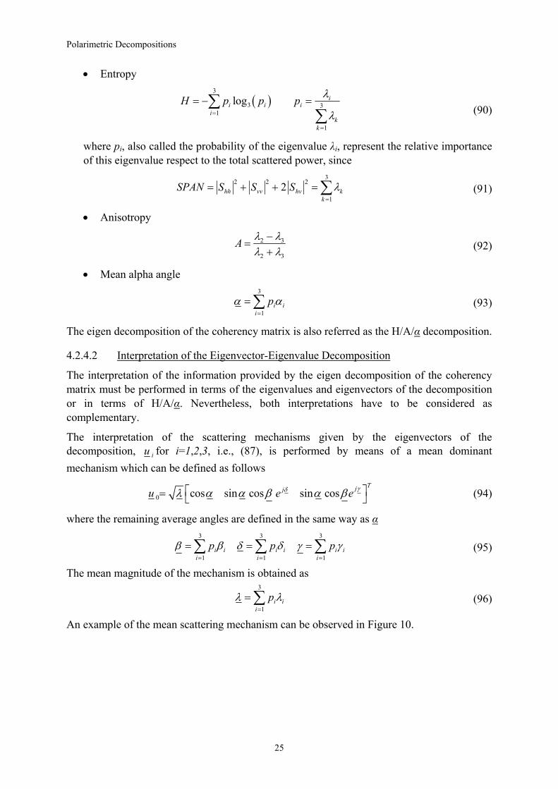
An example of the mean scattering mechanism can be observed in Figure 10.

25


( )cosλ α ( ) ( )sin cosλ α β ( ) ( )sin sinλ α β

Figure 10 Main scattering mechanism provided by the eigenvector-eigenvalue based decomposition..

The study of the mechanism given in (94) is mainly performed through the interpretation of the mean alpha angle, since its values can be easily related with the physics behind the scattering process. The next list reports the interpretation of α:

• α→0: The scattering corresponds to single-bounce scattering produced by a rough surface.

• α→π/4: The scattering mechanism corresponds to volume scattering. • α→π/2: The scattering mechanism is due to double-bounce scattering.

The second part in the interpretation of the eigen decomposition is performed by studying the value of the eigenvalues of the decomposition. A given eigenvalue corresponds to the associated scattered power to the corresponding eigenvector. Consequently, the value of the eigenvalue gives the importance of the corresponding eigenvector or scattering mechanism. The ensemble of scattering mechanisms is studied by means of the entropy H and the anisotropy A.

26


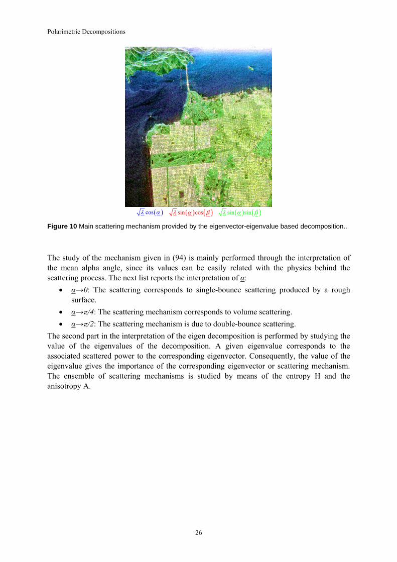
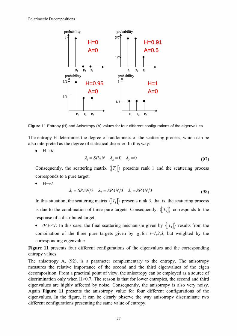
Figure 11 Entropy (H) and Anisotropy (A) values for four different configurations of the eigenvalues.

1probability

p1 p2 p3

3/7probability

p1 p2 p3

1/2probability

p1 p2 p3

1/4

1probability

p1 p2 p3

1/3

H=0 H=0.91

H=1H=0.95

A=0

A=0A=0

A=0.5

The entropy H determines the degree of randomness of the scattering process, which can be also interpreted as the degree of statistical disorder. In this way:

• H→0:

1 2 0 0SPAN 3λ λ λ= = = (97)

Consequently, the scattering matrix [ ]3T presents rank 1 and the scattering process

corresponds to a pure target. • H→1:

1 2 33 3SPAN SPAN SPAN 3λ λ λ= = = (98)

In this situation, the scattering matrix [ ]3T presents rank 3, that is, the scattering process

is due to the combination of three pure targets. Consequently, [ ]3T corresponds to the

response of a distributed target. • 0<H<1: In this case, the final scattering mechanism given by [ ]3T results from the

combination of the three pure targets given by iu for i=1,2,3, but weighted by the corresponding eigenvalue.

Figure 11 presents four different configurations of the eigenvalues and the corresponding entropy values. The anisotropy A, (92), is a parameter complementary to the entropy. The anisotropy measures the relative importance of the second and the third eigenvalues of the eigen decomposition. From a practical point of view, the anisotropy can be employed as a source of discrimination only when H>0.7. The reason is that for lower entropies, the second and third eigenvalues are highly affected by noise. Consequently, the anisotropy is also very noisy. Again Figure 11 presents the anisotropy value for four different configurations of the eigenvalues. In the figure, it can be clearly observe the way anisotropy discriminate two different configurations presenting the same value of entropy.

1/7

1probability

p1 p2 p3

3/7probability

p1 p2 p3

1/2probability

p1 p2 p3

1/4

1probability

p1 p2 p3

1/3

H=0 H=0.91

H=1H=0.95

A=0

A=0A=0

A=0.51/7

27


Entropy H

0.5 1.00 0.5 1.00

Anisotropy A

0.5 1.00

Average alpha angle α

0 45° 90°0 45° 90° Figure 12 Entropy (H), Anisotropy (A) and alpha (α) images.

28

Earth Online - 4. POLARIMETRIC DECOMPOSITIONS · Polarimetric Decompositions kSdl l (18) kS Shrr l l (19) And the helix component presents a left sense. On the contrary, when it is

Documents