Earth and Planetary Science - jess/ChenEPSL2016.pdf · Earth and Planetary Science Letters. ... Available online xxxx. Editor: variability. D. Vance. ... (WPWP), and contains two

Earth and Planetary Science Letters 442 (2016) 61–71

Contents lists available at ScienceDirect

Earth and Planetary Science Letters

www.elsevier.com/locate/epsl

A high-resolution speleothem record of western equatorial Pacific

rainfall: Implications for Holocene ENSO evolution

Sang Chen a,∗, Sharon S. Hoffmann b, David C. Lund c, Kim M. Cobb d, Julien Emile-Geay e, Jess F. Adkins f

a Department of Earth and Environmental Sciences, University of Michigan, Ann Arbor, MI 48109, United Statesb Department of Geography & Geology, University of North Carolina, Wilmington, NC 28403, United Statesc Department of Marine Sciences, University of Connecticut, Avery Point, Groton, CT 06340, United Statesd School of Earth & Atmospheric Sciences, Georgia Institute of Technology, Atlanta, GA 30332, United Statese Department of Earth Sciences, University of Southern California, Los Angeles, CA 90089, United Statesf Division of Geological and Planetary Sciences, California Institute of Technology, Pasadena, CA 91125, United States

a r t i c l e i n f o a b s t r a c t

Article history:Received 29 October 2015Received in revised form 23 February 2016Accepted 28 February 2016Available online xxxxEditor: D. Vance

Keywords:ENSOBorneospeleothem δ18Owestern Pacific rainfallHolocene

The El Niño-Southern Oscillation (ENSO) is the primary driver of interannual climate variability in the tropics and subtropics. Despite substantial progress in understanding ocean–atmosphere feedbacks that drive ENSO today, relatively little is known about its behavior on centennial and longer timescales. Paleoclimate records from lakes, corals, molluscs and deep-sea sediments generally suggest that ENSO variability was weaker during the mid-Holocene (4–6 kyr BP) than the late Holocene (0–4 kyr BP). However, discrepancies amongst the records preclude a clear timeline of Holocene ENSO evolution and therefore the attribution of ENSO variability to specific climate forcing mechanisms. Here we present δ18O results from a U–Th dated speleothem in Malaysian Borneo sampled at sub-annual resolution. The δ18O of Borneo rainfall is a robust proxy of regional convective intensity and precipitation amount, both of which are directly influenced by ENSO activity. Our estimates of stalagmite δ18O variance at ENSO periods (2–7 yr) show a significant reduction in interannual variability during the mid-Holocene (3240–3380 and 5160–5230 yr BP) relative to both the late Holocene (2390–2590 yr BP) and early Holocene (6590–6730 yr BP). The Borneo results are therefore inconsistent with lacustrine records of ENSO from the eastern equatorial Pacific that show little or no ENSO variance during the early Holocene. Instead, our results support coral, mollusc and foraminiferal records from the central and eastern equatorial Pacific that show a mid-Holocene minimum in ENSO variance. Reduced mid-Holocene interannual δ18O variability in Borneo coincides with an overall minimum in mean δ18O from 3.5 to 5.5 kyr BP. Persistent warm pool convection would tend to enhance the Walker circulation during the mid-Holocene, which likely contributed to reduced ENSO variance during this period. This finding implies that both convective intensity and interannual variability in Borneo are driven by coupled air-sea dynamics that are sensitive to precessional insolation forcing. Isolating the exact mechanisms that drive long-term ENSO evolution will require additional high-resolution paleoclimatic reconstructions and further investigation of Holocene tropical climate evolution using coupled climate models.

© 2016 Elsevier B.V. All rights reserved.

1. Introduction

The El Niño-Southern Oscillation (ENSO) is the primary driver of interannual climate variability on a global basis (Cane, 2005;Vecchi and Wittenberg, 2010). Instrumental records are essen-tial for identifying the key features of modern ENSO and its cli-matic impacts, especially sea surface temperature (SST) and re-

* Corresponding author at: Division of Geological and Planetary Sciences, Califor-nia Institute of Technology, Pasadena, CA 91125, United States.

E-mail address: [email protected] (S. Chen).

http://dx.doi.org/10.1016/j.epsl.2016.02.0500012-821X/© 2016 Elsevier B.V. All rights reserved.

gional precipitation anomalies (Xie and Arkin, 1997; Cane, 2005). The fate of ENSO in a greenhouse future, however, remains un-certain due to our incomplete characterization of ENSO processes in state-of-the-art general circulation models (GCMs). Results from Coupled Model Intercomparison Project phase 3 (CMIP3) show both strengthening and weakening of ENSO variability in response to global warming, due to the complex and counteracting feed-backs involved (Collins et al., 2010). Subsequent model develop-ment (CMIP5) has improved representation of ENSO phenomena in GCMs, but is still unable to simulate some key ENSO processes re-alistically (Bellenger et al., 2013). Paleoclimatic archives provide a

62 S. Chen et al. / Earth and Planetary Science Letters 442 (2016) 61–71

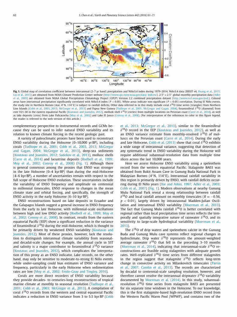
Fig. 1. Global map of correlation coefficient between interannual (2–7 yr band) precipitation and Niño3.4 index during 1979–2014. Niño3.4 data (ERSST v4, Huang et al., 2015;Liu et al., 2015) are obtained from NOAA Climate Prediction Center website (http://www.cpc.ncep.noaa.gov/data/ indices/). 2.5◦ ×2.5◦ global monthly precipitation data (Adler et al., 2003) are obtained from NOAA Global Precipitation Climatology Project (GPCP) Version 2.2 combined precipitation dataset (http://www.esrl.noaa.gov/psd/). Colored areas have interannual precipitation significantly correlated with Niño3.4 index (P < 0.05). White areas indicate non-significant (P > 0.05) correlation. During El Niño events, the study site in Northern Borneo (star, 4◦N, 114◦E) is subject to rainfall deficits. Other data referred to in this study include coral δ18O time series (triangles) from Northern Line Islands (Cobb et al., 2003, 2013; McGregor et al., 2013) and Papua New Guinea (Tudhope et al., 2001; McGregor and Gagan, 2004), foraminiferal δ18O (diamond) from core V21-30 in the eastern equatorial Pacific (Koutavas and Joanides, 2012), mollusk shell δ18O (circles) from multiple locations on Peruvian coast (Carre et al., 2014), as well as lake deposits (cross) from Lake Pallcacocha (Moy et al., 2002) and Lake El Junco (Conroy et al., 2008). (For interpretation of the references to color in this figure legend,

complementary perspective to instrumental records and GCMs be-cause they can be used to infer natural ENSO variability and its relation to known climate forcing in the recent geologic past.

A variety of paleoclimatic proxies have been used to reconstruct ENSO variability during the Holocene (0–10,000 yr BP), including corals (Tudhope et al., 2001; Cobb et al., 2003, 2013; McGregor and Gagan, 2004; McGregor et al., 2013), deep-sea sediments (Koutavas and Joanides, 2012; Sadekov et al., 2013), mollusc shells (Carre et al., 2014) and lacustrine deposits (Rodbell et al., 1999;Moy et al., 2002; Conroy et al., 2008) (Fig. 1). Although there is general consensus among the proxies that ENSO was stronger in the late Holocene (0–4 kyr BP) than during the mid-Holocene (4–6 kyr BP), a number of uncertainties remain with respect to the full scope of Holocene ENSO evolution. These uncertainties include the variability of ENSO frequency and amplitude on centennial to millennial timescales, ENSO response to changes in the mean climate state and orbital forcing, and specifically, the strength of ENSO activity in the early Holocene (6–10 kyr BP).

ENSO reconstructions based on lake deposits in Ecuador and the Galapagos Islands suggest a general increase in ENSO frequency from the early to late Holocene, with millennial-scale oscillations between high and low ENSO activity (Rodbell et al., 1999; Moy et al., 2002; Conroy et al., 2008). In contrast, results from the eastern equatorial Pacific (EEP) show a significant reduction in the variance of foraminiferal δ18O during the mid-Holocene, which is thought to be primarily driven by weakened ENSO variability (Koutavas and Joanides, 2012). Most of these proxies, however, lack the resolu-tion to distinguish interannual climate variability from seasonal-and decadal-scale changes. For example, the annual cycle in SST and salinity is a major contributor to foraminiferal δ18O variance (Koutavas and Joanides, 2012), which complicates the interpreta-tion of this proxy as an ENSO indicator. Lake records, on the other hand, may only be sensitive to moderate-to-strong El Niño events, while under-sampling could bias estimates of ENSO variance and frequency, particularly in the early Holocene when sedimentation rates are low (Moy et al., 2002; Emile-Geay and Tingley, 2016).

Corals are more direct recorders of ENSO variability because they provide decades- to centuries-long reconstructions of tropical marine climate at monthly to seasonal resolution (Tudhope et al., 2001; Cobb et al., 2003; McGregor et al., 2013). A compilation of coral δ18O records from the western and central equatorial Pacific indicates a reduction in ENSO variance from 3 to 5.5 kyr BP (Cobb

et al., 2013; McGregor et al., 2013), similar to the foraminiferal δ18O record in the EEP (Koutavas and Joanides, 2012), as well as an ENSO variance estimate from monthly-resolved δ18O of mol-luscs on the Peruvian coast (Carre et al., 2014). During the early and late Holocene, Cobb et al. (2013) show that coral δ18O exhibits a wide range of interannual variance, suggesting that detection of any systematic trend in ENSO variability during the Holocene will require additional subannual-resolution data from multiple time slices across the last 10,000 years.

Here we assess Holocene ENSO variability using a speleothem record from the western equatorial Pacific. Stalagmite BA03 was obtained from Bukit Assam Cave in Gunung Buda National Park in Malaysian Borneo (4◦N, 114◦E). Interannual rainfall variability in this region is primarily driven by ENSO, with rainfall deficits occur-ring during El Niño years (Xie and Arkin, 1997; Adler et al., 2003;Cobb et al., 2007) (Fig. 1). Modern observations at nearby Gunung Mulu National Park reveal a strong relationship between rainfall δ18O and local rainfall amount on monthly timescales (R = −0.56, p < 0.01), largely driven by intraseasonal Madden-Julian Oscil-lation and interannual ENSO variability (Moerman et al., 2013). The fact that Gunung Mulu rainfall δ18O is better correlated with regional rather than local precipitation time series reflects the tem-porally and spatially integrative nature of rainwater δ18O, and its sensitivity to large-scale hydrological variability (Moerman et al., 2013).

The δ18O of drip waters and speleothem calcite in the Gunung Buda and Gunung Mulu cave systems reflect regional changes in hydroclimate. Drip water δ18O represents the amount-weighted average rainwater δ18O that fell in the preceding 3–10 months (Moerman et al., 2014), indicating that interannual-scale δ18O re-constructions are feasible using stalagmites with adequate growth rates. Well-replicated δ18O time series from different stalagmites in the region suggest that stalagmite δ18O reflects long-term change in convective activity on Milankovitch timescales (Partin et al., 2007; Carolin et al., 2013). The records are characterized by decadal to centennial-scale sampling resolution, however, and therefore cannot resolve the interannual dripwater δ18O variability documented by Moerman et al. (2014). In this study, subannual-resolution δ18O time series from stalagmite BA03 are presented for six separate time windows in the Holocene. To our knowledge, this is the first stalagmite-based high-resolution ENSO record from the Western Pacific Warm Pool (WPWP), and contains two of the

S. Chen et al. / Earth and Planetary Science Letters 442 (2016) 61–71 63

Table 1U–Th dates for BA03 in the age model.

Depth(mm)

MC-ICP-MS measurements Age calculation

[238U] (ppb)a

[232Th] (pmol/g)

δ234U(�)

230Th/238U (×10−3)b

Corrected ages (yr BP)c

2σ error (yr)d

25.0 1764.2 ± 0.5 1.55 ± 0.01 −633.04 ± 0.19 1.91 ± 0.02 263 2244.5 1720.7 ± 2.0 3.11 ± 0.02 −633.26 ± 0.96 2.74 ± 0.03 247 4195.0 1725.9 ± 0.5 5.07 ± 0.01 −631.01 ± 0.18 5.43 ± 0.02 731 64

114.0e 1778.6 ± 0.6 4.02 ± 0.02 −631.66 ± 0.17 5.09 ± 0.14 824 97161.5 1846.9 ± 0.5 2.60 ± 0.01 −630.05 ± 0.16 5.56 ± 0.02 1205 32195.0 2113.1 ± 0.7 1.46 ± 0.01 −631.05 ± 0.19 5.47 ± 0.03 1386 23247.8 1941.3 ± 0.6 6.01 ± 0.02 −631.20 ± 0.19 8.42 ± 0.04 1596 69277.1 1838.2 ± 0.6 8.20 ± 0.02 −630.35 ± 0.21 10.43 ± 0.03 1813 97296.6 1618.7 ± 0.4 0.64 ± 0.01 −630.25 ± 0.19 7.00 ± 0.03 1932 18321.4 1506.9 ± 0.4 0.74 ± 0.01 −625.04 ± 0.18 7.98 ± 0.03 2169 20361.2 1931.2 ± 0.5 2.37 ± 0.01 −630.18 ± 0.18 9.55 ± 0.03 2472 32418.2 1928.0 ± 0.6 5.18 ± 0.01 −626.99 ± 0.16 11.87 ± 0.03 2747 59456.7e 1772.8 ± 0.7 1.44 ± 0.02 −630.27 ± 0.17 11.24 ± 0.15 3116 93495.7 1782.1 ± 0.5 0.52 ± 0.01 −627.98 ± 0.18 11.76 ± 0.03 3402 22518.5 1856.4 ± 0.5 1.09 ± 0.01 −626.51 ± 0.19 12.45 ± 0.04 3516 25581.0 1663.4 ± 0.5 2.59 ± 0.01 −626.35 ± 0.20 14.49 ± 0.04 3870 41645.0 1548.9 ± 0.5 3.12 ± 0.00 −625.91 ± 0.14 16.30 ± 0.02 4276 44697.9 1609.3 ± 0.5 2.01 ± 0.01 −625.06 ± 0.20 17.59 ± 0.05 4910 40763.5e 1726.3 ± 0.6 5.08 ± 0.02 −624.99 ± 0.20 19.53 ± 0.14 5032 110773.7 1721.1 ± 0.5 2.08 ± 0.00 −624.27 ± 0.13 19.22 ± 0.02 5392 29802.9 1706.3 ± 0.5 2.91 ± 0.00 −624.82 ± 0.12 19.80 ± 0.02 5444 38865.1 1995.3 ± 0.6 2.60 ± 0.01 −624.03 ± 0.17 20.87 ± 0.03 5913 36882.5 1255.3 ± 0.3 2.98 ± 0.01 −618.37 ± 0.07 22.67 ± 0.05 6078 59916.8 1367.7 ± 0.3 1.28 ± 0.01 −621.49 ± 0.23 22.09 ± 0.04 6353 35941.0 1516.3 ± 0.4 1.18 ± 0.01 −622.19 ± 0.17 22.70 ± 0.05 6601 34965.5 1518.3 ± 0.4 2.79 ± 0.01 −619.32 ± 0.18 24.35 ± 0.05 6785 48988.8 1806.3 ± 0.5 5.50 ± 0.01 −618.59 ± 0.17 25.72 ± 0.04 6869 69

1016.7 1150.4 ± 0.3 7.04 ± 0.01 −614.61 ± 0.18 29.90 ± 0.06 7217 1321036.5 1305.6 ± 2.1 5.59 ± 0.02 −613.69 ± 1.31 29.99 ± 0.07 7750 1161054.7 1744.9 ± 0.5 3.11 ± 0.01 −618.95 ± 0.16 28.55 ± 0.04 8132 481078.5 2183.4 ± 0.7 5.58 ± 0.01 −618.43 ± 0.18 30.05 ± 0.04 8385 611094.8 2210.4 ± 2.1 1.23 ± 0.02 −618.29 ± 0.79 28.62 ± 0.05 8501 521121.9 1940.9 ± 0.8 2.65 ± 0.01 −617.86 ± 0.43 32.63 ± 0.05 9558 501170.1 1380.0 ± 2.1 1.40 ± 0.02 −613.78 ± 1.25 33.45 ± 0.08 9806 901216.4 1331.5 ± 2.0 3.15 ± 0.02 −612.83 ± 1.25 38.71 ± 0.09 11128 1121246.3 1187.2 ± 2.2 1.79 ± 0.02 −614.48 ± 1.50 39.37 ± 0.10 11627 128

a All measurements are reported with 1σ errors unless otherwise specified.b Reported in terms of activity ratio.c Age corrected based on a multi-isochron derived detrital 230Th/232Th atomic ratio of 69 ± 5 ppm. Ages with 232Th concentration greater than 10 pmol/g, including one

of the four isochrons, are excluded from the age model and not listed in the table.d 2σ errors are derived on a Monte Carlo basis following Carolin et al. (2013).e

only existing ENSO reconstructions from the early Holocene. We then compare the interannual variance in the speleothem record to ENSO proxies from other locations in the equatorial Pacific, and discuss possible mechanisms driving Holocene ENSO evolution.

2. Methods

2.1. U–Th ages

Stalagmite BA03 is 1.3 m long and spans the entire Holocene epoch. The age model for BA03 was constructed with U-series (238U–234U–230Th) dating. Details of the age model can be found in Hoffmann et al. (in preparation). Stalagmites in this region have relatively low 238U concentrations, negative δ234U values and high detrital thorium concentrations (Partin et al., 2007; Carolin et al., 2013). BA03 has 238U concentrations of 1–2 ppm and δ234U val-ues ranging from −630� to −610�. Four isochrons were drilled for BA03 to determine detrital 230Th/232Th ratios with the Os-mond isochron plot method (Hoffmann et al., in preparation). The four isochrons yield a consistent initial 230Th/232Th atomic ratio of 69 ±5 ppm (95% confidence), which, together with measured 232Th concentrations, is used to constrain the initial 230Th in the stalag-mite. The 230Th/232Th ratio in BA03 is lower than stalagmites from the same site reported by Partin et al. (2007), but similar to those in Carolin et al. (2013). In samples with high 232Th, this method tends to over-correct initial 230Th and produces anomalously young ages. Samples with 232Th higher than 10 pmol/g were therefore excluded from the age model to eliminate apparent age reversals. Altogether 36 U–Th dates were used to construct the age model and constrain the growth rates of BA03 over the last 13,000 yr (Table 1). Because BA03 was associated with an active drip when

Fig. 2. U–Th dates for stalagmite BA03. The stalagmite is approximately 1.3 m long and spans 0–13 kyr BP, with a mean growth rate of 100 μm/yr. The figure shows the U–Th dates used in the age model for BA03 with 2σ errors. The age at zero depth is assumed to be zero. BA03 has two distinct growth rates during the Holocene: approximately 54 μm/yr before 7 kyr BP and 145 μm/yr afterwards. The black curve shows the age model for low-resolution δ18O data in Fig. 3 derived from StalAge algorithm (Scholz and Hoffmann, 2011) with 95% confidence interval (shaded). The shaded region is hardly visible in most of the Holocene since the U–Th ages are well constrained.

it was collected, we assume an age of 0 yr at the top of the stalag-mite. The U-series ages indicate that BA03 had two distinct growth rates during the Holocene: 54 μm/yr from 13 to 7 kyr BP and 145 μm/yr from 7 kyr BP to present (Fig. 2).

64 S. Chen et al. / Earth and Planetary Science Letters 442 (2016) 61–71

Fig. 3. (a) Speleothem δ18O records from Borneo. Decadal-resolution BA03 δ18O record (orange line) is shown with U–Th dates (orange triangles) used to construct the age model. Thick black lines on the orange curve mark the windows of high-resolution δ18O analysis shown in Fig. 4. δ18O records of stalagmite SCH02 (red), BA04 (blue) and SSC01 (green) from the same region are also plotted with corresponding U–Th dates (Partin et al., 2007). Also plotted is the September–October–November (SON) insolation on the equator (black, Berger and Loutre, 1991). (b) Speleothem δ18O record from Dongge Cave, China (grey, Dykoski et al., 2005), plotted with corresponding U–Th ages and June–July–August (JJA) insolation at 25◦N (black, Berger and Loutre, 1991). (For interpretation of the references to color in this figure legend, the reader is referred to the web version of this article.)

2.2. δ18O time series

δ18O time series were generated on both decadal and sub-annual timescales on BA03. The growth axis of BA03 was previ-ously milled every 1.5 mm for decadal-scale stable isotope anal-yses (Fig. 3). The age model for the δ18O series was determined with the StalAge algorithm (Scholz and Hoffmann, 2011) to ac-count for age uncertainties. To generate sub-annual resolution data, we milled the stalagmite surface parallel to individual growth bands using a computer-controlled Merchantek micromill system. Six sub-annually resolved time series were generated with this method; they are denoted as 2500, 3300, 5200, 5700, 6700 and 8200 yr BP windows in the following text based on the approx-imate center of their age range. The milling resolution varies from 30–60 μm in different time intervals, corresponding to tem-poral resolution of 0.2–0.4 yr per sample (Table 2). Stable iso-tope analyses were performed on a Finnigan MAT 253 multiple-collector gas source mass spectrometer coupled to a Finnigan Kiel automated carbonate device at the Stable Isotope Labora-tory of the University of Michigan. A total of 3032 analyses were run to generate time series of sufficient resolution and length to capture interannual variability in the six windows through-out the Holocene. Isotopic values are converted to Vienna Pee Dee Belemnite scale (VPDB) using National Bureau of Standards (NBS) 19 (n = 819, δ13C = 1.95 ± 0.05�, δ18O = −2.20 ± 0.07�) and NBS 18 (n = 168, δ13C = −5.01 ± 0.05�, δ18O = −22.99 ±0.08�).

2.3. Time series analysis

The original δ18O time series were interpolated to 0.5-yr res-olution and filtered with a 2–7 yr band wavelet filter1 (Fig. 4) developed from Torrence and Compo (1998). Band-pass filtered versions of the raw and interpolated data yield a similar pattern of relative ENSO-band variance in the six time windows. Multi-taper spectral analyses were performed for the six time series to com-pare spectral features in different time windows and to test the significance of interannual power in the data with respect to red noise (Fig. 5). The red noise background for a given time series was estimated by 2-year band pass filtering the raw data to eliminate high frequencies and then fitting first-order auto-regressive [AR(1)] models to the data following Schneider and Neumaier (2001). The slope and intercept of the fitted AR(1) models, along with their uncertainties, were used to generate 500 Monte Carlo AR(1) time series for each window to test the statistical significance of peaks in the spectra.

The same statistical approach was applied to the Niño3.4 SST index (average SST of region 5◦N–5◦S and 120◦W–170◦W; Huang et al., 2015; Liu et al., 2015) for comparison with the BA03 δ18Ospectra (Fig. 6). To account for the influence of the karst processes on stalagmite δ18O, the Niño3.4 time series was also convolved

1 Matlab code for the wavelet filter can be obtained from: https://github.com/CommonClimate/common-climate/blob/master/wavelet_filter.m.

S. Chen et al. / Earth and Planetary Science Letters 442 (2016) 61–71 65

Fig.

4.H

igh-

reso

luti

on B

A03

δ18

Oti

me

seri

es a

nd 2

–7 y

r ban

dpas

s filt

ered

seri

es. T

op ro

w: B

lue

cros

ses m

ark

the

δ18

Ova

lues

of i

ndiv

idua

l gro

wth

ban

ds m

illed

at s

ub-a

nnua

l res

olut

ion

(303

2 to

tal)

, plo

tted

wit

h a

two-

year

ru

nnin

g mea

n (r

ed li

ne) b

ased

on

a box

car a

vera

ging

algo

rith

m. T

he b

lack

line

s rep

rese

nt 9

5% co

nfide

nce i

nter

vals o

f the

box

car r

unni

ng m

ean. B

otto

m ro

w: B

andp

ass (

2–7

yr) fi

lter

ed δ18

Ose

ries

of t

he si

x ti

me s

erie

s int

erpo

late

d to

0.5

-yr r

esol

utio

n. T

he b

lack

das

hed

lines

mar

k th

e ±0

.1�

rang

e. (F

or in

terp

reta

tion

of t

he re

fere

nces

to co

lor i

n th

is fi

gure

lege

nd, t

he re

ader

is re

ferr

ed to

the w

eb ve

rsio

n of

this ar

ticl

e.)

with a karst response function (g(t) = τ−1e−t/τ , with τ being water residence time in the cave) following Dee et al. (2015). Because τ is uncertain, we considered multiple plausible aquifer recharge times, ranging from 3 months to 2 yrs (Moerman et al., 2014). The spectra of the convolved time series are plotted to-gether with that of Niño3.4 in Fig. 6. In addition, spectral anal-ysis was performed on satellite-based local precipitation at the Borneo site (Adler et al., 2003) to compare with BA03 δ18O data (Fig. 6).

To quantify changes in interannual variance between the differ-ent segments, we used a block-bootstrap approach (Kunsch, 1989), with a block size of 2 years. The test statistic is the ratio of vari-ances in the 2–7 yr band, and the sampling distributions are esti-mated from 5000 bootstrap replicates.

3. Results

The BA03 time series is similar to three other Borneo stalag-mites over the Holocene (Fig. 3a). The mean δ18O decreased by approximately 2� from 13 kyr BP to 5.5 kyr BP. The δ18O min-imum persisted until around 3.5 kyr BP, after which it increased by 1� toward the present. The change in mean δ18O is also re-flected in the high resolution δ18O series (Fig. 4), with a minimum in mean δ18O (−9.7�) occurring in the 3300 yr BP window and a maximum (−8.9�) in the 8200 yr BP window. In addition to long-term changes in mean δ18O, the high-resolution time series show substantial decadal δ18O variations of more than 0.5�. For exam-ple, there are two negative δ18O excursions of 0.6� during the 2490–2530 yr BP interval. Another example occurs between 8190 and 8230 yr BP, which displays a positive δ18O excursion of 0.8�, comparable in magnitude to the δ18O shifts in this region dur-ing Heinrich stadial events (Carolin et al., 2013). The abrupt δ18Oshift during this brief interval may relate to the 8.2 kyr meltwater discharge event in the North Atlantic and will be discussed else-where.

The 2–7 yr bandpass filtered time series show an overall re-duction in variance during the mid-Holocene compared to the early and late Holocene (Fig. 4). Variations of 0.1� magnitude oc-curred regularly in the early (6700 and 8200 windows) and late (2500 window) Holocene, whereas interannual δ18O variations in the mid-Holocene (3300, 5200 and 5700 window) were mostly less than 0.1�. The multi-taper spectra of the high-resolution time se-ries show at least one interannual peak above the 95% quantile of AR(1) processes for each of the time windows (Fig. 5). Although the interannual power in the BA03 δ18O spectra is weak (<25% to-tal variance) compared to the Niño3.4 index (Fig. 6), the peaks are statistically significant features of the data relative to the AR(1) backgrounds.

Results of the block-bootstrap test of equal variance are listed in Table 2. The highest interannual δ18O variance occurs in the 2500 yr window, significantly (P < 0.01) higher than variance in the other windows. The lowest overall δ18O variance oc-curs in the 5200 yr window, which is significantly (P < 0.01) lower than all other windows. We are unable to reject the null hypothesis (P > 0.1) that the interannual variance in the 3300, 5700 and 8200 yr windows are the same. The interpo-lated time series show a slightly different pattern of test results from the ungridded raw data. The interannual variance is in-creased in the 6700 yr window with the interpolation and the three mid-Holocene windows (3300, 5200 and 5700 yr) are in-distinguishable from each other after the interpolation. Note that the comparison of overall interannual variance is strongly in-fluenced by decadal modulations of high and low interannual variance in each window. For example, the 3300 and 5700 yr windows show low overall interannual variance despite some rel-atively large (>0.1�) δ18O shifts, while the overall variance of

66 S. Chen et al. / Earth and Planetary Science Letters 442 (2016) 61–71

Fig. 5. Multi-taper power spectra of the six δ18O time series from BA03 (black line) plotted with fitted AR(1) red noise background. The blue dashed lines mark 50% quantile of the multi-taper spectra of the 500 Monte-Carlo generated AR(1) series, and the red dashed line marks 95% quantile. The orange boxes mark the 2–7 yr period range. Each window has at least one interannual peak above 95% red noise. (For interpretation of the references to color in this figure legend, the reader is referred to the web version of this article.)

Fig. 6. (a) Multi-taper spectra of Niño3.4 index (ERSSTv4, 1950–2014) plotted with fitted AR(1) background. The blue and red dashed lines are 50% and 95% quantiles of 500 Monte-Carlo AR(1) spectra. The orange box marks the 2–7 yr period range. The purple dotted line is a spectrum of 36-yr local precipitation (1979–2014) at the Borneo site with data from the corresponding grid in Fig. 1. (b) Multi-taper spectra of Niño3.4 time series convolved with karst smoothing of different water residence times in the caves following Dee et al. (2015). Smoothing of the ENSO signal in the cave system shifts the interannual and higher frequency power into lower frequencies and make the spectra “redder” and more similar to the BA03 spectra. (For interpretation of the references to color in this figure legend, the reader is referred to the web version of this article.)

the 8200 yr BP window is largely diminished by the minimum interannual variance associated with an apparent 8.2 kyr event in BA03. Exclusion of the 8.2 kyr event makes interannual δ18Ovariance of the 8200 yr window slightly higher than (but indistin-guishable from) the 6700 yr window before and after interpola-tion.

4. Discussion

4.1. Spectral features of BA03 δ18O

Our goal is to quantify the time evolution of ENSO variance over the Holocene. Our sub-annual sample resolution allows for comparisons of the 2–7 yr variance (above the Nyquist frequency),

S. Chen et al. / Earth and Planetary Science Letters 442 (2016) 61–71 67

Table 2P-values for block-bootstrap test of equal variance of 2–7 yr filtered δ18O series.

Interval (yr BP)

N Temporal resolution (yr)

2–7 yr band stdev

2–7 yr percent (%)

2500 3300 5200 5700 6700

Original data2500 847 0.25 0.0528 7.173300 600 0.25 0.0394 11.35 < 0.015200 357 0.18 0.0315 12.04 < 0.01 < 0.015700 319 0.25 0.0410 10.57 < 0.01 0.35 < 0.016700 394 0.40 0.0444 9.93 < 0.01 0.07 < 0.01 0.198200 515 0.35 0.0434 5.66 < 0.01 0.11 < 0.01 0.26 0.39Interpolated2500 423 0.50 0.0537 7.923300 300 0.50 0.0396 13.91 < 0.015200 129 0.50 0.0405 22.13 < 0.01 0.405700 159 0.50 0.0415 12.56 < 0.01 0.38 0.456700 315 0.50 0.0492 12.90 0.21 0.04 0.05 0.098200 361 0.50 0.0404 4.99 < 0.01 0.40 0.49 0.45 0.05

Listed are P-values for a block-bootstrap test (Kunsch, 1989) with the null hypothesis that two samples come from populations of equal variance. N represents the sample sizes for each time series. Underlined values indicate test results where the null hypotheses of equal variance could not be rejected with 90% confidence. Test results are shown for both the data at original resolution and the 0.5-yr step interpolated data. 2–7 yr percent represent the percent of interannual variance in total variance of each window.

but cave processes are known to redden hydroclimate spectra; the spectrum of stalagmite δ18O time series is a distorted ver-sion of the underlying atmospheric signal. Karst water residence times can filter out higher frequency δ18O variations. In a multi-year cave drip water study in the Gunung Mulu cave system, Moerman et al. (2014) found that drip water δ18O reflected an amount-weighted integration of rainfall δ18O during the preced-ing 3–10 months. This work also demonstrated that the resi-dence time of water in the epikarst was inversely correlated with the amplitude of interannual δ18O variations in the drip water. A relatively long transit time of diffuse seepage flow that feeds the drip water is proposed to attenuate the rainfall δ18O signal in the drip water in the Mulu cave system (Cobb et al., 2007;Partin et al., 2013), which would tend to reduce interannual vari-ability in the speleothems (Moerman et al., 2014). This process would help explain the weaker interannual features we observe in our high-resolution δ18O time series from BA03 as compared to the Niño3.4 index. In our spectral analyses, a convolution of the Niño3.4 time series with a karst response function reduces the interannual power by shifting some of it to lower frequen-cies, especially for longer residence times (Fig. 6). Instead of direct recorders of ENSO activity, Moerman et al. (2014) suggested that the speleothems are better suited to reconstruct relative changes in ENSO variability, which is the approach we take here. In do-ing so, we assume a roughly constant water residence time at the drip site of BA03, based on the modern observation of no sig-nificant change in water residence time at a single drip over a 5-year period (Moerman et al., 2014). We are aware of the caveat that changes in residence time may happen on longer timescales. A bootstrap test of changes in ENSO variance of the karst-filtered Niño3.4 index suggests no significant reduction (p < 0.05) in the interannual band variance unless the residence time is increased to 18 months, which requires large changes in the hydrogeology of the cave system. A change in residence time from 3 to 10 months, as observed in the modern cave system, does not cause significant changes in interannual variance.

In the different BA03 time windows, we see an overall increase in total variance in the interannual band when ENSO activity is high (Fig. 4), rather than discrete, broad spectral peaks in the 2–7 yr interval (Fig. 5). It should also be noted that the maxi-mum power in the δ18O spectra does not lie in the interannual band, as is the case with Niño3.4 index. The interannual power accounts for a maximum of 22% of total power in the six time win-dows (Table 2), compared to 60% for the Niño3.4 index. The strong power at decadal and longer periods in the δ18O spectra suggests

that the stalagmite δ18O proxy is ‘red shifted’ like most paleocli-mate records. The longer and more variable time series (2500 and 8200 yr windows) are influenced more by these low-frequency variations compared to shorter and less variable windows (5200 and 5700 yr), which accounts for the changes in the fraction of interannual variance. The BA03 spectra are more similar to the spectra of Niño3.4 convolved with a long-residence-time karst fil-ter at interannual and lower frequencies (Fig. 6). We also note that the spectra of BA03 at frequencies higher than the interannual band are “white” rather than “red” and more closely resemble local precipitation instead of karst-filtered Niño3.4. At these frequencies, dripwater δ18O in the caves more closely track local rainfall, an atmospheric process that is insensitive to regional SST variability. Despite the complex natural processes driving δ18O variability in BA03, the relatively robust interannual features in the δ18O spec-tra suggest that the interannual trends in the spectra during the Holocene reflect changes in ENSO variability.

4.2. Pattern of Holocene ENSO evolution

A comparison of the Borneo results with fossil coral δ18O data from the central and western equatorial Pacific shows that both proxies show reduced δ18O variance from approximately 3.5 to 5.5 kyr BP (Fig. 7). An ENSO variance minimum at 4.6 kyr BP was also found in molluscs from the Peruvian coast (Carre et al., 2014). In addition, core V21-30 in the EEP records an interval of reduced foraminiferal δ18O variance from approximately 4 to 6 kyr BP (Koutavas and Joanides, 2012). Foraminiferal δ18O variance is calculated using the δ18O of single tests in each 1-cm stratum representing a deposition interval of approximately 80 yr, with an age model based on linear regression of radiocarbon dates dur-ing the Holocene (Fig. 7, Koutavas and Joanides, 2012). Given the several-hundred-year age uncertainty for the V21-30 age model, the four independent proxies all appear to show a reduction in interannual δ18O variance during the mid-Holocene (Fig. 7). The overall agreement between different records that span the equato-rial Pacific implies that ENSO is the primary driver of their com-mon variability.

In addition to the mid-Holocene ENSO minimum, our data have extended previous ENSO records from the WPWP (Tudhope et al., 2001; McGregor and Gagan, 2004), particularly during the early Holocene (6–10 kyr BP). Our results show a moderate level of variance in the early Holocene, consistent with the coral, foraminiferal and mollusc records. Substantial ENSO variance in the early Holocene is in marked contrast to the EEP lacustrine

68 S. Chen et al. / Earth and Planetary Science Letters 442 (2016) 61–71

Fig. 7. Comparison of Holocene ENSO variability estimates from BA03 with foraminiferal, coral, mollusc and lake sediment records. (a) Estimates of ENSO variability from stalagmite BA03 (squares) and foraminifera (circles, Koutavas and Joanides, 2012). BA03 δ18O estimates are based on the standard deviation of the 2–7 yr band in overlapping 30-yr windows (5-yr step). Foraminiferal δ18O variance is calculated using the δ18O of single tests in each 1-cm stratum with the original published age model (Koutavas and Joanides, 2012). (b) Coral δ18O standard deviations are calculated in the same way as BA03 and plotted as percent differences from modern corals (1968–1998) for each site. Coral time series shorter than 30 years are plotted with cross-filled circles (Cobb et al., 2013; McGregor et al., 2013). Also plotted is ENSO-driven seasonal SST range variance on Peruvian coast calculated from monthly molluscan shell δ18O measurements (pink, Carre et al., 2014). Variance is plotted as percent difference from modern (0–60 yr BP). The vertical bars mark 1σ uncertainty of the estimates, and the horizontal bars mark the time range of shells for the variance estimate. (c) Lake records from Lake Pallcacocha in Ecuador (blue, Moy et al., 2002) and El Junco in the Galapagas Islands (red, Conroy et al., 2008). Lake Pallcacocha record is based on reflective intensity of red light of the lake deposits. The variance of red intensity within overlapping 30-yr windows (5-yr step) is shown. Lake El Junco record is based on percentage of sand in the sediment grains. The low ENSO activity in early Holocene (6–10 kyr BP) in the lake records is distinct from the interannual records in the (a) and (b). (For interpretation of the references to color in this figure legend, the reader is referred to the web version of this article.)

records that show little or no ENSO activity (Moy et al., 2002;Conroy et al., 2008). Given the complexities of ascribing flood de-posits to El Niño events and the sensitivity of the lake records to event magnitude, such discrepancies are not surprising. The lake records also lack sufficient temporal resolution in the early Holocene to capture ENSO variability with low sedimentation rates. In a reanalysis of the Lake Pallcacocha data (Moy et al., 2002), Emile-Geay and Tingley (2016) showed that non-linear response of alpine runoff to ENSO activity in the eastern Pacific could sig-

nificantly bias ENSO variance estimates. Indeed, the alpine lake clastic flows have been reinterpreted as records of glaciation and soil erosion in a follow-up study (Rodbell et al., 2008).

In sum, our results together with published records imply that ENSO was quite active in the early Holocene compared to mid-Holocene. Simulating the reconstructed pattern of moderate vari-ance in the early Holocene, low variance in the mid-Holocene, and high variance in the late Holocene will be an important first-order test for modeling studies evaluating long-term ENSO variability.

S. Chen et al. / Earth and Planetary Science Letters 442 (2016) 61–71 69

4.3. Potential driving mechanisms

As indicated by low-resolution Borneo speleothem records (Fig. 3a), 3.5–5.5 kyr BP is an interval of anomalously high con-vective activity in the WPWP relative to the rest of the Holocene (Partin et al., 2007). This convective maximum in Borneo cor-responds to a maximum in boreal fall (September–October–November, SON) insolation on the equator (Fig. 3a). There is also a strong correspondence between speleothem δ18O in Bor-neo and equatorial fall insolation over the last 150,000 years (Carolin et al., 2013; Carolin et al., submitted for publication). Mod-ern observations of rainfall and cave drip water δ18O in Borneo have identified a δ18O minimum during SON (Cobb et al., 2007;Moerman et al., 2013). Results from an isotope modeling study suggest that the mid-Holocene minimum in Borneo δ18O is best described by changes in SON rather than annual average rain-fall (Tierney et al., 2012). The δ18O signal may therefore reflect a precession-driven maximum in SON insolation that promoted con-vective activity in Borneo, consistent with the interpretation from longer records (Partin et al., 2007; Carolin et al., 2013).

ENSO-band variability in the Borneo δ18O record suggests influ-ences from both internal climate variability and external forcing, depending on the timescale in question. On decadal and centen-nial timescales, we observe a wide-range of ENSO-band variance in BA03 (Fig. 4), consistent with the decadal-scale pattern in coral records (Cobb et al., 2013) and both forced (Liu et al., 2014) and unforced (Wittenberg, 2009) ENSO simulations. The lack of clear signal suggests that ENSO is governed by processes internal to the climate system on these timescales (Cobb et al., 2013). How-ever, ENSO-band variance shows a clear pattern on millennial and longer timescales when comparing different ENSO proxies (Fig. 7). In particular, the mid-Holocene minimum in interannual variance coincides with the overall maximum in Borneo convective activ-ity, suggesting that the two are linked. We propose that persistent convective activity in the WPWP was part of a basin-scale shift, with enhanced Walker circulation, easterly winds, and upwelling in the eastern equatorial Pacific. Such a shift would suppress the development of El Niño events and would account for reduced variance in ENSO proxies from the eastern, central, and western tropical Pacific. It therefore appears that the mean state of the WPWP, at least on millennial timescales, is closely linked to ENSO behavior during the Holocene.

Several modeling and observational studies suggest that ENSO may be paced by precession-driven changes in the seasonal distri-bution of insolation in the tropics. Early modeling work (Clement et al., 1996, 1999) invoked an ocean thermostat mechanism in which uniform warming in the equatorial Pacific strengthens the zonal SST gradient and the atmospheric Walker Circulation dur-ing boreal fall. As a consequence, upwelling in the EEP increases, further intensifying the zonal SST contrast and thereby creating a positive feedback that suppresses El Niño development. Because boreal fall (SON) is the primary growth phase of El Niño events, the mid-Holocene insolation maximum during SON could trigger the thermostat response and therefore modulate El Niño events. SST reconstructions across the equatorial Pacific have revealed a maximum zonal SST gradient during the mid-Holocene (Koutavas and Joanides, 2012), suggesting that ENSO variability is closely linked to tropical Pacific mean state, which is in turn paced by pre-cessional forcing. A monthly-resolved coral δ18O time series from the central Pacific has also identified damping of El Niño events during their growth phase in SON around 4.3 kyr BP (McGregor et al., 2013), in agreement with the prediction of the thermostat mechanism.

Other work suggests that additional factors may govern long-term ENSO behavior. Timmermann et al. (2007) argue that the position of the ITCZ and its associated band of highly reflective

clouds plays an important role in the cross-equatorial distribu-tion of insolation and the resulting wind and SST response in the EEP. Their model results, however, do not produce a mid-Holocene ENSO minimum as inferred from the proxy data, but millennial-scale variability in ENSO that is sensitive to boreal summer pre-cessional insolation. It has also been suggested that reduced ENSO variance was related to an intensified Asian summer monsoon (Liu et al., 2000), but the Borneo stalagmites demonstrate that coupled dynamics in the tropical Pacific are paced by boreal fall insola-tion and out of phase with Asian summer monsoon variability (Fig. 3), similar to the pattern in longer Borneo records (Carolin et al., 2013; Carolin et al., submitted for publication). In addition, the SST annual cycle in the equatorial Pacific may modulate ENSO variability through frequency entrainment (Chang et al., 1994;Timmermann et al., 2007). Climate models involving the frequency entrainment mechanism predict a negative correlation between the strength of the annual cycle and ENSO variability, in contrast to paleoclimate proxy observations that show weak positive correla-tion (Emile-Geay et al., 2016). The difference between proxy and models requires further modeling investigation to develop climate models that can accurately simulate forced changes in seasonality in the tropics to reveal its role in ENSO variability (Emile-Geay et al., 2016).

Results from the Paleoclimate Modeling Intercomparison Project (PMIP) also display a wide range of ENSO responses to mid-Holocene (6 kyr) insolation forcing. An ensemble of models simu-lates mid-Holocene ENSO amplitudes of −35% to +20% relative to pre-industrial conditions (Masson-Delmotte et al., 2013). The me-dian of the multi-model ensemble represents a 15% reduction in ENSO amplitude, in agreement with a transient coupled simulation (Liu et al., 2014). In PMIP-2 model runs, the standard deviation of several ENSO indices decreased in the mid-Holocene (6 kyr) simulations (Zheng et al., 2008; An and Choi, 2013). The largest response was in Niño3.4 which displayed an 18% reduction. By comparison, the PMIP-3 runs showed only a 5% reduction in the same index (An and Choi, 2013). Virtually all of the ENSO indices show a much weaker response in the PMIP3 than the PMIP2 exper-iments (An and Choi, 2013) and the magnitude of mid-Holocene ENSO reduction is not as large as inferred from paleoclimate prox-ies. With the range of related climatic factors and feedbacks, it is unlikely that any one process will provide a complete explanation of the Holocene ENSO pattern. Nevertheless, the correlation be-tween reduced ENSO variance and a precession-driven maximum in SON insolation suggests the two phenomena are coupled. The emerging picture of anomalously low ENSO variance from 3.5 to 5.5 kyr BP, as opposed to progressively increasing ENSO variability during the Holocene suggested by earlier work, sets a key goal for future modeling studies.

5. Conclusions

Our subannual-resolution stalagmite δ18O records show re-duced ENSO variance during the mid-Holocene, high ENSO vari-ability in the late Holocene, and moderate but active ENSO in the early Holocene. Our record from the western equatorial Pa-cific is consistent with coral, foraminiferal and mollusc records from the central and eastern Pacific, suggesting that ENSO was the common driver. Reduced interannual climate variability during the mid-Holocene in the equatorial Pacific coincides with an interval of anomalously high convective activity in the WPWP. The paleo-climate data therefore suggest that the mean state of the WPWP is a key factor governing ENSO behavior on millennial and longer timescales. The mean state is likely paced by equatorial fall insola-tion and appears to be decoupled from Northern Hemisphere sum-mer insolation. The emerging pattern of Holocene ENSO variability will serve as an important validation test for future models of

70 S. Chen et al. / Earth and Planetary Science Letters 442 (2016) 61–71

ENSO dynamics. Ideally, future data-model intercomparison studies will refine our understanding of the key ocean–atmosphere feed-backs that drive long-term ENSO evolution, leading to improved predictions of ENSO in a warming climate.

Acknowledgements

We would like to thank Gunung Buda and Gunung Mulu Na-tional Park crew for field assistance. We are grateful to Lora Wingate who performed the stable isotope analyses. We would also like to thank Rachel Sortor, Rachel Franzblau, Rachel Seltz, Alec Washabaugh and Naomi Huntley for help with micromilling, and Stacy Carolin for help with the U–Th dating. Derek Vance, Kathleen Johnson and an anonymous reviewer provided construc-tive feedbacks that helped improve the manuscript. The research was supported by NSF grant AGS-1103385.

References

Adler, R.F., Huffman, G.J., Chang, A., Ferraro, R., Xie, P., Janowiak, J., Rudolf, B., Schnei-der, U., Curtis, S., Bolvin, D., Gruber, A., Susskind, J., Arkin, P., 2003. The version 2 Global Precipitation Climatology Project (GPCP) monthly precipitation analysis (1979-present). J. Hydrometeorol. 4, 1147–1167.

An, S.-I., Choi, J., 2013. Mid-Holocene tropical Pacific climate state, annual cycle, and ENSO in PMIP2 and PMIP3. Clim. Dyn., 1–14.

Bellenger, H., Guilyardi, E., Leloup, J., Lengaigne, M., Vialard, J., 2013. ENSO rep-resentation in climate models: from CMIP3 to CMIP5. Clim. Dyn. 42 (7–8), 1999–2018. http://dx.doi.org/10.1007/s00382-013-1783-z.

Berger, A., Loutre, M.F., 1991. Insolation values for the climate of the last 10 million years. Quat. Sci. Rev. 10 (4), 297–317.

Cane, M.A., 2005. The evolution of El Niño, past and future. Earth Planet. Sci. Lett. 230 (3–4), 227–240.

Carolin, S.A., Cobb, K.M., Adkins, J.F., Clark, B., Conroy, J.L., Lejau, S., Malang, J., Tuen, A.A., 2013. Varied response of western Pacific hydrology to climate forcings over the last glacial period. Science 340 (6140), 1564–1566.

Carolin, S.A., Cobb, K.M., Adkins, J.F., Lynch-Stieglitz, J., Moerman, J.W., Lejau, S., Malang, J., Clark, B., Tuen, A.A., submitted for publication. Northern Borneo rain-fall variability across MIS 5 and 6 revealed in stalagmite oxygen isotopic records. Earth Planet. Sci. Lett.

Carre, M., Sachs, J.P., Purca, S., Schauer, A.J., Braconnot, P., Falcon, R.A., Julien, M., Lavallee, D., 2014. Holocene history of ENSO variance and asymmetry in the eastern tropical Pacific. Science 345 (6200), 1045–1048.

Chang, P., Wang, B., Li, T., Ji, L., 1994. Interactions between the seasonal cycle and the Southern Oscillation – frequency entrainment and chaos in a coupled ocean–atmosphere model. Geophys. Res. Lett. 21 (25), 2817–2820.

Clement, A.C., Seager, R., Cane, M.A., Zebiak, S.E., 1996. An ocean dynamical thermo-stat. J. Climate 9 (9), 2190–2196.

Clement, A.C., Seager, R., Cane, M.A., 1999. Orbital controls on the El Niño/Southern Oscillation and the tropical climate. Paleoceanography 14 (4), 441–456.

Cobb, K.M., Adkins, J.F., Partin, J.W., Clark, B., 2007. Regional-scale climate influ-ences on temporal variations of rainwater and cave dripwater oxygen isotopes in northern Borneo. Earth Planet. Sci. Lett. 263 (3), 207.

Cobb, K.M., Charles, C.D., Cheng, H., Edwards, R.L., 2003. El Nino/Southern Oscilla-tion and tropical Pacific climate during the last millennium. Nature 424 (6946), 271–276.

Cobb, K.M., Westphal, N., Sayani, H.R., Watson, J.T., Di Lorenzo, E., Cheng, H., Ed-wards, R.L., Charles, C.D., 2013. Highly variable El Nino-Southern Oscillation throughout the Holocene. Science 339 (6115), 67–70.

Collins, M., An, S.-I., Cai, W., Ganachaud, A., Guilyardi, E., Jin, F.-F., Jochum, M., Lengaigne, M., Power, S., Timmermann, A., Vecchi, G., Wittenberg, A., 2010. The impact of global warming on the tropical Pacific Ocean and El Nino. Nat. Geosci. 3 (6), 391–397.

Conroy, J.L., Overpeck, J.T., Cole, J.E., Shanahan, T.M., Steinitz-Kannan, M., 2008. Holocene changes in eastern tropical Pacific climate inferred from a Galápagos lake sediment record. Quat. Sci. Rev. 27 (11), 1166.

Dee, S., Emile-Geay, J., Evans, M.N., Allam, A., Steig, E.J., Thompson, D.M., 2015. PRYSM: an open-source framework for proxy system modeling, with applica-tions to oxygen-isotope systems. J. Adv. Mod. Earth Syst. 7. http://dx.doi.org/10.1002/2015MS000447.

Dykoski, C.A., Edwards, R.L., Cheng, H., Yuan, D., Cai, Y., Zhang, M., Lin, Y., Qing, J., An, Z., Revenaugh, J., 2005. A high-resolution, absolute-dated Holocene and deglacial Asian monsoon record from Dongge Cave, China. Earth Planet. Sci. Lett. 233 (1), 71.

Emile-Geay, J., Cobb, K.M., Carre, M., Braconnot, P., Leloup, J., Zhou, Y., Harrison, S.P., Correge, T., McGregor, H.V., Collins, M., Driscoll, R., Elliot, M., Schneider, B., Tudhope, A., 2016. Links between tropical Pacific seasonal, interannual, and or-bital variability during the Holocene. Nat. Geosci. 9 (2), 168–173.

Emile-Geay, J., Tingley, M.P., 2016. Inferring climate variability from nonlinear prox-ies: application to paleo-ENSO studies. Clim. Past 12, 31–50. http://dx.doi.org/10.5194/cp-12-31-20-2016.

Hoffmann, S.S., Lund, D.C., Adkins, J.F., Cobb, K.M., in preparation. Centennial-scale precipitation variability in Borneo over the past 12,000 years.

Huang, B., Banzon, V.F., Freeman, E., Lawrimore, J., Liu, W., Peterson, T.C., Smith, T.M., Thorne, P.W., Woodruff, S.D., Zhang, H.-M., 2015. Extended reconstructed sea surface temperature version 4 (ERSST.v4). Part I: upgrades and intercompar-isons. J. Climate 28 (3), 911–930.

Koutavas, A., Joanides, S., 2012. El Niño-Southern Oscillation extrema in the Holocene and Last Glacial Maximum. Paleoceanography 27 (4).

Kunsch, H.R., 1989. The jackknife and the bootstrap for general stationary observa-tions. Ann. Stat. 17, 1217–1241.

Liu, W., Huang, B., Thorne, P.W., Banzon, V.F., Zhang, H.-M., Freeman, E., Lawrimore, J., Peterson, T.C., Smith, T.M., Woodruff, S.D., 2015. Extended reconstructed sea surface temperature version 4 (ERSST.v4): Part II. Parametric and structural un-certainty estimations. J. Climate 28 (3), 931–951.

Liu, Z., Kutzbach, J., Wu, L., 2000. Modeling climate shift of El Nino variability in the Holocene. Geophys. Res. Lett. 27 (15), 2265–2268.

Liu, Z., Lu, Z., Wen, X., Otto-Bliesner, B.L., Timmermann, A., Cobb, K.M., 2014. Evolu-tion and forcing mechanisms of El Nino over the past 21,000 years. Nature 515 (7528), 550–553.

Masson-Delmotte, V., Schulz, M., Abe-Ouchi, A., Beer, J., Ganopolski, A., González Rouco, J.F., Jansen, E., Lambeck, K., Luterbacher, J., Naish, T., Osborn, T., Otto-Bliesner, B., Quinn, T., Ramesh, R., Rojas, M., Shao, X., Timmermann, A., 2013. Information from paleoclimate archives. In: Stocker, T.F., Qin, D., Plattner, G.-K., Tignor, M., Allen, S.K., Boschung, J., Nauels, A., Xia, Y., Bex, V., Midgley, P.M. (Eds.), Climate Change 2013: The Physical Science Basis. Contribution of Work-ing Group I to the Fifth Assessment Report of the Intergovernmental Panel on Climate Change. Cambridge University Press, Cambridge, United Kingdom and New York, NY, USA.

McGregor, H.V., Fischer, M.J., Gagan, M.K., Fink, D., Phipps, S.J., Wong, H., Woodroffe, C.D., 2013. A weak El Niño/Southern Oscillation with delayed seasonal growth around 4300 years ago. Nat. Geosci. 6 (11), 949.

McGregor, H.V., Gagan, M.K., 2004. Western Pacific coral δ18O records of anomalous Holocene variability in the El Niño–Southern Oscillation. Geophys. Res. Lett. 31 (11), L11204.

Moerman, J.W., Cobb, K.M., Adkins, J.F., Sodemann, H., Clark, B., Tuen, A.A., 2013. Diurnal to interannual rainfall δ18O variations in northern Borneo driven by re-gional hydrology. Earth Planet. Sci. Lett. 369–370, 108–119.

Moerman, J.W., Cobb, K.M., Partin, J.W., Meckler, A.N., Carolin, S.A., Adkins, J.F., Le-jau, S., Malang, J., Clark, B., Tuen, A.A., 2014. Transformation of ENSO-related rainwater to dripwater δ18O variability by vadose water mixing. Geophys. Res. Lett. 41 (22), 7907–7915.

Moy, C.M., Seltzer, G.O., Rodbell, D.T., Anderson, D.M., 2002. Variability of El Nino/Southern Oscillation activity at millennial timescales during the Holocene epoch. Nature 420 (6912), 162–165.

Partin, J.W., Cobb, K.M., Adkins, J.F., Clark, B., Fernandez, D.P., 2007. Millennial-scale trends in west Pacific warm pool hydrology since the Last Glacial Maximum. Nature 449 (7161), 452–455.

Partin, J.W., Cobb, K.M., Adkins, J.F., Tuen, A.A., Clark, B., 2013. Trace metal and carbon isotopic variations in cave dripwater and stalagmite geochemistry from northern Borneo. Geochem. Geophys. Geosyst. 14 (9), 3567–3585.

Rodbell, D.T., Seltzer, G.O., Anderson, D.M., Abbott, M.B., Enfield, D.B., Newman, J.H., 1999. An approximately 15,000-year record of El Nino-driven alluviation in southwestern ecuador. Science 283 (5401), 516–520.

Rodbell, D.T., Seltzer, G.O., Mark, B.G., Smith, J.A., Abbott, M.B., 2008. Clastic sedi-ment flux to tropical Andean lakes: records of glaciation and soil erosion. Quat. Sci. Rev. 27 (15–16), 1612–1626.

Sadekov, A.Y., Ganeshram, R., Pichevin, L., Berdin, R., McClymont, E., Elderfield, H., Tudhope, A.W., 2013. Palaeoclimate reconstructions reveal a strong link between El Nino-Southern Oscillation and Tropical Pacific mean state. Nat. Commun. 4, 2692.

Schneider, T., Neumaier, A., 2001. ARFIT-A Matlab package for the estimation of parameters and eigenmodes of multivariate autoregressive models. ACM Trans. Math. Softw. 27 (1), 58–65.

Scholz, D., Hoffmann, D.L., 2011. StalAge – an algorithm designed for construction of speleothem age models. Quat. Geochronol. 6 (3), 369.

Tierney, J.E., Oppo, D.W., LeGrande, A.N., Huang, Y., Rosenthal, Y., Linsley, B.K., 2012. The influence of Indian Ocean atmospheric circulation on warm pool hydrocli-mate during the Holocene epoch. J. Geophys. Res. 117 (19).

Timmermann, A., Lorenz, S.J., An, S.I., Clement, A., Xie, S.P., 2007. The effect of orbital forcing on the mean climate and variability of the tropical pacific. J. Climate 20 (16), 4147.

Torrence, C., Compo, G.P., 1998. A practical guide to wavelet analysis. Bull. Am. Me-teorol. Soc. 79 (1), 61–78.

Tudhope, A.W., Chilcott, C.P., McCulloch, M.T., Cook, E.R., Chappell, J., Ellam, R.M., Lea, D.W., Lough, J.M., Shimmield, G.B., 2001. Variability in the El Niño-

S. Chen et al. / Earth and Planetary Science Letters 442 (2016) 61–71 71

Southern Oscillation through a glacial-interglacial cycle. Science 291 (5508), 1511–1517.

Vecchi, G.A., Wittenberg, A.T., 2010. El Niño and our future climate: where do we stand? Wiley Interdiscip. Rev.: Clim. Change.

Wittenberg, A.T., 2009. Are historical records sufficient to constrain ENSO simula-tions? Geophys. Res. Lett. 36 (12). http://dx.doi.org/10.1029/2009gl038710.

Xie, P., Arkin, P.A., 1997. Global precipitation: a 17-year monthly analysis based on gauge observations, satellite estimates, and numerical model outputs. Bull. Am. Meteorol. Soc. 78 (11), 2539–2558.

Zheng, W., Braconnot, P., Guilyardi, E., Merkel, U., Yu, Y., 2008. ENSO at 6 ka and 21 ka from ocean–atmosphere coupled model simulations. Clim. Dyn. 30 (7–8), 745–762.