Basel Committee on Banking Supervision Early lessons from the Covid-19 pandemic on the Basel reforms July 2021

Welcome message from author
This document is posted to help you gain knowledge. Please leave a comment to let me know what you think about it! Share it to your friends and learn new things together.
Transcript
Basel Committee on Banking Supervision
Early lessons from the Covid-19 pandemic on the Basel reforms July 2021

This publication is available on the BIS website (www.bis.org).
© Bank for International Settlements 2021. All rights reserved. Brief excerpts may be reproduced or translated provided the source is stated.
ISBN - 978-92-9259-491-6 (online)
Early lessons from the Covid-19 pandemic on the Basel reforms iii
Contents
Glossary .................................................................................................................................................................................................. v
Early lessons from the Covid-19 pandemic on the Basel reforms ................................................................................. 1
Executive summary ........................................................................................................................................................................... 1
Introduction ......................................................................................................................................................................................... 4
1. The international banking system during the pandemic ......................................................................................... 4
2. The resilience of the banking system ............................................................................................................................. 13
2.1. Overall resilience ........................................................................................................................................................... 13
2.2. Regulatory measures and resilience outcomes during the Covid-19 pandemic ................................. 17
2.3. Impact on lending ........................................................................................................................................................ 20
3. Capital framework .................................................................................................................................................................. 25
3.1 The functioning of capital buffers .......................................................................................................................... 25
3.2 Countercyclical capital policy during the pandemic ....................................................................................... 33
3.3 Insights from pricing of Additional Tier 1 instruments ................................................................................. 40
4. The Liquidity Coverage Ratio ............................................................................................................................................ 45
5. Leverage ratio and market intermediation .................................................................................................................. 52
6. The cyclicality of bank regulatory requirements during the pandemic ............................................................ 62
6.1. Capital impact from credit loss provisioning ..................................................................................................... 62
6.2. Capital for banks’ market activities ........................................................................................................................ 66
Annex 1: List of data sources ...................................................................................................................................................... 71
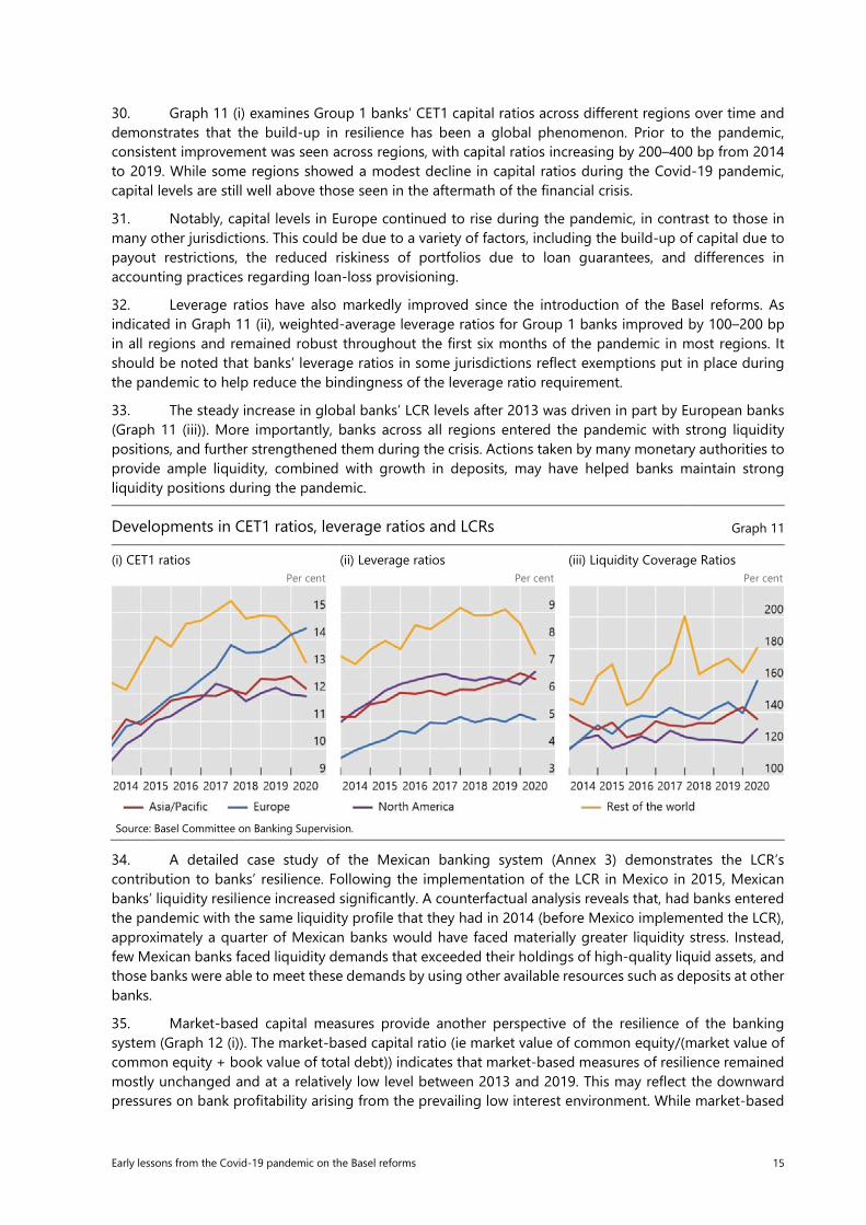
Annex 2: TFE survey questionnaire ........................................................................................................................................... 74
Annex 3: The liquidity buffer – case studies ......................................................................................................................... 77
Annex 4: Collation of supplemental tables and charts ..................................................................................................... 83
Annex 5: Members of the Task Force on Evaluations ....................................................................................................... 87

Early lessons from the Covid-19 pandemic on the Basel reforms v
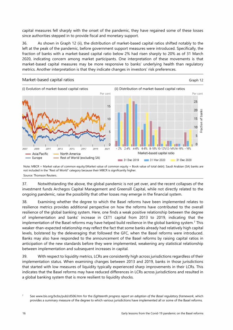
Glossary
AT1 Additional Tier 1 BCBS Basel Committee on Banking Supervision BIS Bank for International Settlements bp basis point CBR Combined buffer requirement CCoB Capital conservation buffer CCP Central counterparty CCR Counterparty credit risk CCyB Countercyclical capital buffer CD Certificate of deposit CDS Credit default swap CECL Current expected credit losses CET1 Common Equity Tier 1 CoCo Contingent convertible security CP Commercial Paper CRA Credit rating agency CVA Credit valuation adjustment D-SIB Domestic systemically important bank ECB European Central Bank ECL Expected credit losses EMEA Europe, Middle East and Africa FINMA Swiss Financial Market Supervisory Authority FRTB Fundamental Review of the Trading Book FX Foreign exchange GDP Gross domestic product GFC Global Financial Crisis G-SIB Global systemically important bank HLBA Historical look-back approach HQLA High-quality liquid assets IAS International Accounting Standard IFRS International Financial Reporting Standard IL(M) Incurred loss (method) IMM Internal Model Method LCR Liquidity Coverage Ratio LLA Loan loss allowance MDA Maximum distributable amount MMF Money market funds
vi Early lessons from the Covid-19 pandemic on the Basel reforms
MPG Macroprudential Policy Group NFC Non-financial corporate NSFR Net Stable Funding Ratio OSFI Office of the Superintendent of Financial Institutions (Canada) P&L Profit and loss PLA P&L attribution test pp percentage point(s) QIS Quantitative Impact Study RWA Risk-weighted asset SA-CCR Standardised approach for CCR SFT Secured financing transaction SICR Significant increases in credit risk SME Small and medium-sized entity SNL Standard and Poor's Market Intelligence SRB Systemic risk buffer SRS Supervisory Reporting System TFE Task Force on Evaluations USD US dollar (s)VaR (Stressed) value at risk WGL Working Group on Liquidity YTM Yield to maturity YTW Yield to worst
Early lessons from the Covid-19 pandemic on the Basel reforms 1
Early lessons from the Covid-19 pandemic on the Basel reforms
Executive summary
Beginning in 2009, the Basel Committee on Banking Supervision (the Committee) developed a set of new regulatory standards, commonly referred to as the Basel reforms, in response to the Global Financial Crisis of 2007–09.1 These standards aimed to strengthen the regulation, supervision and risk management of banks. Following their issuance, the Committee has deemed it appropriate to evaluate the impact of those standards already implemented on the resilience and behaviour of the banking system.
As part of this evaluation, the Committee has started to assess the ongoing Covid-19 pandemic’s impact on the banking system, as it has posed a significant global test of the Basel reforms. This report provides a preliminary assessment of whether the reforms implemented thus far have functioned as intended in light of the pandemic, which has resulted in a pronounced global economic shock, albeit one significantly different in nature from the financial crisis that motivated the Basel reforms.
The report reflects the Committee’s initial findings based upon empirical analysis of a combination of vendor and regulatory data, case studies and the results of a supervisory survey conducted by the Committee. The findings of this report should be considered in light of (i) the incomplete data available to date regarding the impact of the pandemic, which continues to unfold and whose full effect on the economy may not yet be clear, and (ii) the difficulty of distinguishing between the effects of the Basel reforms and those of the extensive and wide-ranging monetary and fiscal support measures undertaken by authorities to address the economic impact of the pandemic.
The report finds that the increased quality and higher levels of capital and liquidity held by banks have helped them absorb the sizeable impact of the Covid-19 pandemic thus far, suggesting that the Basel reforms have achieved their broad objective of strengthening the resiliency of the banking system. Banks and the banking system would have faced greater stress had the Basel reforms not been adopted. Throughout the unprecedented global economic downturn the banking system has continued to perform its fundamental functions, as banks have continued to provide credit and other critical services. While the report finds that some features of the Basel reforms, including the functioning of capital and liquidity buffers, the degree of countercyclicality in the framework, and the treatment of central bank reserves in the leverage ratio may warrant further consideration, it does not seek to draw firm conclusions regarding the need for potential revisions to the reforms.
Following a brief narrative regarding the impact of the pandemic on the banking system (Section 1), this report outlines the Committee’s initial findings regarding (i) the overall resilience of the banking system during the pandemic (Section 2); (ii) the usability of capital buffers, members’ experience with the countercyclical capital policies and price movements of Additional Tier 1 (AT1) capital instruments (Section 3); (iii) liquidity buffers (Section 4); (iv) the impact of the leverage ratio on financial intermediation (Section 5); and (v) the cyclicality of specific Basel capital requirements (Section 6).
The overall resilience of the banking system during the pandemic
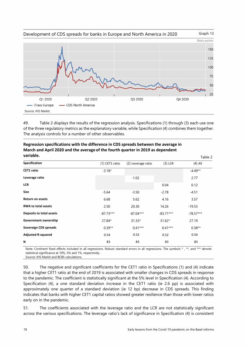
As noted, the analysis indicates that the banking system has remained resilient through the pandemic, strengthened by substantial increases in capital and liquidity held by banks since the adoption of the Basel reforms. No internationally active bank has failed or required significant public sector funding since the onset of the pandemic, though future losses may emerge as the pandemic remains ongoing. Banks have generally managed to absorb temporary increases in the costs of liquidity and higher credit risk while
1 See Basel III: international regulatory framework for banks at www.bis.org/bcbs/basel3.htm and Minimum capital requirements for market risk at www.bis.org/bcbs/publ/d457.htm.
2 Early lessons from the Covid-19 pandemic on the Basel reforms
substantially maintaining their services to customers. Market measures of resilience (eg banks’ credit default swap (CDS) spreads) do, however, indicate that some banks experienced strain early in the pandemic. Regression results suggest that banks with higher Common Equity Tier 1 (CET1) capital ratios experienced smaller increases in CDS spreads. Moreover, the analysis indicates that more strongly capitalised banks showed greater increases in lending to businesses and households than other banks. Thus, the global banking system has been able to complement and support monetary and fiscal authorities’ efforts to maintain economic activity during the pandemic, helping to absorb the shock rather than amplifying it, as occurred during the 2007–09 financial crisis.
The usability of capital buffers and price movements of AT1 capital instruments
The analysis indicates that most banks maintained capital ratios well above their minimum requirements and buffers during the pandemic partially due to authorities reducing capital requirements and buffers and imposing restrictions on capital distributions via dividend payments and share buybacks, as well as due to the extensive fiscal and monetary support provided to borrowers. This makes it difficult to draw conclusions regarding banks’ willingness to use capital buffers. Though some evidence suggests that banks may have been hesitant to use their regulatory capital buffers had it been necessary.
Regression results, including a detailed study of loan data from the euro area, indicate that banks that had less headroom (ie the amount of capital resources above minimum capital regulatory requirements and buffers) tended to lend less during the pandemic than those with more headroom. However, it is unclear whether this reluctance to use capital buffers reflects banks’ uncertainty regarding potential future losses or the wider market stigma that may result if a bank were to operate in its buffers.
Most authorities that maintained a positive countercyclical capital buffer (CCyB) prior to the pandemic reduced them in order to provide banks with additional headroom. Similarly, several authorities that did not have positive CCyBs lowered other regulatory requirements or buffer levels. While it is difficult to assess the quantitative effect of these capital releases independent of other measures, analysis provides some evidence that the capital release had a positive effect on lending during the pandemic. These findings, taken together with supervisors’ survey responses, suggest that it may be beneficial to consider whether there is sufficient releasable capital in place to address future systemic shocks.
The report also includes an analysis of price and yield movements of AT1 capital instruments compared to those of subordinated debt instruments and common equity. The analysis indicates that the pandemic resulted in increased AT1 yield premia for both preferred stock and contingent convertible securities relative to unsecured debt, suggesting that market participants generally perceived AT1 instruments to be riskier than debt. Furthermore, thus far during the pandemic, the two types of AT1 instruments have experienced broadly similar price movements indicating that investors do not perceive one instrument to be riskier than the other. Regression analyses also show that AT1 prices are positively associated with both equity and subordinated long-term debt prices. The report does not directly seek to address the issue of AT1 instruments’ loss-absorption capacity on a going-concern basis.
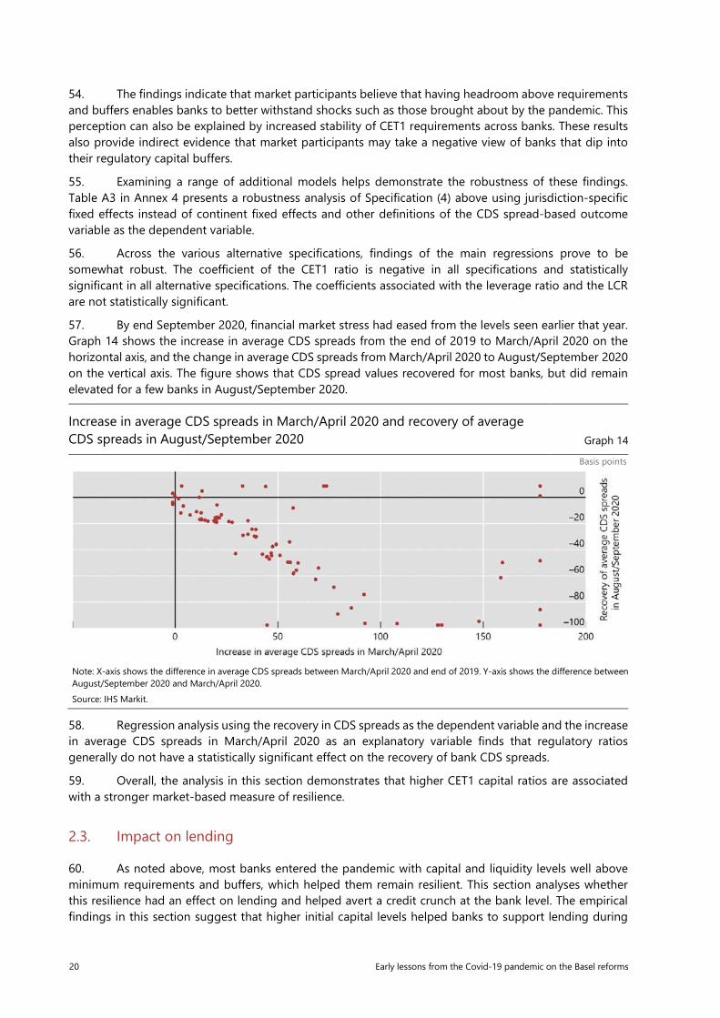
Liquidity buffers
Certain banks faced liquidity pressure in the early phase of the pandemic. The severity of the pressure largely depended on banks’ funding models. For example, banks reliant on unsecured wholesale money markets were more likely to have experienced pressure as funding sources dried up and they experienced large draws on loan facilities. In contrast, banks with stable deposit franchises experienced negligible liquidity pressure even at the peak of the stress. While an increase in the amount of high-quality liquid assets that the Liquidity Coverage Ratio (LCR) requires banks to hold helped banks absorb this liquidity pressure, measures taken by central banks and governments to support economies significantly reduced liquidity pressures. Overall, banks met large drawdown demands on committed lines and engaged in early buybacks of funding instruments from money market funds. Despite relatively limited liquidity stress, some jurisdictional studies highlighted that a range of banks took defensive action, reflecting in part their targeting of internal LCR levels well above 100%. However, these actions do not appear to have
Early lessons from the Covid-19 pandemic on the Basel reforms 3
contributed materially to the wider disruption in financial markets that prompted central banks to intervene in March 2020.
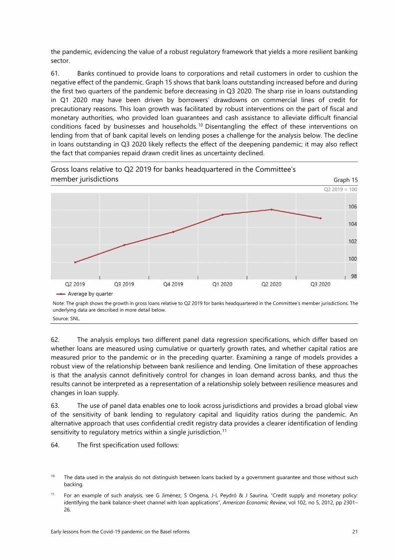
The impact of the leverage ratio on financial intermediation
While the leverage ratio (which has not yet been implemented by all member jurisdictions) was not a binding constraint for most banks during the pandemic, the analysis – based on detailed jurisdictional studies – examines whether banks that had a smaller amount of capital above leverage ratio requirements and buffers were less active than other banks in financial market intermediation during the pandemic. Overall, bank positions in government bond and repurchase agreement (repo) markets remained stable or rose in response to the rapid surge in client demand for liquidity at the onset of the crisis, though there is evidence that leverage ratio requirements may have reduced banks’ incentives to mitigate the large imbalances that emerged in some markets. Several member jurisdictions temporarily exempted central bank reserves from the leverage ratio calculation, which eased banks’ balance sheet constraints on their intermediation activity.
The cyclicality of specific Basel capital requirements
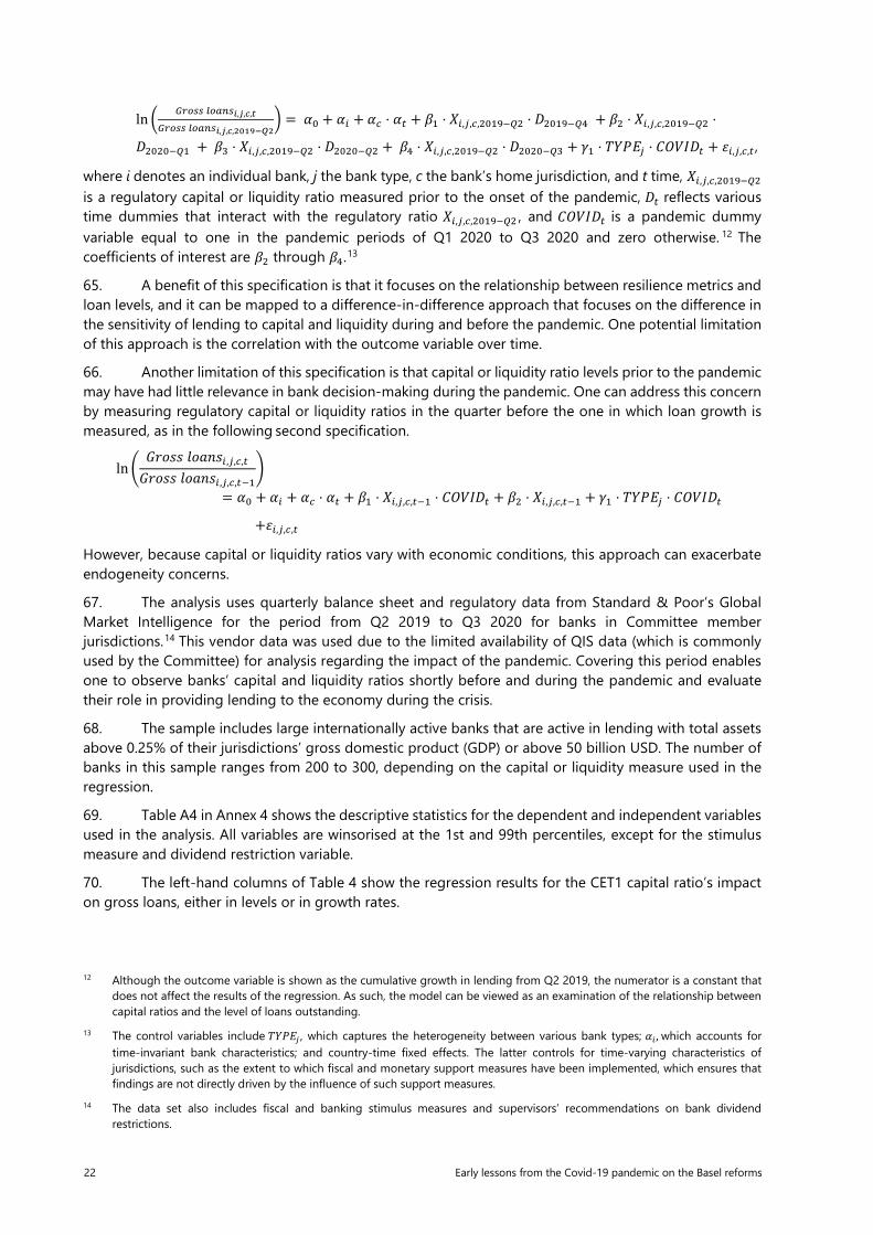
The report concludes with an early examination of the cyclicality (defined as the extent to which regulatory requirements respond in the opposite direction to movements in economic activity) of the impact of credit loss provisions and market risk requirements on capital positions during the pandemic. The analysis indicates that extensive governmental support measures to borrowers significantly dampened the impact of the economic contraction on bank capital. Measures taken to delay the recognition of credit provisions in the measurement of regulatory capital also deferred the impact. Collectively, these measures make it difficult to draw conclusions about the cyclicality of capital requirements. The analysis finds that sources of cyclicality in the current (ie Basel 2.5) market risk framework prompted supervisors to take relief measures in several jurisdictions. However, revisions to this framework, agreed upon in January 2019, are expected to mitigate these sources of cyclicality.
The analysis presented herein will be updated and included, as relevant, in a more comprehensive evaluation report covering the Basel reforms implemented over the past decade that the Committee plans to publish in 2022 as additional data on the impact of the Covid-19 pandemic becomes available.
4 Early lessons from the Covid-19 pandemic on the Basel reforms
Introduction
1. Beginning in 2009, in response to the 2007–09 Global Financial Crisis (GFC), the Committee developed a new set of regulatory standards commonly referred to as the Basel reforms. These reforms aimed to strengthen the regulation, supervision and risk management of banks. Nearly a decade after this initiative began, the Committee has deemed it appropriate to evaluate the impact that these reforms have had on the banking system.
2. As part of this evaluation, the Committee has assessed the impact of these reforms on the resilience and behaviour of banks during the Covid-19 pandemic, which has posed a significant test of the reforms on a global scale. This report presents the Committee’s evaluation, which is based on a combination of vendor and regulatory bank-level data, jurisdictional case studies and the results of supervisory surveys.2 The data used are described in Annex 1.
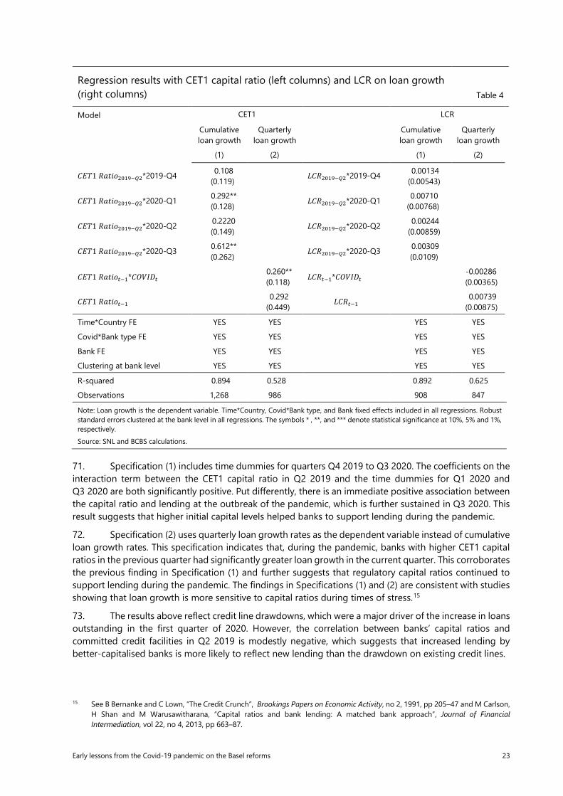
3. The findings in this report are not fully comprehensive or conclusive as the pandemic is ongoing and its full effects on the banking system may not yet have emerged. As such, the report does not seek to draw firm conclusions regarding the need for potential revisions to the Basel reforms. The analysis presented herein will be updated and included, as relevant, in a full evaluation report on the Basel reforms to be published in 2022.
1. The international banking system during the pandemic
4. The spread of the Covid-19 virus and the measures taken to control it resulted in large asset price declines, severe dislocations in funding markets and extraordinary economic contractions around the world. Governments and central banks responded with extensive fiscal, monetary and regulatory support measures. In contrast to the GFC, in which banks were the sources and propagators of stress, to date banks have remained resilient and have complemented public sector support by continuing to provide core financial services to help cushion the impact of the pandemic on the broader economy.
Financial market turbulence
5. In the early months of 2020, as the Covid-19 virus spread from country to country, authorities reacted by imposing lockdowns and social distancing measures. Production ceased in many sectors. Households cut back on spending and increased precautionary savings. Many people were unable to work, and unemployment rates rose in many jurisdictions.
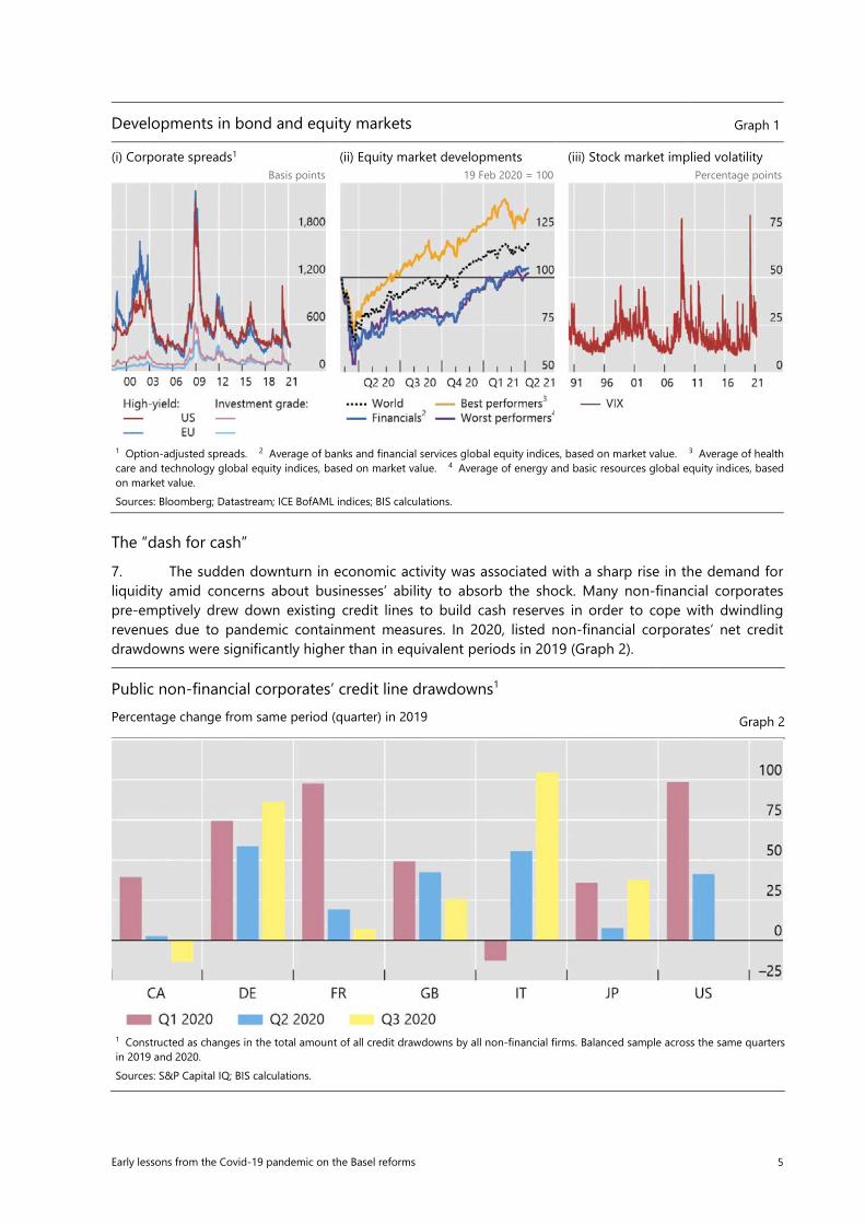
6. While the timing of Covid-19 outbreaks and containment measures differed across jurisdictions, close economic and financial interdependencies resulted in the rapid transmission of the shock through global markets. In March 2020, concerns about the trajectory of the pandemic and its impact on economic growth sharply diminished risk appetite, as evidenced by periods of extreme volatility in equity and other markets (Graph 1). The S&P 500 fell by 30% between February and March 2020 and implied volatility spiked to levels not seen since 2008. Credit spreads widened sharply, especially for high-yield bonds. Issuance of leveraged loans and private debt largely ceased and emerging markets experienced large capital outflows and sharp movements in foreign exchange rates.
2 Note that as part of its Covid-19 burden-relief measures, the Committee did not conduct a quantitative impact study (QIS)
collecting bank data covering H1 2020.
Early lessons from the Covid-19 pandemic on the Basel reforms 5
Developments in bond and equity markets Graph 1
(i) Corporate spreads1 (ii) Equity market developments (iii) Stock market implied volatility
Basis points 19 Feb 2020 = 100 Percentage points
The “dash for cash”
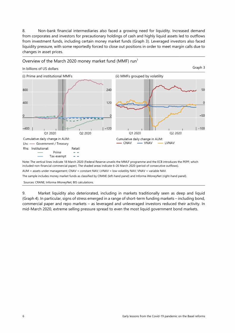
7. The sudden downturn in economic activity was associated with a sharp rise in the demand for liquidity amid concerns about businesses’ ability to absorb the shock. Many non-financial corporates pre-emptively drew down existing credit lines to build cash reserves in order to cope with dwindling revenues due to pandemic containment measures. In 2020, listed non-financial corporates’ net credit drawdowns were significantly higher than in equivalent periods in 2019 (Graph 2).
Public non-financial corporates’ credit line drawdowns1 Percentage change from same period (quarter) in 2019 Graph 2
1 Option-adjusted spreads. 2 Average of banks and financial services global equity indices, based on market value. 3 Average of health care and technology global equity indices, based on market value. 4 Average of energy and basic resources global equity indices, based on market value. Sources: Bloomberg; Datastream; ICE BofAML indices; BIS calculations.
1 Constructed as changes in the total amount of all credit drawdowns by all non-financial firms. Balanced sample across the same quarters in 2019 and 2020. Sources: S&P Capital IQ; BIS calculations.
6 Early lessons from the Covid-19 pandemic on the Basel reforms
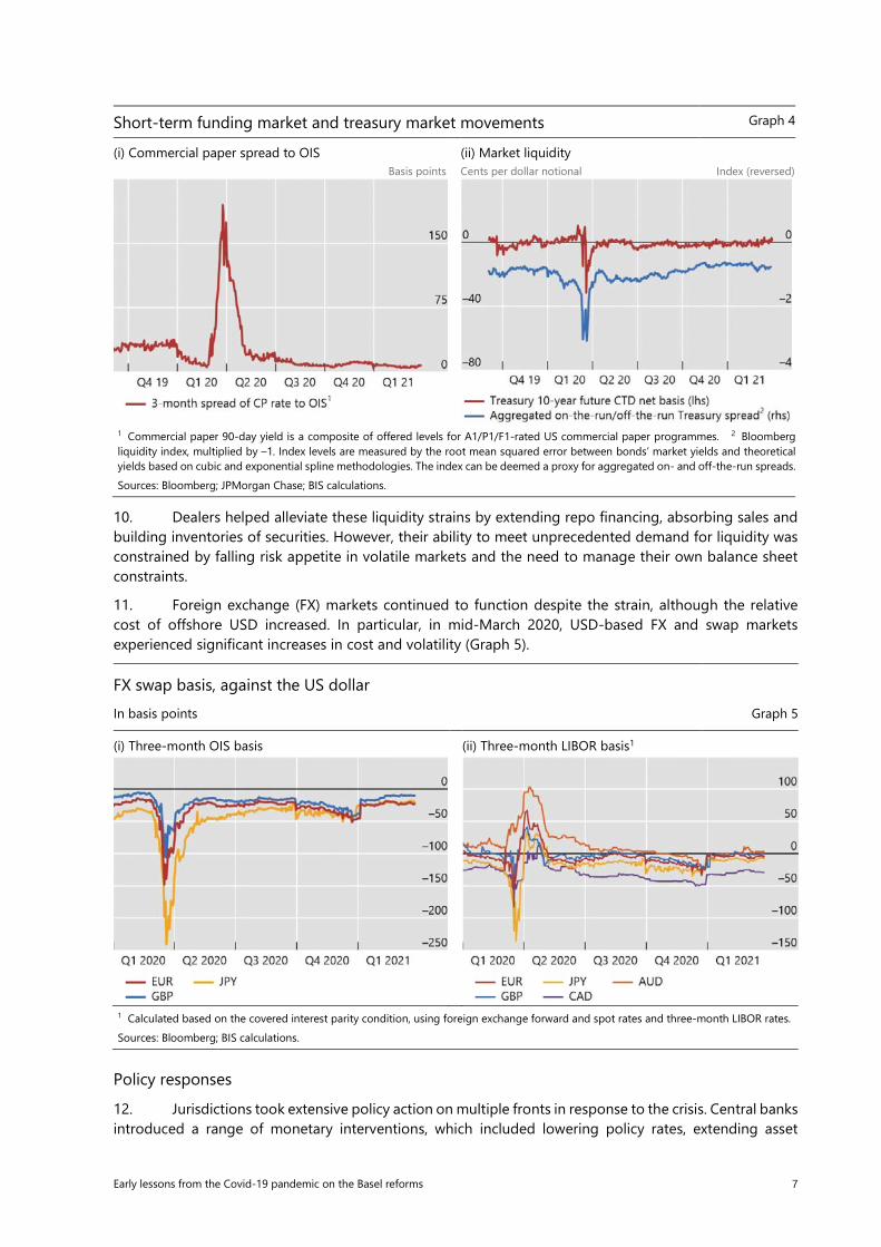
8. Non-bank financial intermediaries also faced a growing need for liquidity. Increased demand from corporates and investors for precautionary holdings of cash and highly liquid assets led to outflows from investment funds, including certain money market funds (Graph 3). Leveraged investors also faced liquidity pressure, with some reportedly forced to close out positions in order to meet margin calls due to changes in asset prices.
Overview of the March 2020 money market fund (MMF) run1
In billions of US dollars Graph 3
(i) Prime and institutional MMFs (ii) MMFs grouped by volatility
Note: The vertical lines indicate 18 March 2020 (Federal Reserve unveils the MMLF programme and the ECB introduces the PEPP, which included non-financial commercial paper). The shaded areas indicate 6–26 March 2020 (period of consecutive outflows). AUM = assets under management; CNAV = constant NAV; LVNAV = low-volatility NAV; VNAV = variable NAV. The sample includes money market funds as classified by CRANE (left-hand panel) and Informa iMoneyNet (right-hand panel).
Sources: CRANE; Informa iMoneyNet; BIS calculations.
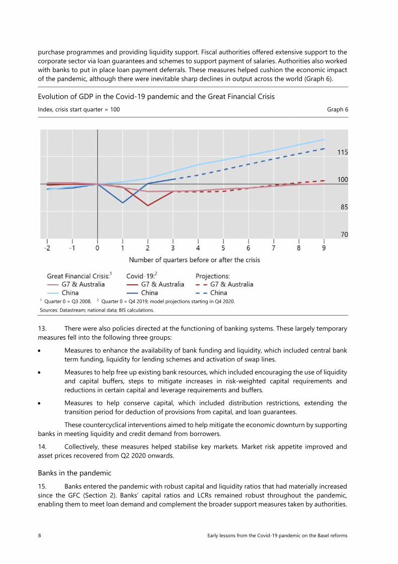
9. Market liquidity also deteriorated, including in markets traditionally seen as deep and liquid (Graph 4). In particular, signs of stress emerged in a range of short-term funding markets – including bond, commercial paper and repo markets – as leveraged and unleveraged investors reduced their activity. In mid-March 2020, extreme selling pressure spread to even the most liquid government bond markets.
Early lessons from the Covid-19 pandemic on the Basel reforms 7
10. Dealers helped alleviate these liquidity strains by extending repo financing, absorbing sales and building inventories of securities. However, their ability to meet unprecedented demand for liquidity was constrained by falling risk appetite in volatile markets and the need to manage their own balance sheet constraints.
11. Foreign exchange (FX) markets continued to function despite the strain, although the relative cost of offshore USD increased. In particular, in mid-March 2020, USD-based FX and swap markets experienced significant increases in cost and volatility (Graph 5).
FX swap basis, against the US dollar
In basis points Graph 5
(i) Three-month OIS basis (ii) Three-month LIBOR basis1
Policy responses
12. Jurisdictions took extensive policy action on multiple fronts in response to the crisis. Central banks introduced a range of monetary interventions, which included lowering policy rates, extending asset
Short-term funding market and treasury market movements Graph 4
(i) Commercial paper spread to OIS (ii) Market liquidity Basis points Cents per dollar notional Index (reversed)
1 Commercial paper 90-day yield is a composite of offered levels for A1/P1/F1-rated US commercial paper programmes. 2 Bloomberg liquidity index, multiplied by –1. Index levels are measured by the root mean squared error between bonds’ market yields and theoretical yields based on cubic and exponential spline methodologies. The index can be deemed a proxy for aggregated on- and off-the-run spreads. Sources: Bloomberg; JPMorgan Chase; BIS calculations.
1 Calculated based on the covered interest parity condition, using foreign exchange forward and spot rates and three-month LIBOR rates. Sources: Bloomberg; BIS calculations.
8 Early lessons from the Covid-19 pandemic on the Basel reforms
purchase programmes and providing liquidity support. Fiscal authorities offered extensive support to the corporate sector via loan guarantees and schemes to support payment of salaries. Authorities also worked with banks to put in place loan payment deferrals. These measures helped cushion the economic impact of the pandemic, although there were inevitable sharp declines in output across the world (Graph 6).
Evolution of GDP in the Covid-19 pandemic and the Great Financial Crisis Index, crisis start quarter = 100 Graph 6
13. There were also policies directed at the functioning of banking systems. These largely temporary measures fell into the following three groups:
• Measures to enhance the availability of bank funding and liquidity, which included central bank term funding, liquidity for lending schemes and activation of swap lines.
• Measures to help free up existing bank resources, which included encouraging the use of liquidity and capital buffers, steps to mitigate increases in risk-weighted capital requirements and reductions in certain capital and leverage requirements and buffers.
• Measures to help conserve capital, which included distribution restrictions, extending the transition period for deduction of provisions from capital, and loan guarantees.
These countercyclical interventions aimed to help mitigate the economic downturn by supporting banks in meeting liquidity and credit demand from borrowers.
14. Collectively, these measures helped stabilise key markets. Market risk appetite improved and asset prices recovered from Q2 2020 onwards.
Banks in the pandemic
15. Banks entered the pandemic with robust capital and liquidity ratios that had materially increased since the GFC (Section 2). Banks’ capital ratios and LCRs remained robust throughout the pandemic, enabling them to meet loan demand and complement the broader support measures taken by authorities.
1 Quarter 0 = Q3 2008. 2 Quarter 0 = Q4 2019; model projections starting in Q4 2020. Sources: Datastream; national data; BIS calculations.
Early lessons from the Covid-19 pandemic on the Basel reforms 9
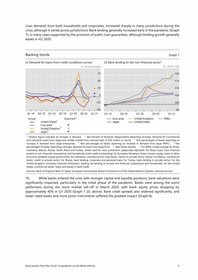
Loan demand, from both households and corporates, increased sharply in many jurisdictions during the crisis, although it varied across jurisdictions. Bank lending generally increased early in the pandemic (Graph 7), in many cases supported by the provision of public loan guarantees, although lending growth generally eased in H2 2020.
Banking trends Graph 7
(i) Demand for loans from credit conditions survey1 (ii) Bank lending to the non-financial sector7 In net percentage Q1 2019 =100
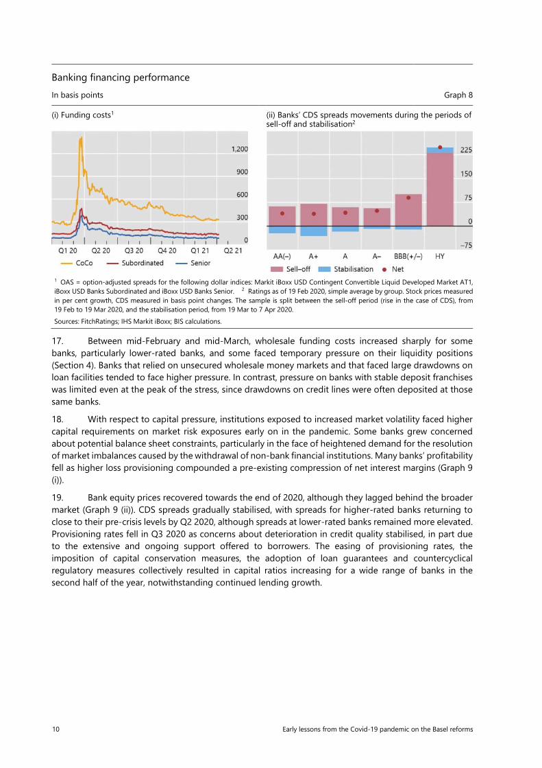
16. While banks entered the crisis with stronger capital and liquidity positions, bank valuations were significantly impacted, particularly in the initial phase of the pandemic. Banks were among the worst performers during the stock market sell-off in March 2020, with bank equity prices dropping by approximately 40% in Q1 2020 (Graph 1 (ii), above). Bank credit spreads also widened significantly, and lower-rated banks and more junior instruments suffered the greatest impact (Graph 8).
1 Positive figure indicates an increase in demand. 2 Net Percent of Domestic Respondents Reporting Stronger Demand for Commercial and Industrial Loans from large and middle-market firms (annual sales of $50 million or more). 3 Net percentages of banks reporting an increase in demand from large enterprises. 4 Net percentages of banks reporting an increase in demand from large PNFCs. 5 Net percentages of banks reporting a stronger demand for loans from large firms. 6 Next three months. 7 For EMEs, simple average for Brazil, Indonesia, Mexico, Russia, South Africa and Turkey. Series used for each jurisdiction (seasonally adjusted): For Brazil, loans from financial system to non-financial corporations and households (total credit outstanding); for European Monetary Union, money supply, loans to other Eurozone residents except government; for Indonesia, commercial and rural banks’ claims on private sector (loans); for Mexico, commercial banks’ credit to private sector; for Russia, bank lending, corporate and personal loans; for Turkey, bank lending to private sector; for the United Kingdom, monetary financial institutions’ sterling net lending to private non-financial corporations and households; for the United States, commercial banks’ loans and leases in bank credit. Sources: Bank of England; Bank of Japan; European Central bank; Board of Governors of the Federal Reserve System; national sources.
10 Early lessons from the Covid-19 pandemic on the Basel reforms
17. Between mid-February and mid-March, wholesale funding costs increased sharply for some banks, particularly lower-rated banks, and some faced temporary pressure on their liquidity positions (Section 4). Banks that relied on unsecured wholesale money markets and that faced large drawdowns on loan facilities tended to face higher pressure. In contrast, pressure on banks with stable deposit franchises was limited even at the peak of the stress, since drawdowns on credit lines were often deposited at those same banks.
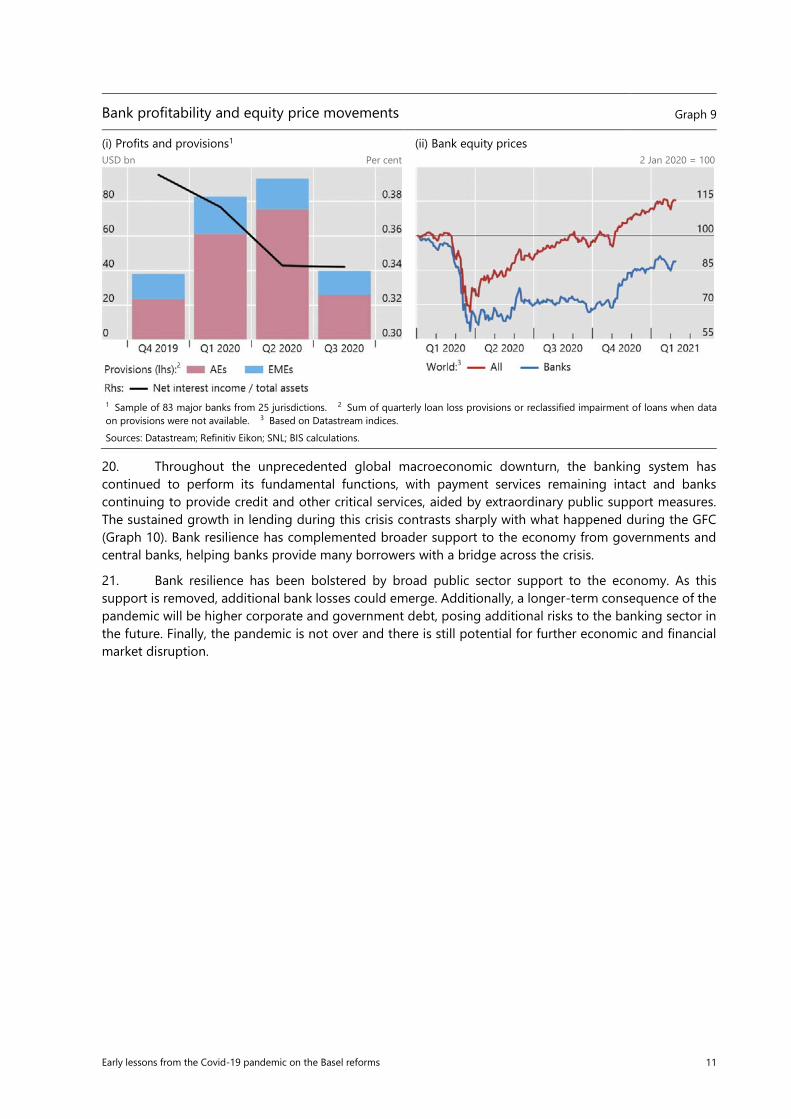
18. With respect to capital pressure, institutions exposed to increased market volatility faced higher capital requirements on market risk exposures early on in the pandemic. Some banks grew concerned about potential balance sheet constraints, particularly in the face of heightened demand for the resolution of market imbalances caused by the withdrawal of non-bank financial institutions. Many banks’ profitability fell as higher loss provisioning compounded a pre-existing compression of net interest margins (Graph 9 (i)).
19. Bank equity prices recovered towards the end of 2020, although they lagged behind the broader market (Graph 9 (ii)). CDS spreads gradually stabilised, with spreads for higher-rated banks returning to close to their pre-crisis levels by Q2 2020, although spreads at lower-rated banks remained more elevated. Provisioning rates fell in Q3 2020 as concerns about deterioration in credit quality stabilised, in part due to the extensive and ongoing support offered to borrowers. The easing of provisioning rates, the imposition of capital conservation measures, the adoption of loan guarantees and countercyclical regulatory measures collectively resulted in capital ratios increasing for a wide range of banks in the second half of the year, notwithstanding continued lending growth.
Banking financing performance In basis points Graph 8
(i) Funding costs1 (ii) Banks’ CDS spreads movements during the periods of sell-off and stabilisation2
1 OAS = option-adjusted spreads for the following dollar indices: Markit iBoxx USD Contingent Convertible Liquid Developed Market AT1, iBoxx USD Banks Subordinated and iBoxx USD Banks Senior. 2 Ratings as of 19 Feb 2020, simple average by group. Stock prices measured in per cent growth, CDS measured in basis point changes. The sample is split between the sell-off period (rise in the case of CDS), from 19 Feb to 19 Mar 2020, and the stabilisation period, from 19 Mar to 7 Apr 2020. Sources: FitchRatings; IHS Markit iBoxx; BIS calculations.
Early lessons from the Covid-19 pandemic on the Basel reforms 11
Bank profitability and equity price movements Graph 9
(i) Profits and provisions1 (ii) Bank equity prices USD bn Per cent 2 Jan 2020 = 100
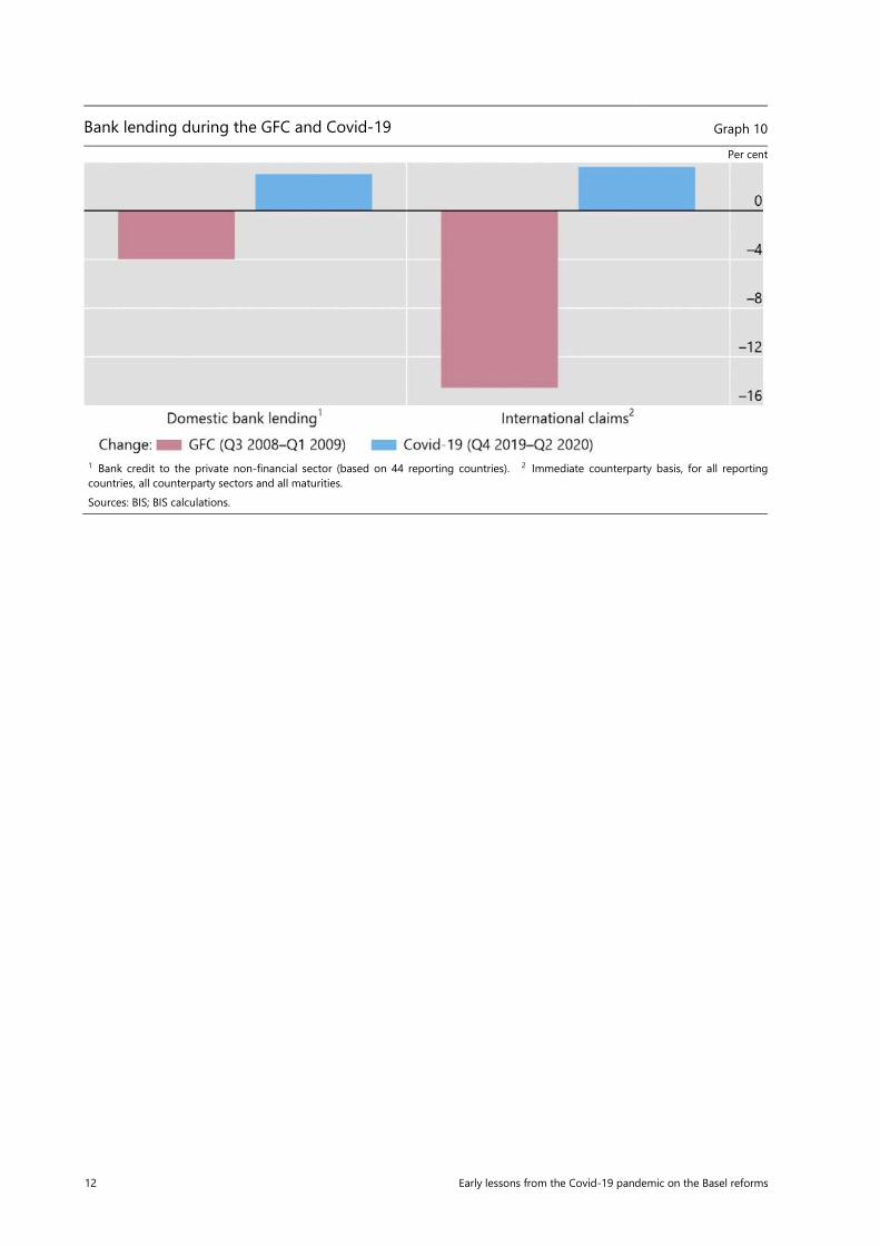
20. Throughout the unprecedented global macroeconomic downturn, the banking system has continued to perform its fundamental functions, with payment services remaining intact and banks continuing to provide credit and other critical services, aided by extraordinary public support measures. The sustained growth in lending during this crisis contrasts sharply with what happened during the GFC (Graph 10). Bank resilience has complemented broader support to the economy from governments and central banks, helping banks provide many borrowers with a bridge across the crisis.
21. Bank resilience has been bolstered by broad public sector support to the economy. As this support is removed, additional bank losses could emerge. Additionally, a longer-term consequence of the pandemic will be higher corporate and government debt, posing additional risks to the banking sector in the future. Finally, the pandemic is not over and there is still potential for further economic and financial market disruption.
1 Sample of 83 major banks from 25 jurisdictions. 2 Sum of quarterly loan loss provisions or reclassified impairment of loans when data on provisions were not available. 3 Based on Datastream indices. Sources: Datastream; Refinitiv Eikon; SNL; BIS calculations.
12 Early lessons from the Covid-19 pandemic on the Basel reforms
Bank lending during the GFC and Covid-19 Graph 10
Per cent
1 Bank credit to the private non-financial sector (based on 44 reporting countries). 2 Immediate counterparty basis, for all reporting countries, all counterparty sectors and all maturities. Sources: BIS; BIS calculations.
Early lessons from the Covid-19 pandemic on the Basel reforms 13
2. The resilience of the banking system
22. A key objective of the Basel reforms is to build a resilient banking system that can absorb shocks and continue to support economic activity. Bank resilience helps mitigate the adverse consequences of shocks and facilitates a rapid recovery once a crisis abates. This section examines the resilience of the global banking system during the pandemic and investigates the extent to which the Basel reforms may have contributed to such resilience.
2.1. Overall resilience
23. The lack of failure of any internationally-active banks to date during the pandemic demonstrates the resilience of the global banking system. While governments and central banks have provided exceptional support to the economy, indirectly supporting banks, most major banks have not needed a significant infusion of public funds, nor have they sustained heavy losses or faced extended liquidity pressure. Rather, the banking system has continued to provide essential financial services to the economy during this period.
24. This section provides a time series analysis of resilience, focusing on the period since the implementation of the Basel reforms in the early 2010s to the present.
25. The analyses are carried out using both the Committee’s Quantitative Impact Study (QIS) and Supervisory Reporting Systems (SRS) data (collectively, QIS/SRS data), as well as vendor data for a sample of large banks.3 The assessment looks at banks’ risk-weighted regulatory capital ratios, non-risk-based leverage ratios, and the two liquidity metrics included in the Basel reforms: the LCR and the Net Stable Funding Ratio (NSFR).
26. As shown in Table 1, banks’ overall resilience has, in general, significantly improved since the adoption of the initial Basel reforms. From 2013 to the end of 2019, banks’ capital, leverage and liquidity positions improved as reforms were implemented.4 As of 30 June 2020, approximately three months into the Covid-19 crisis, banks’ capital, leverage and liquidity positions had remained strong and did not appear to be significantly impacted by the pandemic, reflecting in part the exceptional policy support measures that had been taken.
3 Information considered for this section of the report was obtained through previous QIS and SRS data collections. External vendor data from SNL was used as an additional source to validate results.
4 The analysis of the impact of Basel reforms reflects data from 2013 onwards in order to discount the build-up of capital that took place during and immediately after the 2007–09 global financial crisis and the European sovereign debt crisis.

14 Early lessons from the Covid-19 pandemic on the Basel reforms
Overview of results, using consistent sample of banks,5 in per cent Table 1
31 December 2013 31 December 2019 30 June 2020
Group 1
Of which: G-SIBs
Group 2
Group 1
Of which: G-SIBs
Group 2
Group 1
Of which: G-SIBs
Group 2
Risk-based capital, initial Basel III framework
CET1 ratio 10.1 9.9 8.4 12.9 12.8 13.9 12.7 12.5 14.5
Tier 1 ratio 10.4 10.3 9.1 14.5 14.4 14.9 14.3 14.2 15.5
Total ratio 11.8 11.6 10.8 17.0 16.9 17.3 16.9 16.7 18.1
Leverage ratio: Fully phased-in final Basel III Tier 1 leverage ratios 4.5 4.4 3.9 6.2 6.2 5.1 6.1 N/A N/A
Liquidity
LCR 122.3 127.1 145.8 136.1 132.8 163.1 140.3 136.7 188.3
NSFR 112.5 115.0 113.0 116.9 118.0 120.7 118.7 120 122.5
27. More specifically, as of year-end 2019, Common Equity Tier 1 (CET1), Tier 1 and total capital ratios had all improved significantly compared to year-end 2013 across Group 1 banks, global systemically important banks (G-SIBs) and Group 2 banks. For instance, weighted-average CET1 ratios improved by nearly 300 basis points (bp) for Group 1 banks and G-SIBs, and by more than 500 bp for Group 2 banks. Following the outbreak of the pandemic, weighted-average capital ratios declined slightly (by less than 30 bp) for Group 1 banks and G-SIBs.6 Overall, banks maintained their strong capital positions during the pandemic, demonstrating general resilience against a significant and unprecedented negative economic shock. This result also reflects fiscal support measures that helped reduce loan losses and payout restrictions, which in turn helped banks retain capital.
28. Liquidity positions have also improved materially, both qualitatively and quantitatively, since end-2013. Both the LCR and NSFR were notably higher for Group 1 and Group 2 banks by end-2019. During this period, as banks built up liquidity buffers, the LCR increased by an average of approximately 15 percentage points (pp) for Group 1 and Group 2 banks and by a more modest but significant average of 6 pp for G-SIBs. NSFR data suggests a more modest improvement in banks’ funding stability, possibly because the NSFR is still in the process of being implemented globally. Both liquidity metrics were further strengthened over the first half of 2020.
29. Note that capital levels in many jurisdictions have been bolstered in 2020 by government, regulatory, monetary and fiscal policy assistance measures, including temporary debt relief programmes. While the pandemic may ease as vaccinations become more widespread, some jurisdictions could see meaningful deterioration in capital ratios, particularly as support is withdrawn.
5 “Group 1” banks are defined as internationally active banks that have Tier 1 capital of more than €3 billion and include all 29 institutions that have been designated as global systemically important banks (G-SIBs). “Group 2” banks are banks that have Tier 1 capital of less than €3 billion or are not internationally active. The set of Group 2 banks is not an internationally representative sample.
6 Group 2 banks experienced an increase in capital ratios, largely driven by one sample bank’s 5 pp increase. The set of Group 2 banks is not an internationally representative sample.
Note: Due to the cancellation of the end-2020 Basel III monitoring exercise, the 30 June 2020 final Basel III leverage ratios are not available (Only the weighted-average initial Basel III leverage ratio for Group 1 banks is presented). 30 June 2020 NSFR numbers are approximated based on both QIS and SNL. Sources: Basel Committee on Banking Supervision; SNL.
Early lessons from the Covid-19 pandemic on the Basel reforms 15
30. Graph 11 (i) examines Group 1 banks’ CET1 capital ratios across different regions over time and demonstrates that the build-up in resilience has been a global phenomenon. Prior to the pandemic, consistent improvement was seen across regions, with capital ratios increasing by 200–400 bp from 2014 to 2019. While some regions showed a modest decline in capital ratios during the Covid-19 pandemic, capital levels are still well above those seen in the aftermath of the financial crisis.
31. Notably, capital levels in Europe continued to rise during the pandemic, in contrast to those in many other jurisdictions. This could be due to a variety of factors, including the build-up of capital due to payout restrictions, the reduced riskiness of portfolios due to loan guarantees, and differences in accounting practices regarding loan-loss provisioning.
32. Leverage ratios have also markedly improved since the introduction of the Basel reforms. As indicated in Graph 11 (ii), weighted-average leverage ratios for Group 1 banks improved by 100–200 bp in all regions and remained robust throughout the first six months of the pandemic in most regions. It should be noted that banks’ leverage ratios in some jurisdictions reflect exemptions put in place during the pandemic to help reduce the bindingness of the leverage ratio requirement.
33. The steady increase in global banks’ LCR levels after 2013 was driven in part by European banks (Graph 11 (iii)). More importantly, banks across all regions entered the pandemic with strong liquidity positions, and further strengthened them during the crisis. Actions taken by many monetary authorities to provide ample liquidity, combined with growth in deposits, may have helped banks maintain strong liquidity positions during the pandemic.
Developments in CET1 ratios, leverage ratios and LCRs Graph 11
(i) CET1 ratios (ii) Leverage ratios (iii) Liquidity Coverage Ratios Per cent Per cent Per cent
34. A detailed case study of the Mexican banking system (Annex 3) demonstrates the LCR’s contribution to banks’ resilience. Following the implementation of the LCR in Mexico in 2015, Mexican banks’ liquidity resilience increased significantly. A counterfactual analysis reveals that, had banks entered the pandemic with the same liquidity profile that they had in 2014 (before Mexico implemented the LCR), approximately a quarter of Mexican banks would have faced materially greater liquidity stress. Instead, few Mexican banks faced liquidity demands that exceeded their holdings of high-quality liquid assets, and those banks were able to meet these demands by using other available resources such as deposits at other banks.
35. Market-based capital measures provide another perspective of the resilience of the banking system (Graph 12 (i)). The market-based capital ratio (ie market value of common equity/(market value of common equity + book value of total debt)) indicates that market-based measures of resilience remained mostly unchanged and at a relatively low level between 2013 and 2019. This may reflect the downward pressures on bank profitability arising from the prevailing low interest environment. While market-based
Source: Basel Committee on Banking Supervision.
16 Early lessons from the Covid-19 pandemic on the Basel reforms
capital measures fell sharply with the onset of the pandemic, they have regained some of these losses since authorities stepped in to provide fiscal and monetary support.
36. As shown in Graph 12 (ii), the distribution of market-based capital ratios shifted notably to the left at the peak of the pandemic, before government support measures were introduced. Specifically, the fraction of banks with a market-based capital ratio below 2% had risen sharply to 20% as of 31 March 2020, indicating concern among market participants. One interpretation of these movements is that market-based capital measures may be more responsive to banks’ underlying health than regulatory metrics. Another interpretation is that they indicate changes in investors’ risk preferences.
Market-based capital ratios Graph 12
(i) Evolution of market-based capital ratios (ii) Distribution of market-based capital ratios Per cent Per cent
37. Notwithstanding the above, the global pandemic is not yet over, and the recent collapses of the investment funds Archegos Capital Management and Greensill Capital, while not directly related to the ongoing pandemic, raise the possibility that other losses may emerge in the financial system.
38. Examining whether the degree to which the Basel reforms have been implemented relates to resilience metrics provides additional perspective on how the reforms have contributed to the overall resilience of the global banking system. Here, one finds a weak positive relationship between the degree of implementation and banks’ increase in CET1 capital from 2013 to 2019, indicating that the implementation of the Basel reforms may have helped build resilience in the global banking system.7 This weaker-than-expected relationship may reflect the fact that some banks already had relatively high capital levels, bolstered by the deleveraging that followed the GFC, when the Basel reforms were introduced. Banks may also have responded to the announcement of the Basel reforms by raising capital ratios in anticipation of the new standards before they were implemented, weakening any statistical relationship between implementation and subsequent increases in capital.
39. With respect to liquidity metrics, LCRs are consistently high across jurisdictions regardless of their implementation status. When examining changes between 2013 and 2019, banks in those jurisdictions that started with low measures of liquidity typically experienced sharp improvements in their LCRs. This indicates that the Basel reforms may have reduced differences in LCRs across jurisdictions and resulted in a global banking system that is more resilient to liquidity shocks.
7 See www.bis.org/bcbs/publ/d506.htm for the Eighteenth progress report on adoption of the Basel regulatory framework, which provides a summary measure of the degree to which various jurisdictions have implemented all or some of the Basel reforms.
Note: MBCR = Market value of common equity/(Market value of common equity + Book value of total debt). Saudi Arabian (SA) banks are not included in the “Rest of World” category because their MBCR is significantly higher. Source: Thomson Reuters.
Early lessons from the Covid-19 pandemic on the Basel reforms 17
2.2. Regulatory measures and resilience outcomes during the Covid-19 pandemic
40. As noted above, the banking system entered the pandemic with robust capital and liquidity levels, bolstered by the Basel reforms. One can further examine the impact of these reforms by looking at the relationship between regulatory measures and outcome measures of resilience. As no major internationally active bank has thus far failed during the pandemic, this analysis uses banks’ CDS spreads as an outcome measure of resilience.
41. CDS spreads are an imperfect measure of bank resilience because they can experience significant volatility due to changes in market sentiment, which may not always reflect changes in specific banks’ resilience. Nevertheless, CDS spreads are one of several metrics that provide a market-based view of a bank’s resilience that is not inextricably determined by regulatory requirements, and can thus help shed light on the effects of regulatory requirements on bank resilience. If higher regulatory ratios signal greater resilience, one would expect a negative relationship between regulatory ratios and CDS spreads.
42. A regression model is used to estimate the relationship between banks’ regulatory measures and changes in CDS spreads during the pandemic. The primary regression model can be summarised by the following equation, where i denotes individual banks:
Δ𝐶𝐶𝐶𝐶𝐶𝐶𝑖𝑖,2020 = 𝛼𝛼 + 𝛽𝛽 𝑋𝑋𝑖𝑖,2019 + 𝛾𝛾𝐶𝐶𝐶𝐶𝐶𝐶𝐶𝐶𝐶𝐶𝐶𝐶𝐶𝐶𝐶𝐶𝑖𝑖,2019 + 𝛿𝛿𝑐𝑐 + 𝜖𝜖𝑖𝑖.
43. Δ𝐶𝐶𝐶𝐶𝐶𝐶𝑖𝑖,2020 is calculated as the difference in an individual bank’s CDS spreads between March/April 2020 and the end of 2019. Bank regulatory ratios at the end of 2019 (𝑋𝑋𝑖𝑖,2019), used as explanatory variables, include the CET1 capital ratio, the leverage ratio and the LCR, considered individually or as a whole.
44. The regression includes the bank-specific control variables as of year-end 2019, reported in the table below, as well as continent-specific fixed effects (𝛿𝛿𝑐𝑐) for: (i) Americas; (ii) Asia and Australia; and (iii) Europe, Middle East and Africa.
45. The data on regulatory ratios for large internationally active banks are from S&P Market Intelligence (SNL). The total sample comprises 83 banks located in Committee member jurisdictions for which CDS spreads of sufficient quality are available and all three regulatory ratios (ie CET1 ratio, leverage ratio and LCR) and control variables are available. All values of regulatory ratios are winsorised at the 5th and 95th percentiles. All-in CET1 capital requirements and buffers (ie minimum Pillar I requirements, regulatory buffers and Pillar II requirements) are available for a subsample of 60 banks from a survey that was conducted by the Committee’s Task Force on Evaluations (TFE survey).8 The relatively small sample sizes limit the ability to draw definitive conclusions from the regression analysis.
46. The data source for bank CDS spreads is IHS Markit, and quoted five-year spreads at the senior unsecured debt level are used. The analysis considers the average CDS spread value in March and April 2020 minus the average CDS spread value in Q4 2019 as the main dependent variable.
47. Table A2 in Annex 4 presents the descriptive statistics for the data used in the analysis (ie the number of observations, the mean, the standard deviation, and the minimum and maximum values). All continuous values are winsorised at the 5th and 95th percentiles.
48. The regression analysis focuses on the increase in CDS spreads that occurred in March/April 2020. As shown in Graph 13, indices of bank CDS spreads rose quickly as the pandemic began and subsided once authorities intervened with fiscal and monetary measures to alleviate financial market strain.
8 See Annex 2 for further information on the TFE survey.
18 Early lessons from the Covid-19 pandemic on the Basel reforms
Development of CDS spreads for banks in Europe and North America in 2020 Graph 13
Basis points
49. Table 2 displays the results of the regression analysis. Specifications (1) through (3) each use one of the three regulatory metrics as the explanatory variable, while Specification (4) combines them together. The analysis controls for a number of other observables.
Regression specifications with the difference in CDS spreads between the average in March and April 2020 and the average of the fourth quarter in 2019 as dependent variable. Table 2 Specification (1) CET1 ratio (2) Leverage ratio (3) LCR (4) All
CET1 ratio -3.18 * -4.49 **
Leverage ratio -1.02 2.77
LCR 0.04 0.12
Size -5.64 -3.50 -2.78 -4.51
Return on assets 6.68 5.62 4.16 3.57
RWA to total assets 2.50 20.30 14.26 -19.53
Deposits to total assets -87.73 *** -87.04 *** -83.71 *** -78.57 ***
Government ownership 27.84 * 31.33 * 31.62 * 27.19
Sovereign CDS spreads 0.39 ** 0.41 *** 0.41 *** 0.38 **
Adjusted R-squared 0.54 0.52 0.52 0.54
N 83 83 83 83
Note: Continent fixed effects included in all regressions. Robust standard errors in all regressions. The symbols * , **, and *** denote statistical significance at 10%, 5% and 1%, respectively. Source: IHS Markit and BCBS calculations.
50. The negative and significant coefficients for the CET1 ratio in Specifications (1) and (4) indicate that a higher CET1 ratio at the end of 2019 is associated with smaller changes in CDS spreads in response to the pandemic. The coefficient is statistically significant at the 5% level in Specification (4). According to Specification (4), a one standard deviation increase in the CET1 ratio (ie 2.6 pp) is associated with approximately one quarter of a standard deviation (ie 12 bp) decrease in CDS spreads. This finding indicates that banks with higher CET1 capital ratios showed greater resilience than those with lower ratios early on in the pandemic.
51. The coefficients associated with the leverage ratio and the LCR are not statistically significant across the various specifications. The leverage ratio’s lack of significance in Specification (4) is consistent
Source: IHS Markit.
Early lessons from the Covid-19 pandemic on the Basel reforms 19
with the its design as a regulatory backstop. Unexpectedly, the LCR also appears not to have significantly affected CDS spreads. This may reflect the fact that there were few instances of sustained liquidity pressure at internationally active banks during the pandemic.9 While a few banks experienced liquidity stress early on in the crisis, this stress quickly subsided as authorities intervened to ease financial market strain. One notable feature of the pandemic was the contrast between a resilient banking system and the strain put on some non-bank financial institutions, as well as liquidity shortfalls in financial markets, as discussed in Section 1.
52. With respect to the control variables, the results indicate that banks with a higher ratio of deposits to total assets experienced significantly smaller increases in CDS spreads during the pandemic. This may indicate that banks with more retail-oriented business models were less impacted by the pandemic than banks with more capital markets-oriented business models. Banks located in jurisdictions where sovereign CDS spreads rose more sharply in early 2020 showed significantly greater increases in CDS spreads during the pandemic, indicating that the sovereign spread may capture broader macroeconomic and fiscal difficulties. This result may also reflect a market perception that sovereign stress impacts banks.
53. Estimating the previous regressions using CET1 ratio requirements and buffers and the amount of CET1 headroom (defined as a bank’s CET1 capital in excess of its minimum capital requirements and buffers) as separate explanatory variables enables us to further understand the effect of bank capital on resilience. The sample shrinks due to the lack of available data on capital requirements and buffers for all of the banks. Furthermore, the data set does not include information on all aspects of Pillar 2 requirements for all jurisdictions. Table 3 shows the regression results in this subsample, with the regressions including the leverage ratio and LCR provided for completeness. The regression results in column (4) suggest that the negative relationship between CDS spreads and the CET1 ratio is driven by the effect that CET1 headroom has. As before, the coefficients associated with the leverage ratio and the LCR are not statistically significant in this subsample.
Regression specifications with the difference in CDS spreads between the average in March and April 2020 and the average of Q4 2019 as dependent variable. Table 3
Model (1) CET1 requirement and
headroom
(2) Leverage ratio (3) LCR (4) All
CET1 requirement -0.11 -0.28
CET1 headroom -1.96 -3.14**
Leverage ratio 0.10 3.16
LCR 0.12 0.12
Size 0.83 2.66 3.63 1.35
Return on assets -7.97 -8.94 -10.54 -12.08
RWA to total assets 9.89 11.30 15.46 -5.71
Deposits to total assets -38.21 -38.03* -36.84* -35.02
Government ownership 8.74 10.38 10.27 7.51
Sovereign CDS spreads 0.51*** 0.53*** 0.51*** 0.47***
Adjusted R-squared 0.62 0.62 0.63 0.62
N 60 60 60 60
Note: Continent fixed effects included in all regressions. Robust standard errors in all regressions. The symbols * , **, and *** denote statistical significance at 10%, 5% and 1%, respectively. Source: IHS Markit and BCBS calculations.
9 The fact that the LCR is disclosed with a lag in some jurisdictions may also have contributed to the lack of market reaction.
20 Early lessons from the Covid-19 pandemic on the Basel reforms
54. The findings indicate that market participants believe that having headroom above requirements and buffers enables banks to better withstand shocks such as those brought about by the pandemic. This perception can also be explained by increased stability of CET1 requirements across banks. These results also provide indirect evidence that market participants may take a negative view of banks that dip into their regulatory capital buffers.
55. Examining a range of additional models helps demonstrate the robustness of these findings. Table A3 in Annex 4 presents a robustness analysis of Specification (4) above using jurisdiction-specific fixed effects instead of continent fixed effects and other definitions of the CDS spread-based outcome variable as the dependent variable.
56. Across the various alternative specifications, findings of the main regressions prove to be somewhat robust. The coefficient of the CET1 ratio is negative in all specifications and statistically significant in all alternative specifications. The coefficients associated with the leverage ratio and the LCR are not statistically significant.
57. By end September 2020, financial market stress had eased from the levels seen earlier that year. Graph 14 shows the increase in average CDS spreads from the end of 2019 to March/April 2020 on the horizontal axis, and the change in average CDS spreads from March/April 2020 to August/September 2020 on the vertical axis. The figure shows that CDS spread values recovered for most banks, but did remain elevated for a few banks in August/September 2020.
Increase in average CDS spreads in March/April 2020 and recovery of average CDS spreads in August/September 2020 Graph 14
Basis points
58. Regression analysis using the recovery in CDS spreads as the dependent variable and the increase in average CDS spreads in March/April 2020 as an explanatory variable finds that regulatory ratios generally do not have a statistically significant effect on the recovery of bank CDS spreads.
59. Overall, the analysis in this section demonstrates that higher CET1 capital ratios are associated with a stronger market-based measure of resilience.
2.3. Impact on lending
60. As noted above, most banks entered the pandemic with capital and liquidity levels well above minimum requirements and buffers, which helped them remain resilient. This section analyses whether this resilience had an effect on lending and helped avert a credit crunch at the bank level. The empirical findings in this section suggest that higher initial capital levels helped banks to support lending during
Note: X-axis shows the difference in average CDS spreads between March/April 2020 and end of 2019. Y-axis shows the difference between August/September 2020 and March/April 2020. Source: IHS Markit.
Early lessons from the Covid-19 pandemic on the Basel reforms 21
the pandemic, evidencing the value of a robust regulatory framework that yields a more resilient banking sector.
61. Banks continued to provide loans to corporations and retail customers in order to cushion the negative effect of the pandemic. Graph 15 shows that bank loans outstanding increased before and during the first two quarters of the pandemic before decreasing in Q3 2020. The sharp rise in loans outstanding in Q1 2020 may have been driven by borrowers’ drawdowns on commercial lines of credit for precautionary reasons. This loan growth was facilitated by robust interventions on the part of fiscal and monetary authorities, who provided loan guarantees and cash assistance to alleviate difficult financial conditions faced by businesses and households. 10 Disentangling the effect of these interventions on lending from that of bank capital levels on lending poses a challenge for the analysis below. The decline in loans outstanding in Q3 2020 likely reflects the effect of the deepening pandemic; it may also reflect the fact that companies repaid drawn credit lines as uncertainty declined.
Gross loans relative to Q2 2019 for banks headquartered in the Committee’s member jurisdictions Graph 15
Q2 2019 = 100
62. The analysis employs two different panel data regression specifications, which differ based on whether loans are measured using cumulative or quarterly growth rates, and whether capital ratios are measured prior to the pandemic or in the preceding quarter. Examining a range of models provides a robust view of the relationship between bank resilience and lending. One limitation of these approaches is that the analysis cannot definitively control for changes in loan demand across banks, and thus the results cannot be interpreted as a representation of a relationship solely between resilience measures and changes in loan supply.
63. The use of panel data enables one to look across jurisdictions and provides a broad global view of the sensitivity of bank lending to regulatory capital and liquidity ratios during the pandemic. An alternative approach that uses confidential credit registry data provides a clearer identification of lending sensitivity to regulatory metrics within a single jurisdiction.11
64. The first specification used follows:
10 The data used in the analysis do not distinguish between loans backed by a government guarantee and those without such backing.
11 For an example of such analysis, see G Jiménez, S Ongena, J-L Peydró & J Saurina, “Credit supply and monetary policy: identifying the bank balance-sheet channel with loan applications”, American Economic Review, vol 102, no 5, 2012, pp 2301–26.
Note: The graph shows the growth in gross loans relative to Q2 2019 for banks headquartered in the Committee’s member jurisdictions. The underlying data are described in more detail below. Source: SNL.
22 Early lessons from the Covid-19 pandemic on the Basel reforms
ln �𝐺𝐺𝐺𝐺𝐺𝐺𝐺𝐺𝐺𝐺 𝑙𝑙𝐺𝐺𝑙𝑙𝑙𝑙𝐺𝐺𝑖𝑖,𝑗𝑗,𝑐𝑐,𝑡𝑡
𝐺𝐺𝐺𝐺𝐺𝐺𝐺𝐺𝐺𝐺 𝑙𝑙𝐺𝐺𝑙𝑙𝑙𝑙𝐺𝐺𝑖𝑖,𝑗𝑗,𝑐𝑐,2019−𝑄𝑄2� = 𝛼𝛼0 + 𝛼𝛼𝑖𝑖 + 𝛼𝛼𝑐𝑐 ⋅ 𝛼𝛼𝑡𝑡 + 𝛽𝛽1 ⋅ 𝑋𝑋𝑖𝑖,𝑗𝑗,𝑐𝑐,2019−𝑄𝑄2 ⋅ 𝐶𝐶2019−𝑄𝑄4 + 𝛽𝛽2 ⋅ 𝑋𝑋𝑖𝑖,𝑗𝑗,𝑐𝑐,2019−𝑄𝑄2 ⋅
𝐶𝐶2020−𝑄𝑄1 + 𝛽𝛽3 ⋅ 𝑋𝑋𝑖𝑖,𝑗𝑗,𝑐𝑐,2019−𝑄𝑄2 ⋅ 𝐶𝐶2020−𝑄𝑄2 + 𝛽𝛽4 ⋅ 𝑋𝑋𝑖𝑖,𝑗𝑗,𝑐𝑐,2019−𝑄𝑄2 ⋅ 𝐶𝐶2020−𝑄𝑄3 + 𝛾𝛾1 ⋅ 𝑇𝑇𝑇𝑇𝑇𝑇𝐸𝐸𝑗𝑗 ⋅ 𝐶𝐶𝐶𝐶𝐶𝐶𝐶𝐶𝐶𝐶𝑡𝑡 + 𝜀𝜀𝑖𝑖,𝑗𝑗,𝑐𝑐,𝑡𝑡 ,
where i denotes an individual bank, j the bank type, c the bank’s home jurisdiction, and t time, 𝑋𝑋𝑖𝑖,𝑗𝑗,𝑐𝑐,2019−𝑄𝑄2 is a regulatory capital or liquidity ratio measured prior to the onset of the pandemic, 𝐶𝐶𝑡𝑡 reflects various time dummies that interact with the regulatory ratio 𝑋𝑋𝑖𝑖,𝑗𝑗,𝑐𝑐,2019−𝑄𝑄2 , and 𝐶𝐶𝐶𝐶𝐶𝐶𝐶𝐶𝐶𝐶𝑡𝑡 is a pandemic dummy variable equal to one in the pandemic periods of Q1 2020 to Q3 2020 and zero otherwise. 12 The coefficients of interest are 𝛽𝛽2 through 𝛽𝛽4.13
65. A benefit of this specification is that it focuses on the relationship between resilience metrics and loan levels, and it can be mapped to a difference-in-difference approach that focuses on the difference in the sensitivity of lending to capital and liquidity during and before the pandemic. One potential limitation of this approach is the correlation with the outcome variable over time.
66. Another limitation of this specification is that capital or liquidity ratio levels prior to the pandemic may have had little relevance in bank decision-making during the pandemic. One can address this concern by measuring regulatory capital or liquidity ratios in the quarter before the one in which loan growth is measured, as in the following second specification.
ln�𝐺𝐺𝐶𝐶𝐶𝐶𝐶𝐶𝐶𝐶 𝐶𝐶𝐶𝐶𝑙𝑙𝐶𝐶𝐶𝐶𝑖𝑖 ,𝑗𝑗,𝑐𝑐,𝑡𝑡
𝐺𝐺𝐶𝐶𝐶𝐶𝐶𝐶𝐶𝐶 𝐶𝐶𝐶𝐶𝑙𝑙𝐶𝐶𝐶𝐶𝑖𝑖 ,𝑗𝑗,𝑐𝑐,𝑡𝑡−1�
= 𝛼𝛼0 + 𝛼𝛼𝑖𝑖 + 𝛼𝛼𝑐𝑐 ⋅ 𝛼𝛼𝑡𝑡 + 𝛽𝛽1 ⋅ 𝑋𝑋𝑖𝑖,𝑗𝑗,𝑐𝑐,𝑡𝑡−1 ⋅ 𝐶𝐶𝐶𝐶𝐶𝐶𝐶𝐶𝐶𝐶𝑡𝑡 + 𝛽𝛽2 ⋅ 𝑋𝑋𝑖𝑖,𝑗𝑗,𝑐𝑐,𝑡𝑡−1 + 𝛾𝛾1 ⋅ 𝑇𝑇𝑇𝑇𝑇𝑇𝐸𝐸𝑗𝑗 ⋅ 𝐶𝐶𝐶𝐶𝐶𝐶𝐶𝐶𝐶𝐶𝑡𝑡
+𝜀𝜀𝑖𝑖,𝑗𝑗,𝑐𝑐,𝑡𝑡
However, because capital or liquidity ratios vary with economic conditions, this approach can exacerbate endogeneity concerns.
67. The analysis uses quarterly balance sheet and regulatory data from Standard & Poor’s Global Market Intelligence for the period from Q2 2019 to Q3 2020 for banks in Committee member jurisdictions.14 This vendor data was used due to the limited availability of QIS data (which is commonly used by the Committee) for analysis regarding the impact of the pandemic. Covering this period enables one to observe banks’ capital and liquidity ratios shortly before and during the pandemic and evaluate their role in providing lending to the economy during the crisis.
68. The sample includes large internationally active banks that are active in lending with total assets above 0.25% of their jurisdictions’ gross domestic product (GDP) or above 50 billion USD. The number of banks in this sample ranges from 200 to 300, depending on the capital or liquidity measure used in the regression.
69. Table A4 in Annex 4 shows the descriptive statistics for the dependent and independent variables used in the analysis. All variables are winsorised at the 1st and 99th percentiles, except for the stimulus measure and dividend restriction variable.
70. The left-hand columns of Table 4 show the regression results for the CET1 capital ratio’s impact on gross loans, either in levels or in growth rates.
12 Although the outcome variable is shown as the cumulative growth in lending from Q2 2019, the numerator is a constant that does not affect the results of the regression. As such, the model can be viewed as an examination of the relationship between capital ratios and the level of loans outstanding.
13 The control variables include 𝑇𝑇𝑇𝑇𝑇𝑇𝐸𝐸𝑗𝑗 , which captures the heterogeneity between various bank types; 𝛼𝛼𝑖𝑖 , which accounts for time-invariant bank characteristics; and country-time fixed effects. The latter controls for time-varying characteristics of jurisdictions, such as the extent to which fiscal and monetary support measures have been implemented, which ensures that findings are not directly driven by the influence of such support measures.
14 The data set also includes fiscal and banking stimulus measures and supervisors’ recommendations on bank dividend restrictions.
Early lessons from the Covid-19 pandemic on the Basel reforms 23
Regression results with CET1 capital ratio (left columns) and LCR on loan growth (right columns) Table 4
Model CET1 LCR
Cumulative loan growth
Quarterly loan growth
Cumulative loan growth
Quarterly loan growth
(1) (2) (1) (2)
𝐶𝐶𝐸𝐸𝑇𝑇1 𝑅𝑅𝑙𝑙𝐶𝐶𝑖𝑖𝐶𝐶2019−𝑄𝑄2*2019-Q4 0.108 (0.119)
𝐿𝐿𝐶𝐶𝑅𝑅2019−𝑄𝑄2*2019-Q4 0.00134 (0.00543)
𝐶𝐶𝐸𝐸𝑇𝑇1 𝑅𝑅𝑙𝑙𝐶𝐶𝑖𝑖𝐶𝐶2019−𝑄𝑄2*2020-Q1 0.292** (0.128)
𝐿𝐿𝐶𝐶𝑅𝑅2019−𝑄𝑄2*2020-Q1 0.00710 (0.00768)
𝐶𝐶𝐸𝐸𝑇𝑇1 𝑅𝑅𝑙𝑙𝐶𝐶𝑖𝑖𝐶𝐶2019−𝑄𝑄2*2020-Q2 0.2220 (0.149)
𝐿𝐿𝐶𝐶𝑅𝑅2019−𝑄𝑄2*2020-Q2 0.00244 (0.00859)
𝐶𝐶𝐸𝐸𝑇𝑇1 𝑅𝑅𝑙𝑙𝐶𝐶𝑖𝑖𝐶𝐶2019−𝑄𝑄2*2020-Q3 0.612** (0.262)
𝐿𝐿𝐶𝐶𝑅𝑅2019−𝑄𝑄2*2020-Q3 0.00309 (0.0109)
𝐶𝐶𝐸𝐸𝑇𝑇1 𝑅𝑅𝑙𝑙𝐶𝐶𝑖𝑖𝐶𝐶𝑡𝑡−1*𝐶𝐶𝐶𝐶𝐶𝐶𝐶𝐶𝐶𝐶𝑡𝑡 0.260**
(0.118) 𝐿𝐿𝐶𝐶𝑅𝑅𝑡𝑡−1*𝐶𝐶𝐶𝐶𝐶𝐶𝐶𝐶𝐶𝐶𝑡𝑡 -0.00286
(0.00365)
𝐶𝐶𝐸𝐸𝑇𝑇1 𝑅𝑅𝑙𝑙𝐶𝐶𝑖𝑖𝐶𝐶𝑡𝑡−1 0.292
(0.449) 𝐿𝐿𝐶𝐶𝑅𝑅𝑡𝑡−1
0.00739 (0.00875)
Time*Country FE YES YES YES YES
Covid*Bank type FE YES YES YES YES
Bank FE YES YES YES YES
Clustering at bank level YES YES YES YES
R-squared 0.894 0.528 0.892 0.625
Observations 1,268 986 908 847
Note: Loan growth is the dependent variable. Time*Country, Covid*Bank type, and Bank fixed effects included in all regressions. Robust standard errors clustered at the bank level in all regressions. The symbols * , **, and *** denote statistical significance at 10%, 5% and 1%, respectively. Source: SNL and BCBS calculations.
71. Specification (1) includes time dummies for quarters Q4 2019 to Q3 2020. The coefficients on the interaction term between the CET1 capital ratio in Q2 2019 and the time dummies for Q1 2020 and Q3 2020 are both significantly positive. Put differently, there is an immediate positive association between the capital ratio and lending at the outbreak of the pandemic, which is further sustained in Q3 2020. This result suggests that higher initial capital levels helped banks to support lending during the pandemic.
72. Specification (2) uses quarterly loan growth rates as the dependent variable instead of cumulative loan growth rates. This specification indicates that, during the pandemic, banks with higher CET1 capital ratios in the previous quarter had significantly greater loan growth in the current quarter. This corroborates the previous finding in Specification (1) and further suggests that regulatory capital ratios continued to support lending during the pandemic. The findings in Specifications (1) and (2) are consistent with studies showing that loan growth is more sensitive to capital ratios during times of stress.15
73. The results above reflect credit line drawdowns, which were a major driver of the increase in loans outstanding in the first quarter of 2020. However, the correlation between banks’ capital ratios and committed credit facilities in Q2 2019 is modestly negative, which suggests that increased lending by better-capitalised banks is more likely to reflect new lending than the drawdown on existing credit lines.
15 See B Bernanke and C Lown, “The Credit Crunch”, Brookings Papers on Economic Activity, no 2, 1991, pp 205–47 and M Carlson, H Shan and M Warusawitharana, “Capital ratios and bank lending: A matched bank approach”, Journal of Financial Intermediation, vol 22, no 4, 2013, pp 663–87.

24 Early lessons from the Covid-19 pandemic on the Basel reforms
74. Table A5 in Annex 4 presents results obtained using the total capital ratio, a broader measure of regulatory capital, as the regulatory capital measure of interest. Using this variable instead of the CET1 capital ratio, one finds significant coefficients for the interaction terms in Specification (1) regarding the time dummies for Q1 2020, Q2 2020 and Q3 2020 and no significance in Specification (2).
75. Results from a specification that includes a triple interaction term for regulatory capital ratios with a Covid-19 pandemic dummy and the extent of the fiscal support provided during the pandemic suggest that the sensitivity of lending to bank capital declines with fiscal support16 (ie the estimated coefficient on the capital ratio during the pandemic declines as fiscal support increases).
76. With respect to the robustness of the findings above, using a longer data period prior to the pandemic or fixing the capital ratio as of Q4 2019 instead of Q2 2019 weakens the statistical significance of Specification (1), while the significance of Specification (2) remains the same. By contrast, omitting the data of banks from jurisdictions that may be overrepresented in the sample, focusing on net loans instead of gross loans, or controlling for demand effects by including loan yields leads to statistically significant results for Specification (1) and a lack of significance for Specification (2). The statistical significance of both specifications weakens when one adds more bank-specific control variables to the model. This highlights the challenge of disentangling the effects of bank capital from those of other bank characteristics. In sum, these findings indicate that the positive and statistically significant relationship between capital ratios and lending shown above appears in many, but not all, of the different model specifications that can be used to examine this question.
77. Overall, the analysis indicates that robust capital levels at banks helped ensure that businesses and households had access to credit during the pandemic. Therefore, the global banking system was able to complement and support monetary and fiscal authorities’ efforts to maintain economic activity during the Covid-19 crisis, helping absorb the shock rather than amplifying it as it did during the GFC.
78. With respect to the relationship between liquidity measures and bank lending, the right-hand columns of Table 4 find no significant relationship between liquidity measured using the LCR and lending growth. This finding is consistent with the observation that the pandemic did not entail prolonged and widespread liquidity stress at banks. Therefore, differences in resilience due to liquidity risk did not affect lending outcomes.
16 This finding is statistically significant in some of the specifications tested.
Early lessons from the Covid-19 pandemic on the Basel reforms 25
3. Capital framework
79. Capital buffers are an important feature of the Basel reforms. Based on experience from the pandemic to date, Section 3.1 considers the effectiveness of buffers in meeting their intended objectives of absorbing losses and helping maintain the provision of key financial services to the real economy.
80. As discussed above, bank capital positions have remained strong throughout the pandemic. Many banks have maintained, and in some cases increased, their headroom above minimum regulatory capital requirements and buffers while maintaining lending, due in part to the extraordinary public sector support measures put in place as well as supervisory actions to cease or limit capital distributions.17 Very few banks used their buffers.18
81. Based on bank behaviour during the pandemic, this section first discusses how banks might manage their capital positions in the future if significant additional losses were to emerge as economic support measures are withdrawn. The assessment is based partly on intelligence from Committee outreach sessions with international banks and bank investors conducted in 2020, the TFE survey, and other public sources. This section also reviews changes in banks’ capital headroom over the past year and presents a regression analysis that indicates whether banks’ lending has varied based on their headroom above minimum capital requirements and buffers.
82. Section 3.2 considers the impact of countercyclical capital policies adopted during the pandemic and draws preliminary lessons regarding the release of capital buffers. Section 3.3 discusses pricing trends of Additional Tier 1 (AT1) capital instruments during the pandemic.
3.1 The functioning of capital buffers
83. The buffer framework was introduced as part of the Basel reforms. Buffers sit above minimum requirements and include the following:
Capital conservation buffer (CCoB): The CCoB was introduced to ensure that banks have an additional layer of usable capital. The buffer is set at 2.5% of total risk-weighted assets (RWAs).
Countercyclical capital buffer (CCyB): The CCyB is activated and increased by authorities when aggregate credit growth is judged to be excessive and associated with a build-up of system-wide risk. The buffer can be reduced during a downturn to help ensure that banks maintain the flow of credit in the economy.
Global systemically important bank buffer: G-SIBs are subject to additional capital buffers to reduce the probability and impact of their distress and failure. The size of this buffer depends on a bank's systemic importance.
Domestic systemically important bank (D-SIB)/other systemic buffers: D-SIB capital buffers focus on the impact that the distress or failure of a bank could have on the domestic economy. Banks designated as D-SIBs may be subject to higher capital buffers reflecting their domestic systemic importance. In setting D-SIB buffers, the Basel framework provides for national discretion to accommodate structural characteristics of a jurisdictions’ domestic financial system. Thus, D-SIB methodologies and the level of D-SIB buffers vary across jurisdictions.
Pillar 2 buffers: Capital buffers introduced as part of the Pillar 2 framework represent supervisory expectations regarding additional buffers needed to ensure that a bank’s overall capital is
17 “Capital headroom” is defined as the surplus of a bank’s capital resources above minimum regulatory requirements and buffers. 18 Four jurisdictions observed instances of banks drawing down on their capital buffers after Q4 2019. In two jurisdictions, these
involved small or non-systemically important banks. In the other two jurisdictions, drawing down on buffers may not have been a response to the pandemic, as some banks had already dipped into their buffers at an earlier date.
26 Early lessons from the Covid-19 pandemic on the Basel reforms
adequate with respect to its risks. In contrast to the buffers above, these buffers are not treated as extensions of the CCoB, with associated distribution restrictions. Their form and treatment vary across jurisdiction.
84. A notable design feature of the Basel buffer regime are the automatic distribution restrictions imposed on banks that draw down on their buffers. These restrictions seek to progressively reduce the amount of distributions that banks are permitted to make as their capital position falls further into their buffers. This feature was introduced partly to deter behaviours seen during the GFC, when banks with weak capital positions maintained generous distributions to shareholders, other capital providers and employees.
85. The Committee specified19 in 2019 that capital buffers are intended to be used by banks to:
• “absorb losses in times of stress by having an additional overlay of capital that is above minimum requirements and that can be drawn down; and
• help maintain the provision of key financial services to the real economy in a downturn by reducing incentives for banks to deleverage abruptly and excessively”.
The Committee also stated that it “…continues to be of the view that banks and market participants should view the capital buffers set out in the Basel III framework as usable in order to absorb losses and maintain lending to the real economy”. In June 2020, the Committee also reiterated that it “…views a measured drawdown on banks' Basel III buffers to meet these objectives as both anticipated and appropriate in the current period of stress”.20
Qualitative insights on buffer usability from supervisors and the industry
86. In the TFE survey responses, a number of supervisors noted that it was difficult to draw a clear picture of capital buffer usability at this stage given that most banks had had strong capital positions going into the pandemic and have been able to maintain significant capital headroom while continuing to lend. A few supervisors believed that, if necessary, banks may be willing to draw down on their capital buffers in the future, for example to accommodate losses or an increase in RWAs.
87. Other sources indicated that there may be impediments to banks’ use of their capital buffers. At Committee outreach sessions, a range of banks and bank investors stated that banks would be unwilling to voluntarily draw down on their capital buffers during periods of stress. In the TFE survey, approximately a third of respondents noted that banks had indicated a reluctance to draw down on their capital buffers. The survey also found that most banks maintain headroom above their minimum requirements and buffers. Specific capital management approaches vary across banks, but common approaches are the use of absolute capital ratio targets (eg X%) or a target amount of capital headroom above minimum requirements and buffers (eg +X bp).
88. While banks have generally not needed to use buffers to meet loan demand so far in the pandemic, given their capital headroom, there are reasons why banks might be reluctant to dip into their buffers if necessary, to meet such demand in the future. Explanations can be grouped into the following broad categories, and may operate in combination:
• Market stigma: A third of survey respondents highlighted market stigma. Buffer use could be seen by markets as a sign of weakness, negatively affecting a bank’s share price, credit rating and access to low-cost funding. Concerns about market reaction may have been acute in the context of Covid-19, since many banks were subject to a negative credit rating outlook at the beginning
19 The Committee’s Newsletter on buffer usability, published in October 2019 at www.bis.org/publ/bcbs_nl22.htm. 20 See the Committee’s press release in June 2020 at www.bis.org/press/p200617.htm, which states: “Supervisors will provide
banks sufficient time to restore buffers taking account of economic and market conditions and individual bank circumstances.” Also see the Committee press release in March 2020 at www.bis.org/press/p200320.htm.
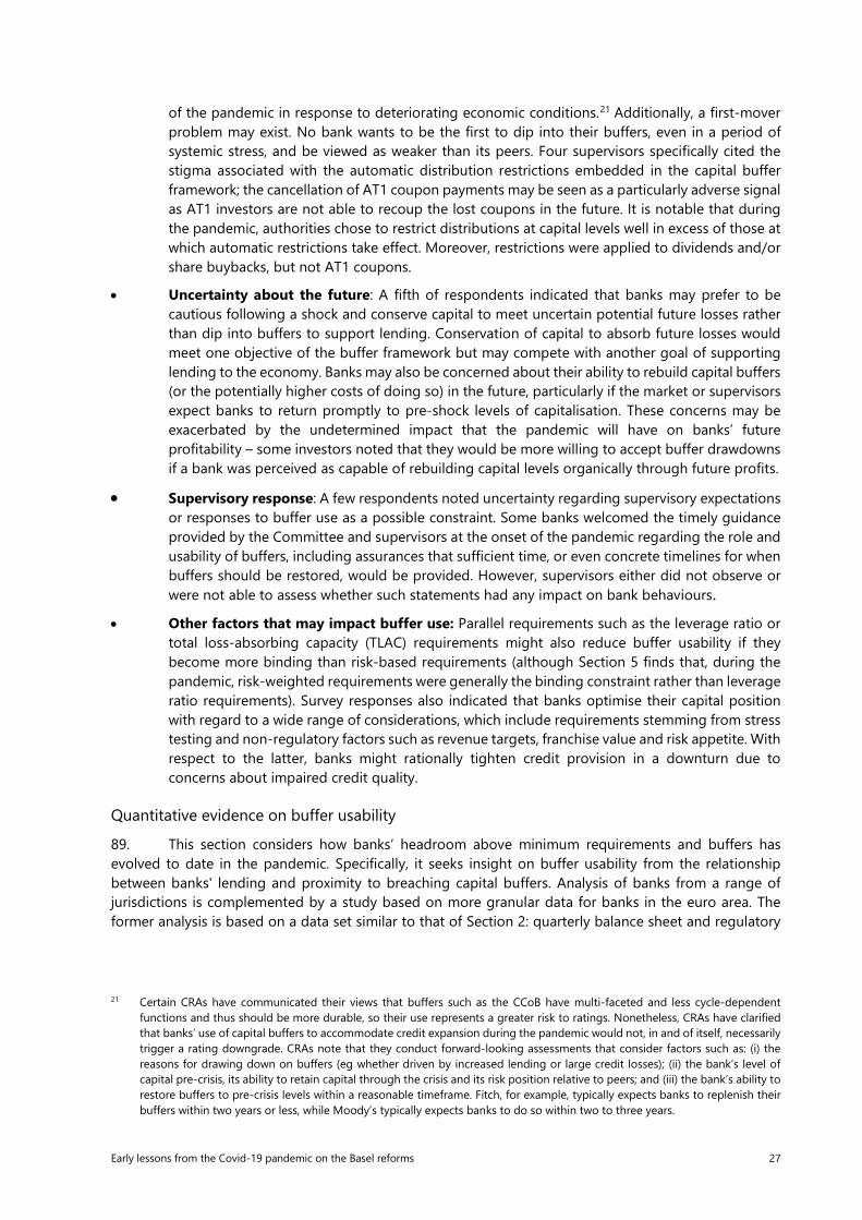
Early lessons from the Covid-19 pandemic on the Basel reforms 27
of the pandemic in response to deteriorating economic conditions.21 Additionally, a first-mover problem may exist. No bank wants to be the first to dip into their buffers, even in a period of systemic stress, and be viewed as weaker than its peers. Four supervisors specifically cited the stigma associated with the automatic distribution restrictions embedded in the capital buffer framework; the cancellation of AT1 coupon payments may be seen as a particularly adverse signal as AT1 investors are not able to recoup the lost coupons in the future. It is notable that during the pandemic, authorities chose to restrict distributions at capital levels well in excess of those at which automatic restrictions take effect. Moreover, restrictions were applied to dividends and/or share buybacks, but not AT1 coupons.
• Uncertainty about the future: A fifth of respondents indicated that banks may prefer to be cautious following a shock and conserve capital to meet uncertain potential future losses rather than dip into buffers to support lending. Conservation of capital to absorb future losses would meet one objective of the buffer framework but may compete with another goal of supporting lending to the economy. Banks may also be concerned about their ability to rebuild capital buffers (or the potentially higher costs of doing so) in the future, particularly if the market or supervisors expect banks to return promptly to pre-shock levels of capitalisation. These concerns may be exacerbated by the undetermined impact that the pandemic will have on banks’ future profitability – some investors noted that they would be more willing to accept buffer drawdowns if a bank was perceived as capable of rebuilding capital levels organically through future profits.
• Supervisory response: A few respondents noted uncertainty regarding supervisory expectations or responses to buffer use as a possible constraint. Some banks welcomed the timely guidance provided by the Committee and supervisors at the onset of the pandemic regarding the role and usability of buffers, including assurances that sufficient time, or even concrete timelines for when buffers should be restored, would be provided. However, supervisors either did not observe or were not able to assess whether such statements had any impact on bank behaviours.
• Other factors that may impact buffer use: Parallel requirements such as the leverage ratio or total loss-absorbing capacity (TLAC) requirements might also reduce buffer usability if they become more binding than risk-based requirements (although Section 5 finds that, during the pandemic, risk-weighted requirements were generally the binding constraint rather than leverage ratio requirements). Survey responses also indicated that banks optimise their capital position with regard to a wide range of considerations, which include requirements stemming from stress testing and non-regulatory factors such as revenue targets, franchise value and risk appetite. With respect to the latter, banks might rationally tighten credit provision in a downturn due to concerns about impaired credit quality.
Quantitative evidence on buffer usability
89. This section considers how banks’ headroom above minimum requirements and buffers has evolved to date in the pandemic. Specifically, it seeks insight on buffer usability from the relationship between banks' lending and proximity to breaching capital buffers. Analysis of banks from a range of jurisdictions is complemented by a study based on more granular data for banks in the euro area. The former analysis is based on a data set similar to that of Section 2: quarterly balance sheet and regulatory
21 Certain CRAs have communicated their views that buffers such as the CCoB have multi-faceted and less cycle-dependent functions and thus should be more durable, so their use represents a greater risk to ratings. Nonetheless, CRAs have clarified that banks’ use of capital buffers to accommodate credit expansion during the pandemic would not, in and of itself, necessarily trigger a rating downgrade. CRAs note that they conduct forward-looking assessments that consider factors such as: (i) the reasons for drawing down on buffers (eg whether driven by increased lending or large credit losses); (ii) the bank’s level of capital pre-crisis, its ability to retain capital through the crisis and its risk position relative to peers; and (iii) the bank’s ability to restore buffers to pre-crisis levels within a reasonable timeframe. Fitch, for example, typically expects banks to replenish their buffers within two years or less, while Moody’s typically expects banks to do so within two to three years.
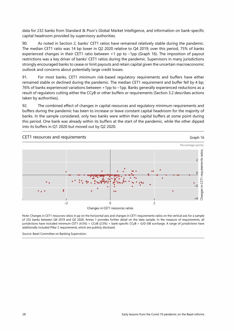
28 Early lessons from the Covid-19 pandemic on the Basel reforms
data for 232 banks from Standard & Poor’s Global Market Intelligence, and information on bank-specific capital headroom provided by supervisory authorities.
90. As noted in Section 2, banks’ CET1 ratios have remained relatively stable during the pandemic. The median CET1 ratio was 14 bp lower in Q2 2020 relative to Q4 2019; over this period, 75% of banks experienced changes in their CET1 ratio between +1 pp to –1pp (Graph 16). The imposition of payout restrictions was a key driver of banks’ CET1 ratios during the pandemic. Supervisors in many jurisdictions strongly encouraged banks to cease or limit payouts and retain capital given the uncertain macroeconomic outlook and concerns about potentially large credit losses.
91. For most banks, CET1 minimum risk-based regulatory requirements and buffers have either remained stable or declined during the pandemic. The median CET1 requirement and buffer fell by 4 bp; 76% of banks experienced variations between +1pp to –1pp. Banks generally experienced reductions as a result of regulators cutting either the CCyB or other buffers or requirements (Section 3.2 describes actions taken by authorities).
92. The combined effect of changes in capital resources and regulatory minimum requirements and buffers during the pandemic has been to increase or leave constant capital headroom for the majority of banks. In the sample considered, only two banks were within their capital buffers at some point during this period. One bank was already within its buffers at the start of the pandemic, while the other dipped into its buffers in Q1 2020 but moved out by Q2 2020.
CET1 resources and requirements Graph 16
Percentage points
Note: Changes in CET1 resources ratios in pp on the horizontal axis and changes in CET1 requirements ratios on the vertical axis for a sample of 232 banks between Q4 2019 and Q2 2020. Annex 1 provides further detail on the data sample. In the measure of requirements, all jurisdictions have included minimum CET1 (4.5%) + CCoB (2.5%) + bank-specific CCyB + G/D-SIB surcharge. A range of jurisdictions have additionally included Pillar 2 requirements, which are publicly disclosed.
Source: Basel Committee on Banking Supervision.
Early lessons from the Covid-19 pandemic on the Basel reforms 29
93. The fact that most banks’ capital ratios have been well above required minimums and buffers makes it difficult to assess whether banks would be willing to use their buffers if necessary in the future. Fear of imminently breaching buffers is unlikely to have been a key consideration for most banks during the pandemic.22 However, some banks had less capital headroom than others (Graph 17). If banks with capital levels closer to their buffers are found to be more likely to restrain lending, this could be interpreted as a reluctance to make use of buffers. Such reluctance could either reflect banks’ uncertainty regarding potential future losses or the more general market stigma that may result if a bank were to operate in its buffers.
94. In line with the approach used in Section 2.3 to evaluate the link between resilience and lending, two regression models are used to assess whether proximity to overall minimum requirements and buffers23 has been related to bank lending during the pandemic. The first specification is:
𝐶𝐶𝐶𝐶 �𝐺𝐺𝐶𝐶𝐶𝐶𝐶𝐶𝐶𝐶 𝐶𝐶𝐶𝐶𝑙𝑙𝐶𝐶𝐶𝐶𝑖𝑖,𝑗𝑗,𝑐𝑐,𝑡𝑡
𝐺𝐺𝐶𝐶𝐶𝐶𝐶𝐶𝐶𝐶 𝐶𝐶𝐶𝐶𝑙𝑙𝐶𝐶𝐶𝐶𝑖𝑖 ,𝑗𝑗,𝑐𝑐,2019𝑄𝑄1�
= 𝛼𝛼𝑖𝑖 + 𝛼𝛼𝑡𝑡 ∙ 𝛼𝛼𝑐𝑐 + 𝛽𝛽1 𝐶𝐶𝑖𝑖𝐶𝐶𝐶𝐶𝐶𝐶𝐷𝐷𝑅𝑅𝑖𝑖,2019𝑄𝑄1 × 𝐶𝐶2019−𝑄𝑄3 + 𝛽𝛽2𝐶𝐶𝑖𝑖𝐶𝐶𝐶𝐶𝐶𝐶𝐷𝐷𝑅𝑅𝑖𝑖,2019𝑄𝑄1 × 𝐶𝐶2019−𝑄𝑄4+ 𝛽𝛽3 𝐶𝐶𝑖𝑖𝐶𝐶𝐶𝐶𝐶𝐶𝐷𝐷𝑅𝑅𝑖𝑖,2019𝑄𝑄1 × 𝐶𝐶2020−𝑄𝑄1+ 𝛽𝛽4 𝐶𝐶𝑖𝑖𝐶𝐶𝐶𝐶𝐶𝐶𝐷𝐷𝑅𝑅𝑖𝑖,2019𝑄𝑄1 × 𝐶𝐶2020−𝑄𝑄2 + 𝛽𝛽5 𝐶𝐶𝑖𝑖𝐶𝐶𝐶𝐶𝐶𝐶𝐷𝐷𝑅𝑅𝑖𝑖,2019𝑄𝑄1 × 𝐶𝐶2020−𝑄𝑄3 + 𝛿𝛿 𝑋𝑋𝑖𝑖,2019𝑄𝑄1 × 𝐶𝐶𝐶𝐶𝐶𝐶𝐶𝐶𝐶𝐶𝑡𝑡+ 𝛾𝛾 𝑇𝑇𝑇𝑇𝑇𝑇𝐸𝐸𝑗𝑗 × 𝐶𝐶𝐶𝐶𝐶𝐶𝐶𝐶𝐶𝐶𝑡𝑡 + 𝜖𝜖𝑖𝑖,𝑗𝑗,𝑐𝑐,𝑡𝑡 (1)
95. In equation (1), i denotes an individual bank, j the bank type (ie savings bank, commercial bank, etc.), c the bank’s home jurisdiction, and t time. The dependent variable is the change in loans relative to Q1 2019.24 The variables of interest are the interaction terms between capital headroom in Q1 2019
22 This is consistent with a summary of bank loan officer surveys reported by the International Monetary Fund (Global Financial Stability Report April 2021, pp 20–2). As of Q4 2020, respondents mentioned that “economic outlook and borrower risk” were important current reasons for tightening lending standards, while only a few survey respondents saw “capital and liquidity” as drivers of tightening lending standards.
23 “Buffers” consist of the sum of Pillar 1 requirements such as the CCoB, bank-specific CCyB, and D/G-SIB surcharges, as well as publicly available Pillar 2 requirements and buffers. Certain Pillar 2 requirements and buffers are not publicly disclosed in all jurisdictions, so for some jurisdictions, the focus is on Pillar 1 buffers.
24 This is equivalent to a specification in levels since the amount of loans in Q1 2019 simply acts as a scaling factor.
Changes in capital headroom Graph 17
Note: Headroom above minimum and regulatory requirements in pp: Q4 2019 and Q2 2020 for a sample of 242 banks. Source: Basel Committee on Banking Supervision.
30 Early lessons from the Covid-19 pandemic on the Basel reforms
(𝐶𝐶𝑖𝑖𝐶𝐶𝐶𝐶𝐶𝐶𝐷𝐷𝑅𝑅𝑖𝑖,2019𝑄𝑄1)25 and a set of time dummies for Q3 2019 to Q3 2020. A positive coefficient 𝛽𝛽 on the interaction term would indicate that banks with less headroom prior to the pandemic reduced their lending relative to other banks, other things equal.26
96. A second specification assesses lending growth in relation to capital headroom in the preceding quarter:
ln�𝐺𝐺𝐶𝐶𝐶𝐶𝐶𝐶𝐶𝐶 𝐶𝐶𝐶𝐶𝑙𝑙𝐶𝐶𝐶𝐶𝑖𝑖 ,𝑗𝑗,𝑐𝑐,𝑡𝑡
𝐺𝐺𝐶𝐶𝐶𝐶𝐶𝐶𝐶𝐶 𝐶𝐶𝐶𝐶𝑙𝑙𝐶𝐶𝐶𝐶𝑖𝑖 ,𝑗𝑗,𝑐𝑐,𝑡𝑡−1�
= 𝛼𝛼𝑖𝑖 + 𝛼𝛼𝑡𝑡 ∙ 𝛼𝛼𝑐𝑐 + 𝛽𝛽1 ⋅ 𝐶𝐶𝑖𝑖𝐶𝐶𝐶𝐶𝐶𝐶𝐷𝐷𝑅𝑅𝑖𝑖,𝑗𝑗,𝑐𝑐,𝑡𝑡−1 × 𝐶𝐶𝐶𝐶𝐶𝐶𝐶𝐶𝐶𝐶𝑡𝑡 + 𝛽𝛽2 ⋅ 𝐶𝐶𝑖𝑖𝐶𝐶𝐶𝐶𝐶𝐶𝐷𝐷𝑅𝑅𝑖𝑖,𝑗𝑗,𝑐𝑐,𝑡𝑡−1 + 𝛿𝛿 𝑋𝑋𝑖𝑖,𝑗𝑗,𝑐𝑐,𝑡𝑡−1 + 𝛾𝛾1⋅ 𝑇𝑇𝑇𝑇𝑇𝑇𝐸𝐸𝑗𝑗 ⋅ 𝐶𝐶𝐶𝐶𝐶𝐶𝐶𝐶𝐶𝐶𝑡𝑡 + 𝜀𝜀𝑖𝑖,𝑗𝑗,𝑐𝑐,𝑡𝑡
where i denotes an individual bank, j the bank type, c the bank’s home jurisdiction, and t time. The dependent variable is quarterly loan growth. The variable of interest is the interaction between the lagged measures of capital headroom and the pandemic dummy. A positive coefficient for this interaction term would indicate that banks with less headroom in the previous period reduced their lending relative to other banks, other things equal. Other variables are defined as above.
97. The first specification yields positive and significant coefficients for the capital headroom interaction terms (Table 5, column 1). This effect becomes more pronounced as time progresses in the pandemic period. These results indicate that banks with less capital headroom lent less during the pandemic than banks with more headroom, controlling for other sources of variability. Robustness tests indicate that the results remain significant in three out of five cases when also controlling for capital levels.27
98. In the second specification, there is initially a statistically insignificant coefficient for the interaction term (Table 5, column 3). However, this interaction is significant when bank-level control variables are included (Table 5, column 4). The interaction is also significant when the pandemic dummy interacts with capital headroom in Q1 2019 instead of the lagged variable (Table 5, columns 5 and 6). These findings suggest that specifications without additional control variables may suffer from omitted variable bias. The models in columns 4 and 6 directly control for lagged capital levels, which indicate that capital headroom exerted a positive impact on lending behaviour over and above the effect of capital levels.28
25 Capital headroom is defined as the difference between the bank’s reported CET1 capital ratio and the bank’s specific minimum capital requirement and buffers, as obtained from supervisory authorities.
26 The equation also includes an interaction term between a dummy for the bank’s type and the pandemic dummy to control for the possibility that different types of banks may have reacted differently to the pandemic. Bank fixed effects (𝛼𝛼𝑖𝑖) control for time-invariant heterogeneity across banks, and country × year interactions control for time-varying heterogeneity across countries, such as economic conditions and country-specific support measures. A number of control additional variables are added, including the logarithm of total assets, the return on assets, the non-performing loan ratio, the loan-to-asset ratio, and the deposit-to-asset ratio, each interacted with the pandemic dummy. The expression 𝜖𝜖𝑖𝑖,𝑗𝑗,𝑐𝑐,𝑡𝑡 is the error term. Standard errors are clustered at the bank level.
27 Simultaneously including capital headroom and capital levels in continuous form is not possible in specification 1 due to high correlation between the variables in Q1 2019. It is, however, possible in specification 2, which uses lagged control variables.
28 A number of additional robustness checks have been conducted and show broadly consistent results.
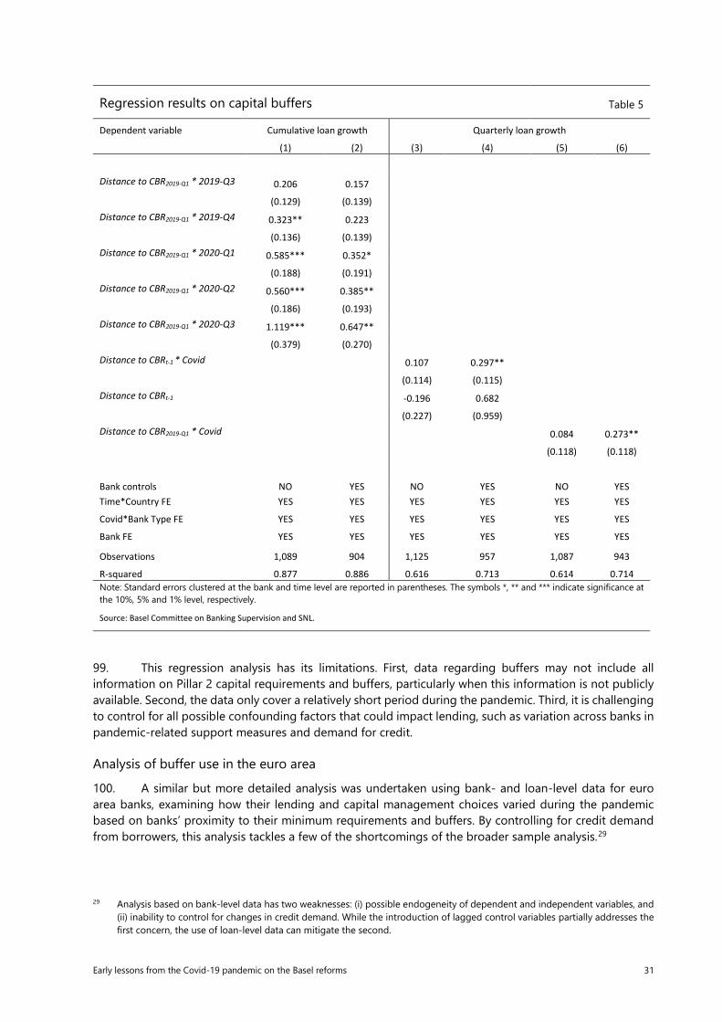
Early lessons from the Covid-19 pandemic on the Basel reforms 31
Regression results on capital buffers Table 5
Dependent variable Cumulative loan growth Quarterly loan growth
(1) (2) (3) (4) (5) (6)
Distance to CBR2019-Q1 * 2019-Q3 0.206 0.157
(0.129) (0.139) Distance to CBR2019-Q1 * 2019-Q4 0.323** 0.223
(0.136) (0.139) Distance to CBR2019-Q1 * 2020-Q1 0.585*** 0.352*
(0.188) (0.191) Distance to CBR2019-Q1 * 2020-Q2 0.560*** 0.385**
(0.186) (0.193) Distance to CBR2019-Q1 * 2020-Q3 1.119*** 0.647**
(0.379) (0.270) Distance to CBRt-1 * Covid 0.107 0.297**
(0.114) (0.115) Distance to CBRt-1 -0.196 0.682
(0.227) (0.959) Distance to CBR2019-Q1 * Covid 0.084 0.273**
(0.118) (0.118)
Bank controls NO YES NO YES NO YES Time*Country FE YES YES YES YES YES YES
Covid*Bank Type FE YES YES YES YES YES YES
Bank FE YES YES YES YES YES YES
Observations 1,089 904 1,125 957 1,087 943
R-squared 0.877 0.886 0.616 0.713 0.614 0.714 Note: Standard errors clustered at the bank and time level are reported in parentheses. The symbols *, ** and *** indicate significance at the 10%, 5% and 1% level, respectively.
Source: Basel Committee on Banking Supervision and SNL.
99. This regression analysis has its limitations. First, data regarding buffers may not include all information on Pillar 2 capital requirements and buffers, particularly when this information is not publicly available. Second, the data only cover a relatively short period during the pandemic. Third, it is challenging to control for all possible confounding factors that could impact lending, such as variation across banks in pandemic-related support measures and demand for credit.
Analysis of buffer use in the euro area
100. A similar but more detailed analysis was undertaken using bank- and loan-level data for euro area banks, examining how their lending and capital management choices varied during the pandemic based on banks’ proximity to their minimum requirements and buffers. By controlling for credit demand from borrowers, this analysis tackles a few of the shortcomings of the broader sample analysis.29
29 Analysis based on bank-level data has two weaknesses: (i) possible endogeneity of dependent and independent variables, and (ii) inability to control for changes in credit demand. While the introduction of lagged control variables partially addresses the first concern, the use of loan-level data can mitigate the second.
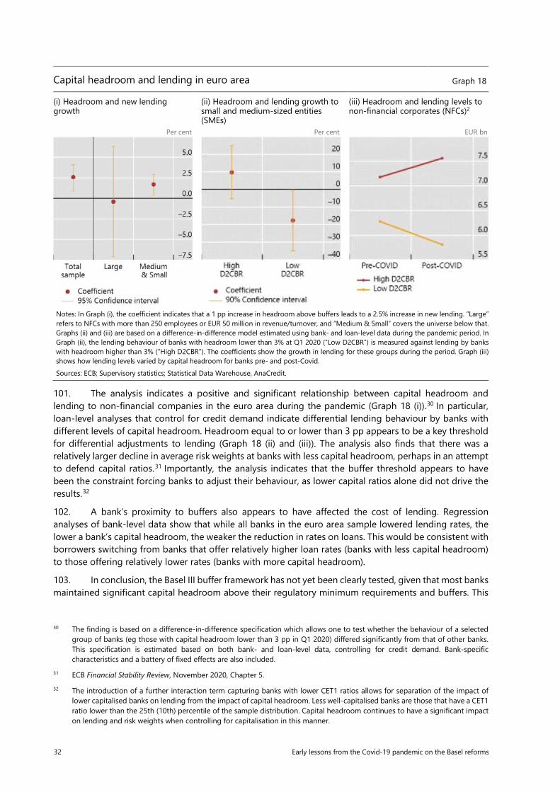
32 Early lessons from the Covid-19 pandemic on the Basel reforms
Capital headroom and lending in euro area Graph 18
(i) Headroom and new lending growth
(ii) Headroom and lending growth to small and medium-sized entities (SMEs)
(iii) Headroom and lending levels to non-financial corporates (NFCs)2
Per cent Per cent EUR bn
101. The analysis indicates a positive and significant relationship between capital headroom and lending to non-financial companies in the euro area during the pandemic (Graph 18 (i)).30 In particular, loan-level analyses that control for credit demand indicate differential lending behaviour by banks with different levels of capital headroom. Headroom equal to or lower than 3 pp appears to be a key threshold for differential adjustments to lending (Graph 18 (ii) and (iii)). The analysis also finds that there was a relatively larger decline in average risk weights at banks with less capital headroom, perhaps in an attempt to defend capital ratios.31 Importantly, the analysis indicates that the buffer threshold appears to have been the constraint forcing banks to adjust their behaviour, as lower capital ratios alone did not drive the results.32
102. A bank’s proximity to buffers also appears to have affected the cost of lending. Regression analyses of bank-level data show that while all banks in the euro area sample lowered lending rates, the lower a bank’s capital headroom, the weaker the reduction in rates on loans. This would be consistent with borrowers switching from banks that offer relatively higher loan rates (banks with less capital headroom) to those offering relatively lower rates (banks with more capital headroom).
103. In conclusion, the Basel III buffer framework has not yet been clearly tested, given that most banks maintained significant capital headroom above their regulatory minimum requirements and buffers. This
30 The finding is based on a difference-in-difference specification which allows one to test whether the behaviour of a selected group of banks (eg those with capital headroom lower than 3 pp in Q1 2020) differed significantly from that of other banks. This specification is estimated based on both bank- and loan-level data, controlling for credit demand. Bank-specific characteristics and a battery of fixed effects are also included.
31 ECB Financial Stability Review, November 2020, Chapter 5. 32 The introduction of a further interaction term capturing banks with lower CET1 ratios allows for separation of the impact of
lower capitalised banks on lending from the impact of capital headroom. Less well-capitalised banks are those that have a CET1 ratio lower than the 25th (10th) percentile of the sample distribution. Capital headroom continues to have a significant impact on lending and risk weights when controlling for capitalisation in this manner.
Notes: In Graph (i), the coefficient indicates that a 1 pp increase in headroom above buffers leads to a 2.5% increase in new lending. “Large” refers to NFCs with more than 250 employees or EUR 50 million in revenue/turnover, and “Medium & Small” covers the universe below that. Graphs (ii) and (iii) are based on a difference-in-difference model estimated using bank- and loan-level data during the pandemic period. In Graph (ii), the lending behaviour of banks with headroom lower than 3% at Q1 2020 (“Low D2CBR”) is measured against lending by banks with headroom higher than 3% (“High D2CBR”). The coefficients show the growth in lending for these groups during the period. Graph (iii) shows how lending levels varied by capital headroom for banks pre- and post-Covid. Sources: ECB; Supervisory statistics; Statistical Data Warehouse, AnaCredit.
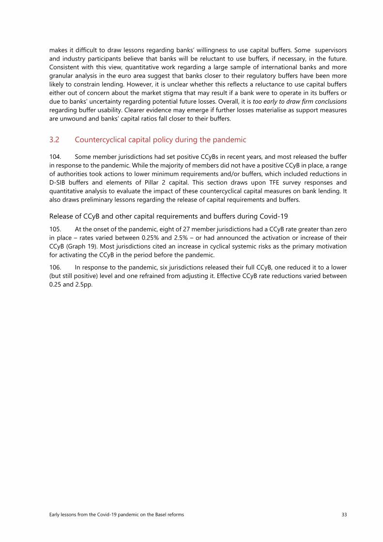
Early lessons from the Covid-19 pandemic on the Basel reforms 33
makes it difficult to draw lessons regarding banks’ willingness to use capital buffers. Some supervisors and industry participants believe that banks will be reluctant to use buffers, if necessary, in the future. Consistent with this view, quantitative work regarding a large sample of international banks and more granular analysis in the euro area suggest that banks closer to their regulatory buffers have been more likely to constrain lending. However, it is unclear whether this reflects a reluctance to use capital buffers either out of concern about the market stigma that may result if a bank were to operate in its buffers or due to banks’ uncertainty regarding potential future losses. Overall, it is too early to draw firm conclusions regarding buffer usability. Clearer evidence may emerge if further losses materialise as support measures are unwound and banks’ capital ratios fall closer to their buffers.
3.2 Countercyclical capital policy during the pandemic
104. Some member jurisdictions had set positive CCyBs in recent years, and most released the buffer in response to the pandemic. While the majority of members did not have a positive CCyB in place, a range of authorities took actions to lower minimum requirements and/or buffers, which included reductions in D-SIB buffers and elements of Pillar 2 capital. This section draws upon TFE survey responses and quantitative analysis to evaluate the impact of these countercyclical capital measures on bank lending. It also draws preliminary lessons regarding the release of capital requirements and buffers.
Release of CCyB and other capital requirements and buffers during Covid-19
105. At the onset of the pandemic, eight of 27 member jurisdictions had a CCyB rate greater than zero in place – rates varied between 0.25% and 2.5% – or had announced the activation or increase of their CCyB (Graph 19). Most jurisdictions cited an increase in cyclical systemic risks as the primary motivation for activating the CCyB in the period before the pandemic.
106. In response to the pandemic, six jurisdictions released their full CCyB, one reduced it to a lower (but still positive) level and one refrained from adjusting it. Effective CCyB rate reductions varied between 0.25 and 2.5pp.
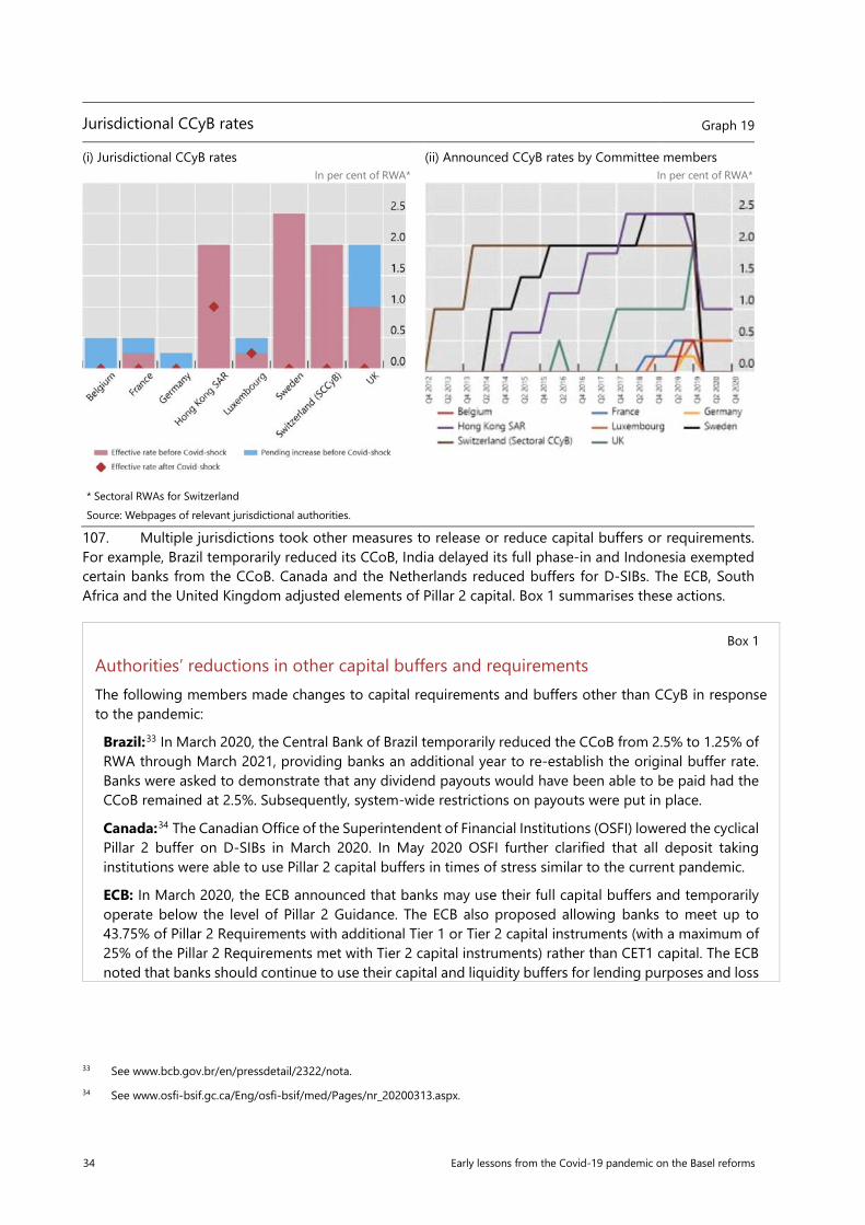
34 Early lessons from the Covid-19 pandemic on the Basel reforms
107. Multiple jurisdictions took other measures to release or reduce capital buffers or requirements. For example, Brazil temporarily reduced its CCoB, India delayed its full phase-in and Indonesia exempted certain banks from the CCoB. Canada and the Netherlands reduced buffers for D-SIBs. The ECB, South Africa and the United Kingdom adjusted elements of Pillar 2 capital. Box 1 summarises these actions.
33 See www.bcb.gov.br/en/pressdetail/2322/nota. 34 See www.osfi-bsif.gc.ca/Eng/osfi-bsif/med/Pages/nr_20200313.aspx.
Jurisdictional CCyB rates Graph 19
(i) Jurisdictional CCyB rates (ii) Announced CCyB rates by Committee members In per cent of RWA* In per cent of RWA*
* Sectoral RWAs for Switzerland Source: Webpages of relevant jurisdictional authorities.
Box 1
Authorities’ reductions in other capital buffers and requirements The following members made changes to capital requirements and buffers other than CCyB in response to the pandemic:
Brazil:33 In March 2020, the Central Bank of Brazil temporarily reduced the CCoB from 2.5% to 1.25% of RWA through March 2021, providing banks an additional year to re-establish the original buffer rate. Banks were asked to demonstrate that any dividend payouts would have been able to be paid had the CCoB remained at 2.5%. Subsequently, system-wide restrictions on payouts were put in place.
Canada:34 The Canadian Office of the Superintendent of Financial Institutions (OSFI) lowered the cyclical Pillar 2 buffer on D-SIBs in March 2020. In May 2020 OSFI further clarified that all deposit taking institutions were able to use Pillar 2 capital buffers in times of stress similar to the current pandemic.
ECB: In March 2020, the ECB announced that banks may use their full capital buffers and temporarily operate below the level of Pillar 2 Guidance. The ECB also proposed allowing banks to meet up to 43.75% of Pillar 2 Requirements with additional Tier 1 or Tier 2 capital instruments (with a maximum of 25% of the Pillar 2 Requirements met with Tier 2 capital instruments) rather than CET1 capital. The ECB noted that banks should continue to use their capital and liquidity buffers for lending purposes and loss
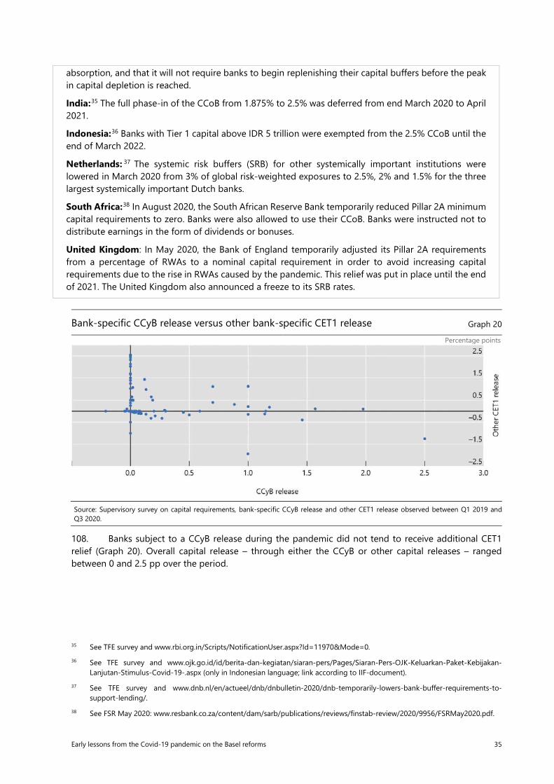
Early lessons from the Covid-19 pandemic on the Basel reforms 35
Bank-specific CCyB release versus other bank-specific CET1 release Graph 20
Percentage points
108. Banks subject to a CCyB release during the pandemic did not tend to receive additional CET1 relief (Graph 20). Overall capital release – through either the CCyB or other capital releases – ranged between 0 and 2.5 pp over the period.
35 See TFE survey and www.rbi.org.in/Scripts/NotificationUser.aspx?Id=11970&Mode=0. 36 See TFE survey and www.ojk.go.id/id/berita-dan-kegiatan/siaran-pers/Pages/Siaran-Pers-OJK-Keluarkan-Paket-Kebijakan-
Lanjutan-Stimulus-Covid-19-.aspx (only in Indonesian language; link according to IIF-document). 37 See TFE survey and www.dnb.nl/en/actueel/dnb/dnbulletin-2020/dnb-temporarily-lowers-bank-buffer-requirements-to-
support-lending/. 38 See FSR May 2020: www.resbank.co.za/content/dam/sarb/publications/reviews/finstab-review/2020/9956/FSRMay2020.pdf.
absorption, and that it will not require banks to begin replenishing their capital buffers before the peak in capital depletion is reached.
India:35 The full phase-in of the CCoB from 1.875% to 2.5% was deferred from end March 2020 to April 2021.
Indonesia:36 Banks with Tier 1 capital above IDR 5 trillion were exempted from the 2.5% CCoB until the end of March 2022.
Netherlands: 37 The systemic risk buffers (SRB) for other systemically important institutions were lowered in March 2020 from 3% of global risk-weighted exposures to 2.5%, 2% and 1.5% for the three largest systemically important Dutch banks.
South Africa:38 In August 2020, the South African Reserve Bank temporarily reduced Pillar 2A minimum capital requirements to zero. Banks were also allowed to use their CCoB. Banks were instructed not to distribute earnings in the form of dividends or bonuses.
United Kingdom: In May 2020, the Bank of England temporarily adjusted its Pillar 2A requirements from a percentage of RWAs to a nominal capital requirement in order to avoid increasing capital requirements due to the rise in RWAs caused by the pandemic. This relief was put in place until the end of 2021. The United Kingdom also announced a freeze to its SRB rates.
Source: Supervisory survey on capital requirements, bank-specific CCyB release and other CET1 release observed between Q1 2019 and Q3 2020.
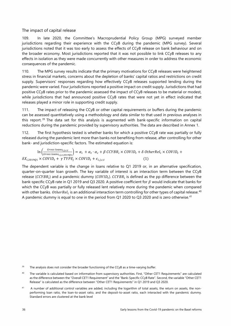
36 Early lessons from the Covid-19 pandemic on the Basel reforms
The impact of capital release
109. In late 2020, the Committee’s Macroprudential Policy Group (MPG) surveyed member jurisdictions regarding their experience with the CCyB during the pandemic (MPG survey). Several jurisdictions noted that it was too early to assess the effects of CCyB release on bank behaviour and on the broader economy. Most jurisdictions reported that it was not possible to link CCyB releases to any effects in isolation as they were made concurrently with other measures in order to address the economic consequences of the pandemic.
110. The MPG survey results indicate that the primary motivations for CCyB releases were heightened stress in financial markets, concerns about the depletion of banks' capital ratios and restrictions on credit supply. Supervisors’ responses regarding how effectively CCyB releases supported lending during the pandemic were varied. Four jurisdictions reported a positive impact on credit supply. Jurisdictions that had positive CCyB rates prior to the pandemic assessed the impact of CCyB releases to be material or modest, while jurisdictions that had announced positive CCyB rates that were not yet in effect indicated that releases played a minor role in supporting credit supply.
111. The impact of releasing the CCyB or other capital requirements or buffers during the pandemic can be assessed quantitatively using a methodology and data similar to that used in previous analyses in this report. 39 The data set for this analysis is augmented with bank-specific information on capital reductions during the pandemic provided by supervisory authorities. The data are described in Annex 1.
112. The first hypothesis tested is whether banks for which a positive CCyB rate was partially or fully released during the pandemic lent more than banks not benefiting from release, after controlling for other bank- and jurisdiction-specific factors. The estimated equation is:
ln �𝐺𝐺𝐺𝐺𝐺𝐺𝐺𝐺𝐺𝐺 𝑙𝑙𝐺𝐺𝑙𝑙𝑙𝑙𝐺𝐺𝑖𝑖,𝑗𝑗,𝑐𝑐,𝑡𝑡
𝐺𝐺𝐺𝐺𝐺𝐺𝐺𝐺𝐺𝐺 𝑙𝑙𝐺𝐺𝑙𝑙𝑙𝑙𝐺𝐺𝑖𝑖,𝑗𝑗,𝑐𝑐,2019𝑄𝑄1� = 𝛼𝛼𝑖𝑖 + 𝛼𝛼𝑡𝑡 ∙ 𝛼𝛼𝑐𝑐 + 𝛽𝛽 𝐶𝐶𝐶𝐶𝑇𝑇𝐷𝐷𝑅𝑅𝑖𝑖 × 𝐶𝐶𝐶𝐶𝐶𝐶𝐶𝐶𝐶𝐶𝑡𝑡 + 𝛿𝛿 𝐶𝐶𝐶𝐶ℎ𝑒𝑒𝐶𝐶𝑅𝑅𝑒𝑒𝐶𝐶𝑖𝑖 × 𝐶𝐶𝐶𝐶𝐶𝐶𝐶𝐶𝐶𝐶𝑡𝑡 +
𝛿𝛿𝑋𝑋𝑖𝑖,2019𝑄𝑄1 × 𝐶𝐶𝐶𝐶𝐶𝐶𝐶𝐶𝐶𝐶𝑡𝑡 + 𝛾𝛾 𝑇𝑇𝑇𝑇𝑇𝑇𝐸𝐸𝑗𝑗 × 𝐶𝐶𝐶𝐶𝐶𝐶𝐶𝐶𝐶𝐶𝑡𝑡 + 𝜖𝜖𝑖𝑖,𝑗𝑗,𝑐𝑐,𝑡𝑡 (1)
The dependent variable is the change in loans relative to Q1 2019 or, in an alternative specification, quarter-on-quarter loan growth. The key variable of interest is an interaction term between the CCyB release (𝐶𝐶𝐶𝐶𝑇𝑇𝐷𝐷𝑅𝑅𝑖𝑖) and a pandemic dummy (𝐶𝐶𝐶𝐶𝐶𝐶𝐶𝐶𝐶𝐶𝑡𝑡). 𝐶𝐶𝐶𝐶𝑇𝑇𝐷𝐷𝑅𝑅𝑖𝑖 is defined as the pp difference between the bank-specific CCyB rate in Q1 2019 and Q3 2020. A positive coefficient for 𝛽𝛽 would indicate that banks for which the CCyB was partially or fully released lent relatively more during the pandemic when compared with other banks. 𝐶𝐶𝐶𝐶ℎ𝑒𝑒𝐶𝐶𝑅𝑅𝑒𝑒𝐶𝐶𝑖𝑖 is an additional interaction term controlling for other types of capital release.40 A pandemic dummy is equal to one in the period from Q1 2020 to Q3 2020 and is zero otherwise.41
39 The analysis does not consider the broader functioning of the CCyB as a time-varying buffer. 40 The variable is calculated based on information from supervisory authorities. First, “Other CET1 Requirements” are calculated
as the difference between the “Overall CET1 Requirement” and the “Bank-Specific CCyB Rate”. Second, the variable “Other CET1 Release” is calculated as the difference between “Other CET1 Requirements” in Q1 2019 and Q3 2020.
41 A number of additional control variables are added, including the logarithm of total assets, the return on assets, the non-performing loan ratio, the loan-to-asset ratio, and the deposit-to-asset ratio, each interacted with the pandemic dummy. Standard errors are clustered at the bank level
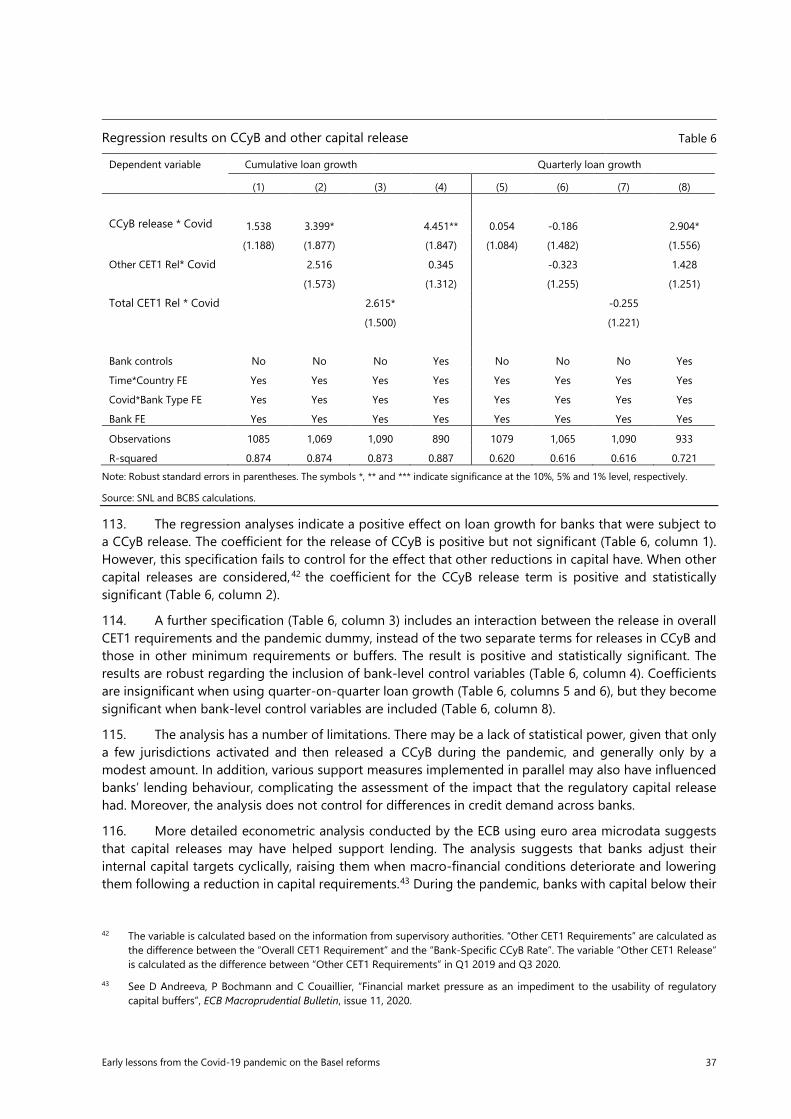
Early lessons from the Covid-19 pandemic on the Basel reforms 37
Regression results on CCyB and other capital release Table 6
Dependent variable Cumulative loan growth Quarterly loan growth
(1) (2) (3) (4) (5) (6) (7) (8)
CCyB release * Covid 1.538 3.399* 4.451** 0.054 -0.186 2.904*
(1.188) (1.877) (1.847) (1.084) (1.482) (1.556)
Other CET1 Rel* Covid 2.516 0.345 -0.323 1.428
(1.573) (1.312) (1.255) (1.251)
Total CET1 Rel * Covid 2.615* -0.255
(1.500) (1.221)
Bank controls No No No Yes No No No Yes
Time*Country FE Yes Yes Yes Yes Yes Yes Yes Yes
Covid*Bank Type FE Yes Yes Yes Yes Yes Yes Yes Yes
Bank FE Yes Yes Yes Yes Yes Yes Yes Yes
Observations 1085 1,069 1,090 890 1079 1,065 1,090 933
R-squared 0.874 0.874 0.873 0.887 0.620 0.616 0.616 0.721 Note: Robust standard errors in parentheses. The symbols *, ** and *** indicate significance at the 10%, 5% and 1% level, respectively.
Source: SNL and BCBS calculations.
113. The regression analyses indicate a positive effect on loan growth for banks that were subject to a CCyB release. The coefficient for the release of CCyB is positive but not significant (Table 6, column 1). However, this specification fails to control for the effect that other reductions in capital have. When other capital releases are considered,42 the coefficient for the CCyB release term is positive and statistically significant (Table 6, column 2).
114. A further specification (Table 6, column 3) includes an interaction between the release in overall CET1 requirements and the pandemic dummy, instead of the two separate terms for releases in CCyB and those in other minimum requirements or buffers. The result is positive and statistically significant. The results are robust regarding the inclusion of bank-level control variables (Table 6, column 4). Coefficients are insignificant when using quarter-on-quarter loan growth (Table 6, columns 5 and 6), but they become significant when bank-level control variables are included (Table 6, column 8).
115. The analysis has a number of limitations. There may be a lack of statistical power, given that only a few jurisdictions activated and then released a CCyB during the pandemic, and generally only by a modest amount. In addition, various support measures implemented in parallel may also have influenced banks’ lending behaviour, complicating the assessment of the impact that the regulatory capital release had. Moreover, the analysis does not control for differences in credit demand across banks.
116. More detailed econometric analysis conducted by the ECB using euro area microdata suggests that capital releases may have helped support lending. The analysis suggests that banks adjust their internal capital targets cyclically, raising them when macro-financial conditions deteriorate and lowering them following a reduction in capital requirements.43 During the pandemic, banks with capital below their
42 The variable is calculated based on the information from supervisory authorities. “Other CET1 Requirements” are calculated as the difference between the “Overall CET1 Requirement” and the “Bank-Specific CCyB Rate”. The variable “Other CET1 Release” is calculated as the difference between “Other CET1 Requirements” in Q1 2019 and Q3 2020.
43 See D Andreeva, P Bochmann and C Couaillier, “Financial market pressure as an impediment to the usability of regulatory capital buffers”, ECB Macroprudential Bulletin, issue 11, 2020.
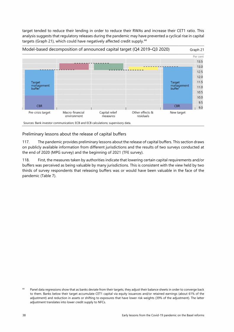
38 Early lessons from the Covid-19 pandemic on the Basel reforms
target tended to reduce their lending in order to reduce their RWAs and increase their CET1 ratio. This analysis suggests that regulatory releases during the pandemic may have prevented a cyclical rise in capital targets (Graph 21), which could have negatively affected credit supply.44
Model-based decomposition of announced capital target (Q4 2019–Q3 2020) Graph 21
Per cent
Preliminary lessons about the release of capital buffers
117. The pandemic provides preliminary lessons about the release of capital buffers. This section draws on publicly available information from different jurisdictions and the results of two surveys conducted at the end of 2020 (MPG survey) and the beginning of 2021 (TFE survey).
118. First, the measures taken by authorities indicate that lowering certain capital requirements and/or buffers was perceived as being valuable by many jurisdictions. This is consistent with the view held by two thirds of survey respondents that releasing buffers was or would have been valuable in the face of the pandemic (Table 7).
44 Panel data regressions show that as banks deviate from their targets, they adjust their balance sheets in order to converge back to them. Banks below their target accumulate CET1 capital via equity issuances and/or retained earnings (about 61% of the adjustment) and reduction in assets or shifting to exposures that have lower risk weights (39% of the adjustment). The latter adjustment translates into lower credit supply to NFCs.
Sources: Bank investor communication; ECB and ECB calculations; supervisory data.
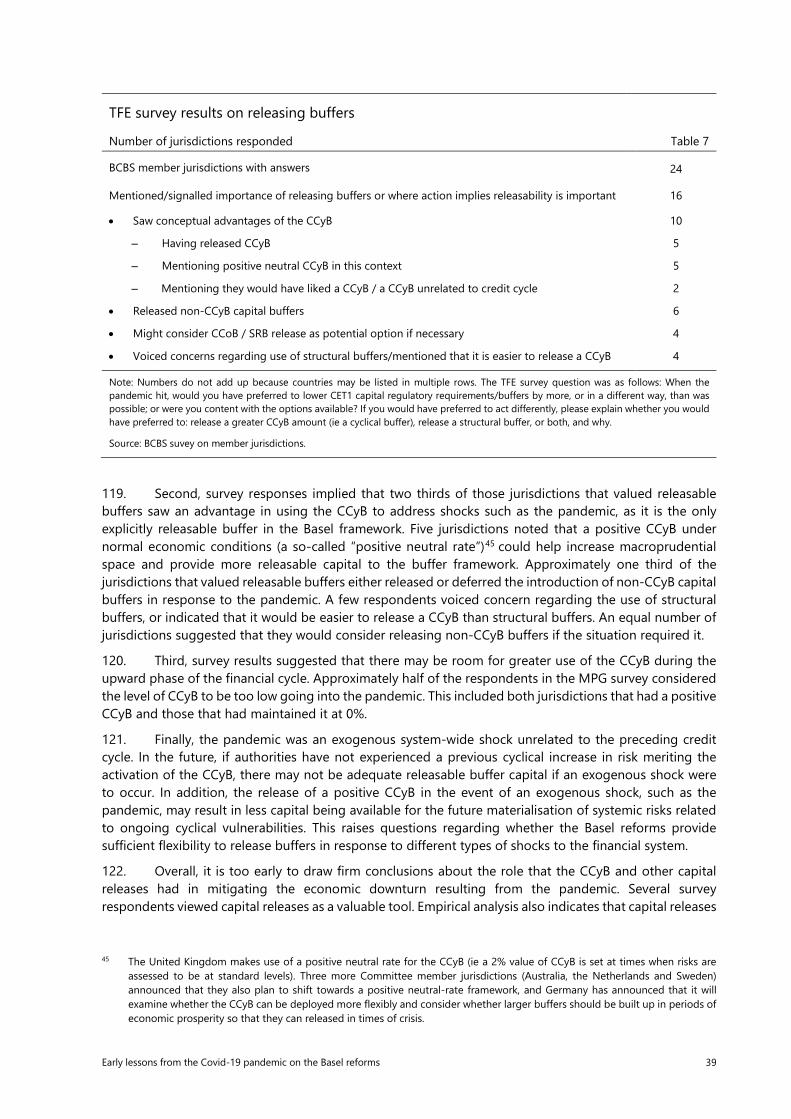
Early lessons from the Covid-19 pandemic on the Basel reforms 39
TFE survey results on releasing buffers
Number of jurisdictions responded Table 7
BCBS member jurisdictions with answers 24
Mentioned/signalled importance of releasing buffers or where action implies releasability is important 16
• Saw conceptual advantages of the CCyB 10
– Having released CCyB 5
– Mentioning positive neutral CCyB in this context 5
– Mentioning they would have liked a CCyB / a CCyB unrelated to credit cycle 2
• Released non-CCyB capital buffers 6
• Might consider CCoB / SRB release as potential option if necessary 4
• Voiced concerns regarding use of structural buffers/mentioned that it is easier to release a CCyB 4
Note: Numbers do not add up because countries may be listed in multiple rows. The TFE survey question was as follows: When the pandemic hit, would you have preferred to lower CET1 capital regulatory requirements/buffers by more, or in a different way, than was possible; or were you content with the options available? If you would have preferred to act differently, please explain whether you would have preferred to: release a greater CCyB amount (ie a cyclical buffer), release a structural buffer, or both, and why.
Source: BCBS suvey on member jurisdictions.
119. Second, survey responses implied that two thirds of those jurisdictions that valued releasable buffers saw an advantage in using the CCyB to address shocks such as the pandemic, as it is the only explicitly releasable buffer in the Basel framework. Five jurisdictions noted that a positive CCyB under normal economic conditions (a so-called “positive neutral rate”)45 could help increase macroprudential space and provide more releasable capital to the buffer framework. Approximately one third of the jurisdictions that valued releasable buffers either released or deferred the introduction of non-CCyB capital buffers in response to the pandemic. A few respondents voiced concern regarding the use of structural buffers, or indicated that it would be easier to release a CCyB than structural buffers. An equal number of jurisdictions suggested that they would consider releasing non-CCyB buffers if the situation required it.
120. Third, survey results suggested that there may be room for greater use of the CCyB during the upward phase of the financial cycle. Approximately half of the respondents in the MPG survey considered the level of CCyB to be too low going into the pandemic. This included both jurisdictions that had a positive CCyB and those that had maintained it at 0%.
121. Finally, the pandemic was an exogenous system-wide shock unrelated to the preceding credit cycle. In the future, if authorities have not experienced a previous cyclical increase in risk meriting the activation of the CCyB, there may not be adequate releasable buffer capital if an exogenous shock were to occur. In addition, the release of a positive CCyB in the event of an exogenous shock, such as the pandemic, may result in less capital being available for the future materialisation of systemic risks related to ongoing cyclical vulnerabilities. This raises questions regarding whether the Basel reforms provide sufficient flexibility to release buffers in response to different types of shocks to the financial system.
122. Overall, it is too early to draw firm conclusions about the role that the CCyB and other capital releases had in mitigating the economic downturn resulting from the pandemic. Several survey respondents viewed capital releases as a valuable tool. Empirical analysis also indicates that capital releases
45 The United Kingdom makes use of a positive neutral rate for the CCyB (ie a 2% value of CCyB is set at times when risks are assessed to be at standard levels). Three more Committee member jurisdictions (Australia, the Netherlands and Sweden) announced that they also plan to shift towards a positive neutral-rate framework, and Germany has announced that it will examine whether the CCyB can be deployed more flexibly and consider whether larger buffers should be built up in periods of economic prosperity so that they can released in times of crisis.
40 Early lessons from the Covid-19 pandemic on the Basel reforms
may have helped support lending. Going forward, it may be useful to carry out additional analyses based on more granular data. This could offer further insight into the role and sufficiency of releasable capital in the Basel framework, including in responding to systemic shocks unrelated to a previous build-up of risk in a credit cycle.
3.3 Insights from pricing of Additional Tier 1 instruments
123. While CET1 capital is the primary component of regulatory capital, AT1 capital (which includes qualifying contingent convertible securities (CoCos) and preferred stock) is designed to act as an additional loss-absorbing capital instrument. Prior to the GFC, regulators used a Tier 1 capital measure that encompassed both common equity and instruments similar to those currently defined as AT1. Under healthy economic circumstances, AT1 instruments behave more like debt, having fixed coupons that banks are not obliged to pay, limited upside and no control rights. However, during periods of stress, these instruments are designed to behave like equity, absorbing losses and protecting creditors.
124. Like the more ubiquitous CET1 capital instruments, AT1 instruments – which, together with CET1 capital instruments, comprise Tier 1 capital under the Basel reforms – are subject to payout restrictions when banks make use of regulatory buffers.46
125. As a result of the pandemic, supervisors encouraged banks to use part or all of their buffers, which, in certain cases, could result in AT1 coupon suspensions. Doing so would lower the price that investors are willing to pay for AT1 instruments, thus elevating AT1 yields. Conversely, if market participants do not find it credible that AT1 coupons will be suspended, AT1 yields would not be expected to increase to the same extent. The global economic shock of the pandemic provides for the first systemic test of the market’s perception of AT1 instrument’s loss absorbing capacity. It also provides insights on whether market participants view CoCos and preferred stock as equivalent forms of capital.
126. In the United States, the most common AT1 instrument is preferred stock, which typically has a fixed dividend paid before common stock dividends are paid and a payout that is prioritised over common shares in the case of bankruptcy. In Europe, CoCos are the most common AT1 capital instrument. When capital ratios are above the trigger point, these hybrid instruments are senior to common stock but subordinated to other debt claims.
127. While preferred stock is a long-established source of subordinated bank financing, CoCos are a more recent development. CoCos became popular following the GFC.47 They are designed to absorb losses and recapitalise banks when their capital ratio falls below a certain level, either by including contractual terms that convert the instrument to common equity or by requiring a principal write-down.
128. AT1 instruments are intended to absorb losses on a going-concern basis through the suspension of coupon payments, principal write-down, or conversion to common stock. Some express concern that AT1 instruments may not be going-concern capital (similar to CET1 capital, absorbing losses while the business continues) but rather gone-concern capital (similar to Tier 2 capital, only absorbing losses after the point of non-viability). While both going-concern and gone-concern capital are designed to be loss-absorbing, their difference lies in when each instrument absorbs losses.
129. Under current US and European regulatory capital requirements, when a bank’s capital ratio falls below a required capital buffer level, automatic distribution restrictions – which may include limits on or the suspension of AT1 coupon payments and preferred stock dividend payments – are triggered. During the pandemic, several regulators imposed system-wide restrictions on common stock dividends. However,
46 For example, the stress capital buffer in the US or the combined buffer requirement in the EU. 47 CoCos were conceived in Merton, R C (1990): "The Financial System and Economic Performance”, Journal of Financial Services
Research, no. 4, pp 263–300.
Early lessons from the Covid-19 pandemic on the Basel reforms 41
regulators did not restrict AT1 coupon payments, which are fully discretionary regardless of banks’ capital ratios.
130. The two analyses below use securities data on preferred stock and CoCos from Bloomberg LLC to compare their performance to that of subordinated debt and common equity. They focus on the following three key questions: (i) whether markets perceive AT1 instruments to be riskier than debt; (ii) whether markets perceive systematic differences between the loss absorbency of the two types of AT1 instruments; and (iii) whether AT1 instrument prices move with debt or equity prices. The analysis does not directly address whether AT1 instruments are appropriately considered gone-concern or going-concern capital, which would require a more sophisticated analysis.48
131. The data include daily prices and two measures of yield – the daily yield to maturity (YTM) and the daily yield to worst (YTW) – for each security from 1 January 2019 to 24 March 2021. To facilitate comparison, the sample is restricted to banks with both outstanding AT1 and subordinated long-term debt instruments (with two to seven years remaining maturity). The data cover 45 large US and European banks that have at least one active and marketable AT1 instrument and subordinated long-term debt security with a fixed-rate coupon. The analysis treats the onset of the pandemic in the United States and Europe as of March 2020.
132. YTM is the most common approach to measuring bond yields and represents the total anticipated return on a bond when held to maturity. However, in the case of preferred stock, CoCos and other perpetual instruments, YTM can be viewed as a misnomer because these securities do not mature. Rather, YTM is calculated as the amount of the yearly coupon payment divided by the instrument’s price.
133. By contrast, YTW is the yield implied by the current bond price, coupon, and least advantageous (and possible) call or retirement date. Because AT1 instruments usually have an embedded call (most commonly exercisable quarterly or annually five years from issuance for CoCos and five to 10 years from issuance for preferred stock), YTM and YTW may differ substantially. Historically, banks have generally called AT1 instruments as early as possible in order to provide investors with the risk and return profile of a five-year bond instead of that of a perpetual security.
134. US banks only have outstanding preferred stock as AT1 instruments, whereas European banks only have outstanding CoCos as AT1 instruments. Thus, one cannot distinguish between differences in preferred stock and CoCos across the two continents. However, the use of monthly data and a difference-in-difference estimation method allows one to obtain a clear result.
135. The evolution of the median YTM and YTW values over the sample period provides an indicative analysis of the behaviour of CoCos, preferred stock and subordinated long-term debt instruments. In March 2020, YTM and YTW on subordinated long-term debt, CoCos and preferred stock all became elevated. Consistent with the fact that these securities face greater risk of loss, Graph 22 shows that spreads over long-term risk-free rates rose in March 2020. In general, YTW rose more than YTM. While preferred stock yields declined when markets stabilised, YTW on CoCos remained somewhat elevated while YTM declined more.
48 For example, see F Fiordelisi, G Pennacchi & O Ricci, “Are contingent convertibles going-concern capital?”, Journal of Financial Intermediation, vol 43, 2020, pp 1008–22.
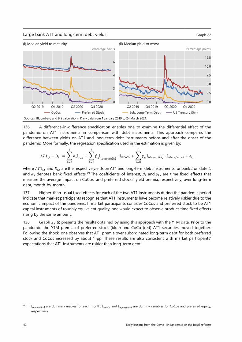
42 Early lessons from the Covid-19 pandemic on the Basel reforms
Large bank AT1 and long-term debt yields Graph 22
(i) Median yield to maturity (ii) Median yield to worst Percentage points Percentage points
136. A difference-in-difference specification enables one to examine the differential effect of the pandemic on AT1 instruments in comparison with debt instruments. This approach compares the difference between yields on AT1 and long-term debt instruments before and after the onset of the pandemic. More formally, the regression specification used in the estimation is given by:
𝐴𝐴𝑇𝑇1𝑖𝑖,𝐶𝐶 − 𝐶𝐶𝑖𝑖,𝐶𝐶 = �α𝑘𝑘𝕝𝕝𝑖𝑖=𝑘𝑘
𝐶𝐶
𝑘𝑘=0
+ �β𝑘𝑘𝕝𝕝𝐶𝐶∈𝑚𝑚𝐶𝐶𝐶𝐶𝐶𝐶ℎ(𝑘𝑘)
𝑇𝑇
𝑘𝑘=0
⋅ 𝕝𝕝𝑖𝑖∈𝐶𝐶𝐶𝐶𝐶𝐶𝐶𝐶 + �𝛾𝛾𝑘𝑘
𝑇𝑇
𝑘𝑘=0
𝕝𝕝𝐶𝐶∈𝑚𝑚𝐶𝐶𝐶𝐶𝐶𝐶ℎ(𝑘𝑘) ⋅ 𝕝𝕝𝑖𝑖∈𝑝𝑝𝐶𝐶𝑒𝑒𝑝𝑝𝑒𝑒𝐶𝐶𝐶𝐶𝑒𝑒𝑝𝑝 + 𝜀𝜀𝑖𝑖,𝐶𝐶
where 𝐴𝐴𝑇𝑇1𝑖𝑖,𝑡𝑡 and 𝐶𝐶𝑖𝑖 ,𝑡𝑡 are the respective yields on AT1 and long-term debt instruments for bank 𝑖𝑖 on date 𝐶𝐶, and 𝛼𝛼𝑘𝑘 denotes bank fixed effects.49 The coefficients of interest, 𝛽𝛽𝑘𝑘 and 𝛾𝛾𝑘𝑘 , are time fixed effects that measure the average impact on CoCos’ and preferred stocks’ yield premia, respectively, over long-term debt, month-by-month.
137. Higher-than-usual fixed effects for each of the two AT1 instruments during the pandemic period indicate that market participants recognise that AT1 instruments have become relatively riskier due to the economic impact of the pandemic. If market participants consider CoCos and preferred stock to be AT1 capital instruments of roughly equivalent quality, one would expect to observe product-time fixed effects rising by the same amount.
138. Graph 23 (i) presents the results obtained by using this approach with the YTM data. Prior to the pandemic, the YTM premia of preferred stock (blue) and CoCo (red) AT1 securities moved together. Following the shock, one observes that AT1 premia over subordinated long-term debt for both preferred stock and CoCos increased by about 1 pp. These results are also consistent with market participants’ expectations that AT1 instruments are riskier than long-term debt.
49 𝕝𝕝𝐶𝐶∈𝑚𝑚𝐶𝐶𝐶𝐶𝐶𝐶ℎ(𝑘𝑘) are dummy variables for each month. 𝕝𝕝𝑖𝑖∈𝐶𝐶𝐶𝐶𝐶𝐶𝐶𝐶 and 𝕝𝕝𝑖𝑖∈𝑝𝑝𝐶𝐶𝑒𝑒𝑝𝑝𝑒𝑒𝐶𝐶𝐶𝐶𝑒𝑒𝑝𝑝 are dummy variables for CoCos and preferred equity, respectively.
Sources: Bloomberg and BIS calculations. Daily data from 1 January 2019 to 24 March 2021.
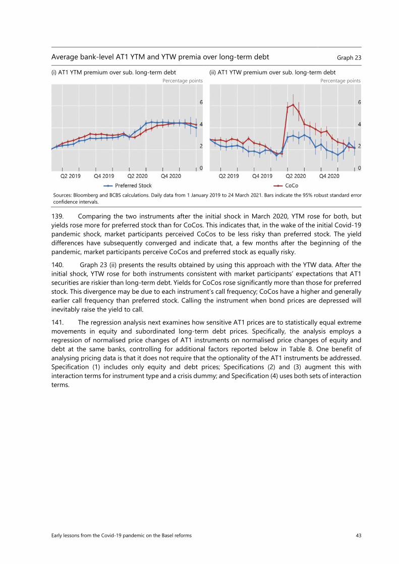
Early lessons from the Covid-19 pandemic on the Basel reforms 43
Average bank-level AT1 YTM and YTW premia over long-term debt Graph 23
(i) AT1 YTM premium over sub. long-term debt (ii) AT1 YTW premium over sub. long-term debt Percentage points Percentage points
139. Comparing the two instruments after the initial shock in March 2020, YTM rose for both, but yields rose more for preferred stock than for CoCos. This indicates that, in the wake of the initial Covid-19 pandemic shock, market participants perceived CoCos to be less risky than preferred stock. The yield differences have subsequently converged and indicate that, a few months after the beginning of the pandemic, market participants perceive CoCos and preferred stock as equally risky.
140. Graph 23 (ii) presents the results obtained by using this approach with the YTW data. After the initial shock, YTW rose for both instruments consistent with market participants’ expectations that AT1 securities are riskier than long-term debt. Yields for CoCos rose significantly more than those for preferred stock. This divergence may be due to each instrument’s call frequency; CoCos have a higher and generally earlier call frequency than preferred stock. Calling the instrument when bond prices are depressed will inevitably raise the yield to call.
141. The regression analysis next examines how sensitive AT1 prices are to statistically equal extreme movements in equity and subordinated long-term debt prices. Specifically, the analysis employs a regression of normalised price changes of AT1 instruments on normalised price changes of equity and debt at the same banks, controlling for additional factors reported below in Table 8. One benefit of analysing pricing data is that it does not require that the optionality of the AT1 instruments be addressed. Specification (1) includes only equity and debt prices; Specifications (2) and (3) augment this with interaction terms for instrument type and a crisis dummy; and Specification (4) uses both sets of interaction terms.
Sources: Bloomberg and BCBS calculations. Daily data from 1 January 2019 to 24 March 2021. Bars indicate the 95% robust standard error confidence intervals.
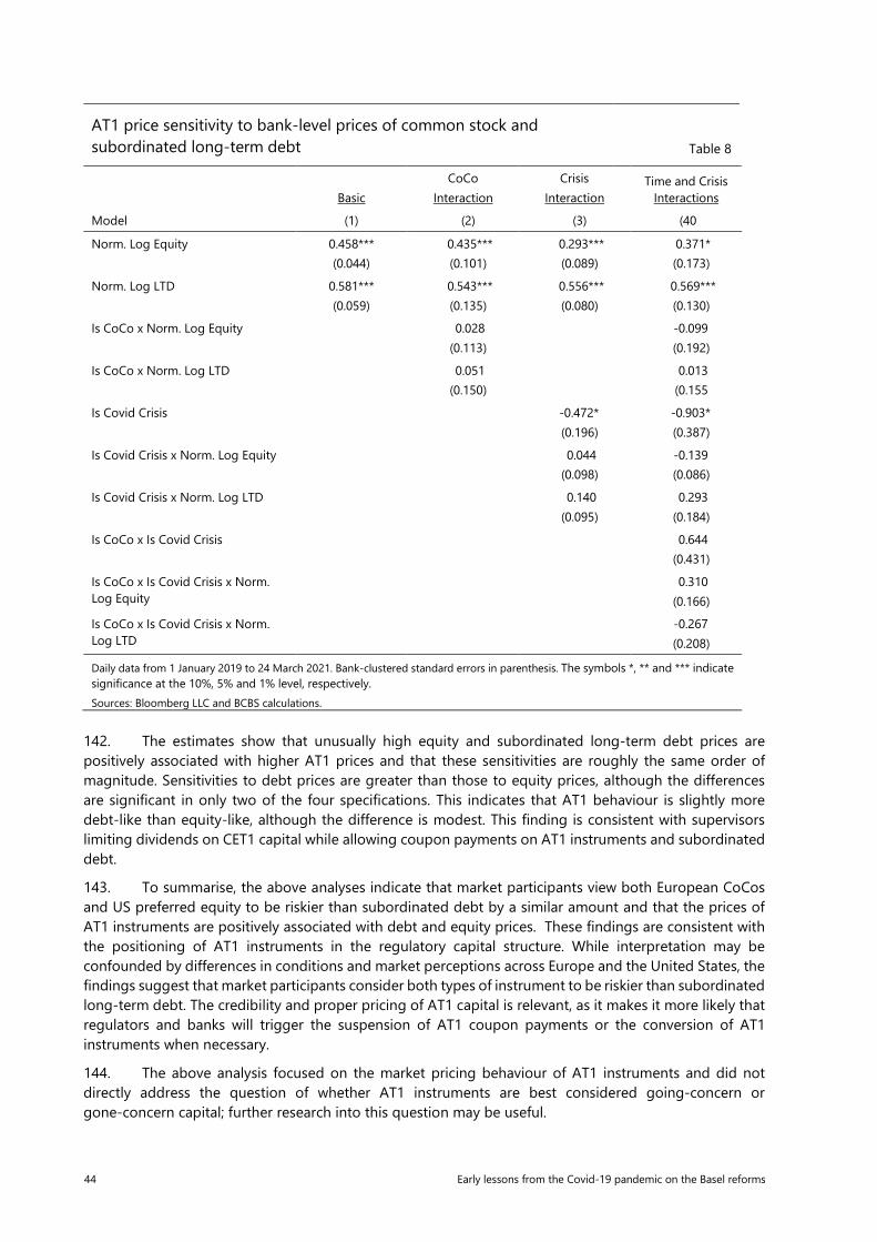
44 Early lessons from the Covid-19 pandemic on the Basel reforms
142. The estimates show that unusually high equity and subordinated long-term debt prices are positively associated with higher AT1 prices and that these sensitivities are roughly the same order of magnitude. Sensitivities to debt prices are greater than those to equity prices, although the differences are significant in only two of the four specifications. This indicates that AT1 behaviour is slightly more debt-like than equity-like, although the difference is modest. This finding is consistent with supervisors limiting dividends on CET1 capital while allowing coupon payments on AT1 instruments and subordinated debt.
143. To summarise, the above analyses indicate that market participants view both European CoCos and US preferred equity to be riskier than subordinated debt by a similar amount and that the prices of AT1 instruments are positively associated with debt and equity prices. These findings are consistent with the positioning of AT1 instruments in the regulatory capital structure. While interpretation may be confounded by differences in conditions and market perceptions across Europe and the United States, the findings suggest that market participants consider both types of instrument to be riskier than subordinated long-term debt. The credibility and proper pricing of AT1 capital is relevant, as it makes it more likely that regulators and banks will trigger the suspension of AT1 coupon payments or the conversion of AT1 instruments when necessary.
144. The above analysis focused on the market pricing behaviour of AT1 instruments and did not directly address the question of whether AT1 instruments are best considered going-concern or gone-concern capital; further research into this question may be useful.
AT1 price sensitivity to bank-level prices of common stock and subordinated long-term debt Table 8
Basic
CoCo Interaction
Crisis Interaction
Time and Crisis Interactions
Model (1) (2) (3) (40
Norm. Log Equity 0.458*** (0.044)
0.435*** (0.101)
0.293*** (0.089)
0.371* (0.173)
Norm. Log LTD 0.581*** (0.059)
0.543*** (0.135)
0.556*** (0.080)
0.569*** (0.130)
Is CoCo x Norm. Log Equity
0.028 (0.113)
-0.099 (0.192)
Is CoCo x Norm. Log LTD
0.051 (0.150)
0.013
(0.155
Is Covid Crisis
-0.472* (0.196)
-0.903* (0.387)
Is Covid Crisis x Norm. Log Equity
0.044 (0.098)
-0.139 (0.086)
Is Covid Crisis x Norm. Log LTD
0.140 (0.095)
0.293 (0.184)
Is CoCo x Is Covid Crisis
0.644 (0.431)
Is CoCo x Is Covid Crisis x Norm. Log Equity
0.310 (0.166)
Is CoCo x Is Covid Crisis x Norm. Log LTD
-0.267 (0.208)
Daily data from 1 January 2019 to 24 March 2021. Bank-clustered standard errors in parenthesis. The symbols *, ** and *** indicate significance at the 10%, 5% and 1% level, respectively. Sources: Bloomberg LLC and BCBS calculations.
Early lessons from the Covid-19 pandemic on the Basel reforms 45
4. The Liquidity Coverage Ratio
145. This section considers whether the LCR functioned as expected during the pandemic, particularly during the “dash for cash” period of March 2020.
146. Liquidity buffers are intended to improve the banking sector’s ability to absorb shocks caused by financial and economic stress, thus reducing the risk of spillover from the financial sector to the real economy, and give central banks time to take appropriate measures.50 In general, buffers of high-quality liquid assets (HQLA)51 built up as a result of the LCR framework helped banks maintain market confidence and weather the pandemic (Section 2.1). However, some banks did experience short-lived pressure on their liquidity positions. This section discusses how banks responded, including whether they were willing to use liquid asset buffers. It also examines the steps taken by supervisors in response to actual or anticipated liquidity pressure. Finally, it considers whether any lessons can be taken regarding the design of the LCR.
147. The analysis in this section is based on: (i) detailed feedback from a TFE survey of 27 supervisory authorities which covered the functioning of the LCR in the pandemic (Annex 2), as well a survey conducted in 2019 by the Committee’s Working Group on Liquidity (WGL) (the WGL survey); and (ii) detailed studies of bank liquidity developments in specific jurisdictions (Annex 3).
Evolution of banks’ liquidity positions
148. Banks in most jurisdictions experienced downward pressure on their liquidity buffers in March 2020, when the financial market stress was at its peak.
149. Draws on credit lines by customers seeking to raise cash in the face of uncertainty about the extent and duration of the pandemic were the most common and material source of outflows, according to more than half of the respondents to the TFE survey. Approximately one third of these respondents noted drawdowns greater than the prescribed LCR outflow rates. However, as noted below, downward pressure on LCRs was often mitigated by an increase in HQLA as corporate entities re-deposited the proceeds into the banking sector.52
150. Pressure to buy back debt and loss of access to wholesale funding markets were also identified as important sources of liquidity pressure by a third and a quarter of jurisdictions, respectively. Debt buybacks stemmed from disruption in money markets as corporations and institutional investors shifted away from investment vehicles such as MMFs that invest in bank liabilities (eg commercial paper and repos). This resulted in MMFs being less willing to roll over short-term investments, adversely impacting bank funding. Further, because these MMFs tend to run a liquidity mismatch in order to attain more attractive yields, they were ill-equipped to meet the surge in redemptions and turned to bank issuers to repurchase their debt. Banks often meet such requests in order to preserve relationships, even though there is no contractual obligation to repurchase. Box 2 below discusses the debt buyback experience during the pandemic.
50 See the Committee’s press release in January 2013 at www.bis.org/publ/bcbs238.htm and LCR 20.6 (3) (f) of the Basel
Framework. 51 The term “buffers of high-quality liquid assets” refers to banks’ total volume of HQLA as defined in the LCR standard (LCR 30). 52 In general, the impact on LCRs was partially offset by an increase in LCR net outflows, which depended on the type of
commitment drawn and whether the deposit was operational or non-operational.
46 Early lessons from the Covid-19 pandemic on the Basel reforms
Box 2
Money market funds and buybacks during the pandemic
Many investors consider bank deposits and placements at MMFs to be close substitutes because they see holding MMF units as cash-like and generally being redeemable on demand. Yet banks tend to face more stringent rules for insuring against liquidity outflows than MMFs do.53 As a result, investors may obtain a higher interest rate at an MMF than with a deposit at a bank. Moreover, funds at MMFs are often then channelled to banks via investment in bank commercial paper (CP) or certificates of deposit (CD). In addition to non-maturing liabilities, the LCR considers liabilities that contractually mature within the next 30 days. Therefore, the LCR does not require banks to hold liquidity against CP or CDs with a residual maturity greater than 30 days, but rather leaves it to national discretion (LCR 40.73), while “the potential need for the bank to buy back debt or honour non-contractual obligations in the interest of mitigating reputational risk” is foreseen in the LCR scenario (LCR 20.2 (7)).
MMFs may turn to banks to buy back their own paper in times of stress, given that secondary markets for CP and CD can become illiquid. During the March 2020 “dash for cash”, many MMFs experienced large outflows. Due to their liquidity mismatch, some MMFs found they could not liquidate assets to meet redemptions and, in some cases, asked banks to execute buybacks. Some banks did so in order to maintain relationships, while others denied requests or priced buybacks in a way that was unattractive to MMFs.
The impact of these buybacks varied across jurisdictions. For example, buybacks by major UK banks – from all counterparties, not just MMFs – constituted approximately 6–8% of outstanding unsecured debt with a maturity of less than one year. As 60–80% of this debt had a residual maturity longer than 30 days, the buybacks reduced the LCR for major UK banks by 1–5 pp.
151. A quarter of jurisdictions cited derivative margin outflows as an additional driver of LCR pressure. Some respondents referenced counterparty calls for variation margin, while others noted that central counterparties (CCPs) increased initial margin requirements in response to higher volatility. Case studies suggest that this was the most significant source of pressure on US G-SIBs in the first half of March 2020, prior to public intervention to stabilise markets, as well as a source of pressure for some UK banks.
152. In the TFE survey, a fifth of jurisdictions pointed to cyclicality in the LCR standard. Some noted that the Historical Look-Back Approach (HLBA), designed to model stressed variation margin outflows resulting from a market shock, did not adequately reflect banks’ risks during the pandemic with respect to either the size or timing of the requirement. The HLBA is discussed further in Box 3.
Box 3
The Historical Look-Back Approach during the pandemic This box assesses the cyclicality of the HLBA. The HLBA aims to capture potential liquidity needs related to derivatives activity. Under this approach, a bank must identify the largest absolute net 30-day collateral flow during the preceding 24 months. The absolute net collateral flow is based on both realised outflows and inflows.
In response to the TFE survey, some jurisdictions noted that the LCR was materially impacted because of the HLBA as asset repricing and increased trading volumes led to large flows of variation margin, which were subsequently reflected in banks’ HLBA calculations. Some view that the HLBA may lead to an overcalibration of liquidity needs following a stress event. Given the 24-month look-back window, banks face a spike in LCR outflows which, absent a larger shock during this time window, remains a liquidity outflow in the LCR for the next two years. Furthermore, due to low collateral outflows during the previous look-back period, the HLBA underestimated outflows prior to the pandemic.
53 The LCR requires banks to hold enough liquid assets to meet 40% of outflows of non-financial corporate deposits and 100% of outflows of financial institution deposits within 30 days. The regulations that apply to MMFs are different in nature and vary across jurisdictions. For example, EU and GBP MMFs must hold 30% of their assets in weekly liquidity.
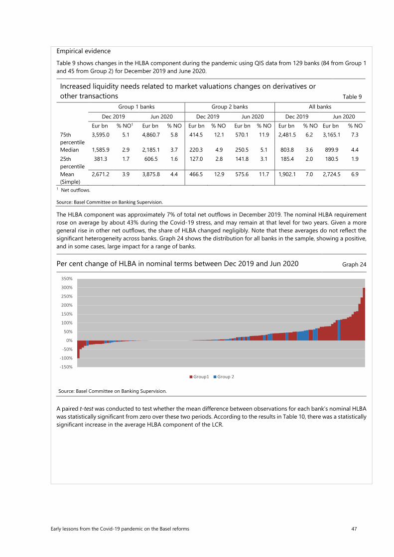
Early lessons from the Covid-19 pandemic on the Basel reforms 47
Empirical evidence
Table 9 shows changes in the HLBA component during the pandemic using QIS data from 129 banks (84 from Group 1 and 45 from Group 2) for December 2019 and June 2020.
Increased liquidity needs related to market valuations changes on derivatives or other transactions Table 9 Group 1 banks Group 2 banks All banks
Dec 2019 Jun 2020 Dec 2019 Jun 2020 Dec 2019 Jun 2020 Eur bn % NO1 Eur bn % NO Eur bn % NO Eur bn % NO Eur bn % NO Eur bn % NO 75th percentile
3,595.0 5.1 4,860.7 5.8 414.5 12.1 570.1 11.9 2,481.5 6.2 3,165.1 7.3
Median 1,585.9 2.9 2,185.1 3.7 220.3 4.9 250.5 5.1 803.8 3.6 899.9 4.4 25th percentile
381.3 1.7 606.5 1.6 127.0 2.8 141.8 3.1 185.4 2.0 180.5 1.9
Mean (Simple)
2,671.2 3.9 3,875.8 4.4 466.5 12.9 575.6 11.7 1,902.1 7.0 2,724.5 6.9
1 Net outflows.
Source: Basel Committee on Banking Supervision.
The HLBA component was approximately 7% of total net outflows in December 2019. The nominal HLBA requirement rose on average by about 43% during the Covid-19 stress, and may remain at that level for two years. Given a more general rise in other net outflows, the share of HLBA changed negligibly. Note that these averages do not reflect the significant heterogeneity across banks. Graph 24 shows the distribution for all banks in the sample, showing a positive, and in some cases, large impact for a range of banks.
Per cent change of HLBA in nominal terms between Dec 2019 and Jun 2020 Graph 24
Source: Basel Committee on Banking Supervision.
A paired t-test was conducted to test whether the mean difference between observations for each bank’s nominal HLBA was statistically significant from zero over these two periods. According to the results in Table 10, there was a statistically significant increase in the average HLBA component of the LCR.
-150%
-100%
-50%
0%
50%
100%
150%
200%
250%
300%
350%
Group1 Group 2
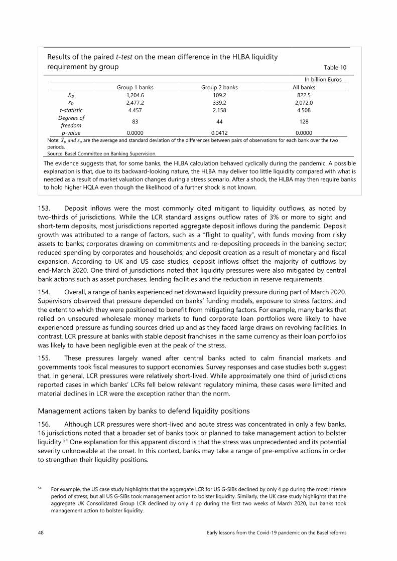
48 Early lessons from the Covid-19 pandemic on the Basel reforms
Results of the paired t-test on the mean difference in the HLBA liquidity requirement by group Table 10
In billion Euros Group 1 banks Group 2 banks All banks
𝑋𝑋�𝐷𝐷 1,204.6 109.2 822.5 𝐶𝐶𝐷𝐷 2,477.2 339.2 2,072.0
t-statistic 4.457 2.158 4.508 Degrees of freedom 83 44 128
p-value 0.0000 0.0412 0.0000 Note: 𝑋𝑋�𝐷𝐷 𝑙𝑙𝐶𝐶𝑝𝑝 𝐶𝐶𝐷𝐷 are the average and standard deviation of the differences between pairs of observations for each bank over the two periods. Source: Basel Committee on Banking Supervision.
The evidence suggests that, for some banks, the HLBA calculation behaved cyclically during the pandemic. A possible explanation is that, due to its backward-looking nature, the HLBA may deliver too little liquidity compared with what is needed as a result of market valuation changes during a stress scenario. After a shock, the HLBA may then require banks to hold higher HQLA even though the likelihood of a further shock is not known.
153. Deposit inflows were the most commonly cited mitigant to liquidity outflows, as noted by two-thirds of jurisdictions. While the LCR standard assigns outflow rates of 3% or more to sight and short-term deposits, most jurisdictions reported aggregate deposit inflows during the pandemic. Deposit growth was attributed to a range of factors, such as a “flight to quality”, with funds moving from risky assets to banks; corporates drawing on commitments and re-depositing proceeds in the banking sector; reduced spending by corporates and households; and deposit creation as a result of monetary and fiscal expansion. According to UK and US case studies, deposit inflows offset the majority of outflows by end-March 2020. One third of jurisdictions noted that liquidity pressures were also mitigated by central bank actions such as asset purchases, lending facilities and the reduction in reserve requirements.
154. Overall, a range of banks experienced net downward liquidity pressure during part of March 2020. Supervisors observed that pressure depended on banks’ funding models, exposure to stress factors, and the extent to which they were positioned to benefit from mitigating factors. For example, many banks that relied on unsecured wholesale money markets to fund corporate loan portfolios were likely to have experienced pressure as funding sources dried up and as they faced large draws on revolving facilities. In contrast, LCR pressure at banks with stable deposit franchises in the same currency as their loan portfolios was likely to have been negligible even at the peak of the stress.
155. These pressures largely waned after central banks acted to calm financial markets and governments took fiscal measures to support economies. Survey responses and case studies both suggest that, in general, LCR pressures were relatively short-lived. While approximately one third of jurisdictions reported cases in which banks’ LCRs fell below relevant regulatory minima, these cases were limited and material declines in LCR were the exception rather than the norm.
Management actions taken by banks to defend liquidity positions
156. Although LCR pressures were short-lived and acute stress was concentrated in only a few banks, 16 jurisdictions noted that a broader set of banks took or planned to take management action to bolster liquidity.54 One explanation for this apparent discord is that the stress was unprecedented and its potential severity unknowable at the onset. In this context, banks may take a range of pre-emptive actions in order to strengthen their liquidity positions.
54 For example, the US case study highlights that the aggregate LCR for US G-SIBs declined by only 4 pp during the most intense period of stress, but all US G-SIBs took management action to bolster liquidity. Similarly, the UK case study highlights that the aggregate UK Consolidated Group LCR declined by only 4 pp during the first two weeks of March 2020, but banks took management action to bolster liquidity.
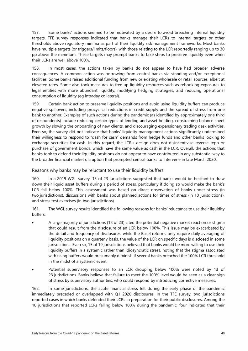
Early lessons from the Covid-19 pandemic on the Basel reforms 49
157. Some banks’ actions seemed to be motivated by a desire to avoid breaching internal liquidity targets. TFE survey responses indicated that banks manage their LCRs to internal targets or other thresholds above regulatory minima as part of their liquidity risk management frameworks. Most banks have multiple targets (or triggers/limits/floors), with those relating to the LCR reportedly ranging up to 30 pp above the minimum. These targets may prompt banks to take steps to preserve liquidity even when their LCRs are well above 100%.
158. In most cases, the actions taken by banks do not appear to have had broader adverse consequences. A common action was borrowing from central banks via standing and/or exceptional facilities. Some banks raised additional funding from new or existing wholesale or retail sources, albeit at elevated rates. Some also took measures to free up liquidity resources such as rebooking exposures to legal entities with more abundant liquidity, modifying hedging strategies, and reducing operational consumption of liquidity (eg intraday collateral).
159. Certain bank action to preserve liquidity positions and avoid using liquidity buffers can produce negative spillovers, including procyclical reductions in credit supply and the spread of stress from one bank to another. Examples of such actions during the pandemic (as identified by approximately one third of respondents) include reducing certain types of lending and asset holding, constraining balance sheet growth by slowing the onboarding of new clients, and discouraging expansionary trading desk activities. Even so, the survey did not indicate that banks’ liquidity management actions significantly undermined their willingness to respond to “dash for cash” demands from hedge funds and other banks looking to exchange securities for cash. In this regard, the LCR’s design does not disincentivise reverse repo or purchase of government bonds, which have the same value as cash in the LCR. Overall, the actions that banks took to defend their liquidity positions do not appear to have contributed in any substantial way to the broader financial market disruption that prompted central banks to intervene in late March 2020.
Reasons why banks may be reluctant to use their liquidity buffers
160. In a 2019 WGL survey, 13 of 23 jurisdictions suggested that banks would be hesitant to draw down their liquid asset buffers during a period of stress, particularly if doing so would make the bank’s LCR fall below 100%. This assessment was based on direct observation of banks under stress (in two jurisdictions), discussions with banks about planned actions for times of stress (in 10 jurisdictions), and stress test exercises (in two jurisdictions).
161. The WGL survey results identified the following reasons for banks’ reluctance to use their liquidity buffers:
• A large majority of jurisdictions (18 of 23) cited the potential negative market reaction or stigma that could result from the disclosure of an LCR below 100%. This issue may be exacerbated by the detail and frequency of disclosures: while the Basel reforms only require daily averaging of liquidity positions on a quarterly basis, the value of the LCR on specific days is disclosed in some jurisdictions. Even so, 15 of 19 jurisdictions believed that banks would be more willing to use their liquidity buffers in a systemic rather than idiosyncratic stress, noting that the stigma associated with using buffers would presumably diminish if several banks breached the 100% LCR threshold in the midst of a systemic event.
• Potential supervisory responses to an LCR dropping below 100% were noted by 13 of 23 jurisdictions. Banks believe that failure to meet the 100% level would be seen as a clear sign of stress by supervisory authorities, who could respond by introducing corrective measures.
162. In some jurisdictions, the acute financial stress felt during the early phase of the pandemic immediately preceded or overlapped with Q1 2020 disclosures. In the TFE survey, two jurisdictions reported cases in which banks defended their LCRs in preparation for their public disclosures. Among the 10 jurisdictions that reported LCRs falling below 100% during the pandemic, four indicated that their
50 Early lessons from the Covid-19 pandemic on the Basel reforms
disclosure rules (which only require daily averaging in compliance with the Basel standard55) helped banks avoid any adverse market reaction. Respondents in two of the 10 jurisdictions believed that there was no adverse market reaction to LCRs falling below 100% due to supervisory authorities’ public statements reiterating the usability of liquidity buffers.
163. Overall, 10 of 27 jurisdictions indicated that they believed banks would be reluctant to allow their LCR to fall (including below 100%) in response to even stronger pressures than those exerted during the pandemic, citing similar reasons noted earlier: potential negative market reaction, uncertain supervisory responses, and a desire to maintain reserves in the event of further intensification of stress.
Supervisory actions during the pandemic
164. Supervisory authorities responded to actual and anticipated liquidity pressures with a wide range of actions. These may also provide useful lessons.
165. Several jurisdictions, including India, Indonesia, Korea, Mexico, South Africa, Turkey and the UAE temporarily reduced or amended their LCR standard. These actions were motivated by a concern that banks’ liquidity positions might come under pressure and that banks would take action to prevent their LCR from declining. This could have undesirable knock-on effects, such as liquidity hoarding and reduced lending. During the pandemic, liquidity pressures did not materialise to the extent that many originally feared they would, although some jurisdictions noted that these actions, including the reduction of internal liquidity targets, may still have helped support lending.
166. Mexico temporarily adjusted its LCR standard to allow banks to exclude market movements observed in March 2020 from the calculation of the HLBA and from calculations of price volatility to determine assets’ eligibility as HQLA. Banks were also allowed to compute their LCR using a constrained averaging approach in order to reduce the effect of spot observations. These measures were designed to reduce the pressure to comply with the LCR, to incentivise banks to make use of their buffers in order to support lending, and to avoid excessive LCR cyclicality.
167. A number of jurisdictions, including Canada, the euro area, Germany, Italy, Japan, Malaysia, the Netherlands, Sweden, the United Kingdom and the United States, issued public communications to reiterate the flexibility built into the standard and to clarify the role of buffers in the context of the pandemic. The Committee’s press release in March 202056 noted that “the Basel III framework includes capital and liquidity buffers that are designed to be used in periods of stress”. These statements helped alleviate uncertainty regarding the supervisory response to a bank’s LCR falling below 100%. Respondents from 12 jurisdictions observed banks lowering internal targets and/or approving temporary exemptions to internal targets following these public announcements. However, the survey responses suggest that a majority of banks left limits and targets unchanged.
168. To summarise, it is difficult to draw clear conclusions about the functioning of the LCR given the relatively short period of liquidity stress, which quickly abated following decisive action taken by authorities. While it is evident that banks typically target LCR ratios well above 100% and took steps to avoid falling below this level, there is no evidence that such actions had widespread adverse effects or that they were inconsistent with prudent liquidity management under conditions of high uncertainty.
169. Nevertheless, the episode does raise questions regarding how banks might behave in a more severe liquidity stress scenario and whether bank actions could be destabilising from a macroprudential perspective. Policy actions taken by some authorities during the pandemic suggest there may be value in considering the impact of disclosure practices, supervisory messaging on buffer usability and the role of buffer release during a systemic stress. Finally, notwithstanding the unique nature of the Covid-19 stress, experience suggests that certain aspects of the LCR’s design were quite cyclical (ie the treatment of margin
55 See DIS85 of the Basel Framework. 56 See www.bis.org/press/p200320.htm.

Early lessons from the Covid-19 pandemic on the Basel reforms 51
outflows under the HLBA) or that certain outflows may have been inadequately captured (ie certain debt buybacks from MMFs).
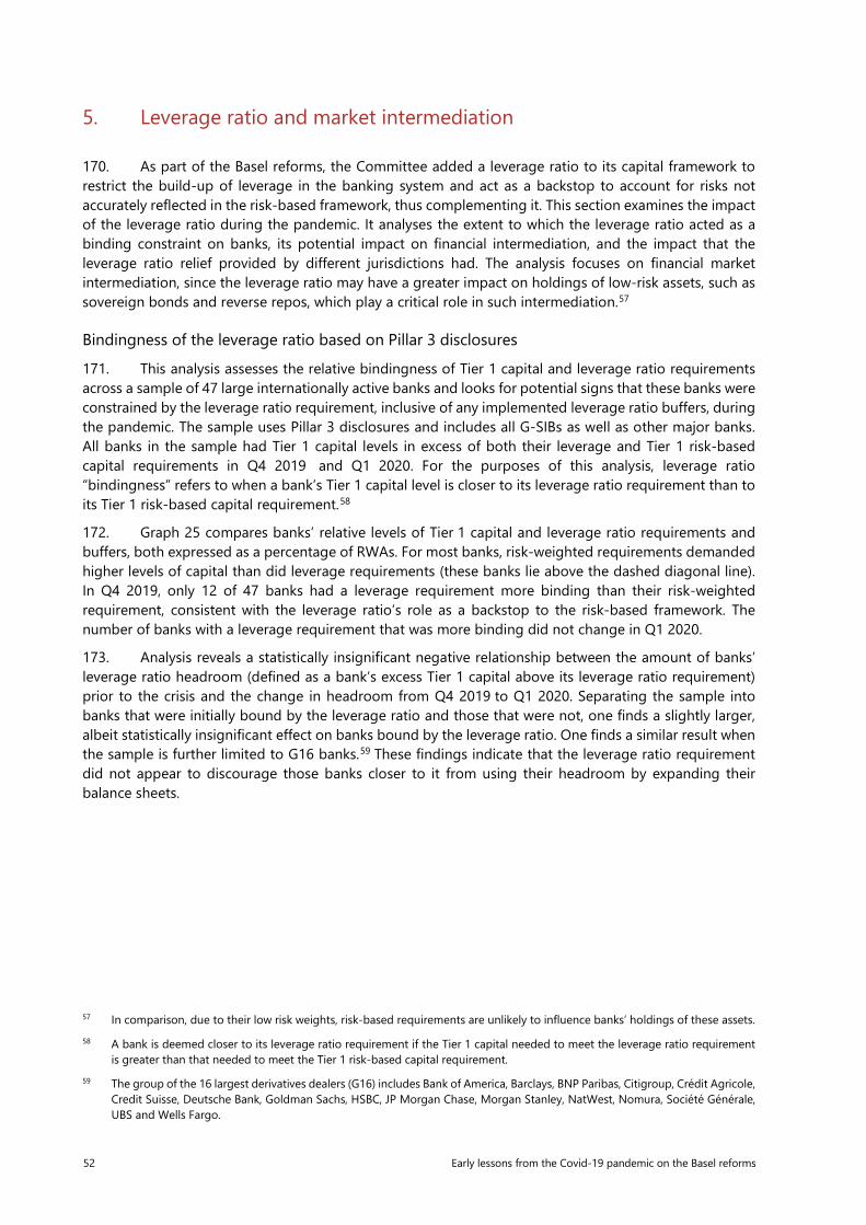
52 Early lessons from the Covid-19 pandemic on the Basel reforms
5. Leverage ratio and market intermediation
170. As part of the Basel reforms, the Committee added a leverage ratio to its capital framework to restrict the build-up of leverage in the banking system and act as a backstop to account for risks not accurately reflected in the risk-based framework, thus complementing it. This section examines the impact of the leverage ratio during the pandemic. It analyses the extent to which the leverage ratio acted as a binding constraint on banks, its potential impact on financial intermediation, and the impact that the leverage ratio relief provided by different jurisdictions had. The analysis focuses on financial market intermediation, since the leverage ratio may have a greater impact on holdings of low-risk assets, such as sovereign bonds and reverse repos, which play a critical role in such intermediation.57
Bindingness of the leverage ratio based on Pillar 3 disclosures
171. This analysis assesses the relative bindingness of Tier 1 capital and leverage ratio requirements across a sample of 47 large internationally active banks and looks for potential signs that these banks were constrained by the leverage ratio requirement, inclusive of any implemented leverage ratio buffers, during the pandemic. The sample uses Pillar 3 disclosures and includes all G-SIBs as well as other major banks. All banks in the sample had Tier 1 capital levels in excess of both their leverage and Tier 1 risk-based capital requirements in Q4 2019 and Q1 2020. For the purposes of this analysis, leverage ratio “bindingness” refers to when a bank’s Tier 1 capital level is closer to its leverage ratio requirement than to its Tier 1 risk-based capital requirement.58
172. Graph 25 compares banks’ relative levels of Tier 1 capital and leverage ratio requirements and buffers, both expressed as a percentage of RWAs. For most banks, risk-weighted requirements demanded higher levels of capital than did leverage requirements (these banks lie above the dashed diagonal line). In Q4 2019, only 12 of 47 banks had a leverage requirement more binding than their risk-weighted requirement, consistent with the leverage ratio’s role as a backstop to the risk-based framework. The number of banks with a leverage requirement that was more binding did not change in Q1 2020.
173. Analysis reveals a statistically insignificant negative relationship between the amount of banks’ leverage ratio headroom (defined as a bank’s excess Tier 1 capital above its leverage ratio requirement) prior to the crisis and the change in headroom from Q4 2019 to Q1 2020. Separating the sample into banks that were initially bound by the leverage ratio and those that were not, one finds a slightly larger, albeit statistically insignificant effect on banks bound by the leverage ratio. One finds a similar result when the sample is further limited to G16 banks.59 These findings indicate that the leverage ratio requirement did not appear to discourage those banks closer to it from using their headroom by expanding their balance sheets.
57 In comparison, due to their low risk weights, risk-based requirements are unlikely to influence banks’ holdings of these assets. 58 A bank is deemed closer to its leverage ratio requirement if the Tier 1 capital needed to meet the leverage ratio requirement
is greater than that needed to meet the Tier 1 risk-based capital requirement. 59 The group of the 16 largest derivatives dealers (G16) includes Bank of America, Barclays, BNP Paribas, Citigroup, Crédit Agricole,
Credit Suisse, Deutsche Bank, Goldman Sachs, HSBC, JP Morgan Chase, Morgan Stanley, NatWest, Nomura, Société Générale, UBS and Wells Fargo.
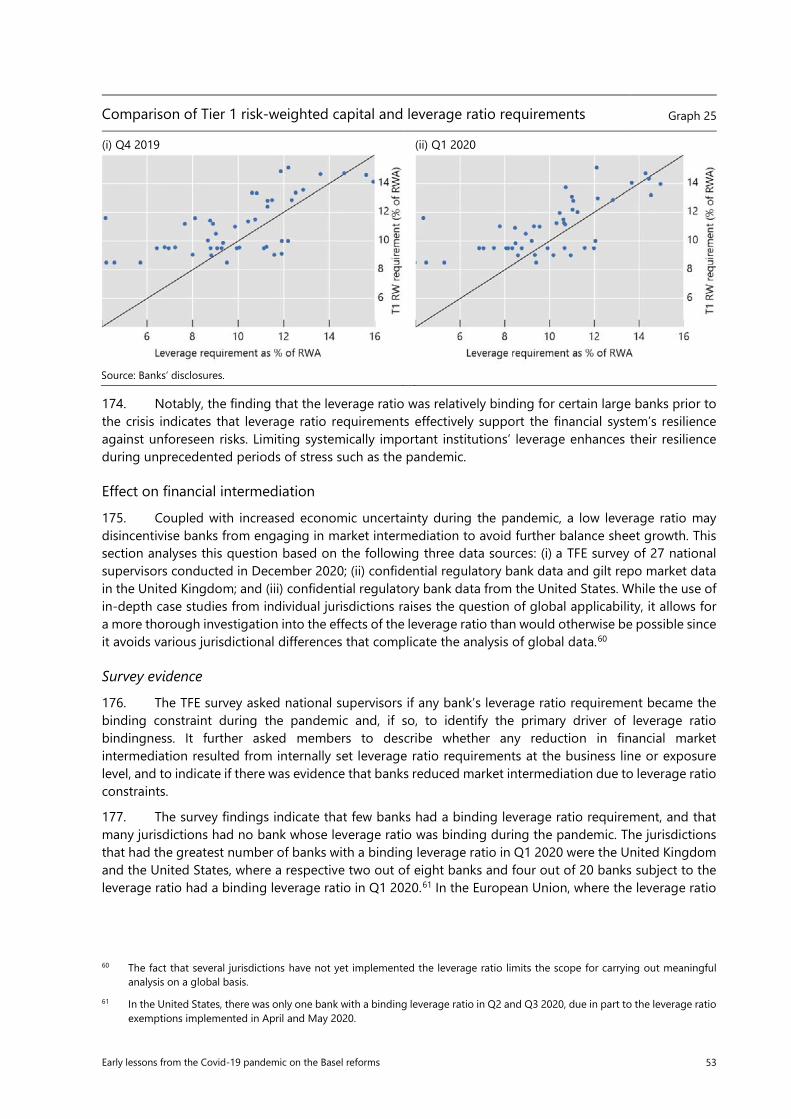
Early lessons from the Covid-19 pandemic on the Basel reforms 53
Comparison of Tier 1 risk-weighted capital and leverage ratio requirements Graph 25
(i) Q4 2019 (ii) Q1 2020
Source: Banks’ disclosures.
174. Notably, the finding that the leverage ratio was relatively binding for certain large banks prior to the crisis indicates that leverage ratio requirements effectively support the financial system’s resilience against unforeseen risks. Limiting systemically important institutions’ leverage enhances their resilience during unprecedented periods of stress such as the pandemic.
Effect on financial intermediation
175. Coupled with increased economic uncertainty during the pandemic, a low leverage ratio may disincentivise banks from engaging in market intermediation to avoid further balance sheet growth. This section analyses this question based on the following three data sources: (i) a TFE survey of 27 national supervisors conducted in December 2020; (ii) confidential regulatory bank data and gilt repo market data in the United Kingdom; and (iii) confidential regulatory bank data from the United States. While the use of in-depth case studies from individual jurisdictions raises the question of global applicability, it allows for a more thorough investigation into the effects of the leverage ratio than would otherwise be possible since it avoids various jurisdictional differences that complicate the analysis of global data.60
Survey evidence
176. The TFE survey asked national supervisors if any bank’s leverage ratio requirement became the binding constraint during the pandemic and, if so, to identify the primary driver of leverage ratio bindingness. It further asked members to describe whether any reduction in financial market intermediation resulted from internally set leverage ratio requirements at the business line or exposure level, and to indicate if there was evidence that banks reduced market intermediation due to leverage ratio constraints.
177. The survey findings indicate that few banks had a binding leverage ratio requirement, and that many jurisdictions had no bank whose leverage ratio was binding during the pandemic. The jurisdictions that had the greatest number of banks with a binding leverage ratio in Q1 2020 were the United Kingdom and the United States, where a respective two out of eight banks and four out of 20 banks subject to the leverage ratio had a binding leverage ratio in Q1 2020.61 In the European Union, where the leverage ratio
60 The fact that several jurisdictions have not yet implemented the leverage ratio limits the scope for carrying out meaningful analysis on a global basis.
61 In the United States, there was only one bank with a binding leverage ratio in Q2 and Q3 2020, due in part to the leverage ratio exemptions implemented in April and May 2020.
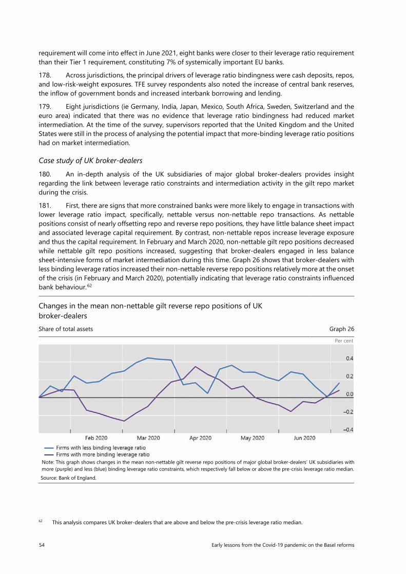
54 Early lessons from the Covid-19 pandemic on the Basel reforms
requirement will come into effect in June 2021, eight banks were closer to their leverage ratio requirement than their Tier 1 requirement, constituting 7% of systemically important EU banks.
178. Across jurisdictions, the principal drivers of leverage ratio bindingness were cash deposits, repos, and low-risk-weight exposures. TFE survey respondents also noted the increase of central bank reserves, the inflow of government bonds and increased interbank borrowing and lending.
179. Eight jurisdictions (ie Germany, India, Japan, Mexico, South Africa, Sweden, Switzerland and the euro area) indicated that there was no evidence that leverage ratio bindingness had reduced market intermediation. At the time of the survey, supervisors reported that the United Kingdom and the United States were still in the process of analysing the potential impact that more-binding leverage ratio positions had on market intermediation.
Case study of UK broker-dealers
180. An in-depth analysis of the UK subsidiaries of major global broker-dealers provides insight regarding the link between leverage ratio constraints and intermediation activity in the gilt repo market during the crisis.
181. First, there are signs that more constrained banks were more likely to engage in transactions with lower leverage ratio impact, specifically, nettable versus non-nettable repo transactions. As nettable positions consist of nearly offsetting repo and reverse repo positions, they have little balance sheet impact and associated leverage capital requirement. By contrast, non-nettable repos increase leverage exposure and thus the capital requirement. In February and March 2020, non-nettable gilt repo positions decreased while nettable gilt repo positions increased, suggesting that broker-dealers engaged in less balance sheet-intensive forms of market intermediation during this time. Graph 26 shows that broker-dealers with less binding leverage ratios increased their non-nettable reverse repo positions relatively more at the onset of the crisis (in February and March 2020), potentially indicating that leverage ratio constraints influenced bank behaviour.62
Changes in the mean non-nettable gilt reverse repo positions of UK broker-dealers Share of total assets Graph 26
Per cent
Note: This graph shows changes in the mean non-nettable gilt reverse repo positions of major global broker-dealers’ UK subsidiaries with more (purple) and less (blue) binding leverage ratio constraints, which respectively fall below or above the pre-crisis leverage ratio median. Source: Bank of England.
62 This analysis compares UK broker-dealers that are above and below the pre-crisis leverage ratio median.
Early lessons from the Covid-19 pandemic on the Basel reforms 55
182. Second, analysis using regulatory data for the UK gilt repo market, which contains transaction-level information on repo prices (spreads), volumes and other trade characteristics, suggests that leverage ratio constraints may have affected gilt repo pricing.
183. The analysis examines broker-dealer activity in term gilt reverse repos with a maturity greater than three months from 20 January 2020 to 18 March 2020.63 It labels trading days in January and February 2020 as “normal times” and uses the remaining trading days to gauge activity during the pandemic. The data set used in the analysis cover approximately half of the term repo market. Notably, following significant growth in February 2020, in early March reverse repo spreads began to rise rapidly and the expansion of broker-dealer repo positions slowed down.
184. As shown in the left-hand column of Table 11, regression analysis indicates that broker-dealers charged a small balance sheet premium of approximately 1 bp on the more leverage ratio-intensive non-nettable term repo transactions in the period prior to the pandemic. This premium increased to approximately 6 bp between 1 March and 8 March, and to approximately 8 bp between 9 March and 18 March. This substantial increase represents 40–55% of the mean spread (14 bp) for these transactions in normal times.
Regression results on the price effect of reverse repo position nettability and the volume effect of broker-dealer leverage constraints on the UK gilt repo market in March 20201 Table 11
Spread on non-nettable vs. nettable term gilt reverse repo trades
(“balance sheet premium”) (bp)
Daily volume of term reverse repo trades of more vs. less
leverage-constrained broker-dealers (per cent of dealer assets)
Treatment dummy2 1.0095* (0.5212)
Treatment dummy3 0.0763***
(0.0147)
Treatment effect4 5.6378*** (1.0232)
Treatment effect4 –0.0402***
(0.015)
Maturity bucket 7.1274*** (0.3455)
Trade size –0.0094***
(0.0021)
R-squared 0.752 0.388
N 2,908 430
Dealer fixed effect YES YES (dealer country)
Time fixed effect YES YES
Other fixed effects and control variables
Counterparty sector and collateral type fixed effects.
Level of pre-stress central bank reserves relative to assets, leverage ratio exposure measure.
1 Standard errors are reported in brackets. The symbols *, **, and *** denote statistical significance at 10%, 5% and 1%, respectively. 2 The treatment dummy is one for non-nettable trades and zero for nettable trades. 3 The treatment dummy is one for more-leverage-constrained banks, which are defined as those having leverage ratios below median at the end of Q4 2019, and zero otherwise. 4 The treatment effect is the product of the treatment dummy and the treatment period dummy. The treatment period dummy is zero before the treatment date (1 March) and one afterwards. Source: Bank of England.
185. The right-hand column of Table 11 shows that leverage-constrained broker-dealers had approximately 8 bp higher term repo volume, as a fraction of total assets prior to the crisis, likely reflecting
63 Data after 18 March 2020 are excluded in order to filter out the effect of large-scale central bank interventions in the gilt and gilt repo markets, which took place after 19 March 2020.
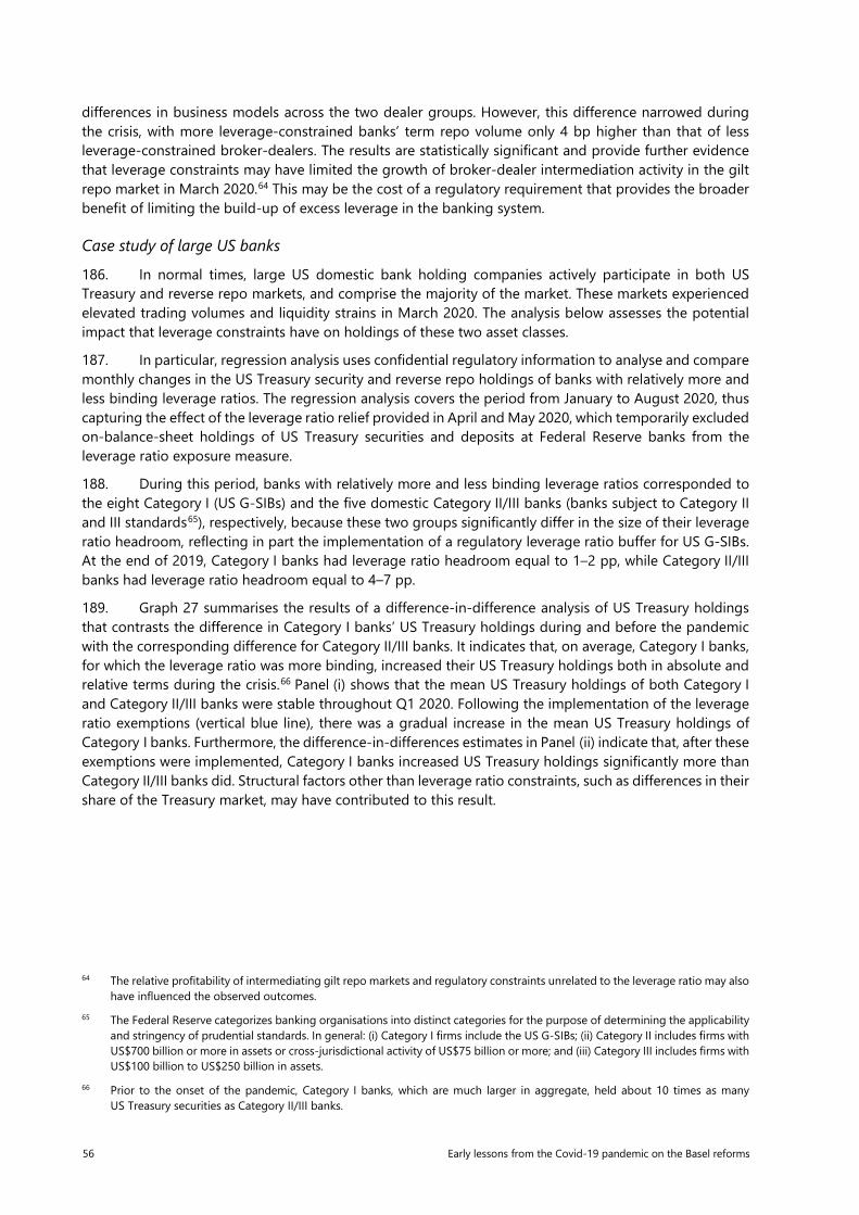
56 Early lessons from the Covid-19 pandemic on the Basel reforms
differences in business models across the two dealer groups. However, this difference narrowed during the crisis, with more leverage-constrained banks’ term repo volume only 4 bp higher than that of less leverage-constrained broker-dealers. The results are statistically significant and provide further evidence that leverage constraints may have limited the growth of broker-dealer intermediation activity in the gilt repo market in March 2020.64 This may be the cost of a regulatory requirement that provides the broader benefit of limiting the build-up of excess leverage in the banking system.
Case study of large US banks
186. In normal times, large US domestic bank holding companies actively participate in both US Treasury and reverse repo markets, and comprise the majority of the market. These markets experienced elevated trading volumes and liquidity strains in March 2020. The analysis below assesses the potential impact that leverage constraints have on holdings of these two asset classes.
187. In particular, regression analysis uses confidential regulatory information to analyse and compare monthly changes in the US Treasury security and reverse repo holdings of banks with relatively more and less binding leverage ratios. The regression analysis covers the period from January to August 2020, thus capturing the effect of the leverage ratio relief provided in April and May 2020, which temporarily excluded on-balance-sheet holdings of US Treasury securities and deposits at Federal Reserve banks from the leverage ratio exposure measure.
188. During this period, banks with relatively more and less binding leverage ratios corresponded to the eight Category I (US G-SIBs) and the five domestic Category II/III banks (banks subject to Category II and III standards65), respectively, because these two groups significantly differ in the size of their leverage ratio headroom, reflecting in part the implementation of a regulatory leverage ratio buffer for US G-SIBs. At the end of 2019, Category I banks had leverage ratio headroom equal to 1–2 pp, while Category II/III banks had leverage ratio headroom equal to 4–7 pp.
189. Graph 27 summarises the results of a difference-in-difference analysis of US Treasury holdings that contrasts the difference in Category I banks’ US Treasury holdings during and before the pandemic with the corresponding difference for Category II/III banks. It indicates that, on average, Category I banks, for which the leverage ratio was more binding, increased their US Treasury holdings both in absolute and relative terms during the crisis.66 Panel (i) shows that the mean US Treasury holdings of both Category I and Category II/III banks were stable throughout Q1 2020. Following the implementation of the leverage ratio exemptions (vertical blue line), there was a gradual increase in the mean US Treasury holdings of Category I banks. Furthermore, the difference-in-differences estimates in Panel (ii) indicate that, after these exemptions were implemented, Category I banks increased US Treasury holdings significantly more than Category II/III banks did. Structural factors other than leverage ratio constraints, such as differences in their share of the Treasury market, may have contributed to this result.
64 The relative profitability of intermediating gilt repo markets and regulatory constraints unrelated to the leverage ratio may also have influenced the observed outcomes.
65 The Federal Reserve categorizes banking organisations into distinct categories for the purpose of determining the applicability and stringency of prudential standards. In general: (i) Category I firms include the US G-SIBs; (ii) Category II includes firms with US$700 billion or more in assets or cross-jurisdictional activity of US$75 billion or more; and (iii) Category III includes firms with US$100 billion to US$250 billion in assets.
66 Prior to the onset of the pandemic, Category I banks, which are much larger in aggregate, held about 10 times as many US Treasury securities as Category II/III banks.
Early lessons from the Covid-19 pandemic on the Basel reforms 57
Mean changes in US Treasury holdings of large US bank holding companies Graph 27
(i) Mean levels of US Treasury holdings (% of bank assets at the end of 2019)
(ii) Mean diff-in-diff of US Treasury holdings (pp relative to end of 2019)
Panel (i) shows the mean US Treasury holdings of Category I and Category II/III firms, expressed as a percentage of their total assets at the end of 2019. Panel (ii) shows point estimates and 90% confidence intervals for the mean difference in US Treasury holding changes between the two groups of firms, relative to the end 2019. The vertical blue and green lines mark the leverage ratio reliefs that temporarily exempted central bank reserves and US Treasury securities from the total leverage exposure of US bank holding companies (relief announced on 1 April 2020) and US depository institutions (relief announced on 15 May 2020), respectively. Source: Board of Governors of the Federal Reserve System
190. Notably, the analysis reveals no evidence of an increase in Treasury holdings during the peak of the financial market stress in March 2020, despite considerable selling pressure in the market prior to the Federal Reserve’s large-scale asset purchases. This may suggest that banks were unwilling to absorb the excess market supply of Treasuries in March 2020, potentially reflecting concern regarding economic uncertainty, internal risk limits or regulatory requirements.
191. There is no clear pattern in the mean change of reverse repo positions of banks with more and less binding leverage ratios, indicating that differences in the bindingness of the leverage ratio had no discernible effects on the intermediation of reverse repos.
Effects of leverage ratio exemptions during the pandemic
192. National supervisors implemented various leverage ratio exemptions in order to alleviate potential balance sheet constraints faced by financial institutions as they struggled to satisfy an unprecedented demand for liquidity during the “dash for cash”. During this period, banks sought to accommodate client needs – eg asset sales, fund redemptions, secured financing transactions and credit line drawdowns – while ensuring compliance with both internal risk management policies and regulatory capital and liquidity requirements.
193. As banks absorbed some of the asset sales and financing pressure, there was concern that the rapid expansion of their balance sheets would exhaust their leverage ratio headroom. Table 12 shows that the total leverage exposure of large banks increased globally by 2.9% in Q1 2020. Swiss, UK, and US banks experienced a substantial growth in on-balance-sheet exposures. Japanese and UK banks saw a 1.2% and 5.1% increase, respectively, in their secured financing transaction (SFT) exposures. Furthermore, it is estimated that broker-dealers in the Japanese, UK, and US government bond markets provided additional liquidity equivalent to 1.2%–3.8% of the underlying market size through inventory build-up and reverse repo transactions.
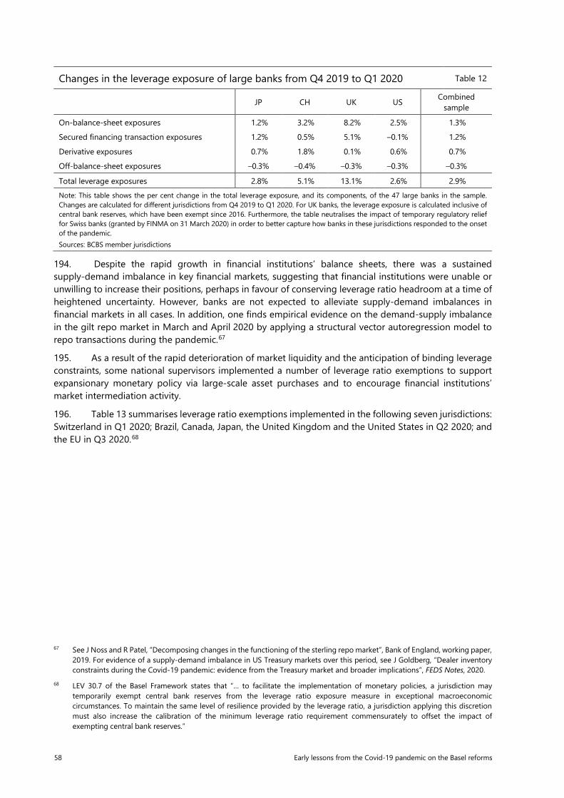
58 Early lessons from the Covid-19 pandemic on the Basel reforms
Changes in the leverage exposure of large banks from Q4 2019 to Q1 2020 Table 12
JP CH UK US Combined sample
On-balance-sheet exposures 1.2% 3.2% 8.2% 2.5% 1.3%
Secured financing transaction exposures 1.2% 0.5% 5.1% –0.1% 1.2%
Derivative exposures 0.7% 1.8% 0.1% 0.6% 0.7%
Off-balance-sheet exposures –0.3% –0.4% –0.3% –0.3% –0.3%
Total leverage exposures 2.8% 5.1% 13.1% 2.6% 2.9% Note: This table shows the per cent change in the total leverage exposure, and its components, of the 47 large banks in the sample. Changes are calculated for different jurisdictions from Q4 2019 to Q1 2020. For UK banks, the leverage exposure is calculated inclusive of central bank reserves, which have been exempt since 2016. Furthermore, the table neutralises the impact of temporary regulatory relief for Swiss banks (granted by FINMA on 31 March 2020) in order to better capture how banks in these jurisdictions responded to the onset of the pandemic. Sources: BCBS member jurisdictions
194. Despite the rapid growth in financial institutions’ balance sheets, there was a sustained supply-demand imbalance in key financial markets, suggesting that financial institutions were unable or unwilling to increase their positions, perhaps in favour of conserving leverage ratio headroom at a time of heightened uncertainty. However, banks are not expected to alleviate supply-demand imbalances in financial markets in all cases. In addition, one finds empirical evidence on the demand-supply imbalance in the gilt repo market in March and April 2020 by applying a structural vector autoregression model to repo transactions during the pandemic.67
195. As a result of the rapid deterioration of market liquidity and the anticipation of binding leverage constraints, some national supervisors implemented a number of leverage ratio exemptions to support expansionary monetary policy via large-scale asset purchases and to encourage financial institutions’ market intermediation activity.
196. Table 13 summarises leverage ratio exemptions implemented in the following seven jurisdictions: Switzerland in Q1 2020; Brazil, Canada, Japan, the United Kingdom and the United States in Q2 2020; and the EU in Q3 2020.68
67 See J Noss and R Patel, “Decomposing changes in the functioning of the sterling repo market”, Bank of England, working paper, 2019. For evidence of a supply-demand imbalance in US Treasury markets over this period, see J Goldberg, “Dealer inventory constraints during the Covid-19 pandemic: evidence from the Treasury market and broader implications”, FEDS Notes, 2020.
68 LEV 30.7 of the Basel Framework states that “… to facilitate the implementation of monetary policies, a jurisdiction may temporarily exempt central bank reserves from the leverage ratio exposure measure in exceptional macroeconomic circumstances. To maintain the same level of resilience provided by the leverage ratio, a jurisdiction applying this discretion must also increase the calibration of the minimum leverage ratio requirement commensurately to offset the impact of exempting central bank reserves.”
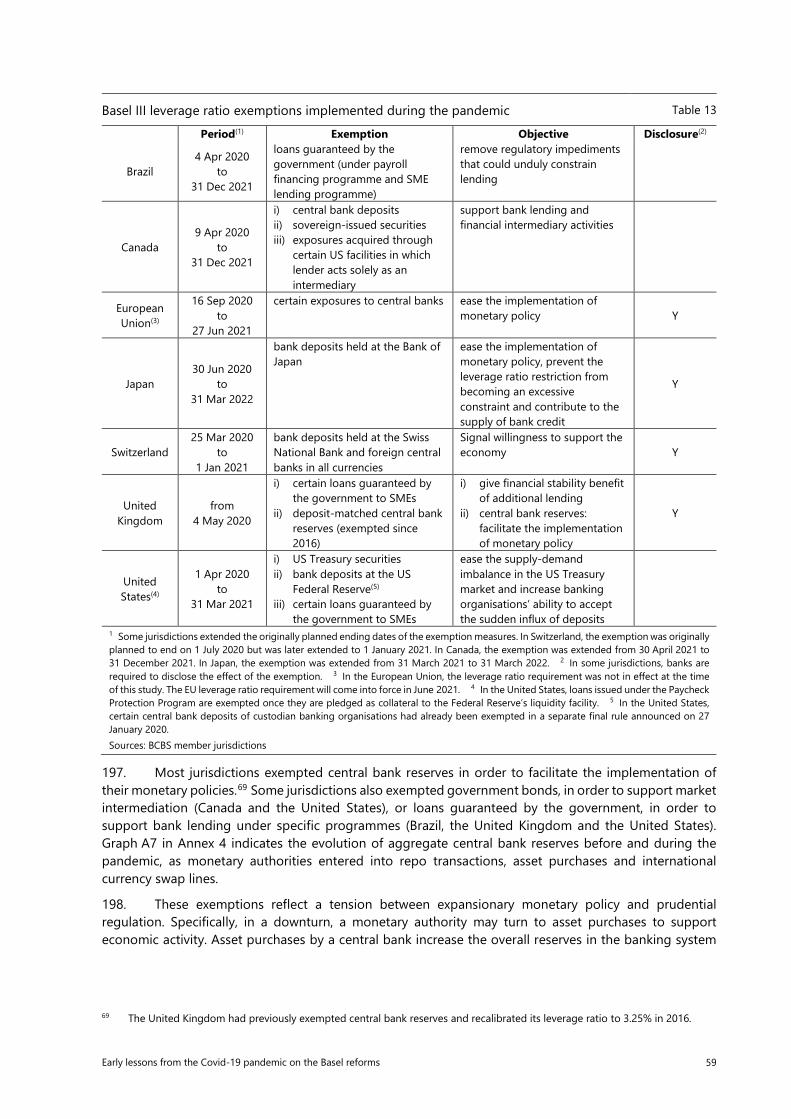
Early lessons from the Covid-19 pandemic on the Basel reforms 59
Basel III leverage ratio exemptions implemented during the pandemic Table 13
Period(1) Exemption Objective Disclosure(2)
Brazil 4 Apr 2020
to 31 Dec 2021
loans guaranteed by the government (under payroll financing programme and SME lending programme)
remove regulatory impediments that could unduly constrain lending
Canada 9 Apr 2020
to 31 Dec 2021
i) central bank deposits ii) sovereign-issued securities iii) exposures acquired through
certain US facilities in which lender acts solely as an intermediary
support bank lending and financial intermediary activities
European Union(3)
16 Sep 2020 to
27 Jun 2021
certain exposures to central banks ease the implementation of monetary policy Y
Japan 30 Jun 2020
to 31 Mar 2022
bank deposits held at the Bank of Japan
ease the implementation of monetary policy, prevent the leverage ratio restriction from becoming an excessive constraint and contribute to the supply of bank credit
Y
Switzerland 25 Mar 2020
to 1 Jan 2021
bank deposits held at the Swiss National Bank and foreign central banks in all currencies
Signal willingness to support the economy Y
United Kingdom
from 4 May 2020
i) certain loans guaranteed by the government to SMEs
ii) deposit-matched central bank reserves (exempted since 2016)
i) give financial stability benefit of additional lending
ii) central bank reserves: facilitate the implementation of monetary policy
Y
United States(4)
1 Apr 2020 to
31 Mar 2021
i) US Treasury securities ii) bank deposits at the US
Federal Reserve(5) iii) certain loans guaranteed by
the government to SMEs
ease the supply-demand imbalance in the US Treasury market and increase banking organisations’ ability to accept the sudden influx of deposits
1 Some jurisdictions extended the originally planned ending dates of the exemption measures. In Switzerland, the exemption was originally planned to end on 1 July 2020 but was later extended to 1 January 2021. In Canada, the exemption was extended from 30 April 2021 to 31 December 2021. In Japan, the exemption was extended from 31 March 2021 to 31 March 2022. 2 In some jurisdictions, banks are required to disclose the effect of the exemption. 3 In the European Union, the leverage ratio requirement was not in effect at the time of this study. The EU leverage ratio requirement will come into force in June 2021. 4 In the United States, loans issued under the Paycheck Protection Program are exempted once they are pledged as collateral to the Federal Reserve’s liquidity facility. 5 In the United States, certain central bank deposits of custodian banking organisations had already been exempted in a separate final rule announced on 27 January 2020. Sources: BCBS member jurisdictions
197. Most jurisdictions exempted central bank reserves in order to facilitate the implementation of their monetary policies.69 Some jurisdictions also exempted government bonds, in order to support market intermediation (Canada and the United States), or loans guaranteed by the government, in order to support bank lending under specific programmes (Brazil, the United Kingdom and the United States). Graph A7 in Annex 4 indicates the evolution of aggregate central bank reserves before and during the pandemic, as monetary authorities entered into repo transactions, asset purchases and international currency swap lines.
198. These exemptions reflect a tension between expansionary monetary policy and prudential regulation. Specifically, in a downturn, a monetary authority may turn to asset purchases to support economic activity. Asset purchases by a central bank increase the overall reserves in the banking system
69 The United Kingdom had previously exempted central bank reserves and recalibrated its leverage ratio to 3.25% in 2016.
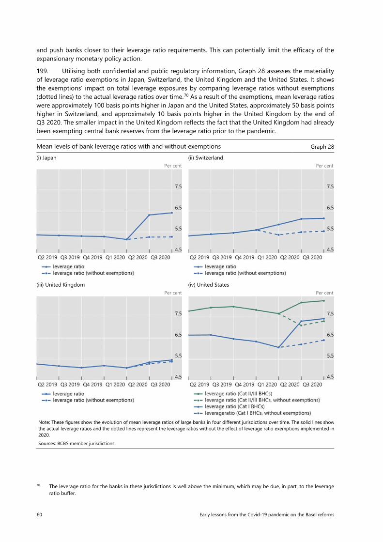
60 Early lessons from the Covid-19 pandemic on the Basel reforms
and push banks closer to their leverage ratio requirements. This can potentially limit the efficacy of the expansionary monetary policy action.
199. Utilising both confidential and public regulatory information, Graph 28 assesses the materiality of leverage ratio exemptions in Japan, Switzerland, the United Kingdom and the United States. It shows the exemptions’ impact on total leverage exposures by comparing leverage ratios without exemptions (dotted lines) to the actual leverage ratios over time.70 As a result of the exemptions, mean leverage ratios were approximately 100 basis points higher in Japan and the United States, approximately 50 basis points higher in Switzerland, and approximately 10 basis points higher in the United Kingdom by the end of Q3 2020. The smaller impact in the United Kingdom reflects the fact that the United Kingdom had already been exempting central bank reserves from the leverage ratio prior to the pandemic.
Mean levels of bank leverage ratios with and without exemptions Graph 28
(i) Japan (ii) Switzerland Per cent Per cent
(iii) United Kingdom (iv) United States
Per cent Per cent
70 The leverage ratio for the banks in these jurisdictions is well above the minimum, which may be due, in part, to the leverage ratio buffer.
Note: These figures show the evolution of mean leverage ratios of large banks in four different jurisdictions over time. The solid lines show the actual leverage ratios and the dotted lines represent the leverage ratios without the effect of leverage ratio exemptions implemented in 2020. Sources: BCBS member jurisdictions
Early lessons from the Covid-19 pandemic on the Basel reforms 61
200. When interpreting the effect these exemptions had, the differences across jurisdictions are worth noting. Some jurisdictions also have a leverage buffer on top of the 3% minimum, which helps explain the high leverage ratios observed. Furthermore, in some jurisdictions, banks are required to disclose the impact that exemptions have had along with the ongoing leverage ratio without exemptions. The combination of such disclosure requirements and the leverage ratio exemptions may incentivise banks to maintain the same leverage ratio level without exemptions in order to signal their resilience.
201. On 30 June 2020, the Financial Service Agency of Japan announced a temporary exemption of central bank reserves from leverage ratio exposures with disclosure requirements. The ratio of central bank reserves to total assets for G-SIBs in that country increased from 24.1% at end-2019 to 25.9% by end-2020. The exemption aimed to prevent the leverage ratio restriction from becoming a constraint and to promote the supply of bank credit to the economy. The measure was originally planned to terminate in March 2021 but was later extended until March 2022.
202. Switzerland allowed for central bank deposits in all currencies to be temporarily excluded from the leverage ratio. To date, no evidence has emerged that the introduction or expiration of the leverage ratio exemption had any effect on financial market intermediation in Switzerland.
203. The United Kingdom had maintained an exemption for deposit-matched central bank reserves and a recalibrated leverage ratio minimum of 3.25% since 2016. In response to the pandemic, the Prudential Regulation Authority allowed banks to exclude loans provided under the UK government’s Bounce Back Loan Scheme full guarantee from the leverage ratio exposure measure. The exemption of these loans was designed to support the UK government’s lending programme.
204. In response to the pandemic, US banking agencies exempted US Treasury securities and Federal Reserve deposits from the leverage ratio of bank holding companies and depository institutions. The goal of this relief was to promote the smooth functioning of financial markets and to support the flow of credit to businesses and households. As discussed above, empirical analysis suggests that the exemptions may have had a meaningful positive effect on US G-SIBs’ US Treasury holdings.
205. In summary, while the leverage ratio helps enhance overall bank resilience, an in-depth analysis of data from two jurisdictions indicates that leverage ratio constraints may have affected banks’ responses to the extraordinary demand for liquidity that arose early in the pandemic. Temporary leverage ratio exemptions implemented by several jurisdictions supported expansionary monetary policy and eased constraints on banks’ intermediation activity.
62 Early lessons from the Covid-19 pandemic on the Basel reforms
6. The cyclicality of bank regulatory requirements during the pandemic
206. This section examines the cyclicality of the Basel framework’s (i) capital impact of credit loss provisions and (ii) market risk capital requirements during the pandemic.71 Credit loss provisioning tends to increase during economic downturns, resulting in a decline in bank capital levels. In order to maintain required capital ratios, banks may have to reduce lending to corporates and households at the same time that lending is needed to stimulate economic activity and counter the impact of the downturn. Thus, the possibility that capital requirements could result in (pro)cyclical lending activity is cause for concern.72 Similarly, capital requirements regarding banks’ market activity may also increase during periods of market volatility, leading banks to reduce their market activity and potentially undermine market liquidity.
6.1. Capital impact from credit loss provisioning73
207. Ordinarily, a major global economic shock would impact banks’ credit risk exposures. During the pandemic, this has been mitigated by extraordinary public sector support provided to borrowers. It is thus too early to draw lessons regarding the cyclicality of credit risk requirements, and credit risk effects may emerge as support measures are phased out. This subsection is limited to a preliminary discussion of changes in credit loss provisions given their explicit forward-looking focus. The section discusses how credit loss provisions impact the measurement of capital rather than on assessing the underlying accounting standards.
208. In the aftermath of the GFC, accounting standard-setting bodies introduced expected credit losses (ECL) standards to replace incurred loss (IL) approaches. The move from the backward-looking IL to forward-looking ECL standards was intended to strengthen financial stability by addressing the “too little, too late” problem of delayed loss recognition.
209. To implement the ECL approach, the International Accounting Standards Board issued International Financial Reporting Standard 9: Financial Instruments (IFRS 9). The ECL approach implemented by the Financial Accounting Standards Board in the United States is known as the Current Expected Credit Losses (CECL) standard. IFRS 9 classifies financial assets into three stages with varying time horizons for estimating loan loss allowances, while CECL requires recognition of lifetime losses from day 1 for all loans.
210. The pandemic has highlighted concerns regarding the potential cyclicality of the way ECL standards interact with capital requirements. These concerns stem in part from the manner in which ECL approaches use forward-looking economic scenarios to assess loan losses. Generally, it is difficult to predict turning points in normal business cycles using macroeconomic models, let alone the path that unanticipated and unprecedented events, such as the pandemic, could take. A sudden change in economic outlook could lead to a sharp rise in provisions for and deductions from capital, potentially leading to procyclical lending behaviour. On the other hand, ECL approaches also offer a degree of flexibility, allowing banks to form judgments regarding what might be “reasonable and supportable” forecasts and providing for the use of management overlays based on expert judgement regarding loss model outputs. This flexibility, if exercised appropriately, can help banks fairly present credit risk expectations and mitigate potential sudden changes in provisioning.
71 Section 4 also discusses the cyclicality of the liquidity requirement’s HLBA approach. 72 See the Committee Chair’s speech for further discussion regarding the (pro)cyclicality of specific Basel capital requirements at
www.bis.org/speeches/sp210420.pdf. 73 See also the Committee’s literature review on the procyclicality of loan loss provisions at www.bis.org/bcbs/publ/wp39.htm.
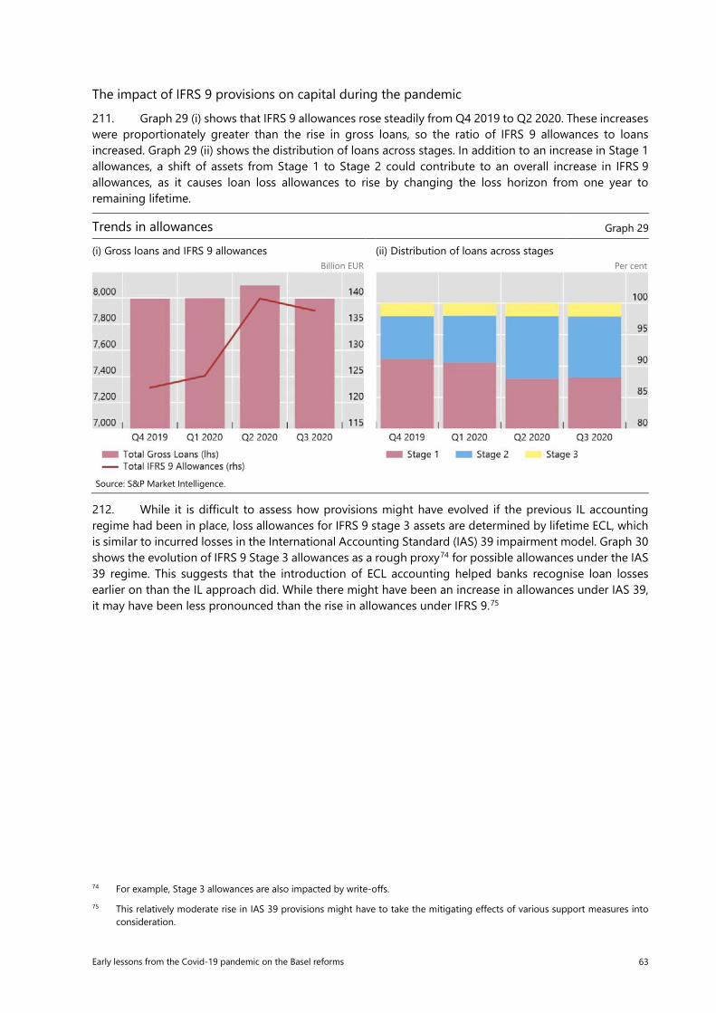
Early lessons from the Covid-19 pandemic on the Basel reforms 63
The impact of IFRS 9 provisions on capital during the pandemic
211. Graph 29 (i) shows that IFRS 9 allowances rose steadily from Q4 2019 to Q2 2020. These increases were proportionately greater than the rise in gross loans, so the ratio of IFRS 9 allowances to loans increased. Graph 29 (ii) shows the distribution of loans across stages. In addition to an increase in Stage 1 allowances, a shift of assets from Stage 1 to Stage 2 could contribute to an overall increase in IFRS 9 allowances, as it causes loan loss allowances to rise by changing the loss horizon from one year to remaining lifetime.
Trends in allowances Graph 29
(i) Gross loans and IFRS 9 allowances (ii) Distribution of loans across stages Billion EUR Per cent
212. While it is difficult to assess how provisions might have evolved if the previous IL accounting regime had been in place, loss allowances for IFRS 9 stage 3 assets are determined by lifetime ECL, which is similar to incurred losses in the International Accounting Standard (IAS) 39 impairment model. Graph 30 shows the evolution of IFRS 9 Stage 3 allowances as a rough proxy74 for possible allowances under the IAS 39 regime. This suggests that the introduction of ECL accounting helped banks recognise loan losses earlier on than the IL approach did. While there might have been an increase in allowances under IAS 39, it may have been less pronounced than the rise in allowances under IFRS 9.75
74 For example, Stage 3 allowances are also impacted by write-offs. 75 This relatively moderate rise in IAS 39 provisions might have to take the mitigating effects of various support measures into
consideration.
Source: S&P Market Intelligence.
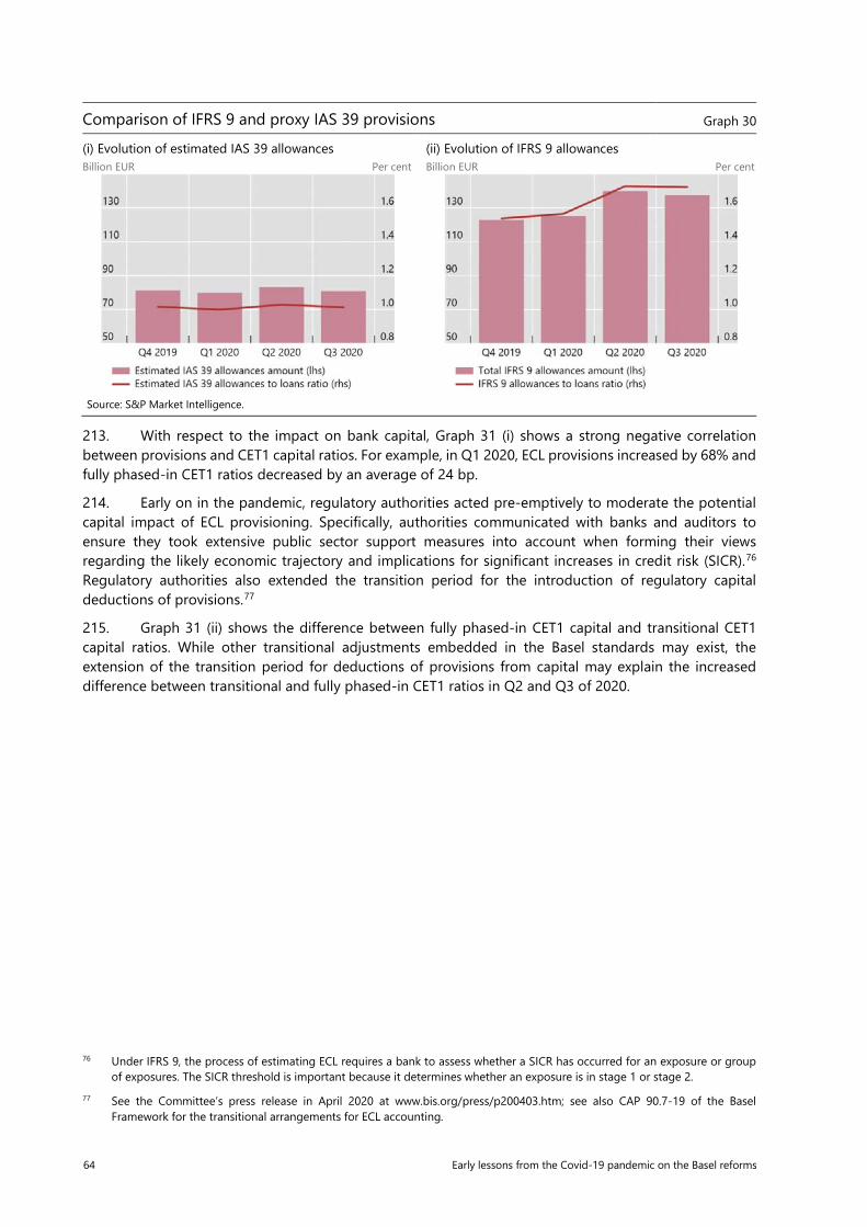
64 Early lessons from the Covid-19 pandemic on the Basel reforms
Comparison of IFRS 9 and proxy IAS 39 provisions Graph 30
(i) Evolution of estimated IAS 39 allowances (ii) Evolution of IFRS 9 allowances Billion EUR Per cent Billion EUR Per cent
213. With respect to the impact on bank capital, Graph 31 (i) shows a strong negative correlation between provisions and CET1 capital ratios. For example, in Q1 2020, ECL provisions increased by 68% and fully phased-in CET1 ratios decreased by an average of 24 bp.
214. Early on in the pandemic, regulatory authorities acted pre-emptively to moderate the potential capital impact of ECL provisioning. Specifically, authorities communicated with banks and auditors to ensure they took extensive public sector support measures into account when forming their views regarding the likely economic trajectory and implications for significant increases in credit risk (SICR).76 Regulatory authorities also extended the transition period for the introduction of regulatory capital deductions of provisions.77
215. Graph 31 (ii) shows the difference between fully phased-in CET1 capital and transitional CET1 capital ratios. While other transitional adjustments embedded in the Basel standards may exist, the extension of the transition period for deductions of provisions from capital may explain the increased difference between transitional and fully phased-in CET1 ratios in Q2 and Q3 of 2020.
76 Under IFRS 9, the process of estimating ECL requires a bank to assess whether a SICR has occurred for an exposure or group of exposures. The SICR threshold is important because it determines whether an exposure is in stage 1 or stage 2.
77 See the Committee’s press release in April 2020 at www.bis.org/press/p200403.htm; see also CAP 90.7-19 of the Basel Framework for the transitional arrangements for ECL accounting.
Source: S&P Market Intelligence.
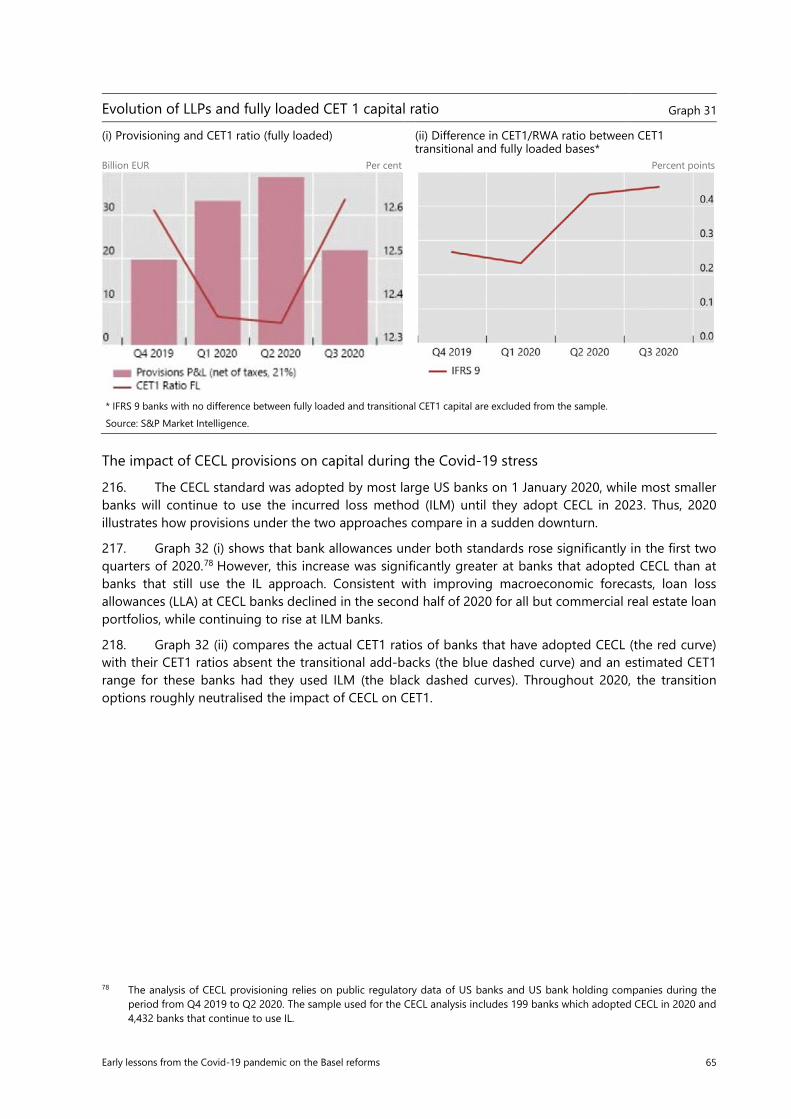
Early lessons from the Covid-19 pandemic on the Basel reforms 65
Evolution of LLPs and fully loaded CET 1 capital ratio Graph 31
(i) Provisioning and CET1 ratio (fully loaded) (ii) Difference in CET1/RWA ratio between CET1 transitional and fully loaded bases*
Billion EUR Per cent Percent points
The impact of CECL provisions on capital during the Covid-19 stress
216. The CECL standard was adopted by most large US banks on 1 January 2020, while most smaller banks will continue to use the incurred loss method (ILM) until they adopt CECL in 2023. Thus, 2020 illustrates how provisions under the two approaches compare in a sudden downturn.
217. Graph 32 (i) shows that bank allowances under both standards rose significantly in the first two quarters of 2020.78 However, this increase was significantly greater at banks that adopted CECL than at banks that still use the IL approach. Consistent with improving macroeconomic forecasts, loan loss allowances (LLA) at CECL banks declined in the second half of 2020 for all but commercial real estate loan portfolios, while continuing to rise at ILM banks.
218. Graph 32 (ii) compares the actual CET1 ratios of banks that have adopted CECL (the red curve) with their CET1 ratios absent the transitional add-backs (the blue dashed curve) and an estimated CET1 range for these banks had they used ILM (the black dashed curves). Throughout 2020, the transition options roughly neutralised the impact of CECL on CET1.
78 The analysis of CECL provisioning relies on public regulatory data of US banks and US bank holding companies during the period from Q4 2019 to Q2 2020. The sample used for the CECL analysis includes 199 banks which adopted CECL in 2020 and 4,432 banks that continue to use IL.
* IFRS 9 banks with no difference between fully loaded and transitional CET1 capital are excluded from the sample. Source: S&P Market Intelligence.
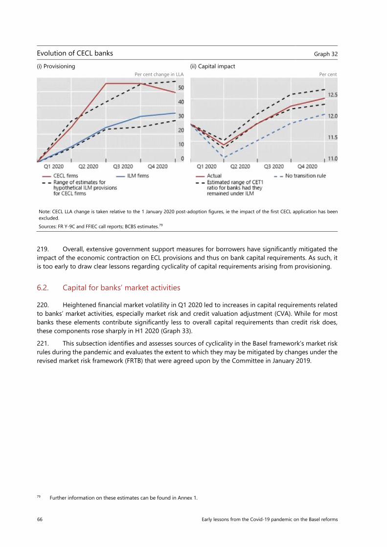
66 Early lessons from the Covid-19 pandemic on the Basel reforms
Evolution of CECL banks Graph 32
(i) Provisioning (ii) Capital impact Per cent change in LLA Per cent
219. Overall, extensive government support measures for borrowers have significantly mitigated the impact of the economic contraction on ECL provisions and thus on bank capital requirements. As such, it is too early to draw clear lessons regarding cyclicality of capital requirements arising from provisioning.
6.2. Capital for banks’ market activities
220. Heightened financial market volatility in Q1 2020 led to increases in capital requirements related to banks’ market activities, especially market risk and credit valuation adjustment (CVA). While for most banks these elements contribute significantly less to overall capital requirements than credit risk does, these components rose sharply in H1 2020 (Graph 33).
221. This subsection identifies and assesses sources of cyclicality in the Basel framework’s market risk rules during the pandemic and evaluates the extent to which they may be mitigated by changes under the revised market risk framework (FRTB) that were agreed upon by the Committee in January 2019.
79 Further information on these estimates can be found in Annex 1.
Note: CECL LLA change is taken relative to the 1 January 2020 post-adoption figures, ie the impact of the first CECL application has been excluded. Sources: FR Y-9C and FFIEC call reports; BCBS estimates.79
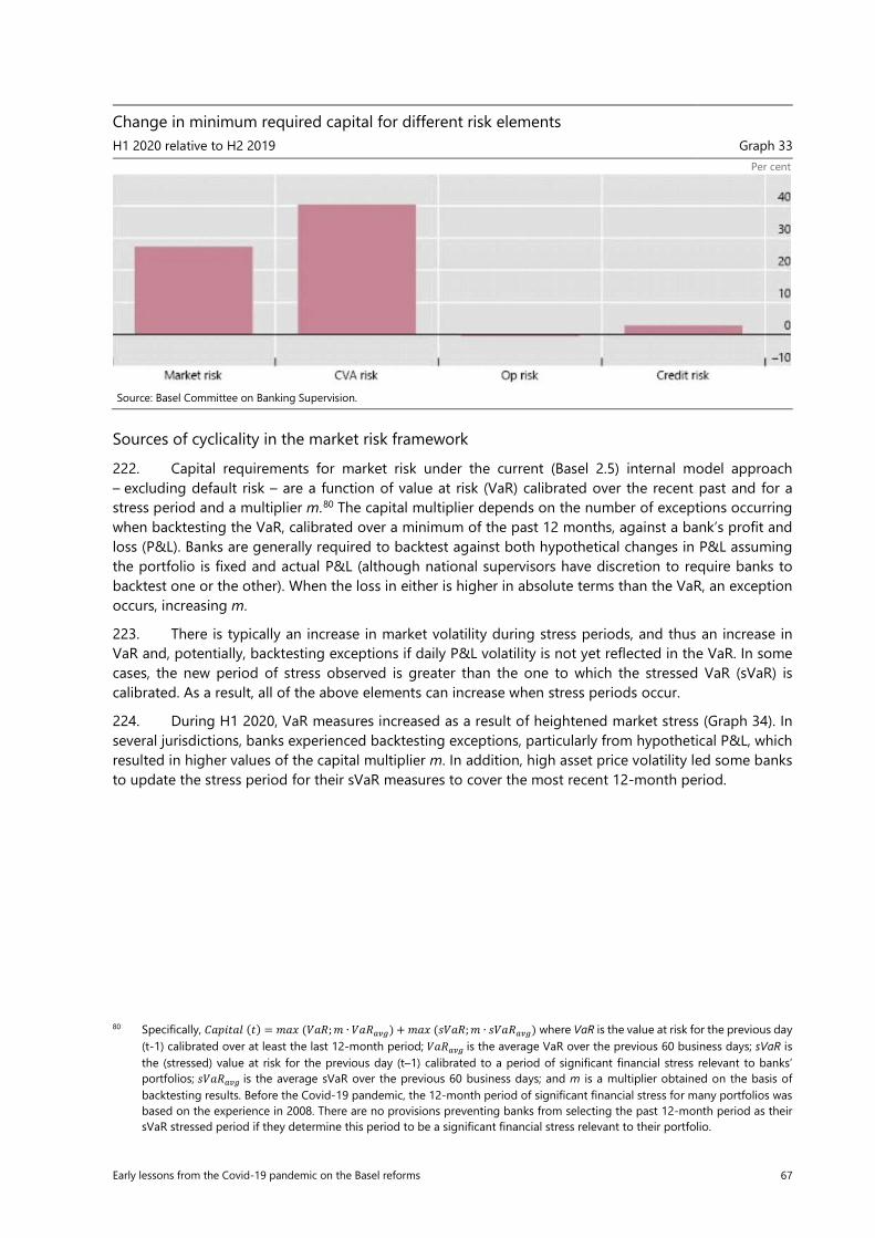
Early lessons from the Covid-19 pandemic on the Basel reforms 67
Change in minimum required capital for different risk elements H1 2020 relative to H2 2019 Graph 33
Per cent
Sources of cyclicality in the market risk framework
222. Capital requirements for market risk under the current (Basel 2.5) internal model approach – excluding default risk – are a function of value at risk (VaR) calibrated over the recent past and for a stress period and a multiplier m.80 The capital multiplier depends on the number of exceptions occurring when backtesting the VaR, calibrated over a minimum of the past 12 months, against a bank’s profit and loss (P&L). Banks are generally required to backtest against both hypothetical changes in P&L assuming the portfolio is fixed and actual P&L (although national supervisors have discretion to require banks to backtest one or the other). When the loss in either is higher in absolute terms than the VaR, an exception occurs, increasing m.
223. There is typically an increase in market volatility during stress periods, and thus an increase in VaR and, potentially, backtesting exceptions if daily P&L volatility is not yet reflected in the VaR. In some cases, the new period of stress observed is greater than the one to which the stressed VaR (sVaR) is calibrated. As a result, all of the above elements can increase when stress periods occur.
224. During H1 2020, VaR measures increased as a result of heightened market stress (Graph 34). In several jurisdictions, banks experienced backtesting exceptions, particularly from hypothetical P&L, which resulted in higher values of the capital multiplier m. In addition, high asset price volatility led some banks to update the stress period for their sVaR measures to cover the most recent 12-month period.
80 Specifically, 𝐶𝐶𝑙𝑙𝑝𝑝𝑖𝑖𝐶𝐶𝑙𝑙𝐶𝐶 (𝐶𝐶) = 𝑚𝑚𝑙𝑙𝑚𝑚 (𝐶𝐶𝑙𝑙𝑅𝑅;𝑚𝑚 ∙ 𝐶𝐶𝑙𝑙𝑅𝑅𝑙𝑙𝑎𝑎𝑎𝑎) + 𝑚𝑚𝑙𝑙𝑚𝑚 (𝐶𝐶𝐶𝐶𝑙𝑙𝑅𝑅;𝑚𝑚 ∙ 𝐶𝐶𝐶𝐶𝑙𝑙𝑅𝑅𝑙𝑙𝑎𝑎𝑎𝑎) where VaR is the value at risk for the previous day (t-1) calibrated over at least the last 12-month period; 𝐶𝐶𝑙𝑙𝑅𝑅𝑙𝑙𝑎𝑎𝑎𝑎 is the average VaR over the previous 60 business days; sVaR is the (stressed) value at risk for the previous day (t–1) calibrated to a period of significant financial stress relevant to banks’ portfolios; 𝐶𝐶𝐶𝐶𝑙𝑙𝑅𝑅𝑙𝑙𝑎𝑎𝑎𝑎 is the average sVaR over the previous 60 business days; and m is a multiplier obtained on the basis of backtesting results. Before the Covid-19 pandemic, the 12-month period of significant financial stress for many portfolios was based on the experience in 2008. There are no provisions preventing banks from selecting the past 12-month period as their sVaR stressed period if they determine this period to be a significant financial stress relevant to their portfolio.
Source: Basel Committee on Banking Supervision.
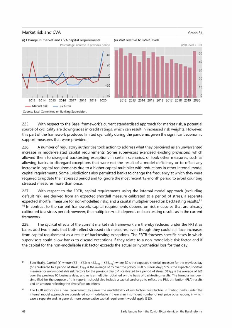
68 Early lessons from the Covid-19 pandemic on the Basel reforms
Market risk and CVA Graph 34
(i) Change in market and CVA capital requirements (ii) VaR relative to sVaR levels Percentage increase in previous period sVaR level = 100
225. With respect to the Basel framework’s current standardised approach for market risk, a potential source of cyclicality are downgrades in credit ratings, which can result in increased risk weights. However, this part of the framework produced limited cyclicality during the pandemic given the significant economic support measures that were provided.
226. A number of regulatory authorities took action to address what they perceived as an unwarranted increase in model-related capital requirements. Some supervisors exercised existing provisions, which allowed them to disregard backtesting exceptions in certain scenarios, or took other measures, such as allowing banks to disregard exceptions that were not the result of a model deficiency or to offset any increase in capital requirements due to a higher capital multiplier with reductions in other internal model capital requirements. Some jurisdictions also permitted banks to change the frequency at which they were required to update their stressed period and to ignore the most recent 12-month period to avoid counting stressed measures more than once.
227. With respect to the FRTB, capital requirements using the internal model approach (excluding default risk) are derived from an expected shortfall measure calibrated to a period of stress, a separate expected shortfall measure for non-modelled risks, and a capital multiplier based on backtesting results.81, 82 In contrast to the current framework, capital requirements depend on risk measures that are already calibrated to a stress period; however, the multiplier m still depends on backtesting results as in the current framework.
228. The cyclical effects of the current market risk framework are thereby reduced under the FRTB, as banks add two inputs that both reflect stressed risk measures, even though they could still face increases from capital requirement as a result of backtesting exceptions. The FRTB foresees specific cases in which supervisors could allow banks to discard exceptions if they relate to a non-modellable risk factor and if the capital for the non-modellable risk factor exceeds the actual or hypothetical loss for that day.
81 Specifically, 𝐶𝐶𝑙𝑙𝑝𝑝𝑖𝑖𝐶𝐶𝑙𝑙𝐶𝐶 (𝐶𝐶) = 𝑚𝑚𝑙𝑙𝑚𝑚 (𝐸𝐸𝐶𝐶 + 𝐶𝐶𝐸𝐸𝐶𝐶;𝑚𝑚 ∙ 𝐸𝐸𝐶𝐶𝑙𝑙𝑎𝑎𝑎𝑎 + 𝐶𝐶𝐸𝐸𝐶𝐶𝑙𝑙𝑎𝑎𝑎𝑎) where ES is the expected shortfall measure for the previous day (t-1) calibrated to a period of stress; ESavg is the average of ES over the previous 60 business days; SES is the expected shortfall measure for non-modellable risk factors for the previous day (t-1) calibrated to a period of stress; SESavg is the average of SES over the previous 60 business days; and m is a multiplier obtained on the basis of backtesting results. The formula has been simplified for the purpose of this report. It should also include a capital surcharge to reflect the P&L attribution (PLA) results and an amount reflecting the diversification effects.
82 The FRTB introduces a new requirement to assess the modellability of risk factors. Risk factors in trading desks under the internal model approach are considered non-modellable if there is an insufficient number of real price observations, in which case a separate and, in general, more conservative capital requirement would apply (SES).
Source: Basel Committee on Banking Supervision.
Early lessons from the Covid-19 pandemic on the Basel reforms 69
229. Under the FRTB, the backtesting approach is used not just for capital purposes but also to determine whether trading positions can be capitalised via an internal model approach in addition to a separate P&L attribution (PLA) test. Again, the FRTB foresees specific cases in which supervisors could allow banks to keep using internal models for capitalising their risks when trading desks do not meet the requirements of either the backtesting or the PLA tests. The FRTB also allows supervisors to discard these failures under extraordinary systemic circumstances, such as the pandemic. However, this discretion does not extend to the exceptions occurring for backtesting performed at bank-wide level for the purpose of determining the multiplier m.
230. Finally, a period of financial stress may make some risk factors less observable in the market. The status of certain risk factors may change from being modellable to non-modellable, leading to an increase in capital requirements. As with the backtesting and PLA requirements, the FRTB permits supervisors to allow banks to treat risk factors that no longer pass the modellability test as modellable.
231. Under the new standardised approach for market risk, the capital requirements for credit spread risk are calculated based on sensitivities and risk weights, while the current framework uses risk weights based on credit ratings. It is not clear whether the new standardised approach is less cyclical than the current framework; sensitivities may still vary during periods of stress even though the new risk weights should be less cyclical since they are determined based on three ratings categories (high-yield vs investment grade vs other).
Sources of cyclicality in the CVA framework
232. In the current CVA framework, capital requirements under the advanced method (CVA internal model) are calculated using a two-step process. First, banks calculate regulatory CVA as a function of derivatives exposures and derivative counterparties’ credit spreads. Second, the market risk internal model approach for credit spread risk is applied to the regulatory CVA number.
233. The cyclicality of current advanced method capital requirements thus has two main drivers: cyclicality from the current market risk framework (see the discussion above) and cyclicality in regulatory CVA arising in part from increases in counterparty credit spreads or substantial mark-to-market movements.
234. Under the current standardised method, CVA capital is the product of counterparty credit risk (CCR) derivatives exposures and risk weights based on counterparty ratings. Thus, capital requirements under the standardised method generally increase when CCR exposures increase (similar to the CVA advanced method) and when derivatives counterparties’ experience ratings downgrade (similar to the current market risk standardised approach).
235. As Graph 34 above illustrates, CVA capital requirements rose sharply in H1 2020. This includes the effect of supervisory actions taken to limit excessive increases in market risk, which might have had an impact on the CVA framework.
236. Under the 2019 Basel CVA standard, the current advanced method is replaced by a new standardised approach for CVA. Capital requirements under this approach are a function of regulatory CVA and the new market risk standardised approach. As no internal model approach is provided in the new framework, excess cyclicality from the current market risk internal model approach is fully mitigated. Additionally, the new standardised CVA approach extends the eligibility of hedges to include instruments that hedge the variability of the exposure component of CVA, thereby reducing cyclicality. However, the reliance on ratings in the FRTB’s standardised approach is a potential source of cyclicality for the new standardised approach for CVA.
237. Additionally, the new standardised approach for CVA captures CVA exposure risks (ie the effect on CVA of movements in market prices, given that movements in market prices affect derivatives exposures and CVA is a function of derivatives exposures) rather than just counterparty credit spreads.
70 Early lessons from the Covid-19 pandemic on the Basel reforms
Cyclical increases in regulatory CVA would increase CVA exposure risks, leading to increases in capital requirements. However, CVA exposure risks constitute a relatively small part of total CVA risk.83
238. The new basic approach for CVA is broadly similar to the current standardised method and should have the same drivers of cyclicality. However, the new approach uses a less granular classification of credit ratings, removing cyclicality for most ratings migrations except with respect to the investment grade/high-yield boundary.
Sources of cyclicality in the CCR framework
239. CCR RWAs are the product of derivatives or SFT exposures and risk weights from the credit risk framework. The Basel framework provides for the Standardised Approach for CCR (SA-CCR) and the Internal Model Method (IMM) as part of the CCR framework.
240. The CCR RWAs derived using the IMM are obtained by taking the higher value of RWAs calculated on the basis of derivatives exposures calibrated to current market data and RWAs based on derivatives exposures calibrated to a historical period of stress to credit spreads. As a result, CCR RWAs do not generally exhibit the same degree of cyclicality, unlike market risk and CVA capital requirements, which are derived by adding both a stressed and non-stressed measure.
241. Sudden market stresses are a potential driver of CCR cyclicality as they may cause significant changes in mark-to-market positions, which could increase derivatives exposures. During the H1 2020 stress, some banks experienced material but temporary spikes in CCR exposures ahead of settlement due to large margin calls following significant intraday market price movements.
242. CCR capital requirements increased to a lesser extent in H1 2020 than market risk or CVA risk did.
243. Cyclicality is largely unchanged in the future CCR framework. This is partly because no changes are made to the IMM and because the main driver of CCR exposure cyclicality (market volatility leading to significant changes in mark-to-market positions) is inherent to all current and future CCR methods. Similar to the current exposure method, SA-CCR sets different potential future exposure add-ons referencing investment grade and high-yield names.
244. In summary, the analysis finds sources of cyclicality in the current traded risk framework, which prompted supervisors in several jurisdictions to introduce relief measures during the Covid-19 pandemic. However, it is expected that revisions to this framework agreed to in January 2019 (the FRTB) will mitigate the primary sources of this cyclicality. While sources of cyclicality in the future framework remain, including backtesting exceptions and constraints on modellability, supervisors may respond if concerned regarding excessive cyclicality.
83 Data from a QIS exercise in June 2019 indicate that counterparty credit spreads account for approximately 70% of the risk, thus exposures risks account for 30%.
Early lessons from the Covid-19 pandemic on the Basel reforms 71
Annex 1: List of data sources
Graph 1 BIS staff made additional calculations to following vendor-sourced data: (i) Option-adjusted spread data for ICE Bank of America Merrill Lynch Fixed Income corporate bond Indices; (ii) Bloomberg; and (iii) Datastream.
Graph 2 SNL data for credit line drawdowns for non-financial corporations based in Canada, France, Germany, Japan Italy, the United Kingdom and the United States for Q1, Q2 and Q3 2020. BIS staff made additional calculations to these vendor-sourced data.
Graph 3 CRANE, Informa iMoneyNet and BIS calculations.
Graph 4 90-day commercial paper rate to 3-month overnight index swap basis data for the period from Q4 2019 through Q1 2021 sourced from JPMorgan Chase and Co. (left panel) and Treasury spread liquidity index data for the period from Q3 2019 through Q1 2021 from Bloomberg. BIS staff made additional calculations to these vendor-sourced data.
Graph 5 (i) Bloomberg data for euro, British pound and Japanese yen spot exchange and three-month forward rates against the US dollar from Q4 2020 through Q1 2021. (ii) Bloomberg data on three-month LIBOR for the same period for the Canadian dollar, euro, Japanese yen, British pound and Australian dollar. BIS staff made additional calculations to these vendor-sourced data.
Graph 6 Datastream, national data and BIS calculations.
Graph 7 Loan demand data from surveys conducted by the Bank of England, the Bank of Japan, the European Central Bank and the Board of Governors of the Federal Reserve System from 2018 through Q1 2021.
Graph 8 IHS Markit data in both panels. (i) Option-adjusted spreads for Markit iBoxx data for iBoxx Contingent Convertible Liquid Developed Market, iBoxx Banks Senior and iBoxx Banks Subordinated indices for the period from January 2020 through April 2021 are included. (ii) Bank-level CDS spreads are aggregated by ratings cohorts based on ratings provided by Fitch Ratings used to separate bank data by the ratings cohort shown in the right panel. Both panels show data that was subjected to further calculation by BIS staff.
Graph 9 (i) SNL database for the four quarters from Q4 2019 through Q3 2020 and a sample of 83 banks across 25 jurisdictions. (ii) Datastream, Refinitiv Eikon and subject to calculations by BIS staff.
Graph 10 BIS and BIS calculations.
Table 1 and Graph 11
For the reporting dates end-2013 through end-December 2019, data from the Committee’s Basel III monitoring exercises and data from supervisory reporting systems were used. For the end-June 2020 reporting date, only data from supervisory reporting systems were available. End-June 2020 NSFR fugures are approximated based on both the Committee’s data and SNL.
Graph 12 Market value of common equity and book values of total debt from 2007 through Q1 2021 for a sample of 60 banks across all geographies, sourced from Thompson Reuters and calculated as the market value of common equity as a percentage of the market value of total assets (the sum of the market value of common equity and the book value of total debt).
Graphs 13 and IHS Markit using five-year contract indices (maturity date end of December 2024) for European banks (iTraxx Euro Senior Financials Index) and North American banks (CDXNAIGFIN).
Bank-level CDS data sourced from IHS Markit for all banks headquartered in BCBS member jurisdictions with CDS spread data in sufficient quality. From this sample, those banks for which regulatory reporting data are also available in SNL for the considered time horizon were selected (in case of missing data, other sources on SNL or public data sources (eg annual reports or regulatory disclosures) are used if available). Sovereign CDS spreads were also sourced from IHS Markit. Moreover, for Table 3, CET1 all-in requirements are available from a survey that the BCBS Secretariat has conducted among regulatory authorities in the TFE context. Consequently, the analysis considers only those banks for which CDS spreads of sufficient quality; data for the CET1 ratio, leverage ratio, and LCR; and all considered bank-level control variables are available.
14 Tables 2 and 3
72 Early lessons from the Covid-19 pandemic on the Basel reforms
Graph 15, Tables 4, A4 and A5
Quarterly balance sheet and regulatory data for banks in Committee member jurisdictions sourced from SNL for the period from Q2 2019 to Q3 2020. The sample includes banks that are active in lending with total assets above 0.25% of the jurisdictions’ GDP and/or above 50 bn USD. In total, the number of banks ranges between 200 and 300, depending on the capital or liquidity measure used in the regression.
Table 5, Graphs 16 and 17
Capital data sourced from the SNL as well as supervisory survey responses.
Table 6 Capital data sourced from the SNL.
Graph 18 (i) The red dot (total sample) in the graph on the left is built using a loan-level (new lending) cross-sectional regression (Q2 2020) where interacted with the distance to combined buffer requirement (CBR) with a dummy that is equal to one if a loan is covered by government guarantee schemes, zero otherwise. In the chart, what is reported is the single coefficient capturing the relationship between distance to CBR and new lending (in log) when the dummy is equal to zero, ie for loans that are not covered by guarantees. The interpretation of the coefficient indicates that a 1pp increase in the distance to CBR leads to a 2.5% increase in new lending. And yes, the yellow lines represent confidence intervals. (ii) The graph is constructed using bank-level difference-in-differences regressions over the period Q2 2019 to Q2 2020. The dependent variable is quarterly change in lending growth. High D2CBR banks (control) are those that (in Q1 2020) had a distance to the CBR above the first quartile of the distance to CBR distribution (ie 3%). Low D2CBR banks (treatment) are those that (in Q1 2020) had a distance to the CBR below the first quartile of the distance to CBR distribution. The bar chart is plotting the regressions coefficient (beta2 and beta3, respectively). Beta2 indicates lending behaviour for the control group pre-/post-Covid while beta3 is the difference-in-differences coefficient. For banks in the control group, lending growth after Covid has been positive (7.2 pp) whilst for banks closer to the Maximum Distributable Amount (MDA) trigger has been negative immediately after Covid (17pp) in comparison to the control group pre-Covid. The sum of the two coefficients (beta2 + beta3) is statistically significant, confirming different behaviour between these two groups of banks after the shock. (iii) The graph comes from plotting difference-in-differences regression coefficients (Q1 2020 to Q2 2020). The dependent variable is the log of lending volume to NFCs (the analysis takes the exponential to get euro amounts). The dot (pre-Covid) for the control group (High D2CBR) comes from plotting the constant in the DiD regression. The single dummy estimated coefficient is used to get the dot (pre-Covid) for the treatment (Low D2CBR). That provides the difference between the treated and control pre-Covid (the distance between the two dots pre-Covid). Post-Covid, the other estimated coefficients coming from the DiD estimation are applied. Specifically, to estimate the difference in lending for the control group pre-/post-Covid we apply the time dummy (Covid in this case). This gives us the slope of the red line. The DiD coefficient (double interaction) is applied to get the slope of the yellow line (treatment group).
Graph 19 Public websites of the authorities in the following countries: Belgium, France, Germany, Hong Kong SAR, Luxembourg, Sweden, Switzerland and the United Kingdom.
Graph 20 Supervisory survey on capital requirements. The variable CCyB release is defined as the absolute difference between the bank-specific CCyB rate in Q1 2019 and Q3 2020. Other CET1 release (excluding CCyB release) is defined similarly. First, “Other CET1 Requirements” are calculated as the difference between the “Overall CET1 Requirement” and the “Bank-Specific CCyB rate”. Second, the variable “Other CET1 Release” is calculated as the difference between “Other CET1 Requirements” in Q1 2019 and Q3 2020.
Graph 21 53 large banks of the euro area announcing public CET1 ratio targets and using panel regression. Explanatory variables include the announced capital requirements (MDA trigger plus Pillar 2 Guidance), total assets in logarithmic form, return on assets, risk weight density (RWA over Total Original Exposures), net interest margin, non-performing loan ratio, impairment ratio, the average 5-year ahead domestic GDP growth according to the Consensus of Professional Forecasters and the Main Refinancing Operation rate.
Table 7 Supervisory survey.
Graphs 22 and 23, Table 8
Bloomberg LLC, using a news review. The covered time period is from January 2019 through March 2021. In a couple of iterations, a subset of these dates from January through September 2020 was used. • The sample included US- and Europe-based banks that have issued currently outstanding additional
Tier 1 and subordinated long-term debt instruments with at least two and up to seven years in remaining maturity during the sample period. This led to a sample size of 68 banks. Of these firms, 65 have at least one suitable subordinated long-term debt instrument and 48 had at least one suitable additional Tier 1 instrument. Only 45 firms had securities of both types, although several of these firms have multiple suitable securities.
• Prices and yields data for the instruments were sourced from Bloomberg. It is unclear how liquid some of these securities are, particularly the AT1 and debt instruments. As a result, there may be

Early lessons from the Covid-19 pandemic on the Basel reforms 73
measurement error between the reported quotes and the true prices that could modestly influence the results of the analysis. Subject to that limitation, this is the best available data.
• Each bank in the sample was allowed to have up to two suitable capital instruments in our data. Where more than one instrument was available, an average was used to specify that bank’s yields.
Tables 9 and 10, Graph 24
For the reporting dates end-December 2019, data from the Committee’s Basel III monitoring exercises and for the end-June 2020 reporting date, data from supervisory reporting systems. A sample contais 84 Group 1 banks and 45 Group 2 banks.
Graph 25 Two quarterly (Q4 2019 and Q1 2020) Pillar 3 disclosures for all 31 G-SIBs and an additional 16 banks as follows: 4 Australian, 6 Canadian, 7 EU, 7 Japanese, 4 Swiss, 6 UK and 13 US banks. Q4 2019 and Q1 2020 data are measured as of 31 December 2019 and 31 March 2020, respectively, for all but Canadian banks, for which the data are measured on 31 January 2020 and 30 April 2020, respectively. The charts reflect the impact of regulatory relief granted to Swiss banks (by the FINMA on 31 March 2020) and Canadian banks (by the OSFI on 9 April 2020). Moreover, the charts correct for the incentive effect of the transition from the capital conservation buffer to the stress capital buffer in the United States in 2020.84
Graph 26 and Table 11
Weekly Bank of England Sterling Money Market data collection and Bank of England regulatory returns for a sample of nine UK broker-dealer subsidiaries of global banks for Q4 2019 and Q1 2020.
Graph 27 Monthly data from US Federal Reserve Complex Institution Liquidity Monitoring Report for US domestic holding companies over the period from January 2019 through August 2020.
Table 12 Changes in monthly data between January 2019 and December 2020 sourced from four jurisdictions as follows: (i) Japan – Monthly Bank of Japan Current Account balances by sector, aggregate Bank of Japan reserves. (ii) Switzerland – Monthly Banking Statistics for aggregate national and foreign reserves of large banks
in Switzerland, excluding foreign branches. (iii) United States – US Federal Reserve Money Stock Measures Report, aggregate US central bank
reserves. (iv) United Kingdom – UK RPMB3VO Bank of England Bankstats table, aggregate Bank of England reserves
for all UK-resident monetary financial institutions.
Table 13 Supervisory information provided by each jurisdiction.
Graph 28 (i) Japan – quarterly Pillar 3 disclosures for Japanese G-SIBs. (ii) Switzerland – quarterly Pillar 3 disclosures for G-SIBs in Switzerland. (iii) United Kingdom – Pillar 3 disclosures for all large banks and building societies subject to the Basel
leverage ratio requirement. (iv) United States – US Federal Financial Institutions Examination Council Regulatory Capital Report for all
domestically headquartered bank holding companies Subject to the Advanced Capital Adequacy Framework.
Graphs 29–31 SNL quarterly data from Q4 2019 through Q3 2020. From the original sample mentioned above, three sub-samples were selected as follows: • Graphs 29 and 30: 51-bank sample with those banks that use IFRS and included regulatory data for
IFRS distribution allowances by stages. • Graph 31 (i): 93-bank sample (including banks that use IFRS 9, US GAAP/CECL and other national
GAAPs) which included data on both provisions recorded in P&L and capital information. This sample was used when estimating the impact of provisions on CET1 capital.
• Graph 31 (ii): Sample of 32 banks which use IFRS 9; shows a positive difference between fully-loaded and transitional CET1. Sample includes 24 European banks, 6 Saudi Arabian banks, 1 Korean bank and 1 South African bank.
Graph 32 Quarterly Federal Reserve reporting form Y-9C and call report data from Q1 2020 through Q4 2020. The analysis estimates what allowances (relative to loans) for CECL firms in 2020 would have been under ILM using a linear regression. Its equation chose predictor variables which account for differences across firms that relate to their allowance levels: the relative size of different loan portfolios, loan quality, past allowances, lending growth and firm size.
Graphs 33 and 34 For the reporting dates end-December 2019, data from the Committee’s Basel III monitoring exercises and for the end-June 2020 reporting date, data from supervisory reporting systems.
84 This does not include the effects of the US exclusion, which went into force on 1 April 2020.

74 Early lessons from the Covid-19 pandemic on the Basel reforms
Annex 2: TFE survey questionnaire
1. Capital buffers
In this survey, “capital targets” refers to both publicly stated and/or internal bank capital ratio targets, unless otherwise specified.
1. Did your jurisdiction make any changes to its Pillar 2 requirements in response to the Covid-19 pandemic? If yes, please provide the following details:
o Weighted average percentage change in Pillar 2 requirements (by RWA) for banks in your jurisdiction
o Description of the change in requirements o Objective/policy intent for the change o The scope/type of banks to which the change applies o Is the change permanent or temporary? If temporary, please list the date that the change
will expire o Is the change publicly disclosed?
2. What is the most common approach that banks in your jurisdiction use to set capital targets: (i)
absolute capital ratio targets (eg 13% of RWAs); (ii) capital ratio headroom above minimum and buffer requirements (eg headroom of 200 bp); or (iii) other approaches?
3. For those banks that target absolute capital ratios, what was their weighted-average (by RWA) common equity Tier 1 (CET1) capital ratio (eg 13%) for the following quarters?
o 2019 Q4 o 2020 Q2 o Please note the scope of banks in your jurisdiction covered by this response (ie some, most
or all).
4. For banks that target a specific amount of headroom above their minimum and buffer requirements, what was the weighted-average size (by RWA) of their CET1 capital ratio headroom (eg 200 bp) for the following quarters?
o 2019 Q4 o 2020 Q2 o Please note the scope of banks in your jurisdiction covered by this response (ie some, most
or all).
5. Please describe any market reaction to banks that experienced a drop in their capital levels or that set lower capital targets (eg changes in these banks’ CDS spreads, ratings, equity prices, as well as reactions from investors and/or rating agencies)?
6. If your jurisdiction released a Covid-specific public statement regarding buffer usability, please describe banks’ reactions, including any changes in their target capital ratios and lending behaviour.
7. To what extent (eg % of RWA) did banks in your jurisdiction dip into their regulatory capital buffers? Please report the number of internationally active banks that dipped into their buffers as well as the weighted average CET1 ratio of the dip (eg 1pp into buffers):
o Please indicate the actual outcomes during the period between 2019 Q4 and 2020 Q2. o Please indicate the projections in the most recent stress-test scenarios in your jurisdiction.
Early lessons from the Covid-19 pandemic on the Basel reforms 75
8. What, if any, constraints have made banks reluctant to draw down on their capital buffers (eg concern about supervisory reaction, conservation of capital for future losses, uncertainty in outlook, concerns about funding costs to re-build capital)?
9. Please describe any observed differences in behaviour (eg recapitalisation, de-risking, reduced lending) between:
o Banks that were close to or below capital targets versus those that were well above them. o Banks that are projected to dip into their regulatory capital buffers in the stress test versus
those that are not.
10. In retrospect, would you have preferred to lower CET1 capital regulatory requirements by more than was possible (ie through the CCyB or other means)? If yes, please explain whether you would have preferred to: release a greater CCyB amount (ie a cyclical releasable buffer), reduce a fixed buffer, or both, and why.
2. Liquidity buffers
11. Do banks in your jurisdiction set internal/public liquidity coverage ratio (LCR) targets? If so, what was the average target (weighted by RWAs)? Did they raise or lower these targets during the Covid-19 pandemic?
12. Has one or more bank in your jurisdiction publicly reported an LCR below the relevant regulatory minimum during the Covid stress? If yes, what was the supervisory and market reaction?
13. Did supervisors in your jurisdiction lower the minimum LCR ratio below 100%? If so, was this policy effective in encouraging banks to lower their LCR?
14. Did you observe evidence (behavioural or via supervisory discussions) of banks in your jurisdiction being hesitant or unwilling to let their LCR fall (including below 100%) at any point during the Covid stress? If yes, which of the factors listed below would best explain this hesitance/unwillingness?
o Market reaction (based on public disclosure requirements or the bank’s own disclosures) o An expected (or unexpected) supervisory response o Internal risk appetites/LCR targets o Other
15. What key steps did banks take to manage their liquidity positions as any regulatory requirements or internal targets were approached/breached (eg drawdown on stock of HQLA; drawdown on central bank liquidity; increase cash inflows (eg reduce rollover of maturing loans); reduce lending/facilities extended)?
16. Which of the following were the most material outflows during the most intense phases of the Covid-19 pandemic (multiple selections possible)? Please elaborate.
o Retail deposit outflows o Corporate credit facility drawdowns o Secured lending/collateral swap flows o Technical factors (eg higher outflow calculations from HLBA) o Early debt buyback requests o CCPs/counterparty margin calls o Other
17. Were any of the channels listed in Q16 significantly more severe than anticipated in the LCR stress scenario?
76 Early lessons from the Covid-19 pandemic on the Basel reforms
3. Leverage ratio
18. Were there any banks in your jurisdiction whose leverage ratio became a binding constraint (ie was the leverage ratio closer than risk-weighted capital ratios to minimum requirements) during the Covid-19 pandemic? If yes, which type of banks and what was the primary driver of this (eg influx of cash deposits, increase in repo activity).
19. Is there evidence that these banks reduced market intermediation (ie encumbered or unencumbered holdings of domestic sovereign bonds, participation in the repo/reverse repo market, etc.)?
20. If yes, were these reductions the result of the leverage ratio being self-imposed at a business line or exposure level (ie a broker dealer subsidiary), or at the consolidated level?
21. Please discuss whether your jurisdiction granted banks any leverage ratio exemptions, the type of exemptions granted (eg an exemption on domestic government bond holdings or central bank deposits for purposes of calculating the leverage ratio), the timing of when the exemptions took place, and whether the exemptions were disclosed.
22. If yes to Q21, please discuss the outcome that the exemptions were designed to achieve. In your judgement, did the exemptions have a positive effect on market intermediation?
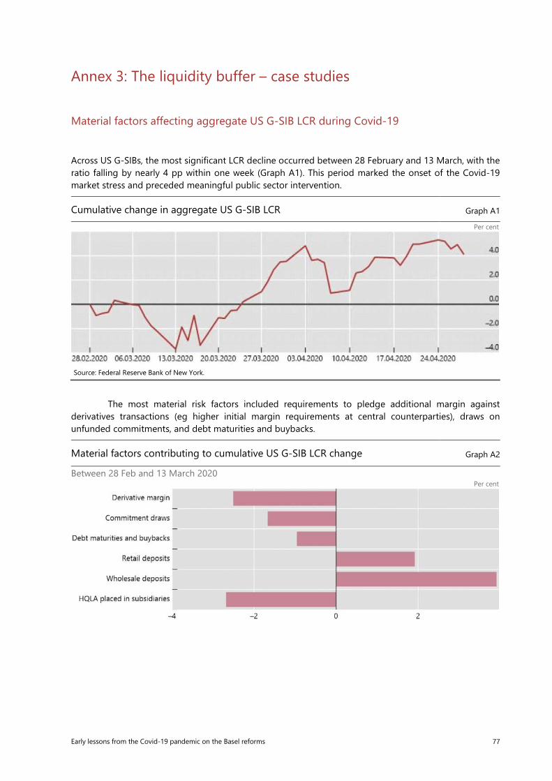
Early lessons from the Covid-19 pandemic on the Basel reforms 77
Annex 3: The liquidity buffer – case studies
Material factors affecting aggregate US G-SIB LCR during Covid-19
Across US G-SIBs, the most significant LCR decline occurred between 28 February and 13 March, with the ratio falling by nearly 4 pp within one week (Graph A1). This period marked the onset of the Covid-19 market stress and preceded meaningful public sector intervention.
Cumulative change in aggregate US G-SIB LCR Graph A1
Per cent
Source: Federal Reserve Bank of New York.
The most material risk factors included requirements to pledge additional margin against derivatives transactions (eg higher initial margin requirements at central counterparties), draws on unfunded commitments, and debt maturities and buybacks.
Material factors contributing to cumulative US G-SIB LCR change Graph A2
Between 28 Feb and 13 March 2020 Per cent
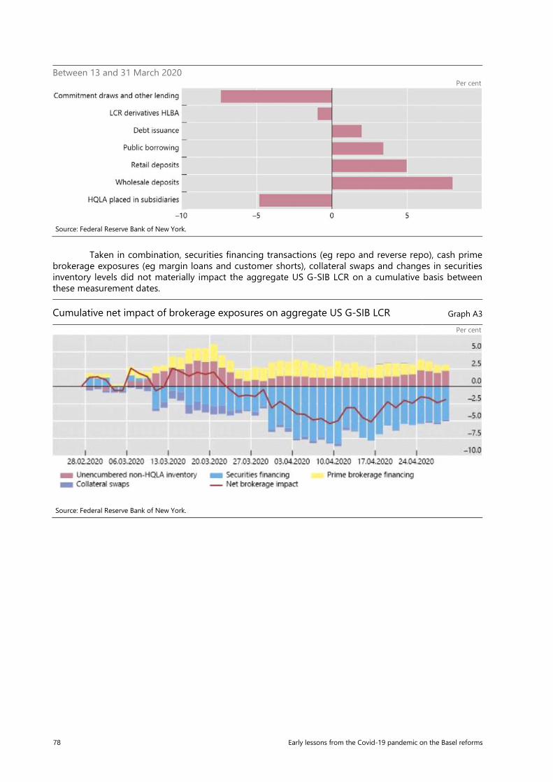
78 Early lessons from the Covid-19 pandemic on the Basel reforms
Between 13 and 31 March 2020 Per cent
Taken in combination, securities financing transactions (eg repo and reverse repo), cash prime
brokerage exposures (eg margin loans and customer shorts), collateral swaps and changes in securities inventory levels did not materially impact the aggregate US G-SIB LCR on a cumulative basis between these measurement dates.
Cumulative net impact of brokerage exposures on aggregate US G-SIB LCR Graph A3
Per cent
Source: Federal Reserve Bank of New York.
Source: Federal Reserve Bank of New York.
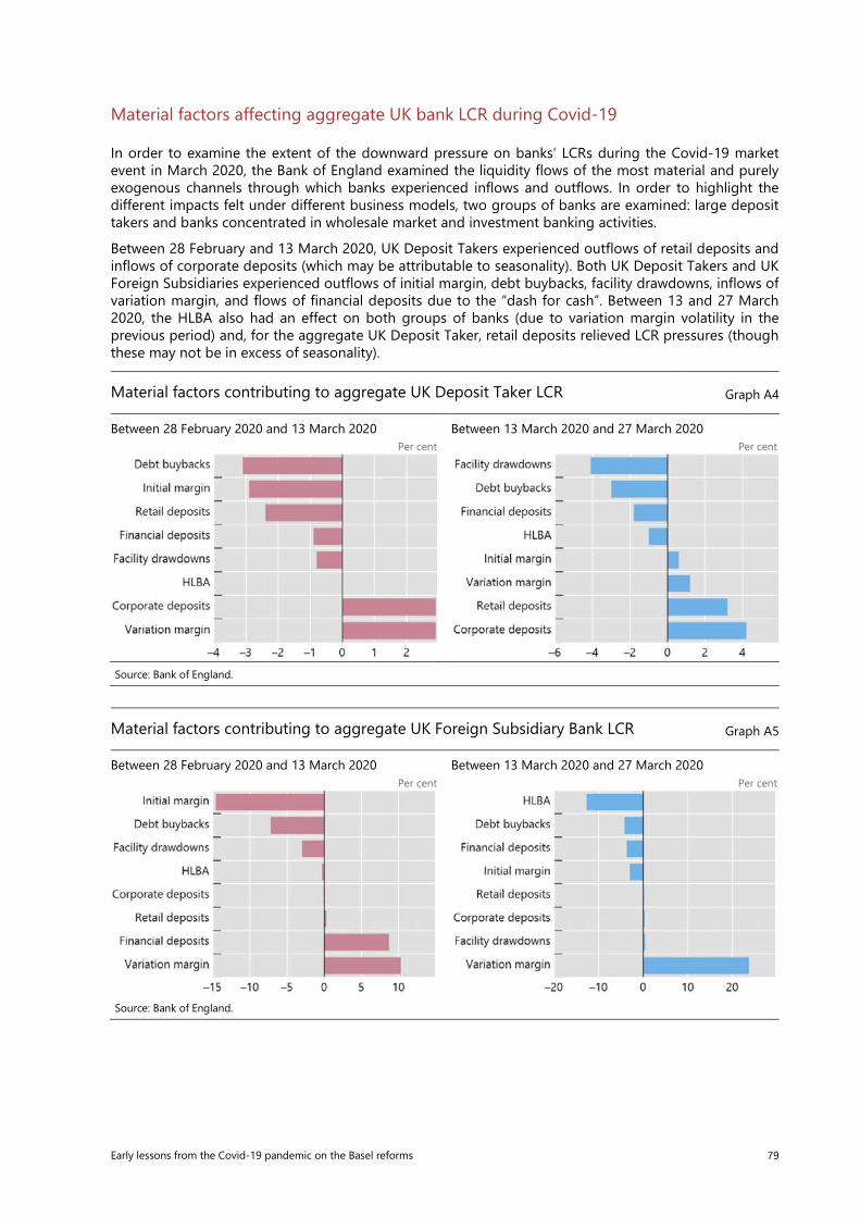
Early lessons from the Covid-19 pandemic on the Basel reforms 79
Material factors affecting aggregate UK bank LCR during Covid-19
In order to examine the extent of the downward pressure on banks’ LCRs during the Covid-19 market event in March 2020, the Bank of England examined the liquidity flows of the most material and purely exogenous channels through which banks experienced inflows and outflows. In order to highlight the different impacts felt under different business models, two groups of banks are examined: large deposit takers and banks concentrated in wholesale market and investment banking activities.
Between 28 February and 13 March 2020, UK Deposit Takers experienced outflows of retail deposits and inflows of corporate deposits (which may be attributable to seasonality). Both UK Deposit Takers and UK Foreign Subsidiaries experienced outflows of initial margin, debt buybacks, facility drawdowns, inflows of variation margin, and flows of financial deposits due to the “dash for cash”. Between 13 and 27 March 2020, the HLBA also had an effect on both groups of banks (due to variation margin volatility in the previous period) and, for the aggregate UK Deposit Taker, retail deposits relieved LCR pressures (though these may not be in excess of seasonality).
Material factors contributing to aggregate UK Deposit Taker LCR Graph A4
Between 28 February 2020 and 13 March 2020 Between 13 March 2020 and 27 March 2020 Per cent Per cent
Source: Bank of England.
Material factors contributing to aggregate UK Foreign Subsidiary Bank LCR Graph A5
Between 28 February 2020 and 13 March 2020 Between 13 March 2020 and 27 March 2020 Per cent Per cent
Source: Bank of England.
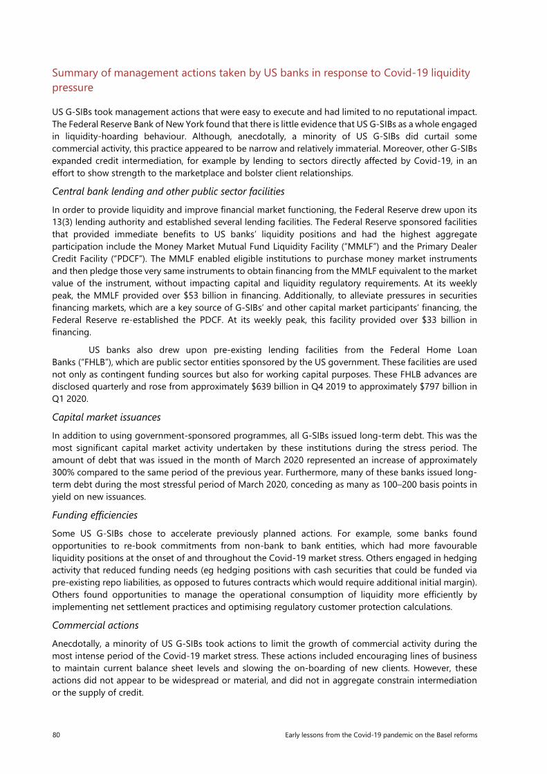
80 Early lessons from the Covid-19 pandemic on the Basel reforms
Summary of management actions taken by US banks in response to Covid-19 liquidity pressure
US G-SIBs took management actions that were easy to execute and had limited to no reputational impact. The Federal Reserve Bank of New York found that there is little evidence that US G-SIBs as a whole engaged in liquidity-hoarding behaviour. Although, anecdotally, a minority of US G-SIBs did curtail some commercial activity, this practice appeared to be narrow and relatively immaterial. Moreover, other G-SIBs expanded credit intermediation, for example by lending to sectors directly affected by Covid-19, in an effort to show strength to the marketplace and bolster client relationships.
Central bank lending and other public sector facilities
In order to provide liquidity and improve financial market functioning, the Federal Reserve drew upon its 13(3) lending authority and established several lending facilities. The Federal Reserve sponsored facilities that provided immediate benefits to US banks’ liquidity positions and had the highest aggregate participation include the Money Market Mutual Fund Liquidity Facility (“MMLF”) and the Primary Dealer Credit Facility (“PDCF”). The MMLF enabled eligible institutions to purchase money market instruments and then pledge those very same instruments to obtain financing from the MMLF equivalent to the market value of the instrument, without impacting capital and liquidity regulatory requirements. At its weekly peak, the MMLF provided over $53 billion in financing. Additionally, to alleviate pressures in securities financing markets, which are a key source of G-SIBs’ and other capital market participants’ financing, the Federal Reserve re-established the PDCF. At its weekly peak, this facility provided over $33 billion in financing.
US banks also drew upon pre-existing lending facilities from the Federal Home Loan Banks (“FHLB”), which are public sector entities sponsored by the US government. These facilities are used not only as contingent funding sources but also for working capital purposes. These FHLB advances are disclosed quarterly and rose from approximately $639 billion in Q4 2019 to approximately $797 billion in Q1 2020.
Capital market issuances
In addition to using government-sponsored programmes, all G-SIBs issued long-term debt. This was the most significant capital market activity undertaken by these institutions during the stress period. The amount of debt that was issued in the month of March 2020 represented an increase of approximately 300% compared to the same period of the previous year. Furthermore, many of these banks issued long-term debt during the most stressful period of March 2020, conceding as many as 100–200 basis points in yield on new issuances.
Funding efficiencies
Some US G-SIBs chose to accelerate previously planned actions. For example, some banks found opportunities to re-book commitments from non-bank to bank entities, which had more favourable liquidity positions at the onset of and throughout the Covid-19 market stress. Others engaged in hedging activity that reduced funding needs (eg hedging positions with cash securities that could be funded via pre-existing repo liabilities, as opposed to futures contracts which would require additional initial margin). Others found opportunities to manage the operational consumption of liquidity more efficiently by implementing net settlement practices and optimising regulatory customer protection calculations.
Commercial actions
Anecdotally, a minority of US G-SIBs took actions to limit the growth of commercial activity during the most intense period of the Covid-19 market stress. These actions included encouraging lines of business to maintain current balance sheet levels and slowing the on-boarding of new clients. However, these actions did not appear to be widespread or material, and did not in aggregate constrain intermediation or the supply of credit.
Early lessons from the Covid-19 pandemic on the Basel reforms 81
LCR trigger levels for management actions: information from UK banks’ recovery plans
Banks are required to maintain recovery plans which detail the means by which they would identify capital and liquidity stresses, the actions they could take to respond to those stresses, and what implications those actions might have, eg on their profitability. These plans contain valuable insights into the judgments that banks might make during a period of stress: what actions they would take, on what timescale, and what cost they would be willing to bear in doing so.
In their plans, banks include recovery indicators which they monitor to determine the point at which they escalate governance decisions and take recovery actions. The calibration of these indicators offers useful insight into banks’ understanding of the appropriate actions to take in times of stress.
However, banks also monitor a broader suite of indicators. In reality, banks maintain frameworks of early warning indicators (EWIs) calibrated to warn of stress scenarios of differing degrees. Recovery plan indicators should be on the most severe end of that spectrum, and one would expect that their breach would precipitate banks’ most urgent actions.
UK authorities reviewed the recovery plans of a representative sample of UK banks which, between them, represent the majority of banking assets in the UK and a multiplicity of UK banks’ business models. They represent a significant portion of retail and wholesale credit provision in the UK. Our findings have been aggregated, anonymised and detailed below.
Conclusions and recommendations
No bank calibrated its LCR recovery indicator below 100%. This suggests that banks consider urgent measures necessary to improve their liquidity positions at no lower than that level. Some banks’ recovery triggers were calibrated at higher than 100%. Recovery plan stresses should be quite severe in nature (ie the kind of stress that the bank would not survive without taking action), so this is a useful insight into banks’ motivations for quickly restoring their liquidity positions during or following a period of stress.
Banks identify a range of liquidity recovery options, many of which could have damaging effects on the economy if taken in large scale during a period of stress. For example, all of the banks in our sample indicated that they would cut lending during a period of stress. The pace at which banks say they will take liquidity recovery actions, and the scale of those actions, indicate that promptly returning to a robust liquidity position during a period of stress is a priority for banks. We cannot conclude that the principal motivation behind this is being able to disclose an LCR above 100%, or if that is just a consequence of banks’ attempts to satisfy other constraints.
The Covid-19 stress was not severe enough on banks’ liquidity positions to provide good insight into how banks are likely to behave in a severe (recovery plan-style) liquidity stress. No bank in our sample triggered a recovery indicator during the Covid-19 stress, despite those indicators being calibrated quite high.
It is possible that, in a stress episode, banks will act differently to how they said they would in their recovery plans. This could be because the situation is different to the one set out in the plan, or because the plan is not a good representation of the bank’s actual intentions. The Basel standard assumes that banks’ responses to stress will be different based on the situation at hand. The Covid-19 stress was likely not severe enough to test this hypothesis.
Nevertheless, some banks took some defensive actions in the Covid-19 stress. This indicates significant reluctance to use liquidity buffers in a stress of a severity which is, in relative terms, not exceptionally severe. These defensive actions included declining to roll funding and cutting some lending. But, in our sample, these actions were limited in scope and scale. These banks’ provision of credit in the economy was generally robust throughout the stress, although the demand for some types of credit (eg mortgage loans) may have been subdued.
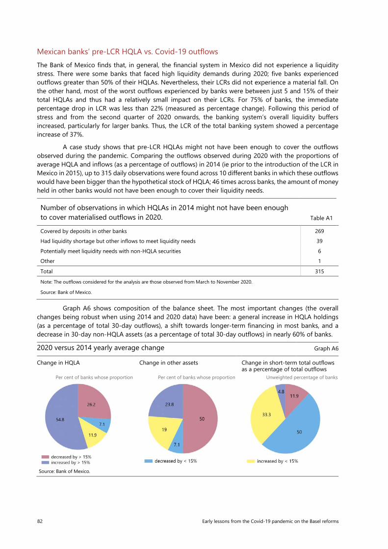
82 Early lessons from the Covid-19 pandemic on the Basel reforms
Mexican banks’ pre-LCR HQLA vs. Covid-19 outflows The Bank of Mexico finds that, in general, the financial system in Mexico did not experience a liquidity stress. There were some banks that faced high liquidity demands during 2020; five banks experienced outflows greater than 50% of their HQLAs. Nevertheless, their LCRs did not experience a material fall. On the other hand, most of the worst outflows experienced by banks were between just 5 and 15% of their total HQLAs and thus had a relatively small impact on their LCRs. For 75% of banks, the immediate percentage drop in LCR was less than 22% (measured as percentage change). Following this period of stress and from the second quarter of 2020 onwards, the banking system’s overall liquidity buffers increased, particularly for larger banks. Thus, the LCR of the total banking system showed a percentage increase of 37%.
A case study shows that pre-LCR HQLAs might not have been enough to cover the outflows observed during the pandemic. Comparing the outflows observed during 2020 with the proportions of average HQLA and inflows (as a percentage of outflows) in 2014 (ie prior to the introduction of the LCR in Mexico in 2015), up to 315 daily observations were found across 10 different banks in which these outflows would have been bigger than the hypothetical stock of HQLA; 46 times across banks, the amount of money held in other banks would not have been enough to cover their liquidity needs.
Number of observations in which HQLAs in 2014 might not have been enough to cover materialised outflows in 2020. Table A1
Covered by deposits in other banks 269
Had liquidity shortage but other inflows to meet liquidity needs 39
Potentially meet liquidity needs with non-HQLA securities 6
Other 1
Total 315
Note: The outflows considered for the analysis are those observed from March to November 2020.
Source: Bank of Mexico.
Graph A6 shows composition of the balance sheet. The most important changes (the overall changes being robust when using 2014 and 2020 data) have been: a general increase in HQLA holdings (as a percentage of total 30-day outflows), a shift towards longer-term financing in most banks, and a decrease in 30-day non-HQLA assets (as a percentage of total 30-day outflows) in nearly 60% of banks.
2020 versus 2014 yearly average change Graph A6
Change in HQLA Change in other assets Change in short-term total outflows as a percentage of total outflows
Per cent of banks whose proportion Per cent of banks whose proportion Unweighted percentage of banks
Source: Bank of Mexico.
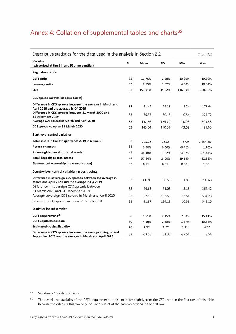
Early lessons from the Covid-19 pandemic on the Basel reforms 83
Annex 4: Collation of supplemental tables and charts85
Descriptive statistics for the data used in the analysis in Section 2.2 Table A2
Variable (winsorised at the 5th and 95th percentiles) N Mean SD Min Max
Regulatory ratios
CET1 ratio 83 13.76% 2.58% 10.30% 19.50% Leverage ratio 83 6.65% 1.87% 4.50% 10.84% LCR 83 153.01% 35.22% 116.00% 238.32%
CDS spread metrics (in basis points)
Difference in CDS spreads between the average in March and April 2020 and the average in Q4 2019 83 51.44 49.18 -1.24 177.64
Difference in CDS spreads between 31 March 2020 and 31 December 2019 83 66.35 60.15 0.54 224.72
Average CDS spread in March and April 2020 83 142.56 125.70 40.03 509.58 CDS spread value on 31 March 2020 83 143.54 110.09 43.69 425.08
Bank-level control variables
Total assets in the 4th quarter of 2019 in billion € 83 708.08 738.5 57.9 2,454.28 Return on assets 83 0.60% 0.56% -0.42% 1.70% Risk-weighted assets to total assets 83 48.48% 17.02% 24.97% 81.44% Total deposits to total assets 83 57.64% 18.00% 19.14% 82.83% Government ownership (no winsorisation) 83 0.11 0.31 0.00 1.00
Country-level control variables (in basis points)
Difference in sovereign CDS spreads between the average in March and April 2020 and the average in Q4 2019 83 41.71 58.55 1.89 209.63
Difference in sovereign CDS spreads between 31 March 2020 and 31 December 2019
83 46.63 71.03 -5.18 264.42
Average sovereign CDS spread in March and April 2020 83 92.83 132.56 12.56 534.23 Sovereign CDS spread value on 31 March 2020 83 92.87 134.12 10.38 543.25
Statistics for subsamples
CET1 requirement86 60 9.61% 2.15% 7.00% 15.11% CET1 capital headroom 60 4.36% 2.55% 1.67% 10.62% Estimated trading liquidity 78 2.97 1.22 1.21 4.37 Difference in CDS spreads between the average in August and September 2020 and the average in March and April 2020 82 -33.58 31.33 -97.54 8.54
85 See Annex 1 for data sources. 86 The descriptive statistics of the CET1 requirement in this line differ slightly from the CET1 ratio in the first row of this table
because the values in this row only include a subset of the banks described in the first row.

84 Early lessons from the Covid-19 pandemic on the Basel reforms
Regression specifications with either jurisdiction-level instead of continent-level fixed effects or alternative measurements of the CDS spreads metric as dependent variable Table A3
Difference Difference Level Level
Value in 2020 Average of March and April 31 March Average of
March and April 31 March
Value in 2019 Average of 4th quarter 31 December - -
CET1 ratio –9.14 *** –6.54 ** –5.23 –7.71
Leverage ratio 8.63 1.89 5.49 7.82
LCR 0.31 0.14 0.31 0.34
Size –5.04 –9.06 –15.42 –20.83
Return on assets 0.53 1.24 –9.72 –20.69
RWA to total assets –103.54 –33.99 –31.74 –73.49
Deposits to total assets –78.10 *** –96.36 ** –67.93 –84.98
Government ownership 5.84 45.24 ** 39.84 64.59
Sovereign CDS spreads1 0.33 * 0.73 0.54
Continent-group fixed effects No Yes Yes Yes Country fixed effects Yes No No No Adjusted R-squared 0.68 0.46 0.89 0.80
N 67 83 83 83
Note: Robust standard errors in all regressions. The symbols *, ** and *** denote statistical significance at 10%, 5% and 1%, respectively. 1 The sovereign CDS spread metric is calculated in accordance with the CDS spread metric that is used as dependent variable: either the difference or the level of the respective time periods is considered.
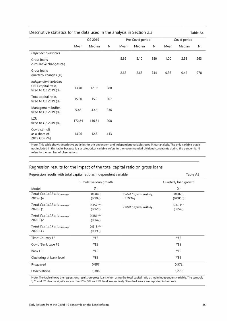
Early lessons from the Covid-19 pandemic on the Basel reforms 85
Descriptive statistics for the data used in the analysis in Section 2.3 Table A4
Q2 2019 Pre-Covid period Covid period
Mean Median N Mean Median N Mean Median N
Dependent variables
Gross loans cumulative changes (%)
5.89 5.10 380 1.00 2.53 263
Gross loans, quarterly changes (%) 2.68 2.68 744 0.36 0.42 978
Independent variables CET1 capital ratio, fixed to Q2 2019 (%) 13.70 12.92 288
Total capital ratio, fixed to Q2 2019 (%) 15.60 15.2 307
Management buffer, fixed to Q2 2019 (%) 5.48 4.45 236
LCR, fixed to Q2 2019 (%) 172.84 146.51 208
Covid stimuli, as a share of 2019 GDP (%)
14.06 12.8 413
Note: This table shows descriptive statistics for the dependent and independent variables used in our analysis. The only variable that is not included in this table, because it is a categorical variable, refers to the recommended dividend constraints during the pandemic. N refers to the number of observations.
Regression results for the impact of the total capital ratio on gross loans Regression results with total capital ratio as independent variable Table A5
Cumulative loan growth Quarterly loan growth
Model (1) (2) 𝑇𝑇𝐶𝐶𝐶𝐶𝑙𝑙𝐶𝐶 𝐶𝐶𝑙𝑙𝑝𝑝𝑖𝑖𝐶𝐶𝑙𝑙𝐶𝐶 𝑅𝑅𝑙𝑙𝐶𝐶𝑖𝑖𝐶𝐶2019−𝑄𝑄2 ⋅2019-Q4
0.0840 (0.103)
𝑇𝑇𝐶𝐶𝐶𝐶𝑙𝑙𝐶𝐶 𝐶𝐶𝑙𝑙𝑝𝑝𝑖𝑖𝐶𝐶𝑙𝑙𝐶𝐶 𝑅𝑅𝑙𝑙𝐶𝐶𝑖𝑖𝐶𝐶𝑡𝑡−⋅ 𝐶𝐶𝐶𝐶𝐶𝐶𝐶𝐶𝐶𝐶𝑡𝑡
0.0876 (0.0856)
𝑇𝑇𝐶𝐶𝐶𝐶𝑙𝑙𝐶𝐶 𝐶𝐶𝑙𝑙𝑝𝑝𝑖𝑖𝐶𝐶𝑙𝑙𝐶𝐶 𝑅𝑅𝑙𝑙𝐶𝐶𝑖𝑖𝐶𝐶2019−𝑄𝑄2 ⋅2020-Q1
0.357*** (0.120)
𝑇𝑇𝐶𝐶𝐶𝐶𝑙𝑙𝐶𝐶 𝐶𝐶𝑙𝑙𝑝𝑝𝑖𝑖𝐶𝐶𝑙𝑙𝐶𝐶 𝑅𝑅𝑙𝑙𝐶𝐶𝑖𝑖𝐶𝐶𝑡𝑡− 0.601** (0.249)
𝑇𝑇𝐶𝐶𝐶𝐶𝑙𝑙𝐶𝐶 𝐶𝐶𝑙𝑙𝑝𝑝𝑖𝑖𝐶𝐶𝑙𝑙𝐶𝐶 𝑅𝑅𝑙𝑙𝐶𝐶𝑖𝑖𝐶𝐶2019−𝑄𝑄2 ⋅2020-Q2
0.381*** (0.142)
𝑇𝑇𝐶𝐶𝐶𝐶𝑙𝑙𝐶𝐶 𝐶𝐶𝑙𝑙𝑝𝑝𝑖𝑖𝐶𝐶𝑙𝑙𝐶𝐶 𝑅𝑅𝑙𝑙𝐶𝐶𝑖𝑖𝐶𝐶2019−𝑄𝑄2 ⋅2020-Q3
0.518*** (0.199)
Time*Country FE YES YES
Covid*Bank type FE YES YES
Bank FE YES YES
Clustering at bank level YES YES
R-squared 0.887 0.572
Observations 1,386 1,279
Note: The table shows the regressions results on gross loans when using the total capital ratio as main independent variable. The symbols *, ** and *** denote significance at the 10%, 5% and 1% level, respectively. Standard errors are reported in brackets.

86 Early lessons from the Covid-19 pandemic on the Basel reforms
Evolution of aggregate central bank reserves over time Graph A7
(i) Japan (ii) Switzerland Trillion JPY Billion CHF
(iii) United Kingdom (iv) United States
Billion GBP Billion USD
Note: This figure shows the evolution of aggregate central bank reserves in four different jurisdictions in 2019 and 2020. The panels for Japan, the United Kingdom and the United States show national central bank reserves held by all banks. The panel for Switzerland shows both national and foreign central bank reserves held by all banks. Sources: Bank of Japan; Swiss National Bank; Bank of England; Federal Reserve Bank of New York.

Early lessons from the Covid-19 pandemic on the Basel reforms 87
Annex 5: Members of the Task Force on Evaluations
Co-chairs Mr Dominique Laboureix French Prudential Supervision and Resolution Authority
Ms Jing Yang Bank of Canada
The representatives in italics are members of technical issue sub-teams or provided analytical support at the Secretariat.
Belgium Ms Claire Renoirte National Bank of Belgium Brazil Mr Eduardo Carvalho de Castro Central Bank of Brazil Canada Ms Alexandra Lai
Mr David Xiao Chen Ms Alissa Gorelova
Bank of Canada
China Mr Qi Xiang China Banking and Insurance Regulatory Commission
France Mr Philippe Billard Ms Noemie Dentu Mr Thomas Ferriere
French Prudential Supervision and Resolution Authority
Germany Mr Alexander Schulz Deutsche Bundesbank Mr Daniel Foos Ms Kristin Hessberger Ms Carina Mössinger Mr Kamil Pliszka Mr Thomas Schmitz-Lippert Federal Financial Supervisory Authority (BaFin)
India Mr Vaibhav Chaturvedi Reserve Bank of India Italy Mr Marcello Bofondi Bank of Italy Japan Mr Hitoshi Sasaki Bank of Japan Mr Minoru Aosaki Financial Services Agency Korea Ms Ji Young Lee Bank of Korea Mr Kichul Suh Financial Supervisory Service Mexico Mr Jorge Luis García Ramírez
Ms Liduvina Cisneros Ruiz Bank of Mexico
Netherlands Mr Hans Brits Netherlands Bank Russia Mr Evgeny Rumyantsev Central Bank of the Russian Federation Saudi Arabia Ms Sara ALThenyan Saudi Arabian Monetary Authority Singapore Mr Kenneth Gay Monetary Authority of Singapore Spain Mr Gabriel Jiménez
Ms Rebeca Anguren Mr Diego Hernández
Bank of Spain
Sweden Mr Jonas Niemeyer Sveriges Riksbank

88 Early lessons from the Covid-19 pandemic on the Basel reforms
Switzerland Ms Maja Ganarin Wallmer Swiss National Bank Mr Tim Frech Swiss Financial Market Supervisory Authority FINMA Turkey Mr Uğur Dönmez Banking Regulation and Supervision Agency United Kingdom Mr Simon Hall
Mr Muhammad Anuar Ms Yuliya Baranova Ms Katie Low Mr Natan Misak Mr Tobias Neumann Mr George Speight Ms Quynh-Anh Vo
Bank of England (Covid-19 Workstream co-lead)
Mr Damien Lynch Ms Isabel Spirgel-Sinclair Mr Mahmoud Fatouh
Prudential Regulation Authority
United States Mr Missaka Warusawitharana
Ms Fang Du Mr Akos Horvath Mr Benjamin S Kay Mr Marco Goncalves Migueis Mr Timothy Mooney
Board of Governors of the Federal Reserve System (Covid-19 Workstream co-lead)
Mr Scott Nagel Mr Joseph Gunshor Ms Mona Jabbour Ms Irina Veksler Mr Phil Weed
Federal Reserve Bank of New York
Mr Peter Yen Federal Deposit Insurance Corporation Mr Mark Ginsberg Office of the Comptroller of the Currency
European Central Bank
Mr Markus Behn Ms Nadya Wildmann
ECB
Mr Florian Weidenholzer Mr Martin Vandervoort
ECB Single Supervisory Mechanism
Observers Mr Elöd Takáts Bank for International Settlements
Mr Lars Overby European Banking Authority Mr Rodrigo Coelho Mr Rachid Awad
Financial Stability Institute International Monetary Fund
Academic advisors Mr Viral V Acharya New York University Stern School of Business Mr Thorsten Beck The Business School, University of London
Mr Xavier Freixas Dargallo Universitat Pompeu Fabra, Barcelona

Early lessons from the Covid-19 pandemic on the Basel reforms 89
Secretariat Mr Skylar Brooks Ms Eléonore Huet Mr Olivier Prato Mr Page Conkling Mr Masaya Hatoma Mr Martin Birn Mr Sietse Bracke Ms Nadia Esham Ms Bettina Farkas Ms Anamaria Illes Ms Eleonora Scognamiglio Ms Huiming Yang Mr Markus Zoss
Bank of Canada French Prudential Supervision and Resolution Authority Bank for International Settlements
Related Documents