1 Early Environments and Child Outcomes: An Analysis Commission for the Independent Review on Poverty and Life Chances Elizabeth Washbrook Centre for Market and Public Organization, University of Bristol December 2010 The author thanks Debbie Lawlor, Cathy Chittleborough, Paul Gregg and Jane Waldfogel for their helpful discussions and advice. This project was partly supported by the ESRC funded project ‘The Impact of Family Socio-economic Status on Outcomes in Childhood and Adolescence’ (RES-060-23-0011).

Welcome message from author
This document is posted to help you gain knowledge. Please leave a comment to let me know what you think about it! Share it to your friends and learn new things together.
Transcript
1
Early Environments and Child Outcomes: An Analysis Commission for the Independent Review on Poverty and Life Chances
Elizabeth Washbrook
Centre for Market and Public Organization, University of Bristol
December 2010
The author thanks Debbie Lawlor, Cathy Chittleborough, Paul Gregg and Jane Waldfogel for their helpful
discussions and advice. This project was partly supported by the ESRC funded project ‘The Impact of
Family Socio-economic Status on Outcomes in Childhood and Adolescence’ (RES-060-23-0011).
2
Table of Contents
1. Project Overview 5
2. Millennium Cohort Study Data 9
2.1. The sample 9
2.2. Age five outcomes 10
2.2.1. BAS Cognitive z-score 10
2.2.2. SDQ Behaviour problems score 11
2.2.3. General ill-health rating 11
2.2.4. Body Mass Index (BMI) 12
2.2.5. Descriptive statistics 12
2.3. Key drivers 14
2.3.1. Mother’s age at the birth of the child 15
2.3.2. Parental educational qualifications 15
2.3.3. The home learning environment 15
2.3.4. Parental warmth and sensitivity 15
2.3.5. Authoritative parenting 15
2.3.6. Parental mental health and well-being 16
2.3.7. Health behaviours 16
2.3.8. Housing conditions 16
2.3.9. Preschool education 16
2.4. Baseline controls 16
2.5. Family characteristics 17
2.6. Age three outcomes 17
2.7. Low-income status 20
3
3. Millennium Cohort Study Findings 23
3.1. Explaining the variation in age five outcomes 23
3.2. Simulating outcomes with varying levels of the drivers 28
3.2.1. Methodology 28
3.2.2. Results for broad sets of predictors 30
3.2.3. Individual variables 36
4. ALSPAC Findings 39
4.1. The data 39
4.2. Explaining the variation in GCSE performance 43
4.3. Simulating GCSE performance with varying levels of the drivers 44
Appendix A: Methodology A1 Method 1. The proportion of variation in the outcome explained by
different predictors A1
Method 2. Simulations of the predicted outcome with varying
levels of the drivers A2
Estimation details A3
Appendix B: Descriptive statistics and detailed regressions A4 Table B1. Descriptive statistics and income gaps for MCS predictors A4
Table B2. Age five MCS outcome regressions A10
Table B3. ALSPAC descriptive statistics, income gaps and GCSE
regression coefficients A22
Appendix C: Variable construction A31
4
List of Figures and Tables
Table 2.1. Associations between BAS cognitive sub-scales 11 Table 2.2. Summary statistics for age five MCS outcomes, overall and by low-income status 12 Figure 2.1. Distributions of age five MCS outcome variables, by low-income status 13 Table 2.3. Pairwise correlations of age five MCS outcomes 14 Table 2.4. Summary statistics for age three MCS outcomes, overall and by low-income status 19 Table 2.5. Pairwise correlations of age three and age five MCS outcomes 19 Table 2.6. Household incomes in the MCS 21 Table 3.1. Proportion of the variation in age five outcomes explained by different sets of
predictors 23 Figure 3.1. Proportion of variation in the age five cognitive score explained by different sets
of predictors 25 Figure 3.2. Proportion of variation in the age five SDQ behaviour score explained by
different sets of predictors 26 Figure 3.3. Proportion of variation in the general ill-health scale explained by different sets
of predictors 27 Figure 3.4. Proportion of variation in body mass index explained by different sets of
predictors 28 Table 3.2. Simulated BAS cognitive scores of the average low-income child 31 Table 3.3. Simulated SDQ behaviour scores of the average low-income child 33 Table 3.4. Simulated general ill-health scale of the average low-income child 34 Table 3.5. Simulated body mass index of the average low-income child 35 Table 3.6. The contribution of individual variables to the income gap in age five
outcomes 36 Table 4.1. GCSE points scores 40 Figure 4.1. The distribution of average capped GCSE points scores in the maximum and
the estimation samples 41 Table 4.2. Summary statistics for average GCSE points score, overall and by
low-income status 41 Figure 4.2. The distribution of average capped GCSE points scores, by income
group 42 Table 4.3. Household incomes in ALSPAC 42 Figure 4.3. Proportion of variation in average capped GCSE points scorse explained by
different sets of predictors 44 Table 4.4. Simulated average GCSE points score of the average low-income child 45 Table 4.5. The contribution of individual variables to the income gap in the average
capped GCSE points score 46

5
1. Project Overview
The analysis in this report was commissioned by the Independent Review on Poverty and Life Chances to
inform its recommendations on the adoption of a set of official Life Chances Indicators. The aim of the
proposed indicators is to measure annual progress at a national level on a range of factors in young
children which we know to be predictive of children’s future outcomes, and so provide a metric for
assessing how successful we are as a country in making more equal life’s outcomes for all children.
The aims of the analysis are to:
Test the predictive power of the key drivers identified by the Review for children’s cognitive,
behavioural, social and emotional, and health outcomes at age five.
Model the extent to which varying the key drivers predicts the gap in children’s outcomes at age
five, between those from low income households and the mainstream.
Examine the association between indicators of children’s environments measured in the first
five years of life and their GCSE performance at the end of compulsory schooling.
The initial shortlist of key drivers identified by the Review after assessment of the evidence were:
Mother’s age at the birth of the child
Parental educational qualifications
The home learning environment
Parental warmth and sensitivity
Authoritative parenting
Parental mental health and well-being
Health behaviours
Housing conditions
Preschool education
The analysis draws on two data sources. First, predictors of age five outcomes are assessed using the
Millennium Cohort Study (MCS) – a nationally representative survey of around 19,000 children born in
the UK in 2000/01. This study tracks children through their early childhood years and covers a range of
topics, including: children’s cognitive and behavioural development and health; parenting; parents’
socio-demographic characteristics; income and poverty; as well as other factors. Second, early
predictors of educational achievement at age 16 are assessed using the Avon Longitudinal Study of
Parents and Children (ALSPAC) – a population-based survey of around 14,000 children born in the Avon
area of England in 1991/2. ALSPAC covers similar topics to the MCS in the first five years of life and has
6
the advantage that we can link these early measures to a crucial measure of educational achievement
assessed over a decade later1.
The analysis uses two complementary techniques to assess the predictive power of early life indicators
for children’s outcomes. The first contrasts the proportion of the variation in outcomes that can be
explained by alternative sets of predictor variables. Essentially different types of drivers are allowed to
‘compete’ for explanatory power in the hypothetical situation in which each sub-set of predictors is all
that is observed by the analyst about the child’s early environment. Since many of the predictor
variables are strongly inter-related there will a great degree of ‘overlap’ in the variation predicted by
different sets of variables.
The second technique adopts a conditional framework in which the predictive power of each variable is
estimated holding all other predictors constant and so isolates the independent predictive power of
each driver. These estimates are then used to simulate the predicted outcome of a low-income child
under different scenarios. The baseline scenario sets the values of the driver variables to the average
among low-income children (those in the poorest 20% of families), and so estimates the average
outcome of children in this group as they are observed in reality. Alternative scenarios then set the
values of the driver variables the average among higher-income children (those in the richest 80% of
families), and so estimate the predicted outcome of an average low-income child after an improvement
in each aspect of the early environment to the level experienced by children in the mainstream.
Section 2 sets out details of the Millennium Cohort Study dataset and they way it is used to measure the
age five outcomes and the key drivers of interest. Section 3 presents the results of the MCS analysis for
a range of outcomes at age five using the two methodologies described above and highlights key issues
of interpretation. The ALSPAC analysis in Section 4 utilizes many of the concepts and techniques laid out
in the previous two chapters so much of the previous discussion is not repeated. A brief introduction to
the ALSPAC data introduces the outcome measure of GCSE performance and highlights the key
differences between the two datasets before the presentation of results in the same format as the MCS
analysis.
The purpose of this report is to provide statistical evidence for the Review team to consider, with some
guide to its interpretation, rather than to provide over-arching recommendations. A key component of
the analysis is therefore the detailed tables of variable description provided in Appendices B and C,
which may be of less interest to the general reader. Nevertheless, some broad points do emerge from
the analysis. Overall, the analysis found that the key drivers – such as home learning environment,
mother’s educational qualifications, positive parenting, maternal mental health and mother’s age at
birth of first child – as well as demographic and family characteristics, explain a significant proportion of
the variance in children’s cognitive, behavioural, social and emotional, and general health outcomes at
1 For further information on the two datasets see the survey websites: www.bristol.ac.uk/alspac (ALSPAC) and
http://www.cls.ioe.ac.uk/studies.asp?section=000100020001 (MCS).
7
age five. While the majority of variance remains unexplained, these proportions are comparable with
similar types of analyses conducted in this area.
All of the key drivers were found to have some predictive power, although no single group could explain
the income-related gap in any of the outcomes at age five on its own. There were, however, some
differences in the relative importance of drivers across different outcomes. For example, parental
education and home learning environment emerged as relatively strong predictors of children’s
cognitive outcomes, while parental sensitivity and parental mental health were strong predictors of
children’s social and emotional outcomes. Varying the key drivers so that children from low income
households had levels comparable with the average for other children was found to predict virtually all
of the difference in children’s outcomes at age five. No single driver was found to predict these gaps,
rather, it was a result of the cumulative effect of varying all the key drivers.
Analysis of GCSE performance using the ALSPAC data shows that around 32% of the variation in
attainment at 16 can predicted on the basis of indicators observed at or before the age of five. Varying
the key drivers for low-income children to average levels experienced by the higher 80% of the income
distribution predicts an improvement of over six grades at GCSE in total, or around 60% of the observed
difference in GCSE performance between the low-income group and the rest.
While these findings are based on correlation and therefore should not be interpreted as causation, the
vast and diverse body of evidence showing similar findings to these gives us reason to think that many of
these connections are causal.
This project was conducted on a limited timescale in order to provide evidence for the Review.
However, it draws heavily on previous work conducted by the author and other colleagues, using the
MCS and ALSPAC data to analyze similar topics. Listed below are some key publications that discuss the
data and issues in more detail than is permitted here. All errors in this report are the author’s own.
Goodman, Alissa and Paul Gregg. Poorer children’s educational attainment: how important are attitudes
and behaviour? Joseph Rowntree Foundation, York, 2010. Available at:
http://www.jrf.org.uk/publications/educational-attainment-poor-children
Gregg, Paul, Carol Propper and Elizabeth Washbrook. Understanding the Relationship between Parental
Income and Multiple Child Outcomes: A Decomposition Analysis. CMPO Working Paper No. 08/193.
University of Bristol, 2008. Available at:
http://www.bris.ac.uk/cmpo/publications/papers/2008/wp193.pdf

8
Hobcraft, J. N. and Kiernan, K. E. Predictive factors from age 3 and infancy for poor child outcomes at age
5 relating to children’s development, behaviour and health: evidence from the Millennium Cohort Study.
University of York, 2010. Available at:
http://www.york.ac.uk/depts/spsw/staff/documents/HobcraftKiernan2010PredictiveFactorsChildrensD
evelopmentMillenniumCohort.pdf
Waldfogel, Jane and Elizabeth Washbrook. Income-related gaps in school readiness in the US and the UK:
An analysis of the mediating factors. Paper prepared for the IRP Conference on Intergenerational
Mobility (IGM) within and across Nations. University of Wisconsin–Madison, September 20-22, 2009.
Waldfogel, Jane and Elizabeth Washbrook. Low Income and Early Cognitive Development in the UK.
Report for the Sutton Trust. Sutton Trust, London, February 2010. Available at:
http://www.suttontrust.com/research/low-income-and-early-cognitive-development-in-the-uk/

9
2. Millennium Cohort Study Data
2.1. The sample
The Millennium Cohort Study (MCS) is a nationally representative sample of around 19,000 born in the
United Kingdom in 2000/01. Children eligible for inclusion in the MCS were those born between 1
September 2000 and 31 August 2001 (for England and Wales), and between 23 November 2000 and 11
January 2002 (for Scotland and Northern Ireland), alive and living in the UK at age nine months.
The geography of electoral wards was used as a sampling frame. The sample is clustered geographically
and disproportionately stratified to over-represent: (1) the three smaller countries of the UK (Wales,
Scotland and Northern Ireland); (2) areas in England with higher minority ethnic populations in 1991
(where at least 30 per cent of the population were Black or Asian); and (3) disadvantaged areas (drawn
from the poorest 25 per cent of wards based on the Child Poverty Index). A list of all nine month old
children living in the sampled wards was derived from Child Benefit records provided by the Department
of Social Security. Child Benefit claims cover virtually all of the child population except those ineligible
due to recent or temporary immigrant status.
The MCS surveyed cohort families three times, when the cohort members were roughly 9 months, 3
years and 5 years of age. Future sweeps are planned or released only recently and are not used in this
study. At each sweep there were separate questionnaires for the Main Carer and the Main Carer’s
partner (if present in the household). Interviews were carried out using computer-assisted personal
interview (CAPI) software on a laptop, and using a confidential computer-assisted self-completion
interview (CASI) for sensitive subjects. Direct child assessments of cognitive ability and anthropomorphic
measurements were carried out at sweeps 2 and 3.
In total 19,417 children participated in at least one of the first three sweeps of the MCS. The sample
used in this analysis is restricted to the 15,460 children (79.2% of the total) who participated in the third
sweep at age five. An additional sample selection criterion – that families have at least one valid
household income measure at any of the three waves (see below) – results in the exclusion of 205
children, leaving a maximum analysis sample of 15,255. Weights provided with the MCS data are used in
all analyses to provide nationally representative estimates. The weights correct both for the stratified
cluster sample design and for non-random attrition between sweeps.
The Millennium Cohort Study is funded by the Economic and Social Research Council and a consortium
of Government Departments headed by the Office for National Statistics (ONS). Data are publicly
available from the UK Data Archive.
10
The MCS is a very rich dataset and contains detailed measurements on a variety of aspects of the lives of
children and their families. This analysis distinguishes five broad types of variable, each of which is
described more fully in the following sections.
Age five outcomes
Key drivers
Baseline controls
Family characteristics
Age three outcomes
2.2. Age five outcomes
Analysis is conducted separately for four age five outcomes, reflecting the fact that development is
multi-dimensional and that drivers are likely to vary in their importance for cognitive, socio-emotional
and physical aspects of development.
2.2.1. BAS Cognitive z-score
The measure of cognitive ability is derived from three assessments from the British Ability Scales (BAS)
administered directly to the child by the MCS interviewer. The assessments were the Naming
Vocabulary scale, which measures verbal ability; the Picture Similarities scale, which measures pictorial
reasoning ability; and the Pattern Construction scale, which measures spatial ability. Each assessment
produces an ability score that reflects both the number of correct items and the difficulty of the items
administered (which responds to the child’s performance).
This analysis uses a combined score to facilitate comparison between cognitive development in general
and other aspects of development such as the socio-emotional and the physical. The three scores are
combined using principal components analysis (PCA), a technique that extracts a single index which
captures the maximum possible variation in the three scores. This index, which is normalized to mean
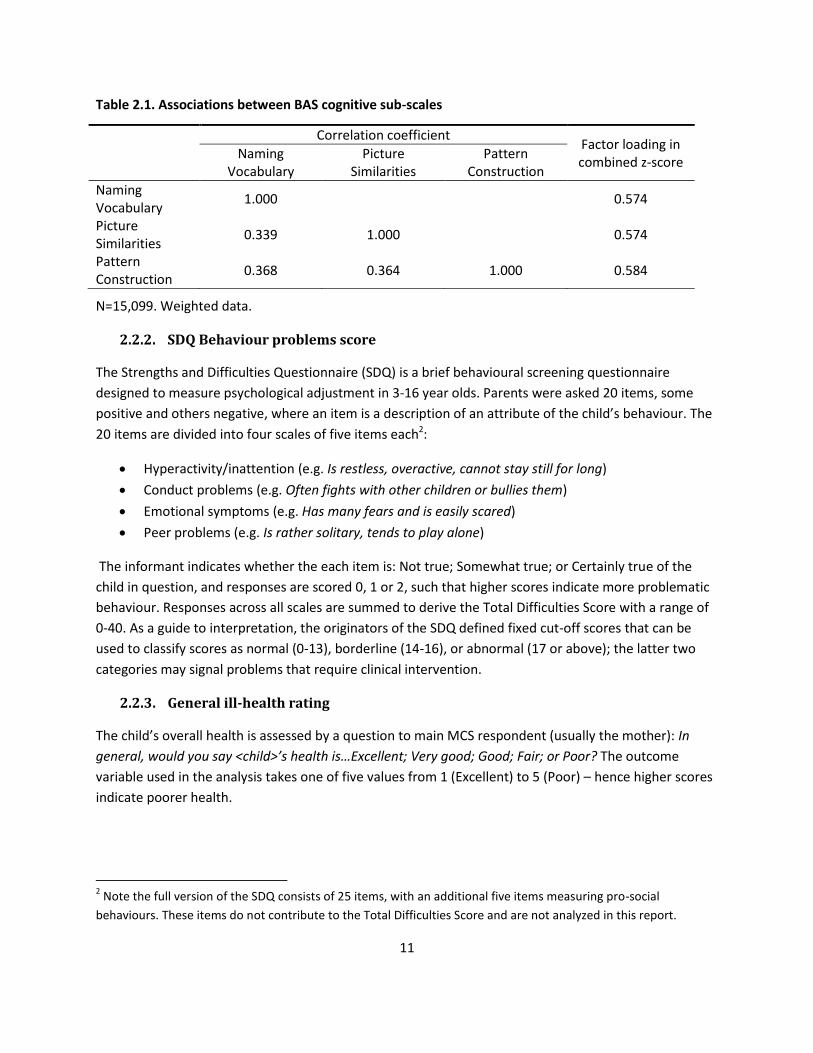
zero and unit variance, explains 58% of the total variation in the three scores. Table 2.1 shows the
correlation coefficient between each pair of ability scales and the PCA ‘factor loading’ which serves as a
weight for the scale in the construction of the combined index. It is clear that the three aspects of
cognitive ability are moderately positively correlated with one another, and make roughly equal
contributions to the combined cognitive index.
11
Table 2.1. Associations between BAS cognitive sub-scales
Correlation coefficient Factor loading in combined z-score
Naming Vocabulary
Picture Similarities
Pattern Construction
Naming Vocabulary
1.000 0.574
Picture Similarities
0.339 1.000 0.574
Pattern Construction
0.368 0.364 1.000 0.584
N=15,099. Weighted data.
2.2.2. SDQ Behaviour problems score
The Strengths and Difficulties Questionnaire (SDQ) is a brief behavioural screening questionnaire
designed to measure psychological adjustment in 3-16 year olds. Parents were asked 20 items, some
positive and others negative, where an item is a description of an attribute of the child’s behaviour. The
20 items are divided into four scales of five items each2:
Hyperactivity/inattention (e.g. Is restless, overactive, cannot stay still for long)
Conduct problems (e.g. Often fights with other children or bullies them)
Emotional symptoms (e.g. Has many fears and is easily scared)
Peer problems (e.g. Is rather solitary, tends to play alone)
The informant indicates whether the each item is: Not true; Somewhat true; or Certainly true of the
child in question, and responses are scored 0, 1 or 2, such that higher scores indicate more problematic
behaviour. Responses across all scales are summed to derive the Total Difficulties Score with a range of
0-40. As a guide to interpretation, the originators of the SDQ defined fixed cut-off scores that can be
used to classify scores as normal (0-13), borderline (14-16), or abnormal (17 or above); the latter two
categories may signal problems that require clinical intervention.
2.2.3. General ill-health rating
The child’s overall health is assessed by a question to main MCS respondent (usually the mother): In
general, would you say <child>’s health is…Excellent; Very good; Good; Fair; or Poor? The outcome
variable used in the analysis takes one of five values from 1 (Excellent) to 5 (Poor) – hence higher scores
indicate poorer health.
2 Note the full version of the SDQ consists of 25 items, with an additional five items measuring pro-social
behaviours. These items do not contribute to the Total Difficulties Score and are not analyzed in this report.
12
2.2.4. Body Mass Index (BMI)
Body Mass Index (BMI) is one of the most widely used methods for assessing body composition or
estimating levels of body fat. BMI is calculated by dividing an individual's weight (in kilograms) by their
height (in metres) squared and gives an indication of whether weight is in proportion to height. In
adults there are static cut off values for BMI among underweight, healthy weight, overweight and
obesity; however these are not appropriate for children. The healthy BMI range for children changes
substantially with age and is different between boys and girls. Interpretation of BMI values in children
therefore depends on comparison with age- and sex-specific growth reference charts. This analysis uses
the continuous measure of BMI as an indicator of the risk of childhood obesity.
2.2.5. Descriptive statistics
The maximum analysis sample consists of 15,255 children who participated in the age five wave of the
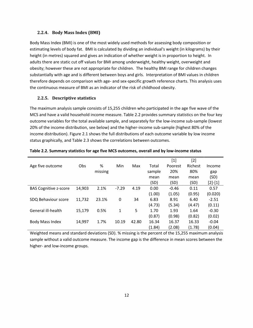
MCS and have a valid household income measure. Table 2.2 provides summary statistics on the four key
outcome variables for the total available sample, and separately for the low-income sub-sample (lowest
20% of the income distribution, see below) and the higher-income sub-sample (highest 80% of the
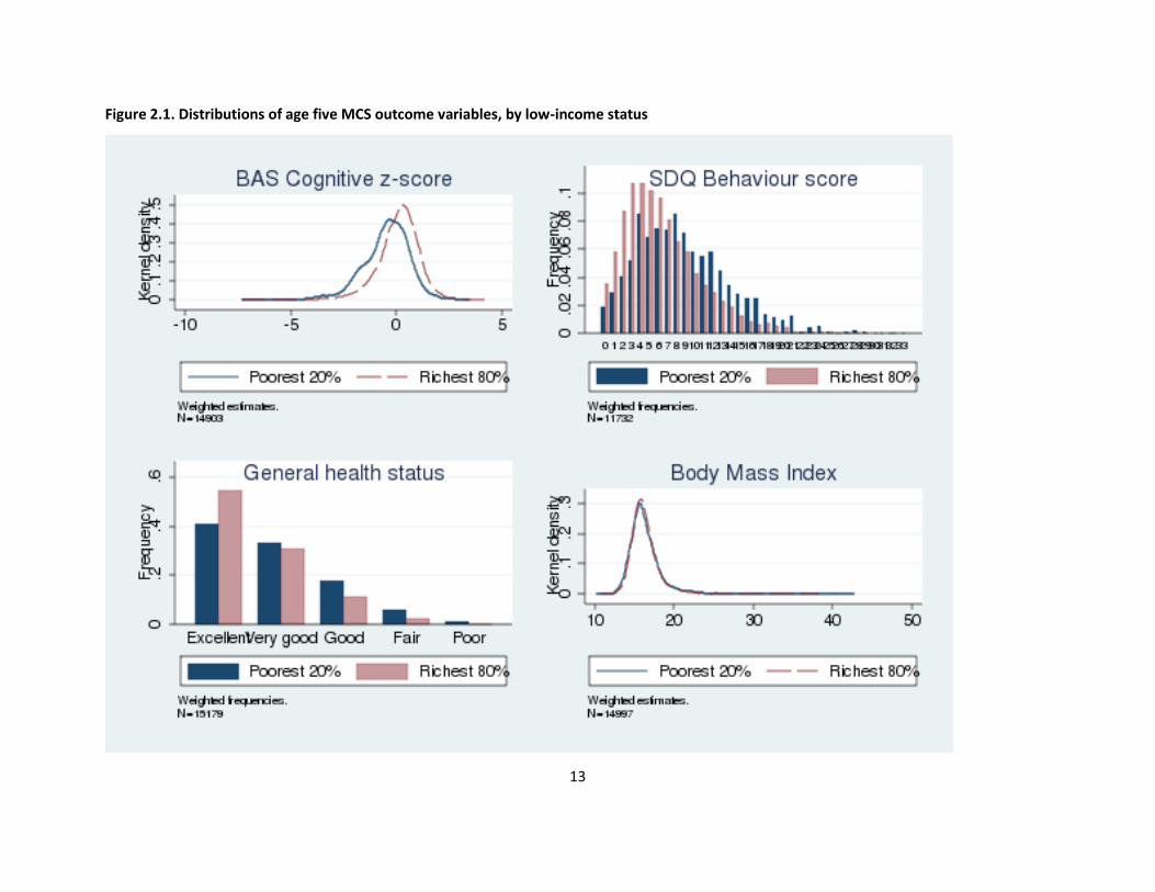
income distribution). Figure 2.1 shows the full distributions of each outcome variable by low income
status graphically, and Table 2.3 shows the correlations between outcomes.
Table 2.2. Summary statistics for age five MCS outcomes, overall and by low-income status
Age five outcome
Obs
%
missing
Min
Max
Total
sample mean (SD)
[1] Poorest
20% mean (SD)
[2] Richest
80% mean (SD)
Income
gap (SD)
[2]-[1]
BAS Cognitive z-score 14,903 2.1% -7.29 4.19 0.00 (1.00)
-0.46 (1.05)
0.11 (0.95)
0.57 (0.020)
SDQ Behaviour score 11,732 23.1% 0 34 6.83 (4.73)
8.91 (5.34)
6.40 (4.47)
-2.51 (0.11)
General ill-health 15,179 0.5% 1 5 1.70 (0.87)
1.93 (0.98)
1.64 (0.82)
-0.30 (0.02)
Body Mass Index 14,997 1.7% 10.19 42.80 16.34 (1.84)
16.37 (2.08)
16.33 (1.78)
-0.04 (0.04)
Weighted means and standard deviations (SD). % missing is the percent of the 15,255 maximum analysis
sample without a valid outcome measure. The income gap is the difference in mean scores between the
higher- and low-income groups.
13
Figure 2.1. Distributions of age five MCS outcome variables, by low-income status
14
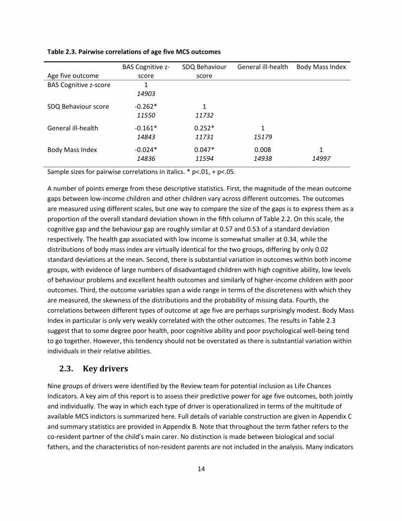
Table 2.3. Pairwise correlations of age five MCS outcomes
Age five outcome
BAS Cognitive z-score
SDQ Behaviour score
General ill-health Body Mass Index
BAS Cognitive z-score 1 14903
SDQ Behaviour score -0.262* 1 11550 11732
General ill-health -0.161* 0.252* 1 14843 11731 15179
Body Mass Index -0.024* 0.047* 0.008 1 14836 11594 14938 14997
Sample sizes for pairwise correlations in italics. * p<.01, + p<.05.
A number of points emerge from these descriptive statistics. First, the magnitude of the mean outcome
gaps between low-income children and other children vary across different outcomes. The outcomes
are measured using different scales, but one way to compare the size of the gaps is to express them as a
proportion of the overall standard deviation shown in the fifth column of Table 2.2. On this scale, the
cognitive gap and the behaviour gap are roughly similar at 0.57 and 0.53 of a standard deviation
respectively. The health gap associated with low income is somewhat smaller at 0.34, while the
distributions of body mass index are virtually identical for the two groups, differing by only 0.02
standard deviations at the mean. Second, there is substantial variation in outcomes within both income
groups, with evidence of large numbers of disadvantaged children with high cognitive ability, low levels
of behaviour problems and excellent health outcomes and similarly of higher-income children with poor
outcomes. Third, the outcome variables span a wide range in terms of the discreteness with which they
are measured, the skewness of the distributions and the probability of missing data. Fourth, the
correlations between different types of outcome at age five are perhaps surprisingly modest. Body Mass
Index in particular is only very weakly correlated with the other outcomes. The results in Table 2.3
suggest that to some degree poor health, poor cognitive ability and poor psychological well-being tend
to go together. However, this tendency should not be overstated as there is substantial variation within
individuals in their relative abilities.
2.3. Key drivers
Nine groups of drivers were identified by the Review team for potential inclusion as Life Chances
Indicators. A key aim of this report is to assess their predictive power for age five outcomes, both jointly
and individually. The way in which each type of driver is operationalized in terms of the multitude of
available MCS indictors is summarized here. Full details of variable construction are given in Appendix C
and summary statistics are provided in Appendix B. Note that throughout the term father refers to the
co-resident partner of the child’s main carer. No distinction is made between biological and social
fathers, and the characteristics of non-resident parents are not included in the analysis. Many indicators

15
are observed at more than one wave and repeat measures are included separately in the analysis
wherever possible.
2.3.1. Mother’s age at the birth of the child
Five categories: less than 20; 20 to 24; 25 to 29; 30 to 34; 35 and over.
2.3.2. Parental educational qualifications
Mother’s and father’s highest qualification, measured when the child is five years old. Six categories per
parent: None; Overseas qualifications only; NVQ1 (GCSE D-G); NVQ2 (GCSE A-C); NVQ3 (A-level);
NVQ4/5 (Degree).
2.3.3. The home learning environment
Frequency someone at home tries to teach the child the alphabet, songs/poems/rhymes, or counting;
Number of days a week mother and father read to child; Number of times a week mother and father
engage in creative activities with child (drawing/painting, musical activities, telling stories not from a
book); Number of times a week mother and father engage in play activities with child (playing physically
active games, playing with games/toys indoors, taking child to the park/playground); Interviewer
observation of whether the home environment is safe, clean, light and uncluttered; Number of library
visits in a typical month; Child attends a weekly organized sporting activity; Number of places child has
visited in the last year (of play/concert, gallery/museum, zoo, cinema, professional sporting event,
theme park).
2.3.4. Parental warmth and sensitivity
Mother’s and father’s scores on the 15-item self-complete Pianta Parent-Child Relationship scale
(assesses the degree of warmth and conflict in parent-child interactions); Number of positive mother-
child interactions observed by interviewer (derived from 11 items, e.g. Mother conversed with child at
least twice during visit); Mother’s and father’s attitudes to child-rearing (derived from 5 items capturing
preferences for structured versus more laissez-faire child-rearing style, e.g. Babies should be picked up
whenever they cry).
2.3.5. Authoritative parenting
Child usually or always has regular bedtimes, child usually or always has regular mealtimes; Parent
makes sure child obeys instructions or requests more than half the time; Frequency of non-violent
disciplinary behaviours (sending child to room, taking away treats, telling child off); Frequency of harsh
disciplinary behaviours (smacking child, ignoring child, shouting at child); Child watches more than 3
hours of TV per day; Child plays computer games more than one hour per day.

16
2.3.6. Parental mental health and well-being
Mother’s and father’s self-rated mental health (Malaise scale at MCS Wave 1, Kessler 6 scale at Waves 2
and 3); Mother and father ever diagnosed by a doctor with depression/anxiety; Mother’s self esteem
(Modified Rosenberg Self Esteem scale); Mother’s locus of control (derived from 3 items assessing how
far the respondent feels in control of her life); Mother’s social support (derived from 3 items assessing
self-perceptions of emotional, instrumental and financial support available to the mother); Mother’s life
satisfaction (rating on a 10-point scale of how satisfied the mother is with the way her life has turned
out so far).
2.3.7. Health behaviours
Health at birth (birth weight, gestation length, placement in Special Care Unit); duration of breast
feeding (Never, less than 6 months, more than 6 months); health care utilization (mother received
prenatal care in the first trimester, baby had all immunizations by 9 months); Mother smoked in
pregnancy (none, less than 10 a day, 10 a day or more); Anyone smokes in same room as child; Mother
and father drink alcohol 3 times a week or more; Mother’s and father’s number of symptoms of
problem drinking; Mother and father used recreational drugs since birth of child; Mother and father
overweight (BMI of 25 or more) or obese (BMI of 30 or more).
2.3.8. Housing conditions
At least one room in home per person at all MCS waves; home has central heating at all waves, home
free of damp at all waves, child has access to a garden at all waves, local area has a safe place for
children to play (mother report).
2.3.9. Preschool education
Child attended nursery class/nursery school, preschool or playgroup; attended day nursery; and
attended childminder before age 5; Age at which child first attended early education; first attended day
nursery; and first attended childminder (censored at 5 years); Child ever attended early education
provider full-time (roughly more than 15 hours per week).
2.4. Baseline controls
The key drivers are the focus of this analysis, but we can also observe other family characteristics that
are likely to be correlated with both child outcomes and the drivers of interest. Two sets of other
predictors are included in the analysis which help to isolate the predictive power of the focal drivers
from other correlated influences.
A restricted set of baseline predictors are included in all models and their predictive power forms the
minimum against which the power of other predictors is evaluated. They are
Child’s gender
17
A cubic polynomial in age in months at assessment
Binary indicators for single parent family at the three MCS waves (9 months, 3 years and 5 years)
Child gender and age are important determinants of child outcomes, but factors that are beyond the
family’s control. The inclusion of number of parents in the baseline is necessary because many of the
drivers of interest relate to the characteristics of resident fathers. Since around one in five children do
not have a resident father, these controls are needed to avoid confusing the predictive power of
different paternal characteristics with the simple presence or absence of a father figure.
2.5. Family characteristics
The second set of additional predictors are referred to as family characteristics. They are:
Child’s race/ethnicity (White; Pakistani; Bangladeshi; Indian; Other Asian; Black Caribbean; Black
African; Mixed; Other)
Parental place of birth and language spoken in the home (mother born outside UK; father born
outside UK; primary language spoken in the home mostly or entirely language other than
English)
Parental disability (mother and father have any longstanding illness, disability or infirmity; have
a longstanding illness that limits activities)
Country and region (UK country and government office region at birth)
Local area deprivation (Decile group of the Index of Multiple Deprivation (IMD))
Social housing tenure (Child ever lived in council or housing association rented home at any of
the three MCS waves; Child always lived in social housing at all three MCS waves)
Disposable household income (Log of equivalized disposable household income averaged over
the three MCS waves)
It is clear that, as markers of a family’s social and cultural resources, many of these variables will have
role in shaping the drivers of interest. Their inclusion in the analysis allows us to test whether broad
demographic characteristics – ‘who parents are’ – are more or less predictive of outcomes as the focal
drivers – indicators of ‘what parents do’. In addition, when we conduct simulations of the outcomes of
low-income children after the key drivers are varied we are able to statistically ‘hold constant’ these
characteristics, many of which are hard or impossible to shift via conventional policy mechanisms.
2.6. Age three outcomes
We are also interested in the predictive power of children’s outcomes at age three, two years prior to
the final outcome assessments. Prior outcomes, however, are a very different class of predictor from the

18
drivers and family characteristics, and change the interpretation of the model dramatically. Age five
outcomes reflect the combination of developmental ability as it is crystallized at age three and
developmental progress in the following two years. Many of the influences that affect the earlier
outcome will also affect its subsequent trajectory. Conceiving of a process in which those influences can
vary while intermediate outcomes are held fixed, or in which intermediate outcomes vary but
environmental influences remain unchanged is hypothetical and potentially misleading. The inclusion of
age three outcomes does, however, help to throw light on the age at which disparities associated with
different predictors become ‘embedded’ in the developmental process. For this reason two sets of
estimates are provided in the analysis: a ‘levels’ model that excludes age three outcomes as predictors
and a ‘value-added’ model that includes them. The first assesses the total association between the
predictors and age five outcomes, regardless of when the influences are manifest; the second assesses
the influences of the predictors on trajectories between three and five in the scenario that age three
outcomes are fixed.
Age three outcomes included in the value-added models are:
BAS Naming Vocabulary score (identical to one of the three sub-scales that go to make up the
age five BAS cognitive z-score)
Bracken School Readiness Assessment (measures 88 functionally relevant educational concepts
in six sub-tests: Colours; Letters; Numbers/Counting; Shapes; Comparisons; Shapes).
SDQ Behaviour score (the Total Difficulties score, identical to the age five measure)
Body Mass Index (identical to the age five measure)
Note, the Picture Similarities, Pattern Construction and general health measures were not administered
at age three, and the Bracken School Readiness Assessment was not administered at age five.
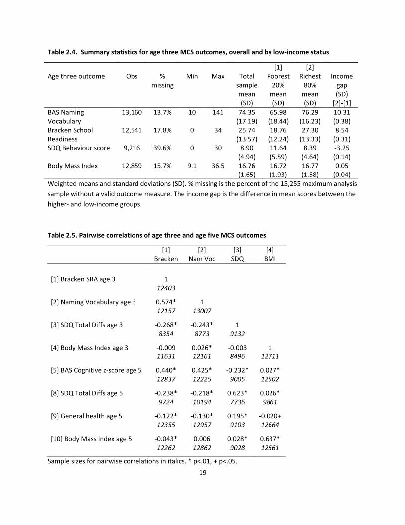
Table 2.4 shows summary statistics for the age three outcomes. Expressing the income gaps as a
proportion of the total sample standard deviation gives estimates of 0.60 for Naming Vocabulary, 0.63
for the Bracken, 0.66 for the SDQ and a (statistically insignificant) difference of 0.03 of a standard
deviation in BMI in the favour of low-income children. Expressed this way the income gaps in cognitive
and behaviour outcomes are slightly larger at age three than age five, but note that the cognitive scales
are not comparable over time. Nevertheless it is clear that substantial disparities in developmental
outcomes by household income are already apparent by age three.
19
Table 2.4. Summary statistics for age three MCS outcomes, overall and by low-income status
Age three outcome
Obs
%
missing
Min
Max
Total
sample mean (SD)
[1] Poorest
20% mean (SD)
[2] Richest
80% mean (SD)
Income
gap (SD)
[2]-[1]
BAS Naming Vocabulary
13,160 13.7% 10 141 74.35 (17.19)
65.98 (18.44)
76.29 (16.23)
10.31 (0.38)
Bracken School Readiness
12,541 17.8% 0 34 25.74 (13.57)
18.76 (12.24)
27.30 (13.33)
8.54 (0.31)
SDQ Behaviour score 9,216 39.6% 0 30 8.90 (4.94)
11.64 (5.59)
8.39 (4.64)
-3.25 (0.14)
Body Mass Index 12,859 15.7% 9.1 36.5 16.76 (1.65)
16.72 (1.93)
16.77 (1.58)
0.05 (0.04)
Weighted means and standard deviations (SD). % missing is the percent of the 15,255 maximum analysis
sample without a valid outcome measure. The income gap is the difference in mean scores between the
higher- and low-income groups.
Table 2.5. Pairwise correlations of age three and age five MCS outcomes
[1] Bracken
[2] Nam Voc
[3] SDQ
[4] BMI
[1] Bracken SRA age 3 1
12403
[2] Naming Vocabulary age 3 0.574* 1
12157 13007
[3] SDQ Total Diffs age 3 -0.268* -0.243* 1
8354 8773 9132
[4] Body Mass Index age 3 -0.009 0.026* -0.003 1
11631 12161 8496 12711
[5] BAS Cognitive z-score age 5 0.440* 0.425* -0.232* 0.027*
12837 12225 9005 12502
[8] SDQ Total Diffs age 5 -0.238* -0.218* 0.623* 0.026*
9724 10194 7736 9861
[9] General health age 5 -0.122* -0.130* 0.195* -0.020+
12355 12957 9103 12664
[10] Body Mass Index age 5 -0.043* 0.006 0.028* 0.637*
12262 12862 9028 12561
Sample sizes for pairwise correlations in italics. * p<.01, + p<.05.
20
Table 2.5 provides the correlations among the age three outcome measures, and between them and the
age five outcomes. It is notable that vocabulary and the Bracken are strongly positively correlated, and
that correlations ‘within domains’ over time are much higher than correlations between domains. The
own correlations between SDQ and BMI at three and five are .62 and .64 respectively, indicating a lot of
persistence in skills and abilities over the two-year period.
2.7. Low-income status
The simulation analysis conducted below is based on the difference in the early environments between
the poorest 20% of children and other children. It is useful, therefore, to gain some sense of how this
group is defined and of how their incomes compare to the rest of the population.
The key income measure is derived from the question – asked to the main respondent in each if the 9-
month, 3-year and 5-year MCS Waves - Which of the groups on this card represents you [^and your
husband/wife]'s total take-home income from all these sources and earnings, after tax and other
deductions? Respondents were given a choice of 19 bands, with different values presented to single
parents and those in a couple. A representative value for each band was assigned using calculations
from the Family Resources Survey, and values were deflated to 2008 pounds using the annual All Items
RPI. Incomes were equivalized using the modified OECD scale, with a couple with no children as the
reference case (i.e. given a weight of one). A simple average of values from each of the three MCS waves
was calculated. Where households did not have three valid observations (36% of the age 5 sample),
averages were taken over the one or two observations available. Finally, this average income measure
was used to divide families into five equal size groups (quintiles) over the age five sample using the
survey weights.
Table 2.6 gives summary statistics on the final income measure, overall and by income quintile. The key
variable used in much of this analysis is the quintile 1 dummy, which we refer to as indicating low
income. Table 2.6 shows that this is defined as families with an average equivalized net annual
disposable income over the period of the survey of less than £8564 in 2008 prices. This cut-off is low.
The relative poverty lines over the MCS survey years (60% median equivalized disposable income BHC)
in 2008 prices range from £12106 in 2001 to £12605 in 2007. Imposing one of these lines as the
threshold of low-income would result in roughly one-third of all MCS families being classed as poor.

21
Table 2.6. Household incomes in the MCS
Obs Mean Std. Dev. Min Max
Total age five sample 15255 20848 15351 548 107461
Income quintile 1 (‘Low income’) 3445 6152 1690 548 8563
Income quintile 2 3301 11125 1589 8564 13967
Income quintile 3 2952 17079 1824 13970 20303
Income quintile 4 2892 24666 2748 20304 29825
Income quintile 5 2665 45232 15193 29825 107461
Income quintiles 2-5 (‘Higher income’) 11810 24493 15051 8564 107461
Note. Incomes are average equivalized annual net income in 2008 prices. Quintile groups correspond to
20% of the weighted distributions, hence the unequal distribution of unweighted observations shown
above.
There are several reasons why incomes in the MCS appear low:
The way the income question is phrased (above) makes it likely that respondents will not include
non-cash benefits in their total income, such as housing benefit, council tax benefit and free
school meals. These do, however, contribute to the HBAI definition of income used to calculate
official relative poverty rates.
Against this is the fact that the MCS surveys only young families who because of their stage in
the life cycle tend to have lower incomes than all families with children. Maternal incomes are
likely to be particularly low in the first wave as many are on maternity leave.
All income numbers are equivalized to the income of a couple with no children. The vast
majority of MCS families will have had actual incomes that are larger than this. (Though this
does not affect the poverty line calculations.)
The comparison with poverty lines is slightly misleading as that criterion is applied to incomes in
a single year. Here we average over incomes measured over a 4-5 year period. Note that this
should result in less families being classed as poor because transitory periods of low income will
be averaged out. Our measure is more akin to a measure of long-run or persistent poverty.
However, a check of incomes in each specific year against the relevant poverty line also suggests
somewhere around a third of families in each survey wave are classed as poor, though they will
not be the same families in every wave.
The incomes of the richest families will be underestimated because of the top-coding of the
highest income bracket. Again, this will have little effect on who is classed as poor at the other
end of the income distribution.

22
The reference group for calculating the income-related gap in predictors is all families above the £8563
cut-off – those in quintiles 2 to 5. These families had an average income of around £24500, roughly four
times the average income of the quintile 1 group.
23
3. Millennium Cohort Study Findings
3.1. Explaining the variation in age five outcomes
The first method used to assess the predictive power of different sets of predictors is to compare the
proportion of the total variation in the outcome they explain when added individually to a common
baseline model. Intuitively we compare the variability in the outcomes we would predict for children on
the basis of their observed characteristics with the variability in the outcomes we observe in reality. The
statistic used for this comparison is the adjusted R-squared from a linear regression. A standard R-
squared takes values between 0 and 1, with 0 indicating that none of the variation is explained at all,
and 1 indicating a ‘perfect fit’ in which the predicted outcome for each child coincides exactly with their
actual outcome. The adjusted R-squared is a slight modification to this statistic in which predictive
power is adjusted for the number of explanatory variables (see Appendix A for more details).
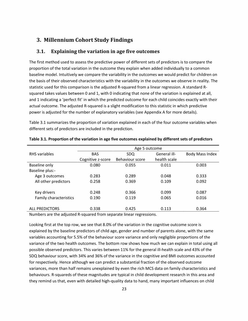
Table 3.1 summarizes the proportion of variation explained in each of the four outcome variables when
different sets of predictors are included in the prediction.
Table 3.1. Proportion of the variation in age five outcomes explained by different sets of predictors
Age 5 outcome
RHS variables BAS Cognitive z-score
SDQ Behaviour score
General ill-health scale
Body Mass Index
Baseline only 0.080 0.055 0.011 0.003 Baseline plus:-
Age 3 outcomes 0.283 0.289 0.048 0.333 All other predictors 0.258 0.369 0.109 0.092 Key drivers 0.248 0.366 0.099 0.087 Family characteristics 0.190 0.119 0.065 0.016
ALL PREDICTORS 0.338 0.425 0.113 0.364
Numbers are the adjusted R-squared from separate linear regressions.
Looking first at the top row, we see that 8.0% of the variation in the cognitive outcome score is
explained by the baseline predictors of child age, gender and number of parents alone, with the same
variables accounting for 5.5% of the behaviour score variance and only negligible proportions of the
variance of the two health outcomes. The bottom row shows how much we can explain in total using all
possible observed predictors. This varies between 11% for the general ill-health scale and 43% of the
SDQ behaviour score, with 34% and 36% of the variance in the cognitive and BMI outcomes accounted
for respectively. Hence although we can predict a substantial fraction of the observed outcome
variances, more than half remains unexplained by even the rich MCS data on family characteristics and
behaviours. R-squareds of these magnitudes are typical in child development research in this area and
they remind us that, even with detailed high-quality data to hand, many important influences on child
24
development will inevitably be unobserved or mismeasured. Put another way, children with identical
observable characteristics will still end up with very different outcomes.
The second and third rows contrast the proportion of variance explained when a) the four age three
outcomes, and b) all other predictors (all the drivers and family characteristics) are added separately to
the baseline model. The inclusion of age three outcomes as predictors for the cognitive outcome
increases the proportion explained sharply from 8% to 28.3%. Without knowledge of age three
outcomes, all the other predictors combined can explain 25.8% of the cognitive outcome variation. In
one sense, therefore, knowing only the values of the child’s four outcomes at age three gives a better
prediction of his or her cognitive outcome at five than knowing all the many other driver and predictor
variables taken from the survey data. These two types of predictor are highly correlated however.
Adding age three outcomes to a model including all other available predictors increases the explained
variation in the cognitive outcome from 25.8% to 33.8%, an increase of 8 percentage points, while
adding other available predictors to a model including age three outcomes also increases the explained
variation, from 28.3 to 33.8% or by 5.5 percentage points. Although there is a high degree of overlap,
therefore, both types of information can be said to have independent predictive power.
The relative power of age three outcomes and other predictors varies somewhat for the other outcome
types. Age three outcomes are relatively less accurate predictors of behaviour problems and general
health than other factors (although recall that general health is not one of the observed age three
measures). For body mass index, however, age three outcomes predict three times the variance
predicted by the other variables, with most of this coming from the strong persistence in body mass
index over time shown in Table 2.5. In all cases the two types of predictor contain independent but
strongly overlapping information, as is illustrated the fact that the proportion explained by all predictors
in total is greater than the proportion explained by one type alone, but much less than the sum of
adjusted R-squareds from the two restricted regressions. This is to be expected: many of the factors that
influence development by age five will be partly ‘captured’ by outcomes at age three, but equally
idiosyncratic individual differences in development not predicted by the other variables will tend to
persist over time.
The fourth and fifth rows of Table 3.1 compare the relative predictive power of the set of key drivers in
total with the set of family characteristics. Family characteristics as a group are relatively strong
predictors of outcomes, but again are highly correlated with the drivers of interest. For example, family
characteristics can explain 19% of the variation in the cognitive outcome when added individually to the
baseline model but, starting from a situation in which all key drivers are observed, additional knowledge
of family characteristics only increases the explained variance by one percentage point – from 24.8% to
25.8%. A similar pattern can be seen for the other three outcomes. This emphasizes that indicators of
‘who parents are’, that is broad indicators of their socio-economic resources, are predictive of outcomes
largely because they are correlated with ‘what parents do’ in terms of the early environments they
create for their children. If we can characterize the child’s environment in terms of the observed key
drivers then knowledge of a family’s characteristics improves our prediction of the child’s outcome only
slightly.
25
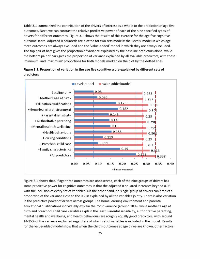
Table 3.1 summarized the contribution of the drivers of interest as a whole to the prediction of age five
outcomes. Next, we can contrast the relative predictive power of each of the nine specified types of
drivers for different outcomes. Figure 3.1 shows the results of this exercise for the age five cognitive
outcome score. Adjusted R-squareds are plotted for two sets models: the ‘levels’ model in which age
three outcomes are always excluded and the ‘value-added’ model in which they are always included.
The top pair of bars gives the proportion of variance explained by the baseline predictors alone, while
the bottom pair of bars gives the proportion of variance explained by all available predictors, with these
‘minimum’ and ‘maximum’ proportions for both models marked on the plot by the dotted lines.
Figure 3.1. Proportion of variation in the age five cognitive score explained by different sets of
predictors
Figure 3.1 shows that, if age three outcomes are unobserved, each of the nine groups of drivers has
some predictive power for cognitive outcomes in that the adjusted R-squared increases beyond 0.08
with the inclusion of every set of variables. On the other hand, no single group of drivers can predict a
proportion of the variance close to the 0.258 explained by all the variables jointly. There is also variation
in the predictive power of drivers across groups. The home learning environment and parental
educational qualifications individually explain the most variance (around 18%), while mother’s age at
birth and preschool child care variables explain the least. Parental sensitivity, authoritative parenting,
mental health and wellbeing, and health behaviours are roughly equally good predictors, with around
14-15% of the variance explained regardless of which set of variables is included in the model. Results
for the value-added model show that when the child’s outcomes at age three are known, other factors
26
have a much more marginal impact on the fit of the model. The home learning environment and
parental qualifications are again the two types of driver that add the most predictive power, but in this
case only increase the adjusted R-squared over the baseline by around 2 percentage points. Finally, it is
noticeable that of any single group, family characteristics increase the explained variance by the most in
both the levels and value-added models. As discussed previously it is likely that these characteristics are
associated with all the types of drivers as they shape the social and cultural environment in which the
family operates. It is plausible, therefore, that they act as ‘summary measures’ and their strong
predictive power reflects their correlation with a large number of different environmental factors.
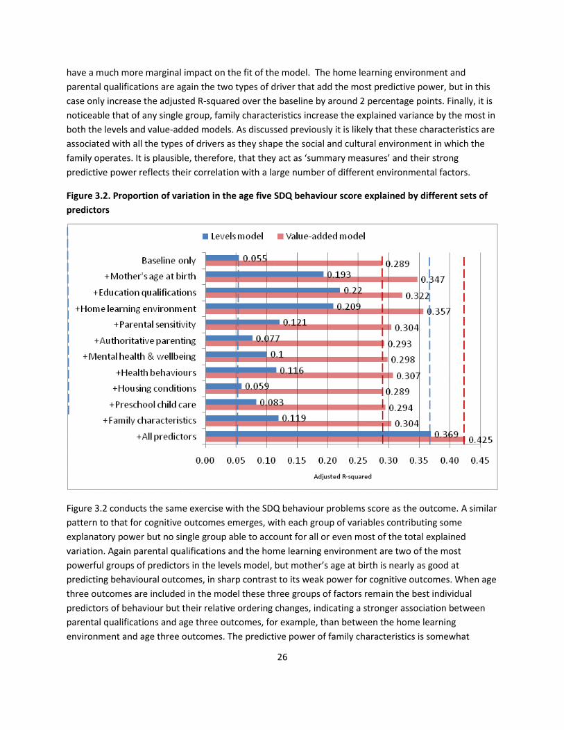
Figure 3.2. Proportion of variation in the age five SDQ behaviour score explained by different sets of
predictors
Figure 3.2 conducts the same exercise with the SDQ behaviour problems score as the outcome. A similar
pattern to that for cognitive outcomes emerges, with each group of variables contributing some
explanatory power but no single group able to account for all or even most of the total explained
variation. Again parental qualifications and the home learning environment are two of the most
powerful groups of predictors in the levels model, but mother’s age at birth is nearly as good at
predicting behavioural outcomes, in sharp contrast to its weak power for cognitive outcomes. When age
three outcomes are included in the model these three groups of factors remain the best individual
predictors of behaviour but their relative ordering changes, indicating a stronger association between
parental qualifications and age three outcomes, for example, than between the home learning
environment and age three outcomes. The predictive power of family characteristics is somewhat
27
weaker for behaviour than for cognitive outcomes and tells us less about a child’s likely behaviour
outcomes at age five than, for example, knowledge of the home learning environment.
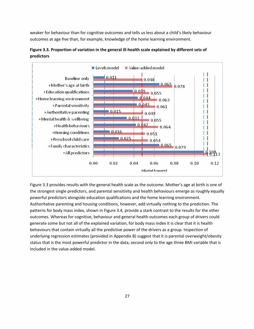
Figure 3.3. Proportion of variation in the general ill-health scale explained by different sets of
predictors
Figure 3.3 provides results with the general health scale as the outcome. Mother’s age at birth is one of
the strongest single predictors, and parental sensitivity and health behaviours emerge as roughly equally
powerful predictors alongside education qualifications and the home learning environment.
Authoritative parenting and housing conditions, however, add virtually nothing to the prediction. The
patterns for body mass index, shown in Figure 3.4, provide a stark contrast to the results for the other
outcomes. Whereas for cognitive, behaviour and general health outcomes each group of drivers could
generate some but not all of the explained variation, for body mass index it is clear that it is health
behaviours that contain virtually all the predictive power of the drivers as a group. Inspection of
underlying regression estimates (provided in Appendix B) suggest that it is parental overweight/obesity
status that is the most powerful predictor in the data, second only to the age three BMI variable that is
included in the value-added model.
28
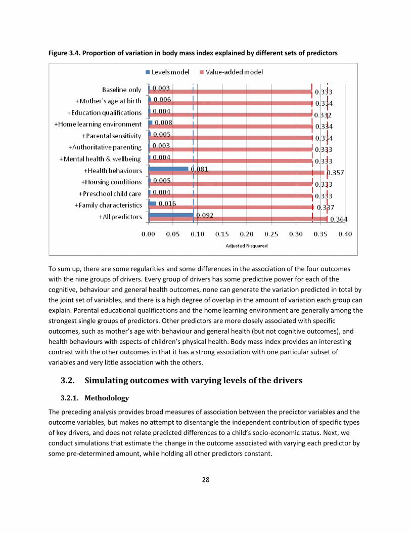
Figure 3.4. Proportion of variation in body mass index explained by different sets of predictors
To sum up, there are some regularities and some differences in the association of the four outcomes
with the nine groups of drivers. Every group of drivers has some predictive power for each of the
cognitive, behaviour and general health outcomes, none can generate the variation predicted in total by
the joint set of variables, and there is a high degree of overlap in the amount of variation each group can
explain. Parental educational qualifications and the home learning environment are generally among the
strongest single groups of predictors. Other predictors are more closely associated with specific
outcomes, such as mother’s age with behaviour and general health (but not cognitive outcomes), and
health behaviours with aspects of children’s physical health. Body mass index provides an interesting
contrast with the other outcomes in that it has a strong association with one particular subset of
variables and very little association with the others.
3.2. Simulating outcomes with varying levels of the drivers
3.2.1. Methodology
The preceding analysis provides broad measures of association between the predictor variables and the
outcome variables, but makes no attempt to disentangle the independent contribution of specific types
of key drivers, and does not relate predicted differences to a child’s socio-economic status. Next, we
conduct simulations that estimate the change in the outcome associated with varying each predictor by
some pre-determined amount, while holding all other predictors constant.

29
Technical details of the simulation methodology are provided in Appendix A. To summarize, the
‘contribution’ of a predictor variable is given by its linear regression coefficient from a model containing
all available explanatory variables. This coefficient gives the predicted difference in the outcome
between two otherwise identical children who differ only by one unit in the value of the variable in
question. The nature of the methodology means that this difference is the same for all pairs of children,
regardless of the initial level of their outcome or their other observed characteristics. It follows that we
can select the amount by which we wish to vary each factor, multiply it by its associated coefficient and
sum up the terms to get the simulated differences in outcomes for any pattern of predictor differences.
The question is then to select a) the magnitude of the changes in the predictors in which we are
interested, and b) the initial level of child’s outcome prior to the specified changes in predictors. Any
values can be chosen for these, resulting in different simulations.
The simulations we conduct select the average outcome of a child in the bottom fifth of the income
distribution as the baseline, and we vary each predictor by the difference in its average value between
families in the bottom fifth of the income distribution and those in the higher four-fifths. Hence the
simulations estimate the outcome of the average low-income child if the level of the predictor among
low-income children were raised to its level among higher-income children, effectively eliminating the
‘income gap’ in the predictor of interest.
A brief example helps to illustrate the technique, and also highlights some potential pitfalls in the
interpretation of the simulations. Parents were asked to how many of six places of interest (e.g. a zoo, a
museum, a cinema) they had taken the child in the last year. The average number for the higher-income
group was 3.8 and for the lower income group 2.7, giving an ‘income gap’ in places of interest of about
1.1. The regression coefficient indicates that one extra place of interest visited is associated with a
difference in the cognitive z-score of 0.05. The average cognitive score of a child in the bottom income
quintile as observed in reality is -0.46 standard deviations, and after the elimination of the income gap in
trips to places of interest this rises to -0.46 + (1.1×0.05) = -0.41, an improvement of about 5% of a
standard deviation. (Note the numbers used in this calculation, along with all the regression coefficients
and income gaps employed in the simulations are provided in Appendix B.)
First, the simulation tells us about predicted rather than causal differences in outcomes. It seems
implausible that if we were take a child to the zoo once a year, leaving everything else unchanged, this
would cause a 5% improvement in cognitive ability. Rather, it seems likely that there is something
unobserved about parents or children in families that visit a lot of places of interest that is associated
with better cognitive outcomes. The 5% figure is calculated after adjusting for other observable
differences between families undertaking different numbers of trips, such as income, education, the
frequency the child is read to and whether the child has regular bedtimes, so it is not factors such as
these that drive the coefficient. However, if many aspects of parenting cluster together, so that parents
who undertake a lot of visits also tend to read a lot to their children and enforce regular bedtimes, it is
difficult for the statistical model to isolate the effect of trips alone. In this case the coefficient may be
driven by a small number of unrepresentative observations. In the simulations we sum over a number of
30
related individual variables to give a total for, say, the home learning environment, that is less
vulnerable to this problem because the distortions in any single coefficient will tend to even out.
Second, the importance of a particular driver in the simulation will depend crucially on the size of the
income gap – that is, how much it differs between low- and higher-income groups in the population we
observe. If a factor varies little between low- and higher-income families on average it will have little
impact in the simulations, even if the coefficient is large and the predictor is very consequential for the
outcome of interest. Third, the simulations rely on the magnitudes of the coefficients and income gaps,
but tell us nothing about the precision with which they are estimated. The simulated outcome of -0.41
described above is a point estimate, one associated with some degree of uncertainty that is not
estimated by the simple simulation technique.
Despite these limitations, the simulations are a useful way of summarizing a very large number of
associations between income group, predictors and outcomes (see the large tables of underlying
statistics in Appendix B). They give us a sense of the relative importance of income gaps in different
groups of drivers as risk factors for the current population of low-income children. Risk factors are not
causal determinants, but it should not be assumed that they necessarily over-estimate the potential
impact of policy-induced changes on the drivers of interest. The drivers were selected on the basis of a
wide body of evidence suggesting causality, including ‘gold standard’ randomized control studies, from
diverse disciplines such as psychology, economics and epidemiology. In addition, mismeasurement of
any of the key concepts will tend to bias downwards the estimated regression coefficients. The relatively
low adjusted R-squareds shown in the previous section imply that there are many influences on
children’s development that are not captured by the MCS variables, and complex psychological
constructs such as the warmth and sensitivity of parent-child interactions are particularly likely to be
poorly captured by infrequent survey measures. Further, the simple methodology used here assumes
the predicted effect of varying each driver is the same for advantaged and disadvantaged children alike,
whereas in fact the causal effect potentially differs depending on the overall nature of the home
environment. Issues of this type are beyond the scope of this study, but the simulations provided here
can at least help point to the areas in which the environments experienced by low-income children are
most strongly associated with the observed deficits in age five outcomes.
3.2.2. Results for broad sets of predictors
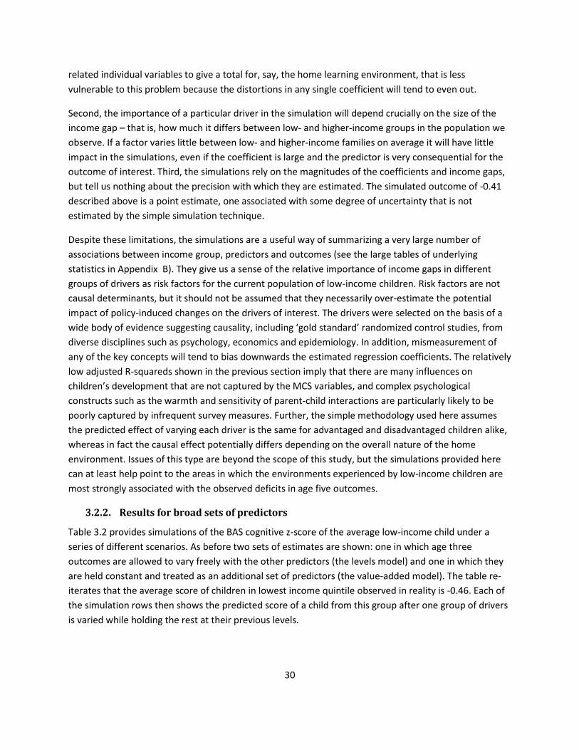
Table 3.2 provides simulations of the BAS cognitive z-score of the average low-income child under a
series of different scenarios. As before two sets of estimates are shown: one in which age three
outcomes are allowed to vary freely with the other predictors (the levels model) and one in which they
are held constant and treated as an additional set of predictors (the value-added model). The table re-
iterates that the average score of children in lowest income quintile observed in reality is -0.46. Each of
the simulation rows then shows the predicted score of a child from this group after one group of drivers
is varied while holding the rest at their previous levels.
31
Table 3.2. Simulated BAS cognitive scores of the average low-income child
Actual scores (raw means)
Poorest 20% (Low-income) -0.46 Richest 80% (Higher-income) 0.11 Prediction after increasing predictors to the average
among the richest 80%
Predictors varied Levels model Value-added model
Mother’s age at birth -0.44 -0.43 Parental educational qualifications -0.32 -0.36 Home learning environment -0.33 -0.39 Parental sensitivity -0.39 -0.44 Authoritative parenting -0.43 -0.43 Mental health and wellbeing -0.45 -0.45 Health behaviours -0.42 -0.43 Housing conditions -0.43 -0.44 Preschool childcare -0.46 -0.46 ALL DRIVERS -0.02 -0.19 Age 3 outcomes - -0.20 ALL DRIVERS & AGE 3 OUTCOMES -0.02 0.07 Baseline controls -0.41 -0.42 Family characteristics -0.33 -0.42 ALL PREDICTORS 0.15 0.14
For example, the levels model estimates show that if the educational qualifications of low-income
parents were raised to the average levels of the rest of the population of parents the score of the
average low-income child is predicted to increase from -0.46 to -0.32, an improvement of 0.14 of a
standard deviation, or around 30% of the starting score. Changes in parental education may have
second-order effects on things like parenting behaviours, but note that any second-order effects
operating through other observed predictors will not show up in this estimate because by construction
they are held constant.
By this measure, parental qualifications and the home learning environment are the two most powerful
predictors of the gap in cognitive outcomes. The predicted score following an equalization of the home
learning environment alone increases by 0.13 of a standard deviation (0.46-0.33), implying that
equalization of these two sets of drivers in isolation would raise the child’s predicted score to -0.19 (an
increase of 0.14+0.13 standard deviations). The ‘All drivers’ row shows that the child’s predicted
outcome after the elimination of income gaps in all the drivers is -0.02. Hence the majority of the overall
simulated change comes from the 0.27 difference associated with parental education and the home
32
learning environment while the contribution the other drivers, although individually quite small, in total
sums to 0.17 of a standard deviation. The simulated score for a low-income child after all the drivers are
varied can be contrasted with the average score of a higher-income child, shown at the top of the table.
The elimination of income gaps in all the drivers is predicted to go a long way to raising the score of the
average low-income child – from -0.46 to -0.02 – but it is still not predicted to reach the level of the
average higher-income child at 0.11.
The right-hand column provides estimates in which age three outcomes are held fixed. The elimination
of the income gap in parental education was predicted to raise the child’s score to -0.32 when no
restriction was placed on age three outcomes. Holding age three outcomes fixed, the same change is
predicted to increase the score less, to -0.36. As we would expect, the simulated effect of all the drivers
is smaller when we constrain them to have no effect on age three outcomes. Another indication of the
strong predictive power of age three outcomes is given by the estimate that eliminating differences in
outcomes between low- and higher-income children at age three, even leaving all other drivers and
family characteristics unchanged, would increase the predicted score by 0.26 standard deviations to -
0.20. Of course, this estimate is hypothetical as it is difficult to conceive of a situation in which age three
outcomes could vary but all parental characteristics and behaviours remain unchanged. Summing
together the results show that eliminating the income gaps in all the drivers of interest and in age three
outcomes, but leaving the other ‘fixed’ characteristics of families unchanged, increases the predicted
score of the average low-income child to 0.07, almost to the level of the average higher-income child.
Hence in combination the drivers of interest and age three outcomes can predict virtually all of the raw
difference in average outcomes between low-income children and the rest, even if other fixed
predictors such as ethnicity, local area and household income are assumed constant.
The final rows of the table indicate the importance of factors that are associated with the differential
family characteristics of low-income children but that are not captured by the measured drivers of
interest. Differences in household income, ethnicity, neighbourhood conditions and the like shift the
predicted outcome down from -0.33 to -0.46 in the levels model, but only from -0.42 to -0.46 in the
value-added model, again highlighting the overlap between the two sets of variables.
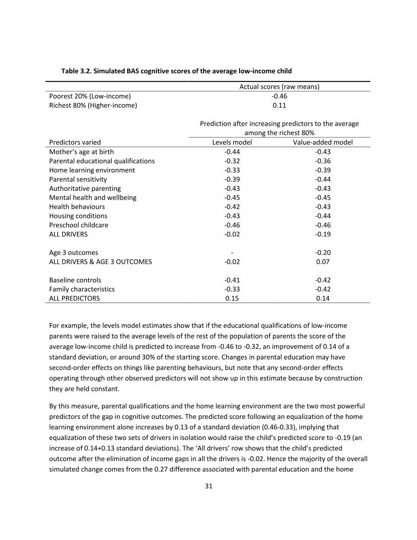
Table 3.3 provides simulations of the SDQ behaviour problems score. A similar picture emerges in that
together the elimination of the income gaps in all the drivers of interest predict a fall in the score of the
average low-income child from the 8.91 points observed in reality to 6.57 points in the levels model,
almost not quite as low as the average higher-income child at 6.40. Holding age three outcomes
constant increases the simulated problems score in this scenario to 7.24 points, but varying both drivers
and age three outcomes predicts a score slightly better than that of the average higher-income child at
5.99 points.
33
Table 3.3. Simulated SDQ behaviour scores of the average low-income child
Actual scores (raw means)
Poorest 20% (Low-income) 8.91 Richest 80% (Higher-income) 6.40 Prediction after increasing predictors to the average
among the richest 80%
Predictors varied Levels model Value-added model
Mother’s age at birth 8.78 8.81 Parental educational qualifications 8.66 8.70 Home learning environment 8.53 8.66 Parental sensitivity 8.30 8.58 Authoritative parenting 8.74 8.79 Mental health and wellbeing 8.40 8.47 Health behaviours 8.68 8.71 Housing conditions 8.87 8.89 Preschool childcare 8.91 8.92 ALL DRIVERS 6.57 7.24 Age 3 outcomes - 7.66 ALL DRIVERS & AGE 3 OUTCOMES 6.57 5.99 Baseline controls 8.65 8.64 Family characteristics 8.79 9.07 ALL PREDICTORS 6.18 5.88
Varying each group of drivers individually has only a modest impact on the predicted outcome. The
largest two differences are generated by the parental sensitivity group of drivers, which lower the score
in the levels model from 8.91 to 8.30, and the parental mental health and well-being group, which
individually lower the score from 8.91 to 8.40. Again, the simulated effects of these changes are smaller
when age three outcomes are held constant in the value-added model. It is noticeable that the two
most powerful drivers for behaviour outcomes – parental sensitivity and mental health – are different to
the most powerful drivers for cognitive outcomes – parental education and the home learning
environment. Nevertheless, in both cases it is the combined power of all the groups of drivers that shifts
the predicted outcome towards the level observed among the higher-income group of children. Each
group plays only a small role alone, but when summed together the predicted difference in the outcome
is not trivial.
34
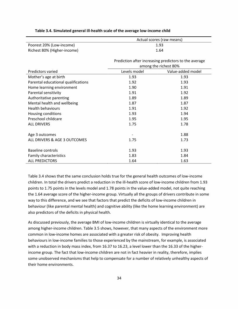
Table 3.4. Simulated general ill-health scale of the average low-income child
Actual scores (raw means)
Poorest 20% (Low-income) 1.93 Richest 80% (Higher-income) 1.64 Prediction after increasing predictors to the average
among the richest 80%
Predictors varied Levels model Value-added model
Mother’s age at birth 1.93 1.93 Parental educational qualifications 1.92 1.93 Home learning environment 1.90 1.91 Parental sensitivity 1.91 1.92 Authoritative parenting 1.89 1.89 Mental health and wellbeing 1.87 1.87 Health behaviours 1.91 1.92 Housing conditions 1.93 1.94 Preschool childcare 1.95 1.95 ALL DRIVERS 1.75 1.78 Age 3 outcomes - 1.88 ALL DRIVERS & AGE 3 OUTCOMES 1.75 1.73 Baseline controls 1.93 1.93 Family characteristics 1.83 1.84 ALL PREDICTORS 1.64 1.63
Table 3.4 shows that the same conclusion holds true for the general health outcomes of low-income
children. In total the drivers predict a reduction in the ill-health score of low-income children from 1.93
points to 1.75 points in the levels model and 1.78 points in the value-added model, not quite reaching
the 1.64 average score of the higher-income group. Virtually all the groups of drivers contribute in some
way to this difference, and we see that factors that predict the deficits of low-income children in
behaviour (like parental mental health) and cognitive ability (like the home learning environment) are
also predictors of the deficits in physical health.
As discussed previously, the average BMI of low-income children is virtually identical to the average
among higher-income children. Table 3.5 shows, however, that many aspects of the environment more
common in low-income homes are associated with a greater risk of obesity. Improving health
behaviours in low-income families to those experienced by the mainstream, for example, is associated
with a reduction in body mass index, from 16.37 to 16.23, a level lower than the 16.33 of the higher-
income group. The fact that low-income children are not in fact heavier in reality, therefore, implies
some unobserved mechanisms that help to compensate for a number of relatively unhealthy aspects of
their home environments.
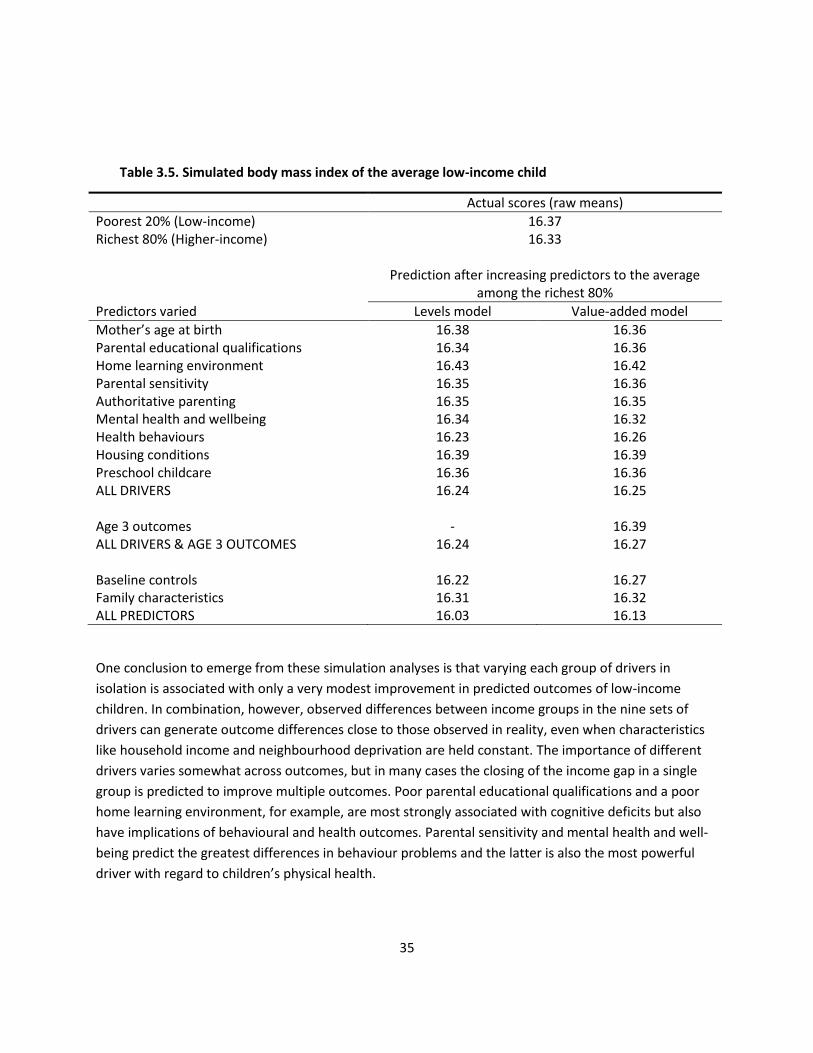
35
Table 3.5. Simulated body mass index of the average low-income child
Actual scores (raw means)
Poorest 20% (Low-income) 16.37 Richest 80% (Higher-income) 16.33 Prediction after increasing predictors to the average
among the richest 80%
Predictors varied Levels model Value-added model
Mother’s age at birth 16.38 16.36 Parental educational qualifications 16.34 16.36 Home learning environment 16.43 16.42 Parental sensitivity 16.35 16.36 Authoritative parenting 16.35 16.35 Mental health and wellbeing 16.34 16.32 Health behaviours 16.23 16.26 Housing conditions 16.39 16.39 Preschool childcare 16.36 16.36 ALL DRIVERS 16.24 16.25 Age 3 outcomes - 16.39 ALL DRIVERS & AGE 3 OUTCOMES 16.24 16.27 Baseline controls 16.22 16.27 Family characteristics 16.31 16.32 ALL PREDICTORS 16.03 16.13
One conclusion to emerge from these simulation analyses is that varying each group of drivers in
isolation is associated with only a very modest improvement in predicted outcomes of low-income
children. In combination, however, observed differences between income groups in the nine sets of
drivers can generate outcome differences close to those observed in reality, even when characteristics
like household income and neighbourhood deprivation are held constant. The importance of different
drivers varies somewhat across outcomes, but in many cases the closing of the income gap in a single
group is predicted to improve multiple outcomes. Poor parental educational qualifications and a poor
home learning environment, for example, are most strongly associated with cognitive deficits but also
have implications of behavioural and health outcomes. Parental sensitivity and mental health and well-
being predict the greatest differences in behaviour problems and the latter is also the most powerful
driver with regard to children’s physical health.
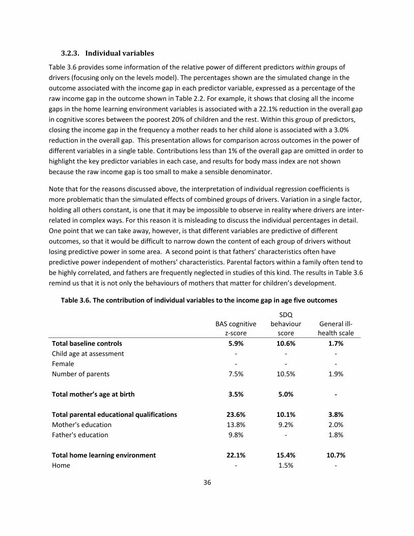
36
3.2.3. Individual variables
Table 3.6 provides some information of the relative power of different predictors within groups of
drivers (focusing only on the levels model). The percentages shown are the simulated change in the
outcome associated with the income gap in each predictor variable, expressed as a percentage of the
raw income gap in the outcome shown in Table 2.2. For example, it shows that closing all the income
gaps in the home learning environment variables is associated with a 22.1% reduction in the overall gap
in cognitive scores between the poorest 20% of children and the rest. Within this group of predictors,
closing the income gap in the frequency a mother reads to her child alone is associated with a 3.0%
reduction in the overall gap. This presentation allows for comparison across outcomes in the power of
different variables in a single table. Contributions less than 1% of the overall gap are omitted in order to
highlight the key predictor variables in each case, and results for body mass index are not shown
because the raw income gap is too small to make a sensible denominator.
Note that for the reasons discussed above, the interpretation of individual regression coefficients is
more problematic than the simulated effects of combined groups of drivers. Variation in a single factor,
holding all others constant, is one that it may be impossible to observe in reality where drivers are inter-
related in complex ways. For this reason it is misleading to discuss the individual percentages in detail.
One point that we can take away, however, is that different variables are predictive of different
outcomes, so that it would be difficult to narrow down the content of each group of drivers without
losing predictive power in some area. A second point is that fathers’ characteristics often have
predictive power independent of mothers’ characteristics. Parental factors within a family often tend to
be highly correlated, and fathers are frequently neglected in studies of this kind. The results in Table 3.6
remind us that it is not only the behaviours of mothers that matter for children’s development.
Table 3.6. The contribution of individual variables to the income gap in age five outcomes
BAS cognitive z-score
SDQ behaviour
score General ill-health scale
Total baseline controls 5.9% 10.6% 1.7%
Child age at assessment - - -
Female - - -
Number of parents 7.5% 10.5% 1.9%
Total mother’s age at birth 3.5% 5.0% -
Total parental educational qualifications 23.6% 10.1% 3.8%
Mother's education 13.8% 9.2% 2.0%
Father's education 9.8% - 1.8%
Total home learning environment 22.1% 15.4% 10.7%
Home - 1.5% -
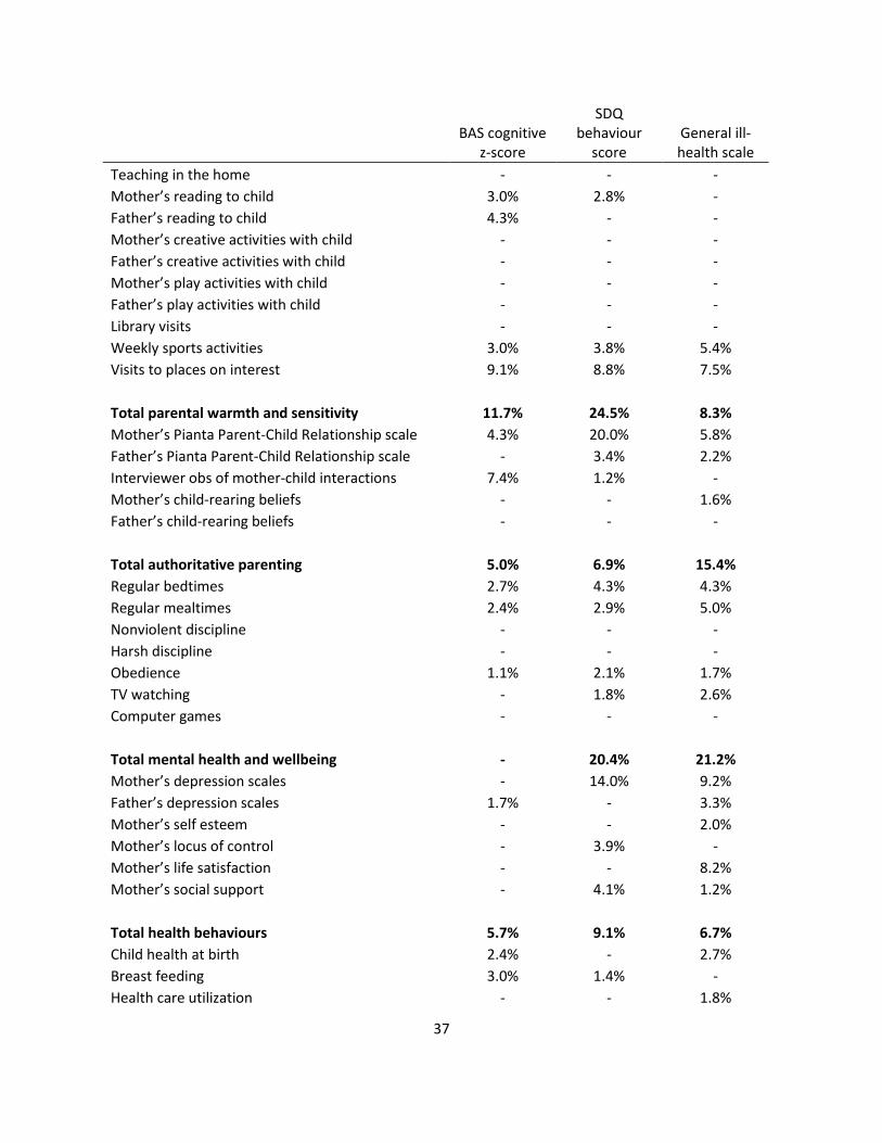
37
BAS cognitive z-score
SDQ behaviour
score General ill-health scale
Teaching in the home - - -
Mother’s reading to child 3.0% 2.8% -
Father’s reading to child 4.3% - -
Mother’s creative activities with child - - -
Father’s creative activities with child - - -
Mother’s play activities with child - - -
Father’s play activities with child - - -
Library visits - - -
Weekly sports activities 3.0% 3.8% 5.4%
Visits to places on interest 9.1% 8.8% 7.5%
Total parental warmth and sensitivity 11.7% 24.5% 8.3%
Mother’s Pianta Parent-Child Relationship scale 4.3% 20.0% 5.8%
Father’s Pianta Parent-Child Relationship scale - 3.4% 2.2%
Interviewer obs of mother-child interactions 7.4% 1.2% -
Mother’s child-rearing beliefs - - 1.6%
Father’s child-rearing beliefs - - -
Total authoritative parenting 5.0% 6.9% 15.4%
Regular bedtimes 2.7% 4.3% 4.3%
Regular mealtimes 2.4% 2.9% 5.0%
Nonviolent discipline - - -
Harsh discipline - - -
Obedience 1.1% 2.1% 1.7%
TV watching - 1.8% 2.6%
Computer games - - -
Total mental health and wellbeing - 20.4% 21.2%
Mother’s depression scales - 14.0% 9.2%
Father’s depression scales 1.7% - 3.3%
Mother’s self esteem - - 2.0%
Mother’s locus of control - 3.9% -
Mother’s life satisfaction - - 8.2%
Mother’s social support - 4.1% 1.2%
Total health behaviours 5.7% 9.1% 6.7%
Child health at birth 2.4% - 2.7%
Breast feeding 3.0% 1.4% -
Health care utilization - - 1.8%
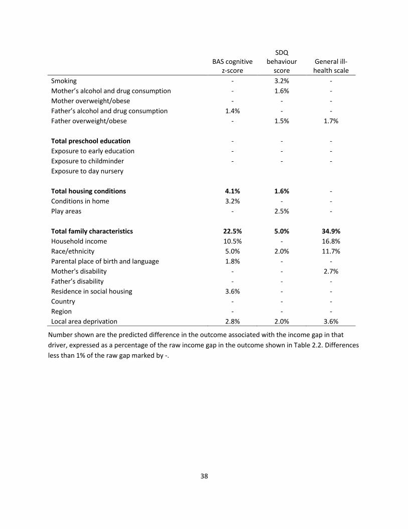
38
BAS cognitive z-score
SDQ behaviour
score General ill-health scale
Smoking - 3.2% -
Mother’s alcohol and drug consumption - 1.6% -
Mother overweight/obese - - -
Father’s alcohol and drug consumption 1.4% - -
Father overweight/obese - 1.5% 1.7%
Total preschool education - - -
Exposure to early education - - -
Exposure to childminder - - -
Exposure to day nursery
Total housing conditions 4.1% 1.6% -
Conditions in home 3.2% - -
Play areas - 2.5% -
Total family characteristics 22.5% 5.0% 34.9%
Household income 10.5% - 16.8%
Race/ethnicity 5.0% 2.0% 11.7%
Parental place of birth and language 1.8% - -
Mother's disability - - 2.7%
Father’s disability - - -
Residence in social housing 3.6% - -
Country - - -
Region - - -
Local area deprivation 2.8% 2.0% 3.6%
Number shown are the predicted difference in the outcome associated with the income gap in that
driver, expressed as a percentage of the raw income gap in the outcome shown in Table 2.2. Differences
less than 1% of the raw gap marked by -.

39
4. ALSPAC Findings
4.1. The data
ALSPAC is a cohort study that recruited around 14,000 pregnant women who were resident in the Avon
area of England whose expected date of delivery fell between 1st April 1991 and 31st December 1992. It
therefore covers children in three school years: those taking GCSEs in 2006/07, 2007/08 and 2008/09.
Study families were surveyed via high frequency postal questionnaires from the time of pregnancy
onwards, and via a number of hands-on clinics in which ALSPAC staff administered a range of detailed
physical, psychometric and psychological tests to the children. ALSPAC has been linked to the National
Pupil Database (NPD), which contains school identifiers and results on national Key Stage school tests for
all children in the state school system.
Unlike the MCS, ALSPAC was not designed to nationally representative although in fact the population it
covers is relatively broad. The Avon area has a population of 1 million and includes the city of Bristol
(population 0.5 million), and a mixture of rural areas, inner city deprivation, leafy suburbs and moderate
sized towns. The 1991 census was used to compare the population of mothers with infants under 1 year
of age resident in Avon with those in the whole of Britain. The sample is broadly representative of the
national population although the mothers of infants in Avon were slightly more likely to be affluent, on
average, than those in the rest of Britain (as measured by, for example, living in owner occupied
accommodation, having a car available to the household and having one or more persons per room).
The sample pregnancies resulted in 13,988 children alive at one year. Linkage to the administrative NPD
means that of these 11,640 (83%) have valid GCSE records. The remaining 17% lack records because
they did not attend a state school in England in Year 11, for example because they attended a private
school or because they had left the country3. However, attrition among the sample children means that
a large number do not have any data on the key drivers measured at ages 3, 4 or 5, and so contribute
little information to this study. The consequences of attrition are discussed further below.
The key outcome variable is the child’s average capped GCSE and equivalents points score. This is
calculated as the child’s total points score from their 8 best GCSEs (or equivalents) divided by 8. The
relationship between points and grades is shown in Table 4.1 – one GCSE grade in one subject is
equivalent to 6 points on the original scale. The outcome in this analysis is normalized for ease of
interpretation, so that 6 points is equivalent to 8 GCSE grades in total – the difference between eight
grade Ds and eight grade Cs for example.
3 GCSE results are available for private school pupils in England, but as yet these have not been matched to
ALSPAC.
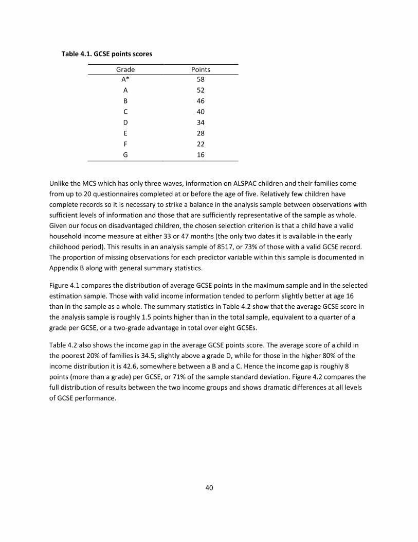
40
Table 4.1. GCSE points scores
Grade Points
A* 58
A 52
B 46
C 40
D 34
E 28
F 22
G 16
Unlike the MCS which has only three waves, information on ALSPAC children and their families come
from up to 20 questionnaires completed at or before the age of five. Relatively few children have
complete records so it is necessary to strike a balance in the analysis sample between observations with
sufficient levels of information and those that are sufficiently representative of the sample as whole.
Given our focus on disadvantaged children, the chosen selection criterion is that a child have a valid
household income measure at either 33 or 47 months (the only two dates it is available in the early
childhood period). This results in an analysis sample of 8517, or 73% of those with a valid GCSE record.
The proportion of missing observations for each predictor variable within this sample is documented in
Appendix B along with general summary statistics.
Figure 4.1 compares the distribution of average GCSE points in the maximum sample and in the selected
estimation sample. Those with valid income information tended to perform slightly better at age 16
than in the sample as a whole. The summary statistics in Table 4.2 show that the average GCSE score in
the analysis sample is roughly 1.5 points higher than in the total sample, equivalent to a quarter of a
grade per GCSE, or a two-grade advantage in total over eight GCSEs.
Table 4.2 also shows the income gap in the average GCSE points score. The average score of a child in
the poorest 20% of families is 34.5, slightly above a grade D, while for those in the higher 80% of the
income distribution it is 42.6, somewhere between a B and a C. Hence the income gap is roughly 8
points (more than a grade) per GCSE, or 71% of the sample standard deviation. Figure 4.2 compares the
full distribution of results between the two income groups and shows dramatic differences at all levels
of GCSE performance.
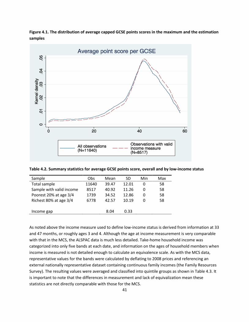
41
Figure 4.1. The distribution of average capped GCSE points scores in the maximum and the estimation
samples
Table 4.2. Summary statistics for average GCSE points score, overall and by low-income status
Sample Obs Mean SD Min Max
Total sample 11640 39.47 12.01 0 58 Sample with valid income 8517 40.92 11.26 0 58 Poorest 20% at age 3/4 1739 34.52 12.86 0 58 Richest 80% at age 3/4 6778 42.57 10.19 0 58 Income gap 8.04 0.33
As noted above the income measure used to define low-income status is derived from information at 33
and 47 months, or roughly ages 3 and 4. Although the age at income measurement is very comparable
with that in the MCS, the ALSPAC data is much less detailed. Take-home household income was
categorized into only five bands at each date, and information on the ages of household members when
income is measured is not detailed enough to calculate an equivalence scale. As with the MCS data,
representative values for the bands were calculated by deflating to 2008 prices and referencing an
external nationally representative dataset containing continuous family incomes (the Family Resources
Survey). The resulting values were averaged and classified into quintile groups as shown in Table 4.3. It
is important to note that the differences in measurement and lack of equivalization mean these
statistics are not directly comparable with those for the MCS.
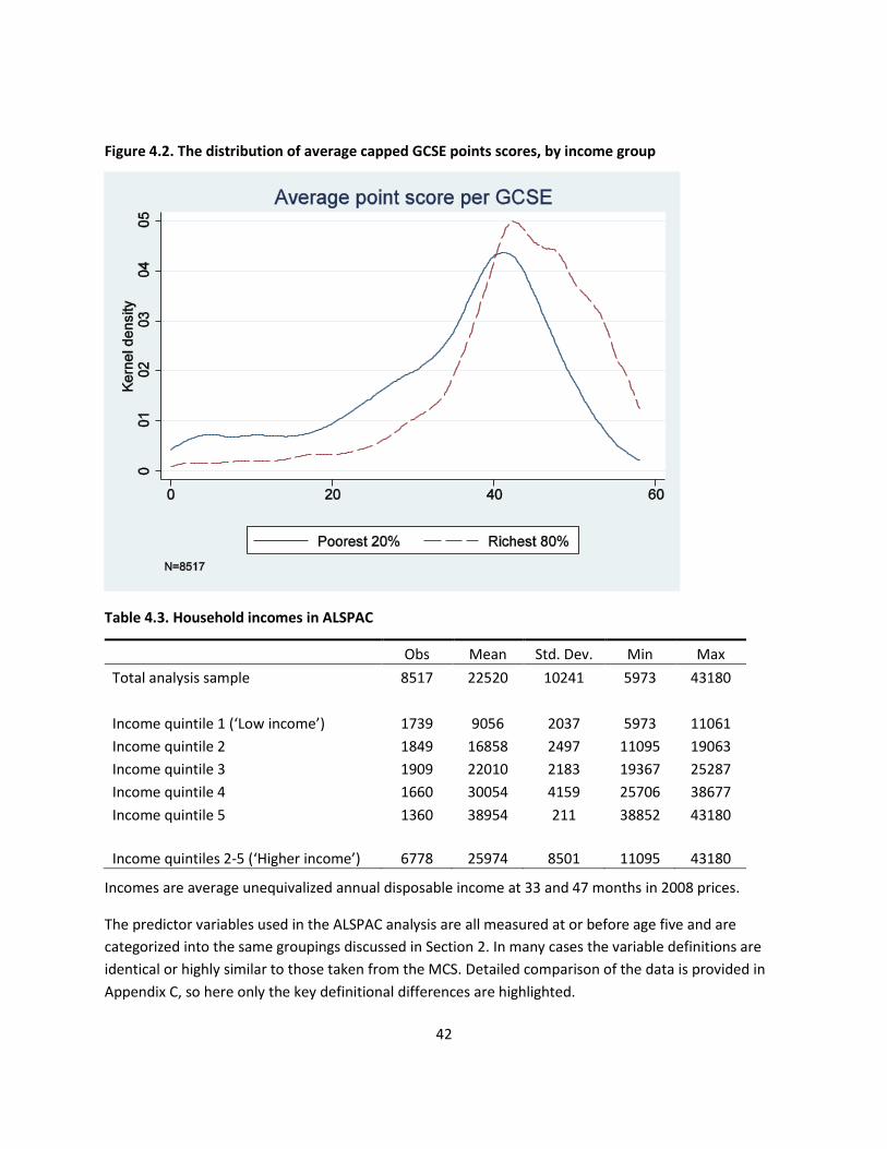
42
Figure 4.2. The distribution of average capped GCSE points scores, by income group
Table 4.3. Household incomes in ALSPAC
Obs Mean Std. Dev. Min Max
Total analysis sample 8517 22520 10241 5973 43180
Income quintile 1 (‘Low income’) 1739 9056 2037 5973 11061
Income quintile 2 1849 16858 2497 11095 19063
Income quintile 3 1909 22010 2183 19367 25287
Income quintile 4 1660 30054 4159 25706 38677
Income quintile 5 1360 38954 211 38852 43180
Income quintiles 2-5 (‘Higher income’) 6778 25974 8501 11095 43180
Incomes are average unequivalized annual disposable income at 33 and 47 months in 2008 prices.
The predictor variables used in the ALSPAC analysis are all measured at or before age five and are
categorized into the same groupings discussed in Section 2. In many cases the variable definitions are
identical or highly similar to those taken from the MCS. Detailed comparison of the data is provided in
Appendix C, so here only the key definitional differences are highlighted.

43
Baseline controls replace child age at assessment with dummy variables for year and month of
birth, and the three single parenthood variables are measured at 8, 33 and 47 months.
Age three outcomes of the kind used in the MCS analysis are not available in ALSPAC, so all
results relate only to the ‘levels’ model.
A number of parental characteristics are measured only for the mother, rather than the mother
and the father as in the MCS analysis (e.g. depression, child-rearing beliefs, parent-child
relationship scale). However, paternal qualifications and a number of paternal parenting
activities are included as they were reported by the mother. Some information collected
directly from fathers is available in the ALSPAC dataset but low response rates and limited time
in which to carry out the extensive coding needed mean they are not used here. Analysis of the
MCS data suggests that mothers’ and fathers’ characteristics are highly correlated and that the
omission of fathers’ characteristics does little to reduce the overall predictive power of the
model, but tends to inflate slightly the association of mothers’ characteristics with child
outcomes.
No interviewer observations of mother-child interactions or the home environment are
available, so parenting measures rely entirely on self-report.
No measure of local deprivation (such as decile group of the Index of Multiple Deprivation used
in the MCS analysis) is available.
4.2. Explaining the variation in GCSE performance
This section repeats the analysis of Section 3.1 using the ALSPAC data with average GCSE points
replacing age five scores as the outcome variable. The results in Figure 4.3 show the proportion of
outcome variance explained (the adjusted R-squared) by a baseline set of controls, alternative sets of
predictor variables and finally all predictors in combination. As before, all predictors are measured at or
before age five, so the results give an indication of how far it is possible to predict GCSE performance at
16 purely on the basis of early life circumstances.
The baseline controls are indicators of the child’s age at assessment, gender and number of parents in
the household at three dates prior to the age of six. The top bar of Figure 4.3 shows that together these
variables can explain 8% of the variation in GCSE performance. Adding all the predictor variables
available increases this proportion to around 32%, a similar proportion to the explained variation in age
five MCS outcomes. Clearly, early life circumstances are extremely powerful predictors of educational
attainment in adolescence, although again they cannot account for the majority of the variance.
Inspection of the intermediate bars shows that the drivers vary in their individual predictive power. Each
group increases the proportion of variance explained beyond the baseline, but none can generate the
predicted variation alone that is generated by the combined set of drivers in total. Parental educational
qualifications stand out as the most powerful single key driver, explaining around a quarter of the
44
variation in GCSE performance when added to the baseline controls. Health behaviours such as breast
feeding and smoking are also one of the most powerful groups of predictors, an interesting finding given
that at age five they were more predictive of behavioural and health outcomes than of cognitive ability.
Of the three groups of parenting measures, the home learning environment generates the most
variation in predicted outcomes while measures of parental sensitivity predict the least. (Note however
that the absence of interviewer observations of mother-child interactions in ALSPAC means that
parental sensitivity is likely to be particularly poorly measured in ALSPAC relative to the MCS.) Finally,
family characteristics such as income, social housing tenure and parental disability are second only to
parental education in individual predictive power, again suggesting that broad measures of socio-
economic resources are related to the drivers of educational attainment in multiple ways.
Figure 4.3. Proportion of variation in average capped GCSE points scorse explained by different sets of
predictors
4.3. Simulating GCSE performance with varying levels of the drivers
This section repeats the simulation analysis of Section 3.2 to explore the variation in the predicted GCSE
performance of low-income children associated with different levels of the key drivers. As before, the
benchmark variation in each predictor is the gap in mean values between children in the lowest income
quintile and the rest. The simulations use the coefficient from a fully controlled linear regression
predicting the average GCSE score as a ‘weight’ for each income gap, and take the GCSE score of the
average low-income child observed in reality as the baseline case. (All underlying coefficients and
income gaps used in the simulations are provided in Appendix B.)
45
Table 4.4. Simulated average GCSE points score of the average low-income child
Actual scores (raw means)
Poorest 20% (Low-income) 34.52 Richest 80% (Higher-income) 42.57 Predictors varied Prediction after increasing predictors to the average
among the richest 80%
Mother’s age at birth 34.58 Parental educational qualifications 36.61 Home learning environment 35.06 Parental sensitivity 34.58 Authoritative parenting 34.63 Mental health and wellbeing 34.99 Health behaviours 35.69 Housing conditions 34.58 Preschool childcare 34.64 ALL DRIVERS 39.19 Baseline controls 34.93 Family characteristics 37.64 ALL PREDICTORS 42.72
Table 4.4 shows that the mean score of the lowest income quintile is 34.5, and that increasing all the
drivers in total from their actual values to the average of the higher-income group predicts an
increase of 4.7 points to 39.2. This is equivalent to just over half a grade per GCSE or over six grades
spread over eight entries. This is a substantial difference, equal to 60% of the raw income gap of 8
points between the two income groups. The simulations after varying each group of drivers
individually give the same conclusion as the variance analysis in the previous section – parental
educational qualification and health behaviours are the two most powerful drivers, associated with
a 2.1 and 1.2 point increase respectively in the predicted score. The impact of other drivers is more
marginal although together they sum up to a non-trivial amount. The simulation that varies family
characteristics in isolation shows that even when the other predictors are held constant, factors
such as income, social housing and parental disability are important predictors of the disparity in
GCSE performance, generating a difference of 3.1 points on average between groups. This suggests
that the mechanisms through which family characteristics affect GCSE performance are relatively
poorly captured by the observed measures of early life drivers in the ALSPAC dataset. In contrast,
the predictive power of family characteristics for age five MCS outcomes is more closely related to
the specified drivers. One potential explanation is that family characteristics are more strongly
related to children’s experiences during primary and secondary school than early environmental
measures, and that these are the more immediate influences on educational performance at 16.
46
Table 4.5. The contribution of individual variables to the income gap in the average capped GCSE
points score
Predictor % of income
gap explained
Total baseline controls 5.0%
Month and year of birth -
Female -
Number of parents 5.5%
Total mother’s age at birth -
Total parental educational qualifications 25.9%
Mother’s education 11.9%
Father’s education 14.1%
Total home learning environment 6.7%
Teaching in the home 2.2%
Library visits -
Visits to places of interest -
Mother’s reading to child -
Father’s reading to child 3.4%
Mother’s creative activities with child -
Mother’s play activities with child -
Father’s creative activities with child -
Father’s play activities with child -
Weekly sports activities -
Total parental warmth and sensitivity -
Maternal bonding score -
Child-rearing beliefs -
Total authoritative parenting 1.4%
Discipline -
Regular bedtimes 1.7%
Regular mealtimes -
Enforcement of obedience -
Hours of TV watching -
Hours of computer games -
Total mental health and wellbeing 5.8%
Mother’s depression scales 1.5%
47
Predictor % of income
gap explained
Mother’s self esteem -
Mother’s locus of control 4.7%
Mother’s social support -
Total health behaviours 14.5%
Child health at birth -
Breast feeding 3.0%
Antenatal care 1.3%
Smoking 8.9%
Alcohol consumption -
Mother overweight/obese -
Total housing conditions -
Persons per room 1.9%
Central heating 1.2%
Damp -
Access to garden -
Total preschool education 1.4%
Exposure to nursery 1.4%
Exposure to childminder -
Total family characteristics 38.8%
Household income at age 3/4 16.7%
Child is non-white -
Mother born outside UK -
Household member disability -
Residence in social housing 22.0%
Number shown are the predicted difference in GCSE performance associated with the income gap in
that driver, expressed as a percentage of the raw income gap of 8.04 points per GCSE. Differences less
than 1% of the raw gap are marked by -.
Table 4.5 provides some information of the relative power of different predictors within groups of
drivers in a way comparable to the MCS analysis in Section 3.2. Again the interpretation of individual
percentages is problematic given the observational nature of the data. Nevertheless it is clear that
income-related differences in virtually all the groups of early-life drivers have some predictive power for
educational outcomes measured over a decade later. The strong association of low household income
and residence in social housing with underperformance at GCSE is also striking, given that the estimates
hold constant all observable measures of the early home environment.
Related Documents


