Early Agricultural Communities in Northern and Eastern India: an archaeobotanical investigation. Volume I Emma Louise Harvey Thesis submitted in fulfilment of the requirements of the degree of Doctor of Philosophy in the Institute of Archaeology, University of London. 2006 1

Welcome message from author
This document is posted to help you gain knowledge. Please leave a comment to let me know what you think about it! Share it to your friends and learn new things together.
Transcript
Early Agricultural Communities in Northern and Eastern India:
an archaeobotanical investigation.
Volume I
Emma Louise Harvey
Thesis submitted in fulfilment o f the
requirements of the degree of Doctor of Philosophy in the
Institute of Archaeology, University of London.
2006
1

UMI Number: U592092
All rights reserved
INFORMATION TO ALL USERS The quality of this reproduction is dependent upon the quality of the copy submitted.
In the unlikely event that the author did not send a complete manuscript and there are missing pages, these will be noted. Also, if material had to be removed,
a note will indicate the deletion.
Dissertation Publishing
UMI U592092Published by ProQuest LLC 2013. Copyright in the Dissertation held by the Author.
Microform Edition © ProQuest LLC.All rights reserved. This work is protected against
unauthorized copying under Title 17, United States Code.
ProQuest LLC 789 East Eisenhower Parkway
P.O. Box 1346 Ann Arbor, Ml 48106-1346

Early Agricultural Communities in Northern and Eastern India:
an archaeobotanical investigation.
PhD Thesis by Emma Louise Harvey
Abstract
This thesis aims to contribute to the growing knowledge o f early agricultural communities
in India. The transition to agriculture is a fundamental change in society however, less is
known about this transformation in the Indian sub-continent than other world regions. In
this thesis the focus is on the Northern and Eastern areas o f India and specifically the
Ganges Plain and the state of Orissa. Some archaeobotanical work has been conducted in
the Gangetic area but this work lacks quantification making it hard to compare to better
studied regions (South India and Northwestern India). A number o f sites in the Belan River
Valley are investigated here and these sites (Chopani-Mando, Koldihwa, and Mahagara)
have been suggested to be only evidence of a transition from wild rice exploitation to
domestic rice agriculture although no systematic archaeobotanical analysis had been
conducted. A methodological study o f rice identification methods has been conducted as
part o f this thesis to help to clarify this issue. This thesis found this transition was unlikely
to take place because dating of these sites does not demonstrate a continuous chronology
and the evidence for wild rice at Chopani-Mando is not present. Koldihwa and Mahagara
do show evidence o f rice cultivation as well as having introduced crops (wheat, barley,
winter pulses, native India pulses and millets).
Orissa has had no previous archaeobotanical studies conducted and therefore this
thesis is the first to present evidence for the early agricultural communities in this area.
There seems to be a rather late appearance o f agriculture in the Chalcolithic period found at
sites in the coastal and lowland areas (Golbai Sasan and Gopalpur). Rice, native India
pulses (horsegram, pigeonpea, and Vigna sp.), and millets have been found at these sites.
No introduced winter crops were found. The Central and Northern uplands o f Orissa do not
demonstrate the same subsistence pattern. There was no evidence o f agricultural or wild
plant food found at the sites (Bajpur, Banabasa, Malakhoja) investigated in this thesis.
2
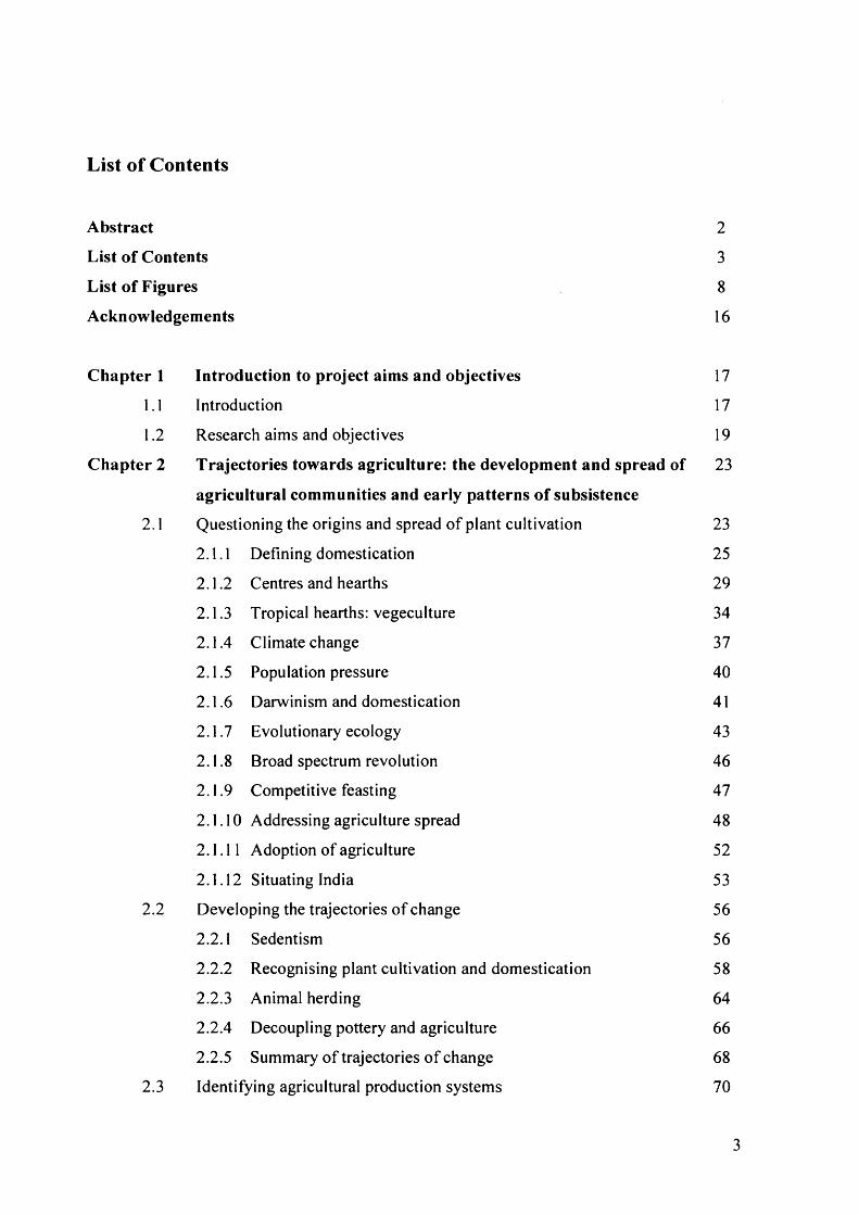
List of Contents
Abstract 2
List o f Contents 3
List o f Figures 8
Acknowledgements 16
Chapter 1 Introduction to project aims and objectives 17
1.1 Introduction 17
1.2 Research aims and objectives 19
Chapter 2 Trajectories towards agriculture: the development and spread of 23
agricultural communities and early patterns o f subsistence
2.1 Questioning the origins and spread of plant cultivation 23
2.1.1 Defining domestication 25
2.1.2 Centres and hearths 29
2.1.3 Tropical hearths: vegeculture 34
2.1.4 Climate change 37
2.1.5 Population pressure 40
2.1.6 Darwinism and domestication 41
2.1.7 Evolutionary ecology 43
2.1.8 Broad spectrum revolution 46
2.1.9 Competitive feasting 47
2.1.10 Addressing agriculture spread 48
2.1.11 Adoption of agriculture 52
2.1.12 Situating India 53
2.2 Developing the trajectories of change 56
2.2.1 Sedentism 56
2.2.2 Recognising plant cultivation and domestication 58
2.2.3 Animal herding 64
2.2.4 Decoupling pottery and agriculture 66
2.2.5 Summary of trajectories o f change 68
2.3 Identifying agricultural production systems 70
3

2.3.1 Trajectories o f agricultural systems 70
2.3.2 Identifying social changes 76
2.4 Summary 78
2 .4 .1 Key issues to consider for Northern and Eastern India 80
Chapter 3 Geographical background to study areas 81
3.1 Population 81
3.2 Physical features, geology, and soils 82
3.3 Climate and vegetation 87
3.4 Modern agriculture in India 94
3.5 Ancient crops and crop origins 96
3.6 Palaeoclimate and palaeoenvironment 107
3.7 Tribal groups 110
3.8 Summary 118
Chapter 4 Early farming communities in Northern and Eastern India 120
4.1 Early farming settlements in the Ganges Valley 121
4.2 Early farming settlements in Orissa 136
4.3 Summary of issues 153
Chapter 5 Methodology: site descriptions, field and laboratory methods 156
5.1 Field methods 156
5.1.1 Site selection and sampling in Uttar Pradesh 156
5.1.2 Site selection and sampling in Orissa 159
5.1.3 Extractions methods in the field 164
5.2 Laboratory methods 164
5.2.1 Extraction in the laboratory 164
5.2.2 Identification 166
5.3 Qualitative and quantitative analysis 171
5.4 Taphonomy and approaches to the analysis o f crop processing activities 177
Chapter 6 Rice identification methodologies: problems and prospects 185
6.1 Terminology for the rice plant including rice phytoliths 185
6.1.1 Rice plant anatomy 185
6.1.2 Rice phytolith descriptions 187
6.2 Rice taxonomy, domestication issues, and why identification 188
is problematic
4

188
190
193
196
199
203
208
209
209
211
212
216
219
221
221
222
225
231
236
236
237
248
259
259
261
262
265
265
265
271
275
275
5
6.2.1 Rice taxonomy
6.2.2 Pathways to domestication
Review of current rice identification methods
6.3.1 Measurement o f caryopses or spikelets
6.3.2 Measuring bi-peaked tubercules on the rice.husk
6.3.3 The use o f phytoliths for identifying rice species
The present study of the identification methods o f rice
6.4.1 Measuring the caryopsis
6.4.2 Measuring double-peaked husk cells
Results of the modern study of identification methods for rice
6.5.1 Identification using measurements o f the caryopsis
6.5.2 Identification using double-peaked husk phytolith
Conclusions of the rice identification study
Results of macro-botanical and phytolith analysis
Macro-botanical results
7.1.1 Identifications and preservation issues
7.1.2 Results from Uttar Pradesh
7.1.3 Results from Orissa
Phytolith analysis results
7.2.1 Identification of phytolith remains
7.2.2 Results from Uttar Pradesh
7.2.3 Results from Orissa
Comparisons of macro-remains and phytolith data
7.3.1 Weed ecology
7.3.2 Investigation o f crop processing
7.3.3 General patterns
Interpreting, evaluating data, and concluding remarks
Economic patterns
8.1.1 Sites in the Belan River Valley, Uttar Pradesh
8.1.2 Sites in Orissa
Implications for the development o f agricultural societies in Northern
and Eastern India
8.2.1 Belan River Valley

8.2.2 Orissa
8.3 Pathways to agriculture and India as part o f the world view
8.4 Methodological issues and further work
279
283
285
Bibliography 287
Appendices 364
Chapter 4
4.1 Table of published archaeobotanical data from Ganges and Orissan sites 364
Chapter 5
5.1 Extraction method for phytoliths from sediments 367
5.2 Dry ashing method for making phytolith reference slides 369
5.3 Method for preparation o f spodograms 369
5.4 Description o f terms used for phytoliths in the thesis 370
Chapter 6
6.1 Table of published rice measurements from archaeological sites in South Asia 375
Chapter 7
7.1 Raw data table for macro-botanical remains from Koldihwa 380
7.2 Raw data table for macro-botanical remains from Mahagara 383
7.3 Raw data table for macro-botanical remains from Chopani-Mando 389
7.4 Table o f ubiquity values for Belan River Valley sites 391
7.5 Ubiquity values for published archaeobotanical data in North Indian 393
Prehistoric sites
7.6 Raw data table for macro-botanical remains from Gopalpur 394
7.7 Raw data table for macro-botanical remains from Golbai Sasan 397
7.8 Raw data table for macro-botanical remains from Bajpur 400
7.9 Raw data table for macro-botanical remains from Malakhoja 402
7.10 Raw data table for macro-botanical remains from Banabasa 404
7.11 Results table for phytolith absolute densities (number per gram of sediment) 406
from Koldihwa
7.12 Results table for phytolith absolute densities (number per gram of sediment) 408
from Mahagara
7.13 Results table for phytolith absolute density (number per gram of sediment) 410
6

7.14
7.15
7.16
7.17
7.18
7.19
7.20
7.21
7.22
7.23
7.24
from Chopani-Mando
Table of relative frequencies o f single-celled and multi-celled phytolith 412
types calculated using the total number of single-celled phytoliths and total
multi-celled phytoliths respectively for Chopani-Mando
Table of relative frequencies o f single-celled and multi-celled phytolith 414
types calculated using the total number o f single-celled phytoliths and total
multi-celled phytoliths respectively for Koldihwa
Table of relative frequencies o f single-celled and multi-celled phytolith 416
types calculated using the total number of single-celled phytoliths and total
multi-celled phytoliths respectively for Mahagara
Results table for phytolith absolute density (number per gram of sediment) 418
from Bajpur
Results table for phytolith absolute density (number per gram of sediment) 420
from Malakhoja
Results table for phytolith absolute density (number per gram of sediment) 422
from Gopalpur
Results table for phytolith absolute density (number per gram o f sediment) 425
from Golbai Sasan
Table o f relative frequencies of single-celled and multi-celled phytolith types 428
calculated using the total number o f single-celled phytoliths and total
multi-celled phytoliths respectively for Bajpur
Table o f relative frequencies o f single-celled and multi-celled phytolith types 430
calculated using the total number o f single-celled phytoliths and total
multi-celled phytoliths respectively for Malakhoja
Table o f relative frequencies of single-celled and multi-celled phytolith types 432
calculated using the total number o f single-celled phytoliths and total
multi-celled phytoliths respectively for Gopalpur
Table o f relative frequencies o f single-celled and multi-celled phytolith types 434
calculated using the total number o f single-celled phytoliths and total
multi-celled phytoliths respectively for Golbai Sasan
7

List of Figures
Chapter 1
1.1 Map o f areas o f study in this project 445
1.2 Table of possible indigenous Indian crops that could be present on the sites 446
under investigation in Gangetic India and Orissa
1.3 Table of introduced crops that may be present at the sites under investigation 448
in Gangetic India and Orissa
Chapter 2
2.1 The general expected subsistence stages in the evolution o f agriculture and 449
domesticated cereal crops adapted from Harris (1989, 1996), with possible
occurrences on Gangetic sites included at the bottom
Chapter 3
3.1 Political map of South Asia with geographic features 450
3.2 Geological map of India 451
3.3 Soil map o f India 452
3.4 Monsoon rainfall map of India 453
3.5 Annual Rainfall map of India 454
3.6 Map o f modern vegetation of India 455
3.7 Diagram o f palaeoenvironmental data from the Ganges region 456
3.8 Table o f modes of subsistence used by some o f the modern tribal groups 457
3.9 Table shows the year round agricultural scheduling for two tribal groups 458
Chapter 4
4.1 Table o f published radiocarbon dates and a multiplot for foraging sites in 459
Northern India
4.2 Tables o f dates and multiplots for early farming settlements in Uttar Pradesh 460
and Bihar
4.3 Map o f the Ganges River Valley showing the important sites mentioned in 465
the text
4.4 Timeline o f fully excavated sites from the Ganges River Valley 466
4.5 Map o f Orissa showing the important sites mentioned in the text 467
8
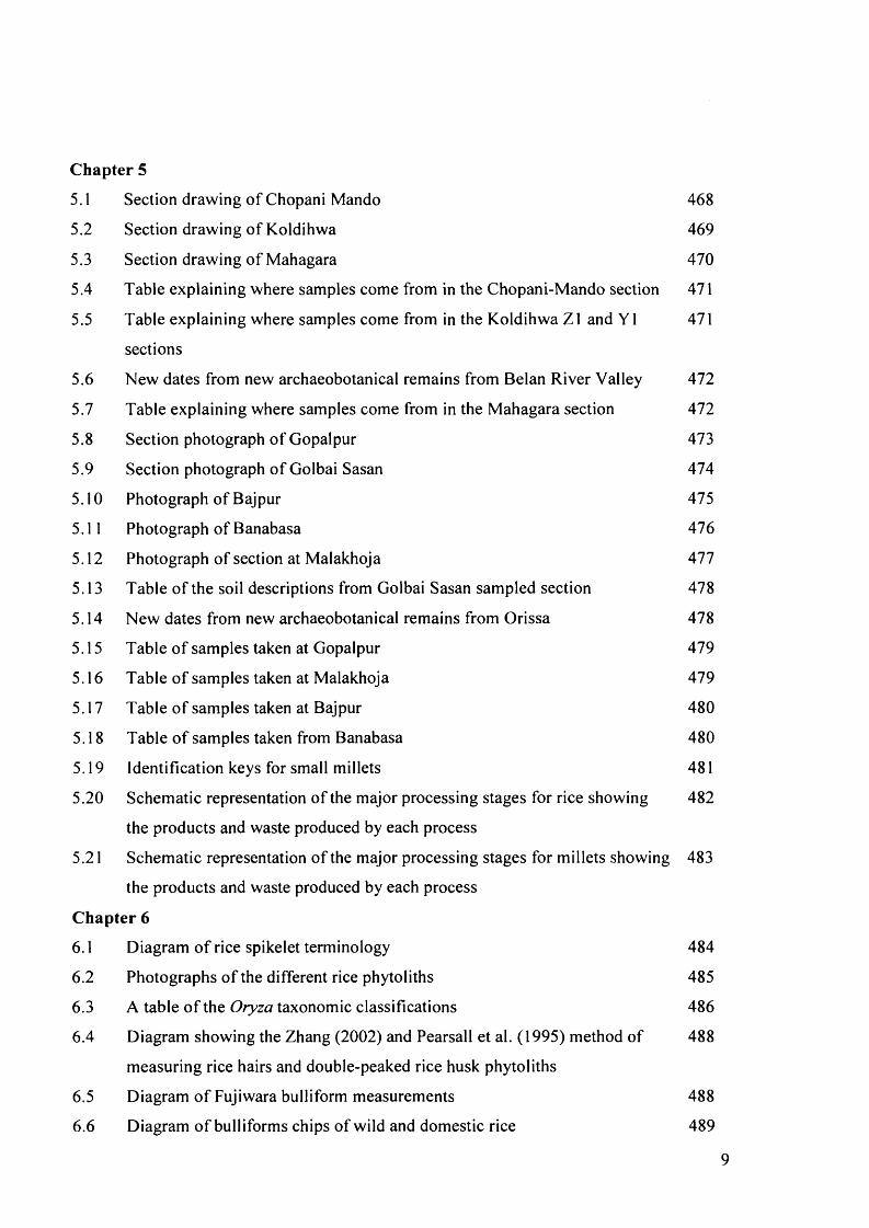
C hap ter 5
5.1 Section drawing o f Chopani Mando 468
5.2 Section drawing of Koldihwa 469
5.3 Section drawing o f Mahagara 470
5.4 Table explaining where samples come from in the Chopani-Mando section 471
5.5 Table explaining where samples come from in the Koldihwa Z1 and Y1
sections
471
5.6 New dates from new archaeobotanical remains from Belan River Valley 472
5.7 Table explaining where samples come from in the Mahagara section 472
5.8 Section photograph o f Gopalpur 473
5.9 Section photograph o f Golbai Sasan 474
5.10 Photograph of Bajpur 475
5.11 Photograph of Banabasa 476
5.12 Photograph of section at Malakhoja 477
5.13 Table of the soil descriptions from Golbai Sasan sampled section 478
5.14 New dates from new archaeobotanical remains from Orissa 478
5.15 Table o f samples taken at Gopalpur 479
5.16 Table of samples taken at Malakhoja 479
5.17 Table o f samples taken at Bajpur 480
5.18 Table o f samples taken from Banabasa 480
5.19 Identification keys for small millets 481
5.20 Schematic representation of the major processing stages for rice showing
the products and waste produced by each process
482
5.21 Schematic representation of the major processing stages for millets showing
the products and waste produced by each process
483
C h ap ter 6
6.1 Diagram o f rice spikelet terminology 484
6.2 Photographs o f the different rice phytoliths 485
6.3 A table o f the Oryza taxonomic classifications 486
6.4 Diagram showing the Zhang (2002) and Pearsall et al. (1995) method of
measuring rice hairs and double-peaked rice husk phytoliths
488
6.5 Diagram o f Fujiwara bulliform measurements 488
6.6 Diagram o f bulliforms chips of wild and domestic rice 489
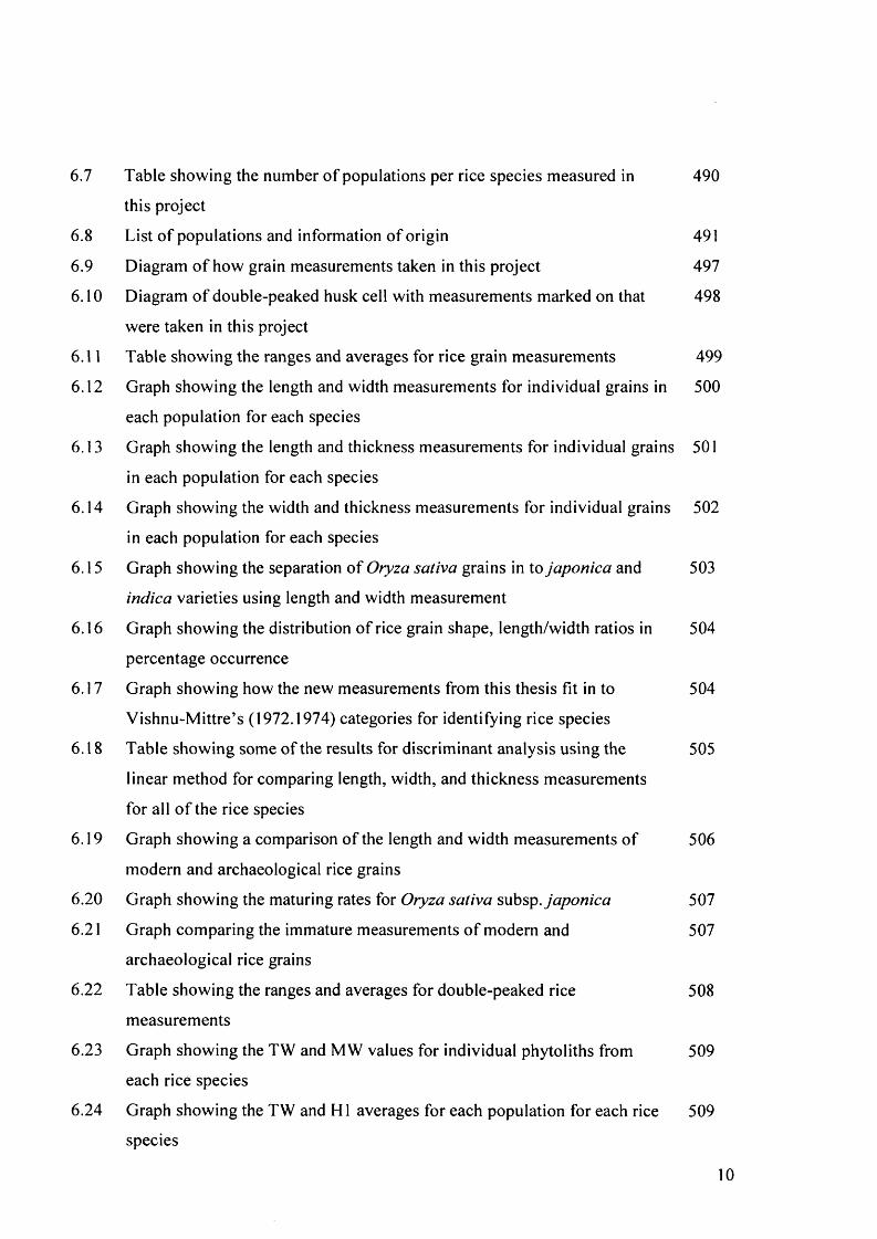
6.7 Table showing the number o f populations per rice species measured in 490
this project
6.8 List of populations and information of origin 491
6.9 Diagram o f how grain measurements taken in this project 497
6.10 Diagram of double-peaked husk cell with measurements marked on that 498
were taken in this project
6.11 Table showing the ranges and averages for rice grain measurements 499
6.12 Graph showing the length and width measurements for individual grains in 500
each population for each species
6.13 Graph showing the length and thickness measurements for individual grains 501
in each population for each species
6.14 Graph showing the width and thickness measurements for individual grains 502
in each population for each species
6.15 Graph showing the separation o f Oryza sativa grains in to japonica and 503
indica varieties using length and width measurement
6.16 Graph showing the distribution of rice grain shape, length/width ratios in 504
percentage occurrence
6.17 Graph showing how the new measurements from this thesis fit in to 504
Vishnu-M ittre’s (1972.1974) categories for identifying rice species
6.18 Table showing some of the results for discriminant analysis using the 505
linear method for comparing length, width, and thickness measurements
for all o f the rice species
6.19 Graph showing a comparison o f the length and width measurements o f 506
modern and archaeological rice grains
6.20 Graph showing the maturing rates for Oryza sativa subsp .japonica 507
6.21 Graph comparing the immature measurements o f modern and 507
archaeological rice grains
6.22 Table showing the ranges and averages for double-peaked rice 508
measurements
6.23 Graph showing the TW and MW values for individual phytoliths from 509
each rice species
6.24 Graph showing the TW and HI averages for each population for each rice 509
species
10

6.25 Table showing the results o f discriminant analysis using the linear method 510
for measurements o f double-peaked husk phytoliths for all rice species
6.26 Table showing the results of discriminant analysis using the linear method 511
for all measurements (TW, MW, H I, H2, CD, PA, CA) o f double-peaked
husk phytoliths using wild versus domestic categories
6.27 Graph showing archaeological and modern double-peaked husk phytolith 512
measurements
6.28 Graph of archaeological rice bulliforms chips from Gopalpur and Golbai 513
Sasan
6.29 Graph of archaeological rice bulliform chips from Mahagara and Koldihwa 514
Chapter 7
7.1 Graph showing modern length and width measurements o f Vigna radiata 515
and Vigna mungo (wild and domestic species)
7.2 Graph showing modern length and width measurements o f Vigna radiata 515
and Vigna mungo (wild and domestic species) with 20% shrinkage adjustment
7.3 Graph showing archaeological length and width measurements for Vigna sp. 516
seeds with dashed line separating possible wild from possible domestic types
7.4 Graph showing length vs plumule length/length measurements for
identifying Vigna mungo and Vigna radiata
7.5 Ubiquity pie charts for sites in the Belan River Valley
7.6 Graph o f ubiquity values comparing the Belan River Valley sites
7.7 Graph comparing ubiquity values for new Belan River Valley sites and the
published North Indian sites
7.8 Bar chart o f relative frequencies o f macro-remains from Mahagara
7.9 Bar chart o f relative frequencies o f macro-remains in Z1 section from
Koldihwa
7.10 Bar chart o f relative frequencies o f macro-remains in Y 1 sections from
Koldihwa
7.11 Charts showing the vertical changes in the sequence from Mahagara
7.12 Charts showing the vertical changes in the sequence from Koldihwa Z1
7.13 Charts showing the vertical changes in the sequence from Koldihwa Y 1
7.14 Table o f correlations for Mahagara macro-remains
11
516
517
518
518
519
520
520
521
522
523
524
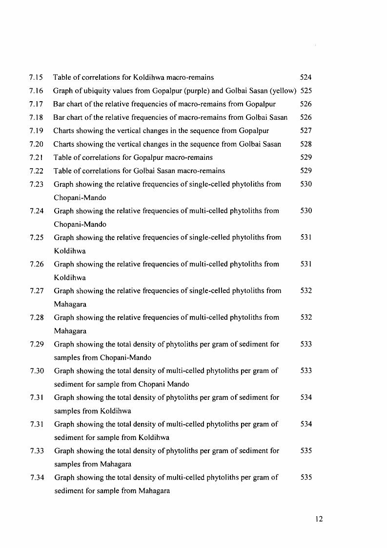
7.15
7.16
7.17
7.18
7.19
7.20
7.21
7.22
7.23
7.24
7.25
7.26
7.27
7.28
7.29
7.30
7.31
7.31
7.33
7.34
Table of correlations for Koldihwa macro-remains 524
Graph o f ubiquity values from Gopalpur (purple) and Golbai Sasan (yellow) 525
Bar chart o f the relative frequencies of macro-remains from Gopalpur 526
Bar chart o f the relative frequencies of macro-remains from Golbai Sasan 526
Charts showing the vertical changes in the sequence from Gopalpur 527
Charts showing the vertical changes in the sequence from Golbai Sasan 528
Table o f correlations for Gopalpur macro-remains 529
Table of correlations for Golbai Sasan macro-remains 529
Graph showing the relative frequencies o f single-celled phytoliths from 530
Chopani-Mando
Graph showing the relative frequencies o f multi-celled phytoliths from 530
Chopani-Mando
Graph showing the relative frequencies o f single-celled phytoliths from 531
Koldihwa
Graph showing the relative frequencies o f multi-celled phytoliths from 531
Koldihwa
Graph showing the relative frequencies o f single-celled phytoliths from 532
Mahagara
Graph showing the relative frequencies o f multi-celled phytoliths from 532
Mahagara
Graph showing the total density of phytoliths per gram o f sediment for 533
samples from Chopani-Mando
Graph showing the total density of multi-celled phytoliths per gram of 533
sediment for sample from Chopani Mando
Graph showing the total density of phytoliths per gram o f sediment for 534
samples from Koldihwa
Graph showing the total density of multi-celled phytoliths per gram of 534
sediment for sample from Koldihwa
Graph showing the total density of phytoliths per gram o f sediment for 535
samples from Mahagara
Graph showing the total density of multi-celled phytoliths per gram of 535
sediment for sample from Mahagara
12
7.35 Graph showing the absolute density of single-celled phytoliths from
Chopani-Mando
536
7.36 Graph showing the absolute density of multi-celled phytoliths from
Chopani-Mando
536
7.37 Graph showing the absolute density of single-celled phytoliths from
Koldihwa
537
7.38 Graph showing the absolute density of multi-celled phytoliths from
Koldihwa
537
7.39 Graph showing the absolute density of single-celled phytoliths from
Mahagara
538
7.40 Graph showing the absolute density of multi-celled phytoliths from
Mahagara
538
7.41 Graph showing the different grass subfamilies from Chopani-Mando 539
7.42 Graph showing the different grass subfamilies from Koldihwa 539
7.43 Graph showing the different grass subfamilies from Mahagara 540
7.44 Table of correlations for Chopani-Mando single-celled phytoliths 541
7.45 Table of comparisons for Koldihwa single-celled phytoliths 541
7.46 Table o f correlations for Mahagara single-celled phytoliths 542
7.47 Table of correlations for Koldihwa multi-celled phytoliths 543
7.48 Table of correlations from Mahagara multi-celled phytoliths 544
7.49 Graph showing the relative frequencies o f single-celled phytoliths from
Bajpur
545
7.50 Graph showing the relative frequencies o f multi-celled phytoliths from
Bajpur
545
7.51 Graph showing the relative frequencies o f single-celled phytoliths from
Malakhoja.
546
7.52 Graph showing the relative frequencies o f multi-celled phytoliths from
Malakhoja
546
7.53 Graph showing the relative frequencies o f single-celled phytoliths from
Gopalpur
547
7.54 Graph showing the relative frequencies o f multi-celled phytoliths from 547
Gopalpur

7.55
7.56
7.57
7.58
7.59
7.60
7.61
7.62
7.63
7.64
7.65
7.66
7.67
7.68
7.69
7.70
7.71
Graph showing the relative frequencies of single-celled phytoliths from 548
Golbai Sasan
Graph showing the relative frequencies o f multi-celled phytoliths from 548
Golbai Sasan
Graph showing the total density of phytoliths per gram o f sediment for 549
samples from Bajpur
Graph showing the total density of multi-celled phytoliths per gram of 549
sediment from Bajpur
Graph showing the absolute density for single-celled phytoliths from Bajpur 550
Graph showing the absolute density for multi-celled phytoliths from Bajpur 550
Graph showing the total density of phytoliths per gram o f sediment for 551
samples from Malakhoja
Graph showing the total density of multi-celled phytoliths per gram of 551
sediment from Malakhoja
Graph showing the absolute density of single-celled phytoliths from 552
Malakhoja
Graph showing the absolute density o f multi-celled phytoliths from 552
Malakhoja
Graph showing the total density of phytoliths per gram o f sediment for 553
samples from Gopalpur
Graph showing the total density of multi-celled phytoliths per gram of 553
sediment from Gopalpur
Graph showing the absolute density o f single-celled phytoliths from 554
Gopalpur
Graph showing the absolute density o f multi-celled phytoliths from 554
Gopalpur
Graph showing the total density of phytoliths per gram o f sediment for 555
samples from Golbai Sasan
Graph showing the total density of multi-celled phytoliths per gram of 555
sediment from Golbai Sasan
Graph showing the absolute density o f single-celled phytoliths from 556
Golbai Sasan
14
7.72 Graph showing the absolute density of multi-celled phytoliths from 556
Golbai Sasan
7.73 Graph showing the different grass subfamilies from Bajpur 557
7.74 Graph showing the different grass subfamilies from Malakhoja 557
7.75 Graph showing the different grass subfamilies from Gopalpur 558
7.76 Graph showing the different grass subfamilies from Golbai Sasan 558
7.77 Table o f correlations of single-celled phytoliths from Bajpur 559
7.78 Table of correlations o f single-celled phytoliths from Malakhoja 560
7.79 Table of correlations of single-celled phytoliths from Gopalpur 560
7.80 Table of correlations of single-celled phytoliths from Golbai Sasan 561
7.81 Table o f correlations for Gopalpur multi-celled phytoliths 562
7.82 Table o f correlations for Golbai Sasan multi-celled phytoliths 563
7.83 Tables o f weeds present in the archaeobotanical assemblages and their 564
environmental implications
7.84 Graph showing the ratio o f rice leaf/stem phytoliths to rice husk 566
phytoliths at Koldihwa and Mahagara
7.85 Graph showing the ratio o f rice leaf/stem phytoliths to rice husk 566
phytoliths at Gopalpur and Golbai Sasan
7.86 Vertical charts o f absolute counts and densities for macro-remains and 567
phytoliths at Golbai Sasan
7.87 Vertical charts o f absolute counts and densities for macro-remains and 568
phytoliths for Gopalpur
7.88 Vertical chart o f absolute counts and densities o f macro-remains and 569
phytoliths from Mahagara
7.89 Vertical chart o f absolute counts and densities for macro-remains and 570
phytolith from section Y1 at Koldihwa
7.90 Vertical chart o f absolute counts and densities for macro-remains and 571
phytoliths from section Z1 at Koldihwa
15

Acknowledgements
Firstly, I would like to thank my supervisors Dorian Fuller and Arlene Rosen, who have
offered sound advice and help throughout my PhD. I would like to add a special thanks to
Dorian for helping me to organise and for also joining me on fieldwork trips in India. I
know that I will not forget our first trip to Orissa when we got drenched the whole time by
the summer monsoons.
I have also benefited from collaborations with Indian scholars particularly in Orissa
and I have really appreciated the insight that these academics have given me. Therefore, I
would like to thank Dr Rabi Mohanty, Dr Kishor Basa, Dr Basanta Mohanta, Dr Mukund
Kajale, Dr J N Pal, Dr M C Gupta. I would like to offer special thanks to Rabi, who assisted
me with travel and other arrangements during time spent in Pune and his wife who fed me
delicious Indian food. I also owe a lot to Basanta who acted as an organiser and guide for
fieldwork trips to Orissa. He was particularly good at finding good places to eat!
I was able to conduct this thesis through an AHRB scholarship, so thank you to
them. I also had financial support from the UCL Graduate fund, NERC for radiocarbon
dating, and the British Academy for fieldwork costs. Without this money, this project
would not have got off the ground so I owe many thanks to these generous organisations.
I would like to say a big thank you to everyone else at the Institute o f Archaeology
who has helped me during this thesis. Thanks to those in 306 (Sue, Meriel, Ruth, Alison,
Phil, and Edgar), who have offered sensible advice, suggestions, and emotional support
when times have been hard. A big thank you goes to Stuart Brookes who was patient
enough to teach me how to use Adobe illustrator and InDesign, which helped me a great
deal with making my diagrams look presentable. Thanks also to Sandra Bond who has
helped me with my lab work and any other technical frustrations I have had.
Finally, many thanks goes to my family who have always been supportive of my
academic pursuits. Special thanks to my Dad who has offered much needed emotional and
sometimes financial support throughout all my years as a student. And of course, great
thanks goes to Alex who has given endless support and definitely inspired me to get my act
together and finally finish this thesis!
16
Chapter 1
Introduction to project aims and objectives
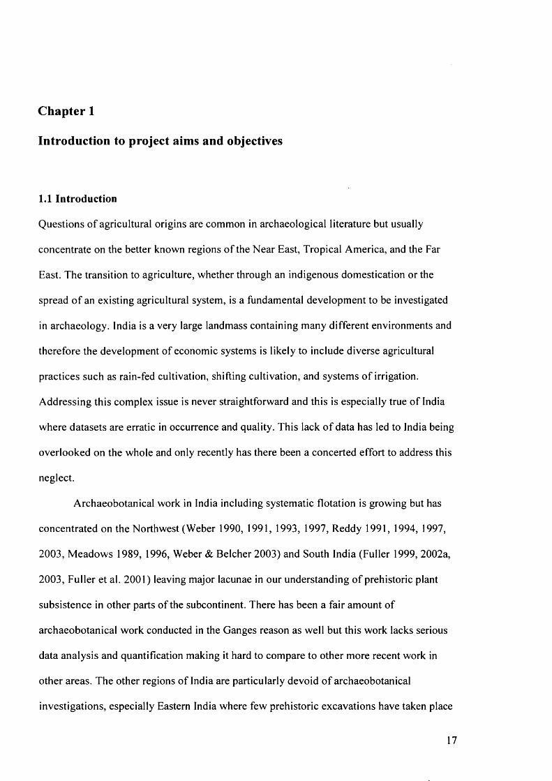
1.1 Introduction
Questions of agricultural origins are common in archaeological literature but usually
concentrate on the better known regions o f the Near East, Tropical America, and the Far
East. The transition to agriculture, whether through an indigenous domestication or the
spread o f an existing agricultural system, is a fundamental development to be investigated
in archaeology. India is a very large landmass containing many different environments and
therefore the development of economic systems is likely to include diverse agricultural
practices such as rain-fed cultivation, shifting cultivation, and systems o f irrigation.
Addressing this complex issue is never straightforward and this is especially true o f India
where datasets are erratic in occurrence and quality. This lack o f data has led to India being
overlooked on the whole and only recently has there been a concerted effort to address this
neglect.
Archaeobotanical work in India including systematic flotation is growing but has
concentrated on the Northwest (Weber 1990, 1991, 1993, 1997, Reddy 1991, 1994, 1997,
2003, Meadows 1989, 1996, Weber & Belcher 2003) and South India (Fuller 1999, 2002a,
2003, Fuller et al. 2001) leaving major lacunae in our understanding o f prehistoric plant
subsistence in other parts of the subcontinent. There has been a fair amount of
archaeobotanical work conducted in the Ganges reason as well but this work lacks serious
data analysis and quantification making it hard to compare to other more recent work in
other areas. The other regions of India are particularly devoid o f archaeobotanical
investigations, especially Eastern India where few prehistoric excavations have taken place

let alone any with systematic environmental sampling. This lack o f archaeobotanical work
is surprising as the Gangetic region and Eastern India offers great potential for investigating
indigenous domestications.
As far as phytolith analysis is concerned, little work has been conducted in the
whole o f South Asia (Fujiwara 1992, Kajale et al. 1995, Madella 1995, 1997, 2003, Kajale
& Eksambekar 1997, 2001a, 2001b, Eksambekar et al. 1999, Harvey et al. 2005) and this
presents certain problems for beginning investigations such as establishing a reference
collection for the region. However, the persistence of phytoliths in tropical areas offers
great potential to complement organic archaeobotanical assemblages and should be
incorporated more frequently into archaeological projects in South Asia.
This project seeks to contribute to the growing body o f archaeobotanical work in
India concentrating specifically on Northern and Eastern prehistoric sites (see figure 1.1 for
map o f study areas). In North-Central India, the early farming sites located in the Belan
River Valley (part o f the Vindhyas culture) are reported to have the earliest evidence o f rice
domestication (Sharma et al. 1980b). However, there is controversy over the dating of these
sites (Allchin & Allchin 1982: 118, Pandey 1988, Kajale 1991: 169, Possehl & Rissman
1992, Bellwood 1996: 488, Glover & Higham 1996: 416, Mandal 1997, Tewari et al. 2000,
Singh 2001, Fuller 2002a: 299, Tewari et al. 2003) and the archaeobotanical evidence is
currently poor due to a lack of systematic sampling and flotation, and also a lack of
quantification. A re-examination of these sites, which includes hunter-gatherer sites and
farming settlements, will elucidate whether this is in fact an area o f indigenous
domestication and establish a more detailed insight into the economic systems of these
communities.
Orissa, in Eastern India, has been completely neglected as far as archaeobotanical
work is concerned. Few excavations have taken place in this state (Sengupta & Panja 2002:
18
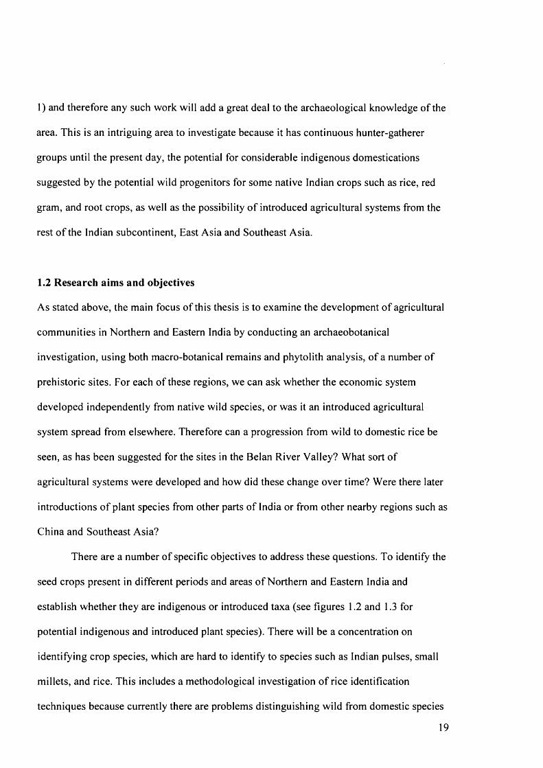
1) and therefore any such work will add a great deal to the archaeological knowledge of the
area. This is an intriguing area to investigate because it has continuous hunter-gatherer
groups until the present day, the potential for considerable indigenous domestications
suggested by the potential wild progenitors for some native Indian crops such as rice, red
gram, and root crops, as well as the possibility o f introduced agricultural systems from the
rest o f the Indian subcontinent, East Asia and Southeast Asia.
1.2 Research aims and objectives
As stated above, the main focus of this thesis is to examine the development o f agricultural
communities in Northern and Eastern India by conducting an archaeobotanical
investigation, using both macro-botanical remains and phytolith analysis, o f a number of
prehistoric sites. For each of these regions, we can ask whether the economic system
developed independently from native wild species, or was it an introduced agricultural
system spread from elsewhere. Therefore can a progression from wild to domestic rice be
seen, as has been suggested for the sites in the Belan River Valley? What sort o f
agricultural systems were developed and how did these change over time? Were there later
introductions o f plant species from other parts of India or from other nearby regions such as
China and Southeast Asia?
There are a number of specific objectives to address these questions. To identify the
seed crops present in different periods and areas o f Northern and Eastern India and
establish whether they are indigenous or introduced taxa (see figures 1.2 and 1.3 for
potential indigenous and introduced plant species). There will be a concentration on
identifying crop species, which are hard to identify to species such as Indian pulses, small
millets, and rice. This includes a methodological investigation o f rice identification
techniques because currently there are problems distinguishing wild from domestic species
19

using macroscopic remains and phytoliths. This analysis will start to address issues o f
whether there are any clear changes from wild to domestic crops, or whether there are any
clear introductions o f some crops, or whether at this point we can not accurately distinguish
this change.
Another objective is to establish evidence for on site plant use and processing o f
other plant resources used by the early farming peoples o f Northern and Eastern India by
using phytolith analysis, including evidence for additional plant species not in the seed
record (e.g.: bananas, sugarcane, various curcurbits, palms, and root crops such as taro).
Agricultural systems will be assessed by looking at crop processing activities and the
changes in these systems in relation to changes in crop repertoire, and archaeological phase
will be analysed. Investigations into crop processing are usually examined through the
analysis o f macro-botanical remains. In this project, both macro-remains and phytolith
analysis will be used to interpret crop processing stages and crop husbandry methods.
Combining macroscopic remains and phytolith data can add to the interpretations by
filtering out some o f the negative effects o f organic preservation problems (Harvey &
Fuller 2005). A close examination o f the weed species present in the samples will also be
conducted to examine agricultural practices in more detail.
The chronology needs to be refined for the early farming communities in Northern
and Eastern India and the antiquity o f crop species will be established through direct AMS
dating. There is much controversy over the dating o f early agricultural sites in the Gangetic
region o f India and there is a complete lack o f any firm chronology for Orissa. Therefore,
having the newly excavated archaeobotanical material dated will enable these issues with
the chronology to be addressed and allow a better understanding o f the agricultural
developments in these regions.
20

The early farming communities o f Northern and Eastern India will be considered in
relation to the archaeological record o f other parts of India, including specifically the
evidence for early agricultural systems and plant domestications, and assess the likelihood
of independent agricultural origins in Northern and Eastern India.
The evidence from Northern and Eastern India will also be examined in relation to
explanations for the origins of agriculture that have been proposed from other world
regions such as the Near East, New World tropics, and Eastern North America. An
assessment o f current theories of agricultural origins will be conducted in relation to how
these theories can be applied to India. Looking at pathways towards agriculture for other
world regions will help to assess the current and new evidence from India.
Finally, the differences o f using macroscopic and microscopic plant remains
(phytolith analysis) will be evaluated in terms of their use to addresses the questions
relating to agricultural development. What are the strengths and weaknesses of each
technique? This will draw on the ability to identify plant species and plant parts using these
methods and how this can effect the interpretations drawn in this project. How much do
preservation problems affect the interpretations made using macroscopic remains?
The theoretical issues surrounding this thesis are discussed and assessed in chapter two
including an examination of the approaches used to try to identify early agricultural
systems. Chapter three will go on to discuss the geographical setting o f the thesis. This will
include a review o f the modern day landscapes, geology, soil, climate, and vegetation types.
Potential crops that may be found during this investigation are discussed including where
these may have come from originally. There is also a brief introduction to modern day
minority tribal groups and their traditional subsistence practices. Chapter four discusses all
o f the currently published archaeological and archaeobotanical data for the regions of
21

study. This chapter tries to establish the pattern of early agricultural communities that is
currently available and draw out specific issues that need to be addressed further in this
thesis. In chapter five, the methodology used for this thesis in the field and in the laboratory
is discussed and then in chapter six rice identification methods are examined and a new
study o f reference material is reported. The results are presented and discussed in terms of
the identifications that can be made for the ancient rice remains from India. Full results of
the macroscopic and phytolith analyses are presented in chapter seven and then finally
these results are discussed and interpreted in chapter eight.
22

Chapter 2
Trajectories towards agriculture: the development and spread of
agricultural communities and early patterns of subsistence
2.1 Questioning the origins and spread of plant cultivation
The origin o f agricultural communities continues to be an important question within
archaeology whatever world region is being investigated. Why humans decided to begin
farming after such a long period as hunter-gatherers is still o f great interest. Recently, the
majority o f this work has concentrated on regional studies emphasizing when, where, and
what. Hence, much less attention has been paid to the questions o f how and why this
transition occurred except for studies in the Near East, which are heavily theorized. Many
of the established theories were developed when little data was available and therefore the
newly acquired data may not fit well with some o f these models. It is also not always clear
what aspect o f agricultural origins is being addressed by some models, for example,
whether it is the onset o f plant cultivation or sedentary life that is being explained.
Therefore, this makes the comparison o f such models challenging and some may only relate
to certain geographic regions and others to all transitions. Harris (1973) summarises that
there are two approaches: i) the generalizing cultural evolutionary approach - to understand
transformations from one major level to another in people’s overall cultural progress; ii)
particularizing culture-historical approach - to reconstruct the actual sequence of events
that took place in specific locations at known times. These are essentially the two ends o f
the spectrum in terms of the approaches to archaeological research termed nomothetic
(comparative) and ideographic (regionally focused) (Trigger 1989).
23
These approaches are applying either a regional focus or a more general world view
of the transitions towards farming societies. The amount of evidence available will
determine which o f these approaches is more readily taken. Generalised models suit areas
that lack data, whereas the more regionalist approach is only feasible when there is enough
evidence to be more specific about sequences in a certain regional area. Applying general
models is particularly difficult because it is becoming more and more apparent from new
data that the transition to farming in many parts o f the world happened at different times
and under different circumstances. This means that a one-size-fits-all model is not
appropriate. It seems a much better approach to assess the situation on an individual basis
for specific regional areas and for specific prehistoric groups before considering similarities
and differences with other situations.
There are a number of common themes in theoretical studies based on external or
internal (stress or non-stress) factors affecting the hunter-gatherer groups that could lead to
a shift towards plant cultivation. The majority o f these models have a central factor, which
is the main cause for the change. This does somewhat over simplify the situation and it is
likely that the transition occurred for a number o f reasons, which are different in different
places and situations. These factors that have become central focuses o f theories can be
environmental, climatic, demographic, biological, or social. Here, a number of these
models will be reviewed and critically assessed for their use in Indian archaeology. The
transition to farming communities in India is still known from rather scarce evidence and
this will hamper the application of some o f the models. Although, it will be as interesting to
discover that some of the models do not fit the current data as it will if some of them fit
well. There is likely to be a very complicated transition to agricultural communities in India
because the region is so geographically vast and there are a number o f different prehistoric
groups, which may all have different pathways towards agriculture. There is also likely to
24

be some indigenous development o f agriculture, as well as the later introduction of
domestic plants from other regions. When the introduction o f these taxa occurs, how this
happens, and what this means for the prehistoric peoples’ everyday lives, is of equal
importance to the development of indigenous agriculture because it demonstrates another
significant social change within the early farming communities. It must also be
remembered that the domestication of plants is only one aspect o f the social and economic
transformation o f society that accompanied the change from food procurers to food
producers.
2.1.1 Defining domestication
There are certain terminological difficulties when discussing the transition from food
procurement to food production therefore it is important to define the definitions used here.
As Harris (1996) points out, there is little agreement over the terms used to describe the
development o f agriculture. Researchers use the terms agriculture, cultivation, horticulture,
domestication, and husbandry in different ways and this has led to misunderstandings in the
literature. Harris (1989, 1996a, 1996b) suggests that these terms can not be used
autonomously and should be thought of as an ‘evolutionary continuum of people-plant
interactions’. He has constructed a diagram to show this change over time and a modified
version o f this can be found later in this chapter as figure 2.1. This diagram shows a
progressive sequence from food procurement of wild plants to the cultivation o f wild plants
on a small scale and then on a larger scale and eventually the step to crop production, which
is termed agriculture and involves domesticated plants. Ford’s (1985) continuum of
categories for the stages of food production is similar to Harris’s model but has some subtle
differences. He does suggest, like Harris, that these are interacting categories although he
uses the term incipient agriculture for the beginnings o f plant cultivation. He agrees that
25
domestication should be used for the genetic change o f the plant. There are differences in
the definition of food production as Ford suggests that food production is the deliberate
manipulation of plant species by humans including in this the protective tending of wild
plants, where as Harris (1989) regards this activity as part o f food procurement not food
production.
There are a number o f problems with both o f these sequences. Firstly, they suggest
a uni-linear progression, which is obviously not the case because not all agricultural
developments would be the same. This is however, pointed out by Harris (1996: 4) and he
states that this diagram is not meant to imply that all domestications have a similar
pathway. This is a problem that is raised by Yen (1989) as he points out that there is an
assumption with these models that hunting-and-gathering is a transitional state rather than a
choice o f subsistence strategy. Yen proposes that food gatherers can be seen to
“domesticate” the environment by manipulating it much like agriculturalists would modify
it to produce their crops. Therefore, there are two parallel forms o f food production (Yen
1989: 71): i) the intensification of foraging through social development including activities
such as the use o f fire to encourage re-growth and the tending o f wild plants; and ii) the
technological development o f agriculture through more successively intensive methods
narrowing the species to specific environments. These are joined later by a third parallel,
which is the development of state agriculture that is producing for a surplus. There can be a
progression from one stage to the next but these three modes o f subsistence still exist side
by side and are specific subsistence choices.
The second issue with Harris’s model (1989, 1996) is the placement of
domestication within this sequence. His model implies that to have agriculture there needs
to be a genetic change in the plant. This excludes some forms o f horticulture from the
definition o f agriculture because some crops are not produced on large scales and never
26
become domesticated in the genetic sense such as root and tuber crops. Hather (1996)
suggests that domestication needs to be removed because it is not a single event but a
continuous process occurring under selective pressure. This leaves a sequence from wild
procurement to complex agricultural systems. Cultivation begins when the plant is being
planted and managed where as agriculture begins when this process is relied on for
subsistence. In a sense, it is not domestication that we should really be looking for but the
signs o f the beginning o f cultivation because ancient people would not be interested in
domesticating the plant as such but manipulating it to yield more produce whether this kept
it wild or forced it to change genetically.
A different way of looking at the definition o f domestication is proposed by Rindos
(1980, 1984). In Rindos’s definition, domestication can be any symbiotic relationship
between plants and humans. This model o f co-evolution proposes three types of
domestication. These do not form an evolutionary process as they can all occur at the same
time. Firstly, incidental domestication is the relationship between non-agricultural societies
and the plants that they feed on. The plants do not have to be domesticated and they take
advantage o f human dispersal and protective behaviour that increases their fitness. This is
like the wild plant procurement stage of Harris’s (1989, 1996a, 1996b) model. Secondly,
specialized domestication sees changes in the behaviour o f the agent. These are specific
behaviours that enhance the success o f the plant. Humans become dependent on certain
plants for survival. This includes the storage, planting, and protection of plants by humans.
This would be the cultivation stage o f Harris’s model but Hather would call this agriculture
because o f the humans dependence on the plant. Finally, agricultural domestication is the
establishment and refinement of systems o f agricultural production. This is what most
scholars would term domestication and is where the genetic change occurs (Harlan 1995,
Zohary & Hopf 2000).
Rindos, therefore, is encompassing the very beginning o f people-plant relationships
in his definition o f domestication, i.e. most hunter-gatherers. The focus o f many scholars on
the genetic change definition o f domestication stems from our ability to recognise
morphological changes in the plant but this really only recognises the end o f the
development. It is much harder to recognise wild cultivation archaeologically but this must
be attempted if we are to progress in our knowledge o f the full transition to complex
agriculture o f genetically domestic crops. This has been attempted through the analysis of
arable weeds such as demonstrated at Abu Hureya (Hillman et al. 2001) and argued for
PPNA sites (Willcox 1999, Colledge 2001).
This thesis will follow the majority o f scholars (Harris 1989, 1996a, 1996b, Smith
2001a) for using the term food procurement to refer to collecting wild food resources and
the term food production will be used to describe any form o f production from low-level
production o f wild species to intensive agricultural systems. The tending o f wild plants will
be included in food procurement as has been done by Harris (1989, 1996a, 1996b).
Cultivation will be used for any conscious human actions on the plants, such as planting
and weeding, to increase its production. Agriculture can refer to either wild production or
the production o f domestic crops but does define a more complex subsistence system
(Hather 1996). The terms domestic and domestication refer to plants that have genetically
changed and therefore rely on human intervention to reproduce.
28

2.1.2 Centres and hearths
The path of studies concerning agricultural origins has been continually influenced by the
founding work o f De Candolle (1886) and Vavilov (1926). While De Candolle (1886)
attempted to locate centres o f domestication based on botanical knowledge, ancient texts,
and linguistic inferences, it was Vavilov (1926) who led the first o f the modern botanical
approaches to the geography o f agricultural origins. Vavilov’s theory o f ‘Centres o f origin’
concentrates on when and where agriculture first happens. He mapped the distribution and
degree o f genetic diversity o f crops throughout the world. Initially, he identified five places
of independent primary domestication based on areas o f high plant diversity, o f which India
was one, and this later developed into twelve centres. His theory is now discounted because
it is clear that high plant diversity can occur in different areas to plant domestication and
early agriculture (Harris 1996a). However, many theories have been developed from
Vavilov’s and the idea of a ‘Centre’ is still prominent in most literature on agricultural
origins (Sauer 1952, Zhukovsky 1970, Harlan 1971, Hawkes 1983, MacNeish 1991, to
name just a few!). This idea o f ‘centres’ o f origin (Vavilov 1926) is rather outdated but still
influences theories because it focuses on the major crops used by the western world today.
This idea should be abandoned as some form of indigenous agriculture probably occurred
on most continents because many regions have wild relatives o f crops in their regional flora
and therefore specific food stuffs will develop according to the local environment. In some
regions, such as in South Asia, these wild relatives have been under-studied. In addition,
archaeobotanical approaches have been hampered because o f preservation problems or lack
of archaeological investigations. Domestication may have happened many times in some
areas depending on the availability of suitable plants and appropriate cultural conditions.
The likelihood o f one single event o f domestication for each plant species is also rather
dubious and this could have occurred in different geographical locations across a wild
29
species range. Therefore it depends to some degree on how large the distribution o f the wild
progenitor is to the likelihood of more than one location of domestication. The transition to
agriculture should be seen as a scale of development with many stages much like that
suggested by Harris’s evolutionary classification of systems (Harris 1996b) although this
does not mean there is only a single, recurrent uni-lineal pathway.
However, the majority of the models for agricultural origins do concentrate on the
few better studied centres o f origin, which are often sources o f major crops o f the modern
age. These regions are South West Asia, South America, and the Far East as well as North
America. Few models have been applied to or developed from evidence from the Indian
subcontinent and this is largely due to the lack o f archaeobotanical and archaeozoological
data currently available for the periods needed in the region. An early study that does relate
to the Indian subcontinent is the model developed by Sauer (1952). He suggests the idea
that root and tuber cultivation preceded seed cultivation and this has long been an
influential theory for tropical agricultural origins (Heine-Geldren 1923, Sauer 1936, 1952,
Nakao 1966, Harris 1969, Lathrap 1977, Piperno & Pearsall 1998). The early theoretical
work o f Sauer (1936, 1952) concentrates on ‘hearths o f domestication’, which are found in
areas o f marked diversity o f plants and animals, much like Vavilov’s ‘centres’. The two
hearths, which Sauer focuses on, are South America and Southeast Asia. This includes
India as part o f the Southeast Asian hearth. His theory was not particularly well tested and
the idea o f hearths in the Vavilov (1926) sense is obviously outdated. Therefore many
scholars have been sceptical o f its content (e.g: Zohary 1970, Bender 1975, Harris 1977,
MacNeish 1991) but there are some interesting points that can be drawn from the model.
The hearths o f domestication were suggested by Sauer to be very lush and therefore
he proposes that cultivation did not begin out of a shortage o f food but because these people
had time to experiment. This is a very different view to that proposed for most o f the Near
30
Eastern models, which focus on stress factors that cause food shortages to bring about the
start o f cultivation. However, Byrd (2005) has suggested recently that the start o f the
progression towards farming societies in the Near East began in a time when food was
readily available.
What also differs in Sauer’s model is the location o f domestication. He believes that
cultivation began in upland wooded areas and not in the oases o f the Near East proposed by
Childe (1952). He also suggests that agriculture began in sedentary villages located near to
water and that the progenitors o f farming were fishing folk (Sauer 1952). This difference of
location may be just a geographic difference and it is probably best to interpret the location
o f early sites on a regional basis rather than world scale. The location will differ due to the
location o f available food resources and existing hunter-gatherer economic strategies. In
tropical areas this may mean in more forested margins, and in drier areas, oases will be the
areas with food resources. Hence, the development o f farming communities in tropical
regions is likely to be very different to the development in the Near East and other drier
regions because o f the plants available to be cultivated and the local climatic regimes. The
issue o f sedentism and how it relates to the beginnings o f agriculture will be discussed later
in this chapter.
Sauer (1952) also proposes that the people who developed agriculture would have
had some previous skills that they could apply to this new activity. This has also been
elaborated by Harris (1977) and this could be related to the types o f foods being exploited
and brought under cultivation or the tools used that could be adapted for use in the
cultivation o f plants as processing techniques or processing/harvesting tools (Harris 1977,
Wright 1994).
An aspect o f Sauer’s model that has to be considered is whether hunter-gatherers
could have existed within tropical rain forests without any outside influences. It is usually
31

assumed that hunter-gatherers would have lived within many different environments in the
past and modem day studies typically focus on groups that live within rainforests.
However, the majority o f these groups have some reliance on agriculturalists and do not
rely solely on wild forest foods. Bailey et al. (1989) have proposed that rainforests could
not support a group o f pure hunter-gatherers because edible plants and animals are very
widely dispersed. Although, it may be true that most hunter-gatherer groups today do trade
forest products for agricultural foodstuffs, there are still examples o f groups that are
thought to live in total isolation in the recent past, for example, the Andaman islanders of
the Indian Ocean (although they do exploit more than one environment). Sauer’s (1952)
model is based on living in forest margins and hunter-gatherer groups are usually fairly
mobile exploiting a number o f different habitats. A good example o f this is the inhabitants
o f the Indian Andaman Islands. As well as exploiting forest products such as honey, tubers,
yams, and fruits, coastal resources are an important part o f their diet (Cipriani 1966, Bailey
et al. 1989). Therefore, hunter-gatherers that exist in rain forest areas are likely to exploit a
number o f different environments to fulfil the requirements o f their diet.
Townsend (1990) has proposed that hunter-gatherers could actually exist in
isolation if they exploited the forest resources fully. She argues that Bailey et al. (1989)
have underestimated the use o f tree crops, including palms such as sago, which is a good
source o f carbohydrate. The manipulation o f the forest by hunter-gatherers is another issue
that has to be considered because this could still be termed as food procurement. Clearing
the forest for regeneration to create patches, which will produce more edible species is only
one way to alter the rainforest and solves the issue o f widely dispersed resources, which are
less efficient to exploit. Therefore, hunter-gatherers may be able to live in isolation within
rain forests if they make full use o f their environment.
32

Bailey (1990) has proposed that only through archaeological evidence can this
debate be settled. Recent evidence that starts to disprove this theory (Bailey et al. 1989)
comes from Niah Cave in Sarawak. Starch grain analysis (Barton 2005) has suggested the
exploitation o f a number of carbohydrate rich foodstuffs such as yam, and sago palm. This
is supported by parenchyma finds (Paz 2005), and evidence for bone digging implements
(Rabett 2005). Therefore, the debate is still open as to whether hunter-gatherer groups
could have existed solely on forest products although this new evidence suggests that it
may have been possible in the past. It is also clear that these groups could have settled
within forest margins and exploited a number of different environments rather than solely
relying o f forest foods.
Therefore, there seems to be two streams of theoretical influence within the
question o f agricultural origins. The oasis-based hearths initially proposed by Pumpelly
(1908) and later developed by Childe (1952). This specific pathway is discussed later in the
chapter relating to climate change factors. This theory is usually used for the Near East and
relates to deficiencies in the environment to provide resources. Many scholars have
followed this pathway towards agriculture such as in Near Eastern studies in various
modified forms (Bar-Yosef & Meadows 1995, Smith 1995, Hillman et al. 2001, Willcox
2004) and also in the Far East (Cohen 1998, Yasuda 2002a). The opposing theory base
comes initially from Sauer (1952) and is based on rich forested environments providing
stability for the development of cultivation. This theory is popular with scholars that
research tropical environments such as parts of Asia and South America (Harris 1969,
1972, Lathrap 1977, Hather 1996, Pipemo & Pearsall 1998). It is clear from these two
opposing theory bases that there is not only one kind of environment in which cultivation
and later agriculture could have developed. These models are based on different regions
and therefore have different expectations for the beginnings of cultivation.
33

2.1.3 Tropical hearths: vegeculture.
The most important point to come from Sauer’s (1952) theory is his suggestion that root
and tuber agriculture predated seed agriculture. He explains this using Southeast Asia,
where he perceives taro cultivation as a pre-requisite to rice domestication (Sauer 1952:
28). Even though it is unlikely that root and tuber agriculture brought about rice
domestication in Southeast Asia, as the archaeology now suggests that this occurred at least
once in South China and then spread to Southeast Asia (Glover & Higham 1996), roots and
tubers probably played a key role in the transition to agriculture in the tropics. The
cultivation of roots and tubers probably did precede seed cultivation in Southeast Asia and
rice was an introduced crop in to this area rather than a domesticated one (Gorman 1969,
1977, Golson & Hughes 1976). The presence of early cultivation of tuber crops is also
likely in Eastern and North eastern parts of India although in these regions rice could have
been domesticated locally within India whether in the East or North of the country.
Harris (1969) has also suggested that root and tuber agriculture is fundamental to
our understanding o f plant domestication and the beginnings o f agriculture. However, the
study of these crops has been neglected and therefore our picture of agricultural origins as a
whole lacks this aspect, which may indeed be some of the earliest cultivation in the world.
Investigations on the whole are much fewer in the tropics but when studies are conducted
they are hindered by the lack of organic remains present. Bio-archaeological studies in
tropical zones are hampered by the fast turn over of carbon, which results in the decay of
archaeological remains at a much faster rate than in temperate or semi-arid regions (Hather
1992, Pipemo & Pearsall 1998). Therefore, plant macro-remains and other organics are
hard to recover and generally found in lower densities in tropical regions. Consequently
datasets are limited, fragmentary, and difficult to analyse. In addition to preservation issues,
only a small amount o f work has been conducted on how to identify roots and tubers in
34

archaeological deposits and many more studies are needed. Macroscopic preservation of
roots and tubers is as rare as other macro-remains on tropical archaeological sites, and
added to this, poor identification methods, makes recognition o f this material very
challenging. Consequently, different approaches are needed to overcome the problem of
identifying tropical plant remains (Hather 1992, 1994, 1996, Pipemo & Pearsall 1998).
Techniques such as phytolith analysis, starch grain analysis, and the identification of roots
and tubers through parenchyma fragments should be combined with the more traditionally
used archaeobotanical methods of macro-remains and palynology to establish detailed bio-
archaeological datasets for past tropical agriculture.
Harris (1977) suggests that vegeculture was an obvious choice for the beginning of
cultivation in the tropics because it was already being exploited and therefore the
technology was available. Root crops have the ability to store starch over long dry and cold
seasons and when matured can be left in the ground until needed, thus preventing rotting.
Root and tuber crops are also quicker to propagate because they are grown from cuttings
and do not remove as many nutrients from the soil as most seed crops. The harvesting of
root and tuber crops would have resulted in discarded parts being left and therefore the
regeneration o f some of these would be observed. Harvesting therefore may actually
promote proliferation. Andersen (1997) suggests that the collection of wild tubers using
digging sticks, by Native Californian’s, actually maintains the production o f the food plant.
Harris (1977) suggests the move to cultivation would have been a simple step and started as
a minor activity o f hunter-gatherers, which later developed into a specialised mode of
production once these groups came under stress. Therefore the initial steps of plant
domestication in the tropics could be unconscious acts that were later developed in to a
deliberate agricultural system.
35

Sauer’s early work has also influenced Japanese scholars o f whom Nakao (1966,
see Sasaki 2002 for English summary) was the first to suggest vegeculture as the basis for
farming culture. He classified agricultural systems in to three types: Mediterranean - the
Near Eastern seed crop package including wheat and barley; Savannah - semi-arid zones of
India and Africa including rice and millets; Vegeculture - wet tropical zones including
bananas, taro, yams, and sugarcane. Nakao and later Hotta (1983, 1999) also believed that
root and tuber agriculture originated in Southeast Asia (including Eastern India).
There are two aspects to the development of root and tuber agriculture in Asia. One
is, as discussed above, the indigenous development of root and tuber agriculture in
Southeast Asia and the other is the development from or introduction of rice agriculture to
this initial subsistence system. Tanaka (2002) has suggested that rice growing techniques
closely resemble those used in root and tuber crop cultivation. Rice transplantation
techniques are used predominantly in East and Southeast Asia and this is similar to the
individual selection, harvesting, and planting of root and tuber crops. These systems are
much more individually focused than the community based wheat and barley sowing
methods (Tanaka 2002). This may reflect the differences between the development of
indica and japonica types as this system relates more to inundated rice o f Eastern Asia
rather than the rain-fed rice of South Asia.
It is also suggested that rice agriculture in India is more like the wheat and barley
system (Tanaka 2002). However, this model does not account for the later introduction of
wheat and barley agricultural systems in to India and probably does not relate to the initial
systems of cultivation. Rice was grown in India before wheat and barley were introduced
from North-western parts of the Indian sub-continent. Therefore, early cultivation systems
may have resembled root and tuber cultivation systems before this time. Evidence for this
may be found in the material culture associated with these early agricultural communities.
36
Digging sticks are the only piece o f technology specifically developed for root and tuber
cultivation (Sasaki 2002). Evidence for ancient digging sticks is lacking because of
preservation issues but ringstones may be associated with them. These ringstones are found
throughout Northern India in pre-ceramic/Mesolithic contexts onwards and have been
recovered from the prehistoric sites o f the Ganges Valley and in the state o f Orissa (for
examples see Sharma et al. 1980, Mohanta 2002).
Root and tuber cultivation must have played a significant role in the development o f
agriculture in tropical regions but has so far been predominantly overlooked. This
development may have also influenced the beginning o f rice cultivation in some areas and
the spread of rice in to Southeast Asia was probably introduced in to an existing root and
tuber cultivation system. However, many more studies are needed to confirm the existence
o f early root and tuber cultivation in the Indian subcontinent and this question cannot yet be
answered, as insufficient amounts o f charred tuberous material has been recovered through
flotation from the sites analysed in this thesis.
2.1.4 Climate change
The majority o f other models differ from Sauer’s (1952) non-stressful (or “food choice”)
development o f agriculture and promote the importance o f external factors that cause stress
resulting in food shortages. Climatic and environmental change is a very popular model
(“food stress”) because o f the vast amount o f work focused on the Near East. Childe’s
(1952) oases model, based on Pumpelly’s (1908) earlier work, suggests climate change as
the prime mover for cultural changes and specifically agricultural origins. At the time this
theory was developed, there was reasonably good evidence for climatic changes at the end
of the Pleistocene in Europe but no evidence from South West Asia. Childe (1952),
however, proposed that Post-Pleistocene desiccation led to the concentration o f people,
37

beast, and plant at oases. He said that this might promote a symbiosis between people and
beast implying animal domestication, and plant domestication was also suggested. He
implies that this close association would inevitably lead to the discovery o f agriculture
assuming that it was an obvious choice. This is still an assumption that is made in many
studies today such as in early agricultural sites in China where the discovery o f any rice is
usually considered to be domestic and therefore agricultural. Wild gathering as well as wild
cultivation, especially for plant species such as rice, should also be considered for these
sites, which may have previously been considered to show domesticated plant agriculture.
Childe’s model set a trend in Near Eastern studies, which is now dominated by
models o f climate and environmental change (Bar-Yosef & Meadows 1995, Smith 1995,
Harris 1996, Willcox 1999, Hillman et al. 2001). This factor is now widely accepted as the
predominant cause o f the emergence o f agriculture in this region. The Near East benefits
from detailed palaeoecological studies that have revealed an environmental deterioration as
a result o f the Younger Dryas episode from ca. 11,000 to 10,000 B.P. (van Zeist & Bottema
1977, Bottema 1986, Baruch & Bottema 1991, Baruch 1994). The cooler and drier climate
of the Younger Dryas resulted in most o f the exploitable natural resources declining in this
region. Hillman and his team’s work (Hillman 1996, Hillman et al. 2001) at Abu Hureya is
a good example o f how climate change has been used to explain the beginning o f
cultivation and subsequent domestication o f cereals in the Near East. Detailed
archaeobotanical investigations revealed an increase in arable weeds around 11,000 B.P.
(uncalibrated), which led to the conclusion that the people o f Abu Hureya had begun
cultivating wild cereals (annual wild rye and wild wheats). This coincides with the
beginning o f the Younger Dryas period, which caused declines in many wild species
through a phased process, and it was therefore concluded as the factor that greatly
influenced the start o f cultivation in this area. Moving from Abu Hureya was another option
38

for these peoples but Hillman (Hillman et al. 2001) suggests that this was not done because
it was the richest area for natural resources and therefore other areas would have been more
depleted during the Younger Dryas.
The Near East presents an example of a major climate shift that has a detrimental
effect on the environment and consequently stresses sedentary hunter-gatherers causing the
beginning o f cultivation. However, not every world region has agricultural origins that
coincide with the beginning of the Holocene. Models that promote climate change as the
prime mover, tend to be better suited to the datasets of the ‘centres of origin’ where
processes are focused in very tight delimited ecological zones rather than the more
dispersed and long-term emergence of agriculture in the tropical ‘non-centres’ (Harlan
1971) where ecological zones are more extensive or patchily distributed. Agriculture in
India appears after the end of the Pleistocene and therefore the accompanying
environmental change did not affect the hunter-gatherers to the same degree as those in the
Near East but these groups may have been affected later by Holocene fluctuations in
monsoon rainfall (Fuller & Korisetter 2004). The emergence of agricultural societies in
India seems to have occurred over a much longer temporal period because interaction
occurs between hunter-gatherers and farmers to the present day. The introduction of
agriculture from other regions into parts of India also plays a role in the overall
development o f agriculture, therefore climate change can not explain all the moves towards
plant cultivation. Again, it is better to approach this transition on a more regional basis
especially in such a large sub-continent as India.
39
2.1.5 Population pressure
Another model that promotes a stress-induced development o f agriculture is the suggestion
of population increases and pressure creating food shortages. This factor is also used in
Near Eastern models. Cohen (1977a, 1977b) argues that population growth and pressure is
a significant trend among pre-agricultural peoples that led to the beginning of agricultural
societies. His model is based on earlier work by Boserup (1965), who suggests the
progression to more complex agricultural technologies is a response to growing population.
The problem with population models for the emergence of agriculture is their general
nature. These models are vague and it is hard to prove population growth and its link to
agricultural origins. Keeley’s (1995) study of hunter-gatherer societies suggests that
population pressure alone only leads to socio-economic complexity not proto-agriculture.
Rosenberg (1998) suggests that population pressure may in fact induce territoriality and
sedentism although this may only occur where resources are available in concentrated
patches.
Many o f these population based studies have focused on the ecological concept of
carrying capacity, which relates to the maximum level of consumption of any resource that
an environment can tolerate. However, this idea is not relevant to humans because of their
broad diet (Cohen 1977a). Humans rarely exploit all o f the resources available to them and
therefore if there is a scarcity of one resource then they can shift to another. It therefore
does not take into account how foragers respond to changing resource densities (Piperno &
Pearsall 1998).
Another factor o f the population model is its uni-linear approach to the process of
agricultural origins. It assumes that every hunter-gatherer group grew in number and
therefore became agricultural. This is not true for many areas where hunter-gatherers
persist to the present day such as in India and Africa. There are also cases o f newly
40

agricultural groups returning to foraging in times of famine if the appropriate knowledge is
still available (Harris 1980). Pipemo & Pearsall (1998) think that population pressure was
not a significant factor in the New World tropics because the area was settled by so few
people but populations may have increased later due to horticultural intensification.
Therefore, models based predominantly on population may have little relevance to studies
of agricultural origins in the tropics. However, population growth may have played some
role in combination with other factors in some parts of the world.
2.1.6 Darwinism and domestication
The application of Darwinian evolutionary theory to the question o f origins of agriculture
has brought a more biological explanation to the debate. Rindos (1980, 1984) believes that
unconscious selection was the pre-eminent force behind the domestication of plants and
animals. He suggests that consciousness is not needed for domestication and this model
deals directly with the process of domestication o f the plant or animal. This is also
proposed by other scholars (Harlan 1995, Zohary & Hopf 2000, Gepts 2004). Co-evolution
is the evolutionary process in which the establishment of a symbiotic relationship between
organisms increases the fitness of all and brings about changes in the traits of the
organisms. Rindos (1984: 99) does not suggest this is the cause o f domestication but
proposes that it is a pre-requisite to agriculture. As discussed above, Rindos has a rather
different definition o f domestication to other researchers, however his definition does
encompass the whole spectrum of change. Rindos (1984) is promoting an unconscious
domestication o f plants but he is not denying the initiative of humans. They could have
selected for pleasing attributes or those that were useful to them. He does emphasize the
point that these people could not have foreseen an agricultural economy because no such
thing had previously existed at that time (Rindos 1984, Watson 1995). This is an important
41

point to keep in mind when thinking about the transition to agriculture because, even
though hunter-gatherers would have had an in depth knowledge o f their environment and
the plants in it, they had no knowledge of agriculture, nor the genetic architecture of the
domestication syndrome that the world ultimately selects. Therefore, it is quite right to
expect the very initial steps towards agriculture to be unconscious and then human initiative
would have taken the next steps. Rindos’s theory is, however, a one sided view of the
development o f agriculture focusing on how this process happened. It does not account for
social changes in hunter-gatherer society or the external factors o f climate and
environmental change, which may have allowed for this development in the interactions
between man and plant. Hence, it does not consider why this happened and Rindos goes
further by saying that to ask why humans began close associations with certain plants is a
question without real meaning (Rindos 1984: 141). This is one way of avoiding the hard
question of why humans began using plants but there has to be a cause for this change even
if it is that the humans wanted to use the plants.
Initially, if we are looking at food procurement, they had a dietary need for the
plants and probably experimentation was the key to deciding what was edible and what
wasn’t. Humans must have been the driving force but a change to cultivating these plants
could have many causes. Farrington & Urry (1985) suggest that plants have specific
cultural values and this is why they are exploited or produced. This can be for a number of
reasons such as for material culture, decoration, and medicines, as well as food. Selection
of food resources will initially be based on edibility but cultural habits and preferences are
also likely to influence choice and the amount of effort given to collection or production of
certain food stuffs. Therefore, avoiding the question o f why these plants are being exploited
is to miss out a vital part of the investigation even if it is probably the hardest issue to
address.

2.1.7 Evolutionary ecology
Another application of Darwinian Theory is evolutionary or behavioural ecology, which
has focused on why these associations took place and what circumstances led humans to
select certain species for exploitation (Smith & Winterhalder 1992, Pipemo & Pearsall
1998). Evolutionary ecology is the application of natural selection theory to the study of
adaptation and biological design in an ecological setting (Winterhalder & Smith 1992).
When this involves behaviour it is called behavioural ecology. They both use simple
mathematical models to understand complex systems. Behavioural ecology differs from
Rindos’s co-evolutionary theory by emphasizing the decision making of animals capable of
flexible and learned behaviour. The key principle behind behavioural ecology is
optimization, which means that an individual relates to their environment in such a way to
maximise their reproductive success (Shennan 2002). The humans or animals have the
capacity to adjust quickly to varying ecological circumstances. The intentionality of the
development o f agriculture, which is a sticking point of most theories, is less problematic
when applying behavioural ecology because human behaviour is seen as the motivating
force (Pipemo & Pearsall 1998). Optimal foraging theory and in particular the Diet Breath
and patch selection models (MacArthur & Pianka 1966, Emlen 1966, Charnov & Orians
1973, Winterhalder & Smith 1981, 1992, Smith 1983, Keegan 1986, Hawkes & O ’Connell
1992, Winterhalder & Goland 1993, 1997) have been applied to hunter-gatherer strategies
and also less frequently to agricultural subsistence.
These foraging models contain three components: decisions, currencies, and
constraints (Kaplan & Hill 1992). The decisions are the foraging problems that are being
analysed. The currency defines the measurement scale for evaluating the effects of the
decisions. This can be a measure of energy, protein, survivorship, or fertility. The
constraints are all of the other terms that are in the model. These models investigate what
43
happens when foragers encounter resources and have to decide whether or not to pursue
this resource or move to find another one. These models can be formally tested using
ethnographic studies of modem hunter-gatherers and horticulturalists. This has shown in
supporting propositions that energy is a useful currency to use and that energetic concerns
are major constraints on foraging decisions (Pipemo & Pearsall 1998:17, Shennan 2002).
This approach has been used in some cases to try to explain the transition to farming
communities (Hawkes & O ’Connell 1992, Winterhalder & Goland 1997, Piperno &
Pearsall 1998, Hawkes et al. 2001). In their examination of the origins of agriculture in the
lowland Neotropics, Piperno & Pearsall (1998) suggest that behavioural ecology and
particularly the diet breath model is the most appropriate way to explain the transition to
plant cultivation. They rely heavily on the diet breath model because they believe that it
makes a number o f valuable predictions (Piperno & Pearsall 1998: 17-18): “i) resources
will enter the diet as a function not of their own abundance but of the abundance of higher
ranked resources; ii) as the abundance of higher ranked resources decline and foragers
begin to do better by investing less time in them and more time handling lower ranked
resources; iii) the foragers will now choose a broader diet because it results in higher return
rates than could be achieved by more searching; iv) the reduction in search time will permit
greater investments in storage and food processing, which adds to the nutritional quality of
what is eaten and extending the use life of the food item; v) the broader diet and decreased
search time will also lead to smaller foraging radii and may increase residential stability; vi)
changes in diet breath may result in human demographic change, whose direction is
dependent on the characteristics of the resources newly incorporated in to the diet”. This
bares close resemblance to Flannery’s (1969) broad spectrum revolution and also addresses
the issues o f sedentism and population pressure.
44

There have been arguments as to whether these models can be applied to humans
because humans have free will and therefore may have different goals to those assumed by
the models. These models take no account of cultural choices as mentioned above, which
may play a large role in the selection of certain foodstuffs and other materials. Therefore,
optimal foraging theory may not be applicable to archaeological studies and is probably
better left to ethnography. Smith (1983: 629) proposes that foraging theory is useful for
generating hypotheses but when models are applied to archaeological data they are
inherently limited by a lack of direct measures of either foraging costs or harvest rates. To
actually apply the models to archaeological situations, ethnographic analogies or
experimental data can be used but these come with their own limitations. Bettinger (1983:
640) adds that uncertainties about tactics are compounded by estimates of search time
within specific patches and the distribution of patches within the habitat. This results in the
rapid accumulation of uncertainties even in simple models and makes optimal foraging
theory no more than a rough analogy in archaeology. He again suggests that it is best used
as a generator o f hypotheses rather than a source o f rigorous quantitative models (Bettinger
1983).
Shennan (2002) suggests that these models are in fact useful for addressing
archaeological problems. They should be used as hypotheses and seeing where the model
does not fit is very interesting. This can lead to interpretations of why this might be and
therefore determine specific behaviours. For example, the behaviour o f men usually fits
optimal foraging models because they select hunting, which maximises outcomes. Women
tend to fit a lot less to the idea of optimisation than men because their activities do not
maximise their efforts (Shennan 2002: 147). Therefore, behavioural ecology may help to
determine agricultural origins if the right methodology is applied. Appropriate
45

archaeological evidence needs to be found that can be used to test and refine these models
and then there is a chance that they can help to determine past behaviours.
2.1.8 Broad spectrum revolution
The broad spectrum revolution (BSR) was initially proposed as a period that saw the
broadening of the resource base o f foragers and this process was involved in the transition
to animal herding (Flannery 1969). The BSR was explained as the shift away from hunting
large ungulate mammals to the exploitation of birds, reptiles, fish, invertebrates, and
previously ignored plant resources. Since Flannery proposed this theory for the
development o f agricultural settlements, much more evidence has come to light but this
theory is still common in the literature (Clark & Yi 1983, Stiner et al. 1999, Stiner 2001,
Munro 2004, Weiss et al. 2004). Initially, Flannery placed the BSR in the middle of the
Upper Palaeolithic about 20,000 BP and it was proposed to be closely linked to the
emergence o f pre-agricultural settlements. However, recent studies have pushed this date
further back as far as the Middle Palaeolithic for faunal remains (Stiner et al. 1999, Stiner
2001) and to 23,000 BP for plant remains (Weiss et al. 2004) and therefore it does not have
as much relation to early villages as was first suggested in the initial theory. The plant
remains evidence from Ohalo II does demonstrate that a large variety of different species
were exploited especially grasses but this does not necessarily support the BSR theory as
there is no earlier evidence to compare it with to demonstrate a ‘revolution’. Edwards
(1989a) has suggested that if all of the evidence is compared for faunal and floral remains
from the Mugharan period to the PPNB then it is clear that there is no BSR in the Middle or
Upper Palaeolithic and therefore it can not be used to address the issue of the development
of agricultural settlements. The evidence in fact suggests that a broad spectrum subsistence
pattern was normal throughout much of the Upper Pleistocene in the Levant and there was
46

no visible increase in faunal diversity in this period (Edwards 1989a: 240-241). Therefore,
there is no relationship between broad spectrum foraging and the rise of food production.
2.1.9 Competitive feasting
Another theory, which uses an internal factor, this time a social one, to explain the
transition to plant cultivation, is Hayden’s aggrandizer feasting model (Hayden 1995a,
1995b, 1998, 2001, 2003). This theory is very different to other models of agricultural
origins as it suggests certain plants were domesticated first o f all as luxury foods. This is in
contrast to the normal suggestion that early plants were staple crops. The feasting model
suggests luxury foods were developed for consumption in feasts. Hayden (2003) suggests
feasts are important for the consumption of surpluses and there is significant competition to
display wealth at the most important feasts. He uses ethnographic examples from Southeast
Asia to explain how rice was first domesticated as a luxury food (Hayden 2003). However,
he suggests that rice comes from wild hill rice, which does not fit well with current
archaeological and genetic evidence (see discussion in chapter 6 below). The wild
progenitors of rice (Oryza rufipogon and Oryza nivara), which are confirmed by genetic
studies (Chen et al. 1993, Cheng et al. 2003), are both lowland species (Vaughan 1994) and
therefore it is more likely that rice was domesticated at lowland sites, which is also
suggested by the current archaeological evidence. Hayden (2003) proposes a number of
reasons why rice would be a luxury food including its good taste, its use as alcohol, and
that rice is used in rituals and the ideological life o f modern hill tribes. Although he is quite
right that rice is used in rituals today, this does not mean that it was a luxury food or was
given a prestigious status that allowed it to be domesticated. Rice is a staple today as well
as being used in many rituals so the link of luxury food and rituals is not the only possible
explanation. He argues that because we see ethnographic examples of this practice today
47
there is no reason to think it was different in the past. This is a large assumption, which is
equally likely to be untrue. It can not be assumed that what happens today was also
occurring in prehistoric times (Gould 1980, Trigger 1995). It is also hard to find direct
evidence o f feasting on archaeological sites therefore Hayden’s theory has many flaws and
deserves a cynical review.
2.1.10 Addressing agriculture spread
As well as questioning the development of indigenous agriculture, the spread of established
crop packages or single crops in to areas with no previous cultivation or in to areas with
existing indigenous cultivation systems needs to be addressed. The beginnings of
agriculture in some world regions, such as Europe and Egypt, was not the result of local
domestications but instead a diffusion of domestic plants and animals or the immigration of
agricultural communities from other regions. Less attention has been paid to regions that
had some local development of domestic species, sometimes suggested to be of minor
importance, which was later replaced with another agricultural package developed
elsewhere (Fuller 1999). Examples of this would be the Eastern Woodlands of North
America and South India.
At the forefront of discussion on this particular topic is frontier theory, which
considers the colonisation by agriculturalists, and their interactions with hunter-gatherer
groups in regions with no previous agriculture, within a single framework (Alexander 1978,
1980, 1984, Alexander & Mohammad 1980, Dennell 1983, 1985, Zvelebil 1986, 1996).
There are two types o f frontiers: the moving frontier and static frontier. These have been
termed ‘spread zone’ and ‘friction zone’ by Bellwood (2001). The moving frontier (or
‘spread zone’) sees the expansion and colonisation of new lands by agriculturalists. Hunter-
gatherers will react to the moving frontier and are either destroyed by the farmers through
48
absorption or acculturation, or retreat into isolation. The moving frontier has been
suggested to occur until all the usable land is taken up or until the limits o f climatic
tolerance o f the plants and animals are reached (Alexander 1978). Hence friction is created
by some kind of boundary, which restricts further movement and the moving frontier
therefore stops setting up a static frontier. Interactions between hunter-gatherers and
agriculturalists will occur and components o f the agricultural package may be adopted by
the hunter-gatherers. Static frontiers would have also existed where isolated groups o f
hunter-gatherers were left behind the moving frontier.
There are three models to show how the frontier moved forward and the causes of
the move (Alexander 1980): i) a steady horizontal spread, which is also known as the wave
o f advance model caused by demic explosion (Ammerman & Cavalli-Sforza 1971, 1973,
1984); ii) a selective horizontal spread that involves hopping from place to place whether
for favourable soil conditions, water, or other factors (Ammerman & Cavalli-Sforza 1971,
1973, 1984, Renfrew 1987, Van Andel & Runnells 1995, Cavalli-Sforza 1996, 2002); iii) a
selective vertical spread, which are variations o f transhumance (Higgs et al. 1964, 1966).
The wave o f advance model appears commonly in the literature on the spread o f agriculture
and encompasses the demic diffusion o f agriculturalists (Harris 1996c, Bellwood &
Renfrew 2002, Bellwood 2005). This model has also been used to explain the dispersal of
languages, which in some cases is thought to be linked to the spread o f agriculture such as
the movement o f Indo-Europeans in to Europe and the Austronesians in to Southeast Asia
(Renfrew 1987, 1996, Bellwood 1989, 1991, 1996, Bellwood & Renfrew 2002, Bellwood
2005).
The wave o f advance model has been applied commonly to explain the spread of
agricultural communities in to Europe and specifically the spread of the
Linearbandkeramick (LBK) culture. Renfrew (2002) has argued that, even though recent
49
genetic evidence may not seem to fit the wave o f advance model (Richards et al 1996,
Underhill et al 2000, 2002), it in fact can explain the expansion o f languages and farming,
demonstrating significant gene flow between the incoming and existing populations.
However, some scholars have been very critical o f explaining the whole o f European
expansion using this model (Alexander 1978, Zvelebil 1995, 1996, 2002, Zvelebil &
Zvelebil 1988). The rapid dissemination o f the LBK culture, which spread from Slovenia to
the Paris basin in 200 years, can be seen to contradict population pressure models such as
the wave of advance model by being too fast. Furthermore, Alexander (1978) suggests that
this model is inappropriate to explain the spread o f any agricultural communities because it
conceals the local variations that can occur by the smoothness implied by the curve and it
also does not account for more than one period o f frontier advance. He proposes that
selective horizontal spread is more appropriate to explain the spread of the LBK
agricultural communities (Alexander 1978, Barrett 1994, 1999, Whittle 1996a, 1996b,
1997, Thomas 1999).
However, the northerly and westerly expansion of pioneer farmers o f the LBK from
the Hungarian plain to Germany and the low countries was a complete cultural replacement
and has been seen as a good example of the rapid migration and colonisation by agricultural
groups (Clark 1952, Ammerman & Cavalli-Sforza 1971, 1984, Bogucki 1987, 1996, Price
et al. 1995) but the role o f the indigenous hunter-gatherers should not be underestimated.
After 5400 BC, the LBK populations were spread through the fertile loesslands and had
established permanent villages at the edges o f floodplains with their characteristic timber
longhouses (Hamond 1981, Bogucki 1988, Modderman 1988, Whittle 1996a) and
characteristic incised pottery. These villages only leave negative features filled with
archaeological deposits. These settlements had an economy of emmer and einkom wheat,
broomcom millet, cattle, sheep, goat, and pig. It has been suggested therefore that the
50
agricultural communities hopped from one suitable area to the next being particularly
selective about the placement of their settlements. This is a form o f shifting cultivation and
was originally proposed by Childe (1929: 45-46). The argument for this pattern o f shifting
cultivation comes from the lack o f tell formation (Childe 1929), the evidence for
discontinuity o f settlements (Soudsky & Pavlu 1972), the assumption that soils will be
rapidly exhausted (Childe 1929), and pollen evidence for clearance and burning of
woodlands (Wasylikowa et al. 1985, Rosch 1990). Bogaard (2002, 2004), however,
suggests that this argument is open to question and her reassessment o f the published data
along with new archaeobotanical analysis clearly rejects the shifting cultivation model. She
argues for a more permanent fixed plot cultivation system where agriculture spread through
adoption rather than migration based on the analysis o f weed seed data. This is in
agreement with the assumption that humans would want to fully exploit their environment
rather than waste it by moving on quickly (Bogaard 2004: 155). During the LBK period,
crops were grown in intensive garden cultivation in fixed plots and sown in the autumn
(Bogaard, 2002, 2004: 160). Manuring was also practised therefore preventing soil
exhaustion and also negating the need for careful site selection because soils could always
be improved.
However, this does not mean that this agricultural scheme was adopted throughout
the whole of Europe and there was much the same continuation o f material culture in other
parts o f the continent (Zvelebil 1995, 1996, 2002, Zvelebil & Zvelebil 1988). This will be
discussed in more detail below.
51

2.1.11 Adoption of agriculture
The causes o f the adoption of domestic plants and animals also needs to be considered. This
can be either the adoption of a crop package in to an area previously with solely hunter-
gatherers or can be the introduction of a secondary crop package in to an existing
indigenous cultivation system. Secondary crop packages may compliment existing
economic systems or could replace them altogether (See papers in Weber & Belcher 2003).
This can again include models o f food stress or food choice. Demographic and
environmental/climatic change causes have been suggested in much the same way as with
cases o f indigenous domestication (Zvelebil 1986). However, social factors, especially
social competition, seem to be favoured for the adoption o f crop packages. The adoption of
farming can be seen as a means of maintaining social control or the competition for status
(Sahlins 1974). This includes social models such as the competitive feasting model
(Hayden 1995a, 1995b, 1998,2001, 2003) and tradeable, culturally valued foods
(Farrington & Urry 1985, Sherratt 1999). Interactions between hunter-gatherers and farmers
would have made new foods available and these may have been considered with some
status. Zvelebil (1996, 2002) has suggested that the hunter-gatherers o f the Baltic regions
and North and East Europe did not see the migration o f farming people in to their
territories. This is partly due to the intolerance o f some crops to the environmental and
climatic conditions in these areas causing a natural barrier for farmers. Hence, the adoption
o f farming by the indigenous foragers in these regions o f Europe took place through
contact, inter-marriage, and socially related mobility between foragers and farmers within
frontier zones (Zvelebil 2002). He proposes that demic explosion is unbelievable and any
estimates o f population are unreliable. The size and density o f Mesolithic populations is
always underestimated. Therefore, the spread o f agriculture into Europe was a combination
52

of the migration o f farmers and the adoption o f agricultural elements by the indigenous
foragers although the degrees of input from these two sources varied by region.
2.1.12 Situating India
As far as India is concerned a number o f different theories have been proposed. From its
initial status as a ‘centre of origin’ (Vavilov 1926), it has been demoted by most scholars to
be an area o f agricultural introduction or at best an area with minor crop domestications
(Harlan 1971, MacNeish 1991, Bellwood 2005). Hutchinson (1976) suggested agricultural
communities were established by either the introduction o f African crops or the local
domestication o f summer crops (see also, Possehl 1986). North-west India is clearly an area
o f predominantly agricultural introduction and it is likely that this was due to the migration
o f people and their crops and animals from South West Asia also with some local animal
and plants domestications (Meadow 1989, 1996, 1998, Weber 1991, 1997, 1999, Weber &
Belcher 2003, Fuller & Madella 2001). This began the establishment of the Harappan
civilisation in this part of India. Further migration o f the Harappan people and their
agricultural package has been suggested for the rest o f India (Chakrabarti 1999) but the
adoption o f the crops and animals seems more plausible due to a lack of change in material
culture in most areas. The adoption o f the ‘Harappan’ package in Rajasthan and Madhya
Pradesh may be related to climatic factors (Madella & Fuller 2006).
However, the Peninsula of India is less known and this is partly due to a lack of data
in some regions but also due to the likelihood of a number o f areas o f indigenous
domestication. The origins of agriculture in South India has been addressed recently by
Fuller (1999, 2002a, 2003a, 2003b, Fuller et al. 2001, Fuller & Korisettar 2004) inferring
the indigenous domestication of crops as well as later introductions from a number of
53

different regions. He has suggested that the local domestication o f a number o f crops
happened due to climatic and environmental changes (Fuller & Korisettar 2004).
Fuller (1999) also puts forward a series o f modes for agricultural origins and
suggests that it is important to distinguish between indigenous and introduced agriculture.
He proposes four main types o f agricultural origins:
1 A) Primary centres of major crops - wild progenitors o f major crops are present,
and the transition usually occurs during the early Holocene and there are
innovations of material culture. This includes areas such as South West Asia, South-
central China, South America, West Africa, and sub-Saharan East Africa.
1B) Primary centres of minor crops with “overstamping” - wild progenitors of
minor crops that have been largely replaced by secondary diffusion o f major crops.
This includes Japan, North China, Eastern woodlands o f North America, Ethiopia,
parts of Southeast Asia, and South India.
2A) Secondary centres, introduced by immigrant wave (moving frontier) - crop
package arrives from elsewhere and there is a full scale material culture change.
Areas include Central East Europe, Thailand and Southeast Asia, Northwest South
Asia, and the Iranian-Baluchistan region.
2B) Secondary centres, adopted from adjacent farmers (static front) - the adoption
of crops in piecemeal fashion and in some cases material culture was also adopted.
This includes Northern and Atlantic Europe, Egypt, Southwest North America, parts
of India, and Central Asia.
This addresses what, where, and sometimes when agriculture occurred in different world
regions but leaves out how and why it occurred. He has left these questions to be addressed
at a regional level as with his work in South India. In this series, South India has been put
into IB as minor millet crops were domesticated with secondary introductions of non-native
54
millets, which over-stamped the local crops. However, this category needs to be expanded
because some regions may have introductions that can be slotted into the existing system
extending it rather than providing a new agricultural system altogether.
The other parts o f India have been put in to 2B but this again may be due to lack of
data in some cases. If India has an area o f rice domestication, which is a major crop, as is
proposed for the Gangetic area and Orissa in this project, it will fit in to IA but these areas
may also have later introductions and therefore these areas do not fit into one specific
category o f Fuller’s series. Consequently, this suggests again that India is rather more
complex than first thought and there are likely to be a number o f different transitions to
agriculture depending on the local wild progenitors and influences from outside the region.
It has become clear with this review of theories for agricultural origins and spread that there
are certain limitations to each of the models. The majority o f the limitations relate to the
general nature o f the theories. This means that they can not be applied to every situation
even though this may be attempted and many o f the older theories were developed when
very little data was available. To develop a theory for agricultural origins as a whole is over
simplifying the situation that faces us. What should be addressed is the extensive and
complex mosaic of many different and distinct developmental problems that occurred
during this time o f immense change (Smith 2001b: 202). In each region, the local
environment and culture are different and this brings different plants and animals under
domestication in different ways and at separate times. A much more regional approach will
address the complexities in the transition to farming societies. This needs to start with the
collection o f appropriate data such as archaeobotanical and archaeozoological
investigations. Once this has taken place at a number o f sites and a chronology has been
established then theories as to how and why domestication may have occurred in a specific
55
area can be put forward. However, it is still important to recognise parallels in other world
regions, which may help to develop answers to the questions involved in agricultural
origins. Looking at the complex sequence o f developments, not just one single part of the
transition, will allow greater insight into the questions of why and how these changes took
place.
2.2 Developing the trajectories of change
Many o f the theories for agricultural origins focus on single causes for what is a huge social
and economic change. It is much better to see this transition as a process with several key
elements: sedentism, cultivation, herding, and pottery development. These elements seem
to occur at different times and in different orders throughout the prehistoric world. The
sequence o f these elements may in fact be the key to interpreting the hard questions of how
and why the transition to agricultural communities occurred. Only by examining all o f these
developments can we get an entire picture o f the process and in particular the specific
transitions that happened in different world regions or sub-regions.
2.2.1 Sedentism
Sedentism is seen as a pre-requisite to agriculture in most Near Eastern models of
agricultural origins (Smith 1995, Bar-Yosef & Meadows 1995, Byrd 2005). Byrd’s recent
article (Byrd 2005) suggests that sedentism occurred at the onset o f the Natufian period in
the Near East by complex hunter-gatherers, which is supported by Munro (2004). The
formation of settlements occurred at a time o f optimal climatic conditions and happened in
the most productive parts of the Near East. This was driven by social factors such as
population aggregation, resource intensification, surpluses, and major changes in group
dynamics, social interactions, and ideology (Bryd 2005). He goes on to suggest plant
56

cultivation happened initially as a supplement to the diet because grasses were declining
due to intensive exploitation and possibly environmental/climatic factors. However, some
scholars suggest a more seasonal use o f some sites (Edwards 1989, Harris 2002) that could
also have brought about these changes. Therefore in the Near East there is definitely a
move towards sedentism initially, which is followed by the development o f plant
cultivation.
In Harris’s (1977) model, heavily based on tropical regions, a reduction in mobility
is suggested as a key difference between hunter-gatherers and agricultural societies. Harris
(1977) has pointed out that ethnographic studies have found links between sedentism and
increases in population. He suggests that this may lead to an intensification o f labour input
into food procurement and consequently increasingly specialized exploitation of
agricultural resources. However, there should not be a particular emphasis on sedentism as
a prerequisite to agriculture in tropical regions because it is not always necessary for
agricultural production. A reduction in mobility as a factor in inducing cultivation is
complicated in the tropics because o f the use o f shifting cultivation systems. The nature of
swidden or shifting cultivation suggests a degree of continued mobility even with
cultivation. Swidden is a small-scale cultivation method but relies on a large amount of
fallow land and therefore extensive areas are needed, which usually requires constant
settlement movement (Harris 1972). Although, this is not always the case, as Pratap (2000)
demonstrates in his study o f shifting cultivation in Eastern India where rotation of
cultivation plots can support permanent settlements. Permanence o f settlement can happen
with swidden cultivation if certain conditions are right such as the amount o f land, fallow
period, climate, soil type, vegetation cover, crop type and their demands on the soil (Jochim
1981). However, this demonstrates that a reduction in mobility is related to the type o f early
cultivation method and local conditions required for this system can also influence
57

mobility. Tropical hunter-gatherers may be more likely to start cultivation on a seasonal
level or continuously shifting basis and therefore permanent settlements are not necessarily
needed before cultivation can begin. Non-permanence or seasonal camps are much harder
to find archaeologically than permanent settlements because there will not be constant
accumulation of artefacts and organic debris. This makes these types of sites more
ephemeral than a fully settled site. Therefore, if the initial stages o f plant cultivation occur
during a more mobile phase of occupation it will be much harder to detect and this may be
likely for certain parts o f India.
Sedentism could also result from agricultural intensification and especially the
development of more complex all year around agricultural systems, which require year
round occupation. Most single season agricultural systems could be left after planting to
develop on their own, even though tending may mean a better yield, and then the
cultivators could return when the crop needs to be harvested. This would suit hunter-
gatherers who were beginning to cultivate but still relied on wild foods for most of their
diet. Therefore the issue of sedentism as a pre-requisite to plant cultivation is not clear cut
and the type of cultivation system will play a key role in whether settlement is required.
2.2.2 Recognising plant cultivation and domestication
The development of plant cultivation is obviously a key element in the development of
agricultural societies. In places such as the Near East this seems to be much easier to
recognise due to the type of crops that are involved, major grain and pulse crops, and also
because of the huge amount of detailed work that has now been conducted at archaeological
sites and on the biology of the crops involved (for the plants see Zohary & Hopf 2000).
This has shown that a number of crops were domesticated in this region before animals
were domesticated. India is potentially a much more complicated situation because there
58
are a large number o f crops that could be indigenous and also many which are likely to
have been introduced from other regions. Many of these crops are rare or hard to recognise
in conventional archaeological remains such as curcurbits, yams, taro, which is due to a
large extent on poor preservation. There is also a need to refine identification criteria for
some more common finds in India archaeological deposits such as rice, which is hard to
identify to species, and some India pulses, although Fuller (1999, 2002a, Fuller & Harvey
in press) has started to resolve some of the problems. Another problem is that a lot o f the
wild progenitors of these crops have not been investigated in great detail and the
methodology o f how to distinguish accurately between wild and domestic species is not
greatly developed. Also adding to this is the lack o f archaeobotanical work that has been
conducted in India, although it has been growing more rapidly in recent years, but there is
not a vast dataset for any of the South Asian Neolithic regions as is available for the Near
East. The majority o f sites in India that have been analysed lack quantification for looking
at assemblage change especially for weed floras therefore hindering interpretations o f the
early development of plant cultivation.
As already discussed above, roots and tubers may be very important in the
development o f agriculture in tropical regions, which may be the case for areas such as
Northeast India, including Orissa, and Southeast Asia. Initial cultivation could have
occurred very easily due to propagation of these crops from cuttings (Harris 1977). These
crops are unfortunately very hard to find archaeologically and usually we must rely on the
identification o f agricultural structures such as the terraces and pondfields constructed in
Polynesia (Kirch 1994). It is sometimes possible to find charred remains during flotation
but these are usually rare and hard to identify. Therefore, much more work needs to be
conducted on how to identify these remains and also the application of other methods such
as starch grain analysis needs to be applied but this is unfortunately outside the content of

this project. Hence, the available material must be investigated, which in this case is
charred seeds and phytoliths.
When investigating the signs o f the development o f agriculture, the morphological
change in the plants provides an important benchmark although this does only indicate the
later stages o f the process. A number o f features change when a plant becomes
domesticated and the most important to recognise are the loss of natural seed dispersal, the
increase in seed size, and reduction or loss o f seed dormancy, which is sometimes seen in
the thinning of the seed coat (Harlan et al 1973, Hillman & Davies 1990a, 1990b, Harlan
1995, Smith 1995, Zohary & Hopf 2000). The toughening o f the rachis in cereals or the
reduction o f shrinking tissue in the pods of pulses is a result o f selection for the loss of
natural seed dispersal (Harlan 1995). This is often regarded as the quintessential
domestication trait. This feature allows more o f the seeds to be collected by humans
because the seeds stay on the plant where as in wild plants their seeds are freely dispersed
when ripe, which is not advantageous to humans. This phenotypic change can be
recognised from the plant remains found on archaeological sites and specifically the rachis
or other attachments of the spikelet with cereals. In rice, the attachment of the spikelet base
to the rachilla becomes toughened and a rough scar on the rachilla is a feature of
domesticated types where as a smooth scar identifies wild species (Thompson 1996).
However, the degree o f immature harvesting must be taken into account as this will also
produce a rough scar even in wild rice. This change in pulses is much harder to find
because pods are not usually found and the change in the tissue of the pod would be hard to
recognise in ancient material.
Studies have been conducted to try to estimate the length o f time in which this
development occurred, in other words how long it took wild plants that were being
exploited to become domesticated therefore having the non-shattering feature (Hillman &
60

Davies 1990a, 1990b, Willcox 1999). This change is a process, which humans play a role
in. The first phase is when the plant population has purely brittle rachises. This will
continue until mutants are generated although it is likely that some non-shattering mutants
are present in all large populations of wild grasses (Harlan et al. 1973). The cultivation of
the plants by humans, and specifically the type o f harvesting method used, will either select
for or against these non-shattering mutants. Harvesting by cutting or uprooting will select
more of the toughened rachis mutants and over time more and more will be incorporated in
to the next generation sown the subsequent year. The rate of this change is important for
questions of agricultural origins especially addressing how and why this change occurred.
Wheat and barley are almost exclusively self-pollinating species and therefore under strong
selection from harvesting methods could develop in to domesticates in 20 to 30 years but
weak selection will be much slower (Hillman & Davies 1990a, 1990b). Lower proportions
of mutants sown relative to wild growing plants, immature harvesting, or harvesting
methods other than by cutting the plant will mean weak selection pressure on the
population. Rice is a cross-pollinating species and shows significant out-breeding of 40-
60% of fertilised florets (Oka & Morishma 1967). Fuller has suggested, using Hillman and
Davies (1990a, 1990b) calculations, that with strong selection pressure domestication could
occur in approximately 50 years (Fuller in press a) and it has been shown that under
favourable selective conditions, including the isolation of the crop from outside influence,
selection of domestic characteristics for grain stocks, and hand sowing, that domestic traits
within the population will increase quickly over several generations (Oka & Morishma
1971). Over five generations, grain weight and spikelet number tended to increase as well
as there being a considerable decrease in seed shedding (Oka & Morishma 1971: 357).
When ideal selective conditions are not present then domestication could slow down
dramatically even to more than 1000 years (Fuller in press a). Certain factors can reduce the
61

likelihood o f selection for domestic traits such as the harvesting method including paddle
and basket harvesting that is common for wild cereals, re-sowing in the area o f natural wild
species, collection of a large enough proportion o f the harvest, and the harvesting of
immature grains will reduce the proportion o f domestic mutants in the population. Wild rice
is usually expected to be harvested when the majority of grains are immature to achieve the
best recovery of grain. Basket harvesting is common with wild grasses (Jenks 1900, Harris
1984), therefore this would reduce the selective pressure making the domestication rate
slower.
Increases in seed size and the reduction or loss o f seed dormancy are other changes
that occur during domestication. The increase in seed size is thought to be a direct influence
from humans who would select for larger seeds therefore producing a greater density of
plant material. Some changes in seed size probably occurred at the point o f domestication
in some species but the development o f large seed sizes compared to the smaller wild
progenitors as is clearly seen today did not occur until much later (Jupe 2003, Jupe & Fuller
in prep, Fuller & Harvey in press). The loss of dormancy is reflected in the thinning o f the
seed coat, which allows the seeds to germinate quickly when planted. This change is the
result o f pressure to grow rapidly to compete for space and light in an agricultural field.
There is also no need for a seed bank to be established in the soil to maintain the wild
plants therefore the wild seeds with varying thicknesses in seed coats no longer exist
because the seed crops (with thin seed coats) will be planted each year by humans. A good
example o f both o f these changes can be seen in the Eastern Woodlands of North America
where the independent domestication o f a number o f local wild plants was determined from
investigations o f seed size change and the thinning o f the seed coats of archaeological
specimens (Smith 1992, 1995). Until recently, the first agricultural remains in this part of
the world were thought to be maize, which arrived from Central America in the mid to late
62
first millennium AD (Smith 1992, 1995, Bellwood 2005). However, at a number o f sites in
the central interior of the Eastern Woodlands, plant remains have been found that
demonstrate domestic species including summer squash (Curcurbita pepo), and annual
forbes such as goosefoot (Chenopodium berlandieri), sunflower (Helianthus annus), and
sumpweed (Iva annua). This appearance o f domestic species begins about 4,000 B.P.
(Smith 1992, 1995). At the sites of Ash and Russell Cave, large collections of goosefoot
were found in storage pits sometimes as much as 50,000 seeds. These remains were found
to have seed coats from 10 to 20 microns thick, which is much thinner than wild species but
compares well with other domesticated Chenopodium species (Chenopodium quinoa and
Chenopodium berlandieri subsp. nuttalliae) that are cultivated today in South and Central
America. Maygrass, little barley, and knotweed were also found in large quantities at some
sites. None o f these crops are major staples in North America today and most of them are
not cultivated at all, which is the result o f later over-stamping by maize. At this time, the
people o f the Eastern woodlands were becoming increasingly sedentary. From the seventh
millennium BP, there is a move to more seasonal occupation and the annual reoccupation
o f the same sites located in floodplains (Smith 1992:52). Therefore, the move towards
sedentary life occurred prior to the initial domestication of plants in this area, although they
remain seasonally mobile while cultivators, with the development o f pottery and animal
herding occurring even later.
63

2.2.3 Animal herding
Part of the whole agricultural package is the rearing of animals, which adds another
dimension to subsistence systems. Animals provide an additional source of food in the form
of meat, milk, and eggs, as well as having other properties useful for subsistence such as
traction, manure, and hides. Herding of animals is particularly important in some early
subsistence systems and may have pre-dated plant cultivation. The herding of highly
mobile animals such as sheep, goat, and cattle could have fitted in well with some mobile
hunter-gatherer societies. Transhumant pastoralists are suggested to be present during the
first stages of development of agricultural systems in places such as Africa and South India.
In Africa, domestic animals have been suggested to appear about 9500-8840 BP in
the eastern Sahara and are accompanied with incised, stamped, and impressed pottery
(Marshall & Hildebrandt 2002, Bellwood 2005). Gautier (1980, 1987, 2001) and Wendorf
(Close & Wendorf 1992, Wendorf et al. 1984, 2001, Wendorf & Schild 1980) have found
cattle remains at Bir Kiseiba and Nabta Playa that they argue was herded, however this
evidence is still controversial due to scarce morphological data. Recent morphological and
genetic studies support a separate origin for cattle in Africa (Grigson 1991, 2000, Bradley
et al. 1996, Bradley & Loftus 2000, Hanotte et al. 2002, Marshall & Hildebrandt 2002,
Bruford et al. 2003) and some scholars have suggested a single geographic origin in the
eastern Sahara (Gautier 1987, Hanotte et al. 2002). Further support comes from linguist
studies that link the Northern Sudanic branch of the Nilo-Saharan family with the practise
of cattle herding and pottery, with an estimate from glotto chronology of about 9000 BC
(Ehret 1993, 1997, 2000, 2002, Bellwood 2005). Therefore, the other sources of supporting
evidence for early cattle domestication in the eastern Sahara give more weight to the
argument even if current archaeological finds are not so convincing.
64

With the possibility of cattle herding and pottery being early in Africa, it might be
expected that plant cultivation and sedentism occurred shortly after, however, this does not
seem to be the case (Marshall & Hildebrandt 2002, Barker 2003, Neuman 2004, Bellwood
2005). Plant cultivation and sedentism happened much later in Africa, although the
exploitation of wild grasses, such as millets, seems to have accompanied the early herding
and pottery phase. It has been suggested that cultivation may have occurred of a number of
these grasses due to the appearance of microliths that could be used for sickles and grinding
stones in Sudan about 5000 BC (Haaland 1999) but there is not really any over whelming
evidence for cultivation rather than just harvesting. As has been suggested above for rice,
all the indigenous crops of African Sahel and Savanna are annual cross pollinators and
therefore would have been slow to domesticate especially if cultivated in the wild
progenitors’ habitats. This is reflected in the very late appearance o f domestic plants of
pearl millet at Tichtt in Mauretania and Birimi in northern Ghana about 1500 BC and of
sorghum and African rice at about 1000 BC (Wetterstrom 1998, D’Andrea & Casey 2002).
However, domestication could have occurred before this time and the lack of data at
present hinders a complete insight in to this phase of African development therefore more
excavation and environmental sampling of sites is needed if these dates are to be pushed
back.
Parallels can be seen between the sequence of events in Africa and the evidence
found in South India. The earliest pastoralism in Peninsular India is from the Ashmound
culture of Neolithic South India. Evidence to reconstruct the events of the whole of South
India is still lacking but a growing weight of evidence is coming from Karnataka and
Andrah Pradesh. This has demonstrated sites with animal pens, mounds of burnt dung,
hoof-prints, and animal bones of predominantly cattle but some sheep and goat from about
2800 BC (Allchin 1963, Korisettar et al 2001a, 2001b, Fuller 2003a, in press b). It has been

suggested that there is a separate domestication of southern zebu cattle because of
differences seen in rock art depictions in the area (Allchin & Allchin 1974, 1997).
However, there is currently no archaeozoological evidence for this particular development
and therefore the introduction of cattle from northwest India is much more plausible
because sheep and goat are also introduced in to the area (Fuller in press b, Fuller 2005). At
this time these people were still seasonally mobile and had pottery wares much like the
early pastoralists o f Africa. Again plant cultivation and sedentism came later but with not
as much of a time gap in this region. Plant cultivation, which was probably initially
indigenous, appears about 2300 BC with a package of two millets (Brachiaria ramosa and
Setaria verticillata) and two pulses ( Vigna radiata and Macrotyloma uniflorum) (Fuller
1999, 2001, 2003a, in press b, Fuller et al. 2001, 2004). Therefore, there seems to be a
similar development of the transition from hunter-gatherers to farmers in parts of the
African and Indian Savannahs.
2.2.4 Decoupling pottery and agriculture
Pottery is not a necessary component of early agriculture as can be seen in the sequence of
development in the Near East but pottery wares are present in Mesolithic contexts in other
parts o f the world. In Asia and Africa, there is a very different pattern to that found in the
Near East, where there is a pre-pottery Neolithic and therefore cultivation begins before
pottery manufacture. Pottery has occurred in parts of Asia and Africa for a very long time
(Rice 1999, Agrawal 2002, Jiarong 2002, Tsutsumi 2002, Yasuda 2002b). The earliest
ceramics have been found in Yuchanyan, China dating perhaps as early as 17,000 B.P.
(Jiarong 2002) and it is well known that the pottery industries in the Jomon culture of Japan
were well established before agriculture began at the end of the Pleistocene (Imamura
1996). Pre-agricultural ceramics are also found in early African deposits (Close 1995, Jesse
66
2003) and these ceramics contain grass impressions that come from wild ‘millets’ although
unlikely to be crops (Fuller & Smith 2004, Bellwood 2005). In India, pottery is found in
Mesolithic deposits and occurs frequently in the Mesolithic sites o f the Northern Vindyhas,
in Uttar Pradesh. Handmade ceramics are found in the upper layers of a number of
Mesolithic rock shelters and open air-sites in this area: Morahana Pahar, Baghai Khor,
Lekhahia, Ghagharia and Chopani-Mando (Sharma & Misra 1980, Sharma et al. 1980a, Pal
1986). These ceramics are crude and handmade and have been dated to approximately
5,000 BC. They could represent contact with early Neolithic groups, which occur in this
area at a similar time, but the ceramics are significantly different and can be suggested to
represent the existence of primitive ceramic industries in the Mesolithic period of this
region (Pal 1986). This development seems to have little to do with plant domestication or
animal herding, which came later in this area.
It is worth considering whether the appearance of early ceramics could be another
form of evidence that may suggest the early use o f roots and tubers in the tropics. Pottery,
as mentioned above, is found much earlier in Asia and Africa, two regions which have root
and tuber agriculture. Does this early appearance of ceramics before evidence for seed
cultivation demonstrate an earlier phase of root and tuber exploitation and cultivation? The
majority of roots and tubers have to be processed to eliminate bitterness and toxins (Harris
1977). Pottery would be a useful commodity to assist this process but is not necessary.
Pipemo and Pearsall (1998: 319) suggest that ceramics may be linked to the development
and spread o f certain crops in the Neotropic. The development o f new cooking techniques
using pottery made lima and common beans a more important resource as well as the
introduction of ceramic griddles, which were used to bake bitter manioc cakes and have
been suggested to have quickened the development of this particular crop (Pipemo &
Pearsall 1998: 319) However, the use of ceramics for root and tuber processing is just one
67
explanation for the early appearance of pottery and it has also been linked to other
economic activities such as the intensified exploitation o f shellfish, hunting, nut collecting,
and fruit or other plant resources such as the beans suggested above (Ikawa-Smith 1976,
Pipemo & Pearsall 1998, Rice 1999). Rice (1999) proposes that early pottery wares could
have been used for cooking, storage, or as serving containers. Much o f the early pottery
remains in the New World are found at sites with shellmiddens, which has lead to
speculation about their uses as short-term storage or processing vessels for shellfish (Rice
1999). Pottery may make the exploitation of shellfish and molluscs less labour intensive
because this activity can require substantial processing time (Osbom 1980) and therefore
heating would cause the bi-valve shells to open making them easier to procure. In the
southeastern United States, shellfish was suggested to have been steamed open but meat
was smoked or dried and stored for later consumption, which may have been in ceramic
containers (Claassen 1991). The small size of many vessels and the lack of sooting may
support suggestions that early ceramics could have been used predominantly for food
service rather than cooking (Ingold 1983, Rice 1999). This may not be true for India, which
generally has larger open containers in the Neolithic and smaller vessels.
2.2.5 Summary of trajectories of change
What can be drawn from this review of trajectories is that areas of agricultural development
can have very different sequences of this complex transition. This transformation of society
can in fact have a number of different causes for each part o f the sequence and the order of
progression may also play a part in why and how each change happened. The best known
area o f plant and animal domestication, the Near East, seems to start with the development
of complex sedentary (or seasonally mobile) hunter-gatherers, which then developed plant
cultivation that led to domestication. This may suggest that sedentary life was related to
68
social factors because these societies were choosing to aggregate and become less mobile.
The development of plant cultivation can be seen to relate to food stress factors such as the
over exploitation of wild resources or a decline in wild grasses due to climatic and
environmental change because these communities were settled and therefore could not
move to avoid this stress (Moore et al. 2000, Byrd 2005). Animal husbandry and the
development of pottery are later developments in this area. A similar pattern seems to have
occurred in the Eastern Woodlands of North America where a move towards seasonal
occupation was accompanied by the start o f plant cultivation and eventual domestication.
Again, it has been suggested that pottery is a later development. The initial move towards
agriculture in parts of Africa and South India begins with cattle herding (and perhaps sheep
and goat), which allows the continuation of a more mobile existence. Pottery is also an
early development in these areas. Both areas demonstrate the domestication of local flora.
In South India, this occurs a few centuries after the beginning of herding but present
evidence from Africa suggests this development occurred much later. Sedentism seems to
be related to the development of plant domestication in both areas. The trajectories towards
agricultural societies in Northern and Eastern India will be discussed in the following
chapter from the available evidence and suggestions will be made as to how this might be
developed with the proposed work in this project.
69

2.3 Identifying agricultural production systems
2.3.1 Trajectories of agricultural systems
Although, the origins of agriculture are given the most attention when examining early
agricultural communities, what is mostly forgotten is the actual development of the
agricultural systems and how these change over time. A recent example o f work that
addresses these sorts of issues is Bogaard’s (2004) investigation of early agricultural
systems in LBK Europe, which demonstrates the identification of a fixed plot subsistence
system using the analysis of weed ecology. Changes in agricultural systems can have
fundamental effects on the social interactions of communities. Knowledge of primitive
cultivation systems will help to recognise them in an archaeological context.
The development of plant cultivation and the emergence of agricultural systems
have predominantly been seen as an evolutionary process from primitive cultivation to
complex agricultural systems. These linear transformations from hunter-gatherers to
shifting cultivators to sedentary agriculturalists suggests higher levels of energy input with
each subsequent level producing more nutrients per unit of land. Shifting cultivation or
swidden is regarded as a primitive form of cultivation because o f its mobility and the low
labour input per unit o f land, and this associates it with the first step from a hunter-gatherer
society however as suggested above this is not always the case as has been shown in
Europe (Bogaard 2004). A clear example of this uni-linear development is the work of
Boserup (1965), who formed an evolutionary sequence of increasing intensification of
production based on the length of the fallow period. In this model, shifting cultivation is
considered primitive because it requires a lot of fallow land and less intensive labour input,
which is left for many years to regenerate. Spencer and Stewart (1973) have also suggested
a hierarchical list o f agricultural systems starting with shifting cultivation becoming more
sedentary and complex. Upland rice is generally associated with swidden and therefore
70
mobility (White 1995). However, swidden cultivation should not necessarily be associated
with mobility or labelled as a primitive form of cultivation. It is a widespread form of
cropping system in the tropics, especially in forested areas, which offers an alternative
agricultural system to fixed plot agriculture (Barrau 1958, 1961, Kirch 1994). It is likely
that upland rice systems were developed initially from lowland Oryza nivcira domestication
and therefore a further step up the sequence from the start o f rice cultivation (White 1995).
It is also debateable that sedentary agriculture is more complex than some systems of
shifting cultivation (Latinis 2000).
Harris has suggested that the most primitive forms o f cultivation in the tropics are
household gardens that later develop in to swidden plots (Harris 1973). Early agriculture in
the Neotropics has also been suggested to have begun with small-scale horticulture, which
then develops in to swidden cultivation (Pipemo & Pearsall 1998). There is a broad
spectrum of exploitation from the beginning and a growing degree of complexity and size
in swidden agriculture over time. Swidden cultivation has even been suggested to have
supported complex societies such as the Maya civilisation (Harris 1972). This demonstrates
that swidden should not be seen as the beginning of the process of agricultural origins but
as a different trajectory to fixed plot systems.
A contrast to tropical shifting cultivation is the example of temperate shifting
cultivation in Neolithic Europe. As mentioned above, this was a long held view of the
method of migration of a crop package across central Europe (Childe 1929, Whittle 1996a,
1996b, 1997). There is a key difference between tropical and temperate shifting cultivation
that adds to the arguments against this form of subsistence system in this area and this is the
difference in soil types. Tropical swidden cultivation is generally practiced on thin, rapidly
leached soils that have high rainfall and are exhausted fairly quickly therefore movement
o f land is necessary. These soils, therefore, may not be attractive for initial experiments
71
with plant cultivation. The temperate systems are based on much better soils and manuring
was also used to enrich them (Bogaard 2004) therefore allowing the soils to be used over
longer time periods. Although, it has been concluded that LBK Europe was in fact based on
fixed plot agriculture rather than shifting cultivation, the study by Bogaard (2004) identifies
some interesting methods for the analysis of different cultivation systems using weed
ecology, which could be applied to tropical areas with sufficient ecological and
archaeobotanical data.
Another implication of Bogaard’s (2004) study that may apply to this thesis is the
fact that these sites were always thought to be short-lived because they contained little
positive evidence of settlement in terms of structures but are now thought to be occupied
over a longer time period. Does this mean that sites that have shifting cultivation are even
more ephemeral? If so, this implies a real challenge for identifying shifting cultivators in
the tropics or recognising seasonally occupied sites from early periods.
Arboreal-based economies are another alternative to sedentary agriculture in the
tropics (Latinis 2000) and have relevance to highland forested areas in Orissa, India.
Arboreal resources include the exploitation of forest understory, gap, and fringe plants and
animals that provide food, medicines, building materials, and other economic products.
Swidden is commonly associated with arboreal-based economies but arboriculture also
includes smaller scale cultivation systems such as the growing of fruit trees in the house
gardens of rice farmers. These practices require a high degree o f environmental
management because trees have long maturation rates and therefore arboreal-based systems
require long term planning and investment. There also needs to be the distinction between
growing tree crops that are staples such as breadfruit and minor crops such as mangos and
tamarind. In India, tree crops are generally of minor importance, which supplement other
types of agriculture.
72
Arboreal-based economies are still poorly understood but may have played a
significant role in past subsistence economies. Many parts of island Southeast Asia are
forested and presently contain many such subsistence systems. Muluku, in eastern
Indonesia, contains mountainous tropical forest, and provides ethnographic evidence of an
arboreal-based subsistence system. Traditional Mulukan subsistence can be divided in to
two systems: arboreal and coastal marine based. Resources within the arboreal subsistence
system are categorised into long term and short term classes. Long term practices are
predominant and short term garden plots are cultivated but are later turned into long term
plots. Three aspects of this model are important for archaeological investigations of
forested areas. Firstly, this study suggests that the Malukan arboreal-based system would be
invisible in the archaeological record prior to the introduction o f exotic New World species.
This is the result of the use of slash and rot rather than slash and bum. In addition to the
likely lack of charred remains, any pollen or seed remains that did survive would appear
much like the natural environment. This type of subsistence system is a manipulation of the
natural environment and therefore may not be altered enough to be visible archaeologically.
Secondly, conventional categories of hunter-gatherers and farmers may not apply to this
particular type o f subsistence (Latinis 2000). Gosden (1995) suggests that we need to reject
these pre-existing categories to fully appreciate the richness and variety of the subsistence
economies of forested tropical areas. Thirdly, the Malukan arboreal-based subsistence
system has superiority in this particular environment. The Malukan villages have
neighbouring wet-rice farmers, who have adopted aspects of the arboreal-based system but
the Malukans have resisted adopting the rice agriculture. This results from the arboreal-
based system containing more food choices and having a higher calorie intake than found in
wet-rice farming. This may well have implications for other areas where introduced
73
agricultural systems have not been adopted by the indigenous population and may have
resulted in the persistence of traditional arboreal-based economies to the present day.
Another alternative trajectory to the uni-linear development of agricultural systems
is the seasonally flooded rice cultivation model (White 1995). This refers to fixed field
systems not shifting systems. This model is based on the assumption that the initial steps
towards rice cultivation and domestication must have taken place in the habitat of the wild
progenitor. This model is appropriate to explain the domestication of Oryza nivara but not
Oryza rufipogon. Early cultivation happened in fixed plots that were seasonally inundated
with water such as the edges of lakes and rivers. More labour intensive wetland rice
cultivation and upland shifting cultivation systems are developed later. This is seen as a
shift from opportunistic cultivation to systematic, integrated, and focused cultivation. A
similar model has been suggested by Sherratt (1980) for the Near East. He proposed that
these seasonally flooded areas would have had prolonged productivity because there is no
need for water control, minor forest clearance, and the fertility is replaced through run off.
With these models mobility is not an issue because these fixed plots could be exploited
whether the cultivators were seasonally mobile or sedentary.
White’s (1995) rice model has implications for the beginning of rice cultivation in
India. Early farming sites in the Belan River Valley are situated close to the banks o f the
river much like the sites from Thailand discussed in her model. At Mahagara, there are
areas close to the site, which would have seasonally flooded and could have been used in
the manner outlined by White (1995). These areas would have contained wild rice that
could have been manipulated for greater yields. However, if this was the case, then
domestication would have been a slow process with the amount o f out-breeding that would
have taken place using the natural habitat of wild rice as has been suggested above. This
means that low selection pressure was likely for rice domestication in this environment.
74

This does not rule out this model because the early cultivators were not aiming to
domesticate the rice, as they had no knowledge of this at the time, all they would have been
aiming for is to secure their harvests and also produce greater yields. The process of sowing
seeds would have been enough to do this and any effect on the plant produced by certain
harvesting methods would have been unconscious and non-domesticate harvesting methods
such as basket harvesting may have been efficient. This may have promoted a shift towards
river edge settlements and increases in the degree of sedentism.
The uni-linear approach to agricultural origins and changes in agricultural systems
needs to be rethought for tropical regions. Many different systems of exploitation,
cultivation, and agriculture exist in tropical regions and it is therefore not a simple process.
Shifting cultivation and arboreal-based economies can be complex and are able to support
sedentary societies or be utilised by seasonally mobile groups. Some of these primitive
forms of agriculture may be hard to recognise archaeologically because they resemble the
natural habitats of the area such as with arboreal systems and also if wetland rice
cultivation is occurring in the natural environment of the wild progenitor. All of these
different subsistence systems need to be investigated in greater detail to produce a fuller
insight in to the spectrum of trajectories towards agriculture in the tropics as well as other
world regions.
75

2.3.2 Identifying social changes
Currently, there are very few studies that attempt to recognise changes in the social
complexity of early agricultural societies, even in the large amount of literature written on
the Near East (Byrd 1994, 2005, Bar-Yosef & Meadow 1995, Hayden 1995b, Watson
1995, Kuijt 2000a, 2000b). Kuijt (2000b) suggests that more attention should be paid to
how changes in the scale of communities and the nature of civic leadership and social
complexity reflect how Neolithic peoples created new ways of living with the recent
innovation of food production systems. The development or intensification of agricultural
systems creates changes in the organisation of society. Increasingly complex systems of
subsistence require more focus on the organisation of labour whether this is at a household
or community level. Obviously, the larger a community gets, or the increased need for
surpluses for trade or storage, then the more food it has to produce, which might provoke a
number of different economic reactions. Changes to food processing techniques (Wright
1994, 2000), more community based agriculture, or the need to employ more labour than
exists within the household (Stone et al. 1990), and the intensification or the extension of
the existing agricultural system may all be developments due to an increased need for food
stuffs.
The recognition of these changes in archaeological assemblages has been
approached in a number of ways. Wright (1994) has suggested that the intensification of
use of foodstuffs is the result of more intensified processing methods that exposes more
starch for digestion. This has been demonstrated by changes in the types and numbers of
ground-stone tools used in the Near East from the Upper Palaeolithic to the Pottery
Neolithic. Two episodes of intensification have been suggested, one coinciding with the
move towards sedentism and the other with the onset o f farming. There is a trend towards
increasing numbers o f grinding tools, which were used to maximise the value of plant foods
76

from limited areas and also the same harvest could support increasing numbers o f people in
the settlements. This is an interesting way of addressing the question o f agricultural
intensification and applies to wild foods as well as domesticated ones.
Changes in architecture and the size of settlements may demonstrate population
aggregation as a result o f a need for the centralization of labour and the development of
regional economic and ritual centres. Kuijt (2000b) suggests that the abandonment of large
villages of the late pre-pottery Neolithic B in the Jordanian Highlands was the result o f the
inability to develop new means of organising leadership in the face of rapid economic and
environmental changes. This transition to small pottery Neolithic villages o f less than one
hundred people demonstrates the process o f decentralisation of the society. Such patterns of
architectural and settlement change need to be investigated in the regions under study in
this project and compared to the archaeobotanical data, which may give greater insight into
the social changes that accompanied any economic changes in these communities.
Archaeobotanical assemblages can also be used to understand social organisation
including the deployment and scheduling of labour throughout the year. Fuller and
colleagues have used macro-botanical remains (Fuller et al. in press, Stevens 2003, in
press) as well as phytolith analysis (Harvey & Fuller 2005) to demonstrate differences in
social organisation on a number of sites. This form of social archaeobotany suggests that
the content o f the archaeobotanical assemblage is much more informative than the context.
There are two types of context: Hodder’s (1991) ‘contextual archaeology’ is where an
artefact or site is seen in relation to its social setting, specific to a known time and place,
where as an archaeological context refers to the specific type o f deposits in which the finds
are found. Archaeobotanists use the second type of context as a starting point for
interpreting human activities; however the majority o f archaeobotanical assemblages are
not related to their depositional environments. Most samples are in fact from secondary or
77

tertiary deposits and therefore using the context would be misleading for these particular
assemblages. This was recognised implicitly by Hillman in his 1973 paper. Fuller et al. (in
press) go further by suggesting these re-deposited materials reflect average and recurrent
patterns of activity. Therefore, the examination of the content of these deposits can be used
to infer crop processing stages and lead to interpretations o f social organisation. Key to
these social interpretations is the stage at which the crop is stored because this has
relevance to the organisation of labour (Stevens 2003). There are three choices for initial
processing of the grain: storage of the whole panicle and straw; storage in spikelet form;
storage as cleaned grain. This implies an increasingly large seasonal workforce for initial
processing and decreasing daily processing on the site. These different choices of labour
will effect what is found in the archaeobotanical assemblages.
Traditionally, macro-botanical remains are used for the interpretations of crop
processing stages but there are problems with the preservational biases associated with the
need for charring for the survival of the assemblage. This can be overcome by the use of
phytolith analysis (Harvey & Fuller 2005) and this is discussed further in chapter five as it
relates directly to the methodological approaches employed in this project.
2.4 Summary
There still seem to be many issues unresolved in terms of the development of agriculture
and the spread of crop plants and this is particularly the case with India. Much work has
been concerned with the questions of what, when, and where agriculture began and less
work on the harder questions of how and why these processes occurred has taken place.
Many theories concerned with agricultural origins developed when there was a limited
archaeological dataset and this led to general models. Most theories are concerned with a
central factor such as population growth, environmental or climatic change, biological, and
78
social issues. This approach oversimplifies this complex transition because the
development of agriculture, whether indigenous or introduced, should be seen as a mosaic
of many processes, which are all interacting to form a unique trajectory towards a new
subsistence strategy. Each region’s development should be investigated separately,
although interaction and influences with other areas should also be considered. India is a
good example of how complex this transition can potentially be as from present evidence
there seems to be many areas that developed individual agricultural systems. The unique
nature o f this development is influenced by the local climate and environment, and
consequently the plants and animals located within it, which could potentially be
domesticated. Plant cultivation is only one of the developments of agricultural
communities. Sedentism, pottery, and animal herding are also important related
developments and the order in which these occur and how they happen seem to be different
in the various world regions. As well as investigating agricultural development, the actual
agricultural system used, further changes and developments o f this system, and the
implications this had on how the society organises itself is another aspect, which needs
attention in this project. This can be investigated in a number of ways but in this project the
archaeobotanical assemblage will be used to try and give a more social insight in to the
development o f agricultural subsistence in the Neolithic and Chalcolithic communities of
Northern and Eastern India. This is to determine the basis o f subsistence and its social
organisation.
79

2.4.1 Key issues to consider for Northern and Eastern India
• This area lacks a large database therefore drawing together current evidence with
the new data from this project can start to address the questions of what, when, and
where agricultural developments occurred.
• With all o f this evidence, an idea of the trajectory towards agriculture can be
formulated allowing a greater insight in to the questions of why and how these
changes might have happened.
• A quantitative analysis of the data in this project can start to address the complex
questions of agricultural development on a different level than most other studies in
India. This will enable investigations in to the agricultural systems and their social
organisation.
80
Chapter 3
Geographical background to study areas
In this chapter the modern geographic setting is introduced including the population,
physical features, geology, soils, climatic regimes, and vegetations patterns. Modern
agriculture is discussed for the two study regions as well as an overview of the likely
indigenous and introduced crops that may be encountered during the archaeobotanical
analysis. Current evidence for palaeoclimate and landscape changes in antiquity are
discussed. The last part o f the chapter looks at tribal groups within India today, particularly
those that still populate Orissa, who use different modes of subsistence including hunting
and gathering and traditional forms of agriculture. This focuses on their subsistence
regimes and their exploitation of natural resources versus agricultural production.
3.1 Population
Today India has a population of over 1 billion. Religion is a very important part of Indian
society with the largest two religious groups being Hindus (82%) and Muslims (11%).
Other religious groups include Christians, Buddhists, Sikhs, Jains, and Parsis but these are
in relatively small numbers compared to the other two groups. Hinduism, which includes
many sects, deities, and variants, dominates Indian culture and this is reflected in the
system of hereditary castes, which makes up Indian society today (Robinson 1989). This
emphasizes hereditary social differences and promotes inequality between groups in
society. There is still a predominantly rural population in India with 75% of people living
in the countryside but all control of the country comes from within the cities most of which
are located on the Indo-Gangetic Plain.
81
India is also made up of regional and tribal groupings and this is reflected in the
huge number o f languages, which are spoken in the country. There are 18 official languages
and more than one thousand dialects. Generally, Indo-European languages are spoken in the
north and Dravidian languages in the south. Hindi is the national language although not
always spoken and English is spoken throughout the country, especially by the well
educated classes, a legacy of colonial times. In Uttar Pradesh, Hindi is the dominant
language. In Orissa, Oriya is the state language although there are many tribal languages
also spoken. Munda languages are spoken in Southern Orissa and parts o f adjacent states.
These are related to the Austro-Asiatic language family o f Southeast Asia and the spread of
this language through Orissa has been suggested to relate to a certain subsistence pattern
such as upland shifting cultivation (Fuller in press b). Most authors have assumed a
Neolithic immigration from Southeast Asia (Glover & Higham 1996, Bellwood 2005,
Fuller 2003a) although recently a case has been made for migration from India (Fuller in
press b).
3.2 Physical features, geology, and soils
India is the seventh largest country in the world and dominates the South Asian sub
continent. For a political map with physical features see figure 3.1. The land mass it
occupies is 32,87,782 sq km (Qazi 2000). India is 12 times the size of the United Kingdom.
It is situated solely in the northern hemisphere between 8° 4’ and 37°6’ North latitude and
68°7’ and 97°25’ East longitudes. The land frontier in the north covers 15, 200 km and the
coastline is 7516.5 km long. India stretches from the Himalayas in the North to Cape
Comorin in the South. It lies between Afghanistan, and Pakistan on its western border and
Bangledesh, and Burma on the eastern borders with Southeast Asia further to the east (fig.
3.1). The Himalaya forms a natural boundary with Nepal and China to the North o f India,
82

and together with the hills of Pakistan and the hills of Northeast Assam and Burma, clearly
demarcates the Indian subcontinent.
The Indian landmass can be divided into three distinct areas: the Himalayas and its
associated mountain ranges to the west and east marking the Northern boundary of the
Indian subcontinent; the Indo-Gangetic Alluvial plain from the Indus delta to Assam; and
the Peninsula, which is the area south o f the Indo-Gangetic plain composed largely of
archean granites, gneisses, and the Deccan basalts.
The Himalayas dominate the northern borders o f India. This mountain system is
approximately 160 km wide and 2400 km long. The Himalayas can be divided in to three
parallel ranges; i) Greater Himalayas, ii) Lesser Himalayas, and iii) outer Himalayas. The
Himalayas are the youngest and highest mountains o f the world. They did not come into
existence until approximately 65-70 million years ago but the mountains major period of
upheaval started in the late Cretaceous and continued on through to the Lower Pleistocene.
During the last 20,000 years, the Himalayas have risen approximately 2,000 metres
(Mathur 2003).
Tertiary metamorphic rocks make up the central part o f the Himalayas and they
were created as a result o f the crumpling and Assuring process of the Indian plate moving
underneath the Asian Plate (Robinson 1989). For a geological map o f India see figure 3.2.
The rest o f the range contains older rock formations and all major periods are represented
throughout the range. The highest peaks are in the Greater Himalayas: Mount Everest
(29,141 ft), and Kanchanjanga (27,815 ft). This great height has economic importance as it
acts as a climatic barrier for the monsoons and also prevents cold northerly winds from
entering the country (Qazi 2000).
South of the Himalayas is the Indo-Gangetic plain, which is between 200-300 km
wide and about 2400 km long. It originated in the Eocene period, 40 million years ago. This
83
area is formed of deep alluvial deposits ranging in depth from 100m to over 5000m (see
figure 3.3 for a soil map o f India). Massive beds of clay, silt, and sand make up today’s
rivers in this region. The oldest alluvial deposits, dating to the middle Pleistocene, are
found from West Bengal to Uttar Pradesh. The alluvial deposits have been deposited in a
large part by the River Ganga, the most important river in India. The Ganga originates in
the Himalaya at a height of 6000 m in the Gangotri glacier from a little ice in cave Gomukh
(Hajra et al. 1996) and is also fed by many other tributaries that come down from the
Himalayas. It flows in a westerly direction for the first 30 km then sweeps southwards. It
forms the largest alluvial plain in the world. The land is generally flat but tilts slightly
eastwards. From the Yamuna River in the west to the Bay of Bengal in the east there is a
drop of 700 ft. The Indo-Gangetic plain has the most economically important agricultural
soils in South Asia. The alluvial silts are high in nutrients and therefore very fertile. As a
result this is one of the most densely populated areas in the world and most o f India’s
largest cities are concentrated on the plain. The Belan River valley, in which some of the
sites investigated on this project are located, is part of this fertile Indo-Gangetic plain and
lies in the Vindyhan plateau which occupies part of the trans-Yamuna tract of Uttar Pradesh
(Joshi 1968).
The Peninsula is made up of the Deccan Plateau and Coastal plains. It lies to the
South o f the Indo-Gangetic plain and is separated from it by a number of hill ranges; the
Vindhyas, Satpura, Mahadeo, Maikal and Sarguja (Qazi 2000). The Peninsula tilts
eastwards meaning that the majority of rivers drain in to the eastern coastal plains. In the
north Deccan, the chief rivers are Chambal, Son, Parvati, Damodar, Ken, and Betwa, which
all drain in to the Ganga River. Most o f the other major rivers (Mahanadi, which is Orissa’s
largest River, Godavari, Krishna, and Cauvery) drain in to the Bay of Bengal, while a
couple of Rivers (Tapti, Narmada) flow westwards and drench the northern peninsula. The
84

state of Orissa, which is the other area of study, is situated on the eastern coast of
Peninsular India with the states of West Bengal and Bihar to the north and Andhra Pradesh
to the south.
The Archean rocks, which comprise a large part of the Peninsula, are some of the
oldest in the world. High grade gneissic rocks are found in five regions; the oldest of these
(charnockites and khondalites) are found in southern and eastern India and date to 3100
million years ago. Gneisses are also found in the Eastern Ghats, Rajasthan, the Aravalli-
Dehli belt, and Bihar and Orissa in the north-eastern part of the Peninsula. Red soils have
developed from this Archaean bedrock and cover most of the Peninsula area (Spate 1957).
They are light sandy to gravely soils and can be easily worked but do not retain water. Red
soils can be cultivated easily and provide the majority of matrix for the cultivation of rice,
millets, potatoes, and fruits in Orissa (Missal 1994). These are different from laterites,
which are also present but only in limited areas and many o f these are under the highest
rainfall regimes. Laterites can be extremely acidic and lack lime and organic matter.
Therefore, these soils are not always good agricultural soils and are more likely to be
exploited as building material in this area. In Orissa, laterites are largely found capping hills
and plateaus and can be to a considerable thickness. Large areas of Khurda district are
made up of laterites. Rice can be grown on these soils, as in this area, they are rich in
nutrients (Hajra et al. 1996). Overlying the Archaean base are ancient sedimentary rocks.
The oldest of these is the Vindhyan series dating to the pre-Cambrian period. These consist
of sandstones, shales, and limestones. These beds stretch from Bihar in the east to the
Aravallis in the west. Post-Cambrian deposits consist o f a Gondwana series of sedimentary
rocks and are concentrated in three main areas: the Damodar valley of West Bengal, an
outcrop in Madhya Pradesh along the Mahanadi River, and a series along the Godavari
from Nagpur to the delta. These are very important economically because they contain the
85

majority of India’s coal resources. Cretaceous lava flows o f the Deccan trap are the most
recent geological formation on the peninsula and form clay-rich black ‘cotton’ soils. As the
name indicates these are best suited to cotton cultivation and can be found in the southern
districts of Orissa, the Bundelkhand region of Uttar Pradesh, and to the south in
Maharashtra. These soils are rich in nitrogen and organic matter. Orissa also contains more
recent alluvial soils in the coastal and deltaic regions, which are highly productive
agricultural soils predominantly used for rice paddy. Orissa’s coast is made up of sand and
sand dunes alternating with deltaic swamps (Hajra et al. 1996). Some of these coastal tracts
are formed of peats. An area of cultivated alluvial and lateritic formations lies behind the
coastal belt.
The state o f Orissa has very diverse physical features. There is a series of broken
mountain systems, which is a continuous range of hills broken by the Mahanadi valley
(Swaminathan & Ellis 1996). High peaks in this range are Mahendragiri (1501m) and
Meghasini (1250m). The Eastern Ghats extend over southern districts of the state and
constitutes 36% of the total area of the state. The hill ranges of the Eastern Ghats have
extensive plateaus at elevations of 300m and 450m. The chief river o f the region is the
Mahanadi River, which is the fourth largest basin in India. The Rivers source is in the
Maikal Hills in Madhya Pradesh and flows east through the Eastern Ghats and enters the
Bay of Bengal east of Cuttack, forming a huge delta in Orissa. Another geographic feature
in Orissa is Chilka Lake. It is the largest salt water lake in India being 64 kms in length and
80kms in width. Chilka Lake was formed by the deposition of sand away from the shore,
which cut off a portion of the sea to form a saline lake. It is connected to the Bay of Bengal
and receives flood water from the River Daya and other rivulets.
86
3.3 Climate and vegetation
Even though India is a tropical region, the climate varies considerably. The Rajasthan
desert, being the driest and hottest, is situated in the north-west and much wetter areas are
found in the north-east of the country. The climate of the Indian sub-continent is dominated
by two monsoon systems (Robinson 1989). The north-east (or winter) monsoon, originating
from high pressure build up in Central Asia, is generally weak and only affects north
western parts of India and the Southeast Peninsula. The more significant southwest
monsoon (summer monsoon) determines the pattern of rainfall over the whole of India
between 1st of June and the middle of October and provides 90 % of the annual rainfall. For
a map of the rainfall during the monsoon see figure 3.4. The date o f onset is earlier in
Calcutta than in Delhi. Most of all the major Rivers are fed by the monsoons, both winter
and summer, and floods often occur in the Indus, Ganges, and Peninsular rivers.
Agriculture is reliant on both monsoons and therefore if the rains are late or fail altogether
it has dire affects on economic output.
The Belan River valley is situated in Allahabad district of Uttar Pradesh. This
district is characterised by a long and hot summer from March to June (Joshi 1968). The
highest temperatures are reached in May when the mean daily maximum is 41.8°C. This is
followed by the on-set of the southwest monsoon in June. Temperatures drop, humidity
rises, and rainfall increases considerably. Eighty eight per cent o f the rainfall is
concentrated in July and August and the normal annual rainfall is 975.4mm. A map of the
annual rainfall for India can be seen in figure 3.5. From mid-November through to
February, temperatures are at their lowest with January being the coldest month (daily
maximum 23.7°C). Temperatures can, however, reach as little as 1.1°C.
These climatic conditions support the growth of dry deciduous and xerophytic
forests. For a map of the vegetation found in India see figure 3.6. Tropical dry deciduous
87
forest used to be widespread and would have covered the majority of Allahabad district but
it is now restricted to the trans-Yumana area because of agricultural development of the
fertile alluvial soils (Pal 2002). The forests have now degraded to open scrub jungles with
scattered small trees like Butea monosperma (a dry deciduous tree), Streblus asper,
Case aria tomentosa, Holarrhena antidysenterica, Mallotus philippensis and thorny species
such as Ziziphus, Acacia, and Mimosa (Roy 1996). Dense forests are very restricted in the
Indo-Gangetic Plain and can be found in the Terai regions of the Himalayas and areas
bordering Bundelkhand, Vindhya, and Kaimur Hills. Further east of Uttar Pradesh in Bihar,
more forested areas can be found and in West Bengal tropical evergreen forests and
mangroves are found. Shorea robusta, Tectona grandis, Madhuca latifolia, Mangifera
indica, Dalbergia sissoo are all very important economic plants and are found in the
moister variants of dry deciduous or moist deciduous vegetation. Groves of mango and
guava are found in the Allahabad area. This may indicate that aboriculture replaced the
indigenous forest in this area.
In the Indo-Gangetic plain there are five types of forests: i) Sal forest, ii) Mixed
forests, iii) Swamp forest, iv) Alluvial forests, v) Mangroves of Sunderbans (Roy 1996).
Sal forest is dominated by Sal {Shorea robusta), which makes up 90% of this type of forest.
It grows best in well-drained loamy soils, found mostly on slopes. Sal forest is found
predominantly in North Kheri, which is in northern Uttar Pradesh. This is probably the late
Holocene composition and likely to be the result o f human action. It must also be pointed
out that there is an equifinality problem with thorny scrub vegetation that could result from
lower rainfall or human impact.
The Mixed forests are characterised by a large number of species and these vary
depending on local factors. Common species include Bombax officinalis, Lagerstroemia
parviflora, Stereospernum suaveolens, Emblica offcinalis, Adina cordifolia, etc (Roy 1996:

222). In drier conditions, thorny species are also present such as species of Ziziphus and
Acacia. In the Vindyhan region, dry mixed deciduous forest and dry thorny forests are the
dominating forest types. Mixed deciduous forest includes Terminalia tomentosa,
Anogeissus latifolia, Cordia myxa, Acacia catechu, Ficus tomentosa, Albizia lebbeck.
Dendrocalamus strictus is the common bamboo and Tectona grandis can occur on
quartzites and gneiss in Jhansi district. Moisture loving species will occur next to perennial
streams and in moist ravines such as Terminalia arjuna, Syzygium cumini, Ficus glomerata,
etc. Dry thorny forests occur in dry, usually level, ground. This scrub vegetation includes
Ziziphus spp., Acacia leucophloea, Butea monosperma, Capparis aphylla etc.
Swamp forests occur in water-logged areas and they are characterised by water-
loving species such as Syzygium cumini, Trewia nudiflora, Ficus glomerata, Terminalia
arjuna, Celtis tetrandra, and Albizia procera etc (Roy 1996). At the edges of streams, it
includes the trees Barringtonia acutangula and Salix tetrasperma. Alluvial forests are
formed on alluvium deposited on the banks of rivers and are dominated by Tamarix dioica,
Saccharum spontaneum, and Saccharum munga. When the alluvium ceases to be deposited
then the forest will be invaded by savannah trees such as Acacia catechu, Dalbergia sissoo,
Ziziphus mauritiana.
Mangrove forests are permanently wet with tidal salt water. These are restricted in
the Indo-Gangetic plain to the Sunderbans of West Bengal (Roy 1996). They consist of
distinctive species such as Heritiera fomes, Rhizophora spp., Kandelia candel, Avicennia
alba, Bruguiera conjugate.
Orissa follows the same general pattern of climate as Uttar Pradesh but is significantly
wetter and there are more variations in temperature due to changes in altitude. Summer
(March to June) has high temperatures, ranging from 27°C to 49°C, and occasional rains
89

(Dash 1997). The monsoon period starts in July and lasts until October. The average
rainfall is 1600mm per annum and 80% of this falls in this period. Orissa suffers
devastating floods each year due to the monsoon rains, which causes the Mahanadi River to
break its banks. After the monsoon rains have subsided, lower temperatures ensue from
November through to February ranging from 4.4°C to 15.6°C.
Orissa’s geographical position, its wide range of physical features, and climatic
conditions creates an extremely diverse flora. This gives the state a vast economic potential
(Missal 1994). The hilly forests, high peaks, long coastline, large riverine system, brackish
waters, and coastal plains construct a wide range of ecological habitats and therefore a
broad spectrum of vegetation. The substantial monsoon in Orissa prevents there being any
deserts or semi-arid areas in the state but anthropogenic degradation can still lead to scrub
vegetation. The forested areas of Orissa have been declining in recent years due to
agricultural exploitation and from 1990 to 1993 the coverage is reported to have reduced
from 35.4% to 16.9% in the state (Sinha 1999). The district of Phulbani in the west of
Orissa has the greatest coverage of forest being 53.7% of the vegetation. An interesting
aspect of the forest vegetation in Orissa is the overlapping of southern and northern types of
forests in the Koraput District (Swaminathan & Ellis 1996). This means that the Sal forest
of the north merges with the Teak forest from more southern parts. This is the result of the
difference in climatic and edaphic factors preferred by Teak and Sal. Sal generally requires
wetter (1200 to 2000 mm) and slightly colder climates (10°C to 20°C). Teak survives in
warmer (16°C to 25°C) and drier areas (min annual rainfall = 750mm and max same as for
sal). They also have different soil preferences. Sal grows on acidic iron rich soils and can
be found on laterite. Teak is found on alluvial, iron rich, and black soils, which are well-
drained (Meher-Homji 2001).
90
There are six types of forest in Orissa (Swaminathan & Ellis 1996, Verma 1996): i)
Northern tropical moist deciduous forest, ii) Tropical semi-evergreen forest, iii) Southern
tropical dry deciduous forest, iv) Dry savannah forest, v) Montane subtropical forest, vi)
Scrub forest.
Northern tropical deciduous forest consists of two types, Sal forest and then the rest.
Sal forests are dominated by Shorea robusta usually forming 60 to 90 % of the top canopy.
These forests are found mostly in the northern and central parts of Orissa. The composition
of the forest depends on the rainfall and humidity of the specific area. Sal prefers moist,
moderately heavy but well drained soils (Meher-Homji 1971). Under dry conditions,
northern and eastern aspects are favourable. Sal trees occur on level ground, in valleys, and
on the slopes of hills. Shifting cultivation has disturbed this type of natural vegetation and
has resulted in its replacement by scrub forest, bamboo, or grasslands where extreme
degradation has taken place but Sal generally does well under human disturbance such as
long fallow and coppicing. Parlakimedi on the southern border o f Orissa with Andhra
Pradesh seems to be the southern most extent of Sal. Some of the trees that Sal can be seen
in association with are Albiziaprocera, Anogeissus latifolia, Diospyros melanoxylon,
Madhuca longifolia, and Terminalia alata. In coastal Sal forests, Aphanamixis polyst achy a,
Elaeocarpus robusta, E. tectorius are present as well as Amomum dealbatum because of the
rich ground. The large bamboos, Bambusa arundinacea and Dendrocalamus strictus, can
also be found in coastal forests.
Meher-Homji (2001) has separated the Sal forests of Orissa in to five different
vegetation types depending on changes in soils, rainfall, and altitude in this area. All the
forest types are dominated by Sal (Shorea robusta). Shorea-Buchanania-Cleistanthus (dry
deciduous Sal) vegetation type occurs in Dhenkanal, Sambalpur, Bolangir, Kalahandi, and
Baudh-Khondmal districts of Orissa. These areas have an annual rainfall o f 1400-2000 mm.
91
The second vegetation type is Shorea-Cleistanthus-Croton (dry deciduous) and is not much
different from the first type but occurs in slightly drier areas and at altitudes of 100m to
400m. This vegetation type can be found in Balasore and Keonjhar districts of Orissa.
Shorea-Terminalia-Adina (intermediate between dry and moist Sal forest) vegetation type
is found mostly in Southern Orissa. Shifting cultivation that is conducted in this forest
usually produces Cajanus cajan (Pigeon pea) and Curcuma longa (turmeric) as well as rice.
In Puri and Cuttuck districts, moist deciduous forest is dominant (Shorea-Dillenia-
Pterospermum type). The fifth type of Sal forest is Shorea-Syzygium operculatum-Toona-
Symplocos type (an evergreen forest) and occurs in plateaux and hill regions of Bihar and
Orissa such as the Similipal massif and the Keonjhar plateau. This type of forest is
described below.
Tropical semi evergreen forests are moist deciduous forest mixed with some
evergreen elements. These forests can be found in Simplipal National Tiger Park of
Mayurbhanj district, and in Keonjhar, Puri, Ganjam and Koraput districts. Characteristic
large trees are Artocarpus lakoocha, Bridelia tomentosa, Dillenia pentagyna, Firmiana
colorata, Mangerifera indica (fruit), Michelia champaca, and Xylia xylocarpa. Some of the
smaller trees present are Aphanamixis polystachy a, Mesua nagassarium and Phoebe
lanceolata.
The Southern tropical dry deciduous forest is the most common type of forest along
the Eastern Ghats (Swaminathan & Ellis 1996: 484). Trees that are commonly encountered
are Buchanania lanzan, Cassia fistula, Gardenia gummifera, Hardwickia binata, Madhuca
longifolia, Tectona grandis, Terminalia alata, T. cuneata, T. bellirica and T. chebula. The
lower canopy is entirely deciduous. Bamboos (Dendrocalamus strictus) grow well in these
forests but canes and palms are absent.
92
Dry savannah forests are the result of biotic factors such as burning and grazing.
They are seen mostly on hill tops and common trees include Phyllanthus emblica,
Pterocarpus marsupium and Terminalia chebula mixed with Phoenix humilis var.
pedunculata (source of fruit). This type of forest only occurs very rarely in Orissa.
Scrub forest is a result of degraded dry deciduous forest and is usually found at
bases of hills and on the borders of villages. Bamboos are present and the scrub is often
thorny, predominantly made up of Acacia and Ziziphus species.
Bamboo formations oust Sal and Terminalia in many of the valleys and eastern
plains. Thorny bamboo (Bambusa arundinacea) is prevalent in these areas where as
Dendrocalamus strictus occupies hills and some areas o f the Central tract (Haines 1925).
As mentioned above, the coastal tracts of alluvium are dedicated to agriculture
particularly rice paddies. The forest date (Phoenix sylvestris) and the toddy palm (Borassus
flabelliformis) are present in more sandy areas and also Coco nucifera nearer the sea
(Haines 1925). Mangrove formations are also present in Orissa from the Baitarani River to
south of the Mahanadi River. Saline marshes are present in Balasore and other places in
Orissa having characteristic species such as Exoecaria agallocha and Acanthus ilicifolius
(Haines 1925).
93

3.4 Modern agriculture in India
Agriculture plays a significant role in the economy of modem day India. Approximately
one-third of India’s gross national product comes from agricultural production. Rice is the
dominant crop o f India, producing between 1980 and 1984, 54.6 million metric tonnes of
grain (Robinson 1989). On average 160.7 million hectares are cultivated per year and 25%
of this is rice. Today in India, each person consumes 1.5kg of rice per day. Wheat is the
next highly produced crop covering 15% of the cropped area. Other crops exploited in India
are a large variety of millets and pulses, maize, roots and tubers, sugar cane, groundnut,
cotton, jute, coffee, tea, tobacco and rubber. Fruit crops are also an important part of Indian
cultivation systems especially mangos, coconuts, and jackfruit.
The scheduling of crops is determined by the wet and dry seasons. There are two
main types of crops: kharif or monsoon crops, which are sown after the onset of the rains in
June or July and harvested during the autumn; and rabi crops, which are sown after the
rainy season and harvested in the spring. Typical kharif crops are rice, sorghum, cotton,
sesame, and some small millets. Wheat, barley, linseed, gram, rapeseed and mustard are all
used as rabi crops but none of the mentioned crops are exclusively kharif or rabi crops and
if conditions are favourable can be produced in either season. For example, different
varieties of rice can be used to produce four crops per year in some parts of India.
Agriculture dominates the economy of Uttar Pradesh and 76% of the people rely on
it for work. Wheat is the most important crop in the state and Uttar Pradesh has 33% of the
total cultivated area of wheat within India (Tiwari 1971). It is predominantly grown in the
Ganga Yamuna tract and is an autumn sown crop relying on the alluvium of the Ganges
Plain and the cool winter climate. Rice is the next most important crop and is the staple diet
of the eastern districts of Uttar Pradesh. The yield of rice per acre is low compared to other
states although the state has about 20 % of the total cultivated area o f rice in India. Other
94

important crops are maize, barley, pearl millet, and chickpea. Pulses make up about 20 %
of the cultivated area within Uttar Pradesh. Sesame and groundnut are the most important
oil crops each covering about 1% of the total cultivated area in the state. Cotton is not a
highly produced crop within Uttar Pradesh and needs irrigation in most areas. It is better
suited to the black cotton soils of central India. Sugarcane is an important cash crop and
Uttar Pradesh produces a large amount of India’s total yield (46%). It is well suited to the
loam and clay loam alluvium found throughout the state and grows best in regions with 750
to 1200 mm of rainfall. Most of the production is in un-irrigated fields within the state
therefore relying on rainfall and particularly the monsoon period flooding of the rivers.
Orissa follows this general pattern of crop production with rice being its dominant
crop (Sinha 1999). This is predominantly wetland rice grown on the alluvial deposits left by
the huge riverine system that traverses the state. Finger millet is the second most important
crop in Orissa. Maize is the next highly produced and then wheat. Other millets and a
number of pulses are also produced in many areas. Oil seeds such as groundnut, sesame and
mustard (Brassica juncea) are produced. Sugarcane is an important cash crop as well as
potato and jute. In the more hilly areas of the state, forest products are exploited and
shifting agriculture is still practised in some areas by the tribal groups, which is discussed
in more detail below. Primitive methods are employed such as ‘slash and burn’, called
Jhum or, in Orissa, podu cultivation. This practise relies heavily on the rains as irrigation is
hard to employ on hill slopes and is therefore not even attempted in the majority of cases
(Patnaik 1997). This type of agriculture causes substantial damage to the forest and has
therefore been discouraged in recent years. Hence, tribal groups are turning to a
combination of forest and wetland cultivation or relying only on wetland regimes.
95
3.5 Ancient crops and crop origins
There are a large number of crops which may have been exploited by the early farming
communities in the Indo-Gangetic plain and Eastern parts of Peninsular India (see figures
1.2 and 1.3). It is becoming clear that some of these crops are indigenous to India and this
may even have occurred in the regions under investigation here. However, to grasp the
whole picture of early agricultural production, crops could also have come from other
countries and become adopted by the early people in the given areas because they fitted in
to an existing agricultural system allowing the intensification or extension of existing
production, and in some cases, gradually have replaced or ‘overstamped’ the existing plant
species.
Rice is of major importance in India today and was equally as important in
antiquity. As discussed in Chapter two, the origin of rice is still under consideration but
through genetic studies it is known that there are two or more domestication sequences
(Chen et al. 1993, Cheng et al. 2003). One of these is likely to be within India and
specifically within the two areas of study here. Parts of Uttar Pradesh and Orissa have
populations of wild rice, especially Oryza nivara, which indicates that this broad region is
the most likely place of domestication. Early archaeological evidence for rice is apparent in
these areas and will be discussed in more detail in the next chapter.
A number of pulses could have originated in Orissa and Uttar Pradesh. One species
that is clearly of East Indian origin is pigeon pea (Cajanus cajari). The wild form, Cajanus
cajanifolia, can be found in the Bastar region of Chattisgarh, in Southern Orissa, and
adjacent northern Andhra Pradesh (De 1974, van der Maeson 1980, 1986, 1990, 1995,
Smartt 1985a, 1990, Jha & Ohri 1996).
It is not yet clear where Vigna radiata and Vigna mungo originated within India due
to a need for new botanical investigations of their wild progenitors and a re-examination of
96

old herbarium samples. The two wild progenitors, which are now known to be distinct
species (Arora et al. 1973, Lukoki et al. 1980, Miyazaki 1982, Chandel et al. 1984,
Poehlman 1991, Lawn 1995, Kaga et al. 1996, Ghafoor et al. 2002), used to be grouped
together as Phaeseolus sublobatus or Vigna radiata subsp. sublobata sensu lato. They have
also been suggested more recently to show differences in distribution (Arora et al 1973,
Sharma et al. 1977, Ignacimuthu and Babu 1985, Babu et al. 1988, Arora and Mauria 1989,
Fuller 2002a, 2003b, Fuller and Korisettar 2004). A new re-assessment o f old herbarium
samples has been initiated by Fuller (Fuller & Harvey in press) and reinforces previous
evidence for distinct distributions but also suggests some overlapping areas. Populations of
the wild Vigna mungo var. silvestris Lukoki, Marechal & Otoul, occur in the northern
Western Ghats and extend in to the hills o f Rajasthan stretching all the way to Mount Abu.
It also occurs in the central Indian hills. Wild mungo co-occurs with Vigna sublobata
(Roxb.) Verc. sensu stricto in the southern part of the Western Ghats. The wild form of
Vigna radiata can be found in some of the Eastern Ghat hills and Western Himalayan
foothills. These distributions may suggest that in the areas o f study Vigna mungo is likely
to be a component of early agriculture in Uttar Pradesh as its wild species is distributed
towards the northern/western part of the Peninsula, where as in Orissa, Vigna radiata might
be expected to occur earlier than Vigna mungo.
Another Indian pulse that may have originated in the study areas is Macrotyloma
uniflorum Lam. Verdcourt (horsegram). The wild progenitor is thought to be native to
Indian savannah zones (Jansen 1989) and Mehra (1997) suggests an origin in the southern
and eastern peninsula. Recent re-examinations by Fuller (Fuller & Harvey in press) of
herbarium specimens in Pune and Calcutta have suggested wild populations through
Rajasthan, Madhya Pradesh, Maharastra, and southeastern Karnataka. If this information is
combined with distributions o f dry tropical evergreen and savannah vegetation then wild
97

populations could occur over a large area including southern, northern, and eastern parts of
India. More botanical studies are needed to isolate the true distribution of the wild
progenitor for this pulse crop.
Tropical millets are also likely to be found in the deposits from the sites studied in
this project. Although not indigenous to these particular parts of India, a number o f species
have been suggested to be native to Neolithic sites in Southern India. Fuller (1999, 2002a,
2003a, Fuller et al. 2001) suggests a crop package of two millets (Bracharia ramosa,
Setaria verticillata) and two pulses (Vigna radiata, Macrotyloma uniflorum) for the initial
phase of the Southern Neolithic. These two millets are minor crops today in parts of South
India but are not always exploited in a domestic state (De Wet et al. 1983, Kimata et al.
2000). Some populations o f Bracharia ramosa are domesticated in the sense o f whole or
partial loss of natural seed dispersal (Fuller 2003a), however Setaria verticillata is usually
gathered from wild stands (Gammie 1911) and is rarely cultivated (Maheshwari & Singh
1965: 145-146). Both of these small millets are found in wild stands in the dry-deciduous
zone and thorn scrub savannah. Today they are restricted predominantly to Western
Peninsular India, but may have been more widespread in the past. The domestic form of
Bracharia ramosa is grown by Hill tribes today in the Eastern Ghats of India (De Wet
1995a).
Other small millets such as little millet (Panicum sumatrense), kodo millet
(Paspalum scrobiculatum L.), sawa millet (Echinochloa colona L. Link), and yellow foxtail
millet (Setariapumila) are also likely to have been exploited in the study areas. Little millet
is grown in Burma and across India and Sri Lanka (De Wet et al. 1983a, De Wet 1995a)
and is an important cereal in the Eastern Ghats o f India. Its wild progenitor (Panicum
sumatrense subsp. psilopodium) is still a weed of arable fields today and the domestic crop
can be used as flour or boiled (or parboiled) like rice (Kimata 1989). Wild kodo millet
98
grows throughout the tropics and Old World but the domestic form is only grown in India
(De Wet et al. 1983b, De Wet 1995a). Sawa millet is cultivated throughout India but is also
grown in other countries such as Egypt (De Wet et al. 1983c).
A number of Curcurbitaceae species are native to the Northern half of India
including the Indo-Gangetic plain and Orissa. Macroscopic remains have been found of
some of these species on Gangetic sites but usually from later levels. There is also the
potential to look for these plants through phytolith remains as in Central and South
America ancient cucurbits have been identified through phytolith analysis (Bozarth 1987,
Piperno et al. 2000, Bryant 2003, Piperno & Stohert 2003). In this thesis, reference material
will be sought of Indian cucurbits and the phytoliths will be examined to aid their
identification in the archaeological samples.
The Curcurbitaceae species likely to come from India include vegetables and fruits
such as cucumbers (Cucumis sativus L.), melon (Cucumis meld), and ivy gourd (Coccinia
grandis L. Voigt.). However, many of these species require a lot more botanical
investigation on their wild distributions to allow more definite areas o f origin. Most of the
species are thought to be of Asian origin but have no specific areas highlighted. The
cucumber is probably the most likely of this family to have an Indian origin. The feral or
wild variety, Cucumus sativus var. hardwickii has the same chromosome number as the
domestic species and is found throughout the Southern Himalayan foothills (Bates &
Robinson 1995). This suggests that Northern India may be a possible area of domestication
for this species.
The wild progenitor of melon, Cucumis prophetarum, is distributed in Africa but
also stretches to India and therefore it could also be domesticated in Northern parts of India
(Bates & Robinson 1995, Choudhury 1996:151). Adding to the case for an Indian origin of
melon is the fact that there are many Sanskrit terms including one for the wild species
99
demonstrating that it was a commonly known plant in ancient times (Choudhury 1996,
Decker-Walters 1999: 103).
Two species of Luffa may be of Indian origin. Luffa cylindrica (sponge gourd) is
thought to have come from Southwest China, Southeast Asia, or South Asia. The wild
progenitor of the angular gourd, Luffa acutangula var. amara, is found in India and this is
its likely place o f origin (Marr et al. 2005). Other gourds such as wax gourd (Benincasa
hispada), bitter gourd (Momordica charantia) (Marr et al. 2004), balsam apple (Momordica
dioica), and snake gourd (Trichosanthes cucumerian var. anguina) are all species that are
distributed throughout most of Asia including India. The squash melon (Praecitrullus
flstulosus) and pointed gourd (Trichosanthes dioica) have been suggested to have a more
isolated origin and are thought to be native to India (Bates et al. 1995). All of the gourds are
important summer crops today and provide food in the form of the fleshy fruit and the seeds
are eaten of some of the species. Oil from some of the seeds is used for medicinal purposes,
such as from the cucumber, which it is thought to be good for the brain and body
(Choudhury 1996).
Sesame has been previously suggested to have its origin in Africa (Hiltebrandt
1932, Nayar & Mehra 1970, Mehra 2000) because of its great economic importance there
but is now argued to be of South Asian origin as two unique sections of the genus Sesamum
exist in India (Bedigen & Harlan 1986, Bedigan et al. 1985, 1986, Powell 1991, Bedigan
1998, 2000, 2003, Bhat et al. 1999, Hiremath & Path 1999, Zohary & Hopf 2000, Fuller &
Madella 2001, Fuller 2002a, 2003b). Genetic proxy evidence supports this claim
demonstrating that the cultivated Sesamum indicum is in a subgenus containing 26
chromosomes and also the fruit capsules are not ribbed and do not have protruding locules
(Patil 1999). This work has also shown through hybidization experiments that Sesamum
mulaynam Nair (= Sesamum malabaricum) has high compatibility with Sesamum indicum
100
and therefore demonstrating it is the wild progenitor. More work is needed on the
distribution of this wild form (Fuller 2003b) but it is currently thought to be found along
the west coast o f South India, the western part of the Himalayas, and a small population in
western Pakistan. Sesame is a possible crop plant for the early sites in this study coming
from Northern India.
Roots and tubers are an important part of the agricultural system in Eastern India
and may have been some of the earliest cultivated species. In Asia, they can be grouped in
to two main family groups: the Araceae and the Dioscoreaceae. Within the Araceae are the
edible taros: Alocasia indica (Roxb.) Schott, (thought to be the same as A.macrorrhiza),
Alocasia macrorrhiza (L.) Schott. (Giant taro), Colocasia esculenta (L.) Schott. (Taro),
Colocasia esculenta var. globulifera (L.) Schott. (Dasheen), and Cyrtosperma chammisonis
(Schott) Merr. (Giant swamp taro) (Plucknett 1976). The majority of these species are
thought to originate in Southeast Asia but Alocasia spp. have been suggested to have come
from India. The Asian species of the Dioscoreaceae are Dioscorea alata L. (Greater Yam),
Dioscorea bulbifera L. (Potato or Aerial Yam), Dioscorea esculenta (Lour.) Burk. (Lesser
Yam), Dioscorea hispida Dennst., Dioscorea nummularia Lam., Dioscorea opposita
Thunb. (Chinese Yam), and Dioscorea pentaphylla L. (Purseglove 1972). Like the Asian
species of taro, most of the yams are thought to have originated in Southeast Asia but
Assam is included within the definition of Southeast Asia. The Greater yam is one of the
species that may come from North-east India (Purseglove 1972: 100) and may have
developed from Dioscorea hamiltonni Hook, or Dioscorea persimilis L..
Another possible indigenous crop is sugarcane (Saccharum spp). The origins of this
crop are still problematic as a number of places in Asia have the wild relatives present. It
was first suggested that the origin o f S. officinarum was in New Guinea and that this
species evolved from S. robustum (Brandes 1958). Then this domesticate travelled to China
101
and India where introgression occurred with wild canes to produce S. sinense and S.
barberi. More recent genetic work by Daniels and colleagues (Daniels & Daniels 1975,
1993, Daniels & Roach 1987, Daniels et al. 1974, 1980, 1991) has suggested that there is
more than one origin o f sugarcane. S. robustum is a hybrid of three wild canes: S.
spontaneum L., Erianthus arundinaceus (Retz.) Jeswiet, and Miscanthus sinensis Andress.
Not all o f these taxa are native to the part o f New Guinea thought to be the area of
sugarcane evolution therefore there was some agent that brought these species together. It
has been suggested that humans were the agent and brought in these different canes
(Daniels & Daniels 1993). For example, S. spontaneum was used by prehistoric Taiwanese
people as pig fencing and therefore it has been proposed to have travelled as part of the
Austronesian package to New Guinea (Daniels & Daniels 1993). This is supported by
linguistic evidence that suggests sugarcane as one o f the elements o f Austronesian dispersal
(Blust 1976, 1984, Bellwood 2005: 142). Daniel & Roach (1987) first put forward that S.
barberi was not a hybrid of S. officinarum and S. spontaneum. This means that it evolved
independently in India and it was also found that it is related to Erianthus sp. It is therefore
likely that there are three areas o f origin for sugarcane: India, China, and New Guinea.
Primitive species o f S. spontaneum are found in the Himalayan foothills of northern India
(Roach 1995). Phytolith remains of Saccharum sp. have been found at the sites of Kot Diji
in Northwest India dating to 2930-2580 BC (Madella 2003).
Much recent attention has focused on the dispersal o f bananas to Africa through the
identification of phytolith remains and this crop is likely to have spread from India (Mbida
et al. 2000, 2001, 2004, Lejju et al. 2006). Domestic bananas contain two different genomes
(A and B) related to their wild progenitors, and from recent genetic studies, it has been
suggested that Musa acuminata banksii F.Muell. was the wild progenitor o f the A genome
(Lebot et al. 1993, Lebot 1999). The B genome is proposed to have come from
102
Musa balbisiana Colla, which occurs wild in parts of India, Sri Lanka, Burma, and
southwest China (Simmonds 1995). Relic populations of this wild banana species have
been seen in Orissa, Eastern India by the author and have been reported to be used by tribal
groups in Koraput, southern Orissa (Komel 2006: 49). Early evidence of banana
cultivation, presumably Musa acuminata, comes from Kuk swamp in New Guinea dating to
about 5000-4490 BC (Denham et al. 2003, 2004). From South Asia, there is evidence of
wild banana seeds from Sri Lanka demonstrating the possible use of Musa balbisiana as
early as 10,000 BP by hunter gatherers (Kajale 1989) and also phytolith analysis has
revealed Musa type morphotypes from Kot Diji, a Harappan site in Sindh (Madella 2003).
However, these are likely to be domesticates because this region of South Asia would not
have wild species present. Wild and domestic bananas could therefore have been exploited
by the prehistoric peoples of Orissa and may also possibly be found at sites in the Ganges
region.
The Palmae family has a number of species that are of economic importance and
may have originated within Asia. There are many palms that are cultivated within India but
here only the three most important species are highlighted. Coconut (Cocos nucifera L.) is
an important crop throughout the humid tropics today and can be used for many purposes
such as for its oil, water from the nut, and the heart of the palm can be eaten as well as the
desiccated coconut (Harries 1995). Today India produces approximately one quarter of the
world’s coconuts. There is a large area in which this species could have originated
including South America, the south west Pacific, and the Indian Ocean. Although, the most
likely place is on the coasts and islands between Southeast Asia and the western Pacific
(Harries 1995).
Date palm {Phoenix dactylifera) is another possible domesticate although only in
Northwestern India. It is believed to be native to western India and the Arabian Gulf. There
103

are about 12 species of Phoenix and there is much hybridisation between them (Wrigley
1995). The domestic species is very diverse and adapted to a wide range of environments.
Little work has been carried out on the genetics of date palm. The fruits are the main
product of this species and are divided into three groups on the basis of the characteristics
of the fruit: soft, semi-dry, and hard. The wild date palm or forest date (.Phoenix sylvestris)
is used as a source of palm sugar that can be fermented in to toddy and maybe native
throughout India.
Palmyra Palm (Borassus flabellifer) is a very useful plant and therefore has a large
economic value. It has its origins within India and Malaya (McCurrah 1960). It is said to
have 801 uses (Basu & Chakraverty 1994). These include: as food stuffs, as beverages such
as jaggery and (alcoholic) toddy, and as fiber, wood, and paper (Davies & Johnson 1987,
Basu & Chakraverty 1994). The mature stem is hard and termite resistant and therefore can
be used in villages for making roof beams and semi-permanent structures (Basu &
Chakraverty 1994). Evidence of its use can be traced back to prehistoric times when the
palmyra leaf was used for Sanskrit writing (Davies & Johnson 1987). It is distributed
throughout India but has large concentrations in Tamil Nadu, Andhra Pradesh, and
generally the eastern side of India.
Early agricultural communities would have also adopted crops from outside of the Indian
sub-continent. There are three main areas where crops have come from: Southwest Asia,
Africa, and China/Southeast Asia (Hutchinson 1976, Willcox 1992, Fuller 2002a, 2003a, in
press b). A crop package that might be found on the sites in this project is the Near Eastern
crops. This group includes the cereals wheat (Triticum spp.) and barley (Hordeum vulgare
L. sensu lato), winter pulses such as chickpea (Cicer arietinum L.), grasspea (Lathryus
sativus L.), pea (Pisum sativum L.) and lentil {Lens culinaris L.), and also flax {Linum
104
usitatissimum L.). A great deal of research has been conducted on the origin of these crops
in South west Asia (Harris 1996, Hillman et al. 1997, 2001, Zohary & Hopf 2000) and this
has been discussed to some extent in chapter two. This crop package spread in to South
Asia and was well established by the Harappan civilisation dominating the agriculture of
northwestern South Asia (Vishnu-Mittre & Savithri 1982, Costantini & Biasini 1985,
Meadow 1989, 1996, Weber 1998, 1999, Tengberg 1999, Zohary & Hopf 2000, Fuller &
Madella 2001, Fuller 2003a), however it is not clear whether they travelled as one distinct
package or whether the cereals came first and then were followed by the pulses. The site of
Mehrgarh in central Baluchistan shows the earliest evidence of Near Eastern crops. From
the earliest levels, c.6000-7000 BC, there are plant impressions in mud brick. The majority
of these are from barley, some being 6-row domesticated barley and some wild barley.
Glume and naked wheats are also present. More flotation was needed when this site was
excavated especially in the lower levels as no seed evidence was found. This lack of
charred remains may bias against pulses and flax which are not present in any form.
However, pulse remains have been found at Miri Qalat and could suggest a separate
diffusion of pulses over a longer time period (Tengberg 1999). It is hard to interpret clearly
what is happening during this period of spread from the Near East because there are so few
sites with archaeology in Baluchistan.
This Near Eastern crop package spreads eastwards in to India by about 3000 BC.
Evidence so far published, which is discussed in chapter four, shows it spreading along the
Ganges River as far east as Bihar ca. 2000 BC. How far east it travels is not known because
Eastern India is poorly sampled for archaeobotanical remains and hopefully this project will
help to answer this question to some extent. Therefore this crop package is likely to be
found at the Ganges Valley sites analysed in this project and may also be found in Orissa.
105
African crops were spreading over the Indian Ocean or Arabian Sea reach India by
the early 2nd millennium BC (Fuller 2002a, Fuller & Madella 2001). Three important
African millet crops and two pulses are seen in India: great millet (Sorghum bicolor (L.)
Moench.), finger millet (Eleusine coracana (L.) Gaertner), pearl millet (Pennisetum
glaucum (L.) R. Br.), cowpea (Vigna unguiculata (L.) Walp.), and hyacinth bean {Lablab
purpureus (L.) Sweet). These crops have different regional origins and therefore different
routes and times to arrive in India (Fuller 2003a, 2003c). Cowpea and hyacinth bean are
widely cultivated in Africa today. Botanical surveys (Verdcourt 1970, 1971, Fuller 2002a,
2003c, Fuller & Harvey 2005) and new DNA evidence (Pengelly & Maass 2001, Maass et
al. 2005) suggest an east African origin for Lablab where as Cowpea is likely to come from
West Africa (Ng 1995, Fuller 2003c).
Chinese crops found in India are common foxtail millet (Setaria italica (L.)
Beauv.), proso millet (Panicum miliaceum L.), hemp (Cannabis sativus L.), and rice (Oryza
sativa L.). Rice has been discussed previously, but as well as a possible origin of Oryza
sativa subsp. indica in India, japonica type rice could have spread from China. Hemp is
indigenous to temperate Asia and was a valued fibre and oil crop in ancient times in China
(Small 1995).
Common foxtail millet’s closest wild relative is Setaria viridis (green foxtail
millet). This species has a very wide range and could have been domesticated anywhere
from Europe to Japan (de Wet 1995, 2000, Zohary & Hopf 2000, Jones 2004). Setaria
viridis is found in the Southwest China (Chang 1983). Panicum miliaceum is thought to be
indigenous to North China and possibly also in Europe (Chang 1983, Jones 2004). Panicum
spontaneum may be its closest relative.
Both Setaria italica and Panicum miliaceum are adapted to semi-arid and infertile
soils. This means that they prefer dry temperate regions with summer rainfall and long cold
106
seasons. They have a short growing season, which makes them very good for primitive
cultures as they need less attention than other types of crops and can be grown over short
periods of time. These millets were particularly important in the Yangshao period where
shifting and repetitive occupation did not hinder their cultivation (Li 1983). Early finds of
common foxtail millet and proso millet in China mean that they are likely to be
domesticated in this area and then spread west in to India (Lu 1999).
3.6 Palaeoclimate and palaeoenvironment
Palaeoclimatic and paleoenvironmental evidence for India is limited but it is clear
that the climate at the end of the Pleistocene and beginning of the Holocene was not
uniform throughout the sub-continent (Chakrabarti 1999: 95). A great deal of the recent
studies have focused on the Northwest region of India because climate change has been
seen as a key factor in the rise and fall of the Harappan civilisation (Singh 1971, Singh et al
1974, Bryson & Swain 1981, Agrawal 1982, Swain et al 1983). However, this view has
been criticised by many archaeologists (Misra 1984, Paddaya 1994, Possehl 1997a, 1997b,
1999, Fuller & Madella 2001, Madella & Fuller 2006) and more detailed re-examinations
of the available data is leading to a different view. The majority of the evidence for
palaeoclimate and palaeoenvironment has come from the salt lakes of Rajasthan and
Gujarat such as Bap-Malar playa (Deotare et al. 1998, 2004a, 2004b), Sambhar Lake
(Singh et al. 1974), Didwana Lake (Wasson et al. 1984, Singh et al. 1990) and Lunkaransar
Lake (Enzel et al 1999). Madella & Fuller (2006) suggest that there are problems with
using sedimentological data for implying climate change because the drying of these lakes
is not always related to the climate and can be the result o f more local tectonic changes.
Palynological studies tend to have more of a regional focus and can therefore be used to
show climatic patterns. The general pattern that has come out of these studies is that during
107
the Last Glacial Maximum and the Younger Dryas there were dry periods in which the
Lakes were generally dry or held little water, the environment was dominated by grasses,
sedges, Chenopdiaceae, and Artemisia. This was followed by a long much wetter period in
the early Holocene although there were some brief arid episodes within this period such as
about 6000 BC. The middle Holocene, from about 5000 BC, was an even wetter phase
showing high levels of water at Didwana and Lunkaransar Lake. These wet conditions,
especially the increase in winter rainfall, may have encouraged pre-Harappan villages to
conduct winter-spring agriculture. Then approximately 3000 BC a drier period begins.
Madella & Fuller’s (2006) re-examination of the current data has led them to conclude that
the Harappan civilisation began in a time of drying conditions. There was a decline in the
rainfall by the time of the Mature Harappan period, which may have caused the
establishment of more urbanism and centralisation. This is a potential climatic pattern that
could be applied to other regions of India and the evidence from other areas can be
compared to this general climatic pattern of change.
There are some studies for the Gangetic plain and it is clear that there has been
considerable movement of the Ganges River, which would have affected the water supply
and therefore environment throughout the plain. Therefore, this needs to be taken in to
account with any palaeoenvironmental study because the changes in environment may be
the result o f tectonic movements rather than climatic changes.
It has been suggested that there are a number of tectonic movements in the Ganga
Plain. The most important for this thesis are the movements within the central alluvial
plain. A number of lakes and ponds formed from evolving river channels during 8000 to
5000 BP (Singh 2005). However, tectonic movement in this same period meant that these
lakes became cut off from their water supply. From about 5000 BP, these lakes reduced in
size and became much smaller ponds because of increased siltation and also a drier climate.
108
While these lakes would have provided good habitats for wild rice species, this may have
contracted as they shrunk especially for Oryza ruftpogon, although populations of Oryza
nivara may have expanded.
As in the Northwest of India, there have been palynological studies conducted on
lake sediments from the Ganges plain such as Sanai Lake (Sharma et al. 2001, 2004),
Basaha Lake (Chauhan et al. 2004), Misa Tal (Singh 2005), Lahuradewa Lake deposits
(Singh 2005) and Sarai-Nahar-Rai (Gupta 1976). This has enabled the reconstruction of
palaeoenvironment over the last 15,000 years (see figure 3.7 for a diagram of
palaeoenvironmental data from the Ganges region). Throughout this period there was a
general pattern o f open grassland with a few forest patches (Singh 2005). The pollen
analysis has demonstrated that these lakes are thought to have formed around 8000 BP and
had swampy areas surrounding them. Some of the lakes expanded during 7700 and 6600
BP and then there was a reduction after 6000 BP. This may have something to do with
tectonic changes and also a drying climate at this time. It has been suggested from pollen
studies that it was a rich environment with grasslands, swamps, and forests (Gupta 1976).
Agricultural activity has also been proposed from the beginning of lake formation at most
of the locations (Singh 2005) but this is based on the appearance of so-called “cerealia”
pollen and also “rice” phytoliths. There are certain problems with using both of these
remains as indicators of agriculture. The rice bulliforms could be mis-identified and may in
fact be a wild species of rice or another grass from the Oryzeae tribe (see chapter six for
further discussion on the problems of rice identification methods). The identification of
cereal pollen is also problematic. Pollen can be used to identify landscape changes
associated with agriculture such as forest clearance but it is difficult to identify specific
cereal species. Few grass species can be separated using pollen because the grains are very
similar and are only distinguished on size, which is not an accurate method because of
109

intra-species variations. This is especially true in India where there are many wild polyploid
grasses that have large pollen grains, which overlap with the European cereal size range
and also some India crops such as rice and small millets have small pollen therefore in the
wild size range (Vishnu-Mittre 1974, 1976a, 1976b, 1981a, 1985, Vishnu-Mittre & Guzder
1975, Vishnu-Mittre & Sharma 1983, Maloney 1990, 1994). Therefore, neither “rice”
phytoliths nor “cerealia” pollen can be used in this way to indicate agriculture.
These changes in the landscape, and particularly the formation o f lakes, seem to
coincide with the peopling of these areas. From approximately 8000-7000 BP, Mesolithic
sites are found in this region close to the lakes such as Sarai-Nahar-Rai. Another important
aspect of this change in the landscape was that it created an environment that would have
suited the wild rice species Oryza nivara, which may account for the supposed change to
cultivated rice bulliforms in the Lahuradewa sequence. This change may in fact indicate the
shift from Oryza rufipogon, which requires year round wet conditions, to Oryza nivara,
which is better suited to seasonally flooded areas. This could have been exploited by the
ancient people and may have been the start o f a closer relationship between wild rice plants
and humans in this area.
3.7 Tribal groups
Typical descriptions of modem tribal groups focus on these people demonstrating primitive
existence that can be used to infer past hunter-gatherer societies. Examples are often based
on pristine and isolated groups from Africa (Lee 1969, 1979) or Australia and South Asia is
normally overlooked because the tribal groups are thought to be less “pure” and therefore
not as useful for analogues (Morrison 2002). The isolation of hunter-gatherers is a currently
debated topic in the literature (Bailey et al. 1989, Townsend 1990, Barton 2005) and has
been discussed in chapter 2 in relation to the ability to exist in isolation in tropical
110

rainforests. The majority of tribal groups today do not exist in isolation and are part of
complex economic systems but should this prevent them being studied? Morrison (2002:
10) suggests that studies of these groups can be used to help investigate archaeological
questions. It is the way in which the study is approached and how the data is used that has
to be changed. She proposes a multidisciplinary approach to take in to account long term
histories, environmental and ecological issues, as well as situating the groups in a political
framework (Morrison 2002: 6). These groups should not be seen as primitive because they
have been constantly developing over long time scales and are usually a complex mix of
varying economic strategies. The only truly isolated hunter-gatherers today are those on the
Andaman Island off the east coast of India (Bose 2002).
Another consideration is the categories that groups are put in to and whether they
are really appropriate to explain the economic systems used. The non-pristine groups are a
good example of how it is very hard to classify tribal groups in to certain categories.
Morrison (2002) points out that normally the so-called more advanced element gets priority
therefore groups that are predominantly foragers but practise a small amount of agriculture
will be called agriculturalists. This is also true of foragers who trade, who are often called
specialists or traders (Morrison 2002: 12-13). It is particularly important that these rigid
categories are avoided in archaeological studies because transitional societies may have
been practising a combination of these different modes.
Here a summary is presented of the tribal groups found in the regions of study. It is
clear that they practise a number of different economic strategies and these usually involve
a mixture of different modes of subsistence. There is a focus on the economic strategies
used and the scheduling of agricultural activities during the year, which are summarised in
tables that can be found in figure 3.8 and 3.9.
I l l
There are a number of different language family groups spoken in the India sub
continent including Indo-European, Austro-Asiatic (Munda), Dravidian, and Tibeto-
Burman. Most o f the tribal groups speak minority languages such as languages in the
Munda family although some have adapted majority languages. This implies intensive
contact and exchange with settled majority groups predominantly plains farmers. All of the
Munda languages have ancestral agricultural vocabulary within them (Zide & Zide 1976) as
do the majority of Dravidian languages (Southworth 1976, Fuller 2002b). An example of
this is the appearance of some South Asian pulse names in proto-Munda vocabulary. Black
gram (Vigna mungo) and a red pulse, which may be Cajanus cajan both feature in the
language (Fuller 1999, 2002a, 2002b). A new model has been put forward by Fuller
(2002b), which suggests early Dravidians to be more ‘Mesolithic’ than previously thought.
Reconstructed vocabularies suggest practises that occurred prior to agriculture such as the
use of wild seeds and tubers including technology for dehusking, threshing, and grinding
(Fuller 2002b: 207). Other agricultural terms have been borrowed from proto-Munda
languages suggesting that agriculture was probably earlier in these Munda speaking groups
than in the Dravidian groups. This means that Orissa, as the area with the greatest number
of Munda speaking tribal groups, is an important area in terms of early agriculture.
Tribes in India have become known as ‘scheduled tribes’ which, is a tribe that is
recognised in a list of tribes declared by the government (Mehta 2004). In the 1951 census,
the population of scheduled tribes was 5.3% (19,147,054 persons) of the total population.
This has increased to 8.01% (67,758,380 persons) in the most recent survey taken in 1991.
The majority o f the tribal people live in Northeastern India. The state of Mizoram has the
highest percentage of scheduled tribes; 94.8% of the population.
Uttar Pradesh only has a small tribal population. In the 1991 census, 0.02% of the
population was recorded as scheduled tribes (Mandal et al. 2002). There are only five tribes
112
in this area: Tharu (Indo-European), Bhotia (Sino-Tibetan), Bhoksa (Sino-Tibetan), Raji
(Sino-Tibetan), and Jaunsari (Indo-European). Most of the Gangetic plain is dominated by
non-tribal people and this may be the result of the lack of forested areas. Tribal groups
occur in small numbers over Uttar Pradesh but the same tribal groups have much larger
numbers in Uttaranchal to the north of the state. These groups are all dependent on settled
agriculture and animal husbandry for their survival. The languages spoken vary for each
group but there are similarities between the language groups of some of the tribal people.
The languages o f the Jaunsari and Tharu are both from the Indo-Aryan language group but
differ from the dominant Hindi. Bhotia and Raji tribes speak languages that are based in the
Tibeto-Burman language family and the Bhokas speak Hindi.
Orissa has a considerable amount of tribal people making up 22.43% of the
population (Mandal et al. 2002). Over 50% of these people live in the highland belt, which
includes some areas of dense forest. The highland belt is located in the districts of
Mayurbhanj, Koraput, Sundargarh, Keonjhar, and Kalahandi. These people have relied
mainly on the forest and forest products in the recent past but in some areas increasingly
practise settled cultivation, which correlates with deforestation. Orissa has 63 scheduled
tribes and the five tribes with the largest populations (Census 1991) are the Khond (of the
South-Central Dravidian language family), Gond (of the South-Central Dravidian language
groups) in the South, and Santal (Munda), Kolha (Munda), and Saora (Munda) in the North
and West (Mandal et al. 2002). Within Orissa the tribal groups practice a number of
different economic strategies. Figure 3.8 shows a table o f some of the tribal groups that are
found in Orissa and surrounding areas indicating the modes of subsistence used in the
recent past. It is clear that they fall into two main groups as can be seen by the
archaeological categories given at the end of the table. The first category is the ‘hunter-
gatherers’ although a better description is forager-traders. These groups rely on hunting and
113

gathering forest products for their livelihood but a large part of their diet including the
staple of rice is procured from nearby agriculturalists. This raises the question as to what
the ancestors o f these groups did before they traded for their staple crop. Were they
previously fully reliant on forest products, and the decline in forested areas has stopped this
way of life, or were they previously practising some agriculture but have become
increasingly specialized forager-traders. The linguistic information mentioned above
suggests these groups have been agriculturalists in the past due to ancestral agricultural
vocabulary (Fuller 2002b) and therefore their present occupation is probably a relatively
modern transformation.
The other type of tribal group that exists today and probably gives more insight into
what these groups would have been like in ancient times are those that practise agriculture.
The predominant method is shifting cultivation but some intensive irrigated methods are
used to produce rice. What is interesting about these groups is that they are often not purely
agriculturalists. They also rely on forest products, and trade. This means that they have
rather complicated modes of subsistence but these may provide useful analogies for
potential Neolithic systems.
As mentioned above, some of the tribes in Orissa still predominantly practice
foraging (Patnaik 2005), although this is not their only mode of subsistence. These groups
are the Birhor (Munda), Chenchu (Dravidian), Mallar (Malto, North Dravdian), Korwa
(Munda), and the Hill Kharia (Munda) of Sundergarh and Mayurbhanj. They are small in
number, approximately 10,000 individuals and are nomadic, travelling in small groups.
They live in bamboo huts and leaf shelters. These groups are not completely isolated and
tend to trade with neighbours. In Orissa, usually in these groups, males do hunting as their
main task where as females are concerned with gathering root and tubers. It has been
suggested that no storage of supplies seems to take place as they have a lack of concern for
114

food shortage but this may just be an urban myth (Patnaik 2005:18) and trade probably fills
in lean periods of wild exploitation. The Birhor trade hunted animals and make items out of
forest products such as rope and baskets to trade for staples such as rice with their
neighbouring farmers. In recent years, this group has also been employed for catching
Rhesus monkeys for scientific research.
Larger numbers of tribes exist today in Orissa practising shifting cultivation on hill
tops and slopes including both Dravidian and Munda language groups: Dongria and Kutia
Khonds (both Dravidian), Lanjia Saoras, Juangs, Bondo Paroja, Bhuinys, and Bhumijs (the
rest are Munda speaking tribes). This type o f agriculture is called podu cultivation in Orissa
(Mandal et al. 2002). All activities with this type o f agriculture are preformed on a
communal basis. A hill is selected each year for cultivation at a village meeting. Sometimes
fields are divided in to families at the consent of the community. The process involves slash
and bum agriculture, and the use of long sharpened sticks (hoes) to loosen the top soil. The
seeds are then broadcast in to the fields. After two to three years when successively
different crops are sown, they will shift to another field. Individual plots are hereditary but
fallow plots are communal. This type o f agriculture is preferred over other forms because it
produces a variety of edible crops with minimal effort (Mandal et al. 2002). Mixed crops
consist of millets, pulses, and vegetables and particular plants are grown because of food
habits and ecological conditions (Patnaik 2005: 20).
When looking at the forms o f agriculture practiced by these tribal groups, it is
clear that they are using the natural environment and local habitats to the fullest extent and
not investing greatly in agriculture but just exploiting the natural conditions. Although,
swidden involves a lot of time investment to grow and tend the crop, it is conducted in a
basic manner such as with hoes and does not involve the same initial investment as with the
creation o f an irrigation system. Any agriculture that is practiced uses low technological
115

methods. A good example of this is the economic system employed by the Juangs. Juangs
are only found in Orissa and are confined to Keonjhar and Dhenkanal districts. During the
colonial period, their economic strategy was largely based on forest products but due to a
decline in natural resources, agriculture has become their dominant mode of subsistence
again (Patnaik 2005).
Juang settlements are located on foot hills or hill slopes and close to a source of
water. Settlements used to frequently move within the village boundary to be close to the
swidden patch being cultivated (Mehta 2004). Now Juangs have permenant settlements
because of legal land holdings given to them by the state government.
The Juangs recognise five different land types that can be cultivated. There are ekan
(swidden land), bila (wet land), gaddak (plain unirrigated cultivable upland), bakadi
(manured land next to settlements), and muji bakadi (kitchen gardens) (Mehta 2004:290).
The bakadi is for crops that are reliant on rain water and includes crops such as maize,
mustard, and horsegram. Maize is sown in late summer (June) and harvested during
September. Mustard is then sown in September/October and harvested during December.
Kitchen gardens are grown around the homesteads and they grow seasonal crops and a
large variety of vegetable crops. These crops include pumpkin, ash gourd, bottle gourd,
taro, yam, ginger, turmeric, papaya, banana, and other vegetables. Bila and gaddak are used
for rice and occasionally wheat. The wet lands are seasonally inundated lands close to
rivers. In this land, two crops of rice can be grown each year.
The majority of the Juangs’ time is spent on their swidden cultivation (shifting
cultivation). Family labour is generally employed for all swidden activities but communal
help is extended with remuneration. Women do most of the agricultural work except for
ploughing and sowing. The Juangs believe that if women sow crops then the soil will lose
fertility (Mehta 2004). Two plots are used every year on the hill slopes. They have a set
116

pattern of cultivation for swidden plots. The principal crop in the first year is Guizotia
abyssinica (Niger), which is sown in June/July and harvested in November/December. This
crop can be grown with others around the edges of the plots with Vigna umbellata or Vigna
mungo in the middle, but is usually grown in a separate plot. In ditches, taro (Colocasia
esculenta) is grown and sweet potato (Ipomoea batatas) is grown near the niger plots.
During the second year the plot is used to grow rice and pigeonpea, which is sown in May
or June. These crops are grown with cucumber and bitter gourd in the middle of the plot. A
number of millets and pulses are grown around the edge of the plot: Eleusine coracana,
Setaria italica, Sorghum spp., Vigna mungo, Pennisetum typhoid.es, Vigna unguiculata, and
Vigna umbellata. In the third year, Guizotia abyssinica is grown again and after this crop
the land is left fallow for five to seven years. Another plot is selected for cultivation;
therefore in this case it is the field that shifts not the settlement (Bose 2002: 14). Villages in
Orissa do occasionally move but this is a rare occurrence today. Tribes in northeast India
are more likely to move more frequently but again this was more likely to have occurred in
the past.
This agricultural system provides the tribe with four months worth of food. A large
amount of the produce is consumed but maize, mustard, and niger are traded for other
goods at the nearby market. Forest products account for another two months worth of
supplies and then the rest o f the year is spent in hunger or an earning source is found
outside the village (Mehta 2004). This is a problem that results from modem land
restrictions and therefore was probably different in the past.
Figure 3.9 shows examples of two different agricultural schedules for two tribal
groups. The Paharia only practise swidden cultivation but the activities are spread
throughout most of the year with only January being free o f agricultural work. They start to
clear fields much earlier in February than the Bondo’s do with their swidden plots. This is
117

surprising that the work is spread out so much and may well be the result o f this tribe being
sedentary and therefore having all year in the same location.
The Bondo practise two types of agriculture: swidden and irrigated methods. Their
agricultural regime is also spread out throughout the year but swidden is restricted to a
shorter period because the other fields need to be planted before them. The beginning of the
year is dedicated to the irrigated fields and the swidden plots are not cleared until April.
3.8 Summary
India is a diverse sub-continent with mountain ranges, river valleys, and coastal plains. The
particular regions of focus in this project are equally as varied. The Belan River Valley is
part of the vast Gangetic plain, which provides a ready supply of fertile alluvium for
cultivation. This area seems to have been populated after a drying of the climate that
created lakes and good environments for annual wild rice. Orissa is a mix of highlands with
patches of dense forest and the coastal lowland area, which has river channels, lakes, and
mangroves. Both regions have fairly high rainfall that is determined predominantly by the
summer monsoon. This means that these areas have rich tropical environments with many
exploitable wild resources such as wild rice, fruits, roots and tubers. Some areas, such as
the alluvial plains of the Ganges River Valley and the coastal plain of Orissa, are preferred
for more intensive permanent cultivation where as more upland areas such as the hills of
North Orissa are used for shifting cultivation. These environments are produce vast
amounts of agricultural produce today and therefore have the potential to be exploited for
agricultural land in the past.
There is the potential for the development of many indigenous crops in both regions
and also for many crops to be introduced. It is likely, as indicated from previous evidence
that initial cultivation concentrated on indigenous monsoon season crops. This will be
118

discussed in more detail in the next chapter with archaeobotanical evidence from the
Gangetic region as well as a review of current archaeological evidence from both of the
study areas.
119
Chapter 4
Early farming communities in Northern and Eastern India.
There is a growing wealth of data on early farming communities in India. This goes some
way to start to explain the development of agricultural subsistence but there are still many
holes in our knowledge and a lot of conflicting information. Many excavations have been
conducted in the Gangetic valley, especially Uttar Pradesh. This has proved a close link
between the sites in this region during what has been termed the “Neolithic and
Chalcolithic” periods. However, accurate dating of these sites is definitely still an issue and
therefore a refined chronology is still not obvious. This produces problems because it
means that it is hard to investigate other issues, which require sequences of dates such as
the development of pottery wares and agricultural systems on a regional basis. A review of
the available published dates will be conducted here as well as a critical assessment of
published botanical data from these sites.
Orissa has a different problem as very little is known about the early farming
communities in this area. Few excavations have taken place and therefore it is still hard to
make assumptions about how sites relate to each other. However, a review of the available
information is presented here, highlighting similarities and differences throughout the
relevant time periods and over different parts of the state.
During these reviews the terms defined by the excavators will be used for periods of
the site such as Mesolithic, Neolithic, and Chalcolithic, and these terms are commonly used
in Indian archaeological literature. These terms are usually applied in a very general way
and sometimes do not fully explain phases appropriately. Generally, the Mesolithic period
refers to deposits that have microliths, but they can also have crude pottery, and polished
120

and ground stone implements, which are sometimes thought of as elements of the Neolithic.
This phase usually does not have structural elements but this also varies from site to site.
The Neolithic is used to refer to the period when farming appears although hard evidence to
indicate farming is rarely available. A well developed pottery industry, polished stone tools,
bone tools, and ground stone implements are all common. However, sometimes stone tools
are not present and bone tools are more common such as at some sites in Orissa. Cord
impressed wares are thought to be a defining element of Neolithic culture but do continue
into other phases. These sites usually have some structural evidence. The Chalcolithic is
when copper appears at sites and this period can have the same material elements as the
Neolithic in every other way. At some sites new pottery wares appear such as white painted
black and red ware that is a feature of the Narhan culture. This period generally has a well-
developed agricultural base and many structural elements are also present. Giving names
for specific cultures is more helpful for comparing sites and relates better to the actual
material culture elements found at sites. These terms will also be used and developed
during this review to aid the distinction of relationships between sites.
4.1 Early farming settlements in the Ganges Valley
There has been a long history of exploration and excavation in Uttar Pradesh. This started
as early as 1860 when Le Mesurier discovered Neolithic celts near to Allahabad on the
Tons River (Le Mesurier 1961, Pal 1986). A number of rock shelters with painted
depictions of animals were also found in the 19th century in Mirzapur by Carlleyle (Brown
1889) and Cockbum (1883a, 1883b). These caves contained microliths and also crude
handmade pottery (Smith 1906). Early work was also conducted by Ghosh (1932), who
described a number of rockshelters including Lekhania and Mehdariya in Mirzapur. The
first systematic study of the area was conducted by the University of Allahabad and this
121

work has continued to the present day. These studies have included extensive surveys of
river valleys, and the excavation of a large variety of sites. This work began in the 1950’s
with surveys o f Banda, Allahabad, Mirzapur, and Varanasi districts o f southern Uttar
Pradesh, which discovered Mesolithic open-air settlements, rockshelters, and Neolithic sites
(1AR 1955-56: 4, IAR 1956-57: 14). It was not until the 1960’s that excavations started to
be conducted and preceded on a number o f sites such as Chopani Mando (IAR 1966-67:38)
and Lekhahia (Misra 1977). During the mid 1970’s a number o f important Neolithic sites
were excavated; Koldihwa, Panchoh, and Mahagara. These sites established for the first
time the elements found within Neolithic deposits from this region such as the specific
pottery types and stone implements (Sharma & Mandal 1980, Sharma et al. 1980a). More
recent excavations from the University of Allahabad has concentrated on the sites o f Tokwa
(Misra et al. 2000, 2000-2001) and Jhusi (Misra et al. 1996, Misra et al. 1998-1999).
Other surveys and excavations have been carried out in northern Uttar Pradesh by
Rakesh Tewari and colleagues from the U P State Archaeology department in combination
with a number of Universities. Recent work has included the excavations of Lahuradewa
and Malhar (Tewari et al. 1999-2000, 2001-2002, 2002-2003, 2003-2004a, 2003-2004b).
Both are important sites in terms of the development of the Neolithic culture in this region,
which will be discussed further below.
The transition to farming is still rather unknown in the Ganges Valley although there is
growing evidence for the spread of agriculture towards the east of the country. There are a
number o f sites with “Mesolithic” phases that have been excavated in the Middle Ganga
plain and these sites will be discussed later in this chapter. Further to the south, in the Belan
River Valley, the site of Chopani-Mando is o f importance because it is thought to show the
start o f rice cultivation through wild rice exploitation and this is thought to have developed
122
into an agricultural practice at the two nearby ‘Neolithic’ sites of Koldihwa and Mahagara
(Sharma et al. 1980, Kumar & Pant 1999-2000, Kumar 2000-2001). This is the only
potential evidence of a transition to farming in this region. Chopani-Mando is located on a
small tributary of the Belan River, 77km southeast of Allahabad (Sharma et al. 1980a,
Sharma & Misra 1980). The site has three main periods starting in ca. 17,000 B.C with an
Epipaleolithic phase producing blades, points, and scrapers. Subsequently, there is a
microlithic period with some evidence of structures, non-geometric and geometric
microliths. Period three has the appearance of crude ceramics and the continuance of
microliths. This last period is termed the ‘advanced Mesolithic’ and could be contemporary
with the settled farming sites of the Belan River Valley. Deposits at this site are not
substantial, although there is evidence for some structures and therefore it is likely to
represent a seasonally settled hunter-gatherer site rather than a permanent settlement.
The other relevance of this site is the early appearance of crude ceramics, which are
different to those found at the early farming settlements in this region and could
demonstrate the first appearances of pottery in this area. Ceramics have been found in other
hunter-gatherer sites in this region such as Morahana Pahar, Baghai Khor, Lekhahia, and
Ghagharia rock-shelter (Pal 1986), and therefore is likely to be a development originating
in this period before the start of the early farming settlements. The pottery found at these
sites is all very crude. It is all handmade and uses non levigated clay. There are two main
wares; brownish grey ware and ochreous red ware. Some of the pottery has cord
impressions or incised designs. This pottery could be considered the initial stages of pottery
development in this area but the shapes, decorative motifs, and the size of the pots bare
little resemblance to the later Neolithic pottery, which is much more advanced. This has
been considered to suggest there is no influence from this Mesolithic society on the
123

Neolithic people (Pal 1986: 87-88) or that the earlier pottery was just inspiration (stimulus
diffusion, sensu Kroeber 1940) for making their own pottery rather than direct diffusion.
There is little evidence for the exploitation of plants at Chopani-Mando. Wild rice
grain impressions in pottery have been reported as well as a number o f wild animal remains
(Sharma et al. 1980a, Sharma & Misra 1980) although rice impressions of any sort
appeared rare in the sherds from the author’s recent re-evaluation. Re-examining this site
for archaeobotanical remains may reveal evidence for the exploitation of wild plants and of
particular importance is to establish the use of wild crop progenitors such as wild rice.
Consequently, this site has been systematically sampled for archaeobotanical remains,
which is discussed in more detail in chapter five.
Chopani-mando also needs to be considered in relation to other hunter-gatherer sites
in the region. A number of sites surrounding the horse-shoe lakes in the Middle Ganga
plain have been suggested as regular habitation sites for foragers. Sarai-Nahar-Rai,
Mahadaha, and Damdama all produced evidence of structures, such as burnt plaster floors
and hearths, as well as a considerable number of burials (Sharma et al. 1980b, Varma et al.
1985, Lukacs 1992, Lukacs & Pal 1993, Chattopadyaya 1996, Pal 2002). The lack of
burials at Chopani-Mando may indicate that this site was not used in the same manner as
these other examples, e.g. as a seasonal camp. All the Middle Ganga plain sites contain
evidence o f wild animal exploitation, especially deer and gazelle (Chattopadyaya 2002),
and at Damdama evidence of the foraging of wild seeds and roots has been suggested
(Kajale 1990). Damdama also offers evidence for chickens in the later levels (Thomas et al.
1995) and this may suggest early chicken husbandry at this site. Evidence for early
cultivation and husbandry may be present at all these sites and should be investigated
further.
124

Dating evidence for these forager sites is controversial (a table of all available dates
can be found in figure 4.1). An early date from Sarai-Nahar-Rai (10,050 ±110 BP) is
considered unacceptable but late Holocene dates have also been questioned (Agrawal
1982a, 1982b, Possehl & Rissman 1992, Chattopadhyaya 1996). For Mahadaha, an
accelerator date has been taken from a charred animal bone giving an age o f 6,320 ± 80 BP
(Chattopadhyaya 1996). Thus, a middle Holocene date has been suggested for this site and
as a result for Sara-Nahar-Rai and Damdama because of the similarities between all of
these sites. However, some forager sites do produce exclusively late Holocene dates, such
as Lekhahia, and therefore these sites may be later. This should not be seen as a problem
because foragers could overlap with the early farming culture in this region as may be
demonstrated at Chopani-Mando but it is also equally likely that there is a considerable
time gap between the Mesolithic sites and the Neolithic sites discovered so far.
From the hunter-gatherer, semi-sedentary sites, there is a move towards sites with more
sedentary occupation, which have a developed agricultural system. However, there are
certain problems with these sites, which make it complicated to form a clear chronology.
The dating evidence is contradictory and does not form a clear sequence with the earlier
hunter-gatherer sites. The artefactual evidence does not follow on from the hunter-gatherer
sites either. Therefore, it is likely that there is a gap of some time between the ‘Mesolithic’
occupation o f this area and the later sedentary sites. There are also few sites that
demonstrate the initial phases of this ‘Neolithic’ Phase and this will be discussed in more
detail below.
The early farming settlements of the Vindhyas culture are characterized from
evidence of over 40 sites in the Belan, Adwa, Son, Rihand, Ganga, Lapari, and Paisuni
valleys in Uttar Pradesh (a map of the sites mentioned in the text can be found in figure 4.3
125
and a timeline for Ganges sites can be seen in figure 4.4). The main characteristics of the
Vindhyas culture, defined by the Indian excavators, are sedentism, characteristic pottery
(cord-impressed, rusticated, black burnished, and red burnished ware), rounded polished
stone implements, Neolithic blades, and an economy based on domesticated cattle and rice
agriculture (Pal 1986, Pandey 1988, Allchin & Allchin 1997, Mandal 1997). This project is
focused on two early farming sites in the Belan River Valley: Koldihwa (IAR 1975-76,
Vishnu-Mittre & Savithri 1975-76, Misra 1977b, Sharma et al. 1980a, Pal 1986), and
Mahagara (IAR 1975-76, IAR 1981-82, Sharma et al. 1980a, Pal 1986). Current evidence
seems to suggest that sedentary agriculture, including domestic cattle (Chattopadyaya
2002), occurs at these sites from the mid/late third millennium BC but what is at issue is
when sedentism occurred, when ceramic production began, and when the transition from
the foraging of wild rice to its cultivation and the morphological domestication of rice
happened, and when cattle became domesticated. How these transitions are related to one
another should also be considered. Therefore, systematic sampling for the recovery of
archaeobotanical remains has been conducted at Koldihwa and Mahagara to address these
issues and more details of the methods used can be seen in chapter five.
Before we can start to discuss the cultural elements o f these sites, a chronology
needs to be established. There has been considerable controversy over dates of sites in the
Middle Ganga valley (Allchin & Allchin 1982: 118, Pandey 1988, Kajale 1991: 169,
Mandal 1997, Singh 2001, Fuller 2002a: 299), which have been claimed to have the earliest
evidence o f rice domestication in India (Sharma et al. 1980a). Early radiocarbon dates
reported by Sharma et al. (1980a) for Koldihwa have been considered to be unreliable by
many scholars (Possehl & Rissman 1992, Glover & Higham 1996: 416, Bellwood 1996:
488, Fuller 2002a: 299). The beginning of the early farming culture in this area has
therefore been considered to date to around 4th-3rd millennium BC because of more reliable
126
dates published for Khunjun II (Possehl & Rissman 1992) and a single AMS date from a
sherd of rice tempered pottery from Khairadih (Bellwood et al. 1992). A table of the
radiocarbon dates for the sites discussed is in figure 4.2. However, recently excavated sites
in the Central Ganga Plain, Lahuradewa and Malhar, have produced dates of 6th - 5th
millennium BC based on three bulk charcoal dates (Tewari et al. 1999-2000, 2001-2002,
2002-2003, 2003-2004a, 2003-2004b) and flotation sampling at these sites has produced
evidence for the presence of rice (although further work is needed on its domestication
status). The single date of 5474 BC from Malhar was not taken from a primary cultural
deposit. In fact, it was not part of the cultural sequence found at the site and has therefore
not been used to date it. Period one of Malhar starts between c.2200 and 1800 BC and the
earlier date has not been related to the artefacts found. Although it may suggest human
activity on the site at this time, there is no clue what this was as the excavators suggest the
“organic material happened to be trodden from some unrecorded area o f early human
activity and randomly dumped in the pit by the settlers” (Tewari et al. 2003-2004b: 186-
187). This date should therefore be discounted as a Neolithic date as it does not correspond
with the site that was actually excavated.
There are also problems with the dates from Lahuradewa. Although the early dates
come from charcoal in deposits of period IA, there is 2000 years between these dates and
the dates given for period IB. These two periods are extremely similar in artefacts and the
excavators have even said about the ceramic industries that “the tradition of earlier phase
continued to occur in almost the same proportions and variations” (Tewari et al. 2002-
2003). It is hard to believe that this continuation occurred for 2000 years and the deposits
are not substantial enough for this length of time. Even the two dates that have been
produced for Period IA are 1000 years apart and therefore it can be surmised that this phase
127
should be re-dated to check the peculiarly early dates, which could easily be the result of
the old wood effect.
The evidence from Koldihwa also suggests that the early dates are not accurate.
Again, from the early dates of the 6th millennium BC through to the later dates of the 2nd
millennium BC is a long time period and would need to present substantial deposits. Such
large deposits are not present either at Koldihwa or Mahagara. Consequently, if we are to
accept the early dates there must be a gap in the cultural sequence at some point. This is not
obviously apparent looking at the material culture, which is consistent throughout the
deposits. It is more likely that these early dates are still incorrect and that there is in fact a
shorter span of occupation starting in 4th - 3rd millennium BC based on dates from Khunjun
II ( Possehl & Rissman 1992). A re-examination of the evidence from these sites along with
additional archaeobotanical work will hopefully establish a clear chronology and whether
there is evidence for an independent rice domestication in this area.
It can therefore be suggested that the deposits of settled agricultural sites start to
appear in the 4th-3rd millennium BC. As mentioned above, there are few deposits that show
the initial phase of Neolithic farming, which seems to suggest subsistence solely based on
rice as well as an established pottery industry. Deposits of this type are thought to come
from Koldihwa and Mahagara but no systematic archaeobotanical samples have been taken
and therefore this project aims to clarify the agricultural evidence from these sites. At
present, two other sites, Senuwar (Singh 2004, Saraswat 2004) and Lahuradewa (Tewari et
al. 2002-2003), have these deposits and they have been sampled for archaeobotanical
remains. A table of all the published archaeobotanical remains in the Ganges Valley and
Orissa can be seen in appendix 4.1. They both present similar evidence o f rice being
present from the beginning of the deposits. At Lahuradewa, cultivated rice and wild rice
(Oryza rufipogori) were identified (Tewari et al. 2002-2003) but there are issues concerning
128

the accurate identification o f rice species therefore definite identifications o f either species
can not be confirmed. In this case, only very few rice grains are present in the lowest levels
and it has not been stated the amount found at Senuwar but both are present along with
Setaria glauca (it can also be called Setaria pumila and there are still some identification
concerns with this species). Rice husk impressions are found in pottery and mud clods at
both sites. At Senuwar, Coix lachrymal jobi was also present in the lowest levels. Both of
these species are common weeds o f rice fields and also occur in the local area today
(Saraswat 2004: 490). As is pointed out by Saraswat (2004:490), when referring to
Senuwar, it is clear that rice cultivation was a method known to the settlers o f the site when
they first arrived. However, he also suggests that Koldihwa, Lahuradewa, and Malhar show
earlier evidence from 6th - 5th millennium BC (Saraswat 2004: 533-535), which is
suggested here to in fact be a similar age or more likely slightly earlier than the deposits
found at Senuwar. This phase at Senuwar dates to about 2200 BC (Singh 2004). This rice
cultivation could well be of wild rice because at present the problems with identifying rice
to species hinder accurate identification and this is something that will be addressed in
detail later in this thesis.
The artefactual evidence from these sites (Lahuradewa and Koldihwa/Mahagara)
also suggests that the initial phase is o f a similar age to that found at Senuwar. This
evidence again demonstrates well-developed ‘Neolithic’ communities containing developed
pottery industries, some stone tools including microliths, polished celts, querns and mullers,
and also bone tools. There is some evidence o f structures in these initial phases such as post
holes and burnt clay lumps thought to suggest wattle and daub housing. Cord impressed
ware is present at all o f the sites and contributes the majority o f the pottery assemblage at
Koldihwa. Senuwar is dominated by coarse red ware with some corded ware. Lahuradewa
also has some corded ware but is dominated by a coarse fabric red ware and coarse black
129

and red ware, which has been suggested as the first development o f the later fine fabric
black and red ware found in the region (Tewari et al. 2002-2003). Domestic animals are
present at all o f these sites (except for Lahuradewa) in this initial phase. All this evidence
points to a developed society that settled with many of the common elements found in
‘Neolithic’ communities. Rice cultivation (whether of wild or domestic rice) and the
rearing of domestic animals seem to be a known skill of these groups when they settled at
the sites. However, at this stage the settlement could still be seasonal to coincide with the
rice cultivation and harvesting because there are not extensive structural remains although
the excavators suggest these are fully settled sites.
It can not be seen that this small number of sites were in complete isolation since
there is evidence to suggest that other sites may contain the same phase but have not been
excavated as completely so do not give such full evidence. This is especially true of
archaeobotanical evidence because there are no other remains apart from husk and straw
impressions in pottery. These sites are either not as large or not as well preserved as the
sites already discussed above. The lack of clear dating is also an issue with these related
sites.
The discovery of a number of sites around Senuwar is a good example of this.
During the investigation of this area a number of sites were found as well as Senuwar:
Sakas, Malaon, Badalgarh, Daindih, Akorhi (Singh 2004). The first three of the sites were
found in the foothills and the others in the plain along with Senuwar. All the sites are
thought to have similar phases and material cultures to those found at Senuwar. Malaon and
Badalgarh were particularly badly preserved. Singh (2004: 6-7) has suggested Senuwar was
the “parent” settlement because it is larger and located in the middle of all of these related
sites. However, no excavations have been reported of these sites and if this was done it may
130

reveal more information concerning the development of this group o f sites that is not
currently known.
A number o f other sites may also possibly have similar early deposits and only
through archaeobotanical investigation will it be known if it is the same initial phase
because many of the same artefacts continue to the next phase. Bhunadih (Singh & Singh
1997-1998) is located to the east of Lahuradewa and has cord impressed red ware and plain
red ware in its initial phase. However, the excavator compares it to pottery from Imlidih-
Khurd (Saraswat 1992-1993, Singh 1992-1993), which does not show this initial phase but
a slightly more developed first agricultural phase. Again, this has only been separated by
archaeobotanical evidence, which is not available from Bhunadih. Moving further east the
sites of Taradih (IAR 1985-1986) and Pandu Rajar Dhibi (IAR 1984-1985) also show
artefactual evidence but have no archaeobotanical evidence for this initial phase. Further
archaeobotanical studies are definitely needed to confirm how widespread this rice
agriculture phase is in the region.
During the Neolithic phase at Lahuradewa (IB) and Senuwar (1) there is a considerable
change in the agricultural base of the sites. This phase occurs at both sites at approximately
2200-2100 BC. Winter cereals and pulses appear during this phase but there is no
significant change in the artefactual evidence. At Lahuradewa, barley is present and at
Senuwar, wheat, barley, and lentils are present in this phase. Dish-on-stand pottery forms
are found at Lahuradewa implying diffusion from the Harappan region. This is a significant
change in subsistence and shows an expansion of the agricultural system and a likely
intensification of production. This is the first definite evidence o f the cultivation of
domestic crops in this region as all o f the introductions are non-local and must be
131
domesticates. It also implies an adopted agricultural regime into a pre-existing indigenous
cultivation system.
This change in subsistence may also suggest a change in the length of settlement at
the site because a double cropping system would require year round occupation or the
majority of the year settled in one place. These new crops are likely to come from the
Harappan civilisation in Northwest India and it has been suggested that they were brought
by migrating people because at this time the Harappan civilisation was collapsing (Saraswat
2004). However, these crops had already diffused in to the Upper Ganges and Haryana sites
by pre-Harappan times (3000-2500 BC). Diffusion of this new crop package may have
occurred instead of the migration of new people in to the sites because there is no evidence
of other new remains, which would be expected with a new population. These crops also
appeared in a piecemeal fashion, the earliest being at Damdama, then Lahuradewa, and then
further east, which again points to diffusion rather than immigration. In addition to winter
crops, more summer crops appear that are not local to these locations, such as Macrotyloma
uniflorum and Vigna spp, which are likely to come from the Upper Ganges/Himalayan
foothills or from South/Southwest India. These new agricultural elements are likely to be
found at Koldihwa and Mahagara at a similar time but at present the lack of
archaeobotanical investigation hinders this comparison. This is an issue that can hopefully
be resolved in this project as previously there was only evidence for wheat and mungbean
in the Iron Age phase of Koldihwa (Misra 1977).
Senuwar does demonstrate some subtle differences between the initial Neolithic
phase (IA) and the later one (IB). Phase IB has more structural evidence and the
introduction of a new type of structure. Circular wattle and daub houses are found in IB
along with mud structures, which were not found in IA. The initial phase does not show
any plans of houses either but this may be the result of the restricted areas for this phase
132

found during excavations. The evidence in IA consisted of rammed earth floors, post holes,
and clay lumps with reed impressions. In phase IB circular and rectangular house plans
were found. With the changes in agricultural products, it might be expected that domestic
tools would change but there seems to be a continuation in the types found at Senuwar but
there is an increase in the numbers found in IB. Pottery types also continue in to Phase IB
with some refinement of the fabric. Therefore, this introduction of new structural elements
and the increase in structures during phase IB might suggest that there was an increase in
the settlement intensity or permanence at Senuwar in this phase. This may mean that the
site was finally settled for the whole year rather than seasonally settled, which is supported
by the two seasons of cereal cultivation. However, there is still no definitive evidence for
this and more work is needed on the early settlement of these sites to fully understand what
this change in subsistence meant to the people of the Ganges Valley.
There are a number of other sites that show Neolithic artefacts along with the same
summer and winter crop package but these are found in the initial phase of the sites.
Imlidih-Khurd (Saraswat 1992-1993, Singh 1992-1993) is located just west of Lahuradewa
and demonstrates clear evidence of this phase with rice and winter crops present. The initial
phases of Malhar (Tewari et al. 1999-2000, 2003-2004a, 2003-2004b), Tokwa (Misra et al.
2000-2001), Waina (IAR 1994-1995, Saraswat 2004-2005), and Chirand (Varma 1971,
Vishnu-Mittre 1972, IAR 1981-82) also demonstrate similar evidence. Again, there are
some sites that do not have archaeobotanical evidence or any radiocarbon dates and
therefore can not clearly be placed within either part o f the Neolithic but have been
suggested to be similar to the deposits of the above sites. These sites include Chechar-
Kutubpur (IAR 1977-78), Maner (IAR 1989-90), and the previously mentioned sites of
Taradih, Bhunadih, and Pandu Rajar Dhibi.
133

Chalcolithic deposits are found in all of the sites mentioned with Neolithic deposits. Singh
(2004: xiii) suggests that this phase is found at all sites in Bihar and dates to approximately
between 1950 and 1300 BC. This period may appear later at some sites and lasts until 700
BC. This phase is characterised by the addition of copper and a refinement of earlier
material. Pottery is a particularly important feature of this region at this time and shows that
the majority of sites had some sort o f link whether just trade or they may have had some
sort of cultural affinity. Painted black slipped ware and painted black and red ware is
common on most of these sites, although other earlier pottery types continue. Painting is
usually in white and sometimes black or ochre pigment. Linear designs are common but
cord-impressed patterns also continue at most sites. Copper objects such as fish hooks,
rods, and nail cutters are present. There is much clearer evidence of structures in this period
with post holes, rammed earth floors, mud walls, and circular house plans being common.
Grain bins are found at Lahuradewa, Agiabar (Singh & Singh 1999-2000), and Waina,
which may suggest another intensification of production in the ability to produce a larger
surplus perhaps to support increased trade or craft specialists.
The site of Narhan (Singh 1994) gives it name to the culture of this period (the
Narhan culture) and elements of this culture can be seen at the majority of sites in the
Ganges region. The main feature of the culture is the white painted black and red ware
pottery and also black slipped ware is painted occasionally in phase one but becomes the
dominant ware in the second phase of the site. Narhan is located on the left bank of the
River Ghaghara, in Gorakhpur district, Uttar Pradesh. The site has two ancient occupation
mounds. Mound one is fairly flat and is partially occupied by the present village o f Narhan
and also some of the site is under cultivation. A major part o f mound one has been swept
away by the River, which lies directly on its south-western side. Mound two is to the
northeast of the modem village and is about 300 sq metres in area. It rises to a height of
134

5.50m and has also been disturbed by agriculture and brick robbing, which has affected the
upper 1.35m of deposits. Both mounds have been subjected to excavation and five cultural
phases were found. The first two periods are the most important for issues of early
agricultural development and show Chalcolithic and Iron Age deposits. The typical Narhan
culture is found in phase one of the site and has the white painted pottery as well as plain
and slipped red ware. The black and red ware is found as bowls, basins, and vases. There is
evidence o f structures including post holes, reed impressed clay lumps, hearths, and
rammed earth floors. Other artefacts include pottery discs, bone points, and one polished
stone axe. Two iron objects were found in the upper deposits of this phase. Domestic
animals (humped cattle, sheep/goat), wild antelope and horse were all found. Fish was also
exploited as a foodstuff. Plant remains are rich right from the beginning of the deposits and
contain rice as well as wheat, barley, winter pulses, and some of the native Indian pulses.
This represents a well developed agricultural system and suggests a double cropping
system. These deposits are thought to date from 1300 BC to 700 BC.
As well as Narhan there are a number of sites that appear in the Chalcolithic. The
sites of Khairadih (Singh 1987-88), Manjhi (IAR 1983-84, Chanchala 2000-2001), and
Agiabar (Singh & Singh 1999-2000) all appear with the characteristic Narhan painted
pottery as well as the other aspects of this period. By this time there were a large number of
agricultural sites established in Uttar Pradesh and Bihar. From the current archaeobotanical
evidence it seems that the sites all have similar economic systems including well-developed
double cropping agricultural systems and they were also raising domestic animals. The sites
were all settled year round by the late Neolithic/Chalcolithic period. A well developed
pottery industry was present from the beginning of the Neolithic and continued to be
refined in to the Chalcolithic period displaying similar cultural elements throughout the
region. Whether there is a similar pattern of growth in Orissa will be discussed below.
135

4.2 Early farming settlements in Orissa
Orissa is one of the most poorly studied areas of India in terms of archaeological
investigations and in particular agricultural development. Few excavations have taken place
in this state and there is a complete lack of archaeobotanical sampling and flotation. This is
not the result of a deficiency in archaeological remains as Orissa appears to have abundant
archaeological sites of all periods (Basa & Mohanty 2000, Sengupta & Panja 2002) and
therefore offers the potential for new investigations in to the prehistory of this area.
Studies of prehistory in Orissa began in 1876 when V Ball (Ball 1876) found four
Palaeoliths in Angul, Talcher, Dhenkanal, and Bursapalli. It took until the 1930’s for the
first explorations to begin with Paramanansa Acharya and a Harvard University researcher,
E C Worman. They explored the lower Palaeolithic site o f Kuliana in Mayurbhanj, which
was later excavated by N K Bose and D Sen (1948) of Calcutta University. More surveys
were conducted by Calcutta University in 1950’s. The first Neolithic site to be excavated
was Kuchai in Mayurbhanj, during the 1960’s (IAR 1961-62: 36). However, it was not until
the 1980’s that more widespread surveys were conducted and a growing knowledge of the
Stone Age became clear for the whole state of Orissa (Basa 2000: 38).
It is clear that there are differences between the prehistoric sites in different parts of
the state, which may be due to their geographic positions however, it is best to work
through the sites and types of sites chronologically (see figure 4.5 for a map of the sites
mentioned in the text from Orissa). Prehistoric settlements in the coastal plain and riverine
areas o f Orissa seem to have been established by the 3rd millennium BC and are located
close to Chilka Lake and the Mahanadi delta, which feeds in to it (Misra 2002). These sites
are substantial mounds with continuous sequences of deposits from the Neolithic through to
the Iron Age (1st millennium BC). A number o f these sites have been explored: Golbai
Sasan (Sinha 1993, 2000, Mohanty 1994), Gopalpur (Kar 1995, 2000, Kar et al. 1998), and
136
Khameswaripalli (Behera 2002). At the later site, the excavators have not defined a
Neolithic phase and therefore the site starts at a so called Chalcolithic phase. This will be
discussed in more detail below. There are a few other riverine sites that have been defined
as Chalcolithic and have similar artefacts to the multi-phased sites; Bhejidihi in Angul
district and Kurmigudi in Sambalpur district. These sites all seem to have similar
Chalcolithic and Iron Age phases, which will be discussed below. The fact that these sites
are all close to rivers and generally multi-phased is similar to the sites in the Ganges Valley
discussed above.
In contrast to these mounded sites are highland sites, which appear to be more
ephemeral and therefore do not have the depth of deposits found in the coastal lowlands.
Some highland sites near to Chilka Lake have been suggested as Mesolithic hunter-gatherer
sites from microlithic finds, which may represent the people who later moved to the
lowland sedentary sites (Misra 2002). However in North Orissa, these ephemeral sites are
probably more contemporaneous with the settled farming societies in the lowlands
especially the earlier Neolithic deposits and may therefore represent a subsistence choice of
shifting cultivation or more mobile peoples with seasonal camps. Shifting cultivators still
exist today in the North Orissan Highlands and areas of adjacent states (Mohanty 1998,
Pratap 2000) and therefore suggests a potentially different pathway for prehistoric people to
the settled life of the lowlands. Hence, two different trajectories may be apparent at the
same time in Orissa: a move to settled agricultural life in the lowlands and a more mobile
life incorporating shifting cultivation or seasonal cultivation in the highlands.
If the sites are examined chronologically, then the pattern stated above becomes more
complex. Characteristic artefacts of the Neolithic industry in Orissa are axes, adzes, chisels,
bar celts, scrapers, ring stones, shoulder celts, and pottery (Mohanty 1992, Mohanta 2000).
137

Heavy stone artefacts are also present such as pounders and grinding stones. Dash (1987,
2000) has conducted a lithic study on Neolithic material resulting in the suggestion of five
stages of lithic development in Orissa: i) elongated and bigger oblong types, ii) fine oval
and egg shaped tools, iii) triangular types with rounded corners and cylindrical types, iv)
quadrangular forms without comer edges, v) purely quadrangular and faceted forms.
However it must be remembered that this study was conducted wholly on surface
collections (Basa 1997). Lithic remains are not always present in Neolithic deposits and
neither is pottery therefore the type of site seems to be important for the choice of material
culture. Botanical evidence is rare and has only been reported as impressions in pottery but
this is likely to be due to the lack of systematic environmental sampling at all of the sites in
question.
Golbai Sasan is the most extensively excavated o f the mounded sites and therefore
offers the best evidence of early farming settlements in this area (Sinha 1993, 2000,
Mohanty 1994). The site is located on the left bank of the river Mandakini, a tributary of
the Daya River, which flows in to Chilka Lake. The excavators have recognised three
distinct periods: Neolithic, Chalcolithic, and Iron Age. The Neolithic period at this site is
one of only two excavated Neolithic deposits in Orissa. The other is in Kuchai (Thapar
1961-62, Basa 1997) in Mayurbhanj, northern Orissa, which is discussed below. The
Neolithic deposits at Golbai Sasan cover only a small area of the excavations. There are
five layers giving a total depth of just over 1 metre of deposits (Sinha 2000). No clear
structures were found but post holes and what is thought to be a floor level of rammed clay
was discovered. No stone tools were found but there were some worked bone tools. The
pottery present was mostly handmade and only some sherds appeared to be wheelmade.
Two wares were found: dull red and grey wares. The grey wares sometimes had chocolate
coloured slips or washes. Some of the pottery has paintings in red ochre and cord or reed
138

impressions. The shapes present were bowls, vases, and pot stands. There is no faunal or
floral evidence reported from this phase of the site but no environmental sampling was
conducted during the excavations. It is interesting that this site does not have any of the
characteristic stone tools that are found on other Neolithic sites. This may be due to only a
small area being discovered or could suggest these people relied on other materials to make
tools such as the bone tools found. This site was chosen to be systematically sampled for
environmental remains because it has considerable depth of deposits and therefore is likely
to have a build up of organic debris including macro-botanical remains and phytoliths.
Gopalpur has not been excavated but from surface collection is thought to have an
affinity with Golbai Sasan and is suggested to have a Neolithic phase (Kar 1995-1996,
2000, Kar et al. 1998,) Similar Neolithic pottery types have been found: dull red and grey
ware. It is not clear what of the other evidence collected from this site comes from this
earliest phase such as the celts that were found and therefore these artefacts will be
discussed in the section on Chalcolithic deposits. This site was also chosen for systematic
sampling to recover archaeobotanical remains for investigation in this project.
Kuchai, the other excavated site, does not appear to have the same depth of deposits
as Golbai Sasan but does have some similar remains. The site is located 8 km from
Baripada, northern Orissa and 6 km east of Burhabalang River. Excavations took place in
the 1960s to a depth of 1.40m (Thapar 1961-62, 1985). Neolithic deposits are
approximately 40 cm deep with a total depth of all occupation deposits reaching about 75
cm. Red ware pottery was found, which was tempered with a coarse grit. This was
sometimes slipped and incised or decorated with finger-tips. An orange-brown ware was
also found. Some of the pottery has been reported to have wild rice impressions (Vishnu-
Mittre 1976). Unlike Golbai Sasan, Kuchai does have stone tools from this period which
are all o f butt-end variety: butt-ended axes, faceted hoes, chisels, maceheads, pounders, and
139
grinding stones. Below the Neolithic deposit is a Mesolithic layer. This is the earliest layer
on the site and consists of gravel mixed with greyish earth and loose laterite. There is no
pottery in this layer but it contains non-geometric microliths. This site was visited during
the 2003 field season but was found to have been destroyed by modem agricultural
activities and therefore no samples were taken.
The nearby site of Baidyapur, which lies 16 km south of the Burhabalang River,
shows similar pottery wares to Kuchai. Handmade coarse red ware was present along with
one fragment o f fine red slipped ware, which was possibly a cooking vessel. Husks of
domestic rice have been reported from this site (Vishnu-Mittre 1974). The exploitation of
wild rice for pottery temper at Kuchai and possible domestic rice at Baidyapur is interesting
and may suggest rice, whether “wild” or “domestic”, as a foodstuff because of the presence
of grinding stones at Kuchai.
The deposits from Kuchai and Golbai Sasan are quite different. They do have
similar coarse red wares but also have other different pottery wares. The presence of stone
tools at Kuchai is in contrast to the lack of stone tools at Golbai Sasan although this site
contains bone tools. These differences may be expected because o f their different locations
and may be the result of availability and exploitation of resources. They demonstrate two
different Neolithic traditions existing in Orissa.
A survey of Neolithic sites in northern Orissa has been conducted by Mohanta
(2002). Thirty nine sites were discovered based on large collections of surface finds being
found. Eight of the sites were at foothills, eight at piedmont but the majority were found on
river banks. This may be because it is generally easier to field walk along the edge of rivers
and therefore there is more chance of discovering sites in these particular locations.
However, it is interesting that there are a lot of sites along river banks and this shows
similarity with other areas in Orissa. The majority of sites found in Mohanta’s study lacked
140
any stratigraphy. Most were large scatters of lithic material. Ceramics were rarely found on
these sites and no plant remains were recovered.
An example of one of these sites is Banabasa. The site is a small hillock close to the
left bank of the river Khairi in Mayurbhanj, North Orissa. There are three distinct locations
at the site covering an area of 125 x 27 square metres. Banabasa 3 is in the piedmont area
and Banabasa 1 and 2 are on the banks of the river. Banabasa 2 was sampled for
environmental remains in this project because it was thought to have the greatest depth of
deposit: up to 50cm at the most. Sampling of this site is discussed in chapter 5. There was
no stratigraphy seen during sampling and no clear evidence of occupation material such as
charcoal or pottery. Lithic scatters were the only material found, but not in the trench, just
on the surface including axe, adze, broken celt, chopper, chisel, ringstone, hammer stone,
and microliths.
Mohanta (2002: 186) comments that these northern Neolithic sites have similar
lithic remains to those found at Sulabhdihi in the Sundargarh district of Orissa (Behera
1991-1992, 1992, 2000). Sulabhdihi has been interpreted as a mass production site for
semi-finished celts. It consists of 4 large debris mounds entirely made of dolerite debris. All
stages o f the manufacturing process are represented apart from the latter stages. As well as
this site there is a whole complex of pebble tool sites in this area (Behera 1992). They are
known as the Bonaigarh Neolithic complex. This consists o f a set o f pebble tools: bored
pebbles, chopper-chopping tools, unifacially flaked pebbles, waisted flat pebbles, worked
split pebbles, worked elongated pebbles, elongated knives and grain pounders. Behera
(1992: 62) suggests that such a broad spectrum of pebble tools are needed to exist in the
forests of this region.
More Neolithic sites have been found in Pallahara in Angul district, central Orissa.
16 prehistoric sites have been discovered of which nine contained Neoliths (Basa et al
141

2000, Mohanta 2002). The remains found were axes, chisels, flakes, and chips. Two celt
manufacturing sites were located, one close to Pallahara college and the other at Bajpur.
The difference o f these sites to the other lithic scatter sites is that they also contain pottery.
Trial trenches have been excavated at Bajpur.
Bajpur is situated on the left hand side of the National Highway 6 towards Keonjhar
and 1km away from Pallahara College. The site area is about 200 sq. m and contains
surface finds of finished and unfinished stone tools and pottery sherds. Previous trial
trenches revealed little organic remains except a small amount o f charcoal. Lithics were
recovered as well as red ware pottery some with red slip. The site consists of three layers
with a total depth of approximately 0.85 m. There are two Neolithic levels preceded by a
lower Mesolithic level. This site has been sampled in this project. Environmental samples
were taken from an area not under cultivation down to 50cm and therefore we have
sampled down to the Mesolithic deposit. Unfortunately, rice cultivation has encroached on
the site and much is now under cultivation including the central part o f the site where these
earlier observations were made. This means that the new trial trench is probably not in the
richest part of the site and therefore may not reflect what has been found previously.
The nearby site of Kamparkala on the right bank of the Kakharua River was
previously trial trenched and revealed a large amount of lithics and pottery (Mohanta 2002:
12). The lithics present were flakes, blades, chips, chisels, points, ringstones, fluted cores,
end scrapers, discs, axes, and lunates. Red ware pottery was also found most of which was
body sherds and was a medium to coarse texture. These remains are similar to those found
at Bajpur. There were also other Neolithic sites around this area where similar lithics were
collected.
Another survey has been conducted in the area o f Darpankhas, Jajpur district,
coastal Orissa (Sahoo 2000, Sahoo & Tripathy 1988-89). The majority of sites found
142

contained Mesolithic lithics, but five sites had Neolithic remains. They contained a small
amount of lithics and these were a wide variety of types. Ground axes, chipped axes, adzes,
chisels, shouldered axes, ringstones, and arrowheads were present.
The evidence for the Neolithic phase in Orissa demonstrates geographic differences
in the material remains and also shows that more large-scale excavations are needed to fully
understand this period. A single TL date has been taken from the final phase at Kuchai of
1000 BC but this seems rather late for Neolithic deposits and can be considered as terminus
ante quem. There is no other dating evidence for any of the sites but a date of the 3rd
millennium BC seems plausible from current Chalcolithic dates. It is clear that radiocarbon
dates are needed to confirm the age of this phase throughout the state. Large excavations
have only taken place at Golbai Sasan and Kuchai, which have not clearly shown evidence
of permanent settlement although post holes and a possible floor were present at the former
site. Red ware pottery, mostly with a coarse fabric, seems to be consistent throughout the
state. Other pottery wares are also present at some sites. The lithic remains found in
northern and central Orissa are similar. The large scatters of material seem to occur on
areas with little evidence for settlement. These sites have very little or no stratigraphy and
in the majority of cases lack pottery. The majority of these sites are probably specialised
lithic working sites such has been suggested by Behera (2000) for Sulabhdihi. However,
some of the sites such as Bajpur and certainly Kuchai are more likely to be occupation
sites. The lack of buildings and shallowness of deposits suggests that occupation in these
places may have been short lived or seasonal. Kuchai and Baidyapur have the only
economic evidence suggesting the use of wild and possibly domestic rice. Golbai Sasan and
Gopalpur demonstrate a different Neolithic phase to that found at the northern and central
sites. There are no lithics in the Neolithic phases of Golbai Sasan, while Gopalpur has celts
present although these may come from later phases. Both sites have the distinctive red ware
143
pottery. Bone tools seem to play a significant part in the material culture of these sites. This
difference in material culture may relate to the activities o f these prehistoric peoples. It has
been suggested that a large variety of stone tools relates to the exploitation of forest
products such as hunting and gathering or shifting cultivation (Behera 1992). The coastal or
riverine sites of Golbai Sasan and Gopalpur have this different tool assemblage and
therefore may rely on a different subsistence strategy in this phase such as fishing and
wetland agriculture.
More Chalcolithic sites have been excavated than Neolithic sites and therefore it is slightly
easier to try to define this phase in Orissa. The Chalcolithic phase in Orissa is recognised
by having many of the same elements as the previous Neolithic period but with the addition
of copper objects and new pottery wares such as black and red ware. This period seems to
continue at most sites into what has been termed the Ferro-Chalcolithic phase, which has
the addition o f iron objects with many of the Chalcolithic elements persisting. This phase
would be termed Iron Age in most other regions of India.
Once more, Golbai Sasan is the most extensively excavated site of the phase. This
site has the only recorded radiocarbon dates (IAR 1993-1994) for the coastal sites. Four
dates have been reported and they are rather confusing. Layer 13, at a depth of 3.9m, is the
beginning of the Chalcolithic deposits, which is dated to 4100 ± 100 BP (PRL 1637)
however, layer 4 at a depth of 1.55m is dated to 4310 ± 100 BP (PRL 1642). There are also
two other dates that are 2600 ± 90 BP (PRL 1641), which is a Chalcolithic deposit at 2.4m
and then 2710 ± 90 BP (PRL 1646), which is from Neolithic deposit at 4.65m. It is clear
that this is all very contradictory and hard to interpret. The excavators have taken the date
from the lowest level of Chalcolithic deposits as a true date but it is hard to accept any of
144
the dates. Old wood residuality and mixing of deposits overall are processes that also need
to be considered. It is clear that further dating is needed to clarify the situation.
At Golbai Sasan, the excavators have suggested an influx of people on to the site at
the start of this period because new technologies are found, such as stone tools, copper
tools, and different pottery wares (Sinha 1993, 2000). These deposits are substantially
larger than the Neolithic phase of this site and may suggest that this site is now settled year
round but more work on the Neolithic phase is needed before this can be confirmed. The
Chalcolithic deposits consist o f ten layers and over five metres o f deposits. In the lower
levels of the Chalcolithic phase at the site, there is clear evidence of circular huts with post
holes and hearths. Thirteen huts of different sizes are present with floors of rammed red
clay. In an upper level of this period an extended female child burial was found that
contained copper bangles and the head was severed. Bone tools were an important part of
the material culture and they made up approximately 75% of all artefacts. There was a wide
variety of bone tools including spearheads, points, burins, diggers, blades, adzes, pick axes,
and chisels. These tools could be used for many purposes such as hunting and fishing,
domestic use, and digging. The lithic remains added to the tool assemblage with celts,
adzes, chisels, polishers, querns, shouldered celts, and knife blades. Copper tools were also
found including chisels and fish hooks. Terracotta human figurines and faience objects
were present.
Pottery from Golbai Sasan was predominantly wheel made with red burnished slip
ware, dull red ware, black slipped or burnished ware, black and red ware, buff ware, grey
ware, and chocolate ware. These could be painted (in red ochre), or incised. Most types
were of fine to medium texture fabrics. Common shapes include vases, bowls, lids, jars,
dishes and dishes on stands. Some very small pots were present, which may have been used
as crucibles.
145

Charred grains of rice and horsegram were found during the excavations but no
systematic environmental sampling took place. The remains of domestic cattle, sheep, and
goat were found along with wild animals such as elephant, deer, bear, antelope and fish.
Sea fish and river fish remains were present. Therefore, the economy , of this site is based on
some agriculture (the full extent of which is not known at present), raising animals, hunting
of animals, and fishing.
The next phase at this site has been termed Ferro-Chalcolithic because it sees the
addition of iron objects (Sinha 2000). Much of the same artefacts are found in this phase as
the one before and there is no break in the deposits between the two phases. There are no
clear hut plans in these layers but floor levels and post holes are present. Black and red
ware pottery in this phase is of a rough texture compared to the earlier phase and two new
shapes appear: tumbler and a convex sided bowl.
There are a number of other sites that have similar evidence to Golbai Sasan and
they are thought to be associated with the site. They are all large mounds with substantial
occupation deposits. The sites also tend to be close to rivers, if not right on a river bank.
Gopalpur is geographically the closest site to Golbai Sasan that has been explored (Kar
1995-1996, 2000, Kar et al. 1998). The site is located 72 km south of Bhubaneswar, in
Nayagarh District. There is a stream, Khatiari, which cuts through the mound exposing a
clear section. From surface explorations at Gopalpur, similar pottery to that found at Golbai
Sasan was recovered including the earlier red and grey wares, and the subsequent black and
red wares associated with the Chalcolithic. Other types present are red slipped ware, dull
red ware, cream slipped ware, chocolate ware, and burnished black ware. None of the
pottery has been painted but decoration occurs in the form of incised and applique designs.
Two types of stone tools were found: celts and larger domestic tools. The larger celts are
triangular and the smaller celts are trapezoid and flat. The domestic stone tools found are
146
rubbing stones, querns, pestles, and perforated stones. No metal objects were found during
the exploration but villagers have reported finding copper and iron objects in the river bed
and on the surface o f the site (Kar 2000: 375). There is less evidence of a rich bone tool
industry but bones o f domestic animals (cattle and buffalo) as well as wild animals (nilgai,
chital, wild pig and rhino) were found (Kar et al. 1998). No plant remains have been
reported from Gopalpur and therefore from previous work implications can not be made
concerning the agricultural activities of these people.
The site o f Khameswaripali is located 12km east o f Sonepur town in Subarnapur
district (Behera 2000-2001, 2002). This is in the Middle Mahanadi Valley. The site lies on
the left bank of the Mahanadi River and rises seven metres above it. The site area is about
130 m in length and 80 m wide. Three trenches have been excavated at this site; one on the
highest part of the site (3m x 3m) and two on moderate slopes at the sides of the site (3m x
3m and 2.50m x 2m). The excavation went down to natural soil and habitational deposits
range from 2.20m to 1.40m. The excavators found three cultural phases but split phase one
in to two parts. No radiocarbon dates have been reported from this site but the excavators
suggest that the site dates between the late 3rd millennium BC and the early 2nd millennium
BC. Phase IA overlaid the natural soil and was 0.65-0.75m thick. There were no clear
structures found but burnt clay lumps with reed impressions were present, which have been
interpreted as evidence of wattle and daub houses. The pottery was wheelmade and had
four main types: plain and painted black and red ware, burnished black/dark grey ware, red
slipped ware, and plain red ware. Black and red ware was the dominant type, which was
sometimes slipped and burnished. Dishes and large vessels were absent in this phase but
bowls, small vases, and basins were present. An interesting aspect o f the pottery
assemblage is bowls and vases painted with white pigment, usually in lines or zigzag
motifs. This resembles the pottery o f the Narhan culture found in the Ganges Valley and
147

might suggest the excavators dating is too early as the Narhan culture is not established
until about 1300 BC. It would be interesting to collect environmental samples from this site
to see if it also has the economic features of the Narhan culture, especially the winter crops.
However, this has not been possible in this project.
The plain red ware, found at Khameswaripali, is also interesting because it is coarse
as in the Neolithic sites previously discussed. This ware was present as vases, handis
(cooking vessels), pots with ring bases, bowls, perforated bases, basins, shallow bowls on
stand and lids with handles. Some of these vessels have cord impressions. Other artefacts
found are bone tools, beads, pottery discs, small axes, and a few microliths. No copper%
objects are found in this phase. No environmental sampling took place during these
excavations but there is some idea of the economy from animal bones found. These were
domestic animals such as cattle, buffalo, sheep/goat, and wild animals such as wild boar,
wild ungulates, and molluscs. Impressions of rice and millets were found on clay lumps and
may also suggest some agriculture. However, the excavator has suggested only a small
level of agriculture due to the lack of large storage vessels. Crops do not always have to be
stored in this way so this is not necessarily true. It is only really with systematic
environmental sampling that this question can be answered.
Phase IB has deposits between 0.30 to 0.50m thick. There is clear evidence of
structures in this phase. A portion of a stone circle was found with a mud wall on top. There
were also post holes near this structure. Pottery wares continued from the previous phase
with the addition of black slipped ware. New objects found were bone points, possible
ivory bangles, terracotta beads, and stone pestles. This phase is thought to also have the
same economy as IA. These two part phases are definitely related and have probably been
separated because of the capping layer above IA and the structures and new artefacts in IB.
148

It is interesting that these phase I deposits do not have copper and if there was not such a
developed pottery assemblage then this phase would probably be called Neolithic.
In phase II, copper objects are found and the pottery assemblage deteriorates.
Deposits for this phase are 0.30 to 0.50m thick. There is no evidence for structures except
for burnt mud brick. The majority of materials continue from the previous phase but there is
less burnishing and white slip on pottery, and plain red ware is dominant. Dishes and
storages vessels appear in this phase.
The third phase has the addition of iron and there are further changes in the pottery
assemblage. Grit tempered red ware is dominant, some with red slip. There are lots of
different shapes including large sized vessels. Beads, glass bangles, copper rings, pottery
discs, and cowri shells are present. This phase has some of the early elements found at the
nearby early historic site of Manamunda (IAR 1989-1990).
Another riverine Chalcolithic site is Bhejidihi, situated on the left bank of the San-
Karandi River north of Bhejidihi village in Angul district (Pradhan 2002). The site
measures 150m by 120m. Two trenches of 3m x 3m were excavated exposing five
occupation layers. These were split in to two phase: I.) Chalcolithic and II.) Iron Age. The
Chalcolithic phase resembles somewhat the remains from phase II at Khameswaripali. Red
ware pottery is dominant but red slipped ware, black ware, black slipped ware, and black
and red ware are also present. The red ware is of a coarse to fine texture with a coarse sand
temper. Some o f the sherds are painted with black wavy lines. Other artefacts are stone
celts, bladelets, fluted cores, beads, bone points, and copper ingots with a crucible.
Kurmigudi also has similar remains to Khameswaripali and Bhejidihi (Pradhan
2002). This is another mound site that lies on the left bank of Karandi jor, a tributary of the
Mahanadi River. It is situated 0.5 km to the west o f the village Pankhimal, in Sambalpur
149

district. The site is 115m by 75m and a trial trench (2m x 2m) has revealed two occupation
layers both Chalcolithic. There was a large amount of pottery, which was similar to the
wares found at Bhejidihi except that no painted pottery was found. Red ware, with a coarse
fabric, was the dominant type in both layers. Other artefacts include stone celts, fluted
cores, bladelets, ring stones, bone points, crucibles, and worked antlers.
All of the above Chalcolithic sites are situated in coastal Orissa or the middle
Mahanadi River valley close to river banks. They are substantial mounds with most of the
sites being multi-phased with thick deposits. This means that they are sedentary long-lived
sites. Bone tools are o f clear importance at these sites and probably relate to a routine
activity performed by all of these sites such as fishing and agriculture. Stone tools do not
seem to play such a large role with celts and domestic stone objects such as grinding stones
being the most common. Copper objects are also found but appear in small numbers.
Pottery is well developed at these sites with some hand made vessels but the majority are
wheel made. Coarse red ware seems to appear consistently at all o f the sites. Black and red
ware is also present at all of the sites and has some interesting variations such as the white
painted designs at Khameswaripali, which resembles that of the Narhan culture pottery.
In Northern and Central parts of Orissa state, there are more Chalcolithic sites although
they differ in size compared to the sites of the Coastal and Middle Mahanadi River valley
tending not to have as substantial deposits. Sankerjang is a group of mounds located in
Angul district, Central Orissa (Yule et al. 1989, 1990, Yule & Rath 2000). This site covers
approximately 500 square metres and is a cemetery site. During excavations three layers
were found. The upper two layers were sterile but the third contained a large number of
stone and copper artefacts as well as nine burials. The lithics present were axes, adzes,
chisels, shouldered celts and ringstones. Copper bangles and celts were found. The skeletal
150

remains included five children and four adults. Handmade pottery was also present
although it is not mentioned what type was present. A radiocarbon date has been published
from this site, 2590 ± 60 BP (KH 3755), which was the first reported date for Orissa (Basa
1994: 12-13).
In Northern Orissa, there are two known Chalcolithic sites: Baghada and Kuanr.
Ten copper double axes were found accidentally at Baghada, 30cm beneath the surface
(Cobden-Ramsey 1916: 336-337). The actual site lies 1km west of the village of Baghada,
on both river banks of the Gulpha River. Section scrapings have been conducted to assess
the stratigraphy o f the site and revealed about 80 cm of deposits in six layers therefore the
occupation deposits are fairly shallow. Layers three, four, and five contained artefacts
including red ware pottery and unidentified objects.
Trial trenches have been excavated at Kuanr (Ray et al. 2000). The site is located on
top o f a mound, on the right bank of a tributary called Masani nallah, in Kanjipani area of
Keojhar district. The site lies under forest cover. The mound is kidney shaped and
approximately 196 m long. The artefacts were found just below the top soil on top of a
layer of reddish brown soil. The stratigraphy was fairly shallow and there was no evidence
of structures. The test pits revealed a large amount of artefacts including lithics, pottery,
and metal objects. A wide range of lithics were present such as axe, adze, saddle-quem,
ring-stone, hammer stone, scrapers, blades, points, awls, borers, knives, flakes, and chips.
These were nearly all made of basalt. The celts made by chipping, pecking, and grinding
techniques; polishing was only used on one tool. Potsherds were fragmentary with red and
buff wares found. Some of the pottery was slipped and had a coarse to medium fabric with
grit temper. Husk and straw temper was present in some of the sherds. Nine bangles and
two rings were found and they were made of bronze.
151
There are few excavated Chalcolithic sites in Central and Northern areas of Orissa.
However, similarities and differences to the Coastal and Riverine sites can be assessed. The
central and northern sites have shallower deposits especially if they are compared to Golbai
Sasan. There is no structural evidence from any of these sites and it could therefore be
suggested that none of these sites represent long term occupation sites. Similar lithic and
metal remains are present on all of the sites. Red ware pottery is present at Kuanr much like
at the coastal sites. There is a complete lack of economic remains and therefore there are no
clues to the subsistence of the Chalcolithic people of central and northern Orissa.
Overall, evidence is still limited for the Neolithic and Chalcolithic periods of Orissa and
particularly evidence for the development of farming societies. This is due to a lack of large
scale excavations and Golbai Sasan is really the only site with clear evidence for all
periods. It is also the only site to have a clear stratigraphic sequence of lithics, pottery, and
metal objects. There is some evidence for subsistence strategies in Orissa from hand-picked
finds and pottery inclusions. In the Neolithic phase, wild rice and possible domestic rice has
been found in pottery in Northern Orissa. However, there is little structural evidence and
therefore year round settlement may not yet be in existence at this time. Therefore, any
plant cultivation would have been based around seasonal or short term camps.
In the Chalcolithic phase, there is much more evidence for substantial occupation in
the coastal and Middle Mahanadi areas of Orissa and therefore long term and probably year
round settlements can be suggested. This may suggest a more settled agriculture regime or
even two seasons of crops. Evidence from Golbai Sasan shows remains of rice and
horsegram but none of this evidence has come from systematic environmental sampling.
Animal bones from the same site have shown evidence for domestic animals and also wild
animals. Fish bones and molluscs have been found at some sites as well as fish hooks. This
152

demonstrates a rich economic system. However, the new samples in this project, taken from
some of the sites mentioned above, will add a great deal to this rather sketchy outline of the
economy that is presently known and start to build a more detailed insight in to what plants
were being exploited and also the agricultural regimes practised by the prehistoric people of
Orissa.
4.3 Summary of issues
Much more evidence has come from excavations of sites in the Ganges Valley to that
currently available from Orissa. This means that a pattern is emerging for the development
of agricultural societies in the Ganges Valley but there are still many issues that need
clarification such as the initial development of agricultural systems and whether rice was
domesticated locally. Very little archaeobotanical evidence comes from the Mesolithic sites
in this region but there are some remains of wild rice and other wild grasses, which suggest
a gathering economy. There is also some evidence of structures but the deposits are shallow
and therefore these sites are likely to be seasonal. The initial phases of the Neolithic
demonstrates some evidence of rice exploitation, which may be the cultivation of rice but
more studies are needed to confirm this and also whether it is domestic as suggested by the
excavators. However, if we assume rice cultivation then this is a known technique from the
beginning of these sites therefore these people settled at these locations with previous
knowledge of rice exploitation. The settlement at this point may be seasonal because there
are not substantial structural deposits however the excavators suggest that they are fully
settled sites. At this time there is a developed Neolithic artefact assemblage with cord
impressed pottery, and lithics. The next important development is during the later part of
the Neolithic, when Southwest Asian crops and more indigenous crops are added to the
economy. This demonstrates a significant change in the subsistence pattern of the region
153
but does not coincide with any large change in material culture. This may suggest that the
crops came to the sites through diffusion rather than brought by migrating people as has
been suggested by some scholars (Saraswat 2004). This is the first definite evidence of the
use of domestic crops and plant cultivation in this region. The addition of the new winter
crops meant a change to a new double cropping system as well as the extension of existing
summer crop species cultivated and this may suggest, along with some changes and
increases in structural evidence, that these sites were now occupied all year round.
What this current evidence does not address is the issue o f the transition between
the earlier Mesolithic sites into the much later Neolithic sites. If the millennium BC
dates are ignored from the Neolithic sites then there may be a large gap of time between
these two cultures. It has been suggested that Chopani Mando, Koldihwa, and Mahagara
may demonstrate a transition from wild to domestic rice. This can be explored in this
project as environmental samples have been collected from all o f these sites. Whether the
rice is wild or domestic is something that needs to be addressed in this project and a
thorough review of current identification methods will be conducted along with suggestions
of new approaches to this question. The issue of when the Southwest Asian crops arrive at
Koldihwa and Mahagara can also be investigated and hopefully a detailed archaeobotanical
investigation can give insight in to the agricultural systems at these sites.
It is not clear at present what the economy of the Neolithic or Chalcolithic is in any
part of Orissa. Present evidence seems to suggest that permanent settlement did not occur
until the Chalcolithic but further investigations are needed in to the Neolithic phase. It will
be interesting to find out what crops are present in Orissa and when they start to appear at
different sites. Will the Southern Coastal mounded sites present similar economies to the
northern and central sites? It may also be possible to establish when agriculture began in
different parts of Orissa and whether any elements of the economy are indigenous. The
154

introduction of Southwest Asian crops may also be an issue to consider in Orissa as they
had reached Bihar by about 2000 BC but may not come to Orissa until later or may not
have arrived at all.
The next chapter gives details of the sites sampled in this project, sets out new
dating evidence, and discusses the archaeobotanical methods used both in the field and in
the laboratory.
155
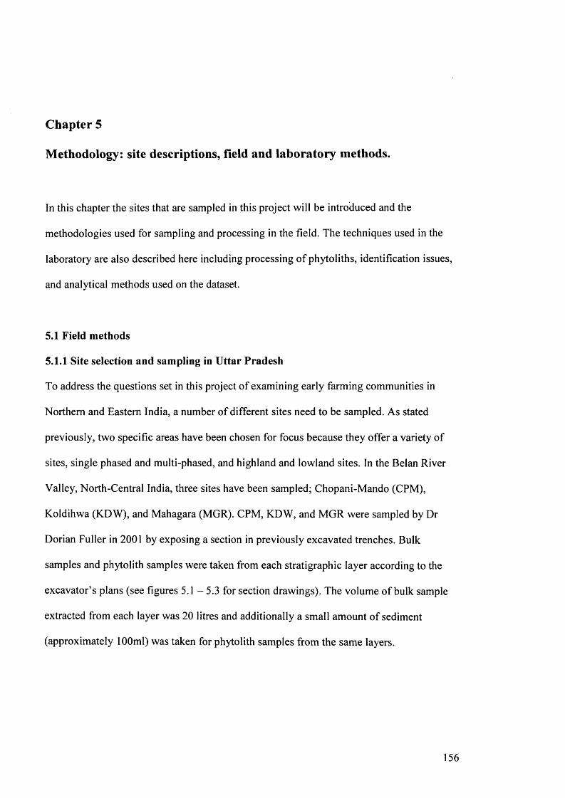
Chapter 5
Methodology: site descriptions, field and laboratory methods.
In this chapter the sites that are sampled in this project will be introduced and the
methodologies used for sampling and processing in the field. The techniques used in the
laboratory are also described here including processing of phytoliths, identification issues,
and analytical methods used on the dataset.
5.1 Field methods
5.1.1 Site selection and sampling in Uttar Pradesh
To address the questions set in this project of examining early farming communities in
Northern and Eastern India, a number of different sites need to be sampled. As stated
previously, two specific areas have been chosen for focus because they offer a variety of
sites, single phased and multi-phased, and highland and lowland sites. In the Belan River
Valley, North-Central India, three sites have been sampled; Chopani-Mando (CPM),
Koldihwa (KDW), and Mahagara (MGR). CPM, KDW, and MGR were sampled by Dr
Dorian Fuller in 2001 by exposing a section in previously excavated trenches. Bulk
samples and phytolith samples were taken from each stratigraphic layer according to the
excavator’s plans (see figures 5.1 - 5.3 for section drawings). The volume of bulk sample
extracted from each layer was 2 0 litres and additionally a small amount of sediment
(approximately 1 0 0 ml) was taken for phytolith samples from the same layers.
156
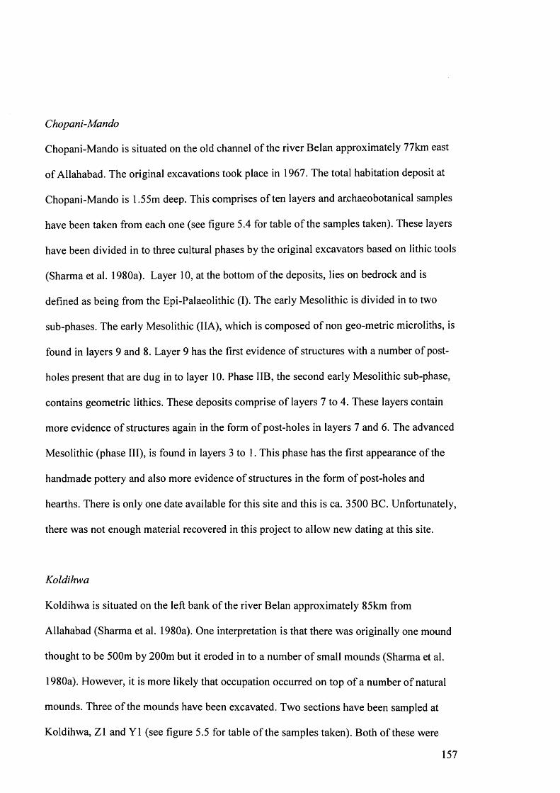
Chopani-Mando
Chopani-Mando is situated on the old channel of the river Belan approximately 77km east
of Allahabad. The original excavations took place in 1967. The total habitation deposit at
Chopani-Mando is 1.55m deep. This comprises of ten layers and archaeobotanical samples
have been taken from each one (see figure 5.4 for table of the samples taken). These layers
have been divided in to three cultural phases by the original excavators based on lithic tools
(Sharma et al. 1980a). Layer 10, at the bottom of the deposits, lies on bedrock and is
defined as being from the Epi-Palaeolithic (I). The early Mesolithic is divided in to two
sub-phases. The early Mesolithic (IIA), which is composed of non geo-metric microliths, is
found in layers 9 and 8 . Layer 9 has the first evidence of structures with a number of post
holes present that are dug in to layer 10. Phase IIB, the second early Mesolithic sub-phase,
contains geometric lithics. These deposits comprise of layers 7 to 4. These layers contain
more evidence of structures again in the form of post-holes in layers 7 and 6 . The advanced
Mesolithic (phase III), is found in layers 3 to 1. This phase has the first appearance of the
handmade pottery and also more evidence of structures in the form of post-holes and
hearths. There is only one date available for this site and this is ca. 3500 BC. Unfortunately,
there was not enough material recovered in this project to allow new dating at this site.
Koldihwa
Koldihwa is situated on the left bank of the river Belan approximately 85km from
Allahabad (Sharma et al. 1980a). One interpretation is that there was originally one mound
thought to be 500m by 200m but it eroded in to a number of small mounds (Sharma et al.
1980a). However, it is more likely that occupation occurred on top of a number of natural
mounds. Three of the mounds have been excavated. Two sections have been sampled at
Koldihwa, Z1 and Y1 (see figure 5.5 for table of the samples taken). Both of these were
157
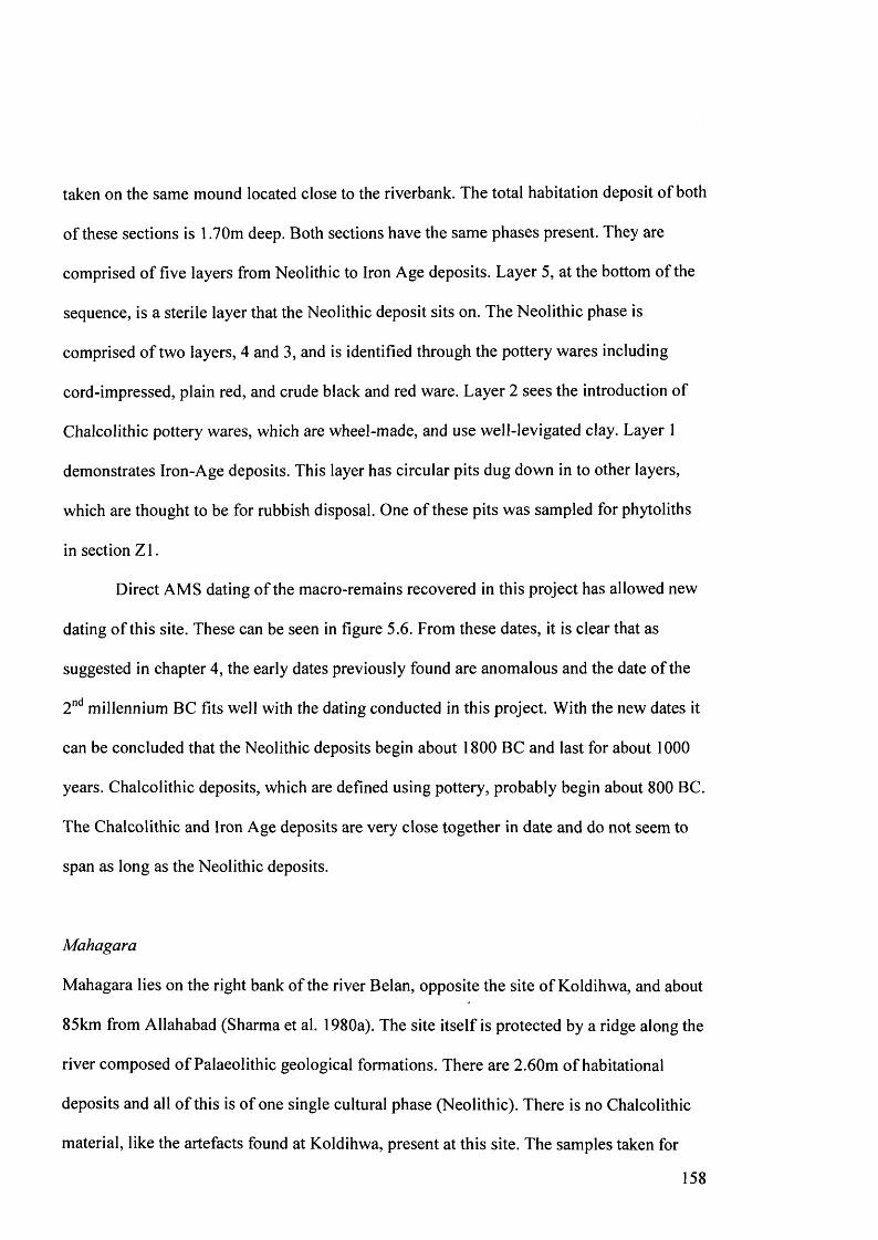
taken on the same mound located close to the riverbank. The total habitation deposit of both
of these sections is 1.70m deep. Both sections have the same phases present. They are
comprised of five layers from Neolithic to Iron Age deposits. Layer 5, at the bottom of the
sequence, is a sterile layer that the Neolithic deposit sits on. The Neolithic phase is
comprised of two layers, 4 and 3, and is identified through the pottery wares including
cord-impressed, plain red, and crude black and red ware. Layer 2 sees the introduction of
Chalcolithic pottery wares, which are wheel-made, and use well-levigated clay. Layer 1
demonstrates Iron-Age deposits. This layer has circular pits dug down in to other layers,
which are thought to be for rubbish disposal. One of these pits was sampled for phytoliths
in section Z l.
Direct AMS dating of the macro-remains recovered in this project has allowed new
dating of this site. These can be seen in figure 5.6. From these dates, it is clear that as
suggested in chapter 4, the early dates previously found are anomalous and the date of the
2nd millennium BC fits well with the dating conducted in this project. With the new dates it
can be concluded that the Neolithic deposits begin about 1800 BC and last for about 1000
years. Chalcolithic deposits, which are defined using pottery, probably begin about 800 BC.
The Chalcolithic and Iron Age deposits are very close together in date and do not seem to
span as long as the Neolithic deposits.
Mahagara
Mahagara lies on the right bank of the river Belan, opposite the site of Koldihwa, and about
85km from Allahabad (Sharma et al. 1980a). The site itself is protected by a ridge along the
river composed o f Palaeolithic geological formations. There are 2.60m of habitational
deposits and all o f this is of one single cultural phase (Neolithic). There is no Chalcolithic
material, like the artefacts found at Koldihwa, present at this site. The samples taken for
158
this project come from the ‘index square’, which was excavated down to the natural soil in
the southern part of the site (see table in figure 5.7 for the samples taken). This revealed 17
layers. These are divisible in to six structural phases. The early levels (layers 17 and 16) are
found in limited areas over the site and do not have any structural evidence. From the
middle of the section there is structural activity and the uppermost levels have the most
structural evidence with house plans and floors. There is no detailed stratigraphic
information given in the site report about the structural phases and how these relate to the
layers.
The new dates conducted on the macro-remains recovered for this project
demonstrate consistent dates with those previously taken at this site. The deposits are likely
to begin about 1700 to 1600 BC and the middle phase of the site is probably about 1500
BC. The site was abandoned before the transition to the Chalcolithic phase ca. 1400/1300
BC, unlike most sites in the region that continue directly into this phase.
5.1.2 Site selection and sampling in Orissa
A field season in Orissa was conducted in September-October 2003 and this recovered
samples from a number of sites with long temporal sequences and also from what appeared
to be short lived semi-sedentary sites. Sites were selected that had been previously
excavated or surveyed by the Indian collaborators (Dr R Mohanty - Deccan College, Pune,
Dr K Basa, and Dr B Mohanta - Utkal University, Bhubaneshwar). These sites were
thought to have the potential to recover archaeological plant remains. Two lowland sites in
South Orissa (Puri District), Gopalpur (GPR), and Golbai Sasan (GBSN), have been
previously explored and the later excavated but no archaeobotanical sampling had taken
place (Sinha 1993, 2000, Mohanty 1994, Kar 1995-1996, 2000, Kar et al. 1998). These
sites are both extensive mounds with cultural sequences spanning the Neolithic through to
159

the Iron Age. Therefore, systematic sampling was conducted at both of these sites by
exposing a clean section at the side of the mounds with direction from the excavators (see
figures 5.8 and 5.9). Bulk samples (20 litres) and phytolith samples (approximately 100ml)
were taken from all the stratigraphic layers. Sampling at Gopalpur was hindered by a high
water table, which prevented some of the lower levels being sampled but Neolithic deposits
may still have been sampled.
In the same field season, a number of sites were sampled in Central and Northern
Orissa (in the districts of Dhenkanal and Mayurbhanj) but none of these had long sequences
and probably represent more short lived sites or seasonal camps. The sites sampled were
Bajpur, and Banabasa. Sampling at Bajpur and Banabasa was conducted by digging lm by
lm trenches and taking samples ( 2 0 litre bulk and phytolith samples) every 1 0 cm until
sterile deposits were reached (see figures 5.10 and 5.11 for photos). Another site was
sampled in this same area (Dhenkanal district), Malakhoja, which is located close to the site
of Sankerjang. This site had more sunstantial deposits than the other sites in this area and
was in fact a small mound. Therefore, Malakhoja was sampled from a freshly cut section as
had been conducted at other such mounded sites in South Orissa and 20 litre bulk samples
and phytolith samples were taken (see 5.12 for photo of section). The stratigraphy at this
site was not as clear as the mounded sites in South Orissa and contained few visible
artefacts.
Golbai Sasan
This site has already been described in chapter 4 but the stratigraphy will be explained
again here in relation to the samples taken. Golbai Sasan is a large mounded site with
habitational deposits of about 6 metres (Sinha 1993, 2000, Mohanty 1994). The Neolithic
deposits have been reported by the excavators to only cover a very small area and therefore
160
the section sampled in this project probably does not include this phase (Sinha 2000). The
mound is divided in to two by a road that goes through the eastern side. The section was
sampled on the east side of the western mound at the side o f the road. The Chalcolithic
deposit is the most substantial at the site and is likely to make up the majority of the
sampled section. This phase consists of 10 layers and the lower levels have structural
evidence. The sample numbers start from the top of the section and descriptions of the soil
and levels can be seen in figure 5.13. No samples were taken from layers 2, 4, and 6
because these were hard laterite layers and also no sample was taken from layer 4A because
it was too thin. The very upper layers of this section could be Iron Age deposits.
There are a number of dates that have been published from the original excavation,
but they are rather contradictory. Neolithic levels have produced a date o f 1200 BC and the
Chalcolithic deposits have dates at the bottom of 2950 BC. There are also other
Chalcolithic dates from higher up the site of 3350 BC and 950 BC. A new set of dates has
been conducted on grains from the new samples taken in this project and these make more
sense than the previously published dates (see figure 5.14). The bottom of the sampled
section (13D) is dated to 1265 BC and 1215 BC. Sample 9 is about in the middle of the
section and is dated to 1220 BC. Sample 3 is near to the top of the section and gives a date
of 1215 BC. All of these dates are quite late and suggest a very short time span of the site
even though this site has substantial deposits. All of the ceramics collected from the
environmental samples also suggest Chalcolithic deposits. The new dates do suggest a
rather short period for such a substantial site and this could result from how the samples
have been taken. They may well come from eroded material that has washed successively
from the top of the mound even though there appeared to be clear stratigraphy. Even if this
is the case, the samples can still be used to examine the Chalcolithic phase of the site
although interpretations of change through the section are proposed with caution.
161

Gopalpur
Gopalpur is another site with a substantial mound and the habitational deposits are about 4
to 5 metres in height (Kar 1995-1996, 2000, Kar et al. 1998). It is hard to tell the exact
extent of the mound in antiquity because the area is being extensively cultivated today and
therefore much of the site has been ploughed away. This site has not been excavated and
consequently there is little stratigraphic information available. The sampled section was
taken on the southeast facing section of the mound, which is also the side where the river
cuts through the site. The sample numbers start from the bottom of the sequence, which
was as far down as could be sampled because of the high water table level at the time of
year the site was visited (see figure 5.15 for table of the samples taken). Even though there
is Neolithic pottery at this site, there is no information as to the extent o f Neolithic deposits
or whether there are any at all because this type of pottery is also found in Chalcolithic
deposits. From the flotation sample, black and red ware pottery was found in the lowest
samples and throughout the section. This type of pottery is thought to be consistent with
Chalcolithic cultures and therefore the lowest sample is probably of Chalcolithic age. This
could mean that this site is exclusively Chalcolithic or that the Neolithic deposits are
restricted as has been found at Golbai Sasan.
There are no previous dates for this site so the dates conducted in this project are the
only dates available so far. The dates taken do make a good sequence of dates and make
sense in terms of a chronological sequence by getting older down the section. Sample 2 at
the bottom of the sequence gave a date of 1395 BC. Samples 6 and 8 gave dates of 1265
BC and 1320 BC respectively. At the top of the section, sample 13 gave a date of 1170 BC.
These are all Chalcolithic in age, which was expected from the material remains.
162

Malakhoja
Malakhoja is another mounded site but not as substantial as Gopalpur and Golbai Sasan. It
lies close to the site of Sankerjang, in Dhenkanal district. A section was sampled at the side
of this site where 10 flotation samples were taken and four phytolith samples. The deposits
were about 1.40 metres in depth and all consisted of a red sandy sediment. There did not
appear to be much anthropogenic inclusions and particularly no organic material was
obvious. This site is thought to be Iron Age in date but there is no previous dating. No
dating was conducted for this site in this project because insufficient organic material was
available (see figure 5.16 for table of the samples taken).
Bajpur and Banabasa
Both of these sites have been described in as much detail as is available in chapter 4.
Neither o f these sites presented any stratigraphy or artefacts in the trenches excavated for
environmental sampling (see figures 5.17 and 5.18 for a table o f the samples taken). At
Bajpur, four flotation samples and five phytolith samples were taken. The topsoil was taken
as a sample for phytoliths but not for flotation because it will probably reflect the local
vegetation rather than the archaeological remains. At Banabasa, three samples were taken
for flotation and four for phytolith analysis. There was no pottery present at this site and
only finds of lithics were found on the surface. There is no dating for these sites although
they have been suggested to be Neolithic from the lithic remains (ground stone axes) found
on the surface of the sites. Unfortunately, there was not sufficient archaeobotanical material
for dating in the new samples taken for this project from either o f these sites.
163
5.1.3 Extractions methods in the field
Macroscopic remains
Flotation was carried out at all the sites mentioned above. This consisted of a bucket
flotation method using 500 micron sieve bags for the flot and 2mm sieves for the heavy
residue fraction. The nature of fieldwork in India means that flotation methods have to be
portable and low-tech; therefore flotation machines are not practical. Efficient recovery of
macro-remains is also necessary in India and bucket flotation offers the best method for this
because it is easier to check that all the flot material has been collected. Once processed, the
flots and residues are dried in the field and the residues are sorted for plant material so that
it can be transported back to the UK with the flots.
5.2 Laboratory methods
5.2.1 Extraction in the laboratory
Macroscopic remains
Once back in the UK, the samples are sorted for all the botanical remains. The whole of the
sample is sorted as the flots are usually not very large. Firstly, the flot is separated in to
different sized fractions (2mm, 1mm, 500 microns, and less than 500 microns) to enable the
extraction of plant material from the flots. All plant material is removed from all the
fractions using a low powered binocular microscope. Charcoal is only removed from the
2 mm fraction. Once all the botanical material is separated it is ready to be identified.
Microscopic remains
There is no standard extraction method for getting phytoliths from sediments. Each
laboratory has a different way of processing sediments with advantages and disadvantages
in using each method (Lentfer & Boyd 1998, 1999, Madella et al. 1998). All the procedures
are based on the same principle of removing the soil particles to leave the phytoliths clear
164
when mounted on the slide. This involves removing the clays, carbonates, organic matter,
and oxides of iron or aluminium (Pearsall 2000, Pipemo 2006). Heavy-liquid flotation
methods are the most common procedures used. The heavy-liquid involved varies and
includes bromoform and acetone (Oberholster 1968), bromoform and tetrachloromethane
(Twiss et al. 1969), tetrabromethane and absolute ethyl alcohol (Rovner 1971), potassium
iodide, and cadium iodide (Carbone 1977, Pipemo 1988, Pearsall 2000), zinc bromide
(Mulholland 1985), and sodium polytungstate (Hart 1988, Rosen 1995, 1999, Madella et al.
1998). All are adjusted to a density of around 2.3 for the phytoliths to float at the final stage
of the processing. Sodium polytungstate is the only one of these chemicals that is non toxic
and therefore not dangerous to use. Consequently, the development of a method using
sodium polytungstate is much better than exposing researchers to toxic substances.
Rosen (1995) has developed a technique using sodium polytungstate that although
being complex does produce excellent results. Madella et al. (1998) have produced a less
complicated procedure using predominantly centrifugation to remove the soil particles. It
does have the advantage of using only two containers and therefore is less likely to have
accidental loss o f phytoliths. However, the author has used both methods and the Madella
et al. (1998) technique is not as efficient as the Rosen method for getting rid of the soil
particles. The phytolith assemblages are much cleaner using the Rosen method because the
organic matter is burnt off and the clays are settled using gravity. The cleaner end product
of this method makes it easier to count and recognise the phytoliths. Using more containers
in the Rosen method could be seen as a disadvantage but if the researcher is thorough when
transferring between containers then there should be minimal loss of sample. If this same
procedure is followed for all the samples then any loss should be equivalent throughout.
The Rosen method of extraction is therefore used in this project and this procedure
also encompasses Albert & Weiner’s (2001) quantitative approach. This allows densities of
165

phytoliths in each sample to be calculated by measuring weights throughout the extraction
process. With this method, there must be great attention paid when mounting the slides to
get the material spread out evenly. Calculations must be adjusted if there are a lot of other
remains present in the sample apart from phytoliths such as diatoms. Other methods can be
used for quantitative evaluations, such as the use of Lycopodium spores, but there are also
problems with these methods (Powers & Padmore 1993) and therefore the former method is
thought to give the best quantitative data. Full details of the extraction method used in this
project can be found in appendix 5.1.
5.2.2 Identification
Macroscopic remains
Identification proceeds by comparing the recovered plant remains to the modem
comparative collections at the Institute of Archaeology, University College London, and
relevant pictures of reference material (Noda et al. 1985, Vaughan 1994, Galinato et al.
1999, Nesbitt 2006). The identification of macroscopic plant material is not always straight
forward. The nature of archaeobotanical remains means that the material is usually
fragmentary and only certain parts of the plant survive. Indian material also has many taxa
that are problematic to identify to species level (rice, native pulses, and small millets) and
wild species for which reference material and illustrated guides are not available. These
problems have been thoroughly investigated recently by Fuller (1999, 2002a) for the
cultivated crops and therefore will not be reiterated here. The methods used by Fuller
(1999, 2002a) will be used for identification in this project and are briefly discussed below.
Morphometries and size ratio can be used to overcome some of these problems of
identification. However, measurements need to be considered as part o f a population and
therefore individual measurements are meaningless (Hubbard 1992, Fuller 2002a). The
166

effect of charring on size also needs to be considered as this may cause difficult
differentiation o f some species groups on the basis o f length-breath ratios, such as Indian
Vigna species. Experiments are currently taking place to reassess this issue and its
implications on the identification of charred pulses (Jupe 2003, Jupe & Fuller in prep,
Fuller & Harvey in press). Rice is another crop, which is commonly measured for
identification (Vishnu-Mittre 1961, Constantini 1987, Oka 1988, Wenming 1991,
Thompson 1996: 176, Chen & Jiang 1997) but this approach also needs to be re-examined
especially in India. This will be conducted as part of this thesis and is reviewed in chapter
six.
In addition to morphometries, the examination of archaeobotanical specimens under
a scanning electron microscope can be used to correctly identify some Indian plant species.
The identification of specific millets, rice, and pulses benefit from this type o f analysis
because certain species have distinct surface patterns (Fuller 1999, Fuller et al. 2004, fig.
6 ). A key for the identification of small millets can be seen in figure 5.19.
Parenchyma is another important class of macroscopic plant material that is recovered
during flotation. This material will be separated from the seeds and other macro-remains
during sorting and identified separately. High level magnification is needed for the
identification o f parenchyma and usually SEM is required. However, few comparative
collections are available and none specifically for India. Some work has been conducted in
Southeast Asia (Hather & Kirch 1991, Hather 1994, 1996), which could be used as a
starting point to attempt identification of any such material that was present in Indian
samples.
167

Microscopic remains
Establishing a reference collection for Indian crop plants and associated weeds was
an important part o f this project. It is essential that this is conducted so that the
archaeological phytolith assemblages can be identified in more detail and therefore a
greater degree of data analysis can be applied to the samples. The focus o f the reference
collection is economic plants of India but also associated wild plants such as wild ancestors
and weeds.
Plant material can be made into reference slides for phytolith analysis in a number
of ways including dry ashing (Parr et al. 2001a), microwave digestion (Parr et al. 2001b),
spodograms (Pearsall 2000), and chemical oxidation (Pearsall 2000). The type o f plant
material and whether measurements are going to be taken can determine which method is
needed. If measurements need to be taken throughout the plant part then spodograms are a
good option because they leave the cells undisturbed. This also helps to understand the
morphology o f the plant, where particular cells occur in the plant, and can be used to
identify multi-celled phytoliths. Chemical oxidation, microwave digestion, and dry ashing
require the plant material to be cut up prior to the processing therefore the phytoliths on the
slides will be broken up to some extent.
Dry ashing and spodograms were used to establish the reference collection for
Indian plants. Both these methods will be used to examine crop plants but spodograms are
especially important because attention needs to be given to how to identify plant parts as
well as being able to identify the plant genus or species. Details of these methods can be
seen in appendix 5.2 and 5.3.
A review o f phytolith systematics is not given here but for a good review o f the European
history of the discipline see Powers (1992). Most arable crops have been researched in
168
terms of phytoliths; maize (Pearsall 1978, 1982, Pipemo 1984, Pipemo & Pearsall 1998,
Pipemo 2006), rice (Watanbe 1968, Pearsall et al. 1995, Zhao et al. 1998, Zheng et al.
2003a), common bean (Bozarth 1990), sugar cane (Madella 1995, 1997), New World
curcurbits (Bozarth 1987, Pipemo et al. 2000, Bryant 2003, Carter 2003), roots and tubers
(Carter 2003), fruits and vegetables (Wilson 1985, Cumming 1992, Mindzie 2001) and
wheat and barley (Rosen 1992, Ball et al. 1993, 1996). India presents somewhat of a
challenge for phytolith analysts because many o f the crops that are used have not been
thoroughly examined and therefore established criteria for identification are not available
for all crops. Native Indian millets and pulses are common components of archaeobotanical
assemblages and phytoliths from these taxa need to be characterised. Fujiwara et al. (1992)
have supposedly identified finger millet in Harappan samples but have given no details
about how they were identified. Krishnan et al. (2 0 0 0 ) have constructed a key o f single
cells from Indian grasses, which includes many types o f millet. However, it is hard to
believe that the identification of millets can be achieved just from measuring short cells
because when looking at reference material the size varies considerably and there seems to
be significant overlap.
The approach taken for identifying plant types in this project is to use descriptions
o f multi-cell panels following the example of work conducted on wheat and barley species
by Rosen (1992). These rely on a number of characteristics unique to the plant and all of
these distinguishing features must be seen before the identification can be made.
Identification using this method has been started on millets during the authors M.Sc. thesis
(Harvey 2002) and will be continued during this project as well as studies of other common
economic plants such as Indian pulses, curcurbits, and palms.
Morphometries are also used in phytolith analyses to distinguish between plants at
genus and species level (Ball & Brotherson 1992, Ball et al. 1993, 1996). Single-cells can
169
also be unique to certain plants and morphometries has been used to distinguish these at a
high level. Rice has many cells that can be recognised: bulliforms (Fujiwara 1993, Zheng et
al. 2003), bilobes and double-peaked glume cells (Pearsall et al. 1995, Lu et al. 1997,
Whang et al.1998, Zhao 1998) but it is not clear at present to what taxonomic level these
morphotypes can be identified. An examination of the morphometric methods used to
identify rice is part o f this project and is discussed in the next chapter.
Plants that are common arable weeds can also be recognised. Phragmites sp. and
Arundo donax are particularly distinctive (Greiss 1957, Ollendorf et al. 1988). Cyperaceae
can also be identified easily to family by recognising the distinctive cones (Ollendorf
1992). Palms are another type of plant that can be recognised using phytoliths and this will
be explored further in this thesis as usually only date palm is identified. India has many
palm species that may have been utilised in antiquity and two particular species of
economic value are coconut and palmyra palm. A brief discussion of the findings found
during the examination o f reference material is presented in chapter 7.
Short cell grass classification schemes are frequently used and this will be applied to the
samples (Twiss et al. 1969, Brown 1984, Mulholland & Rapp 1992a, 1992b, Pearsall &
Dinan 1992). This means that the quantity of phytoliths in each of the ecological groupings
can be compared. The Twiss et al. (1969) classification scheme was based on Bowden’s
(1963) re-division of grass subfamilies using microscopic characteristics. Many floras have
published percentage data for these subfamilies but this has caused a biased view of their
occurrence in certain environments (Cross 1980). Cross (1980) has reassessed these data
and concluded that there are three main areas that these subfamilies can be classified as
occurring in; C4 tropical group includes Andropogoneae, Paniceae, Chloridoideae, and
Aristideae, C3 sub-tropical contains Arundinoideae, and C3 North temperate group is
170
Pooideae (Festucoids). This means that in South Asia the C4 tropical group should
dominate the phytolith assemblage with a few grasses from other subfamilies.
Descriptions of the phytolith categories identified in this project can be seen in
appendix 5.4. This outlines the terms used to describe the phytolith morphotypes in the text
and also a description of the morphotype using the International Code for Phytolith
Nomenclature 1.0 (Madella et al. 2005). Multi-celled phytoliths are described in detail with
appropriate diagrams.
5.3 Qualitative and quantitative analysis
Macroscopic remains
Archaeobotanists approach the numerical analysis of archaeobotanical remains in many
different ways. It depends entirely on the amount of plant remains that are found and also
the type o f questions that are to be addressed. It is important to remember that
archaeobotanical datasets are incomplete and therefore interpretation should progress with a
certain degree of caution. The influences of taphonomy on the assemblages must be
considered and this issue is discussed in depth below. Before beginning quantitative
analysis of data the following points must be considered (Pearsall 2000): i) do not use
statistics that you do not understand; ii) begin with simple tabulation and then work
towards more complex techniques; iii) do not use approaches that require more rigor than
the data is capable of.
The most basic form of analysis is qualitative presentation of data. This is
presenting the presence/absence or scales of abundance of species that appear on the site.
Detailed descriptions are usually given in such cases and this level of data presentation is
only really appropriate for initial reports of archaeological material.
171

To address any archaeological questions, quantitative analysis must be attempted on
the archaeobotanical dataset. Quantitative analysis can be split in to two types: i) non-
multivariate and ii) multivariate. Non-multivariate analysis includes counts or weights of
items, tables, ratios, densities, ranking, species diversity, and ubiquity. These methods are
used predominantly in archaeobotanical analysis. They suit smaller data sets with a
manageable amount of taxa but can also be used on large data sets. All archaeobotanical
reports start with a table of either counts or weights of items recovered. These are the
absolute counts. The data can be assessed in its raw form or can be reduced, standardised,
and transformed to reduce skewness in the dataset (Jones 1991). After this simple
presentation of the data, the direction that data analysis progresses, depends on what
questions are being addressed.
In this project, it must be considered how to record items in the samples. The
fragmentary nature of the material means that counting is an issue, which has to be
considered carefully. Therefore, complete seeds, chaff, and other plant parts are recorded as
one item in the tables. The majority of cereals and pulses are not whole and therefore the
number of halves and quarters are also recorded. Calculations will be made to estimate the
number of complete grains in each sample where halves are counted as 0.5 and quarters as
0.25. A total number of items will also be calculated as well as the number of items per litre
of sediment to give an idea of the density of archaeobotanical remains per sample.
Simple quantitative methods can be used to investigate many archaeological
questions. Ratios are a direct way of analysing data and help to standardise it. It is a good
way of comparing samples of unequal size, samples differing in circumstances of
deposition or preservation, and comparing quantities of different categories of material that
are equivalent in some respect (Miller 1988). Ubiquity values, which are the percentage of
a taxon in the site or phase, are a very useful but simple method of analysis. This is a form
172
of denominator ratio. Ubiquity analysis can reinforce presence/absence information and its
strength is that the score of 1 taxon does not affect the score of another (Popper 1988).
Therefore different taxa can be evaluated independently. This method provides the relative
importance of taxa and can be used to focus on changes in importance o f specific plant
species within and between sites. Along with a relative method of analysis such as ubiquity,
it is essential to compare the outcome with an absolute method, such as assessing raw data,
to give an overall assessment of the data.
Comparative ratios can be used to compare two items and are helpful for answering
specific questions. Comparing different plant parts either macro-remains or phytolith
morphotypes can be used to address issues of crop processing as discussed in the section
below. This can demonstrate whether these plant parts have the same pathway in to the site
(Harvey & Fuller 2005). Ratios can also be used to demonstrate one taxon replaces another
over time, or that one food plant increases in use over another (Pearsall 2000). Therefore,
using simple methods of data analysis can produce a high degree of interpretation. It is
important to present data simply showing a clear route to the interpretations and therefore
the results can be understood by any audience.
Multivariate analysis is still not commonly used by archaeobotanists. As mentioned above,
most archaeobotanical assemblages can be interpreted using simple qualitative and
quantitative methods. Multivariate methods tend to be directed at specific questions such as
the study of weed ecology and the interpretation of crop processing stages. Phytosociology,
autecology, and “FIBS” are applied by archaeobotanists to the study the weed ecology of
species present in the archaeobotanical assemblage (Jones 1987, van der Veen 1992,
Charles et al. 1997, Bogaard et al. 1999, 2001, 2005, Jones et al. 2000, 2005, Bogaard
2004). Using these methods on Indian assemblages is challenging because data on Indian
173

weed ecology is not readily available. There is also the problem that archaeobotanical
criteria for weed identifications is still poorly developed. However, some general aspects of
weed ecology may be informative for prehistoric India by suggesting aspects of growing
conditions such as wetland weeds indicative of wet-paddy rice systems. This can be applied
to the phytolith assemblage as well as the macro-remains as long as good enough
identifications can be made.
As the macro-botanical dataset is not particularly large in this project, multivariate
methods will be restricted to the methodological investigation of rice identification. Simple
methods of analysis will be used on the macro-remains data such as ubiquity and ratios to
compare within and between the sites. This analysis, in combination with the phytolith
assemblage data, will hopefully give a detailed interpretation of the economies of the sites
under investigation.
Microscopic remains
Many of the same issues of quantification, as have been stated above for macro-remains,
also apply to phytolith analysis such as the importance of considering taphonomy and the
limitations of the dataset. Counting methods for phytoliths vary according to the researcher.
Qualitative analysis such as quick scans giving an abundance scale for morphotypes is the
simplistic way of summarising samples. However, quantitative analysis allows a greater
degree of data analysis that can be combined with the macro-botanical data set. Therefore
in this project, the phytoliths are examined under a transmitted light microscope at 400 x
magnification. The slides are scanned in rows using a standard single-cell and multi-cell
scan procedure (Piperno & Pearsall 1993, Pearsall 2000). It was aimed to count between
300-400 single-cells and 100-200 multi-celled phytoliths in each sample but this may not
be possible on all slides. In those cases, the entire slide is scanned. The number of
174
microscope fields counted per slide will also be recorded to allow the calculation of the
density of phytoliths in each sample (Albert & Weiner 2001). This allows the phytolith
types in each slide to be compared as well as the densities between the samples. The
densities are calculated per gram of sediment and this means that the phytolith counts are
standardised. The raw counts are not used for data analysis because they are not
quantitative in terms of relating directly to the amount of the phytoliths in the particular
sample but are just counts of what has been encountered on the slide. Adjusting these raw
counts to densities aids comparisons of phytolith morphotypes within and between samples.
Relative frequencies of the raw counts will be calculated and compared to the absolute
counts because the former method is the usual form of analysis used by phytolith analysts.
There are draw backs with using relative frequencies because it emphasises morphotypes
with the highest values and therefore may not draw out patterns as well as absolute counts.
As with macro-remains, it is important to start data analysis of the phytolith
assemblage in the simplest way. This usually means to look at the density of phytoliths
overall in samples and compare this over time and between sites. This can begin to suggest
whether the sites have had substantial input of plant remains or not. Examining also which
phytolith morphotypes are present in high or low values will move towards more firm
interpretations such as looking at the level of grass phytoliths compared to dicotyledon
phytoliths. Specific morphotypes that relate to crop plants are obviously important to
concentrate on during the analysis phase and the densities of these in the assemblage can be
related to the use of these crops in different phases of the site.
Some researchers utilise methods from palynology such as stratigraphic bar charts
showing changes in phytolith morphotypes or groups over time (Pearsall 2000, Pipemo
2006). These are useful for looking at changes over time in general groups. Palynological
methods of data analysis are good for answering certain questions about general changes
175
and these methods are used when pollen analysis is being combined with phytolith data.
This could be used in this thesis to combine the macro-remain data with the phytolith
analysis. However, as there is a combination of macroscopic and microscopic analysis in
this thesis, the phytolith data can also be treated like the macro-botanical data set as it has
been sampled from the same locations. The strength of phytoliths is that plant parts can be
identified as well as specific plant families, genera or even species just as in macro-
botanical identifications. This means that the data set can be approached in much the same
way as analysing macro-remains of seeds and chaffs.
At a basic level, quantitative methods such as ubiquity could be used to assess the
data and the relative importance o f different plants and plant parts. This will also allow the
comparison of the phytolith data with ubiquity values from the macro-botanical
assemblage, which can add more weight to arguments about the importance of certain crops
at certain times and in certain areas.
Ratios can also be used to compare phytolith morphotypes. Comparisons can be
made between different plant parts to investigate the input o f these parts in to the deposits.
This method can be used to assess the origin of the sample and this will be discussed in
more detail in the taphonomy section below. Such methods have been used to determine
environmental conditions around sites by showing a dominance of certain floras such as
grassland or wetland habitats. Samples from archaeological sites should be considered as
selected by humans and therefore the remains will relate to human activities rather than a
complete picture o f the local environment.
5.4 Taphonomy and approaches to the analysis of crop processing activities
Interpretations of the archaeobotanical data must always be considered in terms of the
taphonomy of the samples. Firstly, there is a depositional bias, which is what plant material
176
gets in to the site. This will be affected by the general environment and climate of the area
as to what plants can be exploited and grown at the site. There is also the filter o f human
choice which directly affects what plant material ends up at the site (Dennell 1972). Plant
material can also be brought on to the site accidentally such as seeds o f weed plants
transported on animals or naturally transported such as wind blown seeds but this will
account for a very small proportion of the plant remains and is also unlikely to be preserved
unless, for example, animal dung was being used as a fuel (Helbaek 1969, Miller 1984,
1993, 1997, Miller & Smart 1984, Neff 1989, Hillman et al. 1997, Charles 1998, Samuel
2001, Madella 2003).
Secondly, preservation determines what plant material will survive in the sediment.
Macro-botanical remains are commonly preserved as charred material but could also
survive through waterlogging, desiccation, or mineralization. Plant material coming in to
contact with fire on the site is very selective in terms of what plant material will become
charred. It is important that the plant material is only exposed to low temperatures
otherwise it will be incinerated. This can occur in a number of ways (Hillman 1981): i)
during the drying or parching of the crop product; ii) burning a diseased crop; iii) use of
crop waste as fuel and incorporation o f waste into dung as fuel; iv) accidental burning
during cooking or destruction of a house by fire. This may suggest that macro-botanical
material is most likely to come from daily processing waste (Fuller 2002a, Stevens 2003).
Differential preservation also has to be considered because many plant parts are fragile and
will be burnt away in fires therefore not surviving archaeologically (Boardman & Jones
1990).
Lastly, there is a bias in the recovery o f the samples. Where and how a sample is
taken will affect the outcome of the archaeobotanical assemblage o f a site. Different
sampling strategies mean that there is more or less chance o f recovering all the information
177
possible from a site. Flotation methods also affect the recovery of plant material such as
sieve sizes and the quantity o f bulk sample taken. All of these factors must be considered
while interpreting archaeobotanical samples.
It has already been discussed in chapter two, how the content o f a sample can be an
indicator of crop processing activities even though they come from secondary or tertiary
deposits (Fuller et al. in press, Harvey & Fuller 2005). This is very different to most other
archaeological work that relies on the context to help with interpretations. This new
approach, however, has grown out of the earlier founding work of Hillman (1973, 1981,
1984) who created models of crop processing activities using ethnographic studies from
Turkey. This work has been developed by Jones (1984a, 1984b, 1987) particularly for
wheats, barley, and some pulses from the western Mediterranean. These crop-processing
models for application in archaeobotany were developed from observations o f present day
traditional, non-mechanized agricultural communities. It is important to consider how
different methods of processing the crop will affect the composition of grains, chaff, straw,
and weeds in an archaeological assemblage. The application o f crop processing models to
archaeobotanical assemblages is now fairly routine and models have been developed for
many other crops and regions: barley and rye in Fennoscandia (Englemark 1989, Viklund
1998) and western Mediterranean (Pena-Chocarro 1999); quinoa and other crops in Peru
(Bruno & Whitehead 2003); millets in India (Reddy 1991, 1994, 1997, 2003), in China (Lu
2002), in Nepal (Lundstrom-Bandais et al. 2002), in Africa (D’Andrea et al. 1999, Young
1999, Young & Thompson 1999); and rice in Thailand (Thompson 1996). All of these
models focus on the use of macroscopic remains to interpret crop processing stages. These
remains have certain issues associated with them such as their reliance on charring for
preservation and the differential preservation o f plant parts (Harvey & Fuller 2005). These
178

problems can affect the proportions of plant parts in archaeological assemblages on top of
the filters o f crop processing. In particular, this will affect light plant parts and fragile weed
seed, which are more likely to be incinerated (Boardman & Jones 1990) and also early
processing stages are less likely to be represented as they are unlikely to come in to contact
with fire (Jones 1987, van der Veen 1992, Stevens 2003). There is also more chance o f the
early processing waste being seasonally produced and remaining off-site. This will
therefore effect interpretations especially when trying to distinguish between crop
consumer and crop producer sites (Fuller & Madella 2001, Smith 2001, Fuller 2002a,
Stevens 2003, Harvey & Fuller 2005). Routine daily processing is therefore more likely to
be represented and allows inferences to be made about the scale of labour organisation.
Another aspect of preservation to consider, especially for this thesis, is the amount
of organic remains that are preserved at tropical sites. As mentioned previously, the quicker
turn over o f carbon in tropical regions leads to much poorer preservation conditions on
most sites (Hather 1992, Pipemo & Pearsall 1998). This is the reason why, in this thesis,
there is a combination of macro-remains and phytolith analysis. A new approach to
interpreting crop processing stages has been developed, which uses phytoliths (Harvey &
Fuller 2005). Phytoliths have the advantage that they are inorganic and therefore
particularly durable over long periods of time. They do not rely on special preservation
conditions such as carbonisation, to be preserved archaeologically. Therefore, they allow
another insight in to the ancient plant remains, which can be used in combination with
macro-remains. Phytoliths may therefore be able to detect the earlier stages of crop
processing that are unlikely to preserve macro-remains through carbonisation. There are a
number o f problems with using phytoliths, which are discussed in Harvey & Fuller (2005)
but the main issue that has to be overcome is the level of identification. Plant parts as well
as the type of plant can be identified using phytoliths much like the identification of
179

macroscopic remains. However, the identification of phytoliths to species level is limited.
In this thesis, the methods used to identify rice phytoliths to species are investigated and
this may aid this method of interpretation. Other plants such as millets and pulses can not as
yet be identified to species accurately or in the case of pulses do not produce a great deal of
phytoliths but this will hopefully be investigated further during this thesis.
The other factors that will effect what remains are found in the archaeological samples are
the type of crops used and cultural influences on processing techniques. The type of crop
has a primary role on the type of processing that occurs (Reddy 1997, Viklund 1998).
Wheat and barley are found on prehistoric sites in India but these crops have been
considered in some depth elsewhere so will not be discussed in great detail here. Rice,
millets, and pulses are all important crops in India and have not been investigated
thoroughly. How these different crops are likely to be processed and what parts are likely to
end up in archaeological samples in an Asian and particularly Indian context will be
discussed below.
A number of modem day studies have relevance to this thesis including the study of
rice crop processing in Thailand by Thompson (1996) and Reddy’s (1991, 1994, 1997,
2003) study of millets in Northwest India. There have been few studies o f pulses and most
of them examine Southwest Asian species (Jones 1984a, 1987, Butler 1992, Butler et al.
1999). A summary of current evidence for Indian pulses has been conducted by Fuller &
Harvey (in press) but more dedicated studies are needed to observe the traditional
processing of pulses. What all o f these ethnographic studies demonstrate is that there are
two major types o f crops and these two groups have implications on the processing
methods that are used on them and how many processing stages are necessary. These two
groups are hulled crops and free-threshing crops. Hulled crops include glume wheats, rice,
180
hulled millets, which tend to be the small millets native to India, and also ‘pod-threshing’
pulses such as horsegram (a native Indian pulse). Free-threshing species include barley,
free-threshing wheats such as bread wheat, African millets including Eleusine coracana,
Pennisetum glaucum, and some races of Sorghum bicolor, as well as most pulses such as
Lathyrus sativus and the other Southwest Asian pulses, and also some Indian pulses
including Vigna spp. The main difference in processing for these two groups is that the
hulled species require a further stage of pounding to break the husk from the grain. This can
sometimes include parching to help to release o f the grain, which is common for glume
wheats. There are further differences between these two groups that can be seen in the
processing methods, which will be discussed along with regional traditions for the relevant
area.
Harvesting has potentially the greatest impact on what is later included in the
archaeological assemblages (Harvey & Fuller 2005). There are a number o f options open to
harvesters o f rice, millets, and pulse crops (see figures 5.20 and 5.21 for rice and millet
processing diagrams). Reddy (1994, 1997) suggests that it depends on the size of the
panicle for millets. Large panicles found on millets such as sorghums and Pennisetum spp.
are more likely to be harvested by cutting the top of the stalk and therefore just removing
the panicle. This means that the stalk is not harvested and this will also reduce the
collection of weeds. Smaller species o f millet are gathered together in handfuls and cut at
the base of the plant therefore harvesting some of the stalk and potentially more weeds.
Pulses are either uprooted or hand picked. It has been suggested that early cultivators would
have used hand picking because o f the uneven ripening o f primitive cultivars (Fuller &
Harvey in press). This method would not select for weeds where as uprooting could
potentially incorporate a substantial amount of weeds because of some pulses twining
181

growing habit. However, the harvesting technique is probably also a cultural choice as well
as being related to the particular crop involved.
Rice may also be harvested by just taking the panicle and therefore incorporates few
weeds. Thompson (1996) suggests that rice crops do not generally contain a lot of weeds
unlike wheat and barley. This can be the result o f thorough plot clearance, the drowning out
of weeds by wet rice practises, and also reaping using finger knives. The use of finger
knives is restricted to certain regions mainly in China and Southeast Asia and these tools
are not usually used in India. Weeds are an important indicator of crop processing stages
for wheats and barley especially for harvesting methods (Hillman 1981, Jones 1984a, 1987)
and therefore the study of rice cultivation may be hindered because o f the lack of weeds.
However, dry field systems of cultivation do have more weeds present and rice may not
always be harvested by taking just the panicle because the straw is in fact a highly valued
commodity (King 1949, Srinivas 1976, Sherman 1990). It is as useful as the grain and can
be used as food and bedding for animals, thatching for houses, fuel, mulch, and fertilizer.
This means that the straw could be cut with the panicle or be taken during a secondary
harvest. Both o f these methods have been observed by the author in India. This does give
more chance o f weeds being incorporated with the harvest and the presence of wild taxa in
archaeobotanical samples known to be rice weeds such as sedges and other grasses should
be seen as potential sources of information about husbandry practises and crop-processing
stages.
Threshing and winnowing may occur in the field or on specially constructed
threshing floors on the edge o f the village rather than directly next to the domestic
environment. Threshing and winnowing separates straw, leaves, and light weed seeds. Free-
threshing crops may be stored prior to threshing and winnowing but hulled crops are more
likely to be processed further before they are stored. There are ethnographic accounts of
182

threshing on a temporary surface o f woven mating in the field (Srinivas 1976, Sherman
1990) and the author has seen the threshing of rice plants on a permanent mud floor on the
edge o f a village in Northern Orissa. This means that there is much less chance of these
early by-products coming in to contact with fire during this process although they may be
used later for some reason such as fuel or fodder (Watt 1892) causing more chance of
carbonisation. Sieving tends to be used with wheats and barley separating the grain from
the chaff and weeds by size. Rice and millets tend to be separated from chaff parts through
winnowing using baskets and rakes rather than sieves, which are used on other crops
(Thompson 1996, Reddy 1997, Lundstrom-Baudais et al. 2002). It has been suggested that
pulses would also follow this pattern in the same region because of cultural preferences in
husbandry practises although more ethnographic work is needed to fully understand why
certain choices are made for processing pulses (Fuller & Harvey in press).
For storage or for further processing the crop would now be brought in to the
domestic environment if it had not been already. The crop processing from this stage
onwards is likely to be carried out on a daily basis. The earlier stages of processing
generally happen on more of a communal basis or individual families may hire extra labour
at this time of year because of the need to harvest in a certain time limit and then process to
store the products while there is a lot of labour still around. The daily processing in the
domestic setting makes it much more likely that the plant material will end up being
carbonised in the domestic fire than the waste o f previous stages. Waste of this stage has
been suggested to make up the majority of preserved waste archaeologically therefore
variation relates to how bulk initial processing is organised (Harvey & Fuller 2005, Fuller
et al. in press). With glume wheats, parching can be used prior to pounding but is not
essential. Pulses are also routinely parched for consumption or to dry them for storage
(Fuller & Harvey 2005). This will increase their chance o f ending up in the archaeological
183
record. It has been pointed out that pigeonpea, which is rare in archaeological assemblages
is not commonly parched therefore less likely to be preserved. Therefore, parching can
happen as the result o f a certain crop being used such as a hulled crop or can be a
cultural/environmental choice. Glume wheats may be more likely to be parched when they
are grown in cold climates and parching helps to dry them to prevent rotting.
Parching is not necessary for rice and millets but may still be used. Rice is generally
dried in the sun prior to pounding and can be seen laid in front of houses throughout
villages in India. The climate therefore influences the choice not to parch because the crop
can be dried naturally. Thompson (1996) has suggested that rice may be underrepresented
in the archaeological record because of the lack o f parching and therefore is less likely to
come in to contact with fire. Rice can alternatively be par-boiled before pounding to help
release the grain (Watts 1892). Reddy (1994, 1997) suggests parching is more frequently
used for processing hulled millets and parboiling is also used (Kimata 1989). However,
whatever the process, waste products will be produced and the new application of
phytoliths to investigating crop processing stages can help to understand why certain
macro-remains are absent or rare (Harvey & Fuller 2005).
The discussion above has shown that interpreting early agricultural sites is not
straightforward and applying both macro-remains and phytolith analysis will help to
overcome some o f the problems. Phytolith analysis can aid the understanding of
preservation issues and macro-remains can hopefully help to confirm identifications of
phytoliths, which consequently will give a more accurate interpretation. In the next chapter,
the issues surrounding the identification of rice are addressed. This will hopefully aid the
application of the analytical methods presented above and lead to a greater insight in to the
social aspects of the early agricultural communities in Northern and Eastern India.
184

Chapter 6
Rice identification methodologies: problems and prospects
This chapter will focus on the identification of rice in an archaeological context. It will
firstly set out some general characteristics of the rice plant both macroscopic and
microscopic and then discuss the development of taxonomy in the genus Oryza. Possible
wild progenitors and routes towards the domestication of the rice plant are examined
briefly. A number o f identification methods will be reviewed and these are specific
techniques that can be used in Indian archaeological assemblages. The chosen methods are
used on a new set o f modern reference material to assess their successfulness at
determining the species of rice or whether they can identify the wild from the domestic
species.
6.1 Terminology for the rice plant including rice phytoliths
Before discussing in detail the issues of rice identification, it is best to set out the general
terminology that is going to be used in this chapter to describe the rice plant and rice
phytolith morphotypes. A diagram of the parts o f the rice spikelet can be found in figure 6.1
and figure 6.2 shows photographs of the different rice phytoliths.
6.1.1 Rice plant anatomy
The inflorescence of rice is a terminal panicle attached to a long peduncle (Ahn
1993: 53-54). The panicle consists o f numerous spikelets attached by stalk-like pedicels to
the branching panicle. At the apex of each pedicel are two rounded rudimentary glumes and
a raised abscission surface which fits the rachilla of the spikelet (Thompson 1996: 164-
185

166). The spikelets are laterally compressed and comprise o f two sterile lemmas, a rachilla,
and a fertile floret, which consists of the fertile lemma and palea, and the flower that
develops in to the caryopsis. The caryopsis is also called a ‘grain’ or ‘seed’ but is
morphologically a fruit.
The fertile lemma is large, boat-shaped, and has five nerves (Chang & Bardenas
1965). It partly encloses the palea. The lemma is almost V-shaped in cross section and
coriaceous in texture. It has a terminal tuft of trichomes (hairs) and may have an awn on the
distal end, which normally occurs in the wild species (Thompson 1996: 164-166). The awn
is also covered with many trichomes. Both the lemma and palea are highly silicified at
maturity. The fertile palea has a similar structure and epidermal features to the lemma but is
smaller with just 3 nerves. It has no awn.
As well as the fertile bracts, there are two diminutive sterile glumes at the base of
the fertile lemma and palea (Chandraratna 1964). They are rarely more than one-third the
length of the latter. The sterile lemmas are almost equal in size, the upper lemma being
slightly larger than the lower lemma.
The caryopsis is tightly enclosed by the fertile lemma and palea. The pericarp, testa,
and aleurone layer cover the starch endosperm and embryo of the caryopsis. The embryo is
at the basal part of the ventral side. This is also the side of the lemma and can be called the
abdomen (Matsuo & Hoshikawa 1993). The opposite side, which has the palea is called the
back of the grain (dorsal side). The rest of the grain consists of endosperm. The grain has
two vertical ridgelines protruding on both of its sides (Matsuo & Hoshikawa 1993).
186

6.1.2 Rice phytolith descriptions
The genus Oryza has a number o f phytolith morphotypes, which are distinctive from other
genera in the tribe Oryzeae. The leaves of the rice plant produce distinctive fan-shaped or
keystone bulliforms. Similar phytoliths may also be found in other grasses including
Oryzoideae, Bambusoideae, Panicoideae, Arundinoideae, and Eragrostidoideae (Lu et al.
1997). However, those found in rice are very widely flared cells and come in a number of
forms, which vary according to the extent of flaring and width of the top (Pearsall et al.
1995). The base is symmetrical. There are also varying numbers of chipped facets on the
fan edge o f the cell, which may allow identification to species and this is discussed in more
detail below (Lu et al. 2002).
The fertile glumes (palea and lemma) of the rice plant have unique epidermal cells.
Glume cells with single- and double-peaked hairs are common. The double-peaked hairs
are produced abundantly and do not occur in other genera o f the tribe. The single-peaked
hair has been observed in a number o f millets including Setaria italica and therefore is not
a unique morphotype (Pearsall et al. 1995, Lu et al. 1997). Although, it has been noted by
the author that rice has very deeply serrated epidermis, which is attached to the double- and
single-peaked hairs while the millets tend to have clear dendritic cells and the peaks are
more hook shaped. The term single- or double-peaked glume or husk phytoliths is used to
refer to these rice phytolith morphotypes. These peaked phytoliths can occur as single cells
or as multi-celled panels. The author has observed through modem and ancient material
that multi-celled panels appear more commonly than single cells. This may be due to the
high degree of silicification in these particular cells that seems to prevent breakage.
There are also a number of short cells that may be characteristic o f the genus, if
measured and compared to other grasses, but are probably more distinctive of the tribe.
There are three short cell types that are produced in the leaf tissues: a dumbbell with
187
scooped ends; a cross with raised comers; and a short cell with a dumbbell base and a thin
plate extending perpendicular to it (Pearsall et al 1995). The ‘scooped’ bilobes are arranged
horizontally and this seems to be a distinctive trait of the tribe because these dumbbells can
be found in Leersia hexandra and Zizania caduciflora.
6.2 Rice taxonomy, domestication issues, and why identification is problematic
6.2.1 Rice taxonomy
Oryza belongs to the subfamily Oryzoideae, in the family Poaceae (Gramineae). This
subfamily has tropical and temperate species (Vaughan 1989). South Asia has a number of
genera other than Oryza; Leersia, Hygroryza, Porteresia, and Zizania. The genus Oryza is
small, containing about 23 species, but its species are ecologically diverse. The genus
Oryza was named in 1753 by Linnaeus (Vaughan et al. 2003). In 1886, DeCandolle (1886)
was the first to suggest identifying wild progenitors to address the issue of agricultural
origins. He identified rice as being from Southern Asia, from China to Bengal, although he
attributed the domestication of rice to China. In 1910, Kuwada determined the somatic
chromosome number of rice to be 24. Morinaga and colleagues (Morinaga & Fukushima
1934) did genomic studies of rice and assigned the genomic identities AA, BBCC, CC,
CCDD to different species. This determined that the cultivars {Oryza sativa and Oryza
glaberrina) were put in to the AA group and therefore their ancestors also had to be within
this genomic group. However, it was not until the 1960s that Tateoka’s work (Tateoka
1963, 1964) clarified the basic groups of species within the genus and he called these
groups species complexes. A table of the current species complexes can be seen in Figure
6.3. Little has changed in the nomenclature for the genus since the 1960’s. However, one
notable addition to Tateoka’s original work, which is important for this particular study, is
the description of the new species Oryza nivara and therefore the revised circumscription
188

of Oryza rufipogon in 1965 by Sharma and Shastry (1965). Oryza nivara and Oryza
rufipogon are the likely wild progenitors of Asian domestic rice.
Oryza sativa, the Asian domestic species o f rice, is an annual grass that is extremely
diverse but the species can be divided into three major groupings o f traditional varieties.
The indica variety is usually slender with awnless grains, light green leaves, and many
tillers (Vaughan 1994). By contrast, japonica generally has roundish, pubescent grains,
dark leaves, and few tillers. The third variety is known as javanica or tropical japonica but
it is not always separated from japonica. It typically has large, rounded, awned, pubescent
spikelets, low shattering, and few tillers. Further sub divisions have been suggested by
some scholars but are not generally used (Wang et al. 1998). Vaughan (1994: 66) suggests
that morphological features alone are insufficient to identify these varietal groups, however
some scholars do use certain morphometric criteria to distinguish them and the pros and
cons of some of these methods will be discussed later in this chapter.
Intense selection outside of the more conventional shallow water paddy fields has
created the great diversity found today in the domestic species, Oryza sativa, and
consequently it can be grown worldwide in tropical, subtropical, and also in temperate
regions. Oryza sativa can be cultivated in dryland or wetland fields. Some extreme
ecotypes have been created such as deep water rice, which can be grown in water up to 4m
deep and floating rice can be grown at even greater depths. Domestic rice varieties can be
cultivated in altitudes from sea level to 3,000m. In the Indian state o f West Bengal, and also
in Bangladesh, four seasonal ecotypes are cultivated producing four rice crops a year
(Chang 1995) and in many countries double-cropping is common having a wet and dry
season rice crop. This enormous diversity in forms and consequently cultivation methods is
a key factor in the debate about identification issues. Oryza sativa has so many different
varieties that are grown today that its morphological features are very diverse within
189

populations and also between different populations. This makes it extremely hard to
distinguish the domestic species from the wild species especially when using the few
morphological criteria available in archaeological studies.
6.2.2 Pathways to domestication
There is still much debate as to where, when, and how rice became domesticated. The wild
progenitor of Asian rice is still under discussion although more recent genetic studies give
the strongest evidence for this issue. Initially, African {Oryza glaberrima) and Asian rice
{Oryza sativa) were thought to have a common origin (Chatterjee 1948, Chandraratna
1964: 3) and it has also been suggested that African rice had developed from Asian rice
(Nayar 1973: 185-193). However, it is now accepted that these two domestic species have
separate origins with different wild progenitors on different continents (Chang 1989, Ahn
1993).
The pathway towards domestication for the Asian species was initially thought to be
polyphyletic. Watts (1891: 498-506) suggested that each different form of domestic rice
had different wild progenitors. However, the development of the current nomenclature,
which is based on genomic groupings, has meant that the potential wild progenitors have
narrowed to just two candidates {Oryza rufipogon Griff and Oryza nivara Sharma et
Shastry).
Oryza rufipogon is the perennial wild species. It can be found in open swampy
habitats such as swamps, marshes, open ditches, swampy grasslands, and rice fields
especially deepwater rice fields (Vaughan 1989, 1994). It grows in water 0.2 - 4m deep and
prefers clay/loam soil and black soil. It is found at low altitudes from sea level to 1,400m. It
is distributed widely throughout the world including monsoonal parts of India, Sri Lanka,
the Southeast Asian mainland and islands, as well as Australia and parts of South America.
190
In India, it has many local names such as balunga (Oriya) and pasaha (Hindi) and it is
sometimes used as a human food.
Oryza nivara is the annual wild rice species. It differs in its ecological preferences
to the perennial wild species because it needs a seasonally dry habitat (Vaughan 1989,
1994). Therefore, it can also be found in swampy areas with Oryza rufipogon but prefers
the edges of ponds and tanks, banks of streams, shallow ditches, and can be found in or
around rice fields. It grows in shallow water up to 0.3m. It also grows at lower altitudes
than Oryza rufipogon, from sea level to 700m. Oryza nivara has a much more restricted
distribution including India, Bangladesh, Myanmar, Nepal, Sri Lanka, Cambodia, Laos, and
Thailand. However, it may also occur in South China but is just not identified because
Chinese taxonomists tend not to recognise this species. Its local Oriya name is jharaha and
it is regularly eaten by tribal people, Bhramins on days of fasting, and by the poor (Raju
1999).
There are a number of theories as to which of these wild rice developed in to the
domestic form. Three main views seem to be recurring in the literature. An evolutionary
process from wild perennials to wild annuals to domestic rice is a common theory and can
be seen in the domestication of other crop plants. This theory has been suggested for both
African and Asian domestic rice by Chang (1995). It was made to fit in to the then available
evidence for rice domestication in China (Chang 1989, 1995). Wild perennial rice has also
been suggested to have given rise to wild annual and domestic species separately. Oka
(1988) suggests there may be an intermediate type which evolves in to the wild annual in
response to the natural habitat and evolves in to the domestic species as a response to
human intervention. Wild perennial and wild annual rice could also have given rise to
separate domestic varieties (Second 1984, Ahn 1993, Crawford & Shen 1998).
191
With all these theories it must be remembered that the domestication of rice is a
process and not an event, especially not a single event and therefore could have happened
more than once and in a number of different places. Ahn (1993: 28) is quite right when he
suggests that all the controversy may be meaningless because domestication would not
occur without human intervention (whether conscious or unconscious) and therefore
perennial and annual rice species both have the potential to be domesticated. He also points
out that there is no reason to believe the same evolutionary process occurred throughout
Asia. The wild progenitors of rice are distributed throughout South Asia, Southeast Asia,
and China, and consequently this means domestication could have occurred potentially
anywhere and any number of times in these areas following different pathways.
Genetic evidence is our best clue to the question o f how many times and from
which wild types o f rice the domesticated form evolved. Current genetic studies have
suggested a polyphyletic origin for domestic rice (Cheng et al. 2003). It has been suggested
previously that there are a number of substantial genetic distinctions between indica and
japonica varieties and this suggests separate origins (Sato et al. 1990, Sano & Morishma
1992, Chen et al. 1993, 1994, Wan & Ikehashi 1997, Crawford & Shen 1998). Recent
studies have gone further by linking the annual wild rice to indica and the perennial wild
rice to japonica (Chen et al. 1993, 1994, Cheng et al. 2003). This is contrary to most
archaeological evidence that is put forward, which proposes one origin in China (Glover &
Higham 1996, Bellwood 2005). Therefore, current genetic evidence could be seen to
suggest one origin for japonica in China and another origin for indica, one of which may be
in India. The work by Cheng et al. (2003) indicates multiple indica origins. Both of these
wild progenitors are lowland species and therefore domestication is likely to have occurred
in these areas rather than in upland areas as suggested by some scholars (Hayden 2003).
192

This means that it is important to assess the identification methods used to
distinguish wild species of rice from the cultivar. Some of the methods have been
developed using Chinese material and therefore do these same methods work on Indian
assemblages? Especially, if we assume separate origins, won’t the initial domesticates be
different in India and China?
There is also an inherent problem when studying the domestication of rice and that
is the problem of obtaining true archaic specimens of wild rice because of continuous
hybridization between wild, weedy, and domestic species of rice (Ahn 1993). This means
that it is hard to assess whether the comparisons we are making today are correct. Therefore
we must always be critical of our modern studies, especially when using them to identify
ancient rice specimens.
6.3 Review of current rice identification methods
As mentioned above, the identification of rice is still a problem, especially distinguishing
some of the wild species from the domestic ones. It is easy to identify rice from other
cereals through the grains’ distinctive gross morphology but differentiating between species
within the genus Oryza is usually conducted using the morphology of the grains as well as
the accessory parts. Taxonomists use various criteria to determine the species of rice
including shape, size, articulation, rachilla of the spikelet, texture, tuberculation, existence
of pubescence in fertile lemma, and the presence, length, and robustness of awn, and the
sterile lemma. Therefore in modem populations of rice, the difference between wild and
domestic species can be easily determined using multiple characteristics. A problem arises
when trying to identify the species using one method as is the case in most
archaeobotanical investigations.
193

Many methods have been put forward for use on archaeobotanical samples but the
only universally accepted technique is by comparing the abscission scar o f the rice glume
base under a scanning electron microscope (Thompson 1996: 186). Wild rice has a smooth
scar because of the shattering nature o f wild species and therefore the non-shattering rachis
o f domestic rice has a rough scar on the spikelet base. This is a good method of
identification because this is a key character of the change from a wild to a domestic
species and therefore would be a useful indicator o f this genetic transformation. However,
this method becomes problematic when examining archaeobotanical assemblages because
these particular remains are rarely found. In Indian assemblages, there is generally poor
preservation of macro-remains and therefore the more delicate parts of the plant such as
chaff do not seem to preserve well. The assemblages analyzed in this project have very
little or no chaff and mostly contain fully cleaned grains o f rice, and this seems to be
consistent throughout Indian prehistoric sites. Hence, other ways of distinguishing wild and
domestic species using the macro-remains that are commonly recovered (the grains and
small husk fragments) have to be investigated.
There is also the issue of immature grains being used especially by gatherers and
cultivators o f wild rice. Immature grains of wild rice are harvested so that they can be
collected before they shatter and are therefore lost. The scar o f an immature rice spikelet
will have a rough scar much like is seen on domestic rice spikelets. Therefore, this method
may not be suitable for examining early farming sites and may in fact be misleading.
As well as examining macro-botanical remains, phytolith analysis has been
conducted in this project, which means this data is also available for identification. Rice
chaff phytoliths occur commonly in the majority o f samples and therefore this supports the
suggestion that the lack o f macroscopic chaff remains is likely to be the result of
preservation issues. Rice phytoliths from the leaves and the floral parts of the plant are used
194

to identify rice to species or even sub-species (Zhao et al. 1998, Lu et al. 2002, Zheng et al.
2003). New methods using morphometries are currently being used on archaeological
assemblages from China (MacNeish & Libby 1995, Zhao 1998). Therefore, can these
methods be used on Indian assemblages if developed for Chinese sites?
It is not going to be attempted here to review all the methods used for the
identification of rice because as mentioned above Indian archaeological assemblages are
limited by preservation problems and also there have previously been several large reviews,
which cover all the issues for macro-remains and for micro-remains on pottery (Thompson
1996: 164-183, Ahn 1993: 53-131). In this review, the focus is put on a number of methods
that are currently used routinely in archaeological investigations both on macro-remains
and phytoliths. These are all morphometric techniques either measuring cleaned grains or
double-peaked phytolith husk cells. Other phytolith identification methods used on leaf
morphotypes are also reviewed here. All the phytolith methods used currently have not
been reviewed together previously and compared on the same body of samples. An aspect
that has never been explored previously is the comparison of macro-remains data with
phytolith data. Will a modern study using both these types o f methods on the same
populations present the same results? Will they be complimentary methods or will the
results conflict? Which will prove to be the best method for distinguishing wild from
domestic species?
195
6.3.1 Measurement of caryopses or spikelets
Although this is a routine method of identification used by archaeobotanists, there is no
standard method of measuring. Many cereals show a change in size after domestication and
this method can be used to investigate this factor (Nesbitt 1997, Colledge 2001, Willcox
2004). This size change may not be an immediate consequence of domestication and may
take many years to become apparent in archaeological remains. However, it is clear that
there is great variation in the size of the rice grain and the spikelet today, especially in
domestic rice, and therefore to use this characteristic a large comparative study is needed.
There are great variations within and between biological populations and at different points
in the crop processing sequence (Thompson 1996: 176). There are even variations between
the size and shape of grains and spikelets on the same plant.
When dealing with archaeobotanical assemblages more variations also have to be
considered. The state of preservation of the rice grains will potentially affect the grains
dimensions. Most of the remains recovered are charred and this can cause shrinkage, which
can also occur through desiccation. Water-logging has the opposite effect o f plumping up
the grains. While studies have been conducted of the charring effects on cereals (Hopf
1955, Renfrew 1973, Crawford 1983, Magid 1989, Boardman & Jones 1990, Nesbitt 1997,
Viklund 1998, Fuller 1999), fewer include rice (Garton 1979, Lone et al. 1993). Garton
(1979) carried out a study of the effects of charring on rice grains and considered a number
of variables including temperature, rate o f heating, and moisture content of grain. Garton
concluded that the dimensions of the grain did not alter significantly. The species of the
grain could be identified after charring however, the length and width of the grain did
reduce. The only time the dimensions can not be used for identification is if there was
visible distortion of the grain. Other studies on cereals have found that in general there is
between a 10% and 20% reduction in the length and breath with generally somewhat more
196

reduction in length leading to plumping (Fuller 1999). However, sometimes these
dimensions can alter as much as 46% (Nesbitt 1997). More work needs to be conducted on
the effects of different preservation states on the size and shape of grains so that this data
can be used along with morphometrical identification methods.
Size difference in the grains can also occur due to premature harvesting and the
imperfect state o f grain development. Harvesting an immature crop is known to take place
with wild species (Raju 1999, Kornel 2006: 49). This may interfere with the measurements
taken of archaeobotanical assemblages. Ahn (1993) has suggested that the reduction in the
thickness and weight of the grain are the only effects of premature harvesting. The grain
usually reaches full length between five and seven days following pollination and the full
width is achieved after the 15th or 16th day. However, not all of spikelets mature at the same
time therefore some will not have reached full maturity on day 15. Hence, length and width
dimensions could be used for identification purposes and the thickness should be used with
caution since it matures last on approximately the 20th day (Matsuo & Hoshikawa 1993:
355-359) but it must also be remembered that some proportion of any crop will be
immature because of the uneven ripening of the panicle.
Measuring errors is another problem that has to be considered when using
morphometric methods. This does not only apply to this method but to the other techniques
discussed below. Measuring the dimensions of grains or spikelets is not done uniformly.
There are various methods used for measuring grains including: i) under a microscope
using an eyepiece graticule; ii) an enlarged image; iii) using calipers. Most researchers do
not say which method they use to measure the grains so can we compare the results? Ahn
(1993: 110) conducted a repetitive test, which included repeating measurements himself
using two different methods (microscope graticule and calipers), and also getting a student
to carry out the same measurements. He found no significant error in the different
197

measurements. However, it is best to use the same type of measurement method for all
measurements to reduce any error and when presenting the data the method used should
always be stated clearly.
There will also be error between researchers due to where the measurements are
taken on the grain. When measuring spikelets, there is a difference of opinion as to whether
the rachilla and sterile lemmas should be included or not. Garton (1979) has excluded the
base of the sterile glume from the measurement but other researchers have included these
parts (Ahn 1993: 110).
The thickness and width of spikelets and grains are also measured differently.
Researcher can choose to take the measurement at the mid-point or the widest or thickest
part of the grain. Therefore, these types of differences in measurements could produce
significant errors and make it hard to compare work from different sources. It is clear that it
is important to provide clear methods when presenting any measurement data so that
measurements can be compared correctly.
These measurements are routinely used to identify rice species in Indian
archaeobotanical reports. Vishnu-Mittre (1972, 1974) presented a calculation
(Length/[Width x Thickness]) using measurements of modern grains as the basis of
identifying ancient rice grains. This has also been used by other scholars (Constantini 1979,
1987, Saraswat 1986a, Saraswat et al. 1994, Chanchala 2000-2001). This calculation
basically identifies domestic rice as being below 1.80 and wild rice species are above 2.20.
The problem with using this method is there is no consideration of the wide variety of sizes
and shapes of grains that are found in domestic varieties. Different figures have been
presented by Savithri (1976) and Sharma (1983) for this calculation and therefore it is
doubtful that this criterion can be used for identifications between rice species. In this
198
project, a new study of the dimensions of modem rice species is being undertaken and this
method will be further investigated with the new set of modern data.
6.3.2 Measuring bi-peaked tubercules on the rice husk
Another method that is used commonly in archaeological studies, especially in India, is
examining the surface patterns of the fertile lemma and palea known as ‘bi-peaked
tubercules’. There are a number of different methods used for the examination and they
can be applied to impressions of husks on pottery, which happens in the majority of studies
in India, and also can be applied to actual preserved rice husks.
Chang (1976) was the first researcher to apply these techniques to archaeological
samples. He used the SUMP (Susuki’s Universal Micro-Printing) method developed by
Katayama (1969). Chang (pers. comm, in Yen 1982:56) describes domestic rice as having
regular cells in a squarish checkerboard pattern where as the wild species have irregular
patterns of cell shape and arrangement. However, in the original study by Katayama (1969),
he determines that there are no significant differences among the species of the Section
Sativa and the differences are with other wild species outside this section. He recognised
that domesticated rice could be distinguished from perennial wild rice by the shape of the
tubercles but does not say there are differences in the cell arrangements. This means that
the wild progenitors of domestic rice (Oryza rufipogon and O. nivara) have similar cell
arrangements to O. sativa and therefore this criterion can not be used to determine wild
from domestic species. It can only be used to determine the Sativa complex from other
species complexes in the genus Oryza. This method could also be used for discriminating
spikelets of Oryza from other genus in the tribe such as Leersia (Katayama 1969, Sharma
1983).
199
Chang also suggests that trichomes are not present in domestic species. Yen (1982)
and Thompson (1996:183) point out that hairs are present on the husks of cultivars,
although they may be absent on some cultivars, therefore this criterion is not accurate and
can not be used for distinguishing wild from domestic species. There is also the issue of
preservation when using this criterion on archaeological material as sometime these hairs
may not survive.
Two studies focused on the tubercules have been carried out by Indian scholars but
these are unpublished (Savithri 1976, Sharma 1983). Extracts of this work has been
published in Thompson (1996:180-183) and she suggests that the identification criteria
stated by these studies is still subjective and does not go any further to distinguish wild
from domestic species. It is clear from the data and descriptions presented in Thompson
(1996:180-183) from these studies that although the researcher may be familiar with these
criteria themselves, it is hard for this data to be used by other researchers. Savithri’s (1976)
examination of the tubercule densities only proves the wide intraspecific variation and
overlap familiar in wild and domestic species and is not diagnostic to species level as she
suggests. It is again clear from these studies that the topography of the lemma and palea can
not be used to securely identify wild from domestic rice species.
Unfortunately, these criteria for the examination o f the husk are used routinely by
many researchers on archaeological specimens. Vishnu-Mittre and his successors from
Lucknow, India, regularly present the results of microtopography investigations of rice
husks as evidence for identifying rice species (for examples see Vishnu-Mittre & Gupta
1968b, Chanchala 1991-1992, Saraswat 1993b). No methods have been published in their
papers and also no quantitative support has been reported but it is clear that Chang’s criteria
are followed in most studies because of identifications o f domestic rice from regular,
200

checkerboard patterns of the husk. Therefore, any identification carried out using this
method should be viewed with caution.
Archaeological studies add more confusion because the material may be distorted
through charring or distortion may occur in the manufacturing process o f pottery meaning
rice husks impressions are misshapen. Experiments are needed to determine the extent to
which such distortions are significant. There is also variation in the tubercules at different
places in the rice husk, which needs to be considered as it is normally hard to determine
which part of the husk the impression comes from. This variation over the rice husk is a key
factor that hinders the ability to identify rice species and equally applies to phytolith
studies.
Zhang (2002) has developed a method of measuring the shape of the bi-peaked tubercule on
the rice husk. This is the same feature as measured by Zhao et al. (1998) but in the latter
study phytoliths are measured. The Zhang (2002) method has been undertaken on modem
rice husks which are not burnt to obtain phytoliths but are instead mounted on SEM stubs
and measured while fresh. Although Zhang (2002) demonstrates that this method works to
some extent there are clear problems with this study.
In the Zhang (2002) study 59 spikelets of modem Oryza sativa subsp indica
including 14 varieties, 54 spikelets of modem Oryza sativa subsp japonica including 14
varieties, and 42 spikelets of wild rice {Oryza rufipogon) were measured in the study. The
Oryza rufipogon may have included some Oryza nivara as this species is not recognised by
Chinese taxonomists but may well occur in South China. In total 155 grains were
measured. This is not a large enough study to establish a method of identification because
there is great variation within and between rice species.
201

This study does not investigate any other wild rice species. The other rice species
that should be included in this study is Oryza nivara as it is the other possible wild
progenitor for domestic rice but this has not been included due to differences in taxonomy.
The lack of wild rice investigated may be due to no other wild rice species occurring in the
particular geographic area under investigation therefore this study may be specific just to
that area although again Oryza nivara may be present but not differentiated from Oryza
rufipogon. However, other wild species may also have similar tubercle shapes to the
domestic species and therefore as many species should be investigated as possible so that
this method can be used in any archaeological study not just those conducted in China.
The number of spikelets measured per population is very low. For the domestic rice,
between 4 and 5 spikelets were measured per variety and it is not clear whether the Oryza
rufipogon comes from one population or more than one. Therefore this study is not very
representative.
The spikelets selected for the study were all mature samples and the measured area
was always in the middle section of the husk. Although this would give the most
comparable results, it is not necessarily what is going to be encountered in archaeological
samples. The ancient grains may be immature or only the tip or end of the husk may be
present. These variables need to be taken in to account in an identification study that is
going to be used on archaeological specimens and it would not be possible with this study
to tell where smaller charred husks or husk silica bodies come from.
The method does not state how many bi-peaked tubercles are measured per grain
therefore it is hard to judge how representative the study is. A large number of tubercles
(minimum of 15 to be representative) should be measured per husk because there will be
variation even over a small area of the husk.
202

Although the Zhang (2002) method has limited application on archaeological
samples, some of the techniques used are interesting and can be applied in different ways.
The measurement of angles on the tubercle is another dimension that could be measured on
double-peaked phytoliths (see figure 6.4). The peak angle and column angle (col angle)
separated out all the rice species well in the original study. This measurement of angle is
likely to be independent of size and relates more to the shape of the tubercle. This means
that it may overcome some of the problems of variation over the husk if shape is a constant
and it is only size that varies. These angles are measured on the double-peaked phytoliths in
this project because there are no macroscopic husks present in the archaeological samples.
Generally in Indian archaeological samples grains are found with no husks remaining. It
will be interesting to see if these angle measurements have a similar affect on phytoliths to
enable them to separate out the different rice species better than other measurements.
6.3.3 The use of phytoliths for identifying rice species
As discussed at the beginning of the chapter, the rice plant produces a number of different
phytolith forms that can be used to identify it. Fan-shaped bulliforms and scooped bilobes
are found in the leaf of all Oryza species. Double-peaked and single-peaked husk cells are
present in the epidermal cells of the rice husks. However, similar phytoliths can also be
found in some grasses and care needs to be taken when using these morphotypes to
recognise rice species.
Using bulliforms for identification
Fujiwara and his team (Fujiwara 1993, Zheng et al. 2003a, 2003b) have developed a
method for distinguishing between the subspecies of domesticated rice. The method
involves taking a number of measurements o f the keystone bulliforms and then applying
203
discriminant function multivariate analysis to separate the subspecies. The original study
for this method has only been published in Japanese and therefore it is hard to determine if
it was carried out on an adequately sized and representative modern reference collection. It
is also not clear if other grasses have been compared to the bulliforms from domestic rice or
whether they have even been compared to wild rice species. If a full comparative study has
not been conducted, there are fairly good reasons because this study was carried out in
Japan, which does not have wild progenitors of rice. However, weedy rices and other
grasses have similar bulliforms which need to be compared to determine if they interfere
with the identification of domestic rice. Japan does have a number of grasses in its flora,
which are in the Oryzeae tribe: Leersia japonica, Leersia oryzoides, Chikusichloa aquatica,
and Zizania latifolia (Ohwi 1965).
Pearsall et al. (1995) has conducted a small study on the use of this method for
distinguishing the wild from the domestic species of rice. They measured five species from
the Oryzeae and Bambusineae tribes: Oryza sativa (two types), Oryza minuta, Leersia
oryzoides, Melocanna baccifera, and Phyllosta bambusoides. As in Fujiwara’s (1993)
method, a series of measurements were taken on the keystone bulliforms: vertical length;
horizontal length; lateral length; ratio of the base length and length of the non base portion
(see figure 6.5). The measurements were put in to a multiple linear discriminant function
analysis package, in this case SPSS, to analyse the data. From this analysis it was
concluded that this method can not be used alone to identify rice archaeologically in
regions where rice relatives exist. Oryza sativa was correctly assigned in to the correct
group 52.33% of the time, which is suggested to be unsatisfactory. Oryza minuta, Leersia
oryzoides, and Melocanna baccifera were misclassified as Oryza sativa 25% of the time.
Although the Pearsall team’s study shows that the measurements they have taken
can not be securely used to determine wild from domestic rice, this is not a definitive study.
204
The sample size was small and a larger study is really needed to determine precisely how
good this method is for distinguishing different Oryzeae taxa, Oryza sativa subspecies, or
even wild from domestic rice. This method may still be utilised in certain
historical/geographical contexts.
The Fujiwara method has been used in China to determine between indica and
japonica domestic rice (Zheng et al 2003a, 2003b) but in these studies it was not used to
identify the presence of domestic rice rather it was simply assumed that all the bulliforms
measured were domesticated. Macroscopic remains are used to identify domestic rice and
then the phytolith analysis is carried out assuming all the keystone bulliforms, o f a
particular shape, are domestic rice. There are two problems with this, firstly the
macroscopic remains may not be identified properly and secondly they have not considered
that wild rices and other grasses will interfere with the measurement of bulliforms. More
care needs to be taken when applying this method to archaeological studies. Although,
given genetic evidence for separate origins o f indica and japonica subspecies, we could
predict on phylogenetic grounds that Oryza rufipogon bulliforms would resemble that of
japonica and Oryza nivara type of indica. This would not help in the distinction between
wild and domestic species.
A recent study by Lu et al. (2002) suggests that keystone bulliforms can be identified as
Oryza sativa by the scale-like decorations on the lateral side o f the bulliforms (see figure
6.6). This is a promising study, which although again is not very large, does show some
interesting results that can be applied to archaeological studies. Seven wild grasses were
compared to six cultivated rice species. The wild grasses included in the study are Oryza
perennis, O. punctata, O. minuta, Leersia oryzoides, L .hexandra, Zizania caduciflora,
Z .miliacea. Oryza perennis is also known as O. rufipogon but could also include O. nivara
205

and weedy O. spontanea hybrid types if they do not separate these species. It is clear from
this study that O. perennis has the closest characteristics to O. sativa, which is what would
be expected. There is actually some overlap in the number of scale decorations between
these species. Lu et al. (2002: 381) have concluded that O. sativa commonly has 8 to 14
scales, while wild rice species have less than 9. Therefore, domestic rice can be identified
when more than 9 scales are present on the bulliforms. From the results presented in the
paper (Lu et al 2002), the Oryza genus could be identified by more than 6 scales.
Although, this is an interesting study, at this point it can not be used securely to
identify domestic rice because the closest relatives have not been tested separately. The
distinction made in this study may in fact just separate indica and O. nivara from japonica
and O. rufipogon. It is also apparent that changes in the different Oryza bulliforms track
post Last Glacial Maximum climate change therefore it is more likely to be showing
migrations of wild rice than a shift from wild to domestic rice. Only with further modem
studies will this method be proved or disproved. Unfortunately none of the above methods
using bulliforms can be tested in this project on new modern material because insufficient
samples o f leaf specimens of rice were available. However, the Lu et al. (2002) method is
going to be conducted on some of the archaeological samples to assess whether it matches
with the results from other methods and whether it is a simple method to use.
Measurement o f double-peaked husk cell phytoliths
A method of measuring double-peaked husk cells has been developed by Pearsall and her
team (Pearsall et al. 1995, Zhao et al. 1998, Zhao 1996), which is now being routinely used
on archaeological samples from China (Zhao 1996, Zhao 1998). To develop this method a
substantial study was conducted, which forms a representative sample for all the rice
species. In the study they used 27 accessions of domestic rice from China and 79 specimens
206
of wild rice species from South and Southeast Asia: i) Oryza granulata Nees et Arn. (3
specimens); ii) Oryza longiglumis Jansen (5); iii) Oryza meyeriana Baill. (4); iv) Oryza
ridleyi Hook.f. (9); v) Oryza minuta J S Presl. (9); vi) Oryza officinalis Wall. (16); vii)
Oryza nivara Sharma et Shastry (15); viii) Oryza rufipogon Griff. (11); ix) Oryza sativa
var. spontanea (7). All the specimens were supplied by IRRI and therefore it can be
assumed that they are identified correctly. Five measurements were taken on 25 individual
double-peaked glume cells per slide (see figure 6.4 for diagram of measurements taken).
It is not clearly stated in the method whether phytoliths were extracted from just one
husk or a number of husks. If it is just one husk, then can this be representative for the
population? The answer to this is probably not but it will demonstrate the variation in the
dimensions of this cell on one husk.
Discriminant analysis was used to separate the results in to three groups: wild,
domestic, and indeterminate. Although they have been able to show that they can make the
measurements separate in to these three groups, this method of analysis seem to be forcing
the data. In the 1995 paper (Pearsall et al. 1995), they comment that there is a large amount
of variation within each species making it impossible to separate the species on means and
ranges. The authors also go on to prove that cluster analysis does not separate the data in to
clear groups. O. rufipogon is in one group and the domestic species as well as the other
wild rice’s are in the other group. It is a shame that they have not demonstrated the use of
simple ratios before going on to use multivariate methods because this lack of initial
separation does not bode well for further analysis. If this method is to work properly then
there should be some separation visible before having to resort to statistical packages to
make separations in to species (Whallon 1987, Baxter 2003: 16).
207
It is apparent from the above review of methods that an independent study needs to be
conducted of these identification methods to determine if they can be used on
archaeological samples or on specimens from another region such as India. The first step is
to independently assess a couple of the methods and this is done below.
6.4 The present study of the identification methods of rice
In this project a study of rice identification methods is being undertaken to compare three
methods using the same rice specimens for each method. The methods that are being used
are: standard length/width/thickness measurements of rice caryopses; the measurement of
double-peaked husk phytoliths using Zhao et al. (1998) method; and the measurement of
double-peaked husk phytoliths by adapting Zhang method of measuring bi peaked
tubercles.
87 modern populations of rice have been collected which include both domestic and
wild species as well as some hybrids. The species that are being measured are Oryza sativa
{indica and japonica), Oryza nivara, Oryza rufipogon, Oryza spontanea, Oryza officinalis,
Oryza granulata, and Oryza punctata. Figure 6.7 shows a table of the number of
populations measured per rice species. A list of the populations used and detailed
information about their origin can be found in figure 6.8. The majority of the samples have
been provided by the International Rice Research Institute in Manila, Philippines. The rest
of the samples were either collected by the author during fieldwork or come from the
collections held at the Institute of Archaeology, London.
208
6.4.1 Measuring the caryopsis
It was decided that grains without their husks would be measured because this is the state in
which rice is usually encountered in Indian archaeological samples. All of the 87
populations were de-husked and the caryopses were measured using a binocular
microscope fitted with an eyepiece graticule. The measurements were taken at xlO
magnification and the graticule was calibrated with a ruler at the beginning of each
measuring session. The grains were lined up horizontally on paper using plastercine so that
a minimum amount of movement would occur making measurement more efficient. Fifteen
grains from each population were measured. A drawing o f how the measurements were
taken on the grain can be seen in figure 6.9. The length was taken from the tip to the base of
the grain, obviously as the whole spikelet is not being measured there is not a problem with
including or not including the base of the sterile glume. The width and thickness were
always measured at the widest or thickest points of the grain.
6.4.2 Measuring double-peaked husk cells
A subset of thirty seven populations was selected for the two phytolith studies. A smaller
number of populations were selected due to time constraints but it was felt that this would
still provide a good study for comparison with the macroscopic data. From the selected
populations all 15 husks, that had previously been taken from the measured grains, were
ashed to provide an average for the population. The husks were first cleaned by washing
them in a petri dish with distilled water. They were then air dried and cut in to small pieces.
These pieces were then placed in small, clean ceramic boats and put in to a cold furnace.
The furnace was heated up to 500°C and the samples were left in the furnace from between
two and three hours. When the husks had turned white they were determined to be ashed
209

and the furnace was turned off. The samples were removed when the furnace was cool.
They were then transferred in to clean glass tubes for storage.
Before mounting, the ashed husks were broken up gently with a clean spatula to
hopefully break up some of the multi-celled panels. If there are too many multi-celled
panels and they are too large then the double-peaked husk cells do not face the right way
for measuring. These phytoliths are hard to turn and therefore a moveable mountant is not
necessary. It was found that enough husk cells were facing the right way for measuring so
any attempts to rotate the phytoliths were not needed. Therefore half of the ash produced
was mounted on to the slide using the mountant Entellan. This is a good mountant for
measuring even though it does dry solid after about a week but it will stay clear for many
years. Canada balsam has the disadvantage of turning yellow after a few years and
therefore is a less good choice for reference slides. Entellan also has the advantage that it is
thinner than Canada balsam and therefore the phytoliths all sink to the bottom of the slide
so that all the phytoliths can be viewed on the same plane when measuring or counting.
This is not the case with Canada balsam which tends to have phytoliths on different levels
in the slide making it harder to work on the slide.
For both phytolith methods of measuring, 25 phytoliths were measured per slide. It was
decided to take photographs of all the phytoliths and then measure off the photographs
because an eyepiece graticule with fine divisions was not available. All photographs were
taken using a trinocular transmitted light microscope and a Nikon digital camera. A
photograph was taken of a fine slide graticule at x 500 and this was used to get the actual
measurements in microns. The co-ordinates o f every phytolith photographed were taken so
that they could be examined again if need be. An imaging package could be used to do the
measuring for this method but in this case each photo was printed in Photoshop and the
210
measurements were taken using calipers and then reading the measurement off the
photograph of the slide graticule. A protractor was used on the photographs for measuring
the angles needed in the Zhang method. The measurements that have been taken can be
seen in figure 6.10.
There are always going to be some errors when taking measurements but these
should be controlled as much as possible. When using this method, it is sometimes hard to
see where to take the measurement at the base of the cell (MW) as the bottom of the cell
was sometimes obscured. Taking measurements from photographs was probably harder
than down a microscope but if the bottom of the cell was not clear then the phytolith was
re-examined on the slide. When measuring began, a number of phytoliths were measured
several times to check that measuring was consistent and it was found to be sufficiently
consistent. Advantages of taking measurements from photographs are that it was a quick
way of measuring and there is a permanent record of the phytoliths measured that can be
referred back to.
6.5 Results of the modern study of identification methods for rice
The results of this study will be assessed at two levels. Whether the different species can be
distinguished from one another and whether wild and domestic species can be recognised.
In a sense it is the later issue that is most important for archaeological application but also
knowing the exact species present especially wild can also have implications as to why the
wild plant was being exploited and if it is likely that there is a progression from one of the
wild progenitors to the domestic species.
211

6.5.1 Identification using measurements of the caryopsis
Comparing the basic measurements
Looking at the results from all of the different rice species that were measured shows that
there is a lot of overlap in the size and shape of the grains. This is clearly shown by figure
6.11, which is a table of the ranges and averages for each species. Oryza sativa has the
largest variation in measurements particularly in the length. The measurements for the other
rice species tend to vary slightly less than those from domestic rice but all the
measurements overlap with each other to some extent.
However, some species can be separated as can be seen in figures 6.12 to 6.14,
which show graphs that compare length, width, and thickness measurements o f each rice
species. The comparison of length with width and length with thickness shows a group that
is shorter and thinner than the other species. This group includes the wild species Oryza
officinalis, O. granulata, and O. punctata. Some o f the O. sativa grains overlap with the
larger grains of these species but generally the former wild species are much smaller than
the other rice grains in the study.
There is also some separation seen in O. sativa, however this species has a very
wide variety of measurements overall. There are some of these grains that are shorter and
some that are longer. Some of this separation is caused by the different varieties of
domestic rice. This is demonstrated in figure 6.15, which shows the japonica variety grains
to be shorter than the majority o f the indica grains. There is a lot o f variety in the indica
type grains and this does overlap to some extent with japonica.
There also seems to be a general pattern that O. sativa grains are the thickest and
widest out o f all o f the grains measured although this only occurs in a small number of the
grains. This can be seen when these measurements are each compared to the length as in
figures 6.12 and 6.13. Comparison o f the width and thickness measurements for all species
212
shows the most overlap and therefore this comparison is the least helpful for distinguishing
the different species. The majority o f the domestic rice grains overlap predominantly with
O. nivara. This species is generally larger than O. rufipogon but there is again a lot of
overlap between the two species. O. spontanea also overlaps with both species but is more
like O. nivara in its size and shape than O. rufipogon.
The hybrids that have been measured show, as might be expected, that they overlap
with O. sativa, O. rufipogon, O. nivara, and O. spontanea. This was really done to
demonstrate that early populations of cultivars, which are likely to have many hybrids in
them, make identifications even harder for archaeological material.
These results demonstrate there is just too much variation in the domestic rice to
allow identification using measurements o f the grain. There is also a fair amount of
variation in wild species especially O. nivara and O. rufipogon causing considerable
overlap between these two species and with others. It might be possible to distinguish
japonica varieties but a larger study needs to be conducted using more japonica grains to
confirm this initial finding. However, this would not have much effect on Indian
archaeological sites as indica varieties are the most likely early cultivars and it is therefore
not surprising that the indica grains overlap predominantly with O. nivara. The only real
possibility o f identifying domestic rice is from very thick (over 2.2 mm) and very wide
(over 3.1) grains but this also should only be used with caution because charring may either
expand archaeological grains or shrink them meaning that this criterion is hard to apply
unless the ancient measurements are adjusted. A distinction that is possible to some extent
is the separation of the Sativa complex from the other wild rice complexes. This may be
useful for archaeological studies but still does not distinguish the wild progenitors from the
domestic species.
213
Ratios and calculations o f the grain measurements
Looking at ratios such as length/width again shows that there is far too much variation in
the domestic species to allow identification from wild species. Figure 6.16 shows the
percentage of occurrence for the L/W ratio of rice species in certain categories. O. sativa
occurs in all of the categories and therefore overlaps with all of the other rice species.
Another calculation that is used by archaeobotanists is L/(W x T) (Vishnu-Mittre
1972, 1974). This has already been suggested to have problems with it because it does not
account for the huge variety in domestic rice (Thompson 1996). This study shows that the
categories used by Vishnu-Mittre (1972, 1974) to identify rice species are inaccurate (see
figure 6.17). The majority of O. sativa grains do have values below 1.8 but some have
larger values. However, the main problem is that O. nivara also shows the majority of
grains with a value below 1.8. O. spontanea, O. granulata, and O. officinalis also have the
majority of grain values below 1.8. O. rufipogon shows higher values with none of the
grains being below 1.8. Therefore this is not a method that can be used to distinguish
between different species of rice.
Multivariate analysis for grain measurements
The multivariate analysis, in this case discriminate analysis using Minitab, of all of the
species and hybrids measured matches the initial findings suggested above (see figure 6.18
for example of results from multivariate analysis). Comparing length, width, and thickness
measurements to achieve correct classification has been most successful for O. granulata,
O. officinalis, and O. punctata. These species were also found to stand out using more
simple methods of analysis. About 52% of the O. sativa grains were classified in to the
correct group and O. nivara had a much lower success of correct classification (28%).
214
By just comparing O. sativa and its wild progenitors, O. nivara and O. rufipogon,
there is slightly more chance of getting the correct classification. O. rufipogon is classified
correctly 80% of the time but the other two species are only classified correctly about 65%
of the time. However, this again demonstrates that there is just too much overlap in the
shape and size of these species to allow accurate identification using this method.
Comparing archaeological grain measurements
Even though it has been demonstrated above that it is very hard to identify rice grains to
species level using grain measurements, a comparison of archaeological measurements with
the modern study will be made to see if any implications can be made as to their
identifications. Generally the archaeological grains are very small in comparison to the
modern rice grains. This could mean a number of things: they could be predominantly
small wild species; or there may have been a considerable amount of shrinkage due to
carbonisation; there is also the possibility that they may be immature grains. All of their
dimensions have reduced and therefore shrinkage definitely plays a part in their small size.
With some adjustment for this shrinkage it can be clearly seen that the archaeological
grains start to overlap with the larger wild and domestic modem grains although some
grains are still very small (see figure 6.19). Some of the archaeological grains, particularly
the ones from Golbai Sasan are close to the size of domestic grains. This means that there
are possibly three groups of archaeological rice grains: mature Sativa complex grains,
immature Sativa complex grains, and small wild rice grains such as O. granulata.
The likelihood of immaturity can be investigated by comparing the archaeological
measurements to graphs showing the measurements of maturing grains (see figures 6.20
and 6.21). Only a graph for japonica is available so the grains from India, which are likely
to be indica would not be as wide and may also be slightly longer in length. However, this
215

can give some idea of the whether there are any potential immature grains in the
archaeological assemblage. Figure 6.21 compares the archaeological measurements to
modem width and length when maturing. It is clear, again, that the archaeological grains
are smaller than the modem measurements. The widths are smaller and to some extent this
is expected because these are likely to be indica rather than japonica. The lengths are
considerably shorter and therefore some of the grains may well be immature. Although,
there is the problem of equifinality using this method because the smaller rice species and
also shrinkage could bring these grains in to the immature range. The grains that are very
small, such as some of the grains from Golbai Sasan and Mahagara, are likely to be wild
whether they are the smaller rice species or immature O. nivara.
6.5.2 Identification using double-peaked husk phytolith
Comparing the basic measurements
By comparing the individual double-peaked husk measurements to each other as well as
using the population averages there is a large amount o f overlap as had been found with the
grain measurements. A table of the ranges and averages for each rice species can be found
in figure 6.22. This shows there is a large range for most of the measurements taken on the
double-peaked husk especially the TW and MW measurement. It is also clear from these
ranges that there is considerable overlap particularly in the measurements of Oryza sativa,
Oryza nivara, and Oryza rufipogon.
Examining the averages showed some of the smaller wild species do seem to
separate using the TW measurement. Oryza granulata has a small average TW and Oryza
officinalis has a larger TW than the other species (see figures 6.23 and 6.24). However,
comparing the individual measurements indicates that this separation is not as straight
forward and there is still considerable overlap with the TW measurements of other species.
216
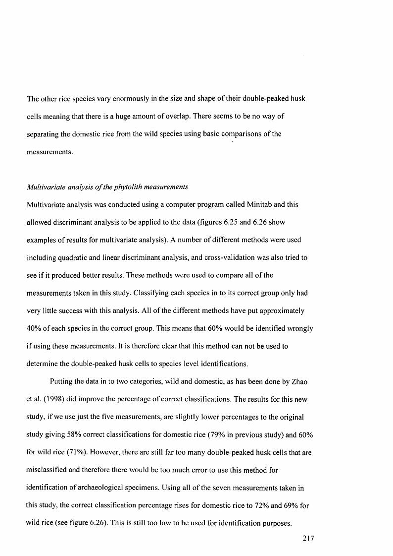
The other rice species vary enormously in the size and shape of their double-peaked husk
cells meaning that there is a huge amount of overlap. There seems to be no way of
separating the domestic rice from the wild species using basic comparisons of the
measurements.
Multivariate analysis o f the phytolith measurements
Multivariate analysis was conducted using a computer program called Minitab and this
allowed discriminant analysis to be applied to the data (figures 6.25 and 6.26 show
examples of results for multivariate analysis). A number of different methods were used
including quadratic and linear discriminant analysis, and cross-validation was also tried to
see if it produced better results. These methods were used to compare all o f the
measurements taken in this study. Classifying each species in to its correct group only had
very little success with this analysis. All of the different methods have put approximately
40% of each species in the correct group. This means that 60% would be identified wrongly
if using these measurements. It is therefore clear that this method can not be used to
determine the double-peaked husk cells to species level identifications.
Putting the data in to two categories, wild and domestic, as has been done by Zhao
et al. (1998) did improve the percentage of correct classifications. The results for this new
study, if we use just the five measurements, are slightly lower percentages to the original
study giving 58% correct classifications for domestic rice (79% in previous study) and 60%
for wild rice (71%). However, there are still far too many double-peaked husk cells that are
misclassified and therefore there would be too much error to use this method for
identification of archaeological specimens. Using all of the seven measurements taken in
this study, the correct classification percentage rises for domestic rice to 72% and 69% for
wild rice (see figure 6.26). This is still too low to be used for identification purposes.
217
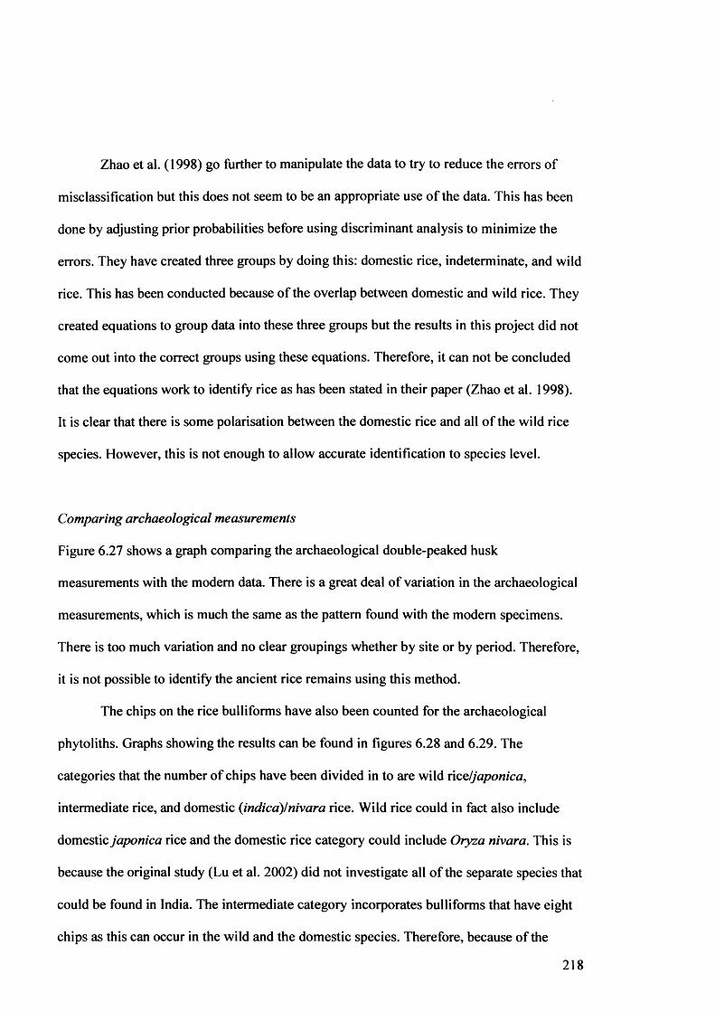
Zhao et al. (1998) go further to manipulate the data to try to reduce the errors of
misclassification but this does not seem to be an appropriate use o f the data. This has been
done by adjusting prior probabilities before using discriminant analysis to minimize the
errors. They have created three groups by doing this: domestic rice, indeterminate, and wild
rice. This has been conducted because of the overlap between domestic and wild rice. They
created equations to group data into these three groups but the results in this project did not
come out into the correct groups using these equations. Therefore, it can not be concluded
that the equations work to identify rice as has been stated in their paper (Zhao et al. 1998).
It is clear that there is some polarisation between the domestic rice and all o f the wild rice
species. However, this is not enough to allow accurate identification to species level.
Comparing archaeological measurements
Figure 6.27 shows a graph comparing the archaeological double-peaked husk
measurements with the modem data. There is a great deal of variation in the archaeological
measurements, which is much the same as the pattern found with the modem specimens.
There is too much variation and no clear groupings whether by site or by period. Therefore,
it is not possible to identify the ancient rice remains using this method.
The chips on the rice bulliforms have also been counted for the archaeological
phytoliths. Graphs showing the results can be found in figures 6.28 and 6.29. The
categories that the number of chips have been divided in to are wild rice/japonica,
intermediate rice, and domestic {indica)!nivara rice. Wild rice could in fact also include
domestic japonica rice and the domestic rice category could include Oryza nivara. This is
because the original study (Lu et al. 2002) did not investigate all o f the separate species that
could be found in India. The intermediate category incorporates bulliforms that have eight
chips as this can occur in the wild and the domestic species. Therefore, because of the
218
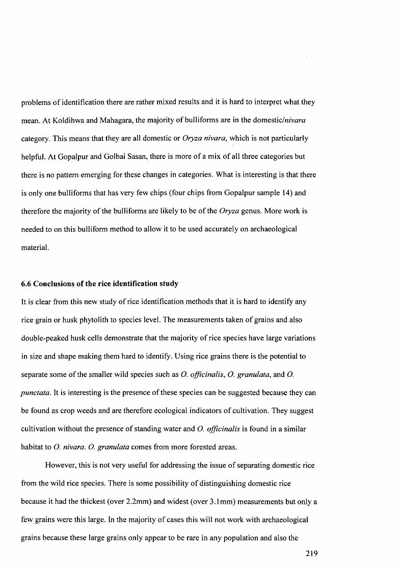
problems of identification there are rather mixed results and it is hard to interpret what they
mean. At Koldihwa and Mahagara, the majority of bulliforms are in the domestic/w/varra
category. This means that they are all domestic or Oryza nivara, which is not particularly
helpful. At Gopalpur and Golbai Sasan, there is more of a mix o f all three categories but
there is no pattern emerging for these changes in categories. What is interesting is that there
is only one bulliforms that has very few chips (four chips from Gopalpur sample 14) and
therefore the majority of the bulliforms are likely to be of the Oryza genus. More work is
needed to on this bulliform method to allow it to be used accurately on archaeological
material.
6.6 Conclusions of the rice identification study
It is clear from this new study of rice identification methods that it is hard to identify any
rice grain or husk phytolith to species level. The measurements taken of grains and also
double-peaked husk cells demonstrate that the majority of rice species have large variations
in size and shape making them hard to identify. Using rice grains there is the potential to
separate some of the smaller wild species such as O. officinalis, O. granulata, and O.
punctata. It is interesting is the presence of these species can be suggested because they can
be found as crop weeds and are therefore ecological indicators o f cultivation. They suggest
cultivation without the presence of standing water and O. officinalis is found in a similar
habitat to O. nivara. O. granulata comes from more forested areas.
However, this is not very useful for addressing the issue of separating domestic rice
from the wild rice species. There is some possibility of distinguishing domestic rice
because it had the thickest (over 2.2mm) and widest (over 3.1mm) measurements but only a
few grains were this large. In the majority of cases this will not work with archaeological
grains because these large grains only appear to be rare in any population and also the
219

shrinkage from carbonisation will adjust these measurements although adding 20%
routinely to archaeological specimens may help to overcome this problem. It may be
possible, therefore, to separate the rice grains in to three groups; mature Sativa complex
grains, immature Sativa complex grains, and small wild rice grains.
There seems to be even more overlap with the measurements taken o f the double
peaked husk cells particularly of O. sativa, O. nivara, and O. rufipogon. Again, there are a
few of the smaller wild species, O. granulata and O. officinalis, that could be separated
using the averages of the TW measurement. However, even by using the multivariate
analysis, none of these species could be separated to a satisfactory level to allow
identification.
At present, this study suggests that there is more potential for using rice grain
measurements than husk phytoliths although neither method is completely successful for
identifying all of the rice species. Husk phytoliths can not be used to identify domestic rice
and there is only a very small potential in using rice grains to identify domestic rice. More
work needs to be conducted on other phytolith methods of identification such as the
methods of measuring bulliforms from rice leaves and counting the chips to determine if
these are accurate methods or not. Unfortunately, identifying rice to species level is still
extremely problematic. It may be that this is never possible and therefore studies that
investigate the domestication of this crop have to be approached more laterally such as
looking for changes in weed flora to suggest cultivation and also trying to identify
immature versus mature harvesting of rice, which will in turn identify the change to the
domestic species. It has been shown here that some of the archaeological rice found in this
project is potentially immature although this is complicated by the shrinkage due to
carbonisation and also small wild rice species. More work is needed to look at alternative
ways to identify the start and development of rice cultivation.
220
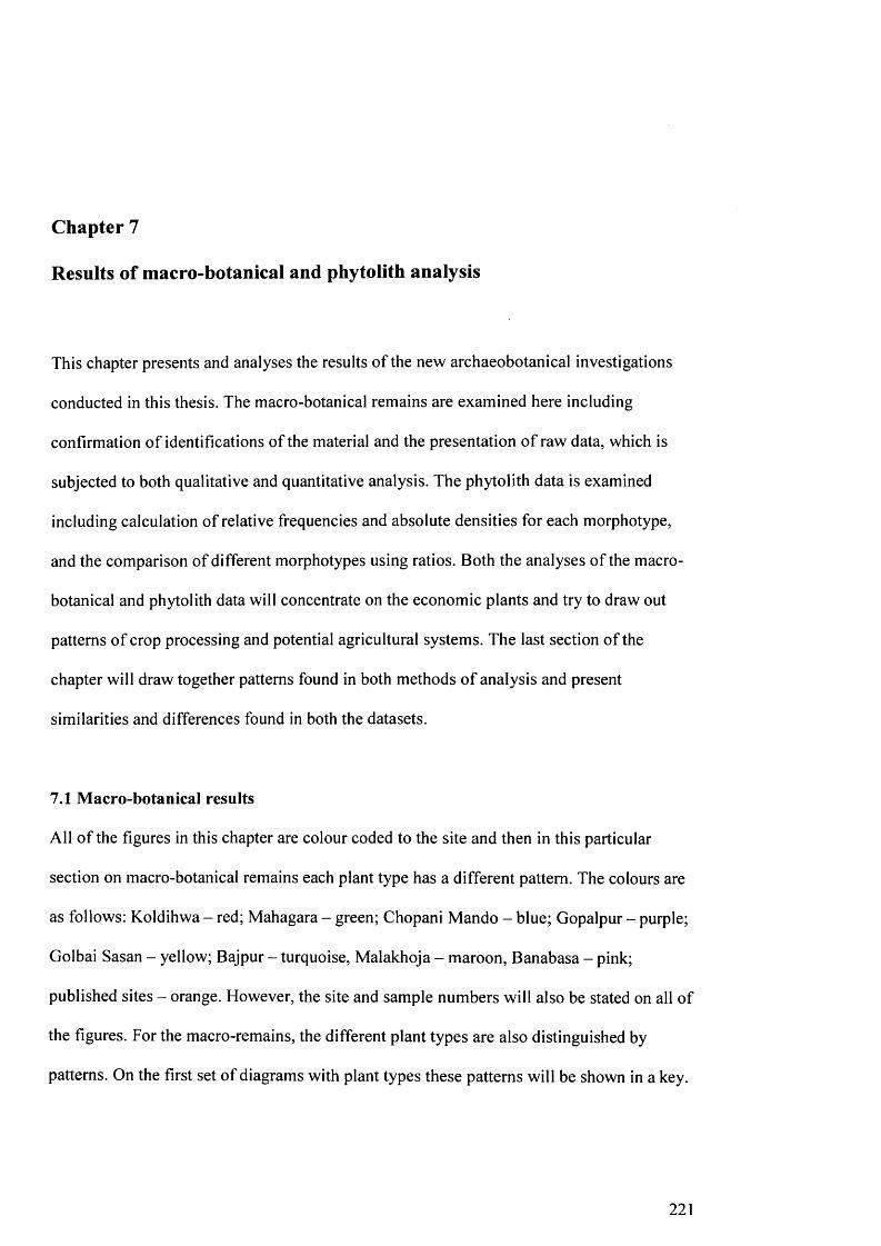
Chapter 7
Results of macro-botanical and phytolith analysis
This chapter presents and analyses the results of the new archaeobotanical investigations
conducted in this thesis. The macro-botanical remains are examined here including
confirmation of identifications of the material and the presentation of raw data, which is
subjected to both qualitative and quantitative analysis. The phytolith data is examined
including calculation of relative frequencies and absolute densities for each morphotype,
and the comparison of different morphotypes using ratios. Both the analyses of the macro-
botanical and phytolith data will concentrate on the economic plants and try to draw out
patterns of crop processing and potential agricultural systems. The last section of the
chapter will draw together patterns found in both methods of analysis and present
similarities and differences found in both the datasets.
7.1 Macro-botanical results
All of the figures in this chapter are colour coded to the site and then in this particular
section on macro-botanical remains each plant type has a different pattern. The colours are
as follows: Koldihwa - red; Mahagara - green; Chopani Mando - blue; Gopalpur - purple;
Golbai Sasan - yellow; Bajpur - turquoise, Malakhoja - maroon, Banabasa - pink;
published sites - orange. However, the site and sample numbers will also be stated on all of
the figures. For the macro-remains, the different plant types are also distinguished by
patterns. On the first set of diagrams with plant types these patterns will be shown in a key.
221
7.1.1 Identifications and preservation issues
There are a number of seeds, which are particularly challenging to identify; rice, some
Indian pulses, and small millets. The identification of rice has been thoroughly dealt with in
chapter six and it was concluded that it is very hard to identify rice to species level. This is
particularly true of distinguishing the wild progenitors from domestic rice. The
archaeological material in this project, therefore, has not been determined to be either wild
or domestic using measurements. However, there is the potential that some of the grains are
immature because of their small size and therefore some grains are likely to be wild. There
are potentially three groups of rice grains in the archaeological assemblages in this project:
mature Sativa complex rice grains, immature Sativa complex rice grains, and small wild
rice species such as O. granulata or O. punctata.
Vigna mungo and Vigna radiata are difficult to distinguish from each other and
therefore morphometries and the examination of the testa cell pattern has been used to
make species identifications. Vigna mungo/radiata seeds were only found at Mahagara,
Koldihwa, and Golbai Sasan. Two whole Vigna sp. seeds were found at Golbai Sasan
(sample 3), which had clear testa patterns. They revealed rows of long and thin rectangular
cells consistent with that of Vigna radiata (Fuller 2002a: 283) and they are also the only
Vigna sp. seeds that had intact testas. The presence of the testa may affect the
measurements as it has been found that if the testa remains intact then it limits the shrinking
caused by charring (Jupe 2003). This is demonstrated in the following graphs, which
clearly show these two particular seeds to be larger in size than the other testa-less Vigna
specimens in the same sample.
Measurements of the whole seeds and cotyledons have been taken of the length,
width, thickness, and plumule length. Two types of graphs can be used to try to separate
these two species and also potentially the wild and domestic species; length vs width, and
222

length vs plumule/length. Two graphs (figures 7.1 and 7.2) show the length and width
measurements of modem domestic and wild Vigna mungo and Vigna radiata and the
second graph is adjusted for 20% shrinkage due to charring. On figure 7.2 a cut offline is
indicted to show the difference in measurements between the wild and modem enlarged
domestic species and this will be used to determine seed identification in this project with a
certain degree of discretion. Figure 7.3 shows a graph of the length and width measurement
separation of these Vigna species in all of the sites examined. The two whole Vigna
specimens with testas are clearly in the domestic range for these species. The other Vigna
specimens are all cotyledons with no testas and fall within the wild range. However, they
probably need to be adjusted to a greater extent for shrinkage because of their lack of testa
and this may be the reason for their smaller size especially the ones that are particularly
small. It is also likely that if these seeds are domestic, they are towards the lower size end
of the modern domestic population measured because any significant change in size from
the wild form may still not have occurred at this time. Therefore, size may not be a useful
criterion, in this particular case, to identify domestication.
To distinguish between Vigna radiata and Vigna mungo, measurements of the
cotyledons are used. Generally, for Vigna mungo the plumule length/length ratio is smaller
than that of Vigna radiata (Fuller 2002a). Figure 7.4 shows a graph of the archaeological
measurements comparing them to modem measurements. There was not a great deal of
cotyledons available for measurement but this analysis gives some idea of what is present
in the samples. The majority of the specimens are in the Vigna mungo range but some are
on the border of the two species and therefore it is best to conclude that both of these
species are present. Mahagara definitely has both species present and the Golbai Sasan
cotyledons could be either species, although we have evidence of testa pattern that points to
223
Vigna radiata while results on other specimens suggest Vigna mungo. Koldihwa could just
have Vigna mungo present.
The first challenge that was encountered when examining the millets present in the
samples was whether they were archaeological or modem intrusions. Particularly in the
samples from the Belan River Valley, there were a lot of modem seeds including partly
blackened millets, which suggests a process o f blackening of recent intrusive material.
Some of these millets were fully blackened and appear charred, which suggest that they are
ancient although very well preserved. What should be noted is that the grains o f Brachiaria
ramosa and Setaria verticillata that had their husks on and appeared to be very well
preserved clearly show husk patterns consistent with these taxa. Those that were partly
blackened were not counted but if they were fully charred then they were counted as being
archaeological. However, these still may be modem and therefore they will not be included
in any data analysis of the sites. In the same samples, these species did occur as fully
charred and more ancient looking caryopses therefore these grains will be included in the
analyses that follow. These grains were identified by the length of the embryo and the
general size and shape of the caryopses as has been explained in chapter five.
Generally the preservation o f the material from the Belan River Valley sites was
worse than the material from the Orissan coastal sites. The quantity of material is less and
the preservation state of the seeds in general is worse. At Golbai Sasan and Gopalpur, there
were some very well preserved macro-botanical remains (whole pulses and rice) but there
was also a high degree o f fragmentation especially o f pulses. The upland sites of Orissa and
Chopani-Mando had very little or no macro-botanical remains. This is likely to be due to
the type o f occupation at these sites although at Chopani-Mando this could result from the
generally poor preservation conditions in this area, as is evident also at the nearby sites of
Mahagara and Koldihwa.
224

7.1.2 Results from Uttar Pradesh
Density o f plant material
Overall, the amount of charred material recovered from the Gangetic sites is disappointing.
All of the sites only produced a small amount of macro-botanicail material especially
Chopani-Mando. For the raw data tables see appendices 7.1, 7.2, and 7.3. As suggested
above this is probably a result of preservation issues as the fluctuating wet, dry, and hot
climate is not favourable for organic preservation. The density o f the flotation samples per
litre of sediment can be seen in the raw data tables (appendices 7.1 to 7.3). This reveals that
the densities are low in all of the samples. Densities range from 9.25ml (KDW 3) to 0.15ml
of charred remains per litre (CPM 69 and 71). Even from Koldihwa and Mahagara there are
very low densities in some samples. Therefore the phytolith analyses may reveal further
information not found in the macro-botanical data set. The low density of charred material
does affect the amount o f data analysis that can be used particularly for the results from
Chopani Mando. Therefore during the analysis of the data no multivariate methods will by
used and the data will be subjected to qualitative and simple quantitative statistical
methods.
Presence/absence and ubiquity values o f plant taxa
As can be seen in figure 7.5, the only plant remains present at Chopani Mando are small
millets and a few weed seeds (see appendix 7.4 for ubiquity value table). These two plant
types occur in 15% of the samples from Chopani Mando. The millets include the possibly
modem Brachiaria ramosa and Setaria verticillata. There is also one fragment of
indeterminate Gramineae, which could be a large cereal grain but was too badly preserved
to identify. Therefore, there is no clear evidence o f agricultural remains from these samples.
The evidence is too poor to conduct further analysis hence the data from Chopani Mando
225

will not be included in any of the analysis below. Phytolith analysis may reveal whether the
lack of macro-botanical remains at this site was due to preservation problems or a result of
none or little organic input in to the site.
At Koldihwa and Mahagara, the remains are still poor but there is evidence of greater
organic deposition. A graph comparing the ubiquity values from all the Belan Valley sites
can be found in figure 7.6. This graph demonstrates that Koldihwa and Mahagara have a
wide range of different plant types present in the samples. All o f the common agricultural
plant types are represented: pulses, large cereal grains, small cereal grains, and fruits. At
Mahagara, rice is the dominant cereal, which is present in 72% of the samples. After rice,
pulses and small millets are the next most commonly occurring plant types found in 63%
and 56% of samples. Vigna sp. is by far the most common pulse occurring in 44% of the
samples. Wheat and barley have low occurrences in the Mahagara samples (3% & 22%).
Weeds are fairly common (34%) although no single weed occurs in more than 9% of
samples. Ziziphus sp. only occurs in few samples (9%) and some parenchyma is also
present (9%).
Koldihwa has similar plant types present to those found in samples from Mahagara.
The most dominant plant types are pulses (60%) and again Vigna sp. is the most common
(45%). The next most commonly occurring plant type is small millets (50%) with Setaria
verticillata occurring in 30% of the samples. Rice occurs in 40% of the samples, which is
less than at Mahagara. Barley and wheat are again not as common as rice (25% and 10%)
but are more commonly found at Koldihwa than at Mahagara. Weeds and Ziziphus sp. are
also more common at Koldihwa (40% and 30%). No parenchyma is present in the samples
from Koldihwa.
226
Comparison o f new data with presence/absence and ubiquity values from other North
Indian Prehistoric sites
The published archaeobotanical data from the North Indian Prehistoric sites is not presented
as raw data and therefore only ubiquity values can be calculated for these sites. See
appendix 4.1 for a table o f the published data for North Indian Prehistoric sites. In general,
there is a lot of similarity between the presence of plant types at Mahagara and Koldihwa
compared to the published sites. The main large cereals of rice, barley and wheat are all
present. Summer and winter pulses are present at both the published sites and the newly
analysed sites but sites such as Malhar, Narhan, and Senuwar have a greater variety of
pulses than at Mahagara and Koldihwa with additional species such as Cicer arietinum and
Macrotyloma uniflorum, which possibly suggests the late adoption of additional pulse
species in this region. The published sites also have more oil plants present as well as the
presence o f melons and cucumber, which do not occur at all at the newly analysed sites
however these seem to occur in the later phases of sites or later dated sites. These sites also
generally have larger sample sizes and therefore may be more likely to produce a larger
variety of plant material.
As discussed in chapter four, there are only a few sites that have been analysed so
far that fall in to a similar date range to the samples analysed in this project and even fewer
of these can be used for calculating ubiquity values: Hulaskera, Manjhi, Narhan, Malhar,
and Senuwar. See appendix 7.5 for a table of ubiquity values from these published sites. Of
these sites, Malhar and Senuwar are the most relevant because they have similar sequences
o f deposits and the dating of these sites falls closest to Koldihwa and Mahagara. All of the
published sites contained all the plant types except for Hulaskera, which did not have fruits
or wheat present. This may have been because of the low sample size at this site compared
to the others. Manjhi also has very small sample size (overall 4 samples) and this may
227

account for the high occurrence of plant material in the samples. At the other sites, there is
a fairly similar occurrence of the plant types. Pulses, barley, and rice occur most frequently.
Weeds also commonly occur in samples from Narhan and Malhar. Wheat, small millets,
and fruits are less common, although wheat does occur in 40% of the samples from Narhan.
Figure 7.7 compares the ubiquity values for the Mahagara and Koldihwa with those
from the published North Indian sites. There does appear to be fairly similar occurrences of
the plant types in the samples from these sites. Pulses and rice are most common although
small millets are also common at Mahagara and Koldihwa occurring in 50% and 56% of
samples compared to 30% and 25% at Malhar and Senuwar. At Malhar there is a very high
occurrence of pulses being present in 75% of samples and lentils are most common of the
pulses. Barley and wheat are less frequently found than rice and pulses at all of the sites.
Weeds are also fairly common at most of the sites except Senuwar where they only occur in
18% of the samples. Fruits are present at all of the sites and are most common at Koldihwa
(30%).
Relative frequency o f plant types
To examine the changes in the relative frequencies of different plant taxa the results of the
samples have been combined for each level. There are two samples per stratigraphic layer
for Koldihwa and Mahagara. Koldihwa has also been split in to the two separate sections
that were sampled; Z1 and Yl.
At Mahagara (see figure 7.8), rice and indeterminate Gramineae are the only
remains present in the lowest level of the section (level 17). Rice is consistently present
from the very beginning of the section right up until level 5 in varying amounts and always
represents a substantial part of the level. In the next level up there is a sharp change with
pulses, barley, and small millets being present along with the previous two plant types.
228

Pulses represent a large part of samples from this level (47%). Pulses are present from level
16 to level 6 and range from 55% (level 12) to 14% (level 6) in the levels. Barley is not as
consistent as rice and pulses and appears in much smaller numbers (17% in level 15 to 5%
in level 14). Wheat is only present in level 13 and is only one fragment. Small millets are
present from level 16 to level 6 with exception of level 7. This plant type ranges from 43%
(level 10) to 4% (levels 8 & 13). Parenchyma is present in small quantities in levels 11 and
14. Fruits only occur in three levels (13, 8, & 6) and only in small amounts. Weeds occur
more frequently than fruits being present in eight levels. They are present from level 13 to
level 5 with exception of level 10.
At Koldihwa, the two sections show quite different sequences of plant types even
though they should represent the same levels on the site. In both sections the lowest
samples taken from level 5 did not contain any plant material apart from some charcoal
mostly found in Z l. No artefacts were found in these levels either. See figure 7.9 and 7.10
for relative frequency charts of both sections sampled. Section Z l begins with a wide
variety of plant types. Pulses, rice, small millets, indeterminate Gramineae, and weeds are
all present in level 4. These pulses include Vigna sp. and lentils, therefore both summer and
winter pulses are represented. Rice is present in all of the levels above level 4 and has its
largest occurrence in level 2 (50%). All of the other plant types continue to be present
throughout the samples with the addition of wheat and fruits in level 2. Wheat is not present
in any other level.
Section Y 1 starts with barley, which is only present as one fragment. Level 3 does
not contain barley but has pulses, small millets, wheat, rice, and fruits present. This is the
only level in section Y1 that contains rice and wheat. Levels 1 and 2 have the same plant
types present but in different amounts; pulses, small millets, barley, indeterminate
Gramineae, fruits, and weeds. In level 2, pulses and small millets have the largest amounts.
229

Weeds occur in the largest quantity in level 1. However, if the samples are combined
further by putting the two sections data together then all o f the plant types would be present
in all levels with the exception of barley in level 3.
Absolute counts and vertical changes in plant taxa
The calculation of absolute counts has only been conducted for pulses and cereal grains that
are identified to at least genus level. Figures 7.11 to 7.13 show vertical charts of absolute
counts for Mahagara and Koldihwa. This demonstrates again the scarcity o f remains found
at these sites. At Mahagara, rice appears in small quantity in sample 52, along with
indeterminate Gramineae (not on figure 11). It is clear with the absolute numbers as it was
with relative frequencies that sample 50 has a significant increase in the quantity of plant
material and the plant taxa present. Vigna sp., lentils, and pulse fragments are present along
with small millets and barley. Although, it is not until sample 46 that a consistent presence
o f all the plant taxa can be seen. Sample 40 has the largest amounts of small millets and
barley where as sample 39 has the largest amount o f rice. From samples 29 upwards there
is no presence of the major plant taxa except for some occasional small millets. Therefore
the major organic input in to the site is between samples 46 and 30. Sample 40 has the
largest amount of plant material.
At Koldihwa, section Y1 begins with barley in sample 17. There are no plant
remains earlier than this. In sample 16, rice, wheat, and pulse fragments are present but
barley is not present again until sample 14. All o f the remains are in very small numbers,
smaller than found at Mahagara. Generally, the amount o f plant material increases moving
up the sequence and this can especially be seen in small millets, barley, and weeds. Rice is
only present in samples 15 and 16 and only in very small numbers. Sample 11 has the
largest amount of plant material in section Y 1, which is the latest sample.
230
In section Z l, the amount of plant material is again very small. The first sample to
have plant material is sample 8, which contains Vigna sp., lentil, pulse fragments, rice and a
weed seed. Barley is not present until the very top of the section in sample 1 and 2. There is
more rice present in this section and one sample contains five grains. One wheat grain is
present in sample 4. Sample 3 contains the largest amount o f plant material in section Z l.
Comparing plant taxa - ratios
Comparing the data from different plant taxa may give some insight into how these plants
became incorporated in the samples and whether different plant taxa relate to one another
or not. This has been done for the different plant taxa found at Koldihwa and Mahagara.
Tables of the ratios generated by this analysis can be seen in figures 7.14 and 7.15. All of
the ratios showed little relationship between any of the plant taxa. This is probably the
result of the poor preservation at these sites and also the small sample size used, which does
not allow a true comparison of what would have been left in antiquity but just those
fragments that have survived.
7.1.3 Results from Orissa
Density o f plant material
As can be seen in the sample from the Belan River Valley, there are differences in the
density of plant material between the sites sampled in Orissa. The density of the flotation
samples per litre of sediment varies throughout the samples. This data can be found in the
raw data tables in appendices 7.6 to 7.10. The largest flotation sample being MKA 2 (7.6
ml) and the smallest being 0.05ml in samples GPR 9 & 10. This does not necessarily mean
that more charred material is in the larger flotation samples because other material can be
found in the samples such as soil or modem plant roots. Two sites contain significantly
231

more charred material than the other three; these are Gopalpur and Golbai Sasan. The other
three sites (Bajpur, Malakhoja, and Banabasa) had little or no charred plant material. Again,
at the later sites it may be a result of preservation and the phytolith analysis may reveal
more information about why there is a scarcity of charred remains.
Presence/absence and ubiquity values o f plant taxa
At Bajpur, there are very little charred remains and even charcoal is scarce. Samples 2 and
3 contained one indeterminate fragment each and sample 4 contained an indeterminate
small millet. All of these were very badly preserved. The samples from Banabasa contain
even less charred material. There are no fragments of seeds and only rare pieces of
charcoal. Malakhoja also has a lack of charred plant remains. In sample 1 there are 3 rice
grains although because of the scarcity of other charred remains this may well be intrusive.
This lack of charred material means that any further analysis of macro-botanical remains
cannot be done on these sites.
The samples from Gopalpur and Golbai Sasan are very different to those from the
other three sampled sites. There is a large amount of different plant taxa found at these
coastal sites, which represent all of the major plant types: pulses, small millets, large
cereals, fruits, and weeds. The pulses present at Gopalpur are Macrotyloma uniflorum and
Cajanus cajan. These pulses are also present at Golbai Sasan as well as Vigna sp. and
Vigna radiata. These sites contain rather a lot of rice compared to the Belan Valley sites
particularly Golbai Sasan. There is also a small amount of rice chaff at both sites. The
coastal Orissan sites do not contain any winter pulses or winter cereals. There is a variety of
small millets present: Setaria sp., Panicum sp., Paspalum sp., and Echinochloa sp. All of
these are present at Gopalpur but Golbai Sasan just has Setaria sp. and Paspalum sp.
Fragments o f fruit stones are present at both sites. Celtis sp. is found at Gopalpur and
232
Ziziphus sp. at Golbai Sasan. There is also a variety of weeds present at both sites including
sedges and wild grasses.
A comparison of ubiquity values for the different plant types found at Gopalpur and
Golbai Sasan can be found in figures 7.16. This shows that the occurrence of the major
plant types is similar for both sites. At Golbai Sasan, pulses and fruits occur more
frequently than at Gopalpur. Rice, small millets, and weeds have very similar ubiquity
values.
Relative frequency o f plant types
Figures 7.17 and 7.18 show charts of the relative frequencies of the different plant types in
the assemblages from Gopalpur and Golbai Sasan. At Gopalpur, pulses dominate the
bottom of the section (samples 1-3). The largest amount o f charred material is found in
samples 2 and 3, which are near the bottom of the section. Large numbers of pulses
(Macrotyloma uniflorum and pulse fragments presumably also horsegram) are found in
samples 2 and 3 (168 and 248 fragments). Rice is present in all the samples and dominates
the samples at the top of the section (samples 10-13). Although, the largest amounts of rice
occurs in samples 6, 7, and 8. Weeds are present throughout the section with exception of
sample 9. Small millets occur sporadically throughout and appear in larger numbers in
samples 6 and 8 than are found in other samples. Single stones o f Celtis sp. are found in
samples 2 and 12.
At Golbai Sasan, a wide variety of plant types are present from the bottom of the
section: pulses, rice, indeterminate Gramineae, fruits, and weeds. Rice dominates the
bottom three samples and is a significant part of all samples in the section. The largest
amount of rice is found in sample 9 (107 fragments). Pulses are also present in significant
numbers in all samples. The largest number of pulses appears in the upper most sample (3
233
with 204 fragments) and this is the result of a large number of Vigna sp. seeds being
present. Small millets occur infrequently throughout and are present in samples 14A, 13A
to 9, 7A, and just one fragment in sample 3. They are only present in small amounts
ranging from one to six fragments. Weeds are present in sample 14B to 8 with the
exception of sample 13 A. They are also only present in small amounts ranging from one to
five fragments. Fruits are present sporadically throughout the section and appear in their
largest numbers in samples 9 and 14B (70 and 16 fragments).
Absolute counts and vertical changes in plant taxa
The calculation of absolute counts still shows that a significantly larger number of charred
remains have been found at the coastal Orissan sites to those found at the Belan Valley
sites. Vertical bar charts of Gopalpur and Golbai Sasan can be seen in figures 7.19 and
7.20.
At Gopalpur, pulses particularly Macrotyloma uniflorum dominate the lower part of
the section. Sample 2 and 3 have the largest amounts of this pulse species (27 and 32
seeds). Cajanus cajan is only present in sample 2 at this site and 1 whole seed was found.
Pulses fade away moving up the section and rice increases in importance. Although, rice is
consistently present throughout the section but not in large quantities. The absolute counts
for rice range from one to ten grains. The largest amounts occur in samples 6 and 8. These
samples also have the largest number of small millets in the section. From sample 8
upwards charred material decreases until sample 15 where there is no plant material
present.
At Golbai Sasan, rice dominates the bottom of the sequence but there are a number
o f different plant taxa also present; weeds, pulse fragments, small millets, and fruit
fragments. It is not until sample 12 that there is significant input from all of the plant taxa.
234

Sample 9 has the largest amount of charred material including the largest amounts of rice,
weeds, and fruit fragments. Sample 3, the uppermost sample, has the largest amount of
pulses, particularly Vigna sp. This taxon is also present in small numbers, ranging from one
to four, in samples 13D, 13C, 12, 11 and 9 but occurs in much larger number in sample 3
(36.5). Cajanus cajan is present in three samples (10, 9, and 3) and only in small amounts.
Macrotyloma uniflorum is present sporadically throughout the section and is also only
present in small amounts.
Comparing plant types - ratios
The greater amount of charred material found at the coastal Orissan sites means that
comparison between the different plant types is likely to be less influenced by preservation
issues and changes in the data reflect ancient patterns and possibly activities. Figure 7.21
shows a table of comparison values of Gopalpur plant types and figure 7.22 shows ratios
from Golbai Sasan. These two sites have similar patterns, when comparing plant types.
Rice and weeds correlate well as does rice and small millets with weeds. Rice and pulses do
not correlate well at either site but at Golbai Sasan there is some correlation if an outlier
(sample 3) is removed from the comparison. Pulses do not correlate with either small
millets or weeds. This may suggest that these two crops are treated differently in terms of
crop processing. Rice and small millets correlate well at Gopalpur (0.79) but not as well at
Golbai Sasan (0.35), which may suggest at the former site they are primarily rice weeds and
at the later may be a separate crop plant. Therefore at Golbai Sasan, Setaria sp. or
Paspalum sp. may have been cultivated as crops although they only appear in very small
numbers in the macro-botanical assemblage and there are more small millets that were not
identified to genus or species level so another small millet is also just as likely.
235
7.2 Phytolith analysis results
7.2.1 Identification of phytolith remains
A lot o f discussion has focused in this thesis on the identification o f rice (particularly
chapter six). Different rice phytolith parts have been counted in this project even though it
is recognised that there are certain problems with some of them. For the single celled
phytoliths, rice bilobes, rice bulliforms, and rice double-peaked glume (or husk, whatever
name is used they are the same thing!) cells are recorded. These are only recognised as
these particular parts if they are classic examples o f these types (examples o f these can be
seen in appendix 5.4). Any variation and they were counted in the general categories for
these morphotypes: keystone or bilobes (double-peaked ‘glume’ cells does not have a
general category because they are easily distinguished). As far as rice husk is concerned,
these were only recognised if the particular cell pattern and peaked cells were present. If
only the cell pattern was present then these multi-cells were recorded as cereal husk. Rice
leaf/stem was recorded when more than one scooped rice bilobe was present in a horizontal
position. Other multi-celled categories are explained in appendix 5.4 including photographs
o f some examples.
The majority of categories used for counting are general and not specific to a
particular genus or species. However, within some of these categories there was great
variation especially keystones and bilobes. Bambusoid type keystones were seen and also
some that may have been other grasses such as Cynodon sp. but there was a great deal of
variation in most o f the samples, which demonstrated the presence of various leaf material.
Another category, which needs to be discussed, is rugulose spheroid. The majority
of scholars would recognise this category as date palm, however in this region there are
many different palms. An examination o f the leaves of the three most common palms has
taken place: date palm, palmyra palm, and coconut palm. They are all fairly similar to each
236

other although palmyra palm has some larger rugulose spheres as well as the small ones.
Some of the rugulose spheres in this project, were the ones consistent with date palm,
having regular small spines and being fairly small in size although these have also been
seen in other palms so these are not diagnostic to a genus or species. There were also some
larger spheres with regular spines but there were some that had irregular spines too, some
much longer than others. Reference material matching the last spheres has not yet been
found. More work needs to be conducted on palm species because even though these
phytoliths could come from the common palms, which are economic plants, they may also
be from the many other species that exist in these tropical areas. Therefore for the moment
they have all been put in this general category.
There was one consistently recurring multi-cell (found only at Golbai Sasan), which
was unidentifiable (indet multi-cell type one). This was a panel of papillae type cells all
grouped together sometimes in a random configuration and sometimes in uniform rows.
This may be part of the tip of a grass husk, which looks fairly similar but not as compact. I
have not seen anything that is exactly like these panels so no identification can be put
forward at present.
7.2.2 Results from Uttar Pradesh
In this project, phytolith samples from Koldihwa and Chopani Mando have been analysed.
Phytolith analysis on samples from Mahagara has been previously conducted by the author
(Harvey 2002) and this information will be presented here again so that it can be compared
to the other Belan River Valley sites easily. More detailed analysis will also be conducted
of this data and the ability to compare it especially with the data from Koldihwa will add a
great deal to the interpretation of the site. It was also not possible to previously assess the
237

data along with the macro-botanical results, which may again change the interpretations
previously suggested.
Presence/absence o f morphotypes
Results tables for all of the Belan River Valley sites can be found in appendices 7.11 to
7.13. At Chopani-Mando, there is quite a large variety of single-celled morphotypes
present in the samples both monocotyledons and dicotyledons but very few multi-celled
phytoliths were present in any of the samples. Long smooth, bulliforms, and keystones are
the most common morphotypes in the samples. Rugulose spheres (Palmae) are present in
all of the samples and these include some with irregular spines. Throughout the whole
section there are no cereal remains present at all. Therefore no rice was present or any
millet remains. A few indeterminate leaf/stem fragments are present in samples 3, 5, and 7.
Unidentifiable husk is present in sample 1 as well as a Cyperaceae multi-cell.
At Koldihwa and Mahagara, there is a larger variety of morphotypes present than is
seen in the samples from Chopani Mando. The most apparent difference is the common
appearance of multi-celled phytoliths in general but these include cereals such as rice and
millets. There were no multi-celled phytoliths at Mahagara or Koldihwa that could be
identified as wheat or barley, which may have been expected from their occurrence in the
macro-botanical assemblages. However, rice is clearly a large part of the samples from
Mahagara and Koldihwa and is present as both multi-celled and single-celled phytoliths.
Long smooth, bulliforms, and keystones frequently occur as at Chopani Mando but there
are also morphotypes such as long dendritic, crosses, flat tower, tracheids, and sheets that
occur much more frequently at Koldihwa and Mahagara. Dicotyledon single celled
phytoliths are more common especially at Koldihwa.
238

Relative frequencies
Tables of the relative frequencies can be seen in appendices 7.14 to 7.16 and graphs of the
relative frequencies can be found in figures 7.23 to 7.28. At Chopani Mando, long smooth
morphotypes have the highest relative frequency ranging from 48% to 55% of the total
single-celled assemblage. Bulliforms and keystones are the next frequent in the samples.
Keystones have their highest frequency in sample 1 being 20%. Bulliforms range from 9%
to 19% with the largest amount occurring in sample 5. After these morphotypes, rugulose
spheroids are the next highest occurrence in the assemblage ranging from 2% to 4%. The
most frequently occurring multi-celled type is in fact not a phytolith but is diatoms, which
makes up 100% of the total multi-celled assemblage in sample 9. Silica aggregates are also
common when they are present in samples ranging from 33% to 56%. Indeterminate
leaf/stem occurs in samples 3, 5, and 7, and ranges from 6% to 33%. Unidentifiable husk
only occurs in sample 1 and makes up 14% of the total multi-celled component of that
sample.
The relative frequencies for Koldihwa show that there is a more even spread of
occurrence over more morphotypes than are found at Chopani Mando. Long smooth,
bulliforms, and keystones make up a large part of most o f the single-celled assemblage but
bilobes also have a similar occurrence. Long smooth range from 11% to 24 %, the highest
occurrences occurring in samples 7 and 11. Bilobes make up more of the assemblage in the
top of the two sections than the lower parts. The highest percentage occurs in sample 1
(29%) with the lowest occurrences for the two sections are in sample 6 (Z1/5) of 6% and in
sample 11 (V 1/5) of 3%. Keystones have the opposite pattern as they are low at the top of
the sections and the frequencies in the assemblage gets higher going down. In section Z l,
sample 1 has 4% but by sample 6 (Z1/5) keystones make up 26%. Bulliforms occur in
varying amounts throughout both sections. The largest percentages occur in samples 5 and
239

9 both being 18%. The next largest occurring morphotypes are long dendritics, rondels, and
saddles. The highest occurrence of long dendritics occurs in sample 3 (10%). Rondels range
from 2% to 10% and saddles range from 3% to 11%. Rice single-celled types occur in
small numbers. Double peaked glume cells have the largest occurrences o f these types of
phytoliths ranging from 0.3% to 1.8% of the assemblage. Dicotyledon single-celled
morphotypes occur in small numbers throughout the samples. Sheet and elongate types
occur in the largest percentages ranging from 0.7% to 4% and 0.2% and 3%.
The multi-celled phytolith assemblages are dominated by four morphotypes types:
indeterminate leaf/stem, unidentified husk, cereal husk, and rice husk. Generally, all o f
these types are present in higher percentages at the top o f the sections and the amounts
decrease going down the sections. The highest percentage for indeterminate leaf/stem
occurs in sample 7 (40%) and for unidentifiable husk in samples 2 and 4 (both 36%).
Cereal husk occurs in greater percentages in section Z l to Y1 and the largest frequency is
28% in sample 3. Rice husk occur most frequently in sample 8 (35%) and ranges from 6%
to 28% in section Zl and from 7% to 35% in section Y l. Rice leaf/stem occurs in small
amounts in some samples ranging from 0.8% to 1.9%. Cyperaceae has the opposite pattern
to the types above. It occurs most in the lower samples and therefore may not have been
brought to the site as a weed of the crop plants. Its largest frequency is in sample 10 (72%).
Millet husk only makes up a small part of the multi-celled assemblages. Sample 1 has the
largest frequency being 4%. Phragmites stem, square cell leaf/stem, polyhedral hair base,
and silica aggregates only occur in very few samples and in small percentages.
The relative frequency o f samples from Mahagara is similar to that of Koldihwa.
Again long smooth, keystones, and bilobes are some o f the highest occurring morphotypes
in each single-celled assemblage but at Mahagara long dendritics and saddles also occur in
similar amounts. Long smooth phytoliths range from 7% to 35% and the largest three
240

percentages occur in samples 8 to 10 at the top of the section. Keystones increase in
frequency going up the section and the largest percentage occurs in sample 9 (30%). The
frequency of bilobes in the samples generally decreases up the section with the lowest
sample being sample 9 (2%) and the largest sample is sample 3 (25%). The amount of
saddles varies throughout the section ranging from 3% in sample 10 to 30% in sample 1.
After sample 1, where the amount of long dendritics is 4%, the amount rises sharply and
then decreases. Sample 2 has 20% and sample 10 has 5%. The lowest amount is in sample
8 being 3%. Bulliforms, long sinuate, and crosses are the next frequent types of single
celled phytoliths. Bulliforms vary in frequency throughout the section ranging from 0.8%
to 9%. Long sinuate types are fairly consistent with most samples having between 4% and
5%. Sample 2 has the largest percentage of 10% and sample 9 the lowest being 2%. Crosses
vary between 1.2% and 7%. Crenates and rondels occur in all of the samples but in small
frequencies. All of the rice single-celled types again occur in small number but not in all of
the samples. There are no rice single-celled phytolith in the top three samples (8 to 10).
Dicotyledon single-celled phytoliths occur in smaller frequencies than at Koldihwa but
different types are more common. Rugulose and smooth spheroids occur more frequently
and in higher percentages at Mahagara. Elongates, tracheids, and sheet types occur in most
o f the samples but are in lower percentages than occur at Koldihwa.
In the multi-celled assemblages, indeterminate leaf/stem and unidentifiable husks
make up a significant part of most samples except for sample 8 to 10. Unidentifiable husk
occur more frequently than indeterminate leaf/stem. It occurs most frequently in samples 3
and 6 (both 62%). Rice husk occurs in samples 1 to 7 and ranges from 2.9% to 12.8%. It
occurs much less frequently than at Koldihwa. Rice leaf/stem are not present in any of the
samples. Diatoms make up a large percentage of some samples especially samples 1, 2, and
8 to 10. Sample 10 has the largest percentage being 94.4%. Millet husk occurs sporadically
241
throughout the sequence in low percentages (1.3 to 5.8%). Cyperaceae occur in half of the
samples in low amounts and Phragmites stem only occurs in three samples (samples 3 to
5).
Absolute densities
The calculation of the density makes it possible to compare between samples in a different
way to using relative frequencies. In this case, the density is calculated of the number of
phytoliths per gram of sediment type. Graphs of the different totals of phytoliths per gram
of sediment can be found in figures 7.29 to 7.34. The total amount of phytoliths per gram of
sediment found in the samples from Chopani Mando is a substantial amount (see figure
7.29). The highest number is in sample 3 being 19,201. The lowest number is in sample 9
being 1711. The majority of the samples are made up o f predominantly single-celled
phytoliths. Multi-celled phytoliths only occur in very small amounts ranging from 2
(sample 7) to 19 (sample 3) per gram of sediment (see figure 7.30). This is an extremely
low amount.
The calculation of the absolute densities does create a slightly different pattern for
the individual morphotypes than the relative frequencies at Chopani Mando (see figures
7.35 and 7.36). This highlights differences in the amount o f long smooth, bulliforms, and
keystones morphotypes between the samples. Sample 3 has a much higher density of long
smooth cells (10,057), bulliforms (2730), and keystones (2863) than other samples except
for sample 1, which also has similar amounts o f bulliforms and keystones. With the
absolute densities, sample 3 has the largest amount o f bilobes (133) and rondels (333) but
with relative frequencies bilobes is highest in sample 9. All other patterns are similar to that
found using relative frequencies. Densities o f multi-celled phytoliths also show a similar
pattern apart from sample 3 having a higher density o f diatoms than sample 9.
242
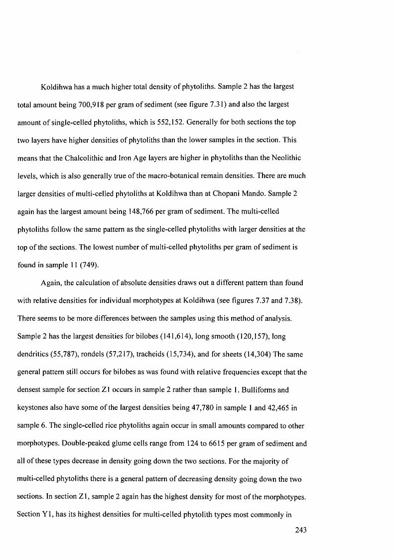
Koldihwa has a much higher total density of phytoliths. Sample 2 has the largest
total amount being 700,918 per gram of sediment (see figure 7.31) and also the largest
amount of single-celled phytoliths, which is 552,152. Generally for both sections the top
two layers have higher densities of phytoliths than the lower samples in the section. This
means that the Chalcolithic and Iron Age layers are higher in phytoliths than the Neolithic
levels, which is also generally true of the macro-botanical remain densities. There are much
larger densities of multi-celled phytoliths at Koldihwa than at Chopani Mando. Sample 2
again has the largest amount being 148,766 per gram of sediment. The multi-celled
phytoliths follow the same pattern as the single-celled phytoliths with larger densities at the
top of the sections. The lowest number of multi-celled phytoliths per gram of sediment is
found in sample 11 (749).
Again, the calculation of absolute densities draws out a different pattern than found
with relative densities for individual morphotypes at Koldihwa (see figures 7.37 and 7.38).
There seems to be more differences between the samples using this method of analysis.
Sample 2 has the largest densities for bilobes (141,614), long smooth (120,157), long
dendritics (55,787), rondels (57,217), tracheids (15,734), and for sheets (14,304) The same
general pattern still occurs for bilobes as was found with relative frequencies except that the
densest sample for section Zl occurs in sample 2 rather than sample 1. Bulliforms and
keystones also have some of the largest densities being 47,780 in sample 1 and 42,465 in
sample 6. The single-celled rice phytoliths again occur in small amounts compared to other
morphotypes. Double-peaked glume cells range from 124 to 6615 per gram of sediment and
all of these types decrease in density going down the two sections. For the majority of
multi-celled phytoliths there is a general pattern of decreasing density going down the two
sections. In section Z l, sample 2 again has the highest density for most of the morphotypes.
Section Y l, has its highest densities for multi-celled phytolith types most commonly in
243

sample 7 but for rice husk and Cyperaceae it is in sample 8. Rice leaf/stem is only present
in small numbers and occurs more in section Yl.
At Mahagara, there is a lower density of total phytoliths than is found at Koldihwa
and even lower than at Chopani Mando. The largest sample at Mahagara is 17,427 per gram
of sediment in sample 5 (see figure 7.33). However, the number of multi-celled phytoliths
is much larger than at Chopani Mando (see figure 7.34). The largest density of multi-celled
phytoliths is found in sample 3 (2206). Sample 3 to 7 have much larger densities of all
phytolith than the other samples in the section.
For the individual morphotypes there is also a very different pattern apparent using
absolute densities at Mahagara (see figure 7.39 and 7.40). Long smooth cells are much less
important in samples than is suggested by relative frequencies. Keystones have the largest
density of phytolith overall and have the highest morphotype density in samples 5 (3635), 6
(3185), 4 (1988) and 7 (1973). Bilobes, saddles, and long dendritics also have large
densities in most samples. Bilobes range from 3069 in sample 5 to 40 in sample 9. Saddles
occur in the highest density in sample 5 (2342). Samples 3 to 5 have the highest density of
long dendritic cells. Bulliforms are much more dense in sample 5 (969) and 7 (839)
compared to other samples. The rice bulliform and bilobe phytoliths both have their largest
densities in sample 7, which is the same as found with relative frequencies. The double
peaked glume cells, however, are densest in sample 6 rather than sample 1 with relative
frequencies. The dicotyledon single-celled phytoliths show a similar pattern to that found
with relative frequencies. The multi-celled phytoliths also demonstrate a different pattern
using absolute densities. Unidentifiable husks have the largest densities in the majority of
samples. Sample 3 has the largest density of this morphotype (1376). This sample also has
the largest density of rice husks (283) and long smooth cells (434). Sample 3 through to 7
generally have more multi-celled phytoliths than other samples. The very top of the
244
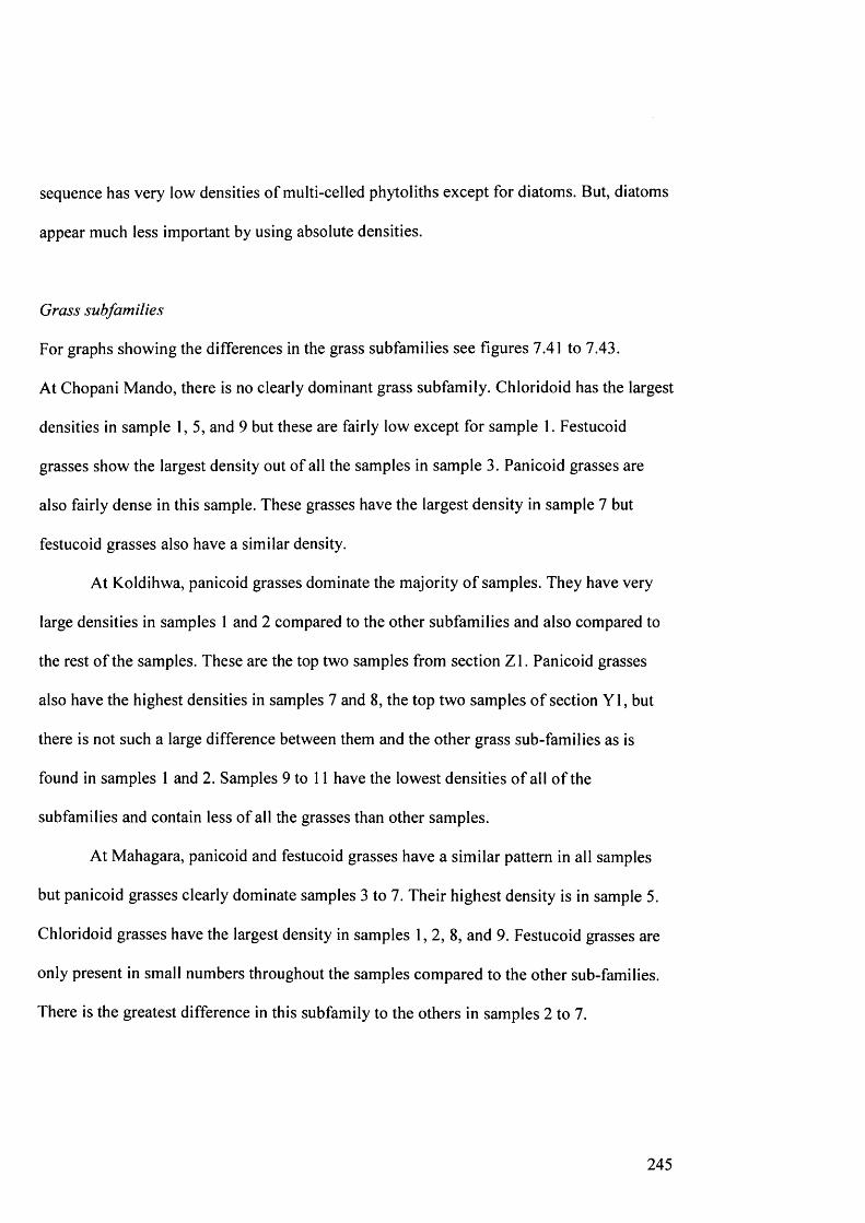
sequence has very low densities of multi-celled phytoliths except for diatoms. But, diatoms
appear much less important by using absolute densities.
Grass subfamilies
For graphs showing the differences in the grass subfamilies see Figures 7.41 to 7.43.
At Chopani Mando, there is no clearly dominant grass subfamily. Chloridoid has the largest
densities in sample 1, 5, and 9 but these are fairly low except for sample 1. Festucoid
grasses show the largest density out of all the samples in sample 3. Panicoid grasses are
also fairly dense in this sample. These grasses have the largest density in sample 7 but
festucoid grasses also have a similar density.
At Koldihwa, panicoid grasses dominate the majority o f samples. They have very
large densities in samples 1 and 2 compared to the other subfamilies and also compared to
the rest of the samples. These are the top two samples from section Z l. Panicoid grasses
also have the highest densities in samples 7 and 8, the top two samples of section Y l, but
there is not such a large difference between them and the other grass sub-families as is
found in samples 1 and 2. Samples 9 to 11 have the lowest densities of all o f the
subfamilies and contain less of all the grasses than other samples.
At Mahagara, panicoid and festucoid grasses have a similar pattern in all samples
but panicoid grasses clearly dominate samples 3 to 7. Their highest density is in sample 5.
Chloridoid grasses have the largest density in samples 1 ,2 ,8 , and 9. Festucoid grasses are
only present in small numbers throughout the samples compared to the other sub-families.
There is the greatest difference in this subfamily to the others in samples 2 to 7.
245

Comparing single-celled phytoliths using ratios
At Chopani Mando, the single-celled phytoliths with large densities (long smooth, long
dendritic, bulliforms, and keystones) have been compared to try to establish whether they
have any relationship. This will help to determine the source of this material. Table of these
comparisons can be seen in figure 7.44. This analysis shows that there is a correlation,
generally a very good one, between these morphotypes.
At Koldihwa, for single-celled phytoliths this analysis was carried out on a larger
variety of morphotypes (long smooth, long dendritic, bulliforms, keystone, bilobes, crosses,
saddles, and rondels) because these samples were generally more variable in terms of
morphotypes than those from Chopani Mando. Figure 7.45 shows a table of these
comparisons. The majority of these morphotypes correlate well especially long smooth with
long dendritic, and bilobes with crosses and also with rondels. Bulliforms do not correlate
well with keystones or other morphotypes. Saddles also do not seem to correlate well with
other morphotypes particularly with rondels. The only morphotype that saddles correlate
fairly well with is bulliforms.
The same comparisons were carried out for the samples from Mahagara with a
fairly similar outcome (see figure 7.46). Again long smooth correlates well with long
dendritics as well as most of the other morphotypes. Long dendritics correlate well with
bilobes and crosses but not as well with rondels and saddles although there is still some
relationship. Bulliforms do not correlate with any other morphotype including keystones.
At Mahagara, saddles correlate well with the other morphotypes but crosses and rondels do
not correlate well together.
246

Comparing plant parts using ratios
Comparative analysis of multi-celled plant cells and the single-celled rice phytoliths has
been conducted for Koldihwa and Mahagara. There are not enough multi-celled phytoliths
nor any rice phytoliths present at Chopani Mando to carry out this analysis. At Koldihwa,
there are rather mixed results (see figure 7.47). Rice husks correlate well with rice bilobes,
indeterminate leaf/stem, unidentifiable husk, millet husk, and cereal husk but only have
some correlation to double-peaked glume cells. They do not correlate with rice bulliforms
or rice leaf/stem. Rice leaf/stem does not correlate with any of these morphotypes. The
single-celled rice phytoliths generally do not correlate well together. There is some
correlation between rice double peaked glume cells and rice bilobes. Rice bulliforms also
has some correlation with the glume cells but correlates very well if sample 3 is excluded.
Rice bilobes and rice bulliforms do not correlate.
At Mahagara there is generally more correlation between the multi-cells and also
between the rice single-celled phytoliths than is found at Koldihwa (see figure 7.48). Rice
husks correlate well with all of the rice single-celled phytoliths, if samples 2 and 3 are
excluded. They also correlate well with indeterminate leaf/stem, and unidentifiable husks.
The single-celled rice phytoliths do not correlate with these multi-celled phytoliths. There
are no correlations with millet husk. Rice bulliforms and rice bilobes correlate well and the
other single-celled phytoliths have some correlation to each other. This suggests a contrast
between Mahagara and Koldihwa.
247
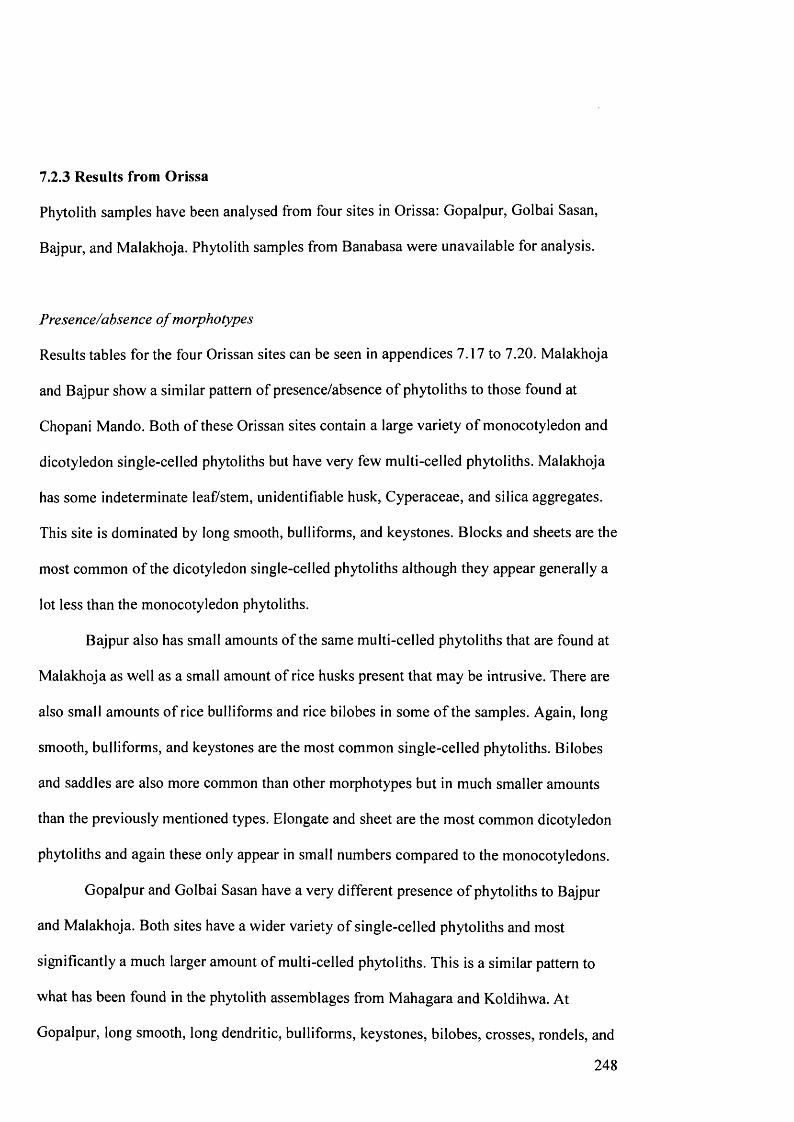
7.2.3 Results from Orissa
Phytolith samples have been analysed from four sites in Orissa: Gopalpur, Golbai Sasan,
Bajpur, and Malakhoja. Phytolith samples from Banabasa were unavailable for analysis.
Presence/absence o f morphotypes
Results tables for the four Orissan sites can be seen in appendices 7.17 to 7.20. Malakhoja
and Bajpur show a similar pattern of presence/absence of phytoliths to those found at
Chopani Mando. Both of these Orissan sites contain a large variety of monocotyledon and
dicotyledon single-celled phytoliths but have very few multi-celled phytoliths. Malakhoja
has some indeterminate leaf/stem, unidentifiable husk, Cyperaceae, and silica aggregates.
This site is dominated by long smooth, bulliforms, and keystones. Blocks and sheets are the
most common o f the dicotyledon single-celled phytoliths although they appear generally a
lot less than the monocotyledon phytoliths.
Bajpur also has small amounts of the same multi-celled phytoliths that are found at
Malakhoja as well as a small amount of rice husks present that may be intrusive. There are
also small amounts of rice bulliforms and rice bilobes in some o f the samples. Again, long
smooth, bulliforms, and keystones are the most common single-celled phytoliths. Bilobes
and saddles are also more common than other morphotypes but in much smaller amounts
than the previously mentioned types. Elongate and sheet are the most common dicotyledon
phytoliths and again these only appear in small numbers compared to the monocotyledons.
Gopalpur and Golbai Sasan have a very different presence of phytoliths to Bajpur
and Malakhoja. Both sites have a wider variety of single-celled phytoliths and most
significantly a much larger amount of multi-celled phytoliths. This is a similar pattern to
what has been found in the phytolith assemblages from Mahagara and Koldihwa. At
Gopalpur, long smooth, long dendritic, bulliforms, keystones, bilobes, crosses, rondels, and
248
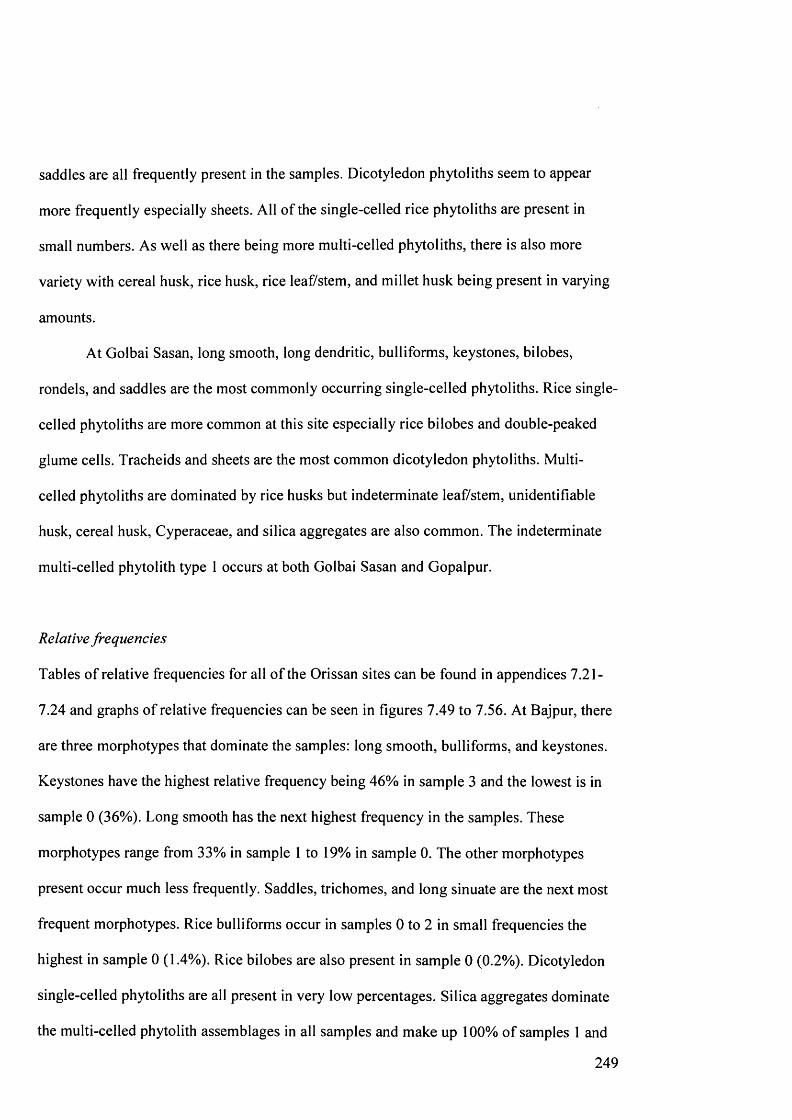
saddles are all frequently present in the samples. Dicotyledon phytoliths seem to appear
more frequently especially sheets. All of the single-celled rice phytoliths are present in
small numbers. As well as there being more multi-celled phytoliths, there is also more
variety with cereal husk, rice husk, rice leaf/stem, and millet husk being present in varying
amounts.
At Golbai Sasan, long smooth, long dendritic, bulliforms, keystones, bilobes,
rondels, and saddles are the most commonly occurring single-celled phytoliths. Rice single
celled phytoliths are more common at this site especially rice bilobes and double-peaked
glume cells. Tracheids and sheets are the most common dicotyledon phytoliths. Multi
celled phytoliths are dominated by rice husks but indeterminate leaf/stem, unidentifiable
husk, cereal husk, Cyperaceae, and silica aggregates are also common. The indeterminate
multi-celled phytolith type 1 occurs at both Golbai Sasan and Gopalpur.
Relative frequencies
Tables of relative frequencies for all of the Orissan sites can be found in appendices 7.21-
7.24 and graphs of relative frequencies can be seen in figures 7.49 to 7.56. At Bajpur, there
are three morphotypes that dominate the samples: long smooth, bulliforms, and keystones.
Keystones have the highest relative frequency being 46% in sample 3 and the lowest is in
sample 0 (36%). Long smooth has the next highest frequency in the samples. These
morphotypes range from 33% in sample 1 to 19% in sample 0. The other morphotypes
present occur much less frequently. Saddles, trichomes, and long sinuate are the next most
frequent morphotypes. Rice bulliforms occur in samples 0 to 2 in small frequencies the
highest in sample 0 (1.4%). Rice bilobes are also present in sample 0 (0.2%). Dicotyledon
single-celled phytoliths are all present in very low percentages. Silica aggregates dominate
the multi-celled phytolith assemblages in all samples and make up 100% of samples 1 and
249

4. Indeterminate leaf/stem is present in sample 0 and 2(11% and 13%). Unidentifiable
husk, Cyperaceae, and rice husk are only present in sample 0 in very small frequencies.
Long smooth, bulliforms, and keystones are again the morphotypes with the highest
frequencies in the samples from Malakhoja. Keystones have the highest frequency of 44%
in sample 4 and the lowest frequency for this type is in sample 9 (36%). Long smooth types
range from 33% (sample 1) to 23% (sample 4). Bulliforms range from 16% (sample 1) to
11% (sample 4). All of the other morphotypes have much lower frequencies. Long sinuate,
trichomes, saddles, and rondels are the next frequent morphotypes. Blocks are also
similarly occurring ranging from 5% in sample 4 to 0.8% in sample 1. No single-celled rice
phytoliths have been found. Again, silica aggregates are the most frequently occurring
multi-celled phytolith. Indeterminate leaf/stem occurs in sample 1 (25%) and 4 (4%).
Unidentifiable husk and Cyperaceae occur in small frequencies in sample 9. There are no
other multi-celled phytoliths including rice phytoliths.
At Gopalpur, keystones and long smooth have the highest frequencies in the
majority of samples. Keystones have high frequencies in sample 6, 12, and 14 (38%, 39%,
and 39%). The lowest value occurs in sample 2 (7%). Long smooth type has highest
frequencies in sample 2, 4, and 10 (34%, 35%, and 33%). In the rest of the samples, this
morphotype makes up between 20% and 30% of the assemblage except for in sample 13
(11%). After these types, bulliforms and bilobes are the most frequent in the samples.
Sample 8 has the highest frequency of bulliforms (21%) and sample 11 and 13 have the
highest frequencies of bilobes (19% and 23%). The other samples have between 11% and
20% frequencies for bulliforms except for sample 2, which has only 8%. Most of the other
samples have much lower frequencies of bilobes, the lowest being in sample 10 at 0.9%.
Long dendritic ranges from 9% to 0%. Rondels and saddles are the next frequent
morphotypes. Rondels range from 12% in sample 13 to 1% in sample 4. The highest
250
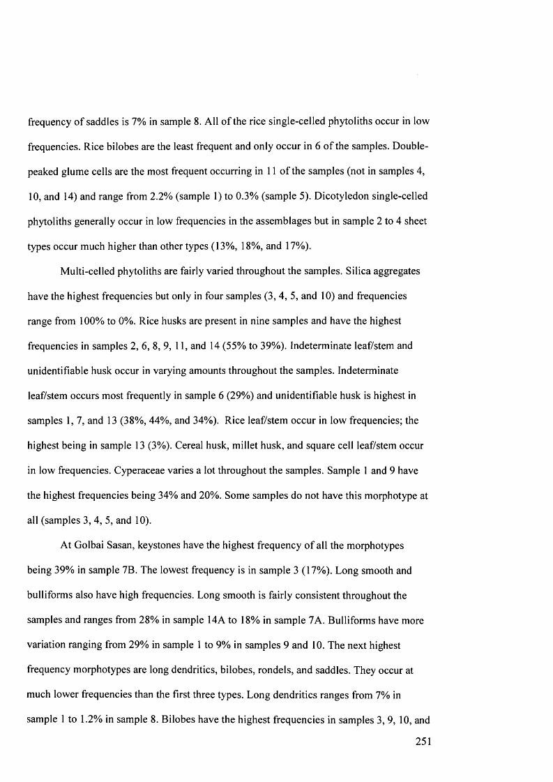
frequency of saddles is 7% in sample 8. All of the rice single-celled phytoliths occur in low
frequencies. Rice bilobes are the least frequent and only occur in 6 of the samples. Double
peaked glume cells are the most frequent occurring in 11 of the samples (not in samples 4,
10, and 14) and range from 2.2% (sample 1) to 0.3% (sample 5). Dicotyledon single-celled
phytoliths generally occur in low frequencies in the assemblages but in sample 2 to 4 sheet
types occur much higher than other types (13%, 18%, and 17%).
Multi-celled phytoliths are fairly varied throughout the samples. Silica aggregates
have the highest frequencies but only in four samples (3, 4, 5, and 10) and frequencies
range from 100% to 0%. Rice husks are present in nine samples and have the highest
frequencies in samples 2, 6, 8, 9, 11, and 14 (55% to 39%). Indeterminate leaf/stem and
unidentifiable husk occur in varying amounts throughout the samples. Indeterminate
leaf/stem occurs most frequently in sample 6 (29%) and unidentifiable husk is highest in
samples 1, 7, and 13 (38%, 44%, and 34%). Rice leaf/stem occur in low frequencies; the
highest being in sample 13 (3%). Cereal husk, millet husk, and square cell leaf/stem occur
in low frequencies. Cyperaceae varies a lot throughout the samples. Sample 1 and 9 have
the highest frequencies being 34% and 20%. Some samples do not have this morphotype at
all (samples 3, 4, 5, and 10).
At Golbai Sasan, keystones have the highest frequency of all the morphotypes
being 39% in sample 7B. The lowest frequency is in sample 3 (17%). Long smooth and
bulliforms also have high frequencies. Long smooth is fairly consistent throughout the
samples and ranges from 28% in sample 14A to 18% in sample 7A. Bulliforms have more
variation ranging from 29% in sample 1 to 9% in samples 9 and 10. The next highest
frequency morphotypes are long dendritics, bilobes, rondels, and saddles. They occur at
much lower frequencies than the first three types. Long dendritics ranges from 7% in
sample 1 to 1.2% in sample 8. Bilobes have the highest frequencies in samples 3, 9, 10, and
251
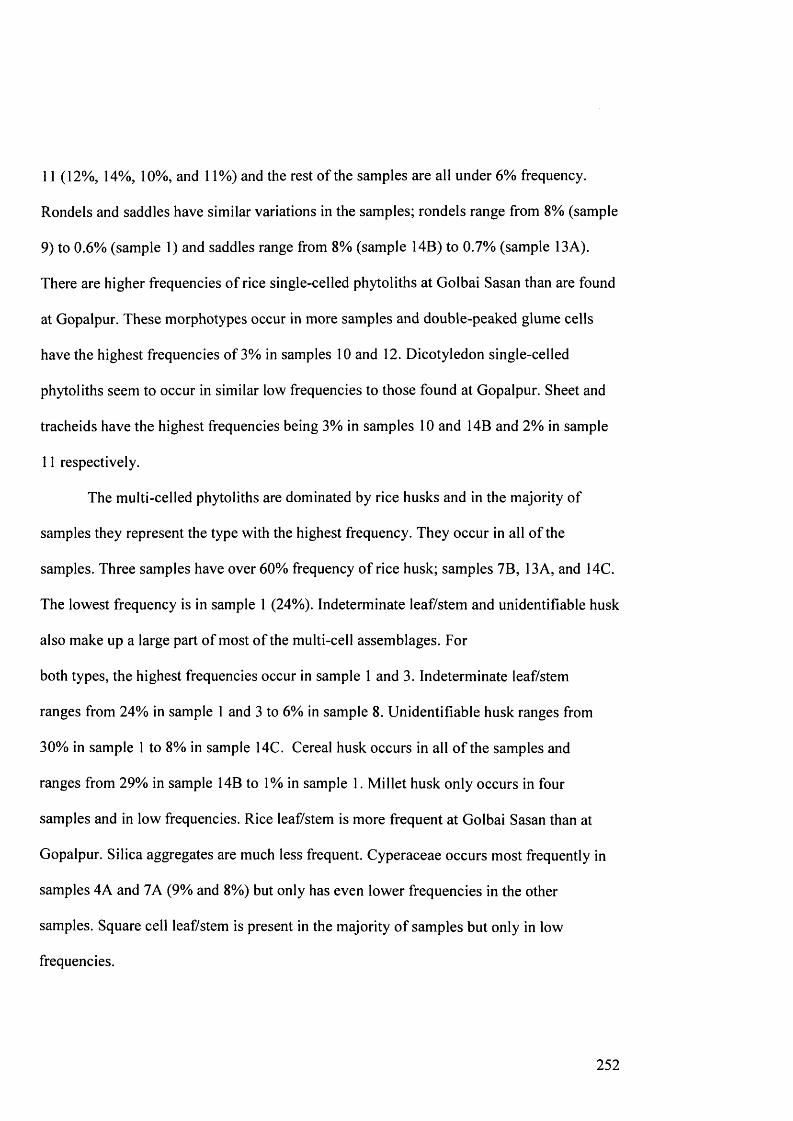
11 (12%, 14%, 10%, and 11%) and the rest of the samples are all under 6% frequency.
Rondels and saddles have similar variations in the samples; rondels range from 8% (sample
9) to 0.6% (sample 1) and saddles range from 8% (sample 14B) to 0.7% (sample 13A).
There are higher frequencies of rice single-celled phytoliths at Golbai Sasan than are found
at Gopalpur. These morphotypes occur in more samples and double-peaked glume cells
have the highest frequencies of 3% in samples 10 and 12. Dicotyledon single-celled
phytoliths seem to occur in similar low frequencies to those found at Gopalpur. Sheet and
tracheids have the highest frequencies being 3% in samples 10 and 14B and 2% in sample
11 respectively.
The multi-celled phytoliths are dominated by rice husks and in the majority of
samples they represent the type with the highest frequency. They occur in all of the
samples. Three samples have over 60% frequency of rice husk; samples 7B, 13 A, and 14C.
The lowest frequency is in sample 1 (24%). Indeterminate leaf/stem and unidentifiable husk
also make up a large part of most of the multi-cell assemblages. For
both types, the highest frequencies occur in sample 1 and 3. Indeterminate leaf/stem
ranges from 24% in sample 1 and 3 to 6% in sample 8. Unidentifiable husk ranges from
30% in sample 1 to 8% in sample 14C. Cereal husk occurs in all o f the samples and
ranges from 29% in sample 14B to 1% in sample 1. Millet husk only occurs in four
samples and in low frequencies. Rice leaf/stem is more frequent at Golbai Sasan than at
Gopalpur. Silica aggregates are much less frequent. Cyperaceae occurs most frequently in
samples 4A and 7A (9% and 8%) but only has even lower frequencies in the other
samples. Square cell leaf/stem is present in the majority of samples but only in low
frequencies.
252

Absolute densities
The total densities of phytoliths from Bajpur are fairly consistent from samples 0 to 3 but
there are a lot more phytoliths in sample 4 (see figure 7.57). Sample 4 has the highest
density of phytoliths (168,157). All of the samples are dominated by single-celled
phytoliths and multi-celled phytoliths are only present in very small densities (see figure
7.58). Sample 0 has the highest density of multi-celled phytoliths (128).
For the absolute densities of individual morphotypes from Bajpur, see figures 7.59
and 7.60. There are similar patterns with the absolute counts to those found with relative
frequencies however sample 4 demonstrates much larger densities for keystones,
bulliforms, and long smooth cells than the other samples. These morphotypes have 76,349,
25,256, and 42,384 phytoliths per gram of sediment. Sample 4 also has the highest densities
for saddles, elongates, and sheets types. The pattern for multi-cells with absolute densities
is again the same as with relative densities.
The total absolute density of phytoliths from Malakhoja is highest in sample 4
(79,373). See figures 7.61 and 7.62 for charts of the total absolute densities of phytoliths
from Malakhoja. The lowest density of total phytoliths is in sample 9. Again the majority of
the total densities are made up of single-celled phytoliths. Multi-celled phytoliths appear in
very low densities throughout all of the samples, which is a similar pattern to Bajpur. The
highest density was found in sample 4 (99) but sample 9 (89) was also much higher than
samples 1 and 7.
For the absolute densities of individual morphotypes from Malakhoja see figures
7.63 and 7.64. The absolute densities show similar patterns to those found with relative
frequencies although there is again more variation between the samples shown with
absolute densities. Keystones have the largest densities especially for sample 4, which has a
much larger density than the other samples. Sample 4 also has the largest density of
253

bulliforms, long smooth, saddles, and block phytoliths. Bulliforms and long smooth have
the next highest densities to keystones. Bulliforms range from 9326 in sample 4 to 1855 in
sample 9. Long smooth types have higher densities than bulliforms ranging from 18,6532
in sample 4 to 4039 in sample 9. The other single-celled morphotypes show a similar
pattern to that found with relative frequencies as do multi-celled phytoliths.
Charts of the total absolute densities of phytoliths from Gopalpur can be found in
figure 7.65 and 7.66. The highest density of phytoliths is found in sample 13 (245,417).
This is much larger than is found at Bajpur and Malakhoja. Sample 13 is much more dense
that the other samples from Gopalpur. The next highest density is in sample 9 (66,622).
Samples 11 and 6 also have fairly similar densities to sample 9 (59,372 and 49,871).
Samples 1 to 5 are particularly low in density compared to the rest of the samples. This
means that the bottom of the section has lower densities of phytoliths than the top. The
lowest density is in sample 1 (1579). At Gopalpur, multi-celled phytoliths are in much
higher densities than has been found at Bajpur and Malakhoja. The highest density of
multi-celled phytoliths is found in sample 13 (21,522). Samples 11,7, and 6 also have high
densities of multi-celled phytolith compared to the other samples although they are much
less than in sample 13 (5262, 4621, and 1965). The rest of the samples have much lower
densities of multi-celled phytoliths and the lowest density is in sample 14 (51).
The absolute densities for individual morphotypes can be found in figures 7.67 and
7.68. These values demonstrate different patterns to those found with relative frequencies.
Bilobes have the highest density overall, which is found in sample 13 (52,489). This is a
much larger figure than is found in the other samples. The lowest density for bilobes is 20
in sample 4. Sample 13 has the highest densities for the majority of morphotypes and they
are mostly much denser than the other samples. This is not the case for keystones where
sample 13 and sample 6 have similar densities (19,045 and 18,380). Generally, samples 1
254
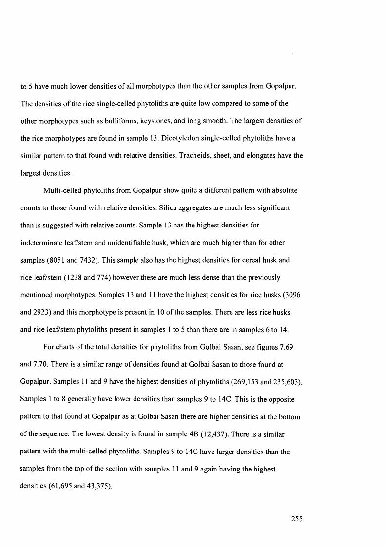
to 5 have much lower densities of all morphotypes than the other samples from Gopalpur.
The densities of the rice single-celled phytoliths are quite low compared to some of the
other morphotypes such as bulliforms, keystones, and long smooth. The largest densities of
the rice morphotypes are found in sample 13. Dicotyledon single-celled phytoliths have a
similar pattern to that found with relative densities. Tracheids, sheet, and elongates have the
largest densities.
Multi-celled phytoliths from Gopalpur show quite a different pattern with absolute
counts to those found with relative densities. Silica aggregates are much less significant
than is suggested with relative counts. Sample 13 has the highest densities for
indeterminate leaf/stem and unidentifiable husk, which are much higher than for other
samples (8051 and 7432). This sample also has the highest densities for cereal husk and
rice leaf/stem (1238 and 774) however these are much less dense than the previously
mentioned morphotypes. Samples 13 and 11 have the highest densities for rice husks (3096
and 2923) and this morphotype is present in 10 of the samples. There are less rice husks
and rice leaf/stem phytoliths present in samples 1 to 5 than there are in samples 6 to 14.
For charts o f the total densities for phytoliths from Golbai Sasan, see figures 7.69
and 7.70. There is a similar range of densities found at Golbai Sasan to those found at
Gopalpur. Samples 11 and 9 have the highest densities of phytoliths (269,153 and 235,603).
Samples 1 to 8 generally have lower densities than samples 9 to 14C. This is the opposite
pattern to that found at Gopalpur as at Golbai Sasan there are higher densities at the bottom
of the sequence. The lowest density is found in sample 4B (12,437). There is a similar
pattern with the multi-celled phytoliths. Samples 9 to 14C have larger densities than the
samples from the top of the section with samples 11 and 9 again having the highest
densities (61,695 and 43,375).
255
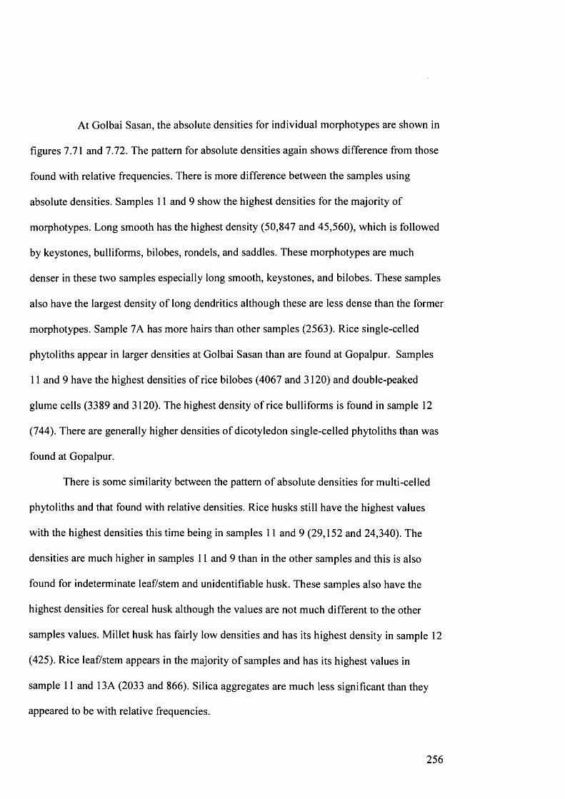
At Golbai Sasan, the absolute densities for individual morphotypes are shown in
figures 7.71 and 7.72. The pattern for absolute densities again shows difference from those
found with relative frequencies. There is more difference between the samples using
absolute densities. Samples 11 and 9 show the highest densities for the majority of
morphotypes. Long smooth has the highest density (50,847 and 45,560), which is followed
by keystones, bulliforms, bilobes, rondels, and saddles. These morphotypes are much
denser in these two samples especially long smooth, keystones, and bilobes. These samples
also have the largest density of long dendritics although these are less dense than the former
morphotypes. Sample 7 A has more hairs than other samples (2563). Rice single-celled
phytoliths appear in larger densities at Golbai Sasan than are found at Gopalpur. Samples
11 and 9 have the highest densities of rice bilobes (4067 and 3120) and double-peaked
glume cells (3389 and 3120). The highest density of rice bulliforms is found in sample 12
(744). There are generally higher densities of dicotyledon single-celled phytoliths than was
found at Gopalpur.
There is some similarity between the pattern o f absolute densities for multi-celled
phytoliths and that found with relative densities. Rice husks still have the highest values
with the highest densities this time being in samples 11 and 9 (29,152 and 24,340). The
densities are much higher in samples 11 and 9 than in the other samples and this is also
found for indeterminate leaf/stem and unidentifiable husk. These samples also have the
highest densities for cereal husk although the values are not much different to the other
samples values. Millet husk has fairly low densities and has its highest density in sample 12
(425). Rice leaf/stem appears in the majority of samples and has its highest values in
sample 11 and 13A (2033 and 866). Silica aggregates are much less significant than they
appeared to be with relative frequencies.
256

Grass families
Graphs of the differences in the grass subfamilies from the Orissan sites can be found in
figures 7.73 to 7.76. At Bajpur, chloridoid grasses are the most common having the highest
densities in samples 1 to 4. Panicoid and festucoid generally have much lower densities
although in sample 0 panicoid grasses have a slightly higher density to chloridoid grasses.
There is a similar pattern found at Malakhoja. Chloridoid grasses have the highest
densities in samples 1, 4, and 9. Sample 4 has the highest density, which is much higher
than the other grass subfamilies. Panicoid grasses have the lowest density in the majority of
samples. These first two sites seem to have a similar pattern to that found at Chopani-
Mando.
Gopalpur has a very different pattern to that found at Bajpur and Malakhoja but a
similar pattern to the mounded sites in the Belan River Valley. Panicoid grasses have the
highest densities in the majority of samples: 1-4, 7-11, and 13. Sample 13 has the highest
density of these grasses. Festucoid grasses have the highest densities in samples 6 and 12.
Sample 13 has the highest density of festucoid grasses overall although panicoid grasses are
the highest in this sample. Chloridoid grasses have the lowest densities throughout most of
the samples. There is a general rise in the grasses towards sample 13 and then they drop
sharply in sample 14.
Panicoid grasses are also dominant at Golbai Sasan. The largest densities are in
sample 9 and 11. Festucoid and chloridoid also have their highest densities in these
samples. Chloridoid is the largest value in sample 14A and 14B.
257

Comparing single-celled phytoliths using ratios
At Bajpur, the majority of single-celled phytoliths do not correlate well together. Long
smooth and long dendritic have no correlation (see figures 7.77). Bulliforms, keystones,
and trichomes correlate well and so do bilobes and crosses but all other combinations of
these morphotypes had very little or no correlation.
Long smooth and long dendritics correlate well at Malakhoja as well as bulliforms,
trichomes, and keystones (see figures 7.78). Bilobes, saddles, and rondels do not correlate
well with each other but seem to correlate with long smooth, long dendritics, keystones,
and bulliforms. Saddles have the most correlation with these morphotypes, then bilobes and
rondels only have some correlation.
Gopalpur and Golbai Sasan have very similar correlations of the single-celled
phytoliths (see figures 7.79 and 7.80). Generally, all the single-celled phytoliths that appear
frequently seem to correlate together very well at both of the sites. Long smooth and long
dendritics correlate well. Only bulliforms and keystones have slightly less correlation than
the others at Gopalpur.
Comparing plant parts using ratios
The lack of multi-celled phytoliths, especially cereal types, at Bajpur and Malakhoja mean
that there can be no comparisons of the multi-celled plant parts. This analysis will therefore
only be conducted on samples from Gopalpur and Golbai Sasan. The morphotypes used for
this analysis are rice bulliforms, double-peaked glume cells, rice bilobes, rice husks, rice
leaf/stem, indeterminate leaf/stem, unidentifiable husk, millet husk, and cereal husk. At
Gopalpur, the majority of these morphotypes correlate fairly well except for double-peaked
glume cell with rice bilobe, rice bulliform with rice bilobe, and rice leaf/stem with rice
bilobe (see figure 7.81). Millet husk also does not correlate with any of the other
258
morphotypes. This is the opposite pattern to that found with macro-remains where rice and
millet correlate well.
At Golbai Sasan, the same morphotypes have been used in this analysis and they
tend to correlate less well than at Gopalpur (see figure 7.82). The rice single-celled and
multi-celled phytoliths show mixed results. Double-peaked glume cells correlate well with
rice bilobes and rice husks but only have some correlation with the other types. Rice
bulliforms do not correlate with rice bilobes, rice husk, and rice leaf/stem. Rice husk
generally correlates well with all of the morphotypes except for rice bulliforms and millet
husk. Again, millet husk does not correlate well with any of the other morphotypes.
Indeterminate leaf/stem and unidentifiable husk correlate well together as well as with the
other morphotypes especially rice husk.
7.3 Comparisons of macro-remains and phytolith data
This section will draw together the analysis of the macro-remains and phytoliths and start to
make suggestions of general patterns in the dataset. Some attempt is made here to discuss
the weed ecology suggested by the plant material found at the mounded sites. Crop
processing is investigated and also more general patterns in the data are presented.
7.3.1 Weed ecology
There are not many weeds present in the macro-remain assemblages in this project and
many of them have been hard to identify to genus or species level. The weeds that are
present only occur in very small numbers. This lack of weeds may be due to the crop being
grown or exploited because rice is thought to have less weed infestation than other crop
plants (Thompson 1996) although this may only be true of more advanced wetland rice
cultivation systems. However, there were some recurring taxa and therefore some
259
implications can be made about the ecology of the possible cultivated fields or areas of
collection. A table of the weeds present is found in figure 7.83 with information about their
occurrence in the specific study areas and information about their habitat is presented
where genus or species is known. At Gopalpur and Golbai Sasan, there is a good
correlation between the rice grains and weeds present in the assemblages. Therefore, the
weeds present are likely to be associated with the rice crop. It is not as clear with the
assemblages from Mahagara and Koldihwa and this may be due to the poor preservation of
the macro-botanical material at these sites.
The majority of weeds present in both areas are known weeds of rice crops such as
Ischaemum rugosum, Commelina benghalensis, and Cyperaceae species. Other plants are
known to be found in disturbed places, which may also indicate that they are found in
agricultural fields. Another strong indicator throughout the weed assemblage is the
presence o f wet loving taxa. This suggests that the rice crop was grown in a wet
environment, which is what would be expected if the crops were to be grown in the local
environment of all of the sites. They are all riverine sites and therefore natural floodplains
exist close to the sites that are ideal for rice cultivation and would have probably held wild
rice populations as has been seen close to the sites today. This indicator of wet environment
is also true of the phytolith assemblages, which consistently contained Cyperaceae multi
celled panels. However, these were not particularly well correlated with the rice phytoliths
except for at Gopalpur (R2 = 0.8528) and therefore the majority of these remains may not
be rice weeds.
There are also a number of taxa that suggest dry conditions such as Tridex sp. and
these may relate to the other crop plants found at the sites, which could be cultivated in
drier conditions than the rice crop or come from another source such as being brought in by
260

animals. Some of the plants are common pasture plants and this may suggest their use as a
fodder plant as animals are present at all of the mounded sites.
The large grass found at Gopalpur, which has not been identified, is the only weed
to occur in fairly large numbers. The identification of this grass would help to suggest
where it may have come from and whether it was exploited as a fodder plant, whether it
was eaten by the people at this site, or it may just have been another weed of the rice crop.
7.3.2 Investigation of crop processing
Results of the analysis of crop processing activities is presented here along with some
interpretations although more discussion of these results and what they mean is included in
the next chapter especially suggestions on the social organisation of the sites.
Traditionally, macro-remains would be used to investigate the crop processing
activities on an archaeological site. However, it is clear in this project that preservation of
macro-remains is a problem especially at the Belan River Valley sites and therefore these
datasets can not be relied on for comparing plant parts. Little or no rice chaff is present at
the sites in this project and it can not be suggested accurately that this means that early
processing waste was definitely not present on the sites originally because of this
preservation issue. Therefore, phytolith analysis is being used here to overcome the
preservational biases of macro-botanical remains.
It is clear from the phytolith assemblages that leaf and stem parts of the rice plant
are present in the majority of samples, which is an indicator that some of this plant material
must have been brought on to the site. Earlier in this chapter correlations have been done
between the different rice phytolith parts. These had mixed results such as Koldihwa that
had some rice phytoliths that correlated well and others that did not. At Mahagara,
Gopalpur, and Golbai Sasan the rice phytoliths seem to have more correlation than has been
261
found at Koldihwa. This may be because the later site is made up of a number of different
periods, which may have differences in processing. The other sites are generally of one
period.
Further analysis can be done using ratios of leaf/stem to floral parts of the individual
samples, which may give more detail of change over time. Graphs of the ratios for rice
phytoliths comparing the leaf and floral parts are shown in figures 7.84 and 7.85. The lower
the ratio value, the more rice husk is present and therefore less early processing waste is
being brought on to the site. This analysis gives some interesting results for the sites and
does seem to show a change at Koldihwa. Mahagara generally shows quite high ratios with
most of the ratios being over 0.5. This means that there are more equal amounts of
leaf/stem and husk or even more leaf/stem than husk parts of rice. Koldihwa demonstrates
the same high ratios for the earlier levels at the site but there is a significant change in the
Chalcolithic phase to lower ratios. This is seen in both the sections that were sampled. At
Gopalpur and Golbai Sasan, there are generally low ratios being under 0.5. A few samples
at Gopalpur have higher values but these may just be specific to a type of context with high
leaf/stem parts. Further interpretations of these differences will be discussed in the next
chapter.
7.3.3 General patterns
There are some interesting patterns within the data set, which are shown in both the macro
remains and phytolith data. The first clear pattern is the difference between the types of
sites analysed in this project. There are a lack of seed remains and also charcoal at the sites
that have less occupation deposits: Chopani-Mando, Bajpur, Malakhoja, and Banabasa.
This pattern is also reflected in the phytolith assemblages as these sites have a lack of
multi-celled phytoliths and particularly lack evidence of crop plants such as rice and
262

millets. These sites also demonstrate low values of panicoid grass phytoliths, which
suggests less input of these grass types in to these sites potentially meaning less crop plants.
Some rice phytoliths have been found at Bajpur but are from the uppermost samples and
therefore may be intrusive. In contrast to these more ephemeral sites, the mounded sites
(Mahagara, Koldihwa, Gopalpur, Golbai Sasan) have a lot more seeds, charcoal, and
phytoliths including crop plants. These sites also have consistently high numbers of
panicoid grass phytoliths. There are large amounts of multi-celled phytoliths at these
mounded sites, which shows a significant difference to the remains found at the ephemeral
sites.
A comparison of the data from macroscopic analysis and phytolith analysis
demonstrates a number of similar patterns in terms of the economic plants. This can only be
done for the mounded sites because these are the only sites to have large quantities of this
material. At most of the sites, there is a great deal of similarity between the macro-remains
data and what is found in the phytolith assemblages. A good example of this can be seen at
Golbai Sasan, where the samples with the largest amounts of rice grains (especially samples
9 and 11) also have the largest densities of rice phytoliths (see figure 7.86). This is also
apparent at Gopalpur, where the dominance of pulse seeds at the bottom of the section is
reflected in the lack of rice phytoliths and also generally less phytoliths in these sample
overall (see figure 7.87). In samples that have larger amounts of rice grains there are
generally higher densities of rice phytoliths at Gopalpur. At Mahagara, there is also a
similar pattern of occurrence throughout the section of macro-remains and phytoliths
although the densities do not correspond as well as at some of the other sites (see figure
7.88). At Koldihwa, the comparisons are slightly less convincing, which may be due to the
lack of macro-remains at this site, although the phytoliths do show the same pattern of
263

increasing density towards the top of the sequences. Section Z 1 shows this more than
section Y1 (see figure 7.89 and 7.90).
The next chapter draws together all o f these results to explore implications about the
overall agricultural development and systems employed by these prehistoric peoples. There
will also be more discussion about the social implications of this data in terms of crop
processing and its effects on labour organisation and settlement patterns. There will also be
comparison of this data with other datasets from India and suggestions will be made as to
how these areas fit into the world view of agricultural development.
264
Chapter 8
Interpreting, evaluating data, and concluding remarks
This chapter will bring together all of the issues discussed in this thesis and interpret the
data presented in the previous chapter using them. The key issues for this study are what
plants are being exploited on these prehistoric sites and are they indigenous crops or
introduced from elsewhere. What can the new plant remains tell us about whether these
people were sedentary for the whole year or whether the sites were only used in certain
seasons. The social organisation of these sites will also be discussed in terms of crop
processing activities. The new dataset will be combined with other Indian data to give an
insight in to the sub-continent as a whole and how it fits in to the world views of
agricultural development.
8.1 Economic patterns
8.1.1 Sites in the Belan River Valley, Uttar Pradesh
Chopani-Mando
The density of macro-remains from all of the sites in the Belan River Valley is
disappointing but does illustrate some interesting patterns. Chopani-Mando is devoid of any
agricultural remains either macro-remains or phytoliths and only possesses very few
remains at all. This is in part due to poor preservation and sample size, which is also seen at
Mahagara and Koldihwa in the macro-remains. However, the phytoliths are not subject to
these same problems and therefore the lack of organic input in to this site has to be caused
by another factor as well as preservation and sample size. This means that it is likely there
was very little or no substantial input of plant material and particularly agricultural crops in
to this site. Hence, the people at Chopani-mando were not relying on cultivation or
collecting large quantities of rice for their subsistence as has been suggested previously
from rare finds of rice in pottery. Palmae phytoliths are present throughout the sampled
section although only in small amounts and this may suggest the exploitation of some palm
species (e.g for hut construction) but this could also be naturally occurring on the site. The
phytolith morphotypes present also suggest a dominance of leafy types and this lack of
inflorescence types may suggest that this site was occupied at the time of year when there
are few flowering plants such as in the dry season. However, this could also mean that they
were consciously not selecting for inflorescences and therefore not using large amounts of
grasses. Diatoms are also present in the samples and indicates some input from the adjacent
meander channel. This may mean that there was seasonal flooding of the site during the
monsoon season and again suggests that the site may have only been occupied in the dry
season. The severe lack of organic remains suggests this site was occupied for short periods
of time allowing any deposited organic material to erode and therefore no continual build
up of material was possible. Other evidence from the site also points to non-permanence
with little evidence of structures in the later levels and no burials as has been found at
similar period sites like those in the middle Ganga Plain.
Mahagara
Mahagara and Koldihwa show considerable differences to Chopani-Mando in their
macro-remain and phytolith assemblages. The density o f macro-remains is higher at
Mahagara and Koldihwa. There are also more multi-celled phytoliths present at these sites
as well as higher densities of a larger variety of single-celled phytoliths. These sites show a
dominance of panicoid grasses, which include crop plants such as rice and millets. The
presence of crop plants as grains and phytoliths is the most important difference from
266

Chopani-Mando and demonstrates deliberate substantial input of organic remains in to the
two mounded sites. The presence of rice as the dominant crop is clear at both of these sites.
Rice is present from the beginning of the deposits at Mahagara. Rice phytoliths only appear
in small numbers in levels 17 and 15 but become much more prevalent from level 13 to 7.
Rice grains are present consistently from level 17 up to level 6. Multi-celled and single
celled rice phytoliths are present rarely at first but become more common in the middle of
the section. This suggests this crop was the first to be exploited whether this was collecting
of wild stands or cultivation.
Using the phytolith assemblage, some inferences can be made about the crop
processing activities at Mahagara and therefore some aspects of social organisation. There
are not enough macro-remains to conduct this sort of analysis properly but if these were the
only remains that were analysed at Mahagara it might be suggested that the rice grains was
being processed off site or even traded in to the site. From the phytolith remains, it is
apparent that there are leaf and stem parts of rice throughout the sampled section. Samples
2 and 3 are excluded because they have a different composition to the rest of the samples
and therefore suggest a higher density of the later processing waste. The majority of
samples from Mahagara demonstrate good correlation between all of the different rice
phytoliths suggesting that they were brought on to the site together. This is also apparent
from the rice leaf/stem to rice husk ratios, which suggest there are equk) amounts of both\
plant parts. Hence, inferences can be made that the rice was harvested by removing the
stem as well as the panicles, which could be from uprooting or by using a sickle, although
sickles have not been found at this site but some of the microliths found may have been
used for this task. The whole of the rice plant was brought on to the site for processing.
This is not surprising because the stem can be as useful as the rice grain. This further
suggests that routine processing included basic threshing and dehusking. It can be taken
267
that the people of Mahagara were processing their crops on a more individual basis
probably in smaller groups because none of the processing occurred in the field at the time
of harvest.
From level 16 at Mahagara, other crops are introduced and this is an interesting
development because it includes barley and lentils, which are not native Indian crops.
Although, it may be the case that in level 17 the sample size is too small to recover these
introduced crops. However, this could also demonstrate a development in the agriculture of
the site as has been demonstrated at Senuwar and Lahuradewa, i.e. certain cultivation of
domesticates. It probably does suggest a move from one cropping season to two and also a
more extensive agricultural system growing a number of different crops in the same season.
In these early levels there is no clear evidence of structures and it is not until the middle of
the section that there are a number of house plans present. The archaeobotanical evidence
does suggest more organic input in to the site in the middle of the section, which seems to
coincide with this intensification of settlement. This could be an indication of the shift to
year round occupation and possibly an increase in the agricultural production.
The winter crops, however, do not represent a large part of the archaeobotanical
assemblage. There are no phytoliths of barley or wheat and this suggests that preservation
and sample size were not the only issue for the lack of evidence for these crops on the site.
They never appear to become very well established compared to rice, which can be seen in
the macro-remains and the phytoliths. This pattern could also suggest that there was a
different process happening to the winter crops and particularly wheat and barley. This
could include processing off site or even trading in of these crops in a cleaned state,
therefore little or no input of waste products on the site. It is clear that the processing of
wheat and barley was not a daily activity on the site as was the processing of rice plants.
268
The phytolith analysis demonstrates that there were probably a number of different
sources of plant material coming on to the site. It has been identified above that cultivation
was one of these sources and this must have contributed a large amount of phytolith
remains including the rice morphotypes but also more general morphotypes such as bilobes,
long dendritics, and some of the leafy types. The millet phytoliths identified at Mahagara
do not correlate well with the rice phytoliths and this suggests they came from a different
source therefore millets could be a separate crop and not a weed of the rice crop. This is
also suggested by the macro-remains, which identifies some o f the millets as Setaria
verticillata. This has been demonstrated as an early crop in South India (Fuller 1999,
2002a, Fuller et al. 2004). The fact that most of the single-celled morphotypes do not
correlate may suggest a number of sources other than cultivation such as wild collecting,
and also the use of dicotyledons, and therefore the use of trees for wood or other domestic
purposes. Palmae phytoliths were also present and may suggest another exploited resource
but not necessarily for food. It was clear during the analysis that there were a wide variety
in the keystone forms and some of these were from reeds, which would be expected on a
riverine site and could have also been used for thatching, matting, or basketry.
Koldihwa
There are similar crops present at Koldihwa to those found at Mahagara. Rice, barley,
wheat, and pulses are found in the Neolithic phase and most of these are found in the
earliest Neolithic deposits. These crops are present throughout the deposits sampled at
Koldihwa. Again, the densities for macro-remains are small but there seems to be a general
increase in density going up the sequence both for macro-remains and phytoliths therefore
moving from the Neolithic to the Chalcolithic phase. Other phytoliths increase going up the
sections coinciding with the crop plants such as bilobes, which may suggest they were from
269

the rice plant or from a weed of the crop. Wheat, barley, and winter pulses are only a very
small component of the assemblage. There are also no phytolith remains of wheat and
barley, which is the same pattern that is found at Mahagara.
This increase in density could be the result of more year round settlement on the site
and therefore increased agricultural input. The previous Neolithic period could therefore
indicate seasonal habitation maybe to coincide with rice harvesting whether this is of wild
rice or cultivated rice, although winter crops are also found in this phase. The shallow depth
of the habitational deposits at this site also suggests a less permanent settlement to that seen
at Mahagara. There are only two thin layers of the Neolithic phase at Koldihwa compared
to the whole of approximately 3 metres of deposits at Mahagara.
With this change in density of plant remains there seems to be an accompanying
shift of crop processing strategy. The Neolithic phase has more rice leaf phytoliths present
and the rice phytolith ratio is higher for the samples in this period. This demonstrates that
the whole of the rice plant is being brought on to the site and suggests a more individual
economic strategy because processing is being done at the site in the domestic environment.
In the Chalcolithic period there is a large increase in the presence of rice husk on the site
and this suggests a shift from the individual processing in the Neolithic to a more
communal strategy in which early stages are conducted off-site, or they shifted to being
consumers. There are problems with separating these two strategies because of equifinality
of their patterns but at this site because of the earlier signs o f on-site processing a shift to
off-site processing is more likely.
The phytolith assemblage at Koldihwa again suggests a number of different plant
sources. Cultivation is probably the predominant source with correlations between the
different rice phytoliths, long smooth and long dendritics, and also morphtypes such as
bilobes. There is a similar amount of correlation between the phytoliths as has been found
270

at Mahagara. There seems to be more dicotyledon phytoliths present at Koldihwa and also
silica aggregates, which can suggest the presence of bark. This may therefore suggest more
use of wood as fuel or for other purposes. The keystone phytoliths were observed to be
variable as has been found at Mahagara, which suggests a number of different sources such
as reeds and other wetland plants. Palmae phytoliths are present sporadically throughout the
samples but suggests another resource that could have been exploited. Cyperaceae
phytoliths were highest in the lower parts of both sections and therefore show an opposite
pattern to the crop plants so are probably not weed crops. These may have occurred
naturally at the site or could have been brought to the site for a specific purpose such as
fodder.
8.1.2 Sites in Orissa
Bajpur, Banabasa, and Malakhoja
As has been found in the Belan River Valley, there are two types of sites in Orissa. The
mounded and later sites of Gopalpur and Golbai Sasan, which show deep archaeological
accumulations and are rich in agricultural remains. The other type of site is the more
ephemeral sites that are likely to be earlier in date and probably not permanently occupied.
These sites (Bajpur, Banabasa, and Malakhoja) are much like Chopani-Mando because the
archaeobotanical samples that were taken have produced very little or no plant remains. It
was hoped though that even if there were no macro-remains that some evidence could be
gained from phytolith analysis. There are phytoliths present in all o f the samples taken,
however, when these are compared to the mounded sites there is a stark contrast in the
morphotypes present. There is less variation in the single-celled phytoliths especially those
that may indicate agricultural plants such as bilobes and single celled rice phytoliths. There
are also very few multi-celled phytoliths, which indicates that there was a less deliberate
271

input of organic matter in to these deposits or the use of plants that do not produce
substantial amounts of phytoliths and are also not likely to be preserved as macro-remains.
Even though this appears to be a disappointing outcome, there are conclusions that
can be drawn from these sites. There obviously was human activity during the Mesolithic
and Neolithic periods in Orissa as these are not the only sites present in the state (Mohanta
2002). However, this activity was obviously very different to what can be seen in the
coastal mounded sites, which are predominantly Chalcolithic in date. This means that these
sites are likely not to be permanent as there is no substantial build up of depositional
material and also they were probably used for different purposes such as specialised lithic
production. Consequently, other places need to be investigated to discover more
habitational deposits for these earlier periods. This may include locating new sites and also
investigating cave sites (Pradhan 2000), which may have early Neolithic deposits.
Gopalpur
The preservation of macro-botanical remains at Gopalpur and at Golbai Sasan is much
better than has been seen at the Belan Valley sites. Both sites have rice and summer pulses
present but the main difference from the Belan River Valley is that there are no winter
crops present on either site. This is probably due to the extremely high rainfall regime in
Orissa and therefore this area is better suited to monsoon crops. This may also suggest that
there was little or no contact between these groups in Orissa and those further to the north
such as Chirand, which has winter crops present.
At Gopalpur there is evidence of a number of crops both as phytoliths and macro
remains. Rice is present throughout the sampled section and appears to be an important part
of the economy at this site. There are also a number of summer pulse crops present.
Horsegram and pigeonpea are both present at Gopalpur although horsegram is much more
272
prominent especially in the earlier levels. This may be due to the difference in processing
between these two species, which disadvantages the survival of pigeonpea.
There seems to be two phases at the site that can be defined using the
archaeobotanical remains. The bottom of the section, therefore the earliest levels, are
dominated by the pulse crops although they do also contain rice. From level 6 upwards,
pulses decline and there is an increase in the rice grains present and also this is where rice
phytoliths start to appear more frequently in the samples. Small millets also appear in larger
densities in level 6 and 8 corresponding with the increase in rice grains, which is also
highest in these levels therefore the macro-remains correlate well. The millet husk
phytoliths do not correlate with the rice phytoliths and therefore this might suggest millet
was a minor crop rather than a weed of the rice crop. Gopalpur, therefore, shows a shift
from pulses as the dominant crop at the bottom of the sequence to rice, which dominates
from the middle of the sequence to the top. Phytolith densities increase going up the
sequence and this makes sense because more phytoliths will be produced by rice processing
than by the processing of pulse crops. This demonstrates that these phytoliths are
predominantly from grasses relating to rice crop most of which are panicoid type.
The majority of samples at Gopalpur suggest a communal strategy for rice
processing with limited parts of early stages represented by leaf/stem phytoliths, indicating
that these early stages of processing were carried out off site, e.g. at the time of the harvest.
Sample 14 and 5 do not fit this pattern and this could result from the specific context that
they come from. Both of these samples are hard to compare to the others because they only
contain rice bulliforms but did have rice grains so may in fact give a similar outcome if
macro-remains and phytoliths are compared. The shift in crop dominance from the bottom
to the top does not seem to affect the processing strategy of the rice crop.
273

The phytolith morphotypes generally correlate well at Gopalpur. This suggests that
they had a similar source. It is obvious that a large amount of the plant material is related to
the rice crop. However, there are suggestions of other plant materials such as woody plants
from silica aggregates and dicotyledon morphotypes. Palm phytoliths occur in small
amounts but this still suggests some exploitation of these plants especially in the later
periods of occupation.
Golbai Sasan
Golbai Sasan has similar plant remains to those found at Gopalpur with the addition of
Vigna radiata and Vigna mungo as another pulse crop. Rice is denser at Golbai Sasan than
at Gopalpur but pulses also play an important role in the economy of this site. Generally all
of the plant types are present throughout the sampled section and there are only changes in
the density of the remains. The middle of the sequence (samples 12 to 9) has the highest
density of material especially sample 9, which has the largest amount of rice grains and
small millets. These samples from the middle of the section contain the majority of rice
phytoliths. Above and below these samples there are fewer macro-remains and phytoliths
apart from sample 3, which contained large amounts of pulses particularly Vigna sp. This
demonstrates that the largest amount of organic input and therefore presumably the densest
occupation may have occurred in this phase of the site. However, the stratigraphy at this
site may be spurious because the new dates on the archaeobotanical material suggest a very
short period of occupation. This is unlikely because of the large accumulation of material at
this site measuring as much as 6 metres. The material taken for samples in this project
could therefore be from material that has washed down the slope and is therefore intrusive
from the later deposits. It is hard to suggest if this is true or not and only with further dating
will this matter be resolved. It will be assumed at present that the material is not slope wash
274

because the stratigraphy looked definite but a note o f caution is put on any interpretations
made here.
The rice phytolith ratios at Golbai Sasan are similar to Gopalpur. All of the samples,
apart from sample 7A that has a slightly higher ratio, have low ratios indicating later stages
o f processing waste only. This means that mainly the rice spikelets were brought on to the
site, and that the straw was separated either when harvesting or by processing in the field.
This can be suggested to indicate more communal labour mobilisation at harvest time with
the initial stages of processing such as threshing and winnowing happening off-site.
Phytolith morphotypes generally correlate well, as at Gopalpur. This again suggests
that the plant remains are from similar sources. Cultivation is probably the main source of
the plant material although there is evidence of woody plants and palms. There is more
support for millets as a separate crop as the millet macro-remains and phytoliths do not
correlate with rice and therefore suggest separate pathways on to the site.
8.2 Implications for the development of agricultural societies in Northern and Eastern
India
8.2.1 Belan River Valley
In terms of the development of agricultural societies, this new data goes some of the way to
address the important issues in Northern and Eastern India. The sites of Chopani-Mando,
Koldihwa, and Mahagara have been previously thought to show a transition from wild rice
cultivation to domestic rice agriculture. This is not an accurate interpretation of these sites.
To start with the dating o f Chopani-Mando is still an issue and the lack o f archaeobotanical
remains found in this project has not allowed new dating, which is needed to make further
interpretation about the chronology. If we are to believe the previous date of ca. 3500 BC
then there is a considerable time gap between Chopani-Mando and the later mounded sites
275

of Koldihwa and Mahagara. This does not suggest a continuation of the tradition or a
transfer of information. It has also been proposed earlier that the crude pottery found at
Chopani-Mando is not related to the pottery found at the later sites. Again this demonstrates
that there is unlikely to have been contact between these two cultures or direct continuity
between these two phases. The new samples taken from Chopani-Mando suggest that this
was a seasonally occupied site and therefore no substantial build up of organic material
occurred. Hence, there is no evidence for wild rice cultivation or even substantial
exploitation o f wild stands at this site. It is also proposed here that Chopani-Mando is not a
similar site to Damdama and Sarai-Nahar-Rai, as has been previously suggested (Sharma et
al. 1980a), because the remains are different and much less suggestive o f any permanent
settlement at the former site.
The beginning levels of a number of sites in the Ganges plain suggest an embryonic
‘Neolithic’ society. The earliest levels of these sites are likely to be seasonally occupied
and do not have evidence of a fully developed agricultural system. This is demonstrated at
Lahuradewa and Senuwar where the beginning of the occupation has less structural
evidence and only rice present (with some weed seeds too). This may mean that at this
point wild rice was being harvested and may not have been managed by these groups or
some cultivation as part of a system of seasonal mobility. Mahagara may well have a
similar beginning to these sites as there is no clear structural evidence until the middle
levels of the site and the plant remains suggest rice exploitation from the very beginning
although other crops do appear slightly later. The dating from Mahagara suggests that this
site began later than Lahuradewa and Senuwar. This time lapse could result from the slow
spread of this culture eastwards and south.
The most apparent and significant change that can be seen through the present
evidence is the development of permanently settled agricultural societies in this region.
276
This seems to occur in the later ‘Neolithic’ when a year round crop package is established
and this introduction of winter crops play a key role in the development of a more settled
lifestyle. This is the second phase at a number of sites (Lahuradewa, Senuwar, and
Mahagara) but a large number of sites in Northern India seem to emerge at this particular
time. The majority of these sites continue to develop with the addition o f copper and new
pottery wares therefore demonstrating a continuation from a developed ‘Neolithic’ culture
to a ‘Chalcolithic’ phase with much of the same elements persisting.
The winter crops must have travelled across from Northwest India as they have
been found at Mehrgarh in Baluchistan by ca. 6000-7000 BC. It seems more likely that
there was a piecemeal diffusion of these crops in the Ganges Valley rather than the
migration of groups in to the area with these crops as has been previously suggested by
some scholars (Saraswat 2004). At Lahuradewa (IB - from about 2500 BC), some pottery
forms of Harappan inspiration, such as dish-on-stand, have been found indicating culinary
diffusion. However, these forms do not seem to be present at Mahagara. This may suggest
that Mahagara just took on the plants from an indeterminate cultural group and not any
pottery forms or could suggest that winter crops were not an important parts of the diet, as
has been indicated by the new archaeobotanical data, and therefore there was no need for
the adoption of new pottery forms.
At Koldihwa, the Neolithic phase starts with summer and winter crops but does not
seem to be a fully permanent site because the archaeobotanical material is not particularly
dense and there are no substantial structural elements. Therefore in this phase the people
used the site seasonally. It is not until the Chalcolithic that the archaeobotanical remains
increase suggesting more organic input and year round occupation is more likely to occur
during this phase.
277

There also seems to be a shift in strategy from the Neolithic to the Chalcolithic. The
deposits at Mahagara and also the Neolithic deposits at Koldihwa suggest a more focused
processing strategy where the whole of the crop is brought on to the site for storage with
routine processing by small scale groups. This is in contrast to the Chalcolithic phase at
Koldihwa that has a more communal emphasis and therefore an absence or few remains of
early processing waste. This indicates a significant change in social organisation. This
coincides with the establishment of a more permanent settlement at Koldihwa and may
mean that the increased labour of a year round agricultural regime needs more co-operation
and therefore more communal effort. Although at Mahagara, this change to more
permanent settlement in the middle of the site is not accompanied with a shift in processing
strategy. This may mean that this is a difference between ‘Neolithic’ groups and
‘Chalcolithic’ groups or could suggest that this was a choice made by the people of
Koldihwa, which may have coincided with an intensification of their agricultural economy.
At present, it can not be assumed that there is the same pattern for other similar sites in the
Ganges Valley as much more archaeobotanical work is needed before this can be
confirmed.
Both of these sites have faunal evidence including domestic cattle, domestic
sheep/goat, equids (only at MGR), antelope, wild boar, tortoise and also fish. There is also
the evidence from Mahagara of cattle hoof-prints from a feature interpreted as a cattle pen
by the excavators. Hence, the prehistoric people were engaging in a complex economic
system including cultivating plants, rearing animals, hunting wild animals, and fishing.
This may have involved the seasonal movement of some groups, such as at Koldihwa, and
eventually led to the establishment of settled communities with the introduction of a more
complex year round agricultural system with indigenous and introduced elements.
278

8.2.2 Orissa
The evidence produced in this project from Orissa has started to address questions of the
development of agricultural communities and suggestions can now be made as to how this
region of India fits in to the prehistory of the sub-continent. At this point it seems that
Orissa was behind in agricultural terms to the people of the Ganges Valley. The Neolithic
sites sampled in this project provide no indications of agriculture although this may be the
result of the use of the sites for more specialised activities rather than domestic purposes.
However, the sites in northern and central Orissa do appear to be seasonally occupied
because of their lack of substantial deposits much like Chopani-Mando. This does suggest a
contrasting lifestyle to the later settled sites found in the coastal plain and therefore a
different economic strategy must have been in place. What this strategy was is open to
speculation at present and much more sampling of different sites and probably larger
sample sizes are needed to help recover some archaeobotanical remains from these earlier
sites. It could be suggested that these societies are mobile foragers, which do not exploit
grasses therefore they probably rely on forest resources or other non-grass staples such as
roots and tubers.
There is a huge contrast in the evidence found at the coastal mounded sites in
Orissa. Although, these sites are thought to have Neolithic deposits, it is unlikely that these
were sampled in this project because of their restricted area. In some ways, this is similar to
Mahagara where there is a lot less structural evidence in the early levels. However, the
majority of the deposits at the Orissan sites and those that have been sampled here are
Chalcolithic in date. This is reflected by the plant evidence found, which suggests
agriculture from the beginning of the sampled sections at Golbai Sasan and Gopalpur. Rice
and summer pulses dominate the deposits at both sites and are present in substantial
amounts to suggest that they were being cultivated. There is also faunal evidence from both
279
sites, which has been reported as domestic cattle, domestic sheep/goat, and wild animals
such as elephant, deer, bear, and antelope. There is further economic evidence in the form
of fish bones, which suggests river and sea fishing. All of this evidence suggests a complex
economic system of cultivated summer crops, the rearing of domestic animals, hunting wild
animals, and also fishing.
A communal processing strategy is suggested for the rice crop at these sites and
may be the result of a more intensive agricultural regime. There are no winter crops present
on these sites and therefore all of the agricultural work occurred in a restricted time of year
during the monsoon period although this does not mean that this was the only time labour
was needed because foraging, hunting, and fishing may have occupied the winter months.
However, the production of the rice crop and also pulse crops during the summer would
have put a lot of pressure on the labour force and may be the reason for communal co
operation and combined effort at this time of the year.
Another issue that must be considered at Golbai Sasan and Gopalpur is what would
have been used as a food plant source in the winter because all of the crops are produced in
the summer months. This suggests that storage of these crops would have been needed to
last the winter or may mean that there is another food source but it has not appeared in the
archaeobotanical record. There is evidence of storage jars at Gopalpur, which could have
been used to store cereals although no such jars have been found at Golbai Sasan. Possible
winter food sources are fruits, green vegetables, and roots and tubers, which can be
harvested throughout the winter months (Pratap 2000: 79-80). All of these plants are hard
to identify and rarely preserve archaeologically therefore it will be difficult to find evidence
of these possible resources.
The lack of winter crops is an interesting pattern. At the start of the project it was
expected that winter crops would be found in Orissa because they are found at Chirand in
280

Bihar to the north of Orissa and links have been made between the pottery wares of sites in
Orissa and Bihar. There could be a number of reasons for the winter crops not travelling
down to Orissa. There may not have been any contact between sites in Bihar and those in
Orissa. As has been seen in this project, there are not substantial Neolithic/ Chalcolithic
sites in Northern Orissa and this may have hindered the transportation of this crop package
to the Southern Orissan sites. The mountainous region of northern Orissa where different
economic regimes are likely to those in the south may have acted as a barrier preventing the
spread of these crops. Another reason may have been the climate in this region, which has
more rainfall, especially in the monsoon period, than is found in the Ganges Valley. This
means that there is less likely to be any problems with producing monsoon crops. Therefore
these prehistoric groups had no need to use winter crops. The spreading of agricultural
production throughout the year could be a risk-buffering strategy for the Vindhyan culture
sites in the Ganges Valley and those in Bihar (like Chirand).
The dominance of summer crops in Orissa is much like the evidence found in South
India, where pulses and millets dominate early farming sites. The pulses present are the
same as found in the Neolithic Ashmound Tradition sites (horsegram and Vigna radiata)
but have the differences of Vigna mungo and pigeonpea (Cajanus cajan). These pulses are
rare and late in South India. Vigna mungo and Vigna radiata are both present at Golbai
Sasan and horsegram is present at both the mounded sites. Vigna radiata and horsegram
could possibly be domesticated in this region but the true area of wild progenitors is still
rather unknown and therefore multiple regions could have first exploited these crops. This
may alternatively suggest that there was contact between the prehistoric Orissan people and
the groups from further South in India as there are larger areas containing the wild
progenitors on the Western Ghats (wild V radiata) and Peninsula in general (wild
281
horsegram). Vigna mungo is more likely to have been domesticated in the northern
Peninsula or western India and then spread eastwards.
An exciting discovery in Orissa is the presence of pigeonpea at Golbai Sasan and
Gopalpur. This is a likely domesticate from this region and is the first evidence from
prehistoric sites in this state. These sites are not within the modern day distribution of the
wild progenitor, although very close to it, and therefore this evidence suggests that these
must be cultivated crops whether domestic or wild. The earliest o f these pigeonpeas from
Gopalpur has been dated directly to 1395 Cal. BC. Pigeonpea is a later addition to South
Indian Late Neolithic sites such as Sanganakallu in the mid-second millennium BC (Fuller
2003a), where it dates to 1400-1300 BC, which again suggests that there may be contact
between Orissa and regions to the South.
The question of rice domestication in India is still in debate and this thesis has made
some strides towards concluding this matter. Rice has been found at all of the mounded
agricultural sites sampled and it was the predominant crop in both regions. This strengthens
the case for early rice exploitation and presumably cultivation although cannot resolve
conclusively whether the rice was wild or domestic. The methodological study of rice
identification methods has demonstrated that it is very difficult and probably impossible to
distinguish wild and domestic species of rice in the Sativa complex using only a few
characteristics even on modern reference material. This is only made more difficult when
trying to apply these methods to archaeological material and therefore the way that this
problem is approached needs to be rethought. The presence of small wild rice species and
ability to distinguish them from the Sativa complex is an interesting development. These
species could be used as food or may be weeds of the rice crop. It would be interesting to
look in future for when these species first appear and even disappear at sites.
282

It is quite clear that rice is being exploited throughout Northern and Eastern India in
the Neolithic and Chalcolithic periods. The density of material at these sites suggests
substantial harvesting and this could result just from wild procurement. However, the
introduction of other known cultivated plants such as wheat, barley, and pulses in to these
areas suggests a more developed economic strategy than gathering. This could still mean
that wild rice is being cultivated and managed, which probably did occur for a very long
time due to the potentially slow rate of evolution in rice populations, since rice more readily
cross-pollinates compared to Near Eastern cereals. The cultivation of wild rice in the same
habitat as wild stands would further prolong the genetic change to domestic species as well
as the harvesting methods used. With rice domestication, and probably all of the cross-
pollinating crop species such as some millets, it is better to try to identify when wild
cultivation began rather than the point of genetic domestication because there is likely to be
a large time gap between the two. This can be approached in a number of ways such as
looking in more detail at changes in weed floras, and also trying to look for changes from
immature to mature grains, which suggests changes in the shattering nature of the plant and
hence identifies the genetic change to domestication. Some of the archaeological rice grains
in this project are likely to be immature suggesting wild rice was being cultivated.
8.3 Pathways to agriculture and India as part of the world view
The evidence gathered in this project has made it clear that India is definitely very diverse
in terms of agricultural development. It needs to be thought of as an equally important area
to any other world regions and has a wealth of evidence to be studied. This makes it a very
interesting region to study and there are still many avenues of investigation to be studied.
The pathway towards agriculture that was taken by the prehistoric people in the
Belan River Valley can be further envisaged using the evidence in this project. Pottery
283

seems to be an early development in this area with evidence coming from Chopani-Mando
and also a number of other Mesolithic sites. The dating of this is still not clear but it was
definitely part of this earlier Mesolithic phase prior to the development of the Neolithic
culture in this region. The next developments are plant cultivation and animal herding that
seem to appear at about the same time at the beginning of the ‘Neolithic’ phase. At this
point, the communities are probably seasonally settled to coincide with the rice growing
season in the monsoon period. With more advances in the agricultural systems and
particularly the adoption of a double-cropping economy, these Neolithic people eventually
became fully settled in year-round villages.
It is still hard to form a complete picture of what is going on in Orissa because
much more work is needed. However, with the current evidence suggestions can be made
about the pathway towards agriculture in this region. The Mesolithic and Neolithic periods
in Orissa are still somewhat unknown and there has been a lack of new archaeobotanical
evidence found in this project. It has become clear that the Northern highland sites existed
on a different economic system and pottery was used at some of the sites. Therefore pottery
seems to be the first development towards agriculture at least at the lowland sites. The
Neolithic phases definitely seem to be mobile or semi-sedentary. There is still no evidence
for plant cultivation or animal herding in the Neolithic so this seems to first occur in the
Chalcolithic along with settled sites. There must be evidence in the Neolithic for the
beginnings of plant cultivation and also possibly animal herding as has been seen in the
Ganges Valley but more sampling is needed to confirm this.
What is clear from both areas is that there is evidence for local domestications such
as pigeonpea, other pulses such as Vigna mungo, and potentially rice even though these
might be fairly late in date compared to other areas of origin. There is also evidence for the
introduction of crops such as the Near Eastern crops, which seems to have been added to
284

the existing rice cultivation system in the Ganges Valley. These regions have presented
evidence for important agricultural developments in Indian prehistory.
8.4 Methodological issues and further work
The combination of macro-botanical and phytolith analysis worked well to address the
questions proposed in this project. Macro-botanical remains were generally readily
identifiable to at least genus level and did occur in reasonable amounts at the majority of
sites. There is, however, definitely a problem of preservation particularly at the sites in the
Belan River Valley. This may in the future be overcome to some extent by increasing the
size of bulk samples but it was quite clear that degradation of organic remains is more
prevalent at sites in India. This could be a result of the climatic regime, which fluctuates
between warm and wet conditions but could also result from other taphonomic issues such
as the crops used in these areas and also crop processing methods. It has been suggested by
Thompson (1996) that rice grains are less likely to be present on archaeological sites as it
does not come in to contact with fire as much as some other crops such as glume wheats.
However, this does not seem to play a role here because rice was consistently the most
prevalent macro-remain at all of the agricultural sites and appeared in fairly large numbers
at Golbai Sasan.
It is definitely beneficial to use phytolith analysis as well as macro-remains to
examine the development of agricultural societies in this region because it adds more
information to the debate. The small amount of macro-remains meant that detailed analysis
could not be relied on for examining crop processing stages. Therefore phytoliths were used
and this gave a good insight in to how strategies on each site were different and where there
were changes over time. It also allowed identification of other plants that were not seen in
the seed assemblage such as palms. However, there are problems that still need to be
285

resolved in phytolith analysis. The most important is problems of identification. The study
of rice identification methods has demonstrated that there are problems o f using phytoliths
to identify rice to species although they can be generally used to identify to genus level. It
would also be beneficial to work on identifying other crop plants more accurately such as
millets, pulses (although phytoliths are not found in great quantities in these plants), and
associated arable weeds. The addition of another analytical method such as starch analysis
will help to identify different plant types further and is something that should be attempted
in further work in this region.
The rice identification study, although being an important step forward, did bring
rather disappointing results. The difficulty of identifying domestic rice is frustrating
because being able to distinguish wild from domestic rice would add to the information
about early agricultural communities in India. It is clear now that this particular question
must be approached from a different angle. Studies looking at different basic cultivation
regimes, such as the wild cultivation of rice, wet rice agriculture, and dry rice agriculture
needs to be conducted to look at changes in agricultural systems. This can start to identify
signatures that can be used to identify different regimes in prehistory including changes in
weed flora and crop processing ratios. It is the beginning of cultivation that needs to be
identified and also changes in economic systems because these are associated with
fundamental changes in prehistoric society such as increased sedentism and the
restructuring of social organisation.
To gain further insight in to the social aspects of the early farming communities a
much more detailed sampling strategy would be needed and this could only be conducted if
full excavation took place. The mounded sites in Orissa would benefit from this, especially
Gopalpur, as no previous stratigraphic excavations have taken place and the mound is being
slowly taken over by rice paddies. The sampling of more sites in Orissa is needed to create
286

a better understanding of the economic systems in place throughout the diverse
environments in the state over different periods of time. Only with more detailed
environmental work will Orissa start to play a significant role in the prehistory of India as a
whole.
287
Bibliography
Agrawal, D. P., 1982a. The Indian Bronze Age cultures and their metal technology, in F
Wendorf and A. E. Close (eds.) Advances in World Archaeology, vol. 1. New York:
Academic Press, 213-264.
Agrawal, D. P., 1982b. The Archaeology o f India. London: Curzon Press.
Agrawal, D. P., 2002. The earliest agriculture and pottery in South Asia, in Y. Yasuda
(ed.) The Origins o f Pottery and Agriculture. New Dehli: Lustre Press, 81-88.
Ahn, S. M., 1993. Origin and differentiation o f domesticated rice in Asia: review o f
archaeological and botanical evidence. PhD dissertation, Institute of Archaeology,
University College London.
Albert, R. M. and S. Weiner, 2001. Study of phytoliths in prehistoric ash layers from
Kerbara and Tabun Caves using a quantitative approach, in J. D. Meunier and F.
Colin (eds.) Phytoliths: applications in earth sciences and human history.
Abingdon: AA Balkema, 251-266.
Alexander, J., 1978. Frontier studies and the earliest farmers in Europe, in D. Green, C.
Haselgrove, and M. Spriggs (eds.) Social organisation and settlement: contributions
from anthropology, archaeology and geography. Part 1. BAR International Series
47(i). Oxford: BAR, 13-29.
Alexander, J., 1980. The frontier in Prehistory, in J. V. S. Megaw (ed.) Hunter, Gatherers,
and First Farmers Beyond Europe. Leicester: Leicester University Press, 25-40.
Alexander, J., 1984. The end of the moving frontier in the Neolithic of North-Eastern
Africa, in L. Krzyzaniak and M. Kobusiewicz (eds.) Origin and early development
offood producing cultures in north-eastern Africa. Poznan: Polish Academy of
Sciences, 57-63.
288

Alexander, J., and A. A. Mohammed, 1980. Frontier Theory and the Neolithic period
Nubia, in J. Plumley (ed.) Nubian Studies. Cambridge.
Allchin, F. R., 1963. Neolithic cattle keepers o f South India: a case study o f the Deccan
Ashmounds. Cambridge: Cambridge University Press.
Allchin, B. and R. Allchin, 1974. Some new thoughts on Indian cattle, in J. E. van
Lohuizen-de Leeuw and J. N. Ubaghs (eds.) Some new thoughts on Indian cattle.
Leiden: E J Brill, 71-77.
Allchin, B. and R. Allchin, 1982. The rise o f civilisation in India and Pakistan.
Cambridge: Cambridge University Press.
Allchin, R. and B. Allchin, 1997. Origins o f a civilisation: the prehistory and early
archaeology o f South Asia. New Delhi: Penguin Books.
Ammerman, A. J., and L. L. Cavalli-Sforza, 1971. Measuring the rate of spread of early
farming in Europe. Man 6, 674.
Ammerman, A. J., and L. L. Cavalli-Sforza, 1973. A population model for the diffusion of
early farming in Europe, in C. Renfrew (ed.) The explanation o f cultural change.
London: Duckworth, 343-357.
Ammerman, A. J., and L. L. Cavalli-Sforza, 1984. The Neolithic transition and the genetics
o f populations in Europe. Princeton: Princeton University Press.
Anderson, M. K., 1997. From tillage to table: the indigenous cultivation of geophytes fro
food in California. Journal o f Ethnobiology 17/2, 149-169.
Arora, R. K. and S. S. Mauria, 1989. Vigna mungo (L.) Hepper, in L. J. G. van der Maeson
and S. Somaatmadja (eds.) Plant resources o f South-East Asia I. Pulses.
Wageningen: Pudoc, 70-77.
Arora, R. K., Chandel, K. P. S., and B. S. Joshi, 1973. Morphological diversity in
Phaeseolus sublobatus Roxb. Current Science 42, 359-361.
Babu, C. R., S. K. Sharma, S. R. Chatterjee, and Y. P. Abrol, 1988. Seed protein and amino
acid composition of wild Vigna radiata var. sublobata (Fabaceae) and two
cultigens, V. mungo and V radiata. Economic Botany 42, 54-61.
Bailey, R. C., 1990. Exciting opportunities in Tropical Rain Forests: a reply to Townsend.
American Anthropologist 92/3, 747-748.
Bailey, R. C., G. Head, M. Jenike, B. Owen, R. Rechtman, and E. Zechenter, 1989.
Hunting and gathering in tropical rain forests: is it possible? American
Anthropologist 91/1, 59-82.
Ball, T. B. and J. D. Brotherson, 1992. The effect of varying environmental conditions
on phytolith morphometries in two species of grass (Bouteloua curtipendual and
Panicum virgatum). Scanning Microscopy 6/4, 1163-1181.
Ball, T., J. D. Brotherson, and J. S. Gardner, 1993. A typologic and morphometric study
of variation in phytoliths from einkom wheat (Triticum monococcum). Canadian
Journal o f Botany 71,1182-1192.
Ball, T., J. S. Gardner, and J. D. Brotherson, 1996. Identifying phytoliths produced by
the inflorescence bracts of three species of wheat (Triticum monococcum L., T.
dicoccum Schrank., and T. aestivum L.) using computer-assisted image and
statistical analyses. Journal o f Archaeological Science 23, 619-632.
Ball, V., 1876. On stone implements found in the tributary states of Orissa. Proceedings o f
the Asiatic Society o f Bengal 1876, 120-121.
Barker, G., 2002. Transitions to farming and pastoralism in North Africa, in P. Bellwood
and C. Renfrew (eds.) Examining the farming/language dispersal hypothesis.
Oxford: Oxbow Books, 113-126.
Barrau, J., 1958. Subsistence agriculture in Melanesia. Hawaii: Bernice P Bishop
Museum.
Barrau, J., 1961. Subsistence agriculture in Polynesia and Micronesia. Hawaii: Bernice P
Bishop Museum.
Barrett, J. C., 1994. Fragments from Antiquity: an archaeology o f the social life in Britain
(2900-1200 BC). Oxford: Blackwell.
Barrett, J. C., 1999. Rethinking the Bronze Age environment, in K. J. Edwards and J. P.
Sadler (eds.) Holocene Environments o f Prehistoric Britain. Quaternary
Proceedings 7, 493-500.
Barton, H., 2005. The case for rainforest foragers: the starch record of Niah Cave,
Sarawak. Asian Perspectives 44/1, 56-72.
Baruch, U., 1994. The Late Quaternary pollen record of the Near East, in O. Bar-Yosef and
R. S. Kra (eds.) Late Quaternary chronology and palaeoclimates o f the Eastern
Mediterranean. Tucson: Radiocarbon, 103-119.
Baruch, U. and S. Bottema, 1991. Palynological evidence for climate change in the
Levant ca. 17,000- 9,000 B.P., in O. Bar-Yosef and F. Valla (eds.) The Natufian
culture in the Levant. Ann Arbor, Michigan: International Monographs in
Prehistory, 11-20.
Bar-Yosef, O. and R. H. Meadows, 1995. The origins of agriculture in the Near East, in
T. D. Price and A. B. Gebauer (eds.) Last Hunters, First Farmers: new perspectives
on the prehistoric transition to agriculture. Sante Fe: School of American Research
Press, 39-94.
Basa, K. K., 1994. Problems and Perspectives in Archaeology o f Orissa, India.
Bhubaneswar: DSA in Anthropology, Utkal University.
Basa, K. K., 1997. Archaeological Heritage, in P. K. Mishra (ed.) Comprehensive History
and Culture in Orissa. Volume 1. New Dehli: Kaveri Books.
291
Basa, K. K., 2000. History of Archaeology in Orissa, in K. K. Basa and P. Mohanty (eds.)
Archaeology o f Orissa. Delhi: Pratibha Prakashan, 16-61.
Basa, K. K., and P. Mohanty, 2000. Archaeology o f Orissa. Delhi: Pratibha Prakashan.
Basa, K. K., T. K. Das, and B. K. Mohanta, 2000. Neolithic Culture of Pallahara, Central
Orissa, in K. K. Basa and P. Mohanty (eds.) Archaeology o f Orissa. Delhi: Pratibha
Prakashan, 264-284.
Basu, S. K., and R. K. Chakraverty, 1994. A manual o f cultivated palms in India. Calcutta:
Botanical Survey of India.
Bates, D. M., and R. W. Robinson, 1995. Cucumbers, melons, and watermelons, in J.
Smartt and N. W. Simmonds (eds.) Evolution o f crop plants. Harlow: Longman
Scientific & Technical, 89-96.
Bates, D. M., L. C. Merrick, and R. W. Robinson, 1995. Minor curcurbits, in J. Smartt
and N. W. Simmonds (eds.) Evolution o f crop plants. Harlow: Longman Scientific
& Technical, 105-111.
Baxter, M., 2003. Statistics in Archaeology. London: Hodder Arnold.
Bedigan, D., 1998. Early history of sesame cultivation in the Near East and beyond, in A.
B. Damania, J. Valkoun, G. Willcox and C. O. Qualset (eds.,) The origins o f
agriculture and crop domestication. The Harlan Symposium. Aleppo, Syria:
ICARDA, 93-101.
Bedigan, D., 2000. Sesame, in K. F. Kiple and C. K. Ornelas-Kiple (eds.) The Cambridge
World history o f food, volume 1. New York: Cambridge University Press, 411-421.
Bedigan, D., 2003. Evolution of sesame revisited: domestication, diversity, and prospects.
Genetic resources and Crop Evolution 50, 779-787.
Bedigan, D. and J. R. Harlan, 1986. Evidence for cultivation of sesame in the ancient
world. Economic Botany 40, 137-154.

Bedigan, D., D. S. Seigler, and J. R. Harlan, 1985. Sesamin, sesamolin and the origin of
sesame. Biochemical Systematics and Ecology 13, 133-139.
Bedigan, D., C. A. Symth, and J. R. Harlan, 1986. Patterns o f morphological variation in
sesame. Economic Botany 40, 353-365.
Behera, P. K., 1991-1992. Sulabhdihi: a Neolithic celt manufacturing centre in Orissa.
Puratattva 22, 124-131.
Behera, P. K., 1992. The pebble tool component of the Bonaigarh Neolithic complex,
Orissa. Man and Environment XVIII/2, 57-63.
Behera, P. K., 2000. Neolithic culture complex of Bonaigarh, Orissa, in K. K. Basa and P.
Mohanty (eds.) Archaeology o f Orissa. Volume 1. New Dehli: Pratibha Prakashan,
222-263.
Behera, P. K., 2000-2001. Excavations at Khameswaripali - a proto Historic settlement in
the middle Mahanadi valley, Orissa: a preliminary report. Pragdhara 11, 13-34.
Behera, P. K., 2002. Khameswaripali: a protohistoric site in the middle Mahanadi Valley,
Orissa: results of first season’s (1996-97) excavation, in G. Sengupta and S. Panja
(eds.) Archaeology o f Eastern India: new perspectives, Kolkata: Jayasree Press,
487-514.
Bellwood, P., 1989. The colonisation of the Pacific: some current hypotheses, in A. V. S.
Hill and W. Serjeantson (eds.) The colonisation o f the Pacific: a genetic trail.
Oxford: Oxford University Press, 1-59.
Bellwood, P., 1991. The Austronesian dispersal and the origin of languages. Scientific
American 265/1, 88-93.
293

Bellwood, P., 1996 The origins and spread of agriculture in the Indo-Pacific region:
gradualism and diffusion or revolutions and colonization?, in D. R. Harris (ed.) The
origins and spread o f agriculture andpastoralism in Eurasia. London: UCL Press,
465-498.
Bellwood, P., 2001. Early agriculturalists population diasporas? Farming, languages, and
genes. Annual Review o f Anthropology 30, 181-207.
Bellwood, P., 2005. First Farmers: the origins o f agricultural societies. Oxford:
Blackwell Publishing.
Bellwood, P., R. Gillespie, G. B. Thompson, J. S. Vogel, I. W. Ardika, and I. Datan, 1992.
New dates for prehistoric Asian rice. Asian Perspectives 31/2, 161-170.
Bellwood, P. and C. Renfrew, 2002. Examining the farming/language dispersal
hypothesis. Oxford: Oxbow Books.
Bender, B., 1975. Farming in Prehistory - from hunter-gatherer to food-producer.
London: John Baker.
Bettinger, R. L., 1983. Comments, in E A Smith Anthropological approaches of optimal
foraging theory: a critical review. Current Anthropology 24/5, 640-641.
Bhat, K. V., P. P. Babrekar and S. Lakhanpaul, 1999. Study of genetic diversity in Indian
and exotic sesame (Sesamum indicum L.) germplasm using random amplified
polymorphic DNA (RAPD) markers. Euphytica 110, 21-33.
Blust, R., 1976. Autronesian culture history: some linguistic inferences and their relations
to the archaeological record. World Archaeology 8/1, 19-43.
Blust, R., 1984. The Austronesian homeland: a linguistic perspective. Asian Perspectives
26/1,45-67.
Boardman, S. and G. E. M. Jones, 1990. Experiments of the effects of charring on cereal
plant components. Journal o f Archaeological Science 17/1, 1-12.
294

Bogaard, A., 2002. Questioning the relevance of shifting cultivation to Neolithic Farming
in the loess belt of Europe: evidence from the Hambach Forest experiment.
Vegetation History and Archaeobotany 11, 155-168.
Bogaard, A., 2004. Neolithic Farming in Central Europe: an archaeobotanical study o f
crop husbandry practices. London: Routledge.
Bogaard, A. C., C. Palmer, G. Jones, M. Charles and J. G. Hodgson, 1999. A FIBS
approach to the use of weed ecology for archaeobotanical recognition of crop
rotation. Journal o f Archaeological Science 26, 1211-1224.
Bogaard, A. C., G. Jones, M. Charles and J. G. Hodgson, 2001. On the archaeobotanical
inference of crop sowing time using the FIBS method. Journal o f Archaeological
Science 28, 1171-1183.
Bogaard, A., G. Jones, and M. Charles, 2005. The impact of crop processing on the
reconstruction of crop sowing time and cultivation intensity from archaeobotanical
weed evidence. Vegetation History and Archaeobotany 14, 505-509.
Bogucki, P., 1987. The establishment of agrarian communities in the North European
Plain. Current Anthropology 28, 1-24.
Bogucki, P., 1988. Forest Farmers and Stockherders. Cambridge: Cambridge University
Press.
Bogucki, P., 1996. The spread of early farming in Europe. American Scientist 84, 242-
253.
Bose, N. K., 2002. Tribal life in India. New Delhi: National Book Trust.
Bose, N. K., and D. Sen, 1948. Excavation in Mayurbhanj. Calcutta: Calcutta University.
Boserup, E., 1965. The Conditions o f Agricultural Growth. Chicago: Aldine.
Bottema, S., 1986. A Late Quaternary pollen diagram fro Lake Urmina (northwestern
Iran). Review o f Palaeobotany and Palynology 47, 241-261.
295

Bowden, B. N., 1963. Sorting out the grasses. New Scientist 360, 94-96.
Bozarth, S. R., 1987. Diagnostic opal phytoliths from rinds of selected Curcurbita species.
American Antiquity 52/3, 607-615.
Bozarth, S. R., 1990. Diagnostic opal phytoliths from pods of selected varieties of
common beans (Phaseolus vulgaris). American Antiquity 55/1, 98-104.
Bradley, D. and R. T. Loftus, 2000. Two Eves for Taurus? Bovine mitochondrial DNA and
African cattle domestication, in R. M. Blench and K. C. MacDonald (eds.) The
origins and development o f African livestock: archaeology, genetics, linguists, and
ethnography. London: UCL Press, 244-250.
Bradley, D., D. E. MacHugh, P. Cunningham and R. T. Loftus, 1996. Mitochondrial
diversity and the origins of African and European cattle. Proceedings o f the
National Academy o f Sciences 93,5131-5135.
Brandes, E. W., 1958. Origin, classification, and characteristics, in E. Artschwager and E.
W. Brandes (eds.) Sugarcane (Saccharum officinarum L.). USDA Agriculture
Handbook 122, 1-35.
Brown, D. A., 1984. Prospects and limits of phytolith keys for grasses in the central
United States. Journal o f Archaeological Science 11, 345-368.
Brown, J. A., 1889. On some highly specialised forms of stone implements found in Asia,
North Africa, and Europe. Journal o f the Royal Anthropological Institute 18, 134-
139.
Bruford, M. W., D. G. Bradley, and G. Luikart, 2003. DNA markers reveal the complexity
of livestock domestication. Nature Reviews Genetics 4, 901-910.
Bruno, M. C., and W. T., Whitehead, 2003. Chenopodium cultivation and formative period
agriculture at Chiripa, Bolivia, Latin American Antiquity 14/3, 339-355.
296
Bryant, V. M., 2003. Invisible clues to New World plant domestication. Science 299,
1029-1030.
Bryson, R. A., and A. M. Swain, 1981. Holocene variations of the monsoon rainfall in
Rajasthan. Quaternary Research 16, 135-145.
Buth, G. M. and K. A. Chowdury, 1971. Plant remains from Atranijikhera Phase III.
Palaeobotanist 20, 280-287.
Butler, A., 1992. Pulse agronomy: traditional systems and implications for early
cultivation, in P C Anderson (ed.) Prehistoire de L'Agriculture: Nouvelle Approches
E xperim enta l et Ethnographiques. Paris: Editions du CNRS, 67-78
Butler, A., Z. Tesfay, C. D'Andrea, and D. Lyons, 1999. The Ethnobotany of Lathyrus
sativus L. in the Highlands of Ethiopia, in M. van der Veen (ed.) The Exploitation o f
Plant Resources in Ancient Africa. New York: Kluwer/Plenum, 123-136
Byrd, B. F., 1994. Public and private, domestic and corporate: the emergence of the
southwest Asian village. American Antiquity 59/4, 639-666.
Byrd, B. F., 2005. Reassessing the emergence o f village life in the Near East. Journal o f
Archaeological Research 13/3, 231-290.
Carbone, V. A., 1977. Phytoliths as palaeoecological indicators. Annals o f the New
York Academy o f Science 288, 194-205.
Carter, J., 2003. Phytolith analysis of Ipomoea batatas (kumara) and Lagenaria siceraria
(gourd) in New Zealand: a method of providing direct evidence o f prehistoric
farming in ancient Polynesia, in D. M. Hart & L. A. Wallis (eds.) Phytolith and
starch research in the Australian-Pacfic-Asian regions: the state o f the art. Terras
Australis 19. Canberra: Pandanus Books, 127-136.
297

Cavalli-Sforza, L. L., 1996. The spread of agriculture and nomadic pastoralism: insights
from genetics, linguists, and archaeology, in D. R. Harris (ed) The origins and
spread o f agriculture and pastoralism in Eurasia. London: UCL Press, 51-69.
Cavalli-Sforza, L. L., 2002. Demic diffusion as the basic process of human expansions, in
P. Bellwood and C. Renfrew (eds.) Examining the farming/language dispersal
hypothesis. Cambridge: MacDonald Institute for Archaeological Research, 79-88.
Chakrabarti, D. K., 1999. India: an archaeological history. Oxford: Oxford University
Press.
Chandel, K. P. S., R. N. Lester, and R. J. Starlin, 1984. The wild ancestors of Urid and
Mung beans (Vigna mungo (L.) Hepper and V. radiata (L.) Wilczek). Botanical
Journal o f the Linnean Society 89, 85-96.
Chanchala, 1991-1992. The fruit and seed remains from ancient Hulaskhera, District
Lucknow, U.P. (c.700 BC- 500AD). Pragdhara 2 65-80.
Chanchala, 1995. Some seed and fruit remains from Kausambi, District Allahabad, U.P.
(ca. 600 BC - 450 AD). Geophytology 24/2, 169-172.
Chanchala Srivastava, 2000-2001. Seed and fruit remains from Ancient Manjhi, District
Saran, Bihar. Pragdhara 11, 143-153.
Chanchala Srivastava, 2002. Botanical remains, in D.P. Tewari (ed.) Excavations at
Charda. Lucknow: Tarun Prakashan, 166-194.
Chandraratna, M. F., 1964. Genetics and breeding o f rice. London: Longmans.
Chang, T. T., 1976. The rice cultures. Philosophical Transactions o f the Royal Society o f
London B, Biological Sciences 275/936, 143-155.
Chang, T. T., 1983. The origins and early cultures of the cereal grains and food
Legumes, in D. N. Keightley (ed.) The origins o f Chinese civilisation. Berkeley:
University of California Press, 65-94.
298
Chang, T. T., 1989. Domestication and spread of the cultivated rices, in D. R. Harris and G.
Hillman (eds.) Foraging and Farming: the evolution o f plant exploitation. London:
Unwin Hyman, 408-417.
Chang, T. T., 1995. Rice (Oryza), in J. Smartt and N. W. Simmonds (eds.) Evolution o f
Crop Plants. Harlow: Longman, 147-155.
Chang, T. T. and E. A. Bardenas, 1965. The morphology and varietal characteristics of the
rice plant. International Rice Research Institute Technical Bulletin, 4. Los Banos:
IRRI.
Charles, M., 1998. Fodder from dung: the recognition and interpretation of dung-derived
plant material from archaeological sites. Environmental Archaeology 1, 111-122.
Charles, M., G. Jones, and J. G. Hodgson, 1997. FIBS in Archaeobotany: Functional
Interpretation of Weed Floras in Relation to Husbandry Practices. Journal o f
Archaeological Science 24, 1151-1161.
Chamov, E., and G. Orians, 1973. Optimal foraging: some theoretical explorations. Salt
Lake City: Department of Biology, University of Utah.
Chatterjee, D., 1948. A modified key and enumeration of the species of Oryza L. Indian
Journal o f Agricultural Science 18, 185-192.
Chattopadhyaya, U. C., 1996. Settlement practices and the spatial organisation of
subsistence and mortuary practices in the Mesolithic Ganges Valley, North-Central
India. World Archaeology 2773, 461-476.
Chattopadhyaya, U. C., 2002. Researches in Archaeozoology of the Holocene Period
(including the Harappan tradition in India and Pakistan), in S. Setter and R.
Korisetter (eds.) Indian Archaeology in retrospect, volume III. Archaeology and
Interactive Disciplines. Publications of the Indian council for Historical Research.
New Delhi: Manohar, 365-422.

Chauhan, M. S., C. Sharma, I. B. Singh, and S. Sharma, 2004. Proxy records of Late
Holocene vegetation changes from Basaha Jheel, Central Ganga Plain. Journal o f
Palaentological Society o f India 49, 27-34.
Chen, W-B., I. Nakamura, Y-I. Sato, and H. Nakai, 1993. Distribution of deletion type in
cpDNA of cultivated and wild rice. Japanese Journal o f Genetics 68, 597-603.
Chen, W-B., Y-I. Sato, I. Nakamura, and H. Nakai, 1994. Indica and Japonica
differentiation in Chinese Landraces. Euphytica 75, 195.
Chen, B. and Q. Jiang, 1997. Antiquity of the earliest cultivated rice in Central China
and its implications. Economic Botany 51/3, 307-310.
Cheng, C., R. Motohashi, S. Tsuchimoto, Y. Fukuta, H. Ohtsubo, and E. Ohtsubo, 2003.
Polyphyletic origin of cultivated rice: based on the interspersion pattern of SINEs.
Molecular Biology and Evolution 20/1, 67-75.
Childe, V. G., 1929. The Danube in Prehistory. Oxford: Clarendon Press.
Childe, V. G., 1952. New light on the most ancient East. New York: Praegar.
Choudhury, B., 1996. Vegetables. New Delhi: National Book Trust.
Cipriani, L., 1966. The Andaman Islanders. London: Weidenfeld andNicolson.
Claassen, C. P., 1991. Gender, shellfishing, and the shell mound Archaic, in J. M. Gero and
M. W. Conkey (eds.) Engendering Archaeology, Women and Prehistory. Oxford:
Basil Blackwell, 276-300.
Clarke, G. and S. Yi, 1983. Niche-width variation in Cantabrian archaeofaunas: a
diachronic study, in J. Clutton-Brock and C. Grigson (eds.) Animal and
Archaeology 1: hunters and their prey. International Series 163. Oxford: British
Archaeological Reports.
Clarke, J. G. D., 1952. Prehistoric Europe: the economic basis. London: Methuen.
300
Close, A., 1995. Few and far between: early ceramics in North Africa, in W. K. Barnett and
J. W. Hoopes (eds.) The Emergence o f Pottery: technological and innovation in
ancient societies. Washington DC: Smithsonian, 23-37.
Close, A. and F. Wendorf, 1992. The beginnings of food production in the eastern Sahara,
in A. B. Gebauer and T. D. Price (eds.) Transitions to Agriculture in Prehistory.
Madison: Prehistory Press, 63-72.
Cobden-Ramsey, L. E. B., 1916. Further relics of the Copper Age. The Journal o f the Bihar
and Orissa Research Society 2, 336-337.
Cockburn, J., 1883a. On the recent existence of Rhinoceros Indicus in Northwest
provinces and a description of an archaic rock painting from Mirzapur representing
the hunting of this animal. Journal o f the Asiatic Society o f Bengal LII/1, 56-64.
Cockburn, J., 1883b. A short account of the petrographs in the caves of rockshelters of the
Kaimur range in Mirzapur District. Proceedings o f the Asiatic Society o f Bengal LII,
125-126.
Cohen, M. N., 1977a. The Food Crisis in Prehistory. New Haven: Yale University of
Press.
Cohen, M. N., 1977b. Population pressure and the origins of agriculture: an archaeological
example from the coast of Peru, in C. A. Reed (ed.) Origins o f Agriculture. The
Hague: Mouton, 135-177.
Cohen, D. J., 1998. The origins of domesticated cereals and the Pleistocene-Holocene
transition in East Asia. The Review o f Archaeology 19/2, 22-29.
Colledge, S., 2001. Plant exploitation on Epipalaeolithic and Early Neolithic sites in the
Levant. BAR International Series 986. Oxford: BAR.
Costantini, L., 1979. Plant remains from Pirak, in J. F. Farrige and M. Santoni (eds.)
Fouilles de Pirak. Volume 1. Paris: Diffusion de Boccard, 324-333.
Costantini, L., and L. Constantini Biasini, 1985. Agriculture in Baluchistan between 7th
and 3rd Millenium BC. Newsletter ofBalchistan Studies 2, 16-37.
Crawford, G. W., 1983. Palaeoethnobotany o f the Kameda Peninsula Jomon.
Anthropological Papers no. 73. Ann Arbor: Museum of Anthropology, Universoyt
of Michigan.
Crawford, G. W. and C. Shen, 1998. The origin of rice agriculture: recent progress in East
Asia. Antiquity 72, 858-866.
Cross, R. A., 1980. Distribution of sub-families of Gramineae in the Old World. Kew
Bulletin 35, 279-289.
Cumming, L. S., 1992. Illustrated phytoliths from assorted food plants, in G. Rapp Jr.
and S. C. Mulholland (eds.) Phytolith Systematics: emerging issues. New York:
Plenum, 175-192.
D’ Andrea, C., and J. Casey, 2002. Pearl millet and Kintampo subsistence. African
Archaeological Review 19, 147-174.
D’Andrea, C., D. Lyons, M. Haile, and A. Butler, 1999. Ethnoarchaeological approaches
to the study of Prehistoric Agriculture in the highlands of Ethiopia, in M. van der
Veen (ed.) The Exploitation o f Plant Resources in Ancient Africa, Kluwer
Academic/ Plenum, New York, 101-122.
Daniels, J. and C. A. Daniels, 1975. Geographical, historical and cultural aspects pf the
origins of Indian and Chinese sugarcanes, S. barberi and S. sinense. ISSCT
Sugarcane Breeders Newsletter 36, 4-23.
Daniels, J., and B. T. Roach, 1987. Taxonomy and Evolution, in D. J. Heinz (ed.)
Sugarcane improvement through breeding. Amsterda: Elsevier, 78-84.
Daniels, J. and C. A. Daniels, 1993. Sugarcane in Prehistory. Archaeology Oceania 28, 1-7.
302
Daniels, J., P. Smith, and N. Paton, 1974. Prehistory and the origin o f sugarcane. ISSCT
Sugarcane Breeders Newsletter 34, 21-26.
Daniels, J., J. B. Ashley, and C. A. Daniels, 1980. The 1914 Sugarcane collecting
expedition to New Guinea. ISSCT Sugarcane Breeders Newsletter 43, 24-38.
Daniels, J., B. Roach, C. Daniels, N. Paton and J. Waldron, 1991. The taxonomic status of
Saccharum barberi Jesw, and S. sinense Roxb. Sugarcane 3, 11-16.
Dash, S. C., 1997. Orissa: states o f our union. Bhubaneshwar: Government of India.
Dash, R. N., 1987. Neoliths of Orissa - a study on Late Stone Age. Unpublished PhD
Thesis, Utkal University, Bhubaneshwar, India.
Dash, R. N., 2000. The Neolithic Culture of Orissa: a typo-technological analysis, in K. K.
Basa and P. Mohanty (eds.) Archaeology o f Orissa. Volume 1. New Dehli: Pratibha
Prakashan, 201 -221.
Davies, T. A., and D. V. Johnson, 1987. Current utilization and further development of the
Palmyra Palm (Borassus flabellifer L., Arecaeae) in Tamil Nadu State, India.
Economic Botany 41/2, 247-266.
De, D. N., 1974. Pigeon Pea, in J Hutchinson (ed.) Evolutionary Studies in World Crops.
Diversity and change in the Indian Subcontinent. Cambridge: Cambridge University
Press, 79-88.
DeCandolle, A., 1886. Origins o f Cultivated Plants. Second edition. London: Keegan
Paul, Trench and Co.
Decker-Walters, D. S., 1999. Curcurbits, Sanskrit, and the Indo-Aryas. Economic Botany
53/1,98-112.
Deotare, B. C., M. D. Kajale, A. A. Kshirsaghar, and S. N. Rajaguru, 1998.
Geoarchaeological and palaeoenvironmental studies around Bap-Malar Playa,
district Jodphur, Rajasthan. Current Science 75, 316-320.
Deotare, B. C., M. D. Kajale, S. N. Rajaguru, and N. Basavaiah, 2004a. Late Quaternary
geomorphology, palynology, and magnetic susceptibility of playas in western
margin of the India Thar desert. Journal o f the India Geographical Union 8, 15-25.
Deotare, B. C., M. D. Kajale, S. N. Rajaguru, S. Kusumgar, A. J. T. Jull, J. D. Donohue,
2004b. Palaeoenvironmental history of Bap-Malar and Kanod playas o f western
Rajasthan, Thar Desert. Proceedings o f the Indian Academy o f Sciences (Earth and
Planetary Sciencesj 113/3, 403-425.
Denham, T., S. Haberle, C. Lentfer, R. Fullagar, J. Field, M. Therin, N. Porch, and B.
Winsborough, 2003. Origins of agriculture at Kuk swamp in the Highlands of New
Guinea. Science 301, 189-193.
Denham, T., S. Haberle, and C. Lentfer, 2004. New evidence and revised interpretations of
early agriculture in Highland New Guinea. Antiquity 78, 839-840.
Dennell R. W., 1972. The interpretation o f plant remains: Bulgaria, in E. S. Higgs (ed.)
Papers in Economic Prehistory. Cambridge University Press, Cambridge, 149-159.
Dennell, R. W., 1983. The expansion o f novel resources over Europe: Neolithic
colonisation and Mesolithic assimilation, in R. W. Dennell (ed.) European
economic prehistory: a new approach. London: Academic Press, 169-189.
Dennell, R. W., 1985. The hunter-gatherer/agricultural frontier in prehistoric temperate
Europe, in S. W. Green and S. M. Perlman (ed.) The archaeology o f frontiers and
boundaries. London: Academic Press, 113-139.
De Wet, J. M. J., 1995a. Minor cereals, in J. Smartt and N. W. Simmonds (eds.) Evolution
o f crop plants, 2nd edition. Harlow: Longman Scientific & Technical, 202-208.
De Wet, J. M. J., 1995b. Foxtail millet, in J. Smartt and N. W. Simmonds (eds.) Evolution
o f crop plants, 2nd edition. Harlow: Longman Scientific & Technical, 170-172.
304
De Wet, J. M. J., 2000. Millets, in K. F. Kiple and K. C. Ornelas (eds.) The Cambridge
World history o f food, volume 1. Cambridge: Cambridge University Press, 112-121.
De Wet, J. M. J., K. E. Prasada Rao, and D. E. Brink, 1983a. Systematics and
domestication of Panicum sumatrense (Gramineae). Journal o f Agricultural
Traditions and Botanical applications 30, 159-168.
De Wet, J. M. J., K. E. Prasada Rao, E. M. H. Mengesha, and D. E. Brink, 1983b. Diversity
in Kodo millet, Paspalum scrobiculatum. Economic Botany 37, 159-163.
De Wet, J. M. J., K. E. Prasada Rao, M. H. Mengesha, and D. E. Brink, 1983c.
Domestication of sawa millet (Echinochloa colona). Economic Botany 37, 283-291.
Edwards, P. C., 1989a. Revising the Broad Spectrum Revolution: and its role in the origins
of Southwest Asian food production. Antiquity 63, 225-246.
Edwards, P. C., 1989b. Problems of recognising the earliest sedentism: the Natufian
example. Journal o f Mediterranean Archaeology 2/1, 5-48.
Ehret, C., 1993. Nilo-Saharans and the Saharo-Sudanese Neolithic, in T. Shaw, P. Sinclair,
B. Andah, and A. Okpoko (eds.) The Archaeology o f Africa. London: Routledge,
104-125.
Ehret, C., 1997. African languages: a historical survey, in J. Vogel (ed.) Encyclopedia of
Precolonical Africa. Sage: Walnut Creek, 159-166.
Ehret, C., 2000. Testing the expectations of glottochronology against the correlations of
language and archaeology in Africa, in C. Renfrew, A. McMahon, and L. Trask
(eds.) Time depth in Historical Linguistics. Cambridge: MacDonald Institute for
Archaeological Research, 373-400.
Ehret, C., 2002. Language family expansions: broadening our understanding of cause
from an African perspective, in P. Bellwood and C. Renfrew (eds.) Examining the
farming/language dispersal hypothesis. Oxford: Oxbow Books, 163-176.
305

Eksambekar, S. P., S. R. Sainkar, & M. D. Kajale, 1999. Phytolith study using scanning
electron microscope (SEM): some initial considerations. Bulletin o f the Deccan
College Post-Graduate Research Institute 58, 85-92.
Engelmark, R., 1989. Weed-seeds in archaeological deposits: models, experiments and
interpretations, in T. B. Larsson and H. Lundmark (eds.) Approaches to Swedish
Prehistory. A Spectrum o f Problems and Perspectives in Contemporary Research.
BAR International Series No. 500, Oxford, 179-187.
Enzel, Y., L. Ely, S. Mishra, R. Ramesh, and R. Amit, 1999. High resolution Holocene
environmental changes in the Thar Desert, northwestern India. Science 284, 125-
127.
Emblen, J., 1966. The role of time and energy in food preference. American Naturalist
100,611-617.
Farrington, I., and J. Urry, 1985. Food and the early history of cultivation. Journal o f
Ethnobiology 5, 143-157.
Flannery, K. V., 1969. Origins and ecological effects of early domestication in Iran and the
Near East, in P. J. Ucko and G. W. Dimbleby (eds.) The Domestication o f Plants
and Animals. London: Duckworth, 73-100.
Ford, R. I., 1985. The processes of plant food production in Prehistoric North America, in
R. I. Ford (ed.) The Prehistory o f Food Production in North America. Museum of
Anthropology No 75. Ann Arbor: University of Michigan, 1-18.
306
Fujiwara, H., 1993. Research into the history of rice cultivation using plant opal
analysis, in D. M. Pearsall and D. R. Pipemo (eds.) Current Research in Phytolith
Analysis: applications in archaeology andpalaeoecology. MASCA Research
Papers in Science and Archaeology, volume 10. Philadelphia: University of
Pennsy 1 vannia, 147-158.
Fujiwara, H., M. R. Mughal, A. Sasaki and T. Matano, 1992. Rice and ragi at Harappa:
preliminary results by plant opals analysis. Pakistan Archaeology 27, 129-142.
Fuller, D. Q., 1999. The emergence o f agricultural societies in South India: botanical and
archaeological perspectives. PhD dissertation, University of Cambridge.
Fuller, D. Q., 2001. Ashmounds and hilltop villages: the search for early agriculture in
southern India. Archaeology International 4, 43-46.
Fuller, D. Q., 2002a. Fifty years of archaeobotanical studies in India: laying a solid
Foundation, in S. Setter and R. Korisetter (eds.) Indian Archaeology in retrospect,
volume III. Archaeology and Interactive Disciplines. Publications o f the Indian
Council for Historical Research. New Delhi: Manohar, 247-364.
Fuller, D. Q., 2002b. An agricultural perspective on dravidian historical linguistics:
archaeological crop packages, livestock, and Dravidian crop vocabulary, in P.
Bellwood and C. Renfrew (eds.) Examining the farming/language dispersal
hypothesis. McDonald Institute Monograph. Oxford: Oxbow books, 191-214.
Fuller, D. Q., 2003a. Indus and non-Indus agricultural traditions: local development and
crop adoptions on the Indian Peninsula, in S. Weber and W. R. Belcher (eds.) Indus
Ethnobiology: new perspectives from the field. Lanham: Lexington Books, 343-396.
Fuller, D. Q., 2003b. Further evidence on the prehistory of Sesame. Asian Agri-History
7/2, 127-137.
307
Fuller, D. Q., 2003c. African crops in prehistoric South Asia: a critical review, in K.
Neuman, A. Butler, and S. Kahlheber (eds.) Food, fuel, andfields. Progress in
African Archaeobotany. Koln: Heinrich-Barht Institut, 239-271.
Fuller, D. Q., 2005. Dung mounds and domesticators: early cultivation and pastoralism in
Karnataka, in C. Jarrige and V. Lefevre (eds.) South Asian Archaeology 2001:
proceedings of the sixteenth international conference of the European Association
of South Asian Archaeologists, held in College de France, Paris, 2-6 July 2001.
Paris: Editions Recherche sur les Civilisations, 105-116.
Fuller, D. Q., in press a. The Ganges on the world Neolithic map: the significance o f recent
research on agricultural origins in northern India. Submitted to Pragdhara, 15th
October 2005.
Fuller, D. Q., in press b. Agricultural origins and frontiers in South Asia: a working
synthesis. Submitted to Journal of World Prehistory, 2005.
Fuller, D. Q., and M. Madella, 2001. Issues in Harappan Archaeobotany: retrospective and
prospect, in S. Settar and R. Korisettar (eds.) Indian Archaeology in Retrospect, Vol
II. Publications of the Indian Council for Historical Research. New Dehli: Manohar,
317-390.
Fuller, D. Q., and R. Korisetter, 2004. The vegetational context of early agriculture in
South India. Man and Environment 19(1), 7-27.
Fuller, D. Q., and L. Smith, 2004. The Prehistory of the Bayuda: new evidence from Wadi
Muqaddam, in T. Kendall (ed.) Nubian Studies 1998: Proceedings o f the ninth
conference o f the International Society o f Nubian Studies, Boston, Massachusetts.
Boston: Northeastern University.
308

Fuller, D. Q., and E. L. Harvey, in press. The Archaeology of Indian Pulses: Processing,
identification, and evidence for cultivation. Submitted to Environmental
Archaeology.
Fuller, D. Q., R. Korisettar, and P. C. Venkatasubbaiah, 2001. Southern Neolithic
cultivation systems: a reconstruction based on archaeobotanical evidence. South
Asian Studies 17, 149-167
Fuller, D. Q., R. Korisettar, P. C. Venkatasubbaiah, and M. K. Jones, 2004. Early plant
domestication in southern India: some preliminary archaeobotanical results.
Vegetation History and Archaeobotany 13, 115 -129.
Fuller, D. Q., C. Stevens, and M. McClatchie, in press. Routine activities, tertiary refuse
and labor organisation: social inferences from everyday archaeobotany, in M.
Madella and M. Savard (eds.) Ancient Plants and people: contemporary trends in
archaeobotany. Tucson: University of Arizona Press.
Galinato, M. I., K. Moody, and C. M., Piggin, 1999. Upland rice weeds o f South and
Southeast Asia. Manila: International Rice Research Institute.
Gammie, G. A., 1911. Millets of the genus Setaria in the Bombay Presidency and Sind.
Memoirs o f the Department o f Agriculture in India. Botanical Series (Pusa) 4/1, 1-
8 .
Garton, D., 1979. A study o f the effects o f charring on rice grain. BA Thesis. Institute of
Archaeology, University College London.
Gautier, A., 1980. Contributions to the archaeozoology of Egypt, in F. Wendorf and R.
Schild (eds.) The Prehistory o f the Eastern Sahara. New York: Academic Press,

Gautier, A., 1984. Archaeozoology of the Bir Kiseiba region, eastern Sahara, in F Wendorf,
R Schild and A Close (eds.) Cattle Keepers o f the Eastern Sahara: the Neolithic o f
Bir Kiseiba. Dallas: Southern Methodist University, 49-72.
Gautier, A., 2001. The early to late Neolithic Archaeofaunas from Nabta and Bir Kiseiba,
in F. Wendor and R. Schild (eds.) Holocene Settlement o f the Egyptian Sahara.
Volume 1: The archaeology of Nabta Playa. New York: Plenum, 609-635.
Gepts, P., 2004. Crop domestication as a long-term selection experiment. Plant Breeding
Reviews 24/2, 1-44.
Ghafoor, A., Z. Ahmad, A. S. Qureshi, and M. Bashir, 2002. Genetic relationship in Vigna
mungo (L.) Hepper and V.radiata (L.) R. Wilczek based on morphological traits and
SDS-PAGE. Euphytica 123, 367-378.
Ghosh, M., 1932. Rock paintings and other antiquities o f prehistoric and later times.
MASI, 24.
Ghosh, S. S. and K Lai, 1963. Plant remains from Rangpur. Ancient India 18-19, 161-75.
Glover, I. and C. F. W. Higham, 1996. New evidence for early rice cultivation in South,
Southeast and East Asia, in D. R. Harris (ed.) The origins and spread o f agriculture
andpastoralism in Eurasia. London: UCL Press, 413-441.
Golson, J. and P. J. Hughes, 1976. The appearance of plant and animal domestication in
New Guinea, in J. Granger (ed.) La Prehistoric OceanienneL Paris: Colloque 22,
Centre National de la Recherche Cientifique, 88-100.
Gorman, C. F., 1969. Hoabinhian: a pebble-tool complex with early plant association in
South-east Asia. Science 163, 671-673.
Gorman, C. F., 1977. A priori models and Thai Prehistory: a reconsideration of the
beginnings of agriculture in Southeast Asia, in C. E. Reed (ed.) Origins o f
Agriculture. The Hague: Mouton Publishers, 321-356.
310

Gosden, C., 1995. Aboriculture and agriculture in Papua New Guinea. Antiquity 69, 807-
817.
Gould, R. A., 1980. Living Archaeology. Cambridge: Cambridge University Press.
Greiss, E. A. M., 1957. Anatomical identification o f some ancient Egyptian plant
material. Cairo: Imprimerie Costa Tsoumas and Co.
Grigson, C., 1991. An African origin for African cattle: some archaeological evidence.
African Archaeological Review 9, 119-144.
Grigson, C., 2000. Bos africanus (Brehm)? Notes on the archaeozoology of the native
cattle of Africa, in R M Blench and K C MacDonald (eds.) The origins and
development o f African livestock: archaeology, genetics, linguists, and
ethnography. London: UCL Press, 38-60.
Gupta, H. P. 1976. Holocene palynology from Meander Lake in the Gange valley, District
Pratapgrah, U P. The Palaeobotanist 25, 109-119.
Haaland, R., 1999. The puzzle of the late mergence of domesticated sorghum in the Nile
valley, in C. Gosden and J. Hather (eds.) The Prehistory o f Food. London:
Routledge, 397-418.
Haines, H. H., 1925. The Botany o f Bihar and Orissa. London: Adlard & Son & West
Newman.
Hajara, P. K., B. D. Sharma, M. Sanjappa, and A. R. K. Shastry, 1996. Flora of India.
Introductory volume (Part 1). Calcutta: Botanical Survey o f India.
Hamond, F., 1981. The colonisation of Europe: the analysis of settlement processes, in I.
Hodder, G. Issac, and N. Hammond (eds.) Pattern o f the Past: studies in honour o f
David Clarke. Cambridge: Cambridge University Press, 211-248.
311

Hanotte, O., D. G. Bradley, J. W. Ochieng, Y. Verjee, E. W. Hill, and J. E. O. Rege, 2002.
African Pastoralism: genetic imprints of origin and migrations. Science 296, 336-
339.
Harlan, J. R., 1971. Agricultural origins: centres and non-centers. Science 174, 468-474.
Harlan, J. R., 1995. The Living Fields: our agricultural heritage. Cambridge: Cambridge
University Press.
Harlan, J. R., J. M. J. De Wet, and E. G. Price, 1973. Comparative evolution of crop plants.
Evolution 27/2, 311-325.
Harlan, J. R., J. M. J. De Wet, and A. Stemler, 1976. Plant domestication and indigenous
African agriculture, in J. R. Harlan, J. M. J. De Wet and A. Stemler (eds.) Origins o f
African Plant Domestication. Paris: Mouton Publishers, 3-19.
Harries, H. C., 1995. Coconut, in J. Smartt and N. W. Simmonds (eds.) Evolution o f crop
plants. 2nd edition. Harlow: Longman Scientific & Technical, 389-394.
Harris, D. R., 1967. New light on plant domestication and the origins of agriculture: a
review. Geographical review 57/1, 90-107.
Harris, D. R., 1969. Agricultural systems, ecosystems, and the origins of agriculture, in P.
J. Ucko and G. W. Dimbleby (eds.) The Domestication and exploitation o f plants
and animals. London: Duckworth, 3-14.
Harris, D. R., 1972. The origins of agriculture in the tropics. American Scientist 60, ISO-
193.
Harris, D. R., 1973. The prehistory of tropical agriculture: an ethnoecological model, in C
Renfrew (ed.) The explanation o f cultural change: models in prehistory. London:
Duckworth, 391-417.
Harris, D. R., 1977. Alternative pathways towards agriculture, in C A Reed (ed.) Origins
o f Agriculture. The Hague: Mouton, 173-249.
312

Harris, D. R., 1980. Commentary: Human occupation and exploitation of savanna
Environments, in D. R. Harris (ed.) Human Ecology in Savanna Environments.
London: Academic Press, 31-39.
Harris, D. R., 1984. Ethnohistorical evidence for the exploitation of wild grasses and forbs;
its scope and archaeological implications, in W. Van Zeist and W. A. Casparie
(eds.) Plants and ancient man: studies in palaeothnobotany. Rotterdam: Balkema,
63-69.
Harris, D. R., 1989. An evolutionary continuum of people-plant interaction, in D. R. Harris
and G. C. Hillman (eds.) Foraging and Farming: the evolution o f plant exploitation.
London: Unwin Hyman.
Harris, D. R., 1996a. Introduction: themes and concepts in the study of early agriculture, in
D. R. Harris (ed.) The Origins and Spread o f Agriculture and Pastoralism in
Eurasia. London: UCL Press, 1-11.
Harris, D. R., 1996b. Domesticatory relationships of people, plants, and animals, in R.
Ellen and K. Fukui (eds.) Redefining nature: ecology, culture, and domestication.
Oxford: Berg, 437-463.
Harris, D. R., 1996c. The Origins and Spread o f Agriculture and Pastoralism in Eurasia.
London: UCL Press.
Harris, D. R., 2002. Development of agro-pastoral economy in the fertile crescent during
the pre-pottery Neolithic period, in R. J. Cappers and S. Bottema (eds.) The Dawn
o f farming in the Near East. Studies in early Near Eastern Production, Subsistence,
and Environment 6, (1999), Berlin: ex oriente, 67-84.
Hart, D. M., 1988. A safe method for the extraction of plant opal from sediments.
Search 19, 293-294.
313
Harvey, E. L., 2002. Investigating Neolithic agriculture using phytolith analysis on two
Asian sites (Yiluo River Valley, Henan Province, China and Mahagara, Uttar
Pradesh, India)Masters Dissertation. Institute of Archaeology, University College
London.
Harvey, E. L., and D. Q. Fuller, 2005. Investigating crop processing using phytolith
Analysis: the example of rice and millets. Journal o f Archaeological Science 32,
739-752.
Harvey, E. L., D. Q. Fuller, J. N. Pal, and M. C. Gupta, 2005. Early agriculture of Neolithic
Vindyhas (North-Central India), in U. Franke-Vogt and H. J. Weisshar (eds.) South
Asian Archaeology 2003. Proceedings o f the European Association for South Asian
Archaeology Conference, Bonn, Germany, 7th-11th July 2003. Aachen: Linden Soft,
329-334.
Hather, J. G., 1992. The Archaeobotany of subsistence in the Pacific. World Archaeology
24, 70-81.
Hather, J. G., 1994. Tropical Archaeobotany: applications and new developments.
London: Routledge.
Hather, J. G., 1996. The origins of tropical vegeculture: Zingiberaceae, Araceae, and
Dioscoreaceae in Southeast Asia, in D. R. Harris (ed.) The Origins and Spread o f
Agriculture and Pastoralism in Eurasia. London: UCL Press, 538-550.
Hather, J. and P. V. Kirch, 1991. Prehistoric sweet potato (Ipomoea batates) fom Mangaia
Island, Central Polynesia. Antiquity 65, 887-93.
Hawkes, J. G., 1983. The diversity o f crop plants. Cambridge: Harvard University Press.
Hawkes, K., and J. O’Connell, 1992. On optimal foraging models and subsistence
transitions. Current Anthropology 33/1. 63-66.
314
Hawkes, K., J. F. O’Connell, N. G. Blurton-Jones, 2001. Hunting and nuclear families:
some lessons from the Hadza about men’s work. Current Anthropology 42/5, 681 -
709.
Hayden, B., 1995a. Pathways to power: principles for creating socioeconomic
inequalities, in T. D. Price and G. Feinman (eds.) Foundations o f Social Inequality.
New York: Plenum Press, 15-85.
Hayden, B., 1995b. A new overview of domestication, in T. D. Price and A. Gebauer (eds.)
Last Hunters-First Farmers: new perspectives on the prehistoric transition to
agriculture. Santa Fe: School of American Research Press, 273-299.
Hayden, B., 1998. Practical and Prestige Technologies: the evolution of material systems.
Journal o f Archaeological Method and Theory 5/1, 1-55.
Hayden, B., 2001. Fabulous Feasts: a prolegomenon to the importance of feasting, in M.
Dietler and B. Hayden (eds.) Feasts: Archaeological and Ethnographic
Perspectives on Food, Politics, and Power. Washington DC: Smithsonian
Institution Press, 23-64.
Hayden, B., 2003. Were luxury foods the first domesticates? Ethnoarchaeological
perspectives from Southeast Asia. World Archaeology 34/3, 458-469.
Heine-Geldern, R., 1923. Sudostasien (Southeast Asia; in German), in G. Buschan (ed.)
Illustrierte Volkerkunde (Illustrated Ethnology) II-1. Stuttgrat: Strecker und
Schroder.
Helbaek, H., 1969. Plant-collecting, dry-farming and irrigation agriculture in prehistoric
Deh Luhran., in F. Hole, K. V. Flannery, and J. A. Neeley (eds.) Prehistory and
Human Ecology o f the Deh Luhran Plain. Ann Arbor: University of Michigan
Museum of Anthropology, 383-426.
315

Higgs, E. S., C. Vita-Finzi, D. R. Harris, A. E. Fagg, 1964. The climate, environment, and
industries of Stone Age Greece: Part 1. Proceedings o f the Prehistoric Society 30,
199.
Higgs, E. S., C. Vita-Finzi, D. R. Harris, A. E. Fagg, 1966. The climate, environment, and
industries of Stone Age Greece: Part 2. Proceedings o f the Prehistoric Society 32, 1.
Hillman, G. C., 1973. Crop husbandry and food products: a modern basis for the
interpretation of plant remains. Anatolian Studies, 23, 241-244.
Hillman, G., 1981. Reconstructing Crop Husbandry Practices from Charred Remains in
Crops, in R. Mercer (ed.) Farming Practice in British Prehistory. Edinburgh:
Edinburgh University Press, 123-162.
Hillman, G.C., 1984. Interpretation of archaeological plant remains: the applications of
ethnographic models from Turkey, in W. Van Zeist and W. A. Casperie (eds.)
Plants and Ancient Man. Proceedings of the 6th Symposium of the International
Workgroup for Palaeoethnobotany, Groningen; 30 May - 3 June 1983. Rotterdam
and Boston, 1-41.
Hillman, G., 1996. Late Pleistocene changes in wild plant-foods available to hunter-
gatherers of the northern Fertile Crescent: possible preludes to cereal cultivation, in
D. R. Harris (ed.) The Origins and Spread o f Agriculture and Pastoralism in
Eurasia. London: UCL Press, 159-203.
Hillman, G. and M. S. Davies, 1990a. Measured domestication rates in wild wheat and
barley under primitive cultivation and their archaeological implications. Journal o f
World Prehistory A, 157-222.
Hillman, G. and M. S. Davies, 1990b. Domestication rates in wild wheat and barley under
primitive cultivation. Biological Journal o f the Linnean Society 39, 39-78.
316

Hillman, G. C., A. J. Legge, and P. A. Rowley-Conwy, 1997. On the charred seeds from
Epipalaeolithic Abu Hureya: Food or Fuel? Current Anthropology 38/4, 651-655.
Hillman, G., R. Hedges, A. Moore, S. Colledge, and P. Pettitt, 2001. New evidence of
Lateglacial cereal cultivation at Abu Hureya on the Euphrates. The Holocene 11/4,
383-393.
Hiltebrandt, V. M., 1932. Sesame (Sesamum indicum L.). (In Russian) Bulletin o f Applied
Botany, Genetics, and Plant Breeding 912, 1-114.
Hiremath, S. C. and C. G. Patil, 1999. Genome homology and the putative progenitor of
sesame. Journal o f Cytology and Genetics 34, 69-74.
Hodder, I., 1991. Reading the Past. 2nd Edition. Cambridge: Cambridge University Press.
Hopf, M., 1955. Form veranderunga van Getreide-Kornern beim Verkohlen. Berischte der
deutschen Bontanischen Geselleshasft 68.
Hotta, M., 1983. Imogata yuyo shokubutsu no kigen to keito: Higashi Azia wo chushin ni
(The origins and differentiation of useful root and tuber plants in East Asia; in
Japanese), in K, Sasaki (ed.) Nihon Noko Bunka no Genryu (The Origins o f
Japanese Agriculture). Tokyo: NHK Publications Association, 19-57.
Hotta, M., 1999. Tonan Azia kara Taiheiyo e: Shokubutu sekai to sono riyo (From
Southeast Asia to the Pacific: Plant diversity and its uses; in Japanese), in S. Nakao
and T. Akimichi (eds.) Tonan ajia, Oseania ni okeru shominzokubunka no deta besu
no sakusei to bunnseki (Statisical analyses o f cultures in Southeast Asia and
Oceania) Osaka: National Museum of Ethnology, 57-84.
Hubbard, R. N. L. B., 1992. Dichotomous keys for the identification of Old World crops.
Review o f Palaeobotany andPalynology 73, 105-115.
Hutchinson, J., 1976. India: local and introduced crops. Philosophical Transactions o f the
Royal Society o f London. Series B, Biological Sciences. 275/936, 129-138.
Ikawa-Smith, F., 1976. On ceramic technology in East Asia. Current Anthropology 17,
513-15.
Imamura, K., 1996. Jomon and Yayoi: the transition to agriculture in Japanese prehistory,
in D. R. Harris (ed.) The Origins and Spread o f Agriculture and Pastoralism in
Eurasia. London: UCL Press, 442-464.
Indian Archaeology 1955-1956 - A Review
Indian Archaeology 1956-1957 — A Review
Indian Archaeology 1961 -1962 - A Review
Indian Archaeology 1966-1967 — A Review
Indian Archaeology 1975-1976-A Review
Indian Archaeology 1977-1978 - A Review
Indian Archaeology 1981-1982 - A Review
Indian Archaeology 1983-1984 - A Review
Indian Archaeology 1984-1985 - A Review
Indian Archaeology 1985-1986-A Review
Indian Archaeology 1989-1990 - A Review
Indian Archaeology 1993-1994 - A Review
Indian Archaeology 1994-1995 — A Review
Ignacimuthu, S. and C. R. Babu, 1985. Sigificance of seed coat pattern in Vigna radiata
var. sublobata. Proceedings of the Indian Academy of Sciences (Plant Sciences) 94,
561-566.
Ingold, T., 1983. The significance of storage in hunting societies. Man 18, 533-571.
Jansen, P. C. M., 1989. Macrotyloma uniflorum (Lam.) Verde., in L. J. G. van der Maeson,
and S. Somaatmadji (eds.) Plant Resources o f South-East Asia 1. Pulses.
Wageningen: Pudoc, 53-54
Jenks, A. E., 1900. The wild rice gatherers o f the upper lakes: a study in American
primitive economics, (Annual report of the Bureau of American Ethnology to the
Secretary of the Smithsonian Institution; v. 19, pt. 2). Government Printing Office,
Washington, D. C.
Jesse, F., 2003. Early ceramics in the Sahara and the Nile Valley, in L. Kryzaniak, K.
Kroeper, and M. Kobusiewicz (eds.) Cultural markers in the Later Prehistory o f
Northeastern Africa and recent research. Studies in African Archaeology 8. Poznan:
Archaeological Museum.
Jha, S. S. and D. Ohri, 1996. Phylogenetic relationships o f Cajanus and its wild relatives
based on seed protein profiles. Genetic Resources and Crop Evolution 43, 275-281.
Jiarong, Y., 2002. Rice and pottery 10,000 yrs BP at Yuchanyan, Dao County, Hunan
Province, in Y. Yasuda (ed.) The Origins o f Pottery and Agriculture. New Dehli:
Lustre Press, 157-166.
Jochim, M. A., 1981. Stategies for survival: cultural behaviour in an ecological context.
London: Academic Press.
Jones, G. E. M., 1984a. Ethnographic and ecological models in the interpretation o f
archaeological plant remains. PhD thesis, University of Cambridge.
Jones, G. E. M., 1984b. Interpretation of archaeological plant remains: ethnographic
models from Greece, in W. Van Zeist and W. A. Casperie (eds.) Plants and Ancient
Man. Proceedings of the 6th Symposium of the International Workgroup for
Palaeoethnobotany, Groningen; 30 May - 3 June 1983, 43-61.
Jones, G. E. M., 1987. The statistical approach to the archaeological identification of crop
processing. Journal o f Archaeological Science, 14, 311-323.
319
Jones, G. E. M., 1991. Numerical analysis in archaeobotany, in W. van Zeist, K.
Wasylikowa and K. E. Behre (eds.) Progress in Old World Palaeoethnobotany.
Rotterdam: Balkema, 63-80.
Jones, G., A. Bogaard, M. Charles, and J. G. Hodgson. 2000. Distinguishing the Effects of
Agricultural Practices Relating to Fertility and Disturbance: a Functional Ecological
Approach in Archaeobotany. Journal o f Archaeological Science, 27, 1073-1084.
Jones, G., M. Charles, A. Bogaard, J. G. Hodgson, and C. Palmer, 2005. The functional
ecology of present-day arable weed floras and its applicability for the identification
of past crop husbandry. Vegetation History and Archaeobotany 14, 493-504.
Jones, M., 1985. Archaeobotany beyond subsistence reconstruction, in G. W. Barker and C.
Gamble (eds.) Beyond Domestication in Prehistoric Europe. New York: Academic
Press, 107-128.
Jones, M., 2004. Between fertile crescents: minor grain crops and agricultural origins, in
M. Jones (ed.) Traces o f ancestry: studies in honour o f Colin Renfrew. MacDonald
Institute Monographs. Oxford: Oxbow Books, 127-135.
Joshi, E. B., 1968. Allahabad: Uttar Pradesh District Gazetteers. Allahabad: Government
Press.
Jupe, M. A., 2003. The effects o f charring on pulses and implications for using size change
to identify domestication in Eurasia. Unpublished BA dissertation. Institute of
Archaeology, University College London.
Jupe, M. A., and D. Q., Fuller, in prep. The effects of charring on pulses: preservation and
size change in open fire and furnace experiments.
Kaga, A., N. Tomooka, Y. Egawa, K. Hosaka, and O. Kamijima, 1996. Species
relationships in the subgenus Ceratropis (Genus Vigna) as revealed by RAPD
analysis. Euphytica 88, 17-24.

Kajale, M. D., 1974. Plant economy at Bhokardan., in S.B. Deo (ed.) Excavations at
Bhokardan 197S. Nagpur: Nagpur University, 217-224.
Kajale, M. D., 1975. A note on grain remains from excavations at Ter (Dist. Osmanabad)
in 1975. Bulletin o f the Deccan College Postgraduate and Research Institute 35(1-
2), 62-64.
Kajale, M. D., 1977. Ancient grains from excavations atNevasa, Maharastra.
Geophytology 7/1, 98-106.
Kajale, M. D., 1984. New light on agricultural plant economy during the first millennium
BC. Palaeobotanical study of plant remains from excavations at Veerapuram,
District Kurnool, Andrah Pradesh, in T. V. G. Sastrij, M. K. Bai and J. V. Prasada
(eds.) Veerapuram: a type site for cultural study in the Krisna Valley. Hyderabad:
Birla Archaeological and cultural Research Institute, 1-15.
Kajale, M. D., 1988. Plant Economy, in H D Sankalia & Z D Anzari (eds.) Excavations at
Inamgaon, Vol I, Part ii. Pune: Deccan College, 727-821.
Kajale, M. D., 1989a. Mesolithic exploitation of wild plants in Sri Lanka: archaeobotanical
study at the cave site of Beli-Lena, in D. R. Harris and G. C. Hillman (eds.)
Foraging and Farming: the evolution o f plant exploitation. London: Routledge,
269-281.
Kajale, M. D., 1989b. Ancient grains from excavations at Hallur (1976 season), District
Dharwar, Karnataka. Bulletin o f the Deccan College Postgraduate and Research
Institute 47-48, 123-126.
Kajale, M. D., 1990. Some initial observations on palaeobotanical evidence for
Mesolithic plant economy from excavations at Damdama, Pratagarh, Uttar Pradesh,
in N. C. Ghosh and S. Chakrabarti (eds.) Adaptation and other essays. Santiniketan:
Visva Bharati Research Publications, 98-102.

Kajale, M. D., 1991. Current status in Indian palaeoethnobotany: introduced and
indigenous food plants with a discussion of the historical and evolutionary
development of Indian agriculture and agricultural systems in general, in J. Renfrew
(ed.) New light in early farming. Edinburgh: Edinburgh University Press, 155-189.
Kajale, M. D., 1996. Palaeobotanical investigations on Chalcolithic Tuljapur Garhi, in B. P.
Bopardikar (ed.) Excavations at Tuljapur Garhi 1984-85 (Vidarbha, Maharashtra).
New Dehli: A.S.I, 47-79.
Kajale, M. D., 2004. Initial examination of plant remains from excavations at Kamrej.
Journal o f Indian Ocean Archaeology 1,81 -86.
Kajale, M. D., and M. Lai, 1989. On the botanical findings from a multicultural site at
Radhan, District Kanpur, Uttar Pradesh. Bulletin o f the Deccan College
Postgraduate and Research Institute 47-48, 109-111.
Kajale, M. D., S. Mulholland, G. Rapp, Jr, 1995. Applications of phytolith analysis: a
potential tool for quaternary environmental and archaeological investigations in the
Indian subcontinent, in S. Wadia, R. Korisetter and V. S. Kale (eds.) Quaternary
Environments and Geoarchaeology o f India. Bangalore: Geological Society of
India, 530-544.
Kajale, M. D. and S. P. Eksambekar, 1997. Application of phytolith analysis to a Neolithic
site at Budihal, District Gulbarga, South India, in A. Pinilla, J. Juan-Tresserras and
M. J. Machado (eds.) The 1st European meeting on phytolith research: the state o f
the art ofphytoliths in soils and plants. Madrid: Centro de ciencias
Medioambiantales, Consejo Superior de Investigaciones Cientificas, 219-229.
322

Kajale, M. D. and S. P. Eksambekar, 2001a. Phytolith approach for investigating ancient
occupations at Balathal, Rajasthan, India. Part 1: Evidence of crops exploited by
initial farmers, in J. D. Meunier and F. Colin (eds.) Phytoliths: applications in earth
sciences and human history. Abingdon: AA Balkema, 199-204.
Kajale, M. D. and S. P. Eksambekar, 2001b. Phytolith approach for investigating ancient
occupations at Balathal, Rajasthan, India. Part 2: Late Chalcolithic to Early Historic
Straigraphy reconstructions, in J. D. Meunier and F. Colin (eds.) Phytoliths:
applications in earth sciences and human history. Abingdon: AA Balkema, 205-
2 1 2 .
Kaplan, H. and K. Hill, 1992. The evolutionary ecology of food acquisition, in E.
A. Smith and B. Winterhalder (eds.) Evolutionary Ecology and Human Behaviour.
New York: Aldine, 167-202.
Kar, S. K., 1995-1996. Further exploration at Golpalpur, Orissa. Puratattva 26, 105-106.
Kar, S. K., 2000. Gopalpur; A Neolithic-Chalcolithic site in coastal Orissa, in K. K. Basa
and P. Mohanty (eds.) Archaeology o f Orissa. Delhi: Pratibha Prakashan, 368-391.
Kar, S. K., K. K. Basa, P. P. Joglekar, 1998. Explorations at Gopalpur, District Nayagarh,
Coastal Orissa. Man and Environment 23/1, 107-114.
Katayama, T., 1969. Botanical studies in the genus Oryza I. Morphological and
anatomical investigation of glume- and leaf surface with the SUMP and histological
method. Memoirs o f the Faculty o f Agriculture Kagoshima University 7/1, 89-117.
Keegan, W. F., 1986. The optimal foraging analysis of horticultural production. American
Antrhopologist 88/1, 92-107.
323

Keeley, L. H., 1995. Protoagricultural practices among hunter-gatherers: a cross-cultural
Survey, in T. D. Price and A. B. Gebauer (eds.) Last Hunters, First Farmers: new
perspectives on the prehistoric transition to agriculture. Sante Fe: School of
American Research Press, 243-272.
Kimata, M., 1989. Grain crop cookery on the Deccan plateau, in S. Sakamoto (ed.) A
preliminary report o f the studies on millet cultivation and its agro-pastoral culture
complex in the India subcontinent, II, 1987. Kyoto: Kyoto University, 33-50.
Kimata, M., E. G. Ashok, and A. Seetharam, 2000. Domestication, cultivation and
utilisation of two small millets, Bracharia ramosa and Setaria glauca, Poaceae in
South India. The Journal o f Economic Botany 54/2, 217-227.
King, F. H., 1949. Farmers o f forty centuries or permanent agriculture in China, Korea,
and Japan. London: Jonathan Cape.
Kirch, P. V., 1994. The wet and the dry: irrigation and agricultural intensification in
Polynesia. Chicago: The University of Chicago Press.
Korisettar, R., P. C. Venkatasubbaiah, and D. Q. Fuller, 2001a. Brahmagiri and beyond: the
archaeology of the Southern Neolithic, in R. Korisettar and S. Settar (eds.)
Brahmagiri and beyond: the archaeology o f the Southern Neolithic. New Delhi:
Manohar.
Korisettar, R., P. P. Joglekar, D. Q. Fuller and P. C. Venkatasubbaiah, 2001b.
Archaeological reinvestigation and archaeozoology of seven southern Neolithic
sites in Karnataka and Andrah Pradesh. Man and Environment 26, 47-66.
Kornel, D., 2006. Tribal crop-livestock systems in South-East India. New Dehli: Manohar.
Krishnan, S., N. P. Samson, P. Ravichandran, D. Narasimhan and P. Dayanandan, 2000.
Phytoliths of Indian grasses and their potential use in identification. Botanical
Journal ofLinnean Society 132, 241-252.
324
Kroeber, A. L., 1940. Stimulus Diffusion. American Anthropologist 42, 1-20.
Kuijt, I., 2000a. Near Eastern Neolithic Research, in I. Kuijt (ed.) Life in Neolithic
Farming Communities: social organisation, identity, and differentiation. New York:
Kluwer Academic.
Kuijt, I., 2000b. People and space in early agricultural villages: exploring daily lives,
community size, and architecture in the late pre-pottery Neolithic. Journal o f
Anthropological Archaeology 19, 75-102.
Kumar, A., 2000-2001. Origin, development, and growth of the Mahagara Neolithic
complex. Pragdhara 11, 1119-124.
Kumar, A. and P. C. Pant, 1999-2000. Economy of the Neolithic cultures of Southern Uttar
Pradesh and Western Bihar. Puratattva 30, 25-29.
Kumar, L. S. S., 1948. Identification of charred ragi and rice grains from the excavations at
Kolhapur 1945-46. Bulletin o f the Deccan College Research Institute XIV (1), 79-
80.
Kusumgar, S. and M. G. Yadava, 2002. Physical dating methods in South Asian
Archaeology: a brief review, in K Paddayya (ed.) Recent Studies in Indian
Archaeology. Indian Council of Historical Research Monograph Series 6. Delhi:
Munshiram Manoharlal Publishers, 403-454.
Kuwada, Y., 1910. A cytologoical study of Oryza sativa L. Botanical Magazine Tokyo 24,
267.
Lathrup, D. W., 1977. “Our Father the Cayman, our Mother the Gourd: Spinden revisited
or a unitary model of the emergence of agriculture”, in C. E. Reed (ed.) Origins o f
Agriculture. The Hague: Mouton Publishers, 712-719.
325
Latinis, D. K., 2000. The development of subsistence system models for island Southeast
Asia and Near Oceania: the nature and role of arboriculture and arboreal-based
economies. World Archaeology, 32/1, 41-67.
Lawn, R. J., 1995. The Asiatic Vigna species, in J. Smartt and N. W. Simmonds (eds.)
Evolution o f Crop Plants, Second Edition. Essex: Longman Scientific and
Technical, 321-326.
Lebot, V., 1999. Biomolecular evidence for plant domestication in Sahul. Genetic
Resources and Crop Evolution 46, 619-628.
Lebot, V., K. M. Aradhya, R. Manshardt, and B. Meilleur, 1993. Genetic relationship
amoung cultivated bananas and plantains from Asia and the Pacific. Euphytica 67/3,
163-175.
Lee, R. B., 1969. IKung bushman subsistence: an input-output analysis, in A. P. Vayda
(ed.) Ecological studies in Cultural Anthropology. New York: Natural History
Press, 47-79.
Lee, R. B., 1979. Kalahari Hunter-Gatherers: men, women, and work in a foraging
society. Cambridge: Harvard University Press.
Lejju, J. B., P. Robertshaw, and D. Taylor, 2006. Africa’s earliest bananas? Journal o f
Archaeological Science 33, 102-113.
Le Mesurier, 1961. Proceedings o f the Asiatic Society o f Bengal, 81-85.
Lentfer, C. J. and W. E. Boyd, 1998. A comparison of three methods for the extraction
of phytoliths from sediments. Journal o f Archaeological Science 25, 1159-1183.
Lentfer, C. J. and W. E. Boyd, 1999. An assessment of techniques for the deflocculation
and removal of clays from sediments used in phytolith analysis. Journal o f
Archaeological Science 26, 31-44.
326
Lone, F. A., M. Khan, and G. M. Buth, 1993. Palaeoethnobotany: plants and ancient man
in Kashmir. Rotterdam: Balkema.
Li, H-L., 1983. The domestication of plants in China: ecogeographical considerations,
in D. N. Keightley (ed.) The origins o f Chinese civilisation. Berkeley: University of
California Press, 21-64.
Lu, H., N. Wu and B. Liu, 1997. Recognition of rice phytoliths, in A. Pinilla, J. Juan-
Tresserras and M. J. Machado (eds.) The 1st European meeting on phytolith
research: the state o f the art ofphytoliths in soils and plants. Madrid: Centro de
ciencias Medioambiantales, Consejo Superior de Investigaciones Cientificas, 159-
174.
Lu, H., Z. Liu, N. Wu, S. Berne, Y. Saito, B. Liu and L. Wang, 2002.Rice domestication
and climate change: phytolith evidence from East. BOREAS 31, 378-385.
Lu, T. L. D., 1999. The transition from foraging to farming and the origins o f
agriculture in China. BAR International Series 11 A. Oxford: Hadrian Books.
Lu, T. L. D., 2002. A green foxtail (Setaria viridis) cultivation experiment in the Middle
Yellow River Valley and some related issues, Asian Perspectives 41/1, 1-14.
Lukacs, J. R., 1992. Mesolithic hunters and foragers of the Gangetic Plain: summary of
current research in dental anthropology. Dental Anthropology News Letter 6/3, 3-8.
Lukacs, J. R. and J. N. Pal, 1993. Mesolithic subsistence in North India: inferences from
dental attributes. Current Anthropology 34/5, 745-765.
Lukoki, L., R. Marechal, and E. Otoul, 1980. Les ancestres sauvages des haricots cultivees:
Vigna radiata (L.) Wilczek et V mungo (L.) Hepper. Bulletin du Jardin Botanique
de Belgique 50, 385-391.
327

Lundstrom-Bandais, K., A. M. Rachoud-Schneider, D. Baudais, and B. Poissonnier, 2002.
Le broyage dans la chaine de transformation du millet (Panicum miliaceum): outils,
gestes et ecofacts, in H. Procopion and R. Treuil (eds.) Moudre et Broyer. 1.
Methoes. CTHS, Paris, 155-180.
Maass, B. L., R. H. Jamnadass, J. Hanson, and B. C. Pengelly, 2005. Diversity in cultivated
and wild Lablab purpureus related to proven amplified fragment length
polymorphism (AFLP). Genetic Resources and Crop Evolution 51.
MacArthur, R. and E. Pianka, 1966. On optimal use of a patchy environment. American
Naturalist 100, 603-609.
MacNeish, R. S., 1991. The origins o f agriculture and settled life. Norman: University of
Oklahoma Press.
MacNeish, R. S. and J. G. Libby, 1995. Origins o f rice agriculture: the preliminary report
o f the Sino-American Jiangxi Project. Publications in Anthropology, No. 13. El Paso
Centennial Museum, The University of Texas.
Madella, M., 1995. A preliminary study of phytolith analysis, agriculture and use of
plants at Kot Diji. Ancient Sindh 2, 93-108.
Madella, M., 1997. Phytolith analysis from the Indus Valley site of Kot Diji Sind,
Pakistan, in A. Sinclair, E. Slater and J. Gowlett (eds.) Archaeological Sciences
1995, Oxbow Monograph 64. Oxford: Oxbow Books, 294-302.
Madella, M., 2003. Investigating agriculture and environment in South Asia: present and
future contributions from opal phytoliths, in S. Weber and W. R. Belcher (eds.)
Indus Ethnobiology: new perspectives from the field. Lanham: Lexington Books,
199-249.
328

Madella, M., and D. Q. Fuller, 2006. Palaeoecology and the Harappan civilisation of
South Asia: a reconsideration. Quaternary Science Reviews (still in press but proof
available online).
Madella, M., A. H. Powers-Jones and M. K. Jones, 1998. A simple method of extraction
of opal phytoliths form sediments using non-toxic heavy liquid. Journal o f
Archaeological Science 25, 801-803.
Madella, M., A. Alexandre, and T. Ball, 2005. International code for phytolith
nomenclature 1.0. Annals o f Botany (available online).
Magid, A. A., 1989. Plant Domestication in the Middle Nile Basin - an archaeobotanical
case study. Cambridge Monograph in African Archaeobotany 45, BAR
International Series 523. Oxford: BAR.
Maheshwari, P. and U. Singh, 1965. Dictionary o f economic plants o f India. New Dehli:
Indian Council for Agricultural Research.
Maloney, B. K., 1990. Grass pollen and the origins of rice agriculture in North Sumatra.
Modern Quaternary Research in Southeast Asia 11,163-166.
Maloney, B. K., 1994. The prospects and problems of using palynology to trace origins of
tropical agriculture: the case study of southeast Asia, in J. G. Hather (ed.) Tropical
Archaeobotany: applications and new developments. London: Routledge, 139-171.
Mandal, D., 1997. Neolithic culture of the Vindhyas: excavations at Mahagara in the
Belan Valley, in V. D. Misra and J. N. Pal (eds.) Indian Prehistory 1980.
Allahabad: University of Allahabad, 163-174.
Mandal, H., S. Mukherjee, and A. Datta, 2002. India: an illustrated atlas o f tribal world.
Kolkata: Anthropologial Survey of India.
329

Marr, K. L., X. Y. Mei, and N. K. Bhattarai, 2004. Allozyme, morphological, and
nutritional analysis bearing on the domestication of Mormordica charantia
(Cucurbitaceae). Economic Botany 58/3, 435-455.
Marr, K. L., N. K. Bhattarai, and Y. M. Xia, 2005. Allozymic, morphological and
phenological diversity in cultivated Luffa actutangula (Curcurbitaceae) from China,
Laos, and Nepal, and allozyme divergence between L. acutangula and L. aegyptica.
Economic Botany 59/2, 154-165.
Marshall, F., and E. Hildebrand, 2002. Cattle and crops: the beginning of food production
in Africa. Journal o f World Prehistory 16/2, 99-143.
Mathur, S. M., 2003. Physical Geology o f India. 2nd Edition. New Dehli: National Book
Trust.
Matsuo, T. and K. Hoshikawa, 1993. Science o f the Rice Plant. Volume One. Tokyo: Food
and Agriculture Policy Research Center.
Mbida, C. A., W. Van Neer, H. Doutrelepont, and L. Vrydaghs, 2000. Evidence for banana
cultivation and animal husbandry during the first millennium BC in the forest of
southern Cameroon. Journal o f Archaeological Science 27, 151-162.
Mbida, C. A., H. Doutrelepont, L. Vrydaghs, R. L. Swennen, R. J. Swennen, H. Beeckman,
E. de Langhe, and P. de Maret, 2001. First evidence of banana cultivation in central
Africa during the third millennium before present. Vegetation History and
Archaeobotany 10, 1-6.
Mbida, C. A., H. Doutrelepont, L. Vrydaghs, R. L. Swennen, R. J. Swennen, H. Beeckman,
E. de Langhe, and P. de Maret, 2004. Yes, there was bananas in Cameroon more
than 2000 years ago. Info Musa 13, 40-42.
McCurrach, J. C., 1960. Palms o f the World. New York: Harpers and Brothers.
330

Meadows, R., 1989. Continuity and change in the agriculture of the Greater Indus Valley:
the palaeoethnobotanical and zooarchaeological evidence, in J. M. Kenoyer (ed.)
Old problems and new perspectives in the archaeology o f South Asia. Wisconsin
Archaeological Reports, vol 2. Madison, Wisconsin: University of Wisconsin Press,
61-74.
Meadows, R., 1996. The origins and spread of agriculture and pastoralism in
Northwestern South Asia, in D. R. Harris (ed.) The Origins and Spread o f
Agriculture and Pastoralism in Eurasia. London: UCL Press, 390-412.
Meadows, R., 1998. Pre- and Proto-Historic agricultural and pastoral transformations in
Northwestern South Asia. The Review o f Archaeology 19/2, 12-21.
Meher-Homji, V. M., 1971. A sketch of the vegetation of the Chota-Nagpur Plateau and its
environs. Journal o f the Indian Botanical Society 50, 162-174.
Meher-Homji, V. M., 1996. Monsoon: a bioclimatologists point of view. Current Science
71/5,352-357.
Meher-Homji, V. M., 2001. Bio climatology and plant geography o f Peninsular India.
Jodphur: Scientific Publishers.
Mehra, K. L., 1997. Biodiversity and subsistence changes in India: Neolithic and
Chalcolithic agq . Asian Agri-History 1, 105-126.
Mehra, K. L., 2000. History of sesame in India and its cultural significance. Asian-Agri
History 4, 5-19.
Mehta, P. C., 2004. Ethnographic atlas o f Indian tribes. New Delhi: Discovery Publishing
House.
Miller, N. F., 1984. The use of dung as fuel: an ethnographic example and an
archaeological application. Palaeoorient 10, 71-79.
331
Miller, N. F., 1988. Ratios in palaeoethnobotanical analysis, in C. A. Hastorf and V. S.
Popper (eds.) Current Palaeoethnobotany: analytical methods and cultural
interpretations o f archaeological plant remains. Chicago: The University of
Chicago Press, 72-85.
Miller, N. F., 1993. Preliminary archaeobotanical results from the 1989 excavation at the
central Asian site of Gonur Depe, Turkmenistan. International Association for the
study o f the Cultures o f Central Asia 19, 149-163.
Miller, N. F., 1997. Reply (to Hillman et al. 1997). Current Anthropology 38/4, 655-659.
Miller, N. F., and T. L. Smart, 1984. Intentional burning of dung as fuel: a mechanism for
the incorporation of charred seeds into the archaeological record, Journal o f
Ethnobiology 4, 15-28.
Mindzie, C. M., H. Doutrelepont, L. Vrydaghs, R. L. Swennen, H. Beeckman, E. de
Langhe, and P. de Maret, 2001. First archaeological evidence of banana cultivation
in central Africa during the thrid millennium before present. Vegetation History and
Archaeobotany 10, 1-6.
Misra, J., 2002. Early historic archaeology of Chilka Lake, Orissa: an ecological
Perspective, in G. Sengupta and S. Panja (eds.) Archaeology o f Eastern India: new
perspectives, Kolkata: Jayasree Press, 163-188.
Misra, V. D., 1977a. Some aspects o f India Archaeology. Allahabad.
Misra, V. D., 1977b. Excavations at Koldihwa: some preliminary observations, in V. D.
Misra (ed.) Some aspects o f Indian Archaeology. Allahabad: Prabhat Prakshan, 107-
1 2 1 .
Misra, V. D., B. B. Misra, J. N. Pandey, and J. N. Pal, 1996. Preliminary report on the
excavations at Jhusi 1995. Pragdhara 6, 63-66.
332

Misra, V. D., J. N. Pal, and M. C. Gupta, 1998-1999. Further excavations at Jhusi.
Pragdhara 9, 45-49.
Misra, V. D., B. B. Misra, J. N. Pal, and M. C. Gupta, 2000. Exploration at Tokwa: a
Neolithic Chalcolithic settlement on the confluence of the Belan and Adwa Rivers,
in S. C. Bhattacharaya, V. D. Misra, J. N. Pandey, and J. N. Pal (eds.) Peeping
through the past: Prof. G R Sharma memorial volume. Department of Ancient
History, Culture & Archaeology, University of Allahabad, 45-57.
Misra, V. D., J. N. Pal, and M. C. Gupta, 2000-2001. Excavation at Tokwa: A Neolithic-
Chalcolithic settlement. Pragdhara 11, 59-72.
Misra, V. D., 1984. Climate, a factor in the rise and fall of the Indus civilisation, in B. B.
Lai and S. P. Gupta (eds.) Frontiers o f the Indus Civilisation. New Delhi: Books
and Books, 461-489.
Missal, S., 1994. State o f Orissa’s Environment. Bhubaneshwar: Council of Professional
Social Workers.
Miyazaki, S., 1982. Classification and phylogenetic relationships o f the Vigan radiata-
mungo-sublobata complex [in Japanese with English summary]. Bulletin o f the
National Institute o f Agricultural Science (Japan) D 33, 1-61.
Modderman, P. J. R, 1988. The Linear Pottery Culture: diversity in uniformity. Berichten
van de Rijksdienst voor bet Oudheidkundig Bodemonderzoek 38, 63-139.
Mohanta, B. K., 2000. Archaeology of Bamanghaty, Mayurbhanj, Orissa. Orissa
Historical Research Journal XLV/1-4, 87-99.
Mohanta, B. K., 2002. Neolithic and post-Neolithic cultures of Northern Orissa (with
special reference to Mayurbhnak and Keonjhar Districts). Unpublished PhD Thesis,
Utkal University, Bhubaneswar, India.
333

Mohanty, B., 1994. Golbai: a new horizon in Orissan Archaeology. Orissa Historical
Research Journal 39/1, 30-32.
Mohanty, P., 1992. Stone Age research in Orissa- an overview. Man in India 72/2, 207-
232.
Mohanty, P., 1998. The system of Juang shifting cultivation in District Keonjhar, Orissa.
Bulletin o f Deccan College Post-Graduate Research Institute 58, 197-207.
Moore, A. M. T., G. C. Hillman, and A. J. Legg, 2000. Village on the Eurphates: from
foraging to farming at Abu Hureya. New York: Oxford University Press.
Morinaga, Y. and E. Fukushima, 1934. Cytogenetical studies on Oryza sativa L. I. Studies
on the haploid plant of Oryza sativa L. Japanese Journal o f Botany 7, 73-106.
Morrison, K. D., 2002. Historicizing adaptation, adapting to history: forager-traders in
South and Southeast Asia, in K. D. Morrison and L. L. Junker (eds.) Forager-
Traders in South and Southeast Asia. Cambridge: Cambridge University Press, 1-
20 .
Mullholland, S. C., 1985. Zinc bromide heavy liquid preparation. Phytolitharien Newsletter
3, 4-6.
Mulholland, S. C. and G. Rapp Jr., 1992a. Phytolith Systematics: an introduction, in G.
Rapp Jr. and S. C. Mulholland (eds.) Phytolith Systematics: emerging issues. New
York: Plenum, 1-14.
Mulholland, S. C. and G. Rapp Jr., 1992b. A morphological classification of grass
silica-bodies, in G. Rapp Jr. and S. C. Mulholland (eds.) Phytolith Systematics:
emerging issues. New York: Plenum, 65-89.
Munro, N. D., 2004. Zooarchaeological measures of hunting pressure and occupation
intensity in the Natufian. Current Anthropology 45, 5-33.
334

Nakao, S., 1966. Saibaishokubutsu to Noko no Kigen (Origins o f agriculture and crops).
Tokyo: Iwanami Shoten. (In Japanese).
Nayar, N. M., 1973. Origin and cytogenetics of rice. Advances in Genetics 17, 153-292.
Nayar, M. N., 1995. Sesame Sesamum indicum L. (Pedaliaceae), in J. Smartt and N. W.
Simmonds (eds.) Evolution o f crop plants. 2nd edition. Essex, UK: Longman
Scientific and Technical, 404-407.
Nayar, M. N., and K. L. Mehra, 1970. Sesame: its uses, botany, cytogenetics and origins.
Economic Botany 24/1, 20-31.
Neff, R., 1989. Plants, in G. van der Kooij and M. M. Ibrahim (eds.) Picking up the
threads... a Continuing Review o f Excavations at Deir Alla, Jordan. Leiden:
Archaeological Centre, University of Leiden, 30-37.
Nesbitt, M., 1997. Archaeobotanical identification of Near Eastern Grass Caryopses.
Doctoral Dissertation. Institute of Archaeology, University College London.
Nesbitt, M., 2006. Identification guide for Near Eastern grass seeds. London: Institute of
Archaeology, University College London.
Neuman, K., 2004. The romance of farming-plant cultivation and domestication in Africa,
in A B Stahl (ed.) African Archaeology: a critical introduction. Oxford: Blackwell,
249-275.
Ng, N. Q., 1995. Cowpea. Vigna unguiculata (Leguminosae- Papilionideae), in J. Smartt
and N. W. Simmonds (eds.) Evolution o f Crop Plants. Essex: Longman Scientific
and Technical, 326-332
Noda, K., C. Prakongvongs, and L. Chaiwirathukul, 1985. Topography o f the seeds and
leaves o f tropical weeds. Project Manual no. 2. Bangkok: National weed science
research institute project.
335

Oberholster, R. E., 1968. A method for separation of plant opal in soil. South African
Journal o f Agricultural Science 11, 195.
Ohwi, J., 1965. Flora o f Japan (in English). Tokyo: National Science Museum.
Ollendorf, A. L., 1992. Toward a classification scheme of sedge (Cyperaceae)
Phytoliths, in G. Rapp Jr. and S. C. Mulholland (eds.) Phytolith Systematics:
emerging issues. New York: Plenum, 91-111.
Ollendorf, A. L., S. C. Mulholland and G. Rapp Jr., 1988. Phytolith analysis as a means
of plant identification: Arundo donax and Phragmites communis. Annals o f Botany
61,209-214.
Oka, H-I., 1988. Origin o f Cultivated Rice. Developments in Crop Science 14.
Amsterdam: Elsevier.
Oka, H-I., and H. Morishma, 1967. Variations in the breeding systems of a wild rice:
Oryza perennis. Evolution 21, 249-258.
Oka, H-I., and H. Morishma, 1971. The dynamics of plant domestication: cultivation
experiments with Oryza perennis and its hybrid with O.sativa. Evolution 25/2, 356-
364.
Osborn, A., 1980. Comment on Yesner. Current Anthropology 21, 740-741.
Paddaya, K., 1994. Investigation of man-environment relationships in Indian archaeology:
some theoretical considerations. Man and Environment XIX, 1-28.
Pal, J. N., 1986. Archaeology o f Southern Uttar Pradesh: ceramic industries o f Northern
Vindhyas. Allahabad: Swabha Prakashan.
Pal, J. N., 2002. The Mesolithic Phase in the Ganga Valley, in K. Paddayya (ed.) Recent
Studies in Indian Archaeology. Indian Council of Historical Research Monograph
Series 6. Delhi: Munshiram Manoharlal Publishers, 60-80.
336
Pandey, J. N., 1988. Northern Vindyan Neolithic settlement, in U N Roy (ed.) Rural
life and folk culture in ancient India. Allahabad: University of Allahabad, 128-138.
Parr, J. F., C. J. Lentfer and W. E. Boyd, 2001a. A comparative analysis of wet and dry
ashing techniques for the extraction of phytoliths from plant material. Journal o f
Archaeological Science 28, 875-886.
Parr, J. F., V. Dolic, G. Lancaster and W. E. Boyd, 2001b. A microwave digestion method
for the extraction of phytoliths fro herbarium specimens. Review o f Palaeobotany
and Palynology 116, 203-212.
Patil, C. G., 1999. Genomic studies and seed oil analysis in some species of Sesamum L.
(Pedaliceae). PhD Dissertation, Karnataka University, Dharwad, India.
Patnaik, N. R., 1997. Economic life of the tribals of Orissa, in N. R. Patnaik (ed.)
Economic History o f Orissa. New Dehli: Indus Publishing Company, 366-389.
Patnaik, N., 2005. Primitive tribes o f Orissa. New Delhi: D K Printworld Ltd.
Paz, V., 2005. Rockshelters, caves, and archaeobotany in Island Southeast Asia. Asain
Perspectives 44/1, 107-118.
Pearsall, D. M., 1978. Phytolith analysis of archaeological soils: evidence for maize
cultivation in formative Ecuador. Science 199, 177-178.
Pearsall, D. M., 1982. Phytolith analysis: application of a new palaeoethnobotanical
technique in archaeology. American Anthropologist 84, 862-871.
Pearsall, D. M., 2000. Palaeoethnobotany: a handbook o f procedures. New York:
Academic Press.
Pearsall, D. M. and E. H. Dinan, 1992. Developing a phytolith classification system, in
G. Rapp Jr. and S. C. Mulholland (eds.) Phytolith Systematics: emerging issues.
New York: Plenum, 37-64.
337

Pearsall, D. M., D. R. Piperno, E. H. Dinan, M. Umlauf, Z. Zhao and R. A. Benfer Jr, 1995.
Distinguishing rice (Oryza sativa Poaceae) from wild Oryza species through
phytolith analysis: results of preliminary research. Economic Botany 49/2, 183-196.
Pena-Chocarro, L., 1999. Prehistoric Agriculture in Southern Spain during the Neolithic
and Bronze Age. The Application of Ethnographic Models, BAR International
Series 818, Oxford.
Pengelly, B. C. and B. L. Maass, 2001. Lablab purpureus (L.) Sweet - diversity, potential
use and determination of a core distribution of this multi-purpose tropical legume.
Genetic Resources and Crop Evolution 48, 261-272.
Piperno, D. R., 1984. A comparison and differentiation of phytoliths from maize and
wild grasses: use of morphological criteria. American Antiquity 49, 361-383.
Piperno, D. R., 1988. Phytolith analysis. New York: Academic Press.
Piperno, D. R., 2006. Phytoliths: a comprehensive guide for archaeologists and
paleaeoecologists. Lanham: Altamira Press.
Piperno, D. R. and D. M. Pearsall, 1993. The nature and status of phytolith analysis, in
D. M. Pearsall and D. R. Piperno (eds.) Current Research in Phytolith Analysis:
applications in archaeology andpalaeoecology. MASCA Research Papers in
Science and Archaeology, volume 10. Philadelphia: University of Pennsylvannia, 9-
18.
Piperno, D. R., and D. M., Pearsall, 1998. The Origins o f Agriculture in the lowland
Neotropics. San Diego: Academic Press.
Piperno, D. R., and K. E. Stohert, 2003. Phytolith evidence for early Holocene Cucurbita
domestication in Southwest Ecuador. Science 299, 1054-1057.
338

Piperno, D. R., T. C. Andres, and K. E. Stothert, 2000. Phytoliths in Curcurbita and other
Neotropical Curcurbitaceae and their occurrence in early archaeological sites from
the lowland American tropics. Journal o f Archaeological Science 27, 193-208.
Plucknett, D. L., 1976. Edible aroids, in N. W. Simmonds (ed.) Evolution o f Crop Plants.
London: Longman, 10-11.
Poehlman, J. M., 1991. The Mungbean. New Delhi: Oxford and IBH.
Popper, V. S., 1988. Selecting quantitative measurements in palaeoethnobotany, in C. A.
Hastorf and V. S. Popper (eds.) Current Palaeoethnobotany: analytical methods and
cultural interpretations of archaeological plant remains. Chicago: The University of
Chicago Press, 53-71.
Possehl, G. L., 1986. African millets in South Asian Prehistory, in J. Jacobsen (ed.) Studies
in the Archaeology o f India and Pakistan. New Dehli: Oxford and IBH, 237-256.
Possehl, G. L., 1997a. Climate and the eclipse of the ancient cities of the Indus, in H. N.
Dalfes, G. Kukla and H. Weiss (eds.) Third millennium BC climate change and Old
World collapse. Heidelberg: Springer, 193-243.
Possehl, G. L., 1997b. The transformation of the Indus civilisation. Journal o f World
Prehistory 11, 425-472.
Possehl, G. L., 1999. Indus Age: The Beginnings. Philadelphia: University of Pennsylvania
Press.
Possehl, G. L., and P. C., Rissman, 1992. The chronology of prehistoric India: from earliest
times to the Iron Age, in R.W. Ehrich (ed.) Chronologies in Old World
Archaeology. Third edition, volume 1. Chicago: University of Chicago Press, 465-
490.
Powell, M. A., 1991. Epistemology and Sumerian Agriculture: the strange case of sesame
and linseed. Aula Orientalis 9, 155-164.
339

Powers, A. H., 1992. Great expectations: a short historical review of European
phytolith systematics, in G. Rapp Jr. and S. C. Mulholland (eds.) Phytolith
Systematics: emerging issues. New York: Plenum, 15-35.
Powers-Jones, A. H. and J. Padmore, 1993. The use of quantitative methods and
statistical analyses in the study of opal phytoliths, in D. M. Pearsall and D. R.
Piperno (eds.) Current Research in Phytolith Analysis: applications in archaeology
andpalaeoecology. MASCA Research Papers in Science and Archaeology, volume
10. Philadelphia: University of Pennsylvannia, 47-56.
Pradhan, S., 2000. Rock art of Orissa, in K. K. Basa and P. Mohanty (eds.) Archaeology o f
Orissa, vol II. Delhi: Pratibha Prakashan, 635-650.
Pradhan, S., 2002. Recent excavations at Chalcolithic sites in Orissa, in G. Sengupta and S.
Panja (eds.) Archaeology o f Eastern India: new perspectives, Kolkata: Jayasree
Press, 521-527.
Pratap, A., 2000. The Hoe and the Axe: an ethnohistory o f shifting cultivation in Eastern
India. Oxford: Oxford University Press.
Price, T. D., B. Gebauer, and L. H. Keeley, 1995. The spread o f farming into Europe north
of the Alps, in T. D. Price and B. Gebauer (eds.) Last Hunters - First Farmers.
Sante Fe: School of American Research Press, 95-126.
Pumpelly, R., 1908. Explorations in Turkestan. Expedition o f 1904. Prehistoric
civilisations o f Anau: Origins, growth, and influence o f environment. Washington
DC: Carnegie Institution.
Purseglove, J. W., 1968. Tropical crops: dicotyledons. London: Longmans.
Purseglove, J. W., 1972. Tropical crops: monocotyledons. London: Longmans.
Qazi, S. A., 2000. Geography o f India. New Dehli: A P H Publishing Corporation.
340

Rabett, R. J., 2005. The early exploitation of Southeast Asian mangroves: bone technology
from caves and open sites. Asian Perspectives 44/1, 154-179.
Raju, R. A., 1999. Ethnobotany o f rice weeds in South Asia. Aspects of Plant Science,
volume 16. New Delhi: Today and Tomorrow’s Printer and Publishers.
Ray, R., A. K. Kundu, and N Bhattacharya, 2000. Chalcolithic cultural remains from a site
near Kanjipani, Orissa, in K. K. Basa and P. Mohanty (eds.) Archaeology o f Orissa.
Delhi: Pratibha Prakashan, 356-367.
Reddy, S. N., 1991. Complementary approaches to Late Harappan subsistence: an example
from Oriyo Timbo, in R. H. Meadow (ed.) Harappan Excavations 1986-1990 - a
multidisciplinary approach to third millennium urbanism. Madison: Prehistory
Press, 127-135.
Reddy, S. N., 1994. Plant usage and subsistence modelling: an ethnoarchaeological
approach to the Last Harappan o f Northwest India. PhD Dissertation. Ann Arbor,
Michagan: University of Wisconsin. University Microfilms.
Reddy, S. N., 1997. If the threshing floor could talk: integration o f agriculture and
pastoralism during the Late Harappan in Gujurat, India. Journal o f Anthropological
Archaeology 16, 162-187.
Reddy, S. N., 2003. Discerning Palates o f the Past: an ethnoarchaeological study o f crop
cultivation and plant usage in India. Ethnoarchaeological Series 5. Michigan, Ann
Arbor: International Monographs in Prehistory.
Renfrew, C., 1987. Archaeology and language: the puzzle of Indo-European origins.
London: Jonathan Cape.
Renfrew, C., 1996. Language families and the spread of farming, in D. R. Harris (ed.) The
origins and spread o f agriculture and pastoralism in Eurasia. London: UCL Press,
70-92.
341

Renfrew, C., 2002. ‘The emergeing synthesis’: the archaeogenetics of farming/language
dispersals and other spread zones, in P. Bellwood and C Renfrew (eds.) Examining
the farming/language dispersal hypothesis. McDonald Institute Monographs.
Oxford: Oxbow books, 3-16.
Renfrew, J., 1973. Palaeoethnobotany. London: Methuen and Co. Ltd.
Rice, P. M., 1999. On the origins of pottery. Journal o f Archaeological Method and
Theory 6/1, 1-54.
Richards, M. R., H. Corte-Real, P. Forster, V. Macaulay, H. Wilkinson-Herbots, A.
Demaine, S. Papiha, R. Hedges, H-J. Bandelt, and B. Sykes, 1996. Palaeolithic and
Neolithic lineages in the European mitochondrial gene pool. American Journal o f
Human Genetics 59, 186-203.
Rindos, D., 1980. Symbiosis, instability, and the origins and spread of agriculture: a new
model. Current Anthropology 21 /6, 1-14.
Rindos, D., 1984. The Origins o f Agriculture: an evolutionary perspective. Orlando:
Academic Press.
Roach, B. T., 1995. Sugar canes, in J. Smartt and N. W. Simmonds (eds.) Evolution o f crop
plants. Harlow: Longman Scientific & Technical, 160-166.
Robinson, F., 1989. The Cambridge encyclopedia o f India, Pakistan, Bangladesh, Sri
Lanka, Nepal, Bhutan and the Maldives. Cambridge: Cambridge University Press.
Robinson, H., 1976. Monsoon Asia. Plymouth: MacDonald and Evans.
Rosch, M., 1990. Vegetationgeschichtliche Untersuchungen in Durchenbergried.
Forschungen undBerichte zur Vor- undFruhgeschichte in Baden-Wurttemberg 37,
9-64.
342

Rosen, A. Miller., 1992. Preliminary identification of silica skeletons from Near
Eastern archaeological sites: an anatomical approach, in G. Rapp Jr. and S. C.
Mulholland (eds.) Phytolith Systematics: emerging issues. New York: Plenum, 129-
147.
Rosen, A. Miller., 1995. Phytolith evidence for Mousterian and Epipalaeolithic plant
exploitation at Hayonim Cave, Israel. Paper presented at the 60th Annual Meeting o f
the society o f American Archaeeology. Minneapolis, Minnesota.
Rosen, A. M., 1999. Phytolith Protocol. Unpublished.
Rosenberg, M., 1998. Cheating at musical chairs: territoriality and sedentism in an
evolutionary context. Current Anthropology 39/5, 653-681.
Rovner, I., 1971. Potential of opal phytoliths for use in palaeoecological reconstruction.
Quaternary Research 1, 343-359.
Roy, G. P., 1996. Indo-Gangetic Plains, in P. K. Hajara, B. D. Sharma, M. Sanjappa, and A.
R. K. Shastry, (eds.) Flora o f India. Introductory volume, (Part 1). Calcutta:
Botanical Survey of India, 220-224.
Sahlins, M., 1974. Stone Age Economies. London: Tavistock Publications.
Sahoo, D., 2000. Prehistory of Darpankhas (District Jajpur), Coastal Orissa, in K K Basa
& P Mohanty (eds.) Archaeology o f Orissa. Volume 1, 173-200.
Sahoo, D. and K. C. Tripathy, 1988-89. Archaeology of coastal Orissa: a glimpse. Manav
3,269-281.
Samuel, D., 2001. Archaeobotanical evidence and analysis, in S. Berthier (ed.)
Peuplement rural st amenagements hydroagricoles dans la moyenne vallee de
VEuphrate fin VII-XIXsiecle. Damas: Institut Francais de Damas, 347-469.
Sankalia, H. D., S. B. Deo, Z. D. Anzari, and S. Ehrhardt, 1960. From history to prehistory
at Nevasa (1954-56). Poona: Deccan College.
343

Sano, R. and H. Morishima, 1992. Indica-Japonica differentiation of rice cultivars viewed
from variations in key characters of isozyme, with special reference to Himalayan
hilly areas. Theoretical and Applied Genetics 84, 266-274.
Saraswat, K. S., 1980. The ancient remains of the crop plants at Atranjikhera (c.2000-1500
BC). Journal o f the Indian Botanical Society 59, 306-319.
Saraswat, K. S., 1986a. Ancient crop plant remains from Springaverapura, Allahabad
(c, 1,050-1,000 BC). Geophytology 16/1, 97-106.
Saraswat, K. S., 1986b. Ancient crop economy of Harappans from Rohira, Punjab (c.2000-
1700 BC). The Palaeobotanist. 35/1, 32-38.
Saraswat, K. S., 1992-1993. Seed & fruit remains at Ancient Imlidih-Khurd, Gorakhpur: a
preliminary report. Pragdhara 3, 37-41.
Saraswat, K. S., 1993. Plant economy of Late Harappans at Hulas. Puratattva 23, 1-12.
Saraswat, K. S., 2003-2004. Plant Economy in Ancient Malhar. Pragdhara 14, 137-171.
Saraswat, K. S., 2004. Plant economy of early farming communities, in B. P. Singh (ed.)
Early farming communities o f the Kaimur, volume II. Jaipur: Publication Scheme,
416-535.
Saraswat, K. S., 2004-2005. Agricultural background of the early farming communities in
the Middle Ganga Plain. Pragdhara 15, 145-178.
Saraswat, K. S. and A. K. Pokharia, 1998. On the remains o f botanical material used in fire-
sacrifice ritualized during Kushana Period at Sanghol (Punjab). Pragdhara 8, 149-
181.
Saraswat, K. S. and A. K. Pokharia, 2001-2002. Harappan plant economy at Ancient Balu,
Haryana. Pragdhara 12, 153-171.
344
Saraswat, K. S., N. K. Sharma, and D. C. Saini, 1994. Plant economy at Ancient Narhan
(c.1300 BC-300/400 AD), in P. Singh (ed.) Excavations at Narhan (1984-1989).
Varanasi: Banaras Hindu University, 255-346.
Sasaki, K., 2002. Studies of vegeculture in Japan - Their origin and development, in S.
Yoshida and P. J. Matthews (eds.) Vegeculture in Eastern Asia and Oceania.
International Area Studies Conference VII, Osaka. JCAS Symposium Series 16.
Kyoto: Nakanishi Printing, 1-16.
Sato, Y-I., R. Ishikawa, and H. Morishima, 1990. Nonrandom association of genes and
characters found in indica x japonica hybrids of rice. Heredity 65, 75-79.
Sauer, C. O., 1936. American agricultural origins: a consideration of nature and
Agriculture, in R. H. Lowie (ed.) Anthropology in honor o f A L Kroeber. Berkeley:
University of California Press, 279-298.
Sauer, C. O., 1952. Agricultural origins and dispersals. New York: The American
Geographical Society.
Savithri, R., 1976. Studies in Archaeobotany together with its bearing upon socio
economy and environment of Indian Protohistoric cultures. PhD thesis, Birbal Sahni
Institute of Paleobotany, University of Lucknow.
Second, G., 1984.The study of isozymes in relation to the distribution of the genus Oryza
in the palaeoenvironment and the subsequent origin of cultivated rice, in R. O.
Whyte (ed.) Evolution o f the East Asian Environment. Hong Kong: Centre of Asian
Studies, 665-681.
Sengupta, G., and S. Panja, 2002. Introduction, in G. Sengupta and S. Panja (eds.)
Archaeology o f Eastern India: new perspectives, Kolkata: Jayasree Press, 1-11.
Sharma, A., 1983. Further contributions to the palaeobotanical history o f crops. PhD
Thesis. Birbal Institute of Palaeobotany, University of Lucknow.
345
Sharma, C., M. S. Chauhan, S. Sharma, M. Sharma, and I. B. Singh, 2001. Proxy records of
Holocene vegetation and climate change from Sanai Tal, Central Ganga Plain, Uttar
Pradesh. National symposium role o f earth sciences integrated development and
related societal issues, Geological Survey of India, Special publication no, 65/3,
199-202.
Sharma, G. R., and D. Mandal, 1980. Excavations at Mahagara. Allahabad: University of
Allahabad.
Sharma, G. R., and B. B. Misra, 1980. Excavations at Chopani-Mando (Belan Valley)
1977-79: Epipalaeolthic to Protoneolithic. Allahabad: University of Allahabad.
Sharma, G. R., V. D. Misra, D. Mandal, B. B. Misra and J. N. Pal, 1980a. Beginnings of
Agriculture (Epi-Palaeolithic to Neolithic: excavations at Chopani-Mando,
Mahadaha, and Mahagara). Allahabad: Abinash Prakashan.
Sharma, G. R., V. D. Misra, and J. N. Pal, 1980b. Excavations at Mahadaha, District
Pratapgarh, Uttar Pradesh: a case study. Allahabad: University of Allahabad.
Sharma, S., M. Joachimski, M. Sharma, H. J. Tobschall, I. B. Singh, C. Sharma, M. S.
Chauhan, and G. Morgenroth, 2004. Lateglacial and Holocene environmental
changes in Ganga Plain, Northern India. Quaternary Science Review 23, 145-159.
Sharma, S. D. and S. V. S. Shastry, 1965. Taxonomic studies in genus Oryza L. III. Oryza
rufipogon Griff, sensu and O.nivara Sharma et Shastry nom. nov. Indian Journal o f
Genetics 25, 157-167.
Shennan, S., 2002. Genes, memes, and human history: Darwinian archaeology and
cultural evolution. London: Thames & Hudson.
Sherman, D. G., 1990. Rice, rupees, and ritual: economy and society amoung the Samosir
Batak o f Sumatra. Stanford: Stanford University Press.
346
Sherratt, A., 1980. Water, soil, and seasonality in early cereal cultivation. World
Archaeology 2, 313-330.
Sherratt, A., 1999. Cash-crops before cash: organic consumables and trade, in C. Gosden
and J. Hather (eds.) The Prehistory o f Food: appetites for change. London:
Routledge, 13-34.
Simmonds, N. W., 1995. Bananas, in J. Smartt and N. W. Simmonds (eds.) Evolution o f
Crop Plants. Harlow: Longman Scientific & Technical, 370-374.
Singh, B. P., 1987-88. Khairadih - a Chalcolithic settlement. Puratattva 18, 28-34.
Singh, G., 1971. The Indus Valley culture seen in the context of postglacial climate and
ecological studies in north-west India. Archaeology and Physical Anthropology o f
Oceania 6, 177-189.
Singh, G., R. D. Joshi, S. K. Chopra, and A. B. Singh, 1974. Late Quaternary history of
vegetation and climate in the Rajasthan Desert, India. Philosophical Transactions o f
the Royal Society o f London 267, 467-501.
Singh, G., R. J. Wasson, and D. P. Agrawal, 1990. Vegetational and seasonal climatic
changes since the last full glacial in the Thar desert, northwestern India. Review o f
Palaeobotany and Palynology 64, 351-358.
Singh, I. B., 2005. Quaternary palaeoenvironments of the Ganga plain and anthropogenic
activity. Man and Environment XXX/1, 1-35.
Singh, P., 1992-1993. Archaeological excavations at Imlidih-Khurd-1992. Pragdhara 3,
21-35.
Singh, P., 1994. Excavations at Narhan (1984-89). Delhi: B R Publishing Corporation.
Singh, P., 2001. The Neolithic cultures of northern and eastern India, in S. Setter and R.
Kori setter (eds.) Prehistory: Archaeology o f South Asia. Indian Archaeology in
retrospect, volume 1. New Delhi: Mandhar.
347
Singh, B. P., 2004. Early farming communities o f Kaimur. Oxford: Oxford University
Press.
Singh, P. and A. K. Singh, 1997-1998. Trial excavations at Bhunadih, District Ballia, UP.
Pragdhara 8, 11 -29.
Singh, P. and A. K. Singh, 1999-2000. Excavations at Agiabir, District Mirzapur (Uttar
Pradesh). Pragdhara 10, 31-55.
Sinha, B. K., 1993. Excavations at Golbai Sasan, District Puri, Orissa. Puratattva 23, 48-
50.
Sinha, B. K., 2000. Golbai: a protohistoric site on the coast o f Orissa, in K. K. Basa and
P. Mohanty (eds.) Archaeology o f Orissa. Delhi: Pratibha Prakashan, 322-355.
Sinha, B. N., 1999. Geography o f Orissa. New Delhi: National Book Trust.
Small, E., 1995. Hemp, in J. Smartt & N. W. Simmonds (eds.) Evolution o f crop plants.
Harlow: Longman Scientific & Technical, 28-32.
Smartt, J., 1985. Evolution of grain legumes. II. Old and New World Pulses o f lesser
economic importance. Experimental Agriculture 21, 1-18.
Smartt, J., 1990. Grain Legumes: evolution and genetic resources. Cambridge: Cambridge
University Press.
Smartt, J. and N. W. Simmonds, 1995. Evolution o f Crop Plants. Harlow: Longman
Scientific & Technical.
Smith, B., 1992. Rivers o f change: essays on early agriculture in Eastern North America.
Washington: Smithsonian Institution Press.
Smith, B. D., 1995. The Emergence o f Agriculture. New York: Scientific American
Library.
Smith, B. D., 2001a. Low-level food production. Journal o f Archaeological Research 9, 1-
43.
348
Smith, B. D., 2001b. The transition to food production, in G. M. Feinman and T. D. Price
(eds.) Archaeology at the Millennium: a sourcebook. New York: Kluwer Academic,
199-229.
Smith, E. A., 1983. Anthropological applications of optimal foraging theory: a critical
review. Current Anthropology 24/'5, 625-651.
Smith, E. A., and B. Winterhalder, 1992. Evolutionary Ecology and Human Behaviour.
New York: Aldine de Gruyter.
Smith, V. A., 1906. Pygmy flints. The Indian Antiquary (A Journal of Oriental Research,
Bombay), XXXV, 185-195.
Smith, W., 2001. When method meets theory: the use and misuse of cereal producer/
consumer models in archaeobotany, in U. Albarella (ed.) Environmental
Archaeology: Meaning and purpose. New York: Kluwer Academic/Plenum Press,
283-298.
Soudsky, B. and I. Pavlu, 1972. The Linear Pottery Culture settlement patterns in central
Europe, in P. Ucko, R. Tringham, and G. Dimbleby (eds.) Man, Settlement, and
Urbanism. London: Duckworth, 317-328.
Southworth, F., 1976. Cereals in South Asian prehistory: the linguistic evidence, in K. A.
R. Kennedy and G. L. Possehl (eds.) Ecological Backgrounds o f South Asian
Prehistory. Ithaca: South Asia Program, Cornell University, 52-75.
Spate, O. H. K., 1957. India and Pakistan: a general and regional geography. London:
Methhuen & Co.
Spencer, J. E. and N. R. Stewart, 1973. The nature of agricultural systems. Annals o f the
Association o f American Geographers 63/4, 529-544.
Srinivas, M. N., 1976. The Remembered Village. Oxford: Oxford University Press.
349
Stevens, C. J., 2003. An investigation of agricultural consumption and production models
for prehistoric and Roman Britain. Environmental Archaeology 8/1, 61-76.
Stevens, C. J., in press. Reconsidering the evidence: towards an understanding of the social
contexts o f subsistence production in Neolithic Britain, in S. Colledge and J.
Conolly (eds.) Archaeobotanical perspectives on the origin and spread o f
agriculture in southwest Asia and Europe. London: UCL Press.
Stiner, M. C., 2001. Thirty years on the “Broad Spectrum Revolution” and Paleolithic
demography. Proceedings o f the National Academy o f Science 98/13, 6993-6996.
Stiner, M. C., N. D. Munro, T. A. Surovell, E .Tchernov, and O. Bar-Yosef, 1999.
Paleolithic population growth pulses evidenced by small animal exploitation.
Science 283/5399, 190-194.
Stone, G. D., R. McC Netting, and M. P. Stone, 1990. Seasonality, labour scheduling, and
agricultural intensification in the Nigerian savanna. American Anthropologist 92, 7-
23.
Swaminathan, M. S. and J. L. Ellis, 1996. Eastern Ghats, in P. K. Hajara, B. D. Sharma, M.
Sanjappa, and A. R. K. Shastry (eds.) Flora o f India. Introductory volume, (Part 1).
Calcutta: Botanical Survey of India, 477-505.
Swain, A. M., J. E. Kitzbach, and S. Hastenrath, 1983. Estimates of Holocene precipitation
for Rajasthan, India, based on pollen and lake-level data. Quaternary Research 19,
1-17.
Tanaka, K., 2002. Crop-raising techniques in Asian rice culture: resemblances to root and
tuber crop cultivation, in S. Yoshida and P. J. Matthews (eds.) Vegeculture in
Eastern Asia and Oceania. International Area Studies Conference VII, Osaka.
JCAS Symposium Series 16. Kyoto: Nakanishi Printing, 45-58.
350
Tateoka, T., 1963. Taxonomic studies of the genus Oryza: key of species and their
enumeration. Botanical Magazine Tokyo 76, 163-173.
Tateoka, T., 1964. Taxonomic studies of the genus Oryza. R F Chandler (ed.) Rice
genetics and cytogenetics. Amsterdam: Elsevier, 15-21.
Tengberg, M., 1999. Crop Husbandry at Miri Qalat, Makran, S W Pakistan (4000-2000
BC). Vegetation History and Archaeobotany 8, 3-12.
Tewari, R., R. K. Srivastava, K. S. Saraswat, and K. K. Singh, 1999-2000. Excavations at
Malhar 1999: A preliminary report, District Chanduali (U.P). Pragdhara 10, 69-98.
Tewari, R., R. K., Srivastava, K. K. Singh, 2001-2002. Excavation at Lahuradeva, District
Sant Nagar, Uttar Pradesh. Puratattva 32, 54-59.
Tewari, R., R. K. Srivastava, K. K. Singh, K. S. Saraswat, and I. B. Singh, 2002-2003.
Preliminary report of the excavation at Lahuradewa, District Sant Kabir Nagar, U.P.
2001-2002: Wider archaeological implications. Pragdhara 13, 37-68.
Tewari, R., R. K. Srivastava, and K. K. Singh, 2003-2004a. Report of the excavations at
Malhar, district Chandauli (Uttar Pradesh) India: 1998-99. Pragdhara 14, 1-112.
Tewari, R., R. K. Srivastava, K. S. Saraswat, and K. K. Singh, 2003-2004b. Outcome of
Malhar excavations: summary and discussion. Pragdhara 14, 185-199.
Thapar, B. K., 1961-62. Excavations at Kuchai, District Mayurbhanj. Indian Archaeology
1961-62-A Review, 36.
Thapar, B. K., 1985. Recent Archaeological discoveries in India. Paris: UNESCO.
Thomas, J., 1999. Understanding the Neolithic. London: Routeledge.
Thomas, P. K., P. P. Joglekar, V. D. Misra, J. N. Pandey, and J. N. Pal, 1995. A preliminary
report of the faunal remains from Damdama. Man and Environment 20, 29-36.
351

Thompson, G. B. 1996. The Excavations o f Khok Phanom Di: A Prehistoric Site in
Central Thailand. Volume IV: Subsistence and Environment: the Botanical
Evidence. The Biological Remains (Part II). Oxford: Oxbow Books.
Tiwari, S., 1971. Gazetter o f Uttar Pradesh. Government of India.
Townsend, P. K., 1990. On the possibility/impossibility of Tropical Forest hunting and
gathering. American Anthropologist 92/3, 745-747.
Trigger, B. G., 1989. 4 history o f archaeological thought. Cambridge: Cambridge
University Press.
Trigger, B. G., 1995. Expanding middle range theory. Antiquity 69, 449-458.
Tsutsumi, T., 2002. Origins of pottery and human strategies for adaptation during
termination of last-glacial period in the Japanese Archaeology , in Y. Yasuda (ed.)
The Origins o f Pottery and Agriculture. New Dehli: Lustre Press, 241-262.
Twiss, P. C., E. Suess, and R. M. Smith, 1969. Morphological classification of grass
phytoliths. Soil Science Society o f America Proceedings 33, 109-115.
Underhill, P. A., 2002. Inference of Neolithic population histories using Y-chromosome
Haplotypes, in P. Bellwood and C. Renfrew (eds.) Examining the farming/language
dispersal hypothesis. Oxford: Oxbow Books, 65-78.
Underhill, P. A., P. Shen, A. A. Lin, L. Jin, G. Passarino, W. H. Yang, E. Kauffman, B.
Bonne-Tamir, J. Bertranpetit, P. Francalacci, M. Ibrahim, T. Jenkins, J. R. Kidd, S.
Q. Mehdi, M. T. Seielstad, R. S. Wells, A. Piazza, R. W. Davis, M. W. Feldman, L.
L. Cavalli-Sforza, and P. J. Oefner, 2000. Y-chromosome sequence variation and
the history of human populations. Nature Genetics 26, 358-361.
Van Andell, T. H., and C. N. Runnells, 1995. The earliest farmers in Europe. Antiquity 69,
481-500.
352
Van der Maeson, L. J. G., 1980. India is the native home of the pigeonpea, in J. C. Arends,
G. Boelema, C. T. de Groot, and A. J. M. Leeuwenberg (eds.) Libergratulatorius in
Honoren H.C.D de wit. Landbouwhoge school Miscellaneous Paper 19.
Wageningen, Netherlands: H Veerman abd B V Zonen, 257-262.
Van der Maeson, L. J. G., 1986. Cajanus DC. andAtylosia W & A. (Leguminosae).
Wageningen: Agricultural University.
Van der Maeson, L. J. G., 1990. Pigeopea: origin, history, evolution and taxonomy, in Y. L.
Nene, S. D. hall, and V. K. Sheila (eds.) The Pigeonpea. Wallingford: CAB
International, 15-46.
Van der Maeson, L. J. G., 1995. Pigeonpea Cajanus cajan, pp. 251-255 in J. Smartt and N.
W. Simmonds (eds.), Evolution o f Crop Plants. Essex: Longman Scientific and
Technical.
van Zeist, W. and S. Bottema, 1977. Palynological investigations in Western Iran.
Palaeohistoria 19, 19-85.
van der Veen, M., 1992. Crop husbandry regimes: an archaeobotanical study o f farming
in Northern England 1000BC -AD 500. Sheffield Archaeological Monographs 3.
Sheffield: J R Collins Publications.
Varma, B. S., 1971. Excavations at Chirand: new light on the Indian Neolithic culture-
complex. Puratattva 4, 18-22.
Varma, R. K., V. D. Misra, J. N. Pandey, and J. N. Pal, 1985. A preliminary report on the
excavations at Damdama (1982-1984). Man and Environment 9, 45-65.
Vaughan, D. A., 1989. The genus Oryza L. Current status o f taxonomy. IRRI Research
paper series. No. 138. Manila: The International Rice Research Institute.
Vaughan, D. A., 1994. Wild relatives o f rice: genetic resources handbook. Los Banos,
Philippines: International Rice Research Institute.
353

Vaughan, D. A., H. Morishma and K. Kadowaki, 2003. Diversity in the Oryza genus.
Current opinion in Plant Biology 6, 139-146.
Vavilov, N. I., 1928. Studies on the origin of cultivated plants. Leningrad: Institut
Botanique Applique et d'Amelioration des Plantes.
Vavilov, N. I., 1926. Agricultural origins and dispersals. Leningrad: Institut Botanique
Applique et dAmelioration des Plantes.
Verdcourt, B., 1970. Studies in the Leguminosae- Papilionoideae for the 'Flora of Tropical
East Africa': III. Kew Bulletin 24/3, 379-443.
Verdcourt, B., 1971. Phaeseoleae, in E. Milne-Redhead and R. M Polhill (eds.) Flora o f
Tropical East Africa, Leguminosae (Part 4), Papilionidae (2). London: Crown
Agents for Overseas Governments and Administrations.
Verma, D. M., 1996. Central India, in P. K. Hajara, B. D. Sharma, M. Sanjappa, and A. R.
K. Shastry, (eds.) Flora o f India. Introductory volume, (Part 1). Calcutta: Botanical
Survey of India, 295-326.
Viklund, K., 1998. Cereals, weeds, and crop processing in Iron Age Sweden. Archaeology
and Environment 14. Department of Archaeology, University of Umeaa, Umeaa,
Sweden.
Vishnu-Mittre, 1961. Plant economy in ancient Navdatoli-Maheshwar. Technical report
on archaeological remains. Poona: Department o f Archaeology and Ancient
History, Deccan College and University of Poona publications 2, 13-52.
Vishnu-Mittre, 1969. Remains of rice and millet, in H. D. Sankalia, S. B. Deo, and Z. D.
Ansari (eds.) Excavations at Ahar (Tambavati). Poona: Deccan College, 229-235.
Vishnu-Mittre, 1972. The Neolithic plant economy of Chirand, Bihar. The Palaeobotanist
21, 18-22.
354

Vishnu-Mittre, 1974. Palaeobotanical evidence in India, in J. Hutchinson (ed.)
Evolutionary studies in World crops: Diversity and change in the Indian
subcontinent. Cambridge: Cambridge University Press, 3-30.
Vishnu-Mittre, 1976a. Palaeoecology of the Rajasthan Desert during the last 10,000
years. The Palaeobotanists 25, 549-558.
Vishnu-Mittre, 1976b. The archaeobotanical and palynological evidence for the early
agriculture in South and Southeast Asia, in M. I. Arnott (ed.) Gastronomy. The
Hague: Mouton and Co, 13-21.
Vishnu-Mittre, 1981. Botanical perspective on the Quaternary. The Palaeobotanist 28-9,
402-412.
Vishnu-Mittre, 1985. The uses of wild plants and the processes of domestication in the
Indian sub-continent, in V. N. Misra and P. Bellwood (eds.) Recent advances in
Indo-Pacific Prehistory. New Dehli: Oxford IBH, 281-291.
Vishnu-Mittre, 1989. Forty years of archaeobotanical research in South Asia. Man and
Environment 14, 1-16.
Vishnu-Mittre and H. P. Gupta, 1968a. Plant remains from Ancient Bhatkuli, District
Amraoti, Maharastra. Purattatva 2, 21-22.
Vishnu-Mittre and H. P. Gupta, 1968b. Ancient plant economy at Paunar, Maharashtra, in
S. B. Deo and M. K. Dhavalikar (eds.) Paunar Excavations 1967. Nagpur:
University Press, 128-134.
Vishnu-Mittre and S. Guzder, 1975. The early domestication of plants in south and
southeast Asia - a critical review. The Palaeobotanist 22, 83-88.
355
Vishnu-Mittre, and R. Savithri, 1971. Ancient plant economy at Hallur. M. S. N. Rao (ed.)
Protohistoric cultures o f the Tungabharda valley: a report on Hallur excavations.
Dharwar: Kamatak University, 125-133.
Vishnu-Mittre, and R. Savithri, 1975-76. Palaeobotanical and pollen analytical
investigations. Koldihwa, District Allahabad. Indian Archaeology 1975-76 - A
Review, 88.
Vishnu-Mittre, and R. Savithri, 1976. Ancient plant economy at Inamgaon. Puratattva 8,
55-63.
Vishnu-Mittre, and R. Savithri, 1982. Food economy of the Harappans, in G L Possehl
(ed.) Harappan Civilisation. New Delhi: Oxford & IBH, 205-221.
Vishnu-Mittre and K. A. Sharma, 1983. Palaeobotanical and pollen analytical
investigations. Indian Archaeology 1979-80 - A Review, 113-114.
Vishnu-Mittre, U. Prakash and N. Awasthi, 1971. Ancient plant economy at Ter,
Maharashtra. Geophytology 1/2, 170-171.
Wan, J. and H. Ikehashi, 1997. Identification of two types of differentiation in cultivated
rice (Oryza sativa L.) detected by polymorphism of isozymes and hybrid sterility.
Euphytica 94, 151-161.
Wang, X., R. Li, C. Sun, Z. Li, H. Cai, and X. Sun, 1998. Identification and classification
of subspecies of Asian cultivated rice and their hybrids. Chinese Science Bulletin
43/22, 1864-1872.
Wasson, R. J., G. I. Smith, and D. P. Agrawal, 1984. Late Quaternary sediments, minerals,
and inferred geochemical history of Didwana Lake, Thar Desert, India.
Palaeogeography, Palaeoclimatology, Palaeoecology 46, 345-372.
356
Wasylikowa, K., L. Starkel, E. Niedzialkowska, S. Skiba, and E. Stworzewicz, 1985.
Environmental change in the Vistula valley at Pleszow caused by Neolithic man.
Przeglad A rcheologiczny 33, 19-55.
Watanabe, N., 1968. Spodographic evidence of rice from Prehistoric Japan. Journal o f
the Faculty o f Science, University of Tokyo, Section 5, volume 3/3, 217-234.
Watson, P. J., 1995. Explaining the transition to agriculture, in T. D. Price and A. B.
Gebauer (eds.) Last Hunters-First Farmers: new perspectives on the prehistoric
transitions to agriculture. Santa Fe: School of American Research Press, 21-38.
Watts, G., 1892. Rice, in Superintendent (ed.) Dictionary o f Economic Products o f India.
Volume 5. Calcutta: Government Printing, 498-653.
Weber, S. A., 1990. Millets in South Asia: Rodji as a case study, in M. Taddei (ed.) South
Asian Archaeology 1987 Rome: IsMEO, 333-348.
Weber, S. A., 1991. Plants and Harrapan subsistence — an example o f stability and change
from Rojdi. New Delhi: Oxford-IBH.
Weber, S. A., 1993. Changes in plant use at Rojdi: implications for early South Asian
subsistence systems, in G. L. Possehl (ed.) Harappan Civilisation: a recent
prespective. New Dehli: Oxford-IBH, 287-294.
Weber, S. A., 1997. Harappa Archaeobotany: a model for subsistence, in R. Allchin and B.
Allchin (eds.) South Asian Archaeology 1995. New Dehli: Oxford-IBH, 115-117.
Weber, S. A., 1998. Out of Africa: the initial impact of millets in South Asia. Current
Anthropology 39/2, 267-274.
Weber, S. A., 1999. Seeds of urbanism: palaeoethnobotany and the Indus Civilisation.
Antiquity 73, 813-826.
Weber, S. A. and W. R. Belcher, 2003. Indus Ethnobiology: new perspectives from the
field. Lanham: Lexington Books.
357

Weiss, E., W. Wetterstrom, D. Nadel, and O. Bar-Yosef, 2004. The broad spectrum
revisited: evidence from plant remains. Proceedings o f the National Academy o f
Science 101/26, 9551-9555.
Wendorf, F., 2001. Holocene settlement o f the Egyptian Sahara.Volume 1: the
Archaeology of Nabta Playa. New York: Plenum.
Wendorf, F. and R. Schild, 1980. Prehistory o f the Eastern Sahara. New York: Academic
Press.
Wendorf, F., R. Schilds, and A. Close, 1984. Cattle keepers o f the eastern Sahara: the
Neolithic o f Bir Kiseiba. Dallas: Southern Methodist University.
Wenming, Y., 1991. China’s earliest rice agriculture remains. Indo-Pacific Prehistory
1990, 1, Papers from the 14th IPPA Congress, Yokyakarta, 118-126.
Wetterstrom, W., 1998. The origns of agriculture in Africa. Review o f Archaeology 19/2,
30-46.
Whallon, R., 1987. Simple statistics, in M. S. Aldenderfer (ed.) Quantitative research in
archaeology: progress and prospects. Newbury Park: Sage Publications, 135-150.
Whang, S. S., K. Kim and W. M. Hess, 1998. Variation of silica bodies in leaf epidermis
long cells within and among seventeen species o f Oryza (Poaceae). American
Journal o f Botany 85/4, 461-466.
White, J. C., 1995. Modelling the development of early rice agriculture: ethnoecological
perspectives from Northeast Thailand. Asian Perspectives 34/1, 37-68.
Whittle, A., 1996a. Europe in the Neolithic. Cambridge: Cambridge University Press.
Whittle, A., 1996b. Houses in context: buildings as process, in T Davill and J Thomas
(eds.) Neolithic Houses in Northwest Europe and Beyond. Oxford: Oxbow , 13-26.
Whittle, A., 1997. Moving on and moving around: Neolithic settlement mobility, in P.
Topping (ed.) Neolithic Landscapes. Oxford: Oxbow, 15-22.
358
Willcox, G., 1992. Some differences between crops of Near Eastern origin and those from
the tropics, in C. Jarrige (ed.) South Asian Archaeology 1989. Monograph in World
Archaeology 14. Madison: Prehistory Press, 139-153.
Willcox, G., 1999. Agrarian change and the beginning of cultivation in the Near East:
evidence from wild progenitors, experimental cultivation and archaeobotanical data,
in C. Gosden and J. Hather (eds.) The Prehistory o f Food: appetites for change.
One World Archaeology. London: Routeledge, 478-500.
Willcox, G., 2004. Measuring grain size and identifying Near Eastern cereal
domestication: evidence from the Euphrates valley. Journal o f Archaeological
Science 31, 145-150.
Williams, M. A. J., and M. F. Clarke, 1995. Quaternary geology and prehistoric
environments in the Son and Belan Valleys, North-Central India, in S. Wadia, R.
Korisettar, and V. S. Kale (eds.) Quaternary environments and geoarchaeology o f
India. Bangalore: Geological Society of India, 282-323.
Wilson, S. M., 1985. Phytolith analysis at Kuk, an early agricultural site in Papua, New
Guinea. Archaeology o f Oceania 20, 90-97.
Winterhalder, B. and C. Goland, 1993. On population, foraging efficiency, and plant
domestication. Current Anthropology 34/5, 710-715.
Winterhalder, B. and C. Goland, 1997. An evolutionary ecology perspective on diet
choice, risk, and plant domestication, in K. J. Gremillion (ed.) People, plants, and
landscape studies in Palaeobotany. Tuscaloosa: University of Alabama Press, 123-
160.
Winterhalder, B. and E. A. Smith, 1981. Hunter-Gatherer Foraging Strategies:
ethnographic and archaeological analyses. Chicago: The University of Chicago
Press.
359
Winterhalder, B. and E. A. Smith, 1992. Evolutionary ecology and the social sciences, in E.
A. Smith and B. Winterhalder (eds.) Evolutionary Ecology and Human Behaviour.
New York: Aldine, 3-23.
Wright, K. I., 1994. Ground-stone tools and hunter-gatherer subsistence in Southwest
Asia: implications for the transition to farming. American Antiquity 59/2, 238-263.
Wright, K. I., 2000. The social origins of cooking and dining in early villages of Western
Asia. Proceedings o f the Prehistoric Society 66, 89-121.
Wrigley, G., 1995. Date palm, Phoenix dactylifera (Palmae), in J. Smartt and N. W.
Simmonds (eds.) Evolution o f crop plants (2nd edn). Harlow: Longman Scientific &
Technical, 399-403.
Wylie, A., 1985. The reaction against analogy. Advances in Archaeological Method and
Theory 8, 63-111
Yasuda, Y., 2002a. The Origins o f Pottery and Agriculture. New Delhi: Lustre Press.
Yasuda, Y., 2002b. The origins of pottery and agriculture in East Asia, in Y. Yasuda (ed.)
The Origins o f Pottery and Agriculture. New Delhi: Lustre Press, 119-142.
Yen, D. E., 1982. Ban Chiang pottery and rice. A discussion on the inclusions in the
pottery matrix. Expedition 24, 51-64.
Yen, D. E., 1989. The domestication of the environment, in D R Harris and G C Hillman
(eds.) Foraging and Farming: the evolution o f plant exploitation. London: Unwin
Hyman.
Young, R., 1999. Ethnobotanical observations: finger millet processing in East Africa.
Vegetation History and Archaeohotany 8, 31-34.
360
Young, R. and G. Thompson, 1999. Missing plant foods? Where is the archaeobotanical
evidence for Sorghum and Finger millet in East Africa, in M. van der Veen (ed.)
The exploitation of plant resources in ancient Africa. Kluwer Academic/Plenum
Press, New York, 63-72.
Yule , P., B. K. Rath, and K. Hojgaard, 1990. Sankarjang - a metals period burial site in the
Dhenkanal uplands of Orissa, in M. Taddei (ed.) South Asian Archaeology 1987.
Part 1. 581-584.
Yule, P. and B. K. Rath, 2000. Sankerjang - a metal period burial site in Dhenkanal
uplands of Orissa, in K. K. Basa and P. Mohanty (eds.) Archaeology o f Orissa.
Volume 1. New Dehli: Pratibha Prakashan, 285-321.
Zhang, W., 2002. The bi-peak-tubercle of rice, the character of ancient rice and the origins
of cultivated rice, in Y. Yasuda (ed.) The Origins o f Pottery and Agriculture. New
Dehli: Lustre Press, 205-216.
Zhao, Z., 1996. Rice domestication in the Middle Yangtze region, China: an application of
phytolith analysis. Unpublished Doctoral Dissertation. Department of
Anthropology, University of Missouri, Columbia.
Zhao, Z., 1998. The middle Yangtze region in China is one place where rice was
domesticated: phytolith evidence from the Diaotonghuan Cave, Northern Jiangxi.
Antiquity 72, 885-897.
Zhao, Z., D. M. Pearsall, R. A. Benfer Jr, and D. R. Piperno, 1998. Distinguishing rice
{Oryza sativa Poaceae) from wild Oryza species through phytolith analysis II:
finalised method. Economic Botany 52/2, 134-145.
Zheng, Y., A. Matsui, and H. Fujiwara, 2003a. Phytoliths of rice detected in the Neolithic
sites in the Valley of Taihu Lake in China. Environmental Archaeology 8/2, 177-
184.
361

Zheng, Y., Y. Dong, A. Matsui, T. Udatsu, and H. Fujiwara, 2003b. Molecular genetic
basis of determining subspecies of ancient rice using the shape of phytoliths.
Journal o f Archaeological Science 30, 1215-1221.
Zhukovsky, D., 1970 (1975). World gene pool o f plants for breeding. Mega-gencentres
and endemic micro-genecentres (in Russian, translated 1975) Leningrad: Publishing
house “Nauka”, Leningrad Division.
Zide, A. R. K., and N. H. Zide, 1976. Proto-Munda cultural vocabulary: evidence for early
agriculture, in P. N. Jenner, L. C. Thompson, and S. Starosta (eds.) Austroasiatic
studies. Honolulu: University of Hawaii Press, 1295-1334.
Zohary, D., 1970. Centers of diversity and centers of origin, in D. H. Frankel and E.
Bennett (eds.) Genetic resources in plants - their exploitation and conservation.
Oxford: Blackwell Scientific, 33-42.
Zohary, D., and M. Hopf, 2000. Domestication o f plants in the Old World. Third edition.
Oxford: Oxford University Press.
Zvelebil, M., 1986. Hunters in Transition. Cambridge: Cambridge University Press.
Zvelebil, M., 1995. Indo-European origins and the agricultural transition in Europe.
Journal o f European Archaeology 3/1, 33-70.
Zvelebil, M., 1996. The agricultural frontier and the transition to farming in the circum-
Baltic region, in D. Harris (ed.) The origins and spread o f agriculture and
pastoralism in Eurasia. London: UCL Press, 323-345.
Zvelebil, M., 2002. Demography and dispersal of early farming populations at the
Mesolithic-Neolithic transition: linguistic and genetic implications, in P. Bellwood
and C. Renfrew (eds.) Examining the farming/language dispersal hypothesis.
Oxford: Oxbow Books, 379-394.
362

Zvelebil, M. and K. V. Zvelebil, 1988. Agricultural transition and Indo-European
dispersals. Antiquity 62, 574-578.
363
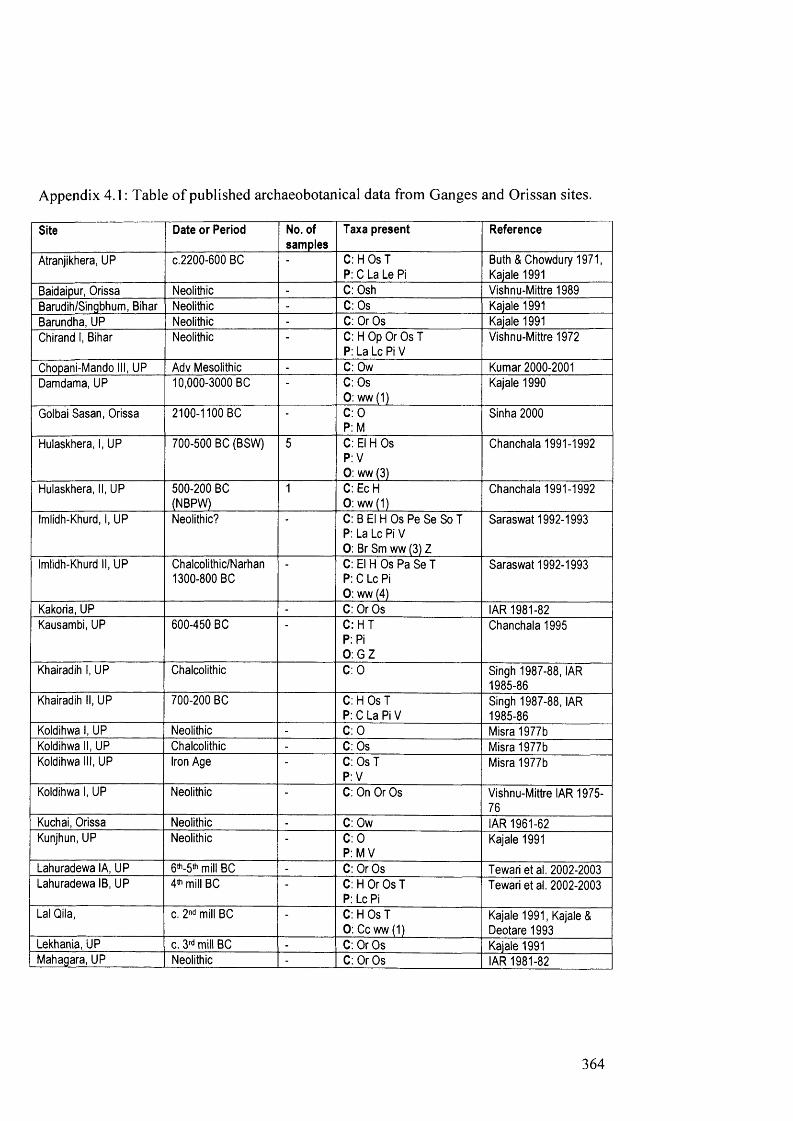
Appendix 4.1: Table of published archaeobotanical data from Ganges and Orissan sites.
Site D ate o r P eriod No. of sa m p le s
T axa p re se n t R e fe re n ce
Atranjikhera, UP c.2200-600 BC - C: H Os T P: C La Le Pi
Buth & Chowdury 1971, Kajale 1991
Baidaipur, Orissa Neolithic - C: Osh Vishnu-Mittre 1989Barudih/Singbhum, Bihar Neolithic - C: Os Kajale 1991Barundha, UP Neolithic - C: Or Os Kajale 1991Chirand 1, Bihar Neolithic - C: H Op Or Os T
P: La Lc Pi VVishnu-Mittre 1972
Chopani-M ando III, UP Adv Mesolithic - C: Ow Kumar 2000-2001Damdama, UP 10,000-3000 BC - C: Os
O: ww (1)Kajale 1990
Golbai Sasan , Orissa 2100-1100 BC - C: O P: M
Sinha 2000
Hulaskhera, 1, UP 700-500 BC (BSW) 5 C: El H OsP: VO: ww (3)
C hanchala 1991-1992
Hulaskhera, II, UP 500-200 BC (NBPW)
1 C: Ec H O: ww (1)
C hanchala 1991-1992
Imlidh-Khurd, 1, UP Neolithic? C: B El H Os Pe S e So T P: La Lc Pi V O: Br Sm ww (3) Z
S arasw at 1992-1993
Imlidh-Khurd II, UP Chalcolithic/Narhan 1300-800 BC
C: El H Os P a Se T P: C Lc Pi O: ww (4)
S arasw at 1992-1993
Kakoria, UP - C: Or Os IAR 1981-82Kausambi, UP 600-450 BC C: H T
P: Pi O: G Z
C hanchala 1995
Khairadih 1, UP Chalcolithic C: O Singh 1987-88, IAR 1985-86
Khairadih II, UP 700-200 BC C: H Os T P: C La Pi V
Singh 1987-88, IAR 1985-86
Koldihwa 1, UP Neolithic - C: O Misra 1977bKoldihwa II, UP Chalcolithic - C: Os Misra 1977bKoldihwa III, UP Iron Age - C: Os T
P: VMisra 1977b
Koldihwa 1, UP Neolithic - C: On Or Os Vishnu-Mittre IAR 1975- 76
Kuchai, Orissa Neolithic - C: Ow IAR 1961-62Kunjhun, UP Neolithic - C: O
P: M VKajale 1991
Lahuradewa IA, UP 6^-5^ mill BC - C: Or Os Tewari e t al. 2002-2003Lahuradewa IB, UP 4th mi|| BC - C: H Or Os T
P: Lc PiTewari e t al. 2002-2003
Lai Qila, c. 2nd mill BC - C: H Os T O: Cc ww (1)
Kajale 1991, Kajale & D eotare 1993
Lekhania, UP c. 3rd mill BC - C: Or O s Kajale 1991M ahagara, UP Neolithic - C: Or O s IAR 1981-82
364

Appendix 4.1 continued: Table of published archaeobotanical data from Ganges and
Orissan sites.
Site Date or Period No. of samples
Taxa present Reference
Malhar 1, UP Pre Iron Age 2150-1600 BC
14 C : Cl H Or Os Pa Ps S e T P : La Lc Pi Vi V O : ww (2)
S arasw at 2003-2004
Malhar II, UP Early Iron Age 1700-800 BC
26 C: El H Os Pa Ps So T P: La Lc M Pi Vi V O: w w (1 1 )Z
S arasw at 2003-2004
Manjhi II, UP 600-50 BC 3 C: Ec El H O s P s Se T P: La Lc Pi Vi V O: Sm Vv w w (16)
C hanchala 2000-2001
Manjhi III, UP 50 BC - AD 300 1 C: Ec El H O s Pa Ps S e T P : La Lc Pi Va Vi V O : B rV v w w (1 8 )Z
C hanchala 2000-2001
Narhan 1, UP BRW1000-800 BC
32 C : Ec H Os Pa Pe P s T P : C La Lc M Pi Va Vi V O: Br Cc Ln Ph Sm ww (23) Z
S arasw at e ta l . 1994
Narhan II, UP BSW800-600 BC
17 C: H O sP: Ca Pi Vi V w w (1)
S arasw at e t al. 1994
Narhan III, UP NBPW 600-200 BC
5 C : H O s Ps T P : La Pi V O: Sm ww(1) Z
S arasw at e t al. 1994
Narhan IV, UP K ushana 200 BC - AD 400
1 O: G S arasw at e t al. 1994
Oriup, Bihar Neolithic - C: Os Kajale 1991Pandu Rajar Dhibi 1, Bihar
2nd mill BC Neolithic
C: Osh Kajale 1991, IAR 1984- 85
Radhan, UP PGW + NBPW - C: H Os P: Pi
Kajale & Lai 1989
Raja-nala-ka-tila 1, UP 1600-1300 BC - C: El H Os Pa T P: La Lc Pi V
S arasw at 2004-2005
Raja-nala-ka-tila II, UP 1300-700 BC C: El H Os P a So T P : C La Lc M Pi Va V O: Al Br Ca Ln Sm
S arasw at 2004-2005
Senuw ar IA, Bihar Neolithic 2200-1950 BC
52 C: Cl El H Os Pa S e So T P: La Lc Pi Vi O: ww (4) Z
S arasw at 2004
Senuw ar IB, Bihar Neolithic- Chaleo 1950-1300 BC
54 C: H Or O s P s S e So T P: C La Lc M Pi Vi V O: Cc ww (4) Z
S arasw at 2004
Senuw ar II, Bihar Chalcolithic 1300-600 BC
40 C: El H Os S e So T P : C La Lc M Pi Va Vi V O: Br Ca Cc Cn Sm ww (8) Z
S arasw at 2004
Sohgaura, UP c. 2nd mill BC - C: H Kajale 1991Springaverapura, UP 1500-1000 BC C: H Os
O: G SmS arasw at 1986a
365

Appendix 4.1 continued: Table of published archaeobotanical data from Ganges and
Orissan sites.
Site Date or Period No. of samples
Taxa present Reference
Taradih, Bihar Chalcolithic C: H TP: Lb Le M Pi V 0 : Z
IAR 1981-82, Kajale 1991
Tokwa, UP Neolithic/Chalcolithic C: H O s P: V0 : Br ff (1)
Misra e t al. 2000-2001
Waina 1, UP 1600-800 BC C: H Os P s Se T P: C La Lc M Pi V 0 : Al G
IAR 1994-95, Sarasw at 2004-2005
Waina II, UP 800-600 BC C: El H Os S e So T P: La Lc M Pi V 0 : Br Ca Ln
IAR 1994-95, Sarasw at 2004-2005
Key for tables: C (cereals/ possible cereals): Cl (Coix lachrymal-jobi), Ec
{Echinochloa), El (Eleusine coracana), H (Hordeum vulgare), O (Oryza sp.), On (Oryza
nivara), Op {Oryza perennis), Or {Oryza rufipogori), Os {Oryza sativa), Osh {Oryza
sativa husk), Pa {Panicum), Pe {Pennisetum glaucum), Ps {Paspalum), Se {Setaria), So
{Sorghum bicolor), T {Triticum). P (Pulses): C {Cicer arietinum), La {Lathyrus), Lb
{Lablab purpureus), Lc (Lens culinaris), Le {Lens esculenta), M {Macrotyloma
uniflorum), Pi {Pisum sativum), Va {Vigna aconitifolia), Vi {Vicia sativa), V (Vigna
mungo/radiata). O (others): Al {Allium), Br {Brassica), Ca {Carthamus), Cc
{Curcurbitaceae), Cn {Cannabis), G {Gossypium), Ln {Linum), Ph {Phoenix), Sm
{Sesamum), Vv {Vitis vinifera), Z {Ziziphus), ff (other fruits/nuts, with no. of taxa), ww
(misc./weeds, with no. of taxa).
366
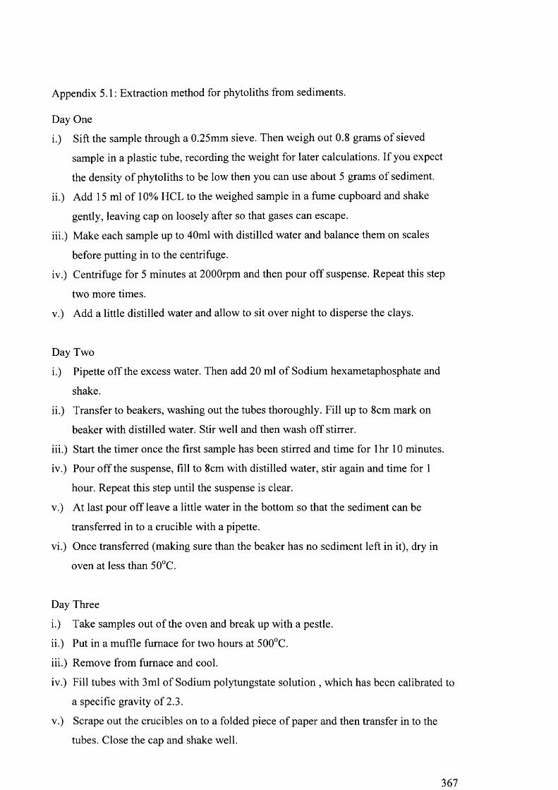
Appendix 5.1: Extraction method for phytoliths from sediments.
Day One
i.) Sift the sample through a 0.25mm sieve. Then weigh out 0.8 grams of sieved
sample in a plastic tube, recording the weight for later calculations. If you expect
the density of phytoliths to be low then you can use about 5 grams of sediment.
ii.) Add 15 ml of 10% HCL to the weighed sample in a fume cupboard and shake
gently, leaving cap on loosely after so that gases can escape.
iii.) Make each sample up to 40ml with distilled water and balance them on scales
before putting in to the centrifuge.
iv.) Centrifuge for 5 minutes at 2000rpm and then pour off suspense. Repeat this step
two more times.
v.) Add a little distilled water and allow to sit over night to disperse the clays.
Day Two
i.) Pipette off the excess water. Then add 20 ml o f Sodium hexametaphosphate and
shake.
ii.) Transfer to beakers, washing out the tubes thoroughly. Fill up to 8cm mark on
beaker with distilled water. Stir well and then wash off stirrer.
iii.) Start the timer once the first sample has been stirred and time for lhr 10 minutes.
iv.) Pour off the suspense, fill to 8cm with distilled water, stir again and time for 1
hour. Repeat this step until the suspense is clear.
v.) At last pour off leave a little water in the bottom so that the sediment can be
transferred in to a crucible with a pipette.
vi.) Once transferred (making sure than the beaker has no sediment left in it), dry in
oven at less than 50°C.
Day Three
i.) Take samples out of the oven and break up with a pestle.
ii.) Put in a muffle furnace for two hours at 500°C.
iii.) Remove from furnace and cool.
iv.) Fill tubes with 3ml of Sodium polytungstate solution , which has been calibrated to
a specific gravity of 2.3.
v.) Scrape out the crucibles on to a folded piece of paper and then transfer in to the
tubes. Close the cap and shake well.
367
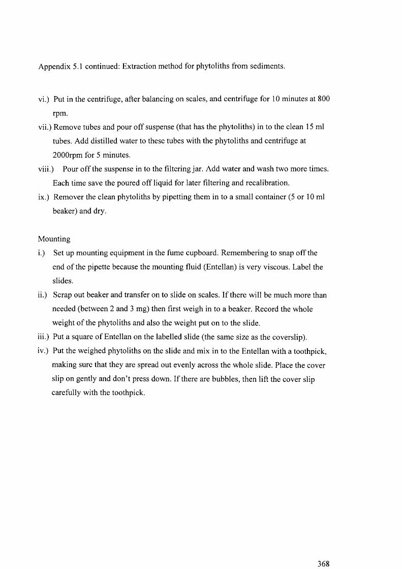
Appendix 5.1 continued: Extraction method for phytoliths from sediments.
vi.) Put in the centrifuge, after balancing on scales, and centrifuge for 10 minutes at 800
rpm.
vii.) Remove tubes and pour off suspense (that has the phytoliths) in to the clean 15 ml
tubes. Add distilled water to these tubes with the phytoliths and centrifuge at
2000rpm for 5 minutes.
viii.) Pour off the suspense in to the filtering jar. Add water and wash two more times.
Each time save the poured off liquid for later filtering and recalibration.
ix.) Remover the clean phytoliths by pipetting them in to a small container (5 or 10 ml
beaker) and dry.
Mounting
i.) Set up mounting equipment in the fume cupboard. Remembering to snap off the
end of the pipette because the mounting fluid (Entellan) is very viscous. Label the
slides.
ii.) Scrap out beaker and transfer on to slide on scales. If there will be much more than
needed (between 2 and 3 mg) then first weigh in to a beaker. Record the whole
weight of the phytoliths and also the weight put on to the slide.
iii.) Put a square o f Entellan on the labelled slide (the same size as the coverslip).
iv.) Put the weighed phytoliths on the slide and mix in to the Entellan with a toothpick,
making sure that they are spread out evenly across the whole slide. Place the cover
slip on gently and don’t press down. If there are bubbles, then lift the cover slip
carefully with the toothpick.
368

Appendix 5.2: Dry ashing method for making phytolith reference slides.
i.) Separate the selected plant in to the parts needed, e.g; stem, leaf, husk.
ii.) Wash thoroughly with distilled water and cut up the plant parts.
iii.) Place the plant parts in separate numbered boats and record, which part is in
each boat (these numbers should be kept throughout the making of slides).
iv.) Put the boats in a 400°C furnace for 2 hours and record their positions so that
they don’t get mixed up when the labels bum off.
v.) After the two hours, turn off the furnace and allow to cool.
vi.) Transfer the ash into numbered 15ml test tubes and add a small amount of 10%
HCL.
vii.) Add distilled water up to 13-14 ml.
viii.) Centrifuge at 2000rpm for 5 minutes. Pour off supernatant with one smooth
action.
ix.) Add distilled water up to 13-14 ml. Centrifuge at 2000rpm for 2 minutes. Pour
off supernatant.
x.) Repeat last step one more time.
xi.) Transfer the ash pellet to a small beaker and put in a drying oven at below 50°C
until dry.
xii.) Then mount on slide with entellan.
Appendix 5.3: Method for preparation of spodograms.
i.) Wash plant material to avoid contamination.
ii.) Trim the plant parts to the desired size so that it fits on to the slide.
iii.) Place the tissue in a petri dish or small beaker and inundate with a 50% bleach
solution and allow to stand over night or until tissue is clear or milky.
iv.) Remove tissues from the bleach solution and place in dish of distilled water to
rinse it.
v.) Dehydrate with ethanol and then mount on a slide using Entellan.
369

Appendix 5.4: Description o f terms used for phytoliths in the thesis.
H arvey phytolith category
ICPN nom enclature Notes
M onocot single cellsLong (smooth) Elongate psilate -
epidermal long cellCome most from stems
Long (sinuate) Elongate sinuate - epidermal long cell
Between smooth and dendritic elongates
Long (rods) Elongate psilate - epidermal long cell
Long and very thin - specific to sedges
Long (dendritic) Elongate dendriform - epidermal long cell
Not just dendriform but any with larger ornamentation than sinuate.Come from grass floral parts
Papillae Papillae cell Anatomical termHairs Hair cell Anatomical term - long
hairs, that would be attached to a hair base
Trichomes Prickle hair cell Anatomical term - short hairs, would have no hair base
Bulliform Parallepipedal bulliform - epidermal short cell
Anatomical term
Ovals Oval smooth epidermal - short cell
These normally have organic matter attached to them
Keystones Cuneiform bulliform - epidermal short cell
Also known as fan-shaped bulliforms
Crenates Tri-lobate - epidermal short cell
-
Bilobes Bilobate - epidermal short cell
In many various shapes and sizes
Crosses Quadra-lobate - epidermal short cell
Lots o f different sizes
Rondels Rondel -
Saddles Saddle -
Cones Conical -
Flat tower Conical with flat top Like a rondel but longer and with a very flat top
Homed tower Conical with irregular proturberances on top
Like a rondel but longer with spikey top
Rice bulliform Cuneiform bulliform Bulliform specific to rice leaves
370
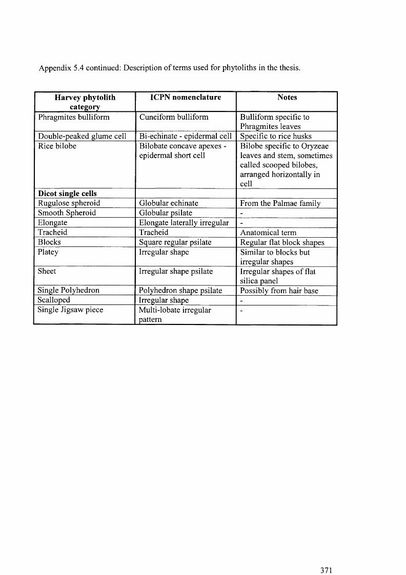
Appendix 5.4 continued: Description o f terms used for phytoliths in the thesis.
H arvey phytolith category
ICPN nom enclature Notes
Phragmites bulliform Cuneiform bulliform Bulliform specific to Phragmites leaves
Double-peaked glume cell Bi-echinate - epidermal cell Specific to rice husksRice bilobe Bilobate concave apexes -
epidermal short cellBilobe specific to Oryzeae leaves and stem, sometimes called scooped bilobes, arranged horizontally in cell
Dicot single cellsRugulose spheroid Globular echinate From the Palmae familySmooth Spheroid Globular psilate -
Elongate Elongate laterally irregular -
Tracheid Tracheid Anatomical termBlocks Square regular psilate Regular flat block shapesPlatey Irregular shape Similar to blocks but
irregular shapesSheet Irregular shape psilate Irregular shapes of flat
silica panelSingle Polyhedron Polyhedron shape psilate Possibly from hair baseScalloped Irregular shape -
Single Jigsaw piece Multi-lobate irregular pattern
-
371
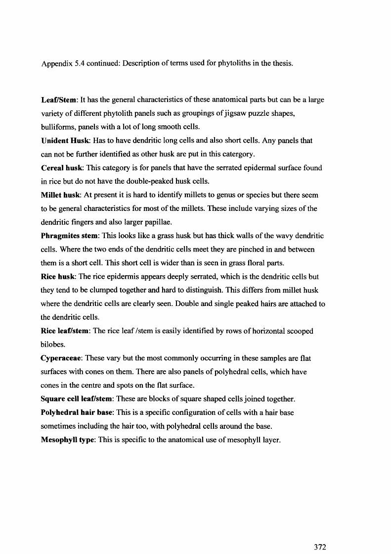
Appendix 5.4 continued: Description o f terms used for phytoliths in the thesis.
Leaf/Stem: It has the general characteristics o f these anatomical parts but can be a large
variety o f different phytolith panels such as groupings o f jigsaw puzzle shapes,
bulliforms, panels with a lot o f long smooth cells.
Unident Husk: Has to have dendritic long cells and also short cells. Any panels that
can not be further identified as other husk are put in this catergory.
Cereal husk: This category is for panels that have the serrated epidermal surface found
in rice but do not have the double-peaked husk cells.
Millet husk: At present it is hard to identify millets to genus or species but there seem
to be general characteristics for most o f the millets. These include varying sizes o f the
dendritic fingers and also larger papillae.
Phragmites stem: This looks like a grass husk but has thick walls o f the wavy dendritic
cells. Where the two ends o f the dendritic cells meet they are pinched in and between
them is a short cell. This short cell is wider than is seen in grass floral parts.
Rice husk: The rice epidermis appears deeply serrated, which is the dendritic cells but
they tend to be clumped together and hard to distinguish. This differs from millet husk
where the dendritic cells are clearly seen. Double and single peaked hairs are attached to
the dendritic cells.
Rice leaf/stem: The rice leaf /stem is easily identified by rows o f horizontal scooped
bilobes.
Cyperaceae: These vary but the most commonly occurring in these samples are flat
surfaces with cones on them. There are also panels o f polyhedral cells, which have
cones in the centre and spots on the flat surface.
Square cell leaf/stem: These are blocks o f square shaped cells joined together.
Polyhedral hair base: This is a specific configuration o f cells with a hair base
sometimes including the hair too, with polyhedral cells around the base.
Mesophyll type: This is specific to the anatomical use o f mesophyll layer.
372

Appendix 5.4 continued: Photographs o f phytolith categories in this thesis. Key: A. Long (smooth); B. Long (sinuate); C. Long (rods); D. Long (dendritic); E. Papillae; F. Hairs;G. Trichomes; H. Bulliform; I. Ovals; J. Keystones; K. Crenates; L. Bilobes; M. Crosses; N. Rondels; O. Saddles; P. Flat tower; Q. Homed tower; R. Rice bulliform; S. Phragmites bulliform; T. Double-peaked glume cell; U. Rice bilobe.

Appendix 5.4 continued: Photographs o f phytolith categories in this thesis.Key: a. Rugulose spheroid; b. Smooth spheroid; c. Elongate; d. Tracheid; e. Blocks; f. Platey; g. Sheet; h. single jigsaw piece.
%
a
e h
25[jm
374
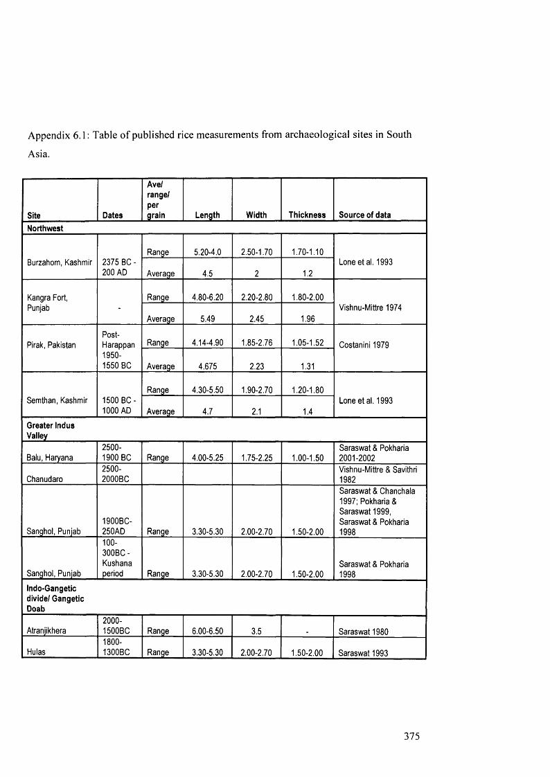
Appendix 6.1: Table o f published rice measurements from archaeological sites in South
Asia.
Site Dates
A ve/ range/ per grain Length Width Thickness Source of data
Northwest
R ange 5.20-4.0 2.50-1.70 1.70-1.10Burzahom, Kashmir 2375 BC -
200 AD A verage 4.5 2 1.2
L o n ee t al. 1993
Kangra Fort, R ange 4.80-6.20 2.20-2.80 1.80-2.00Punjab “
A verage 5.49 2.45 1.96Vishnu-Mittre 1974
Pirak, PakistanPost- H arappan 1950- 1550 BC
R ange 4.14-4.90 1.85-2.76 1.05-1.52 Costanini 1979
A verage 4.675 2.23 1.31
R ange 4.30-5.50 1.90-2.70 1.20-1.80Sem than, Kashmir 1500 B C -
1000 AD A verage 4.7 2.1 1.4Lone e t al. 1993
Greater Indus Valley
Balu, Haryana2500- 1900 BC R ange 4.00-5.25 1.75-2.25 1.00-1.50
S arasw at & Pokharia 2001-2002
Chanudaro2500-2000BC
Vishnu-Mittre & Savithri 1982
Sanghol, Punjab1900BC-250AD R ange 3.30-5.30 2.00-2.70 1.50-2.00
S arasw at & Chanchala 1997; Pokharia & S arasw at 1999, S a rasw at & Pokharia 1998
Sanghol, Punjab
100- 300BC - K ushana period R ange 3.30-5.30 2.00-2.70 1.50-2.00
S arasw at & Pokharia 1998
Indo-Gangetic divide/ Gangetic Doab
Atranjikhera2000-1500BC R ange 6.00-6.50 3.5 S arasw at 1980
Hulas1800-1300BC R ange 3.30-5.30 2.00-2.70 1.50-2.00 S arasw at 1993
375

Appendix 6.1: Table o f published rice measurements from archaeological sites in South
Asia
Site Dates
Ave/range/pergrain Length Width Thickness Source of data
Middle Ganges Valley
Charda, U P
900BC - 1100 AD pre-NBPW to Medieval period R ange 4.00-5.00 1.00-3.00 1.00-1.50
C hanchala Srivastava 2002
Chirand, Bihar2200-1500BC
Smallrange 4.25-4.50 1.50-1.80 1.00-1.00
Vishnu-Mittre 1974Average 4.38 1.65 1
Largerange 5.00-5.25 2.25-2.50 1.25-1.25
Average 5.13 2.38 1.25
Hastinapur, UP506-306BC R ange 5.00-7.00 2.00-2.70 Vishnu-Mittre 1974
Hulaskera, UP700 BC - 250 AD R ange 4.00 - 5.00 1 .7 5 -2 .6 0 1 .0 0 -1 .7 5 C hanchala 1991-1992
Malhar, UP1900 - 800 BC R ange 4.50-5.30 2.00-2.50 1.40-2.00 S arasw at 2003-2004
Manjhi, Bihar250BC-250AD R ange 3.00-5.00 1.25-2.00 1.00-1.75
C hanchala Srivastava 2000-2001
Narhan, UP1300-300BC R ange 4 .0 0 -5 .0 0 1.90-2.20 1.10-1.30 S arasw at e ta l 1994
Oriyup, Bihar Neolithic
R angeimpressions 5.00-5.50 2.25-2.50 Vishnu-Mittre 1974
Pataliputra, Bihar405-115BC
R ange 3.50-5.40 2.50-3.00 2.00-2.50Vishnu-Mittre 1974
A verage 4.95 2.66 1.82
Radhan, UP1000-250BC
R angehistoric 2.40-3.30 1.10-1.70
Kajale & Lai 1989
Average 2.74 1.45 -
R angePGrey/NBPW 2.10-3.30 1.2-1.7
A verage 2.64 1.39 -
Grain B 4.4 2.3 1.5
Grain C 5 1.8 1.5
Average 4.85 2.11 1.5
376
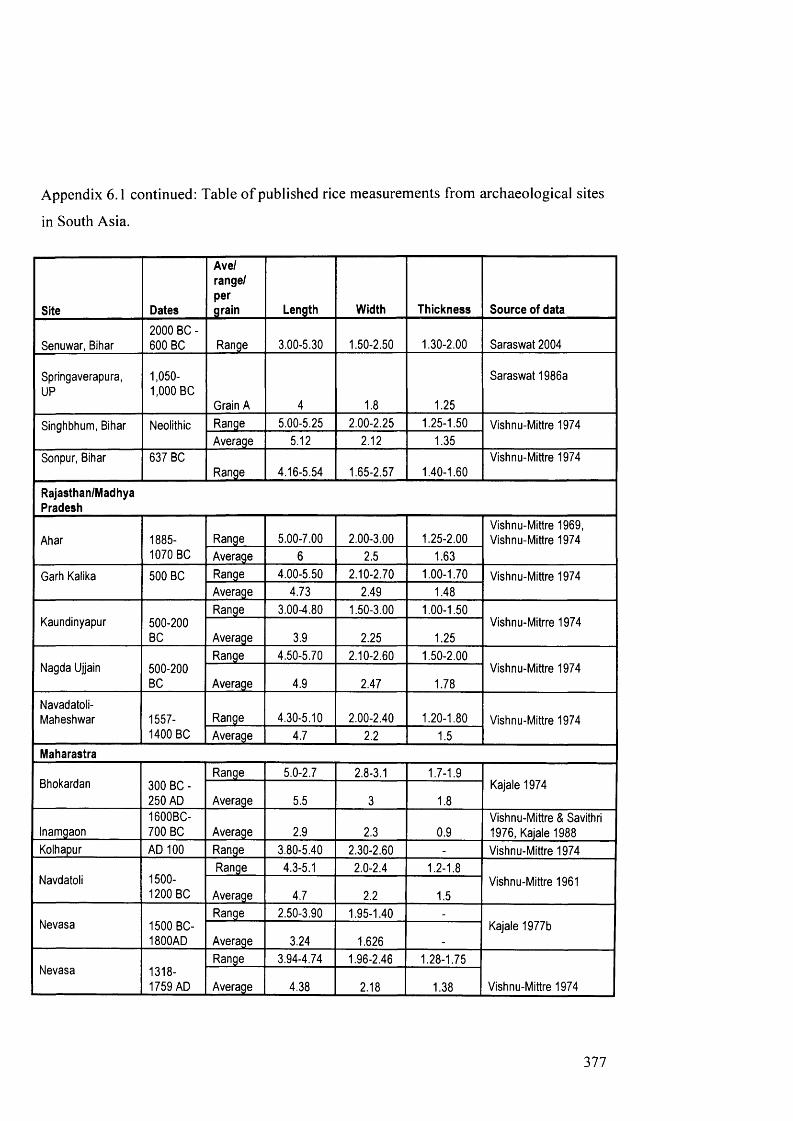
Appendix 6.1 continued: Table o f published rice measurements from archaeological sites
in South Asia.
Site Dates
Ave/range/pergrain Length Width Thickness Source of data
Senuwar, Bihar2000 BC - 600 BC R ange 3.00-5.30 1.50-2.50 1.30-2.00 S arasw at 2004
Springaverapura,UP
1,050- 1,000 BC
Grain A 4 1.8 1.25
S arasw at 1986a
Singhbhum, Bihar Neolithic R ange 5.00-5.25 2.00-2.25 1.25-1.50 Vishnu-Mittre 1974Average 5.12 2.12 1.35
Sonpur, Bihar 637 BCR ange 4.16-5.54 1.65-2.57 1.40-1.60
Vishnu-Mittre 1974
Rajasthan/MadhyaPradesh
Ahar 1885- 1070 BC
R ange 5.00-7.00 2.00-3.00 1.25-2.00Vishnu-Mittre 1969, Vishnu-Mittre 1974
Average 6 2.5 1.63
Garh Kalika 500 BC R ange 4.00-5.50 2.10-2.70 1.00-1.70 Vishnu-Mittre 1974Average 4.73 2.49 1.48
Kaundinyapur 500-200BC
R ange 3.00-4.80 1.50-3.00 1.00-1.50Vishnu-Mitrre 1974
Average 3.9 2.25 1.25
Nagda Ujjain 500-200BC
R ange 4.50-5.70 2.10-2.60 1.50-2.00Vishnu-Mittre 1974
A verage 4.9 2.47 1.78
Navadatoli-M aheshwar 1557-
1400 BC
R ange 4.30-5.10 2.00-2.40 1.20-1.80 Vishnu-Mittre 1974A verage 4.7 2.2 1.5
Maharastra
Bhokardan 300 BC - 250 AD
R ange 5.0-2.7 2.8-3.1 1.7-1.9Kajale 1974
Average 5.5 3 1.8
Inamgaon1600BC- 700 BC A verage 2.9 2.3 0.9
Vishnu-Mittre & Savithri 1976, Kajale 1988
Kolhapur AD 100 R ange 3.80-5.40 2.30-2.60 - Vishnu-Mittre 1974
Navdatoli 1500- 1200 BC
R ange 4.3-5.1 2.0-2.4 1.2-1.8Vishnu-Mittre 1961
A verage 4.7 2.2 1.5
Nevasa 1500 BC- 1800AD
R ange 2.50-3.90 1.95-1.40 -
Kajale 1977bAverage 3.24 1.626
N evasa 1318- 1759 AD
R ange 3.94-4.74 1.96-2.46 1.28-1.75
Vishnu-Mittre 1974Average 4.38 2.18 1.38
377
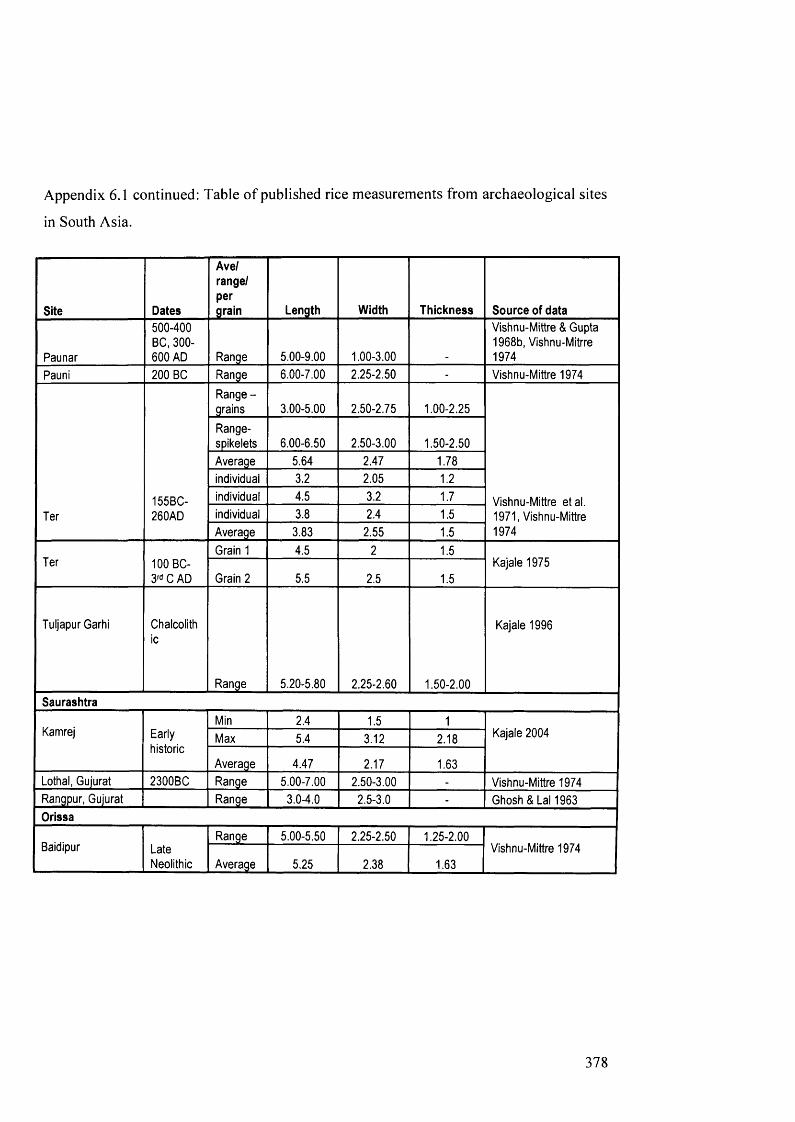
Appendix 6.1 continued: Table o f published rice measurements from archaeological sites
in South Asia.
Site Dates
Ave/range/pergrain Length Width Thickness Source of data
Paunar
500-400 BC, 300- 600 AD R ange 5.00-9.00 1.00-3.00
Vishnu-Mittre & Gupta 1968b, Vishnu-Mitrre 1974
Pauni 200 BC R ange 6.00-7.00 2.25-2.50 - Vishnu-Mittre 1974
Ter155BC-260AD
R ange - grains 3.00-5.00 2.50-2.75 1.00-2.25
Vishnu-Mittre e ta l . 1971, Vishnu-Mittre 1974
Range-spikelets 6.00-6.50 2.50-3.00 1.50-2.50
Average 5.64 2.47 1.78
individual 3.2 2.05 1.2
individual 4.5 3.2 1.7
individual 3.8 2.4 1.5
Average 3.83 2.55 1.5
Ter 100 BC- 3rd C AD
Grain 1 4.5 2 1.5Kajale 1975
Grain 2 5.5 2.5 1.5
Tuljapur Garhi Chalcolithic
R ange 5.20-5.80 2.25-2.60 1.50-2.00
Kajale 1996
Saurashtra
Kamrej Earlyhistoric
Min 2.4 1.5 1Kajale 2004Max 5.4 3.12 2.18
Average 4.47 2.17 1.63
Lothal, Gujurat 2300BC R ange 5.00-7.00 2.50-3.00 - Vishnu-Mittre 1974Rangpur, Gujurat R ange 3.0-4.0 2.5-3.0 - Ghosh & Lai 1963
Orissa
Baidipur LateNeolithic
R ange 5.00-5.50 2.25-2.50 1.25-2.00Vishnu-Mittre 1974
A verage 5.25 2.38 1.63
378

Appendix 6.1 continued: Table o f published rice measurements from archaeological sites
in South Asia.
Site Dates
Ave/range/pergrain Length Width Thickness Source of data
South India
Hallur, Mysore 870 BC R ange 7.00-8.00 2.00-2.50
Vishnu-Mittre & Savithri 1971, Vishnu-Mittre 1974
1000 BC R ange 2.5-2.9 1.10-1.06 - Kajale 1989bA verage 2.62 1.31 -
Kunnatar, M adras 300 BC Grain 7 2 - Vishnu-Mittre 1974
Veerapuram , A.P. 500BC-400AD
R ange 3.10-4.20 1.80-2.50 -
Kajale 1984A verage 4.06 2.24
Kolhapur 1st C. AD
Average sam ple I 4.8 2.6
Kumar 1948Average sam ple II 5.4 2.3Averagesam pleIII 3.8 2.3
379

380
Appendix 7.1: Raw data table for macro-botanical remains from Koldihwa.
Sample Koldihwa
i—om< A
BO
T2
AB
OT3
AB
OT4
m1—Om< A
BO
T6 i—om< A
BO
T8 o>1—Om< AB
OT
10
ABOT
11
ABOT
12
ABOT
13
ABOT
14
ABOT
15
ABOT
16
ABOT
17
ABOT
18
AB
OT1
9
ABOT
20
<i£ CM Eoo co CO in m CM CM CO CO in in
ISJ rsl g; INI M INI rsl INI rsl > >- >- >- >- >- > >- >-Level N INI
TOP BOTTOM TOP BOTTOM
Age by material culture I/A I/A Chaleo Chaleo Neo Neo Neo Neo Sterile Sterile I/A I/A Chaleo Chaleo Neo Neo Neo Neo Sterile Sterile
Soil vol. (1) 20 20 20 20 20 20 20 20 20 20 20 20 20 20 20 20 20 20 20 20
Sample vol (ml) 60 120 185 50 15 30 8 20 10 5 90 50 30 50 180 120 5 5 5 5
Density of sample per litre (ml) 3 6 9.25 2.5 0.75 1.5 0.4 1 0.5 0.25 4.5 2.5 1.5 2.5 9 6 0.25 0.25 0.25 0.25
Vigna sp. (whole) 0 0 0 0 0 0 0 0 0 0 0 0 0 0 0 0 0 0 0 0
p Vigna sp. (cotyledon) 1 1 1 0 0 1 0 0 0 0 0 0 0 1 1 0 0 0 0 0
u Vigna sp. (frag) 0 0 0 0 0 0 0 1 0 0 2 0 1 3 0 0 0 0 0 0
L Vigna cf. radiata 0 0 0 0 0 0 0 0 0 0 0 0 0 0 0 0 0 0 0 0
S Lens culinaris (whole) 0 0 0 0 0 0 0 0 0 0 0 0 0 0 0 0 0 0 0 0
E Lens culinaris (cotyledon) 0 0 0 0 0 0 0 0 0 0 0 0 0 0 0 0 0 0 0 0
S Lens culinaris (frag) 0 0 0 0 0 0 0 1 0 0 0 0 0 0 0 0 0 0 0 0
Lathyrus sativus 0 0 0 0 0 0 0 0 0 0 0 0 0 0 0 0 0 0 0 0
cf. Lathyrus aphaca 0 0 1 0 0 0 0 0 0 0 0 0 0 0 0 0 0 0 0 0
Pisum sativum 0 0 0 0 0 0 0 0 0 0 0 0 0 0 0 0 0 0 0 0
Cajanus/ Lablab? 0 0 0 0 0 0 0 0 0 0 0 0 0 0 0 0 0 0 0 0
Pulse frags 1 1 2 0 3 0 0 1 0 0 0 2 0 1 1 1 0 0 0 0

Appendix 7.1 continued: Raw data table for macro-botanical remains from Koldihwa.
Sample Koldihwa ABOT
1
ABOT
2 CO
1—om< AB
OT
4
ABOT
5
ABOT
6
ABOT
7
ABOT
8
ABOT
9
ABOT
10
ABOT
11
ABOT
12 CO
1—Om< AB
OT
14
AB
OT1
5 CO1—oCO< AB
OT
17
ABOT
18
ABOT
19
ABOT
20
Bracharia ramosa (hulled) well pres 0 0 0 1 1 1 1 0 0 0 1 4 2 0 0 1 0 0 1 0
c B.ramosa (caryopsis) 0 0 2 0 0 0 0 0 0 0 0 0 0 0 0 0 0 0 0 0
E Setaria verticilliata (hulled) well pres 0 0 0 0 0 0 0 2 0 0 1 0 0 0 1 0 0 0 0 0
R S. verticillata (caryopsis) 0 0 3 0 0 0 1 0 0 0 2 1 1 0 1 0 0 0 0 0
E Setaria sp. (caryopsis) 0 0 0 0 0 0 0 0 0 0 0 1 1 0 0 0 0 0 0 0
A Echinochloa sp. (caryopsis) 0 0 0 0 0 0 0 0 0 0 0 0 0 1 0 0 0 0 0 0
L Panicum sumatrense (caryopsis) 0 0 0 0 0 0 0 0 0 0 0 0 1 0 0 0 0 0 0 0
S Panicum sp. (caryopsis) 0 0 0 0 1 0 0 0 0 0 0 0 0 0 0 0 0 0 0 0
Paspalum sp. (caryopsis) 0 0 0 1 0 0 0 0 0 0 0 0 0 0 0 0 0 0 0 0
& Pennisetum (wild) sp. (caryopsis) 0 0 4 0 1 0 0 0 0 0 2 0 0 0 0 0 0 0 0 0
Diqitaria sp. (caryopsis) 0 0 0 0 0 0 0 0 0 0 0 0 0 1 0 0 0 0 0 0
G Indeterminate small millet 0 0 1 0 0 0 0 0 0 0 1 0 0 1 0 0 0 0 0 0
R Hordeum vulqare (caryopsis whole) 3 1 0 0 0 0 0 0 0 0 3 0 1 0 0 0 0 0 0 0
A Hordeum vulqare (caryopsis 1/2) 3 2 0 0 0 0 0 0 0 0 0 0 0 0 0 0 1 0 0 0
S Triticum sp. (free-threshing) 0 0 0 1 0 0 0 0 0 0 0 0 0 0 0 0 0 0 0 0
S cf. Triticum sp. small 0 0 0 0 0 0 0 0 0 0 0 0 0 0 0 2 0 0 0 0
E Oryza sp. (whole caryopsis) 1 1 0 1 0 0 0 0 0 0 0 0 0 0 0 0 0 0 0 0
S Oryza sp. (caryopsis 1/2) 0 2 5 3 0 1 0 2 0 0 0 0 0 0 1 0 0 0 0 0
Oryza sp. (caryopsis 1/4) 3 0 11 0 0 0 0 0 0 0 0 0 0 0 0 1 0 0 0 0
Oryza sp. (qlume frag) 0 0 0 0 0 0 0 0 0 0 0 0 0 0 1 0 0 0 0 0
Oryza sp. (husk frag) 0 0 1 0 0 0 0 0 0 0 0 0 0 0 0 0 0 0 0 0
Unknown Glume bases 0 0 ? 0 0 0 0 0 0 0 0 0 0 0 0 0 0 0 0 0
Indet. Graminae (caryopsis) 4 11 0 0 0 1 0 1 0 0 3 2 0 2 0 0 0 0 0 0
u>00

382
Appendix 7.1 continued: Raw data table for macro-botanical remains from Koldihwa.
Sample Koldihwa
i—oCO<
CM1—om<
CO1—OCO<
i—oCO< AB
OT
5
ABOT
6
ABOT
7
ABOT
8
ABOT
9
ABOT
10
1—om< AB
OT1
2
AB
OT1
3
ABOT
14
ABOT
15
AB
OT1
6
ABOT
17 00
t—O00<
001—OCO< AB
OT
20
Ziziphus sp. 1 0 0 2 0 0 0 0 0 0 4 1 0 1 2 0 0 0 0 0
Cyperaceae type 0 0 1 0 0 2 0 0 0 0 4 3 0 1 0 0 0 0 0 0
Malvaceae type 0 0 1 0 0 0 0 0 0 0 4 0 0 0 0 0 0 0 0 0
w Malvaceae testa 0 0 1 0 0 0 0 0 0 0 0 0 0 0 0 0 0 0 0 0
E Polygonaceae type 0 0 0 0 0 0 0 1 0 0 0 0 0 0 0 0 0 0 0 0
E Rubiaceae type 0 0 0 0 0 0 0 0 0 0 0 2 0 0 0 0 0 0 0 0
D Schleriaceae type 1 0 0 0 0 0 0 0 0 0 0 0 0 0 0 0 0 0 0 0
S Indet culm node 1 0 0 0 0 0 0 0 0 0 0 0 0 0 0 0 0 0 0 0
Indet intemode 0 0 0 0 1 0 0 0 0 0 0 0 0 0 0 0 0 0 0 0
Indet pedestal 0 0 0 0 0 0 0 0 0 0 0 1 0 0 0 0 0 0 0 0
Indet striated seed coat 0 0 0 0 0 0 0 0 0 0 0 0 0 0 1 0 0 0 0 0
Modem seeds Y Y Y Y Y Y Y Y Y Y Y Y Y Y Y Y Y Y Y Y
Charcoal XXX XXX XXX XXX XX XX XX XX XX XX XX XX XXX XXX XX X X X X 0
Shoots 0 Y 0 0 0 0 0 0 0 0 0 0 0 0 0 0 0 0 0 0
Indeterminate 2 6 16 5 9 9 3 7 0 0 27 3 1 1 7 6 0 0 0 0
Total fragments 21 25 50 14 16 15 5 16 0 0 54 20 8 13 16 11 1 0 1 0

Appendix 7.2: Raw data table for macro-botanical remains from Mahagara.
COCN 0 4
i n0 4
< 0CM
h -CM
COCM 8 8 n c o
COCO 3
1 0CO 3
c -c o s s
SampleMahagara S
<
o3
Om< 3
O
3
OCD<
o0 0<
o0 0<
oCO<
o3
o0 0< ,
oGO< ,
o3
oGO< ;
O0 0< ,
o3
o O0 0< i
Level 2 2 3 3 4 4 5 5 6 6 7 7 8 8 9 9 10 10
TOP
Soil vol. (L) 20 20 20 20 20 20 20 20 20 20 20 20 20 20 20 20 20 20
Sample vol. (ml) 8 10 10 15 8 15 10 50 8 10 30 10 20 30 8 10 5 5Density of sample per litre (ml) 0.4 0.5 0.5 0.8 0.4 0.8 0.5 2.5 0.4 0.5 1.5 0.5 1 1.5 0.4 0.5 0.3 0.3
Parenchyma 0 0 0 0 0 0 0 0 0 0 0 0 0 0 0 0 0 0Vigna sp. (whole) 0 0 0 0 0 0 0 0 0 0 0 0 0 0 0 0 0 0
p Vigna sp. (cotyledon) 0 0 0 0 0 0 0 0 0 1 0 0 0 1 0 0 1 1
u Vigna sp. (frag) 0 0 0 0 0 0 0 0 0 0 0 0 1 2 0 0 1 0
Vigna cf. radiata 0 0 0 0 0 0 0 0 0 0 0 0 0 0 0 0 0 0L
SLens culinaris (whole) 0 0 0 0 0 0 0 0 0 0 0 0 0 0 0 0 0 0
ELens culinaris (cotyledon) 0 0 0 0 0 0 0 0 0 0 0 0 0 0 0 0 0 0
SLens culinaris (frag) 0 0 0 0 0 0 0 0 0 0 0 0 0 0 0 0 0 0
Lathyrus sativus 0 0 0 0 0 0 0 0 0 0 0 0 0 0 0 0 0 0
cf. Lathyrus sativus 0 0 0 0 0 0 0 0 0 0 0 0 0 0 0 0 0 0
Pisum sativum 0 0 0 0 0 0 0 0 0 0 0 0 0 0 0 0 0 0Cajanus/Lablab? 0 0 0 0 0 0 0 0 0 0 0 0 0 0 0 0 0 0
Cajanus cajan (whole) 0 0 0 0 0 0 0 0 0 0 0 0 0 0 0 0 0 0
Pulse frags 0 0 0 0 0 0 0 0 1 0 2 1 1 8 2 2 0 0Bracharia ramosa (hulled) well pres 5 1 0 0 0 0 0 0 0 0 0 0 0 0 0 0 0 0
CB.ramosa(caryopsis) 0 0 0 0 0 0 0 0 0 0 0 0 0 0 0 0 0 0
E
Setaria vertidlliata (hulled) well pres 0 0 0 0 0 0 0 0 0 0 0 0 0 0 0 0 0 0
RS. verticillata (caryopsis) 0 0 0 0 0 0 0 0 1 0 0 0 0 0 0 2 0 2
Ecf. S. verticillata (caryopsis) 0 0 0 0 0 0 0 0 0 0 0 0 0 0 0 0 2 0
ASetaria sp. (caryopsis) 0 0 0 0 0 0 0 0 0 0 0 0 0 0 0 0 0 0
383

Appendix 7.2 continued: Raw data table for macro-botanical remains from Mahagara
SampleMahagara mm m m oo co oo oo oo
cf. Panicum sumatrense (caryopsis)
Panicum sp. (caryopsis)
Paspalum sp. (caryopsis)
Indeterminate small millet
Millet spikelet
DactylocteniumaegyptiumHordeumvulgare(caryopsiswhole)Hordeum vulgare (caryopsis 1/2)
cf. Triticum sp.
Free threshing wheat_______
Oryza sp. (whole caryopsis)
Oryza sp. (caryopsis 1/2)
Oryza sp. (caryopsis 1/4)
Oryza sp. (husk frag)
Oryza sativa (glumes)
Oryza sp. (glumes)
Indet. Graminae (caryopsis)
Ziziphus sp.
Fruit frag indet
Sesamum sp. (wild)_______
384

Appendix 7.2 continued: Raw data table for macro-botanical remains from Mahagara
SampleMahagara AB
OT
21
ABOT
22
ABOT
23
ABOT
24
ABOT
25
ABOT
26 r*-
CM1—Om<, AB
OT
28
ABOT
29
ABOT
30
ABOT
31
ABOT
32
ABOT
33 3
i—om< AB
OT
35
ABOT
36
ABOT
37
ABOT
38
Chenopodiaceaetype 0 0 0 0 0 0 0 0 0 0 0 0 0 0 0 0 0 0
Commenlinabenghalensis 0 0 0 0 0 0 0 0 0 0 0 0 0 0 0 0 0 0
w Cyperaceae type 0 0 0 0 0 0 0 1 0 0 0 1 0 0 0 0 0 0
ECyperaceae cf. Scirpus sp. 0 0 0 0 0 0 0 0 1 0 0 0 0 0 0 0 0 0
EEuphorbiaceaetype 0 0 0 0 0 0 0 0 0 0 0 0 1 0 0 0 0 0
D Eragrostis sp. 0 0 0 0 0 0 0 0 0 0 0 0 0 0 0 0 0 0
SIschamemumrugosum 0 0 0 0 0 0 0 0 0 0 0 0 0 0 0 0 0 0
Malvaceae 0 0 0 0 0 0 0 0 0 0 0 0 0 0 0 0 0 0Polygonaceaetype 0 0 0 0 0 0 0 0 0 0 0 0 0 0 0 0 0 0
Portulaceae type 0 0 0 0 0 0 1 0 0 0 0 0 0 0 0 0 0 0
Indet pedestal 0 0 0 0 0 0 0 0 0 0 0 0 0 0 0 0 0 0Indet small legume 0 0 0 0 0 0 0 0 0 0 0 0 0 0 1 0 0 0
Modem seeds Y Y Y Y Y N Y Y Y Y Y Y Y Y Y Y Y Y
Charcoal X X X X X X X XX XX X XX XX XX XXX XXX XX XXX XX
Indeterminate 0 2 0 0 0 3 6 4 7 1 4 1 1 4 17 0 2 2 3 4
Total fragments 7 3 1 0 0 4 9 5 12 10 8 16 11 34 9 30 11 10
385

Appendix 7.2 continued: Raw data table for macro-botanical remains from Mahagara
o>CO
o■'t 5 CM CO 5 •» to r>- s? 5 55 u> CMIOSample Om
«;Om<,
o o O o o O Om<,o o om
<Om<
Om<Mahagara <; <, «; <
Level 11 11 12 12 13 13 14 14 15 15 16 16 17 17
BOTTOM
Soil vol. (L) 20 20 20 20 20 20 20 20 20 20 20 20 20 20
Sample vol. (ml) 10 15 10 15 10 20 10 10 5 5 10 10 10 40Density of sample per litre (ml) 0.5 0.8 0.5 0.8 0.5 1 0.5 0.5 0.3 0.3 0.5 0.5 0.5 2
Parenchyma 2 1 0 0 0 0 1 0 0 0 0 0 0 0Vigna sp. (whole) 0 0 0 0 0 0 0 1 0 0 0 0 0 0
p
Vigna sp. (cotyledon) 3 0 3 0 1 1 1 1 0 0 1 0 0 0
u Vigna sp. (frag) 0 0 0 4 0 3 0 0 0 0 1 1 0 0
L Vigna cf. radiata 0 0 0 0 0 0 0 0 0 0 0 0 0 0
SLens culinaris (whole) 1 0 0 0 0 0 0 0 0 0 0 0 0 0
ELens culinaris (cotyledon) 0 0 0 1 1 2 0 0 0 0 0 3 0 0
SLens culinaris (frag) 0 0 0 2 0 0 1 0 0 0 0 2 0 0
Lathyrus sativus 0 0 0 0 0 2 0 0 0 0 0 0 0 0
cf. Lathyrus sativus 1 0 0 0 0 0 0 0 0 0 0 0 0 0
Pisum sativum 0 0 0 0 0 0 0 0 0 0 0 0 0 0Cajanus/Lablab? 1 0 0 0 0 0 0 0 0 0 0 1 0 0
Cajanus cajan (whole) 0 0 0 0 0 0 0 0 0 0 0 1 0 0
Pulse frags 5 3 4 3 2 5 2 4 0 1 0 9 0 0Bracharia ramosa (hulled) well pres 0 1 0 0 0 0 0 0 0 0 0 0 0 0
CB.ramosa(caryopsis) 0 0 0 0 0 0 0 0 0 0 0 0 0 0
E
Setaria verticilliata (hulled) well pres 0 0 0 0 0 0 0 0 0 0 0 0 0 0
RS. verticillata (caryopsis) 1 2 0 1 0 0 0 1 0 2 0 3 0 0
Ecf. S. verticillata (caryopsis) 0 0 0 0 0 0 0 0 0 0 0 0 0 0
ASetaria sp. (caryopsis) 0 2 0 0 0 0 0 0 0 0 0 0 0 0
386
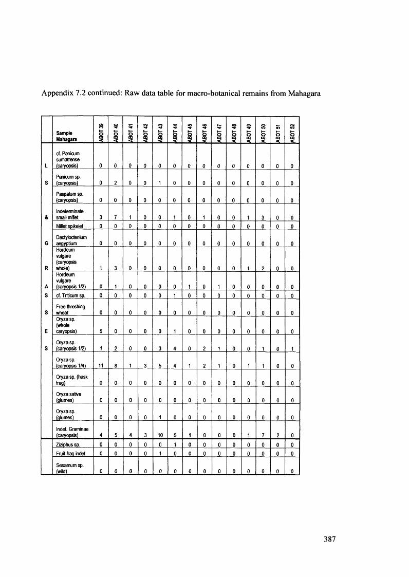
Appendix 7.2 continued: Raw data table for macro-botanical remains from Mahagara
SampleMahagara
om omm m m m m m m m co oo oooo
cf. Panicum sumatrense (caryopsis)
Panicum sp. (caryopsis)
Paspalum sp. (caryopsis)
Indeterminate small millet
Millet spikelet
DactylocteniumaegyptiumHordeumvulgare(caryopsiswhole)Hordeum vulgare (caryopsis 1/2)
cf. Triticum sp.
Free threshing wheat_______Oryza sp.(wholecaryopsis)
Oryza sp. (caryopsis 1(2)
Oryza sp. (caryopsis 1/4)
Oryza sp. (huskfrag)______Oryza sativa (glumes)
Oryza sp. (glumes)
Indet Graminae (caryopsis)
Ziziphus sp.
Fruit frag indet
Sesamum sp. (wild)_______
387

Appendix 7.2 continued: Raw data table for macro-botanical remains from Mahagara
SampleMahagara AB
OT
39
ABOT
40
ABOT
41
ABOT
42
ABOT
43
ABOT
44
ABOT
45
|aBO
T 46
ABOT
47
ABOT
48
ABOT
49
ABOT
50
ABOT
51
ABOT
52
Chenopodiaceaetype 0 0 0 0 1 0 0 0 0 0 0 0 0 0
Commenlinabenghalensis 0 0 0 0 0 1 0 0 0 0 0 0 0 0
w Cyperaceae type 0 1 0 0 0 0 0 0 0 0 0 0 0 0
ECyperaceae cf. Sdrpus sp. 0 0 0 0 0 0 0 0 0 0 0 0 0 0
EEuphorbiaceaetype 0 0 0 0 0 0 0 0 0 0 0 0 0 0
D Eragrostis sp. 0 0 1 0 0 0 0 0 0 0 0 0 0 0
SIschamemumrugosum 0 0 0 0 1 0 0 0 0 0 0 0 0 0
Malvaceae 0 0 0 0 0 0 0 0 0 1 0 0 0 0Polygonaceaetype 1 0 0 0 0 0 0 0 0 0 0 0 0 0
Portulaceae type 0 0 0 0 0 0 0 0 0 0 0 0 0 0
Indet pedestal 1 0 0 0 0 0 0 0 0 0 0 0 0 0Indet small legume 0 0 0 0 0 0 0 0 0 0 0 0 0 0
Modem seeds Y Y Y Y Y Y Y Y Y Y Y Y Y Y
Charcoal XXX XXX XXX XX XX XXX XX XX XX X XX XX XX X
Indeterminate 11 39 22 8 28 17 8 8 1 19 1 30 0 2
Total fragments 52 77 36 25 55 48 16 20 4 23 7 64 2 3
388

Appendix 7.3: Raw data table for macro-botanical remains from Chopani-Mando.
Sample Chopani- Mando AB
OT
53
ABOT
54
ABOT
55 <010
H-Om< AB
OT
57
ABOT
58
ABOT
59
ABOT
60
ABOT
61
ABOT
62
ABOT
63
ABOT
64
ABOT
65
ABOT
66
ABOT
67
ABOT
68
ABOT
69
ABOT
70
1—0m<
CMr--l—Om<
Level 1 1 2 2 3 3 4 4 5 5 6 6 7 7 8 8 9 9 10 10
TOP BOTTOM
Soil vol (L) 20 20 20 20 20 20 20 20 20 20 20 20 20 20 20 20 20 20 20 20
Sample vol (ml) 10 20 10 30 15 40 6 5 8 5 10 30 5 15 5 7 3 5 3 5
Density pre litre of sediment (ml) 0.5 1 0.5 1.5 0.75 2 0.3 0.25 0.4 0.25 0.5 1.5 0.25 0.75 0.25 0.35 0.15 0.25 0.15 0.25
Parenchyma 0 0 0 0 0 0 0 0 0 0 0 0 0 0 0 0 0 0 0 0
p Viqna sp. (fraq) 0 0 0 0 0 0 0 0 0 0 0 0 0 0 0 0 0 0 0 0
u Viqna cf. radiata 0 0 0 0 0 0 0 0 0 0 0 0 0 0 0 0 0 0 0 0
L Len culinaris 0 0 0 0 0 0 0 0 0 0 0 0 0 0 0 0 0 0 0 0
S Lathyrus sativus 0 0 0 0 0 0 0 0 0 0 0 0 0 0 0 0 0 0 0 0
E Pisum sativum 0 0 0 0 0 0 0 0 0 0 0 0 0 0 0 0 0 0 0 0
S Pulse frags 0 0 0 0 0 0 0 0 0 0 0 0 0 0 0 0 0 0 0 0
Cajanus/ Lablab? 0 0 0 0 0 0 0 0 0 0 0 0 0 0 0 0 0 0 0 0
CBracharia ramosa (hulled) well pres 8 9 4 5 1 3 1 0 0 0 0 0 0 0 0 0 1 0 1 1
EB.ramosa(caryopsis) 0 0 0 0 0 0 0 0 0 0 0 0 0 0 0 0 0 0 0 0
RSetaria verticilliata (hulled) well pres 3 1 0 0 0 0 0 0 0 3 0 1 1 0 0 0 0 0 0 1
ES. verticillata (caryopsis) 0 0 0 0 0 0 0 0 0 0 0 0 0 0 0 0 0 0 0 0
A Echinochola colona 5 0 0 0 0 0 0 0 0 0 0 0 0 0 0 0 0 0 0 0
LPanicumsumatrense 0 0 0 0 0 0 0 0 0 0 0 0 0 0 0 0 0 0 0 0
SIndeterminate small millet 0 0 0 4 2 0 0 0 0 0 0 0 0 0 0 0 0 0 0 0
00

Appendix 7.3 continued: Raw data table for macro-botanical remains from Chopani-Mando.
Sample Chopani- Mando AB
OT
53
ABOT
54
ABOT
55
ABOT
56
ABOT
57 COm
i—OCD< AB
OT
59
^BOT
60
ABOT
61
ABOT
62
ABOT
63
ABOT
64
ABOT
65
ABOT
66
ABOT
67
ABOT
68
ABOT
69
ABOT
70 f ' -
1—om<; AB
OT
72
&Millet spikelet Panicum sp. (wild) 0 1 0 0 0 0 0 0 0 0 0 0 0 0 0 0 0 0 0 0
G Hordeum vulgare 0 0 0 0 0 0 0 0 0 0 0 0 0 0 0 0 0 0 0 0
R Triticum sp. 0 0 0 0 0 0 0 0 0 0 0 0 0 0 0 0 0 0 0 0
AOryza sp. (whole caryopsis) 0 0 0 0 0 0 0 0 0 0 0 0 0 0 0 0 0 0 0 0
SOryza sp. (caryopsis frags) 0 0 0 0 0 0 0 0 0 0 0 0 0 0 0 0 0 0 0 0
SOryza sativa (glumes) 0 0 0 0 0 0 0 0 0 0 0 0 0 0 0 0 0 0 0 0
E Oryza sp. (glumes) 0 0 0 0 0 0 0 0 0 0 0 0 0 0 0 0 0 0 0 0
SIndet. Graminae (caryopsis) 0 0 0 0 1 0 0 0 0 0 0 0 0 0 0 0 0 0 0 0
W Cyperaceae 0 0 0 0 0 0 0 0 0 0 2 0 0 0 1 0 0 0 0 0
E cf. Ludwigia sp. 0 0 0 1 0 0 0 0 0 0 0 0 0 0 0 0 0 0 0 0
E Modem seeds Y Y Y Y Y Y Y Y Y Y Y Y Y Y Y Y Y Y Y Y
D Charcoal X X X X X X X X X X 0 X X X X 0 X X X X
S unknowns 2 0 0 0 3 0 0 0 0 2 0 0 0 0 0 0 0 0 0 3
Total fragments 18 11 4 10 7 3 1 0 0 5 2 1 1 0 1 0 1 0 1 5
u>V Oo

Appendix 7.4: Table of ubiquity values for Belan River Valley sites.
Site KDW M G R CPM
no of samples ubiquity
no of samples ubiquity
no of samples ubiquity
Parenchyma 0 0% 3 9% 0 0%
Viqna sp. 9 45% 14 44% 0 0%
Lens culinaris 1 5% 6 19% 0 0%
Lathyrus sativus 0 0% 2 6% 0 0%
Pisum sativum 0 0% 0 0% 0 0%
Cajanus/Lablab? 0 0% 2 6% 0 0%
Cajanus cajan 0 0% 1 3% 0 0%
Pulse frag 9 45% 17 53% 0 0%
All pulses 12 60% 20 63% 0 0%
Bracharia ramosa 1 5% 0 0% 0 0%
Setaria verticillata 6 30% 10 31% 0 0%
Setaria sp. 2 10% 1 3% 0 0%
Echinochloa sp. 1 5% 1 3% 1 5%
Panicum sumatrense 1 5% 0 0% 0 0%
Panicum sp. 1 5% 3 9% 0 0%
Paspalum sp. 1 5% 1 3% 0 0%
Pennisetum (wild) sp. 3 15% 0 0% 0 0%
Digitaria sp. 1 5% 0 0% 0 0%
Indet. small millet 3 15% 10 31% 2 10%
All small millets 10 50% 18 56% 3 15%
Hordeum vulgare 5 25% 7 22% 0 0%
Triticum sp. 2 10% 1 3% 0 0%
Oryza sp. 8 40% 23 72% 0 0%
Indet Graminae 7 35% 14 44% 1 5%
All large cereals 13 65% 25 78% 1 5%
Ziziphus sp. 6 30% 3 9% 0 0%
Fruit frag indet. 0 0% 1 3% 0 0%
Sesamum sp. (wild) 0 0% 1 3% 0 0%
Polyqonaceae 1 5% 1 3% 0 0%
Chenopodiaceae 0 0% 1 3% 0 0%
Cyperaceae 5 25% 3 9% 2 10%
Cyperaceas cf. Scirpus sp. 0 0% 1 3% 0 0%
cf. Ludwiqia sp. 0 0% 0 0% 1 5%
Portulaceae 0 0% 1 3% 0 0%
Euphorbiaceae 0 0% 1 3% 0 0%
Eragostris sp. 0 0% 1 3% 0 0%
Ischamemum rugosum 0 0% 1 3% 0 0%
391
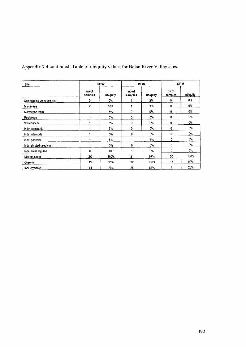
Appendix 7.4 continued: Table o f ubiquity values for Belan River Valley sites.
Site KDW M G R CPM
no of samples ubiquity
no of sam ples ubiquity
no of samples ubiquity
Commenlina benghalensis 0 0% 1 3% 0 0%
Malvaceae 2 10% 1 3% 0 0%
Malvaceae testa 1 5% 0 0% 0 0%
Rubiaceae 1 5% 0 0% 0 0%
Schleriaceae 1 5% 0 0% 0 0%
Indet culm node 1 5% 0 0% 0 0%
Indet internode 1 5% 0 0% 0 0%
Indet pedestal 1 5% 1 3% 0 0%
Indet striated seed coat 1 5% 0 0% 0 0%
Indet small legume 0 0% 1 3% 0 0%
Modem seeds 20 100% 31 97% 20 100%
Charcoal 19 95% 32 100% 18 90%
Indeterminate 14 70% 26 81% 4 20%
392

Appendix 7.5: Ubiquity values for published archaeobotanical data in North Indian Prehistoric sites. Dates are taken directly from the
published reports.
Hulaskera 1 Hulaskera II Hulaskera All Manjhi II Manjhi III Manjhi All Narhan I Narhan II Narhan III
Dates 700-500BC 500-200BC 600-50BC 50BC-AD3001000-
800BC 800-600BC 600-200BC
No of samples 5 1 6 3 1 4 32 17 5
Pulses 20% 0% 17% 100% 100% 100% 78% 59% 20%
Small millets 20% 100% 33% 33% 100% 50% 31% 0% 20%
Barley 60% 100% 67% 100% 100% 100% 63% 47% 20%
Wheat 0% 0% 0% 100% 100% 100% 66% 0% 20%
Rice 40% 0% 33% 100% 100% 100% 75% 53% 20%
Fruits 0% 0% 0% 0% 100% 25% 3% 0% 20%
All weeds 20% 0% 17% 100% 100% 100% 69% 0% 20%
Narhan IV Narhan All Malhar I Malhar II Malhar All Senuwar IA Senuwar IB Senuwar IISenuwar
All
Dates 200BC-AD400 2150-1600BC 1600-800BC2200-
1950BC1950-
1300BC1300-
600BC .
No of samples 1 55 14 26 40 52 54 40 146
Pulses 0% 65% 71% 77% 75% 35% 43% 58% 44%
Small millets 0% 20% 57% 23% 30% 37% 20% 15% 25%
Barley 0% 53% 43% 46% 45% 23% 17% 35% 24%
Wheat 0% 40% 29% 15% 20% 12% 20% 30% 20%
Rice 0% 62% 64% 69% 68% 60% 50% 53% 54%
Fruits 0% 4% 14% 15% 15% 15% 2% 10% 9%
All weeds 0% 42% 43% 62% 55% 10% 9% 40% 18%
v©o->
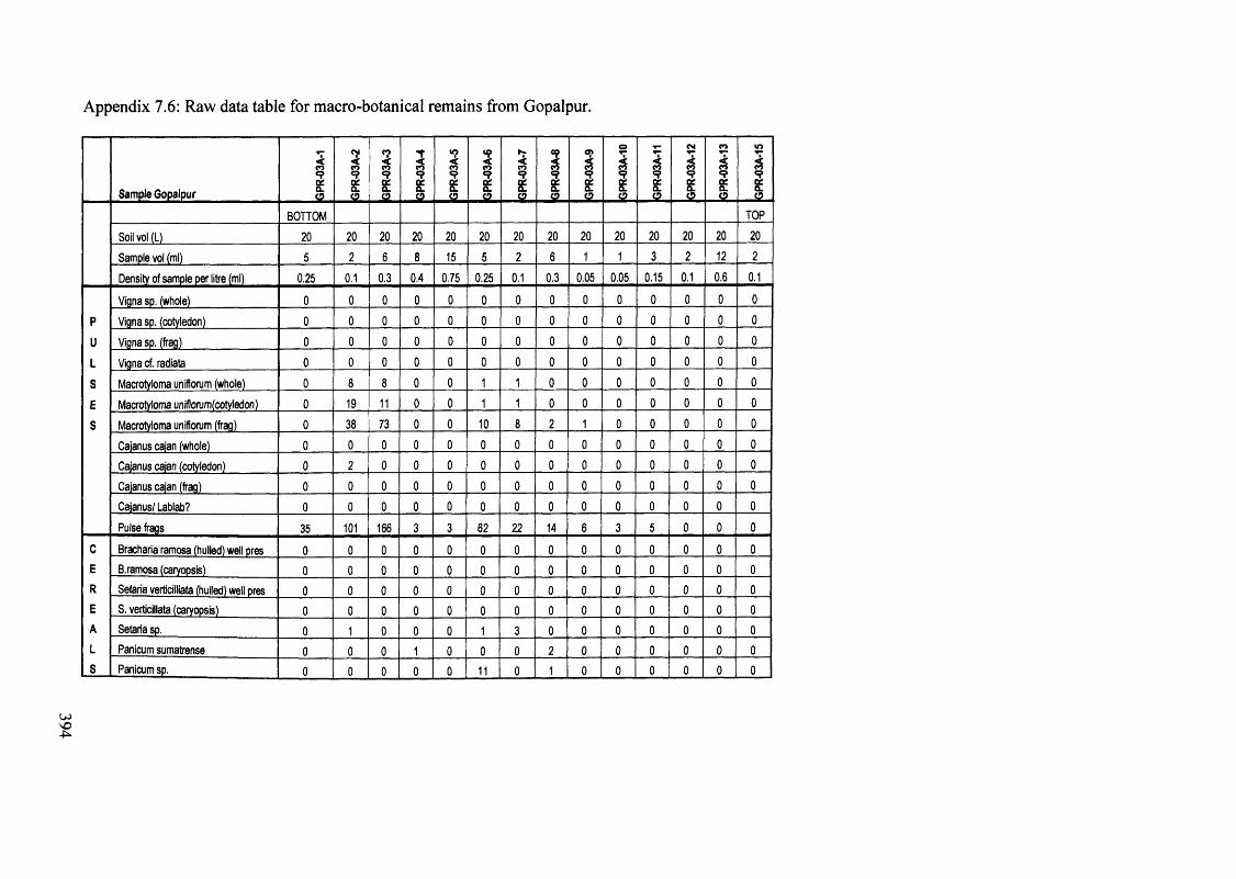
394
Appendix 7.6: Raw data table for macro-botanical remains from Gopalpur.
Sample Gopalpur GPR-
03A-
1
GPR-
03A-
2
GPR-
03A-
3
GPR
-03A
4
GPR-
03A-
5
GPR-
03A-
6
GPR-
03A-
7
GPR-
03A-
8
GPR-
03A-
9
GPR-
03A-
10
GPR-
03A-
11
GPR-
03A-
12
GPR-
03A-
13 in
51o
BOTTOM TOP
Soil vol (L) 20 20 20 20 20 20 20 20 20 20 20 20 20 20
Sample vol (ml) 5 2 6 8 15 5 2 6 1 1 3 2 12 2
Density of sample per litre (ml) 0.25 0.1 0.3 0.4 0.75 0.25 0.1 0.3 0.05 0.05 0.15 0.1 0.6 0.1
Vigna sp. (whole) 0 0 0 0 0 0 0 0 0 0 0 0 0 0
p Vigna sp. (cotyledon) 0 0 0 0 0 0 0 0 0 0 0 0 0 0
u Vigna sp. (frag) 0 0 0 0 0 0 0 0 0 0 0 0 0 0
L Vigna cf. radiata 0 0 0 0 0 0 0 0 0 0 0 0 0 0
S Macrotyloma uniflorum (whole) 0 8 8 0 0 1 1 0 0 0 0 0 0 0
E Macrotyloma uniflomm(cotyledon) 0 19 11 0 0 1 1 0 0 0 0 0 0 0
S Macrotyloma uniflorum (frag) 0 38 73 0 0 10 8 2 1 0 0 0 0 0
Cajanus cajan (whole) 0 0 0 0 0 0 0 0 0 0 0 0 0 0
Cajanus cajan (cotyledon) 0 2 0 0 0 0 0 0 0 0 0 0 0 0
Cajanus cajan (frag) 0 0 0 0 0 0 0 0 0 0 0 0 0 0
Cajanus/ Lablab? 0 0 0 0 0 0 0 0 0 0 0 0 0 0
Pulse frags 35 101 166 3 3 62 22 14 6 3 5 0 0 0
C Bracharia ramosa (hulled) well pres 0 0 0 0 0 0 0 0 0 0 0 0 0 0
E B.ramosa (caryopsis) 0 0 0 0 0 0 0 0 0 0 0 0 0 0
R Setaria verticilliata (hulled) well pres 0 0 0 0 0 0 0 0 0 0 0 0 0 0
E S. verticillata (caryopsis) 0 0 0 0 0 0 0 0 0 0 0 0 0 0
A Setaria sp. 0 1 0 0 0 1 3 0 0 0 0 0 0 0
L Panicum sumatrense 0 0 0 1 0 0 0 2 0 0 0 0 0 0
S Panicum sp. 0 0 0 0 0 11 0 1 0 0 0 0 0 0

Appendix 7.6 continued: Raw data table for macro-botanical remains from Gopalpur.
Sample Gopalpur GPR
-03A
-1
GPR
-03A
-2
GPR
-03A
-3
GPR
-03A
-4
GPR
-03A
-5
GPR
-03A
-6
GPR
-03A
-7
GPR
-03A
-8
GPR
-03A
-9
GPR
-03A
-10
GPR
-03A
-11
GPR
-03A
-12
GPR
-03A
-13
GPR
-03A
-15
Paspalum sp. 0 0 0 0 0 1 0 0 0 0 0 0 0 0
Echinochloa sp. 0 0 0 0 0 1 0 0 0 0 0 0 0 0
& Indeterminate small millets 0 0 0 0 0 14 0 18 0 3 1 0 2 0
Hordeum vulgare 0 0 0 0 0 0 0 0 0 0 0 0 0 0
G Triticum sp. 0 0 0 0 0 0 0 0 0 0 0 0 0 0
R Oryza sp. (whole caryopsis) 0 0 0 1 1 0 0 2 0 0 0 0 0 0
A Oryza sp. (caryopsis 1/2) 3 1 2 1 1 8 2 1 0 2 2 1 2 0
S Oryza sp. (caryopsis 1/4) 0 0 3 3 2 22 15 25 4 4 17 4 8 0
S Oryza sp. (glumes) 0 0 1 0 0 0 0 0 0 0 1 0 1 0
E Oryza sp. (spikelet base) 0 0 0 0 0 2 0 0 0 0 0 0 0 0
S Indet. Graminae (caryopsis) 0 0 0 0 0 1 0 0 0 0 0 0 0 0
Ziziphus sp. 0 0 0 0 0 0 0 0 0 0 0 0 0 0
Celtis sp. 0 1 0 0 0 0 0 0 0 0 0 1 0 0
Cyperaceae type 0 0 0 0 0 0 1 2 0 0 0 0 0 0
W cf. Cyperus sp. 0 0 0 0 0 0 0 3 0 0 0 0 0 0
E cf. Andropogonal sp. 0 0 0 0 0 0 0 1 0 0 0 0 0 0
E Cenchrus sp. type 0 1 0 0 0 0 0 0 0 0 0 0 0 0
D cf. Eragrostis sp. 0 0 0 0 2 0 0 0 0 0 0 0 0 0
S Ischaemum rugosum 0 0 0 0 0 1 0 1 0 1 6 0 0 0
Large grass type 1 0 24 4 1 0 0 0 0 0 0 0 0 0 0
Small grass 0 7 0 0 0 0 2 0 0 0 0 0 0 0
Polygonaceae type 0 0 0 0 0 14 2 2 0 0 4 1 1 0
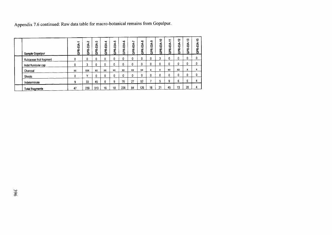
396
Appendix 7.6 continued: Raw data table for macro-botanical remains from Gopalpur.
Sample Gopalpur GPR
-03A
-1
GPR
-03A
-2
G PR
-03
A-3
GPR
-03A
-4
GPR
-03A
-5
GPR
-03A
-6
GPR
-03A
-7
GPR
-03A
-8
G PR
-03
A-9
GPR
-03A
-10
GPR
-03A
-11
GPR
-03A
-12
GPR
-03A
-13
GPR
-03A
-15
Rubiaceae fruit fraqment 0 0 0 0 0 0 0 0 0 3 0 0 0 0
Indet ffunicular cap 0 3 0 0 0 0 0 0 0 0 0 0 0 0
Charcoal XX XXX XX XX XX XX XX XX X X XX XX X X
Shoots 0 Y 0 0 0 0 0 0 0 0 0 0 0 0
Indeterminate 9 33 45 6 9 76 27 52 7 5 9 6 6 4
Total fragments 47 239 313 16 18 226 84 126 18 21 45 13 20 4
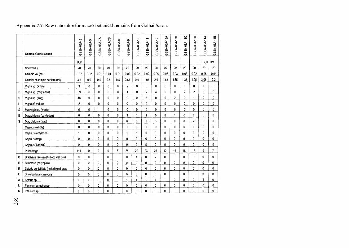
397
Appendix 7.7: Raw data table for macro-botanical remains from Golbai Sasan.
Sample Golbai Sasan GBS
N-0
3A-
3
GB
SN-0
3A-5
GB
SN-0
3A-7
A
GB
SN-0
3A-7
B
GB
SN-0
3A-8
GB
SN-0
3A-9
GB
SN-0
3A-1
0
GB
SN-0
3A-1
1
GB
SN-0
3A-1
2
GB
SN-0
3A-1
3A
GB
SN-0
3A-1
3B
GB
SN-0
3A-1
3C
GB
SN-0
3A-1
3D
GB
SN-0
3A-1
4A
GB
SN-0
3A-1
4B
TOP BOTTOM
Soil vol (L) 20 20 20 20 20 20 20 20 20 20 20 20 20 20 20
Sample vol (ml) 0.07 0.02 0.01 0.01 0.01 0.02 0.02 0.02 0.05 0.03 0.03 0.03 0.02 0.06 0.04
Density of sample per litre (ml) 3.5 0.9 0.4 0.5 0.5 0.85 0.9 1.05 2.4 1.65 1.65 1.35 1.05 3.05 2.2
Vigna sp. (whole) 3 0 0 0 0 2 0 0 0 0 0 0 0 0 0
p Vigna sp. (cotyledon) 39 0 0 0 0 1 0 2 4 0 0 2 2 1 0
u Vigna sp. (frag) 48 0 0 0 0 0 0 5 0 0 2 0 1 0 0
L Vigna cf. radiata 2 0 0 0 0 0 0 0 0 0 0 0 0 0 0
S Macrotyloma (whole) 0 0 1 0 0 0 0 0 0 0 0 0 0 0 0
E Macrotyloma (cotyledon) 0 0 0 0 0 3 1 1 5 0 1 0 0 0 0
S Macrotyloma (frag) 0 0 0 0 0 6 0 0 3 0 0 0 2 0 0
Cajanus (whole) 0 0 0 0 0 1 0 0 0 0 0 0 0 0 0
Cajanus (cotyledon) 1 0 0 0 0 1 1 0 0 0 0 0 0 0 0
Cajanus (frag) 0 0 0 0 0 0 0 0 0 0 0 0 0 0 0
Cajanus/ Lablab? 0 0 0 0 0 0 0 0 0 0 0 0 0 0 0
Pulse frags 111 9 0 4 6 25 29 23 25 12 16 18 12 9 7
C Bracharia ramosa (hulled) well pres 0 0 0 0 0 0 1 0 2 0 0 0 0 0 0
E B.ramosa (caryopsis) 0 0 0 0 0 0 0 0 0 0 0 0 0 0 0
R Setaria verticilliata (hulled) well pres 0 0 0 0 0 0 0 0 0 0 0 0 0 0 0
E S. verticillata (caryopsis) 0 0 0 0 0 0 0 0 0 0 0 0 0 0 0
A Setaria sp. 0 0 0 0 0 1 1 1 1 1 0 0 0 1 0
L Panicum sumatrense 0 0 0 0 0 0 0 0 0 0 0 0 0 0 0
S Panicum sp. 0 0 0 0 0 0 0 0 0 0 0 0 0 0 0

Appendix 7.7 continued: Raw data table for macro-botanical remains from Golbai Sasan.
Sample Golbai Sasan GBS
N-0
3A-
3
GB
SN-0
3A-5
GB
SN-0
3A-7
A
GB
SN-0
3A-7
B
GB
SN-0
3A-8
GB
SN-0
3A-9
GB
SN-0
3A-1
0
GB
SN-0
3A-1
1
GB
SN-0
3A-1
2
GB
SN-0
3A-1
3A
GB
SN-0
3A-1
3B
GB
SN-0
3A-1
3C
GB
SN-0
3A-1
3D
GB
SN-0
3A-1
4A
GB
SN-0
3A-1
4B
Paspalum sp. 0 0 0 0 0 0 0 0 0 0 0 0 0 3 0
& Paspalum sp. cf. vaginatum 1 0 0 0 0 0 0 0 0 0 0 0 0 0 0
Indeterminate small millet 0 0 1 0 0 5 0 3 1 4 0 0 0 0 2
G Hordeum vulgare 0 0 0 0 0 0 0 0 0 0 0 0 0 0 0
R Triticum sp. 0 0 0 0 0 0 0 0 0 0 0 0 0 0 0
A Oryza sp. (whole caryopsis) 1 0 0 0 1 5 0 3 1 1 0 0 3 2 2
S Oryza sp. (caryopsis 1/2) 4 3 0 0 2 19 7 12 17 0 4 4 6 9 12
S Oryza sp. (caryopsis 1/4) 13 15 5 6 4 80 23 25 29 7 13 5 10 12 29
E Oryza sp. (glume) 0 0 0 0 0 0 0 0 0 0 0 0 0 0 0
S Oryza sp. (husk imprints frags) 0 0 0 0 1 3 2 0 1 0 0 1 0 1 0
Indet Graminae (caryopsis) 0 2 0 0 0 24 10 6 13 0 2 0 5 0 7
Ziziphus sp. 0 0 0 0 0 1 2 6 0 0 0 0 0 0 0
Fruit stone unidentified 0 0 0 0 0 54 4 0 4 1 1 1 6 0 16
Ficus sp.? 0 0 0 0 0 15 0 0 0 0 0 0 0 0 0
Aizoceae Trianthamea type 0 0 0 0 0 1 0 0 0 0 1 0 0 0 0
W Asteraceae type 1 0 0 0 0 0 0 0 0 0 0 0 0 0 0
E Asteraceae cf. Eclipta type 0 0 0 0 0 0 0 0 1 0 0 0 0 0 0
E Asteraceae Tridex type 0 0 0 0 0 0 0 0 0 0 0 0 1 0 1
D Cyperaceae type 0 0 0 0 0 0 0 0 1 0 0 0 0 0 0
S Euphorbia type 1 0 0 0 0 0 0 0 0 0 0 0 0 0 0
Euphorbia type cf. Phyllanthus sp. 0 0 0 0 0 0 0 0 0 0 0 0 0 0 1

399
Appendix 7.7 continued: Raw data table for macro-botanical remains from Golbai Sasan.
Sample Golbai Sasan GBS
N-0
3A-
3
GB
SN-0
3A-5
GB
SN-0
3A-7
A
GB
SN-0
3A-7
B
GB
SN-0
3A-8
GB
SN-0
3A-9
GB
SN-0
3A-1
0
GB
SN-0
3A-1
1
GB
SN-0
3A-1
2
GB
SN-0
3A-1
3A
GB
SN-0
3A-1
3B
GB
SN-0
3A-1
3C
GB
SN-0
3A-1
3D
GB
SN-0
3A-1
4A
GB
SN-0
3A-1
4B
Ischaemum ruqosum 0 0 0 0 0 0 0 0 1 0 0 0 0 0 0
Small qrass 0 0 0 0 0 1 0 0 0 0 0 0 0 0 0
Malvaceae type 0 0 0 0 0 0 0 0 0 0 0 0 0 1 0
Polygonaceae type 0 0 0 0 0 0 0 0 0 0 0 0 0 0 1
Portulaca sp. 0 0 0 0 0 0 1 0 0 0 0 0 0 0 0
Rubiaceae cf. Oldenlandia mericarp 0 0 0 0 0 0 1 0 0 0 0 0 1 0 0
Rubiaceae fruit fragment 0 0 0 0 0 0 0 0 0 0 0 1 0 0 1
Scrophulariaceae cf. Lindemia/Scropiatype 0 0 0 0 0 1 2 0 0 0 0 0 0 0 1
Indet embryo 0 0 0 0 0 0 0 0 0 0 0 0 0 1 0
Indet striate seed case 0 0 0 0 1 0 0 0 0 0 0 0 0 0 0
Charcoal XX X XX X X XXX XX XX XX X XX X XX XXX XXX
Indeterminate 47 10 5 3 12 36 18 8 13 23 25 16 36 25 25
Total fragments 272 39 12 13 27 285 103 95 122 49 65 48 85 65 105
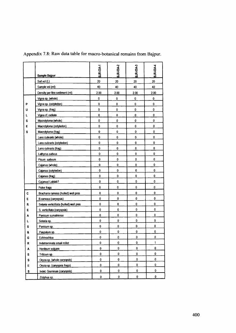
Appendix 7.8: Raw data table for macro-botanical remains from Bajpur.
Sample Bajpur BJR-
03A
-1
BJR-
03A
-2
BJR-
03A
-3
BJR
-03A
4
Soil vol (L) 20 20 20 20
Sample vol (ml) 40 40 40 40
Density per litre sediment (ml) 2.00 2.00 2.00 2.00
Vigna sp. (whole) 0 0 0 0
p Vigna sp. (cotyledon) 0 0 0 0
u Vigna sp. (frag) 0 0 0 0
L Vigna cf. radiata 0 0 0 0
S Macrotyloma (whole) 0 0 0 0
E Macrotyloma (cotyledon) 0 0 0 0
S Macrotyloma (frag) 0 0 0 0
Lens culinaris (whole) 0 0 0 0
Lens culinaris (cotyledon) 0 0 0 0
Lens culinaris (ffag) 0 0 0 0
Lathyrus sativus 0 0 0 0
Pisum sativum 0 0 0 0
Cajanus (whole) 0 0 0 0
Cajanus (cotyledon) 0 0 0 0
Cajanus (frag) 0 0 0 0
Cajanus/ Lablab? 0 0 0 0
Pulse frags 0 0 0 0
C Bracharia ramosa (hulled) well pres 0 0 0 0
E B.ramosa (caryopsis) 0 0 0 0
R Setaria verticilliata (hulled) well pres 0 0 0 0
E S. verticillata (caryopsis) 0 0 0 0
A Panicum sumatrense 0 0 0 0
L Setaria sp. 0 0 0 0
S Panicum sp. 0 0 0 0
& Paspalum sp. 0 0 0 0
G Echinochloa 0 0 0 0
R Indetreminate small millet 0 0 0 1
A Hordeum vulgare 0 0 0 0
S Triticumsp. 0 0 0 0
S Oryza sp. (whole caryopsis) 0 0 0 0
E Oryza sp. (caryopsis frags) 0 0 0 0
S Indet. Graminae (caryopsis) 0 0 0 0
Ziziphus sp. 0 0 0 0
400

Appendix 7.8 continued: Raw data table for macro-botanical remains from Bajpur.
Sample Bajpur BJR-
03A
-1
BJR-
03A
-2
BJR-
03A
-3
BJR
-03A
4
w Weeds seeds 0 0 0 0
E modem seeds XX XX XX XX
E Charcoal XX XX XX XX
D Shoots 0 0 0 0
S Indeterminate 1 1 0 0
Total fragments 1 1 0 1
401

Appendix 7.9: Raw data table for macro-botanical remains from Malakhoja.
Sample Malakhoja
Soil vol (L)
Sample vol (ml)
Density per litre sediment (ml)
152 100
3.75 7.6 0.75 0.75 0.75
Vigna sp. (whole)
Vigna sp. (cotyledon)
Vigna sp. (frag)
Vigna cf. radiata
Macrotyloma (whole)
Macrotyloma (cotyledon)
Macrotyloma (frag)
Lens culinaris (whole)
Lens culinaris (cotyledon)
Lens culinaris (frag)
Lathyrus sativus
Pisum sativum
Cajanus (whole)
Cajanus (cotyledon)
Cajanus (frag)
Cajanus/ Lablab?
Pulse frags
Bracharia ramosa (hulled) well pres
B.ramosa (caryopsis)____________
Setaria verticilliata (hulled) well pres
S. verticillata (caryopsis)
Panicum sumatrense
Setaria sp.
Panicum sp.
Paspalum sp.
Echinochloa
Other millets
Hordeum vulgare
Triticum sp.
Oryza sp. (whole caryopsis)
Oryza sp. (caryopsis frags)
Oryza sp. (husk frag)
Indet Graminae (caryopsis)
Ziziphus sp.
402
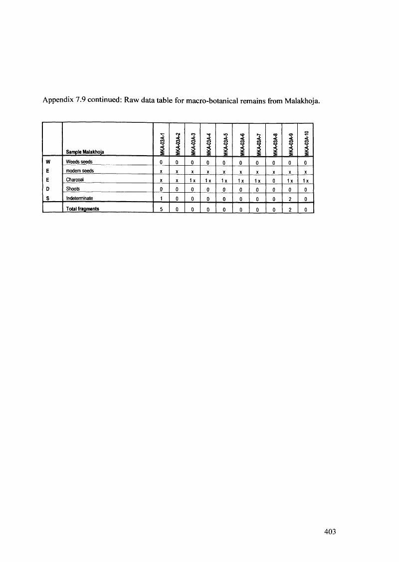
Appendix 7.9 continued: Raw data table for macro-botanical remains from Malakhoja.
Sample Malakhoja MKA
-03A
-1
MK
A-0
3A-2
MK
A-0
3A-3 ' t
<CO
2S M
KA
-03A
-5
MK
A-0
3A-6
MK
A-0
3A-7
MK
A-0
3A-8
MK
A-0
3A-9
MK
A-0
3A-1
0
w Weeds seeds 0 0 0 0 0 0 0 0 0 0
E modem seeds X X X X X X X X X X
E Charcoal X X 1 X 1 X 1 X 1 X 1 X 0 1 X 1 X
D Shoots 0 0 0 0 0 0 0 0 0 0
S Indeterminate 1 0 0 0 0 0 0 0 2 0
Total fragments 5 0 0 0 0 0 0 0 2 0
403

Appendix 7.10: Raw data table for macro-botanical remains from Banabasa.
Sample Banabasa m m mSoil vol (L)
Sample vol (ml)
Density per litre sediment (ml) 3.75
Vigna sp. (whole)
Vigna sp. (cotyledon)
Vigna sp. (frag)
Vigna cf. radiata
Macrotyloma (cotyledon)
Macrotyloma (frag)
Lens culinaris (whole)
Lens culinaris (cotyledon)
Lens culinaris (frag)
Lathyrus sativus
Pisum sativum
Cajanus (whole)
Cajanus (cotyledon)
Cajanus (frag)
Cajanus/ Lablab?
Pulse frag!
Bracharia ramosa (hulled) well pres
B.ramosa (caryopsis)
Setaria verticilliata (hulled) well pres
S. verticillata (caryopsis)
Panicum sumatrense
Setaria sp.
Panicum sp.
Paspalum sp.
Echinochloa
Other millets
Hordeum vulgare
Triticum sp.
Oryza sp. (whole caryopsis)
Oryza sp. (caryopsis frags)
Indet. Graminae (caryopsis)
Ziziphus sp.
Appendix 7.10 continued: Raw data table for macro-botanical remains from Banabasa.404

Sample Banabasa BNA
-03A
-1
BNA
-03A
-2
BNA
-03A
-3
w Weeds seeds 0 0 0
E modem seeds XX XX X
E Charcoal X X X
D Shoots 0 0 0
S Unknowns 0 0 0
Total fragments 0 0 0

406
Appendix 7.11: Results table for phytolith absolute densities (number per gram of sediment) from Koldihwa.
Single-cell KDW-01-1 KDW-01-2 KDW-01-3 KDW-014 KDW-01-5 KDW-01-6 KDW-01-7 KDW-01-8 KDW-01-9 KDW-01-10 KDW-01-11
Long (Smooth) 52926 120157 49351 17106 11909 25877 53262 42974 11131 9463 3341
Long (Sinuate) 6615 7152 2313 2534 1082 2322 5393 3657 706 249 57
Long (Rods) 2940 5721 0 422 0 331 0 0 0 249 57
Long (Dendritic) 30873 55787 28531 8236 6676 6303 14832 15086 3533 1245 485
Papillae 2205 0 771 633 0 0 0 0 0 0 28
Hairs 735 1430 2313 422 0 0 674 3200 353 124 57
Trichomes 7350 5721 12337 844 3067 1658 6067 7772 530 373 314
Bulliform 47780 38622 22362 18795 13894 28863 33036 19658 12014 6973 2256
Ovals 735 1430 0 422 361 332 1348 0 707 249 57
Keystone 18377 20026 16194 15628 16782 42465 25620 22859 21202 11830 4712
Crenates 5146 4291 0 422 180 332 674 457 177 0 28
Bilobes 131581 141614 60148 13938 11910 9953 28991 34746 3357 1868 456
Crosses 15437 11444 1542 1056 541 3649 2697 1829 530 374 456
Rondels 45575 57218 19278 7814 7579 8626 16181 10972 3534 2740 342
Saddles 45575 17165 17736 6547 8301 18579 8091 22402 4240 2989 685
Cones 735 0 771 422 722 1659 0 0 0 0 0
Flat Tower 2205 4291 3856 1478 722 664 0 0 353 0 28
Homed Tower 1470 4291 2313 422 180 0 674 914 0 0 0
Rice bulliform 2940 1430 0 634 0 0 2023 457 530 0 29
Phragmites bulliform 0 0 0 0 0 0 0 0 0 0 0
Double-peaked glume cell 6616 2861 4627 634 0 0 1348 2286 177 125 0
Rice bilobe 1470 2861 1542 422 361 664 674 914 530 374 29
Rugulose Spheroid 0 0 1542 211 0 332 0 914 530 623 86
Smooth Spheroid 0 4291 0 0 541 0 1348 1372 0 249 0
Elongate 6616 7152 3856 2323 1805 2986 6742 3657 353 249 29
Tracheids 1470 15735 771 1056 541 995 2023 4115 177 249 29
Two-Tiered 0 0 0 1689 0 0 0 0 0 0 0
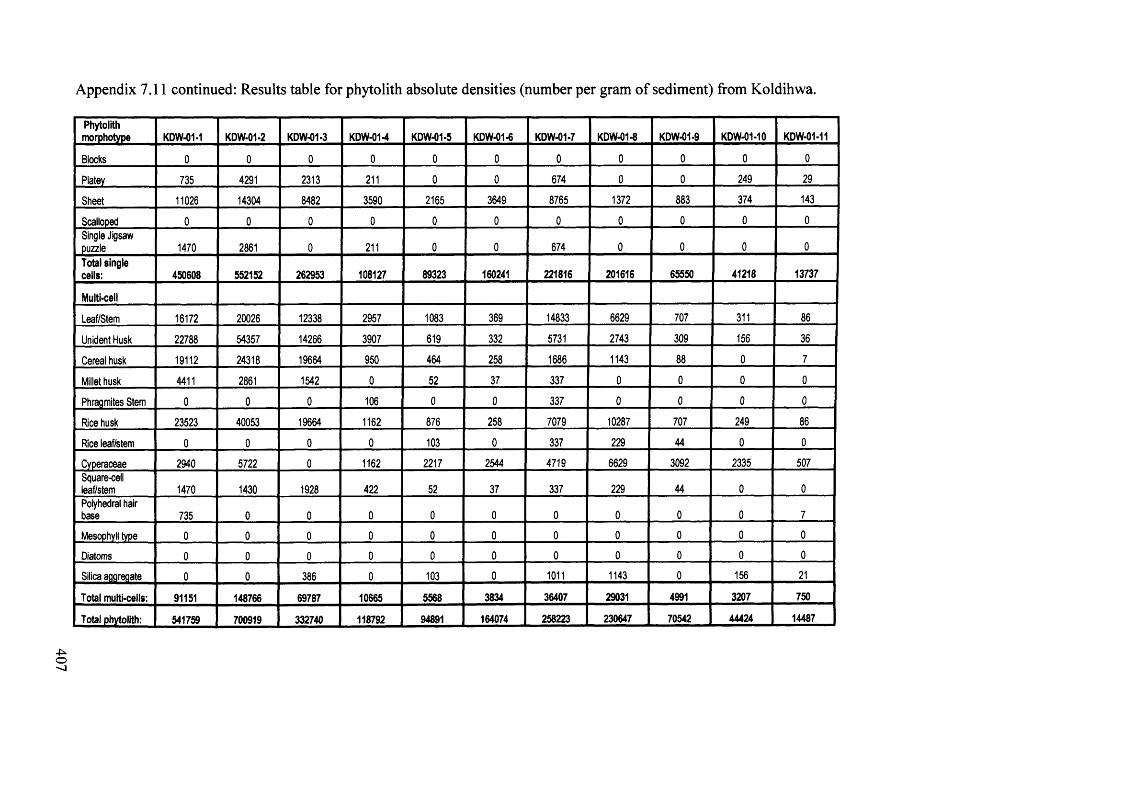
407
Appendix 7.11 continued: Results table for phytolith absolute densities (number per gram of sediment) from Koldihwa.
Phytolithmorphotype KDW-01-1 KDW-01-2 KDW-01-3 KDW-01-4 KDW-01-5 KDW-01-6 KDW-01-7 KDW-01-8 KDW-01-9 KDW-01-10 KDW-01-11
Blocks 0 0 0 0 0 0 0 0 0 0 0
Platey 735 4291 2313 211 0 0 674 0 0 249 29
Sheet 11026 14304 8482 3590 2165 3649 8765 1372 883 374 143
Scalloped 0 0 0 0 0 0 0 0 0 0 0
Single Jigsaw puzzle 1470 2861 0 211 0 0 674 0 0 0 0
Total single cells: 450608 552152 262953 108127 89323 160241 221816 201616 65550 41218 13737
Multi-cell
Leaf/Stem 16172 20026 12338 2957 1083 369 14833 6629 707 311 86
Unident Husk 22788 54357 14266 3907 619 332 5731 2743 309 156 36
Cereal husk 19112 24318 19664 950 464 258 1686 1143 88 0 7
Millet husk 4411 2861 1542 0 52 37 337 0 0 0 0
Phragmites Stem 0 0 0 106 0 0 337 0 0 0 0
Rice husk 23523 40053 19664 1162 876 258 7079 10287 707 249 86
Rice leaf/stem 0 0 0 0 103 0 337 229 44 0 0
Cyperaceae 2940 5722 0 1162 2217 2544 4719 6629 3092 2335 507Square-cellleaf/stem 1470 1430 1928 422 52 37 337 229 44 0 0Polyhedral hair base 735 0 0 0 0 0 0 0 0 0 7
Mesophyll type 0 0 0 0 0 0 0 0 0 0 0
Diatoms 0 0 0 0 0 0 0 0 0 0 0
Silica aggregate 0 0 386 0 103 0 1011 1143 0 156 21
Total multi-cells: 91151 148766 69787 10665 5568 3834 36407 29031 4991 3207 750
Total phytolith: 541759 700919 332740 118792 94891 164074 258223 230647 70542 44424 14487
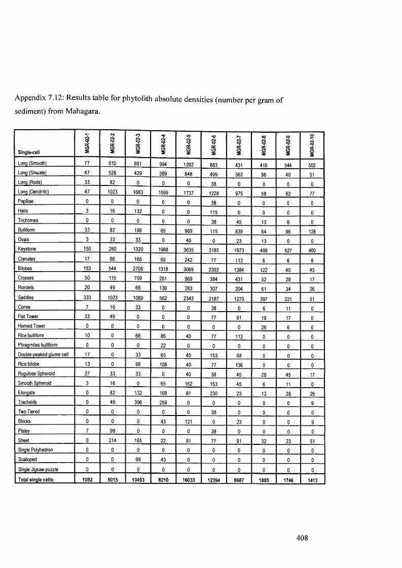
Appendix 7.12. Results table for phytolith absolute densities (number per gram of
sediment) from Mahagara.
Single-cell MG
R-02
-1
MG
R-02
-2
MG
R-02
-3
MG
R-02
-4
MG
R-02
-5
MG
R-02
-6
MG
R-02
-7
MG
R-02
-8
MG
R-02
-9
MG
R-02
-10
Long (Smooth) 77 610 891 994 1292 883 431 416 544 502Long (Sinuate) 47 528 429 389 848 499 363 96 40 51Long (Rods) 33 82 0 0 0 38 0 0 0 0Long (Dendritic) 47 1023 1683 1599 1737 1228 975 58 62 77Papillae 0 0 0 0 0 38 0 0 0 0Hairs 3 16 132 0 0 115 0 0 0 0Trichomes 0 0 0 0 0 38 45 13 6 0Bulliform 33 82 198 65 969 115 839 64 96 128Ovals 3 33 33 0 40 0 23 13 0 0Keystone 150 280 1320 1988 3635 3185 1973 499 527 400
Crenates 17 66 165 65 242 77 113 6 6 9
Bilobes 153 544 2706 1318 3069 2302 1384 122 40 43
Crosses 50 115 759 281 969 384 431 32 28 17
Rondels 20 49 66 130 283 307 204 51 34 26
Saddles 333 1023 1089 562 2342 2187 1270 397 221 51
Cones 7 16 33 0 0 38 0 6 11 0
Flat Tower 33 49 0 0 0 77 91 19 17 0
Horned Tower 0 0 0 0 0 0 0 26 6 0Rice bulliform 10 0 66 86 40 77 113 0 0 0
Phragmites bulliform 0 0 0 22 0 0 0 0 0 0
Double-peaked glume cell 17 0 33 65 40 153 68 0 0 0
Rice bilobe 13 0 66 108 40 77 136 0 0 0
Rugulose Spheroid 27 33 33 0 40 38 45 26 45 17
Smooth Spheroid 3 16 0 65 162 153 45 6 11 0
Elongate 0 82 132 108 81 230 23 13 28 26
Tracheids 0 49 396 259 0 0 0 0 0 9
Two-Tiered 0 0 0 0 0 38 0 0 0 0
Blocks 0 0 0 43 121 0 23 0 0 9
Platey 7 99 0 0 0 38 0 0 0 0
Sheet 0 214 165 22 81 77 91 32 23 51
Single Polyhedron 0 0 0 0 0 0 0 0 0 0
Scalloped 0 0 99 43 0 0 0 0 0 0
Single Jigsaw puzzle 0 0 0 0 0 0 0 0 0 0
Total single cells: 1082 5015 10493 8210 16033 12394 8687 1895 1746 1413
408

Appendix 7.12 continued. Results table for phytolith absolute densities (number per gram
of sediment) from Mahagara.
Multi-cell MG
R-02
-1
MG
R-02
-2
MG
R-02
-3
MG
R-02
-4
MG
R-02
-5
MG
R-02
-6
MG
R-02
-7
MG
R-02
-8
MG
R-02
-9
MG
R-02
-10
Leaf/Stem 12 82 434 278 263 205 156 3 8 0Unident Husk 12 231 1376 649 808 1049 439 15 8 9Millet husk 2 7 0 0 80 26 28 0 0 0Phragmites Stem 0 0 57 19 40 0 0 0 0 0Rice husk 2 27 283 111 40 102 99 0 0 0Cyperaceae 0 0 0 37 61 26 57 0 3 0Square-cell leaf/stem 0 0 0 0 0 0 0 0 0 0Mesophyll type 0 0 0 0 0 0 0 0 0 0
Diatoms 30 163 57 93 101 281 298 252 169 145
Total multi-cells: 59 509 2206 1185 1393 1688 1077 270 189 153
Total phytoliths: 1141 5524 12700 9395 17427 14082 9764 2165 1935 1566
409

Appendix 7.13: Results table for phytolith absolute density (number per gram
sediment) from Chopani Mando.
Single-cell CPM-01-1 CPM-01-3 CPM-01-5 CPM-01-7 CPM-01-9
Lonq (Smooth) 5795 10057 2119 4809 905
Lonq (Sinuate) 216 532 110 174 52
Lonq (Rods) 0 0 0 0 0
Lonq (Dendritic) 36 133 0 21 17
Papillae 0 0 0 0 0
Hairs0 0 0 21 0
Trichomes 431 466 124 217 74
Bulliform 2267 2730 817 1109 158
Ovals 36 0 55 0 4
Keystone 2447 2863 568 805 263
Crenates 0 0 0 0 0
Bilobes 36 133 13 108 30
Crosses 0 0 0 0 0
Rondels 0.00 333 27 87 21
Saddles 216 0.00 55 43 39
Cones 0 0 0 0 0
Flat Tower0 0 0 0 0
Homed Tower 0 0 0 0 0
Rice bulliform 0 0 0 0 0
Phragmites bulliform0 0 0 0 0
Double-peaked glume cell 0 0 0 0 0
Rice bilobe 0 0 0 0 0
Ruqulose Spheroid 252 1132 235 500 70
Smooth Spheroid 0 133 0 21 17
Elongate 36 333 41 130 17
Tracheids0 0 0 0 0
Blocks0 0 0 0 0
Platey 0 66 0 0 17
Sheet 216 266 13 652 13
Scalloped 36 0 0 0 0
Sinqle Jigsaw puzzle 0 0 0 0 0
Total single cells: 12024 19182 4184 8706 1706
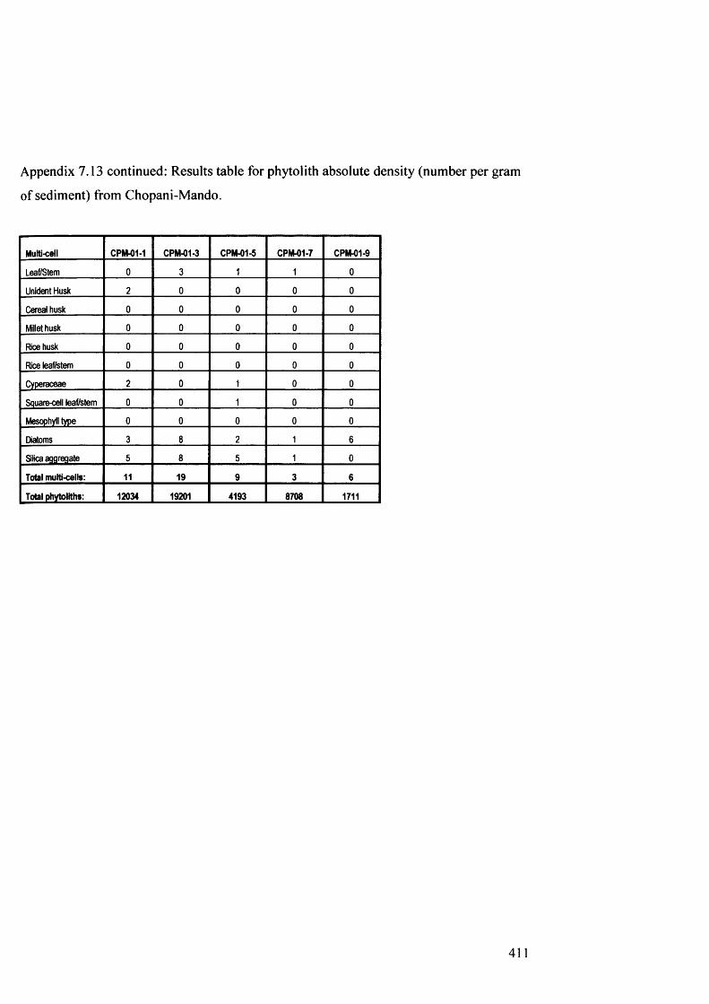
Appendix 7.13 continued: Results table for phytolith absolute density (number per gram
of sediment) from Chopani-Mando.
Multi-cell CPM-01-1 CPM-01-3 CPM-01-5 CPM-01-7 CPM-01-9
Leaf/Stem 0 3 1 1 0
Unident Husk 2 0 0 0 0
Cereal husk 0 0 0 0 0
Millet husk 0 0 0 0 0
Rice husk 0 0 0 0 0
Rice leaf/stem 0 0 0 0 0
Cyperaceae 2 0 1 0 0
Square-cell leaf/stem 0 0 1 0 0
Mesophyll type 0 0 0 0 0
Diatoms 3 8 2 1 6
Silica aggregate 5 8 5 1 0
Total multi-cells: 11 19 9 3 6
Total phytoliths: 12034 19201 4193 8708 1711
411
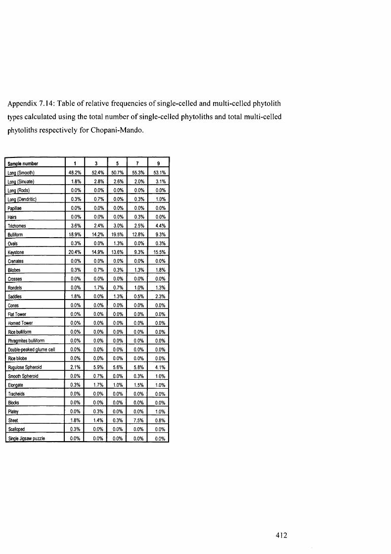
Appendix 7.14: Table o f relative frequencies o f single-celled and multi-celled phytolith
types calculated using the total number o f single-celled phytoliths and total multi-celled
phytoliths respectively for Chopani-Mando.
Sample number 1 3 5 7 9
Long (Smooth) 48.2% 52.4% 50.7% 55.3% 53.1%
Long (Sinuate) 1.8% 2.8% 2.6% 2.0% 3.1%
Long (Rods) 0.0% 0.0% 0.0% 0.0% 0.0%
Long (Dendritic) 0.3% 0.7% 0.0% 0.3% 1.0%
Papillae 0.0% 0.0% 0.0% 0.0% 0.0%
Hairs 0.0% 0.0% 0.0% 0.3% 0.0%
Trichomes 3.6% 2.4% 3.0% 2.5% 4.4%
Bulliform 18.9% 14.2% 19.5% 12.8% 9.3%
Ovals 0.3% 0.0% 1.3% 0.0% 0.3%
Keystone 20.4% 14.9% 13.6% 9.3% 15.5%
Crenates 0.0% 0.0% 0.0% 0.0% 0.0%
Bilobes 0.3% 0.7% 0.3% 1.3% 1.8%
Crosses 0.0% 0.0% 0.0% 0.0% 0.0%
Rondels 0.0% 1.7% 0.7% 1.0% 1.3%
Saddles 1.8% 0.0% 1.3% 0.5% 2.3%
Cones 0.0% 0.0% 0.0% 0.0% 0.0%
Flat Tower 0.0% 0.0% 0.0% 0.0% 0.0%
Homed Tower 0.0% 0.0% 0.0% 0.0% 0.0%
Rice bulliform 0.0% 0.0% 0.0% 0.0% 0.0%
Phragmites bulliform 0.0% 0.0% 0.0% 0.0% 0.0%
Double-peaked glume cell 0.0% 0.0% 0.0% 0.0% 0.0%
Rice bilobe 0.0% 0.0% 0.0% 0.0% 0.0%
Rugulose Spheroid 2.1% 5.9% 5.6% 5.8% 4.1%
Smooth Spheroid 0.0% 0.7% 0.0% 0.3% 1.0%
Elongate 0.3% 1.7% 1.0% 1.5% 1.0%
Tracheids 0.0% 0.0% 0.0% 0.0% 0.0%
Blocks 0.0% 0.0% 0.0% 0.0% 0.0%
Platey 0.0% 0.3% 0.0% 0.0% 1.0%
Sheet 1.8% 1.4% 0.3% 7.5% 0.8%
Scalloped 0.3% 0.0% 0.0% 0.0% 0.0%
Single Jigsaw puzzle 0.0% 0.0% 0.0% 0.0% 0.0%
412
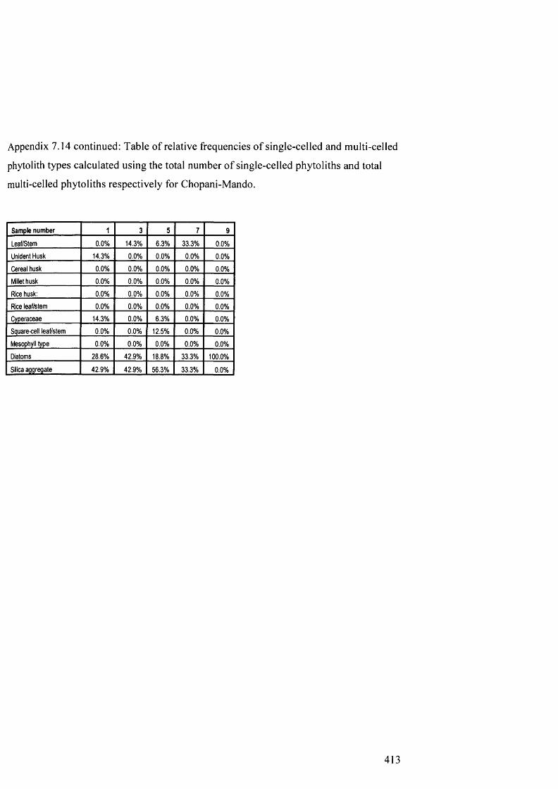
Appendix 7.14 continued: Table of relative frequencies o f single-celled and multi-celled
phytolith types calculated using the total number o f single-celled phytoliths and total
multi-celled phytoliths respectively for Chopani-Mando.
Sample number 1 3 5 7 9
Leaf/Stem 0.0% 14.3% 6.3% 33.3% 0.0%
Unident Husk 14.3% 0.0% 0.0% 0.0% 0.0%
Cereal husk 0.0% 0.0% 0.0% 0.0% 0.0%
Millet husk 0.0% 0.0% 0.0% 0.0% 0.0%
Rice husk: 0.0% 0.0% 0.0% 0.0% 0.0%
Rice leaf/stem 0.0% 0.0% 0.0% 0.0% 0.0%
Cyperaceae 14.3% 0.0% 6.3% 0.0% 0.0%
Square-cell leaf/stem 0.0% 0.0% 12.5% 0.0% 0.0%
Mesophyll type 0.0% 0.0% 0.0% 0.0% 0.0%
Diatoms 28.6% 42.9% 18.8% 33.3% 100.0%
Silica aggregate 42.9% 42.9% 56.3% 33.3% 0.0%
413
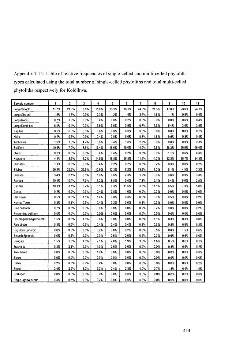
Appendix 7.15: Table o f relative frequencies o f single-celled and multi-celled phytolith
types calculated using the total number o f single-celled phytoliths and total multi-celled
phytoliths respectively for Koldihwa.
Sample number 1 2 3 4 5 6 7 8 9 10 11
Long (Smooth) 11.7% 21.8% 18.8% 15.8% 13.3% 16.1% 24.0% 21.3% 17.0% 23.0% 24.3%
Long (Sinuate) 1.5% 1.3% 0.9% 2.3% 1.2% 1.4% 2.4% 1.8% 1.1% 0.6% 0.4%
Long (Rods) 0.7% 1.0% 0.0% 0.4% 0.0% 0.2% 0.0% 0.0% 0.0% 0.6% 0.4%
Long (Dendritic) 6.9% 10.1% 10.9% 7.6% 7.5% 3.9% 6.7% 7.5% 5.4% 3.0% 3.5%
Papillae 0.5% 0.0% 0.3% 0.6% 0.0% 0.0% 0.0% 0.0% 0.0% 0.0% 0.2%
Hairs 0.2% 0.3% 0.9% 0.4% 0.0% 0.0% 0.3% 1.6% 0.5% 0.3% 0.4%
Trichomes 1.6% 1.0% 4.7% 0.8% 3.4% 1.0% 2.7% 3.9% 0.8% 0.9% 2.3%
Bulliform 10.6% 7.0% 8.5% 17.4% 15.6% 18.0% 14.9% 9.8% 18.3% 16.9% 16.4%
Ovals 0.2% 0.3% 0.0% 0.4% 0.4% 0.2% 0.6% 0.0% 1.1% 0.6% 0.4%
Keystone 4.1% 3.6% 6.2% 14.5% 18.8% 26.5% 11.6% 11.3% 32.3% 28.7% 34.3%
Crenates 1.1% 0.8% 0.0% 0.4% 0.2% 0.2% 0.3% 0.2% 0.3% 0.0% 0.2%
Bilobes 29.2% 25.6% 22.9% 12.9% 13.3% 6.2% 13.1% 17.2% 5.1% 4.5% 3.3%
Crosses 3.4% 2.1% 0.6% 1.0% 0.6% 2.3% 1.2% 0.9% 0.8% 0.9% 3.3%
Rondels 10.1% 10.4% 7.3% 7.2% 8.5% 5.4% 7.3% 5.4% 5.4% 6.6% 2.5%
Saddles 10.1% 3.1% 6.7% 6.1% 9.3% 11.6% 3.6% 11.1% 6.5% 7.3% 5.0%
Cones 0.2% 0.0% 0.3% 0.4% 0.8% 1.0% 0.0% 0.0% 0.0% 0.0% 0.0%
Flat Tower 0.5% 0.8% 1.5% 1.4% 0.8% 0.4% 0.0% 0.0% 0.5% 0.0% 0.2%
Homed Tower 0.3% 0.8% 0.9% 0.4% 0.2% 0.0% 0.3% 0.5% 0.0% 0.0% 0.0%
Rice bulliform 0.7% 0.3% 0.0% 0.6% 0.0% 0.0% 0.9% 0.2% 0.8% 0.0% 0.2%
Phragmites bulliform 0.0% 0.0% 0.0% 0.0% 0.0% 0.0% 0.0% 0.0% 0.0% 0.0% 0.0%
Double-peaked glume cell 1.5% 0.5% 1.8% 0.6% 0.0% 0.0% 0.6% 1.1% 0.3% 0.3% 0.0%
Rice bilobe 0.3% 0.5% 0.6% 0.4% 0.4% 0.4% 0.3% 0.5% 0.8% 0.9% 0.2%
Rugulose Spheroid 0.0% 0.0% 0.6% 0.2% 0.0% 0.2% 0.0% 0.5% 0.8% 1.5% 0.6%
Smooth Spheroid 0.0% 0.8% 0.0% 0.0% 0.6% 0.0% 0.6% 0.7% 0.0% 0.6% 0.0%
Elongate 1.5% 1.3% 1.5% 2.1% 2.0% 1.9% 3.0% 1.8% 0.5% 0.6% 0.2%
Tracheids 0.3% 2.8% 0.3% 1.0% 0.6% 0.6% 0.9% 2.0% 0.3% 0.6% 0.2%
Two-Tiered 0.0% 0.0% 0.0% 1.6% 0.0% 0.0% 0.0% 0.0% 0.0% 0.0% 0.0%
Blocks 0.0% 0.0% 0.0% 0.0% 0.0% 0.0% 0.0% 0.0% 0.0% 0.0% 0.0%
Platey 0.2% 0.8% 0.9% 0.2% 0.0% 0.0% 0.3% 0.0% 0.0% 0.6% 0.2%
Sheet 2.4% 2.6% 3.2% 3.3% 2.4% 2.3% 4.0% 0.7% 1.3% 0.9% 1.0%
Scalloped 0.0% 0.0% 0.0% 0.0% 0.0% 0.0% 0.0% 0.0% 0.0% 0.0% 0.0%
Single Jigsaw puzzle 0.3% 0.5% 0.0% 0.2% 0.0% 0.0% 0.3% 0.0% 0.0% 0.0% 0.0%
414
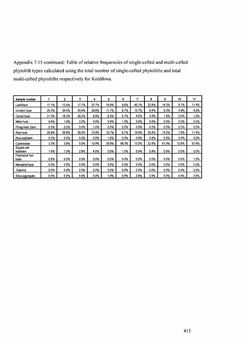
Appendix 7.15 continued: Table o f relative frequencies o f single-celled and multi-celled
phytolith types calculated using the total number o f single-celled phytoliths and total
multi-celled phytoliths respectively for Koldihwa.
Sample number 1 2 3 4 5 6 7 8 9 10 11
Leaf/Stem 17.7% 13.5% 17.7% 27.7% 19.4% 9.6% 40.7% 22.8% 14.2% 9.7% 11.4%
Unident Husk 25.0% 36.5% 20.4% 36.6% 11.1% 8.7% 15.7% 9.4% 6.2% 4.9% 4.8%
Cereal husk 21.0% 16.3% 28.2% 8.9% 8.3% 6.7% 4.6% 3.9% 1.8% 0.0% 1.0%
Millet husk 4.8% 1.9% 2.2% 0.0% 0.9% 1.0% 0.9% 0.0% 0.0% 0.0% 0.0%
Phragmites Stem 0.0% 0.0% 0.0% 1.0% 0.0% 0.0% 0.9% 0.0% 0.0% 0.0% 0.0%
Rice husk 25.8% 26.9% 28.2% 10.9% 15.7% 6.7% 19.4% 35.4% 14.2% 7.8% 11.4%
Rice leaf/stem 0.0% 0.0% 0.0% 0.0% 1.9% 0.0% 0.9% 0.8% 0.9% 0.0% 0.0%
Cyperaceae 3.2% 3.8% 0.0% 10.9% 39.8% 66.3% 13.0% 22.8% 61.9% 72.8% 67.6%Square-cellleaf/stem 1.6% 1.0% 2.8% 4.0% 0.9% 1.0% 0.9% 0.8% 0.9% 0.0% 0.0%Polyhedral hair base 0.8% 0.0% 0.0% 0.0% 0.0% 0.0% 0.0% 0.0% 0.0% 0.0% 1.0%
Mesophyll type 0.0% 0.0% 0.0% 0.0% 0.0% 0.0% 0.0% 0.0% 0.0% 0.0% 0.0%
Diatoms 0.0% 0.0% 0.0% 0.0% 0.0% 0.0% 0.0% 0.0% 0.0% 0.0% 0.0%
Silica aggregate 0.0% 0.0% 0.6% 0.0% 1.9% 0.0% 2.8% 3.9% 0.0% 4.9% 2.9%
415

Appendix 7.16: Table o f relative frequencies o f single-celled and multi-celled phytolith
types calculated using the total number o f single-celled phytoliths and total multi-celled
phytoliths respectively for Mahagara.
Sample number 1 2 3 4 5 6 7 8 9 10
Long (Smooth) 7.1% 12.2% 8.5% 12.1% 8.1% 7.1% 5.0% 22.0% 31.2% 35.5%
Long (Sinuate) 4.3% 10.5% 4.1% 4.7% 5.3% 4.0% 4.2% 5.1% 2.3% 3.6%
Long (Rods) 3.1% 1.6% 0.0% 0.0% 0.0% 0.3% 0.0% 0.0% 0.0% 0.0%
Long (Dendritic) 4.3% 20.4% 16.0% 19.5% 10.8% 9.9% 11.2% 3.0% 3.6% 5.4%
Papillae 0.0% 0.0% 0.0% 0.0% 0.0% 0.3% 0.0% 0.0% 0.0% 0.0%
Hairs 0.3% 0.3% 1.3% 0.0% 0.0% 0.9% 0.0% 0.0% 0.0% 0.0%
Trichomes 0.0% 0.0% 0.0% 0.0% 0.0% 0.3% 0.5% 0.7% 0.3% 0.0%
Bulliform 3.1% 1.6% 1.9% 0.8% 6.0% 0.9% 9.7% 3.4% 5.5% 9.0%
Ovals 0.3% 0.7% 0.3% 0.0% 0.3% 0.0% 0.3% 0.7% 0.0% 0.0%
Keystone 13.8% 5.6% 12.6% 24.2% 22.7% 25.7% 22.7% 26.4% 30.2% 28.3%
Crenates 1.5% 1.3% 1.6% 0.8% 1.5% 0.6% 1.3% 0.3% 0.3% 0.6%
Bilobes 14.2% 10.9% 25.8% 16.1% 19.1% 18.6% 15.9% 6.4% 2.3% 3.0%
Crosses 4.6% 2.3% 7.2% 3.4% 6.0% 3.1% 5.0% 1.7% 1.6% 1.2%
Rondels 1.8% 1.0% 0.6% 1.6% 1.8% 2.5% 2.3% 2.7% 1.9% 1.8%
Saddles 30.8% 20.4% 10.4% 6.8% 14.6% 17.6% 14.6% 20.9% 12.7% 3.6%
Cones 0.6% 0.3% 0.3% 0.0% 0.0% 0.3% 0.0% 0.3% 0.6% 0.0%
Flat Tower 3.1% 1.0% 0.0% 0.0% 0.0% 0.6% 1.0% 1.0% 1.0% 0.0%
Horned Tower 0.0% 0.0% 0.0% 0.0% 0.0% 0.0% 0.0% 1.4% 0.3% 0.0%
Rice bulliform 0.9% 0.0% 0.6% 1.1% 0.3% 0.6% 1.3% 0.0% 0.0% 0.0%
Phragmites bulliform 0.0% 0.0% 0.0% 0.3% 0.0% 0.0% 0.0% 0.0% 0.0% 0.0%
Double-peaked glume cell 1.5% 0.0% 0.3% 0.8% 0.3% 1.2% 0.8% 0.0% 0.0% 0.0%
Rice bilobe 1.2% 0.0% 0.6% 1.3% 0.3% 0.6% 1.6% 0.0% 0.0% 0.0%
Rugulose Spheroid 2.5% 0.7% 0.3% 0.0% 0.3% 0.3% 0.5% 1.4% 2.6% 1.2%
Smooth Spheroid 0.3% 0.3% 0.0% 0.8% 1.0% 1.2% 0.5% 0.3% 0.6% 0.0%
Elongate 0.0% 1.6% 1.3% 1.3% 0.5% 1.9% 0.3% 0.7% 1.6% 1.8%
Tracheids 0.0% 1.0% 3.8% 3.2% 0.0% 0.0% 0.0% 0.0% 0.0% 0.6%
Two-Tiered 0.0% 0.0% 0.0% 0.0% 0.0% 0.3% 0.0% 0.0% 0.0% 0.0%
Blocks 0.0% 0.0% 0.0% 0.5% 0.8% 0.0% 0.3% 0.0% 0.0% 0.6%
Platey 0.6% 2.0% 0.0% 0.0% 0.0% 0.3% 0.0% 0.0% 0.0% 0.0%
Sheet 0.0% 4.3% 1.6% 0.3% 0.5% 0.6% 1.0% 1.7% 1.3% 3.6%
Scalloped 0.0% 0.0% 0.9% 0.5% 0.0% 0.0% 0.0% 0.0% 0.0% 0.0%
Single Jigsaw puzzle 0.0% 0.0% 0.0% 0.0% 0.0% 0.0% 0.0% 0.0% 0.0% 0.0%
416
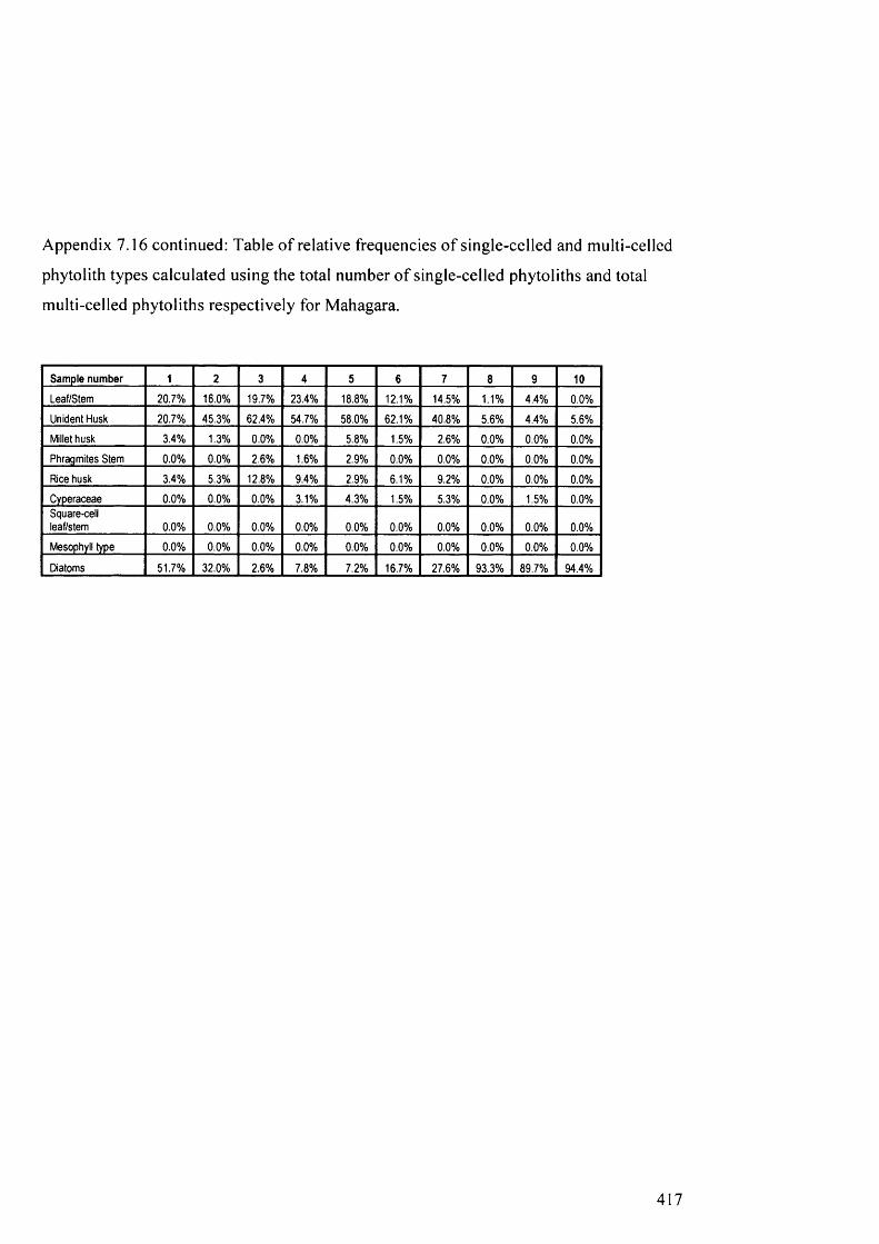
Appendix 7.16 continued: Table o f relative frequencies o f single-celled and multi-celled
phytolith types calculated using the total number o f single-celled phytoliths and total
multi-celled phytoliths respectively for Mahagara.
Sample number 1 2 3 4 5 6 7 8 9 10
Leaf/Stem 20.7% 16.0% 19.7% 23.4% 18.8% 12.1% 14.5% 1.1% 4.4% 0.0%
Unident Husk 20.7% 45.3% 62.4% 54.7% 58.0% 62.1% 40.8% 5.6% 4.4% 5.6%
Millet husk 3.4% 1.3% 0.0% 0.0% 5.8% 1.5% 2.6% 0.0% 0.0% 0.0%
Phragmites Stem 0.0% 0.0% 2.6% 1.6% 2.9% 0.0% 0.0% 0.0% 0.0% 0.0%
Rice husk 3.4% 5.3% 12.8% 9.4% 2.9% 6.1% 9.2% 0.0% 0.0% 0.0%
Cyperaceae 0.0% 0.0% 0.0% 3.1% 4.3% 1.5% 5.3% 0.0% 1.5% 0.0%Square-cellleaf/stem 0.0% 0.0% 0.0% 0.0% 0.0% 0.0% 0.0% 0.0% 0.0% 0.0%
Mesophyll type 0.0% 0.0% 0.0% 0.0% 0.0% 0.0% 0.0% 0.0% 0.0% 0.0%
Diatoms 51.7% 32.0% 2.6% 7.8% 7.2% 16.7% 27.6% 93.3% 89.7% 94.4%
417

Appendix 7.17: Results table for phytolith absolute density (number per gram of
sediment) from Bajpur.
Single-cell BJR-03-0 BJR-03-1 BJR-03-2 BJR-03-3 BJR-03-4
Long (Smooth) 8789 15482 13291 9177 42384
Long (Sinuate) 1143 481 652 1278 4645
Long (Rods) 0 0 0 0 0
Long (Dendritic) 352 288 163 232 290
Papillae 88 0 0 0 290
Hairs 0 0 82 232 581
Trichomes 1143 1250 897 929 3193
Bulliform 12217 6250 6034 6854 25256
Ovals 176 481 245 349 0
Keystone 16172 18655 18999 19516 76349
Crenates 0 0 0 0 0
Bilobes 879 288 163 232 290
Crosses 88 0 0 0 0
Rondels 0 192 245 697 581
Saddles 879 1346 1305 1626 5225
Cones 176 0 0 116 290
Flat Tower 0 0 0 116 0
Homed Tower 88 0 82 0 0
Rice bulliform 615 96 82 0 0
Phragmites bulliform 88 0 0 0 0Double-peaked glume cell 0 0 0 0 0
Rice bilobe 88 0 0 0 0
Rugulose Spheroid 264 96 489 465 581
Smooth Spheroid 176 192 163 0 290
Elongate 264 192 326 349 3193
Tracheids 264 0 0 0 0
Blocks 88 481 163 0 871
Platey 176 0 0 0 581
Sheet 0 0 163 116 2322
Scalloped 0 96 0 0 871
Single Jigsaw puzzle 88 0 0 0 0
Total single cells: 44298 45868 43544 42286 168085
418

Appendix 7.17 continued: Results table for phytolith absolute density (number per gram
o f sediment) from Bajpur.
Multi-cell BJR-03-0 BJR-03-1 BJR-03-2 BJR-03-3 BJR-03-4
Leaf/Stem 15 0 10 0 0
Unident Husk 4 0 0 0 0
Cereal husk 0 0 0 0 0
Millet husk 0 0 0 0 0
Rice husk 7 0 0 0 0
Rice leaf/stem 0 0 0 0 0
Cyperaceae 15 0 0 0 0
Square-cell leaf/stem 0 0 0 0 0
Mesophyll type 0 0 0 0 0
Diatoms 0 0 0 0 0
Silica aggregate 88 112 65 31 73
Indet multi-cell 0 0 0 2 0
Total multi-cells: 128 112 75 34 73
Total phytoliths: 44426 45980 43618 42319 168157
419

Appendix 7.18: Results table for phytolith absolute density (number per gram o f
sediment) from Malakhoja.
Single-cell 1 4 7 9
Long (Smooth) 13970 18653 9514 4090
Long (Sinuate) 916 1554 423 422
Long (Rods) 0 0 0 0
Long (Dendritic) 229 666 282 42
Papillae 115 0 0 0
Hairs 0 0 0 0
Trichomes 802 1554 423 295
Bulliform 7100 9326 3806 1855
Ovals 229 0 0 42
Keystone 16032 34863 12474 4596
Crenates 0 0 0 0
Bilobes 229 222 0 42
Crosses 0 0 0 0
Rondels 229 888 775 0
Saddles 1145 4885 634 211
Cones 0 0 0 0
Flat Tower 0 0 0 0
Homed Tower 0 0 0 0
Rice bulliform 0 0 0 0
Phragmites bulliform 0 0 0 0
Double-peaked glume cell 0 0 0 0
Rice bilobe 0 0 0 0
Rugulose Spheroid 0 222 0 0
Smooth Spheroid 0 0 0 0
Elongate 344 666 141 169
Tracheids 0 0 0 0
Blocks 344 3997 634 506
Platey 0 0 0 0
Sheet 229 1554 141 253
Scalloped 115 222 0 42
Single Jigsaw puzzle 344 0 0 0
Total single cells: 42369 79274 29247 12565
420
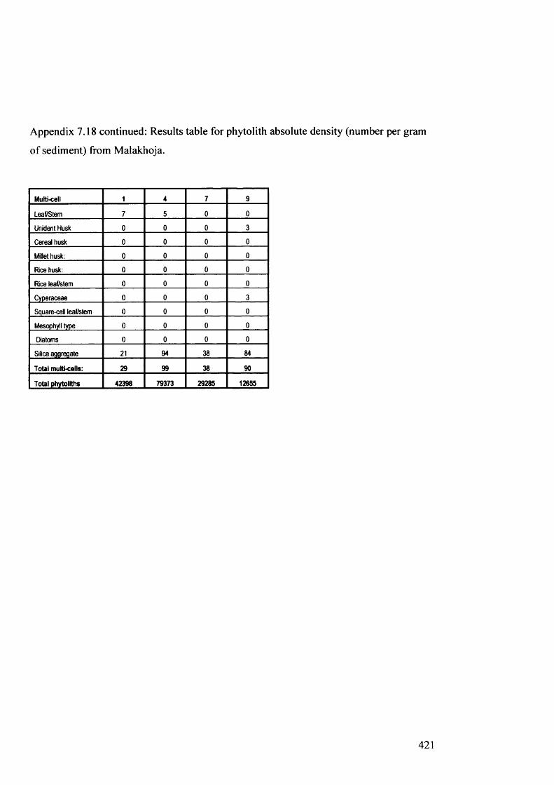
Appendix 7.18 continued: Results table for phytolith absolute density (number per gram
o f sediment) from Malakhoja.
Multi-cell 1 4 7 9
Leaf/Stem 7 5 0 0
Unident Husk 0 0 0 3
Cereal husk 0 0 0 0
Millet husk: 0 0 0 0
Rice husk: 0 0 0 0
Rice leaf/stem 0 0 0 0
Cyperaceae 0 0 0 3
Square-cell leaf/stem 0 0 0 0
Mesophyll type 0 0 0 0
Diatoms 0 0 0 0
Silica aggregate 21 94 38 84
Total multi-cells: 29 99 38 90
Total phytoliths 42398 79373 29285 12655
421

422
Appendix 7.19: Results table for phytolith absolute density (number per gram of sediment) from Gopalpur.
Single-cell GPR-
03A-
1
GPR-
03A-
2
G PR-
03A-
3
GPR-
03A-
4
GPR-
03A-
5
GPR-
03A-
6
GPR-
03A-
7
G PR-
03A-
8
GPR-
03A-
9
GPR-
03A-
10
GPR-
03A-
11
GPR-
03A-
12
GPR-
03A-
13
GPR-
03A-
14
Long (Smooth) 400 1397 755 444 1721 11621 6873 5768 12568 4008 10795 4504 25084 7402
Long (Sinuate) 47 243 136 70 186 474 1195 240 150 332 1080 415 1394 346
Long (Rods) 22 12 118 0 31 119 100 0 0 28 0 0 0 0
Long (Dendritic) 52 207 91 21 140 711 3187 1202 5087 0 4183 474 17187 346
Papillae 0 36 0 0 16 119 299 80 1047 221 0 0 1394 69
Hairs 4 12 27 0 0 237 299 160 0 28 405 0 0 69
Trichomes 22 97 55 12 217 2490 598 961 2394 940 1484 237 2787 346
Bulliform 258 340 373 203 1240 5573 3885 5688 10922 1410 7422 3378 37626 5673
Ovals 9 12 18 12 31 237 0 0 0 0 0 0 929 0
Keystone 142 316 636 191 1675 18380 6673 4086 14662 3732 8501 7348 19045 12176
Crenates 4 24 0 0 0 119 0 80 150 0 135 0 0 0
Bilobes 43 194 100 21 109 2253 3486 1923 7481 111 10255 237 52490 761
Crosses 13 85 18 0 31 237 498 561 748 166 945 0 13006 415
Rondels 34 219 36 12 78 2727 1793 2323 2992 166 1619 711 26942 553
Saddles 26 61 45 8 388 830 996 1923 2843 83 3104 474 7897 1591
Cones 0 12 0 4 62 0 199 80 449 111 405 0 2323 0
Flat Tower 0 0 9 0 0 119 0 0 150 28 405 0 929 0
Horned Tower 4 0 0 0 0 0 0 0 150 0 0 0 465 0
Rice bulliform 4 0 0 0 16 237 0 80 299 0 135 59 465 138
Phragmites bulliform 0 0 0 0 0 0 100 0 0 0 0 59 0 0
Double-peaked glume cell 30 36 9 0 16 237 797 160 299 0 675 237 1858 0
Rice bilobe 4 73 0 0 0 0 100 80 0 0 945 0 465 0

423
Appendix 7.19 continued: Results table for phytolith absolute density (number per gram o f sediment) from Gopalpur.
GPR-
03A-
1
GPR-
03A-
2
G PR-
03 A
-3
GPR-
03A-
4
GPR-
03A-
5
GPR-
03A-
6
GPR-
03A-
7
39eo GP
R-03
A-9
GPR-
03A-
10
<:CO«?£CD GP
R-03
A-12
GPR-
03A-
13
CO<=?OCCLCD
Rugulose Spheroid 0 12 0 0 16 119 0 240 449 55 135 178 465 484
Smooth Spheroid 13 36 18 4 31 0 199 160 598 55 405 59 0 138
Elongate 26 24 18 25 31 237 498 0 150 249 135 59 0 0
Tracheids 56 85 45 12 47 356 996 80 299 0 405 119 7432 0
Blocks 0 0 64 0 0 0 100 0 150 0 0 0 0 0
Platey 30 24 64 4 0 0 0 80 150 0 0 59 0 0
Sheet 103 547 600 220 109 474 100 561 1197 221 540 237 3716 138
Scalloped 0 0 0 0 0 0 0 0 0 0 0 0 0 0
Single Jigsaw puzzle 4 0 0 0 16 0 100 160 150 28 0 0 0 69
Total single cells 1351 4106 3237 1264 6202 47907 33068 26678 65532 11970 54110 18844 223895 30717
Leaf/Stem 43 36 50 0 19 576 1116 216 235 14 855 34 8052 3
Unident Husk 87 49 15 0 5 288 2072 120 86 6 720 20 7432 3
Cereal husk 20 4 0 0 0 51 319 32 0 0 135 0 1239 0
Millet husk 0 0 0 0 0 17 80 16 0 0 0 0 0 0
Rice husk 78 162 0 0 0 864 717 344 513 0 2924 57 3097 23
Rice leatfstem 0 4 0 0 0 17 80 8 0 0 90 0 774 0
Cyperaceae 0 4 0 0 0 102 120 72 224 0 360 22 310 6

424
Appendix 7.19 continued: Results table for phytolith absolute density (number per gram o f sediment) from Gopalpur.
GPR
-03A
-1
GPR
-03A
-2
GPR
-03A
-3
GPR
-03A
-4
GPR
-03A
-5
GPR
-03A
-6
GPR
-03A
-7
GPR
-03A
-8
GPR
-03A
-9
GPR
-03A
-10
GPR
-03A
-11
GPR
-03A
-12
GPR
-03A
-13
GPR
-03A
-14
Square-cell leaf/stem 0 0 0 0 1 34 80 0 0 6 180 2 0 0
Polyhedron 0 0 0 0 0 0 0 0 0 0 0 0 0 0
Polyhedral hair base 0 0 0 0 0 0 0 0 0 0 0 0 0 0
Mesophyll type 0 0 0 0 0 0 0 0 0 0 0 0 0 0
Diatoms 0 0 0 0 0 0 0 0 21 0 0 8 0 0
Silica aggregate 0 154 511 427 48 0 0 32 11 156 0 55 619 17
Indet phytolith 0 0 0 0 0 17 40 0 0 0 0 0 0 0
Total multi-cells 228 413 575 427 74 1965 4622 841 1090 182 5263 198 21522 52
Total phytoliths 1579 4519 3812 1691 6276 49872 37690 27519 66622 12151 59372 19042 245418 30769

425
Appendix 7.20: Results table for phytolith absolute density (number per gram of sediment) from Golbai Sasan.
Single-cell GBSN
-03A
-1
GBSN
-03A
-3
GBSN
-03A
-4A
GBSN
-03A
-5
GBSN
-03A
-7A
GBSN
-03A
-7B
GBSN
-03A
-8
GBSN
-03A
-9
GBSN
-03A
-10
GBSN
-03A
-11
GBSN
-03A
-12
GBSN
-03A
-13
A
GBSN
-03A
-14
A
GBSN
-03A
-14
B
GBSN
-03A
-14
C
Long (Smooth) 5022 9160 2800 4245 12815 2496 6027 45560 10648 50848 8513 14853 17473 12958 22160
Long (Sinuate) 526 1362 478 312 1880 373 328 624 1207 6102 532 495 1915 1178 1919
Long (Rods) 239 0 0 117 0 0 66 0 549 0 213 0 0 294 0
Long (Dendritic) 1913 1733 376 234 3930 186 262 10610 1866 7458 1915 1980 3830 687 3839
Papillae 0 0 0 39 0 0 131 0 220 0 106 0 0 393 0
Hairs 0 0 68 117 2563 112 131 1872 0 1356 106 248 0 294 0
Trichomes 191 371 273 78 513 261 197 4993 439 4068 213 1485 957 98 2792
Bulliform 7222 7303 1434 2960 13670 2384 4521 18099 3622 31865 8406 16090 10771 6577 13261
Ovals 96 0 0 39 0 0 197 0 0 0 0 0 0 98 0
Keystone 6601 7055 3653 6192 18625 4806 7731 35575 6696 37288 8406 26982 19149 17866 21462
Crenates 0 248 0 39 0 0 66 624 110 0 0 0 0 0 523
Bilobes 813 4951 478 234 3759 261 328 26837 4171 23051 2022 4703 1436 1571 4188
Crosses 48 866 34 39 513 37 0 2496 439 2034 426 248 239 294 523
Rondels 143 1238 580 389 1196 335 459 16851 1647 12881 958 1980 957 2258 3490
Saddles 526 1238 717 623 2221 261 328 13106 878 6102 851 495 2394 4712 3315
Cones 0 124 34 0 171 0 197 1872 220 678 213 0 0 393 349
Flat Tower 0 0 0 0 0 0 0 0 0 0 0 0 0 0 0
Homed Tower 48 0 0 0 0 0 0 0 0 0 0 0 0 294 0
Rice bulliform 430 0 0 117 513 149 0 624 439 678 745 495 0 98 523
Phragmites bulliform 0 0 0 0 0 0 0 0 439 0 106 0 0 0 0
Double-peaked glume cell 0 495 0 234 513 75 328 3121 1317 3390 1171 495 479 0 0
Rice bilobe 0 248 0 0 1196 37 0 3121 439 4068 106 248 239 0 698
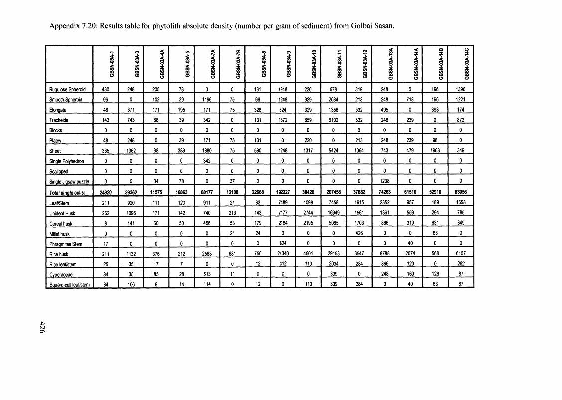
426
Appendix 7.20: Results table for phytolith absolute density (number per gram of sediment) from Golbai Sasan.
GBSN
-03A
-1
GBSN
-03A
-3 I«?z(0COo GB
SN-0
3A-5
GBSN
-03A
-7A
GBSN
-03A
-7B
GBSN
-03A
-8
GBSN
-03A
-9
GBSN
-03A
-10
GBSN
-03A
-11
GBSN
-03A
-12
GBSN
-03A
-13A
GBSN
-03A
-14A
GBSN
-03A
-14B
GBSN
-03A
-14C
Ruqulose Spheroid 430 248 205 78 0 0 131 1248 220 678 319 248 0 196 1396
Smooth Spheroid 96 0 102 39 1196 75 66 1248 329 2034 213 248 718 196 1221
Elongate 48 371 171 195 171 75 328 624 329 1356 532 495 0 393 174
Tracheids 143 743 68 39 342 0 131 1872 659 6102 532 248 239 0 872
Blocks 0 0 0 0 0 0 0 0 0 0 0 0 0 0 0
Platey 48 248 0 39 171 75 131 0 220 0 213 248 239 98 0
Sheet 335 1362 68 389 1880 75 590 1248 1317 5424 1064 743 479 1963 349
Single Polyhedron 0 0 0 0 342 0 0 0 0 0 0 0 0 0 0
Scalloped 0 0 0 0 0 0 0 0 0 0 0 0 0 0 0
Single Jigsaw puzzle 0 0 34 78 0 37 0 0 0 0 0 1238 0 0 0
Total single cells: 24920 39362 11575 16863 68177 12108 22668 192227 38420 207458 37882 74263 61516 52910 83056
Leaf/Stem 211 920 111 120 911 21 83 7489 1098 7458 1915 2352 957 189 1658
Unident Husk 262 1096 171 142 740 213 143 7177 2744 16949 1561 1361 559 294 785
Cereal husk 8 141 60 50 456 53 179 2184 2195 5085 1703 866 319 631 349
Millet husk 0 0 0 0 0 21 24 0 0 0 426 0 0 63 0
Phragmites Stem 17 0 0 0 0 0 0 624 0 0 0 0 40 0 0
Rice husk 211 1132 376 212 2563 681 750 24340 4501 29153 3547 8788 2074 568 6107
Rice leaf/stem 25 35 17 7 0 0 12 312 110 2034 284 866 120 0 262
Cyperaceae 34 35 85 28 513 11 0 0 0 339 0 248 160 126 87
Square-cell leaf/stem 34 106 9 14 114 0 12 0 110 339 284 0 40 63 87
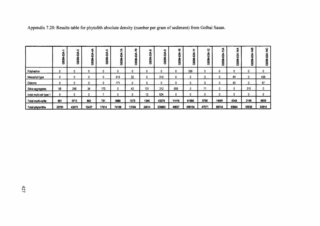
427
Appendix 7.20: Results table for phytolith absolute density (number per gram o f sediment) from Golbai Sasan.
GBSN
-03A
-1
GBSN
-03A
-3
GBSN
-03A
-4A
GBSN
-03A
-5
GBSN
-03A
-7A
GBSN
-03A
-7B
GBSN
-03A
-8
GBSN
-03A
-9
GBSN
-03A
-10
GBSN
-03A
-11
GBSN
-03A
-12
GBSN
-03A
-13A
GBSN
-03A
-14A
GBSN
-03A
-14B
GBSN
-03A
-14C
Polyhedron 0 0 0 0 0 0 0 0 0 339 0 0 0 0 0
Mesophyll type 0 0 0 0 513 32 0 312 0 0 0 0 40 0 436
Diatoms 0 0 0 0 171 0 0 0 0 0 0 0 40 0 87
Silica aggregates 59 248 34 170 0 43 131 312 659 0 71 0 0 210 0
Indet multi-cell type 1 0 0 0 7 0 0 12 624 0 0 0 0 0 0 0
Total multi-cells: 861 3713 862 751 5980 1075 1346 43376 11416 61695 9790 14481 4348 2146 9859
Total phytoliths 25781 43075 12437 17614 74158 13184 24014 235603 49837 269154 47671 88744 65864 55056 92915

Appendix 7.21: Table o f relative frequencies o f single-celled and multi-celled phytolith
types calculated using the total number o f single-celled phytoliths and total multi-celled
phytoliths respectively for Bajpur.
Sample number 0 1 2 3 4
Long (Smooth) 19.8% 33.8% 30.5% 21.7% 25.2%
Long (Sinuate) 2.6% 1.0% 1.5% 3.0% 2.8%
Long (Rods) 0.0% 0.0% 0.0% 0.0% 0.0%
Long (Dendritic) 0.8% 0.6% 0.4% 0.5% 0.2%
Papillae 0.2% 0.0% 0.0% 0.0% 0.2%
Hairs 0.0% 0.0% 0.2% 0.5% 0.3%
Trichomes 2.6% 2.7% 2.1% 2.2% 1.9%
Bulliform 27.6% 13.6% 13.9% 16.2% 15.0%
Ovals 0.4% 1.0% 0.6% 0.8% 0.0%
Keystone 36.5% 40.7% 43.6% 46.2% 45.4%
Crenates 0.0% 0.0% 0.0% 0.0% 0.0%
Bilobes 2.0% 0.6% 0.4% 0.5% 0.2%
Crosses 0.2% 0.0% 0.0% 0.0% 0.0%
Rondels 0.0% 0.4% 0.6% 1.6% 0.3%
Saddles 2.0% 2.9% 3.0% 3.8% 3.1%
Cones 0.4% 0.0% 0.0% 0.3% 0.2%
Flat Tower 0.0% 0.0% 0.0% 0.3% 0.0%
Horned Tower 0.2% 0.0% 0.2% 0.0% 0.0%
Rice bulliform 1.4% 0.2% 0.2% 0.0% 0.0%
Phragmites bulliform 0.2% 0.0% 0.0% 0.0% 0.0%
Double-peaked glume cell 0.0% 0.0% 0.0% 0.0% 0.0%
Rice bilobe 0.2% 0.0% 0.0% 0.0% 0.0%
Rugulose Spheroid 0.6% 0.2% 1.1% 1.1% 0.3%
Smooth Spheroid 0.4% 0.4% 0.4% 0.0% 0.2%
Elongate 0.6% 0.4% 0.7% 0.8% 1.9%
Tracheids 0.6% 0.0% 0.0% 0.0% 0.0%
Blocks 0.2% 1.0% 0.4% 0.0% 0.5%
Platey 0.4% 0.0% 0.0% 0.0% 0.3%
Sheet 0.0% 0.0% 0.4% 0.3% 1.4%
Scalloped 0.0% 0.2% 0.0% 0.0% 0.5%
Single Jigsaw puzzle 0.2% 0.0% 0.0% 0.0% 0.0%
428

Appendix 7.21 continued: Table o f relative frequencies o f single-celled and multi-celled
phytolith types calculated using the total number o f single-celled phytoliths and total
multi-celled phytoliths respectively for Bajpur.
Sample number 0 1 2 3 4
Leaf/Stem 11.4% 0.0% 13.6% 0.0% 0.0%
Unident Husk 2.9% 0.0% 0.0% 0.0% 0.0%
Cereal husk 0.0% 0.0% 0.0% 0.0% 0.0%
Millet husk 0.0% 0.0% 0.0% 0.0% 0.0%
Rice husk 5.7% 0.0% 0.0% 0.0% 0.0%
Rice leaf/stem 0.0% 0.0% 0.0% 0.0% 0.0%
Cyperaceae 11.4% 0.0% 0.0% 0.0% 0.0%
Square-cell leaf/stem 0.0% 0.0% 0.0% 0.0% 0.0%
Mesophyll type 0.0% 0.0% 0.0% 0.0% 0.0%
Diatoms 0.0% 0.0% 0.0% 0.0% 0.0%
Silica aggregate 68.6% 100.0% 86.4% 92.9% 100.0%
Indet multi-cell 0.0% 0.0% 0.0% 7.1% 0.0%
429
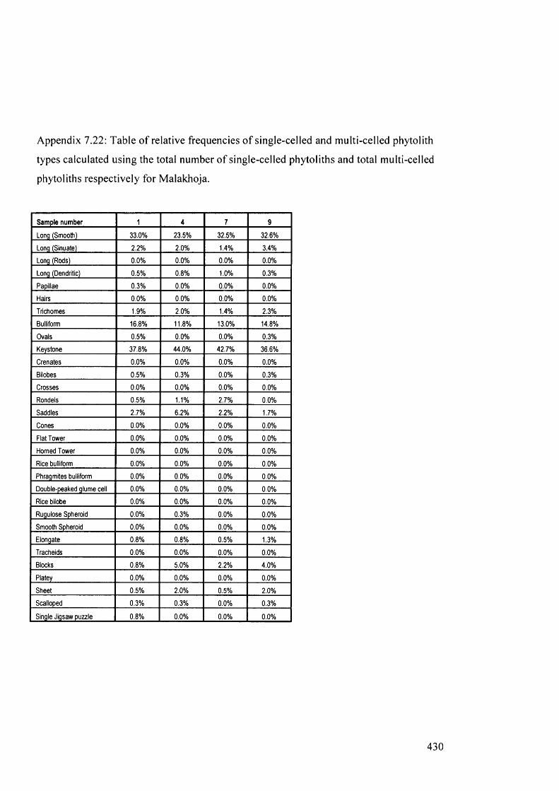
Appendix 7.22: Table o f relative frequencies o f single-celled and multi-celled phytolith
types calculated using the total number o f single-celled phytoliths and total multi-celled
phytoliths respectively for Malakhoja.
Sample number 1 4 7 9
Long (Smooth) 33.0% 23.5% 32.5% 32.6%
Long (Sinuate) 2.2% 2.0% 1.4% 3.4%
Long (Rods) 0.0% 0.0% 0.0% 0.0%
Long (Dendritic) 0.5% 0.8% 1.0% 0.3%
Papillae 0.3% 0.0% 0.0% 0.0%
Hairs 0.0% 0.0% 0.0% 0.0%
Trichomes 1.9% 2.0% 1.4% 2.3%
Bulliform 16.8% 11.8% 13.0% 14.8%
Ovals 0.5% 0.0% 0.0% 0.3%
Keystone 37.8% 44.0% 42.7% 36.6%
Crenates 0.0% 0.0% 0.0% 0.0%
Bilobes 0.5% 0.3% 0.0% 0.3%
Crosses 0.0% 0.0% 0.0% 0.0%
Rondels 0.5% 1.1% 2.7% 0.0%
Saddles 2.7% 6.2% 2.2% 1.7%
Cones 0.0% 0.0% 0.0% 0.0%
Flat Tower 0.0% 0.0% 0.0% 0.0%
Horned Tower 0.0% 0.0% 0.0% 0.0%
Rice bulliform 0.0% 0.0% 0.0% 0.0%
Phragmites bulliform 0.0% 0.0% 0.0% 0.0%
Double-peaked glume cell 0.0% 0.0% 0.0% 0.0%
Rice bilobe 0.0% 0.0% 0.0% 0.0%
Rugulose Spheroid 0.0% 0.3% 0.0% 0.0%
Smooth Spheroid 0.0% 0.0% 0.0% 0.0%
Elongate 0.8% 0.8% 0.5% 1.3%
Tracheids 0.0% 0.0% 0.0% 0.0%
Blocks 0.8% 5.0% 2.2% 4.0%
Platey 0.0% 0.0% 0.0% 0.0%
Sheet 0.5% 2.0% 0.5% 2.0%
Scalloped 0.3% 0.3% 0.0% 0.3%
Single Jigsaw puzzle 0.8% 0.0% 0.0% 0.0%
430

Appendix 7.22 continued: Table o f relative frequencies o f single-celled and multi-celled
phytolith types calculated using the total number o f single-celled phytoliths and total
multi-celled phytoliths respectively for Malakhoja.
Sample number 1 4 7 9
Leaf/Stem 25.0% 4.8% 0.0% 0.0%
Unident Husk: 0.0% 0.0% 0.0% 3.1%
Cereal husk 0.0% 0.0% 0.0% 0.0%
Millet husk 0.0% 0.0% 0.0% 0.0%
Rice husk: 0.0% 0.0% 0.0% 0.0%
Rice leaf/stem 0.0% 0.0% 0.0% 0.0%
Cyperaceae 0.0% 0.0% 0.0% 3.1%Square-cellleaf/stem 0.0% 0.0% 0.0% 0.0%
Mesophyll type 0.0% 0.0% 0.0% 0.0%
Diatoms 0.0% 0.0% 0.0% 0.0%
Silica aggregate 75.0% 95.2% 100.0% 93.8%
431

Appendix 7.23: Table o f relative frequencies o f single-celled and multi-celled phytolith types calculated using the total number o f single
celled phytoliths and total multi-celled phytoliths respectively for Gopalpur.
Sample number 1 2 3 4 5 6 7 8 9 10 11 12 13 14
Long (Smooth) 29.6% 34.0% 23.3% 35.1% 27.8% 24.3% 20.8% 21.6% 19.2% 33.5% 20.0% 23.9% 11.2% 24.1%
Long (Sinuate) 3.5% 5.9% 4.2% 5.6% 3.0% 1.0% 3.6% 0.9% 0.2% 2.8% 2.0% 2.2% 0.6% 1.1%
Long (Rods) 1.6% 0.3% 3.7% 0.0% 0.5% 0.2% 0.3% 0.0% 0.0% 0.2% 0.0% 0.0% 0.0% 0.0%
Long (Dendritic) 3.8% 5.0% 2.8% 1.6% 2.3% 1.5% 9.6% 4.5% 7.8% 0.0% 7.7% 2.5% 7.7% 1.1%
Papillae 0.0% 0.9% 0.0% 0.0% 0.3% 0.2% 0.9% 0.3% 1.6% 1.8% 0.0% 0.0% 0.6% 0.2%
Hairs 0.3% 0.3% 0.8% 0.0% 0.0% 0.5% 0.9% 0.6% 0.0% 0.2% 0.7% 0.0% 0.0% 0.2%
Trichomes 1.6% 2.4% 1.7% 1.0% 3.5% 5.2% 1.8% 3.6% 3.7% 7.9% 2.7% 1.3% 1.2% 1.1%
Bulliform 19.1% 8.3% 11.5% 16.1% 20.0% 11.6% 11.7% 21.3% 16.7% 11.8% 13.7% 17.9% 16.8% 18.5%
Ovals 0.6% 0.3% 0.6% 1.0% 0.5% 0.5% 0.0% 0.0% 0.0% 0.0% 0.0% 0.0% 0.4% 0.0%
Keystone 10.5% 7.7% 19.7% 15.1% 27.0% 38.4% 20.2% 15.3% 22.4% 31.2% 15.7% 39.0% 8.5% 39.6%
Crenates 0.3% 0.6% 0.0% 0.0% 0.0% 0.2% 0.0% 0.3% 0.2% 0.0% 0.2% 0.0% 0.0% 0.0%
Bilobes 3.2% 4.7% 3.1% 1.6% 1.8% 4.7% 10.5% 7.2% 11.4% 0.9% 19.0% 1.3% 23.4% 2.5%
Crosses 1.0% 2.1% 0.6% 0.0% 0.5% 0.5% 1.5% 2.1% 1.1% 1.4% 1.7% 0.0% 5.8% 1.4%
Rondels 2.5% 5.3% 1.1% 1.0% 1.3% 5.7% 5.4% 8.7% 4.6% 1.4% 3.0% 3.8% 12.0% 1.8%
Saddles 1.9% 1.5% 1.4% 0.7% 6.3% 1.7% 3.0% 7.2% 4.3% 0.7% 5.7% 2.5% 3.5% 5.2%
Cones 0.0% 0.3% 0.0% 0.3% 1.0% 0.0% 0.6% 0.3% 0.7% 0.9% 0.7% 0.0% 1.0% 0.0%
Flat Tower 0.0% 0.0% 0.3% 0.0% 0.0% 0.2% 0.0% 0.0% 0.2% 0.2% 0.7% 0.0% 0.4% 0.0%
Homed Tower 0.3% 0.0% 0.0% 0.0% 0.0% 0.0% 0.0% 0.0% 0.2% 0.0% 0.0% 0.0% 0.2% 0.0%
Rice bulliform 0.3% 0.0% 0.0% 0.0% 0.3% 0.5% 0.0% 0.3% 0.5% 0.0% 0.2% 0.3% 0.2% 0.5%
Phragmites bulliform 0.0% 0.0% 0.0% 0.0% 0.0% 0.0% 0.3% 0.0% 0.0% 0.0% 0.0% 0.3% 0.0% 0.0%Double-peaked glume cell 2.2% 0.9% 0.3% 0.0% 0.3% 0.5% 2.4% 0.6% 0.5% 0.0% 1.2% 1.3% 0.8% 0.0%
Rice bilobe 0.3% 1.8% 0.0% 0.0% 0.0% 0.0% 0.3% 0.3% 0.0% 0.0% 1.7% 0.0% 0.2% 0.0%
u>to
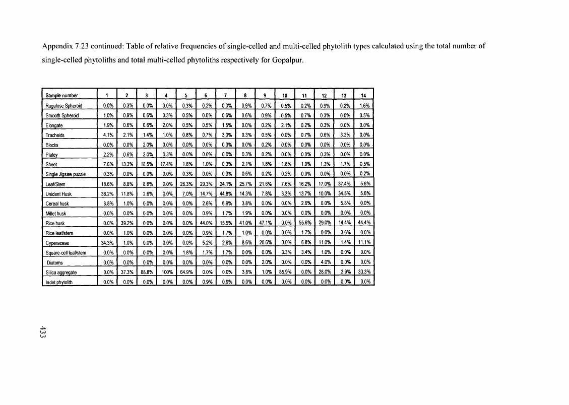
Appendix 7.23 continued: Table o f relative frequencies o f single-celled and multi-celled phytolith types calculated using the total number of
single-celled phytoliths and total multi-celled phytoliths respectively for Gopalpur.
Sample number 1 2 3 4 5 6 7 8 9 10 11 12 13 14
Rugulose Spheroid 0.0% 0.3% 0.0% 0.0% 0.3% 0.2% 0.0% 0.9% 0.7% 0.5% 0.2% 0.9% 0.2% 1.6%
Smooth Spheroid 1.0% 0.9% 0.6% 0.3% 0.5% 0.0% 0.6% 0.6% 0.9% 0.5% 0.7% 0.3% 0.0% 0.5%
Elongate 1.9% 0.6% 0.6% 2.0% 0.5% 0.5% 1.5% 0.0% 0.2% 2.1% 0.2% 0.3% 0.0% 0.0%
Tracheids 4.1% 2.1% 1.4% 1.0% 0.8% 0.7% 3.0% 0.3% 0.5% 0.0% 0.7% 0.6% 3.3% 0.0%
Blocks 0.0% 0.0% 2.0% 0.0% 0.0% 0.0% 0.3% 0.0% 0.2% 0.0% 0.0% 0.0% 0.0% 0.0%
Platey 2.2% 0.6% 2.0% 0.3% 0.0% 0.0% 0.0% 0.3% 0.2% 0.0% 0.0% 0.3% 0.0% 0.0%
Sheet 7.6% 13.3% 18.5% 17.4% 1.8% 1.0% 0.3% 2.1% 1.8% 1.8% 1.0% 1.3% 1.7% 0.5%
Single Jigsaw puzzle 0.3% 0.0% 0.0% 0.0% 0.3% 0.0% 0.3% 0.6% 0.2% 0.2% 0.0% 0.0% 0.0% 0.2%
Leaf/Stem 18.6% 8.8% 8.6% 0.0% 26.3% 29.3% 24.1% 25.7% 21.6% 7.6% 16.2% 17.0% 37.4% 5.6%
Unident Husk 38.2% 11.8% 2.6% 0.0% 7.0% 14.7% 44.8% 14.3% 7.8% 3.3% 13.7% 10.0% 34.5% 5.6%
Cereal husk 8.8% 1.0% 0.0% 0.0% 0.0% 2.6% 6.9% 3.8% 0.0% 0.0% 2.6% 0.0% 5.8% 0.0%
Millet husk 0.0% 0.0% 0.0% 0.0% 0.0% 0.9% 1.7% 1.9% 0.0% 0.0% 0.0% 0.0% 0.0% 0.0%
Rice husk 0.0% 39.2% 0.0% 0.0% 0.0% 44.0% 15.5% 41.0% 47.1% 0.0% 55.6% 29.0% 14.4% 44.4%
Rice leaf/stem 0.0% 1.0% 0.0% 0.0% 0.0% 0.9% 1.7% 1.0% 0.0% 0.0% 1.7% 0.0% 3.6% 0.0%
Cyperaceae 34.3% 1.0% 0.0% 0.0% 0.0% 5.2% 2.6% 8.6% 20.6% 0.0% 6.8% 11.0% 1.4% 11.1%
Square-cell leaf/stem 0.0% 0.0% 0.0% 0.0% 1.8% 1.7% 1.7% 0.0% 0.0% 3.3% 3.4% 1.0% 0.0% 0.0%
Diatoms 0.0% 0.0% 0.0% 0.0% 0.0% 0.0% 0.0% 0.0% 2.0% 0.0% 0.0% 4.0% 0.0% 0.0%
Silica aggregate 0.0% 37.3% 88.8% 100% 64.9% 0.0% 0.0% 3.8% 1.0% 85.9% 0.0% 28.0% 2.9% 33.3%
Indet phytolith 0.0% 0.0% 0.0% 0.0% 0.0% 0.9% 0.9% 0.0% 0.0% 0.0% 0.0% 0.0% 0.0% 0.0%
u>
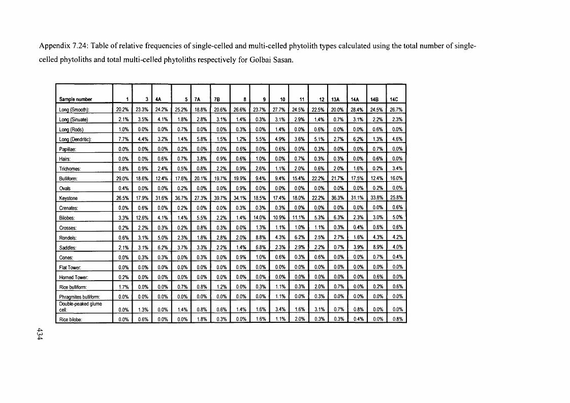
Appendix 7.24: Table o f relative frequencies o f single-celled and multi-celled phytolith types calculated using the total number o f single
celled phytoliths and total multi-celled phytoliths respectively for Golbai Sasan.
Sample number 1 3 4A 5 7A 7B 8 9 10 11 12 13A 14A 14B 14C
Long (Smooth): 20.2% 23.3% 24.2% 25.2% 18.8% 20.6% 26.6% 23.7% 27.7% 24.5% 22.5% 20.0% 28.4% 24.5% 26.7%
Long (Sinuate) 2.1% 3.5% 4.1% 1.8% 2.8% 3.1% 1.4% 0.3% 3.1% 2.9% 1.4% 0.7% 3.1% 2.2% 2.3%
Long (Rods) 1.0% 0.0% 0.0% 0.7% 0.0% 0.0% 0.3% 0.0% 1.4% 0.0% 0.6% 0.0% 0.0% 0.6% 0.0%
Long (Dendritic): 7.7% 4.4% 3.2% 1.4% 5.8% 1.5% 1.2% 5.5% 4.9% 3.6% 5.1% 2.7% 6.2% 1.3% 4.6%
Papillae: 0.0% 0.0% 0.0% 0.2% 0.0% 0.0% 0.6% 0.0% 0.6% 0.0% 0.3% 0.0% 0.0% 0.7% 0.0%
Hairs: 0.0% 0.0% 0.6% 0.7% 3.8% 0.9% 0.6% 1.0% 0.0% 0.7% 0.3% 0.3% 0.0% 0.6% 0.0%
Trichomes: 0.8% 0.9% 2.4% 0.5% 0.8% 2.2% 0.9% 2.6% 1.1% 2.0% 0.6% 2.0% 1.6% 0.2% 3.4%
Bulliform: 29.0% 18.6% 12.4% 17.6% 20.1% 19.7% 19.9% 9.4% 9.4% 15.4% 22.2% 21.7% 17.5% 12.4% 16.0%
Ovals 0.4% 0.0% 0.0% 0.2% 0.0% 0.0% 0.9% 0.0% 0.0% 0.0% 0.0% 0.0% 0.0% 0.2% 0.0%
Keystone 26.5% 17.9% 31.6% 36.7% 27.3% 39.7% 34.1% 18.5% 17.4% 18.0% 22.2% 36.3% 31.1% 33.8% 25.8%
Crenates: 0.0% 0.6% 0.0% 0.2% 0.0% 0.0% 0.3% 0.3% 0.3% 0.0% 0.0% 0.0% 0.0% 0.0% 0.6%
Bilobes: 3.3% 12.6% 4.1% 1.4% 5.5% 2.2% 1.4% 14.0% 10.9% 11.1% 5.3% 6.3% 2.3% 3.0% 5.0%
Crosses: 0.2% 2.2% 0.3% 0.2% 0.8% 0.3% 0.0% 1.3% 1.1% 1.0% 1.1% 0.3% 0.4% 0.6% 0.6%
Rondels: 0.6% 3.1% 5.0% 2.3% 1.8% 2.8% 2.0% 8.8% 4.3% 6.2% 2.5% 2.7% 1.6% 4.3% 4.2%
Saddles: 2.1% 3.1% 6.2% 3.7% 3.3% 2.2% 1.4% 6.8% 2.3% 2.9% 2.2% 0.7% 3.9% 8.9% 4.0%
Cones: 0.0% 0.3% 0.3% 0.0% 0.3% 0.0% 0.9% 1.0% 0.6% 0.3% 0.6% 0.0% 0.0% 0.7% 0.4%
Flat Tower. 0.0% 0.0% 0.0% 0.0% 0.0% 0.0% 0.0% 0.0% 0.0% 0.0% 0.0% 0.0% 0.0% 0.0% 0.0%
Homed Tower 0.2% 0.0% 0.0% 0.0% 0.0% 0.0% 0.0% 0.0% 0.0% 0.0% 0.0% 0.0% 0.0% 0.6% 0.0%
Rice bulliform: 1.7% 0.0% 0.0% 0.7% 0.8% 1.2% 0.0% 0.3% 1.1% 0.3% 2.0% 0.7% 0.0% 0.2% 0.6%
Phragmites bulliform: 0.0% 0.0% 0.0% 0.0% 0.0% 0.0% 0.0% 0.0% 1.1% 0.0% 0.3% 0.0% 0.0% 0.0% 0.0%Double-peaked glume cell: 0.0% 1.3% 0.0% 1.4% 0.8% 0.6% 1.4% 1.6% 3.4% 1.6% 3.1% 0.7% 0.8% 0.0% 0.0%
Rice bilobe: 0.0% 0.6% 0.0% 0.0% 1.8% 0.3% 0.0% 1.6% 1.1% 2.0% 0.3% 0.3% 0.4% 0.0% 0.8%
-p*u->4

Appendix 7.24 continued: Table o f relative frequencies o f single-celled and multi-celled phytolith types calculated using the total number of
single-celled phytoliths and total multi-celled phytoliths respectively for Golbai Sasan.
Sample number 1 3 4A 5 7A 7B 8 9 10 11 12 13A 14A 14B 14C
Rugulose Spheroid 1.7% 0.6% 1.8% 0.5% 0.0% 0.0% 0.6% 0.6% 0.6% 0.3% 0.8% 0.3% 0.0% 0.4% 1.7%
Smooth Spheroid 0.4% 0.0% 0.9% 0.2% 1.8% 0.6% 0.3% 0.6% 0.9% 1.0% 0.6% 0.3% 1.2% 0.4% 1.5%
Elongate 0.2% 0.9% 1.5% 1.2% 0.3% 0.6% 1.4% 0.3% 0.9% 0.7% 1.4% 0.7% 0.0% 0.7% 0.2%
Tracheids 0.6% 1.9% 0.6% 0.2% 0.5% 0.0% 0.6% 1.0% 1.7% 2.9% 1.4% 0.3% 0.4% 0.0% 1.1%
Blocks 0.0% 0.0% 0.0% 0.0% 0.0% 0.0% 0.0% 0.0% 0.0% 0.0% 0.0% 0.0% 0.0% 0.0% 0.0%
Leaf/Stem: 24.5% 24.8% 12.9% 16.0% 15.2% 2.0% 6.2% 17.3% 9.6% 12.1% 19.6% 16.2% 22.0% 8.8% 16.8%
Unident Husk: 30.4% 29.5% 19.8% 18.9% 12.4% 19.8% 10.6% 16.5% 24.0% 27.5% 15.9% 9.4% 12.8% 13.7% 8.0%
Cereal husk: 1.0% 3.8% 6.9% 6.6% 7.6% 5.0% 13.3% 5.0% 19.2% 8.2% 17.4% 6.0% 7.3% 29.4% 3.5%
Millet husk: 0.0% 0.0% 0.0% 0.0% 0.0% 2.0% 1.8% 0.0% 0.0% 0.0% 4.3% 0.0% 0.0% 2.9% 0.0%
Phragmites Stem 2.0% 0.0% 0.0% 0.0% 0.0% 0.0% 0.0% 1.4% 0.0% 0.0% 0.0% 0.0% 0.9% 0.0% 0.0%
Rice husk: 24.5% 30.5% 43.6% 28.3% 42.9% 63.4% 55.8% 56.1% 39.4% 47.3% 36.2% 60.7% 47.7% 26.5% 61.9%
Rice leaf/stem 2.9% 1.0% 2.0% 0.9% 0.0% 0.0% 0.9% 0.7% 1.0% 3.3% 2.9% 6.0% 2.8% 0.0% 2.7%
Cyperaceae 3.9% 1.0% 9.9% 3.8% 8.6% 1.0% 0.0% 0.0% 0.0% 0.5% 0.0% 1.7% 3.7% 5.9% 0.9%
Square-cell leaf/stem 3.9% 2.9% 1.0% 1.9% 1.9% 0.0% 0.9% 0.0% 1.0% 0.5% 2.9% 0.0% 0.9% 2.9% 0.9%
Polyhedron 0.0% 0.0% 0.0% 0.0% 0.0% 0.0% 0.0% 0.0% 0.0% 0.5% 0.0% 0.0% 0.0% 0.0% 0.0%
Mesophyll type 0.0% 0.0% 0.0% 0.0% 8.6% 3.0% 0.0% 0.7% 0.0% 0.0% 0.0% 0.0% 0.9% 0.0% 4.4%
Diatoms 0.0% 0.0% 0.0% 0.0% 2.9% 0.0% 0.0% 0.0% 0.0% 0.0% 0.0% 0.0% 0.9% 0.0% 0.9%
Silica aggregate 6.9% 6.7% 4.0% 22.6% 0.0% 4.0% 9.7% 0.7% 5.8% 0.0% 0.7% 0.0% 0.0% 9.8% 0.0%
Indet multi-cell type 1 0.0% 0.0% 0.0% 0.9% 0.0% 0.0% 0.9% 1.4% 0.0% 0.0% 0.0% 0.0% 0.0% 0.0% 0.0%

Early Agricultural Communities in Northern and Eastern India:
an archaeobotanical investigation.
Volume II
Emma Louise Harvey
Thesis submitted in fulfilment of the
requirements of the degree of Doctor of Philosophy in the
Institute of Archaeology, University of London.
2006
436

List of Figures
Chapter 1
1.1 Map of areas o f study in this project 445
1.2 Table of possible indigenous Indian crops that could be present on the sites 446
under investigation in Gangetic India and Orissa
1.3 Table of introduced crops that may be present at the sites under investigation 448
in Gangetic India and Orissa
Chapter 2
2.1 The general expected subsistence stages in the evolution of agriculture and
domesticated cereal crops adapted from Harris (1989, 1996), with possible
occurrences on Gangetic sites included at the bottom
449
Chapter 3
3.1 Political map of South Asia with geographic features 450
3.2 Geological map o f India 451
3.3 Soil map o f India 452
3.4 Monsoon rainfall map o f India 453
3.5 Annual Rainfall map o f India 454
3.6 Map of modem vegetation o f India 455
3.7 Diagram of palaeoenvironmental data from the Ganges region 456
3.8 Table of modes o f subsistence used by some o f the modem tribal groups 457
3.9 Table shows the year round agricultural scheduling for two tribal groups 458
Chapter 4
4.1 Table of published radiocarbon dates and a multiplot for foraging sites in
Northern India
459
4.2 Tables of dates and multiplots for early farming settlements in Uttar Pradesh
and Bihar
460
4.3 Map of the Ganges River Valley showing the important sites mentioned in
the text
465
4.4 Timeline o f fully excavated sites from the Ganges River Valley 466
4.5 Map of Orissa show ing the important sites mentioned in the text 467
437
Chapter 5
5.1 Section drawing o f Chopani Mando 468
5.2 Section drawing o f Koldihwa 469
5.3 Section drawing o f Mahagara 470
5.4 Table explaining where samples come from in the Chopani-Mando section 471
5.5 Table explaining where samples come from in the Koldihwa Z1 and Y1 471
sections
5.6 New dates from new archaeobotanical remains from Belan River Valley 472
5.7 Table explaining where samples come from in the Mahagara section 472
5.8 Section photograph o f Gopalpur 473
5.9 Section photograph o f Golbai Sasan 474
5.10 Photograph o f Bajpur 475
5.11 Photograph o f Banabasa 476
5.12 Photograph o f section at Malakhoja 477
5.13 Table o f the soil descriptions from Golbai Sasan sampled section 478
5.14 New dates from new archaeobotanical remains from Orissa 478
5.15 Table o f samples taken at Gopalpur 479
5.16 Table o f samples taken at Malakhoja 479
5.17 Table o f samples taken at Bajpur 480
5.18 Table o f samples taken from Banabasa 480
5.19 Identification keys for small millets 481
5.20 Schematic representation of the major processing stages for rice showing 482
the products and waste produced by each process
5.21 Schematic representation of the major processing stages for millets showing 483
the products and waste produced by each process
Chapter 6
6.1 Diagram o f rice spikelet terminology 484
6.2 Photographs o f the different rice phytoliths 485
6.3 A table o f the Oryza taxonomic classifications 486
6.4 Diagram showing the Zhang (2002) and Pearsall et al. (1995) method of 488
measuring rice hairs and double-peaked rice husk phytoliths
6.5 Diagram of Fujiwara bulliform measurements 488
6.6 Diagram of bulliforms chips of wild and domestic rice 489
438

6.7 Table showing the number o f populations per rice species measured in 490
this project
6.8 List of populations and information o f origin 491
6.9 Diagram of how grain measurements taken in this project 497
6.10 Diagram of double-peaked husk cell with measurements marked on that 498
were taken in this project
6.11 Table showing the ranges and averages for rice grain measurements 499
6.12 Graph showing the length and width measurements for individual grains in 500
each population for each species
6.13 Graph showing the length and thickness measurements for individual grains 501
in each population for each species
6.14 Graph showing the width and thickness measurements for individual grains 502
in each population for each species
6.15 Graph showing the separation o f Otyza sativa grains in to japonica and 503
indica varieties using length and width measurement
6.16 Graph showing the distribution o f rice grain shape, length/width ratios in 504
percentage occurrence
6.17 Graph showing how the new measurements from this thesis fit in to 504
Vishnu-Mittre’s (1972.1974) categories for identifying rice species
6.18 Table showing some of the results for discriminant analysis using the 505
linear method for comparing length, width, and thickness measurements
for all o f the rice species
6.19 Graph showing a comparison of the length and width measurements o f 506
modem and archaeological rice grains
6.20 Graph showing the maturing rates for Oryza sativa subsp.japonica 507
6.21 Graph comparing the immature measurements o f modem and 507
archaeological rice grains
6.22 Table showing the ranges and averages for double-peaked rice 508
measurements
6.23 Graph showing the TW and MW values for individual phytoliths from 509
each rice species
6.24 Graph showing the TW and HI averages for each population for each rice 509
species
439

6.25 Table showing the results o f discriminant analysis using the linear method 510
for measurements of double-peaked husk phytoliths for all rice species
6.26 Table showing the results o f discriminant analysis using the linear method 511
for all measurements (TW, MW, HI, H2, CD, PA, CA) of double-peaked
husk phytoliths using wild versus domestic categories
6.27 Graph showing archaeological and modem double-peaked husk phytolith 512
measurements
6.28 Graph o f archaeological rice bulliforms chips from Gopalpur and Golbai 513
Sasan
6.29 Graph o f archaeological rice bulliform chips from Mahagara and Koldihwa 514
Chapter 7
7.1 Graph showing modem length and width measurements o f Vigna radiata 515
and Vigna mungo (wild and domestic species)
7.2 Graph showing modem length and width measurements o f Vigna radiata 515
and Vigna mungo (wild and domestic species) with 20% shrinkage adjustment
7.3 Graph showing archaeological length and width measurements for Vigna sp. 516
seeds with dashed line separating possible wild from possible domestic types
7.4 Graph showing length vs plumule length/length measurements for 516
identifying Vigna mungo and Vigna radiata
7.5 Ubiquity pie charts for sites in the Belan River Valley 517
7.6 Graph o f ubiquity values comparing the Belan River Valley sites 518
7.7 Graph comparing ubiquity values for new Belan River Valley sites and the 518
published North Indian sites
7.8 Bar chart o f relative frequencies o f macro-remains from Mahagara 519
7.9 Bar chart o f relative frequencies of macro-remains in Z1 section from 520
Koldihwa
7.10 Bar chart o f relative frequencies o f macro-remains in Y1 sections from 520
Koldihwa
7.11 Charts showing the vertical changes in the sequence from Mahagara 521
7.12 Charts showing the vertical changes in the sequence from Koldihwa Z 1 522
7.13 Charts showing the vertical changes in the sequence from Koldihwa Y 1 523
7.14 Table o f correlations for Mahagara macro-remains 524
440
7.15
7.16
7.17
7.18
7.19
7.20
7.21
7.22
7.23
7.24
7.25
7.26
7.27
7.28
7.29
7.30
7.31
7.31
7.33
7.34
Table o f correlations for Koldihwa macro-remains 524
Graph o f ubiquity values from Gopalpur (purple) and Golbai Sasan (yellow) 525
Bar chart o f the relative frequencies o f macro-remains from Gopalpur 526
Bar chart o f the relative frequencies o f macro-remains from Golbai Sasan 526
Charts showing the vertical changes in the sequence from Gopalpur 527
Charts showing the vertical changes in the sequence from Golbai Sasan 528
Table o f correlations for Gopalpur macro-remains 529
Table o f correlations for Golbai Sasan macro-remains 529
Graph showing the relative frequencies o f single-celled phytoliths from 530
Chopani-Mando
Graph showing the relative frequencies o f multi-celled phytoliths from 530
Chopani-Mando
Graph showing the relative frequencies o f single-celled phytoliths from 531
Koldihwa
Graph showing the relative frequencies o f multi-celled phytoliths from 531
Koldihwa
Graph showing the relative frequencies o f single-celled phytoliths from 532
Mahagara
Graph showing the relative frequencies o f multi-celled phytoliths from 532
Mahagara
Graph showing the total density of phytoliths per gram o f sediment for 533
samples from Chopani-Mando
Graph showing the total density o f multi-celled phytoliths per gram of 533
sediment for sample from Chopani Mando
Graph showing the total density o f phytoliths per gram o f sediment for 534
samples from Koldihwa
Graph showing the total density of multi-celled phytoliths per gram of 534
sediment for sample from Koldihwa
Graph showing the total density of phytoliths per gram o f sediment for 535
samples from Mahagara
Graph showing the total density of multi-celled phytoliths per gram of 535
sediment for sample from Mahagara
441
7.35 Graph showing the absolute density of single-celled phytoliths from 536
Chopani-Mando
7.36 Graph showing the absolute density of multi-celled phytoliths from 536
Chopani-Mando
7.37 Graph showing the absolute density of single-celled phytoliths from 537
Koldihwa
7.38 Graph showing the absolute density of multi-celled phytoliths from 537
Koldihwa
7.39 Graph showing the absolute density of single-celled phytoliths from 538
Mahagara
7.40 Graph showing the absolute density of multi-celled phytoliths from 538
Mahagara
7.41 Graph showing the different grass subfamilies from Chopani-Mando 539
7.42 Graph showing the different grass subfamilies from Koldihwa 539
7.43 Graph showing the different grass subfamilies from Mahagara 540
7.44 Table of correlations for Chopani-Mando single-celled phytoliths 541
7.45 Table of comparisons for Koldihwa single-celled phytoliths 541
7.46 Table of correlations for Mahagara single-celled phytoliths 542
7.47 Table of correlations for Koldihwa multi-celled phytoliths 543
7.48 Table of correlations from Mahagara multi-celled phytoliths 544
7.49 Graph showing the relative frequencies o f single-celled phytoliths from 545
Bajpur
7.50 Graph showing the relative frequencies o f multi-celled phytoliths from 545
Bajpur
7.51 Graph showing the relative frequencies o f single-celled phytoliths from 546
Malakhoja.
7.52 Graph showing the relative frequencies o f multi-celled phytoliths from 546
Malakhoja
7.53 Graph showing the relative frequencies o f single-celled phytoliths from 547
Gopalpur
7.54 Graph showing the relative frequencies o f multi-celled phytoliths from 547
Gopalpur
442

7.55
7.56
7.57
7.58
7.59
7.60
7.61
7.62
7.63
7.64
7.65
7.66
7.67
7.68
7.69
7.70
7.71
Graph showing the relative frequencies o f single-celled phytoliths from 548
Golbai Sasan
Graph showing the relative frequencies o f multi-celled phytoliths from 548
Golbai Sasan
Graph showing the total density of phytoliths per gram o f sediment for 549
samples from Bajpur
Graph showing the total density of multi-celled phytoliths per gram of 549
sediment from Bajpur
Graph showing the absolute density for single-celled phytoliths from Bajpur 550
Graph showing the absolute density for multi-celled phytoliths from Bajpur 550
Graph showing the total density of phytoliths per gram of sediment for 551
samples from Malakhoja
Graph showing the total density o f multi-celled phytoliths per gram of 551
sediment from Malakhoja
Graph showing the absolute density o f single-celled phytoliths from 552
Malakhoja
Graph showing the absolute density o f multi-celled phytoliths from 552
Malakhoja
Graph showing the total density of phytoliths per gram o f sediment for 553
samples from Gopalpur
Graph showing the total density o f multi-celled phytoliths per gram of 553
sediment from Gopalpur
Graph showing the absolute density of single-celled phytoliths from 554
Gopalpur
Graph showing the absolute density of multi-celled phytoliths from 554
Gopalpur
Graph showing the total density of phytoliths per gram of sediment for 555
samples from Golbai Sasan
Graph showing the total density of multi-celled phytoliths per gram of 555
sediment from Golbai Sasan
Graph showing the absolute density of single-celled phytoliths from 556
Golbai Sasan
443
7.72 Graph showing the absolute density of multi-celled phytoliths from 556
Golbai Sasan
7.73 Graph showing the different grass subfamilies from Bajpur 557
7.74 Graph showing the different grass subfamilies from Malakhoja 557
7.75 Graph showing the different grass subfamilies from Gopalpur 558
7.76 Graph showing the different grass subfamilies from Golbai Sasan 558
7.77 Table of correlations o f single-celled phytoliths from Bajpur 559
7.78 Table of correlations o f single-celled phytoliths from Malakhoja 560
7.79 Table of correlations o f single-celled phytoliths from Gopalpur 560
7.80 Table of correlations of single-celled phytoliths from Golbai Sasan 561
7.81 Table of correlations for Gopalpur multi-celled phytoliths 562
7.82 Table of correlations for Golbai Sasan multi-celled phytoliths 563
7.83 Tables o f weeds present in the archaeobotanical assemblages and their 564
environmental implications
7.84 Graph showing the ratio o f rice leaf/stem phytoliths to rice husk 566
phytoliths at Koldihwa and Mahagara
7.85 Graph showing the ratio o f rice leaf/stem phytoliths to rice husk 566
phytoliths at Gopalpur and Golbai Sasan
7.86 Vertical charts o f absolute counts and densities for macro-remains and 567
phytoliths at Golbai Sasan
7.87 Vertical charts o f absolute counts and densities for macro-remains and 568
phytoliths for Gopalpur
7.88 Vertical chart o f absolute counts and densities o f macro-remains and 569
phytoliths from Mahagara
7.89 Vertical chart o f absolute counts and densities for macro-remains and 570
phytolith from section Y1 at Koldihwa
7.90 Vertical chart o f absolute counts and densities for macro-remains and 571
phytoliths from section Z1 at Koldihwa
444
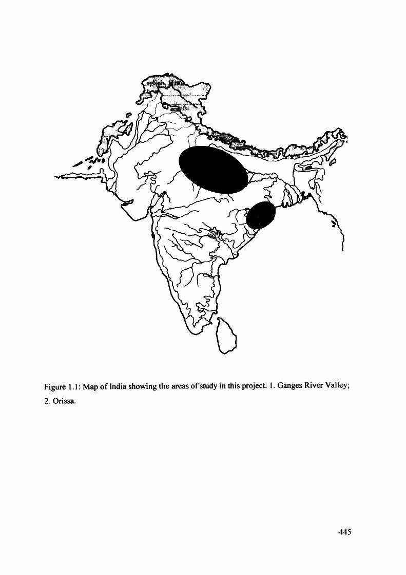
Figure 1.1: Map of India showing the areas of study in this project. 1. Ganges River Valley;
2. Orissa.
445
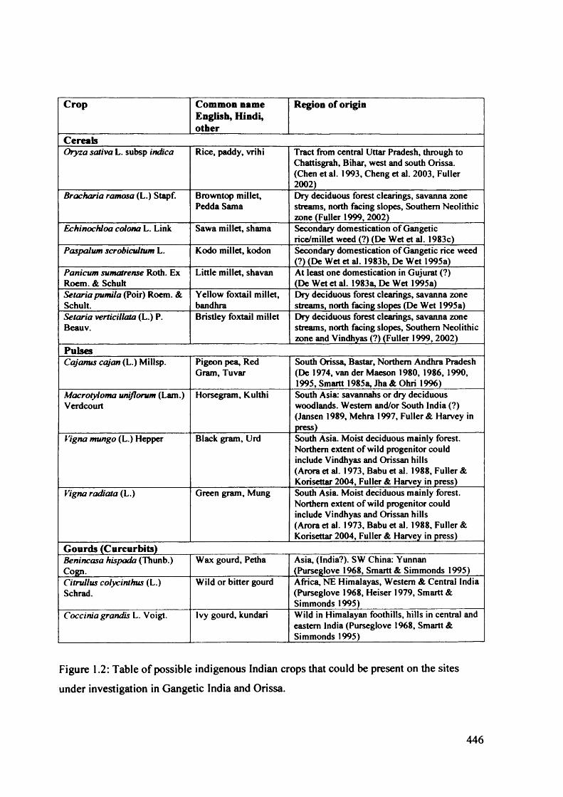
Crop Common name English, Hindi, other
Region of origin
CereabOryza sativa L. subsp indica Rice, paddy, vrihi Tract from central Uttar Pradesh, through to
Chattisgrah, Bihar, west and south Orissa. (Chen et al. 1993, Cheng et al. 2003, Fuller 2002)
Bracharia ramosa (L.) Stapf. Brown top millet, Pedda Sama
Dry deciduous forest clearings, savanna zone streams, north facing slopes, Southern Neolithic zone (Fuller 1999, 2002)
Echinochioa colona L. Link Sawa millet, shama Secondary domestication of Gangetic rice/millet weed (?) (De Wet et al. 1983c)
Pas pal tun scrobicultum L. Kodo millet, kodon Secondary domestication of Gangetic rice weed (?) (De Wet et al. 1983b, De Wet 1995a)
Parti cum sumatrense Roth. Ex Roem. & Schuh
Little millet, shavan At least one domestication in Gujurat (?) (De Wet et al. 1983a, De Wet 1995a)
Setaria pumila (Poir) Roem. & Schult.
Yellow foxtail millet, bandhra
Dry deciduous forest clearings, savanna zone streams, north facing slopes (De Wet 1995a)
Setaria verticillata (L.) P. Beauv.
Bristley foxtail millet Dry deciduous forest clearings, savanna zone streams, north facing slopes, Southern Neolithic zone and Vindhyas (?) (Fuller 1999,2002)
PulsesCajanus cqjan (L.) Millsp. Pigeon pea, Red
Gram, TuvarSouth Orissa, Bastar, Northern Andhra Pradesh (De 1974, van der Maeson 1980, 1986, 1990, 1995, Smartt 1985a, Jha & Ohri 1996)
Macrotyloma uniflorum (Lam.) Verdcourt
Horsegram, Kulthi South Asia: savannahs or dry deciduous woodlands. Western and/or South India (?) (Jansen 1989, Mehra 1997, Fuller & Harvey in press)
Vigna mungo (L.) Hepper Black gram, Urd South Asia. Moist deciduous mainly forest. Northern extent of wild progenitor could include Vindhyas and Orissan hills (Arora et al. 1973, Babu et al. 1988, Fuller & Korisettar 2004, Fuller & Harvey in press)
Vigna radiata (L.) Green gram, Mung South Asia. Moist deciduous mainly forest. Northern extent of wild progenitor could include Vindhyas and Orissan hills (Arora et al. 1973, Babu et al. 1988, Fuller & Korisettar 2004, Fuller & Harvey in press)
Gourds (Curcurbits)Benincasa hispada (Thunb.) Cogn.
Wax gourd, Petha Asia, (India?). SW China: Yunnan (Purseglove 1968, Smartt & Simmonds 1995)
Citrullus colycinthus (L.) Schrad.
Wild or bitter gourd Africa, NE Himalayas, Western & Central India (Purseglove 1968, Heiser 1979, Smartt & Simmonds 1995)
Coccinia grandis L. Voigt. Ivy gourd, kundari Wild in Himalayan foothills, hills in central and eastern India (Purseglove 1968, Smartt & Simmonds 1995)
Figure 1.2: Table of possible indigenous Indian crops that could be present on the sites
under investigation in Gangetic India and Orissa.
446

Crop Common name English, Hindi, other
Region of origin
Gourds continuedCucumis melo L. Melon, Kharbuza Northern/Western India (?), as well as SW
Asia (Bates & Rodibson 1995, Choudhury 1996)
Cucumis sativus L. Cucumbers, Khira Wild in Himalayan foothills and also possibly Orissan high hills (Bates & Robinson 1995)
Luffa cylindrical (L.) M.J. Roem.
Sponge gourd, loofah, Ghiya tori, Nenua
Asia, India, Himalayas and SW China (Marr et al. 2005)
Luffa acutangula (L.) Roxb. Ridged gourd, angled loofah, Kali tori
Wild in Himalayan foothills, hills of central and eastern India (Marr et al. 2005)
Momordica balsamina L. Balsam apple, mocha Wild in Himalayan foothills, hills on central and eastern India through to Southeast Asia (Bates et al. 1995)
Momordica charantia L. Bitter gourd, karela Wild in Himalayan foothills, hills on central and eastern India through to Southeast Asia (Bates et al. 1995, Marr et al. 2004)
Momordica dioeca Roxb. Ex Willd.
Small bitter gourd, mure la, jangli karela
Wild in Himalayan foothills, hills on central and eastern India through to Southeast Asia (Bates et al. 1995)
Praecitrullus fistulosus (Sticks) Pang.
Indian squash melon, Tinda
Wild in Himalayan foothills, hills on central and eastern India (Bates et al. 1995)
Trichosanlhes cucumerina L. Snake gourd, Chichinda
Wild in Himalayan foothills, hills on central and eastern India (Bates et al. 1995)
Trichosanthes dioica Roxb. Pointed gourd, Parwal Wild in Himalayan foothills, hills on central and eastern India (Bates et al. 1995)
TubersColocasia esculenia Schott. Taro, Ghuiyan, Arvi Eastern India and/or Southeast Asia
(Purseglove 1972)Dioscorea spp. Yams, Ratalu Eastern India and/or Southeast Asia
(Purseglove 1972)Palms (Palmae)Borassus flabellifer Palmyra Palm, Tal North to Eastern India and Malaya
(McCurrah 1960, Davies & Johnson 1987, Basu & Chakraverty 1994)
Cocos nucifera L. Coconut, Nariel Coastal and islands of Southeast Asia and the western Pacific (Harries 1995)
Phoenix sylvestris Date palm, forest date Western India and Arabian Gulf (Wrigley 1995)
OthersMusa spp. Banana Eastern India, Sri Lanka, New Guinea
(Simmonds 1995, Komel 2006)Saccharum spp. Sugarcane, ganna Wild in Himalayan foothills, India, China, and
New Guinea (Daniel & Roach 1987, Roach 1995)
Sesamum indicum L. Sesame, Til Western parts of Himalayas, western Pakistan, also wild on west coast of South India (Bedigan 1998, 2003, Fuller 2003b)
Figure 1.2 continued: Table of possible indigenous Indian crops that could be present on
the sites under investigation in Gangetic India and Orissa.
447

Crops Common name English, Hindi, other
Region of origin
CerealsOryza sativa L. subsp. japonica
Rice, paddy, Vrihi Southern China(Chen at al. 1993, Fuller 2002, Cheng et al. 2003)
Panicum miliaceum L. Proso millet, Chin North China and Europe (?) (Chang 1989, Jones 2004)
Setaria itaJica (L.) Beauv.
Common foxtail millet, kangu
Northern China (?), also maybe Europe (?) (Jones 2004)
Hordeum vulgare L. sensu laio
Barley, Yava Near East(Zohary & Hopf 2000)
Triticum spp. Wheat, Gehu Near East (Zohary & Hopf 2000)Eleusine coracana L. Finger millet, Ragi Africa (Fuller 2002, 2003c)Pennisetum glaucum (L.) R. Br.
Pearl millet, Bajra Africa(Fuller 2002, 2003c)
Sorghum bicolor (L.) Moench.
Great millet, Jowar Africa(Fuller 2002, 2003c)
PulsesCicer arietinum L. Chickpea, Gram Near East (Zohary & Hopf 2000)Lathyrus sativus L. Grass pea, Khesari Near East (Zohary & Hopf 2000)Lens culinaris L. Lentil, Masur Near East (Zohary & Hopf 2000)Pisum sativum L. Pea, Matter Near East (Zohary & Hopf 2000)Lablab purpureus (L.) Sweet.
Hyacinth bean, Sem Africa(Fuller 2002, 2003c, Pengelly & Maass 2001, Maass et al. 2005)
Vigna unguiculata (L.) Walp.
Cowpea, Lobia Africa(Ng 1995, Fuller 2002, 2003c)
OthersCannabis sativus L. Hemp, Ganja China and or Central Asia (Small 1995)Linum usitatissimum L. Flax, Linen, Alsi Near East (Zohary & Hopf 2000)
Figure 1.3: Table of introduced crops that may be present at the sites under investigation in
Gangetic India and Orissa.
448

Procurement Cultivation Cropproduction
Wild plant foodprocurement
Wild plant foodproduction - Small scale
Wild plant foodproduction - Large scale
Agriculture - cultivation of domestic crops
Gathering, burning, tending
Replacementplanting,harvesting,storage
Land clearance,
- JFull scale
Agricultural ^production
Plantremains
Otherevidence
Foragers using wild rice and other grasses
Ceramics
Management of wild rice Emergence of arable weeds
Increased sedentismSeasonal----------------------► Year round
Domestic rice and other crops: maybe increase in seed size
IndianGangeticSites
DamdamaChopani-Mando
? - evidence may be missing
Lahuradewa ? * Senuwar * ?
Koldihwa/Mahagara?
Figure 2.1: The general expected subsistence stages in the evolution of agriculture and
domesticated cereal crops adapted from Harris (1989, 1996), with the possible occurrences
on Gangetic sites included at the bottom.
449

r'
AFGHANISTAN CHINA
H i m a l a y a
^/BANGLADESH /
PAKISTAN
I R A N
INDIA
\ BURMA
PM eau
E a » '
Lanka
Figure 3.1: Political map of South Asia with geographic features (after Robinson 1989).
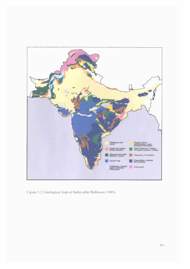
I Himalayan puranas Cuddapn
(f Dharwanan. Khondalites
Unsurveyed
Figure 3.2: Geological map of India (after Robinson 1989).
451
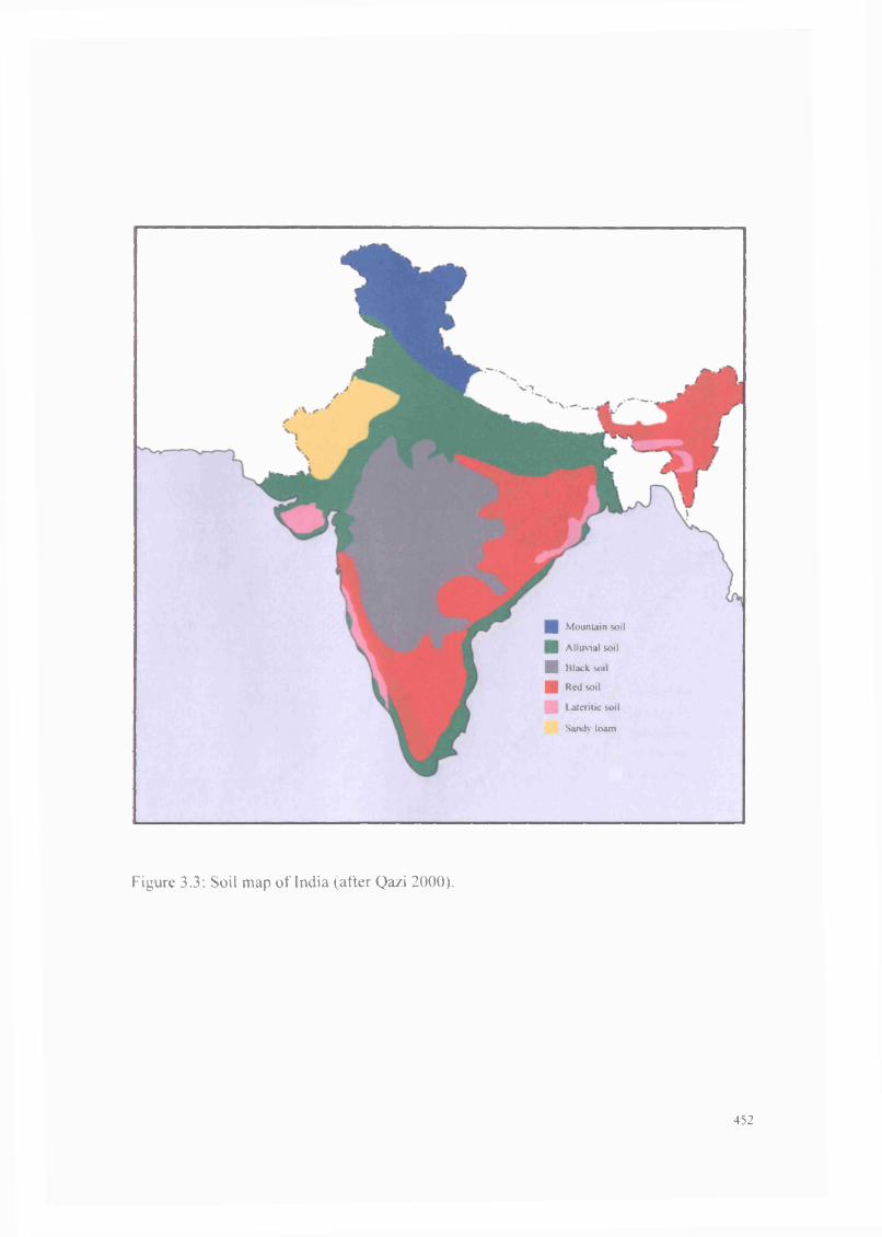
| Mountain soil
| Alluvial soil
■ Black soil
■ Red soil
Latentic soil
Sandy loam
Figure 3.3: Soil map of India (after Qazi 2000).
452
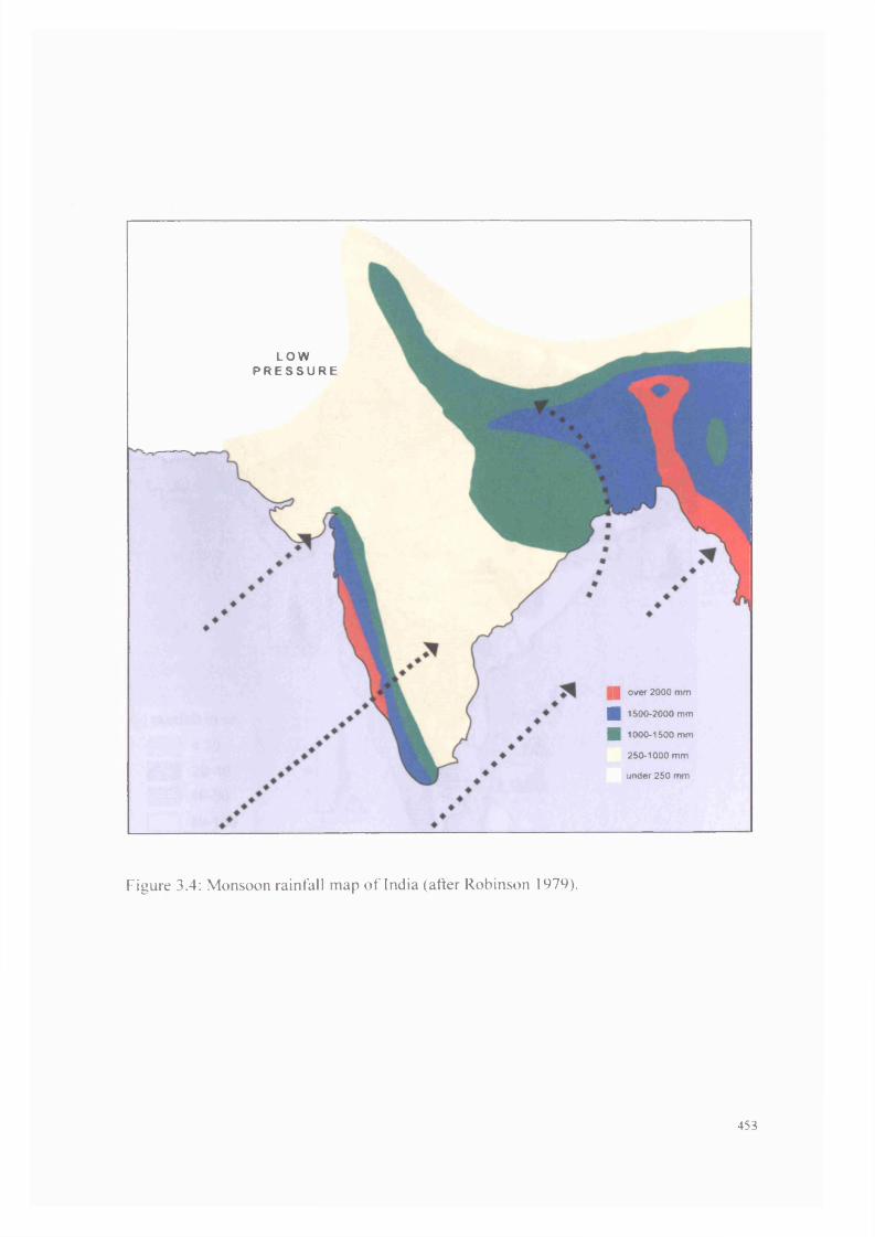
L O WP R E S S U R E
Q over 2000 mm
B 1500-2000 mm
| 1000-1500 mm
250-1000 mm
under 250 mm
Figure 3.4: Monsoon rainfall map of India (after Robinson 1979).
453

Nandi hi
Kodaikarwl
K o z h i k o d e
Is
rainfall in cm
H i <20| g g 40-80
| | 80-160 160-320
Figure 3.5: Annual rainfall map of India (after Fuller 1999).
454
01
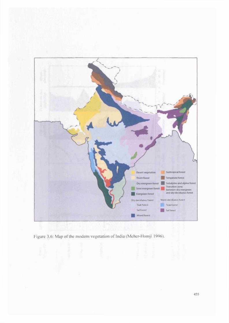
7
Moist deciduous forest
( Teak forest
| Sat forest
Dry deciduous forest
Teak forest
Sal forest
| Mixed forest
Figure 3.6: Map of the modem vegetation of India (Meher-Homji 1996).
455
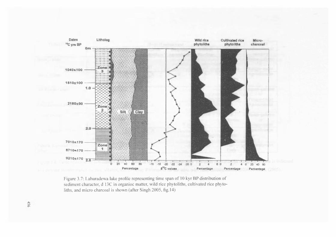
Dates
14C yrs BP
10401.100
181 0 ± 1 00
2 1 8 0 ± 9 0
7010± .170
871 (>*.170
9 2 1 0 ± 1 7 0
0 m
Litholog
mmm•;.* •;.* .v
1 1 #
W.SIlO*
f/\v.:/V’*VVV4
W ild rice phyto lithe
Cultivated ricephyto lithe
Micro-charcoal
vVVv^V'J
JO 40
tfilSiSlSESH
« j | i
16 -18 -26 0
C v.TlueaPercentage Percentage Percentage0 20 40 60
Percentage
Figure 3.7: Lahuradewa lake profile representing time span of 10 kyr BP distribution of sediment character, d 13C in organioc matter, wild rice phytoliths, cultivated rice phyto- liths, and micro charcoal is shown (after Singh 2005, fig. 14)

457
Tribal Group Mode of subsistence Typicalarchaeological
categoryHunting Gathering Swidden
AgricultureIrrigated
AgricultureAnimalHerding
Trade
Birhor, Orissa X X XRope,
monkeys
Hunter-gathereror
Forager-traderJuang, Orissa X X X X X X
Basketry,crops
Agriculturalist
Hill Kharia, Orissa X X XHoney,
arrowroot
Hunter-gathereror
Forager-traderKutia Khond, Orissa X X X X X X
CropsAgriculturalist
Lodha, Orissa X X XSilkworm
Hunter-gathereror
Forager-traderPaudi Bhuinya, Orissa X X X X X X
Crops,fruits
Agriculturalist
Paharia, Rajmahal Hills, Bihar
X X X X XTools
Agriculturalist
Figure 3.8: Table of modes of subsistence used by some of the modem tribal groups. The main products that the group’s trade is indicated
and they are usually traded for rice, alcohol, and clothing. References for the table are Pratap (2000), Mehta (2004), Patnaik (2005).
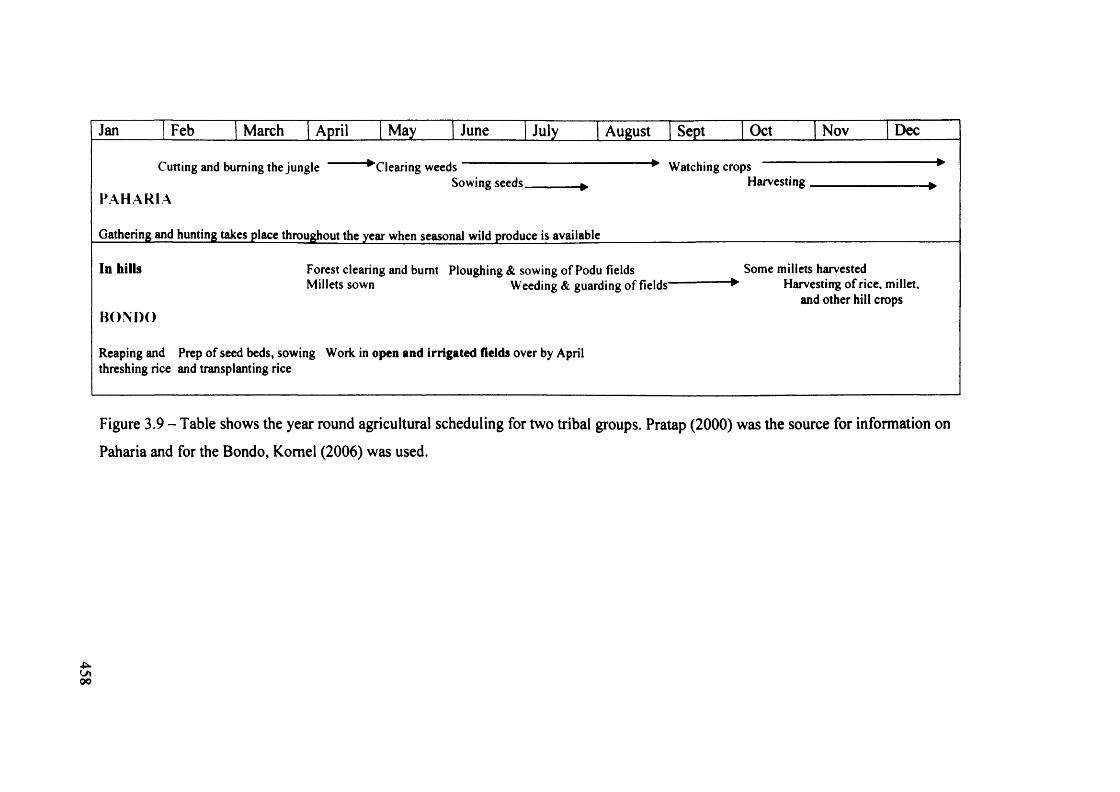
458
Feb March April May June August Sept ... . Oct NovJan Feb March Aoril May June July Aueust SeDt Oct Nov Dec
Cutting and burning the jungle ^Clearing weeds * Watching cropsSowing seeds ^ Harvesting--------------------------
PAHARIA
Gathering and hunting takes place throughout the year when seasonal wild produce is available __________________________________________
In hills Forest clearing and burnt Ploughing & sowing of Podu fields Some millets harvestedMillets sown Weeding & guarding of fields-------------- ► Harvesting of rice, millet,
and other hill cropsBONDO
Reaping and Prep of seed beds, sowing Work in open and irrigated fields over by April threshing rice and transplanting rice
Figure 3.9 - Table shows the year round agricultural scheduling for two tribal groups. Pratap (2000) was the source for information on
Paharia and for the Bondo, Komel (2006) was used.

Site Dates in BP Cal. BC date (Oxcal)
Chopani-Mando, Uttar Pradesh BS-129 4540*110 3500-3030Lekhahia, Madhya Pradesh TF-417 (Phase 3)TF-419 (Phase 1)
3560*1054240*110
2120-17303010-2620
Sarai-Nahar-Rai, Uttar Pradesh TF-1356& 1359 TF-1104
2860*12010050*110
1260-8909950-9300
Mahadaha, Uttar PradeshBS-137BS-138BS-136OxA 1647
2880*2503849*1304010*1206320*80
1400-8002490-20602900-23005470-5140
A n n e p f e n c d U f c > a S M T « r « 4 (1 9 9 * * OfcCel v 3 9 B u l k R a n e y CO O 3k c u b r 4 ad 12 p n b l a p td u o n )
Foragers
BS 129 4540*11OBP
I F 417 356Qt!05BP
T F419 4240*110BP
IF 1356 & 1359 286(H120BP
TF 1104 10050*110BP
BS 137 2880*250BP
BS 138 3849*130BP
BS 136 4010±120BP
OxA 1647 6320*80BP ik
15000CaDBC lOOOOCalBC 5000CaIBC CaDBC/CalAD
Calibrated date
Figure 4.1: Table o f published radiocarbon dates and a multiplot for foraging sites in
Northern India.
459
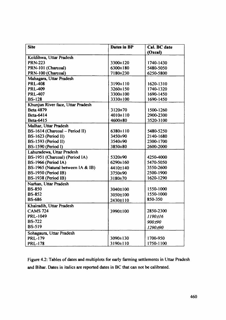
Site Dates in BP Cal. BC date (Oxcal)
Koldihwa, Uttar Pradesh PRN-223PRN-101 (Charcoal) PRN-100 (Charcoal)
3300±120 6300±180 7180±230
1740-14305480-50506250-5800
Mahagara, Uttar PradeshPRL-408PRL-409PRL-407BS-128
3190=t 110 3260±150 3300±100 3330±100
1620-13101740-13201690-14501690-1450
Khunjun River face, Uttar PradeshBeta 4879Beta-6414Beta-6415
3120±70 4010ttl 10 4600±80
1500-12602900-23003520-3100
Malhar, Uttar Pradesh BS-1614 (Charcoal - Period 11) BS-1623 (Period II)BS-1593 (Period II)BS-1590 (Period I)
6380±110 3450±90 3540±90 385Q±80
5480-52502140-16802300-17002600-2000
Lahuradewa, Uttar Pradesh BS-1951 (Charcoal) (Period I A) BS-1966 (Period I A)BS-1965 (Natural between IA & IB) BS-1950 (Period IB)BS-1938 (Period IB)
5320±90 6290±160 4410±140 3750±90 3180±70
4250-40005470-50503550-26002500-19001620-1290
Narhan, Uttar PradeshBS-850BS-852BS-686
304011003050110024301110
1550-10001550-1000850-350
Khairadih, Uttar PradeshCAMS 724PRL-1049BS-722BS-519
39901100 2850-23001190±169001901290190
Sohagaura, Uttar PradeshPRL-179PRL-178
30901130 3190±110
1700-9501750-1100
Figure 4.2: Tables o f dates and multiplots for early farming settlements in Uttar Pradesh
and Bihar. Dates in italics are reported dates in BC that can not be calibrated.
460

Site Dates in BP Cal. BC date (Oxcal)
Barudih, Bihar-Neolithic PhasePRL-188APRL-187PRL-15
2770±1403040±1503290±135
1400-5001700-8501950-1200
Chi rand, Bihar - ChalcolithicTF-444TF-1029TF-1028TF-1030TF-445
2590±1052915±853390±903430±1003500±100
950-4001320-8901920-14902050-14502150-1500
Chirand, Bihar - NeolithicTF-1126TF-1036TF-334TF-1035TF-1127TF-1125TF-1033TF-1034TF-1031TF-1032
2290±1202485±1202715±1203125±1003230±953365±1503390±1103420±1103525±1353600±150
800-50900-3501300-5001700-10501740-12902150-12501950-14002050-14502300-15002500-1500
Senuwar, Bihar BS-908 (Layer 16 - 1A) BS-911 (Layer 14 - IA) BS-910 (Layer 7 - IB) BS-932 (Layer 10 - IB) BS-755 (Layer 7 - IB) BS-757 (Layer 6 - I B ) BS-915 (Layer 6 - II) BS-931 (Layer 4 - I I )
3890±100 3540±130 2960±80 3130±140 3720±120 3450±110 3160±120 2650±110
2700-20002300-15001400-9701750-10002500-17502050-14501750-10501050-400
Figure 4.2 continued: Tables of dates and multiplots for early farming settlements in Uttar
Pradesh and Bihar. Dates for both tables (figures 4.1 & 4.2) are taken from Bellwood et al.
1992, Possehl & Rissman 1992, Chattopadhyaya 1996, Kusumgar & Yadava 2002, and
Tewari et al. 2003.
461

A * * p fce* d e» to e Sterner e d . (199*1 QaCd »3 9 Bnafc Rtetecy (2003t cub r4 ad 12 pnt> uteH ***)|
KDW PRN-223 330Gtl20BP
KDW PRN-101 6300±180BP
KDW PRN-100 718G±23Q©EL
M G R PRL-408 319Q±H0BP
M G R PRL-409 3260±I50BP
M G R PRL-407 330OH00BP
M G R BS-128 3330tlOOBP
KJN Beta 4879 3120±70BP
KJN Beta 6414 40 itttll0B P
KJN Beta 6415 4600t80BP
M L R BS-1623 3550t90BP
M L R BS-1593 3650t90BP
M L R BS-1590 385ftt«OBP
M L R BS-1614 6380*4 10BP
LHA BS-1938 3I80±70BP
LHA BS-1950 375ttt90BP
LHA BS-1%5 4410tl40BP
LHA BS-1951 5320t90BP
LHA BS-1966 6290±160BP
NRN BS- 6 8 6 2430*1 10BP
lOOOOCaBC SOOOCalBC 6000CaIBC 4000CaIBC 2000CalBC CalBC/CalADCafibrated date
Figure 4.2 continued: Multiplot o f available calibrated dates for early farming sites.
462

. (199*1 OkCri v3.9 Bnak Raacy (2003X cab r4 a l:12 pob iMptduoa]
NRN BS-850 304G*100BP
NRN BS-852 3Q50*100BP
KHH CAMS 724 3990*100131^
SGA PRL-179 3090±130BP
SCjA PRL-178 3190*1 I0BP
CHDC TF-444 2590*105BP
C U DC IT-1029 2915±85BP
C H D C TF-1028 3390*90BP
C H D C TT-1030 3430*100BP
CHD C TF-445 3500*100BP
CHD N TF-1126 2290* 120BP
CHD N T F -1036 2485*I20BP
CHD N IT-334 2715± 120BP
CHD N IT-1035 3125* 100BP
CHD N IT-1127 3230*95BP
C l ID N IT-1125 3365* 150BP
CHD N IT-1033 3390* 11013P
Cl ID N IT-1034 3420*110BP
CHD N IT-1031 3525* 135BP
Cl ID N IT-1032 3600* 150BP
4000CaIBC 3000CaIBC 2000CaIBC lOOOCalBC CalBC/CalAD lOOOCalAICafibrated date
Figure 4.2 continued: Multiplot o f available calibrated dates for early farming sites.
463
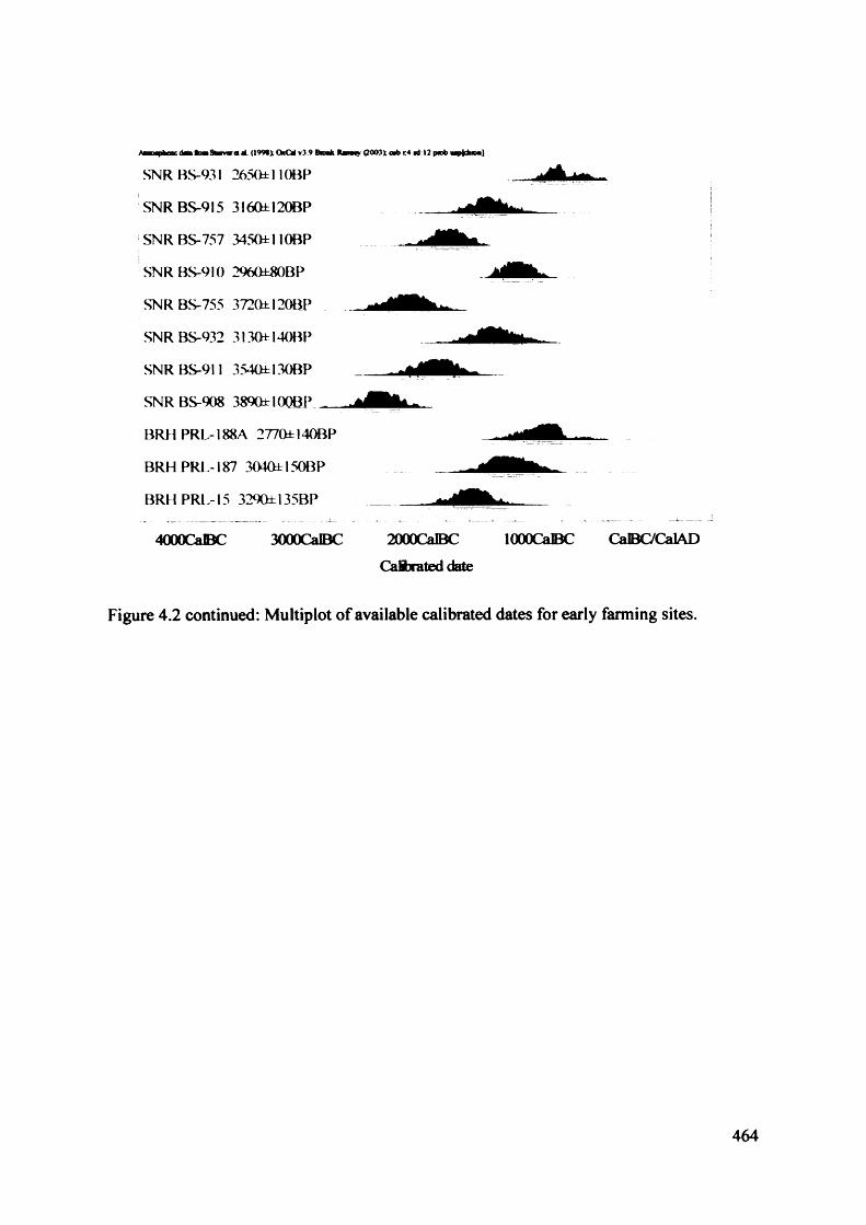
a m q i h u i r d l fc— SMrvCTa A (199*X OhCU v 3 9 B o o k Rj iu j ( 2 0 0 3 k o b c 4 td :1 2 p n b uapfduM i)
SNR BS-931 2650tl 10BP
SNR BS-915 3160tl20BP
SNR BS-757 3450fcllOBP
SNR BS-910 296ttt80BP
SNR BS-755 372Qtl20BP
SNR BS-932 3130tl40BP
SNR BS-911 3540tl30BP
SNR BS-908 389QtlOOBP
BRH PRL-188A 2770tl40BP
BRHPR1-I87 3040±150BP
BRHPRL-15 329Q±135BP
4000CalBC 3000CalBC 2000CaIBC Cafibrated date
lOOOCalBC CalBC/CalAD
Figure 4.2 continued: Multiplot of available calibrated dates for early farming sites.
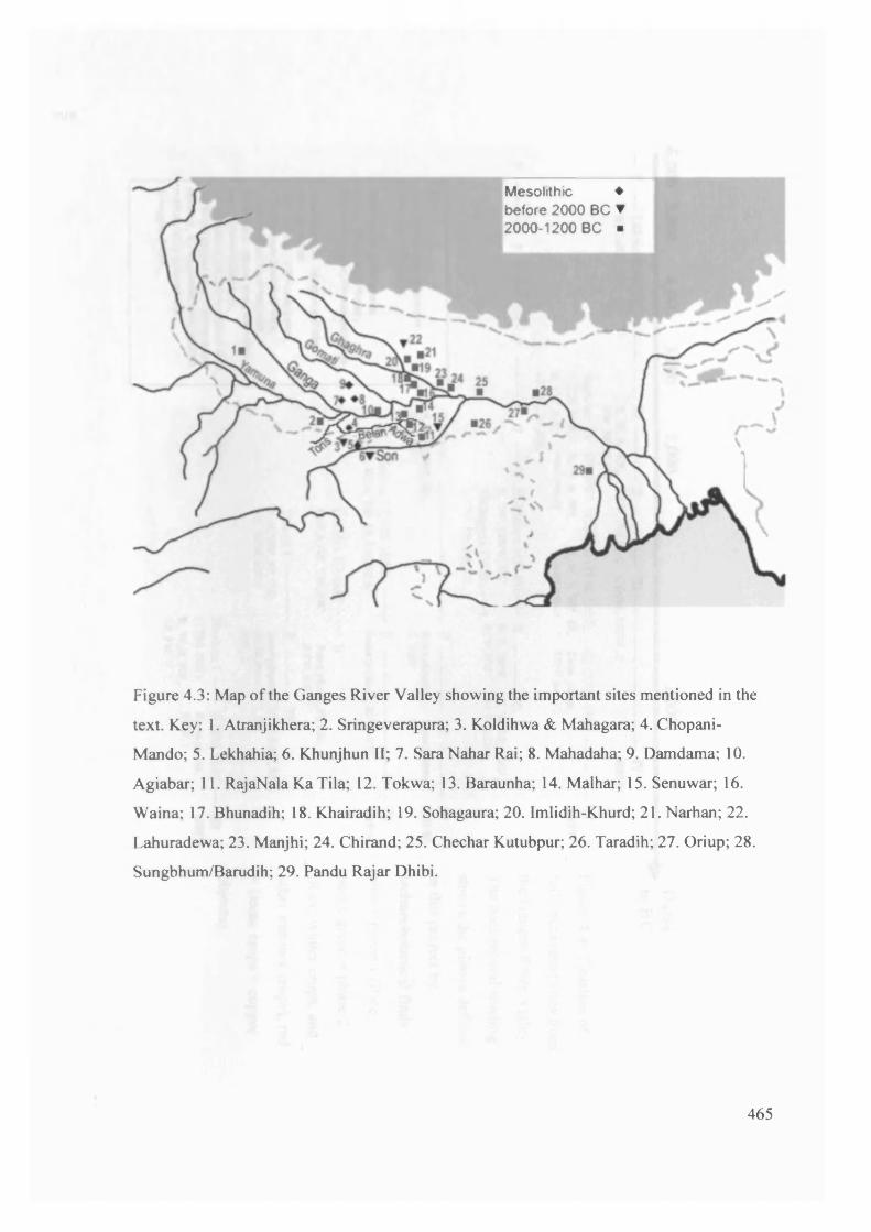
Mesolithic ♦ before 2000 BC ▼ 2000-1200 BC ■
Figure 4.3: Map of the Ganges River Valley showing the important sites mentioned in the
text. Key: 1. Atranjikhera; 2. Sringeverapura; 3. Koldihwa & Mahagara; 4. Chopani-
Mando; 5. Lekhahia; 6. Khunjhun II; 7. Sara Nahar Rai; 8. Mahadaha; 9. Damdama; 10.
Agiabar; 11. RajaNala KaTila; 12. Tokwa; 13. Baraunha; 14. Malhar; 15. Senuwar; 16.
Waina; 17. Bhunadih; 18. Khairadih; 19. Sohagaura; 20. Imlidih-Khurd; 21. Narhan; 22.
Lahuradewa; 23. Manjhi; 24. Chirand; 25. Chechar Kutubpur; 26. Taradih; 27. Oriup; 28.
Sungbhum/Barudih; 29. Pandu Rajar Dhibi.
465

466
6.000 5.000 4.000 3.000 2 .0 0 0 1.000
•>
(28D8 J959^n:(i«sl) i: 0d>:NBPW
CRBV
C hlrand I
•> -----
K e yUttar Pradesh sites inbbietext Bihar sites m text
Bold type «r plants present R=ric«, W=wheat, B=barl«y,WP=wnter pulses, SP=suanner pulses
Normal type are ceramics and other artefacts presentRW*r»d ware, CW»cc*ded ware, CBRW-coarct b lack+red ware, PBRW*paiUed bhck+red were, BSW=bl*ck slipped were, OW=Ckey were, BObumithed ^ey, BR=bunushed red, BB=bumished hUck, RS W*r*d sloped were, PRW*punted red were, RU=iusticalad were, NBPW- northern black polished were O copper, I* iron,
R, W ,B, WP, SP, Same plants, Same plants, NBPWRW, OW C,BRW I
M a lh a r l(1 9 0 0 1600) f >11: jI;:;:; 1 :;:; , HIR, W, B, WP, SP, RW,BRW Sam*plants, I, BSW, GW NBPW
Im lid ih K h u rd I -H— U R,W,B,WP, CW,RW Sam*plants, PBRW,
BSW,RW,C— u — iii
Sam* plants, BRW,BSW,RW, BRW,BSW, I,C RW, C
N arium I Q (800-600) — III(1300 000) Sam* plants, NBPWR ,W .B >WP. ®SW,ISP,PBRW, I
ToJoval —R,B,W P,SP,CW ,RU,HRW,BBW
Dates * iii BC
Figure 4.4: Timeline of
fully excavated sites from
the Ganges River Valley.
The background shading
shows the phases defined
in this project by
archaeobotanical finds:
blue = phase 1 (Rice
only), green = phase 2
(Rice, winter crops, and
other summer crops), red
= (same crops + copper
objects).
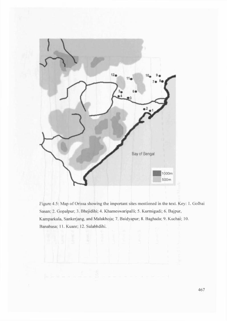
Bay of Bengal
1000m500m
Figure 4.5: Map o f Orissa showing the important sites mentioned in the text. Key: 1. Golbai
Sasan; 2. Gopalpur; 3. Bhejidihi; 4. Khameswaripalli; 5. Kurmigudi; 6. Bajpur,
Kamparkala, Sankerjang, and Malakhoja; 7. Baidyapur; 8. Baghada; 9. Kuchai; 10.
Banabasa; 11. Kuanr; 12. Sulabhdihi.
467

468
LeveM Level 2Level 3
Level 4
Level 5
Level 6
Level 7
Level 8
Level 9
Level 10
Figure 5.1. Section drawing of Chopani Mando.

III1III•
1.70m
lIlllllll
Level 1
Level 3
Level 4
Level 5
Figure 5.2: Section drawing of Koldihwa.
O 'o

Level 6
Level 8
Level
Level 10
Level 11
LevelLevel 13
Level 14
Level 15
Level 16
Level 17
Figure 5.3: Section drawing o f Mahagara.
470

Level number Macro-botanical sample number
Phytolith sample number
Cultural Phase
1 ABOT 53 & 54 1 Advanced Mesolithic2 ABOT 55 & 56 - Advanced Mesolithic3 ABOT 57 & 58 3 Advanced Mesolithic4 ABOT 59 & 60 - Early Mesolithic
Geometric5 ABOT 61 & 62 5 Early Mesolithic
Geometric6 ABOT 63 & 64 - Early Mesolithic
Geometric7 ABOT 65 & 66 7 Early Mesolithic
Geometric8 ABOT 67 & 68 - Early Mesolithic
Non-geometric9 ABOT 69 & 70 9 Early Mesolithic
Non-geometric10 ABOT 71 & 72 - Epi-Palaeolithic
Figure 5.4: Table explaining where samples come from in the Chopani-Mando section.
Level number Macro-botanical sample number
Phytolith sample number
Cultural Phase
Zl-1 A B O T 1 & 2 1 Chalcolithic/ Iron Age
Zl-1 - Pit - 2 Chalcolithic/ Iron Age
Z l-2 ABOT 3 & 4 3 ChalcolithicZ l-3 ABOT 5 & 6 4 NeolithicZ l-4 ABOT 7 & 8 5 NeolithicZ l-5 ABOT 9 & 10 6 SterileY 1 - 1 ABOT 11 & 12 7 Chalcolithic/
Iron AgeY l-2 ABOT 13 & 4 8 ChalcolithicY l-3 ABOT 15 & 16 9 NeolithicY l-4 ABOT 17 & 18 10 NeolithicYl - 5 ABOT 19 & 20 11 Sterile
Figure 5.5 continued: Table explaining where sample come from in the Koldihwa Z1 & Y1
section.
471
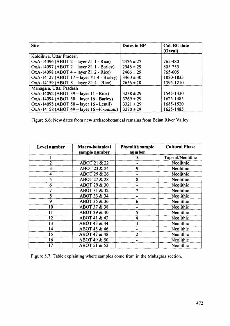
Site Dates in BP Cal. BC date (Oxcal)
Koldihwa, Uttar Pradesh OxA-14096 (ABOT 2 - layer Z1 1 - Rice) OxA-14097 (ABOT 2 - layer Z1 1 - Barley) OxA-14098 (ABOT 4 - layer Z1 2 - Rice) OxA-14127 (ABOT 17 - layer Y1 4 - Barley) OxA-14159 (ABOT 8 - layer Z 1 4 - Rice)
2476 ± 27 2546 ± 29 2466 ± 29 3460 ± 30 2656 ±28
765-480805-755765-6051880-18351395-1210
Mahagara, Uttar Pradesh OxA-14092 (ABOT 39 - layer 11 - Rice) OxA-14094 (ABOT 50 - layer 16 - Barley) OxA-14095 (ABOT 50 - layer 16 - Lentil) OxA-14158 (ABOT 49 - layer 16 -V.radiata)
3238 ± 293269 ± 29 3321 ± 2 93270 ±29
1545-14301625-14851685-15201625-1485
Figure 5.6: New dates from new archaeobotanical remains from Belan River Valley.
Level number Macro-botanical sample number
Phytolith sample number
Cultural Phase
1 - 10 Topsoil/Neolithic2 ABOT 21 & 22 - Neolithic3 ABOT 23 & 24 9 Neolithic4 ABOT 25 & 26 - Neolithic5 ABOT 27 & 28 8 Neolithic6 ABOT 29 & 30 - Neolithic7 ABOT 31 & 32 7 Neolithic8 ABOT 33 & 34 - Neolithic9 ABOT 35 & 36 6 Neolithic10 ABOT 37 & 38 - Neolithic11 ABOT 39 & 40 5 Neolithic12 ABOT 41 & 42 4 Neolithic13 ABOT 43 & 44 3 Neolithic14 ABOT 45 & 46 - Neolithic15 ABOT 47 & 48 2 Neolithic16 ABOT 49 & 50 - Neolithic17 ABOT 51 & 52 1 Neolithic
Figure 5.7: Table explaining where samples come from in the Mahagara section.
472
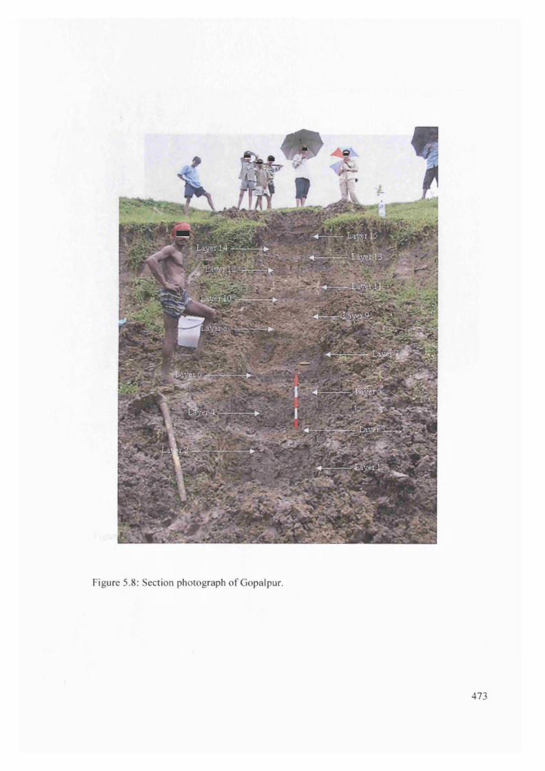
Figure 5.8: Section photograph of Gopalpur.
473
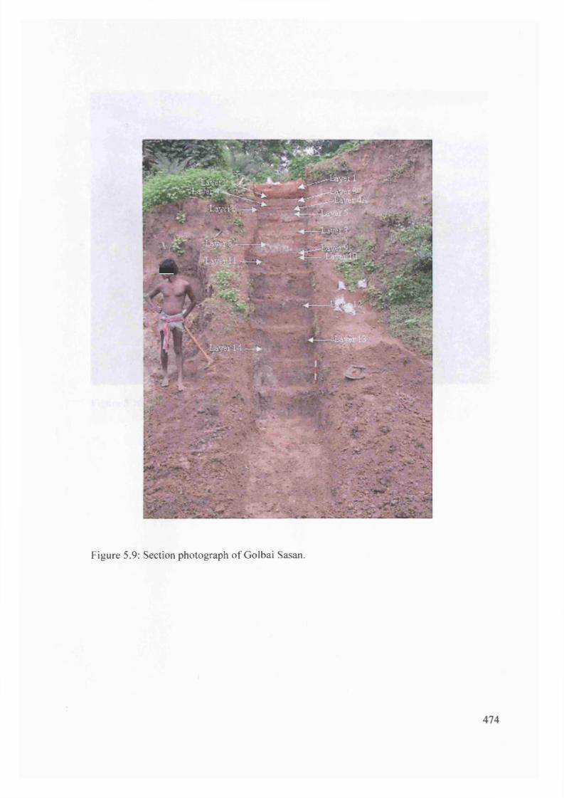
Figure 5.9: Section photograph of Golbai Sasan.
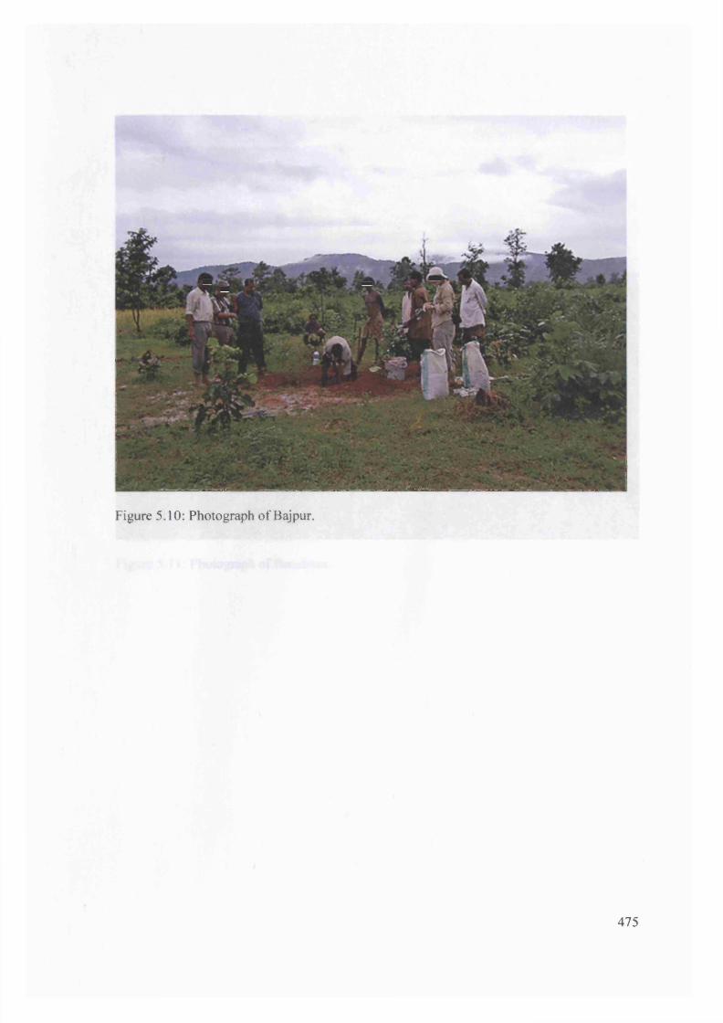
Figure 5.10: Photograph of Bajpur.
475

'■
Figure 5.11: Photograph of Banabasa.
476
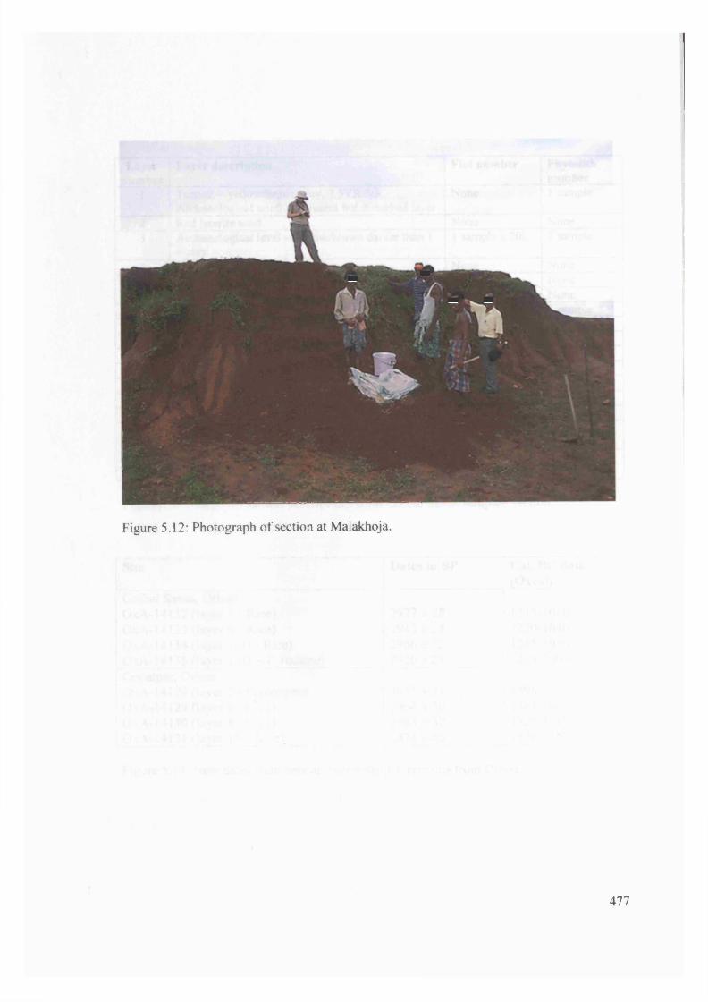
Figure 5.12: Photograph of section at Malakhoja.
477

Layernumber
Layer description Flot number Phytolithnumber
1 Topsoil - yellow/brown clay, 7.5YR 5/3 Archaeological artefacts present but disturbed layer
None 1 sample
2 Red laterite sand None None3 Archaeological level - yellow/brown darker than 1
- clay1 sample x 20L 1 sample
4 Red laterite None None4A Fine grey sand - very thin layer None None6 Red laterite None None5 Above layer 7A 1 sample x 20L 1 sample
7A Thin black layer on top of layer 7B 1 sample x 20L 1 sample7B Yellow/light brown sandy clay 1 sample x 20L 1 sample8 Grey clay 1 sample x 20L 1 sample9 Dark grey clay 1 sample x 20L 1 sample10 Dark red/brown sandy clay 1 sample x 20L 1 sample11 Light yellow brown clay 1 sample x 20L 1 sample12 Dark red/brown clay mottled with charcoal flecking 1 sample x 20L 1 sample13 Light yellow brown 4 samples x 20L
A, B, C, D4 samples A, B, C, D
14 Grey clay - pit with charcoal 3 samples x 20L A, B, C
3 samples A, B, C
Figure 5.13: Table o f the soil descriptions from Golbai Sasan sampled section.
Site Dates in BP Cal. BC date (Oxcal)
Golbai Sasan, Orissa OxA-14132 (layer 3 - Rice) OxA-14133 (layer 9 - Rice) OxA-14134 (layer 13D - Rice) OxA-14135 (layer 1 3 D - V. radiata)
2927 ± 28 2943 ± 28 2966 ±32 2920 ± 29
1215-10101220-10401265-10501215-1005
Gopalpur, Orissa OxA-14128 (layer 2 - Pigeonpea) OxA-14129 (layer 6 - Rice) OxA-14130 (layer 8 - Rice)OxA-14131 (layer 13 - Rice)
3035 ±31 2964 ± 30 2983 ± 32 2874 ± 45
1395-12101365-10451320-11101170-915
Figure 5.14: New dates from new archaeobotanical remains from Orissa.
478

Flot sample number
Phytolith sample number
Level depth
None None 30-40 cm o f soil above top sample but it is disturbed due to
ploughingGPR-03A-15 Phyto 15 395 cmGPR-03A-14 Phyto 14 365 cmGPR-03A-13 Phyto 13 335 cmGPR-03A-12 Phyto 12 295 cmGPR-03A-11 Phyto 11 270 cmGPR-03A-10 Phyto 10 250 cmGPR-03A-9 Phyto 9 205 cmGPR-03A-8 Phyto 8 180 cmGPR-03A-7 Phyto 7 145 cmGPR-03A-6 Phyto 6 115 cmGPR-03A-5 Phyto 5 95 cmGPR-03A-4 Phyto 4 78 cmGPR-03A-3 Phyto 3 60 cmGPR-03A-2 Phyto 2 40 cmGPR-03A-1 Phyto 1 20 cm
None None 0cm at bottom of section
Figure 5.15: Table of samples taken at Gopalpur.
Flot sample number
Phytolith samples number
Level depth Notes
MKA-03A-1 Phyto 1 0 - 40 cm top Topsoil - coarse red ware pottery
MKA-03A-2 None 0 - 40 cm bottom Topsoil - coarse red ware pottery and red
and black wareMKA-03A-3 None 40 - 80 cm top ArchaeologicalMKA-03A-4 Phyto 4 40 - 80 cm middle ArchaeologicalMKA-03A-5 None 40 - 80 cm bottom ArchaeologicalMKA-03A-6 None 80 - 110 cm top ArchaeologicalMKA-03A-7 Phyto 7 80 - 110 cm middle ArchaeologicalMKA-03A-8 None 80 - 110 cm bottom ArchaeologicalMKA-03A-9 Phyto 9 110 - 140 cm top Natural
MKA-03A-10 None 110 - 140 cm bottom Natural
Figure 5.16: Table o f samples taken at Malakhoja. Finds were only found in the top two
samples.
479

Flot sample number
Phytolith samples number
Level depth Notes
None Phyto 0 0-10 cm TopsoilBJR-03A-1 Phyto 1 10-20 cm NeolithicBJR-03A-2 Phyto 2 20-30 cm NeolithicBJR-03A-3 Phyto 3 30-40 cm NeolithicBJR-03A-4 Phyto 4 40-50 cm Mesolithic
Figure 5.17: Table o f samples taken at Bajpur.
Flot sample number
Phytolith samples number
Level depth
None Phyto 0 0-10 cmBNA-03A-1 Phyto 1 10-20 cmBNA-03A-2 Phyto 2 20-30 cmBNA-03A-3 Phyto 3 30-40 cm
Figure 5.18: Table o f samples taken from Banabasa.
480

C. Embryo about l/2(-2/3) length of grain
D. Embryo 2/3-3Z4 length of grain
Panicum miliaceum
< D
< 3 o < o
o y \ o ,
Pcmicum sumatrense
Eleusine coracana Paspalum scrobiculatum
Pennisetumalopecuroides
O S Z ) O
Brachiaria ramosa Setaria italica
< 3 0
(2 2 ) c a < £z
O CD O
Echinochloa colona Setaria Setariapumila verticillata
Figure 5.19: Identification key for small millets using embryo length to overall length of grain (after Fuller 1999, fig. 6.8).
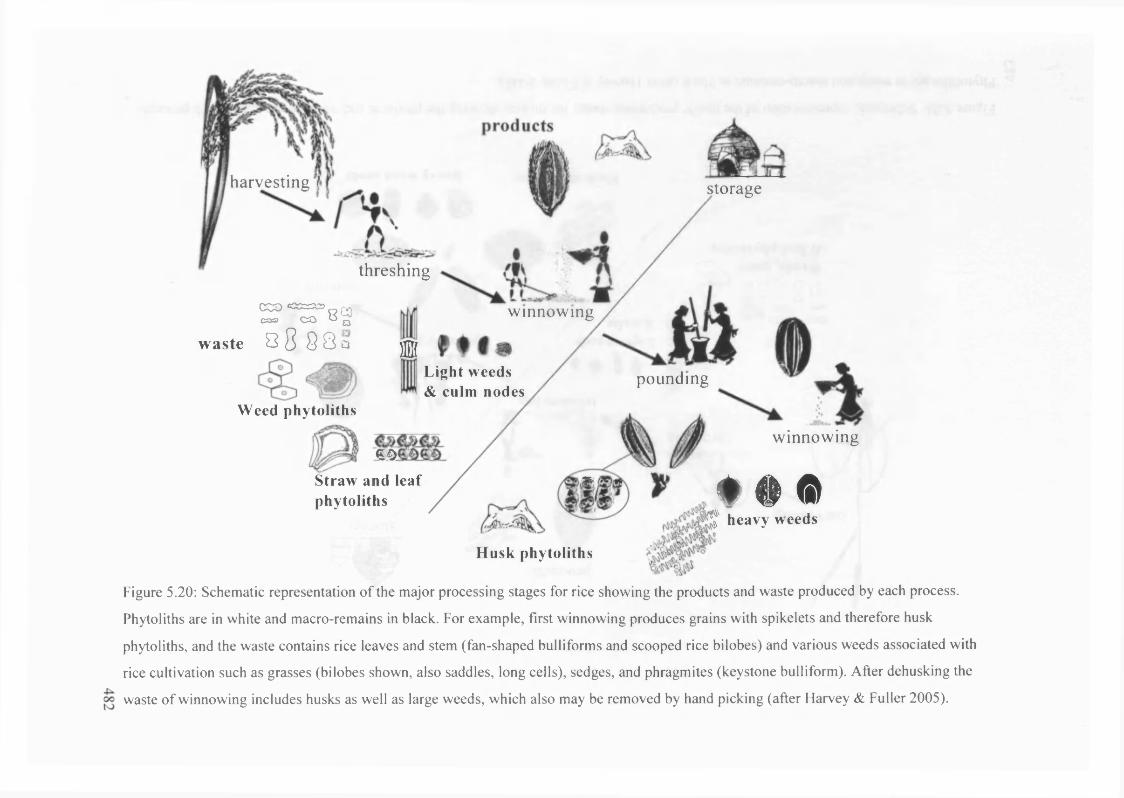
harvesting {
threshing
OZO coczzzxCOS CO
w a ste
8 g
2 8 8 8 q
Weed phytoliths
mStraw and leaf phytoliths
storage
winnowing
KLight weeds & culm nodes
pounding
M
winnowing
Husk phytoliths
♦ | f f i^ heavy w eeds
Figure 5.20: Schematic representation of the major processing stages for rice showing the products and waste produced by each process.
Phytoliths are in white and macro-remains in black. For example, first winnowing produces grains with spikelets and therefore husk
phytoliths, and the waste contains rice leaves and stem (fan-shaped bulliforms and scooped rice bilobes) and various weeds associated with
rice cultivation such as grasses (bilobes shown, also saddles, long cells), sedges, and phragmites (keystone bulliform). After dehusking the
waste of winnowing includes husks as well as large weeds, which also may be removed by hand picking (after Harvey & Fuller 2005).
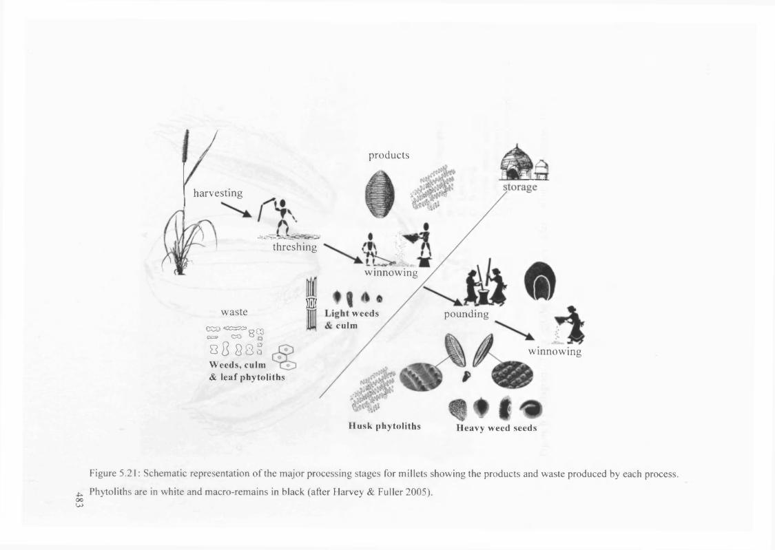
harvesting
products
threshing
wastecso «ss=?a>CSSB CO 8®
S 8 8 8 §Weeds, culm & leaf phytoliths
SW.»winnowing
i iweeds
culmpounding
winnowing
Husk phytoliths Heavy weed seeds
Figure 5.21: Schematic representation of the major processing stages for millets showing the products and waste produced by each process.
^ Phytoliths are in white and macro-remains in black (after Harvey & Fuller 2005).00u>
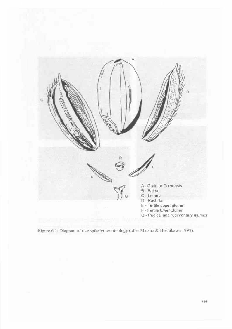
A - Grain or CaryopsisB - PaleaC - LemmaD - RachillaE - Fertile upper glumeF - Fertile lower glumeG - Pedicel and rudimentary glumes
Figure 6.1: Diagram of rice spikelet terminology (after Matsuo & Hoshikawa 1993).
484
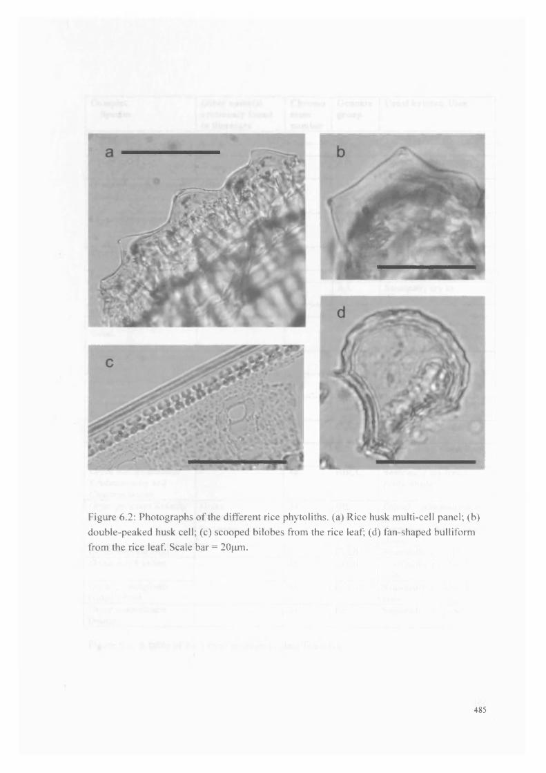
Figure 6.2: Photographs of the different rice phytoliths. (a) Rice husk multi-cell panel; (b) double-peaked husk cell; (c) scooped bilobes from the rice leaf; (d) fan-shaped bulliform from the rice leaf. Scale bar = 20|im.
485

ComplexSpecies
O ther name(s) commonly found in literature
Chromosomenum ber
Genomegroup
Usual habitat; Uses
OryzaOrvza sativa complexOryza sativa L. - 24 AA Upland to Deepwater;
open; cultigenOryza nivara Sharma et Shastry
Oryza ruflpogon (annual form)
24 AA Seasonally dry; open; eaten by tribals, Bhramins and poor
Oryza ruripogon Griff. Oryza perennis, Oryza rufipogon (perennial form)
24 AA Seasonally deepwater and wet year round; open; grains sometimes eaten
Oryza glaberrima Steud. - 24 AA Upland to deepwater; open; cultigen
Oryza barthii A. Chev. O.breviligulata 24 AA Seasonally dry; openOryza longistaminata Chev. Et Roehr.
Oryza barthii 24 AA Seasonally dry to deepwater; open
O.meridionalis Ng - 24 AA Seasonally dry; openOryza glumaepatula Steud.
24 AA Inundated areas that become seasonally dry; open
Oryza officinalis complexalso called Oryza latifolia complex or groupOryza officinalis Wall ex Watt
Oryza minuta 24 CC Seasonally dry; open
Oryza minuta JS Presl. Ex CB Presl.
Oryza officinalis 48 BBCC Stream sides; semi shade
Oryza rhizomatis Vaughan
- 24 CC Seasonally dry; open
Oryza eichingeri Peter - 24 CC Stream sides; forest floor; semi shade
Oryza malapuzhaensis Krishnaswamy and Chandrasakaran
48 BBCC Seasoanlly dry forest pools; shade
Oryza punctata Kotschy ex Streud.
Oryzaschweinfurthiana for tetraploid form
2448
BB,BBCC
Diplod - seasonally dry; openTetraploid - forest floor; shade
Oryza latifolia Desv. - 48 CCDD Seasonally dry; openOryza alta Swallen - 48 CCDD Seasonally inundated;
openOryza grandiglumis (Doell.) Prod.
- 48 CCDD Seasonally inundated; open
Oryza australiensis Domin
- 24 EE Seasonally dry; open
Figure 6.3: A table of the Oryza taxonomic classifications.
486

ComplexSpecies
Other name(s) commonly found in literature
Chromosomenumber
Genomegroup
Usual habitat; Uses
Ridleyanae TateokaOryza schlechteri Pilger - 48 - River banks; openOryza ridleyi complexOryza ridleyi Hook. - 48 HHJJ Seasonally inundated
forest floor; shadeOryza longiglumis Jansen
- 48 HHJJ Seasonally inundated forest floor; shade
Granulata Roschev.Oryza granulata complexOryza granulata Nees et Am ex Watt
- 24 GG Forest floor; shade
Oryza meyeriana (Zoll. Et Mor. Ex Streud.) Baill.
24 GG Forest floor; shade
Brachyantha B.R. LuOryza brachyantha Chev. Et Roehr.
- 24 FF Rock pools; open
Figure 6.3 continued: A table o f the Oryza taxonomic classifications.
487

- CA TW
BPDCD
s HW
CD
MW
B
Figure 6.4: Diagram showing the Zhang (2002) (A) and Zhao et al. (1998) (B) method of measuring rice hairs and double-peaked rice husk phytoliths (after Zhang 2002, fig. 2 and Zhao et al. 1998, fig. 2).
VL
B
HL
Figure 6.5: Diagram of Fujiwara bulliform measurements (after Fujiwara et al. 1993).
488

Culitvated Rice Wild rice
* '•
•*A V i •,
s 3 «•
Scale-like - decoration
40 microns
Figure 6.6: Diagram of bulliforms chips o f wild and domestic rice (after Lu et al. 2002, fig-3).
489
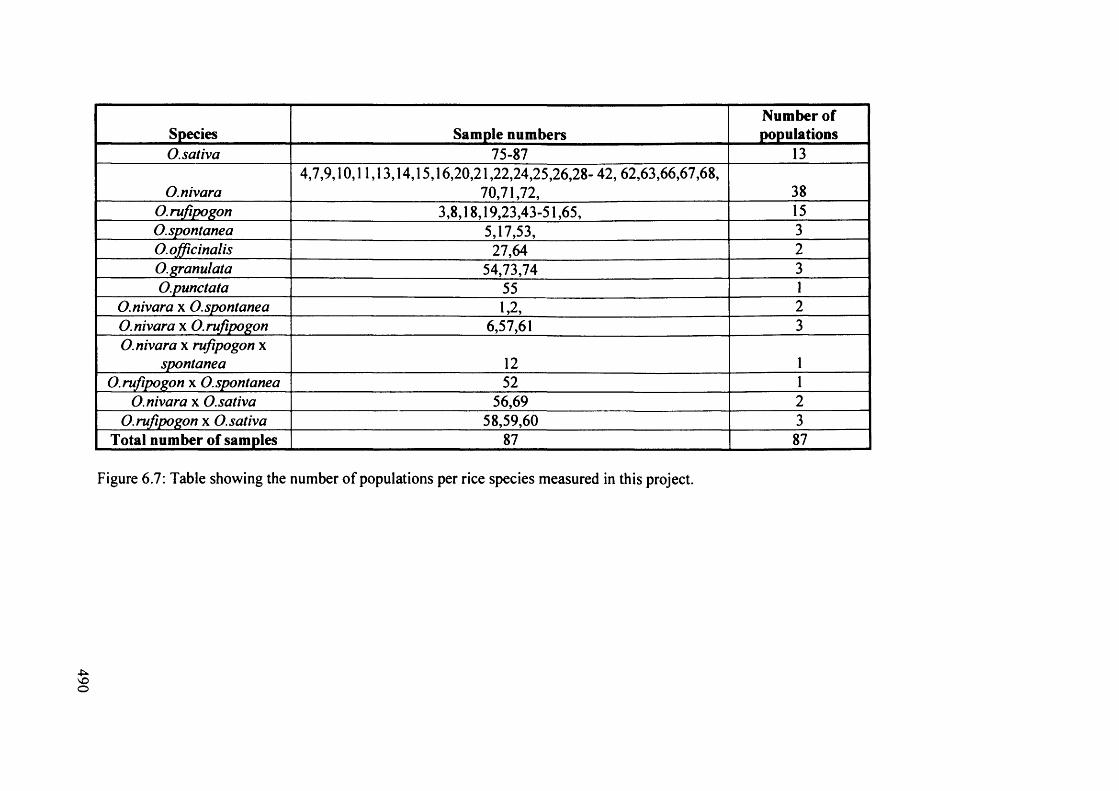
490
Species Sample numbersNumber of populations
0. sativa 75-87 13
O.nivara4,7,9,10,11,13,14,15,16,20,21,22,24,25,26,28- 42, 62,63,66,67,68,
70,71,72, 38O. rufipogon 3,8,18,19,23,43-51,65, 150. spontanea 5,17,53, 30 .officinalis 27,64 2O. granulata 54,73,74 3O.punctata 55 1
O.nivara x 0 .spontanea 1,2, 2O.nivara x O.rufipogon 6,57,61 3O.nivara x rufipogon x
spontanea 12 1O.rufipogon x O.spontanea 52 1
O.nivara x 0 .sativa 56,69 2O.rufipogon x O.sativa 58,59,60 3
Total number of samples 87 87
Figure 6.7: Table showing the number of populations per rice species measured in this project.

SampleNo
AccNo IRRI or USDA Species
DonorCountry
Varietyname District Town Village Latitude
Longitude
Elevation
1 80436 O.nivara & spontanea India Kapni Bastar - Tankwade - - -
2 80532 O.nivara & spontanea India Bastar4KM from
Geeham
3 80538 O.mfipogon India Tatangi Bastar Jagdalpur . 19°5'N 82°0'E -
4 80548 O.nivara India - Bastar Kondagaon Palari 19°40'N 81°40’E -
5 80555 O.spontanea India - Bastar Makri Belgaon 19°49‘N 81°55'E -
6 80556 O.nivara & rufipogon India - Bastar Kondagaon Sargaon 19°40'N 81°38’E -
7 80560 O.nivara India - Bastar Narainpur Nelwao 19°45'N 81°20’E -
8 80562 O.mfipogon India - Bastar Narainpur Deogaon 19°45'N 81°19'E -
9 80573 O.nivara India - Bastar Antagarh Bhaingaon 19°50'N 81 °14'E -
10 80589 O.nivara India Pashahar Bastar Pakhanjoor Chindpara 20°10'N 80°45'E -
11 80593 O.nivara India BastarBhanupratappu
r Kurri 20°20'N 81o10’E
12 80594O.nivara x rufipogon x
spontanea India Bastar Kanker Bewarati
13 80599 O.nivara India - Bastar Kanker Atorgaon 20°10'N 81°28’E -
14 80611 O.nivara India - Koraput Navrangpur Navrangpur 19°10'N 82°35'E -
15 80613 O.nivara India Jhartia Kalahandi Jaipatana Ampani 19°34'N 82°40'E -
16 80621 O.nivara India - Raipur Khariyar road Temari 20°55'N 82°30'E -
17 80626 O.spontanea India Karaga Raipur Mahasamund Mahasamund 21°0’N 82°5’E -
18 80629 O.mfipogon India Pasahar Raipur Arang Arang 21°12'N 81°55'E -
19 80636 O.mfipogon India Karaga Raipur Kasadole Lavan 21 °38'N 82°25'E -
20 80637 O.nivara India - Raipur Kasadole Kasadole 21°38'N 82°25’E -
21 80645 O.nivara India - Bilaspur Takhatpur Chatona 22°2'N 81°55'E -
22 80677 O.nivara India - Durg Bhilai Newai 21°8'N 81°20'E -
Figure 6.8: List o f populations and information o f origin.
VO
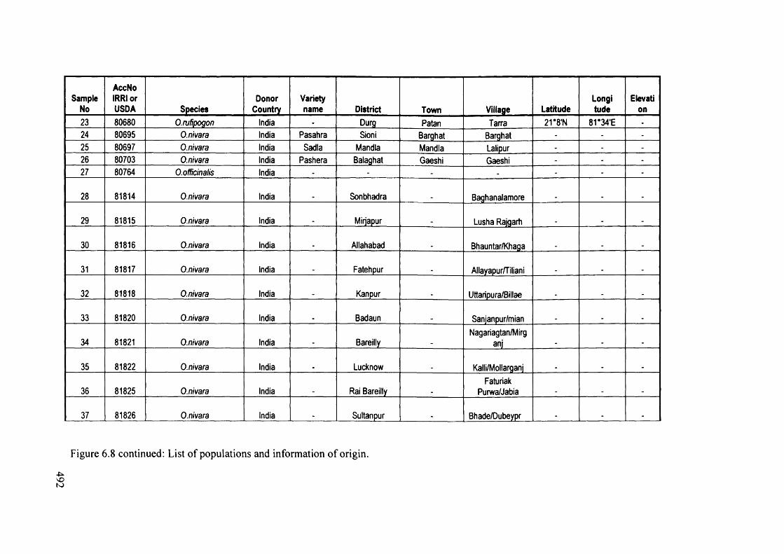
492
SampleNo
AccNo IRRI or USDA Species
DonorCountry
Varietyname District Town Village Latitude
Longitude
Elevation
23 80680 O.rufipogon India - Durg Patan Tarra 21°8'N 81 °34'E -
24 80695 O.nivara India P asah ra Sioni B arghat Barghat - - -
25 80697 O.nivara India Sadla Mandla Mandla Lalipur - - -
26 80703 O.nivara India P ash e ra B alaghat G aeshi Gaeshi - - -
27 80764 0.officinalis India - - - . - - -
28 81814 O.nivara India Sonbhadra B aghanalam ore
29 81815 O.nivara India Mirjapur Lusha Rajgarh
30 81816 O.nivara India Allahabad Bhauntar/Khaga
31 81817 O.nivara India Fatehpur Allayapur/Tiliani
32 81818 O.nivara India Kanpur Uttaripura/Billae
33 81820 O.nivara India Badaun Sanjanpur/m ian
34 81821 O.nivara India BareillyNagariagtan/Mirg
anj
35 81822 O.nivara India Lucknow Kalli/Mollarqanj
36 81825 O.nivara India Rai BareillyFaturiak
Purw a/Jabia
37 81826 O.nivara India . Sultanpur Bhade/Dubeypr . . .
Figure 6.8 continued: List o f populations and information o f origin.

SampleNo
AccNo IRRI or USDA Species
DonorCountry
Varietyname District Town Village Latitude
Longitude
Elevation
38 81827 O.nivara India - Pratapgarh . Patti . - -
39 81829 O.nivara India - Azam garh . M andejafarpur - - -
40 81830 O.nivara India Varanasi Burhani/Burhani
41 81834 O.nivara India . Bhojpur Piro D hanpura 25°15'N 84°20’E -
42 81839 O.nivara India . Jaunpur Dhobhi A nandnagar B 25°30'N 83°'E -
43 81877 O.rufipogon India SonbhadraD evra/R obertsga
nj
44 81878 O.rufipogon India Sidauli Kuchora Bangla
45 81879 O.mfipogon India Lucknow Kalli/Mollarganj
46 81880 O.mfipogon India FaizabadR anapur/Sahebg
anj
47 81885 O.mfipogon India - Gorakhpur Bhatthat Bhatthat 26°50'N 83°32'E -
48 81888 O.mfipogon India - M aharaganj Prenda Sonversha 27°'N 83°15'E -
49 81896 O.mfipogon India - Gonda Nagwa Dumeriadi 26‘ 55'N 82°5'E -
50 81897 O.mfipogon India - Faizabad Pura R oshannagar 26°43'N 82°20'E -
51 81899 O.mfipogon India - Sultanpur A khannagar Mirapur 26°8'N 82°40'E -
52 81901 O.mfipogon x spontanea India Ghazipur Mirjabad Mania 25°30'N 83°55'E
53 81910 O.spontanea India G onda Padri Karpal Mudarwa Maphi 27°'N 81°58'E
54 82044 O.granulata India Kadaka Koraput Junagarh Kavari Gondo 19°30'N 82°35'E -
Figure 6.8 continued: List o f populations and information o f origin.
\oU)

494
SampleNo
AccNo IRRI or USOA Species
DonorCountry
Varietyname District Town Village Latitude
Longitude
Elevation
55 100886 O.punctata Japan CuttackCentral rice res.
Inst.
56 100915 O.nivara x sativa Jap an Calcutta Darshin B arsat
57 101966 O.nivara x rufipogon Jap an70 K M S o f
Jeypore 18°15'N 82°2'E
58 101969 O.rufipogon x sativa Jap an68 KM N of
Jeypore 19‘ 28'N 82°35'E
59 101989 O.rufipogon x sativa Japan - Dharwar Alnawal - 15°30'N 74°40'E -
60 101990 O.rufipogon x sativa Japan DharwarGonagu,Shiggaon 15a0'N 75*10'E
61 102168 O.nivara x rufipogon Japan - Gorakhpur - 26°0'N 83°30'E -
62 104702 O.nivara France31 KM after
Belgaum Belgaum to Goa
63 104705 O.nivara France405 KM before
Panvel121 KM after
Goa Goa to Bombay 16°20'N 73°35'E
64 104707 O.officinalis France DangsW aghai to
Pimpri 20°35'N 73°35'E
65 104709 O.mfipogon France9 KM before
Belgaum513 KM from
BengalorePoona to
Belgaum rd 16°0'N 74°30'E
66 105319 O.nivara India Trichur20 K M SN W of
Trichur2 KMs from
Poorima 10°10'N 76°10'E
67 105320 O.nivara India Palghat34 KMS S of
Palghat Nam m ara 10°10'N 76°20'E
68 105333 O.nivara India Calicut15 KMS E of
Calicut Mukkum H °10 'N 76°10'E
Figure 6.8 continued: List o f populations and information o f origin.
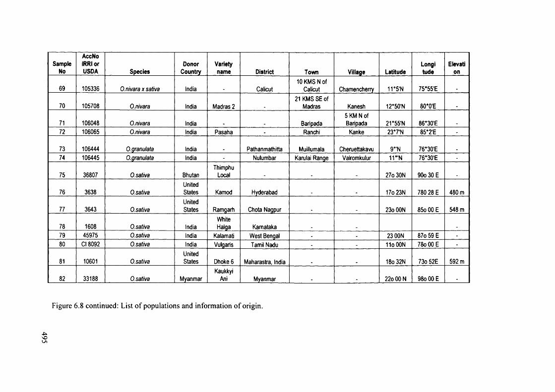
495
SampleNo
AccNoIRRIorUSDA Species
DonorCountry
Varietyname District Town Village Latitude
Longitude
Elevation
69 105336 O.nivara x sativa India Calicut10 KMS N of
Calicut C ham encherry 11°5*N 75°55'E
70 105708 O.nivara India M adras 221 KMS SE of
M adras K anesh 12°50'N 80*0'E
71 106048 O.nivara India Baripada5 KM N of Baripada 21°55*N s e ^ o 'E
72 106065 O.nivara India P a sa h a . Ranchi Kanke 23°7'N 85°2’E -
73 106444 O.granulata India Pathanm athitta Muillumala Cheruettakavu 9°'N 76°30'E
74 106445 0. granulata India - Nulumbar Karulai R ange Valromkulur 11°'N 76°30'E -
75 36807 O.sativa BhutanThimphu
Local 27o 30N 90o 30 E
76 3638 O.sativaUnitedS ta tes Kamod Hyderabad 17o 23N 780 28 E 480 m
77 3643 O.sativaUnitedS ta tes R am garh Chota Nagpur 23o 00N 85o 00 E 548 m
78 1608 O.sativa IndiaWhiteHalga Karnataka
79 45975 O.sativa India Kalamati W est Bengal - - 23 00N 87o 59 E -
80 Cl 8092 O.sativa India Vulgaris Tamil Nadu . . 11o00N 78o 00 E -
81 10601 O.sativaUnitedS ta tes Dhoke 6 M aharastra, India 18o 32N 73o 52E 592 m
82 33188 O.sativa M yanmarKaukkyi
Ani M yanmar 22o 00 N 98o 00 E .
Figure 6.8 continued: List o f populations and information o f origin.

496
SampleNo
AccNo IRRI or USDA Species
DonorCountry
Varietyname District Town Village Latitude
Longitude
Elevation
83 27630 O.sativa Nepal Darwali BagmatiPalung Valley, M akawanpur 27o 38 N 8 5 o 0 4 E
2259m
84 GT O.sativa ThailandChoubunProvince
85 431084 O.sativa M yanmar
Dsi Sel D angar Shah M yanmar 22o 00 N 9 8 o 0 0 E
86 12894 O.sativa India Gom pa 2 Sikkim, India - . 27o 45 N 88o 30 E -
87 EH O.sativa IndiaB hubaneshw ar
m arket - .
Figure 6.8 continued: List of populations and information of origin.

497
Thickness or breath
h
Length
Figure 6.9: Diagram of how grain measurements taken in this project.
Width

CA
/ \ CD
H1
\ /
MW
Figure 6.10: Diagram of double-peaked husk cell with measurements that were taken in this project (after Zhao et al. 1998).
498
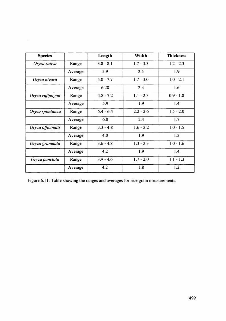
Species Length W idth Thickness
Oryza sativa Range 3.8-8.1 1.7-3 .3 1.2-2.3
Average 5.9 2.5 1.9
Oryza nivara Range © ■ -j 1.7-3 .0 1.0 - 2.1
Average 6.20 2.3 1.6
Oryza rufipogon Range 4 .8 -7 .2 1.1 -2.3 0 .9- 1.8
Average 5.9 1.9 1.4
Oryza spontanea Range 5 .4 -6 .4 2 .2 -2 .6 1 .5-2 .0
Average 6.0 2.4 1.7
Oryza officinalis Range 3 .3 -4 .8 1 .6-2 .2 1.0- 1.5
Average 4.0 1.9 1.2
Oryza granulata Range 3 .6 -4 .8 1.3 -2.3 1.0- 1.6
Average 4.2 1.9 1.4
Oryza punctata Range 3 .9 -4 .6 1 .7-2 .0 1.1 - 1.3
Average 4.2 1.8 1.2
Figure 6.11: Table showing the ranges and averages for rice grain measurements.
499
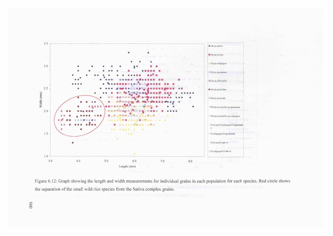
3.5
3.0
2.5
2.0
1.5
1.03.0
♦♦
♦ ♦ ♦ ♦ ♦
♦ ♦ ♦ ♦♦
♦ ♦ *♦♦ ♦ ♦
♦ ♦ ♦ ♦ ■♦ ♦ ♦♦ ♦■ ■
• • • ■ ■ ■x x • • • • X • •
X X • • • • •
♦ ♦ ♦ ♦♦♦ ♦♦♦ ♦♦♦«♦ ■#♦■■♦ c: ■ -
♦ ♦ ♦ ♦ # mm ■ * " " ■ j r r ^ : ■♦ ♦♦ ■ an ^ V*"**■ ■ V
n n i p n n n c ^ y # 1■ H. A■ n a n n " » i n n n n » n n n a f t m -%t n ^ n i■ n n n r n •* nA A * . A \ n m i X A J t t l x m A A
B t X A i l A O i l i l i
♦ a♦ ♦ ♦ ♦ ♦ ♦
in* ♦ ♦ ♦ a <*♦ ♦
a ♦ ♦• a ♦ ♦ ♦ ♦
4.0 5.0 6.0Length (mm)
7.0 8.0
♦ Oryza sativa
■ Oryza m vara
Oryza rufipogon
X Oryza spontanea
X Oryza officinalis
• Oryza granulata
+ Oryza punctata
-Oryza mvara/Oryza spontanea
—Oryza mvara/Oryza rufipogon
O nivara/O rufipogon/O a
O rufipogocvO spontanea
O.nivara/O sativa
O rufipogon/O sativa
Figure 6.12: Graph showing the length and width measurements for individual grains in each population for each species. Red circle shows
the separation of the small wild rice species from the Sativa complex grains.
Utoo

Thick
ness
(m
m)
21
2.0 -
18
1.6 -
1.4
1.2
1.0
0.8 4- 2.0
♦ ♦
♦ ♦♦♦♦♦♦ ♦♦
♦ ♦ ♦♦ + ♦
♦♦ ♦ ♦ ♦♦♦♦ ♦♦♦♦%♦«•■- ■■ ■ ♦♦ ♦
♦ ♦♦ ♦♦ ♦♦♦♦♦ ♦ ♦♦♦
♦ * ♦ ♦ ♦ ♦
x*#x»
X X X + + + ^ + x x +
♦nn 1
■ onnnnwMi nnnnni: ■ .
in<*n rtHN n n n n n n m ■ ■
n « n n n j n »
4 n « n n i
& I U K
3.0 4.0 3.0 6.0
Length (mm)
7.0 8.0 9.0
♦ Oryza sativa
■ Oryza nivara
Oryza rufipogon
X Oryza spontanea
X Oryza officinalis
• Oryza granulate
+ Oryza punctata
•Oryza nivara/Oryza spontanea
—Oryza nivara/Oryza rufipogon
Oryza nivaraOryza rufipogon Oryza spontanea
Oryza rufipogon/Oryza spontanea
Oryza nivara/Oryza sativa
Oryza rufipogon/Oryza sativa
Figure 6.13: Graph showing the length and thickness measurements for individual grains in each population for each species.
Red circle shows the separation of the small wild rice species and the Sativa complex grains.
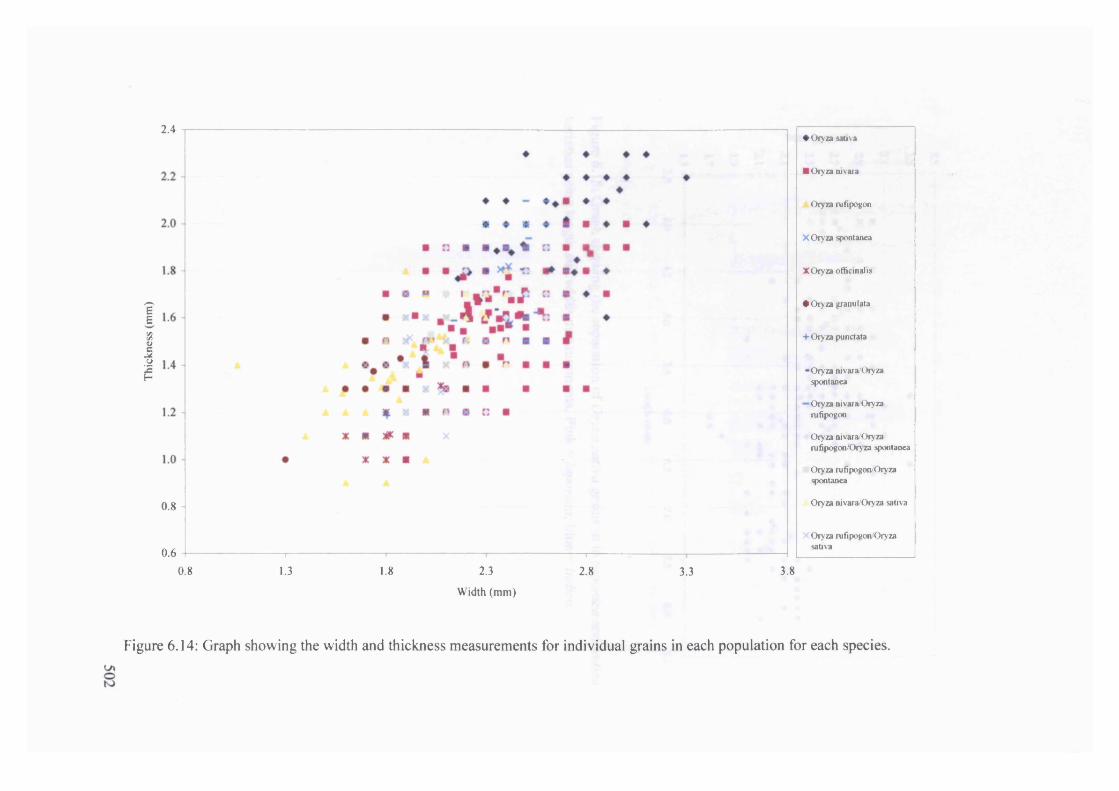
Thi
ckne
ss
(mm
)
2.4♦O ryza sativa
■ Oryza aivara
Ory za rufipogon
X Oryza spontanea
X Oryza officinalis
• Oryza granulata
+ Oryza punctata
Oryza nivara/Oryza spontanea
Oryza nivara'Oryza rufipogon
Oryza nivara/Oryza rufipogon.'Oryza spontanea
Oryza rufipogon/Oryza spontanea
Oryza nivara/Oryza sativa0.8
Oryza rufipogon/Oryza sativa0.6
0.8 1.3 1.8 2.3 2.8 3.83.3
Width (mm)
Figure 6.14: Graph showing the width and thickness measurements for individual grains in each population for each species.

Wid
th
(mm
)
3.5
3 3
2 7♦ ♦ ♦ ♦
2 5
2 3 ♦ ♦♦ ♦ ♦♦♦ ♦ ♦ ♦♦ ♦ ♦ ♦21
♦ ♦
8.55 .0 5.5 6.0 6.5 7.0 7.5 8.04.0
Length (m m )
Figure 6.15: Graph showing the separation of Oryza sativa grains in to japonica and indica
varieties using length and width measurements. Pink =japonica, blue = indica.
503
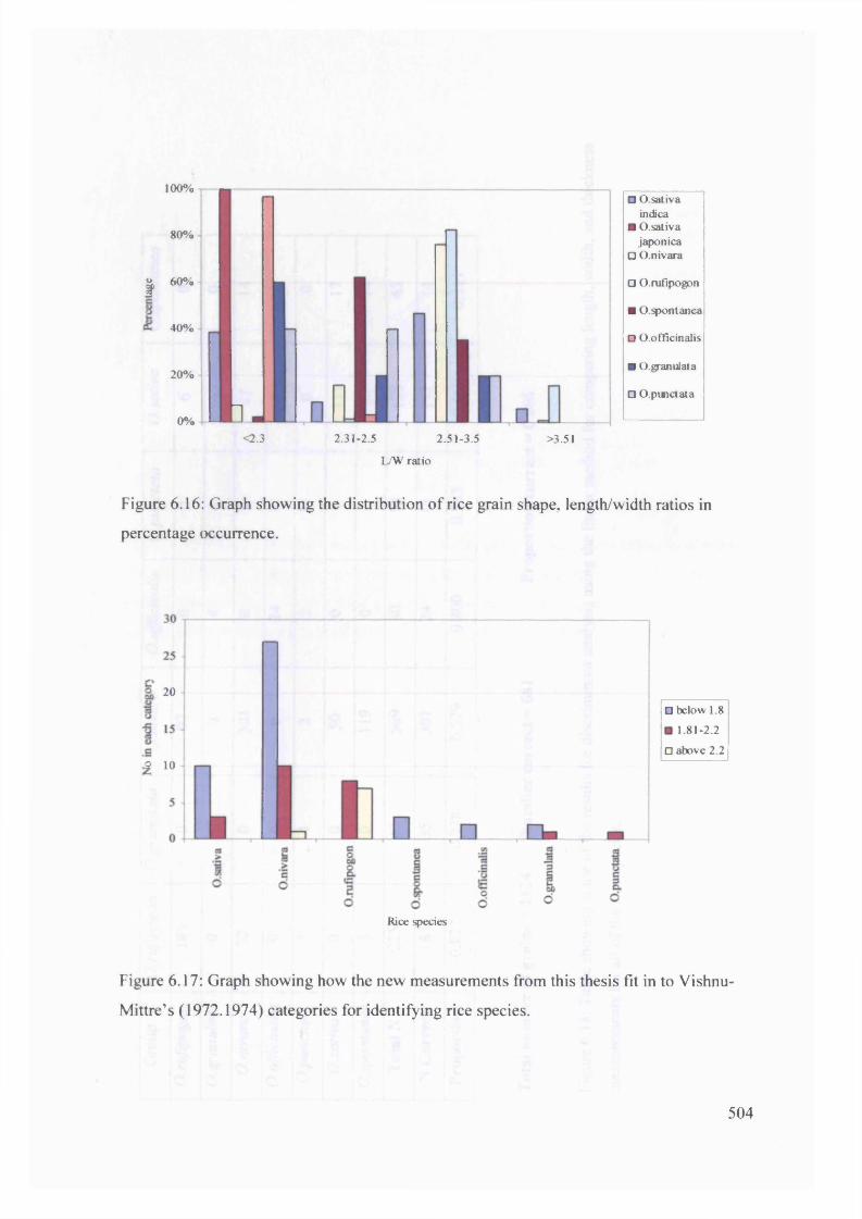
100%
80%
« 60%I
40%
20%
0% E E<2.3 2.31-2.5 2.51-3.5 >3.51
L/W ratio
D O.sativa indica
■ O.sativa japonica
□ O.nivara
□ O.rufipogon
■ O.spontanea
□ O. officinalis
■ O.granulata
□ O.punctata
Figure 6.16: Graph showing the distribution o f rice grain shape, length/width ratios in
percentage occurrence.
20
2 10
Rice species
□ below 1.8
1.81-2.2
□ above 2.2
Figure 6.17: Graph showing how the new measurements from this thesis fit in to Vishnu-
Mittre’s (1972.1974) categories for identifying rice species.
504

Group 0 .rufipogon O.granulata O.nivara O.officinalis O.punctata O.sativa O. spontanea
O. rufipogon 185 0 97 0 0 6 0
O.granulata 0 35 0 4 1 4 0
O.nivara 32 0 301 0 0 47 14
0 .officinalis 0 6 0 24 3 3 0
O.punctata 5 4 2 2 11 0 0
O.sativa 0 0 50 0 0 111 17
0. spontanea 3 0 119 0 0 24 14
Total N 225 45 569 30 15 195 45
N Correct 185 35 301 24 11 111 14
Proportion 0.822 0.778 0.529 0.800 0.733 0.569 0.311
Total num ber of grains = 1124 Num ber correct = 681 Proportion correct = 0.606
Figure 6.18: Table showing some of the results for discriminant analysis using the linear method for comparing length, width, and thickness
measurements for all o f the rice species.

3.50
3.00
2.50•5-oI
2.00
1.50
1.002.00 3.00 4.00 5.00 6.00 7.00 8.00 9.00 10.00
length
Figure 6.19: Graph showing a comparison of the length and width measurements of modem
and archaeological rice grains. The archaeological grains are adjusted for 20% shrinkage.
Red circle shows the archaeological grains that may be classified as small wild rice species
and the blue circle shows those that could be from the Sativa complex of rice species.
xx „
x O.sativa
• O.rufipogon
+ O.nivara
- ().spontanea
- O.officinalis
O.granulata
O.punctata
♦ KDW+20%
■ MCR+20%
GPR+20%
x GBSN+20%
506
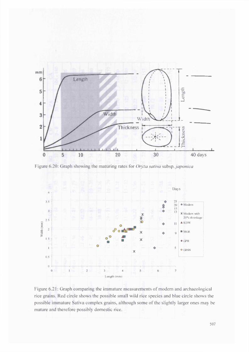
mm
Length
4 -
WidthW i d t h
Thickness
0 305 10 20 40 days
Figure 6.20: Graph showing the maturing rates for Oryza sativa subsp .japonica
4
3 5
3
2.5
2
1.5
1
0 5
0
Days
o° o
X*x>
X
X
X
3 4
Length (m m )
25201513
♦ Modem
X M odern with 20% shrinkage
A K D W
■ MGR
♦ (P R
o GBSN
Figure 6.21: Graph comparing the immature measurements of modem and archaeological rice grains. Red circle shows the possible small wild rice species and blue circle shows the possible immature Sativa complex grains, although some of the slightly larger ones may be mature and therefore possibly domestic rice.
507
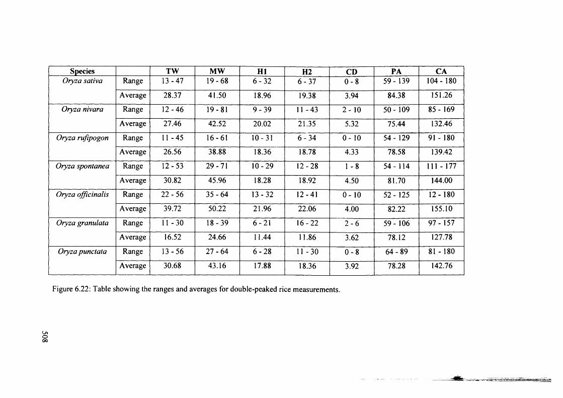
Species TW MW HI H2 CD PA CAOryza sativa Range 13-47 19-68 6 - 3 2 6 - 3 7 0 - 8 59- 139 104- 180
Average 28.37 41.50 18.96 19.38 3.94 84.38 151.26
Oryza nivara Range 12-46 19-81 9 - 3 9 11-43 2 - 10 50- 109 85- 169
Average 27.46 42.52 20.02 21.35 5.32 75.44 132.46
Oryza rufipogon Range 11-45 16-61 10-31 6 - 3 4 0 - 10 54- 129 91 - 180
Average 26.56 38.88 18.36 18.78 4.33 78.58 139.42
Oryza spontanea Range 12-53 29-71 10-29 12-28 1 -8 54-114 111 - 177
Average 30.82 45.96 18.28 18.92 4.50 81.70 144.00
Oryza officinalis Range 2 2- 56 3 5- 64 13-32 12-41 0 - 1 0 52-125 12-180
Average 39.72 50.22 21.96 22.06 4.00 82.22 155.10
Oryza granulata Range 11-30 18-39 6- 21 16-22 2 - 6 59- 106 97-157
Average 16.52 24.66 11.44 11.86 3.62 78.12 127.78
Oryza punctata Range 13-56 2 7 - 6 4 6 - 2 8 11-30 0 - 8 6 4 - 8 9 81 - 180
Average 30.68 43.16 17.88 18.36 3.92 78.28 142.76
Figure 6.22: Table showing the ranges and averages for double-peaked rice measurements.
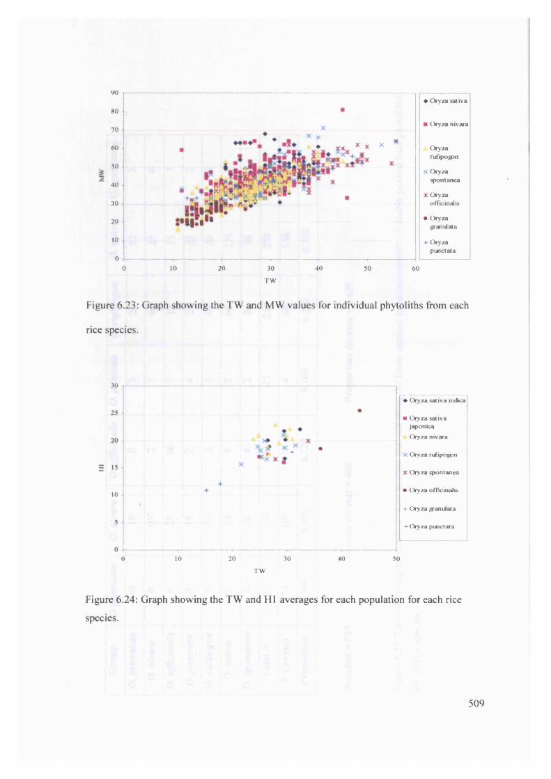
90
80
70
60
50
40
30
20
10
00 10 20 30 40 50 60
TW
Figure 6.23: Graph showing the TW and MW values for individual phytoliths from each
rice species.
♦ Oryza sativa
♦ X♦ XX * * x
m:*1*
Oryza nivara
Oryzarufipogon
X Oryza spontanea
X Oryza officinalis
• Oryza granulata
+ Oryza pu ic ta ta
30
♦ Oryza sativa indica
■ Oryza sativa japonica Oryza nivara
X O ryza rufipogon
X X Oryza spontanea
• Oryza officinalis10
+ Oryza granulata
Oryza p inctata
10 20 30 500 40
TW
Figure 6.24: Graph showing the TW and HI averages for each population for each rice
species.
509
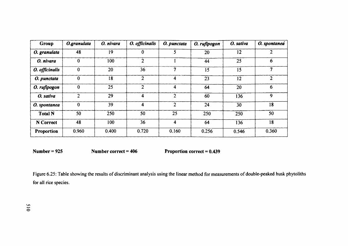
Group O.granulata O. nivara O. officinalis O. punctata O. rufipogon O. sativa O. spontanea
0 . granulata 48 19 0 5 20 12 2
0. nivara 0 100 2 1 44 25 6
0. officinalis 0 20 36 7 15 15 7
0. punctata 0 18 2 4 23 12 2
0 . rufipogon 0 25 2 4 64 20 6
O. sativa 2 29 4 2 60 136 9
0. spontanea 0 39 4 2 24 30 18
Total N 50 250 50 25 250 250 50
N Correct 48 100 36 4 64 136 18
Proportion 0.960 0.400 0.720 0.160 0.256 0.546 0.360
Number = 925 Number correct = 406 Proportion correct = 0.439
Figure 6.25: Table showing the results of discriminant analysis using the linear method for measurements o f double-peaked husk phytoliths
for all rice species.

Group Domestic Wild
Domestic 181 204
Wild 69 471
Total N 250 675
N Correct 181 471
Proportion 0.724 0.698
Total number = 925 Number correct = 652 Proportion correct = 0.705
Figure 6.26: Table showing the results o f discriminant analysis using the linear method for
all measurements (TW, MW, HI, H2, CD, PA, CA) o f double-peaked husk phytoliths using
wild versus domestic categories.
511

MW
90
80
70
60
50
40
30
20
10
0 -0 10 20 30 40 50 60
TW
Figure 6.27: Graph showing archaeological and modem double-peaked husk phytolith measurements.
13
■ *♦' I t
* *A ♦
X A,X X
i f * *******
i i 1 a"
: i i J ! H l S F ♦Ihmi
♦ Oryza sativa
■ Oryza nivara
A Oryza rufipogan
x Oryza spontanea
X Oryza officinalis
♦ Oryza granulata
+ Oryza puictata
■ GPR
GBS♦ K.DW
■ MGR

Sam
ple
num
ber
Sam
ple
num
ber
6 8 10 12
No o f chips
Figure 6.28: Graph o f archaeological rice bulliforms chips from Gopalpur and Golbai Sasan
513
733
6
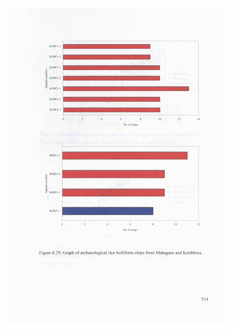
Sam
ple
num
ber
Sam
ple
num
ber
KDW1-3
KDW1-2
KDW1-1
KDW2-2
KDW2-1
KDW3-1
KDW4-1
0 2 4 6 8 10 12 14
No o f chips
MGR1-1
MGR3-2
MGR3-1
MGR5-1
0 2 4 6 8 10 12
No o f chips
Figure 6.29: Graph o f archaeological rice bulliform chips from M ahagara and Koldihwa.
514

A Vigna radial a
x Vigna muigo
A Vigna radiata sub wild
+ Vigna mungo sylv wild
1 1.5 2 2.5 3 3.5 4 4.5 5
Length (mm)
Figure 7.1: Graph showing modern length and width measurem ents o f Vigna radiata and
Vigna mungo (wild and domestic species) (after Fuller & Harvey in press).
A Vigna radiata -20%
x Vigna mungo -20%
A V radiata wild-20%
+ V. mingo wild -20%
1 1.5 2 2.5 3 3.5 4 4.5 5 5.5
Length (mm)
Figure 7.2: Graph showing modern length and width measurements o f Vigna radiata and
Vigna mungo (wild and domestic species) with 20% shrinkage adjustment (after Fuller &
Harvey in press).
3.5
2.5
1.5
T x ^ x x
:a S x \ AxxA A A A X
AVA A A XA V A AA
XXX
A A A
515

♦ GBSN
Q KDWx 2.5
A MGR
1.5 2 2.5 3 3.5 4 4.5 5 5.51L ength (m m )
Figure 7.3: Graph showing archaeological length and width measurements for Vigna sp.
seeds with dashed line separating possible wild from possible domestic types (after Fuller
& Harvey in press).
0.9
0 8
0.7
♦ GBSN0.6
]jj 0.5I 0.4 £
0.3
□ KDW
A MGR
X V.radiata m od
X V, mungo m od
0.2
0.1
0 2 3 4 5 6Length
Figure 7.4: Graph showing length vs plumule length/length measurements for identifying
Vigna mungo and Vigna radiata (after Fuller & Harvey in press).
516
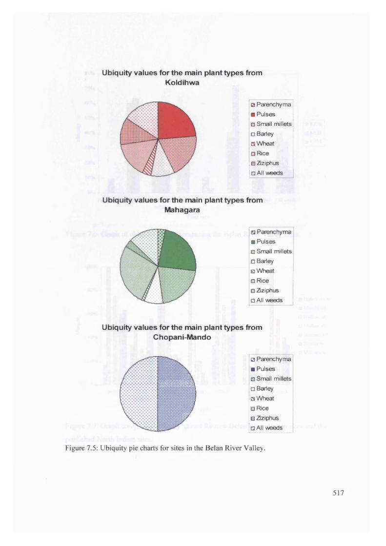
Ubiquity values for the main plant types from Koldihwa
a Parenchyma
■ Pulses
□ Small millets
□ Barley
□ Wheat
□ Rice
B Zziphus
□ All weeds
Ubiquity values for the main plant types from Mahagara
n Parenchyma
■ Pulses
□ Small millets
□ Barley
□ Wheat
□ Rice
B Zziphus
□ All weeds
Ubiquity values for the main plant types from Chopani-Mando
□ Parenchyma
■ Pulses.A
w m m m m■ , i
□ Small millets
□ Barley
□ Wheat
□ Ricey
1B Zziphus
□ All weeds
Figure 7.5: Ubiquity pie charts for sites in the Belan River Valley.
517

80%
■ KDW
■ MGR
■ CPM
Parenchyma Pulses Snail Barley Wheat Rice Ziziphus All weeds millets
Plant type
Figure 7.6: Graph of ubiquity values comparing the Belan River Valley sites.
1 0 0 %
■ Hulaskera all
■ Manjhi all
□ Narhan all
□ Malhar all
□ Senuwar all
■ Koldihwa
■ Mahagara
Pulses Snail Barley Wheat Rice Fruits All weeds millets
Plant type
Figure 7.7: Graph comparing ubiquity values for new Belan River Valley sites and the
published North Indian sites.
518
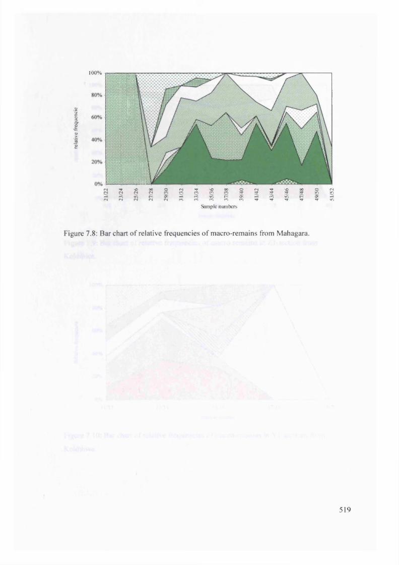
rela
tive
freq
uenc
ie100%
rs t SO 00 © fN •st so 00 o CM ■st SO oo O CMcj § CS S © 1 i J# Tf 5; WO WOco O' co r» Os CO v-> o:£3 <N N «N M ro co co Cl CO ■st ■st St •St •St VO
Sample numbers
Figure 7.8: Bar chart of relative frequencies of macro-remains from Mahagara.
519
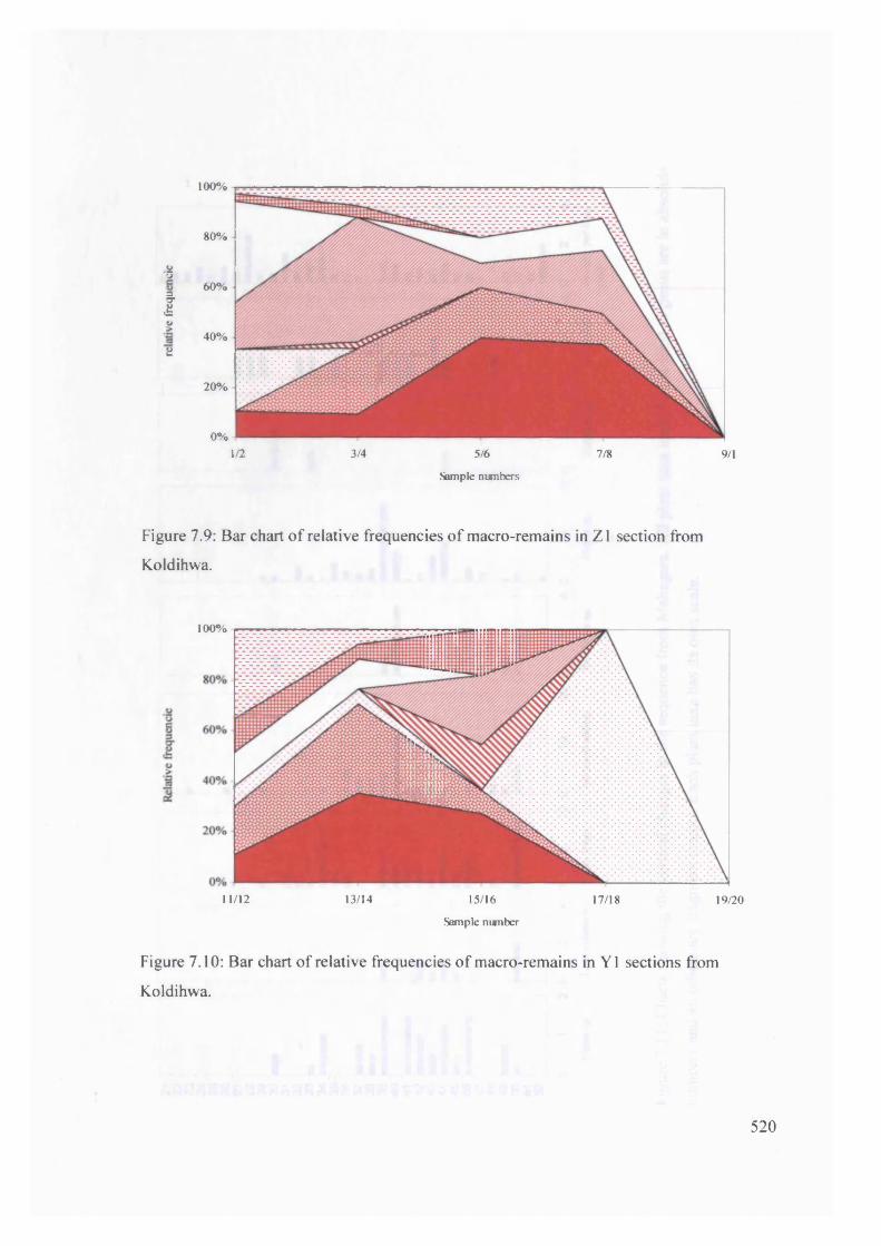
100%
80%
860%3
IU40%
E
20%
0%1/2 3/4 5/6 7/8 9/1
Sample numbers
Figure 7.9: Bar chart of relative frequencies of macro-remains in Z1 section from
Koldihwa.
1 0 0 %
11/12 13/14 15/16 17/18 19/20
Sample number
Figure 7.10: Bar chart of relative frequencies of macro-remains in Y1 sections from
Koldihwa.
520
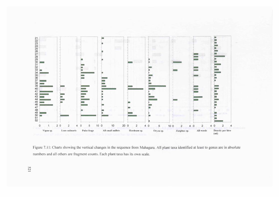
Vigna sp. Lens culinaris Pulse frags All small millets Hordeum sp. Oryza sp. Ziziphus sp. All weeds Density per litre(ml)
Figure 7.11: Charts showing the vertical changes in the sequence from Mahagara. All plant taxa identified at least to genus are in absolute
numbers and all others are fragment counts. Each plant taxa has its own scale.

1 ■ ■
2 ■ ■
7
8 P9
10
0 0.5 1
Vigna sp.
■
■
■
¥7
■
4 00 0.2 0.4 0 2 4 0 10 20 0 2.5 5 0 1 2 0 5 100 2
cu linaris P u k f frags Al*smal1 ■ ® et* H ordeum sp. T riticum sp. O ryza sp. Z iziphus sp. All weedsDeaatty p er litre
Figure 7.12: Charts showing the vertical changes in the sequence from Koldihwa Zl. All plant taxa identified to at least genus are in absolute
counts and all others are fragment counts. Each plant taxa has its own scale.
K)

11 □
12 □
13 □
14
15 □ □ ■
16 □
17
18.
19
20-----------------------------------
-I
p
r0 1 2 0 2 4 0 5 100 2 4 0 2 4 0 0.5 ”* 0 2 5 5 0 5 10
Vigna sp. P u k e frags All sm all m illets H ordeum sp. T r itic u m sp . O ryza sp. Z iziphus sp. All w eeds0 5 10D ensity p e r litre (ml)
Figure 7.13: Charts showing the vertical changes in the sequence from Koldihwa Yl. All plant taxa identified to at least genus are in
absolute counts and all others are fragment counts. Each plant taxa has its own scale.
tou>
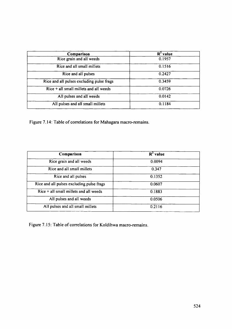
Comparison R valueRice grain and all weeds 0.1957
Rice and all small millets 0.1516
Rice and all pulses 0.2427
Rice and all pulses excluding pulse frags 0.3459
Rice + all small millets and all weeds 0.0726
All pulses and all weeds 0.0142
All pulses and all small millets 0.1184
Figure 7.14: Table o f correlations for Mahagara macro-remains.
Comparison R2 value
Rice grain and all weeds 0.0094
Rice and all small millets 0.347
Rice and all pulses 0.1352
Rice and all pulses excluding pulse frags 0.0607
Rice + all small millets and all weeds 0.1883
All pulses and all weeds 0.0506
All pulses and all small millets 0.2116
Figure 7.15: Table of correlations for Koldihwa macro-remains.
524
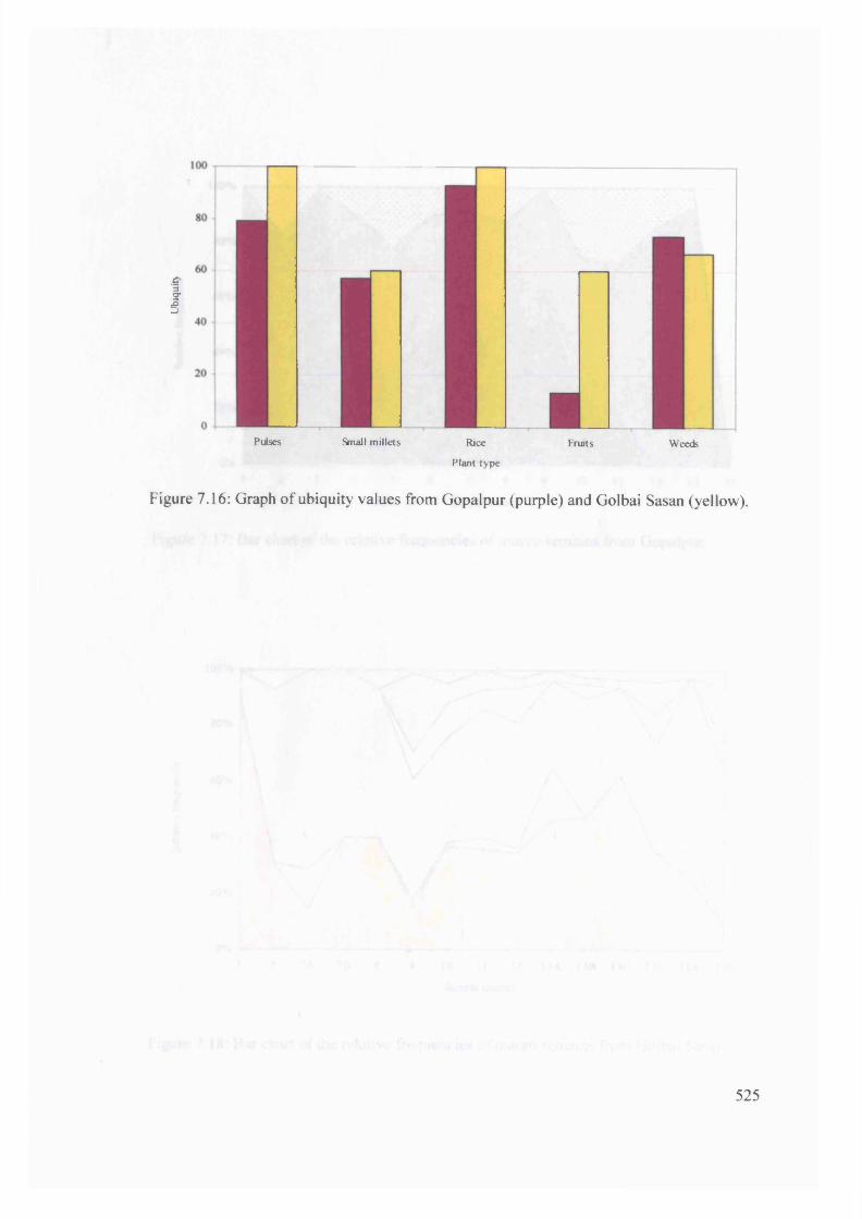
Ubi
quit)
Pulses Snail millets Rice Fruits Weetfc
Plant type
Figure 7.16: Graph of ubiquity values from Gopalpur (purple) and Golbai Sasan (yellow).
525

Rela
tive
freq
uenc
ie
Sample number
Figure 7.17: Bar chart o f the relative frequencies o f macro-remains from Gopalpur.
1 0 0 %
80%
60%
40%
20%
0%3 5 7A 7B 8 9 10 11 12 13A 13B 13C 13D 14A 14B
Sample nun her
Figure 7.18: Bar chart o f the relative frequencies o f macro-remains from Golbai Sasan.

:
M20 4 0 0
uniflorum5 10 o 100 200 0 20 40 0 5 10
C. cajan Pulse frags All small millets Oryza sp.20 40 02 0
Celtis sp. All weeds Density per litre (ml)
Figure 7.19: Charts showing the vertical changes in the sequence from Gopalpur. All plant taxa identified at least to genus are in absolute
counts and all other are fragment counts.
Ulto

3 j . . I □ ■' I □ ' ZZ35 : ZD
7A □ □
"
D7B a
8
9 1 -------------- 1]— 1
□
t )
J
’ □ f—I
□
_ J
= 1 UZZD11 1 12
] p = □ czd
13A1 ZD
D□= i □
T3B !□ Z2 □
Z3 □13D □ D z z d-MA
. 3 = □ VZZD14B : --------------------- 1
c 20 40 ) 2 1 ;2 0 50 100 150 ) 5 10 () 20
Vigna sp. Macrotv loma uniflorum
( ajanus cajan
Pulse frags All small millets Oryza sp.
40 0 30 60 0 10 20 0
All weeds All fruit frags Density per litre (ml)
Figure 7.20: Charts showing the vertical changes in the sequence from Golbai Sasan. All plant taxa identified at least to genus are in absolute
counts and all others are fragment counts. Each plant taxa has its own scale.
CO

Comparison R2 valueRice grain and all weeds 0.0536
Rice grain and all weeds excluding sample 2 0.8311
Rice and all small millets 0.793
Rice and all pulses 0.0037
Rice and all pulses excluding pulse frags 0.0423
Rice + all small millets and all weeds 0.0952
Rice + all small millets and all weeds excluding sample 2 0.7353
All pulses and all weeds 0.2445
All pulses and all small millets 0.0021
Figure 7.21: Table o f correlations for Gopalpur macro-remains.
Comparison R2 valueRice grain and all weeds 0.7795
Rice and all small millets 0.3483
Rice and all pulses 0.0102
Rice and all pulses excluding sample 3 0.4604
Rice and all pulses excluding pulse frags 0.0089
Rice + all small millets and all weeds 0.7399
All pulses and all weeds 0.0145
All pulses and all small millets 0.0023
Figure 7.22: Table of correlations for Golbai Sasan macro-remains.
529
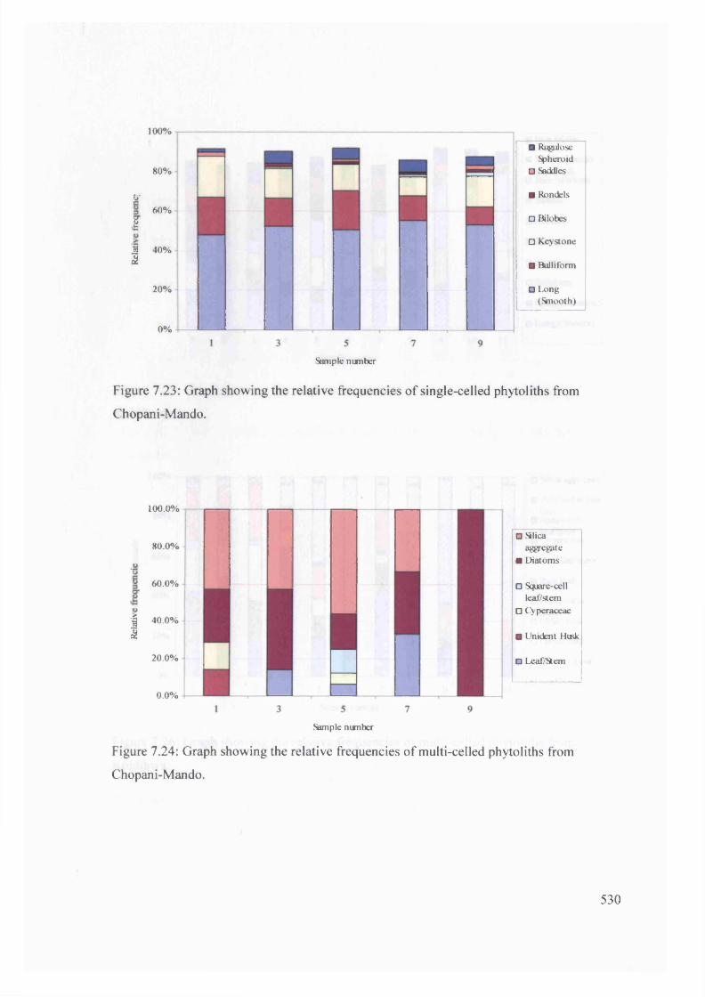
£>*
I
100%
80%
60%
1 40%2
20%
0%
-
■ Rugulose Spheroid
□ Saddles
■ Rondels
□ Bilobes
□ Keystone
■ Bulliform
O Long (Smooth)
Sample number
Figure 7.23: Graph showing the relative frequencies of single-celled phytoliths from
Chopani-Mando.
100.0%
80.0%
60.0%
£ 40.0%
I
20 .0%
0 .0%
iI
□ Silica aggregate
■ Diatoms
□ Square-cell leaf/stem
□ Cyperaceae
■ Unident Husk
□ Leaf/Stem
Sample number
Figure 7.24: Graph showing the relative frequencies of multi-celled phytoliths from
Chopani-Mando.
530

100%
O'
I 40%
2
5 6 7
Sample nisnber
■ Rice bilobe
B Double-peaked glunie cell
□ Rice bulliform
■ Saddles
□ Rondels
■ Bilobes
□ Keystone
□ Bulliform
■ Long (Denckitic)
□ Long (Smooth)
Figure 7.25: Graph showing the relative frequencies of single-celled phytoliths from
Koldihwa.
100%
80%
g 60%
1O2 40%
20%
0% f i n e1 2 3 4 5 6 7 8 9 10 11
Sample nianber
□ Silica aggregate
■ Polyhedral hair base
□ Square-cell leaf/stem
□ Cyperaceae
■ Rice leaf/stem
□ Rice husk
■ Phragmites Stem
□ Millet husk
□ Cereal husk
■ Unident Husk
■ Leaf/Stem
Figure 7.26: Graph showing the relative frequencies of multi-celled phytoliths from
Koldihwa.
531
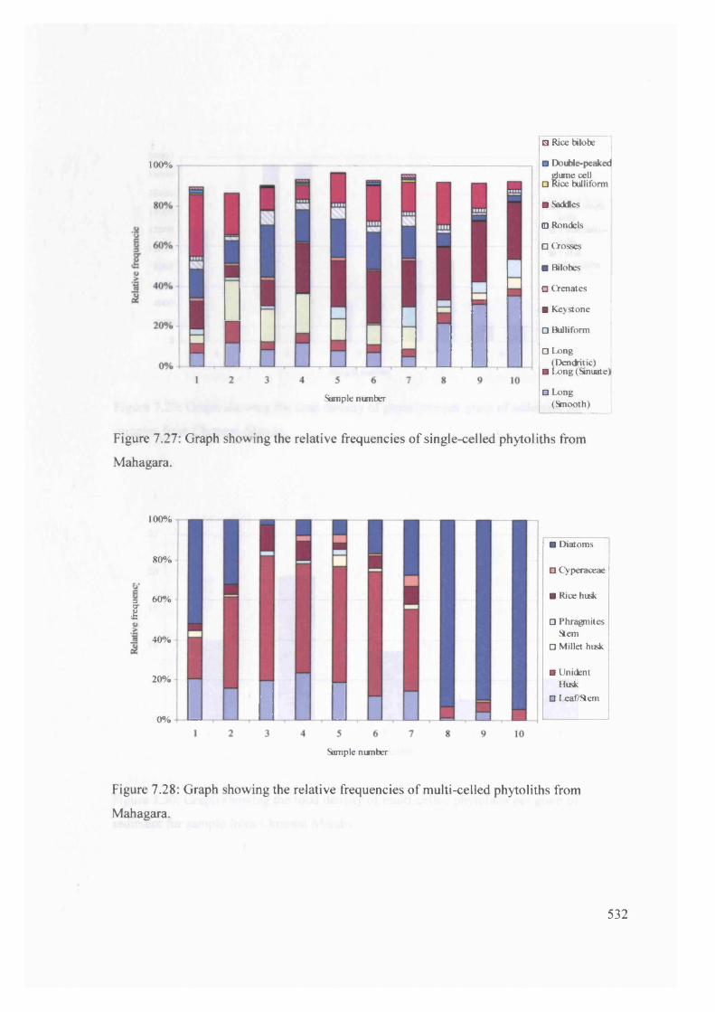
100%
0
Sample number
S Rice bilobe
■ Double-peaked glume cell
□ Rice bulliform
■ Saddles
□ Rondels
□ Crosses
■ Bilobes
O CTenates
■ Keystone
□ Bulliform
□ Long (Dendritic)
■ Long (Sinuate)
B Long (Smooth)
Figure 7.27: Graph showing the relative frequencies of single-celled phytoliths from
Mahagara.
-j
I
100%
80%
60%
40%
20%
0%
B Diatoms
□ Cyperaceae
B Rice husk
□ Phragnites Stem
□ Millet husk
B Unident Husk
B Leaf/Stem
Sample number
Figure 7.28: Graph showing the relative frequencies of multi-celled phytoliths from
Mahagara.
532

20000
18000
16000■ Total single
cells□ Total multi-
cells■ Total
phytoliths
14000
12000
10000
1 3 5 7 9
Sample nunber
Figure 7.29: Graph showing the total density o f phytoliths per gram of sediment for
samples from Chopani-Mando.
25
20
15
Ic10
5
0
Figure 7.30: Graph showing the total density of multi-celled phytoliths per gram of
sediment for sample from Chopani Mando.
1 3 5 7 9
Sample number
533
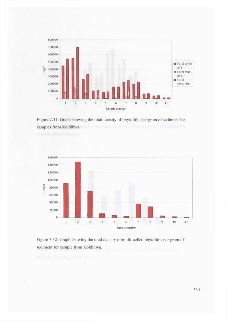
800000
700000
600000
500000
|> 400000
300000
200000
100000
01 2 3 4 5 6 7 8 9 10 11
Sample number
Figure 7.31: Graph showing the total density of phytoliths per gram of sediment for
samples from Koldihwa.
160000
140000
120000
100000
J> 80000
60000
40000
20000
0
Figure 7.32: Graph showing the total density of multi-celled phytoliths per gram of
sediment for sample from Koldihwa.
I I I . _ _1 2 3 4 5 6 7 8 9 10 11
Sample number
l f lU u
Total single cells:
□ Total multicells:
■ Total phytolith:
534

20000
18000
16000
14000 ■ Total single cells:
□ Total multicells:
■ Total phytoliths:
12000
10000
1 2 3 4 5 6 7 8 9 10
Sample nunber
Figure 7.33: Graph showing the total density of phytoliths per gram of sediment for
samples from Mahagara.
2500
1 2 3 4 5 6 7 8 9 10
Sample number
Figure 7.34: Graph showing the total density of multi-celled phytoliths per gram of
sediment for sample from Mahagara.
535

20000
I 800 0
16000
14 0 0 0
12000
10000
Sample number
■ Rugulose Spheroid
□ Saddles
■ Rondels
□ Bilobes
□ Keystone
■ Bulliform
■ Long (Smooth)
Figure 7.35: Graph showing the absolute density of single-celled phytoliths from Chopani-
Mando.
i
□ Silica aggregate
■ Diatoms
□ Square-cell leaf/stem
□ Cyperaceae
■ Unident Husk
B Leaf/Stan
Sample number
Figure 7.36: Graph showing the absolute density of multi-celled phytoliths from Chopani-
Mando.
536
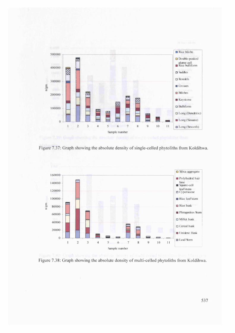
500000
400000
300000
200000
100000
0 ; 1—1 . 1—J T I J H I1 2 3 4 5 6 7 8 9
Sample number
B -10 11
■ Rice bilobe
□ Double-peakedglume cell
■ Rice bulliform
□ Saddles
□ Rondels
■ Crosses
□ Bilobes
■ Keystone
□ Bulliform
□ Long (Denckitic)
■ Long (Sinuate)
□ Long (Smooth)
Figure 7.37: Graph showing the absolute density o f single-celled phytoliths from Koldihwa.
160000
140000
120000
100000
e-g> 80000
60000
40000
20000
0 0 □5 6 7
Sample nirnber
10 11
□ Silica aggregate
■ Polyhedral hair base
■ Square-cell leaf/stem
□ Cyperaceae
■ Rice leaf/stem
□ Rice husk
■ Phragmites Stem
□ Millet husk
□ Cereal husk
■ Unident Husk
□ Leaf/Stem
Figure 7.38: Graph showing the absolute density of multi-celled phytoliths from Koldihwa.
537
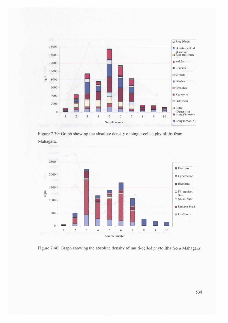
16000
14000
12000
10000
- | 8000
6000
4000
2000
0
Figure 7.39: Graph showing the absolute density of single-celled phytoliths from
Mahagara.
■ Diatoms
□ Cyperaceae
■ Rice husk
□ Phragmites Stem
□ Millet husk
■ Unident Husk
O Leaf/Stem
1 2 3 4 5 6 7 8 9 10
Sample number
Figure 7.40: Graph showing the absolute density of multi-celled phytoliths from Mahagara.
2000
1500
1000
500
^ n ■ B e4 5 6 7
Sample number
10
□ Rice bilobe
■ Double-peaked glume cell
□ Rice bulliform
■ Saddles
■ Rondels
□ Crosses
■ Bilobes
□ Crenates
■ Keystone
□ Bulliform
□ Long (Demkitic)
■ Long (Sinuate)
□ Long(Snooth)
538

350
300
250
200
150
100
3 91 5 7
■totalpanicoid
totalfestucoid
totalchloridoid
Sample number
Figure 7.41: Graph showing the different grass subfamilies from Chopani-Mando.
I
5 6 7
Sample number
10 11
180000
160000
140000
120000
10000080000
60000
40000
20000
totalfestucoid
totalpanicoid
totalchloridoid
Figure 7.42: Graph showing the different grass subfamilies from Koldihwa.
539

4500
4000
3500
3000
c 2500
if 2000
1500
1000
500
2 3 4 5 6 7 8 9 101Sample number
Figure 7.43: Graph showing the different grass subfamilies from Mahagara.
—♦— T otal panicoid
—■— Totalfestucoid
Totalchloridoid
540

Comparison R2 value
Long smooth and long dendritic 0.8178
Bulliform and keystone 0.9696
Long smooth and bulliform 0.8891
Long dendritic and bulliform 0.6264
Long smooth and keystone 0.8328
Long dendritic and keystone 0.6572
Figure 7.44: Table o f correlations for Chopani-Mando single-celled phytoliths.
Comparisons R2 value
Long smooth and long dendritic 0.9208
Bilobes and crosses 0.8456
Bilobes and rondels 0.9726
Bilobes and saddles 0.5509
Crosses and rondels 0.8415
Crosses and saddles 0.6633
Rondels and saddles 0.4568
Bilobes and long dendritic 0.8878
Bilobes and long smooth 0.7473
Bulliform and keystone 0.2265
Bulliform and long dendritic 0.5548
Saddles and long dendritic 0.3129
Saddles and long smooth 0.2188
Saddles and bulliform 0.6409
Saddles and keystone 0.0894
Figure 7.45: Table of comparisons for Koldihwa single-celled phytoliths.
541
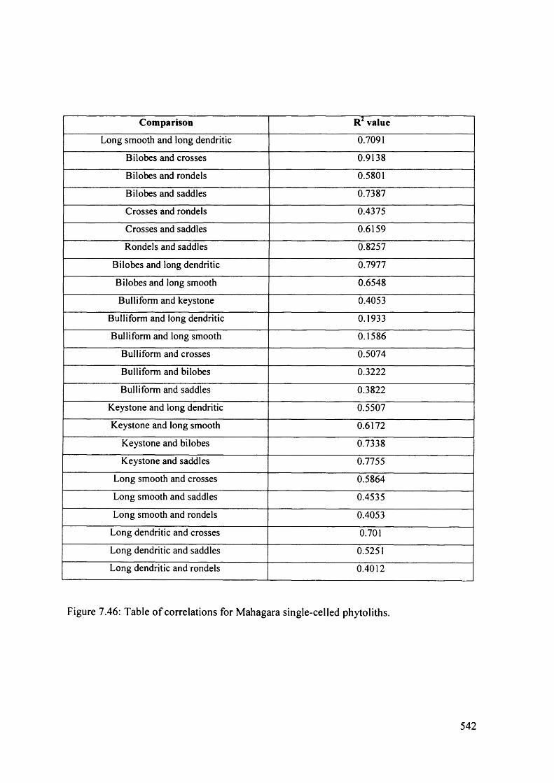
Comparison R value
Long smooth and long dendritic 0.7091
Bilobes and crosses 0.9138
Bilobes and rondels 0.5801
Bilobes and saddles 0.7387
Crosses and rondels 0.4375
Crosses and saddles 0.6159
Rondels and saddles 0.8257
Bi lobes and long dendritic 0.7977
Bilobes and long smooth 0.6548
Bulliform and keystone 0.4053
Bulliform and long dendritic 0.1933
Bulliform and long smooth 0.1586
Bulliform and crosses 0.5074
Bulliform and bilobes 0.3222
Bulliform and saddles 0.3822
Keystone and long dendritic 0.5507
Keystone and long smooth 0.6172
Keystone and bi lobes 0.7338
Keystone and saddles 0.7755
Long smooth and crosses 0.5864
Long smooth and saddles 0.4535
Long smooth and rondels 0.4053
Long dendritic and crosses 0.701
Long dendritic and saddles 0.5251
Long dendritic and rondels 0.4012
Figure 7.46: Table of correlations for Mahagara single-celled phytoliths.
542

Comparison R2 values
Rice bulliform and double-peaked glume cell 0.416
Double-peaked glume cell and rice bilobe 0.44
Rice bulliforms and rice bilobe 0.2017
Rice husk and rice leaf/stem 0.0155
Rice husk and rice bulliform 0.2957
Rice husk and double-peaked glume cell 0.5655
Rice husk and rice bilobe 0.9499
Rice leaf/stem and rice bulliform 0.0642
Rice leaf/stem and double-peaked glume cell 0.0078
Rice leaf/stem and rice bilobe 0.0235
Rice husk and indet leaf/stem 0.8058
Rice husk and unident husk 0.9163
Rice leaf/stem and indet leaf/stem 0.0412
Rice leaf/stem and unident husk 0.0486
Rice husk and Cyperaceae 0.1497
Rice leaf/stem and Cyperaceae 0.3453
Figure 7.47: Table of correlations for Koldihwa multi-celled phytoliths.
543
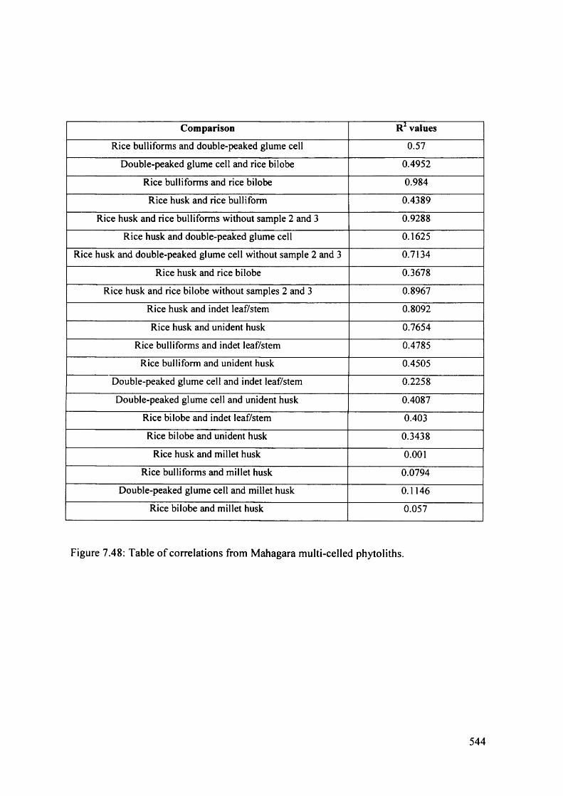
Comparison R2 values
Rice bulliforms and double-peaked glume cell 0.57
Double-peaked glume cell and rice bilobe 0.4952
Rice bulliforms and rice bilobe 0.984
Rice husk and rice bulliform 0.4389
Rice husk and rice bulliforms without sample 2 and 3 0.9288
Rice husk and double-peaked glume cell 0.1625
Rice husk and double-peaked glume cell without sample 2 and 3 0.7134
Rice husk and rice bilobe 0.3678
Rice husk and rice bilobe without samples 2 and 3 0.8967
Rice husk and indet leaf/stem 0.8092
Rice husk and unident husk 0.7654
Rice bulliforms and indet leaf/stem 0.4785
Rice bulliform and unident husk 0.4505
Double-peaked glume cell and indet leaf/stem 0.2258
Double-peaked glume cell and unident husk 0.4087
Rice bilobe and indet leaf/stem 0.403
Rice bi lobe and uni dent husk 0.3438
Rice husk and millet husk 0.001
Rice bulliforms and millet husk 0.0794
Double-peaked glume cell and millet husk 0.1146
Rice bilobe and millet husk 0.057
Figure 7.48: Table of correlations from Mahagara multi-celled phytoliths.
544

100%
80%
20%
Sample number
□ Rice bilobe
■ Rice bullifonn
□ Saddles
■ Keystone
□ Bulliform
□ T richomes
■ Long (Sinuate)
□ Long(Shiooth)
Figure 7.49: Graph showing the relative frequencies of single-celled phytoliths from
Bajpur.
100%
80%
I 60% <
IUI 40% | 1
20%
0% 1
Sample number
□ Indet multi-cell
■ Silica aggregate
□ Cyperaceae
□ Rice husk
■ Unident Husk
□ Leaf/Stem
Figure 7.50: Graph showing the relative frequencies of multi-celled phytoliths from Bajpur.
545
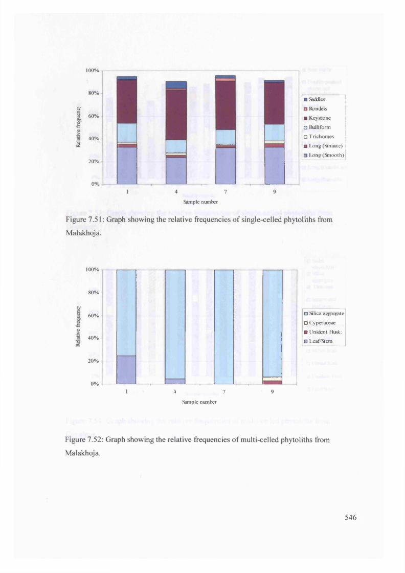
*>•
I>i
100%
80%
60%
40%
20%
0%
■ Saddles
□ Rondels
■ Keystone
□ Bulliform
□ T richomes
■ Long (Sinuate)
□ Long(Snooth)
Sample number
Figure 7.51: Graph showing the relative frequencies of single-celled phytoliths from
Malakhoja.
100%
80%
60%
40%
20%
0%
□ Silica aggregate
□ Cyperaceae
■ Unident Husk:
□ Leaf/Stem
4 7
Sample number
Figure 7.52: Graph showing the relative frequencies of multi-celled phytoliths from
Malakhoja.
546

100%
80%
60%
40%
20%
s
I D B O R■ I
i'
■ Rice bilobe
□ Double-peaked glume cell
O Rice bulliform
■ Saddles
□ Rondels
■ Bilobes
□ Keystone
□ Bulliform
■ Long (Denditic)
□ Long (Smooth)0% l_J
1 2 3 4 5 6 7 8 9 10 11 12 13 14
Sample number
Figure 7.53: Graph showing the relative frequencies of single-celled phytoliths from
Gopalpur.
I
100%
80%
60%
3 40%£
20%
0%1 2 3 4 5 6 7 8 9
Sample number
10 11 12 13 14
□ Indet phytolith
■ Silica aggregate
■ Diatoms
□ Square-cell leaf/stem
■ Cyperaceae
□ Rice leaf/stem
■ Rice husk
□ Millet husk
□ Cereal husk
■ Unident Husk
□ Leaf/Stem
Figure 7.54: Graph showing the relative frequencies o f multi-celled phytoliths from
Gopalpur.
547
^$22$$D
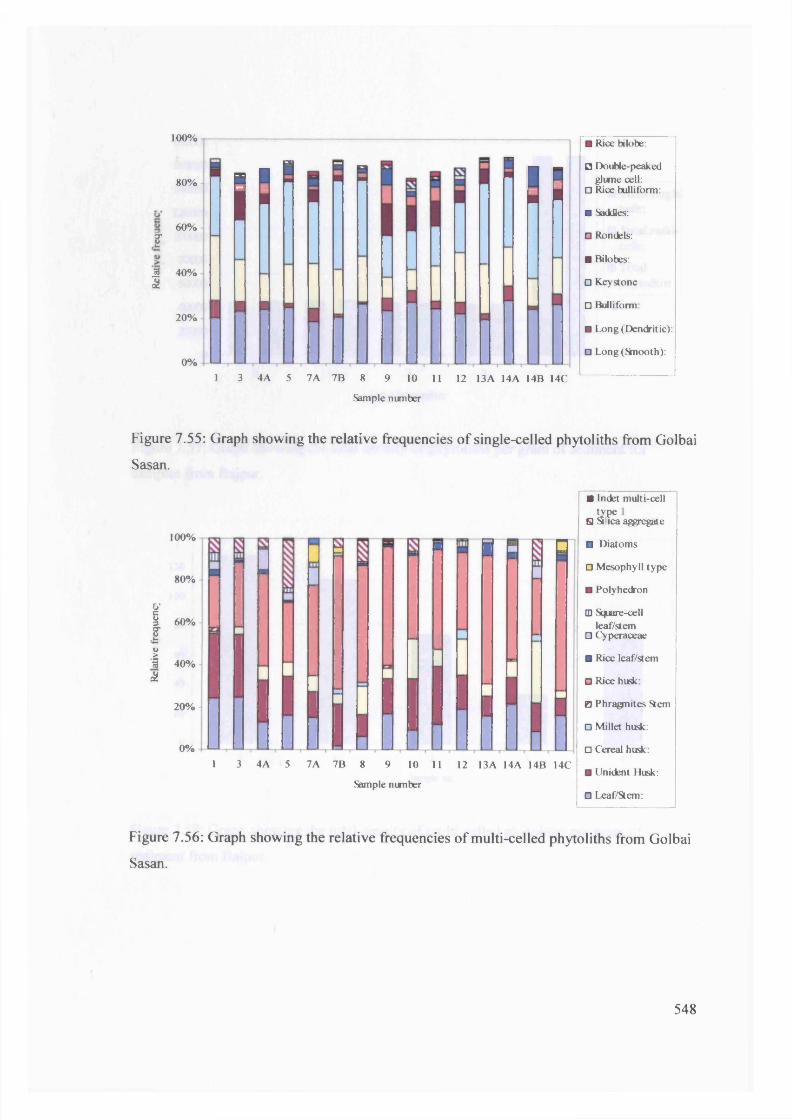
E
100%
80%
60%
M 40% £
20%
h
v «
: ■ 1
0%
R i b
1 3 4A 5 7A 7B 8 9 10 11 12 13A 14A 14B 14C
Sample number
■ Rice bilobe:
□ Double-peaked glume cell:
□ Rice bulliform:
■ Saddles:
□ Rondels:
■ Bilobes:
□ Keystone
□ Bulliform:
■ Long (Dendritic):
□ L ong(Snooth):
Figure 7.55: Graph showing the relative frequencies of single-celled phytoliths from Golbai
Sasan.
1 0 0%
80%
&•§ 60%
101 40% £
20%
0% LJ
:
H
1 3 4A 5 7A 7B 8 9 10 11 12 13A 14A 14B 14C
Sample number
■ Indet multi-cell
■S&1 aggregate
□ Diatoms
□ Mesophyll type
■ Polyhetkon
□ Square-cell leaf/stem
□ Cyperaceae
■ Rice leaf/stem
□ Rice husk:
0 Phragnites Stem
□ Millet husk:
□ Cereal husk:
■ Unident Husk:
□ Leaf/Stem:
Figure 7.56: Graph showing the relative frequencies of multi-celled phytoliths from Golbai
Sasan.
548
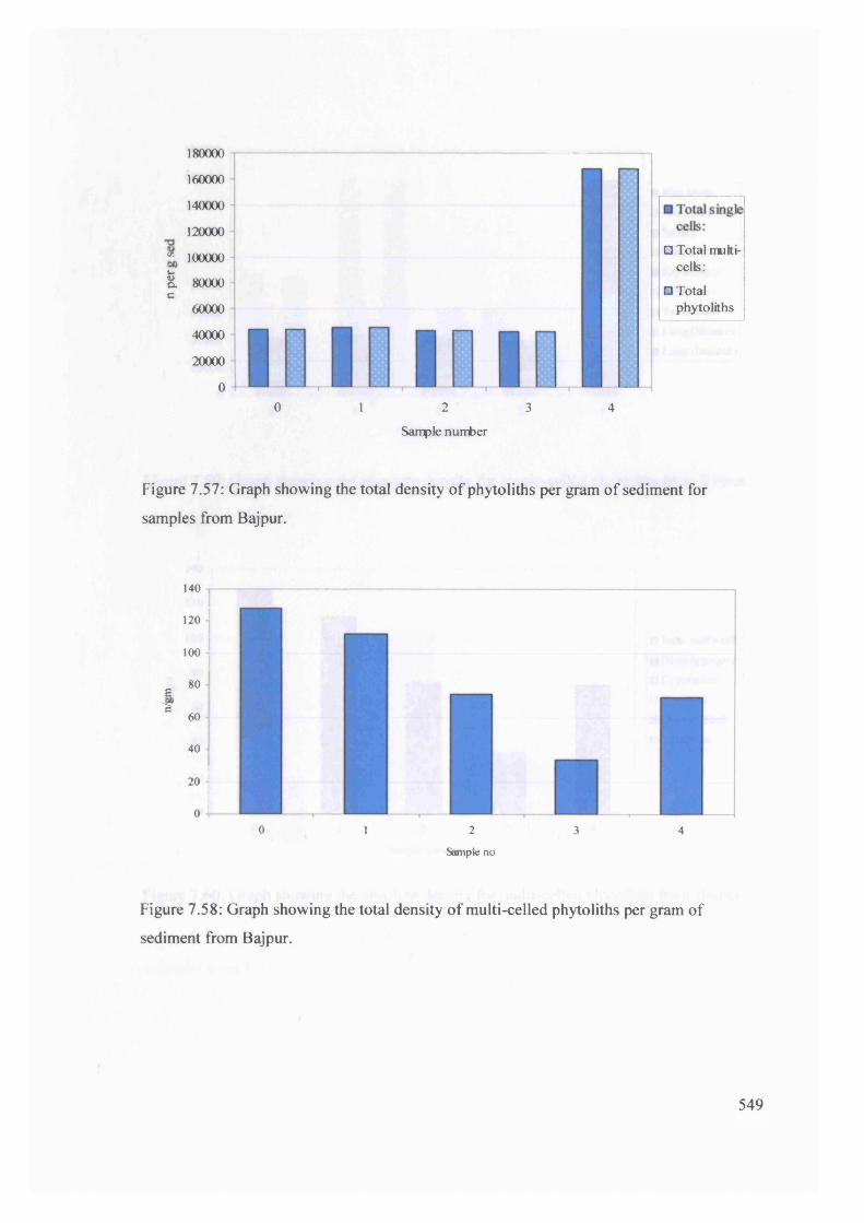
180000
160000
140000
120000
* 100000
£. 80000 e
6 0 0 0 0
4 0 0 0 0
20000
00 1 2 3 4
Sample number
Figure 7.57: Graph showing the total density of phytoliths per gram of sediment for
samples from Bajpur.
140
120
100
B 80 'fi
60
40
20
0
Figure 7.58: Graph showing the total density o f multi-celled phytoliths per gram o f
sediment from Bajpur.
0 1 2 3 4
Sample no
□ Total multicells:
□ Total phytoliths
549
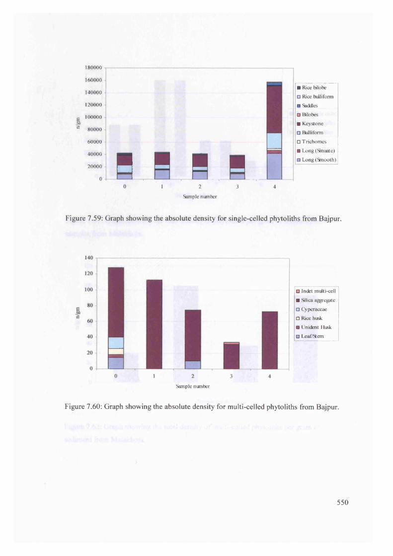
I
180000
160000
140000
120000
100000
80000
60000
40000
20000
0 B i l l1 2 3
Sample number
■ Rice bilobe
□ Rice bulliform
■ Saddles
□ Bilobes
■ Keystone
□ Bulliform
□ T richomes
■ Long (Sinuate)
□ Long(Snooth)
Figure 7.59: Graph showing the absolute density for single-celled phytoliths from Bajpur.
Sample nunber
□ Indet multi-cell
■ Silica aggregate
□ Cyperaceae
□ Rice husk
■ Unident Husk
□ Leaf/Stem
Figure 7.60: Graph showing the absolute density for multi-celled phytoliths from Bajpur.
550

90000
80000
70000
60000
E 50000
d 40000
30000
20000
10000
0
Figure 7.61: Graph showing the total density of phytoliths per gram of sediment for
samples from Malakhoja.
120
100
80
E■£ 60
40
20
0
Figure 7.62: Graph showing the total density of multi-celled phytoliths per gram of
sediment from Malakhoja.
1 4 7 9
Sample number
I Total single cells: □ Total miki-cells:
I Total phytoliths
Sarrple number
551

80000
70000
60000
50000
J> 40000
30000
20000
10000
0 I1 4 7 9
Sample number
Figure 7.63: Graph showing the absolute density o f single-celled phytoliths from
Malakhoja.
120
100
80
J> 60
40
20
01 4 7 9
Sample nunber
Figure 7.64: Graph showing the absolute density of multi-celled phytoliths from
Malakhoja.
P□ Silica aggregate
□ Cyperaceae
■ Unident Husk
□ Leaf/Stem
■ Saddles
□ Rondels
■ Bilobes
□ Keystone
■ Bulliform
□ T richomes
□ Long (Dendritic)
■ Long (Sinuate)
□ Long (Shiooth)
552
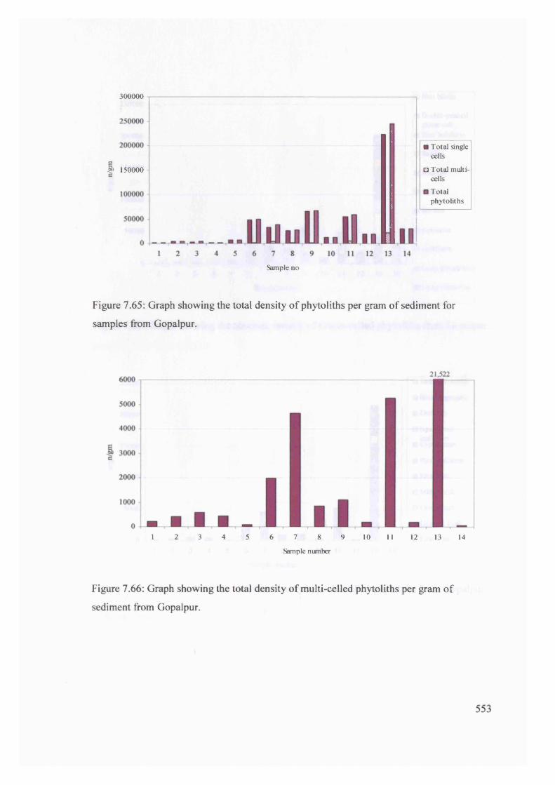
300000
Jj> 150000
Sample no
■ Total single cells
□ Total multicells
■ Total phytoliths
Figure 7.65: Graph showing the total density o f phytoliths per gram of sediment for
samples from Gopalpur.
1 2 3 4 5 6 7 8 9 10 11 12 13 14
Sample number
Figure 7.66: Graph showing the total density o f multi-celled phytoliths per gram o f
sediment from Gopalpur.

I
250000
200000
150000
100000
50000
Sample number
□ Rice bilobe
I Double-peaked glume cell
I Rice bulliform
□ Saddles
Rondels
□ Crosses
Bilobes
□ Keystone
□ Bulliform
■ Long (Dendritic)
□ Long (Staooth)
Figure 7.67: Graph showing the absolute density of single-celled phytoliths from Gopalpur.
25000
20000
15000
10000
5000
□ Indet phytolith
■ Silica aggregate
■ Diatoms
□ Square-cellleaf/stem
■ Cyperaceae
□ Rice leaf/stem
■ Rice husk
□ Millet husk
□ Cereal husk
■ Unident Husk
□ Leaf/Stem
Sample nunber
Figure 7.68: Graph showing the absolute density of multi-celled phytoliths from Gopalpur.
554
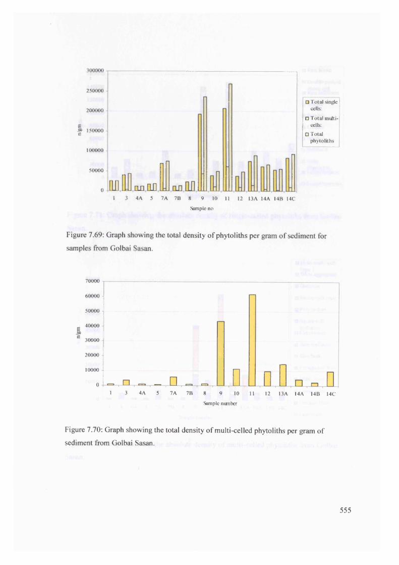
300000
250000
200000
J> 150000
100000
50000
01 3 4A 5 7A 7B 8 9 10 11 12 13A 14A 14B 14C
Sample no
Figure 7.69: Graph showing the total density of phytoliths per gram of sediment for
samples from Golbai Sasan.
70000
60000
50000
40000
30000
20000
10000
0
Figure 7.70: Graph showing the total density of multi-celled phytoliths per gram of
sediment from Golbai Sasan.
—
1 □ 1 1 ... a D a l i-----
------
--□ i I---
------
----
n ! 1 n „ n1 3 4A 5 7A 7B 8 9 10 11 12 13A 14A 14B 14C
Sample number
m i l l an H D
□ Total single cells:
□ Total multicells:
□ Total phytoliths
555

160000
140000
120000
100000
| 80000
60000
40000
20000
0 B a 54A 7 A 7B 8
n
a I t10 11 12 13A 14A 14B 14C
Sample nunber
□ Rice bilobe
■ Double-peakedglume cell
■ Rice bulliform
□ Saddles
■ Rondels
a Crosses
S Bilobes
□ Bulliform
□ Long
□ Long(Snooth)
Figure 7.71: Graph showing the absolute density of single-celled phytoliths from Golbai
Sasan.
70000
6 0 0 0 0
5 0 0 0 0
40000
3 0 0 0 0
20000
. . □ I D I
10000
1 3 4A 5 7A 7B 8 9 10 11 12 13A I4A 14B 14C
Sample nunber
■ Indet multi-cell
■ Silica aggregates
■ Diatoms
□ Mesophyll type
■ Polyhedron
■ Square-cellleaf/stem
□ Cyperaceae
■ Rice leaf/stem
□ Rice husk
■ Phragmites Stem
□ Millet husk
□ Cereal husk
■ Unident Husk
□ Leaf/Stem
Figure 7.72: Graph showing the absolute density o f multi-celled phytoliths from Golbai
Sasan.
556

6000
5000
4000
3000
2000
1000
00 31 2 4
Sample number
Figure 7.73: Graph showing the different grass subfamilies ffom Bajpur.
—♦— totalpanicoid
—■— totalfestucoid
totalchloridoid
6000
5000
4000
J> 3000
2000
1000
01 4 7 9
Sample number
Figure 7.74: Graph showing the different grass subfamilies from Malakhoja.
—♦— totalpanicoid
—a — totalfestucoid
totalchloridoid
557

70000
60000
50000
40000
30000
20000
10000
0 I—*v 1 2 3 4 5 6 7 8 9 10 11 12 13 14
■totalpanicoidtotalfestucoidtotalchloridoid
Sample nimber
Figure 7.75: Graph showing the different grass subfamilies from Gopalpur.
35000
30000
25000
20000
15000
10000
5000
3 4A 5 7A 7B 8 9 10 11 12 13A 14A 14B1
-totalpanicoidtotalfestucoidtotalchloridoid
Sample number
Figure 7.76: Graph showing the different grass subfamilies from Golbai Sasan.
558
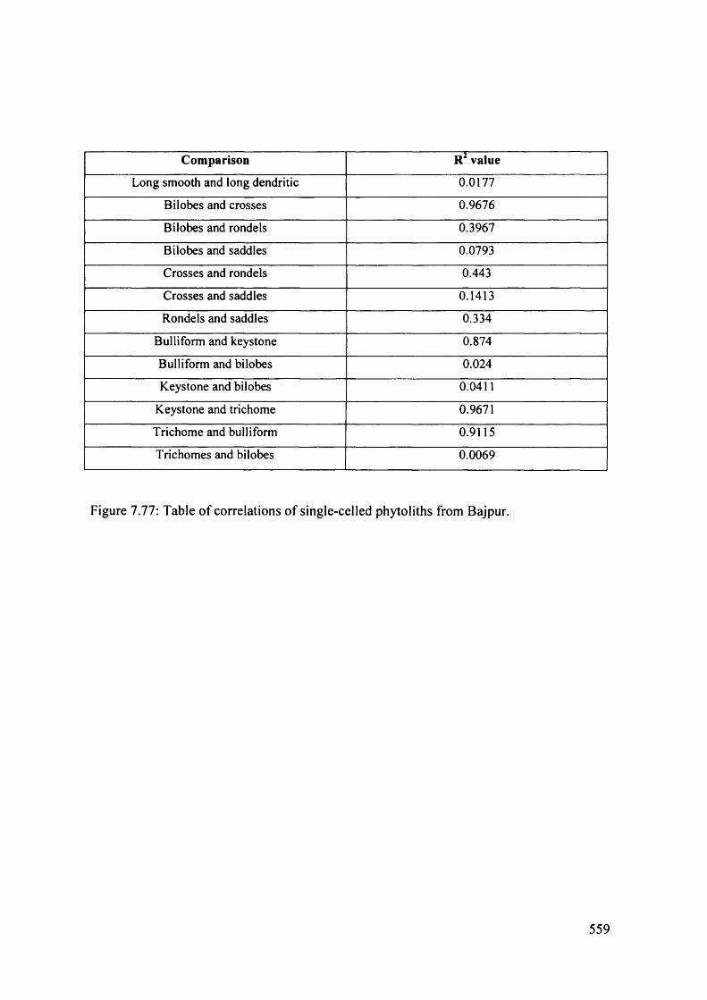
Comparison R value
Long smooth and long dendritic 0.0177
Bilobes and crosses 0.9676
Bi lobes and rondels 0.3967
Bilobes and saddles 0.0793
Crosses and rondels 0.443
Crosses and saddles 0.1413
Rondels and saddles 0.334
Bulliform and keystone 0.874
Bulliform and bilobes 0.024
Keystone and bi lobes 0.0411
Keystone and trichome 0.9671
Trichome and bulliform 0.9115
Trichomes and bilobes 0.0069
Figure 7.77: Table of correlations of single-celled phytoliths from Bajpur.
559

Com parison R 2 value
Long smooth and long dendritic 0.8061
Bi lobes and rondels 0.0114
Bilobes and saddles 0.4378
Rondels and saddles 0.4484
Bulliform and keystone 0.8687
Keystone and trichome 0.9665
Trichomes and bilobes 0.8988
Saddles and bulliforms 0.7458
Saddles and long smooth 0.7451
Saddles and long dendritic 0.9106
Saddles and keystone 0.9549
Long smooth and rondels 0.4376
Long smooth and bilobes 0.6632
Figure 7.78: Table of correlations o f single-celled phytoliths from Malakhoja.
Comparison R2 value
Long smooth and long dendritic 0.8113
Bilobes and crosses 0.9774
Bi lobes and rondels 0.976
Bi lobes and saddles 0.8975
Crosses and rondels 0.9884
Crosses and saddles 0.8276
Rondels and saddles 0.8389
Bulliform and keystone 0.5176
Keystone and trichome 0.767
Bulliform and bilobes 0.9571
Bi lobes and keystone 0.3611
Bilobes and long smooth 0.7615
Bi lobes and long dendritic 0.9672
Figure 7.79: Table o f correlations o f single-celled phytoliths from Gopalpur.
560

Comparison R2 valueLong smooth and long dendritic 0.8581
Bi lobes and crosses 0.9637
Bi lobes and rondels 0.9712
Bi lobes and saddles 0.7636
Crosses and rondels 0.9252
Crosses and saddles 0.7791
Rondels and saddles 0.8562
Bulliform and keystone 0.8368
Keystone and trichome 0.7677
Bulliform and trichome 0.659
Bulliform and bilobes 0.6338
Bilobes and keystone 0.6678
Bi lobes and long smooth 0.8902
Bilobes and long dendritic 0.852
Figure 7.80: Table of correlations o f single-celled phytoliths from Golbai Sasan.
561

Comparison R2 values
Rice bulliform and double-peaked glume cell 0.5177
Double-peaked glume cell and rice bilobe 0.3645
Rice bulliforms and rice bilobe 0.1313
Rice husk and rice leaf/stem 0.5775
Rice husk and rice bulliform 0.4691
Rice husk and double-peaked glume cell 0.7366
Rice husk and rice bilobe 0.8005
Rice leaf/stem and rice bulliform 0.5344
Rice leaf/stem and double-peaked glume cell 0.8572
Rice leaf/stem and rice bilobe 0.224
Rice husk and indet leaf/stem 0.5749
Rice husk and unident husk 0.5474
Rice leaf/stem and indet leaf/stem 0.996
Rice leaf/stem and unident husk 0.9693
Rice husk and millet husk 0.005
Rice leaf/stem and millet husk 0.0003
Rice husk and cereal husk 0.562
Figure 7.81: Table of correlations for Gopalpur multi-celled phytoliths.
562

Comparison R values
Rice bulliform and double-peaked glume cell 0.3602
Double-peaked glume cell and rice bilobe 0.8346
Rice bulliforms and rice bilobe 0.3314
Rice husk and rice leaf/stem 0.6602
Rice husk and rice bulliform 0.3845
Rice husk and double-peaked glume cell 0.8665
Rice husk and rice bilobe 0.9167
Rice leaf/stem and rice bulliform 0.2807
Rice leaf/stem and double-peaked glume cell 0.4851
Rice leaf/stem and rice bilobe 0.5544
Rice husk and indet leaf/stem 0.9743
Rice husk and unident husk 0.8564
Rice leaf/stem and indet leaf/stem 0.5626
Rice leaf/stem and unident husk 0.7875
Rice husk and millet husk 0.0112
Rice husk and cereal husk 0.7469
Rice leaf/stem and millet husk 0.0009
Rice leaf/stem and cereal husk 0.716
Indet leaf/stem and unident husk 0.7841
Figure 7.82: Table of correlations for Golbai Sasan multi-celled phytoliths.
563

Mahagara and Koldihwa
Plant type No of genera or species in region
General habitats
Chenopodiaceae 5 genera + 7 spp Widely distributed, mainly in saline soilsCommelinaceae
Commelina benghalensis (MGR)
4 genera Found throughout India, up to 6000ft. Common in damp places
Occurs from sea level to 1000m, best conditions are high soil moisture, and fertility, sunny and lightly shaded. Loamy, sandy, and rocky soils. Common weed of crops, grasslands, roadsides, and waster places.
Cyperaceae
Scirpus type (MGR)
15 genera
12 spp of Scirpus
Plants of wet or marshy habitats
3 spp suggested as rice weeds, rest found in margins of pond and swampy habitats.
Euphorbiaceae 21 genera Can be weeds of crop plants. Wet and dry condition species.
Gramineae
Eragrostis sp. (MGR)
Ischaemum rugosum (MGR)
16 spp. Variety of environments - 3 dry species but other prefer wet conditions or edges of rivers. Common in pastures and can be a weed of crop plants.
Common weed of rice fields, found throughout India. Annual.
Malvaceae 15 genera Many species hold food products, are fibre plants, or are used medicinally.
Polygonaceae 2 genera Most are wet loving speciesPortulaceae 1 genera, 2 spp. Pot herb and common weed of dry places
Figure 7.83: Tables of weeds present in the archaeobotanical assemblages and their
environmental implications.
564

Gopalpur and Golbai Sasan
Plant type No genera/species General habitatsAizoceae Trianthamea sp. (GBSN)
2 genera1 spp. T. monogyna C4 plant, common at sea level to 800m.
Occurs in cultivated fields, waste places, roadsides, lawns, and gardens. Found in perennial crops and pastures.
Asteraceae Eclipta sp. (GBSN)
Tridex sp. (GBSN)
53 genera 1 spp. E. alba
1 spp.T. procumbens
Common in pastures, and roadsides. Found all over Orissa. Is a medical plant. Occurs in poorly drained wet areas and can survive in saline conditions.Abundant in pastures, banks, and waste grounds. In all districts of Orissa. Drier areas.
Cyperaceae Cyperus sp. (GPR)
16 genera 31 spp.
Plants of wet or marshy habitats.7 species are very common rice weeds. All are found in wet habitats. Some in sandy areas.
Euphorbiaceae Euphorbia sp.
Phyllanthus sp.
42 genera 21 spp.
8 spp.
3 spp common weeds, most found in rocky or sandy places, one spp prefers wet conditions. Most wet loving species and some occur just in the rainy period.
Gramineae Cenchrus sp. Eragrostis sp.
Ischaemum rugosum
90 genera 3 spp 16 spp
Common as a plant of pastures.Some prefer dry conditions and others wet ground.Common weed of rice fields, found throughout India. Annual.
Malvaceae 13 genera Includes common weeds such as many of the Sida species.
Polygonaceae 4 genera Most are wet loving species.Portulaceae Portulaca sp.
1 genera 3 spp. Common in open places and all used as pot
herbs.Rubiaceae Oldenlandia sp.
32 genera 13 spp. Two species are common weeds of wet
environments. Most are found in open, wastelands. Some prefer sandy soils.
Scrophulariaceae Lindernia sp. Scropia sp.
25 genera 3 spp.1 spp. S. dulcis
Found in swamps, and streams.Common on waste ground and damper areas.
Figure 7.83 continued: Tables of weeds present in the archaeobotanical assemblages and
their environmental implications.
565
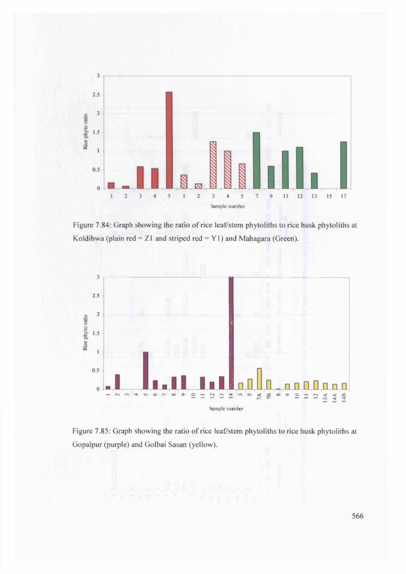
Sample number
Figure 7.84: Graph showing the ratio of rice leaf/stem phytoliths to rice husk phytoliths at
Koldihwa (plain red = Z1 and striped red = Y l) and Mahagara (Green).
—> < N m , - < ^ s o r ' O c o © —• fs m [ 0 » » © - n < < ; dD— - — — •«i- ■'*
Sample number
Figure 7.85: Graph showing the ratio of rice leaf7stem phytoliths to rice husk phytoliths at
Gopalpur (purple) and Golbai Sasan (yellow).

10 □
13A □
13B □
13C p
13D □
14A n
14B 0
0 50 100 150
Total pulses
D
1
s
Total small millets
0 500 1000 0 2500 5000 0 1250 2500 0 2500 5000 0 20000 40000 0 250 500
Rice bulliform Rice bilobe Rice leaf/stem Double-peaked Rice husk Millet huskglume cell
Figure 7.86: Vertical charts of absolute counts and densities for macro-remains and phytoliths at Golbai Sasan.
Os•vj

125 250
T otal pulses
50 0
-
r;
T otal sm all millets
5 10 0 250 500 0 500 1000 0 500 1000
Oryza sp. R ice bulliform Rice bilobe Rice leaf/stem
0 1000 2000 0 2500 5000
D ouble-peaked glum e cell
Rice busk
Figure 7.87: Vertical charts of absolute counts and densities for macro-remains and phytoliths for Gopalpur.
Os00

1223344556 6 778 8 9 9
10101111121213131414151516 16 17 17
0 7.5 15 0 7.5 15 0 2.5 5 0 5 10 0 75 150 0 75 150 0 100 200 0 150 300 0 50 100
T otal pulses T o tal H ordeum sp. O ryza sp. R ice R ice bilobe D ouble-peaked Rice husk M illet husksm all m illets bu llifo rm glum e cell
Figure 7.88: Vertical chart of absolute counts and densities of macro-remains and phytoliths from Mahagara.

11
12
13
14
15
16
17
18
19
20
0 3 0 4 8 0 2 4 0 3 0 1 0 25000 1000 0 500 0 3000 0 11000T otal pulses T o tal sm all H ordeum sp. T riticu m sp. O ryza sp. Rice Rice bilobe Rice D ouble-peaked Rice husk
m illets bulliform leaf/stem glum e cell
Figure 7.89: Vertical chart of absolute counts and densities for macro-remains and phytolith from section Y1 at Koldihwa.
■:■ :
B m b
--jo

3F4
5 "
6 1
7 I
8 ■9
J10 !
f
-
■
0 2.5 5 0 5 10 0 2.5 5 0 1 2 0 5 10 0 1500 3000 0 1500 3000 0 75 150 0 4000 800( 0 50000
T otal pulses T o tal small m illets
H ordeum sp. T riticu m sp. O ryza sp. Rice bulliform Rice bilobe Rice leaf/stem D ouble-peaked Rice husk glum e cell
Figure 7.90: Vertical chart of absolute counts and densities for macro-remains and phytoliths from section Z1 at Koldihwa.
Related Documents