E-index Method for Identifying Dynamic Growth Traits of Poplar

E-index Method for Identifying Dynamic GrowthTraits of PoplarLuman Wang  ( [email protected] )

Peking University Health Science CenterJianxin Wang 

Beijing Forestry UniversityHuiying Qi 

Peking University Health Science Center

Research Article

Keywords: QTL, Growth Process, Earliness Degree, GWAS

Posted Date: November 17th, 2021

DOI: https://doi.org/10.21203/rs.3.rs-1034398/v1

License: This work is licensed under a Creative Commons Attribution 4.0 International License.  Read Full License

1

E-index method for identifying dynamic growth traits of poplar

Luman Wang1,*, Jianxin Wang2 , Huiying Qi1

1Department of Health Informatics and management, Peking University Health Science Center, Beijing

100191, China.

2School of Information Science & Technology, Beijing Forestry University, Beijing 100083, China.

*Corresponding author.

E-mail address: [email protected] (Luman Wang).

Abstract: To detect the mechanism of growth, volume is important to uncover the genetic basis of dynamic complex quantitative traits. Unfortunately, it is difficult to construct the unique simple growth curve to accurately describe the growth process of all trees by the conventional GWAS based on the functional mapping method, which reduces the power of statistics for the growth model. To address this issue, this work adopted a novel approach about the Earliness degree index (E-index). First, it adopted the method of spline interpolation to fit the growth data to acquire the growth curves for each tree. Second, an innovative calculation model based on E-index was used to measure the earliness degree for each growth curve and to identify the potential relationship between QTL effects and traits by a series of hypothesis tests. Besides, a permutation test could be used to estimate the threshold for p values and to screen out significant QTLs from SNPs related to the growth process. To verify the validity and practicability of our model, we applied this method on the data about the volumes of 64 poplar trees chosen randomly from the progeny of two poplar species I-69 and I-45 with 156362 single nucleotide polymorphisms (SNPs). Through the E-index method, 13 significant markers were identified for testcross and 10 for intercross related to the growth process. Overall, this study could help elucidate the underlying genetic mechanisms of complex dynamic traits and perform marker-assisted selection in poplar. Keywords: QTL; Growth Process; Earliness Degree; GWAS

1. Introduction

The growth of trees is a process of dynamic change during its cycle life and is deeply influenced by genetic factors. Accordingly, detecting genetic polymorphisms that regulate economically primary traits plays an important role in identifying targets for genetic modifications that improve productivity. Genome-wide association study reveals putative regulators of bioenergy traits in Populus deltoides. Specifically, the discovery and breeding of superior tree varieties have long been a critical task of forestry management. Because poplar has several distinguishing characteristics such as modest genome size, rapid growth rate, high yield, and relative ease of experimental manipulation [1, 2]. As the perennial woody plant, the poplar is the first species to complete the whole genome sequencing for the study on forestry genomics [3, 4]. Therefore, among the various

2

species of trees, the poplar was considered as the model forest species and is most suitable for genome research.

Quantitative traits are characters of the continuous range of variation and are influenced by both environmental and genetic factors. Quantitative traits are far more common than quality traits and can be hugely polygenic [5]. Studying the genetic characteristics of tree quantitative traits is very important for genetic improvement of cultivated trees. However, the quantitative traits are hard to be like quality traits to accurately distinguish different phenotypes and to analyze genetic behavior such as gene separation, recombination and linkage through dominant and recessive traits. For poplar, volume is one of the significant quantitative traits to measure the economic values and it is quite meaningful to find poplar varieties with high volume in the development process. Therefore, this article dissected the genetic regulation of grown development for poplar to breed varieties with high yields.

The traditional QTL mapping analysis adopted statistical methods to map and identify specific complex loci and was widely applied in agriculture, forestry, fishery and other fields [6, 7]. However, these QTL mapping methods merely focused on the phenotypic data at one single time point individually in the process of biological growth, and it cannot accurately describe the development mechanism of organisms related with the time factor. In order to overcome this limitation, Wu et al. introduced the functional mapping method [8] to search superior genotypes related with developmental process. This method described the growth law by estimating growth parameters for different genotypes at one gene and constructed the statistical model to detect the genotypes with statistically significant difference of growth parameters [9]. Furthermore, the method of functional mapping has been well extended and there have been a wealth of literatures applying it to analyze the growth mechanism of organisms [10-15]. But the functional mapping method does not work well to find the significant gene loci related to traits when the growth curve or function of its growth process is not monotonic or even worse there does not exist uniform function with parameters to fit the successively collected measurement values. To overcome the inherent inadaptability of functional mapping, we proposed E-index method to cumulatively measure earliness degree of development in the overall process which was verified in simulation data and showed very good effect [16].

Further studies would be needed to screen out the gene loci with substantial ability of growth through statistical method of multiple hypothesis testing. Nevertheless, there are hundreds of thousands of SNP makers for each sample of poplar, and the same group of phenotypic data is calculated and tested for so many times. So it will increase the type I error rate, accordingly there will be a lot of wrongly judged to mislead a wrong significant association [17]. Therefore, as the original level of significance α needs to be adjusted. The most convenient way is to use Bonferroni method to correct. That is to say, the significant level of adjustment is α/n, where n is the number of SNP markers. This method is convenient, but it is too conservative to miss the real significant SNP markers easily. To improve the accuracy of correction and to solve the problem of multiplicity, an alternative criterion for many statistical methods was provided such as step down method [18], step up method [19], False Discovery Rates (FDR) method [20], etc. Permutation test as one of the FDR method [21, 22] is based on the rearrangement of sample data for multiple hypothesis tests and is suitable for small samples with unknown overall distribution. In this paper, E-index method combined with permutation test was proposed and applied to detect QTL related with growth of poplar and opened a new way to select more comprehensive species with strong growth ability in

3

breeding.

2. Materials and methods

2.1. Plant materials

As a valuable genetic resource, artificial hybridization is commonly used to identify the significant quantitative traits of species. In this paper, the set of progeny for poplars was chosen through the following hybrid strategy as a pilot study of genetic mapping. First, a full-sib family population of 450 F1 hybrids was generated by a cross between Populus deltoides clone I-69 and Euramerican poplar (P. x euramericana) clone I-45 at Nanjing Forestry University [6]. All of the progeny was planted at Zhangji Forest Farm (34.14°N, 117.38°W) in Jiangsu Province, China, in 1987 and the detail situation of plant environment was described in the several literatures [23, 24].

We randomly chose 64 of these progeny along with their two parents, I69 and I45, to be genotyped genome-wide by single nucleotide polymorphisms (SNPs) using the Applied Biosystems (Foster City, CA, USA) QuantStudio 12K Flex Real-Time PCR System. In all, a total of 156,362 SNPs were available via screening and sorting for quality control, which belongs to testcross and intercross makers respectively [25]. In order to improve the statistical effect, the SNP markers with Minimum Allele Frequency (MAF) ≤ 0.05 were eliminated. So that the genotypic data about 109244 testcross markers segregated from only one heterozygous parent I-69 or I-45 and 38904 intercross markers from both heterozygous parents were acquired ultimately for further analyses. The growth data closely related with the time factor were captured through above trait and values about volumes were measured annually for 24 years from 1987 to 2010. For the phenotypic data of poplar growth, it is almost impossible to find a uniform function be fit all of the growth data well. Thus, we introduced the novel E-index method to replace the traditional QTL mapping analysis to detect the genetic mechanism of growth development. 2.2. E-index’s definition and properties

The concept of E-index was proposed by Wang et al. to measure the earliness degree of growth, which is a powerful tool to quantitatively depict the development features such as the faster or slower, earlier or later growth [16]. This method could successfully identify the specific SNP which govern the growth process for the same biomass at the final time point. In order to expend the scope of applications for any growth process without this restriction, an improved method is founded on framework of the E-index and addresses the issue on poplar. For the character of poplar volume data in experiment, the specific E-index method was implemented through the following biologically meaningful mathematical equations to characterize the interplay between QTLs and development.

Suppose that 𝑓(𝑡) is a growth curve of poplar and it is a continuous function on a closed interval [a, b], a < b, where 𝑡 represents the year (time point) during growth process, and 𝑓(𝑡) is the measure value such as volume or other phenotypic value of poplar sample at time point 𝑡 (year). Also assume that 𝑓(𝑡) is differentiable within its range and 𝑓′(𝑡) is its derivative function. Then the 𝐸-index of the growth curve can be defined as 𝐸𝑎𝑏(𝑓) = 1𝑏−𝑎 ∫ 𝑓′(𝑡)(𝑏 − 𝑡)𝑑𝑡𝑏𝑎 . (1)

In order to illuminate the concept of E-index intuitively, we used 4 types of growth curves (2a) ~ (2d) as followed as an example:

4

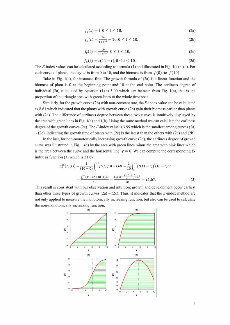
𝑓𝑎(𝑡) = 𝑡, 0 ≤ 𝑡 ≤ 10, (2a) 𝑓𝑏(𝑡) = 201+𝑒−𝑡 − 10, 0 ≤ 𝑡 ≤ 10, (2b)

𝑓𝑐(𝑡) = 101+𝑒6−𝑡 , 0 ≤ 𝑡 ≤ 10, (2c) 𝑓𝑑(𝑡) = 𝑡(11 − 𝑡), 0 ≤ 𝑡 ≤ 10. (2d) The E-index values can be calculated according to formula (1) and illustrated in Fig. 1(a) ~ (d). For each curve of plants, the day 𝑡 is from 0 to 10, and the biomass is from 𝑓(0) to 𝑓(10).

Take in Fig. 1(a), for instance, first. The growth formula of (2a) is a linear function and the biomass of plant is 0 at the beginning point and 10 at the end point. The earliness degree of individual (2a) calculated by equation (1) is 5.00 which can be seen from Fig. 1(a), that is the proportion of the triangle area with green-lines to the whole time span.

Similarly, for the growth curve (2b) with non-constant rate, the E-index value can be calculated as 8.61 which indicated that the plants with growth curve (2b) gain their biomass earlier than plants with (2a). The difference of earliness degree between these two curves is intuitively displayed by the area with green lines in Fig. 1(a) and 1(b). Using the same method we can calculate the earliness degree of the growth curves (2c). The E-index value is 3.99 which is the smallest among curves (2a) ~ (2c), indicating the growth time of plants with (2c) is the latest than the others with (2a) and (2b).

In the last, for non-monotonically increasing growth curve (2d), the earliness degree of growth curve was illustrated in Fig. 1 (d) by the area with green lines minus the area with pink lines which is the area between the curve and the horizontal line 𝑦 = 0. We can compute the corresponding E-index as function (3) which is 21.67: 𝐸010(𝑓𝑑(𝑡)) = 1(10 − 0) ∫ 𝑓′(𝑡)(10 − 𝑡)𝑑𝑡10

0 = 110 ∫ (𝑡(11 − 𝑡))′(10 − 𝑡)𝑑𝑡100

= ∫ (11−2𝑡)(10−𝑡)𝑑𝑡100 10 = (110𝑡−31𝑡22 +2𝑡33 )|01010 = 21.67. (3)

This result is consistent with our observation and intuition: growth and development occur earliest than other three types of growth curves (2a) ~ (2c). Thus, it indicates that the E-index method are not only applied to measure the monotonically increasing function, but also can be used to calculate the non-monotonically increasing function.

5

Fig. 1. Illustrations for E-index calculation of four growth curves. (a) is a growth curve with constant growth rate. (b) is with non-constant rate. (c) is a monotonically increasing growth curve with higher growth rate in earlier half and lower growth rate in later half. (d) is a non-monotonically increasing growth curve. The E-index values for four curves are 5.00, 8.61, 3.99 and 21.67, respectively.

Though phenotypic values of curves (2a) ~ (2d) are approximately same at the end time point where 𝑡 = 10 , the E-index values are very different. If the growth curves are monotonically increasing such as growth curves (2a) ~ (2c), their E-index values are accordingly between 0 and 𝑓(𝑏) − 𝑓(𝑎) = 10. For the non-monotone increasing function, the E-index value might be greater than 10 as growth curve (2d). It indicates that the 𝐸-index for growth curves could be any designated value in the range. Thus, from these four types growth curves, we can calculate the E-index value through the formula above easily to measure how early growth occurs in the whole growth process to know the growth status of every plant.

3. Calculation

To measure the biological growth and development properties, the most of the traditional QTL mapping methods could be applied in the condition of the known growth curves which can be represented by the monotonically increasing function with unique parameters. Nevertheless in the actual process of biological growth, it is difficult to acquire the function that satisfies the above strict requirements. Meanwhile, the growth values at some time points may be missing due to the limitation of the measurement condition or other factors, which may affect the accuracy of curve fitting. Fortunately, E-index method is not restricted by these requirements and works well if we get each function of growth curve for the corresponding samples data, either discrete or continuous. So the challenge is how to find a function fitting the successively collected measurement values well. Here, we adopt spline interpolation approach to fit the phenotypic data of poplar growth to avoid the influence of missing values on curve fitting. Even if the growth values are missing at one or several interpolation time points in the whole process of development, the growth curve also can be well fitted by the spline interpolation method. Based on the fitting growth curves of every plant, the E-index method can be further applied to differentiate complex dynamic traits with the statistical framework and to detect QTL in the developing process. 3.1. Spline interpolation method

Spline interpolation is a form of interpolation with a special type of piecewise polynomial called a spline. To calculate the E-index value about the plant, the spline interpolation can be used to fit the phenotypic data of poplar growth because the interpolation error can be made small even when using low-degree polynomials for the spline. Meanwhile, it has been verified that a typical kind of spline interpolation, the cubic spline interpolation function, fits the growth data well under the condition of unknown growth curve [16]. Here, we took one of the parents of poplar plant I-69 for example to describe the calculation process. We measured the volume values at each time point from 1th year to 24th year as displayed as grey point in the Fig. 2. A smooth curve can be obtained by spline interpolation to fit the data well and be drawn as the red line.

6

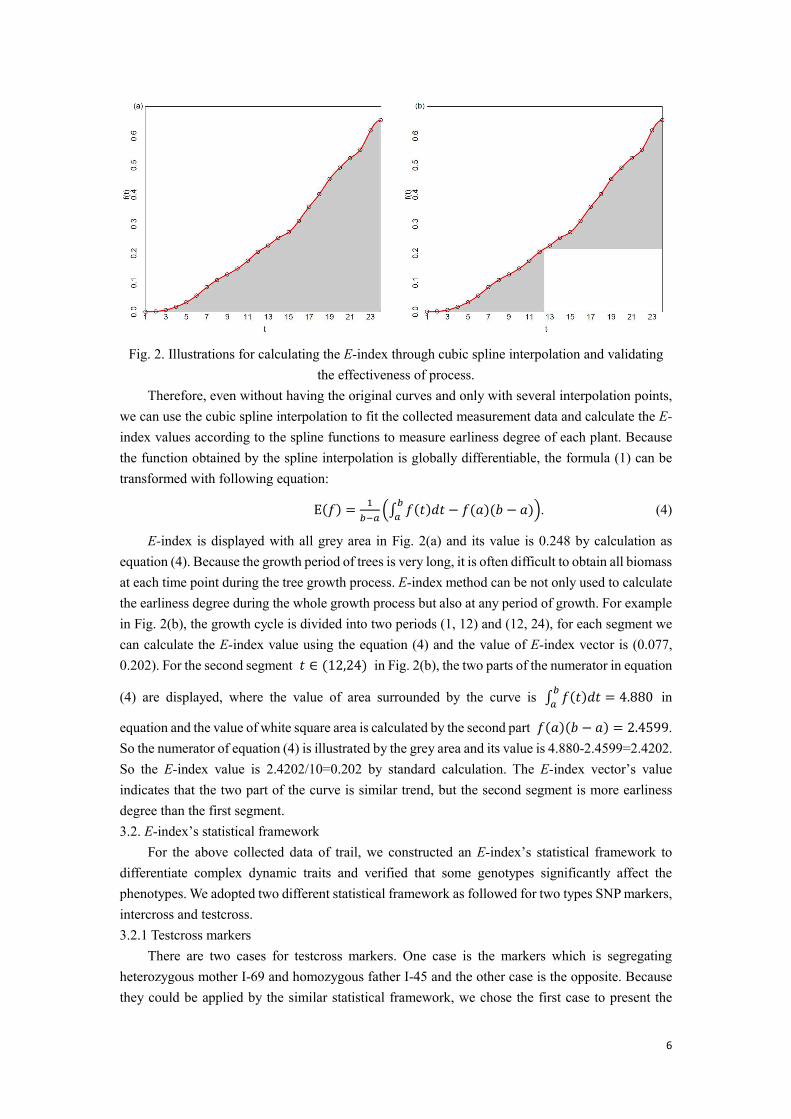
Fig. 2. Illustrations for calculating the E-index through cubic spline interpolation and validating the effectiveness of process.

Therefore, even without having the original curves and only with several interpolation points, we can use the cubic spline interpolation to fit the collected measurement data and calculate the E-index values according to the spline functions to measure earliness degree of each plant. Because the function obtained by the spline interpolation is globally differentiable, the formula (1) can be transformed with following equation: E(𝑓) = 1𝑏−𝑎 (∫ 𝑓(𝑡)𝑑𝑡 − 𝑓(𝑎)(𝑏 − 𝑎)𝑏𝑎 ). (4)

E-index is displayed with all grey area in Fig. 2(a) and its value is 0.248 by calculation as equation (4). Because the growth period of trees is very long, it is often difficult to obtain all biomass at each time point during the tree growth process. E-index method can be not only used to calculate the earliness degree during the whole growth process but also at any period of growth. For example in Fig. 2(b), the growth cycle is divided into two periods (1, 12) and (12, 24), for each segment we can calculate the E-index value using the equation (4) and the value of E-index vector is (0.077, 0.202). For the second segment 𝑡 ∈ (12,24) in Fig. 2(b), the two parts of the numerator in equation

(4) are displayed, where the value of area surrounded by the curve is ∫ 𝑓(𝑡)𝑑𝑡 = 4.880𝑏𝑎 in

equation and the value of white square area is calculated by the second part 𝑓(𝑎)(𝑏 − 𝑎) = 2.4599. So the numerator of equation (4) is illustrated by the grey area and its value is 4.880-2.4599=2.4202. So the E-index value is 2.4202/10=0.202 by standard calculation. The E-index vector’s value indicates that the two part of the curve is similar trend, but the second segment is more earliness degree than the first segment. 3.2. E-index’s statistical framework

For the above collected data of trail, we constructed an E-index’s statistical framework to differentiate complex dynamic traits and verified that some genotypes significantly affect the phenotypes. We adopted two different statistical framework as followed for two types SNP markers, intercross and testcross. 3.2.1 Testcross markers

There are two cases for testcross markers. One case is the markers which is segregating heterozygous mother I-69 and homozygous father I-45 and the other case is the opposite. Because they could be applied by the similar statistical framework, we chose the first case to present the

7

statistical steps in detail. Suppose the genotypes of the progeny are FF for homozygote and FM for heterozygote and the numbers of the corresponding samples are m and n. And suppose that the volume value vector of the ith sample for genotype FF is 𝑉𝑖𝐹𝐹 = (𝑣𝑖,1𝐹𝐹 , 𝑣𝑖,2𝐹𝐹 , ⋯ , 𝑣𝑖,𝑇𝐹𝐹), 𝑖 = 1,2, ⋯ , 𝑚, and that of the jth samples for genotype FM is 𝑉𝑗𝐹𝑀 = (𝑣𝑗,1𝐹𝑀, 𝑣𝑗,2𝐹𝑀, ⋯ , 𝑣𝑗,𝑇𝐹𝑀), 𝑗 = 1,2, ⋯ , 𝑛 at each time point 𝑡, 𝑡 = 1, 2, … , 𝑇 (where 𝑇 = 24). The statistical steps are as followed, using t-test with (m+n-2) degrees of freedom to discover the significance difference between genotype FF and FM. (1) For each phenotype vector 𝑉𝑖𝐹𝐹 and 𝑉𝑗𝐹𝑀 of poplar sample, cubic spline interpolation method can be fit to obtain the continuous curves 𝑓𝑖𝐹𝐹(𝑡) and 𝑓𝑗𝐹𝑀(𝑡), where 𝑡 = 1, 2 ⋯ , 24 is the time point for measurement of plants.

(2) Then formula (4) is applied to calculate each E-index of the fitting curves, namely E𝑖𝐹𝐹 , 𝑖 =1,2, ⋯ , 𝑚 and E𝑗𝐹𝑀, 𝑗 = 1,2, ⋯ , 𝑛 , respectively. And we denote that E-index values as 𝐸𝐹𝐹 =(E1𝐹𝐹 , E2𝐹𝐹 , ⋯ , E𝑚𝐹𝐹) and 𝐸𝐹𝑀 = (E1𝐹𝑀, E2𝐹𝑀 , ⋯ , E𝑛𝐹𝑀). (3) After that a statistic testing can be defined as follows 𝑡 = 𝐸𝐹𝐹̅̅ ̅̅ ̅̅ −𝐸𝐹𝑀̅̅ ̅̅ ̅̅√𝑠2(1/𝑚+1/𝑛), (5)

where 𝐸𝐹𝐹̅̅ ̅̅ ̅ is the mean of the vector 𝐸𝐹𝐹 and 𝐸𝐹𝑀̅̅ ̅̅ ̅̅ is the mean of the vector 𝐸𝐹𝑀 (here we suppose that 𝐸𝐹𝐹̅̅ ̅̅ ̅ > 𝐸𝐹𝑀̅̅ ̅̅ ̅̅ ) and the common variance is denoted as 𝑠2 = (𝑚−1)𝑠𝐹𝐹2 +(𝑛−1)𝑠𝐹𝑀2𝑚+𝑛−2 , (6)

where 𝑠𝐹𝐹2 is the sample variance of 𝐸𝐹𝐹 and 𝑠𝐹𝑀2 is that of 𝐸𝐹𝑀. (4) We can test the null hypothesis that the two groups of samples are not significantly different: 𝐻0: 𝐸𝐹𝐹̅̅ ̅̅ ̅ − 𝐸𝐹𝑀̅̅ ̅̅ ̅̅ = 0, (7) versus the alternative hypothesis that the two groups of growth curves are significantly different: 𝐻1: 𝐸𝐹𝐹̅̅ ̅̅ ̅ − 𝐸𝐹𝑀̅̅ ̅̅ ̅̅ > 0, (8) 𝐻0 will be rejected if 𝑡 > 𝑡𝑎(𝑚 + 𝑛 − 2) , otherwise 𝐻0 will be accepted, where 𝑡 is the computation result of (5) and 𝑡𝑎(𝑚 + 𝑛 − 2) is the 𝑡-distribution value with the confidence level 𝛼 and (𝑚 + 𝑛 − 2) degrees of freedom. 3.2.2 Intercross markers

Intercross markers are segregating both heterozygous parents and the genotypes of progeny are FF, FM and MM. We suppose the number of the corresponding samples are m, n and l, and the volume value vector of the ith sample for genotype FF is 𝑉𝑖𝐹𝐹 = (𝑣𝑖,1𝐹𝐹 , 𝑣𝑖,2𝐹𝐹 , ⋯ , 𝑣𝑖,𝑇𝐹𝐹), 𝑖 = 1,2, ⋯ , 𝑚, that of the jth samples for genotype FM is 𝑉𝑗𝐹𝑀 = (𝑣𝑗,1𝐹𝑀 , 𝑣𝑗,2𝐹𝑀, ⋯ , 𝑣𝑗,𝑇𝐹𝑀), 𝑗 = 1,2, ⋯ , 𝑛 and that of the kth samples for genotype MM is 𝑉𝑘𝑀𝑀 = (𝑣𝑘,1𝑀𝑀, 𝑣𝑘,2𝑀𝑀, ⋯ , 𝑣𝑘,𝑇𝑀𝑀), 𝑘 = 1,2, ⋯ , 𝑙 at each time point 𝑡, 𝑡 = 1, 2, … , 𝑇 (where 𝑇 = 24). The statistical steps are as the following, using analysis of variance (ANOVA) with (𝛾1, 𝛾2) degrees of freedom to discover the significance difference among genotype FF, FM and MM. (1) For each phenotype vector 𝑉𝑖𝐹𝐹, 𝑉𝑗𝐹𝑀 and 𝑉𝑘𝑀𝑀 of poplar sample, cubic spline interpolation method can be fit to obtain the continuous curves 𝑓𝑖𝐹𝐹(𝑡) , 𝑓𝑗𝐹𝑀(𝑡) and 𝑓𝑘𝑀𝑀(𝑡) where 𝑡 =1, 2 ⋯ , 24 is the time point for measurement of plants.

(2) Then formula (4) is applied to calculate each E-index of the fitting curves, namely E𝑖𝐹𝐹 , 𝑖 =1,2, ⋯ , 𝑚, E𝑗𝐹𝑀, 𝑗 = 1,2, ⋯ , 𝑛, and E𝑘𝑀𝑀, 𝑘 = 1,2, ⋯ , 𝑙 respectively. And we denote that E-index values as 𝐸𝐹𝐹 = (E1𝐹𝐹 , E2𝐹𝐹 , ⋯ , E𝑚𝐹𝐹) , 𝐸𝐹𝑀 = (E1𝐹𝑀, E2𝐹𝑀 , ⋯ , E𝑛𝐹𝑀) and 𝐸𝑀𝑀 =(E1𝑀𝑀 , E2𝑀𝑀, ⋯ , E𝑙𝑀𝑀). (3) After that F-test can be defined as follows:

8

𝐹 = 𝑀𝑆𝑇𝑟𝑒𝑎𝑡𝑚𝑒𝑛𝑡𝑠𝑀𝑆𝐸𝑟𝑟𝑜𝑟 = 𝑆𝑆𝑇𝑟𝑒𝑎𝑡𝑚𝑒𝑛𝑡𝑠/𝛾1𝑆𝑆𝐸𝑟𝑟𝑜𝑟/𝛾2 , (9) 𝑆𝑆𝑇𝑟𝑒𝑎𝑡𝑚𝑒𝑛𝑡𝑠 = m(𝐸𝐹𝐹̅̅ ̅̅ ̅ − �̅�)2 + n(𝐸𝐹𝑀̅̅ ̅̅ ̅̅ − �̅�)2 + l(𝐸𝑀𝑀̅̅ ̅̅ ̅̅ − �̅�)2, (10) 𝑆𝑆𝐸𝑟𝑟𝑜𝑟 = ∑ (𝐸𝑖𝐹𝐹 − �̅�)2𝑚𝑖=1 + ∑ (𝐸𝑖𝐹𝑀 − �̅�)2𝑛𝑗=1 + ∑ (𝐸𝑖𝑀𝑀 − �̅�)2𝑙𝑘=1 , (11) where 𝐸𝐹𝐹̅̅ ̅̅ ̅ is the mean of the vector 𝐸𝐹𝐹, 𝐸𝐹𝑀̅̅ ̅̅ ̅̅ is the mean of the vector 𝐸𝐹𝑀, 𝐸𝑀𝑀̅̅ ̅̅ ̅̅ is the mean of the vector 𝐸𝑀𝑀 , and �̅� is the mean of E-index for all samples. The degrees of freedom (𝛾1, 𝛾2) in this statistical value is (2, m+n+l-3). (4) We can test the null hypothesis that the mean of E-indexes values about three groups samples

are not significantly different: 𝐻0: 𝐸𝐹𝐹̅̅ ̅̅ ̅ = 𝐸𝐹𝑀̅̅ ̅̅ ̅̅ = 𝐸𝑀𝑀̅̅ ̅̅ ̅̅ , (12) versus the alternative hypothesis that the three groups of growth curves are not all the same. 𝐻0 will be rejected if 𝐹 > 𝐹𝑎(𝛾1, 𝛾2) , otherwise 𝐻0 will be accepted, where F is the computation result of (9) and 𝐹𝑎(𝛾1, 𝛾2) is the F-distribution value with the confidence level 𝛼 and (𝛾1, 𝛾2 ) degrees of freedom. 3.3. Permutation test

Based on resampling methods, permutation test was advocated by Churchill and Doerge [26], and it were frequently employed in practical data for the high dimensional testing such as GWAS [27]. To find the meaningful SNP effectively, we adopted the permutation test method to filter significant SNP from the first candidate1000 SNP markers with the smallest p values which were acquired by the above statistical framework. For each candidate SNP marker, we recorded the number of different genotypes and the respectively E-index values calculated for each poplar samples. Here, we took a SNP testcross marker Scaffold.Id 9/8587909 as an example. (1) For all poplar samples, there are two genotypes presented as FF and FM for this SNP, and the number of the corresponding genotype is 30 and 34 respectively. For every poplar samples the E-index value can be calculated by equation (4) for the relative measurement value about volume, and the earliness degree of growth curve was obtained. The E-index vector of genotype FF is 𝐸𝐹𝐹 =(0.269, 0.420, 0.523, 0.341, … , 0.384) and E-index vector of genotype FM is 𝐸𝐹𝑀 =(0.456, 0.385, 0.417, 0.272, … , 0.122) . The new vector 𝐸′ = (𝐸𝐹𝐹 , 𝐸𝐹𝑀) as (0.269, 0.420, … , 0.384,0.456, 0.385, … , 0.122) can be produced by merging the two vector 𝐸𝐹𝐹 and 𝐸𝐹𝑀. 30 E-index values from new vector 𝐸′ can be selected randomly as A group and the other 34 values as B group. The statistical framework of t-test was applied and the probability p value could be acquired by equation (5). (2) Repeat (1) steps for 1000 candidate SNP markers, and get specific p values as {𝑝𝑖,𝑗}, 𝑖 = 1, 𝑗 =1,2, … 1000 and the minimum p value as 𝑝𝑖𝑚𝑖𝑛. These results can represent the overall sampling situation in the phenotype of poplar.

(3) Repeat (1)-(2) steps 100 times, and get 100 p values as {𝑝𝑖𝑚𝑖𝑛}, 𝑖 = 1,2, … 100. We calculate the 0.1 quantile of set {𝑝𝑖𝑚𝑖𝑛}, 𝑖 = 1,2, … 100 as the critical thresholds to screen significant QTLs of poplar from candidate SNP markers.

4. Results

From 148,148 SNP markers included testcross and intercross of poplar, the E-index method was used to calculate the relative earliness degree; furthermore, the permutation test was applied to

9

screen out the statistically significant gene fragment as QTL. In the following description, we illustrate the detecting results for significant QTL in detail under different SNP effects, both additive and dominant. 4.1. Manhattan plot

Based on the above E-index method and the statistical framework, the probability p values of testcross and intercross SNP markers can be calculated. Because these values are too small to be difficult to detect their differences between them, we have a logarithmic conversion to the p value represented as the −log (p). The smaller the p value is, the greater the −log (p) value will be [28].

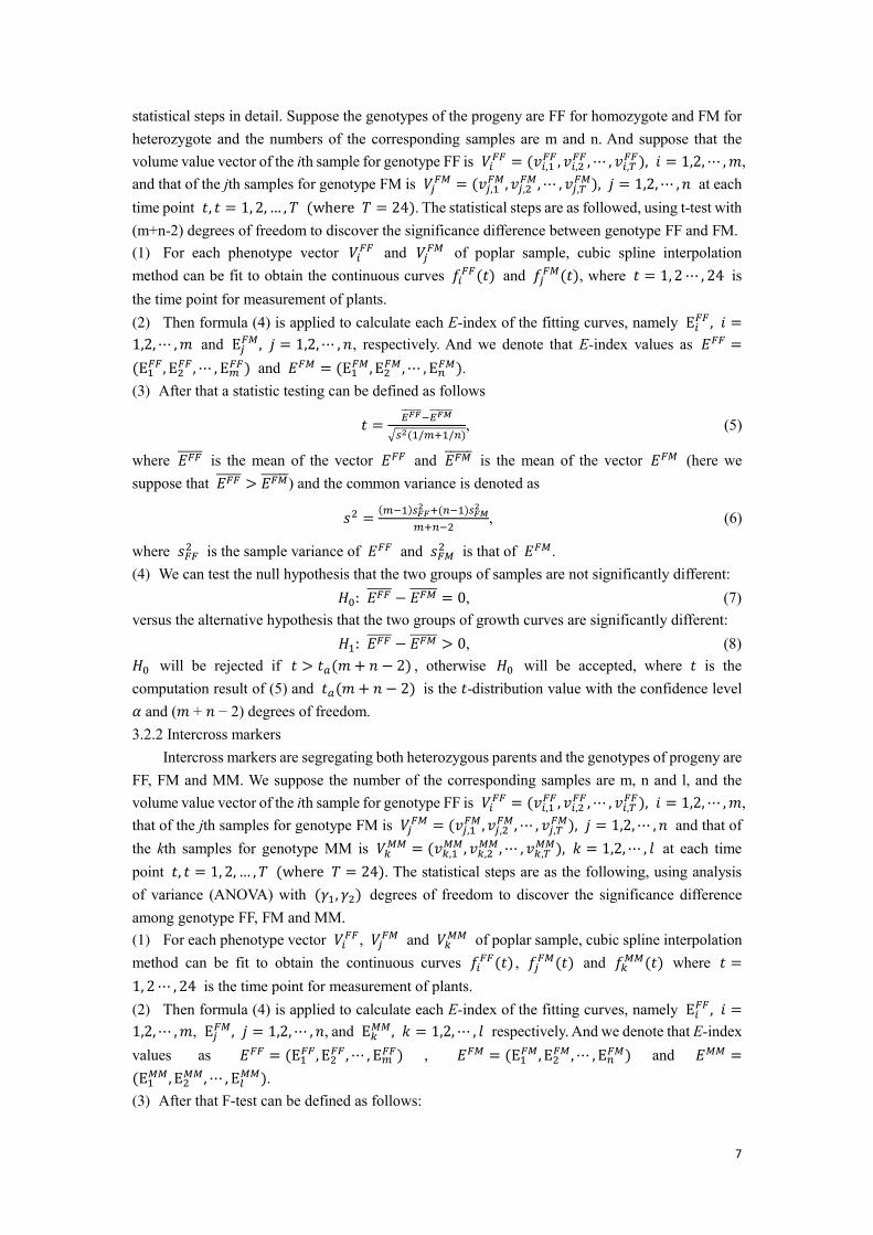
By means of GWAS with the above permutation testing, we made the Manhattan plot across 19 chromosomes for 148,148 SNP makers as shown in Fig. 3 about intercross marker and testcross markers. Significant SNP markers could be screened as QTLs, of which −log (p) values are greater than 8.0 (𝑝𝑚𝑖𝑛 = −ln (3.4E − 4)) for testcross markers and are greater than 9.3 (𝑝𝑚𝑖𝑛 =−ln (8.8E − 5)) for intercross markers. The detailed information about the most statistical significance QTLs for poplar is displayed in the Table 1 included 13 testcross markers and 20 intercross markers and can be shown in Fig. 3 which are the points above the red line.

Table 1. Table about the detailed information of the most statistical significance QTLs for poplar.

Segregating

type SNP Line no. Chr

Physical

Position p-value Allele Heritability

Testcross 86174 966458 9 8587909 7.56E-05 G/C 14.67841473

Marker 87492 979087 9 10689746 0.000183 G/T 5.294085381 155869 1842529 1158 1604 0.000194 A/T 0.789683295 85963 964633 9 8272417 0.000217 C/G 15.94689842 117880 1324045 14 1678181 0.00022 G/T 0.387709183 85960 964624 9 8271390 0.000243 C/T 17.3867404 117854 1323941 14 1662924 0.000244 T/C 0.704029483 86037 965307 9 8374136 0.000256 G/C 12.56545917 118329 1329717 14 2687732 0.000276 T/C 0.028408482 86976 974736 9 10010132 0.000284 G/A 7.307532311 87023 975137 9 10076008 0.000288 A/T 3.894336035 146882 1664089 18 14858485 0.000326 G/A 0.83304914 117682 1322400 14 1385597 0.000335 A/G 0.309231502

Intercross 48971 550358 5 5137853 2.77E-05 C/A 4.530510088

Marker 48892 549457 5 4966044 5.43E-05 A/C 6.515986051 48827 548763 5 4810136 6.57E-05 T/A 7.157324672 48811 548739 5 4808398 6.76E-05 A/G 7.096772128 48826 548762 5 4810091 6.92E-05 A/G 6.563203061 48802 548722 5 4807469 7.85E-05 C/T 6.595937836 48833 548776 5 4811009 8.34E-05 A/G 5.747401429 48814 548745 5 4808912 8.54E-05 G/T 7.315723255 48797 548706 5 4806540 8.62E-05 C/A 7.235539107 48799 548712 5 4806812 8.62E-05 A/G 7.235539107

Notably, most of the testcross markers which are significant for the volume growth process were located on chromosomes 9 and 14 (Fig. 3a). Of these QTLs, 70% were segregating from the heterozygous genotype of mother I-69, suggesting that the I-69 allele contributes more than the I-

10

45 allele to variation in growth form. It appears that intercross QTLs were distributed much more centralized throughout the poplar genome and most of the significant intercross markers for the volume growth process were located on chromosome 5 (Fig. 3b).

Fig. 3. Manhattan plot of significance tests for all testcross (a) and intercross (b) SNP markers across 19 chromosomes of the genome by E-index method for the volume of poplars. Red horizontal lines are the critical thresholds measured by the permutation test. 4.2. QTL detection by E-index method

In order to vividly display the effectiveness of E-index, we choose the most statistically significant SNP markers for additive effects and dominant effects. The typical growth curves of poplar samples about testcross marker Scaffold.Id 9/8587909 are drawn out in Fig. 4(a). Two groups of the growth curves of genotypes FF and FM are generated respectively in red and yellow lines, and the average growth curves for both corresponding genotypes are displayed by blue and green lines. Intuitively, the two groups of growth curves are obviously far apart during the development processes and the most of growth curves about genotype FF are above genotype FM and the end time point. That is to say, the poplar samples with the SNP markers FF for this QTL are early maturity plants during the growth development and have a greater volume than the plants with genotypes FM at the endpoint with high yields. So if we want to get fast-growing poplar samples with great volume, we need to select poplar varieties with genotype FF of this SNP marker. Meanwhile, for the intercross marker Scaffold.Id 5/ 5137853, the growth curves can also be divided into three groups successfully by the E-index method for different genotypes FF, FM and MM in Fig. 4(b). The E-index value can quantify the trend of the whole growth curve vividly neither at any point of time, nor just for the ending time point.

11

Fig. 4. Growth curves of volume for different genotypes at two chosen loci, testcross marker Scaffold.Id 9/8587909 with two genotypes, FF and FM (a), and intercross marker Scaffold.Id 5/ 5137853 with three genotypes, FF, FM and MM (b). 4.3. Calculation of heritability

Heritability is an important measure to characterize the effect of genes on traits [29]. Here we introduced the heritability to explain the additive effects and dominant effects for each significant SNP marker through the measured phenotypic values about the volume of poplar samples and the observed genotypes [30]. There is an additive effect for each significant testcross SNP marker and the values of heritability can be calculated through equation (13) at each time point as followed, ℎ𝑗2 = 2𝑝0𝑝1𝑎𝑗2𝑣𝑎𝑟(�̃�) , 𝑗 = 1, 2 … , 𝑝, (13) 𝑎𝑗 = |𝑦𝐹𝐹̅̅ ̅̅ ̅ − 𝑦𝐹𝑀̅̅ ̅̅ ̅| or 𝑎𝑗 = |𝑦𝐹𝑀̅̅ ̅̅ ̅ − 𝑦𝑀𝑀̅̅ ̅̅ ̅̅ |, by where 𝑝1 is the estimated allele frequency for F, and 𝑝0 is the estimated allele frequency for M, 𝑎𝑗 is the median estimate of the additive effect for SNP j and 𝑦𝐹𝐹̅̅ ̅̅ ̅ , 𝑦𝐹𝑀̅̅ ̅̅ ̅ or 𝑦𝑀𝑀̅̅ ̅̅ ̅̅ are the absolute mean value of the corresponding phenotypes for different genotypes FF, FM or MM. And the variance of all phenotype values about the samples is expressed by 𝑣𝑎𝑟(�̃�).

Meanwhile, there are additive and dominant effects for each significant intercross SNP marker and the value of heritability can be calculated by equation (14) with the similar meaning about the same symbol as followed [31], ℎ𝑗2 = 2𝑝0𝑝1(𝑎𝑗+(𝑝1−𝑝0)𝑑𝑗)2+4𝑝02𝑝12d𝑗2𝑣𝑎𝑟(�̃�) , 𝑗 = 1, 2 … , 𝑝, (14)

𝑎𝑗 = |𝑦𝐹𝐹̅̅ ̅̅ ̅−𝑦𝑀𝑀̅̅ ̅̅ ̅̅ ̅|2 , 𝑑𝑗 = 𝑦𝐹𝑀̅̅ ̅̅ ̅ − 𝑦𝑎𝑙𝑙̅̅ ̅̅ ̅, where 𝑑𝑗 is the median estimate of the dominant effect for SNP j and 𝑦𝑎𝑙𝑙̅̅ ̅̅ ̅ is the mean of phenotypic values for all poplar samples.

The value of heritability could indicate the effects of SNPs and their data about the statically significant SNPs at the beginning time point are also listed in table 1. It can be seen that the mean values of heritability is 6.56% and 6.16% for the selected testcross SNP markers and intercross SNP markers respectively. The dramatic variation of heritability for these markers at each time point of

12

the whole process can be drawn in Fig. 5. It can be seen clearly in the diagram that the two types of heritability curves show a general trend that increases rapidly and then decreases gradually, with a peak at years 3–7.

Fig. 5. The heritability curves of testcross markers (a) and intercross markers (b) with statistically significant in the temporal pattern.

5. Conclusion & Discussion

This paper provided an effective and novel method to apply the E-index theory to measure the earliness degree of development for poplars. Traditional QTL studies, such as functional mapping, are used to identify the growth mechanism according to growth curves which should meet some strict requirements. Nevertheless, in some cases, it is not easy to acquire the uniform function for all of the growth curves to describe the development of poplar trees. Thus, according to this actual situation, we adopted the cubic spline interpolation method to fit the phenotypic measurements about each poplar species well. Then E-index theory was applied to measure the earliness degree of each poplar sample and the hypothesis testing was used about markers to acquire the candidate QTL. Finally, we used the permutation test to verify and screen out the significant SNP markers.

Although this article only deals with the earliness degree for volume growth of poplar, the E-index method can also be applied in other situations with a similar mode of growth. For example, the same method can apply to other traits such as weight, area and so on. Also, it can be extended to any tree species rather than only about poplars described in this experiment. In addition, this paper provided more broadly useful guidelines to get the accurate SNP markers as QTL by measuring earliness degree of development in any growth phase to reveal detailed characteristics of growth and it provided theoretical and practical support for poplar breeding.

Funding

13

This work is supported by National Key R&D Program of China (2017YFC1602002, 2018YFC1603305). Data and program operation by Research Computing Platform of Peking University Health Science Center.

Author information

Affiliations

1Department of Health Informatics and management, Peking University Health Science Center, Beijing 100191, China. 2School of Information Science & Technology, Beijing Forestry University, Beijing 100083, China.

Contributions

WJ provided the main idea. WL, WJ and QH designed the simulation study. WL and WJ wrote the code. WL and QH performed the data application. All authors wrote the manuscript. All authors read and approved the final manuscript.

Corresponding author

Correspondence to Wang Luman.

Availability of data and materials

The datasets used and/or analyzed during the current study are available from the corresponding author on reasonable request.

Declarations

Ethics approval and consent to participate

Not applicable

Consent for publication

Not applicable

Competing interests

14

The authors declare that they have no competing interests.

Reference

1. Ma, T., et al., Genomic insights into salt adaptation in a desert poplar. Nature Communications, 2013. 4.

2. Janz, D., et al., Salt stress induces the formation of a novel type of ‘pressure wood’ in two Populus species. New Phytologist, 2012. 194(1): p. 129-141.

3. Tuskan, G.A., S. Difazio, and S. Jansson, The genome of black cottonwood, Populus trichocarpa (Torr. & Gray). Science, 2006. 313(5793): p. 1596-604.

4. Djerbi, S., et al., The genome sequence of black cottonwood (Populus trichocarpa) reveals 18 conserved cellulose synthase (CesA) genes. Planta, 2005. 221(5): p. 739-746.

5. Anderson, J.T., et al., The evolution of quantitative traits in complex environments. Heredity, 2013. 112(1): p. 4-12.

6. Rong Ling Wu, Ming Xiu Wang, Min-Ren Huang, Quantitative genetics of yield breeding for Populus short rotation culture. I. Dynamics of genetic control and selection model of yield traits. Canadian Journal of Forest Research, 1992. 22(2): p. 175-182.

7. Schmalenbach, I., J. Léon, and K. Pillen, Identification and verification of QTLs for agronomic traits using wild barley introgression lines. Theoretical and Applied Genetics, 2008. 118(3): p. 483-497.

8. Ma, C.X., G. Casella, and R. Wu, Functional Mapping of Quantitative Trait Loci Underlying the Character Process: A Theoretical Framework. Genetics, 2002. 161(4): p. 1751.

9. R. L. Wu, C.X.M., X. Y. Lou, and G. Casella, Molecular dissection of allometry, ontogeny, and plasticity: a genomic view of developmental biology. BioScience, 2003. 53(11): p. 1041-1047.

10. Rongling Wu, C.X.M., Min Lin, Zuoheng Wang, and George Casella, Functional mapping of quantitative trait loci underlying growth trajectories using a transform-both-sides logistic model. Biometrics, 2004. 60(3): p. 729-738.

11. Rongling Wu, C.X.M., Min Lin and George Casella, A general framework for analyzing the genetic architecture of developmental characteristics. Genetics, 2004. 166(3): p. 1541-1551.

12. Li, Q., et al., Functional mapping of genotype-environment interactions for soybean growth by a semiparametric approach. Plant Methods, 2010. 6(1): p. 13.

13. Li, Y. and R. Wu, Functional mapping of growth and development. Biological Reviews, 2010. 85(2): p. 207-216.

14. Zhao, X., et al., Functional mapping of ontogeny in flowering plants. Briefings in Bioinformatics, 2011. 13(3): p. 317-328.

15. Ye, M., et al., Functional mapping of seasonal transition in perennial plants. Briefings in Bioinformatics, 2014. 16(3): p. 526-535.

16. Qi, J., J. Sun, and J. Wang, E-Index for Differentiating Complex Dynamic Traits. BioMed Research International, 2016. 2016: p. 1-13.

17. Storey, J.D., The positive false discovery rate: a bayesian interpretation and the q-value. The Annals of Statistic, 2003. 31(6): p. 2013-2035.

18. Holm, S., A Simple Sequentially Rejective Multiple Test Procedure. Scand J Statist, 1979. 6: p. 65-70.

15

19. Hochberg, Y., A sharper Bonferroni procedure for multiple tests of significanc. Biometrik, 1988. 75(4): p. 800-802.

20. Benjamini, Y. and Y. Hochberg, Controlling the false discovery rate: a practical and powerful approach to multiple testing. Journal of the Royal Statistical Society, 1995. 57(1): p. 289-300.

21. Storey, J.D., A direct approach to false discovery rates. J. R. Statist. Soc.B, 2002. 64(3): p. 479–498.

22. D., S.J., False Discovery Rate. International Encyclopedia of Statistical Science, 2011. 64(3): p. 504-508.

23. Jiang, L., et al., Computational identification of genes modulating stem height-diameter allometry. Plant Biotechnol J, 2016. 14(12): p. 2254-2264.

24. Xu, M., et al., A computational framework for mapping the timing of vegetative phase change. New Phytologist, 2016. 211(2): p. 750-760.

25. Lu, Q., Y. Cui, and R. Wu, A multilocus likelihood approach to joint modeling of linkage,parental diplotype and gene order in a full-sib family. BMC Genetics, 2004. 5(1): p. 20.

26. GA, C. and D. RW, Empirical threshold values for quantitative trait mapping. Genetics, 1994. 138(3): p. 963-971.

27. Miyano, S., et al., Research in Computational Molecular Biology. 2016, USA: 20th Annual Conference.

28. Gibson, G., Hints of hidden heritability in GWAS. Nat Genet, 2010. 42(7): p. 558-60. 29. Judge, M.M., et al., Heritability estimates of meat sensory characteristics are a function of the

number of panellists and their inter-correlations. Meat Sci, 2018. 141: p. 91-93. 30. de Almeida Filho, J.E., et al., The contribution of dominance to phenotype prediction in a pine

breeding and simulated population. Heredity (Edinb), 2016. 117(1): p. 33-41. 31. Li, J., et al., The Bayesian lasso for genome-wide association studies. Bioinformatics, 2011.

27(4): p. 516-523.