An Integrated, Quantitative Introduction to the Natural Sciences, Part 1: Dynamical Models 1 Fall 2011, last updated April 26, 2011 1 Notes from the Integrated Science course for first year undergraduate students at Princeton University. The course is an alternative to the introductory physics and chemistry courses, and is intended to encourage students to think quantita- tively about a much broader set of phenomena (including, especially, the phenom- ena of life) than in the usual introductory examples. We assume that students are comfortable with calculus, and have had some exposure to the ideas and vocab- ulary of high school physics and chemistry. This module about dynamical mod- els comes (mostly) in the first half of the Fall semester. All inquires can be ad- dressed to [email protected]; current students should refer to https://blackboard.princeton.edu for up–to–date course materials.

Welcome message from author
This document is posted to help you gain knowledge. Please leave a comment to let me know what you think about it! Share it to your friends and learn new things together.
Transcript

An Integrated, Quantitative Introduction to theNatural Sciences, Part 1: Dynamical Models1
Fall 2011, last updated April 26, 2011
1Notes from the Integrated Science course for first year undergraduate studentsat Princeton University. The course is an alternative to the introductory physicsand chemistry courses, and is intended to encourage students to think quantita-tively about a much broader set of phenomena (including, especially, the phenom-ena of life) than in the usual introductory examples. We assume that students arecomfortable with calculus, and have had some exposure to the ideas and vocab-ulary of high school physics and chemistry. This module about dynamical mod-els comes (mostly) in the first half of the Fall semester. All inquires can be ad-dressed to [email protected]; current students should refer tohttps://blackboard.princeton.edu for up–to–date course materials.

ii

Preface
As we hope becomes clear, our point of view in this course is rather differentfrom that expressed in conventional introductory science courses. One con-sequence of this is that we can’t simply send you to a standard textbook.These lecture notes, then, are meant to be something that approximates abook, or more precisely a set of books, plus an extra volume for the labs.You’ll see that even the first volume of this project is far from finished. Wehope that, as with the rest of the course, you’ll view this as a collaborativeeffort between students and faculty, and give us feedback on what is missingfrom the notes, or on what needs to be improved.
Relation to the lecturesThis all needs to be re-visedThese notes are not an exact record of the lectures, not least because we
hope the lectures (and the lecturers) are still alive enough to be evolvingfrom year to year. We do try to cover the same topics, though, in more orless the same order. Because the match to the lectures is loose, we suspectthat this text is not a substitute for the notes which you would take duringthe lectures. On the other hand, knowing that some of the details are writtendown here means that you don’t have to worry quite so much about writingdown every word or equation.
For Fall 2010, the rough match between lectures and notes, includingsome material to be covered primarily in precepts, is as follows:
0. Introduction0.1. A physicist’s point of view . . . . . . . . . . . . . . . . . . . . . . . . . . . . F 17 Sep0.2. A biologist’s point of view . . . . . . . . . . . . . . . . . . . . . . . . . . . .M 20 Sep0.3. A chemist’s point of view . . . . . . . . . . . . . . . . . . . . . . . . . . . . W 22 Sep
1. Newton’s laws, chemical kinetics, ...1.1 Starting with F = ma . . . . . . . . . . . . . . . . . . . . . . . . . . . . . . . . . F 24 Sep
iii
iv PREFACE
1.2 Chemical reactions: a dynamic perspective . . . . . . . . . . . . M 27 Sep1.3 Radioactive decay and the age of the solar system . . . . .W 29 Sep1.4 Using computers to solve differential equations . . . . . . . . (precept)1.5 Simple circuits and population dynamics . . . . . . . . . . . . . . (precept)1.6 The complexity of DNA sequences . . . . . . . . . . . . . . . . . . . . . . F 1 Oct
2. Resonance and response2.1 The simple harmonic oscillator . . . . . . . . . . . . . . . . . . . . . . . . . M 4 Oct2.2 Magic with complex exponentials . . . . . . . . . . . . . . . . . . . . . . W 6 Oct2.3 Damping, phases and all that . . . . . . . . . . . . . . . . . . . . . . . . . . . F 8 Oct2.4 Linearization and stability . . . . . . . . . . . . . . . . . . . .M 11 & W 13 Oct2.5 Stability in a real genetic circuit . . . . . . . . . . . . . . . . . . . . . . . F 15 Oct2.6 The driven oscillator . . . . . . . . . . . . . . . . . . . . . . . . . . . . . . . . . . M 18 Oct2.7 One dimensional waves . . . . . . . . . . . . . . . . . . . . . . . .W 20 & F 22 Oct
3. Energy conservation3.1 Kinetic and potential energies . . . . . . . . . . . . . . . . . . . . . . . . . M 25 Oct3.2 Conservative forces and conservation of energy . . . . . . . . W 27 Oct3.3 Collisions . . . . . . . . . . . . . . . . . . . . . . . . . . . . . . . . . . . . . . . . . . . . . .F 29 Oct
4. We are not the center of the universe3.1 Conservation of ~P and ~L . . . . . . . . . . . . . . . . . . . . . . . . . . . . . .M 13 Dec3.2 Universality of gravitation . . . . . . . . . . . . . . . . . . . . . . . . . . . .Tu 14 Dec3.3 Kepler’s laws . . . . . . . . . . . . . . . . . . . . . . . . . . . . . . . . . . . . . . . . . W 15 Dec3.6 Biological counterpoint . . . . . . . . . . . . . . . . . . . . . . . . . . . . . . .Th 16 Dec
The second half of the Fall semester will be covered in a separate volume.
Problems
We cannot possibly overemphasize the importance of derivation as opposedto memorization. Science is not a long list of facts, but rather a structurefor relating many different observations to one another (more about thissoon). Correspondingly, it is not enough for you to learn to recite thingsthat we show you in the lectures; we want you to develop the skills to derivethings for yourself, to develop an understanding of how different things areconnected. In this spirit, we do not want to present a seamless narrative.Rather we want you to pause regularly in the reading of these notes andwork things out for yourselves. This is the role of problems, as well as someoccasional asides. Thus, instead of collecting the problems at the ends ofchapters, as many textbooks do, we embed the problems at their appropriate

v
points in the text, encouraging you to stop and think, pick up a pen (or,as needed, put fingers to keyboard), and calculate. Some of the problemsare small, essentially asking you to be sure that you understand somethingwhich goes by a bit quickly in the text. Others are longer, even open–ended,asking you to explore rather than to find a specific answer.
Students in our course should not be afraid of the large numberof problems they find here! We will assign only a fraction of the prob-lems in the weekly problem sets, which will be announced on the blackboardweb site. The problems which we don’t assign may nonetheless prove useful.Short problems could serve as warmup exercises for the assigned problems,while longer problems might serve as fodder for review as exam times ap-proach. We take this opportunity to remind you that we encourage collabo-ration among the students in working on the problems, and more generallyin learning the material of the course.
Authors
The freshman course evolved through discussions among many faculty. Thelectures which form the basis for these notes on dynamics have been givenin previous years by William Bialek, David Botstein, John Groves, MichaelHecht, Robert Prud’homme, Joshua Rabinowitz, Joshua Shaevitz and NedWingreen. Much has been added to the presentation by Michael Desai,Jeremy England, and Matthias Kaschube, who have led precepts. Becausethe problems play such a central role in the course, we especially thank all ofthose students who suffered through the early versions, and the successionof teaching assistants who have improved the problems as they preparedsolution sets.

vi PREFACE

Contents
Preface iii
0 Introduction 10.1 A physicist’s point of view . . . . . . . . . . . . . . . . . . . . 30.2 A chemist’s point of view . . . . . . . . . . . . . . . . . . . . 200.3 A biologist’s point of view . . . . . . . . . . . . . . . . . . . . 20
1 Newton’s laws, chemical kinetics, ... 211.1 Starting with F = ma . . . . . . . . . . . . . . . . . . . . . . 211.2 Chemical reactions: a dynamic perspective . . . . . . . . . . 421.3 Radioactivity and the age of the solar system . . . . . . . . . 611.4 Using computers to solve differential equations . . . . . . . . 701.5 Simple circuits and population dynamics . . . . . . . . . . . . 751.6 The complexity of DNA sequences . . . . . . . . . . . . . . . 86
2 Resonance and response 992.1 The simple harmonic oscillator . . . . . . . . . . . . . . . . . 992.2 Magic with complex exponentials . . . . . . . . . . . . . . . . 1082.3 Damping, phases and all that . . . . . . . . . . . . . . . . . . 1182.4 Linearization and stability . . . . . . . . . . . . . . . . . . . . 1312.5 Stability and oscillation in a real biochemical circuit . . . . . 1432.6 The driven oscillator . . . . . . . . . . . . . . . . . . . . . . . 1492.7 Wave phenomena in one dimension . . . . . . . . . . . . . . . 1592.8 More about 1D waves . . . . . . . . . . . . . . . . . . . . . . 173
3 The conservation of energy 1813.1 Kinetic and potential energies . . . . . . . . . . . . . . . . . . 1823.2 Conservative forces and potential energy . . . . . . . . . . . . 1863.3 Defining the system . . . . . . . . . . . . . . . . . . . . . . . 1883.4 Internal energy . . . . . . . . . . . . . . . . . . . . . . . . . . 190
vii

viii CONTENTS
3.5 Mechanical equilibrium . . . . . . . . . . . . . . . . . . . . . . 1923.6 Nonconservative forces: Friction and other ways to lose energy 1953.7 Gaining all the energy back: The first law of Thermodynamics197
4 We are not the center of the universe 2014.1 Conservation of P and L . . . . . . . . . . . . . . . . . . . . . 2014.2 Universality of gravitation . . . . . . . . . . . . . . . . . . . . 2094.3 Kepler’s laws . . . . . . . . . . . . . . . . . . . . . . . . . . . 2094.4 Biological counterpoint . . . . . . . . . . . . . . . . . . . . . . 214
Chapter 0
Introduction
La filosofia e scritta in questo grandissimo libro che continua-mente ci sta aperto innanzi a gli occhi (io dico l’universo), manon si puo intendere se prima non s’impara a intender la lin-gua, e conoscer i caratteri, ne’ quali e scritto. Egli e scritto inlingua matematica, e i caratteri sono triangoli, cerchi, ed altrefigure geometriche, senza i quali mezi e impossibile a intenderneumanamente parola; senza questi e un aggirarsi vanamente perun’oscuro laberinto.
G Galilei 1623
Galileo’s remarks usually are paraphrased in English as “the book ofnature is written in the language of mathematics.” Indeed, one way tophrase the goal of physics is that we want to provide a concise and compellingmathematical description of nature, reading and summarizing the grandbook to which Galileo refers. Literally the hope is that everything we seearound us can be derived from a small set of equations. It is remarkablehow much of the world has been “tamed” in this way: We really do knowthe equations that describe much of what happens around us, and in manycases we actually can derive or predict what we will see by starting withthese equations and making fairly rigorous mathematical arguments. Thisis an extraordinary achievement.
We must admit, however, that much of what fascinates us in our immedi-ate experience of the world remains untamed by mathematics. In particular,life seems much more complex than anything we find in the inanimate world,and correspondingly we suspect that it will be much more difficult to arriveat convincing mathematical theories of biological phenomena. To some ex-tent this suspicion is correct, and our current understanding of biology is
1
2 CHAPTER 0. INTRODUCTION
much more descriptive and qualitative than is our understanding of the tra-ditional core areas of physics and chemistry. It is important to emphasize,however, that the conventional ways of teaching greatly exaggerate these dif-ferences. Thus one teaches physics and chemistry (especially to biologists)by presenting only the very simplest of examples, and one teaches biologyby suppressing any role played by quantitative or theoretical analyses inestablishing what we actually know. For a variety of reasons, it is time forthis to change.
We live at an extraordinary moment in the history of science. From thelarge scale structure of the universe as a whole to the forces at work deepinside the atomic nucleus, we really can calculate what we will see when welook closely at the world around us. Emboldened by these successes, thereis a widespread sense that our current qualitative descriptions of biologi-cal phenomena will be replaced by compelling mathematical theories thatare tested and refined through sophisticated quantitative experiments andcomputational analyses, in parallel with our understanding of the inanimateworld. These extraordinary scientific opportunities require a proportion-ately radical rethinking of our approach to undergraduate education, andthis course is a first effort in this direction. Our goal is to present a moreunified view of the sciences as a coherent attempt to discover and codify theorderliness of nature.
It should be clear that, in our view, the current divergence between theteaching of physics and the teaching of biology is a historical artifact whichshould be remedied. At the same time, the development of separate cul-tures in the different disciplines is something we should appreciate, respect,and try to understand. But we must always distinguish the current stateof the culture from our ultimate goals. This distinction is not universallyaccepted. A distinguished 20th century biologist (who shall remain name-less here) also quotes Galileo, but he asserts that Galileo was limited tothe science of his time, and since he didn’t know much biology he of coursecouldn’t realize that biology would be different, and presumably not math-ematical. In contrast, we see no reason to doubt Galileo’s original assertionthat understanding ultimately will mean mathematical understanding.
When we first offered this course in the Fall of 2004, we thought that thegoal of unification was so critical that we should stamp out any referenceto the historical traditions of different disciplines. This now seems a littlenaive. Even if we agree that, as a community of scientists, we would liketo arrive someday at a seamless understanding of both the animate andinanimate worlds, and that we want this understanding to be faithful toGalileo’s vision, today the different disciplines are at very different points

0.1. A PHYSICIST’S POINT OF VIEW 3
along this path. As a result, what a biologist sees as the development ofa more quantitative biology can be quite different from what a physicistsees as the physics of life, and chemists would have yet a different view.These differences are interesting and important, and the tension among theadvocates of the different points of view (perhaps even among your professorsin this course!) is a creative tension. Thus, while we want to prepare youfor a more unified view of the natural world, we want you to understandthe context out which the next generation of scientific developments willcome.1 To do this, we start the course with three lectures that present threedifferent viewpoints: from physics, from chemistry and from biology.
0.1 A physicist’s point of view
The search for a compelling mathematical description of nature has led tothe invention of new mathematical structures; indeed, starting with calculus,much of what we think of as advanced mathematics has its origins in effortsto understand nature. One way to organize our exploration is to identifythe major classes of mathematical ideas that we use in thinking about theworld, and this is the organization that we will follow in this course. Butit makes sense to start by outlining the traditional content of a freshmanphysics course.
Classical mechanics. This is how we predict the trajectory of a ball whenwe throw it, and how we understand and predict the motions of the planetsaround the sun; at it’s core are Newton’s laws. If we broaden our view a bitto include the mechanics of fluids and solids, then this is also the branch ofphysics that governs biological motion on the scale of microns in and aroundcells; at the other end of the size scale, this is the physics that explains whyplanes can fly, why bridges support the weight of cars and trucks, and whythe weather changes, sometimes unpredictably. In its original form, classicalmechanics is the great example of describing the dynamics of the world interms of differential equations, and it is for this purpose that calculus wasinvented.
1In addition, there is the practical fact that you continue your education not as ‘in-tegrated scientists’ (whatever that might mean), but as physicists, chemists, biologists,engineers, ... . We want to prepare students with a coherent introduction to the naturalsciences that will serve them well no matter which discipline they choose for their major.Thus, this is emphatically not a physics or chemistry course for biology majors, but ratheran alternative path into all of the majors. A few brave students have even used the courseas a springboard to non–science majors, and one could argue that our integrated view isespecially useful for people whose science education will end after their freshman year.

4 CHAPTER 0. INTRODUCTION
Figure 1: Not the mathemati-cal tools we had in mind whenwe designed the course.
Thermodynamics and statistical physics. This part of our subject pro-vides laws of astonishing generality, constraining what can and cannot hap-pen even if we don’t understand all the mechanistic details—e.g., the im-possibility of perpetual motion machines. This also is the branch of physicsthat builds a bridge from the image of atoms and molecules whizzing aboutat random to the orderly phenomena that we see on a macroscopic scale.This is the physics of transistors and liquid crystals, of dramatic phenomenasuch as superconductivity and superfluidity, and even of the phase transi-tions that may have driven the extremely rapid expansion of our universein its initial moments. Here the underlying mathematical structure is prob-abilistic: What we see in the world are samples drawn at random out of aprobability distribution (as when we flip a coin or roll dice) and the theoryspecifies the form of the distribution.
Electricity and magnetism. It is a remarkable fact that objects seemto interact with each other over long distances, for example two magnets.In the 1800s these interactions were codified by thinking of each object asgenerating a field that pervades the surrounding space, and then the distantobject responds to the field at its own location. Electric and magnetic fields

0.1. A PHYSICIST’S POINT OF VIEW 5
are among the earliest examples of this sort of description, and eventuallyit was realized that the equations for these fields predict a dynamics of thefields themselves, independent their sources. This dynamics correspondsto propagating waves, much like the classical waves on the water’s surface,but the velocity of propagation turned out to be the speed of light, andwe now understand that light is an electromagnetic wave. Thus electricityand magnetism provides both a great example of how to describe the worldin terms of fields and a dramatic example of unification among seeminglydisparate phenomena, from the lodestone to the laser.
These three great divisions of our subject thus illustrate three differentstyles of mathematical description: Dynamical models in terms of differ-ential equations, probabilistic models, and models where the fundamentalvariables are fields. One of the key ideas that we hope to communicate inthis course is that these styles of mathematical description are applicablefar beyond their origins. In particular, important parts of chemistry andphysics share this underlying mathematical structure, and the same struc-tures are applicable to the more complex phenomena of the living world.Thus instead of organizing our thinking around the historical divisions ofphysics, chemistry and biology, we will present our understanding of theworld as organized by these mathematical ideas.
Dynamical models. Newton’s laws predict the trajectories of objects asthe solutions to differential equations. Strikingly similar differential equa-tions arise in describing the kinetics of chemical reactions, the growth ofbacterial populations, and the dynamics of currents and voltages in electri-cal circuits. Rather than just teaching these separate subjects, we want togive you an appreciation for the generality and power of these ideas as aframework for understanding dynamical phenomena in nature. We won’tstop with the traditional examples, all carefully chosen for their simplic-ity, but will emphasize that the same approach describes complex networksof biochemical reactions in cells, the rich dynamics of electrical activity inneurons and networks, and so on. In order to meet these goals we will intro-duce as early as possible the art of approximation and the use of numericalmethods as ways of getting both exact answers and better intuition.
Probabilistic models. Freshman physics and freshman chemistry eachtackle the conceptually difficult problems of thermodynamics and the statis-tical description of heat. The mathematical models here are probabilistic—when we make measurements on the world we are drawing samples out ofa probability distribution, and the theory specifies the distribution. ButMendelian genetics also is a probabilistic model, and related ideas permeatemodern approaches to the analysis of large data sets. Starting with genetics,

6 CHAPTER 0. INTRODUCTION
we will introduce the ideas of probability and proceed through a rigorousview of statistical mechanics as it applies to the gas laws, chemical equi-librium, etc.. Entropy will be followed from its origins in thermodynamicsto its statistical interpretation, through its role in information theory andcoding, highlighting the startling mathematical unity of these diverse fields.We will introduce the ideas of coarse–graining and approximation, explain-ing how the same formalism applies to ideal gases and to complex biologicalmolecules.
Fields. While electromagnetism provides a compelling example of fielddynamics, the coupled spatial and temporal variations in the concentrationof diffusing molecules also generate simple field equations. These equationsbecome richer as we include the possibility of chemical reactions. Surpris-ingly similar equations describe the migrations of bacterial populations inresponse to variations in the supply of nutrients, and related ideas describeproblems in ecology, epidemiology and even economics (the e–sciences).Even simple versions of the reaction–diffusion problem have important im-plications for how we think about the emergence of spatial patterns (and,ultimately, body structure) in embryonic development. The dramatic pre-diction of light waves from the field equations of electricity and magnetismwill lead us into an understanding of microscopes and X–ray diffraction,the experimental methods that literally allow us to see the inner working ofmatter and life.
Quantum mechanics. The themes of dynamics, fields and probabilitycome together in the quantum world. Rather than a descriptive “modernphysics” course, we will present a concise account of the Schrodinger equa-tion, wave functions and energy levels, aiming at a rigorous derivation ofatomic orbitals that provides a foundation for discussing the periodic table,the geometry of chemical bonding and chemical reactivity. At the sametime we will present some of the compelling paradoxes of quantum mechan-ics, where we have a unique opportunity to discuss the sometimes startlingrelationship between mathematical models and experiment.
Reductionism vs. emergence
There is yet another way of organizing our exploration of scientific ideas,and this is the idea of reductionism. Roughly speaking, there is a viewof physics and chemistry which says that we start with mechanics of theobjects that we see around us, and then we start to take these apart tofind out about their constituents. Once we discover that matter is madefrom molecules, and that molecules are built from atoms, we take apart the

0.1. A PHYSICIST’S POINT OF VIEW 7
atoms to find electrons and the nucleus. Chemistry gives way to atomicphysics, and then to nuclear physics as we try understand how the nucleusis built from its constituent parts, the protons and neutrons. Along theway we learn that protons and neutrons are not unique; if they smash intoeach other with enough energy we see many more particles, each with itsown unique set of properties, and indeed many of these exotic particlesoccur naturally in cosmic rays that rain down on us constantly. Nuclearphysics gives way to particle physics, and eventually we understand thatthe “subatomic zoo” can be ordered by imagining that there are yet morebasic constituents called quarks; similarly the electron has several cousinsin the zoo that are called leptons. The interactions among these particlesare described by fields—just as in electricity and magnetism, and indeedthere are profound mathematical connections among the equations for theelectromagnetic field and the equations for the fields that mediate forces onthis subatomic scale. Again the hope is for unification, and to a remarkableextent this has been achieved.
The march from atoms to quarks in one century is one of the greatchapters in human intellectual history.2 At the same time, describing physicsonly as the constant drive to peel away layers of description, searching for the‘fundamental’ components of the universe, is a bit simplistic. In some circlesthis reductionist drive is emulated—trying to make some area of science“more like physics” often seems to mean making it more reductionist. Atthe same time, for many people “reductionist” is sort of a dirty word: Surelywe must recognize that systems are more than the sum of their parts, andthat essential functions are lost when we tear them to bits in the process ofunderstanding them.
In fact, the portrait of physics as a strict reductionist enterprise missesabout half of what physicists have been doing since ∼1950. The other halfof physics is about how macroscopic or collective properties emerge fromthe interactions among more elementary constituents. A familiar (if, in theend, somewhat complicated) example is provided by water. We know thatpure water is made from only one kind of molecule, and the essence of thereductionist claim is that the properties of water in a given environment(e.g., at some temperature and pressure) are determined by its molecularcomposition. As far as we know, this claim is true. Yet, at the same time,the most obvious properties of liquid water—it feels wet, and it flows—definitely are not properties of single water molecules. It’s not even clear
2As new Princetonians, you can take pride in knowing that some of the important stepsin this grand march took place right here.

8 CHAPTER 0. INTRODUCTION
that a small cluster with tens of molecules would have these properties;when we look at small numbers of molecules, for example, our attention isimmediately drawn to the fact that there is a lot of empty space in betweenthe molecules, while on a human scale this space is imperceptible and thewater seems to be a continuous substance.
The discrepancy between single molecules and macroscopic properties iseven greater if we think about solid water (ice). The statement that an icecube is solid is a statement about rigidity: if we push on one side of the icecube, the whole cube moves together, and in particular the opposite faceof the cube also moves. This property can’t even be defined for a singlemolecule, and it certainly isn’t something that happens if we just have a fewmolecules. Indeed, it’s not obvious why it works at all.
Imagine lifting a one kilogram cube of ice. You grip the edges, apply aforce, and the entire block is raised by say one meter. In the process youhave put about 10 Joules of energy into work against the force of gravity.This is more than enough energy to rip the first layers of water moleculesoff of the faces of the block, but that’s not what happens. Instead of flyingapart in response to the force, or flowing around your fingers like liquidwater, all of the water molecules in the block of ice (even the ones thatyou’re not touching!) move together. This rigidity or solidity of ice clearlyhas something to do with the water molecules, but clearly involves the wholeblock of material being something more than just the “sum of the parts.”
Our whole language for talking about the block of ice or the flow of liquidwater (or the flow of air—wind—in the atmosphere) is different from howwe talk about molecules. Thus we can talk about a tornado as if it were anobject moving across the globe, or about the hardness of the ice surface, andneither of these things correspond in a simple way to the things we mightmeasure for individual molecules. Similar things happen in other materials,sometimes quite dramatically. Thus, while a single electron moving througha solid might rattle around, bumping into various atoms and eventuallylosing its way, when we cool that same hunk of metal down to very lowtemperatures, all the electrons can flow together in an electrical currentthat lasts essentially forever, a phenomenon called superconductivity. Ifeach molecule in a liquid crystal display responded individually to appliedelectric fields, you could never get the bright and brilliant colors that you seeon your laptop computer;3 again there is some collective behavior in large
3Actually, this remark is slightly out of date, since many laptops now have thin filmtransistor displays. Liquid crystal displays still are fairly common for digital cameras,though.

0.1. A PHYSICIST’S POINT OF VIEW 9
groups of molecules, and the whole is more than the sum of the parts.
The understanding of how these sorts of macroscopic, collective behav-iors emerge from the dynamics of electrons, atoms and molecules did notcome in one bold stroke, as in the high school version of science historywhere Einstein writes down the theory of relativity and suddenly everythingchanges. Instead there were many independent strands of thought, whichstarted to come together in the 1960s.4 Gradually it became clear that, atleast in a few cases, it was possible not just to understand that collectiveeffects happen, not just to describe these more macroscopic dynamics, buteven to understand how they can be derived, at least in outline, from some-thing more microscopic. In this process, something remarkable happened:we understood that when macroscopic collective effects arise, once we fo-cus on these effects we lose track of many of the microscopic details. Theflow of a fluid provides a good example, since the equations which describethis flow depend on the density and viscosity of the fluid, and essentiallynothing else. All of the complicated properties of the molecules—the geom-etry of their chemical bonds, their van der Waals interactions and hydrogenbonds with each other, ... —are irrelevant, except to set the values of thosetwo parameters.5 The 1970s brought even more dramatic examples of such‘universality,’ building precise mathematical connections between seeminglycompletely different phenomena, such as the liquid crystals and supercon-ductors mentioned above, but this is going too far for an introduction.
We’ll come back explicitly to these ideas in the second half of the Fallsemester, and more generally our discussion of statistical physics will beall about how to build up from the microscopic description of atoms and
4One of the landmarks was a lecture given in 1967 by our own Phil Anderson, publishedsome years later: PW Anderson, More is different. Science 177, 393–396 (1972). The piecewas written partly in opposition to the notion that the reductionist search is somehow‘more fundamental’ than the search for synthesis, and Phil’s unique combative style comesthrough clearly in his writing. Sociology aside, this paper gives a beautiful statement ofthe idea hinted at above, that even our language for describing things evolves as we movefrom one level (e.g., molecules) to the next (fluids and solids). There can be independentdiscoveries of the relevant mathematical laws at each level, and it is by no means obvioushow to move from one level to the next. Indeed, in those cases where we learn how toderive laws at one level from the dynamics ‘underneath,’ it is a great triumph.
5Actually one can do more. These parameters have units, and nobody tells you whatsystem of units to use. By adjusting your system of units, you can almost make the param-eters all be equal to one, so that there is truly nothing left of the molecular details. Thisisn’t quite right, because there is still a dimensionless ratio of parameters that combinesthe properties of the fluid with the typical spatial scale and speed of the fluid flow, butthis one number (Reynolds’ number) tells the whole story. Flows with the same Reynolds’number look quantitatively the same no matter what molecules make up the fluid.

10 CHAPTER 0. INTRODUCTION
molecules to the phenomena that we observe on a human scale. Perhaps wecan even give a hint of how the ideas of universality have given physiciststhe courage to write down theories for much more complex phenomena, upto the phenomena of perception and memory in the human brain. For now,however, enough philosophy.
The simplest models
All of the models mentioned above involve (at least) some calculus. Butthere is a much simpler class of model, maybe one that is so simple we don’teven think of it is a “model of nature” in the grand sense that we use theword today—models in which one variable is just a linear function of theother. There are many familiar examples:6
• The voltage drop V across a resistor is proportional to the electricalcurrent I that flows through the resistor, V = IR. This is Ohm’s law,and R is the resistance.
• The force F that we feel when we stretch a spring is proportional tothe distance x that we stretch it, F = −κx. This is Hooke’s law, andκ is called the stiffness of the spring.7
• The charge Q on a capacitor is proportional to the voltage differenceV across the capacitor, Q = CV , where C is the capacitance.
• When an object moves through a fluid at velocity v, it experiences adrag force F = −γv, where γ is called the drag or damping constant.
• The force of gravity is proportional to the mass of an object, F = mg(this one is special!).
There are more examples, such as the fact that the rate at which your coffeecools is proportional to the temperature difference between the coffee andthe surrounding air. While simple, there is a lot going on in these “laws.”
First of all, the notion that these are “laws” needs some revisiting. Ob-viously if you take a rubber band and pull, then pull some more, eventuallythe rubber band will snap (don’t blame me for the bruise if you feel com-pelled to verify this). Certainly when the band breaks Hooke’s law stops
6Hopefully these are reminders of things you’ve learned in your high school course. Ifyou miss one, don’t worry, most will come back later in more detail.
7The symbol κ is the Greek letter “kappa,” and (below) γ is “gamma,” both lower case.It’s incredibly useful to know the Greek alphabet; it’s not hard, and if you find yourselfin Athens you’ll be able to read the street signs. See Fig 2.

0.1. A PHYSICIST’S POINT OF VIEW 11
Figure 2: The Greek alphabet: upper case,lower case, and the name of the letter. Fromhttp://gogreece.about.com/. We’ll usu-ally write the lower case sigma as σ. We’ll tryto avoid ι and o, because they are easily con-fused with i and o. By tradition, ∆ and δ areused to indicate differences or changes, andwe try to reserve ε for things that are small.Beyond these conventional choices, each sub-field of science has its own conventions, andthis can be a great source of confusion. Ifsomeone is explaining that in this particu-lar problem, it’s very important to know thevalue of ν, don’t be afraid to ask “ν?”.
being valid, but we suspect that the force stops being proportional to thedistance we have stretched long before the band breaks. These considera-tions describe what happens when we stretch the rubber band, but of coursewe can also compress it, and then we know that it can go slack, so that noforce is required to bring the ends together. See Fig 3. So in what sense isHooke’s law a law?
Statements such as Hooke’s law and Ohm’s law are very good approxi-mations to the properties of many real materials, but they are not “laws”of universal applicability such as Newton’s F = ma. But why do theseapproximations work? Let’s think about some function, perhaps force as afunction of length for the spring, or voltage as a function of current in awire (resistor), etc.. Let’s call this function f(x). If you can see the wholefunction, it might be quite funny looking, as in Fig 4. On the other hand,if we only want to know the value of the function close to the place wherex = x0, we can make approximations (Fig 5).
We could start, for example, by ignoring the variations all together andsaying that since x is close to x0, we’ll just pretend that the function isconstant and equal to f(x0). A bit silly, perhaps, but maybe not so bad.The next best thing is to notice that you can fit a straight line to the functionin the neighborhood of x0, which is the same as writing
f(x) ≈ f(x0) + a(x− x0), (1)
where a is some constant that measures the slope of the line.

12 CHAPTER 0. INTRODUCTION
Figure 3: Force F that opposes lengthening of a rubber band, versus the length x of theband. Straight blue line indicates Hooke’s law, F = κx. At some critical length the bandwill snap; leading up to this it takes extra force, although it’s not obvious exactly whathappens, but after the snap it takes no force to move the ends apart since they’re notconnected (!). At the other side, once the rubber band shortens to the point of goingslack, the force again goes to zero.
The next approximation would be to fit a curve in the neighborhood ofx0, starting with a parabola,
f(x) ≈ f(x0) + a(x− x0) + b(x− x0)2. (2)
Clearly we could keep going, using higher and higher order polynomials totry and describe what is going on in the graph. Notice that by writing ourapproximations in this way we guarantee that they give exactly the rightanswer at the point x = x0.
Some of you will recognize that what we are doing is using the Taylor se-ries expansion of the function f(x) in the neighborhood of x = x0. We recall

0.1. A PHYSICIST’S POINT OF VIEW 13
0 1 2 3 4 5 6 7 8 9 10
−2
0
2
4
6
8
x
f(x)
Figure 4: A function f(x), chosen to have some interesting bumps and wiggles.
from calculus that for any function with reasonable smoothness properties,for some range of x in the neighborhood of x0 we can write
f(x) = f(x0) +
[df(x)
dx
∣∣∣∣x=x0
]· (x− x0)
+1
2
[d2f(x)
dx2
∣∣∣∣x=x0
]· (x− x0)2
+1
3!
[d3f(x)
dx3
∣∣∣∣x=x0
]· (x− x0)3 + · · · , (3)
where · · · are more terms of the same general form; we can write the sameequation as
f(x) = f(x0) +
∞∑n=1
1
n!
[dnf(x)
dxn
∣∣∣∣x=x0
]· (x− x0)n. (4)
Now is a good time to be sure that you remember how to read and un-derstand the summation symbol, as well as the vertical bar that means“evaluated at.”

14 CHAPTER 0. INTRODUCTION
4 4.2 4.4 4.6 4.8 5 5.2 5.4 5.6 5.8 6−1
−0.5
0
0.5
1
1.5
2
2.5
3
x
function
linear approx
quadratic approx
Figure 5: A closer view of the function f(x) from Fig 4 in the neighborhood of x = 5,together with linear and quadratic approximations.
Problem 0: This might seem funny, but ... you should try reading Eq (4) out loud.It is very important that you be able to talk about you are doing when you solve problems,and that you come to see mathematics as integral to your description of the world. It’shard to do these things if you can’t speak equations.
Figure 5 makes clear that the Taylor series works in a practical sense:We can start with a pretty wild function, and if we focus our attention on asmall neighborhood then the first few terms of the Taylor series are enoughto get pretty close to the actual values of the function in this neighborhood.Notice that this practical view is different from what you may have learnedin your calculus class, where the emphasis is on proving that the Taylor seriesconverges—that if we keep enough terms in the series we will eventually getas close as we want. The idea here is that just the first couple of terms areenough as long as we don’t let |x− x0| get to be too big.

0.1. A PHYSICIST’S POINT OF VIEW 15
We can think of “laws” like Hooke’s law or Ohm’s law as the first termsin a Taylor series. Thus, as in Fig 3, the real relation between force andlength (or voltage and current) might be quite complicated, but as long aswe don’t pull or push too much, the linear approximation works. But wehaven’t said what “too much” means. Look back at Fig 4. Although thefunction has lots of bumps and wiggles, they don’t come very close together.Thus, as we sweep out a range of ∆x ∈ [−1,+1], things look pretty smooth.In fact Fig 5 focuses on a region of this size, and inside this region a loworder approximation indeed works very well. So we understand that thefirst terms of a Taylor series are enough if we look at a range of x that issmaller than some natural scale of variations in the function we are tryingto approximate.
A key point in physical systems is that the “natural scale” we are lookingfor has units! When we say that Hooke’s law is valid if we don’t stretch thespring too much, how far is too much corresponds to some real physicaldistance. What is this distance? Similarly, when we pass current through awire, we say that Ohm’s law is valid if we don’t try to use too much currentor apply too large a voltage ... but what is the natural scale of currentthat corresponds to “too much”? Being able to answer these questions is acritical step in thinking quantitatively about the natural world, and we willreturn to these problems several times during the course.
Problem 1: In order to answer questions about the “natural scale” for differentphenomena, you will need to think about orders of magnitude. It might be hard toexplain why something comes out to be exactly 347 (in some units), but you should beable to understand why it is ∼ 300 and not ∼ 30 or ∼ 3000. Indeed, sometimes it’s moresatisfying to have a short argument for the approximate answer than a long argument forthe exact answer.
(a.) What is the typical distance between molecules in liquid water? You should startwith the density of water, ρ = 1 gram/cm3.
(b.) Many bacteria are roughly spherical, with a diameter of d ∼ 1µm. If you divideup the weight of the bacterium, you find that it is 50% water, 30% protein, and 20%other molecules (e.g., RNA, DNA, lipid). A typical protein has a molecular weight of30,000 atomic mass units (or Daltons).8 Roughly how many protein molecules make upa bacterium? A typical bacterium has genes that code for about 5,000 different proteins.On average, how many copies of each protein molecule is present in the cell?
(c.) In [b] you computed an average number of copies for all proteins, but differentproteins are present at very different abundances inside the cell. Indeed, there are impor-tant proteins (such as the transcription factors that help to turn genes on and off) that
8Recall that one atomic mass unit is a mass of one gram per mole.

16 CHAPTER 0. INTRODUCTION
function at concentrations9 of ∼ 1 − 10 nM. How many molecules of these proteins arepresent in the cell?
(d.) To encourage this kind of thinking, Enrico Fermi famously asked “How manypiano tuners are there in America?” during a PhD exam in Physics. Similar questionsinclude: How many students enter high school in the United States each year? How manycollege students each year need to become teachers in order to educate all these people?How many houses does the tooth fairy visit each night?10 Answer these questions, andformulate one of your own.
Problem 2: If we have a block of material with area A and length L, then thestiffness for stretching or compressing along its length will be κ = Y A/L, where Y iscalled the Young’s modulus.
(a.) Explain why the stiffness should be proportional to the area and inversely pro-portional to the length of the block.
(b.) Show that Y has units of an energy density (or energy per unit volume—joules/m3
or erg/cm3). Note that this makes sense because the energy11 that we store in the blockwhen we stretch it by an amount ∆L, Estored = (1/2)κ(∆L)2, works out to be proportionalto the volume (V = AL) of the block:
Estored =1
2κ(∆L)2 =
1
2Y · (AL) ·
(∆L
L
)2
. (5)
(c.) Diamond is one of the stiffest materials known, and it has Y ∼ 1012 N/m2 (orJ/m3). The density of diamond is ρ = 3.52 g/cm3. Convert Y into an energy per carbonatom in the diamond crystal. How does this compare with the energy of the chemicalbonds in the diamond crystal? Note that you’ll need to look up this number . . . be carefulabout units! Does your answer make sense?
Problem 3: Going back to the E coli in Problem 1, we want to understand theimplications of the fact that one bacterium can make a complete copy of itself (dividinginto two bacteria) in τ ∼ 20 min.
(a.) Proteins are synthesized on ribosomes, which can add ∼ 20 amino acids persecond to a growing protein chain. If the typical protein has 300 amino acids, how manyprotein molecules can one ribosome make within the doubling time τ?
(b.) In order to double within τ , the bacterium presumably has to make an extracopy of all of its protein molecules. How many ribosomes does it need in order to do this?Make use of your results from Problem 1 on the numbers of protein molecules per cell.
(c.) The ribosome is quite large as molecules go, with a diameter of ∼ 25 nm. If youcould cut open the bacterium and see all the ribosomes, how far apart would they be?Is there much empty space between the ribosomes, or is the cell’s interior more denselypacked?
9M is the abbrevation for Molar, or moles per liter. The little n stands for nano–; recallthat milli = 10−3, micro = 10−6, nano = 109, pico = 10−12, femto = 10−15, and (youmight not have heard this one) atto = 10−18. Thus, nM denotes a concentration of 10−9
moles per liter.10Admittedly, this is a bit more hypothetical than Fermi’s problem.11Here we ask you to recall from high schol that when you stretch a spring of stiffness κ
by a distance x, the energy that you store in the spring is κx2/2. If you don’t rememberthis, don’t worry; we’ll come back and derive it later in the course.
0.1. A PHYSICIST’S POINT OF VIEW 17
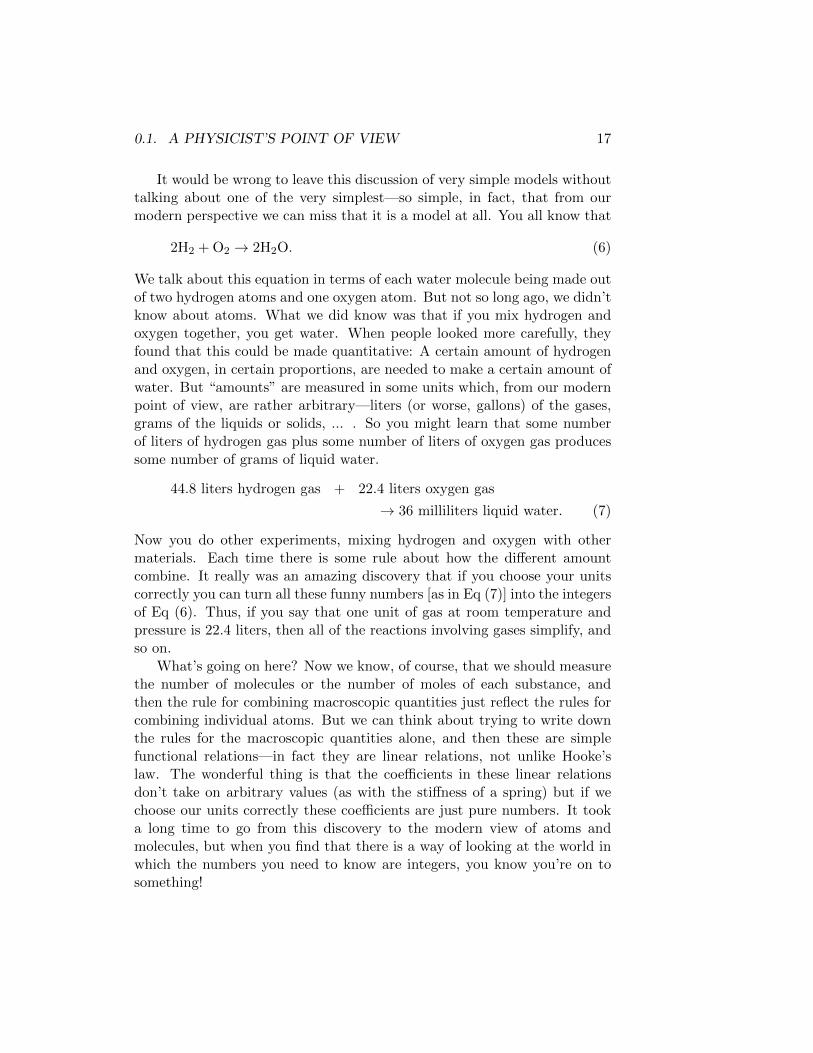
It would be wrong to leave this discussion of very simple models withouttalking about one of the very simplest—so simple, in fact, that from ourmodern perspective we can miss that it is a model at all. You all know that
2H2 + O2 → 2H2O. (6)
We talk about this equation in terms of each water molecule being made outof two hydrogen atoms and one oxygen atom. But not so long ago, we didn’tknow about atoms. What we did know was that if you mix hydrogen andoxygen together, you get water. When people looked more carefully, theyfound that this could be made quantitative: A certain amount of hydrogenand oxygen, in certain proportions, are needed to make a certain amount ofwater. But “amounts” are measured in some units which, from our modernpoint of view, are rather arbitrary—liters (or worse, gallons) of the gases,grams of the liquids or solids, ... . So you might learn that some numberof liters of hydrogen gas plus some number of liters of oxygen gas producessome number of grams of liquid water.
44.8 liters hydrogen gas + 22.4 liters oxygen gas
→ 36 milliliters liquid water. (7)
Now you do other experiments, mixing hydrogen and oxygen with othermaterials. Each time there is some rule about how the different amountcombine. It really was an amazing discovery that if you choose your unitscorrectly you can turn all these funny numbers [as in Eq (7)] into the integersof Eq (6). Thus, if you say that one unit of gas at room temperature andpressure is 22.4 liters, then all of the reactions involving gases simplify, andso on.
What’s going on here? Now we know, of course, that we should measurethe number of molecules or the number of moles of each substance, andthen the rule for combining macroscopic quantities just reflect the rules forcombining individual atoms. But we can think about trying to write downthe rules for the macroscopic quantities alone, and then these are simplefunctional relations—in fact they are linear relations, not unlike Hooke’slaw. The wonderful thing is that the coefficients in these linear relationsdon’t take on arbitrary values (as with the stiffness of a spring) but if wechoose our units correctly these coefficients are just pure numbers. It tooka long time to go from this discovery to the modern view of atoms andmolecules, but when you find that there is a way of looking at the world inwhich the numbers you need to know are integers, you know you’re on tosomething!

18 CHAPTER 0. INTRODUCTION
What physicists do
After all of this, you might still be confused about what physicists do, today.The dividing up of our intellectual explorations into different disciplines is ahuman endeavor, and so to some extent this (as with parallel questions aboutchemistry, biology, other sciences, as well the humanities) is a sociologicalquestion. It might be worth pointing out, however, that disciplines have achoice to define themselves by the objects that they study, or by the kinds ofquestions that they ask. To give an example far from the sciences, one mightwonder whether one should study film in the English department. If bythe discipline of “English” one means “studying books written in English,”then obviously you don’t study film. If, on the other hand, one understands“English” to mean the exploration of certain kinds of questions about theinteraction of language and culture among English speaking peoples, thenfilm is fair game. In this spirit, it seems fair to say that, perhaps morethan most scientific fields, physics is defined by the kinds of questions thatphysicists ask.
Physicists really are interested in fulfilling the Galilean image of readingthe book of Nature, and we fully expect it to be a short book once we havethe right language. As mentioned at the outset, there are many naturalphenomena for which we have a reasonable mathematical description, cor-responding perhaps to well defined chapters in the book. Revisiting these(more or less) known chapters is fun, but more of the community is excitedabout the places where (to strain the metaphor) the text is incomplete.There are two very different ways in which this can happen.
In one class of problems, we’re pretty sure we know the right mathemat-ical description—essentially because the description comes in many parts,and each part has been tested in some detail—but there are broad classesof phenomena that should come out of this description and we don’t knowhow to make the connection. This happens across many different scales,from the nucleus to the weather. Although faster computers certainly help,many of these problems require us to inject new ideas even to make directcomputation of the answer (let alone understanding the answer) feasible.
A very different possibility is to go to extremes, to the more literal edgesof our understanding. Thus, thousands of physicists are working togetheron two experiments in Geneva that will probe the structure and dynamicsof matter on a scale millions of times smaller than the atomic nucleus. Atthe opposite extreme, physicists and astronomers12 are trying to survey the
12The boundary between physics and astronomy is not always so easy to define. Thequestion of whether a university has separate physics and astronomy departments, for

0.1. A PHYSICIST’S POINT OF VIEW 19
Figure 6: What you see at left looks like a perfect crystal of beads, but this actually is asmall (∼ 10 cm diameter) container filled with carbon dioxide at high pressure, and heatedfrom below. The image is formed by passing light through the gas, sometimes called a‘shadowgraph.’ The structure of image is sensitive to the patterns of temperature, becausechanging the temperature of a gas causes a change in refractive index, bending the raysof light and casting shadows. At right, the same container of gas, but with a slightlydifferent amount of heating. Other than the high pressure, there is nothing extreme inthe conditions—temperatures on both the top and bottom of the container are near roomtemperature. What is true is that these temperatures are held very constant (to withina few thousandths of a degree) so that the patterns will not be disrupted by variationsin conditions; similarly, the top and bottom of the container are extremely flat (smoothto within the wavelength of light), and the whole system is held horizontal with highprecision so that the direction of gravity is aligned with axis of symmetry through thecenter of the circle. Despite the fact that conditions are constant, the spiral patternsactually rotates slowly during the experiment. From E Bodenschatz, JR de Bruyn, GAhlers & DS Cannell, Physical Review Letters 67, 3078–3081 (1991).
structure of the universe on the largest possible scales, and to understandthe way in which this structure has evolved over the billions of years sincethe big bang.
Extremes can be more subtle. Thus, for example, we usually think thatthe mysteries of quantum mechanics are confined to the scale of atoms,and last for proportionately short times. Can we stretch the weirdness outto a more human scale? Are there fundamental, or only practical, limits
example, is almost always a question of history. “Astrophysics” seems like a sensibleblending of the different fields, but there are excellent universities that have departmentswith names like “astronomy and astrophysics” that are separate from the physics depart-ment. All terribly confusing.

20 CHAPTER 0. INTRODUCTION
on our ability to do this? This is not just a question of principle, sinceif we could harness the quantum properties of matter on the right scale,we could build computers that are qualitatively more powerful than todaysdigital machines. At present such actual ‘quantum computers’ are the stuffof fiction, but quantum computing, and the surrounding questions of howwe control the dynamics of quantum systems, is a major research topic.
Another boundary of our understanding, which could be thought of asa combination of our two major categories, concerns complexity and orga-nization. We know that if we put many atoms or molecules in a box, theyorganize themselves in interesting ways. There are solids, liquids and gases,but also more refined categories—such as solids that conduct electricity (ornot), or which act as magnets, and so on. Perhaps surprisingly, it’s notclear that we even have a complete catalog for these “states of matter,”let alone a framework within which we can understand why the differentstates emerge from different combinations of atoms and external conditions.Especially intriguing are those cases where matter organizes itself in morecomplex ways, as often happens in response to a continual flow of energythrough the system. Examples along this line of thinking start with verysimple cases, such as the beautiful patterns that form in the flow of a fluidlayer heated from below (Fig 6). The most distant reach along this path ofself–organization into complex states is, of course, life itself.
0.2 A chemist’s point of view
0.3 A biologist’s point of view
[These sections remain to be written. Current students should see the lessformal notes posted to blackboard.]

Chapter 1
Newton’s laws, chemicalkinetics, ...
When you look around you, you see many things changing in time. Ourmost powerful tools for describing such dynamics are based on differentialequations. This mathematical approach to the description of nature startedwith mechanics, and grew to encompass other phenomena. In this sectionof the course, we’ll introduce you to these ideas using what we think are thesimplest examples. Following the historical path, we’ll begin with mechan-ics, but we’ll quickly see how similar equations arise in chemical kinetics,electric circuits and population growth. Sometimes the simple equationshave simple solutions, but even these have profound consequences, such asunderstanding that most of the chemical elements in our solar system werecreated at some definite moment several billion years ago. In other cases sim-ple equations have strikingly complex solutions, even generating seeminglyrandom patterns. This is just a first look at this whole range of phenomena.
1.1 Starting with F = ma
By the time you arrive at the University, you have heard many things aboutelementary mechanics. In fact, much of what we cover in these first lecturesare things you already know. We hope to emphasize several points: First,many of the things which you have may have remembered as isolated factsabout the trajectories of objects really all follow from Newton’s laws by di-rect calculation. Next, you need to take seriously the fact that Netwon’sF = ma is a differential equation. Finally, hidden inside some elemen-tary facts that you learned in high school are some remarkably profound
21

22 CHAPTER 1. NEWTON’S LAWS, CHEMICAL KINETICS, ...
truths about the natural world. We won’t have a chance to discuss theirconsequences, but we’d like to give you some flavor for these advanced butfundamental ideas.
Let us begin with Newton’s famous equation,
F = ma. (1.1)
At the risk of being pedantic, let’s be sure we know what all the symbolsmean. We all have an intuitive feeling for the mass m, although again we’llsee that there is something underneath your intuition that you might nothave appreciated. Acceleration is the clearest one: We describe the positionof a particle as a function of time as x(t), and the then the velocity
v(t) =dx(t)
dt(1.2)
and the acceleration
a(t) =d2x(t)
dt2. (1.3)
As a warning, we’ll sometimes write dx/dt and sometimes dx(t)/dt. Thesetwo ways of writing things mean the same thing; the second version remindsus that we are talking not about variables but about functions—algebrais about equations for variables, but now we have equations for functions.Alternatively we can say that equations like F = ma are statements thatare true at every instant of time, so really when we write F = ma we arewriting an infinite number of equations (!). This may not make you feelbetter.
We have defined all the terms in Newton’s famous Eq, (1.1)—all exceptfor the force F . The definition of force is a minor scandal.1 As far as I know,there is no independent definition of force other than through F = ma. Ifyou want to go out and measure a force you might arrange for that forceto stretch a spring, then look how far it was stretched, and if you know thespring constant you can determine the force. But how did you measure thespring constant? You see the problem.
In effect what Newton did was to say that when we observe accelera-tions we should look for explanations in terms of forces. This embodies theGalilean notion of inertia, that objects in motion tend to keep moving andhence if they change their velocity there should be a reason. If it turns out
1See, for example, F Wilczek, Whence the force of F = ma? I: Culture shock, PhysicsToday 57, 11–12 (2004); http://www.physicstoday.org/vol-57/iss-10/p11.html.
1.1. STARTING WITH F = MA 23
that forces are arbitrarily complicated, then we’re in deep trouble. In thissense, F = ma is a framework for thinking about motion, and its success de-pends on whether the rules that determine the forces in different situationsare simple and powerful.
Leaving aside these difficulties with the definition of force, Newton’s lawbecomes a differential equation
md2x(t)
dt2= F. (1.4)
To build up some intuition, and some practice with the mathematics, we willstart with three simple cases: zero force, a constant force, and a force that isproportional to velocity. Of course these are not just simple examples, theyactually correspond to situations that are fairly common in the real worldand that you will study in the laboratory. Again you probably know muchof will be said here, but it’s worth going through carefully and being sureyou understand how it emerges from the differential equation.
These problems are designed to make you comfortable, once again, with the ideasfrom calculus that we will need in the next sections.
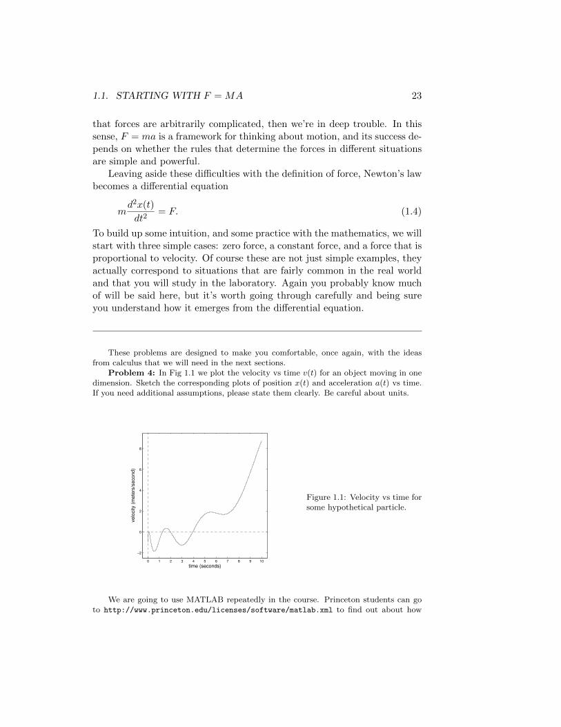
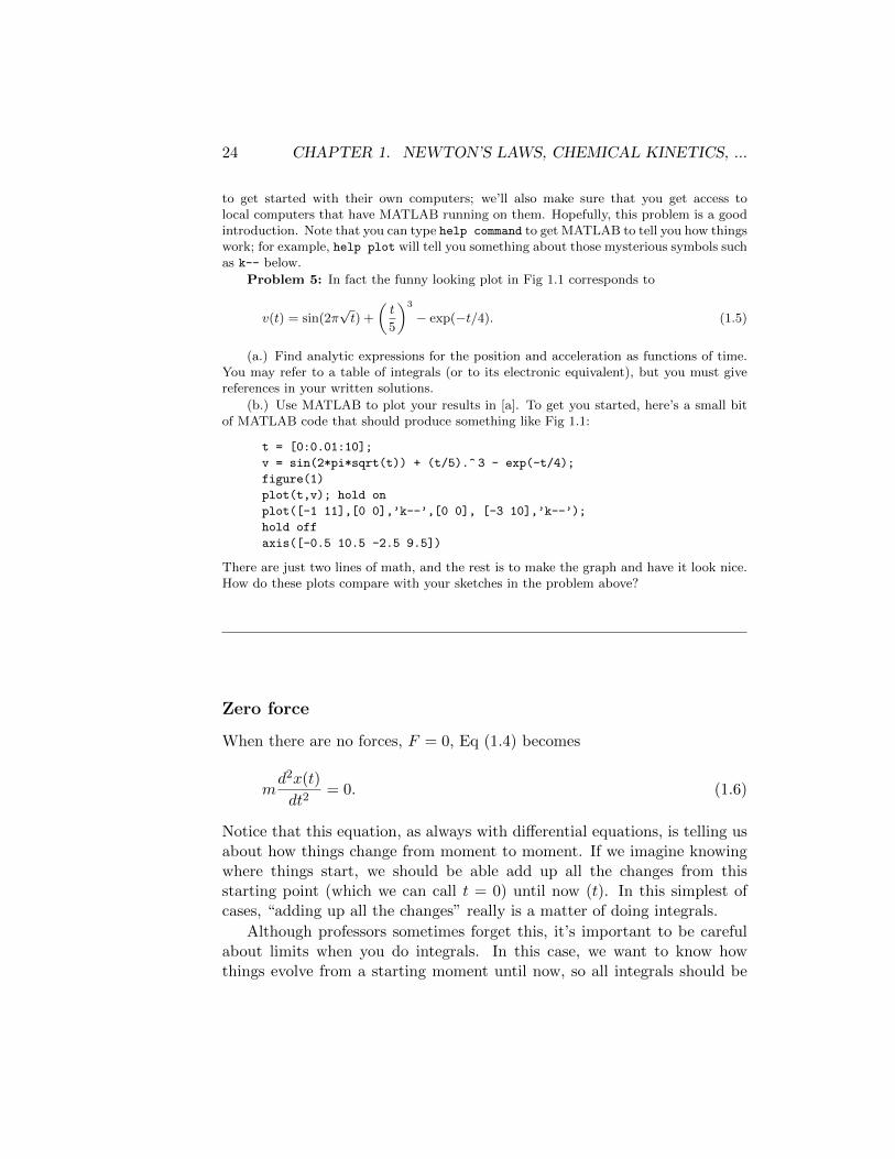
Problem 4: In Fig 1.1 we plot the velocity vs time v(t) for an object moving in onedimension. Sketch the corresponding plots of position x(t) and acceleration a(t) vs time.If you need additional assumptions, please state them clearly. Be careful about units.
0 1 2 3 4 5 6 7 8 9 10
−2
0
2
4
6
8
time (seconds)
velo
city
(met
ers/
seco
nd)
Figure 1.1: Velocity vs time forsome hypothetical particle.
We are going to use MATLAB repeatedly in the course. Princeton students can goto http://www.princeton.edu/licenses/software/matlab.xml to find out about how
24 CHAPTER 1. NEWTON’S LAWS, CHEMICAL KINETICS, ...
to get started with their own computers; we’ll also make sure that you get access tolocal computers that have MATLAB running on them. Hopefully, this problem is a goodintroduction. Note that you can type help command to get MATLAB to tell you how thingswork; for example, help plot will tell you something about those mysterious symbols suchas k-- below.
Problem 5: In fact the funny looking plot in Fig 1.1 corresponds to
v(t) = sin(2π√t) +
(t
5
)3
− exp(−t/4). (1.5)
(a.) Find analytic expressions for the position and acceleration as functions of time.You may refer to a table of integrals (or to its electronic equivalent), but you must givereferences in your written solutions.
(b.) Use MATLAB to plot your results in [a]. To get you started, here’s a small bitof MATLAB code that should produce something like Fig 1.1:
t = [0:0.01:10];
v = sin(2*pi*sqrt(t)) + (t/5).^ 3 - exp(-t/4);
figure(1)
plot(t,v); hold on
plot([-1 11],[0 0],’k--’,[0 0], [-3 10],’k--’);
hold off
axis([-0.5 10.5 -2.5 9.5])
There are just two lines of math, and the rest is to make the graph and have it look nice.How do these plots compare with your sketches in the problem above?
Zero force
When there are no forces, F = 0, Eq (1.4) becomes
md2x(t)
dt2= 0. (1.6)
Notice that this equation, as always with differential equations, is telling usabout how things change from moment to moment. If we imagine knowingwhere things start, we should be able add up all the changes from thisstarting point (which we can call t = 0) until now (t). In this simplest ofcases, “adding up all the changes” really is a matter of doing integrals.
Although professors sometimes forget this, it’s important to be carefulabout limits when you do integrals. In this case, we want to know howthings evolve from a starting moment until now, so all integrals should be

1.1. STARTING WITH F = MA 25
definite integrals from some initial time t = 0 up to now (t). Going carefullythrough the steps
md2x(t)
dt2= 0∫ t
0dtm
d2x(t)
dt2=
∫ t
0dt [0] (1.7)
m
∫ t
0dtd2x(t)
dt2=
∫ t
0dt [0] (1.8)
m
[dx(t)
dt
∣∣∣∣t
− dx(t)
dt
∣∣∣∣t=0
]= 0 (1.9)
dx(t)
dt=
dx(t)
dt
∣∣∣∣t=0
(1.10)
dx(t)
dt= v(0). (1.11)
You should get in the habit of following these derivations with a pen in your hand,not just reading. Whenever we go through a long series of steps, you have to ask yourselfboth (a) if you understand where we are going and why, and (b) if you understand howwe take each step. Near the start of the course, it seems best to lead you in this process,but by the end you should be doing it yourself. So, in this case, let’s see how each stepworked:
Eq (1.7) → (1.8) Since the mass m doesn’t change with time (in this problem!) youcan take it outside the integral.
Eq (1.8) → (1.9) Taking the integral of zero gives zero, while taking the integral of aderivative gives back the function itself.
Eq (1.9) → (1.10) Since the mass isn’t zero, we can divide it through, and then rear-range.
Eq (1.10) → (1.11) Finally, since dx/dt is the velocity, we call dx/dt|t=0 = v(0), theinitial velocity.
What we have shown so far is that the velocity at time t is the same as at time t = 0:Objects in motion stay in motion, as promised.

26 CHAPTER 1. NEWTON’S LAWS, CHEMICAL KINETICS, ...
time t
position x
t=0
initial positionx(0)
slopev(0)
x(t) = x(0) + v(0)t
Figure 1.2: Trajectory of anobject moving with zero force,from Eq. (1.14). Position vs.time is a straight line, with aslope equal to the initial veloc-ity and an intercept equal to theinitial position.
Now we go further, integrating once more:
dx(t)
dt= v(0)∫ t
0dtdx(t)
dt=
∫ t
0dt v(0) (1.12)
x(t)− x(0) = v(0)t (1.13)
x(t) = x(0) + v(0)t. (1.14)
What this shows is that if we plot position vs. time, we should find a straightline, as shown in Fig 1.2.
An important thing to remember is that position and force really arevectors. Thus if the (vector) force is equal to zero, then there is an equationlike Eq (1.14) along each direction. As an example, in two dimensions wemight write
x(t) = x(0) + vx(0)t (1.15)
y(t) = y(0) + vy(0)t. (1.16)
This is important, because the plot of x vs. t (which is what we solve formost directly!) is not what you see when you watch things move. Whatyou actually see is something more like y vs. x as the object moves throughspace. In this case, if you plot y(t) vs. x(t), you get a straight line. You can

1.1. STARTING WITH F = MA 27
see this by a little bit of algebra:
x(t) = x(0) + vx(0)t
x(t)− x(0) = vx(0)t (1.17)
x(t)− x(0)
vx(0)= t (1.18)
⇒ y(t) = y(0) + vy(0)t = y(0) + vy(0) · x(t)− x(0)
vx(0)(1.19)
y(t) =vy(0)
vx(0)x(t) +
[y(0)− vy(0)
vx(0)x(0)
], (1.20)
and we recognize Eq (1.20) as the equation for a line with slope vy(0)/vx(0).So motion without forces is motion at constant velocity, but also motion ina straight line.
Constant force
The standard example of motion with a constant force is the effect of gravityhere on earth. This is a slight cheat, since of course the gravitational pullshould depend on how far we are from the center of the earth. But if wedo our experiments in a room (even a large room) it’s hard to change thisdistance by more than a few meters, while the radius of the earth is measuredin thousands of kilometers, so the changes in distance are only one part ina million. One can measure forces with enough accuracy to see such effects,but for now let’s neglect them.
So, in the approximation that we don’t move too far, and hence the pullof the earth’s gravity is constant, we write
F = −mg, (1.21)
with the convention that x is measured upward; thus the downward force ofgravity is negative, as shown in Fig 1.3. Putting this together with F = ma,we have
md2x(t)
dt2= −mg. (1.22)
The extraordinary thing is that the mass m appears on both sides of theequation, so we can cancel it, leaving
d2x(t)
dt2= −g. (1.23)

28 CHAPTER 1. NEWTON’S LAWS, CHEMICAL KINETICS, ...
positionx
(larger x is higher up)
forceF = -mg
(force pulls down!)
Figure 1.3: A particle moving under the influence of gravity, as in Eq (1.22).
Now in this equation, x(t) denotes the position of the object, and g is aproperty of the earth—none of the properties of the object appear in theequation! Even without solving the equation we thus make the predictionthat all objects should fall toward the earth in exactly the same way, and thisis what Galileo famously is supposed to have tested by dropping differentobjects from the Tower of Pisa and finding that they hit the ground at thesame time.
The statement that every object falls in the same way obviously is wrong,as you know by watching leaves float and flutter to the ground. The idea isthat all these differences arise from forces exerted by the air, and so if wecould take these away and “purify” the effects of gravity we would reallywould see everything fall in the same way.2 A number of science museumshave beautiful demonstrations of this, with long tubes out of which they canpump all the air and then drop either a rock or a feather. Even if you knowthe principles it is pretty compelling to see a feather drop like a rock!
One might be tempted to think that our ability to cancel the masses inEq (1.22) is an approximation. Perhaps. But in the 1950s here at Princeton,Robert Dicke and his colleagues did an amazing experiment to show thatthis approximation is accurate to about 11 decimal places. This certainly
2One should take a moment to appreciate Galileo’s insight, separating these effects inhis mind in advance of methods for doing the experiments.
1.1. STARTING WITH F = MA 29
makes us think that what we have here is not an approximation but reallysomething that one can call a law of nature.
Just so that you know all the words, the mass which appears in F = mais called the inertial mass, since this is what determines the inertia of anobject. Inertia expresses the tendency of objects to keep moving in theabsence of forces, and corresponds intuitively to the effort that we have toexpend in stopping of deflecting the object. We also use inertia in everydayEnglish to mean something quite similar, although not only in reference tomechanics. In contrast, the mass in F = −mg is called the gravitationalmass, for more obvious reasons. The statement that the masses cancelthus is the “equivalence of gravitational and inertial masses,” or simply the“principle of equivalence.”
The essential content of the principle of equivalence is clear from Eq(1.23): You actually can’t tell the difference between a little extra acceler-ation (on the left hand side of the equation) and slightly stronger gravity(on the right). Einstein made the point in a thought experiment, imagin-ing himself trapped in an elevator. Unable to see outside, he argued thathe couldn’t tell the difference between falling freely in a gravitational fieldand being accelerated (e.g. by rocket jets attached to the elevator). Fromthe Newtonian point of view, this equivalence is a coincidence. After all,there are other forces such as electricity and magnetism which aren’t pro-portional to mass, and thus one could have imagined that the gravitationalforce wasn’t proportional to mass either. Indeed, you may remember thatwhen we go beyond the approximation of gravity as a constant force, if twoobjects with masses m1 and m2 are a distance r apart, then the force thatone objects exerts on the other is given by
F = −Gm1m2
r2, (1.24)
where the minus sign indicates that the force is attractive, and G is a con-stant (called Newton’s constant). This is very much like Coulomb’s law forthe force between two particles with charges q1 and q2, again separated bya distance r,
F =q1q2
r2. (1.25)
Thus, except for the constant, the masses act like “gravitational charges,”and it’s a mystery why the gravitational charge3 should be the same as themass in F = ma.
3Another point worth noting concerns the sign of the force. Electrical charges can be

30 CHAPTER 1. NEWTON’S LAWS, CHEMICAL KINETICS, ...
In 1905, Einstein wrote a series of papers that shook the world—on whatwe now call the special theory of relativity, on the idea that light is quan-tized into photons, and on Brownian motion and the size of atoms. Freshfrom these triumphs, he decided that the mysterious coincidence betweeninertial and gravitational masses was a central fact about nature, indeed thecentral fact that needed his attention, and he set out to construct a theoryof gravity in which the principle of equivalence is fundamental. It took hima decade, but the result was the general theory of relativity, arguably thegreatest among his many great achievements. As you may have heard, gen-eral relativity involves a radical rethinking of our ideas about space and timeand predicts the existence of black holes, the expansion of the universe, andother astonishing (but true!) things. We aren’t ready for all this ... so reluc-tantly we will go back to the more mundane falling of things to the ground.But for now we’d like you to remember that when you read about the blackhole in the center of our galaxy, the theory which predicts the existence ofthese exotic objects grew out of Einstein’s taking very seriously a seeminglysimple and obvious coincidence in the physics of everyday objects.
So, back to Eq (1.23). By now it should be clear what to do—integratetwice, as in the case of zero force:
d2x(t)
dt2= −g∫ t
0dtd2x(t)
dt2=
∫ t
0dt [−g] (1.26)
dx(t)
dt− dx(t)
dt
∣∣∣∣t=0
= −gt (1.27)
dx(t)
dt=
dx(t)
dt
∣∣∣∣t=0
− gt (1.28)
dx(t)
dt= v(0)− gt (1.29)∫ t
0dtdx(t)
dt=
∫ t
0dt [v(0)− gt] (1.30)
x(t)− x(0) = v(0)t− 1
2gt2 (1.31)
x(t) = x(0) + v(0)t− 1
2gt2. (1.32)
positive or negative, and from Eq (1.25) we see that oppositely signed charges attract,while similarly signed charges repel one another. In contrast, because the gravitationalcharge is equal to the mass, and all the masses that we experience in everyday life arepositive, all objects attract one another.

1.1. STARTING WITH F = MA 31
Thus we recover the 12gt
2 that you all remember from high school.
Once again, x(t) is not something you literally “see,” since it is whatyou get by plotting position vs. time. On the other hand, position and forceare both vectors, as noted above, but gravity only acts along one dimension(up/down). So if x is the up/down direction and y is measured parallel tothe surface of the earth—opposite the usual convention!—then x obeys Eq(1.32) while y obeys Eq (1.14):
x(t) = x(0) + vx(0)t− 1
2gt2 (1.33)
y(t) = y(0) + vy(0)t. (1.34)
But nobody told you where you should put y = 0, so you might as wellchoose this point so that y(0) = 0. Then the position y is proportional to t,and hence plotting x vs. y is just like plotting x vs. t except for the unitson the horizontal axis. Thus one of the nice things about the trajectories ofobjects in our immediate environment is that distance parallel to the earthprovides a surrogate for time, and we can literally see the trajectories playedout in front of us. In particular, this means that when you throw somethingit follows a parabolic trajectory.
It’s worth going through the algebra of the parabolic trajectory, choosingy(0) = 0 as suggested:
y(t) = vy(0)t (1.35)
t =y(t)
vy(0)(1.36)
x(t) = x(0) + vx(0)t− 1
2gt2 = x(0) + vx(0)
y(t)
vy(0)− 1
2g
[y(t)
vy(0)
]2
(1.37)
x = x(0) +
[vx(0)
vy(0)
]· y −
[g
2v2y(0)
]· y2. (1.38)
I hope it’s clear that this is a parabola.
Standard questions at this point are of the following sort: How far alongthe y axis does the object go before hitting the ground? To answer thisquestion you choose the ground to be at x = 0 and solve for the value ofy = yhit that results in x = 0. This is especially simple if the object startsat x = 0, which kind of makes sense if you fire a rocket off the ground (see
32 CHAPTER 1. NEWTON’S LAWS, CHEMICAL KINETICS, ...
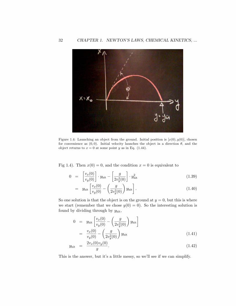
Figure 1.4: Launching an object from the ground. Initial position is [x(0), y(0)], chosenfor convenience as (0, 0). Initial velocity launches the object in a direction θ, and theobject returns to x = 0 at some point y as in Eq. (1.44).
Fig 1.4). Then x(0) = 0, and the condition x = 0 is equivalent to
0 =
[vx(0)
vy(0)
]· yhit −
[g
2v2y(0)
]· y2
hit (1.39)
= yhit
[vx(0)
vy(0)−(
g
2v2y(0)
)yhit
]. (1.40)
So one solution is that the object is on the ground at y = 0, but this is wherewe start (remember that we chose y(0) = 0). So the interesting solution isfound by dividing through by yhit,
0 = yhit
[vx(0)
vy(0)−(
g
2v2y(0)
)yhit
]=
vx(0)
vy(0)−(
g
2v2y(0)
)yhit (1.41)
yhit =2vx(0)vy(0)
g. (1.42)
This is the answer, but it’s a little messy, so we’ll see if we can simplify.
1.1. STARTING WITH F = MA 33
We see that that, from Fig 1.4, vx(0) = v(0) sin θ, where v(0) is the initialspeed of the object and θ is the angle that its initial velocity makes with theground; θ = π/2 corresponds to shooting the object straight up and θ = 0corresponds to skimming along the ground. Similarly vy(0) = v(0) cos θ, sothat the particle hits the ground at
y =2vx(0)vy(0)
g=
2v2(0) sin θ cos θ
g. (1.43)
But you may recall that sin(2θ) = 2 sin θ cos θ, so we have
y =v2(0)
gsin(2θ), (1.44)
which is a nice, compact result.
Perhaps you have seen Eq (1.44) before, in your high school course.What is important here is to emphasize that this, like all the other formulaeof mechanics, are derivable from Newton’s laws. If we had to remember adifferent formula for each different situation, it wouldn’t really be much ofa science. The great achievement of our scientific culture is to have a smallset of principles from which everything can be worked out.
Problem 6: Use Eq (1.38) to find the maximum height that the object reaches alongits trajectory. Recall that to find the maximum of a function you find the place where thederivative is zero. Notice that in this case you are looking for the maximum value of xviewed as function of y, opposite the usual conventions in textbooks. You should be ableto do the same calculation directly from Eq (1.32). Show that you get the same answer.
Drag forces
When you move your arm through the water you feel a force opposing themotion. Part of this force is the inertia of the water that you are moving,but if you go very slowly then the dominant component is the drag generatedby the viscosity of the water, and this force is proportional to the velocity v.The sign of the force is to oppose motion, so we write Fdrag = −γv, whereγ is called the drag coefficient.
34 CHAPTER 1. NEWTON’S LAWS, CHEMICAL KINETICS, ...
Problem 7: Imagine that we have two flat parallel plates, each of area A, separatedby a distance L, and that this space is filled with fluid. If we slide the plates relative toeach other slowly, at velocity v (parallel to plates), then we will find that there is a dragforce Fdrag = −γv which acts to resist the motion. Intuitively, the bigger the plates (largerA) and the closer they are together (smaller L) the larger the drag, and in fact over a rangeof interesting scales one finds experimentally that γ = ηA/L, where the proportionalityconstant η is called the viscosity of the fluid.
(a.) What are the units of viscosity? Instead of expressing your answer in terms offorce, length and time, try to express the viscosity as a combination of energy, length andtime.
(b.) Viscosity is something we can measure (and “feel”) on a macroscopic scale. Butthe properties of a fluid depend on the properties of the molecules out of which it is made.So if we want to understand why the viscosity of water is η = 0.01 in the cgs (centimeter–gram–second) system of units, we need to think about the scales of energy, length andtime that are relevant for the water molecules. Plausibly relevant energy scales are theenergies of the hydrogen bonds between the water molecules (which you can look up),and the thermal energy kBT ∼ 4 × 10⁻²¹ J at room temperature, which is the averagekinetic energy of molecules as they jiggle around in the fluid (more about this later in thesemester). The characteristic length is the size of an individual water molecule, or thedistance between molecules. What is the range of time scales that combines with theseenergies and volume to give the observed viscosity? What do you think this time scalemeans—i. e., what event actually happens on this time scale?
Newton’s basic equation
md2x(t)
dt= F (1.45)
can also be written as
mdv(t)
dt= F, (1.46)
which in this case becomes
mdv(t)
dt= −γv(t). (1.47)
Here I am being careful to show you that v is a function that depends ontime.
It is often said that there are three good ways to solve a differentialequation. Best is to ask someone who knows the answer. Next one guessesthe form of the solution and checks that it is correct. Finally, there are some

1.1. STARTING WITH F = MA 35
more systematic approaches. Let’s try one of these, largely so we can buildup our intuition and make better guesses next time we need them!
We’d like to solve Eq (1.47) the same way that we did in previous cases,by integrating, but this doesn’t work directly—on the right hand side we’dhave to integrate v(t) itself, and clearly we don’t know how to do this. Sowe play a little with the equation, doing something which would make a realmathematician cringe:
mdv
dt= −γv
dv
dt= − γ
mv (1.48)
dv
v= − γ
mdt. (1.49)
Now we can integrate, since on the left we have v and on the right we havedt, with no mixing. Again we should be careful to do definite integrals fromsome initial time t = 0 up until now (t), during which time the velocity runsfrom its initial value v(0) to its current value v(t). Notice that we don’tactually know the value of v(t); indeed this is what we are trying to find.Nonetheless we can put this value as the endpoint of our integral, and solveat the end:
dv
v= − γ
mdt∫ v(t)
v(0)
dv
v= − γ
m
∫ t
0dt (1.50)
[ln v]
∣∣∣∣v(t)
v(0)
= − γmt (1.51)
ln v(t)− ln v(0) = − γmt (1.52)
ln
[v(t)
v(0)
]= − γ
mt (1.53)
v(t) = v(0)e−γt/m. (1.54)
Thus the solution is an exponential decay.
Let’s be sure we understand the steps leading to Eq (1.54):

36 CHAPTER 1. NEWTON’S LAWS, CHEMICAL KINETICS, ...
Eq (1.50) → (1.51) On the right hand side we just use∫dt = t, and on the left we use∫
dvv
= ln v, where ln denotes the natural logarithm. Note that this is why naturallogarithms are natural!
Eq (1.51) → (1.52) This is just evaluating the indefinite integral at it’s endpoints.
Eq (1.52) → (1.53) Now we use ln a− ln b = ln(a/b).
Eq (1.53) → (1.54) Finally, to get rid of the logarithm we exponentiate both sides ofthe equation. We are using ln(ex) = x, or equivalently eln x = x.
Another way of writing our result in Eq (1.54) is
v(t) = v(0)e−t/τ , (1.55)
where the time constant τ = m/γ. We can see that this is the characteristictime scale in the problem by going back to the original equation:
mdv(t)
dt= −γv(t)
m
γ
dv(t)
dt= −v(t). (1.56)
The combination τ = m/γ must be a time scale in order to balance the unitson either side of the equation. This “characteristic time scale” is the onlyterm in the equation that has the units of time, and thus we expect thatwhen we plot the solution we will see all the important variations occurringon this time scale. This is an important idea—we can say on what scale weexpect to see things happen even before we solve the equation—and we willcome back to it several times in the course.
This is a good place to remind ourselves of a special feature of the ex-ponential function. With v(t) = v(0) exp(−t/τ), there is a unique time t1/2such that v is reduced by a factor of two:
v(t1/2) ≡ 1
2v(0) (1.57)
v(0) exp(−t1/2/τ) =1
2v(0) (1.58)
exp(−t1/2/τ) = 1/2 (1.59)
−t1/2/τ = ln(1/2) (1.60)
t1/2/τ = ln(2) (1.61)
t1/2 = τ ln 2. (1.62)
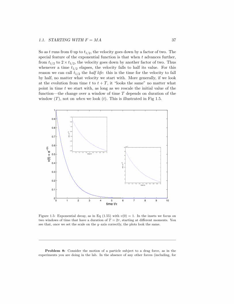
1.1. STARTING WITH F = MA 37
So as t runs from 0 up to t1/2, the velocity goes down by a factor of two. Thespecial feature of the exponential function is that when t advances further,from t1/2 to 2× t1/2, the velocity goes down by another factor of two. Thuswhenever a time t1/2 elapses, the velocity falls to half its value. For thisreason we can call t1/2 the half life: this is the time for the velocity to fallby half, no matter what velocity we start with. More generally, if we lookat the evolution from time t to t + T , it “looks the same” no matter whatpoint in time t we start with, as long as we rescale the initial value of thefunction—the change over a window of time T depends on duration of thewindow (T ), not on when we look (t). This is illustrated in Fig 1.5.
0 1 2 3 4 5 6 7 8 9 100
0.1
0.2
0.3
0.4
0.5
0.6
0.7
0.8
0.9
1
time t/!
v(t)
= e−
t/!
1 1.2 1.4 1.6 1.8 2 2.2 2.4 2.6 2.8 3
0.05
0.1
0.15
0.2
0.25
0.3
0.35
0.4
time t/!
v(t)
= e−
t/!
7 7.2 7.4 7.6 7.8 8 8.2 8.4 8.6 8.8 91
2
3
4
5
6
7
8
9
10x 10−4
time t/!
v(t)
= e−
t/!
Figure 1.5: Exponential decay, as in Eq (1.55) with v(0) = 1. In the insets we focus ontwo windows of time that have a duration of T = 2τ , starting at different moments. Yousee that, once we set the scale on the y–axis correctly, the plots look the same.
Problem 8: Consider the motion of a particle subject to a drag force, as in theexperiments you are doing in the lab. In the absence of any other forces (including, for

38 CHAPTER 1. NEWTON’S LAWS, CHEMICAL KINETICS, ...
the moment, gravity), Newton’s equation F = ma can be written as
Mdv
dt= −γv, (1.63)
where M is the mass of the particle and γ is the drag coefficient; we assume that thevelocities are small, so the drag force is proportional to the velocity. For a sphericalparticle of radius r in a fluid of viscosity η, we have the Stokes’ formula, γ = 6πηr.Assume that the particle also has a mass density of ρ. As shown above, the solutionto Eq (3.50) is an exponential decay: v(t) = v(0) exp(−t/τ), where the time constant τdetermined by all the other parameters in the problem. Be sure that you understand thisbefore doing the rest of this problem!
(a.) Write the time constant τ in terms of M and γ. How does τ scale with the radiusof the particle?
(b.) Suppose that the density ρ is close to that of water, and that the relevant viscosityis also that of water. What value (in seconds) do you predict for the time constant τ whenthe particle has a radius r ∼ 1 cm? What about r ∼ 1 mm or r ∼ 10µm? Be carefulabout units!
(c.) A bacterium like E coli is approximately a sphere with radius r = 1µm. Willyou ever see the bacterium moving in a straight line because of its inertia?
(d.) What is the relationship between the position x(t) and the velocity v(t)? Giventhat v(t) = v(0)e−t/τ , find a formula for x(t) and sketch the result. Label clearly themajor features of your sketch. What happens at long times, t� τ?
(e.) E coli can swim at a speed of ∼ 20µm/s. Imagine that the motors which drivethe swimming suddenly stop at time t = 0. Now there are no forces other than drag, butthe bacterium is still moving at velocity v(0) = 20µm/s. How far will the bacterium movebefore it finally comes to rest?
Problem 9: Let’s try to use these same ideas to describe the motion of a personthrough a swimming pool. Once again the fluid is water, and the density of the “object”is also close to that of water. When a person curls up into a ball, they have a radiusof about 50 cm (a meter in diameter). If a person starts moving at speed v0 through aswimming pool while in this position, then by analogy with the previous problem, what isyour prediction about how long it will take for their velocity to fall from v0 down to v0/2?Does this make sense given your own experience in the water? If not, what do you thinkhas gone wrong? We know that none of you are spherical. You’ll have to decide if this isa key issue, or if these calculations are wrong even for the case of the spherical student.
A very different sort of drag arises when objects move more rapidly.Although this isn’t the same sort of rigorously justifiable approximation asFdrag = −γv, one often finds that drag forces are roughly proportional to thesquare of the velocity at higher velocities. One then has to be careful aboutthe sign of the force; if the velocity is positive then the force is negative,opposing the motion, so we’ll write Fdrag = −cv2. Then F = ma becomes
mdv(t)
dt= −cv2(t). (1.64)

1.1. STARTING WITH F = MA 39
We proceed as before to integrate the equation:
mdv
dt= −cv2
dv
dt= −
( cm
)v2 (1.65)
dv
v2= −
( cm
)dt (1.66)∫ v(t)
v(0)
dv
v2= −
( cm
)∫ t
0dt (1.67)[
−1
v
] ∣∣∣∣v(t)
v(0)
= −( cm
)t (1.68)
− 1
v(t)+
1
v(0)= −
( cm
)t (1.69)
1
v(0)+( cm
)t =
1
v(t)(1.70)
v(t) =1
1v(0) +
(cm
)t
(1.71)
=v(0)
1 + [cv(0)/m]t. (1.72)
It is convenient to write this as
v(t) =v(0)
1 + t/tc, (1.73)
where tc = m/[cv(0)] is the time at which the velocity has fallen to halfof its initial value. Notice that we don’t really have a half life in the waythat we do for the exponential decay: the velocity falls by a factor of two(v(0)→ v(0)/2) after a time tc, but if we wait until t = 2× tc, the velocitydoesn’t fall by another factor of two; in fact v(t = 2tc) = v(0)/3, not v(0)/4.
Problem 10: Go through the derivation from Eq (1.64) to (1.73) and explain whathappens at each step. The strategy for solving the equation is the same as before, but thedetails are different.

40 CHAPTER 1. NEWTON’S LAWS, CHEMICAL KINETICS, ...
0 1 2 3 4 5 6 7 8 9 100
0.1
0.2
0.3
0.4
0.5
0.6
0.7
0.8
0.9
1
t/t1/2
v(t)/
v(0)
drag ! !vdrag ! !v2
Figure 1.6: Time dependence of velocity for particles experiencing fluid drag. When thedrag force is proportional to velocity, the decay is exponential, v(t) = v(0) exp(−t/τ), asin Eq (1.55), where t1/2 = τ ln 2. When the drag force is proportional to velocity squared,the decay is asymptotically ∝ 1/t, as in Eq (1.73).
Figure 1.6 shows the solutions for both Fdrag = γv and Fdrag = −cv2,with parameters chosen so that the time to reach half of the initial velocityis the same in both cases. Notice that the behavior at small times is quitesimilar, but that real differences appear at long times.
It’s worth playing with these results, and seeing how the two cases differ,because the same equations arise in thinking about different chemical kineticschemes, as we’ll see in the next section. One interesting point to thinkabout: If we look at the case where Fdrag = −cv2, then at long times
v(t) =v(0)
1 + [cv(0)/m]t→ v(0)
[cv(0)/m]t=m
ct. (1.74)
Thus, after a while (t � t1/2), the velocity still is decaying with time butthe actual value doesn’t depend any more on the velocity that we startedwith! [An improved version of Fig 1.6 would make this last point clearer;maybe you can generate such a figure for yourself.]
1.1. STARTING WITH F = MA 41
One last point: when do we expect to see the drag be linear, and whendo we expect it will go as the square of the velocity? This is a great question,and you’ll be addressing it in the lab, so we’ll leave it for now.
This problem is about an object falling under the influence of gravity, and hence fitswith the text a few paragraphs back. It is, however, a bit more open ended than theprevious problems, so we place it here at the end of our introduction to F = ma.
Problem 11: A simple model of shooting a basketball is that the ball moves throughthe air influenced only by gravity, so we neglect air resistance. Let’s also simplify and notworry about the rotation of the ball, so the dynamics is described just by its position asa function of time. Choose coordinates so the basket is at position x = 0 and at a heighty = h above the floor (in fact h = 10 ft, but it’s best in these problems not to plug innumbers until the end). When a player located at x = L shoots the ball, it leaves his orher hand at a speed v and at an angle θ measured from the floor (i.e., θ = π/2 would beshooting straight up, θ = 0 would correspond to throwing the ball horizontally, parallel tothe floor). Assume that the shooter is standing still, and the release of the ball happensat some initial height y = h0 above the floor (in practice h0 is somewhere between 5 and7 ft, depending on who’s playing).
(a.) Draw a diagram that represents everything you know about the problem, labelingthings with all the right symbols. Notice that we are treating this as a problem in twodimensions, whereas of course the real problem is three dimensional.
(b.) What is the equation for the trajectory of the ball with as a function of timeafter the player releases it? Write your answer as x(t) and y(t), with t = 0 the moment ofrelease.
(c.) A perfect shot must arrive at the point x = 0, y = h at some time. Presumablythe ball also has to traveling downward at this time. Express these conditions as equationsthat constrain the trajetcory {x(t), y(t)}, and solve to find allowed values of the speed vand angle θ.
(d.) Saying that the ball must be traveling downward might not be enough. In factthe ball has radius r = 4.5′′ and the basket has radius R = 9′′. Continuing with theassumption that we want the ball to pass perfectly through the center of the basket (thatis, x = 0, y = h), what is the real condition on the trajectory?
(e.) The fact that the basket is bigger than the ball means that you don’t have tohave x exactly equal to zero when y = h. To keep things simple let’s assume that the shotstill will go so long as we get within some critical distance |x| < xc at the moment wheny = h. Given what you know so far, what is a plausible value of xc? Turn this conditionon the end of the trajectory into a range of allowed values for v and θ. With typical valuesfor L (think about what these are, or go out to a basketball court and measure!), howaccurately does someone need to control v and θ in order to make the shot?
(f.) What we have done here is oversimplified. You are invited to see how far youcan go in making a more realistic calculation.4 Some things to think about are the thirddimension (e.g., how accurately does the trajectory need to be “pointed” toward the
4You might reasonably ask why we care. The fact that people (well, some people,at least) can make these shots with high probability from many different distances istelling us something about ability of the brain to deliver precise motor commands to our

42 CHAPTER 1. NEWTON’S LAWS, CHEMICAL KINETICS, ...
basket?), and a more careful treatment of the ball going through the hoop so that you canstate more precisely the condition for making the shot. If you were really ambitious youcould think about shots that bounce off the backboard, but that’s probably too much fornow!
1.2 Chemical reactions: a dynamic perspective
Chemical reactions are processes that involve the transformation of one setof molecules into another and drive many of the interesting phenomena weobserve around us. Research in biochemistry over the past century has suc-cessfully linked many traits observed in cells and larger organisms with theunderlying chemical activities of specific biological molecules. One of themost astounding discoveries in this field was the realization that all livingorganisms are surprisingly similar on a biochemical level. While the biolog-ical world is truly diverse in many ways, many of the molecular players areidentical in their size, shape and function across species that are separatedfrom one another by billions of years of evolution.
Chemical kinetics, or reaction kinetics, is the study of the rates of chem-ical reactions. In this section, we will create a mathematical frameworkfor discussing chemical reactions and find that many of the same differen-tial equations we’ve already derived come up in this very different context.Let’s begin by thinking about how your muscles use energy during exercise.You may know that muscles convert chemical energy, stored in high-energybonds in a molecule called adenosine triphostphate (ATP), into mechanicalwork that you can use to run or lift a weight. You also know that you needto breath to make this happen and if you work your muscles too hard theystart to fatigue and become painful (due to the buildup of lactic acid). Howcan we formulate these ideas more concretely?
Reaction diagrams and differential equations
We’ll start by writing down diagrammatic versions of what is going on.During aerobic respiration, glucose in your body is combined with the oxygen
muscles, since it is the action of our muscles that determine the initial conditions of the ballleaving the hand of the shooter. Although the mechanisms are biological, the constraintsare physical. Exploring the constraints makes precise what the system must do in orderto achieve the observed level of performance.

1.2. CHEMICAL REACTIONS: A DYNAMIC PERSPECTIVE 43
you’ve breathed in to produce carbon dioxide, water and energy in the formof molecules like ATP. We might write this more completely like this
C6H12O6 + 6O2 → 6CO2 + 6H2O
Sprinters don’t use very much oxygen during a 10 second race. Instead, theirbodies metabolize glucose directly to generate the ATP needed for musclecontraction. During this process, which is called glycolysis, one molecule ofglucose is converted to two molecules of pyruvate
C6H12O6 → 2CH3COCOO−
You may have spent some time learning about these reactions and per-haps balancing the number of each kind of atom on each side of a reactionformula. But, what should we make of these formulas? Often, they repre-sent a shorthand for keeping track of the start and end points, the reactantsand products, of a reaction. For example, the glycolysis reaction above hasbeen greatly simplified. The entire reaction is really made of many, manysub-reactions, consuming energy from two ATP molecules, but generatingfour new ATP molecules in the process as shown in Figure 1.7. Other times,the diagram really describes the mechanism of the reaction and includes allof the observable intermediate compounds (the letters) and all of the differ-ent pathways (the arrows) that can happen. It this case that we will focuson for now.
Consider the following two reactions
A→ B
A + B→ C
If we are to take these seriously, the first reaction describes the conversion ofA into B in a first order reaction. By first order reaction, we mean that eachmolecule of type “A” makes an independent decision about whether to com-plete the reaction and convert to a B–molecule in any given instant in time.In particular, the probability that an A–molecule will become a B–moleculedoes not depend on encounters with any other molecules. If this is the case,then the number of B–molecules which are created must be proportional tothe number of A molecules that are available to react. In chemistry, we usu-ally talk not about the number of molecules, but about their concentrations(i.e. the number per volume). If we write the concentration of species i asCi, then for our simple first order reaction we have
dCBdt
= kCA, (1.75)

44 CHAPTER 1. NEWTON’S LAWS, CHEMICAL KINETICS, ...
Figure 1.7: The three stages of the glycolysis pathway. From JM Berg, JL Tymocsko &L Stryer, Biochemistry (WH Freeman, San Francisco, 2006).

1.2. CHEMICAL REACTIONS: A DYNAMIC PERSPECTIVE 45
where k is the first order rate constant. Note that sometimes one writes [A]to denote the concentration of A. It is important to get used to differentnotations, as long as they are used consistently within each argument! CAand CB have the same units, so in order for Eq (1.75) to make sense, k hasto have units of 1/time, conventionally 1/s.
If A is turning into B, then each molecule of B which appears mustcorrespond to a molecule of A which disappeared. Thus we have to have
dCAdt
= −kCA. (1.76)
We’ve seen this equation before, since it is the same as for the velocityof a particle moving through a viscous fluid, assuming that the drag isproportional to velocity. So we know the solution:
CA(t) = CA(0)e−kt. (1.77)
Then we can also solve for CB:
dCBdt
= kCA
= kCA(0)e−kt (1.78)∫ t
0dtdCBdt
=
∫ t
0dt kCA(0)e−kt (1.79)
CB(t)− CB(0) = kCA(0)
∫ t
0dt e−kt (1.80)
= kCA(0)
[−1
ke−kt
] ∣∣∣∣tt=0
(1.81)
= kCA(0)
[−1
ke−kt +
1
k
](1.82)
= CA(0)[1− e−kt] (1.83)
CB(t) = CB(0) + CA(0)[1− e−kt]. (1.84)
So we see that CA decays exponentially to zero, while CB rises exponentiallyto its steady state; as an example see Fig 1.8. One of the great examples ofa first order reaction is radioactive decay, and this is why the abundance ofunstable isotopes (e.g., 14C, 235U, ...) in a sample decays exponentially, andthis will be very important in the next section.

46 CHAPTER 1. NEWTON’S LAWS, CHEMICAL KINETICS, ...
Figure 1.8: Dynamics of theconcentrations in a first orderreaction A→ B.
Problem 12: Just to be sure that you understand first order kinetics ... If the halflife of a substance that decays via first order kinetics is t1/2, how long do you have to waituntil 95% of the initial material has decayed? Explain why this question wouldn’t makesense in the case of second order kinetics.
What about the case A + B→ C? If we take this literally as a mecha-nism, we are describing a second order reaction, which means that A and Bmolecules have to find each other in order to make C. The rate at which Cmolecules are made should thus be proportional to the rate at which thesepairwise encounters are happening. What is this rate? If you imagine peo-ple milling around at random in a large room, it’s clear that the number oftimes per second that people run into each other depends both on how manypeople there are and on the size of the room. If you follow one person, therate at which they run into people should go up if there are more people,and down if the room gets bigger. Plausibly, what matters is the densityof people—the number of people divided by the size of the room—which isjust like measuring the concentration of molecules.
To obtain the rate of a second order reaction A + B→ C, we thus need tocount the rate at which A molecules bump into B molecules as they wanderaround randomly. By analogy with the people milling around the room,if we follow one A molecule, the rate at which it bumps into B moleculeswill be proportional to the concentration of B molecules. But then the total
1.2. CHEMICAL REACTIONS: A DYNAMIC PERSPECTIVE 47
rate of encounters between A and B will be proportional to the number of Amolecules multiplied by the concentration of B, so if we measure the numberof encounters per unit volume per second, we’ll get an answer proportionalto the product of the concentrations of A and B. Thus,
d[C]
dt= k2[A][B]. (1.85)
Corresponding the to formation of C is the destruction of both A and B, sowe must have
d[A]
dt= −k2[A][B] (1.86)
d[B]
dt= −k2[A][B]. (1.87)
The rate constant k2 is now a second order rate constant, and you can seethat it has different units from the first order rate constant k in the equationsabove; k2 ∼ 1/(time · concentration), conventionally 1/(M · s).
Perhaps the simplest second order reaction is A + A→ B, for which therelevant equations are
d[A]
dt= −k2[A]2 (1.88)
d[B]
dt= k2[A]2. (1.89)
We have seen this equation before, describing the velocity of a particle thatexperiences drag proportional to velocity squared. Thus we can proceed aswe did before:
d[A]
dt= −k2[A]2
d[A]
[A]2= −k2dt (1.90)∫ [A]t
[A]0
d[A]
[A]2= k2
∫ t
0dt (1.91)
− 1
[A]
∣∣∣∣[A]t
[A]0
= −k2t (1.92)
− 1
[A]t+
1
[A]0= −k2t (1.93)
1
[A]0+ k2t =
1
[A]t(1.94)
[A]t =[A]0
1 + k2[A]0t, (1.95)

48 CHAPTER 1. NEWTON’S LAWS, CHEMICAL KINETICS, ...
where [A]t is the concentration of A at time t, and in particular [A]0 is theconcentration when t = 0. Thus the initial concentration does not decay asan exponential, but rather as ∼ 1/t at long times; the time for decay to halfthe initial value is t1/2 = 1/(k2[A]0) and depends on the initial concentration.Notice that
[A]t�t1/2 ≈[A]0
k2[A]0t=
1
k2t, (1.96)
so that after a while the concentration is still changing, but the amount ofstuff we have left is independent of how much we started with (!).
Problem 13: Check that you understand each of the steps leading to Eq (1.95). Asa test of your understanding, consider the (rather unusual) case of a third order reaction,in which three A molecules come together to react irreversibly. This is described by
d[A]
dt= −k3[A]3. (1.97)
What are the units of the third order rate constant k3? Can you solve this equation?
time t(minutes) [A]/[A]0 [B]/[B]0
0.25 0.7157 0.7635
0.50 0.7189 0.4305
0.75 0.5562 0.5262
1.00 0.4761 0.6195
1.25 0.4948 0.4876
1.50 0.3096 0.3169
1.75 0.3842 0.3702
2.00 0.2022 0.2764
2.25 0.1872 0.2613
2.50 0.1971 0.2738
Table 1.1: Two kinetics experiments.
Problem 14: Imagine that you do two experiments in chemical kinetics. In onecase we watch the decay of concentration is some reactant A, and in the other case thereactant is B. The half lives of both species are about one minute, and perhaps becauseyou are in a hurry you run the reactions out only for 2.5 minutes. You take samples of theconcentration every quarter of a minute, and you get the results in Table 1.1. Perhaps the
1.2. CHEMICAL REACTIONS: A DYNAMIC PERSPECTIVE 49
first thing you notice is that the concentrations don’t decrease monotonically with time.Presumably this is the result of errors in the measurement.
(a.) Can you decide whether the reactions leading to the decay of A and B are firstorder or second order? Are A and B decaying in the same way, or are they different?
(b.) Other than making more accurate measurements, how could you extend theseexperiments to give you a better chance at deciding if the reactions are first or secondorder?
Problem 15: An important step in the production of sulfuric acid involves the changeof sulfur dioxide into sulfur trioxide. Sulfur dioxide, SO2, can react with oxygen to givesulfur trioxide, SO3 through the use of vanadium oxide
SO2 +1
2O2
V2O5−−−→ SO3
If you do this in the lab, you will find that tripling the sulfur dioxide concentration increasesthe rate by a factor of about 3. But tripling the sulfur trioxide concentration lowers thereaction rate by a factor of about 1.7. You will also find that the rate is insensitive to theoxygen concentration as long as you have enough of it.
(a.) Write down the kinetic differential equation for this reaction. What are the unitsof the rate constant?
(b.) If [SO2] is increased by a factor of 2 and [SO3] is increased by a factor of 5, by
how much will the overall reaction change?
An important point about all this is that when we draw a more complexreaction mechanism, each and every arrow corresponds to a term in thedifferential equation, and the sign of the term depends on the direction ofthe arrow. Consider, for example, the reactions shown at the top of Fig 1.9.Really this is a scheme in which B is converted into D, and the A moleculesparticipate but are not consumed: the A molecules are catalysts. Noticethat there are three separate reactions, one for each arrow: A + B → C,which occurs with a second order rate constant k+, C → A + B, whichoccurs with first order rate k−, and C → D+A, with first order rate k. Wewrite k+ and k− because these are forward and reverse processes.
Now we have to write out the differential equations, using the rule thateach reaction or arrow generates its corresponding term. Probably it’s eas-iest to start with the equation for [C], since all three reactions contribute.We see the arrow coming “in” to C from the left, which corresponds to theconcentration of C changing at a rate k+[A][B]. There is a second arrowat the left, which corresponds to the concentration of C changing at a rate−k−[C], where the negative sign is because the arrow points “out” and de-scribes the destruction of C molecules. Finally, there is an arrow point out

50 CHAPTER 1. NEWTON’S LAWS, CHEMICAL KINETICS, ...
A+Bk+−−⇀↽−−k−
Ck−→ D+A
E+Sk+−−⇀↽−−k−
ESV−→ E+P
Figure 1.9: At the top, a reaction scheme for the conver-sion of B into D, using A as a catalyst. At the bottom,this scheme is written to make better connections with theidea of catalysis by an enzyme: E is the enzyme, S is the‘substrate’ that gets converted into the product P , and ESis a complex of the enzyme and substrate bound to one an-other. The rate constants k± have the same notation, butwe write the rate for ES → E + P as V , since it’s the‘velocity’ of the enzyme.
to the right, which corresponds to the concentration of C changing at a rate−k[C]. Putting all of these terms together, we have
d[C]
dt= +k+[A][B]− k−[C]− k[C]. (1.98)
For [B], only the k+ and k− processes contribute:
d[B]
dt= −k+[A][B] + k−[C]. (1.99)
Finally, for [A], all three reactions contribute, but with the opposite signsfrom Eq (1.98):
d[A]
dt= −k+[A][B] + k−[C] + k[C]. (1.100)
The important point here is not to solve these equations (yet), but ratherto be sure that you understand how to go from the pictures with arrowsdescribing the reactions down to the equations that describe quantitativelythe dynamics of the concentrations.
Catalysis
A catalyst is a substance that takes part in a chemical reaction and speedsup the rate but undergoes no permanent chemical change itself. The en-hancement of the reaction rate can come from speeding up existing path-ways between the reactants and products or, more commonly, providingcompletely new pathways by which a reaction can occur. We won’t be ableto discuss the energetics of how a catalyst works until later in the semester,but for now we can examine the dynamics of these economically importantcompounds. Industrial chemistry devotes great effort to finding catalysts to

1.2. CHEMICAL REACTIONS: A DYNAMIC PERSPECTIVE 51
accelerate particular desired reactions without increasing the generation ofundesired products.
One example of a complex catalyst that you’ve all encountered is thesolid catalyst used to reduce the emission of pollutants such as unburnedhydrocarbons, carbon monoxide, and nitrogen oxides in the exhaust of a carengine. A catalytic converter is designed to simultaneously oxidize hydro-carbons and carbon monoxide through the reactions
CO,CxHy,O2Catalyst−−−−−→ CO2,H2O
and reduce nitrogen oxides through the reactions
NO,NO2Catalyst−−−−−→ N2,O2
Clearly, the best catalyst for the reduction reactions may not be the bestfor the oxidation reactions, so two catalysts are usually combined. For per-formance reasons, expensive noble metals, usually platinum as an oxidationcatalyst and rhodium as a reduction catalyst, are deposited on a fine alu-mina mesh which gives a large interaction surface area. Because lead blocksthese catalysts, you have to use unleaded gasoline in your (modern) car. Theuse of expensive materials makes your catalytic converter one of the mostvaluable objects in your car and there are numerous examples of peoplestealing converters off of cars to sell on the black market.
In the bottom of Fig 1.9 ,we have rewritten the catalysis reaction tomake clear that it describes an enzyme ’E’ which converts ‘substrates’ Sinto ‘products’ P . In fact this is one of the standard schemes for describingbiochemical reactions, and it’s called Michaelis–Menten kinetics. To makecontact with the standard discussion, let’s call the concentration of sub-strates [S], the concentration of products [P ], and so on. Then the kineticequations become
d[S]
dt= −k+[S][E] + k−[ES] (1.101)
d[ES]
dt= k+[S][E]− (k− + V )[ES] (1.102)
d[P ]
dt= V [ES] (1.103)
d[E]
dt= −k+[S][E] + (k− + V )[ES] (1.104)
You should notice that Eq’s (1.102) and (1.104) can be combined to tell usthat
d([ES] + [E])
dt= 0, (1.105)

52 CHAPTER 1. NEWTON’S LAWS, CHEMICAL KINETICS, ...
or equivalently that [ES] + [E] = [E]0, the total enzyme concentration.Solving all these equations is hard, but there is an approximation in whicheverything simplifies which was first introduced by Briggs and Haldane in1924.
Suppose that there is a lot of the substrate, but relatively little enzyme.Then the high concentration of the substrate means that the binding of thesubstrate to the enzyme will be fast. Although this isn’t completely obvious,one consequence is that the concentration of the enzyme–substrate complexES will come very quickly to a steady state; in particular this steady statewill be reached before the substrate concentration has a chance to changevery much. But we can find this steady state just by setting d[ES]/dt = 0in Eq (1.102):
0 =d[ES]
dt= k+[S][E]− (k− + V )[ES] (1.106)
⇒ 0 = k+[S][E]− (k− + V )[ES] (1.107)
k+[S][E] = (k− + V )[ES]. (1.108)
Now we use the constancy of the total enzyme concentration, [ES] + [E] =[E]0, to write [E] = [E]0 − [ES], and substitute to solve for [ES]:
k+[S][E] = (k− + V )[ES]
k+[S]([E]0 − [ES]) = (k− + V )[ES] (1.109)
k+[S][E]0 − k+[S][ES] = (k− + V )[ES] (1.110)
k+[S][E]0 = (k− + V )[ES] + k+[S][ES] (1.111)
= (k− + V + k+[S])[ES] (1.112)
k+[S][E]0k− + V + k+[S]
= [ES]. (1.113)
The reason it is so useful to solve for [ES] is that, from Eq (1.103), the rateat which product is formed is just V [ES], so we find
d[P ]
dt= V [E]0
k+[S]
k− + V + k+[S], (1.114)
or
d[P ]
dt= V [E]0
[S]
[S] +Km, (1.115)
where Km = (k− + V )/k+ is sometimes called the Michaelis constant.What is this formula telling us? To begin, the rate at which we make
product is proportional to the concentration of enzymes. Although we have
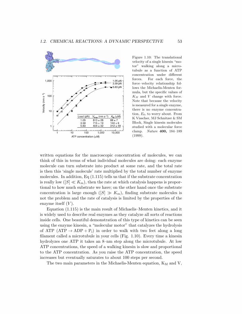
1.2. CHEMICAL REACTIONS: A DYNAMIC PERSPECTIVE 53
Figure 1.10: The translationalvelocity of a single kinesin “mo-tor” walking along a micro-tubule as a function of ATPconcentration under differentforces. For each force, theforce–velocity relationship fol-lows the Michaelis-Menten for-mula, but the specific values ofKM and V change with force.Note that because the velocityis measured for a single enzyme,there is no enzyme concentra-tion, E0, to worry about. FromK Visscher, MJ Schnitzer & SMBlock, Single kinesin moleculesstudied with a molecular forceclamp. Nature 400, 184–189(1999).
written equations for the macroscopic concentration of molecules, we canthink of this in terms of what individual molecules are doing: each enzymemolecule can turn substrate into product at some rate, and the total rateis then this ‘single molecule’ rate multiplied by the total number of enzymemolecules. In addition, Eq (1.115) tells us that if the substrate concentrationis really low ([S]� Km), then the rate at which catalysis happens is propor-tional to how much substrate we have; on the other hand once the substrateconcentration is large enough ([S] � Km), finding substrate molecules isnot the problem and the rate of catalysis is limited by the properties of theenzyme itself (V ).
Equation (1.115) is the main result of Michaelis–Menten kinetics, and itis widely used to describe real enzymes as they catalyze all sorts of reactionsinside cells. One beautiful demonstration of this type of kinetics can be seenusing the enzyme kinesin, a “molecular motor” that catalyzes the hydrolysisof ATP (ATP→ ADP + Pi) in order to walk with two feet along a longfilament called a microtubule in your cells (Fig. 1.10). Every time a kinesinhydrolyzes one ATP it takes an 8–nm step along the microtubule. At lowATP concentrations, the speed of a walking kinesin is slow and proportionalto the ATP concentration. As you raise the ATP concentration, the speedincreases but eventually saturates to about 100 steps per second.
The two main parameters in the Michaelis-Menten equation, KM and V,

54 CHAPTER 1. NEWTON’S LAWS, CHEMICAL KINETICS, ...
are properties of the enzyme itself. For most enzymes in your body, KM
has values in the range of 10−1 to 10−7M. The larger this value, the moresubstrate is needed to push the reaction into the saturated regime. Theeffect of different KM values on human physiology can be seen in examiningthe sensitivity of some people to the effects of digesting ethanol. As youmay know, some people experience a redness of the face and rapid heartrate when they ingest alcohol, which is caused by an excess of acetaldehydein the blood. The break down of ethanol in your body takes place in severalsteps in the liver. Ethanol is first converted into acetaldehyde by an enzymecalled Alcohol dehydrogenase
CH3CH2OH + NAD+ Alchohol dehydrogenase−−−−−−−−−−−−−−⇀↽−−−−−−−−−−−−−− CH3CHO + H+ + NADH
The acetaldehyde is then broken down into acetate by the enzyme Aldehydedehydrogenase
CH3CHO + NAD+ + H2OAldehyde dehydrogenase−−−−−−−−−−−−−−−⇀↽−−−−−−−−−−−−−−− CH3COO− + NADH + 2H+
Most people have two active forms of this second enzyme, a low and ahigh KM form. In people with hightened sensitivity to ethanol, the low KM
form contains a single amino acid substitution and is unable to process theacetaldehyde. Therefore, only the high KM is active and it is only able towork quickly when the concentration of the acetaldehyde substrate is high.As a consequence, less of the chemical is converted to acetate and more isreleased into the blood which induces the physiological response. All becausea single enzyme contains a single amino acid substitution!
Problem 16: The enzyme lysozyme helps to break down complex molecules builtout of sugars. As a first step, these molecules (which we will call S) must bind to theenzyme. In the simplest model, this binding occurs in one step, a second order reactionbetween the enzyme E and the substrate S to form the complex ES:
E + Sk+→ ES, (1.116)
where k+ is the second order rate constant. The binding is reversible, so there is also afirst order process whereby the complex decays into its component parts:
ESk−→ E + S, (1.117)
where k− is a first order rate constant. Let’s assume that everything else which happensis slow, so we can analyze just this binding/unbinding reaction.

1.2. CHEMICAL REACTIONS: A DYNAMIC PERSPECTIVE 55
(a.) Write out the differential equations that describe the concentrations of [S], [E]and [ES]. Remember that there are contributions from both reactions (1.116) and (1.117).
(b.) Use the differential equations you have written to show that if we start with aninitial concentration of enzyme [E]0 and zero concentration of the complex ([ES]0 = 0),then there is a conservation law: [E] + [ES] = [E]0 at all times.
(c.) Assume that the initial concentration of substrate [S]0 is in vast excess, so thatwe can always approximate [S] ≈ [S]0. Show that there is a steady state at which theconcentration of the complex is no longer changing, and that at this steady state
[ES]ss = [E]0 ·[S]
[S] +K, (1.118)
where K is a constant. How is K related to the rate constants k+ and k−?(d.) When the substrate is (N–acetylglucosamine)2, experiments near neutral pH
and at body temperature show that the rate constants are k+ = 4 × 10⁷ M−1s−1 andk− = 1×10⁵ s−1. What is the value of the constant K [in Eq (1.118)] for this substrate? Ata substrate concentration of [S] = 1 mM, what fraction of the initial enzyme concentrationwill be in the the complex [ES] once we reach steady state?
(e.) Show that the concentration of the complex [ES] approaches its steady stateexponentially: [ES](t) = [ES]ss[1− exp(−t/τ)]. Remember that we start with [ES]0 = 0.How is the time constant τ related to the rate constants k+ and k− and to the substrateconcentration [S]? For (N–acetylglucosamine)2, what is the longest time τ that we willfind for the approach to steady state?
Problem 17: The data from Figure 1.10 were taken using a sophisticated OpticalTrap5 that can both track the motion of a single enzyme at very high resolution and applya physical force to the enzyme. As you can see from the figure, pulling backwards on thekinesin motor changes both the maximum speed V and the Michaelis constant KM . Ifonly one of the rates in Fig. 1.9 were to depend on force, could you explain the datashown in the table? Explain your answer.
Problem 18: Under physiological conditions, most enzymes are sub–saturated with[S]/KM between 0.01 and 1.
(a.) At what rate does the enzyme go under these circumstances? Show that for[S]� KM
dP
dt≈ V
KM[E]0[S] (1.119)
(b.) In some sense, the ratio V/KM is a measure of the efficiency of catalysis as ittakes into account both the rate of substrate binding, via KM , and the rate of catalysis,through V . It is worth asking how “efficient” an enzyme can be. Show that (V/KM ) < k+must be true.
(c.) Thinking about what the rate k+ describes, what is the physical nature behindthis limit on the enzymatic rate?
Another interesting example is a sequence or cascade of reactions, asschematized in Fig 1.11. Here we imagine that there is a molecule A which
5For more information on this technology, see http://en.wikipedia.org/wiki/
Optical_tweezers

56 CHAPTER 1. NEWTON’S LAWS, CHEMICAL KINETICS, ...
Figure 1.11: A cascade of enzy-matic reactions.
can be stimulated by some signal to go into an activated state A∗. Oncein this activated state, it can act as a catalyst, converting B molecules intotheir activated state B∗. The active B∗ molecules act as a catalyst for C,and so on. This sort of scheme is quite common in biological systems, andserves as a molecular amplifier—even if we activate just one molecule of A,we can end up with many molecules at the output of such a cascade.
One example that we should keep in mind is happening in the photore-ceptor cells of your retina as you read this. In these cells, the A moleculesare rhodopsin, and the stimulation is what happens when these moleculesabsorb light. Once rhodospin is in an active state, it can catalyze the acti-vation of the B molecules, which are called transducin. Transducin is onemember of a large family of proteins (called G–proteins) that are involvedin many different kinds of signaling and amplification in all cells, not justvision. The C molecules are enzyme called phosphodiesterase, which chewup molecules of cyclic GMP (cGMP, which would be D if we continued ourschematic). Again, lots of cellular processes use cyclic nucleotides (cGMPand cAMP) as internal signals or ‘second messengers’ in cells. In the pho-toreceptors, cGMP binds to proteins in the cell membrane that open holesin the membrane, and this allows the flow of electrical current; more about

1.2. CHEMICAL REACTIONS: A DYNAMIC PERSPECTIVE 57
this later in the course. These electrical signals get transmitted to othercells in the retina, eventually reaching the cells that form the optic nerveand carry information from the eye to your brain.
How can we describe the dynamics of a cascade such as Fig 1.11? Let’sthink about the way in which [B∗] changes with time. We have the ideathat A∗ catalyzes the conversion of B into B∗, so the simplest possibility isthat this is a second order process: the rate at which B∗ is produced willbe proportional both to the amount of A∗ and to the number of available Bmolecules, with a second order rate constant k2. Presumably there is also aback reaction so that B∗ converts back into B at some rate k−. Then thedynamics are described by
d[B∗]
dt= k[A∗][B]− k−[B∗]. (1.120)
There must be something similar for the way in which C∗ is formed bythe interaction of B∗ with C, and for simplicity let’s assume that all therate constants are the same (this doesn’t matter for the point we want tomake here!):
d[C∗]
dt= k[B∗][C]− k−[C∗]. (1.121)
Actually solving these equations isn’t so simple. But let’s think about whathappens at very early times. In Eq (1.120), we can assume that at t = 0 westart with none of the activated B∗. The external stimulus (e.g., a flash oflight to the retina) comes along and suddenly we have lots of A∗. There’splenty of B around to convert, and so there is an initial rate k[A∗]0[B]0,which means that the number of activated B molecules will grow
[B∗] ≈ k[A∗]0[B]0t. (1.122)
Now we can substitute this result into Eq (1.121) to find the dynamicsof [C∗] at short times, again assuming that we start with plenty of [C] andnone of the activated version:
d[C∗]
dt≈ k(k[A∗]0[B]0t)[C] = {k2[A∗]0[B]0[C]0}t (1.123)
⇒ [C∗] ≈(
1
2k2[A∗]0[B]0[C]0
)t2 (1.124)
So we see that the initial rise of [B∗] is as the first power of time, the rise of[C∗] is as the second power, and hopefully you can see that if the cascade

58 CHAPTER 1. NEWTON’S LAWS, CHEMICAL KINETICS, ...
continued with C∗ activating D, then [D∗] would rise as the third power oftime, and so on. In general, if we have a cascade with n steps, we expectthat the output of the cascade will rise as tn after we turn on the externalstimulus.
Many people had the cascade model in mind for different biological pro-cesses long before we knew the identity of any of the molecular components.The idea that we could count the number of stages in the cascade by lookingat how the output grows at short times is very elegant, and in Fig 1.12 we seea relatively modern implementation of this idea for the rod photoreceptorsin the toad retina. It seems there really are three stages to the cascade!
This same basic idea of counting steps in a cascade has been used in verydifferent situations. As an example, in Fig 1.13, we show the probability thatsomeone is diagnosed with colon cancer as a function of their age. The ideais the same, that there is some cascade of events (mutations, presumably),and the power in the growth vs. time counts the number of stages. It’s kindof interesting that if you look only on a linear plot (on the left in Fig 1.13),you might think that there was something specifically bad that happens topeople in their 50s that causes a dramatic increase in the rate at which theyget cancer. In contrast, the fact that incidence just grows as a power of agesuggest that there is nothing special about any particular age, just that aswe get older there is more time for things to have accumulated, and thereare several things that need to happen in order for cancer to take hold.It’s quite amazing it is that these same mathematical ideas describe suchdifferent biological processes occurring on completely different time scales(years vs. seconds).
One can do a little more with the cascade model. If we think a littlemore (or maybe use the equations), we see that the maximum number of[B∗] molecules that will get made depends on their lifetime τ = 1/k−: thereis a competition between A∗ activating B → B∗, and the decay processB∗ → B. This same story happens at every stage, so again the peak numberof molecules at the output will be proportional to some power of the lifetimeof the activated molecules, and this power again counts the number of stagesin the cascade, Thus the cell can adjust its sensitivity—the peak number ofoutput molecules that each activated input A∗ can produce—by modulatingthe lifetimes of the activated states. But if we change this lifetime, we alsochange the overall time scale of the response. Roughly speaking, the timerequired for the response to reach its peak is also proportional to τ . So weexpect that if a cell adjusts its gain by changing lifetimes, then the gain andtime to peak should be related to each other as gain ∝ tnpeak, where thereare n stages in the cascade; of course this value of n should agree with what
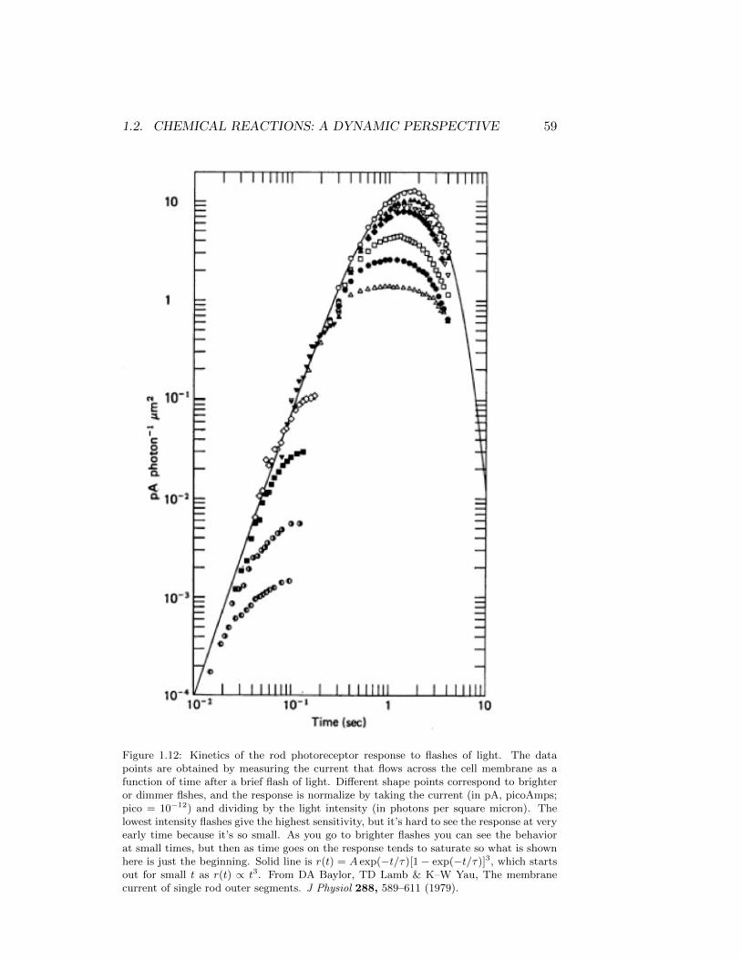
1.2. CHEMICAL REACTIONS: A DYNAMIC PERSPECTIVE 59
Figure 1.12: Kinetics of the rod photoreceptor response to flashes of light. The datapoints are obtained by measuring the current that flows across the cell membrane as afunction of time after a brief flash of light. Different shape points correspond to brighteror dimmer flshes, and the response is normalize by taking the current (in pA, picoAmps;pico = 10−12) and dividing by the light intensity (in photons per square micron). Thelowest intensity flashes give the highest sensitivity, but it’s hard to see the response at veryearly time because it’s so small. As you go to brighter flashes you can see the behaviorat small times, but then as time goes on the response tends to saturate so what is shownhere is just the beginning. Solid line is r(t) = A exp(−t/τ)[1− exp(−t/τ)]3, which startsout for small t as r(t) ∝ t3. From DA Baylor, TD Lamb & K–W Yau, The membranecurrent of single rod outer segments. J Physiol 288, 589–611 (1979).
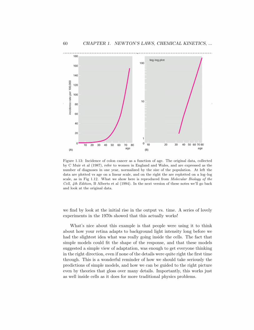
60 CHAPTER 1. NEWTON’S LAWS, CHEMICAL KINETICS, ...
Figure 1.13: Incidence of colon cancer as a function of age. The original data, collectedby C Muir et al (1987), refer to women in England and Wales, and are expressed as thenumber of diagnoses in one year, normalized by the size of the population. At left thedata are plotted vs age on a linear scale, and on the right the are replotted on a log–logscale, as in Fig 1.12. What we show here is reproduced from Molecular Biology of theCell, 4th Edition, B Alberts et al (1994). In the next version of these notes we’ll go backand look at the original data.
we find by look at the initial rise in the output vs. time. A series of lovelyexperiments in the 1970s showed that this actually works!
What’s nice about this example is that people were using it to thinkabout how your retina adapts to background light intensity long before wehad the slightest idea what was really going inside the cells. The fact thatsimple models could fit the shape of the response, and that these modelssuggested a simple view of adaptation, was enough to get everyone thinkingin the right direction, even if none of the details were quite right the first timethrough. This is a wonderful reminder of how we should take seriously thepredictions of simple models, and how we can be guided to the right pictureeven by theories that gloss over many details. Importantly, this works justas well inside cells as it does for more traditional physics problems.

1.3. RADIOACTIVITY AND THE AGE OF THE SOLAR SYSTEM 61
1.3 Radioactivity and the age of the solar system
Most of you are familiar with the phenomenon of radioactive decay: Certainelements have isotopes in which the nucleus is not stable but rather decays,usually emitting some particle in the process. As an example, we have the“beta decay” of the carbon isotope 14C,
14C→ 14N + e− + νe. (1.125)
This means that the carbon nucleus decays into a nitrogen nucleus, givingoff an electron (e−) and a particle you might not know about called ananti–neutrino (νe); the subscript e means that this particular neutrino isassociated with the electron.
To back up a bit, let’s recall that most of the carbon around us is 12C.If you look at the periodic table you can see that carbon has six electrons,and since the atom is neutral there must also be six protons in the nucleus;6 is the “atomic number” of carbon. The “mass number” of 12 comes fromthese six protons plus six neutrons. The isotope 14C has the same numberof electrons and protons—that’s what it means to be an isotope!—but twoextra neutrons in its nucleus.
Looking again at the periodic table, nitrogen has seven electrons andhence seven protons; 14N thus has seven neutrons. So what is happening inthe beta decay of 14C really is
6 protons + 8 neutrons→ 7 protons + 7 neutrons + e− + νe, (1.126)
or more simply the decay of a neutron (n) into a proton (p+), an electronand an anti–neutrino,
n→ p+ + e− + νe. (1.127)
If you just have a neutron sitting in free space, this takes about twelveminutes (!). But with all the particles trapped in the nucleus, it can takemuch longer: more than 5000 years for the decay of 14C.
What you measure when you have a radioactive element is the extraemitted particle, the electron in the case of 14C. So unlike the usual casein chemistry, you don’t measure the concentration of each species, you ac-tually measure the transitions from one species to the other. The particlesthat come out of radioactive decays often have enough energy that you cancount the individual particles, so this is like observing chemical reactionsone molecule at a time. As we will discuss later in the course, the behaviorof individual molecules or individual nuclei is random, so if you watch 1000
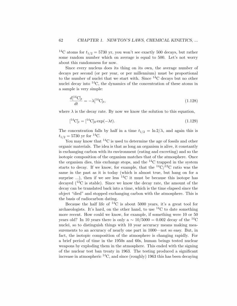
62 CHAPTER 1. NEWTON’S LAWS, CHEMICAL KINETICS, ...
14C atoms for t1/2 = 5730 yr, you won’t see exactly 500 decays, but rathersome random number which on average is equal to 500. Let’s not worryabout this randomness for now.
Since every nucleus does its thing on its own, the average number ofdecays per second (or per year, or per millennium) must be proportionalto the number of nuclei that we start with. Since 14C decays but no othernuclei decay into 14C, the dynamics of the concentration of these atoms ina sample is very simple:
d[14C]tdt
= −λ[14C]t, (1.128)
where λ is the decay rate. By now we know the solution to this equation,
[14C]t = [14C]0 exp(−λt). (1.129)
The concentration falls by half in a time t1/2 = ln 2/λ, and again this ist1/2 = 5730 yr for 14C.
You may know that 14C is used to determine the age of fossils and otherorganic materials. The idea is that as long an organism is alive, it constantlyis exchanging carbon with its environment (eating and excreting) and so theisotopic composition of the organism matches that of the atmosphere. Oncethe organism dies, this exchange stops, and the 14C trapped in the systemstarts to decay. If we know, for example, that the 14C/12C ratio was thesame in the past as it is today (which is almost true, but hang on for asurprise ...), then if we see less 14C it must be because this isotope hasdecayed (12C is stable). Since we know the decay rate, the amount of thedecay can be translated back into a time, which is the time elapsed since theobject “died” and stopped exchanging carbon with the atmosphere. This isthe basis of radiocarbon dating.
Because the half life of 14C is about 5000 years, it’s a great tool forarchaeologists. It’s hard, on the other hand, to use 14C to date somethingmore recent. How could we know, for example, if something were 10 or 50years old? In 10 years there is only a ∼ 10/5000 = 0.002 decay of the 14Cnuclei, so to distinguish things with 10 year accuracy means making mea-surements to an accuracy of nearly one part in 1000—not so easy. But, infact, the isotopic composition of the atmosphere is changing rapidly. Fora brief period of time in the 1950s and 60s, human beings tested nuclearweapons by exploding them in the atmosphere. This ended with the signingof the nuclear test ban treaty in 1963. The testing produced a significantincrease in atmospheric 14C, and since (roughly) 1963 this has been decaying
1.3. RADIOACTIVITY AND THE AGE OF THE SOLAR SYSTEM 63
Figure 1.14: (A) Estimated 14C composition of the atmosphere on a ∼ 1000 yr time scale.(B) Cross section of a swedish pine tree, from which 14C composition can be measured insuccessive rings, as shown in (C). Complied by KL Spalding, RD Bhardwaj, BA Buchholz,H Druid & J Frısen, Cell 122, 133–145 (2005).
exponentially as it mixes with the oceans and biomass (Fig 1.14) Recentlyit has been suggested that this provides a signal that one can use, for ex-ample, to determine the birth dates of cells from different tissues in recentlydeceased people. While slightly macabre on several levels, this techniqueoffers the opportunity to address really crucial questions such as whetherwe are growing new cells in our brain even when we are adults, or if all thecells in the brain are born more or less when we are born.
Problem 19: The radioactive isotope 14C has a half–life of t1/2 = 5730 years. Youfind two human skeletons which you suspect are about 10, 000 years old. The setting inwhich you find these skeletons suggests that they died in two events separated by roughly20 years. How accurately do you need to measure the abundance of 14C in the skeletons inorder to test this prediction? State as clearly as possible any assumptions that are madein interpreting such measurements.
If we want to look at events that take much longer than 5000 years, it’suseful to look for radioactive decays that have much longer half lives. Ifyou poke around the periodic table, you find that heavy elements often have
64 CHAPTER 1. NEWTON’S LAWS, CHEMICAL KINETICS, ...
radioactive isotopes with half lives measured in billions of years. Let’s focuson the uranium isotopes which decay into lead. Specifically, 235U decaysinto 207Pb at a rate λ235 = 9.849× 10⁻¹⁰ yr−1, while 238U decays into 206Pbat a rate λ238 = 1.551× 10⁻¹⁰yr−1:
235Uλ235→ 207Pb + · · · (1.130)
238Uλ238→ 206Pb + · · · , (1.131)
where in both reactions · · · refers to additional fragments that emerge in thefission of the uranium nucleus. If we imagine a hunk of rock that formed attime t = 0 in the distant past, then all of the uranium nuclei are decaying,so what we measure now at time t is
235U(t) = 235U(0) exp(−λ235t) (1.132)238U(t) = 238U(0) exp(−λ238t). (1.133)
Every uranium nucleus that decays adds to the number of lead atoms thatwe find in the rock, so that
207Pb(t) = 207Pb(0) + [235U(0)− 235U(t)] (1.134)206Pb(t) = 206Pb(0) + [238U(0)− 238U(t)]. (1.135)
Remember that we don’t actually know what the isotopic compositions werewhen the rock was first formed. So in order to use these equations to analyzereal data, we should try to get rid of all the terms that involve the isotopiccompositions at t = 0.
We can start with uranium, for which everything we observe today is justa decayed version of where things started; this means that we can invert Eq’s(1.132) and (1.133):
235U(0) = 235U(t) exp(+λ235t) (1.136)238U(0) = 238U(t) exp(+λ238t), (1.137)
and then we can substitute into our equations for the current amount of thetwo lead isotopes [Eq’s (1.134,1.135)] to obtain
207Pb(t) = 207Pb(0) + [235U(t) exp(+λ235t)− 235U(t)] (1.138)206Pb(t) = 206Pb(0) + [238U(t) exp(+λ238t)− 238U(t)], (1.139)
or more simply
207Pb(t) = 207Pb(0) + 235U(t)[exp(+λ235t)− 1] (1.140)206Pb(t) = 206Pb(0) + 238U(t)[exp(+λ238t)− 1], (1.141)

1.3. RADIOACTIVITY AND THE AGE OF THE SOLAR SYSTEM 65
This is almost a relationship between things we can measure—the currentnumbers of atoms of each isotope—but not quite. First of all, we still havethe initial concentrations of the lead isotopes. Second, it’s hard to makeabsolute measurements (how could we be sure that we got all the lead out,as it were), so it would be nice to express things in terms of isotopic ratios.
The key idea is that different rocks start out with different amounts oflead and uranium, because that involves the chemistry of formation of therock, but if all these heavy elements were made in a single event such as asupernova then the ratios of the isotopes would have been the same in allmaterials at t = 0. Since all that happens to the uranium nuclei is that theydecay, the ratio of 235U to 238U still is the same in all materials, althoughof course it might be very different from the ratio at t = 0. To make use ofthis fact, let’s try to solve for the number of 238U atoms as a function of thenumber of 206Pb atoms:
206Pb(t) = 206Pb(0) + 238U(t)[exp(+λ238t)− 1]
⇒ 238U(t) =206Pb(t)− 206Pb(0)
exp(+λ238t)− 1. (1.142)
But if we measure the ratio 235U(t)/238U(t) today and call this ratio R235/238,we can say that
235U(t) = R235/238
206Pb(t)− 206Pb(0)
exp(+λ238t)− 1. (1.143)
This relates the 235U concentration in a sample to the 206Pb concentration,both measured today. But we have seen that the 235U concentration isrelated to the number of atoms of the other lead isotope, through Eq (1.140).
66 CHAPTER 1. NEWTON’S LAWS, CHEMICAL KINETICS, ...
So we can put these equations together:
207Pb(t) = 207Pb(0) + 235U(t)[exp(+λ235t)− 1]
235U(t) = R235/238
206Pb(t)− 206Pb(0)
exp(+λ238t)− 1
⇒ 207Pb(t) = 207Pb(0)
+R235/238
206Pb(t)− 206Pb(0)
exp(+λ238t)− 1[exp(+λ235t)− 1]
(1.144)
= 207Pb(0)− 206Pb(0)R235/238exp(+λ235t)− 1
exp(+λ238t)− 1
+206Pb(t)
[R235/238
exp(+λ235t)− 1
exp(+λ238t)− 1
](1.145)
This is an interesting equation, because it says that the amount of 207Pbthat we find today in a rock should be related to the amount of 206Pb thatwe find in that same piece of rock. But we still have those pesky initialvalues to deal with.
There is yet a third isotope of lead which is both stable and not theproduct of other radioactive decays, and this is 204Pb. So the amount ofthis isotope that we measure today is the same as we would have measuredwhen the rock was formed. This means that we can take our expression for207Pb(t) in Eq (1.145) and normalize by 204Pb(t),
207Pb(t)204Pb(t)
=207Pb(0)204Pb(t)
−206Pb(0)204Pb(t)
R235/238exp(+λ235t)− 1
exp(+λ238t)− 1
+206Pb(t)204Pb(t)
[R235/238
exp(+λ235t)− 1
exp(+λ238t)− 1
], (1.146)
but then we are free to rewrite 204Pb(t)→ 204Pb(0) anyplace where it wouldmake thing look better. So this last equation becomes
207Pb(t)204Pb(t)
=207Pb(0)204Pb(0)
−206Pb(0)204Pb(0)
R235/238exp(+λ235t)− 1
exp(+λ238t)− 1
+206Pb(t)204Pb(t)
[R235/238
exp(+λ235t)− 1
exp(+λ238t)− 1
],
(1.147)
This looks complicated, but it’s not. We can rewrite this equation as
207Pb(t)204Pb(t)
= A+B206Pb(t)204Pb(t)
, (1.148)
1.3. RADIOACTIVITY AND THE AGE OF THE SOLAR SYSTEM 67
where the first important point is that A and B should be the same in allrocks (!).
Actually, Eq (1.148) contains a prediction of tremendous power. Youshould go back over the derivation and see what we had to assume:
• Uranium isotopes decay into lead isotopes as observed in the lab.
• Nothing else decays into lead, which is stable, and no processes produceany new uranium; again these are statements based on laboratoryobservations.
• All of the heavy elements that we find in our neighborhood were madeat some moment t = 0 in the past, and this event set the initial isotopicratios for each element.
• Different materials start with different amounts of uranium and lead.
Notice that the first two assumptions are based on direct measurements.The last item is the assumption that nothing special happens to force arelationship between the lead and uranium content of different materials, soit isn’t really an assumption. The only really startling claim on the list isthat all the heavy elements were made at some specific time in the past. Sothis assumption—literally a hypothesis about the creation of the materialsin our local corner of the universe—makes a prediction about what we willsee if we measure the isotopic composition of many different materials: ifyou plot 207Pb/204Pb vs 206Pb/204Pb, you’ll see a straight line. As you cansee in Fig 1.15 this works!
One can in fact do a little more with the data from Fig 1.15 and relatedexperiments. Our simple form in Eq (1.148) hides the fact that the constantsA and especially B have meaning. Referring to Eq (1.147), we see that theslope B involves the current ratio R235/238 of uranium isotopes, the decayrates λ235 and λ238 of the uranium isotopes, and the time t since the creationof the elements. All of these things except the time t have been measuredindependently. So, by analyzing the slop of the line in Fig 1.15, we determinethe time that has elapsed since the heavy elements were formed. The resultis t = 4.55 × 10⁹ yr. Even better is that you can do all this same analysiswith other combinations of isotopes (e.g., rubidium and strontium) and youget the same answer for t even though everything else is different. This isimpressive evidence that there really was some discrete event several billionyears ago that created the heavy elements in our neighborhood.
Just to avoid confusion, what we have just calculated is not the time ofthe big bang. The heavy elements were formed only once the universe had

68 CHAPTER 1. NEWTON’S LAWS, CHEMICAL KINETICS, ...
0 10 20 30 40 50 600
5
10
15
20
25
30
35
40
45
206Pb/204Pb
207 P
b/20
4 Pb
Figure 1.15: Isotopic composi-tions of some stone meteoritesand terrestrial rocks. The factthat the data fall on a straightline is consistent with a sin-gle ‘moment of creation’ for theheavy elements, and the slopedetermines that this origin was4.55× 109 yr in the past. Fromdata in V RamaMurthy & CCPatterson, Primary isochron ofzero age for meteorites and theearth, Journal of GeophysicalResearch 67, 1161 (1962).
developed to the point of having stars that could “cook” the light elementsinto more bigger nuclei. Actually, it’s not automatic that these estimates forthe age of heavy elements in the solar system should come out younger thanthe age of the universe as a whole (that is, the time since the big bang), whichis estimated from very different kinds of data. There have been some tensemoments in the history of the subject, but everything now is consistent; thebig bang happened 13.7 billion years ago, with an uncertainty of about 1%(!).
It is worth remembering, at this point, that our whole line of argumentleading to this remarkable conclusion hinges on the fact that we can solve thesimple first order differential equation that describes radioactive decay. Weknow that this is the right equation because we have made measurementsin the laboratory, but these measurements cover a range of (at best) a fewyears. Trusting the equations, we extrapolate the solutions over billions ofyears, and we obtain a wonderfully consistent view of the data.
An interesting question is whether there is any other evidence that therelevant parameters are constant over a period that is a significant fractionof the age of the universe. In fact, many people have considered the possi-bility that what we call “fundamental constants” of nature—including theconstants that determine the rates of radioactive decay—might be chang-ing slowly as the universe ages (and, as we now know, expands). Smallrates of change obviously would have big consequences over such long timescales. For better or worse, there is no positive evidence for such changes,

1.3. RADIOACTIVITY AND THE AGE OF THE SOLAR SYSTEM 69
despite many ingenious, high precision measurements. This remains, how-ever, a place where people are looking for cracks in our otherwise quite solidunderstanding.
Problem 20: The Allende chondrites are carbonaceous meteorites that fell near thetown of that name in Mexico on February 8, 1969. Chondrites are a class of meteoritescomposed of tiny, rounded spheres containing silicate minerals (called chondrules). Thechondrules are believed to have formed early in the solar nebula and many geochemicalstudies have been performed on them. Mass spectrometric data obtained from thesechondrules has allowed the determination of their elemental compositions. Shown in Table1.2 are typical data for isotope ratios of rubidium and strontium obtained by Gray andcoworkers in 1973.
(a.) Derive a simple, integrated expression relating the age of such a sample to theisotope ratios.
(b.) Calculate the age of these samples from this data using the known half–life forradioactive decay of 87Rb to 87Sr of 48.8 billion years. Note that the strontium isotopesare stable and do not decay.
87Rb/86Sr 87Sr/86Sr
0.00014 0.698770
0.00019 0.698810
0.00075 0.698890
0.00393 0.698990
0.00432 0.699030
0.00660 0.699250
0.00776 0.699140
0.00853 0.699330
0.05213 0.702140
0.00017 0.698770
Table 1.2: Isotopic ratios from the Allende chondrites.
Intriguingly, these chondrites have been found to contain both natural and unnaturalamino acids. But that is a topic for another day.

70 CHAPTER 1. NEWTON’S LAWS, CHEMICAL KINETICS, ...
1.4 Using computers to solve differential equations
We have been looking so far at differential equations whose solutions canbe constructed from “elementary functions,” functions that we can writedown in some simple form, look at and (hopefully) understand. In general,this isn’t possible and in fact it might just be a historical artifact thatcertain functions have names and others don’t. If you think you have theright equation to describe a system you are interested in, the fact that youcan’t immediately write down the solution shouldn’t stop you. You canmake approximations, which generates a lot of intuition, and you can use acomputer to generate numerical solutions. This latter approach is general,and you should learn how to do it to the point where you feel comfortable.
Let us start with the simplest equation for first order chemical kinetics,in which some molecule A is tranformed into B with a rate constant k. Theconcentration cA of A molecules obeys the equation
dcAdt
= −kcA. (1.149)
As you all know by now, the solution is cA(t) = cA(0) exp(−kt). Let’ssee how we could find this solution numerically, check against the analyticsolution to see that our strategy works, and finally use the same strategy tolook at equations that are not so easy to solve with pen and paper.
Recall that the derivative is defined in calculus as the limit of finitedifferences:
dcA(t)
dt≡ lim
∆t→0
cA(t+ ∆t)− cA(t)
∆t. (1.150)
The key to numerical solutions of differential equations is in essence to takea giant step backward and work with a finite value of ∆t, hoping that wecan make it small enough that we start to see the limiting behavior. In thesimplest case we just make the replacement
dcAdt→ cA(t+ ∆t)− cA(t)
∆t(1.151)
in the differential equation, and proceed:
dcAdt→ cA(t+ ∆t)− cA(t)
∆t= −kcA(t) (1.152)
cA(t+ ∆t)− cA(t) = −[k∆t]cA(t) (1.153)
cA(t+ ∆t) = [1− k∆t]cA(t).
(1.154)

1.4. USING COMPUTERS TO SOLVE DIFFERENTIAL EQUATIONS71
If we decide to measure time in discrete ticks of a clock, where the timebetween ticks is ∆t, then every time t = n · ∆t, where n = 0, 1, 2, 3, . . . .Thus instead of writing cA(t), we can write cA(n), and of course cA(t+∆t) =cA(n+ 1). This means that Eq (1.154) really is an equation that generatescA(n+ 1) from knowledge of cA(n):
cA(n+ 1) = [1− k∆t]cA(n). (1.155)
If we start with some value of cA(0), Eq (1.155) tells us how to generatecA(1), and then we can use this iteratively to generate values for cA at alldiscrete times n. In effect this allows us to “walk” through time, updatingthe value of cA based on the previous value, and in this way we generate a“numerical solution” to our differential equations.
Let’s see how this works in MATLAB. We’ll choose units where the rateconstant k = 1, and our “small steps of time” will be ∆t = 0.01; we’ll haveto come back to the question of whether this choice of ∆t is a good one.We’ll explore times starting at t = 0 and ending at t = 5 (again, in unitswhere k = 1), which means that we need to run for 500 ticks of our discreteclock. With these remarks in mind, the program becomes
cA = zeros(500,1);
cA(1) = 1;
k = 1;
dt = 0.01
for n=2:length(cA);
cA(n) = (1-k*dt)*cA(n-1);
end;
Notice that we start by setting aside space for the thing we trying to com-pute, and we have to set (in the second line) its initial value. A peculiarityof MATLAB is that you start counting at n=1, not at n=0. We also havelines which define the value of the rate constant k and time step ∆t, whichis symbolized by dt in the program; again, our choices of these parametersare just for illustration at the moment. Once you run the program you havestored the “data” on concentration as a function of time, and you’d like toplot it. If you want things in physical units it’s convenient to make a realtime axis,
timeaxis = dt*[0:499];
where we are careful to note that the time corresponding to n=1 is actuallyt = 0. Then you can type

72 CHAPTER 1. NEWTON’S LAWS, CHEMICAL KINETICS, ...
figure(1)
plot(timeaxis,cA)
xlabel(’time (seconds)’)
ylabel(’concentration of A’)
and you should get a reasonable plot with properly labeled axes, and thiswill appear on your screen in a box marked Figure 1. This is not the placefor aesthetic hints, but at some point you’ll want to learn how to make thingslook nice—what is important here is to be sure that when you look at theplot you can read the units! The results are shown in Fig 1.16, where wecompare the numerical solution to a numerical evaluation of the analyticalresult. In this simple case, it’s clear that our numerical strategy “works,” inthat it gives us a solution that agrees with the exact mathematics.
0 0.5 1 1.5 2 2.5 3 3.5 4 4.5 50
0.1
0.2
0.3
0.4
0.5
0.6
0.7
0.8
0.9
1
time t
c A
0 0.5 1 1.5 2 2.5 3 3.5 4 4.5 50
0.1
0.2
0.3
0.4
0.5
0.6
0.7
0.8
0.9
1
time t
c A
Figure 1.16: Numerical solution of the simple differential equation, Eq (1.149). As de-scribed in the text we use the algorithm defined by Eq (1.155), with the rate constantk = 1 s−1 and the initial condition cA(1) = 1 (in some units). The solid line is the re-sult of 500 iterations with ∆t = 0.01 s, and the circles show the exact solution over thesame time window. Inset shows what happens as we increase ∆t, with separate curves for∆t = 0.01, 0.02, 0.05, 0.1, 0.2, 0.5.

1.4. USING COMPUTERS TO SOLVE DIFFERENTIAL EQUATIONS73
We have of course chosen here a VERY simple example. In particular wehave an exact analytical solution, so using the computer is just for the sakeof learning how to do it. In the problems we ask you to play a bit, changingparameters to see what is essential in making things work. In the approachsuggested here, the basic issue is how to choose the size of the discrete timestep dt. The whole idea behind our scheme is to replace derivatives withdifferences, and this gets to be a bad approximation if we make our stepstoo big, as you can see in the inset of Fig 1.16. So this pushes us towardsmaller and smaller values of dt. But if we take very small steps then weneed to take lots of steps to cover the same amount of real time, and so ourcomputation becomes inefficient.
Thanks to the increasing speed of the devices in your computer’s chips,running programs for many time steps is less of a problem than it used tobe, but still there are many situations in which one will need to push thetradeoff between accuracy and efficiency. To do this, one needs to under-stand something about the problem you are solving, but one can also tryto use more intelligent mappings from the continuous differential equationdown to the discrete time steps. This is a whole field of research (numericalanalysis), and as time permits we’ll give you glimpses. For now, it wouldbe good if you felt comfortable with the simplest approaches, so that facedwith some new differential equation you don’t how to solve, you can go tothe computer and quickly see what the solutions look like—and have waysof testing to see if you believe what the computer is telling you!
Problem 21: The basic idea of this section has been to take the differential equation
dc(t)
dt= −kc(t), (1.156)
replace it with a discrete equation
c(t+ ∆t)− c(t)∆t
= −kc(t) (1.157)
⇒ c(t+ ∆t) = (1− k∆t)c(t), (1.158)
and then turn this rule directly into an algorithm.
(a.) Consider the case where k = 10 s−1. Try various values for ∆t (e.g., ∆t =0.001, 0.01, 0.1, 1 s) and run your program for a number of iterations that correspondsto one second of real time. Compare your numerical results with the analytic solutioncA(t) = cA(0) exp(−kt). How small does ∆t need to be in order to get the right answer?How would your answer change if the rate k were ten times faster?

74 CHAPTER 1. NEWTON’S LAWS, CHEMICAL KINETICS, ...
(b.) Write the analogous program for a second order reaction, A+Bk2→ C, described
by the differential equations
dcAdt
= −k2cAcB (1.159)
dcBdt
= −k2cAcB . (1.160)
(c.) Assume initial concentrations of cA(0) = 1 mM and cB(0) = 2 mM. Let k2 =106 M−1s−1. Before you run your program, what value of ∆t seems reasonable? For howlong (in real time) will you need to run in order to see most of the interesting dynamics?
(d.) Run your program using the parameter settings from part [c]. Is there an analyticsolution to which you can compare your results? If you don’t have such a solution, howdo you decide whether your program is giving the right answer?
Problem 22: Let’s try to use these ideas to solve the equations for motion under theinfluence of gravity. Going back to the discussion in Section 1.1, if the height of a particlewith mass m is given by h(t), then Netwon’s equation becomes
md2h
dt2= −mg, (1.161)
again in the limit where we take the force of gravity to be constant. Since we have discussedways of solving equations with one derivative, but not two derivatives, let’s rewrite thisas two equations:
dh
dt= v, (1.162)
dv
dt= −g. (1.163)
Notice that units are arbitrary. Suppose that we define variables h = h/h0, t = t/t0, andv = v/v0, where we choose the velocity scale to be the initial velocity, v0 = v(0).
(a.) Write the differential equations for these new variables, that is
dh
dt= · · · , (1.164)
dv
dt= · · · . (1.165)
(b.) Show that by choosing the scales h0 and t0 correctly, you can make even theconstant g disappear from the equations. What does this mean, qualitatively, about theform of the solutions to these equations?
(c.) Write a program to solve these “dimensionless” equations, discretizing into timesteps of size ∆t as before. Run the program, and compare your results with the exactsolution from the discussion in Section 1.1.
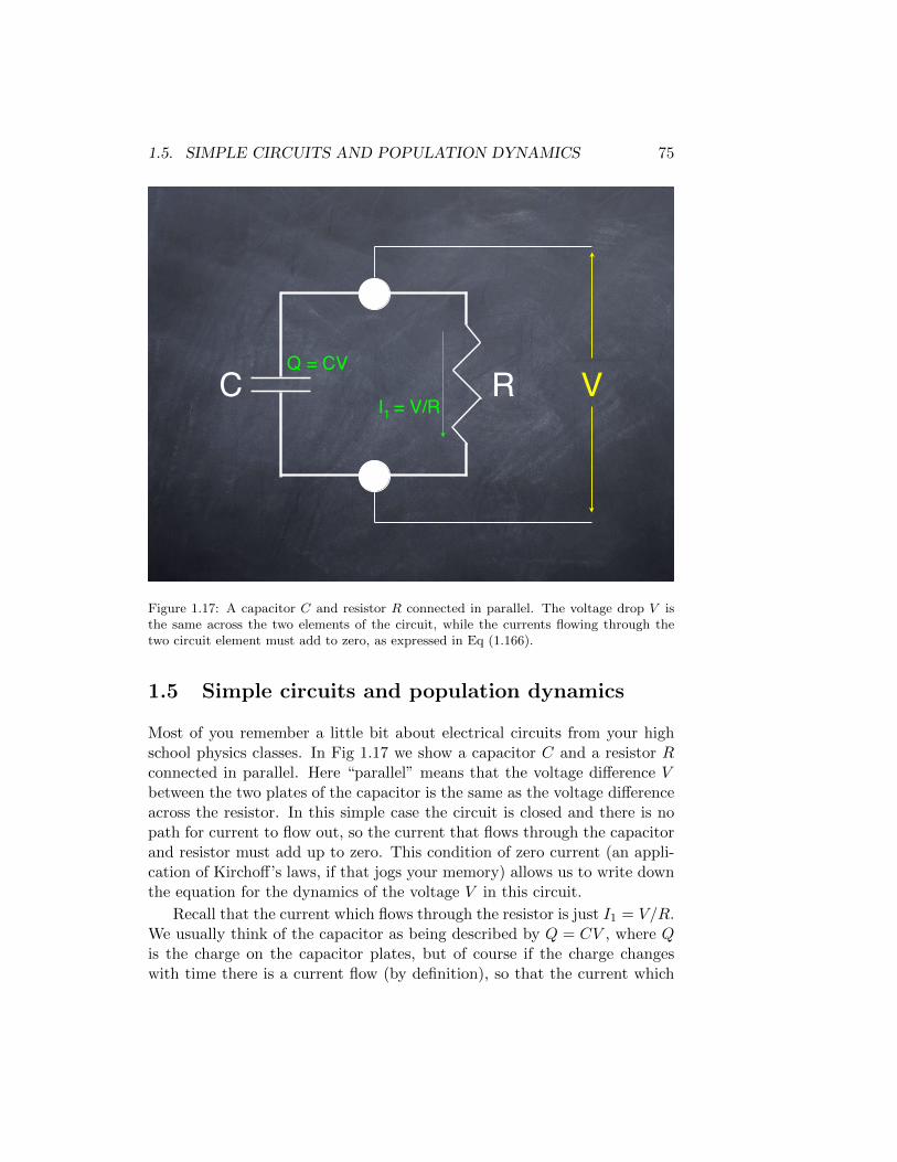
1.5. SIMPLE CIRCUITS AND POPULATION DYNAMICS 75
C R VQ = CV
I = V/R1
Figure 1.17: A capacitor C and resistor R connected in parallel. The voltage drop V isthe same across the two elements of the circuit, while the currents flowing through thetwo circuit element must add to zero, as expressed in Eq (1.166).
1.5 Simple circuits and population dynamics
Most of you remember a little bit about electrical circuits from your highschool physics classes. In Fig 1.17 we show a capacitor C and a resistor Rconnected in parallel. Here “parallel” means that the voltage difference Vbetween the two plates of the capacitor is the same as the voltage differenceacross the resistor. In this simple case the circuit is closed and there is nopath for current to flow out, so the current that flows through the capacitorand resistor must add up to zero. This condition of zero current (an appli-cation of Kirchoff’s laws, if that jogs your memory) allows us to write downthe equation for the dynamics of the voltage V in this circuit.
Recall that the current which flows through the resistor is just I1 = V/R.We usually think of the capacitor as being described by Q = CV , where Qis the charge on the capacitor plates, but of course if the charge changeswith time there is a current flow (by definition), so that the current which

76 CHAPTER 1. NEWTON’S LAWS, CHEMICAL KINETICS, ...
flows through the capacitor is I2 = d(CV )/dt = C(dV/dt). Adding thesecurrents must give zero, and this must be true at every moment of time t:
I1 + I2 =V (t)
R+ C
dV (t)
dt= 0. (1.166)
It is slightly more convenient to write this as
RCdV (t)
dt+ V (t) = 0. (1.167)
We recognize Eq (1.167) as the same equation we have seen before, bothin the mechanics of motion with drag and in first order chemical kinetics.By now we know that the solution is an exponential decay,
V (t) = V (0)e−t/τ , (1.168)
where the time constant τ = RC. As you might guess by looking at thecircuit—there is no battery and no current source—any initial voltage V (0)decays to zero, and this decay happens on a time scale τ = RC. This isimportant because most circuits that we build, including the circuits on thechips in your computer, have some combination of resistance and capaci-tance, and so we know that there is a time scale over which these circuitswill lose their memory. In memory chips we want this to be a very long time,so (roughly speaking) one tries to design the circuit so that R is very large.Conversely, on the processor chips things should happen fast, so RC shouldbe small. You may recall that the capacitance C is determined largely bygeometry—how big are the plates and how far apart are they?—so if wewant to squeeze a certain number of circuit elements into a given area of thechip the capacitances are more or less fixed, and the challenge is to reduceR.
Almost the same equations arise in a very different context, namelypopulation growth. Imagine that we put a small number of bacteria intoa large container, with plenty of food; you will soon do more or less thisexperiment in the lab part of the course. Let’s call n(t) the number ofbacteria present at time t. Because the bacteria divide, n(t) increases. As afirst approximation, it’s plausible that the rate at which new bacteria appearis proportional to the number of bacteria already there, so we can write
dn(t)
dt= rn(t), (1.169)
where r is the “growth rate.” This is just like the equations we have seenso far, but the sign is different.

1.5. SIMPLE CIRCUITS AND POPULATION DYNAMICS 77
When we had an equation of the form
dx
dt= −kx, (1.170)
we found that the solution is of the form x(t) = A exp(−kt), where theconstant A = x(t = 0). More generally we can say that this solution is ofthe form x(t) = A exp(λt), and it turns out the λ = −k. As will becomeclearer in the next few lectures, this exponential form is very general, andhelps us solve a large class of problems. So, let’s try it here.
We guess a solution in the form n(t) = Aeλt, and substitute into Eq(1.169):
dn(t)
dt= rn(t)
d
dt[Aeλt] = r[Aeλt] (1.171)
Ad
dt[eλt] = (1.172)
Aλ[eλt] = Ar[eλt]. (1.173)
Now the exponential of any finite quantity can never be zero, so we candivide both sides of the equation by [eλt] to obtian
Aλ[eλt] = Ar[eλt]
Aλ = Ar. (1.174)
As for the constant A, if this is zero we are in trouble, since then our wholesolution is zero for all time (this is sometimes called the “trivial” solution;we’ll try to avoid using that word in this course). So we can divide throughby A as well, and we find that λ = r. The important point is that by choosingan exponential form for our solution we turned the differential equation intoan algebraic equation, and in this case even the algebra is easy. So we haveshown that the population behaves as n(t) = Aeλt, where λ = r and youshould be able to show that A is the population at t = 0, so that
n(t) = n(0)ert. (1.175)
Thus, rather than decaying exponentially, the population of bacteria growsexponentially with time. Instead of a half–life we now have a doubling timeτdouble = ln 2/r, which is the time required for the population to becometwice as large.

78 CHAPTER 1. NEWTON’S LAWS, CHEMICAL KINETICS, ...
We have (perhaps optimistically) ignored death. But death only happensto bacteria that are alive (!), so again its plausible that the rate at whichthe population decreases by death is proportional to the number of bacteria,−dn(t), where d is the death rate. Then
dn(t)
dt= rn(t)− dn(t) = (r − d)n(t), (1.176)
so if we define a new growth rate r′ = r − d everything is as it was before.In fact, if we are just watching the total number of bacteria we can’t tell thedifference between a slower growth rate and a faster death rate.
These equations for the population of bacteria are approximate. Let’smake a list of some of the things that we have ignored, and see if we canimprove our approximation:
• We’ve assumed that the discreteness of bacteria isn’t important—youcan’t have 305.7 bacteria, but we pretend that n(t) is a continuousfunction. Probably this isn’t too bad if the population is of a reason-able size.
• We’ve assumed that all the bacteria are the same. It’s not so hard tomake sure that they are genetically identical—just start with one anddon’t let things run long enough to accumulate too many mutations.It takes more effort to insure that all the bacteria experience the sameenvironment.
• We’ve assumed that the bacteria don’t murder each other, and moregently that the consumption of food by the ever increasing number ofbacteria doesn’t limit the growth.
• We’ve assumed that the growth isn’t synchronized.
These last two points deserve some discussion.We can model the “environmental impact” of the bacteria by saying
that the effective growth rate r′ gets smaller as the number of bacteriagets larger. Certainly this starts out being linear, so maybe we can writer′ = r0[1− an(t)], so that
dn(t)
dt= r0[1− an(t)]n(t). (1.177)
But then this defines a critical population size nc = 1/a such that oncen = nc the growth will stop (dn/dt = 0)—the environment has reached its
1.5. SIMPLE CIRCUITS AND POPULATION DYNAMICS 79
capacity for sustaining the population. It’s natural to measure the popu-lation size as a fraction of this capacity, so we write x = n/nc, so (beingcareful with all the steps, since this is the kind of thing you’ll need to domany times)
dn(t)
dt= r0[1− an(t)]n(t)
d
dt
(ncn(t)
nc
)= r0
[1− a
(ncn(t)
nc
)](ncn(t)
nc
)(1.178)
ncdx(t)
dt= r0[1− (anc)x(t)]ncx(t) (1.179)
dx(t)
dt= r0x(t)[1− x(t)], (1.180)
where at the last step we cancel the common factor of nc and use the factthat (by our choice of nc) anc = 1.
This equation predicts that if we start with a very small (x� 1) popu-lation, the growth will be exponential with a rate r0, but as x gets close to1 this has to stop, and the population will reach a steady, saturated state.These dynamics will be important in your experiments, so let’s actually solvethis equation.
Problem 23: In the previous paragraph we made some claims about the behavior ofx(t), based on Eq (1.180), but without actually solving the equation (yet). Can you explainwhy these claims are true, also without constructing a full solution? To get started, canyou make a simpler, approximate equation that should describe the dynamics accuratelywhen x� 1?
We use the same idea as before, “moving” the x’s to one side of theequation and the dt to the other:
dx
dt= r0x[1− x] (1.181)
dx
x(1− x)= r0dt. (1.182)
If you remember how to do the integral∫dx
x(1− x),

80 CHAPTER 1. NEWTON’S LAWS, CHEMICAL KINETICS, ...
you can proceed directly from here. If, like me, you remember that∫dx
x= lnx,
but aren’t sure what to do about the more complicated case, then you needto turn the problem you have into the one you remember how to solve.
Problem 24: Starting with∫dx
x= lnx, (1.183)
remind yourself of why∫dx
1− x = − ln(1− x). (1.184)
The trick we need here is that fractions which have products in thedenominator can be expanded so that they just have single terms in thedenominator. What this means is that we want to try writing
1
x(1− x)=A
x+
B
1− x, (1.185)
but we have to choose A and B correctly. The way to do this is to workbackwards:
A
x+
B
1− x=
A(1− x)
x(1− x)+
Bx
x(1− x)(1.186)
=A(1− x) +Bx
x(1− x)(1.187)
=A+ (B −A)x
x(1− x). (1.188)
Now it is clear that if we want this to equal
1
x(1− x),

1.5. SIMPLE CIRCUITS AND POPULATION DYNAMICS 81
then we have to choose A = 1 and B = A = 1. So we have
1
x(1− x)=
1
x+
1
1− x, (1.189)
and now we can go back to solving our original problem:
dx
x(1− x)= r0dt
dx
x+
dx
1− x= r0dt (1.190)
∫ x(t)
x(0)
dx
x+
∫ x(t)
x(0)
dx
1− x=
∫ t
0r0dt (1.191)
ln(x)
∣∣∣∣∣x(t)
x(0)
− ln(1− x)
∣∣∣∣∣x(t)
x(0)
= r0t (1.192)
ln[x(t)]− ln[x(0)]− ln[1− x(t)] + ln[1− x(0)] = r0t (1.193)
ln
[x(t)
x(0)· 1− x(0)
1− x(t)
]= r0t (1.194)
x(t)
x(0)· 1− x(0)
1− x(t)= exp(r0t) (1.195)
x(t)
1− x(t)=
x(0)
1− x(0)exp(r0t).
(1.196)
Note that in the last steps we use the fact that sums (differences) of logs arethe logs of products (ratios), and then we get rid of the logs by exponentiat-ing both sides of the equation. The very last step puts the time dependentx(t) on left side and the initial condition on the right.
Equation (1.196) is almost what we want, but it would be more usefulto write x(t) explicitly. Notice that what we have is of the form
x(t)
1− x(t)= F, (1.197)
where F is some factor. You’ll see things like this again, so it might beworth knowing the trick, which is to invert both sides, rearrange, and invert
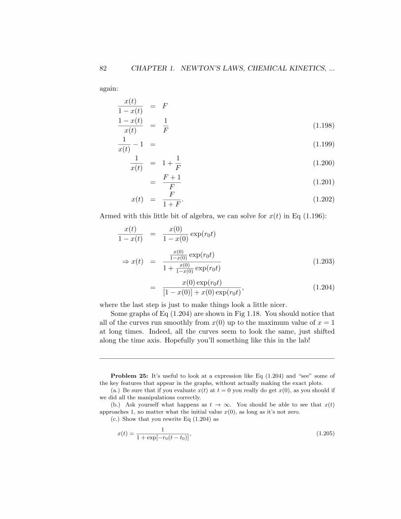
82 CHAPTER 1. NEWTON’S LAWS, CHEMICAL KINETICS, ...
again:
x(t)
1− x(t)= F
1− x(t)
x(t)=
1
F(1.198)
1
x(t)− 1 = (1.199)
1
x(t)= 1 +
1
F(1.200)
=F + 1
F(1.201)
x(t) =F
1 + F. (1.202)
Armed with this little bit of algebra, we can solve for x(t) in Eq (1.196):
x(t)
1− x(t)=
x(0)
1− x(0)exp(r0t)
⇒ x(t) =
x(0)1−x(0) exp(r0t)
1 + x(0)1−x(0) exp(r0t)
(1.203)
=x(0) exp(r0t)
[1− x(0)] + x(0) exp(r0t), (1.204)
where the last step is just to make things look a little nicer.Some graphs of Eq (1.204) are shown in Fig 1.18. You should notice that
all of the curves run smoothly from x(0) up to the maximum value of x = 1at long times. Indeed, all the curves seem to look the same, just shiftedalong the time axis. Hopefully you’ll something like this in the lab!
Problem 25: It’s useful to look at a expression like Eq (1.204) and “see” some ofthe key features that appear in the graphs, without actually making the exact plots.
(a.) Be sure that if you evaluate x(t) at t = 0 you really do get x(0), as you should ifwe did all the manipulations correctly.
(b.) Ask yourself what happens as t → ∞. You should be able to see that x(t)approaches 1, no matter what the initial value x(0), as long as it’s not zero.
(c.) Show that you rewrite Eq (1.204) as
x(t) =1
1 + exp[−r0(t− t0)], (1.205)

1.5. SIMPLE CIRCUITS AND POPULATION DYNAMICS 83
0 2 4 6 8 10 12 14 16 18 200
0.1
0.2
0.3
0.4
0.5
0.6
0.7
0.8
0.9
1
r0 t
norm
aliz
ed p
opul
atio
n si
ze x
(t)
x(0) = 0.1
x(0) = 0.01
x(0) = 0.001
x(0) = 0.0001
Figure 1.18: Dynamics of population growth as predicted by Eq (1.204), the solution toEq (1.180). Time is measured in units of the growth rate r0 of small populations, and thepopulation size is normalized the “capacity” of the environment.
where t0 depends on the initial population. What does this mean about the growth curvesthat start with different values of x(0)?
Problem 26: As discussed in connection with the first laboratory and in Section1.1, an object moving through a fluid at relatively high velocities experiences a drag forceproportional to the square of its velocity. In the presence gravity this means that F = macan be written as
mdv
dt= −av2 +mg, (1.206)
where the velocity v is positive if the object is moving downwards, a is the drag coefficient,and g as usual is the acceleration due to gravity. As noted in the lectures, a similarequations can arise in chemical kinetics.
(a.) For any given system, the usual units of time, speed, etc. might not be verynatural. Perhaps there is some natural time scale t0 and a natural velocity scale v0 suchthat if we measure things in these units our equation will look simpler. Specifically,consider variables u ≡ v/v0 and τ ≡ t/t0. Show that by proper choice of t0 and v0 onecan make all the parameters (m, g, a) disappear from the differential equation for u(τ).
(b.) Solve the differential equation for u(τ). Does this function have a universalshape? Since we have gotten rid of all the parameters, is there anything left on whichthe shape could depend? If you need help doing an integral it’s OK to use a table (orperhaps an electronic equivalent), but you need to give references. Translate your resultsinto predictions about v(t).
(c.) Suppose that the initial velocity v(t = 0) is very close to the terminal velocityv∞ =
√mg/a. Show that your exact solution for v(t) is approximately an exponential
84 CHAPTER 1. NEWTON’S LAWS, CHEMICAL KINETICS, ...
decay back to the terminal velocity. Then go back to Eq (1.206) and write v(t) = v∞ +δv(t), and make the approximation that δv is small, and hence δv2 is even smaller and canbe neglected. Can you now show that this approximate equation leads to an exponentialdecay of δv(t), in agreement with your exact solution?
(d.) Explain the similarities between this problem and the population growth problemthat starts with Eq (1.180) and leads to the results in Fig 1.18. Can you make an exactmapping from one problem to the other?
What about synchronization? Cell growth and division is a cycle, andif this cycle runs like a clock then we can imagine getting all the clocksaligned so that the population of bacteria holds fixed for some length oftime, then doubles as all the cells proceed complete their cycle, then holdsfixed, doubles again, and so on. In fact, real single celled organisms losetheir synchronization if they don’t communicate. On the other hand, manyorganisms (including big complicated ones not so different from us) get syn-chronized by the seasons—we are all familiar with the nearly simultaneousappearance of all the baby birds at the same time of year. This suggests thatrather than writing down a differential equation, we should use one year asthe natural unit of time and ask how the number of organisms in one yearn(t) depends on the number that were there last year n(t− 1). Again if wejust think about growth we would argue that the number of new organismsif proportional to the number that we started with, hence
n(t) = Gn(t− 1), (1.207)
where G > 1 means that we are describing growth from season to seasonwhile G < 1 means that the population is dying out. It’s interesting that inthis case the seasonal synchronization doesn’t make any difference, becausethe solution still is exponential: n(t) = n(0)et/τ , where τ = 1/(lnG).
Problem 27: Verify that Eq (1.207) is solved by n(t) = n(0)et/τ , with τ = 1/(lnG).As a prelude to things which will be important in the next major section of the course,consider a population in which some fraction of the organisms wait for two seasons toreproduce, so that
n(t) = G1n(t− 1) +G2n(t− 2). (1.208)
Can you still find a solution of the form n(t) ∝ et/τ? If so, what is the equation thatdetermines the value of the time constant τ?
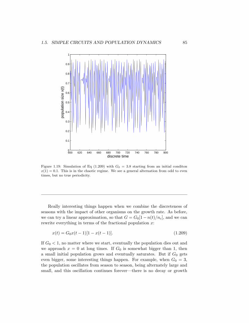
1.5. SIMPLE CIRCUITS AND POPULATION DYNAMICS 85
600 620 640 660 680 700 720 740 760 780 8000
0.1
0.2
0.3
0.4
0.5
0.6
0.7
0.8
0.9
1
discrete time
popu
latio
n si
ze x
(t)
Figure 1.19: Simulation of Eq (1.209) with G0 = 3.8 starting from an initial conditonx(1) = 0.1. This is in the chaotic regime. We see a general alternation from odd to eventimes, but no true periodicity.
Really interesting things happen when we combine the discreteness ofseasons with the impact of other organisms on the growth rate. As before,we can try a linear approximation, so that G = G0[1−n(t)/nc], and we canrewrite everything in terms of the fractional population x:
x(t) = G0x(t− 1)[1− x(t− 1)]. (1.209)
If G0 < 1, no matter where we start, eventually the population dies out andwe approach x = 0 at long times. If G0 is somewhat bigger than 1, thena small initial population grows and eventually saturates. But if G0 getseven bigger, some interesting things happen. For example, when G0 = 3,the population oscillates from season to season, being alternately large andsmall, and this oscillation continues forever—there is no decay or growth

86 CHAPTER 1. NEWTON’S LAWS, CHEMICAL KINETICS, ...
to a steady state. When G0 = 3.5, there is an oscillation with alternatingseasons of large and small population, but it takes a total of four seasonsbefore the population repeats exactly. We say that at G0 = 3 we observe a“period 2” oscillation, and at G0 = 3.5 we observe a “period 4” oscillation. Ifwe keep increasing G0 we can observe period 8, period 16, ... all the powersof 2 (!). The transitions to longer and longer periods come more quicklyas G0 increases, until we exceed a critical value of G0 and the trajectoriesx(t) start to look completely random, even though they are generated bythe simple Eq (1.209); see Fig 1.19.
Problem 28: Write a program to generate the trajectories x(t) that are predicted byEq (1.209). Run this program, exploring different values of G0, and verify the statementsmade in the previous paragraph. In particular, try starting with different initial conditionsx(0), and see whether the solutions are “attracted” to some simple for at long times, orwhether trajectories that start with slightly different values of x(0) end up looking verydifferent from each other. Does this dependence on initial conditions vary with the value ofG0? Can you see what this might have to do with the problem of predicting the weather?
The random looking trajectories of Fig 1.19 are called chaotic, andthe discovery that such simple deterministic equations can generate chaoschanged completely how we look at the dynamics of the world around us.What is remarkable is that the surprising properties of this simple equation(which you can rediscover for yourself even with a pocket calculator) areprovably the properties of a broad class of equations, and one can observethe sequence of period doublings and the resulting chaos in real physicalsystems, matching quantitatively the predictions of the simple model to keyfeatures of the data.
This has been a scant introduction to a rich and beautiful subject. Pleaseask for more references if you are intrigued.
1.6 The complexity of DNA sequences
The native form of DNA is the famous double helix proposed by Watson andCrick in 1953. Most of the essential properties of DNA are inherent in itschemical structure. DNA is a polymer, that is a molecule constructed as achain of (almost) repeating subunits. In particular, DNA is a high polymer,

1.6. THE COMPLEXITY OF DNA SEQUENCES 87
with huge numbers of the these subunits—in the human genome, there areindividual DNA molecules that are 50 to 250 million units long, so that if wecould stretch out these single molecules they would have lengths on the orderof a meter or more. A strand is comprised of a covalent sugar-phosphatebackbone, on which reside four chemically different structure called “bases,”namely adenine (A), guanine (G), cytosine (C) and thymine (T). The twostrands are held together by non–covalent hydrogen bonds between pairs ofbases: A only pairs with T and G only pairs with C. The two strands areopposite in chemical orientation; by convention, sequences are read from theso–called 5’ end.6 If we think of one strand as having the base sequence 5’AGGCTC 3’ then the other, complementary strand in native DNA will havethe sequence 5’ GAGCCT 3’.
Figure 1.20: Three views of base pairing in the double helix.
Let us consider the relative strengths of the bonds in DNA. The strongestare the covalent bonds, such as the carbon–carbon, carbon–oxygen, andoxygen–phosphorus bonds that make up the backbone of each strand andbetween the backbone and the bases. Weaker bonds, called hydrogen bonds,connect the two strands. One can see, in the diagram of the base pairs, thathydrogen bonds consist of a hydrogen atom that is shared between a partially
63’ and 5’ refer to the conventional numbering scheme for the carbon atoms in thesugar residues along the backbone.

88 CHAPTER 1. NEWTON’S LAWS, CHEMICAL KINETICS, ...
negatively-charged atom on a base in one strand and a partially positively-charged atom on the other. It should also be clear that the base-pairingrules are the consequence of the chemical features that allow the formationof stable hydrogen bonds only between A and T or C and G. It is also worthnoting that A and G (called “purines”) are bigger than C and T (called“pyrimidines”). Each of the basepairs has one large base (purine) and onesmall one (pyrimidine) such that when one basepair is stacked on another inthe double-helical structure, the distance across them is the same, providinga constant inter-chain backbone distance. Making paper cutouts of the basepairs and trying to superimpose them (as Jim Watson describes he did in1952) makes the structural constraints clear even to non–chemists.
In general, when we raise the temperature, molecules can access stateswith higher energy. In particular, since forming a bond lowers the energy, weexpect that bonds will break as we heat things up. The weakest bonds breakfirst, so at reasonable temperatures hydrogen bonds will be broken, while itwould take much higher temperatures to break covalent bonds. Thus, as weheat up a DNA molecule, the hydrogen bonds that connect the two strandsof the double helix break, but the strands themselves remain intact—thetwo strands of the double helix begin to separate, the double stranded DNAmolecule becomes two single stranded molecules, and the DNA is said to be“denatured.” Crucially, the two single stranded molecules that emerge froma double helix after denaturation have a special relationship: their nucleotidesequences are different, but complementary. Each single strand contains thesame genetic information, which becomes clear when one thinks about whathappens when each of the strands is copied using the base-pairing rules:copying either of the complementary strands will produce exactly the samedouble helix.
In the double–helical structure of DNA, each successive base pair isstacked on the previous one. The stacking is energetically favorable, andthis contributes to the stability of the DNA structure. The stacking hasanother consequence: the optical properties of the DNA in the ultravioletregion of the spectrum are changed. When the bases are freer to tumble andturn in solution, they absorb more UV light than when there are stackedand conformationally constrained. This works, more or less, base by base,so if we monitor the absorption of light at a wavelength of λ = 260 nm weare essentially counting the fraction of bases that are stacked. If the onlyavailable states are single stranded (denatured) and double stranded, thenthis absorption A260 measures the fraction of denatured molecules, as in Fig1.21; this is a very convenient way to follow DNA denaturation experimen-tally. As DNA denatures, the UV absorbance (A260) rises, until it reaches a
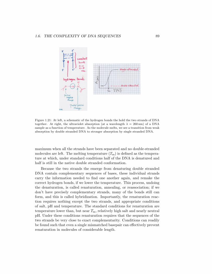
1.6. THE COMPLEXITY OF DNA SEQUENCES 89
Figure 1.21: At left, a schematic of the hydrogen bonds the hold the two strands of DNAtogether. At right, the ultraviolet absorption (at a wavelength λ = 260 nm) of a DNAsample as a function of temperature. As the molecule melts, we see a transition from weakabsorption by double stranded DNA to stronger absorption by single stranded DNA.
maximum when all the strands have been separated and no double-strandedmolecules are left. The melting temperature (Tm) is defined as the tempera-ture at which, under standard conditions half of the DNA is denatured andhalf is still in the native double stranded conformation.
Because the two strands the emerge from denaturing double strandedDNA contain complementary sequences of bases, these individual strandscarry the information needed to find one another again, and remake thecorrect hydrogen bonds, if we lower the temperature. This process, undoingthe denaturation, is called renaturation, annealing, or reassociation; if wedon’t have precisely complementary strands, many of the bonds still canform, and this is called hybridization. Importantly, the renaturation reac-tion requires nothing except the two strands, and appropriate conditionsof salt, pH and temperature. The standard conditions for renaturation aretemperature lower than, but near Tm, relatively high salt and nearly neutralpH. Under these conditions renaturation requires that the sequences of thetwo strands be very close to exact complementarity. Conditions can readilybe found such that even a single mismatched basepair can effectively preventrenaturation in molecules of considerable length.
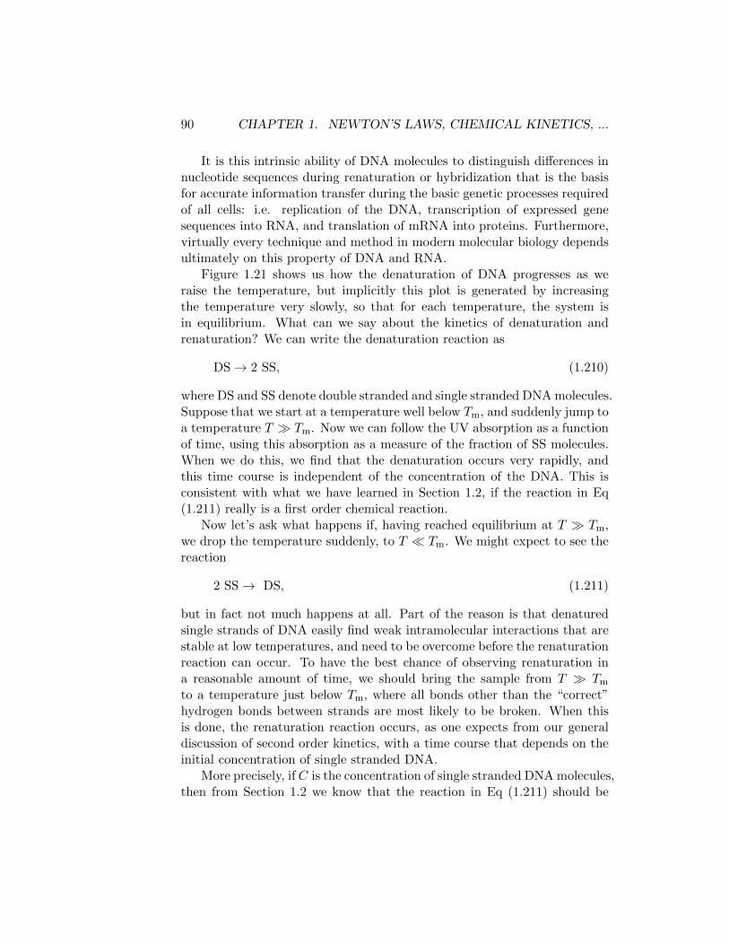
90 CHAPTER 1. NEWTON’S LAWS, CHEMICAL KINETICS, ...
It is this intrinsic ability of DNA molecules to distinguish differences innucleotide sequences during renaturation or hybridization that is the basisfor accurate information transfer during the basic genetic processes requiredof all cells: i.e. replication of the DNA, transcription of expressed genesequences into RNA, and translation of mRNA into proteins. Furthermore,virtually every technique and method in modern molecular biology dependsultimately on this property of DNA and RNA.
Figure 1.21 shows us how the denaturation of DNA progresses as weraise the temperature, but implicitly this plot is generated by increasingthe temperature very slowly, so that for each temperature, the system isin equilibrium. What can we say about the kinetics of denaturation andrenaturation? We can write the denaturation reaction as
DS→ 2 SS, (1.210)
where DS and SS denote double stranded and single stranded DNA molecules.Suppose that we start at a temperature well below Tm, and suddenly jump toa temperature T � Tm. Now we can follow the UV absorption as a functionof time, using this absorption as a measure of the fraction of SS molecules.When we do this, we find that the denaturation occurs very rapidly, andthis time course is independent of the concentration of the DNA. This isconsistent with what we have learned in Section 1.2, if the reaction in Eq(1.211) really is a first order chemical reaction.
Now let’s ask what happens if, having reached equilibrium at T � Tm,we drop the temperature suddenly, to T � Tm. We might expect to see thereaction
2 SS→ DS, (1.211)
but in fact not much happens at all. Part of the reason is that denaturedsingle strands of DNA easily find weak intramolecular interactions that arestable at low temperatures, and need to be overcome before the renaturationreaction can occur. To have the best chance of observing renaturation ina reasonable amount of time, we should bring the sample from T � Tm
to a temperature just below Tm, where all bonds other than the “correct”hydrogen bonds between strands are most likely to be broken. When thisis done, the renaturation reaction occurs, as one expects from our generaldiscussion of second order kinetics, with a time course that depends on theinitial concentration of single stranded DNA.
More precisely, if C is the concentration of single stranded DNA molecules,then from Section 1.2 we know that the reaction in Eq (1.211) should be

1.6. THE COMPLEXITY OF DNA SEQUENCES 91
described by
dC
dt= −kC2, (1.212)
where k is the second order rate constant that characterizes this reaction.We recall from Eq (1.95) that the solution to this equation is
C(t)/C0 =1
1 + kC0t, (1.213)
where C0 is the initial concentration of single stranded DNA. This fits thedata from experiments like those shown in Fig 1.22, and makes the importantprediction that the time scale of the reaction should be inversely proportionalto the initial concentration, and this is easily verified.
Figure 1.22: Time course of the DNA renaturation reaction. We start at a temperatureT > Tm, and jump to T < Tm.
To be more quantitative, we need to think about how we defien andmeasure concentration. For a polymer like DNA, there are two possibledefinitions:
Definition 1: the number of polymer molecules per unit volumeDefinition 2: the number of monomer subunits per unit volume.
Obviously, for DNA molecules containing thousands or millions of nucleotidesubunits, these two definitions give very different numbers. Optical meth-ods, such as absorption of UV light depend on concentration of the subunits

92 CHAPTER 1. NEWTON’S LAWS, CHEMICAL KINETICS, ...
(it is the bases that absorb the light) and thus the conventional assessmentof DNA or RNA concentration is by Definition 2, not Definition 1. Considera collection of 109 large DNA molecules in 1 ml of solution, with averagelength 10, 000 nucleotides (these molecules are referred to as a 10 kilobase-pair (kb) in length). The total number of bases available to absorb UVlight will be 10, 000 × 109 × 2 = 2 × 10¹³ bases. This solution will absorba readily measureable amount of UV light. If we were to cut the moleculesin this solution into pieces of about 1 kb, we would have ten times as manymolecules, and thus, by Definition 1 the concentration would change ten-fold. But the number of bases would remain the same, and by Definition 2(and by measurement using UV absorption) the concentration would remainthe same.
Nucleic acid biochemists and molecular biologists normally use Definition2, because that is what we measure. However, in doing molecular manip-ulations (such as DNA cloning), it is not the size of the molecules that isimportant, but the number of ends. Consider the simplest of all cloningsteps: joining one molecule of DNA to another. In this case, we need toknow the concentration of ends, regardless of the size of the individual DNAmolecules, i.e. the DNA concentration by Definition 1. Knowing this re-quires more than what we can learn from UV absorption—we need to knowalso the sizes of the molecules.
There is also one more complication in analyzing DNA renaturation—but this complication becomes a method for learning something about theDNA molecules themselves. If we take identical DNA molecules, e.g. from apopulation of bacterial DNA viruses, and denature them, we will get exactlytwo kinds of single-stranded molecules each of which is the complement ofthe other. In the following discussion we will call these W (for Watson) andC (for Crick). They have the same information, but different sequences,and their chemical orientation is opposite. Suppose, however, that we wereto fragment the DNA into little pieces, and then denature them? This willmake things a lot more complicated, because now we have many differentkinds of molecules. In Fig 1.23, W is blue, and C is red, and the arrowsindicate their relative chemical orientation. Fragmentation will generatea great variety of different double-stranded DNA molecules (a, b, c, d, e,etc.). When these are denatured, there will be twice as many single-strandedmolecules in the solution. Some of them are still complementary, but if thenumber of fragments is large the probability that any two molecules taken atrandom are complementary becomes extremely small. Specifically, aw canrenature and form a double helix only with ac because all the others havedifferent sequences. Yet the whole ensemble of molecules should eventually

1.6. THE COMPLEXITY OF DNA SEQUENCES 93
renature, because each single-stranded fragment has a complement in thesolution because of the way it was made. But the process will be slow.
Figure 1.23: Schematic of an experiment in which we fragment and then denature DNA.
But suppose that the original virus contained three copies of the samesequence in its DNA. After fragmentation and denaturation, we would have3 times as many copies per unit volume of the single stranded moleculesaw, ac, bw, bc, etc. and time course of the renaturation reaction wouldbe three times faster. In other words, the sequence complexity matters,and, conversely, it should be possible to infer sequence complexity from thekinetics of renaturation of fragmented and denatured DNA molecules.
In the following examples,7 we will make use of the single double strandedDNA molecules that comprise the genomes of bacteriophages T4 and T7,both of which are viruses that grow on the common bacterium Escherichiacoli. Preparations of T4 yield single DNA molecules about 110 kb in length;T7 DNA contains molecules about 40 kb in length. Neither molecule con-tains repeated sequences, and T4 and T7 are not homologous—they haveentirely different nucleotide sequences. We can see the effect of concentrationdirectly if we take just T7 DNA, fragment and denature it, and then rena-ture it at two different concentrations of total DNA (10µg/ml and 30µg/ml,
7Our discussion here follows Genetics: Analysis of Genes and Genomes, Seventh Edi-tion D Hartl & E Jones (Joens & Bartlett, Sudbury MA, 2009).

94 CHAPTER 1. NEWTON’S LAWS, CHEMICAL KINETICS, ...
Figure 1.24: At left, renaturation kinetics of T7 DNA, at two different initial concentra-tions. At right, the corresponding experiment with a mixture of T7 and T4 DNA. Theintial concentrations of the two species of DNA are the same, as measured by A260, whichmeans that we have the sme number of bases from each species. Because the two genomesare of different lengths, this corresponds to different numbers of single stranded molecules.
measured as A260). As we expect, the higher concentration renatures muchfaster because if we have N copies of the single-stranded fragments aw and ac
at 10µg/ml, we will have 3N copies of them at 30µg/ml. If we now make amixture of equal amounts (again determined by A260) of T4 and T7 DNAs,fragmented and denatured, and do a renaturation experiment with them,we find that they behave independently. Indeed, even with this relativelymodest difference in sequence complexity (40kb versus 110kb) we can see avery robust separation of the half times for renaturation of the two DNAs;indeed, most of the T7 DNA has renatured before the T4, as predicted.
Formally, sequence complexity is defined as the longest non-repetitivesequence in a genome. For bacteriophages T4 and T7, it is the entire genome(i.e. 110 kb and 40 kb, respectively). For simple sequences like
5’TTTTTTTTTT 5’GCGCGCGCGC 5’AGTAGTAGTAGT3’AAAAAAAAAA 3’CGCGCGCGCG 3’TCATCATCATCA
the complexity is 1, 2 or 3 basepairs, respectively. Having established abovethat renaturation kinetics is connected to complexity we can seek to infer

1.6. THE COMPLEXITY OF DNA SEQUENCES 95
Figure 1.25: C0t curves for several samples of DNA, comparing with the known numberof base pairs in each molecule.
complexity from the kinetics. Equation (1.213) above provides a charac-teristic quantity C0t1/2 which is equal to the reciprocal of the second-orderrenaturation constant k. The relationship between C0t1/2 (in units of Molar–sec) and complexity (in nucleotide pairs) can be calibrated experimentallyby renaturing fragmented single-stranded preprations derived from double-stranded DNA molecules whose complexity is known by other means. Thisempirical calibration yields the generalization that under standard renatu-ration conditions the complexity N = 5× 10⁵C0t1/2/(M · s), as in Fig 1.25.
The genomes of many organisms contain repetitive DNA sequences. No-tably, mammalian genomes (which are many orders of magnitude largerthan the genomes of viruses and bacteria) consist of about equal amountsof single-copy and repetitive DNA sequences. The repeated sequences canbe short, meaning that some of these sequences are present in thousands tomillions of copies. The numbers and sizes of repeated sequences can readilybe estimated from renaturation kinetics: the principle is exactly the sameas the example given above of a mixture of T4 and T7 DNAs. The exampleshown here is typical for higher eukaryotic genomic DNAs: about 20 per-cent of the total DNA is highly repetitive DNA comprised of low complexitysequences, about 30 percent is middle-repetitive DNA of higher complex-ity, and about 50% is single-copy, typically with a complexity of about 109
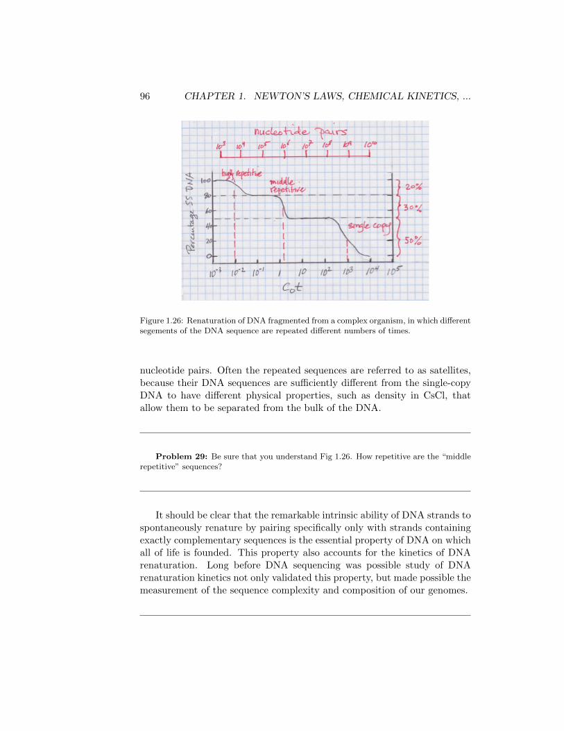
96 CHAPTER 1. NEWTON’S LAWS, CHEMICAL KINETICS, ...
Figure 1.26: Renaturation of DNA fragmented from a complex organism, in which differentsegements of the DNA sequence are repeated different numbers of times.
nucleotide pairs. Often the repeated sequences are referred to as satellites,because their DNA sequences are sufficiently different from the single-copyDNA to have different physical properties, such as density in CsCl, thatallow them to be separated from the bulk of the DNA.
Problem 29: Be sure that you understand Fig 1.26. How repetitive are the “middlerepetitive” sequences?
It should be clear that the remarkable intrinsic ability of DNA strands tospontaneously renature by pairing specifically only with strands containingexactly complementary sequences is the essential property of DNA on whichall of life is founded. This property also accounts for the kinetics of DNArenaturation. Long before DNA sequencing was possible study of DNArenaturation kinetics not only validated this property, but made possible themeasurement of the sequence complexity and composition of our genomes.
1.6. THE COMPLEXITY OF DNA SEQUENCES 97
Problem 30: The total genomic DNA of a newly-discovered species of newt contains1200 copies of a 2 kb repeated sequence, 300 copies of a 6 kb repeated sequence as well as3000 kb of single-copy DNA.
(a.) What will the “Cot curve” (i.e. plot of the fraction of DNA remaining single-stranded vs. C0t) look like? Be sure to label the axes, and indicate the fractional contri-bution of the different kinds of DNA.
(b.) Devise a procedure to prepare reasonably pure samples of the three kinds ofDNA. Explain how you would calculate the times of annealing required for each step.

98 CHAPTER 1. NEWTON’S LAWS, CHEMICAL KINETICS, ...
Chapter 2
Resonance and response
In this section of the course we begin with a very simple system—a masshanging from a spring—and see how some remarkable ideas emerge. We willsee, for example, that it is useful to use imaginary numbers to describe realthings. Most importantly, we will understand how to describe the way sys-tems respond to small perturbations, and this turns out to be very general.Following this path, our intuitive notions that something is stable or unsta-ble can be given precise mathematical formulations. We will take all of thisfar enough to see how the ideas can be used in describing complex biologicalphenomena, from the switches that control the expression of genes to theelectrical impulses that carry information throughout the brain.
2.1 The simple harmonic oscillator
We have been talking about mechanics problems in which there is (a) noforce, (b) a constant force, or (c) a force proportional to the velocity. Theother “simple” case is when the force is proportional to the position, as isthe case when we stretch a spring. Notice that we do these simple cases notbecause we want to torture you with simplified problems that are irrelevantin nature, but rather because, from our discussion of Taylor series and “laws”like Hooke’s law or Ohm’s law, we know that these simple cases are theleading approximations to more complex situations. Hopefully this will beclear before too long.
So, let us consider, as in Fig 2.1, a mass M hanging at the end of aspring with stiffness κ; you can imagine either that the system lies on itsside, or that we ignore the force of gravity. If we measure the position x of
99

100 CHAPTER 2. RESONANCE AND RESPONSE
Figure 2.1: A mass M bound by a spring of stiffness κ, as in Eq (2.2).
the spring in coordinates such that the equilibrium position is x = 0,1 thenthe force on the mass is
F = −κx. (2.1)
In this problem F = ma therefore corresponds to the differential equation
Md2x(t)
dt2= −κx(t). (2.2)
This is an example of a system usually called a simple harmonic oscillator,for reasons that I hope will become clear as we go along.
We will see, remarkably, that to give a full solution it is natural to writethe real displacement of the mass in terms of complex numbers. Once weunderstand how to do this we will see that we can generate a rather complete
1You should convince yourself that we can include gravity just by redefining the zeropoint on the x axis.
2.1. THE SIMPLE HARMONIC OSCILLATOR 101
view of the problem. It is important that the seemingly special problem ofthe harmonic oscillator comes up in many different guises.
Take a moment to think about what Eq (2.2) means. We can draw thefunction x(t). At every point on the graph we can compute the local slope(the derivative or velocity) and then from this new graph we can computethe local slope again (the acceleration). Up to constants, Eq. (2.2) is tellingus that this function we obtain by differentiating twice is just the negativeof the original function x(t)—if we graph the second derivative and flip itupside down it should overly the original graph. Obviously not all functionshave this property, and indeed you will learn in your math courses the veryimportant theorem that (once we specify the initial conditions) the functionswhich satisfy differential equations are unique. This is crucial because itmeans that if we find a solution of a differential equation that satisfies allthe initial conditions, even if we have to guess the form of the solution, thenwe’re done, because there can’t be any other solutions.
Equation (2.2) has a very simple form. Notice that there are two deriva-tives, so we say it is a second order equation. Further, the equation is linear,which means all the terms are proportional to x. The fact that equation islinear implies that the sum of two solutions is also a solution. This is asubtle idea, and we will come back to it. Finally, all the coefficients whichappear in the equation are constants, with no explicit dependence on time.While we may not know how to solve all differential equations, we’ll makea lot of progress on this important special class.
As noted previously, the best way to solve a differential equation is toask someone who knows the answer. In this case, you know the answer fromyour calculus course. Recall that
d
dtsin(ωt) = ω cos(ωt) (2.3)
d
dtcos(ωt) = −ω sin(ωt). (2.4)
Then if we take two derivatives we have
d2
dtsin(ωt) =
d
dt[ω cos(ωt)] = −ω2 sin(ωt) (2.5)
d2
dtcos(ωt) =
d
dt[−ω sin(ωt)] = −ω2 cos(ωt). (2.6)
Thus, sine and cosine have the properties of the function that we are lookingfor: when you differentiate twice, you get back something proportional tothe function itself, with a minus sign.
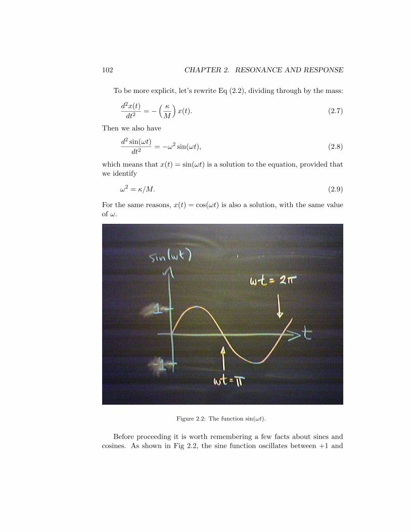
102 CHAPTER 2. RESONANCE AND RESPONSE
To be more explicit, let’s rewrite Eq (2.2), dividing through by the mass:
d2x(t)
dt2= −
( κM
)x(t). (2.7)
Then we also have
d2 sin(ωt)
dt2= −ω2 sin(ωt), (2.8)
which means that x(t) = sin(ωt) is a solution to the equation, provided thatwe identify
ω2 = κ/M. (2.9)
For the same reasons, x(t) = cos(ωt) is also a solution, with the same valueof ω.
Figure 2.2: The function sin(ωt).
Before proceeding it is worth remembering a few facts about sines andcosines. As shown in Fig 2.2, the sine function oscillates between +1 and
2.1. THE SIMPLE HARMONIC OSCILLATOR 103
−1; when the time t shifts by an amount T such that ωT = 2π, the functionhas the same value. We say that T = 2π/ω is the period of the oscillationand f = 1/T = ω/2π is the frequency. Sometimes we are sloppy and referto ω as the frequency.
Problem 31: When a 50 kg person sits on top of a car, the car body moves downtoward the ground by 3 inches. The car body itself weighs one ton.
(a.) What is the effective stiffness of the spring which supports the weight of the car?Use some useful set of units!
(b.) The stiffness comes from the shock absorbers. Suppose that there is no viscosityor damping in the shocks. Then if you are sitting on top of the car and suddenly jumpoff, the height of the car body should oscillate. What is the oscillation frequency?
What we have found is that x(t) = sin(ωt) is “a solution” of the differ-ential equation that encapsulates F = ma for this system, and we have alsofound that x(t) = cos(ωt) is “a solution.” But have we found “the solution”?What do we mean by this? Why is there more than one solution?
Let’s step back from the particular equations and think more generally.As emphasized by Laplace, Newtonian mechanics presents us with a dra-matic view of the world in which, given the initial conditions, we can solvethe differential equations describing the motion of all the relevant objectsand hence predict the future with, it would seem, complete certainty. Obvi-ously this depends on the differential equations having unique solutions—ifwe claim to be able to predict the trajectory of a falling object startingwith F = ma, then this equation had better have a unique solution oncewe specify all the initial conditions. If the solutions weren’t unique, thenmaybe each time we drop a ball something different would happen (!).
So the correct statement is that solutions of the differential equationsare unique once we specify all the initial conditions. How many initialconditions are there? We saw in simple cases that we needed to specify theinitial position and the initial velocity in order to integrate the equations ofmotion, and this is quite general. So when we talk about “a solution” wemean a solution that is consistent with some set of initial conditions; “thesolution” means the solution consistent with the initial conditions in ourparticular physical setting.
What we might be able to do, and indeed what we might hope to do, is towrite down a solution that has parameters, and show that by setting these
104 CHAPTER 2. RESONANCE AND RESPONSE
parameters we can be consistent with any set of initial conditions. Thenwhat we really have is a family of solutions, and at this point we really aredone with our problem—we have a whole family of functions x(t), each ofwhich solves the differential equation, and by picking the right member ofthis family we can agree with the initial position and velocity of the particle.
You have already seen this idea of families of solutions in the simplestcase of zero force. Recall that in this case the position as a function of timeis given by x(t) = x(0) + v(0)t. This function describes a straight line whenwe plot x vs t, but this straight line can have any slope [depending on v(0)]and any intercept [depending on x(0))]. So really we have a family of lines,all of which solve the differential equation F = ma, but to pick one of themwe need to know the initial position and initial velocity of the particle.
Our example of the mass on a spring is a little more complicated thanthe case of zero force, but again simpler than it could be. The simplicityhere is that the equation is linear. That is, if we look at the terms in
d2x(t)
dt2= −
( κM
)x(t), (2.10)
we see that both terms are proportional to x, and this is what we meanby linearity. There is a special consequence of linearity, and this is thesuperposition of solutions. Suppose that we have found one solution of ourequation, a solution consistent with one set of initial conditions, and let’scall this solution x1(t). Suppose also that we have found another solution,consistent with a different set of initial conditions, and let’s call this x2(t).What is remarkable about linear equations is that now we can constructanother function, x(t) = Ax1(t) + Bx2(t), and this is also a solution, onewhich matches yet a third set of initial conditions. To see this, we can justcheck by substitution:
d2x(t)
dt2=
d2[Ax1(t) +Bx2(t)]
dt2(2.11)
= Ad2x1(t)
dt2+B
d2x2(t)
dt2(2.12)
= −( κM
)Ax1(t)−
( κM
)Bx2(t) (2.13)
= −( κM
)[Ax1(t) +Bx2(t)] (2.14)
= −( κM
)x(t), (2.15)
where in going from Eq (2.12) to (2.13) we use the fact that x1(t) andx2(t) each are solutions, which means that d2x1(t)/dt2 = −(κ/M)x1(t),

2.1. THE SIMPLE HARMONIC OSCILLATOR 105
and similarly for x2(t). Thus we see that we can use these two solutionsto construct a whole family of new solutions just by linear combination.Notice that this argument doesn’t depend on knowing the exact form of thesolutions, since all we use is the linearity of the equation.
Why is this so important? By combining two solutions we generate awhole family of solutions, but these have two parameters, A and B. But weknow that once we match the initial position and initial velocity, the solutionis unique. Thus if we can adjust A and B to match the initial position andvelocity, we are done: We have constructed the whole family of solutionsthat we need.
Let’s see how this plays out with our particular example. We have seenthat one possible solution to our problem is x1(t) = sin(ωt), and another isx2(t) = cos(ωt). Thus we can construct the linear combination
x(t) = A sin(ωt) +B cos(ωt), (2.16)
and this should also be a solution. Now because sin(0) = 0 and cos(0) = 1,we can see that
x(0) = B. (2.17)
If we differentiate to find the velocity,
v(t) ≡ dx(t)
dt=d[A sin(ωt) +B cos(ωt)]
dt(2.18)
= Aω cos(ωt)−Bω sin(ωt), (2.19)
so that
v(0) = Aω. (2.20)
So in this case the relationship between the coefficients A,B and the initialconditions is quite simple:
A = x(0), (2.21)
B =v(0)
ω. (2.22)
Let’s summarize what we have done:
• The differential equation F = ma that describes a mass M hangingfrom a spring of stiffness κ is
Md2x(t)
dt2= −κx(t). (2.23)
106 CHAPTER 2. RESONANCE AND RESPONSE
• Solutions to this equation include
x1(t) = sin(ωt), and (2.24)
x2(t) = cos(ωt), (2.25)
where we have to choose
ω =
√κ
M. (2.26)
• Because Eq (2.23) is linear, we can combine these solutions to form afamily of solutions
x(t) = A sin(ωt) +B cos(ωt). (2.27)
• Finally, we can adjust the constants A and B to match the initialposition and initial velocity:
x(t) =v(0)
ωsin(ωt) + x(0) cos(ωt). (2.28)
You might want to play with this solution a little bit, plotting it and seeingwhat it looks like. We will come back and do this, but first let’s look at avery different way of finding these solutions, one which is much more general.
Problem 32: Show that you can rewrite Eq (2.28) in the form
x(t) = A cos(ωt+ φ), (2.29)
where A is called the amplitude and φ is called the phase of the oscillation. Draw (byhand, not with the computer!) the function x(t), being careful to show units on both axesand marking the point where t = 0. Indicate the features of the graph that correspond tothe amplitude, phase and frequency.
Recall our (only partly) joking idea that there are three ways to solvea differential equation. What we did last time was to ask someone whoknew the answer—you knew the properties of sine and cosine from yourcalculus course, and you could see that this is what you needed to solvethe equation. But you remember that when we looked at a mass moving
2.1. THE SIMPLE HARMONIC OSCILLATOR 107
through a fluid, or first order chemical kinetics, we also encountered lineardifferential equations with constant coefficients. The simplest equation inthis class of interest is of the form
dx(t)
dt= ax(t), (2.30)
where a is a constant. We found that we could solve this by guessing asolution of the form x(t) = Aeλt, and then everything works if we set λ = aand A = x(0). Can we use this same “guess and check” method (the secondof the three methods) to solve the mass–spring problem?
To get started, suppose that we have a second order differential equationwhich I’ll write in the suggestive form
d2x
dt2= a2x. (2.31)
You can see that x(t) = Aeat still is a solution. In fact, the exponentialfunction has the property that differentiating is just multiplication by aconstant:
d
dtexp(λt) = λ exp(λt) (2.32)
d2
dt2exp(λt) = λ2 exp(λt) (2.33)
· · · (2.34)
dn
dtnexp(λt) = λn exp(λt). (2.35)
Thus if we try to solve Eq. (2.31) by guessing a solution of the form x(t) ∝exp(λt), we see that this will work if (and only if)
λ2 = a2, (2.36)
which means that λ = ±a. Now we use the idea of combining solutions togenerate a whole family:
x(t) = A exp(at) +B exp(−at), (2.37)
and we have to set the two constants A and B by fixing the initial positionand initial velocity as in the discussion above. Again there are two arbitraryconstants because we are looking at a second order equation.
All this is fine, but how do we use it to solve the equation we really areinterested in, for the mass on a spring? As before we can write this as
d2x(t)
dt2=[− κ
M
]x(t). (2.38)

108 CHAPTER 2. RESONANCE AND RESPONSE
This is just like Eq. (2.31) if we identify a2 = −κ/M . To put it anotherway, we can try to solve Eq. (2.38) by guessing that x(t) = A exp(λt), andif we substitute we find
d2
dt2A exp(λt) =
[− κ
M
]A exp(λt) (2.39)
Aλ2 exp(λt) =[− κ
M
]A exp(λt) (2.40)
λ2 =[− κ
M
](2.41)
λ2 +κ
M= 0. (2.42)
Thus we see that λ obeys a quadratic equation, although a very simple onein this case. There are two solutions, and this is related to the fact that thisis a second order equation:
λ = ±√− κ
M. (2.43)
Now we see something strange, namely that our solution is the square rootof a negative number.
For most of you, at some early point in your education you were taughtabout square roots, and your teachers explained that you can’t take thesquare root of a negative number. Then at some point in high school, per-haps, they told you that it’s OK, but it gets a special name: i =
√−1 is the
unit imaginary number. So, we have the result that the solution of F = mafor this problem must be of the form
x(t) = A exp(+iωt) +B exp(−iωt). (2.44)
It’s absolutely fantastic that imaginary numbers appear in the solution to aphysics problem.
2.2 Magic with complex exponentials
We don’t really know what aspects of complex variables you learned about inhigh school, so the goal here is to start more or less from scratch. Feedbackwill help us to help you, so let us know what you do and don’t understand.Also, if something is not immediately clear you should work through exam-ples ... as usual.
The introduction to square roots in school often makes the point thatthe square root of a negative number is not defined, since after all when

2.2. MAGIC WITH COMPLEX EXPONENTIALS 109
we square a number we always get something positive. Then at some pointyou are told about imaginary numbers, where the basic object is i =
√−1.
It is not clear, perhaps, whether this is some sort of joke (calling them“imaginary” probably doesn’t help!). Here we are asking you to take thesethings very seriously.
Figure 2.3: From our local cafe.
Remember that when you first learned about negative numbers (a longtime ago ... ) there was some mystery about what you do when you add,multiply, etc.. In the end the answer is that the rules are the same, and youhave to apply them in a consistent way. This is true also for complex orimaginary numbers.

110 CHAPTER 2. RESONANCE AND RESPONSE
We begin by recalling that with x and y real numbers, we can form thecomplex number z = x+ iy. The object i is the square root of negative one,i =√−1. Then if we have two of these numbers
z1 = x1 + iy1 (2.45)
z2 = x2 + iy2 (2.46)
we can go through all the usual operations of arithmetic:
z1 + z2 ≡ (x1 + iy1) + (x2 + iy2) (2.47)
= (x1 + x2) + i(y1 + y2); (2.48)
z1 − z2 ≡ (x1 + iy1)− (x2 + iy2) (2.49)
= (x1 − x2) + i(y1 − y2); (2.50)
(z1)× (z2) ≡ (x1 + iy1)× (x2 + iy2) (2.51)
= x1x2 + x1(iy2) + iy1x2 + iy1(iy2) (2.52)
= x1x2 + i(x1y2 + x2y1) + (i2)y1y2 (2.53)
= x1x2 + i(x1y2 + x2y1)− y1y2 (2.54)
= x1x2 − y1y2 + i(x1y2 + x2y1), (2.55)
where in the second to last step we use the fact that i2 = −1. Note thatthis list leaves out division, which we’ll get back to in a moment.
One very useful operation that is new for complex numbers is called“taking the complex conjugate,” or “complex conjugation.” For every com-plex number z = x+ iy, the complex conjugate is defined to be z∗ = x− iy.Note that in elementary physics we usually use z∗ to denote the complexconjugate of z; in the math department and in some more sophisticatedphysics problems it is conventional to write the complex conjugate of z asz, but of course this is just notation. The crucial fact is that
z × z∗ ≡ (x+ iy)× (x− iy) (2.56)
= x2 + x(−iy) + iyx+ (i)(−i)y2 (2.57)
= x2 + i(−xy + yx)− (i2)y2 (2.58)
= x2 + y2. (2.59)
Often we write zz∗ = |z|2, just the way we write the length of a vector interms of its dot product with itself, ~x·~x = |~x|2. This is an important thingon its own, as we will see, but also it makes division a lot easier, which wedo now.

2.2. MAGIC WITH COMPLEX EXPONENTIALS 111
There is a trick, which is to clear the complex numbers from the denom-inator any time we divide:
z1
z2≡ (x1 + iy1)
(x2 + iy2)(2.60)
=z1
z2· z∗2
z∗2(2.61)
=z1z∗2
z2z∗2(2.62)
=z1z∗2
|z2|2(2.63)
=(x1x2 + y1y2) + i(y1x2 − x1y2)
x22 + y2
2
(2.64)
Problem 33: You should be able to add, subtract, multiply and divide these pairs ofcomplex numbers: (a) z1 = 3+4i, z2 = 4+3i. (b) z1 = 3+4i, z2 = 4−3i. (c) z1 = 7−9i,z2 = 27 + 12i. And you should be able to make up your own examples!
It is useful to think about a complex number as being a vector in a twodimensional space, as in Fig. 2.4. In this view, the x axis is the real part
Figure 2.4: Thinking of a com-plex number z = x+iy as a vec-tor in the x−y plane. This is of-ten called the “complex plane.”
112 CHAPTER 2. RESONANCE AND RESPONSE
and the y axis is the imaginary part, as is hinted when we write z = x+ iy.The length of the vector is
|z| ≡√x2 + y2 =
√|z|2 =
√zz∗, (2.65)
and the angle that this makes with the x axis is given by
θ = tan−1(yx
). (2.66)
In this notation,
z ≡ x+ iy (2.67)
=√x2 + y2
(x√
x2 + y2+ i
y√x2 + y2
)(2.68)
= |z|(cos θ + i sin θ). (2.69)
Now there is a very pretty thing, which is that if we multiply two complexnumbers, the magnitudes get multiplied and the angles just add:
z1 × z2 ≡ |z1|(cos θ1 + i sin θ1)× |z1|(cos θ1 + i sin θ1) (2.70)
= (|z1||z2|)[(cos θ1 cos θ2 − sin θ1 sin θ2)
+i(sin θ1 cos θ2 + sin θ1 cos θ1)] (2.71)
= (|z1||z2|)[cos(θ1 + θ2) + i sin(θ1 + θ2)], (2.72)
where in the last step we use the trigonometric identities
cos(θ1 + θ2) = cos θ1 cos θ2 − sin θ1 sin θ2 (2.73)
sin(θ1 + θ2) = sin θ1 cos θ2 + sin θ1 cos θ1. (2.74)
By the same reasoning, one finds
z1
z2=|z1||z2|
[cos(θ1 − θ2) + i sin(θ1 − θ2)]. (2.75)
Problem 34: Derive Eq (2.75). Also, in terms of these θ1 and θ2, what is thecondition for multiplying two complex numbers and getting a real answer?
2.2. MAGIC WITH COMPLEX EXPONENTIALS 113
We now have enough tools to figure out what we mean by the exponentialof a complex number. Specifically, let’s ask what we mean by eiφ. This is acomplex number, but it’s also an exponential and so it has to obey all therules for the exponentials. In particular,
eiφ1eiφ2 = ei(φ1+φ2) (2.76)
eiφ1
eiφ2= ei(φ1−φ2). (2.77)
You see that the variable φ behaves just like the angle θ in the geometrialrepresentation of complex numbers. Furthermore, if we take the complexnumber z = eiφ and multiply by its complex conjugate ...
eiφ ×[eiφ]∗
= eiφ ×[e−iφ
]= ei(φ−φ) = 1. (2.78)
Thus z = eiφ is a complex number with unit magnitude, and the angle inthe complex plane is just φ itself. Thus we see that
eiφ = cosφ+ i sinφ, (2.79)
which finally tells us what we mean by the complex exponential. Notice thatsomething like this formula had to be true because we know that the solutionto the differential equation for the harmonic oscillator can be written eitherin terms of sines and cosines or in terms of complex exponentials; sincesolutions are unique, these must be ralted to each other.
If you consider the special case of φ = π, then sinφ = 0 and cosφ = −1,leading to the famous Euler formula
eiπ + 1 = 0. (2.80)
This is a really beautiful equation, linking the mysterious transcendentalnumbers e and π with the imaginary numbers.
Problem 35: Derive the sum and difference angle identities by multiplying anddividing the complex exponentials. Use the same trick to derive an expression for cos(3θ)in terms of sin θ and cos θ.

114 CHAPTER 2. RESONANCE AND RESPONSE
Armed with these tools, let’s get back to our (complex) expression forthe trajectory,
x(t) = A exp(+iωt) +B exp(−iωt).
We now know that
exp(±iωt) = cos(ωt)± i sin(ωt), (2.81)
so at least it’s clear what our expression means.
To really solve the problem we need to match the initial conditions. Wecan see that
x(0) = A exp(iω · 0) +B exp(−iω · 0) (2.82)
= A+B, (2.83)
because e0 = 1, as always. Now in principle A and B are complex numbers,
A = ReA+ iImA (2.84)
B = ReB + iImB, (2.85)
while of course x(0) is the actual position of an object and thus has to be areal number. Let’s substitute and see how this works:
x(0) = A+B
= ReA+ iImA+ ReB + iImB (2.86)
= (ReA+ ReB) + i(ImA+ ImB). (2.87)
So we can match the reality of the initial condition (never mind its value!)only if
ImB = −ImA. (2.88)
Now we need to do the same thing for the initial velocity. By differenti-ating we see that
v(t) ≡ dx(t)
dt= A
deiωt
dt+B
de−iωt
dt= A(iω)eiωt +B(−iω)e−iωt, (2.89)
and hence
v(0) = iω(A−B). (2.90)

2.2. MAGIC WITH COMPLEX EXPONENTIALS 115
Substituting once again,
v(0) = iω(A−B)
= iω(ReA+ iImA− ReB − iImB) (2.91)
= iω(ReAReB) + (i)(iω)(ImA− ImB) (2.92)
= −ω(ImA− ImB) + iω(ReA− ReB). (2.93)
Notice that the real part of the velocity actually comes from the imaginaryparts of A and B. In order that the imaginary part of the velocity cancelmust have
ReA = ReB. (2.94)
Thus there really is only one independent complex number here, sincewe have shown that This might getting a bit
pedantic. Feedback is appre-ciated.A = ReA+ iImA (2.95)
B = ReA− iImA. (2.96)
When two complex numbers have this relationship—equal real parts andopposite imaginary parts—we say that they are complex conjugates, andthe notation for this is B = A∗. The operation ∗ simply replaces i by −i ina complex number, and clearly (z∗)∗ = z. Hence we can write our solution
x(t) = A exp(+iωt) +B exp(−iωt)= A exp(+iωt) +A∗ exp(−iωt). (2.97)
But note that exp(−iωt) = [exp(+iωt)]∗, so we can write
x(t) = A exp(+iωt) +A∗[exp(+iωt)]∗ (2.98)
= A exp(+iωt) + [A exp(+iωt)]∗. (2.99)
Now x(t) is the sum of a complex number and its complex conjugate. Butwhen we add a complex number to its complex conjugate, we cancel theimaginary part and double the real part:
z + z∗ = [Re(z) + iIm(z)] + [Re(z)− iIm(z)] (2.100)
= 2Re(z). (2.101)
Thus x(t), according to Eq (2.99) will be real at all times. This is good, ofcourse (!). Interestingly, we didn’t actually use this condition—all we didwas to be sure that we match the initial conditions, which of course are real.This is sufficient to insure that trajectories are real forever, which is nice.
116 CHAPTER 2. RESONANCE AND RESPONSE
To proceed further, we recall that all complex numbers can be writtenas
z = Rez + iImz (2.102)
= |z|(cosφ+ i sinφ) (2.103)
= |z| exp(iφ), (2.104)
where z is the magnitude of the complex number and φ is its phase,
|z| =√
[Re(z)]2 + [Im(z)]2 (2.105)
φ = tan−1
[Im(z)
Re(z)
]. (2.106)
If we do this rewriting of A,
A = |A| exp(iφA), (2.107)
then the trajectory becomes
x(t) = [|A| exp(iφA) exp(+iωt)] + [|A| exp(iφA) exp(+iωt)]∗ (2.108)
= [|A| exp(+iωt+ iφA)] + [|A| exp(+iωt+ iφA)]∗. (2.109)
Thus
x(t) = [|A| exp(+iωt+ iφA)] + [|A| exp(+iωt+ iφA)]∗
= 2Re[|A| exp(+iωt+ iφA)] (2.110)
= 2|A|Re[exp(+iωt+ iφA)] (2.111)
= 2|A| cos(ωt+ φA). (2.112)
So, we are done, except that we have to connect this solution to the initialconditions.
We want to find the arbitrary parameters |A| and φA in terms of the
2.2. MAGIC WITH COMPLEX EXPONENTIALS 117
initial position and initial velocity. Let’s just calculate:
x(t = 0) = 2|A| cos(ω(0) + φA) (2.113)
= 2|A| cosφA (2.114)
v(t = 0) =dx(t)
dt
∣∣∣∣∣t=0
(2.115)
=d
dt[2|A| cos(ωt+ φA)]
∣∣∣∣∣t=0
(2.116)
= −2|A|ω sin(ωt+ φA)
∣∣∣∣∣t=0
(2.117)
v(t = 0) = −2|A|ω sinφA (2.118)
v(t = 0)
ω= −2|A| sinφA. (2.119)
So we have two equations, Eq’s (2.114) and (2.119), that link our parametersto the initial conditions. To solve these equations, note that if we sum thesquare of the two equations we have
[x(0)]2 +
[v(0)
ω
]2
= (2|A|)2 cos2 φA + (2|A|)2 sin2 φA (2.120)
= (2|A|)2, (2.121)
so that
2|A| =
√[x(0)]2 +
[v(0)
ω
]2
. (2.122)
Similarly, if we take Eq (2.119) and divide by Eq (2.114), we find
v(0)
ωx(0)= − 2|A| sinφA
2|A| cosφA(2.123)
= tanφA, (2.124)
and hence
φA = tan−1
[v(0)
ωx(0)
]. (2.125)
Thus the amplitude |A| of the oscillation is related to the initial position,with an extra contribution from the initial velocity, while the phase depends

118 CHAPTER 2. RESONANCE AND RESPONSE
Figure 2.5: Position as a func-tion of time for the harmonicoscillator, from Eq (2.112).Note that when the initial ve-locity is zero the phase φA alsois zero. Positive initial veloc-ities correspond (in this nota-tion) to negative phases, andvice versa.
on the relative magnitudes of the initial velocity and position. This is shownschematically in Fig 2.5.
Problem 36: Consider the carbon monoxide molecule CO. To a good approximation,the bond between the atoms acts like a Hooke’s law spring of stiffness κ and equilibriumlength `0. For the purposes of this problem, neglect rotations of the molecule, so thatmotion is only in one dimension, parallel to the bond.
(a.) Write the differential equations corresponding to F = ma for the positions xCand xO of the two atoms. Remember that the two atoms have different masses mC andmO.
(b.) Look for oscillating solutions of the form
xC(t) = x0C +A exp(−iωt) (2.126)
xO(t) = x0O +B exp(−iωt), (2.127)
where the resting positions x0c and x0O are chosen to match the equilibrium length of thebond. Show that solutions of this form exist, and find the natural frequency ω for theseoscillations.
2.3 Damping, phases and all that
If we imagine taking our idealized mass on a spring and dunking it in water(or, more dramatically, in molasses), then there will be a viscous friction or
2.3. DAMPING, PHASES AND ALL THAT 119
drag force which opposes the motion and is proportional to the velocity:2
Md2x(t)
dt2= −κx(t)− γ dx(t)
dt, (2.128)
where κ is the spring constant as before and γ is the damping constant. Theconvention is to put all of these terms on one side of the equation,
Md2x(t)
dt2+ γ
dx(t)
dt+ κx(t) = 0. (2.129)
We’re going to solve this using our trick of guessing a solution with the formx(t) = A exp(λt). Recall that
x(t) = Aeλt (2.130)
⇒ dx(t)
dt= Aλeλt (2.131)
andd2x(t)
dt2= Aλ2eλt. (2.132)
Then can substitute into Eq (2.129):
MAλ2 exp(λt) + γAλ exp(λt) + κA exp(λt) = 0 (2.133)
Mλ2 + γλ+ κ = 0, (2.134)
where in the last step we divide through by A exp(λt) since this can’t bezero unless we are in the uninteresting case A = 0.
What we have shown is that there are solutions of the form x ∝ exp(λt)provided that λ obeys a quadratic equation,
Mλ2 + γλ+ κ = 0. (2.135)
It’s convenient to divide through by the mass M , which gives us
λ2 +( γM
)λ+
( κM
)= 0. (2.136)
This is a quadratic equation, which means that λ can take on two values,which we will call λ±,
λ± =1
2
[− γ
M±√( γ
M
)2− 4
( κM
)]. (2.137)
2Let’s assume that things move slowly enough to make this approximation. You’ll lookat the case of Fdrag ∝ v2 in one of the problems.

120 CHAPTER 2. RESONANCE AND RESPONSE
We will see that these roots of the quadratic are all we need to constructthe trajectory x(t).
Before calculating any further it is useful to recall that we have alreadysolved two limits of this problem. When γ = 0 it is just the harmonicoscillator without damping. Then we see that
λ±(γ = 0) =1
2
[±√−4( κM
)](2.138)
=1
2
[±i2
√κ
M
](2.139)
= ±iω, (2.140)
where as before we write ω =√κ/M . So we recover what we had in the
absence of damping, as we should.Actually we have also solved already another limit, which is κ = 0, be-
cause this is just a particle subject to damping with no other forces. We knowthat in this case the velocity decays exponentially, v(t) = v(0) exp(−γt/M),so we should recover λ = −γ/M . But why are there two values of λ? Let’scalculate:
λ±(κ = 0) =1
2
[− γ
M±√( γ
M
)2]
(2.141)
=1
2
[− γ
M± γ
M
]. (2.142)
Thus we see that
λ−(κ = 0) =1
2
[− γ
M− γ
M
]= − γ
M, (2.143)
which is what we expected. On the other hand,
λ+(κ = 0) =1
2
[− γ
M+
γ
M
]= 0. (2.144)
What does this mean? If say that x(t) ∝ eλt, and λ = 0, then we are reallysaying that x(t) ∝ 1 is a solution—x(t) is constant. This is right, becausein the absence of the spring there is nothing to say that the particle shouldcome to rest at x = 0; indeed, no particular position is special, and whereyou stop just depends on where you start. Thus, the solution has a piecethat corresponds to adding a constant to the position.
You should see that something interesting has happened: In one limit(γ → 0) we have imaginary values of λ and we know that this describes

2.3. DAMPING, PHASES AND ALL THAT 121
sinusoidal oscillations. In the other limit (κ→ 0) we have purely real valuesof λ, and this describes exponential decays, plus constants. Obviously it’sinteresting to ask how we pass from one limit to the other ... .
One of the important ideas here is that looking at λ itself tells us a greatdeal about the nature of the dynamics that we will see in the function x(t),even before we finish solving the whole problem. We already know that whenλ is imaginary, we will see a sine or cosine oscillation. On the other hand,if λ is a real number and negative, then we will see an exponential decay,as in the case of a mass moving through a viscous fluid. Finally, when λ isreal and positive, we see exponential growth, as in the case of a bacterialpopulation (cf Section 1.5). In the present case of the damped harmonicoscillator, we will see cases where λ is real and where it is complex, and wewill have to understand what this combination of real and imaginary partsimplies about x(t).
Before going any further, let’s understand how to use these roots inconstructing the full solution x(t). The general principle again is to make asolution by linear combination,
x(t) = Aeλ+t +Beλ−t. (2.145)
Then we have to match the initial conditions:
x(0) = A+B, (2.146)
v(0) ≡ dx(t)
dt
∣∣∣∣t=0
(2.147)
=[Aλ+e
λ+t +Bλ−eλ−t] ∣∣∣∣t=0
(2.148)
= Aλ+ +Bλ−. (2.149)
After a little algebra you can solve these equations to find
A =λ−x(0)− v(0)
λ− − λ+(2.150)
B =−λ+x(0) + v(0)
λ− − λ+. (2.151)
Problem 37: Derive Eq’s (2.150) and (2.151).

122 CHAPTER 2. RESONANCE AND RESPONSE
Thus the general solution to our problem is
x(t) =[λ−x(0)− v(0)] exp(λ+t) + [−λ+x(0) + v(0)] exp(λ−t)
λ− − λ+. (2.152)
Admittedly this is a somewhat complicated looking expression. Let’s focuson the case where v(0) = 0, so that things get simpler:
x(t) =[λ−x(0)] exp(λ+t) + [−λ+x(0)] exp(λ−t)
λ− − λ+(2.153)
= x(0)λ− exp(λ+t)− λ+ exp(λ−t)
λ− − λ+. (2.154)
Notice that it doesn’t matter if we exchange λ+ and λ−, which makes sensesince our choice of the signs ± in the roots of a quadratic equation is justa convention. Checking for this sort of invariance under different choices ofconvention is a good way to be sure you haven’t made any mistakes!
When we construct x(t), three rather different things can happen, de-pending on the term under the square root in Eq. (2.137). To see this itis useful to define ω0 =
√κ/M as the “natural frequency” of the oscillator,
that is the frequency at which we’d see oscillations if there were no damping.Then
λ± =1
2
[− γ
M±√( γ
M
)2− 4ω2
0
]. (2.155)
Problem 38: Go back to the differential equation that we started with,
Md2x
dt2+ γ
dx
dt+ κx = 0, (2.156)
and gives the units for all the parameters M , γ and κ. Then show that what the naturalfrequency ω0 really does have the units of frequency or 1/time. What are the units ofΓ = γ/2M? Explain why your answer makes sense given the formula for λ±.
The key point is to look at the square root in the formula for λ±, Eq(2.155). If γ/M > 2ω0, then the term under the square root is positive, sothat its square root is a real number, and hence λ± itself is real. Presumably

2.3. DAMPING, PHASES AND ALL THAT 123
this describes exponential decays—the damping or viscous drag is so largethat it destroys the oscillation completely. On the other hand, if γ/M <2ω0, then the term under the square root is negative and its square root isimaginary. So now λ± will be complex numbers. Clearly this is different,and the two cases are called overdamped (γ/M > 2ω0) and underdamped(γ/M < 2ω0), respectively.
Underdamping. This is the case where the combination under the squareroot is negative, that is
γ
2M< ω0. (2.157)
In this case, λ± has an imaginary part,
λ± = − γ
2M± iω (2.158)
ω =
√ω2
0 −( γ
2M
)2. (2.159)
This means that the time dependence of x is given by
x(t) = A exp(λ+t) +B exp(λ−t) (2.160)
= A exp(− γ
2Mt+ iωt
)+B exp
(− γ
2Mt− iωt
)(2.161)
Notice that for x to be real A and B must once again be complex conjugates,so that if A = |A| exp(iφA) as before, we can write
x(t) = A exp(− γ
2Mt+ iωt
)+[A exp
(− γ
2Mt+ iωt
)]∗(2.162)
= |A| exp(
+iφA −γ
2Mt+ iωt
)+[|A| exp
(+iφA −
γ
2Mt+ iωt
)]∗(2.163)
= 2Re[|A| exp
(+iφA −
γ
2Mt+ iωt
)](2.164)
= 2|A| exp(− γ
2Mt)
cos(ωt+ φA) (2.165)
We see that the introduction of damping causes oscillations to occur ata lower frequency, since ω < ω0, and causes these oscillations to decayaccording to the exponential ‘envelope’ outside the cosine. See Fig. 2.6.
Overdamping. This is when
γ
2M> ω0, (2.166)

124 CHAPTER 2. RESONANCE AND RESPONSE
0 2 4 6 8 10 12 14 16 18 20−1.5
−1
−0.5
0
0.5
1
1.5
time
posi
tion
x(t)
undamped motion
damped motion
exponential envelope
Figure 2.6: Comparing the motion of a damped oscillator, following the predictions fromEq (2.165), with that of an undamped oscillator (same equation but with γ = 0). Wechoose units such that ω0 = 1, and for the damped oscillator we take γ/2M = 0.2; in bothcases the initial phase φA = 0.
and now the term inside the square root in Eq (2.155) is positive. Thismeans that both λ+ and λ− are real, and in fact both are negative. Thuswe can write λ+ = −|λ+ and λ− = −|λ−, so that
x(t) = A exp(−|λ+|t) +B exp(−|λ−|t). (2.167)
Thus the displacement consists just of decaying exponentials, and hencethere is no oscillation.
To understand what happens it is convenient to go into the stronglyoverdamped limit, where γ/(2M) � ω0. Then we can do some algebra to

2.3. DAMPING, PHASES AND ALL THAT 125
work out the values of λ±. The easy case is λ−:
λ−(γ/(2M)� ω0) =1
2
[− γ
M−√( γ
M
)2− 4ω2
0
]
≈ 1
2
[− γ
M−√( γ
M
)2]
(2.168)
= − γ
M. (2.169)
Notice that in this case we implement that approximation γ/(2M)� ω0 justby neglecting ω2
0 relative to (γ/2M)2 under the square root. To estimateλ+ in this limit we have to be a bit more careful, and make use of a Taylorseries expansion for the square root.
Problem 39: In general, for small a,
√1 + a = 1 +
1
2a− 1
8a2 + · · · . (2.170)
Derive this expression using the Taylor expansion. When we say that a is “small,” youmight wonder how small it needs to be. Plot the exact function
√1 + a vs a, say in the
range −1 < a < 1, and compare with the approximate expression. When can you getaway with just saying
√1 + a ≈ 1 + a/2? How much does the second term (∼ a2) help?
Can you go a third term and do better?
To carry out the approximation, it’s useful to rearrange things a bit at

126 CHAPTER 2. RESONANCE AND RESPONSE
the beginning:
λ− =1
2
[− γ
M+
√( γM
)2− 4ω2
0
](2.171)
=1
2
− γ
M+
√√√√( γM
)2(
1− 4
(ω0
γ/M
)2) (2.172)
=1
2
− γ
M+
γ
M
√1− 4
(ω0
γ/M
)2 (2.173)
=γ
2M
−1 +
√1− 4
(ω0
γ/M
)2 (2.174)
≈ γ
2M
[−1 + 1− 1
24
(ω0
γ/M
)2
+ · · ·
](2.175)
= − γ
2M
1
24
(ω0
γ/M
)2
=Mω2
0
γ(2.176)
=κ
γ. (2.177)
The key steps were to use the Taylor expansion of the square root,
√1− x ≈ 1− 1
2x+ · · · , (2.178)
and to notice that since the natural frequency is given by ω20 = κ/M , we
have Mω20 = κ. To summarize, in the extreme overdamped limit, we have
x(t) = A exp(− γ
Mt)
+B exp
(−κγt
). (2.179)
Notice that both are exponential decays, one gets faster at large γ andone gets slower at large γ. Intuitively, the fast decay is the loss of inertia(forgetting the initial velocity) and the slow decay is the relaxaton of thespring back to its equilibrium position. Roughly speaking, γ/M is the rate atwhich the initial velocity is forgotten, while κ/γ describes the slow relaxationof the position back to equilibrium at x = 0.

2.3. DAMPING, PHASES AND ALL THAT 127
Problem 40: If the interpretation we have just given for the behavior of λ± in theoverdamped limit is correct, then the decay of the velocity gets faster as γ gets larger,while the decay of the position gets slower. Explain, intuitively, why this makes sense.
To be sure that this interpretation is correct, consider the case where theinitial velocity is zero, which case we should see relatively little contributionfrom the term ∼ exp(−γt/M). To satisfy the initial conditions we musthave
0 =dx(t)
dt
∣∣∣∣t=0
(2.180)
=d
dt
[A exp
(− γ
Mt)
+B exp
(−κγt
)] ∣∣∣∣t=0
(2.181)
=
[A(− γ
M
)exp
(− γ
Mt)
+B
(−κγ
)exp
(−κγt
)] ∣∣∣∣t=0
(2.182)
= −A γ
M−Bκ
γ(2.183)
⇒ Aγ
M= −Bκ
γ(2.184)
A = −BMκ
γ2= −BM ·Mω2
0
γ2= −B
(Mω0
γ
)2
. (2.185)
Thus we see that in the strongly overdamped limit, where γ � Mω0, wehave A� B if the initial velocity is zero, as promised.
Problem 41: Many proteins consist of separate “domains,” often with flexible con-nections between the domains. Imagine a protein that is sitting still, with one extradomain that can move. Assume that this mobile domain is roughly spherical with a ra-dius of r ∼ 1 nm, and that it has a molecular weight m ∼ 30, 000 a.m.u..3 The small pieceof the molecule which connects this domain to the rest of the protein acts like a springwith stiffness κ ∼ 1 N/m.
(a.) If there were no drag, what differential equation would describe the motion ofthe domain? Would the domains oscillate? At what frequency?
(b.) Estimate the drag coefficient for motion of the domain through water. You shoulduse Stokes’ formula, which you explored in the lab.
3Reminder: one mole of atomic mass units (a.m.u.) has a total mass of one gram.
128 CHAPTER 2. RESONANCE AND RESPONSE
(c.) Write out the differential equation that describes motion in the presence ofdamping. Given the parameters above, is the resulting motion of the domain underdampedor overdamped?
(d.) If the spring that attaches the mobile domain to the rest of the protein is stretchedand released with zero velocity, estimate how much time it takes before this displacementdecays to half its initial value.
Problem 42: In your ear, as in the ears of other animals, the “hair cells” whichare sensitive to sound have a bundle of small finger–like structures protruding from theirsurface. These hairs, or stereocilia, bend in response to motion of the surrounding fluid.Directly pushing on the hairs one measures a stiffness of κ ∼ 10−3 N/m. In this problemyou’ll examine the possibility that the stereocilia form a mass–spring system that resonatesin the ω0 ∼ 2π × 103 Hz frequency range that corresponds to the most sensitive range ofhuman hearing.
(a.) What mass would the stereocilia have to have in order that their natural frequencywould come out to be ω0 ∼ 2π × 103 Hz?
(b.) The entire bundle of stereocilia in human hair cells ranges from 1 to 5µm inheight, and the cross–sectional area of the bundle typically is less than 1µm2. Is itplausible that this bundle has the mass that you derived in [a]? You’ll need to make someassumptions about the density of the hairs, and you should state your assumptions clearly.
(c.) Independent of your answer to [b], it still is possible that the stiffness of thestereocilia is the spring in mass–spring resonance, perhaps with the mass provided bysome other nearby structure. But when the stereocilia move through the fluid, this willgenerate a damping or drag coefficient γ. How small would γ have to be in order that thissystem exhibit a real resonance?
(d.) The geometry of the stereocilia is complicated, so actually calculating γ is diffi-cult. You know that for spherical objects γ = 6πηR, with R the radius and η the viscosityof the surrounding fluid (water, in this case). You also experimented with objects of dif-ferent shape and learned something about how damping coefficients depend on size andshape. Using what you know, decide whether γ for the stereocilia can be small enough tosatisfy the conditions for underdamping that you derived in [c].
Problem 43: For the damped harmonic oscillator,
md2x
dt2+ γ
dx
dt+ κx = 0, (2.186)
we found that the solution can be written as x(t) = Aeλ+t + Beλ−t, where λ± are theroots of a quadratic equation, mλ2 + γλ+ κ = 0.
(a.) Find the constants A and B in the case where the initial conditions are x(t) = 1and (dx/dt)|t=0 = 0. Write the function x(t) only in terms of λ±.
(b.)To be sure you understand what underdamping and overdamping really mean,we’d like you to plot the function x(t) in different cases. To make things clear, chooseunits of time so that κ/m = 1. Then if γ = 0 you should just have x(t) = cos(t). Nowconsider values of γ/2m = 0.1, 0.9, 1.1, 10. In each case, use MATLAB to plot x(t) oversome interesting range of times; part of the problem here is for you to decide what isinteresting.
(c.) Write a brief description of your results in [b]. Can you show the slowing ofoscillations in the presence of a small amount of drag? The exponential envelope for thedecay? The disappearance of oscillations in the overdamped regme?
(d.) Use your mathematical expression for x(t) to explore what happens right at thetransition between overdamped and underdamped behavior (“crtitical damping”), where

2.3. DAMPING, PHASES AND ALL THAT 129
λ+ = λ−. Hint: Recall l’Hopital’s rule, which states that if two functions f(y) and g(y)are both zero at y = y0, then
limy→y0
f(y)
g(y)=f ′(y0)
g′(y0, (2.187)
where f ′(y0) is another way of writing (df/dy)|y=y0 . Hopefully you will discover that,in addition to sines, cosines and exponentials, this gives yet another functional form. Itseems remarkable that by varying parameters in one equation we can get such differentpredictions. Maybe even more remarkable is that we can capture this wide range ofbehaviors by using the complex exponentials, although we do have to use them carefully.
Problem 44: So far we have discussed damping of the harmonic oscillator in thecase where the damping is linear, Fdrag = −γv. What happens if Fdrag = −cv2? Inan oscillator, the velocity changes sign during each period of oscillation, so we should becareful and write Fdrag = −c|v|v so that the drag force always opposes the motion. Thenthe relevant differential equation is
Md2x(t)
dt2+ c
∣∣∣∣dx(t)
dt
∣∣∣∣dx(t)
dt+ κx(t) = 0, (2.188)
where as usual M is the mass and κ is the stiffness of the spring to which the mass isattached. Consider an experiment in which we stretch the spring to an initial displacementx(0) = x0 and release it with zero velocity.
(a.) This problem seems to have lots of parameters: M , c, κ and x0. It’s very usefulto simplify the problem by changing units, so you can see that there really aren’t so manyparameters. Consider measuring position in units of the initial displacement, X = x/x0and measuring time in units related to the period of the oscillations, T = ωt, where asusual ω =
√κ/M . Show that Eq (2.188) is equivalent to
d2X
dT 2+B
∣∣∣∣dXdT∣∣∣∣dXdT +X = 0, (2.189)
where B in a dimensionless combination of parameters. What is the formula for B isrelation to all the original parameters?
(b.) Write a simple program in MATLAB to solve Eq (2.189). Clearly you will needto choose time steps ∆T � 1, but you don’t know in advance what to choose so leave thisas a parameter.
(c.) Small values of B should generate relatively small amounts of damping. TryB = 0.1, and run your program for a time long enough to see 20 oscillations; a reasonablevalue for the time step is ∆T = 0.01. Can you see the effects of the damping? Does itlook different from the case of linear damping?
(d.) Do some numerical experiments to see if the choice ∆T = 0.01 really gives areliable solution.
(e.) With linear damping, there is a critical value that destroys the oscillation andleads to “overdamping.” Try increasing the value of B and running your program to seeif there is a similar transition in the case of nonlinear damping.
(f.) Is ∆T = 0.01 still sufficiently small as you explore larger values of B?

130 CHAPTER 2. RESONANCE AND RESPONSE
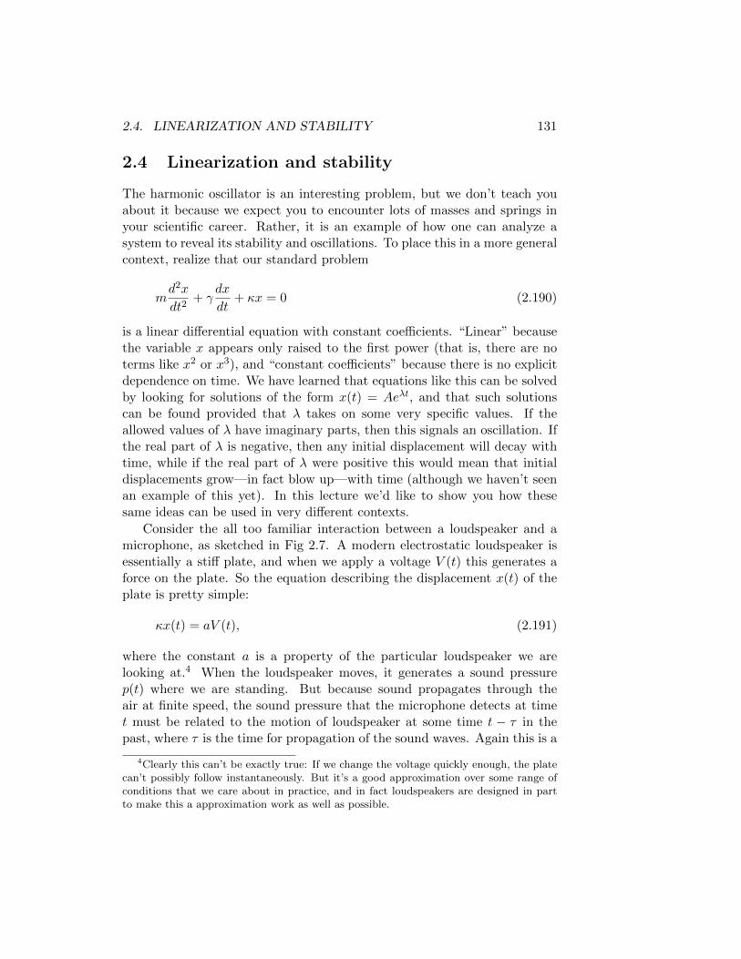
2.4. LINEARIZATION AND STABILITY 131
2.4 Linearization and stability
The harmonic oscillator is an interesting problem, but we don’t teach youabout it because we expect you to encounter lots of masses and springs inyour scientific career. Rather, it is an example of how one can analyze asystem to reveal its stability and oscillations. To place this in a more generalcontext, realize that our standard problem
md2x
dt2+ γ
dx
dt+ κx = 0 (2.190)
is a linear differential equation with constant coefficients. “Linear” becausethe variable x appears only raised to the first power (that is, there are noterms like x2 or x3), and “constant coefficients” because there is no explicitdependence on time. We have learned that equations like this can be solvedby looking for solutions of the form x(t) = Aeλt, and that such solutionscan be found provided that λ takes on some very specific values. If theallowed values of λ have imaginary parts, then this signals an oscillation. Ifthe real part of λ is negative, then any initial displacement will decay withtime, while if the real part of λ were positive this would mean that initialdisplacements grow—in fact blow up—with time (although we haven’t seenan example of this yet). In this lecture we’d like to show you how thesesame ideas can be used in very different contexts.
Consider the all too familiar interaction between a loudspeaker and amicrophone, as sketched in Fig 2.7. A modern electrostatic loudspeaker isessentially a stiff plate, and when we apply a voltage V (t) this generates aforce on the plate. So the equation describing the displacement x(t) of theplate is pretty simple:
κx(t) = aV (t), (2.191)
where the constant a is a property of the particular loudspeaker we arelooking at.4 When the loudspeaker moves, it generates a sound pressurep(t) where we are standing. But because sound propagates through theair at finite speed, the sound pressure that the microphone detects at timet must be related to the motion of loudspeaker at some time t − τ in thepast, where τ is the time for propagation of the sound waves. Again this is a
4Clearly this can’t be exactly true: If we change the voltage quickly enough, the platecan’t possibly follow instantaneously. But it’s a good approximation over some range ofconditions that we care about in practice, and in fact loudspeakers are designed in partto make this a approximation work as well as possible.

132 CHAPTER 2. RESONANCE AND RESPONSE
Figure 2.7: A loudspeaker generates sound, and a microphone picks up these signals.Inevitably, there is some feedback. In the text we analyze this to explain the howlinginstabilities that we all have experienced.
simplification, since in the real world there are many paths from loudspeakerto microphone (echoing off the walls of the room, for example), each of whichhas its own time delay; here we’re going to approximate that there is justone path with one delay. Thus we have
p(t) = bx(t− τ), (2.192)
where b is a constant that measures the efficiency of the loudspeaker.
The whole point of the the microphone, of course, is that sound pres-sure gets converted into an electrical voltage that we can use to drive theloudspeaker. There is some factor g that expresses the “gain” in this trans-formation; if we have an amplifier in the system then turning the knob onthe amplifier adjusts this gain:
V (t) = gp(t). (2.193)

2.4. LINEARIZATION AND STABILITY 133
Putting all of these thing together we have
κx(t) = aV (t)
= agp(t) (2.194)
= agbx(t− τ) (2.195)
x(t) =agb
κx(t− τ). (2.196)
It’s useful to call the combination of parameters agb/κ = G, so the dynamicsof our system is determined simply by
x(t) = Gx(t− τ). (2.197)
It is interesting that Eq (2.197) looks nothing like the differential equa-tions we have been solving. In fact, there are no derivatives, just a delay.Still, the equation is linear, so we might try our usual trick of looking forsolutions in the form x(t) = Aeλt. Substituting, we find:
x(t) = Gx(t− τ)
Aeλt = GAeλ(t−τ) (2.198)
= GAe−λτeλt. (2.199)
As usual, we can divide through by A and by eλt, to obtain
1 = Ge−λτ , (2.200)
or equivalently
eλτ = G. (2.201)
This looks easy to solve: take the (natural) log of both sides, then dividethrough by τ :
eλτ = G
λτ = lnG (2.202)
λ =lnG
τ. (2.203)
We see that if G < 1, then λ will be negative, but if G > 1 then λ willpositive. Since our solutions are of the form x(t) ∼ eλt, positive λ means thatthe displacement of the loudspeaker will blow up with time. This certainlystarts to seem like an explanation of what happens in real life: if we have toolarge a gain in our amplifier (g and hence G is too big), then the “feedback”

134 CHAPTER 2. RESONANCE AND RESPONSE
from microphone to amplifier can lead to an instability in which the systemstarts to make its own sounds. The sound pressure can rise from the pointwhere we barely hear it to the point where it is painful, which correspondsto p or x growing by a factor of 106.
Actually we don’t quite have a theory of the blow up in our audio system.So far, x(t) is growing exponentially, but it’s not oscillating. We knowthat the real instabilities of audio systems occur with the sound pressureoscillating at some frequency, since we hear (admittedly badly tuned) ‘notes’or whistles. Are these somehow hiding in our equations?
We are trying to solve the equation exp(λτ) = G. We have found onesolution, but is this the unique solution? Recall that
exp(2πi) = 1, (2.204)
and also that
[exp(2πi)]2 = exp(4πi) = 1, (2.205)
and so on, so that
exp(2nπi) = 1, (2.206)
for any integer n = ±1,±2,±3, · · · . This means that once we open ourminds to complex numbers, taking logarithms is no longer so easy. Forexample, we can write that
eln 3 = 3. (2.207)
But it’s also true that
eln 3e2πi = eln 3+2πi = 3. (2.208)
So when take the natural log of 3 we might mean what we always meant bythe number ln 3, but we might also mean ln 3 + 2πi, and it’s worse becausewe could mean ln 3 ± 2πi, ln 3 ± 4πi, and so on. All this craziness meansthat our simple equation exp(λτ) = G actually has many solutions:
λτ = lnG± 2nπi (2.209)
λ =lnG
τ± i2nπ
τ, (2.210)
where n = 0, 1, 2, · · · . Now we see that λ can have imaginary parts, atfrequencies which are integer multiples of ω = 2π/τ .

2.4. LINEARIZATION AND STABILITY 135
So, what we have seen is that our trick of looking for solutions in the formx ∼ eλt allows to understand what happens in the microphone–loudspeakersystem. There are oscillations with a frequency such that the period matchesthe delay, which makes sense because this is the condition that the signalfrom the microphone reinforces the motion of the loudspeaker. In fact thereisn’t a single frequency, but a whole set of “harmonics” at integer multiplesof a “fundamental” frequency, just like when we play a note on a musicalinstrument—this idea of harmonics will reappear when we discuss waves ona string, a few lectures from now. If the gain of the amplifier in the systemis small, then these oscillations die away, but if the gain becomes too largethen there is an instability and the amplitude of the oscillations will growexponentially. Presumably this is stopped by the fact that amplifier can’tput out infinite power.
Problem 45: The time τ which appears in our analysis of the loudspeaker andmicrophone is the time for sound to propagate from one element to the other. Given thatthe speed of sound is 330 m/s in air, what are typical values of τ in a classroom? Thedifference between a barely audible sound and one that is painful is a factor of ∼ 106 inp; if we set the amplifier so that the gain G = 2, how long should it take for the signal togrow by this amount? Does this make sense in terms of your experience?
Problem 46: One can think of the mechanics of muscles as having two components—a passive part that is mostly stiffness and drag, and an active part in which the musclegenerates extra force when you pull on it. If we call this active force Factive(t), then thelength of the muscle should obey the differential equation
γdL(t)
dt+ κL(t) = Factive(t), (2.211)
where as usual γ describes the drag and κ the stiffness. Consider a simple model for thedynamics of Factive(t): The active force acts like a stiffness, but it takes a little while todevelop in response to the changes in muscle length. An equation that can describe thisis
τdFactive(t)
dt+ Factive(t) = −κ′L(t), (2.212)
where τ is (roughly) the time it takes for the active force to develop and κ′ is the “activestiffness.” Look for a solution of the form L(t) = L0 exp(λt) and Factive(t) = F0 exp(λt).
(a.) Show that a solution of this form does work provided that L0, F0 and λ obeysome conditions. Write these conditions as two equations for these three variables.
(b.) Show that the two equations you found in [a] are equivalent to a single quadraticequation for λ, as in the case of the harmonic oscillator. Hint: First use one of theequations to solve for F0, then substitute into the second equation. You should find thatL0 drops out, leaving just one equation for λ.
(c.) In general, what is the condition on λ that corresponds to underdamped oscilla-tions?
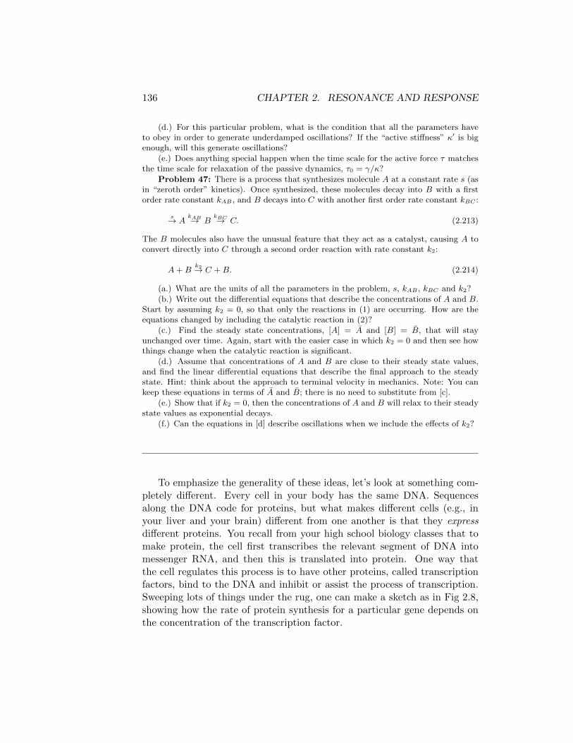
136 CHAPTER 2. RESONANCE AND RESPONSE
(d.) For this particular problem, what is the condition that all the parameters haveto obey in order to generate underdamped oscillations? If the “active stiffness” κ′ is bigenough, will this generate oscillations?
(e.) Does anything special happen when the time scale for the active force τ matchesthe time scale for relaxation of the passive dynamics, τ0 = γ/κ?
Problem 47: There is a process that synthesizes molecule A at a constant rate s (asin “zeroth order” kinetics). Once synthesized, these molecules decay into B with a firstorder rate constant kAB , and B decays into C with another first order rate constant kBC :
s→ AkAB→ B
kBC→ C. (2.213)
The B molecules also have the unusual feature that they act as a catalyst, causing A toconvert directly into C through a second order reaction with rate constant k2:
A+Bk2→ C +B. (2.214)
(a.) What are the units of all the parameters in the problem, s, kAB , kBC and k2?
(b.) Write out the differential equations that describe the concentrations of A and B.Start by assuming k2 = 0, so that only the reactions in (1) are occurring. How are theequations changed by including the catalytic reaction in (2)?
(c.) Find the steady state concentrations, [A] = A and [B] = B, that will stayunchanged over time. Again, start with the easier case in which k2 = 0 and then see howthings change when the catalytic reaction is significant.
(d.) Assume that concentrations of A and B are close to their steady state values,and find the linear differential equations that describe the final approach to the steadystate. Hint: think about the approach to terminal velocity in mechanics. Note: You cankeep these equations in terms of A and B; there is no need to substitute from [c].
(e.) Show that if k2 = 0, then the concentrations of A and B will relax to their steadystate values as exponential decays.
(f.) Can the equations in [d] describe oscillations when we include the effects of k2?
To emphasize the generality of these ideas, let’s look at something com-pletely different. Every cell in your body has the same DNA. Sequencesalong the DNA code for proteins, but what makes different cells (e.g., inyour liver and your brain) different from one another is that they expressdifferent proteins. You recall from your high school biology classes that tomake protein, the cell first transcribes the relevant segment of DNA intomessenger RNA, and then this is translated into protein. One way thatthe cell regulates this process is to have other proteins, called transcriptionfactors, bind to the DNA and inhibit or assist the process of transcription.Sweeping lots of things under the rug, one can make a sketch as in Fig 2.8,showing how the rate of protein synthesis for a particular gene depends onthe concentration of the transcription factor.
2.4. LINEARIZATION AND STABILITY 137
Figure 2.8: Regulation of gene expression. In the simplest picture, proteins are synthesizedat a rate r(F ) that depends on the concentration F of some transcription factor. Thetranscription factor can be an activator or a repressor.
If we take the sketch in Fig 2.8 seriously, we can write the rate of proteinsynthesis as r(F ), where F is the concentration of the transcription factor.Once the proteins are made, they also are degraded by a variety of processes,and let’s assume that we can lump all these together into some first orderrate constant k for degradation. Then the dynamics of protein concentrationare given by
dP
dt= r(F )− kP. (2.215)
Of course, the transcription factor is itself a protein, and so some similardynamics are being played out at another point along the genome. The realproblem of understand the dynamics of transcriptional regulation is to thinkabout these coupled dynamics of different genes. But, to get a feeling forwhat can happen, let’s make a drastic simplification and imagine that theprotein we are looking at actually regulates itself. Then “the transcription
138 CHAPTER 2. RESONANCE AND RESPONSE
Figure 2.9: Steady states of a gene that activates its own expression. With dynamics asin Eq (2.216), steady states are possible when the rate of protein synthesis r(P ) balancesthe rate of degradation kP . With the parameters chosen here, there are three possiblesteady states.
factor” really is the protein we have been discussing, and hence F = P ; thedynamics then are described by
dP
dt= r(P )− kP. (2.216)
Just to be clear, there is no case in nature that is quite this simple. Onthe other hand, there are examples that aren’t too much more complicated(e.g., two proteins which regulate each other), and with modern methodsof molecular biology one can engineer bacteria to implement something likethe simple model we are discussing here. So, it’s oversimplified, but maybenot ridiculously oversimplified (!).
How, then, do we attack a model like that in Eq (2.216)? We can start byasking if there is any way for the system to come to a steady state. This willhappen when dP/dt = 0, which is equivalent to r(P ) = kP . Let’s considerthe case of an activator. Then graphically our problem is shown in Fig 2.9.

2.4. LINEARIZATION AND STABILITY 139
We can plot r(P ) vs P , and we can also plot kP vs P (the last plot justbeing a straight line). Whenever these two plots cross, we have a possiblesteady state. At least in some range of parameters, it’s clear that there arethree possible steady states.
Now we know that not all steady states are created equal. If we balancea ball on top of a hill, there is no force and so it will stay there forever—aslong as nobody kicks it. On the other hand, if the ball is sitting at thebottom of a valley, even kicking it a little bit doesn’t change anything, sinceafter a while it will roll back to the bottom of the valley and come to rest.We say that the bottom of the valley is a stable steady state, the top of thehill is an unstable steady state. Sometimes we call these steady states “fixedpoints” of the dynamics. So it’s natural to ask, of the three fixed points inour problem (Fig 2.9), which ones are stable and which ones are unstable?
To examine the stability of steady states let’s do the mathematical ver-sion of giving the ball a small kick. Suppose that we have identified a steadystate P0. Imagine that P = P0 + δP (t), where the difference δP is going tobe small. We can derive an equation which describes the dynamics of δPby substituting into Eq (2.216):
dP
dt= r(P )− kP
d(P0 + δP )
dt= r(P0 + δP )− k(P0 + δP ) (2.217)
d(P0)
dt+d(δP )
dt≈ r(P0) +
dr(P )
dP
∣∣∣∣P=P0
· δP − kP0 − kδP, (2.218)
where in the last step we have used a Taylor series expansion to approximater(P ) in the neighborhood of P0; since δP is small we just stop with the firstterm.
Now we can simplify things in Eq (2.218) considerably. To begin, P0 isa number, so taking its derivative with respect to time gives us zero, so thatwe have
d(δP )
dt≈ r(P0) +
dr(P )
dP
∣∣∣∣P=P0
· δP − kP0 − kδP. (2.219)
Next we notice that we can group the terms together on the right hand side:
d(δP )
dt≈ [r(P0)− kP0] +
[dr(P )
dP
∣∣∣∣P=P0
− k
]δP. (2.220)
140 CHAPTER 2. RESONANCE AND RESPONSE
But P0 was defined to be a steady state, which means that r(P0) = kP0,and hence the first term in [· · · ] vanishes. All we have left is
d(δP )
dt=
[dr(P )
dP
∣∣∣∣P=P0
− k
]δP, (2.221)
and if we remember that δP has to be small, then it’s OK to write = insteadof ≈.
But we have seen Eq (2.221) before, in other forms. This equation isjust
d(δP )
dt= αδP, (2.222)
where the constant
α =
[dr(P )
dP
∣∣∣∣P=P0
− k
]. (2.223)
We know the solution of Eq (2.222), it’s just δP (t) = δP (0) exp(αt). So ifα < 0 the fixed point P0 is stable, since a small kick away from the steadystate will decay away. If on the other hand we have α > 0, the fixed pointP0 is unstable, since a small kick away from the steady state will grow,much as with the ball on top of the hill. The conclusion from all of this isthat the steady state protein concentration P0 will be stable if dr(P )/dPis less than k when we evaluate it at P = P0. Looking at Fig 2.9, we cansee that the two fixed points at large and small P satisfy this condition;the intermediate fixed point does not. This means that really we have a“bistable” system, in which there are exactly two stable states separated byan unstable point. This is like having two valleys separated by a hill—youcan sit stably in either valley, and you’ll always fall into one or the other,depending on which side of the mountain top you find yourself.
Problem 48: Let’s fill in the details of the calculation above using a more concretemodel. Specifically, let’s formalize the sketches of the function r(F ) in Fig 2.8, by writingequations for r(F ) that look like our sketches:
ract(F ) = rmaxFn
Fn + Fn1/2, (2.224)
rrep(F ) = rmax
Fn1/2Fn + Fn1/2
. (2.225)

2.4. LINEARIZATION AND STABILITY 141
(a.) Plot5 the functions ract(F ) and rrep(F ). Explain the significance of the parame-ters rmax and F1/2.
(b.) Consider the case of “auto–regulation,” in which the protein is its own transcrip-tion factor, so that P = F . As discussed above, the case of activator can have three steadystates where dP/dt = 0. Show that for the repressor there is only one steady state. Youshould be able to make a qualitative, graphical argument, and then use the equations tomake things precise.
(c.) Let the steady state that you found in [c] correspond to P = P0. Assume thatP (t) = P0 + δP (t) and derive an approximate, linear equation for δP (t) assuming that itis small. How small does it nee to be in order for your approximation to be accurate?
(d.) Solve the linear equation from [c]. How does the behavior of the solution dependon the parameters rmax, n, F1/2, and k?
Problem 49: Let’s continue the analysis of a self–activating gene. We have writtenthe dynamics of the protein concentration P as
dP
dt= r(P )− kP, (2.226)
where k is the first order rate constant for degradation of the protein, and r(P ) is the rateof protein synthesis, which depends on P because the protein acts as its own activator.To be explicit, we consider the functional form
r(P ) = rmaxPn
Pn + Fn1/2. (2.227)
(a.) Consider normalized variables p = P/F1/2 and τ = kt. Show that
dp
dτ= a
pn
pn + 1− p, (2.228)
and give a formula that relates a to the original parameters in the problem.(b.) Consider the specific case n = 3. Notice that the condition for a steady state can
written as the problem of finding the roots of a polynomial:
0 = apn
pn + 1− p (2.229)
p = apn
pn + 1(2.230)
pn+1 + p = apn (2.231)
pn+1 − apn + p = 0. (2.232)
Find all the steady state values of p, and plot these as a function of the parameter a. Youmight find the MATLAB function roots to be useful here. Be careful about whether thesolutions you find are real! Can you verify that there are three steady states, as explainedin the notes? What is the condition on a for this to be true? What happens when thiscondition is violated?
(c.) Write a program that solves Eq (2.228).
5Since we already have the sketches, “plot” here means to use a computer to get exactvalues and plot the results. Think about how to choose the parameters. Maybe you canchoose your units in some way to make some of the parameters disappear?
142 CHAPTER 2. RESONANCE AND RESPONSE
(d.) Choose a value for the parameter a which generates (from [b]) three steady states.To run your program you will need to chose a value for the discrete time step. Justifyyour choice, and explain how you will test whether this is a reasonable choice.
(e.) Now run the program, starting at τ = 0 and running out to τ = 10. Try differentinitial values of p(τ = 0). In particular, try initial values that are close to the steady statevalues. Can you verify that two of the steady states are stable, so that if you start nearthem the solution will evolve toward the steady state? What happens if, in contrast, youstart near the unstable state?
Problem 50: As we have noted, the model we have been analyzing is over–simplified.For example, binding of a transcription factor to DNA can’t directly change the rate ofprotein synthesis. Instead, it changes the rate at which mRNA is made, and this in turnchanges the rate of protein synthesis. Let’s call the mRNA concentration M . Then insteadof Eq (2.215) we can write
dM
dt= r(F )− kRNAM, (2.233)
where kRNA is the rate at which mRNA decays. Then if the rate of protein synthesis isproportional to the mRNA concentration we also have
dP
dt= sM − kPP, (2.234)
where s is the rate at which one mRNA molecule gets translated into protein and kP isthe rate at which the protein decays. Again let’s consider a repressor that regulates itself.Then our equations become
dM
dt= rmax
Fn1/2Pn + Fn1/2
− kRNAM, (2.235)
dP
dt= sM − kPP, (2.236)
(a.) Find the conditions for the system to be at a steady state. Reduce your resultsto a single equation that determines the steady state protein concentration P0. Does thisequation have a single solution or multiple solutions?
(b.) Express the protein concentration as a ratio with F1/2, that is P = P/F1/2.Can you simplify the steady state condition and show that is only one combination ofparameters that determines the value of the steady state P0? Plot the dependence of P0
on this combined parameter.(c.) Assume that the system is close to the steady state, so that P = P0 + δP (t) and
M = M0 + δM(t), with δP and δM small. Find the approximate, linear equations thatdescribe the dynamics of δP and δM .
(d.) Look for solutions of these linear equations in the form δP (t) = Aeλt andδM(t) = Beλt. Show that there is a solution of this form if λ is the solution of a quadraticequation.
(e.) Does the quadratic equation for λ allow for complex solutions? As a hint, try the(admittedly unrealistic) case where the protein and mRNA have the same decay rates,kP = kRNA. In contrast, what happens if the mRNA lifetime is very short, that is if kRNA
is very large? Explain in words why this system can oscillate, and why these tend to goaway if the mRNA is short lived.

2.5. STABILITY AND OSCILLATION IN A REAL BIOCHEMICAL CIRCUIT143
Biologically, our simple example of a gene activating itself correspondsto a switch. Given these dynamics, the cell can live happily in two differentpossible states, one in which the expression of the protein is very low andone it which it is almost as high as it can be. If no extra signals come in fromthe outside, once a cell picks on of these “valleys,” it could (in principle) staythere forever. We can think of this as being a much oversimplified model fordifferentiation: Two cells, each with exactly the same DNA, can nonethelessadopt two different fates and look to the outside world like two differentcells (think again about liver and brain). Alternatively, if our model wasdescribing a single celled organism then the two stable states could representtwo very different lifestyles, perhaps appropriate to different environments.
Problem 51: When we discussed simple models for a genetic switch, we considereda protein that could activate its own transcription in a “cooperative” way, so that the rateof protein synthesis was a very steep function of the protein concentration. This actuallywouldn’t be true if activation depended on the binding of just one molecule to the relevantsite along the DNA. Then the synthesis rate would look more like
rsyn(c) = rmaxc
c+K, (2.237)
where c is the protein concentration, K is a constant, and rmax is the maximum rate. Thedynamics of c would then be given by
dc
dt= rsyn(c)− c
τ, (2.238)
where τ is the lifetime of the protein.(a.) Sketch the behavior of rsyn(c). Use this sketch to determine the conditions for a
steady state, dc/dt = 0. Is there more than one steady state? Does your answer dependon the lifetime τ?
(b.) Are the steady states that you found in [a] stable? This requires a real calculation,not just a sketch.
(c.) Can this system function as a switch? Explain why or why not.
2.5 Stability and oscillation in a real biochemicalcircuit
The cell cycle is an oscillator. Observations of cells reveal distinct stagesof the cell cycle as shown schematically in Figure 2.10. We will consider a
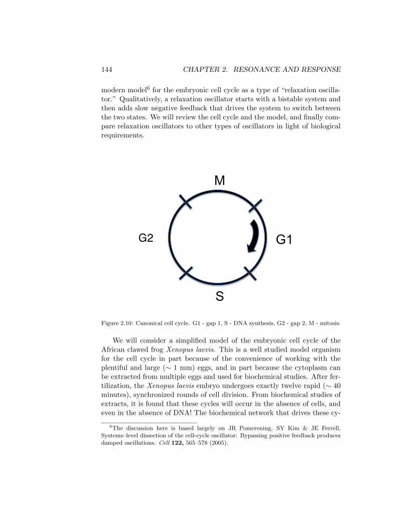
144 CHAPTER 2. RESONANCE AND RESPONSE
modern model6 for the embryonic cell cycle as a type of “relaxation oscilla-tor.” Qualitatively, a relaxation oscillator starts with a bistable system andthen adds slow negative feedback that drives the system to switch betweenthe two states. We will review the cell cycle and the model, and finally com-pare relaxation oscillators to other types of oscillators in light of biologicalrequirements.
G1
S
M
G2
Figure 2.10: Canonical cell cycle. G1 - gap 1, S - DNA synthesis, G2 - gap 2, M - mitosis.
We will consider a simplified model of the embryonic cell cycle of theAfrican clawed frog Xenopus laevis. This is a well studied model organismfor the cell cycle in part because of the convenience of working with theplentiful and large (∼ 1 mm) eggs, and in part because the cytoplasm canbe extracted from multiple eggs and used for biochemical studies. After fer-tilization, the Xenopus laevis embryo undergoes exactly twelve rapid (∼ 40minutes), synchronized rounds of cell division. From biochemical studies ofextracts, it is found that these cycles will occur in the absence of cells, andeven in the absence of DNA! The biochemical network that drives these cy-
6The discussion here is based largely on JR Pomerening, SY Kim & JE Ferrell,Systems–level dissection of the cell-cycle oscillator: Bypassing positive feedback producesdamped oscillations. Cell 122, 565–578 (2005).

2.5. STABILITY AND OSCILLATION IN A REAL BIOCHEMICAL CIRCUIT145
cles is shown schematically in Fig 2.11. We read this schematic to mean thatCdk1 activity is increased by dual positive feedbacks (active Cdk1 activatesits activator Cdc25 and inactivates its inhibitor Wee1), while Cdk1 activityis reduced by a single negative feedback, in which active Cdk1 activates theanaphase promoting complex (APC). Qualitatively, the system resembles asimple relaxation oscillator in which fast positive feedback leads to two sta-ble states, and slow negative feedback leads to oscillations between these twostates. We can capture the essence of their model by considering the Cyclin-Cdk1 complex as an “activator”, and APC as a “repressor”. The activatorrapidly activates its own production and more slowly activates production ofthe repressor. The repressor eventually builds up and represses productionof the activator. The result is an oscillation.
Figure 2.11: The embryonic cell cycle in the African clawed frog Xenopus laevis is drivenby coupled positive and negative feedback loops.
To understand this system mathematically, let’s start with the activator,with no negative feedback. The concentration of activator will increase in
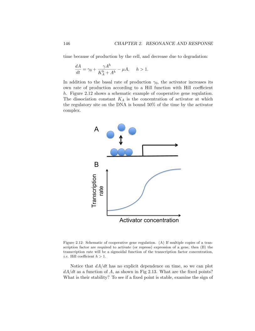
146 CHAPTER 2. RESONANCE AND RESPONSE
time because of production by the cell, and decrease due to degradation:
dA
dt= γ0 +
γAh
KhA +Ah
− µA, h > 1.
In addition to the basal rate of production γ0, the activator increases itsown rate of production according to a Hill function with Hill coefficienth. Figure 2.12 shows a schematic example of cooperative gene regulation.The dissociation constant KA is the concentration of activator at whichthe regulatory site on the DNA is bound 50% of the time by the activatorcomplex.
Activator concentration
Tra
nscrip
tio
n
rate
A
B
Figure 2.12: Schematic of cooperative gene regulation. (A) If multiple copies of a tran-scription factor are required to activate (or repress) expression of a gene, then (B) thetranscription rate will be a sigmoidal function of the transcription factor concentration,i.e. Hill coefficient h > 1.
Notice that dA/dt has no explicit dependence on time, so we can plotdA/dt as a function of A, as shown in Fig 2.13. What are the fixed points?What is their stability? To see if a fixed point is stable, examine the sign of

2.5. STABILITY AND OSCILLATION IN A REAL BIOCHEMICAL CIRCUIT147
dA/dt on either side of the fixed point. Will small deviations from the fixedpoint shrink or grow? As plotted in Figure 2.13, the activator is bistableand will exhibit hysteresis. That is if the activator A starts out high, it willstay high at the upper fixed point, and if A starts out low it will stay lowat the lower fixed point.
dA/dt
!
0
A stabl
e
stabl
e
unstabl
e
slope = -µ
stable stableunstable
Figure 2.13: Production rate of activator, dA/dt, as a function of the activator concentra-tion A.
Now introduce negative feedback. Specifically, introduce a repressor withconcentration R, and let the rate of degradation of A depend on R:
µ→ µ(R).
To be specific, let µ increase linearly with R,
µ(R) = µ0 + βR.
Consider how the dA/dt curve in Fig 2.13 will change as the repressor Rconcentration changes. The rate of degradation of A will increase, meaningthat the linear slope term in dA/dt will get more negative. Eventually thiswill mean that the upper stable fixed point will disappear. In fact, the upperfixed point will merge with the unstable fixed point – this is called a “saddle-node” bifurcation. (The name makes more sense in two dimensions, imaginea 2D stable fixed point and a 2D saddle-shaped fixed point coming together,
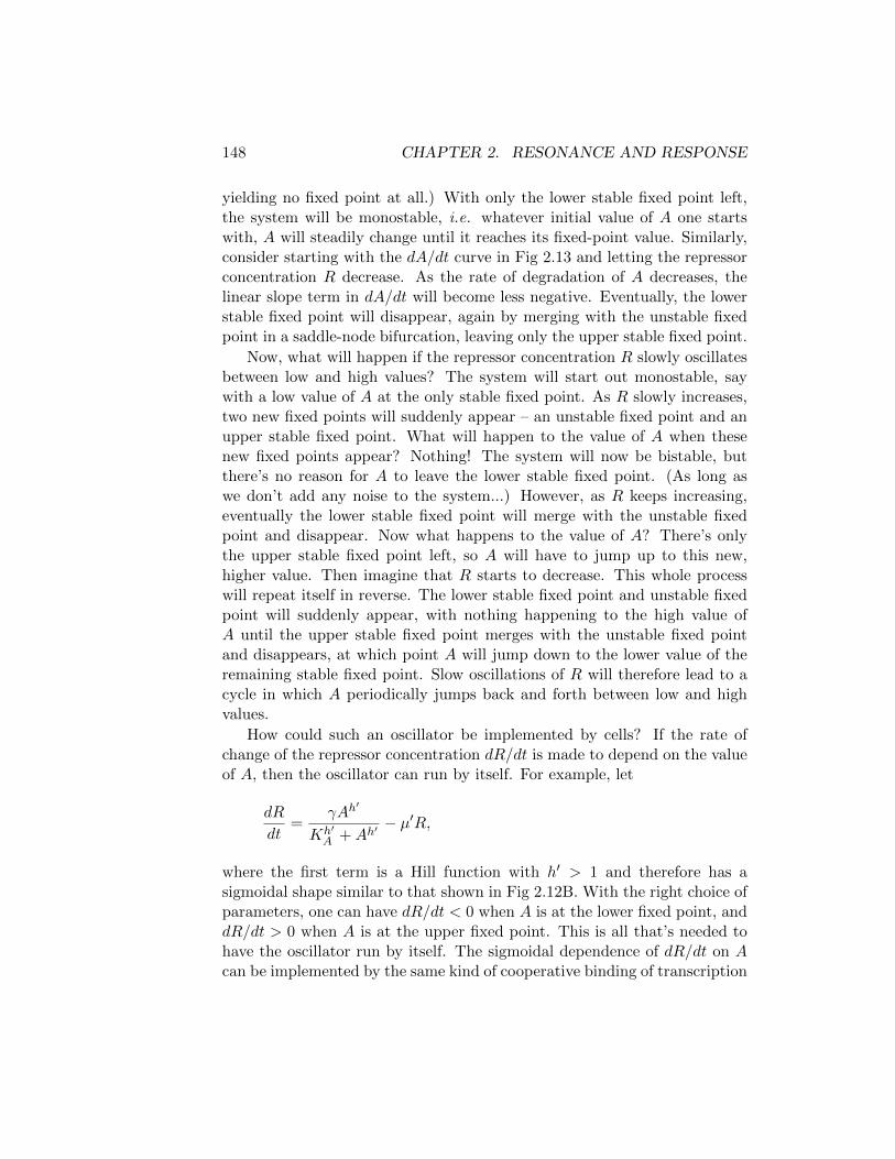
148 CHAPTER 2. RESONANCE AND RESPONSE
yielding no fixed point at all.) With only the lower stable fixed point left,the system will be monostable, i.e. whatever initial value of A one startswith, A will steadily change until it reaches its fixed-point value. Similarly,consider starting with the dA/dt curve in Fig 2.13 and letting the repressorconcentration R decrease. As the rate of degradation of A decreases, thelinear slope term in dA/dt will become less negative. Eventually, the lowerstable fixed point will disappear, again by merging with the unstable fixedpoint in a saddle-node bifurcation, leaving only the upper stable fixed point.
Now, what will happen if the repressor concentration R slowly oscillatesbetween low and high values? The system will start out monostable, saywith a low value of A at the only stable fixed point. As R slowly increases,two new fixed points will suddenly appear – an unstable fixed point and anupper stable fixed point. What will happen to the value of A when thesenew fixed points appear? Nothing! The system will now be bistable, butthere’s no reason for A to leave the lower stable fixed point. (As long aswe don’t add any noise to the system...) However, as R keeps increasing,eventually the lower stable fixed point will merge with the unstable fixedpoint and disappear. Now what happens to the value of A? There’s onlythe upper stable fixed point left, so A will have to jump up to this new,higher value. Then imagine that R starts to decrease. This whole processwill repeat itself in reverse. The lower stable fixed point and unstable fixedpoint will suddenly appear, with nothing happening to the high value ofA until the upper stable fixed point merges with the unstable fixed pointand disappears, at which point A will jump down to the lower value of theremaining stable fixed point. Slow oscillations of R will therefore lead to acycle in which A periodically jumps back and forth between low and highvalues.
How could such an oscillator be implemented by cells? If the rate ofchange of the repressor concentration dR/dt is made to depend on the valueof A, then the oscillator can run by itself. For example, let
dR
dt=
γAh′
Kh′A +Ah′
− µ′R,
where the first term is a Hill function with h′ > 1 and therefore has asigmoidal shape similar to that shown in Fig 2.12B. With the right choice ofparameters, one can have dR/dt < 0 when A is at the lower fixed point, anddR/dt > 0 when A is at the upper fixed point. This is all that’s needed tohave the oscillator run by itself. The sigmoidal dependence of dR/dt on Acan be implemented by the same kind of cooperative binding of transcription

2.6. THE DRIVEN OSCILLATOR 149
factors to DNA as shown in Fig 2.12A, now with A regulating transcriptionof the repressor.
This is an example of a “relaxation oscillator”. As promised, we startedwith a bistable system, and added a slow negative feedback (the repressor)that destabilizes each fixed point in turn, so that the output (the concen-tration of activator A) jumps back and forth periodically between low andhigh values. How can one visualize this behavior in a single plot? Theanswer is the phase portrait shown in Fig 2.14. The axes are the concen-trations of activator A and repressor R. If one draws the nullclines, wheredA/dt = 0 and dR/dt = 0, respectively, and draws in a few arrows showingthe direction of flow, i.e. the direction of the vector (dA/dt, dR/dt), onecan qualitatively see how the system behaves. To prove that the fixed pointwhere the nullclines cross is unstable requires a little work, but taking it asgiven that trajectories cycle away from that point, one can see the form ofthe relaxation oscillator emerging from the connected series of arrows.
Now we understand the mathematical model for the embryonic cell cy-cle, but why is this a good way to design an oscillator? For example, whyshould cells use a relaxation oscillator rather than a simple feedback oscil-lator? Consider the oscillator shown schematically in Fig 2.15. A constitu-tively expressed activator that activates its own repressor, with a time delaysomewhere in the feedback loop, will typically lead to oscillations. As someparameter is varied, in this case the delay time, the oscillations will firstappear with a small amplitude, but finite frequency as shown in the figure.This is called a “Hopf bifurcation”. So this simple feedback oscillator hasa tunable amplitude, but approximately fixed frequency. In comparison,a relaxation oscillator has fixed amplitude but tunable frequency, becausethe underlying bistable system sets the amplitude of the jump in A whilethe slow build-up of R sets the frequency. Which type of oscillator bettermatches the requirements of the cell cycle?
2.6 The driven oscillator
We would like to understand what happens when we apply forces to theharmonic oscillator. That is, we want to solve the equation
Md2x(t)
dt2+ γ
dx(t)
dt+ κx(t) = F (t). (2.239)
The problem is that, of course, the solution depends on what we choose forthe force. It seems natural to ask what happens, but we don’t want to have

150 CHAPTER 2. RESONANCE AND RESPONSE
0
0
A
R
nullcline
dA/dt =
nullcline
dR/dt =
Figure 2.14: Phase portrait of a relaxation oscillator based on an activator A that activatesits own production and also activates the production of a repressor R. The repressor feedsback negatively on the activator. All trajectories eventually converge on the same periodicoscillation (indicated by black arrows), with only the phase depending on initial conditions,ı.e. this is an example of a “limit cycle oscillator.”
to answer with a long list—if the force looks like this, then the displacementlooks like that; if the force is different in this way, then the displacement isdifferent in that way ... and so on. Is there any way to give one answer tothe question of what happens in response to applied forces?
One idea is to think of an arbitrary function F (t) as a sequence of shortpules, occurring at the right times with the right amplitudes. This is usefulbecause if we can solve for the response to one pulse, then the response tomany pulses is just the sum of the individual responses. To see this, imaginethat x1(t) is the time dependent displacement that is generated by the force

2.6. THE DRIVEN OSCILLATOR 151
Figure 2.15: Oscillator based on negative feedback with a time delay. Typically, as thetime delay increases, the onset of oscillations occurs via a Hopf bifurcation, in this casestarting with small, finite frequency oscillations around an unstable fixed point.
F1(t), and similarly x2(t) is generated by F2(t). This means that
Md2x1(t)
dt2+ γ
dx1(t)
dt+ κx1(t) = F1(t) (2.240)
Md2x2(t)
dt2+ γ
dx2(t)
dt+ κx2(t) = F2(t). (2.241)
Now we add these two equations together and notice that adding and difer-entiating commute:
[Md2x1(t)
dt2+ γ
dx1(t)
dt+ κx1(t)
]+
[Md2x2(t)
dt2γdx2(t)
dt+ κx2(t)
]= F1(t) + F2(t) (2.242)

152 CHAPTER 2. RESONANCE AND RESPONSE
M
[d2x1(t)
dt2+d2x2(t)
dt2
]+ γ
[dx1(t)
dt+dx2(t)
dt
]+ κ [x1(t) + x2(t)]
= F1(t) + F2(t)
(2.243)
Md2[x1(t) + x2(t)]
dt2+ γ
d[x1(t) + x2(t)]
dt+ κ [x1(t) + x2(t)]
= F1(t) + F2(t).
(2.244)
Thus if we have the force F (t) = F1(t) + F2(t), then the displacement willbe x(t) = x1(t)+x2(t). This “superposition” of solution keeps working if wehave more and more forces to add up, so if we think of the time–dependentforce as being a sum of pulses then the displacement will be the sum ofresponses to the individual pulses, as promised.
Thinking in terms of pulses is a good idea, and we could develop it alittle further, but not now.7 Instead let’s look at using sines and cosines(!). Somewhat remarkably, in the same way that we can make an arbitraryfunction out of many pulses, it turns out that we can make an arbitraryfunction by adding up sines and cosines. This is surprising because sines andcosines are periodic and extended—how then can we make little localizedblips? There is a rigorous theory of all this, but what we need here is justto motivate the idea that sines and cosines are a sensible choice ... .8
To understand that sines and cosines can be used to make any functionwe want, let’s try to make a brief pulse. Let’s start in a window of time thatruns from t = −10 up to t = +10 (in some units). We can make functionslike cos(t), cos(2t), and so on. Let’s do this in MATLAB, just to be explicit.To do this on a computer we need to discrete time steps, so let’s choosesteps of size dt = 0.001:
dt = 0.001;
t = [-10:dt:10];
y= zeros(500,length(t));
for n=1:500;
7We will come back to this in our discussion of waves, starting with the next sections.Stay tuned.
8In fact, these ideas will reappear shortly, and then again much later. The idea thatwe can make arbitrary functions by adding up sines and cosines is called Fourier analysis,and it is an incredibly powerful piece of mathematics, well worth learning properly. Ourapproach here is a bit haphazard—we take a sort of glancing blow at the material, thencircle around for another shot or two before the year is over. We are thinking about abetter organization for all of this, but hope you’ll bear with us for now.

2.6. THE DRIVEN OSCILLATOR 153
−10 −8 −6 −4 −2 0 2 4 6 8 10
−1
−0.8
−0.6
−0.4
−0.2
0
0.2
0.4
0.6
0.8
1
time t
cos(
nt)
Figure 2.16: The first five members of the family of functions cos(nt).
y(n,:) = cos(n*t);
end;
This program will generate functions y(n,t)= cos(nt), as shown in Fig 2.16.Notice that all of these functions line up at t = 0, where they equal one, andthen at other times they have values that have a chance of canceling out.
In fact if we add up all the functions in Fig 2.16, we get the resultsshown at left in Fig 2.17. If instead of looking at the first five terms, we sumup the first five hundred terms, we get the results shown in Fig 2.17. Thisshould be starting to convince you that we can add up lots of cosines and getsomething that looks like a perfectly sharp pulse. The only problem is thatin addition to a pulse at t = 0, we also have pulses at t = ±2π, and if welooked at a bigger window of time we would see pulses at t = ±4π, t = ±6π,etc.. We can start to fix this by including not just cos(t), cos(2t), · · · , butalso terms like cos(1.5t), cos(2.5t), · · · . This will cancel out the pulses att = ±2π. Then if we add not just halves, but also thirds, fourths, etc wecan cancel the pulses at larger and larger times, until eventually all that’s

154 CHAPTER 2. RESONANCE AND RESPONSE
left will be the pulse at t = 0.
−10 −8 −6 −4 −2 0 2 4 6 8 10−6
−4
−2
0
2
4
6
time t
cos(
t) +
cos
(2t)
+ ..
. + c
os(5
t)
−10 −8 −6 −4 −2 0 2 4 6 8 10−600
−400
−200
0
200
400
600
time t
cos(
t) +
cos
(2t)
+ ..
. + c
os(5
00t)
Figure 2.17: Left: The sum of the five functions in Fig 2.16. Right: The sum of fivehundred such functions.
The arguments here are not rigorous, but hopefully give the sense thatadding up sines and cosines allows us to make pulses. If we can make pulses,we can make anything. Thus any force vs time can be thought of as a sumof sines and cosines. This process is called Fourier analysis, and we’ll seemore about this in the spring. For now, we know from the discussion abovethat the displacement in response to this general force can be thought of asthe sum of responses to the individual sine and cosine forces. Let’s solveone of these problems and see how much we can learn.
The problem we want to solve is the damped harmonic oscillator drivenby a force that depends on time as a cosine or sine at some frequency ω:
Md2x(t)
dt2+ γ
dx(t)
dt+ κx(t) = F0 cos(ωt). (2.245)
Actually we might want to do both cosine and sine, and let’s call the motionin response to the sine y(t):
Md2y(t)
dt2+ γ
dy(t)
dt+ κy(t) = F0 sin(ωt). (2.246)
Now these two equations must have the same information hidden in them,since the difference between sine and cosine is just our choice of the pointwhere t = 0.
We’re going to do something a bit weird, which is to combine the twoequations, multiplying the equation for y(t) by a factor of i and then adding
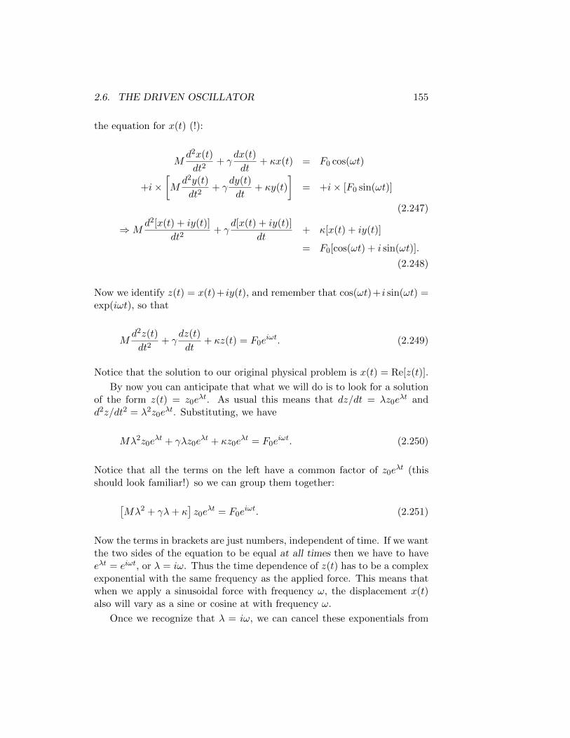
2.6. THE DRIVEN OSCILLATOR 155
the equation for x(t) (!):
Md2x(t)
dt2+ γ
dx(t)
dt+ κx(t) = F0 cos(ωt)
+i×[Md2y(t)
dt2+ γ
dy(t)
dt+ κy(t)
]= +i× [F0 sin(ωt)]
(2.247)
⇒Md2[x(t) + iy(t)]
dt2+ γ
d[x(t) + iy(t)]
dt+ κ[x(t) + iy(t)]
= F0[cos(ωt) + i sin(ωt)].
(2.248)
Now we identify z(t) = x(t)+ iy(t), and remember that cos(ωt)+ i sin(ωt) =exp(iωt), so that
Md2z(t)
dt2+ γ
dz(t)
dt+ κz(t) = F0e
iωt. (2.249)
Notice that the solution to our original physical problem is x(t) = Re[z(t)].
By now you can anticipate that what we will do is to look for a solutionof the form z(t) = z0e
λt. As usual this means that dz/dt = λz0eλt and
d2z/dt2 = λ2z0eλt. Substituting, we have
Mλ2z0eλt + γλz0e
λt + κz0eλt = F0e
iωt. (2.250)
Notice that all the terms on the left have a common factor of z0eλt (this
should look familiar!) so we can group them together:
[Mλ2 + γλ+ κ
]z0e
λt = F0eiωt. (2.251)
Now the terms in brackets are just numbers, independent of time. If we wantthe two sides of the equation to be equal at all times then we have to haveeλt = eiωt, or λ = iω. Thus the time dependence of z(t) has to be a complexexponential with the same frequency as the applied force. This means thatwhen we apply a sinusoidal force with frequency ω, the displacement x(t)also will vary as a sine or cosine at with frequency ω.
Once we recognize that λ = iω, we can cancel these exponentials from
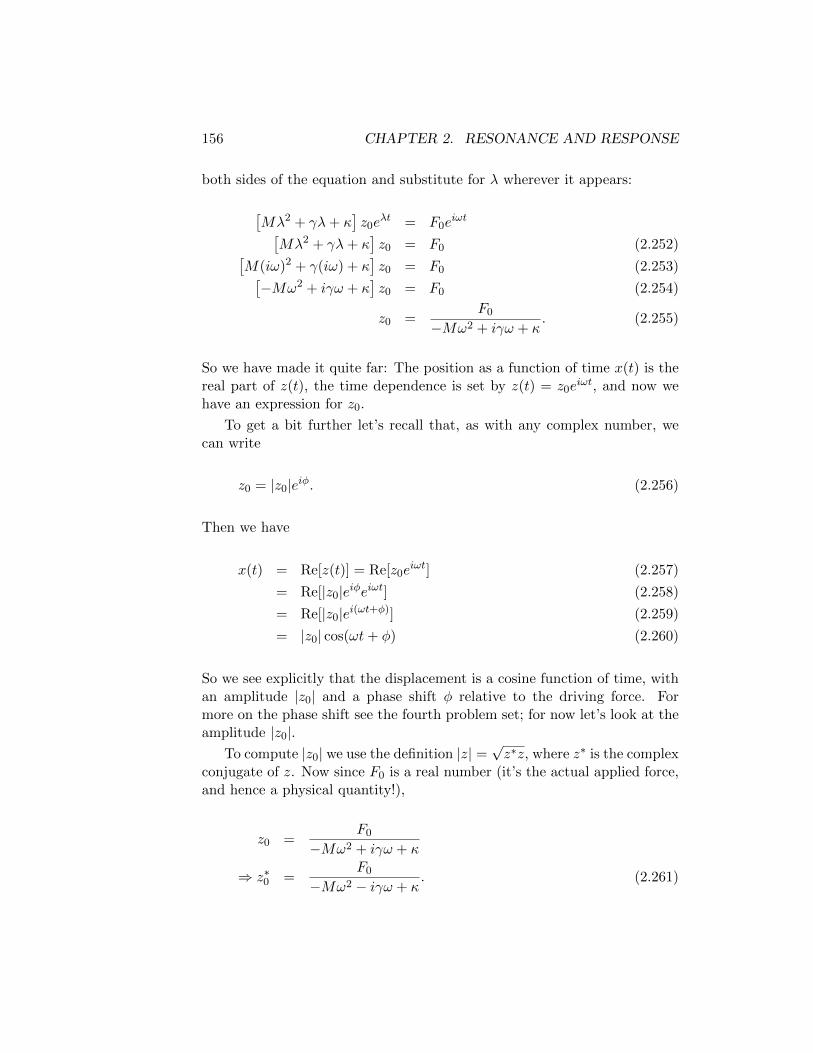
156 CHAPTER 2. RESONANCE AND RESPONSE
both sides of the equation and substitute for λ wherever it appears:
[Mλ2 + γλ+ κ
]z0e
λt = F0eiωt[
Mλ2 + γλ+ κ]z0 = F0 (2.252)[
M(iω)2 + γ(iω) + κ]z0 = F0 (2.253)[
−Mω2 + iγω + κ]z0 = F0 (2.254)
z0 =F0
−Mω2 + iγω + κ. (2.255)
So we have made it quite far: The position as a function of time x(t) is thereal part of z(t), the time dependence is set by z(t) = z0e
iωt, and now wehave an expression for z0.
To get a bit further let’s recall that, as with any complex number, wecan write
z0 = |z0|eiφ. (2.256)
Then we have
x(t) = Re[z(t)] = Re[z0eiωt] (2.257)
= Re[|z0|eiφeiωt] (2.258)
= Re[|z0|ei(ωt+φ)] (2.259)
= |z0| cos(ωt+ φ) (2.260)
So we see explicitly that the displacement is a cosine function of time, withan amplitude |z0| and a phase shift φ relative to the driving force. Formore on the phase shift see the fourth problem set; for now let’s look at theamplitude |z0|.
To compute |z0| we use the definition |z| =√z∗z, where z∗ is the complex
conjugate of z. Now since F0 is a real number (it’s the actual applied force,and hence a physical quantity!),
z0 =F0
−Mω2 + iγω + κ
⇒ z∗0 =F0
−Mω2 − iγω + κ. (2.261)

2.6. THE DRIVEN OSCILLATOR 157
Putting these together we have
|z0|2 =F0
−Mω2 + iγω + κ· F0
−Mω2 − iγω + κ(2.262)
=F 2
0
(−Mω2 + iγω + κ)(−Mω2 − iγω + κ)(2.263)
=F 2
0
(−Mω2 + κ)2 + (γω)2. (2.264)
Thus the amplitude of oscillations in response to a force at frequency ω isgiven by
|z0| =F0√
(−Mω2 + κ)2 + (γω)2(2.265)
We see that the amplitude is proportional to the magnitude of the forceF0, which means that the whole system is linear; this follows from the factthat the differential equation is linear. Thus it makes sense to measure thecoefficient which relates the magnitude of the force to the magnitude of thedisplacement:
G(ω) ≡ |z0|F0
=1√
(−Mω2 + κ)2 + (γω)2. (2.266)
This is plotted in Fig 2.18, for examples of underdamped and overdampedoscillators. Here we look at some simple limits to get a feeling for how itshould behave.
Notice first that at zero frequency we have
G(ω) =1
κ. (2.267)
This makes sense: zero frequency corresponds to applying a constant force,and if we do this we expect to stretch the spring by a constant amount—sincenothing is changing in time mass and drag are irrelevant. The proportional-ity between force and displacement is the stiffness κ, which appears here as1/κ because we ask how much displacement you get for a fixed force, ratherthan the other way around.
At very high frequencies, the Mω2 term is bigger than all the others,and so we find
G(ω →∞) ≈ 1
Mω2. (2.268)

158 CHAPTER 2. RESONANCE AND RESPONSE
100
101
102
103
104
10−4
10−3
10−2
10−1
100
101
frequency ω
ampl
itude
G(ω
)underdamped
overdamped
Figure 2.18: Comparing the response G(ω) for overdamped and underdamped oscillators.In both cases we choose units where κ = 1 and ω0 = 100. The underdamped casecorresponds to γ = 10 and the overdamped case γ = 200. Note the constant behaviorG(ω → 0) = 1/κ at low frequencies, and the asymptotic G(ω → ∞) ≈ 1/(Mω2) at highfrequencies. The latter behavior shows up as a line of slope two on this log–log plot.
This actually means that if we are pushing the system at very high frequen-cies we hardly feel the stiffness or damping at all. What we feel instead isthe inertia provided by the mass, and the applied force goes into acceleratingthis mass.
Finally we notice that, in the denominator of the expression for G(ω) [Eq(2.266)] there is the combination (−Mω2 +κ)2. This can never be negative,but it becomes zero when Mω2 = κ, which is the same as ω = ω0, where werecall that ω0 =
√κ/M is the natural frequency of the oscillator. Thus when
we drive the system with a force that oscillates at the natural frequency, thedenominator of G(ω) can become small, and if γ is small enough this shouldresult in a very large response. This large response is called a resonance.
The plot of G(ω) in Fig 2.18 makes clear how the resonance looks: apeak in the amplitude of oscillations as a function of frequency. What is

2.7. WAVE PHENOMENA IN ONE DIMENSION 159
interesting is that condition for seeing this peak is the same as the conditionfor underdamping in the motion with no force. Thus the response of thesystem to applied forces is very closely related to it’s “free” decay in theabsence of forces. For underdamped oscillators there is a resonant peak andfor overdamped oscillators the response just gets smaller as the frequencygets higher, monotonically.
Problem 52: For the driven harmonic oscillator,
Md2x(t)
dt2+ γ
dx(t)
dt+ κx(t) = F (t), (2.269)
we showed that if F (t) = F cos(ωt), then the position as a function of time can be writtenas
x(t) = Re[A exp(iωt)], (2.270)
where A is given by
A =F
−Mω2 + iγω + κ. (2.271)
Recall that, as with any complex number, we can write A = |A| exp(iφA).(a.) Be sure you understand how to go from Eq (2.271) to the expression for |A|,
as covered in the lecture. Then derive an expression for φA, showing explicitly how itdepends on the driving frequency ω.
(b.) Does the phase shift φA have simple behaviors at low frequency (ω → 0) or athigh frequency (ω →∞)? Can you give an intuitive explanation for these limiting results?
(c.) Is there anything special about the phase shift at the resonance point where ω =ω0 =
√κ/M? Does this depend on whether the oscillator is underdamped or overdamped?
2.7 Wave phenomena in one dimension
Waves are all around us and can take on many forms. Some are familiar, likethe planar waves seen at the beach or the more circular wavefronts observedwhen you drop a pebble into water. Others, such as the waves that giverise to sound and light, are less obvious to us even though we rely on themconstantly. Waves have the amazing ability to transport information andenergy across space without actually moving material in the direction ofpropagation and are the basis for much of the modern technology we take
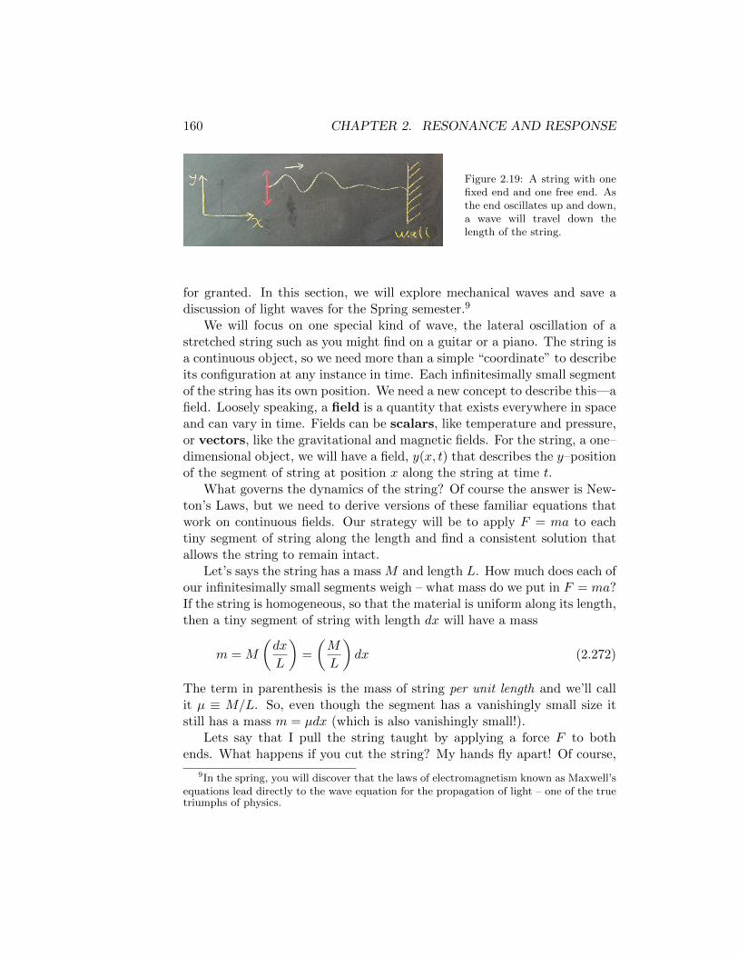
160 CHAPTER 2. RESONANCE AND RESPONSE
Figure 2.19: A string with onefixed end and one free end. Asthe end oscillates up and down,a wave will travel down thelength of the string.
for granted. In this section, we will explore mechanical waves and save adiscussion of light waves for the Spring semester.9
We will focus on one special kind of wave, the lateral oscillation of astretched string such as you might find on a guitar or a piano. The string isa continuous object, so we need more than a simple “coordinate” to describeits configuration at any instance in time. Each infinitesimally small segmentof the string has its own position. We need a new concept to describe this—afield. Loosely speaking, a field is a quantity that exists everywhere in spaceand can vary in time. Fields can be scalars, like temperature and pressure,or vectors, like the gravitational and magnetic fields. For the string, a one–dimensional object, we will have a field, y(x, t) that describes the y–positionof the segment of string at position x along the string at time t.
What governs the dynamics of the string? Of course the answer is New-ton’s Laws, but we need to derive versions of these familiar equations thatwork on continuous fields. Our strategy will be to apply F = ma to eachtiny segment of string along the length and find a consistent solution thatallows the string to remain intact.
Let’s says the string has a mass M and length L. How much does each ofour infinitesimally small segments weigh – what mass do we put in F = ma?If the string is homogeneous, so that the material is uniform along its length,then a tiny segment of string with length dx will have a mass
m = M
(dx
L
)=
(M
L
)dx (2.272)
The term in parenthesis is the mass of string per unit length and we’ll callit µ ≡ M/L. So, even though the segment has a vanishingly small size itstill has a mass m = µdx (which is also vanishingly small!).
Lets say that I pull the string taught by applying a force F to bothends. What happens if you cut the string? My hands fly apart! Of course,
9In the spring, you will discover that the laws of electromagnetism known as Maxwell’sequations lead directly to the wave equation for the propagation of light – one of the truetriumphs of physics.

2.7. WAVE PHENOMENA IN ONE DIMENSION 161
it doesn’t matter where along the string you cut it, the same thing willhappen.
Figure 2.20: Applying a forceto the ends of a string leads to atension throughout the length.
Now, lets suppose that in the very instance that you cut the string youalso grab the two new ends and hold them together. You will need to applya force of F to each of the new ends in order to balance the force that I amapplying to the outer ends. Again, it doesn’t matter where along the stringyou do this, you will need to apply equal and opposite force to each end inorder to hold them together.
Figure 2.21: The tension in thestring is equal to the appliedforce F .
In fact, before you cut the string, this same force must have existedwithin the string in order to bind each atom of string to its neighbors. Oth-erwise the string would move or break because of the lack of force balance.We’ll call this force inside the string the tension.
Problem 53: A real string will have a bit of elasticity to it and will act like a springwith a large spring constant. If you have a spring, instead of a string, it will stretch ifyou apply a force to the ends. After it comes to its new equilibrium length, what is thetension in the spring?
The field y(x, t) is a function of two variables, x and t. We’d like tobe able to take derivatives of y, for instance to calculate the velocity of thestring in the y–direction, but we need to be careful. Let’s start by reviewingthe concept of a differential of a function f(x) which depends on a single

162 CHAPTER 2. RESONANCE AND RESPONSE
variable. If we change x by a tiny incremental amount dx, then the definitionof the first derivative tells us that the function changes by an amount
df ≡(df
dx
)dx (2.273)
But what if I told you that f = ax2 and asked you to find df . Youwould probably say that the derivative of f is 2ax, making the differentialdf = 2ax dx. But why isn’t it x2 da or maybe the sum of these two things?I know that we have ingrained in you the desire to take derivatives withrespect to x and t, but starting now we need to pay a little more attentionto the bookkeeping.
To define the differential of a function of more than one variable, we needto introduce the concept of a partial derivative. Consider a function f(x, y)which depends on variables x and y. If we keep the variable y fixed andlet the variable x change by an amount dx, then f changes by a differentialamount
df =
[lim
∆x→0
f(x+ ∆x, y)− f(x, y)
∆x
]dx (2.274)
The expression inside the brackets looks like a derivative, but because f is afunction of two variables and we are differentiating with respect to only oneof them, we call it a partial derivative and denoted it by ∂f/∂x. When yousay it aloud, this expression is read “the partial derivative of f with respectto x,” or “the partial of f with respect to x.” Practically, all you have to dois treat all other variables constant, except the one you are differentiatingwith.
Consider the function f(x, y) = x2 + xy − y2 which is shown in Figure2.22. Using these rules we have
∂f
∂x= 2x+ y (2.275)
and
∂f
∂y= x− 2y (2.276)
If you start at point (x, y) and ask how much the function f(x, y) haschanged when you move to point (x+dx, y+dy), we can do this in two steps,each time calculating one partial derivative. We first calculate the change

2.7. WAVE PHENOMENA IN ONE DIMENSION 163
Figure 2.22: A function of two variables.
in f as we go from (x, y) to (x + dx, y) and then add it to the change in fwhen we go from (x+ dx, y) to (x+ dx, y+ dy) to find the total differential.
df ≡(∂f
∂x
)dx+
(∂f
∂y
)dy (2.277)
So, the differential of f(a, x) = ax2 really is df = 2ax dx+ x2 da.Going back to f(x, y) = x2 + xy − y2, we have four different possible
second derivatives:
∂2f
∂x2= 2 (2.278)
∂2f
∂x∂y= 1 (2.279)
∂2f
∂y∂x= 1 (2.280)
∂2f
∂y2= −2 (2.281)
You may have noticed that ∂2f∂x∂y = ∂2f
∂y∂x . We won’t go through it, but youcan show that for any “nice” function, where the function and its derivativesare continuous, the order of differentiation doesn’t matter.
Problem 54: If you haven’t seen these before you should probably write down a fewexamples and try them out for yourself.
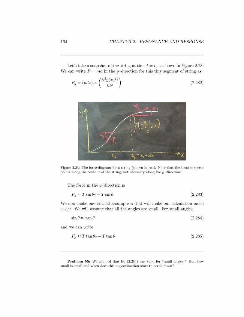
164 CHAPTER 2. RESONANCE AND RESPONSE
Let’s take a snapshot of the string at time t = t0 as shown in Figure 2.23.We can write F = ma in the y–direction for this tiny segment of string as:
Fy = (µdx)×(∂2y(x, t)
∂t2
)(2.282)
Figure 2.23: The force diagram for a string (shown in red). Note that the tension vectorpoints along the contour of the string, not necessary along the y–direction.
The force in the y–direction is
Fy = T sin θ2 − T sin θ1 (2.283)
We now make one critical assumption that will make our calculation mucheasier. We will assume that all the angles are small. For small angles,
sin θ ≈ tan θ (2.284)
and we can write
Fy ≈ T tan θ2 − T tan θ1 (2.285)
Problem 55: We claimed that Eq (2.284) was valid for “small angles.” But, howsmall is small and when does this approximation start to break down?

2.7. WAVE PHENOMENA IN ONE DIMENSION 165
(a.) Using MATLAB plot the error in Equation 2.284 as a function of the θ. If youwant to define a regime in which the approximation is valid, you need to specify an errorthat you are willing to live with. For an error of 1%, what is the “threshold” angle abovewhich the approximation can not be used.
(b.) If you go online10 you can see a high speed video of someone strumming aguitar. Based on an analysis of this video, what is the maximum angle achieved by anylocal section of guitar string? Is our small angle approximation valid for waves on a guitarstring? For your estimated maximum angle, what error does our approximation introduce?
The tangent is the change in y divided by the change in x of the string,i.e. tan θ = ∂y
∂x . So, we are left with
Fy = T
[∂y(x2, t)
∂x− ∂y(x1, t)
∂x
](2.286)
As dx becomes smaller and smaller, the term in brackets becomes the secondpartial derivative evaluated at x1 times dx:
∂2y(x1, t)
∂x2=
d
dx
[∂y(x1, t)
∂x
]≡
∂y(x1+dx,t)∂x − ∂y(x1,t)
∂x
dx(2.287)
Plugging all this into Equation 2.282, we have
T∂2y(x1, t)
∂x2dx = µ
∂2y(x1, t)
∂t2dx (2.288)
This looks pretty messy, but we can clean it up by defining a new constant,
c ≡√
Tµ . Our results is therefore:[∂2
∂x2− 1
c2
∂2
∂t2
]y(x, t) = 0 (2.289)
This is called the wave equation and relates the spatial and temporal deriva-tives of y(x, t) to each other. It is solutions to this equation that will giverise to many interesting phenomena, including the traveling and standingwaves we will study in more detail.
What is c? We can start by calculating its dimensions:
• [T ] = Newtons = kg ms2
10One example is http://www.guitar-tube.com/watch/high-speed-guitar-video.
html, but you are welcome to find other videos.

166 CHAPTER 2. RESONANCE AND RESPONSE
• [µ] = masslength = kg
m
• [c] =√
kg m/s2
kg/m =√
m2
s2= m
s
So, c is a speed! We will see soon that is the velocity of traveling waves onthe string.
What are the solutions of the wave equation? If we choose any functionF (x) (ok, make it a nice well–defined function...), we will show that F (x−ct)is a solution to Equation 2.289. To start, we need to take derivatives of Fwith respect to x and t, keeping track of the fact that the argument of Finclude both x and t.11
∂
∂xF (x− ct) = F ′(x− ct) (2.290)
∂2
∂x2F (x− ct) = F ′′(x− ct) (2.291)
∂
∂tF (x− ct) = F ′(x− ct)× (−c) (2.292)
∂2
∂t2F (x− ct) = F ′′(x− ct)× (c2) (2.293)
Putting Equations 2.291 and 2.293 into Equation 2.289 we find that[∂2
∂x2− 1
c2
∂2
∂t2
]F (x− ct) = F ′′(x− ct)− c2
c2F ′′(x− ct) = 0 (2.294)
so that F (x − ct) is a solution. You can check for yourself that F (x + ct)will also work. Recall that we didn’t specify the shape of F at all, just thatthe argument of the function was x− ct. This will allow us to create manydifferent wave shapes that all travel along the string.
But what does the solution F (x−ct) mean? Consider an arbitrary initialstring conformation y(x, 0) = f(x). We know that y(x, t) = f(x − ct) willbe a solution to the wave equation that retains this initial shape at t = 0.At a later time, t, the height of the string at position x is y(x) = f(x− ct).Hopefully you can see that the segment of string at position x′ = x − ct isat the same y–position at time t as the segment at x was at t = 0. Thewaveform has moved a distance ct in time t, i.e. with velocity c. Over time,the waveform retains its shape, but moves to the right at a constant speedc.
11The prime notation here denotes the derivative with respect to the argument of F ,i.e. ′ ≡ ∂
∂X , where in this case X = x− ct.
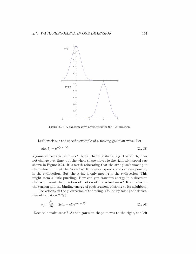
2.7. WAVE PHENOMENA IN ONE DIMENSION 167
t=0
-2 2 4 6
0.2
0.4
0.6
0.8
1.0
t=4/c
-2 2 4 6
0.2
0.4
0.6
0.8
1.0
Figure 2.24: A gaussian wave propagating in the +x–direction.
Let’s work out the specific example of a moving gaussian wave. Let
y(x, t) = e−(x−ct)2 (2.295)
a gaussian centered at x = ct. Note, that the shape (e.g. the width) doesnot change over time, but the whole shape moves to the right with speed c asshown in Figure 2.24. It is worth reiterating that the string isn’t moving inthe x–direction, but the “wave” is. It moves at speed c and can carry energyin the x–direction. But, the string is only moving in the y–direction. Thismight seem a little puzzling. How can you transmit energy in a directionthat is different the direction of motion of the actual mass? It all relies onthe tension and the binding energy of each segment of string to its neighbors.
The velocity in the y–direction of the string is found by taking the deriva-tive of Equation 2.295
vy =∂y
∂t= 2c(x− ct)e−(x−ct)2 (2.296)
Does this make sense? As the gaussian shape moves to the right, the left
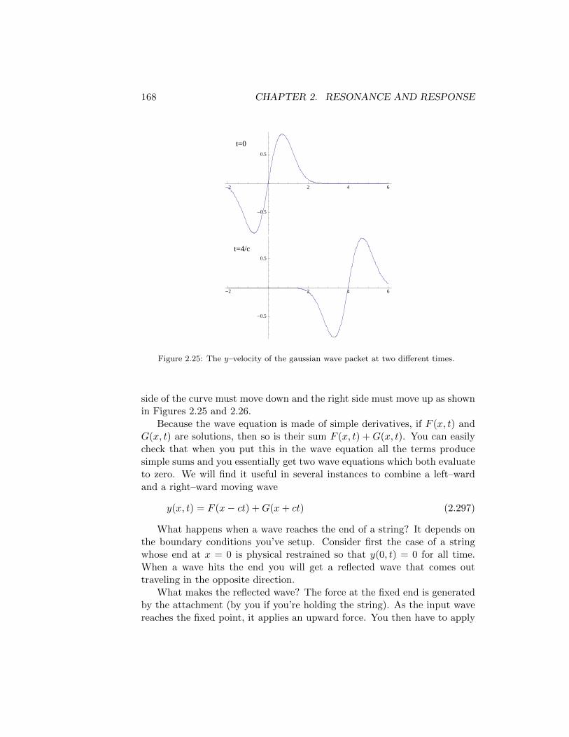
168 CHAPTER 2. RESONANCE AND RESPONSE
t=0
-2 2 4 6
-0.5
0.5
t=4/c
-2 2 4 6
-0.5
0.5
Figure 2.25: The y–velocity of the gaussian wave packet at two different times.
side of the curve must move down and the right side must move up as shownin Figures 2.25 and 2.26.
Because the wave equation is made of simple derivatives, if F (x, t) andG(x, t) are solutions, then so is their sum F (x, t) + G(x, t). You can easilycheck that when you put this in the wave equation all the terms producesimple sums and you essentially get two wave equations which both evaluateto zero. We will find it useful in several instances to combine a left–wardand a right–ward moving wave
y(x, t) = F (x− ct) +G(x+ ct) (2.297)
What happens when a wave reaches the end of a string? It depends onthe boundary conditions you’ve setup. Consider first the case of a stringwhose end at x = 0 is physical restrained so that y(0, t) = 0 for all time.When a wave hits the end you will get a reflected wave that comes outtraveling in the opposite direction.
What makes the reflected wave? The force at the fixed end is generatedby the attachment (by you if you’re holding the string). As the input wavereaches the fixed point, it applies an upward force. You then have to apply
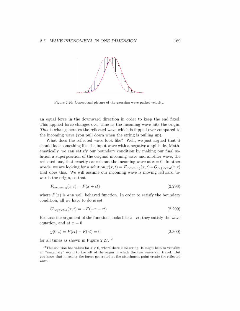
2.7. WAVE PHENOMENA IN ONE DIMENSION 169
Figure 2.26: Conceptual picture of the gaussian wave packet velocity.
an equal force in the downward direction in order to keep the end fixed.This applied force changes over time as the incoming wave hits the origin.This is what generates the reflected wave which is flipped over compared tothe incoming wave (you pull down when the string is pulling up).
What does the reflected wave look like? Well, we just argued that itshould look something like the input wave with a negative amplitude. Math-ematically, we can satisfy our boundary condition by making our final so-lution a superposition of the original incoming wave and another wave, thereflected one, that exactly cancels out the incoming wave at x = 0. In otherwords, we are looking for a solution y(x, t) = Fincoming(x, t)+Greflected(x, t)that does this. We will assume our incoming wave is moving leftward to-wards the origin, so that
Fincoming(x, t) = F (x+ ct) (2.298)
where F (x) is any well–behaved function. In order to satisfy the boundarycondition, all we have to do is set
Greflected(x, t) = −F (−x+ ct) (2.299)
Because the argument of the functions looks like x−ct, they satisfy the waveequation, and at x = 0
y(0, t) = F (ct)− F (ct) = 0 (2.300)
for all times as shown in Figure 2.27.12
12This solution has values for x < 0, where there is no string. It might help to visualizean “imaginary” world to the left of the origin in which the two waves can travel. Butyou know that in reality the forces generated at the attachment point create the reflectedwave.
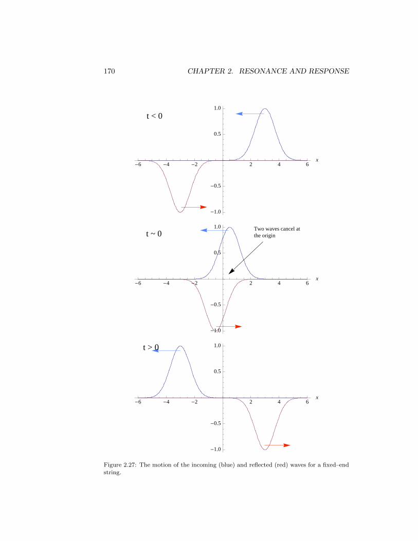
170 CHAPTER 2. RESONANCE AND RESPONSE
t < 0
-6 -4 -2 2 4 6x
-1.0
-0.5
0.5
1.0
t ~ 0Two waves cancel atthe origin
-6 -4 -2 2 4 6x
-1.0
-0.5
0.5
1.0
t > 0
-6 -4 -2 2 4 6x
-1.0
-0.5
0.5
1.0
Figure 2.27: The motion of the incoming (blue) and reflected (red) waves for a fixed–endstring.

2.7. WAVE PHENOMENA IN ONE DIMENSION 171
Now lets send a wave down a string in which one end is fixed at x = 0but is free to move in the y–direction. You can create something like this byimagining the end of the string is attached to a frictionless ring that movesalong a rod at x = 0 as shown in Figure 2.28.
Figure 2.28: A string with a “free” endat x = 0.
In this case, the boundary condition is that the derivative of y withrespect to x has to be zero at the origin for all time. So, we have
∂y(x, t)
∂x
∣∣∣∣x=0
= 0 (2.301)
In this case the solution is y(x, t) = F (x + ct) + F (−x + ct) so that thereflected wave amplitude has the same sign as the incoming wave and is notflipped over. Lets check that this satisfies the boundary conditions.
y(x, t) = F (x+ ct) + F (−x+ ct) (2.302)
y(0, t) = 2F (ct) (2.303)
∂y(x, t)
∂x
∣∣∣∣x=0
= F ′(x+ ct) +−1 ∗ F ′(−x+ ct)
∣∣∣∣x=0
(2.304)
= F ′(ct)− F ′(ct) = 0 X (2.305)
Note that in this case the end moves over time.Consider the following sinusoidal waveform with amplitude A and wave-
length λ that travels to the right along the x–axis:
y(x, t) = A sin
[2π
λ(x− ct)
](2.306)
The wave obviously transfers energy along the x–axis. But what is each bitof string doing? If we look at the y–position of a piece of string at positionx = 0 we find:
y0(t) = −A sin2πct
λ(2.307)
172 CHAPTER 2. RESONANCE AND RESPONSE
The piece moves harmonically in time. As the wave moves to the right,each piece of string continually goes up and down in a sinusoidal pattern intime. It is also worth noting that if we chose a piece of string at a differentposition along the x–axis, the motion will be the same except for a phaseshift. The amplitude of the motion of each piece doesn’t depend on x.
There’s another set of solutions to the wave equation in which the waveamplitude but not the shape depends on time. We will call these waves“standing waves.” The fact that the shape doesn’t depend on time meansthat we can separate the x and t variables in our solution:
y(x, t) = f(x)g(t) (2.308)
The shape of the waveform is given by the function f(x) and doesn’t changewith time. But the amplitude is given by g(t), which does change over time.In particular, if f(x0) = 0 for some point x0, then y(x0, t) = 0 for all times.This type of point in a wave, where there is no motion, is called a node andit will be important in our thinking about musical instruments.
Putting this into the wave equation we get:(∂2
∂x2− 1
c2
∂2
∂t2
)f(x)g(t) =
∂2f(x)
∂x2g(t)− 1
c2
∂2g(t)
∂t2f(x) = 0 (2.309)
We can rearrange Equation 2.309 to find an equation that relates terms withf(x)’s in them to terms with g(t)’s in them.
∂2f(x)∂x2
f(x)=
1
c2
∂2g(t)∂t2
g(t)(2.310)
This equation must be true for any particular f(x) and g(t). The only waythis can work out is if each side of Equation 2.310 is equal to a constant thatdoesn’t depend on your choice of f(x) or g(t). We will call this constantk2 (the meaning of k will become apparent in a bit). We now have twodifferential equations which separately govern the behavior of f(x) and g(t):
∂2f(x)
∂x2+ k2f(x) = 0 (2.311)
∂2g(t)
∂t2+ k2c2g(t) = 0 (2.312)
You’ve seen these second–order equations before and they have solutions:
f(x) = A cos(kx) (2.313)
g(t) = A cos(ωt) (2.314)
2.8. MORE ABOUT 1D WAVES 173
where ω ≡ kc. In order to satisfy the wave equation and retain the separationof variables, both the spatial wave shape and the temporal wave amplitudemust be harmonic.
Our general solution is therefore
y(x, t) = A cos(kx) cos(ωt) (2.315)
Now we see that the constant k is the spatial angular frequency of theharmonic wave shape. It is traditionally called the wave number. ω is thetemporal angular frequency of the wave amplitude. We can relate these tosome more familiar quantities, the wavelength λ and the frequency ν:
k ≡ 2π
λ(2.316)
ω ≡ 2πν (2.317)
Why is this called a wave? Unlike the traveling wave solutions frombefore, there doesn’t seem to be any motion along the x–axis in this solution.We can rewrite Equation 2.315 to recover terms that look like our F (x− ct)solutions:
y(x, t) = A cos(kx) cos(ωt) (2.318)
=A
2cos(kx+ ωt) +
A
2cos(kx− ωt) (2.319)
=A
2cos [k(x+ ct)] +
A
2cos [k(x− ct)] (2.320)
The standing wave solution is just the superposition of a left–moving and aright–moving traveling wave. Figure 2.29 may help you visualize this.
2.8 More about 1D waves
Musical instruments like the guitar, violin, hammer dulcimer, piano, harp-sichord etc. use standing waves on strings with two fixed ends to producetones of a certain pitch. Lets now fix both ends of a string and ask whatkind of standing wave solutions we get.
The boundary condition is that the lateral displacement at each endmust be zero, i.e. y(0, t) = y(L, t) = 0. We will look for standing wavesolutions where we can separate the spatial and temporal wave functionsy(x, t) = f(x)g(t) that satify this condition, i.e. where f(0) = f(L) = 0.

174 CHAPTER 2. RESONANCE AND RESPONSE
Figure 2.29: Snapshots of two oppositely directed traveling waves (red and bludrope) andtheir sum (black, a standing wave) over time. t = 0 is at the upper left and the timemoves to the right and then down.
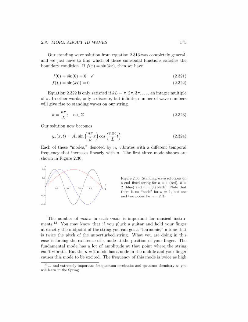
2.8. MORE ABOUT 1D WAVES 175
Our standing wave solution from equation 2.313 was completely general,and we just have to find which of these sinusoidal functions satisfies theboundary condition. If f(x) = sin(kx), then we have
f(0) = sin(0) = 0 X (2.321)
f(L) = sin(kL) = 0 (2.322)
Equation 2.322 is only satisfied if kL = π, 2π, 3π, . . . , an integer multipleof π. In other words, only a discrete, but infinite, number of wave numberswill give rise to standing waves on our string.
k =nπ
L; n ∈ Z (2.323)
Our solution now becomes
yn(x, t) = An sin(nπLx)
cos(nπcLt)
(2.324)
Each of these “modes,” denoted by n, vibrates with a different temporalfrequency that increases linearly with n. The first three mode shapes areshown in Figure 2.30.
0.2 0.4 0.6 0.8 1.0
x
L
-1.0
-0.5
0.5
1.0
y
Figure 2.30: Standing wave solutions ona end–fixed string for n = 1 (red), n =2 (blue) and n = 3 (black). Note thatthere is no “node” for n = 1, but oneand two nodes for n = 2, 3.
The number of nodes in each mode is important for musical instru-ments.13 You may know that if you pluck a guitar and hold your fingerat exactly the midpoint of the string you can get a “harmonic,” a tone thatis twice the pitch of the unperturbed string. What you are doing in thiscase is forcing the existence of a node at the position of your finger. Thefundamental mode has a lot of amplitude at that point where the stringcan’t vibrate. But the n = 2 mode has a node in the middle and your fingercauses this mode to be excited. The frequency of this mode is twice as high
13... and extremely important for quantum mechanics and quantum chemistry as youwill learn in the Spring.

176 CHAPTER 2. RESONANCE AND RESPONSE
as the n = 1 mode and that is why you hear an octave tone. If you nowpush your finger down to fret the note at the middle position you hear thesame high tone. In this case, you are exciting the n = 1 mode but you’veshortened the length by a factor of two which gives the same frequency
(Fundamental) n = 1, L =L′
2; ω =
1πcL′
2
=2πc
L′(2.325)
(1st Harmonic) n = 2, L = L′; ω =2πc
L′(2.326)
You may recall that the wave speed was related to the tension in the
string and the mass per unit length, c =√
Tµ . The frequency of vibration is
therefore
ν =n
2L
√T
µ(2.327)
If you examine the strings on an instrument, you’ll see that the higher thepitch, the thinner the string and thus the lower the mass per unit lengthbecause ν ∼ µ−1/2. In order to tune the frequency of an individual string,you change the tension and use the fact that ν ∼ T 1/2.
Problem 56: A organ pipe also uses standing sound waves of air vibrations insidethe pipes to produce musical notes. The bottom of the pipe is closed and the air can’tmove there but the top of the pipe is open and the air can move. You will model this bythinking about waves on a string and assuming a mixed boundary condition where oneend of the string is fixed and the other is free to move in the y–direction as discussedabove.
(a.) What are the standing wave solutions that you get in this case?(b.) For the pipe organ, what are the relevant analogs of the tension and the mass
per unit length? How would you go about tuning a pipe organ?
You should be a little concerned about our discussion of strumminga guitar string. When you hit the string to strum it, the string shapecertainly doesn’t look like the perfect sine waves we found as the standingwave solutions. What happens to the string and how can we relate it to thestanding waves? To start, we will assume that we have a string with two

2.8. MORE ABOUT 1D WAVES 177
fixed ends and start the wave with an initial shape u(x) and y–velocity v(x),i.e.
y(x, 0) = u(x) (2.328)
∂
∂ty(x, t)
∣∣∣∣t=0
= v(x) (2.329)
Key math concept: What we need to do now is write the initialwaveform as a superposition of the different standing wave solutions – thesines and cosines. You already know that any arbitrary function can bewritten as a sum of polynomials in a Taylor’s series. When we discussedthe driven oscillator, we also claimed that any periodic function could bewritten as a sum of sines and cosines, which was first shown by the Frenchmathematician J. Fourier (1768–1830) 14
f(x) = A0 +∑n
[An sin(nkx) +Bn cos(nkx)] (2.330)
where k = 2πλ is the wave number associated with the wavelength of f(x).
Since the ends of our string are fixed, we have nodes at x = 0, L and wecan consider L to be our period. The fixed end at x = 0 implies that wecan’t have any of the cosine terms from Equation 2.330. We can thereforewrite the general standing wave solution as
y(x, t) =∑n
[An sin(knct) +Bn cos(knct)] sin(knx) (2.331)
where kn = nπL . We have kept both the sine and cosine terms in time to
allow us to match any initial condition.Lets look at this more carefully now. Each of the terms of the sum in
Equation 2.331 is a standing wave solution to the wave equation that obeysthe fixed–end boundary conditions. Our task is to find the different coeffi-cients An and Bn such that y(x, t) matches our initial conditions describedby u(x) and v(x).
u(x) = y(x, 0) =∑n
Bn sin(nπxL
)(2.332)
v(x) =∂y(x, t)
∂t
∣∣∣∣t=0
=∑n
An
(nπxL
)sin(nπxL
)(2.333)
14If the function is not periodic, the sum is replaced with an integral in what is calleda Fourier Transform. You’ll return to this topic in the Spring semester.
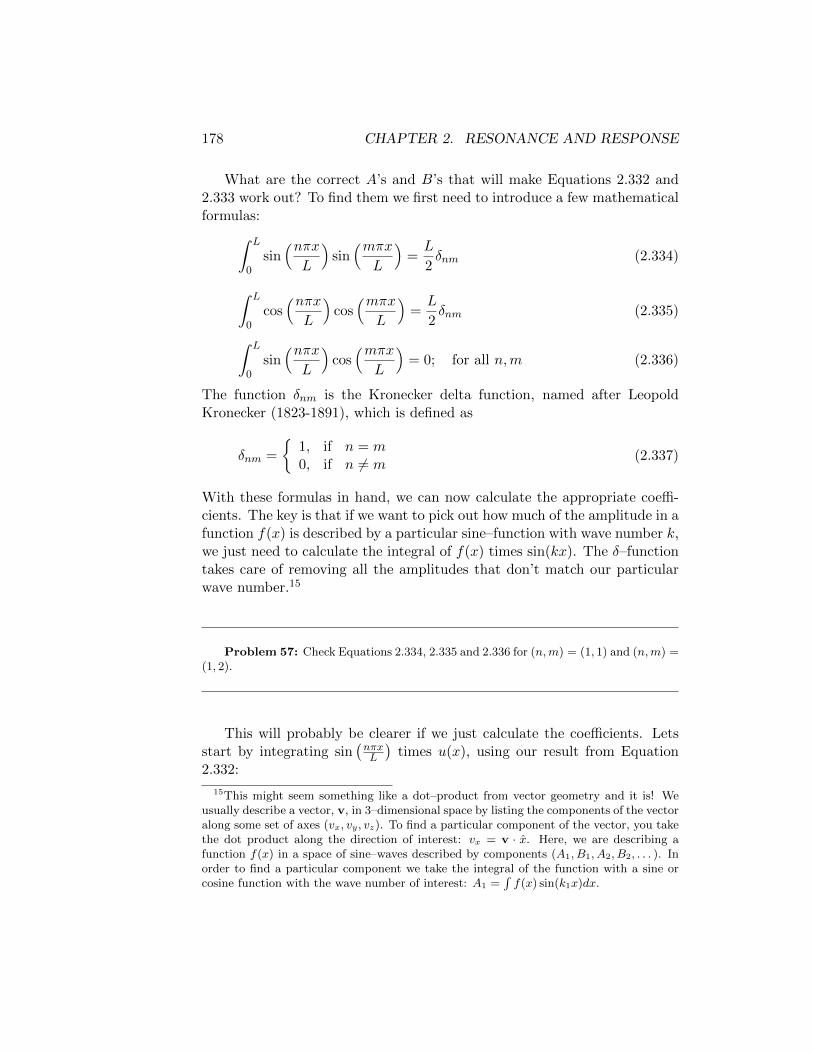
178 CHAPTER 2. RESONANCE AND RESPONSE
What are the correct A’s and B’s that will make Equations 2.332 and2.333 work out? To find them we first need to introduce a few mathematicalformulas:∫ L
0sin(nπxL
)sin(mπx
L
)=L
2δnm (2.334)
∫ L
0cos(nπxL
)cos(mπx
L
)=L
2δnm (2.335)
∫ L
0sin(nπxL
)cos(mπx
L
)= 0; for all n,m (2.336)
The function δnm is the Kronecker delta function, named after LeopoldKronecker (1823-1891), which is defined as
δnm =
{1, if n = m0, if n 6= m
(2.337)
With these formulas in hand, we can now calculate the appropriate coeffi-cients. The key is that if we want to pick out how much of the amplitude in afunction f(x) is described by a particular sine–function with wave number k,we just need to calculate the integral of f(x) times sin(kx). The δ–functiontakes care of removing all the amplitudes that don’t match our particularwave number.15
Problem 57: Check Equations 2.334, 2.335 and 2.336 for (n,m) = (1, 1) and (n,m) =(1, 2).
This will probably be clearer if we just calculate the coefficients. Letsstart by integrating sin
(nπxL
)times u(x), using our result from Equation
2.332:
15This might seem something like a dot–product from vector geometry and it is! Weusually describe a vector, v, in 3–dimensional space by listing the components of the vectoralong some set of axes (vx, vy, vz). To find a particular component of the vector, you takethe dot product along the direction of interest: vx = v · x. Here, we are describing afunction f(x) in a space of sine–waves described by components (A1, B1, A2, B2, . . . ). Inorder to find a particular component we take the integral of the function with a sine orcosine function with the wave number of interest: A1 =
∫f(x) sin(k1x)dx.

2.8. MORE ABOUT 1D WAVES 179
∫ L
0dx sin
(nπxL
)u(x) =
∫ L
0dx sin
(nπxL
)[∑m
Bm sin(mπx
L
)](2.338)
=∑m
Bm
[∫ L
0dx sin
(nπxL
)sin(mπx
L
)](2.339)
=∑m
Bm
(L
2
)δnm (2.340)
=L
2Bn (2.341)
We can do the same with v(x):∫ L
0dx sin
(nπxL
)v(x) =
∫ L
0dx sin
(nπxL
)[∑m
mπc
LAm sin
(mπxL
)](2.342)
=∑m
mπc
LAm
[∫ L
0dx sin
(nπxL
)sin(mπx
L
)](2.343)
=∑m
mπc
LAm
(L
2
)δnm (2.344)
=L
2
nπc
LAn =
nπc
2An (2.345)
So, thats it. Equations 2.341 and 2.345 allow us to calculate the coeffi-cients An and Bn from our initial conditions u(x) and v(x):
An =2
nπc
∫ L
0sin(nπxL
)v(x)dx (2.346)
Bn =2
L
∫ L
0sin(nπxL
)u(x)dx (2.347)
Problem 58: In this problem you’ll think about the standing wave produced whenyou pluck a string on a guitar. As you let go of the string it starts as an approximately

180 CHAPTER 2. RESONANCE AND RESPONSE
triangular shape at rest. Our initial conditions are:
u(x) =
{x/L, if 0 ≤ x ≤ L/2
1− x/L, if L/2 ≤ x ≤ L (2.348)
v(x) = 0 (2.349)
(a.) Sketch the initial shape of the waveform.(b.) Calculate the Fourier amplitudes An and Bn that satisfy the initial conditions.(c.) How fast does each of the n modes vibrate? Do you hear all these “notes”?(d.) You’ve seen that friction is proportional to velocity. In general, the dissipation
of energy in the vibrating string is also proportional to velocity. Using this fact, describein words what happens to all the modes after you pluck the string. What consequencedoes this have for the perceived “note” that is played when you pluck the string?

Chapter 3
The conservation of energy
So far in this course we have used Newton’s laws to solve the dynamics ofa number of specific systems by writing these laws as differential equations,v = dx
dt and F = md2xdt2
. If we know the starting position and velocity of anobject, we can then use the velocity and force to update these quantitiesiteratively over time. In fact, this is exactly how one solves these types ofdifferential equations numerically on a computer, by moving incrementallyin dt–sized time steps. In some sense, we can think of Newton’s laws as“local” in time in that they tell us how to go from one point in time to thenext.
But there are other kinds of statements that we can make about a phys-ical system that are not local in time. These include the idea that the earthrevolves around the sun and that a mass on a spring will go up and downover and over. The term “goes around the sun” is most certainly not a localstatement because if you watch the system at any one time you only see itmove by one time step and can’t see that the orbit of the earth is an ellipseand that it even closes on itself and will continue in the same orbit. Thesestatements are more “global” and they describe not just how the systemgoes from time point to time point, but rather how the system will behaveforever.
Another kind of global statement comes in the form of conservation laws,which state that a particular measurable property of a system remains con-stant in time, even as the system evolves. Examples include the conservationof energy and momentum which you have probably seen before. One trulybeautiful concept that arose in the early 20th century is called Noether’sTheorem, which draws a one–to–one correspondence between symmetries innature and conservation laws. As an example of this, we will see later on
181

182 CHAPTER 3. THE CONSERVATION OF ENERGY
that the conservation of momentum is true even when Newton’s laws don’thold, e.g. in Quantum Mechanics, and that this law is related directly tothe fact that physical systems behave the same regardless of how they arepositioned in space.
3.1 Kinetic and potential energies
Let’s start by supposing that the force on an object is a function of theposition of the object in space but not on the velocity or time so that wecan write
mdx2
dt2= F (x) (3.1)
The familiar example of a mass on a spring, F (x) = −kx, is just one example.We will now look for a quantity, E, that remains fixed in time so thatdE/dt = 0. This constant may depend on the position and/or velocity ofthe object so that E(x, v) is a function of two variables. We can write thetotal differential of E as
dE(x, v) =
[∂E(x, v)
∂x
]dx+
[∂E(x, v)
∂v
]dv (3.2)
The condition that E remain constant in time then becomes
dE(x, v)
dt=
[∂E(x, v)
∂x
]dx
dt+
[∂E(x, v)
∂v
]dv
dt= 0 (3.3)
which can be rewritten as[∂E(x, v)
∂v
]dv
dt= −
[∂E(x, v)
∂x
]dx
dt(3.4)
Now, if we multiply Equation 3.1 by dx/dt, we find that[mdx
dt
]dv
dt= [F (x)]
dx
dt(3.5)
Comparing the two previous equations, we see that they look quite sim-ilar. If we can find a form for E(x, v) such that the terms in brackets oneach side of the equations are equal, then we will have found our constantof the motion. This procedure produces two equations for E(x, v)
∂E(x, v)
∂v= m
dx
dt= mv (3.6)

3.1. KINETIC AND POTENTIAL ENERGIES 183
−∂E(x, v)
∂x= F (x) (3.7)
In general, this looks like it might be messy, but it isn’t because each equa-tion above only depends on x or v, but not both. When we integrate equation3.6 with respect to v, the constant of integration will not depend on v, butcan depend on x. Equation 3.6 therefore requires that
E(x, v) =1
2mv2 + g(x) (3.8)
where g(x) is the “constant” of integration. Likewise, integration of equation3.7 yields 1
E(x, v) = −∫ x
0F (x′)dx′ + h(v) (3.9)
Because of the separation of variables in these two equations, both will besatisfied if we write
E(x, v) =1
2mv2 −
∫ x
0F (x′)dx′ (3.10)
So thats it. Newton’s second law guarantees that E, which we can nowidentify as the total energy, remains constant as the system evolves in time.In fact, Newton’s equations are equivalent to the statement that the totalenergy remains constant along a particle’s trajectory.
The first term in the energy is related to the motion of the particle andwe call this the kinetic energy, K = 1
2mv2. The second term in the energy
is related to how much energy is stored in the system at position x due tothe force. We call this term the potential energy
U(x) = −∫ x
0F (x′)dx′ (3.11)
The total energy can then be written as E = K + U .Let’s now use the mass on a spring to illustrate this concept. The force
on the spring is F (x) = −kx so that the potential energy function is givenby
U(x) = −∫ x
0(−kx′)dx′ = 1
2kx2 (3.12)
1The choice of the lower integrant is a bit arbitrary at this point, but rest assured thatwe will come back to that soon.

184 CHAPTER 3. THE CONSERVATION OF ENERGY
and the total energy is
E =1
2mv2 +
1
2kx2 (3.13)
Using Newton’s equations, we have already solved for the position of themass as a function of time, and found it to be
x(t) = Aeiωt +A∗eiωt (3.14)
where the complex amplitude A depends on the initial position and velocity.Differentiating this equation with respect to time, we can find the velocity
v(t) = iωAeiωt − iωA∗eiωt (3.15)
Plugging these values into equation 3.13 we find that
1
2mv2 +
1
2kx2 =
1
2m[iωAeiωt − iωA∗eiωt
]2+
1
2k[Aeiωt +A∗eiωt
]2(3.16)
=1
2m[−ω2A2e2iωt − ω2A∗2e−2iωt + ω2AA∗
](3.17)
+1
2k[A2e2iωt +A∗2e−2iωt +AA∗
](3.18)
=1
2k[(A2 −A2)e2iωt + (A∗2 −A∗2)e−2iωt + 2|A|2
](3.19)
= k|A|2 (3.20)
Where we have used the fact that ω2 = k/m. So, we see that our solutiondoes indeed lead to a constant energy, with value E = k|A|2. You can checkfor yourself that |A|2 does indeed look like the total energy at time t = 0.
One way to look at the different solutions to a set of dynamical equationsis to plot them in “phase space.” In mathematics and physics, a phase spaceis a space in which all possible states of a system are represented, witheach possible state corresponding to one unique point. For the mechanicalsystems we’ve been looking at, phase space consists of all possible values ofthe position and velocity variables, i.e. a two-dimensional space in whichthe axes are x and v. Our conservation of energy equation for the harmonicoscillator (Eq. 3.13) can be rewritten as
x2
2E/k+
v2
2E/m= 1 (3.21)

3.1. KINETIC AND POTENTIAL ENERGIES 185
This is just the equation for an ellipse in the x–v plane (Fig. 3.1)! Overtime, the system repeatedly traces out this ellipse forever. The length ofthe major and minor axes are governed by the mass, spring stiffness and thetotal energy. For a given k and m, the size of the ellipse is set by the energy.A system with more energy will move at a larger distance from the originthan a system will less energy. Different initial conditions, i.e. position andvelocity, change where on the ellipse the system starts, but not the shape orsize of the ellipse.
Figure 3.1: Phase space plot ofthe trajectory of two harmonicoscillators at different energies.
Problem 59: You reach out your dorm room window and throw a ball up into theair. The ball has a mass m = 0.1 kg, and assume that it leaves your hand when it isat a height h0 = 5 m above the ground. With a little effort you manage to impart aninitial (upward) velocity v0 = 5 m/s to the ball. Neglect friction or drag as the ball movesthrough the air, so the only relevant force is gravity. In case you forget, g = 9.8 m/s2.
(a.) What is the initial kinetic energy of the ball (in Joules)?
(b.) Use conservation of energy to determine the maximum height hmax that the ballwill reach above the ground.
(c.) As the ball falls back toward the ground, it passes your window again. At themoment when it is exactly at its initial height h0, what is its velocity? Why? Hint: Youdon’t need a calculator to do this part of the problem.
Problem 60: Consider a simple harmonic oscillator: A mass M and a spring ofstiffness κ, with no damping. Assume an initial condition x(t = 0) = x0 and v(t = 0) = 0.
(a.) Sketch the potential energy and kinetic energy as a function of time. Label theaxes, and relate major features of your sketch to the parameters of the problem.

186 CHAPTER 3. THE CONSERVATION OF ENERGY
(b.) What is the value of the potential energy averaged over one cycle of the oscilla-tion?
(c.) What is the value of the kinetic energy averaged over one cycle of the oscillation?
Problem 61: Instead of starting with F = ma, one can solve the type of dynamicsproblems that we have been studying this semester in terms of the conservation of energy.
(a.) For a particle that starts at position x0 with total energy E at time t = 0, showthat the position can be found using the following integral
t =
∫ x
x0
±dx′√2m
[E − U(x′)](3.22)
What does the ± mean and which sign should you choose?
(b.) Solve for the trajectory x(t) for a harmonic oscillator, U(x) = 12kx2, using
Equation 3.22 for the initial condition: x(t = 0) = x0 and v(t = 0) = v0. Does youranswer agree with our previous calculations?
3.2 Conservative forces and potential energy
When we began the semester, we had a little trouble coming up with adefinition for a force beyond Newton’s second law, i.e. that a force is whatcauses the acceleration of mass. Now we can go a little farther in that weknow that the force can be written as the derivative of the potential energy.Forces of this kind are called conservative forces because they, in some sense,conserve mechanical energy.
One important consequence of this is that the work done by a force onan object depends only on the initial and final positions, and is independentof the path taken between these locations. To see this, we can calculate thework done in moving from position x1 to position x2 against a force
W =
∫ x2
x1
F (x)dx = −∫ x2
x1
dU(x)
dxdx = U(x1)− U(x2) (3.23)
The final answer only depends on the value of the potential energy at aand b and does not remember how the system moved between these twopositions. If you move a mass from height h1 to height h2, gravity does workon the mass and the magnitude of this energy doesn’t depend on whetheryou moved the the mass in a straight path between the endpoints or a veryconvoluted one as in Figure 3.2. Another way of putting this same conceptis that no work is done by an external force if an object is moved in a closedpath, i.e. it ends up where it started.
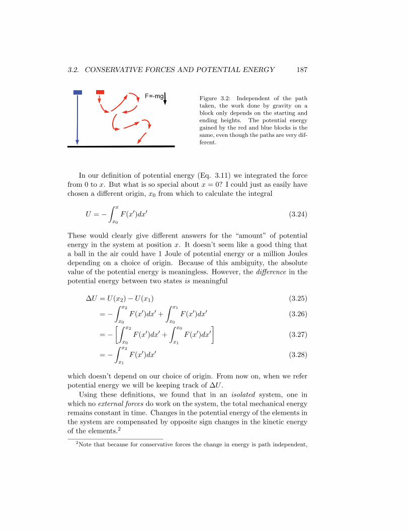
3.2. CONSERVATIVE FORCES AND POTENTIAL ENERGY 187
Figure 3.2: Independent of the pathtaken, the work done by gravity on ablock only depends on the starting andending heights. The potential energygained by the red and blue blocks is thesame, even though the paths are very dif-ferent.
In our definition of potential energy (Eq. 3.11) we integrated the forcefrom 0 to x. But what is so special about x = 0? I could just as easily havechosen a different origin, x0 from which to calculate the integral
U = −∫ x
x0
F (x′)dx′ (3.24)
These would clearly give different answers for the “amount” of potentialenergy in the system at position x. It doesn’t seem like a good thing thata ball in the air could have 1 Joule of potential energy or a million Joulesdepending on a choice of origin. Because of this ambiguity, the absolutevalue of the potential energy is meaningless. However, the difference in thepotential energy between two states is meaningful
∆U = U(x2)− U(x1) (3.25)
= −∫ x2
x0
F (x′)dx′ +
∫ x1
x0
F (x′)dx′ (3.26)
= −[∫ x2
x0
F (x′)dx′ +
∫ x0
x1
F (x′)dx′]
(3.27)
= −∫ x2
x1
F (x′)dx′ (3.28)
which doesn’t depend on our choice of origin. From now on, when we referpotential energy we will be keeping track of ∆U .
Using these definitions, we found that in an isolated system, one inwhich no external forces do work on the system, the total mechanical energyremains constant in time. Changes in the potential energy of the elements inthe system are compensated by opposite sign changes in the kinetic energyof the elements.2
2Note that because for conservative forces the change in energy is path independent,
188 CHAPTER 3. THE CONSERVATION OF ENERGY
∆K + ∆U = 0 (3.29)
3.3 Defining the system
We will now look at the effect of an external force on a system. Imaginethat we draw a boundary around the objects that we are interested in, say amass and a spring, and call everything within the boundary the system, andeverything outside of the boundary the environment. Inside the boundary,the different masses can move around and possess kinetic energy. Therecan also be elements that generate conservative forces within the systemand we will talk about these elements by looking at their potential energies.Outside the boundary, things in the environment can apply forces on thesystem and transfer energy to/from the system. This transfer of energy willbe called “mechanical work”, Wext. Our equation for the conservation ofenergy then equates changes in the energy in the system to the work doneby the external environment.
∆Ktotal + ∆Utotal = Wext,total (3.30)
In the paragraph above, there is a subtle distinction between the energiesin the system, both kinetic and potential, and the external work. Workrepresents the transfer of energy to a system by forces in the environmentcaused by a change in parameters of the system such as the volume, magneticor electric fields or the gravitational potential. This transferred energy canthen cause an increase or decrease in the energies inside the system. Objectswithin the system can posses a certain amount of kinetic or potential energy,but an object never “has W Joules of work.”
We need to make pick a convention for the sign of the work done bya force. We will define positive external work done by the environmenton the system as work that increases the energy of the system. Negativework would then transfer energy out of the system and decrease the systemenergy3.
we can use the ∆ to refer to the total change in a quantity comparing the initial andfinal states. Unlike the typical trick of using ∆ to sneak in calculus with out saying so,we really mean the total change in the kinetic and potential energies and do not need toconsider small changes in the limit ∆→ 0.
3This choice is arbitrary and we could just as easily reverse all the signs as long as wekeep everything consistent.

3.3. DEFINING THE SYSTEM 189
So, how do we decide what is in the “system” and what is in the “en-vironment”? Well, it actually doesn’t matter in the end. We are free todraw the boundary wherever we want and use Equation 3.30 to calculatethe balance of energy. Of course, the conservation of energy must alwayshold. Lets look at an example to try to make this clear.
Assume you have a mass M suspended from a spring of stiffness k underthe influence of gravity. Where do we draw the boundary of the system?
1. It might seem natural to draw the boundary around mass and thespring. The spring generates potential energy and gravity is an exter-nal force. The change in kinetic energy, i.e. the change in the speed, ofthe mass plus the change in potential energy from the spring is equalto the external work done by gravity.
∆K + ∆Uspring = Wgravity (3.31)
2. We could, however, draw the boundary around just the mass. In thiscase, there are no force–generating elements inside the boundary andthus no potential energy to consider. So, our equation of conservationof energy becomes
∆K = Wspring +Wgravity (3.32)
Which leads to the same equation for the kinetic energy. The signof Wspring in this case is opposite that of Uspring in the previous casebecause of our definition of the sign of the work. You should work thisthrough in your head to make sure you understand what’s going on.
3. What is so special about the spring? We could equally as well choosethe mass and the earth(!) as our system. The earth generatespotential energy in the system and the spring applies an external force
∆K + ∆Ugravity = Wspring (3.33)
Again, the same thing.
4. Finally, lets just say that the whole universe is the system. Thespring and gravity create potential energy and there are no externalforces.
∆K + ∆Ugravity + ∆Uspring = 0 (3.34)

190 CHAPTER 3. THE CONSERVATION OF ENERGY
All of these representations are equally as valid and we are free to choosewhatever one we want. In practice, one usually tries to choose the definitionthat makes the solution to a problem easiest, but this is not always apparentat the outset.
Problem 62: (a.) Show that two observers in different frames of reference that aremoving relative to each other will measure different positions and velocities, but will agreeon the accelerations and forces. Assume that one observer is on a train moving with speedv0 relative to the ground where a second observer stands
(b.) Because the two observers measure different velocities, they will not agree onthe value of the kinetic energy of an object. Show that even though the two observersdisagree about this, they do agree that if an external force changes that velocity, then thework done by the force, assuming no potential energy, is given by W = ∆K. It should bereassuring to know that these two observers will measure the same laws of physics eventhough the numerics may not always agree.
3.4 Internal energy
Before we move on, its worth noting that most objects we encounter inthe real world are not “point particles,” but instead are rather complicatedthings. Energy can be stored inside of an object that we can’t “see,” andtherefore our consideration of energy must include these things. In describ-ing the change in energy of a person, an atomistic description in which wedescribe the position and velocity of every atom and the interactions be-tween them would indeed conform to the type of formalism we’ve developedpreviously. But that seems a bit cumbersome, and we’d like to be able totalk about the position of the person and not the 1028 atoms that make uphim or her. In order to do this, we need to lump all the energy one canstore in the interactions between atoms in the body into one quantity, theinternal energy, Eint. Potential energy or external work can, therefore, beconverted either into a change in kinetic energy or a change in the internalenergy of the object.
∆K + ∆U + ∆Eint = Wext (3.35)
What types of things can make up an “internal” energy? Anything,really. These include the kinetic motion of molecules within an object4, a
4We will soon make a connection between this idea and the temperature of an object

3.4. INTERNAL ENERGY 191
change in the chemical bonding forces between molecules in an object (e.g.by changing the lattice spacing in a crystal), electric and magnetic fields,light ...
Exercise: Come up with three specific examples of an internal energy in a biologicalorganism.
As an example, lets think about how the muscles in your arm work tolift a weight. If you lift the weight slowly from height h1 to height h2, youchange the potential energy of the system, which we’ll define as you plus theweight, by the amount of work done by the gravitational force
∆Wext = mg(h2 − h1) (3.36)
Because you moved the weight slowly, the change in the kinetic energy will benegligible. Furthermore, there aren’t any springs or other simple mechanicalelements in the system for which a change in potential energy could com-pensate for the external work. What must be happening is that your bodyis changing the amount of internal energy stored in your muscles and bones,even though we don’t really see it (although we might see some signs of thisexertion as you start to turn red and sweat).
Figure 3.3: The design of amuscle.

192 CHAPTER 3. THE CONSERVATION OF ENERGY
The muscles in your body are made up of a series of parallel fibers thatcan generate mechanical forces by shrinking in length (Fig. 3.3). The shrink-ing unit within a fiber is called a sarcomere, which is made up of an array ofactin filaments (one of the main structural fibers in all of your cells) and aspecial enzyme called myosin. Myosin is a molecular motor, like the kinesinwe saw earlier, that uses chemical energy to produce mechanical work. Inparticular, myosin catalyzes the hydrolysis of ATP: ATP → ADP + Pi.This process releases some of the energy stored in the ATP molecule andmyosin is built such that some of this energy is used to rotate a lever armwithin the protein. This rotation slides the myosin “thick” filament relativeto the two actin “thin” filaments in the sarcomere so that the unit getsshorter. When you lift a weight, your “internal” energy is changing by anamount mg(h2 − h2) and this energy comes from energy stored in the ATPmolecules in your muscles.
Problem 63: For every ATP molecule hydrolyzed, myosin slides an actin filamenta distance d ∼ 4 nm along in a sarcomere. The ATP hydrolysis reaction releases ∼50 kJ/mole of energy.
(a.) How much energy is released by one ATP molecule?(b.) If myosin can use all of this energy to do mechanical work, and if it uses one
ATP molecule for each step along the actin filament, how much force can it generate whilemoving through its step of length d?
(c.) How many myosin molecules must be working together when you hold up a 1 kgweight against the force of gravity?
3.5 Mechanical equilibrium
One can deduce many of the properties of a particle’s motion by examiningthe shape of the potential energy function U(x). Because the kinetic energy,T = 1
2mv2, is always greater than zero, the total energy E must be greater
than or equal to the potential energy for any real–world motion. Let’sexamine the the potential energy profile sketched in Fig. 3.4. A particlewith energy E4 is unbounded by the potential and is free to move along thex–axis. Of course, it will slow down and speed up due to the potential, butit will not stop or turn around. Now consider a particle with energy E3
moving to the left towards x7. The particle will keep moving, speeding upand slowing down, until it reaches x7, where the potential energy is equalto the total energy. At this point the kinetic energy must be zero and the
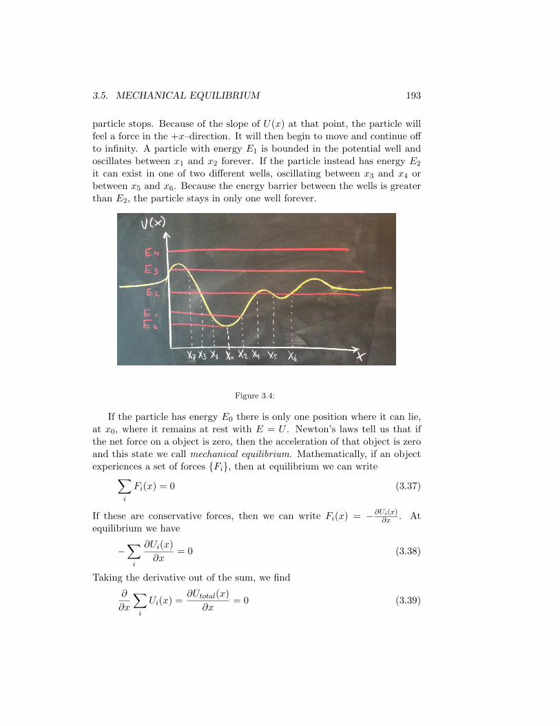
3.5. MECHANICAL EQUILIBRIUM 193
particle stops. Because of the slope of U(x) at that point, the particle willfeel a force in the +x–direction. It will then begin to move and continue offto infinity. A particle with energy E1 is bounded in the potential well andoscillates between x1 and x2 forever. If the particle instead has energy E2
it can exist in one of two different wells, oscillating between x3 and x4 orbetween x5 and x6. Because the energy barrier between the wells is greaterthan E2, the particle stays in only one well forever.
Figure 3.4:
If the particle has energy E0 there is only one position where it can lie,at x0, where it remains at rest with E = U . Newton’s laws tell us that ifthe net force on a object is zero, then the acceleration of that object is zeroand this state we call mechanical equilibrium. Mathematically, if an objectexperiences a set of forces {Fi}, then at equilibrium we can write∑
i
Fi(x) = 0 (3.37)
If these are conservative forces, then we can write Fi(x) = −∂Ui(x)∂x . At
equilibrium we have
−∑i
∂Ui(x)
∂x= 0 (3.38)
Taking the derivative out of the sum, we find
∂
∂x
∑i
Ui(x) =∂Utotal(x)
∂x= 0 (3.39)

194 CHAPTER 3. THE CONSERVATION OF ENERGY
Since the derivative of the total potential energy with respect to x is zero, thepotential energy must be an extremum (a minimum, maximum or inflectionpoint) at equilibrium. An equilibrium point can be stable or unstable toperturbations depending on the sign of the second derivative of the potentialenergy. If we look at the force on an object a distance δx from an equilibriumpoint we find
F (xeq + δx) = −∂U(x)
∂x
∣∣∣∣x=xeq+δx
(3.40)
≈ −∂U(xeq)
∂x− ∂2U(xeq)
∂x2δx (3.41)
= −∂2U(xeq)
∂x2δx (3.42)
This looks like a spring with a restoring force that pulls the object towards
the equilibrium point if∂2U(xeq)∂x2
> 0, i.e. if the potential energy is a mini-mum at the equilibrium point. This is called a stable equilibrium point. If∂2U(xeq)∂x2
< 0 and the equilibrium point is a maximum then the force pushesthe object farther away from xeq and the point is an unstable equilibriumpoint.
As an example, lets consider a mass m attached to the end of a springof stiffness k under the influence of gravity. The total potential energy isgiven by
U(x) =1
2k(x− x0)2 −mg(x− x0) (3.43)
To find the equilibrium point(s), we take the derivative and set it to zero
dU
dx= k(xeq − x0)−mg = 0 (3.44)
Which gives xeq = x0 + mgk . The second derivative of the potential energy
at xeq is just k which is greater than zero so that the energy is a minimumat the equilibrium point at it is stable as you could have guesses.
Problem 64: Consider a particle under the influence of a force
F (x) = −kx+k
βx3 (3.45)
where k and β are both positive constants.
3.6. NONCONSERVATIVE FORCES: FRICTION AND OTHER WAYS TO LOSE ENERGY195
(a.) Solve for the potential energy U(x).(b.) Describe the motion for particles with different energies at various positions.(c.) What happens when E = 1
4kβ?
3.6 Nonconservative forces: Friction and other waysto lose energy
Your intuition should be telling you that there is something about theseidealized pictures that doesn’t quite match with your experience. First ofall, towards the beginning of the class we learned about friction and windresistance, forces whose magnitudes are proportional not to position, but tovelocity and the velocity squared respectively. For these types of forces, apotential of the form U(x) clearly makes no sense. Its not the position thatgoverns the force but how fast the position is changing. The work done bythese forces depends not on the endpoints, but on the speed an object movesalong a particular path between the endpoints. We will call these types offorces nonconservative.5 For these types of forces, you can not define apotential energy and the equation for the conservation of energy we derivedbefore doesn’t hold! So, what good is a conservation law if it only works forsome kinds of forces? Soon, we’ll amend our definitions to patch this up,but for now lets put the conservation of energy on hold.
As an example, consider an object moving with a constant velocity inthe presence of a friction force
F (x) = −γx (3.46)
If the object travels a distance ∆x = v∆t, then the work done by the forceon the object is
W = F (x)∆x = −γv∆x = −γv (v∆t) = −γv2∆t (3.47)
The work does not depend on the position (we could repeat the experiment2 meters to the right and nothing would change), or even the direction, but
5The idea of nonconservative forces is somewhat misleading and is usually due to themacroscopic treatment of something that is really the sum of many microscopic parts. Forexample, friction is caused by the conservative forces between the atoms in a moving objectand the thing its moving against. Each one of these microscopic forces is conservative andcan be written as the gradient of a potential. But, the resultant force on the object asa whole appears to be nonconservative. In reality, there are no nonconservative forces inthe universe in that we know of.

196 CHAPTER 3. THE CONSERVATION OF ENERGY
instead on the amount of time the object spent moving. If the object movesin a closed path, say out a meter and back, the object looses energy thewhole time even though it started and stopped at the exact same position.
Problem 65: Energy of an underdamped oscillator
(a.) Derive an expression for the energy of an underdamped oscillator as treated inChapter 2.3.
(b.) Graph the energy as a function of time.
(c.) Make a phase-space plot of the trajectory of the underdamped oscillator. Doesthe system move in a closed orbit?
Problem 66: Derive the formula for the energy of a spring–mass system in whichthe drag force is equal to Fdrag = −ε dx
dt
2which is the correct form for air resistance.
Problem 67: Imagine that we drop a ball of mass m from an initial height h0.
(a.) Neglecting friction, use conservation of energy to plot the ball’s velocity v(t) =dh/dt as a function of its height h(t).
(b.) Suppose that as the ball falls through the air it experiences a drag force−γ(dh/dt);again it starts from a height h0. Without solving any differential equations, show how theplot of v(t) vs. h(t) will change as a result of this friction.
(c.) Solve the differential equation corresponding to F = ma to find an expression forh(t) in the presence of friction. Show that there are simple limiting behaviors for small tand large t. Plot h(t) and indicate these simple limits, as well as the time scale on whichthe plot crosses over from one limit to the other.
(d.) Plot the amount of time T required to hit the ground [h(T ) = 0] as a functionof the initial height h0. Hint: The small t and large t limits in [c] correspond to small h0
and large h0 regions of this plot.
So, we’ve seen that friction forces can’t be described by a potential andthe conservation laws we wrote before don’t seem to hold. Is friction theonly example where this breaks down? Lets return to the weight liftingexample. After you’ve lifted the weight, what if you try to hold it up foreverwith your muscles. From experience, we know that you’ll get tired, butwhy? The position of the weight isn’t changing, so there’s no change ingravitational potential energy. Nothing is moving, so there’s no friction orkinetic energy. Why is it that your body has to keep using up energy tohold the weight up? It turns out that your muscles have no way to “lock in”a position. Instead, they have to keep burning ATP to maintain a certaindegree of muscle fiber shrinkage, which is why you get tired. But where doesall this energy go?

3.7. GAINING ALL THE ENERGY BACK: THE FIRST LAW OF THERMODYNAMICS197
3.7 Gaining all the energy back: The first law ofThermodynamics
So far, we have only talked about one method of transferring energy intoor out of a system – through mechanical work. There is a second way oftransferring energy, and that is through heat. We’ll clarify what heat is indetail when we tackle the subject of Thermodynamics later in the term, butit should comfort you that there is a connection between heat and ways oflosing energy like friction.
If you take the heat into account, and we write down all of the energy(including the energy in the system and the work done and heat transferred)then energy really is conserved. This is known as the first law of thermo-dynamics. Towards the end of the course we will see that the conservationof energy is implied by a very deep principle, that the laws of Nature arethe same over time, i.e. that if you do an experiment today you will get thesame answer if you repeat the experiment tomorrow. By taking this conceptseriously, one can show that the conservation of energy must hold!
Stated another way, the first law says that the energy in the universeis always conserved. No matter how we look at it, there are no ways ofcreating or destroying energy, just ways of moving it around. This leadsus to a nice conclusion, that there is really only one universe – or at leastthe conclusion that our universe can not exchange energy with any otheruniverses.6
[Need to integrate these problems into previous sections, check for re-dundancy.]
Problem 68: You reach out your dorm room window and throw a ball up into theair. The ball has a mass m = 0.1 kg, and assume that it leaves your hand when it isat a height h0 = 5 m above the ground. With a little effort you manage to impart aninitial (upward) velocity v0 = 5 m/s to the ball. Neglect friction or drag as the ball movesthrough the air, so the only relevant force is gravity. In case you forget, g = 9.8 m/s2.
(a.) What is the initial kinetic energy of the ball (in Joules)?
(b.) Use conservation of energy to determine the maximum height hmax that the ballwill reach above the ground.
6At this point the discussion becomes a bit philosophical. What does it mean to haveanother universe in which you can’t exchange energy and hence can’t see or probe inany meaningful way? We’ll leave that discussion for another class (perhaps in anotherdepartment).

198 CHAPTER 3. THE CONSERVATION OF ENERGY
(c.) As the ball falls back toward the ground, it passes your window again. At themoment when it is exactly at its initial height h0, what is its velocity? Why? Hint: Youdon’t need a calculator to do this part of the problem.
Problem 69: Imagine that we drop a ball of mass m from an initial height h0.(a.) Neglecting friction, use conservation of energy to plot the ball’s velocity v(t) =
dh/dt as a function of its height h(t).(b.) Suppose that as the ball falls through the air it experiences a drag force−γ(dh/dt);
again is starts from a height h0. Without solving any differential equations, show how theplot of v(t) vs. h(t) will change as a result of this friction.
(c.) Solve the differential equation corresponding to F = ma to find an expression forh(t) in the presence of friction. Show that there are simple limiting behaviors for small tand large t. Plot h(t) and indicate these simple limits, as well as the time scale on whichthe plot crosses over from one limit to the other.
(d.) Plot the amount of time T required to hit the ground [h(T ) = 0] as a functionof the initial height h0. Hint: The small t and large t limits in [c] correspond to small h0
and large h0 regions of this plot.Problem 70: Consider a simple harmonic oscillator: A mass M and a spring of
stiffness κ, with no damping. Assume an initial condition x(t = 0) = x0 and v(t = 0) = 0.(a.) Sketch the potential energy and kinetic energy as a function of time. Label the
axes, and relate major features of your sketch to the parameters of the problem.(b.) What is the value of the potential energy averaged over one cycle of the oscilla-
tion?(c.) What is the value of the kinetic energy averaged over one cycle of the oscillation?Problem 71: Inside your muscle there are “motor molecules” called myosin that
convert the chemical energy of ATP into mechanical work. As they do this, the myosinmolecules move in steps of size d ∼ 4 nm along filaments of actin. Breaking down the ATPmolecule releases ∼ 50 kJ/mole of energy.
(a.) How much energy is released by one ATP molecule?(b.) If myosin can use all of this energy to do mechanical work, and if it uses one
ATP molecule for each step along the actin filament, how much force can it generate whilemoving through its step of length d?
(c.) How many myosin molecules must be working together when you hold up a 1 kgweight against the force of gravity?
Problem 72: Consider a particle of mass m that moves in one dimension x. In theabsence of damping, Newton’s equation (F = ma) can be written as
md2x
dt2= −dV (x)
dx, (3.48)
where V (x) is the potential energy. Conservation of energy is the statement that dE/dt =0, where
E =1
2m
(dx
dt
)2
+ V (x). (3.49)
If we add damping to the system, Newton’s equation becomes
md2x
dt2= −γ dx
dt− dV (x)
dx. (3.50)
Show that if x(t) follows Eq (3.50), then the energy E decreases in time as dEdt
= −γv2.Note that this corresponds to your intuition—viscous drag “sucks energy” out of the

3.7. GAINING ALL THE ENERGY BACK: THE FIRST LAW OF THERMODYNAMICS199
motion. Hint: Remember the chain rule,
d
dtg(x) =
dg(x)
dx· dx(t)
dt. (3.51)

200 CHAPTER 3. THE CONSERVATION OF ENERGY

Chapter 4
We are not the center of theuniverse
4.1 Conservation of P and L
We have discussed the conservation of energy, showing how the existence ofa potential energy constrains the possible form of forces that enter Netwon’sF = ma. In these lectures we’ll discuss the conservation of momentumand angular momentum. We will start with a fairly conventional freshmanphysics point of view, namely that conservation of momentum follows fromthe law of action and reaction. Then we will see that there is a deeperview, namely that conservation of momentum follows from insisting thatour description of the world in terms of a potential energy as a function ofposition(s) doesn’t depend on where we choose to put the origin of coordinatesystem. This independence is called “invariance” to translations, and theidea that conservation laws follow from invariance principles is one of thefundamental ideas of modern physics. After the discussion of momentum wewill turn to angular momentum, which introduces some complications butexposes the same link between invariance and conservation. As we shall see,invariance is the statement that our description of the world, in a coordinatesystem that we chose, should be the same as that obtained by a differentperson who might choose a different coordinate system. In this sense there isno special coordinate system in which one obtains uniquely correct answers.This seems simple enough, but it means that our personal, human point ofview is not privileged.
Consider a system of particles in which the different particles apply forces
201

202 CHAPTER 4. WE ARE NOT THE CENTER OF THE UNIVERSE
to one another in pairs. Then when we write F = ma for the ith particle,
mi~ai ≡d~pi
dt= ~Fi (4.1)
=∑
j
~Fj→i, (4.2)
where ~pi ≡ mi~vi is the momentum of the ith particle, and~Fj→i is the forcewhich particle j exerts on particle i. The law of action and reaction is thenthe statement that
~Fj→i = −~Fi→j. (4.3)
This is enough to show that the total momentum
~Ptotal =∑
i
~pi (4.4)
is conserved. To show this we just compute the time derivative of ~P bysubstitution:
d~Ptotal
dt=
∑i
d~pi
dt(4.5)
=∑
i
~Fi (4.6)
=∑
i
∑j
~Fj→i (4.7)
=∑
all pairs ij
~Fj→i (4.8)
But when we sum over all pairs, we must count (for example) the pair (1,7)and the pair (7,1). Thus the sum over all pairs includes both the term ~F1→7
and the term ~F7→1. But when we add these two terms we get zero, becauseof Eq. (4.3), and this is true for every pair ij. Thus∑
all pairs ij
~Fj→i = 0, (4.9)
and hence
d~Ptotal
dt= 0, (4.10)
4.1. CONSERVATION OF P AND L 203
which means that momentum is conserved.
There is a different way to go at proving conservation of momentum,and this illustrates the general connection between conservation laws andsymmetries or invariances. We know that forces can be found by takingderivatives of the potential energy. The potential energy is a function of the(vector) positions of all the particles:
V = V (~r1, ~r2, · · · , ~rN), (4.11)
where there are N particles in our system. It sounds reasonable that, ifthe potential energy is going to mean something, it should not depend onthe coordinate system we use to define the locations of all the particles. Inparticular, if we take our coordinate system with us as we move one step, allof the position vectors ~ri will shift by a constant amount. To make thingssimple, let’s focus on shifts along the x axis. Then it is useful to explicitabout the components of the vector positions: ~ri ≡ (xi, yi, zi). We can writethe potential energy as
V = V (x1, x2, · · · , xN; y1, y2, · · · , yN; z1, z2, · · · , zN), (4.12)
and then if we shift our coordinate system by an distance d along the x axisthe potential energy becomes
V → V (x1 + d, x2 + d, · · · , xN + d; y1, y2, · · · , yN; z1, z2, · · · , zN). (4.13)
What we would like is that this transformation actually leaves the potentialenergy unchanged, so that
V (x1, x2, · · · , xN; y1, y2, · · · , yN; z1, z2, · · · , zN)
= V (x1 + d, x2 + d, · · · , xN + d; y1, y2, · · · , yN; z1, z2, · · · , zN).
(4.14)
Obviously not all the potential functions that we might write down havethis property, so our possible models of the world are constrained by thisinvariance.
We’d like Eq (4.14) to a be global statement, valid for any value of ~d. Butas is often true in calculus, we can check for global constancy by consideringonly small shifts: the global statement that something is constant is thelocal statement that derivatives are zero, applied at every point. Thus welook at very small d, so we can use a Taylor series expansion. In doingthis, it’s important to remember here that we can do an expansion for x1

204 CHAPTER 4. WE ARE NOT THE CENTER OF THE UNIVERSE
while holding all the other xi fixed, so that there really isn’t anything specialabout our use of partial derivatives here! So, we have
V (x1 + d, x2 + d, · · · , xN + d; y1, y2, · · · , yN; z1, z2, · · · , zN)
≈ V (x1, x2, · · · , xN; y1, y2, · · · , yN; z1, z2, · · · , zN)
+
[d∂V
∂x1+ d
∂V
∂x2+ · · ·+ d
∂V
∂xN
](4.15)
Then to make sure that V doesn’t change, we must have
d∂V
∂x1+ d
∂V
∂x2+ · · ·+ d
∂V
∂xN= 0. (4.16)
Notice that we can take out the common factor of d, so really this is
∂V
∂x1+∂V
∂x2+ · · ·+ ∂V
∂xN= 0. (4.17)
But −∂V/∂xi is just the force acting on particle i (in the x direction). Sowe have just shown that the sum of all the forces must be zero, independentof any assumptions about forces acting in paris or ideas about action andreaction: The result follows from the invariance of the potential energy withrespect to translations of our coordinate system. Notice that we did thisspecifically for the x direction, but we could equally have looked along y orz, and hence we know that the sum of the vector forces also is zero.
To finish this discussion, let’s be clear once more that the zero sum ofall forces results in conservation of momentum. To keep things simple let’sjust focus on the x components:
mid2xi
dt2≡ dpxi
dt= −∂V
∂xi(4.18)
⇒N∑
i=1
dpxidt
= −N∑
i=1
∂V
∂xi(4.19)
d
dt
[N∑
i=1
pxi
]= −
N∑i=1
∂V
∂xi(4.20)
= 0, (4.21)
where in the last step we use Eq (4.17). So what we have shown is thatthe x component of the total momentum does not change with time. Againwe could have done this for the y or z components, and so really we knowthat demanding that the potential energy be unchanged under translationsimplies conservation of momentum.

4.1. CONSERVATION OF P AND L 205
It is good to think a bit about this result, which really is quite remark-able. When we say that we want our description of the world to be thesame no matter what we choose for the origin of our coordinate system, thissounds like a philosophical statement: we want our mathematical models tohave certain “nice” properties. But this particular nice property implies theconservation of momentum, and this a statement about measurable quanti-ties in the physical world around us!
Let’s keep going with the idea of invariance under changes of coordinatesystem. In addition to invariance under translations, we’d also like to insiston invariance under rotations—it shouldn’t matter which way we are lookingwhen we decide to set up our coordinate system, just as it doesn’t matterwhere we are standing. Suppose we start with some coordinate system inwhich the particles are at positions ~r1, ~r2, · · · , ~rN. Now we turn by someangle θ, and these positions become ~r′1, ~r
′2, · · · , ~r′N in our new coordinate
system. We want to insist that
V (~r1, ~r2, · · · , ~rN) = V (~r′1, ~r′2, · · · , ~r′N). (4.22)
Obviously in order to impose this condition we have to understand how thepositions ~ri tranform into ~r′i when we rotate.
For simplicity let’s work in two dimensional space. Then by the vectorposition of ~ri the ith particle what we really mean is the pair xi, yi:
~ri = xix + yiy, (4.23)
where x and y are unit vectors in the x and y directions, respectively (alsocalled i and j). Now if we rotate our x and y coordinate system through anangle θ, then the coordinates of a particle will transform as
xi → x′i = xi cos θ + yi sin θ (4.24)
yi → y′i = yi cos θ − xi sin θ (4.25)
It will turn out that we want to know what happens when we make a smallturn, so that θ is very small. In fact so small that we only want to keep termslinear in θ. Why? Because (as in the discussion of momentum conservation,where we took ~d to be small) we are going to impose our condition on thepotential energy by insisting that the derivative of the potential energy withrespect to the rotation angle θ is zero, since this is enough to make sure thatV never changes no matter how much we rotate.
With this in mind, let’s recall that for small θ,
cos θ ≈ 1− 1
2θ2 + · · · , (4.26)
sin θ ≈ θ − 1
3!θ3 + · · · , (4.27)

206 CHAPTER 4. WE ARE NOT THE CENTER OF THE UNIVERSE
so if we want to keep linear terms in θ, we approximate cos θ as being 1, andsin θ as being θ:
xi → x′i = xi + θyi (4.28)
yi → y′i = yi − θxi. (4.29)
So, what happens to the potential energy under this transformation?We start with
V (~r1, ~r2, · · · ) = V (x1, y1, x2, y2, · · · ) (4.30)
because we agree to work in two dimensions (you can do all of this in 3Dbut the algebra is more complicated!). Thus when we rotate our coordinatesystem by a small angle θ the potential transforms as
V (x1, y1, x2, y2, · · · )→ V (x1 +θy1, y1−θx1, x2 +θy2, y2−θx2, · · · ); (4.31)
remember that · · · means that we keep going until we have listed the coor-dinates of all N particles in the system.
Since θ is small we can use the Taylor series idea once more:
V (x1 + θy1, y1 − θx1, x2 + θy2, y2 − θx2, · · · )
≈ V (~x1, ~x2, · · · ) + θy1∂V
∂x1− θx1
∂V
∂y1+ θy2
∂V
∂x2− θx2
∂V
∂y2+ · · · .
(4.32)
Collecting all of the terms, we find the transformation of V under smallrotations:
V → V − θN∑
i=1
(xi∂V
∂yi− yi
∂V
∂xi
). (4.33)
Now what appears under the summation in Eq. (4.33) is an interest-ing combination of things. First, remember that forces are related to thederivatives of the potential energy:
~Fi =
(−∂V∂xi
)x +
(−∂V∂yi
)y. (4.34)
The second thing to remember is about cross products. If we have twovectors in two dimensional (xy) space,
~a = axx + ayy (4.35)
~b = bxx + byy, (4.36)
4.1. CONSERVATION OF P AND L 207
then their cross product ~a×~b is a vector pointing out of the xy plane in thez direction,
~a×~b = (axby − aybx)z. (4.37)
Third, recall that ~ri = xix+yiy. Now we can put these three things togetherto realize that
xi∂V
∂yi− yi
∂V
∂xi= −z·(~ri×~Fi). (4.38)
[Be sure to check that you understand these steps!]The object ~τi = ~ri×~Fi is something you have seen in your high school
physics courses: it is the torque on the ith particle. Notice that the torquealways points in the z direction if our particles are confined to the xy plane,which is why sometimes we forget that torque is a vector. So it’s interestingthat when we ask how the potential energy transforms under rotations, thetorque just pops out:
V → V + θz·
(N∑
i=1
~τi
). (4.39)
Furthermore, if we want to have invariance under rotations then the coeffi-cient of θ needs to be zero, so we must have
N∑i=1
~τi = 0. (4.40)
But now we are almost done. Let’s look at Netwon’s equations,
d~pi
dt= ~Fi. (4.41)
Notice that we have one of these (vector) equations for each particle. Sincewe know something about torques, it makes sense to take the cross productof each side of the equation with the vector ~ri:
~ri×d~pi
dt= ~ri×~Fi = ~τi. (4.42)
The combination on the left of this equation is a little awkward, so we canmake it nicer by realizing that
d(~ri×~pi)
dt=d~ri
dt×~pi + ~ri×
d~pi
dt. (4.43)

208 CHAPTER 4. WE ARE NOT THE CENTER OF THE UNIVERSE
Since ~pi = mi(d~ri/dt), the term
d~ri
dt×~pi = mi
d~ri
dt×d~ri
dt= 0, (4.44)
since the cross product of a vector with itself is zero. Thus
~ri×d~pi
dt=d(~ri×~pi)
dt, (4.45)
and hence Newton’s equations imply that
d(~ri×~pi)
dt= ~τi. (4.46)
As you know, we call the combination
~Li ≡ ~ri×~pi (4.47)
the angular momentum of the ith particle; Eq. (4.46) usually is written as
d~Li
dt= ~τi. (4.48)
Finally, let’s add up all these equations (one for each particle):
N∑i=1
d~Li
dt=
N∑i=1
~τi (4.49)
d~Ltotal
dt=
N∑i=1
~τi, (4.50)
where the total angular momentum is the sum of individual angular mo-menta, by analogy with the total (linear) momentum ~P defined above,
~Ltotal =
N∑i=1
~Li. (4.51)
Now put Eq. (4.50) together with Eq. (4.40), and we find
d~Ltotal
dt= 0, (4.52)
which means that angular momentum is conserved.To recap:

4.2. UNIVERSALITY OF GRAVITATION 209
• The equation
d~Li
dt= ~τi (4.53)
is just F = ma in disguise (for particle i), so there is nothing reallynew here.
• In principle the forces ~Fi can be arbitrary functions of position.
• If we assume that
a. forces are derived from a potential energy V ,
b. the potential energy does not depend on the coordinate systemis which we measure the particle positions, and
c. in particular V is invariant under rotations of our coordinatesystem,
then the total angular momentum ~Ltotal =∑ ~Li is conserved,
d~Ltotal
dt= 0. (4.54)
4.2 Universality of gravitation
[This section remains to be written. Current students should check onblackboard to see if some more informal notes are posted.]
4.3 Kepler’s laws
You are familiar with the idea that one can solve some mechanics problemsusing only conservation of energy and (linear) momentum. Thus, some ofwhat we see as objects move around in the world is a direct consequenceof these conservation laws rather than being the result of some detailed“mechanism.” It is nice to give an example of how conservation of angularmomentum has similarly powerful (and perhaps more famous) consquences.
We recall that roughly 500 years ago, Kepler made one of the great break-throughs (not just in physics, but in human thought), providing evidencethat planet motions as describe by Tycho Brahe are much more simply de-scribed in a world model with the sun (rather than the earth) at the center.I don’t think we can overstate the importance of realizing that we are notat the center of the universe.
210 CHAPTER 4. WE ARE NOT THE CENTER OF THE UNIVERSE
Quantitatively, Kepler noticed several things (Kepler’s laws): The orbitsof planets around the sun are elliptical, the periods of the orbits are relatedto their radii, and as the orbit proceeds it sweeps out equal area in equaltimes. Of these, the equal area law is the one which is related to conservationof angular momentum.
If the orbits were circular it would be trivial that they sweep out areaat a constant rate. The equal area law is, in a sense, all that is left of the‘perfection’ that people had sought with circular orbits.
If we are at a distance r from the center of our coordinate system (thesun), and we move by an angle ∆θ, then for small angles the area that isswept out is
∆A =1
2r2∆θ =
(1
2r2dθ
dt
)∆t. (4.55)
The equal area law is the statement that the term in parentheses,
dA
dt=
1
2r2dθ
dt, (4.56)
is a constant, independent of time.We know that angular momentum is conserved, so let’s see if this has
something to do with the equal area law. The vector position of the planetcan always be written as ~r = rr, where r is a unit vector pointing outwardtoward the current location. The velocity consists of components in the rdirection and in the θ direction, around the curve,
d~r
dt=dr
dtr + r
dθ
dtθ. (4.57)
Hence
~p ≡ md~r
dt= m
dr
dtr +mr
dθ
dtθ (4.58)
~L ≡ ~r×~p = (rr)×(mdr
dtr
)+ (rr)×
(mr
dθ
dtθ
). (4.59)
To finish the calculation we pull all the scalars out of the cross porducts,
~L =
(rm
dr
dt
)(r×r) +
(mr2dθ
dt
)(r×θ), (4.60)
and then we note that
r×r = 0, (4.61)
r×θ = z. (4.62)

4.3. KEPLER’S LAWS 211
Thus we find that the angular momentum is given by
~L =
(mr2dθ
dt
)z. (4.63)
Comparing Eq. (4.56) with Eq. (4.63), we see that
dA
dt=
1
2m(~L·z), (4.64)
so that conservation of angular momentum (~L = constant) implies thatdA/dt is a constant—the equal area law.
To go further in deriving Kepler’s laws we need to know about the actualforces between the sun and the planets. You probably know that one ofNewton’s great triumphs was to realize that if gravity obeys the “inversesquare law,” then the rate at which the moon is falling toward the earthas it orbits is consistent with the rate at which objects we can hold in ourhands fall toward the ground. In modern language we say that the potentialenergy for two masses M and m separated by a distance r is given by
V (r) = −GMm
r, (4.65)
where G is (appropriately enough) known as Newton’s constant. We areinterested in the case where m is the mass of a planet and M is the massof the sun. We choose a coordinate system in which the sun is fixed at theorigin.
To understand what happens it is useful to write down the total energyof the system. We have the potential energy explicitly, so we need the kineticenergy. We know that the velocity has two components, one in the radialdirection and one in the angular direction,
d~r
dt=dr
dtr + r
dθ
dtθ, (4.66)
so that
1
2mv2 ≡ 1
2m
∣∣∣∣d~rdt∣∣∣∣2 =
1
2m
[(dr
dt
)2
+
(rdθ
dt
)2]. (4.67)
So the total energy of the system, kinetic plus potential, is given by
E =1
2m
[(dr
dt
)2
+
(rdθ
dt
)2]− GMm
r. (4.68)
212 CHAPTER 4. WE ARE NOT THE CENTER OF THE UNIVERSE
But we know that angular momentum is conserved, so we can say somethingabout the term that has dθ/dt in it:
Lz = mr2dθ
dt(4.69)
dθ
dt=
Lzmr2
. (4.70)
Substituting into our expression for the total energy this becomes
E =1
2m
[(dr
dt
)2
+
(rLzmr2
)2]− GMm
r(4.71)
=1
2m
(dr
dt
)2
+L2z
2mr2− GMm
r(4.72)
=1
2m
(dr
dt
)2
+ Veff(r), (4.73)
where in the last step we have introduced an “effective potential”
Veff(r) =L2z
2mr2− GMm
r. (4.74)
Notice that by doing this our expression for the total energy comes to looklike the energy for motion in one dimension (r), with a potential energythat has one part from gravity and one part from the indirect effect of theangular momentum.
Notice that the contribution from angular momentum is positive, andvaries as ∼ 1/r2. This means that the corresponding force F = −∂V/∂r ∼1/r is positive—it pushes outward along the radius. This force is what weexperience when we sit in a car going around a curve: the “centrifugal”force. Imagine that we tie a weight on the end of a string and swing it in acircle over our heads. The string will stay taught, and this must be becausethere is a force pulling outward; again this is the centrifugal force, and isgenerated by this special term in the effective potential. Notice that we haveeliminated any mention of the angle θ, and in the process have changed thepotential energy for motion along the radial direction r. This is a muchmore general idea.
We often eliminate coordinates in the hope of simplifying things, andtry to take account of their effects through an effective potential for thecoordinates that we do keep in our description. This is very importantin big molecules, for example, where we don’t want to keep track of everyatom but hope that we can just think about a few things such as the distance

4.3. KEPLER’S LAWS 213
0 0.2 0.4 0.6 0.8 1 1.2 1.4 1.6 1.8 2−100
−80
−60
−40
−20
0
20
40
60
80
100
radius (arbitrary units)
pote
ntia
l V(r
)
gravitational potential ∼ −1/r
centrifugal potential ∼ +1/r2
total effective potential
harmonic approximation
Figure 4.1: Effective potential energy for planetary motion, from Eq (4.74).

214 CHAPTER 4. WE ARE NOT THE CENTER OF THE UNIVERSE
between key residues or the angle between two big “arms” of the molecule.It’s not at all obvious that this should work, even as an approximation,although in the present case it’s actually exact.
Recall that the total energy is the sum of kinetic and potential, and thistotal is conserved or constant over time. There is a minimum effective po-tential energy for radial motion, as can be seen in Fig 4.1, If the total energyis equal to this minimum, then there can be no kinetic energy associatedwith the coordinate r, hence dr/dt = 0. Thus for minimum energy orbits,the radius is constant—the planet moves in a circular orbit.
If we look at orbits that have energies just a bit larger than the minimum,we can approximate Veff(r) as being like a harmonic oscillator. Then theradius should oscillate in time, but time is being marked by going aroundthe orbit, so really the radius will be a sine or cosine function of the angle,and this is the description of an ellipse if it is not too eccentric. In fact ifyou work harder you can show that the orbits are exactly ellipses for anyvalue of the energy up to some maximum. This is another of Kepler’s laws.Once you have the ellipse you can relate its size (the analog of radius for acircle) to the period of the orbit, and this is the last of Kepler’s laws.
Notice that if the energy is positive then it is possible for the planet toescape toward r → ∞ at finite velocity, and then the orbit is not bound.But if the total energy is negative, there is no escape, and the radius rmoves between two limiting values, namely the points where the total energyintersects the effective potential. We really should say more about all this,but it is treated in many standard texts. [But should add something aboutrotation curves and dark matter in galaxies!]
4.4 Biological counterpoint
[This section remains to be written. Current students should check onblackboard to see if some more informal notes are posted.]
Related Documents