Dynamics on Grassmannians and resolvents of cone operators

arX

iv:0

907.

0023

v1 [

mat

h.A

P] 3

0 Ju

n 20

09

DYNAMICS ON GRASSMANNIANS AND RESOLVENTS OF

CONE OPERATORS

JUAN B. GIL, THOMAS KRAINER, AND GERARDO A. MENDOZA

Abstract. The paper proves the existence and elucidates the structure ofthe asymptotic expansion of the trace of the resolvent of a closed extensionof a general elliptic cone operator on a compact manifold with boundary asthe spectral parameter tends to infinity. The hypotheses involve only minimalconditions on the symbols of the operator. The results combine previous in-vestigations by the authors on the subject with an analysis of the asymptoticsof a family of projections related to the domain. This entails a fairly detailedstudy of the dynamics of a flow on the Grassmannian of domains.

1. Introduction

In [14] we analyzed the behavior of the trace of the resolvent of an elliptic coneoperator on a compact manifold as the spectral parameter increases radially as-suming, in addition to natural ray conditions on its symbols, that the domain isstationary. Here we complete our analysis with Theorem 1.4, which describes thebehavior of the aforementioned trace without any restriction on the domain. Themain new ingredient is Theorem 4.13 on the asymptotics of a family of projectionsrelated to the domain. This involves a fairly detailed analysis of the dynamics of aflow on the Grassmannian of domains.

Let M be a smooth compact n-dimensional manifold with boundary Y . A coneoperator on M is an element A ∈ x−m Diffm

b (M ; E), m > 0; here Diffmb (M ; E) is

the space of b-differential operators of Melrose [26] acting on sections of a vectorbundle E → M and x is a defining function of Y in M , positive in

M . Associatedwith such an operator is a pair of symbols, the c-symbol cσσ(A) and the wedgesymbol A∧. The former is a bundle endomorphism closely related to the regularprincipal symbol of A, indeed ellipticity is defined as the invertibility of cσσ(A). Thewedge symbol is a partial differential operator on N+Y , the closed inward pointingnormal bundle of Y in M , essentially the original operator with coefficients frozenat the boundary. See [14, Section 2] for a brief overview and [11, Section 3] for adetailed exposition of basic facts concerning cone operators.

Fix a Hermitian metric on E and a smooth positive b-density mb on M (xmb isa smooth everywhere positive density on M) to define the spaces xγL2

b(M ; E). LetA be a cone operator. The unbounded operator

A : C∞c (

M ; E) ⊂ xγL2b(M ; E) → xγL2

b(M ; E) (1.1)

2000 Mathematics Subject Classification. Primary: 58J35; Secondary: 37C70, 35P05, 47A10.Key words and phrases. Resolvents, trace asymptotics, manifolds with conical singularities,

spectral theory, dynamics on Grassmannians.

1

2 JUAN B. GIL, THOMAS KRAINER, AND GERARDO A. MENDOZA

admits a variety of closed extensions with domains D ⊂ xγL2b(M ; E) such that

Dmin ⊂ D ⊂ Dmax, where Dmin is the domain of the closure of (1.1) and

Dmax =

u ∈ xγL2b(M ; E) : Au ∈ xγL2

b(M ; E)

.

When A is c-elliptic, A is Fredholm with any such domain (Proposition 1.3.16of Lesch [22]). The set of closed extensions is parametrized by the elements ofthe various Grassmannian manifolds associated with the finite-dimensional spaceDmax/Dmin, a useful point of view exploited extensively in [11]. Without loss ofgenerality, assume γ = −m/2.

Associated with N+Y there are analogous Hilbert spaces x−m/2∧ L2

b(N+Y ; E∧).Here x∧ is the function determined by dx on N+Y , E∧ is the pull back of E|Y toN+Y , and the density is x−1

∧ mY where mY is the density on Y obtained by contrac-tion of mb with x∂x. We will drop the subscript ∧ from x∧ and E∧, and trivializeN+Y as Y ∧ = [0,∞) × Y using the defining function. The space x−m/2L2

b(Y∧; E)

carries a natural unitary R+ action (, u) 7→ κu which after fixing a Hermitianconnection on E is given by

κu(x, y) = m/2u(x, y) for > 0, (x, y) ∈ Y ∧.

The minimal and maximal domains, D∧,min and D∧,max, of A∧ are defined in ananalogous fashion as those of A, the first of these spaces being the domain of theclosure of

A∧ : C∞c (

Y ∧; E) ⊂ x−m/2L2b(Y

∧; E) → x−m/2L2b(Y

∧; E). (1.2)

A fundamental property of A∧ is its κ-homogeneity, κA∧ = −mA∧κ. ThusD∧,min and D∧,max are both κ-invariant, hence there is an R+ action

7→ κκκ : D∧,max/D∧,min → D∧,max/D∧,min

which in turn induces for each d′′ an action on Grd′′(D∧,max/D∧,min), the Grass-mannian of d′′-dimensional subspaces of D∧,max/D∧,min. Observe that since the

quotient is finite dimensional these actions extend holomorphically to C\R−.Assuming the c-ellipticity of A we constructed in [11, Theorem 4.7] and reviewed

in [14, Section 2] a natural isomorphism

θ : Dmax/Dmin → D∧,max/D∧,min

allowing in particular passage from a domain D for A to a domain D∧ for A∧ whichwe shall call the associated domain.

We showed in [12] that if

cσσ(A) − λ is invertible for λ in a closed sector Λ ( C which is asector of minimal growth for A∧ with the associated domain D∧

defined via D∧/D∧,min = θ(D/Dmin),(1.3)

then Λ is also a sector of minimal growth for AD, the operator A with domainD, and for ℓ ∈ N sufficiently large, (AD − λ)−ℓ is an analytic family of trace classoperators. In [14] we gave the asymptotic expansion of Tr(AD − λ)−ℓ under thecondition that D was stationary. Recall that a subspace D ⊂ Dmax with Dmin ⊂ Dis said to be stationary if θ(D/D∧,max) ∈ Grd′′(D∧,max/D∧,min) is a fixed point ofthe action κκκ. More generally, assuming only (1.3), we now prove:

DYNAMICS ON GRASSMANNIANS AND RESOLVENTS OF CONE OPERATORS 3

Theorem 1.4. For any ϕ ∈ C∞(M ; End(E)) and ℓ ∈ N with mℓ > n,

Tr(

ϕ(AD − λ)−ℓ)

∼∞∑

j=0

rj(λiµ1 , . . . , λiµN , log λ)λνj/m as |λ| → ∞,

where each rj is a rational function in N + 1 variables, N ∈ N0, with real numbersµk, k = 1, . . . , N , and νj > νj+1 → −∞ as j → ∞. We have rj = pj/qj withpj, qj ∈ C[z1, . . . , zN+1] such that qj(λ

iµ1 , . . . , λiµN , log λ) is uniformly boundedaway from zero for large λ.

The above expansion is to be understood as the asymptotic expansion of a symbolinto its components as discussed in the appendix. As shown in [14],

Tr(

ϕ(AD − λ)−ℓ)

∼n−1∑

j=0

αjλn−ℓm−j

m + αn log(λ)λ−ℓ + sD(λ)

with coefficients αj ∈ C that are independent of the choice of domain D, anda remainder sD(λ) of order O(|λ|−ℓ). Here we will show that sD(λ) is in facta symbol that admits an expansion into components that exhibit in general thestructure shown in Theorem 1.4. More precisely, let

M = ℜσ/m : σ ∈ specb(A), −m/2 < ℑσ < m/2 , (1.5)

where specb(A) denotes the boundary spectrum of A (see [26]), and let

E = additive semigroup generated by

ℑ(σ − σ′) : σ, σ′ ∈ specb(A), −m/2 < ℑσ ≤ ℑσ′ < m/2 ∪ (−N0), (1.6)

a discrete subset of R− without points of accumulation. Then

sD(λ) ∼∑

ν∈Eν≤−ℓm

rν(λiµ1 , . . . , λiµN , log λ)λν/m as |λ| → ∞, (1.7)

where the µi are the elements of M and the rν are rational functions of theirarguments as described in the theorem.

An analysis of the arguments of Sections 3 and 4 shows that the structure ofthe functions rν depends strongly on the relation of the domain with the part ofthe boundary spectrum in the ‘critical strip’ σ ∈ C : −m/2 < ℑσ < m/2. Thisincludes what elements of the set M actually appear in the rν , and whether theyare truly rational functions and not just polynomials. We will not follow up on thisobservation in detail, but only single out here the following two cases because oftheir special role in the existing literature. When D is stationary, the machineryof Sections 3 and 4 is not needed, and we recover the results of [14]: the rν arejust polynomials in log λ, and the numbers ν in (1.7) are all integers. If D is non-stationary, but the elements of specb(A) in the critical strip are vertically aligned,then again there is no dependence on the elements of M, but the coefficients aregenerically rational functions of log λ. Note that all second order regular singu-lar operators in the sense of Bruning and Seeley (see [2, 3, 21]) have this specialproperty.

By standard arguments, Theorem 1.4 implies corresponding results about theexpansion of the heat trace Tr

(

ϕe−tAD)

as t → 0+ if AD is sectorial, and about thestructure of the ζ-function if AD is positive. It has been observed by other authorsthat the resolvent trace, the heat kernel, and the ζ-function for certain model

4 JUAN B. GIL, THOMAS KRAINER, AND GERARDO A. MENDOZA

operators may exhibit so called unusual or exotic behavior [6, 7, 8, 19, 20, 21, 25].This is accounted for in Theorem 1.4 by the fact that the components may havenon-integer orders νj belonging to the set E, and that the rj may be genuine rationalfunctions and not mere polynomials. For example, the former implies that the ζ-function of a positive operator might have poles at unusual locations, and the latterthat it might not extend meromorphically to C at all. Both phenomena have beenobserved for ζ-functions of model operators.

Earlier investigations on this subject typically relied on separation of variablesand special function techniques to carry out the analysis near the boundary. Thisis one major reason why all previously known results are limited to narrow classesof operators. Here and in [14] we develop a new approach which leads to thecompletely general result Theorem 1.4. This result is new even for Laplacians withrespect to warped cone metrics, or, more generally, for c-Laplacians (see [14]).

Throughout this paper we assume that the ray conditions (1.3) hold. We willrely heavily on [14], where we analyzed (AD − λ)−ℓ using the representation

(AD − λ)−1 = B(λ) +[

1 − B(λ)(A − λ)]

FD(λ)−1T (λ) (1.8)

obtained in [12] with the aid of the formula

(AD − λ)−ℓ =1

(ℓ − 1)!∂ℓ−1

λ (AD − λ)−1.

In [14] we described in full generality the asymptotic behavior of the operatorfamilies B(λ), [1 − B(λ)(A − λ)], and T (λ), and gave an asymptotic expansion ofFD(λ)−1 if D is stationary. Therefore, to complete the picture we only need to showthat FD(λ)−1 has a full asymptotic expansion and describe its qualitative featuresfor a general domain D.

We end this introduction with an overview of the paper. There is a formulasimilar to (1.8) concerning the extension of (1.2) with domain D∧. The analysisof FD(λ)−1 in [14] was facilitated by the fact that the corresponding operatorF∧,D∧(λ)−1 for A∧,D∧ has a simple homogeneity property when D is stationary. InSection 2 we will establish an explicit connection between the operator F∧,D∧(λ)−1

and a family of projections for a general domain D∧. This family of projections,previously studied in the context of rays of minimal growth in [11, 13], is analyzedfurther in Sections 3 and 4, and is shown to fully determine the asymptotic structureof F∧,D∧(λ)−1, summarized in Proposition 2.17. As a consequence, we obtain inProposition 2.20 a description of the asymptotic structure of (A∧,D∧ − λ)−1.

The family of projections is closely related to the curve through D∧/D∧,min

determined by the flow defined by κκκ on Grd′′(D∧,max/D∧,min). The behavior of

an abstract version of κκκ−1ζ (D∧/D∧,min) is analyzed in extenso in Section 3. Let

E denote a finite dimensional complex vector space and a : E → E an arbitrarylinear map. The main technical result of Section 3 is an algorithm (Lemmas 3.5and 3.11) which is used to obtain a section of the variety of frames of elements ofGrd′′(E) along etaD for all sufficiently large t (really, all complex t with |ℑt| ≤ θand ℜt large). The dependence of the section on t is explicit enough to allow thedetermination of the nature of the Ω-limit sets of the flow t 7→ eta on Grd′′(E)(Proposition 3.3).

The results of Section 3 are used in Section 4 to obtain the asymptotic behaviorof the aforementioned family of projections, and consequently of F∧,D∧(λ)−1 when

DYNAMICS ON GRASSMANNIANS AND RESOLVENTS OF CONE OPERATORS 5

λ ∈ Λ as |λ| → ∞, assuming only the ray condition (1.3) for A∧ on D∧ (in theequivalent form given by (iii) of Theorem 2.15).

The work comes together in Section 5. There we obtain first the full asymptoticsof FD(λ)−1 using results from [12, 14] and the asymptotics of F∧,D∧(λ)−1 obtainedearlier. This is then combined with work done in [14] on the asymptotics of therest of the operators in (1.8), giving Theorem 5.6 on the asymptotics of the traceTr

(

ϕ(AD − λ)−ℓ)

. The manipulation of symbols and their asymptotics is carriedout within the framework of refined classes of symbols discussed in the appendix.

2. Resolvent of the model operator

In [11, 12, 13] we studied the existence of sectors of minimal growth and thestructure of resolvents for the closed extensions of an elliptic cone operator A andits wedge symbol A∧. In particular, in [12] we determined that Λ is a sector ofminimal growth for AD if cσσ(A)−λ is invertible for λ in Λ, and if Λ is also a sectorof minimal growth for A∧ with the associated domain D∧. In this section we willbriefly review and refine some of the results concerning the resolvent of A∧,D∧ inthe closed sector Λ.

The set

bg-res(A∧) = λ ∈ C : A∧ − λ is injective on D∧,min and surjective on D∧,max ,

introduced in [11], is of interest for a number of reasons, including the propertythat if λ ∈ bg-res(A∧) then every closed extension of A∧ − λ is Fredholm. Usingthe property

κA∧ = −mA∧κ (2.1)

one verifies that bg-res(A∧) is a disjoint union of open sectors in C. Defining d′′ =− ind(A∧,min−λ) and d′ = ind(A∧max−λ) for λ in one of these sectors, one has thatif (A∧,D∧−λ) is invertible, then dim(D∧/D∧,min) = d′′ and dimker(A∧,max−λ) = d′.The dimension of D∧,max/D∧,min is d′ + d′′.

From now on we assume that Λ 6= C is a fixed closed sector such that Λ\0 ⊂bg-res(A∧) and resA∧,D∧ ∩ Λ 6= ∅. Without loss of generality we also assume thatΛ has nonempty interior. The set resA∧,D∧ ∩Λ is discrete, in particular connected.

Corresponding to (1.8) there is a representation

(A∧,D∧ − λ)−1 = B∧(λ) +[

1 − B∧(λ)(A∧ − λ)]

F∧,D∧(λ)−1T∧(λ) (2.2)

for λ ∈ Λ ∩ res(A∧,D∧). As we shall see in Section 5, if Λ is a sector of minimalgrowth for A∧,D∧ , then the asymptotic structure of F∧,D∧(λ)−1 determines muchof the asymptotic structure of the operator FD(λ)−1 in (1.8).

If D∧ is κ-invariant, then F∧,D∧(λ)−1 has the homogeneity property

κκκ−1|λ|1/mF∧,D∧(λ)−1 = F∧,D∧(λ)−1 (2.3)

and is, in that sense, the principal homogeneous component of FD(λ)−1. Thisfacilitates the expansion of FD(λ)−1 as shown in [14, Proposition 5.17]. However,if D∧ is not κ-invariant, F∧,D∧(λ)−1 fails to be homogeneous and its asymptoticbehavior is more intricate.

The identity (2.2) obtained in [12] begins with a choice of a family of operators

K∧(λ) : Cd′′

→ x−m/2L2b(Y

∧; E) which is κ-homogeneous of degree m and such

6 JUAN B. GIL, THOMAS KRAINER, AND GERARDO A. MENDOZA

that

(

A∧ − λ K∧(λ))

:

D∧,min

⊕

Cd′′→ x−m/2L2

b(Y∧; E)

is invertible for all λ ∈ Λ\0. The homogeneity condition on K∧ means that

K∧(mλ) = mκK∧(λ) for > 0. (2.4)

Defining the action of R+ on Cd′′

to be the trivial action, this condition on thefamily K∧(λ) becomes the same homogeneity property that the family A∧ − λ hasbecause of (2.1). Other than this the choice of K∧ is largely at our disposal. Thatsuch a family K∧(λ) exists is guaranteed by the condition that Λ\0 ⊂ bg-res(A∧).

Let λ0 ∈

Λ be such that A∧,D∧ − λ is invertible for every λ = eiϑλ0 ∈ Λ. Wefix λ0 (for convenience on the central axis of the sector) and a cut-off functionω ∈ C∞

c ([0, 1)), and define

K∧(λ) = (A∧ − λ)ω(x|λ|1/m)κκκ|λ/λ0|1/m for λ ∈ Λ\0 (2.5)

acting on D∧/D∧,min∼= Cd′′

. The factor ω(x|λ|1/m)κκκ|λ/λ0|1/m in (2.5) is to beunderstood as the composition

D∧/D∧,min

κκκ|λ/λ0|1/m

−−−−−−−→ D∧,max/D∧,min∼= E∧,max ⊂ D∧,max

ω(x|λ|1/m)−−−−−−−→ D∧,max

in which the last operator is multiplication by the function ω(x|λ|1/m) and weuse the canonical identification of D∧,max/D∧,min with the orthogonal complementE∧,max of D∧,min in D∧,max using the graph inner product,

(u, v)A∧ = (A∧u, A∧v) + (u, v), u, v ∈ D∧,max.

By definition, K∧(λ) satisfies (2.4) and the family

(

A∧ − λ K∧(λ))

:D∧,min

⊕D∧/D∧,min

→ x−m/2L2b(Y

∧; E)

is invertible for every λ on the arc λ ∈ Λ : |λ| = |λ0| through λ0. Therefore, usingκ-homogeneity, it is invertible for every λ ∈ Λ\0. If

(

B∧(λ)

T∧(λ)

)

: x−m/2L2b(Y

∧; E) →D∧,min

⊕D∧/D∧,min

is the inverse of(

A∧,min − λ K∧(λ))

, then T∧(λ)(A∧ − λ) = 0 on D∧,min, so itinduces a map

F∧(λ) = [T∧(λ)(A∧ − λ)] : D∧,max/D∧,min → D∧/D∧,min

whose restriction F∧,D∧(λ) = F∧(λ)|D∧/D∧,minis invertible for λ ∈ res(A∧,D∧)∩Λ\0

and leads to (2.2). Moreover, since T∧(λ)K∧(λ) = 1, we have

F∧,D∧(λ)−1 = q∧(A∧,D∧ − λ)−1K∧(λ)

= q∧(A∧,D∧ − λ)−1(A∧ − λ)ω(x|λ|1/m)κκκ|λ/λ0|1/m ,

where q∧ : D∧,max → D∧,max/D∧,min is the quotient map.For λ ∈ bg-res(A∧) let K∧,λ = ker(A∧,max − λ). Then ([11, Lemma 5.7])

λ ∈ res(A∧,D∧) if and only if D∧,max = D∧ ⊕K∧,λ (2.6)

DYNAMICS ON GRASSMANNIANS AND RESOLVENTS OF CONE OPERATORS 7

in which case we let πD∧,K∧,λbe the projection on D∧ according to this decompo-

sition. If B∧,max(λ) is the right inverse of A∧,max − λ with range K⊥∧,λ, then

(A∧,D∧ − λ)−1 = πD∧,K∧,λB∧,max(λ)

and B∧,max(λ)(A∧,max − λ) is the orthogonal projection onto K⊥∧,λ. Thus

πD∧,K∧,λB∧,max(λ)(A∧,max − λ) = πD∧,K∧,λ

and therefore,

F∧,D∧(λ)−1 = q∧ πD∧,K∧,λω(x|λ|1/m)κκκ|λ/λ0|1/m .

Let

D = D∧/D∧,min, K∧,λ =(

K∧,λ + D∧,min

)

/D∧,min. (2.7)

Again by Lemma 5.7 of [11], either of the conditions in (2.6) is equivalent to D ∩K∧,λ = 0, hence to

D∧,max/D∧,min = D ⊕ K∧,λ (2.8)

by dimensional considerations, since dimK∧,λ = dimK∧,λ = d′. Let then πD,K∧,λ

be the projection on D according to the decomposition (2.8). Then q∧ πD∧,K∧,λ=

πD,K∧,λq∧ and

F∧,D∧(λ)−1 = πD,K∧,λq∧ω(x|λ|1/m)κκκ|λ/λ0|1/m

= πD,K∧,λκκκ|λ/λ0|1/m (2.9)

since multiplication by (1 − ω(x|λ|1/m)) maps D∧,max into D∧,min for every λ.We will now express F∧,D∧(λ)−1 in terms of projections with K∧,λ0 in place of

K∧,λ. This will of course require replacing D by a family depending on λ.Fix λ ∈

Λ, let Sλ,m be the connected component of ζ : ζmλ ∈

Λ containing R+.Since Λ 6= C, Sλ,m omits a ray, and so the map R+ ∋ 7→ κκκ ∈ Aut(D∧,max/D∧,min)extends holomorphically to a map

Sλ,m ∋ ζ 7→ κκκζ ∈ Aut(D∧,max/D∧,min).

It is an elementary fact that

κκκ−1ζ

(

πD,K∧,λ

)

κκκζ = πκκκ−1ζ D,κκκ−1

ζ K∧,λ.

A simple consequence of (2.1) is that κ−1ζ K∧,λ = K∧,λ/ζm if ζ ∈ R+, hence also

κκκ−1ζ K∧,λ = K∧,λ/ζm for such ζ since the maps q∧|K∧,λ

: K∧,λ → K∧,λ are isomor-phisms. Therefore

κκκ−1ζ

(

πD,K∧,λ

)

κκκζ = πκκκ−1ζ D,K∧,λ/ζm

(2.10)

if ζ ∈ R+. This formula holds also for arbitrary ζ ∈ Sλ,m. To see this we makeuse of the family of isomorphisms P(λ′) : K∧,λ0 → K∧,λ′ (defined for λ′ in theconnected component of bg-res(A∧) containing λ0) constructed in Section 7 of [11].Its two basic properties are that λ′ 7→ P(λ′)φ is holomorphic for each φ ∈ K∧,λ0 andthat κP(λ′) = P(mλ′) if ∈ R+. These statements are, respectively, Proposition7.9 and Lemma 7.11 of [11]. Let

f : D∧,max → C

be an arbitrary continuous linear map that vanishes on K∧,λ. For any φ ∈ K∧,λ0

the function

Sλ,m ∋ ζ 7→ 〈f, κζP(λ/ζm)φ〉 ∈ C

8 JUAN B. GIL, THOMAS KRAINER, AND GERARDO A. MENDOZA

is holomorphic and vanishes on R+, the latter because κζP(λ/ζm) = P(λ) for suchζ. Therefore 〈f, κζP(λ/ζm)φ〉 = 0 for all ζ ∈ Sλ,m. Since f is arbitrary, we must

have κζP(λ/ζm)φ ∈ K∧,λ. Therefore P(λ/ζm)φ ∈ κ−1ζ K∧,λ. Since P(λ/ζm) :

K∧,λ0 → K∧,λ/ζm is an isomorphism, K∧,λ/ζm = κ−1ζ K∧,λ when ζ ∈ Sλ,m. This

shows

K∧,λ/ζm = κ−1ζ K∧,λ

and hence that (2.10) holds for ζ ∈ Sλ,m.The principal branch of the m-th root gives a bijection

( · )1/m : λ−10

Λ → Sλ0,m. (2.11)

The reader may now verify that with this root, and with the notation ζ = ζ/|ζ|whenever ζ ∈ C\0, one has

κκκ−1|λ|1/mF∧,D∧(λ)−1 = κκκ−1

|λ0|1/mκκκ(λ/λ0)1/m

(

πκκκ−1

(λ/λ0)1/mD,K∧,λ0

)

κκκ−1

(λ/λ0)1/m(2.12)

when λ ∈

Λ ∩ res(A∧,D∧). The arguments leading to this formula remain valid ifΛ is replaced by a slightly bigger closed sector, so the formula just proved holds in(Λ\0) ∩ res(A∧,D∧).

The projection πκκκ−1

(λ/λ0)1/mD,K∧,λ0

is thus a key component of the resolvent of

A∧,D∧ whose behavior for large |λ| will be analyzed in Section 4 under a certainfundamental condition which happens to be equivalent to the condition that Λ is asector of minimal growth for A∧,D∧ . We now proceed to discuss this condition.

The condition that the sector Λ with Λ\0 ⊂ bg-res(A∧) is a sector of minimalgrowth for A∧,D∧ was shown in [11, Theorem 8.3] to be equivalent to the invertibilityof A∧,D∧ − λ for λ in

ΛR = λ ∈ Λ : |λ| ≥ R

together with the uniform boundedness of πκ−1

|λ|1/mD,Kλ

in ΛR. Further, it was

shown in [13] that along a ray containing λ0, this condition is in turn equivalent torequiring that the curve

7→ κκκ−1 D : [R,∞) → Grd′′(D∧,max/D∧,min)

does not approach the set

VK∧,λ0= D ∈ Grd′′(D∧,max/D∧,min) : D ∩ K∧,λ0 6= 0 (2.13)

as → ∞, a condition conveniently phrased in terms of the limiting set

Ω−(D) =

D′ ∈ Grd′′(D∧,max/D∧,min) : ∃ ν → ∞ in R+

such that κκκ−1ν

D → D′ as ν → ∞

:

A ray rλ0 ∈ C : r > 0 contained in bg-res(A∧) is a ray of minimal growth forA∧,D∧ if and only if

Ω−(D) ∩ VK∧,λ0= ∅.

Define

Ω−Λ (D) =

D′ ∈ Grd′′(D∧,max/D∧,min) : ∃ ζν∞ν=1 ⊂ C with λ0ζν ∈ Λ and

|ζν | → ∞ s.t. κκκ−1

ζ1/mν

D → D′ as ν → ∞

. (2.14)

DYNAMICS ON GRASSMANNIANS AND RESOLVENTS OF CONE OPERATORS 9

in which we are using the holomorphic extension of 7→ κκκ to Sλ0,m and the m-throot is the principal branch, as specified in (2.11). We can now consolidate all theseconditions as follows.

Theorem 2.15. Let Λ be a closed sector such that Λ\0 ⊂ bg-res(A∧), let λ0 ∈

Λ.The following statements are equivalent:

(i) Λ is a sector of minimal growth for A∧,D∧ ;(ii) there are constants C, R > 0 such that ΛR ⊂ res(A∧,D∧) and

∥

∥

∥πκκκ−1

ζ1/mD,K∧,λ0

∥

∥

∥

L (D∧,max/D∧,min)≤ C

for every ζ such that λ0ζ ∈ ΛR;(iii) Ω−

Λ (D) ∩ VK∧,λ0= ∅.

Proof. By means of (2.10) we get the identity

πκκκ−1

ζ1/mD,K∧,λ0

= κκκ−1

ζ1/mκκκ|λ0|1/m

(

πκκκ−1

|λ|1/mD,K∧,λ

)

κκκ−1|λ0|1/mκκκζ1/m ,

which is valid for large λ ∈ Λ, ζ = λ/λ0, and ζ = ζ/|ζ|. Since κκκζ1/m and κκκ−1

ζ1/mare

uniformly bounded, [11, Theorem 8.3] gives that (i) and (ii) are equivalent.We now prove that (ii) and (iii) are equivalent. Let E∧,max = D∧,max/D∧,min and

assume (iii) is satisfied. Since Ω−Λ (D) and VK∧,λ0

are closed sets in Grd′′(E∧,max),

there is a neighborhood U of VK∧,λ0and a constant R > 0 such that if |λ0ζ| > R

then κκκ−1ζ1/mD 6∈ U . Let δ : Grd′′(E∧,max) × Grd′(E∧,max) → R be as in Section 5

of [11]. Since VK∧,λ0is the zero set of the continuous function V 7→ δ(V , K∧,λ0),

there is a constant δ0 > 0 such that δ(κκκ−1ζ1/mD, K∧,λ0) > δ0 for every ζ such that

λ0ζ ∈ ΛR. Then [11, Lemma 5.12] gives (ii).Conversely, let (ii) be satisfied. Suppose Ω−

Λ (D) ∩ VK∧,λ06= ∅ and let D0 be

an element in the intersection. Thus D0 ∩ K∧,λ0 6= 0 and there is a sequence

ζν∞ν=1 ⊂ C with λ0ζν ∈ Λ such that |ζν | → ∞ and Dν = κκκ−1

ζ1/mν

D → D0 as ν → ∞.

If ν is such that |λ0ζν | > R, then λ0ζν ∈ res(A∧,D∧) and D ∩ K∧,λ0ζν = 0, soDν ∩ K∧,λ0 = 0. Thus for ν large enough Dν 6∈ VK∧,λ0

.

Pick u ∈ D0∩K∧,λ0 with ‖u‖ = 1. Let πDν be the orthogonal projection on Dν .Since Dν → D0 as ν → ∞, we have πDν → πD0 , so uν = πDν u → πD0u = u. For νlarge, Dν 6∈ VK∧,λ0

, so uν − u 6= 0. Now, since uν ∈ Dν , u ∈ K∧,λ0 , and uν → u,

πDν ,K∧,λ0

(

uν − u

‖uν − u‖

)

=uν

‖uν − u‖→ ∞ as ν → ∞.

But this contradicts (ii). Hence Ω−(D) ∩ VK∧,λ0= ∅.

If D∧ is not κ-invariant, the asymptotic analysis of F∧,D∧(λ)−1 (through theanalysis of the projection πD,K∧,λ

) leads to rational functions of the form

r(λiµ1 , . . . , λiµN , log λ) =p(λiµ1 , . . . , λiµN , logλ)

q(λiµ1 , . . . , λiµN , log λ)(2.16)

with µℓ ∈ R for ℓ = 1, . . . , N , where q(z1, . . . , zN+1) is a polynomial over C suchthat |q(λiµ1 , . . . , λiµN , log λ)| > δ for some δ > 0 and every sufficiently large λ ∈ Λ,

10 JUAN B. GIL, THOMAS KRAINER, AND GERARDO A. MENDOZA

and

p(λiµ1 , . . . , λiµN , log λ) =∑

α,k

aαk(λ)λiαµ logk λ

with µ = (µ1, . . . , µN), α ∈ NN0 , k ∈ N0, and coefficients

aαk ∈ C∞(Λ\0, L (D∧/D∧,min,D∧,max/D∧,min))

such that aαk(mλ) = κκκaαk(λ) for every > 0.

Proposition 2.17. If Λ is a sector of minimal growth for A∧,D∧ , then for R > 0large enough, the family F∧,D∧(λ) = F∧(λ)|D∧/D∧,min

is invertible for λ ∈ ΛR and

F∧,D∧(λ)−1 has the following properties:

(i) F∧,D∧(λ)−1 ∈ C∞(ΛR; L (D∧/D∧,min,D∧,max/D∧,min)), and for every α, β ∈N0 we have

∥

∥

∥κκκ−1|λ|1/m∂α

λ ∂β

λF∧,D∧(λ)−1

∥

∥

∥= O(|λ|

νm−α−β) as |λ| → ∞, (2.18)

with ν = 0;(ii) for all j ∈ N0 there exist rational functions rj of the form (2.16) and a

decreasing sequence of real numbers 0 = ν0 > ν1 > · · · → −∞ such that forevery J ∈ N, the difference

F∧,D∧(λ)−1 −J−1∑

j=0

rj(λiµ1 , . . . , λiµN , log λ)λνj/m (2.19)

satisfies (2.18) with ν = νJ + ε for any ε > 0.

The phases µ1, . . . , µN , and the exponents νj in (2.19) depend on the boundaryspectrum of A. In fact, µ1, . . . , µN ∈ M and νj ∈ E for all j, see (1.5) and (1.6).

This suggests the introduction of operator valued symbols with a notion of as-ymptotic expansion in components that take into account the above rational struc-ture and the κ-homogeneity of their numerators. The idea of course is to have a classof symbols whose structure is preserved under composition, differentiation, and as-

ymptotic summation. In the appendix we propose such a class, Sν+

R(Λ; E, E), a

subclass of the operator-valued symbols S∞(Λ; E, E) introduced by Schulze, where

E and E are Hilbert spaces equipped with suitable group actions. The space

Sν+

R(Λ; E, E) is contained in Sν+ε(Λ; E, E) for any ε > 0.

As reviewed at the beginning of the appendix, the notion of anisotropic homo-geneity in S(ν)(Λ; E, E) depends on the group actions in E and E. Thus homo-geneity is always to be understood with respect to these actions.

In the symbol terminology, we have

F∧,D∧(λ)−1 ∈(

S0+

R ∩ S0)

(ΛR;D∧/D∧,min,D∧,max/D∧,min),

where D∧/D∧,min carries the trivial action and D∧,max/D∧,min is equipped with κκκ.

Proof of Proposition 2.17. Since Λ is a sector of minimal growth for A∧,D∧ , thereexists R > 0 such that (A∧,D∧ − λ) is invertible for λ ∈ ΛR, which by definition isequivalent to the invertibility of F∧,D∧(λ). Since the map ζ 7→ κκκζ1/m is uniformly

bounded (recall that ζ = ζ/|ζ|), the relation (2.12) together with Theorem 2.15

DYNAMICS ON GRASSMANNIANS AND RESOLVENTS OF CONE OPERATORS 11

give the estimate (2.18) for α = β = 0. If we differentiate with respect to λ (or λ),then

∂λF∧,D∧(λ)−1 = −F∧,D∧(λ)−1[

∂λF∧,D∧(λ)]

F∧,D∧(λ)−1

= −F∧,D∧(λ)−1[

∂λF∧(λ)]

F∧,D∧(λ)−1.

Now, if we equip D∧/D∧,min with the trivial group action and D∧,max/D∧,min withκκκ, then F∧(λ) : D∧,max/D∧,min → D∧/D∧,min is homogeneous of degree zero, hence∥

∥∂λF∧(λ)κκκ|λ|1/m

∥

∥ is O(|λ|−1) as |λ| → ∞. Therefore,∥

∥

∥κκκ−1|λ|1/m∂λF∧,D∧(λ)−1

∥

∥

∥= O(|λ|−1) as |λ| → ∞,

since κκκ−1|λ|1/m∂λF∧,D∧(λ)−1 can be written as

−[

κκκ−1|λ|1/mF∧,D∧(λ)−1

][

∂λF∧(λ)κκκ|λ|1/m

][

κκκ−1|λ|1/mF∧,D∧(λ)−1

]

,

and the first and last factors are uniformly bounded by our previous argument. Thecorresponding estimates for arbitrary derivatives follow by induction.

Next, observe that by (2.12),

F∧,D∧(λ)−1 = κκκζ1/m

(

πκκκ−1

ζ1/mD,K∧,λ0

)

κκκ−1

ζ1/m

with ζ = λ/λ0 and ζ = ζ/|ζ|. For λ ∈ ΛR let k(λ) = κκκζ1/m and k(λ) = κκκ−1

ζ1/m. Then

k(λ) is a homogeneous symbol in S(0)(ΛR;D∧,max/D∧,min,D∧,max/D∧,min), wherethe first copy of the quotient is equipped with the trivial action and the target space

carries κκκ. Similarly, k(λ) ∈ S(0)(ΛR;D∧/D∧,min,D∧,max/D∧,min) with respect tothe trivial action on both spaces.

Finally, the asymptotic expansion claimed in (ii) follows from Theorem 4.13

together with the homogeneity properties of k(λ) and k(λ).

As a consequence of Proposition 2.17, and since B∧(λ), [1 − B∧(λ)(A∧ − λ)],and T∧(λ) in (2.2) are homogeneous of degree −m, 0, and −m, in their respectiveclasses, we obtain:

Proposition 2.20. If Λ is a sector of minimal growth for A∧,D∧ , then for R > 0large enough, we have

(A∧,D∧ − λ)−1 ∈(

S(−m)+

R∩ S−m

)

(ΛR; x−m/2L2b,D∧,max),

where the spaces are equipped with the standard action κ. The components haveorders ν+ with ν ∈ E and their phases belong to M, see (1.5) and (1.6).

3. Limiting Orbits

We will write E instead of D∧,max/D∧,min and denote by a : E → E the infini-tesimal generator of the R+ action (, v) 7→ κκκ−1

v on E , so that κκκ−1 D = etaD with

t = log . In what follows we allow t to be complex. The spectrum of a is relatedto the boundary spectrum of A by

spec a = −iσ − m/2 : σ ∈ specb(A), −m/2 < ℑσ < m/2 . (3.1)

For each λ ∈ spec a let Eλ be the generalized eigenspace of a associated with λ,let πλ : E → E be the projection on Eλ according to the decomposition

E =⊕

λ∈spec a

Eλ.

12 JUAN B. GIL, THOMAS KRAINER, AND GERARDO A. MENDOZA

Define N : E → E and Nλ : Eλ → Eλ by

N = a −∑

λ∈spec a

λπλ, Nλ = N |Eλ,

respectively, and let

a′ : E → E , a′ =∑

λ∈spec a

(iℑλ)πλ. (3.2)

For µ ∈ ℜ(spec a) let

Eµ =⊕

λ∈spec aℜλ=µ

Eλ,

let πµ : E → E be the projection on Eµ according to the decomposition

E =⊕

µ∈ℜ(spec a)

Eµ,

and let

Nµ = N |Eµ: Eµ → Eµ.

Fix an auxiliary Hermitian inner product on E so that⊕

Eλ is an orthogonal

decomposition of E . Then a′ is skew-adjoint and eta′

is unitary if t is real.

Proposition 3.3. For every D ∈ Grd′′(E) there is D∞ ∈ Grd′′(E) such that

dist(etaD, eta′

D∞) → 0 as ℜt → ∞ in Sθ = t ∈ C : |ℑt| ≤ θ (3.4)

for any θ > 0. The set

Ω+θ (D) =

D′ ∈ Grd′′(E) : ∃ tν ⊂ Sθ : ℜtν → ∞ and limν→∞

etνaD = D′

is the closure of

eta′

D∞ : t ∈ Sθ

.

We are using Ω+ for the limit set for consistency with common usage: we areletting ℜt tend to infinity.

If F is a vector space, we will write F [t, t−1] for the space of polynomials in tand t−1 with coefficients in F (i.e., the F -valued rational functions on C with poleonly at 0). If p ∈ F [t, t−1], let cs(p) denote the coefficient of ts in p, and if p 6= 0,let

ord(p) = max s ∈ Z : cs(p) 6= 0 .

The proof of the proposition hinges on the following lemma.

Lemma 3.5. Let D ⊂ E be an arbitrary nonzero subspace. Define D1 = D and byinduction define

µℓ = max

µ ∈ ℜ(spec a) : πµDℓ 6= 0

, Dℓ+1 = ker πµℓ|Dℓ , Dµℓ

= (Dℓ+1)⊥∩Dℓ

starting with ℓ = 1. Let L be the smallest ℓ such that Dℓ+1 = 0. Thus

πµℓ|Dℓ : Dµℓ

→ πµℓDµℓ

is an isomorphism (3.6)

and D =⊕L

ℓ=1 Dµℓ. Then for each ℓ there are elements

pℓk ∈ πµℓ

Dµℓ[t, 1/t], k = 1, . . . , dimDµℓ

,

DYNAMICS ON GRASSMANNIANS AND RESOLVENTS OF CONE OPERATORS 13

such that with

qℓk(t) = etNµℓ pℓ

k(t)

we have that ord qℓk = 0 and the elements

gℓk = c0(q

ℓk), k = 1, . . . , dimDµℓ

, are independent.

The proof will be given later.

Proof of Proposition 3.3. Suppose D ⊂ E is a subspace. With the notation ofLemma 3.5 let

Dµℓ,∞ = span

gℓk : k = 1, . . . , dimDµℓ

.

Since etNµℓ is invertible and qℓk(t) = gℓ

k + hℓk(t) with hℓ

k(t) = O(t−1) for large ℜt(t ∈ Sθ), the vectors pℓ

k(t) form a basis of πµℓDµℓ

for all sufficiently large t. Using(3.6) we get unique elements

pℓk ∈ Dµℓ

[t, 1/t], πµℓpℓ

k = pℓk.

For each ℓ the pℓk(t) give a basis of Dµℓ

if t is large enough, and therefore also the

e−tµℓpℓk(t), k = 1, . . . , dimDµℓ

,

form a basis of Dµℓfor large ℜt. Consequently, the vectors

etae−tµℓpℓk(t), k = 1, . . . , dimDµℓ

, ℓ = 1, . . . , L,

form a basis of etaD for large ℜt. We have, with Nλ = N |Eλ,

etae−tµℓpℓk(t) =

∑

λ∈spec a

et(λ−µℓ)etNλπλpℓk(t)

=∑

λ∈spec a

ℜλ=µℓ

et(λ−µℓ)etNλπλpℓk(t) +

∑

λ∈spec a

ℜλ<µℓ

et(λ−µℓ)etNλπλpℓk(t)

= eta′

etNµℓ πµℓpℓ

k(t) +∑

λ∈spec a

ℜλ<µℓ

et(λ−µℓ)etNλπλpℓk(t)

= eta′

(gℓk + hℓ

k(t)) +∑

λ∈spec a

ℜλ<µℓ

et(λ−µℓ)etNλπλpℓk(t)

so etae−tµℓpℓk(t) = eta′

gℓk +hℓ

k(t) where hℓk(t) = O(t−1) as ℜt → ∞ in Sθ. It follows

that (3.4) holds with D∞ =⊕L

ℓ=1 Dµℓ,∞. This completes the proof of the firstassertion of Proposition 3.3.

Remark 3.7. The formulas for the vℓk(t) = etae−tµℓpℓ

k(t) given in the last displayedline above will eventually give the asymptotics of the projections πetaD,K (assumingVK∩Ω+(D) = ∅, see Theorem 2.15). Note that the shift by m/2 in (3.1) is irrelevantand that the coefficients of the exponents in the formula for vℓ

k(t) belong to

λ −ℜλ′ : λ, λ′ ∈ spec a, ℜλ ≤ ℜλ′ (3.8)

Because of (3.1), this set is equal to

− i σ − iℑσ′ : σ, σ′ ∈ specb(A), −m/2 < ℑσ ≤ ℑσ′ < m/2 . (3.9)

14 JUAN B. GIL, THOMAS KRAINER, AND GERARDO A. MENDOZA

If all elements of σ ∈ specb(A) : −m/2 < ℑσ < m/2 have the same real part, thenall elements of (3.8) have the same imaginary part ν, the operator a′ is multiplica-tion by iν, and we can divide each of the vℓ

k(t) by eitν to obtain a basis of etaD inwhich the coefficients of the exponents are all real.

To prove the second assertion of the proposition, we note first that (3.4) implies

that Ω+θ (D) is contained in the closure of eta′

D∞ : t ∈ Sθ. To prove the oppositeinclusion, it is enough to show that

eta′

D∞ ∈ Ω+θ (D) (3.10)

for each t ∈ Sθ, since Ω+θ (D) is a closed set. Writing eta′

D∞ as eiℑt a′

(eℜt a′

D∞)further reduces the problem to the case θ = 0 (that is, t real). While proving (3.10)

we will also show that the closure X of eta′

D∞ : t ∈ R is an embedded torus,equal to Ω+

0 (D).

Let λkKk=1 be an enumeration of the elements of spec a. Define f : RK ×

Grd′′(E) → Grd′′(E) by

f(τ, D) = eP

iτkπλk D,

τ = (τ1, . . . , τK). This is a smooth map. Since the πλkcommute with each other,

f defines a left action of RK on Grd′′(E). For each τ ∈ RK define

fτ : Grd′′(E) → Grd′′(E), fτ (D) = f(τ, D)

and for each D ∈ Grd′′(E) let

fD : RK → Grd′′(E), fD(τ) = f(τ, D).

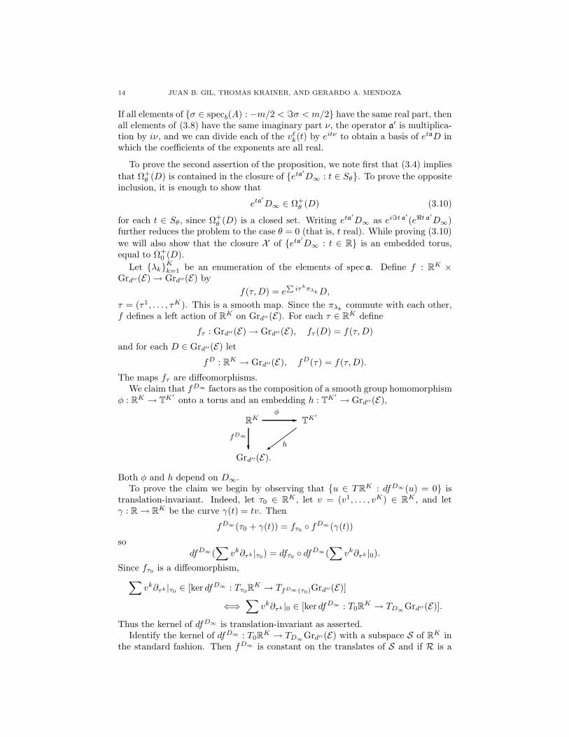
The maps fτ are diffeomorphisms.We claim that fD∞ factors as the composition of a smooth group homomorphism

φ : RK → TK′

onto a torus and an embedding h : TK′

→ Grd′′(E),

RK TK′

Grd′′(E).?

fD∞

φ-

h.

.......................................................................................................=

Both φ and h depend on D∞.To prove the claim we begin by observing that u ∈ TRK : dfD∞(u) = 0 is

translation-invariant. Indeed, let τ0 ∈ RK , let v = (v1, . . . , vK) ∈ RK , and letγ : R → RK be the curve γ(t) = tv. Then

fD∞(τ0 + γ(t)) = fτ0 fD∞(γ(t))

sodfD∞(

∑

vk∂τk |τ0) = dfτ0 dfD∞(∑

vk∂τk |0).

Since fτ0 is a diffeomorphism,∑

vk∂τk |τ0 ∈ [ker dfD∞ : Tτ0RK → TfD∞(τ0)Grd′′(E)]

⇐⇒∑

vk∂τk |0 ∈ [ker dfD∞ : T0RK → TD∞Grd′′(E)].

Thus the kernel of dfD∞ is translation-invariant as asserted.Identify the kernel of dfD∞ : T0RK → TD∞Grd′′(E) with a subspace S of RK in

the standard fashion. Then fD∞ is constant on the translates of S and if R is a

DYNAMICS ON GRASSMANNIANS AND RESOLVENTS OF CONE OPERATORS 15

subspace of RK complementary to S, then fD∞ |R is an immersion. Renumberingthe elements of spec a′ (and reordering the components of RK accordingly) we may

take R = RK′

× 0.Since fD∞ |R is an immersion, the sets FD′ =

τ ∈ R : fD∞(τ) = D′

are dis-

crete for each D′ ∈ fD∞(R). Using again the property fD∞(τ1+τ2) = fτ1fD∞(τ2)for arbitrary τ1, τ2 ∈ RK , we see that FD∞ is an additive subgroup of R andthat fD∞ is constant on the lateral classes of FD∞ . Therefore fD∞ |R factorsthrough a (smooth) homomorphism φ : R → R/FD∞ and a continuous map

R/FD∞ → Grd′′(E). Since fD∞ is 2π-periodic in all variables, 2πZK′

⊂ FD∞ ,

so R/FD∞ is indeed a torus TK′

. Since φ is a local diffeomorphism and fD∞ issmooth, h is smooth.

With this, the proof of the second assertion of the proposition goes as follows.Let L ⊂ RK be the subspace generated by (ℑλ1, . . . ,ℑλK). This is a line or the

origin. Its image by φ is a subgroup H of TK′

, so the closure of φ(L) is a torus

G ⊂ TK′

, and h(φ(L)) is an embedded torus X ⊂ Grd′′(E). On the other hand,

h φ(L) = fD∞(L) is the image of the curve γ : t → eta′

D∞, so the closure of theimage of γ is X . Clearly, Ω+

0 (D) ⊂ X . The equality of Ω+0 (D) and X is clear if

γ is periodic or L = 0. So assume that γ is not periodic and L 6= 0. ThenH 6= G and there is a sequence gν

∞ν=1 ⊂ G\H such that gν → e, the identity

element of G. Let v be an element of the Lie algebra of G such that H is the imageof t 7→ exp(tv). For each ν there is a sequence tν,ρ

∞ρ=1, necessarily unbounded

because gν /∈ H , such that gν = limρ→∞ exp(tν,ρv). We may assume that tν,ρ∞ρ=1

is monotonic, so it diverges to +∞ or to −∞. In the latter case we replace gν byits group inverse, so we may assume that limρ→∞ tν,ρ = ∞ for all ν. Thus if g ∈ His arbitrary, then h(ggν) ∈ Ω+

0 (D) and h(ggν) converges to h(g). Since Ω+0 (D) is

closed, this shows that h φ(H) ⊂ Ω+0 (D). Consequently, also X ⊂ Ω+

0 (D).This completes the proof of the second assertion of Proposition 3.3.

As a consequence of the proof we have that Ω+θ (D) is a union of embedded tori:

Ω+θ (D) =

⋃

s∈[−θ,θ]

eisa′

eta′D∞ : t ∈ R.

The proof of Lemma 3.5 will be based on the following lemma. The properties ofthe elements pℓ

k ∈ πµℓDµℓ

[t, 1/t] whose existence is asserted in Lemma 3.5 pertain

only Eµℓ, Nµℓ

, and the subspace πµℓDµℓ

of Eµℓ. For the sake of notational simplicity

we let W = πµℓDµℓ

and drop the µℓ from the notation. The space E comes equipped

with some Hermitian inner product, and N is nilpotent.

Lemma 3.11. There is an orthogonal decomposition

W =

J⊕

j=0

Mj⊕

m=0

Wmj

(with nontrivial summands) and nonzero elements

Pmj ∈ Hom(Wj,m,W ′

j)[t, t−1] (3.12)

where

Wj,m =

Mj⊕

m′=m

Wm′

j , W ′j =

j⊕

j′=0

Wj′,0,

16 JUAN B. GIL, THOMAS KRAINER, AND GERARDO A. MENDOZA

satisfying the following properties.

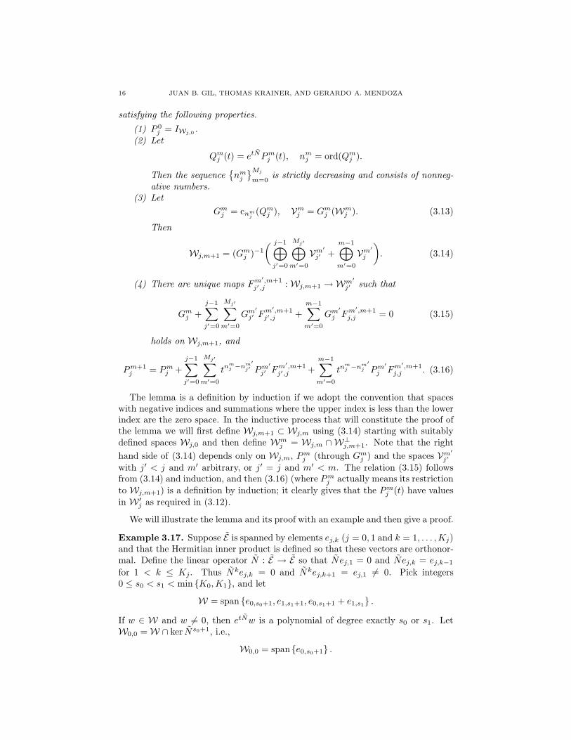
(1) P 0j = IWj,0 .

(2) Let

Qmj (t) = etNPm

j (t), nmj = ord(Qm

j ).

Then the sequence

nmj

Mj

m=0is strictly decreasing and consists of nonneg-

ative numbers.(3) Let

Gmj = cnm

j(Qm

j ), Vmj = Gm

j (Wmj ). (3.13)

Then

Wj,m+1 = (Gmj )−1

( j−1⊕

j′=0

Mj′⊕

m′=0

Vm′

j′ +m−1⊕

m′=0

Vm′

j

)

. (3.14)

(4) There are unique maps Fm′,m+1j′,j : Wj,m+1 → Wm′

j′ such that

Gmj +

j−1∑

j′=0

Mj′∑

m′=0

Gm′

j′ Fm′,m+1j′,j +

m−1∑

m′=0

Gm′

j Fm′,m+1j,j = 0 (3.15)

holds on Wj,m+1, and

Pm+1j = Pm

j +

j−1∑

j′=0

Mj′∑

m′=0

tnmj −nm′

j′ Pm′

j′ Fm′,m+1j′,j +

m−1∑

m′=0

tnmj −nm′

j Pm′

j Fm′,m+1j,j . (3.16)

The lemma is a definition by induction if we adopt the convention that spaceswith negative indices and summations where the upper index is less than the lowerindex are the zero space. In the inductive process that will constitute the proof ofthe lemma we will first define Wj,m+1 ⊂ Wj,m using (3.14) starting with suitablydefined spaces Wj,0 and then define Wm

j = Wj,m ∩ W⊥j,m+1. Note that the right

hand side of (3.14) depends only on Wj,m, Pmj (through Gm

j ) and the spaces Vm′

j′

with j′ < j and m′ arbitrary, or j′ = j and m′ < m. The relation (3.15) followsfrom (3.14) and induction, and then (3.16) (where Pm

j actually means its restriction

to Wj,m+1) is a definition by induction; it clearly gives that the Pmj (t) have values

in W ′j as required in (3.12).

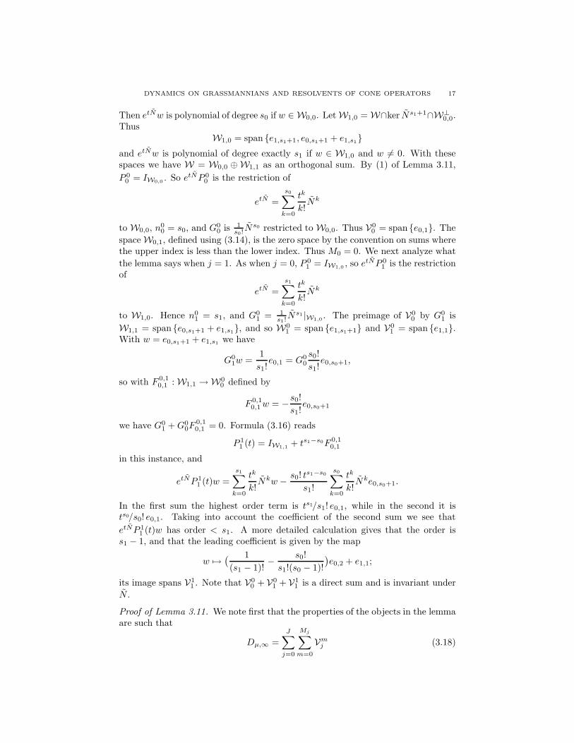
We will illustrate the lemma and its proof with an example and then give a proof.

Example 3.17. Suppose E is spanned by elements ej,k (j = 0, 1 and k = 1, . . . , Kj)and that the Hermitian inner product is defined so that these vectors are orthonor-mal. Define the linear operator N : E → E so that Nej,1 = 0 and Nej,k = ej,k−1

for 1 < k ≤ Kj. Thus Nkej,k = 0 and Nkej,k+1 = ej,1 6= 0. Pick integers0 ≤ s0 < s1 < min K0, K1, and let

W = span e0,s0+1, e1,s1+1, e0,s1+1 + e1,s1 .

If w ∈ W and w 6= 0, then etNw is a polynomial of degree exactly s0 or s1. LetW0,0 = W ∩ ker Ns0+1, i.e.,

W0,0 = span e0,s0+1 .

DYNAMICS ON GRASSMANNIANS AND RESOLVENTS OF CONE OPERATORS 17

Then etNw is polynomial of degree s0 if w ∈ W0,0. Let W1,0 = W∩ker Ns1+1∩W⊥0,0.

ThusW1,0 = span e1,s1+1, e0,s1+1 + e1,s1

and etNw is polynomial of degree exactly s1 if w ∈ W1,0 and w 6= 0. With thesespaces we have W = W0,0 ⊕ W1,1 as an orthogonal sum. By (1) of Lemma 3.11,

P 00 = IW0,0 . So etNP 0

0 is the restriction of

etN =

s0∑

k=0

tk

k!Nk

to W0,0, n00 = s0, and G0

0 is 1s0!N

s0 restricted to W0,0. Thus V00 = span e0,1. The

space W0,1, defined using (3.14), is the zero space by the convention on sums wherethe upper index is less than the lower index. Thus M0 = 0. We next analyze what

the lemma says when j = 1. As when j = 0, P 01 = IW1,0 , so etNP 0

1 is the restrictionof

etN =

s1∑

k=0

tk

k!Nk

to W1,0. Hence n01 = s1, and G0

1 = 1s1!N

s1 |W1,0 . The preimage of V00 by G0

1 is

W1,1 = span e0,s1+1 + e1,s1, and so W01 = span e1,s1+1 and V0

1 = span e1,1.With w = e0,s1+1 + e1,s1 we have

G01w =

1

s1!e0,1 = G0

0

s0!

s1!e0,s0+1,

so with F 0,10,1 : W1,1 → W0

0 defined by

F 0,10,1 w = −

s0!

s1!e0,s0+1

we have G01 + G0

0F0,10,1 = 0. Formula (3.16) reads

P 11 (t) = IW1,1 + ts1−s0F 0,1

0,1

in this instance, and

etNP 11 (t)w =

s1∑

k=0

tk

k!Nkw −

s0! ts1−s0

s1!

s0∑

k=0

tk

k!Nke0,s0+1.

In the first sum the highest order term is ts1/s1! e0,1, while in the second it ists0/s0! e0,1. Taking into account the coefficient of the second sum we see that

etNP 11 (t)w has order < s1. A more detailed calculation gives that the order is

s1 − 1, and that the leading coefficient is given by the map

w 7→( 1

(s1 − 1)!−

s0!

s1!(s0 − 1)!

)

e0,2 + e1,1;

its image spans V11 . Note that V0

0 + V01 + V1

1 is a direct sum and is invariant under

N .

Proof of Lemma 3.11. We note first that the properties of the objects in the lemmaare such that

Dµ,∞ =

J∑

j=0

Mj∑

m=0

Vmj (3.18)

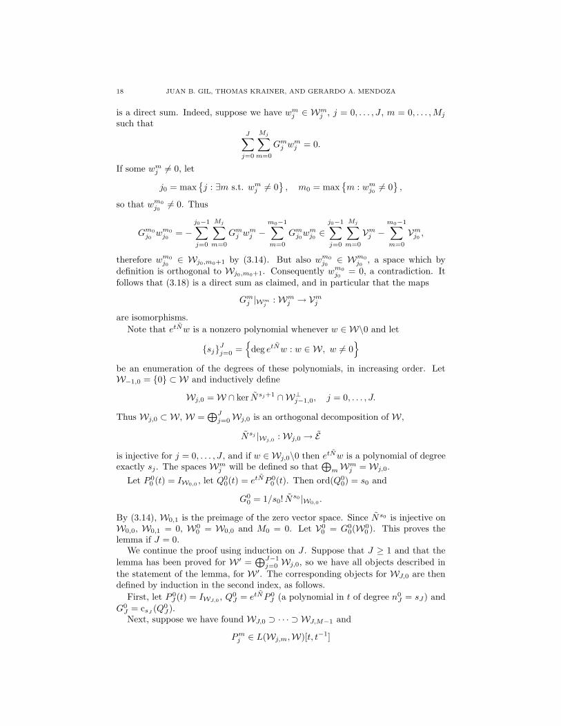
18 JUAN B. GIL, THOMAS KRAINER, AND GERARDO A. MENDOZA

is a direct sum. Indeed, suppose we have wmj ∈ Wm

j , j = 0, . . . , J , m = 0, . . . , Mj

such thatJ

∑

j=0

Mj∑

m=0

Gmj wm

j = 0.

If some wmj 6= 0, let

j0 = max

j : ∃m s.t. wmj 6= 0

, m0 = max

m : wmj0 6= 0

,

so that wm0

j06= 0. Thus

Gm0

j0wm0

j0= −

j0−1∑

j=0

Mj∑

m=0

Gmj wm

j −m0−1∑

m=0

Gmj0w

mj0 ∈

j0−1∑

j=0

Mj∑

m=0

Vmj −

m0−1∑

m=0

Vmj0 ,

therefore wm0

j0∈ Wj0,m0+1 by (3.14). But also wm0

j0∈ Wm0

j0, a space which by

definition is orthogonal to Wj0,m0+1. Consequently wm0

j0= 0, a contradiction. It

follows that (3.18) is a direct sum as claimed, and in particular that the maps

Gmj |Wm

j: Wm

j → Vmj

are isomorphisms.

Note that etNw is a nonzero polynomial whenever w ∈ W\0 and let

sjJj=0 =

deg etNw : w ∈ W , w 6= 0

be an enumeration of the degrees of these polynomials, in increasing order. LetW−1,0 = 0 ⊂ W and inductively define

Wj,0 = W ∩ ker Nsj+1 ∩W⊥j−1,0, j = 0, . . . , J.

Thus Wj,0 ⊂ W , W =⊕J

j=0 Wj,0 is an orthogonal decomposition of W ,

Nsj |Wj,0 : Wj,0 → E

is injective for j = 0, . . . , J , and if w ∈ Wj,0\0 then etNw is a polynomial of degreeexactly sj. The spaces Wm

j will be defined so that⊕

m Wmj = Wj,0.

Let P 00 (t) = IW0,0 , let Q0

0(t) = etNP 00 (t). Then ord(Q0

0) = s0 and

G00 = 1/s0! N

s0 |W0,0 .

By (3.14), W0,1 is the preimage of the zero vector space. Since Ns0 is injective onW0,0, W0,1 = 0, W0

0 = W0,0 and M0 = 0. Let V00 = G0

0(W00 ). This proves the

lemma if J = 0.We continue the proof using induction on J . Suppose that J ≥ 1 and that the

lemma has been proved for W ′ =⊕J−1

j=0 Wj,0, so we have all objects described in

the statement of the lemma, for W ′. The corresponding objects for WJ,0 are thendefined by induction in the second index, as follows.

First, let P 0J (t) = IWJ,0 , Q0

J = etNP 0J (a polynomial in t of degree n0

J = sJ) and

G0J = csJ (Q0

J).Next, suppose we have found WJ,0 ⊃ · · · ⊃ WJ,M−1 and

Pmj ∈ L(Wj,m,W)[t, t−1]

DYNAMICS ON GRASSMANNIANS AND RESOLVENTS OF CONE OPERATORS 19

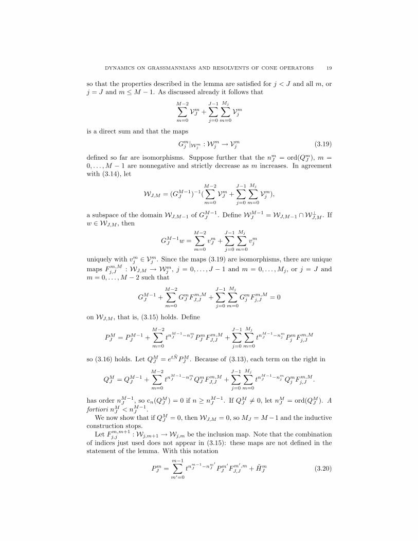
so that the properties described in the lemma are satisfied for j < J and all m, orj = J and m ≤ M − 1. As discussed already it follows that

M−2∑

m=0

VmJ +

J−1∑

j=0

Mj∑

m=0

Vmj

is a direct sum and that the maps

Gmj |Wm

j: Wm

j → Vmj (3.19)

defined so far are isomorphisms. Suppose further that the nmJ = ord(Qm

J ), m =0, . . . , M − 1 are nonnegative and strictly decrease as m increases. In agreementwith (3.14), let

WJ,M = (GM−1J )−1(

M−2∑

m=0

VmJ +

J−1∑

j=0

Mj∑

m=0

Vmj ),

a subspace of the domain WJ,M−1 of GM−1J . Define WM−1

J = WJ,M−1 ∩W⊥J,M . If

w ∈ WJ,M , then

GM−1J w =

M−2∑

m=0

vmJ +

J−1∑

j=0

Mj∑

m=0

vmj

uniquely with vmj ∈ Vm

j . Since the maps (3.19) are isomorphisms, there are unique

maps Fm,Mj,J : WJ,M → Wm

j , j = 0, . . . , J − 1 and m = 0, . . . , Mj, or j = J andm = 0, . . . , M − 2 such that

GM−1J +

M−2∑

m=0

GmJ Fm,M

J,J +

J−1∑

j=0

Mj∑

m=0

Gmj Fm,M

j,J = 0

on WJ,M , that is, (3.15) holds. Define

PMJ = PM−1

J +

M−2∑

m=0

tnM−1J −nm

J PmJ Fm,M

J,J +

J−1∑

j=0

Mj∑

m=0

tnM−1J −nm

j Pmj Fm,M

j,J

so (3.16) holds. Let QMJ = etNPM

J . Because of (3.13), each term on the right in

QMJ = QM−1

J +M−2∑

m=0

tnM−1J −nm

J QmJ Fm,M

J,J +J−1∑

j=0

Mj∑

m=0

tnM−1J −nm

j Qmj Fm,M

j,J .

has order nM−1J , so cn(QM

J ) = 0 if n ≥ nM−1J . If QM

J 6= 0, let nMJ = ord(QM

J ). A

fortiori nMJ < nM−1

J .We now show that if QM

J = 0, then WJ,M = 0, so MJ = M −1 and the inductiveconstruction stops.

Let Fm,m+1j,j : Wj,m+1 → Wj,m be the inclusion map. Note that the combination

of indices just used does not appear in (3.15): these maps are not defined in thestatement of the lemma. With this notation

PmJ =

m−1∑

m′=0

tnm−1J −nm′

J Pm′

J Fm′,mJ,J + Hm

J (3.20)

20 JUAN B. GIL, THOMAS KRAINER, AND GERARDO A. MENDOZA

for m = 1, . . . , M and some HmJ ∈ L(WJ,m,W ′)[t, t−1]. Let Pm be the set of finite

strictly increasing sequences ννν = (ν0, ν1, . . . , νk) of elements of 0, . . . , m withν0 = 0 and νk = m. For ν = (ν0, . . . , νk) ∈ Pm (m ≥ 1) define

FνννJ = F ν0,ν1

J,J · · · Fνm−1,νm

J,J

nνννJ = (nν1−1

J − nν0

J ) + (nν2−1J − nν1

J ) + · · · + (nνk−1J − n

νk−1

J ).

Since the nm′

J strictly decrease as m′ increases, the numbers nνννJ are strictly negative

except when ννν is the maximal sequence νννmax in 0, . . . , m, in which case nνννmax

J = 0and Fνννmax is the inclusion of WJ,m in WJ,0. It is not hard to prove (by inductionon m, using (3.20)) that

PmJ = P 0

J

∑

ννν∈Pm

tnνννJ Fννν

J + HmJ (3.21)

for all m ≥ 1 where HmJ ∈ L(WJ,m,W ′)[t, t−1]. If QM

J = 0, then PMJ = 0, so, since

NsJ HMJ = 0,

NsJ PMJ =

∑

ννν∈PM

tnνννJ NsJ Fννν

J = 0

In particular, NsJ Fνννmax

J = c0(NsJ PM

J ) = 0. Since NsJ is injective on WJ,0, weconclude that the inclusion of WJ,M in WJ,0 is zero. This means that WJ,M = 0,so the inductive construction stops with MJ = M − 1.

We will now show that there is a finite M such that QMJ = 0. The inductive

construction gives, as long as QmJ 6= 0, the numbers nm

J = ord(QmJ ) which form a

strictly decreasing sequence in m, with n0J = sJ . Suppose nM−1

J ≥ 0, QMJ 6= 0,

and nMJ < 0. In particular, the coefficient of t0 in QM

J vanishes. Using (3.21) withm = M we have

etNPMJ =

∑

ννν∈PM

sJ∑

s=0

ts+nνννJ

s!NsFννν

J + etNHMJ

The coefficient of t0 is

c0(etNPM

J ) =∑

ννν∈PM

1

(−nνννJ)!

N−nνννJ Fννν

J + c0(etNHM

J );

recall that nνννJ ≤ 0. Since HM

J maps into W ′, NsJ c0(HMJ ) = 0, and since Ns|WJ,0 =

0 if s > sJ , NsJ N−nνννJ = 0 if nννν

J 6= 0. Thus

NsJ c0(etNPM

J ) = NsJ Fνννmax

J

where νννmax = (0, 1, . . . , M). Since c0(etNPM

J ) = 0 by hypothesis, since Fνννmax

J is

the inclusion of WJ,M in WJ,0, and since NsJ is injective on WJ,0, WJ,M = 0.

Proof of Lemma 3.5. Apply Lemma 3.11 to each of the spaces Wµℓ= πµℓ

Dµℓ. The

corresponding objects are labeled adjoining ℓ as a subindex. Get in particular,decompositions

πµℓDµℓ

=

Jℓ⊕

j=0

Mj,ℓ⊕

m=0

Wmj,ℓ ⊂ Eµℓ

DYNAMICS ON GRASSMANNIANS AND RESOLVENTS OF CONE OPERATORS 21

for each ℓ, and operators Gmj,ℓ : Wm

j,ℓ → Vmj,ℓ ⊂ Eµℓ

such that

Jℓ⊕

j=0

Mj,ℓ⊕

m=0

Gmj,ℓ|Wm

j,ℓ:

Jℓ⊕

j=0

Mj,ℓ⊕

m=0

Wmj,ℓ → Dµℓ,∞ =

Jℓ⊕

j=0

Mj,ℓ⊕

m=0

Vmj,ℓ

is an isomorphism. Let dmj,ℓ = dimWm

j,ℓ and pick a basis

wmj,ℓ.k, 1 ≤ k ≤ dm

j,ℓ

of Wmj,ℓ, j = 0, . . . , Jℓ, m = 0, . . . , Mj,ℓ. Then pm

j,ℓ,k(t) = t−nmj,ℓPm

j,ℓ(t)wmj,ℓ,k ∈ Wµℓ

.These elements

pmj,ℓ,k ∈ Wµℓ

[t, t−1], j = 0, . . . , Jℓ, m = 0, . . . , Mj,ℓ, ℓ = 1, . . . dmj,ℓ

are the ones Lemma 3.5 claims exist. Indeed, since Qmj,ℓ(t) = etNµℓ Pm

j,ℓ(t),

limℜt→∞t∈Sθ

etNµℓ t−nmj,ℓPm

j,ℓ(t)wmj,ℓ,k = Gm

j,ℓwmj,ℓ,l.

Since the Gmj,ℓw

mj,ℓ,k form a basis of Dµ,∞, the t−nm

j,ℓPmj,ℓ(t)w

mj,ℓ,k, form a basis of

Wµℓfor all t ∈ Sθ with large enough real part.

4. Asymptotics of the projection

With the setup and (slightly changed) notation leading to and in the proof ofProposition 3.3, given a subspace D ⊂ E and the linear map a : E → E we have, forfixed θ ≥ 0 and t ∈ Sθ = t ∈ C : |ℑt| ≤ θ, that

etaD = span vk(t) , ℜt ≫ 0

with

vk(t) = eta′

gk(t) +∑

λ∈spec a

ℜλ<µk

et(λ−µk)pk,λ(t). (4.1)

The gk(t) are polynomials in 1/t with values in Eµk, the collection of vectors

g∞,k = limt→∞

gk(t)

is a basis of D∞, the µk form a finite sequence, possibly with repetitions, of elementsin the set ℜλ : λ ∈ spec a, and

pk,λ(t) = etNλπλpk(t)

where the p(t) are polynomials in t and 1/t with values in E . The additive semi-group Sa ⊂ C (possibly without identity) generated by the set (3.8) is a subset ofλ ∈ C : ℜλ ≤ 0 and has the property that ϑ ∈ Sa : ℜϑ > µ is finite for everyµ ∈ R.

Proposition 4.2. Let K ∈ Grd′(E) be complementary to D, suppose that

VK ∩ Ω+θ (D) = ∅. (4.3)

Then there are polynomials pϑ(z1, . . . , zN , t) with values in End(E) and C-valuedpolynomials qϑ(z1, . . . , zN , t) such that

∃C, R0 > 0 such that |qϑ(eitℑλ1 , . . . , eitℑλN , t)| > C if t ∈ Sθ, ℜt > R0 (4.4)

22 JUAN B. GIL, THOMAS KRAINER, AND GERARDO A. MENDOZA

and such that

πetaD,K =∑

ϑ∈Sa

etϑpϑ(eitℑλ1 , . . . , eitℑλN , t)

qϑ(eitℑλ1 , . . . , eitℑλN , t), t ∈ Sθ, ℜt > R0

with uniform convergence in norm in the indicated subset of Sθ.

Proof. Let K ⊂ E be complementary to D as indicated in the statement of theproposition, let u = [u1, . . . , ud′ ] be an ordered basis of K. Write g for an orderingof the basis g∞,k of D∞. With the vk(t) ordered as the g∞,k to form v(t), wehave

[

v(t) u]

=[

g u]

·

[

α(t) 0β(t) I

]

(4.5)

where

α(t) =∑

k

∑

λ∈spec aℜλ≤µk

et(λ−µk)αk,λ(t), β(t) =∑

k

∑

λ∈spec aℜλ≤µk

et(λ−µk)βk,λ(t). (4.6)

The entries of the matrices αk,λ(t) and βk,λ(t) are both polynomials in t and 1/t,but only in 1/t if ℜλ = µk. Define

α(0)(t) =∑

k

∑

λ∈spec aℜλ=µk

et(λ−µk)αk,λ(t), α(t) =∑

k

∑

λ∈spec aℜλ<µk

et(λ−µk)αk,λ(t), (4.7)

likewise β(0)(t) and β(t). Note that α(t) and β(t) decrease exponentially as ℜt → ∞with |ℑt| bounded.

The hypothesis (4.3) gives that[

α(t) 0β(t) I

]

is invertible for every sufficiently large ℜt, so α(t) is invertible for such t. In fact,

there are C, R0 > 0 such that | det(α(t))| > C if t ∈ Sθ, ℜt > R0. (4.8)

For suppose this is not the case. Then there is a sequence tν in Sθ with ℜtν → ∞as ν → ∞ such that detα(tν) → 0. Since both α(tν) and β(tν) are bounded, wemay assume, passing to a subsequence, that they converge. It follows that etνaDconverges, by definition, to an element D′ ∈ Ω+

θ (D). Also the matrix in (4.5)converges. The vanishing of the determinant of the limiting matrix implies thatK ∩ D′ 6= 0, contradicting (4.3). Thus (4.8) holds.

If φ ∈ E then of course

φ =[

g u]

·

[

ϕ1

ϕ2

]

where the ϕi are columns of scalars. Substituting

[

g u]

=[

v(t) u]

·

[

α(t)−1 0−β(t)α(t)−1 I

]

gives

φ =[

v(t) u]

·

[

α(t)−1 0−β(t)α(t)−1 I

] [

ϕ1

ϕ2

]

=[

v(t) u]

·

[

α(t)−1ϕ1

−β(t)α(t)−1ϕ1 + ϕ2

]

,

hence

φ = v(t) · α(t)−1ϕ1 + u ·(

− β(t)α(t)−1ϕ1 + ϕ2)

;

DYNAMICS ON GRASSMANNIANS AND RESOLVENTS OF CONE OPERATORS 23

This is the decomposition of φ according to E = etaD ⊕ K, therefore

πetaD,Kφ = v(t) · α(t)−1ϕ1.

Replacing v(t) = g · α(t) + u · β(t) we obtain

πetaD,Kφ =(

g · α(t) + u · β(t))

α(t)−1ϕ1

=(

g + u · β(t)α(t)−1)

ϕ1.(4.9)

The matrix α(0)(t) is invertible because of (4.8) and the decomposition α(t) =α(0)(t) + α(t), so

β(t)α(t)−1 = β(t)α(0)(t)−1(

I + α(t)α(0)(t)−1)−1

= β(t)α(0)(t)−1∞∑

ℓ=0

(−1)ℓ[α(t)α(0)(t)−1]ℓ.(4.10)

The series converges absolutely and uniformly in t ∈ Sθ : ℜt > R0 for some realR0 ∈ R. The entries of α(0)(t) are expressions

∑

λ∈spec a

eitℑλN

∑

ν=0

cλ,νt−ν ,

hence

detα(0)(t) = q(eitℑλ1 , . . . , eitℑλN , 1/t)

for some polynomial q(z1, . . . , zN , 1/t). Note that because of (4.8),

there are C, R0 > 0 such that | det(α0(t))| > C if t ∈ Sθ, ℜt > R0. (4.11)

Since α(0)(t)−1 = (det α(0)(t))−1∆(t)† where ∆(t)† is the matrix of cofactors ofα(0)(t), (4.10) and (4.6) give

β(t)α(t)−1 =∑

ϑ∈Sa

rϑ(t)etϑ (4.12)

where Sa was defined before the statement of Proposition 4.2 as the additivesemigroup generated by λ −ℜλ′ : λ, λ′ ∈ spec a, ℜλ ≤ ℜλ′ and rϑ(t) is a matrixwhose entries are of the form

pϑ(eitℑλ1 , . . . , eitℑλN , t, 1/t)

q(eitℑλ1 , . . . , eitℑλN , 1/t)nϑ

for some polynomial pϑ(z1, . . . , zN , t, 1/t) and nonnegative integers nϑ. Multiplyingthe numerator and denominator by the same nonnegative (integral) power of t wereplace the dependence on 1/t by polynomial dependence in eitℑλ1 , . . . , eitℑλN , tonly. This gives the structure of the “coefficients” of the etϑ stated in the propositionfor the expansion of πetaD,K .

The terms in (4.12) with ℜϑ = 0 come from β(0)(t)α(0)(t)−1. So the principalpart of πetaD,K is

σσ(πetaD,K)φ =(

g + u · β(0)(t)α(0)(t)−1)

ϕ1

This principal part is not itself a projection, but

‖ σσ(πetaD,K) − πeta′D∞,K‖ → 0 as ℜt → ∞, t ∈ Sθ.

24 JUAN B. GIL, THOMAS KRAINER, AND GERARDO A. MENDOZA

We now restate Proposition 4.2 as an asymptotics for the family (2.10) using thenotation κκκ for the action on E and express the asymptotics of πκκκ−1

ζ1/mD,K in terms of

the boundary spectrum of A exploiting (3.1). Condition (4.14) below correspondsto our geometric condition in part (iii) of Theorem 2.15 expressing the fact thatΛ is a sector of minimal growth for A∧,D∧ . The Ω-limit set is the one defined in

(2.14). Recall that by ζ1/m we mean the root defined by the principal branch ofthe logarithm on C\R−. We let λ0 6= 0 be an element in the central axis of Λ and

define Λ = ζ : ζλ0 ∈ Λ; this is a closed sector not containing the negative realaxis.

Let S ⊂ C be the additive semigroup generated by

σ − iℑσ′ : σ, σ′ ∈ specb(A), −m/2 < ℑσ ≤ ℑσ′ < m/2 .

Thus −iS = Sa. Let σ1, . . . , σN be an enumeration of the elements of Σ =specb(A) ∩ −m/2 < ℑσ < m/2.

Theorem 4.13. Let K ∈ Grd′(E) be complementary to D, suppose that

VK ∩ Ω−Λ (D) = ∅. (4.14)

Then there are polynomials pϑ(z1, . . . , zN , t) with values in End(E) and C-valuedpolynomials qϑ(z1, . . . , zN , t) such that

∃C, R0 > 0 such that |qϑ(ζiℜσ1/m, . . . , ζiℜσN /m, t)| > C if ζ ∈ Λ, |ζ| > R0

(4.15)and such that

πκκκ−1

ζ1/mD,K =

∑

ϑ∈S

ζ−iϑ/mpϑ(ζiℜσ1/m, . . . , ζiℜσN /m, m−1 log ζ)

qϑ(ζiℜσ1/m, . . . , ζiℜσN /m, m−1 log ζ), ζ ∈ Λ, |ζ| > R0

with uniform convergence in norm in the indicated subset of Λ.

The elements ϑ ∈ S are of course finite sums ϑ =∑

njk(σj − iℑσk) for somenonnegative integers njk, with σj , σk ∈ Σ and ℑσj ≤ ℑσk. Separating real and

imaginary parts we may write ζ−iϑ/m as a product of factors

ζnjk(ℑσj−ℑσk)/m

ζinjkℜσk/m.

We thus see that we may also organize the series expansion of πκκκ−1

ζ1/mD,K in the

theorem as

πκκκ−1

ζ1/mD,K =

∑

ϑ∈SR

ζ−iϑ/mpϑ(ζiℜσ1/m, . . . , ζiℜσN /m, m−1 log ζ)

qϑ(ζiℜσ1/m, . . . , ζiℜσN /m, m−1 log ζ)

where SR ⊂ R is the additive semigroup generated by

ℑσ −ℑσ′ : σ, σ′ ∈ Σ, ℑσ′ ≤ ℑσ′

and pϑ, qϑ are still polynomials.

Remark 4.16. If Σ lies on a line ℜσ = c0, then −iS ⊂ R− − ic0. Also in thiscase, the coefficients of the exponents in (4.1) can be assumed to have vanishingimaginary part (see Remark 3.7). Assuming this, the coefficients of the exponents in(4.7) are real, in particular detα(0)(t) is just a polynomial in 1/t, the coefficients rϑ

in the expansion (4.12) can be written as rational functions of t only. Consequently,

DYNAMICS ON GRASSMANNIANS AND RESOLVENTS OF CONE OPERATORS 25

in the expansion of the projection in Theorem 4.13, the powers −iϑ are real ≤ 0and the coefficients can be written as rational functions of log ζ.

5. Asymptotic structure of the resolvent

For the analysis of (AD − λ)−ℓ for ℓ ∈ N sufficiently large we make use of therepresentation (1.8) of the resolvent as

(AD − λ)−1 = B(λ) + GD(λ), (5.1)

where B(λ) is a parametrix of (Amin − λ) and

GD(λ) = [1 − B(λ)(A − λ)]FD(λ)−1T (λ). (5.2)

The starting point of our analysis is

(AD − λ)−ℓ =1

(ℓ − 1)!∂ℓ−1

λ (AD − λ)−1 for any ℓ ∈ N.

We are thus led to further analyze the asymptotic structure of the pieces involvedin the representation of the resolvent. In [14] we described in full generality thebehavior of B(λ), [1 − B(λ)(A − λ)], and T (λ), and we analyzed FD(λ)−1 in thespecial case that D is stationary. In the case of a general domain D, we now obtainas a consequence of Theorem 4.13 the following result.

Proposition 5.3. For R > 0 large enough we have

FD(λ)−1 ∈(

S0+

R ∩ S0)

(ΛR;D∧/D∧,min,Dmax/Dmin).

The components of FD(λ)−1 have orders ν+ with ν ∈ E, the semigroup defined in(1.6), and their phases belong to the set M defined in (1.5).

Here S0(ΛR;D∧/D∧,min,Dmax/Dmin) denotes the standard space of (anisotropic)operator valued symbols of order zero on ΛR (see the appendix), where D∧/D∧,min

carries the trivial group action, and Dmax/Dmin is equipped with the group action

κ = θ−1κκκρθ. The symbol class S0+

R(ΛR;D∧/D∧,min,Dmax/Dmin) is discussed in

the appendix (see Definition A.4). Recall that ΛR = λ ∈ Λ : |λ| ≥ R.

Proof of Proposition 5.3. We follow the line of reasoning of [14, Propositions 5.10and 5.17]. The crucial point is that we now know from Theorem 4.13 and Propo-sition 2.17 that F∧,D∧(λ)−1 belongs to the symbol class

(

S0+

R ∩ S0)

(ΛR;D∧/D∧,min,D∧,max/D∧,min),

where the actions on D∧/D∧,min and D∧,max/D∧,min are, respectively, the trivialaction as above and κκκ. The components of F∧,D∧(λ)−1 have orders ν+ with ν ∈ E,and their phases belong to the set M. Consequently, Φ0(λ) = θ−1F∧,D∧(λ)−1

belongs to(

S0+

R ∩ S0)

(ΛR;D∧/D∧,min,Dmax/Dmin),

and we have the same statement about the orders and phases of its components.Phrased in the terminology of the present paper, we proved (see [14, Proposition

5.10]) that the operator family

F (λ) = [T (λ)(A − λ)] : Dmax/Dmin → D∧/D∧,min

belongs to the symbol class(

S0+

R ∩ S0)

(ΛR;Dmax/Dmin,D∧/D∧,min),

26 JUAN B. GIL, THOMAS KRAINER, AND GERARDO A. MENDOZA

and that

F (λ)Φ0(λ) − 1 = R(λ) ∈ S−1+ε(ΛR;D∧/D∧,min,D∧/D∧,min)

for any ε > 0. More precisely, F (λ) is an anisotropic log-polyhomogeneous operatorvalued symbol. We thus can infer further that in fact

R(λ) ∈ S(−1)+

R(ΛR;D∧/D∧,min,D∧/D∧,min),

and that the components of R(λ) have orders ν+ with ν ∈ E, ν ≤ −1, andphases belonging to the set M. The usual Neumann series argument then yields

the existence of a symbol R1(λ) ∈ S(−1)+

R(ΛR;D∧/D∧,min,D∧/D∧,min) such that

F (λ)Φ0(λ)(1 + R1(λ)) = 1 for λ ∈ ΛR. Consequently FD(λ)−1 = Φ0(λ)(1 + R1(λ))belongs to

(

S0+

R ∩ S0)

(ΛR;D∧/D∧,min,Dmax/Dmin),

and its components have the structure that was claimed.

With Proposition 5.3 and our results in [14, Section 5] at our disposal, we nowobtain a general theorem about the asymptotics of the finite rank contributionGD(λ) in the representation (5.1) of the resolvent. Before stating it we recall andrephrase the relevant results from [14] about the other pieces involved in (5.2) usingthe terminology of the present paper.

Concerning T (λ) we have ([14, Proposition 5.5]):

i) For any cut-off function ω ∈ C∞c ([0, 1)) the function T (λ)(1−ω) is rapidly

decreasing on Λ taking values in L (x−m/2Hsb ,D∧/D∧,min), and

t(λ) = T (λ)ω ∈ S−m(Λ;Ks,−m/2,D∧/D∧,min).

Here Ks,−m/2 is equipped with the (normalized) dilation group action κ,and we give D∧/D∧,min again the trivial action.

ii) The family t(λ) admits a full asymptotic expansion into anisotropic homo-geneous components. In particular, we have

t(λ) ∈ S(−m)+

R(Λ;Ks,−m/2,D∧/D∧,min).

The spaces Ks,−m/2 are weighted cone Sobolev spaces on Y ∧. We discussed themin [12, Section 2] and reviewed the definition in [14, Section 4] (see also [28],where different weight functions as x → ∞ are considered). Note that K0,−m/2 =x−m/2L2

b(Y∧; E).

Concerning 1 − B(λ)(A − λ) we have, for arbitrary ϕ ∈ C∞(M ; End(E)) ([14,Proposition 5.20]):

iii) The operator function P (λ) = ϕ[1 − B(λ)(A − λ)] is a smooth function

ΛR → L (Dmax/Dmin, x−m/2Hs

b )

which is defined for R > 0 large enough. Let ω ∈ C∞c ([0, 1)) be an arbitrary

cut-off function. Then (1 − ω)P (λ) is rapidly decreasing on ΛR, and

p(λ) = ωP (λ) ∈ S0(ΛR;Dmax/Dmin,Ks,−m/2),

where Ks,−m/2 is equipped with the (normalized) dilation group action κ,and the quotient Dmax/Dmin is equipped with the group action κ.

DYNAMICS ON GRASSMANNIANS AND RESOLVENTS OF CONE OPERATORS 27

iv) p(λ) is an anisotropic log-polyhomogeneous operator valued symbol on ΛR.In particular,

p(λ) = ωP (λ) ∈ S0+

R (ΛR;Dmax/Dmin,Ks,−m/2).

With M as in (1.5) and E as in (1.6) we have:

Theorem 5.4. Let ϕ ∈ C∞(M ; End(E)), and let ω, ω ∈ C∞c ([0, 1)) be arbitrary

cut-off functions. For R > 0 large enough the operator family GD(λ) is defined onΛR, and

(1 − ω)ϕGD(λ), ϕGD(λ)(1 − ω) ∈ S (ΛR, ℓ1(x−m/2Hsb , x−m/2Ht

b)).

Moreover,

ωϕGD(λ)ω ∈(

S(−m)+

R∩ S−m

)

(ΛR;Ks,−m/2,Kt,−m/2),

where the spaces Ks,−m/2 and Kt,−m/2 are equipped with the group action κ. Infact, ωϕGD(λ)ω takes values in the trace class operators, and all statements aboutsymbol estimates and asymptotic expansions hold in trace class norms. The com-ponents have orders ν+ with ν ∈ E, ν ≤ −m, and their phases belong to M.

Corollary 5.5. For R > 0 sufficiently large and ϕ ∈ C∞(M ; End(E)), the operatorfamily ϕGD(λ) is a smooth family of trace class operators in x−m/2L2

b for λ ∈ ΛR,

and Tr(

ϕGD(λ))

∈(

S(−m)+

R∩ S−m

)

(ΛR). The components have orders ν+ withν ∈ E, ν ≤ −m, and their phases belong to the set M.

Theorem 5.4 and Corollary 5.5 follow at once from the previous results aboutthe pieces involved in the representation (5.2) for GD(λ) and the properties ofthe operator valued symbol class discussed in the appendix. In the statement ofCorollary 5.5 the scalar symbol spaces are also anisotropic with anisotropy m. Inparticular, this means that Tr

(

ϕGD(λ))

= O(|λ|−1) as |λ| → ∞.We are now in the position to prove the trace expansion claimed in Theorem 1.4.

To this end, we need the following result ([14, Theorem 4.4]):

v) Let ϕ ∈ C∞(M ; End(E)). If mℓ > n, then ϕ∂ℓ−1λ B(λ) is a smooth family

of trace class operators in x−m/2L2b, and the trace Tr

(

ϕ∂ℓ−1λ B(λ)

)

is alog-polyhomogeneous symbol on Λ. For large λ we have

Tr(

ϕ∂ℓ−1λ B(λ)

)

∼n−1∑

j=0

αjλn−ℓm−j

m + αn log(λ)λ−ℓ + r(λ),

where

r(λ) ∈(

S(−ℓm)+

R∩ S−ℓm

)

(Λ).

Now, combining v) with Corollary 5.5, we finally obtain:

Theorem 5.6. Let Λ ⊂ C be a closed sector. Assume that A ∈ x−m Diffmb (M ; E),

m > 0, with domain D ⊂ x−m/2L2b satisfies the ray conditions (1.3). Then Λ is a

sector of minimal growth for AD, and for mℓ > n, (AD−λ)−ℓ is an analytic familyof trace class operators on ΛR for some R > 0. Moreover, for ϕ ∈ C∞(M ; End(E)),

Tr(

ϕ(AD − λ)−ℓ)

∈(

S(n−ℓm)+

R,hol ∩ Sn−ℓm)

(ΛR).

The components have orders ν+ with ν ∈ E, ν ≤ n− ℓm, where E is the semigroupdefined in (1.6), and their phases belong to the set M defined in (1.5).

28 JUAN B. GIL, THOMAS KRAINER, AND GERARDO A. MENDOZA

More precisely, we have the expansion

Tr(

ϕ(AD − λ)−ℓ)

∼n−1∑

j=0

αjλn−ℓm−j

m + αn log(λ)λ−ℓ + sD(λ)

with constants αj ∈ C independent of the choice of domain D, and a domain

dependent remainder sD(λ) ∈(

S(−ℓm)+

R,hol ∩ S−ℓm)

(ΛR).

If all elements of the set σ ∈ specb(A) : −m/2 < ℑσ < m/2 are verticallyaligned, then the coefficients rν in the expansion (1.7) of sD(λ) are rational functionsof log λ only. This is because, in this case, the series representation of the projectionin Theorem 4.13 contains only real powers of ζ and rational functions of log ζ, seeRemark 4.16. This simplifies the structure of F∧,D∧(λ)−1 according to Section 2,and consequently the structure of FD(λ)−1 (see the proof of Proposition 5.3). Asrecalled in this section, the terms coming from B(λ) and the other pieces in therepresentation (5.2) of GD(λ) do not generate phases.

If D is stationary, then the expansion (1.7) of sD(λ) is even simpler: the rν arejust polynomials in log λ, and the numbers ν are all integers. To see this recall thatif D∧ is κ-invariant, then F∧,D∧(λ)−1 is homogeneous, see (2.3), so it belongs tothe class

S(0)(ΛR;D∧/D∧,min,D∧,max/D∧,min)⊂(

S0+

R ∩S0)

(ΛR;D∧/D∧,min,D∧,max/D∧,min).

Consequently, by the proof of Proposition 5.3, FD(λ)−1 is log-polyhomogeneous.This property propagates throughout the rest of the results in this section and givesthe structure of sD(λ) just asserted.

Appendix A. A class of symbols

Let Λ ⊂ C be a closed sector. Let E and E be Hilbert spaces equipped withstrongly continuous group actions κ and κ, > 0, respectively. Recall that the

space Sν(Λ; E, E) of anisotropic operator valued symbols on the sector Λ of order

ν ∈ R is defined as the space of all a ∈ C∞(Λ, L (E, E)) such that for all α, β ∈ N0

‖κ−1|λ|1/m∂α

λ ∂β

λa(λ)κ|λ|1/m‖

L (E,E) = O(|λ|ν/m−α−β) as |λ| → ∞ in Λ.

By S(ν)(Λ; E, E) we denote the space of anisotropic homogeneous functions of de-

gree ν ∈ R, i.e., all a ∈ C∞(Λ \ 0, L (E, E)) such that

a(mλ) = ν κa(λ)κ−1 for > 0 and λ ∈ Λ \ 0.

Clearly χ(λ)S(ν)(Λ; E, E) ⊂ Sν(Λ; E, E) with the obvious meaning of notation,

where χ ∈ C∞(R2) is any excision function of the origin. When E = E = C

equipped with the trivial group action the spaces are dropped from the notation.Such symbol classes were introduced by Schulze in his theory of pseudodifferential

operators on manifolds with singularities, see [28]. In particular, classical symbols,i.e. symbols that admit asymptotic expansions into homogeneous components, playa prominent role, and we have used such symbols in [12] for the construction of aparameter-dependent parametrix B(λ) to Amin−λ. As we see in the present paper,the structure of resolvents (AD − λ)−1 for general domains D is rather involved,and classical symbols do not suffice to describe that structure. We are thereforeled to introduce a new class of (anisotropic) operator valued symbols that admit

DYNAMICS ON GRASSMANNIANS AND RESOLVENTS OF CONE OPERATORS 29

certain expansions of more general kind. As turns out, this class occurs naturallyand is well adapted to describe the structure of resolvents in the general case.

Recall that V [z1, . . . , zM ] denotes the space of polynomials in the variables zj,j = 1 . . . , M , with coefficients in V for any vector space V . We shall make use ofthis in particular for V = C and V = S(0)(Λ; E, E). In what follows, all holomorphicpowers and logarithms on

Λ are defined using a holomorphic branch of the logarithmwith cut Γ 6⊂ Λ.

Definition A.1. Let ν ∈ R. We define S(ν+)R

(Λ; E, E) as the space of all functionss(λ) of the following form:

There exist polynomials p ∈ S(0)(Λ; E, E)[z1, . . . , zN+1] and q ∈ C[z1, . . . , zN+1]in N + 1 variables, N = N(s) ∈ N0, and real numbers µk = µk(s), k = 1, . . . , N ,such that the following holds:

(a) |q(λiµ1 , . . . , λiµN , log λ)| ≥ c > 0 for λ ∈ Λ with |λ| sufficiently large;(b) s(λ) = r(λ)λν/m, where

r(λ) =p(λiµ1 , . . . , λiµN , log λ)

q(λiµ1 , . . . , λiµN , log λ). (A.2)

To clarify the notation, we note that

p(λiµ1 , . . . , λiµN , log λ) =∑

|α|+k≤M

aα,k(λ)λiµ1α1 · · ·λiµN αN logk λ

as a function Λ \ 0 → L (E, E) with certain aα,k(λ) ∈ S(0)(Λ; E, E).

We call the µk the phases and ν+ the order of s(λ).

Every s(λ) ∈ S(ν+)R

(Λ; E, E) is an operator function defined everywhere on Λexcept at λ = 0 and the zero set of q(λiµ1 , . . . , λiµN , log λ). The latter is a discretesubset of Λ\0, and it is finite outside any neighborhood of zero in view of property(a).

Proposition A.3. (1) S(ν+)R

(Λ; E, E) is a vector space.

(2) Let E be a third Hilbert space with group action κ, > 0. Composition ofoperator functions induces a map

S(ν+

1 )R

(Λ; E, E) × S(ν+

2 )R

(Λ; E, E) → S((ν1+ν2)+)R

(Λ; E, E).

(3) For α, β ∈ N0 we have

∂αλ ∂β

λ: S

(ν+)R

(Λ; E, E) → S((ν−mα−mβ)+)R

(Λ; E, E).

(4) Let s(λ) ∈ S(ν+)R

(Λ; E, E). Then

χ(λ)s(λ) ∈ Sν+ε(Λ; E, E)

for any ε > 0 and any excision function χ ∈ C∞(R2) of the set where s(λ)is undefined.

(5) Let s(λ) ∈ S(ν+)R

(Λ; E, E) and assume that

‖κ−1|λ|1/ms(λ)κ|λ|1/m‖

L (E,E) = O(|λ|ν/m−ε)

as |λ| → ∞ for some ε > 0. Then s(λ) ≡ 0 on Λ.

In particular, S(ν+

1 )R

(Λ; E, E) ∩ S(ν+

2 )R

(Λ; E, E) = 0 whenever ν1 6= ν2.

30 JUAN B. GIL, THOMAS KRAINER, AND GERARDO A. MENDOZA

Proof. (1) and (2) are obvious. For (3) note that

∂αλ ∂β

λ: S(ν0)(Λ; E, E) → S(ν0−mα−mβ)(Λ; E, E)

for any ν0. Consequently, ∂αλ ∂β

λacts in the spaces

S(ν0)(Λ; E, E)[λiµ1 , . . . , λiµN , log λ] → S(ν0−mα−mβ)(Λ; E, E)[λiµ1 , . . . , λiµN , log λ]

C[λiµ1 , . . . , λiµN , log λ] → S(−mα−mβ)(Λ)[λiµ1 , . . . , λiµN , log λ]

with the obvious meaning of notation (the latter is a special case of the former inview of C ⊂ S(0)(Λ)). (3) is an immediate consequence of these observations.

(4) follows at once in view of property (a) in Definition A.1 (and using (3) toestimate higher derivatives). Note also that, for large λ, the numerator in (A.2)can be regarded as a polynomial in log λ of operator valued symbols of order zero.

In the proof of (5) we may without loss of generality assume that ν = 0, so s(λ)

is of the form (A.2). Since |q(λiµ1 , . . . , λiµN , log λ)| = O(logM |λ|) as |λ| → ∞ wesee that it is sufficient to consider the case q ≡ 1, so s(λ) = p(λiµ1 , . . . , λiµN , log λ).For this case we will prove that if

‖κ−1|λ|1/ms(λ)κ|λ|1/m‖

L (E,E) → 0

as |λ| → ∞, then s(λ) ≡ 0 on Λ. For this proof we can without loss of gener-ality further assume that s(λ) contains no logarithmic terms, so we have s(λ) =p(λiµ1 , . . . , λiµN ). Moreover, we can assume that the numbers µ1, . . . , µN ∈ R areindependent over the rationals, for if this is not the case we can choose rationally

independent numbers µ1, . . . , µK ∈ R such that µj =∑K

k=1 zjkµk with coefficientszjk ∈ Z, and so

λiµj =

K∏

k=1

(

λiµk)zjk

for every j = 1, . . . , N . Consequently, there are numbers Nj ∈ N, j = 1, . . . , K,

and a polynomial p ∈ S(0)(Λ; E, E)[z1, . . . , zK ] such that

λiµ1N1 · · ·λiµKNK p(λiµ1 , . . . , λiµN ) = p(λiµ1 , . . . , λiµK ),

and both assertion and assumption are valid for p if and only if they hold for p. Sowe can indeed assume that the numbers µj , j = 1, . . . , N , are independent over therationals.

Now let λ0 ∈ Λ be arbitrary with |λ0| = 1, and consider the function f : (0,∞) →L (E, E) defined by

f() = κ−1 p(imµ1λiµ1

0 , . . . , imµN λiµN

0 )κ.

This function is of the form

f() =∑

|α|≤M

aα(iµ1)α1 · · · (iµN )αN

for certain aα ∈ L (E, E), and by assumption ‖f()‖L (E,E) → 0 as → ∞. Let

p0(z) =∑

|α|≤M aαzα, z = (z1, . . . , zN) ∈ CN , and consider the curve

7→ (iµ1 , . . . , iµN ) ∈ S1 × . . . × S1

on the N -torus. The image of this curve for > 0 is a dense subset of the N -torus,where 0 > 0 can be chosen arbitrarily, because the µj are independent over therationals. The function f is merely the operator polynomial p0(z) restricted to

DYNAMICS ON GRASSMANNIANS AND RESOLVENTS OF CONE OPERATORS 31

that curve. Since f() → 0 as → ∞, this implies that for any ε > 0 we have‖p0(z)‖ < ε for all z in a dense subset of the N -torus. This shows that p0(z) is thezero polynomial, and so the function f() = 0 for all > 0.

Consequently, the function p(λiµ1 , . . . , λiµN ) vanishes along the ray through λ0,and because λ0 was arbitrary the proof is complete.

Definition A.4. For ν ∈ R define Sν+

R(Λ; E, E) as the space of all operator valued

symbols a(λ) that admit an asymptotic expansion

a(λ) ∼∞∑

j=0

χj(λ)sj(λ), (A.5)

where sj(λ) ∈ S(ν+

j )

R(Λ; E, E), ν = ν0 > ν1 > . . . and νj → −∞ as j → ∞, and

χj(λ) is a suitable excision function of the set where sj(λ) is undefined.

We call sj(λ) the component of order ν+j of a(λ). The components are uniquely

determined by the symbol a(λ) (see Proposition A.6).

Familiar symbol classes like classical (polyhomogeneous) symbols, symbols thatadmit asymptotic expansions into homogeneous components of complex degrees,or log-polyhomogeneous symbols are all particular cases of the class defined inDefinition A.4. In particular, the denominators q in (A.2) are equal to one in allthose cases.

Of particular interest in the context of this paper are symbols a(λ) with theproperty that all components sj(λ) have orders ν+

j with νj ∈ E, the semigroup

defined in (1.6), and phases in the set M defined in (1.5).

Proposition A.6. (1) Sν+

R(Λ; E, E) is a vector space. For any ε > 0 we have

the inclusion Sν+

R(Λ; E, E) ⊂ Sν+ε(Λ; E, E).

(2) Let a(λ) ∈ Sν+

R(Λ; E, E). The components sj(λ) in (A.5) are uniquely

determined by a(λ).

(3) Let E be a third Hilbert space with group action κ, > 0. Composition ofoperator functions induces a map

Sν+1

R(Λ; E, E) × S

ν+2

R(Λ; E, E) → S

(ν1+ν2)+

R(Λ; E, E).

The components of the composition of two symbols are obtained by formallymultiplying the asymptotic expansions (A.5) of the factors.

(4) For α, β ∈ N0 we have

∂αλ ∂β

λ: Sν+

R (Λ; E, E) → S(ν−mα−mβ)+

R(Λ; E, E).

If sj(λ) are the components of a(λ) ∈ Sν+

R(Λ; E, E), then ∂α

λ ∂β

λsj(λ) are

the components of ∂αλ ∂β

λa(λ).

(5) Let aj(λ) ∈ Sν+

j

R(Λ; E, E), νj → −∞ as j → ∞, and let ν = max νj. Let

a(λ) be an operator valued symbol such that a(λ) ∼∑∞

j=0 aj(λ).

Then a(λ) ∈ S ν+

R(Λ; E, E), and the component of a(λ) of order M+ is

obtained by adding the components of that order of the aj(λ). This is afinite sum for each M ≤ ν and will yield a nontrivial result for at mostcountably many values of M that form a sequence tending to −∞.

32 JUAN B. GIL, THOMAS KRAINER, AND GERARDO A. MENDOZA

Proof. Everything follows from Proposition A.3 and standard arguments. Becauseof its importance we will, however, prove (2):

To this end, assume that 0 ∼∑∞

j=0 χj(λ)sj(λ) with sj(λ) ∈ S(ν+

j )

R(Λ; E, E),

νj > νj+1 → −∞ as j → ∞. We need to prove that all sj(λ) are zero. Because

χ0(λ)s0(λ) ∼ −∞∑

j=1

χj(λ)sj(λ)

we see that χ0(λ)s0(λ) ∈ Sν1+ε(Λ; E, E) for every ε > 0. Choose ε > 0 such thatν1 + ε < ν0. Then ‖κ−1

|λ|1/mχ0(λ)s0(λ)κ|λ|1/m‖L (E,E) = O(|λ|(ν1+ε)/m) as |λ| → ∞,

and by Proposition A.3(5) we obtain that s0(λ) ≡ 0 on Λ. Consequently all sj(λ)are zero by induction, and (2) is proved.

By Sν+

R,hol(Λ; E, E) we denote the class of symbols a(λ) ∈ Sν+

R(Λ; E, E) that are

holomorphic in

Λ. Let sj(λ) be the components of a(λ) ∈ Sν+

R,hol(Λ; E, E). By

Proposition A.6, ∂λsj(λ) are the components of ∂λa(λ) ≡ 0, and consequently allcomponents sj(λ) are holomorphic.

In the case of holomorphic scalar symbols (or, more generally, holomorphic op-erator valued symbols with trivial group actions), we can improve the descriptionof the components as follows.

Proposition A.7. Let a(λ) ∈ Sν+

R,hol(Λ), a(λ) ∼∑∞

j=0 χj(λ)sj(λ) with components

sj(λ) of order ν+j .

For every j ∈ N0 there exist polynomials pj, qj ∈ C[z1, . . . , zNj+1] in Nj + 1variables with constant coefficients, Nj ∈ N0, and real numbers µjk, k = 1, . . . , Nj,such that the following holds:

(a) |qj(λiµj1 , . . . , λiµjNj , log λ)| ≥ cj > 0 for λ ∈ Λ with |λ| sufficiently large;

(b) sj(λ) = rj(λiµj1 , . . . , λiµjNj , log λ)λνj/m, where rj = pj/qj.

Proof. We already know that the components sj(λ) are holomorphic. We just needto show that in this case the numerator polynomials p in Definition A.1 can bechosen to have constant coefficients rather than homogeneous coefficient functions.This, however, follows from Lemma A.8 below.

Lemma A.8. Let f1(λ), . . . , fM (λ) be holomorphic functions on Λ\0, and let p ∈S(0)(Λ)[z1, . . . , zM ]. Assume that the function p(f1(λ), . . . , fM (λ)) is holomorphicon

Λ, except possibly on a discrete set.Then there is a polynomial p0 ∈ C[z1, . . . , zM ] with constant coefficients such

that

p(f1(λ), . . . , fM (λ)) = p0(f1(λ), . . . , fM (λ))

as functions on Λ \ 0.

Proof. Since all singularities are removable, we know that p(f1(λ), . . . , fM (λ)) isholomorphic everywhere on

Λ. We have

p(f1(λ), . . . , fM (λ)) =∑

|α|≤D

aα(λ/|λ|)f1(λ)α1 · · · fM (λ)αM .

DYNAMICS ON GRASSMANNIANS AND RESOLVENTS OF CONE OPERATORS 33

Let λ0 ∈

Λ. Define

p0(z1, . . . , zM ) =∑

|α|≤D

aα(λ0/|λ0|)zα11 · · · zαM

M

Then clearly

p(f1(λ), . . . , fM (λ)) = p0(f1(λ), . . . , fM (λ))

on the ray through λ0. By uniqueness of analytic continuation this equality neces-sarily holds everywhere on

Λ, and by continuity then also on Λ \ 0.

References

[1] J. Bruning and R. Seeley, Regular singular asymptotics, Adv. in Math. 58 (1985), 133–148.[2] , The resolvent expansion for second order regular singular operators, J. Funct. Anal.

73 (2) (1987) 369–429.[3] , The expansion of the resolvent near a singular stratum of conical type, J. Funct.

Anal. 95 (1991), no. 2, 255–290.[4] C. Callias, The heat equation with singular coefficients I. Operators of the form −d2/dx2 +

k/x2 in dimension 1, Comm. Math. Phys. 88 (3) (1983) 357–385.[5] J. Cheeger, On the spectral geometry of spaces with cone-like singularities, Proc. Nat. Acad.

Sci. USA 76 (1979), 2103–2106.[6] H. Falomir, M.A. Muschietti, P.A.G. Pisani, On the resolvent and spectral functions of a

second order differential operator with a regular singularity, J. Math. Phys. 45 (12) (2004)4560–4577.

[7] H. Falomir, M.A. Muschietti, P.A.G. Pisani, and R. Seeley, Unusual poles of the ζ-functions

for some regular singular differential operators, J. Phys. A 36 (2003), no. 39, 9991–10010.[8] H. Falomir, P.A.G. Pisani, and A. Wipf, Pole structure of the Hamiltonian ζ-function for a

singular potential, J. Phys. A 35 (2002), 5427–5444.[9] J. Gil, Heat trace asymptotics for cone differential operators, Ph.D. thesis, Universitat Pots-

dam, 1998.[10] , Full asymptotic expansion of the heat trace for non-self-adjoint elliptic cone opera-

tors, Math. Nachr. 250 (2003), 25–57.[11] J. Gil, T. Krainer, and G. Mendoza, Geometry and spectra of closed extensions of elliptic

cone operators, Canad. J. Math. 59 (2007), no. 4, 742–794.[12] , Resolvents of elliptic cone operators, J. Funct. Anal. 241 (2006), no. 1, 1–55.[13] , On rays of minimal growth for elliptic cone operators, Oper. Theory Adv. Appl.

172 (2007), 33–50.[14] , Trace expansions for elliptic cone operators with stationary domains, submitted.[15] J. Gil and P. Loya, Resolvents of cone pseudodifferential operators, asymptotic expansions

and applications, Math. Z. 259 (2008), no. 1, 65–95.[16] J. Gil and G. Mendoza, Adjoints of elliptic cone operators, Amer. J. Math. 125 (2003) 2,

357–408.[17] P. Gilkey, Invariance theory, the heat equation, and the Atiyah-Singer index theorem, CRC

Press, Boca Raton, Ann Arbor, 1996, second edition.[18] G. Grubb and R. Seeley, Weakly parametric pseudodifferential operators and Atiyah–Patodi–

Singer boundary problems, Invent. Math. 121, 481–529 (1995).[19] K. Kirsten, P. Loya, and J. Park, The very unusual properties of the resolvent, heat kernel,

and zeta function for the operator −d2/dr2− 1/(4r2), J. Math. Phys. 47 (2006), no. 4,

043506, 27 pp.[20] , Functional determinants for general self-adjoint extensions of Laplace-type operators

resulting from the generalized cone, Manuscripta Math. 125 (2008), no. 1, 95–126.[21] , Exotic expansions and pathological properties of ζ-functions on conic manifolds, J.

Geom. Anal. 18 (2008), no. 3, 835–888.

[22] M. Lesch, Operators of Fuchs type, conical singularities, and asymptotic methods, Teubner-Texte zur Math. vol 136, B.G. Teubner, Stuttgart, Leipzig, 1997.

[23] P. Loya, On the resolvent of differential operators on conic manifolds, Comm. Anal. Geom.10 (2002), no. 5, 877–934.

34 JUAN B. GIL, THOMAS KRAINER, AND GERARDO A. MENDOZA

[24] , Parameter-dependent operators and resolvent expansions on conic manifolds, IllinoisJ. Math. 46 (2002), no. 4, 1035–1059.

[25] P. Loya, P. McDonald, and J. Park, Zeta regularized determinants for conic manifolds, J.Funct. Anal. 242 (2007), no. 1, 195–229.

[26] R. Melrose, The Atiyah-Patodi-Singer index theorem, Research Notes in Mathematics,A K Peters, Ltd., Wellesley, MA, 1993.

[27] E. Mooers, Heat kernel asymptotics on manifolds with conic singularities, J. Anal. Math. 78

(1999) 1–36.[28] B.–W. Schulze, Pseudo-differential operators on manifolds with singularities, Studies in

Mathematics and its Applications, 24. North-Holland Publishing Co., Amsterdam, 1991.[29] R. Seeley, Complex powers of an elliptic operator, Singular Integrals, AMS Proc. Symp. Pure

Math. X, 1966, Amer. Math. Soc., Providence, 1967, pp. 288–307.

Penn State Altoona, 3000 Ivyside Park, Altoona, PA 16601-3760

Department of Mathematics, Temple University, Philadelphia, PA 19122