Dynamics of lattice kinks

arX

iv:n

lin/0

0030

06v1

[nl

in.P

S] 2

Mar

200

0

Dynamics of lattice kinks

P.G. Kevrekidis ∗ and M.I. Weinstein †

February 8, 2008

Abstract

We consider a class of Hamiltonian nonlinear wave equations governing afield defined on a spatially discrete one dimensional lattice, with discretenessparameter, d = h−1, where h > 0 is the lattice spacing. The specific cases weconsider in detail are the discrete sine-Gordon (SG) and discrete φ4 models. Forfinite d and in the continuum limit (d→ ∞) these equations have static kink-like(heteroclinic) states which are stable. In contrast to the continuum case, due tothe breaking of Lorentz invariance, discrete kinks cannot be “Lorentz boosted”to obtain traveling discrete kinks. Peyrard and Kruskal pioneered the study ofhow a kink, initially propagating in the lattice dynamically adjusts in the absenceof an available family of traveling kinks. We study in detail the final stages ofthe discrete kink’s evolution during which it is pinned to a specified lattice site(equilibrium position in the Peierls-Nabarro barrier). We find:(i) for d sufficiently large (sufficiently small lattice spacing), the state of thesystem approaches an asymptotically stable ground state static kink (centeredbetween lattice sites).(ii) for d sufficiently small d < d∗ the static kink bifurcates to one or more timeperiodic states. For the discrete φ4 we have: wobbling kinks which have the samespatial symmetry as the static kink as well as “g-wobblers” and “e-wobblers”,which have different spatial symmetry. In the discrete sine-Gordon case, the “e-wobbler” has the spatial symmetry of the kink whereas the “g-wobbler” has theopposite one. These time-periodic states may be regarded as a class of discretebreather / topological defect states; they are spatially localized and time periodicoscillations mounted on a static kink background.

The large time limit of solutions with initial data near a kink is markedby damped oscillation about one of these two types of asymptotic states. Incase (i) we compute the characteristics of the damped oscillation (frequencyand d- dependent rate of decay). In case (ii) we prove the existence of, andgive analytical and numerical evidence for the asymptotic stability of wobblingsolutions.

∗Department of Physics and Astronomy, Rutgers University, Piscataway, NJ 08854-8019 USA†Mathematical Sciences Research, Bell Laboratories - Lucent Technologies, and Department of

Mathematics, University of Michigan - Ann Arbor, 600 Mountain Avenue, Murray Hill, NJ 07974-0636 USA

1

The mechanism for decay is the radiation of excess energy, stored in internal

modes, away from the kink core to infinity. This process is studied in detailusing general techniques of scattering theory and normal forms. In particular,we derive a dispersive normal form, from which one can anticipate the characterof the dynamics. The methods we use are very general and are appropriate forthe study of dynamical systems which may be viewed as a system of discreteoscillators (e.g. kink together with its internal modes) coupled to a field (e.g.dispersive radiation or phonons). The approach is based on and extends anapproach of one of the authors (MIW) and A. Soffer in previous work. Changes inthe character of the dynamics, as d varies, are manifested in topological changesin the phase portrait of the normal form. These changes are due to changes inthe types of resonances which occur among the discrete internal modes and thecontinuum radiation modes, as d varies.

Though derived from a time-reversible dynamical system, this normal formhas a dissipative character. The dissipation is of an internal nature, and corre-sponds to the transfer of energy from the discrete to continuum radiation modes.The coefficients which characterize the time scale of damping (or lifetime of theinternal mode oscillations) are a nonlinear analogue of “Fermi’s golden rule”,which arises in the theory of spontaneous emission in quantum physics.

1 Introduction

Coherent structures, e.g. kinks, solitary waves, vortices, play a central role, as carriersof energy, in many physical systems. An understanding of their dynamical proper-ties, e.g. stability, instability, metastability, is an important problem. While for manyyears Hamiltonian partial differential equations and their coherent structures, definedon a spatial continuum, have received a great deal of attention, there has been in-creasing interest in spatially discrete systems. Two important reasons are that (a)certain phenomenoma are intrinsically associated with discreteness and (b) numericalapproximations of continuum systems involve the introduction of discreteness, whichmay lead to spurious numerical phenomena which require recognition. Some examplesof the use of discrete systems in the modeling of physical phenomena are: the problemof dislocations propagating on a lattice (for which the Frenkel - Kontorova or discretesine-Gordon model was originally proposed) [22, 1, 23], arrays of coupled Josephsonjunctions, [55, 25, 60], the problem of the local denaturation of the DNA double helix[61, 17, 19, 18] and coupled optical waveguide arrays [21, 43].

A result of the many investigations of discrete systems over the last ten to fifteenyears has been a recognition, mainly through numerical experiments and heuristicarguments, of the often sharp contrast in behavior between the dynamics of discretesystems and their continuum analogues. Some of these contrasts are easy to anticipate.For example, continuum systems modeling phenomena in a homogeneous environmentare translation invariant in space, and may have further symmetry, e.g. Galilean orLorentz invariance that enable one to construct traveling solutions from static solutions.The analogous discrete system is expected to lose these symmetries and therefore theexistence of traveling wave solutions is now brought into question. A natural question

2

concerns the propagation of energy in the lattice; if one initializes the system withdata which, for the continuum model would result in a coherent structure propagatingthrough the continuum, what is the corresponding behavior for the energy distributionon intermediate and long times scales on the lattice? Does the system “find” a coherentstructure to carry the energy? Does the energy get trapped or pinned? In this paperwe seek to obtain insight into these questions for a class of discrete nonlinear waveequations. The special cases we consider in detail are the discrete sine-Gordon (SG)and discrete φ4 equations. The methods however are rather general and apply tosystems which can be viewed as the interaction between a finite dimensional system of“oscillators” with an infinite-dimensional system governing a continuous spectrum ofwaves; see the further discussion below and in section 7.

The basic characteristics of the dynamics of coherent structures in discrete systemswere systematically explored in a pioneering paper by Peyrard and Kruskal [48]; seealso the contemporaneous papers [27, 47, 59]. Of particular relevance to our workare the more recent articles of Boesch, Willis and coworkers [59, 54, 8, 9, 11, 10]. Inthis work the discrete sine-Gordon equation is solved with kink-like initial data on thelattice. Observed is a rapid initial velocity adjustment of the kink, a quasi-steady statephase, resonances of the kink oscillations with phonons (continuous spectral modes)and the emission of radiation, which results in the kink’s deceleration and eventualpinning in the Peierls-Nabarro (PN) potential. The final stage involves the relaxationto an asymptotic state, which is either a static or time-periodically “dressed” kink.In a rough sense, this is a result of the absence of a smooth family of traveling kinksolutions due to broken Lorentz invariance. Insight into this process can be gleaned bystudying the linearized spectrum about the kink.

An important feature of the discrete systems that makes them very different fromtheir continuum analogues is the presence of additional neutral oscillatory modes inthe spectrum of the linearization about the coherent structures. The sources of theseinternal modes are principally of two types; see for example [7, 34, 30, 31]. (1) Thecontinuum system is translation invariant, a symmetry which leads to the continuumlinearization having zero modes, eigenmodes and generalized eigenmodes correspondingto zero frequency. Viewed as a perturbation of the continuum system, the discrete, but“nearly” continuum problem is expected to have nearby modes to which these zeromodes have been perturbed. If the coherent state is stable, these modes should beneutrally stable, i.e. that is, they must correspond to purely imaginary eigenvalues.(2) It is possible that discrete neutral modes may emerge from the continuous (phonon)spectrum.

Although some of these phenomena have been identified in the early numericalinvestigations [16], there has not been a systematic dynamical systems study relatingparticular resonances to the rate with which the kink is trapped by a “valley” in thePN potential or, once inside such a valley, the rate with which the kink relaxes to itsasymptotic state. The main results in this direction date from the work of Ishimoriand Munakata [27], in which the McLaughlin-Scott direct perturbation scheme [41] isused, valid in only in the nearly continuum regime, and the work of Boesch, Willis andEl-Batanouny [8], which is based on numerical simulations and heuristic arguments.

In this paper, we introduce a systematic approach to the study of these phenomena.

3

The work is based on the recent work of one of us (MIW) with A. Soffer on a timedependent theory of metastable states in the context of: quantum resonances [51],ionization type problems (parametrically excited Hamiltonians) [52] and resonance andradiation damping of bound states in nonlinear wave equations [53]; see also [33, 42]A fruitful point of view adopted in these works and in the present work is that thedynamics can be understood as the interaction between a finite dimensional dynamicalsystem, governing the bound state (internal modes plus kink) part of the solution andan infinite dimensional dynamical system and governing radiative behavior. Usingthe tools of scattering theory and the idea of normal forms, we derive a dispersivenormal form, which is a closed (up to controllable error terms) finite dimensional systemgoverning the internal mode components of the perturbation. From this normal formmany aspects of the the large time asymptotic state are deducible.

The discrete systems we study (e.g. discrete sine-Gordon and discrete φ4) dependon a discreteness parameter, d; as d increases the continuum limit is approached. Thecharacter of the normal form (topological character of its phase portrait) changes withd because the kinds of resonances which occur among discrete mode oscillations andcontinuum radiation (classifiable in terms of integer linear combinations of internalmode frequencies) change with d.

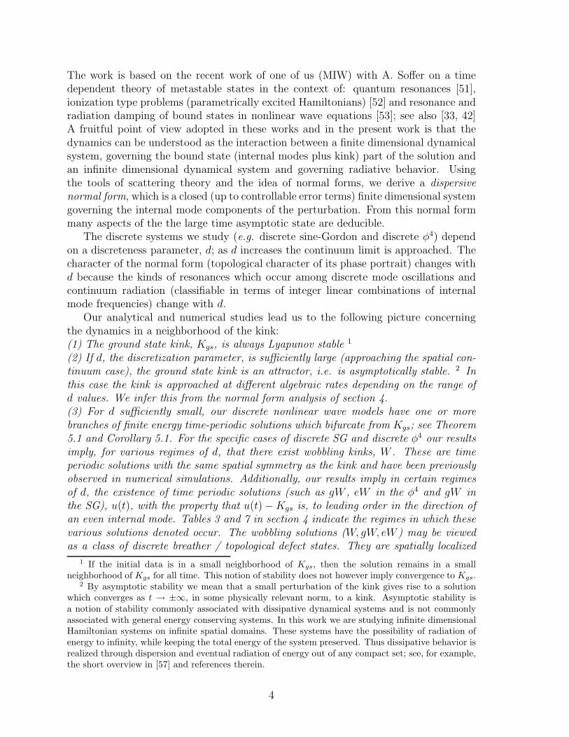
Our analytical and numerical studies lead us to the following picture concerningthe dynamics in a neighborhood of the kink:(1) The ground state kink, Kgs, is always Lyapunov stable 1

(2) If d, the discretization parameter, is sufficiently large (approaching the spatial con-tinuum case), the ground state kink is an attractor, i.e. is asymptotically stable. 2 Inthis case the kink is approached at different algebraic rates depending on the range ofd values. We infer this from the normal form analysis of section 4.(3) For d sufficiently small, our discrete nonlinear wave models have one or morebranches of finite energy time-periodic solutions which bifurcate from Kgs; see Theorem5.1 and Corollary 5.1. For the specific cases of discrete SG and discrete φ4 our resultsimply, for various regimes of d, that there exist wobbling kinks, W . These are timeperiodic solutions with the same spatial symmetry as the kink and have been previouslyobserved in numerical simulations. Additionally, our results imply in certain regimesof d, the existence of time periodic solutions (such as gW , eW in the φ4 and gW inthe SG), u(t), with the property that u(t) −Kgs is, to leading order in the direction ofan even internal mode. Tables 3 and 7 in section 4 indicate the regimes in which thesevarious solutions denoted occur. The wobbling solutions (W, gW, eW ) may be viewedas a class of discrete breather / topological defect states. They are spatially localized

1 If the initial data is in a small neighborhood of Kgs, then the solution remains in a smallneighborhood of Kgs for all time. This notion of stability does not however imply convergence to Kgs.

2 By asymptotic stability we mean that a small perturbation of the kink gives rise to a solutionwhich converges as t → ±∞, in some physically relevant norm, to a kink. Asymptotic stability isa notion of stability commonly associated with dissipative dynamical systems and is not commonlyassociated with general energy conserving systems. In this work we are studying infinite dimensionalHamiltonian systems on infinite spatial domains. These systems have the possibility of radiation ofenergy to infinity, while keeping the total energy of the system preserved. Thus dissipative behavior isrealized through dispersion and eventual radiation of energy out of any compact set; see, for example,the short overview in [57] and references therein.

4

and time-periodic oscillations mounted on a static kink background. The usual discretebreathers [2, 38] are mounted on a zero background. This is analogous to the situationwith solitons. Dark solitons of the defocusing nonlinear Schrodinger (NLS) equationare mounted on a non-zero continuous wave background, while standard solitons offocusing NLS sit on a zero background.(4) Numerical simulations and the normal form analysis indicate that in various dregimes these time periodic states are local attractors for the dynamics.(5) The analysis of section 5 implies some nonexistence results concerning solutionsof discrete nonlinear wave equations in a neighborhood of the kink. We have that incertain regimes of the discreteness parameter, d, no nontrivial time-periodic solutionexists, and that time quasiperiodic solutions do not exist in any regime of d. On theother hand, the normal form analysis and numerical simulations indicate, in someregimes of d, that periodic or quasiperiodic oscillations can be very long lived; seesection 6, and in particular, the discussion of Regime VI in section 6.1. Thus, we maythink of the system as possessing metastable periodic and quasi-periodic solutions. Inregimes of d where we show that the wobbling kink, W , is unstable on long time scalesdue to a resonance of the “shape mode” with continuum radiation modes, we have theanalogue of the the wobbling solution of continuum φ4, proved to be stable on large butfinite time scales by Segur [50]. On an infinite time scale this wobbling solution behavesas those of the discrete system for large enough d; eventually the oscillations damp atan algebraic rate leaving a kink in the limit [39, 49]. For the continuum system, thelimiting kink may be traveling, while for the discrete system it is a static ground state(centered between lattice sites) kink.

In (2) the dispersive normal form has a dissipative character; the effect of couplingthe internal mode oscillations to radiation is modeled by an appropriate nonlinear fric-tion; see section 4 and the discussion in the introduction to [53] on another relatedmodel. The damping or friction coefficients are given by formulae which can be un-derstood as a nonlinear generalization of Fermi’s golden rule, arising in the context ofthe theory of spontaneous emission in atomic physics. Finally, it is worth noting thatwe obtain a dissipative and therefore apparently time-irreversible normal form from asystem which is conservative and time-reversible. There is no contradiction because thedissipation is of an internal nature; it signifies the transfer of energy from the discreteinternal mode oscillations to the continuum dispersive waves which propagate to infin-ity. That dissipative dynamical systems emerge from conservative systems which area coupling of a low dimensional dynamics to infinite dimensional dynamics (“massesand springs coupled to strings”) has been observed in many contexts; see, for example,[35, 5, 37] and the discussion in [51, 52, 53].

The paper is organized as follows:

• Section 2 begins with a general discussion of discrete nonlinear wave equationswhich support kink-like (heteroclinic) structures and then specializes to a discus-sion of the discrete sine-Gordon (SG) and discrete φ4 systems.

• In section 3, we present the decomposition of solutions into discrete internal modecomponents and radiative components, enabling us to view the dynamics near akink as the interaction of finite and infinite dimensional Hamiltonian systems.

5

• In section 4 the dispersive normal forms are derived and discussed for both dis-crete SG and discrete φ4.

• In section 5, we prove that if Ω is an internal mode frequency and no multipleof it lies in the continuous spectrum of the kink (phonon band), then there is afamily of finite energy time periodic solutions which bifurcate from the kink inthe “direction” of the corresponding internal mode. The proof is based on thePoincare continuation method and is an application of the implicit function the-orem in an appropriate Banach space. This approach was used also by MacKayand Aubry [38], who constructed discrete breathers of nonlinear wave equationsin the anti-integrable limit.

• In section 6 we combine the normal form analysis of section 4 and existencetheory for periodic solutions of section 5 with observations based on numericalsimulations to obtain a detailed picture of the dynamics in a neighborhood of theground state kink.

• Finally, in section 7, we summarize our results and give directions of interest forfuture research.

1.1 Notation

• ZZ denotes the set of all integers and IR denotes the set of real numbers.

• For u = uii∈ZZ, δ2hu denotes the discrete Laplacian of u defined by:

(δ2hu)i = h−2 (ui+1 − 2ui + ui−1) . (1.1)

In the case h = 1 we shall use the simplified notation δ2 = δ21.

• The inner product of vectors u and v in l2(ZZ) is given by

〈u, v〉 =∑

j

ujvj. (1.2)

• The t subscript denotes time partial derivatives, e.g. ut(t) = ∂tu(t), whereas idenotes the lattice site numbering.

• l2(ZZ) is the Hilbert space of sequences uii∈ZZ which are square summable.

• Hs(I) denotes the Hilbert space of functions f , defined on I ⊂ IR such that f andall its derivatives of order ≤ s are square-integrable. For the case of 2π periodicfunctions, I = S1

2π, an equivalent norm on Hs is given by:

‖f‖2Hs =

∑

n∈ZZ

(1 + |n|2)s|fn|2, (1.3)

where fn denotes the nth Fourier coefficient of f :

fn = (2π)−12

∫ 2π

0e−2πintf(t) dt. (1.4)

6

• For example, H2(IR; l2(ZZ)) denotes the space of functions f(t, i) which are H2,as functions of t, with values in the space of l2(ZZ) functions.

• σ(B) and σcont(B) denote respectively the spectrum and the continuous (phonon)spectrum of the operator B.

• 0 < d denotes the discretization parameter; d large is the spatial continuumregime, while for d small the effects of discreteness are strong.

2 Discrete and continuum wave equations

2.1 General Background

Two model nonlinear wave equations on lattices that have played a central role in thetheory of nonlinear waves are the discrete sine-Gordon equation (SG) and the discreteφ4 model (φ4). These equations may be viewed as governing the dynamics of a chainof unit mass particles which, in equilibrium, are equally spaced, a unit distance apart.The particles are then subjected to a conservative force derived from a potential. Interms of the displacement ui of the ith particle from equilibrium the equations of motionare3:

ui,tt = (δ2u)i − d−2V ′(ui). (2.1)

The case of SG and φ4 correspond, respectively, the choices of potential:

V (u) = 1 − cosu, (SG)

V (u) =1

4(1 − u2)2. (φ4)

More generally, we assume V has three continuous derivatives and satisfies certainconstraints appearing below, related to the existence of kink solutions or homoclinicorbits.

The parameter d is a fixed constant with, d−2, having the interpretation of the ratioof on- site potential energy to elastic coupling energy.Relation between discrete and continuum systems: The parameter d can also beseen to play the role of the reciprocal of the lattice spacing in passing between contin-uum and discrete models. Consider the continuum model governing the displacementv(T, x):

vTT = vxx − V ′(v). (2.2)

Introducing the lattice spacing parameter, h, and replacing uxx(x) by (δ2u)i we obtainthe discrete nonlinear wave equation governing vi = v(T, i; h):

vi,TT = (δ2hv)i − V ′(vi). (2.3)

The form of the discrete nonlinear wave equation we use is obtained by setting t = h−1Tand defining the time-scaled displacement u(t, i; h) = v(T, i; h). Then, u(t, i; h) satisfies(2.1) with d = h−1.

3We use the notational conventions introduced by Peyrard and Kruskal [48].

7

Taking the formal limit d ↑ ∞ or equivalently h ↓ 0 we have that

U(T, i) ≡ limd→∞

u(dT, i; d−1) = limd→∞

v(T, i; d−1) (2.4)

satisfies the associated continuum nonlinear wave equation (2.2).Hamiltonian structure: The discrete and continuum equations we consider are in-finite dimensional Hamiltonian systems with Hamiltonian energy functionals4:

H =∑

i

1

2u2

i,t +1

2(ui+1 − ui)

2 + d−2V (ui) (2.5)

in the discrete case and

H =∫

IR

1

2(u2

T + u2x) + V (u) dx. (2.6)

Static kink solutions: Consider time-independent or static solutions of these dy-namical systems. In each case, such solutions satisfy the equation obtained by settingtime derivatives equal to zero. Thus, in the discrete case we have:

(δ2K)i = V ′(Ki), (2.7)

and in the continuum caseK ′′(x) = V ′(K(x)) (2.8)

Spatially uniform solutions occur at the critical points of the potential, V . Of particularinterest are the static kink solutions. These are static solutions which are heteroclinic.That is, they are static solutions which can be viewed as connections, as i → ±∞(respectively x → ±∞) in the phase space of two distinct ”unstable” equilibria, valuesK±

∗ for which

V (K+∗ ) = V (K−

∗ ), V ′(K±∗ ) = 0

V ′′∗ ≡ V ′′(K+

∗ ) = V ′′(K−∗ ) > 0. (2.9)

Kink solutions can also be constructed by variational methods. Consider the Hamil-tonian energy functional, H restricted to t-independent functions:

h[u] =∑

i

(

1

2(ui+1 − ui)

2 + d−2V (ui))

, discrete case (2.10)

h[u] =∫

IR

1

2u2

x + V (u) dx continuum case. (2.11)

Then, the Euler Lagrange equations associated with h[u] is the equation for the kink,(2.7). That is, if Kgs denotes a minimizer of h[u] then since for all ψ ∈ l2(ZZ),

d

dτh[Kgs + τψ] |τ=0 = 0. (2.12)

4 There is freedom in the choice of potential V ; we choose V so that the Hamiltonian energy ofthe static kink is finite.

8

40 60 80 100 120 140 160 1800

1

2

3

4

5

6

u

i

Figure 1: Ground state static kink for the very strongly discrete sine-Gordon model(–o–) d = 0.6, and very close to the continuum limit d = 10.

This implies that for all ψ ∈ l2(ZZ)

∑

i

[

−(δ2Kgs)i + d−2V ′(Kgs,i)]

ψi = 0. (2.13)

This is equivalent to (2.7). A solution constructed by minimization of h[u] is called aground state kink.5

Invariance and broken invariance:An important structural difference between the discrete and continuum cases is

that the continuum case has greater symmetry. In particular, (2.2) has the propertyof translation and Lorentz invariance, while (2.1) does not. A consequence of this isthat static solutions of (2.2) can be translated:

K(x) 7→ K(x− x0) (2.14)

5 A proof that the minimum of the functional (2.10) is attained can be given using the followingstrategy, used in a similar problem [56]: For positive integers, N , define hN [u] to be the truncatedHamiltonian, where the summation is taken over −N ≤ n ≤ N . Consider hN , restricted to vectorssatisfying u±N = K±

∗ . For any admissible vector, u = ui|i|≤N , it is possible, by rearrangement, toreplace it with another, v, which is monotonically increasing and for which h[v] ≤ h[u]. Therefore the

minimizer of hN [·], K(N)gs , is monotonically increasing from K−

∗ to K+∗ . A priori estimates, derived

from the Euler-Lagrange equation (2.7), and the boundary conditions enable one to pass to the limitand obtain a minimizer of h[·], Kgs = Kgs,ii∈ZZ, a monotonically increasing static kink.

9

to give a recentered kink and Lorentz boosted:

K(x) 7→ K((x− vt)/√

1 − v2), |v| < 1, (2.15)

to give a traveling solution of velocity v. These symmetries are absent in the discretemodels. Discrete models do however have a discrete translation symmetry but in themodels considered this does not give rise to discrete traveling waves.Dynamic stability of kinks: The issue of dynamic stability is a subtle one. First,there is the question of what is the object we expect to be stable. Also, since oursystems are infinite dimensional and not all norms are equivalent, different choices ofnorms will measure different phenomena. Here we briefly discuss three related notionsof stability we have in mind: (a) orbital Lyapunov stability, (b) asymptotic stabilityand (c) linear spectral stability.(a) Orbital Lyapunov stability means stability of the shape of the kink; if at t = 0 thedata is nearly shaped like a kink then it remains shaped like a kink for all t 6= 0. Thekink-like part of the solution will typically move so the solution at different times isnear some time-dependent spatial translate of the static kink (element of the symmetrygroup orbit of the static kink).

In the continuum case, orbital Lyapunov stability in the space H1(IR) is a conse-quence of characterization of the kink as a local minimizer of H. A detailed proof ispresented in [24]. A simple proof of Lyapunov stability of ground state discrete kinkscan be given based on the same ideas. 6

(b) Orbital asymptotic stability means that if the initial data is nearly a kink then thesolution converges to kink (possibly traveling, in the continuum case or pinned in thediscrete case) as t→ ∞.

For both notions (a) and (b) we see that the stable object is the family of solitarywave solutions. That is, in the case where there is a multiparameter family of solutions(kinks, solitary waves ...), it is the collection of all such that is the stable object.Concerning the terminology orbital stability, this family of solutions is related to theset of functions generated by applying elements of the equation’s symmetry group tothe solution (here, static kink), and thus we can think of the group orbit as stable.(c) Spectral stability:

As is well known, dynamic stability of the particular solution is related to thespectrum of the linearization of the dynamical system about this solution. Lineariza-tion about the kink gives an evolution equation for infinitesimal perturbations of the

6The proof is based on the following idea. Since Kgs is an energy minimizer, by (2.24), the secondvariation at the kink, B2 is non-negative. In fact, it is strictly positive; that is, for all ψ ∈ l2(ZZ),〈ψ,B2ψ〉 ≥ ω2

g〈ψ, ψ〉, where ω2g = ω2

g(d) > 0 is the discrete eigenvalue to which the zero mode ofthe continuum equation perturbs due to discretization of space. Suppose we have initial data near akink: u(0) = Kgs + v0, ∂tu(0) = v1 and let u(t) = Kgs + v(t) be the resulting solution. Assume that‖v0, v1‖l2 ∼ ε, where ε is sufficiently small. Then, since Kgs is a critical point of h[·] we have:

ε ∼ h[Kgs + v(t)]|t=0 − h[Kgs] = h[Kgs + v(t)] − h[Kgs] =1

2〈v(t), B2v(t)〉 + O(‖v(t)‖3

l2 )

≥ω2

g

2‖v(t)‖2

l2 − c‖v(t)‖3l2 .

implying that ‖v(t)‖l2 ∼ O(ε) for all t 6= 0, and Kgs is stable.

10

following form:(

∂2t +B2

)

p = 0. (2.16)

For the discrete case:B2pi = −(δ2p)i + d−2V ′′(Ki)pi, (2.17)

and for the continuum case:

B2p = −pxx + V ′′(K(x))p. (2.18)

At a minimum we expect that stability can hold only if no solutions of the linearizedevolution equation, corresponding to finite energy initial conditions, can grow as |t|increases. In carrying out linear stability analysis we seek solutions of the form pi =eλtPi (respectively, p = eλtP (x)) and obtain linear eigenvalue problems of the form:

(

B2 + λ2)

P = 0. (2.19)

Explicitly, we have:

− λ2Pi = −(δ2P )i + d−2V ′′(Ki)Pi, discrete case

−λ2P = −Pxx + V ′′(K(x))P. continuum case

We say λ is in the l2 spectrum (respectively, L2 spectrum) of the linearization aboutthe kink, or simply spectrum of the kink if the operator B2+λ2 does not have a boundedinverse on l2 (respectively L2). The spectrum will typically consist of two parts: (i) thepoint spectrum consisting of isolated eigenvalues of finite multiplicity, for which thecorresponding solution of (2.19) is in the Hilbert space, and due to the infinite extent ofthe spatial domain (ii) continuous spectrum, whose corresponding solutions (radiationor phonon modes) of (2.19) are bounded and oscillatory over the entire spatial domain.

Note that the eigenvalue equation (2.19) has the following symmtery: if λ has theproperty that (2.19) has a nontrivial solution solution then −λ, λ and −λ also have thisproperty. To avoid exponential growing solutions, we must require that the linearizedspectrum is a subset of the imaginary axis. If this holds we say the solution is spectrallystable.Spectrum of the kink:

We are interested in the set of λ’s for which the eigenvalue equation

(B2 + λ2)P = 0 (2.20)

has a nontrivial solution. We begin by discussing the spectrum of B2 and then takesquare roots to a obtain the spectrum of the the linearization about the kink.

We now make two general remarks about the spectrum of the kink solution, oneconcerning the continuous spectrum and one concerning the point spectrum.Continuous spectrum: The continuous spectrum is determined by the solutions of theconstant coefficient equation obtained from (2.19) by evaluating its coefficients at spa-tial infinity. In the discrete case we obtain:

− λ2Pi = −(δ2P )i + d−2V ′′∗ Pi, (2.21)

11

where V ′′∗ = limi→±∞ V ′′(Ki). This constant coefficient equation can be solved in

terms of exponentials which yield the character of the exact continuum eigensolutionsof (2.19). We let λ = iω. We find bounded oscillatory solutions of the form: Pn =exp(

√−1kn), n ∈ ZZ, k real and arbitrary, where satisfies the dispersion relation:

ω2 = 4 sin2(k/2) + d−2V ′′∗ . (2.22)

It follows that the continuous spectrum of B2 is the positive interval from d−2V ′′∗ to

d−2V ′′∗ + 4. Therefore, the continuous spectrum of the linearization about the kink

solution consists of two intervals on the imaginary axis: ±i[d−1√

V ′′∗ ,

√

4 + d−2V ′′∗ ].

Point spectrum: An important conclusion, concerning the point spectrum of kink forthe continuum equation, can be made as a consequence of the equation’s symmetrygroup. If K(x) is a kink then translation invariance implies that K ′(x) is a zero mode,a solution of the linear eigenvalue problem with eigenvalue zero, B2K = 0. Thiszero mode is often called the Goldstone mode. Since the eigenfunction, K ′ does notchange sign, zero is the ground state energy (lowest point in the point spectrum) ofthe Sturm-Liouville operator −∂2

x + V ′′(K(x)). This eigenvalue is of multiplicity one.If one views the discrete model as a perturbation of the continuum model, due

to the absence of corresponding symmetries in the discrete problem one expects theeigenvalue at zero to move, as d decreases from infinity (h, the lattice spacing, increasesfrom zero), to the right of zero or to the left of zero. In terms of the spectrum of thekink (plus or minus the square root of the spectrum of B2), this means that in thediscrete case the spectrum of the kink consists of either (a) a purely imaginary pair,±iωs (stable case) or (b) a pair of real eigenvalues, symmetrically situated about theorigin (unstable case). We shall see both cases in our study of specific discrete modelsand we shall refer to these eigenvalues and corresponding modes loosely as Goldstonemodes as well.

As we shall see in the specific models considered, other eigenvalues may appearin the gap between the upper and lower branches of the continuous spectrum. Suchmodes of the linearization which lie in this gap are called internal modes, and theirnumber and location can change with d. For SG we shall find that there are one or twopairs of internal modes, while for the φ4 model there are two or three pairs of internalmodes.

Finally, we remark that in the case of a ground state kink, one obtained by mini-mization of h[u], the spectrum of B2 is non-negative and the kink is spectrally stable.To see this, let Kgs denote a minimizer of h[u], which as indicated above, is a criticalpoint of h[·]. Furthermore, for all ψ ∈ l2(ZZ),

d2

dτ 2h[Kgs + τψ] |τ=0 ≥ 0. (2.23)

A calculation yields that this is equivalent to:

1

2〈ψ,B2ψ〉 ≥ 0, for all ψ ∈ l2(ZZ). (2.24)

Therefore, d2h[Kgs] = 12B2, the second variation of h[·] at the ground state kink, is a

nonnegative self-adjoint operator. It follows that the spectrum of the kink, ±iσ(B),lies on the imaginary axis.

12

2.2 The Sine-Gordon equation

Consider the discrete SG equation:

ui,tt = (ui+1 + ui−1 − 2ui) −1

d2sin ui. (2.25)

A static discrete 2π kink is a time-independent solution, Kii∈ZZ of (2.25) which sat-isfies the boundary conditions at infinity:

Ki → 0, as i→ −∞, and Ki → 2π, as i→ ∞ (2.26)

It is well-known that there are two static kink solutions, a high energy one centeredon a lattice site and a low energy one centered between two consecutive lattice sites[48, 27, 15, 59, 54, 8, 9, 11, 7, 34, 30, 31]. The low energy kink corresponds to theminimizer of the static Hamiltonian energy, h[u], displayed in (2.10). As d increases(the continuum limit) the energy difference between the two static kink solutions, theso-called Peierls-Nabarro (PN) barrier, tends to zero and the scaled limit u(i; d−1) = Ki,with i/d ≡ x fixed, converges to the continuum SG static kink solution

KSG(x) = 4tan−1(ex). (2.27)

Linear stability analysis about the high energy and low energy kinks was carried outin [3]. From the general discussion of section 2.1, the dispersion relation defining thecontinuous (phonon) spectrum is ω2 = d−2 + 4 sin2(k/2). Therefore, B2 has a band ofcontinuous spectrum of length 4, [d−2, 4 + d−2], and the continuous spectrum of thekink consists of the two bands, ±i[d−1,

√4 + d−2] .

For the case of the high energy kink, the point spectrum of B2 contains a negativeeigenvalue derived from the zero (Goldstone) mode associated with the continuum(translation invariant) case. Since the eigenvalue parameter in (2.19) is −λ2, it followsthat the spectrum of the high energy kink (parametrized by λ) consists of two discretereal (Goldstone) eigenvalues, one positive and one negative, ±ωus. These occur at adistance of order exp(−π2d) [27, 48, 4, 28].

The low energy kink, minimizes the Hamiltonian. The second variation of h[u]at the kink, B2, is therefore a self-adjoint and nonnegative operator. Its spectrum istherefore nonnegative and so the spectrum of the kink is purely imaginary. In this case,the Goldstone mode associated with translation invariance of the continuum problemgives rise to point spectrum consisting of a complex conjugate pair of eigenvalueswith order of magnitude exp(−π2d). Furthermore, for d > de, de ∼ 0.515 a spatiallyantisymmetric edge mode of energy ω2

e (B2e = ω2ee) appears whose corresponding

energy has a distance from the phonon band edge of order O(d−4), for d large [34, 31].This mode is not present in the continuum SG.

2.3 Discrete φ4 Model

Consider the discrete φ4 equation:

ui,tt = (ui+1 + ui−1 − 2ui) +1

d2(ui − u3

i ) (2.28)

13

Spectrum of discrete SG ground state kink

σ(Β2 )

ω

ω

r

i

i

i

-i

-i

ωω

ω

ω

g

e

g

e

i ωmin

-i

-i

i ω

ω

ω

max

min

max

0 ω ω ω ωg2

e2

min2

max2

Figure 2: Upper panel: schematic of spectrum of B2, σ(B2), consisting of two (ford > de ∼ 0.515) positive discrete eigenvalues (ω2

g < ω2e) and a finite band of continuous

spectrum extending from ω2min = 1/d2 to ω2

max =√

4 + 1/d2. Lower panel: schematic

of spectrum of the kink, given by ±iσ(B).

14

Discrete SG ground state kink and its internal modes

92 94 96 98 100 102 104 106 108 1100

2

4

6

u i

92 94 96 98 100 102 104 106 108 1100

0.5

1

g i

60 70 80 90 100 110 120 130 140 150−0.5

0

0.5

e i

i

Figure 3: Three panels in order correspond to (a) discrete SG kink, (b) spatially evenGoldstone mode (c) spatially odd edge mode (present for d > de ∼ 0.515)

15

In most ways the situation is quite similar to that discussed for the discrete SG.The φ4 model has low and high energy kinks. The low energy kink is centered betweenlattice sites while the high energy kink is centered at a lattice site. As d increasesthe energy difference, the PN barrier, tends to zero, and finally, in the scaled limitu(i; d−1) = Ki, with i/d ≡ x fixed, converges ot the continuum φ4 kink,

Kφ4(x) = tanh(x/√

2). (2.29)

Most qualitative properties of the spectrum of the linearization about the φ4 kinkare analogous to those in the SG case. The single key difference can be traced to thespectrum associated with the continuum case. In addition to the zero (Goldstone)mode, the spectrum of the operators B2 has internal mode of odd parity with eigen-frequency ω2

s = 3/(4d2). Therefore, the spectrum of the kink has purely imaginaryinternal modes associated with the energies ωs = ±i

√3/(2d). These modes are called

shape modes.Turning now to the discrete φ4 model we see that B2 for the discrete case has the

following properties:

• The dispersion relation is ω2 = 2/d2+4 sin2(k/2), and therefore B2 has continuousspectrum extending from 2/d2 to 2/d2 + 4.

• B2 has a positive internal Goldstone mode with energy ω2g , so that B2g = ω2

gg.This mode, which is traceable to the zero mode of the continuum model, isspatially even and ωg is exponentially small in d [28].

• B2 has an internal odd shape mode with energy ω2s , so that B2s = ω2

ss. Thismode, which is traceable to the internal shape mode of the continuum φ4 model,is spatially odd.

• For d > de (de ∼ 0.82) B2 has an internal edge mode which is even and withcorresponding energy ω2

e , with B2e = ω2ee, which emerges from the continuous

spectrum. For large d we have [34, 31]

ωe2 ∼ 2d−2 − 2

152d−6. (2.30)

It follows that the spectrum of the discrete φ4 kink consists of pair of two or threecomplex conjugate pairs of internal modes at energies ±iωg, ±iωs, and for d > de,±iωe.

In the next section we shall see that whether or not certain integer linear combina-tions of the internal mode frequencies land in the continuous spectrum determines thelarge time asymptotic behavior.

16

Spectrum of discrete φ4 ground state kink

σ(Β2 )

ω

ω

r

i

i

i

-i

-i

ωω

ω

ω

g

e

g

e

i ωmin

-i

-i

i ω

ω

ω

max

min

max

0 ω ω ω ωg2

e2

min2

max2

i ωs

-i ωs

ωs2

Figure 4: Upper panel: schematic of spectrum of B2, σ(B2), consisting of three (ford > de ∼ 0.82) positive discrete eigenvalues (ω2

g < ω2s < ω2

e) and a finite band of

continuous spectrum extending from ω2min = 2/d2 to ω2

max =√

4 + 2/d2. Lower panel:

schematic of spectrum of the kink, given by ±iσ(B).

3 Resonances and radiation damping

That we can Lorentz boost a static kink and obtain a traveling kink on the spatialcontinuum (section 2) motivates the following question:

What happens if we attempt to cause a kink to propagate through the lattice?The numerical and formal asymptotic investigation was initiated in [48],[47]. For

example, choose as initial conditions for the discrete sine Gordon system the stateui(t = 0) = K(i/

√1 − v2), where K(x) is the continuum kink and 0 < |v| < 1. Disper-

sive radiation plays an important role in the dynamics. The kink moves approximatelyas particle under the influence of the sinusoidal (Peierls-Nabarro) potential. As thekink propagates, its velocity alternately increases and decreases, depending on the lo-cation of its center of mass relative to the peaks and troughs of the potential. Thisoscillation leads to a resonance with the continuous spectrum [48, 8] and a transfer ofenergy from the propagating kink to radiation modes. Eventually, the kink has slowedso that its energy no longer exceeds the PN barrier and then executes a damped oscil-lation about a fixed lattice site to which it is pinned. It is this latter process that westudy here.

17

Discrete φ4 ground state kink and its internal modes

95 100 105 110−1

−0.5

0

0.5

1

ui

i95 100 105 110

0

0.2

0.4

0.6

0.8

gi

i

95 100 105 110

−0.6

−0.4

−0.2

0

0.2

0.4

0.6

si

i50 100 150

−0.25

−0.2

−0.15

−0.1

−0.05

0

0.05

ei

i

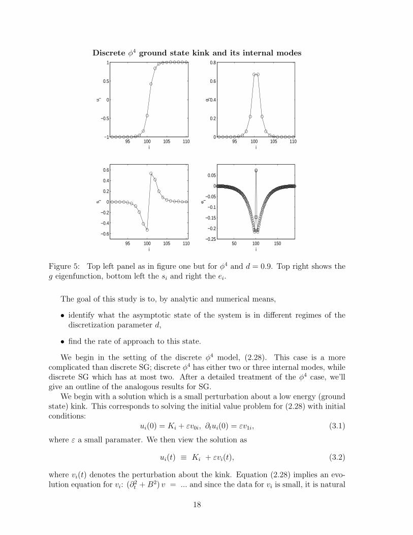
Figure 5: Top left panel as in figure one but for φ4 and d = 0.9. Top right shows theg eigenfunction, bottom left the si and right the ei.

The goal of this study is to, by analytic and numerical means,

• identify what the asymptotic state of the system is in different regimes of thediscretization parameter d,

• find the rate of approach to this state.

We begin in the setting of the discrete φ4 model, (2.28). This case is a morecomplicated than discrete SG; discrete φ4 has either two or three internal modes, whilediscrete SG which has at most two. After a detailed treatment of the φ4 case, we’llgive an outline of the analogous results for SG.

We begin with a solution which is a small perturbation about a low energy (groundstate) kink. This corresponds to solving the initial value problem for (2.28) with initialconditions:

ui(0) = Ki + εv0i, ∂tui(0) = εv1i, (3.1)

where ε a small paramater. We then view the solution as

ui(t) ≡ Ki + εvi(t), (3.2)

where vi(t) denotes the perturbation about the kink. Equation (2.28) implies an evo-lution equation for vi: (∂2

t +B2) v = ... and since the data for vi is small, it is natural

18

to expand vi in terms of the modes of the linearization about the kink. Recall thatthe operator B2 is positive and self-adjoint, and has, depending on the range of d′sconsidered, two or three internal modes g, s, and e (if d > de):

B2gi = ω2ggi, B

2si = ω2ssi, B

2ei = ω2eei

0 < ω2g < ω2

s < ω2e < 4 + 2d−2,

whereB2ψi ≡ −δ2ψi + d−2(3K2

i − 1)ψi. (3.3)

We assume these internal modes to be normalized so that the set g, s, e is orthonor-mal in l2(ZZ). We also introduce the operator which projects onto the orthogonalcomplement of the subspace of internal modes:

Pcψ ≡ ψ − 〈g, ψ〉g − 〈s, ψ〉s− 〈e, ψ〉e (3.4)

Pc is the projection onto the continuous spectral part of B2 (phonon or radiationmodes) and therefore the solutions of (∂2

t +B2)u = 0 with data in the range of Pc areexpected to decay dispersively as t→ ±∞.

We expand the perturbation εvi in terms of the internal mode subspace and itsorthogonal complement and thus

ui(t) = Ki + εa(t)gi + εb(t)si + εc(t)ei + ε2ηi(t), (3.5)

with

〈g, η(t)〉 = 〈s, η(t)〉 = 〈e, η(t)〉 = 0,

Pcη = η

Substitution of (3.5) into (2.28) yields

(att + ωg2a)gi + (btt + ωs

2b)si + (ctt + ωe2c)ei + ε∂2

t ηi

= −εB2η − d−2(3εKiM2i + ε2M3

i + 6ε2KiηMi + 3ε3M2i ηi + O(ε4)) (3.6)

where:Mi ≡ a(t)gi + b(t)si + c(t)ei. (3.7)

Notice that from here on for simplicity and compactness we drop the spatial indices i.We next project (3.6) onto the internal modes g, s and e, as well as on the range

of Pc. This yields the following coupled system of four equations for the three internalmode amplitudes and the continuous spectral part:

∂2t a + ωg

2a = − 1

d2

(

3ε〈g,KM2〉 + ε2〈g,M3〉 + 6ε2〈g,KMη〉 + 6ε3〈g,M2η〉)

+ O(ε4)

(3.8)

∂2t b+ ωs

2b = − 1

d2

(

3ε〈s,KM2〉 + ε2〈s,M3〉 + 6ε2〈s,KMη〉 + 6ε3〈s,M2η〉)

+ O(ε4)

(3.9)

∂2t c+ ωe

2c = − 1

d2

(

3ε〈e,KM2〉 + ε2〈e,M3〉 + 6ε2〈e,KMη〉 + 6ε3〈e,M2η〉)

+ O(ε4))

(3.10)

∂2t η +B2η = − 1

d2Pc

(

εM3 + 3KM2 + O(εηM) + O(ε4η3))

. (3.11)

19

The initial data for a(t), b(t), c(t) is:

a(0) = 〈g, v0〉, ∂ta(0) = 〈g, v1〉b(0) = 〈s, v0〉, ∂tb(0) = 〈s, v1〉c(0) = 〈e, v0〉, ∂tb(0) = 〈e, v1〉η(0) = Pcv0, ∂tη(0) = Pcv1 (3.12)

For simplicity we shall assume:

η(0) = 0, ∂tη(0) = 0 (3.13)

corresponding to perturbations of the kink which only excite the internal modes. Thegeneral case can be treated as well; see [53].

The system (3.8-3.11) may be viewed as finite dimensional Hamiltonian system gov-erning three oscillators with amplitudes a, b and c and natural frequencies ±ωg,±ωs,±ωe,coupled by nonlinearity to an infinite dimensional Hamiltonian wave equation for afield η. Systems of this type have been analyzed rigorously and the behavior of theirsolutions determined on short, intermediate and infinite time scales [52, 53]. Theanalysis we present uses and extends the methods of these works. Roughly speakingwe transform the system (3.8)-(3.11) into an equivalent dynamical system, which isa perturbation of a normal form for which one obtains information on: (i) what theasymptotic state of the system is, and (ii) how this asymptotic state is approached.

4 The dispersive normal form

Our goal in this section is to derive the normal forms which give detailed informationon the dynamics in a neighborhood of the ground state static kink of SG and φ4. Inparticular, the normal forms anticipate the existence of time-periodic solutions. Thesepredictions are upheld by the rigorous results of section 5. In section 6, the normal formanalysis is then joined with the existence theory of section 5 and numerical simulationsto fill out the picture of what the dynamics are in a neighborhood of the kink.

4.1 The normal form for discrete φ4

At this stage, we have in (3.8-3.11) a formulation of the discrete φ4 dynamical as asystem governing the discrete internal modes interacting, due to nonlinearity, with asystem governing dispersive waves (phonons). Our goal in this section is to presentand implement a method, based on [52, 53], leading to a reformulation of the coupleddiscrete-continuum mode system (3.8-3.11) as a perturbed dispersive normal form inwhich the nature of the energy transfer among modes is made explicit.

Ideally, one could solve the equation for the dispersive part, η, explicitly in termsof the discrete mode amplitudes: a, b, and c and then substitute the result into themode amplitude equations to get a closed system of equations for a, b, and c. This thencould be used in the equation for η to determine its behavior. Due to the system’s

20

nonlinearity, one can’t expect to solve for the exact behavior of η in terms of a, b andc. Instead we solve perturbatively in ε. Let

η ≡∞∑

j=0

εjη(j). (4.1)

Then,∂2

t η(0) +B2η(0) = −3d−2KM2. (4.2)

The function η captures the leading order radiative response, to the internal modeexcitations.

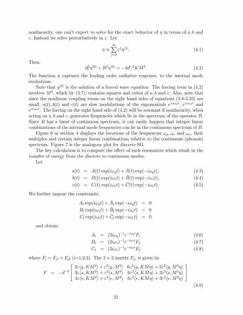
Note that η(0) is the solution of a forced wave equation. The forcing term in (4.2)involves M2, which by (3.7), contains squares and cubes of a, b and c. Also, note thatsince the nonlinear coupling terms on the right hand sides of equations (3.8-3.10) aresmall, a(t), b(t) and c(t) are slow modulations of the exponentials e±iωgt, e±iωst ande±iωet. The forcing on the right hand side of (4.2) will be resonant if nonlinearity, whenacting on a, b and c, generates frequencies which lie in the spectrum of the operator B.Since B has a band of continuous spectrum, it can easily happen that integer linearcombinations of the internal mode frequencies can lie in the continuous spectrum of B.

Figure 6 in section 4 displays the locations of the frequencies ωg, ωs and ωe, theirmultiples and certain integer linear combinations relative to the continuous (phonon)spectrum. Figure 7 is the analogous plot for discrete SG.

The key calculation is to compute the effect of such resonances which result in thetransfer of energy from the discrete to continuum modes.

Let

a(t) = A(t) exp(iωgt) + A(t) exp(−iωgt), (4.3)

b(t) = B(t) exp(iωst) + B(t) exp(−iωst), (4.4)

c(t) = C(t) exp(iωet) + C(t) exp(−iωet), (4.5)

We further impose the constraints:

At exp(iωgt) + At exp(−iωgt) = 0

Bt exp(iωst) + Bt exp(−iωst) = 0

Ct exp(iωet) + Ct exp(−iωet) = 0.

and obtain:

At = (2iωg)−1e−iωgtF1 (4.6)

Bt = (2iωs)−1e−iωstF2 (4.7)

Ct = (2iωe)−1e−iωetF3 (4.8)

where Fi = Fi1 + Fi2 (i=1,2,3). The 3 × 2 matrix Fij is given by

F = −d−2

3ε〈g,KM2〉 + ε2〈g,M3〉 6ε2〈g,KMη〉 + 3ε3〈g,M2η〉3ε〈s,KM2〉 + ε2〈s,M3〉 6ε2〈s,KMη〉 + 3ε3〈s,M2η〉3ε〈e,KM2〉 + ε2〈e,M3〉 6ε2〈e,KMη〉 + 3ε3〈e,M2η〉

(4.9)

21

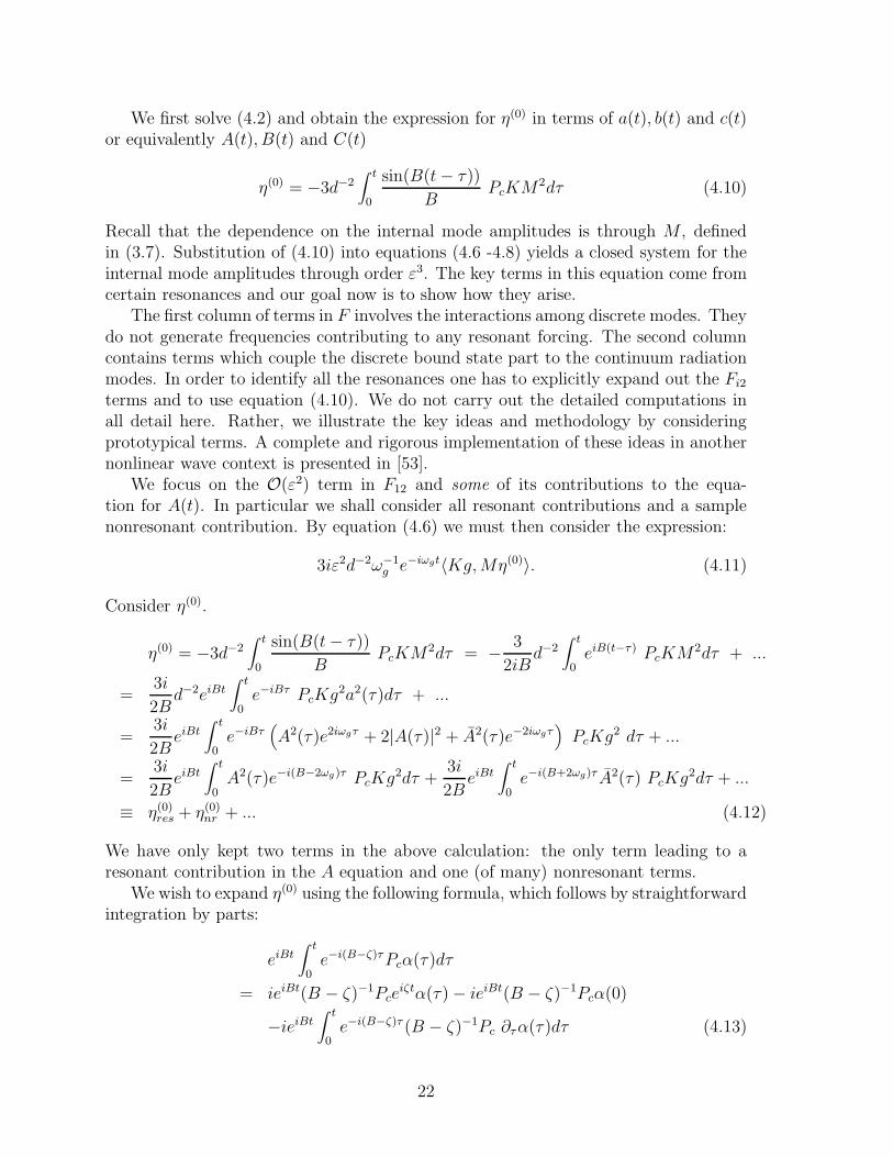
We first solve (4.2) and obtain the expression for η(0) in terms of a(t), b(t) and c(t)or equivalently A(t), B(t) and C(t)

η(0) = −3d−2∫ t

0

sin(B(t− τ))

BPcKM

2dτ (4.10)

Recall that the dependence on the internal mode amplitudes is through M , definedin (3.7). Substitution of (4.10) into equations (4.6 -4.8) yields a closed system for theinternal mode amplitudes through order ε3. The key terms in this equation come fromcertain resonances and our goal now is to show how they arise.

The first column of terms in F involves the interactions among discrete modes. Theydo not generate frequencies contributing to any resonant forcing. The second columncontains terms which couple the discrete bound state part to the continuum radiationmodes. In order to identify all the resonances one has to explicitly expand out the Fi2

terms and to use equation (4.10). We do not carry out the detailed computations inall detail here. Rather, we illustrate the key ideas and methodology by consideringprototypical terms. A complete and rigorous implementation of these ideas in anothernonlinear wave context is presented in [53].

We focus on the O(ε2) term in F12 and some of its contributions to the equa-tion for A(t). In particular we shall consider all resonant contributions and a samplenonresonant contribution. By equation (4.6) we must then consider the expression:

3iε2d−2ω−1g e−iωgt〈Kg,Mη(0)〉. (4.11)

Consider η(0).

η(0) = −3d−2∫ t

0

sin(B(t− τ))

BPcKM

2dτ = − 3

2iBd−2

∫ t

0eiB(t−τ) PcKM

2dτ + ...

=3i

2Bd−2eiBt

∫ t

0e−iBτ PcKg

2a2(τ)dτ + ...

=3i

2BeiBt

∫ t

0e−iBτ

(

A2(τ)e2iωgτ + 2|A(τ)|2 + A2(τ)e−2iωgτ)

PcKg2 dτ + ...

=3i

2BeiBt

∫ t

0A2(τ)e−i(B−2ωg)τ PcKg

2dτ +3i

2BeiBt

∫ t

0e−i(B+2ωg)τ A2(τ) PcKg

2dτ + ...

≡ η(0)res + η(0)

nr + ... (4.12)

We have only kept two terms in the above calculation: the only term leading to aresonant contribution in the A equation and one (of many) nonresonant terms.

We wish to expand η(0) using the following formula, which follows by straightforwardintegration by parts:

eiBt∫ t

0e−i(B−ζ)τPcα(τ)dτ

= ieiBt(B − ζ)−1Pceiζtα(τ) − ieiBt(B − ζ)−1Pcα(0)

−ieiBt∫ t

0e−i(B−ζ)τ (B − ζ)−1Pc ∂τα(τ)dτ (4.13)

22

with α(τ) = A2(τ) PcKg2, for example, and that τ -derivatives of A are of order ε. For

the term η(0)res, ζ = 2ωg, which for d in the range [0.54, 0.6364] lies in the continuous

spectrum; see Table 2 and Figure 6 below. Such resonant terms are of paramountinterest and govern energy transfer. To treat these resonant terms, an appropriatemodification of (4.13) is required. We use the following:Let κ = sgn(t), which is equal to +1 if t > 0 and −1 for t < 0.

eiBt∫ t

0e−i(B−ζ)τPc α(τ)dτ =

ieiBt(B − ζ + iκ0)−1Pc eiζtα(τ) − ieiBt(B − ζ + iκ0)−1Pc α(0)

−ieiBt∫ t

0e−i(B−ζ)τ (B − ζ + iκ0)−1Pc ∂τα(τ)dτ, (4.14)

where(B − ζ + iκ0)−1 = lim

ǫ↓0(B − ζ + iκǫ)−1. (4.15)

Remark 4.1 (1) The sense in which the operator expansions (4.13) and (4.14) arecorrect is in a distributional sense. That is, equality holds when multiplying both sidesby a smooth function with spatial support which is compact and integrating both sidesover all space.(2) Formula (4.14) is proved by first writing the integral on the left hand side as

∫ t

0exp(−i(B − ζ + iκǫ)τ) Pcα(τ) dτ. (4.16)

For any ǫ > 0 (4.13) can be used with ζ replaced by ζ − iǫ. We then pass to the limitas ǫ ↓ 0.(3) The choice of regularization, +i0 (κ = 1) for t > 0 and −i0 (κ = −1) for t < 0 isconnected with the condition that the latter two terms in (4.14) consist of outgoing ra-diation at spatial infinity, and is therefore time-decaying in an appropriate local energysense [53]. In this article, we take into account only the first term in (4.14). Reference[53] contains a fully detailed and rigorous treatment in a related context. Henceforth,we shall for simplicity assume t > 0 and therefore work with the +i0 regularization.(4) If ζ does not lie in the continuous spectrum the formula (4.14) reduces to (4.13).

We now continue the expansion of η(0) using (4.13) to study η(0)nr and (4.14) to study

η(0)res:

η(0)res = −3

2d−2B−1(B − 2ωg + i0)−1A(t)2 PcKg

2 + ...

η(0)nr = −3

2d−2B−1(B + 2ωg)

−1A(t)2 PcKg2 + ...

Substitution of η(0) = η(0)res + η(0)

nr + ... into (4.11) we have:

3iε2d−2ω−1g e−iωgt〈Kg,Mη(0)〉

23

= 3iε2d−2ω−1g e−iωgt

(

Aeiωgt + Ae−iωgt)

〈Kg2, η(0)〉 + ...

= −9

2iε2d−4ω−1

g |A|2A〈Kg2, B−1(B − 2ωg + i0)−1 PcKg2 + ...〉

−9

2iε2d−4ω−1

g A3e−3iωgt〈Kg2, B−1(B + 2ωg)−1 PcKg

2〉 + ...

≡ ε2(

−Γ2ωg+ iΛ2ωg

)

|A(t)|2A(t) + ρ(t)A3(t) (4.17)

To calculate Λ and Γ, we apply a generalization to self-adjoint operators of thewell-known distributional identity:

limǫ→0

(ξ ± iǫ)−1 = P.V. ξ−1 ∓ iπδ(ξ), (4.18)

where δ(ξ) is the Dirac delta mass at ξ = 0 and P.V. denotes the principal valueintegral.

Therefore, using (4.18) we obtain:

ε2Γ2ωg≡ ε2Γ(2ωg) =

9π

4ω2g

ε2d−4 〈Kg2, δ(B − 2ωg)Kg2〉, (4.19)

ε2Λ2ωg≡ ε2Λ(2ωg) = −9

2ε2d−4〈Kg2, P.V.(B − 2ωg)PcKg

2〉. (4.20)

Remark 4.2 (1) Had we done this calculation for the B (respectively, C) equation,we’d have obtained as a coefficient of |B|2B (respectively, |C|2C) the quantity ε2(−Γ2ωs

+iΛ2ωs

) (respectively, ε2(−Γ2ωe+ iΛ2ωe

)) (2) If ζ ∈ σcont(B), then Γζ is always nonneg-ative and, generically, is strictly positive. It is the analogue of Fermi’s golden rulewwhich arises in the context of the theory of spontaneous emission [36],[51]. Apartfrom a positive constant prefactor, Γζ is the square of the Fourier transform of Kg2

relative to the continuous spectral part of B evaluated at ζ.

The above calculations yield the following information on the structure of the equa-tion for A(t):

At = ε2(

−Γ2ωg+ iΛ2ωg

)

|A|2A+ .... (4.21)

Extensive calculations, of which the above are representative, yield a system of theform:

At = ε2(

α1|A|2 + α2|B|2 + α3|C|2)

A

ε4(

α4|A|4 + α5|A|2|B|2 + α6|B|4 + α7|B|2|C|2 + α8|C|4)

A

+ εΞA(t, A,B, C; ε)

Bt = ε2(

β|A|2 + β2|B|2 + β3|C|2)

B

ε4(

β4|A|4 + β5|A|2|B|2 + β6|B|4 + β7|B|2|C|2 + β8|C|4)

B

+ εΞB(t, A,B, C; ε)

24

Ct = ε2(

γ1|A|2 + γ2|B|2 + γ3|C|2)

C

ε4(

γ4|A|4 + γ5|A|2|B|2 + γ6|B|4 + γ7|B|2|C|2 + γ8|C|4)

C

+ εΞC(t, A,B, C; ε) (4.22)

The coefficients αj, βj and γj are, in general, complex numbers. The terms ΞA,ΞA and ΞA involve bounded and oscillatory complex exponentials in t multiplyingmonomials in A,B,C of cubic or higher degree. Also, in order to obtain the fifthdegree terms it is necessary to construct η through second order in ε (and therefore thecontinuous spectral part of the perturbation about the kink, ε2η, through ε4. Couplingto η is neglected as is the dynamical equation for η. The preceding calculation givesα1 = −Γg + iΛg plus a further term contributed by the O(ε2) entry of F11 in (4.9).An exhaustive tabulation of all coefficients αj , βj, γj would be, to put it midly, a verylengthy exercise. Since the principal effect we seek to illuminate is that of nonlinearresonant coupling on the internal mode amplitudes |A|, |B| and |C|, we only tabulatethose coefficients up to the order considered which may play a role.

For this it is convenient to introduce the notation:

G(ζ) = PcB−1(B − ζ + i0)−1Pc (4.23)

Table 1A: Principal φ4 g-mode coefficients

Term Coefficient (αj)|A|2A − 9

2 id−4ω−1

g 〈Kg2, G(2ωg)Kg2〉

|B|2A −9id−4ω−1g 〈Kgs,G(ωg + ωs)Kgs〉

|C|2A −9id−4ω−1g 〈Kge,G(ωg + ωe)Kge〉

|A|4A − 34 id

−4ω−1g 〈g3, G(3ωg)g

3〉|B|4A − 9

4 id−4ω−1

g 〈gs2, G(ωg + 2ωs)gs2〉

|C|4A − 94 id

−4ω−1g 〈ge2, G(ωg + 2ωe)ge

2〉|A|2|B|2A − 9

2 id−4ω−1

g 〈g2s,G(2ωg + ωs)g2s〉

|A|2|C|2A − 92 id

−4ω−1g 〈g2e,G(2ωg + ωe)g

2e〉|B|2|C|2A −9id−4ω−1

g 〈gse,G(ωg + ωs + ωe)gse〉

Table 1B: Principal φ4 s-mode coefficients

Term Coefficient (βj)|B|2B − 9

2 id−4ω−1

s 〈Ks2, G(2ωs)Ks2〉

|A|2B −9id−4ω−1s 〈Kgs,G(ωg + ωs)Kgs〉

|C|2B −9id−4ω−1s 〈Kse,G(ωs + ωe)Kse〉

|B|4B − 34 id

−4ω−1s 〈s3, G(3ωs)s

3〉|A|4B − 9

4 id−4ω−1

s 〈sg2, G(2ωg + ωs)sg2〉

|C|4B − 94 id

−4ω−1s 〈se2, G(ωs + 2ωe)se

2〉|A|2|B|2B − 9

2 id−4ω−1

s 〈gs2, G(ωg + 2ωs)s2g〉

|A|2|B|2B − 92 id

−4ω−1s 〈gs2, G(2ωs − ωg)s

2g〉|B|2|C|2B − 9

2 id−4ω−1

s 〈s2e,G(2ωs + ωe)s2e〉

|A|2|C|2B −9id−4ω−1s 〈gse,G(ωs + ωe − ωg)gse〉

|A|2|C|2B −9id−4ω−1s 〈gse,G(ωg + ωs + ωe)gse〉

Table 1C: Principal φ4 e-mode coefficients

25

Term Coefficient (γj)

|C|2C − 92 id

−4ω−1e 〈Ke2, G(2ωe)Ke

2〉|B|2C −9id−4ω−1

e 〈Kse,G(ωs + ωe)Kse〉|A|2C −9id−4ω−1

e 〈Kge,G(ωg + ωe)Kge〉|C|4C − 3

4 id−4ω−1

e 〈e3, G(3ωe)e3〉

|B|4C − 94 id

−4ω−1e 〈s2e,G(2ωs + ωe)s

2e〉|A|4C − 9

4 id−4ω−1

e 〈g2e,G(2ωg + ωe)g2e〉

|C|2|B|2C − 92 id

−4ω−1e 〈se2, G(ωs + 2ωe)se

2〉|C|2|B|2C − 9

2 id−4ω−1

e 〈se2, G(2ωe − ωs)se2〉

|C|2|A|2C − 92 id

−4ω−1e 〈ge2, G(ωg + 2ωe)ge

2〉|C|2|A|2C − 9

2 id−4ω−1

e 〈ge2, G(2ωe − ωg)ge2〉

|B|2|A|2C −9id−4ω−1e 〈gse,G(ωg + ωs + ωe)gse〉

|B|2|A|2C −9id−4ω−1e 〈gse,G(ωs + ωe − ωg)gse〉

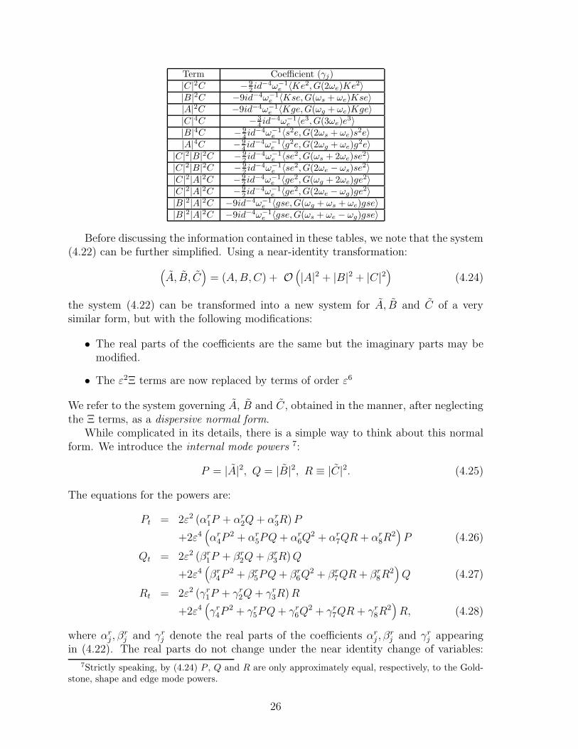
Before discussing the information contained in these tables, we note that the system(4.22) can be further simplified. Using a near-identity transformation:

(

A, B, C)

= (A,B,C) + O(

|A|2 + |B|2 + |C|2)

(4.24)

the system (4.22) can be transformed into a new system for A, B and C of a verysimilar form, but with the following modifications:

• The real parts of the coefficients are the same but the imaginary parts may bemodified.

• The ε2Ξ terms are now replaced by terms of order ε6

We refer to the system governing A, B and C, obtained in the manner, after neglectingthe Ξ terms, as a dispersive normal form.

While complicated in its details, there is a simple way to think about this normalform. We introduce the internal mode powers 7:

P = |A|2, Q = |B|2, R ≡ |C|2. (4.25)

The equations for the powers are:

Pt = 2ε2 (αr1P + αr

2Q+ αr3R)P

+2ε4(

αr4P

2 + αr5PQ+ αr

6Q2 + αr

7QR+ αr8R

2)

P (4.26)

Qt = 2ε2 (βr1P + βr

2Q+ βr3R)Q

+2ε4(

βr4P

2 + βr5PQ+ βr

6Q2 + βr

7QR+ βr8R

2)

Q (4.27)

Rt = 2ε2 (γr1P + γr

2Q+ γr3R)R

+2ε4(

γr4P

2 + γr5PQ+ γr

6Q2 + γr

7QR+ γr8R

2)

R, (4.28)

where αrj , β

rj and γr

j denote the real parts of the coefficients αrj , β

rj and γr

j appearingin (4.22). The real parts do not change under the near identity change of variables:

7Strictly speaking, by (4.24) P , Q and R are only approximately equal, respectively, to the Gold-stone, shape and edge mode powers.

26

A 7→ A, B 7→ B, C 7→ C, and are therefore given by the real parts of the coefficientsdisplayed in Table 1. In general, as the reader may note, a contribution to the abovementioned internal mode power equations of the form |A|2m1 |B|2m2 |C|2m3 comes from afrequency combination m1ωg+m2ωs+m3ωe landing in the band of continuous spectrumthrough a term

(M(K, g, s, e), G(m1ωg +m2ωs +m3ωe)M(K, g, s, e)) (4.29)

where M is the appropriate monomial combination of the relevant spatial parts.As the discreteness parameter, d, varies the spectrum of the kink (the continuous

spectrum and the number and location of the internal modes) changes. As indicatedin Figure 6, for different values of d various integer linear combinations of the internalmode frequencies, the simplest of which are those appearing as arguments of G(·) inTable 1, may lie in the continuous spectrum.

How does this influence the character of the normal form?Let ζ denote one such linear combination of frequencies. By (4.18):

G(ζ) = Pc B−1(B − ζ)−1 Pc, ζ /∈ σcont(B)

G(ζ) = Pc P.V. B−1(B − ζ)−1 Pc − iπ

ζPc δ(B − ζ) Pc, ζ ∈ σcont(B). (4.30)

Each of the coefficients of the system listed in Table 1 is a positive multiple of anexpression of the form −i〈f,G(ζ)f〉, where f is spatially localized. Therefore, if ζ doesnot lie in the continuous spectrum of B, the associated coefficient of the system for thepowers P,Q,R, αr = ℜα, βr = ℜβ or γr = ℜγ, will be zero. On the other hand, if ζdoes lie in the continuous spectrum of B, this coefficient will be of the form:

Γζ ≡ −πζ〈Pcf, δ(B − ζ) Pcf〉

= −πζ|FB[f ](ζ)|2 ,

where FB denotes the Fourier transform with respect to the continuous spectral part ofthe operator B. Generically, one has Γζ is strictly negative. Therefore, such resonancesare associated with nonlinear damping of energy in the internal modes. This does notcontradict the Hamiltonian character of the equations of motion. The A, B, C system iscoupled to the dispersive system governing η; damping of the discrete mode amplitudesimplies a transfer of energy from the discrete to continuum modes. The informationcontained in Figure 6 enables us to determine, for each d, which combinations ofharmonics appear in the phonon band. Then Tables 1A, 1B and 1C, together with(4.26-4.28) give us the precise form of the internal mode power equations, from whichwe can ascertain the detailed behavior of solutions in a neighborhood of the static kink.

In the Table 2 (below) we present the form of the internal mode power equationsfor different ranges of the parameter, d. There are numerous changes in the form ofthese equations as d varies, so for clarity, we indicate only the key transitions. Thesekey transitions occur across values of d where there is a topological change in the phaseportrait of the system governing the internal mode powers. Such changes are found

27

Arithmetic of φ4 kink frequencies

0.5 1 1.5 20

1

2

3

4

ω

d0.5 1 1.5 2

1

2

3

4

ω

d

0.8 1 1.2 1.4 1.6 1.8

1

2

3

4

ω

d0.5 1 1.5 2

1

2

3

4

ω

d

0.8 1 1.2 1.4 1.6 1.8

1

2

3

4

ω

d0.8 1 1.2 1.4 1.6 1.8

1

2

3

4

ω

d

Figure 6: Integer linear combinations of internal mode frequencies: In all 6 panels,the band is indicated by dash-dotted lines. Top left shows the goldstone frequency as afunction of d (solid) and its second (dashed) and third (dotted) harmonics for φ4. Thetop right panel follows the same sequence of symbols for the shape mode harmonicswhile the left panel of the second row does so for the edge mode. The right panel of thesecond row shows the combinations of ωg, ωs that can appear in the band. In particular:ωg +ωs :o, 2ωg +ωs :x, 2ωs +ωg : +, 2ωs −ωg : ∗. Similarly in the bottom left panel forthe g, e modes. In particular: ωg + ωe : o, 2ωg + ωe : x, 2ωe + ωg : +, 2ωi − ωg : ∗. Andin the case of bottom right panel s, e modes are shown but so are combinations of all 3frequencies. In particular: ωs+ωe : o, 2ωs+ωe : x, 2ωe+ωs : +, 2ωi−ωs : ∗, ωs+ωg+ωe :diamonds, ωs + ωe − ωg :down triangles.

28

due to a change in the nature of the set of equilibria, e.g. going from a system withone line of equilibria to one where there are two lines of equilibria, or due to a changein the number of internal modes (jump in the dimensionality of the phase portrait).The latter transition occurs at d = de, de ∼ 0.82, when a point eigenvalue emergesfrom the edge of the continuous spectrum and appears as a third internal mode, e, anedge mode, with corresponding frequency ωe.

Table 2: φ4 internal mode power equations

Regimes of d Resonances System FormI : d < 0.5398 2ωs − ωg, . . . Pt = 0, Qt = −ε4PQ2II : 0.5398 ≤ d < 0.6145 2ωg, ωg + ωs Pt = −ε2PP,Q,2ωg ∈ σcont 2ωs − ωg Qt = −ε2PQ1, ε2QIII : 0.6145 ≤ d < 0.6364 2ωg, 2ωs − ωg Pt = −ε2P 2,

Qt = −ε4PQ2IV : 0.6364 ≤ d < 0.6679 ωg + ωs Pt = −ε2PQ,2ωg /∈ σcont 2ωs − ωg Qt = −ε2PQ1, ε2QV : 0.6679 ≤ d < de 3ωg, 4ωg, 2ωs − ωg Pt = −ε4P 31, ε2P − ε2PQ1, ε2P,de ∼ 0.82 ωg + ωs, 2ωg + ωs Qt = −ε2PQ1, ε2P,QV I : de ≤ d < 0.9229 4ωg, 5ωg, 2ωs − ωg Pt = −ε2PQ1, ε2P, R1, ε2P, ε4P 3 + ...ωe appears ωg + ωs, 2ωg + ωs, 2ωe − ωs Qt = −ε2PQ1, ε2P,Q,R + ...

ωg + ωe, 2ωg + ωe, ωe + ωs − ωg Rt = ε2PR1, ε2P,Q − ε4QR2 + ...V II : 0.9229 ≤ d < d∗ nωg5≤n≤38, 2ωs Pt = −ε2n−2Pn + ...d∗ ∼ 1.2234 ωg + ωs, ωg + ωe, 2ωg + ωs, Qt = −ε2Q2 + ...2ωs ∈ σcont 2ωg + ωe, 2ωg + 2ωs, ωg + 2ωs, Rt = −ε2RQ,P+ ...

ωg + ωs + ωe, ωs + ωe, 2ωe − ωs

2ωe − ωg, ωe + ωs − ωg, 2ωs − ωg

V III : d∗ ≤ d nωg (5 ≤ n ≤ N), 2ωs, 2ωe Pt = −ε2n−2Pn + ...2ωe ∈ σcont Qt = −ε2Q2 + ...

Rt = −ε2R2 + ...

Remark on notation: We illustrate the notation of the table with the followingexample. Consider the regime V. This regime can be broken into three subregimesillustrated in the following table:

Table 3: internal mode power equations for subregime VSubregime of d Resonances System Forma) 0.6679 ≤ d < 0.743 3ωg, ωg + ωs Pt = −ε2C1PQ− ε4C2P

3,2ωs − ωg Qt = −ε2C3PQ− ε4C4PQ

2

b) 0.743 ≤ d < 0.7622 3ωg, 4ωg Pt = −ε2C1PQ− ε4C2P3 − ε6C5P

4,ωg + ωs, 2ωs − ωg Qt = −ε2C3PQ− ε4C4PQ

2

c) 0.7622 ≤ d < 0.7687 3ωg, ωg + ωs, 2ωs − ωg Pt = −ε2C1PQ− ε4C2P3 − ε4C6P

2Q− ε6C5P4

4ωg, 2ωg + ωs Qt = −ε2C3PQ− ε4C4PQ2 − ε4C7P

2Qc) 0.7687 ≤ d < de ωg + ωs, 2ωg + ωs Pt = −ε2C1PQ− ε4C6P

2Q− ε6C5P4

de ∼ 0.82 4ωg, 2ωs − ωg Qt = −ε2C3PQ− ε4C4PQ2 − ε4C7P

2Q

Although the details of the system form change between regimes, the topological char-acter of the phase portrait and therefore the qualitative nature of the solutions doesnot change; each phase portrait has P = 0 as a stable line of equilibria. For regime

29

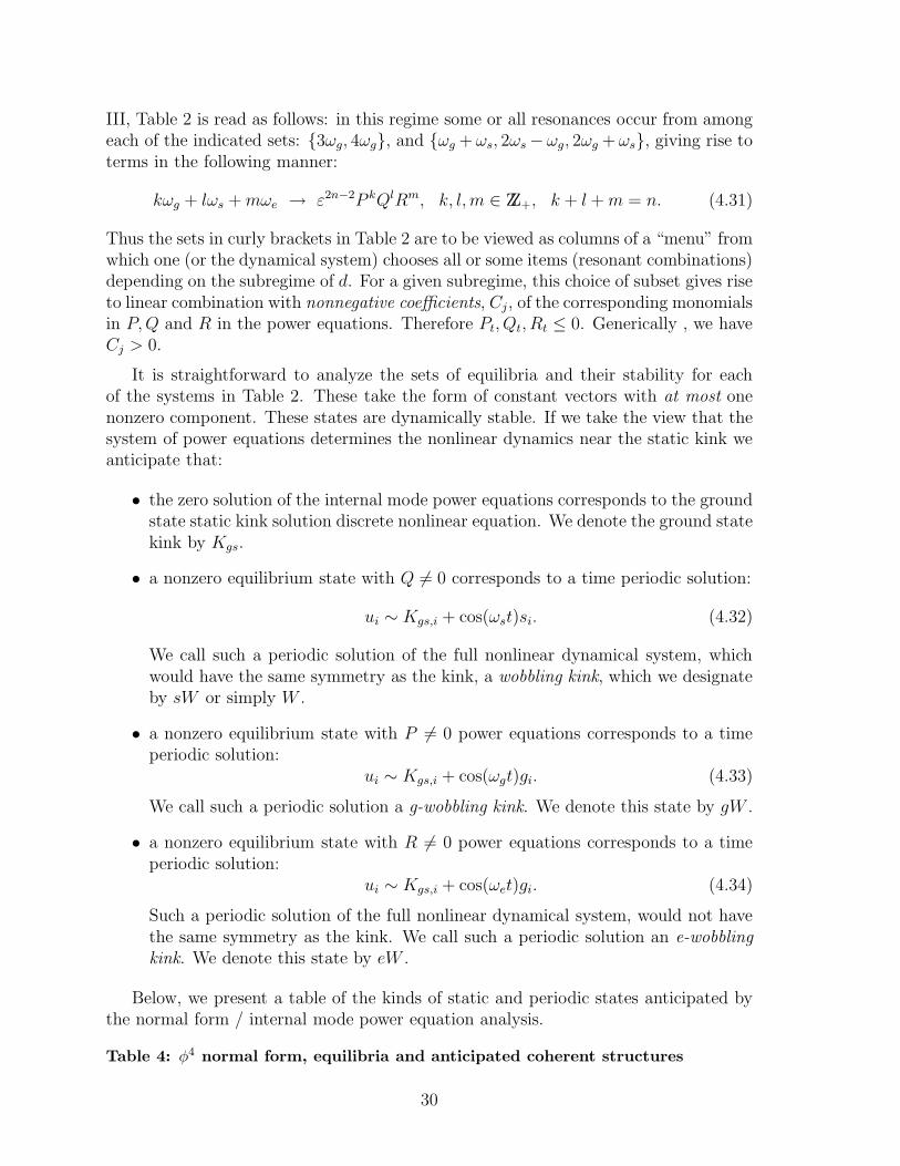
III, Table 2 is read as follows: in this regime some or all resonances occur from amongeach of the indicated sets: 3ωg, 4ωg, and ωg + ωs, 2ωs − ωg, 2ωg +ωs, giving rise toterms in the following manner:

kωg + lωs +mωe → ε2n−2P kQlRm, k, l,m ∈ ZZ+, k + l +m = n. (4.31)

Thus the sets in curly brackets in Table 2 are to be viewed as columns of a “menu” fromwhich one (or the dynamical system) chooses all or some items (resonant combinations)depending on the subregime of d. For a given subregime, this choice of subset gives riseto linear combination with nonnegative coefficients, Cj, of the corresponding monomialsin P,Q and R in the power equations. Therefore Pt, Qt, Rt ≤ 0. Generically , we haveCj > 0.

It is straightforward to analyze the sets of equilibria and their stability for eachof the systems in Table 2. These take the form of constant vectors with at most onenonzero component. These states are dynamically stable. If we take the view that thesystem of power equations determines the nonlinear dynamics near the static kink weanticipate that:

• the zero solution of the internal mode power equations corresponds to the groundstate static kink solution discrete nonlinear equation. We denote the ground statekink by Kgs.

• a nonzero equilibrium state with Q 6= 0 corresponds to a time periodic solution:

ui ∼ Kgs,i + cos(ωst)si. (4.32)

We call such a periodic solution of the full nonlinear dynamical system, whichwould have the same symmetry as the kink, a wobbling kink, which we designateby sW or simply W .

• a nonzero equilibrium state with P 6= 0 power equations corresponds to a timeperiodic solution:

ui ∼ Kgs,i + cos(ωgt)gi. (4.33)

We call such a periodic solution a g-wobbling kink. We denote this state by gW .

• a nonzero equilibrium state with R 6= 0 power equations corresponds to a timeperiodic solution:

ui ∼ Kgs,i + cos(ωet)gi. (4.34)

Such a periodic solution of the full nonlinear dynamical system, would not havethe same symmetry as the kink. We call such a periodic solution an e-wobblingkink. We denote this state by eW .

Below, we present a table of the kinds of static and periodic states anticipated bythe normal form / internal mode power equation analysis.

Table 4: φ4 normal form, equilibria and anticipated coherent structures

30

Regime of d Equilibria Coherent structuresI: d < 0.5398 (P, 0) : P ≥ 0 Kgs, W, gW

(0, Q) : Q ≥ 0II-III: 0.5398 ≤ d < 0.6364 (0, Q) : Q ≥ 0 Kgs, WIV: 0.6364 ≤ d < 0.6679 (0, Q) : Q ≥ 0 Kgs, W, gW

(P, 0) : P ≥ 0V: 0.6679 ≤ d < de (0, Q) : Q ≥ 0 Kgs, Wde ∼ 0.82VI: de ≤ d < 0.9229 (0, Q, 0) : Q ≥ 0 Kgs, W, eW

(0, 0, R) : R ≥ 0VII: 0.9229 ≤ d < 1.2234 (0, 0, R) : R ≥ 0 Kgs, eWd∗ ∼ 1.2234VIII: d∗ ≤ d (0, 0, 0) Kgs

4.2 The normal form for discrete sine-Gordon

The procedure for deriving the normal form for the internal mode amplitudes and theinternal mode power equations presented in sections 3 and 4.1 can be applied to thediscrete sine-Gordon equation as well. The implementation is actually simpler becausefor discrete SG there are only two internal modes: g and e; see section 2. Therefore,the decomposition of the solution is:

ui(t) = Ki + εa(t)gi + εb(t)ei + ε2ηi(t), (4.35)

where

〈g, η(t)〉 = 〈e, η(t)〉 = 0

Pcη ≡ η − 〈g, η(t)〉g − 〈e, η(t)〉e = η(t)

As in the previous subsection the amplitude equations for the slowly varying mod-ulation functions can be obtained:

At = ε2(

α1|A|2 + α2|B|2)

A+ ε4α3|B|4A+ ΞA(A,B, t)

Bt = ε2(

β1|A|2 + β2|B|2)

A+ ε4β3|B|4A+ ΞB(A,B, t) (4.36)

The coefficients αj , βj can be evaluated along the lines detailed in the pervious sectionand are tabulated below.

Table 5A : Principal SG g-mode coefficients

|A|2A − 18d

−4ωg−1〈sinKg2, G(2ωg) sinKg2〉

|A|4A − 34(3!)2 d

−4ω−1g 〈cosKg3, G(3ωg) cosKg3〉

|B|2A − 12d

−4ω−1g 〈sinKge,G(ωg + ωe) sinKge〉

|B|4A − 94(3!)2 d

−4ωg−1〈cosKge2, G(ωg + 2ωe) cosKge2〉

|A|2|B|2A − 184(3!)2 d

−4ω−1g 〈cosKg2e,G(2ωg + ωe) cosKg2e >

31

Table 5B : Discrete SG e-mode coefficients

|B|2B − 18d

−4ω−1e 〈sinKe2, G(ωe) sinKe2〉

|B|4B − 34(3!)2 d

−4ω−1e 〈cosKe3, G(3ωe) cosKe3〉

|A|2B − 12d

−4ω−1e 〈sinKge,G(ωg + ωe) sinKge〉

|A|4B − 94(3!)2 d

−4ω−1e 〈cosKeg2, G(ωe + 2ωg) cosKeg2〉

|A|2|B|2B − 184(3!)2 d

−4ω−1e 〈cosKe2g,G(ωg + 2ωe) cosKe2g〉

|A|2|B|2B − 184(3!)2 d

−4ω−1e 〈cosKe2g,G(2ωe − ωg) cosKe2g〉

As with discrete φ4, the details of the internal mode power equations change asd varies due to the different types of resonances with the continuous spectrum whichmay occur. For discrete SG there are essentially only two regimes, and one value of theparameter d across which there is a topological change in the phase portraits. Sincethe detailed picture is simpler we tabulate it in greater detail.

Figure 7 displays the variation of the internal mode frequencies (ωg, ωe), certainmultiples of them and certain other integer linear combinations of them. As withdiscrete φ4, transitions in the structure of the normal form occur across values of d forwhich there is a change in the set of integer linear combinations which lie in the bandof continuous spectrum. The precise normal form and power equations can be workedout using the coefficient Table 5 and the expression for G(ζ), (4.30). Notice that onlythe leading order terms are given in these internal mode power equations.

Table 6: SG internal mode power equations

Regime of d Resonances System FormI: d < de ∼ 0.515 None Pt = 0II: de ≤ d < .565 2ωe − ωg, 3ωg − ωe Pt = −ε6P 3Q, Qt = −ε4PQ2III: 0.565 ≤ d < 0.65 2ωg, 2ωe − ωg Pt = −ε2P 2, Qt = −ε4PQ20.65 ≤ d < 0.7 2ωg, ωg + ωe Pt = −ε2PP,Q,

Qt = −ε2PQ1, ε2Q0.7 ≤ d < 0.76 2ωg, 3ωg, ωg + ωe, Pt = −ε2PP,Q, ε4P 2,

2ωe − ωg Qt = −ε2PQ1, ε2Q0.76 ≤ d < 0.785 3ωg, ωg + ωe, Pt = −ε2PQ − ε2P 2,

2ωe − ωg Qt = −ε2PQ1, ε2Q0.785 ≤ d < 0.8 3ωg, 4ωg Pt = −ε2PQ, ε2P 2, ε6P 4,

ωg + ωe, 2ωe − ωg Qt = −ε2PQ1, ε2PQ0.8 ≤ d < 0.847 3ωg, 4ωg, 2ωe − ωg Pt = −ε2PQ, ε2P 2, ε2PQ, ε4P 3,

ωg + ωe, 2ωg + ωe Qt = −ε2PQ1, ε2Q, ε2P0.847 ≤ d < d∗ 3ωg, 4ωg, 5ωg, 2ωe − ωg Pt = −ε2PQ, ε2P 2, ε4P 3, ε2PQ, ε6P 4,d∗ ∼ 0.86 ωg + ωe, 2ωg + ωe Qt = −ε2PQ1, ε2Q, ε2PIV: d∗ ≤ d < 0.9 3ωg, 4ωg, 5ωg, 2ωe Pt = −ε2PQ, ε2P 2, ε4P 3, ε2PQ,

ωg + ωe, 2ωg + ωe, 2ωe − ωg Qt = −ε2QP,Q, ε2PQ, ε2P 20.9 ≤ d < 0.99 4ωg, 5ωg, 2ωe Pt = −ε2PQ, ε4P 3, ε2PQ, ε4P 4,

ωg + ωe, 2ωg + ωe, 2ωe − ωg Qt = −ε2QP,Q, ε2PQ, ε2P 20.99 ≤ d < 1.003 5ωg, 2ωe, 2ωe − ωg Pt = −ε2PQ, ε2PQ, ε6P 4,

ωg + ωe, 2ωg + ωe Qt = −ε2QQ, ε2PQ, ε2P 21.003 ≤ d nωg (n ≥ 5), 2ωe, ωg + ωe Pt = −ε2PQ, ε2PQ, ε2n−2Pn−1, ε2Q2, ...,

2ωg + ωe, ωg + 2ωe Qt = −ε2QP,Q, ε4P 2, ε4PQ, ...

The inferred coherent structures are displayed in the following table.

Table 7: SG normal form, equilibria and anticipated coherent structures

32

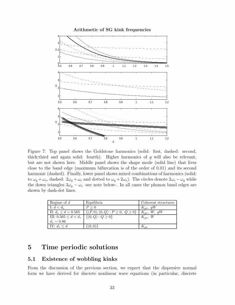
Arithmetic of SG kink frequencies

0.5 0.6 0.7 0.8 0.9 1 1.1 1.2 1.3 1.4 1.50

1

2

3

4

ω

0.5 0.6 0.7 0.8 0.9 1 1.1 1.2

1

2

3

4

ω

0.5 0.6 0.7 0.8 0.9 1 1.1 1.2

1

2

3

4

ω

d

Figure 7: Top panel shows the Goldstone harmonics (solid: first, dashed: second,thick:third and again solid: fourth). Higher harmonics of g will also be relevant,but are not shown here. Middle panel shows the shape mode (solid line) that livesclose to the band edge (maximum bifurcation is of the order of 0.01) and its secondharmonic (dashed). Finally, lower panel shows mixed combinations of harmonics (solid:to ωg +ωs, dashed: 2ωg +ωe and dotted to ωg +2ωe). The circles denote 2ωe−ωg whilethe down triangles 3ωg − ωe -see note below-. In all cases the phonon band edges areshown by dash-dot lines.

Regime of d Equilibria Coherent structuresI: d < de P ≥ 0 Kgs, gWII: de ≤ d < 0.565 (P, 0), (0, Q) : P ≥ 0, Q ≥ 0 Kgs, W, gWIII: 0.565 ≤ d < d∗ (0, Q) : Q ≥ 0 Kgs, Wd∗ ∼ 0.86IV: d∗ ≤ d (0, 0) Kgs

5 Time periodic solutions

5.1 Existence of wobbling kinks

From the discussion of the previous section, we expect that the dispersive normalform we have derived for discrete nonlinear wave equations (in particular, discrete

33

SG and φ4) models the dynamics in a neighborhood of the static kink solution. Thisnormal form captures the effects of nonlinear resonant interactions of the internal andcontinuum mode fluctuations about the kink. Tables 4 and 7 indicate for discrete φ4

discrete SG the anticipated existence of periodic solutions which bifurcate from thestatic kink solution. In this section we prove, under suitable nonresonance hypotheses,the existence of such time periodic solutions.

In tables 3 and 5 we see that these normal forms fall into two categories (i) those forwhich the origin is the only equilibrium (d sufficiently large, d > d∗) (ii) d is such thatthe normal form admits one or two lines of equilibria. In case (i) we see that the zerosolution is asymptotically stable. By (3.5) and (4.35) this suggests that the groundstate kink is a stable attractor. At d∗ there is a bifurcation in the phase portrait; ford < d∗, zero is no longer an isolated equilibrium. Rather, the normal form now has aline of stable equilibria passing through the origin. This then suggests an approximatesolution of the nonlinear wave equation of the form:

uj ∼ Kj + εBeq cos(Ωt)ξΩ,j , j ∈ ZZ (5.1)

where ξΩ denotes an internal mode Ω its corresponding frequency; BχΩ = ΩχΩ andε is small. If such a family of periodic solutions exists, we say this family bifurcatesfrom the kink solution in the direction of the internal mode, ξΩ. Such directions forbifurcation are available for d < d∗.For d < d∗ are there bifurcating time periodic solutions?

In view of the analysis of the regime d > d∗, one must be cautious about reaching aconclusion about the large time behavior on the basis of the above approximation. Infact we learn from the regime d > d∗ that radiation damping, due to resonant couplingof oscillations to the continuum, may lead to the slow decay of a solution which appearsto be time-periodic on shorter time scales.

On the other hand, given the approximate periodic solution (5.1) it is certainlynatural to attempt a perturbative (in ǫ) construction of a true time-periodic solution.The approach we use is the Poincare continuation, which is standard in the persis-tence theory of periodic solutions of systems of ordinary differential equations [14]. Asin typical perturbation expansions, one expects a hierarchy of linear inhomogeneousproblems governing contributions to the expansion at various orders in ǫ. Solvabilityat each order requires that one can arrange for the solution to each inhomogeneousproblem to be time periodic of some common period. That this can be achieved inthe problem at hand follows from the following nonresonance condition, verified in ournumerical investigation of the spectrum of the kink:(NR) Assume that no integer multiple of the internal mode frequency Ω lies in thecontinuous spectrum of B.

A precise statement of the result is as follows:

Theorem 5.1 Let K = Kii∈ZZ denote a ground state kink. Assume that the linearoperator, B, acting on the space l2(ZZ), has a simple eigenvalue, Ω, with correspondingeigenfunction, ξΩ satisfying BξΩ = ΩξΩ. Also assume the nonresonance condition(NR). Then, in a neighborhood of K, there is a curve of solutions ǫ 7→ y(t; ǫ) passingthrough the ground state kink with the following properties:

34

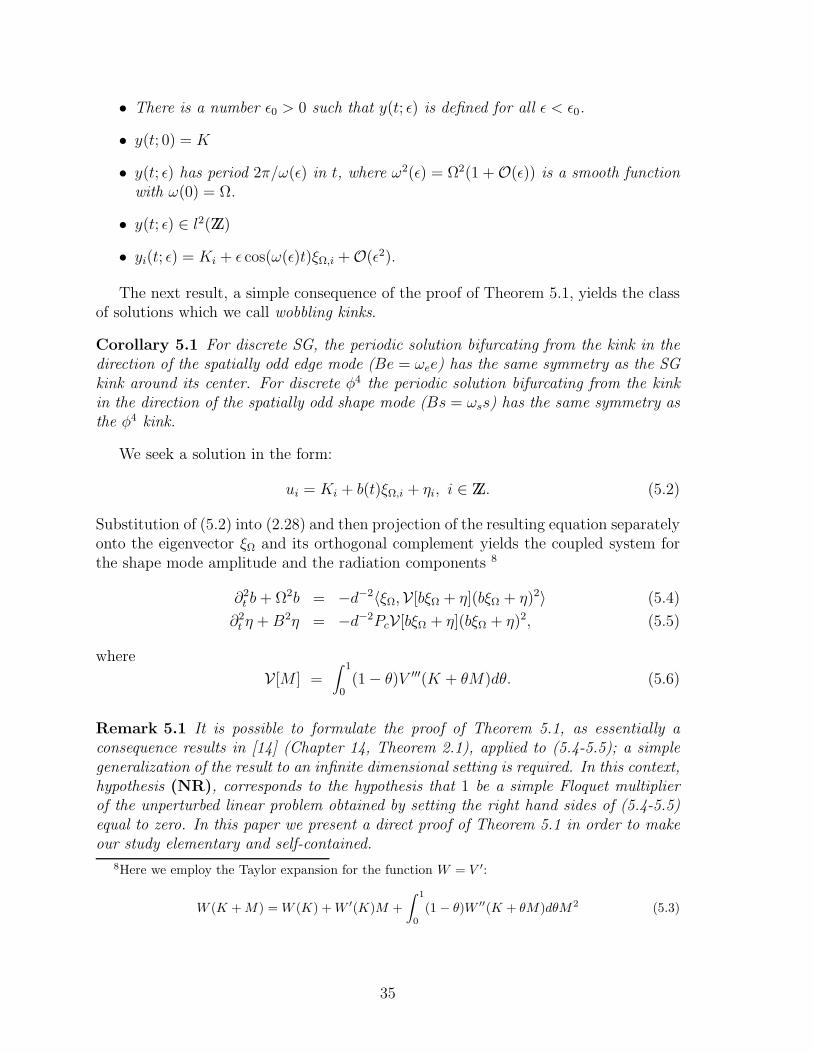
• There is a number ǫ0 > 0 such that y(t; ǫ) is defined for all ǫ < ǫ0.

• y(t; 0) = K

• y(t; ǫ) has period 2π/ω(ǫ) in t, where ω2(ǫ) = Ω2(1 + O(ǫ)) is a smooth functionwith ω(0) = Ω.

• y(t; ǫ) ∈ l2(ZZ)

• yi(t; ǫ) = Ki + ǫ cos(ω(ǫ)t)ξΩ,i + O(ǫ2).

The next result, a simple consequence of the proof of Theorem 5.1, yields the classof solutions which we call wobbling kinks.

Corollary 5.1 For discrete SG, the periodic solution bifurcating from the kink in thedirection of the spatially odd edge mode (Be = ωee) has the same symmetry as the SGkink around its center. For discrete φ4 the periodic solution bifurcating from the kinkin the direction of the spatially odd shape mode (Bs = ωss) has the same symmetry asthe φ4 kink.

We seek a solution in the form:

ui = Ki + b(t)ξΩ,i + ηi, i ∈ ZZ. (5.2)

Substitution of (5.2) into (2.28) and then projection of the resulting equation separatelyonto the eigenvector ξΩ and its orthogonal complement yields the coupled system forthe shape mode amplitude and the radiation components 8

∂2t b+ Ω2b = −d−2〈ξΩ,V[bξΩ + η](bξΩ + η)2〉 (5.4)

∂2t η +B2η = −d−2PcV[bξΩ + η](bξΩ + η)2, (5.5)

where

V[M ] =∫ 1

0(1 − θ)V ′′′(K + θM)dθ. (5.6)

Remark 5.1 It is possible to formulate the proof of Theorem 5.1, as essentially aconsequence results in [14] (Chapter 14, Theorem 2.1), applied to (5.4-5.5); a simplegeneralization of the result to an infinite dimensional setting is required. In this context,hypothesis (NR), corresponds to the hypothesis that 1 be a simple Floquet multiplierof the unperturbed linear problem obtained by setting the right hand sides of (5.4-5.5)equal to zero. In this paper we present a direct proof of Theorem 5.1 in order to makeour study elementary and self-contained.

8Here we employ the Taylor expansion for the function W = V ′:

W (K +M) = W (K) +W ′(K)M +

∫ 1

0

(1 − θ)W ′′(K + θM)dθM2 (5.3)

35

We shall be considering small perturbations of the static kink, and therefore introducerescaled internal mode and radiation components:

b = ǫb1, η = ǫη1, (5.7)

where ǫ is a small parameter. Since the nonlinear wave equations considered are au-tonomous, we can’t a priori specify the period, we leave the period unspecified atthis stage and introduce a new time variable, τ , with respect to which the sought-forperiodic solution is 2π periodic. Let

t = ω(ǫ)−1τ, ω(0) = Ω, (5.8)

andb1(t) = β1(τ), β1(τ + 2π) = β1(τ). (5.9)

Then, equations (5.4-5.5) become:

(

ω2(ǫ)∂2τ + Ω2

)

β1(τ) = ǫFβ(β1, η1; ǫ)

Fβ(β1, η1; ǫ) ≡ −d−2〈ξΩ,V[ǫ(β1ξΩ + η1)](β1ξΩ + η1)2〉

(5.10)(

ω2(ǫ)∂2τ + B2

)

η1(τ, i) = ǫFη(β1, η1; ǫ)

Fη(β1, η1; ǫ) ≡ −d−2PcV[ǫ(β1ξΩ + η1)](β1ξΩ + η1)2 (5.11)

Let

ω2(ǫ) = Ω2(1 + ǫσ(ǫ)), (5.12)

where σ(ǫ) is to be determined. Then (5.10) becomes

(

∂2τ + 1

)

β1 =ǫ

1 + ǫσ(ǫ)[σ(ǫ)β1 + Ω−2Fβ(β1, η1; ǫ)]. (5.13)

We extract the leading order behavior by defining:

β1 = cos(τ) + ǫβ2, (5.14)

where

(∂τ2 + 1)β2 =

1

1 + ǫσ(ǫ)[σ(ǫ) cos(τ) + ǫσ(ǫ)β2 + Ω−2Fβ (cos(τ) + ǫβ2, η1; ǫ) (5.15)

By the Fredholm alternative, equation (5.15) has an even 2π periodic solution if andonly if

Pcos(σ cos(τ) + ǫσβ2 + Ω−2Fβ) = 0. (5.16)

Here,

Pcos g = π−1∫ 2π

0cos(µ)g(µ)dµ (5.17)

36

is the projection onto the even 2π periodic null space of ∂2τ + 1. The orthogonality

constraint (5.16) can be rewritten as

πσ + ǫσ∫ 2π

0cos(τ)β2(τ)dτ + ω−2

s

∫ 2π

0cos(τ)Fβ (cos(τ) + ǫβ2(τ), η1; ǫ) dτ = 0 (5.18)

We have therefore reformulated the problem of finding a periodic solution of the discretenonlinear wave equation, or equivalently (5.4-5.5), as the problem of finding 2π periodicsolutions in τ , (β2(ǫ), η1(ǫ), σ(ǫ)), of the system:

F (β2, η1, σ; ǫ) = 0, (5.19)

where F = (F1, F2, F3)t, is defined by:

F1(β2, η1, σ; ǫ) = (∂2τ + 1)β2

−(1 + ǫσ)−1[

σ cos(τ) + ǫσβ2 + Ω−2Fβ (cos(τ) + ǫβ2, η1; ǫ)]

(5.20)

F2(β2, η1, σ; ǫ) =(

Ω2(1 + ǫσ)∂2τ +B2

)

η1(τ, i) − ǫFη(cos(τ) + ǫβ2, η1; ǫ)

(5.21)

F3(β2, η1, σ; ǫ) = −(1 + ǫσ)−1[

πσ + ǫσ∫ 2π

0cos(τ)β2dτ

+ Ω−2∫ 2π

0cos(τ)Fβ(cos(τ) + ǫβ2(τ), η1; ǫ)dτ

]

(5.22)

We view F as a mapping of (ζ, ǫ) ∈ X 7→ F (ζ, ǫ) ∈ Y . Here, X and Y are definedby:

X : ζ = (β, η, σ) such that

β = β(τ) ∈ H2, even, and 2π periodic

η = η(τ, ·) ∈ H2 even, and 2π periodic in τ

with values in the space of l2(ZZ) functions and σ ∈ IR

Y : ζ = (β, η, ρ) such that

β = β(τ) ∈ L2, even, and 2π periodic

η = η(τ, ·) ∈ L2 even, and 2π periodic in τ

with values in the space of l2(ZZ) functions and

ρ =∫ 2π

0β(µ) cos(µ)dµ.

We find a particular ζ (0) ∈ X for which F (ζ (0); 0) = 0, and then seek to constructcurve of solutions ǫ 7→ ζ(ǫ), ζ(0) = ζ (0), for all sufficiently small ǫ using the implicitfunction theorem [44]. To find ζ (0) we set ǫ = 0 and consider the system F (ζ ; 0) = 0.

Taking η1 = η(0)1 ≡ 0 and σ = σ(0) = 0, we find that β

(0)2 satisfies the equation:

(

∂2τ + 1

)

β(0)2 = −d−2Ω−2〈ξΩ,V[0]ξ2

Ω〉 cos2(τ), (5.23)

which has the solution

β(0)2 = −1

2d−2Ω−2〈ξΩ V[0]ξ2

Ω〉(

1 − 1

3cos(2τ)

)

. (5.24)

37

Thus, ζ (0) = (β(0)2 , 0, 0) ∈ X satisfies F (ζ (0); 0) = 0. We shall now use the implicit

function theorem to continue this solution to show that this solution deforms uniquelyto nearby solutions for ǫ sufficiently small and nonzero.

To apply the implicit function theorem, it suffices to check that dζF (ζ (0); 0) isbounded and invertible. A computation yields:

dζF (ζ (0); 0) =

∂τ2 + 1 0 − cos(τ)

0 Ω2∂2τ +B2 0

0 0 −π

(5.25)

Invertibility of dζF (ζ (0); 0) can be shown by solving the system of inhomogeneous equa-tions:

dζF · δζ = R (5.26)

where

δζ =

δβ2

δη1

δσ

, R =

BEΣ

and Σ ≡∫ 2π

0cos(τ)B(τ)dτ. (5.27)

The third equation implies:δσ = −π−1Σ. (5.28)

Substitution into the first equation yields the equation an δβ2:

(

∂2τ + 1

)

δβ2 = B − π−1∫ 2π

0cos(µ)B(µ)dµ cos(τ), (5.29)

which has an even 2π periodic solution. Finally the second equation can be rewrittenas

(Ω2∂τ2 +B2)δη1 = E =

∞∑

n=0

cos(nτ)en (5.30)

which can then be solved by Fourier series: δη1 =∑∞

n=0gn cos(nτ). We obtain

gn = (B2 − n2Ω2)−1en. (5.31)

By (NR), en is well-defined for each n. Note also that there is a strictly positiveminimum distance of the set nΩ to σ(B). Therefore,

‖gn‖l2(ZZ) ≤ dist(

(nΩ)2, σ(B2))−1 ‖En‖l2(ZZ), (5.32)

from which we have boundedness of the inverse: (Ω2∂2τ +B2)

−1:

‖δη1‖H2(IR;l2(ZZ)) ≤ C‖E‖L2(IR;l2(ZZ)). (5.33)

By the implicit function theorem there is a number ǫ0 > 0 such that for ǫ < ǫ0 thenonlinear wave equation has a unique periodic solution of the form:

yi(τ, ǫ) = Ki + (ǫ cos(τ) + ǫ2β2(τ))ξΩ,i + ǫη1(i, τ ; ǫ) (5.34)

38

with τ = ω(ǫ)t, ω2(ǫ) = Ω2(1 + ǫσ(ǫ)) and β2, η1 2π periodic functions of τ . Note thatη1 = O(ǫ), by the equation F2 = 0, so that we have (5.1). This completes the proof ofTheorem 5.1.

To prove Corollary 5.1, we note that by hypothesis, the direction of bifurcation isspatially odd. It is simple to check that the entire proof goes through with the spaces Xand Y additionally constrained to consist of functions η, such that η(·,−i) = −η(·, i).

5.2 Do quasiperiodic solutions bifurcate from the kink?

If we attempt using the above method of proof to construct quasiperiodic solutions, wedo not succeed. To be specific, suppose we seek to construct a quasiperiodic solutionwhich is generated by the two internal modes ξΩ1 and ξΩ1. Formally, we seek ui(t) =u(i, t) in the form:

u(i, t) = K(i) + ǫ2

∑

j=1

αjξΩj(i) cos(Ωjt) + ǫη1(i, t) (5.35)

Substitution into the nonlinear wave equation gives

(

∂2t +B2

)

η1 = −d−2ǫ V

ǫ2

∑

j=1

αjξΩjcos(Ωjt) + ǫη1

×

2∑

j=1

αjξΩjcos(Ωjt) + η1

2

.

Expansion of η1(i, t) as a power series in ǫ,

η1(i, t) =∞∑

j=0

ǫjη(j)1 (i, t), (5.36)

leads to a hierarchy of inhomogeneous equations of the form:(

∂2t +B2

)

η(j)1 = S(j)(t) (5.37)

where as j increases S(j)(t) contains a finite sum of terms with time-frequencies of the

form n1Ω1 +n2Ω2 with |n1| ≤ N(j)1 , |n2| ≤ N

(j)2 and N

(j)1 , N

(j)2 increasing with j. Thus

it is natural to solve for each η(j)1 as a truncated multiple Fourier series:

η(j)1 =

∑

|n1|≤N(j)1 ,n2≤N

(j)2

ei(n1Ω1+n2Ω2)tg(j)n1,n2

. (5.38)

Substitution into (5.37) yields:

(

B2 − (n1Ω1 + n2Ω2)2)

g(j)n1,n2

= G(j)n1,n2

, (5.39)

39

where G(j)n1,n2

denotes the term in S(j)(t) which is proportional to exp(i(n1Ω1 +n2Ω2)t).In order to ensure the general solvability of (5.39) we need that for any n1, n2 ∈ ZZ,

n1Ω1 + n2Ω2 /∈ ±σ(B). (5.40)

Although it is nongeneric for a frequency in the point spectrum (internal mode fre-quency) to be hit, since the continuous spectrum (phonon band) is an interval, gener-ically one has n1Ω1 + n2Ω2 ∈ σcont(B), for infinitely many choices of n1, n2. For suchchoices the operator on the right hand side of (5.39) is not invertible and these resonantfrequencies are an obstruction to solvability. A closer look at the set of resonances andtheir contribution on the dispersive normal form, would give insight into the lifetimeof such eventually decaying quasiperiodic oscillations.

6 Large time behavior in a neighborhood of Kgs

In this section we combine the normal form analysis of section 4, and the existencetheory for time periodic solutions of section 5 with numerical simulation to get a moredetailed picture of the large time behavior of discrete φ4 and SG in a neighborhoodof the ground state kink. We shall make repeated use of Tables 2 and 4 for φ4 andof Tables 6 and 7 for SG in which the normal form / power equations and coherentstructures are tabulated. In interpreting these tables we recall that ε, introduced in(3.5), measures the size of the component of the perturbation about the kink in theinternal mode subspace. In full simulations of the evolution equation ε is typically oforder 10−1, and therefore some of the decay phenomena anticipated by our analysis,occur on very large time scales (e.g. τ ∼ ε−2, ε−4 or longer) and are difficult to simulateaccurately.

In each of the various d− ranges we proceed as follows: we mention the relevantcoherent structures (the high energy kink is omitted because it is unstable). These areall anticipated by the normal form analysis and their existence is established rigorouslyin section 5. We then discuss the numerically observed large time behavior for differentclasses of initial conditions. This gives evidence of the attracting nature of the periodicsolutions constructed in section 5 in various regimes of the discreteness parameter d.

As mentioned in the introduction, this is related to the final stages of the evolutionof a propagating kink, pinned to a particular lattice site, and its damped oscillation toan asymptotic state within the Peierls-Nabarro potential.

6.1 Discrete φ4

Regimes II, III and V: The coherent structures of interest are: Kgs and W . Nu-merical simulations show that the wobbling kink, W , is a local attractor.Regimes I,IV: The coherent structures of interest are: Kgs , W and gW .

Experiment 1 (data given by Kgs plus a small multiple of the Goldstone (even)g-mode): solution appears to approach gW .

Experiment 2 (data given by Kgs plus a small multiple of the shape (odd) s-mode):solution appears to approach W .

40

0 20 40 60 80 100

135140145150155160165

−0.05

0

0.05

ti

ui−

ki

500 600 700 800 900 1000 1100 1200 1300 1400 1500

−0.1

−0.05

0

0.05

0.1

0.15

<u

−K

|s>

t

Figure 8: Simulation of discrete φ4 with d = 0.8 in Regime IV. Upper panel: u(t)−Kgs

is seen to be approximately equal to the (spatially odd) shape mode. Lower panel:Projection of u(t) −Kgs onto the shape mode, s; principal frequency of oscillation isapproximately ωs

41

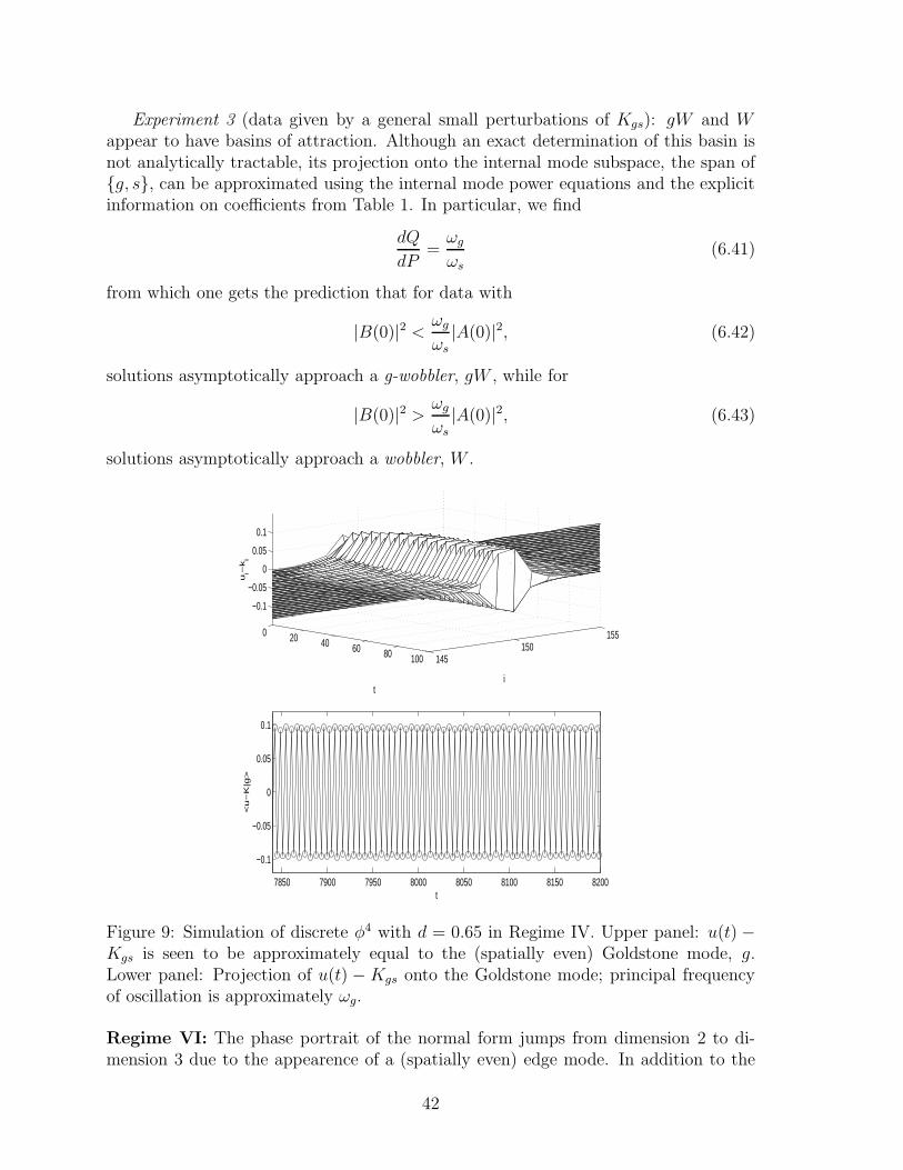
Experiment 3 (data given by a general small perturbations of Kgs): gW and Wappear to have basins of attraction. Although an exact determination of this basin isnot analytically tractable, its projection onto the internal mode subspace, the span ofg, s, can be approximated using the internal mode power equations and the explicitinformation on coefficients from Table 1. In particular, we find

dQ

dP=ωg

ωs

(6.41)

from which one gets the prediction that for data with

|B(0)|2 < ωg

ωs

|A(0)|2, (6.42)

solutions asymptotically approach a g-wobbler, gW , while for

|B(0)|2 > ωg

ωs

|A(0)|2, (6.43)

solutions asymptotically approach a wobbler, W .

0 20 40 60 80 100 145150

155

−0.1

−0.05

0

0.05

0.1

it

ui−

ki

7850 7900 7950 8000 8050 8100 8150 8200

−0.1

−0.05

0

0.05

0.1

<u

−K

|g>

t

Figure 9: Simulation of discrete φ4 with d = 0.65 in Regime IV. Upper panel: u(t) −Kgs is seen to be approximately equal to the (spatially even) Goldstone mode, g.Lower panel: Projection of u(t) − Kgs onto the Goldstone mode; principal frequencyof oscillation is approximately ωg.

Regime VI: The phase portrait of the normal form jumps from dimension 2 to di-mension 3 due to the appearence of a (spatially even) edge mode. In addition to the

42

ground state kink, Kgs, there are time-periodic (wobbling solutions) W and eW . Nu-merical simulations indicate the presence of very long lived quasiperiodic oscillationsabout the kink. These appear to be oscillations of the form represented in the first twoterms of (5.35). Strong evidence of the eventual decay of such oscillations can be seenas follows:

• In section 5.2 we have shown that an attempt to construct quasiperiodic solutionsbreaks down due to a high order resonance, i.e. n1ωs + n2ωe ∈ σcont(B), where|n1| + |n2| is large. In this particular case, we have −ωs + 2ωe ∈ σcont(B); seeTable 2.

• Such resonances correspond to obstructions in the power equations to equilibriumsolutions of the form: (0, Q,R) with both Q and R nonzero. The obstructingterm is the term −ε4QR2 in the R equation.

• Linearization of the power equations about any equilibrium point (0, Qeq, 0) or(0, 0, Req) shows that each line of equilibria is asymptotically stable, correspond-ing to the conclusion that quasiperiodic oscillations will damp with a resultingasymptotically periodic state, W or eW , depending on initial conditions. Thetime scale of decay of these oscillations, τ , is set by the order in ε of the obstruct-ing terms, e.g. τ ∼ ε−4.

Regime VII: The coherent structures of interest are: Kgs and eW .Experiment 1: For data which is an odd perturbation of Kgs. Kgs is the attractor.Experiment 2: For general data, eW appears to be a local attractor.Regime VIII: The coherent structure of interest is Kgs.Experiment 1 (data given by Kgs plus an small perturbation in the direction of the

(odd) shape mode): approach to Kgs at a rate O(t−12 ).

Experiment 2 (data given by Kgs plus an small perturbation in the direction of the

(even) edge mode): approach to Kgs at a rate O(t−12 ).

Experiment 3 (data given by Kgs plus an small perturbation in the direction of the(even) Goldstone mode): perturbation from Kgs appears to decay but at a differentrate and on much longer time scales than in Experiments 1 and 2.

6.2 Discrete sine-Gordon

Following the model of the previous subsection, we indicate relevant coherent structuresand briefly discuss the dynamics in a neighborhood of the ground state kink for thediscrete sine-Gordon equation.Regime I: The coherent structures of interest are: Kgs and gW . For general data,gW appears to be a local attractor.Regime II: The coherent structures of interest are: Kgs, W and gW . The dynamicalbehavior is as, for example, in regime IV for the φ4 model.Regime III: The coherent structures of interest areKgs andW . Numerical simulationsshow that W is a local attractor.

43

0

50

100

100110120130140150160170180190200

−0.04

−0.02

0

0.02

0.04

ti

ui−

ki

7000 7200 7400 7600 7800 8000 8200 8400 8600 8800 9000−0.2

−0.1

0

0.1

0.2

<u

−K

|e>

t

Figure 10: Simulation of discrete φ4 with d = 1.1 in Regime IV. Upper panel: u(t) −Kgs is seen to be approximately equal to the (spatially even) edge mode, e. Lowerpanel: Projection of u(t) −Kgs onto the edge mode; principal frequency of oscillationis approximately ωe.

44

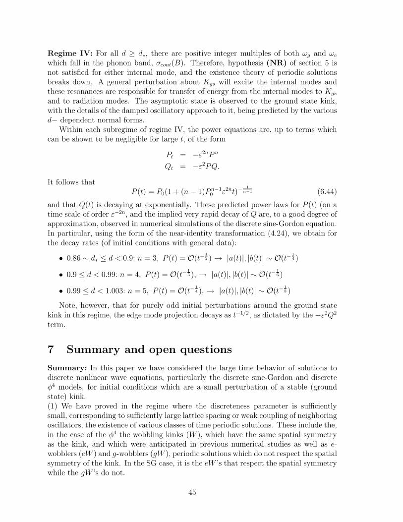
Regime IV: For all d ≥ d∗, there are positive integer multiples of both ωg and ωe

which fall in the phonon band, σcont(B). Therefore, hypothesis (NR) of section 5 isnot satisfied for either internal mode, and the existence theory of periodic solutionsbreaks down. A general perturbation about Kgs will excite the internal modes andthese resonances are responsible for transfer of energy from the internal modes to Kgs

and to radiation modes. The asymptotic state is observed to the ground state kink,with the details of the damped oscillatory approach to it, being predicted by the variousd− dependent normal forms.

Within each subregime of regime IV, the power equations are, up to terms whichcan be shown to be negligible for large t, of the form

Pt = −ε2nP n

Qt = −ε2PQ.

It follows thatP (t) = P0(1 + (n− 1)P n−1

0 ε2nt)−1

n−1 (6.44)

and that Q(t) is decaying at exponentially. These predicted power laws for P (t) (on atime scale of order ε−2n, and the implied very rapid decay of Q are, to a good degree ofapproximation, observed in numerical simulations of the discrete sine-Gordon equation.In particular, using the form of the near-identity transformation (4.24), we obtain forthe decay rates (of initial conditions with general data):

• 0.86 ∼ d∗ ≤ d < 0.9: n = 3, P (t) = O(t−12 ) → |a(t)|, |b(t)| ∼ O(t−

14 )

• 0.9 ≤ d < 0.99: n = 4, P (t) = O(t−13 ), → |a(t)|, |b(t)| ∼ O(t−

16 )

• 0.99 ≤ d < 1.003: n = 5, P (t) = O(t−14 ), → |a(t)|, |b(t)| ∼ O(t−

18 )

Note, however, that for purely odd initial perturbations around the ground statekink in this regime, the edge mode projection decays as t−1/2, as dictated by the −ε2Q2

term.

7 Summary and open questions

Summary: In this paper we have considered the large time behavior of solutions todiscrete nonlinear wave equations, particularly the discrete sine-Gordon and discreteφ4 models, for initial conditions which are a small perturbation of a stable (groundstate) kink.(1) We have proved in the regime where the discreteness parameter is sufficientlysmall, corresponding to sufficiently large lattice spacing or weak coupling of neighboringoscillators, the existence of various classes of time periodic solutions. These include the,in the case of the φ4 the wobbling kinks (W ), which have the same spatial symmetryas the kink, and which were anticipated in previous numerical studies as well as e-wobblers (eW ) and g-wobblers (gW ), periodic solutions which do not respect the spatialsymmetry of the kink. In the SG case, it is the eW ’s that respect the spatial symmetrywhile the gW ’s do not.

45

(2) We have used the methods of scattering theory and ( Hamiltonian dispersive) nor-mal forms to study the final stages of pinning of a kink to a particular lattice site. Forlarge values of the discreteness parameter (“near” the continuum regime), the asymp-totic state is a static kink. In contrast, for small values of the discreteness parameter,the above time periodic states can be attracting orbits. This is in sharp contrast tothe behavior of solutions for the corresponding continuum equation in which a (pos-sibly moving) kink is the attractor. Our analysis makes clear the relation of broken(Lorentz) invariance to these contrasting dynamics. Our results give a systematic clar-ification of the physicist’s heuristic picture of the dynamics of the center of mass of thekink as the effective (radiation-) damped motion of a massive particle in the Peierls-Nabarro potential. The approach to asymptotic state is via a slow damped (periodicor quasiperiodic) oscillation. The damping of the oscillation can indeed be very, veryslow, and the lifetime is deducible from the normal form.

The methods we use are very systematic and general, and apply to many situa-tions [51, 52, 53] where the dynamical system can be viewed as the interaction of twosubsystems: a finite dimensional subsystem, here governing the kink and its internaloscillations, and an infinite dimensional dynamical system, here governing dispersiveradiation. In particular, one problem of related interest in which these methods can bereadily generalized is the behavior of pulse-like breathing modes in the discrete non-linear Schrodinger equation iψi,t = −kδ2ψi − |ψi|2ψi. Using the monochromatic gaugesymmetry of this equation, we can convert the time periodic problem of the breathingsolutions into a static problem by looking for solutions of the form ψi = exp(

√−1ωt)ui

and studying their stability in the frame rotating with the same frequency ω (the so-called rotating wave approximation). The excitation and nonlinear Lyapunov stabilityof such states (see for example footnote 6 in section 2) is established in [58] This notionof stability, being defined in terms of conserved integrals, is insensitive to the radiativebehavior and the asymptotic approach to a ground state. For a recent account of the(numerical) construction and stability of such modes, see for instance [32]. Then, oncethe problem has been posed on the rotating wave frame, it has become a static problemamenable to the same techniques for the study of dispersive waves and the radiationlosses of the pulse-like coherent structure as the kink-like structures studies in thiswork. Exponentially small effects in the solutions for this class of systems arising forproblems with a perturbed form of nonlinearity have been explored using perturba-tion theory techniques [45, 46]. These techniques are applicable to a restricted regimeof parameter space because of the adiabatic approximation they entail. However, tocapture, primarily, radiation effects caused by the discretization in the dynamics ofcontinuum-like coherent structures our technique is obviously most appropriate (andclearly by no means restricted in its applicability) as illustrated by the analysis givenabove. What’s more, the phenomena present in such an analysis are in general of thepower-law type rather than exponential.

Open questions: There are many related open problems of which we now mentionseveral.

• Although the normal form analysis anticipates the existence and stability proper-ties of various time-periodic solutions, we only have a rigorous theory concerning

46

their existence. Linear stability theory would require an infinite dimensional Flo-quet analysis, and nonlinear stability theory would require the analogue of ournormal form in a neighborhood of a periodic, rather than static, solution. Numer-ically, the asymptotic stability of the time periodic structures can be concludedfrom their persistence for long time integrations (to the extent of our compu-tational power). The periodic structure construction and stability can also beperformed using a limit-cycle type of technique similar to the one considered in[2, 40]. The rigorous stability theory however is still a challenging open mathe-matical problem.

• A rigorous infinite time theory, as in [53], for discrete nonlinear wave equationswith kinks is a challenging open question. The problem is challenging even inthe continuum case, where the kink is the sole attractor. In this case, the normalform yields the correct asymptotic rate of decay [39, 49]. However, due to thestrength of the interaction (in space dimension one) of the dispersive and boundstate components, the deviation of the full solution, u(t), from the kink plus itsinternal mode modulations is not asymptotically free, i.e. not a free dispersivesolution of the linear Klein-Gordon equation. Rather, it requires a solution-dependent logarithmic in time corrected phase [49], characteristic of long rangescattering problems.

• Of interest would be more detailed long time simulations which would furtherelucidate the large time dynamics and assist in mapping out basins of attractionfor various periodic states.

• Our study gives a detailed picture of the final stages of the pinning of a kink to aparticular lattice site. However, the early stages of a kink plus large perturbationpropagating in a lattice have some of the same features of the regime we con-sider. Namely [48], as the kink’s center of mass moves under the influence of thePeierls-Nabarro potential, it executes repeated acceleration and slowing with anapproximate PN frequency. This oscillation appears to resonate with continuousradiation modes, resulting in an emission of energy, deceleration of the kink andeventual capture of the kink by a particular lattice site. It would be of interestto extend and apply the ideas of the current paper to this problem.

• In this paper we have analyzed the problem of radiative effects of discretenessfor the 2 − π kinks within the P-N barrier (for a recent review on the effects ofdiscreteness as well as the physical applications of a number of models similarto the ones considered here see [6]). It is well-known however that in the SGlattices multiple kinks (2nπ kinks in general) can also exist. For these kinks firstmentioned in [48] the static stability picture was analyzed in [3]. There are anumber of open problems regarding the behavior of such modes:

1. Their motion prior to pinning is only very slightly effected by radiative phe-nomena [48]. This phenomenon hasn’t been accounted for satisfactorily tothe best of our knowledge to date. In fact, this forms a part of a more

47

general problem concerning the motion of coherent structures in lattices.It is known that under certain conditions and for potential different thanthe ones considered here [12, 26] there exist lattice systems with travellingwave solutions. Hence, it would be very interesting to elucidate the generalconditions under which such lattice systems support travelling wave solu-tions (or equivalently under which conditions solutions to the advance-delayequations of the travelling wave frame exist).

2. When trapped (eventually) in the PN barrier these moving 4− π kinks alsoradiate in a way that can be captured by the analysis of this paper. Theproblem there will have more (as shown in [3]) internal modes bifurcatingfrom the continuum and hence will be more complicated but it can still beanalyzed in the way presented above.

AcknowledgementsThanks are expressed to N.J. Balmforth, A.R. Bishop, J.L. Lebowitz, C.K.R.T.

Jones, Y.G. Kevrekidis, H. Segur and A. Soffer for stimulating discussions and forsuggesting some important references. P.G.K. gratefully acknowledges assistanshipsupport from the Computational Chemodynamics Laboratory of Rutgers University,fellowship support from the “Alexander S. Onasis” Public Benefit Foundation and alsopartial support from DIMACS.

References

[1] W. Atkinson, N. Cabrera Phys. Rev. A, 138, 763, 1965

[2] S. Aubry Physica D, 103, 201, 1997

[3] N.J. Balmforth, R.C. Craster, P.G. Kevrekidis Physica D, 135, 212,2000

[4] A.R. Bishop, S.E. Trullinger, J.A. Krumhansl Physica D, 1, 1, 1980

[5] L. Bonilla & J.B. Keller, J. Stat. Phys., 42 1115-1125, 1986

[6] O.M. Braun, Yu. S. Kivshar Phys. Rep., 306, 1, 1998

[7] O.M. Braun, Yu. S. Kivshar, M. Peyrard Phys. Rev. E, 56, 6050, 1997

[8] R. Boesch, P. Stancioff, C.R. Willis Phys. Rev. B, 38, 6713, 1988

[9] R. Boesch, C.R. Willis Phys. Rev. B, 42, 6371, 1990

[10] R. Boesch, C.R. Willis, M. El-Batanouny Phys. Rev. B, 40, 2284,1989

[11] R. Boesch, C.R. Willis Phys. Rev. B, 39, 361, 1989

[12] J.W. Cahn, J. Mallet-Paret, E.S. Van Vleck SIAM J. Appl. Math., 59, 455, 1998

48

[13] J. Carr, Applications of Center Manifold Theory, Applied Mathematical Sciences,Volume 35, Springer Verlag, New York-Berlin, 1981

[14] E. Coddington & N. Levinson, Theory of Ordinary Differential Equations, Mc-Graw Hill, New York 1955

[15] J.A. Combs, S. Yip Phys. Rev. B, 28, 6873, 1983

[16] J.F. Currie, S.E. Trullinger, A.R. Bishop, J.A. Krumhansl Phys. Rev. B, 15, 5567,1977

[17] T. Dauxois Phys. Lett. A, 159, 390 1991.

[18] T. Dauxois, M. Peyrard, A.R. Bishop Physica D, 66, 35, 1993

[19] T. Dauxois, M. Peyrard, C.R. Willis Physica D, 57, 267, 1992

[20] P.G. Drazin, Solitons, Cambridge University Press, 1983.

[21] H.S. Eisenberg, Y. Silberberg, R. Morandotti, A.R. Boyd & J.S. Aitchison, Phys.Rev. Lett. 81, 3383, 1998.

[22] J. Frenkel, T. Kontorova J. Phys. USSR , 1 137, 1939.

[23] J.H. Heiner Phys. Rev. A, 136, 863, 1964.

[24] D.B. Henry, J.F. Perez & W.F. Wreszinski, Comm. Math. Phys. 85, 351–361, 1982

[25] T. Holst, L.E. Guettero, N. Gronbech-Jensen, J.A. Blackburn, J. Bindlev-Hansenin Superconducting Devices and their Applications, Springer-Verlag, 1992.

[26] G. Iooss, K. Kichgassner, Travelling waves in a chain of coupled nonlinear oscil-lators, (preprint), 1999

[27] Y. Ishimori, T. Munakata J. Phys. Soc. Japan, 51, 3367, 1982

[28] P.G. Kevrekidis, C.K.R.T. Jones, T. Kapitula, Exponentially small splitting ofheteroclinic orbits: from the rapidly forced pendulum to discrete solitons, Phys.Lett. A, submitted, 2000.

[29] J.P. Keener, D.W. McLaughlin Phys. Rev. A, 16, 777, 1977

[30] P.G. Kevrekidis GFD 1998 Summer School Proceedings, WHOI, 1999 (availableat http://www.whoi.edu/gfd/ )

[31] P.G. Kevrekidis, C.K.R.T. Jones, Bifurcation of internal solitary wave modes fromthe essential spectrum, Phys. Rev. E, to appear, 2000

[32] P.G. Kevrekidis, K.Ø. Rasmussen, A.R. Bishop Localized excitations and theirthresholds, Phys. Rev. E, to appear, 2000

49

[33] E. Kirr, M.I. Weinstein, Parametrically excited Hamiltonian Partial DifferentialEquations, submitted, 1999

[34] Yu. S. Kivshar, D.E. Pelinovsky, T. Cretegny, M. Peyrard Phys. Rev. Lett., 80,5032, 1998

[35] H. Lamb Proc. Lond. Math. Soc. 32 208–211, 1900

[36] L.D. Landau, E.M. Lifschitz, Quantum Mechanics, Reading, MA: Addison-Wesley,1958.

[37] J.L. Lebowitz J. Phys. A, 194,1, 1993

[38] R. S. MacKay, S. Aubry Nonlinearity, 7, 1623, 1994

[39] N. Manton & H. Merabet, Nonlinearity, 10, 3, 1997

[40] P.J. Martinez, L.M. Floria, J.L. Marin, S. Aubry, J.J. Mazo Physica D, 119, 175,1998

[41] D.W. McLaughlin, A.C. Scott Phys. Rev. A, 18, 1652, 1978

[42] P.D. Miller, A. Soffer & M.I. Weinstein, Metastability of breather modes of timedependent potentials, Nonlinearity, to appear, 2000.

[43] R. Morandotti, U. Peschel, J.S. Aitchison, H.S. Eisenberg & Y. Silberberg, Phys.Rev. Lett. 83 2726–2729, 1999

[44] L. Nirenberg, Topics in Nonlinear Functional Analysis, Courant Institute LectureNotes, 1974

[45] D.E. Pelinovsky, V.V. Afanasjev, Yu.S. Kivshar Phys. Rev. E, 53, 1940, 1996

[46] D.E. Pelinovsky Physica D, 119, 301, 1998

[47] M. Peyrard, S. Aubry, J. of Phys. C, 16, 1593, 1983

[48] M. Peyrard, M.D. Kruskal Physica D, 14, 88, 1984

[49] R. Pyke, A. Soffer & M.I. Weinstein, (in preparation).

[50] H. Segur J. Math. Phys., 24, 1439, 1983

[51] A. Soffer, M.I. Weinstein Geome. func. anal. - GAFA, 8, 1086–1128, 1998

[52] A. Soffer, M.I. Weinstein Journal of Statistical Physics, 93, 359-390, 1998

[53] A. Soffer, M.I. Weinstein Inventiones Mathematicae, 136, 9–74, 1999

[54] P. Stancioff, C. Willis, M. El-Batanouny, S. Burdick Phys. Rev. B, 33, 1912, 1986

50

[55] A.V. Ustinov, T. Doderer, I.V. Vernik, N.F. Pedersen, R.P Huebener, V. A.Oboznov Physica D, 68, 41 1994

[56] M.I. Weinstein, Rocky Mtn. J. Math. 21, 821–827, 1991

[57] M.I. Weinstein, Contemp. Math. 200, 223-235, 1996

[58] M.I. Weinstein Nonlinearity, 12 673, 1999

[59] C. Willis, M. El-Batanouny, P. Stancioff Phys. Rev. B, 33, 1904, 1986

[60] K. Xu,D. Lu,X. Yao The Chinese Journal of Low Temperature Physics, 14, 293,1992.

[61] X. Yang, Y. Zhuo, X. Wu Phys. Lett A, 234, 152, 1997.

51