DYNAMICAL RESONANCES AND SSF SINGULARITIES FOR A MAGNETIC SCHR ¨ ODINGER OPERATOR MAR ´ IA ANG ´ ELICA ASTABURUAGA, PHILIPPE BRIET, VINCENT BRUNEAU, CLAUDIO FERN ´ ANDEZ, AND GEORGI RAIKOV Dedicated to Vesselin Petkov on the occasion of his 65th birthday Abstract. We consider the Hamiltonian H of a 3D spinless non-relativistic quantum particle subject to parallel constant magnetic and non-constant electric field. The operator H has infinitely many eigenvalues of infinite multiplicity embedded in its continuous spectrum. We perturb H by appropriate scalar potentials V and investigate the transformation of these embedded eigenvalues into resonances. First, we assume that the electric potentials are dilation-analytic with respect to the variable along the magnetic field, and obtain an asymptotic expansion of the resonances as the coupling constant κ of the perturbation tends to zero. Further, under the assumption that the Fermi Golden Rule holds true, we deduce estimates for the time evolution of the resonance states with and without analyticity assumptions; in the second case we obtain these results as a corollary of suitable Mourre estimates and a recent article of Cattaneo, Graf and Hunziker [11]. Next, we describe sets of perturbations V for which the Fermi Golden Rule is valid at each embedded eigenvalue of H; these sets turn out to be dense in various suitable topologies. Finally, we assume that V decays fast enough at infinity and is of definite sign, introduce the Krein spectral shift function for the operator pair (H + V,H), and study its singularities at the energies which coincide with eigenvalues of infinite multiplicity of the unperturbed operator H. 2000 AMS Mathematics Subject Classification: 35P25, 35J10, 47F05, 81Q10 Keywords: magnetic Schr¨odinger operators, resonances, Mourre estimates, spectral shift function 1. Introduction In the present article we consider a magnetic Schr¨odinger operator H which, from a physics point of view, is the quantum Hamiltonian of a 3D non-relativistic spinless quantum particle subject to an electromagnetic field (E, B) with electric component E = -(0, 0,v 0 0 ) where v 0 is a scalar potential depending only on the variable x 3 , and magnetic component B = (0, 0,b) where b is a positive constant. From a mathematical point of view this operator is remarkable because of the generic presence of infinitely many eigenvalues of infinite multiplicity, embedded in the continuous spectrum of H . These eigenvalues have the form 2bq + λ, q ∈ Z + , where 2bq , q ∈ Z + , are the Landau 1

Welcome message from author
This document is posted to help you gain knowledge. Please leave a comment to let me know what you think about it! Share it to your friends and learn new things together.
Transcript
DYNAMICAL RESONANCES AND SSF SINGULARITIES FOR AMAGNETIC SCHRODINGER OPERATOR
MARIA ANGELICA ASTABURUAGA, PHILIPPE BRIET, VINCENT BRUNEAU,CLAUDIO FERNANDEZ, AND GEORGI RAIKOV
Dedicated to Vesselin Petkov on the occasion of his 65th birthday
Abstract. We consider the Hamiltonian H of a 3D spinless non-relativistic quantumparticle subject to parallel constant magnetic and non-constant electric field. Theoperator H has infinitely many eigenvalues of infinite multiplicity embedded in itscontinuous spectrum. We perturb H by appropriate scalar potentials V and investigatethe transformation of these embedded eigenvalues into resonances. First, we assumethat the electric potentials are dilation-analytic with respect to the variable along themagnetic field, and obtain an asymptotic expansion of the resonances as the couplingconstant κ of the perturbation tends to zero. Further, under the assumption thatthe Fermi Golden Rule holds true, we deduce estimates for the time evolution of theresonance states with and without analyticity assumptions; in the second case weobtain these results as a corollary of suitable Mourre estimates and a recent article ofCattaneo, Graf and Hunziker [11]. Next, we describe sets of perturbations V for whichthe Fermi Golden Rule is valid at each embedded eigenvalue of H; these sets turnout to be dense in various suitable topologies. Finally, we assume that V decays fastenough at infinity and is of definite sign, introduce the Krein spectral shift function forthe operator pair (H +V,H), and study its singularities at the energies which coincidewith eigenvalues of infinite multiplicity of the unperturbed operator H.
2000 AMS Mathematics Subject Classification: 35P25, 35J10, 47F05, 81Q10
Keywords: magnetic Schrodinger operators, resonances, Mourre estimates, spectralshift function
1. Introduction
In the present article we consider a magnetic Schrodinger operator H which, from aphysics point of view, is the quantum Hamiltonian of a 3D non-relativistic spinlessquantum particle subject to an electromagnetic field (E,B) with electric componentE = −(0, 0, v′0) where v0 is a scalar potential depending only on the variable x3, andmagnetic component B = (0, 0, b) where b is a positive constant. From a mathematicalpoint of view this operator is remarkable because of the generic presence of infinitelymany eigenvalues of infinite multiplicity, embedded in the continuous spectrum of H.These eigenvalues have the form 2bq + λ, q ∈ Z+, where 2bq, q ∈ Z+, are the Landau
1

2 M. A. ASTABURUAGA, PH. BRIET, V. BRUNEAU, C. FERNANDEZ, AND G. RAIKOV
levels, i.e. the infinite-multiplicity eigenvalues of the (shifted) Landau Hamiltonian, and
λ is a simple eigenvalue of the 1D operator − d2
dx2 + v0(x). We introduce the perturbedoperator H + κV where V is a H-compact multiplier by a real function, and κ ∈ R isa coupling constant, and study the transition of the eigenvalues 2bq + λ, q ∈ Z+, into a“cloud” of resonances which converge to 2bq + λ as κ → 0.In order to perform this analysis, we assume that V is axisymmetric so that the operatorH + κV commutes with the x3-component of the angular-momentum operator L. Inthis case H +κV is unitarily equivalent to the orthogonal sum ⊕m∈Z(H(m) +κV ) whereH(m) is unitarily equivalent to the restriction of H onto Ker (L − m), m ∈ Z. Thisallows us to reduce the analysis to a perturbation of a simple eigenvalue 2bq + λ of theoperator H(m) with fixed magnetic quantum number m.We apply two different approaches to the definition of resonances. First, we supposethat v0 and V are analytic in x3, and following the classical approach of Aguilar andCombes [2], define the resonances as the eigenvalues of the dilated non-self-adjoint op-erator H(θ) + κVθ. We obtain an asymptotic expansion as κ → 0 of each of theseresonances in the spirit of the Fermi Golden Rule (see e.g. [34, Section XII.6]), andestimate the time decay of the resonance states. A similar relation between the small-coupling-constant asymptotics of the resonance, and the exponential time decay of theresonance state has been established by Herbst [19] in the case of the Stark Hamiltonian,and later by other authors in the case of various quantum Hamiltonians (see e.g. [36],[17], [3]).Our other approach is close to the time dependent methods developed in [35] and [12],and, above all, to the recent article by Cattaneo, Graf and Hunziker [11], where the dy-namic estimates of the resonance states are based on appropriate Mourre estimates [25].We prove Mourre type estimates for the operators H(m), which might be of independentinterest, and formulate a theorem on the dynamics of the resonance states which can beregarded as an application of the general abstract result of [11].Both our approaches are united by the requirement that the perturbation V satisfiesthe Fermi Golden Rule for all embedded eigenvalues for the operators H(m), m ∈ Z.We establish several results which show that the set of such perturbations is dense var-ious topologies compatible with the assumptions of our theorems on the resonances ofH + κV .Further, we cancel the restriction that V is axisymmetric but suppose that it decays fastenough at infinity, and has a definite sign, introduce the Krein spectral shift function(SSF) for the operator pair (H +V, H), and study its singularity at each energy 2bq +λ,q ∈ Z+, which, as before, is an eigenvalue of infinite multiplicity of the unperturbedoperator H. We show that the leading term of this singularity can be expressed via theeigenvalue counting function for compact Berezin-Toeplitz operators. Using the well-known results on the spectral asymptotics for such operators (see [29], [32]), we obtainexplicitly the main asymptotic term of the SSF as the energy approaches the fixed point2bq + λ for several classes of perturbations with prescribed decay rate with respect tothe variables on the plane perpendicular to the magnetic field.It is natural to associate these singularities of the SSF to the accumulation of resonances

RESONANCES AND SSF SINGULARITIES FOR A MAGNETIC SCHRODINGER OPERATOR 3
to these points because it is conjectured that the resonances are the poles of the SSF.This conjecture is justified by the Breit-Wigner approximation which is mathematicallyproved in other cases (see for instance [26], [27], [10], [7]).The article is organized as follows. In Section 2 we summarize some well-known spectralproperties of the operators H and H(m) and their perturbations, which are systemati-cally exploited in the sequel. Section 3 is devoted to our approach based on the dilationanalyticity, while Section 4 contains our results obtained as corollaries of appropriateMourre estimates. In Section 5 we discuss the density in suitable topologies of the setsof perturbations V for which the Fermi Golden Rule holds true for every embeddedeigenvalue 2bq + λ of the operator H(m), m ∈ Z. Finally, the asymptotic analysis of theSSF near the points 2bq + λ can be found in Section 6.We dedicate the article to Vesselin Petkov with genuine admiration for his most signifi-cant contributions to the spectral and scattering theory for partial differential operators.In particular, we would like to mention his keystone results on the distribution of res-onances, and the Breit-Wigner approximation of the spectral shift function for variousquantum Hamiltonians (see [26], [27], [10]), and, especially, his recent works on magneticStark operators (see [13], [14]). These articles as well as many other works of Vesselinhave strongly influenced and stimulated our own research.
2. Preliminaries
2.1. In this subsection we summarize some well-known facts on the spectral properties ofthe 3D Schrodinger operator with constant magnetic field B = (0, 0, b), b = const. > 0.More details could be found, for example, in [4] or [9, Section 9].Let
H0 := H0,⊥ ⊗ I‖ + I⊥ ⊗H0,‖where I‖ and I⊥ are the identity operators in L2(Rx3) and L2(R2
x1,x2) respectively,
H0,⊥ :=
(i
∂
∂x1
− bx2
2
)2
+
(i
∂
∂x2
+bx1
2
)2
− b, (x1, x2) ∈ R2,
is the Landau Hamiltonian shifted by the constant b, and
H0,‖ := − d2
dx23
, x3 ∈ R.
The operator H0,⊥ is self-adjoint in L2(R2), the operator H0,‖ is self-adjoint in L2(R), andhence the operator H0 is self-adjoint in L2(R3). Moreover, we have σ(H0,⊥) = ∪∞q=0{2bq},and every eigenvalue 2bq of H0,⊥ has infinite multiplicity (see e.g. [4]). Denote by pq theorthogonal projection onto Ker (H0,⊥ − 2bq), q ∈ Z+. Since σ(H0,‖) = [0,∞), we haveσ(H0) = ∪∞q=0[2bq,∞) = [0,∞).
Let now m ∈ Z+, % = (x21 + x2
2)1/2. Put
H(m)0,⊥ := −1
%
∂
∂%%
∂
∂%+
(m
%− b%
2
)2
− b.
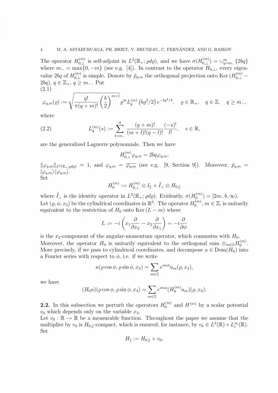
4 M. A. ASTABURUAGA, PH. BRIET, V. BRUNEAU, C. FERNANDEZ, AND G. RAIKOV
The operator H(m)0,⊥ is self-adjoint in L2(R+; %d%), and we have σ(H
(m)0,⊥ ) = ∪∞q=m−{2bq}
where m− = max{0,−m} (see e.g. [4]). In contrast to the operator H0,⊥, every eigen-
value 2bq of H(m)0,⊥ is simple. Denote by pq,m the orthogonal projection onto Ker (H
(m)0,⊥ −
2bq), q ∈ Z+, q ≥ m−. Put(2.1)
ϕq,m(%) :=
√q!
π(q + m)!
(b
2
)m+1
%mL(m)q
(b%2/2
)e−b%2/4, % ∈ R+, q ∈ Z, q ≥ m−,
where
(2.2) L(m)q (s) :=
q∑
l=m−
(q + m)!
(m + l)!(q − l)!
(−s)l
l!, s ∈ R,
are the generalized Laguerre polynomials. Then we have
H(m)0,⊥ ϕq,m = 2bqϕq,m,
‖ϕq,m‖L2(R+;%d%) = 1, and ϕq,m = ϕq,m (see e.g. [9, Section 9]). Moreover, pq,m =|ϕq,m〉〈ϕq,m|.Set
H(m)0 := H
(m)0,⊥ ⊗ I‖ + I⊥ ⊗H0,‖
where I⊥ is the identity operator in L2(R+; %d%). Evidently, σ(H(m)0 ) = [2m−b,∞).
Let (%, φ, x3) be the cylindrical coordinates in R3. The operator H(m)0 , m ∈ Z, is unitarily
equivalent to the restriction of H0 onto Ker (L−m) where
L := −i
(x1
∂
∂x2
− x2∂
∂x1
)= −i
∂
∂φ
is the x3-component of the angular-momentum operator, which commutes with H0.
Moreover, the operator H0 is unitarily equivalent to the orthogonal sum ⊕m∈ZH(m)0 .
More precisely, if we pass to cylindrical coordinates, and decompose u ∈ Dom(H0) intoa Fourier series with respect to φ, i.e. if we write
u(% cos φ, % sin φ, x3) =∑
m∈Zeimφum(%, x3),
we have
(H0u)(% cos φ, % sin φ, x3) =∑
m∈Zeimφ(H
(m)0 um)(%, x3).
2.2. In this subsection we perturb the operators H(m)0 and H(m) by a scalar potential
v0 which depends only on the variable x3.Let v0 : R → R be a measurable function. Throughout the paper we assume that themultiplier by v0 is H0,‖-compact, which is ensured, for instance, by v0 ∈ L2(R)+L∞ε (R).Set
H‖ := H0,‖ + v0.

RESONANCES AND SSF SINGULARITIES FOR A MAGNETIC SCHRODINGER OPERATOR 5
Then we haveσess(H‖) = σess(H0,‖) = [0,∞).
For simplicity, throughout the article we suppose also that
(2.3) inf σ(H‖) > −2b.
Evidently, (2.3) holds true if the negative part v0,− of the function v0 is bounded, andwe have ‖v0,−‖L∞(R) < 2b.Assume now that the discrete spectrum of H‖ is not empty; this would follow, forexample, from the additional conditions v0 ∈ L1(R) and
∫R v0(x)dx < 0 (see e.g. [34,
Theorem XIII.110]). Occasionally, we will impose also the assumption that the discretespectrum of H‖ consists of a unique eigenvalue; this would be implied, for instance, bythe inequality
∫R |x|v0,−(x)dx < 1 (see e.g. [5, Chaper II, Theorem 5.1]).
Let λ be a discrete eigenvalue of the operator H‖ which necessarily is simple. Thenλ ∈ (−2b, 0) by (2.3). Let ψ be an eigenfunction satisfying
(2.4) H‖ψ = λψ, ‖ψ‖L2(R) = 1, ψ = ψ.
Denote by p‖ = p‖(λ) the spectral projection onto Ker(H‖ − λ). We have p‖ = |ψ〉〈ψ|.Suppose now that v0 satisfies
(2.5) |v0(x)| = O(〈x〉−m0
), x ∈ R, m0 > 1,
where 〈x〉 := (1+|x|2) 12 . Then the multiplier by v0 is a relatively trace-class perturbation
of H0,‖, and by the Birman-Kuroda theorem (see e.g. [33, Theorem XI.9]) we have
σac(H‖) = σac(H0,‖) = [0,∞).
Moreover, by the Kato theorem (see e.g. [34, Theorem XIII.58]) the operator H‖ has nostrictly positive eigenvalues. Finally, for all E > 0 and s > 1/2 the operator-norm limit
(2.6) 〈x〉−s(H‖ − E)−1〈x〉−s := limδ↓0〈x〉−s(H‖ − E − iδ)−1〈x〉−s,
exists in L(L2(R)), and for each compact subset J of R+ = (0,∞) and each s > 1/2there exists a constant CJ,s such that for each E ∈ J we have
(2.7) ‖〈x〉−s(H‖ − E)−1〈x〉−s‖ ≤ CJ,s
(see [1]).Suppose again that (2.5) holds true, and let us consider the differential equation
(2.8) −y′′ + v0y = k2y, k ∈ R.
It is well-known that (2.8) admits the so-called Jost solutions y1(x; k) and y2(x; k) whichobey
y1(x; k) = eikx(1 + o(1)), x →∞,
y2(x; k) = e−ikx(1 + o(1)), x → −∞,
uniformly with respect to k ∈ R (see e.g. [5, Chapter II, Section 6] or [37]). The pairs{yl(·; k), yl(·;−k)}, k ∈ R, l = 1, 2, form fundamental sets of solutions of (2.8). Definethe transition coefficient T (k) and the reflection coefficient R(k), k ∈ R, k 6= 0, by
y2(x; k) = T (k)y1(x;−k) +R(k)y1(x; k), x ∈ R.

6 M. A. ASTABURUAGA, PH. BRIET, V. BRUNEAU, C. FERNANDEZ, AND G. RAIKOV
It is well known that T (k) 6= 0, k ∈ R \ {0}. On the other hand, the Wronskian ofthe solutions y1(·; k) and y2(·; k) is equal to −2ikT (k), and hence these solutions arelinearly independent for k ∈ R \ {0}. For E > 0 set
Ψl(x; E) :=1√
4π√
ET (√
E)yl(x;
√E), l = 1, 2.
Evidently, Ψl(·; E) ∈ C1(R) ∩ L∞(R), E > 0, l = 1, 2. Moreover, the real and theimaginary part of both functions Ψl(·; E), l = 1, 2 with E > 0 do not vanish identically.Further, Im 〈x〉−s(H‖ −E)−1〈x〉−s with E > 0 and s > 1/2 is a rank-two operator withan integral kernel
K(x, x′) = π∑
l=1,2
〈x〉−sΨl(x; E)Ψl(x′; E)〈x′〉−s, x, x′ ∈ R.
2.3. Fix now m ∈ Z, and set
H(m) := H(m)0 + I⊥ ⊗ v0.
Since v0 is H0,‖-compact and the spectrum of H(m)0,⊥ is discrete, the operator I⊥ ⊗ v0
is H(m)0 -compact. Therefore, the operator H(m) is well-defined on Dom(H
(m)0 ), and we
haveσess(H
(m)) = σess(H(m)0 ) = [2bm−,∞).
Further, if λ is a discrete eigenvalue of H‖, then 2bq + λ is a simple eigenvalue of H(m)
for each integer q ≥ m−. If q = m−, then this eigenvalue is isolated, but if q > m−,then due to (2.3), it is embedded in the essential spectrum of H(m). Moreover,
(2.9) H(m)Φq,m = (2bq + λ)Φq,m, q ≥ m−,
Φq,m = ϕq,m ⊗ ψ, ϕq,m being defined in (2.1), and ψ in (2.4). Set
(2.10) Pq,m := pq,m ⊗ p‖.
Then we have Pq,m = |Φq,m〉〈Φq,m|.Finally, introduce the operator
H := H0 + I⊥ ⊗ v0.
Even though the operator I⊥ ⊗ v0 is not H0-compact (unless v0 = 0), it is H0-boundedwith zero relative bound so that the operator H is well-defined on Dom(H0). Evidently,the operator H is unitarily equivalent to the orthogonal sum ⊕m∈ZH(m). Up to theadditive constant b, the operator H is the Hamiltonian of a quantum non-relativisticspinless particle in an electromagnetic field (E,B) with parallel electric componentE = −(0, 0, v′0(x3)), and magnetic component B = (0, 0, b).Note that if λ is a discrete eigenvalue of H‖, then 2bq + λ, q ∈ Z+ is an eigenvalue ofinfinite multiplicity of H. If q = 0, this eigenvalue is isolated, and if q ≥ 1, it lies onthe interval [0,∞) which constitutes a part of the essential spectrum of H. Moreover,if (2.5) holds, then σac(H) = [0,∞), so that in this case 2bq + λ, q ∈ N, is embedded inthe absolutely continuous spectrum of H.
RESONANCES AND SSF SINGULARITIES FOR A MAGNETIC SCHRODINGER OPERATOR 7
2.4. In this subsection we introduce appropriate perturbations of the operators H andH(m), m ∈ Z+.Let V : R3 → R be a measurable function. Assume that V is H0-bounded with zerorelative bound. By the diamagnetic inequality (see e.g. [4]) this would follow, forinstance, from V ∈ L2(R3) + L∞(R3). On Dom(H) = Dom(H0) define the operatorH + κV , κ ∈ R.Remark: We impose the condition that the relative H0-bound is zero just for the sake ofsimplicity. If V is H0-bounded with arbitrary finite relative bound, then we could againdefine H + κV but only for sufficiently small |κ|.Occasionally, we will impose the more restrictive assumption that V is H0-compact; thiswould follow from V ∈ L2(R3) + L∞ε (R3). In particular, V is H0-compact if it satisfiesthe estimate
(2.11) |V (x)| = O(〈X⊥〉−m⊥〈x3〉−m3
), x = (X⊥, x3), m⊥ > 0, m3 > 0.
Further, assume that V is axisymmetric, i.e. V depends only on the variables (%, x3).
Fix m ∈ Z and assume that the multiplier by V is H(m)0 -bounded with zero relative
bound. Then the operator H(m) + V is well defined on Dom(H(m)) = Dom(H(m)0 ).
Define the operator H(m) + κV , κ ∈ R.For z ∈ C+ := {ζ ∈ C | Im ζ > 0}, m ∈ Z, q ≥ m−, introduce the quantity
Fq,m(z) := 〈(H(m) − z)−1(I −Pq,m)V Φq,m, V Φq,m〉where 〈·, ·〉 denotes the scalar product in L2(R+ × R; %d%dx3), which we define to belinear with respect to the first factor. If λ is a discrete eigenvalue of H‖ we will say thatthe Fermi Golden Rule Fq,m,λ is valid if the limit
(2.12) Fq,m(2bq + λ) = limδ↓0
Fq,m(2bq + λ + iδ),
exists and is finite, and
(2.13) Im Fq,m(2bq + λ) > 0.
3. Resonances via dilation analyticity
3.1. In this subsection we will perturb H(m)0 by an axisymmetric potential V (%, x3)
so that the simple eigenvalue 2bq + λ of H(m)0 becomes a resonance of the perturbed
operator. In order to use complex scaling, we impose an analyticity assumption. Weassume that the potential v0 satisfies (2.5), and extends to an analytic function in thesector
Sθ0 = {z ∈ C | |Argz| ≤ θ0, or |z| ≤ r0}with θ0 ∈ (0, π/2). As already used in similar situations (see e.g. [4], [38]) we introducecomplex deformation in the longitudinal variable, (U(θ)f)(%, x3) = eθ/2f(%, eθx3), f ∈L2(R3), θ ∈ R. For θ ∈ R we have
H(m)(θ) = U(θ)H(m)U−1(θ) = H(m)0 ⊗ I + I ⊗H‖(θ),
8 M. A. ASTABURUAGA, PH. BRIET, V. BRUNEAU, C. FERNANDEZ, AND G. RAIKOV
with H‖(θ) = −e−2θ d2
dx23
+ v0,θ(x3), and v0,θ(x3) := v0(eθ x3). By assumption, the family
of operators {H‖(θ), |Im θ| < θ0}, form a type (A) analytic family of m-sectorialoperators in the sense of Kato (see for instance [20, Section 15.4], [2]). Then the discretespectrum of H0,‖(θ) is independent of θ and we have
σ(H(m)(θ)) =⋃
q≥m−
{2bq + σ(H‖(θ))},
σ(H‖(θ)) = e−2θR+ ∪ σdisc(H‖) ∪ {z1, z2, ....}where σdisc(H‖) denotes the discrete spectrum of H‖, and z1, z2, .... are (complex) eigen-values of H‖(θ) in {0 ≥ Arg z > −2Im θ}, Im θ > 0. In the sequel, we assume thatσdisc(H‖) = {λ}.Further, we assume that V is axisymmetric, H
(m)0 -compact, and admits an analytic
extension with respect to x3 ∈ Sθ0 . Let
Vθ(%, x3) := V (%, eθx3).
Then the family of operators {H(m)(θ) + κVθ, |Im θ| < θ0, |κ| ≤ 1}, form also ananalytic family of type (A) for sufficiently small κ.By definition, the resonances of H(m) + κV in
Sm−(θ) :=⋃
q≥m−
{z ∈ C; 2bq < Rez < 2b(q + 1), −2Imθ < Arg(z − 2bq) ≤ 0}
are the eigenvalues of H(m)(θ) + κVθ, Imθ > 0.For V axisymmetric and H0-compact, we define the set of the resonances Res(H +κV,S0(θ)) of the operator H + κV in S0(θ) by
Res(H + κV,S0(θ)) :=⋃
m∈Z{eigenvalues of H(m)(θ) + κVθ} ∩ S0(θ).
In other words, the set of resonances of H + κV is the union with respect to m ∈ Z ofthe resonances of H(m) +κV . This definition is correct since the restriction of H +κVonto Ker(L − m) is unitarily equivalent to H(m) + κV . Moreover using a standarddeformation argument (see, for instance, [20, Chapter 16]), we can prove that theseresonances coincide with singularities of the function z 7→ 〈(H + κV − z)−1 f, f〉, for fin a dense subset of L2(R3).
Theorem 3.1. Fix m ∈ Z, q > m−. Assume that:
• v0 satisfies (2.5), and admits an analytic extension in Sθ0;• inequality (2.3) holds true, and H‖ has a unique discrete eigenvalue λ;
• V is axisymmetric, H(m)0 -compact, and admits an analytic extension with respect
to x3 in Sθ0.
Then for sufficiently small |κ|, the operator H(m) +κV has a resonance wq,m(κ) whichobeys the asymptotics
(3.1) wq,m(κ) = 2bq + λ + κ〈V Φq,m, Φq,m〉 − κ2 Fq,m(2q + λ) + Oq,m,V (κ3), κ → 0,
RESONANCES AND SSF SINGULARITIES FOR A MAGNETIC SCHRODINGER OPERATOR 9
the eigenfunction Φq,m being defined in (2.9), and the quantity Fq,m(2q+λ) being definedin (2.12).
Proof. Fix θ such that θ0 > Im θ ≥ 0 and assume that z ∈ C is in the resolvent set ofthe operator H(m)(θ) + κVθ. Put
R(m)κ,θ (z) := (H(m)(θ) + κVθ − z)−1.
By the resolvent identity, we have
(3.2) R(m)κ,θ (z) = R
(m)0,θ (z)−κR
(m)0,θ (z)VθR
(m)0,θ (z)+κ2 R
(m)0,θ (z)VθR
(m)0,θ (z)VθR
(m)0,θ (z)+O(κ3),
as κ → 0, uniformly with respect to z in a compact subset of the resolvent sets ofH(m)(θ) + κV and H(m)(θ).Now note that the simple embedded eigenvalue 2bq + λ of H(m) is a simple isolatedeigenvalue of H(m)(θ). According to the Kato perturbation theory (see [22, SectionVIII.2]), for sufficiently small κ there exists a simple eigenvalue wq,m(κ) of H(m)(θ)+κVθ
such that limκ→0 wq,m(κ) = wq,m(0) = 2bq + λ. For |κ| sufficiently small, define theeigenprojector
(3.3) Pκ(θ) = Pκ,q,m(θ) :=−1
2iπ
∫
Γ
R(m)κ,θ (z)dz
where Γ is a small positively oriented circle centered at 2bq + λ. Evidently, for u ∈RanPκ(θ) we have (H(m)(θ) + κVθ)u = wq,m(κ)u; in particular, for u ∈ RanP0(θ) wehave H(m)(θ)u = (2bq + λ)u. Since wq,m(κ) is a simple eigenvalue, we have
(3.4) wq,m(κ) = Tr
(−1
2iπ
∫
Γ
zR(m)κ,θ (z)dz
)
for Γ and κ as above. Inserting (3.2) into (3.4), we get
wq,m(κ) =
(3.5)
2bq + λ +κTr(P0(θ) Vθ P0(θ))− κ2
2iπTr
(∫
Γ
zR(m)0,θ (z) Vθ R
(m)0,θ (z) Vθ R
(m)0,θ (z) dz
)+ O(κ3)
as κ → 0. Next, we have
(3.6) Tr(P0(θ) Vθ P0(θ)) = Tr(Pq,m V Pq,m) = 〈V Φq,m, Φq,m〉L2(R+×R;%d%dx3),
the orthogonal projection Pq,m being defined in (2.10). For θ ∈ R the relation isobvious since the operators P0,q,m(θ) Vθ P0,q,m(θ) and Pq,m V Pq,m are unitarily equiv-alent. For general complex θ identity (3.6) follows from the fact the function θ 7→Tr(P0,q,m(θ) Vθ P0,q,m(θ)) is analytic.Set
Q0(θ) := I − P0(θ), H(m)(θ) := H(m)(θ)Q0(θ).
By the cyclicity of the trace, we have
(3.7) Tr
(∫
Γ
zR(m)0,θ (z) Vθ R
(m)0,θ (z) Vθ R
(m)0,θ (z)dz
)= T1 + T2 + T3 + T4
10 M. A. ASTABURUAGA, PH. BRIET, V. BRUNEAU, C. FERNANDEZ, AND G. RAIKOV
where
T1 :=
∫
Γ
z(2bq + λ− z)−3 Tr (P0(θ) Vθ P0(θ)Vθ P0(θ)) dz,
T2 :=
∫
Γ
z(2bq + λ− z)−2 Tr(P0(θ) Vθ (H(m)(θ)− z)−1Q0(θ) Vθ P0(θ)
)dz,
T3 := Tr
(∫
Γ
z(H(m)(θ)− z)−1Q0(θ)Vθ(H(m)(θ)− z)−1Q0(θ)Vθ(H
(m)(θ)− z)−1Q0(θ)dz
),
T4 :=
∫
Γ
z (2bq + λ− z)−1 Tr(P0(θ) Vθ(H
(m)(θ)− z)−2Q0(θ) Vθ P0(θ))dz.
Since∫Γz(2bq +λ− z)−3dz = 0, and the function z 7→ (H(m)(θ)− z)−1 is analytic inside
Γ, we have
(3.8) T1 = T3 = 0.
Further, using the identity
(2bq + λ− z)−2P0(θ) Vθ (H(m)(θ)− z)−1Q0(θ) Vθ P0(θ)+
(2bq + λ− z)−1P0(θ) Vθ (H(m)(θ)− z)−2Q0(θ) Vθ P0(θ) =
∂
∂z
((2bq + λ− z)−1P0(θ) Vθ (H(m)(θ)− z)−1Q0(θ) Vθ P0(θ)
),
integrating by parts, and applying the Cauchy theorem, we obtain
(3.9) T2 + T4 = 2iπ Tr(P0(θ) Vθ (H(m)(θ)− 2bq − λ)−1 (I −P0(θ)) Vθ P0(θ)
).
Arguing as in the proof of (3.6), we get(3.10)
Tr(P0(θ) Vθ (H(m)(θ)− 2bq − λ− iδ)−1Q0(θ) Vθ P0(θ)
)= Fq,m(2q + λ + iδ), δ > 0.
For θ fixed such that Im θ > 0, the point 2bq + λ is not in the spectrum of H(m)(θ).Taking the limit δ ↓ 0 in (3.10), we find that (3.9) implies
(3.11) T2 + T4 = 2iπ Fq,m(2q + λ).
Putting together (3.5) – (3.8) and (3.11), we deduce (3.1). ¤
Remarks: (i) We will see in Section 4 that generically Im Fq,m(2q +λ) > 0 for all m ∈ Z,and q > m−.(ii) Taking into account the above remark, we find that Theorem 3.1 implies that generi-cally near 2bq+λ, q ≥ 1, there are infinitely many resonances of H+κV with sufficientlysmall κ, namely the resonances of the operators H(m) + κV with m > −q.
3.2. In this subsection we consider the dynamical aspect of resonances. We prove thefollowing proposition which will be extended to non-analytic perturbations in Section 4.

RESONANCES AND SSF SINGULARITIES FOR A MAGNETIC SCHRODINGER OPERATOR 11
Proposition 3.1. Under the assumptions of Theorem 3.1 there exists a function g ∈C∞
0 (R;R) such that g = 1 near 2bq + λ, and
(3.12) 〈e−i(H(m)+κV )tg(H(m) + κV )Φq,m, Φq,m〉 = a(κ)e−iwq,m(κ)t + b(κ, t), t ≥ 0,
with a and b satisfying the asymptotic estimates
|a(κ)− 1| = O(κ2),
|b(κ, t)| = O(κ2(1 + t)−n), ∀n ∈ Z+,
as κ → 0 uniformly with respect to t ≥ 0.
In order to prove the proposition, we will need the following
Lemma 3.1. Set
Qκ(θ) := I − Pκ(θ), R(m)κ,θ (z) :=
((H(m)(θ) + κVθ)Qκ(θ)− z
)−1
Qκ(θ),the projection Pκ(θ) being defined in (3.3). Then for |κ| small enough, there exists a
finite-rank operator F (m)κ,θ , uniformly bounded with respect to κ, such that
(3.13) P0(θ) = Pκ(θ)+κ(R
(m)κ,θ (wq,m(κ))VθPκ(θ)+Pκ(θ)VθR
(m)κ,θ (wq,m(κ))
)+κ2F (m)
κ,θ .
Proof. By the resolvent identity, we have
(3.14) R(m)0,θ (ν) = R
(m)κ,θ (ν) + κR
(m)κ,θ (ν)VθR
(m)κ,θ (ν) + κ2 R
(m)κ,θ (ν)VθR
(m)κ,θ (ν)VθR
(m)0,θ (ν).
Moreover by definition of R(m)κ,θ and of H(m) := H(m)Q0, we have:
(3.15) R(m)κ,θ (ν) = (wq,m(κ)− ν)−1Pκ(θ) + R
(m)κ,θ (ν),
R(m)0,θ (ν) = (2bq + λ− ν)−1P0(θ) + (H(m)(θ)− ν)−1Q0(θ),
where ν 7→ R(m)κ,θ (ν) and ν 7→ (H(m)(θ) − ν)−1Q0(θ) are analytic near 2bq + λ. Then,
from the Cauchy formula, the integration of (3.14) on a small positively oriented circle
centered at 2bq+λ, yields (3.13) with F (m)κ,θ a linear combination of finite-rank operators
of the form P1 Vθ P2 Vθ P3, where {P0(θ), Pκ(θ)} ∩ {Pj, j = 1, 2, 3} 6= ∅, and
Pj ∈ {P0(θ), Pκ(θ), R(m)κ,θ (ν), (H(m)(θ)−ν)−1Q0(θ), with ν = wq,m(κ) or ν = 2bq+λ}.
Since these operators are uniformly bounded in κ with |κ| small enough, F (m)κ,θ is a
finite-rank operator which also is uniformly bounded in κ with |κ| small enough. ¤Proof of Proposition 3.1: Pick at first any g ∈ C∞
0 (R;R) such that g = 1 near 2bq + λ.We have
〈e−i(H(m)+κV )tg(H(m) + κV )Φq,m, Φq,m〉 = Tr (e−i(H(m)+κV )tg(H(m) + κV )Pq,m).
By the Helffer-Sjostrand formula,
(3.16) e−i(H(m)+κV )t g(H(m)+κV )Pq,m =1
π
∫
R2
∂g
∂z(z) e−izt (H(m)+κV −z)−1 Pq,mdxdy

12 M. A. ASTABURUAGA, PH. BRIET, V. BRUNEAU, C. FERNANDEZ, AND G. RAIKOV
where z = x + iy, z = x− iy, g is a compactly supported, quasi-analytic extension of g,and the convergence of the integral is understood in the operator-norm sense (see e.g.[15, Chapter 8]).Consider the functions
σ±(z) := Tr ((H(m) + κV − z)−1 Pq,m), ±Imz > 0.
Following the arguments of the previous subsection, we find that
(3.17) σ+(z) = Tr (R(m)κ,θ (z)P0,q,m(θ)), Im z > 0, θ0 > Im θ > 0.
Inserting (3.13) into (3.17), and using the cyclicity of the trace, and the elementaryidentities
Pκ(θ) R(m)κ,θ (z) R
(m)κ,θ (wq,m(κ)) = 0 = R
(m)κ,θ (wq,m(κ))Pκ(θ) R
(m)κ,θ (z),
we get
σ+(z) = Tr (R(m)κ,θ (z)Pκ(θ)) + κ2Tr (R
(m)κ,θ (z)F (m)
κ,θ ).
Applying (3.15), we obtain
(3.18) σ+(z) =(1 + κ2r(κ)
)(wq,m(κ)− z)−1 + κ2G+(κ, z),
where r(κ) := Tr (Pκ(θ)F (m)κ,θ ), and G+(κ, z) is analytic near 2bq + λ and uniformly
bounded with respect to |κ| small enough. Similarly,
(3.19) σ−(z) =(1 + κ2r(κ)
)(wq,m(κ)− z)−1 + κ2G−(κ, z),
where G−(κ, z) is analytic near 2bq+λ and uniformly bounded with respect to |κ| smallenough. Now, assume that the support of g is such that we can choose g supported on aneighborhood of 2bq+λ where the functions z 7→ G±(κ, z) are holomorphic. Combining(3.16) with the Green formula, we get
(3.20) Tr (e−i(H(m)+κV )t g(H(m) + κV )Pq,m) =1
2iπ
∫
Rg(µ) e−iµt (σ+(µ)− σ−(µ))dµ.
Making use of (3.18) – (3.19), we get
1
2iπ
∫
Rg(µ) e−iµt (σ+(µ)− σ−(µ))dµ =
κ2
2iπ
∫
Rg(µ) e−iµt (G+(κ, µ)−G−(κ, µ))dµ
+1 + κ2r(κ)
2iπ
∫
Rg(µ) e−iµt (wq,m(κ)− µ)−1dµ
−1 + κ2r(κ)
2iπ
∫
Rg(µ) e−iµt (wq,m(κ)− µ)−1dµ.
Pick ε > 0 so small that g(µ) = 1 for µ ∈ [2bq + λ− 2ε, 2bq + λ + 2ε]. Set
Cε := (−∞, 2bq + λ− ε] ∪ {2bq + λ + εeit, t ∈ [−π, 0]} ∪ [2bq + λ + ε, +∞),
g(µ) := 1, µ ∈ Cε \ R.

RESONANCES AND SSF SINGULARITIES FOR A MAGNETIC SCHRODINGER OPERATOR 13
Taking into account (3.20), bearing in mind that Im wq,m(κ) < 0, and applying theCauchy theorem, we easily find that
(3.21) Tr (e−i(H(m)+κV )t g(H(m)+κV )Pq,m) = (1+κ2r(κ))e−iwq,m(κ)t+κ2∑
j=1,2,3
Ij(t;κ)
where
I1(t;κ) :=1
2iπ
∫
Rg(µ) e−iµt (G+(κ, µ)−G−(κ, µ))dµ,
I2(t;κ) :=1
2iπ
∫
Cε
g(µ) e−iµt(r(κ)(wq,m(κ)− µ)−1 − r(κ)(wq,m(κ)− µ)−1)dµ,
I3(t;κ) := −Im wq,m(κ)
κ2π
∫
Cε
g(µ) e−iµt(wq,m(κ)− µ)−1(wq,m(κ)− µ)−1 dµ.
Integrating by parts, we find that
(3.22) |Ij(t;κ)| = O((1 + t)−n), t > 0, j = 1, 2, 3, ∀n ∈ Z+,
uniformly with respect to κ, provided that |κ| is small enough; in the estimate of I3(t;κ)we have taken into account that by Theorem 3.1 we have |Im(wq,m(κ))| = O(κ2).Putting together (3.21) and (3.22), we get (3.12).
4. Mourre estimates and dynamical resonances
In this section we obtain Mourre estimates for the operator H(m) and apply them com-bined with a recent result of Cattaneo, Graf, and Hunziker (see [11]) in order to in-vestigate the dynamics of the resonance states of the operator H(m) without analyticassumptions.
4.1. Let v0 : R→ R. Set
(4.1) vj(x3) := xj3v
(j)0 (x3), j ∈ Z+,
provided that the corresponding derivative v(j)0 of v0 is well-defined.
Let
A := − i
2
(x3
d
dx3
+d
dx3
x3
)
be the self-adjoint operator defined initially on C∞0 (R) and then closed in L2(R). Set
A := I⊥ ⊗ A. Let T be an operator self-adjoint in L2(R+ × R; %d%dx3) such thateisAD(T ) ⊆ D(T ), s ∈ R. Define the commutator [T, iA] in the sense of [21] and [11],
and set ad(1)A (T ) := −i[T, iA]. Define recursively
ad(k+1)A (T ) = −i[ad
(k)A (T ), iA], k ≥ 1,
provided that the higher order commutators are well-defined. Evidently, for each m ∈ Zwe have
(4.2) ikad(k)A (H(m)) = 2kI⊥ ⊗H0,‖ +
k∑j=1
ck,jvj, k ∈ Z+,

14 M. A. ASTABURUAGA, PH. BRIET, V. BRUNEAU, C. FERNANDEZ, AND G. RAIKOV
with some constants ck,j independent of m; in particular, ck,k = (−1)k. Therefore theH0,‖-boundedness of the multipliers vj, j = 1, . . . , k, guarantees the H(m)-boundedness
of all the operators ad(j)A (H(m)) , j = 1, . . . , k.
Let J ⊂ R be a Borel set, and T be a self-adjoint operator. Denote by PJ(T ) the spectralprojection of the operator T associated with J .
Proposition 4.1. Fix m ∈ Z. Let λ ∈ (−2b, 0), q ∈ Z, q > m−. Put
(4.3) J = (2bq + λ− δ, 2bq + λ + δ)
where δ > 0, δ < −λ/2, and δ < (2b + λ)/2. Assume that the operators vj(H0,‖ + 1)−1,j = 0, 1, are compact. Then there exist a positive constant C > 0 and a compact operatorK such that
(4.4) PJ(H(m))[H(m), iA]PJ(H(m)) ≥ CPJ(H(m)) + K.
Proof. Let χ ∈ C∞0 (R;R) be such that supp χ = [2bq+λ−2δ, 2bq+λ+2δ], χ(t) ∈ [0, 1],
∀t ∈ R, χ(t) = 1, ∀t ∈ J . In order to prove (4.4), it suffices to show that
(4.5) χ(H(m))[H(m), iA]χ(H(m)) ≥ Cχ(H(m))2 + K
with a compact operator K. Indeed, if inequality (4.5) holds true, we can multi-ply it from the left and from the right by PJ(H(m)) obtaining thus (4.4) with K =PJ(H(m))KPJ(H(m)).Next (4.2) yields
[H(m), iA] = 2I⊥ ⊗H0,‖ − v1.
Therefore,
χ(H(m))[H(m), iA]χ(H(m)) = 2χ(H(m))(I⊥ ⊗H0,‖
)χ(H(m))− χ(H(m))v1χ(H(m)) =
(4.6) 2χ(H(m)0 )
(I⊥ ⊗H0,‖
)χ(H
(m)0 ) + 2K1 −K2
where
K1 := χ(H(m))(I⊥ ⊗H0,‖
)χ(H(m))− χ(H
(m)0 )
(I⊥ ⊗H0,‖
)χ(H
(m)0 ),
K2 := χ(H(m))v1χ(H(m)).
Since the operator v1(H(m)0 + 1)−1 is compact, the operators v1(H
(m) + 1)−1, v1χ(H(m)),and K2 are compact as well. Let us show that K1 is also compact. We have
K1 = (χ(H(m))− χ(H(m)0 ))
(I⊥ ⊗H0,‖
)χ(H(m))+
(4.7) χ(H(m)0 )
(I⊥ ⊗H0,‖
)(χ(H(m))− χ(H
(m)0 )).
By the Helffer-Sjostrand formula and the resolvent identity,
χ(H(m))− χ(H(m)0 ) = − 1
π
∫
R2
∂χ
∂z(z)(H(m) − z)−1v0(H
(m)0 − z)−1dxdy.
RESONANCES AND SSF SINGULARITIES FOR A MAGNETIC SCHRODINGER OPERATOR 15
Since the support of χ is compact in R2, and the operator ∂χ∂z
(H(m)−z)−1v0(H(m)0 −z)−1
is compact for every (x, y) ∈ R2 with y 6= 0, and is uniformly norm-bounded for every
(x, y) ∈ R2, we find that the operator χ(H(m)) − χ(H(m)0 ) is compact. On the other
hand, it is easy to see that the operators(I⊥ ⊗H0,‖
)χ(H(m)) =
(I⊥ ⊗H0,‖
)(H(m) + 1)−1(H(m) + 1)χ(H(m)) =
(I⊥ ⊗H0,‖
)(H
(m)0 + 1)−1(I − v0(H
(m) + 1)−1)(H(m) + 1)χ(H(m))
and
χ(H(m)0 )
(I⊥ ⊗H0,‖
)= χ(H
(m)0 )(H
(m)0 + 1)(H
(m)0 + 1)−1
(I⊥ ⊗H0,‖
)
are bounded. Taking into account (4.7), and bearing in mind the compactness of the
operator χ(H(m))−χ(H(m)0 ), and the boundedness of the operators
(I⊥ ⊗H0,‖
)χ(H(m))
and χ(H(m)0 )
(I⊥ ⊗H0,‖
), we conclude that the operator K1 is compact.
Further, since δ < −λ/2, and hence 2bj > 2bq + λ + 2δ for all j ≥ q, we have
χ(H0,‖ + 2bj) = 0, j ≥ q.
Therefore,
χ(H(m)0 ) =
∞∑j=m−
pj,m ⊗ χ(H0,‖ + 2bj) =
q−1∑j=m−
pj,m ⊗ χ(H0,‖ + 2bj),
and
(4.8) χ(H(m)0 )
(I⊥ ⊗H0,‖
)χ(H
(m)0 ) =
q−1∑j=m−
pj,m ⊗(χ(H0,‖ + 2bj)2H0,‖
).
By the spectral theorem,
q−1∑j=m−
pj,m⊗(χ(H0,‖ + 2bj)2H0,‖
)H0,‖ ≥
q−1∑j=m−
(2b(q− j) + λ− 2δ)pj,m⊗ χ(H0,‖ + 2bj)2 ≥
(4.9) (2b + λ− 2δ)
q−1∑j=m−
pj,m ⊗ χ(H0,‖ + 2bj)2 = C1χ(H(m)0 )2
with C1 := 2b + λ− 2δ > 0. Combining (4.6), (4.8), and (4.9), we get
(4.10) χ(H(m))[H(m), iA]χ(H(m)) ≥ 2C1χ(H(m))2 + 2C1K3 + 2K1 −K2
where K3 := χ(H(m)0 )2 − χ(H(m))2 is a compact operator by the Helffer-Sjostrand
formula. Now we find that (4.10) is equivalent to (4.5) with C = 2C1 and K =2C1K3 + 2K1 −K2. ¤
16 M. A. ASTABURUAGA, PH. BRIET, V. BRUNEAU, C. FERNANDEZ, AND G. RAIKOV
Remark: Mourre estimates for various magnetic quantum Hamiltonians can be found in[18, Chapter 3].
4.2. By analogy with (4.1) set
Vj(%, x3) = xj3
∂jV (%, x3)
∂xj3
, j ∈ Z+.
We have
ikad(k)A (V ) =
k∑j=1
ck,jVj
with the same constants ck,j as in (4.2).We will say that the condition Oν , ν ∈ Z+, holds true if the multipliers by vj, j = 0, 1,are H0,‖-compact, and the multipliers by vj, j ≤ ν, are H0,‖-bounded. Also, for a fixedm ∈ Z we will say that the condition Cν,m, ν ∈ Z+, holds true if the condition Oν is
valid, the multiplier by V is H(m)0 -bounded with zero relative bound, and the multipliers
by Vj, j = 1, . . . , ν, are H(m)0 -bounded.
By Proposition 4.1 and [11, Lemma 3.1], the validity of condition Cν,m with ν ≥ 5 anda given m ∈ Z guarantees the existence of a finite limit Fq,m(2bq + λ) with q > m− in(2.12), provided that (2.3) holds true, and λ is a discrete eigenvalue of H0,‖ + v0.Combining the results of Proposition 4.1 and [11, Theorem 1.2], we obtain the following
Theorem 4.1. Fix m ∈ Z, n ∈ Z+. Assume that:
• the condition Cν,m holds with ν ≥ n + 5;• inequality (2.3) holds true, and λ is a discrete eigenvalue of H‖;• inequality (2.13) holds true, and hence the Fermi Golden Rule Fq,m,λ is valid.
Then there exists a function g ∈ C∞0 (R;R) such that supp g = J (see (4.3)), g = 1 near
2bq + λ, and
(4.11) 〈e−i(H(m)+κV )tg(H(m) + κV )Φq,m, Φq,m〉 = a(κ)e−iλq,m(κ)t + b(κ, t), t ≥ 0,
where
(4.12) λq,m(κ) = 2bq + λ + κ〈V Φq,m, Φq,m〉 − κ2Fq,m(2bq + λ) + oq,m,V (κ2), κ → 0.
In particular, we have Im λq,m(κ) < 0 for |κ| small enough. Moreover, a and b satisfythe asymptotic estimates
|a(κ)− 1| = O(κ2),
|b(κ, t)| = O(κ2| ln |κ||(1 + t)−n),
|b(κ, t)| = O(κ2(1 + t)−(n+1)),
as κ → 0 uniformly with respect to t ≥ 0.
We will say that the condition Cν , ν ∈ Z+, holds true if the condition Oν is valid,the multiplier by V is H0-bounded with zero relative bound, and the multipliers by Vj,j = 1, . . . , ν, are H0-bounded.

RESONANCES AND SSF SINGULARITIES FOR A MAGNETIC SCHRODINGER OPERATOR 17
For m ∈ Z and q ≥ m− denote by Φq,m : R3 → C the function written in cylindrical
coordinates (%, ϕ, x3) as Φq,m(%, φ, x3) = (2π)−12 eimφΦq,m(%, x3).
Corollary 4.1. Fix n ∈ Z+. Assume that:
• the condition Cν holds with ν ≥ n + 5;• inequality (2.3) is fulfilled, and λ is a discrete eigenvalue of H0,‖ + v0;• for each m ∈ Z, q > m−, inequality (2.13) holds true, and hence the Fermi
Golden Rule Fq,m,λ is valid.
Then for every fixed q ∈ N, and each m ∈ {−q + 1, . . . , 0} ∪ N we have
〈e−i(H+κV )tg(H + κV )Φq,m, Φq,m〉L2(R3) = a(κ)e−iλq,m(κ)t + b(κ, t), t ≥ 0,
where g, λq,m(κ), a, and b are the same as in Theorem 4.1.
Remarks: (i) If q ∈ N, then Corollary 4.1 tells us that typically the eigenvalue 2bq +λ ofthe operator H, which has an infinite multiplicity, generates under the perturbation κVinfinitely many resonances with non-zero imaginary part. Note however that 2q +λ is adiscrete simple eigenvalue of the operator H(−q), and therefore the operator H(−q) +κVhas a simple discrete eigenvalue provided that |κ| is small enough. Generically, thiseigenvalue is an embedded eigenvalue for the operator H + κV .(ii) If q = 0, then λ is an isolated eigenvalue of infinite multiplicity for H. By Theorem6.1 below, in this case there exists an infinite series of discrete eigenvalues of the operatorH + V which accumulate at λ, provided that the perturbation V has a definite sign.
5. Sufficient conditions for the validity of the Fermi Golden Rule
In this section we describe certain classes of perturbations V compatible with the hy-potheses of Theorems 3.1 - 4.1, for which the Fermi Golden rule Fq,m,λ is valid for everym ∈ Z and q > m−. The results included are of two different types. Those of Subsection5.1 are less general but they offer a constructive approximation of V by potentials forwhich the Fermi Golden Rule holds. On the other hand, the results of Subsection 5.2are more general, but they are more abstract and less constructive.
5.1. Assume that v0 ∈ C∞(R) satisfies the estimates
(5.1) |v(j)0 (x)| = Oj
(〈x〉−m0−j), x ∈ R, j ∈ Z+, m0 > 1.
Then condition Oν is valid for every ν ∈ Z+. Moreover, in this case the eigenfunctionψ (see (2.4)) is in the Schwartz class S(R), while the Jost solutions yj(·; k), j = 1, 2,belong to C∞(R) ∩ L∞(R).Suppose that (2.3) holds true, and the discrete spectrum of the operator H‖ consists ofa unique eigenvalue λ. Fix m ∈ Z, and q ∈ Z+ such that q > m−. Then it is easy tocheck that we have
Im Fq,m(2bq + λ) =
(5.2) π∑
l=1,2
q−1∑j=m−
∣∣∣∣∫ ∞
0
∫
Rϕj,m(%)ϕq,m(%)ψ(x3)Ψl(x3; 2b(q − j) + λ)V (%, x3)dx3%d%
∣∣∣∣2
.

18 M. A. ASTABURUAGA, PH. BRIET, V. BRUNEAU, C. FERNANDEZ, AND G. RAIKOV
In what follows we denote by L2Re(R+; %d%) the set of real functions W ∈ L2(R+; %d%).
Lemma 5.1. The set of functions W ∈ L2Re(R+; %d%) for which
(5.3)
∫ ∞
0
ϕq−1,m(%)ϕq,m(%)W (%)%d% 6= 0
for every m ∈ Z, q > m−, is dense in L2Re(R+; %d%).
Proof. Since the Laguerre polynomials L(0)q , q ∈ Z+, (see (2.2)) form an orthogonal
basis in L2(R+; e−sds), the set of polynomials is dense in L2(R+; e−sds). Pick W ∈L2
Re(R+; %d%). Set w(s) := W (√
2s/b)es/2, s > 0. Evidently, w = w ∈ L2(R+; e−sds).Pick ε > 0 and find a non-zero polynomial P with real coefficients such that
∫ ∞
0
e−s (P(s)− w(s))2 ds <bε2
4.
Note that the coefficients of P could be chosen real since the coefficients of the Laguerrepolynomials are real. Changing the variable s = b%2/2, we get
(5.4)
∫ ∞
0
(P(b%2/2)e−b%2/4 −W (%)
)2
%d% <ε2
4.
Now set Wα(%) := P(b%2/2)e−αb%2/2, % ∈ R+, α ∈ (0,∞), where the real polynomial Pis fixed and satisfies (5.4). We will show that the set
(5.5) A :=
{α ∈ (0,∞) |
∫ ∞
0
ϕq−1,m(%)ϕq,m(%)Wα(%)%d% 6= 0, ∀m ∈ Z, ∀q > m−
}
is dense in (0,∞). Actually, for fixed m ∈ Z and q > m−, we have∫ ∞
0
ϕj,m(%)ϕq,m(%)Wα(%)%d% = Πq,m(γ(α))
where Πq,m is a real polynomial of degree 2q + m + 1 + degP , and γ(α) := (1 + α)−1.Note that γ : (0,∞) → (0, 1) is a bijection. Denote by Nq,m the set of the zeros of Πq,m
lying on the interval (0, 1). Set
N :=⋃
m∈Z
∞⋃q=m−+1
Nq,m.
Evidently, the sets N and γ−1(N ) are countable, and A = (0,∞) \ γ−1(N ). Therefore,A is dense in (0,∞). Now, pick α0 ∈ A so close to 1/2 that
(5.6)
∫ ∞
0
P(b%2/2)2(e−b%2/4 − e−α0b%2/2
)2
%d% <ε2
4.
Assembling (5.4) and (5.6), we obtain
(5.7) ‖W −Wα0‖L2(R+;%d%) < ε.
¤

RESONANCES AND SSF SINGULARITIES FOR A MAGNETIC SCHRODINGER OPERATOR 19
Denote by K(R) the class of real-valued continuous functions u : [0,∞) → R such thatlims→∞ u(s) = 0. Set ‖u‖K(R) := maxs∈[0,∞) |u(s)|.Lemma 5.2. The set of functions W ∈ L2
Re(R+; %d%) for which (5.3) holds true forevery m ∈ Z, q > m−, is dense in K(R).
Proof. By the Stone-Weierstrass theorem for locally compact spaces, we find that theset of functions e−αsP(s), s > 0 where α ∈ (0,∞), and P is a polynomial, is dense inK(R).
Let W ∈ K(R); then we have u ∈ K(R) where u(s) := W (√
2s/b), s > 0. Pick ε > 0and find α ∈ (0,∞) and a polynomial P such that ‖W−Wα‖K(R) < ε/2 where, as in the
proof of Lemma 5.1, Wα(%) = e−αb%2/2P(b%2/2). Next pick α0 ∈ A (see (5.5)) such that‖Wα −Wα0‖K(R) ≤ ε/2. Therefore, similarly to (5.7) we have ‖W −Wα0‖K(R) ≤ ε. ¤Fix ν ∈ Z+. We will write V ∈ Dν if
‖V ‖2Dν
:=ν∑
j=0
∫ ∞
0
∫
R
(xj
3
∂jV (%, x3)
∂xj3
)2
dx3%d% < ∞.
Note that if Oν holds, and V ∈ Dν , then Cν is valid.
Theorem 5.1. Assume that:
• v0 ∈ C∞(R) satisfies (5.1);• inequality (2.3) holds true;• we have σdisc(H‖) = {λ}.
Fix ν ∈ Z+. Then the set of real perturbations V : R+ × R → R for which the FermiGolden Rule Fq,m,λ is valid for each m ∈ Z and q > m−, is dense in Dν.
Proof. We will prove that the set of perturbations V for which the integral
(5.8) Iq,m,λ(V ) := Re
∫ ∞
0
∫
Rϕq−1,m(%)ϕq,m(%)ψ(x3)Ψ1(x3; 2b + λ)V (%, x3)dx3%d%
does not vanish for each m ∈ Z and q > m−, is dense in Dν . By (5.2) this will implythe claim of the theorem. Set
ω(x) := ψ(x)Re Ψ1(x; 2b + λ), x ∈ R.
Note that 0 6= ω = ω ∈ S(R). Set
V⊥(%) =
∫
Rω(x3)V (%, x3)dx3, % ∈ R+.
Evidently, V⊥ ∈ L2Re(R+; %d%). Fix ε > 0. Applying Lemma 5.1, we find V⊥ ∈
L2Re(R+; %d%) such that
(5.9)
∫ ∞
0
ϕq−1,m(%)ϕq,m(%)V⊥(%)%d% 6= 0
for every m ∈ Z, q > m−, and
(5.10) ‖V⊥ − V⊥‖L2(R+;%d%) < ε.
20 M. A. ASTABURUAGA, PH. BRIET, V. BRUNEAU, C. FERNANDEZ, AND G. RAIKOV
Set
(5.11) V (%, x3) :=V⊥(%)ω(x3)
‖ω‖2L2(R)
+ V (%, x3)− V⊥(%)ω(x3)
‖ω‖2L2(R)
, % ∈ R+, x3 ∈ R.
We have
Iq,m,λ(V ) =
∫ ∞
0
ϕq−1,m(%)ϕq,m(%)V⊥(%)%d% 6= 0
for every m ∈ Z, q > m−. On the other hand, (5.10) and (5.11) imply
‖V − V ‖2Dν≤ ε2
∑νj=0
∫R x2jω(j)(x)2dx
‖ω‖2L2(R)
.
¤Fix again ν ∈ Z+. We will write V ∈ Eν if V : R+ → R is continuous and tends to zero
at infinity, and the functions xj3
∂jV (%,x3)
∂xj3
, j = 1, . . . , ν, are bounded. If Oν holds, and
V ∈ Eν , then Cν holds true. For V ∈ Eν define the norm
‖V ‖Eν :=ν∑
j=0
sup(%,x3)∈R+×R
∣∣∣∣xj3
∂jV (%, x3)
∂xj3
∣∣∣∣ .
Arguing as in the proof of Theorem 5.1, we obtain the following
Theorem 5.2. Assume that v0 satisfies the hypotheses of Theorem 5.1. Fix ν ∈ Z+.Then the set of perturbations V : R+ × R→ R for which the Fermi Golden Rule Fq,m,λ
is valid for each m ∈ Z and q > m−, is dense in Eν.
5.2. For H a subspace of Lr(R), let us introduce the space
(5.12) H† := {ω ∈ S(R) | ∀χ ∈ H,
∫
Rω(x)χ(x)dx = 0}.
Clearly, if C∞b (R) ⊂ H then H† = {0}. This property holds yet if H∞(Sθ) ⊂ H where
H∞(Sθ) is the set of smooth bounded functions on R admitting analytic extension onSθ. It is enough to note that if ω(x0) 6= 0 then for C sufficiently large, the function
χ(x3) := e−C(x3−x0)2 is in H∞(Sθ) and satisfies∫R ω(x)χ(x)dx 6= 0.
Theorem 5.3. Assume that v0 satisfies the hypotheses of Theorem 5.1. Let p ≥ 1,r ≥ 1, δ ∈ R.Let H be a Banach space contained in Lr(R) such that the injection H ↪→ Lr(R) iscontinuous, and H† = {0}.Then the set of real perturbations V : R+ × R → R, for which the Fermi Golden RuleFq,m,λ is valid for each m ∈ Z and q > m−, is dense in Lp(R+, 〈%〉δ%d%;H).
Proof. As in the case of Theorems 5.1 – 5.2, we will prove that the set of perturbationsV for which the integral (5.8) does not vanish for each m ∈ Z and q > m−, is dense inLp(R+, 〈%〉δ%d%;H).Let
Mq,m,λ := {V ∈ Lp(R+, 〈%〉δ%d%;H); Iq,m,λ(V ) 6= 0}.

RESONANCES AND SSF SINGULARITIES FOR A MAGNETIC SCHRODINGER OPERATOR 21
Since for 1/p′ + 1/p = 1 and 1/r′ + 1/r = 1 we have
|Iq,m,λ(V )| ≤ ‖ϕq−1,mϕq,m‖Lp′ (R+,〈%〉−δ%d%;R) ‖ω‖Lr′ (R) ‖V ‖Lp(R+,〈%〉δ%d%;Lr(R)),
the continuity of the injection H ↪→ Lr(R) implies that Mq,m,λ is an open subset of theBanach space Lp(R+, 〈%〉δ%d%;H). Then according to the Baire Lemma, we have only tocheck that each Mq,m,λ is a dense in Lp(R+, 〈%〉δ%d%;H). Let V ∈ Lp(R+, 〈%〉δ%d%;H) \Mq,m,λ.Since 0 6= ω = ω ∈ S(R), the assumptions on H imply the existence of a Φ ∈ H suchthat ∫
Rω(x3)Φ(x3)dx3 6= 0.
Moreover, % 7→ ϕq−1,m(%)ϕq,m(%)% is a product of polynomial and exponential functions.Then there exists %0 ∈ R+ such that ϕq−1,m(%0)ϕq,m(%0)%0 6= 0, and for χ0 supportednear %0, we have ∫ ∞
0
ϕq−1,m(%)ϕq,m(%)χ0(%)%d% 6= 0.
Consequently,{V (%, x3) + 1
nχ0(%)Φ(x3)
}n∈N is a sequence of functions inMq,m,λ tending
to V in Lp(R+, 〈%〉δ%d%;H). ¤
6. Singularities of the spectral shift function
6.1. Suppose that v0 satisfies (2.5). Assume moreover that the perturbation V : R3 → Rsatisfies (2.11) with m⊥ > 2 and m3 = m0 > 1. Then the multiplier by V is a relativelytrace-class perturbation of H. Hence, the spectral shift function (SSF) ξ(·; H + V,H)satisfying the Lifshits-Krein trace formula
Tr(f(H + V )− f(H)) =
∫
Rf ′(E)ξ(E; H + V, H)dE, f ∈ C∞
0 (R),
and normalized by the condition ξ(E; H + V,H) = 0 for E < inf σ(H + V ), is well-defined as an element of L1(R; 〈E〉−2dE) (see [24], [23]).If E < inf σ(H), then the spectrum of H + V below E could be at most discrete, andfor almost every E < inf σ(H) we have
ξ(E; H + V, H) = −rankP(−∞,E)(H + V ).
On the other hand, for almost every E ∈ σac(H) = [0,∞), the SSF ξ(E; H + V, H) isrelated to the scattering determinant det S(E; H +V, H) for the pair (H +V, H) by theBirman-Krein formula
det S(E; H + V, H) = e−2πiξ(E;H+V,H)
(see [6]).Set
Z := {E ∈ R|E = 2bq + µ, q ∈ Z+, µ ∈ σdisc(H‖) or µ = 0}.Arguing as in the proof of [9, Proposition 2.5] we can easily check the validity of thefollowing
22 M. A. ASTABURUAGA, PH. BRIET, V. BRUNEAU, C. FERNANDEZ, AND G. RAIKOV
Proposition 6.1. Let v0 and V satisfy (2.5), and (2.11) with m⊥ > 2 and m0 = m3 > 1.Then the SSF ξ(·; H + V, H) is bounded on every compact subset of R \ Z, and iscontinuous on R \ (Z ∪ σp(H + V )), where σp(H + V ) denotes the set of the eigenvaluesof the operator H + V .
In what follows we will assume in addition that
(6.1) 0 ≤ V (x), x ∈ R3,
and will consider the operators H ± V which are sign-definite perturbations of theoperator H. The goal of this section is to investigate the asymptotic behaviour of theSSF ξ(·; H ±V,H) near the energies which are eigenvalues of infinite multiplicity. Moreprecisely, if (2.3) holds true, and λ ∈ σdisc(H‖), we will study the asymptotics as η → 0of ξ(2bq + λ + η; H ± V, H), q ∈ Z+, being fixed.Let T be a compact self-adjoint operator. For s > 0 denote
n±(s; T ) := rankP(s,∞)(±T ), n∗(s; T ) := n+(s; T ) + n−(s; T ).
Put
U(X⊥) :=
∫
RV (X⊥, x3)ψ(x3)
2dx3, X⊥ ∈ R2,
the eigenfunction ψ being defined in (2.4).
Theorem 6.1. Let v0 and V satisfy (2.5), (2.11) with m⊥ > 2 and m0 = m3 > 1, and(6.1). Assume that (2.3) holds true, and λ ∈ σdisc(H‖). Fix q ∈ Z+. Then for eachε ∈ (0, 1) we have(6.2)n+((1 + ε)η; pqUpq) + O(1) ≤ ±ξ(2bq + λ± η; H ± V, H) ≤ n+((1− ε)η; pqUpq) + O(1),
(6.3) ξ(2bq + λ∓ η; H ± V, H) = O(1),
as η ↓ 0.
Applying the well known results on the spectral asymptotics for compact Berezin-Toeplitz operators pqUpq (see [29], [32]), we obtain the following
Corollary 6.1. Assume the hypotheses of Theorem 6.1.(i) Suppose that U ∈ C1(R2), and
U(X⊥) = u0(X⊥/|X⊥|)|X⊥|−α(1 + o(1)), |X⊥| → ∞,
|∇U(X⊥)| ≤ C1〈X⊥〉−α−1, X⊥ ∈ R2,
where α > 2, and u0 is a continuous function on S1 which is non-negative and does notvanish identically. Then we have
ξ(2bq + λ± η; H ± V, H) = ± b
2π
∣∣{X⊥ ∈ R2|U(X⊥) > η}∣∣ (1 + o(1)) =
±η−2/α b
4π
∫
S1u0(s)
2/αds (1 + o(1)), η ↓ 0,

RESONANCES AND SSF SINGULARITIES FOR A MAGNETIC SCHRODINGER OPERATOR 23
where |.| denotes the Lebesgue measure.(ii) Let U ∈ L∞(R2). Assume that
ln U(X⊥) = −µ|X⊥|2β(1 + o(1)), |X⊥| → ∞,
for some β ∈ (0,∞), µ ∈ (0,∞). Then we have
ξ(2bq + λ± η; H ± V, H) = ±ϕβ(η) (1 + o(1)), η ↓ 0, β ∈ (0,∞),
where
ϕβ(η) :=
b2µ1/β | ln η|1/β if 0 < β < 1,
1ln (1+2µ/b)
| ln η| if β = 1,β
β−1(ln | ln η|)−1| ln η| if 1 < β < ∞,
η ∈ (0, e−1).
(iii) Let U ∈ L∞(R2). Assume that the support of U is compact, and that there exists aconstant C > 0 such that U ≥ C on an open non-empty subset of R2. Then we have
ξ(2bq + λ± η; H ± V,H) = ±(ln | ln η|)−1| ln η|(1 + o(1)), η ↓ 0.
Remarks: (i) The threshold behaviour of the SSF for various magnetic quantum Hamil-tonians has been studied in [16] (see also [30], [31]), and recently in [8]. The singularitiesof the SSF described in Theorem 6.1 and Corollary 6.1 are of somewhat different naturesince 2bq +λ is an infinite-multiplicity eigenvalue, and not a threshold in the continuousspectrum of the unperturbed operator.(ii) By the strict mathematical version of the Breit-Wigner representation for the SSF(see [26], [27]), the resonances for various quantum Hamiltonians could be interpretedas the poles of the SSF. In [7] a Breit-Wigner approximation of the SSF near the Lan-dau level was obtained for the 3D Schrodinger operator with constant magnetic field,perturbed by a scalar potential satisfying (2.11) with m⊥ > 2 and m3 > 1. Moreover,it was shown in [7] that typically the resonances accumulate at the Landau levels. Itis conjectured that the singularities of the SSF ξ(·; H ± V, H) at the points 2bq + λ,q ∈ Z+, are due to accumulation of resonances to these points. One simple motiva-tion for this conjecture is the fact that if V is axisymmetric, then the eigenvalues ofthe operators pqUpq, q ∈ Z+, appearing in (6.2) are equal exactly to the quantities〈V Φq,m, Φq,m〉L2(R+×R;%d%dx3), m ≥ −q, occurring in (3.1) and (4.12). We leave for afuture work the detailed analysis of the relation between the singularities of the SSF atthe points 2bq + λ and the eventual accumulation of resonances at these points. Hope-fully, in this future work we will also extend our results of Sections 3 – 5 to the case ofnon-axisymmetric perturbations V .(iii) As mentioned above, if λ ∈ σdisc(H‖), then λ is an isolated eigenvalue of H of infinitemultiplicity. Set
λ− :=
{sup{µ ∈ σ(H), µ < λ} if λ > inf σ(H),−∞ if λ = inf σ(H),
λ+ := inf{µ ∈ σ(H), µ > λ}.
24 M. A. ASTABURUAGA, PH. BRIET, V. BRUNEAU, C. FERNANDEZ, AND G. RAIKOV
By Pushnitski’s representation of the SSF (see [28]) and the Birman-Schwinger principlefor discrete eigenvalues in gaps of the essential spectrum, we have
ξ(λ− η; H − V ; H) = −n+(1; V 1/2(H − λ + η)−1V 1/2) =
−rankP(λ−,λ−η)(H − V ) + O(1), η ↓ 0,
ξ(λ + η; H + V ; H) = n−(1; V 1/2(H − λ− η)−1V 1/2) =
rankP(λ+η,λ+)(H + V ) + O(1), η ↓ 0.
Then Theorem 6.1 and Corollary 6.1 imply that the perturbed operator H − V (resp.,H + V ) has an infinite sequence of discrete eigenvalues accumulating to λ from the left(resp., from the right).
6.2. This subsection contains some preliminary results needed for the proof of Theorem6.1.In what follows we denote by S1 the trace class, and by S2 the Hilbert-Schmidt class ofcompact operators, and by ‖ · ‖j the norm in Sj, j = 1, 2.Suppose that η ∈ R satisfies
(6.4) 0 < |η| < min
{2b + λ,
1
2dist
(λ, σ(H‖) \ {λ}
)}.
Note that inequalities (6.4) combined with (2.3), imply
λ + η ∈ (−2b, 0), λ + η 6∈ σ(H‖), dist (λ + η, σ(H‖)) = |η|.Set Pj = pj ⊗ I‖, j ∈ Z+. For z ∈ C+ := {ζ ∈ C|Im ζ > 0}, j ∈ Z+, and W := V 1/2, put
Tj(z) := WPj(H − z)−1W.
Proposition 6.2. Assume the hypotheses of Theorem 6.1. Suppose that (6.4) holdstrue. Fix q ∈ Z+. Let j ∈ Z+, j ≤ q. Then the operator-norm limit
(6.5) Tj(2bq + λ + η) = limδ↓0
Tj(2bq + λ + η + iδ)
exists in L(L2(R3)). Moreover, if j < q, we have Tj(2bq + λ + η) ∈ S1, and
(6.6) ‖Tj(2bq + λ + η)‖1 = O(1), η → 0.
Proof. We have
(6.7) Tj(z) = M(t⊥,j ⊗ t‖(z − 2bj))M, z ∈ C+,
whereM := W (X⊥, x3)〈X⊥〉m⊥/2〈x3〉m3/2,
t⊥,l := 〈X⊥〉−m⊥/2pl〈X⊥〉−m⊥/2, l ∈ Z+,
t‖(ζ) := 〈x3〉−m3/2(H‖ − ζ)−1〈x3〉−m3/2, ζ ∈ C+.
Since the operators M and t⊥ are bounded, in order to prove that the limit (6.5) existsin L(L2(R3)), it suffices to show that the operator-norm limit
(6.8) limδ↓0
t‖(2b(q − j) + λ + η + iδ)
RESONANCES AND SSF SINGULARITIES FOR A MAGNETIC SCHRODINGER OPERATOR 25
exists in L(L2(R); L2(R)). If j < q, the limit in (6.8) exists due to the existence of thelimit in (2.6). If j = q, the limit in (6.8) exists just because λ + η 6∈ σ(H‖).Further, set
t‖,0(ζ) := 〈x3〉−m3/2(H0,‖ − ζ)−1〈x3〉−m3/2, ζ ∈ C+ \ {0}.For E = 2b(q − j) + λ + η, from the resolvent equation we deduce
(6.9) t‖(E) = t‖,0(E)(I‖ − Mt‖(E))
where M := v0(x3)〈x3〉m3 is a bounded multiplier. By [9, Section 4.1], the operatort‖,0(E) with E ∈ R \ {0} is trace-class, and we have
(6.10) ‖t‖,0(E)‖1 ≤ c√|E|(1 + E
1/4+ )
with c independent of E.Assume j < q. Then (6.9), (6.10), and (2.7) imply t‖(2b(q − j) + λ + η) ∈ S1, and
(6.11) ‖t‖(2b(q − j) + λ + η)‖1 = O(1), η → 0.
Finally, for any l ∈ Z+ we have t⊥,l ∈ S1, and
(6.12) ‖t⊥,l‖1 =b
2π
∫
R2
〈X⊥〉−m⊥dX⊥
(see e.g. [9, Subsection 4.1]). Bearing in mind the structure of the operator Tj (see(6.7)) and the boundedness of the operator M , we find that Tj(2b(q − j) + λ + η) ∈ S1,and due to (6.11) and (6.12), estimate (6.6) holds true. ¤Now set P+
q :=∑∞
j=q+1, q ∈ Z+, the convergence of the series being understood in thestrong sense. For z ∈ C+ set
T+q (z) := W (H − z)−1P+
q W.
Proposition 6.3. Assume that v0, V , and λ, satisfy the hypotheses of Theorem 6.1,and η ∈ R satisfies (6.4). Fix q ∈ Z+. Then the operator-norm limit
(6.13) T+q (2bq + λ + η) = lim
δ↓0T+
q (2bq + λ + η + iδ)
exists in L(L2(R3), L2(R3)). Moreover, T+q (2bq + λ + η) ∈ S2, and
(6.14) ‖T+q (2bq + λ + η)‖2 = O(1), η → 0.
Proof. Due to (2.3), the operator-valued function
C+ 3 z 7→ (H − z)−1P+q 7→ L(L2(R3); L2(R3))
admits an analytic continuation in {ζ ∈ C |Re ζ < 2bq}. Since λ + η < 0, and W isbounded, we immediately find that the limit in (6.13) exists. Evidently, the operator-valued function C+ 3 z 7→ (H0 − z)−1P+
q 7→ L(L2(R3)) also admits an analytic contin-uation in {ζ ∈ C |Re ζ < 2bq}, and for E = 2bq + λ + η we have
(6.15) T+q (E) = W (H0 − E)−1P+
q (W − v0(H − E)−1P+q W ).
26 M. A. ASTABURUAGA, PH. BRIET, V. BRUNEAU, C. FERNANDEZ, AND G. RAIKOV
Arguing as in the proof of [16, Proposition 4.2], we obtain
W (H0 − 2bq − λ− η)−1P+q ∈ S2,
and
(6.16) ‖W (H0 − 2bq − λ− η)−1P+q ‖2 = O(1), η → 0.
Since λ < 0, we have
(6.17) ‖W − v0(H − 2bq − λ− η)−1P+q W‖ = O(1), η → 0.
Putting together (6.15) and (6.16)-(6.17), we obtain (6.14). ¤6.3. In this subsection we prove Theorem 6.1.Suppose that η ∈ R satisfies (6.4). Fix q ∈ Z+. Set
T (2bq + λ + η) := T−q (2bq + λ + η) + Tq(2bq + λ + η) + T+
q (2bq + λ + η),
whereT−
q (2bq + λ + η) =∑j<q
Tj(2bq + λ + η).
Note that the operators Tq(2bq + λ + η) and T+q (2bq + λ + η) are self-adjoint.
By Pushnitski’s representation of the SSF for sign-definite perturbations (see [28]), wehave(6.18)
ξ(2bq + λ + η; H ± V,H) = ± 1
π
∫
Rn∓(1, Re T (2bq + λ + η) + s Im T (2bq + λ + η))
ds
1 + s2.
By (6.18) and the well-known Weyl inequalities, for each ε ∈ (0, 1) we have
n∓(1 + ε; Tq(2bq + λ + η))−Rε(η) ≤ ±ξ(2bq + λ + η; H ± V, H) ≤(6.19) n∓(1− ε; Tq(2bq + λ + η)) + Rε(η)
whereRε(η) :=
n∗(ε/3; Re T−q (2bq + λ + η)) + n∗(ε/3; T+
q (2bq + λ + η)) +3
ε‖T−
q (2bq + λ + η)‖1 ≤
(6.20)6
ε
∑j<q
‖Tj(2bq + λ + η)‖1 +9
ε2‖T+
q (2bq + λ + η)‖22 = O(1), η → 0,
due to Propositions 6.1 – 6.2.Next, set
τq = W (pq ⊗ p‖)W, Tq(λ + η) := W (pq ⊗ (H‖ − λ− η)−1(I‖ − p‖))W,
provided that η ∈ R satisfies (6.4). Evidently,
Tq(2bq + λ + η) = −η−1τq + Tq(λ + η).
Applying again the Weyl inequalities, we get
n±(s(1 + ε)|η|; (sign η)τq)− n∗(sε; Tq(λ + η)) ≤ n∓(s; Tq(2bq + λ + η)) ≤
RESONANCES AND SSF SINGULARITIES FOR A MAGNETIC SCHRODINGER OPERATOR 27
(6.21) n±(s(1− ε)|η|; (sign η)τq) + n∗(sε; Tq(λ + η))
for each s > 0, ε ∈ (0, 1), and η satisfying (6.4). Note that since pqUpq ≥ 0 we have
(6.22) n±(s|η|; (sign η) τq) =
{n+(s|η|; pqUpq) if ± η > 0,0 if ± η < 0,
for every s > 0. Further,
(6.23) Tq(λ + η) = M(t⊥,q ⊗ t‖(λ + η))M
wheret‖(λ + η) := 〈x3〉−m3/2(H‖ − λ− η)−1(I‖ − p‖)〈x3〉−m3/2.
Obviously,
(6.24) ‖t‖(λ + η)‖ ≤ ‖(H‖ − λ− η)−1(I‖ − p‖)‖ = O(1), η → 0.
On the other hand, similarly to (6.9) we have
(6.25) t‖(λ+ η) = t‖,0(λ+ η)(I‖− M t‖(λ+ η))−〈x3〉−m3/2(H0,‖−λ− η)−1p‖〈x3〉−m3/2.
Since p‖〈x3〉−m3/2 is a rank-one operator, we have
‖〈x3〉−m3/2(H0,‖−λ−η)−1p‖〈x3〉−m3/2‖1 ≤ ‖〈x3〉−m3/2(H0,‖−λ−η)−1‖‖p‖〈x3〉−m3/2‖2 ≤
(6.26)
∫
R〈x〉−m3ψ(x)2dx |λ + η|−1 = O(1), η → 0.
Putting together (6.25), (6.10), (6.24), and (6.26), we get
(6.27) ‖t‖(λ + η)‖1 = O(1), η → 0,
which combined with (6.23) and (6.12) yields
(6.28) n±(s; Tq(λ + η)) ≤ s−1‖Tq(λ + η)‖ = O(1), η → 0.
Now (6.2) – (6.3) follow from estimates (6.19) – (6.22), and (6.28).
Acknowledgements. M. A. Astaburuaga and C. Fernandez were partially supportedby the Chilean Laboratorio de Analisis Estocastico PBCT - ACT 13. V. Bruneauwas partially supported by the French ANR Grant no. JC0546063. V. Bruneau andG. Raikov are partially supported by the Chilean Science Foundation Fondecyt underGrants 1050716 and 7060245.
References
[1] S. Agmon, Spectral properties of Schrodinger operators and scattering theory, Ann. Sc. Norm.Super. Pisa, Cl. Sci., IV. Ser. 2, (1975), 151-218.
[2] J. Aguilar, J.M. Combes, A class of analytic perturbations for one-body Schrodinger Hamil-tonians, Comm. Math. Phys. 22 (1971), 269–279.
[3] J. Asch, M. A. Astaburuaga, P. Briet, V. Cortes, P. Duclos, C. Fernandez, Sojourntime for rank one perturbations, J. Math. Phys. 47 (2006), 033501, 14 pp.
[4] J. Avron, I. Herbst, B. Simon, Schrodinger operators with magnetic fields. I. General inter-actions, Duke Math. J. 45 (1978), 847-883.

28 M. A. ASTABURUAGA, PH. BRIET, V. BRUNEAU, C. FERNANDEZ, AND G. RAIKOV
[5] F. A. Berezin, M. A. Shubin, The Schrodinger Equation, Kluwer Academic Publishers, Dor-drecht, 1991.
[6] M.S.Birman, M. G. Kreın, On the theory of wave operators and scattering operators, Dokl.Akad. Nauk SSSR 144 (1962), 475–478 (Russian); English translation in Soviet Math. Doklady3 (1962).
[7] J.F.Bony, V.Bruneau, G.D.Raikov, Resonances and spectral shift function near Landau lev-els, Ann. Inst. Fourier 57 (2007), 629-671.
[8] P. Briet, G. Raikov, E. Soccorsi, Spectral properties of a magnetic quantum Hamiltonianon a strip, mp arc Preprint 07-166.
[9] V. Bruneau, A. Pushnitski, G. D. Raikov, Spectral shift function in strong magnetic fields,Algebra i Analiz 16 (2004), 207 - 238; see also St. Petersburg Math. Journal 16 (2005), 181-209.
[10] V. Bruneau, V. Petkov Meromorphic continuation of the spectral shift function, Duke Math.J. 116 (2003), 389-430.
[11] L. Cattaneo, G. M. Graf, W. Hunziker, A general resonance theory based on Mourre’sinequality, Ann. Henri Poincare 7 (2006), 583–601.
[12] O. Costin, A. Soffer, Resonance theory for Schrodinger operators, Comm. Math. Phys. 224(2001), 133–152.
[13] M. Dimassi, V. Petkov, Spectral shift function and resonances for non-semi-bounded and StarkHamiltonians, J. Math. Pures Appl. 82 (2003), 1303–1342.
[14] M. Dimassi, V. Petkov, Resonances for magnetic Stark Hamiltonians in two-dimensional case,Int. Math. Res. Not. 2004, no. 77, 4147–4179.
[15] M. Dimassi, J. Sjostrand, Spectral Asymptotics in the Semi-Classical Limit, LMS LectureNote Series, 268, Cambridge University Press Cambridge, 1999.
[16] C. Fernandez, G. D. Raikov, On the singularities of the magnetic spectral shift function atthe Landau levels, Ann. Henri Poincare 5 (2004), 381 - 403.
[17] C. Ferrari, H. Kovarık, On the exponential decay of magnetic Stark resonances, Rep. Math.Phys. 56 (2005), 197–207.
[18] C. Gerard, I. ÃLaba, Multiparticle Quantum Scattering in Constant Magnetic Fields, Mathe-matical Surveys and Monographs, 90, AMS, Providence, RI, 2002.
[19] I. W. Herbst, Exponential decay in the Stark effect, Comm. Math. Phys. 75 (1980), 197–205.[20] P.D. Hislop, I.M. Sigal, Introduction to spectral theory. With applications to Schrodinger
operators, Applied Mathematical Sciences, 113, Springer-Verlag, New York, 1996. x+337 pp.[21] A. Jensen, E. Mourre, P. Perry, Multiple commutator estimates and resolvent smoothness
in quantum scattering theory Ann. Inst. H. Poincare Phys. Theor. 41 (1984), 207–225.[22] T. Kato, Perturbation Theory for Linear Operators, Springer Verlag, Berlin/Heidelberg/New
York, 1966.[23] M. G. Krein, On the trace formula in perturbation theory, Mat. Sb. 33 (1953), 597-626 (Russian).[24] I. M. Lifshits, On a problem in perturbation theory, Uspekhi Mat. Nauk 7 (1952), 171-180
(Russian).[25] E. Mourre, Absence of singular continuous spectrum for certain self-adjoint operators, Comm.
Math. Phys. 78 (1981), 391–408.[26] V. Petkov, M. Zworski, Breit-Wigner approximation and the distribution of resonances,
Comm. Math. Phys. 204 (1999), 329–351.[27] V. Petkov, M. Zworski, Semi-classical estimates on the scattering determinant, Ann. Henri
Poincare 2 (2001), 675–711.[28] A. Pushnitskiı, A representation for the spectral shift function in the case of perturbations of
fixed sign, Algebra i Analiz 9 (1997), 197–213 (Russian); English translation in St. PetersburgMath. J. 9 (1998), 1181–1194.
[29] G. D. Raikov, Eigenvalue asymptotics for the Schrodinger operator with homogeneous magneticpotential and decreasing electric potential. I. Behaviour near the essential spectrum tips, Comm.PDE 15 (1990), 407-434; Errata: Comm. PDE 18 (1993), 1977-1979.
RESONANCES AND SSF SINGULARITIES FOR A MAGNETIC SCHRODINGER OPERATOR 29
[30] G.D.Raikov, Spectral shift function for Schrodinger operators in constant magnetic fields, Cubo,7 (2005), 171-199.
[31] G.D.Raikov, Spectral shift function for magnetic Schrodinger operators, Mathematical Physicsof Quantum Mechanics, Lecture Notes in Physics, 690 (2006), 451-465.
[32] G.D.Raikov, S.Warzel, Quasi-classical versus non-classical spectral asymptotics for magneticSchrodinger operators with decreasing electric potentials, Rev. Math. Phys. 14 (2002), 1051–1072.
[33] M.Reed, B.Simon, Methods of Modern Mathematical Physics. III. Scattering Theory, AcademicPress, New York, 1979.
[34] M.Reed, B.Simon, Methods of Modern Mathematical Physics. IV. Analysis of Operators, Aca-demic Press, New York, 1979.
[35] A. Soffer, M. Weinstein, Time dependent resonance theory, Geom. Funct. Anal. 8 (1998),1086–1128.
[36] E. Skibsted, On the evolution of resonance states, J. Math. Anal. Appl. 141 (1989), 27–48.[37] S.-H. Tang, M. Zworski, Potential Scattering on the Real Line, Lecture notes available at
http://math.berkeley.edu/ zworski/tz1.pdf .[38] X.P. Wang, Barrier resonances in strong magnetic fields, Commun. Partial Differ. Equations
17, (1992) 1539-1566.
Departamento de Matematicas, Facultad de Matematicas, Pontificia Universidad Catolicade Chile, Vicuna Mackenna 4860, Santiago de ChileE-mail address: [email protected]
Centre de Physique Theorique, CNRS-Luminy, Case 907, 13288 Marseille, FranceE-mail address: [email protected]
Universite Bordeaux I, Institut de Mathematiques de Bordeaux, UMR CNRS 5251, 351,Cours de la Liberation, 33405 Talence, FranceE-mail address: [email protected]
Departamento de Matematicas, Facultad de Matematicas, Pontificia Universidad Catolicade Chile, Vicuna Mackenna 4860, Santiago de ChileE-mail address: [email protected]
Departamento de Matematicas, Facultad de Matematicas, Pontificia Universidad Catolicade Chile, Vicuna Mackenna 4860, Santiago de ChileE-mail address: [email protected]
Related Documents