Dynamical and topological robustness of the mammalian cell cycle network: A reverse engineering approach

Dynamical and Topological Robustness of the Mammalian Cell Cycle Network:A Reverse Engineering Approach

Gonzalo A. Ruza, Eric Golesa, Marco Montalvaa, Gary B. Fogelb

aFacultad de Ingenierıa y Ciencias, Universidad Adolfo Ibanez, Av. Diagonal Las Torres 2640, Santiago, ChilebNatural Selection, Inc., 5910 Pacific Center Blvd., Suite 315, San Diego, CA USA 92121

Abstract

A common gene regulatory network model is the threshold Boolean network, used for example to model the Arabidop-sis thaliana floral morphogenesis network or the fission yeast cell cycle network. In this paper, we analyze a logicalmodel of the mammalian cell cycle network and its threshold Boolean network equivalent. Firstly, the robustness ofthe network was explored with respect to update perturbations, in particular, what happened to the attractors for allthe deterministic updating schemes. Results on the number of different limit cycles, limit cycle lengths, basin of at-traction size, for all the deterministic updating schemes were obtained through mathematical and computational tools.Secondly, we analyzed the topology robustness of the network, by reconstructing synthetic networks that containedexactly the same attractors as the original model by means of a swarm intelligence approach. Our results indicate thatnetworks may not be very robust given the great variety of limit cycles that a network can obtain depending on theupdating scheme. In addition, we identified an omnipresent network with interactions that match with the originalmodel as well as the discovery of new interactions. The techniques presented in this paper are general, and can beused to analyze other logical or threshold Boolean network models of gene regulatory networks.

Keywords: Gene regulatory networks, Boolean networks, Threshold networks, Update robustness, Topologyrobustness, Bees algorithm

1. Introduction

Over forty years ago, Stuart Kauffman introduced Boolean networks (BNs) as a mathematical model of generegulatory networks (GRNs) (Kauffman, 1969). GRNs represent the process of gene regulation, which determineswhen and where genes will be active/inactive through the interactions of DNA, RNA, proteins, and other substanceswithin the cell. BNs are very simple and can be described as follows. Nodes represent genes and edges representthe interaction between the genes (i.e., a regulation process). Each gene is considered to act as an on-off device, thetwo states (on/off) represent respectively, the status of a gene being active (gene value = 1) or inactive (gene value= 0). Given that each node can only have two values, for a network with n nodes, this implies that the network has2n different states. The dynamics of the network (how the values of the nodes change through time) are governedby a set of Boolean rules and an updating scheme. In the original model, the updating scheme was considered to besynchronous or parallel, such that at each time step, node values for all nodes were updated at the same time. Animportant characteristic of BNs are steady state attractors for network convergence. There are two types of attractors:1) fixed point, where once a network reaches that state it can never escape, and 2) a limit cycle, where the networkreturns to a previous state with a certain periodicity. The attractors are of interest in the context of GRNs since theyrepresent different cell types.

BNs are very popular within GRN modelers, in part due to their simplicity. However, this same characteristic isa focus for criticism as not being very realistic. For example, parallel updating schemes have been used to modelthe Arabidopsis thaliana floral morphogenesis network (Mendoza and Alvarez-Buylla, 1998), the fission yeast cellcycle network (Davidich and Bornholdt, 2008), and the budding yeast cell cycle network (Li et al., 2004). Theseclearly include a large assumption about the extreme regularity and tight control of global gene expression. At firstsight, this could lead to think that the parallel updating scheme is unrealistic and wrong. Nevertheless, it is capable ofexhibiting a dynamic behavior similar to that of biological cells (Kauffman et al., 2003; Wuensche, 2004), specially

Preprint submitted to BioSystems October 25, 2013

when cell differentiation is associated to fixed points, which are invariant to update perturbation, thus, making theparallel updating mode a computationally convenient selection, which is quite exhaustive in the presence of strongstability, where the updating scheme does not influence significantly the dynamic of the model. An example where thisphenomena occurs, and that one could consider that the parallel is exhaustive enough, given that the behavior exhibitedwith the parallel is similar for any other deterministic updating scheme is the budding yeast cell cycle network (Liet al., 2004) which contains seven fixed points, and the basin of attraction for each fixed point, in particular the one thatrepresents the G1 phase, does not change significantly when changing the updating scheme (Goles et al., 2013). Forthe general case where one can not assure strong stability beforehand, an interesting question arises: what happensto the models that assume a parallel updating scheme if a change in the updating scheme (an update perturbation)occurs? Do the attractors remain the same, or are new attractors derived?

The construction of GRN models from data is typically referred to as a reverse engineering problem (Liang et al.,1998; Akutsu et al., 1999). Building GRNs is a difficult task given the large space of possible GRN models thatmight fit the data and the need to search that space in reasonable time to derive useful solutions. Several approachesusing evolutionary computation (EC) have been proposed to aid in this search. For example in Mendoza et al. (2012),Boolean network models of GRN were inferred using genetic algorithms (GAs) to optimize a Tsallis entropy function.GAs were also used in Repsilber et al. (2002) for the reconstruction of multistate discrete network models for GRN,allowing each node (gene) to have more than two states, and also in Kikuchi et al. (2003) for modeling GRN as anS-system. Differential evolution (DE) has been used for GRN reconstruction using S-systems in Chowdhury et al.(2012), and in Noman and Iba (2007) with an information criteria-based fitness evaluation instead of the conventionalmean squared error-based fitness evaluation. Other optimization methods such as simulated annealing (SA) havebeen used. In Liu et al. (2009), SA was used to model GRNs as Bayesian networks, and Gonzalez et al. (2007)used SA to derive S-system models of biochemical networks, whereas Ruz and Goles (2010) used threshold Booleannetworks. Swarm intelligence has also been used for the inference of GRNs. For instance, in Kentzoglanakis andPoole (2012) a combination of particle swarm optimization (PSO) and ant colony optimization (ACO) was used toreverse engineer GRNs, under the recurrent neural network (RNN) model, from temporal gene expression data. TheACO has also been used to search for network structures with PSO used to finding the RNN model parameters.Similarly, in Xu et al. (2007), PSO was used to find the network structure and parameters of GRN modeled byRNN, using time-series gene expression data. A comparison between EAs, PSO, and an artificial bee colony (ABC)approach, with GRNs modeled as S-systems, was conducted in Forghany et al. (2012). The results on two small-sizeand a medium-sized hypothetical gene regulatory networks showed that a modified version of ABC outperformedthe other techniques. Recently, the bees algorithm (BA) (Pham et al., 2006) for reverse engineering of GRN wasintroduced in Ruz and Goles (2013). Comparisons with SA for learning threshold Boolean networks showed thatthe bees algorithm outperformed SA, obtaining a larger number of solutions using fewer edges in the network. Thebees algorithm has been used to build synthetic networks of the budding yeast cell-cycle in Ruz et al. (2012), andfor promoting cell proliferation for biotechnological applications. In Ruz and Goles (2012), a reverse engineeringtechnique was applied to the reconstruction of the mammalian cell cycle network using the binary gene expressiondata generated by the logical model in Faure et al. (2006). This reverse engineering method used an informationtheoretic approach combined with a modified version of the original bees algorithm.

Here we present extensions to Ruz and Goles (2012). First, we analyze the dynamics of the mammalian cell cyclenetwork under different updating schemes. It is important to note that, while in Ruz and Goles (2012) we providedresults for only 5000 sequential updating schemes, in this paper, we analyzed all possible deterministic updatingschemes. This is a difficult problem, given that there are an exponential number of updates. If the network has nnodes, the number of updates is given by (Demongeot et al., 2008):

Tn =

n−1∑k=0

(nk

)Tk, T0 = 1.

For a mammalian cell cycle network with n = 10, we have that T (10) = 102247563. To analyze this vast amount ofdynamics, we combined mathematical results with recent computational techniques developed in Goles et al. (2013)and in Aracena et al. (2013). We then analyzed the topology of the network, and for this portion, we used the beesalgorithm to reconstruct synthetic networks that contained exactly the same attractors of the original model. Usingthis reverse engineering approach, we are able to identify interactions which are always present and that match with

2

the original model as well as new interactions in these GRNs.The rest of the paper is organized as follows. Section 2 gives a brief description of Boolean networks, the mam-

malian cell cycle network of Faure et al. (2006), and the bees algorithm. The robustness of the network under all thedeterministic updating schemes is carried out in section 3. Section 4 approaches the study of the topology robustnessusing the bees algorithm. General conclusions are offered in section 5.

2. Background

2.1. Boolean networksLet x be a finite set of n variables, x = x1, . . . , xn, with xi ∈ 0, 1 for i = 1, . . . , n. A Boolean network is a pair

(G, F), where G = (V,E) is a finite directed graph; V being the set of n nodes and E the set of edges. F is a Booleanfunction, F : 0, 1n → 0, 1n composed of n local functions fi : 0, 1n → 0, 1. Furthermore, each local function fidepends only on variables belonging to the neighborhood Vi = j ∈ V|( j, i) ∈ E. The indegree, K, of vertex i is |Vi|.The updating schemes are repeated periodically, and since the hypercube is a finite set, the dynamics of the networkconverges to attractors which are fixed points or limit cycles, defined by

• Fixed point: xt+1i = xt

i for i = 1, . . . , n.

• Limit cycle: xt+pi = xt

i for i = 1, . . . , n.

where p > 1 is a positive integer called the limit cycle length. The set of states that can lead the network to a specificattractor is termed the basin of attraction. There are many ways of updating the values of a Boolean network, someexamples are (Aracena et al., 2009):

• Parallel or synchronous mode: where every node is updated at the same time.

• Sequential updating mode: where in every time step, every node is updated in a defined sequence.

• Block-sequential: the set of nodes, for a given sequence, is partitioned into blocks. The nodes in a same blockare updated in parallel, but blocks follow each other sequentially.

• Asynchronous deterministic: where in every time step, only one node is updated following a defined sequence.

2.2. The mammalian cell cycle modelInitially, a differential model for the control of the mammalian cell cycle network was introduced by Novak and

Tayson (Novak and Tayson, 2004). Then, a logical version for this model was presented by Faure et al. (Faure et al.,2006). In this logical model, the mammalian cell cycle network consisted of 10 genes (that characterize enzymaticcomplexes and cofactors), therefore, there are 210 = 1024 possible states. When updated in parallel, the network hastwo attractors. One attractor is a limit cycle of length seven that is used to model the cell cycle, and the other is a fixedpoint attractor. The updating rules for each node are as follows,

CycD =CycD (1)

Rb =(CycD ∧CycB) ∧ ([CycE ∧CycA] ∨ p27) (2)

E2F =(Rb ∧CycA ∧CycB) ∨ (p27 ∧ Rb ∧CycB) (3)

CycE =(E2F ∧ Rb) (4)

CycA =(Rb ∧Cdc20 ∧Cdh1 ∧ UbcH10) ∧ (E2F ∨CycA) (5)

p27 =(CycD ∧CycB) ∧ ([CycE ∧CycA] ∨ [p27 ∧CycE ∧CycA]) (6)Cdc20 =CycB (7)

Cdh1 =(CycA ∧CycB) ∨Cdc20 ∨ (p27 ∧CycB) (8)

UbcH10 =Cdh1 ∨ (Cdh1 ∧ UbcH10 ∧ [Cdc20 ∨CycA ∨CycB]) (9)

CycB =Cdc20 ∧Cdh1 (10)

3

W =

CycD Rb E2F CycE CycA p27 Cdc20 Cdh1 UbcH10 CycBCycD 1 0 0 0 0 0 0 0 0 0Rb −4 0 0 −1 −1 3 0 0 0 −4E2F 0 −3 0 0 −1 1 0 0 0 −3CycE 0 −1 1 0 0 0 0 0 0 0CycA 0 ∗ ∗ 0 ∗ 0 ∗ ∗ ∗ 0p27 −2 0 0 −1 −1 1 0 0 0 −2

Cdc20 0 0 0 0 0 0 0 0 0 1Cdh1 0 0 0 0 −1 1 5 0 0 −3

UbcH10 0 0 0 0 1 0 1 −4 3 1CycB 0 0 0 0 0 0 −3 −1 0 0

Θ =

0−1−10∗−10−1−1−1

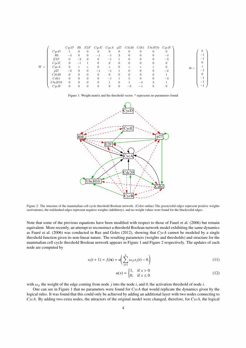
Figure 1: Weight matrix and the threshold vector. * represents no parameters found

CycE

E2F

CycA

Cdc20

UbcH10

Cdh1

CycB

CycD

p27Rb

Figure 2: The structure of the mammalian cell cycle threshold Boolean network. (Color online) The green/solid edges represent positive weights(activations), the red/dashed edges represent negative weights (inhibitory), and no weight values were found for the black/solid edges.

Note that some of the previous equations have been modified with respect to those of Faure et al. (2006) but remainequivalent. More recently, an attempt to reconstruct a threshold Boolean network model exhibiting the same dynamicsas Faure et al. (2006) was conducted in Ruz and Goles (2012), showing that CycA cannot be modeled by a singlethreshold function given its non-linear nature. The resulting parameters (weights and thresholds) and structure for themammalian cell cycle threshold Boolean network appears in Figure 1 and Figure 2 respectively. The updates of eachnode are computed by

xi(t + 1) = fi(x) = u( n∑

j=1

ω jix j(t) − θi

)(11)

u(x) =

1, if x > 00, if x ≤ 0 (12)

with ω ji the weight of the edge coming from node j into the node i, and θi the activation threshold of node i.One can see in Figure 1 that no parameters were found for CycA that would replicate the dynamics given by the

logical rules. It was found that this could only be achieved by adding an additional layer with two nodes connecting toCycA. By adding two extra nodes, the attractors of the original model were changed, therefore, for CycA, the logical

4

Pajek

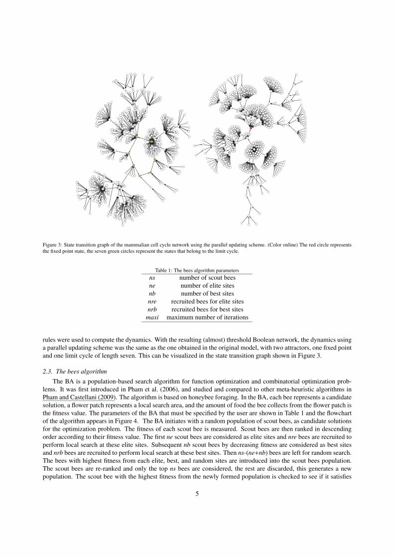
Figure 3: State transition graph of the mammalian cell cycle network using the parallel updating scheme. (Color online) The red circle representsthe fixed point state, the seven green circles represent the states that belong to the limit cycle.

Table 1: The bees algorithm parametersns number of scout beesne number of elite sitesnb number of best sitesnre recruited bees for elite sitesnrb recruited bees for best sites

maxi maximum number of iterations

rules were used to compute the dynamics. With the resulting (almost) threshold Boolean network, the dynamics usinga parallel updating scheme was the same as the one obtained in the original model, with two attractors, one fixed pointand one limit cycle of length seven. This can be visualized in the state transition graph shown in Figure 3.

2.3. The bees algorithm

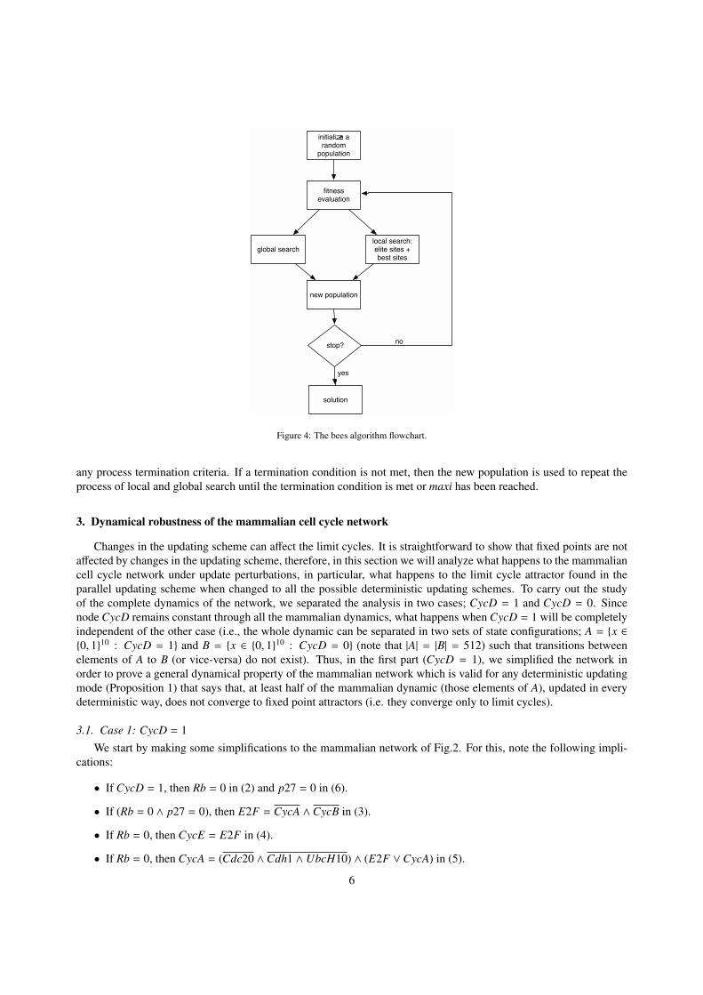
The BA is a population-based search algorithm for function optimization and combinatorial optimization prob-lems. It was first introduced in Pham et al. (2006), and studied and compared to other meta-heuristic algorithms inPham and Castellani (2009). The algorithm is based on honeybee foraging. In the BA, each bee represents a candidatesolution, a flower patch represents a local search area, and the amount of food the bee collects from the flower patch isthe fitness value. The parameters of the BA that must be specified by the user are shown in Table 1 and the flowchartof the algorithm appears in Figure 4. The BA initiates with a random population of scout bees, as candidate solutionsfor the optimization problem. The fitness of each scout bee is measured. Scout bees are then ranked in descendingorder according to their fitness value. The first ne scout bees are considered as elite sites and nre bees are recruited toperform local search at these elite sites. Subsequent nb scout bees by decreasing fitness are considered as best sitesand nrb bees are recruited to perform local search at these best sites. Then ns-(ne+nb) bees are left for random search.The bees with highest fitness from each elite, best, and random sites are introduced into the scout bees population.The scout bees are re-ranked and only the top ns bees are considered, the rest are discarded, this generates a newpopulation. The scout bee with the highest fitness from the newly formed population is checked to see if it satisfies

5

initialize a random population

fitness evaluation

global searchlocal search: elite sites + best sites

new population

stop?

solution

no

yes

Figure 4: The bees algorithm flowchart.

any process termination criteria. If a termination condition is not met, then the new population is used to repeat theprocess of local and global search until the termination condition is met or maxi has been reached.

3. Dynamical robustness of the mammalian cell cycle network

Changes in the updating scheme can affect the limit cycles. It is straightforward to show that fixed points are notaffected by changes in the updating scheme, therefore, in this section we will analyze what happens to the mammaliancell cycle network under update perturbations, in particular, what happens to the limit cycle attractor found in theparallel updating scheme when changed to all the possible deterministic updating schemes. To carry out the studyof the complete dynamics of the network, we separated the analysis in two cases; CycD = 1 and CycD = 0. Sincenode CycD remains constant through all the mammalian dynamics, what happens when CycD = 1 will be completelyindependent of the other case (i.e., the whole dynamic can be separated in two sets of state configurations; A = x ∈0, 110 : CycD = 1 and B = x ∈ 0, 110 : CycD = 0 (note that |A| = |B| = 512) such that transitions betweenelements of A to B (or vice-versa) do not exist). Thus, in the first part (CycD = 1), we simplified the network inorder to prove a general dynamical property of the mammalian network which is valid for any deterministic updatingmode (Proposition 1) that says that, at least half of the mammalian dynamic (those elements of A), updated in everydeterministic way, does not converge to fixed point attractors (i.e. they converge only to limit cycles).

3.1. Case 1: CycD = 1We start by making some simplifications to the mammalian network of Fig.2. For this, note the following impli-

cations:

• If CycD = 1, then Rb = 0 in (2) and p27 = 0 in (6).

• If (Rb = 0 ∧ p27 = 0), then E2F = CycA ∧CycB in (3).

• If Rb = 0, then CycE = E2F in (4).

• If Rb = 0, then CycA = (Cdc20 ∧Cdh1 ∧ UbcH10) ∧ (E2F ∨CycA) in (5).

6

• If p27 = 0, then Cdh1 = (CycA ∧CycB) ∨Cdc20 in (8).

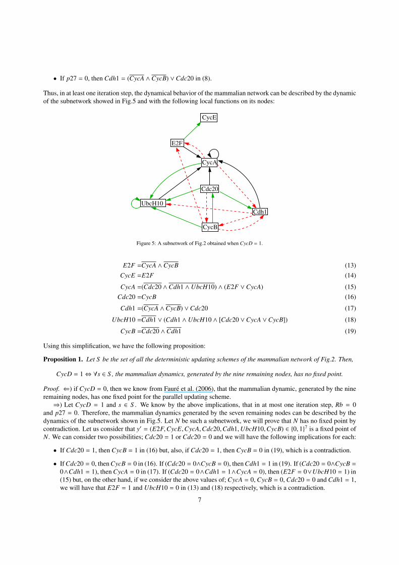
Thus, in at least one iteration step, the dynamical behavior of the mammalian network can be described by the dynamicof the subnetwork showed in Fig.5 and with the following local functions on its nodes:

CycE

E2F

CycA

Cdc20

UbcH10

Cdh1

CycB

Figure 5: A subnetwork of Fig.2 obtained when CycD = 1.

E2F =CycA ∧CycB (13)CycE =E2F (14)

CycA =(Cdc20 ∧Cdh1 ∧ UbcH10) ∧ (E2F ∨CycA) (15)Cdc20 =CycB (16)

Cdh1 =(CycA ∧CycB) ∨Cdc20 (17)

UbcH10 =Cdh1 ∨ (Cdh1 ∧ UbcH10 ∧ [Cdc20 ∨CycA ∨CycB]) (18)

CycB =Cdc20 ∧Cdh1 (19)

Using this simplification, we have the following proposition:

Proposition 1. Let S be the set of all the deterministic updating schemes of the mammalian network of Fig.2. Then,

CycD = 1⇔ ∀s ∈ S , the mammalian dynamics, generated by the nine remaining nodes, has no fixed point.

Proof. ⇐) if CycD = 0, then we know from Faure et al. (2006), that the mammalian dynamic, generated by the nineremaining nodes, has one fixed point for the parallel updating scheme.⇒) Let CycD = 1 and s ∈ S . We know by the above implications, that in at most one iteration step, Rb = 0

and p27 = 0. Therefore, the mammalian dynamics generated by the seven remaining nodes can be described by thedynamics of the subnetwork shown in Fig.5. Let N be such a subnetwork, we will prove that N has no fixed point bycontradiction. Let us consider that y′ = (E2F,CycE,CycA,Cdc20,Cdh1,UbcH10,CycB) ∈ 0, 17 is a fixed point ofN. We can consider two possibilities; Cdc20 = 1 or Cdc20 = 0 and we will have the following implications for each:

• If Cdc20 = 1, then CycB = 1 in (16) but, also, if Cdc20 = 1, then CycB = 0 in (19), which is a contradiction.

• If Cdc20 = 0, then CycB = 0 in (16). If (Cdc20 = 0∧CycB = 0), then Cdh1 = 1 in (19). If (Cdc20 = 0∧CycB =

0∧Cdh1 = 1), then CycA = 0 in (17). If (Cdc20 = 0∧Cdh1 = 1∧CycA = 0), then (E2F = 0∨UbcH10 = 1) in(15) but, on the other hand, if we consider the above values of; CycA = 0, CycB = 0, Cdc20 = 0 and Cdh1 = 1,we will have that E2F = 1 and UbcH10 = 0 in (13) and (18) respectively, which is a contradiction.

7

Therefore, N cannot have fixed points.

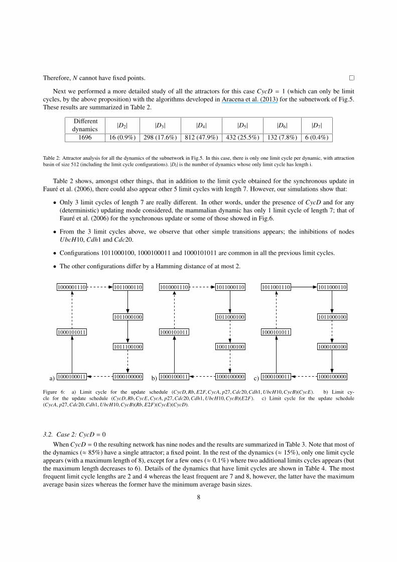
Next we performed a more detailed study of all the attractors for this case CycD = 1 (which can only be limitcycles, by the above proposition) with the algorithms developed in Aracena et al. (2013) for the subnetwork of Fig.5.These results are summarized in Table 2.

Differentdynamics |D2| |D3| |D4| |D5| |D6| |D7|

1696 16 (0.9%) 298 (17.6%) 812 (47.9%) 432 (25.5%) 132 (7.8%) 6 (0.4%)

Table 2: Attractor analysis for all the dynamics of the subnetwork in Fig.5. In this case, there is only one limit cycle per dynamic, with attractionbasin of size 512 (including the limit cycle configurations). |Di | is the number of dynamics whose only limit cycle has length i.

Table 2 shows, amongst other things, that in addition to the limit cycle obtained for the synchronous update inFaure et al. (2006), there could also appear other 5 limit cycles with length 7. However, our simulations show that:

• Only 3 limit cycles of length 7 are really different. In other words, under the presence of CycD and for any(deterministic) updating mode considered, the mammalian dynamic has only 1 limit cycle of length 7; that ofFaure et al. (2006) for the synchronous update or some of those showed in Fig.6.

• From the 3 limit cycles above, we observe that other simple transitions appears; the inhibitions of nodesUbcH10, Cdh1 and Cdc20.

• Configurations 1011000100, 1000100011 and 1000101011 are common in all the previous limit cycles.

• The other configurations differ by a Hamming distance of at most 2.

a)

1011000110

1011000100

1011100100

1000100000

1000001110

1000101011

1000100011 b)

1011000110

1011000100

1001100100

1000100000

1010001110

1000101011

1000100011 c)

1011000110

1011000100

1000100100

1000100000

1011001110

1000101011

1000100011

Figure 6: a) Limit cycle for the update schedule (CycD,Rb, E2F,CycA, p27,Cdc20,Cdh1,UbcH10,CycB)(CycE). b) Limit cy-cle for the update schedule (CycD,Rb,CycE,CycA, p27,Cdc20,Cdh1,UbcH10,CycB)(E2F). c) Limit cycle for the update schedule(CycA, p27,Cdc20,Cdh1,UbcH10,CycB)(Rb, E2F)(CycE)(CycD).

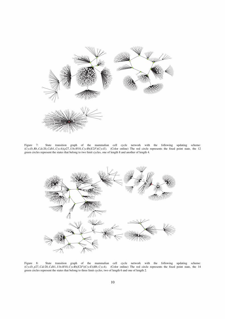
3.2. Case 2: CycD = 0When CycD = 0 the resulting network has nine nodes and the results are summarized in Table 3. Note that most of

the dynamics (≈ 85%) have a single attractor; a fixed point. In the rest of the dynamics (≈ 15%), only one limit cycleappears (with a maximum length of 8), except for a few ones (≈ 0.1%) where two additional limits cycles appears (butthe maximum length decreases to 6). Details of the dynamics that have limit cycles are shown in Table 4. The mostfrequent limit cycle lengths are 2 and 4 whereas the least frequent are 7 and 8, however, the latter have the maximumaverage basin sizes whereas the former have the minimum average basin sizes.

8

Number ofdynamics

Range of lim.cycles length

Different 130297 2-8with 1 lim. cycle 19719 (15.1%) 2-8with 2 lim. cycles 163 (0.1%) 2-6

without lim. cycles 110415 (84.7%) –

Table 3: General attractor analysis for all the dynamics of the subnetwork in Fig.2 when CycD = 0.

Dynamics withat least 1

AverageBasin Size

lim. cycle of length 2 6587 140.5lim. cycle of length 3 3383 321.7lim. cycle of length 4 6148 273.4lim. cycle of length 5 2892 298.1lim. cycle of length 6 919 325lim. cycle of length 7 21 363.3lim. cycle of length 8 63 372.9

Table 4: A more detailed analysis of the values showed in Table 3 for the dynamics having a limit cycle.

In summary, the previous cases of analysis allow us to say that every deterministic dynamic of the mammaliannetwork can be divided into two components; one containing half of the configurations converging to a single limitcycle (case CycD = 1), the other one, with a single fixed point and, possibly, with at most two limit cycles.

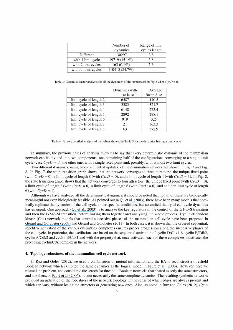
Two different dynamics, using block sequential updates, of the mammalian network are shown in Fig. 7 and Fig.8. In Fig. 7, the state transition graph shows that the network converges to three attractors: the unique fixed point(with CycD = 0), a limit cycle of length 8 (with CycD = 0), and a limit cycle of length 4 (with CycD = 1). In Fig. 8,the state transition graph shows that the network converges to four attractors: the unique fixed point (with CycD = 0),a limit cycle of length 2 (with CycD = 0), a limit cycle of length 6 (with CycD = 0), and another limit cycle of length6 (with CycD = 1).

Although we have analyzed all the deterministic dynamics, it should be noted that not all of these are biologicallymeaningful nor even biologically feasible. As pointed out in Qu et al. (2003), there have been many models that nom-inally replicate the dynamics of the cell cycle under specific conditions, but no unified theory of cell cycle dynamicshas emerged. One approach (Qu et al., 2003) is to analyze the key regulators in the control of the G1-to-S transitionand then the G2-to-M transition, before linking them together and analyzing the whole process. Cyclin-dependentkinase (Cdk) network models that control successive phases of the mammalian cell cycle have been proposed inGerard and Goldbeter (2009) and Gerard and Goldbeter (2011). In both cases, it is shown that the ordered sequential,repetitive activation of the various cyclin/Cdk complexes ensures proper progression along the successive phases ofthe cell cycle. In particular, the oscillations are based on the sequential activation of cyclin D/Cdk4-6, cyclin E/Cdk2,cyclin A/Cdk2 and cyclin B/Cdk1 and with the property that, once activated, each of these complexes inactivates thepreceding cyclin/Cdk complex in the network.

4. Topology robustness of the mammalian cell cycle network

In Ruz and Goles (2012), we used a combination of mutual information and the BA to reconstruct a thresholdBoolean network which exhibited the same dynamics as the logical model in Faure et al. (2006). However, here werelaxed the problem, and considered the search for threshold Boolean networks that shared exactly the same attractors,and no others, of Faure et al. (2006), but not necessarily the same complete dynamics. The resulting synthetic networksprovided an indication of the robustness of the network topology, in the sense of which edges are always present andwhich can vary, without losing the attractors or generating new ones. Also, as noted in Ruz and Goles (2012), CycA

9

Pajek

Figure 7: State transition graph of the mammalian cell cycle network with the following updating scheme:(CycD,Rb,Cdc20,Cdh1,CycA)(p27,UbcH10,CycB)(E2F)(CycE). (Color online) The red circle represents the fixed point state, the 12green circles represent the states that belong to two limit cycles, one of length 8 and another of length 4.

Pajek

Figure 8: State transition graph of the mammalian cell cycle network with the following updating scheme:(CycD, p27,Cdc20,Cdh1,UbcH10,CycB)(E2F)(CycE)(Rb,CycA). (Color online) The red circle represents the fixed point state, the 14green circles represent the states that belong to three limit cycles, two of length 6 and one of length 2.

10

cannot be modeled by a single threshold function, therefore, it is natural to ask if this phenomena is due to the specificattractors or the complete dynamics of the logical model. To carry out this analysis we used BA to search for networksthat contain exactly the same attractors as the original model and then analyzed the resulting topologies.

There are three parts that need to be defined when implementing the BA.

4.1. Coding of solutions

The solutions, network weights and thresholds, are coded using an adjacency matrix Ω and a vector Θ respectively,as in Figure 1. The initial Ωg, g = 1, . . . , ns in the BA were generated randomly, with an indegree K ≤ 5 and integerweight values in the range [−5, 5]. The threshold vectors Θg where all set to the original values that appear in Figure 1.The * was replaced by a 0.

4.2. Definition of the fitness function

The fitness function for the Boolean network B, was given by the deviation of the network output, defined by oi

for each node i, and the target value ai (attractor) for each node i, which was computed by

f itness(B) =1

8n

8∑t=1

n∑i=1

(oi(t) − ai(t))2 (20)

where n is the number of nodes in the network, and 8 is the number of attractor vectors that the network must contain.For this particular application, there is one limit cycle of length seven and one fixed point. Also, the solutions werepenalized by adding half of the maximum value of (20), (i.e. 0.5, when additional attractors appeared).

4.3. Neighborhood search strategy

During the local search, each recruited bee from the elite or best sites generates a candidate solution, Ωnew andΘnew, based on the current solution, Ωold and Θold, corresponding to the scout bee which found that site. For this, aneighborhood search strategy was used for the weight matrix (the pseudocode appears in Algorithm 1), and anotherfor the threshold vector (the pseudocode appears in Algorithm 2).

Using the above definitions, the general bees algorithm is shown in Algorithm 3.

4.4. Simulation setup

The BA algorithm was used to find 100 networks that contained exactly the two attractors of the original logicalmodel. The following BA parameters were used ns = 20, ne = 5, nb = 10, nre = 20, nrb = 5, and maxi = 4000.For Algorithm 1, the neighborhood range parameter ngh was set to 3. These parameters were found empirically afterseveral runs based on the effectiveness of the resulting networks.

4.5. Results

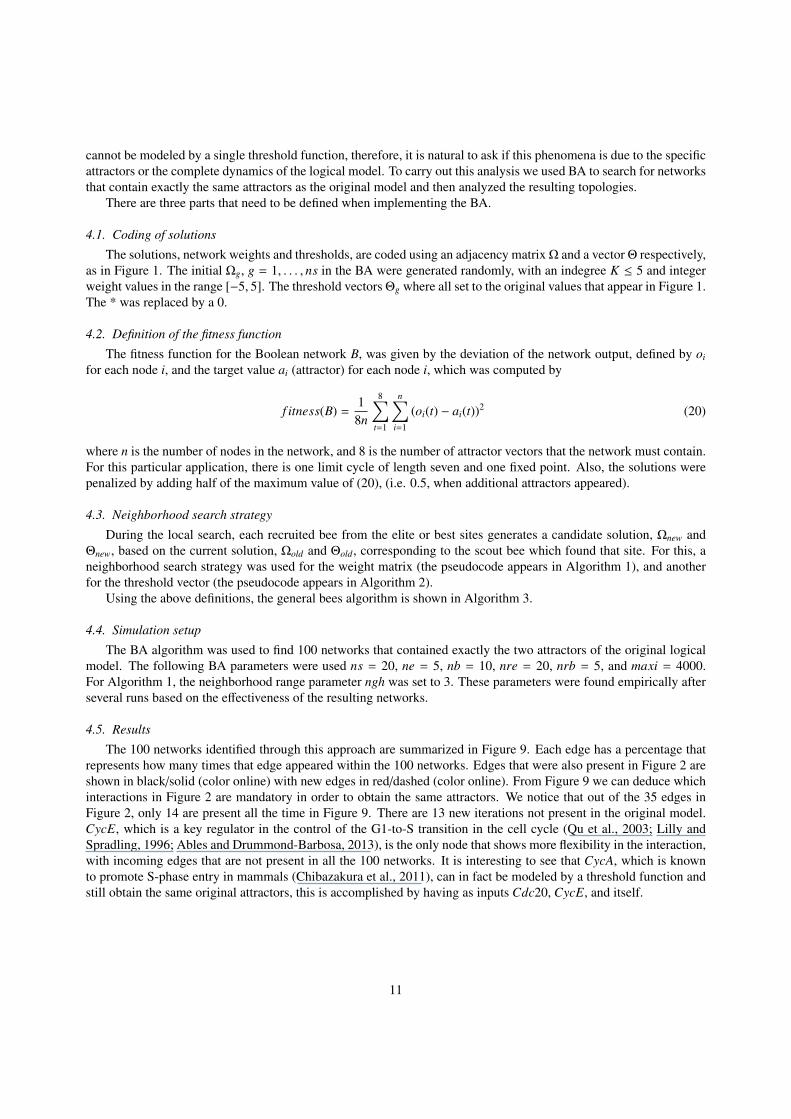
The 100 networks identified through this approach are summarized in Figure 9. Each edge has a percentage thatrepresents how many times that edge appeared within the 100 networks. Edges that were also present in Figure 2 areshown in black/solid (color online) with new edges in red/dashed (color online). From Figure 9 we can deduce whichinteractions in Figure 2 are mandatory in order to obtain the same attractors. We notice that out of the 35 edges inFigure 2, only 14 are present all the time in Figure 9. There are 13 new iterations not present in the original model.CycE, which is a key regulator in the control of the G1-to-S transition in the cell cycle (Qu et al., 2003; Lilly andSpradling, 1996; Ables and Drummond-Barbosa, 2013), is the only node that shows more flexibility in the interaction,with incoming edges that are not present in all the 100 networks. It is interesting to see that CycA, which is knownto promote S-phase entry in mammals (Chibazakura et al., 2011), can in fact be modeled by a threshold function andstill obtain the same original attractors, this is accomplished by having as inputs Cdc20, CycE, and itself.

11

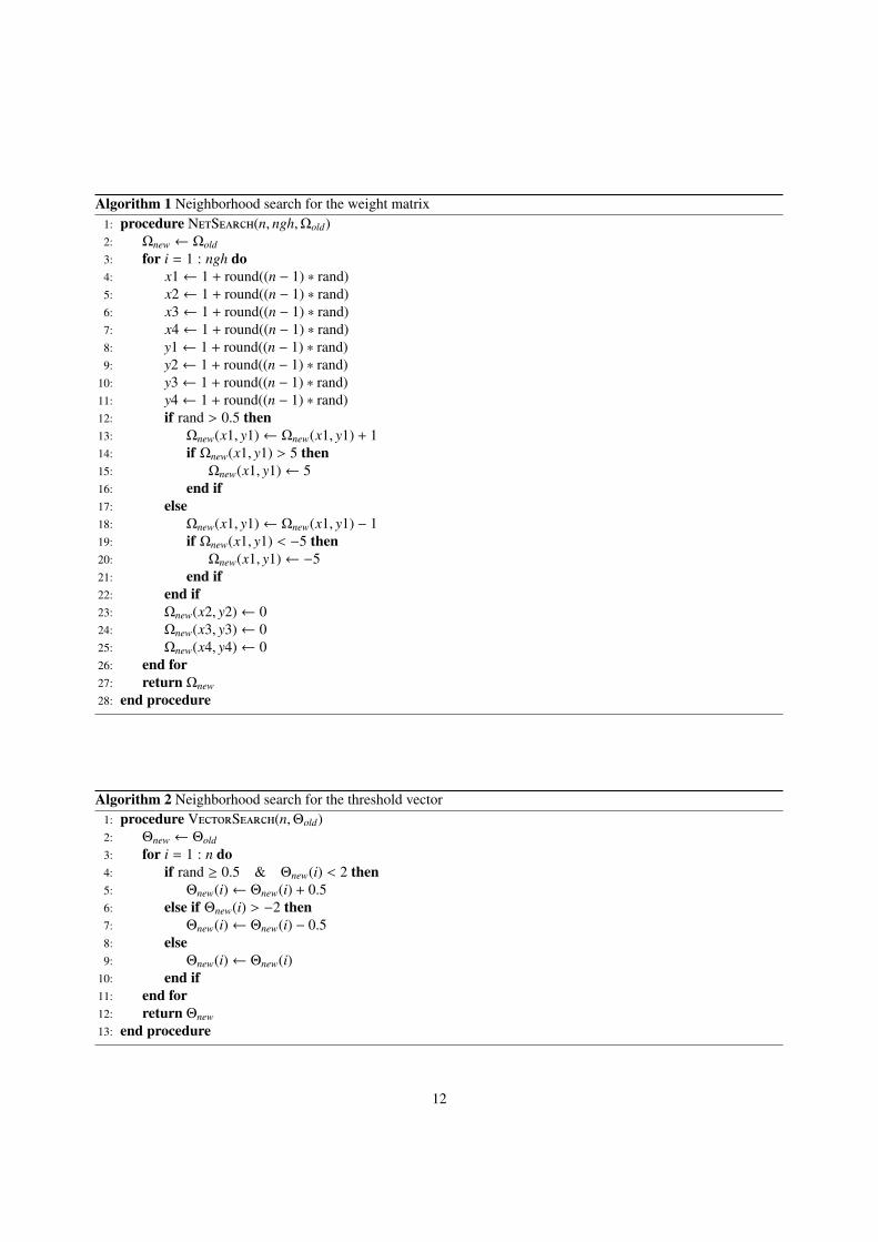
Algorithm 1 Neighborhood search for the weight matrix1: procedure NetSearch(n, ngh,Ωold)2: Ωnew ← Ωold

3: for i = 1 : ngh do4: x1← 1 + round((n − 1) ∗ rand)5: x2← 1 + round((n − 1) ∗ rand)6: x3← 1 + round((n − 1) ∗ rand)7: x4← 1 + round((n − 1) ∗ rand)8: y1← 1 + round((n − 1) ∗ rand)9: y2← 1 + round((n − 1) ∗ rand)

10: y3← 1 + round((n − 1) ∗ rand)11: y4← 1 + round((n − 1) ∗ rand)12: if rand > 0.5 then13: Ωnew(x1, y1)← Ωnew(x1, y1) + 114: if Ωnew(x1, y1) > 5 then15: Ωnew(x1, y1)← 516: end if17: else18: Ωnew(x1, y1)← Ωnew(x1, y1) − 119: if Ωnew(x1, y1) < −5 then20: Ωnew(x1, y1)← −521: end if22: end if23: Ωnew(x2, y2)← 024: Ωnew(x3, y3)← 025: Ωnew(x4, y4)← 026: end for27: return Ωnew

28: end procedure

Algorithm 2 Neighborhood search for the threshold vector1: procedure VectorSearch(n,Θold)2: Θnew ← Θold

3: for i = 1 : n do4: if rand ≥ 0.5 & Θnew(i) < 2 then5: Θnew(i)← Θnew(i) + 0.56: else if Θnew(i) > −2 then7: Θnew(i)← Θnew(i) − 0.58: else9: Θnew(i)← Θnew(i)

10: end if11: end for12: return Θnew

13: end procedure

12

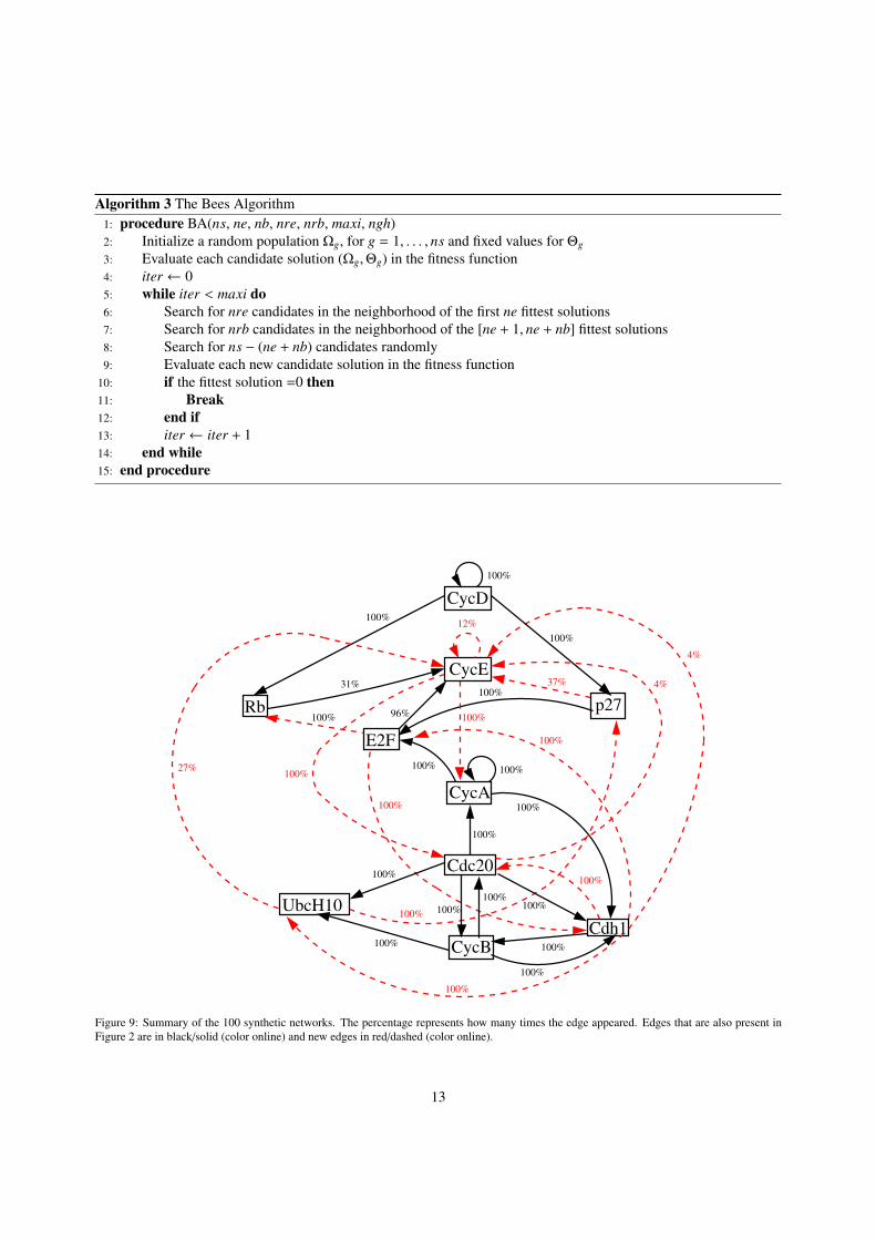
Algorithm 3 The Bees Algorithm1: procedure BA(ns, ne, nb, nre, nrb, maxi, ngh)2: Initialize a random population Ωg, for g = 1, . . . , ns and fixed values for Θg

3: Evaluate each candidate solution (Ωg,Θg) in the fitness function4: iter ← 05: while iter < maxi do6: Search for nre candidates in the neighborhood of the first ne fittest solutions7: Search for nrb candidates in the neighborhood of the [ne + 1, ne + nb] fittest solutions8: Search for ns − (ne + nb) candidates randomly9: Evaluate each new candidate solution in the fitness function

10: if the fittest solution =0 then11: Break12: end if13: iter ← iter + 114: end while15: end procedure

31%100%

100%

100%

100%

12%

37%

100%

100%

100%100%

96%

100%

100%

100%

100%

100%

100%

27%

4%

4%

100%

100%

100%

100%

100%

100%

100%

100%100%

CycE

E2F

CycA

Cdc20

UbcH10

Cdh1

p27Rb

CycD

CycB

Figure 9: Summary of the 100 synthetic networks. The percentage represents how many times the edge appeared. Edges that are also present inFigure 2 are in black/solid (color online) and new edges in red/dashed (color online).

13

5. Conclusion

The mammalian cell cycle logical model and its equivalent threshold Boolean network model were analyzed.First we studied the behavior of the model under update perturbations, in particular, we analyzed what happens to theattractors of the network for all the possible deterministic dynamics. To do this, we separated the network’s dynamicsaccording to the two possible values of the CycD node, due to its constant nature. We have not only validated theresults presented in Faure et al. (2006) for the case CycD = 1; the existence of a single limit cycle of length seven and afix point, under the parallel updating scheme, but we have also proved a simple result (Proposition 1) that explains thisphenomenon whatever the updating scheme considered. Moreover, by using tools for the classification of differentdynamics (Aracena et al. (2013)), we have completely determined the full asymptotic behavior of the mammaliannetwork under every deterministic updating mode for both cases; CycD = 1 and CycD = 0.

In the first case, we make some preliminary simplifications in the model which are equivalent to say that thesubconfiguration (CycD,Rb, p27) = (1, 0, 0) is an alliance in the sense of Goles et al. (2013) because these valuesremain invariant against any deterministic update schedule. On the other hand, we observe that the range of the limitcycle lengths is between 2 and 7, being 4 the most frequent length (about 48% of all the different dynamics) and eachof these cycles with a basin of attraction containing all the configurations such that CycD = 1. Furthermore, in theparticular case of limit cycles of length 7, we exhibit all the possible limit cycles of the same length (evidently, inthe presence of CycD) that can exist when the mammalian network is updated in a deterministic way. These limitcycles are not very different between them (Hamming distance bounded by 2), they have 3 common configurationsand, additionally to the activations of nodes Cdc20 and CycA showed in Faure et al. (2006), these limit cycles exhibitother simple transitions; the inhibition of nodes UbcH10, Cdh1 and Cdc20.

In the second case, it was observed that most of the dynamics have the fixed point, and only a few have additionallyone or two limit cycles, with a maximum limit cycle length equal to 8, although the most frequent cycle length is 2.We notice that, although the mammalian cell cycle network model was constructed considering the parallel updatingscheme, the limit cycles vary considerably in type and basin size, depending on the updating scheme employed,resulting in a model which is not very robust with respect to update perturbation. We could say that the limit cycleused to represent the cell cycle is an artifact caused by the parallel update in the sense of Klemm and Bornholdt(2005).

Given that genes are activated or inhibited in a fundamentally asynchronous way, GRN modelers, under theBoolean network approach, should try to associate cell differentiation or any biological behavior of interest to fixedpoints of the model, given that these are invariant to update changes (perturbations), therefore, eliminating the updateissue when considering biological implementations.

To analyze the topology of the network, we adopted a reverse engineering approach, using BA to reconstructthreshold Boolean networks that contained exactly the same attractors as the original model. 100 networks werefound, where it was possible to identify which interactions (edges) are present all the time, and new interactions thatyield the same attractors. By relaxing the problem to having networks with the same attractors as the original logicalmodel, it was found the CycA can be modeled by a threshold function, with inputs Cdc20, CycE, and itself.

Although the techniques used in this work were applied to analyze the mammalian cell cycle network, these aregeneral, and could be employed to analyze other logical or threshold network models of gene regulatory networks.

Acknowledgment

The authors would like to thank Conicyt-Chile under grant Fondecyt 11110088 (G.A.R.), Fondecyt 1100003(E.G.), Fondecyt 3130466 (M.M.), Basal(Conicyt)-CMM, and ANILLO ACT-88 for financially supporting this re-search.

References

Ables, E.T., Drummond-Barbosa, D., 2013. Cyclin E controls Drosophila female germline stem cell maintenance independently of its role inproliferation by modulating responsiveness to niche signals. Development 140, 530–540.

Akutsu, T., Miyano, S., Kuhara, S., 1999. Identification of genetic networks from a small number of gene expression patterns under the Booleannetwork model, in: Pac. Symp. Biocomput, pp. 17–28.

14

Aracena, J., Demongeot, J., Fanchon, E., Montalva, M., 2013. On the number of different dynamics in Boolean networks with deterministic updateschedules. Mathematical Biosciences 242, 188 – 194.

Aracena, J., Goles, E., Moreira, A., Salinas, L., 2009. On the robustness of update schedules in Boolean networks. Biosystems 97, 1–8.Chibazakura, T., Kamachi, K., Ohara, M., Tane, S., Yoshikawa, H., Roberts, J.M., 2011. Cyclin A promotes S-phase entry via interaction with the

replication licensing factor Mcm7. Molecular and Cellular Biology 31, 248–255.Chowdhury, A.R., Chetty, M., Vinh, X.N., 2012. On the reconstruction of genetic network from partial microarray data. volume 7663 LNCS of

Lecture Notes in Computer Science (including subseries Lecture Notes in Artificial Intelligence and Lecture Notes in Bioinformatics).Davidich, M.I., Bornholdt, S., 2008. Boolean network model predicts cell cycle sequence of fission yeast. PLoS ONE 3(2), e1672.Demongeot, J., Elena, A., Sene, S., 2008. Robustness in regulatory networks: A multi-disciplinary approach. Acta Biotheoretica 56, 27–49.Faure, A., Naldi, A., Chaouiya, C., Thieffry, D., 2006. Dynamical analysis of a generic Boolean model for the control of the mammalian cell cycle.

Bioinformatics 22, e124–e131.Forghany, Z., Davarynejad, M., Snaar-Jagalska, B.E., 2012. Gene regulatory network model identification using artificial bee colony and swarm

intelligence, in: 2012 IEEE Congress on Evolutionary Computation, CEC 2012.Gerard, C., Goldbeter, A., 2009. Temporal self-organization of the cyclin/Cdk network driving the mammalian cell cycle. PNAS 106, 21643–21648.Gerard, C., Goldbeter, A., 2011. A skeleton model for the network of cyclin-dependent kinases driving the mammalian cell cycle. Interface Focus

1, 24–35.Goles, E., Montalva, M., Ruz, G.A., 2013. Deconstruction and dynamical robustness of regulatory networks: Application to the yeast cell cycle

networks. Bulletin of mathematical biology 75, 939–966.Gonzalez, O.R., Kuper, C., Jung, K., Naval Jr., P.C., Mendoza, E., 2007. Parameter estimation using simulated annealing for s-system models of

biochemical networks. Bioinformatics 23, 480–486.Kauffman, S., Peterson, C., Samuelsson, B., Troein, C., 2003. Random Boolean network models and the yeast transcriptional network. PNAS 100,

14796–14799.Kauffman, S.A., 1969. Metabolic stability and epigenesis in randomly constructed genetic nets. Journal of Theoretical Biology 22, 437–467.Kentzoglanakis, K., Poole, M., 2012. A swarm intelligence framework for reconstructing gene networks: Searching for biologically plausible

architectures. IEEE/ACM Transactions on Computational Biology and Bioinformatics 29, 358–371.Kikuchi, S., Tominaga, D., Arita, M., Takahashi, K., Tomita, M., 2003. Dynamics modeling of genetic networks using genetic algorithm and

s-system. Bioinformatics 19, 643–650.Klemm, K., Bornholdt, S., 2005. Stable and unstable attractors in boolean networks. Phys. Rev. E. 72, 055101–055104.Li, F., Long, T., Lu, Y., Ouyang, Q., Tang, C., 2004. The yeast cell-cycle network is robustly designed. PNAS 101, 4781–4786.Liang, S., Fuhrman, S., Somogyi, R., 1998. Reveal, a general reverse engineering algorithm for inference of genetic network architectures, in: Pac.

Symp. Biocomput, pp. 18–29.Lilly, M.A., Spradling, A.C., 1996. The drosophila endocycle is controlled by Cyclin E and lacks a checkpoint ensuring S-phase completion. Genes

& Development 10, 2514–2526.Liu, G., Feng, W., Wang, H., Liu, L., Zhou, C., 2009. Reconstruction of gene regulatory networks based on two-stage Bayesian network structure

learning algorithm. Journal of Bionic Engineering 6, 86–92.Mendoza, L., Alvarez-Buylla, E.R., 1998. Dynamics of the genetic regulatory network for arabidopsis thaliana flower morphogenesis. J Theor

Biol. 193, 307–319.Mendoza, M.R., Lopes, F.M., Bazzan, A.L.C., 2012. Reverse engineering of grns: An evolutionary approach based on the tsallis entropy, in:

GECCO’12 - Proceedings of the 14th International Conference on Genetic and Evolutionary Computation, pp. 185–192.Noman, N., Iba, H., 2007. Inferring gene regulatory networks using differential evolution with local search heuristics. IEEE/ACM Transactions on

Computational Biology and Bioinformatics 4, 634–647.Novak, B., Tayson, J.J., 2004. A model for restriction point control of the mammalian cell cycle. Journal of Theoretical Biology 230, 563–579.Pham, D.T., Castellani, M., 2009. The bees algorithm: modelling foraging behaviour to solve continuous optimization problems. Proc. IMechE

Part C: J. Mechanical Engineering Science 223, 2919–2938.Pham, D.T., Ghanbarzadeh, A., Koc, E., Otri, S., Rahim, S., Zaidi, M., 2006. The bees algorithm, a novel tool for complex optimisation problems,

in: Proc. of the Second International Virtual Conference on Intelligent production machines and systems (IPROMS 2006), pp. 454–459.Qu, Z., Weiss, J.N., MacLellan, W.R., 2003. Regulation of the mammalian cell cycle: a model of the G1-to-S transition. Am J Physiol Cell Physiol

284, C349–C364.Repsilber, D., Liljenstrom, H., Andersson, S.G.E., 2002. Reverse engineering of regulatory networks: simulation studies on a genetic algorithm

approach for ranking hypotheses. Biosystems 66, 31–41.Ruz, G.A., Goles, E., 2010. Learning gene regulatory networks with predefined attractors for sequential updating schemes using simulated

annealing, in: Proc. of IEEE the Ninth International Conference on Machine Learning and Applications (ICMLA 2010), pp. 889–894.Ruz, G.A., Goles, E., 2012. Reconstruction and update robustness of the mammalian cell cycle network, in: 2012 IEEE Symposium on Computa-

tional Intelligence and Computational Biology, CIBCB 2012, pp. 397–403.Ruz, G.A., Goles, E., 2013. Learning gene regulatory networks using the bees algorithm. Neural Computing and Applications 22, 63–70.Ruz, G.A., Timmermann, T., Goles, E., 2012. Building synthetic networks of the budding yeast cell-cycle using swarm intelligence, in: Proceedings

- 2012 11th International Conference on Machine Learning and Applications, ICMLA 2012, pp. 120–125.Wuensche, A., 2004. Basins of attraction in network dynamics: A conceptual framework for biomolecular networks, in: Modularity in Development

and Evolution, pp. 288–311.Xu, R., Wunsch II, D.C., Frank, R.L., 2007. Inference of genetic regulatory networks with recurrent neural network models using particle swarm

optimization. IEEE/ACM Transactions on Computational Biology and Bioinformatics 4, 681–692.

15