Dynamic Topography Estimates Using Geosat Data and A Gravimetric Geoid In the Gulf Stream Region

Geophys. J . fnt. (1994) 117, 511-528

Dynamic topography estimates using Geosat data and a gravimetric geoid in the Gulf Stream region

Richard H. Rapp and Yan Ming Wang Department of Geodetic Science and Surveying, The Ohio Stare University, Columbus, OH 43210, USA

Accepted 1993 November 2. Received 1993 October 26; in original form 1993 June 22

S U M M A R Y A gravimetric geoid undulation, on a 3' x 3' grid has been calculated in the Gulf Stream region: 30" 5 @ I 45", 278" 5 ,I 5 318". These undulations were calculated using two 360 potential coefficient models, land, ship and altimeter-derived gravity anomalies, and bathymetric data. Least-squares collocation and fast Fourier transform procedures were used with various data selection and gridding procedures. Results from five different undulation computations are described with comparisons made with synthetic geoid undulations along Geosut tracks in the region. The standard deviation of the undulation differences was f 1 4 c m when a cubic polynomial was used to model long-wavelength errors. A point verification of the geoid undulation at the laser tracking station on Bermuda was also made with a discrepancy ('ground truth' minus model undulation) of 40 cm, within the predicted standard deviation. The gravimetric geoid undulation was used to compute dynamic topography along Geosat tracks for comparison with existing estimates based on hydrographic data in the Gulf Stream region. The agreement between these two estimates is on the order of f 1 5 cm although the discrepancies can reach 60 cm. The larger differences are usually associated with a location on a track that passes near a seamount where the gravity data may be inadequate to represent the high-frequency variations in the geoid undulations. This effect will be represented in the undulation standard deviations that have been calculated using the least-squares collocation procedure. The average accuracy is f l 6 c m with the range from f 1 4 to f48cm. The dynamic height derived from the gravimetric undulations and altimeter data has been used to calculate characteristics of the Gulf Stream (width, velocity, centre location, height profile) using an implied velocity model for the set. The results are compared with previous estimates with generally good agreement. However, the maximum velocities and the jump function are approximately 30 per cent larger than previous studies that used an average of altimeter tracks to define the geoid undulation. The dynamic topography was calculated for the entire region using a mean sea surface based on Geos-3, Seasat and Geosat data. The results are compared with two hydrographic estimates due to Martel/Wunsch and LeTraon/Mercier. The agreement is at the f 2 5 c m level with the best correlation coefficient reaching 0.72 with the Martel/Wunsch model.

Key words: geoid, Geosat, North Atlantic, topography.

satellite altimeter measurements to the ocean surface and accurate geoid undulations, dynamic topography can be INTRODUCTION

Dynamic topography will be defined as the separation studied along the satellite ground track or on a global, or between the ocean surface and the geoid. The geoid is an long-wavelength, basis. An example of local studies of equipotential surface of the Earth's gravity field that dynamic topography is the analysis of Cheney & Marsh coincides in a spatial and time average sense with the mean (1981) using Seasat altimeter data and geoid undulations ocean surface in a global (or ocean-wide) sense. Using derived from a potential coefficient model and surface

511

by guest on February 19, 2016http://gji.oxfordjournals.org/

Dow

nloaded from

http://gji.oxfordjournals.org/

512 R. H . Rapp and Y . M . Wang

gravity data. Global analyses of dynamic topography have used long-wavelength geoid undulation models implied by potential coefficient models that are estimated, in most cases, simultaneously with a spherical harmonic representation of dynamic topography (Denker & Rapp 1990; Nerem, Tapley & Shun 1990). This paper covers local dynamic topography determinations using geoid undulation data and no additional discussion on global determinations is considered.

Although geoid undulations play a critical role in one procedure for determining dynamic topography, the lack of a sufficiently accurate gravimetrically determined geoid has hampered this type of analysis. The limitation has been pointed out by numerous authors (e.g. Mitchell, Hallock & Thompson 1987; Zlotnicki & Marsh 1989; Kelly & Gille 1990; Tai 1990). Non-gravimetrically estimated geoid undulation determinations have been carried out by temporarily averaging sea surface heights, and considering the average geoid (Kelly & Gille 1990), or by constructing a 'synthetic geoid' (Porter et al. 1989) from an altimetrically implied mean sea surface and a mean mesocale dynamic topography implied by an oceanographic model such as the Harvard Gulfcast (Robinson et al. 1989). In procedures using satellite altimeter data the resultant 'geoid' is dependent on the radial orbit accuracy of the altimeter satellite and/or the radial orbit error models used to improve the distributed altimeter data. Incomplete radial error removal can cause synthetic geoid determinations to be contaminated by the residual errors. Errors in the oceanographic dynamic topography affect the estimate of the synthetic geoid.

In the past several years numerous improvements have been made concerning available terrestrial gravimetric data, altimeter-derived gravity anomalies and potential coefficient models, as well as new theory that allows the rapid calculation of geoid undulations considering the accuracy of the potential coefficient model and the terrestrial data. This paper describes the computation of a gravimetric geoid in the north-west Atlantic Ocean using several different data sets and techniques. The geoid undulations are used to calculate dynamic topography using Geosat altimeter data with comparisons made to oceanographic estimates described by Porter, Dobson & Glenn (1992a, b).

DATA TO B E USED

Based on the general location of the Gulf Stream shown in Zlotnicki (1990), the following region was chosen for the geoid undulation computation: 30" 5 @ 5 45"; 278" 5 A 5

318". This region includes a significant portion of the continental USA in order to keep the area rectangular for computational convenience. Other published geoid undulation computations for this general area are those of Marsh & Chang (1978), Albuisson et al. (1979) and Wessel & Watts (1988).

The general technique for the geoid undulation determination is to combine a potential coefficients representation of the Earth's gravitational potential with surface gravity data. The potential coefficient models to be used are the degree 360 model described in Rapp, Wang & Pavlis (1991a) and the JGM-2 model (Lerch et al. 1993) augmented by the OSU91A model from degree 71 to 360.

The OSU91A model was a combination of an a priori potential coefficient model (GEM-T2, Marsh et al. 1990), terrestrial gravity data, local gravity anomalies derived from satellite altimeter data and Geosat altimeter data. The long-wavelength accuracy of the OSU91A model is directly influenced by the accuracy of the GEM-T2 model.

The terrestrial gravity data used come from several sources. The primary source of the terrestrial ship data was Cochran (1990, private communication) who made available data from the Lamont-Doherty Geological Observatory gravity library (Wessel & Watts 1988). A total of 157300 points were obtained in the following area: 30"s @ 545"; 278" 5 A 5 318". These data were obtained from ship data that had been cross-over adjusted to reduce inconsistencies in the data. A bias term remained in the free-air anomalies as is discussed shortly.

Additional gravity data, primarily in the Bermuda area (31" 5 @ 5 34"; 294" 5 A 5 297") were obtained from the National Geodetic Survey in 1983. A total of 15731 point values were available and used previously by Despotakis (1987) for a geoid undulation computation at a laser tracking station on Bermuda. Gravity data in the Nova Scotia area, near @=43", A=295", were taken from the National Geodetic Survey point data file that was on the CD-ROM GRAVITY (Hittelman et al. 1992). A 3 ' x 3 ' terrain corrected free-air anomaly data set for the USA was provided by Milbert ( I 992, private communication). This data set was used in the computation of GEOID90 (Milbert 1991). A subset (24" 5 @ 5 53"; 230" 5 A 5 294") of the full data set was used in this geoid determination.

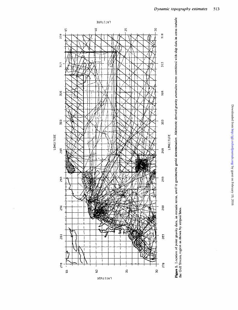
A plot of all the available point data (excluding the 3' x 3' gridded data) is shown in Fig. 1. One clearly sees substantial areas, primarily in the eastern part, where no point data is available in numerous 1" X 1" compartments. Some of these empty areas are in locations of irregular bathymetry (e.g. sea mounts) that create significant signatures in the geoid. In later portions of our tests, we used gravity anomalies, on a 0.125" grid, derived from Geos-3, Seasat and Geosat altimeter data (BaSiC & Rapp 1992). These data would be used (1) in a 2" border outside the basic computational area to reduce edge effects and (2) in conjunction with the ship data in areas for which the altimeter anomaly predictions would not be adversely affected by the dynamic topography not being taken into account in the estimation of the gravity anomalies. This area was chosen to be outside of the Gulf Stream area and away from the coastal areas where the ship data were readily available. The locations of where altimeter-derived anomalies were used for some tests are shown in Fig. 1. Details of how the ship and altimeter anomalies were merged are given later.

A product used in our computations was the residual terrain model (RTM) effects on gravity and the geoid undulation. The RTM effects are computed using the gravitational influence of the topography and bathymetry using a 5' X 5' elevation file (ETOPOSU). These effects are used in the remove/restore procedure described by Forsberg & Tscherning (1981). This process removes the high- frequency effects of the topography from a signal to form a residual signal. Comptutational details are given in Forsberg (1985b). The residual signal is processed to calculate the desired residual quantity after which the RTM effect on this quantity is added back or restored. RTM effects were used


Dow

nloaded from


D d

rn

m m -

3 h

m 0 m

rn 7) N

m W N

rn m (u

m P N

Dynamic topography estimates

e, 9 a

8

Y

0 0 (?

m ... m

m m c

m 0 m

m 0 0

W D 3 c 0 z D

a , L

N

.-. m

m m N

m W N

m a, N

m p. N

2 H

513 by guest on February 19, 2016

http://gji.oxfordjournals.org/D

ownloaded from


514 R . H. Rapp and Y . M . Wang

in the anomaly and undulation computations described by BaSiC & Rapp (1991, pp. 5-7). The 5 ’ ~ 5 ’ grid of these effects were used in several tests to improve the anomaly and undulation estimation, primarily in areas lacking sufficiently dense ship data.

DATA CORRECTION

The gravity material available for use was referred to several different reference gravity systems. An initial step was t o correct all the anomaly data to a single system defined by the following parameters: a (equatorial radius), 637 8136.3 rn ; l/f (inverse flattening), 298.257; GM (geocentric gravitational constant), 398 600.4415 km-’ sP2; and w (angular velocity of the Earth), 7.292 115 x lo-’ rad s-’. The normal gravity formula, to define a theoretical gravity value on the surface of the reference ellipsoid, is:

y = 978 032.8( 1 + 0.0052790 sin2 @

+ 0.000 0233 sin @ + . . .)mgal, (1)

where 1 mgal equals ms-’. The free-air anomaly data were referred to the gravity formula of the Geodetic Reference System 1967 or 1980. To correct anomalies (AgGKSh7 or AgciusxJ given in either system to the anomalies referred to the system (eq. 1) of this paper, one must make the following corrections:

where 6 y , = 0.9 mgal and 6 y , = 0.1 mgal. The initial analysis of the Cochran ship data showed a

systematic difference between the anomalies implied by the OSU91A model and the altimeter-derived anomalies. Considering the complete data set, the average difference (ship minus model) was 11.5 mgal with the 91A model and 13.5 mgal with the altimeter-derived anomalies. Similar systematic differences have been pointed out by Wessel & Watts (1988). For this analysis, we adopt a 13 mgal bias factor. The Cochran data were then corrected for this bias term as well as an atmospheric correction term of 0.87 mgal. The corrected anomalies, referred to the reference system defined through eq. (l), were then:

AgJCochran) = Ag(Cochran) - 13 - 6 y , - 0.87 mgal. (4)

The 3’ x 3’ gridded data obtained from Milbert referred to the GRS80 system. These values were corrected using by, and the atmospheric correction. The data in the Nova Scotia area were referred to the GRS67 system so that the corrected anomaly was found by subtracting 6 y , and the atmospheric correction.

The NGS gravity data (15731 points) in the Bermuda area were compared with 1012 points in common with the Cochran data. A mean difference (Cochran-NGS) of 8 mgal was found. Considering the bias of - 13 mgal used for the Cochran data, the implied bias for the NGS data was -5 mgal. This bias and the atmospheric correction were then applied to create a corrected ‘Bermuda’ data set.

Several different anomaly data sets were created. In the early parts of this study, the 3’ x 5’ Milbert gridded data were merged with the Cochran ship data. In this merger, the

NGS data were used on land and the ship data used when the depth exceeded 3 m. In addition, a 2“ border of 0.125” gridded, altimeter-derived anomalies (Bgsii. & Rapp 1992) were added to complete data set A. A second point data set (B) was created towards the end of the study through the addition of the Nova Scotia and Bermuda data, and the altimeter-derived gravity anomalies. Gridded anomaly files were established with both set A and set B using procedures to be described later.

GEOID UNDULATION COMPUTATIONAL PROCEDURES

The fundamental equation for the calculation of a geoid undulation ( N ) given a global set of free-air gravity anomalies (Ag) is the Stokes’ equation (Heiskanen & Moritz 1967):

0

where R is an average Earth radius, y is an average normal gravity value, and S ( v ) is the Stokes’ function. Eq. ( 5 ) has numerous assumptions and limitations that make this equation unsuitable for the current undulation requirements. In the past few years, many techniques have been developed that combine potential coefficient information and terrestrial gravity data. A summary of some of these methods can be found in papers by Sideris (1993) and Sjoberg (1993).

For this paper, two methods were selected for the evaluation of eq. (5). The primary method is a Fast Fourier Transform procedure using gridded anomaly data and an optimum combination procedure described by Wang (1993). The second procedure is that of least-squares collocation described, generally, in Moritz (1989) with numerous papers on applications in geoid undulation computations (e.g. Tscherning 1985). The primary method is represented by the following equation:

where 6gK is a residual anomaly defined by: M

%K(@, A) = Ag’(@? - c Agn(@j (7) n = 2

where Ag‘ is the terrain and atmospherically corrected free-air gravity anomaly, M is the maximum degree of the reference potential coefficient model, R is a mean Earth radius (6371 km), r,, is the geocentric distance to point P, y,, is the normal gravity a t point P, a, is the integration area. s, is defined as follows:

where c, are the potential coefficient degree variances while s, are the potential coefficient error degree variances. For the OSU model, s, is essentially 1 at n = 2, and slowly


Dow

nloaded from


Dynamic topography estimates 515

decreasing to 0.4 at degree 360. The Ag,($, A) are computed from the fully normalized potential coefficients as:

GM " A&(@, A) = 7 (n - 1) ( :),(C,,.. cos mh

m=O

where r, @ and A are the geocentric coordinates, Cnm and Snm are fully normalized potential coefficients and P,, is the fully normalized Legendre function.

The GM and a are parameters associated with the potential coefficient model. Eq. (9) gives the radial component of the gravity anomaly. However, for the highest precision, a normal component is needed (Pavlis 1988, Section 2.2.1). To obtain this component, a set of correction terms needs to be applied to Ag,. The impact of these terms on geoid undulation computations was found using 1" x 1" mean correction terms computed by Pavlis using OSU89B potential coefficient model (Rapp & Pavlis 1990). The root mean square undulation correction, in the area of interest, was f 2 c m with a maximum correction of 4cm. Owing to the small magnitude of this correction, it was not applied in our final undulation determination.

The second term on the right-hand side of eq. (6) can easily be computed after the potential coefficient model and its noise components are defined. The calculation of the integral in eq. (6) is best done, for a large grid, through FFT techniques. Let 6N be the integral in eq. (6):

Noting that da = cos C$ d@ dA, we compute the 2-D Fourier transform of 6 g R cos @:

Wag = F(6gR COS $}. (11)

Let o, be the Fourier transform of the Stokes' function which is taken in the spherical form described by Strang van Hees (1990) as used in program SPFOUR (Forsberg, private communication). SPFOUR was used in the single (versus multiple) band approach with a reference latitude of 37.5". Although multiple band approaches reduce the computational error where the region has a large latitude extent (Forsberg & Sideris 1993), the Gulf Stream region is sufficiently small to allow the single band approach. We then define h through its 2-D Fourier transform as:

where Pagag and Pee are the 2-D power spectral density functions of the residual anomaly and the surface gravity data. Numerically they can be computed by (cf. Schwarz, Sideris & Forsberg 1990, eq. 69):

1 p6g6g(u, =- v ) w ~ g ( u , ')? (13a)

1A I

where IAl is the area with units associated with whg; wag and w, are the discrete 2-D Fourier transformations of the residual gravity anomaly and the error of the surface gravity

data. If we assume the error is stationary white noise (Papoulis 1984, p. 320), then w,, is a constant so that:

where a,, is the standard deviation of the surface gravity data and is assumed to be constant.

The residual (to the potential coefficient model) undulation is then computed through an inverse 2-D Fourier transformation:

Because the Stokes' function is singular at the origin, a term must be separately computed and added to eq. (15) to get the final result. Various forms of this term are described in Schwarz el al. (1990). For this study, the following equation was used:

R A@ Ah cos C$ Y

A = - ( n

where A$ and AA are the grid spacings for the grid of residual anomalies and 6g, is given. The total geoid undulation, on the latitude/longitude grid, is then:

N ( @ , A) = NGA aef + ~ N ( c $ , A) + A w A) , (17)

where the reference undulations are computed from the potential coefficient model and 6N is computed through FFT techniques using eq. (15).

The least-squares collocation procedure uses residual (to OSU91A) anomalies for the calculation of residual geoid undulations, which are added to the undulation implied by the OSU91A model. We have:

N = N(91A) + 6 N , (18)

where 6 N is:

with the estimated error of N as:

In these equations, the C-values are vectors or matrices that represent covariance functions between the subscripted quantities. They were calculated using the procedures described in Bagit & Rapp (1992, eqs (2-18), (2-19), (2-20)). These residual covariances included the error in the reference potential coefficient set (OSUYIA) to degree 360 and the effect of the neglected potential coefficients above degree 360 based on a model described in BaSie & Rapp (1992). ChNnN is, in our case, a single number representing the residual undulation ( 6 N ) variance. Sg is a vector of residual gravity anomalies defined by eq. (7). The length of this vector is determined by the number of known data points to be used in the prediction process.

In eq. (19), a is a scaling parameter used (Hwang 1989, p. 20) to tailor the theoretical covariance function to the case or area under study. The a-value was calculated from the


Dow

nloaded from


516 R. H . Rappand Y. M . Wang

variance (u",) of the residual anomalies:

where the denominator is theoretically determined (based on models) to be 394.61 mga12. In some cases, minimum and maximum values of a were selected so that the undulation standard deviation would be as realistic as possible.

ANOMALY GRIDDING

To implement the FFT processing, it was necessary to grid the residual anomaly data. The data grid was defined as: 28" 5 5 47"; 277" 5 A. 5 320". This area gave a 2" border about the areas in which the geoid undulation was to be computed. The anomaly grid would contain 381 x 861 points. This grid would contain the values of 6g, defined by eq. (7). The gridding was carried out with a current version of the program GEOGRID originally developed by Forbserg (1985a). This program has several prediction procedures. We adopted the collocation procedure that uses a second-order Markov covariance function that takes into account the data noise. The output includes the gridded residual anomaly and its standard deviations. Numerous grids were established t o test various anomaly data sets.

The first grid (GRIDl) was computed from anomaly data from which the RTM effects had been computed on a 5' x 5' grid and were then interpolated to the 3' x 3' grid used in these computations. The anomaly data used in this grid excluded the Bermuda and Nova Scotia data. When this file was used for undulation calculation the RTM undulation effect was added back.

A second grid (GRID2) was computed recognizing that the RTM effect on the gravity anomaly could be used t o improve the gridded anomalies computed from the ship data only because the RTM reflects bathymetric variations. As can be seen from Fig. 1 , there are numerous sparse areas of coverage for which the RTM anomaly can provide helpful information. Let 6g* be 6g, (see eq. 7) minus the RTM anomaly (AgKTM) at a data point. Using the 6g* values, a grid was constructed using GEOGRID, which also gave the standard deviation, u2, of the gridded RTM corrected residual anomaly. Also available were the RTM anomalies at the grid points with a standard deviation, u,, taken as f 5 mgal. A weighted mean residual (to OSUYIA) anomaly was then computed:

6gw = [ 1 + (:)2]-'6g* + AgRTM.

If the ship data are dense in an area a, will be small and the coefficient of 6g* in eq. (22) will be close to 1. If the ship data are sparse, u2 will become larger letting AgKTM play a role in calculating 6gw. Numerical tests showed improved estimates of the residual anomalies could be obtained when this procedure was used.

The final gridded file (GRID3) was computed using a merger of the gridded ship RTM gravity data with the re-gridded altimetric-derived gravity anomalies (6gJ. The 6g, anomalies were used in the area shown in Fig. 1. No such anomalies were used in the Gulf Stream area as tests showed that these anomaly estimates could be contaminated

by dynamic topography remaining in the altimeter data that were processed to recover gravity anomalies. The altimeter-derived anomalies, now referenced to the 91A model, were computed on a 3' x 3' grid using a cubic spline interpolation from the original 0.125" data of BaSiC & Rapp (1992). A similar procedure was applied to calculate the altimeter implied anomaly standard deviations ( u ~ , ) . The mean ( 6 g n ) residual anomaly was thus computed as follows:

where the subscript 'a' stands for the altimeter-derived quantities, while 's' stands for RTM data-related quantities. The us is the GEOGRID-CakUlated standard deviation plus 3 mgal. The 3 mgal is added to slightly downweight the ship implied anomalies. 6gw is the gridded anomaly based on ship data and RTM anomalies as given in eq. (22) while 6g, is the altimeter-derived anomaly.

A realistic accuracy estimate of 6g,, is needed to estimate the geoid undulation accuracy using the least-squares collocation procedure. To obtain this, we computed propagated error terms and also took into account the difference between the gridded ship and altimeter implied anomaly. The following equation was used:

GEOID ESTIMATION

Several different geoid undulation sets were calculated with the data sets, both point and gridded, using either FFT or least-squares collocation (LSC) procedures. All calculations were carried out so that the resultant geoid would be in the tide free system (Rapp et al. 1991b). The geoid undulations refer to an ellipsoid whose equatorial radius in the ideal one and whose flattening is 1/298.257. An estimate of the ideal equatorial radius is 637 8136.3 m in the zero tide system (Rapp el af. 1991b). The estimated standard deviation of this value is 20cm. In the geoid determination using FFT procedures, the mean value of the residual anomaly in the entire region of given data was forced to be zero. Although the mean value was typically small (0.5 mgal), this systematic effect in such a large area causes an improper systematic effect on the computed undulation on the order of 1-2m. Numerous FFT geoids were determined but the analyses from just four are reported in this paper. The geoid undulations computed from G R I D l are designated G E O I D l with similar grid/geoid designations for GEOID2 and GEOID3.

G E O I D 1, 2, 3 were computed using the OSU91A potential coefficient model. At the final stage of the study, the JGM-2 model (Nerem 1993, private communication) became available. This solution, complete to degree 70, was combined with the OSU91A coefficients to form a new 360 model which was used as the reference field, with the anomalies of GRID3 now referred to the new reference field, to create GEOID4. A comparison was made of the OSU91A and JGM-2 undulations in the Gulf Stream with differences up to 25 cm found in open ocean areas and differences reaching 70cm in coastal regions. In some cases


Dow

nloaded from



. m 0

m

m 0 0

c

s: .- I a -

e,

0 5 Y

v1 C

m P a

.- I - a

m


Dow

nloaded from


518 R. H . Rappand Y. M . Wang

differences of 60 cm over 400 km were found. However, a comparison of GEOID 3 and 4 showed extreme differences of only 10 cm with a difference standard deviation of f 3 cm.

Four geoid undulation sets were computed with different anomaly data sets, using the least-squares collocation procedure with the results for only one test reported here. In this computation, yielding GEOID.5, the prediction was carried out using 80 points, in the remove/restore process, and OSU91A as a reference model. The points about each prediction were selected as the closest points in the four quadrants surrounding the prediction point. The mean value of the residual vector 6g was not removed from this vector. The minimum value of (Y for the prediction was set to 0.384. (See BaSii. & Rapp 1992, for the rational.) The undulations were calculated on a 6' x 6' grid, twice the spacing of the FFT calculations, to reduce computer time requirements.

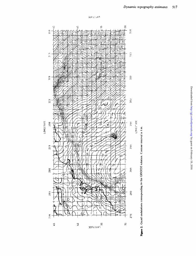
The geoid undulations for GEOID3 are shown in Fig. 2

where the data have been contoured based on a 12' x 12' grid of points. The high-frequency effects present in the computed geoid undulations are not visible on a simple contour plot with the given data spacing and the 1 m contour interval. However, the signature of the continental shelf and Bermuda are clearly apparent in the figure. The extreme differences between the undulations of GEOID3 and OSU91A typically occur over sea mounts where the 91A model does not contain sufficient high- frequency information. For example, a t Bermuda, the difference (N(GEOID3) - N(91A)) equals 1.2 m.

GEOID UNDULATIONS A T BERMUDA

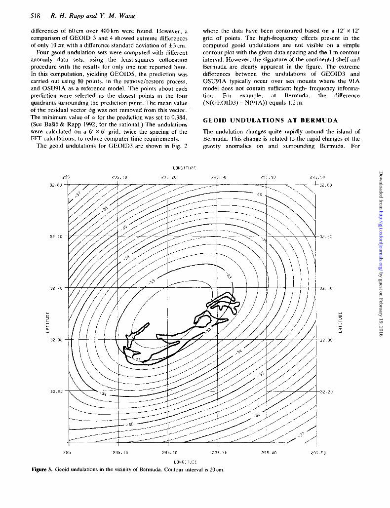
The undulation changes quite rapidly around the island of Bermuda. This change is related to the rapid changes of the gravity anomalies on and surrounding Bermuda. For

32. GO

32.50

W 0 f3 I-

c U _I

- 32.30

32 .20

LBFlGlTClDE

295 295 .10 295.20 295.70

295 295. 10 295 .20 2 9 5 . 3 0

LONGITUOE

Figure 3. Cieoid undulations in the vicinity of Bermuda. Contour interval is 20cm.

-32 . G O

-32 .50

-32 .40

-32.30

-32.20

I I

295. UO 295 .50


Dow

nloaded from



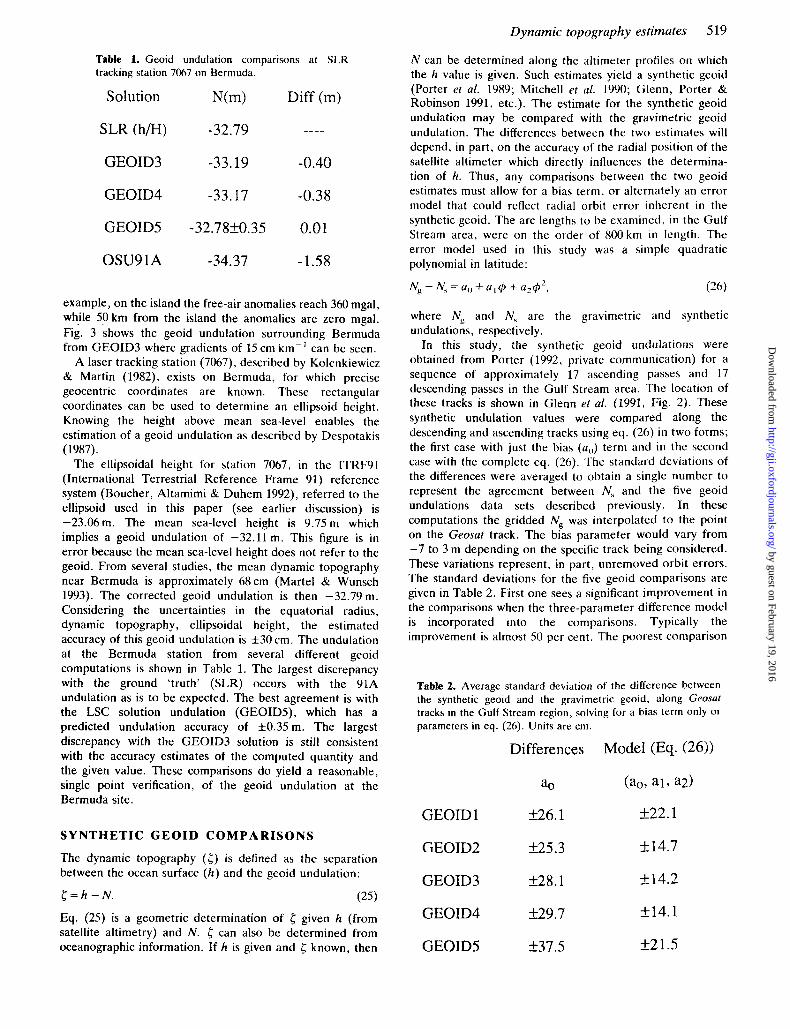
N can be determined along the altimeter profiles on which the h value is given. Such estimates yield a synthetic geoid (Porter et al. 1989; Mitchell et al. 1990; Glenn, Porter & Robinson 1991, etc.). The estimate for the synthetic geoid undulation may be compared with the gravimetric geoid undulation. The differences between the two estimates will depend, in part, on the accuracy of the radial position of the satellite altimeter which directly influences the determination of h. Thus, any comparisons between the two geoid estimates must allow for a bias term, or alternately an error model that could reflect radial orbit error inherent in the synthetic geoid. The arc lengths to be examined. in the Gulf Stream area, were on the order of 800 kin in length. The error model used in this study was a simple quadratic polynomial in latitude:

Table 1. Geoid undulation comparisons at SLR tracking station 7067 on Bermuda.

Solution N(m) Diff (m)

SLR (h/H) -32.79 ----

GEOID3 -33.19 -0.40

GEOID4 -33.17 -0.38

GEOID5 -32.78f0.35 0.01

OSU91A -34.37 -1.58

example, on the island the free-air anomalies reach 360 mgal, while 50 km from the island the anomalies are zero mgal. Fig. 3 shows the geoid undulation surrounding Bermuda from GEOID3 where gradients of 15 cm km-’ can be seen.

A laser tracking station (7067), described by Kolenkiewicz & Martin (1982), exists on Bermuda, for which precise geocentric coordinates are known. These rectangular coordinates can be used to determine an ellipsoid height. Knowing the height above mean sea-level enables the estimation of a geoid undulation as described by Despotakis (1987).

The ellipsoidal height for station 7067, in the ITRFYl (International Terrestrial Reference Frame 91) reference system (Boucher, Altamimi & Duhem 1992), referred to the ellipsoid used in this paper (see earlier discussion) is -23.06111. The mean sea-level height is 9.75 m which implies a geoid undulation of -32.11 m. This figure is in error because the mean sea-level height does not refer to the geoid. From several studies, the mean dynamic topography near Bermuda is approximately 68cm (Martel & Wunsch 1993). The corrected geoid undulation is then -32.79m. Considering the uncertainties in the equatorial radius, dynamic topography, ellipsoidal height, the estimated accuracy of this geoid undulation is f 3 0 cm. The undulation at the Bermuda station from several different geoid computations is shown in Table 1. The largest discrepancy with the ground ‘truth’ (SLR) occurs with the 91A undulation as is to be expected. The best agreement is with the LSC solution undulation (GEOIDS), which has a predicted undulation accuracy of f0.35 m. The largest discrepancy with the GEOID3 solution is still consistent with the accuracy estimates of the computed quantity and the given value. These comparisons do yield a reasonable, single point verification, of the geoid undulation at the Bermuda site.

SYNTHETIC GEOID COMPARISONS

The dynamic topography ( c ) is defined as the separation between the ocean surface ( h ) and the geoid undulation:

5 Z h - N . (25) Eq. (25) is a geometric determination of 5 given h (from satellite altimetry) and N . 5 can also be determined from oceanographic information. If h is given and c known, then

where Ng and N, are the gravimetric and synthetic undulations, respectively.

In this study, the synthetic geoid undulations were obtained from Porter (1992, private communication) for a sequence of approximately 17 ascending passes and 17 descending passes in the Gulf Stream area. The location of these tracks is shown in Glenn et al. (1991, Fig. 2). These synthetic undulation values were compared along the descending and ascending tracks using eq. (26) in two forms; the first case with just the bias (a, , ) term and in the second case with the complete eq. (26). The standard deviations of the differences were averaged to obtain a single number to represent the agreement between N, and the five geoid undulations data sets described previously. In these computations the gridded Ns was interpolated to the point on the Geosat track. The bias parameter would vary from -7 to 3 m depending on the specific track being considered. These variations represent, in part, unremoved orbit errors. The standard deviations for the five geoid comparisons are given in Table 2. First one sees a significant improvement in the comparisons when the three-parameter difference model is incorporated into the comparisons. Typically the improvement is almost 50 per cent. The poorest comparison

Table 2. Average standard deviation of the difference between the synthetic geoid and the gravimetric gcoid, along Geosat tracks in the Gulf Stream region, solving for a bias term only o r parameters in eq. (26). Units are cm.

GEOID 1 k26.1 f22.1

GEOID2 k25.3 k 14.7

GEOID3 f28.1 k14.2

GEOID4 k29.7 f14.1

GEOIDS k37.5 f 2 1.5


Dow

nloaded from


520 R. H . Rapp and Y. M . Wang

GEOID3 - N(P0RTER)

5 3 0 z 30

In - I I I I I I I I 90.00 39 .00 38.00 37 .00 36.00 35.00 3'4.00 33.00 32.SC

LRT I TUOE

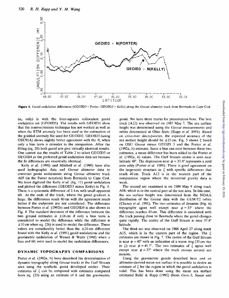
Figure 4. Geoid undulation differences (GEOID3 - Porter, GEOID3 - Kelly) along the Geosat altimeter track from Bermuda to Cape Cod.

(a(, only) is with the least-squares collocation geoid undulation set (GEOIDS). The results with GEOIDl show that the remove/restore technique has not worked as well as when the RTM anomaly has been used in the estimation of the gridded anomaly file used for GEOID2. GEOID3 (using OSU91A) shows slightly better agreement with the N, when only a bias term is consider in the comparison. After the fitting (eq. 26) both geoid sets give virtually identical results. One cannot use the results of Table 2 to select GEOID3 or GEOID4 as the preferred geoid undulation data set because the fit differences are essentially identical.

Kelly et al. (1991) and Mitchell et al. (1990) have also used hydrographic data and Geosat altimeter data to construct geoid undulations along Geosat altimeter track A05 (in the Porter notation) from Bermuda to Cape Cod. We have digitized the Kelly et al. (fig. 11) geoid undulation and plotted the difference (GEOID3 minus Kelly) in Fig. 4. There is a systematic difference of 2.4 m with small apparent tilt. At the ends of the track, where the geoid gradient is large, the differences reach 40 cm with the agreement much better if the endpoints are not considered. The difference between Porter el al. (1992b) and GEOID3 is also shown in Fig. 4. The standard deviation of the difference between the two ground estimates is f 1 8 cm if only a bias term is considered to model the difference while the difference is f lOcm when eq. (26) is used to model the difference. These values are considerably better than the f 2 4 cm difference found with the Kelly et al. (1991) geoid undulations and the gravimetric undulation of Wessel & Watts (1988) when a bias and tilt were used to model the undulation differences.

DYNAMIC TOPOGRAPHY COMPARISONS

Porter er al. (1992a, b) have described the determination of dynamic topography along Geosat tracks in the Gulf Stream area using the synthetic geoid developed earlier. Their estimates of c can be compared with estimates computed from eq. (25) using an estimate of h and the gravimetric

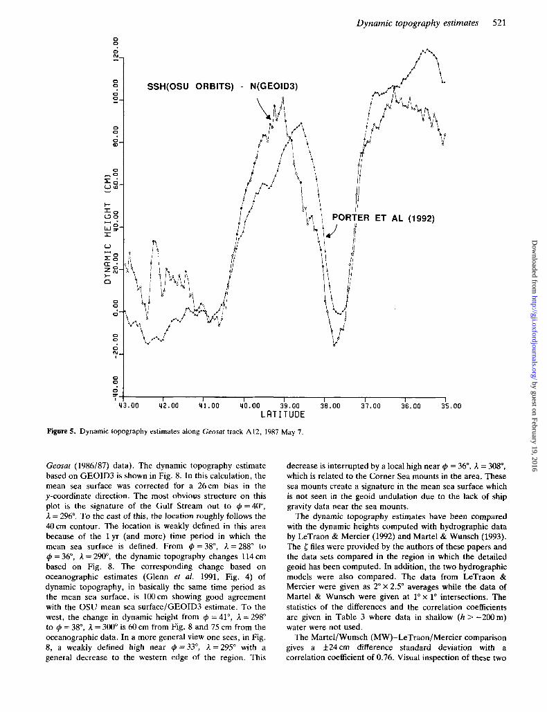
geoid. We have three tracks for presentation here. The first track (A12) was observed on 1987 May 7. The sea surface height was determined using the Geosat measurements and orbits determined at Ohio State (Rapp et a f . 1991). Based on cross-over discrepancies, the expected accuracy of the sea surface height should be f15cm. Fig. 5 shows 5 based on OSU Geosat minus GEOID 3 and the Porter et af. (1992a, b) estimate. Since a bias can exist between these two estimates, a mean difference has been added to the Porter et al. (1992a, b) values. The Gulf Stream centre is seen near latitude 40". The depression near @ = 37.8" represents a cold core eddy (Porter et al. 1989). There is good agreement on the large-scale structure in 5 with specific differences that reach 40cm. Track A12 is in the western part of the computation region where the terrestrial gravity data is weak.

The second arc examined is on 1988 May 9 along track A04, which is in the central part of the test area. In this case, the sea surface height was determined from the NOAA distribution of the Geosat data with the GEM-T2 orbits (Cheney et af. 1991). The two estimates of dynamic (Fig. 6) topography agree well except near @=33" where the difference reaches 40 cm. This difference is associated with the track passing close to Bermuda where the geoid changes quite rapidly. The centre of the Gulf Stream is near 37.8" latitude.

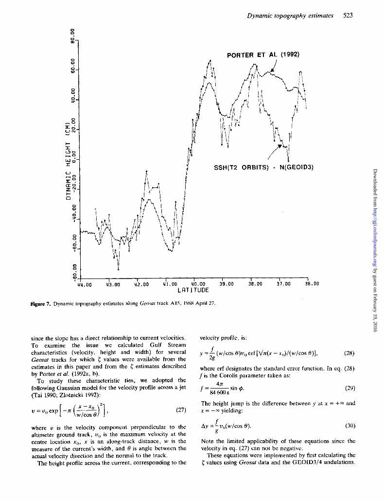
The third arc was observed on 1988 April 27 along track A15, which is in the eastern part of the region. The c estimates are shown in Fig. 7. The centre of the Gulf Stream is near @ = 40" with an indication of a warm ring (30 cm rise in 5 ) near @ = 41.7". The two estimates of 5 agree well except near @ =37" where the track crosses several sea mounts.

Using the gravimetric geoids described here and an altimeter-derived mean sea surface it is possible to derive an estimate of c for the region in which the geoid undulation is valid. This has been done using the mean sea surface estimated BaSii & Rapp (1992) (from Geos-3, Seasat and


Dow

nloaded from


SSH(0SU ORBITS) - N(GEOID3)


ET AL (1992)

0 a- I 1 I I I I I I I 1 93.00 92.00 91.00 90.00 39.00 38.00 37.00 36.00 35.00

LFlT I TUDE

Figure 5. Dynamic topography estimates along Geosat track A12, 1987 May 7.

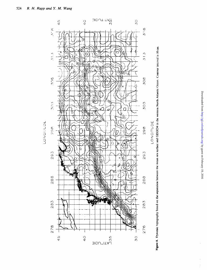
Geosat (1986/87) data). The dynamic topography estimate based on GEOID3 is shown in Fig. 8. In this calculation, the mean sea surface was corrected for a 26cm bias in the y-coordinate direction. The most obvious structure on this plot is the signature of the Gulf Stream out to C$ = 40", A = 296". To the east of this, the location roughly follows the 40cm contour. The location is weakly defined in this area because of the 1 yr (and more) time period in which the mean sea surface is defined. From C$=38", A=288" to @ = 36", A = 290", the dynamic topography changes 114 cm based on Fig. 8. The corresponding change based on oceanographic estimates (Glenn et al. 1991, Fig. 4) of dynamic topography, in basically the same time period as the mean sea surface, is 100cm showing good agreement with the OSU mean sea surface/GEOID3 estimate. To the west, the change in dynamic height from C$ = 41", A = 298" to C$ = 38", A = 300" is 60 cm from Fig. 8 and 75 cm from the oceanographic data. In a more general view one sees, in Fig. 8, a weakly defined high near Cp=33", A=295" with a general decrease to the western edge of the region. This

decrease is interrupted by a local high near r#~ = 36", A = 308", which is related to the Corner Sea mounts in the area. These sea mounts create a signature in the mean sea surface which is not seen in the geoid undulation due to the lack of ship gravity data near the sea mounts.

The dynamic topography estimates have been compared with the dynamic heights computed with hydrographic data by LeTraon & Mercier (1992) and Martel & Wunsch (1993). The 6 files were provided by the authors of these papers and the data sets compared in the region in which the detailed geoid has been computed. In addition, the two hydrographic models were also compared. The data from LeTraon & Mercier were given as 2" x 2.5" averages while the data of Martel & Wunsch were given at 1" x 1" intersections. The statistics of the differences and the correlation coefficients are given in Table 3 where data in shallow (h > -200 m) water were not used.

The Martel/Wunsch (MW)-LeTraonJMercier comparison gives a f 2 4 c m difference standard deviation with a correlation coefficient of 0.76. Visual inspection of these two


Dow

nloaded from



SSH(T2 ORBITS) - N(GEOID3) I

RTER ET AL (199

I I I I I I I 1 . O O 38.00 37.00 36.00 35.00 34.00 33.00 32.00 31.00

LRT I TUDE

Figure 6. Dynamic topography estimates along Geosat track A4, 1988 May 9.

hydrographic-based estimates of <, in the test region, shows similar structure with higher frequency content in the LM file. The high near $ = 34", I = 291" in the MW data is less clearly defined in the L M set. The change in 5 from this point to I = 318" is 36 cm in MW and 42 cm in LM, a good agreement. The corresponding change based on the mean sea surface and GEOID3 (Fig. 8) is 40cm.

Other values in Table 3 indicate the 5 estimates shown in Fig. 8 agree somewhat better with the MW model than the LM model ( f 2 5 c m *32cm). However, this number may also reflect the larger variations in the LM model ( f3Y cm) than those found in the MW ( f 2 5 c m ) model. The correlation between the 5 estimates of this paper is slightly higher (0.72 versus 0.68) with the MW model. One also sees from Table 3 little evidence to prefer one geoid undulation estimate over another. Although the correlation coefficients using GEOID3 are slightly greater than those using GEOID4, the difference standard deviations are comparable.

Since non-oceanic-driven high-frequency effects appear in

Fig. 3, other comparisons were made by averaging the various differences over different cell sizes. In such cases, the agreement between the oceanographic and sea surface height/geoid dynamic topography estimates improves. For example, with a Yo moving average comparison, the standard deviation of the different MW/G4 reduces t o f17 cm (from f 2 5 cm) and the correlation increases to 0.76 (from 0.72). in all these comparisons, one needs to recall that the mean sea surface has been derived from three altimeter data types, with different radial accuracies, widely spaced in time. Improved comparisons should be expected using sea surface height information derived from the Topex/Poseidon mission where accurate (f 10 cm) orbits will be available.

GULF STREAM VELOCITY CHECKS

Comparison of dynamic topography magnitude is not the only way in which one can evaluate 5 models. Additional information can be obtained by considering the slope of 5

I x


Dow

nloaded from



0 0

0 OD I I I I 1 1 I I I

LOT I TUDE Uh.00 93.00 42.00 91.00 90.00 39.00 38.00 37.00 36.00

Figure 7. Dynamic topography estimates along Geosaf track A15, 1988 April 27.

since the slope has a direct relationship to current velocities. To examine the issue we calculated Gulf Stream characteristics (velocity, height and width) for several Geosat tracks for which 5 values were available from the estimates in this paper and from the estimates described by Porter et al. (1992a, b).

To study these characteristic ties, we adopted the following Gaussian model for the velocity profile across a jet (Tai 1990; Zlotnicki 1992):

u = uo exp [-n (-----)7 x - x o

w /cos 9 '

where u is the velocity component perpendicular to the altimeter ground track, ul) is the maximum velocity at the centre location xO, x is an along-track distance, w is the measure of the current's width, and 6 is angle between the actual velocity direction and the normal to the track.

The height profile across the current, corresponding to the

velocity profile, is:

(28) y = - f (w/cos ~ ) u , , erf [&(x - x,))/(w/cos o ) ] ,

2g where erf designates the standard error function. In eq. (28) f is the Corolis parameter taken as:

4n f =- 84 600 s sin (#"

The height jump is the difference between y at x = +a and x = -a yielding:

(30) f Ay = - ~l~(W/COS 0).

Note the limited applicability of these equations since the velocity in eq. (27) can not be negative.

These equations were implemented by first calculating the t values using Geosat data and the GEOID3/4 undulations.

g


Dow

nloaded from


524 R. H . Rapp and Y. M. Wang

0 d-

0 r)

co M c

a3

rs, r

a 0 r)

rl 0 r)

W

iD a N

Z

9

a m N

rl 4) 01

03 b N

0 M

M

M 7

a) 0 r)

r ) 0 r )

a, D N

M m N

a, co nl

r") a) N

co I\ N

Y) .-

c Q

6

c 5 z E +d

E

C

B 0

E 5

* 0 D

0

C

U

5

P d

d


Dow

nloaded from



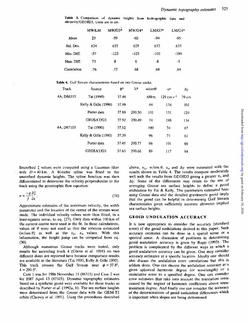
Table 3. Comparison of dynamic heights from hydrographic data and altimetrylGEOID3. Units are in cm.

MW/LM MW/G3; MW/G4* LM/G3* LM/G4*

Mean 23 -59 -60 -94 -95

Std. Dev. f 2 4 E25 f25 It32 f33

Min. Diff. -57 -123 -125 -101 -194

Max. Diff. 73 8 6 -8 -5

Correlation .76 .72 .68 .68 .64

Table 4. Gulf Stream characteristics based on two Geosat tracks.

Track Source 4 O ho Wtcose

4A, D863 15 Tai (1990) 37.46 68km

Kelly & Gille (1990) 37.98 64

Porter data 37.88 290.50 101

GEOS AT/G 3 37.92 290.49 74

4A, D87103 Tai (1990) 37.52 100

Kelly & Gille (1990) 37.39 96

Porter data 37.45 290.77 96

GEOSATlG3 37.63 290.66 89

VO

129 cm s-1

174

131

198

74

71

101

117

AY

79 cm

102

120

134

67

51

88

94

Smoothed values were computed using a Gaussian filter with D =40km. A bi-cubic spline was fitted to the smoothed dynamic heights. The spline function was then differentiated to determine the velocity perpendicular to the track using the geostrophic flow equation:

Approximate estimates of the maximum velocity, the width parameter and the location of the centre of the stream were made. The individual velocity values were then fitted, in a least-squares sense, to eq. (27). Only data within 100 km of the current centre were used in the fit. In these calculations, values of 0 were not used so that the solution estimated (wlcos 0) as well as the v,), xo values. With this information, the height jump can be computed from eq.

Although numerous Geosat tracks were tested, only results for ascending track 4 (Glenn et af . 1991) on two different dates are reported here because comparison results are available in the literature (Tai 1990; Kelly & Gille 1990). This track crosses the Gulf Stream near @ =37.8", 3r = 290.5".

Case 1 was for 1986 November 11 (86315) and Case 2 was for 1987 April 13 (87103). Dynamic topography estimates based on a synthetic geoid were available for these tracks as described by Porter et af . (1992a, b). The sea surface heights were determined from the Geosat data with the GEM-= orbits (Cheney et al. 1991). Using the procedures described

(30).

above, q,, wlcos5, x ~ , and Ay were estimated with the results shown in Table 4. The results compare moderately well with the results from GEOID3 giving a greater % and Ay. Some of the differences may relate to the use of averaging Geosat sea surface heights to define a S o i d undulation by Tai & Kelly. The parameters estimated here using Geosat data and the detailed gravimetric geoid imply that the geoid can be helpful in determining Gulf Stream characteristics given sufficiently accurate altimeter implied sea surface heights.

GEOID UNDULATION ACCURACY

It is now appropriate to consider the accuracy (standard error) of the geoid undulations derived in this paper. Such accuracy estimates can be done in a spatial sense or a spectral sense. A discussion of problems in determining geoid undulation accuracy is given by Rapp (1993). The problem is complicated by the different ways in which a geoid undulation accuracy can be given. One may consider accuracy estimates at a specific location. Ideally one should also discuss the undulation error correlations but this js seldom done. One can discuss the undulation accuracy at's given spherical harmonic degree (or wavelength) or a cumulative error to a specified degree. One can consider error estimates that take into account the truncation error caused by the neglect of harmonic coefficients above Some maximum degree. And finally one can consider the accuracy of the determinations of geoid undulation differences which is important when slopes are being determined.


Dow

nloaded from


526 R. H . Rapp and Y . M. Wang

Rapp et al. (1991b) discuss the accuracy of the geoid undulations computed from the OSU91A potential coefficient model. A global error estimate (including truncation error) is f 5 7 c m . If only ocean areas are considered, this estimate reduces t o f 2 6 cm (Rapp 1992). One expects that this error should be reduced when the detailed gravity data are included in the solution.

There are no optimum procedures to calculate geoid undulation accuracy estimates. Although we have used FFT procedures to calculate our primary undulation residuals, n o accuracy estimates were computed using FFT. Alternately, the method of least-squares collocation does yield an accuracy estimate (eq. 20) on a point-by-point basis. Although this method was not used to calculate the final geoid undulation grid, we felt that its use in undulation accuracy could yield information to assess, at least, the areas where the most accurate determinations of the geoid were made. We then evaluated eq. ( 2 0 ) with the final terrestrial gravity data base on a 6’ x 6’ grid instead of the 3‘ x 3’ grid used for the FIT calculation. As before, the closest 80 data points were used except in the Bermuda area where the closest 80 gridded (3‘ X 3’) anomalies were used. The results of the calculations are sensitive to the value of a computed in eq. (21). In turn, this value depends on how well the reference field fits the anomaly data in the area. To maintain realistic estimates of the geoid undulation, the minimum and maximum values of LY were set to be 0.3 and 2.0, respectively. The average accuracy for the area shown in Fig. 1 is f 1 6 cm. The minimum standard deviation is f l 3 c m while the maximum error is f 4 9 c m . The larger standard deviations are associated with areas lacking terrestrial data and areas of significant anomaly variations that are not well represented in the reference field. Such areas are primarily sea mount areas. The average standard deviation of f l 6 c m is very compatible with the synthetic/gravimetric undulation differences reported in Table 2.

CONCLUSIONS

This paper describes the computation of a gravimetric geoid undulation in the Gulf Stream region using potential coefficient models, land and ship gravity, and bathymetric implied information. A Fast Fourier procedure using a spherical Stokes’ formulation was used to calculate geoid undulations on a 3’ x 3‘ grid. Both the OSU91A and JGM-2 potential coefficient models were used in these tests. The undulation difference when using these two models as a reference field was only f 3 c m . Accuracy estimates were estimated using a least-squares collocation process. The average geoid undulation standard error was f l 6 c m not considering a possible bias due t o a possible error in the equatorial radius (637 8136.3 m) of the ellipsoid to which the undulation refers. The undulation accuracy is variable depending on ship coverage and anomaly gradients. Higher standard deviations occur near sea mounts. In these calculations altimeter-derived anomalies were used t o supplement, in areas away from the Gulf Stream, the ship data.

The gravimetric undulations were compared with the synthetic geoid undulations calculated by Glenn, Porter and others along Geosat tracks in the region. The comparisons

showed an agreement at the f l 4 c m level after allowances were made for long-wavelength systematic errors. These comparisons showed that the use of bathymetric data, in a remove-restore mode gave results poorer than when the bathymetric data were simply used as an aid, through the RTM anomaly, in the calculation of a gridded anomaly file.

The main purpose of the gravimetric undulation computation was to provide a data set that could be used to calculate dynamic topography using sea surface heights derived from satellite altimeter data. To test this usage dynamic topography was calculated along numerous tracks with the results compared with those provided by Porter. The agreement near the Gulf Stream itself was reasonable ( f 1 2 cm differences) although there could be some locations where a poorly determined gravimetric undulation would give unreasonable dynamic topography estimates. Such cases occur in regions lacking sufficient gravity data. In general, the computed geoid undulations reported here are sufficiently accurate for dynamic height estimates.

A dynamic topography data set was created using a mean sea surface (created from Geos-3, Seusat and Geosat altimeter data) and the gravimetric geoid undulation. A contour map of this dynamic topography clearly showed the Gulf Stream and other broad patterns seen in independent oceanographic results. However, high-frequency 5 estimates, caused by lack of gravity data in the determination of the geoid undulation, cause an irregular pattern in the contoured results. This 5 estimate is also contaminated by errors in the mean sea surface.

Comparisons of the 5 estimates were also made with two oceanographic estimates (Martel/Wunsch and LeTraon/ Mercier). The point 5 differences were f 2 5 c m with the MW model and f 3 2 c m with the LM model. These differences should be judged considering that the two oceanographic estimates of 5 differ by f 2 4 cm.

A final set of computations was made along two sets of Geosat tracks to calculate the location, width, velocity and height jump of the Gulf Stream using an implied model of the velocity of this current. The results were in general agreement with previously published values.

An accurate gravimetric undulation can provide a valuable data source for dynamic topography estimates using satellite altimeter data. These undulation estimates are not restricted to being along specific altimeter tracks and they can be used with different altimeter satellite ground tracks. However, the gravimetric undulation is limited by the long-wavelength error in the underlying potential coefficient reference model and by the lack of ship gravity data in certain geographic regions. The results of this paper show that dynamic topography can be reliably determined with the new gravimetric geoid, provided it is used in areas where its calculated accuracy is at the f 2 0 cm level.

ACKNOWLEDGMENTS

The research described in this paper was supported through NASA’s TOPEX Altimeter Research in Ocean Circulation Mission funded through the Jet Propulsion Laboratory under contract 958121. D. Porter, P. LeTraon, F. Martel, J. Cochran and S . Nerem kindly provided data used in this study.


Dow

nloaded from



REFERENCES Albuisson, M., Balmino, G., Monget, J .M., Maynet, B. & Reigber,

C., 1979. Detailed gravimetric geoid for the North Atlantic, Bull. Geod. , 53, 1-10.

BaSiC, T. & Rapp, R., 1992. Oceanwide prediction of gravity anomalies and sea surface heights using Geos-3, Seasat, and Geosat altimeter data and ETOPO5U bathymetric data, Rep. 416, Department of Geodetic Science and Surveying, The Ohio State University, Columbus.

Boucher, C., Altamimi, Z. & Duhem, L., 1992. ITRF 91 and its associated velocity field, IERS Tech. Note, Central Bureau of IERS, Paris.

Cheney, R. & Marsh, J . , 1981. Seasat altimeter observations of dynamic topography in the Gulf Stream region, J . geophys. Res., 86, 473-483.

Cheney, R. et al. 1991. The Complete Geosat Altimefer G D R Handbook, NOAA Manual NOS NGS 7, Rockville, Maryland.

Denker, H. & Rapp, R., 1990. Geodetic and oceanographic results from the analysis o f 1 year of Geosat data, J . geophys. Res.,

Despotakis, V., 1987. Geoid undulation computations at laser tracking stations, Rep. 383, Department of Geodetic Science and Surveying, The Ohio State University, Columbus.

Forsberg, R., 1985a. GEOGRID, Danish Geodetic Institute, Copenhagen.

Forsberg, R., 1985b. Gravity field terrain effect computations by FFT, Bull. Geod. , 59, 342-360.

Forsberg, R. & Sideris, M., 1993. Geoid computations by the multi-band spherical FFT approach, in First Continental Workshop on the Geoid in Europe, Research Institute of Geodesy, Topography and Cartography, Prague, Manuscr. Geod. , 18, 82-90.

Forsberg, R. & Tscherning, C.C., 1981. The use of height data in gravity field approximation by collocation, J . geophys. Res., 86,

Glenn, S.M., Porter, D.L. & Robinson, A.R., 1991. Synthetic geoid validation of Geosat mesoscale dynamic topography in the Gulf Stream region, J . geophys. Res., W, 7145-7166.

Heiskanen, W. & Moritz, H., 1967. Physical Geodesy, W.H. Freeman, San Francisco.

Hittelman, A, , Habermann, R.E., Dater, D . & Di, L., 1992. Gravity, Earth System Data, Alpha Release. National Geophysical Data Center, Boulder, Colorado.

Hwang, C., 1989. Precision gravity anomaly and sea surface height estimation from satellite altimeter data, Rep. 399, Department of Geodetic Science and Surveying, The Ohio State University, Columbus.

Kelly, K., 1991. The meandering Gulf Stream as seen by the Geosat altimeter: surface transport, position, and velocity variances from 73" to 46" W, J . geophys. Res., 96 (C9). 16721-16738.

Kelly, K. & Gille, S . , 1990. Gulf Stream surface transport and statistics at 69"W from the Geosat altimeter, J . geophys. Res.,

Kelly, K., et al., 1991. The mean sea surface height and geoid along the Geosat subtrack from Bermuda to Cape Cod, J . geophys. Res., 96, 12699-12709.

Kolenkiewicz, R. & Martin, C., 1982. SEASAT altimeter height calibrations, J . geophys. Res., 87 (C5), 3189-3198.

Lerch, F.J., et a!., 1993. Gravity model improvement for TOPEX/Poseidon (abstract), EOS, Trans. A m . geophys. Un. , 74(16) 96.

LeTraon, P. & Mercier, H., 1992. Estimating thc North Atlantic mean surface topography by inversion of hydrographic and Lagrangian data, Oceanol. Acta, 15(5), 563-566.

Marsh, J.G. & Chang, E.S., 1978. 5' Detailed gravimetric geoid in the Northwestern Atlantic Ocean, Mar. Geod. , 1, 253-261.

Marsh, J . et al., 1990. The GEM-T2 gravitational model, 1. geophys. Res., 95, 22 034-22 072.

95, 13 151-13 168.

7843- 7854.

95 (C3), 3149-3161.

Martel, F. & Wunsch. C. , 1993. Combined inversion of hydrography, current meter data and altimetric elevations for the North Atlantic circulation, Manuscr. Geod. , 18, 219-226.

Milbert, D., 1991. GEOID90: a high-resolution geoid for the United States, EOS, Trans. Am. geophys. Un. , 72(49), 545.

Mitchell, J . , Hallock, Z. & Thompson, J.D.. 1987. REX and GEOSAT: progress in the first year, Johns Hopkins AFL Technical Digest 8, 234-244.

Mitchell, J.L., Dastugue, J.M., Teague, W.J. & Hallock. Z.R., 1990. The estimation of geoid profiles in the NW Atlantic from simultaneous satellite altimetry and AXBT sections, J . geophys. Res., 95, 17 965- 17 977.

Moritz, H . , 1989. Advanced Physical Geodesy, 2nd Edn., H . Wichmann Verlag, Karlsruhe.

Nerem, R.S., Tapley, B. & Shun, C.K., 1990. Determination of the ocean circulation using Geosat altimetry, J . geophys. Res., 95,

Papoulis, A,, 1984. Signal Analysis, McGraw-Hill International Editions, New York.

Pavlis, N.K., 1988. Modeling and estimation of a low degree geopotential model from terrestrial gravity data, Rep. 386, Department of Geodetic Science and Surveying, The Ohio State University, Columbus.

Porter, D.L., Dobson, E. & Glenn, S . , 1992a. Measurements of dynamic topography during SYNOP utilizing a Geosat synthetic gcoid, Geophys. Rrs. Lef t . , 19(81), 1847-1850.

Porter, D., Dobson, E. & Glenn, S. , 1992b. Geosat Measurements of Dynamic Topography During SYNOP Utilizing a Synthetic Geoid, The Johns Hopkins University, Applied Physics Laboratory, SIR-92U-024, Laurel, Maryland.

Porter, D.L., Robinson, A.R., Glenn, S.M. & Dobson, E.B.. 1989. The synthetic gcoid and the estimation of mesoscalc absolute topography from altimeter data, Johns Hopkins A P L Technicul Digest, 10(4), 369-379.

Rapp, R.H., 1992. Computation and accuracy of global geoid undulation models, in Proc. of Sixth International Geodetic Symposium on Satellite Positioning, p. 865-872, Defense Mapping Agency, Fairfax, Virginia.

Rapp, R.H., 1993. Geoid undulation accuracy, l E E E Trans. Geosci. Remote Sensing, 31(2).

Rapp, R.H. & Pavlis, N.K., 1990. The development and analyses of geopotential coefficient models to spherical harmonic degree 360, J . geophys. Res., 95(B13) 21-885-21 911.

Rapp, R.H., Wang, Y.M. & Pavlis, N.K., IYYlb. The Ohio State 1991 geopotential and sea surface topography harmonic coefficient models, Rep. 410, Department of Geodetic Science and Surveying, The Ohio State University, Columbus.

Rapp, R.H. et al., 1991a. Consideration of permanent tidal deformation in the orbit determination and data analysis f o r the Topex/Poseidon Mission, NASA Technical Memorandum 100775, Goddard Space Flight Centre, Greenbelt, Maryland.

Robinson, A.R., Spall, M.A., Walstead, L.J. & Leslie, W.G., 1989. Data assimilation and dynamical interpolation in GULFCAST experiments, Dyn. Atmos. Ocean, 13, 301-316.

Schwarz, K.P. Sideris, M.G. & Forsberg, R., 1990. The use of F I T techniques in physical geodesy, Geophys. J . Int. , 100,

Sideris, M., 1993. Regional geoid determination, in Geophysical Inferpretafion of the Geoid, CRC Press, Boca Raton, Florida.

Sjoberg, L., 1993. Estimation techniques for geoid determination, in Geophysical Interpretation of the Geoid, CRC Press, Boca Raton, Florida.

Strang van Hees, G., 1990. Stokes' formula using fast fourier techniques, Manuscr. Geod. , 15, 235-239.

Tai, C.K., 1990. Estimating the surface transport of meandering oceanic jet streams from satellite altimetry: surface transport estimates for the Gulf Stream and Kuroshio extension, J . Phys. Oceanogr., 20, 860-879.

3163-3 179.

485-514.


Dow

nloaded from



Tscherning, C.C., 1985. Geoid modelling using collocation in Scandinavia and Greenland, Mar. Geod., 9(1) 1-6.

Wang, Y.M., 1993. On the optimal combination of potential coefficient model with terrestrial gravity for FFT geoid computations, Manuscr. Geod., 18, 406-416.

Wessel, P. & Watts, A.B., 1988. On the accuracy of marine gravity measurements, J. geophys. Res., 93(B1), 393-413.

Zlotnicki, V., 1990. The mean sea level of the Gulf Stream estimated from satellite altimetric and infrared data, in Sea

Surface Topography and the Geoid, Proc. IAG Symposia 104, eds Siinkel, H. & Baker, T., Springer-Verlag. New York.

Zlotnicki, V., 1992. Measuring oceanographic phenomena with altimetric data, presented at the Infernational Summer School of Theoretical Geodesy, Satellite Altimetry in Geodesy and Oceanography, Trieste, Italy.

Zlotnicki, V. & Marsh, 1989. Altimetry, ship gravimetry and the general circulation of the North Atlantic, Geophys. Res. Lett., 16, 1011-1014.


Dow

nloaded from


Dynamic Topography Estimates Using Geosat Data and A Gravimetric Geoid In the Gulf Stream Region

Documents