Dynamic tension in risers and mooring lines: an algebraic ...

Appiieol Ocean Research

E L S E V I E R Applied Ocean Research 23 (2001) 63-81 -

www.elsevier.com/locate/apor

Dynamic tension in risers and mooring lines: an algebraic approximation for harmonic excitation

J.A.P. Aranha*, M.O. Pinto

Department of Naval Engineering, USP, CP61548, Sao Paulo, Brazil

Received 20 June 2000; revised 20 March 2001

Abstract

A riser or mooring line, when excited dynamically at its upper end, resists the imposed displacement by increasing its tension. Viscous damping in the lateral motion is known to be crucial and the resulting problem is thus intrinsically nonlinear. In this paper, an algebraic expression for the dynamic tension, formerly obtained [Polar Engineers, ISOPE'-93 (1993)], is revised and enlarged, once the variation ofthe tension along the suspended length is specifically focused here. The obtained expression is systematically compared with results from usual nonlinear time domain programs and with experiments, showing a fair agreement. This algebraic expression is used then, in two accom­panying papers, to address relevant problems from a more practical point of view: in the first one, the question of the dynamical compression of risers, with a proper estimative of the related critical load, is analyzed in conjunction with the results here derived; in the second one, the algebraic expression is used to obtain an analytic approximation for the probability density function of the dynamic tension in random waves. © 2001 Elsevier Science Ltd. A l l rights reserved.

Keywords: Dyanainic tension; Risers; Algebraic approximation

1. Introduction

Consider a cable, whether i t is a riser or a mooring line,

hanging f r o m a floating system and resting on the sea floor

in the other end. The cable may be made by a junction o f

different materials, as i t is usual i n a mooring line config­

uration, or i t may have some few concentrated buoys or

weights or even i t can also be exposed to the action of a

steady ocean current in the cable's plane. I f the flexural

r ig idi ty EJ is 'small ' , in the sense that its influence can be

fe l t only in the boundary layers where the change in curva­

ture is large, then the equilibrium of the cable can be

determined assuming E J = 0, see Ref. [3] . The static con­

figuration is defined by the functions { 6 { s y , T { s ) ], where 6(s)

is the angle between the tangent to the cable and the

horizontal plane and T(s) is the static tension. I f / is the

suspended length, the curvilinear coordinate of the point

anchored in the floating system is s = l, s = 0 being the

coordinate o f the touchdown point.

Given the static configuration, suppose that a harmonic

motion 11(1) = C/oCos(wf) is imposed at the suspended end

* CoiTesponding author. Address: Department of Naval and Ocean Engi­

neering, EPSUP, Cidade University, CEP 05508-900, Sao Paulo, Brazil.

Tel.: 4-55-11-3818-5340; fax: -1-55-11-3818-5717.

E-mail address: [email protected] (J.A.P. Aranha).

s=l,m the direction o f the cable's tangent; it can be shown,

see Section 4, that the displacement i n the normal direction

gives rise to a small correction in the tension and can there­

fore be ignored. The displacement 11(1) is due to the action

of the sea wave on the floating body and the main objective

of the present analysis is to determine the dynamic tension

f o C i , f ) caused by such displacement.

From a numerical point o f view, the problem is appar­

ently straightforward, even more i f i t is observed that the

large viscous damping i n the lateral motion eliminates a

possible resonant phenomenon. In spite of this, the dynamic

tension can be very large: in fact, when either the amplitude

UQ o f the displacement or the frequency co increases, the

viscous dissipation becomes so strong that the cable almost

freezes i n its equil ibrium position. The imposed displace­

ment is then absorbed elastically by the cable, see Ref. [9 ] ,

giving rise to a large value of the tension. I n fact, in this

l imi t the elastic tension = EA{UQII + / ' ) can be reached,

where E A is the axial stiffness and / ' is the effective length o f

the cable on the ground, see Section 2 fo r a proper defini­

tion; to get an idea about the possible level of tension, i f

C/o = 4 m and / - f / ' = 2000 m the elastic strain ee = C/EA

becomes equal to the steel yield strain.

There are thus two time scales i n the problem, each one

related to particular mechanisms fo r the reactive forces that

can be best visualized in l imi t situations: i f the cable is

0141-1.187/01/$ - see front matter © 2001 Elsevier Science Ltd. A l l rights reserved.

PII: 80141-1187(01)00008-6

64 J-A.P. Aranha, M.O. Pinto / App

loose, for example, i t accommodates the imposed displace­

ment by a geometric change in the catenary and the related

time scale is associated wi th the cable's lateral frequency

cüc; on the other hand, a tight cable absorbs the imposed

displacement elastically, wi th a time scale related to the

elastic axial frequency co^. Obviously, these two time scales

coexist i n an actual problem and the numerical scheme has

then to deal wi th discrepant time scales, since in general, as

seen in Section 2, W e » a>c- Discrepancy i n time scales

presents a natural diff iculty for numerical integration, but

this is not.,the only, source of numerical problems in the

analysis. In fact, the discrete system uses lumped masses

that hits the ground in the vicinity o f the touchdown point,

giving rise to iinpact forces that are propagated along the

)cable. These impact forces are spuiious, since they are

caused by the discretization,' and they impose spurious

high frequency components on the dynamic tension that

are not very much attenuated along the cable, unless the

axial damping is very high. Obviously, this effect

diminishes as the mesh size becomes thinner, but for a typ i ­

cal mesh size the spurious tension, although small compared

w i t h Te, can become noticeable when compared wi th the

static tension, bluixing then the signal of the total tension.

One w i l l have the opportunity to observe this phenomenon

in the few simulations to be shown here and i t is a matter of

concern how to deal numerically wi th these higher harmonic

components, observed also at the suspended end of the

cable. Simply filtering them does not seem to be a wise

solution since, though spurious in the continuum context,

they are innate to the discrete models and, once excited, the

higher hariuonics interact nonlineaiiy, affecting the energy

of the fundainental hartnonic.

These critical remarks about the numerical solutions

j should be looked into a proper perspective: they do not

imply that numerical results are useless and, as a matter of

fact, numerical simulations have been extensively used, in

the present paper and in the accompanying ones, as a refer­

ence for the analytic results. Although recognizing the

usefulness o f these solutions, wi th their numerical robust­

ness and broad generality, the intention here was to draw the

attention to some more subtle aspects o f the cable dynamics

that can be relevant in certain cucumstances.

On the other hand, the same discrepant time scales that

cause numerical trouble can be explored to obtain asympto­

tic solutions for the cable dynamics. The basic idea is mot i ­

vated by the fact that, as seen i n Section 2, the imposed

frequency w is of the order of tnagnitude of the cable's

lateral frequency and so, in general, ca ̂ (o^. I f now k

is the axial wavenuiuber related to w then, f r o m the defini­

t ion o f the axial wave velocity, one has = &)//c = tajk^,

,' In fact, it can be shown (see Ref, [3]) that in the coiüimiousproblem the

cable in general 'rolls' in the ground without striking it. This result is

confirmed by the experiments, since the observed time record of the tension

does not show any evidence of higher harmonics, even when the cable

slackens; see Section 3 of this work.

Ocean Research 23 (2001) 63-81

with /fe ~ TTII + l' being the wavenumber of the first axial

natural mode. I t turns out that k{l + / ' ) ~ TT{IJ)IU)^) < 1,

showing that the natural length scale for the axial dynamic

tension is much larger than the cable's length; i n first

approximation, then, the dynamic tension can be assumed

constant along the cable's length and i t can be obtained

f r o i n the overall dynamic equilibrium of the cable. This is

the basis o f the algebraic approximation derived i n Ref. [2]

where, i n essence, the dynamic equations are integrated

along the suspended length to obtain a closed f o r m expres­

sion for the dynamic tension.

However, one point was not satisfactory, mainly for an

almost vertical riser: for these geometries the variation o f

the dynamic tension along the cable is indeed small, when

compared to the reference tension T^, but i t can be appreci­

able when compared wi th either the static tension or the

dynamic tension at the touchdown. From a more practical

point o f view, then, the variation of the dynamic tension

along the cable must be evaluated and one o f the purposes

in the present work is to present such 'second order' correc­

tion. The other intention was to show, in a more systematic

way, comparison wi th numerical results obtained wi th

different programs, calling the attention to the observed

discrepancies when they happen and commentating them;

at the same time, both the numerical results and the alge­

braic expression are compared wi th a set of experimental

results, disclosing some of the numerical misbehavior

described above.

This paper has been organized wi th the objective to focus

the attention on these issues, placing then in a secondary

plane the mathematical derivation of the algebraic expres­

sion. For this reason. Section 2 presents directiy, besides

some definitions, the final algebraic expression for the

dynamic tension, the discussion being restricted there to

some simple physical arguments that can help to interpret

the final result; Section 3 is dedicated to a more systematic

comparison wi th experiments and numerical results, wi th

some pertinent discussion o f the results. Only i n the Appen­

dix the detailed mathematical derivation of the algebraic

expression is addressed.

2. The algebraic expression for the dynamic tension

Consider a cable fixed at the floating system i n a certain

point S and touching the sea floor at a point O; i f ^ is the

curvilinear coordinate, w i th ^ = 0 at O and ^ = Z at 5, then I

is the suspended length of the cable. The static configuration

is defined by the coordinates {x{sy,z{s)) satisfying the

geometric equations Axids = cos0{s); dz/ds = s in0(5) , w i t h

6{s) being the angle between the cable's tangent and the

horizontal axis. Let q be the submerged weight per unit o f

length of the cable and Tis) its static tension, wi th particular

values defined below:

Ts = T{1), To = r ( 0 ) . (2.1a)

J.A.P. Aranha, M.O. Pinto /AppUed Ocean Research 23 (2001) 63-81 65

Let also A/ be the length o f the cable resting on the sea

floor, that is, the distance between the anchor A and the

touchdown point O, and fji the f i i c t i o n coefficient between

the cable and the soil. I f the length To/inq is smaller than AZ

then, obviously, the static tension is zero in the interval

—AZ :S i ' :S —To/ixq and the effective length of the cable

on the sea floor w i l l be Tol/Mq. Denoting by Z' this length,

and observing that the whole cable is stretched when

AZ < TQ/M' then

Mm{M; To/iJLq). (2.1b)

The effective length enters in the problem through the

definition of the elastic tension T^. As seen i n the Introduc­

tion, this tension appears at the 'freezing condition' , where

the imposed displacement is absorbed elastically by the

cable in a quasi-static way; i n this perspective, the definition

given in Eq. (2. l b ) seems to be the most natural one even fo r

the dynamical problem, as discussed i n Section 4.

. 'The cable's curvature is defined by the function

ds T, (2.2a)

where is directly determined f r o m the static configura­

tion; as i t is shown in Section 4, the lateral harmonic displa­

cement v(s) is, i n first approximation, proportional to the

curvature and so v{s) oc^i{s). This result w i h be used

below..

Finally, the horizontal ocean current, projected in the

plane (x,z), is given by the vector

Vciz) = V,xMs))i, (2.2b)

where is the ciUTent intensity at the sea level and Xc(z(A)

is the current profile along the cable.

2.1. Static parameters

Obviously, the dynamic response depends on the cable's

static configuration and, i n the context of the proposed

asymptotic approximation, a l l static information can be

synthesized in some few integral parameters to be intro­

duced next. The first two of them are defined by

ƒ„ = \XiiA\"<is; n = 2,3. (2.3a)

I t is not diff icul t to explain the physical origin of these

integrals. In fact, since the lateral dynamic displacement is

proportional to the static curvature (v ( j ) oc ; ^ i ( 5 ) ) , then the

inertia force, integrated along the suspended length, should

be proportional to Io i n order to preserve the cable's lateral

kinetic energy; for the same reason, the integrated viscous

damping should be proportional to ƒ3 i n order to preserve the

dissipated power in the lateral motion.

However, i n the presence of a strong horizontal ocean

current V^xdziA) the dynamic viscous force is, i n first

approximation, proportional to V^xdzis)) X sin 9 (s)Xv{s)

and then the dissipated power should be proportional to

the integral 1^, where

\xMs)) sme{s)\ /^{s) ds. (2.3b)

I t remains to define a parameter related to the restoring

forces. As mentioned in the Introduction, there are two

mechanisms for the cable to react to any imposed displace­

ment: the first, by stretching the cable; the second, by adjust­

ing the geometric configuration of the catenary. The ratio

between these two restoring forces is known to be crucial in

the cable dynamics and i t is proportional to the coefficient

A ^ where (see R e f [6])

A 1/2

( z + z'

1/2

(2.3c)

For a loose cable, where the tangent at the suspended end

is almost vertical (Ö(Z) ~ trll), one has ql = Ts and, since

EA/Ts > 1, then yl > 1 in this situation; typically A « 50

f o r a loose cable. For a tight cable, where the angle w i th the

horizontal is small at the sea level (Ö(Z) <C Tr/2), vertical

equil ibrium implies in ql/Ts = sin0(Z) <C 1 and then / I ~ 5.'

Those are the only parameters that depend directly on the

static configuration o f the cable, the remaining ones, to be

defined next, depending on the dynamic properties o f the

cable and on the imposed excitation.

2.2. Dynamic parameters

For a heterogeneous cable, as a mooring line usually is,

the weight q{s), mass m(s), added mass /na(i'), diameter D{s),

stiffness EA(s) and drag coefficient CY){S) change along the

suspended length. Enforcing conservation of kinetic energy,

and recalling that v (5 ) oc Xi(s), the averaged mass and added

mass fo r the dynamic problem can be defined by the

expressions

ri

m; ni„ 1 1

h i

D = 4;?Za

pit

{m{sy,mJ,s)}Ai{s) ds.

q(s) ds; (2.4a)(

E A Z Jo

ds

EA{s)'

w i t h D being the equivalent diameter and {q;EA} the aver­

aged weight and stiffness. In a similar way, enforcing

conservation o f the dissipated power, the averaged drag

coefficients are defined by

^ _ 1 1 ' C ^ i s ) ^ \ X i i s f d s , 0 D

C f c V ) ^ \ X c ( z i s ï ) sme(,s)\Aiis) ds,

(2.4b)

where CD,O is to be used in the absence of an ocean cuiTent

and CD,C when the ocean current is strong; a more

(

66 J.A.P. Aranha, M.O. Pinto /Applied Ocean Research 23 (2001) 63-81

appropriated definit ion for the drag force in an intermediate

situation is introduced in Section 4. The related damping

coefficients are given by the expressions

here

So ^ 2CD.O PTTD'IA TS h f^u

37r ' 77 m + m„ ql II D

(2.5).

2CD,e p7rDV4 2V^

TT in + lUr^ ct)D I2 '

with CÜ being the frequency of the imposed displacement

and (Tu its rms value, see Eq. (2.7a).

As discussed in the Introduction, there are two time scales

related to the distinct mechanisms for the restoring forces;

ithe associated frequencies are

7T

I V in

T,

l + l'

E A

in (2.6)

The frequency co^ is the natural frequency of an horizon­

tal cable wi th length I subjected to the traction Ts and wi th

mass in + in^; the frequency co^ is the elastic axial frequency

of a cable wi th length / + / ' , axial stiffness E A and mass in.

Obviously, they are not the actual natural frequencies of the

cable, neither they intended to be: they serve only as

reference values. I n this context, in particular, i t can be

checked that WJCD,, =^ (Ts/EA)"^ < 1, as anticipated in the

Introduction.

From some simple considerations it is not di f f icul t to

estimate the order o f magnitude of u)^. In fact, f r o m the

equihbrium of a catenary one has Ts = qUsindQ) and,

since q = {in — in^g for an homogeneous cable, then

TT(g/hy^, where the water depth h is assumed o f

j order o f the suspended length /. I t turns out that = 2TTI

öJc « 2{h/gy'^ 20 s. for a water depth h « 1000 m and the

wave frequency <u is of order of magnitude of co^, imply ing

in ft)/öJe < 1. This is the essential assumption in the derived

asymptotic approximation fo r the dynamic tension, as

discussed in the Introduction and further elaborated in the

Section 4. Also, notice that the dynamic excitation is

iiuportant only in deep water: in shallow water {h ~ 10 m)

one has, in general, w <C Wc and the cable response is

quasi-static.

2.3. Excitation parameters

The dynamic motion of the cable is excited by the displa­

cement U(t) = UQCOs{cüt) imposed at the suspended end S

in the tangent direction. Instead of using the displacement

amplitude UQ the fo l lowing parameters w i l l be introduced

o-v' (2.7a)

where CTU is the rms of the imposed displacement and a is

the normalized 'wave envelop'. The reason for this is solely

editorial: Eq. (2.7a) can be extended directly to a random

excitation, to be addressed in an accompanying paper. The

elastic tension T^ is defined accordingly by

re = E A l + l'

(2.7b)

while the information about the imposed wave frequency (o

can be introduced through the non-dimensional parameter

(2.7c)

Notice that for the same value of w/Wc the reduced

frequency f l is larger for a tight cable, where A is smaller.

As expected, this means that the 'freezing situation', where

the imposed displacement is absorbed elastically, is more

l ikely to occur in a tight cable than in a loose one.

2.4. The algebraic expression for the dynamic tension

As discussed in the Introduction, the dynamic tension is

essentially constant along the cable when w/We <C 1. Under

this same condition i t is also possible to show that the lateral

dynamic displacement is, i n first approximation, propor­

tional to the static curvature, or v{s) = Vxi{s), where V is

the displacement amplitude and X\iA is defined i n Eq.

(2.2a). W i t h i n this approximation, i t fo l lows that the rele­

vant dynamic variables are reduced to two discrete values,

the amplitudes of the dynamic tension and of the lateral

displacement. Integrating the equi l ibr ium equations in the

transversal and axial directions, together w i t h the equation

fo r the geometric compatibility, one obtains, wi th the help

of the integral parameters introduced in Section 2 .1 , two

algebraic equations wi th these two unknowns. Solving this

system the dynamic tension can be determined. The math­

ematical derivation is elaborated in Section 4, the final result

being given below. In this way, i f the dynamic tension is

written in the fo rm

T^{s,t) = Tj,{s)

T D ( ^ ) = ^ = < ^ ) e ' * ^ - \

(2.8a)

i t can be shown that the non-dimensional dynamic tension

amplitude r{s) is given by

Tis)

(^^b\n) + {AclinAa' - b{n)^\2c2(s)(jbHn) + mlinAa^ - b{n)^ (4^o ' / ^ ' )

(2.8b)

J.A.P. Aranha, M.O. Pinto / Applied Ocean Research 23 (2001) 63-81 67

with

b{a) 1 - n 2 \ 2

c , ( ^ ) = 1 -

1 + Or 1 + AA

l 2

+ fcClis).

(2.8c)

Notice that Eqs. (2.8a)-(2.8c) already incotporates the

variation of the dynamic tension along the suspended

length. In general this variation is weak, since the term in

s/l is mult ipl ied by the small parameter (w/we)^, but in

certain circumstances, when /2 ^ 1, i t luay becotne impor­

tant, as discussed below.

I t seems worthwhile at this point to analyze Eqs. (2 .8a)-

(2.8c) in some l imi t situations, v,'here then the obtained

result can be more easily inteipreted. In this way, consider

Eq. (2.8a) when ü > 1 (but keeping w / « e <C 1). W i t h an

e i T o r of the f o r m [1 - I - Odca/coA; 1//^^)] one has

[ciis) = 1; bin) = C2is) = 1 + cl} and so, f r o m Eq. (2.8b),

it ' fo l lows that T{S) = a. Also, when CTU/D :§> 1 one has

^0 > 1, see Eq. (2.5), and then f r o m Eq. (2.8b) i t fo l lows,

w i th an error o f the f o r m [1 + 0{{co/a}^)^; D/au)], that again

ris) = a. I n both cases one obtains (see Eqs. (2.7a) and

(2.7b))

\TD(S) E A ^0

l + l'' (W/M,; UQID) > 1, (2.9a)

that is exactly the result anticipated at the Introduction: the

elastic limit can be reached when either the imposed ampli­

tude or the wave frequency becomes large.

I n the other l imi t , when /2 < 1, one has b ( i l ) = 1/

> 1 and f r o m Eq. (2.8b) i t fol lows, wi th an eiror of

the f o r m [1 + 0{n% that

'T{S) = {C,{S)CW + C2{s)) an''.

C2{S)

(2.9b)

t,c,{s). {n<\)

There are two situations where n can become small:

one, when the iiuposed frequency is effectively low and

w/coc ^ 1; the other, when the cable is loose {A :§> I ) and

n can be small even when w/Wj. s 0(1) . The first case is of

l i t t le importance in deep water and, furthermore, this l i m i t is

not wel l described by Eq. (2.9b): when w/wc 1 one

should use a quasi-static solution, as described in Ref. [2]

and discussed in Section 4. However, i f A is so large that

Aiiojw^ = 0{\), as i t may happen in a loose cable, the

dynamic tension is in fact small when compared wi th the

elastic tension Te, since T = 0(n~) <€. 1, but the variation o f

T(S) along the suspended length cannot be disregarded, once

dc2/ds = 0 (1) . Furthermore, although small when compared

to Te, the dynamic tension may be comparable to the static ,

tension and should not be ignored.

The algebraic expression (2.8a)-(2.8c), albeit siiuple,

recovers qualitatively the main features of the dynamic

tension in a submerged cable. I f i t is also shown that it is

quantitatively consistent, then i t provides an interesting

simplification for the proposed problem, wi th possible

imbrications in others directions too. The quantitative

aspect w i l l be addressed next, the possible imbrications

being reserved to the accompanying papers.

3. Experimental and numerical verification of Eqs .

(2.8a)-(2.8c)

In this section the algebraic approxiiuation (2.8a)-(2.8c)

for the amplitude o f the dynamic tension is compared wi th

some experiments and wi th numerical results obtained f ro iu

two distinct time domain programs. Only a survey of this

rather extensive set of comparisons w i l l be presented here,

the intention being to show the typical adherence among '

these results and to draw attention, in certain particular

cases, to some observed disagreements, commentating

them in the l ight o f the perturbations introduced on the

continuous models by the discretization.

3.1. Experimental results

In a research project sponsored by Petrobras, Ref. [1]

analyzed at the USP wavetank the dynamic behavior of

mooring lines; i n the experiments, a chain, anchored in a

point on the wavetank fioor, was excited dynamically at the

suspended end. The imposed motion was harmonic, the

displacement being either along a straight line or else circu­

lar, and the measured output was the total tension at the

suspended end. T w o different chains, wi th relatively dis­

crepant properties, were tested in several geometric con­

figurations and the dynamic excitation varied too, in

amplitude, frequency and type o f motion ( i f straight or

circular). Around a hundred different tests were made and, (

obviously, only a small sample of them w i l l be discttssed

here. However, the results to be presented are typical, being

representative of all experiments realized.

The relevant physical properties o f the two chains are

given in Table 1 and the static configuration can be char­

acterized by the geometric parameters {h; 6^; I j ) , where h is

the water depth, 9^ =• 9(1) is the angle at the suspended end

and I j the total chain length; since the f r ic t ion on the wave-

tank floor can be ignored, l' = I j — 1.

Table 1

Physical properties of the two chains (Ref. [1])

Chain EA (N) q (N/m) D ( m ) m (kg/m) H(j (kg/ra) CD

1 4763 0.360 0.0026 0.042 0.013 1.6

2 17664 0.865 0.0041 0.088 0.027 1.6

(

68 J.A.P. Aranha, M.O. Puito/Applied Ocean Research 23 (2001) 63-81

(a) 2,5

3

1.5

1

0.5

4 Tmax /To

4 Tmin +

'1=

3,5

3

2.5

2

1.5

1

0.5

T / T , H)/D=14.33 A=7.66

Tm fiK /T

Tmin/Tj

0.01 0.1 1 f(Hz) 0.01 0.1 1 f(Hz)

(b)

0.03

0.025

-0.005

5 4.5

4 3.5

3 2.5

2 1.5

1 0.5

0 -0.5

i Tmax/T., j

+

i m i n / I s

0.01 0.1 1 f(Hz)

-1 1 1 T

Experim. 2.8

4 5 6

T i m e (s)

10

Fig, 1, (a) Total tension at the suspended end. Experiments (4-); Eqs. (2.8a)-(2.8c) (- - - ) . (a) UJD = 7,91; (b) Ua/D = 14,33; (c) U^D = 24.21. Chain 2,

A =7,66. (Source: Ref. [1]), (b) Variation of tension in time: experiment (—); Eqs. (2.8a)-(2,8c) ( - - - ) f/o = 0,076 m; ƒ = 0,658. Chain 1, {h =

1.82 m;es = 13.8°;/T = 28.73 m), yi =2 .6 .

The first set of resuhs, presented in Fig. l a , shows the plot

o f the maximum and min imum values o f the total tension in

a cycle as a funct ion of the imposed frequency ƒ (Hz). The

tension has been normalized by the static value T^, see

Eq. (2.1a), and the theoretical values have been determined

by the expression = 1 ± T{Ï){TJTS), wi th T ( / )

given by Eqs. (2.8a)-(2.8c) and by Eq. (2.7b); obviously.

when rmin resulted negative in this expression then the value

Tmin = 0 was taken, since the chain cannot support any

compression. In al l tests o f Fig. l a chain 2 was used i n

the static configuration given by (/; = 2.02 m; 0s = 11-2°;

/ T = 20.3 m) , and only the amplitude t/o of the imposed

circular motion was changed, as defined in the figure

caption. The agreement between the experimental and

J.A.P. Aranlia, M.O. Pinto / AppUed Ocean Researcli 23 (2001) 63-81 69

theoretical values is quite good, even more i f i t is observed

that in several cases, identified by the result T^in = 0 at the

suspended end, the chain slackens as a whole. This is really

a demanding test for the algebraic approximation: i n fact,

the larger influence of the geometric nonlinearity is

expected to happen for a tight cable (small 0s) under strong

dynamic excitation, as in the cases tested, but the alge­

braic approximation does not include this nonlinearity,

the only nonlinear term i n Eqs. (2.8a)-(2.8c) being the

viscous dissipation, see Section 4. The observed concor­

dance shows that the geometric nonhnearity is, indeed,

o f httle concern for this class o f problems. The only

point that deserves a further comment is the f o l l o w i n g :

as explained in Section 4, Eqs. (2.8a)-(2.8c) ceases to

be val id in very low frequency, where a quasi-static solution

must be used; the two horizontal lines in Eig. l a represent

just this solution. This low frequency correction has not

been incorporated in the final solution because it has li t t le

importance in deep water.

I n order to display the generality o f the experi­

mental results and, at the same time, to point out

some more subtle aspects o f the problem. Fig . l b

shows, for- a different chain i n a distinct geometric

configuration, the variation in time of the total tension

at the suspended end. Again, a close agreement is observed,

indicating now that the cable's response is i n fact 'harmo­

nic ' , the experimental result not showing evidences of

higher harmonics.

This same problem was solved by a time domain

numerical program, see Fig . 2a. The overall response

is comparable to the experiment, although two peculia­

rities are conspicuous and should be commented: first, i t

is now clear the evidences of higher harmonics; second,

the tension becomes negative in a short t ime interval, i n

spite of the fact that the chain cannot support a

compressive force. Both phenomenons cannot be real,

since they do not appear in the experiments, and so

they must be due to the discretization. A possible expla­

nation f o r the observed higher harmonics is the impact

forces on the ' lumped ' masses when they h i t the

ground: they give rise then to high frequency oscilla­

tions that are propagated through the cable w i th a small

dissipation, unless the axial damping is assumed to be

very large. This may be indeed one of the resons why

numerical codes sometimes encounter difficult ies to

converge when the sea floor is r ig id , the numerical

integration becoming easier when the ground is assumed

'soft ' . These higher harmonics, although spurious in the

continuum problem, are innate in the discrete system and

so, once generated; they interact w i th each other b inning the

tension signal. As an example, Fig. 2b shows, for a random

excitation, the time history o f the touchdown tension o f a

riser wi th EJ = 0.

Notice not only the large magnitude o f the (unduly)

compression but also how the higher frequency components

apparently enhance the value o f the maximum tension.

(a)

I 7 I 8 9Ï 10 I 11 121 13 I 1 14 15 lfe

Time (s)

700 720 740 760 780 800 820 840 860 880 900 Time (s)

Time (s)

Fig. 2. (a) Same as Fig. lb but obtained from a time domain program

(Orcafiex). (b) Tension at the touchdown of an actual riser in random

excitation. EJ = 0. (c) Compressive force as a function of the mesh size

ÓS (same problem of (b)).

Furthermore, i f EJ 0, as it is usually, some compression

is acceptable, although i t is not known a pr ior i how much.

This is the main motivation o f the accompanying paper on

dynamic compression.

Table 2

Parameters of the risers simulated by Orcaflex and Cable (friction

coefficientiytt = 0.4; axial damping: f A X I A L = 10%)

Dim) ni (kg/m) BA (kN) BJ (kN m^)

(FR) 0.2160 67 1.92 X 10^ 9.84 1.0

(SR) 0.2191 70 2.10X 10^ 9241 1.1

70 J.A.P. Aranha, M.O. Pinto/Applied Ocean Research 23 (2001) 63-81

Table 3

Parameters of the heterogeneous mooring line: Chain 1-Cable-Chain 2 (friction coefficient:/it = 0.4; axial damping: f AXIAL = 10%)

m (kg/m) '"a (Kg/m) q (kN/m) EA (kN) ö ( m ) C D I Am)

Chain 1 203 27.58 1.920 7.94 X 10' 0.095 2 3800 Cable 49 9.56 0.387 5.37 X 10' 0.109 2 lOOO Chain 2 160 21.56 1.513 6.27 X 10' 0.084 2 200

Table 4

Cun'ent profile on the simulations (z* = h~z; / ! = 1000 m)

z' (m) 0 50 too 140 230 340 415 545 640 785 1000

y(m/s) 1.70 1.54 1.39 1.18 0.72 0.78 0.01 -0.28 -0.36 -0.53 0,00

i t is certainly expected that this numerical i l l behavior

should disappear as the mesh size becomes thinner. As an

example, Fig. 2c retakes the problem of Fig. 2a, showing

that indeed the compressive force tends slowly to zero as the

mesh size diminishes. On the other hand, and this is shown

clearly in Fig. 2b, i t is not uncommon to use, i n a real

problem, a reasonably small mesh size and, in spite of

this, to obtain a response where high frequency oscillations

and a compression force above the 'c i i t ical value'^ appear

in a somewhat strong way, maldng dif f icul t to assess the

coiTect behavior o f the cable's dynamic. I t can be argued

that these differences are o f little concern in a real design of

a cable, and one should agree wi th this observation i n most

cases; however, they may become important when the

numerical solution is used as paradigm to ver i fy the quality

o f the analytical approximation, and this is the point o f

concern here. More is going to be said about this question

i n the Section 3.2.

3.2. Numerical results

Two cables, one representing a flexible riser (FR) and the

other a steel riser (SR), wi th typical parameters defined in

Table 2, were numerically simulated under distinct environ­

mental conditions using two different time domain

programs, Orcaflex and Cable respectively. I n this section,

the obtained numerical results are compared wi th the alge­

braic approximation (2.8a)-(2.8c) i n order to check not only

its val idi ty but also to display some particular features that

deserve comments.

A heterogeneous mooring line, w i th properties defined in

Table 3, see Eqs. (2.4a) and (2.4b), was also numerically

simulated and the result is here compared to Eqs. (2.8a)-

(2.8c). To complete the verification o f the theoretical result

it would be necessary to check the behavior of a cable wi th

concentrated forces, due to either a buoy or a weight, but this

case has not been addressed in the numerical analysis. A

simple catenary configuration was assumed in ah simulations.

The f r ic t ion coefficient between the sea floor and the

cable and the axial damping factor were always the same,

^ An analytical expression for this critical load P„ is derived in the

second paper of this series. Obviously, for the chain one has that Pcr = 0.

respectively /A = 0.4 and f A x i A L = 1 0 % ; also the cable's

total length was so large that the effective length was almost

always^ given by / ' = TQIIXQ. The imposed motion at the

suspended end was circular, harmonic, wi th amplitude A

and period P = ITT/CÜ, and the static configuration was iden­

t i f ied by the angle ds at the suspended end. The horizontal

ocean current, when present, had a depth profile defined in

Table 4, typical of Campos Basin.

3.2.1. Numerical results: flexible riser (h = 1000 m)

Fig. 3a and b present, for the flexible riser, the dynamic

tension at the touchdown as a funct ion of the angle 9s o f

the static configuration. The wave period was kept constant,

given by P = 11.5 s, and two distinct amplitudes for the

circular motion were assumed: A = 2.77 and 5.54 m. The

water depth was 1000 m and the dynamic tension Tp was

normalized by the tension (TQ + TR), where TQ is the static

tension at the touchdown and 10 tons is a reference

value given by the fabricant; obviously, the simple relation

TQ/TQ becomes unbounded when 9s —> 'n/2 and it was thus

avoided. In Fig. 3b the angle 9s is the one observed i n the

absence of a c u i T e n t ; after the current is 'turned on ' the static

configuration is changed and the parameters (2.8a)-(2.8c)

are then computed.

I n both cases (w/o or w/ current) the agreement between

Eqs. (2.8a)-(2.8c) and the numerical results f r o m Orcaflex

is fa i r ly good for the smaller amplitude A = 2.77 m; for the

larger amplitude the general trend is similar but the discre­

pancies are obviously more apparent. Fig. 4a helps to

explain this fact: here the static configuration and the period

were kept constant {9$ = 80.5°; P = 11.5 s) but the imposed

amplitude was changed. For the smaller amplitudes the

agreement among the numerical results themselves,

obtained f r o m Cable and Orcaflex programs,'' are good,

and so they are wi th Eqs. (2.8a)-(2.8c); however, as the

amplitude increases the concordance wi th Eqs. (2.8a)-

(2.8c) deteriorates, i n general, but so i t does among the

numerical results. Furthermore, the algebraic approximation

^ When this condition is not fulfilled the total length Ij is given in the

figure caption.

"* Details about the Cable program can be found in Ref. [5] and some

discussion about the Orcaflex program in Ref [7].

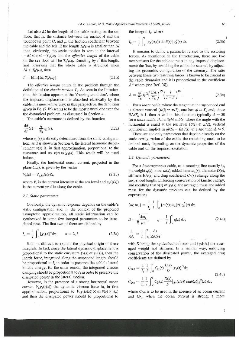
J.A.P. Aranha, M.O. Pinto /Applied Ocean Research 23 (2001) 63-81 71

(b)

45

65 70 75

Top Angle (deg)

50 55 60 65 70 75

Top Angle (deg)

Fig. 3. (a) Dynamic tension at the touchdown (FR) as a function of ds. (w/o current; P = 11.5 s). (—) Eqs. (2.8a)-(2.8c); Orcaflex (O) , (b) Dynamic tension at

the touch down (FR) as a function of 8s. (w/current; P = 11.5 s). (—) Eqs. (2.8a)-(2,8c); Orcaflex ( O ) .

predicts a response somewftere in between the two numer­

ical results. The impact forces on the discrete masses are

possibly the reason fo r the observed deterioration when the

amplitude increases: in this case, they generate at the touch­

down high frequencies oscillations that are propagated

along the cable wi th a relatively small damping,^ and so

they are weakly attenuated. To check this assumption, the

highest point in Fig. 3a, coiTesponding to (A = 5.54 m;

For a Rayleigh damping of the form dSvldt, the damping factor becomes

indeed very small in high frequency even when f AXIAL = 10% for the basic

mode.

ös = 80.5°; P = 11.5 s), was simulated again using now an

axial damping three times larger. The obtained result, also

shown i n Fig. 4a, indicates that wi th this higher damping the

concordance between Orcaflex and Eqs. (2.8a)-(2.8c) is

much better. Notice that in the Cable program the founda­

tion was assumed to be soft while in Orcaflex i t was

assumed to be r ig id and, also, that the discrepancies increase

just when T^TQ> \ , namely, when the cable becomes

dynamically compressed.

I n the other hand, one should expect that the influence o f

these higher harmonics diminishes when both the static and

dynamic tensions become large and the riser is not

72 J.A.P. Aranha, M.O. Pmto /Applied Ocean Research 23 (2001) 63-81

compressed at the touchdown. Fig. 4b gives support to this

conclusion, once i t displays the dynatnic tension at the

touchdown point as a function o f the atuplitude for

(ös = 37.8°; P= 11.5 s): although the maximum amphtude

is now twice the one imposed in the other case, the agree­

ment is very good here, among the numerical results them­

selves and wi th Eqs. (2.8a)-(2.8c) too.

Fig. 5 presents the dynairiic tension at the suspended end

normalized by the static tension Ts as a function of the

amplitude, keeping constant (0s = 70°; P = 1 2 s ) . The

agreement is again fair enough for the smaller amplitudes

but i t becomes evidently discrepant fo r the larger ampli­

tudes. In this same figure a fourth curve was plotted,

named 'Orcaflex filtered': i t corresponds to the sum of

the two first harmonics of the Orcaflex response.

Al though the Orcaflex result seeius to be lost fo r the

(a)

1^

o o 0

2.8 Orcaflex ,5=10% Orcaflex r=30% Cable

3 4 5

Amplitude (m)

(b)

1 r

0.9 -

0.8 -

0.7 -

0.6 -

.0 0.5 -

•

t -0.4 -

0.3 -

0.2 -

0.1 -

0 -

2.8 0 Orcaflex

• Cable

10 12 14

Amplitucie (m)

Fig. 4. (a) Dynamic tension at the touchdown (FR) as a function of amplitude (ös = 80.5°; P = 11.5s.; w/o current): (—) Eqs. (2.8a)-(2.8c); ( O ) Orcaflex;

( • ) Cable; (*) Orcaflex with f AX!AI, = 30%. (Note: two first points of Cable and Orcaflex are coincident), (b) Dynamic tension at the touchdown (FR) as a

function of amplitude (0s = 37.8°; P = 11.5 s; w/o current); k = 2800): (—) Eqs. (2.8a)-(2,8c); (O) Orcaflex; ( • ) Cable. (Note: last six points of Cable and

Orcaflex are coincident).

J.A.P. Aranhn, M.O. Pinto /Applied Ocean Research 23 (2001) 63-81 73

highest amplitudes, since the dynamic tension decreases

then when A increases, i t should be noticed the close

adherence between the fihered response and Eqs. (2 .8a)-

(2.8c), possibly indicating that the disagreement is due to

the high frequency components.

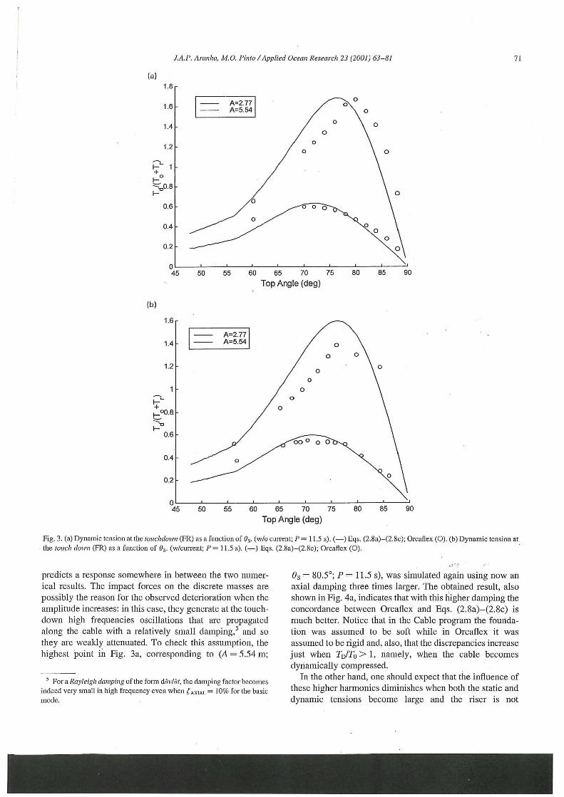
This conjecture can be better visualized with a look to the

corresponding time record in one period. Fig. 6a and b

present, fo r A = 2 m , the total tension at the touchdown

and at the suspended end normalized by the respective

static tension as a funct ion o f the time. The agreement

between the two numerical results and Eqs. (2 .8a) -

(2.8c) is quite good here, although i t should be observed

that i t is less good at the suspended end: the Cable

result is a l i t t le b i t o f f and the Orcaflex time series

shows evidences o f a s t i l l incipient higher harmonics.

This trend has been almost always observed, the agree­

ment between the numerical results (and w i t h

Eqs. (2.8a)-(2.8c)) becoming worse, i n general, at the

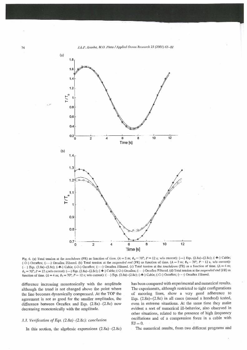
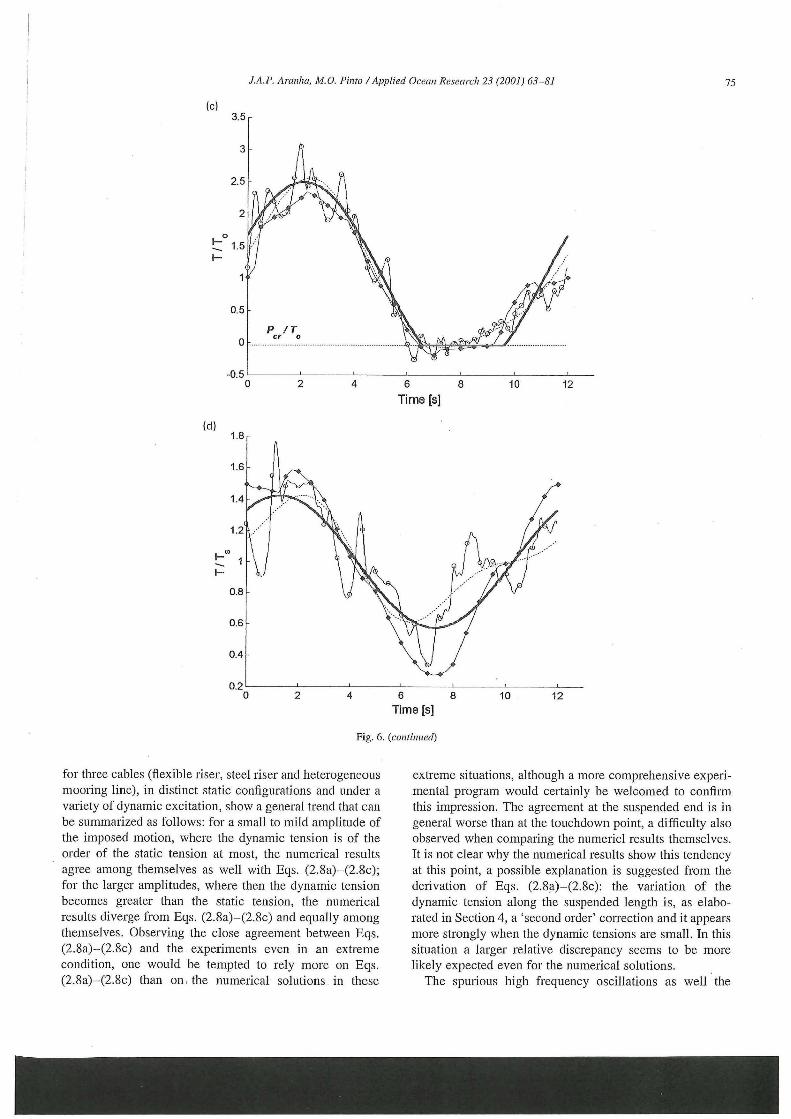
suspended end. Fig . 6c and d repeat the same plots but

f o r A = 4 m . N o w Orcaflex results show the presence of

strong high frequencies oscihations whi le Cable results,

perhaps due to the soft foundation used, show a rela­

t ively smooth time series. However, the experimental

results shown i n Section 3.1 indicate that these high

frequencies oscillations are i n fact spurious, the i n f l u ­

ence o f the soil stiffness being important only fo r the

discrete systems (recall that i n the experiments the fllor

was r ig id) . Fig. 6c and d show, again, that the agree­

ment is worse at the suspended end and that the ' f i l tered

response' is closer to Eqs. (2.8a)-(2.8c).

3.2.2. Numerical results: steel riser (It = 900 m)

Fig. 7a and b show the plot of the dynamic tension at the

touchdown point normalized by the static tension for a steel

riser (SR). In Fig. 7a the static cotifiguration is kept constant

(ös = 80.5°) and the tension is plotted as a funct ion of the

frequency for different amplitudes; i n Fig. 7b the period is

kept constant (F = 8 s) and the tension is plotted as a

fut ict ion of ös fo r different amplitudes. The agreement is

fa i r ly good in general, the e i T o r having a tendency to be

magnified for the larger ös (smaller TQ) i n Fig. 7b.

Fig. 8 shows the plot o f the dynamic tension at the

suspended end normalized by the static tension I's as a

function of the amplitude A ; in all cases (ös = 70°;

12s). The agreement between the two numerical results

and Eqs. (2.8a)-(2.8c) is again good for the smaller ampli­

tudes but they become widely discrepant f o r the larger

amplitudes, mainly the Cable result. The concordance

between Orcaflex and Eqs. (2.8a)-(2.8c) is fair, although

the Orcaflex result shov/s a tendency to an inf lexion point,

similar to the one observed in Fig. 5. Again, the behavior at

the suspended end is worse than at the touchdown point but

this is not restricted to expressions (2.8a)-(2.8c): as i t is

clear f r o m the material presented here, the numerical results

themselves become more discrepant at the suspended end

for a reason not yet we l l understood. A possible explanation

is the intense presence of high frequencies oscillations at

this point, perhaps due to the small damping i n the axial

direction.

3.2.3. Numerical results: heterogeneous line (h = 1000 m)

The heterogeneous line defined i n Table 3 was simulated

by Orcaflex in the condition (ös = 58.5°; P = 10 s) for

different amplitudes of the tangent motion. Fig. 9 shows

the comparison wi th Eqs. (2.8a)-(2.8c) of the obtained

dynamic tension, normalized by the respective static

tension, both at the suspended end (TOP) and at the touch­

down point (TDP). The agreement is fair at the TDP, the

74 J.A.P. Aranha, M.O. Pinto / Applied Ocean Research 23 (2001) 63-81

Fig. 6. (a) Total tension at the touchdown (FR) as function of time. (A = 2 m; ög = 70°; P = 12 s; w/o current): (—) Eqs. (2.8a)-(2.8c); ( - • - ) Cable;

(-0-) Orcaflex; (- - -) Orcaflex Filtered, (b) Total tension at tbe suspended end (FR) as function of time. (A = 2 m; 9s = 70°; P = 12 s, w/o current):

(—) Eqs. (2.8a)-(2.8c); ( - • - ) Cable; (-0-) Orcaflex; (- - -) Orcaflex Filtered, (c) Total tension at the touchdown (FR) as a function of time. (A = 4 m;

0g = 70°; P = 12 s;w/o cun'ent): (—) Eqs. (2.8a)-(2.8c); ( - • - ) Cable; (-0-) Orcaflex; (- - -) Orcaflex Filtered, (d) Total tension at the .suspended end (FR) as

function of time. (A = 4 m; 9s = 70°; P = 12 s; w/o cun-ent): (—) Eqs. (2.8a)-(2.8c); ( - • - ) Cable; (-0-) Orcaflex; (- - -) Orcaflex Filtered.

difference increasing monotonically wi th the amplitude

although the trend is not changed above the point where

the hne becomes dynamically compressed. A t the TOP the

agreement is not as good for the smaller amplitudes, the

difference between Orcaflex and Eqs. (2.8a)-(2.8c) now

decreasing monotonically wi th the amplitude.

3.3. Verification of Eqs. (2.8a)-(2.8c): conclusion

In this section, the algebraic expressions (2.8a)-(2.8c)

has been compared wi th experimental and numerical results.

The experiments, although restricted to tight configurations

of mooring lines, show a very good adherence to

Eqs. (2.8a)-(2.8c) i n al l cases (around a hundred) tested,

even in extreme situations. A t the same time they make

evident a sort o f numerical ill-behavior, also observed in

other situations, related to the presence of high frequency

oscillations and of a compression force in a cable w i t h

EJ = 0.

The numerical results, f r o m two different programs and

J.A.P. Aranha, M.O. Pinto/Applied Ocean Research 23 (2001) 63-81 75

(c)

Time [s]

Fig. 6. (continued)

for three cables (flexible riser, steel riser and heterogeneous

mooring line), i n distinct static configurations and under a

variety of dynamic excitation, show a general trend that can

be summarized as fol lows: fo r a small to m i l d amplitude o f

the imposed motion, where the dynamic tension is of the

order of the static tension at most, the numerical results

agree among themselves as wel l wi th Eqs. (2.8a)-(2.8c);

fo r the larger amplitudes, where then the dynamic tension

becomes greater than the static tension, the numerical

results diverge f r o m Eqs. (2.8a)-(2.8c) and equally airiong

theiuselves. Observing the close agreement between Eqs.

(2.8a)-(2.8c) and the experiments even in an extreme

condition, one would be tempted to rely more on Eqs.

(2.8a)-(2.8c) than on, the numerical solutions in these

extreme situations, although a more comprehensive experi­

mental program would certainly be welcomed to conf i rm

this impression. The agreement at the suspended end is in

general worse than at the touchdown point, a d i f f icul ty also

observed when comparing the numericl results themselves.

I t is not clear why the numerical results show this tendency

at this point, a possible explanation is suggested f r o m the

derivation of Eqs. (2.8a)-(2.8c): the variation o f the

dynamic tension along the suspended length is, as elabo­

rated in Section 4, a 'second order' con'ection and i t appears

more strongly when the dynamic tensions are small. I n this

situation a larger relative discrepancy seems to be more

l ike ly expected even for the numerical solutions.

The spurious high frequency oscillations as wel l the

76 J.A.P. Aranha, M.O. Pmto /Apphed Ocean Research 23 (2001) 63-81

0.5 0,55 0.6 0.65 0.7 0.75

Frequency (rad/s) 0,85

(b)

I '

30 40 50 60 70

Top Angle (deg) 80 90

Fig. 7. (a) Dynamic tension at the touchdown (SR) as a function of frequency (ös = 70°; w/o current): (—) Eqs. (2.8a)-(2.8c); ( - • - ) Cable; (-0-) Orcaflex.

(b) Dynamic tension at the touchdown (SR) as function of ös (P = 8 s; w/o cuirent): (—) Eqs. (2.8a)-(2.8c); (O) Orcaflex; ( • ) Cable (note: cable and Orcaflex

are coincident at A = 0.9 m).

compression above the crit ical value, both caused by the

discretization, tend to disappear as the mesh size

diminishes. No effort was inade i n the present work to

advance further in this direction, the focus being

concentrated more to cover a wide range of situations

rather than a specific case i n depth. Only one exaiuple

about the inflence of discretization was discussed here,

see Fig . 2c.

On the other hand, the algebraic approximation (2.8a)-

(2.8c) has to be looked wi th caution when the suspended

length is so large that the assumption w/we < 1 is not satis­

fied. However, this situation is unlikely to occur in a real

problem unless the material is intrinsically soft, as in the

case of the 'synthetic cables' that are being used lately. The

algebraic expression has to be revised in this case but this is

beyond the scope of the present work.

4. Mathematical derivation of Eqs . (2.8a)-(2.8c)

As seen in the Introduction, the static configuration is

defined by the functions [6(sy,T(s)}, where 6(s) is the

angle between the tangent to the cable and the horizontal

plane and T{s) is the static tension. The dynamic variables

are given by

[Ciis, ty,v(s,ty,^{s,ty,fuis,t)],

J.A.P. Aranha, M.O. Pmto /Applied Ocean Research 23 (2001) 63-81 11

3 4 5

Amplitude [m]

Fig. 8. Dynamic tension at the suspended end (SR) as function of amplimde (ös = 70°; ƒ" = 12 s; w/o current): (—) Eqs. (2.8a)-(2,8c); (-0-) Orcaflex; ( - • - ) Cable.

respectively, the axial displacement, the transversal dis­

placement, the dynamic variation o f the angle d{s) and the

dynamic tension. Assuming, as i t seems reasonable, that

the dynamic displacement is small compared to either the

2,5

2

1,5

1

0,5

0

TDP

- o - O R C A F L E X

For Analitica

—•—Cable

- o - O R C A F L E X

For Analitica

—•—Cable

- o - O R C A F L E X

For Analitica

—•—Cable

Amplitude (m)

TOP

10

4 6

Amplitude (m)

Fig. 9. Dynamic tension at the TOP and TDP as a function of amplitude. Heterogeneous Line. (Bs = 58,5°; P = 10 s; w/o cuirent): (—) Eqs, (2.8a)-(2.8c); (-0-) Orcafiex; ( - • - ) Cable. (Note: Cable and Orcaflex are coincidents at A = 2 m, TDP).

suspended length / or the static angle 6{s), the dynamic

equations can be derived ignoring the geometric non linear­

i ty , wr i t ing them directly in tertns of the static geometric

configuration. The experimental results shown in Section

3.1 gives support to such assumption and, in this context,

the only source of non-linearity is the damping term.

However, this parcel w i l l be writ ten i n the 'linear' f o r m

dv

at (4.1a)

a proper definition for the nonlinear ^ w i l l be given later in

Section 4.2. Then, the dynamic variables should satisfy the

set o f linear equations (see R e f [2])

m-Ais,t) = —^is,t) - Tis)--is) <p(s,t), dt'

(m + ni^)

ds ds

dt' 3?' 2 {s,t) + Cco — {s,t)

= ^(s)Tr,{s,t)+ -ins)<p(s,t)), ds ds

f j , ( s , t ) du d(? -—-— = —is,t) - ~-{s)vis,t),

E A ds ds

dv do 0{s, t)= — (s, t)+ - - (syüis, t),

ds ds

subjected to the fo l lowing boundary conditions:

u{l,t)=UoA'"', i)(Z,0 = Vo-e'"',

/ ( ( - / ' , / ) = 0, 1-5(0,0 = 0.

(4.1b)

(4.1c)

In Eq. (4.1c) UQ and Vo are the amplitudes o f the imposed

motion at the suspended end, in the axial and normal

78 J.A.P. Aranha, M.O. Pmto/Applied Ocean Research 23 (2001) 63-81

directions respectively, and the boundary conditions at the

sea floor deserve some further comments. I n fact, although

the actual position of the instantaneous touchdown point is

of vi ta l importance i n the fatigue analysis of risers, see

Ref. [3] , i t can be shown, i n first approximation, that the

transversal displacement can be taken zero at the static

touchdown point, as impl ied by Eq. (4.1c); more is going

to be said about the touchdown displacement at the end o f

Section 4.3. Also, i f there is no f i ic t ion wi th the sea floor, tire

axial displacement would be zero at the anchor A

placed at i - = - A / ; i n the presence of a f r i c d o n the

static axial displacement is zero f o r s < —l', w i th l'

defined in Eq. (2.1b). One can say that the effective

anchor position i n the static problem is a.t s= -l' and

this position must be preserved in the geometrically

linear dynamic problem; this explains the boundary

condit ion fo r the axial displacement at the sea floor.

Expressing the linear harmonic solution of Eqs. (4 .1a) -

(4.1c) in the f o r m

{u(s, f ) ; v(s, ty, q>(s, t); fj,{s, t)} = {u{sy, visy, V(sy To(s)}-é'",

s (4.2a)

and introducing the non dimensional variables (see

Eqs. (2.7a) and (2.7b) fo r the definit ion of CTU, a and Te)

TD{S) eis) T{s)

E A

-, ^ AA . V ( 5 ) u(s)= , v{s)= ,

0 - u CTU

the dynamic equation reads (see also Eq. (2.6))

(4.2b)

i 7 T F j l ^ j " ^ ^ ^ = d ^ l d ? - d ? i

d0 / di; d0

( - l + t D . ^ ( ^ ) ^ ( . - )

_ E A f / d0

I + / ' d.- - ' ^ ^ + d^

(Av d0 \~W

r D ( 5 )

w i t h

i7(0 = a.

l + l'/dü de

I

idü _ d0 \

^ ds ds )' (4.2c)

17(0 = {VolUQ)a,

4.1. Asymptotic solution

I f the term proportional to the static deformation €{s) is

ignored in the axial equil ibrium equation one obtains, after a

further derivation wi th respect to s, that

( l ± i ' A _ ^A ^ _ A ^ \ \ I ) d f \ d s ds ) U e /

\ a ) J \ds ds / XM^J

ds

^de

ds'

and so

ds + r ' + 1'

OJ

We

2d0

l+l

,/ w ydo (sym-

I f now (üjfwe)' is disregarded when compared to 1 i n the

le f t hand side of the above equation'' then, w i th an e n w of

the f o r m [1 + 0{e; (M/CÜA)]^ one has

di-2 l + l ds {sym-

On the sea floor, where dis) = 0, the dynamic tension is

constant, see Eq. (4.2c), and so dr^ds = 0 for - / ' < . ? < 0;

i f the above equality is integrated f r o m s= -l' to s = I, the

fo l l owing expression is obtained fo r the derivative o f the

dynamic tension at the suspended end:

' de

l + l' •T?[^

ds (5 ) -v ( .v ) ds.

The variation of the dynamic tension along the suspended

length is weak, once i t is proportional to imltoA^, and it can

be assumed of the f o r m

TT,is) T D ( 0 ) + i ( l s i n a / 5 ) - [ T D ( l ) - T D ( 0 ) ] - 5 , (4.3a)

w i t h

[ r D ( 0 - T D ( 0 ) ] dB

(.y)-v(i) ds.

(4.3b)

Now consider the equilibrium Eq. (4.2c) in the transversal

direction, disregarding again the term proportional to eis).

The e i T o r i n this approximation w i l l be analyzed in Section

4.3 o f th i s section but one point should be observed here: the

higher order derivative in the transversal equation is lost in

this approximation and, w i th i t , the imposed boundary

conditions on vis); as i t is usual, this gives rise to a boundary

layer c o i T c c t i o n near the extremities, briefly elaborated i n

üi-1'll) = 0, i7(0) = 0. (4.2d)

The asymptotic solution o f Eqs. (4.2c) and (4.2d) w i h be

elaborated next.

^ Recall that the variation of along the suspended length has a relative

importance only when T D « 1; i f T D = 0(1) this variation is of secondary

importance since it is of order (co/coS' -C 1, see Eq. (4.3b).

J.A.P. Aranha, M.O. Pmto / AppUed Ocean Research 23 (2001) 63-81 79

Section 4.3. Ignoring Iiere these localized c o i T c c t i o n s one

has

( - 1 + 1

where the boundary conditions f o r the axial displace­

ment u(s) have been used. W i t h an error o f the f o r m

[1 + 0 ( ( « / « e ) ' ) ]

T D ( 0 ) = 1 - V T . (4.4d)

EA / dgp TD(0) + i ( l + sin al 5 ) - (TD(1) - TD(0))-J .

The parcel ( T D ( 1 ) - T D ( 0 ) ) is o f order (w/we) < 1 and i t

becomes relevant only when the dynamic tension T D ( 0 ) is

also very small. As seen at the end of Section 2, this situa­

tion occurs for a 'vertical cable' (0s ~ 'n'/2), where T D <C 1

since A ^ 1. However, in this case the term d6/ds(TD{l) —

TT)iO))'s/l in the above expression can be ignored by a

geometric argument: fo r a vertical cable the curvature d0/

d^ is appreciable only i n the vicini ty o f the touchdown point,

where then 5// <C 1. For a 'non vertical cable' the parameter

A decreases and the dynamic tension increases, turning

irrelevant the coirection proportional to ( T D ( 1 ) - T D ( 0 ) ) .

As a conclusion, one has, w i th the help of Eqs. (2.2a),

(2 .3C) and (2.7c), that the transversal equil ibrium equation

reduces to

( - 1 + i^nhis) = ^ i-Xl(s>TD(0). (4.4a)

Expression (4.4a) indicates that, i n first approximation,

the transversal displacement is proportional to the static

curvature and thus

ql h (4.4b)

W i t h Vj being the non dimensional amplitude of the

lateral displacement. Notice that Eq. (4.4b) must be

coirected at the small boundary layers near the extremities

but these corrections have a small integral contribution for

the overall equilibrium of the cable. Placing Eq. (4.4b) into

Eq. (4.4a) one obtains the algebraic relation

( - 1 + i ^ ^ ^ V x = T D ( 0 )

(4.4c)

A second relation can be obtained f r o m the integra­

t ion o f the expression that defines TD{S) i n Eq. (4.2c); i n

fact, f r o m this expression and Eqs. (4.3a) and (4.3b) i t

fo l lows that

-I'll T D ( S ) d 5

d0 _ — {s)v{s) ds

0 ds

l + l' Vl'\

rv •1 d0

0 ds {s)v{s) ds

From Eq. (4.3b) i t also fol lows that

1 [ T D ( 1 ) - T D ( 0 ) ] =

and again the same argument can be used: the variation o f

the dynamic tension along the suspended length has a rela­

tive importance only when T D ( 0 ) "C 1 and, in this case, one

has

1 T D ( 1 ) - r D ( 0 ) ] A7<A'-

Now, i f the damping factor ^ is given, the non dimen­

sional amplitude Vr and the normalized dynamic tension at

the tuchdown point T D ( 0 ) can be determined f r o m the solu­

tion o f the algebraic system Eqs. (4.4c) and (4.4d); the

dynamic tension T D ( 5 ) along the cable is

ruis) = r D ( 0 ) - aj—TrH — - , 0 < ^ < /. (4.5) I + i \ (Wg / /

A proper definit ion for the damping factor ^ w i l l be

elaborated next.

4.2. A model for the viscous damping

The viscous drag force in the dynamic problem is given

by the known expression

d,(s,t)=lpCuD V,(s) sinOis) dv

Tt ( s j )

X Vc(5) sin 0(5) TH - -pCuD\V,is) sine(^s)\V,is) sme(s), (4.6a)

Where V^s) is the projection o f the horizontal ocean current

on the cable's plane. On the other hand, the dissipative force

was assumed, in this section, in f o r m Eq. (4.1a) and the two

expressions can be related by imposing the equality o f the

dissipated power in one cycle, namely

I f ' / dv \ I f ' / - \ ^ { d , i s , t ) . - i s , t ) ) d s = - \ ^ { d : i s , t ) - ^ ( s , t ) ) j . .

<f(t)> 2 ^

•ZTTIOI

f( t )dt .

Placing Eq. (4.1a) i n the above integral, using Eqs. (4.2b)

80 J.A.P. Aranha, M.O. Pinto/Applied Ocean Research 23 (2001) 63-81

and (4.4b) and the definition (2.3a), the fo l lowing relation

can be derived

f ' / dv \

I f Vc(5) = 0 one obtains

(4.6b)

J o \ dt ds

and then

C=a\vACtj,

ql h

f o = 8 2 C D PTTD'IA TS h o^u

37r 7r m + ql Ö

(4.7a)

I n the other hand, f o r a strong current, when yj.sinö(s) >

dvldt, one has

/ 0 ~ ( 5 , f ) / c . ^ idy{s, I

and so

2 C D p7rD74 2V, 4

TT ;?! + /Ha wD I2 (4.7b)

For a moderated current the relative velocity in Eq. (4.6a)

becomes negative in part o f the cycle and the expression for

f is obviously more complicated; to preserve the simplicity,

the fo l l owing definition for the damping coefficient was

assumed in this work

(4.7c)

Nodce here that since, in general, one has

[Uo/D;2VJ(oD] > 1 therefore, in general, one must have

^ > 1: i n short, the viscous damping is super critical i n

the cable's dynamic. Placing now Eq. (4.7c) in to Eq.

(4.4c) and solving the system (4.4c) and (4.4d) one

obtains

\ I -n'

n'

showing that i n fact the cable/reezes ( I V x l — * 0 ) when

either u> or f/o (see expression f o r ^0) increases; using

this value fo r | V T I i n Eq. (4.7c) the foUowing expression

f o r the damping coefficient is obtained:

1

+ (4.8)

W i t h Eq. (4.8) the system (4.4c) and (4.4d) can be solved

and, after some algebra, the resuh (2.8a)-(2.8c) is obtained.

4.3. Quasi-static solution and boundary layers

As has already been seen, the error in the approximation

fo r the axial equation is o f the f o r m [1 + 0(e(s);(ft)/üJe)^)]

and the intension now is to assess the error i n the approx­

imation for the transversal equation. When r^{s) s 0 (1 ) the

e i T o r is, indeed, of this same order of magnitude; however,

when < 1 one has, as seen at the end of Section 2, that

T-ois) = 0 ( i7^) and the error in this approximtion must be

reevaluated. I n this case the approximation used is correct i f

and only i f

or (see Eq. (2.3c))

I t fo l lows then that the proposed dynamic approximation

is vahd when < 1 i f and only i f the inequality

7 7 ^ - ( ^ ƒ » l ( o r ro s 0 { n ' ) » ^ ) (4.9a)

is satisfied simultaneously. In otherwords: when

— < 0 ( l / 7 r ) (4.9b)

the proposed approximation is not vahd anymore but the

response is quasi-static then.

This solution is elaborated in Ref. [2] and only the final

answer w i l be presented here; i n this way, i f 9{s) =

{qllTs)Xo{s) and the integrals

1 cl Jn= ^ -ds. n = 0,1,2,

0 Tis)/Ts

are defined, the quasi static solution is given by

ql Jl 11

(4.10a)

TQE

- ^ \ ö i l ) 0 - Ts Jo

1 + '2

(4.10b)

J.A.P. Aranha, M.O. Pinto /AppUed Ocean Research 23 (2001) 63-81 81

This result is consistent with Eq. (4.9a): since 72 - JI/JQ >

0, then T Q E = O ( I M ^ ) , showing that the dynamic result

(2.8a)-(2.8c) duninishes wi th ü ' until the level O ( I M ^ ) is

reached, when then one should switch to the quasi-static solu­

tion. To make the analysis simpler the fol lowing rule was used

to plot the theoretical curve in Eig. la : i f T(2.8) > T Q E then the

value T D ( 0 ) = T(2.8) was taken; i f T(2.8) < T Q E then T D ( 0 ) = T Q E .

The experimental resuhs confirm the adequacy of such simple

strategy.

Einally, the question of the transversal boundary condi­

tion (4.1C), lost i n the dynamic approximation (2.8a)-(2.8c),

w i l l be br ief ly addressed. To make more direct the

exposition more straightforward, the boundary layer in

the v icni ty o f the touchdown point w i l l be worked out

below. In this case the transversal Eq. (4.2c) is reduced

to {s s 0)

Tn d^v , / CO V E A / &e

(4.11a)

Introducing the parameter p by the expression

i - i f = / r T 7 - ^ " ' ' '

I (4.11b)

P = j | ( l + ^ W - f } e - * ' ^ b l » l ,

then Eq. (4.4b) is, i n the jargon of the boundary layer theory,

an outer solution o f Eq. (4.11a) wi th an error o f order 0 ( 1 /

p'), see R e f [4 ] ; obviously Eq. (4.4b) is a particular solu­

tion of the linear Eq. (4.11a), the total solution, satisfying

the boundary condition v(0) = 0, being given by

v(^) = % raV^ix.is) - A f , ( 0 ) - e -n . (4.11c) ql h

The dynamic angular displacement at the static touch­

down point is equal to

(4.12a)

and, as shown i n R e f [3] , i f the instantaneous touchdown

point is at 5 = X(t) one must have 0(X(O) + ^(O)'e''^' = 0.

Since (0(0) = O;d0/d5(O) = qlTo) then, i f Z ( 0 = Xo-e'"',

the amplitude XQ o f the horizontal displacement of the

touchdown point can be approximated by the expression

/ ql

_ a-i] To f Ts Y 1 r dxi ̂ (4.12b)

In the fatigue induced by the cyclic variation o f the curva­

ture at the touchdown, the motion o f this point, and thus the

amplitude XQ, is of crucial importance. The cyclic variation

of the curvature, obtained in Ref. [3] , compares wel l wi th

some experiments, as discussed in Ref. [8] , and Eq. (4.12b)

makes possible to estimate this variation analytically.

A t the suspended end a similar analysis can be pursued

and the boundary condition v(/) = VQ can then be imposed.

Also, i n a heterogeneous cable the curvature is discontinu­

ous when q(s) is and boundary layers occur at these discon­

tinuity points. Again, these local corrections do not affect

the overall dynamics o f the cable and are of l i t t le practical

importance.

References

[1] Andrade BLR. Estudo experimental do comportamento dinamico de

linhas de amaiTa9ao, Tese de Mestrado, Departmento de Engenharia Naval e Oceanica, EPUSP, 1993.

[2] Aranha JAP, Pesce CP, Martins CA, Andrade BLR. Mechanics of

submerged cables: asymptotic solution for the dynamic tension.

Polar Engineers, ISOPE-93, Singapore, 6-11 June, 1993. [3] Aranha JAP, Martins CA, Pesce CP. Analytical approximation for the

dynamic bending moment at the touchdown point of a catenary riser.

Int J Offshore Polar Engng 1997;7(4):229-300. [4] Bender C, Orzag S. Advanced mathematical methods for Scientist and

Engineers. New York: McGraw-Hill, 1978. [5] Howell CT. Investigation of the Dynamics of Low Tension Cables.

PhD Thesis. Ocean Engineering Department, M I T , 1992. [6] Irvine H M , Caughey TK. The linear theory of the free vibration of a

suspended cable. Phil Trans R Soc Lond A 1974;341:229-315. [7] Larsen CM. Flexible riser analysis: comparison of results from compu­

ter programs. Mar Struct 1992;5(5):103-19 (special issue on flexible

risers (Part 1)). [8] Pesce CP, Aranha JAP, Martins CA, Ricardo OGS, Silva S. Dynamic

curvature in catenary risers at the touchdown region: an experimental study and the analytical boundary layer solution. Int J Offshore Polar Engng 1998;8(4):303-10.

[9] Triantafyllou MS, Bliek A, Shin H. Dynamic analysis as a tool for open-sea mooring system design, presented at the Annual Meeting of the Society of Naval Architects and Marine Engineers, New York, 1985.