Dynamic Template Tracking and Recognition - JHU Vision Lab

Noname manuscript No.(will be inserted by the editor)

Dynamic Template Tracking and Recognition

Rizwan Chaudhry · Gregory Hager · Rene Vidal

Received: date / Accepted: date

Abstract In this paper we address the problem of track-

ing non-rigid objects whose local appearance and mo-

tion changes as a function of time. This class of objects

includes dynamic textures such as steam, fire, smoke,

water, etc., as well as articulated objects such as humans

performing various actions. We model the temporal evo-

lution of the object’s appearance/motion using a Linear

Dynamical System (LDS). We learn such models from

sample videos and use them as dynamic templates for

tracking objects in novel videos. We pose the problem of

tracking a dynamic non-rigid object in the current frame

as a maximum a-posteriori estimate of the location of

the object and the latent state of the dynamical system,

given the current image features and the best estimate

of the state in the previous frame. The advantage of

our approach is that we can specify a-priori the type oftexture to be tracked in the scene by using previously

trained models for the dynamics of these textures. Our

framework naturally generalizes common tracking meth-

ods such as SSD and kernel-based tracking from static

templates to dynamic templates. We test our algorithm

R. ChaudhryCenter for Imaging ScienceJohns Hopkins UniversityBaltimore, MDTel.: +1-410-516-4095Fax: +1-410-516-4594E-mail: [email protected]

G. HagerJohns Hopkins UniversityBaltimore, MDE-mail: [email protected]

R. VidalCenter for Imaging ScienceJohns Hopkins UniversityBaltimore, MDE-mail: [email protected]

on synthetic as well as real examples of dynamic tex-

tures and show that our simple dynamics-based trackers

perform at par if not better than the state-of-the-art.

Since our approach is general and applicable to any

image feature, we also apply it to the problem of human

action tracking and build action-specific optical flow

trackers that perform better than the state-of-the-art

when tracking a human performing a particular action.

Finally, since our approach is generative, we can use

a-priori trained trackers for different texture or action

classes to simultaneously track and recognize the texture

or action in the video.

Keywords Dynamic Templates · Dynamic Textures ·Human Actions · Tracking · Linear Dynamical Systems ·Recognition

1 Introduction

Object tracking is arguably one of the most important

and actively researched areas in computer vision. Ac-

curate object tracking is generally a pre-requisite for

vision-based control, surveillance and object recognition

in videos. Some of the challenges to accurate object

tracking are moving cameras, changing pose, scale and

velocity of the object, occlusions, non-rigidity of the

object shape and changes in appearance due to ambi-

ent conditions. A very large number of techniques have

been proposed over the last few decades, each trying to

address one or more of these challenges under different

assumptions. The comprehensive survey by Yilmaz et al.

(2006) provides an analysis of over 200 publications in

the general area of object tracking.

In this paper, we focus on tracking objects that

undergo non-rigid transformations in shape and appear-

ance as they move around in a scene. Examples of such

mailto:[email protected]



2 Rizwan Chaudhry et al.

objects include fire, smoke, water, and fluttering flags, as

well as humans performing different actions. Collectively

called dynamic templates, these objects are fairly com-

mon in natural videos. Due to their constantly evolving

appearance, they pose a challenge to state-of-the-art

tracking techniques that assume consistency of appear-

ance distributions or consistency of shape and contours.

However, the change in appearance and motion profiles

of dynamic templates is not entirely arbitrary and can

be explicitly modeled using Linear Dynamical Systems

(LDS). Standard tracking methods either use subspacemodels or simple Gaussian models to describe appear-

ance changes of a mean template. Other methods use

higher-level features such as skeletal structures or con-

tour deformations for tracking to reduce dependence on

appearance features. Yet others make use of foreground-

background classifiers and learn discriminative features

for the purpose of tracking. However, all these methods

ignore the temporal dynamics of the appearance changes

that are characteristic to the dynamic template.

Over the years, several methods have been developed

for segmentation and recognition of dynamic templates,

in particular dynamic textures. However, to the best of

our knowledge the only work that explicitly addresses

tracking of dynamic textures was done by Peteri (2010).

As we will describe in detail later, this work also does

not consider the temporal dynamics of the appearance

changes and does not perform well in experiments.

Paper Contributions and Outline. In the proposed

approach, we model the temporal evolution of the ap-

pearance of dynamic templates using Linear Dynamical

Systems (LDSs) whose parameters are learned from

sample videos. These LDSs will be incorporated in a

kernel based tracking framework that will allow us to

track non-rigid objects in novel video sequences. In the

remaining part of this section, we will review some of

the related works in tracking and motivate the need

for dynamic template tracking method. We will then

review static template tracking in §2. In §3, we pose the

tracking problem as the maximum a-posteriori estimate

of the location of the template as well as the internal

state of the LDS, given a kernel-weighted histogram

observed at a test location in the image and the internal

state of the LDS at the previous frame. This results

in a novel joint optimization approach that allows us

to simultaneously compute the best location as well as

the internal state of the moving dynamic texture at the

current time instant in the video. We then show how our

proposed approach can be used to perform simultaneous

tracking and recognition in §4. In §5, we first evaluate

the convergence properties of our algorithm on synthetic

data before validating it with experimental results on

real datasets of Dynamic Textures and Human Activ-

ities in §6, §7 and §8. Finally, we will mention future

research directions and conclude in §9.

Prior Work on Tracking Non-Rigid and Articu-

lated Objects. In the general area of tracking, Isard

and Blake (1998) and North et al. (2000) hand craftmodels for object contours using splines and learn their

dynamics using Expectation Maximization (EM). They

then use particle filtering and Markov Chain Monte-

Carlo methods to track and classify the object motion.

However for most of the cases, the object contours do

not vary significantly during the tracking task. In the

case of dynamic textures, generally there is no well-

defined contour and hence this approach is not directly

applicable. Black and Jepson (1998) propose using a

robust appearance subspace model for a known object

to track it later in a novel video. However there are

no dynamics associated to the appearance changes and

in each frame, the projection coefficients are computed

independently from previous frames. Jepson et al. (2001)

propose an EM-based method to estimate parameters

of a mixture model that combines stable object appear-

ance, frame-to-frame variations, and an outlier model

for robustly tracking objects that undergo appearance

changes. Although, the motivation behind such a model

is compelling, its actual application requires heuristics

and a large number of parameters. Moreover, dynamic

textures do not have a stable object appearance model,instead the appearance changes according to a distinct

Gauss-Markov process characteristic to the class of the

dynamic texture.

Tracking of non-rigid objects is often motivated by

the application of human tracking in videos. In Pavlovic

et al. (1999), a Dynamic Bayesian Network is used to

learn the dynamics of human motion in a scene. Joint

angle dynamics are modeled using switched linear dy-

namical systems and used for classification, tracking

and synthesis of human motion. Although, the track-

ing results for human skeletons are impressive, extreme

care is required to learn the joint dynamic models from

manually extracted skeletons or motion capture data.

Moreover a separate dynamical system is learnt for each

joint angle instead of a global model for the entire ob-

ject. Approaches such as Leibe et al. (2008) maintain

multiple hypotheses for object tracks and continuously

refine them as the video progresses using a Minimum

Description Length (MDL) framework. The work by Lim

et al. (2006) models dynamic appearance by using non-

linear dimensionality reduction techniques and learns

the temporal dynamics of these low-dimensional repre-

sentation to predict future motion trajectories. Nejhum

et al. (2008) propose an online approach that deals with

appearance changes due to articulation by updating the

foreground shape using rectangular blocks that adapt to

Dynamic Template Tracking and Recognition 3

find the best match in every frame. However foreground

appearance is assumed to be stationary throughout the

video.

Recently, classification based approaches have been

proposed in Grabner et al. (2006) and Babenko et al.

(2009) where classifiers such as boosting or Multiple

Instance Learning are used to adapt foreground vs back-

ground appearance models with time. This makes the

tracker invariant to gradual appearance changes due

to object rotation, illumination changes etc. This dis-

criminative approach, however, does not incorporate

an inherent temporal model of appearance variations,

which is characteristic of, and potentially very useful,

for dynamic textures.

? propose a method for unconstrained tracking of

Near-Regular Textures (NRT). NRTs are special static

textures that have an inherent repeating spatial pat-

tern e.g., a checkerboard printed on a flag. As the flag

waves in the air, the checkerboard pattern deforms andself-occludes and results in a Dynamic NRT. ? model

the Dynamic NRT using a spatio-temporal lattice-based

MRF where the lattice models the topology of the NRT

and image-observations are registered to the lattice at

each time-step using belief propagation. Temporal track-

ing is then performed using particle filters by using a

non-stationary Gaussian model for the motion of the

textons and updating the spatial appearance model for

the NRT. Even though this method is promising for

the specific task of tracking NRTs, it require some user

initialization in selection of the repeating unit. Further-more, most dynamic templates such as steam, water,

and human actions are not NRTs and do not have a

fundamental repeating texture unit thereby limiting the

applicability of this method.

In summary, all the above works lack a unified frame-

work that simultaneously models the temporal dynamics

of the object appearance and shape as well as the mo-

tion through the scene. Moreover, most of the works

concentrate on handling the appearance changes due to

articulation and are not directly relevant to dynamic

textures where there is no articulation.

Prior Work on Tracking Dynamic Templates. Re-

cently, Peteri (2010) propose a first method for tracking

dynamic textures using a particle filtering approach

similar to the one presented in Isard and Blake (1998).

However their approach can best be described as a static

template tracker that uses optical flow features. The

method extracts histograms for the magnitude, direc-

tion, divergence and curl of the optical flow field of the

dynamic texture in the first two frames. It then assumes

that the change in these flow characteristics with time

can simply be modeled using a Gaussian distribution

with the initially computed histograms as the mean.

The variance of this distribution is selected as a param-

eter. Furthermore, they do not model the characteristic

temporal dynamics of the intensity variations specific to

each class of dynamic textures, most commonly modeled

using LDSs. As we will also show in our experiments,

their approach performs poorly on several real dynamic

texture examples.

LDS-based techniques have been shown to be ex-

tremely valuable for dynamic texture recognition (Saisan

et al., 2001; Doretto et al., 2003; Chan and Vasconcelos,

2007; Ravichandran et al., 2009), synthesis (Dorettoet al., 2003), and registration (Ravichandran and Vidal,

2008). They have also been successfully used to model

the temporal evolution of human actions for the pur-

pose of activity recogntion (Bissacco et al., 2001, 2007;

Chaudhry et al., 2009). Therefore, it is only natural to

assume that such a representation should also be useful

for tracking.

Finally, Vidal and Ravichandran (2005) propose a

method to jointly compute the dynamics as well as the

optical flow of a scene for the purpose of segmenting

moving dynamic textures. Using the Dynamic Texture

Constancy Constraint (DTCC), the authors show that

if the motion of the texture is slow, the optical flow

corresponding to 2-D rigid motion of the texture (or

equivalently the motion of the camera) can be computed

using a method similar to the Lucas-Kanade optical flow

algorithm. In principle, this method can be extended

to track a dynamic texture in a framework similar to

the KLT tracker. However, the requirement of having

a slow-moving dynamic texture is particularly strict,

especially for high-order systems and would not work in

most cases. Moreover, the authors do not enforce anyspatial coherence of the moving textures, which causes

the segmentation results to have holes.

In light of the above discussion, we posit that there

is a need to develop a principled approach for tracking

dynamic templates that explicitly models the character-istic temporal dynamics of the appearance and motion.

As we will show, by incorporating these dynamics, our

proposed method achieves superior tracking results as

well as allows us to perform simultaneous tracking and

recognition of dynamic templates.

2 Review of Static Template Tracking

In this section, we will formulate the tracking problem

as a maximum a-posteriori estimation problem and show

how standard static template tracking methods such

as Sum-of-Squared-Differences (SSD) and kernel-based

tracking are special cases of this general problem.

Assume that we are given a static template I : Ω →R, centered at the origin on the discrete pixel grid,


Ω ⊂ R2. At each time instant, t, we observe an image

frame, yt : F → R, where F ⊂ R2 is the discrete pixel

domain of the image. As the template moves in the scene,

it undergoes a translation, lt ∈ R2, from the origin of

the template reference frame Ω. Moreover, assume that

due to noise in the observed image the intensity at each

pixel in F is corrupted by i.i.d. Gaussian noise with

mean 0, and standard deviation σY . Hence, for each

pixel location z ∈ Ω + lt = z′ + lt : z′ ∈ Ω, we have,

yt(z) = I(z−lt)+wt(z), where wt(z)iid∼ N (0, σ2

Y ). (1)

Therefore, the likelihood of the image intensity at pixel

z ∈ Ω + lt is p(yt(z)|lt) = Gyt(z)(I(z− lt), σ2Y ), where

Gx(µ,Σ) =1

(2π)n2 |Σ| 12

exp

−1

2(x− µ)>Σ−1(x− µ)

is the n-dimensional Gaussian pdf with mean µ and

covariance Σ. Given yt = [yt(z)]z∈F , i.e., the stack ofall the pixel intensities in the frame at time t, we would

like to maximize the posterior, p(lt|yt). Assuming the

intensity at each pixel in the background is uniformly

distributed, i.e., p(yt(z)|lt) = 1/K if z− lt 6∈ Ω , where

K = 1, and a uniform prior for lt, i.e., p(lt) = |F|−1, we

have,

p(lt|yt) =p(yt|lt)p(lt)

p(yt)

∝ p(yt|lt) =∏

z∈Ω+lt

p(yt(z)|lt)∏

z∈Ω+lt′

1

K(2)

∝ exp

− 1

2σ2Y

∑z∈Ω+lt

(yt(z)− I(z− lt))2

.

The optimum value, lt will maximize the log posterior

and after some algebraic manipulations, we get

lt = argminlt

∑z∈Ω+lt

(yt(z)− I(z− lt))2. (3)

Notice that with the change of variable, z′ = z− lt, we

can shift the domain from the image pixel space F to

the template pixel space Ω, to get lt = argminlt O(lt),

where

O(lt) =∑z′∈Ω

(yt(z′ + lt)− I(z′))2. (4)

Eq. (4) is the well known optimization function used

in Sum of Squared Differences (SSD)-based tracking of

static templates. The optimal solution is found either

by searching brute force over the entire image frame

or, given an initial estimate of the location, by perform-

ing gradient descent iterations: li+1t = lit − γ∇ltO(lit).

Since the image intensity function, yt is non-convex, a

good initial guess, l0t , is very important for the gradient

descent algorithm to converge to the correct location.

Generally, l0t is initialized using the optimal location

found at the previous time instant, i.e., lt−1, and l0 is

hand set or found using an object detector.

In the above description, we have assumed that we

observe the intensity values, yt, directly. However, to

develop an algorithm that is invariant to nuisance fac-

tors such as changes in contrast and brightness, object

orientations, etc., we can choose to compute the value

of a more robust function that also considers the inten-

sity values over a neighborhood Γ (z) ⊂ R2 of the pixel

location z,

ft(z) = f([yt(z′)]z′∈Γ (z)), f : R|Γ | → Rd, (5)

where [yt(z′)]z′∈Γ (z) represents the stack of intensity

values of all the pixel locations in Γ (z). We can therefore

treat the value of ft(z) as the observed random variable

at the location z instead of the actual intensities, yt(z).

Notice that even though the conditional probability

of the intensity of individual pixels is Gaussian, as in

Eq. (1), under the (possibly) non-linear transformation,

f , the conditional probability of ft(z) will no longer be

Gaussian. However, from an empirical point of view,

using a Gaussian assumption in general provides very

good results. Therefore, due to changes in the location

of the template, we observe ft(z) = f([I(z′)]z′∈Γ (z−lt))+

wft (z), where wf

t (z)iid∼ N (0, σ2

f ) is isotropic Gaussian

noise.

Following the same derivation as before, the new

cost function to be optimized becomes,

O(lt) =∑z∈Ω‖f([yt(z

′)]z′∈Γ (z+lt))− f([I(z′)]z′∈Γ (z))‖2

.= ‖F (yt(lt))− F (I)‖2, (6)

where,

F (yt(lt)).= [f([yt(z

′)]z′∈Γ (z+lt))]z∈Ω

F (I).= [f([I(z′)]z′∈Γ (z))]z∈Ω

By the same argument as in Eq. (4), lt = argminlt O(lt)

also maximizes the posterior, p(lt|F (yt)), where

F (yt).= [f([yt(z

′)]z′∈Γ (z)]z∈F , (7)

is the stack of all the function evaluations with neigh-borhood size Γ over all the pixels in the frame.

For the sake of simplicity, from now on as in Eq.

(6), we will abuse the notation and use yt(lt) to denote

the stacked vector [yt(z′)]z′∈Γ (z+lt), and yt to denote

the full frame, [yt(z)]z∈F . Moreover, assume that the

ordering of pixels in Ω is in column-wise format, de-

noted by the set 1, . . . , N. Finally, if the size of the


neighborhood, Γ , is equal to the size of the template, I,

i.e., |Γ | = |Ω|, f will only need to be computed at the

central pixel of Ω, shifted by lt, i.e.,

O(lt) = ‖f(yt(lt))− f(I)‖2 (8)

Kernel based Tracking. One special class of func-

tions that has commonly been used in kernel-based track-

ing methods (Comaniciu and Meer, 2002; Comaniciuet al., 2003) is that of kernel-weighted histograms of

intensities. These functions have very useful properties

in that, with the right choice of the kernel, they can

be made either robust to variations in the pose of the

object, or sensitive to certain discriminatory character-

istics of the object. This property is extremely useful

in common tracking problems and is the reason for the

wide use of kernel-based tracking methods. In particular,

a kernel-weighted histogram, ρ = [ρ1, . . . , ρB ]> with B

bins, u = 1, . . . , B, computed at pixel location lt, is

defined as,

ρu(yt(lt)) =1

κ

∑z∈Ω

K(z)δ(b(yt(z + lt))− u), (9)

where b is a binning function for the intensity yt(z) at

the pixel z, δ is the discrete Kronecker delta function,

and κ =∑

z∈ΩK(z) is a normalization constant such

that the sum of the histogram equals 1. One of the more

commonly used kernels is the Epanechnikov kernel,

K(z) =

1− ‖Hz‖2, ‖Hz‖ < 1

0, otherwise(10)

where H = diag([r−1, c−1]) is the bandwidth scaling

matrix of the kernel corresponding to the size of the

template, i.e., |Ω| = r × c.Using the fact that we observe F =

√ρ, the entry-

wise square root of the histogram, we get the Matusita

metric between the kernel weighted histogram computed

at the current location in the image frame and that of

the template:

O(lt) = ‖√ρ(yt(lt))−

√ρ(I)‖2. (11)

Hager et al. (2004) showed that the minimizer of the

objective function in Eq. (11) is precisely the solution

of the meanshift tracker as originally proposed by Co-

maniciu and Meer (2002) and Comaniciu et al. (2003).

The algorithm in Hager et al. (2004) then proceeds by

computing the optimal lt that minimizes Eq. (11) using

a Newton-like approach. We refer the reader to Hager

et al. (2004) for more details. Hager et al. (2004) then

propose using multiple kernels and Fan et al. (2007)

propose structural constraints to get unique solutions

in difficult cases. All these formulations eventually boil

down to the solution of a problem of the form in Eq.

(??).

Incorporating Location Dynamics. The generative

model in Eq. (2) assumes a uniform prior on the prob-

ability of the location of the template at time t and

that the location at time t is independent of the loca-

tion at time t − 1. If applicable, we can improve the

performance of the tracker by imposing a known motion

model, lt = g(lt−1) + wgt , such as constant velocity or

constant acceleration. In this case, the likelihood model

is commonly appended by,

p(lt|lt−1) = Glt(g(lt−1), Σg). (12)

From here, it is a simple exercise to see that the max-

imum a-posteriori estimate of lt given all the frames,

y0, . . . ,yt can be computed by the extended Kalman

filter or particle filters since f , in Eq. (??), is a func-

tion of the image intensities and therefore a non-linear

function on the pixel domain.

3 Tracking Dynamic Templates

In the previous section we reviewed kernel-based meth-

ods for tracking a static template I : Ω → R. In this

section we propose a novel kernel-based framework for

tracking a dynamic template It : Ω → R. For ease of ex-

position, we derive the framework under the assumption

that the location of the template lt is equally likely on

the image domain. For the case of a dynamic prior on

the location, the formulation will result in an extended

Kalman or particle filter as briefly mentioned at the end

of §2.

We model the temporal evolution of the dynamic

template It using Linear Dynamical Systems (LDSs).

LDSs are represented by the tuple (µ,A,C,B) and sat-

isfy the following equations for all time t:

xt = Axt−1 +Bvt, (13)

It = µ+ Cxt. (14)

Here It ∈ R|Ω| is the stacked vector, [It(z)]z∈Ω , of image

intensities of the dynamic template at time t, and xt is

the (hidden) state of the system at time t. The current

state is linearly related to the previous state by the state

transition matrix A and the current output is linearly

related to the current state by the observation matrix C.

vt is the process noise, which is assumed to be Gaussian

and independent from xt. Specifically, Bvt ∼ N (0, Q),

where Q = BB>.

Tracking dynamic templates requires knowledge of

the system parameters, (µ,A,C,B), for dynamic tem-

plates of interest. Naturally, these parameters have to be

learnt from training data. Once these parameters have


been learnt, they can be used to track the template in a

new video. However the size, orientation, and direction

of motion of the template in the test video might be very

different from that of the training videos and therefore

our procedure will need to be invariant to these changes.

In the following, we will propose our dynamic template

tracking framework by describing in detail each of these

steps,

1. Learning the system parameters of a dynamic tem-

plate from training data,

2. Tracking dynamic templates of the same size, orien-

tation, and direction of motion as training data,

3. Discussing the convergence properties and parameter

tuning, and

4. Incorporating invariance to size, orientation, and

direction of motion.

3.1 LDS Parameter Estimation

We will first describe the procedure to learn the system

parameters, (µ,A,C,B), of a dynamic template from a

training video of that template. Assuming that we canmanually, or semi-automatically, mark a bounding box

of size |Ω| = r × c rows and columns, which best covers

the spatial extent of the dynamic template at each frame

of the training video. The center of each box gives us

the location of the template at each frame, which we use

as the ground truth template location. Next, we extractthe sequence of column-wise stacked pixel intensities,

I = [I1, . . . , IN ] corresponding to the appearance of the

template at each time instant in the marked bounding

box. We can then compute the system parameters using

the system identification approach proposed in Doretto

et al. (2003). Briefly, given the sequence, I, we compute

a compact, rank n, singular value decompostion (SVD)

of the matrix, I = [I1 − µ, . . . , IN − µ] = UΣV >. Here

µ = 1N

∑Nt=1 Ii, and n is the order of the system and is

a parameter. For all our experiments, we have chosen

n = 5. We then compute C = U , and the state sequenceXN

1 = ΣV >, where Xt2t1 = [xt1 , . . . ,xt2 ]. Given XN

1 ,

the matrix A can be computed using least-squares as

A = XN2 (XN−1

1 )†, where X† represents the pseudo-

inverse of X. Also, Q = 1N−1

∑N−1t=1 v′t(v

′t)> where v′t =

Bvt = xt+1 − xt. B is computed using the Cholesky

factorization of Q = BB>.

3.2 Tracking Dynamic Templates

Problem Formulation. We will now formulate the

problem of tracking a dynamic template of size |Ω| =r×c, with known system parameters (µ,A,C,B). Given

yt

l t-1

l t

I

I t-1

t

Fig. 1 Illustration of the dynamic template tracking problem.

a test video, at each time instant, t, we observe an

image frame, yt : F → R, obtained by translating thetemplate It by an amount lt ∈ R2 from the origin of the

template reference frame Ω. Previously, at time instant

t − 1, the template was observed at location lt−1 in

frame yt−1. In addition to the change in location, the

intensity of the dynamic template changes according

to Eqs. (13-14). Moreover, assume that due to noise

in the observed image the intensity at each pixel in Fis corrupted by i.i.d. Gaussian noise with mean 0, andstandard deviation σY . Therefore, the intensity at pixel

z ∈ F given the location of the template and the current

state of the dynamic texture is

yt(z) = It(z− lt) + wt(z) (15)

= µ(z− lt) + C(z− lt)>xt + wt(z), (16)

where the pixel z is used to index µ in Eq. (14) according

to the ordering in Ω, e.g., in a column-wise fashion.

Similarly, C(z)> is the row of the C matrix in Eq. (14)

indexed by the pixel z. Fig. 1 illustrates the tracking

scenario and Fig. 2 shows the corresponding graphical

model representation1. We only observe the frame, ytand the appearance of the frame is conditional on the

location of the dynamic template, lt and its state, xt.

As described in §2, rather than using the image

intensities yt as our measurements, we compute a kernel-

weighted histogram centered at each test location lt,

ρu(yt(lt)) =1

κ

∑z∈Ω

K(z)δ(b(yt(z + lt))− u). (17)

In an entirely analogous fashion, we compute a kernel-

weighted histogram of the template

ρu(It(xt)) =1

κ

∑z∈Ω

K(z)δ(b(µ(z) + C(z)>xt)− u),(18)

1 Notice that since we have assumed that the location ofthe template at time t is independent of its location at timet− 1, there is no link from lt−1 to lt in the graphical model.


l t-1

yt

xt

l t

yt-1

xt-1

Fig. 2 Graphical representation for the generative model ofthe observed template.

where we write It(xt) to emphasize the dependence of

the template It on the latent state xt, which needs to

be estimated together with the template location lt.

Since the space of histograms is a non-Euclidean

space, we need a metric on the space of histograms to be

able to correctly compare the observed kernel-weighted

histogram with that generated by the template. One

convenient metric on the space of histograms is the

Matusita metric,

d(ρ1, ρ2) =

B∑i=1

(√ρ1i −

√ρ2i

)2

(19)

which was also previously used in Eq. (11) for the static

template case by Hager et al. (2004). Therefore, we

approximate the probability of the square root of each

entry of the histogram as,

p(√ρu(yt)|lt,xt) ≈ G√ρu(yt(lt))(

√ρu(It(xt)), σ2

H),

(20)

where σ2H is the variance of the entries of the histogram

bins. The tracking problem therefore results in the max-

imum a-posteriori estimation,

(lt, xt) = argmaxlt,xt

p(lt,xt|√ρ(y1), . . . ,

√ρ(yt)) (21)

where ρ(yi)ti=1 are the kernel-weighted histograms

computed at each image location in all the frames with

the square-root taken element-wise. Deriving an optimal

non-linear filter for the above problem might not be

computationally feasible and we might have to resort to

particle filtering based approaches. However, as we will

explain, we can simplify the above problem drastically

by proposing a greedy solution that, although not prov-

ably optimal, is computationally efficient. Moreover, as

we will show in the experimental section, this solution

results in an algorithm that performs at par or even

better than state-of-the-art tracking methods.

yt

xt

l t

xt-1^

Fig. 3 Graphical Model for the approximate generative modelof the observed template

Bayesian Filtering. Define Pt = √ρ(y1) . . .

√ρ(yt),

and consider the Bayesian filter derivation for Eq. (21):

p(lt,xt|Pt) = p(lt,xt|Pt−1,√ρ(yt))

=p(√ρ(yt)|lt,xt)p(lt,xt|Pt−1)

p(√ρ(yt)|Pt−1)

∝ p(√ρ(yt)|lt,xt)p(lt,xt|Pt−1)

= p(√ρ(yt)|lt,xt)

∫Xt−1

p(lt,xt,xt−1|Pt−1)dxt−1

= p(√ρ(yt)|lt,xt).∫Xt−1

p(lt,xt|xt−1)p(xt−1|Pt−1)dxt−1

= p(√ρ(yt)|lt,xt)p(lt).∫Xt−1

p(xt|xt−1)p(xt−1|Pt−1)dxt−1, (22)

where we have assumed a uniform prior p(lt) = |F|−1.

Assuming that we have full confidence in the estimate

xt−1 of the state at time t − 1, we can use the greedy

posterior, p(xt−1|Pt−1) = δ(xt−1 = xt−1), to greatly

simplify Eq. (22) as,

p(lt,xt|Pt) ∝ p(√ρ(yt)|lt,xt)p(xt|xt−1 = xt−1)p(lt)

∝ p(√ρ(yt)|lt,xt)p(xt|xt−1 = xt−1). (23)

Fig. 3 shows the graphical model corresponding to this

approximation.

After some algebraic manipulations, we arrive at,

(lt, xt) = argminlt,xt

O(lt,xt) (24)

where,

O(lt,xt) =1

2σ2H

‖√ρ(yt(lt))−

√ρ(µ+ Cxt)‖2+

1

2(xt −Axt−1)>Q−1(xt −Axt−1). (25)


0 0.1 0.2 0.3 0.4 0.5 0.6 0.7 0.8 0.9 10

1

2

3

4

5

6

7

8

9

10

Pixel intensity

Bin

num

ber

Binning function assigning bins to pixel intensity ranges. B = 10

(a) Binning function, b(.), for a histogramwith 10 bins, B = 10.

0 0.1 0.2 0.3 0.4 0.5 0.6 0.7 0.8 0.9 10

0.5

1

1.5

Pixel intensity

Exact binning for bin number, u = 5. B = 10

(b) Exact binning

0 0.1 0.2 0.3 0.4 0.5 0.6 0.7 0.8 0.9 10

0.5

1

1.5

Pixel intensity

Approximate binning for bin number, u = 5. B = 10

(c) Approximate binning

Fig. 4 Binning function for B = 10 bins and the correspond-ing non-differentiable exact binning strategy vs our proposeddifferentiable but approximate binning strategy, for bin num-ber u = 5.

Simultaneous State Estimation and Tracking. Toderive a gradient descent scheme, we need to take deriva-

tives of O w.r.t. xt. However, the histogram function, ρ

is not differentiable w.r.t. xt because of the δ function

and hence we cannot compute the required derivative

of Eq. (24). Instead of ρ, we propose to use ζ, where ζis a continuous histogram function defined as,

ζu(yt(lt)) =1

κ

∑z∈Ω

K(z)

(φu−1(yt(z+lt))−φu(yt(z+lt))) , (26)

where φu(s) = (1 + exp−σ(s− r(u)))−1 is the sig-

moid function. With a suitably chosen σ (σ = 100 in

our case), the difference of the two sigmoids is a continu-

ous and differentiable function that approximates a step

function on the grayscale intensity range [r(u− 1), r(u)].

For example, for a histogram with B bins, to uniformly

cover the grayscale intensity range from 0 to 1, we have

r(u) = uB . The difference, φu−1(y) − φu(y), will there-

fore give a value close to 1 when the pixel intensity is

in the range [u−1B , uB ], and close to 0 otherwise, thus

contributing to the u-th bin. Fig. 4(a) illustrates the

binning function b(.) in Eqs. (9, 17, 18) for a specific case

where the pixel intensity range [0, 1] is equally divided

into B = 10 bins. Fig. 4(b) shows the non-differentiable

but exact binning function, δ(b(.), u), for bin number

u = 5, whereas Fig. 4(c) shows the corresponding pro-

posed approximate but differentiable binning function,

(φu−1 − φu)(.). As we can see, the proposed function

responds with a value close to 1 for intensity values

between r(5 − 1) = 0.4, and r(5) = 0.5. The spatial

kernel weighting of the values is done in exactly the

same way as for the non-continuous case in Eq. (9).

We can now find the optimal location and state at

each time-step by performing gradient descent on Eq.

(24) with ρ replaced by ζ. This gives us the followingiterations (see Appendix A for a detailed derivation)[

li+1t

xi+1t

]=

[litxit

]− 2γ

[L>i ai

−M>i ai + di

], (27)

where,

a =√ζ(yt(lt))−

√ζ(µ+ Cxt)

d = Q−1(xt −Axt−1)

L =1

2σ2H

diag(ζ(yt(lt)))− 1

2 U>JK

M =1

2σ2H

diag(ζ(µ+ Cxt))− 1

2 (Φ′)>1

κdiag(K)C.

The index i in Eq. (26) represents evaluation of the

above quantities using the estimates (lit,xit) at iteration

i. Here, JK is the Jacobian of the kernel K,

JK = [∇K(z1) . . .∇K(zN )],

and U = [u1, u2, . . . , uB ] is a real-valued sifting matrix

(analogous to that in Hager et al. (2004)) with,

uj =

φj−1(yt(z1))− φj(yt(z1))

φj−1(yt(z2))− φj(yt(z2))...

φj−1(yt(zN ))− φj(yt(zN ))

,where the numbers 1, . . . , N provide an index in the

pixel domain of Ω, as previously mentioned. Φ′ =

[Φ′1, Φ′2, . . . , Φ

′B ] ∈ RN×B is a matrix composed of deriva-

tives of the difference of successive sigmoid functions

with,

Φ′j =

(φ′j−1 − φ′j)(µ(z1) + C(z1)>xt)

(φ′j−1 − φ′j)(µ(z2) + C(z2)>xt)...

(φ′j−1 − φ′j)(µ(zN ) + C(zN )>xt)

. (28)

Initialization. Solving Eq. (26) iteratively will simul-

taneously provide the location of the dynamic texture in

the scene as well as the internal state of the dynamical

system. However, notice that the function O in Eq. (24)

is not convex in the variables xt and lt, and hence the

above iterative solution can potentially converge to local


minima. To alleviate this to some extent, it is possible to

choose a good initialization of the state and location as

x0t = Axt−1, and l0t = lt−1. To initialize the tracker in

the first frame, we use l0 as the initial location marked

by the user, or determined by a detector. To initialize

x0, we use the pseudo-inverse computation,

x0 = C†(y0(l0)− µ), (29)

which coincides with the maximum a-posteriori estimate

of the initial state given the correct initial location and

the corresponding texture at that time. A good value

of the step-size γ can be chosen using any standardstep-size selection procedure Gill et al. (1987) such as

the Armijo step-size strategy.

We call the above method in its entirety, Dynamic

Kernel SSD Tracking (DK-SSD-T). For ease of expo-

sition, we have considered the case of a single kernel,

however the derivation for multiple stacked and additive

kernels Hager et al. (2004), and multiple collaborative

kernels with structural constraints Fan et al. (2007) fol-

lows similarly.

3.3 Convergence analysis and parameter selection

We will now address the convergence properties of our

proposed algorithm and address practical issues such as

parameter choices.

Convergence of Location for known xt. We would

first like to discuss the case when the template is static,

and can be represented completely using the mean, µ.This is similar to the case when we can accurately syn-

thesize the expected dynamic texture at a particulartime instant before starting the tracker. In this case, our

proposed approach is analogous to the original mean-

shift algorithm (Comaniciu et al., 2003) and follows all

the (local) convergence guarantees for that method.

Convergence of State for known lt. The second

case, concerning the convergence of the state estimate

is more interesting. In traditional filtering approaches

such as the Kalman filter, the variance in the state es-

timator is minimized at each time instant given new

observations. However, in the case of non-linear dynam-

ical systems, the Extended Kalman Filter (EKF) only

minimizes the variance of the linearized state estimate

and not the actual state. Particle filters such as conden-

sation (Isard and Blake, 1998) usually have asymptotic

convergence guarantees with respect to the number of

particles and the number of time instants. Moreover

efficient resampling is needed to deal with cases where

all but one particle have non-zero probabilities. Our

greedy cost function on the other hand aims to maxi-

mize the posterior probability of the state estimate at

each time instant by assuming that the previous state

is estimated correctly. This might seem like a strong

assumption but as our experiments in §5 will show that

with the initialization techniques described earlier, our

method always converges to the correct state.

Convergence of Location and State. Since our pro-

posed formulation results in a non-convex optimization

scheme that is only guaranteed to converge to a local

optimum, it is not easy to provide strong theoretical

guarantees about the convergence of the tracker to the

true location and to the true state. We have therefore

provided several quantitative and qualitative experi-

ments in §6 and §7 to show that the tracked location

and state are estimated accurately.

Parameter Tuning. The variance of the values of in-

dividual histogram bins, σ2H , could be empirically com-

puted by using the EM algorithm, given kernel-weighted

histograms extracted from training data. However, wefixed the value at σ2

H = 0.01 for all our experiments

and this choice consistently gives good tracking per-

formance. The noise parameters, σ2H and Q, can also

be analyzed as determining the relative weights of the

two terms in the cost function in Eq. (24). The first

term in the cost function can be interpreted as a recon-

struction term that computes the difference between the

observed kernel-weighted histogram and the predicted

kernel weighted histogram given the state of the system.The second term can similarly be interpreted as a dy-

namics term that computes the difference between the

current state and the predicted state given the previous

state of the system, regularized by the state-noise co-

variance. Therefore, the values of σ2H and Q implictly

affect the relative importance of the reconstruction term

and the dynamics term in the tracking formulation. As

Q is computed during the system identification stage,

we do not control the value of this parameter. In fact, if

the noise covariance of a particular training system is

large, thereby implying less robust dynamic parameters,

the tracker will automatically give a low-weight to the

dynamics term and a higher one to the reconstruction

term.

3.4 Invariance to Scale, Orientation and Direction of

Motion

As described at the start of this section, the spatial size,

|Ω| = r × c, of the dynamic template in the training

video need not be the same as the size, |Ω′| = r′× c′, of

the template in the test video. Moreover, while tracking,

the size of the tracked patch could change from one

time instant to the next. For simplicity, we have only

considered the case where the size of the patch in the


test video stays constant throughout the video. However,

to account for a changing patch size, a dynamic model

for |Ω′t| = r′t × c′t, can easily be incorporated in the

derivation of the optimization function in Eq. (24). One

commonly used model would be a non-stationary Gaus-

sian where r′t ∼ N (r′t−1, σr) and c′t ∼ N (c′t−1, σc). In

the proposed MAP setting, such a model would eventu-

ally result in another sum-of-squares term in the overall

optimization function in Eq. (24). Furthermore, certain

objects such as flags or human actions have a specific

direction of motion, and the direction of motion in thetraining video need not be the same as that in the test

video.

To make the tracking procedure of a learnt dynamic

object invariant to the size of the selected patch, or

the direction of motion, two strategies could be chosen.

The first approach is to find a non-linear dynamical

systems based representation for dynamic objects that

is by design size and pose-invariant, e.g., histograms.

This would however pose additional challenges in the

gradient descent scheme introduced above and would

lead to increased computational complexity. The second

approach is to use the proposed LDS-based represen-

tation for dynamic objects but transform the system

parameters according to the observed size, orientation

and direction of motion. We propose to use the second

approach and transform the system parameters, µ and

C, as required.Transforming the system parameters of a dynamic

texture to model the transformation of the actual dy-

namic texture was first proposed by Ravichandran and

Vidal (2011), where it was noted that two videos of

the same dynamic texture taken from different viewpoints could be registered by computing the transforma-

tion between the system parameters learnt individually

from each video. To remove the basis ambiguity 2 , we

first follow Ravichandran and Vidal (2011) and convert

all system parameters to the Jordan Canonical Form(JCF). If the system parameters of the training video

are M = (µ,A,C,B) , µ ∈ Rrc is in fact the stacked

mean template image, µim ∈ Rr×c. Similarly, we can

imagine the matrix C = [C1, C2, . . . , Cn] ∈ Rrc×n as a

composition of basis images C imi ∈ Rr×c, i ∈ 1, . . . , n.

Given an initialized bounding box around the test

patch, we transform the observation parameters µ,C

learnt during the training stage to the dimension of

the test patch. This is achieved by computing (µ′)im =

µim(T (x)) and (C ′i)im = C im

i (T (x)), i ∈ 1, . . . , n, where

2 The time series, ytTt=1, can be generated by the systemparameters, (µ,A,C,B), and the corresponding state sequencextTt=1, or by system parameters (µ, PAP−1, CP−1, PB),and the state sequence, PxtTt=1. This inherent non-uniqueness of the system parameters given only the observedsequence is referred to as the basis ambiguity.

T (x) is the corresponding transformation on the image

domain. For scaling, this transformation is simply an

appropriate scaling of the mean image, µim and the basis

images C imi from r × c to r′ × c′ images using bilinear

interpolation. Since the dynamics of the texture of the

same type are assumed to be the same, we only need to

transform µ and C. The remaining system parameters,

A,B, and σ2H , stay the same. For other transformations,

such as changes in direction of motion, the corresponding

transformation T (x) can be applied to the learnt µ,C,

system parameters before tracking. In particular, forhuman actions, if the change in the direction of motion

is simply from left-to-right to right-to-left, µim, and C im

only need to be reflected across the vertical axis to get

the transformed system parameters for the test video.

A Note on Discriminative Methods. In the previ-

ous development, we have only considered foreground

feature statistics. Some state-of-the-art methods also

use background feature statistics and adapt the track-

ing framework according to changes in both foreground

and background. For example, Collins et al. (2005a)

compute discriminative features such as foreground-to-

background feature histogram ratios, variance ratios,

and peak difference followed by Meanshift tracking for

better performance. Methods based on tracking using

classifiers Grabner et al. (2006), Babenko et al. (2009)

also build features that best discriminate between fore-

ground and background. Our framework can be eas-ily adapted to such a setting to provide even better

performance. We will leave this as future work as our

proposed method, based only on foreground statistics,

already provides results similar to or better than the

state-of-the-art.

4 Tracking and Recognition of Dynamic

Templates

The proposed generative approach presented in §3 has

another advantage. As we will describe in detail in this

section, we can use the value of the objective function

in Eq. (24) to perform simultaneous tracking and recog-

nition of dynamic templates. Moreover, we can learn

the LDS parameters of the tracked dynamic template

from the corresponding bounding boxes and compute

a system-theoretic distance to all the LDS parameters

from the training set. This distance can then be used as

a discriminative cost to simultaneously provide the best

tracks and class label in a test video. In the following

we propose three different approaches for tracking and

recognition of dynamic templates using the tracking

approach presented in the previous section at their core.


We would like to point out that our goal is to dis-

criminate at the sequence level, i.e., to simultaneously

track and provide a category label for the dynamic

template. Recently, there has also been some work in

developing discriminative methods for dynamical sys-

tem state estimation. In particular the method by ?

learns a conditional state-space model (CSSM) that at-

tempts to maximize the conditional likelihood of the

state given the observation instead of the more common

joint likelihood of the state and observation. To train

the parameters of the conditional state-space model, theground-truth state sequence is needed alongwith the

corresponding observation sequence. Kim et al. showed

that CSSM provide more accurate state estimates than

regular dynamical system models. This approach how-

ever is not applicable to our case, since 1) there is no

ground-truth for the dynamic template state that can

be used to learn the CSSM parameters, and 2) our goal

is to provide accurate tracks and category labels for the

entire dynamic template and not independently at each

time-instant.

Recognition using tracking objective function.

The dynamic template tracker computes the optimal

location and state estimate at each time instant by

minimizing the objective function in Eq. (24) given

the system parameters, M = (µ,A,C,B), of the dy-

namic template, and the kernel histogram variance, σ2H .

From here on, we will use the more general expression,

M = (µ,A,C,Q,R), to describe all the tracker param-

eters, where Q = BB> is the covariance of the state

noise process and R is the covariance of the observed

image function, e.g., in our proposed kernel-based frame-work, R = σ2

HI. Given system parameters for multiple

dynamic templates, for example, multiple sequences of

the same dynamic texture, or sequences belonging to

different classes, we can track a dynamic texture in a

test video using each of the system parameters. For each

tracking experiment, we will obtain location and state

estimates for each time instant as well as the value of

the objective function at the computed minima. At each

time instant, the objective function value computes the

value of the negative logarithm of the posterior probabil-

ity of the location and state given the system parameters.

We can therefore compute the average value of the ob-

jective function across all frames and use this dynamic

template reconstruction cost as a measure of how close

the observed dynamic template tracks are to the model

of the dynamic template used to track it.

More formally, given a set of training system param-

eters, MiNi=1 corresponding to a set of training videos

with dynamic templates with class labels, LiNi=1, and

test sequence j 6= i, we compute the optimal tracks and

states, (l(j,i)t , x(j,i)t )Tjt=1 for all i ∈ 1, . . . , N, j 6= i and

the corresponding objective function values,

Oij =1

Tj

Tj∑t=1

Oij (l(j,i)t , x

(j,i)t ), (30)

where Oij (l(j,i))t , x

(j,i)t ) represents the value of the objec-

tive function in Eq. (24) computed at the optimal l(j,i)t

and x(j,i)t , when using the system parameters Mi =

(µi, Ai, Ci, Qi, Ri) corresponding to training sequence i

and tracking the template in sequence j 6= i. The value

of the objective function represents the dynamic tem-plate reconstruction cost for the test sequence, j, at the

computed locations l(j,i)t Tjt=1 as modeled by the dynam-

ical system Mi. System parameters that correspond to

the dynamics of the same class as the observed template

should therefore give the smallest objective function

value whereas those that correspond to a different class

should give a greater objective function value. Therefore,

we can also use the value of the objective function as a

classifier to simultaneously determine the class of the

dynamic template as well as its tracks as it moves in a

scene. The dynamic template class label is hence found

as Lj = Lk, where k = argmini Oij , i.e., the label of the

training sequence with the minimum objective function

value. The corresponding tracks l(j,k)t Tjt=1 are used as

the final tracking result. Our tracking framework there-

fore allows us to perform simultaneous tracking and

recognition of dynamic objects. We call this method for

simultaneously tracking and recognition using the objec-

tive function value, Dynamic Kernel SSD - Tracking and

Recognition using Reconstruction (DK-SSD-TR-R).

Tracking then recognizing. In a more traditional

dynamic template recognition framework, it is assumed

that the optimal tracks, ljtTjt=1 for the dynamic tem-

plate have already been extracted from the test video.

Corresponding to these tracks, we can extract the se-

quence of bounding boxes, Yj = yt(ljt )Tjt=1, and learn

the system parameters, Mj for the tracked dynamic

template using the approach described in §3.1. We can

then compute a distance between the test dynamical

system, Mj , and all the training dynamical systems,

Mi, i = 1 . . . N, j 6= i. A commonly used distance

between two linear dynamical systems is the Martin

distance, Cock and Moor (2002), that is based on the

subspace angles between the observability subspaces of

the two systems. The Martin distance has been shown,

e.g., in (Chaudhry and Vidal, 2009; Doretto et al., 2003;

Bissacco et al., 2001), to be discriminative between dy-

namical systems belonging to several different classes.

We can therefore use the Martin distance with Nearest

Neighbors as a classifier to recognize the test dynamic

template by using the optimal tracks, l(j,k)t Tjt=1, from


the first method, DK-SSD-TR-R. We call this track-

ing then recognizing method Dynamic Kernel SSD -

Tracking then Recognizing (DK-SSD-T+R).

Recognition using LDS distance classifier. As we

will show in the experiments, the reconstruction cost

based tracking and recognition scheme, DK-SSD-TR-R,

works very well when the number of classes is small. How-

ever, as the number of classes increases, the classification

accuracy decreases. The objective function value itself

is in fact not a very good classifier with many classes

and high inter class similarity. Moreover, the tracking

then recognizing scheme, DK-SSD-T+R, disconnects

the tracking component from the recognition part. It

is possible that tracks that are slightly less optimal ac-

cording to the objective function criterion may in fact

be better for classification. To address this limitation,

we propose to add a classification cost to our original

objective function and use a two-step procedure that

computes a distance between the dynamical template

as observed through the tracked locations in the test

video and the actual training dynamic template. This

is motivated by the fact that if the tracked locations

in the test video are correct, and a dynamical-systems

based distance between the observed template in the

test video and the training template is small, then it is

highly likely that the tracked dynamic texture in the

test video belongs to the same class as the training video.

Minimizing a reconstruction and classification cost will

allow us to simultaneously find the best tracks and the

corresponding label of the dynamic template.

Assume that with our proposed gradient descent

scheme in Eq. (26), we have computed the optimal tracks

and state estimates, l(j,i)t , x(j,i)t Tjt=1, for all frames in

test video j, using the system parameters corresponding

to training dynamic template Mi. As described above,

we can then extract the corresponding tracked regions,

Y ij = yt(l(j,i)t )Tjt=1, and learn the system parameters

Mij = (µij , A

ij , C

ij , Q

ij) using, the system identification

method in §3.1. If the dynamic template in the observedtracks,Mi

j , is similar to the training dynamic template,

Mi, then the distance between Mij and Mi should be

small. Denoting the Martin distance between two dy-

namical systems,M1,M2 as dM (M1,M2), we propose

to use the classification cost,

Cij = dM (Mij ,Mi). (31)

Specifically, we classify the test video as Lj = Lk, where

k = argmini Cij , and use the extracted tracks, l(j,k)t Tjt=1

as the final tracks. We call this method for simultaneous

tracking and recognition using a classification cost as

Dynamic-Kernel SSD - Tracking and Recognition using

Classifier (DK-SSD-TR-C). As we will show in our ex-

periments, DK-SSD-TR-C gives state-of-the-art results

for tracking and recognition of dynamic templates.

Table ?? gives a summary of the above joint tracking

and recognition approaches, their tracks and class label

assignments as well as the corresponding cost functions.

5 Empirical evaluation of state convergence

In §??, we discussed the convergence properties of our

algorithm. Specifically, we noted that if the template

was static or the true output of the dynamic template

were known, our proposed algorithm is equivalent to the

standard meanshift tracking algorithm. In this section,

we will numerically evaluate the convergence of the state

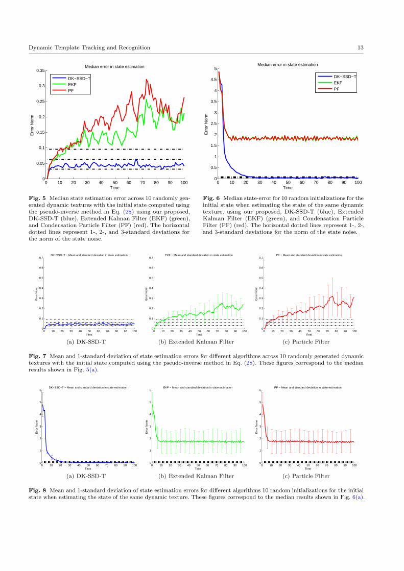
estimate of the dynamic template.We generate a random synthetic dynamic texture

with known system parameters and states at each time

instant. We then fixed the location of the texture and

assumed it was known a-priori thereby reducing theproblem to only the estimation of the state given cor-

rect measurements. This is also the common scenario

for state-estimation in controls theory. Fig. 5(a) shows

the median error in state estimation for 10 randomly

generated dynamic textures using the initial state com-

putation method in Eq. (28) in each case. For each of

the systems, we estimated the state using our proposed

method, Dynamic Kernel SSD Tracking (DK-SSD-T)

shown in blue, Extended Kalman Filter (EKF) shown

in green, and Condensation Particle Filter (PF), with

100 particles, shown in red, using the same initial state.

Since the state, xt is driven by stochastic inputs with

covariance Q, we also display horizontal bars depicting

1-, 2-, and 3-standard deviations of the norm of the noise

process to measure the accuracy of the estimate. As we

can see, at all time-instants, the state estimation error

using our method remains within 1- and 2-standard

deviations of the state noise. The error for both EKF

and PF, on the other hand, increases with time and

becomes much larger than 3-standard deviations of the

noise process.

Figs. 5(b)-5(d) show the mean and standard de-

viation of the state estimates across all ten runs for

DK-SSD-T, EKF and PF respectively. As we can see,

our method has a very small standard deviation and

thus all runs convege to within 1- and 2-standard devi-

ations of the noise process norm. EKF and PF on the

other hand, not only diverge from the true state but the

variance in the state estimates also increases with time,

thereby making the state estimates very unreliable. This

is because our method uses a gradient descent scheme

with several iterations to look for the (local) minimizer

of the exact objective function, whereas the EKF only

uses a linear approximation to the system equations at


0 10 20 30 40 50 60 70 80 90 1000

0.05

0.1

0.15

0.2

0.25

0.3

0.35Median error in state estimation

Time

Err

or N

orm

DK−SSD−TEKFPF

Fig. 5 Median state estimation error across 10 randomly gen-erated dynamic textures with the initial state computed usingthe pseudo-inverse method in Eq. (28) using our proposed,DK-SSD-T (blue), Extended Kalman Filter (EKF) (green),and Condensation Particle Filter (PF) (red). The horizontaldotted lines represent 1-, 2-, and 3-standard deviations forthe norm of the state noise.

0 10 20 30 40 50 60 70 80 90 1000

0.5

1

1.5

2

2.5

3

3.5

4

4.5

5Median error in state estimation

Time

Err

or N

orm

DK−SSD−TEKFPF

Fig. 6 Median state-error for 10 random initializations for theinitial state when estimating the state of the same dynamictexture, using our proposed, DK-SSD-T (blue), ExtendedKalman Filter (EKF) (green), and Condensation ParticleFilter (PF) (red). The horizontal dotted lines represent 1-, 2-,and 3-standard deviations for the norm of the state noise.

0 10 20 30 40 50 60 70 80 90 1000

0.1

0.2

0.3

0.4

0.5

0.6

0.7DK−SSD−T − Mean and standard deviation in state estimation

Time

Err

or N

orm

(a) DK-SSD-T

0 10 20 30 40 50 60 70 80 90 1000

0.1

0.2

0.3

0.4

0.5

0.6

0.7EKF − Mean and standard deviation in state estimation

Time

Err

or N

orm

(b) Extended Kalman Filter

0 10 20 30 40 50 60 70 80 90 1000

0.1

0.2

0.3

0.4

0.5

0.6

0.7PF − Mean and standard deviation in state estimation

Time

Err

or N

orm

(c) Particle Filter

Fig. 7 Mean and 1-standard deviation of state estimation errors for different algorithms across 10 randomly generated dynamictextures with the initial state computed using the pseudo-inverse method in Eq. (28). These figures correspond to the medianresults shown in Fig. 5(a).

0 10 20 30 40 50 60 70 80 90 1000

1

2

3

4

5

6DK−SSD−T − Mean and standard deviation in state estimation

Time

Err

or N

orm

(a) DK-SSD-T

0 10 20 30 40 50 60 70 80 90 1000

1

2

3

4

5

6EKF − Mean and standard deviation in state estimation

Time

Err

or N

orm

(b) Extended Kalman Filter

0 10 20 30 40 50 60 70 80 90 1000

1

2

3

4

5

6PF − Mean and standard deviation in state estimation

Time

Err

or N

orm

(c) Particle Filter

Fig. 8 Mean and 1-standard deviation of state estimation errors for different algorithms 10 random initializations for the initialstate when estimating the state of the same dynamic texture. These figures correspond to the median results shown in Fig. 6(a).


Method Tracks Class label Cost function

DK-SSD-TR-R ltTjt=1 = l(j,k)t Tjt=1 Lj = Lk k = argmini=1,...,N Oij

DK-SSD-T+Rlt

Tjt=1 = l(j,k1)

t Tjt=1 Lj = Lk2 -k1 = argmini=1,...,N Oij k2 = argmini=1,...,N dM (Mk1

j ,Mi)

DK-SSD-TR-C ltTjt=1 = l(j,k)t Tjt=1 Lj = Lk k = argmini=1,...,N Cij

Table 1 Summary of cost functions used to perform tracking and recognition for the three methods proposed in §4.

the current state and does not refine the state estimate

any further at each time-step. With a finite number of

samples, PF also fails to converge. This leads to a much

larger error in the EKF and PF. The trade-off for our

method is its computational complexity. Because of its

iterative nature, our algorithm is computationally more

expensive as compared to EKF and PF. On average itrequires between 25 to 50 iterations for our algorithm

to converge to a state estimate.

Similar to the above evaluation, Fig. 6(a) shows

the error in state estimation, for 10 different random

initializations of the initial state, x0, for one specific

dynamic textures. As we can see, the norm of the state

error is very large initially, but for our proposed method,

as time proceeds the state error converges to below the

state noise error. However the state error for EKF and

PF remain very large. Figs. 6(b)-6(d) show the mean

and standard deviation bars for the state estimation

across all 10 runs. Again, our method converges for all

10 runs, whereas the variance of the state-error is very

large for both EKF and PF. These two experiments show

that choosing the initial state using the pseudo-inverse

method results in very good state estimates. Moreover,our approach is robust to incorrect state initializations

and will eventually converge to the correct state withunder 2 standard deviations of the state noise.

In summary, the above evaluation shows that even

though our method is only guaranteed to converge to

a local minimum when estimating the internal state of

the system, in practice, it performs very well and always

converges to an error within two standard deviations

of the state noise. Moreover, our method is robust to

incorrect state initializations. Finally, since our method

iteratively refines the state estimate at each time instant,

it performs much better than traditional state estimation

techniques such as the EKF and PF.

6 Experiments on Tracking Dynamic Textures

We will now test our proposed algorithm on several

synthetic and real videos with moving dynamic textures

and demonstrate the tracking performance of our algo-

rithm against the state-of-the-art. The full videos of the

corresponding results can be found in the supplemental

material using the figure numbers in this paper.

We will also compare our proposed dynamic tem-

plate tracking framework against traditional kernel-

based tracking methods such as Meanshift (Comaniciu

et al., 2003), as well as the improvements suggested in

Collins et al. (2005a) that use features such as histogram

ratio and variance ratio of the foreground versus the

background before applying the standard Meanshift al-

gorithm. We use the publicly available VIVID Tracking

Testbed3 (Collins et al., 2005b) for implementations of

these algorithms. We also compare our method against

the publicly available4 Online Boosting algorithm first

proposed in Grabner et al. (2006). As mentioned in the

introduction, the approach presented in Peteri (2010)

also addresses dynamic texture tracking using optical

flow methods. Since the authors of Peteri (2010) werenot able to provide their code, we implemented their

method on our own to perform a comparison. We would

like to point out that despite taking a lot of care while

implementing, and getting in touch with the authors

several times, we were not able to get the same results as

those shown in Peteri (2010). However, we are confidentthat our implementation is correct and besides specific

parameter choices, accurately follows the approach pro-

posed in Peteri (2010). Finally, for a fair comparison

between several algorithms, we did not use color features

and we were able to get very good tracks without using

any color information.

For consistency, tracks for Online Boosting (Boost)

are shown in magenta, Template Matching (TM) inyellow, Meanshift (MS) in black, Meanshift with Vari-

ance Ratio (MS-VR) and Histogram Ratio (MS-HR)

in blue and red respectively. Tracks for Particle Filter-

ing for Dynamic Textures (DT-PF) are shown in light

brown, and the optimal tracks for our method, DynamicKernel SSD Tracking (DK-SSD-T), are shown in cyan

whereas any ground truth is shown in green. To better

illustrate the difference in the tracks, we have zoomed

in to the active portion of the video.

3 http://vision.cse.psu.edu/data/vividEval/4 http://www.vision.ee.ethz.ch/boostingTrackers/

index.htm

http://vision.cse.psu.edu/data/vividEval/

http://www.vision.ee.ethz.ch/boostingTrackers/index.htm

http://www.vision.ee.ethz.ch/boostingTrackers/index.htm


Fig. 9 Tracking steam on water waves. [Boost (magenta), TM (yellow), MS (black), MS-VR (blue) and MS-HR (red), DT-PF(light brown), DK-SSD-T (cyan). Ground-truth (green)]

Fig. 10 Tracking water with different appearance dynamics on water waves. [Boost (magenta), TM (yellow), MS (black),MS-VR (blue) and MS-HR (red), DT-PF (light brown), DK-SSD-T (cyan). Ground-truth (green)]

0 50 100 1500

20

40

60

80

100

120

140

160

180

200

Frame #

Pix

el e

rror

Tracker − Ground−truth location error

BoostTMMSMS−VRMS−HRDT−PFDK−SSD−T

0 50 100 1500

20

40

60

80

100

120

140

160

180

200

Frame #

Pix

el e

rror

Tracker − Ground−truth location error

BoostTMMSMS−VRMS−HRDT−PFDK−SSD−T

Fig. 11 Pixel location error between tracker and ground truth location for videos in Fig. 7 (left) and Fig. 8 (right).

6.1 Tracking Synthetic Dynamic Textures

To compare our algorithm against the state-of-the-art

on dynamic data with ground-truth, we first create syn-

thetic dynamic texture sequences by manually placing

one dynamic texture patch on another dynamic texture.

We use sequences from the DynTex database (Peteri

et al., 2010) for this purpose. The dynamics of the fore-

ground patch are learnt offline using the method for

identifying the parameters, (µ,A,C,B,R), in Doretto

et al. (2003). These are then used in our tracking frame-

work.

In Fig. 7, the dynamic texture is a video of steam

rendered over a video of water. We see that Boost, DT-

PF, and MS-HR eventually lose track of the dynamic

patch. The other methods stay close to the patch how-

ever, our proposed method stays closest to the ground

truth until the very end. In Fig. 8, the dynamic texture

is a sequence of water rendered over a different sequence

of water with different dynamics. Here again, Boost and

TM lose tracks. DT-PF stays close to the patch ini-

tially but then diverges significantly. The other trackers

manage to stay close to the dynamic patch, whereas

our proposed tracker (cyan) still performs at par with

the best. Fig. 9 also shows the pixel location error at

each frame for all the trackers and Table 1 provides

the mean error and standard deviation for the whole

video. Overall, MS-VR and our method seem to be the

best, although MS-VR has a lower standard deviation in

both cases. However note that our method gets similar


performance without the use of background information,

whereas MS-VR and MS-HR use background informa-

tion to build more discriminative features. Due to the

dynamic changes in background appearance, Boost fails

to track in both cases. Even though DT-PF is designed

for dynamic textures, upon inspection, all the particles

generated turn out to have the same (low) probability.

Therefore, the tracker diverges. Given the fact that our

method is only based on the appearance statistics of the

foreground patch, as opposed to the adaptively changing

foreground/background model of MS-VR, we attributethe comparable performance (especially against other

foreground-only methods) to the explicit inclusion of

foreground dynamics.

We can also see that the role of dynamics is impor-

tant by comparing the performance of our proposed

method, DK-SSD-T against simple Meanshift tracking

(MS) in Fig. 9 and Table 1. In particular, the mean-

shift tracker can be thought of as the MAP estimate for

the tracking location without incorporating any appear-

ance dynamics, whereas our proposed method explicitly

models the dynamics. As we can see, by incorporat-

ing dynamics, our proposed method works better thansimple meanshift.

To evaluate the correctness of the estimated states

while tracking the above dynamic textures, we perform

two experiments. In the first set, we fix the location ofthe tracker at each time instant to the ground truth

location and only estimate the dynamic texture state.

This experiment is parallel to the state convergence ex-

periments performed in §5 for dynamic textures. In the

second set, we use the state estimated as a result of ourproposed tracking algorithm as above. To qualitativelyevaluate the correctness of the state estimate, we syn-

thesize the dynamic texture at each time instant given

the estimated state.

Fig. ?? shows sample frames of the dynamic texture

patch being tracked in Fig. 7. Fig. ?? shows the resyn-

thesized dynamic texture when the exact location of

the patch is known at each time instant and Fig. ??

shows the resynthesized dynamic texture when the state

is estimated during the tracking process. Similarly, Fig.

?? shows the original and synthesized dynamic texture

patches for the texture in Fig. 8. As we can see, when the

tracked location is perfect, the estimated state generates

a dynamic texture that is very similar to the original

dynamic texture patch. Due to slight errors in tracking,

the estimated state is also slight erroneous and therefore

the synthesized texture matches the original texture on

average and not necessarily at each time instant. Also,

our proposed algorithm results in only a local optimum

of the location and dynamic texture state and the local

Algorithm Fig. 7 Fig. 8

Boost 389 ± 149 82 ± ± 44TM 50 ± 13 78 ± 28MS 12 ± 10 10 ± 8.6MS-VR 9.2 ± 4.3 3.2 ± 2.0MS-HR 258 ± 174 4.6 ± 2.3DT-PF 550 ± 474 635 ± 652DK-SSD-T 8.6 ± 6.8 6.5 ± 6.6

Table 2 Mean pixel error with standard deviation betweentracked location and ground truth.

optimum for the state might be different from the actual

state as we have also outlined earlier.

Finally, we evaluate the robustness of the tracking

process to errors in training. For each of the dynamic

texture patches in Figs. 7, 8, we perform the following

procedure to learn the system parameters of the dynamic

texture from successive inaccurately placed bounding

boxes for training. For a range of values in α ∈ [0, 2], we

choose 10 randomly generated points at a distance of αr

from the center of original dynamic texture patch, where

r is the radius of the original dynamic texture patch.

This allows us to systematically vary the overlap between

the original dynamic texture and dynamic textures at

erroneously placed bounding boxes and compare the

tracking performance of the original texture with respect

to errors in the training location of the training bounding

box. Fig. ?? shows the mean and standard deviation of

the tracking error of 10 experiments for a range of values

of α ∈ [0, 2] for the dynamic textures in Figs. 7 and 8.

As we can see, in general the tracking error is larger

when there is an error in placing the training bounding

box. However, other than for α = 2 for the texture in

Fig. 7, the mean tracking error is never more than 30

pixels from the correct location. This illustrates a mildlevel of robustness of our proposed tracking scheme to

errors in training.

6.2 Tracking Real Dynamic Textures

To test our algorithm on real videos with dynamic tex-

tures, we provide results on three different scenarios

in real videos. We learn the system parameters of the

dynamic texture by marking a bounding box around the

texture in a video where the texture is stationary. We

then use these parameters to track the dynamic texture

in a different video with camera motion causing the

texture to move around in the scene. All the trackers

are initialized at the same location in the test video.

Fig. 10 provides the results for the three examples by

alternatively showing the training video followed by the

tracker results in the test video. Note that since there is

no ground-truth information for these sequences, to get


Original

(a) Original texture

Synthesized

(b) With ground-truth location

Synthesized

(c) With tracking

Fig. 12 Corresponding original and resynthesized dynamic texture patches for the tracked texture in Fig 7.

Original

(a) Original texture

Synthesized

(b) With ground-truth location

Synthesized

(c) With tracking

Fig. 13 Corresponding original and resynthesized dynamic texture patches for the tracked texture in Fig 8.

0 0.2 0.4 0.6 0.8 1 1.2 1.4 1.6 1.8 20

5

10

15

20

25

30

35

40

Relative distance (in terms of patch radius) from true center

Mea

n pi

xel e

rror

with

std

bar

s

Tracking performance as a function of error in training patch location

(a) Tracking the dynamic texture in Fig. 7

0 0.2 0.4 0.6 0.8 1 1.2 1.4 1.6 1.8 24

6

8

10

12

14

16

18

20

22

24

Relative distance (in terms of patch radius) from true center

Mea

n pi

xel e

rror

with

std

bar

s

Tracking performance as a function of error in training patch location

(b) Tracking the dynamic texture in Fig. 8

Fig. 14 Robustness to errors in training. Mean and standard deviation across 10 trials of the mean tracking error for thedynamic textures in Figs. 7,8 when the system parameters are learnt from a bounding box centered away from the groundtruth center. The x-axis corresponds to the fraction of the radius of the actual dynamic texture patch from which the systemparameters were learnt. For example, for x = 0.6, the system parameters were learnt from a dynamic texture patch centered ata random location, 0.6 times the radius of the actual dynamic texture patch whose motion is synthesized in Figs. 7,8.


(a) Training video with labeled stationary patch for learning candle flame dynamic texture system parameters.

(b) Test video with tracked locations of candle flame.

(c) Training video with labeled stationary patch for learning flag dynamic texture system parameters.

(d) Test video with tracked locations of flag.

(e) Training video with labeled stationary patch for learning fire dynamic texture system parameters.

(f) Test video with tracked locations of fire.

Fig. 15 Training and Testing results for dynamic texture tracking. Boost (magenta), TM (yellow), MS (black), MS-VR (blue)and MS-HR (red), DT-PF (light brown), DK-SSD-T (cyan). Training (green).


quantitative results, we would have to manually mark

the bounding box locations in each frame. This results

in a somewhat subjective assesment as the best method

could potentially be different based on the choice of

ground-truth location. Therefore, we will only provide

a qualitative evaluation in the following. We use (row,

column) notation to refer to specific images in Fig. 10.

Candle Flame. This is a particularly challenging scene

as there are multiple candles with similar dynamics and

appearance and it is easy for a tracker to switch between

candles. As we can see from (2,2), MS-HR and MS-VR

seem to jump around between candles. Our method also

jumps to another candle in (2,3) but recovers in (2,4),

whereas MS is unable to recover. DT-PF quickly loses

track and diverges. Overall, all trackers, except DT-PFseem to perform equally well.

Flags. Even though the flag has a distinct appearance

compared to the background, the movement of the flag

fluttering in the air changes the appearance in a dynamic

fashion. Since our tracker has learnt an explicit model

of the dynamics of these appearance changes, it staysclosest to the correct location while testing. Boost, DT-

PF, and the other trackers deviate from the true location

as can be seen in (4,3) and (4,4).

Fire. Here we show another practical application of

our proposed method: tracking fire in videos. We learn a

dynamical model for fire from a training video which is

taken in a completely different domain, e.g., a campfire.

We then use these learnt parameters to track fire in

a NASCAR video as shown in the last row of Fig. 10.

Our foreground-only dynamic tracker performs betterthan MS and TM, the other foreground-only methods

in comparison. Boost, MS-VR and MS-HR use back-ground information, which is discriminative enough in

this particular video and achieve similar results. DT-PF

diverges from the true location and performs the worst.

7 Experiments on Tracking Human Actions

To demonstrate that our framework is general and can

be applied to track dynamic visual phenomenon in any

domain, we consider the problem of tracking humans

while performing specific actions. This is different from

the general problem of tracking humans, as we want to

track humans performing specific actions such as walking

or running. It has been shown, e.g., in Efros et al. (2003);

Chaudhry et al. (2009); Lin et al. (2009) that the optical

flow generated by the motion of a person in the scene

is characteristic of the action being performed by the

human. In general global features extracted from optical

flow perform better than intensity-based global features

for action recognition tasks. The variation in the optical

flow signature as a person performs an action displays

very characteristic dynamics. We therefore model the

variation in optical flow generated by the motion of a

person in a scene as the output of a linear dynamical

system and pose the action tracking problem in terms

of matching the observed optical flow with a dynamic

template of flow fields for that particular action.

We collect a dataset of 55 videos, each containing a

single human performing either of two actions (walking

and running). The videos are taken with a stationary

camera, however the background has a small amount of

dynamic content in the form of waving bushes. Simple

background subtraction would therefore lead to erro-

neous bounding boxes. We manually extract bounding

boxes and the corresponding centroids to mark the loca-

tion of the person in each frame of the video. These are

then used as ground-truth for later comparisons as well

as to learn the dynamics of the optical flow generated

by the person as they move in the scene.

For each bounding box centered at lt, we extract

the corresponding optical flow F(lt) = [Fx(lt), Fy(lt)],

and model the optical flow time-series, F(lt)Tt=1 as

a Linear Dynamical System. We extract the system

parameters, (µ,A,C,Q,R) for each optical flow time-series using the system identification method in §3.1.

This gives us the system parameters and ground-truth

tracks for each of the 55 human action samples.

Given a test video, computing the tracks and internal

state of the optical-flow dynamical system at each time

instant amounts to minimizing the function,

O(lt,xt) =1

2R‖F(lt)− (µ+ Cxt)‖2+

1

2(xt −Axt−1)>Q−1(xt −Axt−1). (32)

To find the optimal lt, and xt, Eq. (31) is optimized in

the same gradient descent fashion as Eq. (24).

We use the learnt system parameters in a leave-

one-out fashion to track the activity in each test video

sequence. Taking one sequence as a test sequence, we

use all the remaining sequences as training sequences.

The flow-dynamics system parameters extracted from

each training sequence are used to track the action in

the test sequence. Therefore, for each test sequence

j ∈ 1, . . . , N, we get N − 1 tracked locations andstate estimate time-series by using all the remaining

N − 1 extracted system parameters. As described in §4,

we choose the tracks that give the minimum objective

function value in Eq. (29).

Fig. 11 shows the tracking results against the state-

of-the-art algorithms. Since this is a human activity

tracking problem, we also compare our method against

the parts-based human detector of Felzenszwalb et al.


Fig. 16 Using the dynamics of optical flow to track a human action. Parts-based human detector (red broken), Boost (magenta),TM (yellow), MS (black), MS-VR (blue) and MS-HR (red), DK-SSD-T (cyan). First row: Tracking a walking person, withoutany pre-processing for state-of-the-art methods. Second row: Tracking a walking person, with pre-processing for state-of-the-artmethods. Third row: Tracking a running person, with pre-processing for state-of-the-art methods.

(2010) when trained on the PASCAL human dataset.

We used the publicly available5 code for this comparison

with default parameters and thresholds6. The detectionwith the highest probability is used as the location of

the human in each frame.

The first row in Fig. 11 shows the results for all

the trackers when applied to the test video. The state-

of-the-art trackers do not perform very well. In fact

foreground-only trackers, MS, TM and DT-PF, lose

tracks altogether. Our proposed method (cyan) gives

the best tracking results and the best bounding box

covering the person across all frames. The parts-based

detector at times does not give any responses or spurious

detections altogether, whereas Boost, MS-VR and MS-

HR do not properly align with the human. Since we use

optical flow as a feature, it might seem that there is animplicit form of background subtraction in our method.

As a more fair comparison, we performed background

subtraction as a pre-processing step on all the test videos

before using the state-of-the-art trackers. The second

row in Fig. 11 shows the tracking results for the same

walking video as in row 1. We see that the tracking

has improved but our tracker still gives the best results.

The third row in Fig. 11 shows tracking results for a

running person. Here again, our tracker performs the

best whereas Boost and DT-PF perform the worst.

5 http://people.cs.uchicago.edu/~pff/latent/6 It might be possible to achieve better detections on this

dataset by tweaking parameters/thresholds. However we didnot attempt this as it is not the focus of our paper.

To derive quantitative conclusions about tracker per-

formance, Fig. 12 shows the median tracker location

error for each video sorted in ascending order. The bestmethod should have the smallest error for most of the

videos. As we can see, both without (1st row) and with

background subtraction (2nd row), our method provides

the smallest median location error against all state of

the art methods for all except 5 sequences. Moreover, as

a black box and without background subtraction as apre-processing step, all state-of-the-art methods perform

extremely poorly.

8 Experiments on Simultaneous Action

Tracking and Recognition

In the previous section, we have shown that given train-

ing examples for actions, our tracking framework, DK-

SSD-T, can be used to perform human action tracking

using system parameters learnt from training data with

correct tracks. We used the value of the objective func-

tion in Eq. (31) to select the tracking result. In this

section, we will extensively test our simultaneous track-

ing and classification approach presented in §4 on the

two-action database introduced in the previous section

as well as the commonly used Weizmann human action

dataset (Gorelick et al., 2007). We will also show that we

can learn the system parameters for a class of dynamic

templates from one database and use it to simultane-

http://people.cs.uchicago.edu/~pff/latent/


0 10 20 30 40 50 600

50

100

150

200

250

300

350

400

Number of sequences

Pix

el lo

catio

n er

ror

Comparison of the median location errors against several methods

DK−SSD−THuman DetectorBoostTMMSMS−VRMS−HRDT−PF

0 10 20 30 40 50 600

2

4

6

8

10

12

14

16

18

20

Number of sequences

Pix

el lo

catio

n er

ror



0 10 20 30 40 50 600

50

100

150

200

250

300

350

400

450

Number of sequences

Pix

el lo

catio

n er

ror



0 10 20 30 40 50 600

2

4

6

8

10

12

14

16

18

20

Number of sequences

Pix

el lo

catio

n er

ror



Fig. 17 Comparison of various tracking methods without (top row) and with (bottom row) background subtraction. Figureson right are zoomed-in versions of figures on left.

ously track and recognize the template in novel videos

from other databases.

8.1 Walking/Running Database

Fig. 13 shows the median pixel tracking error of each test

sequence using the leave-one-out validation described in

the previous section for selecting the tracks, sorted by

true action class. The first 28 sequences belong to the

class walking, while the remaining 27 sequences belong to

the running class. Sequences identified by our proposed

approach as walking are colored blue, whereas sequences

identified as running are colored red. Fig. 13(a) shows

the tracking error and classification result when using

DK-SSD-TR-R, i.e., the objective function value in Eq.

(29) with a 1-NN classifier to simultaneously track and

recognize the action. The tracking results shown also

correspond to the ones shown in the previous section. As

we can see, for almost all sequences, the tracking error is

within 5 pixels from the ground truth tracks. Moreover,

for all but 4 sequences, the action is classified correctly,

leading to an overall action classification rate of 93%.

Fig. 13(b) shows the tracking error and class labels when

we using DK-SSD-TR-C, i.e., the Martin distance based

classifier term proposed in Eq. (30) to simultaneously

track and recognize the action. As we can see, DK-SSD-

TR-C results in even better tracking and classification

results. Only two sequences are mis-classified for an

overall recognition rate of 96%.

To show that our simultaneous tracking and clas-

sification framework computes the correct state of the

dynamical system for the test video given that the class

of the training system is the same, we illustrate several

components of the action tracking framework for two

cases: a right to left walking person tracked using dy-

namical system parameters learnt from another walking

person moving left to right, in Fig. 14, and the same per-

son tracked using dynamical system parameters learnt

from a running person in Fig. 15.


0 10 20 30 40 50 600

5

10

15

20

25

30

Video number − (1−28: Walking, 29−55, Running)

Med

ian

pixe

l err

or

System parameters from 1st NN in objective function values

(a) DK-SSD-TR-R

0 10 20 30 40 50 600

5

10

15

20

25

30

Video number − (1−28: Walking, 29−55, Running)

Med

ian

pixe

l err

or

System parameters from 1st NN using classifier function values

(b) DK-SSD-TR-C

Fig. 18 Simultaneous Tracking and Recognition results showing median tracking error and classification results, when using(a) DK-SSD-TR-R: the objective function in Eq. (29), and (b) DK-SSD-TR-C: the Martin distance between dynamical systemsin Eq. (30) with a 1-NN classifier. (walking (blue), running (red)).

Fig. 14(a) shows a frame with its corresponding op-

tical flow, ground truth tracks (green) as well as the

tracks computed using our algorithm (blue). As we can

see the computed tracks accurately line-up with the

ground-truth tracks. Fig. 14(b) shows a frame and corre-

sponding optical flow along with the ground-truth tracks

used to extract optical flow bounding boxes to learn

the dynamical system parameters. Fig. 14(c) shows the

optical flow extracted from the bounding boxes at the

ground-truth locations in the test video at intervals of 5

frames and Fig. 14(d) shows the optical flow extracted

from the bounding boxes at the tracked locations at the

same frame numbers. As the extracted tracks are very

accurate, the flow-bounding boxes line up very accu-

rately. Since our dynamical system model is generative,

at each time-instant, we can use the computed state,

xt, to generate the corresponding output yt = µ+ Cxt.

Fig. 14(e) displays the optical flow computed in thismanner at the corresponding frames in Fig. 14(d). We

can see that the generated flow appears like a smoothed

version of the observed flow at the correct location. This

shows that the internal state of the system was correctly

computed according to the training system parameters,

which leads to accurate dynamic template generation

and tracking. Fig. 14(f) shows the optical flow at the

bounding boxes extracted from the ground-truth loca-

tions in the training video. The direction of motion is

the opposite as in the test video, however using the

mean optical flow direction, the system parameters can

be appropriately transformed at test time to account

for this change in direction as discussed in §3.3.

Fig. 15(a) repeats the above experiment when track-

ing the same walking person with a running model.

As we can see in Fig. 15(a), the computed tracks are

not very accurate when using the wrong action class

for tracking. This is also evident in the extracted flow

bounding boxes at the tracked locations as the head

of the person is missing from almost all of the boxes.

Fig. 15(f) shows several bounding box optical flow from

the training video of the running person. The states

computed using the learnt dynamical system parame-

ters from these bounding boxes leads to the generated

flows in Fig. 15(e) at the frames corresponding to those

in Fig. 15(d). The generated flow does not match the

ground-truth flow and leads to a high objective function

value.

8.2 Comparison to Tracking then Recognizing

We will now compare our simultaneous tracking and

recognition approaches, DK-SSD-TR-R and DK-SSD-

TR-C to the tracking then recognizing approach where

we first track the action using standard tracking algo-

rithms described in §6 as well as our proposed dynamic

tracker DK-SSD-T, and then use the Martin distancefor dynamical systems with a 1-NN classifier to classify

the tracked action.

Given a test video, we compute the location of the

person using all the trackers described in §6 and then

extract the bounding box around the tracked locations.

For bounding boxes that do not cover the image area, we

zero-pad the optical flow. This gives us an optical-flow


(a) Intensity and optical flow frame with ground-truth tracks(green) and tracked outputs of our algorithm (blue) on testvideo with walking person tracked using system parameterslearnt from the walking person video in (b).

(b) Intensity and optical flow frame with ground-truth tracks(green) used to train system parameters for a walking model.

(c) Optical flow bounding boxes at ground truth locations.

(d) Optical flow bounding boxes at tracked locations.

(e) Optical flow as generated by the computed states at corresponding time instants at the tracked locations.

(f) Optical flow bounding boxes from the training video used to learn system parameters.

Fig. 19 Tracking a walking person using dynamical system parameters learnt from another walking person with oppositewalking direction. The color of the optical flow diagrams represents the direction (e.g., right to left is cyan, right to left is red)and the intensity represents the magnitude of the optical flow vector.

time-series corresponding to the extracted tracks. We

then use the approach described in §3.1 to learn the

dynamical system parameters of this optical flow time-

series. To classify the tracked action, we compute the

Martin distance of the tracked system to all the training

systems in the database and use 1-NN to classify the

action. We then average the results over all sequences

in a leave-one-out fashion.

Table 2 shows the recognition results for the 2-class

Walking/Running database by using this classification

scheme after performing tracking as well as our proposed

simultaneous tracking and recognition algorithms. We

have provided results for both the original sequences

as well as when background subtraction was performed

prior to tracking. We showed in Fig. 12(a) and Fig.

12(c) that all the standard trackers performed poorly

without using background subtraction. Our tracking

then recognizing method, DK-SSD-T+R, provides ac-

curate tracks and therefore gives a recognition rate

of 96.36%. The parts-based human detector of Felzen-

szwalb et al. (2010) tracker fails to detect the person

in some frames and therefore the recognition rate is

the worst. When using background subtraction to pre-

process the videos, the best recognition rate is provided

by TM at 98.18% whereas MS-HR performs at the same

rate as our proposed method. The recognition rate of

the other methods, except the human detector, also

increase due to this pre-processing step. For comparison,

if we use the ground-truth tracks to learn the dynami-

cal system parameters and classify the action using the


(a) Intensity and optical flow frame with ground-truth tracks(green) and tracked outputs of our algorithm (red) on test videowith walking person tracked using system parameters learntfrom the running person video in (b).

(b) Intensity and optical flow frame with ground-truth tracks(green) used to train system parameters for a running model.

(c) Optical flow bounding boxes at ground truth locations.

(d) Optical flow bounding boxes at tracked locations.

(e) Optical flow as generated by the computed states at corresponding time instants at the tracked locations.

(f) Optical flow bounding boxes from the training video used to learn system parameters.

Fig. 20 Tracking a walking person using dynamical system parameters learnt from a running person. The color of the opticalflow diagrams represents the direction (e.g., right to left is cyan, right to left is red) and the intensity represents the magnitudeof the optical flow vector.

Martin distance and 1-NN classification, we get 100%

recognition.

Our joint-optimization scheme using the objective

function value as the classifier, DK-SSD-TR-R, performs

slightly worse at 92.73%, than the best tracking then

recognizing approach. However, when we use the Martin-

distance based classification cost in DK-SSD-TR-C, we

get the best action classification performance, 96.36%.

Needless to say the tracking then recognizing scheme

is more computationally intensive and is a 2-step pro-

cedure. Moreover, our joint optimization scheme based

only on foreground dynamics performs better than track-

ing then recognizing using all other trackers without pre-

processing. At this point, we would also like to note that

even though the best recognition percentage achieved by

the tracking-then-recognize method was 98.18% using

TM, it performed worse in tracking as shown in Fig.

12(d). Overall, our method simultaneously gives the best

tracking and recognition performance.

8.3 Weizmann Action Database

We also tested our simultaneous tracking and testing

framework on the Weizmann Action database (Gorelick

et al., 2007). This database consists of 10 actions with

a total of 93 sequencess and contains both stationary

actions such as jumping in place, bending etc., and non-

stationary actions such as running, walking, etc. We

used the provided backgrounds to extract bounding

boxes and ground-truth tracks from all the sequences

and learnt the parameters of the optical-flow dynamical


Method Recognition% withoutbackgroundsubtraction

Recognition% with back-ground sub-traction

Track then recognizeBoost 81.82 81.82TM 78.18 98.18MS 67.27 89.09MS-VR 74.55 94.55MS-HR 78.18 96.36Human-detector 45.45 50.91DT-PF 69.09 72.73DK-SSD-T+R 96.36 -Ground-truth tracks 100 -

Joint-optimizationDK-SSD-TR-R 92.73 -DK-SSD-TR-C 96.36 -

Table 3 Recognition rates for the 2-class Walking/Runningdatabase using 1-NN with Martin distance for dynamicalsystems after computing tracks from different algorithms

Action Median ± RSE Action Median ± RSE

Bend 5.7 ± 1.9 Side 2.1 ± 0.9Jack 4.2 ± 0.6 Skip 2.8 ± 1.1Jump 1.5 ± 0.2 Walk 3.3 ± 2.4PJump 3.7 ± 1.3 Wave1 14.8 ± 7.4Run 4.2 ± 2.9 Wave2 2.3 ± 0.7

Table 4 Median and robust standard error (RSE) (see text)of the tracking error for the Weizmann Action database, usingthe proposed simultaneous tracking and recognition approachwith the classification cost. We get an overall action recognitionrate of 92.47%.

1.0

1.0

.89 .11

1.0

1.0

1.0

1.0

1.0

.11 .11 .67 .11

.22 .11 .67

bend

jack

jump

pjump

run

side

skip

walk

wave1

wave2bend

jackjump

pjumprun side

skipwalk

wave1wave2

Fig. 22 Confusion matrix for leave-one-out classification onthe Weizmann database using our simultaneous tracking andrecognition approach. Overall recognition rate of 92.47%.

systems using the same approach as outlined earlier. A

commonly used evaluation scheme for the Weizmann

database is leave-one-out classification. Therefore, we

also used our proposed framework to track the action

in a test video given the system parameters of all the

remaining actions.

Method Recognition (%)

Xie et al. (2011) 95.60Thurau and Hlavac (2008) 94.40Ikizler and Duygulu (2009) 100.00Gorelick et al. (2007) 99.60Niebles et al. (2008) 90.00Ali and Shah (2010) 95.75Ground-truth tracks (1-NN Martin) 96.77Our method, DK-SSD-TR-C 92.47

Table 5 Comparison of different approaches for action recog-nition on the Weizmann database against our simultaneoustracking and recognition approach.

Table 3 shows the median and robust standard er-

ror (RSE), i.e., the square-root of the median of (x−median(x))2, of the tracking error for each class. Other

than Wave1, all classes have a median tracking error

under 6 pixels as well as very small deviations from

the median error. Furthermore, we get a simultane-

ous recognition rate of 92.47% which corresponds to

only 7 mis-classified sequences. Fig. 17 shows the corre-

sponding confusion matrix. Fig. 16 shows the median

tracking error per frame for each of the 93 sequences

in the Weizmann database. The color of the stem-plot

indicates whether the sequence was classified correctly

(blue) or incorrectly (red). Table 4 shows the recogni-

tion rate of some state-of-the-art methods on the Weiz-

mann database. However notice that, all these methods

are geared towards recognition and either assume that

tracking has been accurately done before the recogni-

tion is performed, or use spatio-temporal features for

recognition that can not be used for accurate tracking.

Furthermore, if the ground-truth tracks were provided,

using the Martin distance between dynamical systems

with a 1-NN classifier gives a recognition rate of 96.77%.Our simultaneous tracking and recognition approach is

very close to this performance. The method by Xie et al.

(2011) seems to be the only attempt to simultaneously

locate and recognize human actions in videos. However

their method does not perform tracking, instead it ex-

tends the parts-based detector by Felzenszwalb et al.

(2010) to explicitly consider temporal variations caused

by various actions. Moreover, they do not have any track-

ing results in their paper other than a few qualitative

detection results. Our approach is the first to explicitly

enable simultaneous tracking and recognition of dynamic

templates that is generalizable to any dynamic visual

phenomenon and not just human actions.

We will now demonstrate that our simultaneous

tracking and recognition framework is fairly general and

we can train for a dynamic template on one database

and use the models to test on a totally different database.

We used our trained walking and running action models

(i.e., the corresponding system parameters) from the 2-


0 10 20 30 40 50 60 70 80 900

5

10

15

20

25

30

Video number

Med

ian

pixe

l err

or

Using 1st NN with classifier function values − correct (blue), incorrect (red)

Fig. 21 Simultaneous Tracking and Recognition results for the Weizmann database showing median tracking error andclassification results, when using the Martin distance between dynamical systems with a 1-NN classifier. (Correct classification(blue), Incorrect classification (red)).

class walking/running database in §8.1 and applied our

proposed algorithm for joint tracking and recognizingthe running and walking videos in the Weizmann human

action database (Gorelick et al., 2007), without any a-

priori training or adapting to the Weizmann database.

Of the 93 videos in the Weizmann database, there are a

total of 10 walking and 10 running sequences. Fig. 18

shows the median tracking error for each sequence and

the color codes its action, running (red) and walking

(blue). As we can see, all the sequences have under 5

pixel median pixel error and all the 20 sequences are

classified correctly. This demonstrates the fact that our

scheme is general and that the requirement of learning

the system parameters of the dynamic template is not

necessarily a bottleneck as the parameters need not be

learnt again for every scenario. We can use the learnt

system parameters from one dataset to perform tracking

and recognition in a different dataset.

Finally, we will evaluate the robustness of our si-

multaneous tracking and recognition framework with

respect to mild changes in viewpoint and spatial defor-

mation. For this purpose, we use the dynamic templates

learnt from the original 10-class Weizmann human ac-

tion dataset above to track walking actions with several

variations in viewing angle and spatial deformations

found in the Weizmann robustness dataset (Gorelick

et al., 2007). Fig. ?? shows the tracks as well as provides

the action label found using our simultaneous tracking

and recognition algorithm corresponding to several view-

ing angles. Note that all the walking sequences in the

training set are taken from a fully lateral viewing angle,

i.e., 0. We observe that for mild variations in viewing

angle, 5 − 20, the tracking is done perfectly and the

action is also correctly classified. However for larger

variations, 25 − 40, even though the tracks stay closeto the actual person, the action labels are not accu-

rate. Finally with the large variation of 45, both the

tracks as well as the action label are inaccurate. We

can therefore conclude that our simultaneous tracking

and recognition algorithm is robust to mild changes in

viewing angle, however as the change in viewing angle

becomes large, we would require more training samples

with these variations to be able to correctly track and

recognize the same action. Fig. ?? shows the tracks and

provides action labels for various testing sequences with

a walking person and several spatial deformations such

as walking with a briefcase or with a dog, behind large

occlusions, having body parts such as the feet invisible

as well as different styles of walking. For all the various

deformations except behind large occlusions, our algo-

rithms is able to correctly track and classify the walking

action. There is a slight tracking error towards the end

of moonwalk in Fig. ?? (e) and the tracker fails to track

and correctly classify the action when there is a large

occlusion as in walk behind pole in Fig. ?? (g). We can

therefore conclude that our alrgorithm is robust to mild

spatial deformations and style changes. However in its

current form, our proposed algorithm is not invariant

to large occlusions. This is not surprising as we have

only proposed a foreground tracking algorithm without

a motion prior. Having said that, as is common, a sim-

ple linear motion prior could be incorporated, as briefly

discussed at the end of §2, to address large occlusions.


(a) 5 (Walk) (b) 10 (Walk) (c) 15 (Walk) (d) 20 (Walk)

(e) 25 (Side) (f) 30 (Side) (g) 40 (Skip) (h) 45 (PJump)

Fig. 24 Simultaneous tracking and recognition results for walking actions with several variations in the viewpoint. Tracksdepict the locations of successive centers of bounding boxes and the bounding box of the last frame is shown. The colorsdepict correct recognition (blue) of the walking action, and incorrect recognition (red). The recognized action is also written inparenthesis under each figure.

0 2 4 6 8 10 12 14 16 18 200

5

10

15

20

25

30

Video number − (1−10: Run, 11−20, Walk)

Med

ian

pixe

l err

or

System parameters from 1st NN in objective function values

Fig. 23 Tracking walking and running sequences in the Weiz-mann database using trained system parameters from thedatabase introduced in §8.1. The ground-truth label of thefirst 10 sequences is running, while the rest are walking. Theresult of the joint tracking and recognition scheme are labeledas running (red) and walking (blue). We get 100% recognitionand under 5 pixel median location error.

9 Conclusions, Limitations and Future Work

In this paper, we have proposed a novel framework

for tracking dynamic templates such as dynamic tex-

tures and human actions that are modeled by Linear

Dynamical Systems. We posed the tracking problem

as a maximum a-posteriori estimation problem for the

current location and the LDS state, given the current

image features and the previous state. We then proposedseveral methods for performing simultaneous tracking

and recognition of dynamic templates. Through our ex-

tensive experimental evaluation, we can conclude the

following:

– The use of dynamical models for appearance and flow

improves tracking performance. As we have shown,

in the case of tracking dynamic textures, explicitly

modeling foreground appearance dynamics results

in better tracking performance as opposed to static

methods such as mean-shift. Similarly, in the case

of tracking human activities, using action-specific

dynamical models for tracking gives better tracking

performance than static methods as well as tracking-

by-detection methods.

– Our proposed greedy-posterior based tracking and

state-estimation method results in more accurate

state estimates than commonly used one-shot meth-

ods such as Extended Kalman Filters and Particle

Filters. This is because of the use of a gradient-

descent scheme that attempts to find the best (ap-

proximate) state estimate at each time instant. One

shot methods such as EKF and PF on the other

hand are more computationally efficient but tend to

drift.

– Since our proposed method is based on a generative

model for the appearance/flow given a template, we


(a) Walk with briefcase (Walk) (b) Walk with dog (Walk) (c) Walk with knees up (Walk) (d) Walk with limp (Walk)

(e) Moonwalk (Walk) (f) Walk - feet invisible (Walk) (g) Walk behind pole (Run) (h) Walk wearing skirt (Walk)

Fig. 25 Simultaneous tracking and recognition results for walking actions with several deformations, changes in style, occlusions,etc. Tracks depict the locations of successive centers of bounding boxes and the bounding box of the last frame is shown. Thecolors depict correct recognition (blue) of the walking action, and incorrect recognition (red). The recognized action is alsowritten in parenthesis under each figure.

can use the value of the cost function in Eq. (24) as

a measure of how far the observed tracks are from

the given template. This method has been shown toperform good recognition of the tracked template.

– As the number of dynamic template classes increase,

a generative approach alone does not perform very

well. We have shown that our proposed two-step

tracking and recognition scheme that combines theuse of a generative model for tracking with a dis-

criminative model for recognition results in excellent

simultaneous tracking and recognition results.

– Even though our proposed approach requires pre-

trained models for the particular template to be

tracked, we have shown through experiments that

our approach is fairly robust to deformations and

variations in view-point.

Although our simultaneous tracking and recognition

approach has shown promising results, there are cer-

tain limitations. Firstly, as mentioned earlier, since our

method uses gradient descent, it is amenable to converge

to non-optimal local minima. Having a highly non-linear

feature function or non-linear dynamics could poten-

tially result in sub-optimal state estimation which could

lead to high objective function values even when the

correct class is chosen for tracking. Therefore, if possible,

it is better to choose linear dynamics and model system

parameter changes under different transformations in-

stead of modeling dynamics of transformation-invariant

but highly non-linear features. However it must be noted

that for robustness, some non-linearities in features such

as kernel-weighted histograms are necessary and need

to be modeled. Secondly since our approach requiresperforming tracking and recognition using all the train-

ing data, it could be computationally expensive as the

number of training sequences and the number of classes

increases. This can be alleviated by using a smart classi-

fier or more generic one-model-per-class based methods.We leave this as future work.

In other future work, we are looking at online learn-

ing of the system parameters of the dynamic template,

so that for any new dynamic texture in the scene, the

system parameters are also learnt simultaneously as the

tracking proceeds. This way, our approach will be appli-

cable to dynamic templates for which system parameters

are not readily available.

Acknowledgements The authors would like to thank DiegoRother for useful discussions. This work was supported bythe grants, NSF 0941463, NSF 0941362 and ONR N00014-09-10084.

A Derivation of the Gradient Descent Scheme

In this appendix, we will show the detailed derivation of theiterations Eq. (26) to minimimize the objective function in Eq.(24), with ρ, the non-differentiable kernel weighted histogramreplaced by ζ, our proposed differentiable kernel weighted


histogram:

O(lt,xt) =1

2σ2H

‖√ζ(yt(lt))−

√ζ(µ+ Cxt)‖2+

1

2(xt −Axt−1)>Q−1(xt −Axt−1). (33)

Using the change in variable, z′ = z + lt, the proposed kernelweighted histogram for bin u, Eq. (25),

ζu(yt(lt)) =1

κ

∑z∈Ω

K(z).

(φu−1(yt(z + lt))− φu(yt(z + lt))) ,

can be written as,

ζu(yt(lt)) =1

κ

∑z′∈Ω−lt

K(z′ − lt).

(φu−1(yt(z′))− φu(yt(z

′))) , (34)

Following the formulation in Hager et al. (2004), we definethe sifting vector,

uj =

φj−1(yt(z′1))− φj(yt(z′1))φj−1(yt(z′2))− φj(yt(z′2))

...φj−1(yt(z′N ))− φj(yt(z′N ))

. (35)

We can then combine these sifting vectors into the siftingmatrix, U = [u1, . . . , uB ]. Similarly, we can define the kernelvector, K(z) = 1

κ[K(z1),K(z2), . . . ,K(zN )]>, where N =

|Ω| and the indexing of the pixels is performed column wise.Therefore we can write the full kernel-weighted histogram, ζas,

ζ(yt(lt)) = U>K(z′ − lt) (36)

Since U is not a function of lt,

∇lt(ζ(yt(lt))) = U>JK , (37)

where,

JK =1

κ

[∂K(z′ − lt)

∂lt;1,∂K(z′ − lt)

∂lt;2

]= [∇K(z′1 − lt),∇K(z′2 − lt), . . . ,∇K(z′N − lt)]

>. (38)

where ∇K(z′ − lt) is the derivative of the kernel function,e.g., the Epanechnikov kernel in Eq. (10). Therefore the deriva-

tive of the first kernel-weighted histogram,√ζ(yt(lt)) w.r.t. lt

is,

L.=

1

2diag(ζ(yt(lt)))

− 1

2 U>JK (39)

where diag(v) creates a diagonal matrix with v on its diagonaland 0 in its off-diagonal entries. Since yt(lt) does not dependon the state of the dynamic template, xt, the derivative ofthe first kernel-weighted histogram w.r.t. xt is 0.

In the same manner, the expression for the second kernelweighted histogram, for bin u,

ζu(µ+ Cxt) =1

κ

∑z∈Ω

K(z).

(φu−1(µ(z) + C(z)>xt)−

φu(µ(z) +X(z)>xt)

)(40)

By using a similar sifting vector for the predicted dynamictemplate,

Φj =

(φj−1 − φj)(µ(z1) + C(z1)>xt)(φj−1 − φj)(µ(z2) + C(z2)>xt)

...(φj−1 − φj)(µ(zN ) + C(zN )>xt)

, (41)

where for brevity, we use

(φj−1 − φj)(µ(z) + C(z)>xt) =

φj−1(µ(z) + C(z)>xt)− φj(µ(z) + C(z)>xt).

and the pixel indices zj are used in a column-wise fashion asdiscussed in the main text. Using the corresponding siftingmatrix, Φ = [Φ1, Φ2, . . . , ΦB ] ∈ RN×B , we can write,

ζ(µ+ Cxt) = Φ>diag(K(z)) (42)

Since ζ(µ+ Cxt) is only a function of xt,

∇xt(ζ(µ+ Cxt)) = (Φ′)>diag(K(z))C, (43)

where Φ′ = [Φ′1, Φ′2, . . . , Φ

′B ], is the derivative of the sifting

matrix with,

Φ′j =

(φ′j−1 − φ′j)(µ(z1) + C(z1)>xt)

(φ′j−1 − φ′j)(µ(z2) + C(z2)>xt)...

(φ′j−1 − φ′j)(µ(zN ) + C(zN )>xt)

, (44)

and Φ′ is the derivative of the sigmoid function. Therefore, thederivative of the second kernel-weighted histogram,

√ζ(µ+ Cxt)

w.r.t. xt is,

M.=

1

2diag(ζ(µ+ Cxt))

− 1

2 (Φ′)>diag(K(z))C. (45)

The second part of the cost function in Eq. (32) dependsonly on the current state, and the derivative w.r.t. xt can besimply computed as,

d.= Q−1(xt −Axt−1). (46)

When computing the derivatives of the squared differencefunction in first term in Eq. (32), the difference,

a.=√ζ(yt(lt))−

√ζ(µ+ Cxt), (47)

will be multiplied with the derivatives of the individual squareroot kernel-weighted histograms.

Finally, the derivative of the cost function in Eq. (32)w.r.t. lt is computed as,

∇ltO(lt,xt) =1

σ2H

L>a, (48)

and the derivative of the cost function Eq. (32) w.r.t. xt iscomputed as,

∇xtO(lt,xt) =1

σ2H

(−M)>a + d. (49)

We can incorporate the σ−2H term in L and M to get the

gradient descent optimization scheme in Eq. (26).


References

Ali S, Shah M (2010) Human action recognition in videosusing kinematic features and multiple instance learning.IEEE Trans on Pattern Analysis and Machine Intelligence32 (2):288–303

Babenko B, Yang MH, Belongie S (2009) Visual trackingwith online multiple instance learning. In: IEEE Conf. onComputer Vision and Pattern Recognition

Bissacco A, Chiuso A, Ma Y, Soatto S (2001) Recognitionof human gaits. In: IEEE Conference on Computer Visionand Pattern Recognition, vol 2, pp 52–58

Bissacco A, Chiuso A, Soatto S (2007) Classification andrecognition of dynamical models: The role of phase, inde-pendent components, kernels and optimal transport. IEEETransactions on Pattern Analysis and Machine Intelligence29(11):1958–1972

Black MJ, Jepson AD (1998) Eigentracking: Robust match-ing and tracking of articulated objects using a view-basedrepresentation. Int Journal of Computer Vision 26(1):63–84

Chan A, Vasconcelos N (2007) Classifying video with kerneldynamic textures. In: IEEE Conference on Computer Visionand Pattern Recognition, pp 1–6

Chaudhry R, Vidal R (2009) Recognition of visual dynamicalprocesses: Theory, kernels and experimental evaluation.Tech. Rep. 09-01, Department of Computer Science, JohnsHopkins University

Chaudhry R, Ravichandran A, Hager G, Vidal R (2009) His-tograms of oriented optical flow and Binet-Cauchy kernelson nonlinear dynamical systems for the recognition of hu-man actions. In: IEEE Conference on Computer Vision andPattern Recognition

Cock KD, Moor BD (2002) Subspace angles and distancesbetween ARMA models. System and Control Letters46(4):265–270

Collins R, Liu Y, Leordeanu M (2005a) On-line selection ofdiscriminative tracking features. IEEE Trans on PatternAnalysis and Machine Intelligence

Collins R, Zhou X, Teh SK (2005b) An open source track-ing testbed and evaluation web site. In: IEEE Interna-tional Workshop on Performance Evaluation of Trackingand Surveillance (PETS 2005)

Comaniciu D, Meer P (2002) Mean Shift: A robust approachtoward feature space analysis. IEEE Trans on Pattern Anal-ysis and Machine Intelligence 24(5):603–619

Comaniciu D, Ramesh V, Meer P (2003) Kernel-based objecttracking. IEEE Trans on Pattern Analysis and MachineIntelligence 25(5):564–577

Doretto G, Chiuso A, Wu Y, Soatto S (2003) Dynamic textures.Int Journal of Computer Vision 51(2):91–109

Efros A, Berg A, Mori G, Malik J (2003) Recognizing action ata distance. In: IEEE International Conference on ComputerVision, pp 726–733

Fan Z, Yang M, Wu Y (2007) Multiple collaborative kerneltracking. IEEE Trans on Pattern Analysis and MachineIntelligence 29:1268–1273

Felzenszwalb P, Girshick R, McAllester D, Ramanan D (2010)Object detection with discriminatively trained part basedmodels. IEEE Trans on Pattern Analysis and MachineIntelligence 32

Gill PE, Murray W, Wright MH (1987) Practical Optimization.Academic Press

Gorelick L, Blank M, Shechtman E, Irani M, Basri R (2007)Actions as space-time shapes. IEEE Trans on Pattern Anal-ysis and Machine Intelligence 29(12):2247–2253

Grabner H, Grabner M, Bischof H (2006) Real-time trackingvia on-line boosting. In: British Machine Vision Conference

Hager GD, Dewan M, Stewart CV (2004) Multiple kerneltracking with ssd. In: IEEE Conf. on Computer Vision andPattern Recognition

Ikizler N, Duygulu P (2009) Histogram of oriented rectangles:A new pose descriptor for human action recognition. Imageand Vision Computing 27 (10):1515–1526

Isard M, Blake A (1998) Condenstaion–conditional densitypropagation for visual tracking. Int Journal of ComputerVision 29(1):5–28

Jepson AD, Fleet DJ, El-Maraghi TF (2001) Robust onlineappearance models for visual tracking. In: IEEE Conf. onComputer Vision and Pattern Recognition

Leibe B, Schindler K, Cornelis N, Gool LV (2008) Coupledobject detection and tracking from static cameras and mov-ing vehicles. IEEE Trans on Pattern Analysis and MachineIntelligence 30(10):1683–1698

Lim H, Morariu VI, Camps OI, Sznaier M (2006) Dynamicappearance modeling for human tracking. In: IEEE Conf.on Computer Vision and Pattern Recognition

Lin Z, Jiang Z, Davis LS (2009) Recognizing actions by shape-motion prototype trees. In: IEEE International Conferenceon Computer Vision

Nejhum SMS, Ho J, Yang MH (2008) Visual tracking withhistograms and articulating blocks. In: IEEE Conf. on Com-puter Vision and Pattern Recognition

Niebles JC, Wang H, Fei-Fei L (2008) Unsupervised learningof human action categories using spatial-temporal words.International Journal of Computer Vision 79:299–318

North B, Blake A, Isard M, Rittscher J (2000) Learning andclassification of complex dynamics. IEEE Trans on PatternAnalysis and Machine Intelligence 22(9):1016–1034

Pavlovic V, Rehg JM, Cham TJ, Murphy KP (1999) A dy-namic Bayesian network approach to figure tracking usinglearned dynamic models. In: IEEE Int. Conf. on ComputerVision, pp 94–101

Peteri R (2010) Tracking dynamic textures using a particlefilter driven by intrinsic motion information. Vision andApplications, special Issue on Dynamic Textures in Video

Peteri R, Fazekas S, Huskies M (2010) DynTex: A compre-hensive database of dynamic textures. Pattern RecognitionLetters 31:1627–1632, URL www.cwi.nl/projects/dyntex/,online Dynamic Texture Database

Ravichandran A, Vidal R (2008) Video registration usingdynamic textures. In: European Conference on ComputerVision

Ravichandran A, Vidal R (2011) Dynamic texture registra-tion. IEEE Transactions on Pattern Analysis and MachineIntelligence 33:158–171

Ravichandran A, Chaudhry R, Vidal R (2009) View-invariantdynamic texture recognition using a bag of dynamical sys-tems. In: IEEE Conference on Computer Vision and PatternRecognition

Saisan P, Doretto G, Wu YN, Soatto S (2001) Dynamic texturerecognition. In: IEEE Conference on Computer Vision andPattern Recognition, vol II, pp 58–63

Thurau C, Hlavac V (2008) Pose primitive based human actionrecognition in videos or still images. In: IEEE Conferenceon Computer Vision and Pattern Recognition

Vidal R, Ravichandran A (2005) Optical flow estimationand segmentation of multiple moving dynamic textures.In: IEEE Conference on Computer Vision and PatternRecognition, vol II, pp 516–521

Xie Y, Chang H, Li Z, Liang L, Chen X, Zhao D (2011)A unified framework for locating and recognizing human

www.cwi.nl/projects/dyntex/


actions. In: IEEE Conference on Computer Vision andPattern Recognition

Yilmaz A, Javed O, Shah M (2006) Object tracking: A survey.ACM Computing Surveys 38(4):13

Dynamic Template Tracking and Recognition - JHU Vision Lab

Documents