Dynamic System Modelling and Adaptation Framework for Irregular Cellular Networks by Levent Kayili A thesis submitted in conformity with the requirements for the degree of Doctor of Philosophy Graduate Department of Electrical and Computer Engineering University of Toronto c Copyright 2015 by Levent Kayili

Welcome message from author
This document is posted to help you gain knowledge. Please leave a comment to let me know what you think about it! Share it to your friends and learn new things together.
Transcript

Dynamic System Modelling and Adaptation Framework forIrregular Cellular Networks
by
Levent Kayili
A thesis submitted in conformity with the requirementsfor the degree of Doctor of Philosophy
Graduate Department of Electrical and Computer EngineeringUniversity of Toronto
c© Copyright 2015 by Levent Kayili

Abstract
Dynamic System Modelling and Adaptation Framework for Irregular Cellular Networks
Levent Kayili
Doctor of Philosophy
Graduate Department of Electrical and Computer Engineering
University of Toronto
2015
In the decades since the development of the traditional cell concept, there has been much
research in the field of cellular networks for greater adaptability. In particular, networks
with irregular deployment of base stations (BSs) having widely different power classes,
have received much attention in industry and academia alike. In such networks, BSs of
both high and low power capabilities, are deployed in broad accordance with user traffic
demand. In this thesis, we consider irregular cellular networks from the viewpoint of the
design, adaptability and dynamism of adaptive resource allocation.
Despite extensive research in the area, to our knowledge high-level system modelling
for simulation purposes did not receive attention in the literature. We consider the devel-
opment of such a model in this thesis. In particular, we assume a network with universal
frequency allocation and power assignment. A high-level model representation and an
adaptive coordinated resource allocation strategy is developed for such a network. A
modified Monte Carlo simulation is proposed as a simulation model, which includes rep-
resentation of BS and terminal deployments in scenarios either with or without hotspots,
as well as a set of dynamics occurring at a large time scale. A representation including
such dynamics is expected to be important for the consideration of adaptive resource
allocation strategies and other adaptive functions such as Self Organization (SO) that
operate at an assumed large time scale.
A shadowing model with spatial correlation is considered as part of the system
model, and is generalized for a network with an arbitrary number of distinct BS power
ii

classes. Enhancements are then proposed to an adaptive re-configurable resource alloca-
tion framework which is based on dynamically forming scheduling cells at a large time
scale. In particular, a strategy for BS power adaptation at a large time scale is proposed
for improved interference mitigation.
The dynamic adaptation case of BS outage compensation is additionally studied as
an application of the model and adaptive resource allocation.
It is believed that the high-level model with resource allocation can serve as a skeleton
network model to be tailored to different purposes for more realistic network representa-
tion and design.
iii

Acknowledgements
First and foremost, I would like to begin by extending my deep gratitude to my supervisor,
Professor Sousa. His guidance and support throughout my studies inspired me greatly in
the pursuit of my research. I learned so much from him throughout the years, for which
I am truly grateful.
I would also like to thank the members of my defense committee Professor Adve,
Professor Leon-Garcia, and Professor Valaee, and the external examiner, Professor Ro-
drigues, for their time in reading my thesis and providing many helpful comments and
suggestions.
I cannot overstate the value of having great colleagues throughout my years as a
graduate student. For this reason, I would like to sincerely thank my fellow graduate
students for their camaraderie and for providing the opportunity for many interesting
conversations and discussions over the years.
Finally, I would like to thank my parents, who have supported me, and encouraged
me greatly throughout my Ph.D. studies. I am truly grateful for their support, and I
believe that without it, the completion of my work would not have been possible.
iv
Contents
1 Introduction 1
1.1 Motivation . . . . . . . . . . . . . . . . . . . . . . . . . . . . . . . . . . . 1
1.2 Approach . . . . . . . . . . . . . . . . . . . . . . . . . . . . . . . . . . . 3
1.3 Contributions . . . . . . . . . . . . . . . . . . . . . . . . . . . . . . . . . 5
1.4 Scope . . . . . . . . . . . . . . . . . . . . . . . . . . . . . . . . . . . . . 7
1.5 Outline . . . . . . . . . . . . . . . . . . . . . . . . . . . . . . . . . . . . . 7
2 Background and Preliminaries 10
2.1 Cellular Network Preliminaries . . . . . . . . . . . . . . . . . . . . . . . . 10
2.2 User Scheduling Metrics . . . . . . . . . . . . . . . . . . . . . . . . . . . 13
2.2.1 Total Rate Maximization . . . . . . . . . . . . . . . . . . . . . . . 13
2.2.2 Proportional Fair Scheduling . . . . . . . . . . . . . . . . . . . . . 14
2.3 Resource Allocation Strategies . . . . . . . . . . . . . . . . . . . . . . . . 15
2.4 Adaptive Resource Allocation Framework for Irregular BS Deployment . 17
2.5 General Slow-Time-Scale Adaptive Algorithms . . . . . . . . . . . . . . . 21
2.6 The ITU System Model: High-Level Reference Model for the Regular
Cellular Network . . . . . . . . . . . . . . . . . . . . . . . . . . . . . . . 24
2.6.1 Channel Modelling . . . . . . . . . . . . . . . . . . . . . . . . . . 24
2.7 Considerations for an Irregular Cellular Network Model . . . . . . . . . . 26
2.8 Correlated Shadowing Model for Irregular BS Deployment . . . . . . . . 28
3 Adaptation Case: BS Outage Compensation 32
3.1 Relevant Work and Contribution . . . . . . . . . . . . . . . . . . . . . . 32
3.1.1 Relevant Work . . . . . . . . . . . . . . . . . . . . . . . . . . . . 32
3.1.2 Contribution . . . . . . . . . . . . . . . . . . . . . . . . . . . . . 32
3.1.3 Key Results . . . . . . . . . . . . . . . . . . . . . . . . . . . . . . 33
3.2 Introduction . . . . . . . . . . . . . . . . . . . . . . . . . . . . . . . . . . 33
3.3 Problem Statement and Proposed Algorithmic Approach . . . . . . . . . 35
v

3.4 Proportional Fair Compensation Algorithm . . . . . . . . . . . . . . . . . 37
3.4.1 Outage User Cell Re-association . . . . . . . . . . . . . . . . . . . 38
3.4.2 Generation of Compensating Cluster . . . . . . . . . . . . . . . . 41
3.4.3 BS Power Adjustment . . . . . . . . . . . . . . . . . . . . . . . . 42
3.4.4 Overall Algorithm . . . . . . . . . . . . . . . . . . . . . . . . . . . 43
3.4.5 Information Exchange Requirements . . . . . . . . . . . . . . . . 44
3.5 PLM Compensation Algorithm . . . . . . . . . . . . . . . . . . . . . . . 44
3.6 Simulation/Evaluation . . . . . . . . . . . . . . . . . . . . . . . . . . . . 45
3.6.1 Numerical Results . . . . . . . . . . . . . . . . . . . . . . . . . . 47
4 Dynamic System Model (Single Power Class) 54
4.1 Relevant Work . . . . . . . . . . . . . . . . . . . . . . . . . . . . . . . . 54
4.1.1 Terminal and BS Deployment Models in Cellular Networks . . . . 54
4.1.2 Terminal Mobility Models in Cellular Networks . . . . . . . . . . 56
4.2 Approach and Contributions . . . . . . . . . . . . . . . . . . . . . . . . . 57
4.3 Introduction . . . . . . . . . . . . . . . . . . . . . . . . . . . . . . . . . . 58
4.4 Drop Deployment Model . . . . . . . . . . . . . . . . . . . . . . . . . . . 59
4.5 Time Evolution . . . . . . . . . . . . . . . . . . . . . . . . . . . . . . . . 61
4.5.1 Terminal Arrival and Departure Models . . . . . . . . . . . . . . 62
4.5.2 BS Deployment and Outage Models . . . . . . . . . . . . . . . . . 63
4.5.3 Terminal Movement Model . . . . . . . . . . . . . . . . . . . . . . 64
4.5.4 BS Movement Model . . . . . . . . . . . . . . . . . . . . . . . . . 65
4.6 Typical Parameter Values . . . . . . . . . . . . . . . . . . . . . . . . . . 68
4.7 The Outline of the Network Model of the Thesis . . . . . . . . . . . . . . 72
5 BS Power Adaptation (Single Power Class) 76
5.1 Relevant Work: Interference Coordination Strategies for Heterogeneous
Networks . . . . . . . . . . . . . . . . . . . . . . . . . . . . . . . . . . . . 76
5.2 Contribution: Adaptive Resource Allocation Framework with Power Adap-
tation . . . . . . . . . . . . . . . . . . . . . . . . . . . . . . . . . . . . . 80
5.2.1 Key Results . . . . . . . . . . . . . . . . . . . . . . . . . . . . . . 80
5.3 Introduction . . . . . . . . . . . . . . . . . . . . . . . . . . . . . . . . . . 81
5.4 BS Power Adaptation Algorithm . . . . . . . . . . . . . . . . . . . . . . 82
5.4.1 Total Rate Maximizing (TRM) Power Adaptation . . . . . . . . . 82
5.4.2 Proportional Fair Power Adaptation . . . . . . . . . . . . . . . . 84
5.5 Adaptive Resource Allocation Framework with Power Adaptation . . . . 85
5.6 Simulations . . . . . . . . . . . . . . . . . . . . . . . . . . . . . . . . . . 86
vi

6 Static Model of Multiple Power Classes 97
6.1 Relevant Work . . . . . . . . . . . . . . . . . . . . . . . . . . . . . . . . 97
6.2 Contribution . . . . . . . . . . . . . . . . . . . . . . . . . . . . . . . . . . 97
6.3 Introduction . . . . . . . . . . . . . . . . . . . . . . . . . . . . . . . . . . 98
6.4 Deployment Model with Hotspots . . . . . . . . . . . . . . . . . . . . . . 99
6.5 Distance Dependent Path Loss Model . . . . . . . . . . . . . . . . . . . . 101
6.6 Inhomogeneous Shadowing with Correlation . . . . . . . . . . . . . . . . 102
6.6.1 Generation of Shadowing for Links between BS-Terminal Pairs . . 104
6.6.2 Shadowing Model Consistency Verification . . . . . . . . . . . . . 108
6.6.3 Implementation of Model in Practical Network Simulations . . . . 110
7 Dynamic System Model (Multiple Power Classes) 112
7.1 Relevant Work and Contribution . . . . . . . . . . . . . . . . . . . . . . 112
7.1.1 Key Results . . . . . . . . . . . . . . . . . . . . . . . . . . . . . . 112
7.2 Introduction . . . . . . . . . . . . . . . . . . . . . . . . . . . . . . . . . . 113
7.3 Time Evolution . . . . . . . . . . . . . . . . . . . . . . . . . . . . . . . . 113
7.3.1 Terminal Arrival and Departure Models . . . . . . . . . . . . . . 115
7.3.2 BS Deployment and Outage Models . . . . . . . . . . . . . . . . . 116
7.3.3 Terminal Movement Model . . . . . . . . . . . . . . . . . . . . . . 117
7.3.4 BS Movement Model . . . . . . . . . . . . . . . . . . . . . . . . . 119
7.4 Typical Parameter Values . . . . . . . . . . . . . . . . . . . . . . . . . . 119
7.5 Simulations . . . . . . . . . . . . . . . . . . . . . . . . . . . . . . . . . . 123
8 Conclusion 132
8.1 Summary . . . . . . . . . . . . . . . . . . . . . . . . . . . . . . . . . . . 132
8.2 Future Work . . . . . . . . . . . . . . . . . . . . . . . . . . . . . . . . . . 134
Bibliography 136
vii

List of Figures
2.1 Regular cellular network deployment. The black and red points represent
a BS and terminals, respectively. . . . . . . . . . . . . . . . . . . . . . . 11
2.2 Representation of the irregular cellular network deployment. The green
circles represent terminals, and the blue squares of different sizes represent
BSs of different power classes. . . . . . . . . . . . . . . . . . . . . . . . . 12
2.3 Hypothetical scenario for terminal scheduling. . . . . . . . . . . . . . . . 14
2.4 Flowchart for the adaptive resource allocation framework. . . . . . . . . . 18
2.5 Algorithm for the adaptive resource allocation framework . . . . . . . . . 19
2.6 Algorithm for fast PF resource allocation for a given subframe l ∈ F . . . 20
2.7 The flowchart for the drop-based simulation framework based on the ITU
common reference model. . . . . . . . . . . . . . . . . . . . . . . . . . . . 25
2.8 The wireless link between a fixed base station and a moving terminal. . . 29
2.9 Wireless links with a common endpoint. . . . . . . . . . . . . . . . . . . 29
2.10 Wireless links without a common endpoint. . . . . . . . . . . . . . . . . . 29
2.11 A realization of the potential field [8]. . . . . . . . . . . . . . . . . . . . . 30
3.1 BS outage scenario. The light blue square is the outage BS (BS n0), the
light blue circles are the outage users, dark blue squares are the candidate
BSs, dark blue circles are the associated users, and the red squares and
circles are the BSs and users outside the candidate set, respectively. . . . 35
3.2 Outage user cell association update. . . . . . . . . . . . . . . . . . . . . . 41
3.3 Compensating BS power update. . . . . . . . . . . . . . . . . . . . . . . 43
3.4 Overall iteration of the PF compensation algorithm. . . . . . . . . . . . . 43
3.5 PLM Compensation Algorithm. . . . . . . . . . . . . . . . . . . . . . . . 46
3.6 User average spectral efficiency, in bps/Hz, as a function of the average
number of BSs with raised power for (a) regular and (b) irregular networks. 50
viii

3.7 Outage user QoS violation probability, in percent, as a function of the
average number of BSs with raised power for (a) regular and (b) irregular
networks. . . . . . . . . . . . . . . . . . . . . . . . . . . . . . . . . . . . 51
3.8 Non-outage user QoS violation probability, in percent, as a function of the
average number of BSs with raised power for (a) regular and (b) irregular
networks. . . . . . . . . . . . . . . . . . . . . . . . . . . . . . . . . . . . 52
4.1 Outline of the Simulation Framework. . . . . . . . . . . . . . . . . . . . . 60
4.2 Simulation area for deployment in networks with a single BS power class. 62
4.3 The terminal movement illustration. . . . . . . . . . . . . . . . . . . . . . 65
4.4 Algorithm for the terminal movement at the simulation subdrop. . . . . . 66
4.5 The BS movement illustration. . . . . . . . . . . . . . . . . . . . . . . . . 67
4.6 Algorithm for the BS movement at the simulation subdrop. . . . . . . . . 67
4.7 Sample realization of the evolution of the number of terminals K(b) over
subdrops b, with K(0) = 25, the arrival parameter λt = 3 terminals, and
the departure parameter µt = 5 subdrops. . . . . . . . . . . . . . . . . . 70
4.8 Sample realization of the evolution of the number of BSsN(b) over subdrops
b, with N(0) = 7, the arrival parameter λbs = 0.5 BSs, and the departure
parameter µbs = 20 subdrops. . . . . . . . . . . . . . . . . . . . . . . . . 71
4.9 A realization of the potential field [8]. . . . . . . . . . . . . . . . . . . . . 72
4.10 Flowchart of the general network model in the thesis. . . . . . . . . . . . 73
5.1 Extended adaptive resource allocation framework with power adaptation. 86
5.2 Algorithm for the adaptive resource allocation framework with TRM power
adaptation . . . . . . . . . . . . . . . . . . . . . . . . . . . . . . . . . . . 87
5.3 Algorithm for the adaptive resource allocation framework with PF power
adaptation . . . . . . . . . . . . . . . . . . . . . . . . . . . . . . . . . . . 88
5.4 Simulation area for cellular network. . . . . . . . . . . . . . . . . . . . . 89
5.5 Comparison of power adaptation schemes and the equal power level sce-
nario for varying δBS in terms of 5th percentile spectral efficiency, with
K = 28 users. . . . . . . . . . . . . . . . . . . . . . . . . . . . . . . . . . 92
5.6 Comparison of power adaptation schemes and the equal power level sce-
nario for varying δBS in terms of 50th percentile spectral efficiency, with
K = 28 users. . . . . . . . . . . . . . . . . . . . . . . . . . . . . . . . . . 92
5.7 Cumulative distribution functions for spectral efficiency at δBS = 4h/3 =
333.3 m, with (a) normal magnification and (b) increased magnification,
with K = 28 users. . . . . . . . . . . . . . . . . . . . . . . . . . . . . . . 93
ix

5.8 Comparison of power adaptation schemes and the equal power level sce-
nario for varying δBS in terms of the sum log utility, with K = 28 users. . 94
5.9 Comparison of power adaptation schemes and the equal power level sce-
nario for varying δBS in terms of the user average spectral efficiency, with
K = 28 users. . . . . . . . . . . . . . . . . . . . . . . . . . . . . . . . . . 94
5.10 Comparison of power adaptation schemes and the equal power level sce-
nario for varying δBS in terms of the user average spectral efficiency, with
K = 56 users. . . . . . . . . . . . . . . . . . . . . . . . . . . . . . . . . . 95
6.1 Simulation area for deployment in networks with multiple BS power classes
and explicit hotspot modelling. . . . . . . . . . . . . . . . . . . . . . . . 99
6.2 Sample radio link in an irregular cellular network. Here, L is the total
length of the link path; k ∈ K is an index value for a terminal; n ∈ N and
p ∈ N are index values for the BSs such that n 6= p, n 6= 1, n 6= 2, p 6= 1
and p 6= 2; and lm is the length of path segment assigned to a BS m ∈ N . 105
6.3 Algorithm for assigning path segments to BSs . . . . . . . . . . . . . . . 107
6.4 Shadowing simulation scenario. . . . . . . . . . . . . . . . . . . . . . . . 109
6.5 Comparison of normalized correlation as a function of normalized distance,
d/dc,eff,2. . . . . . . . . . . . . . . . . . . . . . . . . . . . . . . . . . . . . 110
7.1 Outline of the Simulation Framework. . . . . . . . . . . . . . . . . . . . . 114
7.2 The terminal movement illustration. . . . . . . . . . . . . . . . . . . . . . 118
7.3 Algorithm for the terminal movement at the simulation subdrop. . . . . . 118
7.4 The BS movement illustration. . . . . . . . . . . . . . . . . . . . . . . . . 120
7.5 Algorithm for the BS movement at the simulation subdrop. . . . . . . . . 120
7.6 Comparison of power adaptation schemes and the equal power level sce-
nario for varying terminal displacement in terms of (a) 5th percentile spec-
tral efficiency, and (b) 50th percentile spectral efficiency. . . . . . . . . . 126
7.7 Comparison of power adaptation schemes and the equal power level sce-
nario for varying terminal displacement in terms of (a) the sum log utility,
and (b) the user average spectral efficiency. . . . . . . . . . . . . . . . . . 127
7.8 Comparison of power adaptation schemes and the equal power level sce-
nario for varying number of users in terms of (a) 5th percentile spectral
efficiency, and (b) 50th percentile spectral efficiency. . . . . . . . . . . . . 130
7.9 Comparison of power adaptation schemes and the equal power level sce-
nario for varying number of users in terms of (a) the sum log utility, and
(b) the user average spectral efficiency. . . . . . . . . . . . . . . . . . . . 131
x

Chapter 1
Introduction
1.1 Motivation
The cellular concept in mobile telephone networks was developed in the late 1960s. In
the original cellular paradigm, an area was divided up into cells with more or less regular
sizes, with BSs placed at cell centres. A hexagonal cell model was typically used for the
representation of the coverage areas in this network. In order to allocate the frequency
spectrum resource efficiently to mobile users, and provide acceptable user rates, it was
necessary to reduce the effects of co-channel interference. This was achieved through a
static frequency allocation strategy known as classical frequency reuse, which allowed re-
use of the spectrum resource at a fixed distance while keeping the co-channel interference
low. The network was designed for the provision of acceptable wireless service over a
given geographical area, however, it accounted for little in the form of dynamism or
adaptation. In particular, the frequency allocation strategy was static, and there was
no capability for organic growth of the network, in particular, from the viewpoint of
adaptation of the resource allocation. Such a network shall be referred to, in this work,
as a regular cellular network.
The traditional cellular network with regular deployment can be said to have a high-
level reference model for the purpose of simple Monte Carlo simulation, which provides a
high-level representation of the system. Such a model, that is well-known and commonly
used, has been described in the International Telecommunication Union (ITU) guide-
lines [1] which was developed for the IMT-Advanced and is applicable to 3GPP LTE.
According to the model, the BS deployment is regular and the coverage areas are repre-
sented by a regular (hexagonal) cell pattern. There is an allowance for a great amount
of detail for modelling the variation of multipath fading at the small time scale, but
channel modelling at the (assumed) larger time scale, in particular, the shadow fading
1

Chapter 1. Introduction 2
follows the classical lognormal model, which does not take into account more realistic
effects like the shadowing spatial correlation. In addition, the simulation methodology
for the system model does not consider the gradual evolution of the system at time scales
much larger than the multipath fading, which are due to the dynamical changes in the
network. Instead, independent snapshots known as simulation drops are typically used in
Monte Carlo type simulation. A simulation drop, in this context, is defined as a random
deployment of mobile terminals on a network area with fixed BS deployments, follow-
ing the hexagonal cell pattern. Within each drop, the set of active terminals and their
deployments as well as large-scale channel components such as path loss and shadowing
are fixed, and there are only virtual terminal movements, which result in the multipath
fading due to the Doppler effect. This high-level model can be associated with a model
for the organization of resource allocation, which is the traditional scheme of classical
frequency reuse, as already mentioned. Thus classical frequency reuse (CFR) is consid-
ered as part of the overall model. The system model based on the traditional cell concept
with regular deployment, little large-scale dynamism as well as classical frequency reuse
shall be referred to, in this thesis, as the regular cellular network model.
In the decades since the development of the traditional cell concept, there has been
much research in the field of cellular networks for greater adaptability. In order to meet
the increasing demands from mobile users while allowing the efficient use of the fre-
quency spectrum, BSs of different transmit power capabilities, known as power classes,
have started being used. The deployment of these BSs have been in broad accordance
with the user traffic demand. In particular, in areas with high density of user traffic, or
local hotspots, low-power BSs with small cell sizes have started being used. In other areas
with lower density of traffic, high-power BSs having large cell sizes were still utilized. The
heterogeneous cellular network was therefore born as a research area and received much
attention as a vast and varied field. While many definitions exist for heterogeneous net-
works, we consider the definition of a network with a single air interface and technology,
and multiple power classes such as femto, pico, micro and macro BSs. Techniques were
required for the organic growth of such networks, especially in terms of the adaptability
of the resource allocation. Strategies that were much more dynamic than the classical
frequency reuse were therefore proposed and adopted. In addition, much research work
was done to enhance the modelling of the heterogeneous cellular network with regard to
various aspects such as deployment, mobility and multipath fading channel models as
well as, in a few cases, the shadowing. However, a number of unrealistic assumptions
continued to be used in some of the work, mainly for the purpose of analytical tractability
and simplicity of the modelling. These included, e.g., the use of the Poisson point pro-

Chapter 1. Introduction 3
cess (PPP) as a deployment model, which was shown to be unrealistic in real networks.
They also included the use of uncorrelated lognormal shadowing and Rayleigh multipath
fading models.
Despite the extensive research on system modelling, to our knowledge high-level sys-
tem modelling for simulation purposes, like the ITU model, did not receive attention in
the literature. We consider the development of such a model in this thesis. We assume
a network with universal frequency allocation and power assignment. The main motiva-
tion of such a high-level simulation model is to provide a candidate for a new high-level
reference model, in the face of new research and practical developments such as hetero-
geneous networks as well as recent research on adaptive resource allocation strategies
as well as self organization (SO) that commonly work at an assumed large time scale.
The goal is to provide a high-level model representation, including an adaptive resource
allocation strategy, over which new and different research efforts can then make grad-
ual improvements driven by the need to represent the network with as much realism as
required or desired for each particular situation. In our view, a benefit of the model is
that researchers need not be forced to make unrealistic assumptions about deployment,
shadowing, multipath fading, large time scale evolution including movement, as well as
the interferers for the purpose of analysis and design. For instance, some works could
provide more detail on realistic deployment and shadowing, and other works more detail
on realistic multipath fading models. This contrasts with the efforts to make the models
more analytically tractable using models of varying degrees of realism. Similarly, some
works can focus on the aspect of resource allocation at the small time scale (or on multiple
antennas), and others on making small adjustments at a larger time scale to the cellular
architecture in order to adapt to the dynamism of the network. Different modifications
made to such a high-level reference model by different researchers can then be compared.
1.2 Approach
For the purpose of model development, we consider a network which includes BSs with
multiple power classes deployed according to an irregular pattern, as in a heterogeneous
cellular network. The generic type of network that is considered shall be referred to
as an irregular cellular network. In this thesis, we develop a high-level model for the
irregular cellular network as a modification of the regular cellular network model of the
ITU. This model, which shall be referred to as the irregular cellular network model,
must have characteristics that contrast with the regular cellular network model. In the
new paradigm, high- and low-powered BSs are deployed in an irregular pattern in broad

Chapter 1. Introduction 4
accordance with the user demand. Thus a model of arbitrary BS deployment must be
considered in place of the hexagonal deployment. Since the dynamics of the network at
time scales other than the assumed multipath fading scale are gaining a lot of importance,
the independent snapshot method of drop simulation is, inadequate, and an improved
concept is needed. The set of additional dynamics in the model occurring at a slower
scale can include terminal activations, deactivations and movements, BS deployments and
outages, gradual changes in the large-scale channel components among others. Finally, a
more realistic shadowing model is needed to reflect gradual variation of shadowing over
space and the time as well as the diverse radio propagation environments in the network.
Additionally, we consider and enhance a strategy for spectrum resource allocation [2]
for the described irregular cellular network model. The particular resource allocation
strategy is based on the idea of independent units of cells formed for coordinated resource
allocation, which are known as scheduling cells or clusters. According to the framework,
the scheduling cells, which represent a variation of the well-known cellular architecture,
are updated dynamically with the changing network conditions at a large time scale, and
the resource allocation takes place at the faster time scale of the multipath fading. Due
to the existence of BSs with multiple power classes deployed in an irregular fashion, it
is proposed that the adaptive resource allocation framework include large-time-scale BS
power adaptation for the optimization of user performance.
The parts of the work are summarized in the following:
• Initially, we discuss the BS outage as a type of dynamic change in the irregular
cellular network, formulate a BS outage compensation problem and propose an
algorithmic framework for the problem. Effectively, BS outage compensation is
used as a specific case of the dynamic system model and adaptations for irregular
cellular networks that are studied in the rest of the thesis. This work was published,
in part, in [3].
• We extend the adaptive resource allocation framework from [2], proposing BS power
adaptation as an additional form of adaptation for the irregular cellular network
with either a single or multiple power classes. This work is part of a journal paper [4]
that will be submitted for publication.
• We propose BS and terminal deployment models that are appropriate for networks
with either single or multiple power classes. This work is also part of the journal
paper [4] that will be submitted for publication.
• We propose a model for large-time-scale network evolution for either a single or
Chapter 1. Introduction 5
multiple power classes, which consists of such dynamic changes as terminal arrival,
departure and movements as well as BS deployments and outages. This contribu-
tion was published, in large part, in [5], and forms part of the contribution in [4].
• We propose path loss and shadow fading models for the case of multiple power
classes. This work has been accepted to be published in [6].
1.3 Contributions
The contributions of the thesis are summarized in the following.
Base Station Outage: Network Model and Compensation Algorithm
Most works in the literature consider the base station (or cell) outage compensation
(COC) for homogeneous or regular networks. Furthermore, even works that consider
irregular networks do not explicitly consider the modelling aspect of the problem. We
focus on the modelling of a BS outage for an irregular network with multiple power
classes in a general sense. Both the positions of BSs and the power classes are modelled.
In addition, we consider the adaptive resource allocation strategy as part of the overall
model. Specifically, we adopt the concept of cluster or scheduling cell for the purpose of
coordinated adaptive resource allocation. To our knowledge, the use of a scheduling cell
is new for the COC literature. Direct sum log utility maximization based on proportional
fairness is the primary formulation used in finding a compensating cluster, outage user
cell associations, and the adjusted BS power levels. The use of proportional fairness
in the COC formulation is additionally different from the literature for COC. Finally,
the shadowing model with spatial correlation for irregular deployment is considered for
greater realism. Base station outage compensation is discussed in Chapter 3.
Deployment Model
The most common model in the literature for irregular deployments is the PPP model
due to its simplicity and analytical tractability. However, the PPP model was shown
to be unrealistic in real irregular networks. Other more realistic models exist (with the
primary example being the Ginibre process [7]) however most such models have the issue
of being difficult to handle. In this work, we consider the development of a baseline
deployment model for Monte Carlo simulation with the primary consideration being the
model simplicity and a baseline realism, which is implemented through arbitrariness
or randomness of deployment with a minimum separation between the nodes and the

Chapter 1. Introduction 6
elements in the network. Deployment scenarios both with hotspots (multiple power
classes) and without hotspots (single power class) are considered. Since this is meant as
a generic model, guidelines for parameter values are provided for baseline realism of the
simulation scenario. Deployment models are discussed in Chapters 4 and 6 for the case
of single power class and multiple power classes, respectively.
Mobility Model
Most other models in the literature do not consider terminal movements over an arbitrar-
ily large time scale as a snapshot. We propose a generic model for individual mobility
(similar to the random walk model) that is meant as a generic model appropriate for
a time scale that is orders of magnitude larger than the multipath fading time scale.
The primary consideration for the model is its simplicity. A similar movement model is
also then considered for BSs. Deployment scenarios both with hotspots (multiple power
classes) and without hotspots (single power class) are considered for the movements.
Since this is meant as a generic model, guidelines for parameter values are provided for
the baseline realism of the simulation scenario. Mobility models are discussed in Chapters
4 and 7 for the case of single power class and multiple power classes, respectively.
Shadowing Model
Most of the work in the literature considers the uncorrelated lognormal shadowing model.
While a few authors proposed correlated shadowing models for links with a common end
and more recently, for links without a common end, to our knowledge, no work considers a
theory for variation of the shadowing parameters, i.e. standard deviation and correlation
distance, in a network with an arbitrary number of radio propagation environments.
Such a theory is proposed based on a hypothesis for the shadowing properties, and a
method of generation of shadowing for radio links is provided based on the work in [8].
Finally, model consistency is verified for a particular scenario, and the implementation
in practical simulations is discussed. The model is intended for the baseline realism of
the simulation scenario. The shadowing model for multiple power classes is discussed in
Chapter 6.
Adaptive Resource Allocation Framework with Power Adaptation
An adaptive resource allocation framework based on clustering and power control at a
large time scale and coordinated proportional fair resource allocation at a small time scale
is proposed for a generic irregular network. Note that in heterogeneous networks, the cell

Chapter 1. Introduction 7
association is normally determined based on maximizing long-term received power and
membership to different tiers is explicitly considered. In this work, we assume associa-
tion to a cell of any tier based on maximization of long-term channel gains. The primary
contribution is the power control algorithm for the purpose of adaptive resource alloca-
tion at a large time scale. While much of the literature considers power control at the
multipath fading time scale, the acquisition of channel information at this scale can lead
to substantial signaling requirements. In addition, much of the literature considers static
or semi-static allocation of a dedicated spectrum for the purpose of resource allocation.
Our contribution considers the use of the entire spectrum for greater spectral efficiency
and the power adaptation at a large time scale, to reduce the signaling requirement. As
the adaptive framework is to be used for a general or arbitrarily large time scale, the
availability of individual QoS requirements at such periodicity are not assumed. Instead,
a central entity does its best effort to maximize either the long-term sum rate or the
sum log utility (based on proportional fairness) over the time scale under the modest
assumption of base station power constraints. The framework is intended as a baseline
adaptive resource allocation framework for an irregular network. The adaptive resource
allocation framework with power adaptation is discussed in detail in Chapter 5.
1.4 Scope
• Multiple antenna technologies such as beamforming or MIMO are not explicitly
considered.
• Downlink communication is exclusively considered.
• Orthogonal frequency division multiple access (OFDMA) scheme such as that used
in 3GPP LTE is considered for the analysis.
• Full buffer traffic is considered for scheduling.
1.5 Outline
In Chapter 2, we provide a background for resource allocation strategies and the high-
level reference model for cellular networks. We begin by giving preliminaries for the
cellular network in Section 2.1. The basic definition is specialized to the cases of regular
and irregular cellular networks. Finally, the computation of data rates for user scheduling
in cellular networks is described. We then review the scheduling metrics and resource

Chapter 1. Introduction 8
allocation strategies utilized in cellular networks in Sections 2.2 and 2.3, respectively.
An adaptive resource allocation framework for irregular BS deployment is discussed in
detail in Section 2.4. General slow-time-scale adaptive algorithms in the literature are
then reviewed in Section 2.5. In the later part of the chapter, we introduce the high-
level reference model for the regular cellular network paradigm in Section 2.6, which is
represented in the ITU model. Then the considerations for the for the irregular cellular
networks are summarized in Section 2.7. Finally, the literature on a model for correlated
shadowing that is appropriate for irregular BS deployment is reviewed in Section 2.8.
Chapter 3 presents a model for a BS outage and a framework for compensation of the
outage. Section 3.1 discusses the relevant work, contribution and key results. Section 3.2
starts the chapter with an introduction. In Section 3.3, the problem statement is given
and the proposed algorithmic approach is discussed. The proportional fair algorithm for
BS outage compensation is developed in Section 3.4. The path loss minimizing com-
pensation algorithm is proposed in Section 3.5. The algorithms are evaluated through
numerical simulations in Section 3.6.
Chapter 4 presents a system model which includes time evolution for the irregular
network with a single BS power class and no power level adaptation. Sections 4.1 and 4.2
discuss the relevant work and the approach and contributions. Section 4.3 introduces the
topic. The method for drop deployment is introduced in Section 4.4. The time evolution
methodology is developed in Section 4.5. The typical parameter values for the system
model are discussed in Section 4.6. Finally, the outline of the network model of the thesis
is given in Section 4.7.
Chapter 5 presents algorithms for BS power level adaptation and an extended adaptive
resource allocation framework for networks with a single BS power class. Sections 5.1
and 5.2 discuss the relevant work, contributions and key results. Section 5.3 introduces
the topic. The power adaptation algorithms are developed in Section 5.4. The overall
adaptive resource allocation framework including the power adaptation is presented in
Section 5.5. Finally, simulations are performed in Section 5.6.
Chapter 6 presents the system model without time evolution for cellular networks
with multiple BS power classes. Sections 6.1 and 6.2 discuss the relevant work and con-
tributions, respectively. Section 6.3 introduces the topic. In Section 6.4, drop deployment
with explicit modelling of hotspots is discussed. In Section 6.5, the distance-dependent
path loss model is specialized to the network with multiple BS power classes. The model
of correlated shadowing with inhomogeneous channel parameters is detailed in Section
6.6.
Chapter 7 presents the final system model with time evolution for networks with

Chapter 1. Introduction 9
multiple BS power classes. Section 7.1 discusses the relevant work, contribution and key
results. Section 7.2 begins the discussion of the chapter. The modified time evolution
methodology is detailed in Section 7.3. In Section 7.4, the typical parameter values for
the model are discussed. Illustrative simulations results are presented for the network
with multiple power classes in Section 7.5.
Chapter 8 concludes the thesis with a summary of the work and possible future
research directions.
Chapter 2
Background and Preliminaries
In this chapter, we provide a background for resource allocation strategies and the high-
level reference model for cellular networks. We begin by giving preliminaries for the
cellular network in Section 2.1. We then review the scheduling metrics and resource
allocation strategies utilized in cellular networks in Sections 2.2 and 2.3, respectively.
An adaptive resource allocation framework for irregular BS deployment is discussed in
detail in Section 2.4. General slow-time-scale adaptive algorithms in the literature are
then reviewed in Sections 2.5.
In the later part of the chapter, we introduce the high-level reference model for the
regular cellular network paradigm in Section 2.6, which is represented in the ITU model.
Then the considerations for a high-level model for the irregular cellular network are
summarized in Section 2.7. Finally, the literature on a model for correlated shadowing
that is appropriate for irregular BS deployment is reviewed in Section 2.8.
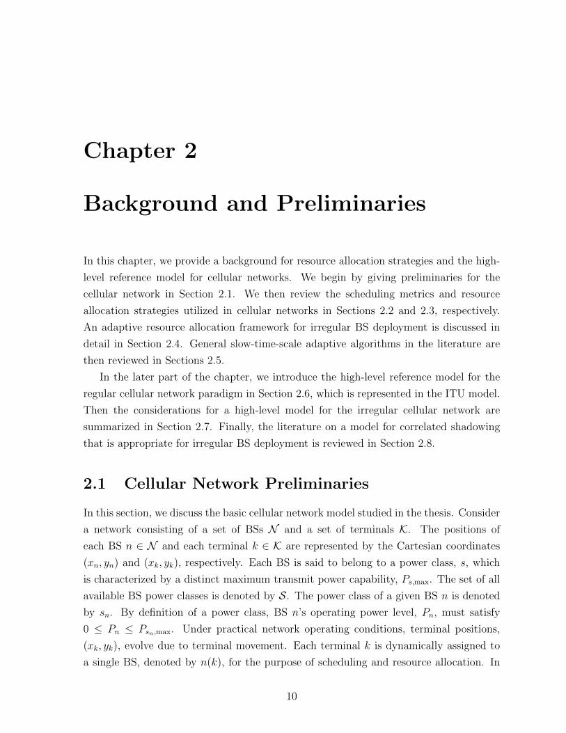
2.1 Cellular Network Preliminaries
In this section, we discuss the basic cellular network model studied in the thesis. Consider
a network consisting of a set of BSs N and a set of terminals K. The positions of
each BS n ∈ N and each terminal k ∈ K are represented by the Cartesian coordinates
(xn, yn) and (xk, yk), respectively. Each BS is said to belong to a power class, s, which
is characterized by a distinct maximum transmit power capability, Ps,max. The set of all
available BS power classes is denoted by S. The power class of a given BS n is denoted
by sn. By definition of a power class, BS n’s operating power level, Pn, must satisfy
0 ≤ Pn ≤ Psn,max. Under practical network operating conditions, terminal positions,
(xk, yk), evolve due to terminal movement. Each terminal k is dynamically assigned to
a single BS, denoted by n(k), for the purpose of scheduling and resource allocation. In
10

Chapter 2. Background and Preliminaries 11Regular Network (Traditional)
Fixed cell
boundaries
Cell membership is
straightforward
Classical frequency
reuse
Scheduling is
organized in
straightforward way.
8
Figure 2.1: Regular cellular network deployment. The black and red points represent aBS and terminals, respectively.
the following, the basic model introduced in this section is specialized for the cases of
regular and irregular cellular networks.
Regular Cellular Network
Cells in the regular network are modelled with the hexagonal cell structure of Figure 2.1;
therefore, the base station coordinates, (xn, yn), coincide with the hexagon centres. The
number of power classes in the regular network (or the number of elements in set S) is
equal to one, that is, S ≡ |S| = 1, and the maximum transmit power capability of each
BS is represented by a constant, Pmax. Finally, the operating power level, Pn, of each BS
is typically held constant at Pmax.
Irregular Cellular Network
The focus of this thesis is the study and modelling of the irregular network. In the
irregular network, BSs are deployed in an inhomogeneous or arbitrary pattern, hence,
the BS coordinates, (xn, yn), are irregular as shown in Figure 2.2. In addition, BSs
belong to a number of different power classes, which are characterized by a wide range
of maximum power capabilities. Therefore, in the irregular network, S = |S| > 1. It will
also be proposed later in the thesis that the BS power levels, Pn, be dynamically adapted
in the range 0 ≤ Pn ≤ Psn,max, according to changing network conditions.

Chapter 2. Background and Preliminaries 12
Irregular Cellular Network
1. Dynamic BS assignmentsbased on
max channel gain
2. Dynamically formclusters
(scheduling cells)
3
Figure 2.2: Representation of the irregular cellular network deployment. The green circlesrepresent terminals, and the blue squares of different sizes represent BSs of different powerclasses.
Computation of Transmittable Data Rates for Scheduling
In this thesis, we adopt the organization of the time-frequency resource allocation from
3GPP LTE standards [9]. Terminal scheduling is performed at the LTE subframe (which
corresponds to the assumed time scale of multipath fading variation) and requires the
knowledge of transmittable data rates for links between all terminals and BSs. Note
that computation of transmittable data rates further requires the knowledge of channel
gains for all links. Let C be the set of available subcarriers in orthogonal frequency
division multiplexing (OFDM). The channel power gain between BS n ∈ N and terminal
k ∈ K on subcarrier c ∈ C is computed as the product of the distance-dependent path
loss component, PLn,k, the large-scale shadowing component, SFn,k, and the small-scale
multipath component, mn,k,c:
gn,k,c = PLn,kSFn,kmn,k,c. (2.1)
where the models for the channel components are elaborated later in Section 2.6. The
transmittable rate, between terminal k and BS n on subcarrier c, has been approximated
in [2] for the LTE system, through curve fitting of the Shannon rate formula with an
SINR gap, γ:

Chapter 2. Background and Preliminaries 13
rk,n,c ∼= Bc min
(log2
(1 +
SINRk,n,c
γ
), 5.5547
), (2.2)
where
γ = 2, (2.3)
SINRk,n,c =pn,cgn,k,c
N0 +∑
j∈N, j 6=n pj,cgj,k,c. (2.4)
Here, BC is the subcarrier bandwidth, pn,c is the power transmitted on subcarrier c by
BS n and N0 is the noise power on each subcarrier at the receiver.
2.2 User Scheduling Metrics
There has been much research by various authors [10–13] on the appropriate metric to
be used for resource allocation including user scheduling. In the following, we consider
full-buffer persistent data traffic conditions. Two significant scheduling metrics known
as total rate maximization and proportional fair scheduling are described under such
conditions.
2.2.1 Total Rate Maximization
The traditional scheduling strategy has been the maximization of the total system rate in
the long term [14], which shall be referred to as the total rate maximization (TRM). Under
this strategy, the average rate performance of the system as a whole is optimized without
regard for any single individual user’s performance. The long-term TRM optimization
objective is given by
max∑k∈Kn
Rk for all n ∈ N . (2.5)
where Kn = k|n(k) = n is the set of terminals assigned to BS n for scheduling, and Rk is
the time-averaged rate for terminal k. Consider a single-frequency system. The terminal
scheduled by BS n at subframe t is determined with the knowledge of the transmittable
rate, rk(t), as
k∗n(t) = arg maxk∈Kn
rk(t) for all n ∈ N , (2.6)
which has been shown to be equivalent to the long-term optimization of (2.5). In prac-
tice, there is a significant problem with the use of the total rate maximization of (2.5)
and (2.6). Consider the simple hypothetical scenario consisting of a single BS and two

Chapter 2. Background and Preliminaries 14
BS
Terminal 1 Terminal 2
Figure 2.3: Hypothetical scenario for terminal scheduling.
stationary terminals depicted in Figure 2.3. Terminal 1 is much closer to the BS than
Terminal 2, and therefore Terminal 1 will tend to have much higher channel gain on
average. We additionally assume that the channel gain fluctuations over time are small
in comparison to Terminal 1’s channel gain. According to the TRM criterion of (2.6),
therefore, Terminal 1 would be scheduled at all of the subframes, and Terminal 2 would
not be scheduled at any of the subframes. This situation where Terminal 2 is deprived of
service is commonly referred to as the fairness problem in the literature [10,15]. Propor-
tional fair (PF) scheduling criterion [14], which was proposed in order to overcome the
fairness problem, is discussed in the next section.
2.2.2 Proportional Fair Scheduling
According to the proportional fair (PF) criterion, scheduling should maximize the sum
log utility (SLU) function, which is computed as the sum of the logarithm of the average
user rates. Therefore, the long-term optimization objective is
max∑k∈Kn
log(Rk) for all n ∈ N . (2.7)
Since the logarithm function increases at a continually decreasing (or diminishing) rate,
PF scheduling overcomes the fairness problem encountered in TRM. In particular, con-
sider the scenario depicted in Figure 2.3. Terminal 2, i.e., the user with the weak channel,
is said to be treated fairly, because a given increase in user data rate, for example, 10
kbps, for Terminal 2 (the weak user) results in a greater increase in utility than the same
amount of data rate increase for Terminal 1 (the strong user). The concept of the de-
creasing rate of utility increase is known in economics as the law of diminishing marginal
returns or law of diminishing marginal utility [16]. Under SLU maximization, Terminal
2 is therefore expected to achieve a non-zero average data rate. In fact, as discussed

Chapter 2. Background and Preliminaries 15
in detail in [17], both terminals achieve a long-term rate that is approximately propor-
tional to their average transmittable rate based on the respective channel gains, which
is the reason for the term proportional fairness. For more details on the properties of PF
scheduling, the reader may refer to some of the many works on the topic [10–15,17].
For a single-frequency system, the optimization of (2.7) is realized by scheduling
terminal k∗n(t) at each subframe t, with the knowledge of instantaneous achievable rate
rk(t) and time-averaged rate Rk(t), that is,
k∗n(t) = arg maxk∈Kn
rk(t)
Rk(t)for all n ∈ N (2.8)
Note that the time-averaged rate is updated at each subframe based on an exponential
moving average:
Rk(t+ 1) =
(1− 1
T0
)Rk(t) +
(1
T0
)rk(t) (2.9)
where T0 is the averaging window size selected for smooth averaging. In a system with
multiple frequencies, the scheduling is performed either independently in each subcarrier
at the subframe or through more elaborate strategies. Note that the PF scheduling will
be used in the rest of the thesis.
2.3 Resource Allocation Strategies
In the traditional cellular network, the BSs are deployed according to a regular pattern,
which is modeled with hexagons. The strategy of classical frequency reuse is utilized.
According to this scheme, the BSs are partitioned into groups of geographically adjacent
cells, known as frequency reuse clusters. The frequency reuse factor (FRF) defines the
size of the clusters, and the available spectrum is distributed among the BSs according to
pre-defined patterns. The FRF is said to be an indicator of the level of frequency reuse
in the network. In early networks, high (or conservative) reuse factors were used for the
avoidance of excessive interference. However, the scheme did not consider the variation
of traffic load in the cells. In addition, the ever growing demand for capacity necessitated
more aggressive frequency reuse, which would cause degraded performance for terminals
at the cell edges.
More recently, the fractional frequency reuse (FFR) technique was proposed as an
alternative to classical frequency reuse. In this scheme (also referred to as static FFR),
two different frequency reuse patterns are applied: a higher (or conservative) reuse factor
for the cell-edge terminals with weak channel gains, and a lower (or aggressive) reuse

Chapter 2. Background and Preliminaries 16
factor for the stronger or cell-centre terminals. The drawback of the method was that
the terminal partitioning was based solely on distances from the BSs, and the spectrum
assignments again did not adapt to the variations of traffic load.
To overcome the limitations of static FFR, techniques have recently been proposed
in the literature that attempt to adapt to the variation in traffic, by using different
methods to organize the frequency resource allocation. This goal is commonly achieved by
coordination of resource allocation between neighboring BSs, which is also referred to in
the literature as inter-cell interference coordination (ICIC). Different types of techniques
are reviewed in the following.
Dynamic FFR
Dynamic FFR schemes attempt to adapt to variations of traffic while maintaining the
general concept of FFR in the method. Boudreau et al. [18] have proposed an adaptive
frequency reuse strategy for interference coordination suitable for 4G networks. The
scheme switches between three different frequency-power profiles according to the traffic
load in each cell.
Ali and Leung [19] present an elaborate dynamic frequency allocation technique while
maintaining the general idea of fractional frequency reuse. The frequency allocation is
determined according to the average performance of all terminals in the network on all
available frequency resources.
Two-Level Resource Allocation
A number of works in the literature deal with resource allocation at two levels (phases)
or time scales. The common idea of these methods is that a frequency reuse pattern is
decided based on slow-varying traffic distributions in the first phase, and at a faster time
scale, the second phase fine-tunes the resource allocation inside each cell. Bonald et al.
propose a two-level scheme for multi-cell coordination for the purpose of scheduling [20].
In the first phase, the activity of the interfering BSs is determined through interference
coordination with the goal of transmission rate maximization. A TDMA transmission
scheme is assumed. In the second phase, the load balancing is performed in order to
divert traffic from heavily-loaded to lightly-loaded cells.
Li and Liu extend the two-level resource allocation framework to a multi-cell OFDMA
system [21]. In the first phase, the available spectrum is assigned to the terminals in the
network by the radio network controller. In the second phase, the BSs independently
modify the channel assignment in each cell according to the buffer sizes of the active

Chapter 2. Background and Preliminaries 17
terminals.
Scheduling and resource allocation requires the knowledge of SINRs, which depend
on the channel information for both the desired signal links and the interference links.
It has, therefore, been noted that for ideal resource allocation, BSs need to have accu-
rate network-wide channel information at every instant. However, acquiring the channel
information from out of the cell can lead to an excessively large signalling complexity in
practice. While most of the recent resource allocation techniques assume full knowledge
of the channel information in the network to simplify the problem, Chang et al. [22]
devise a scheme that takes this aspect into account. A two-level framework based on
graph theory is proposed. In the first phase, intercell interference is reduced with no
knowledge of out-of-cell interference, based solely on the geographical locations of termi-
nals. In the second phase, the resource allocation is performed according to knowledge
of instantaneous channel gains.
2.4 Adaptive Resource Allocation Framework for Ir-
regular BS Deployment
A solution for coordinated resource allocation for a network with irregular deployment,
which considered the issue of channel information signaling, was developed in [2]. An
important goal of the work was to design a resource allocation framework that could
adapt to the variations of traffic load in the cells, which is comparable to the adaptive
resource allocation strategies in the previous section. The primary design constraint
was that the resource allocation was required to be flexible and adaptive enough to be
suitable for irregular BS deployment. The case of a single BS power class, with BSs
placed uniformly at random without restriction, was primarily considered in the work.
Note that a practical application could be in a network with both small and large cells.
A workable strategy to reduce the signalling requirements is to periodically group
the BSs in the network into separate clusters, also referred to as scheduling cells (SCs).
An OFDMA system such as the 3GPP LTE was considered. Inside each SC, channel
information is exchanged and the resource allocation is coordinated. However, SCs act
independently from one another during the course of scheduling at the LTE subframe
level. The set of SCs is updated dynamically with the changing traffic distribution at
a slower time scale. A complete adaptation framework that incorporates PF scheduling
was developed. The flowchart outlining the adaptive framework is depicted in Figure 2.4.
At the large time scale, terminals are assigned to BSs according to the long-term channel

Chapter 2. Background and Preliminaries 18
l = l + 1
Coordinated resource
allocation in each cluster
Form clusters
(scheduling cells)
Assign terminals to BSs
l mod F = 0?
No
Yes
Figure 2.4: Flowchart for the adaptive resource allocation framework.
gains, and the SCs are formed based on the interference or SINR caused by each cell on
every other cell. Then, at the subframe time scale, proportional fair resource allocation
is performed with coordination or exchange of channel information inside each SC. The
scheduling has been combined with on-off power switching and is executed in parallel
in each subcarrier. Note that the power switching is designed to allow added flexibility
due to finer variations of traffic distributions. The algorithmic framework for adaptive
resource allocation is detailed in Figure 2.5, which lists both the slow-scale adaptation and
fast-scale resource allocation steps. The details of the fast resource allocation algorithm
are given in Figure 2.6. In the following, other important details are discussed in relation
to (1) the clustering algorithm, (2) the fast resource allocation algorithm and (3) the
requirements for channel information signalling.
Clustering Algorithm
The clustering algorithm specified in Figure 2.5 operates on the principle that BSs cre-
ating a lot of interference on each others’ terminals should be assigned to the same
cluster (so that interference can then be avoided through fast scheduling). Therefore,
the algorithm needs as inputs the set of BS assignments n(k)k∈K, the long-term time-
averaged channel gains, Gn,k = PLn,kSFn,k, for all n and k, and the BS power level
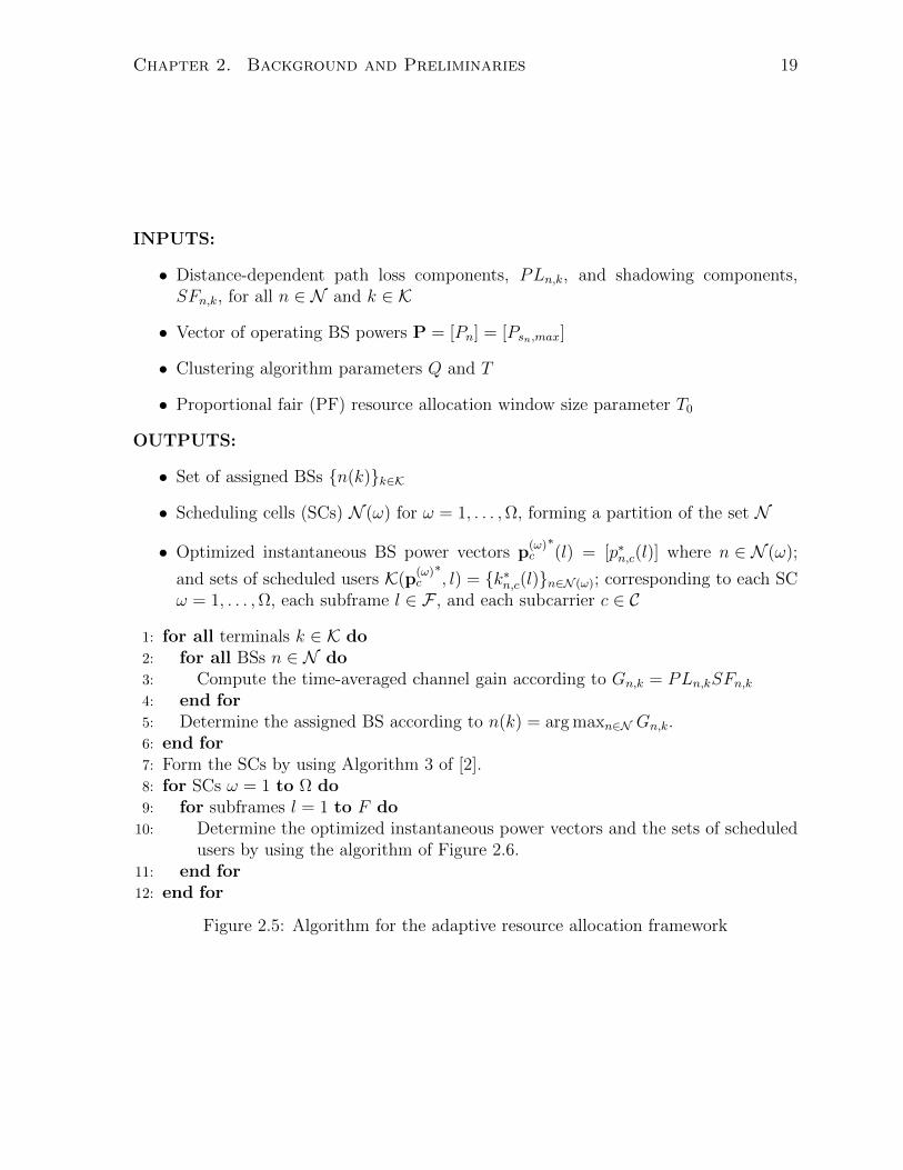
Chapter 2. Background and Preliminaries 19
INPUTS:
• Distance-dependent path loss components, PLn,k, and shadowing components,SFn,k, for all n ∈ N and k ∈ K
• Vector of operating BS powers P = [Pn] = [Psn,max]
• Clustering algorithm parameters Q and T
• Proportional fair (PF) resource allocation window size parameter T0
OUTPUTS:
• Set of assigned BSs n(k)k∈K
• Scheduling cells (SCs) N (ω) for ω = 1, . . . ,Ω, forming a partition of the set N
• Optimized instantaneous BS power vectors p(ω)c
∗(l) = [p∗n,c(l)] where n ∈ N (ω);
and sets of scheduled users K(p(ω)c
∗, l) = k∗n,c(l)n∈N (ω); corresponding to each SC
ω = 1, . . . ,Ω, each subframe l ∈ F , and each subcarrier c ∈ C
1: for all terminals k ∈ K do2: for all BSs n ∈ N do3: Compute the time-averaged channel gain according to Gn,k = PLn,kSFn,k4: end for5: Determine the assigned BS according to n(k) = arg maxn∈N Gn,k.6: end for7: Form the SCs by using Algorithm 3 of [2].8: for SCs ω = 1 to Ω do9: for subframes l = 1 to F do
10: Determine the optimized instantaneous power vectors and the sets of scheduledusers by using the algorithm of Figure 2.6.
11: end for12: end for
Figure 2.5: Algorithm for the adaptive resource allocation framework

Chapter 2. Background and Preliminaries 20
INPUTS:
• Set of coordinated BSs A = N (ω)
• Set of assigned BSs n(k)k∈K
• BS power level vector P = [P1, . . . , PA]
• Fast-changing channel gains, gk,n,c, ∀k ∈ K,∀n ∈ A,∀c ∈ C
OUTPUTS:
• Optimized instantaneous BS power vectors, p∗c(l) = [p∗1,c(l), . . . , p∗A,c(l)]
T , ∀c ∈ C
• Sets of scheduled users, K(p∗c , l) = k∗n,c(l)n∈A, ∀c ∈ C
1: for all subcarriers c = 1 to C do2: Initialize maxSum to 0.3: for all vectors pc(l) ∈ 0, Pn/C2A×1 do4: for all n ∈ A do5: Set k∗n,c(l) = arg maxk∈Kn
rk,n,c(l)
Rk,n(l)
6: end for7: Form the candidate user set K(pc, l) = k∗n,c(l)n∈A8: Compute newSum =
∑k∈K(pc,l)
rk,n,c(l)
Rk,n(l)
9: if newSum > maxSum then10: Set maxSum to newSum, p∗c(l) to pc(l), and K(p∗c , l) to K(pc, l)11: end if12: end for13: end for14: for all terminals k ∈ K do15: Update the time-averaged user rate based on the scheduled user rates by using
Rk,n(k)(l + 1) =(
1− 1T0
)Rk,n(k)(l) +
(1T0
)∑c|k∈K(p∗
c ,l)rk,n(k),c(l)
16: end for
Figure 2.6: Algorithm for fast PF resource allocation for a given subframe l ∈ F .

Chapter 2. Background and Preliminaries 21
vector P = [P1, . . . , PN ], for the computation of long-term SINRs. We let F denote the
set of subframes in the analysis. According to the proposed method, the set of clusters
are determined by running the K-means clustering algorithm [23] on an SINR-based BS
similarity matrix. Note that the clustering algorithm requires two parameters, Q and T ,
as inputs: Parameter Q limits the maximum number of clusters in each iteration of the
algorithm. Parameter T adjusts the tendency of BSs to join a cluster. It is, therefore,
possible to adjust the cluster sizes by tuning parameters Q and T together. Detailed
algorithm steps are found in [2].
Fast Resource Allocation
The fast PF resource allocation specified in Figure 2.6 is performed independently at each
SC ω. Note that to simplify the exposition, the set of coordinated BSs is denoted by
A = N (ω), and the set of their assigned terminals by K in Figure 2.6. Additionally, the
SC index ω is dropped in the rest of the variables. The algorithm steps are shown for a
given subframe l ∈ F . PF scheduling discussed in Section 2.2.2 together with binary (on
or off) PF power switching is used. At the end of the power optimization and scheduling,
the time-averaged rate of each user is updated with the total scheduled user rate over
the subframe.
Channel Information
In summary, the requirements for channel information signalling is significantly reduced
due to clustering. In order to perform BS assignment and clustering, the long-term
channel gains, Gn,k, between all BSs and terminals need to be known at a central entity
at every F subframes—which is a low frequency. In contrast, the estimate of fast-varying
channel gains, gn,k,c, need to be exchanged at every subframe only for BSs and terminals
inside the given SC.
2.5 General Slow-Time-Scale Adaptive Algorithms
There has been a recent recognition in the wider community of the need for adaptation
at time scales larger than the fast multipath fading time scale (i.e. at the LTE subframe).
Such slowly-adaptive algorithms have prominently been studied in the context of 3GPP
LTE Self Organizing Networks (SON) [24]. In Sections 2.3 and 2.4, we discussed resource
allocation frameworks that commonly work at two different time scales. The adaptations
at the slow time scale such as the dynamic re-organization of the frequency reuse patterns,

Chapter 2. Background and Preliminaries 22
and dynamic BS assignments and clustering can be considered similar to SON functions1.
More generally, the main driving force for SON has been the need to automate the
configuration, optimization, maintenance, troubleshooting and recovery of the cellular
system. Automation of tasks previously performed manually is expected to enable more
agile adaptation in face of the greater dynamism of emerging irregular cellular networks,
and simultaneously to reduce operating and other costs incurred by wireless operators. A
wide variety of SON functions have been proposed in the literature [25–29]. In the most
common taxonomy, the functions are classified based on the phases corresponding to the
life cycle of the cellular system equipment, that is, deployment, operation, maintenance,
redeployment, recovery etc. The adaptive functions and algorithms that organize these
phases are classified into (a) self configuration, (b) self optimization and (c) self healing.
Each of the categories is reviewed in the following, together with function and algorithm
contributions from the SON literature.
Self Configuration: Self configuration functions are primarily executed at the de-
ployment and re-deployment phases of the network equipment life cycle. A number of
different parameters can be configured, including radio propagation parameters such as
antenna type, antenna gain, and antenna azimuth and tilt angles. The authors in [25]
proposed an antenna tilt optimization method for the purpose of achieving higher system
capacity and better coverage. In particular, they demonstrated an approach based on
simulated annealing that uses measurements of terminal SINR information. An impor-
tant aspect of the method is that it was specifically designed to utilize readily available
terminal measurements in an online manner. The authors in [26] proposed an alterna-
tive game theoretic method for antenna tilt optimization. Furthermore, they proved the
existence of a Nash equilibrium which can be achieved in a non-cooperative game for the
optimization of system-wide utility function.
Self Optimization: Self optimization is primarily executed at the operation phase of
the network life cycle, and involves continuous optimization of system parameters after
their initial configuration, in order to ensure efficient performance of the system. A variety
of parameter optimizations for realization of distinct goals are possible. The authors in
[27] proposed a scheme for balancing the load across multiple cells, and avoiding intercell
interference, by performing intercell and intra-cell handovers in a partial frequency reuse
(PFR) scheme for OFDMA. Authors in [28] developed a method for adaptive organization
of an fractional frequency reuse (FFR) scheme for the purpose of interference control.
1There have been few attempts to formulate a precise definition of Self Organization (SO). One suchattempt [24] emphasizes the need for stability, scalability and agility of the algorithms to be consideredSO, distinguishing it from the non-self-organized type of system adaptation.

Chapter 2. Background and Preliminaries 23
Table 2.1: Classification of time scales.
Time Scale System Dynamics Adaptation
Fastest Multipath fading User scheduling
Medium
Slow terminal movements Self optimization functions
Terminal activation Cell assignments
Terminal deactivation Clustering
Slowest
BS Deployments Self configuration
BS Outages Self healing
BS Movements Cell outage management
The basic idea of the algorithm was to dynamically create efficient FFR patterns in order
to adapt to the changing user traffic distributions and system conditions.
Self Healing: Self healing functions are primarily executed during recovery from faults
and failures that can be due to component malfunctions or natural disasters. Self heal-
ing is a systematic process which is comprised of several stages including (a) remote
monitoring, (b) detection, (c) diagnosis and (d) triggering of compensation actions for
the clearing of the fault or failure. The reference [29] considered the self healing for the
fault referred to as a cell outage. A cell outage is defined as a rare and catastrophic
failure of a BS, which results in ceasing of all signal transmission and reception at the
BS. The authors in [29] provided a full description for the management of cell outages
in LTE networks, reviewing both detection and compensation algorithms, and discussing
the role of operator policies in the design of detection and compensation schemes.
We note that self optimization functions are generally intended for execution on a
relatively frequent basis during the operation of the wireless network, e.g. after a cer-
tain number of subframes. In contrast, self configuration and self healing functions are
commonly executed infrequently as events such as BS deployments and outages tend to
be rare. A classification of dynamism and adaptation with approximate demarcation of
different time scales is provided in Table 2.1. Note that the multipath fading time scale
is included in the taxonomy. Terminal movements, activations and de-activations are
classified as medium scale dynamics due to their relative high frequency. BS dynamics
such as outages, deployments and movements are classified as slow-scale dynamics due
to the low frequency of occurrence. Note that BS movements are not common in today’s
cellular networks, however, they are included with the thought that they may become
feasible for emerging and future networks. According to classification of the adaptation
functions, user scheduling occurs at the fastest time scale, self optimization in SON oc-
Chapter 2. Background and Preliminaries 24
curs at the medium time scale, and self configuration and self healing at the slowest time
scale. The medium- and slowest-scale dynamics can be considered as the focus of the
adaptations in this dissertation.
2.6 The ITU System Model: High-Level Reference
Model for the Regular Cellular Network
The ITU system model [1] provides a high-level reference for the modelling of a cellu-
lar system, which was designed for the regular cellular network paradigm. The model
will be used in this thesis as a starting point for developing a high-level model for the
irregular cellular network. The ITU model is based, in part, on the idea of generating a
large number of snapshots, known as simulation drops, for the purpose of Monte Carlo
simulation. A simulation drop, in this context, is defined as a random deployment of
mobile terminals on a network area with fixed BS deployments, following the hexagonal
cell pattern. Within each drop, the set of active terminals and their deployments as well
as large-scale channel components such as path loss and shadowing are fixed, and there
are only virtual terminal movements, which result in the multipath fading due to the
Doppler effect. As mentioned in Section 2.1, the time scale for multipath fading corre-
sponds to a subframe in LTE, which is the basic time unit for user scheduling. In order
to obtain statistically representative results at this time scale, a large number of LTE
subframes are simulated within each simulation drop. The flowchart of the simulation
methodology is given in Figure 2.7, where the number of drops used in the simulation is
denoted by the variable P , and the number of LTE subframes per drop by F . Notably,
the simulation drops themselves are generated independently from each other, that is, as
uncorrelated snapshots of network configurations. In addition, the model uses standard
large-scale channel models, in particular, for shadow fading, that are static in time and
statistically uncorrelated in space. In the following, we review the channel modelling
in the ITU model, considering distance-dependent path loss, shadowing and multipath
fading.
2.6.1 Channel Modelling
Distance-Dependent Path Loss
A typical expression for the distance-dependent path loss model is given as follows: Let
A be the path loss exponent parameter, B the intercept parameter, C the frequency

Chapter 2. Background and Preliminaries 25
j = j + 1
Perform user scheduling
Generate subframe j of drop i (multipath fading)
Compute path loss and shadowing for all links
Generate simulation drop i
j mod F = 0?
No
Yes
i = i + 1
i =P? STOP
No
Yes
Figure 2.7: The flowchart for the drop-based simulation framework based on the ITUcommon reference model.
dependence parameter and X the environment-specific parameter. dn,k is the distance
between BS n and terminal k in metres, and fc is the system frequency in GHz. The
path loss from BS n to any terminal k is given by [30]
PLn,k[dB] = A log10(dn,k) +B + C log10
(fc5.0
)+X (2.10)
As an example, A = 20, B = 46.4, C = 20 and X = 0 are typical values for free space.
Shadowing
Shadowing channel gain is represented using the common log-normal model [31]. For the
link between a BS n and a terminal k, logSFn,k is, therefore, generated as a Gaussian
random variable with zero mean and standard deviation σ.

Chapter 2. Background and Preliminaries 26
Multipath Fading
Modelling of fast-varying channel components mn,k,c at the subcarrier and subframe
granularity is discussed in this section.
Frequency variation in the wireless channel is due to the multiple path (multi-path)
components with different excess propagation delays, or different echoes of the transmit-
ted pulse. The distribution of the delay values for the echoes, weighed by signal power, is
referred to as the delay spread for the channel. The delay spread affects the rate of varia-
tion of the channel response with frequency. The frequency variation due to delay spread
is commonly modelled through statistical means with a frequency correlation function.
The channel time variation arises due to the motion of the terminal with respect
to each of the multipath channel components. In particular, the different signal multi-
path components undergo frequency shifts (Doppler shifts) that are proportional to the
relative velocity of the terminal with respect to the angle of arrival of the component.
The distribution of the Doppler shifts, weighed by signal power, is referred to as the
Doppler spread for the channel. The Doppler spread is related to the rate of variation
of the channel response in time. The time variation due to Doppler spread is commonly
modelled through statistical means with a time correlation function.
Finally, the spatial variation occurs due to the constructive and destructive interfer-
ence of the electromagnetic waves for the multipath components arriving at a receiver
with multiple antenna elements. Note that the situation with multiple antennas is not
considered in the thesis.
The literature contains many different models for time, frequency and space variation
of the wireless channel [9, 32–35]. However, the joint computation of channel variation
in all three variables can prove to be challenging. The ITU provides a channel model
appropriate for the OFDM scheme incorporating all three types of variations, which is
based on the concept known as ray clusters. Detailed explanation of the model is provided
in [1].
2.7 Considerations for an Irregular Cellular Network
Model
The irregular cellular network has characteristic that are very different from the regular
cellular network, which has the ITU model as a high-level representation. A more ap-
propriate high-level model would be able to provide a common network representation as
a reference for the consideration of different types of dynamical changes in the network

Chapter 2. Background and Preliminaries 27
in the design of appropriate dynamic resource allocation and adaptation as well as SON
strategies.
The limitations of the existing ITU model is described in the following: First, the
hexagonal deployment pattern is inadequate due to the irregular deployment of BSs in
the new network paradigm. Second, more accurate channel models are needed due to
irregularity of BS deployment. In particular, a more realistic shadowing model than the
common lognormal model should be developed that can represent the gradual variation of
shadowing over space and the time as well as the diverse radio propagation environments
in the network. Third, the snapshot simulation method using simulation drops does not
accurately represent the dynamism in the network. Such dynamics are important for the
accurate evaluation of dynamic resource allocation frameworks, and other adaptation
and SON functions that were discussed in Sections 2.3-2.5. In particular, we note that
in implementing slowly-adaptive functions, it is important to minimize signaling com-
plexity and overhead resulting from, e.g., the exchange of channel information. This is
especially true if centralized decision making or coordination is required for the specific
implementation. The signalling complexity can potentially be reduced by considering
that the evolution of the cellular channel and environment is gradual in time, meaning
that each execution of the function can partially utilize the information from the previous
execution. It would, therefore, be possible to design algorithms with reduced signalling
complexity. To evaluate the performance of reduced-complexity adaptive algorithms, it
becomes necessary to accurately model the time evolution of the cellular system and
channel at such slow time scales.
In this thesis, we propose a new system model framework, which is appropriate as a
high-level model for the irregular network. The main considerations for the model are as
follows:
1. The deployment model should reflect both the arbitrariness of deployment and the
broad level of agreement between the positions of terminals and BSs (e.g. due to
planning).
2. Since the original simulation drop concept of the ITU model does not allow the
modelling of network time evolution at the slow time scale, an appropriate modifi-
cation of the concept should be devised.
3. The shadowing model should represent the shadowing correlation as well as the
diverse radio propagation environments present in the network.

Chapter 2. Background and Preliminaries 28
2.8 Correlated Shadowing Model for Irregular BS
Deployment
The classical lognormal shadowing model gives no information on the correlation of shad-
owing over the network (also known as spatial correlation). Consider the special case of a
link between a fixed base station and a moving terminal as depicted in Figure 2.8: Due to
the inherent correlation in the topography of the physical environment, the channel gain
experienced by the terminal cannot change abruptly after having traveled a relatively
small distance. In 1991, Gudmundson proposed a method [36] to model the spatial cor-
relation of shadowing. According to the Gudmundson model, the correlation between the
links A-B and A-C shown in Figure 2.9, is given as a function of the distance d between
the links as
R(d) = σ2e−d/dc (2.11)
where σ is the shadowing standard deviation, and dc is an important parameter known
as the shadowing correlation distance. Note that the Gudmundson correlation model
considers the correlation between pairs of links with a common endpoint; specifically,
either between a terminal and multiple BSs, or between a BS and multiple terminals.
Other research in cellular networks [31, 37–39] expanded on Gudmundsons work, also
focusing on the correlation between pairs of links with a common endpoint. More recent
work [40] considered the mathematical feasibility of shadowing correlation models, as well
as the calculation of aggregate interference in scenarios with correlated shadowing [41–43].
However, the literature in cellular networks did not report on the correlation between
pairs of links with no common endpoint, illustrated in Figure 2.10, effectively neglecting
such correlation. Links without a common endpoint frequently have low correlation in
traditional cellular networks, due to the regular spacing and large distances between BSs.
Thus it can be acceptable to neglect such correlation in the model. However, in irregular
networks, BSs can, at times, be very close together. Therefore, the correlation between
two links with no common end cannot be neglected in such scenarios. An appropriate
correlation model incorporating non-common-endpoint links was proposed in [8], which
is discussed in the following.
We first define the potential field as a random process whereby each realization is a
function from the plane to real numbers. Thus, if we fix a point in the plane, the result is a
real random variable. According to the spatially correlated shadowing model, shadowing
is computed from a Gaussian potential field generated over the network area. Note that
the potential field is stored in a vector denoted by u. A homogeneous shadow fading

Chapter 2. Background and Preliminaries 29
BS
Terminal at time t1
Terminal at time t2
Figure 2.8: The wireless link between a fixed base station and a moving terminal.
A
B
C
d
Figure 2.9: Wireless links with a common endpoint.
A
B
C D
Figure 2.10: Wireless links without a common endpoint.

Chapter 2. Background and Preliminaries 30
Figure 2.11: A realization of the potential field [8].
scenario with fixed shadowing standard deviation, σ0 (in dB), and correlation distance,
dc, is considered. The value of the potential field at point A defines the potential level
of point A and is denoted by uA. For a cellular network with N BSs and K terminals,
J = N +K potential levels are generated according to the following steps:
• Step 1: Generate a J×1 vector v whose elements are independent Gaussian random
variables with zero mean and unity standard deviation.
• Step 2: Generate a J × J correlation matrix R = [rij] such that
rij =σ2
0
2e−dij/dc (2.12)
where dij is the distance between point i and point j.
• Step 3: Decompose the correlation matrix using Cholesky factorization such that
R = BBH.
• Step 4: Calculate the J × 1 potential level vector u according to
u = Bv (2.13)

Chapter 2. Background and Preliminaries 31
A realization of the shadowing potential field is depicted in Figure 2.11. The shadowing
between point A and point B (normally, a terminal and a BS) is then computed as a
function of the two potential levels according to
SF [dB] = f (uA, uB) = sgn (uA + uB) · |uA − uB| . (2.14)
It was shown in [8] that the above potential field method of shadowing generation results
in the correct lognormal shadowing with spatial correlation, and the resulting shadowing
values satisfy a number of essential statistical properties that are detailed in the work.
We note that all the correlated shadowing models discussed in this thesis will be based
on the foundation of the potential field model discussed in this section.
Finally, it is important to mention that different radio propagation environments
would cause different radio-channel characteristics, and therefore, the values of shad-
owing channel parameters, σ0, and dc, need to be different based on the environments.
Typically, propagation environments are characterized by urban, suburban or rural, and
indoor or outdoor scenarios. Different environments also frequently have different sizes
of cells. The values of σ0, and dc (as well as other types of channel parameters for
multipath fading or distance-dependent path loss) are normally obtained by conducting
channel measurements in practical propagation scenarios [1, 30, 36, 44, 45]. Note that
the consideration of varying shadowing model parameter values will be important in the
development and implementation of the model in this chapter.
Chapter 3
Adaptation Case: BS Outage
Compensation
3.1 Relevant Work and Contribution
3.1.1 Relevant Work
A cell outage is defined as a rare and catastrophic failure of a BS, which results in ceasing
of all signal transmission and reception at the BS. Following the outage, the users assigned
to the outage BS lose service and adaptation of the network needs to be performed. The
type of adaptation has been referred to, in the context of 3GPP LTE SON, as cell outage
compensation (COC).
A small number of works in the literature have explored the COC problem. In ho-
mogeneous networks, the literature [29,46–48] focused on the development of algorithms
for cell outage compensation by tuning of various control parameters in different types
of systems, including antenna tilt, pilot power and uplink target received power, in order
to mitigate the performance effects due to the outage in accordance with operator pol-
icy. In the area of heterogeneous networks, the authors in [49] and [50] studied the cell
outage compensation problem and offered algorithm solutions based on the adjustment
of antenna gains and transmission powers.
3.1.2 Contribution
Most works in the literature consider the base station (or cell) outage compensation
(COC) for homogeneous or regular networks. Furthermore, even works that consider
irregular networks do not explicitly consider the general modelling aspect of the problem.
32

Chapter 3. Adaptation Case: BS Outage Compensation 33
We focus on the modelling of a BS outage for an irregular network with multiple power
classes in a general sense. Both the positions of BSs and the power classes are modelled.
In addition, we consider the adaptive resource allocation strategy as part of the overall
model. Specifically, we adopt the concept of cluster or scheduling cell for the purpose of
coordinated adaptive resource allocation. To our knowledge, the use of a scheduling cell
is new for the COC literature. Direct sum log utility maximization based on proportional
fairness is the primary formulation we used in finding a compensating cluster, outage user
cell associations, and the adjusted BS power levels. The use of proportional fairness in
the COC formulation is additionally different from the literature for COC.
Finally, the shadowing model with spatial correlation, discussed in Chapter 2, is
considered for greater realism especially of the irregularly deployed network.
3.1.3 Key Results
The results indicate that both COC algorithms show robustness toward cell outage in
terms of user average spectral efficiency, and outage user and non-outage user QoS vio-
lation probabilities for both a regular and an irregular network. In particular, the COC
algorithms are shown to achieve a large percentage (nearly 75%) of the user spectral
efficiency of the no outage scenario in both network types. In addition, the proportional
fairness-based COC algorithm is shown to allow the tuning, or trading off, of the average
number of BSs with raised power—which is a measure of the algorithm cost—against
different measures of performance including user spectral efficiency.
3.2 Introduction
Chapter 2 discussed adaptive resource allocation strategies that respond to network vari-
ations (such as due to traffic changes) for cellular networks. In addition, more general
adaptive functions in the 3GPP LTE SON literature were reviewed. The focus of the
discussion in this thesis is slow- and medium-time-scale adaptations. Typical adapted
parameters include transmit power, antenna gain, antenna tilt and other parameters re-
lated to the adaptive frequency re-use scheme that is employed. This thesis focuses on
dynamic adaptations with the final aim of improved spectral resource allocation, that is
appropriate for the irregular cellular network paradigm. In particular, BS assignments,
clustering and power adaptation (power control) will be mainly considered in the devel-
opment of the schemes.
In this chapter, we study BS (or cell) outage compensation as a specific case of

Chapter 3. Adaptation Case: BS Outage Compensation 34
dynamic adaptation for the irregular cellular network. A BS outage is defined as a rare
and catastrophic failure of a BS, which results in ceasing of all signal transmission and
reception at the BS. Following the outage, the users assigned to the outage BS lose service
and adaptation of the network needs to be performed. The type of adaptation has been
referred to, in the context of 3GPP LTE SON, as cell outage compensation (COC).
Several works [29, 46–48] studied the concept of COC and proposed algorithms for its
implementation. In summary, the proposed COC algorithms aim to mitigate the effects
of the cell outage without the requirement for manual intervention. Particularly, the users
assigned to the BS that have lost service—which shall be referred to as outage users—
have their cell assignments switched to physically nearby BSs, known as compensating
BSs or cells. Adjustments are also made to a selected control parameter (e.g. BS transmit
power) in the compensating BSs.
In this thesis, a distinct approach for outage compensation is proposed, partially
based on concepts studied throughout the thesis, such as BS assignments, power adap-
tations and scheduling clusters. The authors of [46–48] showed that, in attempting to
compensate for the outage, there exists the risk of sacrificing the performance in terms of
data rate in the nearby compensating cells. For this reason, the concept of compensating
cells is refined in this work as follows: Instead of being classified, merely, as a group
of cells assisting in compensation, compensating cells explicitly form the compensating
cluster with resource allocation coordination—similar to the clustering concept discussed
in Chapter 2. In addition, the methods for outage user cell association and BS power ad-
justment in existing COC algorithms are typically based on traditional criteria, including
total rate maximization (TRM) or path loss minimization (PLM). Note that the path
loss minimization means the maximization of the long-term average (or expected value)
of the channel power gain between a BS and a user. However, for resource allocation,
proportional fairness (PF) (equivalent to maximization of the sum-log utility (SLU)) was
established to be a better criterion than TRM, as it has the property of achieving a
balance between two conflicting goals: the maximization of total rate (TRM) and the
maintenance of perfect fairness among users. In this work, we, therefore, propose a COC
algorithm based on the PF criterion, as the final aim of the work is the PF resource
allocation under the cell outage scenario.
The chapter first considers a model of the BS outage in a network with irregular
BS deployment and distinct power levels. Then methods are developed for BS outage
compensation, with an emphasis on the variation of architecture resulting from the use
of the compensating cluster. The rest of this chapter is organized as follows: The COC
problem formulation and proposed algorithmic approach is described in Section 3.3. The

Chapter 3. Adaptation Case: BS Outage Compensation 35
BS n0d0
Figure 3.1: BS outage scenario. The light blue square is the outage BS (BS n0), thelight blue circles are the outage users, dark blue squares are the candidate BSs, dark bluecircles are the associated users, and the red squares and circles are the BSs and usersoutside the candidate set, respectively.
COC algorithm based on the PF criterion is developed in Section 3.4. The simplified COC
algorithm based on PLM is discussed in Section 3.5. Finally, the numerical evaluations
are presented in Section 3.6.
3.3 Problem Statement and Proposed Algorithmic
Approach
We consider that a BS nO has experienced an outage. Let KO be the set of users currently
associated with BS nO—otherwise known as outage users. Let NC be the set of candidate
BSs, which are specified as those BSs located within a pre-determined distance, dO, from
BS nO (based on the channel power). The BS outage is illustrated for a sample scenario
in Figure 3.1. The COC problem—consisting of joint cell association, cluster formation
and power adaptation—is stated in terms of the following three questions:
1. Which BSs should be in the compensating cluster?
Determine the set of BSs comprising the compensating cluster, denoted as NCO,
such that NCO ⊆ NC ⊂ N .

Chapter 3. Adaptation Case: BS Outage Compensation 36
2. What are the compensating BS power levels?
For each BS n ∈ NCO, determine the operating power level, Pn.
3. Which BSs should be associated with the outage users?
For each outage user, k ∈ KO, find the associated BS n(k) ∈ NC .
In relation to point 3, we form the set of BSs newly associated with any of the outage
users:
NAS = n|Kn,O 6= ∅, (3.1)
where Kn,O = k|n(k) = n; k ∈ KO is the set of all outage users assigned to BS n. As the
goal of a utility maximizing algorithm (such as a PF or TRM procedure) is to maximize
the utility function over all outage users and the relevant non-outage users, the resource
allocation must be coordinated among some (or all) of the BSs in NAS. Equivalently,
the associations set NAS and the coordination set NCO must not be disjoint, which is
expressed mathematically as:
NAS ∩NCO 6= ∅. (3.2)
Note that the condition of (3.2) will be useful in the development of COC algorithms
later in this chapter.
We emphasize that the COC problem statement of this section considers the clus-
tering, user cell associations and BS power levels in a limited geographic area, within a
distance dO from the outage BS. According to the adaptive resource allocation framework
of Chapter 2, however, the same type of adaptations should also typically be performed
elsewhere in the network, which can have an effect on the COC solution inside the area
of question. The effect of BSs outside the candidate BS area are neglected in the present
contribution, as interference received from BSs at a sufficiently large distance tends to be
small, and the research’s primary aim is to develop an approximate, tractable algorithm
for compensation.
Our detailed study of the stated COC problem based on utility maximization (such
as PF or TRM procedures) has shown that difficulty arises in finding an optimal solution
to the COC problem, even in a limited physical area, due to the mutual dependence of
individual problem parts. In particular, the key mutual dependencies are listed in the
following:
• As per (3.2), the best choice for compensating cluster, NCO, is dependent on the
outage user cell associations, n(k).
• The best choice for NCO is, in general, dependent on the BS power levels, Pn, as
shown in the clustering algorithm development of [2].

Chapter 3. Adaptation Case: BS Outage Compensation 37
• The actual measured other-cell interference will tend to reduce with increased clus-
ter size, which will affect the optimal choice for BS power levels Pn. Thus, the
optimal choice for Pn is itself dependent on the choice of compensating cluster,
NCO.
• The best cell association, n(k), for each outage user is, in general, dependent on
the choice of Pn as discussed in [27,51].
We conclude from the discussion that it is not straightforward to solve all three parts of
the COC problem directly. Therefore, we take the approach of decoupling the problem
parts, and providing low-complexity heuristic solutions. In particular, the main proposed
solution, which is based on the proportional fair criterion, will consist of iteration between
the following steps:
1. Fixing BS power levels, Pn, and solving for the updated outage user cell associa-
tions, n(k).
2. Fixing the BS power levels, Pn, and the user cell associations, n(k), and solving for
the compensating cluster set, NCO.
3. Fixing the user cell associations, n(k), and the compensating cluster set, NCO, and
solving for the updated BS power levels, Pn.
Additionally, the secondary COC solution method will be a further simplified algorithm
based on the TRM and PLM criteria—referred to as the PLM COC algorithm. Details
of the PF COC and PLM COC algorithms are discussed in the following sections.
3.4 Proportional Fair Compensation Algorithm
In the previous section, it was mentioned that adaptations are considered for a limited
geographic area, and the effect of BSs outside the candidate set, n /∈ NC , and their
terminals, k such that n(k) /∈ NC , are neglected. Consequently, certain assumptions are
needed for the BS power levels and cell associations for cells outside the candidate BS
set, which will be applied to both the PF and the PLM compensation algorithms.
Let E[gn,k] be the long-term average (or expected value) of the channel power gain
between BS n and user k, P0n the maximum allowed power level based on the transmission
capability of BS n and αn a power multiplier constant which depends on the BS index
n. It is assumed that
1. The BSs n /∈ NC operate at a constant power setting Pn = P0n/αn.

Chapter 3. Adaptation Case: BS Outage Compensation 38
2. The associated BS for non-outage users (both within and outside the candidate
cells) is determined according to the traditional method of maximizing E[gn,k]:
n(k) = arg maxn
E[gn,k], (3.3)
which shall be referred to as the path loss minimization (PLM) method.
Note that it was explained in Chapter 2 that the maximum allowed BS power level, P0n,
is normally determined based on the BS power class, s. In particular, P0n is equal to the
distinct maximum power capability, Psn,max, of the power class sn. However, the present
chapter uses a simplified model of BS deployment for the irregular network, which does
not consider the complete realistic modelling of hotspot deployment. Such a model will
be developed in detail in Chapter 6. In this chapter, individual maximum BS power
capabilities, P0n, will be determined through a heuristic optimization method, to provide
a form of realism to the analysis. The power capability optimization is discussed in
Section 3.6.
In this section, the PF outage compensation algorithm is discussed, which consists of
the steps of:
1. Outage user cell re-association
2. Compensating cluster generation
3. BS power adjustment
3.4.1 Outage User Cell Re-association
The cell re-association of outage users is discussed in this section. Denote the vector of
associated BSs for outage users as nKO= [n(k1), n(k2), n(k3), . . . , n(kKO)]. The propor-
tional fair outage user cell association problem is given by
maxnKO
SCO (3.4)
subject to n(k) ∈ NC , k ∈ KO
where SCO is the sum-log utility for the compensating cluster users and is computed by
SCO =∑
k∈KCO
logRk,n(k) (3.5)

Chapter 3. Adaptation Case: BS Outage Compensation 39
Here, KCO = k|n(k) = n;n ∈ NCO is the set of users assigned to the BSs in the
compensating cluster (which is as yet undetermined), and Rk,n(k) is the long-term average
rate for user k from BS n(k). Note that the use of the PF scheduling strategy at the
subframe time scale is assumed throughout the analysis. Under the assumption, Rk,n(k)
is approximated as [27]:
Rk,n(k) =G(Kn(k))
Kn(k)
E[rk,n(k)] (3.6)
Here, Kn(k) is the number of terminals assigned to BS n(k), G(y) is a quantity known
as the multiuser diversity scheduling gain, expressed in terms of the number of assigned
users, and E[rk,n(k)] is the long-term average of the instantaneous achievable rate of
user k from BS n, where rk,n, the instantaneous rate over the entire frequency band, is
given by rk,n =∑
c∈C rk,n,c. The derivation in [27] showed that the multiplicative factor,
G(Kn(k))/Kn(k), in (3.6) accounts for the PF scheduling in the system. In particular,
the numerator G(Kn(k))—the scheduling gain—accounts for the multiplicative increase
in the average rates due to the diversity from scheduling multiple users. The denominator
Kn(k) accounts for the relative reduction in the average rates due to division of the time-
frequency resource among the users assigned to BS n(k). It was shown in [27] that under
an easily satisfiable set of conditions, PF scheduling results in equal division of resources
among the users. Furthermore, the scheduling gain, G(y), was approximated as
G(y) =
y∑i=1
1
i(3.7)
Finally, we approximate E[rk,n(k)] as a function of total bandwidth, BT and the average
SINRs, SINRk,n(k), which in turn depend on the power levels and the channel gains:
E[rk,n(k)] = BT log2
(1 +
SINRk,n(k)
2
)
= BT log2
(1 +
Pn(k)E[gn(k),k]
2(N0C +∑
j 6=n(k) PjE[gk,j])
)(3.8)
Thus, by substitution of (3.7) and (3.8) into (3.6), the expression for Rk,n(k) is evaluated
as
Rk,n(k) =
∑Kn(k)
i=11i
Kn(k)
BT log2
(1 +
Pn(k)E[gn(k),k]
2(N0C +∑
j 6=n(k) PjE[gk,j])
)(3.9)

Chapter 3. Adaptation Case: BS Outage Compensation 40
Finally, the substitution of (3.9) into (3.4) yields the optimization:
maxnKO
SCO (3.10)
subject to n(k) ∈ NC , k ∈ KOSCO =
∑k∈KCO
logRk,n(k)
Rk,n(k) =
∑Kn(k)
i=11i
Kn(k)
BT log2
(1 +
Pn(k)E[gn(k),k]
2(N0C +∑
j 6=n(k) PjE[gk,j])
), k ∈ KCO
The authors in [27] show that the direct solution of the optimization problem of (3.10)
is highly complex computationally. To reduce algorithmic complexity, they take the
approach of determining the initial cell associations offline by using a direct solution,
and periodically updating the associations using a simpler heuristic online solution. For
this purpose, an efficient cell association update technique is proposed, which is based
on the following property:
Proposition 3.1 [27] Assume that a user k is initially associated with BS n. Then,
under a set of modest assumptions, switching the association of user k to another BS j
will result in an increase in the overall network-wide sum-log utility if
Rk,j > Rk,n. (3.11)
In this section, we propose a heuristic iterative cell association update technique for
outage users, inspired by Proposition 3.1 and the solution approach of [27]. The detailed
algorithm is given in Figure 3.2. Note that the method requires an initial set of cell
associations, n(k), for outage users, k ∈ KO, which are typically computed according to
PLM:
n(k) = arg maxn∈NC
E[gn,k] (3.12)
The optimal BS for switching is then computed for each user based on maximizing the
increase in Rk,n. In addition, a single outage user is selected for switching at each iteration
in order to avoid oscillatory behaviour of the algorithm.

Chapter 3. Adaptation Case: BS Outage Compensation 41
Require: The candidate set NC . Initial cell associations, n(k), for each outage user,k ∈ KO.
1: repeat2: for all outage users k ∈ KO do3: Initialize the flag: γ(k)← 04: for all BSs j ∈ NC do5: Compute Rk,j according to (3.6), with values of Kj and E[rkj] adjusted as
appropriate.6: end for7: if
Rk,jRk,n(k)
> 1 for some j ∈ NC then
8: Find j∗k , the optimal BS to switch to, from j∗k = arg maxj∈NCRk,jRk,n(k)
.
9: else10: Raise the flag: γ(k)← 111: end if12: end for13: if γ(k) = 0 for some value of k ∈ KO then14: Find user k∗ that will have its cell association switched as
k∗ = arg maxk∈KORk,j∗
k
Rk,n(k).
15: Execute the switch: n(k∗)← j∗k∗16: end if17: until no more cell association switches are possible, i.e. γ(k) = 1,∀k ∈ KO.
Figure 3.2: Outage user cell association update.
3.4.2 Generation of Compensating Cluster
Let SINRth be a pre-determined threshold for long-term average SINRs, SINRk,n(k).
We determine the set of BSs comprising the compensating cluster as:
NCO = n|Kn,O 6= ∅; NOT(SINRk,n(k) < SINRth,∀k ∈ Kn,O
) (3.13)
where the condition, NOT(SINRk,n(k) < SINRth,∀k ∈ Kn,O
), serves to exclude those
BSs that provide low average SINR for outage users. This can serve to restrict the size
of the compensating cluster.
Note that from (3.1), NAS = n|Kn,O 6= ∅. Therefore, NCO computed according to
(3.13) satisfies NCO ⊆ NAS and the required condition of (3.2):
NAS ∩NCO 6= ∅ (3.14)
In the remainder of this chapter, SINRth is set to 0 as a specialization of (3.13), that is,

Chapter 3. Adaptation Case: BS Outage Compensation 42
the second condition in (3.13) is not utilized. Therefore,
NCO = n|Kn,O 6= ∅ ≡ NAS (3.15)
which also satisfies (3.2).
3.4.3 BS Power Adjustment
We consider the optimization of the BS power levels, Pn, based on the maximization of
a weighted sum-log utility function over all the users in the compensating cluster. Let
PNCO= [Pn1 , Pn2 , Pn3 , . . . , PnNCO ] be the compensating cluster BS power vector. The BS
power optimization problem is expressed as
maxPNCO
Sβ,CO (3.16)
subject to Sβ,CO = β∑k∈KO
logRk,n(k) + (1− β)∑
k∈KCO,k /∈KO
logRk,n(k)
0 ≤ Pn ≤ P0n, n ∈ NCO
where Sβ,CO is the weighted sum-log utility, Rk,n(k) is computed from (3.9), β is the weight
assigned to the contribution of outage users to Sβ,CO, chosen in the range 0 ≤ β ≤ 1, and
(1− β) represents the weight assigned to the contribution of non-outage users to Sβ,CO.
Due to the non-convexity of (3.16) and the anticipated solution complexity [52], a
simple heuristic greedy power increase method is proposed as an approximate solution.
It is assumed that each BS n ∈ NCO is initially operating below its maximum power level
at P0n/αn1. Details of the algorithm are given in Figure 3.3. Note that Sβ,CO(Pn = P ′n)
represents the Sβ,CO value computed after modification of a single BS’s power level, where
P ′n is a temporary variable. According to the method, a single BS is selected at each step
for power increase in greedy fashion. The step is then repeated iteratively until no more
power increases are possible.
1The reduction factor of SINR, the long-term SINR, due to operating below P0n is given by
αnN0C+
∑j 6=n,j∈NCO
P0nE[gk,j ]/αn+∑
j 6=n,j/∈NCOP0nE[gk,j ]
N0C+∑
j 6=n P0nE[gk,j ]. While this may be significant, especially for a
rare event like a cell outage, the concern of the thesis is not on the rarity of the event. The focus ofthe thesis is on providing a model for a change in the network configuration and the correspondingadaptation.

Chapter 3. Adaptation Case: BS Outage Compensation 43
Require: Initial power levels, Pn = P0n/αn, for each BS, n ∈ NCO.1: repeat2: Form the candidate BS set for power increase according to
NCPI = n|Pn = P0n/αn,∀n ∈ NCO.3: for all BSs n ∈ NCPI do4: Assign temporary variable: P ′n ← αnPn = P0n
5: Compute Sβ,CO(Pn = P ′n).6: end for7: Find optimum power increase BS, n∗ = arg maxn∈NCPI Sβ,CO(Pn = P ′n)8: Implement power increase: Pn∗ ← αn∗Pn∗ = P0n∗
9: until NCPI = ∅.
Figure 3.3: Compensating BS power update.
Require: Maximum power level, P0n and power multiplier, αn, ∀n ∈ N . Candidate setNC .
1: for all n ∈ N do2: Pn ← P0n/αn.3: end for4: for all k ∈ K do5: n(k)← arg maxnE[gn,k]6: n(k)(0) ← n(k)7: end for8: repeat9: for all k ∈ KO do
10: n(k)← n(k)(0)
11: end for12: Use Algorithm 1 to update the cell association, n(k), for each outage user, k ∈ KO.13: Use eq. (3.15) to update the compensating cluster NCO.14: Use a single iteration of Algorithm 2 to find the optimum power increase BS n∗
and increment its power.15: until NCPI = ∅
Figure 3.4: Overall iteration of the PF compensation algorithm.
3.4.4 Overall Algorithm
The overall algorithm relies on fixing any two of cell association, clustering and power
levels, and solving for the other through the methods described in this section. The
iteration steps are shown in Figure 3.4.

Chapter 3. Adaptation Case: BS Outage Compensation 44
3.4.5 Information Exchange Requirements
The information exchange required is similar to that of the clustering and BS assignment
procedure of [2], which was discussed in Chapter 2. In particular, the long-term average
channel gains, E[gn,k], between BSs and users need to be known at a central node.
Additionally, the central node needs to know the traffic load information for the BSs,
i.e., the number of users, Kn, assigned to each BS, for the execution of cell re-association
and BS power adjustment steps. Note that the channel and load information exchange
occurs on an infrequent basis due to the rare nature of the BS outage occurrences. In
contrast, fast-varying channel gains, gn,k,c, need to be exchanged for the purpose of fast
scheduling at the subframe time scale, for BSs inside the compensating cluster.
3.5 PLM Compensation Algorithm
A simplified PLM compensation procedure is discussed in this section. In the particular
algorithm realization, the outage user cell associations are determined according to the
PLM method:
n(k) = arg maxn∈NC
E[gn,k], ∀k ∈ KO (3.17)
The set of BSs comprising the compensating cluster is computed from (3.13), with
SINRth set to zero:
NCO = n|Kn,O 6= ∅ ≡ NAS (3.18)
Finally, we consider the power optimization problem based on maximization of a weighted
sum rate function, denoted by S ′β,CO:
maxPNCO
S ′β,CO (3.19)
subject to S ′β,CO = β∑k∈KO
Rk,n(k) + (1− β)∑
k∈KCO,k /∈KO
Rk,n(k)
0 ≤ Pn ≤ P0n, n ∈ NCO
In order to reduce algorithm signalling complexity, S ′β,CO is replaced by a simplified
sum rate function S ′′β,CO, which is defined in terms of E[rk,n(k)] in place of Rk,n(k). The

Chapter 3. Adaptation Case: BS Outage Compensation 45
optimization becomes
maxPNCO
S ′′β,CO (3.20)
subject to S ′′β,CO = β∑k∈KO
E[rk,n(k)] + (1− β)∑
k∈KCO,k /∈KO
E[rk,n(k)]
0 ≤ Pn ≤ P0n, n ∈ NCO
We note that the computation of outage user cell associations, n(k), from (3.17) does
not require knowledge of the rates Rk and, hence is not dependent on the power levels
Pn. Similarly, the computation of compensating cluster NCO from (3.18) only requires
the knowledge of cell associations from (3.17), and not the power levels. In contrast,
the power level optimization of (3.20) requires knowledge of both the cell associations
and the compensating set. As a consequence, the outage user cell associations, n(k), the
compensating cluster, NCO, and the power levels, Pn, can be found sequentially rather
than in iterative fashion. The heuristic greedy method of the previous section is again
used for the power level adjustments. The overall PLM algorithm is detailed in Figure 3.5.
The requirements for information exchange are similar to those of the PF compensa-
tion algorithm. In particular, the long-term average channel gains, E[gn,k], need to be
known at a central node. However, one advantage is that the exchange of load informa-
tion, Kn, for each BS is not required.
3.6 Simulation/Evaluation
We simulate both a regularly-deployed and an irregularly-deployed cellular network for
the evaluation of the COC algorithms. In each case, the network is composed of 19 BSs,
and the outage BS is located at the centre of the circular simulation area. The simulation
methodology and parameters are largely based on the ITU recommendations. Note
that a single subcarrier has been assumed for the evaluation. In the irregular network
deployment, the BSs are positioned according to the uniform statistical distribution over
the network area. In addition, the spatially correlated shadowing model of [8] detailed in
Chapter 2, which considers correlation for irregular deployment, is utilized. A summary
of the model parameters is provided in Table 3.1.
As indicated in Table 3.1, the initial BS power levels are all equal to P0/α for the
regular network. In this simulation, the initial power levels for the irregular network are
computed by means of a fast heuristic optimization. In particular, we consider the total
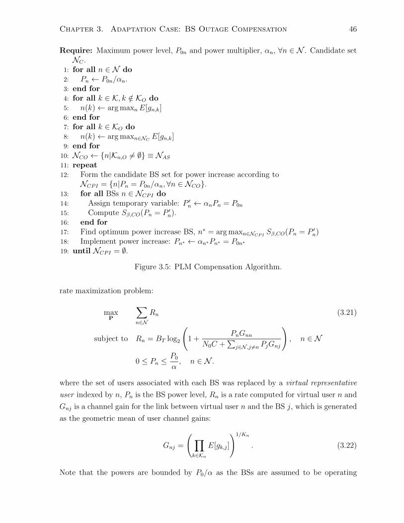
Chapter 3. Adaptation Case: BS Outage Compensation 46
Require: Maximum power level, P0n and power multiplier, αn, ∀n ∈ N . Candidate setNC .
1: for all n ∈ N do2: Pn ← P0n/αn.3: end for4: for all k ∈ K, k /∈ KO do5: n(k)← arg maxnE[gn,k]6: end for7: for all k ∈ KO do8: n(k)← arg maxn∈NC E[gn,k]9: end for
10: NCO ← n|Kn,O 6= ∅ ≡ NAS11: repeat12: Form the candidate BS set for power increase according to
NCPI = n|Pn = P0n/αn,∀n ∈ NCO.13: for all BSs n ∈ NCPI do14: Assign temporary variable: P ′n ← αnPn = P0n
15: Compute Sβ,CO(Pn = P ′n).16: end for17: Find optimum power increase BS, n∗ = arg maxn∈NCPI Sβ,CO(Pn = P ′n)18: Implement power increase: Pn∗ ← αn∗Pn∗ = P0n∗
19: until NCPI = ∅.
Figure 3.5: PLM Compensation Algorithm.
rate maximization problem:
maxP
∑n∈N
Rn (3.21)
subject to Rn = BT log2
(1 +
PnGnn
N0C +∑
j∈N ,j 6=n PjGnj
), n ∈ N
0 ≤ Pn ≤P0
α, n ∈ N .
where the set of users associated with each BS was replaced by a virtual representative
user indexed by n, Pn is the BS power level, Rn is a rate computed for virtual user n and
Gnj is a channel gain for the link between virtual user n and the BS j, which is generated
as the geometric mean of user channel gains:
Gnj =
(∏k∈Kn
E[gk,j]
)1/Kn
. (3.22)
Note that the powers are bounded by P0/α as the BSs are assumed to be operating

Chapter 3. Adaptation Case: BS Outage Compensation 47
Table 3.1: Simulation parameters.
Parameter Value
Bandwidth per subcarrier 15 kHz
BS power budget per subcarrier, P0 18.22 dBm
The factor α√
10
Initial BS powers for regular network P0/α
Noise figure at terminal 7 dB
Background noise power spectral den-sity
-174 dBm/Hz
Distance-dependent path-loss (carrierfrequency = 2 GHz)
PL = 128.1 + 37.6 log10(d)[dB], d in km
Shadowing standard deviation, σ0 8 dB
Shadowing correlation distance, dc 50 m
Inter-site distance 500 m
Total number of cells 19
Number of Users in Centre Cell 66
Number of Users per Cell in the OtherCells
10
Number of subcarriers 1
Subframe size (= time slot size) 1 ms
PF scheduling window size, T0 5 subframes
below their maximum power capabilities. The optimization of (3.21) can be thought of
as a fast way to estimate realistic BS power capabilities for a given random distribution
of users and BSs. It was shown in [53] that under the assumption of high SINR (i.e. if
(PnGnn)/(N0C+∑
j∈N ,j 6=n PjGnj) 1), (3.21) reduces to a convex geometric program—
a type of problem easily solved through interior-point methods. For the current problem,
the solution is obtained by using CVX, a package for solving convex programs [54].
3.6.1 Numerical Results
In evaluating the COC algorithms, the following performance metrics are considered:
• User Average Spectral Efficiency: The total spectral efficiency (or the rate per
total bandwidth) of the users in the compensating cluster normalized by the total
number of users in the compensating cluster.
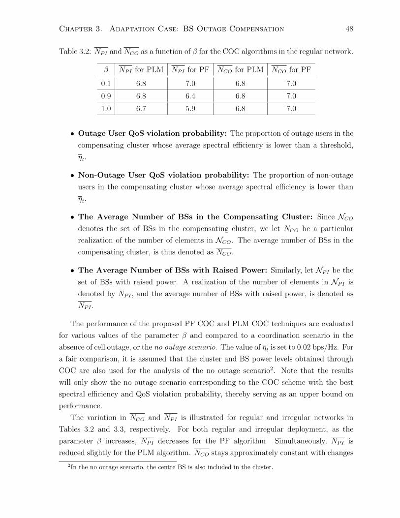
Chapter 3. Adaptation Case: BS Outage Compensation 48
Table 3.2: NPI and NCO as a function of β for the COC algorithms in the regular network.
β NPI for PLM NPI for PF NCO for PLM NCO for PF
0.1 6.8 7.0 6.8 7.0
0.9 6.8 6.4 6.8 7.0
1.0 6.7 5.9 6.8 7.0
• Outage User QoS violation probability: The proportion of outage users in the
compensating cluster whose average spectral efficiency is lower than a threshold,
ηt.
• Non-Outage User QoS violation probability: The proportion of non-outage
users in the compensating cluster whose average spectral efficiency is lower than
ηt.
• The Average Number of BSs in the Compensating Cluster: Since NCOdenotes the set of BSs in the compensating cluster, we let NCO be a particular
realization of the number of elements in NCO. The average number of BSs in the
compensating cluster, is thus denoted as NCO.
• The Average Number of BSs with Raised Power: Similarly, let NPI be the
set of BSs with raised power. A realization of the number of elements in NPI is
denoted by NPI , and the average number of BSs with raised power, is denoted as
NPI .
The performance of the proposed PF COC and PLM COC techniques are evaluated
for various values of the parameter β and compared to a coordination scenario in the
absence of cell outage, or the no outage scenario. The value of ηt is set to 0.02 bps/Hz. For
a fair comparison, it is assumed that the cluster and BS power levels obtained through
COC are also used for the analysis of the no outage scenario2. Note that the results
will only show the no outage scenario corresponding to the COC scheme with the best
spectral efficiency and QoS violation probability, thereby serving as an upper bound on
performance.
The variation in NCO and NPI is illustrated for regular and irregular networks in
Tables 3.2 and 3.3, respectively. For both regular and irregular deployment, as the
parameter β increases, NPI decreases for the PF algorithm. Simultaneously, NPI is
reduced slightly for the PLM algorithm. NCO stays approximately constant with changes
2In the no outage scenario, the centre BS is also included in the cluster.

Chapter 3. Adaptation Case: BS Outage Compensation 49
Table 3.3: NPI and NCO as a function of β for the COC algorithms in the irregularnetwork.
β NPI for PLM NPI for PF NCO for PLM NCO for PF
0.1 5.8 5.9 5.8 5.8
0.9 5.8 5.5 5.8 5.9
1.0 5.7 5.3 5.8 5.9
in β in all cases. In summary, the PF algorithm allows for significant adjustment of NPI—
which can be thought of as the cost of the compensation algorithm implementation—by
variation of β. The range of adjustment is generally larger for regular deployment. The
user average spectral efficiency, outage user QoS violation probability and non-outage user
QoS violation probability are plotted as functions of NPI in Figures 3.6-3.8, respectively.
Figures 3.6a and 3.6b indicate that approximately 75% of the user spectral efficiency
of the no outage scenario is achieved by both COC algorithms for regular and irregular
deployment, with NPI at a maximum (corresponding to β = 0.1). However, if a slightly
smaller user spectral efficiency is sufficient, β can be set higher, resulting in lower NPI
for the PF algorithm. Effectively, the PF algorithm allows for a trade-off between low
compensation cost (NPI) and high user spectral efficiency.
Figure 3.7a indicates that outage user QoS violation rate for the PF algorithm is
around 6-9% under regular deployment, compared to approximately 4.5% for the no
outage scenario—which represents a modest increase. In addition, the violation rate for
the PLM COC algorithm is close to 8%. Effectively, the PF algorithm is shown to achieve
a trade-off between QoS violation rate and compensation cost (NPI) under the regular
deployment scenario.
Similarly, Figure 3.7b indicates for irregular deployment that the QoS violation rate
for the PF algorithm is around 10-12%, compared to approximately 7% for the no outage
scenario. The violation rate for the PLM COC algorithm is close to 11.5%. The PF
algorithm also achieves a trade-off between QoS violation rate andNPI under the irregular
deployment scenario.
Similar trends as Figure 3.7 are shown for the non-outage user QoS violation proba-
bility in Figure 3.8. In particular, a modest increase in violation rates compared to the
no outage scenario is obtained. The PF algorithm achieves a trade-off between violation
rate and NPI . Additionally, the non-outage user QoS violation rate stays below about
2% for both COC algorithms in the two deployment scenarios.

Chapter 3. Adaptation Case: BS Outage Compensation 50
(a)
(b)
Figure 3.6: User average spectral efficiency, in bps/Hz, as a function of the averagenumber of BSs with raised power for (a) regular and (b) irregular networks.

Chapter 3. Adaptation Case: BS Outage Compensation 51
(a)
(b)
Figure 3.7: Outage user QoS violation probability, in percent, as a function of the averagenumber of BSs with raised power for (a) regular and (b) irregular networks.
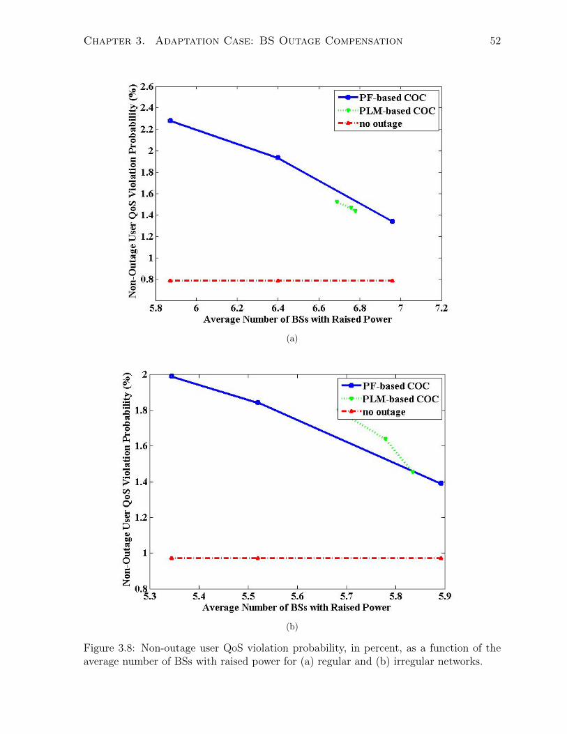
Chapter 3. Adaptation Case: BS Outage Compensation 52
(a)
(b)
Figure 3.8: Non-outage user QoS violation probability, in percent, as a function of theaverage number of BSs with raised power for (a) regular and (b) irregular networks.

Chapter 3. Adaptation Case: BS Outage Compensation 53
In summary, both the PF and PLM COC algorithms show robustness toward cell
outage. Specifically, they achieve a large percentage of the user spectral efficiency of
the no outage scenario and result in only a modest increase in the QoS violation rates.
In addition, the PF COC algorithm is tunable and allows for trading off NPI , which is
related to algorithm cost, against various measures of user performance.

Chapter 4
Dynamic System Model (Single
Power Class)
4.1 Relevant Work
4.1.1 Terminal and BS Deployment Models in Cellular Net-
works
A number of spatial point processes have been used to model the deployment of BSs
and terminals in multi-tier or heterogeneous cellular networks. Spatial point processes
are the generalization of point processes indexed by time to the higher dimensions, in
particular, two-dimensional space.
Among the point processes, the simplest and most popular is the Poisson Point Pro-
cess (PPP). In the PPP model, each node is placed independently over area A with the
density of nodes given by λ. The probability that there are n nodes in area A is thus
given by the Poisson distribution and is equal to (λA)ne−λA/n! The procedure to gen-
erate the PPP is to first draw Poisson distributed number n and then to place n points
uniformly at random in A. The PPP is suitable to model a network composed of a large
number of nodes randomly and independently existing in some area. In the cellular net-
works, it has been commonly used to model the terminal deployments [55] as well as BS
deployments [56,57]. Typically, the nodes in different tiers are modelled via independent
homogeneous PPPs.
Similar to PPP as far as the independent and identically distributed node locations,
the Binomial Point Process (BPP) has the only distinguishing feature that it generates a
fixed number of nodes in a given area. It has been used to model deployment of a known
number of mobile users in a cell of known size [58].
54

Chapter 4. Dynamic System Model (Single Power Class) 55
More general models have also been considered in the literature. The Poisson Cluster
Process (PCP), in particular, models the random patterns produced by random clusters.
A PCP is constructed from a parent PPP by replacing each point with a cluster of points
where the points are independently and identically distributed in the spatial domain.
The PCP has commonly been used to model a network where nodes occur in clusters
e.g. according to certain social behaviour such as users gathered around Wi-Fi hotspots.
In cellular networks, the combination of a PPP and a PCP has been applied in the
heterogeneous networks [59] where the PPP represents the mobile users in a macrocell
and the PCP represents femtocells or hotspots.
Although the distance among BSs are random in a cellular network, we cannot find
two BSs owned by the same provider that are arbitrarily close to each other. Thus
research has considered the Matern hard core point process (MHCPP) which imposes
a minimum distance, dmin between nodes. The MHCPP is obtained by starting from a
PPP. A random score uniformly distributed in [0, 1] is assigned to each point in the PPP,
then all the points that fall within a distance less than dmin from another point with a
lower score is deleted. This results in a minimum separation between any points of dmin.
MHCPP has been used in place of the basic PPP process to model BS deployments in a
cellular network where there is a restriction on BS separation due to such constraints as
geographical constraints as well as network planning or due to the MAC protocol that
avoids nearby simultaneous transmissions [60–62]. However, dealing with MHCPPs is
relatively more complicated compared to the PPP. Therefore, the PPP model remains
appealing partially due to its simplicity and analytical tractability [63–65].
Recent research has also considered more realistic point processes that capture the
cellular network characteristics with greater accuracy. Gibbs family of processes, in
particular, model the repulsion between the BS nodes, making it less likely that BSs
are located close to each other. Gibbs processes belong to the category of Soft Core
point processes (SCPP) as they do not impose a hard minimum distance between nodes.
Research in [65, 66] has shown that the Gibbs processes model BS spatial locations in
real networks more accurately compared to PPP models.
Ginibre process is another point process that can be used to model the repulsion
between BSs. Deng et al [7] consider and study the Ginibre point process as a model for
wireless networks. They introduce the β-GPP as an intermediate process between PPP
and GPP through consideration of the accuracy, tractability and practicality tradeoffs.
They derive the coverage probability of a typical user in a cellular network and show that
it compares well with actual base station deployments.
The authors in [67] investigate the spatial modelling issue. Both the deterministic,

Chapter 4. Dynamic System Model (Single Power Class) 56
hexagonal model at one end and the random deployment following a Poisson point process
(PPP) at the other extreme are considered. The authors utilize a modified perturbed
hexagonal lattice model that lies in between the PPP and the hexagonal model in terms
of irregularity. A frequency reuse-1 interference network is then assumed and an upper
bound on the average total interference as a function of distance is provided. The paper
specifies the loss in coverage probability when moving from a perfect lattice to the random
BS deployment.
4.1.2 Terminal Mobility Models in Cellular Networks
There exist a number of statistical models to represent movement in cellular networks.
The most widely-used is the random walk model [68, 69], which is sometimes referred
to as Brownian motion. According to this model, a terminal moves by choosing an ar-
bitrary direction and speed from the given ranges [vmin, vmax] and [0, 2π], respectively.
Each movement in the model is performed either for a constant time or for a constant
distance travelled. Then a new speed and direction are selected. The random walk model
represents a memoryless mobility pattern as the current speed and direction are inde-
pendent of past speeds and direction. However, this model can result in unrealistically
sudden turns and stops.
A similar model as the random walk model is the random waypoint model, which is
also widely used [70,71]. According to the model, a terminal chooses a random destination
in the simulation area and a speed that is uniformly distributed between [vmin, vmax]. It
then moves to the destination at the chosen speed. After arrival at the destination, the
terminal pauses for a predetermined length of time before repeating the process.
Gauss-Markov mobility model was introduced to improve the realism of the random
walk model [72, 73]. In this model, a nodes next location is generated by its current
location and velocity. The variation of one tuning parameter allows the variation of
the degree of randomness in the mobility pattern. At one extreme of the parameter
value, the random walk model is obtained and the other extreme results in linear motion.
Intermediate values of randomness are obtained between the two extremes.
Another category of mobility models known as group mobility models represent par-
ticular types of user movement as a group [74], such as a group of young children walking
in a single file (column mobility model), a group of students touring a museum (nomadic
community mobility model) or police officers pursuing an escaped criminal (pursue mo-
bility model).

Chapter 4. Dynamic System Model (Single Power Class) 57
4.2 Approach and Contributions
System Model Approach of the Thesis
A system model for an irregular cellular network is considered, which is based on the
concept of Monte Carlo simulations. The model explicitly specifies the representations
of terminal and BS deployments, shadow fading as well as the large-time-scale evolution
model of the system. Scenarios with either a single or multiple BS power classes are con-
sidered. Much of the literature considers classical models particularly for the deployment
(e.g. PPP), and the shadowing (e.g. lognormal shadowing) for the purpose of simplicity
and analytical tractability despite their lack of realism.
Our primary contributions include the deployment models for BSs and terminals,
terminal movement (mobility) models, and shadowing model with correlation for multiple
power classes. The model is considered primarily as a generic reference model for the
purpose of the design of resource allocation with adaptation at a large time scale, for an
irregular cellular network. The goal of developing the model is that it can be used along
with any modifications as desired, in order to model the cellular network as realistically
as desired in terms of the interference, deployment positions, movement and channel
models (shadowing and multipath fading) among other elements.
Deployment Model
The most common model in the literature for irregular deployments is the PPP model
due to its simplicity and analytical tractability. However, the PPP model was shown
to be unrealistic in real irregular networks. Other more realistic models exist (with the
primary example being the Ginibre process [7]) however most such models have the issue
of being difficult to handle. In this work, we consider the development of a baseline
deployment model for Monte Carlo simulation with the primary consideration being the
model simplicity and a baseline realism, which is implemented through arbitrariness
or randomness of deployment with a minimum separation between the nodes and the
elements in the network. Deployment scenarios both with hotspots (multiple power
classes) and without hotspots (single power class) are considered. Since this is meant as
a generic model, guidelines for parameter values are provided for baseline realism of the
simulation scenario.
Note that this chapter deals with the deployment model without hotspots or the
single power class scenario. The deployment model including hotspots and multiple BS
power classes is elaborated in Chapter 6.
Chapter 4. Dynamic System Model (Single Power Class) 58
Mobility Model
Most other models in the literature do not consider terminal movements over an arbitrar-
ily large time scale as a snapshot. We propose a generic model for individual mobility
that is meant as a generic model appropriate for a time scale that is orders of magnitude
larger than the multipath fading time scale. The primary consideration for the model
is its simplicity. A similar movement model is also then considered for BSs. Deploy-
ment scenarios both with hotspots (multiple power classes) and without hotspots (single
power class) are considered for the movements. Since this is meant as a generic model,
guidelines for parameter values are provided for the baseline realism of the simulation
scenario.
Note that this chapter deals with the movement (mobility) model without hotspots
or the single power class scenario. The mobility model including hotspots and multiple
BS power classes is elaborated in Chapter 7.
4.3 Introduction
In Chapter 3, we studied the BS outage as a specific case of a dynamic change occurring in
the irregular cellular network, and BS outage compensation as an adaptation in response
to the particular type of dynamic change. In Chapters 4 through 7, we propose a full
system model that incorporates a wide array of dynamic changes occurring in the irregular
network, and study an algorithmic framework for system adaptation.
The resource allocation framework of [2] was shown to have the capability to adapt
to the slow traffic variations, and the clustering concept was designed for the irregular
deployment of BSs. The case of a single BS power class was primarily considered. The
scheduling and on-off power switching at the subcarriers further adjusts to the variations
in the traffic and channel conditions at a finer level. The adaptive resource allocation
framework has thus been adopted in this chapter for the model with network time evolu-
tion. In the following, the system model of the ITU will be modified as needed to meet
the requirements of the irregular network with a single BS power class.
Recall that the original drop-based simulation method of the ITU model does not
allow the modelling of network evolution at the slow time scale (i.e. the time scale of the
simulation drop). Therefore, we propose a modified method of drop-based simulation,
which is summarized as follows: First, we re-define the simulation drop as an independent
deployment of both terminals and BSs. Second, we define a new term subdrop as a
modified version of a given simulation drop, which is obtained by making small step-

Chapter 4. Dynamic System Model (Single Power Class) 59
wise changes to the initial drop configuration. Time evolution at the slow scale is thus
obtained by implementing a series of subdrops for each drop, which consist of gradual
dynamic changes. The dynamics studied include terminal arrivals and departures, BS
deployments and outages as well as terminal movements. In this thesis, BS movements
are also considered as they provide a way to represent the arbitrariness or time variation
of the BS locations with respect to the terminals in the model, and are believed to be
plausible in emerging and future networks.
The system model is developed in stages in Chapters 4 through 7. In this chapter,
the system simulation model with network time evolution is considered for the irregular
network with a single BS power class and constant BS power levels. Adaptation of BS
power levels (power control) will be discussed in Chapter 5. The static system model and
the time evolution model for a network with multiple power classes will be examined in
Chapters 6 and 7, respectively.
In the current model, the simulation proceeds as summarized in Figure 4.1. Both the
generation of drops, subdrops and subframes, together with slow-scale time evolution, as
well as the execution of slowly-adaptive functions and fast resource allocation are shown.
The framework requires details of channel models, methods of drop deployment and time
evolution as well as slow adaptation and fast resource allocation algorithms. Note that
the multipath, correlated shadowing and path loss channel models, described in Chapter
2, are used in the current model. The rest of the chapter details the proposed drop
deployment and time evolution models. The methodology of simulation drop deployment
is developed in Section 4.4. The time evolution model is discussed in Section 4.5. Finally,
typical parameter values for the models are detailed in Section 4.6.
4.4 Drop Deployment Model
Realistic modelling of simulation drop deployment is considered in this section. Recall
that a drop is defined as the independent and mathematically random deployment of
a number of terminals and BSs in a network simulation area. In practical irregular
networks, variety of restrictions are typically imposed on the positioning of BSs due to
various reasons, including broad-level deployment planning by wireless operators, and
public and private property considerations. Therefore, it is essential that the proposed
random deployment model have certain mathematical restrictions to reflect the practical
constraints of deployment. Note that the imposed restrictions are parametrized so that
they can be adapted to a large number of practical situations by the tuning of parameters.
A circular area as shown in Figure 4.2 is utilized in the deployment of the network

Chapter 4. Dynamic System Model (Single Power Class) 60
shadowing potential field realization as discussed in Section
3.2 is fixed. In other words, the dynamism in subdrops re-
sults solely from gradual changes relating to BSs and termi-
nals on a given and fixed topography.
Let 𝒩(𝑏)and 𝒦(𝑏) be the set of BSs and terminals active
at subdrop 𝑏, respectively. Specifically, 𝒩(0) and 𝒦(0)
denote the set of BSs and terminals active at subdrop 0. At
each subsequent subdrop 1 ≤ 𝑏 ≤ 𝐵, ΔK 𝑎(𝑏)
terminals arrive
at uniform randomly distributed locations according to the
standard Poisson distribution
𝑓(𝑖; 𝜆𝑡) = 𝑃𝑟(ΔK 𝑎(𝑏)
= 𝑖) =𝜆𝑡
𝑖𝑒−𝜆𝑡
𝑖!,
where 𝑓( ) denotes the probability mass function, and
𝜆𝑡 > 0 is the Poisson parameter. Each terminal departs the
j = j + 1
STOP
No
Generate subframe l of subdrop j
Compute path loss and shadowing for
all terminal-BS links
Execute slowly adaptive algorithms
Yes
l = l + 1 l mod F = 0?
Generate simulation drop i
Check arrivals,
departures and
movements
Generate subdrop j of drop i
j mod B = 0?
Yes
Yes
i = P?
No
No i = i + 1
Perform coordinated resource alloca-
tion in each cluster
Figure 4.1: Outline of the Simulation Framework.
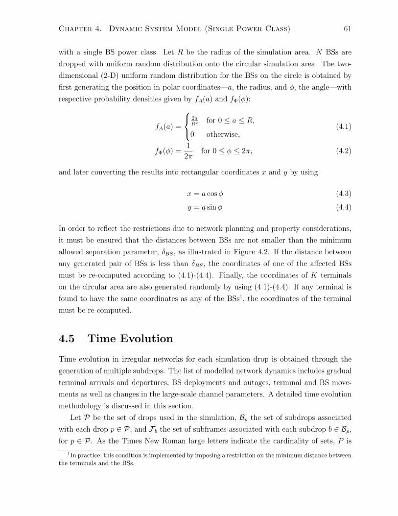
Chapter 4. Dynamic System Model (Single Power Class) 61
with a single BS power class. Let R be the radius of the simulation area. N BSs are
dropped with uniform random distribution onto the circular simulation area. The two-
dimensional (2-D) uniform random distribution for the BSs on the circle is obtained by
first generating the position in polar coordinates—a, the radius, and φ, the angle—with
respective probability densities given by fA(a) and fΦ(φ):
fA(a) =
2aR2 for 0 ≤ a ≤ R,
0 otherwise,(4.1)
fΦ(φ) =1
2πfor 0 ≤ φ ≤ 2π, (4.2)
and later converting the results into rectangular coordinates x and y by using
x = a cosφ (4.3)
y = a sinφ (4.4)
In order to reflect the restrictions due to network planning and property considerations,
it must be ensured that the distances between BSs are not smaller than the minimum
allowed separation parameter, δBS, as illustrated in Figure 4.2. If the distance between
any generated pair of BSs is less than δBS, the coordinates of one of the affected BSs
must be re-computed according to (4.1)-(4.4). Finally, the coordinates of K terminals
on the circular area are also generated randomly by using (4.1)-(4.4). If any terminal is
found to have the same coordinates as any of the BSs1, the coordinates of the terminal
must be re-computed.
4.5 Time Evolution
Time evolution in irregular networks for each simulation drop is obtained through the
generation of multiple subdrops. The list of modelled network dynamics includes gradual
terminal arrivals and departures, BS deployments and outages, terminal and BS move-
ments as well as changes in the large-scale channel parameters. A detailed time evolution
methodology is discussed in this section.
Let P be the set of drops used in the simulation, Bp the set of subdrops associated
with each drop p ∈ P , and Fb the set of subframes associated with each subdrop b ∈ Bp,for p ∈ P . As the Times New Roman large letters indicate the cardinality of sets, P is
1In practice, this condition is implemented by imposing a restriction on the minimum distance betweenthe terminals and the BSs.

Chapter 4. Dynamic System Model (Single Power Class) 62
BS
R
Figure 4.2: Simulation area for deployment in networks with a single BS power class.
the total number of simulation drops, Bp is the number of subdrops associated with drop
p, and Fb is the number of subframes associated with subdrop b. The number of subdrops
used in each drop is equal, that is, Bp is equal to a constant B for all p ∈ P . Similarly, an
equal number of subframes is utilized in each subdrop, or Fb = F for all b ∈ Bp, p ∈ P .
For consistency of notation, the initial deployment of a drop before any time evolution is
referred to as subdrop 0. The remaining subdrops associated with the drop are numbered
from 1 to B − 1. It is important to note the relationship between the drop, subdrop and
the shadowing model random potential field [8] discussed in Chapter 2. In particular,
for all subdrops b ∈ Bp associated with a given simulation drop p ∈ P , the realization
of the random potential field is modelled to be constant. In other words, the physical
topography can be conceptualized as fixed within each simulation drop, and the changes
in shadowing over the subdrops result solely from BS and terminal movements on the
fixed topography. The detailed modelling of the dynamics is discussed in the following.
4.5.1 Terminal Arrival and Departure Models
Let K(b) be the set of terminals active at subdrop b. In particular, K(0) denotes the set
of terminals that are active at the initial subdrop, indexed by 0. At each subsequent
subdrop 1 ≤ b ≤ B− 1, [∆Ka](b) terminals arrive to the system according to the Poisson
distribution:
f(i;λt) = Pr([∆Ka](b) = i
)=λite−λt
i!, i = 0, 1, 2, . . . (4.5)
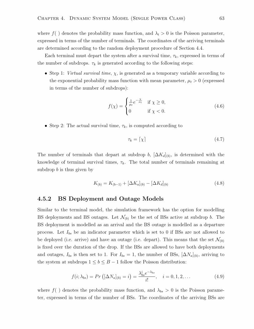
Chapter 4. Dynamic System Model (Single Power Class) 63
where f( ) denotes the probability mass function, and λt > 0 is the Poisson parameter,
expressed in terms of the number of terminals. The coordinates of the arriving terminals
are determined according to the random deployment procedure of Section 4.4.
Each terminal must depart the system after a survival time, τk, expressed in terms of
the number of subdrops. τk is generated according to the following steps:
• Step 1: Virtual survival time, χ, is generated as a temporary variable according to
the exponential probability mass function with mean parameter, µt > 0 (expressed
in terms of the number of subdrops):
f(χ) =
1µte− χµt if χ ≥ 0,
0 if χ < 0.(4.6)
• Step 2: The actual survival time, τk, is computed according to
τk = dχe (4.7)
The number of terminals that depart at subdrop b, [∆Kd](b), is determined with the
knowledge of terminal survival times, τk. The total number of terminals remaining at
subdrop b is thus given by
K(b) = K(b−1) + [∆Ka](b) − [∆Kd](b) (4.8)
4.5.2 BS Deployment and Outage Models
Similar to the terminal model, the simulation framework has the option for modelling
BS deployments and BS outages. Let N(b) be the set of BSs active at subdrop b. The
BS deployment is modelled as an arrival and the BS outage is modelled as a departure
process. Let Ibs be an indicator parameter which is set to 0 if BSs are not allowed to
be deployed (i.e. arrive) and have an outage (i.e. depart). This means that the set N(0)
is fixed over the duration of the drop. If the BSs are allowed to have both deployments
and outages, Ibs is then set to 1. For Ibs = 1, the number of BSs, [∆Na](b), arriving to
the system at subdrops 1 ≤ b ≤ B − 1 follow the Poisson distribution:
f(i;λbs) = Pr([∆Na](b) = i
)=λibse
−λbs
i!, i = 0, 1, 2, . . . (4.9)
where f( ) denotes the probability mass function, and λbs > 0 is the Poisson parame-
ter, expressed in terms of the number of BSs. The coordinates of the arriving BSs are

Chapter 4. Dynamic System Model (Single Power Class) 64
determined according to the random deployment procedure of Section 4.4.
Each BS departs the system after a survival time, τn, (expressed in number of sub-
drops), which is generated according to the following steps:
• Step 1: Virtual survival time, χ, is generated according to the exponential proba-
bility mass function with mean parameter µbs > 0:
f(χ) =
1µbse− χµbs if χ ≥ 0,
0 if χ < 0.(4.10)
• Step 2: The actual survival time, τn, is computed according to
τn = dχe (4.11)
Similar to the terminals, the number of BSs that depart at subdrop b, [∆Nd](b), is deter-
mined with the knowledge of BS holding times, τn. The total number of BSs remaining
at subdrop b is given by
N(b) = N(b−1) + [∆Na](b) − [∆Nd](b) (4.12)
4.5.3 Terminal Movement Model
Terminals are moved at every subdrop through a randomly generated displacement in
a random direction. The movement model is illustrated in Figure 4.3. The full algo-
rithm for the terminal movement at the subdrop is given in Figure 4.4. Direction of
movement over the xy-plane is represented by angle θk,b, which is drawn from a uniform
random distribution in the interval [0, 2π]. The displacement, denoted as ∆dk,b, is drawn
from a uniform random distribution in [∆dt,min,∆dt,max], where ∆dt,min and ∆dt,max
are model parameters. Terminals are moved at each subdrop through the displacement
∆dk,b in the direction represented by angle θk,b. However, it is ensured that terminals
do not go out of the bounds of the circular simulation area of radius R illustrated in
Figure 4.2. Consequently, a check condition is utilized in the realization of the termi-
nal movements2. As long as a terminal would remain within the simulation area, i.e.,
if (xk + ∆dk,b cos θk,b)2 + (yk + ∆dk,b sin θk,b)
2 ≤ R2, its coordinates (xk, yk) are updated
2While terminals going out of bounds could be treated as a departure, the check condition is used torepresent the departures and movements separately.

Chapter 4. Dynamic System Model (Single Power Class) 65
(xk, yk)
(xk+dk,bcosθk,b, yk
+dk,bsinθk,b)
dk,b
θk,b
y
x
Figure 4.3: The terminal movement illustration.
according to:
xk ← xk + ∆dk,b cos θk,b (4.13)
yk ← yk + ∆dk,b sin θk,b (4.14)
If the full movement would place the terminal out of the simulation area, i.e., if (xk +
∆dk,b cos θk,b)2 + (yk + ∆dk,b sin θk,b)
2 > R2; terminal is first moved through a partial
displacement α < ∆dk,b, it is then placed at a position at 180 degrees from its position
in the circular simulation area, and finally, the remainder of the movement is completed
at its new location. The updated coordinates of the terminal are therefore given by
xk ← −(xk + α cos θk,b) + (∆dk,b − α) cos θk,b (4.15)
yk ← −(yk + α sin θk,b) + (∆dk,b − α) sin θk,b (4.16)
where α is determined by solving
α2 + 2α(xk cos θk,b + yk sin θk,b) + (x2k + y2
k −R2) = 0 (4.17)
4.5.4 BS Movement Model
Similar to the terminals, the proposed simulation framework has the option for modelling
BS movements. Let πbs be a fixed probability of BS movement. At each subdrop, BSs

Chapter 4. Dynamic System Model (Single Power Class) 66
Require: xk, yk, for terminals k ∈ K, and parameters ∆dt,min and ∆dt,max1: for all terminals k ∈ K do2: Generate ∆dk,b ∼ U ∈ [∆dt,min,∆dt,max], and θk,b ∼ U ∈ [0, 2π].3: if (xk + ∆dk,b cos θk,b)
2 + (yk + ∆dk,b sin θk,b)2 ≤ R2 then
4: xk ← xk + ∆dk,b cos θk,b5: yk ← yk + ∆dk,b sin θk,b6: else7: Solve for α in α2 + 2α(xk cos θk,b + yk sin θk,b) + (x2
k + y2k −R2) = 0
8: xk ← −(xk + α cos θk,b) + (∆dk,b − α) cos θk,b9: yk ← −(yk + α sin θk,b) + (∆dk,b − α) sin θk,b
10: end if11: end for
Figure 4.4: Algorithm for the terminal movement at the simulation subdrop.
are moved with probability πbs through a random displacement in a random direction.
The movement model is illustrated in Figure 4.5. The detailed algorithm is described in
Figure 4.6. The direction of movement over the xy-plane, represented by angle θn,b, is
drawn from a uniform distribution in the interval [0, 2π]. The displacement, denoted as
∆dn,b, is drawn from a uniform distribution in [∆dbs,min,∆dbs,max]. As long as a BS would
remain within the simulation area, i.e., if (xn+∆dn,b cos θn,b)2+(yn+∆dn,b sin θn,b)
2 ≤ R2,
its coordinates (xn, yn) are updated according to:
xn ← xn + ∆dn,b cos θn,b (4.18)
yn ← yn + ∆dn,b sin θn,b (4.19)
If the movement would place the BS out of the simulation area, the coordinate update
is given by
xn ← −(xn + α cos θn,b) + (∆dn,b − α) cos θn,b (4.20)
yn ← −(yn + α sin θn,b) + (∆dn,b − α) sin θn,b (4.21)
where α is determined by solving
α2 + 2α(xn cos θn,b + yn sin θn,b) + (x2n + y2
n −R2) = 0 (4.22)

Chapter 4. Dynamic System Model (Single Power Class) 67
(xn, yn)
(xn+dn,bcosθn,b, yn
+dn,bsinθn,b)
dn,b
θn,b
y
x
Figure 4.5: The BS movement illustration.
Require: xn, yn, for BSs n ∈ N , and parameters πbs, ∆dbs,min and ∆dbs,max1: for all BSs n ∈ N do2: Generate γ such that Pr(γ = 1) = πbs and Pr(γ = 0) = 1− πbs.3: if γ = 1 then4: Generate ∆dn,b ∼ U ∈ [∆dbs,min,∆dbs,max], and θn,b ∼ U ∈ [0, 2π].5: if (xn + ∆dn,b cos θn,b)
2 + (yn + ∆dn,b sin θn,b)2 ≤ R2 then
6: xn ← xn + ∆dn,b cos θn,b7: yn ← yn + ∆dn,b sin θn,b8: else9: Solve for α in α2 + 2α(xn cos θn,b + yn sin θn,b) + (x2
n + y2n −R2) = 0
10: xn ← −(xn + α cos θn,b) + (∆dn,b − α) cos θn,b11: yn ← −(yn + α sin θn,b) + (∆dn,b − α) sin θn,b12: end if13: end if14: end for
Figure 4.6: Algorithm for the BS movement at the simulation subdrop.

Chapter 4. Dynamic System Model (Single Power Class) 68
Table 4.1: Typical parameter values.
Parameter Typical Range and/or Value
Minimum BS separation, δBS δBS R
Numbers of subdrops, B typical value of 20
Numbers of drops, P P B, typical value of 300
Scheduling average window size, T0 typical value of 5
Numbers of subframes, F F T0, F P , typical value of 100
Terminal arrival parameter, λt typical value of 3 terminals
BS arrival parameter, λbs λbs λt, typical value of 0.5 BSs
Terminal departure parameter, µt typical value of 5 subdrops
BS departure parameter, µbs µbs µt, typical value of 20 subdrops
Maximum terminal displacement, ∆dt,max 0.1dc ≤ ∆dt,max ≤ 10dc
Minimum terminal displacement, ∆dt,min 0 ≤ ∆dt,min ≤ 14∆dt,max
Maximum BS displacement, ∆dbs,max 0.1dc ≤ ∆dbs,max ≤ 10dc
Minimum BS displacement, ∆dbs,min 0 ≤ ∆dbs,min ≤ 14∆dbs,max
BS movement probability, πbs πbs 1
4.6 Typical Parameter Values
In this section, we discuss typical values for the time evolution and drop deployment
model parameters. Although there may be many ways to set some of the parameters,
a few important suggestions will be made. Recommended values and ranges for the
parameters are summarized in Table 4.1. Justification for the recommendations are
discussed in the following.
We first consider the minimum BS separation parameter, δBS, in the drop deployment
model. Note that if δBS were on the order of the simulation area radius R, that is,
δBS ≈ R, the number of BSs fitting in the simulation area would be severely limited.
Therefore, it is recommended that δBS be small in comparison to R, or satisfy δBS R,
so that a large number of BSs can be used in the system simulation while the practical
separation constraints are still satisfied.
In the time evolution model, we begin by considering the setting of the total number
of drops, P , the number of subdrops, B, and the number of subframes, F , as well as the
scheduling averaging window size, T0. The primary consideration is that a sufficiently
large number of drops, subdrops and subframes be used in the simulation so that the
simulation results will be representative (in a statistical sense) of the different types of

Chapter 4. Dynamic System Model (Single Power Class) 69
possible network configurations and slow and fast network evolutions. A secondary and
competing consideration is that P , B, and F must be small enough that the simulations
can be completed on a given computer system in a desirable amount of time. (Note that
the program execution times can vary greatly depending on the system; therefore, the
issue is not considered in detail here.) In order to balance the two competing factors, we
propose the strategy of setting P as high as possible while setting B and F at a moderate
value to keep the computational complexity sufficiently low. There is an expectation that
even if the values B and F are relatively low, the values PB and PBF (i.e. the total
number of subdrops and subframes, respectively) will be high enough to be statistically
representative of evolution scenarios. A P value of 300 (which is high) and a B value of 20
(which is moderately low) are suggested and seem to work well in practice. Note that the
P value can also be set higher for greater accuracy. The setting of the F value must be
done in conjunction with the T0 value. In the exponential averaging of (2.9) in Chapter 2,
the setting of T0 affects the response of the average rates, R, to the instantaneous rates,
r. Small T0 values result in fast but not instantaneous response times; and conversely,
large T0 values result in slow response times, but smoother averaging. We recommend
a typical low T0 value of T0 = 5 from the literature [75], which results in a relatively
fast response time. In order to ensure adequate statistical averaging of results with
exponential averaging, the value of F is recommended to be higher than the B value.
Setting F = 100 is shown to work well in practice.
The setting of terminal arrival and departure, and BS deployment and outage pa-
rameters are considered next. It is important to note that in realistic networks, the BS
deployments and outages occur much less frequently compared to terminal arrival and
departure events. It is, therefore, suggested that BS and terminal model parameters, λbs,
λt, µbs and µt, satisfy the relations:
λbs λt (4.23)
µbs µt (4.24)
Setting of the actual parameter values are expected to depend on many other factors,
including the subdrop time duration and initial number of terminals, K(0), and number
of BSs, N(0) used in the model. However, nominal settings of λbs = 0.5 BSs, λt = 3
terminals, µbs = 20 subdrops and µt = 5 subdrops are suggested, and are shown to work
well in practice. Figures 4.7 and 4.8 illustrate sample realizations of the evolution of the
number of terminals and BSs, respectively, with the suggested model values.
We finally discuss the parameter settings for the terminal and BS movement models.

Chapter 4. Dynamic System Model (Single Power Class) 70
Figure 4.7: Sample realization of the evolution of the number of terminals K(b) oversubdrops b, with K(0) = 25, the arrival parameter λt = 3 terminals, and the departureparameter µt = 5 subdrops.
Since subdrops are designed to model small gradual changes over the network configura-
tion, we suggest setting the maximum terminal displacement parameter, ∆dt,max, large
enough to cause a small but noticeable change in shadowing over one subdrop. It is known
from correlated shadowing theory that movement on the order of correlation distance,
dc, results in a noticeable change in shadowing. Therefore, ∆dt,max needs to satisfy
0.1dc ≤ ∆dt,max ≤ 10dc. (4.25)
Furthermore, it is recommended that the minimum displacement parameter, ∆dt,min, be
set as low as possible, and possibly set to zero, to allow a wide random variation of
terminal displacement. Hence, it should satisfy
0 ≤ ∆dt,min ≤1
4∆dt,max. (4.26)
Similar to BS arrivals and departures, BS movements are expected to occur very infre-

Chapter 4. Dynamic System Model (Single Power Class) 71
Figure 4.8: Sample realization of the evolution of the number of BSs N(b) over subdropsb, with N(0) = 7, the arrival parameter λbs = 0.5 BSs, and the departure parameterµbs = 20 subdrops.
quently. Thus it is suggested that πbs satisfy
πbs 1. (4.27)
Finally, for the same reasons as terminal models, it is recommended that the values of
maximum and minimum BS displacements, ∆dbs,max and ∆dbs,min, satisfy similar in-
equality relations:
0.1dc ≤ ∆dbs,max ≤ 10dc (4.28)
0 ≤ ∆dbs,min ≤1
4∆dbs,max. (4.29)

Chapter 4. Dynamic System Model (Single Power Class) 72
4.7 The Outline of the Network Model of the Thesis
The basic structure of the general network model in the thesis is outlined in block diagram
form in Figure 4.10. Note that this is a more detailed version of the block diagram of
Figure 4.1. However, note that the model of Figure 4.10 does not include all of the
details discussed in the full model of the thesis. For instance, there is much more detail
in terms of hotspot deployment, and shadowing with multiple propagation environments
(Chapter 6); BS dynamics (Chapters 4 and 7); and the BS power adjustment algorithms
(Chapter 5) in the complete model.
Figure 4.9: A realization of the potential field [8].

Chapter 4. Dynamic System Model (Single Power Class) 73
j = j + 1
STOP
No
Generate subframe l of subdrop j:
- Compute the multipath fading for all
terminal-BS links.
Channel values:
- Compute the path loss values PLn,k
for all N(j)K(j) terminal-BS links.
- Compute the shadowing values SFn,k
for all N(j)K(j) terminal-BS links as a
function of the potential field (u)
values.(2)
Large-Time-Scale Adaptations
- Determine the terminal BS associa-
tions based on maximization of large-
scale channel gain, Gn,k = PLn,kSFn,k.
- Adjust BS power levels, Pn.(3)
- Partition the BSs into scheduling
cells (clusters) for scheduling coordi-
nation.(4) Yes
l = l + 1 l mod F = 0?
Generate simulation drop i:
- Randomly deploy N(0) BSs with
minimum separation, BS.
- Randomly deploy K(0) terminals.
- Generate the underlying Gaussian
shadowing potential field, u.(1)
Dynamics:
- Account for terminal
movements.
- Account for any terminal
arrivals and/or departures:
K(j)= K(j-1)+[Ka](j)- [Kd](j).
Generate subdrop j of drop i:
- Sets of terminals and BSs and their
positions.
j mod B = 0?
Yes
Yes
i = P?
No
No
i = i + 1
Fine Resource Allocation
- In each cluster, determine the user
scheduling, with coordination.(5)
Figure 4.10: Flowchart of the general network model in the thesis.

Chapter 4. Dynamic System Model (Single Power Class) 74
Greater explanation is given in the following for the parts marked with superscript
numbers (1) through (5) in Figure 4.10:
(1) Generation of Shadowing Potential Field
A shadowing potential field is a random process whereby each realization is obtained as
a function from the plane to the set of real numbers. Note that the potential field is
stored in a vector denoted by u. Let σ0 be the shadowing standard deviation and dc the
correlation distance. The value of the potential field at point A defines the potential level
of point A and is denoted by uA. For a cellular network with N BSs and K terminals,
J = N +K potential levels are generated according to the following steps:
• Step 1: Generate a J×1 vector v whose elements are independent Gaussian random
variables with zero mean and unity standard deviation.
• Step 2: Generate a J × J correlation matrix R = [rij] such that
rij =σ2
0
2e−dij/dc (4.30)
where dij is the distance between point i and point j.
• Step 3: Decompose the correlation matrix using Cholesky factorization such that
R = BBH.
• Step 4: Calculate the J × 1 potential level vector u according to
u = Bv (4.31)
A sample realization of the potential field over a grid of points is shown in Figure 2.11,
reproduced for convenience in Figure 4.9. It is important to note that the underlying
potential field is fixed when generating a simulation drop. Then in the generation of
individual subdrops in a drop, the terminals move, and new ones appear and old ones
disappear, on top of the given and fixed potential field.
(2) Computation of Shadowing
In particular, the shadowing between points A and B ( a terminal and a BS) is computed
as a function of the two potential levels according to
SF [dB] = f (uA, uB) = sgn (uA + uB) · |uA − uB| . (4.32)

Chapter 4. Dynamic System Model (Single Power Class) 75
(3) Adjustment of Power Levels
Pn is the operating power level of BS n and is determined by maximizing some utility in
the long run, in particular, either the total rate or the sum log utility. Note that detailed
algorithms are given in Chapter 5. Once the power level is fixed, the BS transmits with
a constant power in each subcarrier (or does not transmit in the subcarrier), as the LTE
is based on constant power, variable rate transmission.
(4) Clustering
BSs that are close together will tend to cause greater interference on each other and will
tend to be grouped into the same cluster. The K-means clustering algorithm is used,
where the similarity matrix is determined by a measure of the mutual interference of a
pair of BSs on each other’s users. Note that the clustering was described in Section 2.4 of
Chapter 2. Thus, it can be said that the clustering changes based on the large-time-scale
variations of traffic and will need to be adapted dynamically.
(5) Coordination in the Clusters
Coordination in each cluster means that the neighbouring BSs may not transmit at the
same time (and at the same frequency subcarrier); or if they do transmit at the same
time, they select the scheduled users with coordination. As already mentioned, the power
level is not varied at this smallest time scale. Note that the detailed algorithm is given
in Section 2.4 of Chapter 2.

Chapter 5
BS Power Adaptation (Single Power
Class)
5.1 Relevant Work: Interference Coordination Strate-
gies for Heterogeneous Networks
A variety of interference coordination methods for heterogeneous networks have been
studied in detail in the literature. Much of the work focuses on femto access points
(FAPs) and their interaction with the macro BSs (MBSs). Femtocells operate in licensed
spectrum and improve the indoor coverage where the macro signal tends to be weak. A
primary advantage of the femtocells is that they can be easily and inexpensively deployed
by users since they are connected to the network through the residential broadband wire-
less connections. A number of interference management methods exist for heterogeneous
networks involving femto and macro and other BS networks. The literature commonly
classifies the interference as either co-tier, i.e., between the network elements belonging
to the same tier in the network, or as cross-tier, i.e., between network elements belonging
to different tiers.
In orthogonal frequency division multiple access (OFDMA)-based femto networks,
there is a flexibility to assign orthogonal subcarriers to femto and macrocells. This
gives an advantage to OFDMA networks over CDMA networks. Research in OFDMA
networks has focused on effective interference management schemes in order to mitigate
and reduce the co-tier and cross-tier interferences, which would enhance the throughput
in the network.
Li et al. [76] presented a strategy for clustering of femtocells in order to mitigate the
downlink interference for an OFDMA closed access femto network. The proposed scheme
76

Chapter 5. BS Power Adaptation (Single Power Class) 77
uses a combination of dynamic frequency band allocation among femto and macro BSs
and clustering of femto BSs based on location. In particular, a portion of the band is
dedicated to the macro BS users and the rest reused by both macro and femto BSs.
The dedicated frequency band for the macro users is intended to mitigate the macro
user downlink deadzone problem, where a cell edge macro user experiences severe co-
channel interference from nearby femtocells. A clustering algorithm is used to determine
the cross-tier and co-tier frequency reuse. Femto BSs are allocated into frequency reuse
clusters based on a calculated threshold distance. If the distance between two femto BSs
is above the threshold, they are assigned to the same cluster and the femto users share
the same frequency band. If the distance is less than the threshold, they are assigned to
different clusters to avoid co-tier and cross-tier interference.
Fractional frequency reuse (FFR) has been considered as an interference management
strategy in the literature. The basic idea is that the frequency spectrum is divided into
subbands and each subband is assigned to different macrocells and sub-areas of the
macrocells and/or the femtocells. The authors in [77] propose a scheme encompassing
fractional frequency reuse with pilot sensing to reduce cross-tier interference between
femto and macrocells. In particular, a frequency reuse factor (FRF) of 3 or above is
utilized for the macrocells. The femto BSs determine the frequency reuse by sensing
the macro BS pilot signals and avoiding the band with the highest pilot signal power.
However, the frequency partitioning, in this scheme, is static which results in inefficient
spectrum use and deterioration of throughput in the system.
Juang et al. [78] propose a dynamic adaptive FFR scheme for femto networks. The
paper considers the effect of the femto BS interference on the macro users. As the
primary interference at the macrocell edges is the inter-macrocell interference, the work
focuses on the femto BSs in highly dense inner regions. The scheme uses FFR radio
resource hopping or orthogonal FFR radio resource allocation: If the femto BS is located
in a dense inner region, an orthogonal FFR resource allocation is used by the femtocell.
Otherwise, an arbitrary FFR radio resource hopping pattern is adopted.
Power control has been considered and adopted for the purpose of interference mit-
igation. The advantage of power control is that it permits interference coordination so
that the entire bandwidth can be used (universal frequency reuse) resulting in greater
efficiency. Chandrasekhar et al. [59] propose an uplink power control algorithm for a
macrocell underlaid with femtocells. A fundamental theoretical relation is derived which
provides the largest feasible cellular SINR for any set of feasible femtocell SINRs. Then
the authors propose a utility-based power adaptation algorithm where femtocells indi-
vidually maximize an objective function consisting of an SINR dependent reward, and a

Chapter 5. BS Power Adaptation (Single Power Class) 78
penalty proportional to the interference at the macrocell. In the case that cellular users
are unable to achieve SINR targets due to femtocell interference, an algorithm reduces
SINR targets of strongest femto interferers.
The authors of [79] study power control in heterogeneous networks. In particular, the
outage probability problem was considered under Rayleigh fading. Then a total power
minimization problem with outage specification constraints was used for minimization of
the energy consumption. A minimum worst outage probability guarantee was established
for femtocell users.
Most of the works have considered power control at the multipath fading time scale,
however, this can lead to substantial signalling load due to channel information require-
ments. Nai et al. [80] use a formulation that is appropriate for the larger time scale of
the shadowing. They treat the problem of joint admission and power control in two-tier
small cell networks. The proposed algorithm maximizes the number of small cell users
admitted while guaranteeing a QoS for the macrocell users.
Jin et al [81] propose a scheme where the uplink power control for femto cells is decided
on a per cluster basis. The large-scale channel information and shadowing variation is
exploited and an interference allowance per femtocell is determined based on aggregate
interference. Both a centralized and a distributed sensing algorithm are proposed. In
centralized sensing, the macro BS estimates the number of active femtocells per cluster
and broadcasts the interference allowance to femtocells. In distributed sensing, each cell
senses the activity of others and determines a power setting.
Ha et al [82] propose a joint base station association and power control algorithm
for heterogeneous cellular networks. In particular, the power control algorithm utilizes
non-cooperative game theory. Furthermore, an adaptation mechanism is devised for the
power control algorithm so that it can support the SINR requirements of all users when-
ever possible while exploiting multiuser diversity to improve system throughput. The
proposed framework focuses on heterogeneous networks with multiple tiers and different
QoS requirements (voice and data users). An application is then presented for two-tier
macro-femto networks with a hybrid spectrum access strategy.
The combination of fractional frequency reuse and power control has also been con-
sidered as a hybrid approach. Li et al [83] propose a fractional frequency reuse and power
control scheme in order to coordinate the interference among high and low power nodes
in a heterogeneous network. The algorithm considers both the spectral efficiency and
user fairness in the design. In particular, optimization formulations based on maximizing
the sum of the long term log-scale throughput are considered for both the power control
and resource allocation schemes with fractional frequency reuse. The performance is then
Chapter 5. BS Power Adaptation (Single Power Class) 79
studied for a particular network model with macro BSs deployed according to the hexag-
onal structure and four micro nodes uniformly deployed in each sector. In distributed
power control, the estimation of interference powers at the receiver is an important issue.
In most algorithms, perfect estimation of interference power is assumed. Karamad et
al. [84] focus on and investigate this problem. While modern algorithms assume that
perfect channel information is available locally, this is not guaranteed to be the case.
The authors consider the performance degradation due to estimation errors and quantify
the resulting transmit power and SINR errors.
Other techniques for interference mitigation including coordinated beamforming and
clustered resource allocation have also been investigated in the literature. Yu et al [85]
propose a scheme for coordinating transmit and receive beamforming and resource allo-
cation schemes across multiple base stations for interference mitigation in both macrocell
and mixed macrocell and femtocell/picocell deployment. Coordination among different
base stations is considered particularly important for a scenario with heavy overlap of
femto/pico and macro BSs. The scheme jointly optimizes the proportional fair schedul-
ing, spatial multiplexing, and power spectrum adaptation using a heuristic method.
Hosseini et al [86] propose a cluster-based coordinated beamforming and power allo-
cation scheme for MIMO heterogeneous networks. In the scheme, the small cells form
clusters based on the distance which is an indication of interference. The small cells within
a cluster share users data symbols and cancel the intra-cluster interference through zero
forcing beamforming, which is a network MIMO scheme. Furthermore, a distributed
power control scheme is proposed for inter-cluster interference mitigation, which involves
the exchange of low-rate messages among cluster representatives.
Akoum et al [87] consider interference coordination with clustering from the point of
view of adaptive limited feedback. In particular, the work studies a network modelled
by a Poisson point process to provide an analytical assessment of the performance of
coordination. An intercell interference nulling strategy is applied to coordinate the in-
terference inside the clusters. It is assumed that channel knowledge is exchanged among
coordinating base stations in a cluster and the performance of interference coordination
is evaluated. The authors propose a scheme for determining the average cluster size as
well as for adapting the amount of limited feedback to maximize the coordination gains.
Lee et al [88] study the performance of coordinated beamforming with dynamic clus-
tering using a stochastic geometry approach. They derive analytical expressions for the
signal to interference ratio (SIR) distributions in terms of the number of BSs per cluster,
the number of antennas per BS and the pathloss exponent. The benefit of coordinated
beamforming and optimal cluster cardinality are investigated.

Chapter 5. BS Power Adaptation (Single Power Class) 80
Singh et al [89] study the effect of power control combined with load balancing, or the
offloading of users onto small cells, on the SIR or rate coverage in the uplink in a K-tier
heterogeneous network. A tractable and general model is provided to characterize the
SIR and rate distribution as a function of the association and power control parameters.
5.2 Contribution: Adaptive Resource Allocation Frame-
work with Power Adaptation
An adaptive resource allocation framework based on clustering and power control at a
large time scale and coordinated proportional fair resource allocation at a small time scale
is proposed for a generic irregular network. Note that in heterogeneous networks, the cell
association is normally determined based on maximizing long-term received power and
membership to different tiers is explicitly considered. In this work, we assume associa-
tion to a cell of any tier based on maximization of long-term channel gains. The primary
contribution is the power control algorithm for the purpose of adaptive resource alloca-
tion at a large time scale. While much of the literature considers power control at the
multipath fading time scale, the acquisition of channel information at this scale can lead
to substantial signaling requirements. In addition, much of the literature considers static
or semi-static allocation of a dedicated spectrum for the purpose of resource allocation.
Our contribution considers the use of the entire spectrum for greater spectral efficiency
and the power adaptation at a large time scale, to reduce the signaling requirement. As
the adaptive framework is to be used for a general or arbitrarily large time scale, the
availability of individual QoS requirements at such periodicity are not assumed. Instead,
a central entity does its best effort to maximize either the long-term sum rate or the
sum log utility (based on proportional fairness) over the time scale under the modest
assumption of base station power constraints. The framework is intended as a baseline
adaptive resource allocation framework for an irregular network.
5.2.1 Key Results
The performance of the system with the BS power adaptation algorithms is evaluated
for a particular system scenario and the effect of irregularity is considered by varying
the minimum BS separation, δBS. Improvements in terms of 50th percentile spectral
efficiency, sum log utility and user average spectral efficiency are obtained. In particu-
lar, both algorithms achieve nearly 10% improvement in median spectral efficiency and
between 3-9% improvement in user average spectral efficiency.

Chapter 5. BS Power Adaptation (Single Power Class) 81
It is shown that performance degrades significantly due to the irregularity of deploy-
ment as the distance between users and BSs become larger. In addition, the improvement
from the power adaptation algorithms is observed to increase with increasing irregular-
ity, indicating that power adaptation algorithms partially compensate for the effect of
irregularity.
5.3 Introduction
In Chapter 4, we studied a dynamic system model consisting of a simulation and adap-
tation framework for the irregular network with a single power class and constant power
levels. In this chapter, we introduce the adaptation of BS power levels which will form
part of the extension of the original adaptation framework.
Recall that regular networks are characterized by the more or less regular deployment
of BSs, equal maximum BS power capabilities (due to a single BS power class) as well
as regular deployment of terminals. Therefore, in order to optimize the average received
signal and interference powers at the terminals in the long term, and hence, the SINRs
and transmittable rates, it has generally been adequate to operate the BSs at constant
power levels (i.e. usually at their maximum). Irregular networks, however, have charac-
teristics that are very different from the regular networks. BS deployment and terminal
locations are arbitrary or irregular, and BS maximum power capabilities are unequal due
to multiple power classes. Thus the BS power operating levels are not expected to be op-
timized at their respective maximum power levels. In this thesis, we propose the dynamic
adaptation of BS power levels within their allowable ranges for irregular networks. The
power adaptation shall operate at the slow time scale and form part of an extended adap-
tive resource allocation scheme based on the framework discussed in Chapter 2, which
included slow-scale BS assignments and network clustering, and fast-scale proportional
fair (PF) resource allocation.
In this chapter, we consider BS power adaptation for an irregular network with a
single BS power class, which, however, can be applicable to the case of multiple BS
power classes that is studied later in the thesis. The rest of this chapter is organized
as follows: The BS power adaptation algorithm with two variant forms is developed in
Section 5.4. The overall extended adaptive resource allocation framework with power
adaptation is described in Section 5.5. Finally, simulations are performed in Section 5.6.
Chapter 5. BS Power Adaptation (Single Power Class) 82
5.4 BS Power Adaptation Algorithm
In this section, we propose the adaptation of BS power levels in such a way as to mitigate
the effects of intercell interference and improve the transmittable user rates under dynam-
ically changing network conditions. Similar to the discussion in Section 2.2 of Chapter 2,
problem formulations based on total rate maximization (TRM) and proportional fairness
(PF) are considered in the following. It is expected that the PF formulation will offer
better system performance due to its ability to achieve a balance between TRM and user
fairness in the long term. However, both methods are considered in terms of the mathe-
matical formulation, implementation (e.g. the signalling requirements) and the resulting
system performance in the rest of the chapter.
5.4.1 Total Rate Maximizing (TRM) Power Adaptation
Total rate maximizing (TRM) BS power adaptation is discussed in this section. Let
P(b) = [P1(b), . . . , PN(b)] be the vector of BS power levels at a given subdrop b, Rk,n(k)(b)
be the data rate for terminal k from the associated BS, n(k), averaged over subdrop b
and Rk(b) be the current long-term user rate averaged over many subdrops. In analogy
to problem (2.5) of Chapter 2, the TRM power optimization problem is first expressed
as a function of the long-term user rates, Rk(b):
maxP(b)
∑k∈K
Rk(b) (5.1)
subject to 0 ≤ Pn(b) ≤ Psn,max, ∀n ∈ N
From the TRM simplication procedure of Section 2.2, it is recognized that the problem
(5.1) should be transformed into a form that is easily solvable at each subdrop. The
equivalent optimization is given in terms of Rk,n(k)(b), the user rates averaged over the
subdrop:
maxP(b)
∑k∈K
Rk,n(k)(b) (5.2)
subject to 0 ≤ Pn(b) ≤ Psn,max ∀n ∈ N
For simplicity of notation, the subdrop index b is dropped to yield:
maxP
∑k∈K
Rk,n(k) (5.3)
subject to 0 ≤ Pn ≤ Psn,max ∀n ∈ N

Chapter 5. BS Power Adaptation (Single Power Class) 83
Note that the use of the PF scheduling strategy at the fast subframe time scale is assumed
throughout the analysis. Under this assumption, Rk,n(k), the user rate averaged over the
single subdrop, is approximated in a similar manner as the derivation in (3.6)-(3.9) from
Chapter 3:
Rk,n(k) =G(Kn(k))
Kn(k)
BT log2(1 + SINRk,n(k))
=G(Kn(k))
Kn(k)
BT log2
(1 +
Pn(k)Gn(k),k
N0C +∑
j 6=n(k) PjGj,k
)(5.4)
where Kn(k) is the number of terminals assigned to BS n(k), SINRk,n(k) is the SINR
at terminal k averaged over the duration of the subdrop, BT is the total bandwidth,
Gn(k),k = PLn(k),kSFn(k),k is channel gain between a user and its associated BS averaged
over the subdrop, and G(y) is a quantity known as the scheduling gain, expressed as
a function of the number of users in question—which accounts for the multiplicative
increase in the average rates due to the scheduling of multiple users. Note that G(y) is
estimated as:
G(y) =
y∑i=1
1
i(5.5)
Problem Solution
Note that the optimization problem of (5.3) is known to be non-convex, hence, there is
no guarantee of a solution with standard solution methods. Therefore, we consider an
approximate solution as follows: Under high SINR conditions, i.e., for SINRk,n(k) 1 ∀k, the problem (5.3) can be expressed as a geometric program which can be solved
through convex programming techniques [53]. In this case, the optimization becomes
minP
∏k∈K
[INSRk,n(k)
]wk(5.6)
subject to INSRk,n(k) =N0C +
∑j 6=n(k) PjGj,k
Pn(k)Gn(k),k
∀k ∈ K
wk =G(Kn(k))
Kn(k)
∀k ∈ K
0 ≤ Pn ≤ Psn,max ∀n ∈ N
where INSRk,n(k) = 1/SINRk,n(k) is the reciprocal of the time-averaged SINR for user
k and wk is a specified weighting factor. We note that the high SINR condition is
not assured in general in the context of the BS power adaptation, and the geometric
Chapter 5. BS Power Adaptation (Single Power Class) 84
programming method is used in this thesis as an approximate solution of the power
adjustment problem. Later in this chapter, the power adaptation algorithm will be
evaluated for a selected network scenario which will serve as a verification of the proposed
methodology.
5.4.2 Proportional Fair Power Adaptation
Proportional fair (PF) BS power adaptation is considered in this section. As discussed
in Section 2.2 of Chapter 2, adaptation according to the PF criterion is equivalent to the
sum log utility (SLU) maximization. The PF power optimization procedure is developed
in a similar manner as the TRM procedure in Section 5.4.1. In analogy to (2.7) of Chapter
2, the power optimization problem is first expressed as a function of the long-term user
rates:
maxP
∑k∈K
log(Rk) (5.7)
subject to 0 ≤ Pn ≤ Psn,max ∀n ∈ N
where P is the vector of BS power levels at the subdrop. Similar to the procedure for PF
scheduling described in Section 2.2, the problem (5.7) is transformed into a form that is
easily solvable at each subdrop, given by
maxP
∑k∈K
Rk,n(k)
Rk
(5.8)
subject to 0 ≤ Pn ≤ Psn,max ∀n ∈ N
In addition, the PF scheduling strategy is again used at the subframe time scale; therefore,
the user rate averaged over the subdrop, Rk,n(k), is computed according to (5.4) and (5.5).
Furthermore, the long-term user rate Rk is updated at each subdrop according to
Rk =
(1− 1
W0
)Rk +
(1
W0
)Rk,n(k), (5.9)
where W0 is the exponential averaging window size parameter. Finally, through the
high SINR approximation, the optimization of (5.8) is transformed into the geometric

Chapter 5. BS Power Adaptation (Single Power Class) 85
program:
minP
∏k∈K
[INSRk,n(k)
]wk(5.10)
subject to INSRk,n(k) =N0C +
∑j 6=n(k) PjGj,k
Pn(k)Gn(k),k
∀k ∈ K
0 ≤ Pn ≤ Psn,max ∀n ∈ N
where weightings, wk, for the PF formulation are given by
wk =G(Kn(k))
Kn(k)
1
Rk
∀k ∈ K (5.11)
Similar to the TRM, the geometric program is solved through convex programming tech-
niques.
5.5 Adaptive Resource Allocation Framework with
Power Adaptation
In this section, we discuss the overall extended adaptive resource allocation frame-
work with power adaptation. We note that it might be possible to jointly optimize the
BS power adaptation step together with terminal-BS assignment and clustering steps
described in Chapter 2. Such absolute algorithmic optimization, however, has not been
the aim of this work, as the main goal has been the development of a workable and
practical adaptation framework. The overview of the proposed framework is shown in
Figure 5.1. As the power adaptation step requires the BS assignments as input, and
the clustering step requires both the BS assignments and the operating powers, the BS
assignment should be executed first, followed by power adaptation and clustering, re-
spectively. The detailed pseudocode of the adaptive framework is shown for the cases
of TRM and PF power adaptation in Figures 5.2 and 5.3, respectively, which follow a
similar structure as the algorithm of Figure 2.5. The extended adaptation algorithms
return P∗ = [P ∗1 , . . . , P∗N ], the optimized BS power vector, as an additional output. Fur-
thermore, the framework with PF power adaptation additionally requires W0, the power
adaptation window size, as an input parameter.
The signalling requirements of the adaptive resource allocation framework is signifi-
cantly lower than resource allocation without clustering. In particular, the BS assignment
and clustering steps require that the long-term channel gains Gn,k be known at a central

Chapter 5. BS Power Adaptation (Single Power Class) 86
l = l + 1
Coordinated resource
allocation in each cluster
Form clusters
(scheduling cells)
Set BS powers
Assign terminals to BSs
l mod F = 0?
No
Yes
Figure 5.1: Extended adaptive resource allocation framework with power adaptation.
node at a periodicity of F subframes. The power adaptation (based on the formulations
of (5.6) and (5.10)) additionally requires the knowledge of traffic load for the BSs, i.e.,
the number of users, Kn, assigned to each BS, at the central entity. Fast-varying channel
gains, gn,k,c, need to be exchanged for the purpose of fast scheduling at the subframe
time scale, for BSs inside a given cluster.
5.6 Simulations
Simulations have been performed using the proposed model to evaluate the performance
of the BS power adaptation algorithms. The minimum BS separation parameter, δBS,
was varied in the evaluation to observe the effect of irregularity on performance. The
evaluations additionally illustrate the use of the proposed model in a particular scenario.
Note that a simplified system model is utilized in the simulation. The model param-
eters are summarized in Table 5.1. The simulation area for the scenario is illustrated in

Chapter 5. BS Power Adaptation (Single Power Class) 87
INPUTS:
• Distance-dependent path loss components, PLn,k, and shadowing components,SFn,k, for all n ∈ N and k ∈ K
• Clustering algorithm parameters Q and T
• Proportional fair (PF) resource allocation window size parameter T0
OUTPUTS:
• Set of assigned BSs n(k)k∈K
• Optimized BS power level vector P∗ = [P ∗1 , . . . , P∗N ]
• Scheduling cells (SCs) N (ω) for ω = 1, . . . ,Ω, forming a partition of the set N
• Optimized instantaneous BS power vectors p(ω)c
∗(l) = [p∗n,c(l)] where n ∈ N (ω);
and sets of scheduled users K(p(ω)c
∗, l) = k∗n,c(l)n∈N (ω); corresponding to each SC
ω = 1, . . . ,Ω, each subframe l ∈ F , and each subcarrier c ∈ C
1: for all terminals k ∈ K do2: for all BSs n ∈ N do3: Compute the time-averaged channel gain according to Gn,k = PLn,kSFn,k4: end for5: Determine the assigned BS according to n(k) = arg maxn∈N Gn,k.6: end for7: Find the optimized BS power level vector by solving the optimization problem of
(5.6).8: Form the SCs by using Algorithm 3 of [2].9: for SCs ω = 1 to Ω do
10: for subframes l = 1 to F do11: Determine the optimized instantaneous power vectors and the sets of scheduled
users by using the algorithm of Figure 2.6.12: end for13: end for
Figure 5.2: Algorithm for the adaptive resource allocation framework with TRM poweradaptation

Chapter 5. BS Power Adaptation (Single Power Class) 88
INPUTS:
• Distance-dependent path loss components, PLn,k, and shadowing components,SFn,k, for all n ∈ N and k ∈ K
• Power adaptation window size parameter W0
• Clustering algorithm parameters Q and T
• Proportional fair (PF) resource allocation window size parameter T0
OUTPUTS:
• Set of assigned BSs n(k)k∈K
• Optimized BS power level vector P∗ = [P ∗1 , . . . , P∗N ]
• Scheduling cells (SCs) N (ω) for ω = 1, . . . ,Ω, forming a partition of the set N
• Optimized instantaneous BS power vectors p(ω)c
∗(l) = [p∗n,c(l)] where n ∈ N (ω);
and sets of scheduled users K(p(ω)c
∗, l) = k∗n,c(l)n∈N (ω); corresponding to each SC
ω = 1, . . . ,Ω, each subframe l ∈ F , and each subcarrier c ∈ C
1: for all terminals k ∈ K do2: for all BSs n ∈ N do3: Compute the time-averaged channel gain according to Gn,k = PLn,kSFn,k4: end for5: Determine the assigned BS according to n(k) = arg maxn∈N Gn,k.6: end for7: Find the optimized BS power level vector by solving the optimization problem of
(5.10).8: Form the SCs by using Algorithm 3 of [2].9: for SCs ω = 1 to Ω do
10: for subframes l = 1 to F do11: Determine the optimized instantaneous power vectors and the sets of scheduled
users by using the algorithm of Figure 2.6.12: end for13: end for
Figure 5.3: Algorithm for the adaptive resource allocation framework with PF poweradaptation

Chapter 5. BS Power Adaptation (Single Power Class) 89
2.78 h
h
Figure 5.4: Simulation area for cellular network.
Figure 5.4. The inter-BS distance in the regular deployment is taken to be 2h = 500
m based on the urban macro environment in the ITU model. The simulation area ra-
dius of R = 2.78h is used in order to equal the area of the hexagonal pattern in the
regular deployment. The time evolution in this scenario considers terminal movements
with constant displacement and uniformly random direction, and neglects other types
of dynamics. Constant terminal displacements values as listed in Table 5.1 have been
chosen according to (4.25). BSs are not allowed to power on and off, as a non-zero lower
limit, Pmin, has been imposed on the BS power levels. The difference between Pmin and
Pmax has been set to 6 dB. Note that the remainder of the parameter values were sup-
plemented from the ITU model. P = 150 simulation drops each consisting of B = 20
subdrops are used in the evaluation. Both the total rate maximization (TRM) power
adaptation of (5.6) and the proportional fair (PF) power adaptation of (5.10) are sim-
ulated for comparison against the utilization of equal BS powers, or Pn = Pmax, for all
BSs.
In order to see the effect of irregularity, the value of minimum BS separation parameter
δBS was varied in the simulation from a value of 0 to 2h in increments of 2h/3 as shown

Chapter 5. BS Power Adaptation (Single Power Class) 90
Table 5.1: Simulation Model Parameters
Parameter Value
Simulation area radius, R 2.78h = 695m
Nominal number of terminals, K 28
Total number of BSs, N 7
Bandwidth, BT 15 kHz
Noise figure at terminal 7 dB
Background noise power spectraldensity
-174 dBm/Hz
Path loss, PL −[ 128.1 + 37.6 log10 d ], d in km
Shadowing standard deviation, σ0 10 dB
Shadowing correlation distance, dc 50 m
Maximum BS power capability, Pmax 46 dBm
Minimum allowed BS power, Pmin 40 dBm
Terminal displacement dc(s)/3 = 16.67m
Power adjustment window size, W0 4
Table 5.2: The variation of δBS.
Deployment type δBS
Irregular
0 m
2h/3 = 166.66 m
4h/3 = 333.33 m
Regular 2h = 500 m

Chapter 5. BS Power Adaptation (Single Power Class) 91
in Table 5.2. Note that δBS = 0 m represents the case of completely arbitrary or irregular
deployment with no restriction on separation, and δBS = 2h = 500 m represents the case
of maximum BS separation, which was implemented by using the regular hexagonal BS
placement of the regular cellular network model. The other values represent intermediate
cases of BS separation.
Overall Performance
Initially, a constant number of terminals is assumed. We look at different measures to
understand the performance in terms of different criteria. The 5th percentile or cell edge
spectral efficiency as well as sum log utility are used to as indicators of the performance in
terms of user fairness. The 50th percentile (median) and user average spectral efficiency
(defined as the total spectral efficiency, or the rate per total bandwidth, normalized per
user in the system) are used to understand typical or average user performance.
Figure 5.5 shows the 5th percentile (cell edge) spectral efficiency with varying δBS.
The equal BS power method, in this case, has equal or higher cell edge spectral effi-
ciency than the PF and TRM methods for most δBS values. In addition, the TRM has
the lowest performance. However, the complete cumulative distribution functions (for
which the plot was produced for the case of δBS = 166.6 m in Figure 5.7) show that
the equal power method has improvement only below about the 5th percentile and PF
and TRM methods have better performance at other percentiles. Figure 5.6 shows the
50th percentile (median) spectral efficiency. The TRM algorithm shows about 10% im-
provement over the equal power method, and the PF algorithm performs nearly as well
as the TRM algorithm. Figure 5.8 shows the variation of sum log utility (SLU) with
BS separation, where PF and TRM methods achieve improvement over the equal power
method. In this case, the PF method has a slightly better performance. The user average
spectral efficiency for the system is plotted in Figure 5.9, where PF and TRM methods
achieve approximately 3-7% and 5-9% improvement, respectively. It is concluded for this
scenario that while the PF algorithm does better in terms of measures of fairness and
TRM in terms of typical or average user performance, both algorithms generally obtain
improvement over the equal power assignment.
We note that it is possible for the PF and TRM curves for specific percentiles to cross
each other (i.e. the 5th and 50th percentiles in Figures Figure 5.5 and Figure 5.6), as
the amount of spread in spectral efficiency is larger for the TRM than the PF. However,
the PF and TRM curves for user average spectral efficiency and the SLU must not cross
each other; as the PF outperforms in terms of SLU, and TRM outperforms in terms of
user average spectral efficiency.

Chapter 5. BS Power Adaptation (Single Power Class) 92
0.16
0.17
0.18
0.19
0.2
0.21
0.22
0.23
0.24
0.25
0 100 200 300 400 500
5th
%le
Sp
ectr
al E
ffic
iency
(b
ps/
Hz)
Minimum Separation between BSs
Equal Power
PF
TRM
Figure 5.5: Comparison of power adaptation schemes and the equal power level scenariofor varying δBS in terms of 5th percentile spectral efficiency, with K = 28 users.
0.7
0.8
0.9
1
1.1
1.2
0 100 200 300 400 500
50
th %
le S
pec
tral
Eff
icie
ncy
(b
ps/
Hz)
Minimum Separation between BSs
Equal Power
PF
TRM
Figure 5.6: Comparison of power adaptation schemes and the equal power level scenariofor varying δBS in terms of 50th percentile spectral efficiency, with K = 28 users.

Chapter 5. BS Power Adaptation (Single Power Class) 93
0
0.1
0.2
0.3
0.4
0.5
0.6
0.7
0.8
0.9
0 0.5 1 1.5 2 2.5
Cu
mu
lati
ve
Dis
trib
uti
on
Fu
nct
ion
Spectral efficiency (bps/Hz)
Equal Power
PF
TRM
(a)
0
0.05
0.1
0.15
0.2
0.25
0.3
0 0.05 0.1 0.15 0.2 0.25 0.3 0.35 0.4 0.45 0.5
Cu
mu
lati
ve
Dis
trib
uti
on
Fu
nct
ion
Spectral Efficiency (bps/Hz)
Equal Power
PF
TRM
(b)
Figure 5.7: Cumulative distribution functions for spectral efficiency at δBS = 4h/3 =333.3 m, with (a) normal magnification and (b) increased magnification, with K = 28users.
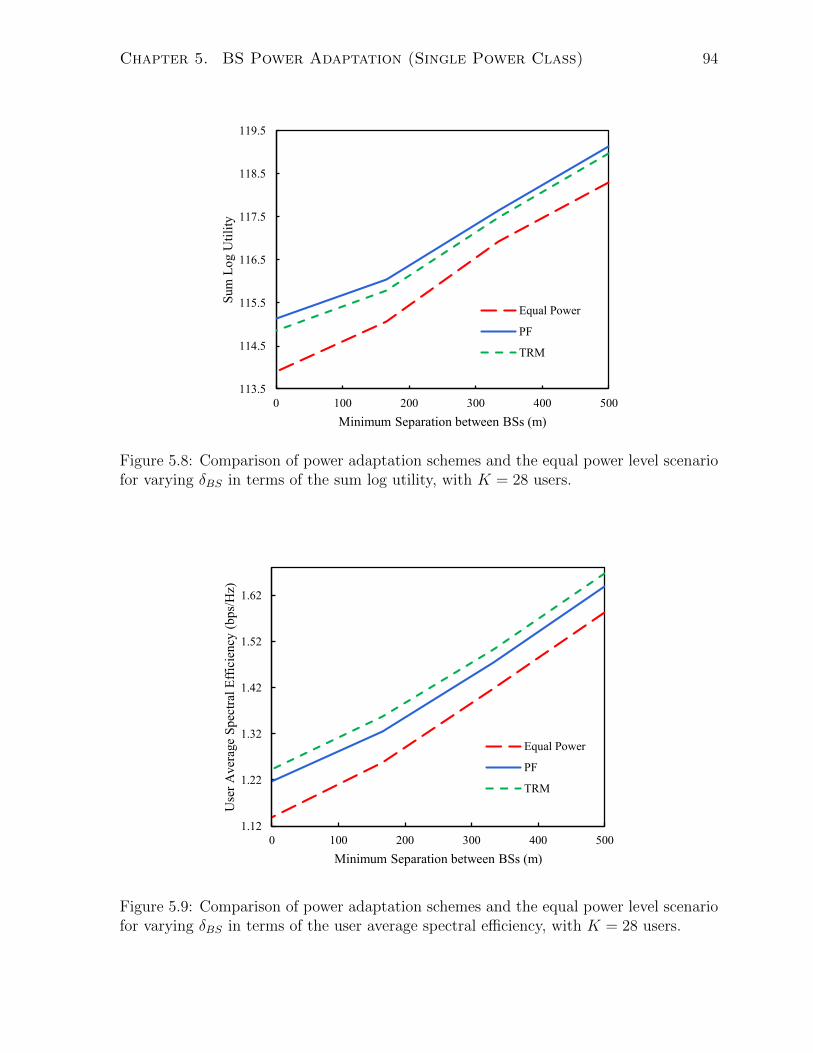
Chapter 5. BS Power Adaptation (Single Power Class) 94
113.5
114.5
115.5
116.5
117.5
118.5
119.5
0 100 200 300 400 500
Sum
Lo
g U
tili
ty
Minimum Separation between BSs (m)
Equal Power
PF
TRM
Figure 5.8: Comparison of power adaptation schemes and the equal power level scenariofor varying δBS in terms of the sum log utility, with K = 28 users.
1.12
1.22
1.32
1.42
1.52
1.62
0 100 200 300 400 500
Use
r A
ver
age
Sp
ectr
al E
ffic
iency
(b
ps/
Hz)
Minimum Separation between BSs (m)
Equal Power
PF
TRM
Figure 5.9: Comparison of power adaptation schemes and the equal power level scenariofor varying δBS in terms of the user average spectral efficiency, with K = 28 users.

Chapter 5. BS Power Adaptation (Single Power Class) 95
0.76
0.81
0.86
0.91
0.96
1.01
1.06
0 100 200 300 400 500
Use
r A
ver
age
Sp
ectr
al E
ffic
iency
(b
ps/
Hz)
Minimum Separation between BSs (m)
Equal Power
PF
TRM
Figure 5.10: Comparison of power adaptation schemes and the equal power level scenariofor varying δBS in terms of the user average spectral efficiency, with K = 56 users.
Effects of Irregularity
An important trend observed from the results is that all the metrics are lower with re-
duced δBS, and increase with higher δBS. To further investigate the effects of irregularity
of deployment, we consider the user average spectral efficiency. We additionally plot the
user average spectral efficiency for a different number of terminals (K = 56), which is
depicted in Figure 5.10. In particular, a penalty of close to 35% difference in user av-
erage spectral efficiency is obtained for completely irregular deployment (δBS = 0 m) as
compared to the regular deployment (i.e. δBS = 2h = 500 m) with the two different K
values. This result highlights the idea that performance is worse under irregular deploy-
ment since the distance between users and serving BSs become greater under increasing
irregularity.
We additionally consider the percentage improvement in user average spectral effi-
ciency over equal power assignment obtained by different power adaptation algorithms
for both K values, which are listed in Tables 5.3 and 5.4. For a user number of 56, the
improvement for PF and TRM methods are reduced compared to a user number of 28. It
is significant to note, however, that with reduced δBS, or with increasing network irregu-
larity, the improvement in spectral efficiency increases for both K values. The increased
improvement for irregular deployment indicates that the power adaptation algorithms

Chapter 5. BS Power Adaptation (Single Power Class) 96
Table 5.3: Percentage improvement in user average spectral efficiency for different poweradaptation algorithms over equal power assignment with K = 28 users.
Deployment type δBS PF TRM
Irregular
0 m 6.9% 9.1%
2h/3 = 166.66 m 5.3% 7.9%
4h/3 = 333.33 m 3.9% 6.0%
Regular 2h = 500 m 3.6% 5.4%
Table 5.4: Percentage improvement in user average spectral efficiency for different poweradaptation algorithms over equal power assignment with K = 56 users.
Deployment type δBS PF TRM
Irregular
0 m 4.1% 5.8%
2h/3 = 166.66 m 4.0% 5.3%
4h/3 = 333.33 m 2.6% 4.3%
Regular 2h = 500 m 2.6% 3.8%
compensate, in part, for the effect of increasing irregularity in the considered scenario.

Chapter 6
Static Model of Multiple Power
Classes
6.1 Relevant Work
Deployment Model
The literature review for the deployment model in this chapter was included with Chap-
ter 4.
Correlated Shadowing Model for Irregular BS Deployment
The literature review for the correlated shadowing model in this chapter was included in
Chapter 2, Section 2.8.
6.2 Contribution
Deployment Model
The contribution for the deployment model in this chapter was included with Chapter 4.
Correlated Shadowing Model
Most of the work in the literature considers the uncorrelated lognormal shadowing model.
While a few authors proposed correlated shadowing models for links with a common end
and more recently, for links without a common end, to our knowledge, no work considers a
theory for variation of the shadowing parameters, i.e. standard deviation and correlation
distance, in a network with an arbitrary number of radio propagation environments.
97

Chapter 6. Static Model of Multiple Power Classes 98
Such a theory is proposed based on a hypothesis for the shadowing properties, and a
method of generation of shadowing for radio links is provided based on the work in [8].
Finally, model consistency is verified for a particular scenario, and the implementation
in practical simulations is discussed. The model is intended for the baseline realism of
the simulation scenario.
6.3 Introduction
In Chapter 4, we considered system modelling for an irregular network with a single BS
power class, and proposed drop deployment, channel gain and time evolution models for
such a network. Then in Chapter 5, we studied an adaptation framework that is appro-
priate for the irregular network. Starting in this chapter, we develop a system modelling
framework for the irregular network with multiple BS power classes. Note that existence
of multiple power classes imply (1) a number of distinct topographic environments, and
(2) great variation of deployment density of users and BSs, from the highly dense in
local hotspots to the highly sparse e.g. in rural areas. Appropriate drop deployment and
channel models for the particular type of network is considered in this chapter. The time
evolution methodology and system evaluation will be discussed in Chapter 7.
The developments in this chapter are summarized in the following: First, the drop
deployment model of Chapter 4 did not consider the deployment of local hotspots. There-
fore, it will be important, in the following, to develop a realistic method of drop deploy-
ment with explicit modelling of hotspots. Second, the channel models of Chapter 4 were
specified under the assumption of fixed model parameters; that is, the path loss model
assumed fixed values for A, B, C and X parameters. Similarly, the shadowing model
of [8] assumed fixed values for σ0 and dc parameters. In the network with multiple power
classes and distinct topographic environments, the parameter values are expected to be
variable rather than fixed. Note that scenarios with fixed and varying channel parameter
values will be referred to, in this thesis, as homogeneous and inhomogeneous scenarios,
respectively. In the following, it will be important to develop channel models for scenarios
of varying or inhomogeneous parameter values.
The rest of this chapter is organized as follows: The drop deployment method with
explicit modelling of hotspots is proposed in Section 6.4. The path loss and shadow-
ing channel models for inhomogeneous scenarios are developed in Sections 6.5 and 6.6,
respectively.
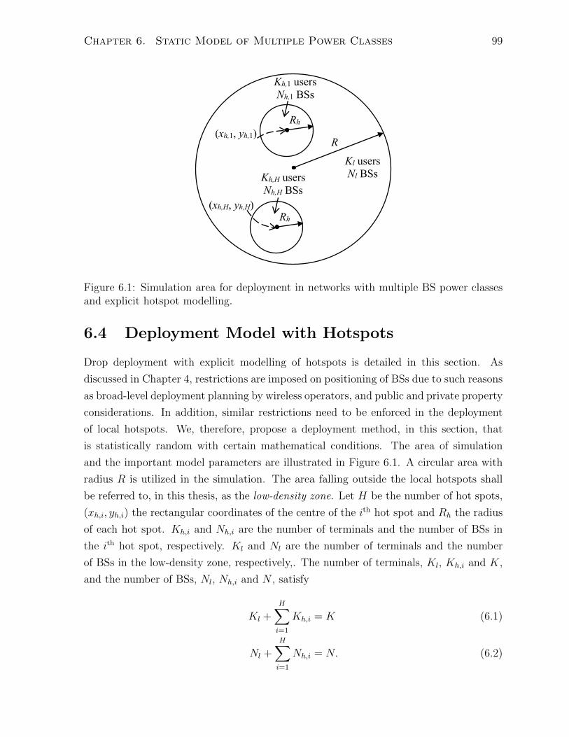
Chapter 6. Static Model of Multiple Power Classes 99
R
Rh
(xh,H, yh,H)
(xh,1, yh,1)
Kh,1 users
Nh,1 BSs
Kh,H users
Nh,H BSs
Rh
Kl users
Nl BSs
Figure 6.1: Simulation area for deployment in networks with multiple BS power classesand explicit hotspot modelling.
6.4 Deployment Model with Hotspots
Drop deployment with explicit modelling of hotspots is detailed in this section. As
discussed in Chapter 4, restrictions are imposed on positioning of BSs due to such reasons
as broad-level deployment planning by wireless operators, and public and private property
considerations. In addition, similar restrictions need to be enforced in the deployment
of local hotspots. We, therefore, propose a deployment method, in this section, that
is statistically random with certain mathematical conditions. The area of simulation
and the important model parameters are illustrated in Figure 6.1. A circular area with
radius R is utilized in the simulation. The area falling outside the local hotspots shall
be referred to, in this thesis, as the low-density zone. Let H be the number of hot spots,
(xh,i, yh,i) the rectangular coordinates of the centre of the ith hot spot and Rh the radius
of each hot spot. Kh,i and Nh,i are the number of terminals and the number of BSs in
the ith hot spot, respectively. Kl and Nl are the number of terminals and the number
of BSs in the low-density zone, respectively,. The number of terminals, Kl, Kh,i and K,
and the number of BSs, Nl, Nh,i and N , satisfy
Kl +H∑i=1
Kh,i = K (6.1)
Nl +H∑i=1
Nh,i = N. (6.2)

Chapter 6. Static Model of Multiple Power Classes 100
In addition, we introduce the following minimum separation parameters: δHS is the
minimum separation between hotspots, δedge is the minimum separation between the edge
of each hotspot and the edge of the simulation area, δBSH is the minimum separation
between BSs inside hotspots, and δBSL is the minimum separation between BSs in the
low-density zone. The deployment of hotspots, BSs and terminals in a given simulation
drop is generated according to the following steps
1. Set the input parameters: Set the parameters N , K, R, H, Rh, δHS, δedge, δBSH ,
δBSL, Kl, and Kh,i for each hot spot i. For the purpose of realism, it must be
assured that Rh R, δHS R, δedge R, δBSH R and δBSL R. Since the
typical distances inside hotspots are smaller than those in the low-density zone,
it is suggested that δBSH be an order of magnitude smaller than δBSL, that is,
δBSH δBSL.
2. Drop the hotspots: Generate the coordinates (xh,i, yh,i) for each of the H hot spots
randomly according to (4.1)-(4.4). If the separation between any of the hotspots
is smaller than δHS, or the separation between a hotspot and the simulation area
edge is smaller than δedge, repeat the step of coordinate generation according to
(4.1)-(4.4).
3. Drop the terminals:
(a) Create the coordinates, (xk, yk), of the Kh,i terminals inside each hot spot by
first generating random quantities a and φ with probability densities:
fA(a) =
2aR2 for 0 ≤ a ≤ Rh,
0 otherwise,(6.3)
fΦ(φ) =1
2πfor 0 ≤ φ ≤ 2π, (6.4)
and later converting the results into rectangular coordinates according to
xk = xh,i + a cosφ (6.5)
yk = yh,i + a sinφ (6.6)
(b) Generate the coordinates of the Kl low-density zone terminals according to
(4.1)-(4.4). If any of the low-density zone terminal coordinates fall inside one
of the hotspots, re-generate the coordinates of affected terminals.

Chapter 6. Static Model of Multiple Power Classes 101
4. Drop the BSs:
(a) Determine the number of base stations that will be deployed in each of the
different areas as a function of the ratio of terminals in a given area to the
total number of terminals in the simulation, that is,
Nl = Round
(NKl
K
)(6.7)
Nh,i = Round
(NKh,i
K
)(6.8)
where Round( ) returns the nearest integer for any real number.
(b) Generate the coordinates, (xn, yn), of the Nh,i BSs inside each hot spot, ac-
cording to (6.3)-(6.6). If the separation between any of the BSs is smaller than
δBSH , or if any of the BSs fall on one of the users, re-generate the coordinates
of the affected BSs.
(c) Generate the coordinates of Nl low-density zone BSs inside the simulation
area. If any of the low-density zone BSs fall inside one of the hotspots; or the
separation between any of the BSs is smaller than δBSL; or, lastly, if any of
the BSs fall on one of the users, re-generate coordinates of the affected BSs
until the situation is corrected.
6.5 Distance Dependent Path Loss Model
Modelling of distance-dependent path loss for the inhomogeneous network scenario is
considered in this section. A straightforward extension of the homogeneous model of
Chapter 2 is proposed. In inhomogeneous network scenarios, there exist a variety of
radio propagation environments as well as distinct BS power classes. We hypothesize,
in this work, that the distinct topographic environments, with unique path loss model
parameters, correspond directly to the transmitting BS power classes—as evidenced in
some of the relevant literature [1,9,30,35,90]. In particular, the path loss model parame-
ters A, B, C and X in the inhomogeneous scenario are modelled as functions of the BS’s

Chapter 6. Static Model of Multiple Power Classes 102
power class, sn,
A = A(sn) (6.9)
B = B(sn) (6.10)
C = C(sn) (6.11)
X = X(sn) (6.12)
The path loss from BS n to any terminal k is, therefore, given by [30]
PLn,k(sn)[dB] = A(sn) log10(dn,k) +B(sn) + C(sn) log10
(fc5.0
)+X(sn) (6.13)
where dn,k is the distance between BS n and terminal k in metres, and fc is the system
frequency in GHz. The detailed verification of the validity of this model under practical
conditions is recommended as a future research project. We note that the path loss
values will be required in the computation of shadowing according to the model of the
next section.
6.6 Inhomogeneous Shadowing with Correlation
In this section, we extend the correlated lognormal shadowing model of [8] (for the ho-
mogeneous scenario) to generate correlated shadowing for the inhomogeneous scenario,
where shadowing parameters, σ0, standard deviation, and dc, correlation distance, are
allowed to vary over space. Before providing the complete model, we find it necessary
to discuss the nature of spatial variation of shadowing parameters in realistic irregular
networks. Note that shadowing has traditionally been a little investigated area of wireless
channel modelling. In particular, although several authors [36,44,45] published real-world
shadowing measurement results for specific environments and situations, to our knowl-
edge, none of the literature reported on a general theory for the variation of shadowing
parameters in inhomogeneous wireless networks. We, therefore, note here some relevant
properties, as discussed in [9,40,91], to help in the development of a physically justifiable
inhomogeneous shadowing model:

Chapter 6. Static Model of Multiple Power Classes 103
Table 6.1: The variation of σ0 and dc based on the radio propagation environments [1].
Radio Environment Ps,max [dBm] Typical distance be-tween neighbouringcells [m]
dc [m]
Indoor hotspot 21 60 6
Urban micro 41 200 13
Urban macro 46 500 50
Suburban macro 46 1299 50
Rural macro 46 1732 120
1. Shadowing is a large-scale phenomenon averaged over small displacements in space,
which is dependent on the attenuation and scattering caused by objects in the
environment, and should not by nature vary quickly in space.
2. Small cells (where BSs have small Ps,max) typically show certain properties with
respect to the shadowing parameters whereas large cells (where BSs have large
Ps,max) tend to show the opposite properties with respect to the same parameters.
For instance, the correlation distance, dc, in small cells tend to be smaller due
to the large number of small electromagnetic scatterers and attenuating objects
typically present in small-cell environments. Conversely, in large cells, dc tends
to be larger due to the small number of large scatterers and attenuating objects
in such environments. Table 6.1 shows a list of the dc values for different radio
environments, (obtained from IMT-Advanced guidelines [1]), where the trend of
dc values is confirmed. The values increase with increasing Ps,max and distance
between BSs, from the indoor hotspot environment to the rural macro environment.
3. The effect of an attenuating object, e.g. a vehicle, on shadowing is different in a
short link (e.g. 5 m) and in a long link (e.g. 500 m). The attenuating effect is
stronger in the short link as the vehicle is considered long in proportion to the total
length of the link.
4. When a propagation front passes through successive areas in the wireless channel,
the gains (or losses) in shadowing are multiplicative and thus add in the logarithmic
domain.
In light of points 1 to 4, we hypothesize the following principles for the generation of
shadowing parameters in the cellular network:

Chapter 6. Static Model of Multiple Power Classes 104
Principle 1: Homogeneous Scenario
As per point 2, the topographic properties can be modeled to correspond directly to the
BS power class associated with each of the cells. Thus, in the homogeneous scenario, the
shadowing parameters σ0 and dc, should be modelled as functions of the BS power class
s:
σ0 = σ0(s) (6.14)
dc = dc(s) (6.15)
Principle 2: Inhomogeneous Scenario
In the inhomogeneous scenario, there exist cells (or BSs) of various power classes. Fur-
thermore, some radio links between BSs and terminals cross through a number of cells
of different power classes over different lengths, which is illustrated in Figure 6.2. As
per Principle 1, and point 4, effective shadowing parameters (denoted by σ0,eff and dc,eff)
for such radio links are expected to be mathematical functions of (1) the homogeneous
shadowing parameters corresponding to power classes of the cells crossed (i.e. σ0(s) and
dc(s)), and (2) the length over which the cells are crossed.
In the following, we develop the spatially correlated shadowing model for the inho-
mogeneous network scenario. The generation of shadowing for individual radio links,
including the calculation of effective shadowing parameters according to Principle 2 and
the actual computation of shadowing values, is detailed in Section 6.6.1. The model con-
sistency verification is discussed in Section 6.6.2. The practical model implementation for
a full network through the use of complexity reduction techniques is discussed in Section
6.6.3.
6.6.1 Generation of Shadowing for Links between BS-Terminal
Pairs
The inhomogeneous shadowing model with spatial correlation has a similar underlying
structure as the homogeneous shadowing model, as it is also based on the computation
of the potential level vector (potential field). The primary difference is that multiple
sets of shadowing parameters, σ0,eff and dc,eff, as well as potential fields, u, will need
to be generated. Consider the sample radio link between a BS n ∈ N and a terminal
k ∈ K, depicted in Figure 6.2, which crosses through several cells of potentially distinct
BS power classes. Shadowing is generated for each radio link according to the following

Chapter 6. Static Model of Multiple Power Classes 105
associated with each of the cells. Thus, in the homogeneous
scenario, the shadowing parameters 𝜎0 and 𝑑𝑐 , should be
modelled as functions of the BS power class 𝑠:
𝜎0 = 𝜎0(𝑠)
𝑑c = 𝑑c(𝑠)
Principle 2: In the inhomogeneous scenario, there exist cells
(or BSs) of various power classes. Furthermore, some radio
links between BSs and terminals cross through a number of
cells of different power classes over different lengths, as
illustrated in Fig. 1. As per Principle 1, and points 3 and 4,
effective shadowing parameters (denoted by 𝜎0,𝑒𝑓𝑓 and 𝑑𝑐,𝑒𝑓𝑓)
for such radio links is expected to depend on (a) the
shadowing parameters corresponding to power classes of the
cells crossed (i.e. 𝜎0(𝑠) and 𝑑𝑐(𝑠)), and (b) the length over
which the cells are crossed. Detailed expressions for 𝜎0,𝑒𝑓𝑓
and 𝑑𝑐,𝑒𝑓𝑓 will be given in the next subsection.
D. Detailed Shadowing Model
The inhomogeneous shadowing model has a similar underlying structure as the homogeneous shadowing modelreviewed in Section II in that it is also based on computation of the potential level vector (potential field). The main difference is that multiple sets of 𝜎0,eff and 𝑑c,eff are used in the model,
hence, multiple potential fields must be calculated. The steps of shadowing generation are described in the following:
1) Calculation of Effective Shadowing Standard
Deviation, 𝜎0,𝑒𝑓𝑓:The effective standard deviation will potentially have a
distinct value for each radio link. Let 𝜎0,eff(𝑛, 𝑘) be the
effective standard deviation for the link between BS 𝑛 ∈ 𝒩 and terminal 𝑘 ∈ 𝒦. Hence there are a total of 𝑁𝐾 values of
𝜎0,eff(𝑛, 𝑘) that need to be calculated. The indices (𝑛, 𝑘) are
dropped in the following discussion except where necessary.The calculation for each link consists of the following steps:
Step 1: Calculate the length of the link path, 𝐿, illustrated in
Fig. 1, according to
𝐿 = √(𝑥𝑛 − 𝑥𝑘)2 + (𝑦𝑛 − 𝑦𝑘)2
Step 2: Partition the link path into 𝑁 path segments by
assigning segments of the path to a BS 𝑚 ∈ 𝒩 . The
assignment is based on path loss minimization. The path
segment lengths are denoted by 𝑙1, 𝑙2, … , 𝑙𝑁, where not all of
𝑙1, 𝑙2, … , 𝑙𝑁 are equal to zero and ∑ 𝑙𝑚𝑁𝑚=1 = 𝐿. The detailed
procedure is given in Algorithm 1.
Step 3: Calculate 𝜎0,𝑒𝑓𝑓 for the link as the weighted average
of the homogeneous shadowing standard deviation for each
BS 𝑚’s power class, 𝜎0(𝑠𝑚):
𝜎0,eff =∑ (𝑙𝑚)𝛼𝜎0(𝑠𝑚)𝑁
𝑚=1
∑ (𝑙𝑚)𝛼𝑁𝑚=1
Fig. 1. Sample radio link in an irregular cellular network. Here, 𝐿 is the total
length of the link path, 𝑙𝑚 is the length of path segment assigned to BS 𝑚 ∈𝒩, 𝑘 ∈ 𝒦 is an index value for a terminal, and 𝑛 ∈ 𝒩 and 𝑝 ∈ 𝒩 are index
values for BSs such that 𝑛 ≠ 𝑝, 𝑛 ≠ 1, 𝑛 ≠ 2, 𝑝 ≠ 1, 𝑝 ≠ 2.
where 𝛼 > 0 is a parameter used for tuning the weighting of
longer path segments in relation to shorter path segments1.
2) Calculation of Effective Shadowing Correlation
Distance, 𝑑𝑐,𝑒𝑓𝑓:
Having calculated σ0,eff ’s, the effective correlation
distance, 𝑑𝑐,eff, is also calculated for each of the 𝑁𝐾 radio links
as the weighted average of the homogeneous correlation distance for each BS 𝑚’s power class, 𝑑c(𝑠𝑚):
𝑑c,eff =∑ (𝑙𝑚)𝛼𝑑c(𝑠𝑚)𝑁
𝑚=1
∑ (𝑙𝑚)𝛼𝑁𝑚=1
3) Computation of Potential Fields:The procedure is similar to the generation of the potential
field in the homogeneous scenario. The difference is that multiple potential fields are generated, one for each of the radiolinks as they can have distinct shadowing parameters, 𝜎0,eff and
𝑑c,eff . The potential levels are generated according to the
following steps:
Step 1: Generate a single 𝐽 × 1 vector 𝒗 whose elements are
independent Gaussian random variables with zero mean and
unity standard deviation.
Step 2: Generate a 𝐽 × 𝐽 correlation matrix 𝑹 = [𝑟𝑖𝑗] for
each radio link such that
𝑟𝑖𝑗 =𝜎0,eff
2
2e−𝑑𝑖𝑗 𝑑𝑐,eff⁄
Step 3: Decompose each correlation matrix 𝑹 using the
Cholesky factorization such that 𝑹 = 𝑩𝑩𝑯.
1 As 𝛼 increases, the relative weighting of longer path segments’ standarddeviation increases.
BS 2 → s2
BS n → sn
BS 1 → s1 BS p → sp
Terminal k
lnl1
lp L
l2 = 0
Figure 6.2: Sample radio link in an irregular cellular network. Here, L is the total lengthof the link path; k ∈ K is an index value for a terminal; n ∈ N and p ∈ N are indexvalues for the BSs such that n 6= p, n 6= 1, n 6= 2, p 6= 1 and p 6= 2; and lm is the lengthof path segment assigned to a BS m ∈ N .
steps:
• Step 1: Calculate effective shadowing standard deviation, σ0,eff, and effective shad-
owing correlation distance, dc,eff, for the link according to Principle 2.
• Step 2: Compute the Gaussian potential field vector, u, as a function of σ0,eff and
dc,eff, that is, u = u(σ0,eff, dc,eff). (A potential field was defined in [8] as a random
process whereby each realization is a function from the plane to the real numbers.
Thus, if we fix a point in the plane, the outcome is a Gaussian random variable.)
• Step 3: Compute the shadowing value, SF , for each radio link as a function of the
respective entries of the potential field vector u(σ0,eff, dc,eff).
Detailed algorithms for each of the steps are discussed in the following.
Calculation of Effective Shadowing Standard Deviation and Effective Shad-
owing Correlation Distance
Let σ0,eff(n, k) and dc,eff(n, k) be the effective shadowing standard deviation and effective
shadowing correlation distance, respectively, for the link between BS n and terminal k,
illustrated in Figure 6.2. σ0,eff(n, k) and dc,eff(n, k) will potentially have distinct values

Chapter 6. Static Model of Multiple Power Classes 106
for each radio link; therefore, there are a total of NK values of σ0,eff(n, k) and dc,eff(n, k)
that need to be calculated. The calculation for each link is detailed in the following steps:
• Step 1: Calculate the length of the link path, L(n, k) = dn,k, shown in Figure 6.2,
according to
L(n, k) =√
(xn − xk)2 + (yn − yk)2 (6.16)
• Step 2: Partition the link path into N path segments by assigning segments of the
path to a BS m ∈ N as shown in Figure 6.2 The assignment is based on path loss
minimization. The path segment lengths are denoted by lm(n, k) for m ∈ N , where
lm(n, k) are not all zero and∑
m∈N lm(n, k) = L(n, k). The detailed procedure is
given in Figure 6.3.
• Step 3: Compute the total path length corresponding to each BS power class s ∈ S
ls(n, k) =∑
sm=s,m∈N
lm(n, k) (6.17)
• Step 4: By using Principle 2, compute σ0,eff(n, k) as the weighted average of the
homogeneous shadowing standard deviation for each BS power class, σ0(s), where
the weights are proportional to the lengths, ls(n, k):
σ0,eff(n, k) =
∑s∈S [ls(n, k)]α σ0(s)∑
s∈S [ls(n, k)]α. (6.18)
Here α > 0 is a parameter used for tuning the weighting of longer path segments in
relation to shorter path segments. As α increases, the relative weighting of longer
path segments increases.
• Step 5: Similar to σ0,eff calculation, compute dc,eff(n, k) as the weighted average of
the homogeneous shadowing correlation distance for each BS power class, dc(s):
dc,eff(n, k) =
∑s∈S [ls(n, k)]α dc(s)∑
s∈S [ls(n, k)]α(6.19)
Note that the indices (n, k) in the various terms are dropped in the remainder of the
discussion to simplify the notation.

Chapter 6. Static Model of Multiple Power Classes 107
Require: Z, a large positive integer parameter1: Generate Z equally-spaced points on the link path, forming the set of points Z.2: for all points z ∈ Z do3: for all BSs m ∈ N do4: Compute the path loss, PL(sm), between point z and BS m from (6.13).5: end for6: Assign point z to the BS m∗z = arg minPL(sm).7: end for8: Use the boundaries of BS assignment between contiguous groups of points z to par-
tition the link path into path segments, indexed by the BS m (see Figure 6.2).9: for all m ∈ N do
10: return The length of each path segment, lm.11: end for
Figure 6.3: Algorithm for assigning path segments to BSs
Computation of Potential Fields
Let J = N + K be the total number of points (BSs and users) in the network. The
potential field vector u = u(σ0,eff, dc,eff), of size J × 1, is calculated according to the
following steps:
• Step 1: Generate a J×1 vector v whose elements are independent Gaussian random
variables with zero mean and unity standard deviation.
• Step 2: Compute the J × J correlation matrix R = [rij] for each pair of values of
σ0,eff and dc,eff, that is, R = R(σ0,eff, dc,eff), such that
rij =σ2
0,eff
2e−dij/dc,eff (6.20)
where dij denotes the distance between point i and point j.
• Step 3: Decompose the correlation matrix R(σ0,eff, dc,eff) using Cholesky factoriza-
tion such that
R(σ0,eff, dc,eff) = B(σ0,eff, dc,eff)[B(σ0,eff, dc,eff)]H. (6.21)
• Step 4: Compute the J × 1 potential field vector u(σ0,eff, dc,eff) according to
u(σ0,eff, dc,eff) = B(σ0,eff, dc,eff)v (6.22)

Chapter 6. Static Model of Multiple Power Classes 108
Computation of Shadowing for the Radio Link
Let uA be the potential level or the value of the potential field at some given point A. The
shadowing between a terminal and a BS, denoted as point A and point B, respectively,
is then computed as a function of the respective potential levels, uA(σ0,eff, dc,eff) and
uB(σ0,eff, dc,eff), according to
SF [dB] = sgn(uA(σ0,eff, dc,eff) + uB(σ0,eff, dc,eff)
)·∣∣uA(σ0,eff, dc,eff)− uB(σ0,eff, dc,eff)
∣∣(6.23)
6.6.2 Shadowing Model Consistency Verification
We emphasize that the inhomogeneous shadowing model with spatial correlation has a
similar underlying structure as the homogeneous shadowing model. The primary differ-
ence is that multiple sets of shadowing parameters, σ0,eff and dc,eff, as well as potential
fields, u, are generated. Thus, we consider the consistency of the proposed inhomo-
geneous model with the earlier homogeneous model. In the following, the correlation
between two links with a common end is simulated as a verification of the consistency
of the proposed shadowing model in a simple inhomogeneous scenario. The simulation
model is based on the setup used in [8]. The terminals k1 and k2 are located at a dis-
tance D from the BS as depicted in Figure 6.4. Let σ0,eff,1 and dc,eff,1 be the shadowing
parameters for link 1 between the BS and terminal k1. Similarly, let σ0,eff,2 and dc,eff,2 be
the shadowing parameters for link 2 between the BS and terminal k2. It is assumed that
the distance D is large, in particular, D max(dc,eff,1, dc,eff,2). We study the correlation
between the shadow fading channel gains g1 and g2 between the BS (the common end)
and the two terminals k1 and k2, respectively. By varying the angle θ, we observe the cor-
relation at different distances d while keeping the distance D between the terminals and
the BS fixed. Note that in varying θ (and therefore d), the relationships θ1 = θ2 = θ/2,
and d1 = d2 = d/2 are preserved at all times for consistency of analysis.
Three separate cases of shadowing parameter values are considered in the analysis,
which are described in the following: Case (a) is the homogeneous shadowing scenario,
where σ0,eff,1 = σ0,eff,2 and dc,eff,1 = dc,eff,2. In case (b), the shadowing standard deviation
of link 1 is double with respect to link 2 while the shadowing correlation distance remains
the same, that is, σ0,eff,1 = 2σ0,eff,2 and dc,eff,1 = dc,eff,2. Finally in case (c), the shadowing
correlation distance of link 1 is double with respect to link 2 while the shadowing standard
deviation remains the same, or, σ0,eff,1 = σ0,eff,2 and dc,eff,1 = 2dc,eff,2.
Figure 6.5 depicts the normalized correlation for cases (a)-(c) as a function of distance

Chapter 6. Static Model of Multiple Power Classes 109
Step 4: Calculate the 𝐽 × 1 potential level vector 𝒖 for each
radio link according to
𝐮 = 𝐁𝐯
Step 5: Construct the matrix of potential levels 𝑼 according
to
𝐔 = [𝐮(1,1), … , 𝐮(𝑛, 𝑘), … , 𝐮(𝑁, 𝐾)]
where 𝒖(𝑛, 𝑘) represents the potential level vector generated
using the parameters 𝜎0,𝑒𝑓𝑓(𝑛, 𝑘) and 𝑑𝑐,𝑒𝑓𝑓(𝑛, 𝑘).
4) Calculation of Shadowing for a Radio Link:The shadowing between point A and point B (a terminal
and a BS) is computed according to (3), where the appropriatecolumn of the 𝐔 matrix is determined by the correspondingindices, (𝑛, 𝑘), of the radio link considered.
Algorithm 1 Path Segment Assignment to BSs
1. Generate 𝑍 equally-spaced points on the link path where𝑍 is a positive integer parameter that is chosensufficiently large.
2. Use the appropriate path loss expression 𝑃𝐿(𝑠𝑚) tocalculate the path loss between each BS 𝑚 ∈ 𝒩 and the𝑍 equally-spaced points on the link path.
3. Assign each point to the BS with the smallest 𝑃𝐿(𝑠𝑚).
4. Hence, partition the link path into path segments byassigning contiguous sets of points to one of the BSs𝑚 ∈ 𝒩. The partitioning determines the path segmentlengths 𝑙1, 𝑙2, … , 𝑙𝑁, as illustrated in Fig. 1, such that notall of 𝑙1, 𝑙2, … , 𝑙𝑁 are equal to zero, and ∑ 𝑙𝑚
𝑁𝑚=1 = 𝐿.
IV. MODEL VERIFICATION
In this section, the correlation between two links with a common end is simulated as a verification of the proposedshadowing model in a simple inhomogeneous scenario. The simulation model is based on the setup used in [10]. Theterminals 𝑘1 and 𝑘2 are located at a distance 𝐷 from the BS asdepicted in Fig. 2. Let 𝜎0,eff,1 and 𝑑c,eff,1 be the shadowing
parameters for link 1 between the BS and terminal 𝑘1 .Similarly, let 𝜎0,eff,2 and 𝑑c,eff,2 be the shadowing parameters
for link 2 between the BS and terminal 𝑘2. It is assumed that
the distance 𝐷 is large, in particular, 𝐷 ≫ max(𝑑c,eff,1, 𝑑c,eff,2).
We study the correlation between the shadow fading channel gains 𝑔1 and 𝑔2 between the BS (the common end) and the twoterminals 𝑘1 and 𝑘2, respectively. By varying the angle 𝜃, weobserve the correlation at different distances 𝑑 while keepingthe distance 𝐷 between the terminals and the BS fixed. Note that in varying 𝜃 (and therefore 𝑑), the relationships 𝜃1 = 𝜃2 =𝜃 2⁄ , and 𝑑1 = 𝑑2 = 𝑑 2⁄ are preserved at all times forconsistency of analysis.
Three separate cases of shadowing parameter values are
considered in the analysis, which are described in the
following: Case (a) is the homogeneous shadowing scenario,
Fig. 2. Shadowing simulation scenario.
where 𝜎0,eff,1 = 𝜎0,eff,2 and 𝑑c,eff,1 = 𝑑c,eff,2 . In case (b), the
shadowing standard deviation of link 1 is double with respect
to link 2 while the shadowing correlation distance remains the
same, that is, 𝜎0,eff,1 = 2𝜎0,eff,2 and 𝑑c,eff,1 = 𝑑c,eff,2. Finally in
case (c), the shadowing correlation distance of link 1 is double
with respect to link 2 while the shadowing standard deviation
remains the same, or, 𝜎0,eff,1 = 𝜎0,eff,2 and 𝑑c,eff,1 = 2𝑑c,eff,2.
Fig. 3 depicts the normalized correlation for cases (a)-(c) as
a function of distance 𝑑, given by
𝜌(𝑑) =𝐸[𝑔1𝑔2]
𝜎0,eff,1𝜎0,eff,2
The correlation curve of case (a) agrees with the homogeneous
shadowing analysis performed in [10]. In addition, case (b)
differs from case (a) only in the values of 𝜎0,eff,1 and 𝜎0,eff,2.
Consequently, the normalized correlation curve of case (b) is
exactly the same as case (a) owing to the division by the factor
(𝜎0,eff,1𝜎0,eff,2) in (13). Finally, the correlation curve of case
(c) has the same maximum point as cases (a) and (b), however
it decays at a different rate as a function of distance. To study
the decay rate under inhomogeneous 𝑑c,eff conditions, we
introduce the resultant effective correlation distance—defined
as the distance at which the correlation between the
shadowing of links 1 and 2 drops to approximately 0.40 times
the maximum correlation 2 . Let 𝑑c,eff,1−2 be the resultant
effective correlation distance between links 1 and 2. Since half
of the length 𝑑 falls in the region with 𝑑c,eff,1 and the other
half in the region with 𝑑c,eff,2 , 𝑑c,eff,1−2 should intuitively
satisfy
𝑑c,eff,2 ≤ 𝑑c,eff,1−2 ≤ 𝑑c,eff,1
In case (c), 𝑑c,eff,1−2 is determined from Fig. 3 to be
approximately equal to 1.3𝑑c,eff,2 , thereby agreeing with the
inequality of (14). In conclusion, the analysis shows that the
2 The definition of resultant correlation distance is consistent with cases (a) and (b) where the effective correlation distances of the two links are equal.
k2 k1
g2
BS
g1
D
d2 = d/2 d1 = d/2
= /2 = /2
d
Figure 6.4: Shadowing simulation scenario.
d, given by
ρ(d) =E[g1g2]
σ0,eff,1σ0,eff,2
(6.24)
The Gudmundson correlations modelled by e−d/dc are additionally depicted with ap-
propriate values of dc for reference1. The correlation curve of case (a) agrees with the
homogeneous shadowing analysis performed in [8]. In addition, case (b) differs from case
(a) only in the values of σ0,eff,1 and σ0,eff,2. Consequently, the normalized correlation curve
of case (b) is exactly the same as case (a) owing to the division by the factor (σ0,eff,1σ0,eff,2)
in (6.24). Finally, the correlation curve of case (c) has the same maximum point as cases
(a) and (b), however it decays at a different rate as a function of distance. To study
the decay rate under inhomogeneous dc,eff conditions, we introduce the resultant effective
correlation distance—defined as the distance at which the correlation between the shad-
owing of links 1 and 2 drops to approximately 0.40 times the maximum correlation2. Let
dc,eff,1−2 be the resultant effective correlation distance between links 1 and 2. Since half
of the length d falls in the region with dc,eff,1 and the other half in the region with dc,eff,2,
dc,eff,1−2 should intuitively satisfy
dc,eff,2 ≤ dc,eff,1−2 ≤ dc,eff,1. (6.25)
In case (c), dc,eff,1−2 is determined from Figure 6.5 to be approximately equal to 1.3dc,eff,2,
1The main difference between Gudmundson’s and our model is that as the distance between thetwo terminals increases, our model predicts a correlation which decreases and converges to a non-zeroconstant value, which can be justified through physical arguments about obstructions in the vicinity ofa BS [8].
2The definition of resultant correlation distance is consistent with cases (a) and (b) where the effectivecorrelation distances of the two links are equal.

Chapter 6. Static Model of Multiple Power Classes 110
0
0.1
0.2
0.3
0.4
0.5
0.6
0.7
0.8
0.9
1
0 1 2 3 4
No
rmal
ized
co
rrel
atio
n f
unct
ion
Normalized distance, d/dc,eff,2
Gudmundson
(dc,eff,2)
Gudmundson
(1.3dc,eff,2)
Case (a) and (b)
Case (c)
Figure 6.5: Comparison of normalized correlation as a function of normalized distance,d/dc,eff,2.
thereby agreeing with the inequality of (6.25). In conclusion, the analysis shows that
the proposed shadowing model produces consistent results in a simple inhomogeneous
shadowing scenario.
6.6.3 Implementation of Model in Practical Network Simula-
tions
The calculation of potential field vectors u(σ0,eff, dc,eff) in the proposed inhomogeneous
shadowing model requires a number of matrix computations as discussed earlier in the
section. Since the values of σ0,eff and dc,eff can be distinct for each BS-terminal link, it
appears as though a large number of matrix computations is required, possibly leading
to prohibitive computational complexity for the model. However, upon close examina-
tion, the number of distinct pair of values of (σ0,eff, dc,eff), hence, the number of required
matrix computations, is much reduced in a practical network simulation scenario. This
is explained below for two distinct types of radio links. The first is the type of link
whose path crosses through either a single cell or through multiple cells all belonging to
a single BS power class s. The second is the type of link whose path crosses through cells
belonging to multiple power classes.

Chapter 6. Static Model of Multiple Power Classes 111
Link Path over Cells with Single Power Class
The total number of distinct (σ0,eff, dc,eff) values is low in this case because in practical
irregular networks, the total number of power classes, S, is likely to be low. Consider the
BS power classes recommended for evaluation in the IMT-Advanced guidelines [1], which
are listed in Table 6.1. The total number of distinct power classes is five. In order to
allow for additional types of cell topographies, we assume a higher estimate of six distinct
power classes. Under this assumption, the total number of (σ0,eff, dc,eff) values as obtained
by (6.18) and (6.19), as well as the number of repetitions of matrix computations will
also be six.
Link Path over Cells with Multiple Power Classes
In this type of link, the number of distinct (σ0,eff, dc,eff) values can, strictly speaking,
be very high. However, the total number can be reduced by using approximations for
(σ0,eff, dc,eff) values while maintaining an acceptable level of precision for the shadowing
model. In particular, if σ0,eff(n, k) for the link between BS n and terminal k is sufficiently
close to σ0,eff(n1, k1) for the link between BS n1 and terminal k1, or∣∣∣∣σ0,eff(n, k)− σ0,eff(n1, k1)
σ0,eff(n1, k1)
∣∣∣∣ ≤ ε, (6.26)
where ε is a small positive real constant, then σ0,eff(n, k) is approximated as σ0,eff(n1, k1).
Similarly, if ∣∣∣∣dc,eff(n, k)− dc,eff(n1, k1)
dc,eff(n1, k1)
∣∣∣∣ ≤ ε, (6.27)
then dc,eff(n, k) is approximated as dc,eff(n1, k1). The value of ε should be tuned appro-
priately in order to have a low number of distinct (σ0,eff, dc,eff) values while at the same
time maintaining an acceptable level of shadowing model accuracy.

Chapter 7
Dynamic System Model (Multiple
Power Classes)
7.1 Relevant Work and Contribution
The literature review and the main contribution for the mobility model in this chapter
was included with Chapter 4, and for the BS power adaptation algorithm is included
with Chapter 5. A set of key results is discussed in the following:
7.1.1 Key Results
The performance of the system with BS power adaptation algorithms is studied for
different values of the terminal movement parameter and for different number of users.
The case of two different power classes is considered. Improvements in terms of 5th
percentile spectral efficiency, 50th percentile spectral efficiency, sum log utility and user
average spectral efficiency over the equal power setting have been obtained. In particular,
the algorithms achieve as much as 100% increase in 5th %le spectral efficiency, 8 %
increase in median spectral efficiency, and 5% increase in user average spectral efficiency.
A variation of the PF power adaptation algorithm is additionally studied, where the
power optimization problem is carried out separately and independently within each
power class. The independent adaptation can be important to consider as it reduces the
required exchange of channel information. The main observation is that the indepen-
dent PF method performs relatively poorly in terms of cell edge spectral efficiency and
SLU, which represent measures of fairness. However, the method still provides relative
improvement in terms of median spectral efficiency (5%) and user average spectral effi-
ciency (2%). Therefore, it remains a consideration if the reduced signalling proves to be
112

Chapter 7. Dynamic System Model (Multiple Power Classes) 113
an important criteria in the particular implementation.
7.2 Introduction
In Chapters 4 and 5, we studied the dynamic system model and the BS power adaptation,
respectively, for networks having a single BS power class. In Chapter 6, we introduced
the static model for networks having multiple BS power classes.
The use of the extended adaptive resource allocation framework with power adapta-
tion is proposed for the case of the network with multiple power classes. This can be
explained with respect to the clustering and power adaptation steps of the framework:
Firstly, the clustering concept was devised for a network with irregular deployment of
BSs, and it was designed to be self-configurable in the face of different types of dynamic
changes in the network. Secondly, the power adaptation step is applicable and expected
to be especially important in a network with a wide array of power levels.
In this chapter, we first discuss the time evolution to complete the dynamic model
for networks with multiple power classes. Later, we present evaluation results for the
complete irregular network system model with BS power adaptation.
The outline of the full dynamic system model is shown in Figure 7.1, which is the
same as the model outline of Chapter 4 given in Figure 4.1. However, the details of the
time evolution differ due to the existence of multiple BS power classes as discussed in
the following. The time evolution methodology is detailed in Section 7.3. Typical model
values are described in Section 7.4. Finally, evaluation results for the system model and
the adaptation framework are presented in Section 7.5.
7.3 Time Evolution
Time evolution in networks with multiple power classes follows the same principle as
the method of Chapter 4, Section 4.5. The list of modelled network dynamics includes
gradual terminal arrivals and departures, BS deployments and outages, and terminal and
BS movements. The main difference of the model for multiple power classes relates to
the positioning of arriving terminals and BSs due to the existence of local hotspots. The
detailed time evolution methodology is discussed in this section.
The necessary variables were previously defined in Chapter 4. In summary, P is
the total number of simulation drops, B is the number of subdrops associated with
each drop, and F is the number of subframes associated with each subdrop. We recall
that the initial deployment of a drop before any time evolution is indexed by 0, and

Chapter 7. Dynamic System Model (Multiple Power Classes) 114
shadowing potential field realization as discussed in Section
3.2 is fixed. In other words, the dynamism in subdrops re-
sults solely from gradual changes relating to BSs and termi-
nals on a given and fixed topography.
Let 𝒩(𝑏)and 𝒦(𝑏) be the set of BSs and terminals active
at subdrop 𝑏, respectively. Specifically, 𝒩(0) and 𝒦(0)
denote the set of BSs and terminals active at subdrop 0. At
each subsequent subdrop 1 ≤ 𝑏 ≤ 𝐵, ΔK 𝑎(𝑏)
terminals arrive
at uniform randomly distributed locations according to the
standard Poisson distribution
𝑓(𝑖; 𝜆𝑡) = 𝑃𝑟(ΔK 𝑎(𝑏)
= 𝑖) =𝜆𝑡
𝑖𝑒−𝜆𝑡
𝑖!,
where 𝑓( ) denotes the probability mass function, and
𝜆𝑡 > 0 is the Poisson parameter. Each terminal departs the
j = j + 1
STOP
No
Generate subframe l of subdrop j
Compute path loss and shadowing for
all terminal-BS links
Execute slowly adaptive algorithms
Yes
l = l + 1 l mod F = 0?
Generate simulation drop i
Check arrivals,
departures and
movements
Generate subdrop j of drop i
j mod B = 0?
Yes
Yes
i = P?
No
No i = i + 1
Perform coordinated resource alloca-
tion in each cluster
Figure 7.1: Outline of the Simulation Framework.

Chapter 7. Dynamic System Model (Multiple Power Classes) 115
the remaining subdrops associated with the drop are numbered from 1 to B − 1. In
addition, for all subdrops associated with a given simulation drop, the realization of the
random shadowing potential field is modelled to be constant. In other words, the physical
topography can be conceptualized as fixed within each simulation drop, and the changes
in shadowing over the subdrops result solely from BS and terminal movements on the
fixed topography. The detailed modelling of the dynamics is discussed in the following.
7.3.1 Terminal Arrival and Departure Models
The terminal arrival and departure models with local hotspots follow the same general
structure as the models without hotspots. We let K(0) denote the number of terminals
that are active at the initial subdrop, indexed by 0. The number of terminals, [∆Ka](b),
arriving to the system at each of subdrops 1 ≤ b ≤ B − 1, is generated according to
Poisson random distribution:
f(i;λt) = Pr([∆Ka](b) = i
)=λite−λt
i!, i = 0, 1, 2, . . . (7.1)
where f( ) denotes the probability mass function, and λt > 0 is the Poisson parameter,
expressed as the number of terminals.
The arriving terminals are randomly assigned to either (a) one of the hot spots i with
probability Kh,i/K or (b) the low-density zone with probability Kl/K. The terminal
coordinates are then randomly generated according to the procedure discussed in Chap-
ter 6, Section 6.4. In particular, the terminals that are assigned to one of the hotspots i
are dropped according to step 3.a, and the terminals that are assigned to the low-density
zone are dropped according to step 3.b.
Each terminal must depart the system after a survival time, τk, expressed in terms of
number of subdrops. τk is generated according to the following steps:
• Step 1: Virtual survival time, χ, is generated as a temporary variable according to
the exponential probability mass function with mean parameter µt > 0, expressed
in number of subdrops:
f(χ) =
1µte− χµt if χ ≥ 0,
0 if χ < 0.(7.2)
• Step 2: The actual survival time, τk, is computed according to
τk = dχe (7.3)
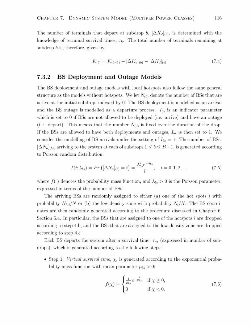
Chapter 7. Dynamic System Model (Multiple Power Classes) 116
The number of terminals that depart at subdrop b, [∆Kd](b), is determined with the
knowledge of terminal survival times, τk. The total number of terminals remaining at
subdrop b is, therefore, given by
K(b) = K(b−1) + [∆Ka](b) − [∆Kd](b) (7.4)
7.3.2 BS Deployment and Outage Models
The BS deployment and outage models with local hotspots also follow the same general
structure as the models without hotspots. We let N(0) denote the number of BSs that are
active at the initial subdrop, indexed by 0. The BS deployment is modelled as an arrival
and the BS outage is modelled as a departure process. Ibs is an indicator parameter
which is set to 0 if BSs are not allowed to be deployed (i.e. arrive) and have an outage
(i.e. depart). This means that the number N(0) is fixed over the duration of the drop.
If the BSs are allowed to have both deployments and outages, Ibs is then set to 1. We
consider the modelling of BS arrivals under the setting of Ibs = 1. The number of BSs,
[∆Na](b), arriving to the system at each of subdrops 1 ≤ b ≤ B−1, is generated according
to Poisson random distribution:
f(i;λbs) = Pr([∆Na](b) = i
)=λibse
−λbs
i!, i = 0, 1, 2, . . . (7.5)
where f( ) denotes the probability mass function, and λbs > 0 is the Poisson parameter,
expressed in terms of the number of BSs.
The arriving BSs are randomly assigned to either (a) one of the hot spots i with
probability Nh,i/N or (b) the low-density zone with probability Nl/N . The BS coordi-
nates are then randomly generated according to the procedure discussed in Chapter 6,
Section 6.4. In particular, the BSs that are assigned to one of the hotspots i are dropped
according to step 4.b, and the BSs that are assigned to the low-density zone are dropped
according to step 4.c.
Each BS departs the system after a survival time, τn, (expressed in number of sub-
drops), which is generated according to the following steps:
• Step 1: Virtual survival time, χ, is generated according to the exponential proba-
bility mass function with mean parameter µbs > 0:
f(χ) =
1µbse− χµbs if χ ≥ 0,
0 if χ < 0.(7.6)
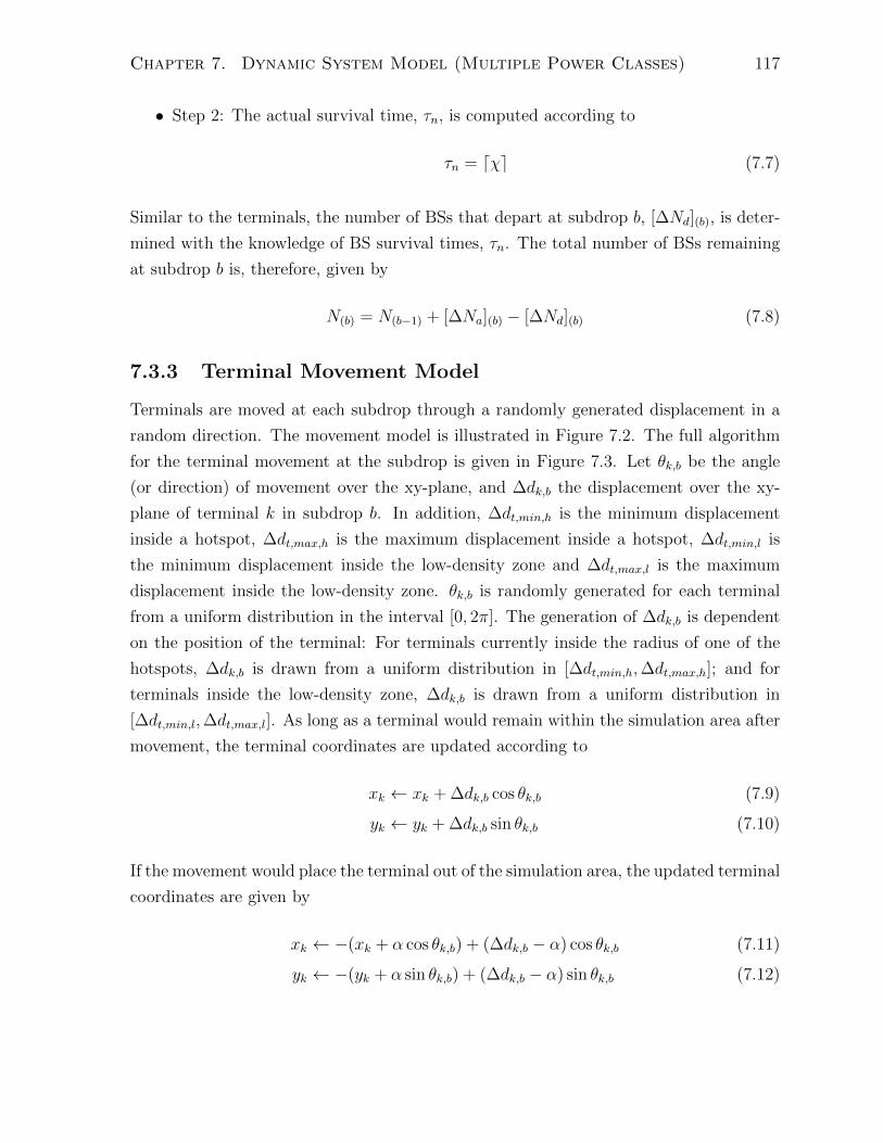
Chapter 7. Dynamic System Model (Multiple Power Classes) 117
• Step 2: The actual survival time, τn, is computed according to
τn = dχe (7.7)
Similar to the terminals, the number of BSs that depart at subdrop b, [∆Nd](b), is deter-
mined with the knowledge of BS survival times, τn. The total number of BSs remaining
at subdrop b is, therefore, given by
N(b) = N(b−1) + [∆Na](b) − [∆Nd](b) (7.8)
7.3.3 Terminal Movement Model
Terminals are moved at each subdrop through a randomly generated displacement in a
random direction. The movement model is illustrated in Figure 7.2. The full algorithm
for the terminal movement at the subdrop is given in Figure 7.3. Let θk,b be the angle
(or direction) of movement over the xy-plane, and ∆dk,b the displacement over the xy-
plane of terminal k in subdrop b. In addition, ∆dt,min,h is the minimum displacement
inside a hotspot, ∆dt,max,h is the maximum displacement inside a hotspot, ∆dt,min,l is
the minimum displacement inside the low-density zone and ∆dt,max,l is the maximum
displacement inside the low-density zone. θk,b is randomly generated for each terminal
from a uniform distribution in the interval [0, 2π]. The generation of ∆dk,b is dependent
on the position of the terminal: For terminals currently inside the radius of one of the
hotspots, ∆dk,b is drawn from a uniform distribution in [∆dt,min,h,∆dt,max,h]; and for
terminals inside the low-density zone, ∆dk,b is drawn from a uniform distribution in
[∆dt,min,l,∆dt,max,l]. As long as a terminal would remain within the simulation area after
movement, the terminal coordinates are updated according to
xk ← xk + ∆dk,b cos θk,b (7.9)
yk ← yk + ∆dk,b sin θk,b (7.10)
If the movement would place the terminal out of the simulation area, the updated terminal
coordinates are given by
xk ← −(xk + α cos θk,b) + (∆dk,b − α) cos θk,b (7.11)
yk ← −(yk + α sin θk,b) + (∆dk,b − α) sin θk,b (7.12)

Chapter 7. Dynamic System Model (Multiple Power Classes) 118
(xk, yk)
(xk+dk,bcosθk,b, yk
+dk,bsinθk,b)
dk,b
θk,b
y
x
Figure 7.2: The terminal movement illustration.
Require: xk, yk, for terminals k ∈ K, and parameters ∆dt,min,h, ∆dt,max,h, ∆dt,min,l, and∆dt,max,l
1: for all terminals k ∈ K do2: if terminal k is inside a hotspot then3: Generate ∆dk,b ∼ U ∈ [∆dt,min,h,∆dt,max,h], and θk,b ∼ U ∈ [0, 2π].4: else5: Generate ∆dk,b ∼ U ∈ [∆dt,min,l,∆dt,max,l], and θk,b ∼ U ∈ [0, 2π].6: end if7: if (xk + ∆dk,b cos θk,b)
2 + (yk + ∆dk,b sin θk,b)2 ≤ R2 then
8: xk ← xk + ∆dk,b cos θk,b9: yk ← yk + ∆dk,b sin θk,b
10: else11: Solve for α in α2 + 2α(xk cos θk,b + yk sin θk,b) + (x2
k + y2k −R2) = 0
12: xk ← −(xk + α cos θk,b) + (∆dk,b − α) cos θk,b13: yk ← −(yk + α sin θk,b) + (∆dk,b − α) sin θk,b14: end if15: end for
Figure 7.3: Algorithm for the terminal movement at the simulation subdrop.
where α is determined by solving
α2 + 2α(xk cos θk,b + yk sin θk,b) + (x2k + y2
k −R2) = 0 (7.13)

Chapter 7. Dynamic System Model (Multiple Power Classes) 119
7.3.4 BS Movement Model
Similar to the terminals, the proposed simulation framework has the option for modelling
BS movements. Let πbs be a fixed probability of BS movement. At each subdrop, BSs
are moved with probability πbs through a random displacement in a random direction.
The movement model is illustrated in Figure 7.4. The detailed algorithm for the BS
movement at the subdrop is described in Figure 7.5. Let θn,b be the angle (or direction)
of movement over the xy-plane, and ∆dn,b the displacement over the xy-plane of BS
n in subdrop b. In addition, ∆dbs,min,h is the minimum displacement inside a hotspot,
∆dbs,max,h is the maximum displacement inside a hotspot, ∆dbs,min,l is the minimum
displacement inside the low-density zone and ∆dbs,max,l is the maximum displacement
inside the low-density zone. θn,b is randomly generated for each BS from a uniform
distribution in the interval [0, 2π]. The generation of ∆dn,b is dependent on the position
of the BS: For BSs currently inside the radius of one of the hotspots, ∆dn,b is drawn
from a uniform distribution in [∆dbs,min,h,∆dbs,max,h]; and for BSs currently inside the
low-density zone, ∆dn,b is drawn from a uniform distribution in [∆dbs,min,l,∆dbs,max,l]. As
long as a terminal would remain within the simulation area after movement, the terminal
coordinates are updated according to
xn ← xn + ∆dn,b cos θn,b (7.14)
yn ← yn + ∆dn,b sin θn,b (7.15)
If the movement would place the BS out of the simulation area, the coordinate update
is given by
xn ← −(xn + α cos θn,b) + (∆dn,b − α) cos θn,b (7.16)
yn ← −(yn + α sin θn,b) + (∆dn,b − α) sin θn,b (7.17)
where α is determined by solving
α2 + 2α(xn cos θn,b + yn sin θn,b) + (x2n + y2
n −R2) = 0 (7.18)
7.4 Typical Parameter Values
In this section, we discuss typical values for the time evolution model parameters. Rec-
ommended values and ranges for the parameters are summarized in Table 7.1. Note

Chapter 7. Dynamic System Model (Multiple Power Classes) 120
(xn, yn)
(xn+dn,bcosθn,b, yn
+dn,bsinθn,b)
dn,b
θn,b
y
x
Figure 7.4: The BS movement illustration.
Require: xn, yn, for BSs n ∈ N , and parameters πbs, ∆dbs,min,h, ∆dbs,max,h, ∆dbs,min,land ∆dbs,max,l
1: for all BSs n ∈ N do2: Generate γ such that Pr(γ = 1) = πbs and Pr(γ = 0) = 1− πbs.3: if γ = 1 then4: if BS N is inside a hotspot then5: Generate ∆dn,b ∼ U ∈ [∆dbs,min,h,∆dbs,max,h], and θn,b ∼ U ∈ [0, 2π].6: else7: Generate ∆dn,b ∼ U ∈ [∆dbs,min,l,∆dbs,max,l], and θn,b ∼ U ∈ [0, 2π].8: end if9: if (xn + ∆dn,b cos θn,b)
2 + (yn + ∆dn,b sin θn,b)2 ≤ R2 then
10: xn ← xn + ∆dn,b cos θn,b11: yn ← yn + ∆dn,b sin θn,b12: else13: Solve for α in α2 + 2α(xn cos θn,b + yn sin θn,b) + (x2
n + y2n −R2) = 0
14: xn ← −(xn + α cos θn,b) + (∆dn,b − α) cos θn,b15: yn ← −(yn + α sin θn,b) + (∆dn,b − α) sin θn,b16: end if17: end if18: end for
Figure 7.5: Algorithm for the BS movement at the simulation subdrop.

Chapter 7. Dynamic System Model (Multiple Power Classes) 121
Table 7.1: Typical parameter values.
Parameter Typical Range and/or Value
Numbers of subdrops, B typical value of 20
Numbers of drops, P P B, typical value of 300
Scheduling average window size,T0
typical value of 5
Numbers of subframes, F F T0, F P , typical value of 100
Terminal arrival parameter, λt typical value of 3 terminals
BS arrival parameter, λbs λbs λt, typical value of 0.5 BSs
Terminal departure parameter, µt typical value of 5 subdrops
BS departure parameter, µbs µbs µt, typical value of 20 subdrops
Hotspot maximum terminal dis-placement, ∆dt,max,h
0.1dc,h ≤ ∆dt,max,h ≤ 10dc,h
Hotspot minimum terminal dis-placement, ∆dt,min,h
0 ≤ ∆dt,min,h ≤ 14∆dt,max,h
Low-density zone maximum ter-minal displacement, ∆dt,max,l
0.1dc,l ≤ ∆dt,max,l ≤ 10dc,l
Low-density zone minimum ter-minal displacement, ∆dt,min,l
0 ≤ ∆dt,min,l ≤ 14∆dt,max,l
Hotspot maximum BS displace-ment, ∆dbs,max,h
0.1dc,h ≤ ∆dbs,max,h ≤ 10dc,h
Hotspot minimum BS displace-ment, ∆dbs,min,h
0 ≤ ∆dbs,min,h ≤ 14∆dbs,max,h
Low-density zone maximum BSdisplacement, ∆dbs,max,l
0.1dc,l ≤ ∆dbs,max,l ≤ 10dc,l
Low-density zone minimum BSdisplacement, ∆dbs,min,l
0 ≤ ∆dbs,min,l ≤ 14∆dbs,max,l
BS movement probability, πbs πbs 1

Chapter 7. Dynamic System Model (Multiple Power Classes) 122
that many of the parameters have the same recommended values and ranges as the time
evolution model for a single power class, thus the reader is asked to refer to Chapter 4
for the justification of those recommended ranges. In the following, we discuss the ranges
of maximum and minimum displacement parameters. Similar to Chapter 4, the maxi-
mum displacement parameters should be set large enough to cause a small but noticeable
change in shadowing over the subdrop. Therefore, we apply the basic principle of (4.25)
and (4.26) for the recommended ranges of the maximum and minimum terminal displace-
ment parameters based on the correlation distance, dc, that is
0.1dc ≤ ∆dt,max ≤ 10dc, (7.19)
0 ≤ ∆dt,min ≤1
4∆dt,max. (7.20)
It was discussed in Chapter 6, however, that in inhomogeneous networks, there exist
multiple distinct dc values corresponding to the distinct power classes. We, therefore,
define the typical correlation distance inside the hotspots and outside the hotspots (or
in the low-density zone). Let dc,h be the typical correlation distance inside the hotspots
and dc,l be the typical correlation distance inside the low-density zone. dc,h and dc,l are
computed as the average of the correlation distances, dc, for the BS power classes that
are found inside the hotspots and the low-density zone, respectively. In analogy to (7.19)
and (7.20), the terminal displacement parameter ∆dt,max,h should, hence, be bounded by
multiples of dc,h, or
0.1dc,h ≤ ∆dt,max,h ≤ 10dc,h (7.21)
and the parameter ∆dt,min,h should be bounded as
0 ≤ ∆dt,min,h ≤1
4∆dt,max,h (7.22)
Similarly, the parameters ∆dt,max,l and ∆dt,min,l should satisfy the relations based on
multiples of dc,l:
0.1dc,l ≤ ∆dt,max,l ≤ 10dc,l (7.23)
0 ≤ ∆dt,min,l ≤1
4∆dt,max,l (7.24)

Chapter 7. Dynamic System Model (Multiple Power Classes) 123
By similar reasoning as the terminals, the BS displacement parameters ∆dbs,max,h, ∆dbs,min,h,
∆dbs,max,l and ∆dbs,min,l should satisfy:
0.1dc,h ≤ ∆dbs,max,h ≤ 10dc,h (7.25)
0 ≤ ∆dbs,min,h ≤1
4∆dbs,max,h (7.26)
0.1dc,l ≤ ∆dbs,max,l ≤ 10dc,l (7.27)
0 ≤ ∆dbs,min,l ≤1
4∆dbs,max,l (7.28)
7.5 Simulations
In this section, system simulations are performed in order to demonstrate the use of the
proposed system modelling and the benefit of the BS power adaptation in the network
with multiple power classes. Note that a simplified system model is utilized in the simu-
lation. Hotspotted deployment with two distinct power classes is considered, consisting
of the outdoor pico power class (used exclusively inside hotspots) and the macro power
class (used exclusively inside the low-density zone). The time evolution model will con-
sider terminal movements with constant displacement and uniformly random direction
both inside and outside hotspots, and neglect other types of dynamics such as terminal
arrivals and departures.
The model parameters (largely based on the suggested values in Table 7.1 and sup-
plemented with the ITU guidelines where needed) are summarized in Tables 7.2 and 7.3.
Table 7.2 contains the deployment scenario parameters, and Table 7.3 lists other physical
model parameters.
The number of BSs in the low-density zone and in hotspots have been computed as
a function of the nominal number of terminals according to (6.7) and (6.8), respectively.
The total number of terminals will be varied in the simulation, with the proportion of
terminals inside each area kept constant. Similarly, the constant terminal displacements
listed in Table 7.3 have been chosen according to (7.21) and (7.23), and will be varied in
simulation. Note that the BSs are not allowed to power on and off, as a non-zero lower
limit, Ps,min, has been imposed on the BS power levels. The difference between Ps,min
and Ps,max is set to 6 dB for both of the power classes.
A simplified method for determining effective shadowing standard deviation, σ0,eff,
and shadowing correlation distance, dc,eff, is introduced. The procedure is described in
the following: First, the σ0,eff values are equal to 10 dB for all links, as σ0(s) in the
homogeneous scenario is equal for both BS power classes. Second, the dc,eff values are

Chapter 7. Dynamic System Model (Multiple Power Classes) 124
Table 7.2: Deployment scenario parameters
Parameter Value
Simulation area radius, R 375 m
Number of hotspots, H 2
Hotspot radius, Rh 40 m
Nominal number of terminals in the low-density zone, Kl 36
Nominal number of terminals in hotspot 1, Kh,1 12
Nominal number of terminals in hotspot 2, Kh,2 36
The total nominal number of terminals, K 84
Number of BSs in the low-density zone, Nl 3
Number of BSs in hotspot 1, Nh,1 1
Number of BSs in hotspot 2, Nh,2 3
Total number of BSs, N 7
approximated by using certain properties of the specific deployment scenario considered.
In particular, from Table 7.2, the number of hotspots, H, is small and the hotspot radius,
Rh, is much smaller than the simulation radius, R, that is, Rh R. Furthermore, there
are only two available power classes, one of which (the outdoor pico) is used exclusively
for hotspots, and the other (the macro) for the low-density zone. Thus, it is concluded
that the path between certain types of links, for instance, that between a macro BS and
a terminal in the low-density zone is statistically unlikely to cross through the outdoor
pico power class. Additionally, for other types of links, such as that between a macro
BS and a terminal inside a hotspot, the path does cross through the outdoor pico power
class, however, the respective path length segment is statistically expected to be small.
Consequently, from (6.19), the dc,eff value for the two types of links is approximated to
be equal to the homogeneous dc(s) for the macro BS cell, or dc,eff∼= dc(s) = 50 m. A
similar analysis for links between pico BSs and terminals inside the same hotspot shows
that the dc,eff value is exactly equal to the homogeneous dc(s) for the outdoor pico BS
cell, or dc,eff = dc(s) = 10 m. The dc,eff values used for different link types are listed in
Table 7.4.
P = 150 simulation drops each consisting of B = 20 subdrops are used in the eval-
uation. Both the total rate maximization (TRM) power adaptation of (5.6) and the
proportional fair (PF) power adaptation of (5.10) are simulated for the purpose of com-
parison. The TRM and PF algorithms are also compared against the utilization of equal
BS powers according to the power classes, that is, where the Pn = Psn,max is used for all
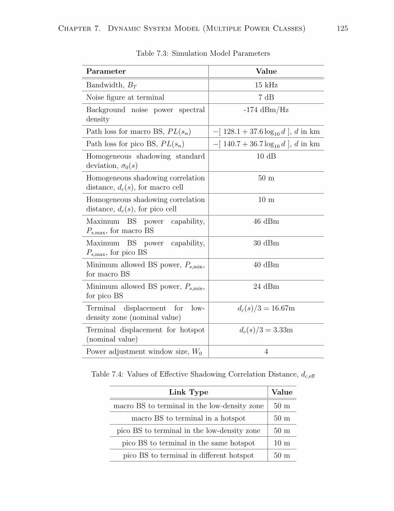
Chapter 7. Dynamic System Model (Multiple Power Classes) 125
Table 7.3: Simulation Model Parameters
Parameter Value
Bandwidth, BT 15 kHz
Noise figure at terminal 7 dB
Background noise power spectraldensity
-174 dBm/Hz
Path loss for macro BS, PL(sn) −[ 128.1 + 37.6 log10 d ], d in km
Path loss for pico BS, PL(sn) −[ 140.7 + 36.7 log10 d ], d in km
Homogeneous shadowing standarddeviation, σ0(s)
10 dB
Homogeneous shadowing correlationdistance, dc(s), for macro cell
50 m
Homogeneous shadowing correlationdistance, dc(s), for pico cell
10 m
Maximum BS power capability,Ps,max, for macro BS
46 dBm
Maximum BS power capability,Ps,max, for pico BS
30 dBm
Minimum allowed BS power, Ps,min,for macro BS
40 dBm
Minimum allowed BS power, Ps,min,for pico BS
24 dBm
Terminal displacement for low-density zone (nominal value)
dc(s)/3 = 16.67m
Terminal displacement for hotspot(nominal value)
dc(s)/3 = 3.33m
Power adjustment window size, W0 4
Table 7.4: Values of Effective Shadowing Correlation Distance, dc,eff
Link Type Value
macro BS to terminal in the low-density zone 50 m
macro BS to terminal in a hotspot 50 m
pico BS to terminal in the low-density zone 50 m
pico BS to terminal in the same hotspot 10 m
pico BS to terminal in different hotspot 50 m

Chapter 7. Dynamic System Model (Multiple Power Classes) 126
0
0.005
0.01
0.015
0.02
0.025
0.03
0.035
0.04
0 0.5 1 1.5 2
5th
%le
Sp
ectr
al E
ffic
iency
(b
ps/
Hz)
Terminal Displacement in Multiples of dc(s)
Equal Power
PF
TRM
(a)
0.35
0.355
0.36
0.365
0.37
0.375
0.38
0.385
0.39
0.395
0.4
0 0.5 1 1.5 2
50
th %
le S
pec
tral
Eff
icie
ncy
(b
ps/
Hz)
Terminal Displacement in Multiples of dc(s)
Equal Power
PF
TRM
(b)
Figure 7.6: Comparison of power adaptation schemes and the equal power level scenariofor varying terminal displacement in terms of (a) 5th percentile spectral efficiency, and(b) 50th percentile spectral efficiency.
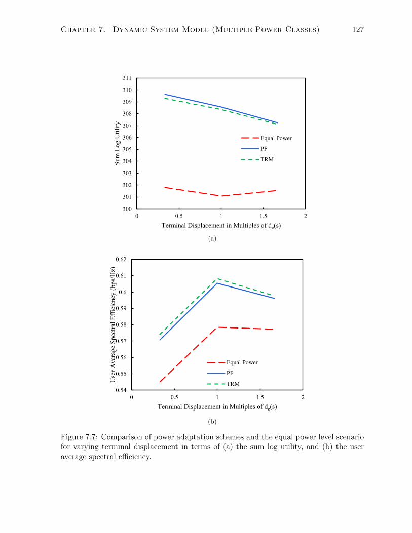
Chapter 7. Dynamic System Model (Multiple Power Classes) 127
300
301
302
303
304
305
306
307
308
309
310
311
0 0.5 1 1.5 2
Sum
Lo
g U
tili
ty
Terminal Displacement in Multiples of dc(s)
Equal Power
PF
TRM
(a)
0.54
0.55
0.56
0.57
0.58
0.59
0.6
0.61
0.62
0 0.5 1 1.5 2
Use
r A
ver
age
Sp
ectr
al E
ffic
iency
(b
ps/
Hz)
Terminal Displacement in Multiples of dc(s)
Equal Power
PF
TRM
(b)
Figure 7.7: Comparison of power adaptation schemes and the equal power level scenariofor varying terminal displacement in terms of (a) the sum log utility, and (b) the useraverage spectral efficiency.

Chapter 7. Dynamic System Model (Multiple Power Classes) 128
BSs of each of the macro and the outdoor pico power classes.
The variation of the terminal displacement parameters was simulated for a constant
number of users, K = 84. Figure 7.6a shows the variation of 5th percentile (cell edge)
spectral efficiency. Both the TRM and PF methods show over 100% improvement in
cell edge spectral efficiency over the equal BS power method. Figure 7.6b shows the
50th percentile (median) spectral efficiency for the different power setting methods. 8%
increase in median spectral efficiency is obtained for low values of terminal displacement,
which however drops to 2% for higher values of displacement. Figure 7.7a and 7.7b show
the sum log utility (SLU) and user average spectral efficiency variation with increasing
terminal displacements. It is observed that both PF and TRM methods improve the SLU.
The methods also improve the user average spectral efficiency obtained in the network
with nearly 5% increase. We note that there is only a small difference between the PF
and TRM methods with respect to both the SLU and user average spectral efficiency
obtained.
The variation of the total number of users is considered next with the terminal dis-
placement values set to dc(s)/3. A variation of the PF power adaptation algorithm,
referred to as independent PF method, was additionally considered in this section. In
particular, the original PF and TRM power adaptation consider the optimization of (5.6)
or (5.10) jointly over the entire set of BSs and terminals. In the independent PF method,
the PF power adaptation of (5.10) was carried out separately and independently for the
pico and the macro BSs, respectively. In each case, the power adaptation considered
either the pico (or macro) BSs and the terminals assigned to the pico (or macro) BSs as
the whole set of BSs, N , and terminals, K, respectively, in the optimization of (5.10).
In other words, the interference from either the macro or pico BSs were neglected in
the solution. Terminal data rates were then computed normally with the two separately
obtained sets of BS power levels. The independent PF can be important to consider as
it limits the coordination for BS power adaptation to within one set of BSs (either the
pico or macro in the particular case), thereby limiting the required exchange of channel
information.
Figure 7.8a shows the variation of 5th percentile (cell edge) spectral efficiency with
respect to the total number of users for the different power setting methods. The TRM-
based method achieves approximately 100% improvement compared to the equal BS
power method. Furthermore, the PF-based method achieves around 110% improvement
over the equal BS power method. The independent PF method shows negligible improve-
ment over the equal power method in terms of cell edge spectral efficiency. Figure 7.8b
shows the 50th percentile (median) spectral efficiency for the different power setting

Chapter 7. Dynamic System Model (Multiple Power Classes) 129
methods. Both the TRM and PF methods show close to 8% improvement in median
spectral efficiency over the equal power setting methods. The independent PF method
also achieves 5% improvement over equal power setting. Figure 7.9a and 7.9b show the
sum log utility (SLU) and user average spectral efficiency variation with increasing ter-
minal displacements. Both PF and TRM methods are shown to improve the SLU. The
independent PF method has SLU that is nearly equal to the equal power method, repre-
senting negligible improvement. The PF and TRM also show close to 5% improvement
in the user average spectral efficiency over the equal power method, and the independent
PF shows 2% improvement.
It can be concluded that the TRM and PF algorithms show improvement over the
equal power method. A smaller improvement is obtained for median spectral efficiency
and user average spectral efficiency, which represents the overall system performance.
Greater improvement is obtained for cell edge spectral efficiency and SLU, representing
a measure of fairness among users. It can be observed that the independent PF method
performs poorly in terms of cell edge spectral efficiency and SLU. However, if the reduced
signalling proves to be an important criteria in the particular implementation, the method
can be used due to the improvement it provides in median spectral efficiency and total
system rate.

Chapter 7. Dynamic System Model (Multiple Power Classes) 130
0.01
0.02
0.03
0.04
0.05
0.06
20 30 40 50 60 70 80 90
5th
%le
Sp
ectr
al E
ffic
iency
(b
ps/
Hz)
Total Number of Users
Equal Power
PF
Independent PF
TRM
(a)
0.3
0.4
0.5
0.6
0.7
0.8
0.9
20 30 40 50 60 70 80 90
50
th %
le S
pec
tral
Eff
icie
ncy
(b
ps/
Hz)
Total Number of Users
Equal Power
PF
Independent PF
TRM
(b)
Figure 7.8: Comparison of power adaptation schemes and the equal power level scenariofor varying number of users in terms of (a) 5th percentile spectral efficiency, and (b) 50thpercentile spectral efficiency.

Chapter 7. Dynamic System Model (Multiple Power Classes) 131
100
150
200
250
300
28 56 84
Sum
Lo
g U
tili
ty
Total Number of Users
Equal Power
PF
Independent PF
TRM
(a)
0.48
0.58
0.68
0.78
0.88
0.98
1.08
1.18
20 30 40 50 60 70 80 90
Use
r A
ver
age
Sp
ectr
al E
ffic
iency
(b
ps/
Hz)
Total Number of Users
Equal Power
PF
Independent PF
TRM
(b)
Figure 7.9: Comparison of power adaptation schemes and the equal power level scenariofor varying number of users in terms of (a) the sum log utility, and (b) the user averagespectral efficiency.
Chapter 8
Conclusion
8.1 Summary
In this thesis, we consider the development of a high-level system model for simulation
purposes for a generic irregular cellular network. We assume a network with universal
frequency allocation and power assignment. The main goal is to provide a high-level
model representation, including an adaptive resource allocation strategy. It is believed
that a high-level simulation model can allow for representation of the network with as
much realism as desired, tailored to each particular scenario.
An existing high-level reference model (represented in the ITU model) uses the hexag-
onal deployment pattern, independent simulation drop concept and the common lognor-
mal shadowing model, and is primarily suitable for regular cell deployment with little
dynamism. In contrast, the proposed model is designed for the irregular cellular net-
work having arbitrary deployment with small and large BSs and increased dynamism
and adaptation. The model considers a wide array of dynamic changes that are expected
to occur in the irregular network. As part of the model, an adaptive resource allocation
framework that works at both a slower and a faster time scale is considered.
We first discussed BS outage as a specific type of dynamic network change in Chap-
ter 3. BS outage compensation was then considered as the adaptation in response to
the BS outage. First, a model of the network in an outage was devised for an irregular
cellular network. In particular, the BS positions and power classes were modelled in a
general sense. Then, an outage compensation method that uses the idea of the cluster
or scheduling cell combined with cell re-association and power adjustment was proposed.
Simulations were performed with correlated shadowing for non-common-end links that
is appropriate for irregular deployments. Through evaluations using the proposed mod-
elling, it was demonstrated that the proposed algorithms show robustness against the
132
Chapter 8. Conclusion 133
outage in both regular and irregular networks.
The high-level model and the adaptive resource allocation framework for the irregular
network was developed and enhanced, in stages, in the remainder of the thesis:
In Chapter 4, the system model with time evolution was considered for the irregular
network with a single BS power class and constant power levels. A modification of the
ITU simulation drop concept was proposed. A drop deployment methodology considering
both the arbitrariness and the restrictions of deployment was discussed. Finally, a time
evolution methodology considering an array of dynamic changes such as terminal arrivals
and departures, BS deployments and outages as well as BS and terminal movements
was detailed. The parameters for the drop deployment and time evolution models were
considered and typical values were suggested.
Chapter 5 considered the adaptation of BS power levels which form an extension of
an adaptive resource allocation framework for irregular networks. BS power adaptation
algorithms which made use of the total rate maximization and proportional fairness
were proposed. Then, a high-level adaptive resource allocation framework based on
clustering and power control at a large time scale and coordinated proportional fair
resource allocation at a small time scale was proposed for a generic irregular network.
The simulation results illustrate the use of the system model, with the suggested ranges of
the model parameters. The results showed the improvement that was obtained by using
the power adaptation algorithms, as well as the general degradation of performance
for increased values of the BS separation parameter. Finally, the power adaptation
algorithms were shown to compensate, in part, for the effect of irregularity.
Chapter 6 considered the extension of the model to the case of multiple power classes
without time evolution. The drop deployment methodology was modified to be suitable
to model the deployment of hotspots. Then an enhanced correlated shadowing model
was proposed for the network having multiple radio propagation environments. For this
purpose, a theory was proposed for variation of the shadowing parameters, (standard
deviation and correlation distance) in a network with an arbitrary number of radio prop-
agation environments. The model consistency with an earlier model was verified for a
particular scenario, and the implementation in practical simulations was discussed.
Finally, Chapter 7 extended the time evolution methodology of Chapter 4 to the
situation with multiple power classes and hotspots. The high-level adaptive resource
allocation framework of Chapter 5 with BS power adaptation was applied for the case of
multiple power classes. Simulation results showed the use of the model and the improve-
ments obtained by the BS power adaptation in terms of different measures of performance
(5th percentile, 50th percentile and user average spectral efficiencies as well as sum log

Chapter 8. Conclusion 134
utility) for a network with multiple power classes.
The simulation results illustrate the use of the system model, with the suggested
ranges of the model parameters. In addition, improvements obtained by the BS power
adaptation in terms of different measures of performance (5th percentile, 50th percentile
and user average spectral efficiencies as well as sum log utility) for a network with multiple
power classes were discussed, and the effect of limited coordination was evaluated.
The proposed high-level model provided an arbitrary deployment method, a large-
scale time evolution method and a correlated shadowing model appropriate for the irreg-
ular cellular network considered in the thesis. It is believed that a high-level simulation
model can serve as a skeleton network model over which different researchers can make
modifications. This can allow for representation of the network with as much realism as
needed, tailored to each particular scenario.
8.2 Future Work
• The deployment of additional BSs in an irregular cellular network would normally
improve the system performance. Consider that there are a limited number of
extra BSs that can be deployed. It would be interesting to study where is the
best location to deploy the additional BSs in order to enhance the cellular system
performance.
• Traditionally, measures such as cell capacity, coverage probability and average SINR
or rate, among others, have been used to quantify the performance in the cellular
system. Looking to the future or as a parallel area of research, a high-level simu-
lation model could facilitate the development of new measures of performance for
irregular cellular networks, that are more appropriate than the above traditional
performance measures. This is because the simulation model need not be bound
by the analytical tractability as a constraint. Instead, the constraint can be the
utility of the performance measure corresponding to the desired level of realism for
the application. For instance, new and more appropriate measures of user perfor-
mance could be developed for an irregular network where the concept of cells is
more flexible due to the dynamism of BSs (such as due to deployments, outages
and the formation of scheduling cells or clusters). Additionally, the analysis in this
thesis assumes full buffer traffic once a terminal is active. In the future, improved
performance metrics could be devised to quantify the user experience for varied
traffic patterns other than full buffer at a finer time scale.

Chapter 8. Conclusion 135
• Throughout this work, it is assumed for the purpose of scheduling that the ter-
minals have full buffer traffic. It would be an interesting problem to consider the
proportional fair scheduling and the adaptation framework under the condition
that the traffic is not full buffer. The system model, the scheduling and the slow
adaptation algorithms could be adapted for such a traffic scenario.
• In this thesis, we were able to justify the inhomogeneous distance-dependent path
loss and shadowing channel models through physical arguments. However, it would
be a worthwhile effort to verify the channel models by gathering real-world mea-
surements under inhomogeneous network conditions.
• The dynamic system model of this thesis makes it possible to represent the grad-
ual time evolution of the irregular cellular network. This can enable the study
and evaluation of adaptive algorithms with reduced signalling in practically real-
izable scenarios. It would, therefore, be interesting to consider the reduction of
signalling for the proposed specific adaptation framework. In particular, a variety
of signalling reduction schemes could be considered and analyzed under different
practical system evolution scenarios.

Bibliography
[1] Guidelines for Evaluation of Radio Interface Technologies for IMT-Advanced, ITU-R
M.2135, Std., 2008.
[2] B. Golkar and E. S. Sousa, “Resource allocation in autonomous cellular networks,”
IEEE Trans. Wireless Commun., vol. 12, no. 11, pp. 5572–5583, Nov. 2013.
[3] L. Kayili and E. Sousa, “Cell outage compensation for irregular cellular networks,”
in IEEE Wireless Communications and Networking Conference (WCNC), Istanbul,
Turkey, Apr. 2014.
[4] ——, “Dynamic system modelling and adaptive resource allocation for irregular
cellular networks,” 2015, to be submitted to IEEE Trans. Wireless Commun.
[5] ——, “Channel simulation with large-scale time evolution in irregular cellular net-
works,” in Proc. 22nd European Signal Processing Conference (EUSIPCO), Lisbon,
Portugal, Sep. 2014.
[6] ——, “Extended shadow fading model for irregular cellular networks,” in IEEE
Wireless Communications and Networking Conference (WCNC), New Orleans, LA,
Mar. 2015.
[7] N. Deng, W. Zhou, and M. Haenggi, “The ginibre point process as a model for
wireless networks with repulsion,” IEEE Transactions on Wireless Communications,
vol. 14, no. 1, pp. 107–121, Jan 2015.
[8] B. Golkar and E. Sousa, “A network shadow fading model for autonomous infras-
tructure wireless networks,” in Proc. 20th European Signal Processing Conference
(EUSIPCO), August 2012.
[9] F. Khan, LTE for 4G Mobile Broadband: Air Interface Technologies and Perfor-
mance, 1st ed. New York, NY, USA: Cambridge University Press, 2009.
136
Bibliography 137
[10] W. Anchun, X. Liang, Z. Shidong, X. Xibin, and Y. Yan, “Dynamic resource manage-
ment in the fourth generation wireless systems,” in Proc. International Conference
on Communication Technology (ICCT 2003), Apr. 2003.
[11] F. Berggren and R. Jantti, “Asymptotically fair transmission scheduling over fading
channels,” IEEE Trans. Wireless Commun., vol. 3, no. 1, pp. 326–336, Jan. 2004.
[12] J. Hajipour and V. Leung, “Proportional fair scheduling in multi-carrier networks
using channel predictions,” in IEEE International Conference on Communications
(ICC 2010), May 2010.
[13] H. Kim, K. Kim, Y. Han, and S. Yun, “A proportional fair scheduling for multicarrier
transmission systems,” in IEEE Vehicular Technology Conference (VTC 2004), Sep.
2004.
[14] F. Kelly, “Charging and rate control for elastic traffic,” European Transactions on
Telecommunications, vol. 8, pp. 33–37, 1997.
[15] P. Viswanath, D. Tse, and R. Laroia, “Opportunistic beamforming using dumb
antennas,” IEEE Trans. Inf. Theory, vol. 48, no. 6, pp. 1277–1294, Jun. 2002.
[16] A. Mas-Colell, M. Whinston, and J. Green, Microeconomic Theory. Oxford Uni-
versity Press, 1995.
[17] J. Holtzman, “Asymptotic analysis of proportional fair algorithm,” in IEEE Per-
sonal, Indoor and Mobile Radio Communications (PIMRC 2001), Sep. 2001.
[18] G. Boudreau, J. Panicker, N. Guo, R. Chang, N. Wang, and S. Vrzic, “Interference
coordination and cancellation for 4g networks,” IEEE Communications Magazine,
vol. 47, no. 4, pp. 74–81, April 2009.
[19] S. Ali and V. Leung, “Dynamic frequency allocation in fractional frequency reused
OFDMA networks,” IEEE Transactions on Wireless Communications, vol. 8, no. 8,
pp. 4286–4295, August 2009.
[20] T. Bonald, S. Borst, S. Borst, and A. Proutiere, “Inter-cell scheduling in wireless data
networks,” in 11th European Wireless Conference 2005 - Next Generation Wireless
and Mobile Communications and Services (European Wireless), April 2005, pp. 1–7.
[21] G. Li and H. Liu, “Downlink radio resource allocation for multi-cell OFDMA sys-
tem,” IEEE Transactions on Wireless Communications, vol. 5, no. 12, pp. 3451–
3459, December 2006.

Bibliography 138
[22] R. Chang, Z. Tao, J. Zhang, and C.-C. Kuo, “Multicell OFDMA downlink resource
allocation using a graphic framework,” IEEE Transactions on Vehicular Technology,
vol. 58, no. 7, pp. 3494–3507, Sept 2009.
[23] U. Von Luxburg, “A tutorial on spectral clustering,” Statistics and computing,
vol. 17, no. 4, pp. 395–416, 2007.
[24] O. Aliu, A. Imran, M. Imran, and B. Evans, “A survey of self organisation in future
cellular networks,” IEEE Commun. Surveys Tuts., vol. 15, no. 1, pp. 336–361, Feb.
2013.
[25] A. Temesvary, “Self-configuration of antenna tilt and power for plug & play deployed
cellular networks,” in IEEE Wireless Communications and Networking Conference
(WCNC 2009), Apr. 2009.
[26] G. Calcev and M. Dillon, “Antenna tilt control in cdma networks,” in Proc. Interna-
tional Workshop on Wireless Internet (WICON 2006), Boston, Massachusetts, Aug.
2006.
[27] K. Son, S. Chong, and G. Veciana, “Dynamic association for load balancing and in-
terference avoidance in multi-cell networks,” IEEE Trans. Wireless Commun., vol. 8,
no. 7, pp. 3566–3576, Jul. 2009.
[28] B. Rengarajan, A. Stolyar, and H. Viswanathan, “Self-organizing dynamic fractional
frequency reuse on the uplink of OFDMA systems,” in Information Sciences and
Systems (CISS 2010), Mar. 2010.
[29] M. Amirijoo, L. Jorguseski, T. Kurner, R. Litjens, M. Neuland, L. Schmelz, and
U. Turke, “Cell outage management in LTE networks,” in International Symposium
on Wireless Communication Systems (ISWCS 2009), Sep. 2009.
[30] WINNER II Channel Models, IST-WINNER II Deliverable 1.1.2 v.1.2, 2008.
[31] F. Graziosi, M. Pratesi, M. Ruggieri, and F. Santucci, “A multicell model of handover
initiation in mobile cellular networks,” IEEE Trans. Veh. Technol., vol. 48, no. 3,
pp. 802–814, May 1999.
[32] R. Clarke, “A statistical theory of mobile-radio reception,” The Bell System Tech-
nical Journal, vol. 47, no. 6, pp. 957–1000, Jul. 1968.
[33] W. C. Jakes and D. C. Cox, Eds., Microwave Mobile Communications. Wiley-IEEE
Press, 1994.

Bibliography 139
[34] D. Tse and P. Viswanath, Fundamentals of Wireless Communication. New York,
NY, USA: Cambridge University Press, 2005.
[35] A. Molisch, Wireless Communications, 2nd ed. Wiley, 2010.
[36] M. Gudmundson, “Correlation model for shadow fading in mobile radio systems,”
IEEE Commun. Lett., vol. 27, no. 23, pp. 2145–2146, Nov. 1991.
[37] F. Graziosi and F. Santucci, “A general correlation model for shadow fading in
mobile radio systems,” IEEE Commun. Lett., vol. 6, no. 3, pp. 102–104, Mar. 2002.
[38] K. Kumaran, S. E. Golowich, and S. Borst, “Correlated shadow-fading in wireless
networks and its effect on call dropping,” Wireless Networks, vol. 8, no. 1, pp. 61–71,
Jan. 2002.
[39] I. Forkel, M. Schinnenburg, and M. Ang, “Generation of two-dimensional correlated
shadowing for mobile radio network simulation,” in Proc. 7th International Sympo-
sium on Wireless Personal Multimedia Communications (WPMC), September 2004.
[40] S. Szyszkowicz, H. Yanikomeroglu, and J. Thompson, “On the feasibility of wireless
shadowing correlation models,” IEEE Trans. Veh. Technol., vol. 59, no. 9, pp. 4222–
4236, Nov. 2010.
[41] S. Szyszkowicz and H. Yanikomeroglu, “A simple approximation of the aggregate
interference from a cluster of many interferers with correlated shadowing,” IEEE
Transactions on Wireless Communications, vol. 13, no. 8, pp. 4415–4423, Aug 2014.
[42] S. Roy and S. Kundu, “Outage analysis in presence of correlated interferers in a
cognitive-cellular network,” in 2010 IEEE Symposium on Industrial Electronics Ap-
plications (ISIEA), Oct 2010, pp. 100–105.
[43] M. Di Renzo, A. Guidotti, and G. Corazza, “Average rate of downlink heterogeneous
cellular networks over generalized fading channels: A stochastic geometry approach,”
IEEE Transactions on Communications, vol. 61, no. 7, pp. 3050–3071, July 2013.
[44] G. Hess and S. Gilbert, “Shadowing variability in an urban land mobile environment
at 900 MHz,” Electron. Lett., vol. 26, no. 10, pp. 646–648, May 1990.
[45] E. Perahia, D. Cox, and S. Ho, “Shadow fading cross correlation between basesta-
tions,” in IEEE Vehicular Technology Conference (VTC), May 2001.
Bibliography 140
[46] M. Amirijoo, L. Jorguseski, R. Litjens, and R. Nascimento, “Effectiveness of cell
outage compensation in LTE networks,” in IEEE Consumer Communications and
Networking Conference (CCNC), Jan. 2011.
[47] M. Amirijoo, L. Jorguseski, R. Litjens, and L. Schmelz, “Cell outage compensation
in LTE networks: Algorithms and performance assessment,” in IEEE Vehicular
Technology Conference (VTC), May 2011.
[48] F. Li, X. Qiu, L. Meng, H. Zhang, and W. Gu, “Achieving cell outage compensa-
tion in radio access network with automatic network management,” in Proc. IEEE
GLOBECOM Workshops, Dec. 2011.
[49] O. Onireti, A. Zoha, J. Moysen, A. Imran, L. Giupponi, M. Imran, and
A. Abu Dayya, “A cell outage management framework for dense heterogeneous net-
works,” IEEE Transactions on Vehicular Technology, vol. PP, no. 99, pp. 1–1, 2015.
[50] W. Xue, H. Zhang, Y. Li, D. Liang, and M. Peng, “Cell outage detection and com-
pensation in two-tier heterogeneous networks,” International Journal of Antennas
and Propagation, 2014.
[51] T. Bu, L. Li, and R. Ramjee, “Generalized proportional fair scheduling in third
generation wireless data networks,” in Proc. IEEE INFOCOM, Apr. 2006.
[52] S. Boyd and L. Vandenberghe, Convex Optimization. New York, NY, USA: Cam-
bridge University Press, 2004.
[53] M. Chiang, “Geometric programming for communication systems,” Foundations and
Trends in Communications and Information Theory, vol. 2, no. 12, pp. 1–154, Aug.
2005.
[54] M. Grant and S. Boyd. (2012, Sep.) CVX: Matlab software for disciplined convex
programming, version 2.0 beta. [Online]. Available: http://cvxr.com/cvx
[55] M. Win, P. Pinto, and L. Shepp, “A mathematical theory of network interference
and its applications,” Proceedings of the IEEE, vol. 97, no. 2, pp. 205–230, Feb 2009.
[56] H. Dhillon, R. Ganti, and J. Andrews, “Load-aware modeling and analysis of het-
erogeneous cellular networks,” IEEE Transactions on Wireless Communications,
vol. 12, no. 4, pp. 1666–1677, April 2013.

Bibliography 141
[57] R. Heath, M. Kountouris, and T. Bai, “Modeling heterogeneous network interference
using poisson point processes,” IEEE Transactions on Signal Processing, vol. 61,
no. 16, pp. 4114–4126, Aug 2013.
[58] J. Zhang and J. Andrews, “Distributed antenna systems with randomness,” IEEE
Transactions on Wireless Communications, vol. 7, no. 9, pp. 3636–3646, September
2008.
[59] V. Chandrasekhar and J. Andrews, “Spectrum allocation in tiered cellular net-
works,” IEEE Transactions on Communications, vol. 57, no. 10, pp. 3059–3068,
October 2009.
[60] H. ElSawy and E. Hossain, “On cognitive small cells in two-tier heterogeneous net-
works,” in 2013 11th International Symposium on Modeling Optimization in Mobile,
Ad Hoc Wireless Networks (WiOpt), May 2013, pp. 75–82.
[61] H. ElSawy, E. Hossain, and D. I. Kim, “Hetnets with cognitive small cells: user
offloading and distributed channel access techniques,” IEEE Communications Mag-
azine, vol. 51, no. 6, pp. 28–36, June 2013.
[62] H. ElSawy and E. Hossain, “Two-tier hetnets with cognitive femtocells: Downlink
performance modeling and analysis in a multichannel environment,” IEEE Trans-
actions on Mobile Computing, vol. 13, no. 3, pp. 649–663, March 2014.
[63] J. Andrews, F. Baccelli, and R. Ganti, “A tractable approach to coverage and rate
in cellular networks,” IEEE Transactions on Communications, vol. 59, no. 11, pp.
3122–3134, November 2011.
[64] M. Haenggi, J. Andrews, F. Baccelli, O. Dousse, and M. Franceschetti, “Stochastic
geometry and random graphs for the analysis and design of wireless networks,”
IEEE Journal on Selected Areas in Communications, vol. 27, no. 7, pp. 1029–1046,
September 2009.
[65] A. Guo and M. Haenggi, “Spatial stochastic models and metrics for the structure
of base stations in cellular networks,” IEEE Transactions on Wireless Communica-
tions, vol. 12, no. 11, pp. 5800–5812, November 2013.
[66] D. Taylor, H. Dhillon, T. Novlan, and J. Andrews, “Pairwise interaction processes
for modeling cellular network topology,” in 2012 IEEE Global Communications Con-
ference (GLOBECOM), Dec 2012, pp. 4524–4529.

Bibliography 142
[67] S. Banani, A. Eckford, and R. Adve, “The penalty for random deployment in hexag-
onal lattice networks with perturbed interferers,” in 2014 Globecom Workshops (GC
Wkshps), Dec 2014, pp. 1272–1277.
[68] I. Rubin and C. W. Choi, “Impact of the location area structure on the perfor-
mance of signaling channels in wireless cellular networks,” IEEE Communications
Magazine, vol. 35, no. 2, pp. 108–115, Feb 1997.
[69] M. Zonoozi and P. Dassanayake, “User mobility modeling and characterization of
mobility patterns,” IEEE Journal on Selected Areas in Communications, vol. 15,
no. 7, pp. 1239–1252, Sep 1997.
[70] J. Broch, D. A. Maltz, D. B. Johnson, Y.-C. Hu, and J. Jetcheva, “A performance
comparison of multi-hop wireless ad hoc network routing protocols,” in Proceedings
of the 4th Annual ACM/IEEE International Conference on Mobile Computing
and Networking, New York, NY, USA, 1998, pp. 85–97. [Online]. Available:
http://doi.acm.org/10.1145/288235.288256
[71] C.-C. Chiang and M. Gerla, “On-demand multicast in mobile wireless networks,” in
Sixth International Conference on Network Protocols, Oct 1998, pp. 262–270.
[72] B. Liang and Z. Haas, “Predictive distance-based mobility management for PCS
networks,” in Proc. Eighteenth Annual Joint Conference of the IEEE Computer and
Communications Societies, IEEE INFOCOM ’99, vol. 3, Mar 1999, pp. 1377–1384
vol.3.
[73] V. Tolety, “Load reduction in ad hoc networks using mobile servers,” Master’s thesis,
1999.
[74] M. Sanchez and P. Manzoni, “Anejos: a java based simulator for ad hoc networks,”
Future Generation Computer Systems, vol. 17, pp. 573–583, 2001.
[75] M. Kaneko, P. Popovski, and J. Dahl, “Proportional fairness in multi-carrier system:
upper bound and approximation algorithms,” IEEE Commun. Lett., vol. 10, no. 6,
pp. 462–464, June 2006.
[76] H. Li, X. Xu, D. Hu, X. Qu, X. Tao, and P. Zhang, “Graph method based clustering
strategy for femtocell interference management and spectrum efficiency improve-
ment,” in 6th International Conference on Wireless Communications Networking
and Mobile Computing (WiCOM), Sept 2010, pp. 1–5.

Bibliography 143
[77] T.-H. Kim and T.-J. Lee, “Throughput enhancement of macro and femto networks
by frequency reuse and pilot sensing,” in IEEE International Performance, Com-
puting and Communications Conference, IPCCC 2008, Dec 2008, pp. 390–394.
[78] R.-T. Juang, P. Ting, H.-P. Lin, and D.-B. Lin, “Interference management of fem-
tocell in macro-cellular networks,” in Proceedings of the 9th Conference on Wireless
Telecommunications Symposium, Piscataway, NJ, USA, 2010, pp. 132–135.
[79] C. W. Tan, “Optimal power control in rayleigh-fading heterogeneous networks,” in
2011 Proceedings IEEE INFOCOM, April 2011, pp. 2552–2560.
[80] S. E. Nai, T. Quek, and M. Debbah, “Shadowing time-scale admission and power
control for small cell networks,” in 15th International Symposium on Wireless Per-
sonal Multimedia Communications (WPMC), 2012, Sept 2012, pp. 628–632.
[81] M. S. Jin, S. A. Chae, and D. I. Kim, “Per cluster based opportunistic power control
for heterogeneous networks,” in IEEE 73rd Vehicular Technology Conference (VTC
Spring), 2011, May 2011, pp. 1–5.
[82] V. N. Ha and L. B. Le, “Distributed base station association and power control
for heterogeneous cellular networks,” IEEE Transactions on Vehicular Technology,
vol. 63, no. 1, pp. 282–296, Jan 2014.
[83] Q. Li, R. Hu, Y. Xu, and Y. Qian, “Optimal fractional frequency reuse and power
control in the heterogeneous wireless networks,” IEEE Transactions on Wireless
Communications, vol. 12, no. 6, pp. 2658–2668, June 2013.
[84] E. Karamad and R. Adve, “Distributed power control subject to channel and inter-
ference estimation errors,” in 48th Annual Conference on Information Sciences and
Systems (CISS), 2014, March 2014, pp. 1–6.
[85] W. Yu, T. Kwon, and C. Shin, “Multicell coordination via joint scheduling, beam-
forming, and power spectrum adaptation,” IEEE Transactions on Wireless Com-
munications, vol. 12, no. 7, pp. 1–14, July 2013.
[86] K. Hosseini, W. Yu, and R. Adve, “Cluster based coordinated beamforming and
power allocation for mimo heterogeneous networks,” in 13th Canadian Workshop
on Information Theory (CWIT), 2013, June 2013, pp. 96–101.
[87] S. Akoum and R. Heath, “Interference coordination: Random clustering and adap-
tive limited feedback,” IEEE Transactions on Signal Processing, vol. 61, no. 7, pp.
1822–1834, April 2013.

Bibliography 144
[88] N. Lee, D. Morales-Jimenez, A. Lozano, and R. Heath, “Spectral efficiency of dy-
namic coordinated beamforming: A stochastic geometry approach,” IEEE Transac-
tions on Wireless Communications, vol. 14, no. 1, pp. 230–241, Jan 2015.
[89] S. Singh, X. Zhang, and J. G. Andrews, “Uplink rate distribution in heterogeneous
cellular networks with power control and load balancing,” in IEEE Intl. Conf. on
Commun.(ICC), 2015.
[90] COST Action 231, “Digital radio mobile towards future generation systems, final
report,” European Communities, Tech. Rep. EUR 18957, 1999.
[91] P. Agrawal and N. Patwari, “Correlated link shadow fading in multi-hop wireless
networks,” IEEE Trans. Wireless Commun., vol. 8, no. 8, pp. 4024–4036, Aug. 2009.
Related Documents