Dynamic Surveillance: A Case Study with Enron Email Data Set · 2014-09-02 · Dynamic Surveillance: A Case Study with Enron Email Data Set 3 a maximum intelligence return from the

Dynamic Surveillance: A Case Study with EnronEmail Data Set

Heesung Do, Peter Choi, and Heejo Lee

Wantreez Music Inc. Seoul, KoreaEmulex Corporation, Costa Mesa, CA, USA

Div. of Computer and Communication [email protected]

[email protected]

[email protected]

Abstract. Surveillance is a critical measure to break anonymity. Whilesurveillance with unlimited resources is often assumed as a means, againstwhich, to design stronger anonymity algorithms, this paper addresses thegeneral impact of limited resource on surveillance efficiency. The generalimpact of limited resource on identifying a hidden group is experimen-tally studied; the task of identification is only done by following com-munications between suspects, i.e., the information of whos talking towhom. The surveillance uses simple but intuitive algorithms to returnmore intelligence with limited resource. The surveillance subject used inthis work is the publicly available Enron email data set, an actual traceof human interaction. The initial expectation was that, even with lim-ited resource, intuitive surveillance algorithms would return the higherintelligence than a random approach by exploiting the general propertiesof power law-style communication map. To the contrary, the impact oflimited resource was found large to the extent that intuitive algorithmsdo not return significantly higher intelligence than a random approach.

Keywords: Surveillance, Budget, Anonymity, Email Data Set

1 Introduction

One of the popular models of observer in the anonymity research is the one withunlimited resource and computing power such that the observer can monitorevery single communication occurrence between any entities and exploit anypossible derived information from the observation. Anonymity algorithms thatcan confuse such a powerful observer are regarded highly effective.

To understand the mighty power of the observer from a different perspective,one can ask this simple question, ”what happens with limited resource?” Thisis the motivation of this paper. However, a glimpse of the anonymity researchreveals the vast space of exploration to answer the question in a comprehensivemanner. Different anonymity systems will cause different impact on resource-limited surveillance. This paper takes one small step to obtain insights into theimpact of limited resource on surveillance.

2 Heesung Do, Peter Choi, and Heejo Lee

The model for this work involves a simple anonymity group and simplesurveillance algorithms; the anonymity group is the target for the surveillanceto find. The target group does not employ sophisticated anonymity algorithmsbut encryption. The surveillance uses only the information of communicationrelationship (whos talking to whom) to find the entire target group.

The limited resource can be implemented in many different ways. In thispaper, it is represented as the ”budget”, which is loosely defined as the unit ofresource to monitor one subject (potential or identified hidden group member).So the number of subjects under surveillance is linearly proportional to thebudget.

One consequence with the budget is that the surveillance has to make a deci-sion at some points whether to continue to monitor the subjects currently undersurveillance or replace the subject with another potentially more promising one.By ”promising” it is meant that the new subject would likely be to reveal moremembers of the hidden group. Note that surveillance with unlimited resourcewould not need to change the monitoring subject. That kind of surveillancewould just keep adding more subjects. This is the point where the attribute”dynamic” is introduced to better characterize the nature of surveillance withlimited budget; the critical decision is made dynamically at points in time.

This dynamism creates the two parameters; period and selection algorithms.The period is some time amount, at the end of which, the surveillance makes astrategic decision to select more promising subjects for next surveillance period.The selection algorithms assign a priority to each candidate subject. Top prioritysubjects, as many as the budget allows, will be selected for next surveillanceperiod.

The selection algorithms in this experiment are high-degree-first (HDF),high-traffic-first (HTF), and random (RAND). The ”degree” means the num-ber of edges from the node in the communication map. There is one-to-onerelationship between the node in the communication map and one subject inthe real world. The HDF assigns priority based on the degree; higher degreereceives higher priority. Likewise, in HTF, higher traffic (higher communicationoccurrences) nodes receive higher priorities. Lastly, the RAND assigns priorityin a random fashion. It is chosen as the baseline against which the performancesof HDF and HTF are compared.

This paper uses the publicly available email data set of once American energycompany Enron, as a trace of actual human communication. The process ofidentifying the target group is performed by following the communication of aselected target. The experiments show the general impact of limited resource onthe intelligence obtained by the surveillance. The intelligence is measured by thenumber of Enron employees as the hidden group and the number of third partieswho have communicated with any employee of Enron.

With the well known power-law phenomenon in social graph, where a fewnodes are connected to a large portion of the entire nodes while a large portionof the nodes is connected only to a few other nodes, it may be natural to expect

Dynamic Surveillance: A Case Study with Enron Email Data Set 3

a maximum intelligence return from the surveillance by following the largestdegree or largest traffic volume subjects.

Surprisingly, the simulated surveillance shows the opposite. Both HDF andHTF do not return noticeably higher intelligence than RAND. In other words,the impact of limited resource can be larger than expected.

The paper is organized as follows. A brief survey on related work and back-ground information are given in Section II. The surveillance model, simulationoverview and simulation data are described in Section III. Section IV detailsthe impact of limited resource by showing the returning intelligence from HDF,HTF, and RAND with various periods and budgets. The concluding remarksand future work are provided in Section V.

2 Related Work

In a broad sense, this paper belongs to the other side of the general idea ofanonymity research (for example, [2] [3] [9] [13] [16]). While the general goal ofanonymity research is to hide the communication relationships and the partici-pants identities, the goal of surveillance is to reveal such information.

There is one research work addressing the efficiency of surveillance at anabstract level [7]. The focus of the work of [7] is different from that of thispaper, however. The former investigates the impact that the revelation of onesingle member of the target group brings to the discovery of the entire targetgroup. Surprisingly, one single member revelation is found to divulge about 50other members of the same target group. So, carefully planned surveillance wouldneed to monitor only one fiftieth of the estimated target group population.

This paper, in comparison, treats each target subject individually. It doesnot take the clustering coefficient (relationships existing among members of thesame group) into account. From the perspective of [7], this work can be said toinvestigate an extreme case, where each and every group has only one member.From some distance, this work seems to be related to the existing surveillancesystems such as Carnivore [17] and NarusInsight [12]. The details of the systemsare not known to the authors, however.

A number of research works have utilized the publicly available Enron emaildata set. Shetty et al. [14] created a MySql database from raw Enron emailcorpus, analyzed the statistics of the data set, and derived a social networkgraph. Keila et al. [11] explored the structure of the data set and analyzed therelationships among individuals by using the word use frequency. In additionto the study of analyzing the Enron email data set itself, some work [1][4][15]use the data set as a testbed for the applied research. In relation to this paper,one of them investigates the communication map of the email data set in greatdetail [8]. To the best of the authors knowledge, this paper is the first attemptto utilize the data set to investigate surveillance efficiency issues with limitedresource.


3 Surveillance Model

3.1 Simulation Overview

The goal of this paper is to obtain insights into the impact of limited resourceon the intelligence returned by surveillance. The intelligence in this experimentis to identify firstly the target (hidden) group and secondly the group of thirdparties who have communicated with any surveillance subject.

The target group is assumed unaware of the surveillance. It does not takeany measure against the surveillance. So, whatever seen by the surveillance isthe actual communication in this model.

The process of identifying the target group is performed by following the com-munication map drawn from observation of communication between one knownsubject and another subject. The content of the communication is assumed prop-erly encrypted so that decipherment of the message is not practical. However,the identity of communicating subject is assumed to be decode-able by somemeans.

Since the surveillance finds more unidentified subjects anyway as time pro-gresses, the communication map grows accordingly. However, the communicationmap adds only newly identified subjects. Otherwise, it adds more edges or in-crease traffic volumes. As the resource is limited, the communication map isalways a subset of what has happened in the real world.

At the end of each monitoring time window, within the limited budget, thesurveillance has to make a decision about which discovered subjects will beunder next round surveillance. The selected subjects will determine the qualityof next round surveillance because any new discovery will be done by identifiedcommunications with any of those subjects. The three algorithms for the targetselection in this work are HDF, HTF, and RAND.

By identifying each subject this way the surveillance will eventually identifyand establish the entire target group if time and budget allow. The simulatedsurveillance is done when the communication is exhausted, i.e., all the inputdata is exhausted. Different intelligence will be returned at the end of one simu-lation run with a different set of period, selection algorithms, and budget. Thissurveillance process is simulated by the software designed for the purposes.

To obtain one point in the figures in what follows the simulation is performedas follows.

1. A simulation data set is given, which is a trace of actual human interactions.

(a) Each communication occurrence of the data set is associated with thetime of occurrence and the sender and receiver.

(b) so, the entire data set is a collection of communications on the time linefrom the beginning to the ending time points.

2. Set the surveillance period, subject selection algorithm, budget.3. Read the first time slice of the simulation data set based on the period.4. At the beginning of the first period,

(a) Select some subjects from the slice randomly as many as the budget.


(b) Put those under surveillance.(c) Run surveillance.

i. Observe the communication chronologically.ii. Create the communication map accordingly.

5. At the end of the first period, run the subject selection algorithm.(a) Select the top priority subjects as many as the budget.(b) Put those under surveillance.

6. Read the next time slice of the simulation data set based on the period.(a) Run the surveillance with the subjects selected at the end of the previous

round.i. Observe the communications with the selected subjects chronologi-

cally.ii. Update the communication map accordingly.

7. At the end of the current period, run the subject selection algorithm.(a) Select the top priority subjects as many as the budget.(b) Put those under surveillance.

8. Repeat the above two steps (6, 7) until the input data set is exhausted.9. At the end of the run report the intelligence.

(a) The identified subjects of the hidden group.(b) The identified third party subjects, who have communicated with one of

the identified subject of the hidden group.(c) Other information as desired.

10. Repeat the entire procedure above 30 times with the same set of period,selection algorithm, and budget.

11. Obtain the averaged intelligence of the 30 runs.

The averaged intelligence should not be affected by the seed subjects, whichare randomly selected from the first time slice of the simulation data set.

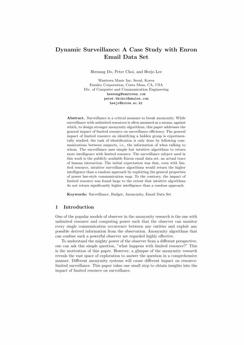
Fig. 1. Illustration of the surveillance model under limited budget. This example showsbudget 3, so that only three nodes (3 red nodes) can be put under surveillance.


Illustration of Limited Resource Figure 1 shows an example of surveillanceunder a limited budget. The graph represents a communication map amongsubjects from a period. The budget is set to 3. There are 23 nodes in the com-munication map. However, the surveillance can only identify 14 nodes; 3 red(or dark in black-and-white) nodes and 11 grey nodes. The rest 9 nodes cannotbe observed by the surveillance due to the limited budget. In other words, thesurveillance returns the intelligence of the 11 discovered nodes.

3.2 Simulation Data

The input data to the simulation is the Enron email data set. So, in this work,each unique email address is treated as an unique individual or a possible surveil-lance subject. The target group is the set of unique email addresses which arein the form of ”[email protected]”. Identifying the target group then be-comes identifying all unique email addresses which end with ”@enron.com”. Thethird parties are identified when their communication with any known subjectis identified by the surveillance

The first public release of the Enron email data set was done in May 2002 bythe Federal Energy Regulatory Commission [6]. Since the public release, severalgroups have subsequently processed and used the data set for a range of differentresearch purposes. As a result, there are a few different versions available now.In this paper, the ISI (Information Sciences Institute) MySql version [10] of thedata set is used. The ISI version was originally based on the CMU (CarnegieMellon University) version [5].

The CMU version contains 517,431 messages from 151 employees. By re-moving meaningless messages from the CMU version, the ISI version now holds252,759 messages from 151 employees, about half of the CMU version. This workslightly improves the ISI version in terms of message validity for surveil- lancepurposes. As a result, the MySql file size changes from 740 Mbytes (ISI version)to 667 Mbytes in this work. The data set used in this work has 252,692 emailmessages, 75,529 unique email addresses from Jan. 4, 1998 through Dec. 21,2002.

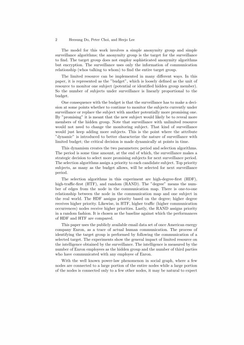
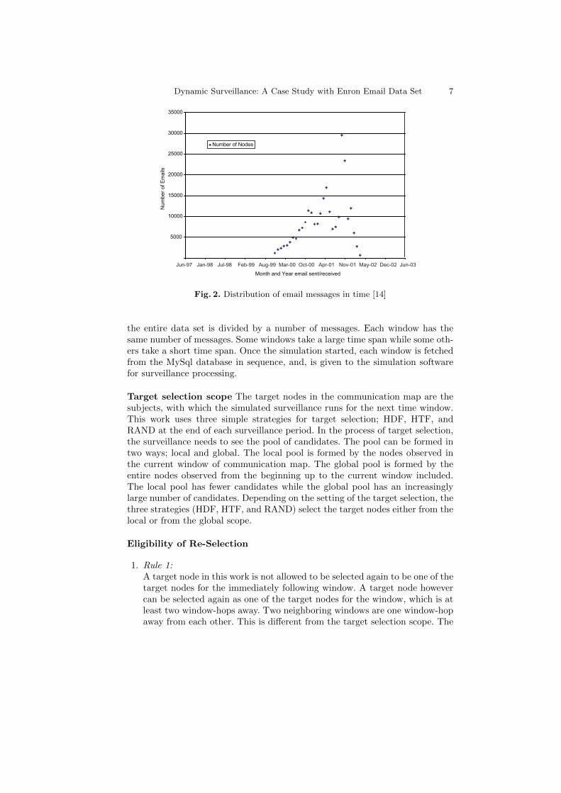
So, the simulated surveillance is to identify all the 151 employees ([email protected]) and other third parties who communicated with one of theemployees. Figure 2 shows the message distribution for the 5-year time period.The message volume peaks around Oct. 2001.

4 Experimental Results

4.1 Simulation Specifics

Surveillance time window The two types of window are used in this work;time based and message based. In the time based, the entire data set is dividedby a time period. Each window has the same time span. Some windows see alarge number of email messages while some others do not. In the message based,


5000

10000

15000

20000

25000

30000

35000

Month and Year email sent/received

Num

ber

of

Em

ails

Number of Nodes

Jun-97 Jan-98 Jul-98 Feb-99 Aug-99 Mar-00 Oct-00 Apr-01 Nov-01 May-02 Dec-02 Jun-03

Fig. 2. Distribution of email messages in time [14]

the entire data set is divided by a number of messages. Each window has thesame number of messages. Some windows take a large time span while some oth-ers take a short time span. Once the simulation started, each window is fetchedfrom the MySql database in sequence, and, is given to the simulation softwarefor surveillance processing.

Target selection scope The target nodes in the communication map are thesubjects, with which the simulated surveillance runs for the next time window.This work uses three simple strategies for target selection; HDF, HTF, andRAND at the end of each surveillance period. In the process of target selection,the surveillance needs to see the pool of candidates. The pool can be formed intwo ways; local and global. The local pool is formed by the nodes observed inthe current window of communication map. The global pool is formed by theentire nodes observed from the beginning up to the current window included.The local pool has fewer candidates while the global pool has an increasinglylarge number of candidates. Depending on the setting of the target selection, thethree strategies (HDF, HTF, and RAND) select the target nodes either from thelocal or from the global scope.

Eligibility of Re-Selection

1. Rule 1:A target node in this work is not allowed to be selected again to be one of thetarget nodes for the immediately following window. A target node howevercan be selected again as one of the target nodes for the window, which is atleast two window-hops away. Two neighboring windows are one window-hopaway from each other. This is different from the target selection scope. The


+6 hours +6 hours +6 hours

Target

Candidates

Target

Candidates

Target

Candidates

(a) HTF, local scope, two subjects, six-hour, re-selection eligibility

+6 hours +6 hours +6 hours

Target

Candidates

Target

Candidates

Target

Candidates

(b) HDF, global scope, two subjects, six-hour, eligibility

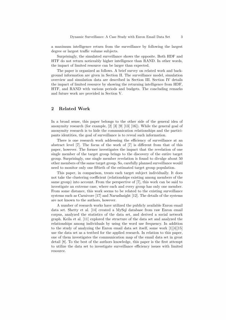
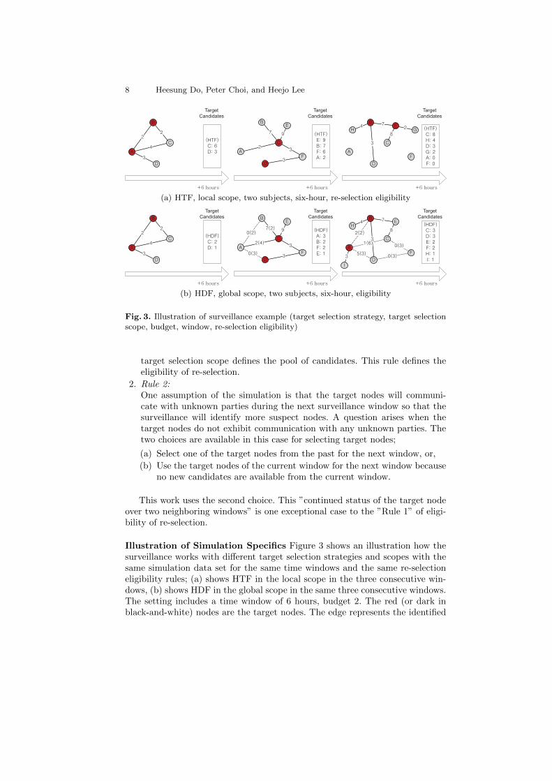
Fig. 3. Illustration of surveillance example (target selection strategy, target selectionscope, budget, window, re-selection eligibility)

target selection scope defines the pool of candidates. This rule defines theeligibility of re-selection.

2. Rule 2:One assumption of the simulation is that the target nodes will communi-cate with unknown parties during the next surveillance window so that thesurveillance will identify more suspect nodes. A question arises when thetarget nodes do not exhibit communication with any unknown parties. Thetwo choices are available in this case for selecting target nodes;

(a) Select one of the target nodes from the past for the next window, or,

(b) Use the target nodes of the current window for the next window becauseno new candidates are available from the current window.

This work uses the second choice. This ”continued status of the target nodeover two neighboring windows” is one exceptional case to the ”Rule 1” of eligi-bility of re-selection.

Illustration of Simulation Specifics Figure 3 shows an illustration how thesurveillance works with different target selection strategies and scopes with thesame simulation data set for the same time windows and the same re-selectioneligibility rules; (a) shows HTF in the local scope in the three consecutive win-dows, (b) shows HDF in the global scope in the same three consecutive windows.The setting includes a time window of 6 hours, budget 2. The red (or dark inblack-and-white) nodes are the target nodes. The edge represents the identified


communication between nodes. The weight of the edge is the communicationvolume; the number of email messages exchanged by the pair of nodes.

In the first window of the Figure 3 (a), there are two target nodes (A, B).Through the target nodes, the surveillance observes the communication betweenA and B, A and C, A and D, and, B and C. In terms of HTF, A is still the highesttraffic node with 9 communications. However, since there are other unknownnodes, C and D, A is not allowed to be selected to be a target node for thenext window. Accordingly, C and D are selected as the target nodes for the nextwindow of 6 hours. In the second window of (a), C is the highest traffic node.Again, however, other new so-far unknown nodes are selected as the target nodesfor the third window; E and B.

The same rules are applied in Figure 3 (b). The differences are the targetselection strategy and scope; HDF in the global scope. The target nodes of thefirst window are A and B. At the end of the first window, A and B are still thehighest degree nodes. Due to the ”eligibility of re-selection”, however, C and Dare selected as the target nodes for the second window. The global scope of thesecond window is represented by the solid and dotted lines between nodes. Thesolid line is the communication occurred in the current window. The dotted lineis the communication observed in previous windows. Likewise, the number inthe parenthesis on the edge is the cumulative communications between the pairof nodes up to the immediately preceding window, while the number out of theparenthesis represents the communications observed in the current window.

In Figure 3 (b), both B and F have the same degree, 2, at the end of thesecond window. The tie is broken in this work in favor of higher traffic; B has7(2) + 0(2), while F has 3 + 3. Eventually A and B are selected as the targetnodes for the third window. Note that A and B were the target nodes for thefirst window. Both A and B are eligible to be a target node for third windowbecause the first and third windows are two window-hops apart. Note that thetwo communication maps made by HDF and HTF grow differently with the samesimulation data set. Both communication maps are incomplete anyway due tothe limited resource.

4.2 Dynamic Surveillance with Limited Budget

In the figures below, the ”suspects”are the unique email addresses of 151 Enronemployees. The ”nodes” are the unique addresses, which are either suspects orany other addresses, which have communicated with the employees at least onceduring the surveillance.

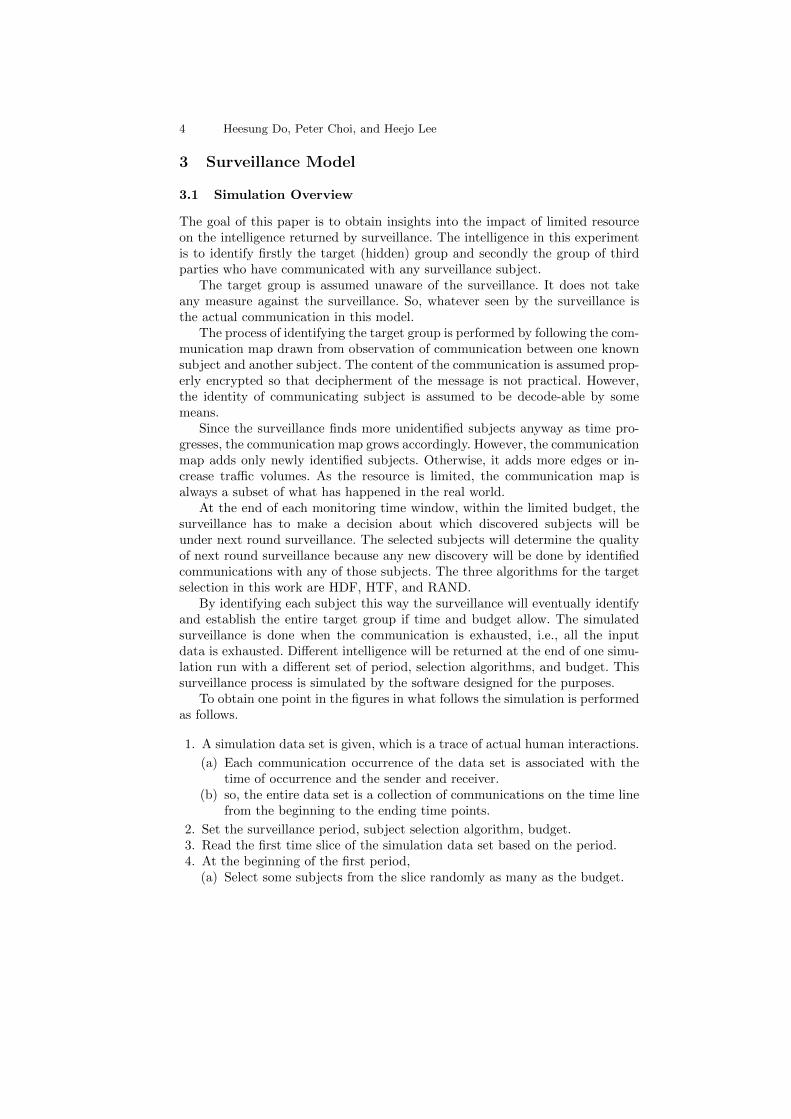
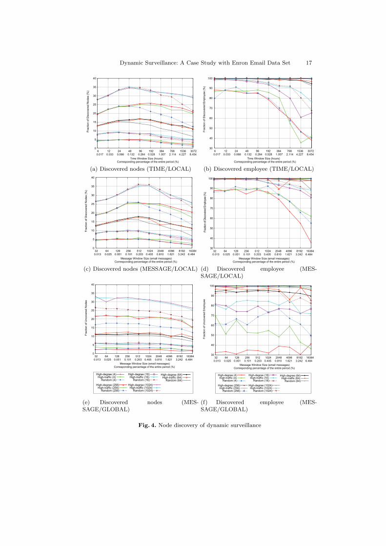
Figure 4 shows six graphs which differ from each other in the window type andtarget selection scope. The first column (a, c, e) shows the node discovery, and,the second column (b, d, f) shows the suspect discovery. The first 4 graphs (a, b,c, d) are obtained using the target selection from the local scope, while the lasttwo (e, f) are obtained by the global scope target selection. The X-axis showsthe surveillance window size in either message or time and its correspondingpercentage of the entire surveillance period (5 years). Note that the X-axis is nota time line. One simulation run produces a value at one point of the curve. The


Y-axis show the averaged intelligence either node or suspect discovery percentageagainst the entire data set size with the given budget, window, target selectionstrategy, and target selection scope.

The first two (a, b) use time windows while the last four (c, d, e, f) usemessage windows. Each graph has five sets of curves; each set represents thebudget 4, 16, 64, 256, and 1024. Each set of the graph in turn shows the perfor-mance of the three target selection strategies; HDF, HTF and RAND under thesame conditions of budget and window. Each graph has fifteen curves in total,therefore.

Each point is obtained by the average value of 30 simulation runs with thesame simulation setting but different seed nodes. For example, in (a), both HDFand HTF with the window of 96 hours and budget 256 produce the node discov-ery ratio of about 25%. This is the averaged value of 30 simulation runs. So eachgraph is a collection of averaged values from a set of independent simulationruns. Simulation runs higher than 30 do not produce noticeable difference. Thebest possible node discovery in this experiment as seen in the figure is about35% or 36% of the entire nodes when the email data set is exhausted.

Global vs. Local Scopes The last two graphs (e, f) use the global target se-lection scope while the first four (a, b, c, d) graphs use the local scope. Onecan expect that the global scope would return higher intelligence because thelarger pool of candidates. To the contrary, the results are the opposite. The nodediscovery rates of (e) are lower than those of (a) and (c). Similarly, the perfor-mance of (f) is lower than (b) and (d). The reason is in the limited budget. Theglobal scope tend to select the same target nodes again in later windows due totheir accumulated higher degrees and traffic volumes. This trend prevents othernew more promising nodes from being selected. The local scope, however, has toselect the target nodes from the new local pool at each window.

Budget vs. Discovery Rates With the increasing budgets, the 151 suspectnodes (employee addresses) are 100% discovered. As can be seen from (b), (d)and (f), the complete suspect (employee) discovery is achieved with the budgets256 and 1,024. So, budgets higher than 1,024 are not experimented. The graphs(a), (c) and (e) show that higher budgets yield higher discovery of nodes. How-ever, while the budget is increased by 4 times at each step, the discovery ratioincreases only sub-linearly.

The ratio of discovery to budget is found only to decrease. With this kindof sub-linearity, an absurdly large budget would be required to discover highernodes than shown in (a) and (c). Further, the return intelligence is found in-creasingly marginal from each multiplicatively higher budget investment.

Time vs. Message-BasedWindow In this experiment, as can be seen in Fig-ure 4 (a) and (c) or (b) and (d), no big performance difference is found betweenthe two different kinds of surveillance period; time and message windows. This issomewhat counter intuitive because the number of communication occurrences


in the time window is likely to be different for each period. The logical explana-tion to this is that the variation of the message volume in the time window wasnot to the extent, where performance degradation would be seen. As seen later,both windows find new nodes at a rather constant rate.

HDF, HTF vs. RAND In (a) and (c), the set of curves seems to have amild peak. Interestingly, the three selection strategies do not show much per-formance difference until that point. After the peak, RAND shows the lowestperformance while HTF is only slightly lower than HDF. Throughout the rangeof budgets, HDF and HTF do not show noticeable difference. One possible log-ical explanation to these results is that, up to some window sizes and budgets,for example, 512 messages or 48 to 96 hours and 64 or higher budgets, intuitivealgorithms do not necessarily perform better than a random approach. In otherwords, the windows and budgets up to the peak point may not be large enoughfor the intuitive algorithms to exploit some patterns in the communication maps.

Peak Interestingly, in (a) and (c), there tends to be a peak in the node discoveryratio. For example, in (a), the node discovery reaches about a little more than35% with the budget 1024, the window of 48 hours regardless of the strategy.Similarly, in (c), the ratio reaches about 36% with the budget 1024, the windowof 512 messages, again, regardless of the strategies. The peak becomes more rec-ognizable with higher budgets. In this work, the peak is interpreted that budgetslarger than certain percentage of the entire nodes may have some optimal rangeof windows to maximize the return intelligence.

The peak is clearer in the message windows in (c) although the overall perfor-mances are not much different from those of time windows in (a). This is becausethe number of message appearing in each window is constant in (c), while it isnecessarily fluctuating in the time windows in (a). The even distribution of mes-sages in (b) must have helped manifest the optimal range of windows.

The performance degradation of (a) and (c) after the peak point is alsointerpreted due to the larger window. The peak point is effectively the turningpoint where the window size becomes sufficiently large to create the global scopeeffect for target selection. By the same argument, the global scope also producesflat curves in (e),

Another side effect of the global scope is the larger gap between RAND andthe other two (HDF, HTF) with large budgets (256, 1,024). In (a) and (c), thegap between RAND and the other two becomes visible only with large budgetsand large windows. Statistically RAND has higher probability to choose worsenodes in the global scope than in the local scope. The wider variety of the globalscope contributes to the poor target node selection of RAND. In the local scope,since it is always created by the most promising nodes from the previous window,RAND has lower probability to choose low performing nodes.


4.3 Variations of Dynamic Surveillance

Strategically Uneven Budget Allocation So far, the budget is evenly allo-cated to each window. This is to reflect the general situation that the dynamicsurveillance would not know when more new nodes would appear in the surveil-lance. Without knowing the future information, the strategy of even budgetallocation would be a reasonable choice.

The general question is whether there would be a better way of budget al-location in an effort to improve node discovery. To be fair, the total amount ofbudget needs to be assumed fixed. The total amount of budget is defined as theaverage budget per window multiplied by the number of windows of the entiresurveillance period, 5 years.

One immediate way is to allocate a relatively large portion of budget tothe early stage of surveillance. The idea is to exploit the general pattern ofcommunication map that a small percentage of nodes are connected to most ofthe nodes.

The hope is that if such small percentage of nodes would be discovered atan early stage, the node discovery would be more effective for the rest of thesurveillance even with less amount of budget to the following windows. Therefore,the two variations of budget allocation are experimented here: firstly 50% of thetotal budget to the early 10% of the surveillance period, secondly 90% of thetotal budget to the early 10% of the surveillance period. The rest of surveillancewindows receive the even distribution of the remaining budget in both cases.

Figure 5 shows the results of the two cases; (a) and (c) show the node andsuspect discovery rates for the first case (50% allocation first), and, (b) and (d)show the second case (90% allocation first). In comparison to Figure 4 (c) and(d) (message window, local scope), the node discovery rates of Figure 5 (a) and(c) are not higher, and those of Figure 5 (b) and (d) are lower. These resultsapparently do not support the hope of finding more node.

More interestingly, in Figure 5, (b) and (d) (90% budget to the first 10%of surveillance period) show even lower rates than in (a) and (c) (50% budgetto the first 10% of surveillance period). This result means that higher budgetallocation to the early stage results in even lower node discovery. In an effortto understand this interesting result, the micro behavior of node discovery isfurther analyzed next.

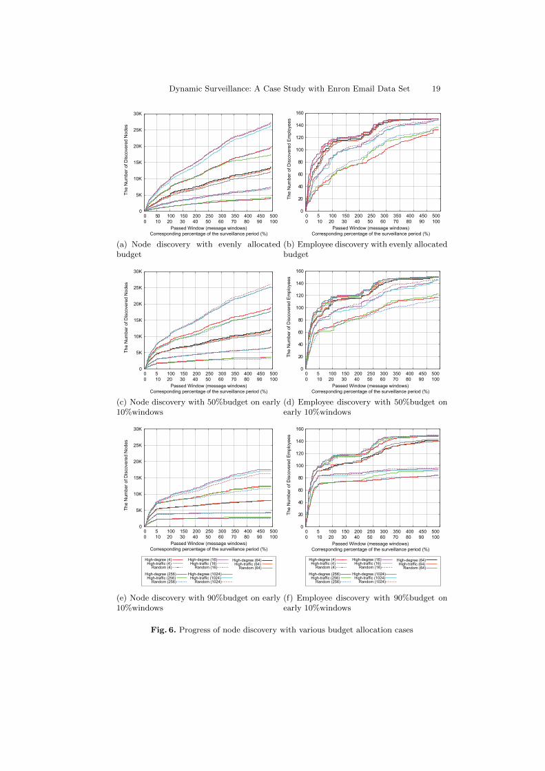
Micro Observation of Node Discovery Figure 6 shows the ”progress” ofnode discovery of three budget allocation cases; even, 50% first, and 90% first al-locations. The X-axis shows the time line in the number of surveillance windows.The Y-axis shows the return intelligence either the number of nodes identified (a,c, e) or the number of suspects (employees) (b, d, f) as the one time simulationprogresses on the time line. As such, the returning intelligence (Y-axis) onlygrows on the time line (X-axis).

Note that these figures are different from the previous ones (Figure 4), wherethe curves show the averaged return intelligence of multiple independent simu-lation runs. Different points of the curve are from different simulation runs. In


comparison, different curves of Figure 6 are from different simulation runs. Thepoints of one curve are all from the same simulation runs.

The left column of three graphs, (a), (c) and (e), show the node discoveryand the right three (b, d, f) show the suspect discovery. The first row, (a) and(b), are for the even distribution, the middle two (c) and (d) for the 50% first,and, the bottom two (e) and (f) are for the 90% first.

The highlight of this figure is the growing rate of the returning intelligence.In (a), the even distribution of budget, the node discovery grows almost linearlyand eventually tops around 27,000 nodes, which is about 35% of the entire nodes.

In (c) the discovery grow rapidly for the first 10% surveillance period andthe growth rate goes down immediately after the first 10% surveillance period.This phenomenon stands out more distinctively in (e). This trend remains thesame even in the suspect discovery rates in (d) and (f).

Interestingly, in (e), the 90% first does not boost the node discovery rateeven for the early 10% of surveillance period in comparison to (c). Evidently,this tells that more than 50% budget allocation to the early 10% of surveillancewould not result any more intelligence return in this case study.

From a slightly different angle, this also suggests that the higher budgetallocation to the early 10% of surveillance was not much effective because thepossible pattern (power-law, for example) of communication map was not fullyrecognizable in the early stage even by the temporarily large budgets. So, in thiscase study, choosing the even budget distribution seems favorable for the twoselection algorithms, HDF and HTF.

4.4 Surveillance with Unlimited Resource

Using the same simulation data set, this section runs the simulation with un-limited resource, i.e., the surveillance monitors every single communication oc-currence between any two nodes. The communication map is complete at anygiven moment, therefore. The motivation is to see the difference between theintelligence returned by resource-limited and -unlimited surveillance.

Figure 7 shows four graphs on the X-Y plane with a logarithmic scale onthe X axis. As before, the Y-value is the ratio of node (unique email address:both employee and third party combined) discovery. The X axis shows the toppercentage of nodes with the priorities assigned by the target selection algorithm.

For example, in (b), the top 1% of nodes selected (on X-axis) either byHDF or HTF are connected with the other 70% or higher (Y-axis) nodes ofthe communication map. This means that the selection of top 1% nodes bythe selection algorithms can identify more than 70% of the nodes at the givenmoment. Since the surveillance has unlimited computing power, each single nodeor communication addition causes a new complete computation of the entirecommunication map. This allows the algorithm to assign the priority based onthe exact global and complete view at any moment.

The four graphs are obtained as follows. First, take the first 0.1%, 1%, 10%,and 100% portion of the simulation data set from the time line. (Remember thatthe simulation data set is a chronologically ordered communication occurrences


among subjects.) Second, sort out the selected portion using the three algo-rithms; HDF, HTF, and RAND. Here, all the nodes, which ever communicatedwith any of the selected nodes are considered discovered. Third, create a curvefor each selection algorithm for the four different sets.

Since the four first portions (0.1%, 1%, 10%, and 100%) are different in sizefrom each other, the connectivity of the top percentage of the first portion tothe rest of the first portion is different from each other, too. For example, thenode discovery by top 1% is more than 80% in (a), more than 70% in (b), morethan 50% in (c), and lastly more than 40% in (d). The larger the first portion,the smaller the top percentage nodes connectivity.

Note that Figure 7 cannot be directly compared to Figure 4, where the X-axiswas a time line while it is the top percentage of priority by the chosen targetselection algorithm.

One convenient way to interpret the four graphs is to regard each one (a, b,c, d) as the snapshot of the surveillance with unlimited resource at the momentswhere the communication map reaches the first 0.1%, 1%, 10%, and eventually100% of the entire nodes. Because it is resource limitation-free, the surveillanceknows exactly what has happened. The current communication map itself reveals100% discovery at any time. This is the big difference between the resource-limited and -unlimited surveillance.

With the always complete Communication map a few interesting observationsare readily available.

1. As the surveillance progresses, HDF returns higher intelligence than HTF,2. RAND returns constantly poor intelligence.3. The curve patterns do not seem to change regardless of the size of the early

portion of data set.

Considering these observations, it can be said that there maybe some patternsin the complete communication map, and, the HDF seems to exploit the patternsmost effectively. It indirectly shows that the pattern may be a power law-style.Since RAND does not utilize any pattern, it should return the worst intelligence.

There is an interesting observation with the sizes of window. Figure 4 usesa range of window sizes. For example, the largest window size in Figure 4 (c) is16,384 messages, which corresponds to about 6.5% of the entire data set. Thiswindow size is actually larger than those of Figure 7 (a) and (b). The largestwindow of Figure 4 (a) is 3,072 hours, corresponding to about 8.5% of the entiresurveillance period. Interestingly even these large window sizes do not make thenode discovery higher than 40% in Figure 4 (a) and (c).

Again, the major contributor to this interesting result is the incompletenessof the communication map due to the limited budget. The incomplete mapconstantly leads a sub-optimal selection of target nodes for next surveillanceround. This phenomenon continues even with considerably large window sizes.

Lastly, the lowest curve in Figure 7 (d), is a hypothetical case, in which thetarget group uses an anonymity system such that the node discovery is perfectlylinearly proportional to the surveillance budget. So, in order to find out X numberof subjects of the target group, the budget of X should be invested. Finding the


existence of such an anonymity system is out of the scope. This case, however,gives the lower bound to the surveillance performance. Even RAND performsbetter than this imaginary case.

5 Conclusions

The motivation of this work is to obtain insights into the impact of limitedresource on the intelligence returned by surveillance. This work takes an ex-perimental method in an effort to approach the right answer. The experimentwas done in a form of simulated surveillance using a publicly available Enronemail data set. The data set does not contain a complicated anonymity algo-rithms except data encryption. So the target selection algorithms were simplefor the surveillance. However, the nature of the data set, a reflection of humaninteractions as a real trace, gives some credit on the actuality of the data set.

The experiment was done firstly with limited resource and followed by an-other form of surveillance with unlimited resource for comparison. As seen inthe two strikingly different graphs (Figure 4, Figure 7), the impact of limitedresource can be larger than expected. As seen in Figure 4, the idea of exploit-ing some intuitive patterns (high degree or high traffic) on the communicationmap was not effective with limited budgets. After the peak points, larger bud-gets and larger window sizes produced worse intelligence. Although both HDFand HTF perform much better that RAND after the peak, the intelligence re-turned by both was monotonically decreasing with considerably larger budgetsand window sizes.

By comparing the two surveillance cases (resource limited vs. unlimited),even though this work is about only one single case study with Enron emaildata set, some conclusions can be drawn that:

– Surveillance with limited resource may have some optimal points in terms ofthe combination of budget and window size that can maximize the qualityof intelligence returned by the surveillance.

– Even allocation of budgets throughout the surveillance may work better thanstrategically uneven allocations.

– The incompleteness of the communication map seems to be maintainedthroughout the surveillance. This may be the major contributor to the obser-vation that both HDF and HTF do not return significantly higher intelligencethan RAND.

This work, although the generality is limited due to the scope of single casestudy, solicits further work, including but not limited to, on the optimal combi-nation of budget and window size while the hidden group size is still unknown(with possible estimates of the group size), and, on the minimum size of com-munication map that is yet large enough to show some patterns to be utilized.


References

1. L. Akoglu, M. McGlohon, and C. Faloutsos. Anomaly detection in large graphs.In CMU-CS-09-173 Technical Report, 2009.

2. N. Bansod, A. Malgi, B. K. Choi, and J. Mayo. Muon: Epidemic based mu-tual anonymity in unstructured p2p networks. Computer Networks, 52(5):915–934,2008.

3. O. Berthold, H. Federrath, and S. Kopsell. Web mixes: A system for anonymousand unobservable internet access. In Workshop on Design Issues in Anonymityand Unobservability, pages 115–129, 2000.

4. A. Chapanond, M. S. Krishnamoorthy, and B. Yener. Graph theoretic and spectralanalysis of enron email data. Computational & Mathematical Organization Theory,11(3):265–281, 2005.

5. CMU. Enron email dataset. http://www.cs.cmu.edu/ enron.6. F. E. R. Commission. Enron investigation.

http://www.ferc.gov/industries/electric/indus-act/wec/enron/info-release.asp.7. G. Danezis and B. Wittneben. The economics of mass surveillance and the ques-

tionable value of anonymous communications. In R. Anderson, editor, Proceedingsof the Fifth Workshop on the Economics of Information Security (WEIS 2006),Cambridge, UK, June 2006.

8. J. Diesner, T. L. Frantz, and K. M. Carley. Communication networks from theenron email corpus ”it’s always about the people. enron is no different”. Compu-tational & Mathematical Organization Theory, 11(3):201–228, 2005.

9. D. M. Goldschlag, M. G. Reed, and P. F. Syverson. Onion routing. Commun.ACM, 42(2):39–41, 1999.

10. ISI. Enron dataset. http://www.isi.edu/ adibi/Enron/Enron.htm.11. P. S. Keila and D. B. Skillicorn. Structure in the enron email dataset. Computa-

tional & Mathematical Organization Theory, 11(3):183–199, 2005.12. NarusInsight. Narusinsight solutions for traffic intelligence.

http://www.narus.com/index.php/product.

13. R. Sherwood, B. Bhattacharjee, and A. Srinivasan. P5: A protocol for scalableanonymous communication. Journal of Computer Security, 13(6):839–876, 2005.

14. J. Shetty and J. Adibi. The enron email dataset database schema and brief statis-tical report, 2004.

15. J. Shetty and J. Adibi. Discovering important nodes through graph entropy thecase of enron email database. In Proceedings of the 3rd international workshop onLink discovery, LinkKDD ’05, pages 74–81, New York, NY, USA, 2005. ACM.

16. C. Shields and B. N. Levine. A protocol for anonymous communication over theinternet. In ACM Conference on Computer and Communications Security, pages33–42, 2000.

17. H. E. Ventura, J. M. Miller, and M. Deflem. Governmentality and the war on terror:Fbi project carnivore and the diffusion of disciplinary power. Critical Criminology,13:55–70, 2005.


0

5

10

15

20

25

30

35

40

6

0.017

12

0.033

24

0.066

48

0.132

96

0.264

192

0.528

384

1.057

768

2.114

1536

4.227

3072

8.454

Fra

ctio

n o

f D

isco

ve

red

No

de

s (

%)

Time Window Size (hours)

Corresponding percentage of the entire period (%)

(a) Discovered nodes (TIME/LOCAL)

30

40

50

60

70

80

90

100

Fra

ctio

n o

f D

isco

ve

red

Em

plo

ye

e (

%)

6

0.017

12

0.033

24

0.066

48

0.132

96

0.264

192

0.528

384

1.057

768

2.114

1536

4.227

3072

8.454

Time Window Size (hours)


(b) Discovered employee (TIME/LOCAL)

32

0.013

64

0.025

128

0.051

256

0.101

512

0.203

1024

0.405

2048

0.810

4096

1.621

8192

3.242

16384

6.484

Message Window Size (email messages)

0

5

10

15

20

25

30

35

40

Fra

ctio

n o

f D

isco

ve

red

No

de

s (

%)


(c) Discovered nodes (MESSAGE/LOCAL)

30

40

50

60

70

80

90

100

Fra

ctio

n o

f Dis

cove

red E

mplo

yee (%

)

32

0.013

64

0.025

128

0.051

256

0.101

512

0.203

1024

0.405

2048

0.810

4096

1.621

8192

3.242

16384

6.484



(d) Discovered employee (MES-SAGE/LOCAL)

0

5

10

15

20

25

30

35

40

Fra

ctio

n o

f U

nco

ve

red

No

de

s

32

0.013

64

0.025

128

0.051

256

0.101

512

0.203

1024

0.405

2048

0.810

4096

1.621

8192

3.242

16384

6.484



High-degree (4)High-traffic (4)

Random (4)


Random (16)


Random (64)


Random (256)


Random (1024)

(e) Discovered nodes (MES-SAGE/GLOBAL)

30

40

50

60

70

80

90

100

Fra

ctio

n o

f U

nco

ve

red

Em

plo

ye

e

32

0.013

64

0.025

128

0.051

256

0.101

512

0.203

1024

0.405

2048

0.810

4096

1.621

8192

3.242

16384

6.484




Random (4)


Random (16)


Random (64)


Random (256)


Random (1024)

(f) Discovered employee (MES-SAGE/GLOBAL)

Fig. 4. Node discovery of dynamic surveillance


0

5

10

15

20

25

30

35

40

Fra

ctio

n o

f U

nco

ve

red

No

de

s (

%)

32

0.013

64

0.025

128

0.051

256

0.101

512

0.203

1024

0.405

2048

0.810

4096

1.621

8192

3.242

16384

6.484



(a) Discovered nodes with 50% budget onearly 10% windows

0

5

10

15

20

25

30

35

40

Fra

ctio

n o

f U

nco

ve

red

No

de

s (

%)

32

0.013

64

0.025

128

0.051

256

0.101

512

0.203

1024

0.405

2048

0.810

4096

1.621

8192

3.242

16384

6.484



(b) Discovered nodes with 90% budget onearly 10% windows

20

30

40

50

60

70

80

90

100

Fra

ctio

n o

f U

nco

ve

red

Em

plo

ye

e

32

0.013

64

0.025

128

0.051

256

0.101

512

0.203

1024

0.405

2048

0.810

4096

1.621

8192

3.242

16384

6.484




Random (4)


Random (16)


Random (64)


Random (256)


Random (1024)

(c) Discovered employee with 50% budget onearly 10% windows

20

30

40

50

60

70

80

90

100

Fra

ctio

n o

f U

nco

ve

red

Em

plo

ye

e

32

0.013

64

0.025

128

0.051

256

0.101

512

0.203

1024

0.405

2048

0.810

4096

1.621

8192

3.242

16384

6.484




Random (4)


Random (16)


Random (64)


Random (256)


Random (1024)

(d) Discovered employee with 90% budget onearly 10% windows

Fig. 5. Node discovery with variable budget distribution in before-event surveillance(message window based)


0

5K

10K

15K

20K

25K

30K

0

0

5

10

0 100

20

150

30

200

40

250

50

300

60

350

70

400

80

450

90

500

100

Th

e N

um

be

r o

f D

isco

ve

red

No

de

s

Passed Window (message windows)

Corresponding percentage of the surveillance period (%)

(a) Node discovery with evenly allocatedbudget

0

20

40

60

80

100

120

140

160

Th

e N

um

be

r o

f D

isco

ve

red

Em

plo

ye

es

0

0

5

10

100

20

150

30

200

40

250

50

300

60

350

70

400

80

450

90

500

100



(b) Employee discovery with evenly allocatedbudget

0 0

0

5

10

100

20

150

30

200

40

250

50

300

60

350

70

400

80

450

90

500

100



5K

10K

15K

20K

30K

Th

e N

um

be

r o

f D

isco

ve

red

No

de

s

25K

(c) Node discovery with 50%budget on early10%windows

0

20

40

60

80

100

120

140

160

Th

e N

um

be

r o

f D

isco

ve

red

Em

plo

ye

es

0

0

5

10

100

20

150

30

200

40

250

50

300

60

350

70

400

80

450

90

500

100



(d) Employee discovery with 50%budget onearly 10%windows

0

5K

10K

15K

20K

30K

Th

e N

um

be

r o

f D

isco

ve

red

No

de

s

0

0

5

10

100

20

150

30

200

40

250

50

300

60

350

70

400

80

450

90

500

100



25K


Random (4)


Random (16)


Random (64)


Random (256)


Random (1024)

(e) Node discovery with 90%budget on early10%windows

0

20

40

60

80

100

120

140

160

Th

e N

um

be

r o

f D

isco

ve

red

Em

plo

ye

es

0

0

5

10

100

20

150

30

200

40

250

50

300

60

350

70

400

80

450

90

500

100




Random (4)


Random (16)


Random (64)


Random (256)


Random (1024)

(f) Employee discovery with 90%budget onearly 10%windows

Fig. 6. Progress of node discovery with various budget allocation cases


0

10

20

30

40

50

60

70

80

90

100

0.1 1 10 100

Fra

ctio

n o

f D

isco

ve

red

No

de

s (

%)

Fraction of Nodes under Surveillance (%)

High-degreeHigh-traffic

Random

(a) 0.1% data of whole email messages

0

10

20

30

40

50

60

70

80

90

100

0.01 0.1 1 10 100

Fra

ctio

n o

f D

isco

ve

red

No

de

s (

%)



Random

(b) 1% data of whole email messages

0

10

20

30

40

50

60

70

80

90

100

0.001 0.01 0.1 1 10 100

Fra

ctio

n o

f D

isco

ve

red

No

de

s (

%)



Random

(c) 10% data of whole email messages

0

10

20

30

40

50

60

70

80

90

100

10E-4 10E-3 10E-2 1 10 100

Fra

ctio

n o

f D

isco

ve

red

No

de

s (

%)



RandomWorst case

0

8K

15K

22K

30K

38K

45K

53K

60K

68K

76K

Th

e N

um

be

r o

f U

nco

ve

red

No

de

s

(d) 100% data of whole email messages

Fig. 7. Surveillance with unlimited resource

Dynamic Surveillance: A Case Study with Enron Email Data Set · 2014-09-02 · Dynamic Surveillance: A Case Study with Enron Email Data Set 3 a maximum intelligence return from the

Documents