Dynamic Stability and Flight Control of Biomimetic Flapping ...

aerospace

Article

Dynamic Stability and Flight Control of BiomimeticFlapping-Wing Micro Air Vehicle

Muhammad Yousaf Bhatti, Sang-Gil Lee and Jae-Hung Han *

�����������������

Citation: Bhatti, M.Y.; Lee, S.-G.;

Han, J.-H. Dynamic Stability and

Flight Control of Biomimetic

Flapping-Wing Micro Air Vehicle.

Aerospace 2021, 8, 362. https://

doi.org/10.3390/aerospace8120362

Academic Editor: Mostafa Nabawy

Received: 18 October 2021

Accepted: 20 November 2021

Published: 24 November 2021

Publisher’s Note: MDPI stays neutral

with regard to jurisdictional claims in

published maps and institutional affil-

iations.

Copyright: © 2021 by the authors.

Licensee MDPI, Basel, Switzerland.

This article is an open access article

distributed under the terms and

conditions of the Creative Commons

Attribution (CC BY) license (https://

creativecommons.org/licenses/by/

4.0/).

Department of Aerospace Engineering, Korea Advanced Institute of Science and Technology,Daejeon 34141, Korea; [email protected] (M.Y.B.); [email protected] (S.-G.L.)* Correspondence: [email protected]

Abstract: This paper proposes an approach to analyze the dynamic stability and develop trajectory-tracking controllers for flapping-wing micro air vehicle (FWMAV). A multibody dynamics simulationframework coupled with a modified quasi-steady aerodynamic model was implemented for stabilityanalysis, which was appended with flight control block for accomplishing various flight objectives.A gradient-based trim search algorithm was employed to obtain the trim conditions by solving thefully coupled nonlinear equations of motion at various flight speeds. Eigenmode analysis showedinstability that grew with the flight speed in longitudinal dynamics. Using the trim conditions, welinearized dynamic equations of FWMAV to obtain the optimal gain matrices for various flight speedsusing the linear-quadratic regulator (LQR) technique. The gain matrices from each of the linearizedequations were used for gain scheduling with respect to forward flight speed. The reference trackingaugmented LQR control was implemented to achieve transition flight tracking that involves hovering,acceleration, and deceleration phases. The control parameters were updated once in a wingbeat cycleand were changed smoothly to avoid any discontinuities during simulations. Moreover, trajectoriestracking control was achieved successfully using a dual loop control approach. Control simulationsshowed that the proposed controllers worked effectively for this fairly nonlinear multibody system.

Keywords: biomimetic flapping-wing micro air vehicle; flight dynamics and stability; hovering andforward flight; LQR optimal controller; dual loop position controller

1. Introduction

In recent years, research and development involving bio-inspired aerospace systemshave increased because of surging demands in micro and nano air vehicles for bothcommercial and military applications with stringent size, nimbleness, concealment, andspace requirements. Moreover, these systems are also expected to possess high agility,hovering capability, sudden obstruction avoidance, quick shifting from hovering to forwardspeed and vice versa, and moving object tracking with smart navigation. These exceptionalfeatures are common traits of nature-based flyers; therefore, scientists are trying to mimictheir remarkable flights. For this, a large amount of work has been done in the design anddevelopment of micro-scale flying robots such as KUBeetle-S [1], autonomous FWMAV [2],saturn aircraft [3], robobee [4], robotic dragonfly [5], ornithopter-type MAV [6], locust-likesmall-scale robots [7], and entomopter [8]. Mimicking insects’ flight impose challengesin several fields that still need detailed attention, including low Reynolds number-basedunsteady aerodynamics, mathematical modeling, flight dynamics, trim methodologies,control approaches, miniature hardware requirements, lightweight materials, and powersystem requirements.

Most of the FWMAV’s flight dynamics and control work in literature is based onlimitations and assumptions considering varying degree of complexity in various areas.These questionable aspects include consideration of wing inertia [9], flexibility of wing [10],nonlinearity of mathematical model [11,12], fidelity of the aerodynamic model [13,14], and

Aerospace 2021, 8, 362. https://doi.org/10.3390/aerospace8120362 https://www.mdpi.com/journal/aerospace

Aerospace 2021, 8, 362 2 of 32

consideration of the coupling between the planes of motion [15]. Different types of researchworks are available that have ignored or adopted one or more of these aspects for theFWMAV’s stability analysis and control implementation. This may result in less accuratecharacterization of the system’s dynamic stability, and implementing control to it mightlead to incorrect results in flight performance analysis.

Three assumptions are chiefly employed while deriving the nonlinear equations ofmotion: neglecting the wings inertial effects, averaging the FWMAV’s body dynamics overeach flapping cycle, and linearizing the nonlinear time-periodic (NLTP) model for ease instability characterization and control implementation [15,16]. Using these assumptions,the eigenvalue analysis technique is used for stability characterization. Most of the earlieststudies have ignored the wings inertial effects on the complete FWMAV’s system foreither stability and/or control work [11,17–25]. Taylor and Thomas [11,17] were the firstto analyze the dynamic flight stability of flapping wings flight but also ignored the winginertial effects like other studies [18–25]. However, Orlowski and Girard [9] in theirsimulations compared the results with and without the wing inertia. The simulationscomparison showed that neglecting the wing inertia caused a significant difference in theresults. Similarly, some researchers reported that considering the wing inertia is necessaryto accurately understand and simulate the FWMAV system [26–30].

Another simplifying assumption is that most of the stability analysis studies forhovering and/or forward flight are conducted on the basis of averaging of the bodydynamics over each flapping cycles [11,17–19,21,22,25]. Averaging theorem is based onthe singular perturbation theory, and smaller errors are expected for higher flappingfrequencies as suggested by Taha et al. [16]. Moreover, the third assumption of linearizingthe NLTP model to linear time invariant (LTI) model for undergoing the stability analysisof FWMAVs is also widely adopted [11,19,31]. Dietl and Garcia [20] utilized floquet theoryfor analyzing the dynamic stability using a linearized time-periodic (LTP) model, which isalso supported by other researchers [16,32,33]. In contrast, some studies have used directtime integration approach to solve the fully coupled nonlinear FWMAV model for stabilityanalysis, which incorporates NLTP effects [12,15,34].

Regarding aerodynamics, many studies are available that used either high-fidelity orlow-fidelity models with their own advantages and disadvantages. High-fidelity modelsinclude computational fluid dynamics (CFD), which are related to the direct numericalsimulations (DNS), such as employed by Sun and Xiong [25], Sun et al. [19], Gao et al. [35],and Xiong and Sun [31]. Although these high-fidelity models much better incorporatethe unsteady flow effects, they are computationally very expensive and may not be theoptimal choice for intensive stability analysis and control simulations, as discussed byTaha et al. [16]. On the other hand, low-fidelity aerodynamic models, such as steadyand quasi-steady (QS) models, consume less computational cost and time and producereasonable results for both stability and control analyses. The steady state models are basedon different aerodynamic theories: actuator disk theory as utilized by Pennycuick [36]and Ellington [37], lift line theory devised by Prandtl and employed by Phlips et al. [38],and vortex ring theory as suggested by Ansari [39]. In contrast, basic QS aerodynamicmodels suggest that the instantaneous forces on the wings are fully dependent on theinstantaneous flapping velocity, rotational angle, and wing’s design, regardless of theflow field. Xuan et al. [40] reviewed these aerodynamic models and categorized them asOsborne, Walker, and Dickinson models, which are based on blade element theory thatignores span wise flows and wake-related unsteady effects. However, the modified QSmodel in the current study considered the additional lift from leading edge vortex (LEV)and the effects of wing rotation as discussed in previous studies [41,42].

Dynamic stability has been extensively studied because most insect-like FWMAVsdo not have tail wing for stabilization. Taha et al. [43] conducted a longitudinal stabilityanalysis of the averaged and linearized dynamics of hovering insects. They found that themean angle of attack and flapping frequency have effects on damping in longitudinal plane.Sun et al. [19] also analyzed the hovering flight regarding longitudinal flight dynamics

Aerospace 2021, 8, 362 3 of 32

characteristics of four different insects. They found that all of the four insects have oneunstable oscillatory mode, one stable fast subsidence mode, and one stable slow subsidencemode. Au and Park [44] showed that modes of FWMAV can be changed depending uponthe location of the center of gravity position. Regarding forward flight, some studieswere also conducted for different insect models [10,31,45]. These studies showed that inlongitudinal plane, all of the insect models are unstable. Moreover, Cheng and Deng [46]explained the principles of the flapping counter torque (FCT), which results in significantdamping in system dynamics.

In order to control FWMAV, which is a nonlinear system, both linear and nonlinearcontrol methods have been applied. For linear control methods, Oppenheimer et al. [47]used wing bias as the control input. The difference in flapping frequency between upstrokeand downstroke was generated by the wing bias. A linear controller was designed to trackthe trajectory in three-dimensional space. Moreover, Loh et al. [48] used the proportional–integral–differential (PID) controller for the hovering FWMAV. Flapping frequency, phasedifference of wing kinematics, and shift in center of gravity were used as the control inputs.For nonlinear control method, Khanmirza et al. [49] designed a controller with quaternion-based dynamic wrench method for trajectory tracking. With that controller, the FWMAVachieved the cruise and the Cuban-8 maneuvers. Banazadeh and Taymourtash [50] appliedan adaptive sliding mode technique for position control in the presence of uncertainties.Three control inputs were used: flapping amplitude, stroke plane angle, and phase offlapping motion. Desired trajectory can be followed without prior information aboutuncertainties. Although the above research works have provided essential informationfor FWMAV control, these studies have ignored the wing inertia effects in their controlsimulations. A few researchers have considered the wing inertial effects in their controlsimulations [14,51,52].

A few previous studies have dealt with multibody model incorporating the winginertia effect and FWMAV dynamics–aerodynamics coupling. Since the multibody modelof a novel flapping wing rotor (FWR), which included the wing inertia, agreed well withexperimental results [53], the current study also incorporated the wing inertia effect. Thecurrent study employed a multibody dynamics simulation framework that was appendedwith a gradient-based trim search algorithm to find the trimmed wing kinematics andinitial conditions for velocities to obtain a linear periodic-based solution for the nonlinearFWMAV model, which has been ignored in previous studies [19,25,31]. These previousstudies neglected the influence of FWMAV’s body dynamics and dynamics–aerodynamicscoupling and did not provide the periodic solution in free-flying conditions as assertedby Kim et al. [45] and Wu et al. [54]. Additionally, the current study utilized a modifiedquasi-steady (QS) aerodynamics model that considers the wing pitching moment effect,added-mass effect, and rotational flow effect and accounted for the shift in the aerodynamiccenter at higher angles of attack. Using the simulation framework, we characterizedlongitudinal dynamic stability for simplified wing kinematics, as it is suitable for controlimplementation purposes. Regarding FWMAV control, previous studies have consideredcontrolling only the hovering or low forward speeds conditions [48,55], while some studieshave ignored wings inertial effect in controlling the FWMAV [48–50,55–58]. However, thecurrent study considered controlling the hovering condition, forward flight conditions,transition flight conditions, and trajectories tracking while considering the wings inertialeffects. Since dynamic characteristics, trim conditions, and aerodynamics characteristicsvary with the flight speed of the FWMAV, the controllers designed by linearizing the systemaround hovering state cannot function well when the FWMAV is required to accelerate.Consequently, a transition flight controller was designed that utilizes speed-dependentgain scheduling to account for our parametric varying nonlinear system. Using the trimsearch results, we linearized the equations of motion at various flight speeds to obtainthe optimal gain matrices using the LQR control technique. These gain matrices wereutilized to model the gain function that varies with the forward speed references. Thisspeed-dependent gain matrix function is input to the feedback control loop of the FWMAV

Aerospace 2021, 8, 362 4 of 32

in control simulations such as transition flight tracking that involves hovering, acceleration,constant speed, deceleration, and hovering phases. Results show the controller workedwell with varying forward flight speed references. Moreover, previous studies have usedcomplicated nonlinear control methods for position controlling [14,51,52]; however, inthe current study, by adjusting forward speed references with a proportional-integral(PI) controller that uses position errors as input, we tracked various reference trajectorieswith increasing level of complexity to validate the effectiveness of our position controller.Control simulations showed that combinations of different linear control techniques workwell to effectively control both the linear and nonlinear models.

The rest of the paper is organized as follows: In Section 2, the materials and methodsare presented, including FWMAV model and coordinate systems definitions, details of thewing kinematics and aerodynamic model, the multibody dynamics simulation framework,and the gradient-based trim search algorithm. It also details the linearization of nonlinearequations of motion for the FWMAV system. Moreover, it explains the design of thecontroller for transition flight tracking by obtaining optimal gains with the augmented LQRcontrol technique and the design of trajectory tracking controller. Results and discussionare presented in Section 3. Firstly, it shows the results of stability characterization forlongitudinal dynamics in both hovering and forward flight. Next, the results of fixedflight conditions’ control and transition flight control are discussed. Furthermore, Section 3details the results of various reference trajectories tracking. Finally, concluding remarks arepresented in Section 4.

2. Materials and Methods2.1. FWMAV Multibody Model and Coordinate Systems2.1.1. FWMAV Multibody Modeling

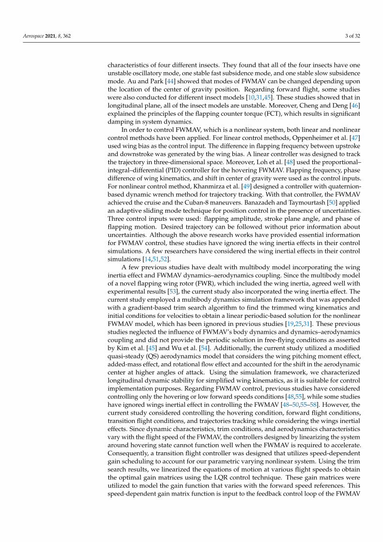
In this study, a full-scale multibody dynamic model of a hawkmoth-like FWMAVis considered. The reference insect is modeled into five rigid parts: head, thorax, andabdomen that form the main body and a pair of wings to precisely locate the center ofgravity as shown in Figure 1 [10,15,35,45,59]. Since the fore and hind wings flap in asynchronous manner, they are assembled as a single wing. Each wing is connected tothe thorax with a 3 degrees of freedom (DOF) revolute joint, while the head, thorax, andabdomen are connected with fixed joints. The morphological parameters for the referencehawkmoth-like FWMAV are obtained from Gao et al. [35], Ellington [59], Hedrick andDaniel [60], and O’Hara and Palazotto [61]. Each wing is divided into five strips of width∆r for applying the QS aerodynamic model as depicted in Figure 1. Figure 1 and Table 1detail the morphological data and nomenclature related to the reference FWMAV modelutilized in this study.

Aerospace 2021, 8, x FOR PEER REVIEW 4 of 32

were utilized to model the gain function that varies with the forward speed references. This speed-dependent gain matrix function is input to the feedback control loop of the FWMAV in control simulations such as transition flight tracking that involves hovering, acceleration, constant speed, deceleration, and hovering phases. Results show the control-ler worked well with varying forward flight speed references. Moreover, previous studies have used complicated nonlinear control methods for position controlling [14,51,52]; how-ever, in the current study, by adjusting forward speed references with a proportional-integral (PI) controller that uses position errors as input, we tracked various reference tra-jectories with increasing level of complexity to validate the effectiveness of our position controller. Control simulations showed that combinations of different linear control tech-niques work well to effectively control both the linear and nonlinear models.

The rest of the paper is organized as follows: In Section 2, the materials and methods are presented, including FWMAV model and coordinate systems definitions, details of the wing kinematics and aerodynamic model, the multibody dynamics simulation frame-work, and the gradient-based trim search algorithm. It also details the linearization of nonlinear equations of motion for the FWMAV system. Moreover, it explains the design of the controller for transition flight tracking by obtaining optimal gains with the aug-mented LQR control technique and the design of trajectory tracking controller. Results and discussion are presented in Section 3. Firstly, it shows the results of stability charac-terization for longitudinal dynamics in both hovering and forward flight. Next, the results of fixed flight conditions’ control and transition flight control are discussed. Furthermore, Section 3 details the results of various reference trajectories tracking. Finally, concluding remarks are presented in Section 4.

2. Materials and Methods 2.1. FWMAV Multibody Model and Coordinate Systems 2.1.1. FWMAV Multibody Modeling

In this study, a full-scale multibody dynamic model of a hawkmoth-like FWMAV is considered. The reference insect is modeled into five rigid parts: head, thorax, and abdo-men that form the main body and a pair of wings to precisely locate the center of gravity as shown in Figure 1 [10,15,35,45,59]. Since the fore and hind wings flap in a synchronous manner, they are assembled as a single wing. Each wing is connected to the thorax with a 3 degrees of freedom (DOF) revolute joint, while the head, thorax, and abdomen are con-nected with fixed joints. The morphological parameters for the reference hawkmoth-like FWMAV are obtained from Gao et al. [35], Ellington [59], Hedrick and Daniel [60], and O’Hara and Palazotto [61]. Each wing is divided into five strips of width rΔ for applying the QS aerodynamic model as depicted in Figure 1. Figure 1 and Table 1 detail the mor-phological data and nomenclature related to the reference FWMAV model utilized in this study.

Figure 1. FWMAV multibody model and coordinate systems. Figure 1. FWMAV multibody model and coordinate systems.

Aerospace 2021, 8, 362 5 of 32

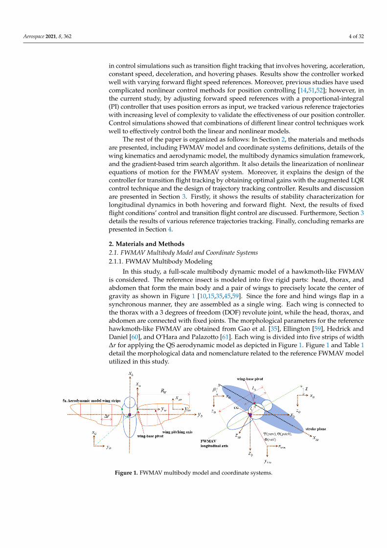
Table 1. Morphological parameters and nomenclature of the reference hawkmoth-like FWMAV.

Parameter (Unit) Description Value

ms (mg) Total system’s mass 1437.5mw (mg) Single wing’s mass 48.3Ls (mm) Total length of the system (anterior tip to posterior tip) 40.2Rw (mm) Wing span 48.3r2 (mm) Radius of second moment of wing area 24.6tw (mm) Wing thickness 3.7 × 10−2

Sw (mm2) Single wing area 879.8c (mm) Mean aerodynamic chord 18.1l1 (mm) Distance between center of mass (CG) and wing-pivot point 10.9l (mm) Distance between center of mass (CG) and anterior tip 20.5

Iyy (kg·mm2) Mass moment of inertia of the system 0.28χo (o) Trimmed body pitch angle Trimmed resultβo (o) Trimmed stroke plane angle Trimmed result

fo (Hz) Trimmed flapping frequency Trimmed resultφo (o) Trimmed stroke positional angle Trimmed resultαo (o) Trimmed feathering angle Trimmed resultf (Hz) Flapping frequency Wing kinematicsφ (o) Stroke positional angle Wing kinematicsα (o) Feathering angle Wing kinematics

2.1.2. Coordinate Systems

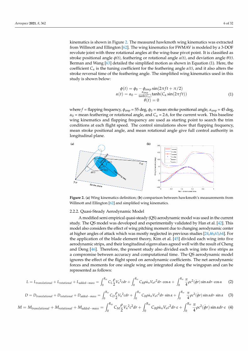
To model the 6-DOF FWMAV system, we used six different coordinate systems, asshown in Figure 1. Global coordinate system [xG yG zG] is used for defining the globallocations, attitudes, and linear and angular velocities of the system. This frame is utilizedin obtaining equilibrium conditions of the model at different flight speeds. It is also usedfor reference trajectories tracking. Body coordinate system [xb yb zb] is connected to thelocation of the overall center of mass of the system. All body flight states are defined in thiscoordinate system. When all Euler angles for FWMAV attitudes are zero, the xb axis of thisframe is parallel to the xG axis. The yb axis stretches out to the right wing’s tip. The bodypitch angle χ is defined as the angle between the xG axis and the body longitudinal axis.The positioning of the body coordinate system with respect to the global coordinate systemis parameterized by this sequence of Euler angles: Ψ (yaw), Θ (pitch), and Φ (roll). Stroke-plane coordinate system [xsp ysp zsp] is the key frame to describe the resultant aerodynamicforces and moments. The induced aerodynamics forces and moments by the 6-DOF body’smotion are added to the instantaneous ones as produced by each aerodynamic strip in thisframe. The angle β between the xsp axis and the xG axis is defined as the stroke-plane angle.Wing-fixed coordinate system [xw yw zw] is defined at the wing-base pivot point. The ywaxis of this coordinate system is stretched out in the span-wise direction and defines thewing pitching axis. The wing-fixed coordinate system defines the wing kinematics on thebasis of the stroke-plane coordinate system. Aerodynamic strip coordinate system [xstr ystrzstr] is connected to each of the aerodynamic strips of both of the wings. The purpose ofthis coordinate system is to describe the periodic aerodynamic forces and moments on eachof the strip along the wingspan by applying the blade-element theory on the basis of theexperimentally obtained aerodynamic coefficients. Lastly, the trim coordinate system [xtrimytrim ztrim] is defined when the trim conditions are searched during the implementation ofthe trim search algorithm. The xtrim axis of this coordinate system is parallel to the globalcoordinate system’s xG axis during trimmed state. This coordinate system is attached tothe center of mass of the FWMAV model.

2.2. Wing Kinematics and Aerodynamic Model2.2.1. FWMAV Wing Kinematics

For the stability and control analyses of the FWMAV, we employed a simplifiedwing kinematics in the current study, and its comparison with measured hawkmoth wing

Aerospace 2021, 8, 362 6 of 32

kinematics is shown in Figure 2. The measured hawkmoth wing kinematics was extractedfrom Willmott and Ellington [62]. The wing kinematics for FWMAV is modeled by a 3-DOFrevolute joint with three rotational angles at the wing-base pivot point. It is classified asstroke positional angle φ(t), feathering or rotational angle α(t), and deviation angle θ(t).Berman and Wang [63] detailed the simplified motion as shown in Equation (1). Here, thecoefficient Cα is the tuning coefficient for the feathering angle α(t), and it also alters thestroke reversal time of the feathering angle. The simplified wing kinematics used in thisstudy is shown below:

φ(t) = φ0 − φamp sin(2π f t + π/2)α(t) = α0 −

αamptanh(Cα)

tanh(Cα sin(2π f t))θ(t) = 0

(1)

where f = flapping frequency, φamp = 55 deg, φ0 = mean stroke positional angle, αamp = 45 deg,α0 = mean feathering or rotational angle, and Cα = 2.6, for the current work. This baselinewing kinematics and flapping frequency are used as starting point to search the trimconditions at each flight speed. The control simulations show that flapping frequency,mean stroke positional angle, and mean rotational angle give full control authority inlongitudinal plane.

Aerospace 2021, 8, x FOR PEER REVIEW 6 of 32

2.2. Wing Kinematics and Aerodynamic Model 2.2.1. FWMAV Wing Kinematics

For the stability and control analyses of the FWMAV, we employed a simplified wing kinematics in the current study, and its comparison with measured hawkmoth wing kin-ematics is shown in Figure 2. The measured hawkmoth wing kinematics was extracted from Willmott and Ellington [62]. The wing kinematics for FWMAV is modeled by a 3-DOF revolute joint with three rotational angles at the wing-base pivot point. It is classified as stroke positional angle ϕ(t), feathering or rotational angle α(t), and deviation angle θ(t). Berman and Wang [63] detailed the simplified motion as shown in Equation (1). Here, the coefficient Cα is the tuning coefficient for the feathering angle α(t), and it also alters the stroke reversal time of the feathering angle. The simplified wing kinematics used in this study is shown below:

( ) sin(2 )

( ) tanh( sin(2 ))ta

/ 2

nh( )( ) 0

0 amp

amp0

t ft

t C ftCt

αα

φ φ φ πα

α α π

θ

π= − +

= −

=

(1)

where f = flapping frequency, ϕamp = 55 deg, ϕ0 = mean stroke positional angle, αamp = 45 deg, α0 = mean feathering or rotational angle, and Cα = 2.6, for the current work. This base-line wing kinematics and flapping frequency are used as starting point to search the trim conditions at each flight speed. The control simulations show that flapping frequency, mean stroke positional angle, and mean rotational angle give full control authority in lon-gitudinal plane.

Figure 2. (a) Wing kinematics definition; (b) comparison between hawkmoth’s measurements from Willmott and Ellington [62] and simplified wing kinematics.

2.2.2. Quasi-Steady Aerodynamic Model A modified semi empirical quasi-steady (QS) aerodynamic model was used in the

current study. The QS model was developed and experimentally validated by Han et al. [42]. This model also considers the effect of wing pitching moment due to changing aero-dynamic center at higher angles of attack which was mostly neglected in previous studies [24,46,63,64]. For the application of the blade element theory, Kim et al. [45] divided each wing into five aerodynamic strips, and their longitudinal eigenvalues agreed well with the result of Cheng and Deng [46]. Therefore, the present study also divided each wing into five strips as a compromise between accuracy and computational time. The QS aero-dynamic model ignores the effect of the flight speed on aerodynamic coefficients. The net aerodynamic forces and moments for one single wing are integrated along the wingspan and can be represented as follows:

2 2 2

0 0 0cos ( ) sin cos

2 4w w wR R R

translational rotational added mass L Rn n nL L L L C V cdr C V c dr c r drρ π

ρα α ρ φ α α−= + + = + ⋅ + ⋅ (2)

Figure 2. (a) Wing kinematics definition; (b) comparison between hawkmoth’s measurements fromWillmott and Ellington [62] and simplified wing kinematics.

2.2.2. Quasi-Steady Aerodynamic Model

A modified semi empirical quasi-steady (QS) aerodynamic model was used in the currentstudy. The QS model was developed and experimentally validated by Han et al. [42]. Thismodel also considers the effect of wing pitching moment due to changing aerodynamic centerat higher angles of attack which was mostly neglected in previous studies [24,46,63,64]. Forthe application of the blade element theory, Kim et al. [45] divided each wing into fiveaerodynamic strips, and their longitudinal eigenvalues agreed well with the result of Chengand Deng [46]. Therefore, the present study also divided each wing into five strips asa compromise between accuracy and computational time. The QS aerodynamic modelignores the effect of the flight speed on aerodynamic coefficients. The net aerodynamicforces and moments for one single wing are integrated along the wingspan and can berepresented as follows:

L = Ltranslational + Lrotational + Ladded−mass =∫ Rw

0CL

ρ

2Vn

2cdr +∫ Rw

0CRρ

.αnVnc2dr· cos α +

∫ Rw

0

π

4ρc2(

..φr) sin αdr· cos α (2)

D = Dtranslational + Drotational + Dadded−mass =∫ Rw

0CD

ρ

2Vn

2cdr +∫ Rw

0CRρ

.αnVnc2dr· sin α +

∫ Rw

0

π

4ρc2(

..φr) sin αdr· sin α (3)

M = Mtranslational + Mrotational + Madded−mass =∫ Rw

0CM

ρ

2Vn

2c2dr +∫ Rw

0CRρ

.αnVnc2dr·ε +

∫ Rw

0

π

4ρc2(

..φr) sin αdr·ε (4)

Aerospace 2021, 8, 362 7 of 32

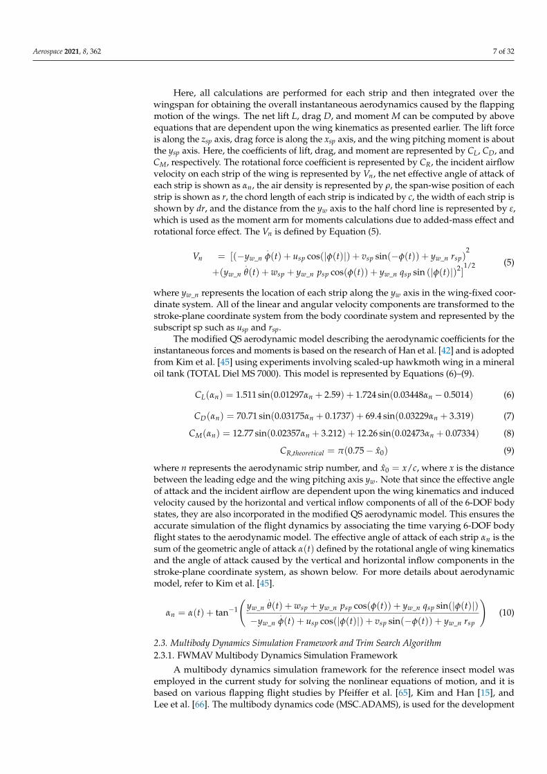
Here, all calculations are performed for each strip and then integrated over thewingspan for obtaining the overall instantaneous aerodynamics caused by the flappingmotion of the wings. The net lift L, drag D, and moment M can be computed by aboveequations that are dependent upon the wing kinematics as presented earlier. The lift forceis along the zsp axis, drag force is along the xsp axis, and the wing pitching moment is aboutthe ysp axis. Here, the coefficients of lift, drag, and moment are represented by CL, CD, andCM, respectively. The rotational force coefficient is represented by CR, the incident airflowvelocity on each strip of the wing is represented by Vn, the net effective angle of attack ofeach strip is shown as αn, the air density is represented by ρ, the span-wise position of eachstrip is shown as r, the chord length of each strip is indicated by c, the width of each strip isshown by dr, and the distance from the yw axis to the half chord line is represented by ε,which is used as the moment arm for moments calculations due to added-mass effect androtational force effect. The Vn is defined by Equation (5).

Vn = [(−yw_n.φ(t) + usp cos(|φ(t)|) + vsp sin(−φ(t)) + yw_n rsp)

2

+(yw_n.θ(t) + wsp + yw_n psp cos(φ(t)) + yw_n qsp sin (|φ(t)|)2]

1/2 (5)

where yw_n represents the location of each strip along the yw axis in the wing-fixed coor-dinate system. All of the linear and angular velocity components are transformed to thestroke-plane coordinate system from the body coordinate system and represented by thesubscript sp such as usp and rsp.

The modified QS aerodynamic model describing the aerodynamic coefficients for theinstantaneous forces and moments is based on the research of Han et al. [42] and is adoptedfrom Kim et al. [45] using experiments involving scaled-up hawkmoth wing in a mineraloil tank (TOTAL Diel MS 7000). This model is represented by Equations (6)–(9).

CL(αn) = 1.511 sin(0.01297αn + 2.59) + 1.724 sin(0.03448αn − 0.5014) (6)

CD(αn) = 70.71 sin(0.03175αn + 0.1737) + 69.4 sin(0.03229αn + 3.319) (7)

CM(αn) = 12.77 sin(0.02357αn + 3.212) + 12.26 sin(0.02473αn + 0.07334) (8)

CR,theoretical = π(0.75− x0) (9)

where n represents the aerodynamic strip number, and x0 = x/c, where x is the distancebetween the leading edge and the wing pitching axis yw. Note that since the effective angleof attack and the incident airflow are dependent upon the wing kinematics and inducedvelocity caused by the horizontal and vertical inflow components of all of the 6-DOF bodystates, they are also incorporated in the modified QS aerodynamic model. This ensures theaccurate simulation of the flight dynamics by associating the time varying 6-DOF bodyflight states to the aerodynamic model. The effective angle of attack of each strip αn is thesum of the geometric angle of attack α(t) defined by the rotational angle of wing kinematicsand the angle of attack caused by the vertical and horizontal inflow components in thestroke-plane coordinate system, as shown below. For more details about aerodynamicmodel, refer to Kim et al. [45].

αn = α(t) + tan−1

(yw_n

.θ(t) + wsp + yw_n psp cos(φ(t)) + yw_n qsp sin(|φ(t)|)

−yw_n.φ(t) + usp cos(|φ(t)|) + vsp sin(−φ(t)) + yw_n rsp

)(10)

2.3. Multibody Dynamics Simulation Framework and Trim Search Algorithm2.3.1. FWMAV Multibody Dynamics Simulation Framework

A multibody dynamics simulation framework for the reference insect model wasemployed in the current study for solving the nonlinear equations of motion, and it isbased on various flapping flight studies by Pfeiffer et al. [65], Kim and Han [15], andLee et al. [66]. The multibody dynamics code (MSC.ADAMS), is used for the development

Aerospace 2021, 8, 362 8 of 32

of this simulation framework, and the QS aerodynamic model (written in FORTRAN)is integrated into it, as shown in Figure 3. Here, ADAMS solver requires the FWMAVmodel, morphological data, kinematics constraints, and wing kinematics along with theaerodynamic loadings. The forces and moments for the nonlinear model are evaluated onthe basis of the aerodynamic loadings from the QS aerodynamic model that requires thewing and body parameters. For the multibody modeling, the model is composed of fiverigid bodies and four kinematics constraints. Two kinematics constraints join the threebodies (head, thorax, and abdomen) with fixed joints, and two other kinematics constraintslink the two wings to the thorax with 3 degrees of freedom revolute joints. In ADAMS, thenonlinear equations of motion for system are expressed in the form of differential-algebraicequations (DAE formulation) as shown in Equation (11), which are dependent upon themultibody model configuration and the constraints applied.

Ms..q + ηT

q λ− PTG(q,.q) = 0

η(q, t) = 0(11)

where Ms represents the mass matrix of the dynamic system, q is the set of coordinatesdepicting the displacements, η is the set of the model configuration and applied kinematicsconstraints equations, λ represents the Lagrange multipliers for handling multiple con-straints, G denotes the set of applied forces and gyroscopic terms of the inertial forces, PT

represents the matrix that projects the applied forces in the q direction, and ηq representsthe gradient of the constraints at any given state.

This simulation framework uses the GSTIFF integrator developed by Gear [67] to solvethe nonlinear DAE model. The solution process for this integrator occurs in two phases,namely, the prediction phase and the correction phase. The integrator employs Taylor’sseries for the prediction phase, which is an explicit process. In contrast, the correctionphase (implicit process) occurs after the prediction phase, and it is based on the iterativeNewton–Raphson algorithm. For the convergence of the DAE integrator and other details,refer to [15,45,65–67].

Aerospace 2021, 8, x FOR PEER REVIEW 8 of 32

2.3. Multibody Dynamics Simulation Framework and Trim Search Algorithm 2.3.1. FWMAV Multibody Dynamics Simulation Framework

A multibody dynamics simulation framework for the reference insect model was em-ployed in the current study for solving the nonlinear equations of motion, and it is based on various flapping flight studies by Pfeiffer et al. [65], Kim and Han [15], and Lee et al. [66]. The multibody dynamics code (MSC.ADAMS), is used for the development of this simulation framework, and the QS aerodynamic model (written in FORTRAN) is inte-grated into it, as shown in Figure 3. Here, ADAMS solver requires the FWMAV model, morphological data, kinematics constraints, and wing kinematics along with the aerody-namic loadings. The forces and moments for the nonlinear model are evaluated on the basis of the aerodynamic loadings from the QS aerodynamic model that requires the wing and body parameters. For the multibody modeling, the model is composed of five rigid bodies and four kinematics constraints. Two kinematics constraints join the three bodies (head, thorax, and abdomen) with fixed joints, and two other kinematics constraints link the two wings to the thorax with 3 degrees of freedom revolute joints. In ADAMS, the nonlinear equations of motion for system are expressed in the form of differential-alge-braic equations (DAE formulation) as shown in Equation (11), which are dependent upon the multibody model configuration and the constraints applied.

( , ) 0( , ) 0

T Ts q

t+ − =

=

M q η λ P G q qη q

(11)

where Ms represents the mass matrix of the dynamic system, q is the set of coordinates depicting the displacements, η is the set of the model configuration and applied kinemat-ics constraints equations, λ represents the Lagrange multipliers for handling multiple con-straints, G denotes the set of applied forces and gyroscopic terms of the inertial forces, PT represents the matrix that projects the applied forces in the q direction, and ηq represents the gradient of the constraints at any given state.

This simulation framework uses the GSTIFF integrator developed by Gear [67] to solve the nonlinear DAE model. The solution process for this integrator occurs in two phases, namely, the prediction phase and the correction phase. The integrator employs Taylor’s series for the prediction phase, which is an explicit process. In contrast, the cor-rection phase (implicit process) occurs after the prediction phase, and it is based on the iterative Newton–Raphson algorithm. For the convergence of the DAE integrator and other details, refer to [15,45,65–67].

Figure 3. Multibody dynamics simulation framework for FWMAV model.

2.3.2. Gradient-Based Trim Search Algorithm During the trimmed flight, all 6-DOF forces and moments are in equilibrium and do

not require extra control efforts to maintain that state unless there are some perturbations. Trim flight conditions are evaluated for both hovering and forward flight conditions. Trim conditions are difficult to find for FWMAV model as it involves periodic changes in the aerodynamic forces and moments. In this study, a gradient-based trim search algorithm

Figure 3. Multibody dynamics simulation framework for FWMAV model.

2.3.2. Gradient-Based Trim Search Algorithm

During the trimmed flight, all 6-DOF forces and moments are in equilibrium and donot require extra control efforts to maintain that state unless there are some perturbations.Trim flight conditions are evaluated for both hovering and forward flight conditions. Trimconditions are difficult to find for FWMAV model as it involves periodic changes in theaerodynamic forces and moments. In this study, a gradient-based trim search algorithmwas utilized that is based on the studies of Lee et al. [66] and Kim et al. [45]. This algorithmfinds the wing kinematics and initial conditions as shown in Equation (13) that satisfies the

Aerospace 2021, 8, 362 9 of 32

trim criteria mentioned in Equation (12). The overbar denotes the wingbeat cycle averagedvalues that can be evaluated by Equation (14).

F = [Fx Fy Fz] = [0 0 msg]M = [Mx My Mz] = [0 0 0]

x = [u w q Θ v p r Φ] = [uo 0 0 0 0 0 0 0](12)

[ fo, αo(t), φo(t), θo(t)]|F=M=0 (13)

F = 1T∫ bT

aT F(t) dtT = 1/ f , t ∈ [aT, bT], a < b, f or all a, b ∈ Z

(14)

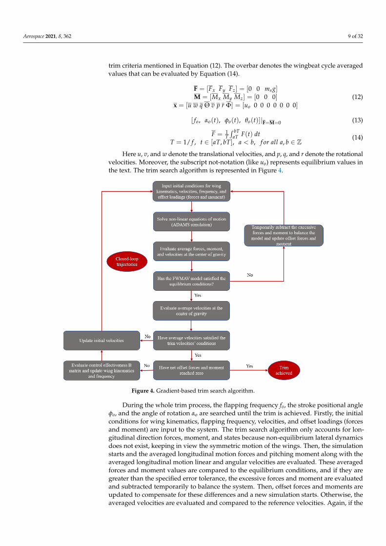
Here u, v, and w denote the translational velocities, and p, q, and r denote the rotationalvelocities. Moreover, the subscript not-notation (like uo) represents equilibrium values inthe text. The trim search algorithm is represented in Figure 4.

Aerospace 2021, 8, x FOR PEER REVIEW 9 of 32

was utilized that is based on the studies of Lee et al. [66] and Kim et al. [45]. This algorithm finds the wing kinematics and initial conditions as shown in Equation (13) that satisfies the trim criteria mentioned in Equation (12). The overbar denotes the wingbeat cycle av-eraged values that can be evaluated by Equation (14).

[ ] [0 0 ]

[ ] [0 0 0]

[ ] [ 0 0 0 0 0 0 0]

x y z s

x y z

o

F F F m g

M M M

u w q v p r uΘ Φ

= =

= =

= =

F

M

x

(12)

0[ , ( ), ( ), ( )]o o o of t t tα φ θ

= =F M (13)

1 ( )

1/ , [ , ], , ,

bT

aTF F t dt

TT f t aT bT a b for all a b

=

= ∈ < ∈

(14)

Here u, v, and w denote the translational velocities, and p, q, and r denote the rota-tional velocities. Moreover, the subscript not-notation (like uo) represents equilibrium val-ues in the text. The trim search algorithm is represented in Figure 4.

Figure 4. Gradient-based trim search algorithm.

During the whole trim process, the flapping frequency fo, the stroke positional angle ϕo, and the angle of rotation αo are searched until the trim is achieved. Firstly, the initial conditions for wing kinematics, flapping frequency, velocities, and offset loadings (forces and moment) are input to the system. The trim search algorithm only accounts for longi-tudinal direction forces, moment, and states because non-equilibrium lateral dynamics does not exist, keeping in view the symmetric motion of the wings. Then, the simulation starts and the averaged longitudinal motion forces and pitching moment along with the averaged longitudinal motion linear and angular velocities are evaluated. These averaged forces and moment values are compared to the equilibrium conditions, and if they are

Figure 4. Gradient-based trim search algorithm.

During the whole trim process, the flapping frequency fo, the stroke positional angleφo, and the angle of rotation αo are searched until the trim is achieved. Firstly, the initialconditions for wing kinematics, flapping frequency, velocities, and offset loadings (forcesand moment) are input to the system. The trim search algorithm only accounts for lon-gitudinal direction forces, moment, and states because non-equilibrium lateral dynamicsdoes not exist, keeping in view the symmetric motion of the wings. Then, the simulationstarts and the averaged longitudinal motion forces and pitching moment along with theaveraged longitudinal motion linear and angular velocities are evaluated. These averagedforces and moment values are compared to the equilibrium conditions, and if they aregreater than the specified error tolerance, the excessive forces and moment are evaluatedand subtracted temporarily to balance the system. Then, offset forces and moments areupdated to compensate for these differences and a new simulation starts. Otherwise, theaveraged velocities are evaluated and compared to the reference velocities. Again, if the

Aerospace 2021, 8, 362 10 of 32

differences of these velocities are greater than the specified error tolerance for the velocities,then the initial velocities are updated, and a new simulation starts.

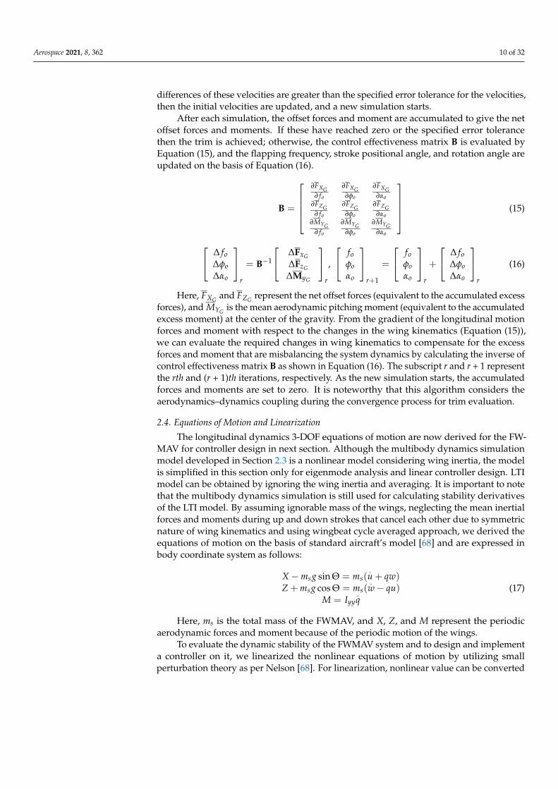
After each simulation, the offset forces and moment are accumulated to give the netoffset forces and moments. If these have reached zero or the specified error tolerancethen the trim is achieved; otherwise, the control effectiveness matrix B is evaluated byEquation (15), and the flapping frequency, stroke positional angle, and rotation angle areupdated on the basis of Equation (16).

B =

∂FXG

∂ fo

∂FXG∂φo

∂FXG∂αo

∂FZG∂ fo

∂FZG∂φo

∂FZG∂αo

∂MYG∂ fo

∂MYG∂φo

∂MYG∂αo

(15)

∆ fo∆φo∆αo

r

= B−1

∆FxG

∆FzG

∆MyG

r

,

foφoαo

r+1

=

foφoαo

r

+

∆ fo∆φo∆αo

r

(16)

Here, FXG and FZG represent the net offset forces (equivalent to the accumulated excessforces), and MYG is the mean aerodynamic pitching moment (equivalent to the accumulatedexcess moment) at the center of the gravity. From the gradient of the longitudinal motionforces and moment with respect to the changes in the wing kinematics (Equation (15)),we can evaluate the required changes in wing kinematics to compensate for the excessforces and moment that are misbalancing the system dynamics by calculating the inverse ofcontrol effectiveness matrix B as shown in Equation (16). The subscript r and r + 1 representthe rth and (r + 1)th iterations, respectively. As the new simulation starts, the accumulatedforces and moments are set to zero. It is noteworthy that this algorithm considers theaerodynamics–dynamics coupling during the convergence process for trim evaluation.

2.4. Equations of Motion and Linearization

The longitudinal dynamics 3-DOF equations of motion are now derived for the FW-MAV for controller design in next section. Although the multibody dynamics simulationmodel developed in Section 2.3 is a nonlinear model considering wing inertia, the modelis simplified in this section only for eigenmode analysis and linear controller design. LTImodel can be obtained by ignoring the wing inertia and averaging. It is important to notethat the multibody dynamics simulation is still used for calculating stability derivativesof the LTI model. By assuming ignorable mass of the wings, neglecting the mean inertialforces and moments during up and down strokes that cancel each other due to symmetricnature of wing kinematics and using wingbeat cycle averaged approach, we derived theequations of motion on the basis of standard aircraft’s model [68] and are expressed inbody coordinate system as follows:

X−msg sin Θ = ms(.u + qw)

Z + msg cos Θ = ms(.

w− qu)M = Iyy

.q

(17)

Here, ms is the total mass of the FWMAV, and X, Z, and M represent the periodicaerodynamic forces and moment because of the periodic motion of the wings.

To evaluate the dynamic stability of the FWMAV system and to design and implementa controller on it, we linearized the nonlinear equations of motion by utilizing smallperturbation theory as per Nelson [68]. For linearization, nonlinear value can be converted

Aerospace 2021, 8, 362 11 of 32

to the sum of trim reference (wingbeat cycle averaged) value and a small perturbationabout it as follows:

u = uo + ∆u, w = wo + ∆w, q = qo + ∆q.u =

.uo + ∆

.u,

.w =

.wo + ∆

.w,

.q =

.qo + ∆

.q, Θ = Θo + ∆Θ

X = Xo + ∆X, Z = Zo + ∆Z, M = Mo + ∆M(18)

Here, for satisfying the trim conditions, we can assume that.uo = 0,

.wo = 0,

.qo = 0,

and qo = 0. Moreover, uo 6= 0 and wo 6= 0 because of the forward flight speed andup/down motion in the body coordinate system. Using previously discussed assumptionsand previous equations, we obtain Equation (19).

∆X−msg cos Θo∆Θ = ms

[∆

.u + wo∆q

]∆Z−msg sin Θo∆Θ = ms

[∆

.w− uo∆q

]∆M = Iyy∆

.q

(19)

As the aerodynamic forces and moment are dependent upon the dynamic variables,their changes can therefore be written as sum of aerodynamic derivatives as per Nelson [68].These aerodynamic forces’ and moments’ derivatives with respect to dynamic variablesare expressed in Equation (20).

∂X∂u = Xu, ∂X

∂w = Xw, ∂X∂q = Xq,

∂Z∂u = Zu, ∂Z

∂w = Zw, ∂Z∂q = Zq,

∂M∂u = Mu, ∂M

∂w = Mw, ∂M∂q = Mq

(20)

Using Equation (20), the aerodynamic forces and moment terms in Equation (19) canbe written as follows:

∆X = Xu∆u + Xw∆w + Xq∆q∆Z = Zu∆u + Zw∆w + Zq∆q

∆M = Mu∆u + Mw∆w + Mq∆q(21)

After substituting the aerodynamic forces and moment terms in Equation (19) andrearranging, we obtain the following standard state-space form of our 3-DOF longitudinalFWMAV system (Equation (22)) [44,45]. This model is used for the controller designand implementation.

∆

.u

∆.

w∆

.q

∆q

=

Xums

Xwms

Xqms− wo −g

Zums

Zwms

Zqms

+ uo 0MuIyy

MwIyy

MqIyy

00 0 1 0

∆u∆w∆q∆Θ

(22)

For longitudinal dynamic stability characterization, the nondimensionalization ofEquation (22) is carried out as per Equation (23).

ms+ = ms

ρUST , g+ = gTU , Iyy

+ =Iyy

ρU2SwcT2

∆u+ = ∆uU , ∆w+ = ∆w

U , ∆q+ = ∆qTX+

u = XuρUSw

, X+w = Xw

ρUSw, X+

q =Xq

ρUSwc ,

Z+u = Zu

ρUSw, Z+

w = ZwρUSw

, Z+q =

ZqρUSwc ,

M+u = Mu

ρUSwc , M+w = Mw

ρUSwc , M+q =

MqρU2SwcT

(23)

Here, U is the reference velocity given by 2 f r2φamp, T is 1/f or wingbeat cycle period,c is the mean chord, and ρ is the air density. The nondimensionalized 3-DOF equations

Aerospace 2021, 8, 362 12 of 32

of motion for stability study is expressed in Equation (24), where A+longitudinal is system’s

matrix in longitudinal direction.∆

.u+

∆.

w+

∆.q+

∆q

= A+longitudinal

∆u+

∆w+

∆q+

∆Θ

=

X+

ums+

X+w

ms+X+

qms+− w+

o −g+

Z+u

ms+Z+

wms+

Z+q

ms++ u+

o 0M+

uI+yy

M+w

I+yy

M+q

I+yy0

0 0 1 0

∆u+

∆w+

∆q+

∆Θ

(24)

2.5. Augmented LQR Controller Design for Transition Flight Tracking

In this section, augmented LQR control method is discussed in terms of obtainingthe optimal gain matrices for controlling both the linear and nonlinear FWMAV modelsinvolving various flight speeds for performing different maneuvers.

2.5.1. Gain-Scheduled LQR Controller Design for Linear System

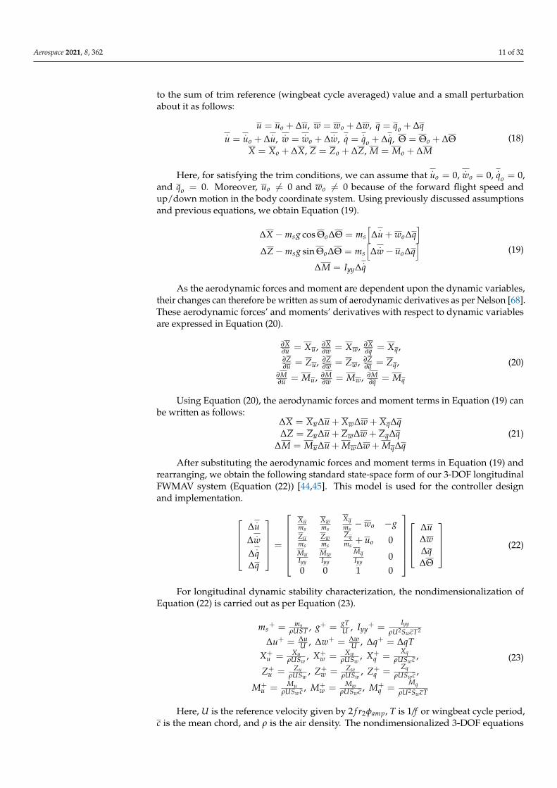
The trim conditions are obtained for various forward flight speeds. At each trimcondition, the linearized FWMAV equations are obtained and expressed as Equation (22).The standard state-space form for the linearized system along with the normalized controleffectiveness matrix is shown in Equation (25), and it is obtained for trim conditions at eachforward flight speed. The simplified version is shown in Equation (26), and the outputis shown in Equation (27). The schematics of the control implementation for the linearsystem for reference velocity profile tracking in the transition flight of FWMAV is shown inFigure 5. The block model shown in Figure 5 uses a gain-scheduled optimal LQR controllerbased on forward flight speed that must account for the time-varying dynamic behavior ofthe nonlinear FWMAV model.

∆

.u

∆.

w∆

.q

∆q

=

Xums

Xwms

Xqms− wo −g

Zums

Zwms

Zqms

+ uo 0MuIyy

MwIyy

MqIyy

00 0 1 0

∆u∆w∆q∆Θ

+

∂FXG

∂ fo/ms

∂FXG∂φo

/ms∂FXG∂αo

/ms∂FZG∂ fo

/ms∂FZG∂φo

/ms∂FZG∂αo

/ms∂MYG

∂ fo/Iyy

∂MYG∂φo

/Iyy∂MYG

∂αo/Iyy

∆ fo

∆φo∆αo

(25)

.X =

∆

.u

∆.

w∆

.q

∆q

= A

∆u∆w∆q∆Θ

+ Bc

∆ fo∆φo∆αo

.X = AX + Bcuc (26)

Y =

∆uG∆wG∆Θ

=

cos Θr sin Θr 0 0− sin Θr cos Θr 0 −uo

0 0 0 1

∆u∆w∆q∆Θ

= CXY = CX + DuC = CX (27)

where A is the system matrix, Bc is the normalized control effectiveness matrix that isobtained from the gradient-based trim search algorithm, uc is the control input, Y is theoutput (perturbations in velocities and body pitch angle in global coordinate system), thematrix output is C, D is the zero matrix, and the state variables are expressed as X. Here,Θr is the reference body pitch angle during each of the trimmed state.

Aerospace 2021, 8, 362 13 of 32

Aerospace 2021, 8, x FOR PEER REVIEW 13 of 32

o

o

o

uu fwwqq

q

φα

Θ

Δ Δ Δ ΔΔ = = + Δ ΔΔ Δ ΔΔ = +

c

c c

X A B

X AX B u

(26)

cos sin 0 0-sin cos 0 - 0 0 0 1

G r r

G r r o

uu

ww u

q

Θ ΘΘ Θ

Θ Θ

Δ Δ Δ = Δ = = Δ Δ Δ = + =C

Y CX

Y CX Du CX

(27)

where A is the system matrix, Bc is the normalized control effectiveness matrix that is obtained from the gradient-based trim search algorithm, uc is the control input, Y is the output (perturbations in velocities and body pitch angle in global coordinate system), the matrix output is C, D is the zero matrix, and the state variables are expressed as X. Here, rΘ is the reference body pitch angle during each of the trimmed state.

Figure 5. Schematic diagram of gain-scheduled LQR control loop for transition flight tracking of the linear model.

Figure 5 shows that there is an integral action applied in the control implementation. The error in the velocities and the body pitch angle are passed through the integral action for removing any steady-state error that can compensate for any uncertainty in the system. The states, which are defined as differences from their references, themselves can be used as error estimation; therefore, an augmented state-space form of the equations of motion are written using integral states with over-curved notation. The subscript r denotes the reference states in Equation (28) for the system output equation. The augmented state-space form of the system is represented as Equation (29).

0

rt

r

r G

u uw w dtΘ Θ

− = = − = −

I IY X X Y (28)

= = + = +

= +

cc c c

II

c c

BX XA 0X u AX B u

XC 0 0X

X AX B u

(29)

The LQR optimal control determines the control gain K

[3 × 7], which is split into the gains KS [3 × 4] and KI [3 × 3] for the system states and the integral states, respectively, for the augmented full state feedback controller design. The LQR method optimizes the solution by minimizing the cost function J as shown in Equation (30) and as discussed in [69]. The optimal gain matrices K

and the matrix P are determined by solving the alge-

braic Riccati equation (ARE), as shown in Equation (31). For each forward flight speed,

Figure 5. Schematic diagram of gain-scheduled LQR control loop for transition flight tracking of the linear model.

Figure 5 shows that there is an integral action applied in the control implementation.The error in the velocities and the body pitch angle are passed through the integral actionfor removing any steady-state error that can compensate for any uncertainty in the system.The states, which are defined as differences from their references, themselves can be usedas error estimation; therefore, an augmented state-space form of the equations of motionare written using integral states with over-curved notation. The subscript r denotes thereference states in Equation (28) for the system output equation. The augmented state-spaceform of the system is represented as Equation (29).

Y =.XI =

u− urw− wrΘ−Θr

G

⇒ XI =∫ t

0Ydt (28)

_.X =

[ .X.XI

]=

[A 0C 0

][XXI

]+

[Bc0

]_uc =

_A

_X +

_Bc

_uc

_.X =

_A

_X +

_Bc

_uc (29)

The LQR optimal control determines the control gain_K [3 × 7], which is split into the

gains KS [3 × 4] and KI [3 × 3] for the system states and the integral states, respectively,for the augmented full state feedback controller design. The LQR method optimizes thesolution by minimizing the cost function J as shown in Equation (30) and as discussed

in [69]. The optimal gain matrices_K and the matrix P are determined by solving the

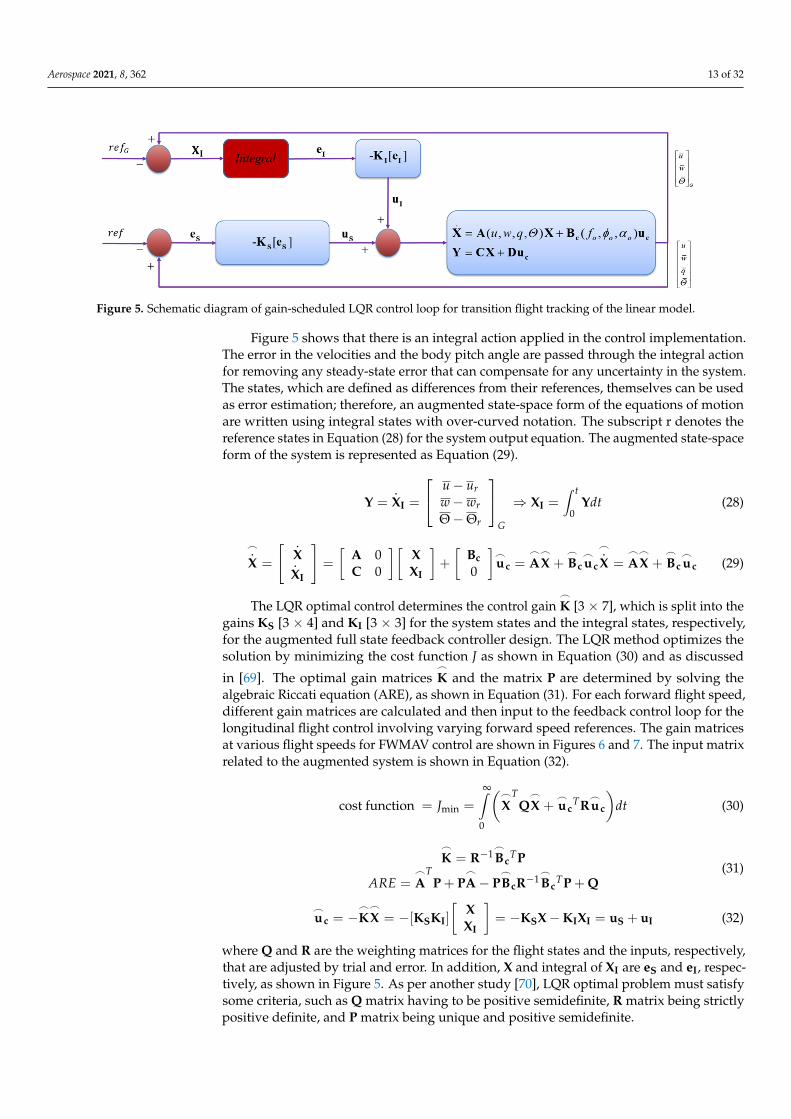
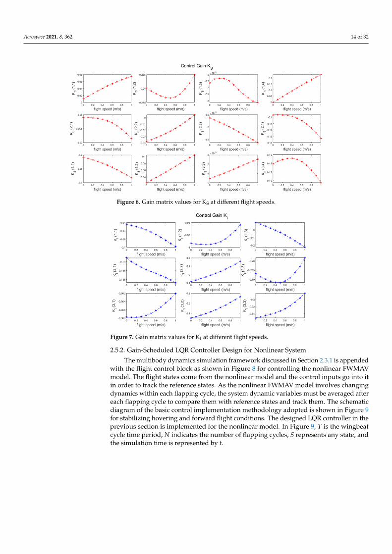
algebraic Riccati equation (ARE), as shown in Equation (31). For each forward flight speed,different gain matrices are calculated and then input to the feedback control loop for thelongitudinal flight control involving varying forward speed references. The gain matricesat various flight speeds for FWMAV control are shown in Figures 6 and 7. The input matrixrelated to the augmented system is shown in Equation (32).

cost function = Jmin =

∞∫0

(_X

TQ

_X +

_uc

TR_uc

)dt (30)

_K = R−1

_Bc

TP

ARE =_A

TP + P

_A− P

_BcR−1

_Bc

TP + Q(31)

_uc = −

_K

_X = −[KSKI]

[XXI

]= −KSX−KIXI = uS + uI (32)

where Q and R are the weighting matrices for the flight states and the inputs, respectively,that are adjusted by trial and error. In addition, X and integral of XI are eS and eI, respec-tively, as shown in Figure 5. As per another study [70], LQR optimal problem must satisfysome criteria, such as Q matrix having to be positive semidefinite, R matrix being strictlypositive definite, and P matrix being unique and positive semidefinite.

Aerospace 2021, 8, 362 14 of 32

Aerospace 2021, 8, x FOR PEER REVIEW 14 of 32

different gain matrices are calculated and then input to the feedback control loop for the longitudinal flight control involving varying forward speed references. The gain matrices at various flight speeds for FWMAV control are shown in Figures 6 and 7. The input ma-trix related to the augmented system is shown in Equation (32).

( )min0

cost function T TJ dt∞

= = + c cX QX u Ru (30)

1

1

T

T TARE

−

−

=

= + − +c

c c

K R B PA P PA PB R B P Q

(31)

[ ] = − = − = − = +

c S I S I I S I

I

Xu KX K K -K X K X u u

X (32)

where Q and R are the weighting matrices for the flight states and the inputs, respectively, that are adjusted by trial and error. In addition, X and integral of XI are eS and eI, respec-tively, as shown in Figure 5. As per another study [70], LQR optimal problem must satisfy some criteria, such as Q matrix having to be positive semidefinite, R matrix being strictly positive definite, and P matrix being unique and positive semidefinite.

Figure 6. Gain matrix values for KS at different flight speeds.

Figure 7. Gain matrix values for KI at different flight speeds.

Figure 6. Gain matrix values for KS at different flight speeds.

Aerospace 2021, 8, x FOR PEER REVIEW 14 of 32

different gain matrices are calculated and then input to the feedback control loop for the longitudinal flight control involving varying forward speed references. The gain matrices at various flight speeds for FWMAV control are shown in Figures 6 and 7. The input ma-trix related to the augmented system is shown in Equation (32).

( )min0

cost function T TJ dt∞

= = + c cX QX u Ru (30)

1

1

T

T TARE

−

−

=

= + − +c

c c

K R B PA P PA PB R B P Q

(31)

[ ] = − = − = − = +

c S I S I I S I

I

Xu KX K K -K X K X u u

X (32)

where Q and R are the weighting matrices for the flight states and the inputs, respectively, that are adjusted by trial and error. In addition, X and integral of XI are eS and eI, respec-tively, as shown in Figure 5. As per another study [70], LQR optimal problem must satisfy some criteria, such as Q matrix having to be positive semidefinite, R matrix being strictly positive definite, and P matrix being unique and positive semidefinite.

Figure 6. Gain matrix values for KS at different flight speeds.

Figure 7. Gain matrix values for KI at different flight speeds. Figure 7. Gain matrix values for KI at different flight speeds.

2.5.2. Gain-Scheduled LQR Controller Design for Nonlinear System

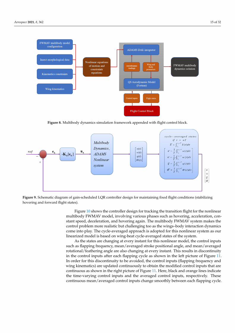
The multibody dynamics simulation framework discussed in Section 2.3.1 is appendedwith the flight control block as shown in Figure 8 for controlling the nonlinear FWMAVmodel. The flight states come from the nonlinear model and the control inputs go into itin order to track the reference states. As the nonlinear FWMAV model involves changingdynamics within each flapping cycle, the system dynamic variables must be averaged aftereach flapping cycle to compare them with reference states and track them. The schematicdiagram of the basic control implementation methodology adopted is shown in Figure 9for stabilizing hovering and forward flight conditions. The designed LQR controller in theprevious section is implemented for the nonlinear model. In Figure 9, T is the wingbeatcycle time period, N indicates the number of flapping cycles, S represents any state, andthe simulation time is represented by t.

Aerospace 2021, 8, 362 15 of 32

Aerospace 2021, 8, x FOR PEER REVIEW 15 of 32

2.5.2. Gain-Scheduled LQR Controller Design for Nonlinear System The multibody dynamics simulation framework discussed in Section 2.3.1 is ap-

pended with the flight control block as shown in Figure 8 for controlling the nonlinear FWMAV model. The flight states come from the nonlinear model and the control inputs go into it in order to track the reference states. As the nonlinear FWMAV model involves changing dynamics within each flapping cycle, the system dynamic variables must be av-eraged after each flapping cycle to compare them with reference states and track them. The schematic diagram of the basic control implementation methodology adopted is shown in Figure 9 for stabilizing hovering and forward flight conditions. The designed LQR controller in the previous section is implemented for the nonlinear model. In Figure 9, T is the wingbeat cycle time period, N indicates the number of flapping cycles, S repre-sents any state, and the simulation time is represented by t.

Figure 8. Multibody dynamics simulation framework appended with flight control block.

Figure 9. Schematic diagram of gain-scheduled LQR controller design for maintaining fixed flight conditions (stabilizing hovering and forward flight states).

Figure 10 shows the controller design for tracking the transition flight for the nonlin-ear multibody FWMAV model, involving various phases such as hovering, acceleration, constant speed, deceleration, and hovering again. The multibody FWMAV system makes the control problem more realistic but challenging too as the wings–body interaction dy-namics come into play. The cycle-averaged approach is adopted for this nonlinear system as our linearized model is based on wing-beat cycle-averaged states of the system.

As the states are changing at every instant for this nonlinear model, the control inputs such as flapping frequency, mean/averaged stroke positional angle, and mean/averaged

Figure 8. Multibody dynamics simulation framework appended with flight control block.

Aerospace 2021, 8, x FOR PEER REVIEW 15 of 32

2.5.2. Gain-Scheduled LQR Controller Design for Nonlinear System The multibody dynamics simulation framework discussed in Section 2.3.1 is ap-

pended with the flight control block as shown in Figure 8 for controlling the nonlinear FWMAV model. The flight states come from the nonlinear model and the control inputs go into it in order to track the reference states. As the nonlinear FWMAV model involves changing dynamics within each flapping cycle, the system dynamic variables must be av-eraged after each flapping cycle to compare them with reference states and track them. The schematic diagram of the basic control implementation methodology adopted is shown in Figure 9 for stabilizing hovering and forward flight conditions. The designed LQR controller in the previous section is implemented for the nonlinear model. In Figure 9, T is the wingbeat cycle time period, N indicates the number of flapping cycles, S repre-sents any state, and the simulation time is represented by t.

Figure 8. Multibody dynamics simulation framework appended with flight control block.

Figure 9. Schematic diagram of gain-scheduled LQR controller design for maintaining fixed flight conditions (stabilizing hovering and forward flight states).

Figure 10 shows the controller design for tracking the transition flight for the nonlin-ear multibody FWMAV model, involving various phases such as hovering, acceleration, constant speed, deceleration, and hovering again. The multibody FWMAV system makes the control problem more realistic but challenging too as the wings–body interaction dy-namics come into play. The cycle-averaged approach is adopted for this nonlinear system as our linearized model is based on wing-beat cycle-averaged states of the system.

As the states are changing at every instant for this nonlinear model, the control inputs such as flapping frequency, mean/averaged stroke positional angle, and mean/averaged

Figure 9. Schematic diagram of gain-scheduled LQR controller design for maintaining fixed flight conditions (stabilizinghovering and forward flight states).

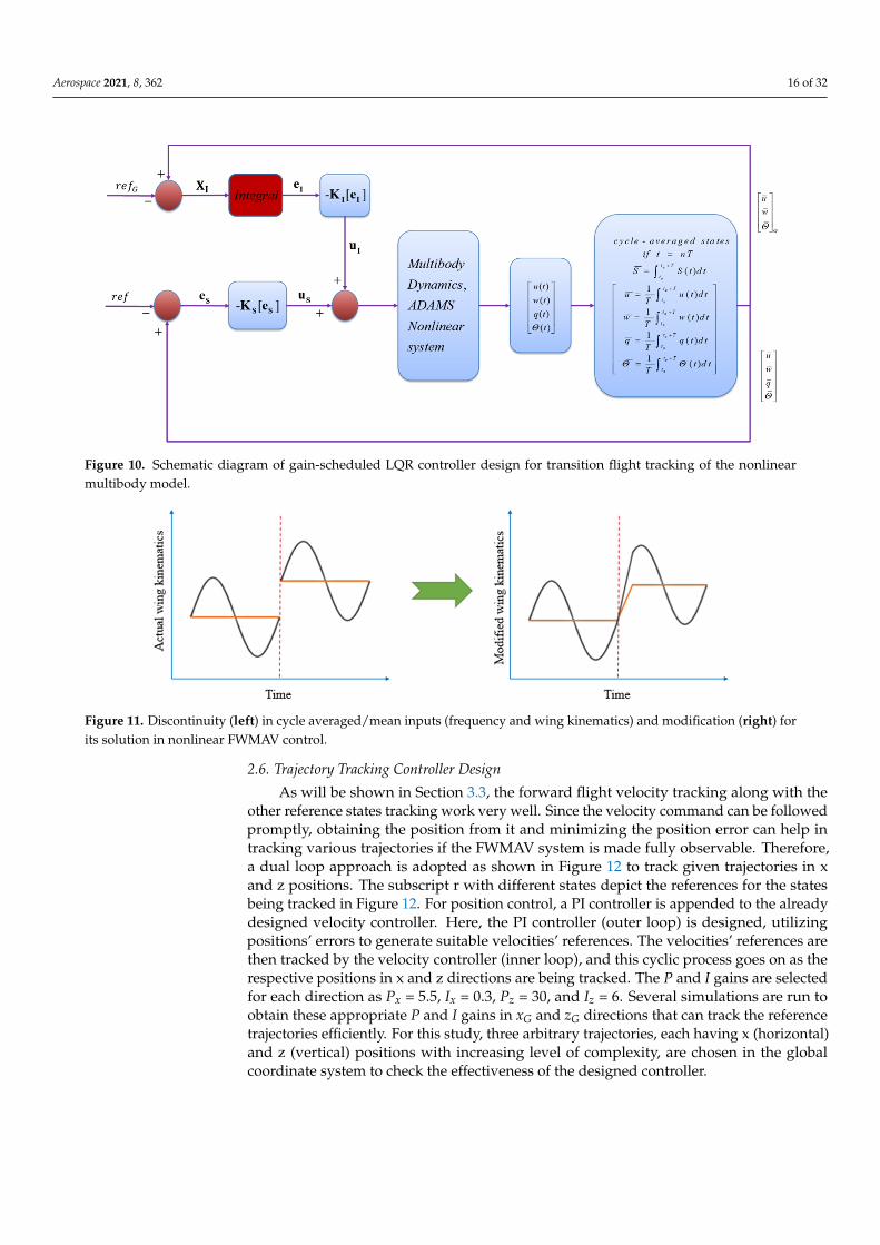
Figure 10 shows the controller design for tracking the transition flight for the nonlinearmultibody FWMAV model, involving various phases such as hovering, acceleration, con-stant speed, deceleration, and hovering again. The multibody FWMAV system makes thecontrol problem more realistic but challenging too as the wings–body interaction dynamicscome into play. The cycle-averaged approach is adopted for this nonlinear system as ourlinearized model is based on wing-beat cycle-averaged states of the system.

As the states are changing at every instant for this nonlinear model, the control inputssuch as flapping frequency, mean/averaged stroke positional angle, and mean/averagedrotational/feathering angle are also changing at every instant. This results in discontinuityin the control inputs after each flapping cycle as shown in the left picture of Figure 11.In order for this discontinuity to be avoided, the control inputs (flapping frequency andwing kinematics) are updated continuously to obtain the modified control inputs that arecontinuous as shown in the right picture of Figure 11. Here, black and orange lines indicatethe time-varying control inputs and the averaged control inputs, respectively. Thesecontinuous mean/averaged control inputs change smoothly between each flapping cycle.

Aerospace 2021, 8, 362 16 of 32

Aerospace 2021, 8, x FOR PEER REVIEW 16 of 32

rotational/feathering angle are also changing at every instant. This results in discontinuity in the control inputs after each flapping cycle as shown in the left picture of Figure 11. In order for this discontinuity to be avoided, the control inputs (flapping frequency and wing kinematics) are updated continuously to obtain the modified control inputs that are con-tinuous as shown in the right picture of Figure 11. Here, black and orange lines indicate the time-varying control inputs and the averaged control inputs, respectively. These con-tinuous mean/averaged control inputs change smoothly between each flapping cycle.

Figure 10. Schematic diagram of gain-scheduled LQR controller design for transition flight tracking of the nonlinear multi-body model.

Figure 11. Discontinuity (left) in cycle averaged/mean inputs (frequency and wing kinematics) and modification (right) for its solution in nonlinear FWMAV control.

2.6. Trajectory Tracking Controller Design As will be shown in Section 3.3, the forward flight velocity tracking along with the

other reference states tracking work very well. Since the velocity command can be fol-lowed promptly, obtaining the position from it and minimizing the position error can help in tracking various trajectories if the FWMAV system is made fully observable. Therefore, a dual loop approach is adopted as shown in Figure 12 to track given trajectories in x and z positions. The subscript r with different states depict the references for the states being tracked in Figure 12. For position control, a PI controller is appended to the already de-signed velocity controller. Here, the PI controller (outer loop) is designed, utilizing posi-tions’ errors to generate suitable velocities’ references. The velocities’ references are then tracked by the velocity controller (inner loop), and this cyclic process goes on as the re-spective positions in x and z directions are being tracked. The P and I gains are selected for each direction as Px = 5.5, Ix = 0.3, Pz = 30, and Iz = 6. Several simulations are run to

Figure 10. Schematic diagram of gain-scheduled LQR controller design for transition flight tracking of the nonlinearmultibody model.

Aerospace 2021, 8, x FOR PEER REVIEW 16 of 32

rotational/feathering angle are also changing at every instant. This results in discontinuity in the control inputs after each flapping cycle as shown in the left picture of Figure 11. In order for this discontinuity to be avoided, the control inputs (flapping frequency and wing kinematics) are updated continuously to obtain the modified control inputs that are con-tinuous as shown in the right picture of Figure 11. Here, black and orange lines indicate the time-varying control inputs and the averaged control inputs, respectively. These con-tinuous mean/averaged control inputs change smoothly between each flapping cycle.

Figure 10. Schematic diagram of gain-scheduled LQR controller design for transition flight tracking of the nonlinear multi-body model.

Figure 11. Discontinuity (left) in cycle averaged/mean inputs (frequency and wing kinematics) and modification (right) for its solution in nonlinear FWMAV control.

2.6. Trajectory Tracking Controller Design As will be shown in Section 3.3, the forward flight velocity tracking along with the

other reference states tracking work very well. Since the velocity command can be fol-lowed promptly, obtaining the position from it and minimizing the position error can help in tracking various trajectories if the FWMAV system is made fully observable. Therefore, a dual loop approach is adopted as shown in Figure 12 to track given trajectories in x and z positions. The subscript r with different states depict the references for the states being tracked in Figure 12. For position control, a PI controller is appended to the already de-signed velocity controller. Here, the PI controller (outer loop) is designed, utilizing posi-tions’ errors to generate suitable velocities’ references. The velocities’ references are then tracked by the velocity controller (inner loop), and this cyclic process goes on as the re-spective positions in x and z directions are being tracked. The P and I gains are selected for each direction as Px = 5.5, Ix = 0.3, Pz = 30, and Iz = 6. Several simulations are run to

Figure 11. Discontinuity (left) in cycle averaged/mean inputs (frequency and wing kinematics) and modification (right) forits solution in nonlinear FWMAV control.

2.6. Trajectory Tracking Controller Design

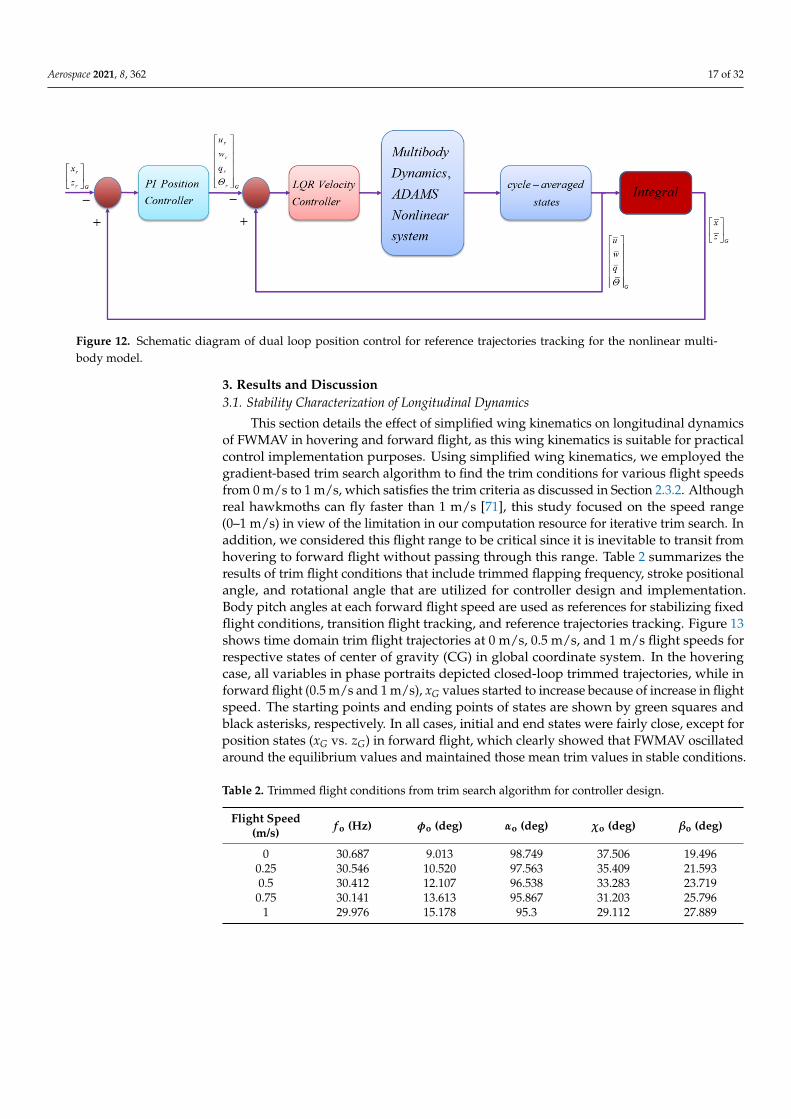
As will be shown in Section 3.3, the forward flight velocity tracking along with theother reference states tracking work very well. Since the velocity command can be followedpromptly, obtaining the position from it and minimizing the position error can help intracking various trajectories if the FWMAV system is made fully observable. Therefore,a dual loop approach is adopted as shown in Figure 12 to track given trajectories in xand z positions. The subscript r with different states depict the references for the statesbeing tracked in Figure 12. For position control, a PI controller is appended to the alreadydesigned velocity controller. Here, the PI controller (outer loop) is designed, utilizingpositions’ errors to generate suitable velocities’ references. The velocities’ references arethen tracked by the velocity controller (inner loop), and this cyclic process goes on as therespective positions in x and z directions are being tracked. The P and I gains are selectedfor each direction as Px = 5.5, Ix = 0.3, Pz = 30, and Iz = 6. Several simulations are run toobtain these appropriate P and I gains in xG and zG directions that can track the referencetrajectories efficiently. For this study, three arbitrary trajectories, each having x (horizontal)and z (vertical) positions with increasing level of complexity, are chosen in the globalcoordinate system to check the effectiveness of the designed controller.

Aerospace 2021, 8, 362 17 of 32

Aerospace 2021, 8, x FOR PEER REVIEW 17 of 32

obtain these appropriate P and I gains in xG and zG directions that can track the reference trajectories efficiently. For this study, three arbitrary trajectories, each having x (horizon-tal) and z (vertical) positions with increasing level of complexity, are chosen in the global coordinate system to check the effectiveness of the designed controller.

Figure 12. Schematic diagram of dual loop position control for reference trajectories tracking for the nonlinear multibody model.

3. Results and Discussion 3.1. Stability Characterization of Longitudinal Dynamics

This section details the effect of simplified wing kinematics on longitudinal dynamics of FWMAV in hovering and forward flight, as this wing kinematics is suitable for practical control implementation purposes. Using simplified wing kinematics, we employed the gradient-based trim search algorithm to find the trim conditions for various flight speeds from 0 m/s to 1 m/s, which satisfies the trim criteria as discussed in Section 2.3.2. Although real hawkmoths can fly faster than 1 m/s [71], this study focused on the speed range (0–1 m/s) in view of the limitation in our computation resource for iterative trim search. In addition, we considered this flight range to be critical since it is inevitable to transit from hovering to forward flight without passing through this range. Table 2 summarizes the results of trim flight conditions that include trimmed flapping frequency, stroke positional angle, and rotational angle that are utilized for controller design and implementation. Body pitch angles at each forward flight speed are used as references for stabilizing fixed flight conditions, transition flight tracking, and reference trajectories tracking. Figure 13 shows time domain trim flight trajectories at 0 m/s, 0.5 m/s, and 1 m/s flight speeds for respective states of center of gravity (CG) in global coordinate system. In the hovering case, all variables in phase portraits depicted closed-loop trimmed trajectories, while in forward flight (0.5 m/s and 1 m/s), xG values started to increase because of increase in flight speed. The starting points and ending points of states are shown by green squares and black asterisks, respectively. In all cases, initial and end states were fairly close, except for position states (xG vs. zG) in forward flight, which clearly showed that FWMAV oscillated around the equilibrium values and maintained those mean trim values in stable condi-tions.

Table 2. Trimmed flight conditions from trim search algorithm for controller design.

Flight Speed (m/s) fo (Hz) ϕo (deg) αo (deg) χo (deg) βo (deg) 0 30.687 9.013 98.749 37.506 19.496

0.25 30.546 10.520 97.563 35.409 21.593 0.5 30.412 12.107 96.538 33.283 23.719

0.75 30.141 13.613 95.867 31.203 25.796 1 29.976 15.178 95.3 29.112 27.889

Figure 12. Schematic diagram of dual loop position control for reference trajectories tracking for the nonlinear multi-body model.

3. Results and Discussion3.1. Stability Characterization of Longitudinal Dynamics

This section details the effect of simplified wing kinematics on longitudinal dynamicsof FWMAV in hovering and forward flight, as this wing kinematics is suitable for practicalcontrol implementation purposes. Using simplified wing kinematics, we employed thegradient-based trim search algorithm to find the trim conditions for various flight speedsfrom 0 m/s to 1 m/s, which satisfies the trim criteria as discussed in Section 2.3.2. Althoughreal hawkmoths can fly faster than 1 m/s [71], this study focused on the speed range(0–1 m/s) in view of the limitation in our computation resource for iterative trim search. Inaddition, we considered this flight range to be critical since it is inevitable to transit fromhovering to forward flight without passing through this range. Table 2 summarizes theresults of trim flight conditions that include trimmed flapping frequency, stroke positionalangle, and rotational angle that are utilized for controller design and implementation.Body pitch angles at each forward flight speed are used as references for stabilizing fixedflight conditions, transition flight tracking, and reference trajectories tracking. Figure 13shows time domain trim flight trajectories at 0 m/s, 0.5 m/s, and 1 m/s flight speeds forrespective states of center of gravity (CG) in global coordinate system. In the hoveringcase, all variables in phase portraits depicted closed-loop trimmed trajectories, while inforward flight (0.5 m/s and 1 m/s), xG values started to increase because of increase in flightspeed. The starting points and ending points of states are shown by green squares andblack asterisks, respectively. In all cases, initial and end states were fairly close, except forposition states (xG vs. zG) in forward flight, which clearly showed that FWMAV oscillatedaround the equilibrium values and maintained those mean trim values in stable conditions.

Table 2. Trimmed flight conditions from trim search algorithm for controller design.

Flight Speed(m/s) f o (Hz) φo (deg) αo (deg) χo (deg) βo (deg)

0 30.687 9.013 98.749 37.506 19.4960.25 30.546 10.520 97.563 35.409 21.5930.5 30.412 12.107 96.538 33.283 23.7190.75 30.141 13.613 95.867 31.203 25.796

1 29.976 15.178 95.3 29.112 27.889

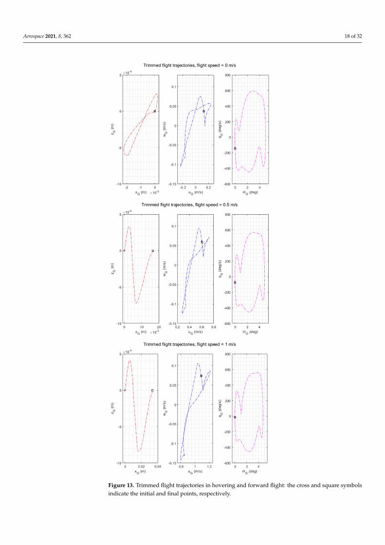
Aerospace 2021, 8, 362 18 of 32Aerospace 2021, 8, x FOR PEER REVIEW 18 of 32

Figure 13. Trimmed flight trajectories in hovering and forward flight: the cross and square sym-bols indicate the initial and final points, respectively.

Figure 13. Trimmed flight trajectories in hovering and forward flight: the cross and square symbolsindicate the initial and final points, respectively.

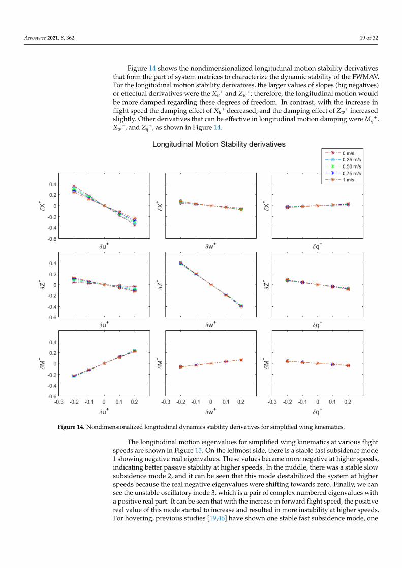
Aerospace 2021, 8, 362 19 of 32

Figure 14 shows the nondimensionalized longitudinal motion stability derivativesthat form the part of system matrices to characterize the dynamic stability of the FWMAV.For the longitudinal motion stability derivatives, the larger values of slopes (big negatives)or effectual derivatives were the Xu

+ and Zw+; therefore, the longitudinal motion would

be more damped regarding these degrees of freedom. In contrast, with the increase inflight speed the damping effect of Xu

+ decreased, and the damping effect of Zw+ increased

slightly. Other derivatives that can be effective in longitudinal motion damping were Mq+,

Xw+, and Zq

+, as shown in Figure 14.

Aerospace 2021, 8, x FOR PEER REVIEW 19 of 32

Figure 14 shows the nondimensionalized longitudinal motion stability derivatives that form the part of system matrices to characterize the dynamic stability of the FWMAV. For the longitudinal motion stability derivatives, the larger values of slopes (big nega-tives) or effectual derivatives were the Xu+ and Zw+; therefore, the longitudinal motion would be more damped regarding these degrees of freedom. In contrast, with the increase in flight speed the damping effect of Xu+ decreased, and the damping effect of Zw+ in-creased slightly. Other derivatives that can be effective in longitudinal motion damping were Mq+, Xw+, and Zq+, as shown in Figure 14.

The longitudinal motion eigenvalues for simplified wing kinematics at various flight speeds are shown in Figure 15. On the leftmost side, there is a stable fast subsidence mode 1 showing negative real eigenvalues. These values became more negative at higher speeds, indicating better passive stability at higher speeds. In the middle, there was a sta-ble slow subsidence mode 2, and it can be seen that this mode destabilized the system at higher speeds because the real negative eigenvalues were shifting towards zero. Finally, we can see the unstable oscillatory mode 3, which is a pair of complex numbered eigen-values with a positive real part. It can be seen that with the increase in forward flight speed, the positive real value of this mode started to increase and resulted in more insta-bility at higher speeds. For hovering, previous studies [19,46] have shown one stable fast subsidence mode, one stable slow subsidence mode, and an unstable oscillatory mode that qualitatively matched to the behavior of our model’s response in hovering as shown in Figure 15. In addition, Kim et al. [45] showed that at higher speeds, the one stable fast subsidence mode, the one stable slow subsidence mode, and the unstable oscillatory modes became more stable, slightly destabilized, and more unstable, respectively. These longitudinal modes’ behaviors were from the measured hawkmoth wing kinematics and agree well with our results.

Figure 14. Nondimensionalized longitudinal dynamics stability derivatives for simplified wing kinematics. Figure 14. Nondimensionalized longitudinal dynamics stability derivatives for simplified wing kinematics.

The longitudinal motion eigenvalues for simplified wing kinematics at various flightspeeds are shown in Figure 15. On the leftmost side, there is a stable fast subsidence mode1 showing negative real eigenvalues. These values became more negative at higher speeds,indicating better passive stability at higher speeds. In the middle, there was a stable slowsubsidence mode 2, and it can be seen that this mode destabilized the system at higherspeeds because the real negative eigenvalues were shifting towards zero. Finally, we cansee the unstable oscillatory mode 3, which is a pair of complex numbered eigenvalues witha positive real part. It can be seen that with the increase in forward flight speed, the positivereal value of this mode started to increase and resulted in more instability at higher speeds.For hovering, previous studies [19,46] have shown one stable fast subsidence mode, one

Aerospace 2021, 8, 362 20 of 32

stable slow subsidence mode, and an unstable oscillatory mode that qualitatively matchedto the behavior of our model’s response in hovering as shown in Figure 15. In addition,Kim et al. [45] showed that at higher speeds, the one stable fast subsidence mode, theone stable slow subsidence mode, and the unstable oscillatory modes became more stable,slightly destabilized, and more unstable, respectively. These longitudinal modes’ behaviorswere from the measured hawkmoth wing kinematics and agree well with our results.

Aerospace 2021, 8, x FOR PEER REVIEW 20 of 32

Figure 15. Nondimensionalized longitudinal dynamics eigenvalues at various flight speeds (hovering and forward flight).

3.2. Flight Control Simulations for Stabilizing Fixed Flight Conditions The results for the nonlinear multibody FWMAV flight control to stabilize hovering

and forward flight states are shown in Figures 16–18 using controller in Figure 9. The simulation results for different cases such as without control, with control, and the refer-ence states are presented. In all simulations, FWMAV was required to move at reference forward speed, zero up/down speed, zero pitch rate, and reference body pitch angle. The instabilities in states increased with the flight speed and made the control problem more challenging. However, overall, it can be seen that the controlled model converged to the reference states within 0.4 s while successfully following all of the required states for a unique set of weighting matrices at different flight speeds with corresponding control gains’ matrices. This would be helpful to obtain an efficient and consistent controller de-sign for the transition flight tracking and reference trajectories tracking of nonlinear model throughout its mission.

Figure 15. Nondimensionalized longitudinal dynamics eigenvalues at various flight speeds (hovering and forward flight).

3.2. Flight Control Simulations for Stabilizing Fixed Flight Conditions

The results for the nonlinear multibody FWMAV flight control to stabilize hoveringand forward flight states are shown in Figures 16–18 using controller in Figure 9. Thesimulation results for different cases such as without control, with control, and the referencestates are presented. In all simulations, FWMAV was required to move at referenceforward speed, zero up/down speed, zero pitch rate, and reference body pitch angle.The instabilities in states increased with the flight speed and made the control problemmore challenging. However, overall, it can be seen that the controlled model converged tothe reference states within 0.4 s while successfully following all of the required states for aunique set of weighting matrices at different flight speeds with corresponding control gains’matrices. This would be helpful to obtain an efficient and consistent controller designfor the transition flight tracking and reference trajectories tracking of nonlinear modelthroughout its mission.

Aerospace 2021, 8, 362 21 of 32Aerospace 2021, 8, x FOR PEER REVIEW 21 of 32

Figure 16. Flight control simulations for hovering flight control. Figure 16. Flight control simulations for hovering flight control.

Aerospace 2021, 8, x FOR PEER REVIEW 21 of 32

Figure 16. Flight control simulations for hovering flight control.

Figure 17. Cont.

Aerospace 2021, 8, 362 22 of 32Aerospace 2021, 8, x FOR PEER REVIEW 22 of 32

Figure 17. Flight control simulations for forward flight control (flight speed = 0.5 m/s).

Figure 18. Flight control simulations for forward flight control (flight speed = 1 m/s).

Figure 17. Flight control simulations for forward flight control (flight speed = 0.5 m/s).

Aerospace 2021, 8, x FOR PEER REVIEW 22 of 32

Figure 17. Flight control simulations for forward flight control (flight speed = 0.5 m/s).

Figure 18. Flight control simulations for forward flight control (flight speed = 1 m/s). Figure 18. Flight control simulations for forward flight control (flight speed = 1 m/s).

Aerospace 2021, 8, 362 23 of 32

3.3. Flight Control Simulations for Transition Flight Tracking

Since the controller maintained the fixed flight conditions very well, it was furtherevaluated to follow the transition flight conditions for performing various maneuvers usingcontrollers from Section 2.5.2. For this, a reference velocity profile that includes hovering,acceleration, constant speed, deceleration, and hovering again was tracked for both thelinear model and nonlinear multibody model. The simulation results and control inputsfor linear model are shown in Figures 19 and 20, respectively. It can be seen that all stateswere tracked efficiently, and the FWMAV accelerated and decelerated each within twoseconds. Maintaining constant speeds involved minimal deviation in results; however, intransition flight conditions (acceleration and deceleration), slight deviations from referenceswere reasonable due to rapidly changing body pitch angle and parametrically changingcontrol gains to maintain the performance. The control simulation results and controlinputs for nonlinear multibody model are shown in Figures 21 and 22, respectively. Allstates, forward speed, up/down speed, pitch angle, and pitch rate were tracked well withsmall deviations during acceleration and deceleration phases only. The reason for theseslight deviations during acceleration and deceleration phases was that body pitch anglerapidly changed and control gains were updated continuously for this parametric varyingnonlinear system. The control inputs for both the linear and nonlinear models variedsmoothly and were within reasonable ranges for transition flight tracking. Even thoughthe control was challenging for this fairly nonlinear multibody system as three inputs werecontrolling four states simultaneously, the simulation results showed that the designedcontroller worked effectively to track the reference velocity profile involving hovering,acceleration, constant speed, deceleration, and again hovering phases.

Aerospace 2021, 8, x FOR PEER REVIEW 23 of 32

3.3. Flight Control Simulations for Transition Flight Tracking Since the controller maintained the fixed flight conditions very well, it was further

evaluated to follow the transition flight conditions for performing various maneuvers us-ing controllers from Section 2.5.2. For this, a reference velocity profile that includes hov-ering, acceleration, constant speed, deceleration, and hovering again was tracked for both the linear model and nonlinear multibody model. The simulation results and control in-puts for linear model are shown in Figures 19 and 20, respectively. It can be seen that all states were tracked efficiently, and the FWMAV accelerated and decelerated each within two seconds. Maintaining constant speeds involved minimal deviation in results; how-ever, in transition flight conditions (acceleration and deceleration), slight deviations from references were reasonable due to rapidly changing body pitch angle and parametrically changing control gains to maintain the performance. The control simulation results and control inputs for nonlinear multibody model are shown in Figures 21 and 22, respec-tively. All states, forward speed, up/down speed, pitch angle, and pitch rate were tracked well with small deviations during acceleration and deceleration phases only. The reason for these slight deviations during acceleration and deceleration phases was that body pitch angle rapidly changed and control gains were updated continuously for this para-metric varying nonlinear system. The control inputs for both the linear and nonlinear models varied smoothly and were within reasonable ranges for transition flight tracking. Even though the control was challenging for this fairly nonlinear multibody system as three inputs were controlling four states simultaneously, the simulation results showed that the designed controller worked effectively to track the reference velocity profile in-volving hovering, acceleration, constant speed, deceleration, and again hovering phases.

Figure 19. Flight control simulations for transition flight control of linear FWMAV model.

Figure 19. Flight control simulations for transition flight control of linear FWMAV model.

Aerospace 2021, 8, x FOR PEER REVIEW 23 of 32

3.3. Flight Control Simulations for Transition Flight Tracking

Since the controller maintained the fixed flight conditions very well, it was further

evaluated to follow the transition flight conditions for performing various maneuvers us-

ing controllers from Section 2.5.2. For this, a reference velocity profile that includes hov-

ering, acceleration, constant speed, deceleration, and hovering again was tracked for both

the linear model and nonlinear multibody model. The simulation results and control in-

puts for linear model are shown in Figures 19 and 20, respectively. It can be seen that all

states were tracked efficiently, and the FWMAV accelerated and decelerated each within

two seconds. Maintaining constant speeds involved minimal deviation in results; how-

ever, in transition flight conditions (acceleration and deceleration), slight deviations from

references were reasonable due to rapidly changing body pitch angle and parametrically

changing control gains to maintain the performance. The control simulation results and

control inputs for nonlinear multibody model are shown in Figures 21 and 22, respec-

tively. All states, forward speed, up/down speed, pitch angle, and pitch rate were tracked

well with small deviations during acceleration and deceleration phases only. The reason

for these slight deviations during acceleration and deceleration phases was that body

pitch angle rapidly changed and control gains were updated continuously for this para-

metric varying nonlinear system. The control inputs for both the linear and nonlinear

models varied smoothly and were within reasonable ranges for transition flight tracking.

Even though the control was challenging for this fairly nonlinear multibody system as

three inputs were controlling four states simultaneously, the simulation results showed

that the designed controller worked effectively to track the reference velocity profile in-

volving hovering, acceleration, constant speed, deceleration, and again hovering phases.

Figure 19. Flight control simulations for transition flight control of linear FWMAV model.

Figure 20. Cont.

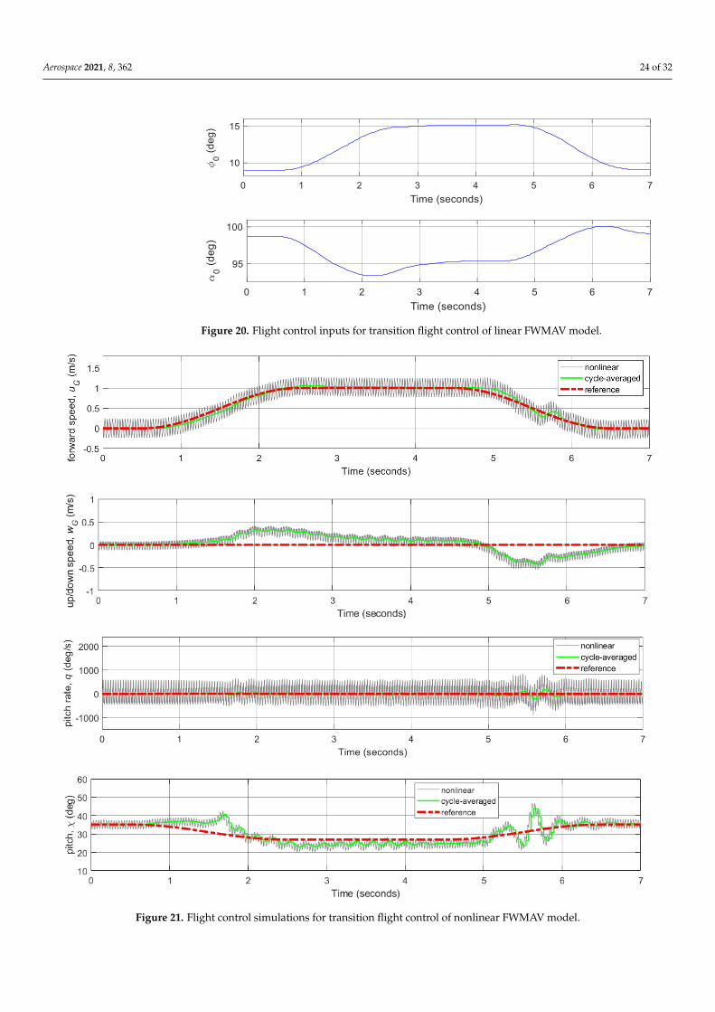
Aerospace 2021, 8, 362 24 of 32Aerospace 2021, 8, x FOR PEER REVIEW 26 of 34

Figure 20. Flight control inputs for transition flight control of linear FWMAV model.

Figure 21. Flight control simulations for transition flight control of nonlinear FWMAV model.

Figure 20. Flight control inputs for transition flight control of linear FWMAV model.

Aerospace 2021, 8, x FOR PEER REVIEW 24 of 32

Figure 20. Flight control inputs for transition flight control of linear FWMAV model.

Figure 21. Flight control simulations for transition flight control of nonlinear FWMAV model.

0 1 2 3 4 5 6 7Time (seconds)

95

100

Figure 21. Flight control simulations for transition flight control of nonlinear FWMAV model.

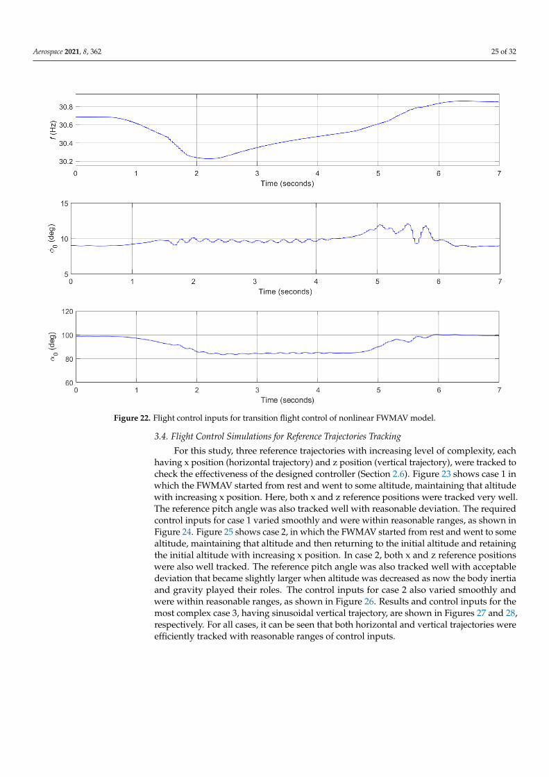
Aerospace 2021, 8, 362 25 of 32Aerospace 2021, 8, x FOR PEER REVIEW 25 of 32

Figure 22. Flight control inputs for transition flight control of nonlinear FWMAV model.

3.4. Flight Control Simulations for Reference Trajectories Tracking For this study, three reference trajectories with increasing level of complexity, each

having x position (horizontal trajectory) and z position (vertical trajectory), were tracked to check the effectiveness of the designed controller (Section 2.6). Figure 23 shows case 1 in which the FWMAV started from rest and went to some altitude, maintaining that alti-tude with increasing x position. Here, both x and z reference positions were tracked very well. The reference pitch angle was also tracked well with reasonable deviation. The re-quired control inputs for case 1 varied smoothly and were within reasonable ranges, as shown in Figure 24. Figure 25 shows case 2, in which the FWMAV started from rest and went to some altitude, maintaining that altitude and then returning to the initial altitude and retaining the initial altitude with increasing x position. In case 2, both x and z refer-ence positions were also well tracked. The reference pitch angle was also tracked well with acceptable deviation that became slightly larger when altitude was decreased as now the body inertia and gravity played their roles. The control inputs for case 2 also varied smoothly and were within reasonable ranges, as shown in Figure 26. Results and control inputs for the most complex case 3, having sinusoidal vertical trajectory, are shown in Figures 27 and 28, respectively. For all cases, it can be seen that both horizontal and verti-cal trajectories were efficiently tracked with reasonable ranges of control inputs.

Figure 22. Flight control inputs for transition flight control of nonlinear FWMAV model.

3.4. Flight Control Simulations for Reference Trajectories Tracking

For this study, three reference trajectories with increasing level of complexity, eachhaving x position (horizontal trajectory) and z position (vertical trajectory), were tracked tocheck the effectiveness of the designed controller (Section 2.6). Figure 23 shows case 1 inwhich the FWMAV started from rest and went to some altitude, maintaining that altitudewith increasing x position. Here, both x and z reference positions were tracked very well.The reference pitch angle was also tracked well with reasonable deviation. The requiredcontrol inputs for case 1 varied smoothly and were within reasonable ranges, as shown inFigure 24. Figure 25 shows case 2, in which the FWMAV started from rest and went to somealtitude, maintaining that altitude and then returning to the initial altitude and retainingthe initial altitude with increasing x position. In case 2, both x and z reference positionswere also well tracked. The reference pitch angle was also tracked well with acceptabledeviation that became slightly larger when altitude was decreased as now the body inertiaand gravity played their roles. The control inputs for case 2 also varied smoothly andwere within reasonable ranges, as shown in Figure 26. Results and control inputs for themost complex case 3, having sinusoidal vertical trajectory, are shown in Figures 27 and 28,respectively. For all cases, it can be seen that both horizontal and vertical trajectories wereefficiently tracked with reasonable ranges of control inputs.

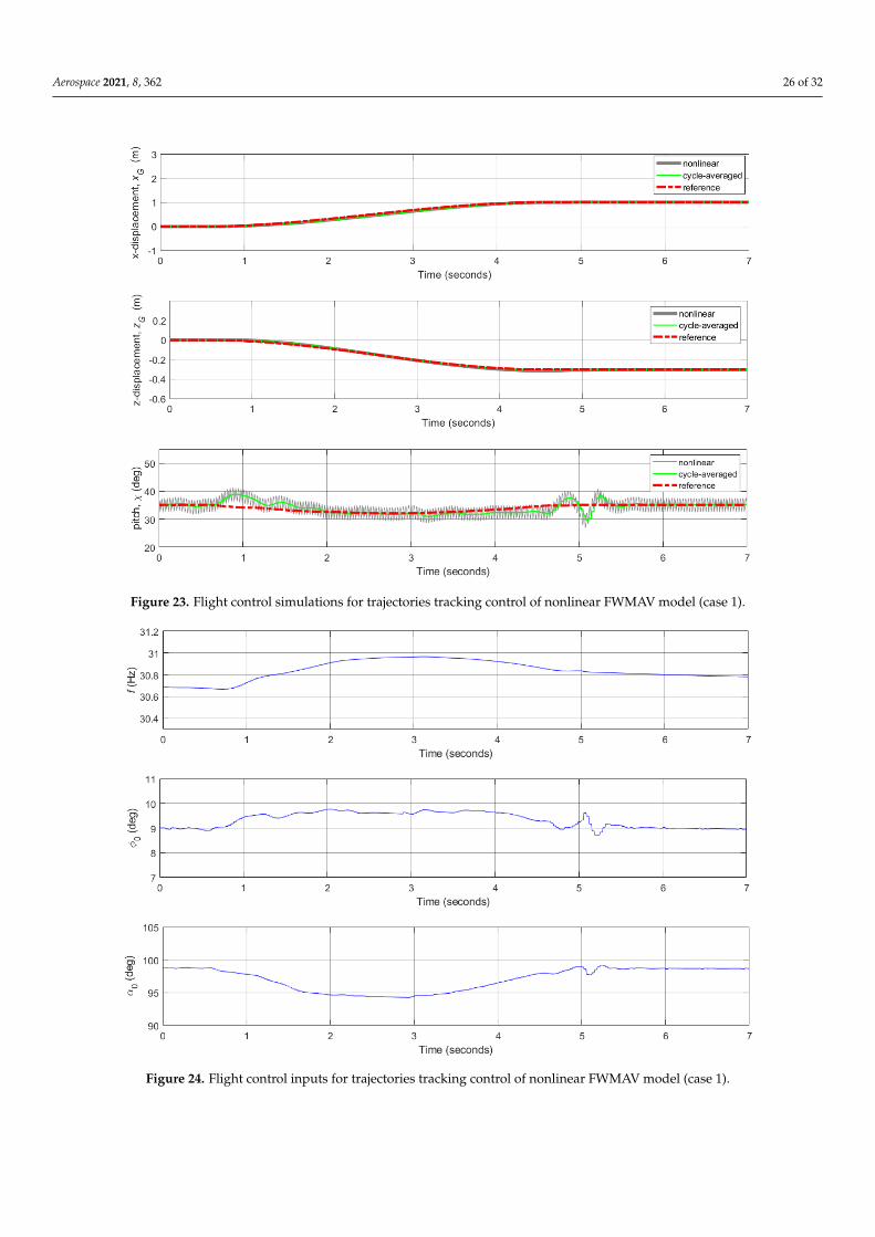
Aerospace 2021, 8, 362 26 of 32Aerospace 2021, 8, x FOR PEER REVIEW 26 of 32

Figure 23. Flight control simulations for trajectories tracking control of nonlinear FWMAV model (case 1).

Figure 24. Flight control inputs for trajectories tracking control of nonlinear FWMAV model (case 1).

Figure 23. Flight control simulations for trajectories tracking control of nonlinear FWMAV model (case 1).

Aerospace 2021, 8, x FOR PEER REVIEW 26 of 32

Figure 23. Flight control simulations for trajectories tracking control of nonlinear FWMAV model (case 1).

Figure 24. Flight control inputs for trajectories tracking control of nonlinear FWMAV model (case 1). Figure 24. Flight control inputs for trajectories tracking control of nonlinear FWMAV model (case 1).

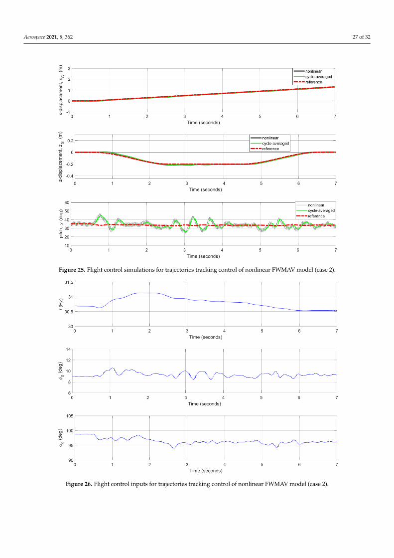
Aerospace 2021, 8, 362 27 of 32Aerospace 2021, 8, x FOR PEER REVIEW 27 of 32

Figure 25. Flight control simulations for trajectories tracking control of nonlinear FWMAV model (case 2).

Figure 26. Flight control inputs for trajectories tracking control of nonlinear FWMAV model (case 2).

Figure 25. Flight control simulations for trajectories tracking control of nonlinear FWMAV model (case 2).

Aerospace 2021, 8, x FOR PEER REVIEW 27 of 32

Figure 25. Flight control simulations for trajectories tracking control of nonlinear FWMAV model (case 2).

Figure 26. Flight control inputs for trajectories tracking control of nonlinear FWMAV model (case 2). Figure 26. Flight control inputs for trajectories tracking control of nonlinear FWMAV model (case 2).

Aerospace 2021, 8, 362 28 of 32Aerospace 2021, 8, x FOR PEER REVIEW 28 of 32

Figure 27. Flight control simulations for trajectories tracking control of nonlinear FWMAV model (case 3).

Figure 28. Flight control inputs for trajectories tracking control of nonlinear FWMAV model (case 3).

Figure 27. Flight control simulations for trajectories tracking control of nonlinear FWMAV model (case 3).

Aerospace 2021, 8, x FOR PEER REVIEW 28 of 32

Figure 27. Flight control simulations for trajectories tracking control of nonlinear FWMAV model (case 3).

Figure 28. Flight control inputs for trajectories tracking control of nonlinear FWMAV model (case 3).

Figure 28. Flight control inputs for trajectories tracking control of nonlinear FWMAV model (case 3).

Aerospace 2021, 8, 362 29 of 32

4. Conclusions

In this study, dynamic stability analysis and flight control simulations were performedfor a hawkmoth-like FWMAV model that considered the influence of time varying inertialeffects of all the model’s parts. A modified quasi-steady (QS) aerodynamic model basedon blade element approach that considered unsteady effects, added-mass effect, wingpitching moment effect, and rotational flow effect was utilized in this study. To find theprecise trim conditions and wing kinematics at different flight speeds, we appended themultibody dynamics simulation framework with a gradient-based trim search algorithmthat incorporates the aerodynamics–dynamics coupling during the convergence processfor trim search calculations. The trim search results showed closed-loop trajectories ofstates that ensure dynamic equilibrium and help in linearization of the nonlinear model.From the eigenmode analysis, regarding longitudinal dynamics, there were stable fastand stable slow subsidence modes and an unstable oscillatory mode that became moreunstable at higher speeds. The dynamic stability characterization results qualitativelyconformed to the results of previous studies as discussed in Section 3.1, and results werecompared between simplified and measured hawkmoth wing kinematics. The trim flightconditions, system matrices, and control matrices for various speeds were then utilized tofind optimal control gains with augmented LQR control technique using gain scheduling.The designed controller worked very well to stabilize both the hovering and forward flightconditions. The gain-scheduled LQR controller was then utilized to achieve transition flighttracking that involves hovering, acceleration, constant speed, deceleration, and hoveringphases for both the linear model and nonlinear multibody model. Since the designedcontroller worked efficiently for forward flight tracking, a dual-loop control technique,with inner velocity control loop and outer PI position control loop, was then implementedfor trajectories tracking control. Three reference trajectories, each having both horizontaltrajectory (x position) and vertical trajectory (z position), with increasing level of complexitywere tracked successfully to validate the performance of the proposed controller. All inall, the control simulation results demonstrated that these combinations of linear controltechniques worked effectively for this fairly nonlinear multibody FWMAV model. Forfuture work, trajectory tracking optimization with minimum energy consumption for themultibody FWMAV model can be considered.

Author Contributions: Conceptualization, M.Y.B., S.-G.L. and J.-H.H.; methodology, M.Y.B. andS.-G.L.; problem formulation, M.Y.B. and J.-H.H.; software integration, M.Y.B. and S.-G.L.; formalanalyses, M.Y.B.; initial results compilation M.Y.B.; resources, J.-H.H.; data curation, J.-H.H. andM.Y.B.; writing—original draft preparation, M.Y.B.; writing—review and editing, M.Y.B., S.-G.L. andJ.-H.H.; visualization, M.Y.B.; final review, J.-H.H. and S.-G.L.; supervision, J.-H.H.; project admin-istration, J.-H.H.; funding acquisition, J.-H.H. All authors have read and agreed to the publishedversion of the manuscript.

Funding: This research was supported by Unmanned Vehicles Core Technology Research andDevelopment Program through the National Research Foundation of Korea (NRF) and UnmannedVehicle Advanced Research Center (UVARC) funded by the Ministry of Science and ICT, the Republicof Korea (2020M3C1C1A01083414).

Institutional Review Board Statement: Not applicable.

Informed Consent Statement: Not applicable.

Data Availability Statement: Not applicable.

Conflicts of Interest: The authors declare no conflict of interest.

References1. Phan, H.V.; Aurecianus, S.; Kang, T.; Park, H.C. KUBeetle-S: An insect-like, tailless, hover-capable robot that can fly with a

low-torque control mechanism. Int. J. Micro Air Veh. 2019, 11, 1756829319861371. [CrossRef]2. Tijmons, S.; De Wagter, C.; Remes, B.; De Croon, G. Autonomous Door and Corridor Traversal with a 20-Gram Flapping Wing

MAV by Onboard Stereo Vision. Aerospace 2018, 5, 69. [CrossRef]

Aerospace 2021, 8, 362 30 of 32

3. Keennon, M.; Klingebiel, K.; Won, H. Development of the nano hummingbird: A tailless flapping wing micro air vehicle.In Proceedings of the 50th AIAA Aerospace Sciences Meeting Including the New Horizons Forum and Aerospace Exposition,Nashville, TN, USA, 9–12 January 2012; p. 588.

4. Pérez-Arancibia, N.O.; Ma, K.Y.; Galloway, K.C.; Greenberg, J.D.; Wood, R.J. First controlled vertical flight of a biologicallyinspired microrobot. bioinspir. Biomim. 2011, 6, 036009. [CrossRef] [PubMed]

5. Ratti, J.; Vachtsevanos, G. A biologically-inspired micro aerial vehicle. J. Intell. Robot. Syst. 2010, 60, 153–178. [CrossRef]6. Srigrarom, S.; Chan, W.-L. Ornithopter type flapping wings for autonomous micro air vehicles. Aerospace 2015, 2, 235–278.

[CrossRef]7. Nguyen, Q.-V.; Park, H.C. Design and demonstration of a locust-like jumping mechanism for small-scale robots. J. Bionic Eng.

2012, 9, 271–281. [CrossRef]8. Michelson, R.; Helmick, D.; Reece, S.; Amarena, C. A reciprocating chemical muscle (RCM) for micro air vehicle ‘Entomopter’flight.

Proc. Assoc. Unmanned Veh. Syst. 1997, 429–435.9. Orlowski, C.T.; Girard, A.R. Modeling and simulation of nonlinear dynamics of flapping wing micro air vehicles. AIAA J. 2011,

49, 969–981. [CrossRef]10. Nguyen, A.T.; Han, J.-H. Wing flexibility effects on the flight performance of an insect-like flapping-wing micro-air vehicle.

Aerosp. Sci. Technol. 2018, 79, 468–481. [CrossRef]11. Taylor, G.K.; Thomas, A.L. Dynamic flight stability in the desert locust Schistocerca gregaria. J. Exp. Biol. 2003, 206, 2803–2829.

[CrossRef]12. Taylor, G.K.; Zbikowski, R. Nonlinear time-periodic models of the longitudinal flight dynamics of desert locusts Schistocerca

gregaria. J. R. Soc. Interface 2005, 2, 197–221. [CrossRef]13. Nguyen, A.T. Effects of Body Aerodynamics and Wing Flexibility on Flight Characteristics of Insect-Like Flapping-Wing Micro

Air Vehicles. Ph.D. Dissertation, Korea Advanced Institute of Science and Technology, Daejeon, Korea, 2017.14. Kalliny, A.N.; El-Badawy, A.A.; Elkhamisy, S.M. Command-filtered integral backstepping control of longitudinal flapping-wing

flight. J. Guid. Control Dyn. 2018, 41, 1556–1568. [CrossRef]15. Kim, J.-K.; Han, J.-H. A multibody approach for 6-DOF flight dynamics and stability analysis of the hawkmoth Manduca sexta.

Bioinspir. Biomim. 2014, 9, 016011. [CrossRef]16. Taha, H.E.; Hajj, M.R.; Nayfeh, A.H. Flight dynamics and control of flapping-wing MAVs: A review. Nonlinear Dyn. 2012, 70,

907–939. [CrossRef]17. Taylor, G.; Thomas, A. Animal flight dynamics II. Longitudinal stability in flapping flight. J. Theor. Biol. 2002, 214, 351–370.

[CrossRef]18. Taylor, G.; Bomphrey, R.; ‘t Hoen, J. Insect flight dynamics and control. In Proceedings of the 44th AIAA Aerospace Sciences

Meeting and Exhibit, Reno, NV, USA, 9–12 January 2006; p. 32.19. Sun, M.; Wang, J.; Xiong, Y. Dynamic flight stability of hovering insects. Acta Mech. Sin. 2007, 23, 231–246. [CrossRef]20. Dietl, J.M.; Garcia, E. Stability in ornithopter longitudinal flight dynamics. J. Guid. Control Dyn. 2008, 31, 1157–1163. [CrossRef]21. Doman, D.; Oppenheimer, M.; Sigthorsson, D. Dynamics and control of a minimally actuated biomimetic vehicle: Part i-

aerodynamic model. In Proceedings of the AIAA Guidance, Navigation, and Control Conference, Chicago, IL, USA, 10–13August 2009; p. 6160.

22. Oppenheimer, M.; Doman, D.; Sigthorsson, D. Dynamics and control of a minimally actuated biomimetic vehicle: Part ii-control.In Proceedings of the AIAA Guidance, Navigation, and Control Conference, Chicago, IL, USA, 10–13 August 2009; p. 6161.

23. Hedrick, T.L.; Cheng, B.; Deng, X. Wingbeat time and the scaling of passive rotational damping in flapping flight. Science 2009,324, 252–255. [CrossRef]

24. Faruque, I.; Humbert, J.S. Dipteran insect flight dynamics. Part 1 Longitudinal motion about hover. J. Theor. Biol. 2010, 264,538–552. [CrossRef]

25. Sun, M.; Xiong, Y. Dynamic flight stability of a hovering bumblebee. J. Exp. Biol. 2005, 208, 447–459. [CrossRef]26. Orlowski, C.; Girard, A.; Shyy, W. Derivation and simulation of the nonlinear dynamics of a flapping wing micro-air vehicle.

In Proceedings of the European Micro-Air Vehicle Conference and Competition, Delft, The Netherlands, 14–17 September 2009.27. Su, W.; Cesnik, C. Flight dynamic stability of a flapping wing micro air vehicle in hover. In Proceedings of the 52nd

AIAA/ASME/ASCE/AHS/ASC Structures, Structural Dynamics and Materials Conference, Denver, CO, USA, 4–7 April2011; p. 2009.

28. Bolender, M. Rigid multi-body equations-of-motion for flapping wing mavs using kane’s equations. In Proceedings of the AIAAGuidance, Navigation, and Control Conference, Chicago, IL, USA, 10–13 August 2009; p. 6158.

29. Gebert, G.; Gallmeier, P.; Evers, J. Equations of motion for flapping flight. In Proceedings of the AIAA Atmospheric FlightMechanics Conference and Exhibit, Monterey, CA, USA, 5–8 August 2002; p. 4872.

30. Grauer, J.A.; Hubbard Jr, J.E. Multibody model of an ornithopter. J. Guid. Control Dyn. 2009, 32, 1675–1679. [CrossRef]31. Xiong, Y.; Sun, M. Dynamic flight stability of a bumblebee in forward flight. Acta Mech. Sin. 2008, 24, 25–36. [CrossRef]32. Wu, J.H.; Sun, M. Floquet stability analysis of the longitudinal dynamics of two hovering model insects. J. R. Soc. Interface 2012, 9,

2033–2046. [CrossRef]33. Strogatz, S.H. Nonlinear Dynamics and Chaos: With Applications to Physics, Biology, Chemistry and Engineering; Westview Press:

Boulder, CO, USA, 1994.

Aerospace 2021, 8, 362 31 of 32

34. Gao, N.; Aono, H.; Liu, H. Perturbation analysis of 6DoF flight dynamics and passive dynamic stability of hovering fruit flyDrosophila melanogaster. J. Theor. Biol. 2011, 270, 98–111. [CrossRef] [PubMed]

35. Gao, N.; Aono, H.; Liu, H. A numerical analysis of dynamic flight stability of hawkmoth hovering. J. Biomech. Sci. Eng. 2009, 4,105–116. [CrossRef]

36. Pennycuick, C.J. Power requirements for horizontal flight in the pigeon Columba livia. J. Exp. Biol. 1968, 49, 527–555. [CrossRef]37. Ellington, C.P. The aerodynamics of hovering insect flight. V. A vortex theory. Philos. Trans. R. Soc. London B Biol. Sci. 1984, 305,

115–144.38. Phlips, P.; East, R.; Pratt, N. An unsteady lifting line theory of flapping wings with application to the forward flight of birds.

J. Fluid Mech. 1981, 112, 97–125. [CrossRef]39. Ansari, S.A. A Nonlinear, Unsteady Aerodynamic Model for Insect-Like Flapping Wings in the Hover with Micro Air Vehicle

Applications. Ph.D. Dissertation, Cranfield University, Bedford, UK, 2004.40. Xuan, H.; Hu, J.; Yu, Y.; Zhang, J. Recent progress in aerodynamic modeling methods for flapping flight. AIP Adv. 2020, 10,

020701. [CrossRef]41. Sane, S.P.; Dickinson, M.H. The aerodynamic effects of wing rotation and a revised quasi-steady model of flapping flight. J. Exp.

Biol. 2002, 205, 1087–1096. [CrossRef]42. Han, J.-S.; Kim, J.-K.; Chang, J.W.; Han, J.-H. An improved quasi-steady aerodynamic model for insect wings that considers

movement of the center of pressure. Bioinspiration Biomim. 2015, 10, 046014. [CrossRef]43. Taha, H.E.; Hajj, M.R.; Nayfeh, A.H. Longitudinal flight dynamics of hovering MAVs/insects. J. Guid. Control Dyn. 2014, 37,

970–979. [CrossRef]44. Au, L.T.K.; Park, H.C. Influence of center of gravity location on flight dynamic stability in a hovering tailless FW-MAV:

Longitudinal motion. J. Bionic Eng. 2019, 16, 130–144. [CrossRef]45. Kim, J.-K.; Han, J.-S.; Lee, J.-S.; Han, J.-H. Hovering and forward flight of the hawkmoth Manduca sexta: Trim search and 6-DOF

dynamic stability characterization. Bioinspir. Biomim. 2015, 10, 056012. [CrossRef] [PubMed]46. Cheng, B.; Deng, X. Translational and rotational damping of flapping flight and its dynamics and stability at hovering. IEEE

Trans. Robot. 2011, 27, 849–864. [CrossRef]47. Oppenheimer, M.W.; Doman, D.B.; Sigthorsson, D.O. Dynamics and control of a biomimetic vehicle using biased wingbeat

forcing functions. J. Guid. Control Dyn. 2011, 34, 204–217. [CrossRef]48. Loh, K.; Cook, M.; Thomasson, P. An investigation into the longitudinal dynamics and control of a flapping wing micro air

vehicle at hovering flight. Aeronaut. J. 2003, 107, 743–753.49. Khanmirza, E.; Yousefi-Koma, A.; Tarvirdizadeh, B. Nonlinear trajectory control of a flapping-wing micro aerial vehicle. Aircr.

Eng. Aerosp. Technol. 2012, 84, 58–65. [CrossRef]50. Banazadeh, A.; Taymourtash, N. Adaptive attitude and position control of an insect-like flapping wing air vehicle. Nonlinear Dyn.

2016, 85, 47–66. [CrossRef]51. Wissa, B.E.; Elshafei, K.O.; El-Badawy, A.A. Lyapunov-based control and trajectory tracking of a 6-DOF flapping wing micro

aerial vehicle. Nonlinear Dyn. 2020, 99, 2919–2938. [CrossRef]52. Khosravi, M.; Novinzadeh, A. A multi-body control approach for flapping wing micro aerial vehicles. Aerosp. Sci. Technol. 2021,

112, 106525. [CrossRef]53. Guo, S.; Li, H.; Zhou, C.; Zhang, Y.L.; He, Y.; Wu, J.H. Analysis and experiment of a bio-inspired flyable micro flapping wing

rotor. Aerosp. Sci. Technol. 2018, 79, 506–517. [CrossRef]54. Wu, J.H.; Zhang, Y.L.; Sun, M. Hovering of model insects: Simulation by coupling equations of motion with Navier–Stokes

equations. J. Exp. Biol. 2009, 212, 3313–3329. [CrossRef]55. Serrani, A.; Keller, B.; Bolender, M.; Doman, D. Robust control of a 3-dof flapping wing micro air vehicle. In Proceedings of the

AIAA Guidance, Navigation, and Control Conference, Toronto, ON, Canada, 2–5 August 2010; p. 7709.56. Schenato, L.; Campolo, D.; Sastry, S. Controllability issues in flapping flight for biomimetic micro aerial vehicles (MAVs).

In Proceedings of the 42nd IEEE International Conference on Decision and Control (IEEE Cat. No. 03CH37475), Maui, HI, USA,9–12 December 2003; pp. 6441–6447.

57. Peng, K.; Lin, F.; Chen, B.M. Modeling and control analysis of a flapping-wing micro aerial vehicle. In Proceedings of the 201713th IEEE International Conference on Control & Automation (ICCA), Ohrid, Macedonia, 3–6 July 2017; pp. 295–300.

58. Zhu, B.; Zuo, Z. Adaptive model predictive control for set-point tracking of a single-DOF flapping-wing unmanned aerial vehicle.In Proceedings of the 2017 13th IEEE International Conference on Control & Automation (ICCA), Ohrid, Macedonia, 3–6 July2017; pp. 861–866.

59. Ellington, C.P. The Aerodynamics of Hovering Insect Flight. II. Morphological Parameters. Philos. Trans. R. Soc. B 1984, 305,17–40.

60. Hedrick, T.L.; Daniel, T.L. Flight control in the hawkmoth Manduca sexta: The inverse problem of hovering. J. Exp. Biol. 2006,209, 3114–3130. [CrossRef]

61. O’Hara, R.P.; Palazotto, A.N. The morphological characterization of the forewing of the Manduca sexta species for the applicationof biomimetic flapping wing micro air vehicles. Bioinspir. Biomim. 2012, 7, 046011. [CrossRef]

62. Willmott, A.P.; Ellington, C.P. The mechanics of flight in the hawkmoth Manduca sexta. I. Kinematics of hovering and forwardflight. J. Exp. Biol. 1997, 200, 2705–2722. [CrossRef]

Aerospace 2021, 8, 362 32 of 32

63. Berman, G.J.; Wang, Z.J. Energy-minimizing kinematics in hovering insect flight. J. Fluid Mech. 2007, 582, 153–168. [CrossRef]64. Faruque, I.; Humbert, J.S. Dipteran insect flight dynamics. Part 2: Lateral–directional motion about hover. J. Theor. Biol. 2010, 265,

306–313. [CrossRef] [PubMed]65. Pfeiffer, A.T.; Lee, J.-S.; Han, J.-H.; Baier, H. Ornithopter Flight Simulation Based on Flexible Multi-Body Dynamics. J. Bionic Eng.

2010, 7, 102–111. [CrossRef]66. Lee, J.-S.; Kim, J.-K.; Kim, D.-K.; Han, J.-H. Longitudinal Flight Dynamics of Bioinspired Ornithopter Considering Fluid-Structure

Interaction. J. Guid. Control Dyn. 2011, 34, 667–677. [CrossRef]67. Gear, C. Simultaneous Numerical Solution of Differential-Algebraic Equations. IEEE Trans. Circuit Theory 1971, 18, 89–95.

[CrossRef]68. Nelson, R.C. Flight Stability and Automatic Control; WCB/McGraw Hill: New York, NY, USA, 1998.69. Skogestad, S.; Postlethwaite, I. Multivariable Feedback Control: Analysis and Design; Wiley: New York, NY, USA, 2007.70. Kwakernaak, H.; Sivan, R. Linear Optimal Control Systems; Wiley-Interscience: New York, NY, USA, 1972.71. Willmott, A.P.; Ellington, C.P. The mechanics of flight in the hawkmoth Manduca sexta. II. Aerodynamic consequences of

kinematic and morphological variation. J. Exp. Biol. 1997, 200, 2723–2745. [CrossRef] [PubMed]