Dynamic self-thinning model for sessile animal populations with multilayered distribution

Dynamic self-thinning model for sessile animal populationswith multilayered distributionIsabel Fuentes-Santos, Alhambra M. Cubillo, Mar�ıa Jos�e Fern�andez-Reiriz and Ux�ıo Labarta

Instituto de Investigaciones Marinas, CSIC, Vigo, Spain

Correspondence

Ux�ıo Labarta, Instituto de Investigaciones

Marinas, CSIC, Eduardo Cabello, 6, 36208,

Vigo, Spain. E-mail: [email protected]

Received 24 October 2012; accepted 7 March

2013.

Abstract

The main drawback of the traditional self-thinning model is how time is

handled. Self-thinning (ST) has been formally recognized as a dynamic process,

while the current ST models have not included the temporal effect. This

restricts the analysis to the average competitive behaviour of the population

and produces a biased estimation of the self-thinning parameters. In this study,

we extend the dynamic ST model introduced by Roderick and Barnes (2004)

to the analysis of multilayered sessile animal populations. For this purpose, we

incorporate the number of layers and the density per layer into the dynamical

approach. The performance of the dynamic model was checked and compared

with the classical ST model through the analysis of mussel populations grown

at different density treatments. Unlike the traditional model, the dynamical

approach detected the effect of culture density on the competitive behaviour of

individuals and allowed to analyse the temporal evolution of intraspecific com-

petition by estimating the ST exponent trajectory. Moreover, this approach

provided an ecological interpretation of any possible value of the ST exponent.

Thus, our results support the use of the dynamic model in the analysis of self-

thinning in sessile animal multilayered populations. The estimation of the ST

exponent trajectory reflects the dynamic nature of the ST process, providing a

more realistic description of population dynamics than the traditional model.

Key words: dynamic approach, intraspecific competition, multilayered population, population

density, population dynamics.

Introduction

The self-thinning process (ST) describes the inverse rela-

tionship between body size of individuals and population

density when intraspecific competition causes mortality

during growth (Westoby 1984). This mechanism, observed

in plants and animals at high population densities, plays an

important role in determining population dynamics and

community structure (Westoby 1984; Weller 1987; Puntieri

1993; Fr�echette & Lefaivre 1995; Marquet et al. 1995; Petra-

itis 1995; Fr�echette et al. 1996; Gui~nez & Castilla 1999,

2001; Gui~nez et al. 2005).

Self-thinning has been analysed using sequential sam-

pling of even-aged populations growing at different densi-

ties (Fig. 1 in Alunno-Bruscia et al. 2000). This allows

plotting individual mass–density (m-N) trajectories

through time. In sessile animals with multilayered distribu-

tion, self-thinning has been modelled by the allometric rela-

tionship (Gui~nez & Castilla 1999):

�m ¼ K n=SLð Þb¼ K N=Lð Þb¼ KNbe ; ð1Þ

where �m is mean individual mass, n is number of individu-

als, S is total surface area occupied, N is density, L is num-

ber of layers, Ne = N/L is the density per layer or effective

density and (K, b) are the model parameters. For a given

population, these parameters are estimated from sequential

measurements of individual mass and effective density.

Self-thinning has been extensively studied in plant popu-

lations, where competition is attributed to space limitations

(spatial self-thinning, SST) and the theoretical exponent

bSST = �3/2 is proposed (Westoby 1984). On the other

hand, Begon et al. (1986) stated that in mobile animal

populations, the ST process would be regulated by food

© 2013 Wiley Publishing Asia Pty Ltd 1

Reviews in Aquaculture (2013) 5, 1–13 doi: 10.1111/raq.12032

https://www.researchgate.net/publication/271814699_Is_There_a_Self-Thinning_Rule_for_Animal_Populations?el=1_x_8&enrichId=rgreq-57ebd5e5-d845-4d77-9164-2f92a5c6653e&enrichSource=Y292ZXJQYWdlOzI1OTIxNTQ4NTtBUzoxMDQyMzMwMzAzODk3NjFAMTQwMTg2MjQ5OTE4Mw==

limitations (food self-thinning, FST) and suggested the

exponent bFST = �4/3. Both exponents were proposed

under assumptions not always fulfilled under natural con-

ditions; therefore, these theoretical exponents should be

calculated for each population under study (Lob�on-Cervi�a

& Mortensen 2006). As sessile animal populations can be

constrained by space or food limitations, most studies

have focussed on determining the competition factor by

Figure 1 Temporal evolution of density (N), effective density (Ne), biomass (B), biomass per layer (BL), number of layers (L) and mean individual mass

( �m) for each density treatment.

Reviews in Aquaculture (2013) 5, 1–13

© 2013 Wiley Publishing Asia Pty Ltd2

I. Fuentes-Santos et al.

comparing the estimated with the theoretical ST exponents

(Fr�echette & Lefaivre 1990; Filgueira et al. 2008; Lachance-

Bernard et al. 2010).

The main drawback of the traditional self-thinning

model (eqn 1) is how time is handled. While time is pres-

ent implicitly due to (K, b) are estimated from sequential

samplings, the time effect is not explicitly included. This

gives rise to two sources of error in the estimation of the ST

parameters. First, b and K are assumed to be constant

across the entire study period, while self-thinning is a

dynamic process and the ST exponent (b) would vary over

time (White 1981; Westoby 1984; Norberg 1988). There-

fore, we are estimating a mean value when we should esti-

mate a temporal trend. On the other hand, the regression

methods currently used in ST studies (reviewed by Zhang

et al. 2005) assume that observations are independent,

overlooking their temporal autocorrelation and resulting in

a biased estimation of the self-thinning parameters.

Thus, while self-thinning has been formally recognized as

a dynamic process, the current models are not dynamic,

failing to include the time effect. Cubillo et al. (2012b) par-

tially overcame this problem fitting the traditional ST

model using frontier analysis, which provides a dynamic

interpretation of the ST process through the temporal evo-

lution of site occupancy. On the other hand, Roderick and

Barnes (2004) proposed a new formulation of self-thinning

as a dynamic problem. The main assumption of this

approach is that b can vary over time, but converges to �1

when total biomass is constant, given that

�m ¼P

m

n¼

Pm

SL

SL

n¼

Pm

SL

n

SL

� ��1

¼P

m

SLN�1

e ¼ KN�1e :

This study extends the dynamic self-thinning model, pro-

posed by Roderick and Barnes (2004) for plants, to the

study of multilayered sessile animal populations. For this

purpose, we include the effective density (Ne) in the origi-

nal model. Then, we give insight into the dynamic interpre-

tation of the different values of the ST exponent. Finally,

we compare the dynamic ST model with the classical model

through the analysis of mussel (Mytilus galloprovincialis

Lmk.) populations grown in suspended culture.

Materials and methods

Experimental design

This work analyses the data set from Cubillo et al.

(2012b), which studied the population dynamics of Myti-

lus galloprovincialis grown in suspended culture. Data were

obtained by sequential sampling of seven initial densities

(220, 370, 500, 570, 750, 800 and 1150 individuals per

metre of rope, ind/m) randomly distributed over a com-

mercial raft. Seven monthly samplings were performed

from thinning-out to harvest (May–November 2008). In

each sampling, a section of known length was taken from

four ropes of each density (28 ropes per sampling date).

Each sample was weighed to obtain the population bio-

mass (B; g). Density was calculated as number of mussels

per metre of rope (N0; ind/m) and standardized to num-

ber of individuals per square metre of rope (N; ind/m2).

Mean individual fresh mass (�m; g) was obtained dividing

the weight of subsamples containing 250–300 mussels by

the number of individuals. To account for multilayering,

we need the effective surface area occupied (Se), that is,

the surface occupied if individuals were arranged in a sin-

gle layer (Gui~nez et al. 2005). The effective surface area

(Se) was obtained using image analysis techniques (Filgue-

ira et al. 2008). The effective density or mean number of

individuals per layer (Ne = N0/Se) and number of layers

(L = N/Ne) were calculated according to Gui~nez and

Castilla (2001).

Dynamic self-thinning model

We extended the dynamic model proposed by Roderick

and Barnes (2004) for the analysis of self-thinning in plants

to the study of multilayered sessile animal populations. For

this purpose, we substituted the density or number of indi-

viduals per unit area (N) by the effective density (Ne)

defined in the self-thinning model (Gui~nez & Castilla 1999;

Cubillo et al. 2012b).

Assuming that the allometric relationship in eqn 1 is

an identity, the unknown parameters (K, b) are

uniquely determined by the effective density and mean

individual mass observed in two instants of time. If

ð�m1;Ne1 and ð�m2;Ne2Þ are the values observed at succes-

sive times t1 and t2, substituting these values in the logarith-

mic transformation of eqn 1 yields:

ln �m1 ¼ logK þ b lnNe1

ln �m2 ¼ logK þ b lnNe2

: ð2Þ

Solving eqn 2 by elimination,

b ¼ lnð�m2=�m1ÞlnðNe2=Ne1Þ ; ð3Þ

and

lnK ¼ ln �m1 � b lnNe1: ð4Þ

Thus, the estimated values of K and b belong to the same

time interval as the measurements used to estimate them.

This procedure is repeated for each pair of consecutive

samplings to estimate the parameters corresponding to

each time interval.



Dynamic self-thinning model for mussels

https://www.researchgate.net/publication/249140066_Theory_of_Growth_Geometry_of_Plants_and_Self-Thinning_of_Plant_Populations_Geometric_Similarity_Elastic_Similarity_and_Different_Growth_Modes_of_Plant_Parts?el=1_x_8&enrichId=rgreq-57ebd5e5-d845-4d77-9164-2f92a5c6653e&enrichSource=Y292ZXJQYWdlOzI1OTIxNTQ4NTtBUzoxMDQyMzMwMzAzODk3NjFAMTQwMTg2MjQ5OTE4Mw==

https://www.researchgate.net/publication/229631247_Layering_the_effective_density_of_mussels_and_mass-density_boundary_curves?el=1_x_8&enrichId=rgreq-57ebd5e5-d845-4d77-9164-2f92a5c6653e&enrichSource=Y292ZXJQYWdlOzI1OTIxNTQ4NTtBUzoxMDQyMzMwMzAzODk3NjFAMTQwMTg2MjQ5OTE4Mw==

https://www.researchgate.net/publication/259215661_Evaluation_of_self-thinning_models_and_estimation_methods_in_multilayered_sessile_animal_populations?el=1_x_8&enrichId=rgreq-57ebd5e5-d845-4d77-9164-2f92a5c6653e&enrichSource=Y292ZXJQYWdlOzI1OTIxNTQ4NTtBUzoxMDQyMzMwMzAzODk3NjFAMTQwMTg2MjQ5OTE4Mw==

The procedure above would be used for a finite number

of sequential samplings. However, from a theoretical view-

point, it is useful to extend the analysis to infinitesimal time

intervals which allows an analytical treatment of self-thin-

ning (Roderick & Barnes 2004). For this purpose, we

should note that

�m2 ¼ �m1 þ d�m

Ne2 ¼ Ne1 þ dNe

ð5Þ

where d denotes a finite difference. Using eqn 5, we can

rewrite eqn 3 as:

b ¼ lnð1þ d�m=�m1Þlnð1þ dNe=Ne1Þ ð6Þ

For infinitesimal time increments, d�m ! d �m and dNe

! dNe, as ln(1 + x)? x for small values of x:

b ¼ d �m

�m

Ne

dNe: ð7Þ

Eqn 7 defines the self-thinning exponent (b) as the quo-tient between the rates of change in individual mean mass

and density, which is very useful in interpreting the

dynamic model.

To link the dynamic model with the self-thinning pro-

cess, we should note that for a set of n individuals at time t,

the total biomass of a given area is

B ¼ m1 þ � � � þmn ¼ n�m: ð8Þ

Thus, if Ne is the effective density, that is, the number of

individuals per unit area in each layer, the biomass per

layer is

BL ¼ n�m

SL¼ Ne �m: ð9Þ

The biomass rate of change is then

dBL

dt¼ �m

dNe

dtþ Ne

d �m

dt; ð10Þ

and when the biomass remains constant, dBL/dt = 0, we

have

�mdNe

dt¼ �Ne

d �m

dt: ð11Þ

Thus, since �m and Ne are always positive, dNe and d �m

must have opposite signs, that is, an increase in mass

implies a decrease in density, which can be due to mortality

as well as reorganization of the individuals into new layers

(migration), and vice versa.

Comparing eqn 7 and 10, we see that b is the ratio of

the terms on the right side of eqn 10. Thus, when biomass

remains constant, b � �1 (eqn 11). This can reflect two

situations: (i) dNe/dt and d �m/dt are bounded away from 0,

and the rates of change in individual mass and effective

density are similar, or (ii) dNe/dt � 0 and d �m/dt � 0;

thus, competition and growth slows down and the system

stabilizes. When dNe/dt < 0, such as under mortality

and/or migration, then b < �1 (e.g., �3/2, �4/3) if dBL/

dt > 0, that is, the growth rate is greater than the mortality

rate; and b > �1 if dBL/dt < 0, that is, the growth rate is

lower than the mortality rate. The opposite holds for

dNe/dt > 0. When the effective density remains constant,

dNe/dt = 0, b tend to (either positive or negative) infinity

(see Table 1).

Statistical analysis

We tested the validity of the dynamic self-thinning model

and compared this approach with the traditional ST

model through the analysis of multilayered mussel popu-

lations grown in suspended culture. Firstly, for each den-

sity treatment, the traditional ST model (eqn 1) was

fitted using the regression methods applied in Cubillo

et al. (2012b). We tested whether the traditional model

can detect different competition patterns among densities.

To discriminate the competition limiting factor, the esti-

mated exponents were compared with the theoretical

food self-thinning (FST) exponent (bFST = �1.33) and

the space self-thinning (SST) exponent obtained using

image analysis (bSST = �1.23; Cubillo et al. 2012b).

To fit the dynamic model, M = 1000 replicates of effec-

tive density (Ne) and mean individual mass (�m) were

obtained using Monte Carlo simulations for each time and

density treatment. Then, the self-thinning exponent and its

95% confidence interval were estimated for each sampling

interval (eqn 7). Tukey tests were applied to determine

whether b = �1, that is, whether the biomass remained

constant between samplings.

The statistical analysis was performed with the help

of the statistical package R 2.12.2 (R Development Core

Team 2011).

Results

Figure 1 shows the temporal evolution of density (N),

effective density (Ne), biomass (B), biomass per layer (BL),

number of layers (L) and mean individual fresh mass (�m)

for each density treatment (Tables A1–A7). While density,

number of layers and biomass depended on the initial den-

sity; the pattern showed by mean individual mass, effective

density and biomass per layer were homogeneous over

the density gradient. We observe a trade-off between the





exponential decrease in effective density and the increase in

individual fresh mass, for all treatments. The density plot

shows that mortality occurred only at high initial densities

(N > 500 ind/m). Thus, for low-density populations, the

decrease in Ne would respond only to reorganization of

individuals into new layers (migration), while for higher

densities, this would also include mortality. At lower densi-

ties, the number of layers increased throughout the experi-

mental period, while at higher densities, the reorganization

of growing individuals caused a continuous readjustment

between the number of layers and the effective density.

Mean individual mass, biomass and biomass per layer

increased in the first months and remained constant in the

last three months.

Table 2 shows the fits of the classical self-thinning model

(eqn 1) for each density treatment. As the different regres-

sion methods applied provide equivalent estimates, only

the linear regression (ordinary least squares, OLS) fit is

shown. Although we obtained a good fit for m-Ne relation-

ships (R2 > 0.94), no significant density effect was observed

on the ST exponents (see CIs for b in Table 2). Compari-

son of the estimated exponents with the theoretical space

(bSST = �1.23; Cubillo et al. 2012b) and food

(bFST = �1.33) ST exponents concluded that competition

for food and space dominated at 220, 500, 700 and

800 ind/m with competition for food dominating at 370,

570 and 1150 ind/m (Table 2). These results point out the

inefficiency of the classical model to discriminate the com-

petition limiting factor.

Table 3 shows the estimated self-thinning exponents

obtained with the dynamic model, and Figures 2–8 show

the plots of the traditional and dynamic fits for each density

treatment. The high variability observed for b in certain

months responded to small changes in effective density

(dNe/dt � 0).

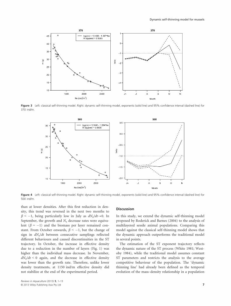
During the first three months, mussels grown at lower

densities (220, 370 and 500 ind/m) presented higher

growth than migration rates, giving rise to a progressive

increase in biomass per layer and to a b < �1 ST exponent

(Figs 2–4). As dL/dt � 0, population biomass also

increased. In the last three months (from September

onwards), both rates were fairly equivalent and tended to 0,

thus b � �1.

Mussels grown at 570 ind/m (Fig. 5) showed a differ-

ent behaviour. In June, the decrease in effective density

– which from this density level responds to both mortal-

ity and reorganization into new layers (migration)

(Fig. 1) – was lower than the growth rate, and b < �1.

In July, the rate of growth and decrease in effective den-

sity were similar and b = �1; as dL/dt � 0, population

biomass remained constant. In August, the growth rate

rose leading to an increase in biomass and b � �1.

From August onwards, both growth and density decrease

were similar and b = �1.

The 700 and 800 ind/m density treatments (Figs 6 and

7) showed a similar pattern. During the first months (up to

September and August, respectively), growth rates were

higher than effective density decrease, leading to a

Table 2 OLS fit for the tridimensional model ( �m ¼ KNbe), estimated

parameters and 95% confidence intervals for each density treatment

Ind/m log(K) CI b CI R2

220 12.40 [11.54, 13.27] �1.25 [�1.36, �1.13] 0.946

370 13.49 [12.64, 14.34] �1.40 [�1.51, �1.28] 0.959

500 12.64 [11.88, 13.40] �1.28 [�1.39, �1.18] 0.961

570 13.30 [12.56, 14.04] �1.37 [�1.47, �1.27] 0.967

700 12.68 [11.88, 13.49] �1.29 [�1.40, �1.18] 0.956

800 13.01 [12.14, 13.89] �1.34 [�1.46, �1.22] 0.953

1150 13.43 [12.41, 14.45] �1.39 [�1.53, �1.26] 0.942

Table 1 Ecological interpretation of self-thinning exponents (b)

Biomass Effective density b Interpretation

dBL/dt = 0 dNe

Ne¼ �d �m

�m

b = �1 Total biomass remains constant

dBL/dt > 0 dNe

Ne[ � d �m

�mdNe/dt < 0 b < �1 d �m/dt > 0, growth rate is greater than

mortality/migration rate

dNe/dt > 0 b > �1 If d �m/dt < 0, individual mass loss is lower

than density increase (�1 < b < 0).

If d �m/dt > 0, both density and mass increase, no

competition is observed (b > 0)

dNe/dt = 0 b ? + ∞ d �m/dt > 0

dBL/dt < 0 dNe

Ne\� d �m

�mdNe/dt < 0 b > �1 If d �m/dt > 0, growth rate is lower than

mortality/migration rate (�1 < b < 0).

If d �m/dt < 0, both density and mass decrease (b > 0)

dNe/dt > 0 b < �1 d �m/dt < 0, that is, individual mass loss is greater than

the rate of density increase.

dNe/dt = 0 b ? �∞ d �m/dt < 0





progressive increase in both biomass per layer and popula-

tion biomass (b < �1). Afterwards, both rates tended to 0

and b = �1, with the exception of November at 700 ind/

m, where the growth rate was higher than 0 and b < �1.

Mussels grown at 1150 ind/m (Fig. 8) followed a differ-

ent pattern than the other density treatments. In June, the

mortality/migration rate was higher than the growth rate

(b > �1), indicating stronger intraspecific competition

Table 3 Estimated self-thinning exponents for the dynamical approach, 95% confidence intervals and P-values of Tukey test for H0: b = �1

June July August September October November

220 b �1.37 �1.36 �1.50 �1.03 �1.86 �0.30

2.5% �1.40 �1.41 �1.54 �1.10 �2.35 �1.50

97.5% �1.34 �1.30 �1.45 �0.96 �1.38 0.89

P <0.0001 <0.0001 <0.0001 0.396 0.001 0.253

370 b �1.58 �1.42 �1.75 �0.94 �0.18 �2.65

2.5% �1.62 �1.46 �1.78 �0.96 �1.16 �4.55

97.5% �1.54 �1.37 �1.71 �0.92 0.80 �0.75

P <0.0001 <0.0001 <0.0001 <0.0001 0.101 0.090

500 b �1.24 �1.50 �1.45 �1.48 �1.34 �0.27

2.5% �1.27 �1.57 �1.51 �1.88 �1.96 �0.95

97.5% �1.22 �1.43 �1.39 �1.09 �0.72 0.41

P <0.0001 <0.0001 <0.0001 0.016 0.278 0.037

570 b �1.54 �1.00 �3.02 �0.96 �0.81 �1.12

2.5% �1.56 �1.10 �3.25 �1.01 �1.58 �1.38

97.5% �1.52 �0.90 �2.80 �0.92 �0.05 �0.87

P <0.0001 0.954 <0.0001 0.126 0.633 0.338

700 b �1.15 �1.62 �1.41 �1.18 �1.46 �2.36

2.5% �1.18 �1.66 �1.50 �1.28 �2.38 �3.33

97.5% �1.12 �1.58 �1.32 �1.09 �0.55 �1.38

P <0.0001 <0.0001 <0.0001 0.0003 0.322 0.007

800 b �1.48 �1.33 �1.50 �1.14 �1.18 �1.75

2.5% �1.54 �1.37 �1.53 �1.39 �1.73 �3.46

97.5% �1.43 �1.30 �1.47 �0.88 �0.62 �0.05

p <0.0001 <0.0001 <0.0001 0.288 0.534 0.388

1150 b �0.84 �5.69 �1.44 �0.98 �1.28 �1.25

2.5% �0.89 �7.83 �1.45 �1.07 �1.41 �1.29

97.5% �0.80 �3.55 �1.42 �0.89 �1.15 �1.21

P <0.0001 <0.0001 <0.0001 0.595 <0.0001 <0.0001

Figure 2 Left: classical self-thinning model. Right: dynamic self-thinning model, exponents (solid line) and 95% confidence interval (dashed line) for

220 ind/m.




than at lower densities. After this first reduction in den-

sity, this trend was reversed in the next two months to

b < �1, being particularly low in July as dNe/dt?0. In

September, the growth and Ne decrease rates were equiva-

lent (b = �1) and the biomass per layer remained con-

stant. From October onwards, b < �1, but the change of

sign in dNe/dt between consecutive samplings reflected

different behaviours and caused discontinuities in the ST

trajectory. In October, the increase in effective density

due to a reduction in the number of layers (Fig. 1) was

higher than the individual mass decrease. In November,

dNe/dt < 0 again, and the decrease in effective density

was lower than the growth rate. Therefore, unlike lower

density treatments, at 1150 ind/m effective density did

not stabilize at the end of the experimental period.

Discussion

In this study, we extend the dynamic self-thinning model

proposed by Roderick and Barnes (2004) to the analysis of

multilayered sessile animal populations. Comparing this

model against the classical self-thinning model shows that

the dynamic approach outperforms the traditional model

in several points.

The estimation of the ST exponent trajectory reflects

the dynamic nature of the ST process (White 1981; West-

oby 1984), while the traditional model assumes constant

ST parameters and restricts the analysis to the average

competitive behaviour of the population. The ‘dynamic

thinning line’ had already been defined as the temporal

evolution of the mass–density relationship in a population


370 ind/m.


500 ind/m.




(Xue & Hagihara 1998; Begon et al. 2006; Nash et al.

2007; Chen et al. 2008). However, its study was limited to

the linear asymptote of this relationship (Fig. 6 in Chen

et al. 2008), overlooking the time effect. From the meth-

odological viewpoint, the assumption of independence for

sequential autocorrelated data by the classical model leads

to underestimate the error (overestimate the goodness of

fit) and produces a biased estimation of the self-thinning

parameters. The dynamic model, which analyses each

sampling interval separately, overcomes this error.

Unlike the classical self-thinning model, the dynamical

approach detected the effect of density treatment on the

competitive behaviour of individuals and population

dynamics. Particularly, the exponent trajectory of the

highest density (1150 ind/m) differed from the other

density treatments, which showed similar trends. How-

ever, it should be noted that similar exponent trends

could reflect different dynamics. Thus, at initial densities

lower than 570 ind/m, the decrease in effective density

was exclusively due to reorganization into new layers

(migration), while at higher densities (570–1150 ind/m),

it also included mortality. At the beginning of our study,

mussel growth exceeded mussel migration/mortality rate,

except for the 1150 ind/m treatment. This indicates a

greater intraspecific competition at high density levels

and suggests that the carrying capacity of the system was


570 ind/m.


700 ind/m.




reached. After the initial fall in Ne, the availability for

limiting resources increased and in the next two months,

as for the lower densities, the individuals were able to

grow at a greater rate than density decreased. In popula-

tions with initial densities below 1150 ind/m, from Sep-

tember onwards, the biomass remained constant and

both density decrease and individual growth tended to 0,

probably because the growth curve asymptote had been

reached (Cubillo et al. 2012a). Therefore, intraspecific

competition was no longer observed for these densities,

while at higher density levels (1150 ind/m), population

needed longer to stabilize and reach asymptotic growth

(Fig. 1).

The classical ST model is based on allometric relation-

ships depending on a series of assumptions (Fr�echette &

Lefaivre 1990) that do not always hold in the natural field.

Conversely, the dynamic model builds on a mathematical

axiom (eqn 8), which validity does not depend on the envi-

ronmental conditions. The dynamic model is a generaliza-

tion of the former but, as it is not based on the same

allometric relationships, the estimated exponents are not

comparable to the theoretical exponents of the classical

model. Rather than discriminating the limiting factor,

which has been one of the main goals in ST analysis, the

dynamic model focusses on analysing the evolution of

intraspecific competition over time (Table 1). Therefore,


800 ind/m.


1150 ind/m.




this new approach provides a more realistic description of

population dynamics. Moreover, the dynamic model allows

the ecological interpretation of any possible value of b,while the traditional model cannot explain any exponent

different from the theoretical ones. Finally, our results con-

firm the difficulty of the classical model to achieve its main

objective of distinguishing the competition limiting factor,

as observed by Cubillo et al. (2012b).

In the application of the dynamic self-thinning

approach, two aspects should be noted. First, changes of

sign in dNe/dt introduce a discontinuity in the trajectory

of the ST exponent. This should be considered when

describing the ST process, because similar exponents can

actually reflect opposite behaviours (Table 1), as observed

for the 1150 ind/m density in the last two months (Fig. 8,

Table 3). In addition, for a proper ecological interpreta-

tion of self-thinning, we should analyse simultaneously

the estimated exponent (b) and the variables involved in

the process (density, total biomass and individual mass, as

well as effective density, number of layers and biomass per

layer for multilayered populations). This highlights the

difficulty of interpreting an intricate process as self-thin-

ning through a single parameter (b).In summary, this study demonstrates the applicability of

the self-thinning dynamic model proposed by Roderick

and Barnes (2004) to the analysis of multilayered sessile

animal populations. Moreover, in contraposition with the

classical self-thinning model, the dynamical approach

allows studying the effect of population density on the

competitive behaviour of individuals and gives insight into

the temporal evolution of intraspecific competition, pro-

viding a more realistic description of population dynamics.

Therefore, this approach would lead to an improvement in

the ecological and economic management of gregarious

sessile animal populations.

Acknowledgments

We wish to thank PROINSA Mussel Farm and their

employees, especially H. Regueiro and M. Garcia for

technical assistance. We are also grateful to Dr. Peteiro

for her help in collecting and processing mussel samples.

This study was supported by the contract-project

PROINSA Mussel Farm, Codes CSIC 20061089 and

0704101100001, a CSIC 201030E071 contract and Xunta

de Galicia PGIDIT06RMA018E and PGIDIT09MMA038E

projects.

References

Alunno-Bruscia M, Petraitis PS, Bourget E, Fr�echette M (2000)

Body size-density relationships for Mytilus edulis in an experi-

mental food-regulated situation. Oikos 90: 28–42.

Begon M, Firbank L, Wall R (1986) Is there a self-thinning rule

for animal populations? Oikos 46: 122–124.

Begon M, Townsend CR, Harper JL (2006) Ecology: From Indi-

viduals to Ecosystems. 4th edn. Blackwell Publishing, Oxford.

Chen K, Kang HM, Bai J, Fang XW, Wang G (2008) Relation-

ship between the Virtual Dynamic Thinning Line and the

Self-Thinning Boundary Line in Simulated Plant Populations.

Journal of Integrative Plant Biology 50: 280–290.

Cubillo AM, Peteiro LG, Fern�andez-Reiriz MJ, Labarta U

(2012a) Influence of stocking density on growth of mussels

(Mytilus galloprovincialis) in suspended culture. Aquaculture

342–343: 103–111.

Cubillo AM, Fuentes-Santos I, Peteiro LG, Fern�andez-Reiriz MJ,

Labarta U (2012b) Evaluation of self-thinning models and

estimation methods in multilayered sessile animal popula-

tions. Ecosphere, 3: art71.

Filgueira R, Peteiro LG, Labarta U, Fern�andez-Reiriz MJ (2008)

The self-thinning rule applied to cultured populations in aggre-

gate growth matrices. Journal of Molluscan Studies 74: 415–418.

Fr�echette M, Lefaivre D (1990) Discriminating between food and

space limitation in benthic suspension feeders using self-thin-

ning relationships.Marine Ecology Progress Series 65: 15–23.

Fr�echette M, Lefaivre D (1995) On self-thinning in animals.

Oikos 73: 425–428.

Fr�echette M, Bergeron P, Gagnon P (1996) On the use of self-

thinning relationships in stocking experiments. Aquaculture

145: 91–112.

Gui~nez R, Castilla JC (1999) A tridimensional self-thinning

model for multilayered intertidal mussels. American Natural-

ist 154: 341–357.

Gui~nez R, Castilla JC (2001) An allometric tridimensional model

of self-thinning for a gregarious tunicate. Ecology 82: 2331–2341.

Gui~nez R, Petraitis PS, Castilla JC (2005) Layering, the effective

density of mussels and mass–density boundary curves. Oikos

110: 186–190.

Lachance-Bernard M, Daigle G, Himmelman JH, Fr�echette M

(2010) Biomass-density relationships and self-thinning of blue

mussels (Mytilus spp.) reared on self-regulated longlines.

Aquaculture 308: 34–43.

Lob�on-Cervi�a J, Mortensen E (2006) Two-phase self-thinning in

stream-living juveniles of lake-migratory brown trout Salmo

trutta L. Compatibility between linear and non-linear patterns

across populations? Oikos 113: 412–423.

Marquet PA, Navarrete SA, Castilla JC (1995) Body size, popula-

tion density, and the energetic equivalence rule. Journal of

Animal Ecology 54: 325–332.

Nash RDM, Geffen AJ, Burrows MT, Gibson RN (2007) Dynam-

ics of shallow-water juvenile flatfish nursery grounds: applica-

tion of the ‘self-thinning rule’. Marine Ecology Progress Series

344: 231–244.

Norberg RA (1988) Theory of growth geometry of plants and

self-thinning of plant populations: geometry similarity, elastic

similarity, and different growth modes of plants parts. Ameri-

can Naturalist 131: 220–256.




Petraitis PS (1995) The role of growth in maintaining spatial

dominance by mussels (Mytilus edulis). Ecology 76: 1337–

1346.

Puntieri JG (1993) The self-thinning rule: bibliography revision.

Preslia Praha 65: 243–267.

R Development Core Team (2011). R: A Language and Environ-

ment for Statistical Computing. R Foundation for Statistical

Computing, Vienna, Austria. Available from URL: http://

www.r-project.org/

Roderick ML, Barnes B (2004) Self-thinning of plant popula-

tions from a dynamic viewpoint. Functional Ecology. 18: 197–

203.

Weller DE (1987) A reevaluation of the -3/2 power rule of plant

self-thinning. Ecological Monographs 57: 23–43.

Westoby M (1984) The self-thinning rule. Advances in Ecological

Research 14: 167–225.

White J (1981) The allometric interpretation of the self-thinning

rule. Journal of Theoretical Biology 89: 475–500.

Xue L, Hagihara A (1998) Growth analysis of the self-thinning

stands of Pinus densiflora Sieb. et Zucc. Ecological Research 13:

183–191.

Zhang L, Bi H, Gove JH, Heath LS (2005) A comparison of alter-

native methods for estimating the self-thinning boundary line.

Canadian Journal of Forest Research 35: 1507–1514.

Appendix 1

Descriptive analysis of the variables involved in the self-thinning process for each density treatment

Table A1 Mean and SD of density (N; ind/m2), effective density (Ne; ind/m2L), number of layers (L), mean individual fresh mass (m; g), total biomass

(B; kg) and biomass per layer (BL; kg) over the experimental period for 220 ind/m

220 N Ne L m B BL

May Mean 2760 2622 1.05 13.0 33.9 32.3

SD 289.2 74.7 0.11 0.90 3.06 1.24

June Mean 2800 2012 1.40 18.7 49.8 35.5

SD 121.8 124.2 0.15 2.02 7.44 1.67

July Mean 2835 1707 1.66 23.1 61.8 37.2

SD 383.8 33.8 0.25 1.44 9.15 2.04

August Mean 2218 1464 1.52 28.6 60.1 39.7

SD 195.1 59.3 0.11 0.99 4.85 1.69

September Mean 2494 1284 1.93 32.3 75.1 39.0

SD 613.3 87.4 0.34 2.94 11.40 1.08

October Mean 2551 1194 2.14 35.4 91.1 42.3

SD 402.6 53.5 0.32 2.50 20.58 3.10

November Mean 2592 1160 2.23 37.2 90.2 40.4

SD 140.3 28.7 0.11 1.79 3.42 1.17



370 N Ne L m B BL

May Mean 4690 2560 1.83 12.3 56.2 30.9

SD 670.0 92.9 0.21 0.86 4.05 2.62

June Mean 4778 2114 2.25 16.5 75.2 33.3

SD 822.3 94.7 0.31 1.45 12.62 1.79

July Mean 4644 1785 2.61 20.7 94.2 36.0

SD 800.3 74.4 0.48 0.68 19.94 1.07

August Mean 4220 1521 2.77 26.9 105.2 38.0

SD 285.5 53.7 0.09 0.98 5.74 0.88

September Mean 3818 1249 3.06 32.3 127.2 41.6

SD 213.3 32.7 0.16 1.42 10.94 4.14

October Mean 4351 1229 3.54 33.4 143.6 40.6

SD 796.2 28.1 0.64 1.57 25.23 1.06

November Mean 3517 1181 2.99 40.0 130.5 44.3

SD 455.9 58.7 0.49 3.84 8.07 5.80






500 N Ne L m B BL

May Mean 6343 2759 2.30 11.7 83.0 36.5

SD 750.9 111.8 0.22 0.94 5.80 5.87

June Mean 5750 2041 2.82 17.1 96.3 33.9

SD 911.2 24.8 0.45 1.46 21.60 3.14

July Mean 6145 1763 3.52 21.1 123.9 35.0

SD 814.8 128.4 0.67 2.42 27.50 1.59

August Mean 5991 1501 3.99 26.1 146.6 36.7

SD 594.0 14.3 0.38 0.63 13.80 0.20

September Mean 6335 1346 4.71 29.6 174.4 37.1

SD 581.0 59.3 0.36 2.31 8.93 1.08

October Mean 5142 1231 4.17 33.3 160.2 38.4

SD 503.8 40.8 0.33 1.87 10.20 0.73

November Mean 5665 1235 4.59 33.0 174.3 38.0

SD 363.2 17.4 0.25 0.57 7.54 0.57



570 N Ne L m B BL

May Mean 7193 2661 2.71 11.6 83.4 30.8

SD 515.0 137.0 0.29 0.15 8.23 1.29

June Mean 7626 2022 3.78 17.7 120.9 32.0

SD 373.5 102.4 0.33 1.39 23.58 5.30

July Mean 7272 1793 4.08 19.5 137.1 33.6

SD 465.6 111.4 0.47 1.84 19.48 1.34

August Mean 6487 1629 3.99 25.1 174.7 44.0

SD 513.2 65.0 0.38 2.38 18.51 4.70

September Mean 6282 1386 4.54 28.9 173.5 38.2

SD 738.8 29.0 0.58 0.72 23.07 0.94

October Mean 6247 1369 4.58 30.3 175.6 38.4

SD 363.6 52.2 0.43 0.96 12.34 1.09

November Mean 5114 1214 4.21 33.5 160.3 38.1

SD 573.2 29.6 0.36 1.95 13.64 1.49



700 N Ne L m B BL

May Mean 8937 2631 3.41 12.6 110.5 32.4

SD 109.4 149.7 0.18 0.83 10.54 1.79

June Mean 7694 2048 3.78 16.7 131.9 34.9

SD 669.2 148.6 0.56 1.84 18.51 1.47

July Mean 6622 1665 3.98 23.2 145.5 36.5

SD 995.5 47.7 0.59 1.14 26.31 2.01

August Mean 6899 1462 4.71 27.6 175.9 37.4

SD 1237.6 46.0 0.71 3.53 24.17 1.61

September Mean 7055 1297 5.45 30.9 208.8 38.3

SD 1074.4 23.5 0.91 1.64 34.92 1.27

October Mean 6934 1246 5.57 33.0 164.8 29.6

SD 366.5 75.8 0.26 2.02 46.98 8.18

November Mean 6929 1169 5.93 35.9 260.1 43.9

SD 366.3 43.3 0.19 2.84 45.55 7.56






800 N Ne L m B BL

May Mean 10127 2667 3.80 11.6 113.4 29.8

SD 576.6 64.3 0.27 1.46 9.91 1.01

June Mean 9603 2166 4.44 15.5 138.2 31.0

SD 121.1 136.7 0.24 1.45 24.26 4.47

July Mean 9225 1801 5.13 19.7 177.7 34.5

SD 1179.7 41.6 0.69 0.73 31.38 1.53

August Mean 8821 1508 5.85 25.5 213.0 36.5

SD 775.8 24.5 0.46 1.28 16.60 1.27

September Mean 7532 1406 5.36 27.0 225.7 42.6

SD 896.6 31.2 0.70 1.20 5.89 5.64

October Mean 7372 1285 5.74 30.7 166.6 29.4

SD 546.2 32.4 0.48 3.41 37.43 8.28

November Mean 8269 1220 6.77 33.9 249.4 36.8

SD 744.0 51.1 0.45 4.69 52.37 6.65



1150 N Ne L m B BL

May Mean 14589 3007 4.87 10.1 160.8 33.2

SD 323.8 182.6 0.32 0.96 19.18 4.84

June Mean 14373 2150 6.71 13.7 214.4 31.9

SD 645.6 113.3 0.56 2.92 29.67 2.80

July Mean 12286 2043 6.05 17.3 215.1 35.5

SD 974.5 113.8 0.79 0.58 33.70 1.51

August Mean 9683 1491 6.49 27.1 243.8 37.5

SD 1076.5 45.1 0.67 1.59 29.26 1.39

September Mean 10056 1339 7.52 29.6 315.4 42.0

SD 403.6 42.4 0.49 1.72 62.80 8.78

October Mean 9061 1530 5.96 25.3 266.9 46.0

SD 782.9 106.1 0.79 2.74 33.20 13.00

November Mean 8453 1221 6.93 33.6 292.0 42.3

SD 925.3 47.9 0.77 1.50 53.44 7.22




Dynamic self-thinning model for sessile animal populations with multilayered distribution

Documents