Dynamic scaling study of vapor deposition polymerization: A Monte Carlo approach

arX

iv:1

010.

4790

v1 [

phys

ics.

com

p-ph

] 2

2 O

ct 2

010

APS/123-QED

The Dynamic Scaling Study of Vapor Deposition Polymerization: A Monte Carlo

Approach

Sairam Tangirala∗ and D.P. LandauCenter for Simulational Physics, The University of Georgia, Athens, GA 30602

Y.-P. ZhaoNanoscale Science and Engineering Center, Department of Physicsand Astronomy, The University of Georgia, Athens, GA 30602

(Dated: October 11, 2013)

The morphological scaling properties of linear polymer films grown by vapor deposition polymer-ization (VDP) are studied by 1+1D Monte Carlo simulations. The model implements the basicprocesses of random angle ballistic deposition (F ), free-monomer diffusion (D) and monomer ad-sorption along with the dynamical processes of polymer chain initiation, extension, and merger. Theratio G = D/F is found to have a strong influence on the polymer film morphology. Spatial andtemporal behavior of kinetic roughening has been extensively studied using finite-length scaling andheight-height correlations H(r, t). The scaling analysis has been performed within the no-overhangapproximation and the scaling behaviors at local and global length scales were found to be verydifferent. The global and local scaling exponents for morphological evolution have been evaluatedfor varying free-monomer diffusion by growing the films at G = 10, 102, 103, and 104 and fixing thedeposition flux F . With an increase in G from 10 to 104, the average growth exponent β ≈ 0.50 wasfound to be invariant, whereas the global roughness exponent αg decreased from 0.87(1) to 0.73(1)along with a corresponding decrease in the global dynamic exponent zg from 1.71(1) to 1.38(2).The global scaling exponents were observed to follow the dynamic scaling hypothesis, zg = αg/β.With a similar increase in G however, the average local roughness exponent αl remained close to0.46 and the anomalous growth exponent β∗ decreased from 0.23(4) to 0.18(8). The interfaces dis-play anomalous scaling and multiscaling in the relevant height-height correlations. The variationof H(r, t) with deposition time t indicates non-stationary growth. A comparison has been madebetween the simulational findings and the experiments wherever applicable.

PACS numbers: 82.20.Wt, 81.15.-z, 68.55.-a, 81.15.Gh

I. INTRODUCTION

Our motivation for gaining theoretical understandingof polymer thin film growth stems from their technolog-ical applications in microelectronic interconnects [1, 2],organic electronics [2], and biotechnology. Various ex-perimental methods like vapor deposition polymerization(VDP) [1, 3–5], ionization assisted polymer deposition[6], sputtering growth [7], pulsed laser deposition [8, 9],and organic molecular beam deposition [10] have beendeveloped to produce a variety of polymer thin films.Polymer film growth is complex compared to the con-ventional inorganic thin film growth process due to poly-mer’s complicated structure and interactions that includeinternal degrees of freedom, limited bonding sites, chain-chain interactions, etc. Many experimental efforts havefocussed on the formation of polymer thin films usingVDP [11–13]. In a typical VDP experiment, a wafer(2-D substrate) is exposed to one or more volatile gasphase precursors that produce free-monomers. The free-monomers impinge on the substrate at random locationsand react on the substrate surface to produce the de-sired deposit. Polymer thin films grown by VDP are

∗Electronic address: [email protected]

made up of long polymer chains formed through the poly-merization reaction occurring during the growth process.The polymerization process involves the interaction oftwo free-monomer molecules in a chemical reaction toinitiate a dimer (polymer chain of length = 2). The free-monomers moving towards the substrate are consumedby either of the two processes: first being chain initia-tion in which new polymer molecules are generated; andsecondly, chain propagation in which the existing poly-mer molecules are extended to higher molecular weight.Besides these two mechanisms, the free-monomer adsorp-tion, diffusion, and polymer merger can be considered asother mechanisms that determine the overall film mor-phology. The chemical nature of the linear polymer chainrestricts the number of bonding sites. A free-monomercan only bond to either of the two active ends of a poly-mer, or to another free-monomer. This bonding con-straint leads to the formation of an entangled or anoverhang configuration, which blocks the region it cov-ers from the access of other incoming free-monomers. Inconventional physical vapor deposition (PVD) processes[14], atoms can nucleate at the nearest neighbors of thenucleated sites and atomistic processes such as surfacediffusion, edge diffusion, step barrier effect, etc. effectthe growth, resulting in the films being compact anddense[15–18]. Recent investigations by Zhao et al. [19]have shown that the submonolayer growth behavior of

2

VDP is very different from that of PVD due to longchain confinement and limited bonding sites, indicatingthat the detailed molecular configuration can drasticallychange the growth behavior [20]. In experiments, thegrowth behavior of polymer thin films have been investi-gated through their morphological evolution study. TheVDP processes for producing Parylene-N (PA-N) filmstypically are far from equilibrium. The precursor ma-terial di-p-xylylene (dimer) is sublimed at 150◦C andthen pyrolized into free-monomers at 650◦C. The free-monomers impinge at random angles onto the Si-waferat room temperature and eventually condense and poly-merize to form the polymer film. By varying the growthrates in the PA-N growth experiments, Zhao et al. [21]reported an average roughness exponent α = 0.72± 0.05and an average growth exponent β = 0.25± 0.03. How-ever, by considering the tip effect of the atomic forcemicroscope [22], the range of α was estimated to be be-tween 0.5 to 0.7 and the authors found the absence ofdynamic scaling hypothesis in the PA-N film growth. Inthe recent experiments done by Lee et al. [23], the au-thors observed unusual changes in the roughening be-havior during the poly(chloro-p-xylylene) growth. In theearly rapid growth regime, they observed β = 0.65 (largerthan the random deposition β = 0.5) and upon com-plete coverage of the substrate (around d = 10nm), theyfound β = 0.0 and the interface width did not evolve withthe film thickness. Finally, during the continuous growthregime, the surface roughness again was found to increasesteadily with a new power law of β = 0.18 [23], which isclose to the results of Zhao et al. [21]. Of the known the-oretical results for dynamic roughening, the MBE non-linear surface diffusion dynamics proposed by Lai andDas Sarma [24] predicted similar exponents as obtainedin the experimental study of Zhao. et al. [21]. However,their nonlinear surface diffusion theory could not explainthe findings of varying local slope in the experiments.Zhao et al. proposed a stochastic growth model based onbulk diffusion [19], which correctly predicted the kineticroughening phenomena observed in their experiment [21]but lacks the details on how polymers evolve. Insufficienttheoretical studies coupled with inconsistencies in the ex-periments motivate us to model the polymer film growthand seek a better understanding of the growth processesthat determine the roughening mechanism. In this pa-per, we study the 1+1D lattice model for the polymerfilms grown by VDP and examine the effects of randomangle deposition, free-monomer diffusion, free-monomeradsorption in determining the evolution of the film’s mor-phology.

II. MODEL AND METHOD

In our simulation, the free-monomers were depositedat random angles on a 1-D substrate of lattice size L ata deposition rate F (in units of monomers per site perunit time). The KISS random number generator [25] was

Active end Next positionafter depositionof a polymer chain

����������������

����������������

Polymer body New chemical bond

������������

������������

������������

������������

������������

������������

������������

������������

������������

������������

����������������

����������������

������������

������������

���������

���������

����������������

����������������

������������

������������

����������������

����������������

������������

������������

���������

���������

������������������������������������������������������������������������������������������������������������������������������������������

������������������������������������������������������������������������������������������������������������������������������������������

2(b)

4(a) 4(b) 3(b)

3(c)

1−Dimensional Substrate

3(a)

4(c)

with saturated bondsFree−monomer

1(a)

after deposition/diffusion

2(a)

3(d)

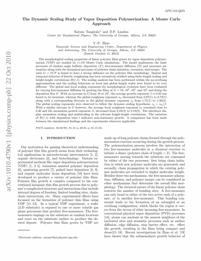
FIG. 1: Schematic of the 1+1D growth model. 1(a): Free-monomer deposition at random angles; 2(a): Adsorbed free-monomer diffuses along along the substrate; 2(b): Adsorbedfree-monomer diffuses on a polymer chain; 3(a,b): Poly-mer chain initiation resulting from random angle deposition;3(c,d): Polymer chain initiation resulting from free-monomerdiffusion on substrate and polymer chain respectively; 4(a,b):Free-monomer deposits onto the active end of a polymer chainresulting in chain propagation; 4(c) Chain propagation due tofree-monomer diffusion.

employed and one deposition time unit corresponded tothe deposition of L free-monomers. The incident free-monomers were released from a height three lattice unitsabove the highest point on the surface with an initialabscissa randomly chosen from 1 ≤ x ≤ L. The de-positing free-monomers have a uniform “launch angle”distribution which corresponds to a nonuniform flux dis-tribution J(θ) ∼ 1/cos(θ) of particles above the surface,where θ is defined as the angle between the direction ofimpinging monomer and the substrate normal [26, 27].Our VDP growth model is similar to the square-latticedisk model studied by Ref. [26] along with additionalconstraints of free-monomer diffusion, limited bonding,polymer-initiation, propagation and merger. The par-ticles followed a ballistic trajectory until contacting thesurface. The impinging free-monomer was then movedto the lattice position nearest to the point of contact.The deposited free-monomers were allowed to diffuse vianearest-neighbor hops with a diffusion rate D (nearestneighbor hops per monomer per unit time). A free-monomer that is deposited on top of an existing poly-mer chain gets adsorbed on the chain and is also allowedto diffuse. The excluded volume constraint was imple-mented by rejecting the diffusion or deposition moves toan already occupied site. As the monomer coverage in-creases on the substrate, the polymer film grows alonga direction perpendicular to the substrate. This “twodimensional” growth is often referred to as the 1+1Dgrowth in literature. Figure 1 shows the schematic ofvarious processes that occur during the non-equilibriumfilm growth on a 1-D substrate of length L with peri-odic boundary conditions. Processes 1(a), 3(a), 3(b),

3

= 10, (c)(a) G G = 10, tt = 15 = 30 G = 10, t

= 15t= 10,6

G(d) (e) G = 10,6

t = 30 t6

= 10,(f) G

(b) = 60

= 60

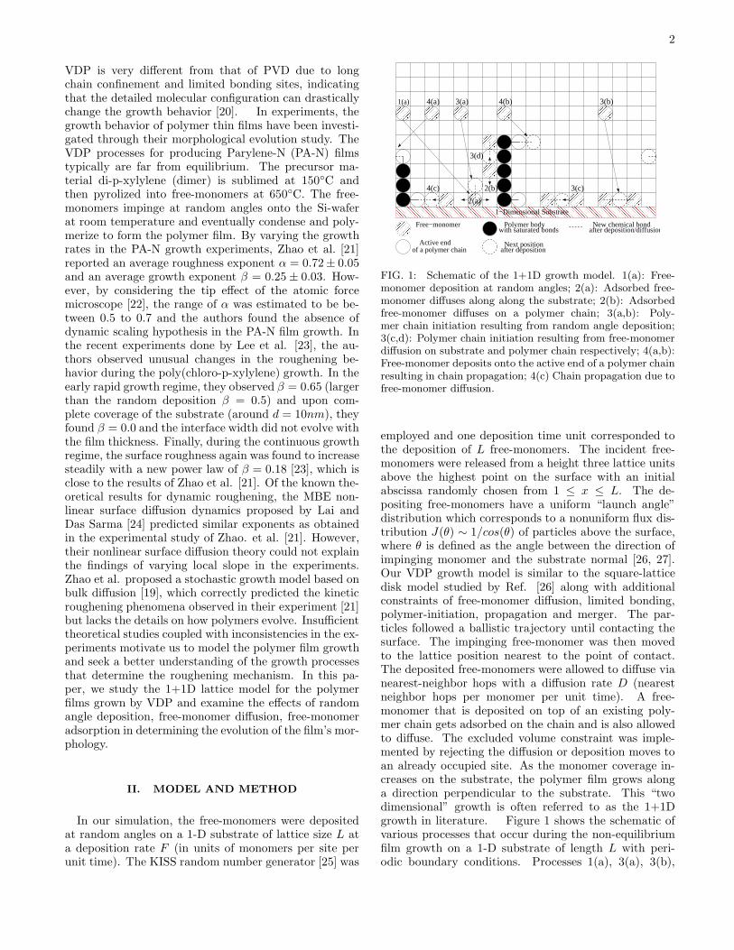
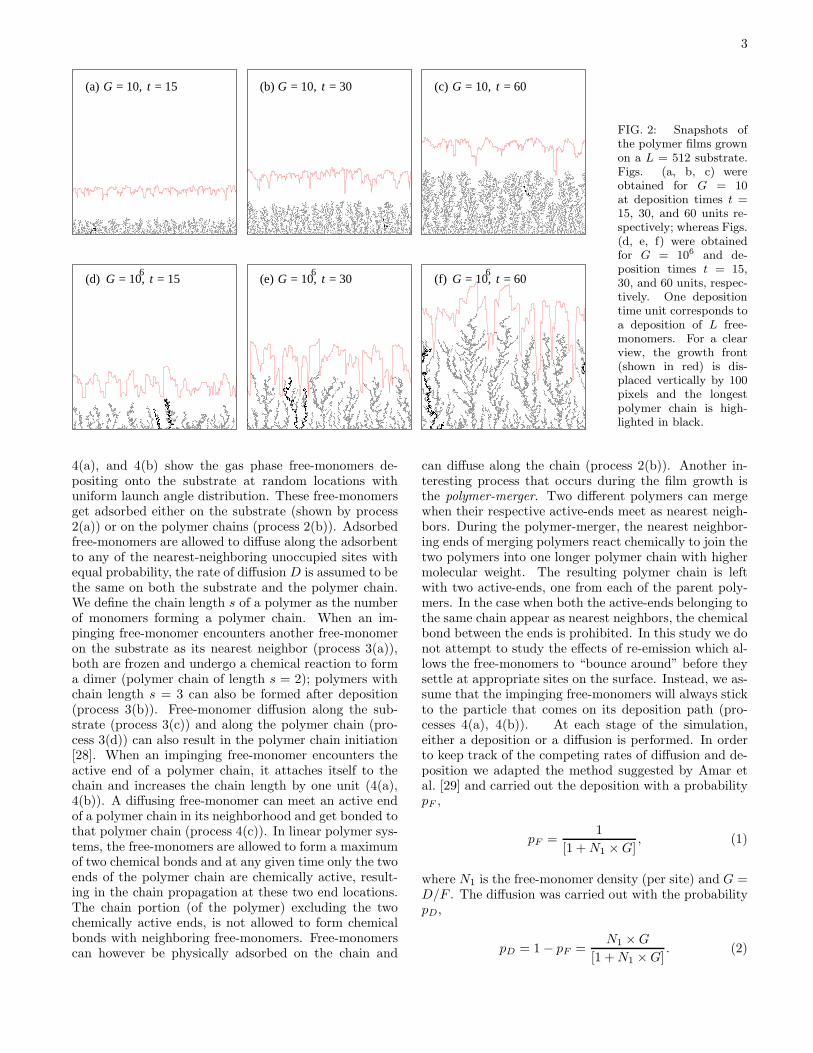
FIG. 2: Snapshots ofthe polymer films grownon a L = 512 substrate.Figs. (a, b, c) wereobtained for G = 10at deposition times t =15, 30, and 60 units re-spectively; whereas Figs.(d, e, f) were obtainedfor G = 106 and de-position times t = 15,30, and 60 units, respec-tively. One depositiontime unit corresponds toa deposition of L free-monomers. For a clearview, the growth front(shown in red) is dis-placed vertically by 100pixels and the longestpolymer chain is high-lighted in black.

4(a), and 4(b) show the gas phase free-monomers de-positing onto the substrate at random locations withuniform launch angle distribution. These free-monomersget adsorbed either on the substrate (shown by process2(a)) or on the polymer chains (process 2(b)). Adsorbedfree-monomers are allowed to diffuse along the adsorbentto any of the nearest-neighboring unoccupied sites withequal probability, the rate of diffusion D is assumed to bethe same on both the substrate and the polymer chain.We define the chain length s of a polymer as the numberof monomers forming a polymer chain. When an im-pinging free-monomer encounters another free-monomeron the substrate as its nearest neighbor (process 3(a)),both are frozen and undergo a chemical reaction to forma dimer (polymer chain of length s = 2); polymers withchain length s = 3 can also be formed after deposition(process 3(b)). Free-monomer diffusion along the sub-strate (process 3(c)) and along the polymer chain (pro-cess 3(d)) can also result in the polymer chain initiation[28]. When an impinging free-monomer encounters theactive end of a polymer chain, it attaches itself to thechain and increases the chain length by one unit (4(a),4(b)). A diffusing free-monomer can meet an active endof a polymer chain in its neighborhood and get bonded tothat polymer chain (process 4(c)). In linear polymer sys-tems, the free-monomers are allowed to form a maximumof two chemical bonds and at any given time only the twoends of the polymer chain are chemically active, result-ing in the chain propagation at these two end locations.The chain portion (of the polymer) excluding the twochemically active ends, is not allowed to form chemicalbonds with neighboring free-monomers. Free-monomerscan however be physically adsorbed on the chain and

can diffuse along the chain (process 2(b)). Another in-teresting process that occurs during the film growth isthe polymer-merger. Two different polymers can mergewhen their respective active-ends meet as nearest neigh-bors. During the polymer-merger, the nearest neighbor-ing ends of merging polymers react chemically to join thetwo polymers into one longer polymer chain with highermolecular weight. The resulting polymer chain is leftwith two active-ends, one from each of the parent poly-mers. In the case when both the active-ends belonging tothe same chain appear as nearest neighbors, the chemicalbond between the ends is prohibited. In this study we donot attempt to study the effects of re-emission which al-lows the free-monomers to “bounce around” before theysettle at appropriate sites on the surface. Instead, we as-sume that the impinging free-monomers will always stickto the particle that comes on its deposition path (pro-cesses 4(a), 4(b)). At each stage of the simulation,either a deposition or a diffusion is performed. In orderto keep track of the competing rates of diffusion and de-position we adapted the method suggested by Amar etal. [29] and carried out the deposition with a probabilitypF ,

pF =1

[1 +N1 ×G], (1)

where N1 is the free-monomer density (per site) and G =D/F . The diffusion was carried out with the probabilitypD,

pD = 1− pF =N1 ×G

[1 +N1 ×G]. (2)

4

In our simulations the incoming free-monomer flux Fwas fixed for different D, thus an increase in D wasparametrized as an increase in G. Throughout thegrowth process the list of all free-monomers and poly-mer chains were continually updated. If a free-monomerencountered another free-monomer or an active end of apolymer as its nearest neighbor, it was added to the poly-mer chain and removed from the free-monomer list. Incases where a free-monomer was the nearest neighbor tothe active ends of more than two polymers, we selected arandom pair of polymers and performed polymer-merger.

III. RESULTS

A. Surface Morphology

In Fig. 2 we show typical snapshots of the polymerfilms generated using L = 512 substrate for two extremecases: G = 10 (Figs. 2a, b, c) and G = 106 (Figs. 2d,e, f) after a deposition time of t = 15 (Figs. 2a, d), t =30 (Figs. 2b, e), and t = 60 (Figs. 2c, f) respectively.For both the values of G, the films show the presence ofcolumnar structures, overhangs, and unoccupied regions.These structures were observed to persist throughout thegrowth process. Presence of these morphological struc-tures can be explained by the shadowing effect inherent inthe growth process and is attributed to the cosθ distri-bution of the impinging free-monomer flux [27, 30–33].Shadowing effects arise when the columnar structuresof the surface “stick out” and shadow their neighbor-ing sites, thus inhibiting the growth in their neighboringsites. Due to the angular flux distribution of the imping-ing free-monomers the taller surface features prevent theincoming flux from entering the lower lying areas of thesurface.For comparable deposition times t, the films grown

at G = 10 (Figs. 2a, b, c) are characterized by smallunoccupied-regions and short polymer chains, resultingin shorter, denser, and compact films. Whereas for G =106 (Figs. 2d, e, f), the films are characterized by largeunoccupied-regions and longer polymer chains resultingin taller, more porous, and less dense films. For a rel-atively low diffusion rate at G = 10, the free-monomersdeposited on the film have a higher probability of encoun-tering another impinging free-monomer as nearest neigh-bor and thereby initiating new polymers. Many suchpolymer initiations inhibit the occurrence of unoccupied-regions and make the film dense and compact. In con-trast, at a higher diffusion rate of G = 106, the free-monomers have a higher probability to diffuse upwardtowards the growth front and the upward diffusion of free-monomers is favored due to the non-symmetric natureof the lattice potential associated with diffusion over astep [15]. The diffusing free-monomers arrive towards thegrowth front and bind to the active ends of the polymersand increase their chain length. This explains the oc-currences of longer polymer chains at higher G observed

100

101

102

103

r

0.1

1

Hq(r

,t)/H

q(max

)

q = 2q = 3q = 4q = 5

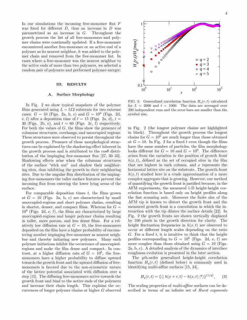
FIG. 3: Generalized correlation function Hq(r, t) calculatedfor L = 2000 and t = 1000. The data are averaged over200 independent runs and the error-bars are smaller than thesymbol size.

in Fig. 2 (the longest polymer chains are highlightedin black). Throughout the growth process the longestchains for G = 106 are much longer than those obtainedat G = 10. In Fig. 2 for a fixed t even though the filmshave the same number of particles, the film morphologylooks different for G = 10 and G = 106. The differencearises from the variation in the position of growth fronth(x, t), defined as the set of occupied sites in the filmthat are highest in each column, and x represents thehorizontal lattice site on the substrate. The growth fronth(x, t) studied here is a crude approximation of a morecomplex aggregate that is growing. However, our methodof quantifying the growth front is justified because, in theAFM experiments, the measured 1-D height-height cor-relation function is based only on height profiles alongthe fast scanning axis. Moreover the finite size of theAFM tip is known to distort the growth front and themeasured growth front is a convolution in which the in-teraction with the tip dilates the surface details [22]. InFig. 2 the growth fronts are shown vertically displacedby 100 pixels in the growth direction for clarity. Theheight fluctuation frequencies in h(x, t) are observed tooccur at different length scales depending on the ratioG. For a fixed t, it is intuitive to think that the heightprofiles corresponding to G = 106 (Figs. 2d, e, f) aremore rougher than those obtained using G = 10 (Figs.2a, b, c). A detailed analysis of the dynamics of interfaceroughness evolution is presented in the later section.The qth-order generalized height-height correlation

function Hq(r, t) (defined below) is commonly used inidentifying multi-affine surfaces [15, 34].

Hq(r, t) = {〈| h(x+ r, t)− h(x, t) |q〉}(1/q), (3)

The scaling properties of multi-affine surfaces can be de-scribed in terms of an infinite set of Hurst exponents

5

0 200 400 600 800 1000t

0

1×103

2×103

3×103

4×103

5×103

Ave

rage

film

hei

ght h

avg

G = 105

G = 103

G = 101

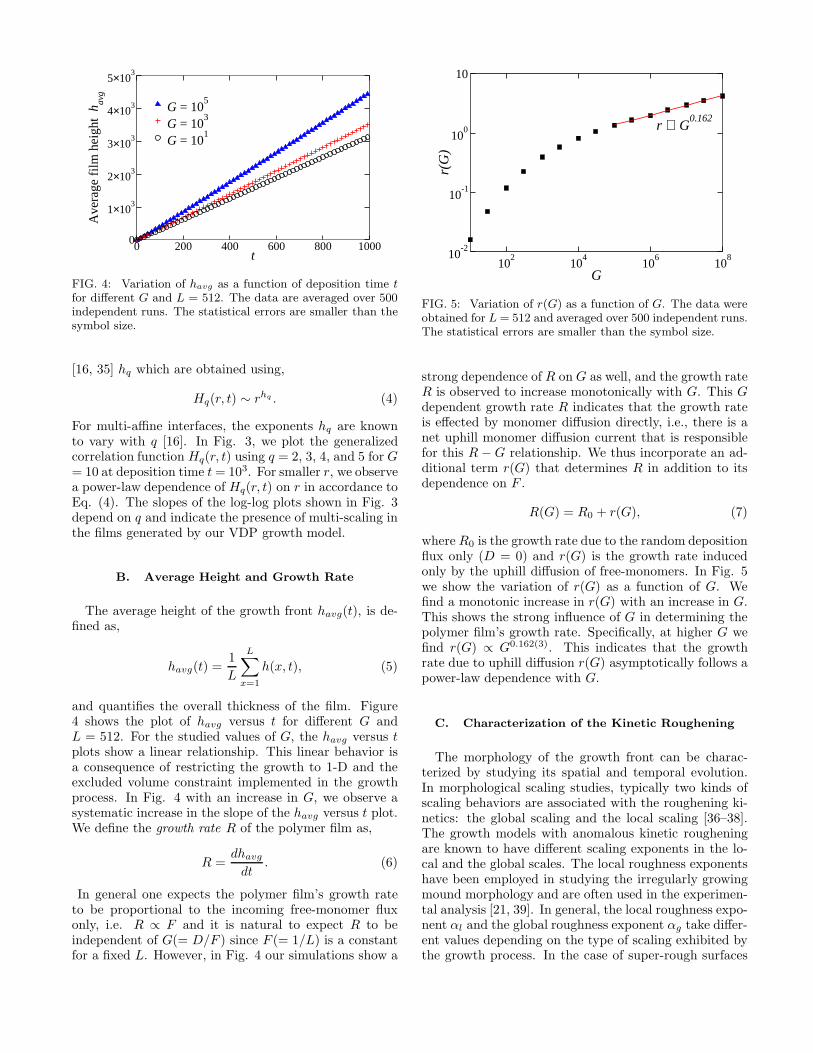
FIG. 4: Variation of havg as a function of deposition time tfor different G and L = 512. The data are averaged over 500independent runs. The statistical errors are smaller than thesymbol size.

[16, 35] hq which are obtained using,

Hq(r, t) ∼ rhq . (4)

For multi-affine interfaces, the exponents hq are knownto vary with q [16]. In Fig. 3, we plot the generalizedcorrelation function Hq(r, t) using q = 2, 3, 4, and 5 for G= 10 at deposition time t= 103. For smaller r, we observea power-law dependence of Hq(r, t) on r in accordance toEq. (4). The slopes of the log-log plots shown in Fig. 3depend on q and indicate the presence of multi-scaling inthe films generated by our VDP growth model.

B. Average Height and Growth Rate

The average height of the growth front havg(t), is de-fined as,

havg(t) =1

L

L∑

x=1

h(x, t), (5)

and quantifies the overall thickness of the film. Figure4 shows the plot of havg versus t for different G andL = 512. For the studied values of G, the havg versus tplots show a linear relationship. This linear behavior isa consequence of restricting the growth to 1-D and theexcluded volume constraint implemented in the growthprocess. In Fig. 4 with an increase in G, we observe asystematic increase in the slope of the havg versus t plot.We define the growth rate R of the polymer film as,

R =dhavg

dt. (6)

In general one expects the polymer film’s growth rateto be proportional to the incoming free-monomer fluxonly, i.e. R ∝ F and it is natural to expect R to beindependent of G(= D/F ) since F (= 1/L) is a constantfor a fixed L. However, in Fig. 4 our simulations show a

102

104

106

108

G

10-2

10-1

100

10

r(G

)

r ∝ G0.162

FIG. 5: Variation of r(G) as a function of G. The data wereobtained for L = 512 and averaged over 500 independent runs.The statistical errors are smaller than the symbol size.

strong dependence of R on G as well, and the growth rateR is observed to increase monotonically with G. This Gdependent growth rate R indicates that the growth rateis effected by monomer diffusion directly, i.e., there is anet uphill monomer diffusion current that is responsiblefor this R −G relationship. We thus incorporate an ad-ditional term r(G) that determines R in addition to itsdependence on F .

R(G) = R0 + r(G), (7)

where R0 is the growth rate due to the random depositionflux only (D = 0) and r(G) is the growth rate inducedonly by the uphill diffusion of free-monomers. In Fig. 5we show the variation of r(G) as a function of G. Wefind a monotonic increase in r(G) with an increase in G.This shows the strong influence of G in determining thepolymer film’s growth rate. Specifically, at higher G wefind r(G) ∝ G0.162(3). This indicates that the growthrate due to uphill diffusion r(G) asymptotically follows apower-law dependence with G.

C. Characterization of the Kinetic Roughening

The morphology of the growth front can be charac-terized by studying its spatial and temporal evolution.In morphological scaling studies, typically two kinds ofscaling behaviors are associated with the roughening ki-netics: the global scaling and the local scaling [36–38].The growth models with anomalous kinetic rougheningare known to have different scaling exponents in the lo-cal and the global scales. The local roughness exponentshave been employed in studying the irregularly growingmound morphology and are often used in the experimen-tal analysis [21, 39]. In general, the local roughness expo-nent αl and the global roughness exponent αg take differ-ent values depending on the type of scaling exhibited bythe growth process. In the case of super-rough surfaces

6

50 100 150 200 250y

0

0.1

0.2

0.3

0.4

0.5

ρ(y)

t = 10t = 20t = 40t = 60

Interface region

Film region

Growth-front

t = tinterface

ends at

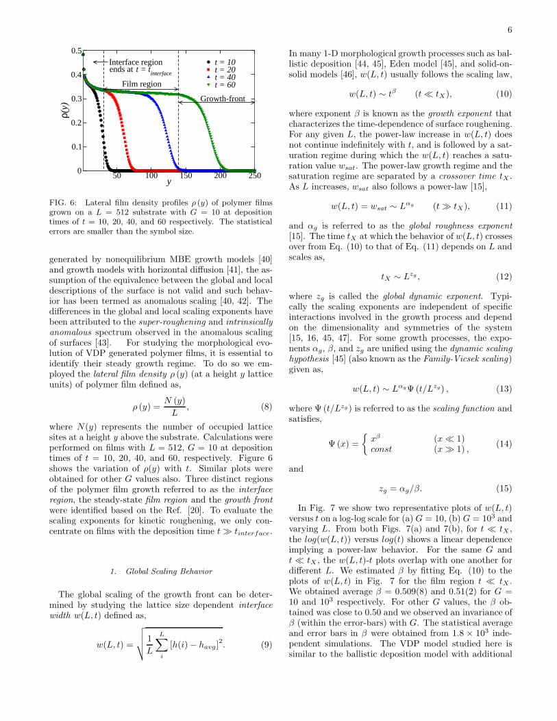
FIG. 6: Lateral film density profiles ρ (y) of polymer filmsgrown on a L = 512 substrate with G = 10 at depositiontimes of t = 10, 20, 40, and 60 respectively. The statisticalerrors are smaller than the symbol size.

generated by nonequilibrium MBE growth models [40]and growth models with horizontal diffusion [41], the as-sumption of the equivalence between the global and localdescriptions of the surface is not valid and such behav-ior has been termed as anomalous scaling [40, 42]. Thedifferences in the global and local scaling exponents havebeen attributed to the super-roughening and intrinsically

anomalous spectrum observed in the anomalous scalingof surfaces [43]. For studying the morphological evo-lution of VDP generated polymer films, it is essential toidentify their steady growth regime. To do so we em-ployed the lateral film density ρ (y) (at a height y latticeunits) of polymer film defined as,

ρ (y) =N (y)

L, (8)

where N(y) represents the number of occupied latticesites at a height y above the substrate. Calculations wereperformed on films with L = 512, G = 10 at depositiontimes of t = 10, 20, 40, and 60, respectively. Figure 6shows the variation of ρ(y) with t. Similar plots wereobtained for other G values also. Three distinct regionsof the polymer film growth referred to as the interface

region, the steady-state film region and the growth front

were identified based on the Ref. [20]. To evaluate thescaling exponents for kinetic roughening, we only con-centrate on films with the deposition time t ≫ tinterface.

1. Global Scaling Behavior

The global scaling of the growth front can be deter-mined by studying the lattice size dependent interface

width w(L, t) defined as,

w(L, t) =

√

√

√

√

1

L

L∑

i

[h(i)− havg]2. (9)

In many 1-D morphological growth processes such as bal-listic deposition [44, 45], Eden model [45], and solid-on-solid models [46], w(L, t) usually follows the scaling law,

w(L, t) ∼ tβ (t ≪ tX), (10)

where exponent β is known as the growth exponent thatcharacterizes the time-dependence of surface roughening.For any given L, the power-law increase in w(L, t) doesnot continue indefinitely with t, and is followed by a sat-uration regime during which the w(L, t) reaches a satu-ration value wsat. The power-law growth regime and thesaturation regime are separated by a crossover time tX .As L increases, wsat also follows a power-law [15],

w(L, t) = wsat ∼ Lαg (t ≫ tX), (11)

and αg is referred to as the global roughness exponent

[15]. The time tX at which the behavior of w(L, t) crossesover from Eq. (10) to that of Eq. (11) depends on L andscales as,

tX ∼ Lzg , (12)

where zg is called the global dynamic exponent. Typi-cally the scaling exponents are independent of specificinteractions involved in the growth process and dependon the dimensionality and symmetries of the system[15, 16, 45, 47]. For some growth processes, the expo-nents αg, β, and zg are unified using the dynamic scaling

hypothesis [45] (also known as the Family-Vicsek scaling)given as,

w(L, t) ∼ LαgΨ(t/Lzg) , (13)

where Ψ (t/Lzg) is referred to as the scaling function andsatisfies,

Ψ (x) =

{

xβ (x ≪ 1)const (x ≫ 1) ,

(14)

and

zg = αg/β. (15)

In Fig. 7 we show two representative plots of w(L, t)versus t on a log-log scale for (a) G = 10, (b) G = 103 andvarying L. From both Figs. 7(a) and 7(b), for t ≪ tX ,the log(w(L, t)) versus log(t) shows a linear dependenceimplying a power-law behavior. For the same G andt ≪ tX , the w(L, t)-t plots overlap with one another fordifferent L. We estimated β by fitting Eq. (10) to theplots of w(L, t) in Fig. 7 for the film region t ≪ tX .We obtained average β = 0.509(8) and 0.51(2) for G =10 and 103 respectively. For other G values, the β ob-tained was close to 0.50 and we observed an invariance ofβ (within the error-bars) with G. The statistical averageand error bars in β were obtained from 1.8 × 103 inde-pendent simulations. The VDP model studied here issimilar to the ballistic deposition model with additional

7

101

102

103

104

t

101

102

w(L

,t)

102

104

101

103

t

101

102

w(L

,t)

= 0.509(8)

(a)

= 0.51(2)

(b)

LLLL

= 150 = 200 = 250 = 300

(A)(B)(C)

(D)

= 300L(A):(B):

β β

(B)(A)

(C)

(D)

(A):(B):(C):(D):

= 250L(C): L = 200(D): L = 150

G = 10 G = 103

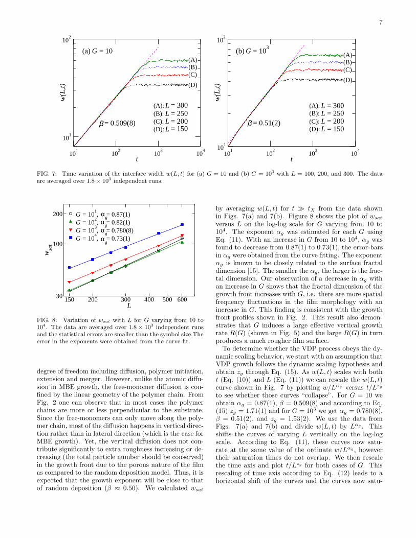
FIG. 7: Time variation of the interface width w(L, t) for (a) G = 10 and (b) G = 103 with L = 100, 200, and 300. The dataare averaged over 1.8× 103 independent runs.

150 200 300 400 500 600L

30

100

200

wsa

t

G = 101, = 0.87(1)

G = 102, = 0.82(1)

G = 103, = 0.780(8)

G = 104, = 0.73(1)

αg

αg

αg

αg

FIG. 8: Variation of wsat with L for G varying from 10 to104. The data are averaged over 1.8 × 103 independent runsand the statistical errors are smaller than the symbol size.Theerror in the exponents were obtained from the curve-fit.

degree of freedom including diffusion, polymer initiation,extension and merger. However, unlike the atomic diffu-sion in MBE growth, the free-monomer diffusion is con-fined by the linear geometry of the polymer chain. FromFig. 2 one can observe that in most cases the polymerchains are more or less perpendicular to the substrate.Since the free-monomers can only move along the poly-mer chain, most of the diffusion happens in vertical direc-tion rather than in lateral direction (which is the case forMBE growth). Yet, the vertical diffusion does not con-tribute significantly to extra roughness increasing or de-creasing (the total particle number should be conserved)in the growth front due to the porous nature of the filmas compared to the random deposition model. Thus, it isexpected that the growth exponent will be close to thatof random deposition (β ≈ 0.50). We calculated wsat

by averaging w(L, t) for t ≫ tX from the data shownin Figs. 7(a) and 7(b). Figure 8 shows the plot of wsat

versus L on the log-log scale for G varying from 10 to104. The exponent αg was estimated for each G usingEq. (11). With an increase in G from 10 to 104, αg wasfound to decrease from 0.87(1) to 0.73(1), the error-barsin αg were obtained from the curve fitting. The exponentαg is known to be closely related to the surface fractaldimension [15]. The smaller the αg, the larger is the frac-tal dimension. Our observation of a decrease in αg withan increase in G shows that the fractal dimension of thegrowth front increases with G, i.e. there are more spatialfrequency fluctuations in the film morphology with anincrease in G. This finding is consistent with the growthfront profiles shown in Fig. 2. This result also demon-strates that G induces a large effective vertical growthrate R(G) (shown in Fig. 5) and the large R(G) in turnproduces a much rougher film surface.To determine whether the VDP process obeys the dy-

namic scaling behavior, we start with an assumption thatVDP growth follows the dynamic scaling hypothesis andobtain zg through Eq. (15). As w(L, t) scales with botht (Eq. (10)) and L (Eq. (11)) we can rescale the w(L, t)curve shown in Fig. 7 by plotting w/Lαg versus t/Lzg

to see whether those curves “collapse”. For G = 10 weobtain αg = 0.87(1), β = 0.509(8) and according to Eq.(15) zg = 1.71(1) and for G = 103 we get αg = 0.780(8),β = 0.51(2), and zg = 1.53(2). We use the data fromFigs. 7(a) and 7(b) and divide w(L, t) by Lαg . Thisshifts the curves of varying L vertically on the log-logscale. According to Eq. (11), these curves now satu-rate at the same value of the ordinate w/Lαg , howevertheir saturation times do not overlap. We then rescalethe time axis and plot t/Lzg for both cases of G. Thisrescaling of time axis according to Eq. (12) leads to ahorizontal shift of the curves and the curves now satu-

8

10-2

10-1

100

t/Lz = 1.53

0.3

0.4

0.5

0.6

0.7

0.8

0.9

w(L

,t)/L

α =

0.78

L = 150L = 200L = 250L = 300

10-2

10-1

100

t/Lz = 1.71

0.2

0.3

0.4

0.5

0.6

w(L

,t)/L

α =

0.87

L = 150L = 200L = 250L = 300

(a) (b)G G= 10 = 103

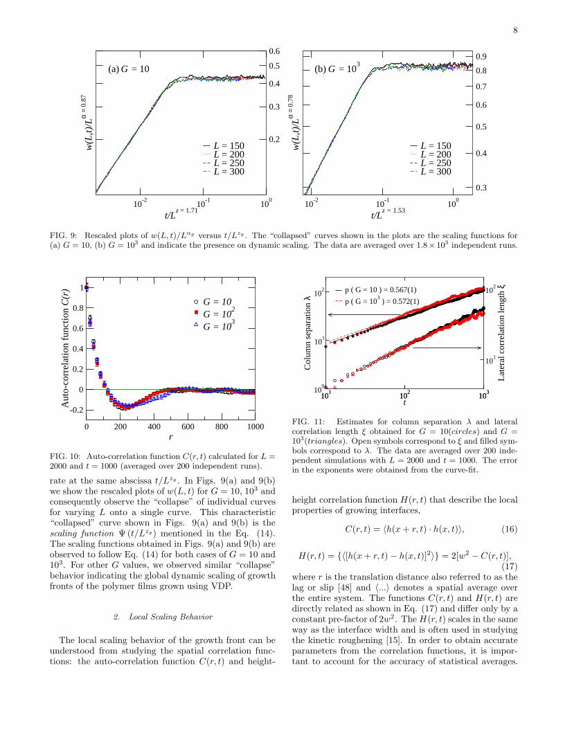
FIG. 9: Rescaled plots of w(L, t)/Lαg versus t/Lzg . The “collapsed” curves shown in the plots are the scaling functions for(a) G = 10, (b) G = 103 and indicate the presence on dynamic scaling. The data are averaged over 1.8× 103 independent runs.

0 200 400 600 800 1000r

-0.2

0

0.2

0.4

0.6

0.8

1

Aut

o-co

rrel

atio

n fu

nctio

n C

(r)

G = 10G = 10

2

G = 103

FIG. 10: Auto-correlation function C(r, t) calculated for L =2000 and t = 1000 (averaged over 200 independent runs).

rate at the same abscissa t/Lzg . In Figs. 9(a) and 9(b)we show the rescaled plots of w(L, t) for G = 10, 103 andconsequently observe the “collapse” of individual curvesfor varying L onto a single curve. This characteristic“collapsed” curve shown in Figs. 9(a) and 9(b) is thescaling function Ψ(t/Lzg) mentioned in the Eq. (14).The scaling functions obtained in Figs. 9(a) and 9(b) areobserved to follow Eq. (14) for both cases of G = 10 and103. For other G values, we observed similar “collapse”behavior indicating the global dynamic scaling of growthfronts of the polymer films grown using VDP.

2. Local Scaling Behavior

The local scaling behavior of the growth front can beunderstood from studying the spatial correlation func-tions: the auto-correlation function C(r, t) and height-

101

102

103

t

100

101

102

Col

umn

sepa

ratio

n λ

p ( G = 10 ) = 0.567(1)

p ( G = 103 ) = 0.572(1)

101

102

103

101

102

Late

ral c

orre

latio

n le

ngth

ξ

FIG. 11: Estimates for column separation λ and lateralcorrelation length ξ obtained for G = 10(circles) and G =103(triangles). Open symbols correspond to ξ and filled sym-bols correspond to λ. The data are averaged over 200 inde-pendent simulations with L = 2000 and t = 1000. The errorin the exponents were obtained from the curve-fit.

height correlation function H(r, t) that describe the localproperties of growing interfaces,

C(r, t) = 〈h(x + r, t) · h(x, t)〉, (16)

H(r, t) = {〈[h(x+ r, t)− h(x, t)]2〉} = 2[w2 − C(r, t)],(17)

where r is the translation distance also referred to as thelag or slip [48] and 〈...〉 denotes a spatial average overthe entire system. The functions C(r, t) and H(r, t) aredirectly related as shown in Eq. (17) and differ only by aconstant pre-factor of 2w2. The H(r, t) scales in the sameway as the interface width and is often used in studyingthe kinetic roughening [15]. In order to obtain accurateparameters from the correlation functions, it is impor-tant to account for the accuracy of statistical averages.

9

101

102

103

100

r

102

103

104

H(r

,t)

t = 500, αl = 0.465(6)

t = 750, αl = 0.461(5)

t = 1000, αl = 0.464(5)

100

102

101

103

r

102

103

104

H(r

,t)

t = 500, αl = 0.470(4)

t = 750, αl = 0.469(4)

t = 1000, αl =0.476(3)

(a) (b)G = 10 G = 103

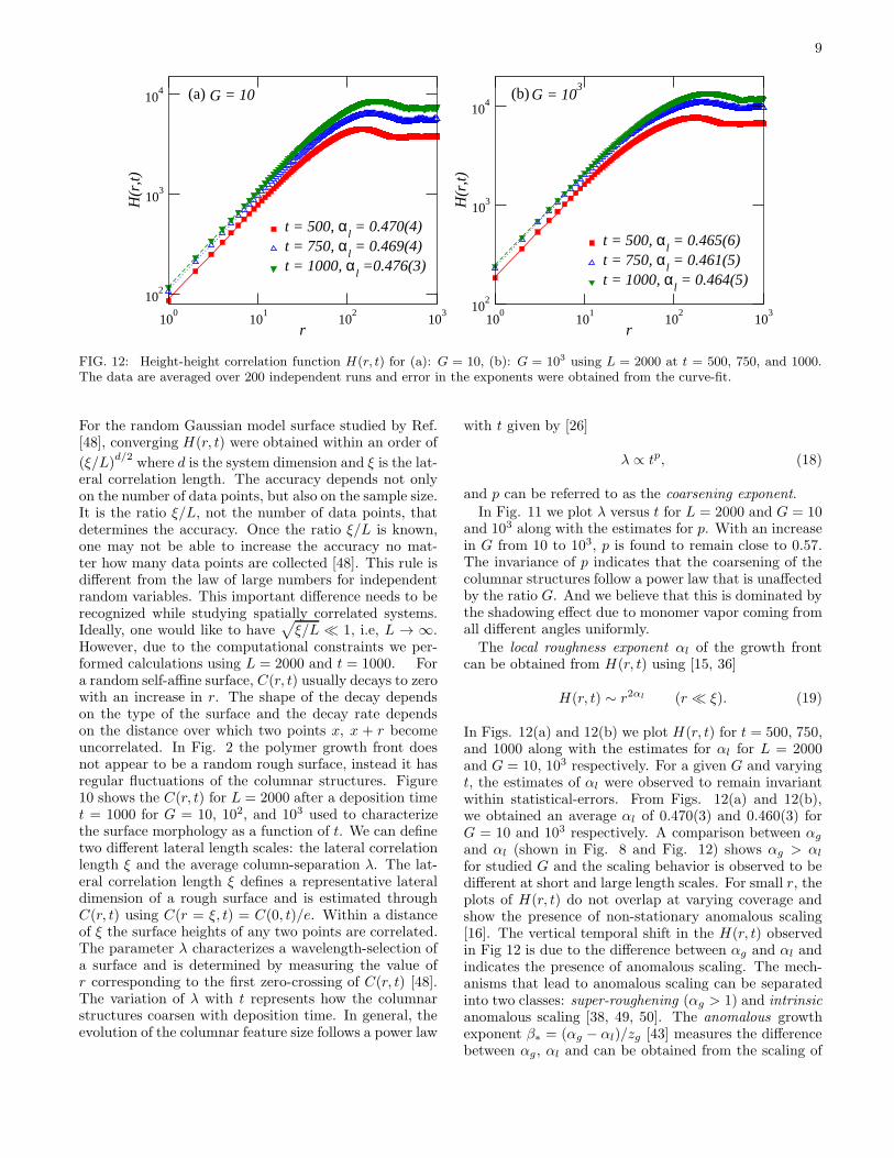
FIG. 12: Height-height correlation function H(r, t) for (a): G = 10, (b): G = 103 using L = 2000 at t = 500, 750, and 1000.The data are averaged over 200 independent runs and error in the exponents were obtained from the curve-fit.

For the random Gaussian model surface studied by Ref.[48], converging H(r, t) were obtained within an order of

(ξ/L)d/2

where d is the system dimension and ξ is the lat-eral correlation length. The accuracy depends not onlyon the number of data points, but also on the sample size.It is the ratio ξ/L, not the number of data points, thatdetermines the accuracy. Once the ratio ξ/L is known,one may not be able to increase the accuracy no mat-ter how many data points are collected [48]. This rule isdifferent from the law of large numbers for independentrandom variables. This important difference needs to berecognized while studying spatially correlated systems.Ideally, one would like to have

√

ξ/L ≪ 1, i.e, L → ∞.However, due to the computational constraints we per-formed calculations using L = 2000 and t = 1000. Fora random self-affine surface, C(r, t) usually decays to zerowith an increase in r. The shape of the decay dependson the type of the surface and the decay rate dependson the distance over which two points x, x + r becomeuncorrelated. In Fig. 2 the polymer growth front doesnot appear to be a random rough surface, instead it hasregular fluctuations of the columnar structures. Figure10 shows the C(r, t) for L = 2000 after a deposition timet = 1000 for G = 10, 102, and 103 used to characterizethe surface morphology as a function of t. We can definetwo different lateral length scales: the lateral correlationlength ξ and the average column-separation λ. The lat-eral correlation length ξ defines a representative lateraldimension of a rough surface and is estimated throughC(r, t) using C(r = ξ, t) = C(0, t)/e. Within a distanceof ξ the surface heights of any two points are correlated.The parameter λ characterizes a wavelength-selection ofa surface and is determined by measuring the value ofr corresponding to the first zero-crossing of C(r, t) [48].The variation of λ with t represents how the columnarstructures coarsen with deposition time. In general, theevolution of the columnar feature size follows a power law

with t given by [26]

λ ∝ tp, (18)

and p can be referred to as the coarsening exponent.In Fig. 11 we plot λ versus t for L = 2000 and G = 10

and 103 along with the estimates for p. With an increasein G from 10 to 103, p is found to remain close to 0.57.The invariance of p indicates that the coarsening of thecolumnar structures follow a power law that is unaffectedby the ratio G. And we believe that this is dominated bythe shadowing effect due to monomer vapor coming fromall different angles uniformly.

The local roughness exponent αl of the growth frontcan be obtained from H(r, t) using [15, 36]

H(r, t) ∼ r2αl (r ≪ ξ). (19)

In Figs. 12(a) and 12(b) we plot H(r, t) for t = 500, 750,and 1000 along with the estimates for αl for L = 2000and G = 10, 103 respectively. For a given G and varyingt, the estimates of αl were observed to remain invariantwithin statistical-errors. From Figs. 12(a) and 12(b),we obtained an average αl of 0.470(3) and 0.460(3) forG = 10 and 103 respectively. A comparison between αg

and αl (shown in Fig. 8 and Fig. 12) shows αg > αl

for studied G and the scaling behavior is observed to bedifferent at short and large length scales. For small r, theplots of H(r, t) do not overlap at varying coverage andshow the presence of non-stationary anomalous scaling[16]. The vertical temporal shift in the H(r, t) observedin Fig 12 is due to the difference between αg and αl andindicates the presence of anomalous scaling. The mech-anisms that lead to anomalous scaling can be separatedinto two classes: super-roughening (αg > 1) and intrinsic

anomalous scaling [38, 49, 50]. The anomalous growthexponent β∗ = (αg − αl)/zg [43] measures the differencebetween αg, αl and can be obtained from the scaling of

10

10-2

10-1

100

101

102

r/t1/z

g

100

101

102

H(r

,t)/r

2αg

t = 500t = 750t = 500

10-2

10-1

100

101

102

r/t1/z

g

10-2

101

100

101

102

H(r

,t)/r

2αg

t = 500t = 750t = 1000

(a) (b)G = 10 G = 103

κ1 = -0.823(8)

κ2 = -1.555(8)κ2 = -1.731(2)

κ1 = -0.621(4)

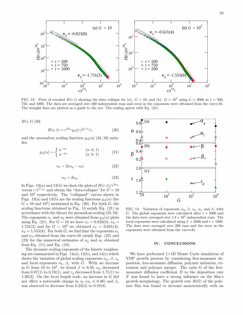
FIG. 13: Plots of rescaled H(r, t) showing the data collapse for (a): G = 10, and (b): G = 103 using L = 2000 at t = 500,750, and 1000. The data are averaged over 200 independent runs and error in the exponents were obtained from the curve-fit.The straight lines are plotted as a guide to the eye. The scaling agrees with Eq. (21).

H(r, t) [50]

H(r, t) = r2αggA(r/t1/zg ), (20)

and the anomalous scaling function gA(u) [43, 50] satis-fies

gA(u) ∼

{

u−κ1 (u ≪ 1)u−κ2 (u ≫ 1)

(21)

κ1 = 2(αg − αl) (22)

κ2 = 2αg. (23)

In Figs. 13(a) and 13(b) we show the plots ofH(r, t)/r2αg

versus r/t1/zg and obtain the “data-collapse” for G = 10and 103 respectively. The “collapsed” curves shown inFigs. 13(a) and 13(b) are the scaling functions gA(u) (forG = 10 and 103) mentioned in Eq. (20). For both G, thescaling functions obtained in Fig. 13 satisfy Eq. (21) inaccordance with the theory for anomalous scaling [43, 50].The exponents κ1 and κ2 were obtained from gA(u) plotsusing Eq. (21). For G = 10 we have κ1 = 0.823(8), κ2 =1.731(2) and for G = 103 we obtained κ1 = 0.621(4),κ2 = 1.555(8). For both G, we find that the exponents κ1

and κ2 obtained from the curve-fit satisfy Eqs. (22) and(23) for the numerical estimates of αg and αl obtainedfrom Eq. (11) and Eq. (19).The dynamic scaling exponents of the kinetic roughen-

ing are summarized in Figs. 14(a), 14(b), and 14(c) whichshows the variation of global scaling exponents αg, β, zgand local exponents αl, β∗ with G. With an increasein G from 10 to 104, we found β ≈ 0.50, αg decreasedfrom 0.87(1) to 0.73(1), and zg decreased from 1.71(1) to1.38(2). On the local length scale, an increase in G didnot effect a noticeable change in αl (αl ≈ 0.46) and β∗

was observed to decrease from 0.23(4) to 0.18(8).

0.6

0.8

0.4

0.2

0.4

0.6

10 102

103

104

G

2.0

1.6

1.2

(a)

(b)

(c)

α

β

z

αg

αl

zg

β*

β

FIG. 14: Variation of exponents αg, β, zg, αl, and β∗ withG. The global exponents were calculated after t = 5000 andthe data were averaged over 1.8× 103 independent runs. Thelocal exponents were calculated using L = 2000 and t = 1000.The data were averaged over 200 runs and the error in theexponents were obtained from the curve-fit.

IV. CONCLUSIONS

We have performed 1+1D Monte Carlo simulation ofVDP growth process by considering free-monomer de-position, free-monomer diffusion, polymer initiation, ex-tension and polymer merger. The ratio G of the free-monomer diffusion coefficient D to the deposition rateF was found to have a strong influence on the film’sgrowth morphology. The growth rate R(G) of the poly-mer film was found to increase monotonically with an

11

increase in G. This is due to the consequence of an up-per diffusion flux of free-monomers. The detailed anal-ysis of the surface morphology indicated the presence ofvery different scaling behavior at global and local lengthscales. The kinetic roughening study of film interfaceindicates anomalous scaling and multiscaling. With anincrease in G from 10 to 104, the global growth expo-nent β ≈ 0.50 was found to be invariant, whereas theglobal roughness exponent αg decreased from 0.87(1) to0.73(1) along with a corresponding decrease in the globaldynamic exponent zg from 1.71(1) to 1.38(2). The globalscaling exponents were found to follow the dynamic scal-ing hypothesis with zg = αg/β for various G. With anincrease in G from 10 to 104, the average local roughnessexponent αl remained close to 0.46 with αl 6= αg, thisobservation is unlike the ones obtained in self-affine sur-faces [15, 35]. The anomalous growth exponent β∗ wasalso found to decrease from 0.23(4) to 0.18(8) with anincrease in G. Even though our model is in 1+1D ascompared to the 2+1D experiments, our estimates of αl

and β∗ are close to the experimental findings of α ≈ 0.5to 0.7 and β = 0.25± 0.03 obtained from the AFM stud-ies of linear PA-N films grown by VDP [21, 51]. The

similarity between the experimental and simulational es-timates appears to be a coincidence since the dimensionof the two systems are totally different. We also did notobserve the changes in the dynamic roughening behaviorreported by Ref. [23], perhaps due to the limitations ofour current simulation model in considering the effect offree-monomer diffusion only. This makes us believe thatthe kinetic roughening of the polymer films is sensitiveto the specific molecular-level interactions, relaxations ofpolymer chains through inter-polymer interactions, andthe intrinsic nature of polymerization process that needto be accounted for in the future simulations.

V. ACKNOWLEDGEMENTS

ST and DPL were partially supported by the NSFgrant DMR-0810223. ST and YPZ were also partiallysupported by NSF grant CMMI-0824728. ST would liketo thank S. J. Mitchell for help with the visualizationtools.

[1] T.-M. Lu and J. A. Moore, Mater. Res. Soc. Bull 20, 28and references therein (1997).

[2] C. P. Wong, Polymers for Electronic and Photonic Ap-plication (Academic Press, Boston, MA, 1993).

[3] W. F. Gorham, Journal of Polymer Science Part A-1:Polymer Chemistry 4, 3027 (1966).

[4] J. Lahann, M. Balcells, H. Lu, T. Rodon, K. F. Jensen,and R. Langer, Analytical Chemistry 75, 2117 (2003).

[5] G. J. Szulczewski, T. D. Selby, K.-Y. Kim, J. D. Hassen-zahl, and S. C. Blackstock, in The 46th InternationalSymposium of the American Vacuum Society (2000),vol. 18, pp. 1875–1880.

[6] H. Usui, in Proceedings of 1998 International Symposiumon Electrical Insulating Materials (1998), pp. 577–582.

[7] H. Biederman, V. Stelmashuk, I. Kholodkov, A. Chouk-ourov, and D. Slavnsk, Surface and Coatings Technology174, 27 (2003).

[8] D. B. Chrisey and G. K. Hubler, eds., Pulsed Laser De-position of Thin Films (Wiley-Interscience, 1994).

[9] A. Piqu, R. C. Y. Auyeung, J. L. Stepnowski, D. W.Weir, C. B. Arnold, R. A. McGill, and D. B. Chrisey,Surface and Coatings Technology 163, 293 (2003).

[10] F. Schreiber, Physica Status Solidi Applied Research201, 1037 (2004).

[11] G. W. Collins, S. A. Letts, E. M. Fearon, R. L. McEach-ern, and T. P. Bernat, Phys. Rev. Lett. 73, 708 (1994).

[12] F. Biscarini, P. Samor’i, O. Greco, and R. Zamboni,Phys. Rev. Lett. 78, 2389 (1997).

[13] J. Fortin and T. Lu, Chemistry of Materials 14, 1945(2002).

[14] D. M. Mattox, Handbook of Physical Vapor Deposition(PVD) Processing (Noyes Publications, Berkshire, UK,1998).

[15] A.-L. Barabasi and H. E. Stanley, Fractal Concepts

in Surface Growth (Cambridge University Press, Cam-bridge, England, 1995).

[16] P. Meakin, Fractals, scaling, and growth far from equilib-rium (Cambridge University Press, Cambridge, England,1998).

[17] S. Pal and D. P. Landau, Phys. Rev. B 49, 10597 (1994).[18] Y. Shim, D. P. Landau, and S. Pal, Phys. Rev. E 58,

7571 (1998).[19] Y.-P. Zhao, A. R. Hopper, G.-C. Wang, and T.-M. Lu,

Phys. Rev. E 60, 4310 (1999).[20] W. Bowie and Y. P. Zhao, Surface Science 563, L245

(2004).[21] Y.-P. Zhao, J. B. Fortin, G. Bonvallet, G.-C. Wang, and

T.-M. Lu, Phys. Rev. Lett. 85, 3229 (2000).[22] J. Aue and J. T. M. De Hosson, Applied Physics Letters

71, 1347 (1997).[23] I. J. Lee, M. Yun, S.-M. Lee, and J.-Y. Kim, Phys. Rev.

B 78, 115427 (2008).[24] Z.-W. Lai and S. Das Sarma, Phys. Rev. Lett. 66, 2348

(1991).[25] G. Marsaglia, J. Mod. Appl. Statist. Methods 2, 2 (2003).[26] J. Yu and J. G. Amar, Phys. Rev. E 66, 021603 (2002).[27] J. T. Drotar, Y.-P. Zhao, T.-M. Lu, and G.-C. Wang,

Phys. Rev. B 62, 2118 (2000).[28] W. F. Beach, Macromolecules 11, 72 (1977).[29] J. G. Amar, F. Family, and P.-M. Lam, Phys. Rev. B 50,

8781 (1994).[30] R. P. U. Karunasiri, R. Bruinsma, and J. Rudnick, Phys.

Rev. Lett. 62, 788 (1989).[31] G. S. Bales and A. Zangwill, Phys. Rev. Lett. 63, 692

(1989).[32] Y.-P. Zhao, J. T. Drotar, G.-C. Wang, and T.-M. Lu,

Phys. Rev. Lett. 82, 4882 (1999).[33] J. T. Drotar, Y.-P. Zhao, T.-M. Lu, and G.-C. Wang,

12

Phys. Rev. B 64, 125411 (2001).[34] A.-L. Barabasi and T. Vicsek, Phys. Rev. A 44, 2730

(1991).[35] F. Family and T. Vicsek, eds., Dynamics of Fractal Sur-

faces (World Scientific, Singapore, 1991).[36] J. Asikainen, S. Majaniemi, M. Dube, J. Heinonen, and

T. Ala-Nissila, Eur. Phys. J. B 30 (2002).[37] J. Krug, Phys. Rev. Lett. 72, 2907 (1994).[38] J. J. Ramasco, J. M. Lopez, and M. A. Rodrıguez, Phys.

Rev. Lett. 84, 2199 (2000).[39] J. H. Jeffries, J.-K. Zuo, and M. M. Craig, Phys. Rev.

Lett. 76, 4931 (1996).[40] S. Das Sarma, S. V. Ghaisas, and J. M. Kim, Phys. Rev.

E 49, 122 (1994).[41] J. G. Amar, P.-M. Lam, and F. Family, Phys. Rev. E 47,

3242 (1993).[42] M. Schroeder, M. Siegert, D. E. Wolf, J. D. Shore, and

M. Plischke, Europhys. Lett. 24, 563 (1993).[43] J. M. Lopez, M. A. Rodrıguez, and R. Cuerno, Phys.

Rev. E 56, 3993 (1997).[44] R. Baiod, D. Kessler, P. Ramanlal, L. Sander, and

R. Savit, Phys. Rev. A 38, 3672 (1988).[45] F. Family and T. Vicsek, Journal of Physics A 18, L75

(1985).[46] J. M. Kim and J. M. Kosterlitz, Phys. Rev. Lett. 62,

2289 (1989).[47] F. Family, Journal of Physics A 19, L441 (1986).[48] Y. Zhao, G.-C. Wang, and T.-M. Lu, Characterization of

amorphous and crystalline rough surface : principles andapplication (Academic Press, San Diego, CA, 2001).

[49] J. M. Lopez and M. A. Rodrıguez, Phys. Rev. E 54,R2189 (1996).

[50] J. M. Lopez, M. A. Rodrıguez, and R. Cuerno, PhysicaA: Statistical and Theoretical Physics 246, 329 (1997).

[51] D. R. Strel’tsov, A. I. Buzin, E. I. Grigor’ev, P. V. Dmit-ryakov, K. A. Mailyan, A. V. Pebalk, and S. N. Chvalun,Nanotechnologies in Russia 3, 494 (2008).