Chapter 3 Dynamic Response Problems and Solutions for Section 3.1 1. Show that, in a partial-fraction expansion, complex conjugate poles have coefficients that are also complex conjugates. (The result of this relation- ship is that whenever complex conjugate pairs of poles are present, only one of the coefficients needs to be computed.) Solution: Consider the second-order system with poles at −α – j β, H(s) = 1 (s + α + j β)(s + α − j β) P erf orm Partial Fraction Expansion: H(s) = C 1 s + α + j β + C 2 s + α − j β C 1 = 1 s + α − j β | s=−α−jβ = 1 2β j C 2 = 1 s + α + j β | s=−α+jβ = − 1 2β j ∴ C 1 = C ∗ 2 2. Find the Laplace transform of the following time functions: (a) f (t)=1+2t (b) f (t)=3+7t + t 2 + δ(t) (c) f (t)= e −t +2e −2t + te −3t (d) f (t)=(t + 1) 2 (e) f (t) = sinh t 75

Welcome message from author
This document is posted to help you gain knowledge. Please leave a comment to let me know what you think about it! Share it to your friends and learn new things together.
Transcript

Chapter 3
Dynamic Response
Problems and Solutions for Section 3.1
1. Show that, in a partial-fraction expansion, complex conjugate poles havecoefficients that are also complex conjugates. (The result of this relation-ship is that whenever complex conjugate pairs of poles are present, onlyone of the coefficients needs to be computed.)
Solution:
Consider the second-order system with poles at −α± jβ,
H(s) =1
(s+ α+ jβ) (s+ α− jβ)P erf orm Partial Fraction Expansion:
H(s) =C1
s+ α+ jβ+
C2s+ α− jβ
C1 =1
s+ α− jβ |s=−α−jβ =1
2βj
C2 =1
s+ α+ jβ|s=−α+jβ = − 1
2βj
∴ C1 = C∗2
2. Find the Laplace transform of the following time functions:
(a) f(t) = 1 + 2t
(b) f(t) = 3 + 7t+ t2 + δ(t)
(c) f(t) = e−t + 2e−2t + te−3t
(d) f(t) = (t+ 1)2
(e) f(t) = sinh t
75

76 CHAPTER 3. DYNAMIC RESPONSE
Solution:
(a)
f(t) = 1 + 2t
Lf(t) = L1(t)+ L2t=
1
s+2
s2
=s+ 2
s2
(b)
f(t) = 3 + 7t+ t2 + δ(t)
Lf(t) = L3+ L7t+ Lt2+ Lδ(t)=
3
s+7
s2+2!
s3+ 1
=s3 + 3s2 + 7s+ 2
s3
(c)
f(t) = e−t + 2e−2t + te−3t
Lf(t) = Le−t+ L2e−2t+ Lte−3t=
1
s+ 1+
2
s+ 2+
1
(s+ 3)2
(d)
f(t) = (t+ 1)2
= t2 + 2t+ 1
Lf(t) = Lt2+ L2t+ L1=
2!
s3+2
s2+1
s
=s2 + 2s+ 2
s3
(e) Using the trigonometric identity,
f(t) = sinh t
=et − e−t2
Lf(t) = Let
2− Le
−t
2
=1
2(1
s− 1)−1
2(1
s+ 1)
=1
s2 − 1

77
3. Find the Laplace transform of the following time functions:
(a) f(t) = 3 cos 6t
(b) f(t) = sin 2t+ 2cos 2t+ e−t sin 2t
(c) f(t) = t2 + e−2t sin 3t
Solution:
(a)
f(t) = 3 cos 6t
Lf(t) = L3 cos 6t= 3
s
s2 + 36
(b)
f(t) = sin 2t+ 2 cos 2t+ e−t sin 2t= Lf(t) = Lsin 2t+ L2 cos 2t+ Le−t sin 2t=
2
s2 + 4+
2s
s2 + 4+
2
(s+ 1)2 + 4
(c)
f(t) = t2 + e−2t sin 3t= Lf(t) = Lt2+ Le−2t sin 3t=
2!
s3+
3
(s+ 2)2 + 9
=2
s3+
3
(s+ 2)2 + 9
4. Find the Laplace transform of the following time functions:
(a) f(t) = t sin t
(b) f(t) = t cos 3t
(c) f(t) = te−t + 2t cos t
(d) f(t) = t sin 3t− 2t cos t(e) f(t) = 1(t) + 2t cos 2t
Solution:
(a)
f(t) = t sin t
Lf(t) = Lt sin t

78 CHAPTER 3. DYNAMIC RESPONSE
Use multiplication by time Laplace transform property (Table A.1,entry #11),
Ltg(t) = − d
dsG(s)
Let g(t) = sin t and use Lsin at = a
s2 + a2
Lt sin t = − d
ds(
1
s2 + 12)
=2s
(s2 + 1)2
=2s
s4 + 2s2 + 1
(b)
f(t) = t cos 3t
Use multiplication by time Laplace transform property (Table A.1,entry #11),
Ltg(t) = − d
dsG(s)
Let g(t) = cos 3t and use Lcos at = s
s2 + a2
Lt cos 3t = − d
ds(
s
s2 + 9)
=−[(s2 + 9)− (2s)s]
(s2 + 9)2
=s2 − 9
s4 + 18s2 + 81
(c)
f(t) = te−t + 2t cos t
Use the following Laplace transforms and properties (Table A.1, en-

79
tries 4,11, and 3),
Lte−at =1
(s+ a)2
Ltg(t) = − d
dsG(s)
Lcos at =s
s2 + a2
Lf(t) = Lte−t+ 2Lt cos t=
1
(s+ 1)2+ 2(− d
ds
s
s2 + 1)
=1
(s+ 1)2− 2
·(s2 + 1)− (2s)s(s2 + 1)2
¸=
2s2 − 1s4 + 2s2 + 1
(d)
f(t) = t sin 3t− 2t cos t
Use the following Laplace transforms and properties (Table A.1, en-tries 11, 3),
Ltg(t) = − d
dsG(s)
Lsin at =a
s2 + a2
Lcos at =s
s2 + a2
Lf(t) = Lt sin 3t− 2Lt cos t= − d
ds
3
s2 + 9− 2(− d
ds
s
s2 + 1)
=−(2s ∗ 3)(s2 + 9)2
− 2((s2 + 1)− (2s)s)(s2 + 1)2
=−6s
(s2 + 9)2+2(s2 − 1)(s2 + 1)2

80 CHAPTER 3. DYNAMIC RESPONSE
(e)
f(t) = 1(t) + 2t cos 2t
L1(t) =1
s
Ltg(t) = − d
dsG(s)
Lcos at =s
s2 + a2
Lf(t) = L1(t)+ 2Lt cos 2t=
1
s+ 2(− d
ds
s
s2 + 4)
=1
s− 2
·(s2 + 4)− (2s)s(s2 + 4)2
¸=
1
s− 2(−s
2 + 4)
(s2 + 4)2
5. Find the Laplace transform of the following time functions (* denotesconvolution):
(a) f(t) = sin t sin 3t
(b) f(t) = sin2 t+ 3cos2 t
(c) f(t) = (sin t)/t
(d) f(t) = sin t ∗ sin t(e) f(t) =
R t0cos(t− τ) sin τdτ
Solution:
(a)f(t) = sin t sin 3t
Use the trigonometric relation,
sinαt sinβt =1
2cos(|α− β|t)− 1
2cos(|α+ β|t)
α = 1 and β = 3
f(t) =1
2cos(|1− 3|t)− 1
2cos(|1 + 3|t)
=1
2cos 2t− 1
2sin 4t
Lf(t) =1
2Lcos 2t− 1
2Lcos 4t
=1
2[s
s2 + 4− s
s2 + 16]
=6s
(s2 + 4)(s2 + 16)

81
(b)f(t) = sin2 t+ 3 cos2 t
Use the trigonometric formulas,
sin2 t =1− cos 2t
2
cos2 t =1 + cos 2t
2
f(t) =1− cos 2t
2+ 3(
1 + cos 2t
2)
= 2 + cos 2t
Lf(t) = L2+ Lcos 2t=
2
s+
s
s2 + 4
=3s2 + 8
s(s2 + 4)
(c) We Þrst show the result that division by time is equivalent to inte-gration in the frequency domain. This can be done as follows,
F (s) =
Z ∞
0
e−stf(t)dtZ ∞
s
F (s)ds =
Z ∞
s
·Z ∞
0
e−stf(t)dt¸ds
Interchanging the order of integration,Z ∞
s
F (s)ds =
Z ∞
0
·Z ∞
s
e−stds¸f(t)dtZ ∞
s
F (s)ds =
Z ∞
0
·−1te−st
¸∞s
f(t)dt
=
Z ∞
0
f(t)
te−stdt
Usin g this result then,
Lsin t =1
s2 + 1,
Lsin tt =
Z ∞
s
1
ξ2 + 1dξ
= tan−1(∞)− tan−1(s)=
π
2− tan−1(s)
= tan−1(1
s)
where a table of integrals was used and the last simpliÞcation followsfrom the related trigonometric identity.

82 CHAPTER 3. DYNAMIC RESPONSE
(d)f(t) = sin t ∗ sin t
Use the convolution Laplace transform property (Table A.1, entry 7),
Lsin t ∗ sin t = (1
s2 + 1)(
1
s2 + 1)
=1
s4 + 2s2 + 1
(e)
f(t) =
Z t
0
cos(t− τ) sin τdτ
Lf(t) = LZ t
0
cos(t− τ) sin τdτ = Lcos(t) ∗ sin(t)
This is just the deÞnition of the convolution theorem,
Lf(t) =s
s2 + 1
1
s2 + 1
=s
s4 + 2s2 + 1
6. Given that the Laplace transform of f(t) is F(s), Þnd the Laplace transformof the following:
(a) g(t) = f(t) cos t
(b) g(t) =R t0
R t10f(τ)dτdt1
Solution:
(a) First write cos t in terms of the related Euler identity (Eq. B.33),
g(t) = f(t) cos t = f(t)ejt + e−jt
2=1
2f(t)ejt +
1
2f(t)e−jt
Then using entry 4 of Table A.1 we have,
G(s) =1
2F (s− j) + 1
2F (s+ j) =
1
2[F (s− j) + F (s+ j)].
(b) Let us deÞne ef(t1) = R t10 f(τ)dτ , then g(t) =R t0ef(t1)dt1,
and from entry 6 of Table A.1 we have L ef(t) = eF (s) = 1sF (s)
and using the same result again, we have
G(s) = 1seF (s) = 1
s (1sF (s)) =
1s2F (s)
7. Find the time function corresponding to each of the following Laplacetransforms using partial fraction expansions:

83
(a) F (s) = 2s(s+2)
(b) F (s) = 10s(s+1)(s+10)
(c) F (s) = 3s+2s2+4s+20
(d) F (s) = 3s2+9s+12(s+2)(s2+5s+11)
(e) F (s) = 1s2+4
(f) F (s) = 2(s+2)(s+1)(s2+4)
(g) F (s) = s+1s2
(h) F (s) = 1s6
(i) F (s) = 4s4+4
(j) F (s) = e−ss2
Solution:
(a) Perform partial fraction expansion,
F (s) =2
s(s+ 2)
=C1s+
C2s+ 2
C1 =2
s+ 2|s=0 = 1
C2 =2
s|s=−2 = −1
F (s) =1
s− 1
s+ 2
L−1F (s) = L−11s− L−1 1
s+ 2
f(t) = 1(t)− e−2t1(t)

84 CHAPTER 3. DYNAMIC RESPONSE
(b) Perform partial fraction expansion,
F (s) =10
s(s+ 1)(s+ 10)
=C1s+
C2s+ 1
+C3
s+ 10
C1 =10
(s+ 1)(s+ 10)|s=0 = 1
C2 =10
s(s+ 10)|s=−1 = −10
9
C3 =10
s(s+ 1)|s=−10 = 1
9
F (s) =1
s−
10
9s+ 1
+
1
9s+ 10
f(t) = L−1F (s) = 1(t)− 109e−t1(t) +
1
9e−10t1(t)
(c) Re-write and carry out partial fraction expansion,
F (s) =3s+ 2
s2 + 4s+ 20
= 3(s+ 2)− 4
3(s+ 2)2 + 42
=3(s+ 2)
(s+ 2)2 + 42− 4
(s+ 2)2 + 42
f(t) = L−1F (s) = (3e−2t cos 4t− 4e−2t sin 4t)1(t)
(d) Perform partial fraction expansion,
F (s) =3s2 + 9s+ 12
(s+ 2)(s2 + 5s+ 11)
=C1s+ 2
+C2s+ C3s2 + 5s+ 11
C1 =3(s2 + 3s+ 4)
(s2 + 5s+ 11)|s=−2 = 6
5
Equate numerators:
6
5(s+ 2)
+C2s+ C3
(s2 + 5s+ 11)=
3s2 + 9s+ 12
(s+ 2)(s2 + 5s+ 11)
(C2 +6
5)s2 + (6 + C3 + 2C2)s+ (2C3 +
66
5) = 3s2 + 9s+ 12

85
Equate like powers of s to Þnd C2 and C3:
C2 +6
5= 3⇒ C2 =
9
5
2C3 +66
5= 12⇒ C3 = −3
5
F (s) =
6
5(s+ 2)
+
9
5s− 3
5(s2 + 5s+ 11)
=
6
5(s+ 2)
+s+
5
2
(s+5
2)2 +
19
4
− 17√19
57
√19
2
(s+5
2)2 + (
√19
2)2
f(t) = L−1F (s) = (65e−2t + e
−5
2tcos
√19
2+ e
−5
2tsin
√19
2)1(t)
(e) Re-write and use entry #17 of Table A.2,
F (s) =1
s2 + 4
=1
2
2
(s2 + 22)
f(t) =1
2sin 2t
(f)
F (s) =2(s+ 2)
(s+ 1)(s2 + 4)
=C1
(s+ 1)+C2s+ C3(s2 + 4)
C1 =2(s+ 2)
(s2 + 4)|s=−1 = 2
5
Equate numerators and like powers of s terms:
(2
5+ C2)s
2 + (C2 + C3)s+ (8
5+ C3) = 2s+ 4
8
5+ C3 = 4 ⇒ C3 =
12
5
C2 + C3 = 2 ⇒ C2 = −25
2
5+ C2 = 0

86 CHAPTER 3. DYNAMIC RESPONSE
F (s) =
2
5(s+ 1)
+−25s+
12
5(s2 + 4)
=
2
5(s+ 1)
+−25s
(s2 + 22)+6
5
2
(s2 + 22)
f(t) =2
5e−t − 2
5cos 2t+
6
5sin 2t
(g) Perform partial fraction expansion,
F (s) =s+ 1
s2
=1
s+1
s2
f(t) = (1 + t)1(t)
(h) Use entry #6 of Table A.2,
F (s) =1
s6
f(t) = L−1 1s6 = t5
5!=t5
60
(i) Re-write as,
F (s) =4
s4 + 4
=12s+ 1
s2 + 2s+ 2+
−12s+ 1
s2 − 2s+ 2=
(s+ 1)− 12s
(s+ 1)2 + 1− (s− 1)−
12s
(s− 1)2 + 1Use Table A.2 entry #19 and Table A.1 entry #5,
f(t) = L−1F (s) = e−t cos(t)− 12
d
dte−t sin(t)− et cos(t)
−12
d
dtet sin(t)
= e−t cos(t)− 12−e−t sin(t) + cos(t)e−t
−et cos(t) + 12et sin(t) + cos(t)et
= − cos(t)−e−t + et
2+ sin(t)−e
−t + et
2
f(t) = − cos(t) sinh(t) + sin(t) cosh(t)

87
(j) Using entry #2 of Table A.1,
F (s) =e−s
s2
f(t) = L−1F (s) = (t− 1)1(t)
8. Find the time function corresponding to each of the following Laplacetransforms:
(a) F (s) = 1s(s+2)2
(b) F (s) = 2s2+s+1s3−1
(c) F (s) = 2(s2+s+1)s(s+1)2
(d) F (s) = s3+2s+4s4−16
(e) F (s) = 2(s+2)(s+5)2
(s+1)(s2+4)2
(f) F (s) = (s2−1)(s2+1)2
(g) F (s) = tan−1(1s )
Solution:
(a) Perform partial fraction expansion,
F (s) =1
s(s+ 2)2
=C1s+
C2(s+ 2)
+C3
(s+ 2)2
C1 = sF (s)|s=0 = 1
(s+ 2)2|s=0 = 1
4
C3 = (s+ 2)2F (s)|s=−2 = 1
s|s=−2 = −1
2
C2 =d
ds[(s+ 2)2F (s)]s=−2
=d
ds[s−1]s=−2
= − 1s2|s=−2
= −14
F (s) =
1
4s+
−14
(s+ 2)+
−12
(s+ 2)2
f(t) = L−1F (s) = (14− 14e−2t − 1
2te−2t)1(t)

88 CHAPTER 3. DYNAMIC RESPONSE
(b) Perform partial fraction expansion,
F (s) =2s2 + s+ 1
s3 − 1=
2s2 + s+ 1
(s− 1)(s2 + s+ 1)=
C1s− 1 +
C2s+ C3s2 + s+ 1
C1 = (s− 1)F (s)|s=1 = 2s2 + s+ 1
s2 + s+ 1|s=1 = 4
3
Equate numerators and like powers of s:
4
3s− 1 +
C2s+ C3s2 + s+ 1
=2s2 + s+ 1
(s− 1)(s2 + s+ 1)s2(4
3+ C2) + s(
4
3− C2 + C3) + (4
3− C3) = 2s2 + s+ 1
4
3+ C2 = 2 ⇒ C2 =
2
34
3− C3 = 1 ⇒ C3 =
1
3
F (s) =
4
3s− 1 +
2
3s+
1
3s2 + s+ 1
=
4
3s− 1 +
2
3
s+1
2
(s+1
2)2 + (
√3
2)2
f(t) = L−1F (s) = 4
3et +
2
3e−t
2 cos
√3
2t
=2
32et + e−
t
2 cos
√3
2t1(t)

89
(c) Carry out partial fraction expansion,
F (s) =2(s2 + s+ 1)
s (s+ 1)2
=C1s+
C2(s+ 1)
+C3
(s+ 1)2
C1 = sF (s)|s=0 = 2(s2 + s+ 1)
(s+ 1)2 |s=0 = 2
C3 = (s+ 1)2F (s)|s=−1 = 2(s2 + s+ 1)
s|s=−1 = −2
C2 =d
ds[(s+ 1)2F (s)]s=−1
=d
ds[2(s2 + s+ 1)
s]s=−1
=2(2s+ 1)s− 2(s2 + s+ 1)
s2|s=−1
= 0
F (s) =2
s+
0
(s+ 1)+
−2(s+ 1)2
f(t) = L−1F (s) = 21− te−t1(t)
(d) Carry out partial fraction expansion,
F (s) =s3 + 2s+ 4
s4 − 16 =As+B
s2 − 4 +Cs+D
s2 + 4=
34s+
12
s2 − 4 +14s− 1
2
s2 + 4
=1
4sinh(2t) +
3
4
d
dt12sinh(2t)− 1
4sin(2t)− 1
4
d
dt12sin(2t)
=1
4sinh(2t) +
3
4cosh(2t)− 1
4sin(2t) +
1
4cos(2t)
(e) Expand in partial fraction expansion and compute the residues using

90 CHAPTER 3. DYNAMIC RESPONSE
the results from Appendix A (pages 822-823),
F (s) =2(s+ 2)(s+ 5)2
(s+ 1)(s2 + 4)2
=C1s+ 1
+C2s− 2j +
C3s+ 2j
+C4
(s− 2j)2 +C5
(s+ 2j)2
C1 = (s+ 1)F (s)|s=−1 = 32
25= 1.280
C4 = (s− 2j)2F (s)|s=2j = −83− 39j20
= −4.150− j1.950C5 = C∗4 = −4.150 + j1.950C2 =
d
ds
£(s− 2j)2F (s)¤ |s=2j = −128− 579j
200= −0.64− j2.895
C3 = C∗2 = −0.64 + j2.895These results can also be veriÞed with the MATLAB residue com-mand,
a =[1 1 8 8 16 16];
b =[2 24 90 100];
[r,p,k]=residue(b,a)
r =
-0.64000000000000 - 2.89500000000002i
-4.15000000000002 - 1.95000000000000i
-0.64000000000000 + 2.89500000000002i
-4.15000000000002 + 1.95000000000000i
1.28000000000001
p =
0.00000000000000 + 2.00000000000000i
0.00000000000000 + 2.00000000000000i
0.00000000000000 - 2.00000000000000i
0.00000000000000 - 2.00000000000000i
-1.00000000000000
k =
[]
We then have,
f(t) = 1.28e−t + 2|C2| cos(2t+ argC2) + 2|C4|t cos(2t+ argC4)= 1.28e−t + 5.92979 cos(2t− 1.788) + 9.1706t cos(2t− 2.702)
where
|C2| = 2.96489, |C4| = 4.5853, argC2 = tan−1(−2.895−0.64 ) = −1.788,
using the atan2 command in MATLAB, and argC4 = tan−1(−1.950−4.150 ) =−2.702 also using the atan2 command in MATLAB.

91
(f)
F (s) =(s2 − 1)(s2 + 1)2
Using the multiplication by time Laplace transform property (TableA.1 entry #11):
− d
dsG(s) = Ltg(t)
We can see that − dds
s
(s2 + 1)=
s2 − 1(s2 + 1)2
.
So the inverse Laplace transform of F (s) is:
L−1F (s) = t cos t
(g) Follows from Problem 5 (c), or expand in series,
tan−1(1
s) =
1
s− 1
3s3+
1
5s5− ...
Then,
L−1tan−1(1s) = 1− t
2
3!+t4
5!− ..... = sin(t)
t.
Alternatively, let us assume L−1tan−1(1s )) = f(t).We use the iden-tity
d
ds[tan−1 s] =
1
1 + s2
which means that L−1− 1s2+1 = −tf(t) = − sin(t). Therefore, f(t) =
sin(t)t .
9. Solve the following ordinary differential equations using Laplace trans-forms:
(a) y(t) + úy(t) + 3y(t) = 0; y(0) = 1, úy(0) = 2
(b) y(t)− 2 úy(t) + 4y(t) = 0; y(0) = 1, úy(0) = 2(c) y(t) + úy(t) = sin t; y(0) = 1, úy(0) = 2
(d) y(t) + 3y(t) = sin t; y(0) = 1, úy(0) = 2
(e) y(t) + 2 úy(t) = et; y(0) = 1, úy(0) = 2
(f) y(t) + y(t) = t; y(0) = 1, úy(0) = −1
Solution:
(a)
y(t) + úy(t) + 3y(t) = 0; y (0) = 1, úy (0) = 2
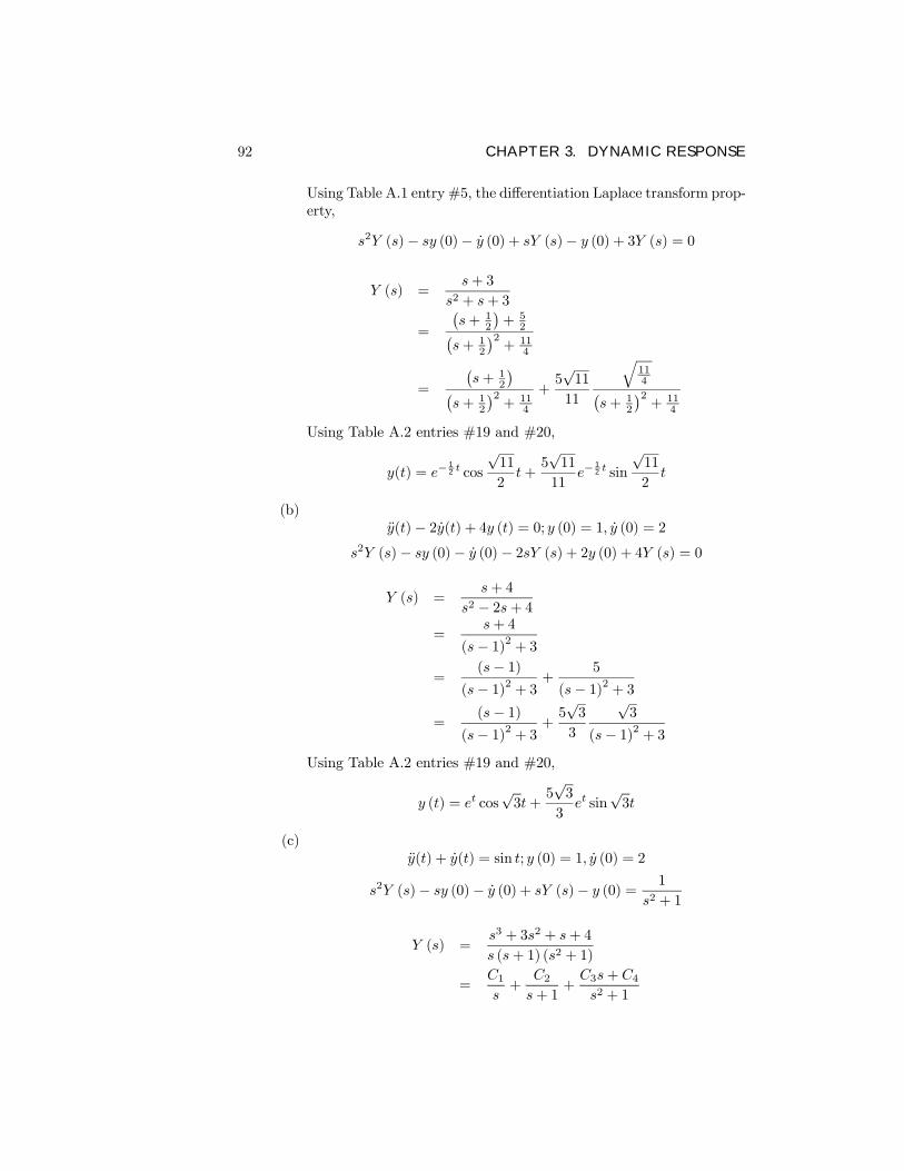
92 CHAPTER 3. DYNAMIC RESPONSE
Using Table A.1 entry #5, the differentiation Laplace transform prop-erty,
s2Y (s)− sy (0)− úy (0) + sY (s)− y (0) + 3Y (s) = 0
Y (s) =s+ 3
s2 + s+ 3
=
¡s+ 1
2
¢+ 5
2¡s+ 1
2
¢2+ 11
4
=
¡s+ 1
2
¢¡s+ 1
2
¢2+ 11
4
+5√11
11
q114¡
s+ 12
¢2+ 11
4
Using Table A.2 entries #19 and #20,
y(t) = e−12 t cos
√11
2t+
5√11
11e−
12 t sin
√11
2t
(b)y(t)− 2 úy(t) + 4y (t) = 0; y (0) = 1, úy (0) = 2
s2Y (s)− sy (0)− úy (0)− 2sY (s) + 2y (0) + 4Y (s) = 0
Y (s) =s+ 4
s2 − 2s+ 4=
s+ 4
(s− 1)2 + 3=
(s− 1)(s− 1)2 + 3 +
5
(s− 1)2 + 3
=(s− 1)
(s− 1)2 + 3 +5√3
3
√3
(s− 1)2 + 3Using Table A.2 entries #19 and #20,
y (t) = et cos√3t+
5√3
3et sin
√3t
(c)y(t) + úy(t) = sin t; y (0) = 1, úy (0) = 2
s2Y (s)− sy (0)− úy (0) + sY (s)− y (0) = 1
s2 + 1
Y (s) =s3 + 3s2 + s+ 4
s (s+ 1) (s2 + 1)
=C1s+
C2s+ 1
+C3s+ C4s2 + 1

93
C1 =s3 + 3s2 + s+ 4
(s+ 1) (s2 + 1)|s=0 = 4
C2 =s3 + 3s2 + s+ 4
s (s2 + 1)|s=−1 = −5
2
4
s+−52
s+ 1+C3s+ C4s2 + 1
=s3 + 3s2 + s+ 4
s (s+ 1) (s2 + 1)
s3µ3
2+ C3
¶+ s2 (4 + C3 + C4) + s
µ3
2+ C4
¶+ 4 = s3 + 3s2 + s+ 4
Match coefficients of like powers of s
C4 +3
2= 1 =⇒ C4 = −1
2
C3 +3
2= 1 =⇒ C3 = −1
2
4
s+−52
s+ 1+− 12s− 1
2
s2 + 1=4
s+−52
s+ 1− 12
s
s2 + 1− 12
1
s2 + 1
Using Table A.2 entries #2, #7, #17, and #18
y (t) = 4− 52e−t − 1
2cos t− 1
2sin t
(d)
y (t) + 3y (t) = sin t; y (0) = 1, úy (0) = 2
s2Y (s)− sy (0)− úy (0) + 3Y (s) =1
s2 + 1
Y (s) =s3 + 2s2 + s+ 3
(s2 + 3) (s2 + 1)
=C1s+ C2s2 + 3
+C3s+ C4s2 + 1
(C1s+ C2)¡s2 + 1
¢+ (C3s+ C4)
¡s2 + 3
¢(s2 + 3) (s2 + 1)
=s3 + 2s2 + s+ 3
(s2 + 3) (s2 + 1)
Match coefficients of like powers of s:
s3 (C1 + C3) + s2 (C2 + C4) + s (C1 + 3C3) + (C2 + 3C4)
= s3 + 2s2 + s+ 3

94 CHAPTER 3. DYNAMIC RESPONSE
C1 + C3 = 1 =⇒ C1 = −C3C2 + C4 = 2 =⇒ C2 = 2− C4C1 + 3C3 = 1 =⇒ −C3 + 3C3 = 1 =⇒ C3 =
1
2
=⇒ C1 = −12
C2 + 3C4 = 3 =⇒ (2− C4) + 3C4 = 3 =⇒ C4 =1
2
=⇒ C2 =3
2
Y (s) =−12s+
32
s2 + 3+
12s+
12
s2 + 1
= −12
s
s2 + 3+
√3
2
√3
s2 + 3+1
2
s
s2 + 1+1
2
1
s2 + 1
y (t) = −12cos√3t+
√3
2sin√3t+
1
2cos t+
1
2sin t
(e)y(t) + 2 úy (t) = et; y (0) = 1, úy (0) = 2
s2Y (s)− sy (0)− úy (0) + 2sY (s)− 2y (0) = 1
s− 1
Y (s) =5s− 4
s (s− 1) (s+ 2)=
C1s+
C2s− 1 +
C3s+ 2
C1 =5s− 4
(s− 1) (s+ 2) |s=0 = 2
C2 =5s− 4s (s+ 2)
|s=1 = 1
3
C3 =5s− 4s (s− 1) |s=−2 = −
7
3
Y (s) =2
s+1
3
1
s− 1 −7
3
1
s+ 2
y (t) = 2 +1
3et − 7
3e−2t
(f) Using the results from Appendix A,
y (t) + y (t) = t; y (0) = 1, úy (0) = −1

95
s2Y (s)− sy (0)− úy (0) + Y (s) =1
s2
Y (s) =s3 − s2 + 1s2 (s2 + 1)
=C1s+C2s2+C3s+ C4s2 + 1
C1 =d
ds
¡s3 − s2 + 1¢(s2 + 1)
|s=0 = 0
C2 =
¡s3 − s2 + 1¢(s2 + 1)
|s=0 = 1
1
s2+C3s+ C4s2 + 1
=s3 − s2 + 1s2 (s2 + 1)¡
s2 + 1¢+ (C3s+ C4) s
2
s2 (s2 + 1)=
s3 − s2 + 1s2 (s2 + 1)
Match coefficients of like powers of s:
C3 = 1
C4 + 1 = −1 =⇒ C4 = −2
Y (s) =1
s2+
s
s2 + 1− 2 1
s2 + 1
y (t) = t+ cos t− 2 sin t10. Write the dynamic equations describing the circuit in Fig. 3.50. Write the
equations in both state-variable form and as a second-order differentialequation in y(t). Assuming a zero input, solve the differential equationfor y(t) using Laplace-transform methods for the parameter values andinitial conditions shown in the Þgure. Verify your answer using the initialcommand in MATLAB.
Solution:
i = Cdy
dt(1)
v = Ldi
dt(2)
u(t)− Ldidt−Ri(t)− y(t) = 0
di
dt=u
L− RLi− 1
Cy (3)

96 CHAPTER 3. DYNAMIC RESPONSE
Figure 3.50: Circuit for Problem 3.10
Put differential equations (2) and (3) into state-space form:·úiúv
¸=
· −RL − 1
L1C 0
¸ ·iv
¸+
·01
¸u
Substituting the given values for L, R, and C we have for equation (3):
di
dt= u− 2dy
dt− y
y + 2 úy + y = u
Characteristic equation:
s2 + 2s+ 1 = 0
(s+ 1)2 = 0
So:y(t) = A1e
−t +A2te−t
Solving for the coefficients:
y(t) = A1e−t +A2te−t
y(t0) = A1e−t0 +A2t0et0 = 1
úy(t) = −A1e−t +A2e−t −A2te−túy(t0) = −A1e−t0 +A2e−t0 −A2te−t0 = 0
⇒ A2 = et0 and A1 = (1− t0)et0
y(t) = (1− t0)et0−t + tet0−t
To verify the solution using MATLAB, re-write the differential equationas, · .
y..y
¸=
·0 1−1 −2
¸ ·y.y
¸+
·1L0
¸u
y =£1 0
¤ · y.y
¸

97
Then the following MATLAB statements,
a=[0,1;-1,-2];
b=[0;1];
c=[1,0];
d=[0];
sys=ss(a,b,c,d);
xo=[1;0];
[y,t,x]=initial(sys,xo);
plot(t,y);
grid;
xlabel(’Time (sec)’);
ylabel(’y(t)’);
title(’Initial condition response’);
generate the initial condition response shown below that agrees with theanalytical solution above.
0 2 4 6 8 10 12 140
0.1
0.2
0.3
0.4
0.5
0.6
0.7
0.8
0.9
1
Time (sec)
y(t)
Initial condition response
Problem 3.10: Initial condition response.
11. Consider the standard second-order system
G(s) =ω2n
s2 + 2ζωns+ ω2n.

98 CHAPTER 3. DYNAMIC RESPONSE
Figure 3.51: Plot of input for Problem 3.11
a) Write the Laplace transform of the signal in Fig. 3.51. b). What isthe transform of the output if this signal is applied to G(s). c) Find theoutput of the system for the input shown in Fig. 3.51.
Solution:
(a) The input signal in Figure 3.51 may be written as:
u(t) = t− t[1(t− 1)]− t[1((t− 2)] + t[1(t− 3)]where 1(t− τ) denotes a unit step.The Laplace transform of the input signal is:
U(s) =1
s2¡1− e−s − e−2s − e−3s¢
(b) The Laplace transform of the output if this signal is applied is:
Y (s) = G(s)U(s) =ω2n
s2 + 2ζωns+ ω2n
µ1
s2
¶¡1− e−s − e−2s − e−3s¢
(c) However to make the mathematical manipulation easier, consideronly the reponse of the system to a ramp input:
Y1(s) =ω2n
s2 + 2ζωns+ ω2n
µ1
s2
¶Partial fractions yields the following:
Y1(s) =1
s2−
2ζωn
s+
2ζωn(s+ 2ζωn − ωn
2ζ )
(s+ ωnζ)2 + (ωnp1− ζ2)2
Use the following Laplace transform pairs for the case 0 ≤ ζ < 1 :

99
L−1 s+ z1
(s+ a)2 + ω2 =
s(z1 − a)2 + ω2
ω2e−at sin(ωt+ φ)
where φ ≡ tan−1³
ωz1−a
´L−1 1
s2 = t ramp
L−11s = 1(t) unit step
and the following Laplace transform pairs for the case ζ = 1 :
L−1 1
(s+ a)2 = te−at
L−1 s
(s+ a)2 = (1− at)e−at
L−1 1s2 = t ramp
L−11s = 1(t) unit step
the following is derived:
y1(t) =
t− 2ζ
ωn+ e−ζωnt
ωn√1−ζ2
sin(ωnp1− ζ2t+ tan−1 2ζ
√1−ζ2
2ζ2−10 ≤ ζ < 1t ≥ 0
t− 2ωn+ 2
ωne−ωnt
¡ωn2 t+ 1
¢ ζ = 1t ≥ 0
Since u(t) consists of a ramp and three delayed ramp signals, usingsuperpostion (the system is linear), then:
y(t) = y1(t)−y1(t−1)−y1(t−2)+y1(t−3) t ≥ 0
12. A rotating load is connected to a Þeld-controlled DC motor with negligibleÞeld inductance. A test results in the output load reaching a speed of1 rad/sec within 1/2 sec when a constant input of 100 V is applied tothe motor terminals. The output steady-state speed from the same test isfound to be 2 rad/sec. Determine the transfer function θ(s)/Vf (s) of themotor.
Solution:
Equations of motion for a DC motor:
Jmθm + b úθm = Kmia,

100 CHAPTER 3. DYNAMIC RESPONSE
Keúθm + La
diadt+Raia = va,
but since theres neglible Þeld inductance La = 0.
Combining the above equations yields:
RaJmθm +Rab úθm = Ktva −KtKe úθm
Applying Laplace transforms yields the following transfer function:
θ(s)
Vf (s)=
Kt
JmRa
s(s+ KtKe
RaJm+ b
Jm)=
K
s(s+ a)
where K = Kt
JmRaand a = KtKe
RaJm+ b
Jm.
K and a are found using the given information:
Vf (s) =100
ssince Vf (t) = 100V
úθ(1
2) = 2 rad/sec
For the given information we need to utilize úθm(t) instead of θm(t):
sθ(s) =100K
s(s+ a)
Using the Final Value Theorem and assuming that the system is stable:
lims→0
100K
s+ a= lims→0
úθ(1
2) = 2 =
100K
a
Take the inverse Laplace transform:
L−1100Ka
a
s(s+ a) =
100K
a(1− e−at) = 2(1− e−at) = 1
0.5 = e−a2 yields a = 1.39
K =2
100a yields K = 0.0278
θ(s)
Vf (s)=
0.0278
s(s+ 1.39)
13. For the tape drive shown in Fig. 2.48, compute the following, using thenumbers given in Problem 2.20 (a):

101
(a) the transfer function from the motor current to the tape position;
(b) the poles and zeros for the transfer function in part (a).
Solution:
(a)
Tape tension
Ia(s)=T (s)
Ia(s)
T = B( úx2 − úx1) + k(x2 − x1)T (s) = (Bs+ k)(X2(s)−X1(s))
From Problem 2.20:
J1 úω1 = −B1ω1 + ktia +Br1( úx2 − úx1) + kr1(x2 − x1)J2 úω2 = −B2ω2 + Fr2 +Br2( úx1 − úx2) + kr2(x1 − x2)úx1 = r1ω1
úx2 = r2ω2
J1s+B1 0 (Bs+ k)r1 −(Bs+ k)r1
0 J2s+B2 −(Bs+ k)r2 (Bs+ k)r2−r1 0 s 00 −r2 0 s
ω1ω2x1x2
=ktIaFr200
X1(s) = Ia(s)15(s+ 800)
s(s2 + 1250s+ 0.4× 106)X2(s) = Ia(s)
4.8× 10⁻⁶s(s2 + 1250s+ 0.4× 106)
X2(s)−X1(s) =15(s+ 800)− 4.8× 10⁻⁶s(s2 + 1250s+ 0.4× 10⁶)Ia(s)
T (s)
Ia(s)= (20s+ 2× 10⁴) 15(s+ 800)− 4.8× 10
−6
s(s2 + 1250s+ 0.4× 10⁶)
(b)
poles at : 0,−625± j996.8zeros at : − 800,−1000

102 CHAPTER 3. DYNAMIC RESPONSE
14. For the system in Fig. 2.50, compute the transfer function from the motorvoltage to position θ2.
Solution:
From Problem 2.23:
Ldiadt+Raia + ke úθ1 = va
ktia = J1θ1 + b( úθ1 − úθ2) + k(θ1 − θ2) +B úθ1J2θ2 + b( úθ2 − úθ1) + k(θ2 − θ1) = 0
So we have:
LsIa(s) +RaIa(s) + skeΘ1(s) = Va(s)
ktIa(s) = s2J1Θ1(s) + b[Θ1(s)−Θ2(s)]s+ k[Θ1(s)−Θ2(s)] +BsΘ1(s)
s2J2Θ2(s) + b[Θ2(s)−Θ1(s)]s+ k[Θ2(s)−Θ1(s)] = 0
we have:
Θ2(s)
Va(s)=
kt(bs+ k)
det
ske 0 Ls+RaJ1s
2 +Bs+ bs+ k −bs− k −kt−bs− k J2s
2 + bs+ k 0
=
kt(bs+ k)
(Ls+Ra)[J1J2s4 + (J1b+BJ2 + bJ2)s
3 + (J1k +Bb+KJ2)s2 +Bks]
+kektJ2s3 + kektbs
2 + kkekts
=kt(bs+ k)
J1J2s5 + J2[J1Ra + L(b+B)]s
4
+[J2kektJ1L(b+ k) + LJ2k +Ra(b+B)J2 − Lb2]s3+[L(b+B)(b+ k)− 2bkL+ J1Ra(b+ k) +RaJ2k − b2Ra]s2
+[kekt(b+ k) + kL(b+ k)− bk2 +Ra(b+B)(b+ k)− 2bkRa]s+ kRab
15. Compute the transfer function for the two-tank system in Fig. 2.54 withholes at A and C.
Solution:
From Problem 2.27 but with s = a tank area we have:
·∆ úh1∆ úh2
¸=1
6a
· −1 01 −1
¸ ·∆h1∆h2
¸+ωina
·10
¸+
· −103a0
¸

103
∆ úh1 =−∆h1 + 6ωin − 20
6a
∆ úh2 =1
6a(∆h1 −∆h2)
s∆h1(s) =−∆h1(s) + 6ωin(s)
6a
s∆h2(s) =1
6a[∆h1(s)−∆h2(s)]
∆h2(s) =ωin(s)
6a[a( 16a + s)]2
∆h2(s)
ωin(s)=
1
6[a( 16a + s)]2
16. For a second-order system with transfer function
G(s) =3
s2 + 2s− 3 ,
determine the following:
(a) DC gain;
(b) the Þnal value to a step input.
Solution:
(a) DC gain G(0) = 3−3 = −1
(b) limt→∞ y(t) =?s2 + 2s+ 3 = 0 =⇒ s = 1,−3Since the system has an unstable pole, the Final Value Theorem isnot applicable. The output is unbounded.
17. Consider the continuous rolling mill depicted in Fig. 3.52. Suppose thatthe motion of the adjustable roller has a damping coefficient b, and thatthe force exerted the rolled material on the adjustable roller is proportionalto the materials change in thickness: Fs = c(T −x). Suppose further thatthe DC motor has a torque constant Kt and a back-emf constant Ke, andthat the rack-and-pinion has effective radius of R.
(a) What are the inputs to this system? The output?
(b) Without neglecting the effects of gravity on the adjustable roller,draw a block diagram of the system that explicitly shows the follow-ing quantities: Vs(s), I0(s), F (s) (the force the motor exerts on theadjustable roller), and X(s).

104 CHAPTER 3. DYNAMIC RESPONSE
Figure 3.52: Continuous rolling mill
(c) Simplify your block diagram as much as possible while still identifyingoutput and each input separately.
Solution:
(a)
Inputs: input voltage −→ vs(t)
thickness −→ T
gravity −→ mg
Output: thickness −→ x
(b) Dynamic analysis of adjustable roller:
mx = c(T − x)−mg − b úx− Fm=⇒ (s2m+ sb+ c)X(s) + Fm(s) +
mg − cTs
= 0 (1)
Torque in rack and pinion:
TRP = RFm = NTmotor
but Tmotor = KtIf io
Fm =NKtIfR
io (2)

105
DC motor circuit analysis:
vs(t) = Raio + Ladiodt+ va(t)
va(t) = ue úθ
θR
N= x
Io(s) =Vs(s)− KeN
R sX(s)
Ra + sLa(3)
Combining (1), (2), and (3):
0 = (s2m+ sb+ c)X(s) +mg − cT
s+NKtIfR
"Vs(s)− KeN
R sX(s)
sLa +Ra
#

106 CHAPTER 3. DYNAMIC RESPONSE
Block diagrams for rolling mill
Problems and Solutions for Section 3.218. Compute the transfer function for the block diagram shown in Fig. 3.53.
Note that ai and bi are constants.
(a) Write the third-order differential equation that relates y and u. (Hint :Consider the transfer function.)
(b) Write three simultaneous Þrst-order (state-variable) differential equa-tions using variables x1, x2, and x3, as deÞned on the block dia-gram in Fig. 3.53. Notice how the same constant parameters enterthe transfer function, the differential equations, and the matrices ofthe state-variable form. (This special structure is called the control

107
Figure 3.53: Block diagram for Problem 3.18
canonical form and will be discussed further in Chapter 7.) Repeatfor the block diagram of Fig. 3.50(b). This is the observer canonicalform for a 3rd order system.
Solution:
Using Masons rule:
Forward paths:b1s+b2s2+b3s3
Feedback paths:
a1s+a2s2+a3s3
Y
U=
b1
s +b2
s2 +b3
s3
1 + a1
s +a2
s2 +a3
s3
(a)
(s3 + a1s2 + a2s+ a3)Y = (b1s
2 + b2s+ b3)U
d3y
dt3+ a1y + a2 úy + a3y = b1u+ b2 úu+ b3u
(b) DeÞnitions from block diagram:
úx3 = x2
úx2 = x1
úx1 = u− a1x1 − a2x2 − a3x3y = b3x3 + b2x2 + b1x1

108 CHAPTER 3. DYNAMIC RESPONSE
Figure 3.54: Block diagrams for Problem 3.19
.x =
−a1 −a2 −a31 0 00 1 0
x+
100
uy =
£b1 b2 b3
¤x
19. Find the transfer functions for the block diagrams in Fig. 3.54.
Solution:
(a) Block diagram for Fig. 3.54 (a)

109
Forward Path Gain1 2 3 4 G11 5 4 G2Loop Path Gain2 3 2 -G1
Y
R=
G11 +G1
+G2
(b) Block diagram for Fig. 3.54 (b)
Block diagram for Fig. 3.54 (b): reduced
Y
R= G7 +
G1G3G4G6(1 +G1G2)(1 +G4G5)
(c) Block diagrams for Fig. 3. 54(c)

110 CHAPTER 3. DYNAMIC RESPONSE
Figure 3.55: Block diagrams for Problem 3.20
Forward Path Gain1 2 3 4 5 6 G1G2G3
1+G2× G4G5
1+G4
1 3 4 5 6 G6G4G5
1+G4
1 7 6 G7
Y
R= G7 +
G6G4G51 +G4
+G1G2G31 +G2
× G4G51 +G4
20. Find the transfer functions for the block diagrams in Fig. 3.55, using thefollowing:
(a) the ideas of Figs. 3.6 and 3.7;
(b) Masons rule.
Solution:
Transfer functions found using the ideas of Figs. 3.6 and 3.7:
(a) Block diagram for Fig. 3.55(a)

111
G∗2 =G2
1−G2H2G∗3 =
G31−G3H3
Y
R=
G1(1 +G∗2)
1 +G1(1 +G∗2)G∗3
=G1(1−G2H2)(1−G3H3) +G1G2(1−G3H3)
(1−G2H2)(1−G3H3) +G1G3(1−G2H2) +G1G2G3
(b) Block diagram for Fig. 3.55(b)
Masons rule: forward path gains,
b3s3,b2s2,b1s
(c) Applying block diagram reduction:
Block diagram for Fig. 3.55(c)

112 CHAPTER 3. DYNAMIC RESPONSE
The method: reduce innermost box, shift b2 to b3 node, reduce nextinnermost box and continue systematically.
(d)
Y
R=b3 + b2(s+ a1) + b1(s
2 + a1s+ a2)
s3 + a1s2 + a2s+ a3
Block diagram for Fig. 3.55(d)
The system is tightly connected , easy to apply Masons.
Mason’s rule:
(a)
Forward Path1 2 3 5 6 p1 = G1G
∗2
1 2 3 4 6 p2 = G1Loop Path2 3 4 7 L1 = G1G
∗3
2 3 5 7 L2 = G1G∗2G
∗3
Y
R=
p1 + p21 + L1 + L2
=G1(1 +G
∗2)
1 +G1G∗3(1 +G∗2)
(b) Loop Path: −a3
s3 ,−a2
s2 ,−a1
s
Y
R=
b3
s3 +b2
s2 +b1
s
1 + a3
s3 +a2
s2 +a1
s
=b3 + b2s+ b1s
2
s3 + a1s2 + a2s+ a3

113
(c) Block diagrams for Fig. 3.55(c)
(d) Masons Rule:
Y
R=
D +AB∗
1 +G(D +AB∗)=
D +DBH +AB
1 +BH +GD +GBDH +GAB
21. Use block-diagram algebra or Masons rule to determine the transfer func-tion between R(s) and Y(s) in Fig. 3.56.
Solution:

114 CHAPTER 3. DYNAMIC RESPONSE
Figure 3.56: Block diagram for Problem 3.21
Block diagram for Fig. 3.56
By block diagram algebra:
Block diagram for Fig. 3.56: reduced

115
Q = R− PH3 − PH4= R− P (H3 −H4)
P = G1NG6 = Y
So:
Y
R=
G1NG61 + (H3 +H4)G1NG6
Now, what is N?
Block diagrams for Fig. 3.56
Move G4 and G3 :
Block diagram for Fig. 3.56: reduced
Combine symmetric loops as in the Þrst step:
Block diagram for Fig. 3.56: reduced

116 CHAPTER 3. DYNAMIC RESPONSE
Which is:
N =O
I=
G4G2 +G5G31 +H2(G4 +G5)
Y (s)
R(s)=
G1(G4G2 +G5G3)G61 +H2(G4 +G5) + (H3 +H4)G1(G4G2 +G5G3)G6
By Masons Rule:
Signal ßow graph
Flow graph for Fig. 3.56
Forward Path Gain1 2 3 4 5 G1G2G4G61 2 6 4 5 G1G3G5G6
Loop Path Gain1 2 3 4 5 1 −G1G2G4G6H31 2 3 4 5 1 −G1G2G4G6H41 2 6 4 5 1 −G1G3G5G6H31 2 6 4 5 1 −G1G3G5G6H43 4 3 −G4H23 4 3 −G5H2
and the determinants are
∆ = 1 + [(H3 +H4)G1(G2G4 +G3G5)G6 +H2(G4 +G5)]
∆1 = 1− (0)∆2 = 1− (0)∆3 = 1− (0)∆4 = 1− (0)
Applying the rule, the transfer function is

117
Figure 3.57: Block diagram for Problem 3.22
Y (s)
R(s)=
1
∆
XGi∆i
=G1(G4G2 +G5G3)G6
1 +H2(G4 +G5) + (H3 +H4)G1(G4G2 +G5G3)G6
22. Use block-diagram algebra to determine the transfer function betweenR(s) and Y(s) in Fig. 3.57.
Solution:
Block diagram for Fig. 3.57
Move node A and close the loop:

118 CHAPTER 3. DYNAMIC RESPONSE
Block diagram for Fig. 3.57: reduced
Add signal B, close loop and multiply before signal C.
Block diagram for Fig. 3.57: reduced
Move middle block N past summer.
Block diagram for Fig. 3.57: reduced
Now reverse order of summers and close each block separately.

119
Figure 3.58: Circuit for Problem 3.23
Block diagram for Fig. 3.57: reduced
Y
R=
feedforwardz | (N +G3) (
1
1 +NH3)| z
feedback
Y
R=G1G2 +G3(1 +G1H1 +G1H2)
1 +G1H1 +G1H2 +G1G2H3
23. For the electric circuit shown in Fig. 3.58, Þnd the following:
(a) the time-domain equation relating i(t) and v1(t);
(b) the time-domain equation relating i(t) and v2(t);
(c) assuming all initial conditions are zero, the transfer function V2(s)/V1(s)and the damping ratio ζ and undamped natural frequency ωn of thesystem;
(d) the values of R that will result in v2(t) having an overshoot of no morethan 25%, assuming v1(t) is a unit step, L = 10 mH, and C = 4 µF.
Solution:
(a)
v1(t) = Ldi
dt+Ri+
1
C
Zi(t)dt

120 CHAPTER 3. DYNAMIC RESPONSE
Figure 3.59: Unity feedback system for Problem 3.24
(b)
v2(t) =1
C
Zi(t)dt
(c)
v2(s)
v1(s)=
1sC
sL+R+ 1sC
=1
s2LC + sRC + 1
(d) For 25% overshoot ζ ≈ 0.4
0.4 ≈ ζ =R
2q
LC
R = 2ζ
rL
C= (2)(0.4)
r10× 10−34× 10−6 = 40Ω
Problems and Solutions for Section 3.324. For the unity feedback system shown in Fig. 3.59, specify the gain K of
the proportional controller so that the output y(t) has an overshoot of nomore than 10% in response to a unit step.
Solution:
Y (s)
R(s)=
K
s2 + 2s+K=
ω2ns2 + 2ζωns+ ω2n
ωn =√K
ζ =2
2ωn=
1√K
(1)
In order to have an overshoot of no more than 10%:
Mp = e−πζ/
√1−ζ2 ≤ 0.10
Solving for ζ :

121
Figure 3.60: Unity feedback system for Problem 3.25
ζ =
s(lnMp)2
π2 + (lnMp)2≥ 0.591
Using (1) and the solution for ζ:
K =1
ζ2≤ 2.86
∴ 0 < K ≤ 2.86
25. For the unity feedback system shown in Fig. 3.60, specify the gain andpole location of the compensator so that the overall closed-loop responseto a unit-step input has an overshoot of no more than 25%, and a 1%settling time of no more than 0.1 sec. Verify your design using MATLAB.
Solution:
Y (s)
R(s)=
100K
s2 + (25 + a)s+ 25a+ 100K=
100K
s2 + 2ζωns+ ω2n
Using the given information:
R(s) =1
sunit step
Mp ≤ 25%
t1% ≤ 0.1 sec
Solve for ζ :
Mp = e−πζ/√1−ζ2
ζ =
s(lnMp)2
π2 + (lnMp)2≥ 0.4037

122 CHAPTER 3. DYNAMIC RESPONSE
Solve for ωn:
e−ζωnts = 0.01 For a 1% settling time
ts ≤ 4.605
ζωn= 0.1
=⇒ ωn ≈ 114.07
Now Þnd a and K :
2ζωn = (25 + a)
a = 2ζωn − 25 = 92.10ω2n = (25a+ 100K)
K =ω2n − 25a100
≈ 107.09
The step response of the system using MATLAB is shown below.
0 0.02 0.04 0.06 0.08 0.1 0.120
0.2
0.4
0.6
0.8
1
1.2
1.4
Time (sec)
y(t)
Step Response
Step Response for Problem 3.25
Problems and Solutions for Section 3.4

123
26. Suppose you desire the peak time of a given second-order system to beless than t0p. Draw the region in the s-plane that corresponds to values ofthe poles that meet the speciÞcation tp < t
0p.
Solution:
s-plane region to meet peak time constraint: shaded
ωdtp = π =⇒ tp =π
ωd< t
0
p
π
t0p< ωd
27. Suppose you are to design a unity feedback controller for a Þrst-order plantdepicted in Fig. 3.61. (As you will learn in Chapter 4, the conÞgurationshown is referred to as a proportional-integral controller). You are todesign the controller so that the closed-loop poles lie within the shadedregions shown in Fig. 3.62.
(a) What values of ωn and ζ correspond to the shaded regions in Fig. 3.62?(A simple estimate from the Þgure is sufficient.)
(b) Let Kα = α = 2. Find values for K and K1 so that the poles of theclosed-loop system lie within the shaded regions.
(c) Prove that no matter what the values of Kα and α are, the controllerprovides enough ßexibility to place the poles anywhere in the complex(left-half) plane.

124 CHAPTER 3. DYNAMIC RESPONSE
Figure 3.61: Unity feedback system for Problem 3.27
Figure 3.62: Desired closed-loop pole locations for Problem 3.27

125
Solution:
(a) The values could be worked out mathematically but working fromthe diagram:
p32 + 22 = 3.6 =⇒ 2.6 ≤ ωn ≤ 4.6
θ = sin−1 ζζ = sin θ
From the Þgure:
θ ≈ 34 ζ1 = 0.554
θ ≈ 70 ζ2 = 0.939
=⇒ 0.6 ≤ ζ ≤ 0.9 (roughly)
(b) Closed-loop pole positions:
s(s+ α) + (Ks+KKI)Kα = 0
s2 + (α+KKα)s+KKIKα = 0
For this case:
s2 + (2 + 2K)s+ 2KKI = 0 (∗)Choose roots that lie in the center of the shaded region,
(s+ (3 + j2))(s+ (3− j2)) = s2 + 6s+ 13 = 0s2 + (2 + 2K)s+ 2KKI = s
2 + 6s+ 13
2 + 2K = 6 =⇒ K = 2
13 = 4KI =⇒ KI =13
4
(c) For the closed-loop pole positions found in part (b), in the (*) equa-tion the value of K can be chosen to make the coefficient of s takeon any value. For this value of K a value of KI can be chosen sothat the quantity KKIKα takes on any value desired. This impliesthat the poles can be placed anywhere in the complex plane.
28. The open-loop transfer function of a unity feedback system is
G(s) =K
s(s+ 2).
The desired system response to a step input is speciÞed as peak timetp = 1 sec and overshoot Mp = 5%.

126 CHAPTER 3. DYNAMIC RESPONSE
(a) Determine whether both speciÞcations can be met simultaneously byselecting the right value of K.
(b) Sketch the associated region in the s-plane where both speciÞcationsare met, and indicate what root locations are possible for some likelyvalues of K.
(c) Pick a suitable value for K, and use MATLAB to verify that thespeciÞcations are satisÞed.
Solution:
(a)
T (s) =Y (s)
R(s)=
G(s)
1 +G(s)=
K
s2 + 2s+K=
ω2ns2 + 2ζωns+ ω2n
Equate the coefficients:
2 = 2ζωnK = ω2n
(*)
=⇒ ωn =√K ζ =
1√K
We would need:
Mp%
100= 0.05 = e
−πζ√1−ζ2 =⇒ ζ = 0.69
tp = 1 sec =π
ωd=
π
ωnp1− ζ2
=⇒ ωn = 4.34
But the combination (ζ = 0.69 , ωn = 4.34) that we need is notpossible by varying K alone. Observe that from equations (*) ζωn =1 6= 0.69× 4.34
(b) Now we wish to have:
M∗p = r × 0.05 = e
−πζ√1−ζ2
t∗p = r × 1 sec = πωd
(**)
where r ≡relaxation factor.Recall the conditions of our system:
ωn =√K
ζ =1√K
replace ωn and ζ in the system (**):
=⇒ − π√K−1 = r × 0.051 sec = π√
K−1

127
=⇒ r × 0.05 = e−r =⇒ r ∼= 2.21K = 1 +
π2
r2=⇒ K = 3.02
then with K = 3.02 we will have:
M∗p = rMp = 2.21× 0.05 = 0.11t∗p = rtp = 2.21× 1 sec = 2.21 sec
Note: * denotes actual location of closed-loop roots.
s-plane regions
% Problem 3.28
K=3.02;
num=[K];
den=[1, 2, K];
sys=tf(num,den);
t=0:.01:3;
y=step(sys,t);
plot(t,y);
yss = dcgain(sys);
Mp = (max(y) - yss)*100;
% Finding maximum overshoot
msg overshoot = sprintf(’Max overshoot = %3.2f%%’, Mp);
% Finding peak time
idx = max(find(y==(max(y))));
tp = t(idx);

128 CHAPTER 3. DYNAMIC RESPONSE
msg peaktime = sprintf(’Peak time = %3.2f’, tp);
xlabel(’Time (sec)’);
ylabel(’y(t)’);
msg title = sprintf(’Step Response with K=%3.2f’,K);
title(msg title);
text(1.1, 0.3, msg overshoot);
text(1.1, 0.1, msg peaktime);
grid on;
0 0.5 1 1.5 2 2.5 30
0.2
0.4
0.6
0.8
1
1.2
1.4
Time (sec)
y(t)
Step Response with K=3.02
Max overshoot = 10.97%
Peak time = 2.21
Problem 3.28: Closed-loop step response
29. The equations of motion for the DC motor shown in Fig. 2.26 were givenin Eqs. (2.63-64) as
Jmθm +
µb+
KtKeRa
¶úθm =
Kt
Rava.
Assume that
Jm = 0.01 kg ·m2,b = 0.001 N ·m · sec,
Ke = 0.02 V · sec,Kt = 0.02 N ·m/A,Ra = 10 Ω.

129
(a) Find the transfer function between the applied voltage va and themotor speed úθm.
(b) What is the steady-state speed of the motor after a voltage va = 10 Vhas been applied?
(c) Find the transfer function between the applied voltage va and theshaft angle θm.
(d) Suppose feedback is added to the system in part (c) so that it becomesa position servo device such that the applied voltage is given by
va = K(θr − θm),
where K is the feedback gain. Find the transfer function between θrand θm.
(e) What is the maximum value of K that can be used if an overshootMp < 20% is desired?
(f) What values of K will provide a rise time of less than 4 sec? (Ignorethe Mp constraint.)
(g) Use MATLAB to plot the step response of the position servo systemfor values of the gain K = 0.5, 1, and Þnd the overshoot and risetime of the three step responses by examining your plots. Are theplots consistent with your calculations in parts (e) and (f)?
Solution:
Jmθm +
µb+
KtKeRa
¶úθm =
Kt
Rava
(a)
JmΘms2 +
µb+
KtKe
Ra
¶Θms =
Kt
RaVa(s)
sΘm(s)
Va(s)=
Kt
RaJm
s+ bJm+ KtKe
RaJm
Jm = 0.01kg ·m2,
b = 0.001N ·m · sec,Ke = 0.02V · sec,Kt = 0.02N ·m/A,Ra = 10Ω.
sΘm(s)
Va(s)=
0.2
s+ 0.104

130 CHAPTER 3. DYNAMIC RESPONSE
(b) Final Value Theorem
úθ(∞) = s(10)(0.2)
s(s+ 0.104)|s=0 = 2
0.104= 19.23
(c)Θm(s)
Va(s)=
0.2
s(s+ 0.104)
(d)
Θm(s) =0.2K(Θr −Θm)s(s+ 0.104)
Θm(s)
Θr(s)=
0.2K
s2 + 0.104s+ 0.2K
(e)
Mp = e−πζ/√1−ζ2
= 0.2 (20%)
ζ = 0.4559
Y (s) =ω2n
s2 + 2ζωns+ ω2n2ζωn = 0.104
ωn =0.104
2(0.4559)= 0.114rad/ sec
ω2n = 0.2K
K < 6.50× 10⁻²
(f)
ωn ≥ 1.8
tr
ω2n = 0.2K
K ≥ 1.01
(g) MATLAB
clear all
close all
K1=[0.5 1.0 2.0 6.5e-2];
t=0:0.01:150;
for i=1:1:length(K1)
K = K1(i);
titleText = sprintf(’ K= %1.4f ’, K);
wn = sqrt(0.2*K);

131
num=wnˆ2;
den=[1 0.104 wnˆ2];
zeta=0.104/2/wn;
sys = tf(num, den);
y= step(sys, t);
% Finding maximum overshoot
if zeta < 1
Mp = (max(y) - 1)*100;
overshootText = sprintf(’ Max overshoot = %3.2f %’, Mp);
else
overshootText = sprintf(’ No overshoot’);
end
% Finding rise time
idx 01 = max(find(y<0.1));
idx 09 = min(find(y>0.9));
t r = t(idx 09) - t(idx 01);
risetimeText = sprintf(’ Rise time = %3.2f sec’, t r);
% Plotting
subplot(3,2,i);
plot(t,y);
grid on;
title(titleText);
text( 0.5, 0.3, overshootText);
text( 0.5, 0.1, risetimeText);
end

132 CHAPTER 3. DYNAMIC RESPONSE
0 50 100 1500
0.5
1
1.5
2 K= 0.4000
Max overshoot = 55.57 Rise time = 4.20 sec
0 50 100 1500
0.5
1
1.5
2 K= 0.5000
Max overshoot = 59.23 Rise time = 3.70 sec
0 50 100 1500
0.5
1
1.5
2 K= 1.0000
Max overshoot = 69.23 Rise time = 2.51 sec
0 50 100 1500
0.5
1
1.5
2 K= 2.0000
Max overshoot = 77.17 Rise time = 1.73 sec
0 50 100 1500
0.5
1
1.5 K= 0.0650
Max overshoot = 19.99 Rise time = 13.66 sec
Problem 3.29: Closed-loop step responses
For part (e) we concluded that K < 6.50 × 10⁻² in order for Mp <20%. This is consistent with the above plots. For part (f) we foundthat K ≥ 1.01 in order to have a rise time of less than 4 seconds.We actually see that our calculations is slightly off and that K canbe K ≥ 0.5, but since K ≥ 1.01 is included in K ≥ 0.5, our answerin part f is consistent with the above plots.
30. You wish to control the elevation of the satellite-tracking antenna shownin Figs. 3.63 and 3.64. The antenna and drive parts have a moment ofinertia J and a damping B; these arise to some extent from bearing andaerodynamic friction but mostly from the back emf of the DC drive motor.The equations of motion are
J θ +B úθ = Tc,
where Tc is the torque from the drive motor. Assume that
J = 600, 000kg·m2 B = 20, 000 N·m·sec
(a) Find the transfer function between the applied torque Tc and theantenna angle θ.
(b) Suppose the applied torque is computed so that θ tracks a referencecommand θr according to the feedback law
Tc = K(θr − θ),

133
Figure 3.63: Satellite Antenna (Courtesy Space Systems/Loral)
Figure 3.64: Schematic of antenna for Problem 3.30

134 CHAPTER 3. DYNAMIC RESPONSE
where K is the feedback gain. Find the transfer function between θrand θ.
(c) What is the maximum value of K that can be used if you wish tohave an overshoot Mp < 10%?
(d) What values of K will provide a rise time of less than 80 sec? (Ignorethe Mp constraint.)
(e) Use MATLAB to plot the step response of the antenna system forK = 200, 400, 1000, and 2000. Find the overshoot and rise timeof the four step responses by examining your plots. Do the plotsconÞrm your calculations in parts (c) and (d)?
Solution:J θ +B úθ = Tc
(a)
JΘs2 +BΘs = Tc(s)
Θ(s)
Tc(s)=
1
Js+B
J = 600, 000kg ·m2
B = 20, 000N ·m · secΘ(s)
Tc(s)=
1.667× 10⁻⁶s(s+ 1
30)
(b)
Θ(s) =1.667× 10⁻⁶K(Θr −Θ)
s(s+ 130)
Θ(s)
Θr(s)=
1.667K × 10−6s2 + 1
30s+ 1.667K × 10−6
(c)
Mp = e−πζ/√1−ζ2
= 0.1 (10%)
ζ = 0.591
Y (s) =ω2n
s2 + 2ζωns+ ω2n
2ζωn =1
30
ωn =130
2(0.591)= 0.0282 rads/ sec
ω2n = 1.667K × 10−6K < 477

135
(d)
ωn ≥ 1.8
tr
ω2n = 1.667K × 10−6K ≥ 304
0 100 200 300 4000
0.2
0.4
0.6
0.8
1
1.2
1.4 K= 200.0000
Max overshoot = 0.08
Rise time = 161.10 sec
0 100 200 300 4000
0.2
0.4
0.6
0.8
1
1.2
1.4 K= 400.0000
Max overshoot = 7.03
Rise time = 76.30 sec
0 100 200 300 4000
0.2
0.4
0.6
0.8
1
1.2
1.4 K= 1000.0000
Max overshoot = 24.54
Rise time = 36.17 sec
0 100 200 300 4000
0.2
0.4
0.6
0.8
1
1.2
1.4 K= 2000.0000
Max overshoot = 38.78
Rise time = 22.64 sec
(e) Problem 3.30: Step responses
(e) The results compare favorably with the predictions made in partsc and d. For K < 477 the overshoot was less than 10, the rise-timewas less than 80 seconds.
31. (a) Show that the second-order system
y + 2ζωn úy + ω2ny = 0, y(0) = yo, úy(0) = 0,
has the response
y(t) = yoe−σtp1− ζ2
sin(ωdt+ cos−1 ζ).
(b) Prove that, for the underdamped case (ζ < 1), the response oscilla-tions decay at a predictable rate (see Fig. 3.65) called the logarith-mic decrement δ, where
δ = lnyoy1= στd
= ln∆y1y1
∼= ln ∆yiyi,

136 CHAPTER 3. DYNAMIC RESPONSE
Figure 3.65: DeÞnition of logarithmic decrement
and τd is the damped natural period of vibration
τd =2π
ωd.
Solution:
(a) The system is second order =⇒ Q(s) = s2+2ζωns+ω2n. The initial
condition response can be obtained by plugging a dirac delta at theinput at the time 0 (this charges the system immediately to itsinitial condition and after that the system evolves by itself).
Inputeffective = y0δ(t)
L[Inputeffective] = y0
We do not know whether the transfer function has Þnite zeros or not,but further thought will reveal the presence of at least one Þnite zeroin the H(s).
lims→∞ sH(s)y0 = y(t)|0+
where
H(s) =P (s)
Q(s)=
P (s)
s2 + 2ζωns+ ω2n.
If P (s) were a constant (no zeros in the H(s)), then the limit in theinitial value theorem would give always zero (which is wrong because

137
we know that the initial value must be y0.) So we need a zero. Wesuggest using the following H(s):
H(s) =−s
s2 + 2ζωns+ ω2n
Y (s) = H(s)y0 =−sy0
s2 + 2ζωns+ ω2n
=R+
s− P+ +R−
s− P−where
P+ = −ζωn + jωnq1− ζ2
P− = −ζωn − jωnq1− ζ2
R+ =−ωnej(π=cos−1 ζ)
2ωnp1− ζ2ejπ/s
R− = R∗+
Note: The residues can be calculated graphically.
R+ = lims→P+
[(s− P+)Y (s)]
=⇒ y(t) = R+eP+t +R−eP−t
y(t) =−e−ζωnt2p1− ζ2
[e+j(ωn√1−ζ2t+π/2−cos−1 ζ)
+ e−j(ωn√1−ζ2t+π/2−cos−1 ζ)]
=⇒ y(t) = y0e−σtp1− ζ2
sin(ωdt− cos−1 ζ)
(b)
dy(t)
dt= 0 =⇒ t =
nπ
ωd(n is any integer)
tMax =2π
ωdn
y(t)|tMax ≡ yn = y0e−σnτdp1− ζ2
sin(cos−1 ζ)
Note:
sin(− cos−1 ζ) =q1− ζ2

138 CHAPTER 3. DYNAMIC RESPONSE
yn =y0p1− ζ2p1− ζ2
e−σnτd (∗)
(Proof of the Þrst line)
σ = lny0yn= στd
From (*)
y1 = y0e−στd =⇒ ln
y0yn= στd
(Proof of the second line)
∆yn = yn−1 − yn∆yn = y0e
−σnτd − y0e−(n−1)στd = y0e−σnτd(1− eστd)
=⇒ ∆ynyn
=y0e
−σnτd
y0e−σnτd(1− eστd)
=⇒ ∆ynyn
=∆yiyi
for all i, n
Problems and Solutions for Section 3.5
32. In aircraft control systems, an ideal pitch response (qo) versus a pitchcommand (qc) is described by the transfer function
Qo(s)
Qc(s)=
τω2n(s+ 1/τ)
s2 + 2ζωns+ ω2n.
The actual aircraft response is more complicated than this ideal transferfunction; nevertheless, the ideal model is used as a guide for autopilotdesign. Assume that tr is the desired rise time, and that
ωn =1.789
tr1
τ=1.6
trζ = 0.89
Show that this ideal response possesses a fast settling time and minimalovershoot by plotting the step response for tr = 0.8, 1.0, 1.2, and 1.5 sec.
Solution:
The following program statements in MATLAB produce the followingplots:
% Problem 3.32

139
tr = [0.8 1.0 1.2 1.5];
t=[1:240]/30;
tback=fliplr(t);
clf;
for I=1:4,
wn=(1.789)/tr(I); %Rads/second
tau=tr(I)/(1.6); %tau
zeta=0.89; %
b=tau*(wnˆ2)*[1 1/tau];
a=[1 2*zeta*wn (wnˆ2)];
y=step(b,a,t);
subplot(2,2,I);
plot(t,y);
titletext=sprintf(’tr=%3.1f seconds’,tr(I));
title(titletext);
xlabel(’t (seconds)’);
ylabel(’Qo/Qc’);
ymax=(max(y)-1)*100;
msg=sprintf(’Max overshoot=%3.1f%%’,ymax);
text(.50,.30,msg);
yback=flipud(y);
yind=find(abs(yback-1)>0.01);
ts=tback(min(yind));
msg=sprintf(’Settling time =%3.1f sec’,ts);
text(.50,.10,msg);
grid;
end

140 CHAPTER 3. DYNAMIC RESPONSE
Figure 3.66: Fig.3.66: Unity feedback system for Problem 3.33
0 2 4 6 80
0.2
0.4
0.6
0.8
1
1.2
1.4tr=0.8 seconds
t (seconds)
Qo/
Qc
Max overshoot=2.3%
Settling time =2.3 sec
0 2 4 6 80
0.2
0.4
0.6
0.8
1
1.2
1.4tr=1.0 seconds
t (seconds)Q
o/Q
c
Max overshoot=2.3%
Settling time =2.9 sec
0 2 4 6 80
0.2
0.4
0.6
0.8
1
1.2
1.4tr=1.2 seconds
t (seconds)
Qo/
Qc
Max overshoot=2.3%
Settling time =3.5 sec
0 2 4 6 80
0.2
0.4
0.6
0.8
1
1.2
1.4tr=1.5 seconds
t (seconds)
Qo/
Qc
Max overshoot=2.3%
Settling time =4.4 sec
Problem 3.32: Ideal pitch response
33. Consider the system shown in Fig. 3.66, where
G(s) =1
s(s+ 3)and D(s) =
K(s+ z)
s+ p. (1)
Find K, z, and p so that the closed-loop system has a 10% overshoot to astep input and a settling time of 1.5 sec (1% criterion).
Solution:
For the 10% overshoot:
Mp = e−πζ/√1−ζ2
= 10%
=⇒ ζ =
s(lnMp)2
π2 + (lnMp)2= 0.

141
For the 1.5sec (1% criterion):
ωn =4.6
ζts=
4.6
(0.6)(1.5)= 5.11
The closed loop transfer function is:
Y (s)
R(s)=
K s+zs+p × 1
s(s+3)
1 +K s+zs+p × 1
s(s+3)
=K(s+ z)
s(s+ 3)(s+ p) +K(s+ z)
Method I.
From inspection, if z = 3, (s + 3) will cancel out and we will have astandard form transfer function. As perfect cancellation is impossible,assign z a value that is very close to 3, say 3.1. But in determining the Kand p, assume that (s+ 3) and(s+ 3.1) cancelled out each other. Then:
Y (s)
R(s)=
K
s2 + ps+K
As the additional pole and zero will degrade the system, pick some largerdamping ration.
Let ζ = 0.7
ωn =4.6
ζts=
4.6
(0.7)(1.5)= 4.38, so let ωn = 4.5
p = 2ζωn = 2× 0.7× 4.5 = 6.3K = ω2n = 20.25
Method II.
There are 3 unknowns (z, p,K) and only 2 speciÞed conditions. We canarbitrarily choose p large such that complex poles will dominate in thesystem response.
Try p = 10z
Choose a damping ratio corresponding to an overshoot of 5% (instead of10%, to be safe).
ζ = 0.707
From the formula for settling time (with a 1% criterion)
ωn =4.6ζts= 4.6
0.707×1.5 = 4.34 adding some margin, let ωn = 4.88
The characteristic equation is
Q(s) = s3 + (s+ p) s2 + (3p+K)s+Kz = (s+ a)(s2 + 2ζωns+ ω2n)

142 CHAPTER 3. DYNAMIC RESPONSE
We want the characteristic equation to be the product of two factors, acouple of conjugated poles (dominant) and a non-dominant real pole farform the dominant poles.
Equate both expressions of the characteristic equation.
ω2na = Kz
2ζωna+ ω2n = 30z +K
2ζωn + a = 3 + 10z
Solving three equations we get
z = 5.77
p = 57.7
K = 222.45
a = 53.79
34. Sketch the step response of a system with the transfer function
G(s) =s/2 + 1
(s/40 + 1)[(s/4)2 + s/4 + 1].
Justify your answer based on the locations of the poles and zeros (do notÞnd inverse Laplace transform). Then compare your answer with the stepresponse computed using MATLAB.
Solution:
From the location of the poles, we notice that the real pole is a factor of20 away from the complex pair of poles. Therefore, the reponse of thesystem is dominated by the complex pair of poles.
G(s) ≈ (s/2 + 1)
[(s/4)2 + s/4 + 1]
This is now in the same form as equation (3.58) where α = 1, ζ = 0.5 andωn = 4. Therefore, Fig. 3.32 suggests an overshoot of over 70%. The stepresponse is the same as shown in Fig. 3.31, for α = 1, with more than70% overshoot and settling time of 3 seconds. The MATLAB plots belowconÞrm this.
% Problem 3.34
num=[1/2, 1];
den1=[1/16, 1/4, 1];

143
sys1=tf(num,den1);
t=0:.01:3;
y1=step(sys1,t);
den=conv([1/40, 1],den1);
sys=tf(num,den);
y=step(sys,t);
plot(t,y1,t,y);
xlabel(’Time (sec)’);
ylabel(’y(t)’);
title(’Step Response’);
grid on;
0 0.5 1 1.5 2 2.5 30
0.2
0.4
0.6
0.8
1
1.2
1.4
1.6
1.8
Time (sec)
y(t)
Step Response
Problem 3.34: Step responses
35. Consider the two nonminimum phase systems,
G1(s) = − 2(s− 1)(s+ 1)(s+ 2)
; (2)
G2(s) =3(s− 1)(s− 2)
(s+ 1)(s+ 2)(s+ 3). (3)
(a) Sketch the unit step responses for G1(s) and G2(s), paying closeattention to the transient part of the response.

144 CHAPTER 3. DYNAMIC RESPONSE
(b) Explain the difference in the behavior of the two responses as itrelates to the zero locations.
(c) Consider a stable, strictly proper system (that is,m zeros and n poles,where m < n). Let y(t) denote the step response of the system. Thestep response is said to have an undershoot if it initially starts off inthe wrong direction. Prove that a stable, strictly proper system hasan undershoot if and only if its transfer function has an odd numberof real RHP zeros.
Solution:
(a) For G1(s) :
Y1(s) =1
sG1(s) =
−2(s− 1)s(s+ 1)(s+ 2)
H(s) = k
Qj(s− zj)Ql(s− pl)
Rpi = lims→pi
[(s− pi)H(s)] = lims→pi
k
Qj(s− zj)Ql
l 6=i(s− pl)= k
Qj(pi − zj)Ql
l 6=i(pi − pl)
Each factor (pi − zj) or (pi − pl) can be thought of as a complexnumber (a magnitude and a phase) whose pictorial representation isa vector pointing to pi and coming from zj or pl respectively.
The method for calculating the residue at a pole pi is:
(1) Draw vectors from the rest of the poles and from all the zeros tothe pole pi.
(2) Measure magnitude and phase of these vectors.
(3) The residue will be equal to the gain, multiplied by the productof the vectors coming from the zeros and divided by the product ofthe vectors coming from the poles.
In our problem:
Y1(s) =−2(s− 1)
s(s+ 1)(s+ 2)=R0s+
R−1(s+ 1)
+R−2(s+ 2)
=1
s− 4
s+ 1+
3
s+ 2
y1(t) = 1− 4e−t + 3e−2t

145
Step Response for G1
Time (sec)
y1(t)
0 1 2 3 4 5 6 7 8 9 10-0.4
-0.2
0
0.2
0.4
0.6
0.8
1
Problem 3.35: Step response for a non-minimum phase system
For G2(s) :
Y2(s) =3(s− 1)(s− 2)
s(s+ 1)(s+ 2)(s+ 3)=1
s+
−9(s+ 1)
+18
(s+ 2)+
−10(s+ 3)
y2(t) = 1− 9e−t + 18e−2t − 10e−3t

146 CHAPTER 3. DYNAMIC RESPONSE
Step Response for G2
Time (sec)
y2(t)
0 1 2 3 4 5 6 7 8 9 10-0.4
-0.2
0
0.2
0.4
0.6
0.8
1
Problem 3.35: Step response of non-minimum phase system
(b) The Þrst system presents an undershoot. The second system, onthe other hand, starts off in the right direction.
The reasons for this initial behavior of the step response will beanalyzed in part c.
In y1(t): dominant at t = 0 the term −4e−tIn y2(t): dominant at t = 0 the term 18e−2t
(c) The following concise proof is from [1] (see also [2]-[3]).
Without loss of generality assume the system has unity DC gain(G(0) = 1) Since the system is stable, y(∞) = G(0) = 1, and it isreasonable to assume y(∞) 6= 0. Let us denote the pole-zero excess asr = n−m. Then, y(t) and its r− 1 derivatives are zero at t = 0, andyr(0) is the Þrst non-zero derivative. The system has an undershootif yr(0)y(∞) < 0. The transfer function may be re-written as
G(s) =
Qmi=1(1− s
zi)Qm+r
i=1 (1− spi)
The numerator terms can be classiÞed into three types of terms:
(1). The Þrst group of terms are of the form (1− αis) with αi > 0.(2). The second group of terms are of the form (1+αis) with αi > 0.
(3). Finally, the third group of terms are of the form, (1+βis+αis2)
with αi > 0, and βi could be negative.
However, β2i < 4αi, so that the corresponding zeros are complex.

147
All the denominator terms are of the form (2), (3), above. Since,
yr(0) = lims→∞ s
rG(s)
it is seen that the sign of yr(0) is determined entirely by the numberof terms of group 3 above. In particular, if the number is odd, thenyr(0) is negative and if it is even, then yr(0) is positive. Sincey(∞) = G(0) = 1,then we have the desired result.[1] Vidyasagar, M., On Undershoot and Nonminimum Phase Zeros,IEEE Trans. Automat. Contr., Vol. AC-31, p. 440, May 1986.
[2] Clark, R., N., Introduction to Automatic Control Systems, JohnWiley, 1962.
[3] Mita, T. and H. Yoshida, Undershooting phenomenon and itscontrol in linear multivariable servomechanisms, IEEE Trans. Au-tomat. Contr., Vol. AC-26, pp. 402-407, 1981.
36. Consider the following second-order system with an extra pole:
H(s) =ω2np
(s+ p)(s2 + 2ζωns+ ω2n).
Show that the unit step response is
y(t) = 1 +Ae−pt +Be−σt sin(ωdt− θ),
where
A =−ω2n
ω2n − 2ζωnp+ p2B =
pq(p2 − 2ζωnp+ ω2n)(1− ζ2)
θ = tan−1p1− ζ2−ζ + tan−1
p1− ζ2
p− ζωn .
(a) Which term dominates y(t) as p gets large?
(b) Give approximate values for A and B for small values of p.
(c) Which term dominates as p gets small? (Small with respect to what?)
(d) Using the explicit expression for y(t) above or the step command inMATLAB, and assuming ωn = 1 and ζ = 0.7, plot the step responseof the system above for several values of p ranging from very smallto very large. At what point does the extra pole cease to have mucheffect on the system response?

148 CHAPTER 3. DYNAMIC RESPONSE
Solution:
Second-order system:
H(s) =ω2np
(s+ p)(s2 + 2ζωns+ ω2n)
Unit step response:
Y (s) =1
sH(s), y(t) = L−1Y (s)
s2 + 2ζωns+ ω2n = (s+ σ + jωd)(s+ σ − jωd)
where σ = ζωn,ωd = ωnp1− ζ2.
Thus from partial fraction expansion:
Y (s) =k1s+
k2s+ p
+k3
s+ σ + jωd+
k4s+ σ − jωd
solving for k1, k2, k3, and k4:
k1 = H(0) =⇒ k1 = 1
k2 =ω2np
s(s+ σ + jωd)(s+ σ − jωd) |s=−p =⇒ k2 =−ω2n
ω2n − 2pζωn + p2k3 = (s+ σ + jωd)Y (s)|s=−σ−jωd
=⇒ k3 =p
2q(1− ζ2) (p2 − 2pζωn + ω2n)
e−iθ = |k3| e−iθ
k4 = k∗3
where
θ = tan−1Ãp
1− ζ2−ζ
!+ tan−1
Ãωnp1− ζ2
p− ζωn
!Thus
Y (s) =1
s+
k2s+ p
+ |k3|µ
e−iθ
s+ σ + jωd+
e+iθ
s+ σ − jωd
¶Inverse Laplace:
y(t) = 1 + k2e−pt + |k3|
³e−iθe−(σ+jωd)t + e+iθe−(σ−jωd)t
´or
y(t) = 1+−ω2n
ω2n − 2pζωn + p2| z A
e−pt+pq
(1− ζ2) (p2 − 2pζωn + ω2n)| z B
e−σt cos(ωdt+θ)

149
(a) As p gets large the B term dominates.
(b) For small p: A ≈ −1, B ≈ 0.(c) As p gets small A dominates.
(d) The effect of a change in p is not noticeable above p ≈ 10.
0 5 10 15 20 250
0.2
0.4
0.6
0.8
1 Step Response for p= 0.10
0 5 10 15 20 250
0.2
0.4
0.6
0.8
1
1.2
1.4 Step Response for p= 1.00
0 5 10 15 20 250
0.2
0.4
0.6
0.8
1
1.2
1.4 Step Response for p= 10.00
0 5 10 15 20 250
0.2
0.4
0.6
0.8
1
1.2
1.4 Step Response for p= 100.00
Problem 3.36: Step responses
37. The block diagram of an autopilot designed to maintain the pitch attitudeθ of an aircraft is shown in Fig. 3.67. The transfer function relating theelevator angle δe and the pitch attitude θ is
θ(s)
δe(s)= G(s) =
50(s+ 1)(s+ 2)
(s2 + 5s+ 40)(s2 + 0.03s+ 0.06),
where θ is the pitch attitude in degrees and δe is the elevator angle indegrees. The autopilot controller uses the pitch attitude error ε to adjustthe elevator according to the following transfer function:
δe(s)
ε(s)= D(s) =
K(s+ 3)
s+ 10.
Using MATLAB, Þnd a value of K that will provide an overshoot of lessthan 10% and a rise time faster than 0.5 sec for a unit step change in θr.After examining the step response of the system for various values of K,comment on the difficulty associated with making rise-time and overshoot

150 CHAPTER 3. DYNAMIC RESPONSE
Figure 3.67: Block diagram of autopilot
measurements for complicated systems.
Solution:
G(s) =Θ(s)
δe(s)=
50 (s+ 1) (s+ 2)
(s2 + 5s+ 40) (s2 + 0.03s+ 0.06)
D(s) =δe(s)
e(s)=K(s+ 3)
(s+ 10)
where
e(s) = Θr −ΘΘ
Θr=
G(s)D(s)
1 +G(s)D(s)
=50K (s+ 1) (s+ 2) (s+ 3)
(s2 + 5s+ 40) (s2 + 0.03s+ 0.06) (s+ 10) +K (s+ 3)
=50K
¡s3 + 6s2 + 11s+ 6
¢s5 + 15.03s4 + 90.51s3 + 403.6s2 + (17.4 +K) s+ (24 + 3K)
Output must be normalized to the Þnal value of Θ(s)Θr(s)
for easy computa-
tion of the overshoot and rise-time. In this case the design criterion forovershoot cannot be met which is indicated in the sample plots.

151
0 50 100 150 2000
0.5
1
1.5
2
2.5 K= 60.0000
Time (sec)
thet
a
Max overshoot = 115.77 Rise time = 0.41 sec
0 50 100 150 2000
0.5
1
1.5
2 K= 6.0000
Time (sec)
thet
a
Max overshoot = 90.67 Rise time = 2.93 sec
0 50 100 150 2000
0.5
1
1.5
2 K= 0.0060
Time (sec)
thet
a
Max overshoot = 85.95 Rise time = 4.11 sec
0 50 100 150 2000
0.5
1
1.5
2 K= 0.0000
Time (sec)
thet
a
Max overshoot = 85.95 Rise time = 4.11 sec
Problem 3.37: Step responses for autopilot
Problems and Solutions for Section 3.6
38. A measure of the degree of instability in an unstable aircraft responseis the amount of time it takes for the amplitude of the time response todouble (see Fig. 3.68) given some nonzero initial condition.
(a) For a Þrst-order system, show that the time to double τ2 is
τ2 =ln 2
p,
where p is the pole location in the RHP.
(b) For a second-order system (with two complex poles in the RHP),show that
τ2 =ln 2
−ζωn .
Solution:

152 CHAPTER 3. DYNAMIC RESPONSE
Figure 3.68: Time to double
(a) First-order system, H(s) could be:
H(s) =k
(s− p)h(t) = L−1 [H(s)] = kepth(τ0) = kepτ0
h (τ0 + τ2) = 2h (τ0) = kep(τ0+τ2)
=⇒ 2kepτ0 = kepτ0epτ2
=⇒ τ2 =ln 2
p
(b) Second-order system:
y (t) = y0eωn|ζ|tq1− ¯ζ2¯ sin(ωn
q1− ¯ζ2¯t+ cos−1 ζ)
where
cos−1 ζ = cos−1 |ζ|+ π
=⇒ y (t) = y0eωn|ζ|tq1− ¯ζ2¯ (−1) sin
µωn
q1− ¯ζ2¯t+ cos−1 |ζ|
Note: Instead of working with a negative ζ, everything is changed to|ζ|.

153
|t0| = −y0 eωn|ζ|tq1− ¯ζ2 ¯
|τ0| = −y0 eωn|ζ|τ0q1− ¯ζ2 ¯
|τ0 + τ2| = −y0 eωn|ζ|(τ0+τ2)q1− ¯ζ2 ¯ = 2 |τ0|
=⇒ eωn|ζ|τ2 = 2
=⇒ τ2 =ln 2
ωn |ζ| =ln 2
−ωnζ (ζ ≤ 0)
Note: This problem shows that σ = ωn |ζ| (the real part of the poles)is inversely proportional to the time to double.
The further away from the imaginary axis the poles lie, the fasterthe response is (either increasing faster for RHP poles or decreasingfaster for LHP poles).
39. Suppose that unity feedback is to be applied around the following open-loop systems. Use Rouths stability criterion to determine whether theresulting closed-loop systems will be stable.
(a) KG(s) = 4(s+2)s(s3+2s2+3s+4)
(b) KG(s) = 2(s+4)s2(s+1)
(c) KG(s) = 4(s3+2s2+s+1)s2(s3+2s2−s−1)
Solution:
(a)
1 +KG = s4 + 2s3 + 3s2 + 8s+ 8 = 0
s4 : 1 3 8
s3 : 2 8
s2 : a b
s1 : c
s0 : d

154 CHAPTER 3. DYNAMIC RESPONSE
where
a =2× 3− 8× 1
2= −1 b =
2× 8− 1× 02
= 8
c =3a− 2ba
=−8− 16−1 = 24
d = b = 8
2 sign changes in Þrst column=⇒2 roots not in LHP=⇒unstable.(b)
1 +KG = s3 + s2 + 2s+ 8 = 0
The Rouths array is,
s3 : 1 2
s2 : 1 8
s1 : −6s0 : 8
There are two sign changes in the Þrst column of the Routh array.Therefore, there are two roots not in the LHP.
(c)1 +KG = s5 + 2s4 + 3s3 + 7s2 + 4s+ 4 = 0
s5 : 1 3 4
s4 : 2 7 4
s3 : a1 a2
s2 : b1 b2
s1 : c1
s0 : d1
where
a1 =6− 72
=−12
a2 =8− 42
= 2
b1 =−7/2− 4−1/2 = 15 b2 =
−4/2− 0−1/2 = 4
c1 =30 + 2
15=32
15d1 = 4
2 sign changes in the Þrst column=⇒2 roots not in the LHP=⇒unstable.

155
40. Use Rouths stability criterion to determine how many roots with positivereal parts the following equations have.
(a) s4 + 8s3 + 32s2 + 80s+ 100 = 0.
(b) s5 + 10s4 + 30s3 + 80s2 + 344s+ 480 = 0.
(c) s4 + 2s3 + 7s2 − 2s+ 8 = 0.(d) s3 + s2 + 20s+ 78 = 0.
(e) s4 + 6s2 + 25 = 0.
Solution:
(a)
s4 + 8s3 + 32s2 + 80s+ 100 = 0
s4 : 1 32 100
s3 : 8 80
s2 : 22 100
s1 : 80− 80022
= 43.6
s0 : 100
=⇒ No roots not in the LHP
(b)
s5 + 10s4 + 30s3 + 80s2 + 344s+ 480 = 0
s5 : 1 30 344
s4 : 10 80 480
s3 : 22 296
s2 : −545 480
s1 : 490
s0 : 480
=⇒ 2 roots not in the LHP.
(c)
s4 + 2s3 + 7s2 − 2s+ 8 = 0
There are roots in the RHP (not all coefficients are >0).

156 CHAPTER 3. DYNAMIC RESPONSE
s4 : 1 7 8
s3 : 2 − 2s2 : 8 8
s1 : −4s0 : 8
=⇒ 2 roots not in the LHP.
(d) The Routh array is,
s3 : 1 20
s2 : 1 78
s1 : −58s0 : 78
There are two sign changes in the Þrst column of the Routh array.Therefore, there are two roots not in the LHP.
(e)
a (s) = s4 + 6s2 + 25 = 0
Two coefficients are missing so there are roots outside the LHP.
Create a new row by da(s)ds
s4 : 1 6 25
s3 : 4 12 ←− new rows2 : 3 25
s1 : 12− 1003= −21.3
s0 : 25
=⇒ 2 roots not in the LHP
check:
a (s) = 0 =⇒ s2 = −3± 4j = 5ej(π±0.92)s =
√5ej(
π2±0.46)+nπj n = 0, 1

157
Problem 3.40: s-plane pole locations
41. Find the range of K for which all the roots of the following polynomialare in the LHP.
s5 + 5s4 + 10s3 + 10s2 + 5s+K = 0.
Use MATLAB to verify your answer by plotting the roots of the polyno-mial in the s-plane for various values of K.
Solution:s5 + 5s4 + 10s3 + 10s2 + 5s+K = 0
s5 : 1 10 5
s4 : 5 10 K
s3 : a1 a2
s2 : b1 K
s1 : c1
s0 : K
where
a1 =5 (10)− 1 (10)
5= 8 a2 =
5 (5)− 1 (K)5
=25−K8
b1 =(a1) (10)− (5) (a2)
a1=55 +K
8
c1 =(b1) (a2)− (a1) (K)
b1=− ¡K2 + 350K − 1375¢
5 (55 +K)
For stability: all terms in Þrst column > 0

158 CHAPTER 3. DYNAMIC RESPONSE
(1) b1 =55+K8 > 0 =⇒ K > −55
(2) c1 =−(K2+350K−1375)
5(55+K) > 0, −(K−3.88)(K+354)5(55+K) > 0 =⇒ −55 < K <3.88
(3) d1 = K > 0
Combining (1), (2), and (3) =⇒ 0 < K < 3.88. If we plot the roots ofthe polynomial for various values of K we obtain the following root locusplot (see Chapter 5),
Root Locus
Real Axis
Imag
Axi
s
-3 -2.5 -2 -1.5 -1 -0.5 0 0.5 1
-2
-1.5
-1
-0.5
0
0.5
1
1.5
2
K=0
K=0
K=0
K=0
K=0K=1
K=3.88
K=3.88
Problem 3.41: s-plane
42. The transfer function of a typical tape-drive system is given by
G(s) =K(s+ 4)
s[(s+ 0.5)(s+ 1)(s2 + 0.4s+ 4)],
where time is measured in milliseconds. Using Rouths stability crite-rion, determine the range of K for which this system is stable when thecharacteristic equation is 1 +G(s) = 0.
Solution:
1 +G (s) = s5 + 1.9s4 + 5.1s3 + 6.2s2 + (2 +K) s+ 4K = 0

159
Figure 3.69: Control system for Problem 3.43
s5 : 1.0 5.1 2 +K
s4 : 1.9 6.2 4K
s3 : a1 a2
s2 : b1 4K
s1 : c1
s0 : 4K
where
a1 =(1.9) (5.1)− (1) (6.2)
1.9= 1.837 a2 =
(1.9) (2 +K)− (1) (4K)1.9
= 2− 1.1K
b1 =(a1) (6.2)− (a2) (1.9)
a1= 1.138 (K + 3.63)
c1 =(b1) (a2)− (4K) (a1)
b1=− ¡1.25K2 + 9.61K − 8.26¢
1.138 (K + 363)=− (K + 8.47) (K − 0.78)
0.91 (K + 3.63)
For stability:
(1) b1 = K + 3.63 > 0 =⇒ K > −3.63(2) c1 > 0 =⇒ −8.43 < K < 0.78
(3) d1 > 0 =⇒ K > 0
Intersection of (1), (2), and (3) =⇒ 0 < K < 0.78
43. Consider the system shown in Fig. 3.69.
(a) Compute the closed-loop characteristic equation.
(b) For what values of (T,A) is the system stable? Hint : An approximateanswer may be found using
e−Ts ∼= 1− Ts

160 CHAPTER 3. DYNAMIC RESPONSE
or
e−Ts ∼= 1− T2 s
1 + T2 s
for the pure delay. As an alternative, you could use the computerMATLAB (Simulink) to simulate the system or to Þnd the roots ofthe systems characteristic equation for various values of T and A.
Solution:
(a) The characteristic equation is,
s(s+ 1) +Ae−Ts = 0
(b) Using e−Ts ∼= 1− Ts, the characteristic equation is,
s2 + (1− TA)s+A = 0
The Rouths array is,
s2 : 1 A
s1 : 1− TA 0
s0 : A
For stability we must have A > 0 and TA < 1.
Using e−Ts ∼= (1−T2 s)
(1+T2 s), the characteristic equation is,
s3 + (1 +2
T)s2 + (
2
T−A)s+ 2
TA = 0
The Rouths array is,
s3 : 1 (2
T−A)
s2 : (1 +2
T)
2A
T
s1 :(1 + 2
T )(2T −A)− 2A
T
(1 + 2T )
0
s0 :2A
T
For stability we must have all the coefficients in the Þrst column bepositive.
The following Simulink diagram simulates the system.

161
Problem 3.43: Simulink simulation diagram
44. Modify the Routh criterion so that it applies to the case where all thepoles are to be to the left of −α when α > 0. Apply the modiÞed test tothe polynomial
s3 + (6 +K)s2 + (5 + 6K)s+ 5K = 0,
Þnding those values of K for which all poles have a real part less than −1.Solution:
Let p = s+α and substitute s = p−α to obtain a polynomial in terms ofp. Apply the standard Routh test to the polynomial in p.
For the example p = s+1 or s = p−1. Substitute this in the polynomial,
(p− 1)3 + (6 +K) (p− 1)2 + (5 + 6K) (p− 1) + 5K = 0
or
p3 + (3 +K) p2 + (4K − 4) p+ 1 = 0.
The Rouths array is,
p3 : 1 4K − 4p2 : 3 +K 1
p1 :(3 +K) (4K − 4)− 1
3 +K0
p0 : 1
We must have K > −3 and 4K2+8K−13 > 0. The roots of the second-order polynomial are K = 1.06 and K = −3.061. The second-orderpolynomial remains positive if K > 1.06 or K < −3.061. Therefore, wemust have K > 1.06.
45. Suppose the characteristic polynomial of a given closed-loop system iscomputed to be

162 CHAPTER 3. DYNAMIC RESPONSE
s4+(11+K2)s3+(121+K1)s
2+(K1+K1K2+110K2+210)s+11K1+100 = 0.
Find constraints on the two gains K1 and K2 that guarantee a stableclosed-loop system, and plot the allowable region(s) in the (K1,K2) plane.You may wish to use the computer to help solve this problem.
Solution:
s5 :
s4 : 1 121 +K1 11K1 + 100
s3 : 11 +K2 K1 +K1K2 + 110K2 + 210 0
s2 :(11K2 + 10K1 + 1121)
K2 + 1111K1 + 100
s1 :10¡111K2
2 +K21K2 + 199K1K2 + 12342K2 +K
21 + 189K1 + 22331
¢(11K2 + 10K1 + 1121)
s0 : 11K1 + 100
For stability the Þrst column must be all positive. This means thatK2 > −11 and K1 > −100
11 . The region of stability is shown in thefollowing Þgure.
Problem 3.45: s-plane region

163
46. Overhead electric power lines sometimes experience a low-frequency, high-amplitude vertical oscillation, or gallop, during winter storms when theline conductors become covered with ice. In the presence of wind, this icecan assume aerodynamic lift and drag forces that result in a gallop up toseveral meters in amplitude. Large-amplitude gallop can cause clashingconductors and structural damage to the line support structures caused bythe large dynamic loads. These effects in turn can lead to power outages.Assume that the line conductor is a rigid rod, constrained to verticalmotion only, and suspended by springs and dampers as shown in Fig. 3.70.A simple model of this conductor galloping is
my +D(α) úy − L(α)v( úy2 + v2)1/2
+ T³nπ`
´y = 0,
where
m = mass of conductor,
y = conductor0s vertical displacement,D = aerodynamic drag force,
L = aerodynamic lift force,
v = wind velocity,
α = aerodynamic angle of attack = − tan−1( úy/v),T = conductor tension,
n = number of harmonic frequencies,
` = length of conductor.
Assume that L(0) = 0 and D(0) = D0 (a constant), and linearize theequation around the value y = úy = 0. Use Rouths stability criterion toshow that galloping can occur whenever
∂L
∂α+D0 < 0.
Solution:
my +
"D (α) úy − L (α) vp
úy2 + v2
#+ T
³nπl
´2y = 0,
Let x1 = y and x2 = úy = úx1

164 CHAPTER 3. DYNAMIC RESPONSE
Figure 3.70: Electric power-line conductor
úx1 = x2
úx2 = − 1m
"D (α)x2 − L (α) vp
x22 + v2
#− T
m
³nπl
´2x1 = 0
α = − tan−1³x2v
´úx1 = f1 (x1, x2)
úx2 = f2 (x1, x2)
úx1 = úx2 = 0 implies x2 = 0
x2 = 0 implies α = 0
α = 0 implies − T
m
³nπl
´2x1 = 0 implies x1 = 0.
∂f1∂x1
= 0,∂f2∂x2
= 1,∂f2∂x1
= − Tm
³nπl
´2

165
∂f2∂x
=∂
∂x2
(− 1m
"D (α)x2 − L (α) vp
x22 + v2
#)
= − 1m 1p
x22 + v2
·∂D
∂α
∂α
∂x2x2 +D (α)− ∂L
∂α
∂α
∂x2
¸−"D (α)x2 − L (α) vp
x22 + v2
#"−x2
(x22 + v2)
32
#
Now
∂α
x2=
∂
∂x2
³− tan−1
³x2v
´´=
−11 +
x22
v2
µ1
v
so
∂f2∂x2
=−1m 1p
x22 + v2
−∂Dα x2
v³1 +
x22
v2
´ +D (α) + ∂L∂αv
v³1 +
x22
v2
´
−"D (α)x2 − L (α) vp
x22 + v2
#"−x2
(x22 + v2)
32
#
∂f2∂x2
|x2=0 = −1
m
½1
v
·D0 +
∂L
∂α
¸¾= − 1
mv
µD0 +
∂L
∂α
For no damping (or negative damping) δx2 term must be ≤ 0 so thisimplies D0 +
∂L∂α < 0.
Problems and Solutions for Section 3.7
47. Repeat Example 3.34 using Simulink.
Solution:
The following Simulink diagram generates the same transient response asin the MATLAB implementation.

166 CHAPTER 3. DYNAMIC RESPONSE
Table 3.1: Step-Response Data for Problem 3.48t y(t) t y(t) t y(t)0 0 0.20 0.0138 0.90 0.44090.02 0.0001 0.22 0.0395 1.00 0.49240.04 0.0005 0.24 0.0480 1.50 0.69040.06 0.0014 0.26 0.0571 2.00 0.81210.08 0.0031 0.28 0.0668 2.50 0.88600.10 0.0057 0.30 0.0771 3.00 0.93090.12 0.0091 0.50 0.1979 3.50 0.95810.14 0.0135 0.60 0.2624 4.00 0.97460.16 0.0187 0.70 0.3253 5.00 0.99070.18 0.0248 0.80 0.3851
Problem 3.47: Simulink diagram
Problems and Solutions for Section 3.8
48. Samples from a step response are given in Table 3.1. Plot this data on alinear scale [y(t) vs. t] and semilog scale [log(y − y∞) vs. t], and obtainan estimate of the transfer function.
Solution:
Model from a step response data:
y = y∞ +Ae−αt +Be−βt + . . .
First approximation: y − y∞ = Ae−αt

167
log (|y − y∞|) = log10 |A|− 0.4343αt
From the line Þt to the following plot Þnd A and α.
A = −1.350.4343α =
0.733− 0.31
= 0.433
α w 1
Second term: y − 1 + 1.35e−t = Be−βt
From the line B = 0.35 β = 5
The model: y = 1− 1.35e−t + 0.35e−5t comparing y to y shows goodapproximation for t > 0.3 (better than 5%).
The transfer function for the above model:
Y (s) =1
s− 1.35
s+ 1+0.35
s+ 5=
s− 0.45s (s+ 1) (s+ 5)
t y y0 0 00.2 0.0138 0.02350.3 0.0771 0.0780.5 0.1979 0.211 0.4924 0.5062 0.8121 0.8173 0.9309 0.9335 0.9907 0.9909

168 CHAPTER 3. DYNAMIC RESPONSE
0 0.5 1 1.5 2 2.5 3 3.5 4 4.5 5-2.5
-2
-1.5
-1
-0.5
0
0.5Plot of log10[y( ) - y(t)] versus t
log|
1 - y
(t)|
Time (sec)
Problem 3.49: Plot of log10[y(∞)-y(t)] versus t
0 0.5 1 1.5 2 2.5 3 3.5 4 4.5 5-0.2
0
0.2
0.4
0.6
0.8
1
1.2Response data vs. fit
y(t)
Time (sec)
--------- A=-1.35, =1, B=.35, = 5
o o o Data
Problem 3.49: Response data vs. Þt
Related Documents