OPERATIONS RESEARCH Vol. 57, No. 5, September–October 2009, pp. 1169–1188 issn 0030-364X eissn 1526-5463 09 5705 1169 inf orms ® doi 10.1287/opre.1090.0725 © 2009 INFORMS Dynamic Pricing for Nonperishable Products with Demand Learning Victor F. Araman Stern School of Business, New York University, New York, New York 10012, and Olayan School of Business, American University of Beirut, Beirut, Lebanon, [email protected] René Caldentey Stern School of Business, New York University, New York, New York 10012, [email protected] A retailer is endowed with a finite inventory of a nonperishable product. Demand for this product is driven by a price- sensitive Poisson process that depends on an unknown parameter that is a proxy for the market size. The retailer has a prior belief on the value of this parameter that he updates as time and available information (prices and sales) evolve. The retailer’s objective is to maximize the discounted long-term average profits of his operation using dynamic pricing policies. We consider two cases. In the first case, the retailer is constrained to sell the entire initial stock of the nonperishable product before a different assortment is considered. In the second case, the retailer is able to stop selling the nonperishable product at any time and switch to a different menu of products. For both cases, we formulate the retailer’s problem as a (Poisson) intensity control problem and derive structural properties of an optimal solution, and suggest a simple and efficient approximated solution. We use numerical computations, together with asymptotic analysis, to evaluate the performance of our proposed policy. Subject classifications : dynamic pricing; Bayesian demand learning; approximations; intensity control; nonhomogeneous Poisson process; optimal stopping. Area of review : Manufacturing, Service, and Supply Chain Operations. History : Received December 2005; revisions received August 2008, January 2009; accepted April 2009. 1. Introduction This paper is concerned with dynamic pricing policies for nonperishable products in the context of a retail opera- tion with uncertain demand. In particular, we investigate the interplay between demand learning and pricing deci- sions and their impact on the long-term performance of the business. Effective retail management is about managing a limited available capacity to procure and sell the right assortment of products while considering present and future market developments. This point of view is captured by one of the most popular measures in the retail industry, namely, aver- age sales per square foot per unit time. Indeed, this measure highlights two fundamental aspects of a retail operation. First, it emphasizes the fact that capacity, measured by store or shelf space, is one of the retailer’s key assets, and thus must be managed as such; the challenge resides in choosing the best possible menu of products; failure to do so results in opportunity costs that would cut directly into the profit margins. Second, it highlights the time value of money when assessing the business performance. For example, a retailer might prefer to sell a product with a 5% margin over another one with a 10% margin if the former sells much faster than the latter (see Gaur et al. 2005 for a comprehensive empirical analysis of this “earns versus turns” trade-off). Thus, in optimizing this measure, retail- ers must balance the short-term benefits obtained by selling a given menu of products and the long-term opportunity costs incurred by allocating their resources (shelf space, time, capital, etc.) to these products instead of a different assortment. In addition to such critical trade-offs, retailers cannot overlook the market conditions in which they compete. Customers’ preferences, competitors’ actions, new product introduction, regulations, and so on, are often unknown to the retailer and need to be factored into the business strategy. As a result, learning about these market factors— induced, for example, through the sales process—should be constantly performed. Such learning would shed more light on future demand and hint at the current strategy to adopt. The same product that sells well today might get stocked on the shelves tomorrow, wasting valuable space that could be used to sell a more profitable alternative. To prevent such a highly undesirable situation, a retailer must continuously monitor the products sales to infer customers’ preferences, identify early-on the selling pattern of each product, and adopt the appropriate strategy. Low-selling items must be removed either by shipping them to a secondary market (e.g., an outlet) or by liquidating their inventory through active price markdowns. It is precisely this relationships between demand learning, pricing policies, and inventory 1169

Welcome message from author
This document is posted to help you gain knowledge. Please leave a comment to let me know what you think about it! Share it to your friends and learn new things together.
Transcript
OPERATIONS RESEARCHVol. 57, No. 5, September–October 2009, pp. 1169–1188issn 0030-364X �eissn 1526-5463 �09 �5705 �1169
informs ®
doi 10.1287/opre.1090.0725©2009 INFORMS
Dynamic Pricing for NonperishableProducts with Demand Learning
Victor F. AramanStern School of Business, New York University, New York, New York 10012, and Olayan School of Business,
American University of Beirut, Beirut, Lebanon, [email protected]
René CaldenteyStern School of Business, New York University, New York, New York 10012,
A retailer is endowed with a finite inventory of a nonperishable product. Demand for this product is driven by a price-sensitive Poisson process that depends on an unknown parameter that is a proxy for the market size. The retailer has aprior belief on the value of this parameter that he updates as time and available information (prices and sales) evolve. Theretailer’s objective is to maximize the discounted long-term average profits of his operation using dynamic pricing policies.We consider two cases. In the first case, the retailer is constrained to sell the entire initial stock of the nonperishableproduct before a different assortment is considered. In the second case, the retailer is able to stop selling the nonperishableproduct at any time and switch to a different menu of products. For both cases, we formulate the retailer’s problem as a(Poisson) intensity control problem and derive structural properties of an optimal solution, and suggest a simple and efficientapproximated solution. We use numerical computations, together with asymptotic analysis, to evaluate the performance ofour proposed policy.
Subject classifications : dynamic pricing; Bayesian demand learning; approximations; intensity control; nonhomogeneousPoisson process; optimal stopping.
Area of review : Manufacturing, Service, and Supply Chain Operations.History : Received December 2005; revisions received August 2008, January 2009; accepted April 2009.
1. IntroductionThis paper is concerned with dynamic pricing policies fornonperishable products in the context of a retail opera-tion with uncertain demand. In particular, we investigatethe interplay between demand learning and pricing deci-sions and their impact on the long-term performance of thebusiness.Effective retail management is about managing a limited
available capacity to procure and sell the right assortmentof products while considering present and future marketdevelopments. This point of view is captured by one of themost popular measures in the retail industry, namely, aver-age sales per square foot per unit time. Indeed, this measurehighlights two fundamental aspects of a retail operation.First, it emphasizes the fact that capacity, measured bystore or shelf space, is one of the retailer’s key assets,and thus must be managed as such; the challenge residesin choosing the best possible menu of products; failure todo so results in opportunity costs that would cut directlyinto the profit margins. Second, it highlights the time valueof money when assessing the business performance. Forexample, a retailer might prefer to sell a product with a 5%margin over another one with a 10% margin if the formersells much faster than the latter (see Gaur et al. 2005 fora comprehensive empirical analysis of this “earns versus
turns” trade-off). Thus, in optimizing this measure, retail-ers must balance the short-term benefits obtained by sellinga given menu of products and the long-term opportunitycosts incurred by allocating their resources (shelf space,time, capital, etc.) to these products instead of a differentassortment.In addition to such critical trade-offs, retailers cannot
overlook the market conditions in which they compete.Customers’ preferences, competitors’ actions, new productintroduction, regulations, and so on, are often unknownto the retailer and need to be factored into the businessstrategy. As a result, learning about these market factors—induced, for example, through the sales process—should beconstantly performed. Such learning would shed more lighton future demand and hint at the current strategy to adopt.The same product that sells well today might get stocked onthe shelves tomorrow, wasting valuable space that could beused to sell a more profitable alternative. To prevent sucha highly undesirable situation, a retailer must continuouslymonitor the products sales to infer customers’ preferences,identify early-on the selling pattern of each product, andadopt the appropriate strategy. Low-selling items must beremoved either by shipping them to a secondary market(e.g., an outlet) or by liquidating their inventory throughactive price markdowns. It is precisely this relationshipsbetween demand learning, pricing policies, and inventory
1169
INFORMS
holds
copyrightto
this
article
and
distrib
uted
this
copy
asa
courtesy
tothe
author(s).
Add
ition
alinform
ation,
includ
ingrig
htsan
dpe
rmission
policies,
isav
ailableat
http://journa
ls.in
form
s.org/.
Araman and Caldentey: Dynamic Pricing for Nonperishable Products with Demand Learning1170 Operations Research 57(5), pp. 1169–1188, © 2009 INFORMS
turns that we study in this paper using a stylized retailoperation.In our model, which is described in detail in §2, a retailer
is endowed with a finite stock of a nonperishable productthat he sells to a population of price-sensitive customerswith unknown demand characteristics. The retailer dynami-cally controls the price of the product and uses all availableinformation (i.e., price and sales history) to learn demandattributes over time. The problem faced by this retaileris based on the so-called exploration versus exploitationtrade-off. On the one hand, pricing policies affect imme-diate revenues (exploitation). On the other hand, the sell-ing pattern they induce impacts the retailer’s ability tolearn demand (exploration); a knowledge that can be usedto increase future profits. We tackle this problem using asequence of models with increasing degree of complex-ity. First, in §3, we study the perfect information case inwhich the retailer knows all demand parameters with cer-tainty. In this setting, we derive an optimal pricing policyand characterize the retailer’s long-term profit as a func-tion of the inventory level. From a practical standpoint,we view this full-information case as a good approximationfor an experienced retailer that sells in a mature market.In §4, we relax the perfect information assumption and con-sider the case in which the demand intensity depends on anunknown parameter, �; a proxy for the size of the market.The retailer has a prior belief with regard to the value of� that he dynamically updates over time. We also assumethat the retailer must deplete the entire stock of the productbefore a different assortment can be sold. This condition issatisfied in many practical situations in which the retailerhas no secondary market to which to ship unpopular itemsor the cost of this shipment is excessive. Section 5 discussesa more general case in which the retailer has imperfectinformation about the value of � while having the option tostop selling the product at any time and switch to a moreprofitable alternative. In §6, we present some extensions ofthe model, and concluding remarks are discussed §7.We believe our model contributes to the existing litera-
ture in a number of directions. First, we propose a parsimo-nious continuous-time formulation to model the problemof a retailer selling nonperishable products with uncer-tain demand characteristics. We use dynamic programmingmethods to formulate the problem and propose a set ofsimple algorithms to efficiently solve it. A distinguishingfeature of our formulation is that it explicitly includes aterminal reward that captures the opportunity cost of theseller’s operations. This opportunity cost can induce theretailer to stop selling the product at any time discardingunsold units, a feature that is not captured by traditionalrevenue management models. We also derive simple man-agerial guidelines that reflect the essential characteristics ofan optimal policy (pricing and stopping) and use numeri-cal experiments and asymptotic analysis to evaluate theirperformance.
In summary, some of the main managerial insights thatwe draw from this paper are the following. The optimalpricing policies in the context of nonperishable products arenot necessarily decreasing functions of the level of inven-tory (as is the case in the traditional revenue managementsetting). Indeed, whether prices are decreasing or increas-ing with inventory depends on the size of the market, thatis, on the value of �. We show that if � (or the beliefthat � is large) is large (respectively, small), then prices dodecrease (increase) with inventory. Furthermore, we showthat for a given inventory level, the optimal price is mono-tonically increasing with �; but, despite this monotonicity,we show that the resulting selling rate is also increasingwith �. In other words, under an optimal pricing policy,popular products have both higher prices and higher inven-tory turns compared to less-popular products. Moreover,we show that optimal prices are lower when the retailerhas the option to stop selling a product and switch to adifferent assortment than when he does not have such astopping option. This result is consistent with the intuitionthat learning is more valuable when the option to stop isavailable and therefore the retailer is willing to sacrificeimmediate revenues—by setting lower prices—and inducedemand learning. On the procurement side, our analysisreveals that for any given level of uncertainty about � theretailer prefers larger batches to smaller batches. In general,large batches give the retailer more time to learn about thetrue value of �. Hence, this result suggests that the upsidereward of learning good news (i.e., that � is high) domi-nates the downside cost of learning bad news (i.e., that �is low) when the inventory position is large.We conclude this introduction by attempting to position
our paper within the vast literature on dynamic pricingand demand learning in operations management. Our pric-ing formulation is closely related to the continuous-time(Poisson) intensity control problem studied by Gallego andvan Ryzin (1994) (see also Bitran and Caldentey 2003,Elmaghraby and Keskinocak 2003, Talluri and van Ryzin2004 for related references), but with some noticeable dif-ferences. First, we depart from the revenue managementsetting by considering a nonperishable product. Unlike theairline industry, where flight departure dates are hard con-straints, our modeling better suits a retail operation inwhich the seller has the flexibility to adjust the durationof the selling season based on market contingencies. As aconsequence, we look at the retailer’s infinite-horizon oper-ations and use a discounted long-term average profit objec-tive function.As we mentioned before, a distinguishing feature of our
demand model is that it depends on an unknown parameter.Practically, we apply dynamic pricing to maximize rev-enues, which creates an incentive for (Bayesian) learning.The underlying process is then a nonhomogeneous Poissonprocess parameterized by the unknown parameter �. Froma mathematical point of view, the learning side of our paper
INFORMS
holds
copyrightto
this
article
and
distrib
uted
this
copy
asa
courtesy
tothe
author(s).
Add
ition
alinform
ation,
includ
ingrig
htsan
dpe
rmission
policies,
isav
ailableat
http://journa
ls.in
form
s.org/.
Araman and Caldentey: Dynamic Pricing for Nonperishable Products with Demand LearningOperations Research 57(5), pp. 1169–1188, © 2009 INFORMS 1171
resembles the sequential testing hypotheses problem stud-ied broadly in statistics; see, for example, Shiryaev (1978)or, more recently, Peskir and Shiryaev (2000). The latterstudy the problem of observing the output of a homoge-neous Poisson process with unknown rate (either high orlow) up to a time that needs to be optimally chosen basedon cost considerations.The economics literature borrows some of these ideas.
Indeed, learning and experimentation through Bayesianupdates in an infinite-horizon setting has been extensivelystudied. Some of the most fundamental questions that thesetypes of studies try to answer relate to the value of learn-ing and whether, for example, optimal strategies eventuallyconverge to the true state of the system or not (see Boltonand Harris 1999, Keller and Rady 1999, and referencestherein). Often in such a stream of research the only con-nection between periods occurs through the belief process,as opposed to operations in general, and our paper in par-ticular, where other state variables such as manufacturingcapacity or inventory levels are included.Bayesian learning in the scope of a periodic inven-
tory control problem has been pioneered by Scarf (1958);see also Azoury (1985), Lovejoy (1990), Eppen andIyer (1997), Lariviere and Porteus (1999), and refer-ences therein. This literature is mainly concerned withdetermining optimal inventory decisions under variousmodes of procurement such as periodic replenishment ornewsvendor-type models. The problem of optimal assort-ment in a multiproduct setting has also received someattention. For example, Caro and Gallien (2007) study adiscrete-time finite-horizon problem using a multiarmedbandit formulation and Bayesian learning. At each timeperiod, the seller must decide the subset of products to offerbased on historical sales data. The authors propose a simpleindex policy based on a relaxation of the dynamic program.In most of this inventory-related research, however, pricingpolicies and their impact on revenues and demand learningare not investigated.More recently, there has been an increased interest in
demand learning models in the context of dynamic pric-ing. Most of this literature focuses on the finite-horizonsetting. Petruzzi and Dada (2002) analyze the problem oflearning while controlling inventory and prices in a dis-crete time setting. Demand in every period is a determin-istic function of price perturbed by an unknown parameterand its probability distribution is updated using successivecensored sale data. In this setting, the authors character-ize the structure of an optimal policy. Recently, Carvalhoand Puterman (2004) studied dynamic pricing of an unca-pacitated system under an exponential demand function(perturbed by a Gaussian noise) with unknown parame-ters, estimated through a Kalman filter. Similarly, Lobo andBoyd (2003) consider a linear price demand function andobtain approximate solutions using convex programmingmethods.
In the context of revenue management, Aviv and Pazgal(2002) introduce Bayesian learning within the dynamicpricing model of Gallego and van Ryzin (1994), but withunknown demand intensity. The prior distribution of thisintensity is assumed to be Gamma, which is a conjugatedistribution for the Poisson demand process. In a simi-lar setting, Aviv and Pazgal (2005) propose a partiallyobserved Markov decision process framework to com-pute an upper bound on the seller’s revenue and derivesome heuristics to approximate the optimal pricing policy.Similar to our infinite-horizon model, Farias and Van Roy(2009) propose a special heuristic (decay balancing) thatshows a good numerical performance for the case in whichthe unknown demand intensity has a Gamma distribution(as in Aviv and Pazgal 2002). Xu and Hopp (2005) proposea piecewise-linear demand model with unknown parame-ters and use Bayes updating to investigate some martin-gale properties of the optimal price process. Bertsimas andPerakis (2006) consider a discrete-time model in whichdemand is a linear function of the price with unknowncoefficients and perturbed by a white noise. Both themonopolistic and oligopolistic cases are studied. Instead ofBayesian learning, the authors use a least-squares estima-tion embedded in a dynamic program with incomplete stateinformation. Some approximations and heuristics are pro-posed to reduce the dimensionality of the problem.Finally, there is a growing stream of literature that
discusses revenue management policies under unknowndemand characteristics using a nonparametric approach.A few representative examples of this stream are Cope(2004), Lim and Shanthikumar (2006), Ball and Queyranne(2009), Besbes and Zeevi (2009), and Eren and Maglaras(2006). In most of these papers, demand uncertainty, ormore precisely model ambiguity, is represented by anuncertainty set, that is, the set of all demand models thatcould potentially be the real one. This ambiguity is handledusing a robust formulation that identifies operating policiesthat will guarantee the best-possible level of performance(in a min-max, competitive ratio, or minimum regret crite-ria, among others) for a given uncertainty set.
2. Model DescriptionLet ���� ��� be a probability space endowed with a stan-dard (rate 1) Poisson process D = �D�t�� t � 0� and let � =��t�t�0 be the usual filtration generated by D. For a given� > 0, we define the probability measure �� under whichD�t� is a Poisson process with rate �. Note that � coincideswith �1. We denote by Ɛ� the expectation operator under��. Also, for every adapted process ft , nonanticipating withrespect to D�t�, we define If �t��
∫ t
0 fs ds.In this probabilistic environment, we consider the fol-
lowing stylized retail operations. At time t = 0, a retailerowns N0 identical units of a nonperishable product that hecan sell to a stochastically arriving stream of buyers. Thesebuyers are price sensitive and their purchasing behavior
INFORMS
holds
copyrightto
this
article
and
distrib
uted
this
copy
asa
courtesy
tothe
author(s).
Add
ition
alinform
ation,
includ
ingrig
htsan
dpe
rmission
policies,
isav
ailableat
http://journa
ls.in
form
s.org/.
Araman and Caldentey: Dynamic Pricing for Nonperishable Products with Demand Learning1172 Operations Research 57(5), pp. 1169–1188, © 2009 INFORMS
is modulated by an �t-adapted price process �pt� t � 0selected by the retailer. In particular, any given price paffects instantaneously the demand rate, which we denoteby �p�. We let D�I�t�� be the corresponding cumulativedemand process up to time t. Under ��, this cumulativedemand defines a nonhomogeneous Poisson process withintensity ��pt�. The parameter � > 0 captures the mag-nitude of the demand intensity, whereas the quantity �p�models buyers’ sensitivity to price. We refer to � as the(demand) scale factor and �p� as the unscaled demandintensity.Consistent with standard economic theory, we assume
that the mapping p �→ �p� is a continuous, nonnegative,and strictly decreasing function of the price p. Further-more, to avoid unrealistic unbounded optimal pricing strate-gies, we impose the additional condition that there existsa price p� (possibly infinite) such that limp�p� = 0 asp ↑ p�. These assumptions guarantee the existence of aninverse demand function p�� that is well defined and con-tinuous in the domain �0�� , where � � �0�. Based onthis one-to-one correspondence between prices and demandintensities, we find it convenient to let the seller controldemand intensities rather than prices. This is a recurrentmodeling approach in the revenue management literaturethat has proven to be calligraphically efficient (e.g., Gallegoand van Ryzin 1994). Under this change of control vari-able, we define an admissible selling strategy as an adaptedmapping � t �→ t , where for each time t � 0, t ∈ �0�� .We denote the set of such admissible strategies by �.Section C.1 in Appendix C describes three examples of
demand models that satisfy the conditions in the previousparagraph: the exponential demand model with �p� =� exp�−�p� (e.g., Smith and Achabal 1998), the lineardemand model with �p� = � − �p, and the quadraticdemand model with �p� =√
�2 − �p. In these cases, � isthe maximum unscaled demand intensity and � capturescustomers’ sensitivity to price. We will use these modelsin our computational experiments throughout the paper.The products we consider in this setting are nonperish-
able in the sense that there is no predetermined end ofseason. Basically, the season will end either when all unitshave been sold or before if the retailer decides to stopbefore this depletion time. He can choose to do so at anyrandom stopping time. We denote by � the set of stoppingtimes with respect to �.There are two sources of demand uncertainty in our
model. First, as described above, we use a Poisson pro-cess to model the arriving pattern of customers. Our choiceof a price-sensitive Poisson process provides mathemati-cal tractability to our model and is a recurrent assump-tion within the dynamic pricing literature in operations; seeBitran and Caldentey (2003) for more details. Second, weassume that the retailer has only partial information aboutthe value of the scale factor �. In particular, � is a ran-dom variable taking values on a discrete set �. For mostof the paper we restrict the analysis to the case in which
� = ��L� �H with �L � �H , where the subscripts L and Hstand for low and high market size, respectively. In §6, weshow how to extend our results to the case in which � isa general finite set.We note that by modeling � as a fixed random variable
we are implicitly assuming that market conditions (e.g.,customers’ preferences, competition, etc.) are not chang-ing over time. Otherwise, it would be more appropriate tomodel � as a �-valued stochastic process. In this respect,our model with a fixed � is well suited for products with ashort life cycle (such as seasonal, perishable, or fashionableitems) with only a few months of selling horizon and forwhich market conditions tend to be relatively stable.The retailer starts the selling season with a prior belief q
that � = �L. As time goes by, and demand data is collected,the retailer is able to update his estimate on the true valueof �. For a given prior q ∈ �0�1 , we use a slight abuseof notation and define the probability measure �q � q��L
+�1− q���H
, with expectation operator Ɛq .The seller’s problem is to dynamically adjust the demand
intensity t to maximize long-term expected cumulativeprofits. In particular, we consider the following intensitycontrol problem:
sup∈�� �∈�
Ɛq
[∫ �
0exp�−rt�p�t�dD�I�t��
+ exp�−r��R
](1)
subject to Nt = N0 −∫ t
0dD�I�s��
(inventory dynamics)� (2)
� � inf�t � 0� Nt = 0
(terminal condition)� (3)
A few remarks about this control problem are in order. Ourmodeling differs from the more traditional revenue man-agement literature (e.g., Talluri and van Ryzin 2004, Bitranand Caldentey 2003, Elmaghraby and Keskinocak 2003) ina couple of dimensions. Because of the nonperishability ofthe product, our model does not consider a fixed finite hori-zon, but rather an infinite-horizon stopping time problem.Note that the stopping time � allows the retailer to stopselling the product at any time satisfying constraint (3), andso backorders are not allowed. Another difference—that isconsistent with our infinite-horizon view of the retailer’soperation—is the use of discount rate r > 0 that penalizesfuture cash flows. Finally, a distinguishing aspect of ourmodel is the terminal value R, which captures the oppor-tunity cost of the retailer’s operation. We interpret R asthe expected discounted cash flows that the seller can getfrom his retail business after he stops selling the currentproduct. In practice, estimating the “correct” value of Ris a difficult task. A commonly used rule-of-thumb is toconsider the historical returns of the operation. (Other inter-pretations based on operational costs or property values
INFORMS
holds
copyrightto
this
article
and
distrib
uted
this
copy
asa
courtesy
tothe
author(s).
Add
ition
alinform
ation,
includ
ingrig
htsan
dpe
rmission
policies,
isav
ailableat
http://journa
ls.in
form
s.org/.
Araman and Caldentey: Dynamic Pricing for Nonperishable Products with Demand LearningOperations Research 57(5), pp. 1169–1188, © 2009 INFORMS 1173
are also possible.) However, this measure fails to take intoaccount new information about markets and products. Wedo not model the problem of computing this opportunitycost because it lies beyond the scope of this paper. Instead,we assume that the retailer has been able to get a good esti-mate of the value of R. It is possible that in some cases thereward R is a function of the terminal inventory N� (similarto the option to “dump” inventory in Eppen and Iyer 1997)or even a function of the seller’s updated beliefs on � attime � (in case of demand correlation between two con-secutive assortments). We postpone the discussion of theseand other extensions to §6.In the following sections, we study problem (1)–(3)
under different degrees of complexity. We start by lookingat the simplest (full-information) case, in which the retailerknows the value of � at t = 0, and then move to the casewhere � is unknown.
3. Dynamic Pricing with PerfectDemand Information
In this section, we solve the retailer’s optimization prob-lem and derive structural properties of its solution, assum-ing that � is fully known so that �q = ��. Also, to easethe exposition, we first solve problem (1)–(3), replacingthe inequality sign in (3) by an equality sign. That is, weassume that all units must be sold before the retailer canstart selling a different assortment. The solution for the casewith the inequality sign in (3) will follow directly from thisanalysis (see the discussion following Proposition 1).Under some minor technical conditions on (see §III.3
in Brémaud 1980), we can rewrite the seller’s optimizationproblem as follows:
W�N0� ��
= supt∈�
Ɛ�
[∫ �
0exp�−rt��c�t�dt + exp�−r��R
](4)
subject to Nt = N0 −∫ t
0dD�I�s��� (5)
� = inf�t � 0� Nt = 0� (6)
where c��� p�� is the unscaled revenue rate function.We denote by c∗ � max�c��� ∈ �0�� the maximumunscaled revenue rate, which is guaranteed to exist giventhe continuity of c�� in �0�� . Without loss of generality,and for the rest of the paper, we normalize the unscaledrevenue rate function (by adequately adjusting the scalefactor �) so that c∗ = rR.
We interpret W�n��� as the value function for the asso-ciated dynamic programming formulation, which measuresthe expected discounted cumulative revenue when the cur-rent inventory level is n and the demand scale factor is �.Observe that W includes revenues from both the currentproduct and future ones (captured by R).Invoking standard stochastic control arguments (Chap-
ter VII, Brémaud 1980), we get the first-order optimality
condition for this value function in the form of the follow-ing Hamilton-Jacobi-Bellman (HJB) equation:
max0���
�−��W�n���−W�n−1����−rW�n���+�c��=0�
W�0� �� = R� (7)
To solve this HJB equation, we find it convenient to rewriteit as follows:
rW�n���
�=��W�n−1���−W�n���� and W�0���=R�
where ��z�� max0���
�z + c��� (8)
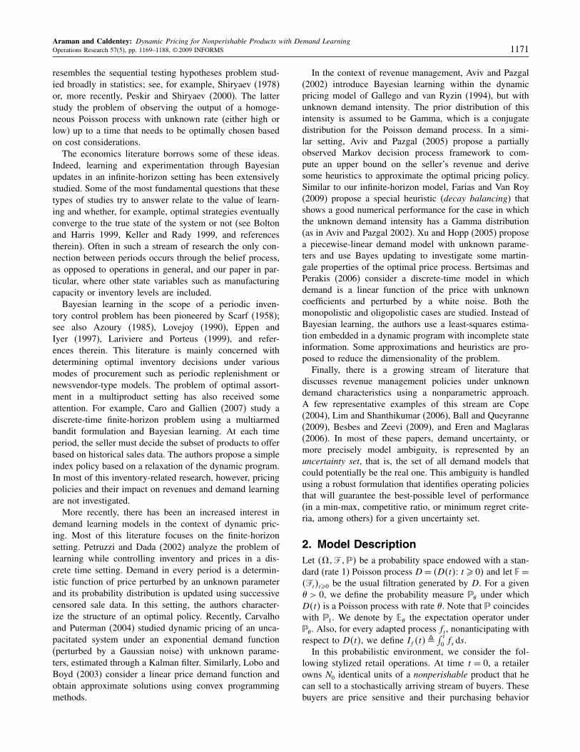
The function ��·� defined on the real line is nonnegativeand monotonically increasing. It admits an inverse functiongiven by ��z� � � −1�z� (z ∈ �+). The function ��·� isknown as the Fenchel-Legendre transform of c�·� and hasbeen extensively studied in the context of convex analysis(see Rockafellar 1997). For future reference, we also definethe function
��z�� inf{ ∈ �0�� � = argmax
0���
�z + c��}� (9)
This function ��z� is nondecreasing and satisfies ��0� =∗ � argmax�c��� ∈ �0�� . Figure 1 plots � , and theFenchel-Legendre transforms � and � for the case of anexponential demand rate (for further details see §C.1 inAppendix C). We note that ��0� = c∗ and ��c∗� = 0.Based on Equation (8), we can compute the value functioniteratively through the recursion
W�0� �� = R and
W�n��� + �
(rW�n���
�
)= W�n − 1� ���
n = 1�2� � � � � (10)
To complete the characterization of the optimal solution,the optimal demand intensity ∗�n� �� for an inventory ofn is given by
∗�n� �� = ��W�n − 1� �� − W�n����� (11)
Using the monotonicity of ��z�, the recursion in (10), andour scaling condition c∗ = rR, we obtain the followingresult.
Proposition 1. For every � > 0 and R� 0 there is a uniquesolution W�n��� to the recursion (10) that is monotoni-cally increasing in � and satisfies limn→� W�n��� = �R.If the scale factor � � 1 (respectively � � 1), then the valuefunction W�n��� is increasing and concave (respectivelydecreasing and convex) as a function of n.
INFORMS
holds
copyrightto
this
article
and
distrib
uted
this
copy
asa
courtesy
tothe
author(s).
Add
ition
alinform
ation,
includ
ingrig
htsan
dpe
rmission
policies,
isav
ailableat
http://journa
ls.in
form
s.org/.
Araman and Caldentey: Dynamic Pricing for Nonperishable Products with Demand Learning1174 Operations Research 57(5), pp. 1169–1188, © 2009 INFORMS
Figure 1. Fenchel-Legendre transforms for the case of an exponential demand rate �p� = � exp�−�p� with � = 10and � = 1.
–2 0 20
10
20
z–2 0 20
6
12
z0 10 15
–3
–2
–1
0
1
2
z
c*
� (z)
c*
Λ
�*
� (z)
ζ(z)
Proof. See §A.1 in Appendix A. �
Proposition 1 highlights the effect of the scale parame-ter � on revenues. For � � 1, the revenue function W�n���is always larger than R, and increases with the inven-tory level. The opposite conclusion holds for � � 1. Basedon this distinction, we say that a product is high revenue(or profitable) if � � 1, and we say that a product is lowrevenue (or unprofitable) if � � 1. From now on, we assumethat �L � 1� �H .
The difference between high-revenue and low-revenueproducts comes from the underlying trade-off that theseller experiences in terms of present and future revenues.In our model, the quantity R captures the future value ofthe seller’s operations after the current product has beendepleted. Therefore, for a given discount rate r , the termrR represents the seller’s average revenue rate from futurebusinesses. On the other hand, the revenue rate gener-ated by the current product is �c��, for a demand inten-sity �. Thus, the seller considers the current operationsto be more profitable than the average future business ifmax��c�� � rR or, equivalently, �c∗ � rR. Given thenormalization c∗ = rR, this condition reduces to � � 1.In other words, for � � 1 the current product offers higherreturns than the average product that the seller usually sells,and so the value function increases with n; in this case,the retailer will always choose to sell this product untilno more units are available. On the other hand, if � � 1,then the seller would like to switch as soon as possiblefrom the current product to a new (more profitable) alter-native. If the seller has to deplete all units before switchingto another product, then the corresponding value functionis a decreasing function of the inventory. In other words,the more units of this low-revenue product the seller has,the longer it is going to take to sell them all and move toa better product. However, if the retailer can stop sellingthe product at any time, then for � < 1 he chooses to stopimmediately, i.e., � = 0.An example of the results in Proposition 1 is depicted
on the left panel in Figure 2. The right panel shows the
corresponding optimal demand intensity ∗�n� �� that wediscuss in Corollary 1 below. Besides the monotonicity andconvexity properties of the value function, Figure 2 alsoconfirms the asymptotic behavior as the inventory growslarge. Specifically, we have that W�n��� → �R as n → �.Interestingly, Proposition 1 holds true without requiring anyspecific condition (such as concavity) on the revenue ratefunction c��. This is a distinguishing feature of our rep-resentation of the value function in (8) in terms of theFenchel-Legendre transform � and its inverse �. Indeed,it is well known that � is unaffected if we replace c�� byits concave hull in Equation (8). The following corollaryfollows from Proposition 1.
Corollary 1. Let ∗ = argmax�c��� ∈ �0�� beits unique maximizer. The optimal demand intensity∗�n� �� is monotonically decreasing in � and satisfieslimn→� ∗�n� �� = ∗. If � � 1 (respectively, � � 1), then∗�n� �� increases (respectively, decreases) with the levelof inventory n.
Proof. The result follows directly from concavity (respec-tively, convexity) of W�n��� in Proposition 1, Equa-tion (11), and the monotonicity of ��·�. �
From a pricing perspective, we note that for a low-revenue product the price increases with the available stock.This is in contrast to most of the dynamic pricing litera-ture (e.g., Gallego and van Ryzin 1994), which is more insynch with our high-revenue product where optimal pricesdecrease with the inventory level. This apparently counter-intuitive result relies on a simple observation. In our setting,the retailer’s trade-off is current versus future revenues. Asthe initial stock increases, the time required to deplete theseunits goes up as well. As a result, the retailer is better offmaximizing current revenues and minimizing future rev-enues by increasing the price. In contrast, for high-revenueproducts the price decreases with inventory.The different pricing behavior between low- and high-
revenue products raises an important issue regarding deple-tion time, specifically, whether we are selling faster when �
INFORMS
holds
copyrightto
this
article
and
distrib
uted
this
copy
asa
courtesy
tothe
author(s).
Add
ition
alinform
ation,
includ
ingrig
htsan
dpe
rmission
policies,
isav
ailableat
http://journa
ls.in
form
s.org/.

Araman and Caldentey: Dynamic Pricing for Nonperishable Products with Demand LearningOperations Research 57(5), pp. 1169–1188, © 2009 INFORMS 1175
Figure 2. Value function (left panel) and optimal demand intensity (right panel) for two values of � under an exponentialdemand model �p� = � exp�−�p�.
0 5 10 15 20 25 302.7
3.3
4.0
4.6
Inventory level (n) Inventory level (n)
Value function
1 5 10 15 20 25 303.0
3.5
4.0
4.5Optimal demand intensity
W(n, �1) �1 > 1
�*(n, �1) �1 > 1
W(n, �2) �2 < 1
�*(n, �2) �2<1
�2R
�1R
R
�*
W(n, 1)
�*(n, 1)
Note. The data used is � = 10, � = 1, r = 1, �1 = 1�2, �2 = 0�8, R = � exp�−1�/��r� ≈ 3�68.
is larger. In fact, even if low-revenue products have lowerprices than high-revenue products, their demand scale fac-tor, �, is smaller. Hence, the net effect on the net demandrate ��p� is unclear. According to Corollary 1, for n suf-ficiently large the pricing policies for both low- and high-revenue products are almost identical, and so the effectiverate of sales increases with �. The following propositionshows that under mild conditions on the demand model(condition (12) below), this conclusion holds for all inven-tory levels.
Proposition 2. Let s∗�n� �� � �∗�n� �� be the optimalrate of sales for a given � and inventory level n. If
d
d�p′���� 0� (12)
then the sales rate s∗�n� �� increases with � for all n.
Proof. See §A.2 in Appendix A. �
Condition (12) on the pricing function p�·� is not par-ticularly restrictive, and it is satisfied by the three demandmodels (exponential, linear, and quadratic) that we describein §C.1 in Appendix C. (A simple derivation of this con-dition translates to a slightly stronger requirement on c�·�than just concavity.) Interestingly, according to this propo-sition, even if prices increase with � the net demand rate,�∗, still increases with �. In other words, the inventoryturns of high-revenue products are higher than those oflow-revenue products even though the former are sold at ahigher price than the latter.As a side remark, we can get an alternative interpretation
of condition (12) using the notion of reservation price (e.g.,
Bitran and Mondschein 1997). Suppose that every arrivingbuyer has a maximum price that he is willing to pay forthe product. The seller is unable to observe this reserva-tion price, but only knows its probability distribution (F )among the population of buyers. In this setting, if the sellercharges a price p the resulting demand intensity equals�p� = ��1 − F �p�� with corresponding inverse demandfunction p�� = F −1�1 − �p�/��. For example, if thereservation price is exponentially distributed with param-eter �, then we recover the exponential demand model�p� = � exp�−�p�, and if the reservation price is uni-formly distributed in �0��/� , then we recover the lineardemand model �p� = � − �p. With this interpretation ofthe demand process, it is a matter of simple calculationsto show that condition (12) is equivalent to the reservationprice distribution (F ) having weakly increasing failure rate(IFR) (e.g., Lariviere 2006).We conclude this section with a brief summary of our
findings under full information. According to our model,the seller can partition the set of products that he sells intwo groups: (i) high-revenue products for which � � 1, and(ii) low-revenue products for which � � 1. High-revenueproducts sell faster (higher inventory turns) and at a higherprice than their low-revenue counterparts. Hence, if theseller were able to identify which products offer high rev-enues and which do not, then he would never engage inprocuring and selling low-revenue products. In practice,however, the seller is rarely capable of perfectly anticipat-ing the selling pattern of a given product. This pattern,which depends on customers’ preferences and market com-petition, only reveals itself as the selling season progresses,long after procurement decisions are made.
INFORMS
holds
copyrightto
this
article
and
distrib
uted
this
copy
asa
courtesy
tothe
author(s).
Add
ition
alinform
ation,
includ
ingrig
htsan
dpe
rmission
policies,
isav
ailableat
http://journa
ls.in
form
s.org/.
Araman and Caldentey: Dynamic Pricing for Nonperishable Products with Demand Learning1176 Operations Research 57(5), pp. 1169–1188, © 2009 INFORMS
With this problem in mind, we study in the followingsection optimal pricing strategies for the case in which theseller has imperfect knowledge about customers’ prefer-ences, or, in our case, the value of the scale factor �.
4. Dynamic Pricing with IncompleteDemand Information
In this section, we consider the case in which the retailerstarts the selling horizon having only partial informationabout the demand scale factor �. We again consider the casein which � can take only two values ��L� �H, with �L �1� �H . (A generalization to the case of a multidimensionalvector � is discussed in §6.) This is the most interestingcase in the sense that the retailer cannot tell whether theproduct being sold is a high-revenue (� = �H > 1) or a low-revenue (� = �L < 1) product. The retailer starts the sellingseason with a prior belief q that � = �L. We also assume inthis section that all initial N0 units must be depleted beforea different product can be offered. This final assumption isrelaxed in §5.The setting here describes, for example, those situations
where the retailer is bringing a new product into the marketand has uncertain information about how well this productwill sell. As the selling period progresses and the demandprocess materializes, the retailer updates his informationand adjusts the price accordingly to maximize cumulativediscounted profits. This active learning process is essen-tially a Bayes update on the distribution of � while theretailer is only observing the sales process over time. It isactive in the sense that the optimal price is not only a resultof the current belief, but also on how it will evolve in thefuture.In formal terms, we embed the model in this section in
a filtered probability space ���� � ��t�t�0��q�. The proba-bility measure �q satisfies (see §2 for notation)
�q = q��L+ �1− q���H
�
Given the retailer’s initial beliefs q, the random variable �satisfies �q�� = �L� = 1 − �q�� = �H� = q. We let qt ��q�� = �L ��t� be the retailer’s belief about the value of �at time t conditional on the available information �t . Recallthat ��t � t � 0� is the filtration generated by the inventory(or equivalently sales) process �N �t� = N0 −
∫ t
0 dDs� t � 0�Note also that the process ��qt��t�� t � 0 is by definitiona �q-martingale.In this setting, the retailer problem becomes
V �N0� q� = sup∈�
Ɛq
[∫ �
0exp�−rt��c�t�dt + exp�−r��R
]�
� = inf�t � 0� Nt = 0� (13)
We will tackle a solution to (13) using dynamic program-ming. For this, we will first derive the specific dynamicsof qt using Bayes’s rule and Itô’s lemma.
Proposition 3. The �q-martingale (belief ) process��qt��t�� t � 0 satisfies the stochastic differential equation
dqt = −��qt−��dDt − ��Lqt− + �H�1− qt−��tdt �
where ��qt��qt�1− qt���H − �L�
�Lqt + �H�1− qt�� (14)
Proof. See §A.3 in Appendix A. �
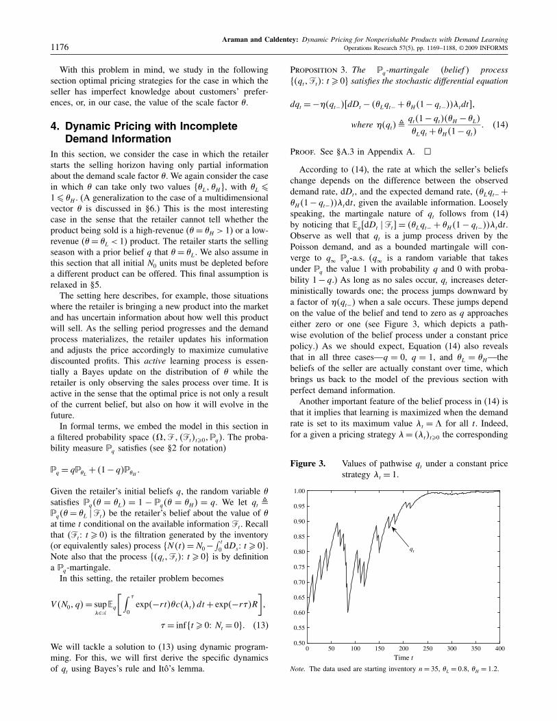
According to (14), the rate at which the seller’s beliefschange depends on the difference between the observeddemand rate, dDt , and the expected demand rate, ��Lqt− +�H�1− qt−��tdt, given the available information. Looselyspeaking, the martingale nature of qt follows from (14)by noticing that Ɛq�dDt � �t = ��Lqt− + �H�1− qt−��tdt.Observe as well that qt is a jump process driven by thePoisson demand, and as a bounded martingale will con-verge to q� �q-a.s. (q� is a random variable that takesunder �q the value 1 with probability q and 0 with proba-bility 1− q.) As long as no sales occur, qt increases deter-ministically towards one; the process jumps downward bya factor of ��qt−� when a sale occurs. These jumps dependon the value of the belief and tend to zero as q approacheseither zero or one (see Figure 3, which depicts a path-wise evolution of the belief process under a constant pricepolicy.) As we should expect, Equation (14) also revealsthat in all three cases—q = 0, q = 1, and �L = �H—thebeliefs of the seller are actually constant over time, whichbrings us back to the model of the previous section withperfect demand information.Another important feature of the belief process in (14) is
that it implies that learning is maximized when the demandrate is set to its maximum value t = � for all t. Indeed,for a given a pricing strategy = �t�t�0 the corresponding
Figure 3. Values of pathwise qt under a constant pricestrategy t = 1.
0 50 100 150 200 250 300 350 4000.50
0.55
0.60
0.65
0.70
0.75
0.80
0.85
0.90
0.95
1.00
Time t
qt
Note. The data used are starting inventory n = 35, �L = 0�8, �H = 1�2.
INFORMS
holds
copyrightto
this
article
and
distrib
uted
this
copy
asa
courtesy
tothe
author(s).
Add
ition
alinform
ation,
includ
ingrig
htsan
dpe
rmission
policies,
isav
ailableat
http://journa
ls.in
form
s.org/.
Araman and Caldentey: Dynamic Pricing for Nonperishable Products with Demand LearningOperations Research 57(5), pp. 1169–1188, © 2009 INFORMS 1177
likelihood ratio process associated with the simple hypothe-ses HH = �� = �H and HL = �� = �L is equal to (seeBrémaud 1980)
t �d���L
��t�
d���H��t�
=(
�L
�H
)Dt
exp���H − �L�I�t��� (15)
where �� ��t denotes the restriction of �� to �t . Hence, forany history �t the likelihood-ratio process is maximized ifwe choose a pricing strategy that maximizes I�t�, that is,setting t = � for all t.
Of course, we are not interested in choosing a pric-ing strategy that maximizes the seller’s learning, but onethat maximizes the discounted expected payoff in Equa-tion (13). Note that the retailer controls the unscaleddemand rate t , whereas the actual rate realized is in fact�t , which in turns induces a revenue rate of �c�t�. Therevenue rate function c�·� satisfies the same set of assump-tions as in the previous section. Therefore, in such a con-text, the problem’s formulation can be written as follows:
V �N0� q�
= sup∈�
Ɛq
[∫ �
0exp�−rt��c�t�dt + exp�−r��R
]
subject to Nt = N0 −∫ t
0dD�I�s���
dqt =��qt−��dDt −��Lqt−+�H�1−qt−��tdt �
q0 = q�
� = inf�t � 0� Nt = 0�
The value function associated with the dynamic program-ming formulation is now V �n�q�, where the state variablesare the level of inventory n and the seller’s beliefs q. Wedefine ��qt� � Ɛq�� � �t = �Lqt + �H�1 − qt� to be theexpected demand scale factor given the available informa-tion at time t.The HJB equation is then given by (see Appendix C.2
for a derivation)
rV �n�q� = max0���
���q��V �n − 1� q − ��q�� − V �n�q�
+ ��q�Vq�n� q� + ��q�c�� � (16)
with ��q� � q�1 − q���H − �L� and boundary condi-tions V �0� q� = R, V �n�0� = W�n��H�, and V �n�1� =W�n��L�. Recall that the function W�n��� is the valuefunction when there is no uncertainty about the true valueof � and is computed using the recursion in Equation (10).As in Equation (10), we can rewrite the HJB condition
using the Fenchel-Legendre transform of c�� in the fol-lowing convenient form:
V �0� q� = R�
V �n�q� + �
(rV �n�q�
��q�
)− ��q�Vq�n� q�
= V �n − 1� q − ��q��� n = 1�2� � � � �
(17)
It also follows from Equations (16) and (17) that the opti-mal demand intensity ∗
V �n� q� satisfies
∗V �n� q� = � � �
(rV �n�q�
��q�
)� (18)
where ��·� is defined in (9) and “�” stands for the compo-sition operator.In general, we have not been able to solve explicitly
the difference-differential equation in (17) to derive thecorresponding optimal pricing policy. However, its recur-sive structure suggests the following algorithm to computeV �n�q�.
Algorithm -VStep 1. Initialization: Set V �0� q� = R for all q ∈ �0�1
and n = 1.Step 2. Iteration: Set F �q� = V �n − 1� q − ��q�� and
solve the following ordinary differential equation (ODE)for G�q� in the domain q ∈ �0�1 :
G�q� + �
(rG�q�
��q�
)− ��q�G′�q� = F �q��
G�0� = W�n��H�� G�1� = W�n��L��
(19)
(Appendix D describes a finite-difference method that weuse to solve this ODE.)Set V �n�q� = G�q� and n = n + 1.Step 3. Go to Step 2.
The main step in this algorithm is to solve the ODE inStep 2. This is not a straightforward task because the bor-der conditions at q = 0 and q = 1 are singular points for thedifferential equation because ��0� = ��1� = 0. Hence, eventhe existence of a solution to (19) is a subtle issue. Fortu-nately, the following proposition takes care of this problem.
Proposition 4. There exists a unique sequence of func-tions, �V �n� ·�� n � 1, defined on �0�1 and satisfying thesystem of Equations (17) with border conditions V �n�0� =W�n��H� and V �n�1� = W�n��L�.
Proof. The proof of this proposition requires a number ofintermediate steps and can be found in Appendix B. �
Despite the fact that we do not have an analytical solu-tion to (17), this optimality condition provides enoughinformation to derive some useful properties that we useto approximate the value function and the correspondingpricing strategy.
Proposition 5. (i) The value function V �n� ·� is monoton-ically decreasing and convex in q. It is also bounded bythe perfect information values for all n� 1 and q ∈ �0�1 :
W�n��L�� V �n�q��W�n��H��
(ii) Furthermore, V �n� ·� converges uniformly to the lin-ear function R��·� as n → �, and
limn→� ∗
V �n� q� = ∗�
INFORMS
holds
copyrightto
this
article
and
distrib
uted
this
copy
asa
courtesy
tothe
author(s).
Add
ition
alinform
ation,
includ
ingrig
htsan
dpe
rmission
policies,
isav
ailableat
http://journa
ls.in
form
s.org/.
Araman and Caldentey: Dynamic Pricing for Nonperishable Products with Demand Learning1178 Operations Research 57(5), pp. 1169–1188, © 2009 INFORMS
Proof. See §A.4 in Appendix A. �
As expected, part (i) of the proposition shows that thevalue function decreases with q and it is bounded by thevalue function in the full-information case when � = �L
and � = �H . The asymptotic result in part (ii) shows thatthe optimal demand intensity converges to ∗, which maxi-mizes the instantaneous revenue rate. Hence, as n gets largethe retailer favors revenue exploitation over demand explo-ration when selecting the optimal selling rate. The asymp-totic result also shows that the value function converges tothe linear function R��Lq + �H�1 − q�� as the number ofinitial units grows to infinity. This limiting behavior sug-gests a simple method to approximate the value function,which we undertake in the following subsection.Before jumping into this asymptotic analysis, let us use
the result in Proposition 5 to extend the result in Proposi-tion 2 to this case with an unknown �. For this, we defines∗�n� q� = ��q�∗
V �n� q� to be the expected selling ratewhen the inventory is n and the belief process is equal to q.As in the full-information case, the following propositionreveals that s∗�n� q� increases with the (expected) marketsize ��q� even if optimal prices are increasing in ��q�.
Proposition 6. Suppose that the demand function satisfies
d
d�p′���� 0�
Then, the sales rate s∗�n� q� decreases with q for all n.
Proof. See §A.5 in Appendix A. �
4.1. Asymptotic Approximation
Based on Proposition 5, it seems that (for a fixed inventorylevel n) V �n�q� is well approximated by a linear functionof q. In particular, we consider for each n � 1 and q ∈�0�1 , the following approximation of V �n�q�:
�V �n�q�� Ɛq�W�n���
= qW�n��L� + �1− q�W�n��H�� (20)
In what follows, we will use the tilde (˜) notation to denotethe asymptotic approximation of quantities such as thevalue function in (20) or the demand intensity in (21).The next result shows that the linear approximation is
not only suggested by the limiting result on V �n� ·�, but italso represents an upper bound for the value function. Moreimportantly, it approaches the value function in a strongsense, i.e., their ratio goes to one uniformly in q. Combin-ing Propositions 1 and 5, we obtain that:
Proposition 7. The approximation in (20) defines anupper bound of the value function, i.e.,
V �n�q�� �V �n�q��
for all q ∈ �0�1 and for all n. Furthermore, the approxima-tion is asymptotically and uniformly (in q) exact, as n goesto infinity. That is,
∣∣V �n�q�/ �V �n�q�∣∣ → 1 uniformly in q
as n goes to �. Note also that under perfect informationV �n�q� = �V �n�q� for q ∈ �0�1 or �L = �H .
Proof. The upper bound is due to the convexity of V in q.Because of the boundedness of V , the uniform convergenceof the ratio is guaranteed if the difference converges uni-formly to zero. Using triangle inequality, we write
�V �n�q�− �V �n�q�∣∣� ∣∣V �n�q�−R��q��+�R��q�− �V �n�q���
Both terms on the right converge to zero uniformly in q—the first one through Proposition 5. The second term issmaller than R�H − W�n��H� + W�n��L� − R�L, which isindependent of q and converges to zero. �
Let us turn to the pricing strategy. The asymptoticapproximation in (20) works directly with the value func-tion, and thus it is unclear how to estimate the optimaldemand rate ∗
V �n� q�. To fill this gap, we propose usingthe optimality condition in (18), using �V �n�q� instead ofV �n�q�. It follows from the linearity of �V �n�q� in q thatthe proposed approximation for ∗�n� q� is given by
�n� q� = �(�q − ��q����W�n��H� − �W�n��L��
− �W�n��H�)� (21)
where �W�n��� = W�n��� − W�n − 1� ��.
Remarks. 1. Because ��z� increases with z, q − ��q�increases with q, and �W�n��H� � 0� �W�n��L�, it fol-lows that �n� q� is increasing in q.2. Furthermore, because ��0� = ∗, we have that
�n� q�� ∗ if and only if
q − ��q���W�n��H�
�W�n��H� − �W�n��L��
3. Using the convexity of V and the fact that �V , is anupper bound of V , we get that
R − V �1� q� + ��q�Vq�1� q��R − V �1� q − ��q��
�R − �V �1� q − ��q���
If we apply � (which is an increasing function) to bothsides, we conclude that
∗V �1� q�� �1� q��
That is, the asymptotic approximation overprices theoptimal solution for n = 1. Unfortunately, for n � 2 wehave not been able to prove (or disprove) a similar claim.
Let us now assess the performance of the asymptoticapproximation by comparing the optimal expected dis-counted revenue V �n�q� to the one obtained using thedemand rate �n� q�. Also, to measure the performance ofour approximation with respect to other alternative policies,we consider the following three heuristics.
INFORMS
holds
copyrightto
this
article
and
distrib
uted
this
copy
asa
courtesy
tothe
author(s).
Add
ition
alinform
ation,
includ
ingrig
htsan
dpe
rmission
policies,
isav
ailableat
http://journa
ls.in
form
s.org/.
Araman and Caldentey: Dynamic Pricing for Nonperishable Products with Demand LearningOperations Research 57(5), pp. 1169–1188, © 2009 INFORMS 1179
1. Myopic Policy. The popular myopic (or certaintyequivalent) approximation of the value function is defined as
V 0�n� q��W�n�Ɛq���� = W�n� ��q���
We note that this policy is asymptotically optimal in thesense that V 0�n� q� converges to R��q� as n goes to infinity.We call this approximation myopic because it models thediscounted profit that a retailer would expect to get if hemyopically considers the expected value ��q� to be thetrue value of the scale factor �. As opposed to our originalactive learning strategy, such strategy falls into the categoryof passive learning. Like our asymptotic policy, this myopicpolicy does not generate a pricing policy directly. It ratherproposes an approximation for the value function that weneed to translate into an implementable pricing strategy.Again, we can use the optimality condition (18) to get ademand rate associated with this myopic policy:
0�n�q�=��V 0�n−1�q−��q��−V 0�n�q�+��q�V 0q �n�q���
We note that despite its simplicity, the computationaleffort required to compute the myopic policy is substan-tially higher than the one needed for the asymptotic policy.Indeed, our asymptotic approximation is fully characterizedby 2�N0 + 1� values ��W�n��L��W�n��H��� 0 � n � N0,whereas the myopic policy is defined by N0 + 1 functions�W�n� ��q��� 0� n�N0 and q ∈ ��L� �H .
2. Single-Price Policy. Another popular approxima-tion in the revenue management literature is the single-price policy. Under this approximation, the price is keptfixed for the entire planning horizon. The popularity ofthis approximation comes from (i) its simplicity from animplementation point of view, and (ii) its asymptotic opti-mality in certain settings with large initial inventory andlarge demand rate (e.g., Gallego and van Ryzin 1994 orBitran and Caldentey 2003). Let us denote by V 1�n� q��the retailer’s expected discounted payoff, starting with nunits of inventory and a belief of q if the fixed-price policyt = is used. It follows that
V 1�n� q�� = Ɛq
[∫ �
0e−rt�c��dt + e−r�R
]
= Ɛq
[(�c��
r
)�1− e−r� � + e−r�R
]
= ��q�c��
r+ Ɛq
[(R − �c��
r
)e−r�
]
= ��q�c��
r+ q
(R − �Lc��
r
)(�L
r + �L
)n
+ �1− q�
(R − �Hc��
r
)(�H
r + �H
)n
�
The last equality uses the fact that under the prob-ability measure ��i
the selling horizon � has a Gamma
distribution with parameters �n��i�, i = L�H . Therefore,Ɛ�i
�e−r� = ��i/�r + �i��n for i = L�H . The correspond-
ing demand rate associated with this single-price approxi-mation is given by
1�n� q� = argmax∈�0��
V 1�n� q���
It is worth noticing that this single-price policy is alsoasymptotically optimal in the sense that
sup∈�0��
limn→� V 1�n� q�� = ��q�c�∗�/r = R��q�
= limn→� V �n�q��
3. Two-Price Policy. An important limitation of theprevious approximation is its inability to adjust the pricebased on the realized demand. This is particularly seriousin our setting, where the demand distribution is unknown.To partially address this limitation, and at the same timepreserve the operational simplicity of the single-price pol-icy, we consider a two-price policy in which the retaileris able to change the price only once. (Feng and Gallego1995 provide structural properties of this type of policiesunder full-demand information in a finite-horizon setting.)A major difficulty for determining the optimal two-pricepolicy is that it requires solving an optimal stopping timeproblem. From a computational standpoint, this is at leastas demanding as computing the optimal value function. Forthis reason, we only consider a suboptimal version thatmakes a single price change right after the first unit issold. The discussion of optimal pricing policies based onstopping time rules is postponed to §5. Under this restric-tion, let us denote by V 2�n� q�� the retailer’s expecteddiscounted payoff starting with n units of inventory and abelief q when the initial demand intensity is set to t = .It follows that
V 2�n� q�� = Ɛ�e−r� �p�� + V 1�n − 1� q�� �
where � is the (random) time at which the first unit is soldif the seller uses a fixed strategy t = , t ∈ �0� � . Thecorresponding demand rate associated with this two-priceapproximation is given by
2�n� q� = argmax∈�0��
V 2�n� q���
Let us now compare the performance of the asymptoticapproximation and the other three heuristics in terms oftheir relative error with respect to the optimal solution. Ifwe let �n� q� be the expected discounted payoff generatedby any of these approximations (using the correspondingpricing policy), then the relative error is defined by
� �n� q��V �n�q� − �n� q�
V �n�q�× 100�
INFORMS
holds
copyrightto
this
article
and
distrib
uted
this
copy
asa
courtesy
tothe
author(s).
Add
ition
alinform
ation,
includ
ingrig
htsan
dpe
rmission
policies,
isav
ailableat
http://journa
ls.in
form
s.org/.
Araman and Caldentey: Dynamic Pricing for Nonperishable Products with Demand Learning1180 Operations Research 57(5), pp. 1169–1188, © 2009 INFORMS
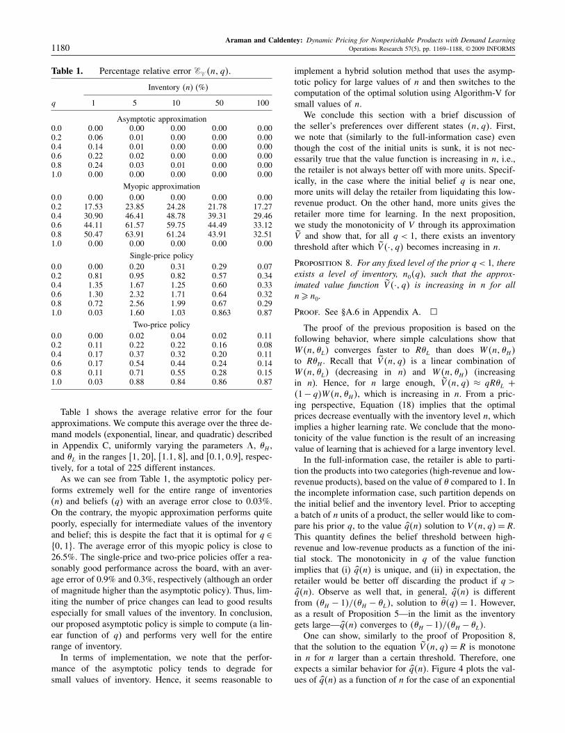
Table 1. Percentage relative error � �n� q�.
Inventory (n) (%)
q 1 5 10 50 100
Asymptotic approximation0.0 0�00 0�00 0�00 0�00 0�000.2 0�06 0�01 0�00 0�00 0�000.4 0�14 0�01 0�00 0�00 0�000.6 0�22 0�02 0�00 0�00 0�000.8 0�24 0�03 0�01 0�00 0�001.0 0�00 0�00 0�00 0�00 0�00
Myopic approximation0.0 0�00 0�00 0�00 0�00 0�000.2 17�53 23�85 24�28 21�78 17�270.4 30�90 46�41 48�78 39�31 29�460.6 44�11 61�57 59�75 44�49 33�120.8 50�47 63�91 61�24 43�91 32�511.0 0�00 0�00 0�00 0�00 0�00
Single-price policy0.0 0�00 0�20 0�31 0�29 0�070.2 0�81 0�95 0�82 0�57 0�340.4 1�35 1�67 1�25 0�60 0�330.6 1�30 2�32 1�71 0�64 0�320.8 0�72 2�56 1�99 0�67 0�291.0 0�03 1�60 1�03 0�863 0�87
Two-price policy0.0 0�00 0�02 0�04 0�02 0�110.2 0�11 0�22 0�22 0�16 0�080.4 0�17 0�37 0�32 0�20 0�110.6 0�17 0�54 0�44 0�24 0�140.8 0�11 0�71 0�55 0�28 0�151.0 0�03 0�88 0�84 0�86 0�87
Table 1 shows the average relative error for the fourapproximations. We compute this average over the three de-mand models (exponential, linear, and quadratic) describedin Appendix C, uniformly varying the parameters �, �H ,and �L in the ranges �1�20 , �1�1�8 , and �0�1�0�9 , respec-tively, for a total of 225 different instances.As we can see from Table 1, the asymptotic policy per-
forms extremely well for the entire range of inventories(n) and beliefs (q) with an average error close to 0.03%.On the contrary, the myopic approximation performs quitepoorly, especially for intermediate values of the inventoryand belief; this is despite the fact that it is optimal for q ∈�0�1. The average error of this myopic policy is close to26.5%. The single-price and two-price policies offer a rea-sonably good performance across the board, with an aver-age error of 0.9% and 0.3%, respectively (although an orderof magnitude higher than the asymptotic policy). Thus, lim-iting the number of price changes can lead to good resultsespecially for small values of the inventory. In conclusion,our proposed asymptotic policy is simple to compute (a lin-ear function of q) and performs very well for the entirerange of inventory.In terms of implementation, we note that the perfor-
mance of the asymptotic policy tends to degrade forsmall values of inventory. Hence, it seems reasonable to
implement a hybrid solution method that uses the asymp-totic policy for large values of n and then switches to thecomputation of the optimal solution using Algorithm-V forsmall values of n.We conclude this section with a brief discussion of
the seller’s preferences over different states �n� q�. First,we note that (similarly to the full-information case) eventhough the cost of the initial units is sunk, it is not nec-essarily true that the value function is increasing in n, i.e.,the retailer is not always better off with more units. Specif-ically, in the case where the initial belief q is near one,more units will delay the retailer from liquidating this low-revenue product. On the other hand, more units gives theretailer more time for learning. In the next proposition,we study the monotonicity of V through its approximation�V and show that, for all q < 1, there exists an inventorythreshold after which �V �·� q� becomes increasing in n.
Proposition 8. For any fixed level of the prior q < 1, thereexists a level of inventory, n0�q�, such that the approx-imated value function �V �·� q� is increasing in n for alln� n0.
Proof. See §A.6 in Appendix A. �
The proof of the previous proposition is based on thefollowing behavior, where simple calculations show thatW�n��L� converges faster to R�L than does W�n��H�to R�H . Recall that �V �n�q� is a linear combination ofW�n��L� (decreasing in n) and W�n��H� (increasingin n). Hence, for n large enough, �V �n�q� ≈ qR�L +�1− q�W�n��H�, which is increasing in n. From a pric-ing perspective, Equation (18) implies that the optimalprices decrease eventually with the inventory level n, whichimplies a higher learning rate. We conclude that the mono-tonicity of the value function is the result of an increasingvalue of learning that is achieved for a large inventory level.In the full-information case, the retailer is able to parti-
tion the products into two categories (high-revenue and low-revenue products), based on the value of � compared to 1. Inthe incomplete information case, such partition depends onthe initial belief and the inventory level. Prior to acceptinga batch of n units of a product, the seller would like to com-pare his prior q, to the value q�n� solution to V �n�q� = R.This quantity defines the belief threshold between high-revenue and low-revenue products as a function of the ini-tial stock. The monotonicity in q of the value functionimplies that (i) q�n� is unique, and (ii) in expectation, theretailer would be better off discarding the product if q > q�n�. Observe as well that, in general, q�n� is differentfrom ��H − 1�/��H − �L�, solution to ��q� = 1. However,as a result of Proposition 5—in the limit as the inventorygets large— q�n� converges to ��H − 1�/��H − �L�.One can show, similarly to the proof of Proposition 8,
that the solution to the equation �V �n�q� = R is monotonein n for n larger than a certain threshold. Therefore, oneexpects a similar behavior for q�n�. Figure 4 plots the val-ues of q�n� as a function of n for the case of an exponential
INFORMS
holds
copyrightto
this
article
and
distrib
uted
this
copy
asa
courtesy
tothe
author(s).
Add
ition
alinform
ation,
includ
ingrig
htsan
dpe
rmission
policies,
isav
ailableat
http://journa
ls.in
form
s.org/.
Araman and Caldentey: Dynamic Pricing for Nonperishable Products with Demand LearningOperations Research 57(5), pp. 1169–1188, © 2009 INFORMS 1181
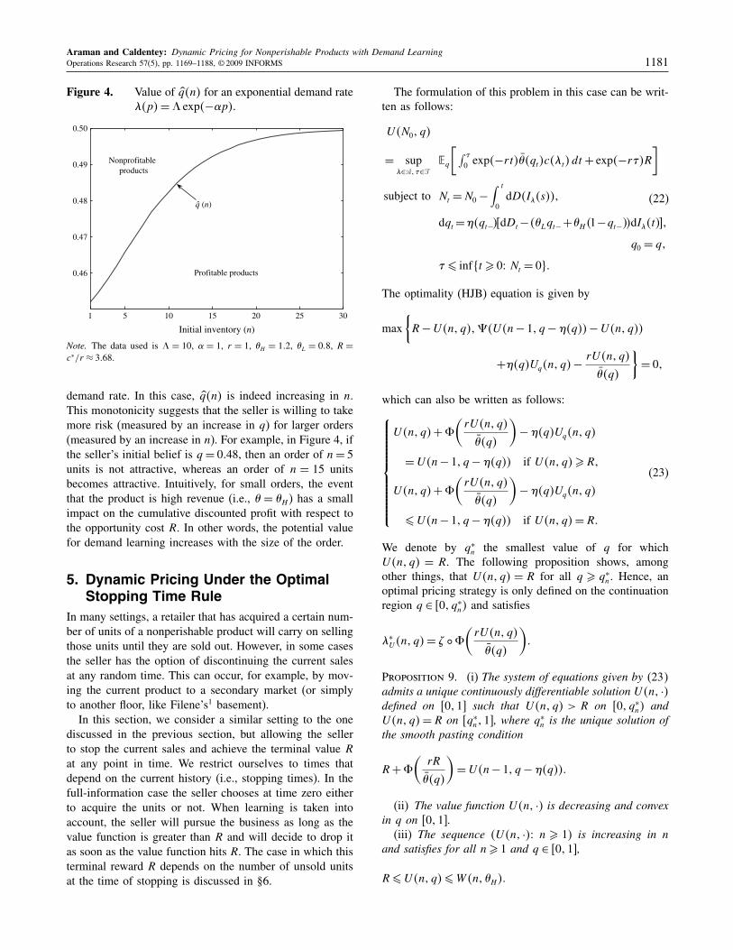
Figure 4. Value of q�n� for an exponential demand rate�p� = � exp�−�p�.
1 5 10 15 20 25 30
0.46
0.47
0.48
0.49
0.50
Initial inventory (n)
Profitable products
Nonprofitableproducts
q (n)
Note. The data used is � = 10, � = 1, r = 1, �H = 1�2, �L = 0�8, R =c∗/r ≈ 3�68.
demand rate. In this case, q�n� is indeed increasing in n.This monotonicity suggests that the seller is willing to takemore risk (measured by an increase in q) for larger orders(measured by an increase in n). For example, in Figure 4, ifthe seller’s initial belief is q = 0�48, then an order of n = 5units is not attractive, whereas an order of n = 15 unitsbecomes attractive. Intuitively, for small orders, the eventthat the product is high revenue (i.e., � = �H ) has a smallimpact on the cumulative discounted profit with respect tothe opportunity cost R. In other words, the potential valuefor demand learning increases with the size of the order.
5. Dynamic Pricing Under the OptimalStopping Time Rule
In many settings, a retailer that has acquired a certain num-ber of units of a nonperishable product will carry on sellingthose units until they are sold out. However, in some casesthe seller has the option of discontinuing the current salesat any random time. This can occur, for example, by mov-ing the current product to a secondary market (or simplyto another floor, like Filene’s1 basement).
In this section, we consider a similar setting to the onediscussed in the previous section, but allowing the sellerto stop the current sales and achieve the terminal value R
at any point in time. We restrict ourselves to times thatdepend on the current history (i.e., stopping times). In thefull-information case the seller chooses at time zero eitherto acquire the units or not. When learning is taken intoaccount, the seller will pursue the business as long as thevalue function is greater than R and will decide to drop itas soon as the value function hits R. The case in which thisterminal reward R depends on the number of unsold unitsat the time of stopping is discussed in §6.
The formulation of this problem in this case can be writ-ten as follows:
U�N0� q�
= sup∈�� �∈�
Ɛq
[∫ �
0 exp�−rt���qt�c�t�dt + exp�−r��R
]
subject to Nt = N0 −∫ t
0dD�I�s���
dqt =��qt−��dDt −��Lqt−+�H�1−qt−��dI�t� �
q0 = q�
� � inf�t � 0� Nt = 0�
(22)
The optimality (HJB) equation is given by
max{
R − U�n�q����U�n − 1� q − ��q�� − U�n�q��
+��q�Uq�n� q� − rU�n�q�
��q�
}= 0�
which can also be written as follows:⎧⎪⎪⎪⎪⎪⎪⎪⎪⎪⎨⎪⎪⎪⎪⎪⎪⎪⎪⎪⎩
U�n�q� + �
(rU�n�q�
��q�
)− ��q�Uq�n� q�
= U�n − 1� q − ��q�� if U�n�q��R�
U�n�q� + �
(rU�n�q�
��q�
)− ��q�Uq�n� q�
�U�n − 1� q − ��q�� if U�n�q� = R�
(23)
We denote by q∗n the smallest value of q for which
U�n�q� = R. The following proposition shows, amongother things, that U�n�q� = R for all q � q∗
n . Hence, anoptimal pricing strategy is only defined on the continuationregion q ∈ �0� q∗
n� and satisfies
∗U �n� q� = � � �
(rU�n�q�
��q�
)�
Proposition 9. (i) The system of equations given by (23)admits a unique continuously differentiable solution U�n� ·�defined on �0�1 such that U�n�q� > R on �0� q∗
n� andU�n�q� = R on �q∗
n�1 , where q∗n is the unique solution of
the smooth pasting condition
R + �
(rR
��q�
)= U�n − 1� q − ��q���
(ii) The value function U�n� ·� is decreasing and convexin q on �0�1 .(iii) The sequence �U�n� ·�� n � 1� is increasing in n
and satisfies for all n� 1 and q ∈ �0�1 ,
R�U�n�q��W�n��H��
INFORMS
holds
copyrightto
this
article
and
distrib
uted
this
copy
asa
courtesy
tothe
author(s).
Add
ition
alinform
ation,
includ
ingrig
htsan
dpe
rmission
policies,
isav
ailableat
http://journa
ls.in
form
s.org/.
Araman and Caldentey: Dynamic Pricing for Nonperishable Products with Demand Learning1182 Operations Research 57(5), pp. 1169–1188, © 2009 INFORMS
(iv) Let s∗�n� q� = ��q�∗U �n� q� be the expected selling
rate. Then, if the demand function satisfies
d
d�p′���� 0�
then the sales rate s∗�n� q� decreases with q for all n.(v) Let ∗
U �n� q� and ∗V �n� q� be the optimal demand
rate for the cases where the option to stop is and is notavailable, respectively. Then, for all n and q,
∗V �n� q�� ∗
U �n� q��
Proof. See §A.7 in Appendix A. �
The previous proposition shows that most propertiesof the value function are maintained when the option ofstopping is permitted. A fundamental difference, however,is that U is increasing in n for all q, as opposed to V thatmight be decreasing in n, for some values of n and largevalues of q. Indeed, with the option of stopping available,one can do at least as well with n + 1 units than with n(under the assumption that the cost of the initial inventoryis sunk). It should also be clear that the value function whenthe option of stopping is not allowed represents a lowerbound for U , i.e., V �n�q� �U�n�q� for all n� 0 and q ∈�0�1�. Part (v) in the proposition follows directly from thisinequality. Intuitively, this result follows from the fact thatthe value of demand learning is higher when the option tostop is available, which gives the retailer more incentivesto set lower prices to learn faster (see Equation (15) andthe discussion that follows it).Now, we suggest the following algorithm to compute the
value function.
Algorithm -UStep 1. Initialization: Set U�0� q� = R for all q ∈ �0�1
and n = 1.Step 2. Iteration: Set F �q� = U�n − 1� q − ��q�� and
(i) solve for the unique solution of
R + �
(rR
��q�
)= F �q��
set q∗n to be this solution.(ii) Solve the following ordinary differential equation
(ODE) for G�q� in the domain q ∈ �0� q∗n :
G�q� + �
(rG�q�
��q�
)− ��q�G′�q� = F �q��
G�q0� = R�
(24)
(iii) Set U�n�q� = G�q� for q � q∗n and U�n�q� = R
otherwise. Set n = n + 1.Step 3. Go to Step 2.
Again, the main step in this algorithm is solving theODE in Equation (24). The task here is simpler thanin §4 because the border condition is well defined; thatis, the ODE does not have a singularity at q∗
n and canbe solved using standard methods (e.g., Picard iteration).Appendix D describes a finite-difference scheme that canbe used to solve this ODE.We now discuss some properties of q∗
n , which is thethreshold value of the belief (when the current stock is nunits) at which the retailer will choose to stop selling thecurrent product and move to the next one. The quantity q∗
n
then allows the retailer to again partition the products intotwo categories of high-revenue and low-revenue ones.
Proposition 10. The sequence �q∗n� n � 1� is increasing
in n and converges to q∗� < 1 as n → �. The sequence
is also bounded by ��H − 1�/��H − �L� ≡ q∗1 � q∗
n �qn < 1, where for all n � 1� the upper bound qn is theunique solution to
R + �
(rR
��q�
)= �q − ��q��R
+ �1− q + ��q��W�n − 1� �H�� (25)
Proof. See §A.8 in Appendix A. �
In the setting where stopping is allowed, we have showedthat the value function U is always increasing in the cur-rent inventory n. Hence, the threshold q∗
n (solution toU�n�q� = R) is increasing as well in n. This monotonic-ity suggests that the seller is willing to take more risks(i.e., measured by larger values of q) for larger initial inven-tory n. Indeed, higher initial inventory levels offer a greateropportunity for learning, which make them more attractiveto the seller. Observe, however, that the upper bound q∗
� isstrictly less than 1, and so the willingness to take risk islimited; if q is greater than q∗
�, then independently of theorder size the seller always rejects such a product.We recall here that for a particular value of inventory
and belief, the value function in the case where stoppingis allowed is always larger than the value function whensuch an option is not available (V �n�q��U�n�q�). There-fore, the threshold q∗
n is always larger than qn (solutionto V �n�q� = R). This inequality implies that the values ofthe belief for which the product is assumed to be a high-revenue one is larger in the case where stopping is allowedcompared to the case where it is not. Put differently, con-sider n units of a product that the retailer is contemplatingselling. If the product’s prior q is such that qn < q < q∗
n ,then the product is considered a nonprofitable one (low-revenue) in the case where stopping is not allowed and aprofitable product (high-revenue) in the case where stop-ping is allowed. Figure 5 depicts the behavior of q∗
n and qn
as a function of n. As we can see, the option of stopping hasa significant effect on the seller’s segmentation of profitableand nonprofitable products. Indeed, it is worth noticing that q� = q∗
1 .
INFORMS
holds
copyrightto
this
article
and
distrib
uted
this
copy
asa
courtesy
tothe
author(s).
Add
ition
alinform
ation,
includ
ingrig
htsan
dpe
rmission
policies,
isav
ailableat
http://journa
ls.in
form
s.org/.

Araman and Caldentey: Dynamic Pricing for Nonperishable Products with Demand LearningOperations Research 57(5), pp. 1169–1188, © 2009 INFORMS 1183
Figure 5. Thresholds q∗n and qn for the exponential
demand model.
5 10 15 20 25 300.44
0.46
0.48
0.50
0.52
0.54
0.56
0.58
0.60
0.62
Inventory (n)
Critical thresholds
Profitable with stopping but
Nonprofitable without stopping
Always nonprofitable
Always profitable
qn*
qn
�H – 1
�H – �L
Note. Data: � = 10, � = 1, r = 1, �H = 1�2, �L = 0�8.
5.1. Bounds and Approximations
We suggested above an algorithm to solve numerically forthe value function U ; however, it is impossible in generalto obtain a closed-form expression for it. The remainder ofthis section will be devoted first to obtain a limiting resultas n gets large, and second to suggesting approximationsto the value function that we later test numerically.
Proposition 11. For all n � 1� the value function U�n� ·�is bounded above and below by piecewise-linear functionssuch that for all q ∈ �0�1 ,
max�Vq�n�0�q + W�n��H��R
�U�n�q�
�max{
W�n��H� − �W�n��H� − R�q
qn
�R
}� (26)
Furthermore, the sequence of value functions �U�n� ·�:n� 1� converges uniformly on �0�1 to a continuously dif-ferentiable function, U��·�, as n → �, such that for allq ∈ �0�1 ,
Rmax���q��1�U��q��Rmax{
�H − �H −1q�
q�1}
� (27)
Proof. See §A.9 in Appendix A. �
The previous proposition shows that the value functionconverges as the number of the initial inventory becomeslarge. It also gives a lower and an upper bound, both linearin q and truncated at R.We denote by U L�n� q� and U U�n� q� the lower and
upper bounds of U�n�q� appearing in (26) (see Figure 6).Lacking a simple limiting result, we suggest these boundsas possible approximations of the optimal value function.
Figure 6. Value function V �n�q� (for n = 10) com-pared to its linear lower and upper boundsfor the exponential demand model �p� =� exp�−�p�, with � = 10 and � = 1.
0 0.1 0.2 0.3 0.4 0.5 0.6 0.7 0.8 0.9 1.03.5
4.0
4.5
5.0
5.5
6.0
6.5
q
Lower bound
V(n, q)
Upper bound
Observe that the lower bound is just the tangent at zerountil it hits R, whereas the upper bound is a straight linelinking the value U�n�0� at zero, to R at qn (recall thatqn is an upper bound of q∗
n). All the parameters of thesesegments are known without having to solve for U . Indeed,the value function at zero is W�n��H�, the tangent at zerois equal to the known value Vq�n�0� (we can prove this byinduction using similar arguments as those in Lemma B.4in Appendix B). Finally, qn is a solution to Equation (25),which is independent of U .To assess the performance of the bound-based approx-
imations, we follow a similar approach to the one usedin §4. We first introduce two additional approximations.The first one is an approximation based on the myopic pol-icy discussed in §4,
U M�n� q� =max�W�n� ��q���R�
The other one, is the piecewise-linear,
U H�n� q�
=
⎧⎪⎪⎪⎪⎪⎨⎪⎪⎪⎪⎪⎩
Vq�n�0�q + W�n��H� for q � q0�
�Vq�n�0�q0 + W�n��H� − R�
·�q − q�/�q0 − q� + R for q ∈ �q0� q��
R for q � q�
(28)
where q0 is such that each “piece” of U H covers half ofthe range of U , i.e., Vq�n�0�q0 + W�n��H� = �W�n��H� −R�/2; see Figure 6. The function U H is a hybrid func-tion, approximating the value function by the lower bound,U L�n� ·� for q � q0 and by a linear function linkingU L�n� q0� at q0 to R at qn. We put, U H�n� q� = R for q � qn.
INFORMS
holds
copyrightto
this
article
and
distrib
uted
this
copy
asa
courtesy
tothe
author(s).
Add
ition
alinform
ation,
includ
ingrig
htsan
dpe
rmission
policies,
isav
ailableat
http://journa
ls.in
form
s.org/.
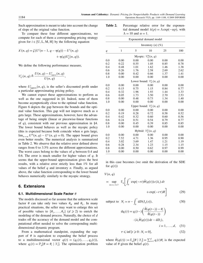
Araman and Caldentey: Dynamic Pricing for Nonperishable Products with Demand Learning1184 Operations Research 57(5), pp. 1169–1188, © 2009 INFORMS
Such approximation is meant to take into account the changeof slope of the original value function.To compare these four different approximations, we
compute for each of them a corresponding pricing strategygiven for i ∈ �U�L�M�H by the following equation
i�n� q� = ��U i�n − 1� q − ��q�� − U i�n� q�
+ ��q�U iq�n� q���
We define the following performance measure,
�iU �n� q��
U�n�q� − U iApprox�n� q�
U�n�q��
where U iApprox�n� q�, is the seller’s discounted profit under
a particular approximating pricing policy.We cannot expect these approximations to perform as
well as the one suggested in §4. Indeed, none of thembecome asymptotically close to the optimal value function.Figure 6 depicts the gap between the bounds and the opti-mal value function. This gap will not improve much as n
gets large. These approximations, however, have the advan-tage of being simple (linear or piecewise-linear functionsof q), consistent with our previous approximation in §4.The lower bound behaves as well as the myopic policy(this is expected because both coincide when n gets large,limn→� U M�n� q� − U L�n� q� = 0). The upper bound giveseven better results. The numerical analysis is summarizedin Table 2. We observe that the relative error defined aboveranges from 0 to 3.5% across the different approximations.The worst cases belong to the values of q between 0�4 and0.6. The error is much smaller for higher values of q. Itseems that the upper-bound approximation gives the bestresults, with a relative error strictly less than 1% for allvalues of the belief q and inventory n. Finally, as arguedabove, the value function corresponding to the lower boundbehaves numerically similarly to the myopic strategy.
6. Extensions
6.1. Multidimensional Scale Factor �
The models discussed so far assume that the unknown scalefactor � can take only two values �H and �L. In manypractical situations, the seller may want to enlarge this setof possible values to ��1� � � � � �d (d � 2) to enrich themodeling of the demand process. Naturally, the choice of d
trades off the accuracy of the demand model and the com-putational effort needed to solve the corresponding multi-dimensional dynamic program.From a mathematical standpoint, expanding the sup-
port of � is equivalent to expanding the belief processto a multidimensional vector q�t� = �q1�t�� � � � � qd�t��,where qi�t� = �q�� = �i � �t . The optimization problem
Table 2. Percentage relative error for the exponen-tial demand model �p� = � exp�−�p�, with� = 10 and � = 1.
Exponential demand model
Inventory (n) (%)
q 1 5 10 25 100
Myopic: �MU �n� q�
0.0 0�00 0�00 0�00 0�00 0�000.2 0�22 0�55 1�05 0�85 0�780.4 0�48 1�01 1�62 1�46 1�380.6 0�26 1�76 2�58 2�69 2�620.8 0�00 0�42 0�66 1�37 1�411.0 0�00 0�00 0�00 0�00 0�00
Lower bound: �LU �n� q�
0.0 0�00 0�00 0�00 0�00 0�000.2 0�15 0�75 1�15 0�84 0�770.4 0�32 1�96 1�93 1�44 1�330.6 0�05 1�73 3�50 2�70 2�530.8 0�00 0�48 0�73 1�34 1�401.0 0�00 0�00 0�00 0�00 0�00
Upper bound: �UU �n� q�
0.0 0�00 0�00 0�00 0�00 0�000.2 0�19 0�28 0�72 0�58 0�520.4 0�42 0�32 0�60 0�60 0�560.6 0�24 0�51 0�54 0�79 0�770.8 0�00 0�45 0�39 0�85 0�851.0 0�00 0�00 0�00 0�00 0�00
Hybrid: �HU �n� q�
0.0 0�00 0�00 0�00 0�00 0�000.2 7�52 4�71 1�36 0�95 0�900.4 3�02 3�69 1�47 1�21 1�190.6 0�28 2�34 1�23 1�15 1�150.8 0�00 0�50 0�62 0�97 0�991.0 0�00 0�00 0�00 0�00 0�00
in this case becomes (we omit the derivation of the SDEfor q�t�)
V �n�q�
= sup∈�� �∈�
Ɛq
[∫ �
0exp�−rt���q�t��c�t�dt
+ exp�−r��R
](29)
subject to Nt = n −∫ t
0dD�I�s��� (30)
dqi�t� = qi�t−�
(��q�t−�� − �i
��q�t−��
)
· �t��q�t��dt − dDt��
i = 1� � � � � d� (31)
� � inf�t � 0 � Nt = 0� (32)
where ��q�t�� �= Ɛq�� � �t = ∑di=1 qi�t��i is the expected
value of � given the belief q�t�.
INFORMS
holds
copyrightto
this
article
and
distrib
uted
this
copy
asa
courtesy
tothe
author(s).
Add
ition
alinform
ation,
includ
ingrig
htsan
dpe
rmission
policies,
isav
ailableat
http://journa
ls.in
form
s.org/.

Araman and Caldentey: Dynamic Pricing for Nonperishable Products with Demand LearningOperations Research 57(5), pp. 1169–1188, © 2009 INFORMS 1185
Based on the results in the previous sections, we knowthat even for the simplest case d = 2, the correspondingHJB optimality condition does not admit a tractable ana-lytical solution. For this reason, we will not analyze thismodel in full detail but simply present the following exten-sion of the asymptotic approximation in Proposition 5 tothis multidimensional case.
Proposition 12. Consider the seller’s optimizationproblem (29)–(32) with constraint (32) replaced by� = inf�t � 0� Nt = 0 (i.e., the stopping time option is notavailable). Then, the corresponding value function V �n�q�is convex in q and converges (uniformly in q) as n goes toinfinite
limn→� V �n�q� = ��q�R�
The proof of this result mimics the proof of Proposi-tion 5, and it is omitted. Based on this result, we proposethe following approximation for V �n�q� if the stoppingoption is not available:
V �n�q� ≈d∑
i=1
qiW�n��i��
Each of the W�n��i� is computed using the recursionin (10).
6.2. Final Reward Function of the Market Proxy �
The final reward, R, is a critical factor of our modeland represents the expected discounted future cashflows ofthe retailer’s operations (otherwise, it could represent theopportunity cost of the space devoted for one product). Onecontribution of this paper is measuring the effect of thisconstant on the optimal pricing strategy. This value repre-sents a reference compared to which one continuously triesto guess whether the product is of low revenue or of highrevenue. It is likely in certain cases that the future valueof a business is affected by the performance of the currentproduct that is being sold. In our case, this translates to Rbeing a function of �; the final reward, R���, is henceforthuncertain and revealed only in the long run. We considerhere an extension of the model studied in the previous sec-tions by adopting a linear model where R��� = R1 + R2�.
Under such an assumption and in the case where no stop-ping is allowed before all units are sold, we can write thefollowing:
V �n�q� = sup∈�� �∈�
Ɛq
{∫ �
0exp�−rt���c�t� − rR2 dt
+ exp�−r���R1 + R2��
}
= sup∈���∈�
Ɛq
{∫ �
0exp�−rt��c�t�dt+exp�−r�� R
}
+ R2��q��
where c�� = c��− rR2 and R = R1� The second equalityis obtained by writing that exp�−r�� = 1− ∫ �
0 r exp�−rt��
We let �V �n�q� = V �n�q� − R2��q�, which brings us backto our original problem of §4. All the results obtained therewill hold for �V when replacing c � c and R � R. In par-ticular, the approximation suggested for V �n�q� under aterminal reward affine in � is given by
�V �n�q�=q� �W�n��L�+R2�L�+�1−q�� �W�n��H�+R2�H��
where �W is the value function corresponding to �V under per-fect information. It is interesting to note that based on (16),the pricing strategy is not affected by this additional linearterm in �. In a similar fashion, we can also generalize theoptimal stopping problem of §5 to the case where, again,the terminal reward R��� is an affine function of �.
6.3. Final Reward with Salvage Value
A potential improvement of our model is to make theopportunity cost R a function of the terminal level of inven-tory. Obviously, this extension is irrelevant if the optionto stop is not available; in this case the final inventory isalways zero. However, if the retailer can stop selling theproduct at any time (as in §5), then we may want to includea salvage value for the unsold units. Specifically, let R�n�be the seller’s opportunity cost when there are n units ofinventory.The formulation of the problem remains almost the same
than in the case of §5 except for the objective function,which becomes
U�N0� q� = sup∈�� �∈�
Ɛq
[∫ �
0exp�−rt���qt�c�t�dt
+ exp�−r��R�N0 − N��
]� (33)
The only difference between this formulation and (22) isthe value of the terminal reward R�n�. Such modificationwill result in the following optimality (HJB) equation foreach fixed n and q ∈ �0�1 :
⎧⎪⎪⎪⎪⎪⎪⎪⎪⎪⎨⎪⎪⎪⎪⎪⎪⎪⎪⎪⎩
U�n�q� + �
(rU�n�q�
��q�
)− ��q�Uq�n� q�
= U�n − 1� q − ��q�� if U�n�q��R�n��
U�n�q� + �
(rU�n�q�
��q�
)− ��q�Uq�n� q�
�U�n − 1� q − ��q�� if U�n�q� = R�n��
(34)
Most of the results of §5 extend directly to this case if weimpose the following two conditions on R�n�.(A1) The function R�n� is increasing in n.(A2) R�n� < W�n��H� for all n.
INFORMS
holds
copyrightto
this
article
and
distrib
uted
this
copy
asa
courtesy
tothe
author(s).
Add
ition
alinform
ation,
includ
ingrig
htsan
dpe
rmission
policies,
isav
ailableat
http://journa
ls.in
form
s.org/.
Araman and Caldentey: Dynamic Pricing for Nonperishable Products with Demand Learning1186 Operations Research 57(5), pp. 1169–1188, © 2009 INFORMS
The monotonicity of R�n� is a natural requirement con-sistent with the notion of salvage value. The second condi-tion guarantees that for every inventory level n the retaileralways prefers to sell a high-revenue product (� = �H ) thanto liquidate it and collect the terminal reward R�n�.The following proposition summarizes the main proper-
ties of U�n�q�. The proof is omitted because it follows thesame line of arguments as the proofs of Propositions 10and 11. Before stating the result, we introduce the followingquantities. Similar to §5, let q∗
n be the solution to U�n�q� =R�n�. Denote by q
nand qn, respectively, the solutions to
�
(rR�n�
��q�
)= R�n − 1� − R�n�
and
R�n� + �
(rR�n�
��q�
)= �q − ��q��R�n − 1�
+ �1− q + ��q��W�n − 1� �H��
Proposition 13. Suppose that conditions (A1) and (A2)hold. Then, the value function U�n�q� is increasing in nand decreasing and convex in q. Furthermore, for everyn, the threshold q∗
n ∈ �qn� qn , and the value function is
bounded by
max{
W�n��H� − �W�n��H� − R�n��q
qn
�R�n�
}
�U�n�q�
�max{
W�n��H� − �W�n��H� − R�n��q
qn
�R�n�
}�
We note that in this case, the threshold q∗n is not neces-
sarily increasing in n. Finally, we mention that other resultsof §5 hold as well; for example, we can similarly usethe upper and lower bounds on U�n�q� as approximationsof the true value function to estimate the optimal pricingstrategy.
7. Concluding RemarksIn this paper, we have studied the problem faced bya retailer that sells nonperishable products to a Poissonarrival stream of price-sensitive customers with unknowndemand intensity. The uncertainty in the demand rate ismodeled by a single factor � that is used as a proxy to cap-ture the unknown size of the market. The retailer is initiallyendowed with a finite inventory of the product and a priorbelief about the value of �. In this setting, the retailer’sproblem is to maximize the expected discounted cumula-tive revenue, adjusting dynamically the price of the productand using Bayesian learning to update the distribution of �.Besides the uncertainty with regard to the demand intensity,the model differs from the traditional revenue management
problem in two important aspects. First, because the prod-uct is nonperishable, the selling horizon is not (a priori)bounded. Second, the model explicitly includes an oppor-tunity cost that the retailer incurs when he decides to sella particular nonperishable product instead of a differentassortment.The analysis of the retailer’s problem was divided in
three parts. In §3, we considered the case in which � isknown with certainty at time 0. In this perfect informationcase, the problem admits a tractable dynamic programmingformulation that we showed how to solve efficiently. Themain insight in this case is that the retailer can partitionthe set of nonperishable products in two categories depend-ing on the value of �. If � is larger than a fixed threshold(that we normalized to 1) the product offers high returnscompared to the retailer’s average revenue (captured bythe opportunity cost R). On the other hand, if � is low(less than 1 in our normalized system), the product gen-erates lower-than-average revenues. Hence, if the retailerwere able to observe in advance the value of �, he wouldonly engage in selling high-revenue products. An inter-esting feature of the solution is that even though optimalprices increase with �, the resulting optimal selling ratesalso increase with �. That is, high-revenue products aresold at a higher price and have a higher inventory turnoverthan low-revenue products.In §4, we relaxed the perfect information assumption
and considered the case in which � is unknown. We alsoassumed that the retailer must sell the initial inventory com-pletely before a different assortment can be offered. Theanalysis of this model is more involved because the statedescription requires a new state variable to capture theretailer’s beliefs about the value of �. As a result, the result-ing dynamic program does not admit a simple analyticalsolution. Nevertheless, we propose a recursive algorithm tosolve the corresponding HJB that requires solving a one-dimensional ODE in each iteration. Because of this lack oftractability, we propose a simple approximation to computethe value function and associated optimal pricing strategy.The proposed policy is based on the fact that as the inven-tory gets large, the retailer’s discounted revenue (as a func-tion of the initial belief) converges uniformly to a straightline that we can characterize in closed form. This asymp-totic property is used to develop a simple approximationthat showed a good performance when compared numer-ically to the optimal solution. Our computational experi-ments, summarized in Table 1, reveal that the asymptoticapproximation has on average a relative error that is lessthan 1%. This is a remarkably good performance if we con-sider that the myopic policy (which is also asymptoticallyoptimal) has an average relative error close to 30%.In §5, we considered the case in which the retailer can
stop selling the product at any time and move to a dif-ferent assortment. This stopping decision depends on theinventory level, the retailer’s beliefs about the true value
INFORMS
holds
copyrightto
this
article
and
distrib
uted
this
copy
asa
courtesy
tothe
author(s).
Add
ition
alinform
ation,
includ
ingrig
htsan
dpe
rmission
policies,
isav
ailableat
http://journa
ls.in
form
s.org/.


Related Documents