Dynamic Pricing and Demand Shaping: Theory and Applications in Online Assortments, Ride Sharing and Smart Grids Shuangyu Wang Submitted in partial fulfillment of the requirements for the degree of Doctor of Philosophy in the Graduate School of Arts and Sciences COLUMBIA UNIVERSITY 2019

Welcome message from author
This document is posted to help you gain knowledge. Please leave a comment to let me know what you think about it! Share it to your friends and learn new things together.
Transcript

Dynamic Pricing and Demand Shaping: Theory and Applications in Online Assortments,
Ride Sharing and Smart Grids
Shuangyu Wang
Submitted in partial fulfillment of therequirements for the degree of
Doctor of Philosophyin the Graduate School of Arts and Sciences
COLUMBIA UNIVERSITY
2019

c©2019
Shuangyu Wang
All rights reserved

ABSTRACT
Dynamic Pricing and Demand Shaping: Theory and Applications in Online Assortments,
Ride Sharing and Smart Grids
Shuangyu Wang
This dissertation consists of three papers in revenue management: on-line assortment op-
timization with reusable resources, spatial distribution of surge price under incentive com-
patible assignment for drivers and optimal price rebates for demand response under power
flow constraints.
In Chapter 2, we study an on-line assortment optimization problem of substitutable
products with fixed reusable capacities. At any time, a potential user with her preference
model (possibly adversarially chosen) arrives to the selling platform and the platform offers
a subset of products from the available set of products to the user. The user selects a
product with probability given by her preference model, uses it for a random duration,
which is distributed according to a distribution that only depends on the product selected,
and generates revenue to the seller. The revenue contribution depends on the product
selected and the actual usage time of this user. The goal of the seller is to find a policy
for determining the assortment offered to each arrival to maximize the expected cumulative
revenue over a time horizon.
We find that a simple myopic policy offering the available assortment that maximizes
the expected revenue from a single user at her arrival time provides a good approximation
for the problem. In particular, we show that the myopic policy is 1/2-competitive, i.e.,
the expected cumulative revenue of the myopic policy is at least 1/2 times the expected
cumulative revenue of an optimal clairvoyant policy that has full information about the
adversarially chosen user sequence, including their preference models and arrival epochs.
The proof is based on partitioning the expected revenue of optimal clairvoyant policy into
two parts and a coupling argument that allows us to bound the two parts in terms of the

expected revenue of the myopic policy.
In Chapter 3, we study the surge pricing problem on a ride sharing platform when
there is a demand shock to the traffic network. The goal of the platform is to maximize
the revenue by setting the prices over the network and the assignments between drivers
and riders. In particular, we model the city as a continuous two dimensional network with
exogenous arrivals of baseline riders, available drivers and demand shocks. We consider the
demand shock only exists in a short time scale, so the rider chooses to request the ride or
not depending on their willingness to pay and the price quoted to them, and the driver
accepts any price to provide service. Since drivers can see the price distribution on driver
app, they only accept the assignment from the locations that are incentive compatible for
them. Thus, the price change at one location may affect the operations over the network
and the platform must consider the incentive of drivers when assigning them.
We develop a model for this surge pricing problem and show the structural properties
of an optimal solution. Once the prices at the location with demand shock is determined,
we can determine the optimal prices on other part of the network. Then, the optimal
assignments between riders and drivers can be determined analytically. The surge pricing
problem reduces to one that only depends on the price at the location with demand shock.
We then extend our model by including strategic behavior of riders, using throughput as
objective, dealing with multiple demand shocks, un-constraining the price and considering
movement time. We also conduct numerical experiments to study the properties of the
model which can not be explored analytically.
In Chapter 4, we study the demand response problem of computing price rebates to offer
to the customers to reduce the consumption in the presence of power flow constraints and
transmission losses on the distribution grid. In particular, we employ alternating current
power flow model for the power flow constraints with transmission loss. However, the
demand response problem with alternating current power flow constraints is known as a non-
convex problem, which is in-tractable to solve. To overcome this, we apply a semidefinite
relaxation of alternating current power flow model to obtain a convex approximation for the

problem. At the same time, to handle the uncertainty in the power reduction of customers,
we use sample average to approach the expected cost and linear injection approximation to
estimate the impact of uncertainty in the power reduction. Based on these relaxations and
approximations, we propose an efficient iterative heuristic to solve the near-optimal offer
price under alternating current power flow constraints and transmission losses. We conduct
a substantial amount of numerical tests on our heuristic and compare its performance with
other popular models. The result shows that our iterative heuristic leads to a significant
reduction in the rebates that one needs to offer to shed a certain demand than the solution
which does not consider full transmission loss in its model.

Contents
List of Figures iv
List of Tables v
Acknowledgments vi
1 Overview 1
2 On-line Assortment Optimization with Reusable Resources 7
2.1 Introduction . . . . . . . . . . . . . . . . . . . . . . . . . . . . . . . . . . . . 7
2.1.1 Other Related Work . . . . . . . . . . . . . . . . . . . . . . . . . . . 11
2.2 Competitive Ratio for IFR Usage time Distributions . . . . . . . . . . . . . 12
2.3 General Usage Time Distributions . . . . . . . . . . . . . . . . . . . . . . . 18
2.4 User Type dependent Usage Times: Bad Examples . . . . . . . . . . . . . . 24
2.5 Numerical Experiment . . . . . . . . . . . . . . . . . . . . . . . . . . . . . . 27
2.5.1 Experiment Setup . . . . . . . . . . . . . . . . . . . . . . . . . . . . 28
2.5.2 Benchmark . . . . . . . . . . . . . . . . . . . . . . . . . . . . . . . . 29
2.5.3 Results . . . . . . . . . . . . . . . . . . . . . . . . . . . . . . . . . . 30
2.5.4 Discussion . . . . . . . . . . . . . . . . . . . . . . . . . . . . . . . . . 31
2.6 Conclusions . . . . . . . . . . . . . . . . . . . . . . . . . . . . . . . . . . . . 32
3 Spatial Distribution of Surge Price under Incentive Compatible Assign-
ment for Drivers 33
i

3.1 Introduction . . . . . . . . . . . . . . . . . . . . . . . . . . . . . . . . . . . . 33
3.1.1 Our Contributions . . . . . . . . . . . . . . . . . . . . . . . . . . . . 34
3.1.2 Literature Review . . . . . . . . . . . . . . . . . . . . . . . . . . . . 36
3.2 Our Model and Problem Formulation . . . . . . . . . . . . . . . . . . . . . . 38
3.3 Surge Pricing Policy . . . . . . . . . . . . . . . . . . . . . . . . . . . . . . . 41
3.3.1 Optimal Policy of Baseline Problem . . . . . . . . . . . . . . . . . . 41
3.3.2 Optimal Surge Pricing . . . . . . . . . . . . . . . . . . . . . . . . . . 42
3.3.3 Structure of Optimal Solution and Algorithm . . . . . . . . . . . . . 44
3.4 Strategic Rider Relocation . . . . . . . . . . . . . . . . . . . . . . . . . . . . 49
3.4.1 Structure of Optimal Solution for Problem Πr . . . . . . . . . . . . . 51
3.5 Multiple Demand Shocks . . . . . . . . . . . . . . . . . . . . . . . . . . . . 52
3.5.1 Structure of Optimal Solution for Problem (3.27) . . . . . . . . . . . 53
3.6 Unconstrained Pricing Problem . . . . . . . . . . . . . . . . . . . . . . . . . 56
3.6.1 Norm Induced Distance Metric c . . . . . . . . . . . . . . . . . . . . 57
3.7 Non-instantaneous Relocation . . . . . . . . . . . . . . . . . . . . . . . . . . 58
3.8 Throughput Maximization . . . . . . . . . . . . . . . . . . . . . . . . . . . . 62
3.8.1 Structure of Optimal Solution for Problem (3.36) . . . . . . . . . . . 63
3.9 Numerical Study . . . . . . . . . . . . . . . . . . . . . . . . . . . . . . . . . 66
3.10 Conclusion . . . . . . . . . . . . . . . . . . . . . . . . . . . . . . . . . . . . 69
4 Near-Optimal Price Rebates for Demand Response under Power Flow
Constraints 71
4.1 Introduction . . . . . . . . . . . . . . . . . . . . . . . . . . . . . . . . . . . . 71
4.2 Problem Definition . . . . . . . . . . . . . . . . . . . . . . . . . . . . . . . . 73
4.2.1 Sample Average Approximation . . . . . . . . . . . . . . . . . . . . . 75
4.2.2 SDP Formulation for AC Power Flow Constraints . . . . . . . . . . 75
4.3 Offer Price Optimization Problem under AC Power Flow Constraints . . . . 78
4.3.1 Linear Supply Function . . . . . . . . . . . . . . . . . . . . . . . . . 79
ii

4.3.2 Linear Approximation for Injected Power . . . . . . . . . . . . . . . 80
4.3.3 Optimization Heuristic . . . . . . . . . . . . . . . . . . . . . . . . . . 81
4.4 Alternative Power Flow Constraints . . . . . . . . . . . . . . . . . . . . . . 82
4.4.1 DC Power Flows . . . . . . . . . . . . . . . . . . . . . . . . . . . . . 82
4.4.2 DCβ Power Flows . . . . . . . . . . . . . . . . . . . . . . . . . . . . 84
4.4.3 No Network . . . . . . . . . . . . . . . . . . . . . . . . . . . . . . . . 85
4.5 Computational Study . . . . . . . . . . . . . . . . . . . . . . . . . . . . . . 86
4.5.1 Setup . . . . . . . . . . . . . . . . . . . . . . . . . . . . . . . . . . . 87
4.5.2 Modified Algorithm . . . . . . . . . . . . . . . . . . . . . . . . . . . 88
4.5.3 Main Results . . . . . . . . . . . . . . . . . . . . . . . . . . . . . . . 88
4.6 Conclusion . . . . . . . . . . . . . . . . . . . . . . . . . . . . . . . . . . . . 92
Bibliography 92
Appendices 100
A Proofs for Chapter 3 101
A.1 Proof of Proposition 3.1 . . . . . . . . . . . . . . . . . . . . . . . . . . . . . 101
A.2 Proof of Proposition 3.2 . . . . . . . . . . . . . . . . . . . . . . . . . . . . . 103
A.3 Proof of Proposition 3.3 . . . . . . . . . . . . . . . . . . . . . . . . . . . . . 104
A.4 Proof of Theorem 3.4 . . . . . . . . . . . . . . . . . . . . . . . . . . . . . . . 105
A.5 Proof of Proposition 3.5 . . . . . . . . . . . . . . . . . . . . . . . . . . . . . 110
A.6 Proof of Theorem 3.10 . . . . . . . . . . . . . . . . . . . . . . . . . . . . . . 113
A.7 Proof of Lemma 3.12 . . . . . . . . . . . . . . . . . . . . . . . . . . . . . . . 115
A.8 Proof of Lemma A.1 . . . . . . . . . . . . . . . . . . . . . . . . . . . . . . . 115
B Numerical Examples for Chapter 3 116
B.1 Counter-example of Theorem 3.10 for General c . . . . . . . . . . . . . . . . 116
iii
List of Figures
3.1 Revenue Maximization Surge Prices as a Function of Distance from Demand
Surge Node 0, Price Constrained: p(x) ≥ pb . . . . . . . . . . . . . . . . . . 35
3.2 Revenue Maximization Surge Prices as a Function of Distance from Demand
Surge Node 0, Price Constrained: p(x) ≥ pb . . . . . . . . . . . . . . . . . . 46
3.3 Optimal Pricing Function p under m = 2 Demand Shocks, Price Constrained:
pmin = pb . . . . . . . . . . . . . . . . . . . . . . . . . . . . . . . . . . . . . 56
3.4 Surge Prices p as a Function of Distance from Surge Node, Price Uncon-
strained: pmin = 0 . . . . . . . . . . . . . . . . . . . . . . . . . . . . . . . . 58
3.5 Hopping Assignment for Problem (3.32) with Movement Time . . . . . . . . 62
3.6 Optimal Price Function p for Revenue and Throughput Maximization, De-
mand Surge at 0, Price Constrained: pmin = pb . . . . . . . . . . . . . . . . 66
iv

List of Tables
2.1 Example of Data in NYHC Survey . . . . . . . . . . . . . . . . . . . . . . . 28
2.2 Values of tmax, C in Experiment . . . . . . . . . . . . . . . . . . . . . . . . . 31
2.3 Ratio of Myopic Policy over Benchmark for Different Capacities and Usage
Times . . . . . . . . . . . . . . . . . . . . . . . . . . . . . . . . . . . . . . . 31
3.1 Optimal Values and Prices when pmin = 0 . . . . . . . . . . . . . . . . . . . 67
3.2 Optimal Values and Prices when pmin = pb . . . . . . . . . . . . . . . . . . . 67
3.3 Percentage of Optimal Value Achieved by Clear-market Heuristic . . . . . . 68
3.4 Solution with Quadratic Dis-utility Function, Λ = 10 . . . . . . . . . . . . . 69
3.5 Solution with Quadratic Dis-utility Function, Λ = 30 . . . . . . . . . . . . . 69
3.6 Solution with Quadratic Dis-utility Function, Λ = 50 . . . . . . . . . . . . . 69
4.1 Comparison of AC, DR, DC and DCβ models at ρ = 15, λ = 10 on IEEE
57-bus test case . . . . . . . . . . . . . . . . . . . . . . . . . . . . . . . . . . 89
4.2 Comparison of AC, DR, DC and DCβ models at ρ = 15, λ = 100 on IEEE
57-bus test case . . . . . . . . . . . . . . . . . . . . . . . . . . . . . . . . . . 90
v
Acknowledgments
First of all, I must give my sincerest gratitude to my advisors, Professor Iyengar and Profes-
sor Goyal. During my PhD study, they used their patient guidance and persistent support
to advice me, and tolerated me when I made mistakes. Without their effort, I would never
make this possible. In particular, in the summer of 2013, they offered me a research as-
sistant position when I was a master student in department. This experience made my
mind to pursue doctorate degree in Operations Research in future. Without them, my PhD
stage would never start. Besides academic guidance, they also gave me valuable suggestions
about my career development and gave me the freedom to arrange my time. Thanks, my
advisors.
At the same time, special thanks to my committee, Professor Sethuraman, Professor
Elmachtoub, and Professor Di, for their support, guidance and helpful suggestions. Profes-
sor Sethuraman and Professor Elmachtoub are faculties in our IEOR department and their
involvement in my works started much earlier than this dissertation. They attended several
presentations of my research and I learned useful comments from them, which helped me
to improve the quality of my works. Professor Di also gave me helpful suggestions about
my dissertation in a short notice time. Thanks to them for being members of my defense
committee and for having a word of advice. Thanks, my committee. I also want to thank
Xiaoyue Gong, David Simchi-Levi and Rajan Udwani for their contribution to the paper
of online assortment optimization for reusable resources. Xiaoyue and David are from MIT
Operations Research Center, they pointed out an error in our previous version of the paper
and provided their correction. Rajan is a post-doc working for Professor Goyal, and he
finished the word editing for this paper. Thanks for their work.
It is a wonderful and unforgettable experience when I was studying at Columbia IEOR
vi

Department in the past 6 years and having the exciting moments with other students,
including Yin Lu, Xingbo Xu, Cun Mu, Linan Yang, Chun Ye, Jing Guo, Octavio Ruiz
Lacedelli, Di Xiao, Ni Ma, Zhipeng Liu, Yanan Pei, Fei He, Wei You, Xu Sun, Michael
Hamilton, Chaoxu Zhou, Shuoguang Yang, Min-hwan Oh, Xuan Zhang and other PhD
students, and also many master students in the classes I was teaching assistant for. I also
feel very grateful to the IEOR staff, Jenny, Shi Yee, Jaya, Carmen, Kristen, Lizbeth and
others. They helped me to deal with all my administrative issues in the department, and
even some problems I created. Without this great community, I do not think I would be
able to get to the finish line. Thanks, my friends.
Finally, I would like to thank my parents for their consistent support and confidence in
me. It is a long journey of pursuing PhD degree, and my life has been changed a lot during
this process. However, their unconditional encouragement and believe in me never changes
at any time. Thanks, my family.
vii

To my parents
viii
Chapter 1
Overview
Revenue management has drawn more and more attention in various industries, such as
on-line retailing and ride-sharing platforms, that provide products or services with limited
inventory. Because the inventory is limited and customers usually have different preferences
for products, the seller can improve its revenue by using a well-designed pricing scheme and
assortment offering strategy. Some methods for revenue management include discriminative
pricing, assortment optimization and so on. In particular, discriminative pricing charges
a customer dependent price and assortment optimization decides the product set or the
ranking of products shown to customer to enhance its potential income. These decisions
are made based on the preference of the customer and the inventory level. This thesis
works on three different types of problems in revenue management, in particular, on-line
assortment optimization with reusable resources, spatial distribution of surge price under
incentive compatibility of drivers and optimal price rebates for demand response under
power flow constraints.
In Chapter 2, we show our work for on-line assortment optimization with reusable re-
sources. In many applications, such as hotel booking, physical storage, clouding computing,
on-line food ordering and so on, by offering different choice sets under different situations,
the seller can reserve some low-inventory items for future customers with high preference
and display the high-inventory items at this time to improve its cumulative revenue in a
1

long period. Especially for those business that discriminative pricing is restricted, a good
assortment offering policy plays a key role in their revenue improvement.
To develop a well designed policy, some critical factors, including the state of platform,
the preference model of current customer arrival and the information about future customer
arrivals, are considered in deciding the choice set. In particular, when the seller has partial
or no information about future incoming arrivals, the problem is an on-line problem. This
type of on-line problem draws much of attention from researchers, as the platform is blurry
of how to balance the revenue in current period with the unknown future arrival users under
its limited inventory.
The problem becomes more complex when dealing with the reusable products. When
the products dealt with are non-reusable, once customers purchase one product, the inven-
tory is removed from the platform permanently. In this case, the platform only needs to
track the inventory level of each product to monitor the system state, which reduces the di-
mensionality of the problem. When the products are reusable, the platform not only needs
to record the inventories on-hand, but also needs to track the state of all in-use products
since these busy units become available in a future time.
In our work, we consider an online assortment optimization problem where we have n
substitutable products with fixed reusable capacities c1, . . . , cn. In each period t, a user
with some preferences (potentially adversarially chosen) arrives to the seller’s platform who
offers a subset of products St, from the set of available products. The user selects product
j ∈ St with probability given by the preference model and uses it for a random number
of periods, tj that is distributed i.i.d. according to some distribution that depends only
on j generating a revenue rj(tj) for the seller. The goal of the seller is to find a policy
that maximizes the expected cumulative over a finite horizon T . Our main contribution in
this work is to show that a simple myopic policy (where we offer the myopically optimal
assortment from the available products to each user) provides a good approximation for the
problem. In particular, we show that the myopic policy is 1/2-competitive, i.e., the expected
cumulative revenue of the myopic policy is at least 1/2 times the expected revenue of an
2
optimal policy that has full information about the sequence of user preference models and
the distribution of random usage times of all the products. In contrast, the myopic policy
does not require any information about future arrivals or the distribution of random usage
times. The analysis is based on a coupling argument that allows us to bound the expected
revenue of the optimal algorithm in terms of the expected revenue of the myopic policy.
To prove this result, we employ a coupling argument to bound the expected revenue
of the optimal clairvoyant policy in terms of the expected revenue of the myopic policy.
We firstly present the coupling argument analysis for the case of exponential usage time
distributions. For this case, we show a relatively easy coupling between the sample paths
for the myopic policy and the optimal clairvoyant policy. However, the argument does not
extend to general usage time distributions. For general usage time distributions, we design
a novel coupling method and charging scheme between the myopic policy and the optimal
clairvoyant policy to bound the expected revenue of the optimal clairvoyant policy.
We would like to emphasize that even with full-information about the user sequence,
computing the optimal clairvoyant policy explicitly is intractable due to the curse of di-
mensionality arising from random user choices and random usage times. Golrezai et al. [39]
use a linear programming relaxation with full-information about the user sequence as the
benchmark for their on-line policy where resources are perishable. On the other hand, our
method does not require the explicit form of the clairvoyant policy or even the problem for-
mulation for the clairvoyant policy. Our coupling analysis is valid for any policy, including
the optimal clairvoyant policy.
In Chapter 3, we study the problem of spatial distribution of surge price on ride-sharing
platform under incentive compatibility of drivers. Compared to traditional transportation
industries, ride-sharing platforms manage the drivers in a different way that it does not
employ any drivers, instead, drivers are self-employed and they have their own preferences
of working. The platform operates to dynamically match the available drivers, who have
their de-centralized response to the platform.
One difficulty that the platform usually encounters is that the amount of ride requests
3

can experience a temporary increase when there is a rain or a sports game is going to
end. We refer this phenomenon as demand surge. When demand surge happens, it creates
imbalance between drivers and riders in a region such that the number of available drivers
is not enough to serve all ride requests. This is the main problem of this chapter to model
the demand surge problem and return a solution.
In practice, two common operational tools that platform can use to handle demand surge
are the price charged to riders and assignment policy between drivers and riders. The price
adjusts the number of effective riders and incentivizes the relocation of the drivers. The first
role has been drawn much attention in practice. When demand surge happens, the ride-
sharing platform increases the price around surge location such that the number of effective
riders reduces to a level that can be served by nearby available drivers. The second role
of the pricing profile, together with the assignment policy, is also very important to serve
the demand surge that it can increase the number of available drivers around the demand
surge location by relocating drivers there. In particular, since the drivers have access to
the price distribution on driver app, they have incentive of serving the high price area to
improve their short term income. As long as the price difference is enough to compensate
their dis-utility of relocation, platform is able to assign drivers to pick up riders at different
locations and to increase the availability of drivers in demand surge area. We call this as
the incentive compatible assignment that the drivers are only willing to work at a place that
maximizes their effective income. By designing a pricing profile with spatial structure and
the assignment policy across the network, the platform can utilize more available drivers
across the network to digest the demand surge.
Our outcome of this chapter is to construct a model for such a surge pricing problem with
the objective of maximizing the revenue for platform. Following the model, we show the
algorithm of constructing the optimal pricing profile and the assignment policy. Resulted
from the solution, the optimal pricing policy gives highest price on demand surge location,
decreases by the dis-utility of drivers for relocation, and remains constant at the baseline
price. The intersection between the pricing policy and baseline price is the boundary of
4

surge region and the inside area of this boundary is the surge region. Within the surge
region, we keep using the drivers on lowest priced location to serve the riders at the highest
priced places until we serve all riders or we are out of available drivers. The remaining
drivers are matched with local riders. We show that the matching rate, i.e., the probability
of drivers who get a ride, is 1 inside the surge region. Outside the surge region, the drivers
are never relocated and they are matched with the riders in the same area. We also discuss 5
extensions to the main problem. At last, we conduct computational experiments to discuss
the properties of the problem that can not be studied analytically.
In Chapter 4, we discuss the optimal price rebates in demand response, which is an
application of revenue management in the electricity market. In electricity market, the
users pay the forward price which is determined in advance, whereas the utility company
pays the real-time price when it needs to fulfill the shortage of supply. This creates a
problem for the utility company that when its supply can not fulfill the overall demand on
the user ends, that it must pay the real-time price to buy electricity, which is usually a
higher price when there is more demand over the market. This happens more frequently
when the regenerative energy is more and more engaged into the grid, as it reduces the
stability of energy supply than the transitional energy sources. Demand response is one
way to reduce the loss from this side. By signing contracts with users in advance, the
utility company has the right to offer a price rebate to users to reduce their load. The load
reduction and rebate structure are specified in the contact. The benefit of demand response
is that the utility company can use a small cost to diminish large cost from buying utility
on the real-time market. In this chapter, we show a heuristic to solve the sub-optimal
price rebates for demand response under power flow constraints and transmission loss of
the distribution grid.
We model the transmission loss using the AC power flow constraints. However, optimal
power flow problem with AC power flow constraints is known as a non-convex problem,
which can not be solved directly by general optimization method. To handle this difficulty,
we use the SDP relaxation for the AC power flow constraints to relax the problem into
5

convex optimization. Another difficulty in the problem is that the actual reduction of end
users given the price rebates are uncertain. We use sample average to approximate the
uncertainty and adjust the power flow constraints for each sample. Following these ideas,
we develop an iterative heuristic for the offer price optimization. This heuristic achieves a
good numerical performance in our computational study as it can return the price rebates
efficiently and save a substantial amount of cost to fulfill the shortfall compared to other
power flow constraints without considering the transmission loss.
In sum, all these three works give some innovative models or methods for revenue man-
agement applications in different areas. Chapter 2, Chapter 3 and Chapter 4 are self-
contained and independent of each other.
6

Chapter 2
On-line Assortment Optimization
with Reusable Resources
2.1 Introduction
Assortment optimization is an important problem that arises in a broad set of applications
including online advertising, recommendations and e-retailing where the goal of the decision-
maker is to select a subset of products from the available universe to offer to the user to
maximize the expected revenue or reward. For any given subset S of offered products,
the selection of the user depends on his or her random preference over the set of products
including the no-purchase or exit option. We model this random selection using a choice-
model that for any offer set S, specifies the probability that the user selects product j ∈
S∪0 (where 0 refers to the no-purchase or exit option). Several parametric choice models
have been studied in the literature including multinomial logit (MNL) model [52, 67, 56],
the nested logit model [87, 57, 26, 36], Markov chain based model [15] and the mixture of
multinomial logit model [58] (see [83, 48, 10] for a detailed overview of these models).
In this paper, we consider an online assortment problem where we are given n substi-
tutable products with fixed capacities or inventories c1, . . . , cn. Users with different choice
models arrive sequentially. For each user, the seller offers a subset S of the available prod-
7

ucts satisfying certain constraints, the user selects a random product j ∈ S ∪ 0 with
probability given by his or her choice model and uses it for a random amount of time, tj
and returns it to the platform generating revenue rj(tj) for the seller. The goal of the
platform or the seller is to design a policy to offer assortments to the users so that the
overall expected revenue is maximized. This fits the setting of classical online product al-
location or revenue management. However, unlike traditional settings where the capacity
or inventory of any product decreases whenever any user selects that product, the products
are reusable in our setting. Such setting arises commonly in many applications including
cloud computing, physical storage and other sharing economy applications.
This problem has been considered in the literature in settings with non-reusable prod-
ucts as well as reusable products. Golerezai et al. [39] consider the online assortment
problem with fixed product capacities for the case of non-reusable products (i.e. inventory
of a product decreases whenever any user selects that product). They give an inventory
balancing based algorithm that is (1− 1/e)-competitive for adversarial arrivals in the limit
of capacities going to infinity. For the case of capacities being equal to one, their algorithm
is 1/2-competetive. They also give a near-optimal algorithm for the case of stochastic i.i.d.
arrivals where in each period there is a user whose type is sampled i.i.d. from a known dis-
tribution over user types. Ma and Simchi-Levi [53] consider a more general setting where
the seller can make joint assortment and pricing decisions and obtain similar guarantees
in the adversarial and stochastic arrivals cases for non-reusable capacities. Most closely
related to our setting is the work of Rusmevichientong et al. [71]. They consider the setting
of stochastic arrivals with known distribution of user types and reusable products and give
a 1/2-approximation for the problem.
We consider an adversarial model for the sequence of user types. Here, user type refers
to the choice model of the user which is revealed to the platform when the user arrives. We
make the following assumptions about choice probabilities and usage time distributions.
Assumption 2.1. For any user type z, assortments S ⊆ T ∈ S and i ∈ S, φz(i, S) ≥
φz(i, T ).
8

Assumption 2.2. For every product j, the usage time distribution depends only on j and
not on the user type.
Assumption 2.1 is mild and without much loss of generality. In fact, all random utility
based choice models including multinomial logit (MNL), nested logit and mixture of MNLs
satisfy Assumption 2.1. Assumption 2.2 is fairly reasonable in many settings where while
the choice of the product depends on the user type but the usage time depends only on
the product. For instance, consider a make-to-order setting where user selects a product
from the offered assortment. Once the user makes the selection, a dedicated server makes
the product for the user. In such a setting, the busy time of the server depends only on
the product. While there are settings where the above assumption does not hold, we show
that without Assumption 2.2, it is not possible to obtain any constant factor competitive
algorithm for the case of adversarial arrivals.
The revenue to the seller, rj(tj) when product j is used for some random time, tj , could
be a general function of the usage time. In particular, we can model fixed revenue for every
use as well as revenue which is an affine function of usage time with fixed component and
per-unit usage time component. Let rj denote the expected revenue of product j where the
expectation is taken over the random usage time of product j, i.e.,
rj = Etj∼Fj [rj(tj)],
where Fj is the cdf of usage time distribution of product j.
Our Contributions. Our main contribution is to show that a myopic policy provides a
good approximation for the online assortment optimization problem with reusable products.
Myopic Policy. For each user, the myopic policy offers an assortment S ∈ S from the set
of available products that maximizes the expected revenue from that user. More specifically,
suppose user at time t has type zt and let It be the set of products available to the myopic
9

policy at time t. Then the myopic policy offers assortment St where
St ∈ argmax
∑i∈S
ri · φzt(i, S) | S ⊆ It, S ∈ S
,
where φz is the choice model for user type z, φz(i, S) is the probability that user type
z selects product i given assortment S and ri is the expected revenue when product i is
selected where the expectation is taken over the random usage time of product i. Recall that
we assume the usage time distribution only depends on the product and is not dependent on
user type. Therefore, the myopic policy only needs the expected revenue, rj from product j
if it is selected and does not need any further information about the usage time distribution.
Further, the optimal set St can be found using any black-box algorithm for static assortment
optimization.
We show that this myopic policy is 1/2-competitive. In other words, the expected
revenue of the myopic policy is at least 1/2 times the expected revenue of an optimal policy
that has full information about the sequence of user types and product usage distributions
(although not the choice realizations and the realization of usage times). We refer to
this as the clairvoyant benchmark. More generally, when the (possibly constrained) static
assortment optimization problem at each stage can only be solved up to within an α factor
of the optimal, our myopic policy is α/2 competitive.
We also show that if the usage time distribution depends on the user type, then there
is no online algorithm that can obtain a constant factor competitive ratio as compared to
our clairvoyant benchmark for the case of adversarial arrivals. We would like to note that
Rusmevichientong et al. [71] consider the case where usage time distributions can depend
on the user type. However, they consider the setting of stochastic arrivals with known
distribution of user types and give a 1/2-approximation compared to the optimal dynamic
programming solution as opposed to the clairvoyant benchmark.
Challenges and New Techniques. We would like to note that even with full-information
about the sequence of users and the usage time distribution, computing an optimal policy
10

is intractable due to the curse of dimensionality. Golrezai et al. [39] use a LP based upper
bound as a benchmark for the case of non-reusable products. One of the challenges in
extending the results to the case of reusable products is the lack of a good LP based upper
bound. A natural LP formulation based on the one in [39] has an unbounded integrality
gap and therefore, is not a useful benchmark for the problem.
In order to prove the competitive ratio bound, we use a coupling argument instead to
upper bound the expected revenue of an optimal algorithm with full information in terms
of the expected revenue of the myopic policy. If the usage time distributions satisfy the
Increasing Failure Rate (IFR) property, it is relatively easy to design such a coupling. How-
ever, that coupling does not extend to general distributions. One of the main contributions
of this work is designing a novel queue-based coupling that allows us to relate the expected
revenue of an optimal policy to the expected revenue of the myopic policy for any usage
time distributions.
2.1.1 Other Related Work
There is a considerable amount of literature on dynamic assortment optimization prob-
lems with non-reusable products starting with [11], which studied the problem of dynamic
assortment optimization for a stochastic arrival model where users choose according to a
multinomial logit choice model (see [77], [51], [35] and [82]) and the user type is drawn
i.i.d. from a stationary distribution. Chan and Farias [22] considered a stochastic depletion
framework for non-stationary environments which includes the assortment planning prob-
lem under random arrivals. They gave a 1/2 competitive myopic policy for this general
framework. More recently, [74] and [85] considered other closely related models for online
product allocation with stochastic arrivals. We refer the reader to [39] for a more detailed
review.
For revenue management with reusable products and random usage times, [50] first
studied a product independent demand model where the users do not exhibit any choice
behavior and the goal is to design a policy to maximize the average revenue in an infinite
11

horizon setting. Owen and Levi [65] extended this model to include user choices and also
study the infinite horizon setting. Chen et al. [23] considered a related problem of control
admission for a system with multiple units of a single product which can be reserved in
advance for time intervals determined by users arriving according to a multi-class Poisson
process.
Product allocations problems also closely relate to online matching problems and of-
ten generalize the classical online bipartite matching problem (see [46]). In this seminal
work, they showed that matching arriving users (the unknown vertices) based on a random
RANKING over all products (vertices on the known side of the graph) gives the best possi-
ble competitive guarantee of (1−1/e). The analysis was considerably simplified in [13], [28],
[38] and extended to more general settings in [2], [61]. There is also a rich body of literature
on online matching with random arrivals [27], [55], [45], [32] and stochastic rewards [60],
[62]. We refer the interested reader to [59] for a more detailed review.
Outline. The rest of the chapter is organized as follows. In Section 2.2, we present the
competitive ratio analysis for the case of IFR usage time distributions. In Section 2.3, we
present the competitive ratio analysis for general usage time distributions. In Section 2.4,
we present a family of examples to show that no online algorithm can have a constant
competitive ratio for adversarial arrivals if the usage time distributions depend on the user
type. In Section 2.5, we use the survey data from New York Health Club to present the
numerical performance of myopic policy. Finally, in Section 2.6 we summarize our results
and mention some directions for future work.
2.2 Competitive Ratio for IFR Usage time Distributions
In this section, we consider the special case when the usage time distribution for each
product satisfies the Increasing Failure Rate (IFR) property and present the competitive
ratio analysis for the myopic policy. For any product j with usage time distribution cdf, Fj
12
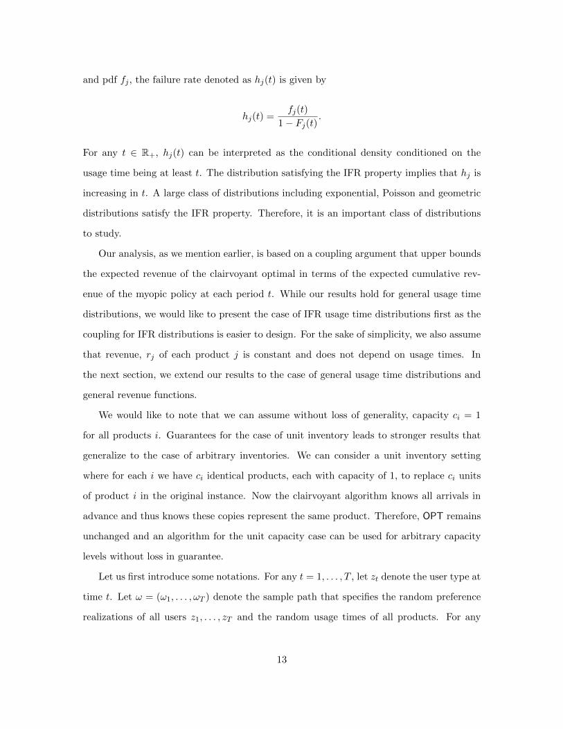
and pdf fj , the failure rate denoted as hj(t) is given by
hj(t) =fj(t)
1− Fj(t).
For any t ∈ R+, hj(t) can be interpreted as the conditional density conditioned on the
usage time being at least t. The distribution satisfying the IFR property implies that hj is
increasing in t. A large class of distributions including exponential, Poisson and geometric
distributions satisfy the IFR property. Therefore, it is an important class of distributions
to study.
Our analysis, as we mention earlier, is based on a coupling argument that upper bounds
the expected revenue of the clairvoyant optimal in terms of the expected cumulative rev-
enue of the myopic policy at each period t. While our results hold for general usage time
distributions, we would like to present the case of IFR usage time distributions first as the
coupling for IFR distributions is easier to design. For the sake of simplicity, we also assume
that revenue, rj of each product j is constant and does not depend on usage times. In
the next section, we extend our results to the case of general usage time distributions and
general revenue functions.
We would like to note that we can assume without loss of generality, capacity ci = 1
for all products i. Guarantees for the case of unit inventory leads to stronger results that
generalize to the case of arbitrary inventories. We can consider a unit inventory setting
where for each i we have ci identical products, each with capacity of 1, to replace ci units
of product i in the original instance. Now the clairvoyant algorithm knows all arrivals in
advance and thus knows these copies represent the same product. Therefore, OPT remains
unchanged and an algorithm for the unit capacity case can be used for arbitrary capacity
levels without loss in guarantee.
Let us first introduce some notations. For any t = 1, . . . , T , let zt denote the user type at
time t. Let ω = (ω1, . . . , ωT ) denote the sample path that specifies the random preference
realizations of all users z1, . . . , zT and the random usage times of all products. For any
13

t = 1, . . . , T , let ω[t] = (ω1, . . . , ωt) refer to the restriction of sample path ω until time t .
From hereon, we refer to the myopic policy as ALG and the clairvoyant optimal as
OPT. Let It(ω) (Ot(ω) respectively) denote the set of available products in ALG (OPT
respectively) at time t on sample path ω. Also, let St(ω) (S∗t (ω) respectively) denote the
assortment offered by ALG (OPT respectively) at time t to user type zt. We would like to
emphasize again that at any time t, the clairvoyant benchmark knows the full sequence of
user types z1, . . . , zT but not the realizations of preferences of future users or the random
future product usage times. Therefore, S∗t (ω) is a function of z1, . . . , zT and ω[t−1] =
(ω1, . . . , ωt−1). In contrast, the online algorithm does not have any information about
the future user types and St(ω) is a function of only user types z1, . . . , zt and ω[t−1] =
(ω1, . . . , ωt−1). More specifically, since ALG is a myopic policy, St(ω) is just the myopically
optimal subset of It(ω) that maximizes the expected revenue for user type zt, i.e.,
St(ω) = argmaxS⊆It(ω) R(S, zt),
where for any assortment S,
R(S, zt) =∑i∈S
ri · φzt(i, S),
is the expected revenue of assortment S for user type zt. Let jt(ω) ∈ St(ω) ∪ 0 be the
product selected by user zt in ALG, and let j∗t (ω) ∈ S∗t (ω)∪ 0 be the product selected by
user zt in OPT at time t on sample path ω. Note that product 0 refers to the do-nothing
or exit option.
We show that for any T and any sequence of user types z1, . . . , zT , if the usage time
distribution for each product satisfies the IFR property, the expected cumulative revenue
of ALG is at least 1/2 times the expected cumulative revenue of OPT where the expectation
is taken over the random preferences and random usage times. In particular, we have the
following theorem.
14

Theorem 2.1. Suppose the usage time distribution for every product satisfies the IFR
property. Then for any time T and sequence of user types z1, . . . , zT ,
Eω
[T∑t=1
R(St(ω), zt)
]≥ 1
2· Eω
[T∑t=1
R(S∗t (ω), zt)
].
To prove the above theorem, we try to upper bound the expected revenue in OPT in
terms of the expected revenue of ALG. In particular, we bound the expected revenue of
S∗t (ω) by bounding the expected revenue from products in S∗t (ω)∩ It(ω) and S∗t (ω) \ It(ω)
separately. For the purpose of analysis, we label each unit of every product differently so
that each unit can be treated as a different product. Therefore, we can assume without loss
of generality the initial inventory ci = 1 for all products i. The following lemma bounds
the total expected revenue in OPT from products that were available in ALG during periods
OPT offered them.
Lemma 2.2. For any sequence of user types z1, . . . , zT , any t = 1, . . . , T and any sample
path ω, ∑j∈S∗
t (ω)∩It(ω)
rj · φzt(j, S∗t (ω)) ≤ R(St(ω), zt)
Proof. From Assumption 2.1 (substitutability of the choice model), we have that
φzt(j, S∗t (ω)) ≤ φzt(j, S∗t (ω) ∩ It(ω)).
Therefore,
∑j∈S∗
t (ω)∩It(ω)
rj · φzt(j, S∗t (ω)) ≤∑
j∈S∗t (ω)∩It(ω)
rj · φzt(j, S∗t (ω) ∩ It(ω))
= R(S∗t (ω) ∩ It(ω), zt)
≤ R(St(ω), zt),
where the last inequality follows from the choice of St(ω) which is the revenue maximizing
subset of It(ω) for user type zt.
15

The following lemma bounds the total expected revenue in OPT from products that
were unavailable in ALG during periods OPT offered them. Here, we present the bound
under the assumption that the usage time distribution for every product satisfies the IFR
property. We extend the argument for general distributions in the following section.
Lemma 2.3. Suppose the usage time distribution for every product satisfies the IFR prop-
erty. Then for any T and sequence of user types z1, . . . , zT ,
Eω
T∑t=1
∑j∈S∗
t (ω)\It(ω)
rj · φzt(j, S∗t (ω))
≤ Eω
[T∑t=1
R(St(ω), zt)
].
Proof. Consider any ω such that j∗t (ω) ∈ S∗t (ω) \ It(ω). For brevity, let us refer to j∗t (ω)
as j∗t . At time t, j∗t is not available in ALG on sample path ω. Therefore, it is in use at
time t and must have been selected in ALG at some previous time period, say t− τ for some
τ ≥ 1. Therefore, ALG received revenue, rj∗t at (t − τ). We charge the revenue, rj∗t that
OPT collects at time t to the revenue that ALG collected at time t− τ . However, we need
to guarantee that the revenue in ALG at time t − τ is not charged multiple times. We do
this by coupling the usage times of j∗t in ALG and OPT that guarantees that j∗t becomes
available in ALG before it becomes available in OPT.
Coupling of Usage Times. Let L denote the random usage time of j∗t . Since the usage
time distribution is IFR, we know that for any u ≥ 0, P (L− ` ≥ u|L ≥ `) is decreasing in
`. This implies that
P (L− τ ≥ u|L ≥ τ) ≤ P (L ≥ u).
Therefore, we can create a coupling between the residual time of j∗t (ω) starting from period t
in ALG with the usage time in OPT as follows. Let u be a random sample from uniform(0, 1).
Set the residual usage time of j∗t in ALG to be F−1(u|L ≥ τ) − τ and the usage time in
OPT to F−1(u) where F is the cumulative density function for usage time distribution of
16

product j∗t (ω). Since F is IFR,
F−1(u|L ≥ τ)− τ ≤ F−1(u),
for any τ ≥ 0 and 0 ≤ u ≤ 1. Therefore, with this coupling, j∗t becomes available in ALG
before it becomes available in OPT. Consequently, we charge the revenue, rj∗t collected by
ALG at time t− τ only once. This implies on any sample path of choice realizations, every
revenue collected by ALG is charged at most once. Therefore,
Eω
T∑t=1
∑j∈S∗
t (ω)\It(ω)
rj · 1(j = j∗t (ω))
≤ Eω
[T∑t=1
rjt(ω)
]= Eω
[T∑t=1
R(St(ω), zt)
]. (2.1)
Consequently, we have
Eω
T∑t=1
∑j∈S∗
t (ω)\It(ω)
rj · φzt(j, S∗t (ω))
≤ Eω
T∑t=1
∑j∈S∗
t (ω)\It(ω)
rj · φzt(j, S∗t (ω) \ It(ω))
= Eω
T∑t=1
∑j∈S∗
t (ω)\It(ω)
rj · 1(j = j∗t (ω))
≤ Eω
[T∑t=1
R(St(ω), zt)
],
where the first inequality follows from Assumption 2.1 and the last inequality follows
from (2.1).
Now we are ready to prove Theorem 2.1.
17

Proof of Theorem 2.1 We have that,
Eω
[T∑t=1
R(S∗t (ω), zt)
]= Eω
T∑t=1
∑j∈S∗
t (ω)
rj · φzt(j, S∗t (ω))
= Eω
T∑t=1
∑j∈S∗
t (ω)∩It(ω)
rj · φzt(j, S∗t (ω)) +∑
j∈S∗t (ω)\It(ω)
rj · φzt(j, S∗t (ω))
≤ Eω
[T∑t=1
R(St(ω), zt)
]+ Eω
T∑t=1
∑j∈S∗
t (ω)\It(ω)
rj · φzt(j, S∗t (ω))
≤ 2 · Eω
[T∑t=1
R(St(ω), zt)
],
where the second last inequality follows from Lemma 2.2 and the last inequality follows
from Lemma 2.3.
2.3 General Usage Time Distributions
In this section, we extend the competitive ratio analysis for the myopic policy for general
usage time distributions and general revenue functions (as functions of usage times) and
show that the myopic policy is 1/2-competitive in general. Similar to the previous section,
we assume without loss of generality that ci = 1 for all products i. We have the following
theorem, in particular.
Theorem 2.4. Suppose for every product j, the usage time is distributed according a distri-
bution that only depends on j. Then for any sequence of user types z1, . . . , zT , the expected
cumulative revenue of the myopic policy is at least 1/2 times the expected cumulative revenue
of the clairvoyant optimal that knows the full sequence, i.e.,
Eω
[T∑t=1
R(St(ω), zt)
]≥ 1
2· Eω
[T∑t=1
R(S∗t (ω), zt)
].
The proof proceeds along similar lines as in the case of IFR usage time distributions. As
18

in the case of IFR usage time distribution, the key challenge is to bound the total expected
revenue in OPT from products that are unavailable in ALG at the time they are offered in
OPT. For the case of IFR usage distributions, we use a coupling and a charging argument
in Lemma 2.3 to show that the total expected revenue from such products is upper bound
by the total expected revenue of ALG. However, the coupling in Lemma 2.3 does not work
for the general distributions. In particular, the coupling of the usage time for a product
j missing in ALG at some time t when user zt selects j in OPT at time t, guarantees that
j becomes available in ALG before it is available in OPT for the case of IFR usage time
distributions ensuring that the revenues in ALG are not charged multiple times. However,
the guarantee does not necessarily hold for the case of more general distributions and we
may end up charging the same revenue of ALG multiple times.
New Coupling Technique. In order to address this issue, we introduce a new coupling
between the usage times in ALG and OPT. In particular, we introduce coupling queues to
specify the coupling of usage times between sample paths in ALG and OPT. We maintain
n queues, Q1, . . . ,Qn with usage time samples for each of the n products. The queues are
initially empty and for each product j we initialize a sequence of T i.i.d. samples of usage
times in Hj .
We use the following coupling between the usage times for any product j in ALG and
OPT. Whenever product j is selected in ALG by some user, we sample a usage time Lj
for product j from the corresponding distribution and push sample Lj to (the bottom of)
queue Qj . Whenever product j is selected in OPT by any user, we first check if queue Qj
is empty. If queue Qj is not empty we pop a sample from Qj for the usage time for this
selection (i.e., we use the sample at the top of Qj and delete the sample from the queue).
Otherwise, we give OPT the next unused sample from Hj .
Lemma 2.5. For any time t = 1, . . . , T and any j = 1, . . . , n, whenever a user selects
product j in OPT the usage time distribution given by the above coupling is i.i.d. according
to the usage time distribution for product j.
19

Proof. When Qj is not empty, the sample that is popped from the queue was originally
picked independently from all previous samples and according to the true distribution, and
added to the queue unconditionally. Any other samples that might have been added to the
queue subsequent to adding this sample do not affect the sample, and it is popped before
them. Therefore, the popped sample is i.i.d. according to the true distribution. When Qj
is empty, samples are chosen from Hj and the claim holds directly.
We are now ready to bound the total expected revenue in OPT from products that are
unavailable in ALG at the time they are offered in OPT. In particular, we have the following
lemma analogous to Lemma 2.3.
Lemma 2.6. For any usage time distributions and sequence of user types z1, . . . , zT ,
Eω
T∑t=1
∑j∈S∗
t (ω)\It(ω)
rj · φzt(j, S∗t (ω))
≤ Eω
[T∑t=1
R(St(ω), zt)
].
Proof. Consider any ω such that j∗t (ω) ∈ S∗t (ω) \ It(ω). Let us refer to j∗t (ω) as j∗t for
brevity. At time t, j∗t is not available in ALG on sample path ω. Therefore, it is in use
at time t and must have been selected in ALG at some previous time period, say t − τ for
some τ ≥ 1. Let L be the random usage time that ALG sampled for j∗t at time (t− τ) and
pushed on the queue Qj∗t corresponding to product j∗t . Since j∗t is still in use by ALG we
get L ≥ τ . Using this and the fact that OPT is able to select j∗t at time t, we have that the
sample L must exist on the queue up to time t (but may be popped at t). Therefore, Qj∗tis non empty before user arrives at t.
Hence, when OPT selects j∗t at time t, we pop a sample from Qj∗t . Suppose the sample
popped by OPT was generated and added to the queue by ALG at time t′ ≤ t − τ . We
charge the revenue earned by OPT for this selection at time t to the revenue earned by
ALG for using j∗t at time t′. Observe that the charging is unique since each sample on the
queue is used at most once by OPT, and we only charge to ALG when the corresponding
sample is used by OPT. We would also like to note that the revenue from a product can
20

now even depend on the usage time duration of the product. The queue based coupling
ensures that every usage time dependent revenue of ALG on any sample path is charged at
most once by selections of OPT that are unavailable in ALG at the time they are offered in
OPT. Therefore,
Eω
T∑t=1
∑j∈S∗
t (ω)\It(ω)
rj · 1(j = j∗t (ω))
≤ Eω
[T∑t=1
rjt(ω)
]= Eω
[T∑t=1
R(St(ω), zt)
]. (2.2)
Simplifying as before, we get
Eω
T∑t=1
∑j∈S∗
t (ω)\It(ω)
rj · φzt(j, S∗t (ω))
≤ Eω
T∑t=1
∑j∈S∗
t (ω)\It(ω)
rj · φzt(j, S∗t (ω) \ It(ω))
= Eω
T∑t=1
∑j∈S∗
t (ω)\It(ω)
rj · 1(j = j∗t (ω))
≤ Eω
[T∑t=1
R(St(ω), zt)
],
where the first inequality follows from Assumption 2.1 and the last inequality follows
from (2.2).
Now we are ready to prove Theorem 2.4.
21

Proof of Theorem 2.4 We have that
Eω
[T∑t=1
R(S∗t (ω), zt)
]= Eω
T∑t=1
∑j∈S∗
t (ω)
rj · φzt(j, S∗t (ω))
= Eω
T∑t=1
∑j∈S∗
t (ω)∩It(ω)
rj · φzt(j, S∗t (ω)) +∑
j∈S∗t (ω)\It(ω)
rj · φzt(j, S∗t (ω))
≤ Eω
T∑t=1
∑j∈S∗
t (ω)∩It(ω)
rj · φzt(j, S∗t (ω))
+ Eω
[T∑t=1
R(St(ω), zt)
]
≤ Eω
T∑t=1
∑j∈S∗
t (ω)∩It(ω)
rj · φzt(j, S∗t (ω) ∩ It(ω))
+ Eω
[T∑t=1
R(St(ω), zt)
]
≤ 2 · Eω
[T∑t=1
R(St(ω), zt)
],
where the third inequality follows from Lemma 2.6 and the second last inequality follows
from Assumption 2.1.
Tightness of 1/2 Competitive Ratio. In this part, we give an example to show that
1/2 competitive ratio is tight for myopic policy in our problem setting, i.e., the competitive
ratio of myopic policy can not be any constant higher than 12 . Suppose platform has two
products 1, 2, with inventory c1 = 1, c2 = 1. Usage time for product j is distributed
as exponential distribution with mean 1/λj . Price rj for product j is deterministic and
independent of usage time. Consider the following two types of users:
1. Choice model of type 1 user:
φ1(j, j) = p, φ1(0, j) = 1− p, p ∈ [0, 1],∀j ∈ 1, 2,
φ1(1, 1, 2) = q, φ1(2, 1, 2) = p− q, φ1(0, 1, 2) = 1− p, q ∈ [0, p].
22
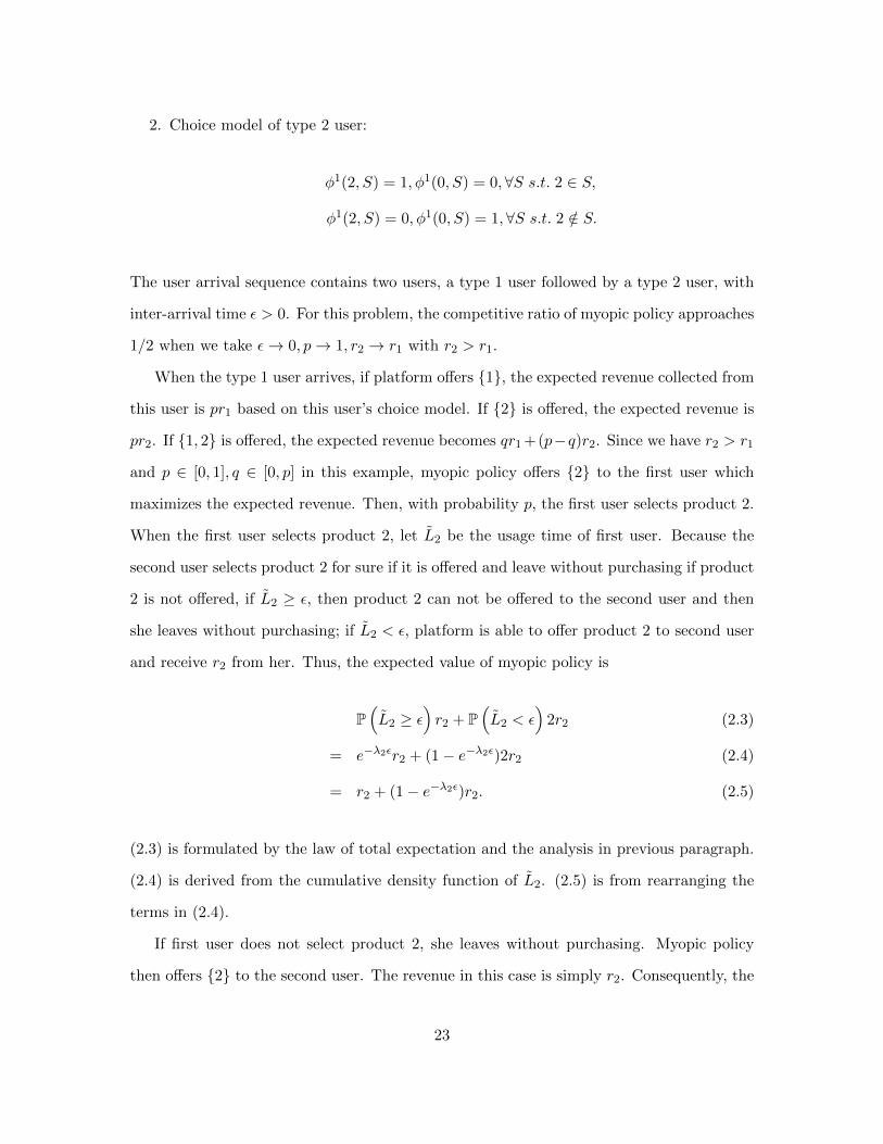
2. Choice model of type 2 user:
φ1(2, S) = 1, φ1(0, S) = 0,∀S s.t. 2 ∈ S,
φ1(2, S) = 0, φ1(0, S) = 1,∀S s.t. 2 /∈ S.
The user arrival sequence contains two users, a type 1 user followed by a type 2 user, with
inter-arrival time ε > 0. For this problem, the competitive ratio of myopic policy approaches
1/2 when we take ε→ 0, p→ 1, r2 → r1 with r2 > r1.
When the type 1 user arrives, if platform offers 1, the expected revenue collected from
this user is pr1 based on this user’s choice model. If 2 is offered, the expected revenue is
pr2. If 1, 2 is offered, the expected revenue becomes qr1 +(p−q)r2. Since we have r2 > r1
and p ∈ [0, 1], q ∈ [0, p] in this example, myopic policy offers 2 to the first user which
maximizes the expected revenue. Then, with probability p, the first user selects product 2.
When the first user selects product 2, let L2 be the usage time of first user. Because the
second user selects product 2 for sure if it is offered and leave without purchasing if product
2 is not offered, if L2 ≥ ε, then product 2 can not be offered to the second user and then
she leaves without purchasing; if L2 < ε, platform is able to offer product 2 to second user
and receive r2 from her. Thus, the expected value of myopic policy is
P(L2 ≥ ε
)r2 + P
(L2 < ε
)2r2 (2.3)
= e−λ2εr2 + (1− e−λ2ε)2r2 (2.4)
= r2 + (1− e−λ2ε)r2. (2.5)
(2.3) is formulated by the law of total expectation and the analysis in previous paragraph.
(2.4) is derived from the cumulative density function of L2. (2.5) is from rearranging the
terms in (2.4).
If first user does not select product 2, she leaves without purchasing. Myopic policy
then offers 2 to the second user. The revenue in this case is simply r2. Consequently, the
23

expected value EM of myopic policy is given by
EM = p(r2 + (1− e−λ2ε)r2
)+ (1− p)r2 = r2 + p
(1− e−λ2ε
)r2.
On the other hand, consider the policy that offers 1 to first user and 2 to the second
user. It takes the advantage of the information of inter-arrival time and choice model of
future user. The expected value of this policy EC is EC = pr1 + r2. Thus, the performance
ratio of the two polices is,
EMEC
=r2 + p
(1− e−λ2ε
)r2
pr1 + r2. (2.6)
Since we have freedom to choose ε, p, r1, r2 as long as they satisfy ε > 0, α2 > α1, p ∈ [0, 1],
we take the limit ε→ 0, α2 → α1, p→ 1. Because the formula in (2.6) is continuous in these
parameters, we have
α2 + p(1− e−λ2ε
)α2
pα1 + α2→ 1
2,
i.e., the competitive ratio of myopic policy can not be any constant higher than 12 .
2.4 User Type dependent Usage Times: Bad Examples
Recall that we show that our myopic policy is 1/2-competetive for the case where the usage
time distributions depend only on the product and not on the user types. In this section,
we consider the case where the product usage time distributions could depend on the user
type. We show that in this case, there is no online algorithm with a constant competitive
ratio in the adversarial arrival model.
It suffices for us to consider a single product, so for a user arriving at time t, let St
denote the random usage duration. Even for the special case of online matching with a
single reusable product we have the following upper bound on the competitive ratio of any
online algorithm.
Theorem 2.7. For online matching with a single reusable product, if the random usage
durations depend on the user, no online (randomized) algorithm can have competitive ratio
24

better than O( logn
n
), where n is the number of users.
Before we prove the above lemma, consider first the special case of algorithms that
always match a user to some available product if such a matching is possible. Suppose we
have a single unit of a single product with reward 1 and the following arrival sequences,
• Sequence A: A single user with usage time duration ∞ (never returns the product).
• Sequence B: A user with usage duration ∞, followed by n users that return the
product right away i.e., P(St = 0) = 1 for all t ∈ 2, . . . , n+ 1.
In order to be competitive on sequence A, the algorithm must match the arrival with
the only available product. Consequently, even on sequence B the algorithm matches the
product to the first user and earn a net reward of 1. An optimal offline algorithm would earn
total reward n on sequence B hence, an online algorithm that always matches an arriving
costumer if possible can never have competitive ratio better than O(
1n
). For the general
case, consider the following family of arrival sequences and subsequent lemma.
• Sequence C(i): ni users, each with identical usage duration distribution where the
item is either returned immediately with probability pi = 1 − 1ni
or never returned
i.e., P(S(i) = 0) = pi = 1− 1ni
and P(S(i) =∞) = 1− pi = 1ni
.
Lemma 2.8. For any given i, if an algorithm generates
Expected Revenue ≥ 1− pαnii
1− pi,
on arrival sequence C(i), then the probability that the product is consumed forever after the
last arrival is at least 1− pαnii .
Proof. Given a randomized algorithm, fix a random seed r for the algorithm and let α(r) ∈
[0, 1] denote the fraction of users that are to be matched by the algorithm if possible (since
all users are identical it does not matter which ones are matched, only the total number).
25

The expected total reward R of the algorithm given seed r is,
E[R|r] = (1− pi) + pi(1− pi)2 · · ·+ pα(r)ni−1i α(r)ni =
1− pα(r)ni
i
1− pi.
Where the last equality follows by summing up the arithmetic-geometric progression.
Observe that for n→∞, 1− pα(r)ni
i → 1− e−α(r) and thus, E[R|r]→ (1− e−α(r))ni.
Now, the probability that the product is consumed forever (extinguished) conditioned
on r is
P(Product Extinguished | r) = 1− pα(r)ni
i .
Therefore,
P(Product Extinguished) = Er[1− pα(r)ni
i ]
=∑r
P(r)(1− pα(r)ni
i ).
Moreover,
E[R] =∑r
P(r)P(Product Extinguished | r)
1− pi=
P(Product Extinguished)
1− pi,
which gives us the desired.
Corollary 2.9. For any given i, the maximum expected revenue generated by any algorithm
(online or offline) for sequence C(i) is1−pnii1−pi = Θ(ni).
Proof. Follows from observing that matching the product to every user possible maximizes
the expected revenue and using Lemma 2.8.
Now we are ready to prove Theorem 2.7.
Proof of Theorem 2.7 Consider the following n sequences D(i) = C(1), . . . , C(i) for
i ∈ [n] that begin with n users arriving from sequence C(1) followed by n2 users from
sequence C(2) and so on in order till C(i). For any sequence D(i) the maximum possible
expected revenue is Θ(ni), since it is lower bounded by (1− pnii )ni = Ω(ni) (matching only
26

the users in C(i) and ignoring earlier users) and at most,(∑i
k=1 ni)
= O(ni).
We prove by contradiction. Consider a β competitive online algorithm and assume β =
Ω( logn
n
)(otherwise we are done). For any such algorithm subjected to arrival sequence D(1),
from Corollary 2.9 and Lemma 2.8 we have that the probability the product is available after
all arrivals is at most 1−β(1−pn1 )→ 1−β(1−1/e). Similarly, in order to be β competitive on
sequence D(2) where the maximum expected profit is Θ(n2), the expected reward generated
from the C(2) part of sequence D(2) must be at least β(1−pn2
2 )n2 as the contribution from
arrivals C(1) is at most Θ(n) = o(βn2) for β = Ω( logn
n
)). Therefore, the probability of
product surviving after all arrivals from C(2) conditioned on product surviving after the
first n arrivals from C(1) is at most 1− β(1− pn2
2 )→ 1− β(1− 1/e). Thus, the probability
of product surviving after all arrivals in D(2) is at most (1− β(1− 1/e))2. More generally,
it follows that the probability of product surviving arrivals from sequence D(i) is at most
(1 − β(1 − 1/e))i. Therefore, on sequence D(n) there is at most a (1 − β(1 − 1/e))n−1
probability that the product survives until the first arrival from sequence C(n). Hence, the
expected revenue on D(n) is,
O
(max
(1− β(1− 1/e))n−1,
1
n
ni).
Therefore, the competitive ratio β of the algorithm must satisfy,
β ≤ O(
max
(1− β(1− 1/e))n−1,
1
n
).
Since the RHS is O( 1n) for β = 2 logn
n we have a contradiction. Hence, β = O( logn
n
). Note
that a more refined argument can be used to further tighten the log factor.
2.5 Numerical Experiment
In this section, we empirically compare the performance of myopic policy with an offline
benchmark. The data is from customer surveys of New York Health Club (NYHC) in a
27

published teaching case from Columbia Business School [54]. The survey contains 1, 000
potential customers of their willingness to pay for 6 different work-out time slots: 6 − 9
a.m., 9 a.m. - noon, noon - 2 p.m., 2 − 5 p.m., 5 − 9 p.m. and 9 p.m. - midnight. For
the number in each cell of Table 2.1, it represents the dollar amount that the questionnaire
answerer is willing to pay for the membership of using the gym in that specific time period.
Client 6− 9 a.m. 9 a.m. - noon noon - 2 p.m. 2− 5 p.m. 5− 9 p.m. 9 p.m. - midnight
1 18 50 41 76 69 41
2 66 14 86 62 71 46
3 60 43 43 26 91 58
Table 2.1: Example of Data in NYHC Survey
We use MNL fit for the choice model of each user arrival and assume the user uses
the time slot for a random amount of days and a fixed capacity for each time slot. In the
following sections, we show the details of the experiments.
2.5.1 Experiment Setup
In this section, we introduce the setup of our experiments. We consider a sequence of 1000
customer arrivals with MNL choice models over time horizon [0, T ]. Each customer has her
choice model for the different time slots with MNL parameters fit from the data in [54]. For
each customer arrival, the club knows the choice model of the customer upon her arrival
and decides an assortment of time slots offered to the customer. The capacity of each time
slot j is cj . In our experiments, we use cj = C, j = 1, ..., 6. Different of assuming C = 1
in proof, we use different values for C. Then, the customer selects a product from the
offering or exit with no purchase based on her choice model. If the user chooses a time slot
j, she pays a fixed price rj and uses that time slot for a random number of days following
distribution uniform(0, tmax). The tmax is same for all products j = 1, ..., 6, i.e., all usage
times are uniform(0, tmax). The user returns the unit after she finishes her usage. We use
Monte Carlo simulation to estimate the expected value of myopic policy, then compare it
to the benchmark.
Choice Model Parameters. In the dataset [54], wjt is given in each cell to represent the
28

willingness to pay of t-th arrival customer for product j. We use wjt to fit MNL model
to estimate the choice probability of t-th arrival customer. Given the prices r1, ..., r6 for all
products and the assortment St ⊆ 1, ..., 6 offered to customer, the choice probability is
given by
φ(j, St) =e(wjt−rj)/µ∑
j∈St e(wjt−rj)/µ + 1
, ∀j ∈ St; φ(j, St) = 0,∀j /∈ St,
where µ is the variance of customer utility, which is estimated from the sample variance of
the willingness to pay data. In our experiment, we use the average value of willingness to
pay for product j as the price rj .
Arrival Process. In this experiment, we consider T = 1000 arrival users. Each user
arrives at time t indexed by her row number in the survey.
Usage Time. We use uniform random usage time for each product. In particular, each
customer uses time slot for a random number of days following distribution uniform(0, tmax).
We use a same distribution for all products j = 1, ..., 6.
2.5.2 Benchmark
In this section, we construct the benchmark policy in this experiment. The benchmark used
in our main conclusion is the optimal clairvoyant policy with full information of the arrival
sequence. However, the value of this benchmark is difficult to compute. In particular, we
need to solve the benchmark value using dynamic programming, which is under the curse
of dimensionality. In this experiment, we have a long customer sequence with a large state
space for the platform. Thus, using optimal clairvoyant policy as benchmark is impractical
for the experiments.
Inspired by the work in [39], we construct an off-line benchmark that uses the full
information of the arrival sequence. The value of the benchmark is determined by the
29
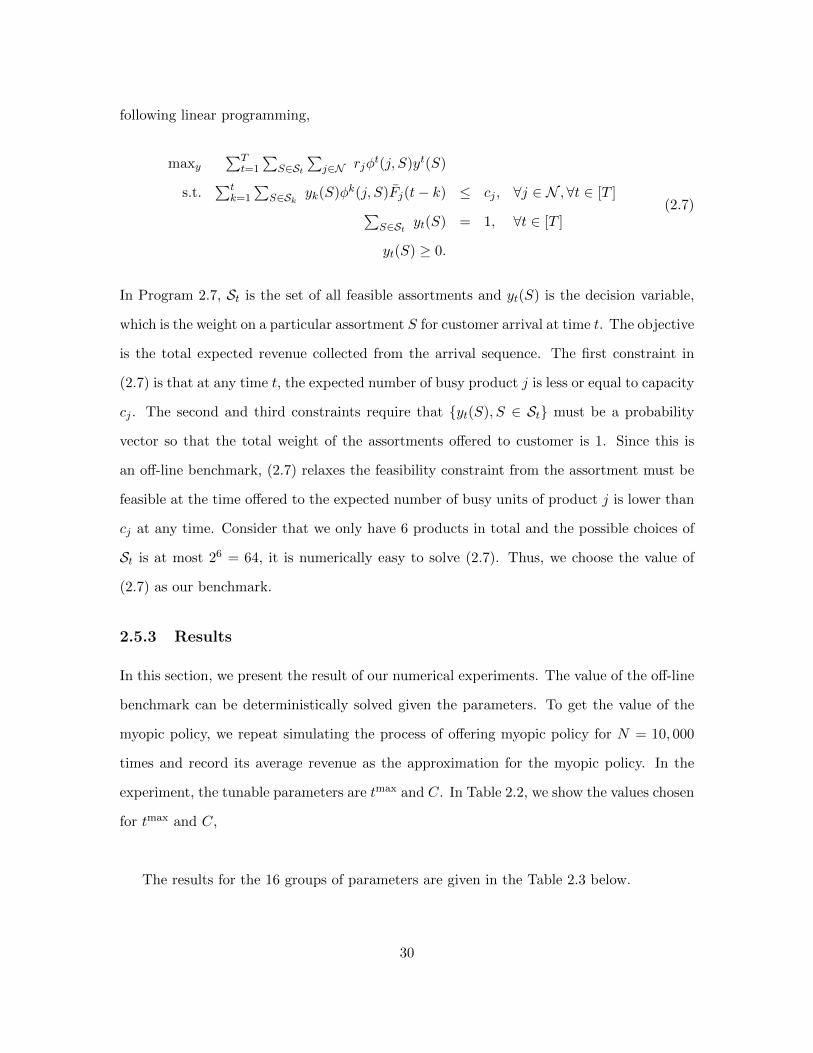
following linear programming,
maxy∑T
t=1
∑S∈St
∑j∈N rjφ
t(j, S)yt(S)
s.t.∑t
k=1
∑S∈Sk yk(S)φk(j, S)Fj(t− k) ≤ cj , ∀j ∈ N ,∀t ∈ [T ]∑
S∈St yt(S) = 1, ∀t ∈ [T ]
yt(S) ≥ 0.
(2.7)
In Program 2.7, St is the set of all feasible assortments and yt(S) is the decision variable,
which is the weight on a particular assortment S for customer arrival at time t. The objective
is the total expected revenue collected from the arrival sequence. The first constraint in
(2.7) is that at any time t, the expected number of busy product j is less or equal to capacity
cj . The second and third constraints require that yt(S), S ∈ St must be a probability
vector so that the total weight of the assortments offered to customer is 1. Since this is
an off-line benchmark, (2.7) relaxes the feasibility constraint from the assortment must be
feasible at the time offered to the expected number of busy units of product j is lower than
cj at any time. Consider that we only have 6 products in total and the possible choices of
St is at most 26 = 64, it is numerically easy to solve (2.7). Thus, we choose the value of
(2.7) as our benchmark.
2.5.3 Results
In this section, we present the result of our numerical experiments. The value of the off-line
benchmark can be deterministically solved given the parameters. To get the value of the
myopic policy, we repeat simulating the process of offering myopic policy for N = 10, 000
times and record its average revenue as the approximation for the myopic policy. In the
experiment, the tunable parameters are tmax and C. In Table 2.2, we show the values chosen
for tmax and C,
The results for the 16 groups of parameters are given in the Table 2.3 below.
30

tmax 30 120 300 600
C 1 2 5 10
Table 2.2: Values of tmax, C in Experiment
Omax\C 1 2 5 10
30 85.42% 96.32% 99.98% 100.00%
120 94.58% 92.20% 96.52% 99.96%
300 98.16% 97.68% 95.88% 96.58%
600 99.23% 99.52% 98.62% 97.69%
Table 2.3: Ratio of Myopic Policy over Benchmark for Different Capacities and Usage Times
2.5.4 Discussion
In Table 2.3, when we fix capacity level C, the ratio is not monotone in the expected usage
time (as we assume the usage time is uniformly distributed). The ratio decreases with
tmax first and then increases with tmax. When usage time is short, it is reasonable to offer
the products in greedy way since the units are returned quickly. When the usage time is
long, myopic policy can still get a good performance since the benchmark is not able to
achieve an outperforming revenue from the customers. If tmax = ∞, i.e., the products are
non-reusable, as long as the platform can sell all the products within the time horizon, it
is the optimal policy. Since the customers are not adversarially chosen in this experiment
and we only have 10 or fewer capacities for each product in our experiments, myopic policy
can achieve a good performance if the usage time is long.
When the usage time distribution is fixed, the ratio decreases with capacity C first and
then increases with C. When the capacity is low, the myopic policy can get a total expected
revenue close to the benchmark as the benchmark itself could not achieve an outstanding
performance. When the capacity is high, the platform actually should offer the products
greedily and the myopic policy is a good solution for the problem.
We need to emphasize that since the arrival sequence is fixed in our experiments instead
of being adversarially chosen, the performance of myopic policy could be worse if we set the
future arrival customers adaptively against the previous realizations in myopic policy. On
the other hand, when the arrival sequence is not adversarially chosen, myopic policy can
31

achieve a better performance than 1/2 competitive ratio. In Table 2.3, myopic policy can
achieve at least 90% of the benchmark value in most experiments. In particular, when the
capacity C increases to 10, the performance ratio of myopic policy never drops below 96%.
This is consistent with the intuition that when the capacity is not scarce, myopic policy is
a good and simple policy to choose.
2.6 Conclusions
In this paper, we consider an online assortment optimization problem with resusable re-
sources or products under an adversarial arrival model. Under the assumption, that product
usage time distributions do not depend on the user type, we show that a myopic policy is
1/2-competitive. In other words, the policy that offers a myopically optimal assortment to
every user from the set of available products achieves an expected revenue that is at least
1/2 times the expected revenue of a clairvoyant algorithm that has full information about
the sequence of user types. For the case of reusable capacities, we do not have a good upper
bound (LP based or otherwise) for the clairvoyant optimal which makes the comparison
with the benchmark challenging. We present a novel stack-based coupling technique that
allows us to relate the expected revenue of the clairvoyant optimal to the expected revenue
of the myopic policy. This coupling is algorithmic and might be of independent interest.
The assumption that product usage time distribution does not depend on user type is
fairly reasonable and satisfied in many settings. We also show that if the assumption is not
satisfied, there is no online algorithm that can be constant-factor competitive as compared
to our clairvoyant benchmark. Therefore, the assumption is necessary to get any non-trivial
performance guarantee for the case of adversarial arrivals.
An interesting open question is to study whether we can obtain results analogous
to the online assortment problem with non-reusable capacities. In particular, a (1 −
1/e)-competitive algorithm in the adversarial arrivals model and better than (1 − 1/e)-
approximation for the stochastic arrivals model, both for the setting of large capacities.
32

Chapter 3
Spatial Distribution of Surge Price
under Incentive Compatible
Assignment for Drivers
3.1 Introduction
Ride-sharing platforms have experienced extraordinary growth in the last few years. It
works as a dynamic marketplace that matches available drivers to sequential ride requests
that arise over time. When the platform decides its pricing and matching policy for current
demand, both future driver availability or ride requests are not known to the platform. In
some extreme cases, the number of ride requests could increase in sudden, which can not
be all served by nearby drivers at normal price. For examples, the amount of ride requests
can experience a temporary surge when there is a rain or a sports game just ends. We refer
this phenomenon as demand surge.
In practice, two common operational tools that platform can use to handle demand
surge are the price charged to riders and assignment policy between drivers and riders. The
real time price serves a twofold role to the two sides of the market. It adjusts the number of
effective riders, i.e., the riders who actually request ride, and incentivizes the relocation of
33

drivers to regions of high price and demand. The first role has been drawn much attention
in practice.
The second role of the price, together with the assignment policy, is also an important
handle to address the demand surge. It can increase the number of available drivers around
the demand surge location by relocating drivers there. In particular, since the drivers have
access to the price distribution over the network, they have incentive to serve in the high
price area. However, there is dis-utility in relocation and since drivers are strategic, they
would trade off the gains from high price with the dis-utility in relocation. Therefore, we
require assignments to be incentive compatible.
The goal is to design a spatial price distribution and matching policy to maximize several
different performance measures while modeling both drivers and riders as strategic agents.
Our particular focus is on scenario of a demand shock added on the baseline demand and
study the problem in short time scale.
3.1.1 Our Contributions
We consider a fluid approximation of the network. The arrival process of drivers and riders
is exogenous. We assume in the baseline case there is sufficient supply to satisfy all demand.
We consider the scenario of a demand shock and model it as a short-lived increase in the
arrival rate of riders at a particular location. We present the details of the model in Section
3.3. The goal of the platform is to decide prices at all locations such that certain performance
measures (throughput/revenue) are maximized when riders and drivers are strategic.
Our main contributions are the following:
1. Structure of Pricing Policy. We show the following results for optimal pricing
policy.
(a) Optimal pricing policy can be completely determined by the prices at surge
locations. For instance, if there is one demand surge, it is a single parameter
problem.
34

(b) In particular, for the one demand surge problem, the price is highest at surge
location and decreases as we move away from the surge that depends on the dis-
utility function, until the price equals the baseline price. Figure 3.1 represents
an example. We refer the locations where p > pb as surge region.
Distance from Surge Node
Pb
0
Surge Price
R
Figure 3.1: Revenue Maximization Surge Prices as a Function of Distance from DemandSurge Node 0, Price Constrained: p(x) ≥ pb
(c) Since the policy depends on a small number of parameters (equal to the number
of surge locations), we propose an algorithm to compute them efficiently.
2. Structure of Assignment Policy. We also show the optimal incentive compatible
assignment assigns all excess supply of drivers in the surge region to the riders at the
surge location. Therefore, all drivers in surge region are matched to demand in surge
region. We refer this as star assignment. All drivers in surge region are matched to
the demand. The drivers outside surge region do not relocation. For this assignment,
we assume drivers can relocate instantaneously even though their is a dis-utility.
Extensions. We discuss several extensions and show that the optimal policy has similar
structure.
35
1. In particular, we consider rider relocation and multiple demand shocks. We extend
our structural optimal results to these cases and give an efficient algorithm to find the
optimal policy.
2. We also consider the case that relocation is not instantaneous. The pricing policy
satisfies similar structure as before. However, optimal assignment is not a star assign-
ment, but needs to be computed by solving an linear programming(LP).
We also conduct numerical experiments for several variants of our model discussed above,
and discuss the insights from the solution. For instance, for the model where relocation is
not instantaneous, we observe that the assignment is a hopping assignment where general
relocation of excess supply is forwards surge location but the drivers may be matched to
riders before reaching the surge location.
3.1.2 Literature Review
Our work focuses on the design of price distribution and matching policy on ride-sharing
platform under demand shock. It sits in the general areas that discuss the revenue manage-
ment under limited capacity and assignment of supply to demand on two-sided platform.
In this part, we discuss the literature in the streams of these areas that are related to our
work.
Firstly, a set of papers discuss general peak-load pricing problem that charges higher
prices during peak periods of demand, see [75], [25] and [34]. The motivation of these
papers is to increase revenue by relocating demand from the peak period to the off-peak
period. Also, the value of dynamic prices in systems that experience congestion has been
extensively studied in the literature [21], [5] and [47]. Banerjee et al. [68] consider a
network of queues with stationary demand arrival process and a closed network for drivers
to describe their arrival processes and actions, and use Markov chain to model the change of
system status. The authors show that static pricing is as good as state-contingent pricing
policy asymptotically, and state-contingent pricing policy is more robust with respect to
36
inaccurate parameters.
Our work is also related to the rapidly increasing literature that explores the design and
operations of on-line marketplaces. Allon et al. [3] study the role of a platform in improving
the operational efficiency of large-scale service marketplaces. More recent works also provide
insights about how platform impacts the behavior of users. For example, Benjaafar et al. [9]
research the affect of product-sharing platform on the decision of individual to own. In [41],
[4] and [44], the authors discuss how the reduction of search cost can result inefficiencies
of online matching markets. We refer readers to [69] and [72] for a summary of works in
two-sided markets.
Next, we discuss the literature on ride-sharing platforms. Gurvich et al. [40] study
the cost of self-scheduling capacity in a news vendor type model in which the firm chooses
the amount of agents it recruits and selects a compensation level in each period. Cachon
et al. [17] consider a single node model that matches the demand and supply in high
and low demand scenarios and analyze various compensation schemes in a setting that the
platform considers the long-term and short-term incentives of drivers. The authors show
that a state dependent pricing policy is better than a unique price for both scenarios, and
fixed commission contracts can be nearly optima. Besides state dependent pricing policy,
how stochasticity in market conditions affects the pricing and compensation decisions of
platform is also extensively discussed in [40], [80] and [7].
There is another set of papers that explore the problem of matching supply with demand
on ride-sharing platform. Feng et al. [33] compare the waiting time performance of on-
demand matching versus traditional street hailing matching. Hu and Zhou [42] consider
a dynamic matching problem as well as the structure of optimal policies. Besides them,
[66] develop a heuristic to determine the assignment between drivers and potential riders
based on a continuous linear program that maximizes the number of matches in a network.
They also establish its asymptotic optimality. Afeche et al. [1] discuss how platforms can
optimally accept ride requests and reposition drivers within a two-location network without
pricing. Yang et al. [88] consider a ride-sharing service motivated model that the agents
37

compete for time changing but location based resources. Since the incentive of drivers is
considered in our model, we point out that several papers, such as [42] and [3], explore the
process for matching supply to demand when capacities are exogenous and all participants
have preferences for being matched.
The works that are most closely related to ours are those that study pricing on ride-
sharing platform with spacial considerations. Castillo et al. [19] take space into account
and point out that surge pricing can help to avoid an inefficient situation that the earnings
of drivers are low due to long pick-up times. Bimpikis et al. [12] focus on pricing for
steady-state conditions in a network. In their model, drivers behave in equilibrium and
decide whether and when to provide service as well as where to relocate. Buchholz [16]
structurally estimates a spatial equilibrium model to understand the welfare cost of taxi
fare regulations. In sum, these papers focus on the equilibrium of ride-sharing system and
analyze spatial pricing policy under time invariant status.
Outline. The rest of the chapter is organized as follows. We introduce the specifics of the
model and problem in Section 3.2. We present the structure of optimal policy in Section
3.3. We discuss the extensions of our model in Section 3.4 - 3.7, and we present numerical
study in Section 3.9. We conclude our findings in Section 3.10.
Notations. In our model, we use V to present the space driver and riders live in. We use
bold character to represent a location in V or a set. In particular, we use lowercase letter to
present a location, e.g., x ∈ V, and uppercase to represent a set. We use regular character
to present a scalar number or a scalar function.
3.2 Our Model and Problem Formulation
In this section, we introduce our model and assumptions, and present the problem formu-
lation.
Arrival Process. We consider a fluid arrival process for drivers with an exogenous, time
invariant rate µ(x) at any x ∈ V. Similarly, we consider a fluid arrival process for riders,
38

with rate λ(x). We assume
Assumption 3.1.
λ(x) ≤ µ(x),∀x ∈ V.
This is a reasonable assumption in practice. If Assumption 3.1 is violated, we can handle
it by reforming it to a new problem with Assumption 3.1 satisfied. Next, we assume
Assumption 3.2 (Integrable Condition).
∫x∈V
µ(x)dx <∞,∫x∈V
λ(x)dx <∞,
and λ and µ are finite everywhere in V.
Assumption 3.2 is an integrability conditions that ensures demand, supply, revenue and
other metrics are bounded. We refer to λ(x) as baseline demand at x. As we consider
the arrivals of drivers and riders as fluids, we assume instantaneous abandon of unmatched
units.
Assumption 3.3. All unmatched riders or drivers are abandoned instantaneously.
Utility of Riders. Riders have willingness-to-pay(WTP) given by a cumulative density
function Fv same for everyone. Therefore, at any location x, if the price is p(x), there is a
rate of λ(x)Fv(p(x)) riders to request rides. Since we have µ(x) ≥ λ(x) from Assumption
3.1, there is sufficient supply to serve demand at location x. Due to Assumption 3.3, re-
maining riders instantaneously leave and drivers are abandoned of rate µ(x)−λ(x)Fv(p(x)).
Next, define pb := arg max pFv(p), and we assume
Assumption 3.4. pFv(p) is weakly decreasing on p ≥ pb.
Assumption 3.4 is not very restrictive, it holds, for example, if Fv has an increasing
hazard-rate, i.e., hF (x) = fv(x)/Fv(x) is an increasing function in x, which is quite general.
Assumption 3.4 is important to prove our main result Theorem 3.4.
39
Utility of Drivers. We start this part by introducing the dis-utility function c. For any
x ∈ V, the dis-utility in repositioning the driver at x to y is modeled using function c(x,y).
In particular, c measures the magnitude of unhappiness of driver location. We assume c is
non-negative and satisfies the triangle inequality,
c(x,y) + c(y, z) ≥ c(x, z), ∀x,y, z ∈ V. (3.1)
We discuss the numerical result that relaxes (3.1) in the Section 3.9. We also assume the
relocation completes instantaneously. We relax this instantaneous relocation assumption in
Section 3.7.
Next, we define the utility of driver at x relocated to y as
U(x,y) = p(y)− c(x,y), (3.2)
i.e., the price at the relocated location minus the dis-utility of location.
Incentive Compatibiltiy Constraint. In assignment policy, platform can relocate a
driver only if it is incentive compatible for the driver. In particular, for ∀x ∈ V, the best
response for driver at x is to relocate to y, where y ∈ arg maxy U(x,y).
For the above best response model, the drivers assume a probability 1 of being matched
if platform relocates them to a different location y. We will see later that this assumption
holds for relocation inside the surge region. Then, we define the incentive compatibil-
ity constraint for assignment as that platform must assign driver at x to a location in
arg maxy U(x,y).
Since platform can relocate drivers, we denote ν(x) as the arrival rate of drivers after
relocation. Then, the rate of actual rides at x becomes min
(λ(x)Fv
(p(x)
), ν(x)
).
Objective of Platform. We assume a fixed proportion of ride price as commission fee
for the platform in our model. Therefore, the goal of platform is to maximize the revenue,
which is also commission maximal.
40

If the demand is at the baseline level λ(x), the optimal pricing policy is to charge the
baseline price pb everywhere. However, if there is a demand surge, the pricing policy is not
pb any more and we discuss its solution in the following Section 3.3.
3.3 Surge Pricing Policy
In this section, we show the formulation of the surge pricing problem and state its structural
properties. We discuss the baseline problem without demand shock first, and then extend
our analysis to problem with demand shock.
3.3.1 Optimal Policy of Baseline Problem
Under the baseline demand, we have λ(x) ≤ µ(x) for all locations. Since we have enough
drivers to serve all riders, there should be no benefit to relocate drivers. To solve the
baseline problem, we firstly introduce an auxiliary problem,
maxp(x)
∫Vp(x)λ(x)Fv
(p(x)
)dx
s.t. pmax ≥ p(x) ≥ pmin.
(3.3)
where decision variable p(x) is the price charged to riders at x. The objective is the overall
revenue rate from all ride requests. Since parameter λ(x) is unchanged in time invariant,
the actual revenue is revenue rate multiplied by a fixed time length. Thus, it is equivalent
to maximize the revenue rate in Problem (3.3). The upper bound pmax and lower bound
pmin denote a reasonable range for the price. For instance, pmin can be set at 0 and pmax
can be set at the support value of willingness to pay distribution Fv.
We claim Problem (3.3) gives an upper bound to the baseline problem. This is because
Problem (3.3) relaxes all the assignment constraints of baseline problem, and the revenue
rate collected at location x for baseline problem is capped by p(x)λ(x)Fv(p(x)
)due to that
the number of actual rides can not surpass the ride requests at any location x. Next, we
solve Problem (3.3), and claim its solution is feasible for the baseline problem. Therefore
41
it is also an optimal solution for the baseline problem.
Problem (3.3) is actually a point-wise maximization problem for each p(x) after ex-
changing the maximization and integral operations. We can rewrite the objective function
in Problem (3.3) as, ∫Vλ(x)
(maxp(x)
p(x)Fv(p(x)
))dx.
The problem is then to maximize pFv(p) where the solution is pb. Thus, the optimal solution
to Problem (3.3) is p(x) ≡ pb. As the price is same everywhere, it is incentive compatible
to retain all drivers at their original locations. Hence, it is the optimal solution for baseline
problem as well. Due to that p(x) = pb is the optimal pricing policy to baseline problem,
we denote pb as the baseline price in Assumption 3.4.
3.3.2 Optimal Surge Pricing
In this section, we present our surge pricing problem. We consider demand shock as addi-
tional ride arrival rate over the baseline demand. In particular, we use Λ to denote the extra
potential riders requesting cars at location 0, and Λ is also exogenous and time invariant
in its life period. Here, we emphasize that Λ is a point mass on 0 with the same unit of∫V λ(x)dx. We model the demand shock as a point mass for the brevity of the model and
result. The additional riders also behave strategically with the willingness-to-pay Fv and
they are abandoned if unmatched.
In the section, we focus on the case that demand surge only happens at one location 0.
In Section 3.5, we present the results of the problem that demand surges appear at multiple
locations.
Due to the existence of demand surge, the platform does not have enough drivers at 0
to serve riders, i.e., (λ(0) + Λ)Fv(p(0)) ≤ µ(0) is violated, and the baseline policy is not
42

optimal either. Our surge pricing problem can be formulated as follows
maxΓ,γ,ν,r,ν0,p
p(0) min
(ν0,ΛFv
(p(0)
))+
∫Vp(x) min
(ν(x), λ(x)Fv
(p(x)
))dx (3.4)
s.t. ν(x) =
∫V
Γ(y,x)dy, ∀x ∈ V (3.5)
µ(x) =
∫V
Γ(x,y)dy + γ(x), ∀x ∈ V (3.6)
ν0 =
∫Vγ(x)dx, (3.7)
(Π) : r(x) ≥ p(y)− c(x,y), ∀x,y ∈ V (3.8)
Γ(x,y)
(r(x)−
(p(y)− c(x,y)
))= 0, ∀x,y ∈ V (3.9)
γ(x)
(r(x)−
(p(0)− c(x,0)
))= 0, ∀x ∈ V (3.10)
Γ(x,y), γ(x), ν(x), r(x), ν0 ≥ 0, ∀x ∈ V (3.11)
pmax ≥ p(x) ≥ pmin,∀x,y ∈ V, (3.12)
where the decision variables are Γ(x,y), relocation flow of drivers from x to y; γ(x),
relocation flow of drivers from x to demand surge location 0; ν(x), arrival rate of drivers at
x after relocation of drivers; r(x), maximum utility for drivers at location x; ν0, arrival rate
of drivers at 0 after relocation; p(x), the price at location x. The objective is the overall
revenue rate including the revenue earned from the baseline demand and the demand surge.
For the constraints, (3.5), (3.6) and (3.7) are flow balance equations, measuring the
inflow and outflow of drivers at each location. We measure the flow into demand surge
location 0 separately because Λ is a point mass of riders at 0, the integral of γ(x) has
the same unit with Λ. (3.8), (3.9) and (3.10) are the incentive compatibility constraints of
drivers. Under optimality, r(x) = maxy p(y)− c(x,y) is the maximum utility for drivers at
x. Since a driver at location x only accepts rides from locations that provide the maximum
utility, there is driver relocation from x to y only if r(x) = p(y)− c(x,y), i.e., the utility of
location y is highest for drivers at point x. If r(x) > p(y)−c(x,y), the utility of location y
is not highest for drivers at x, then there is no driver relocated from x to y. Thus, at least
43
one of Γ(x,y) and r(x)− (p(y)− c(x,y)) is 0 and so is γ(x) and r(x)− (p(y)− c(x,y)). If
the solution to maxy p(y)−c(x,y) is unique and achieved at y, all drivers at x only provide
service at y.
Since Problem Π is a functional optimization problem with infinite dimensions, there is
no general method to solve it. Thus, we need to develop structural properties for the problem
to simplify it. Next, we present these properties for the optimal pricing and assignment
policy, and the algorithm of solving Problem Π.
3.3.3 Structure of Optimal Solution and Algorithm
We start from the following three propositions of the main Problem Π. These properties
can simplify the problem by shrinking its feasible region.
Proposition 3.1 (Flow Exclusiveness). There exists an optimal solution for the surge
pricing Problem Π that satisfies
Γ(xi,xj)Γ(xj ,xk) = 0, ∀xi 6= xj ,xj 6= xk ∈ V.
We present the proof in Appendix A.1. Proposition 3.1 eliminates solutions with drivers
repositioning into a specific node and drivers repositioning out of that same node simul-
taneously, i.e., we only consider the solutions that any node can only be at most a driver
supplier or a driver receiver, and still achieve the same optimal value. We denote a node as
a driver supplier if there are drivers relocated from this location to other locations and as
a driver receiver if there are drivers relocated from other locations to this location. Next,
we present another proposition which shapes the optimal pricing policy.
Proposition 3.2 (Minimal Incentive Compatibility). There exists an optimal solution for
the surge pricing Problem Π that satisfies
∀xi,xj ∈ V, p(xi) ≥ p(xj)− c(xi,xj).
44

We present the proof in Appendix A.2. According to Proposition 3.2, the price at any
location defines an upper and lower bound for the prices on all other locations. Notice that
in the original problem, pricing policy satisfying p(xi) < p(xj) − c(xi,xj) is still feasible,
as long as the prices are in the interval [pmin, pmax]. However, under this pricing policy, we
are not able to retain drivers at location xi as this assignment is not incentive compatible
for drivers. If we increase p(xi) to p(xj)− c(xi,xj), we can still relocate drivers at location
xi, achieving a same assignment as that for p(xi) < p(xj)− c(xi,xj). Furthermore, when
p(xi) = p(xj)− c(xi,xj), we can also retain drivers at location xi. In this way, we increase
the number of feasible assignments and improve the overall revenue.
Another proposition directly resulted from Proposition 3.1 and Proposition 3.2 is that
we only need to consider those solutions that move drivers from nodes at baseline demand
level into nodes with demand surge.
Proposition 3.3 (Star Assignment). There exists an optimal solution for the surge pricing
Problem Π that satisfies
Γ(xi,xj) = 0, for xi 6= xj and xj 6= 0.
We present the proof in Appendix A.3. Proposition 3.3 states that there is an optimal
solution where every relocation is to the surge node. The shape of resulted assignment
likes a star as the relocated drivers flow into the demand surge location from all directions
and the remaining drivers stay at their locations. Proposition 3.3 reduces the dimension of
the feasible region dramatically by limiting the relocation flows. Both Proposition 3.1 and
Proposition 3.3 are about the structures of optimal assignment structure and driver flows.
We emphasize that the original Problem Π may have multiple optimal solutions and
Proposition 3.1, 3.2 and 3.3 guarantee that there exists an optimal solution that satisfies
them. Our goal is to find an optimal solution (both pricing and assignment) that satisfies
above structural properties.
We make an additional assumption that pmin = pb in this section. Under this assump-
45

tion, we show the optimal pricing policy is
p(x) = max
(pb, p(0)− c(x,0)
), ∀x ∈ V.
Therefore, p(x) is completely determined by p(0 and we only need to determine p(0) for
the optimal solution. Figure 3.2 represents an example for the optimal pricing policy when
V = [0,∞) and demand surge happens at 0. The surge region (locations with price higher
than pb) is x ∈ [0, R].
Distance from Demand Shock Node
Pb
0
Surge Price
R
Figure 3.2: Revenue Maximization Surge Prices as a Function of Distance from DemandSurge Node 0, Price Constrained: p(x) ≥ pb
Under this pricing policy, we maximize the revenue by assigning drivers in the following
procedure. Within surge region,
1. Assign drivers at demand shock location 0 and relocate the extra drivers µ(x) −
λ(x)Fv(p(x)
)to 0;
2. If the demand surge is not completely served, assign drivers at the lowest price location
to 0, until the demand surge is processed or the surge region is out of available drivers;
3. Retain the remaining drivers at their original locations.
46

Outside surge region, platform matches the drivers with effective riders at same location.
The details of assignment policy is in the following Algorithm 3.1.
Algorithm 3.1 Optimal Assignment under Pricing Policy (3.13)
1: Λ = ΛFv(p(0)
), µ =
∫S µ(x)dx, µ =
∫S µ(x)− λ(x)Fv
(p(x)
)dx
2: if Λ ≥ µ then3: Set ν0 = µ, ν(x) = 0, ∀x ∈ S4: else if µ > Λ ≥ µ then5: Set ν0 = Λ6: Denote p as the solution p of
∫x|p(x)≤p,x∈S λ(x)Fv
(p(x)
)dx = Λ− µ
7: for x ∈ S do8: if p(x) > p then9: Set ν(x) = λ(x)Fv
(p(x)
)10: else if p(x) ≤ p then11: Set ν(x) = 012: end if13: end for14: else if Λ < µ then15: Set ν0 = µ, ν(x) = λ(x)Fv
(p(x)
), ∀x ∈ S
16: end if17: for x /∈ S do18: Set ν(x) = µ(x)19: end for
Where we denote S := x|p(x) = p(0) − c(x,0) as surge region. Therefore, we have
the following theorem.
Theorem 3.4. If pmin = pb, the optimal pricing policy of Problem Π is in form of,
p(x) = max
(pb, p(0)− c(x,0)
), ∀x ∈ V. (3.13)
Assignment policy determined by Algorithm 3.1 is an optimal assignment of Problem Π.
We present the proof in Appendix A.4.
We emphasize that Theorem 3.4 requires assumption pmin = pb. This condition ensures
that we can apply the monotonicity of pFv(p) specified in Assumption 3.4 to construct the
optimal pricing policy. We discuss the relaxation of this condition in Section 3.6.
Algorithm for Optimal Policy. By Theorem 3.4, the problem is reduced to deciding the
47
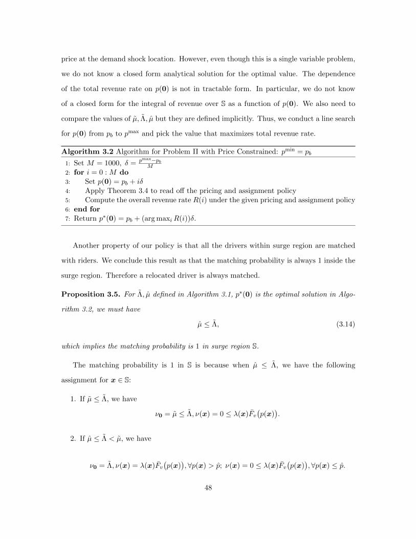
price at the demand shock location. However, even though this is a single variable problem,
we do not know a closed form analytical solution for the optimal value. The dependence
of the total revenue rate on p(0) is not in tractable form. In particular, we do not know
of a closed form for the integral of revenue over S as a function of p(0). We also need to
compare the values of µ, Λ, µ but they are defined implicitly. Thus, we conduct a line search
for p(0) from pb to pmax and pick the value that maximizes total revenue rate.
Algorithm 3.2 Algorithm for Problem Π with Price Constrained: pmin = pb
1: Set M = 1000, δ = pmax−pbM
2: for i = 0 : M do3: Set p(0) = pb + iδ4: Apply Theorem 3.4 to read off the pricing and assignment policy5: Compute the overall revenue rate R(i) under the given pricing and assignment policy6: end for7: Return p∗(0) = pb + (arg maxiR(i))δ.
Another property of our policy is that all the drivers within surge region are matched
with riders. We conclude this result as that the matching probability is always 1 inside the
surge region. Therefore a relocated driver is always matched.
Proposition 3.5. For Λ, µ defined in Algorithm 3.1, p∗(0) is the optimal solution in Algo-
rithm 3.2, we must have
µ ≤ Λ, (3.14)
which implies the matching probability is 1 in surge region S.
The matching probability is 1 in S is because when µ ≤ Λ, we have the following
assignment for x ∈ S:
1. If µ ≤ Λ, we have
ν0 = µ ≤ Λ, ν(x) = 0 ≤ λ(x)Fv(p(x)
).
2. If µ ≤ Λ < µ, we have
ν0 = Λ, ν(x) = λ(x)Fv(p(x)
),∀p(x) > p; ν(x) = 0 ≤ λ(x)Fv
(p(x)
), ∀p(x) ≤ p.
48

We present the proof in Appendix A.5. Consequently, we always have ν0 ≤ Λ, ν(x) ≤
λ(x)Fv(p(x)
), i.e., more effective riders than drivers in surge region.
When we define the utility function for drivers, we use the price instead of the price times
matching probability in utility function as we assume a probability 1 of being matched if
platform relocates driver to a different location. Proposition 3.5 validates this assumption.
3.4 Strategic Rider Relocation
In this section, we discuss the case that riders are also strategic in relocation. We show
that we can reuse the propositions above to solve this new problem. First of all, we define
the effective cost of riders for relocation analogue to the utility of drivers.
Effective Cost of Riders. We start this part by introducing the dis-utility function w
for riders. For any x ∈ V, the dis-utility in repositioning the rider at x to y is modeled
using function w(x,y), which measures the magnitude of unhappiness of rider location. We
assume w is non-negative and satisfies the triangle inequality. We also assume the relocation
completes instantaneously same as the drivers.
Next, we define the effective cost of rider at x relocated to y as
C(x,y) = p(y) + w(x,y), (3.15)
i.e., the price at y plus the dis-utility of relocation.
Incentive Compatibiltiy Constraint. When platform assignment relocates a rider, it is
feasible only if it is incentive compatible for this rider. In particular, for ∀x ∈ V, the best
choice for rider at x is to relocate to y, where y ∈ arg miny C(x,y). Then, we define the
incentive compatibility constraint for rider assignment as that platform must assign rider at
x to a location in arg miny C(x,y). After relocation, this rider contributes to the revenue
at y if he requests ride and gets matched.
Pricing Problem Formulation with Strategic Rider Relocation. In this part, we
49

show the propositions and theorems for solving the problem with strategic rider relocation.
The problem is now formulated as,
max p(0) min(ν0, Λ) +
∫Vp(x) min
(ν(x), λ(x)
)dx (3.16)
s.t. ΛFv(q(0)
)= Λ0 +
∫V
∆(x)dx, (3.17)
λ(x)Fv(q(x)
)= α(x) +
∫VA(x,y)dy, ∀x ∈ V (3.18)
Λ = Λ0 +
∫Vα(x)dx, (3.19)
λ(x) = ∆(x) +
∫VA(y,x)dy, ∀x ∈ V (3.20)
(Πr) : q(x) ≤ p(y) + w(x,y), ∀x,y ∈ V (3.21)
Λ0
(p(0) + w(0,0)− q(0)
)= 0, (3.22)
∆(x)
(p(x) + w(0,x)− q(0)
)= 0, ∀x ∈ V (3.23)
α(x)
(p(0) + w(x,0)− q(x)
)= 0, ∀x ∈ V (3.24)
A(x,y)
(p(y) + w(x,y)− q(x)
)= 0, ∀x,y ∈ V (3.25)
A(x,y),∆(x), α(x), q(x), λ(x),Λ0, Λ ≥ 0, ∀x,y ∈ R2
Constraints (3.5) - (3.12).
Here, the additional decision variables and constraints model the relocation of riders and the
corresponding incentive compatibility constraints. In particular, Λ0 denotes the relocation
of riders from demand shock location 0 to 0; ∆(x) denotes the relocation of riders from
demand shock location 0 to a non-shock location x; α(x) denotes the relocation of riders
from a non-shock location x to demand shock location 0; A(x,y) denotes the relocation of
riders from a non-shock location x to another non-shock location y; q(x) is the minimum
effective cost of requesting a ride for riders at x. (3.17), (3.18), (3.19) and (3.20) denote
the flow balance equations of riders. (3.21), (3.22), (3.23), (3.24) and (3.25) are incentive
compatibility constraints that there is rider relocated from x to y only if the effective cost
50

at y is minimum for riders at x.
3.4.1 Structure of Optimal Solution for Problem Πr
We have similar results for the problem with strategic rider relocation in addition to Propo-
sition 3.1, 3.2 and 3.3.
Proposition 3.6. There exists an optimal solution for Problem Πr that satisfies the fol-
lowing constraints
1. Flow Exclusiveness for Riders:
A(xi,xj)A(xj ,xk) = 0,
∆(xj)A(xj ,xk) = 0,
A(xi,xj)α(xj) = 0,
∆(xj)α(xj) = 0, ∀xi 6= xj ,xj 6= xk ∈ V.
2. Minimal Incentive Compatibility for Riders:
p(xi) ≥ p(xj)− w(xj ,xi) ∀xi,xj ∈ V.
3. Star Assignment for Riders:
∆(xi) = 0, for xi 6= 0; A(xi,xj) = 0, for xi 6= xj .
Then, we have the following theorem.
Theorem 3.7. If pmin = pb, the optimal pricing policy for Problem Πr is in form of,
p(x) = max
(pb, p(0)− c(x,0), p(0)− w(0,x)
), ∀x ∈ V. (3.26)
We denote S := x|p(x) = p(0)− c(x,0) ∪ x|p(x) = p(0)− w(0,x) as surge region.
51

Given pricing policy (3.26), the procedure of constructing the assignment policy is same
as the procedure presented after Algorithm 3.1. However, the explicit algorithm involves
tedious discussions. Therefore we will not show this discussion in this paper.
3.5 Multiple Demand Shocks
In this section, we extend previous analysis for one demand shock to the problem with
multiple demand shocks. Without loss of generality, we show our results for m = 2 demand
shocks. The case of more demand shocks can be generalized from m = 2 demand shocks. In
m = 2 demand shocks problem, we denote that the first demand shock arrives at location
x1 and the second demand shock arrives at location x2 on the network. We formulate the
problem as,
52
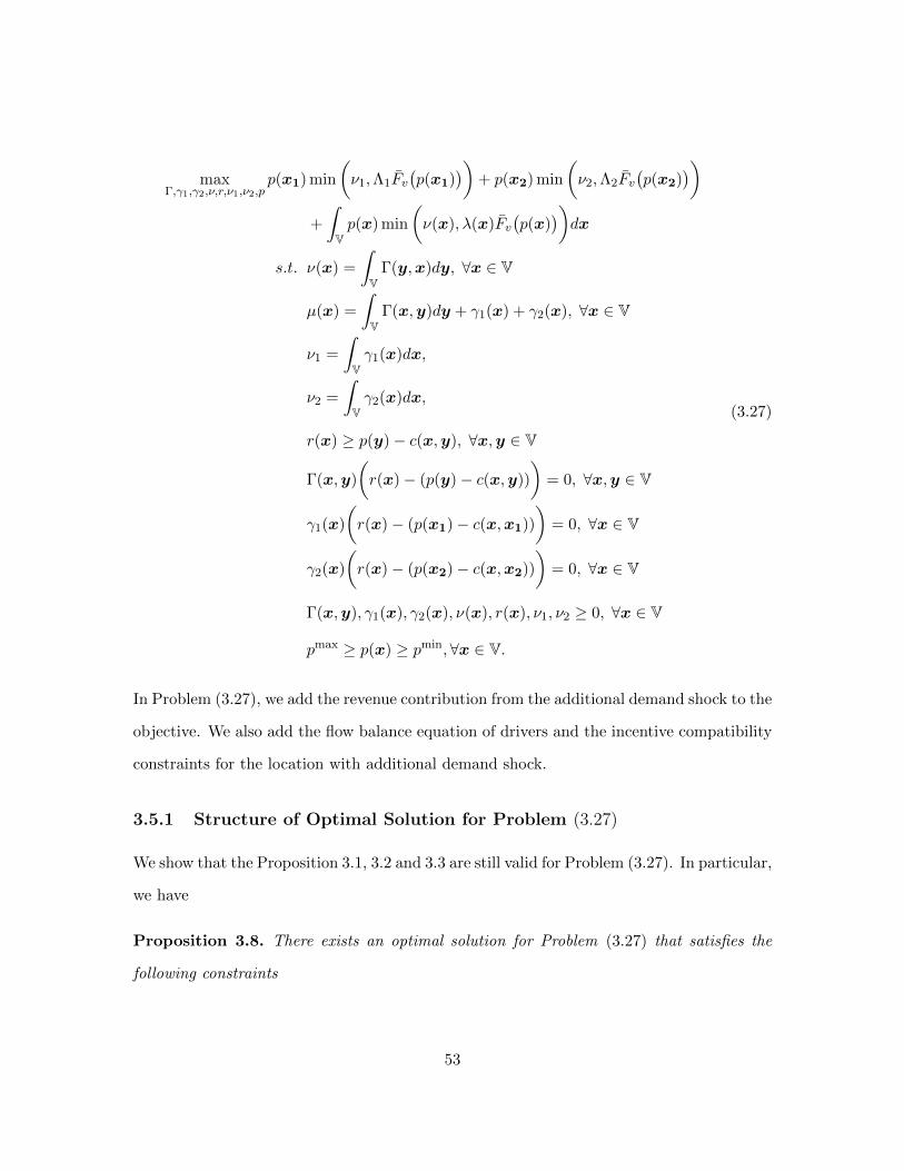
maxΓ,γ1,γ2,ν,r,ν1,ν2,p
p(x1) min
(ν1,Λ1Fv
(p(x1)
))+ p(x2) min
(ν2,Λ2Fv
(p(x2)
))+
∫Vp(x) min
(ν(x), λ(x)Fv
(p(x)
))dx
s.t. ν(x) =
∫V
Γ(y,x)dy, ∀x ∈ V
µ(x) =
∫V
Γ(x,y)dy + γ1(x) + γ2(x), ∀x ∈ V
ν1 =
∫Vγ1(x)dx,
ν2 =
∫Vγ2(x)dx,
r(x) ≥ p(y)− c(x,y), ∀x,y ∈ V
Γ(x,y)
(r(x)− (p(y)− c(x,y))
)= 0, ∀x,y ∈ V
γ1(x)
(r(x)− (p(x1)− c(x,x1))
)= 0, ∀x ∈ V
γ2(x)
(r(x)− (p(x2)− c(x,x2))
)= 0, ∀x ∈ V
Γ(x,y), γ1(x), γ2(x), ν(x), r(x), ν1, ν2 ≥ 0, ∀x ∈ V
pmax ≥ p(x) ≥ pmin, ∀x ∈ V.
(3.27)
In Problem (3.27), we add the revenue contribution from the additional demand shock to the
objective. We also add the flow balance equation of drivers and the incentive compatibility
constraints for the location with additional demand shock.
3.5.1 Structure of Optimal Solution for Problem (3.27)
We show that the Proposition 3.1, 3.2 and 3.3 are still valid for Problem (3.27). In particular,
we have
Proposition 3.8. There exists an optimal solution for Problem (3.27) that satisfies the
following constraints
53

1. Flow Exclusiveness with Multiple Shocks:
Γ(xi,xj)Γ(xj ,xk) = 0, ∀xi 6= xj ,xj 6= xk ∈ V.
2. Star Assignment with Multiple Shocks:
Γ(xi,xj) = 0, for xi 6= xj and xj /∈ x1,x2.
3. Minimal Incentive Compatibility with Multiple Shocks:
p(xi) ≥ p(xj)− c(xi,xj), ∀xi,xj ∈ V.
Based on these propositions, we have the following theorem.
Theorem 3.9. If pmin = pb, the optimal pricing policy of Problem (3.27) is in form of,
p(x) = max
(p(x1)− c(x,x1), p(x2)− c(x,x2), pb
), ∀x ∈ V (3.28)
s.t. |p(x1)− p(x2)| ≤ min
(c(x1,x2), c(x2,x1)
). (3.29)
We denote S = S1 ∪ S2 as surge region, where S1 := x|p(x) = p(x1) − c(x,x1) and
S2 := x|p(x) = p(x2)− c(x,x2).
We emphasize that in Theorem 3.9, Constraint (3.29) creates additional restriction on
the prices for demand surge locations such that they can not be freely searched as in its
individual demand surge problem. The platform needs to find the optimal p(x1) and p(x2)
jointly.
Next, we discuss the assignment policy for Problem (3.27). The procedure of construct-
ing the assignment policy is same as the procedure presented after Algorithm 3.1. However,
we may not have an explicit assignment in some cases. Denote Sb = S1 ∩ S2, i.e., Sb is the
intersection of two surge regions. If∫x∈Sb µ(x)dx = 0, i.e., Sb is a 0-measure set for µ, then
54

this intersection has no contribution to the total revenue. The two surge regions can make
their assignments independently following Algorithm 3.1.
However, when∫x∈Sb µ(x)dx > 0, drivers in Sb can serve both demand shocks. We need
to solve Problem (3.27) for a given pricing policy to get the assignment.
In sum, the platform needs to search the values of p(x1) and p(x2) under the constraint
|p(x1)− p(x2)| ≤ min
(c(x1,x2), c(x2,x1)
)and select the best pair. The algorithm that
processes this method is stated below.
Algorithm 3.3 Algorithm of Solving m = 2 Demand Shocks Problem with pmin = pb
1: Set M = 1000, δ = pmax−pbM
2: for i1 = 0 : M do3: for i2 = 0 : M do4: Set p(x1) = pb + i1δ, p(x2) = pb + i2δ
5: if |p(x1)− p(x2)| ≤ min
(c(x1,x2), c(x2,x1)
)then
6: Apply Theorem 3.9 to read off the pricing policy7: Given pricing policy, solve Problem (3.27) for assignment and overall revenue
rate R(i1, i2)8: end if9: end for
10: end for11: Return (i∗1, i
∗2) = arg max(i1,i2)R(i1, i2), p∗(x1) = pb + i∗1δ, p
∗(x2) = pb + i∗2δ
Figure 3.3 gives an example of the optimal pricing policy when V = (−∞,∞) and
demand shocks are at location x1 and Shock x2.
55

x
P (x)
P = Pb
Shock 1
x1
Shock 2
x2
Figure 3.3: Optimal Pricing Function p under m = 2 Demand Shocks, Price Constrained:pmin = pb
When there are m demand shocks in general, the pricing policy in Theorem 3.9 becomes
p(x) = max
(maxi∈[m]
(p(xi)− c(x,xi)
), pb
),∀x ∈ V
s.t. |p(xi)− p(xj)| ≤ min
(c(xi,xj), c(xj ,xi)
), ∀i, j ∈ [m].
Then, we search for the values of p(x1), ..., p(xm) in Algorithm 3.3 and pick the best one.
3.6 Unconstrained Pricing Problem
In this section, we extend our analysis to the unconstrained pricing problem, i.e., pmin is
strictly lower than the baseline price pb. Without loss of generality, we use pmin = 0 in this
part. The result is valid for any pmin > 0.
The formulation of unconstrained pricing problem is same as Problem Π, we do not
duplicate it here for brevity. For unconstrained pricing problem, Proposition 3.1, 3.2 and
3.3 are still valid. However, as pFv(p) is not decreasing on [pmin, pmax], Theorem 3.4 fails
for pmin = 0.
In particular, for each x which is not a demand shock location, we need to make a
56

separate decision of whether to include it in surge region. If so, the price at x must be
p(0) − c(x,0) following Proposition 3.2 and incentive compatibility constraint. If not,
platform can freely choose p(x) under the constraints in Problem Π. When pmin = pb,
the optimal prices of these two choices coincide to same value p(0) − c(x,0) due to the
monotonicity of pFv(p). However, when pmin = 0, if drivers are not relocated to the demand
shock node, the optimal p(x) may be different from p(0)−c(x,0). Thus, the optimal pricing
policy in Theorem 3.4 is invalid. We show a counter-example about this in Appendix B.1.
Next, we discuss the solution for unconstrained pricing problem under different cases.
3.6.1 Norm Induced Distance Metric c
When dis-utility function c is a norm induced distance metric, we have the following results.
V = [0,∞), Demand Surge at 0. When space V = [0,∞), demand surge happens at
origin, or V is rotational symmetric with respect to the demand shock node, the problem is
reduced to a one-dimensional space. Under this setting, we make an additional assumption
in this section.
Assumption 3.5. pFv(p) is weakly increasing on p ≤ pb.
Together with Assumption 3.4, we in fact assume pFv(p) is uni-modular on [pmin, pmax]
in this section. Then, we have
Theorem 3.10. If pmin = 0, the optimal pricing policy with distance metric c and V =
[0,∞) is in form of,
p(x) = p(0)− c(x, 0), ∀x ≤ l; p(x) = min
(pb, p(l) + c(l, x)
), ∀x ≥ l, (3.30)
where l satisfies p(0) − c(l, 0) ≤ pb. We denote S := x ≤ l as surge region. Under the
pricing policy (3.30), the assignment determined by Algorithm 3.1 is optimal.
Figure 3.4 shows an example of this pricing policy.
57

Pb
Surge Price
Distance from Surge Node
l
Figure 3.4: Surge Prices p as a Function of Distance from Surge Node, Price Unconstrained:pmin = 0
We present the proof in Appendix A.6. In Theorem 3.10, the optimal pricing function
is determined by two parameters, the price at demand shock location p(0) and boundary l
of surge region. Different from Problem Π with pmin = pb that the boundary of surge region
is intrinsically determined by p(0), for unconstrained pricing problem, the boundary l of
surge region needs to be decided separately. We need to search for both of p(0) and l for
optimal policy. Also, the optimal pricing policy for the unconstrained pricing problem can
set price lower than pb at some locations.
When V is rotational symmetric with respect to the demand shock node, we lose the
structure of pricing policy in Theorem 3.10. In particular, Proposition 3.1, 3.2 and 3.3 are
still valid, and the pricing and assignment policy within the surge region are still same as
those in Theorem 3.10. However, we do not any efficient way to determine surge region.
This is the same situation when c is a general function.
3.7 Non-instantaneous Relocation
In this section, we discuss the problem when the relocation of driver is not instantaneous.
For brevity of the model, we use discrete space to present our results. In particular, we
58
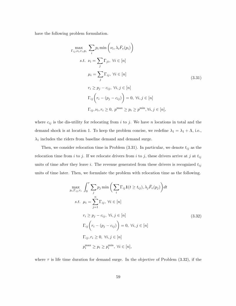
have the following problem formulation.
maxΓij ,νi,ri,pi
∑i
pi min
(νi, λiFv(pi)
)s.t. νi =
∑j
Γji, ∀i ∈ [n]
µi =∑j
Γij , ∀i ∈ [n]
ri ≥ pj − cij , ∀i, j ∈ [n]
Γij
(ri − (pj − cij)
)= 0, ∀i, j ∈ [n]
Γij , νi, ri ≥ 0, pmax ≥ pi ≥ pmin, ∀i, j ∈ [n],
(3.31)
where cij is the dis-utility for relocating from i to j. We have n locations in total and the
demand shock is at location 1. To keep the problem concise, we redefine λ1 = λ1 + Λ, i.e.,
λ1 includes the riders from baseline demand and demand surge.
Then, we consider relocation time in Problem (3.31). In particular, we denote tij as the
relocation time from i to j. If we relocate drivers from i to j, these drivers arrive at j at tij
units of time after they leave i. The revenue generated from these drivers is recognized tij
units of time later. Then, we formulate the problem with relocation time as the following.
maxpi,Γij ,ri
∫ τ
0
∑j
pj min
(∑i
Γij1(t ≥ tij), λjFv(pj))dt
s.t. µi =n∑j=1
Γij , ∀i ∈ [n]
ri ≥ pj − cij , ∀i, j ∈ [n]
Γij
(ri − (pj − cij)
)= 0, ∀i, j ∈ [n]
Γij , ri ≥ 0, ∀i, j ∈ [n]
pmaxi ≥ pi ≥ pmin
i , ∀i ∈ [n],
(3.32)
where τ is life time duration for demand surge. In the objective of Problem (3.32), if the
59

platform relocates drivers from region i to pick up a rider in region j, the platform loses
the riders at j in the first tij units of time. The indicator 1(t ≥ tij) identifies the beginning
time of driver relocation flow Γij contributing to the total revenue.
Without loss of generality, we assume tij ≤ τ,∀(i, j). If this is not true for a pair of
(i, j), then the driver relocation flow from i to j has no contribution to the total revenue
because they arrive after the demand surge ends. Then, we have,
Theorem 3.11. If pmin = pb, the optimal pricing policy of Problem (3.32) is in form of,
pi = max(pb, p1 − ci1), ∀i ∈ [n]. (3.33)
We denote S := i|pi = p1 − ci1 as surge region.
To determine the assignment policy, we first notice that the relocation can only happen
within the surge region. Outside the surge region, relocation is not incentive compatible
and we match all drivers with riders at same location. For the assignment within surge
region, we have the following lemma.
Lemma 3.12. The value of Problem (3.32) remains same if we require at most one of the
following two inequalities
νi > λiFv(pi),∑j 6=i
Γji > 0,
is true for any location i in surge region.
We present the proof in Appendix A.7. Then, for each location i in surge region, we
have,
1. If∑
j 6=i Γji = 0, i.e., there is no driver relocated into i, all the effective riders at node
i are served immediately. The revenue collected from location i in time window [0, τ ]
is
τpi min
(Γii, λiFv(pi)
),
60
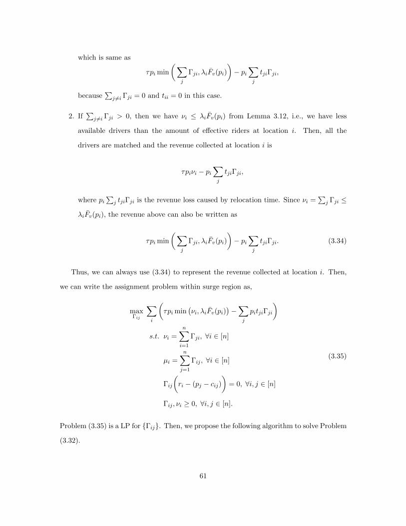
which is same as
τpi min
(∑j
Γji, λiFv(pi)
)− pi
∑j
tjiΓji,
because∑
j 6=i Γji = 0 and tii = 0 in this case.
2. If∑
j 6=i Γji > 0, then we have νi ≤ λiFv(pi) from Lemma 3.12, i.e., we have less
available drivers than the amount of effective riders at location i. Then, all the
drivers are matched and the revenue collected at location i is
τpiνi − pi∑j
tjiΓji,
where pi∑
j tjiΓji is the revenue loss caused by relocation time. Since νi =∑
j Γji ≤
λiFv(pi), the revenue above can also be written as
τpi min
(∑j
Γji, λiFv(pi)
)− pi
∑j
tjiΓji. (3.34)
Thus, we can always use (3.34) to represent the revenue collected at location i. Then,
we can write the assignment problem within surge region as,
maxΓij
∑i
(τpi min
(νi, λiFv(pi)
)−∑j
pitjiΓji
)
s.t. νi =
n∑i=1
Γji, ∀i ∈ [n]
µi =
n∑j=1
Γij , ∀i ∈ [n]
Γij
(ri − (pj − cij)
)= 0, ∀i, j ∈ [n]
Γij , νi ≥ 0, ∀i, j ∈ [n].
(3.35)
Problem (3.35) is a LP for Γij. Then, we propose the following algorithm to solve Problem
(3.32).
61
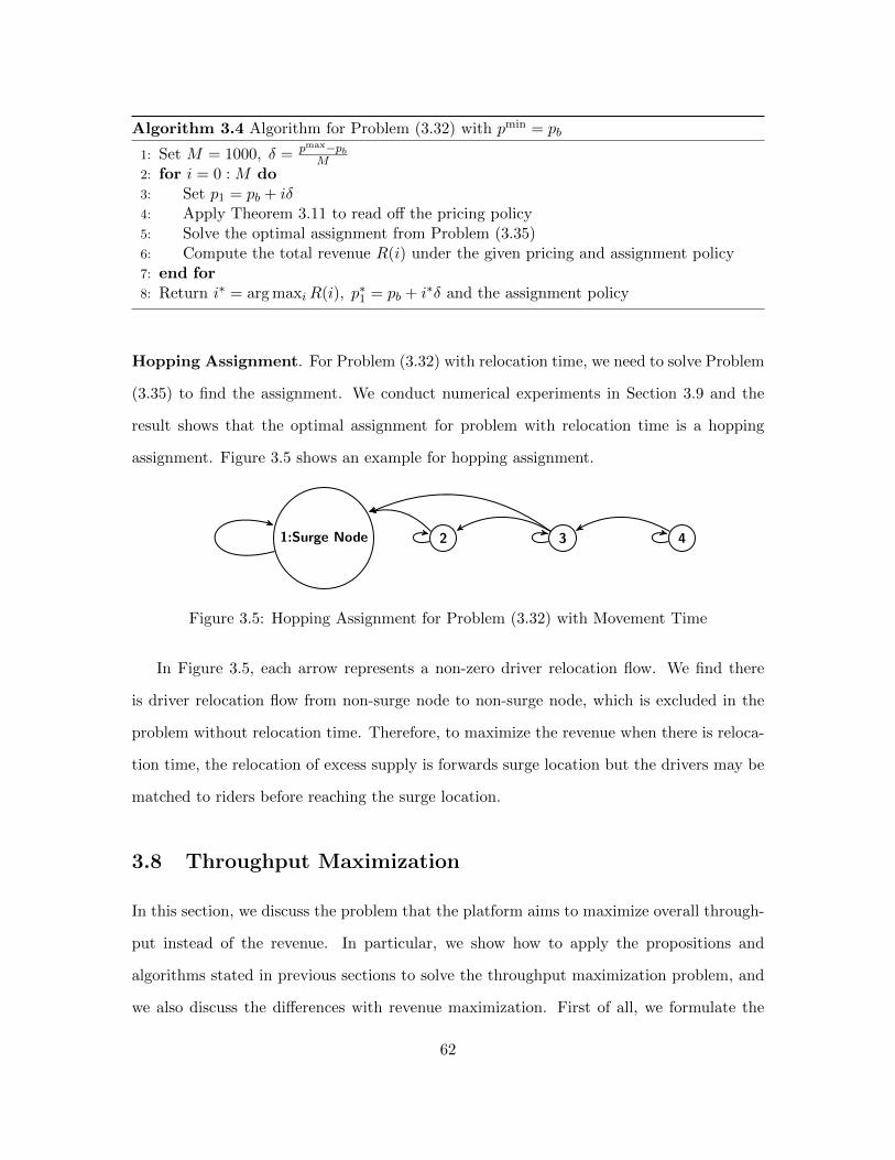
Algorithm 3.4 Algorithm for Problem (3.32) with pmin = pb
1: Set M = 1000, δ = pmax−pbM
2: for i = 0 : M do3: Set p1 = pb + iδ4: Apply Theorem 3.11 to read off the pricing policy5: Solve the optimal assignment from Problem (3.35)6: Compute the total revenue R(i) under the given pricing and assignment policy7: end for8: Return i∗ = arg maxiR(i), p∗1 = pb + i∗δ and the assignment policy
Hopping Assignment. For Problem (3.32) with relocation time, we need to solve Problem
(3.35) to find the assignment. We conduct numerical experiments in Section 3.9 and the
result shows that the optimal assignment for problem with relocation time is a hopping
assignment. Figure 3.5 shows an example for hopping assignment.
1:Surge Node 2 3 4
Figure 3.5: Hopping Assignment for Problem (3.32) with Movement Time
In Figure 3.5, each arrow represents a non-zero driver relocation flow. We find there
is driver relocation flow from non-surge node to non-surge node, which is excluded in the
problem without relocation time. Therefore, to maximize the revenue when there is reloca-
tion time, the relocation of excess supply is forwards surge location but the drivers may be
matched to riders before reaching the surge location.
3.8 Throughput Maximization
In this section, we discuss the problem that the platform aims to maximize overall through-
put instead of the revenue. In particular, we show how to apply the propositions and
algorithms stated in previous sections to solve the throughput maximization problem, and
we also discuss the differences with revenue maximization. First of all, we formulate the
62

throughput maximization problem as,
min
(ν0,ΛFv
(p(0)
))+
∫V
min
(ν(x), λ(x)Fv
(p(x)
))dx
Constraints (3.5) - (3.12).
(3.36)
3.8.1 Structure of Optimal Solution for Problem (3.36)
Since the throughput objective is increasing in ν0 and ν(x) and decreasing in p(x, and the
constraints are same as the revenue maximization problem, we can use the same proofs for
Proposition 3.1, 3.2, 3.3 and Theorem 3.4 to show they are also valid for the throughput
optimization problem. In particular, we have,
Theorem 3.13. The throughput maximization pricing policy is in form of,
p(x) = max
(pmin, p0 − c(x,0)
), ∀x ∈ V. (3.37)
We denote S := x|p(x) = p(0)− c(x,0) as surge region. Under the pricing policy (3.37),
the assignment determined by Algorithm 3.5 is optimal.
Algorithm 3.5 Optimal Assignment for Problem (3.36) under Pricing Policy (3.37)
1: for x ∈ S \ 0 do2: Set ν(x) = λ(x)Fv
(p(x)
)3: end for4: Set ν0 =
∫S µ(x)− λ(x)Fv
(p(x)
)dx
5: for x /∈ S do6: Set ν(x) = µ(x)7: end for
We emphasize that Algorithm 3.1 shown in Theorem 3.4 is also an optimal solution for
this throughput problem. Here, we have multiple optimal assignment policy because for
locations with different prices, there is no difference in their throughput contribution. As
assignment policy uses up all effective riders or drivers is optimal.
Consequently, the throughput problem is also reduced to a single variable problem to
decide p(0). Since the maximum throughput contributed from the entire surge region is the
63

minimum of effective riders and drivers within surge region and this value can be achieved
by the Algorithm 3.5, Problem (3.36) reduces to
max
(min
(ΛFv
(p(0)
)+
∫Sλ(x)Fv
(p(x)
)dx,
∫Sµ(x)dx
)+
∫V\S
λ(x)Fv(p(x)
)dx
)s.t. p(x) = max
(pmin, p(0)− c(x,0)
), ∀x ∈ V
S = x|p(x) = p(0)− c(x,0),
pmax ≥ p(0) ≥ pmin.
(3.38)
The objective in Problem (3.38) is the optimal throughput inside surge region plus the
throughput outside surge region. The constraints are the definitions for p(x) and S, where
p(0) is the only decision variable. Next, we write the objective in Problem (3.38) as
min
(ΛFv
(p(0)
)+
∫Vλ(x)Fv
(p(x)
)dx,
∫Sµ(x)dx+
∫V\S
λ(x)Fv(p(x)
)dx
), (3.39)
by moving∫V\S λ(x)Fv
(p(x)
)dx into the min operator. We claim that the first term in
(3.39) is decreasing with p(0) whereas the second term is increasing with p(0). To show
that, when p(0) increases, p(x) increases, then Fv(p(0)) and Fv(p(x)) decrease. Therefore
the first term in (3.39) decreases. Also, S enlarges when p(0) increases. In the area that
S expands, we use µ(x) to replace λ(x)Fv(p(x)) in the second integral in (3.39). Since
µ(x) ≥ λ(x)Fv(p(x)
), the second term increases with p(0).
Consequently, the optimal p(0) of Problem (3.38) is the solution of
ΛFv(p(0)
)+
∫Sλ(x)Fv
(p(x)
)dx =
∫Sµ(x)dx, (3.40)
i.e., the p(0 that equals the amount of effective riders and drivers inside surge region. Next,
we present the algorithm for solving Problem (3.36).
64
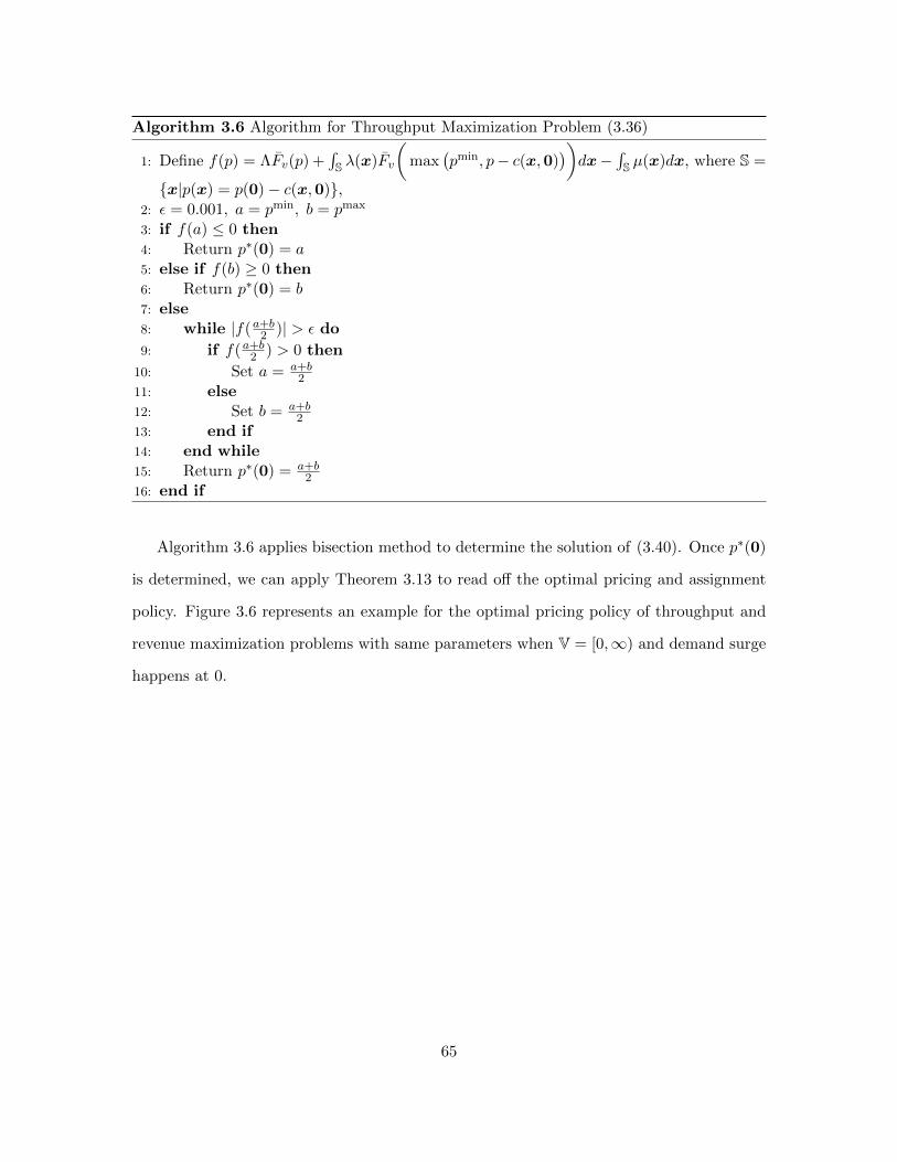
Algorithm 3.6 Algorithm for Throughput Maximization Problem (3.36)
1: Define f(p) = ΛFv(p) +∫S λ(x)Fv
(max
(pmin, p− c(x,0)
))dx−
∫S µ(x)dx, where S =
x|p(x) = p(0)− c(x,0),2: ε = 0.001, a = pmin, b = pmax
3: if f(a) ≤ 0 then4: Return p∗(0) = a5: else if f(b) ≥ 0 then6: Return p∗(0) = b7: else8: while |f(a+b
2 )| > ε do
9: if f(a+b2 ) > 0 then
10: Set a = a+b2
11: else12: Set b = a+b
213: end if14: end while15: Return p∗(0) = a+b
216: end if
Algorithm 3.6 applies bisection method to determine the solution of (3.40). Once p∗(0)
is determined, we can apply Theorem 3.13 to read off the optimal pricing and assignment
policy. Figure 3.6 represents an example for the optimal pricing policy of throughput and
revenue maximization problems with same parameters when V = [0,∞) and demand surge
happens at 0.
65

xP = Pb
P (x)
Throughput
Revenue
Figure 3.6: Optimal Price Function p for Revenue and Throughput Maximization, DemandSurge at 0, Price Constrained: pmin = pb
These two pricing policies yield same structure of p(x) = max
(pb, p(0) − c(x,0)
),
but the throughput optimal pricing curve is at a higher position than the revenue optimal
pricing curve. This is because the throughput maximization solution serves all effective
riders. However, the revenue maximization solution may have some effective riders unserved.
Since the number of excess riders inside surge region is decreasing with p(0), the optimal
p(0) for revenue maximization is lower.
3.9 Numerical Study
In this section, we use the model of Problem (3.31) to conduct numerical analysis for the
surge pricing problem.
Experiment Setup. In this part, we set V as a discrete space with n = 7 locations and
demand surge happens at node 1. The dis-utility function c is defined as cij = C · |i−j|n . The
arrival rate of available drivers is µi = 10, ∀i ∈ [n] and the arrival rate of baseline riders
is λi = 3,∀i ∈ [n]. The willingness to pay function of all riders is Fv(p) = ppmax , where
pmin = 0, pmax = 100. Then, the baseline price pb is 50.
66
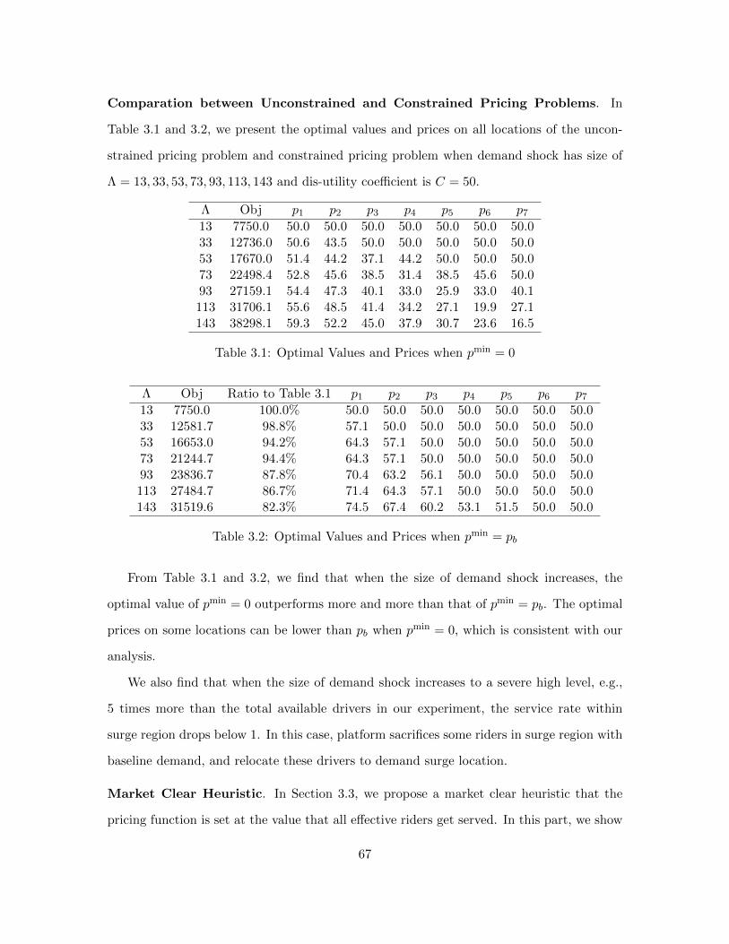
Comparation between Unconstrained and Constrained Pricing Problems. In
Table 3.1 and 3.2, we present the optimal values and prices on all locations of the uncon-
strained pricing problem and constrained pricing problem when demand shock has size of
Λ = 13, 33, 53, 73, 93, 113, 143 and dis-utility coefficient is C = 50.
Λ Obj p1 p2 p3 p4 p5 p6 p7
13 7750.0 50.0 50.0 50.0 50.0 50.0 50.0 50.033 12736.0 50.6 43.5 50.0 50.0 50.0 50.0 50.053 17670.0 51.4 44.2 37.1 44.2 50.0 50.0 50.073 22498.4 52.8 45.6 38.5 31.4 38.5 45.6 50.093 27159.1 54.4 47.3 40.1 33.0 25.9 33.0 40.1113 31706.1 55.6 48.5 41.4 34.2 27.1 19.9 27.1143 38298.1 59.3 52.2 45.0 37.9 30.7 23.6 16.5
Table 3.1: Optimal Values and Prices when pmin = 0
Λ Obj Ratio to Table 3.1 p1 p2 p3 p4 p5 p6 p7
13 7750.0 100.0% 50.0 50.0 50.0 50.0 50.0 50.0 50.033 12581.7 98.8% 57.1 50.0 50.0 50.0 50.0 50.0 50.053 16653.0 94.2% 64.3 57.1 50.0 50.0 50.0 50.0 50.073 21244.7 94.4% 64.3 57.1 50.0 50.0 50.0 50.0 50.093 23836.7 87.8% 70.4 63.2 56.1 50.0 50.0 50.0 50.0113 27484.7 86.7% 71.4 64.3 57.1 50.0 50.0 50.0 50.0143 31519.6 82.3% 74.5 67.4 60.2 53.1 51.5 50.0 50.0
Table 3.2: Optimal Values and Prices when pmin = pb
From Table 3.1 and 3.2, we find that when the size of demand shock increases, the
optimal value of pmin = 0 outperforms more and more than that of pmin = pb. The optimal
prices on some locations can be lower than pb when pmin = 0, which is consistent with our
analysis.
We also find that when the size of demand shock increases to a severe high level, e.g.,
5 times more than the total available drivers in our experiment, the service rate within
surge region drops below 1. In this case, platform sacrifices some riders in surge region with
baseline demand, and relocate these drivers to demand surge location.
Market Clear Heuristic. In Section 3.3, we propose a market clear heuristic that the
pricing function is set at the value that all effective riders get served. In this part, we show
67

the numerical performance for the market clear heuristic. In addition to the parameters
in experiment setup, we use different values for λi and µi to conduct the experiments.
We parameterize λi, µi, and size of demand shock Λ as
µi = βλi, ∀i ∈ [n]; Λ = λ1Λ
λ1= λ1Λscale.
In Table 3.3, we show the performance of market clear heuristic for values of β = 1, 3, 6, 10
and Λscale = 23, 63, 143 in column Obj of Heuristic %, which is percentage of heuristic value
to the optimal value.
β Λscale Obj of Heuristic % β Λscale Obj of Heuristic %
1 23 99.2% 6 23 100.0%1 63 96.0% 6 63 100.0%1 143 93.5% 6 143 99.8%
3 23 100.0% 10 23 100.0%3 63 99.9% 10 63 100.0%3 143 98.7% 10 143 100.0%
Table 3.3: Percentage of Optimal Value Achieved by Clear-market Heuristic
In Table 3.3, we find that market clear heuristic can achieve more than 93% of the
optimal value in our experiments. When β is high or Λscale is low, i.e., the number of
available drivers is ample or the size of the demand shock is small, the heuristic performs
well.
Convex Dis-utility Function c. In this part, we conduct experiment to the case when c
does not satisfy triangle inequality (3.1). In particular, we consider the case that dis-utility
function c is strictly convex,
c(x,y) = 10||x− y||2/7.
We also change the driver arrival rate µi and number of nodes in space V. These numbers
together with the experiment results are shown in Table 3.4, 3.5 and 3.6
68

i pi λiFv(pi) µi νi Γij 1 2 3 4 5 6
1 52.8 7.6 6 7.6 1 6 0 0 0 0 02 51.4 1.0 2 1.0 2 1.6 0.4 0 0 0 03 50.0 2 4 3.5 3 0 0.5 3.5 0 0 04 50.0 3 6 6.0 4 0 0 0 6.0 0 05 50.0 4 8 8.0 5 0 0 0 0 8.0 06 50.0 5 10 10.0 6 0 0 0 0 0 10.0
Table 3.4: Solution with Quadratic Dis-utility Function, Λ = 10
i pi λiFv(pi) µi νi Γij 1 2 3 4 5 6
1 63.9 13.0 6 13.4 1 6.0 0 0 0 0 02 57.0 0.9 2 1.6 2 2.0 0 0 0 0 03 52.8 1.9 4 2.5 3 4.0 0 0 0 0 04 51.4 3.0 6 4.1 4 1.4 1.6 2.5 0.5 0 05 50.0 4.0 8 4.4 5 0 0 0 3.6 4.4 06 50.0 5.0 10 10.0 6 0 0 0 0 0 10.0
Table 3.5: Solution with Quadratic Dis-utility Function, Λ = 30
i pi λiFv(pi) µi νi Γij 1 2 3 4 5 6
1 69.2 17.2 6 17.2 1 6.0 0 0 0 0 02 62.3 0.8 2 0.8 2 2.0 0 0 0 0 03 56.9 1.7 4 3.9 3 4.0 0 0 0 0 04 52.8 2.8 6 3.1 4 5.2 0.8 0 0 0 05 51.4 3.9 8 5.4 5 0 0 3.9 3.1 1.0 06 50.0 5.0 10 5.6 6 0 0 0 0 4.4 5.6
Table 3.6: Solution with Quadratic Dis-utility Function, Λ = 50
The results show that the optimal assignment policy is hopping assignment, not star
assignment any more. The pricing policy is not consistent to the structure in Theorem 3.4
either.
3.10 Conclusion
In this chapter, we consider fluid model and give tractable approach to compute optimal
prices and assignment to match supply with demand during surge scenarios under reasonable
assumptions.
69

Problem is challenging because it is non-convex and has infinite number of decisions
variables. We first show that there exists an optimal solution that satisfies some nice
structural properties. Based on these properties, we design an optimal pricing and matching
policy. The optimal pricing policy is determined by the price at surge node, and the price
decreases with the dis-utility of driver relocation until it reaches baseline price. The optimal
assignment policy relocates excess drivers to demand surge node within surge region and
retains the remaining drivers at their original locations.
We extend our results in a number of directions, including strategic rider relocation,
multiple demand shocks, unconstrained pricing policy, non-instantaneous relocation time,
and throughput maximization, and we obtain similar qualitative results.
70

Chapter 4
Near-Optimal Price Rebates for
Demand Response under Power
Flow Constraints
4.1 Introduction
Due to an increasing integration of renewable sources such as wind and solar power on the
grid, the supply uncertainty in the electricity market has increased significantly. Demand-
side participation has, therefore, become essential to maintain a real-time energy balance in
the grid. There are several ways to increase the demand-side participation for the real-time
energy balance including time of use pricing, real-time pricing for smart appliances, inter-
ruptible demand-response contracts and real-time price rebates and incentives. Typically,
an electric utility buys the forecast day-ahead load in the day-ahead market and pays the
shortfall (if the actual demand turns out to be higher) on the real-time market. However, if
the supply in the real-time market is scarce, the real-time prices can be very high and the
utility is exposed to the high prices. Such a scenario can arise often if a significant fraction
of power is generated by highly uncertain sources such as wind and solar plants. Since end
customers, including residential and most commercial customers, do not pay the real-time
71
prices, the demand does not adjust to the real-time prices and the utility is exposed to the
price shocks. With price rebates or interruptible load contracts, the utility company has
the option of offering financial incentives to the customers to reduce their demand in such
scenarios.
Interruptible load contracts have been studied extensively in the literature as an ap-
proach to demand response, both from the perspective of optimal execution of contracts
(see Oren and Smith [64]. Caves et al. [20]) and also design and pricing (see Fahrioglu
and Alvarado [30], Kamat and Oren [43], Tan and Varaiya [79], Oren [63], Bhattacharta et
al. [84]) and more recently, Bitar and Low [14], Roozbehani et al. [70]. We refer readers to
the survey by Baldick et al. [8] that provides a good overview of the literature.
In this chapter, we consider an alternative approach where the utility can offer real-time
price incentives or rebates to consumers to reduce the power consumption. The goal is to
compute the prices (or rebates) to offer to different consumers to reduce the power consump-
tion such that the required reduction can be achieved in minimum possible cost. Since the
AC power flow model allows us to model the transmission losses in the distribution network,
we can optimize over both the reduction in demand and the reduction of transmission losses
in the network. Our main contribution is that we propose an efficient iterative heuristic to
solve the offer price optimization problem under AC power flow constraints, and we show
that the AC formulation leads to a significant reduction in the rebates that one needs to
offer in order to shed a certain demand.
The main challenge in this problem arises from the non-convexity of AC power flow
constraints and also the uncertainty in price elasticity of the demand. To solve the problem,
we developed our heuristic which gives an iterative procedure to compute the offer prices
to minimize the total expected cost using a sample average approximation (SAA) to deal
with the stochastic optimization problem (4.2), and a semidefinite programming (SDP)
based relaxation to deal with the non-convexity of AC power flow constraints. We conduct
numerical experiments to compare the performance of our heuristic with other optimization
approaches including using DC power flow model or no power flow model at all. Our
72
computational study shows that the performance of our AC power flow based heuristic is
significantly better than the other approaches. Unlike the DC power flow constraints, the
AC power flow constraints model transmission losses. Therefore, we can optimize the offer
prices based on the topology of the grid and leverage both the actual load reduction as well
as the reduction in the transmission losses.
The rest of this chapter is organized as follows. In Section 4.2, we give a full mathemat-
ical formulation to the demand response problem. In Section 4.2.1, we define the sample
average approximation method. In Section 4.2.2, we introduce the remaining model no-
tations and the SDP relaxation for the AC power flow constraints. Next, we present the
iterative heuristic for the offer price optimization problem (4.8) in Section 4.3 and show some
other power flow models for compare in Section 4.4. Finally, we present the computational
study in Section 4.5 and our conclusion in 4.6.
4.2 Problem Definition
In this section, we will give a mathematical formulation for this demand response problem.
Let K := 1, 2, ...,K denote the set of buses, G ⊆ K denote the set of generator buses,
C ⊆ K denote the set of demand buses. Without loss of generality, we assume G ∩ C = ∅.
Let N ⊆ K × K denote the set of transmission lines. Let P gk + jQgk denote the generation
at bus k ∈ G, they are the decision variables in this problem. Let P ci + jQci denote the
nominal load at demand bus i ∈ C, i.e. the demand in the absence of any rebates. They
are given quantities. For each demand bus, we are given the response (or supply) function
Ri(γi), that specifies the mean reduction of load at bus i at any given offer price (or rebate)
γi. We assume that the actual demand reduction is random, and is given by
Ri(γi) = Ri(γi) + εi,
where εi is a mean zero random variable with a known distribution. We assume that the
distribution of εi does not depend on the rebate γi. We allow for the error distributions
73

at different demand buses to be possibly different. The total expected payment at offer
price Γ is given by E[∑
i γi(Ri(γi) + εi)] =∑
i γiR(γi). Meanwhile, the actual payment is∑i γiRi(γi) and it achieves a total reduction of
∑i Ri(γi) on the demand load. The total
reduction on the load plus the reduction on transmission loss contributes the total reduction
in the power generation. Let P g(0) =∑
k∈G Pgk (0,0) be the total power generation when
there is no rebate and P g(Γ, ε) =∑
k∈G Pgk (Γ, ε) be the total power generation when the
rebate vector is Γ and the realization of uncertainty vector is ε. Thus, the total reduction
over the grid is P g(0)− P g(Γ, ε).
We are also given a power reduction target D and we pay a shortfall penalty λ per unit
whenever we are not able to meet target reduction. If P g(0)− P g(Γ, ε) is greater or equal
to D, we achieve our target at the cost of∑
i γiRi(γi). However, if it is smaller than D,
we will suffer from the shortfall penalty of λ(D − (P g(0) − P g(Γ, ε))
)of not fulfilling the
target. Thus, the total expected cost of the demand response program for offer prices Γ is
given by ∑Ki=1 γiRi(γi) + λEε
[(D − (P g(0)− P g(Γ, ε))
)+
], (4.1)
where (y)+ = maxy, 0. Again, P g(0) =∑
k∈G Pgk (0,0) denotes the total generation (or
injection) without any price rebate, and P g(Γ, ε) =∑
k∈G Pgk (Γ, ε) is the total generation
when the price rebate is Γ = (γ1, . . . , γK) and the load at each demand bus i is (P ci −
Ri(γi)− εi + jQci ). From (4.1), it follows that the offer price optimization problem can be
formulated as the following stochastic optimization problem,
minΓ∑K
i=1 γiRi(γi) + λEε[(D − (P g(0)− P g(Γ, ε))
)+
]s.t. P g(0), P g(Γ, ε) satisfy AC power flow constraints.
(4.2)
Note that the power flow constraints for an AC power grid are non-convex and optimizing
over these constraints is NP-hard in general [49]. Therefore, solving (4.2) to compute offer
prices is computationally hard even for very simple supply functions Ri. In the following
sections, we will introduce how to use the SDP relaxation of problem (4.2) to solve the
74
demand response problem.
4.2.1 Sample Average Approximation
The first step is to estimate the expected value in the objective function by using sample
average approximation(SAA), i.e., we approximate the expectation by an average over a
set of samples. Thus, after applying SAA, (4.2) becomes to the following optimization
problem,
minΓ∑K
i=1 γiRi(γi) + λM
∑Mn=1
(D − (P g(0)− P g(Γ, ε(n)))
)+
s.t. P g(0), P g(Γ, ε(n)) satisfy AC power flow constraints,(4.3)
where ε(1), . . . , ε(M) are M IID samples of stochastic error vector ε. SAA will be used to
deal with the expectation in objective function all the time.
4.2.2 SDP Formulation for AC Power Flow Constraints
The second step of solving (4.2) is to introduce the SDP relaxation for the AC power
flow constraints. Our SDP relaxation model is based on the work of Lavaei and Low
(2012). As we stated before, the non-convexity of this problem is from non-convex AC
power flow constraints. Lavaei and Low (2012) derived the circuit model of the power
network through replacing every transmission line and transformer by their equivalent Π
models. In this circuit model, let ykl denote the effective admittance between buses k
and l, and ykk denotes the admittance-to-ground at bus k. Let Y ∈ CK×K represent the
admittance matrix of the distribution network in this equivalent circuit model, where for
each (k, l) ∈ N , Ykl = −ykl if k 6= l, and ykk +∑
m∈Nk ykm otherwise (Nk denotes the set
of all buses that are directly connected to bus k). Let V = (V1, ..., VK) denote the complex
voltage vector and I = (I1, ..., IK) denote the complex current vector. Then, it follows that
75

the power injected into the grid at bus k is given by
Sk = Re(VkI∗k) + jIm(VkI
∗k)
= Re(V ekekY V∗) + jIm(V ekekY V
∗)
= X>YkX + jX>YkX = Tr(YkW ) + jTr(YkW ),
where
Yk := ekeTkY
Yk :=1
2
ReYk + Y T
k
ImY Tk − Yk
ImYk − Y T
k
ReYk + Y T
k
Yk := −1
2
ImYk + Y T
k
ReYk − Y T
k
ReY Tk − Yk
ImYk + Y T
k
X :=
[Re VT Im VT
]TW := XXT ,
and e1, e2, ..., eK are standard unit vectors in RK . Thus, the power injection constraints
are given by
Tr(YkW ) =
P gk k ∈ G,
−P ck k ∈ C,
Tr(YkW ) =
Qgk k ∈ G,
−Qck k ∈ C,
(4.4)
And
Pmink ≤ P gk ≤ P
maxk , Qmin
k ≤ Qgk ≤ Qmaxk , k ∈ G. (4.5)
In addition to the power injection constraints, there are upper and lower bounds on the
magnitude |Vk|2 = Re(Vk)2 +Im(Vk)
2 at bus k, on the magnitude |Vl−Vk|2 of the difference
76

in voltage between bus l and m, re-formulated as
(V mink )2 ≤ Tr(MkW ) ≤ (V max
k )2,
Tr(MlmW ) ≤ (∆V maxlm )2,
(4.6)
where
Mk :=
ekeT 0
0 ekeT
Mlm :=
(el − em)(el − em)T 0
0 (el − em)(el − em)T
.There are line constraints on the voltage, there are also constraints on the real and apparent
power being carried on a line (l,m). The constraint that the real power Plm ≤ Pmaxlm and
the magnitude of the apparent power |Slm| ≤ Smaxlm , can be re-formulated as
TrYlmW ≤ Pmaxlm ,
TrYlmW 2 + TrYlmW 2 ≤ (Smaxlm )2,
(4.7)
where
Ylm := (ylm + ylm)ele>l − ylmele>m
Ylm :=1
2
ReYlm + Y T
lm
ImY Tlm − Ylm
ImYlm − Y T
lm
ReYlm + Y T
lm
Ylm := −1
2
ImYlm + Y T
lm
ReYlm − Y T
lm
ReY Tlm − Ylm
ImYlm + Y T
lm
.
The definition W = XX> is equivalent W 0, i.e. W is symmetric positive semidefinite,
and RankW = 1. Any rank-1 positive semidefinite matrix W that satisfies (4.4)-(4.7)
represents a feasible power flow.
77

Relaxing the rank constraint on W , we obtain an SDP relaxation of the power flow
constraints. The resulting constraint set is the actual one we will use to solve the AC power
flow demand response problem. Lavaei and Low [49] show that the above relaxation is exact
if the distribution network is a tree. Sojoudi and Lavaei [73] extend the results to several
other classes of networks where the above SDP formulation is exact. However, in general,
it is NP-hard to optimize over the power flow constraints.
4.3 Offer Price Optimization Problem under AC Power Flow
Constraints
In this section, we present our heuristic for the offer price optimization problem under AC
power flow constraints. The last step to formulate the whole program is that we need to
connect the objective function (4.3) to the voltage matrix W we defined above. When
applying pricing policy Γ and a given error ε to the demand response problem, we have
P gk (Γ, ε) = TrYkW (ε) for k ∈ G. Notice that W (ε) is a function of ε. For i ∈ C, we have
P ci (γi) = P ci − Ri(γi) − εi. Since −P ci (γi) = TrYiW (ε), we can add a constraint that
links the Γ with W , −P ci − TrYiW (ε)+Ri(γi) + εi = 0.
78
Then, the optimization problem can be written as,
minΓ,W
K∑i=1
γiRi(γi) +λ
M
M∑n=1
(D − (P g(0)− P g(Γ, ε(n)))
)+
(4.8)
s.t. P g(Γ, ε(n)) =∑j∈G
TrYjW
Pmink − P ck ≤ TrYkW ≤ Pmax
k − P ck ∀k ∈ G
Qmink −Qck ≤ TrY kW ≤ Qmax
k −Qck, ∀k ∈ G
(V mink )2 ≤ TrMkW ≤ (V max
k )2, ∀k ∈ K
(TrYlmW )2 + (TrY lmW )2 ≤ (Smaxlm )2, ∀(l,m) ∈ N
TrYlmW ≤ Pmaxlm , ∀(l,m) ∈ N
TrMlmW ≤ (∆V maxlm )2, ∀(l,m) ∈ N
− P ci − TrYiW +Ri(γi) + ε(n)i = 0, ∀i ∈ C
W 0, ∀i ∈ 1, ...,M.
Where the decision variable W is still dependent on the error term ε(n), and we are
going to talk how to simplify and solve it in the following sections.
4.3.1 Linear Supply Function
Recall that we are given a load reduction target D and the random load reduction at demand
bus i as a function of the price rebate γi is Ri(γi)+εi. In general, function Ri(γi) can admit
any form to reflect customer’s preference. For simplicity, we take linear form for the supply
function, as it can reflect consumer’s reference that they are willing to reduce more load
at a higher rebate price. At the same time, we assume εi is independent with each other
and we can generate samples of the random vector ε. Therefore, the supply function turns
to Ri(γi) = aiγi + εi, where ai is a positive constant. Following these assumptions, our
79
objective function becomes to
∑Ki=1 aiγ
2i + λ
M
∑Mn=1
(D − (P g(0)− P g(Γ, ε(n)))
)+. (4.9)
4.3.2 Linear Approximation for Injected Power
Even though we have applied sample average approximation and SDP relaxation model
to the original problem, in optimization problem (4.8), since M ≈ 100 to 1000 and W is
dependent on the error term ε(n) in (4.8), this problem is still intractable even for very
small networks, e.g. a network with K = 30 buses. To solve this dilemma, we construct an
affine function P (Γ, ε) to approximate the power generation P g(Γ, ε) function in a small
neighborhood of a given rebate vector Γ.
In particular, we define
P g(Γ, ε) ≈ P (Γ, ε) = P g(Γ,0) +∑i
πΓi εi, (4.10)
where P g(Γ,0) denotes the total generation when the offer price is Γ and the stochastic
error ε = 0. The sensitivity coefficients πΓ = (πΓi ) depend on the offer price Γ and denote
the change in total injected power per unit change in the demand at bus i. Thus, πΓ can
be interpreted as the dual variables corresponding to the real power balance constraint in
the optimal power flow problem of implementing offer price Γ. Algorithm 4.1 describes the
computation of the linear approximation of the total power generation at any offer price Γ.
We conduct numerical experiments to compare the error of the linear approximation for a
set of test networks and observe that the difference between the true injected power and the
linear approximation is at most, 2% across all test networks. Therefore, the linear approx-
imation provides a good approximation under reasonable bounds on standard deviation of
the stochastic errors.
80

Algorithm 4.1 Linear approximation of Power Generation
1: Input: Offer price Γ.2: Compute a solution W 0 to (4.4)-(4.7) that minimizes total power generation with
demand at each node k ∈ K, P ck −Rk(γk).3: πΓ
k : optimal dual variable for real power balance constraint at bus k ∈ K.4: Return:
P (Γ, ε) = P g(Γ,0) +∑k
πΓk εk.
4.3.3 Optimization Heuristic
Now we are ready to describe our iterative heuristic to compute the offer prices Γ using a
linear approximation of the total power generation (4.10). For the convenience of descrip-
tion, we assume that for the whole distribution network there is a single node where power
is injected from ISO into the distribution network. As mentioned earlier, a direct SAA
approach (4.8) is computationally intractable, since we need W (ε) to satisfy the constraints
for each sample ε and the number of samples is large even for small networks. Therefore,
instead of the direct SAA approach, we start with an initial offer price, Γ0 from solving the
demand response problem with deterministic supply functions and then we can formulate
the optimization problem to compute the offer prices in the next iterate as follows,
minΓ,W
∑i∈K aiγ
2i
+ λM
∑Mn=1
(D − P g(0) + P g(Γ,0) +
∑i∈K π
0i ε
(n)i
)+
s.t. W 0 satisfies (4.4)-(4.7) with P ci + jQci =
P ci − aiγi + jQci for i ∈ C,
(4.11)
where εn : n = 1, . . . ,M denotes M samples of the random vector ε. Note that the
constraints in (4.11) no longer depend on ε; consequently, there is a single positive semidef-
inite variable W . Therefore, we can solve the above problem efficiently. Note also that the
coefficients πi are constants in (4.11). We solve (4.11) to compute the offer prices in the
next iterate. We then compute the linear approximation for the power generation at the
new offer prices and continue this iterative procedure until it converges to a fixed point. We
81

describe the details in Algorithm 4.2.
Algorithm 4.2 Offer Price optimization Heuristic, AC-PF-DR
1: Initialize: t := 0, δ := 1, offer prices Γ0.2: while (δ > 0.001) do
Call Algorithm 4.1 to compute coefficients πΓti .
Solve (4.11) to compute Γt+1.
δ = maxi
|Γt+1i − Γti|
Γti.
t := t+ 1.3: end while4: Return: Γt.
On small instances of distribution networks, we conduct numerical experiments showing
that the algorithm converges quickly. However, the above procedure may not converge in a
reasonable time or may not even converge in general, we may need to modify this algorithm
for concrete instances. We will talk about the modification in the computational study
section.
4.4 Alternative Power Flow Constraints
In this section, we describe some alternative power flow models which will be used as
comparisons to the performance of our iterative heuristic.
4.4.1 DC Power Flows
The DC power flow model is constructed by linearizing the AC power flow equations. Let
θ denote the vector of phase angles of voltage at all the buses. Under typical operating
conditions, the angle difference |θl−θm| for any transmission line (l,m) ∈ N is small ( 10
degrees). Therefore, sin(θl−θm) ≈ (θl−θm) and cos(θl−θm) ≈ 1. For all transmission lines
(l,m) ∈ N , we assume that the resistance is nearly zero and also the magnitude of voltage
is 1 p.u. at all buses. Furthermore, we can, without loss of generality, assume that θ1 = 0.
With these approximations, we can formulate the power flow constraints as P = Bθ, where
P ∈ RK−1 is the vector of power injections for buses 2, . . . ,K, θ ∈ RK−1 is the vector
82

of nodal voltage angles, and B ∈ R(K−1)×(K−1) is the network admittance matrix. The
constraint for bus 1 is linearly dependent on the other constraints and can therefore, be
eliminated. In the DC approximation of the power flow constraints, the injected power
at each node sums up to 0. There is no transmission loss under the DC framework and
the cost on power loss in the objective function vanishes. However, we need to monitor
the differences in phase angles as large phase angle difference could cause instability in the
power network.
Let N ∈ 0,−1, 1K×K be the bus-line incidence matrix for the distribution network,
and let ρ denote the upper bound on allowed angle difference on any link. Then the DC
power flow offer price optimization problem can be formulated as follows.
minΓ,θ(ε(n)),P (ε(n))
∑i∈K aiγ
2i +
λM
∑Mn=1
(D − (P g(0)− P g(Γ, ε(n)))
)+
s.t. P (ε(n)) = Bθ(ε(n))
P g(Γ, ε(n)) =∑
k∈G Pk(ε(n))
−Pk(ε(n)) = P ck − akγk − ε(n)k , ∀k ∈ C∥∥Nθ(ε(n))
∥∥∞ ≤ ρ
Pmink ≤ Pk(ε(n)) ≤ Pmax
k , ∀k ∈ G,
(4.12)
where the notation P (ε(n)), θ(ε(n)) and P g(Γ, ε(n)) emphasizes that the phase angles, the
power on lines, and the overall power generation is a function of the stochastic error sam-
ple ε(n). Note that angle difference constraint can also be modeled as a penalty term
ηEε (Nθ(ε)− ρ)+ in the objective. Unlike the original AC power flow model, the DC model
(4.12) can be solved efficiently as it is actually a quadratic program. We need to emphasize
that since we assume that the resistance on transmission lines is zero, the formulation (4.12)
is not able to model transmission losses.
83

4.4.2 DCβ Power Flows
Since the DC model does not model any transmission loss over the grid, we can expect that
the optimal solution from DC model above will achieve a total reduction of D on the load
when penalty is high, so that the actual reduction over the grid will be greater than D.
If the transmission loss is a large proportion, this is a great waste in the incentive, as the
company overpays the rebates to customer. Therefore, we find an interesting modified DC
model for this purpose, as it is able to include partial transmission loss into the optimization.
We name it DCβ model. This model is actually a two-step method. Firstly, we solve the
OPF problem without any rebate. Then, define:
β = P g(0)∑Kk=1 P
ck
− 1. (4.13)
Here, β is the percentage of transmission loss over the grid when there is no rebate.
Then, in the second step, we use the same β value as our estimation of the percentage
of transmission loss over the grid when there exists rebates. Thus, the total reduction
estimation in this modified DC model becomes to,
(1 + β)K∑i=1
P ci − (1 + β)K∑i=1
(P ci − Ri(γi)) = (1 + β)K∑i=1
Ri(γi).
Thus, we add our estimate of reduction in transmission loss β∑K
i=1 Ri(γi) into the
total reduction. We claim that this estimation will only underestimate the true reduction
in transmission loss, which means that it will never incur a short-fall penalty due to we
overestimate the reduction on the transmission loss. This is because suppose β1 is the real
value of the percentage of transmission loss over the grid when we implement the offer prices
Γ. Then, the actual total reduction is,
(1 + β)∑K
i=1 Pci − (1 + β1)
∑Ki=1(P ci − Ri(γi))
= (β − β1)∑K
i=1 Pci + (1 + β1)
∑Ki=1 Ri(γi).
84

Here, the actual reduction in transmission loss is (β−β1)∑K
i=1 Pci +β1
∑Ki=1 Ri(γi). Because
the load is reduced, we have β1 ≤ β. Then, since the actual reduction can not surpass the
original load, we have∑K
i=1 Ri(γi) ≤∑K
i=1 Pci , which leads to (β − β1)
∑Ki=1 Ri(γi) ≤
(β − β1)∑K
i=1 Pci . Finally, we have
β
K∑i=1
Ri(γi) ≤ (β − β1)
K∑i=1
P ci + β1
K∑i=1
Ri(γi),
i.e., we underestimate the reduction in transmission loss. Then, our problem in step two is:
minΓ,θ(ε(n)),P (ε(n))
∑i∈K aiγ
2i + λ
M
∑Mn=1
(D − (1 + β)(P g(0)− P g(Γ, ε(n)))
)+
s.t. P (ε(n)) = Bθ(ε(n))
P g(Γ, ε(n)) =∑
k∈G Pk(ε(n))
−Pk(ε(n)) = P ck − akγk − ε(n)k , ∀k ∈ C∥∥Nθ(ε(n))
∥∥∞ ≤ ρ
Pmink ≤ Pk(ε(n)) ≤ Pmax
k , ∀k ∈ G.
This problem is actually a quadratic program, which is efficient to solve. Thus, we have
a modified DC model which considers the saving in transmission loss and keeps the model
simple.
4.4.3 No Network
We also consider an offer price optimization approach without any power flow constraints.
In this approach, we assume that for any given offer price Γ, the total load reduction is∑i∈K aiγi + εi, without taking any power flow model or transmission losses into account.
The following offer price optimization problem without power flows
minΓ
K∑i=1
aiγ2i +
λ
M
M∑n=1
(D −
K∑i=1
(aiγi + ε
(n)i
))+
can be solved efficiently since it is a quadratic program.
85

It is easy to find that this method will not give a higher total cost than the DC model
(4.12), as they have same objective but this program has no constraints. However, since
this method considers nothing about the network, the implementation of the rebates may
be very instable.
4.5 Computational Study
Up to now, we have given all the mathematical formulations of this problem and the al-
gorithms to solve the problem. In this section, we are going to talk about the numerical
experiments we conducted for the problems. We have four different price rebates opti-
mization . ΓDR is the solution of price rebates problem for no network model. ΓDC is
the solution of price rebates problem for DC model. ΓDCβ
is the solution of price rebates
problem for DCβ model. ΓAC is the solution of price rebates problem for AC model, solved
by Algorithm 4.2.
After solving the rebates, we compare the performance of our AC power flow offer price
optimization heuristic with the other three approaches by comparing two separate costs,
DR-cost :∑i∈K
γiRi(γi),
Shortfall-penalty :λ
M
M∑n=1
(D − P g(0) + P g(Γ,0) +
∑i∈K
πΓi ε
(n)i
)+,
where Γ ∈ ΓDR,ΓDC ,ΓDC−β,ΓAC. To be specific, After we get the offer prices Γ, we
can compute the DR-cost directly. Then, we use OPF to implement the demand reduction
induced by Γ assuming a deterministic supply function, to get P g(Γ,0) and πΓi , then use
the formula above to compute the final shortfall-penalty. The experimental procedure is
described in Algorithm 4.3.
86
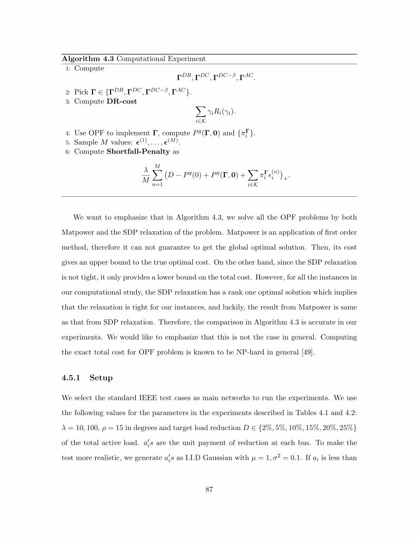
Algorithm 4.3 Computational Experiment
1: Compute
ΓDR,ΓDC ,ΓDC−β,ΓAC .
2: Pick Γ ∈ ΓDR,ΓDC ,ΓDC−β,ΓAC.3: Compute DR-cost ∑
i∈KγiRi(γi).
4: Use OPF to implement Γ, compute P g(Γ,0) and πΓi .
5: Sample M values: ε(1), . . . , ε(M).6: Compute Shortfall-Penalty as
λ
M
M∑n=1
(D − P g(0) + P g(Γ,0) +
∑i∈K
πΓi ε
(n)i
)+.
We want to emphasize that in Algorithm 4.3, we solve all the OPF problems by both
Matpower and the SDP relaxation of the problem. Matpower is an application of first order
method, therefore it can not guarantee to get the global optimal solution. Then, its cost
gives an upper bound to the true optimal cost. On the other hand, since the SDP relaxation
is not tight, it only provides a lower bound on the total cost. However, for all the instances in
our computational study, the SDP relaxation has a rank one optimal solution which implies
that the relaxation is tight for our instances, and luckily, the result from Matpower is same
as that from SDP relaxation. Therefore, the comparison in Algorithm 4.3 is accurate in our
experiments. We would like to emphasize that this is not the case in general. Computing
the exact total cost for OPF problem is known to be NP-hard in general [49].
4.5.1 Setup
We select the standard IEEE test cases as main networks to run the experiments. We use
the following values for the parameters in the experiments described in Tables 4.1 and 4.2:
λ = 10, 100, ρ = 15 in degrees and target load reduction D ∈ 2%, 5%, 10%, 15%, 20%, 25%
of the total active load. a′is are the unit payment of reduction at each bus. To make the
test more realistic, we generate a′is as I.I.D Gaussian with µ = 1, σ2 = 0.1. If ai is less than
87
0, we regenerate the ai. Once they are generated, we will not change them anymore in the
whole procedure. We use MATLAB with the cvx package to solve the SDPs on a 12-core
server.
4.5.2 Modified Algorithm
Algorithm 4.2 for ΓAC works well for small networks such as 14-bus and 30-bus. However,
for larger networks (e.g. 300-bus case), each iteration can take about 15 minutes and the
algorithm is not guaranteed to converge in less than a hundred iterations. Therefore, as
mentioned before, we consider a modified algorithm. In this modified method, we still
get the offer price Γ0 by using the deterministic supply function in the demand response
problem. Then, instead of running a loop, we assume that the values of πi are unchanged.
In the modified approach, we just solve one single SDP instead of iteratively solving a
sequence of SDPs for a convergent solution. We have tested that, for large networks, this
algorithm completes in a much shorter time, and the gap between this sub-optimal solution
with the iterative heuristic solution is negligible.
4.5.3 Main Results
We conducted extensive numerical experiments on a large set of test instances and param-
eters. Not surprisingly, they gave us similar implications about the experiment. Therefore,
we present our result tables for only the IEEE 57-bus network here. A full version of test
result can be found on our Website.
Before we show the tables, there are some additional notations we need to introduce. In
Table 4.1 and Table 4.2, reduction is total reduction over the grid as the sum of reduction
at nodes and reduction in transmission loss; CPU time(s) is CPU time used to compute the
offer prices; (DR-AC)/AC is relative difference of total costs between DR model and AC
model; (DC-AC)/AC is relative difference of total costs between DC model and AC model;
(DCβ-AC)/AC is relative difference of total costs between DCβ model and AC model.
Now, we are ready to display the tables.
88

D 25.02 62.54 125.08 187.62 250.16 312.70
DR model:
DR-cost 14.84 92.72 375.36 860.78 939.66 939.66Shortfall penalty 0.00 0.00 0.00 0.00 470.94 1096.34
Total cost 14.84 92.72 375.36 860.78 1410.60 2036.00
Reduction 26.36 65.67 130.55 194.80 203.07 203.07CPU time(s) 0.69 0.56 0.64 0.72 0.73 0.51
DC model:
DR-cost 14.84 92.72 375.36 860.78 939.66 939.66Shortfall penalty 0.00 0.00 0.00 0.00 470.94 1096.34
Total cost 14.84 92.72 375.36 860.78 1410.60 2036.00
Reduction 26.36 65.67 130.55 194.80 203.07 203.07CPU time(s) 1.08 0.97 0.98 0.90 0.86 0.92
DCβ model β = 0.009
DR-cost 14.57 91.07 368.54 844.88 954.40 954.41Shortfall penalty 0.00 0.00 0.00 0.00 455.94 1081.34
Total cost 14.57 91.07 368.54 844.88 1410.35 2035.74
Reduction 26.13 65.09 129.39 193.08 204.57 204.57CPU time(s) 0.97 1.19 0.76 1.09 0.76 0.83
AC model:
DR-cost 13.34 83.97 343.82 796.73 968.70 968.72Shortfall penalty 0.00 0.01 0.04 0.12 443.44 1068.75
Total cost 13.34 83.98 343.85 796.85 1412.14 2037.48
Reduction 25.02 62.54 125.08 187.61 205.82 205.82CPU time(s) 166.06 342.00 891.67 985.40 842.62 794.06
(DR-AC)/AC 11.2% 10.4% 9.2% 8.0% -0.1% -0.1%(DC-AC)/AC 11.2% 10.4% 9.2% 8.0% -0.1% -0.1%(DCβ-AC)/AC 9.2% 8.4% 7.2% 6.0% -0.1% -0.1%
Table 4.1: Comparison of AC, DR, DC and DCβ models at ρ = 15, λ = 10 on IEEE 57-bustest case
89

D 25.02 62.54 125.08 187.62 250.16 312.70
DR model:
DR-cost 14.84 92.72 375.36 860.78 1583.84 2618.46Shortfall penalty 0.00 0.00 0.00 0.00 0.00 0.00
Total cost 14.84 92.72 375.36 860.78 1583.84 2618.46
Reduction 26.36 65.67 130.55 194.80 258.49 321.79CPU time(s) 0.62 0.53 0.64 0.47 0.76 0.66
DC model:
DR-cost 14.84 92.72 375.36 860.78 1583.84 2618.46Shortfall penalty 0.00 0.00 0.00 0.00 0.00 0.00
Total cost 14.84 92.72 375.36 860.78 1583.84 2618.46
Reduction 26.36 65.67 130.55 194.80 258.49 321.79CPU time(s) 0.80 1.01 0.69 0.76 0.87 1.28
DCβ model β = 0.009
DR-cost 14.57 91.07 368.54 844.88 1552.94 2564.76Shortfall penalty 0.00 0.00 0.00 0.00 0.00 0.00
Total cost 14.57 91.07 368.54 844.88 1552.94 2564.76
Reduction 26.13 65.09 129.39 193.08 256.22 318.96CPU time(s) 0.80 0.94 1.33 0.87 1.11 1.11
AC model:
DR-cost 13.34 83.99 343.90 796.94 1478.78 2465.27Shortfall penalty 0.00 0.00 0.01 0.03 0.05 0.08
Total cost 13.34 83.99 343.91 796.97 1478.83 2465.35
Reduction 25.02 62.55 125.09 187.63 250.17 312.71CPU time(s) 154.91 372.66 1024.36 1007.63 984.60 970.12
(DR-AC)/AC 11.2% 10.4% 9.1% 8.0% 7.1% 6.2%(DC-AC)/AC 11.2% 10.4% 9.1% 8.0% 7.1% 6.2%(DCβ-AC)/AC 9.2% 8.4% 7.2% 6.0% 5.0% 4.0%
Table 4.2: Comparison of AC, DR, DC and DCβ models at ρ = 15, λ = 100 on IEEE57-bus test case
90
The following paragraphs cover the main properties of our heuristics and models based
on the computational results in our experiments.
The offer prices γ are capped at approximately λ2 . This follows from the first order
condition: objective function f ∼ (aiγ2i + λ × max(D − aiγi, 0)) and ∂f
∂γi∼ (2aiγi − aiλ).
We can see that in Table 4.1, when λ = 10, total reduction is capped in columns 5 and 6.
In Table 4.2, when λ = 100, the total reduction is not capped by λ any more.
When the reduction is not capped by λ, the cost of the AC power flow based heuristic
is significantly lower than the other three for all values of the target demand reduction D.
The DC model and no network model compute identical solutions where the total demand
reduction at the demand buses is equal to the target D. Since these two approaches do not
account for transmission losses, the actual reduction in total power generation is greater
than D. These two approaches end up paying more rebate than needed to meet the target.
On the other hand, the AC power flow based heuristic achieves the target demand
reduction through a combination of reduction at load buses and reduction in transmission
losses, since lower cumulative power needs to be transmitted. This is because the AC
power flow models the transmission losses in the optimization phase. Therefore, the total
payments for the AC power flow based heuristic are smaller, especially for large network
whose transmission loss has a larger proportion of total generation.
However, in some large network instances which are not listed here, the cost of DC
model is significantly higher than the cost of no network model because the angle difference
constraint is binding. Therefore, the total cost needs to be higher in DC model.
Maximum angle difference is significantly less than 15 for many test cases. Notice
that this is the phase angle difference from the OPF implementation of given offer prices
from all models. In fact, we can see that the angle difference constraint of 15 in the DC
optimization model can possible be tight even when maximum angle difference for the OPF
implementation of the DC model rebates is 4.
The DCβ model we introduced uses a simple trick to estimate the transmission loss
in DC model, like β = 0.009 in the previous two tables. Therefore, as the consequence
91

of considering partial transmission loss, the total reduction in this model is less than the
original DC model, but still higher than the AC model, ending up with a total cost between
original DC model and AC model. However, this model is much less complex than the AC
model heuristic, and we can achieve a better result by carefully adjusting the value of β.
4.6 Conclusion
In this chapter, we consider a new price rebate approach to demand-response problem un-
der power flow constraints. We consider an AC power flow based model that allows us
to model transmission loss and therefore, optimize the offer prices to achieve the target
demand reduction through a combination of reduction at load buses and reduction in trans-
mission loss. This is important since the DC power flow based model does not consider
the transmission loss and can not account for its reduction at the offer-price optimization
stage. However, the AC power flow based offer price optimization problem is non-convex,
and therefore, intractable and hard to solve. We propose an iterative algorithm to compute
price rebates to achieve the required demand reduction with minimum possible cost. We
conducted computational study to compare the performance of our iterative method with
other demand response models or heuristics. Our results show that our iterative heuristic
performs significantly better than the DC power flow based models or model without any
power flow constraints, which are not able to account for the savings in transmission losses.
Therefore, there is significant value in using an AC power flow based model for demand-
response optimization. It is important to note that our iterative heuristic is exact only when
the electric grid instance satisfies the numerical requirement in [49]. When the requirement
is not satisfied, our iterative heuristic only computes a lower bound of the optimal cost.
The problem of how to design a provably near-optimal algorithm for these instances is an
interesting open question.
92

Bibliography
[1] Philipp Afeche, Zhe Liu, and Costis Maglaras. Ride-hailing networks with strategicdrivers: The impact of platform control capabilities on performance. Working Paper,2018.
[2] Gagan Aggarwal, Gagan Goel, Chinmay Karande, and Aranyak Mehta. Online vertex-weighted bipartite matching and single-bid budgeted allocations. In Proceedings ofthe twenty-second annual ACM-SIAM symposium on Discrete Algorithms, pages 1253–1264. SIAM, 2011.
[3] Gad Allon, Achal Bassamboo, and Eren B. Cil. Large-scale service marketplaces: Therole of the moderating firm. Management Science, 58(10):iv–1962, 2012.
[4] Nick Arnosti, Ramesh Johari, and Yashodhan Kanoria. Managing congestion in de-centralized matching markets. EC, 2014.
[5] Bar Ata and Tava Lennon Olsen. Near-optimal dynamic lead-time quotation andscheduling under convex-concave customer delay costs. Operations Research, 57(3):iv–799, 2009.
[6] Yossi Aviv and Amit Pazgal. Optimal pricing of seasonal products in the presenceof forward-looking consumers. Manufacturing and Service Operations Management,10(3):337–562, 2008.
[7] Jiaru Bai, Kut C. So, Christopher S. Tang, Xiqun Chen, and Hai Wang. Coordinat-ing supply and demand on an on-demand service platform with impatient customers.Forthcoming at MSOM, 2018.
[8] Ross Baldick, Sergey Kolos, and Stathis Tompaidis. Interruptible electricity contractsfrom an electricity retailer’s point of view: valuation and optimal interruption. Oper-ations Research, 54(4):627–642, 2006.
[9] Saif Benjaafar, Guangwen Kong, Xiang Li, and Costas Courcoubetis. Peer-to-peerproduct sharing: Implications for ownership, usage, and social welfare in the sharingeconomy. Forthcoming at Management Science, 2018.
[10] Gerardo Berbeglia, Agustın Garassino, and Gustavo Vulcano. A comparative empiricalstudy of discrete choice models in retail operations. Working Paper, 2018.
93

[11] Fernando Bernstein, A Gurhan Kok, and Lei Xie. Dynamic assortment customizationwith limited inventories. Manufacturing & Service Operations Management, 17(4):538–553, 2015.
[12] Kostas Bimpikis, Ozan Candogan, and Daniela Saban. Spatial pricing in ride-sharingnetworks. Working Paper, 2018.
[13] Benjamin Birnbaum and Claire Mathieu. On-line bipartite matching made simple.ACM SIGACT News, 39(1):80–87, 2008.
[14] Eilyan Bitar and Steven Low. Deadline differentiated pricing of deferrable electricpower service. In Decision and Control (CDC), 2012 IEEE 51st Annual Conferenceon, pages 4991–4997. IEEE, 2012.
[15] Jose H. Blanchet, Guillermo Gallego, and Vineet Goyal. A Markov chain approximationto choice modeling. Operations Research, 64(4):886–905, 2016.
[16] Nicholas Buchholz. Spatial equilibrium, search frictions and efficient regulation in thetaxi industry. Working paper, 2018.
[17] Gerard P. Cachon, Kaitlin M. Daniels, and Ruben Lobel. The role of surge pricing on aservice platform with self-scheduling capacity. Manufacturing and Service OperationsManagement, 19(3):337–507, 2017.
[18] Gerard P. Cachon and Robert Swinney. Purchasing, pricing, and quick response in thepresence of strategic consumers. Management Science, 55(3):iv–511, 2009.
[19] Juan Camilo Castillo, Daniel T. Knoepfle, and E. Glen Weyl. Surge pricing solves thewild goose chase. In 2017 ACM Conference on Economics and Computation, pages241–242. ACM, 2017.
[20] Douglas W Caves and Joseph A Herriges. Optimal dispatch of interruptible and cur-tailable service options. Operations research, 40(1):104–112, 1992.
[21] Sabri Celik and Costis Maglaras. Dynamic pricing and lead-time quotation for a mul-ticlass make-to-order queue. Management Science, 54(6):iv–1211, 2008.
[22] Carri W Chan and Vivek F Farias. Stochastic depletion problems: Effective myopicpolicies for a class of dynamic optimization problems. Mathematics of OperationsResearch, 34(2):333–350, 2009.
[23] Yiwei Chen, Retsef Levi, and Cong Shi. Revenue management of reusable resourceswith advanced reservations. Production and Operations Management, 26(5):836–859,2017.
[24] Maxime C. Cohen, Ruben Lobel, and Georgia Perakis. The impact of demand un-certainty on consumer subsidies for green technology adoption. Management Science,62(5):iv–vii, 1225–1531, 2016.
94

[25] Michael A Crew, Chitru S Fernando, and Paul R Kleindorfer. The theory of peak-loadpricing: A survey. Journal of Regulatory Economics, 8(3):215–248, 1995.
[26] James M. Davis, Guillermo Gallego, and Huseyin Topaloglu. Assortment optimizationunder variants of the nested logit model. Operations Research, 62(2):250–273, 2014.
[27] Nikhil R Devanur and Thomas P Hayes. The adwords problem: Online keywordmatching with budgeted bidders under random permutations. In Proceedings of the10th ACM conference on Electronic commerce, pages 71–78. ACM, 2009.
[28] Nikhil R Devanur, Kamal Jain, and Robert D Kleinberg. Randomized primal-dualanalysis of ranking for online bipartite matching. In Proceedings of the twenty-fourthannual ACM-SIAM symposium on Discrete algorithms, pages 101–107. Society for In-dustrial and Applied Mathematics, 2013.
[29] Wedad Elmaghraby and Pnar Keskinocak. Dynamic pricing in the presence of in-ventory considerations: Research overview, current practices, and future directions.Management Science, 49(10):1275–1444, 2003.
[30] Murat Fahrioglu and Fernando L Alvarado. Designing incentive compatible contractsfor effective demand management. Power Systems, IEEE Transactions on, 15(4):1255–1260, 2000.
[31] Awi Federgruen and Aliza Heching. Combined pricing and inventory control underuncertainty. Operations Research, 47(3):345–494, 1999.
[32] Jon Feldman, Aranyak Mehta, Vahab Mirrokni, and S Muthukrishnan. Online stochas-tic matching: Beating 1-1/e. In Foundations of Computer Science, 2009. FOCS’09.50th Annual IEEE Symposium on, pages 117–126. IEEE, 2009.
[33] Guiyun Feng, Guangwen Kong, and Zizhuo Wang. We are on the way: Analysis ofon-demand ride-hailing systems. Working paper, 2017.
[34] Ian L. Gale and Thomas J. Holmes. Advance-purchase discounts and monopoly allo-cation of capacity. The American Economic Review, 83(1):135–146, 1993.
[35] Guillermo Gallego, Garud Iyengar, Robert Phillips, and A. Dubey. Managing flexibleproducts on a network. CORC Technical Report TR-2004-01, 2004.
[36] Guillermo Gallego and Huseyin Topaloglu. Constrained assortment optimization forthe nested logit model. Management Science, 60(10):2583–2601, 2014.
[37] Guillermo Gallego and Garrett van Ryzin. Optimal dynamic pricing of inventories withstochastic demand over finite horizons. Management Science, 40(8):947–1068, 1994.
[38] Gagan Goel and Aranyak Mehta. Online budgeted matching in random input modelswith applications to adwords. In Proceedings of the nineteenth annual ACM-SIAMsymposium on Discrete algorithms, pages 982–991. Society for Industrial and Applied
95

Mathematics, 2008.
[39] Negin Golrezaei, Hamid Nazerzadeh, and Paat Rusmevichientong. Real-time optimiza-tion of personalized assortments. Management Science, 60(6):1532–1551, 2014.
[40] Itai Gurvich, Martin A Lariviere, and Antonio Moreno-Garcia. Operations in theon-demand economy: Staffing services with self-scheduling capacity. Working paper,2016.
[41] John J. Horton. Buyer uncertainty about seller capacity: Causes, consequences, and apartial solution. Forthcoming at Management Science, 2018.
[42] Ming Hu and Yun Zhou. Dynamic type matching. Working Paper, 2016.
[43] Rajnish Kamat and Shmuel S Oren. Exotic options for interruptible electricity supplycontracts. Operations Research, 50(5):835–850, 2002.
[44] Yash Kanoria and Daniela Saban. Facilitating the search for partners on matchingplatforms. Working Paper, 2017.
[45] Chinmay Karande, Aranyak Mehta, and Pushkar Tripathi. Online bipartite matchingwith unknown distributions. In Proceedings of the forty-third annual ACM symposiumon Theory of computing, pages 587–596. ACM, 2011.
[46] Richard M Karp, Umesh V Vazirani, and Vijay V Vazirani. An optimal algorithm foron-line bipartite matching. In Proceedings of the twenty-second annual ACM symposiumon Theory of computing, pages 352–358. ACM, 1990.
[47] Jeunghyun Kim and Ramandeep S. Randhawa. The value of dynamic pricing in largequeueing systems. Operations Research, 66(2):ii–iv,301–596, 2018.
[48] A.Gurhan Kok, MarshallL. Fisher, and Ramnath Vaidyanathan. Assortment planning:Review of literature and industry practice. In Narendra Agrawal and Stephen A.Smith, editors, Retail Supply Chain Management, volume 223 of International Seriesin Operations Research & Management Science, pages 175–236. Springer US, 2015.
[49] Javad Lavaei and Steven H Low. Zero duality gap in optimal power flow problem.Power Systems, IEEE Transactions on, 27(1):92–107, 2012.
[50] Retsef Levi and Ana Radovanovic. Provably near-optimal lp-based policies for revenuemanagement in systems with reusable resources. Operations Research, 58(2):503–507,2010.
[51] Qian Liu and Garrett J. van Ryzin. On the choice-based linear programming modelfor network revenue management. Manufacturing & Service Operations Management,10(2):288–310, 2008.
[52] Robert Duncan Luce. Individual Choice Behavior: A Theoretical Analysis. Wiley,1959.
96

[53] Will Ma and David Simchi-Levi. Online resource allocation under arbitrary arrivals:Optimal algorithms and tight competitive ratios. Working Paper, 2017.
[54] Costis Maglaras. Personal training at the new york health club, 2007. Case ID 070201published by Columbia CaseWorks, Columbia Business School, https://www8.gsb.
columbia.edu/caseworks/node/261.
[55] Vahideh H Manshadi, Shayan Oveis Gharan, and Amin Saberi. Online stochasticmatching: Online actions based on offline statistics. Mathematics of Operations Re-search, 37(4):559–573, 2012.
[56] Daniel McFadden. Conditional logit analysis of qualitative choice behavior. in P.Zarembka, ed., Frontiers in Econometrics, 1973.
[57] Daniel McFadden et al. Modelling the choice of residential location. Institute of Trans-portation Studies, University of California, 1978.
[58] Daniel McFadden and Kenneth Train. Mixed MNL models for discrete response. Jour-nal of Applied Econometrics, 15(5):447–470, 2000.
[59] Aranyak Mehta et al. Online matching and ad allocation. Foundations and Trends R©in Theoretical Computer Science, 8(4):265–368, 2013.
[60] Aranyak Mehta and Debmalya Panigrahi. Online matching with stochastic rewards.In Foundations of Computer Science (FOCS), 2012 IEEE 53rd Annual Symposium on,pages 728–737. IEEE, 2012.
[61] Aranyak Mehta, Amin Saberi, Umesh Vazirani, and Vijay Vazirani. Adwords andgeneralized on-line matching. In 46th Annual IEEE Symposium on Foundations ofComputer Science (FOCS’05), pages 264–273. IEEE, 2005.
[62] Aranyak Mehta, Bo Waggoner, and Morteza Zadimoghaddam. Online stochasticmatching with unequal probabilities. In Proceedings of the twenty-sixth annual ACM-SIAM symposium on Discrete algorithms, pages 1388–1404. Society for Industrial andApplied Mathematics, 2015.
[63] Shmuel S Oren. Integrating real and financial options in demand-side electricity con-tracts. Decision Support Systems, 30(3):279–288, 2001.
[64] Shmuel S Oren and Stephen A Smith. Design and management of curtailable electricityservice to reduce annual peaks. Operations Research, 40(2):213–228, 1992.
[65] Zachary Owen and David Simchi-Levi. Price and assortment optimization for reusableresources. Available at SSRN 3070625, 2018.
[66] Erhun Ozkan and Amy Ward. Dynamic matching for real-time ridesharing. Workingpaper, 2017.
[67] Robin L. Plackett. The analysis of permutations. Journal of the Royal Statistical
97

Society. Series C (Applied Statistics), 24(2):193–202, 1975.
[68] Carlos Riquelme, Siddhartha Banerjee, and Ramesh Johari. Pricing in ride-sharingplatforms: A queueing-theoretic approach. In 16th ACM Conference on Economicsand Computation, pages 639–639. IEEE, 2015.
[69] Jean-Charles Rochet and Jean Tirole. Two-sided markets: A progress report. TheRAND journal of economics, 37(3):645–667, 2006.
[70] Mardavij Roozbehani, Ali Faghih, Mesrob I Ohannessian, and Munther A Dahleh.The intertemporal utility of demand and price elasticity of consumption in power gridswith shiftable loads. In Decision and Control and European Control Conference (CDC-ECC), 2011 50th IEEE Conference on, pages 1539–1544. IEEE, 2011.
[71] Paat Rusmevichientong, Mika Sumida, and Huseyin Topaloglu. Dynamic assortmentoptimization for reusable products with random usage durations. Working Paper, 2018.
[72] Marc Rysman. The economics of two-sided markets. Journal of Economic Perspectives,23(3):125–143, 2009.
[73] Somayeh Sojoudi and Javad Lavaei. Network topologies guaranteeing zero duality gapfor optimal power flow problem. submitted for publication, 2011.
[74] Clifford Stein, Van-Anh Truong, and Xinshang Wang. Advance service reservationswith heterogeneous customers. arXiv preprint arXiv:1805.05554, 2018.
[75] Peter O. Steiner. Peak loads and efficient pricing. The Quarterly Journal of Economics,71(4):585610, 1957.
[76] Xuanming Su. Intertemporal pricing with strategic customer behavior. ManagementScience, 53(5):iv–864, 2007.
[77] Kalyan Talluri and Garrett Van Ryzin. Revenue management under a general discretechoice model of consumer behavior. Management Science, 50(1):15–33, 2004.
[78] Kalyan T. Talluri and Garrett J. van Ryzin. The Theory and Practice of RevenueManagement. Springer, 2006.
[79] Chin-Woo Tan and Pravin Varaiya. Interruptible electric power service contracts.Journal of Economic Dynamics and Control, 17(3):495–517, 1993.
[80] Terry A. Taylor. On-demand service platforms. Manufacturing and Service OperationsManagement, 20(4):601–800, 2018.
[81] Gunnar T. Thowsen. A dynamic, nonstationary inventory problem for a price/quantitysetting firm. Naval Research Logistics, 22(3):461–476, 1975.
[82] Huseyin Topaloglu. Joint stocking and product offer decisions under the multinomiallogit model. Production and Operations Management, 22(5):1182–1199, 2013.
98

[83] Kenneth E Train. Discrete Choice Methods with Simulation. Cambridge UniversityPress, 2009.
[84] Le Anh Tuan and K. Bhattacharya. Competitive framework for procurement of inter-ruptible load services. Power Systems, IEEE Transactions on, 18(2):889–897, 2003.
[85] Xinshang Wang, Van-Anh Truong, and David Bank. Online advance admission schedul-ing for services with customer preferences. arXiv preprint arXiv:1805.10412, 2018.
[86] E. G. Weyl. A price theory of multi-sided platforms. American Economic Review,100(4):1642–1672, 2010.
[87] Huw Williams Williams. On the formation of travel demand models and economicevaluation measures of user benefit. Environment and Planning A, 3(9):285–344, 1977.
[88] P. Yang, K. Iyer, and PI. Frazier. Mean field equilibria for competitive explorationin resource sharing settings. In 25th International Conference on World Wide Web,pages 177–187. ACM, 2016.
[89] Man Yu, Laurens Debo, and Roman Kapuscinski. Strategic waiting for consumer-generated quality information: Dynamic pricing of new experience goods. ManagementScience, 62(2):iv–vii, 303–630, 2016.
[90] Edward Zabel. Monopoly and uncertainty. The Review of Economic Studies, 37(2):205–219, 1970.
99

Appendices
100

Appendix A
Proofs for Chapter 3
A.1 Proof of Proposition 3.1
Proof. If ∃xi 6= xj ,xj 6= xk ∈ V, such that
Γ(xi,xj) > 0, Γ(xj ,xk) > 0, (A.1)
then we have driver relocation from xi to xj and from xj to xk. Because of the compatible
incentive requirement for driver relocation, we have
p(xj)− c(xi,xj) ≥ p(xi), p(xk)− c(xj ,xk) ≥ p(xj). (A.2)
By linking these two inequalities, we have
p(xk)− c(xj ,xk)− c(xi,xj) ≥ p(xi). (A.3)
From triangle inequality (3.1), we have
c(xi,xk) ≤ c(xi,xj) + c(xj ,xk). (A.4)
101

Next, we discuss three different cases. Firstly, if c(xi,xk) < c(xi,xj) + c(xj ,xk) is true,
use (A.2), we have,
p(xj)− c(xi,xj) ≤ p(xk)− c(xj ,xk)− c(xi,xj) < p(xk)− c(xi,xk).
Thus, xk offers a higher effective price to drivers at xi than xj . The platform should not
assign any drivers to move from xi to xj . It contradicts the incentive compatibility of
drivers.
Secondly, if p(xj) < p(xk)− c(xj ,xk), use (A.2) and (A.4), we also have,
p(xj)− c(xi,xj) < p(xk)− c(xj ,xk)− c(xi,xj) ≤ p(xk)− c(xi,xk).
Thus, xk offers a higher effective price to drivers at xi than xj . The platform should not
assign any drivers to move from xi to xj . It contradicts the incentive compatibility of
drivers.
Finally, if c(xi,xk) = c(xi,xj)+c(xj ,xk) and p(xj) = p(xk)−c(xj ,xk) are true, we have,
p(xj)− c(xi,xj) = p(xk)− c(xj ,xk)− c(xi,xj) = p(xk)− c(xi,xk).
Then drivers at xi are indifferent of going to xj or going to xk. Because of p(xj) =
p(xk) − c(xj ,xk), drivers at xj are indifferent of staying at xj or going to xk. Then, if
Γ(xi,xj) < Γ(xj ,xk), we can send Γ(xi,xj) amount of drivers from xi to xk directly,
canceling Γ(xi,xj) amount of drivers in and out of node xj . If Γ(xi,xj) ≥ Γ(xj ,xk), we
can send Γ(xj ,xk) amount of drivers from xi to xk directly, canceling Γ(xj ,xk) amount of
drivers in and out from node xj . The new constructed driver flow is feasible and it achieves
same net driver flows and objective value as before. More importantly, it satisfies
Γ(xi,xj)Γ(xj ,xk) = 0.
102
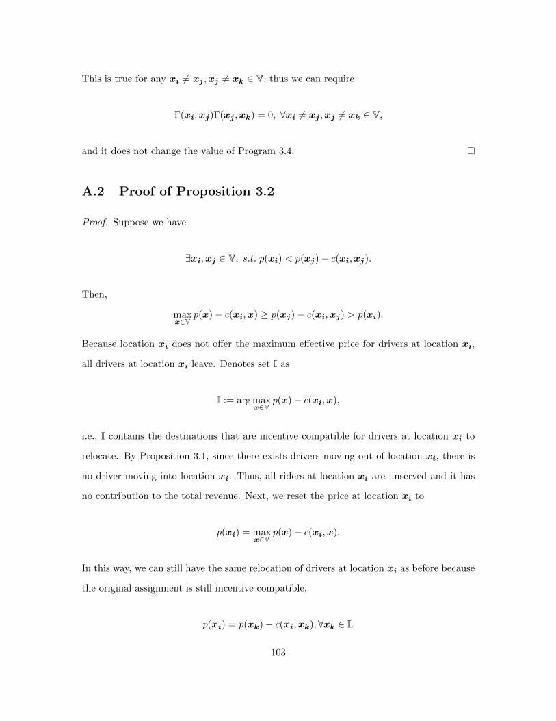
This is true for any xi 6= xj ,xj 6= xk ∈ V, thus we can require
Γ(xi,xj)Γ(xj ,xk) = 0, ∀xi 6= xj ,xj 6= xk ∈ V,
and it does not change the value of Program 3.4.
A.2 Proof of Proposition 3.2
Proof. Suppose we have
∃xi,xj ∈ V, s.t. p(xi) < p(xj)− c(xi,xj).
Then,
maxx∈V
p(x)− c(xi,x) ≥ p(xj)− c(xi,xj) > p(xi).
Because location xi does not offer the maximum effective price for drivers at location xi,
all drivers at location xi leave. Denotes set I as
I := arg maxx∈V
p(x)− c(xi,x),
i.e., I contains the destinations that are incentive compatible for drivers at location xi to
relocate. By Proposition 3.1, since there exists drivers moving out of location xi, there is
no driver moving into location xi. Thus, all riders at location xi are unserved and it has
no contribution to the total revenue. Next, we reset the price at location xi to
p(xi) = maxx∈V
p(x)− c(xi,x).
In this way, we can still have the same relocation of drivers at location xi as before because
the original assignment is still incentive compatible,
p(xi) = p(xk)− c(xi,xk),∀xk ∈ I.
103

By applying Proposition 3.1 again, all other driver relocations which do not involve xi are
still incentive compatible. Since the prices at other locations are unchanged, there is no
new destination added into set I except for location xi itself. At this time, location xi is
still unserved and it contributes nothing to the total revenue. In this way, we have the same
objective value as before at this new price of p(xi), and it satisfies
p(xi) = maxx∈V
p(x)− c(xi,x) ≥ p(xj)− c(xi,xj).
A.3 Proof of Proposition 3.3
Proof. Suppose we have
∃xi 6= xj and xj 6= 0, s.t. Γ(xi,xj) > 0.
Then there are some drivers moving into location xj . By Proposition 3.1, there is no driver
moving out of location xj . All its original drivers µ(xj) are still at location xj . Denote set
K as
K := xk|Γ(xk,xj) > 0,
i.e., the set of locations that supplies drivers to location xj . K is not empty as xi ∈ K.
Because of the incentive must be compatible for these drivers, we have
p(xj) ≥ p(xk) + c(xk,xj), ∀xk ∈ K.
By Proposition 3.2, we can require that
p(xj) ≤ p(xk) + c(xk,xj), ∀xk ∈ K.
104

Thus, we get
p(xj) = p(xk) + c(xk,xj), ∀xk ∈ K.
Consequently, the drivers moving from xk to xj are indifferent of staying at xk or moving
to xj . Next, we send back all the relocated drivers moving into node xj to construct a
new assignment. For location xj , since xj 6= 0 and all its original drivers µ(xj) are still at
location xj , it still has enough drivers to serve all riders. This is because our Assumption
3.1 for the baseline demand
λ(xj)Fv(p(xj)
)≤ λ(xj) ≤ µ(xj).
Thus, it has the same revenue contribution p(xj)λ(xj)Fv(p(xj)
)as before. For all locations
in K, the prices are unchanged and they get more drivers to serve their riders, which may
offer a higher contribution to the total revenue. At the same time, the prices and assignments
at all other locations are still feasible since we do not change any price. Then, we improve
the solution with condition
Γ(xi,xj) = 0.
satisfied for xi and xj .
A.4 Proof of Theorem 3.4
Proof. Firstly, we show the pricing formula (3.13) in Theorem 3.4 is optimal. For any
feasible solution to Program 3.4, we apply Proposition 3.2 such that it satisfies
p(x) ≥ p(0)− c(x,0), ∀x ∈ V.
Since pmin = pb, then p(x) ≥ pb, ∀x ∈ V. Combine it with the inequality above, we have
p(x) ≥ max
(pb, p(0)− c(x,0)
), ∀x ∈ V.
105

We denote set K as
K := x ∈ V|p(x) > max
(pb, p(0)− c(x,0)
).
It is trivial to see that 0 /∈ K. If K is empty, we do not need to do any change, the optimal
pricing function is already achieved. If K is not an empty set, then ∀xk ∈ K, we have
p(xk) > max
(pb, p(0)− c(xk,0)
)≥ p(0)− c(xk,0).
Thus, location xk can not supply drivers to demand shock location 0 because the price
difference is not incentive compatible for relocation. Also, since xk is not a demand shock
location, by Proposition 3.3, there should be no drivers relocated to xk and no drivers
relocated from xk to other non-shock locations. Thus, the available drivers at xk are from
its original drivers
ν(xk) = µ(xk).
Since λ(xk) ≤ µ(xk), its revenue contribution is p(xk)λ(xk)Fv(p(xk)
). This is true for all
locations in K. Next, we set the prices for locations in K to
p(xk) = max
(pb, p(0)− c(xk,0)
),∀xk ∈ V.
Since pFv(p) is a decreasing function on [pb, pmax], the new price p(xk) is lower than its
previous price and it increases its revenue contribution p(xk)λ(xk)Fv(p(xk)
). The only
thing we need to show is ν(xk) = µ(xk) is still feasible for xk ∈ K. Once this part is
proved, then the assignment within K is unchanged. Moreover, since the assignment within
K is unchanged, it will not affect the assignment within R \ K. Because the prices for
locations in R \K are unchanged, the assignment within R \K remains same as before and
so does its revenue contribution. Next, we show ν(xk) = µ(xk) is feasible under the new
prices.
If a location xk in K has to supply drivers to another location xj at the new prices, we
106

have
p(xk) = max
(pb, p(0)− c(xk,0)
)< p(xj)− c(xk,xj) (A.5)
= max
(pb, p(0)− c(xj ,0)
)− c(xk,xj) (A.6)
= p(0)− c(xj ,0)− c(xk,xj) (A.7)
(A.5) and (A.6) are due to the incentive compatibility for relocating drivers from xk to xj
and the definition of pricing formula (3.13). (A.7) is because if p(xj) = pb, due to (A.5),
we have
p(xj) = pb > max
(pb, p(0)− c(xk,0)
)+ c(xk,xj) ≥ pb + 0 = pb,
which is a contradiction. So we must have p(xj) = p(0)− c(xj ,0) and p(0)− c(xj ,0) > pb.
Next, by triangle inequality (3.1) and (A.5), (A.6), (A.7), we have
p(0)− c(xj ,0)− c(xk,xj) ≤ p(0)− c(xk,0)
≤ max
(pb, p(0)− c(xk,0)
)< p(0)− c(xj ,0)− c(xk,xj),
which is a contradiction. Thus, any location xk in K does not have to supply drivers to
another location and it is feasible for them to keep all their drivers. By using the exact
same proof, we can also show that any location xk in K does not have to receive drivers
from another location. Thus, ν(xk) = µ(xk),∀xk ∈ K is feasible under the new prices.
But, its total revenue contribution is improved because of the monotonicity of pFv(p). At
the same time, the revenue contribution from R \ K is unchanged. Thus, we improve our
objective value by resetting its price function to pricing formula (3.13) and this is true for
any feasible solution. Thus, the pricing formula (3.13) in Theorem 3.4 is optimal.
Secondly, given the pricing formula (3.13), we need to show the assignment constructed
107

by Algorithm 3.1 in Theorem 3.4 is optimal. We prove this by two steps. Firstly, we show
the assignment is feasible. Then, we show it is optimal by claiming it achieves an upper
bound value for Program 3.4 under pricing formula (3.13). In Theorem 3.4, there are two
types of assignments. The first type is to match drivers at location x,∀x ∈ V to local riders
at same location, and the second type is to relocate drivers at location x in surge region
to the demand shock location 0. We only need to show these two types of assignments are
incentive compatible for drivers.
In the first part, we have showed that any location xk in K does not have to supply
drivers to another location under pricing formula (3.13). By using the exact same proof, we
can show that for ∀x ∈ V, the drivers at location x do not have to move to other locations,
i.e., it is incentive compatible to keep the drivers at x. Thus, the first type of assignment
is feasible. By definition of surge region S, we have
p(x) = p(0)− c(x,0),∀x ∈ S.
Since p(x) is the maximum effective price for drivers at location x, p(0) − c(x,0) is also
the maximum effective price for drivers at location x, and it is incentive compatible to
relocate drivers to 0. Thus, the second type of assignment is also feasible. The assignment
in Theorem 3.4 is feasible. Secondly, we show it is optimal. In fact, the optimal value of
Program 3.4 is capped by both the rider side and driver side. In particular, outside the
surge region S, the revenue contribution on these places is upper bounded by the potential
demand,
∫x/∈S
p(x) min
(µ(x), λ(x)Fv
(p(x)
))dx ≤
∫x/∈S
p(x)λ(x)Fv(p(x)
)dx.
Then, this upper is achieved in Theorem 3.4 by setting ν(x) = µ(x),∀x /∈ S. This is because
the price satisfies
p(x) > p(0)− c(x,0)
108
outside the surge region by the definition of surge region. Thus, it is not incentive compatible
to relocate them to the demand shock location 0. By Proposition 3.3, all the drivers stay
at their original location. Because µ(x) ≥ λ(x)Fv(p(x)
),∀x /∈ S, the solution can achieve
the revenue upper bound.
Then inside the surge region S, we have the following discussions. If Λ ≥ µ, then all
the drivers in S are not enough to serve the effective riders at the demand shock location,
which has the highest price under pricing formula (3.13). Thus, the revenue inside surge
region is upper bounded by the driver side µp(0). This is achieved by setting
ν0 = µ, ν(x) = 0, ∀x ∈ S.
Next, if µ ≤ Λ < µ, then we have enough drivers to serve the effective riders at the demand
shock location, but not enough for all effective riders inside the surge region S. Then, the
revenue inside surge region is upper bounded by the driver side, capturing the riders at the
locations with highest prices. Then, the upper bound for the revenue is,
p(0)Λ +
∫x|p(x)>p,x∈S
p(x)λ(x)Fv(p(x)
)dx
s.t. Λ +
∫x|p(x)>p,x∈S
λ(x)Fv(p(x)
)dx = µ
(A.8)
In fact, p defined in Algorithm 3.2 is exactly the solution of (A.8). By the definition of p,
we have, ∫x|p(x)≤p,x∈S
λ(x)Fv(p(x)
)dx = Λ− µ
Then, use the definition above, we verify p solves (A.8).
Λ +
∫x|p(x)>p,x∈S
λ(x)Fv(p(x)
)dx
= µ+
∫x|p(x)>p,x∈S
λ(x)Fv(p(x)
)dx+
∫x|p(x)≤p,x∈S
λ(x)Fv(p(x)
)dx
= µ+
∫x|x∈S
λ(x)Fv(p(x)
)dx = µ.
109

In sum, the following value
p(0)Λ +
∫x|p(x)>p,x∈S
p(x)λ(x)Fv(p(x)
)dx
is an upper bound for revenue inside surge region and it is achieved by setting
ν0 = Λ; ν(x) = λ(x)Fv(p(x)
), ∀x ∈ x|p(x) > p, ν(x) = 0, ∀x ∈ x|p(x) ≤ p
inside surge region S. Finally, if Λ < µ, then the number of drivers is higher than the
number of effective riders inside the surge region S, that means we have enough drivers
to serve all the effective riders. Then, the revenue contributed from surge region is upper
bounded by the rider side
p(0)Λ +
∫x∈S
p(x)λ(x)Fv(p(x)
)dx.
This upper bound is achieved by setting
ν0 = µ, ν(x) = λ(x)Fv(p(x)
),∀x ∈ S.
To conclude, the assignment in Theorem 3.4 can achieve a value which is an upper bound
for every feasible assignment given the pricing formula (3.13). Combine with its feasibility,
the assignment in Theorem 3.4 is optimal given the pricing formula (3.13). Theorem 3.4 is
proved.
A.5 Proof of Proposition 3.5
Proof. To prove this proposition, it is equivalent to show that if p(0) and the corresponding
Λ(p(0)
)and µ
(p(0)
)determined in Theorem 3.4 satisfy
Λ(p(0)
)< µ
(p(0)
),
110

then p(0) is not the optimal solution for Program 3.4. To show this claim, we fix p(0) and
its surge region S that leads to Λ(p(0)
)< µ
(p(0)
). It is sufficient to show that ∃ε > 0,
such that if we set p(0) = p(0)− ε, platform can collect more revenue from region S. Now,
suppose the price at demand shock location drops from p(0) to p(0)− ε, all the prices in S
drop. If we have
Λ(p(0)− ε
)< µ
(p(0)− ε
),
then based on the assignment algorithm in Theorem 3.4, all the effective riders in S get
served. Thus, the revenue collected in S is
(p(0)− ε
)ΛFv
(p(0)− ε
)+∫
x∈Smax
(p(0)− ε− c(x,0), pb
)λ(x)Fv
(max
(p(0)− ε− c(x,0), pb
))dx.
(A.9)
On the other hand, the revenue collected in S when p(0) is the price at demand shock node
is
p(0)ΛFv(p(0)
)+
∫x∈S
max
(p(0)−c(x,0), pb
)λ(x)Fv
(max
(p(0)−c(x,0), pb
))dx. (A.10)
Since pFv(p) decreases on p ≥ pb, terms in (A.9) are point-wise larger than terms in (A.10).
Thus, p(0)−ε yields a better solution, and p(0) is not optimal. Consequently, if there exists
one ε > 0 satisfying
Λ(p(0)− ε
)< µ
(p(0)− ε
),
then the proposition is proved.
On the other hand, if ∀ε > 0 and we always have
Λ(p(0)− ε
)≥ µ
(p(0)− ε
),
we claim that we can still find a ε > 0 such that p(0)− ε yields a better solution than p(0).
Pick a positive sequence ε1, ..., εn, ... such that limn→∞ εn = 0. Because εn > 0, we have
111

Λ(p(0)− εn
)≥ µ
(p(0)− εn
). Then, the revenue for platform is at least,
(p(0)− εn
)µ(p(0)− εn
)+∫
x∈Smax
(p(0)− εn − c(x,0), pb
)λ(x)Fv
(max
(p(0)− εn − c(x,0), pb
))dx.
(A.11)
(A.11) is a lower bound because we give up the redundant riders at the demand shock
node, which is the highest loss. Then, as n→∞, since µ is an integral of a function without
mass point, the first term in (A.11) is continuous in εn, and it goes to the limit p(0)µ(p(0)
).
Since we have
µ(p(0)
)> Λ
(p(0)
)= ΛFv
(p(0)
),
the limit p(0)µ(p(0)
)is strictly higher than p(0)ΛFv
(p(0)
). Then, there must exist an εn0
such that (p(0)− εn0
)µ(p(0)− εn0
)> p(0)ΛFv
(p(0)
). (A.12)
The second term in (A.11) is greater than the second term in (A.10) for any εn > 0, which
is also true for εn0 . Thus, when the price at demand shock is p(0) − εn0 , the lower bound
of its maximum possible revenue in S is
(p(0)− εn0
)µ(p(0)− εn0
)+∫
x∈Smax
(p(0)− εn0 − c(x,0), pb
)λ(x)Fv
(max
(p(0)− εn0 − c(x,0), pb
))dx.
This value is strictly greater than the revenue collected in S when p(0) is the price at
demand shock location denoted in (A.10), because of (A.12) and monotonicity of pFv(p).
Thus, we find p(0)− εn0 yields a better solution than p(0). In sum, p(0) is not the optimal
solution for Program 3.4, which concludes this proof.
112

A.6 Proof of Theorem 3.10
Proof. First of all, we state Lemma A.1 and assume it is true at the moment to prove
Theorem 3.10. We give the proof of Lemma A.1 right after this proof.
Lemma A.1. Under the problem setting specified in Theorem 3.10, for any x,y satisfy
p(x) = p(0)− c(x,0), c(y,0) + c(y,x) = c(x,0),
we have
p(y) = p(0)− c(y,0).
Lemma A.1 implies that under the problem setting of Theorem 3.10, if x supplies drivers
to demand shock node 0, any location on the line segment between 0 and x is incentive
compatible to supply drivers to demand shock node 0. In particular, on the ray network,
if x satisfies p(x) = p(0)− c(x, 0), any point y on the line segment between origin 0 and x
has the property of
p(y) = p(0)− c(y, 0)
i.e., y is also incentive compatible to supply drivers to location 0. Denote l as the furthest
point from 0 that satisfies p(l) = p(0)− c(l, 0), i.e.,
l = arg maxx s.t. p(x) = p(0)− c(x, 0).
Because of Lemma A.1, any point x on line [0, l] has p(x) = p(0) − c(x, 0). At the same
time, by definition of l and Proposition 3.2, we have
p(x) > p(0)− c(x, 0),∀x > l.
Thus, for location x > l, it can not supply drivers to demand shock location under incentive
constraint. Then, by Proposition 3.3, for any x > l, the drivers only serve local effective
113

riders at same location. Thus, the prices for locations x > l should optimize local revenue
under incentive compatibility constraint. By Proposition 3.2, for x > l, we have p(x) ≤
p(l)+c(l, x). Due to the uni-modularity of pFv(p) specified in Assumption 3.5, and p(l) ≤ pb,
the optimal price is
min
(pb, p(l) + c(l, x)
), ∀x ≥ l.
As c is a norm induced distance metric, the pricing profile p(x) for x ≥ l is feasible with the
assignment because the price difference for x1, x2 ≥ l is at most |c(x1, l)−c(x2, l)| = c(x1, x2),
which is incentive compatible for retaining all drivers at their original places.
Next, we show l satisfies p(l) ≤ pb. If l violates the property, then for x > l, it needs to
satisfy
p(x) > p(0)− c(x, 0) = p(0)− c(l, 0)− c(l, x) = p(l)− c(l, x),
by the definition of l. However, as p(l) > pb, we have x > l such that c(l, x) ≤ p(l) − pb.
Thus, we have
p(x) > p(l)− c(l, x) = p(0)− c(x, 0) ≥ pb.
Then, following the same analysis in the proof of Theorem 3.4 about the optimality of pricing
formula (3.13), for all these x specified above, setting their pricing profile at max
(p(0) −
c(x, 0), pb
)is a strictly better solution to the total revenue due to the monotonicity of
pFv(p) on p ≥ pb. Thus, in the optimal solution, we must have p(l) ≤ pb.
The optimality of the assignment stated in Theorem 3.10 can be proved using the same
proof of the optimality of the assignment stated in Theorem 3.4. We have showed that
all the assignments stated in Theorem 3.10 are incentive compatible when we prove the
optimality of the pricing function above.
114
A.7 Proof of Lemma 3.12
Proof. If νi > λiFv(pi) and∑
j 6=i Γji > 0 are both true for a location i, we have drivers
relocated to node i and the amount of drivers is more than the amount of effective riders
at location i. Then, we have unmatched drivers at location i. Since we also have drivers
relocated into i, we send these relocated drivers coming from their source locations with the
longest relocation time until νi = λiFv(pi) or∑
j 6=i Γji = 0. Since the revenue contribution
from location i is piλiFv(pi), it is unchanged when we send back these relocated drivers.
Thus, the value of Problem (3.32) remains same.
A.8 Proof of Lemma A.1
Proof. Because of Proposition 3.2, the price p(y) satisfies
p(x) + c(x,y) ≥ p(y) ≥ p(0)− c(y,0). (A.13)
Then, we have
p(x) + c(x,y) = p(0)− c(x,0) + c(x,y) (A.14)
= p(0)− c(y,0)− c(y,x) + c(x,y) (A.15)
= p(0)− c(y,0) (A.16)
(A.14) is because of p(x) = p(0) − c(x,0). (A.15) is due to c(y,0) + c(y,x) = c(x,0).
(A.16) results from the symmetry of a distance metric. Combine (A.16) with (A.13), we
have p(y) = p(0)− c(y,0).
115

Appendix B
Numerical Examples for Chapter 3
B.1 Counter-example of Theorem 3.10 for General c
Proof. In this part, we construct a counter example which shows that Theorem 3.10, in
particular, the pricing formula (3.30) is not optimal. Consider a discrete network with
three nodes 0, 1, 2 on a line. The dis-utility function c has values
c(0, 1) = 20, c(0, 2) = 30, c(1, 2) = 20.
Thus, c can not be a norm induced distance metric since we set 0, 1, 2 on a line, but
c(0, 1) + c(1, 2) 6= c(0, 2). The arrival rates of drivers at each node are
µ0 = 40, µ1 = 40, µ2 = 40,
and the arrival rates of potential riders at each nodes are
λ0 = 100, λ1 = 10, λ2 = 0.
Then, the demand shock happens at node 0. The willingness to pay function Fv is defined
as Fv(p) = ppmax for p ∈ [pmin, pmax] with pmin = 0, pmax = 100. If we use the pricing formula
116
(3.30) in Theorem 3.10, there are three possible values for l. If l = 0, the surge region only
contains the node 0 itself. The optimal price for node 0 is p0 = 60 to maximize the revenue
in surge region under the constraint for pricing formula (3.30) in Theorem 3.10. Then, the
optimal prices for node 1 and 2 are p1 = p2 = 50. The total revenue contribution is
p0µ0 + p1λ1Fv(p1) = 2400 + 250 = 2650.
Next, if l = 1, we do not need to consider this case because it is dominated by l = 2. Since
λ2 = 0, there is no opportunity cost to relocate drivers at node 2, so we can always benefit
from setting a low price at node 2 and relocating the drivers there to other places. Thus, if
l = 2, suppose the price at node 0 is p, then the price at node 1 and node 2 are p− 20 and
p− 30. Because the actual number of rides is capped by the demand, the revenue is upper
bounded by
pλ0Fv(p) + (p− 20)λ1Fv(p− 20), (B.1)
if all the effective riders are served. By plugging the parameters, (B.1) becomes
−1.1p2 + 114p− 240,
with optimal solution p∗ = 51.8 and optimal value 2713.6. Thus, the optimal value given
by using pricing formula 3.30 is upper bounded by 2713.6.
However, if we give up using pricing formula (3.30), we can achieve a better value.
Considering the surge region as 0, 2, i.e., surge region skips node 1, we set the prices as
p0 = 50, p1 = 40, p2 = 20.
Thus, it is incentive compatible to relocate all drivers at node 2 to node 0 and keep the
drivers at nodes 0 and 1 at their original locations. The revenue of this solution is
50 ·min(50, 80) + 40 · 6 = 2740,
117

beating the previous value of 2713.6. Since this price profile violates pricing formula (3.30),
Theorem 3.10 is not valid any more.
118
Related Documents