A Dynamic Optimization Using Lagrangian and Hamiltonian Methods A.1 The Deterministic Finite Horizon Optimization Problem We start with a simplest case of the deterministic finite horizon optimization problem, i.e., there is a terminal point in the decision process. A.1.1 Basic Tools Problems with Equality Constraints: The General Case Readers may have already practiced the static optimization problems with equality constraints many times before; the problems won’t change much if we simply introduce a finite time dimension, i.e., some constraints must hold for each of the periods t ∈{0,...,T }—In a static problem people do maximization with respect to n variables (x 1 ,...,x n ), and in a dynamic context with finite periods t ∈{0,...,T } we just solve basically the same problem with n(T + 1) variables (x 1 ,...,x n(T +1) ). As we know the Theorem of Lagrange, as Theorem A.1 states, provides a powerful characterization of local optima of equality constrained optimization problems in terms of the behavior of the objective function and the constraint functions at these points. Generally such problems have the form as following: max f(x) s.t. x ∈ D = U ∩{x|g(x) = 0} , in which object function f : R n(T +1) → R and constraints g i : R n(T +1) → R k(T +1) , ∀i ∈{1,...,k(T + 1)} be continuously differentiable functions, and U ⊆ R n(T +1) is open. To solve it we set up a function called Lagrangian L : © Springer Nature Switzerland AG 2019 J. Cao, G. Illing, Instructor’s Manual for Money: Theory and Practice, Springer Texts in Business and Economics, https://doi.org/10.1007/978-3-030-23618-2 181

Welcome message from author
This document is posted to help you gain knowledge. Please leave a comment to let me know what you think about it! Share it to your friends and learn new things together.
Transcript
ADynamic Optimization Using Lagrangianand Hamiltonian Methods
A.1 The Deterministic Finite Horizon Optimization Problem
We start with a simplest case of the deterministic finite horizon optimizationproblem, i.e., there is a terminal point in the decision process.
A.1.1 Basic Tools
Problems with Equality Constraints: The General CaseReaders may have already practiced the static optimization problems with equalityconstraints many times before; the problems won’t change much if we simplyintroduce a finite time dimension, i.e., some constraints must hold for each of theperiods t ∈ {0, . . . , T }—In a static problem people do maximization with respect ton variables (x1, . . . , xn), and in a dynamic context with finite periods t ∈ {0, . . . , T }we just solve basically the same problem with n(T +1) variables (x1, . . . , xn(T +1)).As we know the Theorem of Lagrange, as Theorem A.1 states, provides a powerfulcharacterization of local optima of equality constrained optimization problems interms of the behavior of the objective function and the constraint functions at thesepoints. Generally such problems have the form as following:
max f (x)
s.t. x ∈ D = U ∩ {x|g(x) = 0} ,
in which object function f : Rn(T +1) → R and constraints gi : R
n(T +1) →R
k(T +1),∀i ∈ {1, . . . , k(T + 1)} be continuously differentiable functions, andU ⊆ R
n(T +1) is open. To solve it we set up a function called Lagrangian L :
© Springer Nature Switzerland AG 2019J. Cao, G. Illing, Instructor’s Manual for Money: Theory and Practice,Springer Texts in Business and Economics,https://doi.org/10.1007/978-3-030-23618-2
181
182 A Dynamic Optimization Using Lagrangian and HamiltonianMethods
D × Rk(T +1) → R
L (x,λ) = f (x) +k(T +1)∑
i=1
λigi(x)
in which the vector λ = (λ1, . . . , λk(T +1)
) ∈ Rk(T +1) is called Lagrange multiplier.
Theorem A.1 Let f : Rn → R and gi : Rn → Rk be continuously differentiable
functions, ∀i ∈ {1, . . . , k}. Suppose that x∗ is a local maximum or minimum of f
on the set
D = U ∩ {x|gi(x) = 0,∀i ∈ {1, . . . , k}} ,
in which U ⊆ Rn is open. Suppose also that rank (Dg(x∗)) = k. Then, there exists
a vector λ∗ = (λ∗1, . . . , λ
∗k
) ∈ Rk such that
Df(x∗)+
k∑
i=1
λ∗i Dgi(x
∗) = 0.
Then by TheoremA.11 we find the set of all critical points ofL (x,λ) for x ∈ U ,i.e., the first-order conditions
∂L
∂xj
= 0, ∀j ∈ {1, . . . , n(T + 1)},
∂L
∂λi
= 0, ∀i ∈ {1, . . . , k(T + 1)},
which simply say that these conditions should hold for each x and λ in every period.Now we continue to explore the interpretation for the Lagrange multiplier λ. We
relax the equality constraints by adding a sufficiently small constant to each of them,i.e.,
g(x, c) = g(x) + c
in which c = (c1, . . . , ck) is a vector of constants. Now the set of constraintsbecomes
D = U ∩ {x|g(x, c) = 0} .
1Please note that as a tradition people denote the derivative of a multi-variate function f (x) :R
n → R by Df (x), which is an n dimensional vector Df (x) :=[
∂f (x1,...,xn)∂x1
, . . . ,∂f (x1,...,xn)
∂xn
].
A Dynamic Optimization Using Lagrangian and Hamiltonian Methods 183
Then by Theorem A.1 at the optimum x∗(c) there exists λ∗(c) ∈ Rk(T +1) such that
Df(x∗(c)
)+k(T +1)∑
i=1
λ∗i (c)Dgi(x∗(c)) = 0. (A.1)
Define a new function of c, F(c) = f (x∗(c)). Then by chain rule,
DF(c) = Df(x∗(c)
)Dx∗(c).
Insert (A.1) into the equation above, one can get
DF(c) = −⎛
⎝k(T +1)∑
i=1
λ∗i (c)Dgi(x∗(c))
⎞
⎠Dx∗(c),
and this is equivalent to
DF(c) = −k(T +1)∑
i=1
λ∗i (c)Dgi(x∗(c))Dx∗(c). (A.2)
Define another new function of c, Gi(c) = gi(x∗(c)). Then again by chain rule,
DGi(c) = Dgi
(x∗(c)
)Dx∗(c).
Insert this into (A.2), and one can get
DF(c) = −k(T +1)∑
i=1
λ∗i (c)DGi(c). (A.3)
By the equality constraint g(x) + c = 0 one can easily see that
DGi(c) = −ei
in which ei is the i-th unit vector in Rk(T +1), i.e., the vector that has a 1 in the i-th
place and zeros elsewhere. Therefore (A.3) turns out to be
DF(c) = −k(T +1)∑
i=1
λ∗i (c) (−ei )
= λ∗(c).
184 A Dynamic Optimization Using Lagrangian and HamiltonianMethods
From the equation above one can clearly see that the Lagrange multiplier λi
measures the sensitivity of the value of the objective function at its maxima x∗to a small relaxation of the constraint gi . Therefore λi has a very straightforwardeconomic interpretation, that λi represents the maximum amount the decision makerwould be willing to pay for a marginal relaxation of constraint i—this is sometimescalled the shadow price of constraint i at the optima.
Problems with Equality Constraints: A Simplified VersionThe general case may be a little bit messy to go through, now we deal with the sameproblem in a much simplified version, i.e., the univariate case which we are quitefamiliar with. Suppose that an agent maximizes her neoclassical utility functionwithrespect to a single good x, and x must follow an equality constraint,
maxx
u(x),
s.t. g(x) = 0.
Then the problem can be easily solved by setting up Lagrangian
L = u(x) + λg(x),
and the optimal x, denoted by x∗, can be derived from the first-order conditions
∂L
∂x= 0,
∂L
∂λ= 0.
Now relax the constraint a little bit by ε around x∗, and rewrite the optimizationproblem at x∗ as
maxε
u(x∗, ε),
s.t. g(x∗) = ε.
By TheoremA.1 the optimal value of ε can be solved from the first-order conditionsof the Lagrangian
L ′ = u(x∗, ε) + λ[g(x∗) − ε
].
However, since we already know that x∗ is the optimal solution of the originalproblem, and the optimal value of ε must be achieved when ε → 0, i.e.,
∂L ′
∂ε
∣∣∣∣ε→0
= ∂u(x∗, ε)∂ε
− λ = 0,
λ = ∂u(x∗, ε)∂ε
.

A Dynamic Optimization Using Lagrangian and Hamiltonian Methods 185
The last step clearly shows that the Lagrange multiplier λ measures how much theutility changes when the constraint is relaxed a little bit at the optimum, i.e., theshadow price at the optimum.
Problems with Inequality Constraints: The General CaseThe solution of problems with inequality constraints is characterized by thefollowing theorem:
Theorem A.2 Let f be a concave, continuously differentiable function mapping Uinto R, where U ⊆ R
n is open and convex. For i = 1, . . . , l, let hi : U → R beconcave, continuously differentiable functions. Suppose there is some x ∈ U suchthat
hi(x) > 0, i = 1, . . . , l.
Then x∗ maximizes f over
D = {x ∈ U |hi(x) ≥ 0, i = 1, . . . , l}
if and only if there is λ∗ ∈ Rl such that the Kuhn–Tucker first-order conditions hold:
∂f (x∗)∂xj
+j∑
i=1
λ∗i
∂hi(x∗)
∂xj
= 0, j = 1, . . . , n,
λ∗i ≥ 0, i = 1, . . . , l,
λ∗i hi(x
∗) = 0, i = 1, . . . , l.
For problems with inequality constraints, the solution procedure is pretty similar.The only differences are the following: First, of course, the prototype problem isdifferent in the constraints, which are now
x ∈ D = U ∩ {x|h(x) ≥ 0} .
Second, besides the first-order conditions, there is an additional complementaryslackness condition saying that at optimum
λ∗ ≥ 0,
λ∗h∗ = 0.
The economic intuition behind the condition is pretty clear: If any resource i hasa positive value at the optima, i.e., λ∗
i > 0, then it must be exhausted to maximizethe object function, i.e., h∗
i = 0; and if any resource j is left at a positive value at
186 A Dynamic Optimization Using Lagrangian and HamiltonianMethods
the optima, i.e., h∗j > 0, then it must be worthless at all, i.e., λ∗
j = 0. To see howone can arrive at such results, an example is exposed in the next section.
Problems with Inequality Constraints: An ExampleConsider the following two-period Ramsey–Cass–Koopmans problem of a farmer.Suppose that
• Time is divided into two intervals of unit length indexed by t = 0, 1;• Kt and Nt denote the amounts of seeds and labor available in period t ;• Seeds and labor input produce an amount Yt of corn according to the neoclassical
production function Yt = F (Kt , Lt );• For each period t the farmer must decide
– how much corn to produce,– how much corn to eat, and– how much corn to put aside for future production;
• Next period’s seed is next period’s stock of capital Kt+1;• Choice of consumption Ct and investment
– is constrained by current production
Ct + Kt+1 ≤ Yt ,
– aims at maximizing the utility function (assume that U(·) satisfies Inadacondition)
U(C0, C1) = u(C0) + βu(C1);
– Leisure does not appear in the utility function; assume that the farmer worksa given number of hours N each period.
Then the maximization problem turns out to be
maxC0,C1
U(C0, C1) = u(C0) + βu(C1),
s.t. C0 + K1 ≤ F(K0),
C1 + K2 ≤ F(K1),
0 ≤ C0,
0 ≤ C1,
0 ≤ K1,
0 ≤ K2.
A Dynamic Optimization Using Lagrangian and Hamiltonian Methods 187
Comparing with the prototype problem presented in Theorem A.2 we may definethat
x = (C0, C1,K1,K2),
f (C0, C1,K1,K2) = U(C0, C1),
n = 4
as well as the constraints
h1 = F(K0) − C0 − K1 ≥ 0,
h2 = F(K1) − C1 − K2 ≥ 0,
h3 = C0 ≥ 0,
h4 = C1 ≥ 0,
h5 = K1 ≥ 0,
h6 = K2 ≥ 0.
By Theorem A.2 the first-order conditions are
0 = ∂U
∂C0+ λ1
∂h1
∂C0+ . . . + λ6
∂h6
∂C0= ∂U
∂C0− λ1 + λ3, (A.4)
0 = ∂U
∂C1+ λ1
∂h1
∂C1+ . . . + λ6
∂h6
∂C1= ∂U
∂C1− λ2 + λ4, (A.5)
0 = ∂U
∂K1+ λ1
∂h1
∂K1+ . . . + λ6
∂h6
∂K1= −λ1 + λ2F
′(K1) + λ5, (A.6)
0 = ∂U
∂K2+ λ1
∂h1
∂K2+ . . . + λ6
∂h6
∂K2= −λ2 + λ6, (A.7)
as well as λi ≥ 0, ∀i ∈ {1, . . . , 6}. And complementary slackness gives λihi = 0,∀i ∈ {1, . . . , 6}.
Now let’s try to simplify all the statements above. Knowing by Inada conditionthat
limci→0
∂U
∂Ci= +∞
we infer that C0 > 0 and C1 > 0. From complementary slackness one can directlysee that λ3 = λ4 = 0. Then by the strict concavity ofU(·), ∂U
∂Ci> 0. Therefore (A.4)
and (A.5) simply imply that λ1 = ∂U∂C0
> 0 and λ2 = ∂U∂C1
> 0, as well as λ6 > 0from (A.7)—this further implies that K2 = 0 by complementary slackness. Andfrom h2 one can see that F(K1) ≥ C1 > 0, implying that K1 > 0 as well as λ5 = 0.
188 A Dynamic Optimization Using Lagrangian and HamiltonianMethods
Budget Constraint
Indifference Curve
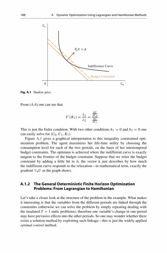
Fig. A.1 Shadow price
From (A.6) one can see that
F ′(K1) = λ1
λ2=
∂U∂C0
∂U∂C1
.
This is just the Euler condition. With two other conditions h1 = 0 and h2 = 0 onecan easily solve for (C0, C1,K1).
Figure A.1 gives a graphical interpretation to this inequality constrained opti-mization problem. The agent maximizes her life-time utility by choosing theconsumption level for each of the two periods, on the basis of her intertemporalbudget constraints. The optimum is achieved where the indifferent curve is exactlytangent to the frontier of the budget constraint. Suppose that we relax the budgetconstraint by adding a little bit to it, the vector λ just describes by how muchthe indifferent curve responds to the relaxation—in mathematical term, exactly thegradient �xU as the graph shows.
A.1.2 The General Deterministic Finite Horizon OptimizationProblems: From Lagrangian to Hamiltonian
Let’s take a closer look at the structure of the problem in the example. What makesit interesting is that the variables from the different periods are linked through theconstraints (otherwise we can solve the problem by simply repeating dealing withthe insulated T + 1 static problems), therefore one variable’s change in one periodmay have pervasive effects into the other periods. So one may wonder whether thereexists a solution method by exploiting such linkage—this is just the widely appliedoptimal control method.
A Dynamic Optimization Using Lagrangian and Hamiltonian Methods 189
As a general exposure, the prototype problem can be described as following.Think about the simplest case with only two variables kt , ct in each period t ∈{0, 1, . . . , T }, T < +∞. The problem is to maximize the object function U :R2(T +1) → R which is the summation of the function u : R2 → R for each period,
constrained by the intertemporal relations of k and c as well as the boundary values
max{ct }U =
T∑
t=0
1
(1 + ρ)tu (kt , ct , t) ,
s.t. kt+1 − kt = g (kt , ct ) ,
kt=0 = k0,
kT +1 ≥ kT +1.
k and c represent two kinds of variables. Variable kt is the one with which eachperiod starts and on which the decision is based, therefore it’s usually called statevariable. And variable ct is the one the decision maker can change in each periodand what is left over is fed back into the next period state variable, therefore it’susually called control variable. The constraint linking these variables across periodsis called the law of motion.
If we express everything in continuous time, we only need to rewrite thesummation by integration and the intertemporal change by the derivative withrespect to time. However solving the continuous time problems with the Lagrangianwould be a bit tricky. And in order to give the readers more exposures to thecontinuous time models, in the section that follows we start with building up thefoundations of finite horizon optimization problems in continuous time. Readersmay extend the same idea into the discrete time problems as an exercise.
Continuous TimeSuppose that time is continuous such that t ∈ [0, T ], T ≤ +∞. A typicaldeterministic continuous time optimization problem can be written as (often peoplesimply set k(T ) to be zero)
max{c(t)}
U =∫ T
0e−ρtu (k(t), c(t), t) dt,
s.t. k(t) = g (k(t), c(t), t) ,
k(0) = k0,
k(T ) ≥ k(T ).
Set up Lagrangian for this problem
L =∫ T
0e−ρt u (k(t), c(t), t) dt +
∫ T
0μ(t)
(g (k(t), c(t), t) − k(t)
)dt + ν
[k(T ) − k(T )
], (A.8)
190 A Dynamic Optimization Using Lagrangian and HamiltonianMethods
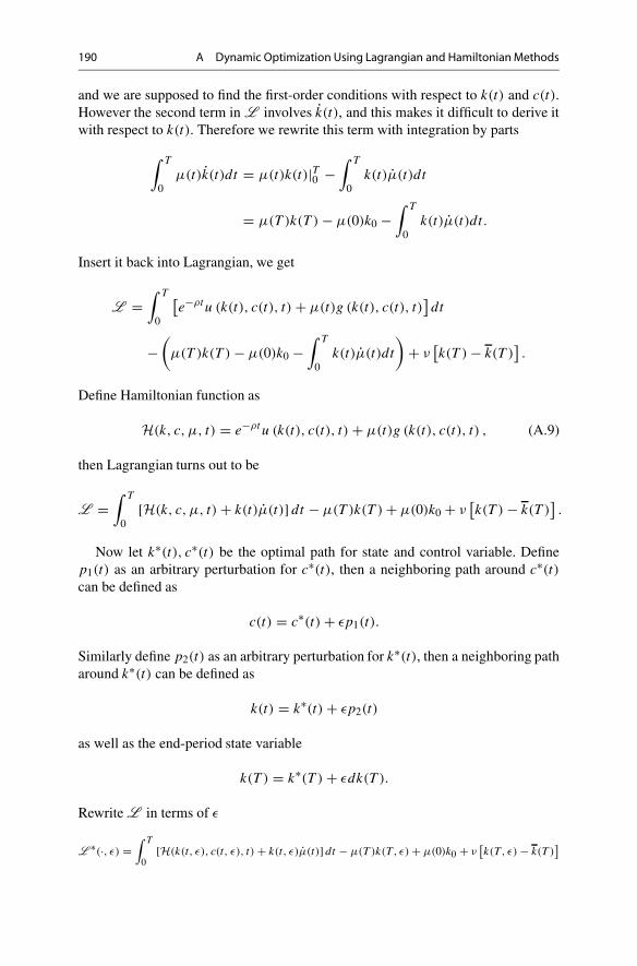
and we are supposed to find the first-order conditions with respect to k(t) and c(t).However the second term in L involves k(t), and this makes it difficult to derive itwith respect to k(t). Therefore we rewrite this term with integration by parts
∫ T
0μ(t)k(t)dt = μ(t)k(t)|T0 −
∫ T
0k(t)μ(t)dt
= μ(T )k(T ) − μ(0)k0 −∫ T
0k(t)μ(t)dt.
Insert it back into Lagrangian, we get
L =∫ T
0
[e−ρtu (k(t), c(t), t) + μ(t)g (k(t), c(t), t)
]dt
−(
μ(T )k(T ) − μ(0)k0 −∫ T
0k(t)μ(t)dt
)+ ν
[k(T ) − k(T )
].
Define Hamiltonian function as
H(k, c, μ, t) = e−ρtu (k(t), c(t), t) + μ(t)g (k(t), c(t), t) , (A.9)
then Lagrangian turns out to be
L =∫ T
0[H(k, c, μ, t) + k(t)μ(t)] dt − μ(T )k(T ) + μ(0)k0 + ν
[k(T ) − k(T )
].
Now let k∗(t), c∗(t) be the optimal path for state and control variable. Definep1(t) as an arbitrary perturbation for c∗(t), then a neighboring path around c∗(t)can be defined as
c(t) = c∗(t) + εp1(t).
Similarly define p2(t) as an arbitrary perturbation for k∗(t), then a neighboring patharound k∗(t) can be defined as
k(t) = k∗(t) + εp2(t)
as well as the end-period state variable
k(T ) = k∗(T ) + εdk(T ).
RewriteL in terms of ε
L ∗(·, ε) =∫ T
0[H(k(t, ε), c(t, ε), t) + k(t, ε)μ(t)] dt − μ(T )k(T , ε) + μ(0)k0 + ν
[k(T , ε) − k(T )
]
A Dynamic Optimization Using Lagrangian and Hamiltonian Methods 191
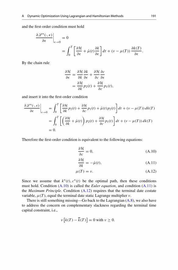
and the first-order condition must hold
∂L ∗(·, ε)∂ε
∣∣∣∣ε→0
= 0
=∫ T
0
[∂H∂ε
+ μ(t)∂k
∂ε
]dt + (ν − μ(T ))
∂k(T )
∂ε.
By the chain rule
∂H∂ε
= ∂H∂k
∂k
∂ε+ ∂H
∂c
∂c
∂ε
= ∂H∂k
p2(t) + ∂H∂c
p1(t),
and insert it into the first-order condition
∂L ∗(·, ε)∂ε
∣∣∣∣ε→0
=∫ T
0
[∂H∂k
p2(t) + ∂H∂c
p1(t) + μ(t)p2(t)
]dt + (ν − μ(T )) dk(T )
=∫ T
0
[(∂H∂k
+ μ(t)
)p2(t) + ∂H
∂cp1(t)
]dt + (ν − μ(T )) dk(T )
= 0.
Therefore the first-order condition is equivalent to the following equations:
∂H∂c
= 0, (A.10)
∂H∂k
= −μ(t), (A.11)
μ(T ) = ν. (A.12)
Since we assume that k∗(t), c∗(t) be the optimal path, then these conditionsmust hold. Condition (A.10) is called the Euler equation, and condition (A.11) isthe Maximum Principle. Condition (A.12) requires that the terminal date costatevariable, μ(T ), equal the terminal date static Lagrange multiplier ν.
There is still something missing—Go back to the Lagrangian (A.8), we also haveto address the concern on complementary slackness regarding the terminal timecapital constraint, i.e.,
ν[k(T ) − k(T )
] = 0 with ν ≥ 0.
192 A Dynamic Optimization Using Lagrangian and HamiltonianMethods
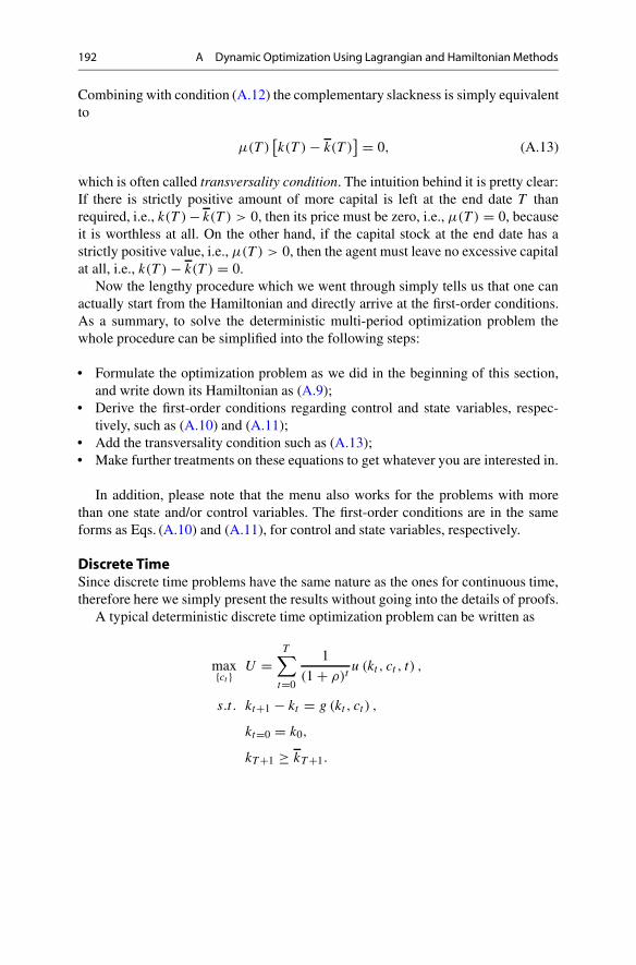
Combining with condition (A.12) the complementary slackness is simply equivalentto
μ(T )[k(T ) − k(T )
] = 0, (A.13)
which is often called transversality condition. The intuition behind it is pretty clear:If there is strictly positive amount of more capital is left at the end date T thanrequired, i.e., k(T ) − k(T ) > 0, then its price must be zero, i.e., μ(T ) = 0, becauseit is worthless at all. On the other hand, if the capital stock at the end date has astrictly positive value, i.e., μ(T ) > 0, then the agent must leave no excessive capitalat all, i.e., k(T ) − k(T ) = 0.
Now the lengthy procedure which we went through simply tells us that one canactually start from the Hamiltonian and directly arrive at the first-order conditions.As a summary, to solve the deterministic multi-period optimization problem thewhole procedure can be simplified into the following steps:
• Formulate the optimization problem as we did in the beginning of this section,and write down its Hamiltonian as (A.9);
• Derive the first-order conditions regarding control and state variables, respec-tively, such as (A.10) and (A.11);
• Add the transversality condition such as (A.13);• Make further treatments on these equations to get whatever you are interested in.
In addition, please note that the menu also works for the problems with morethan one state and/or control variables. The first-order conditions are in the sameforms as Eqs. (A.10) and (A.11), for control and state variables, respectively.
Discrete TimeSince discrete time problems have the same nature as the ones for continuous time,therefore here we simply present the results without going into the details of proofs.
A typical deterministic discrete time optimization problem can be written as
max{ct }U =
T∑
t=0
1
(1 + ρ)tu (kt , ct , t) ,
s.t. kt+1 − kt = g (kt , ct ) ,
kt=0 = k0,
kT +1 ≥ kT +1.
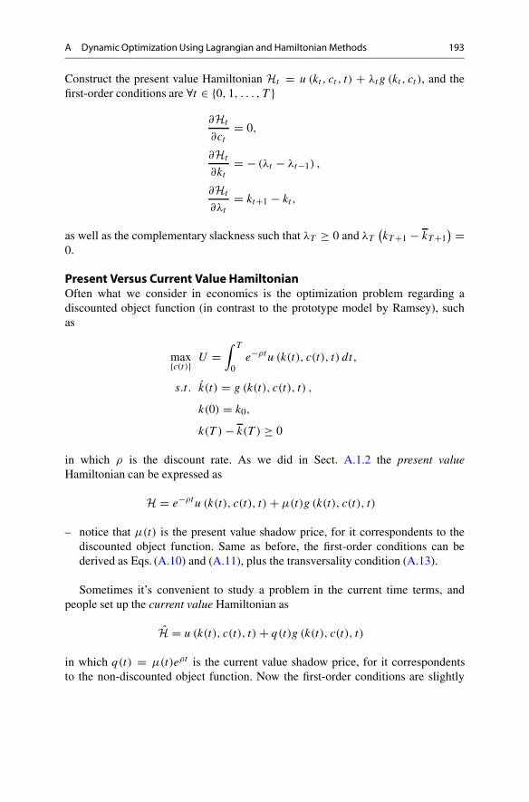
A Dynamic Optimization Using Lagrangian and Hamiltonian Methods 193
Construct the present value Hamiltonian Ht = u (kt , ct , t) + λtg (kt , ct ), and thefirst-order conditions are ∀t ∈ {0, 1, . . . , T }
∂Ht
∂ct
= 0,
∂Ht
∂kt
= − (λt − λt−1) ,
∂Ht
∂λt
= kt+1 − kt ,
as well as the complementary slackness such that λT ≥ 0 and λT
(kT +1 − kT +1
) =0.
Present Versus Current Value HamiltonianOften what we consider in economics is the optimization problem regarding adiscounted object function (in contrast to the prototype model by Ramsey), suchas
max{c(t)}
U =∫ T
0e−ρtu (k(t), c(t), t) dt,
s.t. k(t) = g (k(t), c(t), t) ,
k(0) = k0,
k(T ) − k(T ) ≥ 0
in which ρ is the discount rate. As we did in Sect. A.1.2 the present valueHamiltonian can be expressed as
H = e−ρtu (k(t), c(t), t) + μ(t)g (k(t), c(t), t)
– notice that μ(t) is the present value shadow price, for it correspondents to thediscounted object function. Same as before, the first-order conditions can bederived as Eqs. (A.10) and (A.11), plus the transversality condition (A.13).
Sometimes it’s convenient to study a problem in the current time terms, andpeople set up the current value Hamiltonian as
H = u (k(t), c(t), t) + q(t)g (k(t), c(t), t)
in which q(t) = μ(t)eρt is the current value shadow price, for it correspondentsto the non-discounted object function. Now the first-order conditions are slightly
194 A Dynamic Optimization Using Lagrangian and HamiltonianMethods
different in ∂H∂k
∂H∂c
= 0, (A.14)
∂H∂k
= ρq(t) − q(t), (A.15)
as well as the transversality condition
q(T )e−ρt[k(T ) − k(T )
] = 0. (A.16)
Although Eq. (A.15) is a little more complicated, it is very intuitive. Notice
that ∂H∂k
is just the marginal contribution of the capital to utility, i.e., the dividendreceived by the agent, the equation reflects the idea of asset pricing: given that q(t)
is the capital gain (the change in the price of the asset), and ρ is the rate of return onan alternative asset, i.e., consumption, Eq. (A.15) says that at the optimum the agentis indifferent between the two types of the investment, for the overall rate of returnto the capital,
∂H∂k
+ q(t)
q(t),
equals the return to consumption, ρ. For this reason, Eq. (A.15) is also called non-arbitrage condition.
A.2 Going Infinite
What will happen when we extend the results of finite horizon optimizationproblems into the ones with infinite horizon?
The optimization itself is only a little different—T = +∞ in the object function
U =∫ +∞
0e−ρtu (k(t), c(t), t) dt,
and there will be no terminal time condition any more, because the time doesn’tterminate at all. But this makes a big change of the problem: Now the optimal timepath looks like a kite—we hold the thread at hand, but we don’t know where it ends.
Note that the principles behind the finite time optimization problem are thatfollowing the optimal time path nothing valuable is left over in the end of the world(such that μ(T )
[k(T ) − k(T )
]is non-positive) and the agent doesn’t exit the world
with debt (such thatμ(T )[k(T ) − k(T )
]is non-negative),which are captured in the
transversality condition. To maintain the same principles in the infinite time horizon,
A Dynamic Optimization Using Lagrangian and Hamiltonian Methods 195
we may assume that there is an end of the world, but after a nearly infinitely longtime. Therefore we may impose a similar transversality condition for the problemsof infinite time horizon
limT →+∞ μ(T )
[k(T ) − k(T )
] = 0,
i.e., the value of the state variable must be asymptotically zero: If the quantity ofk(T ) remains different from the constraint asymptotically, then its price,μ(T ), mustapproach 0 asymptotically; if k(T ) − k(T ) grows forever at a positive rate, then thepriceμ(T )must approach 0 at a faster rate so that the product,μ(T )
[k(T ) − k(T )
],
goes to 0.
BDynamic Programming
Dynamic programming is another powerful tool to solve dynamic optimizationproblems.
B.1 Dynamic Programming: The Theoretical Foundation
The theoretical foundation of dynamic programming is contraction mapping. Let’sstart with some formal definitions.
Definition B.1 A metric space (S, ρ) is a non-empty set S and a metric, or distanceρ : S × S → R, which is defined as a mapping, ∀x, y, v, with
1. ρ(x, y) = 0 ⇔ x = y,2. ρ(x, y) = ρ(x, y), and3. ρ(x, y) ≤ ρ(x, v) + ρ(v, y).
For example, a plane(R2, d2
)is a metric space, in which the metric d2 : R2 ×
R2 → R is defined as
d2(x, y) = ||x − y||2 =√
(x1 − y1)2 + (x2 − y2)
2,∀x, y ∈ R2,
i.e., d2(·), or || · ||2, is just the Euclidean distance.
Definition B.2 A norm is a mapping Rn x �→ ||x|| ∈ R on Rn , with
1. ∀x ∈ Rn, ||x|| = 0 ⇔ x = 0,
2. ∀x ∈ Rn, ∀α ∈ R, ||αx|| = |α|||x|| and
3. ∀x, y ∈ Rn,||x + y|| ≤ ||x|| + ||y||.
© Springer Nature Switzerland AG 2019J. Cao, G. Illing, Instructor’s Manual for Money: Theory and Practice,Springer Texts in Business and Economics,https://doi.org/10.1007/978-3-030-23618-2
197
198 B Dynamic Programming
In the definition of metric space, the set S is just arbitrary. It can be a subset ofn dimensional space, i.e., S ⊆ R
n, but it can also be a function space B(X)—a setcontaining all (normally, bounded) functions mapping a set X to R, B : X → R.Then we define a supremum norm on such function space
d∞ = ||f − g||∞ = supx∈X
|f (x) − g(x)|,∀f, g ∈ B(X),
and this metric space of bounded functions on X with supremum norm is denotedby (B(X), d∞).
Having defined all the necessary terms, we continue with a special mapping.
Definition B.3 Suppose a metric space (S, ρ) and a function T : S → S mappingS to itself. T is a contraction mappingwith modulus β, if ∃β ∈ (0, 1), ρ(T x, Ty) ≤βρ(x, y), ∀x, y ∈ S.
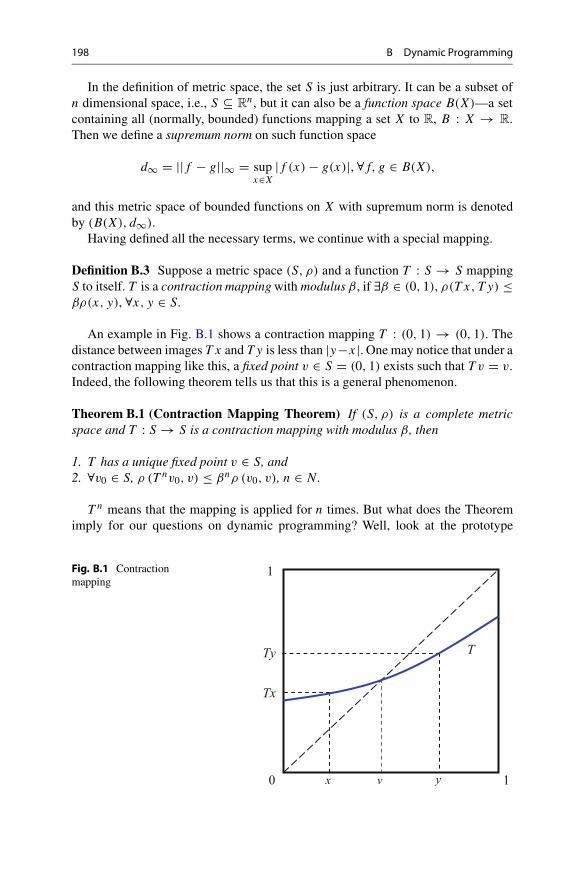
An example in Fig. B.1 shows a contraction mapping T : (0, 1) → (0, 1). Thedistance between images T x and Ty is less than |y−x|. One may notice that under acontraction mapping like this, a fixed point v ∈ S = (0, 1) exists such that T v = v.Indeed, the following theorem tells us that this is a general phenomenon.
Theorem B.1 (Contraction Mapping Theorem) If (S, ρ) is a complete metricspace and T : S → S is a contraction mapping with modulus β, then
1. T has a unique fixed point v ∈ S, and2. ∀v0 ∈ S, ρ (T nv0, v) ≤ βnρ (v0, v), n ∈ N .
T n means that the mapping is applied for n times. But what does the Theoremimply for our questions on dynamic programming? Well, look at the prototype
Fig. B.1 Contractionmapping
x y
Tx
Ty T
0 1
1
v
B Dynamic Programming 199
problem
V (kt) = maxct ,kt+1
{u(ct ) + βV (kt+1)} . (B.1)
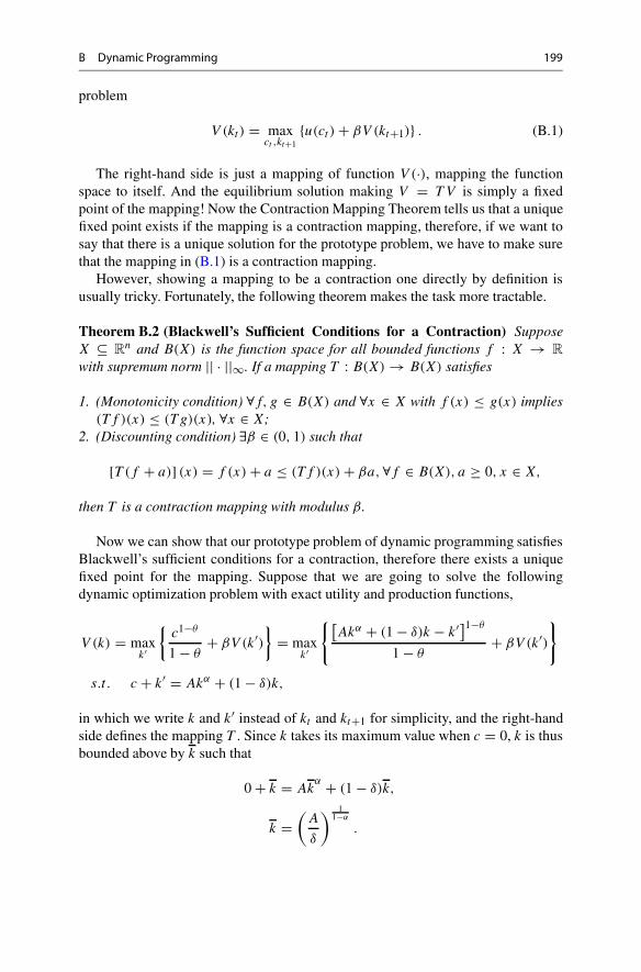
The right-hand side is just a mapping of function V (·), mapping the functionspace to itself. And the equilibrium solution making V = T V is simply a fixedpoint of the mapping! Now the Contraction Mapping Theorem tells us that a uniquefixed point exists if the mapping is a contraction mapping, therefore, if we want tosay that there is a unique solution for the prototype problem, we have to make surethat the mapping in (B.1) is a contraction mapping.
However, showing a mapping to be a contraction one directly by definition isusually tricky. Fortunately, the following theorem makes the task more tractable.
Theorem B.2 (Blackwell’s Sufficient Conditions for a Contraction) SupposeX ⊆ R
n and B(X) is the function space for all bounded functions f : X → R
with supremum norm || · ||∞. If a mapping T : B(X) → B(X) satisfies
1. (Monotonicity condition) ∀f, g ∈ B(X) and ∀x ∈ X with f (x) ≤ g(x) implies(Tf )(x) ≤ (T g)(x), ∀x ∈ X;
2. (Discounting condition) ∃β ∈ (0, 1) such that
[T (f + a)] (x) = f (x) + a ≤ (Tf )(x) + βa,∀f ∈ B(X), a ≥ 0, x ∈ X,
then T is a contraction mapping with modulus β.
Now we can show that our prototype problem of dynamic programming satisfiesBlackwell’s sufficient conditions for a contraction, therefore there exists a uniquefixed point for the mapping. Suppose that we are going to solve the followingdynamic optimization problem with exact utility and production functions,
V (k) = maxk′
{c1−θ
1 − θ+ βV (k′)
}= max
k′
{[Akα + (1 − δ)k − k′]1−θ
1 − θ+ βV (k′)
}
s.t. c + k′ = Akα + (1 − δ)k,
in which we write k and k′ instead of kt and kt+1 for simplicity, and the right-handside defines the mapping T . Since k takes its maximum value when c = 0, k is thusbounded above by k such that
0 + k = Akα + (1 − δ)k,
k =(
A
δ
) 11−α
.
200 B Dynamic Programming
Therefore define the state space X ⊆ [0, k
]as a complete subspace of R, and B(X)
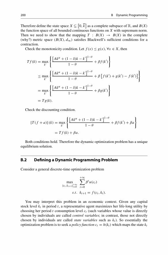
the function space of all bounded continuous functions on X with supremum norm.Then we need to show that the mapping T : B(X) → B(X) in the complete(why?) metric space (B(X), d∞) satisfies Blackwell’s sufficient conditions for acontraction.
Check the monotonicity condition. Let f (x) ≤ g(x), ∀x ∈ X, then
Tf (k) = maxk′
{[Akα + (1 − δ)k − k′]1−θ
1 − θ+ βf (k′)
}
≤ maxk′
{[Akα + (1 − δ)k − k′]1−θ
1 − θ+ β
[f (k′) + g(k′) − f (k′)
]}
= maxk′
{[Akα + (1 − δ)k − k′]1−θ
1 − θ+ βg(k′)
}
= Tg(k).
Check the discounting condition.
[T (f + a)] (k) = maxk′
{[Akα + (1 − δ)k − k′]1−θ
1 − θ+ βf (k′) + βa
}
= Tf (k) + βa.
Both conditions hold. Therefore the dynamic optimization problem has a uniqueequilibrium solution.
B.2 Defining a Dynamic Programming Problem
Consider a general discrete-time optimization problem
max{ct ,kt+1}+∞
t=0
+∞∑
t=0
βtu(ct )
s.t. kt+1 = f (ct , kt ).
You may interpret this problem in an economic context. Given any capitalstock level kt in period t , a representative agent maximizes her life-long utility bychoosing her period t consumption level ct (such variables whose value is directlychosen by individuals are called control variables; in contrast, those not directlychosen by individuals are called state variables such as kt ). So essentially theoptimization problem is to seek a policy function ct = h(kt ) which maps the state kt
B Dynamic Programming 201
into the control ct . As soon as ct is chosen, the transition function kt+1 = f (ct , kt )
determines next period state kt+1 and the same procedure repeats. Such procedureis recursive.
The basic idea of dynamic programming is to collapse a multi-periods probleminto a sequence of two-periods problem at any t using the recursive nature of theproblem
V (kt ) = maxct ,kt+1
+∞∑
i=0
βiu(kt+i)
= maxct ,kt+1
{u(ct ) + β
+∞∑
i=0
βiu(ct+i+1)
}
= maxct ,kt+1
{u(ct ) + βV (kt+1)}
s.t. kt+1 = f (ct , kt ). (B.2)
Equation V (kt ) = maxct ,kt+1 {u(ct ) + βV (kt+1)} is known as Bellman equation.The value function V (·) is only a function of state variable kt because the optimalvalue of ct is just a function of kt . Then the original problem can be solved by themethods we learned for two-periods problems plus some tricks.
B.3 Getting the Euler Equation
The key step now is to find the proper first-order conditions. There are severalpossible approaches, and readers may pick up one of them with which he or shefeels comfortable.
B.3.1 Using Lagrangian
Since the problem looks pretty similar to a maximization problem with equalityconstraint, one may suggest Lagrangian—Let’s try.
Rewrite V (kt ) as
V (kt) = maxct ,kt+1
{u(ct ) + βV (kt+1) + λt [f (ct , kt ) − kt+1]}︸ ︷︷ ︸Lt
.
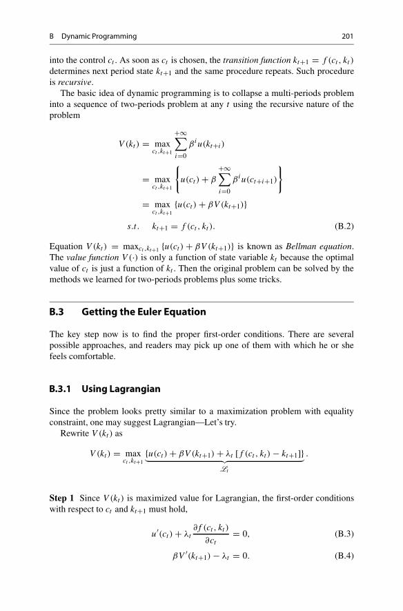
Step 1 Since V (kt ) is maximized value for Lagrangian, the first-order conditionswith respect to ct and kt+1 must hold,
u′(ct ) + λt∂f (ct , kt )
∂ct
= 0, (B.3)
βV ′(kt+1) − λt = 0. (B.4)
202 B Dynamic Programming
Step 2 Since V (kt) is optimized at kt , then
V ′(kt ) = u′(ct )dct
dkt
+ βV ′(kt+1)dkt+1
dkt
+ dλt
dkt[f (ct , kt ) − kt+1]
+λt
[∂f (ct , kt )
∂kt
+ ∂f (ct , kt )
∂ct
dct
dkt
− dkt+1
dkt
]
=[u′(ct ) + λt
∂f (ct , kt )
∂ct
]
︸ ︷︷ ︸(A)
dct
dkt
+ [βV ′(kt+1) − λt
]︸ ︷︷ ︸
(B)
dkt+1
dkt
+dλt
dkt[f (ct , kt ) − kt+1]︸ ︷︷ ︸
(C)
+λt∂f (ct , kt )
∂kt
.
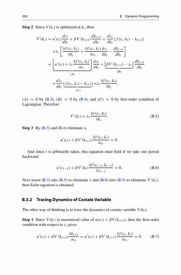
(A) = 0 by (B.3), (B) = 0 by (B.4), and (C) = 0 by first-order condition ofLagrangian. Therefore
V ′(kt) = λt∂f (ct , kt )
∂kt
. (B.5)
Step 3 By (B.3) and (B.4) eliminate λt
u′(ct ) + βV ′(kt+1)∂f (ct , kt )
∂ct
= 0.
And since t is arbitrarily taken, this equation must hold if we take one periodbackward
u′(ct−1) + βV ′(kt)∂f (ct−1, kt−1)
∂ct−1= 0. (B.6)
Next insert (B.3) into (B.5) to eliminate λ and (B.6) into (B.5) to eliminate V ′(kt ),then Euler equation is obtained.
B.3.2 Tracing Dynamics of Costate Variable
The other way of thinking is to trace the dynamics of costate variable V (kt ).
Step 1 Since V (kt ) is maximized value of u(ct ) + βV (kt+1), then the first-ordercondition with respect to ct gives
u′(ct ) + βV ′(kt+1)∂kt+1
∂ct
= u′(ct ) + βV ′(kt+1)∂f (ct , kt )
∂ct
= 0. (B.7)
B Dynamic Programming 203
Step 2 Since V (kt) is optimized at kt , then
V ′(kt ) = u′(ct )dct
dkt
+ βV ′(kt+1)
[∂f (ct , kt )
∂kt
+ ∂f (ct , kt )
∂ct
dct
dkt
]
=[u′(ct ) + βV ′(kt+1)
∂f (ct , kt )
∂ct
]dct
dkt
+ βV ′(kt+1)∂f (ct , kt )
∂kt
.
Apply (B.7) and get
V ′(kt ) = βV ′(kt+1)∂f (ct , kt )
∂kt
. (B.8)
Since t is arbitrarily taken, (B.7) also holds for one period backward, i.e.,
V ′(kt ) = − u′(ct−1)
β∂f (ct−1,kt−1)
∂ct−1
. (B.9)
Step 3 Apply (B.7) and (B.9) into (B.8) and obtain Euler equation.
B.3.3 Using Envelope Theorem
We may also use the Envelope Theorem to find the first-order condition.
Theorem B.3 Suppose that value function m(a) is defined as following:
m(a) = maxx
f (x(a), a).
Then the total derivative of m(a) with respect to a equals the partial derivative off (x(a), a) with respect to a, if f (x(a), a) is evaluated at x = x(a) that maximizesf (x(a), a), i.e.,
dm(a)
da= ∂f (x(a), a)
∂a
∣∣∣∣x=x(a)
.
Proof Since m(a) is maximized value of f (x(a), a) at x = x(a), then
∂f (x(a), a)
∂x= 0
204 B Dynamic Programming
by the first-order condition. Therefore the total derivative of m(a) with respect to a
is
dm(a)
da= ∂f (x(a), a)
∂x
dx(a)
da+ ∂f (x(a), a)
∂a
= ∂f (x(a), a)
∂a
since the first term is equal to 0. �
Solve the budget constraint for ct and get ct = g(kt , kt+1). Apply it to V (kt) andget a univariate optimization problem
V (kt ) = maxkt+1
{u(g(kt , kt+1)) + βV (kt+1)} .
Step 1 Similar as before, since V (kt ) is the maximized value of u(g(kt , kt+1)) +βV (kt+1), then the first-order condition with respect to kt+1 gives
u′(g(kt , kt+1))∂g(kt , kt+1)
∂kt+1+ βV ′(kt+1) = 0. (B.10)
Step 2 Since V (kt ) is already optimized at kt , differentiating V (kt ) with respect tokt gives
dV (kt )
dkt
= ∂V (kt )
∂kt︸ ︷︷ ︸(A)
+ ∂V (kt )
∂kt+1
∂kt+1
∂kt︸ ︷︷ ︸(B)
. (B.11)
This is pretty intuitive: kt may generate a direct effect on V (kt ) as part (A) shows;however, kt may also generate an indirect effect on V (kt ) through kt+1 (rememberthe dynamic budget constraint). And since V (kt) is optimized by kt+1, the first-ordercondition implies that ∂V (kt )
∂kt+1= 0. Therefore Eq. (B.11) becomes
V ′(kt ) = ∂V (kt )
∂kt
= u′(g(kt , kt+1))dg(kt , kt+1)
dkt
(B.12)
which is also called Benveniste–Scheinkman condition.
Step 3 Similar as before, take one period forward for (B.12) and apply it into (B.10)then obtain Euler equation.
B Dynamic Programming 205
B.3.4 Example
Consider a discrete time Ramsey problem for a decentralized economy
max{ct ,bt }+∞
t=0
+∞∑
t=0
βtu(ct )
s.t. bt+1 − bt = wt + rtbt − ct − nbt .
Collapse the infinite horizon problem into a sequence of two-periods problem
V (bt ) = maxct ,bt+1
+∞∑
i=0
βiu(ct+i )
= maxct ,bt+1
{u(ct ) + β
+∞∑
i=0
βiu(ct+i+1)
}
= maxct ,bt+1
{u(ct ) + βV (bt+1)}
s.t. bt+1 = wt + (1 + rt )bt − ct − nbt .
Now we solve the problem with all three approaches.
Using LagrangianRewrite Bellman equation in Lagrangian form
V (bt ) = maxct ,bt+1
{u(ct ) + βV (bt+1) + λt [wt + (1 + rt )bt − ct − nbt − bt+1]} .
Step 1 The first-order conditions of Lagrangian are
u′(ct ) − λt = 0, (B.13)
βV ′(bt+1) − λt = 0, (B.14)
and eliminate λt to get
u′(ct ) = βV ′(bt+1). (B.15)
Step 2 Now differentiate V (bt ) at bt
V ′(bt ) = u′(ct )dct
dbt
+ βV ′(bt+1)(1 + rt − n)
+dλt
dkt[wt + (1 + rt )bt − ct − nbt − bt+1]︸ ︷︷ ︸
=0
206 B Dynamic Programming
+λt
[(1 + rt − n) − dct
dbt
− (1 + rt − n)
]
= [u′(ct ) − λt
]︸ ︷︷ ︸
=0
dct
dbt
+ [βV ′(bt+1) − λt
]︸ ︷︷ ︸
=0
(1 + rt − n) + λt (1 + rt − n).
That is,
V ′(bt ) = λt (1 + rt − n). (B.16)
Step 3 Insert (B.13) and (B.15) into (B.16) and get the desired result.
Tracing Dynamics of Costate VariableNow solve the same problem by tracing the dynamics of the costate variable.
Step 1 Since V (bt ) is the maximized value of u(ct )+βV (bt+1), then the first-ordercondition with respect to bt+1 gives
− u′(ct ) + βV ′(bt+1) = 0. (B.17)
Step 2 Now differentiate V (bt ) at bt
V ′(bt ) = u′(ct )∂ct
∂kt
+ βV ′(bt+1)
[(1 + rt − n) − ∂ct
∂kt
].
That is just
V ′(bt) = β(1 + rt − n)V ′(bt+1). (B.18)
Step 3 Insert (B.17) twice into (B.18) and get the desired result.
Using Envelope TheoremNow solve the same problem with Envelope Theorem.
Step 1 Since V (bt ) is maximized value of u(ct ) + βV (bt+1), then the first-ordercondition with respect to bt+1 gives
− u′(ct ) + βV ′(bt+1) = 0. (B.19)
Step 2 Now the problem is to find V ′(bt+1). Differentiate V (bt ) at bt
V ′(bt) = ∂V (bt)
∂bt
= (1 + rt − n)u′(ct ). (B.20)

B Dynamic Programming 207
Step 3 Take one period backward for (B.19) and insert into (B.20) to obtain theEuler equation.
B.4 Solving for the Policy Function
As seen in previous sections policy function ct = h(kt ) captures the optimal solutionfor each period given the corresponding state variable, therefore one may desire toget the solution of the policy function. Dynamic programming method has a specialadvantage for this purpose, and we will see several approaches in the following.
Now consider the problem of Brock andMirman (1972). Suppose utility functiontakes the form ut = ln ct and the production function follows Cobb–Douglastechnology. No depreciation and population growth.
max{ct ,kt }+∞
t=0
∗∞∑
t=0
βt ln ct
s.t. kt+1 = kαt − ct .
B.4.1 Solution by Iterative Substitution the Euler Equation
Recall that the recursive structure of dynamic programmingmethod implies that theproblem that the optimizer faces in each period is the same as that she faces lastperiod or next period, so the solution to such a problem should be time-invariant.Thus one can start from deriving the solution under some circumstances and iterateit on an infinite time horizon until it is time invariant. However this approach onlyworks when the problem is simple.
Forward InductionSet up the Bellman equation and solve for Euler equation. This gives
1
ct
= αβkα−1t+1
ct+1
kt+1
ct
= αβkαt+1
ct+1
kαt − ct
ct
= αβkαt+1
ct+1
kαt
ct
= αβkαt+1
ct+1+ 1.
208 B Dynamic Programming
Apply this condition to itself and get a geometric serial
kαt
ct= 1 + αβ
(1 + αβ
kαt+2
ct+2
)
= 1 + αβ + α2β2 + α3β3 + . . .
= 1
1 − αβ,
(why?) and this gives
ct = (1 − αβ)kαt .
Another way to see this is exploring saving rate dynamics. Express ct by kt andkt+1
1
kαt − kt+1
= β1
kαt+1 − kt+2
αkα−1t+1 . (B.21)
Define saving rate at time t as
st = kt+1
kαt
,
Rearranging (B.21) gives
1
kαt
1
1 − st= β
1
kαt+1
1
1 − st+1αkα−1
t+1
kt+1
kαt
1
1 − st= αβ
1 − st+1
st
1 − st= αβ
1 − st+1,
and this is
st+1 = 1 + αβ − αβ
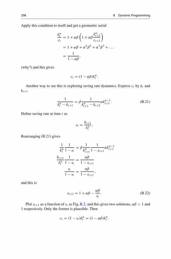
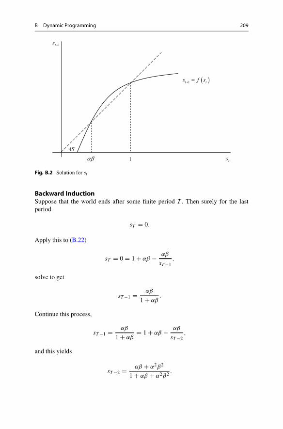
st. (B.22)
Plot st+1 as a function of st as Fig. B.2, and this gives two solutions, αβ < 1 and1 respectively. Only the former is plausible. Then
ct = (1 − st )kαt = (1 − αβ)kα
t .
B Dynamic Programming 209
1ts
ts1
1t ts f s
45
Fig. B.2 Solution for st
Backward InductionSuppose that the world ends after some finite period T . Then surely for the lastperiod
sT = 0.
Apply this to (B.22)
sT = 0 = 1 + αβ − αβ
sT −1,
solve to get
sT −1 = αβ
1 + αβ.
Continue this process,
sT −1 = αβ
1 + αβ= 1 + αβ − αβ
sT −2,
and this yields
sT −2 = αβ + α2β2
1 + αβ + α2β2 .
210 B Dynamic Programming
We find that for any t between 0 and T
st =∑T −t
i=1 αiβi
1 +∑T −ti=1 αiβi
=αβ(1−αT−t βT −t )
1−αβ
1 + αβ(1−αT−t βT −t )1−αβ
= αβ(1 − αT −t βT −t )
1 − αβ + αβ(1 − αT −t βT −t ).
And in the limit
limT −t→+∞ st = αβ
implying that
ct = (1 − αβ)kαt .
B.4.2 Solution by Value-Function Iteration
Another solution method is based on iteration of the value function. The valuefunction actually will be different in each period, just as we earlier found thefunction g(kt ) was different depending on how close we were to the terminal period.But it can be shown (but we do not show this here) that as we iterate through time,the value function converges, just as g(kt ) converged in our earlier example as weiterated back further away from the terminal period. This suggests that if we iterateon an initial guess for the value function, even a guess we know is incorrect, theiterations eventually will converge to the true function.
Guess and VerifyOne may guess the form of solution and try to verify whether it’s true. We guess that
V (kt) = A + B ln kt .
Then the problem becomes
V (kt ) = maxct ,kt+1
{ln ct + βV (kt+1)}
= maxct ,kt+1
{ln ct + β(A + B ln kt+1)}
s.t. kt+1 = kαt − ct .
The first-order condition with respect to kt+1 yields
− 1
ct
+ βB
kt+1= 0,
kt+1 = βB(kαt − kt+1),
B Dynamic Programming 211
kt+1 = βB
1 + βBkαt ,
ct = 1
1 + βBkαt .
Then apply the results to the Bellman equation, and the following must hold if ourconjecture is right
V (kt) = ln
(βB
1 + βBkαt
)+ β
[A + B ln
(1
1 + βBkαt
)]
= lnβB + βA − (1 + βB) ln(1 + βB)︸ ︷︷ ︸A
+ α(1 + βB)︸ ︷︷ ︸B
ln kt
= A + B ln kt .
Solve to get
B = α
1 − αβ,
A = 1
1 − β
[ln(1 − αβ) + αβ
1 − αβlnαβ
],
ct = 1
1 + βBkαt = (1 − αβ)kα
t .
and therefore
kt+1 = βB
1 + βBkαt = αβkα
t ,
ct = 1
1 + βBkαt = (1 − αβ)kα
t .
Value-Function IterationUnfortunately few problems can be solved by simple conjectures. As a last resortone needs onerous effort on value functions. Suppose that the world ends after somefinite period T . Then surely
V (kT +1) = 0,
as well as
cT = kαT , and kT +1 = 0.

212 B Dynamic Programming
Apply these in Bellman equation,
V (kT ) = ln kαT + βV (kT +1) = ln kα
T .
For one period backward,
V (kT −1) = maxcT −1,kT
{ln(cT −1) + βV (kT )}
= maxcT −1,kT
{ln(cT −1) + β ln kα
T
}
s.t. kT = kαT −1 − cT −1.
This is simply a two-period intertemporal optimization with an equality constraint.Using Lagrangian
L = ln(cT −1) + β ln kαT + λ
[kαT −1 − cT −1 − kT
],
first-order conditions give
∂L
∂cT −1= 1
cT −1− λ = 0,
∂L
∂kT
= αβkα−1T
kαT
− λ = αβ1
kT
− λ = 0,
∂L
∂λ= kα
T −1 − cT −1 − kT = 0.
Solve to get
cT −1 = 1
1 + αβkαT −1,
kT = αβ
1 + αβkαT −1.
Then V (kT −1) can be expressed as
V (kT −1) = ln
(1
1 + αβkαT −1
)+ β ln
(αβ
1 + αβkαT −1
)α
= αβ ln(αβ) − (1 + αβ) ln(1 + αβ) + (1 + αβ) ln kαT −1.
Again take one period backward,
V (kT −2) = maxcT −2,kT −1
{ln(cT −2) + βV (kT −1)}
s.t. kT −1 = kαT −2 − cT −2,
B Dynamic Programming 213
and the same procedure applies. After several rounds you may find that for time t
long before T the value function converges to
V (kt ) = maxct ,kt+1
{ln ct + β
[1
1 − β
(ln(1 − αβ) + αβ
1 − αβln αβ
)
+ α
1 − αβln kt+1
]}
s.t. kt+1 = kαt − ct .
As before since V (kt ) is the maximized value the first-order condition with respectto kt+1 still holds
− 1
ct
+ αβ
1 − αβ
1
kt+1= 0,
this yields
ct = (1 − αβ)kαt
kt+1 = αβkαt .
Although this solution method is very cumbersome and computationallydemanding since it rests on brutal-force iteration of the value function, it hasthe advantage that it always works if the solution exists. Actually, the convergenceof the value function is not incidental. The Contraction Mapping Theorem tells usthat the convergence result is always achieved as long as the value function containsa contraction mapping (which works for most of dynamic optimization problemsunder the neoclassical assumptions). Such result is crucial for both theory andapplication. In theory, it ensures that a unique equilibrium solution (the fixed point)exists so that we can say what happens in the long run; in application, it impliesthat even we start iteration from an arbitrary value function, the value function willfinally converge to the true one. Therefore, in practice when the value function ishardly solvable in an analytical way, people usually set up the computer program toperform the iteration and get a numerical solution.
B.5 Extensions
B.5.1 Extension 1: Dynamic Programming Under Uncertainty
Consider a general discrete-time optimization problem
max{ct ,kt+1}+∞
t=0
E0
[+∞∑
t=0
βtu(ct )
]
s.t. kt+1 = ztf (kt ) − ct ,
214 B Dynamic Programming
in which the production f (kt ) is affected by an i.i.d. process {zt }+∞t=0 (technology
shock, which realizes at the beginning of each period t) meaning that such shockvaries over time, but its deviations in different periods are uncorrelated (think aboutthe weather for the farmers). Now the agent has to maximize the expected utilityover time because future consumption is uncertain.
Since technology shocks realize at the beginning of each period, the value of totaloutput is known when consumption takes place and when the end-of-period capitalkt+1 is accumulated. The state variables are now kt and zt . The control variables arect . Similar as before, set up the Bellman equation as
V (kt , zt ) = maxct ,kt+1
{u(ct ) + βEt [V (kt+1, zt+1)]}
s.t. kt+1 = ztf (kt) − ct .
Let’s apply the solution strategies introduced before and see whether they work.
Step 1 The first-order condition with respect to kt+1 gives
− u′(ct ) + βEt
[dV (kt+1, zt+1)
dkt+1
]= 0. (B.23)
Think why it is legal to take derivative within expectation operator.
Step 2 By Envelope Theorem differentiating V (kt , zt ) with respect to kt gives
dV (kt , zt )
dkt
= u′(ct )ztf′(kt ). (B.24)
Step 3 Take one step forward for (B.24) and apply it into (B.23), then we get
u′(ct ) = βEt
[u′(ct+1)zt+1f
′(kt+1)].
Suppose that
f (kt ) = kαt ,
u(ct ) = ln ct .
Then Euler equation becomes
1
ct
= βEt
[1
ct+1zt+1αkα−1
t+1
].
B Dynamic Programming 215
In deterministic case our solutions were
ct = (1 − αβ)kαt ,
kt+1 = αβkαt .
Now let’s guess that under uncertainty the solution is of similar form such that
ct = (1 − A)ztkαt ,
kt+1 = Aztkαt ,
and check whether it’s true or false. The Euler equation becomes
1
(1 − A)zt kαt
= βEt
[1
(1 − A)zt+1kαt+1
zt+1αkα−1t+1
]
= αβ
[1
(1 − A)kt+1
]
= αβ
[1
(1 − A)Aztkαt
].
Therefore it’s easily seen that
A = αβ,
which seems quite similar as before.However since the consumption and capital stock are random variables, it’s
necessary to explore their properties by characterizing corresponding distributions.Assume that ln zt ∼ N
(μ, σ 2
). Take log of the solution above,
ln kt+1 = lnαβ + ln zt + α ln kt .
Apply this result recursively,
ln kt = lnαβ + ln zt−1 + α ln kt−1
= lnαβ + ln zt−1 + α(ln αβ + ln zt−2 + α ln kt−2)
. . .
=(1 + α + α2 + . . . + αt−1
)lnαβ
+(ln zt−1 + α ln zt−2 + . . . + αt−1 ln z0
)
+αt ln k0.
216 B Dynamic Programming
In the limit the mean of ln kt converges to
limt→+∞ E0 [ln kt ] = lnαβ + μ
1 − α.
The variance of ln kt is defined as
var[ln kt ] = E{(ln kt − E [ln kt ])2
}
= E{((
1 + α + α2 + . . . + αt−1)ln αβ + (ln zt−1 + α ln zt−2
+ . . . + αt−1 ln z0
)+ αt ln k0 −
[(1 + α + α2 + . . . + αt−1
)ln αβ
+(1 + α + . . . + αt−1
)μ + αt ln k0
])2}
= E{[
(ln zt−1 − μ) + α (ln zt−2 − μ) + α2 (ln zt−2 − μ) + . . .
+αt−1 (ln z0 − μ)]2}
= E
⎡
⎣(
t∑
i=1
αi−1(ln zt−i − μ)
)2⎤
⎦
=t∑
i=1
α2i−2E[(ln zt−i − μ)2
]
+∑
∀i,j∈{1,...,t}i �=j
αi−1αj−1E[(ln zt−i − μ)(ln zt−j − μ)
]
= 1 − α2t
1 − α2 var [ln zt ]
= 1 − α2t
1 − α2 σ 2,
or simply pass the variance operator through the sum and get
var[ln kt ] = var[ln zt−1] + α2var[ln zt−2] + . . . + α2t−2var[ln z0]=(1 + α2 + . . . + α2t−2
)σ 2
= 1 − α2t
1 − α2 σ 2.
B Dynamic Programming 217
In the limit the variance of ln kt converges to
limt→+∞ var(ln kt ) = σ 2
1 − α2 .
As a conclusion one can say that in the limit ln kt converges to a distribution with
mean lnαβ+μ1−α
and variance σ 2
1−α2 .
B.5.2 Extension 2: Dynamic Programming in Continuous Time
Till now one may get the illusion that dynamic programming only fits discrete time.Now with slight modification we’ll see that it works for continuous time problemsas well. Consider a general continuous time optimization problem
maxct ,kt
∫ +∞
t=0e−ρtu(ct )dt
s.t. kt = φ(ct , kt ) = f (kt ) − ct
in which we assume that φ(ct , kt ) is quasi-linear in ct only for simplicity.Following Bellman’s idea, for arbitrary t ∈ [0,+∞) define
V (kt ) = maxct ,kt
∫ +∞
t
e−ρ(τ−t )u(cτ )dτ.
Now suppose that time goes from t to t + �t , in which �t is very small. Let’simagine what happened from t on. First u(ct ) accumulates during �t . Since �t isso small that it’s reasonable to think that u(ct ) is nearly constant from t to t + �t ,and the accumulation of utility can be expressed as u(ct )�t . Second, from t + �t
onwards the total utility accumulation is just V (kt+�t). Therefore V (kt ) is just thesum of utility accumulation during �t , and discounted value of V (kt+�t), i.e.,
V (kt ) = maxct ,kt
{u(ct )�t + 1
1 + ρ�tV (kt+�t)
}
(Why V (kt+�t) is discounted by 11+ρ�t
?). Rearrange both sides
(1 + ρ�t)V (kt ) = maxct ,kt
{u(ct )(1 + ρ�t)�t + V (kt+�t)}
ρ�tV (kt ) = maxct ,kt
{u(ct )(1 + ρ�t)�t + V (kt+�t) − V (kt )}
ρV (kt ) = maxct ,kt
{u(ct )(1 + ρ�t) + V (kt+�t) − V (kt )
�t
},
218 B Dynamic Programming
and take limit
ρV (kt ) = lim�t→0
maxct ,kt
{u(ct )(1 + ρ�t) + V (kt+�t) − V (kt )
�t
}.
Finally this gives
ρV (kt ) = maxct ,kt
{u(ct ) + V ′(kt )kt
}
= maxct ,kt
{u(ct ) + V ′(kt )φ(ct , kt )
}.
Then you are able to solve it by any of those three approaches. Here we only tryone of them.
Step 1 First-order condition for the maximization problem gives
u′(ct ) + V ′(kt )∂φ(ct , kt )
∂ct
= u′(ct ) − V ′(kt ) = 0. (B.25)
Step 2 Differentiating V (kt ) gives
ρV ′(kt ) = V ′′(kt )φ(ct , kt ) + V ′(kt )∂φ(ct , kt )
∂kt
,
that is,
[ρ − ∂φ(ct , kt )
∂kt
]V ′(kt ) = V ′′(kt )φ(ct , kt ) = V ′′(kt )kt .
Take derivative of V ′(kt ) with respect to t
dV ′(kt )
dt= V ′(kt ) = V ′′(kt )kt =
[ρ − ∂φ(ct , kt )
∂kt
]V ′(kt ),
and get
V ′(kt )
V ′(kt )= ρ − ∂φ(ct , kt )
∂kt
= ρ − f ′(kt ). (B.26)
Step 3 Take derivative of (B.25) with respect to t and get
u′(ct )
u′(ct )= u′′(ct )
u′(ct )ct = V ′(kt )
V ′(kt )= ρ − f ′(kt )

Reference 219
by (B.26), and further arrangement gives
−u′′(ct )ct
u′(ct )
ct
ct
= f ′(kt ) − ρ
ct
ct
= σ[f ′(kt ) − ρ
].
Note that this is exactly the same solution as we got by the optimal controlmethod.
Reference
Brock, W. A., & Mirman, L. J. (1972). Optimal economic growth and uncertainty: The discountedcase. Journal of Economic Theory, 4, 479–513.
Related Documents