Dynamic Obstacle Avoidance Using Bayesian Occupancy Filter and Approximate Inference

Sensors 2013, 13, 2929-2944; doi:10.3390/s130302929OPEN ACCESS

sensorsISSN 1424-8220

www.mdpi.com/journal/sensors

Article

Dynamic Obstacle Avoidance Using Bayesian Occupancy Filterand Approximate InferenceAngel Llamazares 1,⋆, Vladimir Ivan 2, Eduardo Molinos 1, Manuel Ocana 1 andSethu Vijayakumar 2

1 Department of Electronics, University of Alcala, 28871 Alcala de Henares, Madrid, Spain;E-Mails: [email protected] (E.M.); [email protected] (M.O.)

2 Institute of Perception, Action and Behaviour, University of Edinburgh, Edinburgh EH8 9AB, UK;E-Mails: [email protected] (V.V.); [email protected] (S.V.)

* Author to whom correspondence should be addressed; E-Mail: [email protected];Tel.: +34-918-856-726; Fax: +34-918-856-591.

Received: 31 January 2013; in revised form: 14 February 2013 / Accepted: 16 February 2013 /Published: 1 March 2013

Abstract: The goal of this paper is to solve the problem of dynamic obstacle avoidancefor a mobile platform by using the stochastic optimal control framework to compute pathsthat are optimal in terms of safety and energy efficiency under constraints. We proposea three-dimensional extension of the Bayesian Occupancy Filter (BOF) (Coue et al. Int. J.Rob. Res. 2006, 25, 19–30) to deal with the noise in the sensor data, improving the perceptionstage. We reduce the computational cost of the perception stage by estimating the velocity ofeach obstacle using optical flow tracking and blob filtering. While several obstacle avoidancesystems have been presented in the literature addressing safety and optimality of the robotmotion separately, we have applied the approximate inference framework to this problem tocombine multiple goals, constraints and priors in a structured way. It is important to remarkthat the problem involves obstacles that can be moving, therefore classical techniques basedon reactive control are not optimal from the point of view of energy consumption. Someexperimental results, including comparisons against classical algorithms that highlight theadvantages are presented.

Keywords: autonomous navigation; obstacle avoidance; optimal control

Sensors 2013, 13 2930

1. Introduction

Autonomous vehicles have nowadays become popular for applications such as surveillance andpassenger transport. In both cases the safety and efficiency of these systems depends on the abilityof the autonomous navigation system to deal with unpredictable dynamic changes in the environment.Autonomous navigation systems have been studied extensively in the literature [1,2]—core fundamentalrequirements for such systems include perception, localisation, planning and actuation. On-boardsensors are used to perceive the state of the environment while the localisation stage is usually based onfusion of sensory information and a priori map to determine the location of the vehicle within the globalframe. Once the vehicle’s location has been determined, the sequence of actions necessary to reach thegoal can be computed within the planning stage. The resulting plan has to satisfy various constraintssuch as: holonomic constraints, safety, traffic rules, energy efficiency etc. Finally, the actuation stage isresponsible for executing the plan.

The localisation stage can be greatly improved by using Global Positioning System (GPS) or itsenhanced version: the Differential GPS (DGPS) [3]. This provides a global reference for vehicle withthe accuracy of a few centimetres in the case of DGPS. However, when a GPS receiver is deployed inurban environments with high buildings or underground tunnels, the signal can suffer multipath fadingor even Line-Of-Sight (LOS) blockage which renders this sensor inoperative.

For autonomous vehicles to achieve safe operation, understanding safe operation as an obstacleavoidance task that preserves the integrity of the robot and the other objects or people in a dynamicenvironment, a combination of a priory map with sensory information that comes from sensorfusion [4,5] is required. The vehicle can be then safely guided through a mesh of connected way points.Such maps are usually obtained in a semi-autonomous way [6] or using Simultaneous Localization andMapping (SLAM) techniques [4,7,8] to reduce the uncertainty of localisation and mapping processes bydoing both at the same time.

In addition to localisation, a robust autonomous mobile platform requires an obstacle avoidancesystem. Such system ensures that a vehicle navigates safely around the obstacles while trying to reachits goal. Obstacle avoidance can be divided into global and local approaches. While the former approachassumes a complete model of the environment, such as the potential field methods, the local methodsrequire only partial observability of the environment at the cost of guaranteeing only local optimality.However, computational cost is much lower for local methods and they can be often implemented inthe form of reactive controllers. These reactive methods take control of the robot when an obstacle isdetected to prevent collision. They use the nearest portion of the environment modelled using the currentsensor observation. Some representative examples are Vector Field Histogram (VFH+) [9], NearnessDiagram (ND) [10], Curvature-Velocity Method (CVM) [11], its improved version the Lane-CurvatureMethod (LCM) [12] and the Beam-Curvature Method (BCM) [13].

One of the major drawbacks of the reactive methods is that they do not take into account the dynamicchanges of the environment and assume that all obstacles are static. Therefore, they can not predicttheir motion. This is, however, an unrealistic assumption especially when the vehicle deals with ahigh uncertainty over the position, shape and velocity of the obstacles and it is still a challenge forreal world applications [14,15]. It is also crucial to combine the available sensory input in a structured

Sensors 2013, 13 2931

manner. In [16] the authors propose to formulate the planning problem as inference on a graphicalmodel. This framework allows to combine sensory information, constraints and multiple goals inthe form of task variables that may be represented in different spaces such as configuration space,end-effector space (typical for reaching tasks) or even abstract spaces such as topology basedrepresentations of the environment. Hierarchical task variables can be constructed to provide both lowlevel control at the level of dynamics and high level control at the level of task objectives.

This paper, which extends our previous work recently sketched in [17], proposes an obstacleavoidance system that takes into account not only the safety of our vehicle around the dynamic obstaclesbut also optimality of the motion in terms of additional constraints such as the energy consumption.We demonstrate how dynamic obstacles are treated within our navigation system, and how the planningstage can be improved by solving the problem within a stochastic optimal control framework. We reducethe energy consumption of our vehicle by, firstly, using a new probabilistic model of the environmentwithin the perception stage, and secondly by optimising the trajectory using the Approximate InferenceControl (AICO). We compare our proposed method with the classical obstacle avoidance algorithms(VFH+, CVM, LCM and BCM).

The rest of the paper is organized as follows: Section 2 shows the proposed method; Section 3describes the experiments and the actual results; and finally, in Section 4 we conclude and discuss thefuture works.

2. Proposed Method

In this section we propose an extension of the method for avoiding dynamic obstacles in threedimensions while minimising the energy consumption. To tackle this problem, we obtain a probabilisticmodel of the dynamic environment, then we use this model to predict the motion of the obstacles insideour perception stage and finally, we use optimal path planning using approximate inference to improvethe planning stage based on an energy consumption model.

2.1. Probabilistic Model of the Dynamic Environment

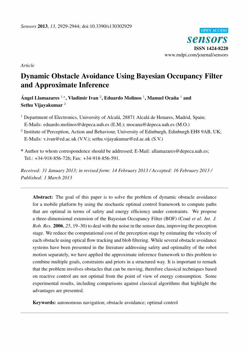
We use the Bayesian Occupancy Filter (BOF) [14] to compute a robust estimate of the position ofthe obstacles. BOF has been successfully used to detect obstacles in a flat world, but does not tacklefor obstacle detection in 3D. In order to add the height into the BOF, we use the information providedby our laser range sensor, mounted at an angle with respect the ground plane, as stated in our previouswork [18]. The height has been discretised at 3 levels, L1 (the wheel height), L2 (the mid-body height)and L3 (the overhead height), converting the cells into cubes. In order to compute the three-dimensionalBOF, all the 3D points inside each cube are projected to the corresponding cell and level. Figure 1 showsthe discretisation at three levels with respect to the robot.

Sensors 2013, 13 2932

Figure 1. Discretisation levels.

The Bayesian Occupancy Filter can be implemented as a loop of a prediction and estimation steps.The authors of [14] suggest that prediction (Equation (1)) and the estimation (Equation (2)) steps can becomputed as follows:

P (etn|nt, ut−1) ∝

∑nt−1

P (nt|nt−1, ut−1)P (et−1n |nt−1) (1)

P (etn|zt, nt) ∝

S∑m=1

(S∏

s=1

P (zts|et

n,m)) (2)

where etn is the occupancy of the cell n at time t, u is the command issued at time t − 1, z are

the observations and m is matching between a cell and an observation. P (nt|nt−1, ut−1) is then thetransition probability defined by the vehicle dynamics. The standard BOF framework has several issueswith the velocity estimation. Firstly, this framework assumes that the velocity of each grid cell isconstant [19]. Secondly, the discretisation has to be performed also in the velocity space, meaning thata separate estimate for each pair of velocities (vx, vy) is required. This discretisation for a large rangeof possible velocities together with calculations of static objects result in high computational costs. Forthese reasons, other authors proposed object detection and clustering techniques to obtain the objects’velocities [20] with an additional constraint that the position of the obstacle has to remain within abounded neighbourhood.

We have improved the system in terms of efficiency, by adding a stage to detect the relative velocitiesof the obstacles without assuming constant velocity objects or discretised velocities. Figure 2 shows theflow diagram of our proposed model.

Firstly, we capture a frame using the laser data. This frame has the form of a zenith image of thedetected obstacles. We then estimate the movement of the obstacles between two frames by computingthe pyramidal implementation of Lukas Kanade optical flow algorithm [21]. Then, we introduce a blobfiltering stage in two steps: (1) we detect the boundaries of the objects and (2) we obtain the averagemotion of all the cells inside each boundary. Each cell has to exceed certain occupancy threshold inorder to reduce the noise in the output of optical flow and the computational cost. This average value andthe time step are used to compute the relative velocities between the obstacles with respect to the robot’slocal frame of reference (along local axis x and y), while the velocity along the z axis is not taken into

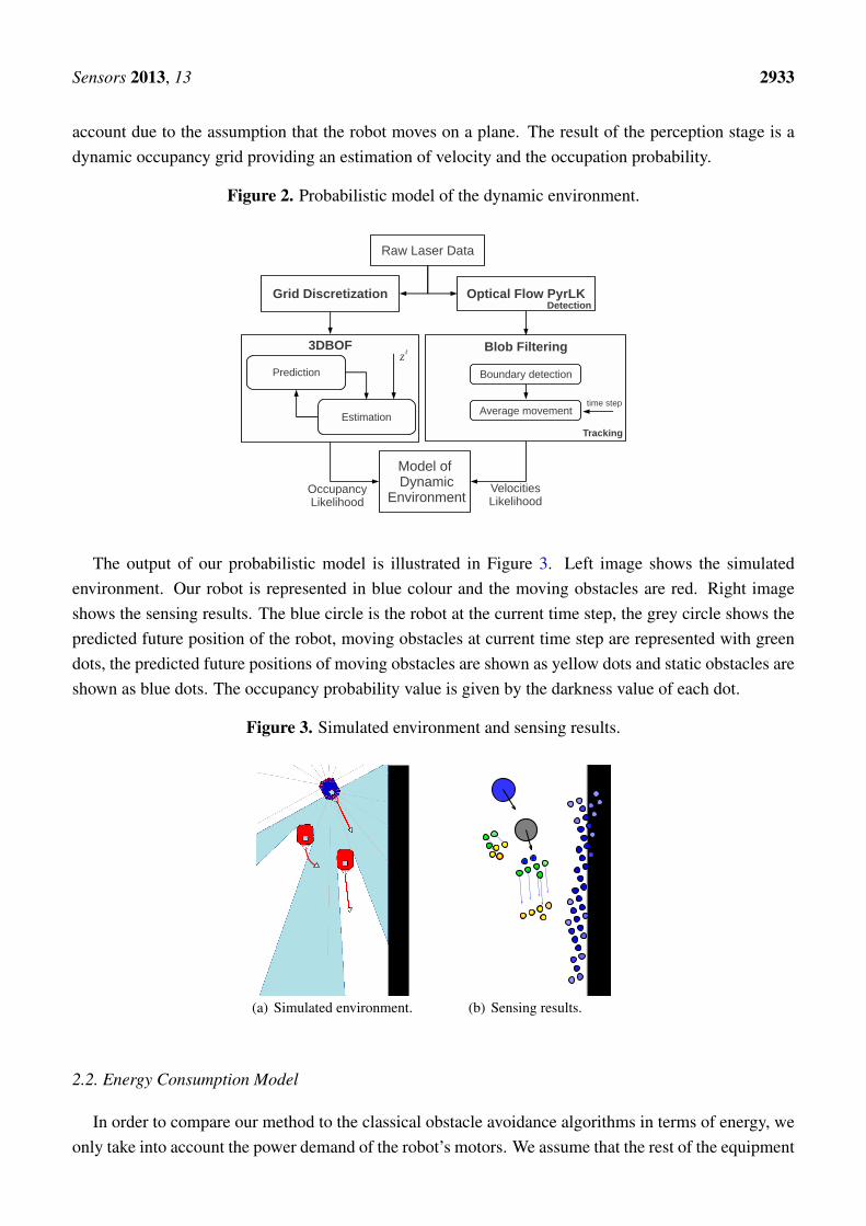
Sensors 2013, 13 2933

account due to the assumption that the robot moves on a plane. The result of the perception stage is adynamic occupancy grid providing an estimation of velocity and the occupation probability.

Figure 2. Probabilistic model of the dynamic environment.

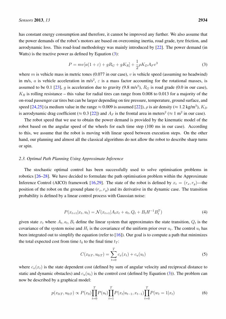
The output of our probabilistic model is illustrated in Figure 3. Left image shows the simulatedenvironment. Our robot is represented in blue colour and the moving obstacles are red. Right imageshows the sensing results. The blue circle is the robot at the current time step, the grey circle shows thepredicted future position of the robot, moving obstacles at current time step are represented with greendots, the predicted future positions of moving obstacles are shown as yellow dots and static obstacles areshown as blue dots. The occupancy probability value is given by the darkness value of each dot.

Figure 3. Simulated environment and sensing results.

(a) Simulated environment. (b) Sensing results.

2.2. Energy Consumption Model

In order to compare our method to the classical obstacle avoidance algorithms in terms of energy, weonly take into account the power demand of the robot’s motors. We assume that the rest of the equipment

Sensors 2013, 13 2934

has constant energy consumption and therefore, it cannot be improved any further. We also assume thatthe power demands of the robot’s motors are based on overcoming inertia, road grade, tyre friction, andaerodynamic loss. This road-load methodology was mainly introduced by [22]. The power demand (inWatts) is the tractive power as defined by Equation (3):

P = mv[a(1 + ε) + gRG + gKR] +1

2ρKDAF v3 (3)

where m is vehicle mass in metric tones (0.077 in our case), v is vehicle speed (assuming no headwind)in m/s, a is vehicle acceleration in m/s2, ε is a mass factor accounting for the rotational masses, isassumed to be 0.1 [23], g is acceleration due to gravity (9.8 m/s2), RG is road grade (0.0 in our case),KR is rolling resistance – this value for radial tires can range from 0.008 to 0.013 for a majority of theon-road passenger car tires but can be larger depending on tire pressure, temperature, ground surface, andspeed [24,25] (a medium value in the range ≈ 0.009 is assumed [22]), ρ is air density (≈ 1.2 kg/m3), KD

is aerodynamic drag coefficient (≈ 0.3 [22]) and AF is the frontal area in meters2 (≈ 1 m2 in our case).The robot speed that we use to obtain the power demand is provided by the kinematic model of the

robot based on the angular speed of the wheels for each time step (100 ms in our case). Accordingto this, we assume that the robot is moving with linear speed between execution steps. On the otherhand, our planning and almost all the classical algorithms do not allow the robot to describe sharp turnsor spin.

2.3. Optimal Path Planning Using Approximate Inference

The stochastic optimal control has been successfully used to solve optimisation problems inrobotics [26–28]. We have decided to formulate the path optimisation problem within the ApproximateInference Control (AICO) framework [16,29]. The state of the robot is defined by xt = (rx, ry)—theposition of the robot on the ground plane (rx, ry) and its derivative in the dynamic case. The transitionprobability is defined by a linear control process with Gaussian noise:

P (xt+1|xt, ut) = N (xt+1|Atxt + at, Qt + BtH−1BT

t ) (4)

given state xt where At, at, Bt define the linear system that approximates the state transition, Qt is thecovariance of the system noise and Ht is the covariance of the uniform prior over ut. The control ut hasbeen integrated out to simplify the equation (refer to [16]). Our goal is to compute a path that minimizesthe total expected cost from time t0 to the final time tT :

C(x0:T , u0:T ) =T∑

t=0

cx(xt) + cu(ut) (5)

where cx(xt) is the state dependent cost (defined by sum of angular velocity and reciprocal distance tostatic and dynamic obstacles) and cu(ut) is the control cost (defined by Equation (3)). The problem cannow be described by a graphical model:

p(x0:T , u0:T ) ∝ P (x0)T∏

t=0

P (ut)T∏

t=1

P (xt|ut−1, xt−1)T∏

t=0

P (wt = 1|xt) (6)

Sensors 2013, 13 2935

where P (ut) is the control prior reflecting the control cost and P (wt = 1|xt) is the probability ofreceiving low cost reflected by constantly observing a random variable wt = 1. The binary randomvariable has the conditional probability P (wt = 1|xt, ut) = exp(C(x0:T , u0:T )). The costs C(x0:T , u0:T )

play the role of the neg-log-probability of wt = 1, in accordance to the typical identification of energywith neg-log-probability. The distance to obstacles is treated as a separate task and it enters the modelthrough a task variable yt that represents position in the task space (see Figure 4). Readers are referedto [16,30–33] for more details how to couple the task variables with states. We compute the posteriorP (x0:T |w0:T = 1) over the state trajectories to solve the path planning problem using the Gaussianmessage passing algorithm. This involves combining the forward (µxt−1→xt), backward ((xt)µxt+1→xt)and cost messages ((xt)µwt→xt(xt)) to compute the posterior marginal belief:

b(xt) = µxt−1→xt(xt)µxt+1→xt(xt)µwt→xt(xt) (7)

Figure 4. Graphical model of AICO in configuration and task space.

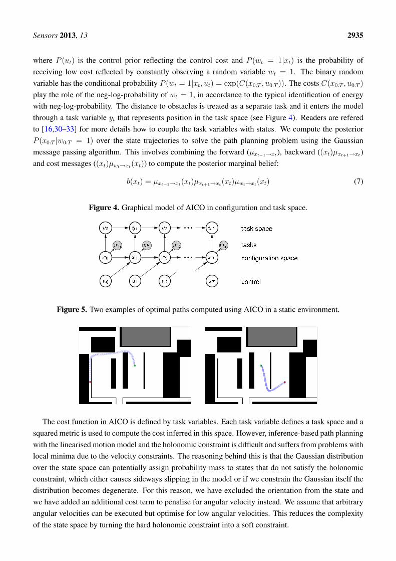
Figure 5. Two examples of optimal paths computed using AICO in a static environment.

The cost function in AICO is defined by task variables. Each task variable defines a task space and asquared metric is used to compute the cost inferred in this space. However, inference-based path planningwith the linearised motion model and the holonomic constraint is difficult and suffers from problems withlocal minima due to the velocity constraints. The reasoning behind this is that the Gaussian distributionover the state space can potentially assign probability mass to states that do not satisfy the holonomicconstraint, which either causes sideways slipping in the model or if we constrain the Gaussian itself thedistribution becomes degenerate. For this reason, we have excluded the orientation from the state andwe have added an additional cost term to penalise for angular velocity instead. We assume that arbitraryangular velocities can be executed but optimise for low angular velocities. This reduces the complexityof the state space by turning the hard holonomic constraint into a soft constraint.

Sensors 2013, 13 2936

In order to achieve robustness and safety of our vehicle, we use a method that yields free paths thattend to maximise the clearance between the vehicle and the obstacles based on a Voronoi graph. Theaim of the global planning is to keep the vehicle at a safe distance from the surrounding obstacles. Wecompute the initial path using graph search on the Voronoi graph. This path is then used as AICOinitialisation and it helps to deal with local minima. Figure 5 shows examples of optimised pathscomputed for static environments.

3. Implementation and Results

In this section we describe the implementation of our system and the experimental results. The resultshave been obtained from the real Seekur Jr. platform and the simulator provided by Mobilerobots.

The results have been evaluated in two stages: firstly we evaluate the gain of using the probabilisticmodel of the environment inside the perception stage of the classical algorithms (VFH+, CVM, LCMand BCM). Secondly, we compare our whole dynamic obstacle avoidance system with the classicalalgorithms.

3.1. Test-Bed

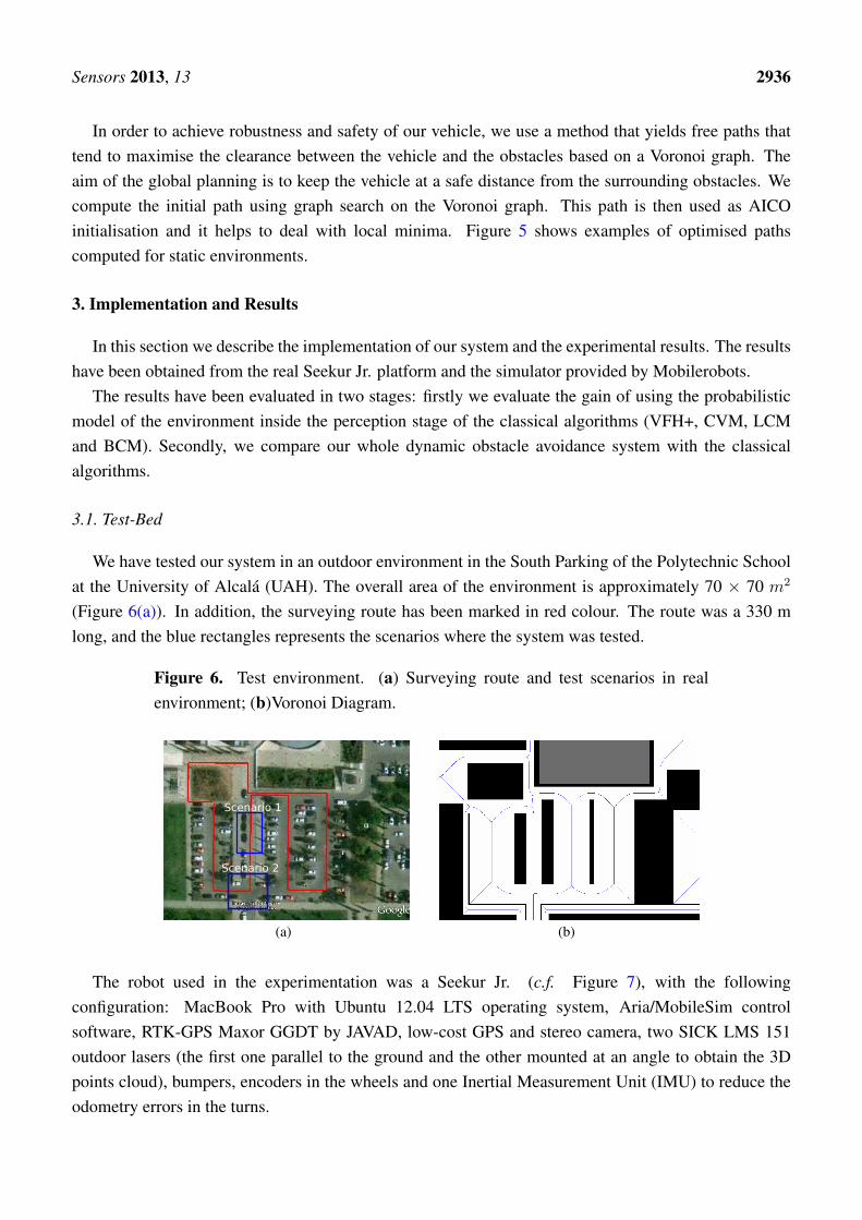
We have tested our system in an outdoor environment in the South Parking of the Polytechnic Schoolat the University of Alcala (UAH). The overall area of the environment is approximately 70 × 70 m2

(Figure 6(a)). In addition, the surveying route has been marked in red colour. The route was a 330 mlong, and the blue rectangles represents the scenarios where the system was tested.

Figure 6. Test environment. (a) Surveying route and test scenarios in realenvironment; (b)Voronoi Diagram.

Scenario 1

Scenario 2

(a) (b)

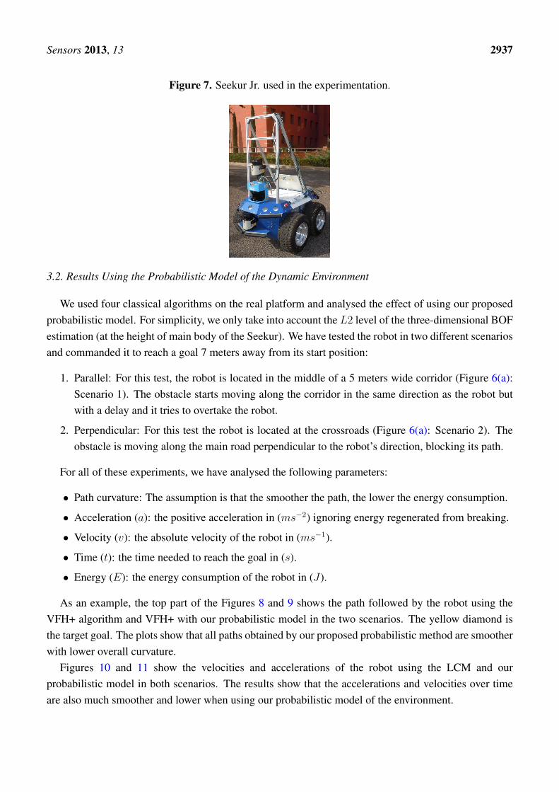
The robot used in the experimentation was a Seekur Jr. (c.f. Figure 7), with the followingconfiguration: MacBook Pro with Ubuntu 12.04 LTS operating system, Aria/MobileSim controlsoftware, RTK-GPS Maxor GGDT by JAVAD, low-cost GPS and stereo camera, two SICK LMS 151outdoor lasers (the first one parallel to the ground and the other mounted at an angle to obtain the 3Dpoints cloud), bumpers, encoders in the wheels and one Inertial Measurement Unit (IMU) to reduce theodometry errors in the turns.

Sensors 2013, 13 2937

Figure 7. Seekur Jr. used in the experimentation.

3.2. Results Using the Probabilistic Model of the Dynamic Environment

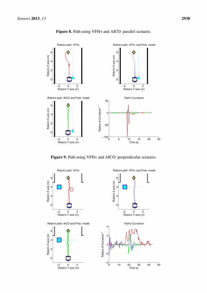
We used four classical algorithms on the real platform and analysed the effect of using our proposedprobabilistic model. For simplicity, we only take into account the L2 level of the three-dimensional BOFestimation (at the height of main body of the Seekur). We have tested the robot in two different scenariosand commanded it to reach a goal 7 meters away from its start position:

1. Parallel: For this test, the robot is located in the middle of a 5 meters wide corridor (Figure 6(a):Scenario 1). The obstacle starts moving along the corridor in the same direction as the robot butwith a delay and it tries to overtake the robot.

2. Perpendicular: For this test the robot is located at the crossroads (Figure 6(a): Scenario 2). Theobstacle is moving along the main road perpendicular to the robot’s direction, blocking its path.

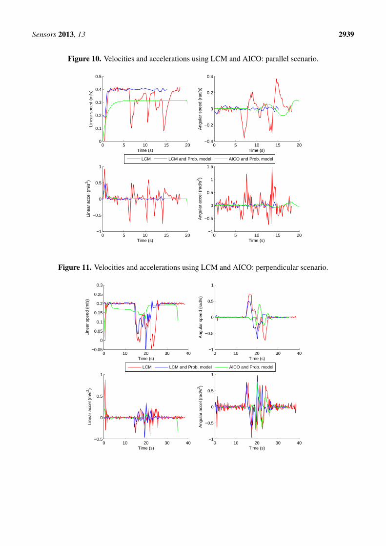
For all of these experiments, we have analysed the following parameters:

• Path curvature: The assumption is that the smoother the path, the lower the energy consumption.

• Acceleration (a): the positive acceleration in (ms−2) ignoring energy regenerated from breaking.

• Velocity (v): the absolute velocity of the robot in (ms−1).

• Time (t): the time needed to reach the goal in (s).

• Energy (E): the energy consumption of the robot in (J).

As an example, the top part of the Figures 8 and 9 shows the path followed by the robot using theVFH+ algorithm and VFH+ with our probabilistic model in the two scenarios. The yellow diamond isthe target goal. The plots show that all paths obtained by our proposed probabilistic method are smootherwith lower overall curvature.

Figures 10 and 11 show the velocities and accelerations of the robot using the LCM and ourprobabilistic model in both scenarios. The results show that the accelerations and velocities over timeare also much smoother and lower when using our probabilistic model of the environment.

Sensors 2013, 13 2938

Figure 8. Path using VFH+ and AICO: parallel scenario.

0

2

4

6

−2 0 2

Robot’s path: VFH+ and Prob. model

Robot’s X

axis

(m

)

Robot’s Y axis (m)

0

2

4

6

−2 0 2

Robot’s path: VFH+R

obot’s X

axis

(m

)


0

2

4

6

−2 0 2

Robot’s path: AICO and Prob. model

Robot’s X

axis

(m

)

Robot’s Y axis (m)0 5 10 15 20 25

−100

−50

0

50

Time (s)

Radiu

s o

f C

urv

atu

re−1

Path’s Curvature

Figure 9. Path using VFH+ and AICO: perpendicular scenario.

0

2

4

6

−2 0 2

Robot’s path: VFH+ and Prob. model

Robot’s X

axis

(m

)


0

2

4

6

−2 0 2

Robot’s path: VFH+

Robot’s X

axis

(m

)


0

2

4

6

−2 0 2

Robot’s path: AICO and Prob. model

Robot’s X

axis

(m

)

Robot’s Y axis (m)0 10 20 30 40 50

−4

−2

0

2

4

Time (s)

Radiu

s o

f C

urv

atu

re−1

Path’s Curvature

Sensors 2013, 13 2939

Figure 10. Velocities and accelerations using LCM and AICO: parallel scenario.

0 5 10 15 200

0.1

0.2

0.3

0.4

0.5

Time (s)

Line

ar s

peed

(m

/s)

0 5 10 15 20−0.4

−0.2

0

0.2

0.4

Time (s)

Ang

ular

spe

ed (

rad/

s)

0 5 10 15 20−1

−0.5

0

0.5

1

Time (s)

Line

ar a

ccel

(m

/s2 )

0 5 10 15 20−1

−0.5

0

0.5

1

1.5

Time (s)

Ang

ular

acc

el (

rad/

s2 )

LCM LCM and Prob. model AICO and Prob. model

Figure 11. Velocities and accelerations using LCM and AICO: perpendicular scenario.

0 10 20 30 40−0.05

0

0.05

0.1

0.15

0.2

0.25

0.3

Time (s)

Line

ar s

peed

(m

/s)

0 10 20 30 40−1

−0.5

0

0.5

1

Time (s)

Ang

ular

spe

ed (

rad/

s)

0 10 20 30 40−0.5

0

0.5

1

Time (s)

Line

ar a

ccel

(m

/s2 )

0 10 20 30 40−1

−0.5

0

0.5

1

Time (s)

Ang

ular

acc

el (

rad/

s2 )

LCM LCM and Prob. model AICO and Prob. model

Sensors 2013, 13 2940

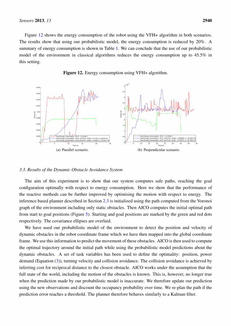
Figure 12 shows the energy consumption of the robot using the VFH+ algorithm in both scenarios.The results show that using our probabilistic model, the energy consumption is reduced by 20%. Asummary of energy consumption is shown in Table 1. We can conclude that the use of our probabilisticmodel of the environment in classical algorithms reduces the energy consumption up to 45.5% inthis setting.

Figure 12. Energy consumption using VFH+ algorithm.

0 5 10 15 20 250

0.002

0.004

0.006

0.008

0.01

0.012

0.014

0.016

0.018

Time (s)

Pow

er (

w)

Total Energy Consumption: VFH+ = 0.21404 JTotal Energy Consumption: VFH+ and Prob. model = 0.1743 J (−18.564 %)Total Energy Consumption: AICO and Prob. model = 0.14552 J (−32.0147 %)

(a) Parallel scenario.

0 5 10 15 20 25 30 35 40 450

0.5

1

1.5

2

2.5

3

3.5

4

4.5

5x 10

−3

Time (s)

Pow

er (

w)

Total Energy Consumption: VFH+ = 0.12495 JTotal Energy Consumption: VFH+ and Prob. model = 0.088383 J (−29.2652 %)Total Energy Consumption: AICO and Prob. model = 0.078974 J (−36.7954 %)

(b) Perpendicular scenario.

3.3. Results of the Dynamic Obstacle Avoidance System

The aim of this experiment is to show that our system computes safe paths, reaching the goalconfiguration optimally with respect to energy consumption. Here we show that the performance ofthe reactive methods can be further improved by optimising the motion with respect to energy. Theinference based planner described in Section 2.3 is initialized using the path computed from the Voronoigraph of the environment including only static obstacles. Then AICO computes the initial optimal pathfrom start to goal positions (Figure 5). Starting and goal positions are marked by the green and red dotsrespectively. The covariance ellipses are overlaid.

We have used our probabilistic model of the environment to detect the position and velocity ofdynamic obstacles in the robot coordinate frame which we have then mapped into the global coordinateframe. We use this information to predict the movement of these obstacles. AICO is then used to computethe optimal trajectory around the initial path while using the probabilistic model predictions about thedynamic obstacles. A set of task variables has been used to define the optimality: position, powerdemand (Equation (3)), turning velocity and collision avoidance. The collision avoidance is achieved byinferring cost for reciprocal distance to the closest obstacle. AICO works under the assumption that thefull state of the world, including the motion of the obstacles is known. This is, however, no longer truewhen the prediction made by our probabilistic model is inaccurate. We therefore update our predictionusing the new observations and discount the occupancy probability over time. We re-plan the path if theprediction error reaches a threshold. The planner therefore behaves similarly to a Kalman filter.

Sensors 2013, 13 2941

Only small changes in the environment between two time steps are expected. In such situationsAICO requires only small number of iterations to converge which makes re-planning computationallyaffordable. The replanning time (3 s on average) is however too long to be use as a reactive controller.

We have applied our proposed method to perform the task while avoiding the obstacles andminimising energy consumption. AICO solves the finite horizon optimisation problems which meansthat the duration of the trajectory needs to be specified a priori. It is not within the scope of this paperto optimise for time, we have therefore set the trajectory duration to 20 s for parallel scenario and 35s for perpendicular scenario, which are the respective average durations as computed using the reactivemethods with our probabilistic model.

Figures 8 and 9 show the results of the path optimization and demonstrate that optimising the energyconsumption further decreases the curvature of the trajectory. Similarly, Figures 10 and 11 show thatthe velocity and acceleration profiles are much smoother. As a result the energy consumption in bothscenarios was reduced by approximately 10% when compared with the best results achieved by thereactive methods as shown in Table 1.

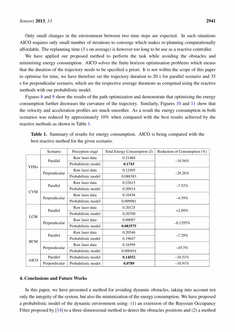
Table 1. Summary of results for energy consumption. AICO is being compared with thebest reactive method for the given scenario.

Scenario Perception stage Total Energy Consumption (J) Reduction of Consumption (%)

VFH+

ParallelRaw laser data 0.21404

–18.56%Probabilistic model 0.1743

PerpendicularRaw laser data 0.12495


CVM





LCM


+2.89%Probabilistic model 0.20709



BCM





AICOParallel Probabilistic model 0.14552 –16.51%

Perpendicular Probabilistic model 0.0789 –10.91%

4. Conclusions and Future Works

In this paper, we have presented a method for avoiding dynamic obstacles, taking into account notonly the integrity of the system, but also the minimization of the energy consumption. We have proposeda probabilistic model of the dynamic environment using: (1) an extension of the Bayesian OccupancyFilter proposed by [14] to a three-dimensional method to detect the obstacles positions and (2) a method

Sensors 2013, 13 2942

to estimate the velocity of these obstacles using a tracking stage based on optical flow and a detectionstage based on blob filtering.

We have used the probabilistic model of the environment inside the perception stage of the fourclassical methods: VFH+, BCM, CVM and LCM. Just by using a single level of the occupancy grid wewere already able to improve the perception stage of these avoidance systems. The results have shownan improvement in energy consumption up to 45.5%. We have also shown that the resulting trajectoriesas well as the velocity and acceleration profiles are much smoother when using our method.

We have implemented a Voronoi graph based global path planner which serves as an initialisationmethod for our inference based local planner: AICO. Within AICO we combine multiple task variables toobtain the optimal path based on obstacle clearance and energy consumption. This method shows furtherqualitative improvement against the reactive methods with an improvement in energy consumption of10.91% and 16.51% respect to the best results of reactive methods in perpendicular and parallel scenariosrespectively. The computational cost of using AICO is currently too high for it to be used in real-timeplanning applications.

In near future, we intend to improve the accuracy of the probabilistic model by refining thediscretisation. We also intend to improve the calculation of the probabilistic model to speed up thealgorithm to accommodate for higher number of cells. The planning algorithm can be improved bysolving the inference at multiple scales and by exploiting parallel computation. Furthermore, we willaddress issues of coverage using topology based properties such as winding numbers [34]. This willallow us to reduce energy consumption by planning optimal route to survey an area such as a parking lotwhen searching for a parking space.

Acknowledgements

This work has been funded by TIN2011-29824-C02-01 and TIN2011-29824-C02-02 (ABSYNTHEproject) from the “Ministerio de Economıa y Competitividad” and a grant of the Fundacion Caja Madrid.

References

1. Montemerlo, M.; Becker, J.; Bhat, S.; Dahlkamp, H.; Dolgov, D.; Ettinger, S.; Haehnel, D.;Hilden, T.; Hoffmann, G.; Huhnke, B.; et al. Junior: The stanford entry in the urban challenge.J. Field Rob. 2008, 25, 569–597.

2. Thrun, S.; Montemerlo, M.; Dahlkamp, H.; Stavens, D.; Aron, A.; Diebel, J.; Fong, P.; Gale, J.;Halpenny, M.; Hoffmann, G.; et al. Winning the DARPA grand challenge. J. Field Rob. 2006,23, 661–692.

3. Enge, P.; Misra, P. Scanning the issue/technology. Special issue on global positioning system.Proc. IEEE 1999, 87, 3–15.

4. Schleicher, D.; Bergasa, L.M.; Ocana, M.; Barea, R.; Lopez, E. Low-cost GPS sensor improvementusing stereovision fusion. Sign. Process. 2010, 90, 3294–3300.

5. Hentschel, M.; Wulf, O.; Wagner, B. A GPS and laser-based localization for urban and non-urbanoutdoor environments. In Proceedings of IROS 2008: IEEE/RSJ International Conference onIntelligent Robots and Systems, Nice, France, 22–26 September 2008; pp. 149–154.

Sensors 2013, 13 2943

6. Thrun, S.; Fox, D.; Burgard, W. A probabilistic approach to concurrent mapping and localizationfor mobile robots. Autonom. Rob. 1998, 5, 253–271.

7. Newman, P.; Cole, D.; Ho, K. Outdoor SLAM using visual appearance and laser ranging. InProceedings of ICRA 2006: IEEE International Conference on Robotics and Automation, Orlando,FL, USA, 15–19 May 2006; pp. 1180–1187.

8. Bekris, K.E.; Click, M.; Kavraki, E.E. Evaluation of algorithms for bearing-only SLAM. InProceedings of ICRA 2006: IEEE International Conference on Robotics and Automation, Orlando,FL, USA, 15–19 May 2006; pp. 1937–1943.

9. Ulrich, I.; Borenstein, J. VFH+: Reliable obstacle avoidance for fast mobile robots. In Proceedingsof ICRA 1998: IEEE International Conference on Robotics and Automation, Leuven, Belgium,16–20 May 1998; pp. 1572–1577.

10. Minguez, J.; Montano, L. Nearness diagram (ND) navigation: Collision avoidance in troublesomescenarios. IEEE Trans. Rob. Autom. 2004, 20, 45–59.

11. Fox, D.; Burgard, W.; Thrun, S. The dynamic window approach to collision avoidance. IEEE Rob.Autom. Mag. 1997, 4, 23–33.

12. Ko, N.Y.; Simmons, R. The lane-curvature method for local obstacle avoidance. In Proceedingsof IROS 1998: IEEE/RSJ International Conference on Intelligent Robots and Systems, Victoria,Canada, 13–17 October 1998; pp. 1615–1621.

13. Fernandez, J.L.; Sanz, R.; Benayas, J.A.; Dieguez, A.R. Improving collision avoidance for mobilerobots in partially known environments: The beam curvature method. Rob. Autonom. Syst. 2004,46, 205–219.

14. Coue, C.; Pradalier, C.; Laugier, C.; Fraichard, T.; Bessiere, P. Bayesian Occupancy Filtering formultitarget tracking: An automotive application. Int. J. Rob. Res. 2006, 25, 19–30.

15. Fulgenzi, C.; Spalanzani, A.; Laugier, C. Dynamic obstacle avoidance in uncertain environmentcombining PVOs and occupancy grid. In Proceedings of ICRA 2007: IEEE InternationalConference on Robotics and Automation, Roma, Italy, 10–14 April 2007.

16. Toussaint, M. Robot trajectory optimization using approximate inference. In Proceedings of 26thInternational Conference on Machine Learning, Montreal, Canada, 14–18 June 2009.

17. Llamazares, A.; Ivan, V.; Ocana, M.; Vijayakumar, S. Dynamic obstacle avoidance minimizingenergy consumption. In Proceedings of the IEEE Intelligent Vehicles Symposium and Workshopon Perception in Robotics, Alcala de Henares, Spain, 3–7 June 2012; pp. P02.1–P02.6.

18. Llamazares, A.; Molinos, E.; Ocana, M.; Bergasa, L.M.; Hernandez, N.; Herranz, F. 3D mapbuilding using a 2D laser scanner. In Proceedings of 13th International Conference on ComputerAided Systems Theory, Las Palmas de Gran Canaria, Spain, 6–11 February 2011; pp. 161–164.

19. Yguel, M.; Tay, C.; Mekhnacha, K.; Laugier, C. Velocity Estimation on the Bayesian OccupancyFilter for Multi-Target Tracking; Report RR-5836; INRIA: Rocquencourt, France, 2006.

20. Mekhnacha, K.; Mao, Y.; Raulo, D.; Laugier, C. Bayesian occupancy filter based “FastClustering-Tracking” algorithm. In Proceedings of IROS 2008: IEEE/RSJ InternationalConference on Intelligent Robots and Systems, Nice, France, 22–26 September 2008.

21. Bouguet, J. Pyramidal Implementation of the Lucas Kanade Feature Tracker; MicroprocessorResearch Labs, Intel Corporation: Santa Clara, CA, USA, 2000.

Sensors 2013, 13 2944

22. Sovran, G.; Bohn, M. Formulae for the Tractive-Energy Requirements of Vehicles Driving the EPASchedules; SAE Technical Paper 810184; SAE International: Warrendale, PA, USA, 1981.

23. Jimnez-Palacios, J.L. Understanding and Quantifying Motor Vehicle Emissions with VehicleSpecific Power and TILDAS Remote Sensing. Ph.D. Thesis, Massachusetts Institute ofTechnology, Cambridge, MA, USA, 1999.

24. Bauer, H.; Dinkler, F.; Crepin, J.; Dietsche, K. Automotive Handbook, 5th ed.; Robert BoschGmbH: Stuttgart, Germany, 2000.

25. Gillespie, T. Fundamentals of Vehicle Dynamics; Society of Automotive Engineers Inc.:Warrendale, PA, USA, 1992.

26. Nakanishi, J.; Rawlik, K.; Vijayakumar, S. Stiffness and temporal optimization in periodicmovements: An optimal control approach. In Proceedings of IEEE/RSJ International Conferenceon Intelligent Robots and Systems (IROS), San Francisco, CA, USA, 2011; pp. 718–724.

27. Braun, D.J.; Howard, M.; Vijayakumar, S. Optimal variable stiffness control: formulation andapplication to explosive movement tasks. Auton. Rob. 2012, 33, 237–253.

28. Rawlik, K.; Toussaint, M.; Vijayakumar, S. An Approximate Inference Approach to TemporalOptimization in Optimal Control. n Proceedings of Neural Information Processing Systems (NIPS),Vancouver, BC, Canada, 6–9 December 2010.

29. Rawlik, K.; Toussaint, M.; Vijayakumar, S. On Stochastic Optimal Control and ReinforcementLearning by Approximate Inference. In Proceedings of Robotics: Science and Systems VIII,Sydney, Australia, 9–13 July 2012.

30. Zarubin, D.; Ivan, V.; Toussaint, M.; Komura, T.; Vijayakumar, S. Hierarchical Motion Planningin Topological Representations. In Proceedings of Robotics: Science and Systems VIII, Sydney,Australia, 9–13 July 2012.

31. Bitzer, S.; Vijayakumar, S. Latent spaces for dynamic movement primitives. In Proceedings of 9thIEEE-RAS International Conference on Humanoid Robots, Paris, France, 7–10 December 2009.

32. Ho, E.S.L.; Komura, T.; Ramamoorthy, S.; Vijayakumar, S. Controlling humanoid robots intopology coordinates. In Proceedings of 2010 IEEE/RSJ International Conference on IntelligentRobots and Systems (IROS), Taipei, Taiwan, 2010, pp. 178–182.

33. Ho, E.S.L.; Komura, T.; Tai, C. Spatial relationship preserving character motion adaptation. ACMTrans. Graph. 2010, 29, 1–8.

34. Vernaza, P.; Narayanan, V.; Likhachev, M. Efficiently finding optimal winding-constrained loopsin the plane. In Proceedings of Robotics: Science and Systems VIII, Sydney, Australia, 9–13 July2012.

c⃝ 2013 by the authors; licensee MDPI, Basel, Switzerland. This article is an open access articledistributed under the terms and conditions of the Creative Commons Attribution license(http://creativecommons.org/licenses/by/3.0/).

Dynamic Obstacle Avoidance Using Bayesian Occupancy Filter and Approximate Inference

Documents